Fluid Mechanics lab 3 pumps and turbines

Fluid Mechanics, ENGI 1635

Experiment 3: Pumps & Turbines

Sean Garrity

Group #63

Preformed: Monday January 19th 2015

Submitted: Monday January 26th 2015

1.0 Purpose

The purpose of this experiment was to become familiar with conductingperformance tests on pumps and turbines determining their respective efficiencies on different settings. This information can be applied when designing or buying a pump or turbine.

2.0 Theory

A pump is a machine that transfers energy to fluid passing through it; a turbine is the opposite as it harnesses energy from a fluid passing through it. Hence pumps require energy and turbines produce energy.

Centrifugal pumps transfer energy by rotating an impeller, the water is then pulled into the pump by the pressure created around the empty area of were water previously was before it to went through the pump. Fluids enter the chamber with the rotating impeller and are then accelerated and forced out the discharge pipe.

Turbines convert kinetic energy from the fluid hitting the blades into power, as fluid strikes the blade the shaft rotates which is connected to a generator which outputs power. A good example is the turbines found in a hydroelectric dam where the water falls due to gravity and creates power. It is important to note that fluid exits a turbine much slower than when it entered.

The efficiency of a pump is defined as the ratio of input power to output power, consequentially the ratio of efficiency of turbine is the opposite. It should be noted that energy is never created or destroyed and that 100% efficiency can never truly be achieved. The equations for calculating input and output power are located below respectively.

Pi = Input power = Tω[1]

Po = Output power = γQH[2]

Where:T(torque in N*M) = 9.806*(mass)*moment arm(0.157 in our case)ω(angular velocity in ) = RPM/60*2πγ(force/unit volume in N/m³) = 9789 (at20C)Q = flow in m³/sH = head in m

The equations for Input and output power of a turbine are located below the same variables are used.

Pi = γQH[3]

Po = volts*amps*3[4]

3.0 Procedure

3.1 Pump test

The motor was turned on and the rheostat was set to various values displayed in Figure 6.0. The head was then set to assorted pressures; the rotation of the motor was checked throughout the experiment and was always within 10 RPM +/- of the recorded value. Next the flow was read off the side of the tank, and the breakforce was noted from the digital scale. For each motor speed 7 trials of various pressures were conducted.

3.2 Turbine test

A centrifugal pump simulated a 9m waterfall passing through a turbine connected to a generator. The turbine vanes were adjusted to half open, three quarters open, and fully open, 5 rheostat readings were used. For each reading the head was kept at 9m, the resulting flow, amp-meter, and volt-meter readings were noted.

*Note an in-depth procedure is available in the 2014 Fluid Mechanics lab manual

4.0 Equipment 4.1 Pump test

The centrifugal pump and pump set up used is displayed in below in Figure 1.0.

Figure 1.0[5]

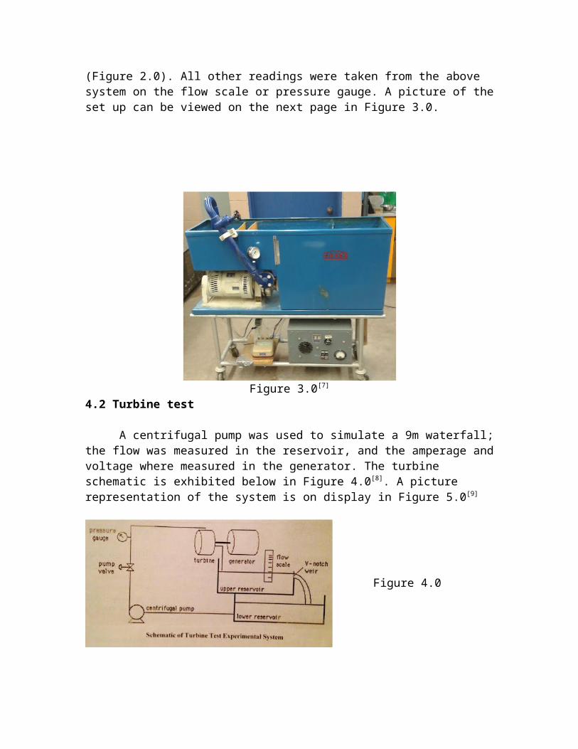
The RPM of the motor was measured by a simple hand-held calibrator(Figure 2.0). All other readings were taken from the above system on the flow scale or pressure gauge. A picture of the set up can be viewed on the next page in Figure 3.0.

Figure 2.0[6]

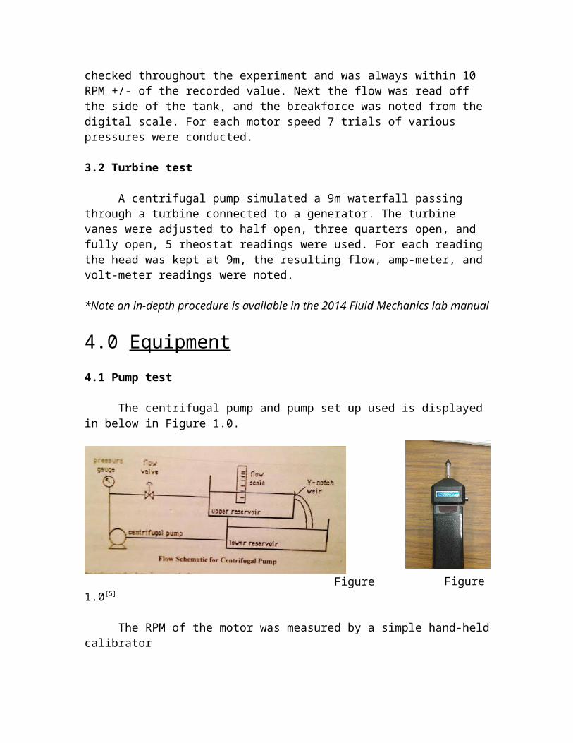
Figure 3.0[7]

4.2 Turbine test

A centrifugal pump was used to simulate a 9m waterfall; the flow was measured in the reservoir, and the amperage and voltage where measured in the generator. The turbine schematic is exhibited below in Figure 4.0[8]. A picture representation of the system is on display in Figure 5.0[9]

Figure 5.0

Figure 4.0

5.0 Results

5.1 Pump test

The data collected for the centrifugal pump test is located in Figure 6.0, and 6.1. Figure 6.1 is similar to Figure 6.0, but includes the most relevant data pertaining to this lab the Mechanical Efficiency.

RPM T (Nm) ω (rad/s) Q (M3/s) H (m) Pi (w) Po (w) Po/ Pi

1600

0.69 167.55 0 5.1 116.08 0 0%1.05 167.55 0.00028 4.5 175.41 12.33 7.03%1.17 167.55 0.00050 4.0 196.04 19.58 9.99%1.20 167.55 0.00060 3.5 201.20 20.56 10.22%1.23 167.55 0.00070 3.0 206.36 20.56 9.96%1.28 167.55 0.00080 2.5 214.10 19.58 9.14%1.31 167.55 0.00090 2.0 219.26 17.62 8.04%

2000

0.99 209.44 0 10.5 206.36 0 0%1.08 209.44 0.00028 9.5 225.71 26.04 11.54%1.25 209.44 0.00055 8.5 261.18 45.76 17.52%1.39 209.44 0.00075 7.5 290.20 55.06 18.97%1.49 209.44 0.00090 6.5 312.77 57.27 18.31%1.57 209.44 0.00105 5.5 328.89 56.53 17.19%1.63 209.44 0.00120 4.5 341.79 52.86 15.47%

2400

1.17 251.33 0 15.5 294.07 0 0%1.28 251.33 0.00028 14.0 321.15 38.37 11.95%1.57 251.33 0.00070 12.5 394.67 85.65 21.70%1.86 251.33 0.00110 11.0 468.18 118.45 25.30%1.97 251.33 0.00125 9.5 495.27 116.24 23.47%2.05 251.33 0.00140 8.0 514.62 109.64 21.30%2.11 251.33 0.00150 6.5 530.09 95.44 18.00%

2800

1.32 293.22 0 22.5 388.22 0 0%1.42 293.22 0.00022 20.5 415.30 44.15 10.63%1.83 293.22 0.00060 18.5 537.19 108.66 20.23%2.16 293.22 0.00110 16.5 631.98 177.67 28.11%2.31 293.22 0.00125 14.5 677.13 177.43 26.20%2.46 293.22 0.00145 12.5 722.27 177.43 24.57%2.62 293.22 0.00160 10.5 767.41 164.46 21.43%

*Note: all decimals used in intermediate calculationsFigure 6.1

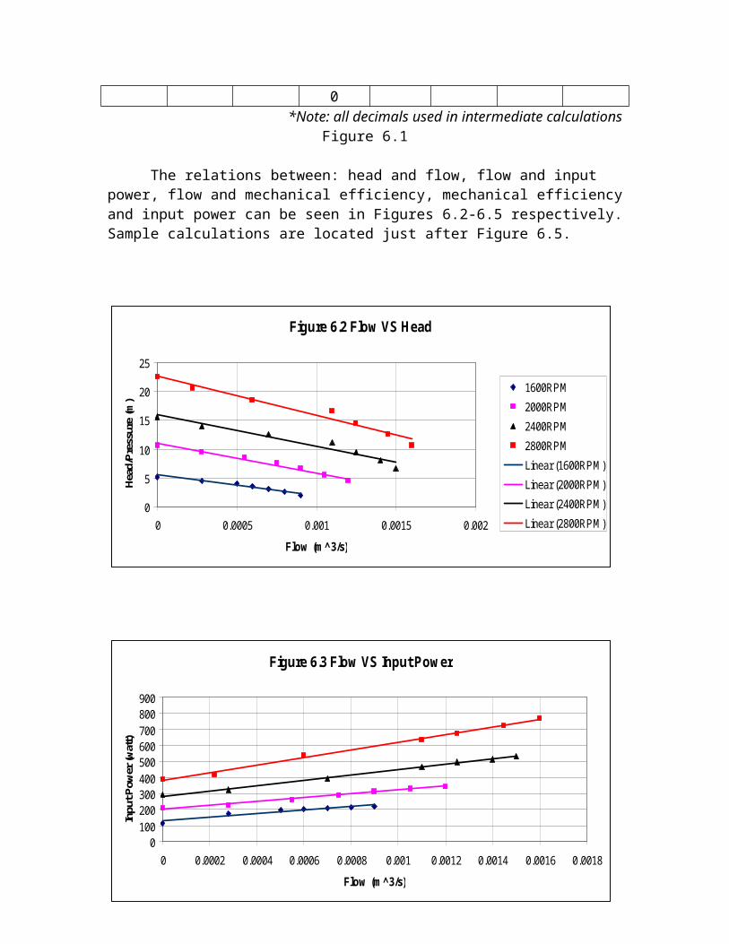
The relations between: head and flow, flow and input power, flow and mechanical efficiency, mechanical efficiency and input power can be seen in Figures 6.2-6.5 respectively. Sample calculations are located just after Figure 6.5.

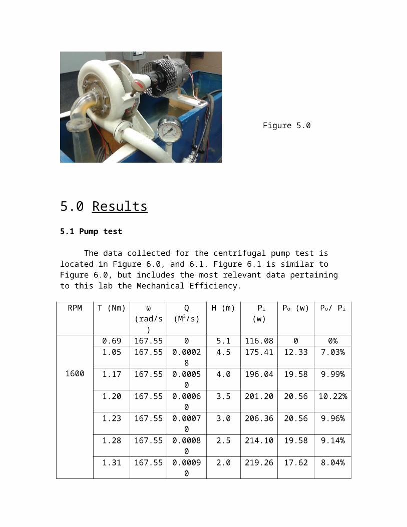
Figure 6.2 Flow VS Head

0

5

10

15

20

25

0 0.0005 0.001 0.0015 0.002

Flow (m^3/s)

Hea

d/P

ress

ure

(m)

1600RPM

2000RPM

2400RPM

2800RPM

Linear (1600RPM)

Linear (2000RPM)

Linear (2400RPM)

Linear (2800RPM)

Figure 6.3 Flow VS Input Power

0100200300400500600700800900

0 0.0002 0.0004 0.0006 0.0008 0.001 0.0012 0.0014 0.0016 0.0018

Flow (m^3/s)

Inpu

t Pow

er (w

att)

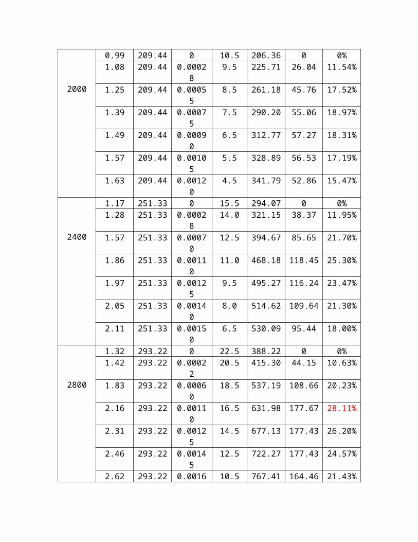
Figure 6.4 Flow VS Mechanical Efficiency

0%

5%

10%

15%

20%

25%

30%

0 0.0002 0.0004 0.0006 0.0008 0.001 0.0012 0.0014 0.0016 0.0018

Flow (m^3/s)

Mec

han

ical

Eff

icie

ncy

Sample Calculations

Pi = Input power = Tω Po = Output power = γQH Mechanical Efficiency = Po/ Pi

T = (9.806)(0.68)(N)(0.157m) T = (9.806)(0.68)(0.157) =1.0469Nm

ω = (1600/60s)(2πrad) = 167.55 rad/s

Pi = (1.0469N.m)(167.55rad/s) = 175.41watt

Po = (9789)(4.5m)(0.001)(0.28M3/s ) = 12.33watt

Mechanical efficiency (Po/ Pi) = 12.33watt/175.41watt*100% = 7.03%

Figure 6.5 Mechanical Efficiency VS Input Power

0%

5%

10%

15%

20%

25%

30%

0 100 200 300 400 500 600 700 800 900

Input Power (watt)

Me

ch

an

ica

l Eff

icie

nc

y

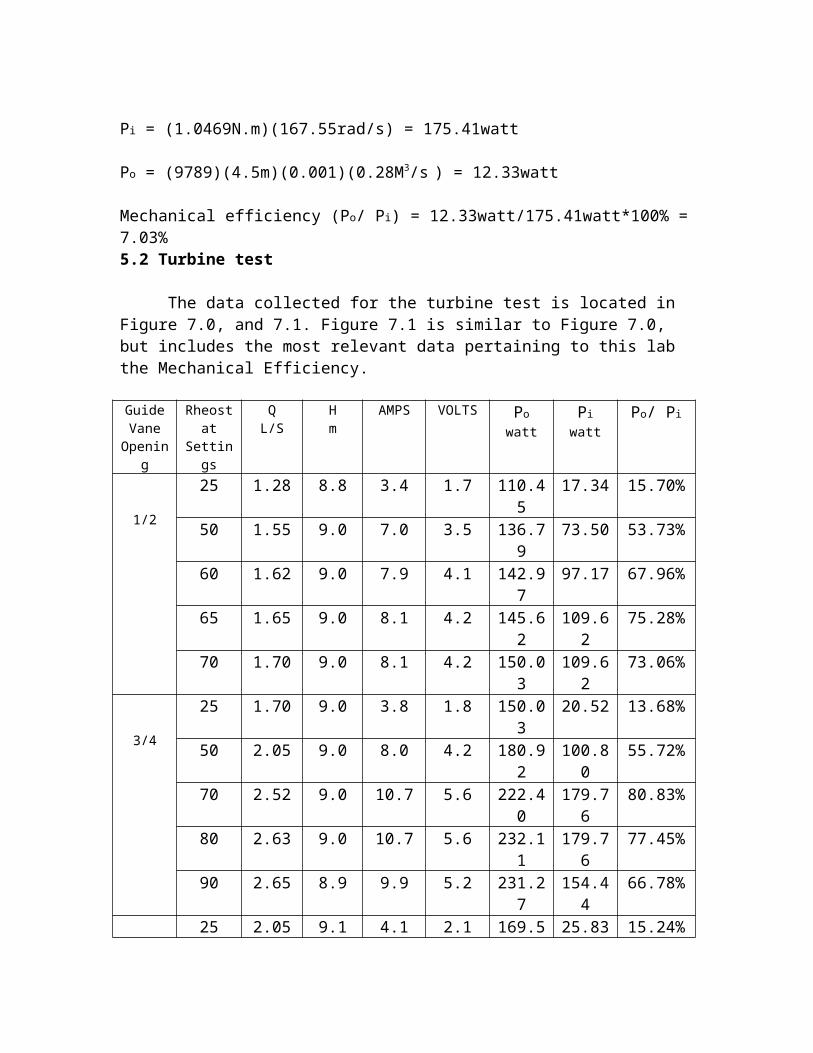
5.2 Turbine test

The data collected for the turbine test is located in Figure 7.0, and 7.1. Figure 7.1 is similar to Figure 7.0, but includes the most relevant data pertaining to this lab the Mechanical Efficiency.

Guide Vane

Opening

RheostatSettings

QL/S

Hm

AMPS VOLTS Po

wattPi

wattPo/ Pi

1/2

25 1.28 8.8 3.4 1.7 110.45 17.34 15.70%50 1.55 9.0 7.0 3.5 136.79 73.50 53.73%60 1.62 9.0 7.9 4.1 142.97 97.17 67.96%65 1.65 9.0 8.1 4.2 145.62 109.62 75.28%70 1.70 9.0 8.1 4.2 150.03 109.62 73.06%

3/4

25 1.70 9.0 3.8 1.8 150.03 20.52 13.68%50 2.05 9.0 8.0 4.2 180.92 100.80 55.72%70 2.52 9.0 10.7 5.6 222.40 179.76 80.83%80 2.63 9.0 10.7 5.6 232.11 179.76 77.45%90 2.65 8.9 9.9 5.2 231.27 154.44 66.78%

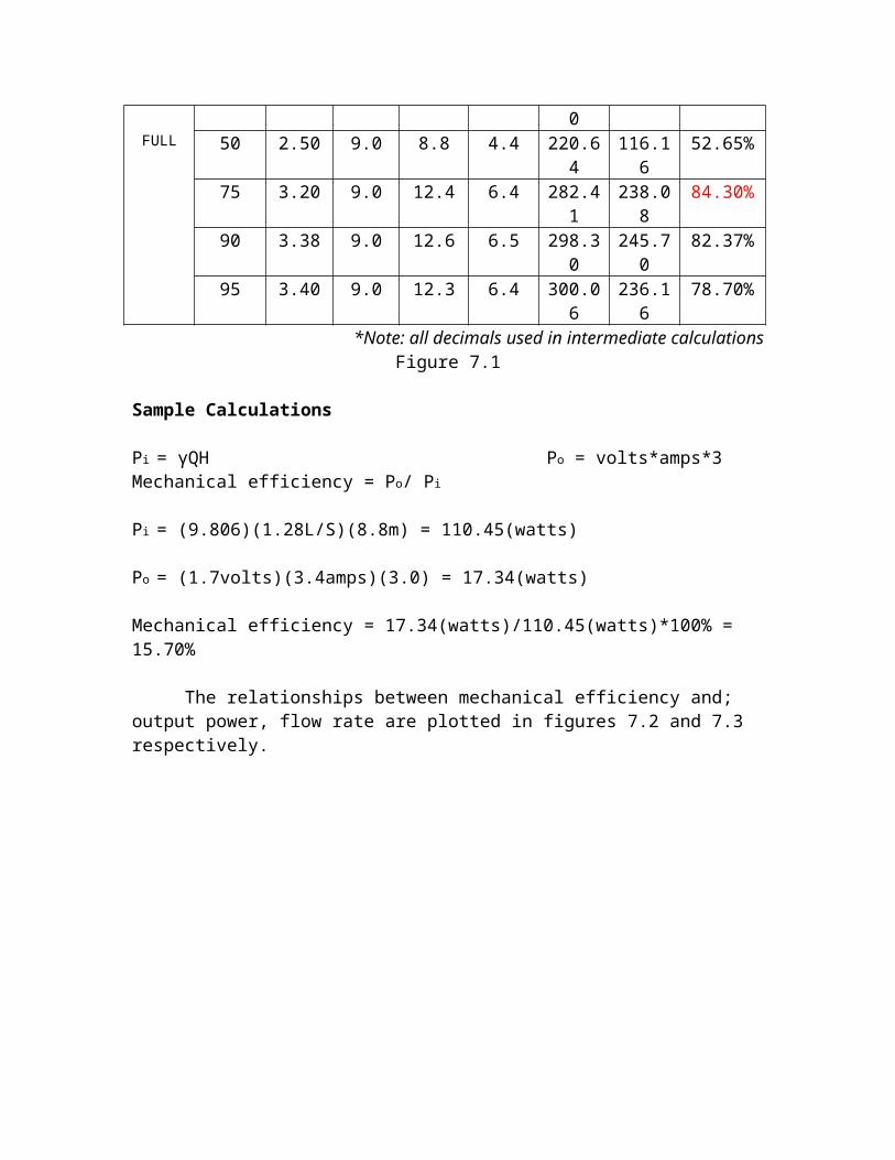
FULL

25 2.05 9.1 4.1 2.1 169.50 25.83 15.24%50 2.50 9.0 8.8 4.4 220.64 116.16 52.65%75 3.20 9.0 12.4 6.4 282.41 238.08 84.30%90 3.38 9.0 12.6 6.5 298.30 245.70 82.37%95 3.40 9.0 12.3 6.4 300.06 236.16 78.70%

*Note: all decimals used in intermediate calculationsFigure 7.1

Sample Calculations

Pi = γQH Po = volts*amps*3 Mechanical efficiency = Po/ Pi

Pi = (9.806)(1.28L/S)(8.8m) = 110.45(watts)

Po = (1.7volts)(3.4amps)(3.0) = 17.34(watts)

Mechanical efficiency = 17.34(watts)/110.45(watts)*100% = 15.70%

The relationships between mechanical efficiency and; output power, flow rate are plotted in figures 7.2 and 7.3 respectively.

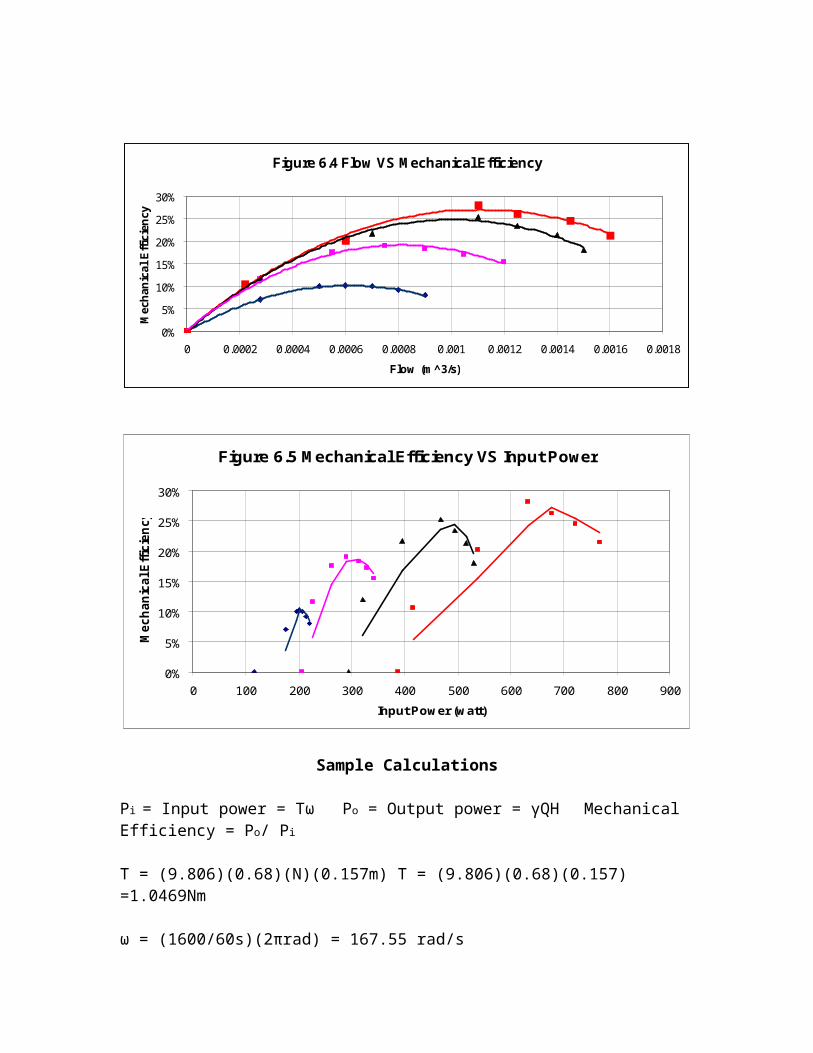
Figure 7.2 Output Power VS Mechanical Efficency

0.00%10.00%20.00%30.00%40.00%50.00%60.00%70.00%80.00%90.00%

0 50 100 150 200 250 300 350

Output Power (watt)

Mec

hani

cal E

ffici

ency

1/2 open

3/4 open

fully open

Poly. (1/2 open)

Poly. (3/4 open)

Poly. (fully open)

Figure 7.3 Flow Rate VS Mechanical Efficiency

0.00%10.00%20.00%30.00%40.00%50.00%60.00%70.00%80.00%90.00%

0 0.5 1 1.5 2 2.5 3 3.5 4

Flow Rate (L/S)

Mec

han

ical

Eff

icie

ncy

6.0 Discussion

6.1 Pump test

The results found in Figure 6.1 state that the pump’s mechanical efficiency varied from about 7%-28%, this is much lower than the acceptable 60% minimum standard efficiency of single impeller centrifugal pumps[10]. The low efficiency is due to the fact that the pump is old and has been used a lot, for example it takes less energy to rotate a new impellor verse an old impellor because the parts are in better condition.

Wear and tear is not a source of error, and the data collected seems very accurate as the expected maximum efficiency was about 30%[11]. However a large amount of manual measurements were taken. A prominent example of human error is that the RPM were most often not their recorded values but were within plus or minus 10, as it is very difficult to set RPM to an exact number by hand.

The maximum efficiency happened at 2800RPM because this was the fastest speed used and as RPM increases so does efficiency. Efficiency is also influenced by the flow rate; if the flow rate is too high then a back-up of fluid occurs. However if the flow rate is too low then the pump is not working to its full potential and the pump may suck in air which can be dangerous or harm the equipment; this did not occur during the experiment because there were no weird noises and the system wasn’t damaged. Just above and below the maximum efficiency shock-loss[12] occurs, this is when the water strikes the impeller at a bad angle, creating more friction slowing down the pump.

At all RPM the pump had to overcome the dynamic coefficient of friction, Figure 6.3 displays this as the y-intercepts of the various plots are all significantly above 0. Figure 6.4 and its parabolic trend-line demonstrate the previously mentioned shock-loss, as a slight increase/decrease in flow causes a decrease in efficiency.

6.2 Turbine test

Figure 7.1 displays the range of mechanical efficiency of the turbine to be from about 14%-84%, this large gap is caused by numerous variables, such as flow-rate, rheostat setting, and vane setting. The vane setting dictates the value of the dynamic coefficient of friction, as the vanes become more open the coefficient decreases. Figure 7.2 demonstrates that there is an optimum value of output power for a turbine just like the relationship of efficiency and input power for a pump.

84.0% is extremely good relative to the pumps of fewer than 30%, but considering about 15% of the original power is lost, it is obviously not a good idea to pump water into a turbine to try to gain energy as that is impossible. Although perpetual energy does not exist, turbines are practical for harnessing natural kinetic energy like that of a tide or falling water and powered turbines help understand how to maximize efficiency.

As I did not personally conduct or witness this experiment I cannot speak with absolute certainty regarding sources of error but a conservative assumption can be made; human error may have been a contributing factor. For example on the flow scale the human eye can only be so good and will never achieve true values of flow rate. Since there is no huge redflags in the data and that it came from a credible source and follows expected trends it is likely the experiment was conducted well.

7.0 Conclusion

The maximum efficiencies of the tested pump and turbine are approximately 28%, and 84% respectively. The generated performance curves display the full range of efficiencies relative to numerous variables for both machines. These curves are highly useful for someone designing or buying a pump or turbine, as all they have to do is check where their expected conditions fall on the curves and then pick a device that will provide maximum efficiency for their specific job.

8.0 References

1. Fluid Mechanics Engineering 1635 Lab Manual 2014 page 292. Fluid Mechanics Engineering 1635 Lab Manual 2014 page 293. Fluid Mechanics Engineering 1635 Lab Manual 2014 page 324. Fluid Mechanics Engineering 1635 Lab Manual 2014 page 325. Fluid Mechanics Engineering 1635 Lab Manual 2014 page 296. Photo courtesy of Thomas Kaszuba 7. Photo courtesy of Thomas Kaszuba8. Fluid Mechanics Engineering 1635 Lab Manual 2014 page 319. Photo courtesy of Thomas Kaszuba 10. Australian Government, department of primary industries (www.dpi.nsw.gov.au)11. Joe Ripku, Lakehead University faculty of engineering12. Joe Ripku, Lakehead University faculty of engineering