Fluid flow in a helical vessel in presence of a stenosis - ArTS

Fluid flow in a helical vessel in presence of a stenosis

Luigino Zovatto . Gianni Pedrizzetti

Accepted: 26 September 2015

Abstract Large arteries are not straight and rather

present curvature and torsion. The present study

analyzed fluid flow in a helical vessel without and

with a stenosis in comparison with an analogous

rectilinear vessel. The analysis is performed by three-

dimensional numerical simulation of the Navier–

Stokes equations under steady conditions considering

stenosis as an axially symmetric reduction of vessel

lumen. Results show that the double curvature gives

rise to persistent secondary motion which combines

with the vorticity separated behind the constriction to

develop a complex three-dimensional vorticity struc-

ture. The curved streamlines and the three-dimen-

sional vortex wake result in a increase of energetic

losses in helical vessels. However, the same symmetry

break due to the double curvature improves the

capacity of self-cleaning and allows a more rapid

wash-out of the flowing blood.

Keywords Arterial flow �Helical vessel � Separation

1 Introduction

This study is dedicated to analysing the flow field

inside a helical vessel in the presence of a reduction of

its lumen (i.e stenosis) and comparing it with the

analogous flow that establishes in a rectilinear vessel.

The study takes its cue from the initial intuition of

Caro [1] and follows later observations made in vivo

and in biomedical models. These have shown that the

presence of a no-planar curvature in a blood vessel (e.g

aorta, carotid) induces secondary motions which avoid

the development of stagnation in the regions down-

stream the separation of the boundary layer [2]. This

fact presents important clinical implications, like the

reduction of the risk of atherosclerosis, such that

recent studies suggested to introduce diagnostic

indexes of vascular risk based on flow helicity [3].

The hydrodynamic analysis first characterizes the

presence of secondary circulation which develops in

the helical vessel. The longitudinal vorticity corre-

sponding to secondary circulations is expected to

combine with the transversal circulation due to

boundary layer separation downstream the constric-

tion. This vorticity interaction develops a complex

three-dimensional wake structure which differs from

normal recirculation regions, possibly presenting open

streamlines and limited areas of stagnation.

The vorticity analysis is thus integrated, in the

second part of the work, by investigating the ability of

blood wash-out using a transport model for a passive

This work has been supported by MIUR (Italian Ministry of

University and Research) under the Grant PRIN

2012HMR7CF.

L. Zovatto (&) � G. PedrizzettiDipartimento Ingegneria e Architettura, Universita degli

Studi di Trieste, Trieste, Italy

e-mail: [email protected]

1

scalar which initially fills the entire lumen. The results

are evaluated in terms of concentration of the solute

and residence time distribution (RTD) to asses the

comparative wash-out properties of helical and recti-

linear vessels, with and without stenosis.

2 Model formulation

2.1 Fundamentals

This study considers the motion of an incompressible

fluid inside a helical vessel. Geometric parameters are

taken from analogy with large arteries with the radius

and the pitch of the helix axis q ¼ 1:5D and p ¼ 2pD,respectively, being D the vessel diameter. Only one

pitch length of the vessel is considered in compliance

with the finite length of an artery tract. Then the

stenosis is considered as axially symmetric with 50 %

reduction of lumen area and a predefined smooth

longitudinal shape. The present fluid dynamics inves-

tigation was performed numerically under steady state

conditions. The Navier–Stokes equations governing

the phenomena are solved for a Reynolds’ number,

Re ¼ VD=m, equal to 1000, a value compatible with

flows in the medium and large size arteries, being the

average velocity V and m the kinematic viscosity.

In what follows, the diameter D and the velocity

V are used as reference units for the dimensionless

formulation.

2.2 Helical geometry of the vessel axis

A helix is a three-dimensional space curve xh!

described by the parametric equations

xh ¼ qcosðtÞ; yh ¼ qsinðtÞ; zh ¼ ct; ð1Þ

where c ¼ p2p and t, 0\t\2p, is the parametric

coordinate along the curve.

The helix curvature and torsion are given by j ¼q

q2þc2and s ¼ c

q2þc2, respectively. Then, the Frenet triad

of tangent, normal and binormal unit vectors are then

defined by

T!¼ dxh

!ds

; N!¼ 1

jd T!

ds; B

!¼ T!� N

!; ð2Þ

where s is the helix arc length which increases linearly

with the parametric coordinate t

s¼Z t

0

ffiffiffiffiffiffiffiffiffiffiffiffiffiffiffiffiffiffiffiffiffiffiffiffiffiffiffiffiffiffiffiffiffiffiffiffiffiffiffiffiffiffiffiffiffiffiffiffiffiffiffiffiffiffidxh

dt

� �2

þ dyh

dt

� �2

þ dzh

dt

� �2s

dt¼ffiffiffiffiffiffiffiffiffiffiffiffiffiffiq2þ c2

pt:

ð3Þ

2.3 Coordinate system

In this study we consider helical coordinate system

first proposed by Wang and Caro [4]. Such an

approach considers planar sections perpendicular to

the helix axis xh!ðsÞ (1), and introduces a coordinate

system ðs; r; hÞ such that a generic position vector in

Cartesian coordinates x! is given by

x!ðs; r; hÞ ¼ xh!ðsÞ þ rcosðhÞN!ðsÞ þ rsinðhÞB!ðsÞ:

ð4Þ

Taking the dot product of the incremental change of

equation (4)

d x! : d x!¼ ðdrÞ2 þ R2pðdhÞ

2 þ ½ð1� kscosðhÞ2R2p�ds2

þ 2sR2pdsdh ð5Þ

produces the mixed term 2sR2pdsdh which highlights

that such coordinate system is non-orthogonal.

A following paper [5], showed that it is sufficient to

replace h in (4) with hþ ss, to end up with an

orthogonal coordinate system. However, literature [6,

7] showed that the velocity field in the two coordinate

systems are related by a simple transformation. In the

same work, it was also demonstrated that the effect of

torsion and secondary circulation were more easily

identified within the non-orthogonal system (4). While

the orthogonal system is best suited for analytical

studies, the (slightly) non-orthogonal is more practical

in the finite element numerical method employed here.

2.4 Helical vessel

The equation for a point the helical vessel is then

described by

x ¼c t � jr sin hð Þ;y ¼q cosðtÞ þ r cosðhÞ cosðtÞ � ssinðhÞsinðtÞð Þ;z ¼q sinðtÞ þ r cosðhÞ sinðtÞ þ ssinðhÞcosðtÞð Þ;

ð6Þ

where the three-dimensional parametric coordinates

are 0� t� 2p, along the vessel axis, 0� h� 2p,

546 Meccanica (2017) 52:545–553

123

2

azimuthal in a cross section, and 0� r�RðtÞ, radial.Here R(t) is the radius of the vessel whose value

outside the stenosis is R ¼ 12. The vessel radius at the

stenosis was describes as Gaussian hill with a 50 %

maximal reduction of the cross section in the mid-

length, t ¼ p of the vessel. In formulae

RðtÞ ¼ 1

2� ð2�

ffiffið

p2ÞÞ

4e� 13

8

ðp� tÞ2

3�ffiffiffi8

p;

ð7Þ

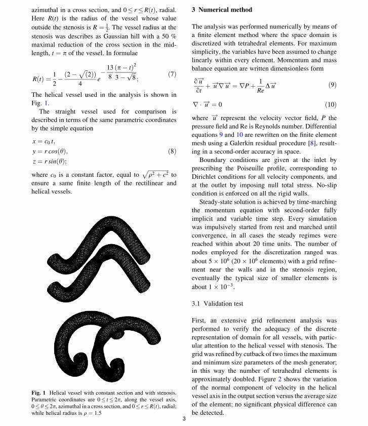
The helical vessel used in the analysis is shown in

Fig. 1.

The straight vessel used for comparison is

described in terms of the same parametric coordinates

by the simple equation

x ¼ c0 t;

y ¼ r cosðhÞ;z ¼ r sinðhÞ;

ð8Þ

where c0 is a constant factor, equal toffiffiffiffiffiffiffiffiffiffiffiffiffiffiffiq2 þ c2

pto

ensure a same finite length of the rectilinear and

helical vessels.

3 Numerical method

The analysis was performed numerically by means of

a finite element method where the space domain is

discretized with tetrahedral elements. For maximum

simplicity, the variables have been assumed to change

linearly within every element. Momentum and mass

balance equation are written dimensionless form

o u!ot

þ u!r u!¼ rPþ 1

ReD u! ð9Þ

r � u!¼ 0 ð10Þ

where u! represent the velocity vector field, P the

pressure field and Re is Reynolds number. Differential

equations 9 and 10 are rewritten on the finite element

mesh using a Galerkin residual procedure [8], result-

ing in a second-order accuracy in space.

Boundary conditions are given at the inlet by

prescribing the Poiseuille profile, corresponding to

Dirichlet conditions for all velocity components, and

at the outlet by imposing null total stress. No-slip

condition is enforced on all the rigid walls.

Steady-state solution is achieved by time-marching

the momentum equation with second-order fully

implicit and variable time step. Every simulation

was impulsively started from rest and marched until

convergence, in all cases the steady regimes were

reached within about 20 time units. The number of

nodes employed for the discretization ranged was

about 5� 106 (20� 106 elements) with a grid refine-

ment near the walls and in the stenosis region,

eventually the typical size of smaller elements is

about 1� 10�3.

3.1 Validation test

First, an extensive grid refinement analysis was

performed to verify the adequacy of the discrete

representation of domain for all vessels, with partic-

ular attention to the helical vessel with stenosis. The

grid was refined by cutback of two times the maximum

and minimum size parameters of the mesh generator;

in this way the number of tetrahedral elements is

approximately doubled. Figure 2 shows the variation

of the normal component of velocity in the helical

vessel axis in the output section versus the average size

of the element; no significant physical difference can

be detected.

Fig. 1 Helical vessel with constant section and with stenosis.

Parametric coordinates are 0� t� 2p, along the vessel axis,

0� h� 2p, azimuthal in a cross section, and 0� r�RðtÞ, radial;while helical radius is q ¼ 1:5

Meccanica (2017) 52:545–553 547

123

3

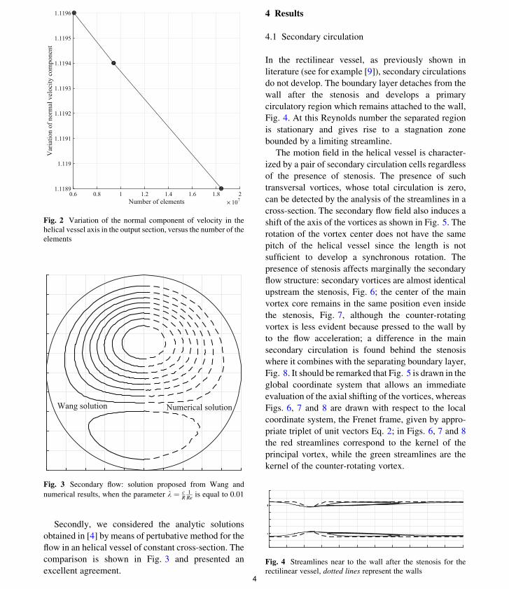
Secondly, we considered the analytic solutions

obtained in [4] by means of pertubative method for the

flow in an helical vessel of constant cross-section. The

comparison is shown in Fig. 3 and presented an

excellent agreement.

4 Results

4.1 Secondary circulation

In the rectilinear vessel, as previously shown in

literature (see for example [9]), secondary circulations

do not develop. The boundary layer detaches from the

wall after the stenosis and develops a primary

circulatory region which remains attached to the wall,

Fig. 4. At this Reynolds number the separated region

is stationary and gives rise to a stagnation zone

bounded by a limiting streamline.

The motion field in the helical vessel is character-

ized by a pair of secondary circulation cells regardless

of the presence of stenosis. The presence of such

transversal vortices, whose total circulation is zero,

can be detected by the analysis of the streamlines in a

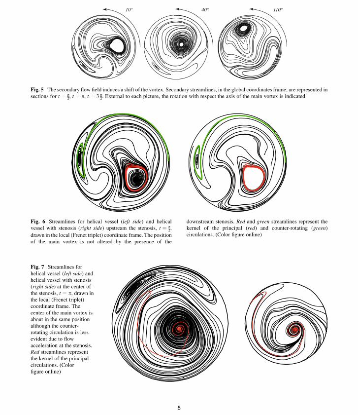
cross-section. The secondary flow field also induces a

shift of the axis of the vortices as shown in Fig. 5. The

rotation of the vortex center does not have the same

pitch of the helical vessel since the length is not

sufficient to develop a synchronous rotation. The

presence of stenosis affects marginally the secondary

flow structure: secondary vortices are almost identical

upstream the stenosis, Fig. 6; the center of the main

vortex core remains in the same position even inside

the stenosis, Fig. 7, although the counter-rotating

vortex is less evident because pressed to the wall by

to the flow acceleration; a difference in the main

secondary circulation is found behind the stenosis

where it combines with the separating boundary layer,

Fig. 8. It should be remarked that Fig. 5 is drawn in the

global coordinate system that allows an immediate

evaluation of the axial shifting of the vortices, whereas

Figs. 6, 7 and 8 are drawn with respect to the local

coordinate system, the Frenet frame, given by appro-

priate triplet of unit vectors Eq. 2; in Figs. 6, 7 and 8

the red streamlines correspond to the kernel of the

principal vortex, while the green streamlines are the

kernel of the counter-rotating vortex.

Number of elements × 1070.6 0.8 1 1.2 1.4 1.6 1.8 2

Var

iatio

n of

nor

mal

vel

ocity

com

pone

nt

1.1189

1.119

1.1191

1.1192

1.1193

1.1194

1.1195

1.1196

Fig. 2 Variation of the normal component of velocity in the

helical vessel axis in the output section, versus the number of the

elements

Numerical solutionWang solution

Fig. 3 Secondary flow: solution proposed from Wang and

numerical results, when the parameter k ¼ cR

1Re

is equal to 0.01

Fig. 4 Streamlines near to the wall after the stenosis for the

rectilinear vessel, dotted lines represent the walls

548 Meccanica (2017) 52:545–553

123

4

°011°04°01

Fig. 5 The secondary flow field induces a shift of the vortex. Secondary streamlines, in the global coordinates frame, are represented in

sections for t ¼ p2, t ¼ p, t ¼ 3 p

2. External to each picture, the rotation with respect the axis of the main vortex is indicated

Fig. 6 Streamlines for helical vessel (left side) and helical

vessel with stenosis (right side) upstream the stenosis, t ¼ p2,

drawn in the local (Frenet triplet) coordinate frame. The position

of the main vortex is not altered by the presence of the

downstream stenosis. Red and green streamlines represent the

kernel of the principal (red) and counter-rotating (green)

circulations. (Color figure online)

Fig. 7 Streamlines for

helical vessel (left side) and

helical vessel with stenosis

(right side) at the center of

the stenosis, t ¼ p, drawn in

the local (Frenet triplet)

coordinate frame. The

center of the main vortex is

about in the same position

although the counter-

rotating circulation is less

evident due to flow

acceleration at the stenosis.

Red streamlines represent

the kernel of the principal

circulations. (Color

figure online)

Meccanica (2017) 52:545–553 549

123

5

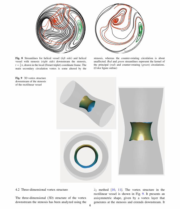
4.2 Three-dimensional vortex structure

The three-dimensional (3D) structure of the vortex

downstream the stenosis has been analyzed using the

k2 method [10, 11]. The vortex structure in the

rectilinear vessel is shown in Fig. 9. It presents an

axisymmetric shape, given by a vortex layer that

generates at the stenosis and extends downstream. It

Fig. 8 Streamlines for helical vessel (left side) and helical

vessel with stenosis (right side) downstream the stenosis,

t ¼ 32p, drawn in the local (Frenet triplet) coordinate frame. The

main secondary circulation vortex is some altered by the

stenosis, whereas the counter-rotating circulation is about

unaffected. Red and green streamlines represent the kernel of

the principal (red) and counter-rotating (green) circulations.

(Color figure online)

Fig. 9 3D vortex structure

downstream of the stenosis

of the rectilinear vessel

550 Meccanica (2017) 52:545–553

123

6

corresponds to a closed recirculation region down-

stream the stenosis.

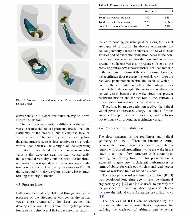
The picture is substantially different in the helical

vessel because the helical geometry breaks the axial

symmetry of the stenosis thus giving rise to a 3D

vortex structure. The boundary layer separating from

the axisymmetric stenosis does not give rise to circular

vortex lines because the strength of the separating

vorticity is modulated by the non-axisymmetric

velocity that develops near the wall; concurrently,

this azimuthal vorticity combines with the longitudi-

nal vorticity corresponding to the secondary circula-

tion describe above. Eventually, as shown in Fig. 10,

the separated vorticity develops streamwise counter-

rotating vorticity filaments.

4.3 Pressure losses

Following the markedly different flow geometry, the

presence of the streamwise vortices in the helical

vessel alters dramatically the shear stresses that

develop at the wall. This is quantified by the pressure

losses in the entire vessel that are reported in Table 1,

the corresponding pressure profiles along the vessel

are reported in Fig. 11. In absence of stenosis, the

helical geometry causes an increase of the wall shear

stresses and of energetic dissipation because the non-

rectilinear geometry deviates the flow and curves the

streamlines. In both vessels, in presence of stenosis the

pressure profile shows the additional localized loss due

to the increased friction at the constriction. However,

the rectilinear duct presents the well-known pressure

recovery phenomenon behind the stenosis, which is

due to the recirculation cell in the enlarged sec-

tion. Differently enough, the recovery is absent in

helical vessel because the wake does not present

backward motion and the net loss at the stenosis is

irremediably lost and not recovered afterward.

Therefore, by an energetic perspective, the helical

vessel gives an increased energy loss that is further

amplified in presence of a stenosis, and performs

worse than a corresponding rectilinear vessel.

4.4 Residence time distribution

The flow structure in the rectilinear and helical

geometry are also different in kinematic terms,

because the former presents a closed recirculation

region, with closed streamlines, while the wake in the

latter is an open flow structure with streamlines

entering and exiting from it. This phenomenon is

expected to give rise to different performances in

terms of ability for wash-out which is analyzed here in

terms of residence time of blood elements.

The concept of residence time distribution (RTD)

was developed long time ago in reactive chemical

engineering, e.g. [12], and is also useful to quantify the

the presence of blood stagnation regions which can

increase the risk of cloth formation in cardiac flows

[13].

The analysis of RTD can be obtained by the

solution of the convection-diffusion equation for

studying the wash-out of arbitrary passive scalar

Fig. 10 Vortex structure downstream of the stenosis of the

helical vessel

Table 1 Pressure losses measured in the vessels

Rectilinear Helical

Total loss without stenosis 1.00 2.88

Total loss with in stenosis 2.75 5.66

Local loss imputable to stenosis 1.75 2.78

Meccanica (2017) 52:545–553 551

123

7

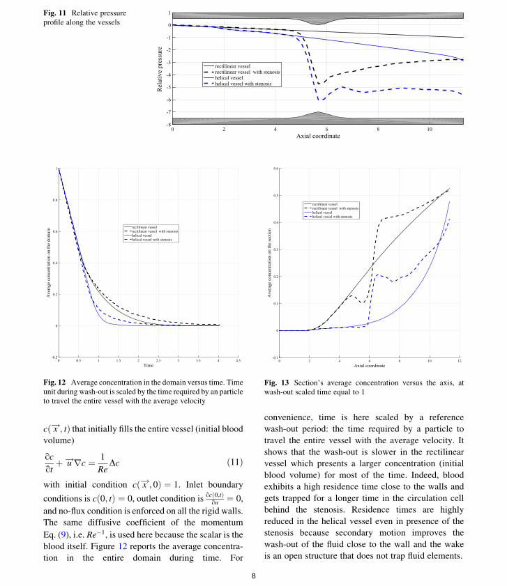
cð x!; tÞ that initially fills the entire vessel (initial bloodvolume)

oc

otþ u!rc ¼ 1

ReDc ð11Þ

with initial condition cð x!; 0Þ ¼ 1. Inlet boundary

conditions is cð0; tÞ ¼ 0, outlet condition isocð0;tÞon

¼ 0,

and no-flux condition is enforced on all the rigid walls.

The same diffusive coefficient of the momentum

Eq. (9), i.e. Re�1, is used here because the scalar is the

blood itself. Figure 12 reports the average concentra-

tion in the entire domain during time. For

convenience, time is here scaled by a reference

wash-out period: the time required by a particle to

travel the entire vessel with the average velocity. It

shows that the wash-out is slower in the rectilinear

vessel which presents a larger concentration (initial

blood volume) for most of the time. Indeed, blood

exhibits a high residence time close to the walls and

gets trapped for a longer time in the circulation cell

behind the stenosis. Residence times are highly

reduced in the helical vessel even in presence of the

stenosis because secondary motion improves the

wash-out of the fluid close to the wall and the wake

is an open structure that does not trap fluid elements.

Axial coordinate0 2 4 6 8 10

Rel

ativ

e pr

essu

re

-8

-7

-6

-5

-4

-3

-2

-1

0

1

rectilinear vesselrectilinear vessel with stenosishelical vesselhelical vessel with stenosis

Fig. 11 Relative pressure

profile along the vessels

Time0 0.5 1 1.5 2 2.5 3 3.5 4 4.5

Ave

rage

con

cent

ratio

n on

the

dom

ain

-0.2

0

0.2

0.4

0.6

0.8

1

rectilinear vesselrectilinear vessel with stenosishelical vesselhelical vessel with stenosis

Fig. 12 Average concentration in the domain versus time. Time

unit during wash-out is scaled by the time required by an particle

to travel the entire vessel with the average velocity

Axial coordinate0 2 4 6 8 10 12

Ave

rage

con

cent

ratio

n on

the

sect

ion

-0.1

0

0.1

0.2

0.3

0.4

0.5

0.6

rectilinear vesselrectilinear vessel with stenosishelical vesselhelical vessel with stenosis

Fig. 13 Section’s average concentration versus the axis, at

wash-out scaled time equal to 1

552 Meccanica (2017) 52:545–553

123

8

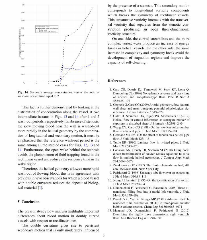
This fact is further demonstrated by looking at the

distribution of concentration along the vessel at two

intermediate instants in Figs. 13 and 14 after 1 and 2

wash-out periods, respectively. In absence of stenosis,

the slow moving blood near the wall is washed-out

more rapidly in the helical geometry by the combina-

tion of longitudinal and secondary motion, it must be

emphasized that the reference wash-out period is the

same among all the studied cases for Figs. 12, 13 and

14. Furthermore, the open wake behind the stenosis

avoids the phenomenon of fluid trapping found in the

rectilinear vessel and reduces the residence time in the

wake region.

Therefore, the helical geometry allows a more rapid

wash-out of flowing blood; this is in agreement with

previous in vivo observations for which a blood vessel

with double curvature reduces the deposit of biolog-

ical material [1].

5 Conclusion

The present steady flow analysis highlights important

differences about blood motion in doubly curved

vessels with respect to rectilinear ones.

The double curvature gives rise to persistent

secondary motion that is only moderately influenced

by the presence of a stenosis. This secondary motion

corresponds to longitudinal vorticity components

which breaks the symmetry of rectilinear vessels.

This streamwise vorticity interacts with the transver-

sal vorticity that separates from the stenotic con-

striction producing an open three-dimensional

vorticity structure.

On one side, the curved streamlines and the more

complex vortex wake produce an increase of energy

losses in helical vessels. On the other side, the same

increase in complexity and symmetry break avoid the

development of stagnation regions and improve the

capacity of self-cleaning.

References

1. Caro CG, Doorly DJ, Tarnawski M, Scott KT, Long Q,

Dumouling CL (1996) Non-planar curvature and branching

of arteries and non-planar-type flow. Proc R Soc A

452:185–197

2. Coppola G, Caro CG (2009) Arterial geometry, flow pattern,

wall shear and mass transport: potential physiological sig-

nificance. J R Soc Interface 6:519–528

3. Gallo D, Steinman DA, Bijari PB, Morbiducci U (2012)

Helical flow in carotid bifurcation as surrogate marker of

exposure to disturbed shear. J Biomech 45:2398–2404

4. Wang CY, Caro CG (1981) On the low-Reynolds-number

flow in a helical pipe. J Fluid Mech 108:185–194

5. Germano M (1981) On the effect of torsion on a helical pipe

flow. J Fluid Mech 125:1–8

6. Tuttle ER (1990) Laminar flow in twisted pipes. J Fluid

Mech 219:545–570

7. Cookson AN, Doorly DJ, Sherwin SJ (2010) Using coor-

dinate transformation of Navier–Stokes equations to solve

flow in multiple helical geometries. J Comput Appl Math

234:2069–2079

8. Zienkiewicz OC (1977) The finite elements method, 4th

edn. McGraw-Hill, New York City

9. Pedrizzetti G (1996) Unsteady tube flow over an expansion.

J Fluid Mech 310:89–111

10. Jeong J, Hussain F (1995) On the identification of a vortex.

J Fluid Mech 285:69–94

11. Domenichini F, Pedrizzetti G, Baccani B (2005) Three-di-

mensional filling flow into a model left ventricle. J Fluid

Mech 539:179–198

12. Pareek VK, Yap Z, Brungs MP (2001) Adesina, Particle

residence time distribution (RTD) in three-phase annular

bubble column reactor. Chem Eng Sci 56:6063–6071

13. Mangual JO, Domenichini F, Pedrizzetti G (2012)

Describing the highly three dimensional right ventricle

flow. Ann Biomed Eng 40:1790–1801

Axial coordinate0 2 4 6 8 10 12

Ave

rage

con

cent

ratio

n on

the

sect

ion

0

0.02

0.04

0.06

0.08

0.1

0.12

0.14

0.16

0.18

0.2

rectilinear vesselrectilinear vessel with stenosishelical vesselhelical vessel with stenosis

Fig. 14 Section’s average concentration versus the axis, at

wash-out scaled time equal to 2

Meccanica (2017) 52:545–553 553

123

9