Tutorial: Missile Silo Launch Introduction The purpose of this tutorial is to provide guidelines to set up and run a dynamic mesh (DM) case using the layering scheme. The tutorial models a missile being launched from a silo. The motion of the missile is predicted using the six degree of freedom (6DOF) solver in FLUENT. In this tutorial, you will learn how to: • Read a mesh file and perform a dynamic mesh calculation. • Enable and configure the 6DOF solver. • Compile a UDF that governs the missile motion. • Set up moving zones. • Set up a dynamic mesh event to control the mesh motion. • Define custom commands to be executed at regular intervals during the simulation. • Run an unsteady calculation for the problem. • Write image files that can be played as an animation. Prerequisites This tutorial assumes that you are familiar with the FLUENT interface, and that you have a good understanding of the basic setup and solution procedures. In this tutorial, you will use the dynamic mesh model. If you have not used this model before, refer to Section 10.6: Dynamic Meshes in the FLUENT 6.2 User’s Guide. Problem Description Consider the launch of a missile from its silo (Figure 1). The 6DOF solver is used to predict the motion of the missile. The UDF (silo.c) is used to specify the properties of the missile (mass and moments of inertia) as well as any body forces that are present. The 6DOF solver applies Newton’s law to determine the acceleration of the missile. c Fluent Inc. March 20, 2006 1

Welcome message from author
This document is posted to help you gain knowledge. Please leave a comment to let me know what you think about it! Share it to your friends and learn new things together.
Transcript

Tutorial: Missile Silo Launch
Introduction
The purpose of this tutorial is to provide guidelines to set up and run a dynamic mesh(DM) case using the layering scheme. The tutorial models a missile being launched from asilo. The motion of the missile is predicted using the six degree of freedom (6DOF) solverin FLUENT.
In this tutorial, you will learn how to:
• Read a mesh file and perform a dynamic mesh calculation.
• Enable and configure the 6DOF solver.
• Compile a UDF that governs the missile motion.
• Set up moving zones.
• Set up a dynamic mesh event to control the mesh motion.
• Define custom commands to be executed at regular intervals during the simulation.
• Run an unsteady calculation for the problem.
• Write image files that can be played as an animation.
Prerequisites
This tutorial assumes that you are familiar with the FLUENT interface, and that you havea good understanding of the basic setup and solution procedures. In this tutorial, you willuse the dynamic mesh model. If you have not used this model before, refer to Section 10.6:Dynamic Meshes in the FLUENT 6.2 User’s Guide.
Problem Description
Consider the launch of a missile from its silo (Figure 1). The 6DOF solver is used to predictthe motion of the missile. The UDF (silo.c) is used to specify the properties of the missile(mass and moments of inertia) as well as any body forces that are present. The 6DOFsolver applies Newton’s law to determine the acceleration of the missile.
c© Fluent Inc. March 20, 2006 1

Missile Silo Launch
Thrust, gravity, and pressure forces are considered in the calculation, whereas the drag onthe missile is neglected. The missile engine starts to fire at t = 0 seconds but the missile isheld fixed in the silo and is not allowed to move until t = 0.1 seconds. The flow is assumedto be inviscid and the domain is axisymmetric.
Figure 1: Problem Schematic of a Missile Inside the Silo
Preparation
1. Copy the files, silo.msh.gz and silo.c to the working directory.
2. Start the 2D, double-precision (2DDP) version of FLUENT.
Setup and Solution
Step 1: Grid
1. Read the mesh file, silo.msh.gz.
File −→ Read −→Case...
2. Scale the grid to inches.
Grid −→Scale...
(a) Under Units Conversion, select in from the Grid Was Created In drop-down list.
(b) Click Scale and close the panel.
2 c© Fluent Inc. March 20, 2006

Missile Silo Launch
3. Set the unit of length to inches.
Define −→Units...
4. Check and display the grid (Figure 2).
Display −→Grid...
GridFLUENT 6.2 (2d, dp, segregated, lam)
Feb 10, 2006
Figure 2: Grid Display
c© Fluent Inc. March 20, 2006 3

Missile Silo Launch
5. Set the view so that the missile points upward (Figure 3).
Display −→Views...
(a) Click Camera....
i. Select Up Vector in the Camera drop-down list.
ii. Set X to 1, Y to 0, and Z to 0.
iii. Click Apply and close the Camera Parameters panel.
The view updates to show the missile pointing upward.
(b) Under Mirror Planes, select axis-in and axis-out.
(c) Click Apply.
The view updates to show the display mirrored about the axis of symmetry. Donot close the Views panel.
(d) Zoom and pan in the display to center the view (Figure 3).
(e) Click Save to save the view and close the Views panel.
The saved view, view-0 appears in the Views list.
6. Create zone surfaces for the two fluid zones.
Surface −→Zone...
(a) Under Zone, select fluid-inner and click Create.
(b) Similarly, create the fluid-outer zone.
7. Display fluid-inner zone surface (Figure 4).
The fluid-inner zone contains the missile and is meshed with quadrilateral elements.This zone is bounded on the top and bottom sides by the interior zones internal-topand internal-bot, respectively.
The task is to move this fluid zone in accordance with the dynamics of the missile.During this process, the layering algorithm builds layers of quadrilateral elements atinternal-bot and collapses layers at internal-top.
A non-conformal interface has to be used between fluid-inner and fluid-outer zones,because the fluid-inner zone will move relative to the rest of the domain.
4 c© Fluent Inc. March 20, 2006

Missile Silo Launch
GridFLUENT 6.2 (2d, dp, segregated, lam)
Feb 10, 2006
Figure 3: Rotated and Mirrored View of the Grid
GridFLUENT 6.2 (2d, segregated, lam)
Mar 17, 2006
Figure 4: The fluid-inner Zone
c© Fluent Inc. March 20, 2006 5

Missile Silo Launch
Step 2: Compile the UDF
Define −→ User-Defined −→ Functions −→Compiled...
1. Click Add... and select silo.c.
2. Click Build.
The Information dialog box is displayed. Read the instructions carefully and click OK.FLUENT creates the appropriate directory structure, makefiles, and compiles the codefor you. The progress of the compilation is shown in the FLUENT console window.You can monitor the progress of the compilation for any linking errors. Alternatively,you can also view the log file with the compilation history that will be created in theworking directory.
3. Click Load.
Step 3: Models
1. Enable the Coupled solver with Explicit formulation, Unsteady time condition, andAxisymmetric space.
Define −→ Models −→Solver...
6 c© Fluent Inc. March 20, 2006

Missile Silo Launch
(a) Select Coupled under Solver, Explicit under Formulation.
(b) Select Axisymmetric under Space, and Unsteady under Time.
Dynamic mesh features are available only in the unsteady solver with first-orderimplicit time discretization.
(c) Retain the default settings for the remaining parameters and click OK.
2. Enable the Energy equation.
Define −→ Models −→Energy...
3. Enable the Spalart-Allmaras turbulence model.
Define −→ Models −→Viscous...
(a) Under Model, select Spalart-Allmaras (1 eqn).
(b) Retain the default settings for the other parameters and click OK.
4. Enable the Species Transport model.
It helps you in distinguishing between air and exhaust gases.
Define −→ Models −→ Species −→Transport & Reaction...
(a) Under Model, select Species Transport.
(b) Click OK.
c© Fluent Inc. March 20, 2006 7
Missile Silo Launch
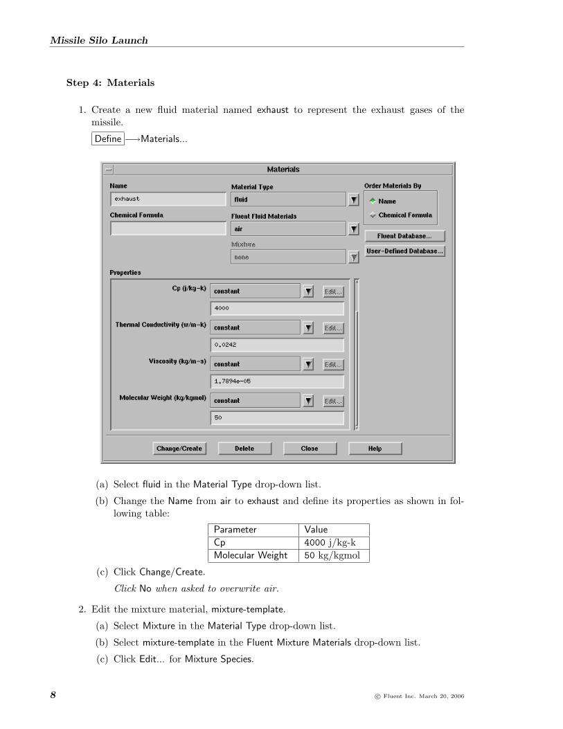
Step 4: Materials
1. Create a new fluid material named exhaust to represent the exhaust gases of themissile.
Define −→Materials...
(a) Select fluid in the Material Type drop-down list.
(b) Change the Name from air to exhaust and define its properties as shown in fol-lowing table:
Parameter Value
Cp 4000 j/kg-kMolecular Weight 50 kg/kgmol
(c) Click Change/Create.
Click No when asked to overwrite air.
2. Edit the mixture material, mixture-template.
(a) Select Mixture in the Material Type drop-down list.
(b) Select mixture-template in the Fluent Mixture Materials drop-down list.
(c) Click Edit... for Mixture Species.
8 c© Fluent Inc. March 20, 2006
Missile Silo Launch
i. Add exhaust and air (in the same order) to the Selected Species list.
ii. Remove h2o, o2, and n2 from the Selected Species list and click OK.
(d) Select ideal-gas for Density.
(e) Click Change/Create and close the Materials panel.
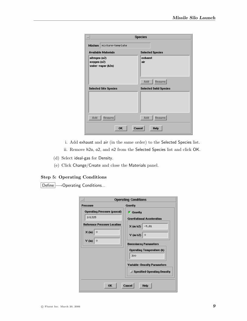
Step 5: Operating Conditions
Define −→Operating Conditions...
c© Fluent Inc. March 20, 2006 9

Missile Silo Launch
1. Keep the default operating pressure of 101325 Pa.
2. Enable Gravity and set the Gravitational Acceleration to -9.81 m/s2 in the X direction.
3. Set the Operating Temperature to 300 K.
4. Set the solution limits for pressure and temperature.
Solve −→ Controls −→Limits...
(a) Set the Minimum Absolute Pressure to 10000 Pa and Maximum Absolute Pressureto 2500000 Pa.
(b) Set the Minimum Static Temperature to 50 K and the Maximum Static Temperatureto 2800 K.
(c) Set the Maximum Turb. Viscosity Ratio to 1e06.
(d) Click OK.
Step 6: Boundary Conditions
Define −→Boundary Conditions...
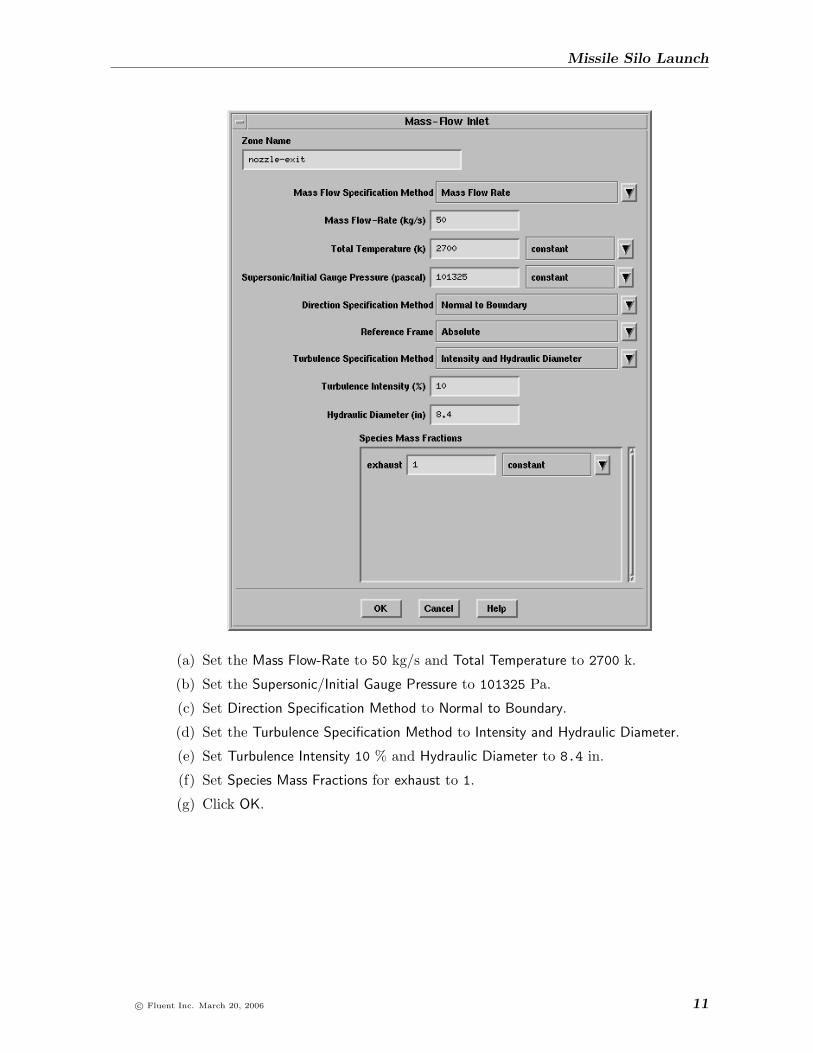
1. Set the boundary conditions for the nozzle-exit zone.
10 c© Fluent Inc. March 20, 2006
Missile Silo Launch
(a) Set the Mass Flow-Rate to 50 kg/s and Total Temperature to 2700 k.
(b) Set the Supersonic/Initial Gauge Pressure to 101325 Pa.
(c) Set Direction Specification Method to Normal to Boundary.
(d) Set the Turbulence Specification Method to Intensity and Hydraulic Diameter.
(e) Set Turbulence Intensity 10 % and Hydraulic Diameter to 8.4 in.
(f) Set Species Mass Fractions for exhaust to 1.
(g) Click OK.
c© Fluent Inc. March 20, 2006 11

Missile Silo Launch
2. Set the boundary conditions for the far-field zone.
(a) Retain the default value of 0 for Gauge Pressure.
(b) Retain the default values of the other parameters and click OK.
3. Ensure that the Type for zones, axis-in and axis-out is axis.
4. Ensure that the Type for zones, interface-in, interface-out-1, and interface-out-2 is in-terface.
Step 7: Dynamic Mesh Setup
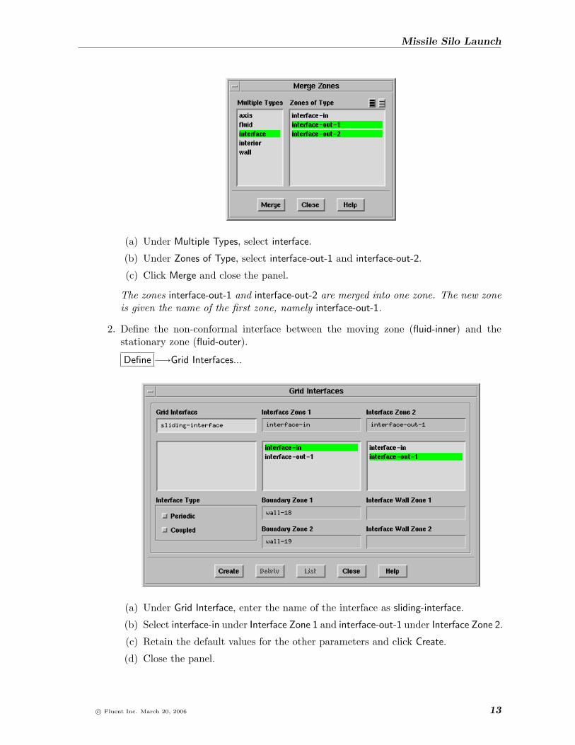
1. Merge interfaces into one zone.
Grid −→Merge...
12 c© Fluent Inc. March 20, 2006
Missile Silo Launch
(a) Under Multiple Types, select interface.
(b) Under Zones of Type, select interface-out-1 and interface-out-2.
(c) Click Merge and close the panel.
The zones interface-out-1 and interface-out-2 are merged into one zone. The new zoneis given the name of the first zone, namely interface-out-1.
2. Define the non-conformal interface between the moving zone (fluid-inner) and thestationary zone (fluid-outer).
Define −→Grid Interfaces...
(a) Under Grid Interface, enter the name of the interface as sliding-interface.
(b) Select interface-in under Interface Zone 1 and interface-out-1 under Interface Zone 2.
(c) Retain the default values for the other parameters and click Create.
(d) Close the panel.
c© Fluent Inc. March 20, 2006 13
Missile Silo Launch
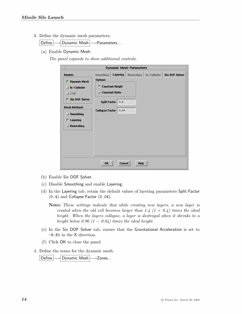
3. Define the dynamic mesh parameters.
Define −→ Dynamic Mesh −→Parameters...
(a) Enable Dynamic Mesh.
The panel expands to show additional controls.
(b) Enable Six DOF Solver.
(c) Disable Smoothing and enable Layering.
(d) In the Layering tab, retain the default values of layering parameters Split Factor(0.4) and Collapse Factor (0.04).
Note: These settings indicate that while creating new layers, a new layer iscreated when the old cell becomes larger than 1.4 (1 + 0.4) times the idealheight. When the layers collapse, a layer is destroyed when it shrinks to aheight below 0.96 (1 − 0.04) times the ideal height.
(e) In the Six DOF Solver tab, ensure that the Gravitational Acceleration is set to-9.81 in the X direction.
(f) Click OK to close the panel.
4. Define the zones for the dynamic mesh.
Define −→ Dynamic Mesh −→Zones...
14 c© Fluent Inc. March 20, 2006

Missile Silo Launch
(a) Create rigid body type zones.
i. Select wall-missile under Zone Names, and Rigid Body under Type.
ii. Select launch::libudf in the Six DOF UDF drop-down list.
iii. Under Six DOF Solver Options, select On and deselect Passive.
iv. Click Create.
The wall-missile zone now appears in the Dynamic Zones list.
v. Follow the previous steps to specify rigid body motion for the nozzle-exit andfluid-inner zones. Enable Passive solver option for these zones.
Note: You must click Create after setting options for each zone.
When a zone is declared Passive, the six DOF solver will not calculate forcesand moments in that zone. However, the zone is still part of the rigid bodymotion. In this case, the moving zones fluid-inner, nozzle-exit, and missile-wall move with the same rigid body motion but the forces are calculated onlyon the non-passive zone, missile-wall.
c© Fluent Inc. March 20, 2006 15

Missile Silo Launch
(b) Create stationary type zones.
While fluid-inner moves in a translational rigid body mode, the upper and lowerboundaries (internal-top and internal-bottom) of this fluid zone must be fixed inorder to provide a location for creating and collapsing layers of cells. Thus, thesetwo zones must be declared stationary explicitly.
i. Select internal-bottom under Zone Names.
ii. Select Stationary under Type.
iii. In the Meshing Options tab, set the value of Cell Height for the adjacentfluid-inner zone to 1 inch and click Create.
This is the ideal cell height near internal-bottom, and it is set equal to thecell height of the quadrilateral mesh adjacent to the internal-bottom zone.
iv. Select internal-top under Zone Names.
v. Select Stationary under Type.
vi. In the Meshing Options tab, set the value of Cell Height for the adjacentfluid-inner zone to 1 inch and click Create.
vii. Close the Dynamic Mesh Zones panel.
16 c© Fluent Inc. March 20, 2006

Missile Silo Launch
5. Define a dynamic mesh event that will hold the missile in place until liftoff at t =0.1 seconds.
Define −→ Dynamic Mesh −→Events...
(a) Set Number of Events to 2.
(b) For event-1, enable the checkbox under On and set At Time to 0.
(c) Click Define... for event-1.
The Define Event panel opens.
c© Fluent Inc. March 20, 2006 17

Missile Silo Launch
i. Select Change Motion Attribute under Type drop-down list.
ii. Under Attribute, select Moving.
iii. Under Status, select Disable.
iv. Select fluid-inner, wall-missile, and nozzle-exit.
v. Click OK.
(d) Similarly, define event-2 to enable zone motion at t = 0.1 sec.
18 c© Fluent Inc. March 20, 2006

Missile Silo Launch
(e) Click Apply and close the panel.
Step 8: Solution Controls
1. Set the solution control parameters.
Solve −→ Controls −→Solution...
c© Fluent Inc. March 20, 2006 19

Missile Silo Launch
(a) Set the discretization scheme for Flow to First Order upwind.
(b) Set the Courant Number to 0.5.
(c) Click OK.
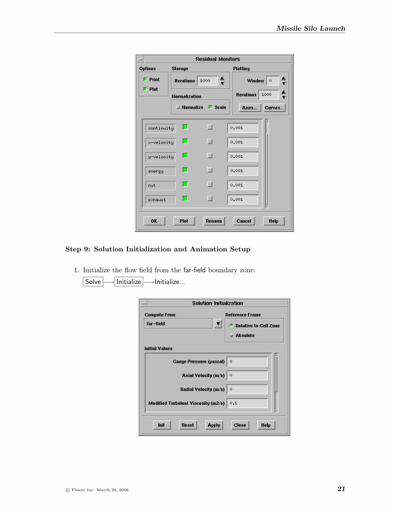
2. Set the residual monitor parameters.
Solve −→ Monitors −→Residual...
(a) Enable the plotting of residuals by selecting Plot under Options.
(b) Disable the Check Convergence option for all the residuals.
You need to scroll down the list of residuals to view exhaust.
20 c© Fluent Inc. March 20, 2006
Missile Silo Launch
Step 9: Solution Initialization and Animation Setup
1. Initialize the flow field from the far-field boundary zone.
Solve −→ Initialize −→Initialize...
c© Fluent Inc. March 20, 2006 21
Missile Silo Launch
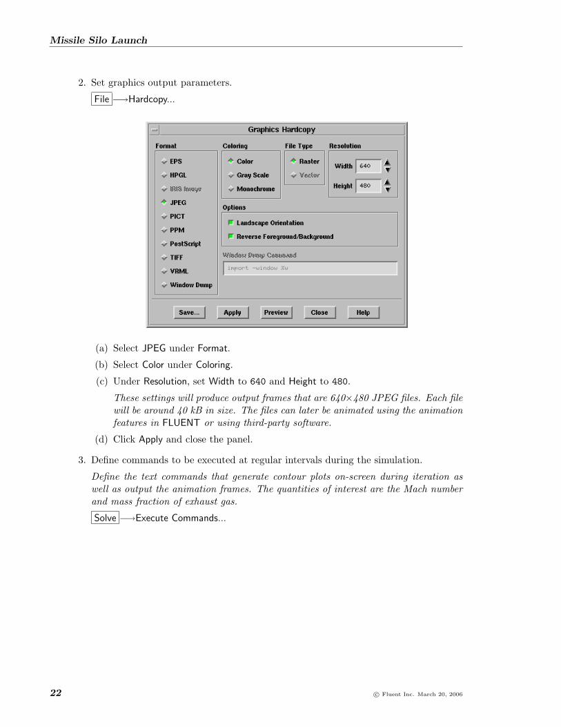
2. Set graphics output parameters.
File −→Hardcopy...
(a) Select JPEG under Format.
(b) Select Color under Coloring.
(c) Under Resolution, set Width to 640 and Height to 480.
These settings will produce output frames that are 640×480 JPEG files. Each filewill be around 40 kB in size. The files can later be animated using the animationfeatures in FLUENT or using third-party software.
(d) Click Apply and close the panel.
3. Define commands to be executed at regular intervals during the simulation.
Define the text commands that generate contour plots on-screen during iteration aswell as output the animation frames. The quantities of interest are the Mach numberand mass fraction of exhaust gas.
Solve −→Execute Commands...
22 c© Fluent Inc. March 20, 2006

Missile Silo Launch
(a) Set Defined Commands to 3.
(b) Select the checkboxes under On for all the commands.
(c) For command-1 and command-2, set Every to 5 and select Time Step from theWhen drop-down list.
(d) Enter the following command in the Command text-entry field for command-1:
disp sw 1 cont mach 0 2 hc mach%t.jpg
(e) Enter the following command in the Command text-entry field for command-2:
disp sw 2 cont exhaust 0 1 hc exhaust%t.jpg
These two commands will instruct FLUENT to do the following every 5 iterations:
• Set the current window (disp sw X)
• Display a filled contour (cont variable min max)
• Write a hardcopy of the filled contour (hc filename)
(f) For command-3, set Every to 50 and select Time Step from the When drop-downlist.
(g) Enter the following command in the Command text-entry field for command-3:
file wcd silo-unsteady-%t.gz
This command will write compressed case and data files to the working directoryevery 50 time steps.
(h) Click OK to close the panel.
4. Initialize the graphics settings by creating initial contour plots.
(a) Open the Contours panel and the Display Options panel simultaneously.
Display −→Options...
Display −→Contours...
c© Fluent Inc. March 20, 2006 23

Missile Silo Launch
(b) In the Display Options panel, set Active Window to 1 and click Set.
Graphics window 1 opens. It is the current active window.
(c) In the Contour Plot panel, select Velocity and Mach Number from the Contours ofdrop-down list, enable Filled under Options, and click Display.
The contour plot of Mach number appears in graphics window 1.
(d) Restore the saved view, view-0 in graphics window 1.
Display −→Views...
i. Under Views, select view-0 and click Restore.
(e) Set Active Window to 2 in the Display Options panel and click Set.
Graphics window 2 opens. It is the current active window.
(f) In the Contour Plot panel, select Species and Mass Fraction of exhaust from theContours of drop-down list, enable Filled under Options, and click Display.
(g) Restore the saved view, view-0 in graphics window 2.
Display −→Views...
(h) Close the Display Options, Contours, and Views panels.
5. Save the case and data files, silo-setup.gz.
Step 10: Calculate the Initial Solution
For this high-speed compressible flow case, you will perform iterations in two stages. First,you will calculate several iterations at a low Courant number in order to stabilize the solu-tion. Then you will increase the Courant number and calculate the remainder of the solutionto convergence. Performing calculations in this way ensures that the solution is stable andhas an acceptable convergence rate.
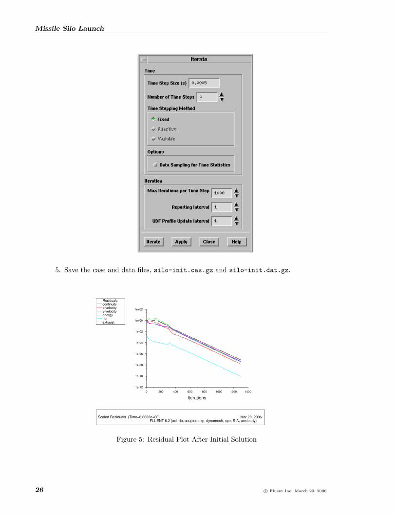
Solve −→Iterate...
24 c© Fluent Inc. March 20, 2006

Missile Silo Launch
1. Set the Time Step Size to 0.0005, Number of Time Steps to 0, and Max Iterations perTime Step to 300.
2. Click Iterate.
FLUENT may give an error message on some systems when you iterate with Numberof Time Steps set to 0. In that case, set Number of Time Steps to 1.
3. Set the Courant number to 1.5.
Solve −→ Controls −→Solution...
4. Set Max Iterations per Time Step to 1000 and click Iterate to continue the solution.
The initial solution is completely converged at the end of 1300 iterations.
c© Fluent Inc. March 20, 2006 25
Missile Silo Launch
5. Save the case and data files, silo-init.cas.gz and silo-init.dat.gz.
Scaled Residuals (Time=0.0000e+00)FLUENT 6.2 (axi, dp, coupled exp, dynamesh, spe, S-A, unsteady)
Mar 20, 2006
Iterations1400120010008006004002000
1e+02
1e+00
1e-02
1e-04
1e-06
1e-08
1e-10
1e-12
exhaustnutenergyy-velocityx-velocitycontinuityResiduals
Figure 5: Residual Plot After Initial Solution
26 c© Fluent Inc. March 20, 2006

Missile Silo Launch
Step 11: Calculate the Unsteady Solution
1. Open the Iterate panel.
Solve −→Iterate...
(a) Set Time Step Size to 0.0005, Number of Time Steps to 550, and Max Iterationsper Time Step to 20.
(b) Click Iterate.
While FLUENT is iterating, you can monitor the progress of solution in the two graph-ics windows. As the solution time reaches t = 0.1 seconds (after 200 time steps), thethrust will begin to move the missile. The motion of the missile will be seen in boththe graphics windows.
2. Save the case and data files, silo-unsteady.cas.gz.
File −→ Write −→Case and Data...
Step 12: Postprocessing
During the the simulation, animation frames are generated every 0.0025 seconds (5 timesteps). These frames are saved in the working directory under the file names machxxxx.jpgand exhaustxxxx.jpg where xxxx stands for the time step number. Also, data files aresaved every 0.025 seconds (50 time steps) as silo-unsteadyxxxx.dat.gz.
You can read the saved case and data files at a particular time step to view the results forpostprocessing.
1. View the results at the moment the rocket is released (t = 0.1 seconds).
0.1 seconds corresponds to 200 time steps.
(a) Read the data file, silo-unsteady0200.dat.gz
File −→ Read −→Data...
(b) Display contours of Mach number at t = 0.1 seconds (Figure 6).
(c) Restore the saved view, view-0.
Display −→Views...
(d) Display contours of mass fraction of exhaust gas at t = 0.1 seconds (Figure 7).
2. Display the results at t = 0.15 seconds (Figure 8 and Figure 9).
The results at 0.15 seconds can be viewed by reading the data file, silo-unsteady0300.dat.gz.
c© Fluent Inc. March 20, 2006 27

Missile Silo Launch
Contours of Mach Number (Time=1.0000e-01) Feb 15, 2006FLUENT 6.2 (axi, dp, coupled exp, dynamesh, spe, S-A, unsteady)
2.94e+00
1.80e-031.49e-012.96e-014.43e-015.90e-017.37e-018.84e-011.03e+001.18e+001.32e+001.47e+001.62e+001.77e+001.91e+002.06e+002.21e+002.35e+002.50e+002.65e+002.79e+00
Figure 6: Contours of Mach Number at t=0.1 s
Contours of Mass fraction of exhaust (Time=1.0000e-01) Feb 15, 2006FLUENT 6.2 (axi, dp, coupled exp, dynamesh, spe, S-A, unsteady)
1.00e+00
0.00e+005.00e-021.00e-011.50e-012.00e-012.50e-013.00e-013.50e-014.00e-014.50e-015.00e-015.50e-016.00e-016.50e-017.00e-017.50e-018.00e-018.50e-019.00e-019.50e-01
Figure 7: Contours of Mass Fraction of exhaust at t=0.1 s
28 c© Fluent Inc. March 20, 2006

Missile Silo Launch
Contours of Mach Number (Time=2.7500e-01) Mar 20, 2006FLUENT 6.2 (axi, dp, coupled exp, dynamesh, spe, S-A, unsteady)
2.98e+00
2.97e-031.52e-013.00e-014.49e-015.98e-017.46e-018.95e-011.04e+001.19e+001.34e+001.49e+001.64e+001.79e+001.94e+002.08e+002.23e+002.38e+002.53e+002.68e+002.83e+00
Figure 8: Contours of Mach Number at t=0.275 s
Contours of Mass fraction of exhaust (Time=2.7500e-01) Mar 20, 2006FLUENT 6.2 (axi, dp, coupled exp, dynamesh, spe, S-A, unsteady)
1.00e+00
0.00e+005.00e-021.00e-011.50e-012.00e-012.50e-013.00e-013.50e-014.00e-014.50e-015.00e-015.50e-016.00e-016.50e-017.00e-017.50e-018.00e-018.50e-019.00e-019.50e-01
Figure 9: Contours of Mass Fraction of exhaust at t=0.275 s
c© Fluent Inc. March 20, 2006 29

Missile Silo Launch
3. Link the image sequences created during the simulation into an animation of theunsteady flow and rocket motion.
Note: This step requires installation of third-party software.
Animations of the rocket motion are provided along with the tutorial files. Theseanimations can be played in any media player that supports the audio/video interleave(AVI) file format.
Summary
In this tutorial, you used FLUENT to solve an unsteady problem using the six degree offreedom solver along with the layering algorithm. While the six degree of freedom solver isapplicable to a three-dimensional flow domain, this tutorial illustrates that it can also beused to predict pure linear motion.
30 c© Fluent Inc. March 20, 2006
Related Documents