FLUENT 6.1 Acoustics Module Manual - julliojullio.pe.kr/fluent6.1/help/pdf/acoustics/fl61aco.pdf · Chapter 1. Aero-Noise Model Theory This chapter presents an overview of the theory

FLUENT 6.1

Acoustics Module Manual

February 2003

Licensee acknowledges that use of Fluent Inc.’s products can only provide an impreciseestimation of possible future performance and that additional testing and analysis, inde-pendent of the Licensor’s products, must be conducted before any product can be finallydeveloped or commercially introduced. As a result, Licensee agrees that it will not relyupon the results of any usage of Fluent Inc.’s products in determining the final design,composition or structure of any product.

Copyright c© 2003 by Fluent Inc.All rights reserved. No part of this document may be reproduced or otherwise used in

any form without express written permission from Fluent Inc.

Airpak, FIDAP, FLUENT, GAMBIT, Icepak, MixSim, and POLYFLOW are registeredtrademarks of Fluent Inc. All other products or name brands are trademarks of their

respective holders.

Fluent Inc.Centerra Resource Park

10 Cavendish CourtLebanon, NH 03766

Contents

1 Aero-Noise Model Theory 1-1

1.1 Introduction . . . . . . . . . . . . . . . . . . . . . . . . . . . . . . . . . 1-1

1.2 Lighthill’s Acoustic Analogy . . . . . . . . . . . . . . . . . . . . . . . . . 1-1

1.3 Intensity and Spectral Density of The Sound . . . . . . . . . . . . . . . . 1-4

1.3.1 Intensity of Sound . . . . . . . . . . . . . . . . . . . . . . . . . . 1-4

1.3.2 Spectral Density and Power Spectral Density of Sound . . . . . . 1-5

1.4 Dipole Sound Strength Distribution on Surface . . . . . . . . . . . . . . 1-7

1.4.1 Surface Dipole Radiation . . . . . . . . . . . . . . . . . . . . . . 1-7

1.4.2 Surface Dipole Strength . . . . . . . . . . . . . . . . . . . . . . . 1-8

2 Using the Aero-Noise Model 2-1

2.1 Introduction . . . . . . . . . . . . . . . . . . . . . . . . . . . . . . . . . 2-1

2.2 Using the Aero-Noise Prediction Model . . . . . . . . . . . . . . . . . . . 2-2

2.2.1 Installing the Aero-Noise Prediction Model . . . . . . . . . . . . 2-2

2.2.2 Setup and Solution Procedure . . . . . . . . . . . . . . . . . . . 2-3

2.3 Postprocessing an Aero-Noise Solution . . . . . . . . . . . . . . . . . . . 2-7

2.3.1 Limitations . . . . . . . . . . . . . . . . . . . . . . . . . . . . . . 2-7

c© Fluent Inc. January 24, 2003 i

CONTENTS

ii c© Fluent Inc. January 24, 2003

Chapter 1. Aero-Noise Model Theory

This chapter presents an overview of the theory and the governing equations for themathematical model for FLUENT’s aero-noise prediction capabilities.

• Section 1.1: Introduction

• Section 1.2: Lighthill’s Acoustic Analogy

• Section 1.3: Intensity and Spectral Density of The Sound

• Section 1.4: Dipole Sound Strength Distribution on Surface

1.1 Introduction

In FLUENT’s Aero-Noise Model, Lighthill’s Acoustic Analogy is applied for aero-noiseprediction. Based on transient flow simulation results (LES modeling is highly recom-mended for capturing wide band sound spectrum), time variation of acoustic pressure iscalculated with the formulation of Lighthill’s Acoustic Analogy.

1.2 Lighthill’s Acoustic Analogy

Aerodynamic sound is generated from fluid flow, which is governed by the well-knownmass conservation and Navier-Stokes momentum equations.

∂ρ

∂t+

∂

∂xi(ρui) = 0 (1.2-1)

∂

∂t(ρui) +

∂

∂xj(ρuiuj + pij) = 0 (1.2-2)

where ρ is density, ui and uj are the velocity components, pij is the stress tensor

pij = −σij + δijp (1.2-3)

where p is the statistic pressure of the flow field, δij the Kronecker delta, and σij is theviscous stress tensor:

σij = µ{∂ui∂xj

+∂uj∂xi− 2

3(∂ui∂xi

)δij} (1.2-4)

c© Fluent Inc. January 24, 2003 1-1

Aero-Noise Model Theory

Equations of sound propagation are derived by use of the above mass and momentumconservation equations as:

∂2ρ

∂t2− a2

0∇2ρ =∂2

∂xi∂xjTij (1.2-5)

Tij = ρuiuj + pij − a20ρδij (1.2-6)

Mathematically, Equation 1.2-5 is a hyperbolic partial differential equation, which de-scribes a wave propagating at the speed of sound a0 in a medium at rest, on whichfluctuating forces are externally applied in the form described by the right hand side ofequation (1.2-5).

Physically, this means that sound is generated by the fluid flow’s fluctuating internalstresses acting on an acoustic medium at rest (without flow), and propagated at thespeed of sound. Lighthill’s analogy separates the analysis of aerodynamic acoustics intotwo steps. The first step is sound generation induced by fluid flow in any real continuousmedium. The second step is sound propagation in a acoustic medium at rest, exerted byexternal fluctuating sources which are a function of Tij, known from the first step.

The equation of sound propagation has been solved by Lighthill[2] and Curle[1] in theform

ρ′(x, t) = ρ(x, t)− ρ0

=1

4πa20

∂2

∂xi∂xj

∫V

Tij(y, t− Ra0

)

RdV (y) +

1

4πa20

∂

∂xi

∫S

ljpij(y, t− Ra0

)

RdS(y)

(1.2-7)

where x is the acoustic observation point where acousticquantities are measured.

y is the point in the flow field where sound is generated.R = |x− y| is therefore the distance between the acoustic

observation point and the point in the flow field wheresound is generated. (Usually, it is assumed that|x| � |y|).

lj is the unit direction vector of the solid boundary,pointing toward the fluid.

t is the current observation time measured at x.

This equation relates fluctuating stresses in a flow field to the acoustic density oscillationwith which conversion from the kinetic energy of fluctuating shearing motion in the flowto the acoustic energy of oscillating longitudinal sound wave can be calculated.

1-2 c© Fluent Inc. January 24, 2003

1.2 Lighthill’s Acoustic Analogy

There are some assumptions to this formulation that limit its applicability. These are:

• The sound is radiated into free space.

• The sound induced by fluid flow is weak (i.e., the backward-interaction of acousticphenomena on the fluid flow is negligible.)

• The fluid flow is not sensitive to the sound induced by the fluid flow.

Lighthill’s acoustic analogy is therefore successfully applicable to the analysis of energy”escaped” from subsonic flows as sound, and not to the analysis of the change in characterof generated sound which is often observed in transitions to supersonic flow due to highfrequency emission associated with shock waves.

ρ′(x) can be transformed into a simpler and numerically more tractable form:

ρ′(x, t) = ρ(x, t)− ρ0

=1

4πa40

∫V

(xi − yi)(xj − yj)R3

∂2

∂t′2Tij(y, t

′)dV (y) +1

4πa30

∫S

(xi − yi)liR2

∂p(y, t′)

∂t′dS(y)

+1

4πa20

∫S

(xi − yi)liR3

p(y, t′)dS(y) (1.2-8)

The first term is derived from the volume integrand in equation (1.2-7), neglecting shortdistance terms (proportional to inverse of R4 and R5). The remaining two terms arederived from the surface integrand in equation (1.2-7). When R is large, the third termis damped faster than the second term. Therefore the second and the third term arecalled the long and short distance terms respectively. Usually, the distance between theobserver’s location and the location at which sound generation occurs is large, and theshort distance term will not appear in the following formulations.

Pressure variation can be derived by using the isentropic relation

dp = a20dρ as

p′(x, t) = p(x, t)− p0

=1

4πa20

∫V

(xi − yi)(xj − yj)R3

∂2

∂t′2Tij(y, t

′)dV (y) +1

4πa0

∫S

(xi − yi)liR2

∂p(y, t′)

∂t′dS(y)

(1.2-9)

where ρ0 is constant atmospheric density.



1.3 Intensity and Spectral Density of The Sound

1.3.1 Intensity of Sound

Intensity of sound at an observation point is defined as:

I(x) =a0

3

ρ0

(ρ(x)− ρ0)2

=1

ρ0a0

(p(x)− p0)2 =1

ρ0a0

< p′2 > (x)

The units of I are W/m2 or J/s/m2. Intensity of sound I(x) represents the acousticenergy received at point x in the unit time and per unit area. If I(x) is integratedaround a large sphere surface which includes the solid obstruction under observation, thetotal amount of acoustic power (W ) radiated from the surface of the obstruction can beobtained.

It is clear that intensity of sound is related to the mean-square acoustic pressure < p′2 >(x), which can be defined from auto-correlation of the acoustic pressure as

C(τ) = limT−∞

1

T

∫ T/2

−T/2p′(x, t)p′(x, t+ τ)dt =< p′2 > (x, τ) (1.3-1)

Letting τ = 0, yields

< p′2 > (x, 0) =< p′2 > (x) (1.3-2)

Intensity of sound can be expressed as Sound Pressure Level relative to base soundpressure p0 set at 2× 10−5 (Pa) as follows:

SPL = 10 log10

I

I0

(dB) (1.3-3)

I0 =p0

2

ρ0a0

(W/m2) (1.3-4)

SPL = 10 log10

< p′2 >

p02

(dB) (1.3-5)


1.3 Intensity and Spectral Density of The Sound

In Lighthill’s and Curle’s dimensional analysis of sound production, the intensity of soundgenerated by quadrupoles IQ varies nearly as

IQ ∼ ρ0U08a0−5L2 (1.3-6)

where U0 is a typical flow velocity in the flow field, and L is a typical dimension of thesolid bodies.

The intensity of sound generated by the dipoles ID is on the order of

ID ∼ ρ0U06a0−3L2 (1.3-7)

From equation (1.3-6) and (1.3-7), it follows that

IQID∼(U0

a0

)2

(1.3-8)

Apparently, at low Mach numbers (M = U0

a0< 1), the contribution to the sound genera-

tion from dipoles dominates over that from quadrupoles.

1.3.2 Spectral Density and Power Spectral Density of Sound

Investigation of frequency components for a given acoustic pressure variation p′(x) isnecessary to analyze the characteristics of the sound generated in flows. The rangeof audible sound frequencies is about 20Hz-20kHz. To reduce the acoustic energy ofnoise within this frequency range is one of the major tasks of acoustics engineering. Toaccomplish this and other tasks in acoustics engineering, it is necessary to understandthe mechanisms of how sound frequencies relate with fluctuating stresses in fluid flows.

For a given acoustic pressure oscillation p′(x, t), measured at point x, a spectral densityP (f) can be defined as the Fourier transform pair with the acoustic pressure

p′(x, t) =∫ ∞−∞

P (f)ei2πfτdf (1.3-9)

P (f) =∫ ∞−∞

p′(x, t)e−i2πftdt (1.3-10)

where f is the frequency in Hz.

The auto-correlation of acoustic pressure is

< p′2 > (x, τ) =∫ ∞−∞

p′(x, t)p′(x, t+ τ)dt (1.3-11)



The Fourier transform pair of the auto-correlation is

< p′2 > (x, τ) =∫ ∞−∞

Φp(f)ei2πfτdf (1.3-12)

Φp(f) =∫ ∞−∞

< p′2 > (x, τ)e−i2πfτdτ (1.3-13)

where Φp(f) is called power spectral density function. By using a correlation theorem,Φp(f) can be expressed as:

Φp(f) = P (f)P ∗(f) (1.3-14)

where P ∗(f) is the conjugate of P (f).

Letting τ = 0, the auto-correlation becomes the mean-square acoustic pressure which isexpressed as:

< p′2 > (x) =∫ ∞−∞

Φp(f)df

=∫ ∞−∞

P (f)P ∗(f)df =∫ ∞−∞|P (f)|2df (1.3-15)

This equation is known as Parseval’s Theorem. It states that the energy in a waveformp′(x, t) obtained by integration over the entire time domain is equal to the energy ofP (f) obtained by integration over the entire frequency domain.

It is apparent that the power spectral density function Φp(f) expresses the contributionto the mean-square acoustic pressure from each frequency component of acoustic energy.

The following example illustrates the application of the derived equations for an acousticpressure expressed as a single cosine mode with a frequency of f0.

p′(t) = A cos(2πf0t) (1.3-16)

where f0 = 1T

, and T is the length of sampling time of the surface pressure.

The Fourier transform of p′(t) is

P (f) =∫ ∞−∞

A cos(2πf0t)e−i2πftdt =

A

2δ(f − f0) +

A

2δ(f + f0) (1.3-17)


1.4 Dipole Sound Strength Distribution on Surface

According to the Parseval Theorem (1.3-15), the power spectral density function Φp(f)can be expressed as

Φp(f) = [P (f)]2 =(A

2

)2

δ(f − f0) +(A

2

)2

δ(f + f0) (1.3-18)

and the waveform energy in the time domain can be calculated from energy integrationin the frequency domain:

< p′2 >=∫ ∞−∞

Φp(f)df = 2(A

2

)2

=A2

2(1.3-19)

In engineering applications, it is common practice to only show the power spectral densityfunction in the range of f ≥ 0 with the part of f ≤ 0 folded and superimposed on to therange of f ≥ 0. Therefore, the plotted power spectral density function is expressed as

Φp(f)fold = 2(A

2

)2

δ(f − f0) =A2

2δ(f − f0) (1.3-20)

This equation states that waveform energy at frequency f0 is equal to the waveformenergy of the time domain. The waveform energy in the frequency domain can be furtherexpressed in dB:

Φp(f)fold = 10 log10

A2

2p02δ(f − f0) (dB) (1.3-21)

1.4 Dipole Sound Strength Distribution on Surface

1.4.1 Surface Dipole Radiation

For flows at low Mach number, where the volume generated noise from quadrupoles isweak, the surface integral will dominate in equation (1.2-9). Furthermore, if the surfacesare stationary or in rigid steady motion, un = 0, giving

p′(x, t) =1

4πa0

∫S

(xi − yi)liR2

∂p(y, t′)

∂t′dS(y) (1.4-1)

The noise is then generated primarily from a dipole source on the surface. The dipolesource is associated with stress fluctuations due to viscous shear stress and local surfacepressure fluctuation ps. In case that the viscous stress component σij is small comparedwith ps, acoustic pressure variation can be expressed by its relation with the fluctuatingsurface pressure:



p′(x, t) =1

4πa0

∫S

(xi − yi)liR2

∂ps(y, t′)

∂t′dS(y) (1.4-2)

1.4.2 Surface Dipole Strength

If both sides of equation (1.4-2) are multiplied with acoustic pressure variation at adelayed time tτ = t+ τ , taking a time average yields auto-correlation of pressure:

< p′(x, t)p′(x, t+ τ) >=

=1

4πa0

∫S

(xi − yi)liR2

{1

T

∫ T/2

−T/2

∂ps(y, t′)

∂t′p′(x, t′ + τ +

R

a0

)dt′}dS(y)

=1

4πa0

∫S

(xi − yi)liR2

<∂ps(y, t

′)

∂t′p′(x, t′ + τ +

R

a0

) > dS(y) (1.4-3)

For a stationary random process, the cross-correlation can be expressed as:

< p′(x)p′(x, τ) >=−1

4πa0

∫S

(xi − yi)liR2

∂

∂τ< psp

′ > (y,x, τ +R

a0

)dS(y) (1.4-4)

Restricting attention to mean-square acoustic pressure (τ = 0), yields

< p′2(x) >=−1

4πa0

∫S

(xi − yi)liR2

∂

∂τ< psp

′ > (y,x,R

a0

)dS(y) (1.4-5)

Thus the fraction of < p′2(x) > associated with unit surface area at the point where pswas measured is

d < p′2(x) >

dS=

(xi − yi)li4πa0R2

∂

∂τ< psp

′ > (y,x,R

a0

) (1.4-6)

By measuring ps at various points on the surface and the cross-correlation between ps(y, t)and acoustic pressure p′(x, t), the complete distribution of surface dipole strength isobtained.


Chapter 2. Using the Aero-Noise Model

This chapter provides an overview of the setup and use of all options and parameterswithin the aero-noise model in FLUENT.

• Section 2.1: Introduction

• Section 2.2: Using the Aero-Noise Prediction Model

• Section 2.3: Postprocessing an Aero-Noise Solution

2.1 Introduction

In FLUENT’s Aero-Noise Model, Lighthill’s Acoustic Analogy is applied to the predictionof the flow induced noise. Two kinds of aero-noise are assumed in a fluid flow: theaero-noise from quadrupole sources induced from free shear layer, and that from dipolesources generated from pressure variation on the surface of obstructions in the fluid flow.In Lighthill and Curle’s dimensional analysis of sound production, it is shown that, at lowMach number (M < 1), the contribution to the sound generation from dipoles dominatesover that from quadrupoles.

In the current model, only Curle’s formulation for the dipole sound generation is used.See Chapter 1 for details.

To precisely predict the aero-noise using Curle’s formulation, the variation of the sur-face pressure needs to be calculated accurately. This is obtained by performing LargeEddy Simulation (LES) in FLUENT. The instantaneous surface pressure data on eachcell face on the sound generation obstruction surface is stored in a data files by usingDEFINE ADJUST UDFs. The surface pressure data is then used for aero-noise calculationby means of an Execute On Demand UDF. Both UDFs should be used as compiled. Whenyou expand the relevant file provided with this module (by tar or unzip depending onyour platform) in your working directory, you will obtain the libudf directory containingthe necessary libraries, and the lib directory containing the scheme file acoustic par.scm.


Using the Aero-Noise Model

2.2 Using the Aero-Noise Prediction Model

2.2.1 Installing the Aero-Noise Prediction Model

The aero-noise prediction model consists of a number of user-defined functions (UDFs)and scheme routines which need to be loaded and activated before calculations can beperformed. These files are provided with your standard installation of FLUENT. They canbe found in your installation area in a directory called addons/acoustics1.1. In orderto load these files, you will need to either provide the complete path to your installationarea when loading, or create a local copy of the files (or a link for UNIX platforms).

Installing the Aero-Noise Prediction Model on Unix/LinuxPlatforms

To install the aero-noise model on Unix and Linux platforms, it is recommended thatyou create links in your local working directory to the files you will need. This can bedone with the commands:

ln -s <path>/addons/acoustics1.1/lib/acoustic_par.scm acoustic_par.scm

ln -s <path>/addons/acoustics1.1 libudf

where <path> represents the location in the file system where FLUENT is installed.

Installing the Aero-Noise Prediction Model on NT/WindowsPlatforms

To install the aero-noise model on Windows platforms, you will need to create copies ofthe aero-noise model folder and the files you will need in your local working folder. Fromyour installation area, you will have to copy the folder

<path>\addons\acoustics1.1

locally and rename it to libudf. Inside this folder are three different ports of the acousticsmodule, one for each type of parallel message passing supported (net, smpi and vmpi).You will need to select one of the folders; ntx86 net, ntx86 smpi, or ntx86 vmpi youwish to use and rename it as ntx86. If you are only running in serial mode, you canrename any of the folders.

You will also need to copy the files

<path>\addons\acoustics1.1\lib\acoustic_par.scm

locally. Note that <path> represents the location in the file system where FLUENT isinstalled.



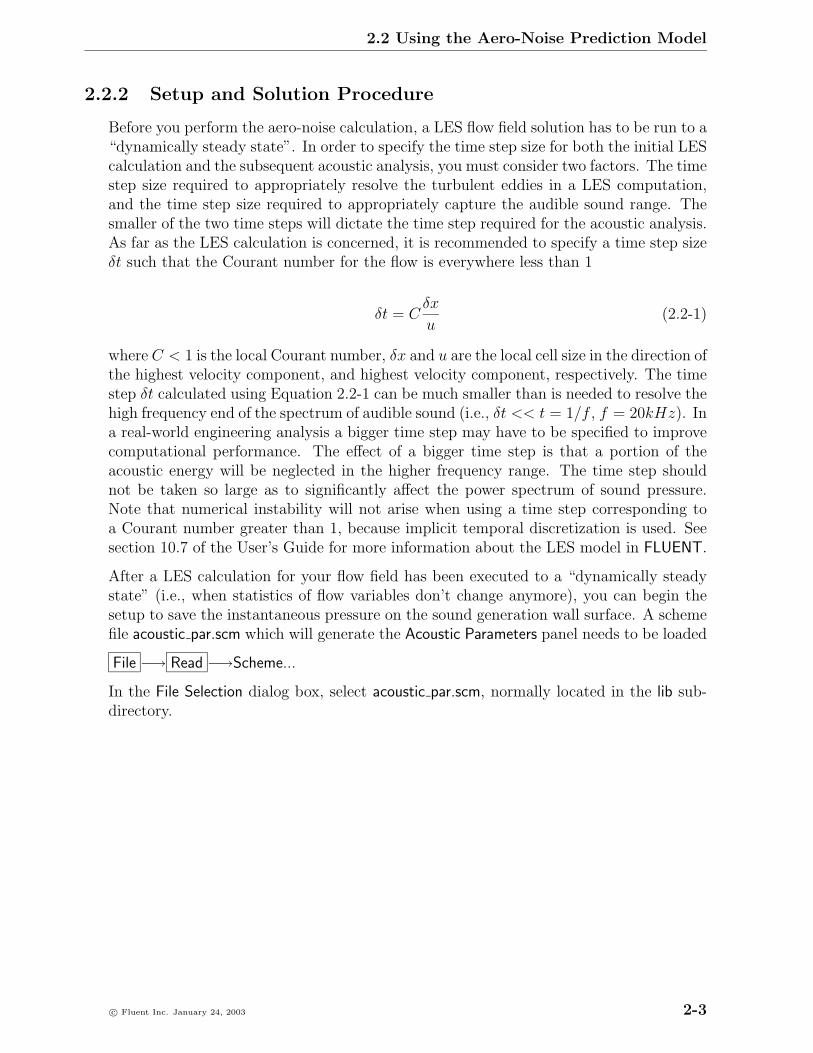
2.2.2 Setup and Solution Procedure

Before you perform the aero-noise calculation, a LES flow field solution has to be run to a“dynamically steady state”. In order to specify the time step size for both the initial LEScalculation and the subsequent acoustic analysis, you must consider two factors. The timestep size required to appropriately resolve the turbulent eddies in a LES computation,and the time step size required to appropriately capture the audible sound range. Thesmaller of the two time steps will dictate the time step required for the acoustic analysis.As far as the LES calculation is concerned, it is recommended to specify a time step sizeδt such that the Courant number for the flow is everywhere less than 1

δt = Cδx

u(2.2-1)

where C < 1 is the local Courant number, δx and u are the local cell size in the direction ofthe highest velocity component, and highest velocity component, respectively. The timestep δt calculated using Equation 2.2-1 can be much smaller than is needed to resolve thehigh frequency end of the spectrum of audible sound (i.e., δt << t = 1/f , f = 20kHz). Ina real-world engineering analysis a bigger time step may have to be specified to improvecomputational performance. The effect of a bigger time step is that a portion of theacoustic energy will be neglected in the higher frequency range. The time step shouldnot be taken so large as to significantly affect the power spectrum of sound pressure.Note that numerical instability will not arise when using a time step corresponding toa Courant number greater than 1, because implicit temporal discretization is used. Seesection 10.7 of the User’s Guide for more information about the LES model in FLUENT.

After a LES calculation for your flow field has been executed to a “dynamically steadystate” (i.e., when statistics of flow variables don’t change anymore), you can begin thesetup to save the instantaneous pressure on the sound generation wall surface. A schemefile acoustic par.scm which will generate the Acoustic Parameters panel needs to be loaded

File −→ Read −→Scheme...

In the File Selection dialog box, select acoustic par.scm, normally located in the lib sub-directory.



Save Surface Pressure

Open the Acoustic Parameters panel

Define −→ User-Defined −→Acoustic Parameters...

1. Set up the inputs for the aero-noise simulation according to the following guidelines

Sound Generation Wall ID Number: Currently, all walls that generate soundneed to be grouped up into a single zone with a single ID number. You can findout the ID number for a particular zone in the Define Boundary Conditions panel.

X,Y,Z Coordinates of Observer Position: The position for the calculation ofAcoustic Pressure and Sound Pressure Level.



Depth in Spanwise Direction for 2D Simulation: This value is only usedfor acoustic calculations, and does not change the default depth value in 2D flowsimulation. The default value in the acoustic calculation is 1.0 m. In 3D acousticcalculations, this value will be ignored.

Number of Time Steps for Each Surface Pressure File: It is recommendedto save the surface pressure data for a calculation with a large number of time stepsinto several separate files with smaller numbers of time steps.

File Name to Save Surface Pressure: Root name of the surface pressure filesis required. The saved surface pressure file name will be the root name followed bya hyphen and a number which is the number of the last time step in that file.

2. Click OK to save your settings and close the panel.

You will return to the Acoustic Parameters panel at next step for aero-noise calculation.

To store the values of surface pressure that will be used for the aero-noise calculations,you need to allocate 1 user-defined memory location

Define −→ User-Defined −→Memory...

Specify 1 for Number of User-Defined Memory Locations. The allocated user-defined mem-ory will be used as an auxiliary array to save surface pressure in the save-pressure-adjustUDF and then be used later to save the distribution of Surface Dipole Strength on thesound generation wall surface in cal-sound UDF.

To activate the UDFs that will be used by the aero-noise model, you will use the User-Defined Function Hooks panel

Define −→ User-Defined −→Function Hooks...

Under Adjust Function, select save-pressure-adjust and click OK to activate the UDF tosave surface pressure values of all cell faces on the sound generating wall surface(s) ateach time step. Data will be saved once the solution is started. Note that the aboveprocedure will be the same for both serial and parallel calculations.

There is a limit to the minimum number of time steps according to the sound calculation!scheme. The minimum number of time steps needs to be larger than n = T/dt, where Tis the sound transmission time through the distance L, which is roughly the length scaleof the sound generating surface, and dt is the time step size applied in the unsteady flow



simulation. If the number of time steps is smaller than the required minimum number,a warning will be displayed along with the indication of the minimum number of timesteps required:

Warning: Number of Time Steps of The Input Surface

Pressure Data Must Be Larger Than: <n>.

Calculate Aero-Noise

Once the unsteady LES calculation is finished, you need to concatenate the separatesurface pressure files into one single input file for the subsequent aero-noise calculation.Open the Acoustic Parameters panel again, and finish the input in this panel using thefollowing directions:

File Name to Read Surface Pressure: A name of a single surface pressure file. Ifthe surface pressure is saved in several separate files such as filename1, filename2, etc.,you will need to concatenate the files into one. For example, on a Unix machine you cando so by typing: cat filename1 filename2 > filename1+2.

File Name to Save Acoustic Pressure: This file will be saved for XY-plots to displayacoustic pressure.

File Name to Save Power Spectrum: This file will be saved for XY-plots of powerspectrum of acoustic pressure in units of Pa2.

File Name to Save Power Spectrum in dB Unit: This file will be saved for XY-plotsof power spectrum of acoustic pressure in dB.

Remember to click OK to save your settings and close the panel.

Note that currently, while you can directly execute the cal-sound UDF in the serial versionof FLUENT at this step, in the parallel version of the solver you still were able to use theDEFINE ADJUST UDF to save surface pressure, but can not use the cal-sound ExecuteOn Demand UDF to calculate aero noise.

In a parallel session of FLUENT save your case and data files, exit the parallel version ofthe solver, start a serial FLUENT session, read in the Scheme file for defining the AcousticParameters panel (acoustic par.scm), and then read in the case and data files you justsaved.

All inputs in the Acoustic Parameters panel are also saved in the case file. Thus, for an!existing case, you need to read in the Scheme file for defining the Acoustic Parameterspanel before reading in case and data files, to avoid a segmentation error in FLUENT.

Define −→ User-Defined −→Execute On Demand...

Select the cal-sound UDF and click Execute. The UDF will calculate Acoustic Pressure,Power Spectrum (in dB), Sound Pressure Level and Surface Dipole Strength.


2.3 Postprocessing an Aero-Noise Solution

2.3 Postprocessing an Aero-Noise Solution

You can perform postprocessing on an aero-noise solution using the postprocessing toolsand options available in FLUENT. Some additional variables will be available for postpro-cessing as described below. This section highlights only some of the suggested proceduresto display and plot the most relevant results obtained from an aero-noise simulation inFLUENT.

To inspect the Acoustic Pressure:

Plot −→File...

Click on Add, and select the relevant file name for the acoustic pressure. Click on Plotin the File XY Plot panel.

To inspect the Power Spectrum (both in units of Pa2 and in dB):

Plot −→File...

Click on Add, and select the relevant file name for the power spectrum. Click on Plot inthe File XY Plot panel.

To inspect the Sound Pressure Level:

This value will be printed in FLUENT’s console window.

To inspect the Surface Dipole Strength:

Display −→Contours...

1. In the Contours Of drop-down list, select User-Defined-Memory and udm-0.

2. Under Surfaces, select the sound generating surface(s).

3. Turn on the Filled option, and turn off Node Values.

4. Click on Display.

Note that the Surface Dipole Strength values are stored in the first layer of cells on thesound generating wall, thus the use of cell values.

2.3.1 Limitations

Currently, only Curle’s sound calculation formulation is implemented in FLUENT’s aero-noise UDF-based model. The model is only applicable to aero-noise predictions forsubsonic external flows such as the flow surrounding vehicles. It is not applicable toaero-noise predictions for internal flows such as flows in mufflers, or to the flows inrotating machinery such as the flows surrounding fans.




Bibliography

[1] N. Curle. The Influence of Solid Boundaries Upon Aerodynamical Sound. Proc. Roy.Soc. London, A231, page 505, 1955.

[2] M. J. Lighthill. On Sound Generated Aerodynamically, I. General Theory. Proc. Roy.Soc. London, A211, page 564, 1952.

c© Fluent Inc. January 24, 2003 Bib-1

FLUENT 6.1 Acoustics Module Manual - julliojullio.pe.kr/fluent6.1/help/pdf/acoustics/fl61aco.pdf · Chapter 1. Aero-Noise Model Theory This chapter presents an overview of the theory

Documents