Fluctuations of the Entropy Production in Anharmonic Chains

Ann. Henri Poincare 3 (2002) 483 – 502c© Birkhauser Verlag, Basel, 20021424-0637/02/030483-20 $ 1.50+0.20/0 Annales Henri Poincare

Fluctuations of the Entropy Productionin Anharmonic Chains

L. Rey-Bellet and L. E. Thomas∗

Abstract. We prove the Gallavotti-Cohen fluctuation theorem for a model of heatconduction through a chain of anharmonic oscillators coupled to two Hamiltonianreservoirs at different temperatures.

1 Introduction

The Gallavotti-Cohen fluctuation theorem refers to a symmetry in the fluctuationsof the entropy production in nonequilibrium statistical mechanics. It was firstdiscovered in numerical experiments of Evans, Cohen and Morris [8] and thendiscussed in [9] in the context of thermostated systems. As a mathematical theoremit was proved for Anosov dynamical systems [9, 10]. Soon thereafter the fluctuationtheorem was discussed in the context of stochastic dynamical systems first byKurchan [17] and then, more systematically by Lebowitz and Spohn, and Maes[22, 18]. In particular, Maes discovered a general formulation of the fluctuationtheorem in the context of space-time Gibbs measures which covers both Markovianstochastic dynamics and chaotic deterministic dynamics (via a Markov partition).As a mathematical theorem the fluctuation theorem is proven for quite generalstochastic models with finite state space, such as lattices gases in a finite box.Relations for the free energy related to the fluctuation theorem have been alsodiscussed in [15, 2].

Among the consequences of the fluctuation theorem is the non-negativity ofentropy production although the proof of its positivity is more difficult and is so farproved only in particular examples [7, 20]. We also note that in the related contextof open systems, classical and quantum, the production of entropy is discussed ata general level in [27, 13, 24]. Again the non-negativity of entropy production isrelatively easy to establish, while the strict positivity has been established only inparticular models [7, 14].

In this paper we consider an open system consisting of a finite (but of arbitrarysize) chain of anharmonic oscillators coupled at its ends only to reservoirs of freephonons at positive and different temperatures [6, 7, 5, 25, 26]. In particular ourmodel is completely Hamiltonian and its phase space is not compact.

∗Partially supported by NSF Grant 980139

484 L. Rey-Bellet and L. E. Thomas Ann. Henri Poincare

In order to establish the fluctuation theorem, two ingredients are needed:one needs to prove a large deviation theorem for the ergodic average of the entropyproduction and establish a symmetry of the large deviation functional. The secondpart is usually relatively straightforward to establish, at a formal level, since itfollows from a symmetry of the generator of the dynamics. This formal derivationfor models related to ours can be found in [22] and [19].

The first part, proving the existence of the large deviation functional, involvestechnical difficulties, in particular if the phase space of the model is not compact.In this case large deviation theorems are established provided the system satis-fies very strong ergodic properties (such as hypercontractivity) see e.g. [3, 4, 29].In addition the entropy production is in general an unbounded observable whilestandard results of large deviations apply only to bounded observables.

In this paper we show how to treat these difficulties in the model at hand.The techniques we use are based on the construction of Liapunov functions forcertain Feynman-Kac semigroups and Perron-Frobenius-like theorem in Banachspaces. We heavily rely on the strong ergodic properties of our model establishedin [6, 7, 5] and especially in [26].

The Hamiltonian of the model, as in [6], has the form

H = HB +HS +HI . (1)

The two reservoirs of free phonons are described by wave equations in Rd withHamiltonian

HB = H(ϕL, πL) +H(ϕR, πR) ,

H(ϕ, π) =12

∫dx (|∇ϕ(x)|2 + |π(x)|2) ,

where L and R stand for the “left” and “right” reservoirs, respectively. The Hamil-tonian describing the chain of length n is given by

HS(p, q) =n∑i=1

p2i

2+ V (q1, · · · , qn) ,

V (q) =n∑i=1

U (1)(qi) +n−1∑i=1

U (2)(qi − qi+1) ,

where (pi, qi) ∈ Rd × Rd are the coordinates and momenta of the ith particle ofthe chain. The phase space of the chain is R2dn. The interaction between the chainand the reservoirs occurs at the boundaries only and is of dipole-type

HI = q1 ·∫

dx∇ϕL(x)ρL(x) + qn ·∫

dx∇ϕR(x)ρR(x) ,

where ρL and ρR are coupling functions (“charge densities”).Our assumptions on the anharmonic lattice described by HS(p, q) are the

following:

Vol. 3, 2002 Fluctuations of the Entropy Production in Anharmonic Chains 485

• H1 Growth at infinity: The potentials U (1)(x) and U (2)(x) are C∞ and growat infinity like ‖x‖k1 and ‖x‖k2 : There exist constants Ai, Bi, and Ci, i = 1, 2such that

limλ→∞

λ−kiU (i)(λx) = Ai‖x‖ki ,

limλ→∞

λ−ki+1∇U (i)(λx) = Aiki‖x‖ki−2x ,

‖∂2U (i)(x)‖ ≤ (Bi + CiU(i)(x))1−

2ki .

Moreover we will assume that

k2 ≥ k1 ≥ 2 ,

so that, for large ‖x‖ the interaction potential U (2) is ”stiffer” than theone-body potential U (1).

• H2 Non-degeneracy: The coupling potential between nearest neighbors U (2)

is non-degenerate: For x ∈ Rd and m = 1, 2, · · ·, let A(m)(x) : Rd → Rdm

denote the linear maps given by

(A(m)(x)v)l1l2···lm =d∑

l=1

∂m+1U (2)

∂x(l1) · · · ∂x(lm)∂x(l)(x)vl .

We assume that for each x ∈ Rd there exists m0 such that

Rank(A(1)(x), · · ·A(m0)(x)) = d .

• H3 Rationality of the coupling: Let ρi denote the Fourier transform of ρi.We assume that

|ρi(k)|2 = 1Qi(k2)

,

where Qi, i ∈ {L,R} are polynomials with real coefficients and no roots onthe real axis.

We introduce now the temperatures of the reservoirs by choosing initial con-ditions for the reservoirs. The Hamiltonian of a reservoir is quadratic in Ψ ≡ (φ, π),H = 〈Ψ,Ψ〉/2, and therefore the Gibbs measure at temperature T , dµT (Ψ) is theGaussian measure with covariance T 〈· , ·〉. To construct nonequilibrium steadystates we assume that

• The initial conditions ΨL = (φL, πL) and ΨR = (φR, πR) of the reservoirsare distributed according the gaussian Gibbs measures dµTL and dµTR re-spectively.

486 L. Rey-Bellet and L. E. Thomas Ann. Henri Poincare

In order to define the heat flow through the bulk of the crystal we considerthe energy of the ith oscillator which we take to be

Hi =p2i

2+ U (1)(qi) +

12

(U (2)(qi−1 − qi) + U (2)(qi − qi+1)

). (2)

Differentiating Hi with respect to time, one finds that

dHi

dt= Φi−1 − Φi ,

where

Φi =(pi + pi+1)

2∇U (2)(qi − qi+1) (3)

is the heat flow from the ith to the (i + 1)th particle. We define a correspondingentropy production by

σi =(1TR

− 1TL

)Φi ,

where TR and TL are the temperatures of the reservoirs.There are other possible definitions of heat flows and corresponding entropy

production that one might want to consider. One might, for example, consider theflows ΦL, ΦR at the boundary of the chains, and define σb = −ΦL/TL − ΦR/TR,or one might take other quantities as local energies. But using conservation lawsit is easy to see that all these heat flows have the same average in the steadystate. Moreover we will show that all the entropy productions have the same largedeviations functionals: the exponential part of their fluctuations are identical.

We denote (p(t), q(t)) = (p(t, p0, q0,ΨL,ΨR), q(t, p0, q0,ΨL,ΨR)) as the Ha-miltonian flow generated by the Hamiltonian (1), and consider the ergodic average

σit ≡ 1

t

∫ t

0

σi(p(s), q(s)) ds .

The quantity σi(p(s), q(s)) depends on both the initial conditions of the chainand of the reservoirs which, by assumption, are distributed according to thermalequilibrium. By the ergodic theorem proven in [26] there exists a measure dν onR2dn such that

limt→∞σi

t =∫

σi dν .

for all (p0, q0) and dµTL and dµTR almost surely. Moreover∫σi dν ≡ 〈σ〉ν is

independent of i and as shown in [7]

〈σ〉ν ≥ 0 and 〈σ〉ν = 0 if and only if TL = TR .

Given a set A ⊂ R, we say that the fluctuations of σi in A satisfy the largedeviation principle with large deviation functional I(w) provided

infw∈Int(A)

I(w) ≤ lim inft→∞ −1

tlogP{σit ∈ A} ≤

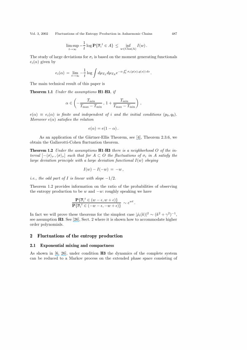
Vol. 3, 2002 Fluctuations of the Entropy Production in Anharmonic Chains 487

lim supt→∞

−1tlogP{σit ∈ A} ≤ inf

w∈Clos(A)I(w) .

The study of large deviations for σi is based on the moment generating functionalsei(α) given by

ei(α) = limt→∞−1

tlog∫

dµTLdµTRe−α

R t0 σi(p(s),q(s)) ds .

The main technical result of this paper is

Theorem 1.1 Under the assumptions H1-H3, if

α ∈(− Tmin

Tmax − Tmin, 1 +

Tmin

Tmax − Tmin

),

e(α) ≡ ei(α) is finite and independent of i and the initial conditions (p0, q0).Moreover e(α) satisfies the relation

e(α) = e(1− α) .

As an application of the Gartner-Ellis Theorem, see [4], Theorem 2.3.6, weobtain the Gallavotti-Cohen fluctuation theorem.

Theorem 1.2 Under the assumptions H1-H3 there is a neighborhood O of the in-terval [−〈σ〉ν , 〈σ〉ν ] such that for A ⊂ O the fluctuations of σi in A satisfy thelarge deviation principle with a large deviation functional I(w) obeying

I(w) − I(−w) = −w ,

i.e., the odd part of I is linear with slope −1/2.Theorem 1.2 provides information on the ratio of the probabilities of observingthe entropy production to be w and −w: roughly speaking we have

P{σit ∈ (w − ε, w + ε)}P{σit ∈ (−w − ε,−w + ε)} ∼ ewt .

In fact we will prove these theorems for the simplest case |ρi(k)|2 ∼ (k2 + γ2)−1,see assumption H3. See [26], Sect. 2 where it is shown how to accommodate higherorder polynomials.

2 Fluctuations of the entropy production

2.1 Exponential mixing and compactness

As shown in [6, 26], under condition H3 the dynamics of the complete systemcan be reduced to a Markov process on the extended phase space consisting of

488 L. Rey-Bellet and L. E. Thomas Ann. Henri Poincare

the phase space of the chain R2dn and of a finite number of auxiliary variableswhich we denote as r. As mentioned at the end of section 1, we just consider thesimplest case |ρ(k)|2 ∼ (k2 + γ2)−1, so that r = (r1, rn) ∈ R2d. For higher orderpolynomials the equations for r given below are replaced by a higher dimensionalsystem of (linear) equations. The resulting equations of motion take the form

q = p ,

p = −∇qV − ΛT r ,dr = (−γr + Λp) dt+ (2γT )1/2dω . (4)

Here p = (p1, · · · , pn) and q = (q1, · · · , qn) denote the momenta and positions of theparticle, r = (r1, rn) are the auxiliary variables and ω is a standard 2d-dimensionalWiener process. The linear map Λ : Rdn → R2d is given by Λ(p1, . . . , pn) =(λp1, λpn) and T : R2d → R2d by T (x, y) = (T1x, Tny). Here T1 ≡ TL andTn ≡ TR are the temperatures of the reservoirs attached to the first and nth

particles respectively, γ is the constant appearing in ρ and λ is a coupling constantequal to ‖ρ‖L2.

The solution of Eq. (4), x(t) = (p(t), q(t), r(t)) with x ∈ X = R2d(n+1) is aMarkov process. We denote T t as the corresponding semigroup

T tf(x) = Ex[f(x(t))] ,

with generator

L = γ (∇rT∇r − r∇r) + (Λp∇r − rΛ∇p) + (p∇q − (∇qV (q))∇p) , (5)

and we denote Pt(x, dy) as the transition probability of the Markov process x(t). In[26] we proved that the Markov process x(t) has smooth transition probabilities, inparticular it is strong Feller, and that it is (small-time) irreducible: For any t > 0,any x ∈ X and any open set A ⊂ X we have Pt(x,A) > 0.

There is a natural energy function associated to Eq.(4), given by

G(p, q, r) =r2

2+H(p, q) ,

which we employ throughout our discussion. In [26] we have constructed a Lia-punov function for x(t) from G: Let t > 0 and 0 < θ < max(T1, Tn)−1. There existan E0 and functions κ = κ(E) < 1 and b = b(E) < ∞ defined for E > E0 suchthat for E > E0,

T teθG(x) ≤ κ(E)eθG(x) + b(E)1{G≤E}(x) . (6)

Moreover κ(E) can be made arbitrarily small by choosing E sufficiently large, infact there exist positive constants c1 = c1(θ, t) and c2 = c2(θ, t) such that

κ(E) ≤ c1e−c2E

2/k2. (7)

Vol. 3, 2002 Fluctuations of the Entropy Production in Anharmonic Chains 489

By results of [21] it is also shown in [26] that the convergence to the uniquestationary state, denoted by µ, occurs exponentially fast: Let H∞,θ denote theBanach space {f ; ‖f‖∞,θ ≡ supx |f(x)|e−θG(x) < ∞}. Then there exist constantsr > 1 and R < ∞

|T tf(x)−∫

fdµ| ≤ Rr−t‖f‖∞,θeθG(x) , (8)

which means that T t, acting on H∞,θ has a spectral gap. The methods of [21] areprobabilistic and rely on a nice probabilistic construction called splitting as wellas coupling arguments and renewal theory.

Under the condition given here, by taking advantage of the fact that theconstant κ in the Liapunov bound (6) can be made arbitrarily small (this is notassumed in [21]), we can prove stronger ergodic properties and also give a directanalytical proof of Eq. (8).

Besides the Banach space H∞,θ defined above we also consider the Banachspace H0

∞,θ = {f, |f |e−θG ∈ C0(X)} with norm ‖ · ‖∞,θ ( C0(X) denotes the setof continuous functions which vanish at infinity). Furthermore for 1 ≤ p < ∞ weconsider the family of Banach spaces Hp,θ = Lp(X, e−pθG(x)dx) and denote ‖ · ‖p,θthe corresponding norms.

Theorem 2.1 If 0 < θTi < 1, the semigroup T t extends to a strongly continuousquasi-bounded semigroup on Hp,θ, for 1 ≤ p < ∞ and on H0

∞,θ. For any t > 0, T t

is compact on Hp,θ, for 1 < p ≤ ∞ and on H0∞,θ.

As an immediate consequence of the spectral properties of positive semi-groups [11] and the irreducibility of x(t) we have

Corollary 2.2 The Markov process x(t) has a unique invariant measure dµ and Eq.(8) holds.

Proof. Since T t is a Markovian, compact, and irreducible semigroup the eigenvalue1 is simple with the constant as the eigenfunction. This shows that the Markovprocess x(t) has a unique invariant measure. Moreover by the cyclicity propertiesof the spectrum of a positive semigroup [11], and by the compactness of T t, thereare no other eigenvalues of modulus 1. Eq. (8) follows immediately. �Proof of Theorem 2.1. In [26], Lemma 3.6, we showed that for some constant CT teθG ≤ ecteθG provided θTi < 1 (see also Lemma 2.9 below). Therefore for f C∞

with compact support we have, using Ito’s and Girsanov’s formulas

e−θGT teθGf(x) = Ex

[eθ(G(x(t))−G(x))f(x)

]= Ex

[eθ

Rt0 γ(Tr(T )−r2) ds+θ

Rt0

√2γTrdω(s)f(x(t))

]= Ex

[eγθTr(T )+γr(θ2T−θ)rf(x(t))

],

490 L. Rey-Bellet and L. E. Thomas Ann. Henri Poincare

where x is the process with generator

Lθ = L+ 2γθrT∇r .

A computation shows that LTθ 1 = γTr(1 − 2θT ). Standard arguments show then

that the semigroup associated with the process x extends to a quasi-boundedand strongly continuous semigroup on Lp(dx), 1 ≤ p < ∞ and on C0(X). Usingthe assumption that θTi < 1 and Feynman-Kac formula we see that e−θGT teθG

extends too to a quasi-bounded and strongly continuous semigroup on Lp(dx),1 ≤ p < ∞ and on C0(X). This implies immediately that T t extends to a stronglycontinuous semigroup on Hp,θ, 1 ≤ p < ∞ and H0

∞,θ. The computation above alsoshows that T t extends to a quasi-bounded semigroup on H∞,θ.

We first prove the compactness of T t for H∞,θ. If f ∈ H∞,θ then |f(x)| ≤‖f‖∞,θe

θG(x) and by (6) and (7) we obtain

|1G≥ETtf(x)| ≤ eθG(x) sup

{y:G(y)≥E}

|T tf(y)|eθG(y)

≤ eθG(x)‖f‖∞,θ sup{y:G(y)≥E}

T te(θG(y))

eθG(y)

≤ κ(E)eθG(x)‖f‖∞,θ . (9)

From the bounds (9) and (7) we conclude that the operator 1{G≥E}T t convergesuniformly to 0 in H∞,θ as E → ∞. The semigroup T t has a C∞ kernel since it isgenerated by a hypoelliptic operator see [26], Proposition 4.1, so, by the Arzela-Ascoli theorem 1{G≤E}T t/21{G≤E} is compact, for any E. Therefore we obtain

T t = limE→∞

1{G≤E}T t/21{G≤E}T t/2 ,

where the limit is in the norm sense from (9) above, i.e., T t is the uniform limitof compact operators, hence is compact.

The compactness of T t for H0∞,θ follows from the same argument. In fact by

Eq.(7), for any t > 0, T tH∞,θ ⊂ H0∞,θ.

To prove the compactness of T t on Hpθ, 1 < p < ∞, we note that

|T tf(x)| = |Ex[f(x(t))]|= |Ex[e

θqG(x(t))e−

θq G(x(t))f(x(t))]|

≤(Ex[eθG(x(t))]

)1/q (Ex[e−

pθq G(x(t))fp(x(t))]

)1/p

.

Thus using the bound (7) and the fact that T t is quasi-bounded on H1,θ we obtain

‖1G≥ETtf‖pθ,p ≤

∫{x:G(x)≥E}

Ex[eθG(x(t))]pq Ex[e−

pθq G(x(t))fp(x(t))]e−pθG(x)dx

Vol. 3, 2002 Fluctuations of the Entropy Production in Anharmonic Chains 491

≤ sup{x:G(x)≥E}

(Ex[eθG(x(t))]

eθG(x)

) pq

‖T t(e−pθq Gfp)‖1,θ

≤ κ(E)pq ect‖e−pθ

p Gfp‖1,θ

= κ(E)pq ect‖f‖pθ,p .

As in the case p = ∞, we conclude from the bound (7) that the operator1G≥ET

t converges uniformly to 0 in Hp,θ as E → ∞. Using that the kernel of1{G≤E}T t1{G≤E} is bounded, we conclude that T t is compact on Hp,θ for 1 < p <∞. �

2.2 Heat flow and generating functionals

In order to define the heat flows we note that we have

d

dtT tH = LT tH = T t(−rΛp) = T t(−λr1p1 − λrnpn) .

Hence we identify Φ0 ≡ −λr1p1 as the observable describing the heat flow fromthe left reservoir into the chain and Φn ≡ λrnpn as the heat flow from the chaininto the right reservoir. As in the introduction we define the energy Hi of the ith

oscillators by Eq.(2), for i ≤ 2 ≤ n− 1, and

H1 =p21

2+ U (1)(q1) +

12U (2)(q1 − q2) ,

Hn =p2n

2+ U (1)(qn) +

12U (2)(qn−1 − qn) .

With the heat flows Φi, i = 1, · · · , n, defined as in Eq. (3) we haveLHi = Φi−1 − Φi , i = 1, · · · , n .

and we define the entropy productions σi, i = 0, · · · , n by

σi =(1T1

− 1Tn

)Φi i = 0, · · · , n .

We now provide several identities involving the generator of the dynamics andthe entropy production, which will play a crucial role in our subsequent analysis.

Lemma 2.3 Let the function Ri, i = 0, · · · , n be given by

Ri =1T1

(r21

2+

i∑k=1

Hi(p, q)

)+1Tn

(n∑

k=i+1

Hi(p, q) +r2n

2

). (10)

Then we haveσi = γrT−1r − Tr(γI) + LRi . (11)

492 L. Rey-Bellet and L. E. Thomas Ann. Henri Poincare

Proof. This is a straightforward computation. �

Remark 2.4 This shows that, up to a derivative, all the entropy productions areequal to the quantity rT−1r − TrγI which is independent of i and involves onlythe r-variables.

Let LT be the formal adjoint of the operator L given by Eq. (5)

LT = γ (∇rT∇r +∇rr) − (Λp∇r − rΛ∇p)− (p∇q − (∇qV (q))∇p) , (12)

and let J be the time reversal operator which changes the sign of the momenta ofall particles, Jf(p, q, r) = f(−p, q, r).

The following identities can be regarded as operator identities on C∞ func-tions. That the left and right side of Eq. (14) actually generate semigroups forsome interval of α is a non trivial result which we will discuss in Section 2.3.

Lemma 2.5 We have the operator identities

eRiJLTJe−Ri = L− σi , (13)

and also for any constant α

e−RiJ(LT − ασi)JeRi = L− (1− α)σi . (14)

Proof. We write the generator L as L = L0 + L1 with

L0 = γ (∇rT∇r − r∇r) (15)L1 = (Λp∇r − rΛ∇p) + (p∇q − (∇qV (q))∇p) . (16)

Since L1 is a first order differential operator we have

e−RiL1eRi = L1 + (L1Ri) = L1 + σi .

Using that ∇rRi = T−1r we obtain

e−RiL0eRi = e−Riγ(∇r − T−1r)T∇re

Ri

= γ∇rT (∇r + T−1r) = LT0 .

This givese−RiLeRi = LT

0 + L1 + σi = JLTJ + σi ,

which is Eq. (13). Since JσiJ = −σi, Eq. (14) follows immediately from Eq. (13).

Remark 2.6 In the equilibrium situation, i.e., for T1 = Tn = T , Eq. (14) is

eG/TJLTJe−G/T = L ,

Vol. 3, 2002 Fluctuations of the Entropy Production in Anharmonic Chains 493

which is simply detailed balance. Eq. (14) can be interpreted in path space in thefollowing manner [18]: Let Π denote the time-reversal in path space on the timeinterval [0, t]: Π(p(s), q(s), r(s)) = (−p(t− s), q(t− s), r(t− s)) and let dP denotethe measure on C([0, t], X) induced by x(t). Then Eq. (13) implies that

dP ◦ΠdP

= eRi(x(t))−Ri(x(0))−R t0 σi(x(s)) ds .

This formula exhibits the fact that the lack of microscopic reversibility is intimatelyrelated to the entropy production.

We now turn to the study of the large deviations. As shown in [26] the Markovprocess x(t) is ergodic. In order to study the large deviations of t−1

∫ t0σi(x(s))ds

we consider the moment generating functionals

Γix(t, α) = Ex

[e−α

Rt0 σi(x(s)) ds

].

Formally the Feynman-Kac formula gives Γix(t, α) = et(L−ασi)1(x), but since σiis not bounded, nor even relatively bounded by L, it is not obvious that Γix(t, α)exists for α �= 0. Our goal is to prove that Γix(t, α) exists and that the limit

e(α) ≡ limt→∞−1

tlog Γix(t, α) (17)

exists and is finite in a neighborhood of the interval [0, 1], and is independent of iand of the initial condition x.

The technical difficulty in proving the existence of the limit (17) lies in thefact that the functions σi are unbounded. Standard large deviation theorems forMarkov processes (see e.g. [3, 4, 29]) are proven usually under strong ergodicproperties for bounded functions and are not directly applicable. Large deviationsfor unbounded functions are considered in [1] for discrete time countable statespace Markov chains under conditions which amount in our case to σ = o(G). Inour case this is clearly not satisfied since, in general σ is not bounded by G.

But the σi are very special observables, in particular they are intimatelylinked with the dynamics as shown by the identities Eqs.(13) and (14). The nextlemma displays another identity which will be important in our analysis.

Lemma 2.7 We have the identity

L− ασi = eαRiLαe−αRi , (18)

whereLα = Lα − ((α− α2)γrT−1r − αTr(γI)

)(19)

andLα = L+ 2αγr∇r . (20)

494 L. Rey-Bellet and L. E. Thomas Ann. Henri Poincare

Proof. As in Lemma 2.5 we write the generator L as L = L0 + L1, see Eqs.(16)and (15). Since L1 is a first order differential operator we have

e−αRiL1eαRi = L1 + α(L1Ri) = L1 + ασi . (21)

Using that ∇rRi = T−1r is independent of i we find that

e−αRiL0eαRi = γ

((∇r + αT−1r)T (∇r + αT−1r)− r(∇r + αT−1r)

)= L0 + αγ(r∇r +∇rr) + (α2 − α)γrT−1r

= L0 + 2αγr∇r + (α2 − α)γrT−1r + αTrγI . (22)

Combining Eqs. (21) and (22) gives the desired result. �

Remark 2.8 The identity (18) shows that all operators L−ασi are conjugate to thesame operator Lα. This will be the key element to prove that e(α) is independentof i. Furthermore it can be seen from Eqs. (19) and (20) that Lα has the form ofL plus a perturbation which is a quadratic form in r and ∇r. Such a perturbationis indeed nicer than ασi. Also it should be noted that Lα has very much the sameform as the operator L: they differ only by the coefficient in front of the term r∇r .This fact will allow us to use several results on L obtained in [26].

2.3 Liapunov Function for Feynman-Kac Semigroups

At this point we begin the study of Lα as the generator of a semigroup.

Proposition 2.9 If θ and α satisfy the condition

−α < θTi < 1− α , (23)

then there exists a constant C = C(α, θ) such that etLαeθG(x) ≤ eCteθG(x).

Proof. We note first that Lα, defined in Eq. (19), for all α ∈ R, is the generatorof a Markov process which we denote as x(t). Indeed we have that

LαG(x) = Tr(γT )− (1 + 2α)r2 ≤ C1 + C2G(x)

Since G grows at infinity, G is a Liapunov function for x(t) and a standard argu-ment [16] shows that the Markov process x(t) is non-explosive. Furthermore wehave the bound

Lα exp θG(x) == exp θG(x)γ

[Tr(θT + αI) + r(θ2T − (1− 2α)θ − α(1− α)T−1)r

]≤ C exp θG(x) , (24)

provided α and Ti, i = 1, n satisfy the inequality

θ2Ti − (1− 2α)θ − α(1− α)T−1i ≤ 0 ,

Vol. 3, 2002 Fluctuations of the Entropy Production in Anharmonic Chains 495

or−α < θTi < 1− α .

We denote σR as the exit time from the set {G(x) < R}, i.e., σR = inf{t ≥0, G(x(t)) ≥ R}. If the initial condition x satisfies G(x) = E < R, we denote byxR(t) the process which is stopped when it exits {G(x) < R}, i.e., xR(t) = x(t)for t < σR and xR(t) = x(σR) for t ≥ σR. Finally we set σR(t) = min{σR, t}.

By Eq. (24), the function W (t, x) = e−CteθG(x) satisfies the inequality (∂t +Lα)W (t, x) ≤ 0 and applying Ito’s formula with stopping time to the functionW (t, x) we obtain

Ex

[e−

R σR(t)0 ((α−α2)γrT−1r−αTr(γI)) dseθG(x(σR(t)))e−CσR(t)

]− eθG(x) ≤ 0 ,

and thus

Ex

[e−

R σR(t)0 ((α−α2)γrT−1r−αTr(γI)) dseθG(x(σR(t)))

]≤ eCteθG(x) .

Since the Markov process x(t) is non-explosive G(xR(t))→ G(x(t)) almost surelyas R → ∞, so by the Fatou lemma we have

etLαeθG(x) ≤ eCteθG(x) .

This concludes the proof of Lemma 2.9. �

The next three theorems are all consequences of the fact that Lα is thegenerator of a Markov process which is similar to the process generated by L:Indeed L and Lα differ only by the coefficient in front of the r∇r term. Thereforerepeating the proofs of [26] we obtain

Theorem 2.10 The semigroup etLα has a smooth kernel qα(t, x, y) which belongsto C∞((0,∞)×X ×X).

Proof. The operator Lα satisfies the same Hormander-type condition that L provenin [26], Proposition 4.1.The result follows then from [12] or [23]. �

Theorem 2.11 The semigroup etLα is positivity improving for all t > 0.

Proof. The semigroup etLα is shown to be irreducible exactly as etL, see [7, 26]using explicit computation and the Support Theorem of [28]. The statement followsthen from the Feynman-Kac formula. �

As is apparent from the form of Lα we will need estimates on the observabler2 in the sequel. Such estimates were also crucial in [26] for the construction of aLiapunov function.

496 L. Rey-Bellet and L. E. Thomas Ann. Henri Poincare

Theorem 2.12 Let 0 ≤ α < 1/k2 and let tE = E1/k2−1/2. There exists a set ofpaths

S(x,E, tE) ⊂ {f ∈ C([0, tE], X) ; f(0) = x,G(x) = E} ,and constants E0 < ∞ and A,B,C > 0 such that for E > E0

P {x ∈ S(x,E, tE)} ≥ 1−Ae−BE2α+1/2−1/k2,

and ∫ tE

0

r2(s) ds ≥ CE3/k2−1/2 , if x ∈ S(x,E, tE) . (25)

Proof. The proof is exactly as in [26]. One first sets T1 = Tn = 0 in the equations ofmotion and then, by a scaling argument, Theorem 3.3 of [26], one shows that thedeterministic trajectory satisfies the estimate (25). Then one shows, see Proposi-tion 3.7 and Corollary 3.8 of [26], that the overwhelming majority of the randomtrajectories follows very closely the deterministic ones. We refer the reader to [26]for further details. �

Remark 2.13 For large energy E, paths satisfying the bound (25) have a very highprobability. From Eq. (25) we obtain that, on a time interval of order 1,

∫ t

0

r2(s) ≥ CE2/k2 ,

for an overwhelming majority of the paths.

Theorem 2.14 Let t > 0 be fixed and suppose that α and θ satisfy the conditionEq.(23). There exist a constant E0 and functions κ(E) and b(E) such that forE > E0

etLαeθG(x) ≤ κ(E)eθG(x) + b(E)1{G≤E}(x) . (26)

Moreover there exist constants c1 and c2 such that

κ(E) ≤ c1e−c2E

2/k2.

Proof. By Proposition 2.9 the function etLαeθG(x) is bounded on any compact set.Therefore to show (26) it suffices to show that

sup{x :G(x)>E}

Ex

[e−

Rt0 (α(1−α)γrT−1r−αTr(γI)) dseθ(G(x(t))−G(x))

]≤ κ(E) .

Using Ito’s formula we have

G(x(t))−G(x) =∫ t

0

γ(Tr(T )− r2) ds+∫ t

0

√2γT rdω(s) ,

Vol. 3, 2002 Fluctuations of the Entropy Production in Anharmonic Chains 497

and thus we obtain

Ex

[e−

Rt0 (α(1−α)γrT−1r−αTr(γI)) dseθ(G(x(t))−G(x))

]= etγTr(θT+αI)Ex

[e−

R t0 r(α(1−α)γT−1−γθ(1−2α))r dse

Rt0 θ

√2γT r dω

]. (27)

Using the Holder’s inequality we find that the expectation on the r.h.s of Eq. (27)can be estimated by

Ex

[e−q

Rt0 r(α(1−α)γT−1−γθ(1−2α))r dse

qpθ22

R t0 (

√2γT r)2 ds

]1/q

×Ex

[e−

p2θ2

2

Rt0 (

√2γT r)2 dsep

Rt0 θ(2γT )1/2r dω)

]1/p

= Ex

[e−qγ

Rt0 r(α(1−α)T−1−θ(1−2α)+pθ2T)r ds

]1/q. (28)

where we have used that the second factor is the expectation of a martingale withexpectation 1.

If θ and α satisfy the condition (23), then, by choosing p sufficiently closeto 1, the quadratic form in the right side of Eq. (28) is negative definite. UsingTheorem 2.12 as in Theorem 3.11 of [26] we obtain

supx∈UC

Ex

[e−

Rt0 (α(1−α)rT−1r−αTr(γI)) dseθ(G(x(t))−G(x))

]≤ eγTr(θT+αI)e−CE2/k2γTr(α(1−α)T−1−(1−2α)θ+pθ2T )

≤ c1e−c2E

2/k2.

and this concludes the proof of Theorem 2.14. �As in Theorem 2.1 we obtain

Theorem 2.15 If α and θ satisfy the condition Eq.(23), then etLα extends to astrongly continuous quasi-bounded semigroup on Hp,θ for 1 ≤ p < ∞ and onH0

∞,θ. Moreover etLα is compact on Hp,θ, 1 < p ≤ ∞ and on H0∞,θ.

Proof. The proof is a repetition of the proof of Theorem 2.1 and is left to thereader. �

As a consequence of Theorem 2.15 and of the theory of semigroup of positiveoperators [11] we obtain

Theorem 2.16 If

α ∈(− Tmin

Tmax − Tmin, 1 +

Tmin

Tmax − Tmin

),

thene(α) = lim

t→∞−1tlog Γix(t, α)

exists, is finite and independent both of i and x.

498 L. Rey-Bellet and L. E. Thomas Ann. Henri Poincare

Proof. By Theorem 2.15, etLα generates a strongly continuous semigroup on H0∞,θ

if−α < θTi < 1− α . (29)

If α ≤ 0, this implies that |α| < θTmin < θTmax < 1 + |α| and so the set of θ wecan choose is non-empty provided

α > − Tmin

Tmax − Tmin.

If 0 < α < 1, we can always find θ such that (29) is satisfied. Finally if α > 1 then(29) implies that that

α < 1 +Tmin

Tmax − Tmin.

By the definition of Ri, Eq. (10), e−αRi ∈ H0∞,θ since −α + θTi < 0. Using now

Lemma 2.7, we see that Γix(t, α) exists and is given by

Γix(t, α) = et(L−ασ)1(x) = eαRietLαe−αRi(x) .

From Theorem 2.11 the semigroup etLα is an irreducible semigroup of compactoperators on the Banach spaceH0

∞,θ. From the cyclicity properties of the spectrumof irreducible operators and from the compactness it follows (see [11], ChapterC-III) that there is exactly one eigenvalue e−te(α) with maximal modulus andthis eigenvalue is real and simple. The corresponding eigenfunction fα is strictlypositive and we denote as Pα the one-dimensional projection on the eigenspacespanned by fα. In particular if g ≥ 0, then Pαg(x) > 0.

From compactness it follows that the complementary projection (1 − Pα)satisfies the bound∣∣∣etLα(1− Pα)f(x)

∣∣∣ ≤ Ce−td(α)‖f‖∞,θeθG(x) . (30)

for some constants C > 0 and d(α) > e(α) and for all t > 0.From Lemma 2.7 and Eq. (30) we obtain, for all x ∈ X , that

limt→∞−1

tlog Γix(t, α)

= limt→∞−1

tlog et(L−ασi)1(x) = lim

t→∞−1tlog eαRietLαe−αRi(x) (31)

= limt→∞

(−1

tαRi(x)

)+ e(α)

+ limt→∞−1

tlog(Pαe

−αRi(x) + ete(α)etLα(1 − Pα)e−αRi(x))

= e(α) .

This concludes the proof of Theorem 2.16. �

Vol. 3, 2002 Fluctuations of the Entropy Production in Anharmonic Chains 499

Using now the identity (14) we can prove the symmetry of e(α). Theorem 1.1is then an immediate consequence of the following result.

Theorem 2.17 If

α ∈(− Tmin

Tmax − Tmin, 1 +

Tmin

Tmax − Tmin

), (32)

thene(α) = e(1− α) .

Proof. If α is in the interval (32) and −α < θTi < 1 − α then etLα is a stronglycontinuous compact semigroup on H0

∞,θ. By Lemma 2.7

et(L−ασi) = eαRietLαe−αRi

is also a strongly continuous compact semigroup on the Banach space H0∞,θ,α =

{f ; |f |e−θG+αRi ∈ C0(x)} with the norm ‖f‖∞,θ,α = sup |f |eθG+αRi .The dual semigroup (et(L−ασi))∗ is a compact semigroup on the Banach space

(of measures) (H0∞,θ,α)

∗. By Theorem 2.11 (et(L−ασi))∗ maps (H0∞,θ,α)

∗ into mea-sures with smooth densities and on densities (et(L−ασi))∗ acts as

(et(L−ασi))∗(ρ(x)dx) = (et(LT−ασi)ρ(x))dx .

By Lemma 2.5 we have

e−Riet(L−(1−α)σi)1(x) = Jet(LT−ασi)Je−R(x) . (33)

Since −α < θTi < 1 − α, e−Ri is a density of a measure in (H0∞,θ,α)

∗. Since(et(L−ασi))∗ is compact and irreducible with spectral radius e(α) we obtain usingEq. (33)

e(α) = limt→∞−1

tlog ‖J(et(LT−ασi)Je−Ri)dx‖

= limt→∞−1

tlog

(sup

f≤eθG+αRi

∫fe−Riet(L−(1−α)σi)1 dx

),

= e(1− α) .

In the last equality we have used Theorem 2.16 and the fact that fe−Ri is a finitemeasure. This concludes the proof of Theorem 2.17. �

We finally obtain the Gallavotti-Cohen fluctuation theorem

Theorem 2.18 There is a neighborhood O of the interval [−〈σ〉ν , 〈σ〉ν ] such thatfor A ⊂ O the fluctuations of σi in A satisfy the large deviation principle with alarge deviation functional I(w) obeying

I(w) − I(−w) = −w ,

i.e., the odd part of I is linear with slope −1/2.

500 L. Rey-Bellet and L. E. Thomas Ann. Henri Poincare

Proof. First we note that e(α) is a real analytic function since it is identified withan eigenvalue of a compact operator. A simple computation gives that

d

dαe(α)

∣∣∣∣α=0

= 〈σ〉ν .

The function e(α) is analytic and convex. By the result of [7] it is not identicallyzero, and so the symmetry the symmetry e(α) = e(1 − α) implies that the set ofthe values of d

dαe(α) is a neighborhood of [−〈σ〉ν , 〈σ〉ν ].The large deviation principle is a direct application of the Gartner-Ellis the-

orem, [4], Theorem 2.3.6. The large deviation functional is given by the Legendretransform of e(α) and so we have

I(w) = supα

{e(α)− αw} = supα

{e(1− α)− αw}= sup

β{e(β)− (1− β)w} = I(−w) − w .

�

References

[1] S. Balaji and S. P. Meyn, Multiplicative ergodicity and large deviations foran irreducible Markov chain, Stoch. Proc. Appl. 90, 123–144 (2000).

[2] G.E. Crooks, Path-ensemble averages in systems driven far from equilibrium,Phys. Rev. E 61, 2361–2366 (2000).

[3] J.-D.Deuschel and D.W. Stroock, Large deviations, Pure and Applied Math-ematics 137, Boston: Academic Press, 1989.

[4] A.Dembo and O. Zeitouni, Large deviations techniques and applications,Applications of Mathematics 38. New-York: Springer-Verlag 1998.

[5] J.-P. Eckmann and M. Hairer, Non-equilibrium statistical mechanics ofstrongly anharmonic chains of oscillators, Commun. Math. Phys. 212, 105–164(2000).

[6] J.-P. Eckmann, C.-A. Pillet and L. Rey-Bellet, Non-equilibrium statisticalmechanics of anharmonic chains coupled to two heat baths at different tem-peratures, Commun. Math. Phys. 201, 657–697 (1999).

[7] J.-P. Eckmann, C.-A. Pillet and L. Rey-Bellet, Entropy production in non-linear, thermally driven Hamiltonian systems, J. Stat. Phys. 95, 305–331(1999).

[8] D.J. Evans, E.G.D. Cohen and G.P. Morriss, Probability of second law vio-lation in shearing steady flows. Phys. Rev. Lett. 71, 2401–2404 (1993).

Vol. 3, 2002 Fluctuations of the Entropy Production in Anharmonic Chains 501

[9] G. Gallavotti and E.G.D. Cohen, Dynamical ensembles in stationary state,J. Stat. Phys. 80, 931–970 (1995).

[10] G. Gentile, Large deviation rule for Anosov flows, Forum Math. 10 89–118(1998).

[11] G. Greiner, Spectral theory of positive semigroups on Banach lattices, InOne-parameter semigroups of positive operators Lecture Notes in Mathematics1184, Ed. R. Nagel, Berlin: Springer, 1986, pp 292–332.

[12] L. Hormander, The Analysis of linear partial differential operators, Vol III,Berlin: Springer, 1985.

[13] V. Jaksic and C.-A. Pillet, On entropy production in quantum statisticalmechanics, Commun. Math. Phys. 217, 285–293 (2001).

[14] V. Jaksic and C-A. Pillet, Non-equilibrium steady states of finite quantumsystems coupled to thermal reservoirs, Preprint (2001).

[15] C. Jarzynski, Hamiltonian derivation of a detailed fluctuation theorem, J.Statist. Phys. 98, 77–102 (2000).

[16] R.Z. Has’minskii, Stochastic stability of differential equations, Alphen aanden Rijn—Germantown: Sijthoff and Noordhoff, 1980.

[17] J. Kurchan, Fluctuation theorem for stochastic dynamics, J. Phys. A 31,3719–3729 (1998).

[18] C. Maes, The fluctuation theorem as a Gibbs property, J. Stat. Phys. 95,367–392 (1999).

[19] C. Maes, Statistical mechanics of entropy production: Gibbsian hypothesisand local fluctuations, Preprint (2001).

[20] C. Maes, F. Redig and M. Verschuere, No current without heat, Preprint(2000)

[21] S.P. Meyn and R.L. Tweedie, Markov Chains and Stochastic Stability. Com-munication and Control Engineering Series, London: Springer-Verlag London,1993.

[22] J.L. Lebowitz and H. Spohn, A Gallavotti-Cohen-type symmetry in thelarge deviation functional for stochastic dynamics, J. Stat. Phys. 95, 333–365 (1999).

[23] J. Norriss, Simplified Malliavin Calculus, In Seminaire de probabilites XX,Lectures Note in Math. 1204, 0 Berlin: Springer, 1986, pp. 101–130.

502 L. Rey-Bellet and L. E. Thomas Ann. Henri Poincare

[24] C.-A. Pillet, Entropy production in classical and quantum systems, MarkovProc. Relat. Fields 7, 145–157, (2001).

[25] L. Rey-Bellet and L.E. Thomas, Asymptotic behavior of thermal non-equilibrium steady states for a driven chain of anharmonic oscillators, Com-mun. Math. Phys. 215, 1–24 (2000).

[26] L. Rey-Bellet and L.E. Thomas, Exponential convergence to non-equilibriumstationary states in classical statistical mechanics, To appear in Commun.Math. Phys.

[27] D. Ruelle, Entropy production in quantum spin systems. Preprint (2000)

[28] D.W. Stroock and S.R.S. Varadhan, On the support of diffusion processeswith applications to the strong maximum principle. In Proc. 6-th BerkeleySymp. Math. Stat. Prob., Vol III, Berkeley: Univ. California Press, 1972, pp.361–368.

[29] L. Wu, Uniformly integrable operators and large deviations for Markov pro-cesses, J. Funct. Anal. 172, 301–376 (2000).

Luc Rey-Bellet and Lawrence E. ThomasDepartment of MathematicsUniversity of VirginiaKerchof HallCharlottesville, VA 22903USAemail: [email protected]: [email protected]

Communicated by Jean-Pierre Eckmannsubmitted 20/10/01, accepted 07/01/02

To access this journal online:http://www.birkhauser.ch