Fluctuations in the ensemble of reaction pathways

Fluctuations in the Ensemble of Reaction Pathways

G. MazzolaDipartimento di Fisica Universitá degli Studi di Trento, Via Sommarive 14, Povo (Trento),

I-38050 Italy. International School for Advanced Studies (SISSA), via Bonomea 265 34136 Trieste, Italy

S. a Beccara and P. FaccioliDipartimento di Fisica Universitá degli Studi di Trento, Via Sommarive 14, Povo (Trento), I-38050 Italy. and

INFN, Gruppo Collegato di Trento, Via Sommarive 14, Povo (Trento), I-38050 Italy.

H. OrlandInstitut de Physique Théorique, Centre d’Etudes de Saclay, F-91191, Gif-sur-Yvette, France

The dominant reaction pathway (DRP) is a rigorous framework to microscopically compute the most probabletrajectories, in non-equilibrium transitions. In the low-temperature regime, such dominant pathways encode theinformation about the reaction mechanism and can be used to estimate non-equilibrium averages of arbitraryobservables. On the other hand, at sufficiently high temperatures, the stochastic fluctuations around the dominantpaths become important and have to be taken into account. In this work, we develop a technique to systematicallyinclude the effects of such stochastic fluctuations, to order kBT . This method is used to compute the probabilityfor a transition to take place through a specific reaction channel and to evaluate the reaction rate.

I. INTRODUCTION

The theoretical investigation of the kinetics of rare conformational reactions of macromolecules represents a fundamental, yetvery challenging task. In view of the large computational cost of performing Molecular Dynamics (MD) simulations of the long-time dynamics of molecular systems, alternative methods have been developed, which allow to sample directly the space of thereactive trajectories in large conformational spaces, without investing time in simulating thermal oscillations in the (meta)-stablestates[1–9].

In particular, the Dominant Reaction Pathways (DRP) approach [5–8] yields by construction the set of most statisticallysignificant reactive trajectories in the over-damped limit of Langevin dynamics. In such an approach, the reactive paths are notcalculated by integrating the equation of motion of the system. Instead, they are obtained by minimizing a target functional,which is rigorously derived starting from the original Langevin equation.

The main advantage of the DRP approach is that it allows to remove the time as the independent variable. Instead, thedominant path is calculated as a function of a curvilinear abscissa l which measures the distance covered in configuration space.This way, the problem of the decoupling of the time scales in the internal dynamics of molecular systems is rigorously bypassedand typically o(100) path discretization steps are sufficient to characterize an entire conformational transition. In the sameformalism, the time-dependent dominant pathway x(t) can be rigorously calculated a posteriori, from the trajectory x(l).

A potential limitation of the DRP approach is that it emphasizes the role played the most probable reactive trajectories. Theseare smooth paths, defined as the maxima of the functional probability density P [x(l)] for the system to make a transition fromgiven reactant to given product configurations. Clearly, the real physical transitions never occur through such smooth dominantpaths, but only through non-differentiable stochastic trajectories. However, it is possible to show that in the low-temperaturelimit the path probability density P [x] is peaked in the regions of the functional path space surrounding the dominant reactionpathways. In such a temperature regime, each dominant reaction pathway can be considered as representative of a differentreaction channel —see Fig. 1—. Hence, if the reaction can occur through n different channels —i.e. there are n distinctdominant reaction pathways— then the probability of making a transition through the i−th channel can be estimated from theequation

Prob.(i-th reaction channel )' P [xi(l)]∑

nk=1 P [xk(l)]

, (1)

where P [xk(l)] is the probability density of the k−th dominant reaction pathway, xk(l). In this formula, the stochastic fluctuationsaround the dominant paths are completely neglected.

The amplitude of the stochastic fluctuations grows with the temperature of the heat-bath — see Fig. 1—. In general, weexpect that in many practical applications it is necessary to go beyond the leading-order approximation (1), i.e. to account alsofor the effect of small stochastic fluctuations around the dominant paths through an expansion in the thermal energy kBT . As weshall see, to the next order in kBT the probability of a reaction channel can be cast in the form

Prob.(i-th reaction channel )' f [xi]P [xi]

∑nk=1 f [xk] P [xk]

, (2)

arX

iv:1

012.

3424

v1 [

cond

-mat

.sta

t-m

ech]

15

Dec

201

0

2

-10

0

10

20

30

40

50

-20 -10 0 10 20y [n

m]

x [nm]

fluctuation from right drpfluctuation from left drp

right drpleft drp

-10

0

10

20

30

40

50

-20 -10 0 10 20

y

[nm

]

x [nm]

fluctuation from right drpfluctuation from left drp

right drpleft drp

!"#$%#&%' !"#$%#&%'

()*+,$%'

!"#$%&'(&)*%+)&,

()*+,$%'

-./0$%&'(&)*%+)&,

FIG. 1: Stochastic fluctuations around two different dominant reaction pathways in a two-dimensional transition. As the temperature raises,the stochastic fluctuations become large and eventually the two paths become statistically indistinguishable.

where f [xk] is the o(kBT ) correction to the probability of the reaction channel defined by the k-th dominant path.The purpose of the present paper is to study the role of such stochastic fluctuations in the reaction kinetics. In the first part of

the work, we provide a rigorous and practical method to compute the f [xk] coefficients, i.e. the contribution to the normalizedpath probability P [x] arising from the path integral over the small stochastic fluctuations around the most probable paths, toorder kBT . In general, numerically performing such a calculation can be quite computationally demanding. However, we shallsee that using a recently developed formulation of the Langevin dynamics at low-time resolution power [14, 15] it is possible todrastically reduce its computational cost.

In the second part of this work, we derive an expression which relates the reaction rate to the probability densities in config-uration space, evaluated in the DRP approach to order kBT . In order, to illustrate and test our method with a high numericalaccuracy, in this work we choose to focus on thermally activated transitions in simple low-dimensional toy systems and leavethe analysis of much more complicated molecular reactions to our future work. We shall show that, once thermal fluctuationsaround the dominant paths are correctly taken into account, it is possible to obtain accurate estimates for the reaction rates andequilibrium population ratios.

The paper is organized as follows. In section II and III we review the DRP formalism. In the subsequent section IV we showhow to compute the contribution to the reaction path probability arising form small stochastic fluctuations around the dominantpaths. In section V, we show that the efficiency of such a calculation can be greatly improved by adopting the low-time resolutionformulation of the Langevin dynamics, which was recently developed in [14, 15]. In section VI, we test our calculation of thepath probability in an analytically solvable model and we find that it gives very accurate results. In section VII we derive anexpression for the reaction rates in terms of the path probability density calculated in the DRP approach, while in section VIIIwe test this formula by computing the reaction rate in some test systems. Our results and conclusions are summarized in sectionIX.

II. PATH INTEGRAL REPRESENTATION OF THE OVER-DAMPED LANGEVIN DYNAMICS

Let us consider a system defined on a generic d-dimensional configuration space. We shall assume that the dynamics is definedby the over-damped Langevin equation

x =−βD∇U(x)+η(t), (3)

where x is a point in the configuration space, β = 1/kBT , D is the diffusion coefficient, U(x) is the potential energy function andη(t) is delta-correlated Gaussian noise, satisfying the fluctuation-dissipation relationship:

〈ηi(t ′)η j(t)〉= 2δi jDδ(t− t ′) (i, j = 1,d). (4)

Note that in the original Langevin Eq. there is a mass term mx. However, for macro-molecular systems this term is damped at atime scale 10−13 s, which much smaller than the time scale associated to local conformational changes.

3

The stochastic differential Eq. (3) generates a probability distribution P(x, t) which obeys the well-known Smoluchowski Eq.:

∂

∂tP(x, t) = D∇ [∇P(x, t)+β∇U(x)P(x, t)] . (5)

Such an Eq. is often written in the form of a continuity equation,

∂

∂tP(x, t) =−∇J(x, t), (6)

where

J(x, t) =−D [∇+β∇U(x)] P(x, t) (7)

is the so-called probability current.By performing the formal substitution P(x, t) = e−

β

2 U(x)Ψ(x, t), the Smoluchowski Eq. (5) can be recast in the form of an

imaginary time Schrödinger Eq.:

− ∂

∂tΨ(x, t) = He f f Ψ(x, t), (8)

where

He f f = −D∇2 +Ve f f (x), (9)

is an effective "quantum" Hamiltonian operator and

Ve f f (x) =β2D

4

((∇U(x))2− 2

β∇

2U(x)). (10)

is called the effective potential.The conditional probability P(x f , t|xi) to find the system at the configuration x f at time t, provided it was prepared in the

configuration xi at time t = 0 is the Green’s function of the Smoluchowski Eq., i.e.

∂

∂tP(x f , t|xi,0)−D∇ [∇P(x f , t|xi,0)+β∇U(x f )P(x f , t|xi,0)] = δ(x f − xi)δ(t). (11)

Formally, the conditional probability P(x f , t|xi) can be related to the imaginary time propagator of the effective "quantum"Hamiltonian (9):

P(x f , t|xi) = e−β

2 (U(x f )−U(xi)) K(x f , t|xi) = e−β

2 (U(x f )−U(xi)) 〈x f |e−tHe f f |xi〉. (12)

Using such a connection, it is immediate to obtain an expression of the conditional probability (12) in the form of a Feynmanpath integral

P(x f , t|xi) = e−β

2 (U(x f )−U(xi)) N∫ x(t)=x f

x(ti)=xi

Dx e−∫ t

0 dτ

(x24D+Ve f f [x]

), (13)

where N is a normalization factor which comes from the Wiener measure and assures that∫

dx P(x, t|xi) = 1. The expression(13) could have been obtained directly by computing the probability of path generated by iterating a discretized representationof the Langevin Eq. (3) — see e.g. the discussion in [5, 15]—. The advantage of the derivation given here is that it does notinvolve the stochastic calculus.

Eq. (13) provides a microscopic representation of the conditional probabilities, formulated in terms of the Langevin trajecto-ries in configuration space which connect xi and x f . In the next sections we shall discuss how such conditional probabilities canbe effectively evaluated using the DRP formalism.

The path integral expression of the conditional probability current (7) is

J(x f , t|xi) =12(〈v(x)〉txi

−D β∇U(x))

P(x, t|xi), (14)

where 〈v(x)〉txidenotes the average velocity the system reaches the configuration xi at time t, i.e.

〈v(x)〉txi=

∫ xxi

Dx x(t) e−Se f f [x]∫ xxi

Dx e−Se f f [x]. (15)

4

III. THE DRP FORMALISM

The DRP approach is based on the saddle-point approximation of the path integral (13). The expansion parameter controllingthe accuracy of such an approximation is the thermal energy kBT , which enters in the definition of the diffusion constant D andof the effective potential Ve f f (x).

The saddle-points are the paths with the highest statistical weight exp(−Se f f [x]), i.e. those which minimize the effectiveaction functional

Se f f [x] =∫ t

0dτ

(x2

4D+Ve f f [x]

). (16)

Note that all such so-called dominant reaction pathways satisfy the boundary conditions

x(0) = xi

x(t) = x f . (17)

By imposing the extremum condition δSe f f [x] = 0, we obtain the equation of motion for the dominant reaction pathways x(t):

12D

¨x(t) = ∇Ve f f [x(t)]. (18)

In principle, a solution of the boundary-value problem (17)-(18) may be obtained by minimizing numerically a discretizedrepresentation of the effective action functional Se f f [x]. In practice, however, the presence of decoupling of time scales makessuch a task very challenging. Indeed, computing a single dominant pathway would require to find a minimum of a function witha large number of degrees of freedom, d×Nt , where Nt the number of time discretization steps.

Fortunately, a major numerical simplification of this problem can be achieved by exploiting the fact that the equation of motion(18) is simplectic, i.e. it conserves the "effective energy"

Ee f f =1

4D˙x2(t)−Ve f f [x(t)]. (19)

Hence, rather than minimizing directly the effective action Se f f [x], it is possible to obtain the dominant reaction pathways usingthe Hamilton-Jacobi (HJ) formulation of classical mechanics. In other words, the trajectories obeying the equation of motion(18) and subject to the boundary conditions (17) are those which minimize the effective HJ functional

SHJ [x(l)] =1√D

∫ x f

xi

dl√

Ee f f (t)+Ve f f [x(l)], (20)

where dl =√

dx2 is the measure of the distance covered by the system in configuration space, during the transition. Theadvantage of the HJ formulation is that it allows to remove the time as an independent variable. Instead, one introduces thecurvilinear abscissa l. Since there is no gap in the length scales of molecular systems, the discretization of the HJ is expected toconverge extremely much faster than the time discretization of the effective action Se f f [x].

The effective energy Ee f f is an external parameter which determines the time at which each configuration of a dominantreaction pathway is visited, according to the usual HJ relationship

t(x) =∫ x

xi

dl1√

4D(Ee f f +Ve f f [x(l)]). (21)

Typically, one is interested in studying transitions which terminate close the local minima of the potential energy U(x). Theresidence time in such end-point configurations must be much longer than that in the configurations visited during the transition.From Eq. (21) it follows that these conditions are verified if

Ee f f ∼−Ve f f (xo). (22)

where xo is a configuration in the vicinity of a local minimum of U(x).In practice, computing the dominant reaction pathway connecting two given configurations xi to x f amounts to minimizing a

discretized version of the effective HJ functional:

SdHJ [x(l)] =

Ns−1

∑n=1

√1D[Ee f f +Ve f f (x(n))] ∆ln,n+1, (23)

5

where Ns is the number of path discretization slices. Once such a path has been determined, one can reconstruct the time atwhich each of the configurations is visited during the transition, using Eq. (21). In particular, the time interval between the n-thand the (n+1)-th slice is

∆tn+1,n =∆ln+1,n√

4D(Ee f f +Ve f f [x(n)]), (24)

where ∆ln+1,n =√

(x(n+1)− x(n))2. For a discussion on how to efficiently perform the relaxation of the HJ action, we referthe reader to [10, 11], where the DRP method is used to investigate ab-initio chemical and conformational transitions in realisticmolecular systems.

Note that, in general, the solution of the boundary value problem (18)-(17) is not unique. Hence, one should in principletake into account for the entire set of dominant paths xi(l) which obey the same boundary conditions (17). In practice, in manytransitions of interest the relative statistical weight of secondary dominant paths with the same boundary conditions is muchsmaller and can be neglected.

The dominant paths which solve the saddle-point equation (18) can be used to estimate the time evolution of an arbitraryconfiguration-dependent observable O(x), during a transition from the reactant to the product. To this end, let hR(x) and hP(x)be the characteristic functions of the reactant and product states respectively —i.e. hR(P)(x) = 1 if x ∈ R(P) and hR(P)(x) = 0otherwise— and let ρ0(x) be the initial distribution of configurations in the reactant state. The average value of the observableO(x) at some intermediate time 0 ≤ τ ≤ t, evaluated over all possible reactive pathways which visit the product state at time treads:

〈O(τ)〉 =

∫dx f hP(x f )

∫dxi hR(xi) e−

β

2 (U(x f )−U(xi)) ρ0(xi)∫ x(t)=x f

x(0)=xiDx O[x(τ)] e−Se f f [x]∫

dx f hP(x f )∫

dxi hR(xi) e−β

2 (U(x f )−U(xi)) ρ0(xi)∫ x(t)=x f

x(0)=xiDx e−Se f f [x]

. (25)

To lowest-order in the DRP saddle-point approximation (i.e. up to corrections of order kBT ) this average can be approximatedwith an average along the dominant paths only. In such an approximation, using the relationship Se f f [x] =−Ee f f t +SHJ [x], wehave

〈O(τ)〉 '∫

dx f hP(x f )∫

dxi hR(xi) e−β

2 (U(x f )−U(xi)) ρ0(xi) ∑k O[xk(τ)] eEke f f t−SHJ [xk]∫

dx f hP(x f )∫

dxi hR(xi) e−β

2 (U(x f )−U(xi)) ρ0(xi) ∑k eEke f f t−SHJ [xk]

, (26)

where the sum ∑k runs over all the dominant paths xk(t), with boundary condition xk(0) = xi, xk(t) = x f . In principle, theeffective energy parameters Ek

e f f have to be fixed in such a way that the total time of the transition is the same for all pathways.In practice, the effects arising from choosing the same value of Ee f f for all reaction pathways are usually found to be negligiblysmall.

Once a dominant path x(τ) has been determined, it is also possible to identify the configuration xT S along this path whichbelongs to the transition state (TS). This can be defined as the set of all configurations from which the system diffuses withprobability 1/2 into the product, before visiting the reactant. Clearly, the reactive pathways cross the transition state. In par-ticular, the configurations of the dominant reaction paths which are representative of the TS can be found by requiring that theprobability to diffuse back to the initial configuration xi along the saddle-point path, equates that of evolving toward the finalconfiguration. To the leading-order in the saddle-point approximation, this condition leads to the simple equation [8]:

U(x f )−U(xi)

2kBT=

∫ xi

xT S

dl

√1D(Ee f f +Ve f f [x(l)])−

∫ x f

xT S

dl

√1D(Ee f f +Ve f f [x(l)]). (27)

This equation can be easily solved for xT S, once the dominant path x(τ) has been calculated.

IV. ACCOUNTING FOR SMALL FLUCTUATIONS AROUND THE DOMINANT PATHS

Let us now go beyond the lowest-order saddle-point approximation, and compute the contribution of the stochastic fluctu-ations around the dominant paths, to order kBT . For sake of simplicity, in the following we shall consider the case in whichthe path integral associated to the conditional probability P(x f , t|xi) has a single saddle-point. The generalization to multipledominant reaction pathways is straightforward: one simply needs to repeat such a calculation for each local maximum of thepath probability.

Let us consider a completely general transition pathway x(τ) with boundary condition x(t) = x f and x(0) = xi and re-write itas the sum of the dominant trajectory x(τ) and a fluctuation y(τ) around it:

x(τ) = x(τ)+ y(τ). (28)

6

Note that, by construction, the fluctuation path y(τ) satisfies the boundary conditions y(0) = y(t) = 0.We now provide an approximation to the path integral defining the conditional probability P(x f , t|xi) by functionally expanding

the action around x(τ):

Se f f [x] = Se f f [x]+12

∫ t

0dτ′∫ t

0dτ′′ δ2Se f f [x]

δxi(τ′)δxk(τ′′)yi(τ)yk(τ)+O(y3) (i,k = 1, . . .d)

' Se f f [x]+12

∫ t

0dτ

∫ t

0dτ′yi(τ) Fτ,τ′

ik [x] yk(τ), (29)

where we have introduced the so-called fluctuation operator F [x], defined as

Fτ,τ′

ik [x]≡δ2Se f f [x]

δxi(τ′)δxk(τ′′)=

[− 1

2Dδik

d2

dτ2 +∂i∂k Ve f f [x(t)]]

δ(τ− τ′). (30)

Note that the fluctuation operator F [x] determines the amplitude of the stochastic fluctuations around the dominant path x(τ).We also stress that the expansion of the effective action does not contain linear terms in the fluctuation field y(τ), because thedominant path x(τ) around which we expand is a solution of the equations of motion (18), i.e. a stationary point of the effectiveaction functional, Se f f [x].

The functional integral over the fluctuation field y(τ) can be performed formally. To this end, expand the fluctuation functiony(τ) in the basis of the (real) complete set of eigenfunctions of F [x]:

y(τ) = ∑n

cnxn(τ), F [x] xn(τ) = λn xn(τ). (31)

where the eigenfunctions xn are chosen so as to satisfy the boundary conditions xn(0) = xn(t) = 0 and the normalization condition∫ t

0dτ xm(τ) xn(τ) = δmn (32)

To second order in the fluctuations, the action reads

Se f f [x] = Se f f [x]+12 ∑

nc2

n λn + ... (33)

and the measure of the functional integral can be re-written as

Dx = Dy = ∏n

∫∞

−∞

dcn√(2π)d

. (34)

Hence, the conditional probability can be written as

P(x f , t|xi) ' e−β

2 (U(x f )−U(xi)) N∫ x(t)=x f

x(0)=xi

Dx e−∫ t

0 dτ

(x24D+Ve f f [x]

)(35)

' N e−β

2 (U(x f )−U(xi)) e−Se f f [x]∫

∞

−∞∏

n

dcn√(2π)d

e−λn c2n

= Ne−

β

2 (U(x f )−U(xi))√det F [x]

e−Se f f [x]. (36)

Eq. (35) does not yet provide a practical tool to compute the conditional probability, since both the normalization factor Nand the determinant of the fluctuation operator det F [x] diverge in the continuum limit. However, there exist a standard trick torepresent the ratio N√

detFin a form which is finite and calculable in the continuum limit. The idea is to introduce a so-called

regulator, i.e. to multiply and divide by the conditional probability density of a fictitious system Preg.(x f , t|xi). Such as systemmust be chosen in such a way that (i) the solutions of the Smoluchowski equation are known analytically and (ii) the DRPexpression (35) to second-order in the fluctuations provides the complete exact result.

For example, one can use as regulator the conditional probability associated to the diffusion in an external harmonic potentialsuch as

UHO(x)≡12

α (x− x0)2. (37)

7

The solution of the Smoluchowski equation for such a simple system are known analytically. In particular, in appendix A weshow that for x f = xi = x0 and choosing the parameter α in such a way that αβDt 1 one has:

Preg.(x0, t|x0) '(

βα

2π

)d/2

. (38)

It is immediate to verify that, for such a system, all the contributions to the expansion (29) beyond the second order in thefluctuation field y(τ) vanish identically. Hence, the second-order DRP approximation yields in fact the correct exact result.Alternatively, one may use as regulator the conditional probability associated to the free Brownian motion:

Preg.(x0, t|x0) =

(1

4πDt

)d/2

. (39)

Also for such a system, there is no contribution to the DRP expansion beyond the second order.In order to remove the divergences in Eq. (35), we multiply and divide by Preg.(x0, t|x0) and we replace the term in the

denominator with its (exact) second-order DRP saddle-point representation:

PDRP(x f , t|xi) = Ne−

β

2 (U(x f )−U(xi))√det F [x]

e−Se f f [x]

=Preg.(x0, t|x0)

Preg.(x0, t|x0)N

e−β

2 (U(x f )−U(xi))√det F [x]

e−Se f f [x] =Preg.(x0, t|x0)

N 1√det Freg.[xreg.]

e−Sreg.e f f [xreg.]

Ne−

β

2 (U(x f )−U(xi))√det F [x]

e−Se f f [x]

= Preg.(x0, t|x0) e−β

2 (U(x f )−U(xi)) eSreg.e f f [xreg.]−Se f f [x]

√1

det(F−1

reg.[xreg.] F [x])

= Preg.(x0, t|x0) e−Ereg.e f f t+Sreg.

HJ [xreg.] exp[−β

2(U(x f )−U(xi))+Ee f f t[x]−SHJ [x]−

12

Tr log(F−1

reg.[xreg.] F [x])]

,

(40)

where Ereg.e f f is the value of the effective energy parameter for which the total time in the regulator conditional probability is the

same as in the probability PDRP(x f , t|xi) we want to compute, i.e.

t[x] =∫ x f

xi

dl√4D(Ee f f +Ve f f [x])

=∫ x f

xi

dl√4D(Ereg.

e f f +V reg.e f f [xreg.])

= treg.[xreg.] (41)

Some comment on the expression (40) are in order. First of all, we observe that the factor det(F−1

reg.[xreg.] F [x])

remains finitein the continuum limit. Then we note that the o(kBT ) correction in the DRP formalism is the analog of the Ginzburg correctionof statistical field theory, and of the one-loop correction of quantum field theory. Finally, we emphasize again the fact that theregulator does not need to have any physical interpretation. It has been introduced as a mere mathematical trick to regulate thedivergences appearing in Eq. (35).

From Eq. (40) it is straightforward to obtain the DRP expression for the probability current,

J(x f , t|xi) = −D (∇+β∇U(x))P(x, t|xi)|x=x f

= D

(√Ee f f +Ve f f (x f )

Duθ(x f )−

β

2∇U(x f )

)PDRP(x f , t|xi) (42)

where uθ(x) is the versor tangent to the dominant path at the configuration x.We note that in deriving Eq. (42), we have neglected the contribution coming form the gradient of the fluctuation determinant,

since these term provides corrections which are of higher order in kBT . The o(kBT ) DRP expression for the probability currentwill be used in section VII to compute the reaction rates.

The DRP formula for the time evolution of the average of the observable O(x) including o(kBT ) corrections reads:

〈O(τ)〉 '

∫dx f hP(x f )

∫dxi hR(xi) e−

β

2 (U(x f )−U(xi)) ρ0(xi) ∑k O[xk(τ)] eEke f f t−SHJ [xk]

√det(Freg.[x0] F−1[xk]

)∫

dx f hP(x f )∫

dxi hR(xi) e−β

2 (U(x f )−U(xi)) ρ0(xi) ∑k eEke f f t−SHJ [xk]

√det(Freg.[x0] F−1[xk]

) . (43)

8

0 0.002 0.004 0.006 0.008 0.011/Ns

0.23

0.24

0.25

0.26

0.27

0.28

Tota

l tim

e

barerenormalized

FIG. 2: The total time for a transition from xi =−1 to x f = 1 in the quartic potential (45), calculated using Eq. (24) with different number ofdiscretization steps, in the original theory and in the EST.

As in Eq. (26), the sum ∑k runs over all the dominant paths xk(t).In practice, the determinant det

(Freg.[xreg.] F−1[x]

)has to be evaluated numerically from a discretized representation of the

fluctuation operator associated to the dominant path F [x]. To obtain such a representation, one needs to express the time deriva-tive using discretized time intervals. It is most convenient to use the intervals ∆ti,i+1 evaluated from the dominant trajectory,according to Eq. (24). The fluctuation operator reads

F [x]i, jk,m =−1/D

∆tm+1,m +∆tm,m−1δi, j

[δk,m+1

∆tm+1,m−δk,m

(1

∆tm+1,m+

1∆tm,m−1

)+

δk,m−1

∆tm,m−1

]+

∂2Ve f f (x(k))∂xi∂x j

δk,m, (44)

where the indexes k,m = 1, . . . ,Ns run over the path frames, while the indexes i, j = 1, . . . ,d label the degrees of freedom of thesystem.

V. IMPROVING THE CONVERGENCE ON THE DRP CALCULATION

The main numerical advantage of the DRP formalism arises from the possibility of replacing the time as a dynamical variable,and replace it with the curvilinear abscissa l. Since there is no gap in the length scales of molecular systems, the convergenceof the discretization of l is usually very fast. As a result, using such a formulation, it is possible to gain information about thereaction mechanism at a very low computational cost.

On the other hand, in order to obtain information about the dynamics, one needs to compute the times at which each configu-ration is visited along the dominant path, using Eq.s (21) and (24). The calculation of the time intervals ∆ti,i+1 is also needed inthe discretized representation of the fluctuation operator (44), which enters in the calculation of the order kBT corrections arisingfrom non-equilibrium stochastic fluctuations around the dominant path.

A potential limitation of the DRP approach resides in the fact that the DRP calculation of the time intervals converges veryslowly with the number of equal displacement discretization steps. As a result, in order to achieve an accurate description of thedynamics, or in order properly take into account of the effects of fluctuations, one needs to use a large number of path frames,with a consequent significant increase of the computational cost of a DRP simulation.

To illustrate this problem in a simple example, let us consider the diffusion of a particle in a one-dimensional quartic externalpotential

U(x) = α(x0− x2)2. (45)

We shall adopts units in which x0 = 1, β = 1/kBT = 5 and D = 1.The dashed line in the left panel of Fig.2 shows the result of the calculation of the total time interval for a dominant transition

from xi = −1 to x f = 1, as a function of the inverse of the number of equally-displaced path discretization steps Ns. Such atime interval was computed by adding up all the elementary time intervals ∆ti,i+1 evaluated according to Eq. (24), by choosingEe f f =−Ve f f (xi)+0.03. This figure shows that, in order to reduce the discretization errors below 1%, one needs to use ∼ 103

path discretization steps.

9

Such a slow convergence is of course a consequence of the decoupling of the time scales characterizing the dynamics of thissystem. Indeed, the quasi-free diffusion in the bottom of the wells is much slower than the crossing of the transition regions,where the force is large. An analog convergence problem is encountered also in molecular systems, since the characteristicinternal time scales are decoupled and range from fractions of ps to ns.

The purpose of this section is to show that the convergence of the calculation of the time intervals in the DRP approach canbe greatly improved by adopting the effective stochastic theory (EST) developed in [14] and briefly reviewed in the appendix B.

The main idea of the EST is to exploit the gap in the internal time scales in order to analytically perform the integral over thefast Fourier components of the paths x(τ) which contribute to the path integral (13). Through such a procedure, the effects of thefast dynamics is rigorously and systematically averaged out by "renormalizing" the effective potential:

Ve f f (x) → V ESTe f f (x) =Ve f f (x)+V R

e f f (x). (46)

V Re f f (x) =

D∆tc (1−b)2π2b

∇2Ve f f (x)+ . . . (47)

In such an Eq., ∆tc is a cut-off time scale which must be chosen much smaller than the fastest internal dynamical time scale andb is a parameter which defines the interval of Fourier modes which are being analytically integrated out — see the discussion inthe appendix B—. Typically, for molecular systems ∆tc ∼ 10−3ps and b∼ 10−2 [15]. The dots in Eq. (47) denote higher ordercorrection in an expansion in the ratio of slow and fast time scales (slow-mode perturbation theory).

The EST generates by construction the same long-time dynamics of the original — or so-called "bare"— theory, but hasa lower time resolution. In the context of MD simulations, this implies that the EST can be integrated using much largerdiscretization time steps [15]. In the context of the DRP simulations, the utility of the EST resides in the fact that fewer pathdiscretization time steps are required in order to achieve a convergent calculation of the time interval from the dominant path,through Eq. (21). Such a gain is clearly visible in Fig. 2, where we compare the total time interval obtained in the bare theoryand in the EST, for different numbers of path discretization steps Ns. From the mathematical point of view, the computationalgain of adopting the EST can be seen as a consequence of the fact that the renormalized effective potential V EST

e f f (x) is in generala smoother function than the bare effective potential Ve f f (x).

VI. TESTING THE DRP CALCULATION WITH o(kBT ) CORRECTIONS ON AN ANALYTICALLY SOLVABLE MODEL

In this section, we assess the accuracy of the DRP o(kBT ) calculation developed in the previous section by computing theconditional probability and the probability current in an exactly solvable model. In particular, let us consider a one-dimensionalpoint particle diffusing in a harmonic oscillator of potential

UHO =12

α x2. (48)

The conditional probability for the point particle to be at the origin xi = 0 at the initial time and to reach the point x f after atime interval t is known analytically and reads:

PHO(x f , t|xi = 0) =

√1

4π

αβ

sinh(α β D t)exp

−

α β x2f cosh(α β D t)

4sinh(α β D t)+

12

α β D t

(49)

Let us now discuss the DRP calculation of the same conditional probability. We choose to use as regulator the conditionalprobability of the free Browian diffusion for x f = xi, i.e.

P0(xi, t|xi) =

√1

4πDt(50)

The NLO DRP result is therefore

PDRP(x f , t|x0) = e−β

4 α2(

x2f−x2

0

)√1

4πDt

√detF0[xi]

detFHO[x]eEe f f t[x]−SHJ [x], (51)

where FHO[x] is the fluctuation operator of the harmonic oscillator evaluated along the dominant path x(τ) evaluated numerically,F0[xi] is the fluctuation operator of the free Brownian theory, evaluated on the static path x(t) = xi — with Se f f [xi] = 0—, whilet[x] and SHJ [x] are computed from the dominant path x(τ) using Eq.s (20) and (21), respectively.

We recall that, in the specific case of the diffusion in an harmonic oscillator, all the contributions to the DRP saddle-pointexpansion beyond the second order vanish identically. Hence, the NLO prediction (51) must agree to numerical accuracy with

10

0 0.2 0.4 0.6 0.8 1xf

0

1

2

3

4P(

xf,t

| xi )

t=1 -exact-t=1 -DRP-t=0.1 -exact -t=0.1 -DRP-Equilibrium

0 0.5Time

0

0.5

1

Prob

abili

ty c

urre

nt a

nd d

ensit

y

P(xf, t) - exact -J(xf, t) - exact -J(xf, t) - DRP -P(xf, t) - DRP -

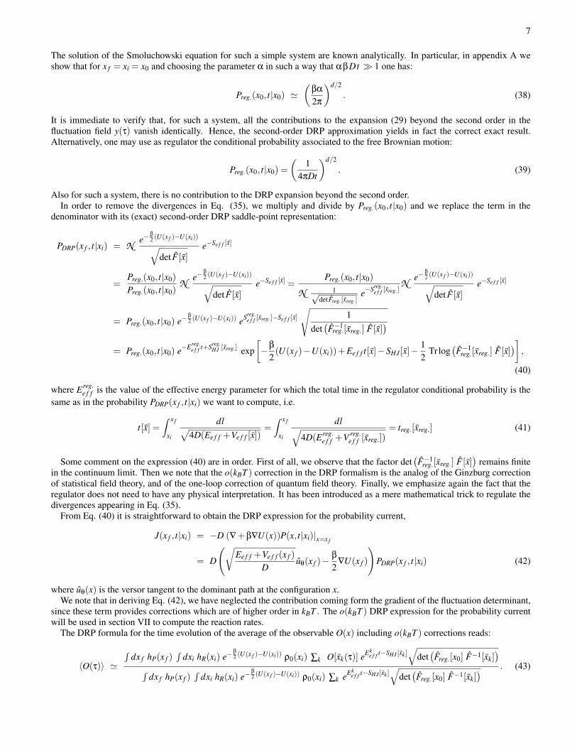
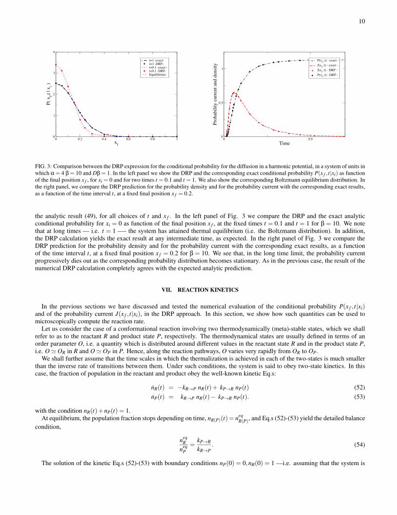
FIG. 3: Comparison between the DRP expression for the conditional probability for the diffusion in a harmonic potential, in a system of units inwhich α = 4 β = 10 and Dβ = 1. In the left panel we show the DRP and the corresponding exact conditional probability P(x f , t|xi) as functionof the final position x f , for xi = 0 and for two times t = 0.1 and t = 1. We also show the corresponding Boltzmann equilibrium distribution. Inthe right panel, we compare the DRP prediction for the probability density and for the probability current with the corresponding exact results,as a function of the time interval t, at a fixed final position x f = 0.2.

the analytic result (49), for all choices of t and x f . In the left panel of Fig. 3 we compare the DRP and the exact analyticconditional probability for xi = 0 as function of the final position x f , at the fixed times t = 0.1 and t = 1 for β = 10. We notethat at long times — i.e. t = 1 —- the system has attained thermal equilibrium (i.e. the Boltzmann distribution). In addition,the DRP calculation yields the exact result at any intermediate time, as expected. In the right panel of Fig. 3 we compare theDRP prediction for the probability density and for the probability current with the corresponding exact results, as a functionof the time interval t, at a fixed final position x f = 0.2 for β = 10. We see that, in the long time limit, the probability currentprogressively dies out as the corresponding probability distribution becomes stationary. As in the previous case, the result of thenumerical DRP calculation completely agrees with the expected analytic prediction.

VII. REACTION KINETICS

In the previous sections we have discussed and tested the numerical evaluation of the conditional probability P(x f , t|xi)and of the probability current J(x f , t|xi), in the DRP approach. In this section, we show how such quantities can be used tomicroscopically compute the reaction rate.

Let us consider the case of a conformational reaction involving two thermodynamically (meta)-stable states, which we shallrefer to as to the reactant R and product state P, respectively. The thermodynamical states are usually defined in terms of anorder parameter O, i.e. a quantity which is distributed around different values in the reactant state R and in the product state P,i.e. O' OR in R and O' OP in P. Hence, along the reaction pathways, O varies very rapidly from OR to OP.

We shall further assume that the time scales in which the thermalization is achieved in each of the two-states is much smallerthan the inverse rate of transitions between them. Under such conditions, the system is said to obey two-state kinetics. In thiscase, the fraction of population in the reactant and product obey the well-known kinetic Eq.s:

nR(t) = −kR→P nR(t)+ kP→R nP(t) (52)nP(t) = kR→P nR(t)− kP→R nP(t). (53)

with the condition nR(t)+nP(t) = 1.At equilibrium, the population fraction stops depending on time, nR(P)(t) = neq

R(P), and Eq.s (52)-(53) yield the detailed balancecondition,

neqR

neqP

=kP→R

kR→P. (54)

The solution of the kinetic Eq.s (52)-(53) with boundary conditions nP(0) = 0,nR(0) = 1 —i.e. assuming that the system is

11

initially prepared in the reactant state— are

nP(t) = neqP

(1− e−kt

), (55)

nR(t) = 1−nP(t), (56)

where k = kR→P + kP→R is the thermal relaxation rate.In the opposite short-time regime, i.e. for t 1

k , nP(t) grows linearly with the reaction rate kR→P:

nP(t)' kR→P t (kR→P t 1). (57)

Hence, the reaction rate kR→P can be written as

kR→P = limt→0

ddt

nP(t). (58)

The limit in such an equation means that the time t is chosen much smaller than the inverse reaction rate — i.e. kR→P t 1—,yet much larger than all the thermalization time scales in the reactant state. The possibility of making such a choice is guaranteedby the assumption of two-state kinetics.

In order to microscopically compute the rate in the DRP approach, we need the path integral expression of the populationfraction nP(t), solution of the Eq.s (52)-(53) with boundary condition nP(0) = 0. In the appendix C we show that such a solutionis given by

nP(t) =∫

dx f hP(x f )∫

dxi hP(xi) ρ0(xi) P(x f , t|xi)

= N∫

dx f hP(x f )∫

dxi hP(xi)ρ0(xi) e−β

2 (U(x f )−U(xi))∫ x(t)=x f

x(ti)=xi

Dx e−∫ t

0 dτ

(x24D+Ve f f [x]

), (59)

where ρ0(x) is the initial normalized distribution of the configurations in the reactant state and hR(x) and hP(x) are the charac-teristic functions of the reactant and product state, respectively.

Eq. (58) becomes

kR→P(kR→Pt1)

=∫

dx f hP(x f )∫

dxi hP(xi)ρ0(xi)∂

∂tP(x f , t|xi). (60)

Using the Smoluchowski Eq. we can rewrite this as

kR→P(kt1)=

ddt

nP(t) =∫

dx f hP(x f )∫

dxihR(xi)ρ0(xi)∂

∂tP(x f , t|xi) (61)

=∫

dx f hP(x f )∫

dxihR(xi)ρ0(xi)∇ · J(x f , t|xi) (62)

We now introduce a closed surface ∂W which surrounds the product state. Using Gauss’s divergence theorem, we find:

kR→P(kt1)=

∫dxi hR(xi) ρ0(xi)

∫∂W

dσ · J(x f , t|xi) (63)

= −∫

∂Wd|σ| nx · J(x f , t|xi) (64)

where J(x f , t|xi) denotes the average of the current with respect to the initial configuration in the reactant, i.e.

J(x f , t|xi)≡∫

dxi hR(xi) ρ0(xi) J(x f , t|xi), (65)

and nx is the unitary vector normal to the dividing surface ∂W at the point x, oriented out-ward. Note that if the surface ∂W ischosen in such a way that it intersects the transition region, then Eq. (64) yields in fact a multi-dimensional generalization ofKramers’ flux-over-population expression for the reaction rate[16].

The Eq.(63) contains the integrals over two large dimensional spaces, which may be difficult to perform in practical applica-tions. Hence, it is useful to introduce further approximations. First of all, we observe that under the assumption of two-statekinetics, the current J(x f , t|xi) becomes quasi-instantaneously independent on the initial configuration xi. This fact allows toremove the average over the initial configurations in the reactant, since for any choice of xi ∈ R one has

J(x f , t|xi)' J(x f , t|xi) ∀xi ∈ R. (66)

12

!1.5 !1.0 !0.5 0.0 0.5 1.0 1.5

!1.0

!0.5

0.0

0.5

1.0

!"#$%&'()*+&'+,'(

!W

-#./,+,'(0+'1( u!(xTS)

FIG. 4: The definition of ∂W as the hyper-surface orthogonal to the dominant path the the point xT S solution of the transition state Eq. (27).

Let us consider first the case in which the reaction occurs through a single channel, i.e. that all the stochastic paths starting formxi and ending up in the product after a short time t are confined in a small bundle around a single dominant reaction pathway. Inorder to estimate the flux of the current through the dividing surface, we insert the DRP expression for the current, i.e.

kR→P ' −∫

∂Wd|σ|x nx · JDRP(x, t|xi)' Preg.(x0, t|x0) e−Ereg.

e f f t+Sreg.HJ [x0]

×∫

∂Wd|σ|x nx ·

12(〈x(x)〉txi

−β∇U(x))

e−β

2 (U(x)−U(xi)) eEe f f t−SHJ [x]√

det(Freg[x0]F−1[x]) (67)

In the low-temperature limit, the leading dependence on x in the integrand of Eq. (67) comes from the exponential factors andwe can neglect the dependence on x of all the non-exponential terms. In addition, in the same limit, we can use the approximation

SHJ [x]'1

2kBT

∫ x

xi

dl |∇U [x(l)]|= β

2(U(x)−U(xi)) (68)

Hence, up to corrections of higher order in kBT , the flux (67) takes the form

kR→P =−∫

x∈∂Wd|σ|x nx · J(x, t|xi)'−Z∂W eβU(xT S) (nx∂W · JDRP(x∂W , t|xi)), (69)

where x∂W is a configuration on the dividing surface ∂W and Z∂W is the partition function

Z∂W =∫

x∈∂Wd|σ|x e−βU(x). (70)

Eq. (69) is independent on the specific choice of the dividing surface. We now specialize to the case in which ∂W is thehyper-surface orthogonal to the dominant reaction pathway, at the point xT S solution of the transition state Eq. (27) — seeFig. 4 —. With such a choice,

nx = −uθ(xT S), uθ(xT S)≡˙x(lT S)

| ˙x(lT S)|. (71)

Note that uθ(xT S) is the unit vector tangent to the dominant path at the configuration xT S (lT S is the value of the curvilinearabscissa a for which Eq. (27) is satisfied). Correspondingly, the partition function reads

Z∂W ≡ ZT S =∫

dx δ [(x− xT S) · uθ(xT S)] e−βU(x), (72)

The partition function (72) can be estimated in local harmonic approximation, by running short MD simulations starting fromxT S, subject to the constraint to lie on the surface orthogonal to the tangent to the reaction pathway at xT S, i.e.

ZT S ' e−βU(xT S)d

∏i=1

√2π〈(xi− xi

T S)2〉⊥, (73)

13

where xi is the i−th coordinate of the configuration x and

〈(xi− xiT S)

2〉⊥ ≡∫

dx (xi− xiT S)

2 δ [(x− xT S) · uθ] e−βU(x)∫dx δ [(x− xT S) · uθ] e−βU(x)

. (74)

Hence, using the DRP expression for the reaction current we arrive to our final result:

kR→P ' ZT S

∣∣∣∣∣√

Ee f f +Ve f f (xT S)

Duθ(x)−

β

2∇U(xT S)

∣∣∣∣∣ Preg.(x0, t|x0)]

eEreg.e f f t−Sreg.

HJ [xreg.]

√det(Freg.[xreg.]F−1[x]

)e−

β

2 (U(xT S)−U(xi))+Ee f f t[x]−SHJ [x].

(75)

In such an Eq., the effective energy parameter Ee f f must be chosen in such a way that the total time t[x] evaluated accordingto Eq. (21) is much larger than the relaxation time in the reactant and yet much smaller than the total relaxation rate. In such atime regime, the flux of probability current across the transition state is stationary and the value of the expression (75) must beindependent on the specific value of Ee f f chosen.

Finally, if the reaction can occur through more than one reaction pathway, the total rate is obtained simply by adding up allsuch contributions:

kR→P ' ∑k

ZkT S eβU(xk

T S) |J(xkT S, t|xi)|. (76)

For very simple systems, computing the rate by means of Eq.(75) of Eq. (76) is expected to be more computationally expensivethan in standard Kramers theory [16]. On the other hand, the advantage of the DRP method developed here is that it does notrequire to know a priori the location of the transition state. Hence, we expect that our method may be used to investigate thekinetics of two-state reactions in large configuration spaces, which are generally characterized by a complicated energy surface.In particular, for many complex molecular systems, the transition state cannot by guessed from the structure of the interaction,and the multi-dimensional Kramers theory is therefore useless.

We also observe that the DRP method presented in this section bares some similarity with other existing techniques for ratecalculation. In particular, the identification of the reaction coordinate l from a statistical important reaction pathway is alsoused in the so-called milestoning method [17]. An important advantage of such an approach with respect to the DRP methoddeveloped here is that it does not require to assume two-state kinetics. On the other hand, the present method is much lesscomputationally expensive, as it does not require to evaluate the first-passage-time distributions from the different milestones,from MD simulations.

The DRP Eq. (75) bares also some similarity also with Chandler’s theory [18] and with transition state theory [19]. Indeed,in both such approaches, the rate is related to the flux of reactive trajectories through the transition state. On the other hand, westress the fact that in the present DRP approach, such a flux is evaluated over non-equilibrium trajectories.

Finally we note that, in the transition path sampling algorithm [2], the rate is usually calculated starting from the path integralexpression of the product population fraction, i.e. Eq. (59). However, in such an approach, the normalization of the path integralis obtained by evaluating the free energy of the transition path ensemble, i.e. the reversible work which is required to constraintthe final configurations of the paths into the product state. On the other hand, in the DRP approach, such a normalization isguaranteed by construction a priori, by the regularization procedure.

VIII. TESTING THE DRP CALCULATION OF THE REACTION RATES

In order to test the scheme developed in the previous section for rate calculations, we study the reaction kinetics of somesimple two-dimensional toy systems, for which very accurate results can be obtained also using other methods. In particular, inwide range of temperatures, the rate for such systems can be accurately evaluated using Kramers theory or computed directly byrunning long MD simulations.

Let us begin by considering the rate of escape from a standard two-dimensional bi-stable potential,

U(x,y) = a(x2−ω2)2 +by2 (77)

with a = 1/8, b = 2, and ω = 2. In this simple case, the dominant path connecting xi = −ω to x f = ω is known analytically(straight horizontal line). We have represented such a path using Ns = 150 equally spaced steps. In addition, performing anaccurate calculation of the fluctuation determinants for such a simple two-dimensional system is straightforward, even withoutresiding on the low time resolution effective description.

We recall that in the DRP approach, the total time of the transition is determined by the value of the effective energy parameterEe f f , according to Eq. (21). The same parameter is used in the calculation of all the discretized time intervals which enter in thefluctuation determinant. On the other hand, our prediction for the rate must obviously not depend on the choice of Ee f f .

14

1 1.5 2Time

0

0.5

1

1.5

2

2.5

3J(

xf, t

| x i) /

10-9

20 40 60 80 100 !

0.93

0.94

0.95

0.96

0.97

0.98

0.99

1

K D

RP /K

Kra

mer

s

FIG. 5: Left panel: The absolute value of the normalized probability current at the sadde-point x f = 0, evaluated with the DRP method atdifferent times t, for xi =−ω and β = 5. The different total times are determined by different choices of the effective energy parameter. Righpanel: The ratio between the reaction rates evaluated with the DRP method and with Kramers theory.

In order to see how this condition can be satisfied, we recall that our rate expression (58) requires the time interval t to bemuch smaller than the inverse rate, kR→Pt 1. At the same time, t must be chosen much larger than the thermalization timein the reactant state, to assure single exponential relaxation. If both conditions are simultaneously satisfied, then one shouldobserve a stationary flux through the transition state. Consequently, our rate expression (76) should become independent on theprecise choice of t — hence of Ee f f —.

In order to test if such a stationary current is realized in our simulations, in the left panel of Fig. 5 we plot the DRP current atthe saddle-point as a function of the total time (hence for different values of the effective energy). We can clearly see that for thelongest times the current becomes stationary, hence the rate stops depending on the specific choice of Ee f f . The right panel ofFig. 5 shows that, in this system, the calculation of the rate using Kramers’ theory using the DRP approach agree within ' 1%accuracy.

Let us now consider a toy model which allows to specifically assess the role played by the stochastic fluctuations around thedominant path, in the kinetics of the reaction. To this end, we study the two-dimensional three-state system, consisting of areactant R, and of two products P1 and P2, shown in the left panel of Fig. 6 The functional form of the potential energy is

U [x,y] := ax6 +bx4 + cx2 + k1 exp[− (x− x1)

2

2σ

]+(x4−2x2 +κx+Ω)y2 (78)

with a = 5/64, b = −10/16, c = 1, k1 = −0.6, x1 = 0, σ = 0.3, κ = 0.5 and Ω = 2. Also in this case, the dominant pathsare known analytically. The HJ action and the fluctuation determinants appearing in Eq. (75) are evaluated using Ns = 100discretization steps.

This model is built is such a way that the energy barrier separating the reactant to the two products is the same. Yet, the steeperstructure of the potential energy on the right of the reactant tends to disfavor large stochastic fluctuations, along the dominantpath of the reaction R→ P2. We therefore expect that the rate of escape from R to P1 should be larger than that from R to P2.This fact is clearly seen in the right panel of Fig. 6, were we compare the ratio kR→P1/kR→P2 evaluated using Kramers theoryand using the DRP method. We see that the two approaches give results which agree within about 2% accuracy. In both cases,the reaction P→ P2 is about 50% slower than the reaction P→ P1.

IX. CONCLUSIONS

In this paper, we have analyzed the role of the stochastic fluctuations around the most probable reaction pathways, in systemsobeying the over-damped Langevin dynamics. Such fluctuations affect the probability for a transition to take place through aspecific reaction channel in a given time, hence the kinetic of the reaction. For sufficiently small temperatures, the fluctuationsin the ensemble of reaction pathways are confined within small bundles around the locally most probable reaction pathways. Insuch a regime, we have developed a technique to efficiently compute their contribution, to order kBT accuracy. Clearly, in theopposite high-temperature regime, the stochastic fluctuations become very large and overshadow the information encoded in thedominant paths. In this case, the accuracy of the DRP approach breaks down.

15

!2 !1 0 1 2

!1.0

!0.5

0.0

0.5

1.0

!"#$"#%"

50 100 150 200 250 300 !

0.55

0.56

0.57

0.58

0.59

K R

P2 /

K R

P1

DRP Kramers

FIG. 6: Left panel: The contour plot of the potential energy (78). Right panel: the ratio of the rates kR→P2/kR→P1 evaluated in the DRPapproach and using Kramers theory. using Kramers theory, DRP calculations and direct MD simulations.

We have shown that the calculation of the time intervals and of the fluctuation determinant can be made much more efficientby adopting a low-time resolution effective description, in which the fast dynamics is analytically pre-averaged out. Indeed, inthe effective stochastic theory, the convergence of DRP calculations is achieved using much fewer discretization paths.

The o(kBT ) expression of the conditional probability was used to derive a formula for the reaction rate, within a flux-over-population approach. We have illustrated and tested our results on simple toy models, where accurate or even exact results couldbe obtained with alternative methods. In the future, we plan to apply these techniques to investigate the kinetics of much morecomplicated molecular reactions.

Acknowledgments

Part of this work was performed when P.F. was visiting the IPhT at CEA (Saclay) under a CNRS grant. P.F. and S.B. aremembers of the Interdisciplinary Laboratory for Computational Sciences (LISC), a joint venture of Trento University and FBK.The authors acknowledge useful discussions with F. Pederiva.

Appendix A: The Conditional Probability for the Diffusion in a d−Dimensional Harmonic Potential

Here we review the exact calculation of the conditional probability for a point-particle diffusing in the d−dimensional har-monic external potential

U(x) =12 ∑

iω

2i (x

i− xi0)

2. (A1)

For sake of simplicity, we discuss such an evaluation in the case x f = xi = 0 and we choose the origin of the configuration spacein such a way xi

0 = 0. We also choose units in which the viscosity γ = 1/βD is set to 1.In this case the effective action of the static solution x = 0 is Se f f [x] =− t

2 ∑i ω2i , hence:

PHO(0, t|0) = N et2 ∑i ω2

i t 1√det[δi j(−β

2∂2

∂t2 +β

2 ω4i )]

= N ′et2 ∑i ω2

i t(

2β

)d/2 1√det[δi j(− ∂2

∂t2 +ω4i )] , (A2)

where in the last step we have absorbed the factor β/2 which appears in the fluctuation operators into the normalization constantN .

16

The normalized eigen-functions and eigen-values of the fluctuation operator with the boundary conditions y(t) = y(0) = 0 are:

yin(τ) =

√2t

sin[n π

tτ

](A3)

λin =

(πn)2

t2 +ω4i (n = 1,2, . . . , i = 1, . . . ,d) (A4)

Notice that the same eigenfunctions are also eigenstates of the fluctuation operator for the free diffusion

F0 =−δi jδ(τ′− τ)

∂2

∂τ2 , (A5)

with eigenvalues

λi0n =

(π

t

)2n2 (n = 1,2, . . . , i = 1, . . . ,d) (A6)

As usual, in order to get rid of the unknown normalization N ′ we multiply and divide by a regulator, in this case the freepropagator P0(0, t|0):

PHO(0, t|0) = P0(0, t|0) et2 ∑i ω2

i

√√√√√ ∏di=1 ∏n≥1

((nπ)2

t2

)∏

di=1 ∏

∞n≥1

((nπ)2

t2 +ω4i

) (A7)

=

(β

4π t

)d/2

et2 ∑i ω2

i

√√√√ 1

∏di=1 ∏

∞n≥1

(1+ ω4

i t2

(niπ)2

) (A8)

Using the result

∏n≥1

(1+

ω4i t

(niπ)2

)=

Sinh(ωit)ω2

i t(A9)

we find

PHO(0, t|0) =

(β

4 π

)d/2

et2 ∑i ω2

id

∏i=1

√ω2

i

sinh(ω2i t)

(A10)

Notice that, in the long time limit, sinh(ω2i t)→ 1

2 eαit2 , so PHO(0, t|0) converges to the inverse of the partition function, as it

should:

PHO(0, t|0)→(

β

2π

)d/2

∏i

ωi =1

ZHO(A11)

Notice also that, for this system, the thermalization time does not depend on the temperature.

Appendix B: Effective Stochastic Theory

In this section, we sketch the derivation of the EST. For all further details we refer the reader to the original paper [14]. Forsimplicity and without loss of generality, it is convenient to consider the path integral with periodic boundary conditions

Z(t)≡∫

dx P(x|x; t) =∮

Dx e−Se f f [x]. (B1)

The starting point to develop the EST consists in introducing the Fourier components of the paths,

x(ωn) =1t

∫ t

0dτ x(τ) e−iωnt (B2)

x(τ) = x(τ+ t) = ∑n

x(ωn) eiωnt . (B3)

17

where ωn2π

t n, are the Fourier frequencies (n = 0,±1,±2, . . .).The path integral (B1) is defined in the continuum limit. Numerical simulations are always performed using a finite discretiza-

tion time step ∆t. Clearly, the shortest time intervals which can be explored in a numerical simulation is of the order of few ∆t.Equivalently, the largest frequencies of the Fourier transform of the stochastic paths x(ω) are of the order few fractions of anultra-violet (UV) cut-off Ω≡ 2π/∆t.

Let us now split the Fourier modes of the paths contributing to (13) in high-frequency —or "fast"— modes and low-frequency—or "slow"— modes. To this end, we introduce a real number 0 < b < 1 such that the frequency range (0,Ω) is split in twointervals (0,b Ω)∪ (b Ω,Ω). Correspondingly, one can define the "fast" component of the path x>(τ) and the "slow" componentof the path x<(τ), by summing over the Fourier modes in the (0,b Ω) and (b Ω,Ω) range, respectively:

x<(t) = ∑|ωn|≤bΩ

x(ωn) e iωnt (B4)

x>(t) = ∑bΩ≤|ωn|≤Ω

x(ωn) e iωnt . (B5)

The complete path integral (B1) can therefore be exactly re-written in the following way:

Z(t) =∮

Dx<∮

Dx> e−Se f f [x<+x>] ≡∮

Dx< e−Se f f [x<] e−S>[x<], (B6)

where

e−S>[x<(τ)] ≡∮

Dx>eSe f f (x<]−Se f f [x<+x>] (B7)

is called the renormalized part of the effective action.The EST is constructed by explicitly evaluating S>[x<], i.e. by performing the path integral over fast modes x>(τ). In the limit

in which the fast and slow modes are separated by a large gap in the spectrum of Fourier modes — i.e. if the system displays adecoupling of time scales—such an integral can be carried out analytically in a perturbative approach based on Feynman diagramtechniques[14]. The expansion parameter such a perturbation theory is the ratio between the typical frequency ω of the slowmodes and the UV cut-off bΩ. Clearly, if hard and slow modes are decoupled, the ratio ω/(bΩ) is a small number, hence theterms proportional to higher and higher powers L of such a ratio provide smaller and smaller corrections.

If one accounts only for the leading corrections in the 1/bΩ expansion, the renormalized part of the action takes the form ofan effective interaction term [14], i.e.

e−S>[x<(τ)] = e−∫ t

0 dτ V Re f f [x<(τ)] (B8)

where

V Re f f (x) '

D0 (1−b)π bΩ

∇2Ve f f (x). (B9)

We emphasize that the result of the EST construction is a new expression for the same path integral (B1), in which the UVcutoff been lowered from Ω to bΩ. Equivalently, the path integral is discretized according to a larger elementary time step,∆t→ ∆t/b:

Z∆t(t) ≡∮

∆tDx e−Se f f [x] ∝

∮∆t/b

Dx e−Se f f [x]−∫ t

0 dτ V Re f f [x(τ)] ≡ Z∆t/b

EST (t) (B10)

In these expressions, the symbol∮

∆t denotes the fact that the path integral is discretized according to an elementary time step∆t and we have suppressed the subscript "<", in the paths. It can be shown that the proportionality factor between Z∆t(t) andZ∆t/b

EST (t) depends only on t and does not contribute to the statistical averages.

Appendix C: Path Integral Expression for the Population Fractions nP(t) and nR(t)

In this section we provide a microscopic representation of the solutions nP(t) and nR(t) of the kinetic Eq.s (52)-(53). Let usconsider in particular the case in which the system is initially prepared in the reactant state, i.e. nR(0) = 1 and nP(0) = 0. Letρ0(x) be the initial distribution of the configurations in the reactant state. Clearly, such a choice of initial conditions implies thenormalization condition ∫

dx hR(x)ρ0(x) = 1, (C1)

18

where hR(x) is the characteristic function of the reactant, i.e. hR(x) = 1 if x ∈ R and 0 otherwise. Under the assumption oftwo state kinetics, the thermalization in the reactant occurs over a very short time scale, hence the specific choice of the initialdistribution in the reactant is in fact irrelevant.

We now show that a microscopic representation for the product population fraction nP(t) is obtained by averaging the condi-tional probability P(x f , t|xi) over the initial configurations xi in the reactant and summing over all possible final configurationsx f in the product, i.e.

nP(t) =∫

dx f hP(x f )∫

dxi hP(xi) ρ0(xi) P(x f , t|xi)

= N∫

dx f hP(x f )∫

dxi hP(xi)ρ0(xi) e−β

2 (U(x f )−U(xi))∫ x(t)=x f

x(ti)=xi

Dx e−∫ t

0 dτ

(x24D+Ve f f [x]

). (C2)

We observe that Eq. (C2) satisfies the correct initial condition, nP(0) = 0.Let us now introduce the complete set of eigenstates Ψn(x) of the "quantum" Hamiltonian He f f ,

He f f Ψn(x) = knΨn(x). (C3)

In particular, it is immediate to verify that the ground state of He f f has a vanishing eigenvalue and reads

Ψ0(x) =e−

β

2 U(x)√

Z, (C4)

where Z is the partition function of the system,

Z =∫

dx e−βU(x). (C5)

By inserting the resolution of the identity, 1 = ∑n |n〉 〈n|, into the "quantum" propagator (12) we obtain the so-called spectralrepresentation of the conditional probability:

P(x, t|xi) = e−β/2(U(x)−U(xi))∞

∑n=0

Ψ∗n(x) Ψn(xi)e−knt . (C6)

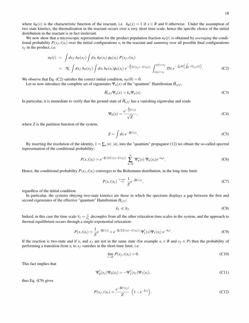
Hence, the conditional probability P(x f , t|xi) converges to the Boltzmann distribution, in the long time limit:

P(x, t|xi)t→∞→ 1

Ze−βU(x), (C7)

regardless of the initial condition.In particular, the systems obeying two-state kinetics are those in which the spectrum displays a gap between the first and

second eigenstates of the effective "quantum" Hamiltonian He f f :

k1 k2. (C8)

Indeed, in this case the time scale τ1 =1k1

decouples from all the other relaxation time scales in the system, and the approach tothermal equilibrium occurs through a single-exponential relaxation:

P(x, t|xi)'1Z

e−βU(x)+ e−β/2(U(x)−U(xi)) Ψ†1(x)Ψ1(xi) e−k1t . (C9)

If the reaction is two-state and if xi and x f are not in the same state (for example xi ∈ R and x f ∈ P) then the probability ofperforming a transition from xi to x f vanishes in the short-time limit, i.e.

limt→0

P(x f , t|xi) = 0. (C10)

This fact implies that

Ψ†0(x f )Ψ0(xi) =−Ψ

†1(x f )Ψ1(xi), (C11)

thus Eq. (C9) gives

P(x f , t|xi) =e−βU(x f )

Z

(1− e−k1t

). (C12)

19

We emphasize that Eq. (C10) —and therefore Eq. (C11)— are not justified if x f and xi are in the same state. Indeed, in theapproximation of two-state kinetics, the local thermalization in the R and P states is assumed to occur instantaneously, as theonly finite time scale is the mean-first-passage time across the barrier.

Using the spectral decomposition (C9) we find

nP(t) =∫

dx f hP(x f )∫

dxi hR(xi) ρ0(xi)e−βU(x f )

Z

(1− e−k1t

). (C13)

The product population fraction at time t then reads

nP(t) = neqP

(1− e−k1t

). (C14)

where neqP = ZP

Z . Hence, we have recovered Eq. (55) and we have shown that first excited state of the quantum effectiveHamiltonian is the equilibrium relaxation rate of the system, k1 = k.

[1] C. Dellago. P. G. Bolhuis, F. S. Csajka, and D. Chandler, J. Chem. Phys. 108, 1964 (1998).[2] P. G. Bolhuis, D. Chandler, C. Dellago, and P. L. Geissler, Ann. Rev. Phys. Chem. 53, 291 (2002).[3] A. Ghosh, R. Elber and H. A. Sheraga, Proc. Nat. Acad. Sci. 99, 10394 (2002).[4] D.M. Zuckerman and T.B. Woolf, Phys. Rev. E 63, 016702 (2000).[5] R. Elber, and D. Shalloway, J. Chem. Phys. 112 5539 (2000).[6] P. Faccioli, M. Sega, F. Pederiva and H. Orland, Phys. Rev. Lett. 97, 108101 (2006).[7] M. Sega, P. Faccioli, F. Pederiva, G. Garberoglio and H. Orland, Phys. Rev. Lett. 99, 118102 (2007).[8] E. Autieri, P. Faccioli, M. Sega, F. Pederiva and H. Orland, J. Chem Phys. 130, 064106 (2009).[9] P. Eastman, N. Gronbech-Jensen, and S. Doniach, J. Chem. Phys. 114, 3823 (2001).

[10] S. a Beccara, P. Faccioli, G. Garberoglio, M. Sega, F. Pederiva, H. Orland, arXiv:1007.5235, J. Chem. Phys. in press[11] S. a Beccara, G. Garberoglio, P. Faccioli and F. Pederiva, J. Chem. Phys. 132 111102 (2010) (comm.)[12] P. Faccioli, Journ. Phys. Chem. B112 (2008) 13756.[13] P. Faccioli, A. Lonardi and H. Orland, J. Chem. Phys. 133, 045104 (2010).[14] O. Corradini, P. Faccioli and H. Orland, Phys. Rev. E80 (2009) 061112.[15] P. Faccioli, J. Chem. Phys. 133 164106(2010)[16] P. Hänggi, P. Talkner and M. Borkovec, Rev. Mod. Phys. 62, 251 (1990).[17] A. K. Farajian and R. Elber, J. Chem. Phys. 120, 10880 (2004).[18] D. Chandler, J. Chem. Phys. 68, 2959 (1978).[19] D.G. Truhlar, B.C. Garrett and S. J. Klippenstein, Journ. Phys. Chem. 100, 12771 (1996).