Fluctuating Hydrodynamics and Debye-Hückel-Onsager Theory for Electrolytes Aleksandar Donev Courant Institute of Mathematical Sciences, New York University, New York, NY, 10003 Alejandro L. Garcia Department of Physics and Astronomy, San Jose State University, San Jose, CA, 95192 Jean-Philippe Péraud, Andy Nonaka, John B. Bell Center for Computational Science and Engineering, Lawrence Berkeley National Laboratory, Berkeley, CA, 94720 Abstract We apply fluctuating hydrodynamics to strong electrolyte mixtures to compute the concentration corrections for chemical potential, diffusivity, and conductivity. We show these corrections to be in agreement with the limiting laws of Debye, Hückel, and Onsager. We compute explicit corrections for a symmetric ternary mixture and find that the co-ion Maxwell-Stefan diffusion coefficients can be negative, in agreement with experimental findings. Keywords: fluctuating hydrodynamics, computational fluid dynamics, Navier-Stokes equations, low Mach number methods, multicomponent diffusion, electrohydrodynamics, Nernst-Planck equations 1. Introduction Due to the long-range nature of Coulomb forces between ions it is well-known that electrolyte solutions have unique properties that distinguish them from ordinary mixtures [1]. Colligative properties, such as osmotic pressure, and transport properties, such as mobility, have corrections that scale with the square root of concentration [2, 3, 4, 5]. This macroscopic effect has a mesoscopic origin, specifically, due to the competition of thermal and electrostatic energy at scales comparable to the Debye length. The traditional derivation of the thermodynamic corrections is by way of solving the Poisson-Boltzmann equation. For example, an approximate solution gives the Debye-Hückel limiting law for the activity coef- ficient [2, 6]. The derivation of the transport properties, as developed by Onsager and co-workers [7, 8, 9], has a similar starting point but is much more complicated. Here, we present an alternative approach using fluctuating hydrodynamics (FHD) [10]. This paper generalizes our previous derivation for binary elec- trolytes [11] to arbitrary solute mixtures, and, as an illustrative example, calculates transport properties for a ternary electrolyte. It should be noted that our FHD approach extends closely-related density functional Email address: [email protected] (Aleksandar Donev) Preprint submitted to Elsevier August 23, 2018

Welcome message from author
This document is posted to help you gain knowledge. Please leave a comment to let me know what you think about it! Share it to your friends and learn new things together.
Transcript
Fluctuating Hydrodynamics and Debye-Hückel-Onsager Theory forElectrolytes
Aleksandar Donev
Courant Institute of Mathematical Sciences, New York University, New York, NY, 10003
Alejandro L. Garcia
Department of Physics and Astronomy, San Jose State University, San Jose, CA, 95192
Jean-Philippe Péraud, Andy Nonaka, John B. BellCenter for Computational Science and Engineering, Lawrence Berkeley National Laboratory, Berkeley, CA, 94720
Abstract
We apply fluctuating hydrodynamics to strong electrolyte mixtures to compute the concentration corrections
for chemical potential, diffusivity, and conductivity. We show these corrections to be in agreement with the
limiting laws of Debye, Hückel, and Onsager. We compute explicit corrections for a symmetric ternary
mixture and find that the co-ion Maxwell-Stefan diffusion coefficients can be negative, in agreement with
experimental findings.
Keywords: fluctuating hydrodynamics, computational fluid dynamics, Navier-Stokes equations, low Mach
number methods, multicomponent diffusion, electrohydrodynamics, Nernst-Planck equations
1. Introduction
Due to the long-range nature of Coulomb forces between ions it is well-known that electrolyte solutions
have unique properties that distinguish them from ordinary mixtures [1]. Colligative properties, such as
osmotic pressure, and transport properties, such as mobility, have corrections that scale with the square
root of concentration [2, 3, 4, 5]. This macroscopic effect has a mesoscopic origin, specifically, due to the
competition of thermal and electrostatic energy at scales comparable to the Debye length.
The traditional derivation of the thermodynamic corrections is by way of solving the Poisson-Boltzmann
equation. For example, an approximate solution gives the Debye-Hückel limiting law for the activity coef-
ficient [2, 6]. The derivation of the transport properties, as developed by Onsager and co-workers [7, 8, 9],
has a similar starting point but is much more complicated. Here, we present an alternative approach using
fluctuating hydrodynamics (FHD) [10]. This paper generalizes our previous derivation for binary elec-
trolytes [11] to arbitrary solute mixtures, and, as an illustrative example, calculates transport properties for
a ternary electrolyte. It should be noted that our FHD approach extends closely-related density functional
Email address: [email protected] (Aleksandar Donev)
Preprint submitted to Elsevier August 23, 2018
theory calculations of relaxation corrections to the conductivity [12] of binary electrolytes to account for
advection, which enables us to also compute the electrophoretic corrections [2].
First formulated by Landau and Lifshitz to predict light scattering spectra [13, 14], more recently FHD
has been applied to study various mesoscopic phenomena in fluid dynamics [10, 15, 16, 17]. The current
popularity of fluctuating hydrodynamics is due, in part, to the availability of efficient and accurate numerical
schemes for solving the FHD equations [18, 19, 20, 21, 22, 23, 24, 25, 26]. While in this work we give analytical
results for dilute electrolytes under simplifying assumptions, numerical techniques can in principle be used
to compute the transport coefficients for moderately dilute solutions.
From the work of Onsager et al. [7, 8, 9] we can obtain the Fickian diffusion matrix for sufficiently
dilute electrolytes. For neutral multispecies mixtures, especially non-dilute ones, using binary Maxwell-
Stefan (MS) diffusion coefficients (inverse friction coefficients) [27, 28] is preferred because generally they
are positive and depend weakly on concentration. In this paper we use our FHD formulation to calculate
the effective macroscopic (renormalized) co-ion and counter-ion MS coefficients for binary and symmetric
ternary electrolytes. For sufficiently dilute binary electrolytes both theory and experiments show that the
counter-ion MS friction coefficient diverges as the inverse square root of the ionic strength [28]. This strong
concentration dependence implies that there are cross-diffusion terms that couple the electrodiffusion of the
different species even in the absence of an (external) electric field. Such effects are not captured in the
widely-used Poisson-Nernst-Planck (PNP) model of electrodiffusion, which is only accurate for very dilute
solutions. Our results show that for a symmetric ternary mixture all MS friction coefficients diverge as
the inverse square root of the ionic strength and the co-ion coefficient can be negative, in agreement with
experimental findings.
Obtaining MS coefficients as a function of concentration is quite difficult for multicomponent electrolytes,
and in practice various empirical fits are used following the work of Newman and collaborators [3], especially
in modeling electrodes in Li-ion batteries [29, 30, 31, 32]. These fits have sometimes been informed by tracer
diffusion coefficients of ions in binary electrolyte solutions [33]. Some authors have computed MS coefficients
by Green-Kubo formulas using molecular dynamics [34, 35]. Asymptotic expansions for dilute solutions can
be computed using our FHD-based approach and thus ground empirical fits of the concentration dependence
used in chemical engineering.
A complete model of transport in electrolyte mixtures must also account for advection and thus include
the momentum conservation (velocity) equation. This is commonly not done for dilute solutions based on
arguments that the velocities are negligible (small Peclet number), but these arguments have often been
flawed. This is because there is a Lorentz force in the momentum equation that induces nontrivial velocities
even in the electroneutral bulk [36]. Here we demonstrate that the coupling between charge fluctuations
and velocity fluctuations via the Lorentz force is responsible for the so-called electrophoretic correction to
the diffusion coefficients; it is this correction that can make the co-ion MS coefficient negative. Even more
unexpected couplings between mass and momentum transport have been uncovered in double layers, where
2
charges are nonzero and applied electric fields can introduce pressure gradients that then drive nontrivial
barodiffusion [37].
This paper is organized as follows. Section 2 presents the FHD equations for a strong electrolyte; we
show that the equilibrium solution leads to the Debye-Hückel limiting law for activity. The non-equilibrium
solutions derived in Section 3 yield the relaxation and electrophoretic corrections to conductivity and dif-
fusion originally derived by Onsager [7, 8]. An additional renormalization correction due to correlations of
concentration and velocity fluctuations is also derived [15]. Section 4 highlights an interesting co-ion cross-
diffusion effect found in a ternary mixture. Section 5 outlines FHD applications for electrolytes that go far
beyond re-deriving classical results.
2. Fluctuating hydrodynamics for electrolytes
We consider an electrolyte solution with Nsp solute species and let wi(r, t) be the mass fraction for
species i at position r and time t. The charge of a molecule (ion) is eVi, where Vi is the valence and e is the
elementary charge; we also write it as mizi where mi is the molecule mass and zi is the specific charge. We
denote the vectors w = (w1, . . . , wNsp)T and similarly z = (z1, . . . , zNsp)T , where (·)T denotes transpose.
The fluid mixture is assumed incompressible with constant mass density ρ, isothermal with temperature
T , and, on average, locally electroneutral (∑i zi〈wi〉 = 0).
2.1. Stochastic transport equations
For dilute ionic solutions, the transport (conservation) equation for solute species i is
∂twi = −∇ · (F i + F i), (1)
where F i is the hydrodynamic (dissipative and advective) flux, and F i is the stochastic flux. The diffusive
flux is given by the Nernst-Planck equation so the total hydrodynamic flux is
F i = −D0i
(∇wi + eViwi
kBT∇φ
)+ vwi, (2)
where v is the fluid velocity, D0i is the “bare” Fickian diffusion coefficient,1 φ is the electric potential, and kB
is Boltzmann’s constant. The dielectric permittivity ε is taken as constant so φ is defined by the electrostatic
equation
−ε∇2φ = q, where q = ρe∑i
wiVimi
= ρ∑i
wizi (3)
is the charge density.
The stochastic species flux is
F i =
√2D0
imiwiρ
Zi, (4)
1The term bare refers to the fact that D0i will later be renormalized by the fluctuations to its macroscopic value Di.
3
where Z is a Gaussian white noise vector field with independent components that are uncorrelated in time and
space. This flux has zero mean (〈F i〉 = 0) and its variance satisfies the fluctuation-dissipation theorem [10].
We will refer to (1,2,3,4) as the (fluctuating) Poisson-Nernst-Planck (PNP) equations [22]. Note that
summing (1) over all species gives the continuity equation ∇ · v = 0.
The equation for momentum transport is
ρ∂tv = −ρ∇ · (vvT )−∇p+ µ∇2v + qE +√µkBT ∇ · (V + VT ), (5)
where p is pressure, µ = νρ is the shear viscosity, and E = −∇φ is the electric field. The last term in (5) is
the divergence of the stochastic stress tensor, where V is a white noise tensor field.
2.2. Structure factor
The static structure factor Sfg(k) characterizes the cross-correlations between the fluctuations of two
scalar quantities f(r) and g(r),
Sfg(k) = 〈δf(k)δg(k)∗〉 (6)
where f(k) is the Fourier transform of f(r) and (·)∗ denotes conjugate transpose. By Plancherel’s theorem,
〈(δf)(δg)∗〉 = 1(2π)3
∫dk Sfg(k). (7)
Here the quantities of interest are the fluctuations of the mass fractions δwi = wi − wi from their average
wi = 〈wi〉, and the fluctuations of the fluid velocity2 δv. In the non-equilibrium situations considered here
we are only interested in the velocity component in the direction of the applied thermodynamic force (e.g.,
external electric field). This is taken as the x-direction so only vx is retained in the structure factors.
A central quantity in our calculations is the (Nsp + 1)× (Nsp + 1) Hermitian matrix of structure factors
S =
Sww Swv
Swv∗ Svv
, (8)
where the matrix Sww = 〈(δw)(δw)∗〉 and the vector Swv have elements
[Sww]ij = Swi,wj = 〈(δwi)(δwj)∗〉 and [Swv]i = Swi,vx = 〈(δwi)(δvx)∗〉, (9)
and Svv = 〈(δvx)(δvx)∗〉.
The structure factor is easily calculated by linearizing (1) and (5) and transforming into Fourier space,3
∂tU = MU + N Z, (10)
2We take the average fluid velocity as zero so δv = v; the notation emphasizes that velocity is a fluctuating quantity.3The double curl operator is applied to the Fourier transform of (5) to eliminate the pressure term using the incompressibility
constraint [10].
4
where U = (δw1, . . . , δwNsp , δvx)T . This stochastic ODE describes an Ornstein-Uhlenbeck process, so the
structure factor is the solution of the linear system [38]
MS + SM∗ = −N N ∗. (11)
The right hand side is a diagonal matrix with elements,
[N N ∗]ii = 2ρ
k2D0imiwi i ≤ Nsp
k2⊥νkBT i = Nsp + 1
, (12)
where k2⊥ = k2 − k2
x = k2 sin2 θ, and θ is the angle between k and the x axis.
At thermodynamic equilibrium,
Meq =
Meqww 0
0 −νk2
, (13)
where
[Meqww]ij = −D0
i
(k2δij + zj
zi
Iiλ2
). (14)
Here the Debye length λ is
λ =√εkBT
I, where I = ρ
∑i
miwiz2i (15)
is the ionic strength and Ii = miwiz2i /(∑
jmjwjz2j
)is the relative ionic strength. This can easily be
derived from the Fourier transform of the PNP equations. In particular, from (3) and the condition of local
electroneutrality, the fluctuations in the electric field can be expressed in terms of species fluctuations,
δE = −ιkδφ = − ιk
εk2 δq = −ρ ιkεk2
∑i
ziδwi, (16)
where ι =√−1.
Solving (11) at thermodynamic equilibrium gives Seqwv = 0 and Seq
vv = sin2(θ)kBT/ρ. In the case where
the solutes are neutral (Vi = 0 for all species), which we denote by superscript “n”, the matrix Seq,nww is
diagonal with S(eq,n)wi,wi = miwi/ρ independent of k. For a mixture involving ionic species, [22]
Seqww = Seq,n
ww −1
1 + k2λ2 Π where Πi,j = λ2
εkBT(miziwi) (mjzjwj) . (17)
2.3. Renormalization of chemical potentials
It is well-known that the colligative properties (e.g., vapor pressure) of electrolyte solutions depend on
their ionic strength, i.e., that the chemical potential of the ions are different from those in a dilute mixture
of neutral species. Specifically, ionic interactions contribute to the Gibbs free energy and this leads to a
correction for the activity.
The average increase in the electrostatic energy is ∆G = 12 〈δqδφ〉. Using (7,16) we obtain
∆G = ρ2
2ε(2π)3
∫zT (Seq
ww − Seq,nww ) z
k2 dk, (18)
5
where we have subtracted Seq,nww to avoid an ill-defined integral that is actually zero due to the overall
electroneutrality. From (17), the renormalization of the free energy due to fluctuations is
∆G = − kBT8πλ3 = − I8πελ. (19)
As shown in [2], this result leads directly to the limiting law of Debye and Hückel for point ions. The
integration in (18) is over all wavenumber; however, FHD is a mesoscopic theory so it does not apply below
molecular scales. Introducing an upper bound kmax ∼ π/a, where a is an effective ion radius, reduces the
correction ∆G by a fraction ∼ a/λ for a λ, in agreement with the Debye–Hückel limiting law for finite-size
ions.
3. Fluctuations and Transport
Non-equilibrium systems are driven by thermodynamics forces, such as a gradient of concentration or an
applied electric field. Transport coefficients such as diffusivity and conductivity are obtained from the linear
response, namely the fluxes resulting from weak thermodynamic forces. The linear response is modified due
to correlations in the hydrodynamic fluctuations,
F i = 〈F i(w,v)〉 = F i(〈w〉, 〈v〉) +D0i
eVikBT
〈δwiδE〉+ 〈δvδwi〉
≡ F0i + F relx
i + F advi (20)
to quadratic order in the fluctuations. The term Frelxi is the relaxation correction and F adv
i the advection
correction. The term “relaxation” refers to the average force experienced by an ion from its asymmetric
ionic cloud relaxing due to thermal fluctuations [2].
In what follows we obtain expressions for 〈δwiδE〉 and 〈δvδwi〉 from the structure factor and show that
F i can be written as (2) with renormalized diffusion coefficients that depend on the ionic strength. As
we shall see, fluctuating hydrodynamics yields the same relaxation and electrophoretic corrections as those
obtained by Onsager and co-workers [7, 8], plus an additional advection enhancement that is given by a
Stokes-Einstein formula [15] and is independent of the valences.
For this analysis it is useful to write the matrix M as
M = Meq + M′ +O(X 2), (21)
where X is the applied thermodynamic force. In this expansion Meq is O(X 0) and M′ is O(X 1). Similarly,
we can write the structure factor as S = Seq+S′+O(X 2). The noise covariance matrix N N ∗ is unchanged,4
so expanding (11) in powers of X gives the correction to the structure factors to linear order in X as the
solution of the linear system
MeqS′ + S′(Meq)∗ = −M′Seq − Seq(M′)∗. (22)
4This is the so-called local equilibrium assumption, which is valid when the applied gradients are not too large.
6
3.1. Renormalization of diffusion
For neutral species, diffusion can be analyzed by imposing a concentration gradient separately for each
species and formulating the linearized response. For charged species, however, the concentration gradient of
a given species must be balanced by the other concentration gradients in order to preserve electroneutrality
in the mean,∑i zi∇wi = 0; as mentioned, we assume all concentration gradients are in the x-direction.
For an imposed concentration gradient X ≡ ∇xw in the absence of an external electric field (〈E〉 = 0),
the relaxation of composition fluctuations follows the linearized equations
∂tδwi = D0i
∇2δwi −Iiλ2zi
∑j
zjδwj
− D0imizikBT
δEx∇xwi − δvx∇xwi. (23)
The linearized momentum equation is the same as in equilibrium. Using (16) we obtain the linear correction
to the relaxation matrix,
M′ =
ι cos θk
ρεkBT
πzT −∇xw
0 0
, (24)
where the column vector π has elements πi = D0imizi∇xwi.
3.1.1. Advective correction
The advective correction F advi to the fluxes due to nonzero correlation 〈δvδwi〉 in (20) can be calculated
rather easily since S′wv solves
MeqwwS
′wv − νk2S′wv = kBT
ρsin2 θ ∇xw. (25)
Using the constraint zT∇xw = 0 gives
S′wv = −kBT sin2 θ
k2ρDiag(D0
i + ν)−1 ∇xw. (26)
Integrating over k and using (7) then yields
Fadvi = 〈δvδwi〉 = − kBT
3πρ(D0i + ν)ai
∇wi, (27)
where we have introduced a molecular length ai to set an upper bound of π/ai for the wavenumber in order
for the integral (7) to converge. One can interpret ai as the molecular hydrodynamic diameter that enters
in the Stokes-Einstein formula [15].
The advective contribution to the fluxes (27) can be absorbed into the PNP equations by redefining or
renormalizing the diffusion coefficients from their bare values D0i to
Di = D0i + kBT
3πµai, (28)
7
3.1.2. Relaxation correction
The relaxation correction F relxi due to the nonzero correlation 〈δwiδE〉 in (20) can be computed in
principle by solving for S′ww the linear system
MeqwwS
′ww + S′ww(Meq
ww)T = −ι cos θk
ρ
εkBT(πzTSeq
ww − Seqwwzπ
T ). (29)
This can be simplified further to the system
DΩS′ww + S′wwΩTD = ιkλ2 cos θ
ρ (1 + k2λ2)(πκT − κπT
), (30)
where D = Diag(D0i ), the column vector κ has elements κi = miwizi, and the matrix Ω = k2λ2 (zTκ) I +
κzT . The solution S′ww is a purely imaginary anti-symmetric matrix with zeros on the diagonal.
Given a solution to (29), we can use (9,16) to obtain
Frelxi = D0
i
eVikBT
〈δwiδE〉 = −D0i
eViεkBT
ρ
8π3
∑j
zj
∫dk
ιk
k2S′wi,wj
. (31)
Since all computations are linear, the final result can be written as a correction to Fick’s law, F relxx =
−Drelx∇xw, where, in general, Drelx is not diagonal and includes cross-diffusion terms. As done earlier
with (18), introducing an upper bound kmax ∼ π/a in (31) reduces the relaxation correction by a fraction
∼ a/λ, in agreement with Onsager’s calculations for finite-size ions. One can also express the results in terms
of corrections to the binary Maxwell-Stefan diffusion coefficients (see Section 4 and the Appendix) [28, 11].
In general, it is difficult to solve (29) in closed form; an explicit but lengthy formulation for the relaxation
correction to diffusion is given by Onsager and Kim [8] in terms of solutions to eigenvalue problems.5 In
Appendix A we give explicit results for a binary electrolyte, and in Section 4 for a symmetric ternary
electrolyte mixture.
3.2. Renormalization of conductivity
By Ohm’s law, the electrical conductivity Λi for species i is given by ziF i = ΛiEext, where Eext is the
applied electric field. In [11], we derived the renormalization of the conductivity of a 1:1 electrolyte solution
with ions of equal mobility. To generalize that result we follow the same procedure as for the renormalization
of the diffusion coefficients, except that instead of imposing concentration gradients we apply an external
electric field X ≡ Eext = Eextex. From the linearized PNP equations in the presence of an applied field one
can easily obtain
M′ =
−ιk cos θkBT
α 0
Eext sin2(θ)zT 0
, (32)
where α = Diag(D0imiziEext
).
5Note that in our calculation only a linear system needs to be solved and integrals performed, without actually computing
eigenvalues.
8
3.2.1. Advective correction
As in the derivation in subsection 3.1.1, the advective correction to the fluxes is computed by solving for
S′wv the linear system
MeqwwS
′wv − νk2S′wv = −λ
2k2 sin2 θ
1 + λ2k2 Seq,nww zEext, (33)
to obtain
S′wi,v = λ2 sin2 θ
1 + λ2k2miwizi
ρ(D0i + ν) Eext. (34)
This gives via (7) the flux correction
Fadvi = 〈δvδwi〉 ≈
(1
3πai− 1
6πλ
)miwiziµ
Eext, (35)
for Schmidt number Sc 1 and λ a, as suitable for dilute solutions in a liquid.
The advection contribution to the conductivity coming from (35) has two terms. The first contribution
involves the molecular cutoff a and is consistent with the renormalization of the diffusion coefficient in (28).
The second contribution involves the Debye length and is precisely the electrophoretic term obtained by
Onsager and Fuoss [7]; it leads to strong cross-species corrections to the PNP equations of order square root
in the ionic strength.
3.2.2. Relaxation correction
For the relaxation contribution we need to solve for S′ww the system
MeqwwS
′ww + S′ww(Meq
ww)∗ = −ι k cos(θ)kBT (1 + k2λ2) (α Π−Π α) . (36)
This can be simplified further to the system
DΩS′ww + S′wwΩTD = ιkλ2 cos θ
ρkBT (1 + k2λ2)(ωκT − κωT
)Eext, (37)
where we used the same notation as in (30), and the column vector ω has elements ωi = D0im
2i z
2iwi. The
solution S′ww is a purely imaginary anti-symmetric matrix with zeros on the diagonal.
After solving for S′ww, the flux correction can be obtained by performing an integral over k. We give
explicit results in Appendix A for a general binary case, and in Section 4 for a symmetric ternary case.
4. Symmetric Ternary Ion Mixture
We now consider a ternary system with one cation and two anions (valences V1 = +1, V2 = V3 = −1) in a
solvent. To simplify the analysis we take the ions to have equal masses mi = m (and thus equal charges per
mass z = e/m) and “bare” diffusivity D0i = D0. By the electroneutrality condition the average composition
of the mixture can be written as w = w0(1, f, 1 − f)T , where f(r) is the relative fraction between the two
anions.
For this symmetric ternary mixture, instead of the concentrations (w1, w2, w3), we introduce as variables:
the total mass fraction of solutes n = w1 + w2 + w3, the mass fraction of net charge c = w1 − (w2 + w3),
9
and the difference in mass fractions between the anions s = w2 −w3. These have average values 〈n〉 = 2w0,
〈c〉 = 0, and 〈s〉 = w0(2f − 1). The corresponding hydrodynamic fluxes areF n
F c
F s
= −D0
∇n
∇c
∇s
+ D0mz
kBTE
c
n
−s
+ v
n
c
s
. (38)
In the basis (n, c, s, vx) the equilibrium matrix Meq is
Meq =
−D0k2 0 0 0
0 −D0k2 −D0λ−2 0 0
0 − 12D
0(1− 2f)λ−2 −Dk2 0
0 0 0 −νk2
, (39)
and the noise covariance matrix is
N N ∗ = 2k2D0mw0
ρ
2 0 (2f − 1) 0
0 2 (1− 2f) 0
(2f − 1) (1− 2f) 1 0
0 0 0 sin2(θ)νkBTD0mw0
. (40)
4.1. Renormalization of diffusion coefficients
We first set the applied electric field to zero and write the gradients of concentrations in terms of the
independent gradients of saltiness ∇w0 and label (or color) of the anions ∇f ,
∇xw = (∇xw0, f (∇xw0) + w0(∇xf), (1− f) (∇xw0)− w0(∇xf)) . (41)
In the basis (n, c, s, vx),
M′ =
0 0 0 −2 (∇xw0)
0 ι cos(θ)D0
kw0λ2 (∇xw0) 0 0
0 ι cos(θ)D0
2kw0λ2 g12 0 g12
0 0 0 0
, (42)
where g12 = (1− 2f) (∇xw0)− 2w0 (∇xf).
The relaxation contributions to the fluxes are obtained from (31),
Frelxn = F
relxc = 0, F
relxs = D0m(2−
√2)
24πρλ3 ∇f. (43)
The advective contributions are obtained from (27) and are simply found to be consistent with the PNP
equations after a renormalization of the diffusion coefficients according to (28). In particular, there is no
electrophoretic contribution to F adv when the thermodynamic forces are due to concentration gradients.
10
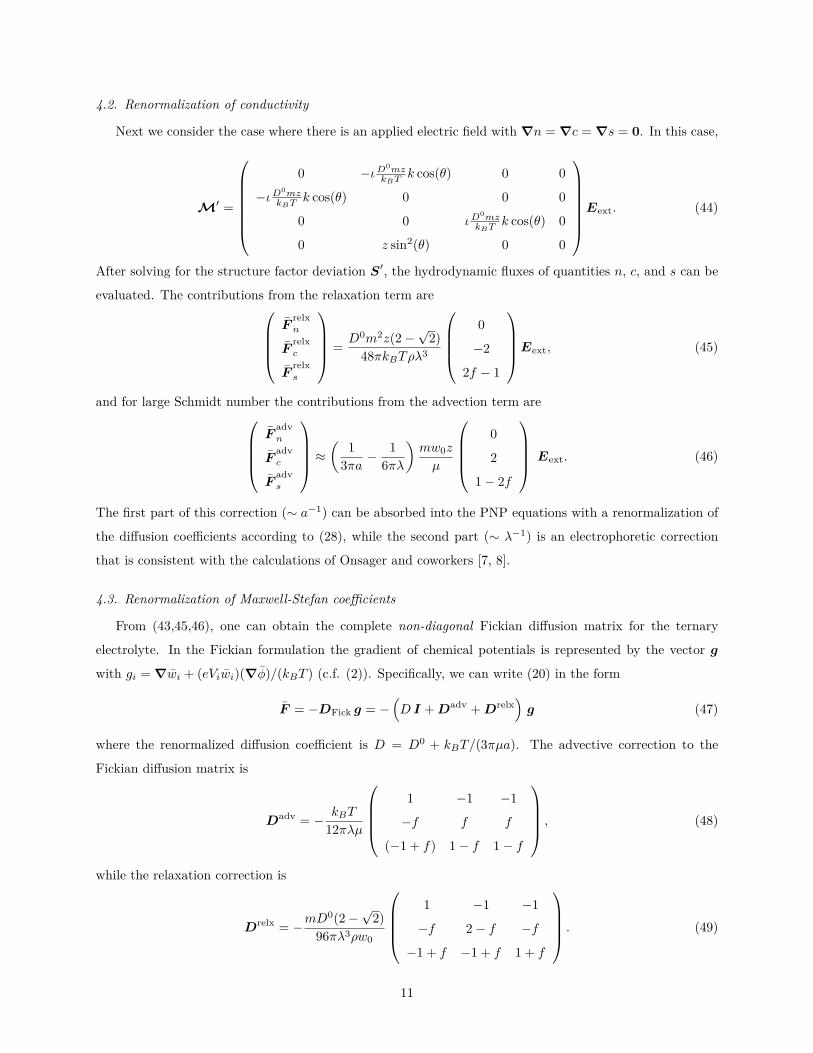
4.2. Renormalization of conductivity
Next we consider the case where there is an applied electric field with ∇n = ∇c = ∇s = 0. In this case,
M′ =
0 −ιD
0mzkBT
k cos(θ) 0 0
−ιD0mzkBT
k cos(θ) 0 0 0
0 0 ιD0mzkBT
k cos(θ) 0
0 z sin2(θ) 0 0
Eext. (44)
After solving for the structure factor deviation S′, the hydrodynamic fluxes of quantities n, c, and s can be
evaluated. The contributions from the relaxation term areF
relxn
Frelxc
Frelxs
= D0m2z(2−√
2)48πkBTρλ3
0
−2
2f − 1
Eext, (45)
and for large Schmidt number the contributions from the advection term areF
advn
Fadvc
Fadvs
≈(
13πa −
16πλ
)mw0z
µ
0
2
1− 2f
Eext. (46)
The first part of this correction (∼ a−1) can be absorbed into the PNP equations with a renormalization of
the diffusion coefficients according to (28), while the second part (∼ λ−1) is an electrophoretic correction
that is consistent with the calculations of Onsager and coworkers [7, 8].
4.3. Renormalization of Maxwell-Stefan coefficients
From (43,45,46), one can obtain the complete non-diagonal Fickian diffusion matrix for the ternary
electrolyte. In the Fickian formulation the gradient of chemical potentials is represented by the vector g
with gi = ∇wi + (eViwi)(∇φ)/(kBT ) (c.f. (2)). Specifically, we can write (20) in the form
F = −DFick g = −(D I +Dadv +Drelx
)g (47)
where the renormalized diffusion coefficient is D = D0 + kBT/(3πµa). The advective correction to the
Fickian diffusion matrix is
Dadv = − kBT
12πλµ
1 −1 −1
−f f f
(−1 + f) 1− f 1− f
, (48)
while the relaxation correction is
Drelx = −mD0(2−
√2)
96πλ3ρw0
1 −1 −1
−f 2− f −f
−1 + f −1 + f 1 + f
. (49)
11
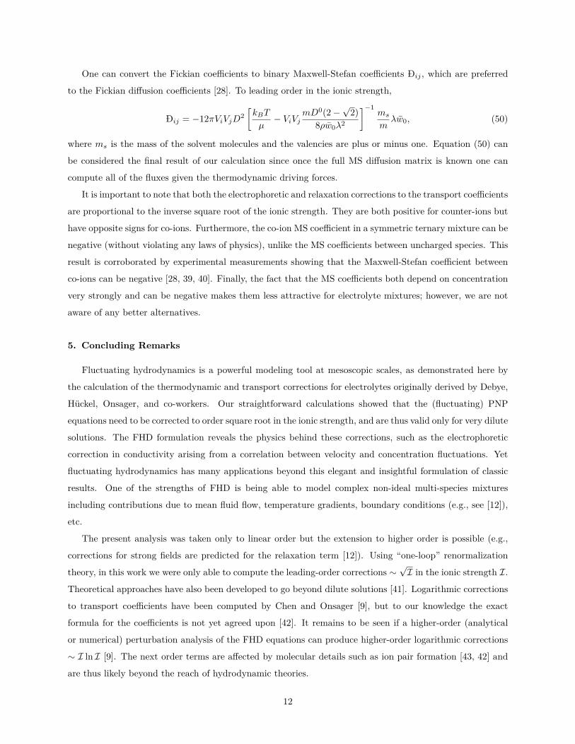
One can convert the Fickian coefficients to binary Maxwell-Stefan coefficients Ðij , which are preferred
to the Fickian diffusion coefficients [28]. To leading order in the ionic strength,
Ðij = −12πViVjD2[kBT
µ− ViVj
mD0(2−√
2)8ρw0λ2
]−1ms
mλw0, (50)
where ms is the mass of the solvent molecules and the valencies are plus or minus one. Equation (50) can
be considered the final result of our calculation since once the full MS diffusion matrix is known one can
compute all of the fluxes given the thermodynamic driving forces.
It is important to note that both the electrophoretic and relaxation corrections to the transport coefficients
are proportional to the inverse square root of the ionic strength. They are both positive for counter-ions but
have opposite signs for co-ions. Furthermore, the co-ion MS coefficient in a symmetric ternary mixture can be
negative (without violating any laws of physics), unlike the MS coefficients between uncharged species. This
result is corroborated by experimental measurements showing that the Maxwell-Stefan coefficient between
co-ions can be negative [28, 39, 40]. Finally, the fact that the MS coefficients both depend on concentration
very strongly and can be negative makes them less attractive for electrolyte mixtures; however, we are not
aware of any better alternatives.
5. Concluding Remarks
Fluctuating hydrodynamics is a powerful modeling tool at mesoscopic scales, as demonstrated here by
the calculation of the thermodynamic and transport corrections for electrolytes originally derived by Debye,
Hückel, Onsager, and co-workers. Our straightforward calculations showed that the (fluctuating) PNP
equations need to be corrected to order square root in the ionic strength, and are thus valid only for very dilute
solutions. The FHD formulation reveals the physics behind these corrections, such as the electrophoretic
correction in conductivity arising from a correlation between velocity and concentration fluctuations. Yet
fluctuating hydrodynamics has many applications beyond this elegant and insightful formulation of classic
results. One of the strengths of FHD is being able to model complex non-ideal multi-species mixtures
including contributions due to mean fluid flow, temperature gradients, boundary conditions (e.g., see [12]),
etc.
The present analysis was taken only to linear order but the extension to higher order is possible (e.g.,
corrections for strong fields are predicted for the relaxation term [12]). Using “one-loop” renormalization
theory, in this work we were only able to compute the leading-order corrections ∼√I in the ionic strength I.
Theoretical approaches have also been developed to go beyond dilute solutions [41]. Logarithmic corrections
to transport coefficients have been computed by Chen and Onsager [9], but to our knowledge the exact
formula for the coefficients is not yet agreed upon [42]. It remains to be seen if a higher-order (analytical
or numerical) perturbation analysis of the FHD equations can produce higher-order logarithmic corrections
∼ I ln I [9]. The next order terms are affected by molecular details such as ion pair formation [43, 42] and
are thus likely beyond the reach of hydrodynamic theories.
12
It is important to point out that at higher concentrations one must use a complete multicomponent trans-
port model including nonideality of the solution and the flux of the solvent that comes from the conservation
of mass [28, 41, 44]. In our work [22] we have summarized the complete mass and momentum transport
equations consistent with nonequilibrium thermodynamics, without the need to single out a solvent species
or assume a dilute solution. Ion crowding can be modelled with additional (e.g. fourth order) terms not
included in traditional models [45]. Here we treated strong electrolyte solutions but the extension to weak
electrolytes, as well as general electrochemistry, is straight-forward. Another important extension of this
work is to consider the AC conductivity of electrolytes as a function of frequency [46]; this is in principle a
straighforward but tedious extension of the approach.
We should also mention some limitations of our calculations. In the analytical perturbative approach
followed here, all corrections to the linearized fluctuating PNP equations appear additively, not multiplica-
tively as they should. For example, the g appearing in (47) should include contributions from (19). Similarly,
we wrote the relaxation corrections in terms of bare diffusion coefficients D0, but in reality the bare coeffi-
cients are simultaneously renormalized by the advective correction. Multiplicative effects like these can be
important and are easily computed by nonlinear computational fluctuating hydrodynamics (e.g., see [15]).
Numerical methods for solving the FHD equations are well-established and these are especially useful for
including the effects of boundary conditions (e.g., conductivity corrections are predicted for the relaxation
term in a confined binary mixture [12]) and nonlinearities. Care is needed, however, to avoid double-counting
the contribution of the fluctuations to transport. In computational formulations the renormalization depends
on the coarse-graining scale (e.g., grid size) and this must be carefully evaluated by stochastic numerical
analysis. With this caveat, fluctuating hydrodynamics promises to be a powerful mesoscopic formulation for
electrolytes.
Acknowledgements
We thank Martin Bazant for invaluable advice on how to place our work in the broader context of elec-
trolyte modeling. This work was supported by the U.S. Department of Energy, Office of Science, Office of
Advanced Scientific Computing Research, Applied Mathematics Program under award Award DE-SC0008271
and contract DE-AC02-05CH11231. A. Donev was supported in part by the Division of Chemical, Bioengi-
neering, Environmental and Transport Systems of the National Science Foundation under award CBET-
1804940.
Appendix A. Binary Electrolytes
In this appendix, we generalize the binary electrolyte theory presented in [11] by letting the two ionic
species have different physical properties, in particular, unequal diffusion coefficients. We still assume equal
valences, V1 = V2 = V , because it simplifies the expressions greatly while retaining the interesting features.
13
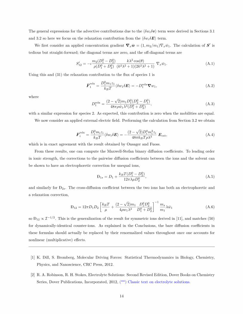
The general expressions for the advective contributions due to the 〈δwiδv〉 term were derived in Sections 3.1
and 3.2 so here we focus on the relaxation contribution from the 〈δwiδE〉 term.
We first consider an applied concentration gradient ∇xw = (1,m2/m1)∇xw1. The calculation of S′ is
tedious but straight-forward; the diagonal terms are zero, and the off-diagonal terms are
S′12 = −ιm2(D01 −D0
2)ρ(D0
1 +D02)
kλ2 cos(θ)(k2λ2 + 1)(2k2λ2 + 1) ∇xw1. (A.1)
Using this and (31) the relaxation contribution to the flux of species 1 is
Frelx1 = D0
1m1z1
kBT〈δw1δE〉 = −Drelx
1 ∇w1, (A.2)
where
Drelx1 = (2−
√2)m1D
01(D0
2 −D01)
48πρw1λ3(D01 +D0
2) , (A.3)
with a similar expression for species 2. As expected, this contribution is zero when the mobilities are equal.
We now consider an applied external electric field. Performing the calculation from Section 3.2 we obtain
Frelxi = D0
imizikBT
〈δwiδE〉 = − (2−√
2)D0im
2i zi
48πkBTρλ3 Eext, (A.4)
which is in exact agreement with the result obtained by Onsager and Fuoss.
From these results, one can compute the Maxwell-Stefan binary diffusion coefficients. To leading order
in ionic strength, the corrections to the pairwise diffusion coefficients between the ions and the solvent can
be shown to have an electrophoretic correction for unequal ions,
Ð1s = D1 + kBT (D01 −D0
2)12πλµD0
2, (A.5)
and similarly for Ð2s. The cross-diffusion coefficient between the two ions has both an electrophoretic and
a relaxation correction,
Ð12 = 12πD1D2
[kBT
µ+ (2−
√2)m1
4ρw1λ2D0
1D02
D01 +D0
2
]−1ms
m1λw1 (A.6)
so Ð12 ∝ I−1/2. This is the generalization of the result for symmetric ions derived in [11], and matches (50)
for dynamically-identical counter-ions. As explained in the Conclusions, the bare diffusion coefficients in
these formulas should actually be replaced by their renormalized values throughout once one accounts for
nonlinear (multiplicative) effects.
[1] K. Dill, S. Bromberg, Molecular Driving Forces: Statistical Thermodynamics in Biology, Chemistry,
Physics, and Nanoscience, CRC Press, 2012.
[2] R. A. Robinson, R. H. Stokes, Electrolyte Solutions: Second Revised Edition, Dover Books on Chemistry
Series, Dover Publications, Incorporated, 2012, (**) Classic text on electrolyte solutions.
14
[3] J. Newman, K. E. Thomas-Alyea, Electrochemical Systems, Wiley, 2012, (**) Modern textbook on
electrochemical systems.
[4] M. Wright, An Introduction to Aqueous Electrolyte Solutions, Wiley, 2007, An approachable introduc-
tory textbook on electrolyte solutions.
[5] R. Krishna, Highlighting coupling effects in ionic diffusion, Chemical Engineering Research and Design
114 (2016) 1–12, A review article highlighting several distinguishing characteristics of ionic diffusion
including diffusional coupling effects.
[6] P. Debye, E. Hückel, Zur theorie der elektrolyte, Physikalische Zeitschrift 24 (1923) 185–206, Original
paper presenting the approximate solution of the Poisson-Boltzmann equation.
[7] L. Onsager, R. Fuoss, Irreversible processes in electrolytes. diffusion, conductance and viscous flow in
arbitrary mixtures of strong electrolytes, J. Phys. Chem. 1932 (1932) 2689, (**) Original derivation of
the Onsager limiting law for conductivity and diffusion.
[8] L. Onsager, S. K. Kim, The relaxation effects in mixed strong electrolytes, The Journal of Physical
Chemistry 61 (2) (1957) 215–229, (*) A reformulation of the theory introduced by Onsager and Fuoss.
[9] M.-S. Chen, L. Onsager, The generalized conductance equation, The Journal of Physical Chemistry
81 (21) (1977) 2017–2021, (**) In this third article in a series by Onsager and coworkers, the next order
logarithmic correction term is derived.
[10] J. M. O. D. Zarate, J. V. Sengers, Hydrodynamic fluctuations in fluids and fluid mixtures, Elsevier
Science Ltd, 2006, (**) A modern manuscript on fluctuating hydrodynamics for both equilibrium and
non-equilibrium systems.
[11] J.-P. Péraud, A. J. Nonaka, J. B. Bell, A. Donev, A. L. Garcia, Fluctuation-enhanced electric con-
ductivity in electrolyte solutions, Proceedings of the National Academy of Sciences 114 (41) (2017)
10829–10833, (**)This paper derives the renormalization of transport using fluctuating hydrodynamics
but is restricted to a symmetric 1:1 binary electrolyte solution.
[12] V. Démery, D. S. Dean, The conductivity of strong electrolytes from stochastic density functional theory,
Journal of Statistical Mechanics: Theory and Experiment 2016 (2) (2016) 023106, This paper applies
stochastic density functional theory to obtain the renormalized conductivity for a binary electrolyte.
[13] L. Landau, E. Lifshitz, Fluid Mechanics, Vol. 6 of Course of Theoretical Physics, Pergamon Press,
Oxford, England, 1959, (**) Classic text on fluid mechanics; fluctuating hydrodynamics is introduced
in a short chapter in this edition of the book.
[14] B. J. Berne, R. Pecora, Dynamic Light Scattering, Robert E. Krieger Publishing Company, 1990, A
complete treatment of light scattering covering both theoretical and experimental work.
15
[15] A. Donev, T. G. Fai, E. Vanden-Eijnden, A reversible mesoscopic model of diffusion in liquids: from
giant fluctuations to Fick’s law, Journal of Statistical Mechanics: Theory and Experiment 2014 (4)
(2014) P04004, x.
[16] A. Vailati, R. Cerbino, S. Mazzoni, C. J. Takacs, D. S. Cannell, M. Giglio, Fractal fronts of diffusion in
microgravity, Nature Communications 2 (2011) 290.
[17] F. Croccolo, J. M. Ortiz de Zárate, J. V. Sengers, Non-local fluctuation phenomena in liquids, The
European Physical Journal E 39 (12) (2016) 125.
[18] A. Donev, A. J. Nonaka, Y. Sun, T. G. Fai, A. L. Garcia, J. B. Bell, Low Mach Number Fluctuating Hy-
drodynamics of Diffusively Mixing Fluids, Communications in Applied Mathematics and Computational
Science 9 (1) (2014) 47–105.
[19] A. J. Nonaka, Y. Sun, J. B. Bell, A. Donev, Low Mach Number Fluctuating Hydrodynamics of Binary
Liquid Mixtures, Communications in Applied Mathematics and Computational Science 10 (2) (2015)
163–204.
[20] A. Donev, A. J. Nonaka, A. K. Bhattacharjee, A. L. Garcia, J. B. Bell, Low Mach Number Fluctuating
Hydrodynamics of Multispecies Liquid Mixtures, Physics of Fluids 27 (3) (2015) 037103.
URL http://scitation.aip.org/content/aip/journal/pof2/27/3/10.1063/1.4913571
[21] C. Kim, A. J. Nonaka, A. L. Garcia, J. B. Bell, A. Donev, Stochastic simulation of reaction-diffusion
systems: A fluctuating-hydrodynamics approach, J. Chem. Phys. 146 (12), software available at https:
//github.com/BoxLib-Codes/FHD_ReactDiff. doi:http://dx.doi.org/10.1063/1.4978775.
URL http://aip.scitation.org/doi/full/10.1063/1.4978775
[22] J.-P. Péraud, A. Nonaka, A. Chaudhri, J. B. Bell, A. Donev, A. L. Garcia, Low mach number fluctuating
hydrodynamics for electrolytes, Phys. Rev. Fluids 1 (2016) 074103, (**) Formulation of the low-Mach
number fluctuating hydrodynamic equations for electrolytes and an accurate, efficient numerical scheme
for solving them. doi:10.1103/PhysRevFluids.1.074103.
[23] K. Lazaridis, L. Wickham, N. Voulgarakis, Fluctuating hydrodynamics for ionic liquids, Physics Letters
A 381 (16) (2017) 1431–1438.
[24] N. K. Voulgarakis, J.-W. Chu, Bridging fluctuating hydrodynamics and molecular dynamics simulations
of fluids, J. Chem. Phys. 130 (13) (2009) 134111.
[25] B. Shang, N. Voulgarakis, J. Chu, Fluctuating hydrodynamics for multiscale modeling and simulation:
Energy and heat transfer in molecular fluids, J. Chem. Phys. 137 (4) (2012) 044117–044117.
[26] P. J. Atzberger, Spatially Adaptive Stochastic Numerical Methods for Intrinsic Fluctuations in Reaction-
Diffusion Systems, J. Comp. Phys. 229 (9) (2010) 3474 – 3501.
16
[27] R. Krishna, J. Wesselingh, The maxwell-stefan approach to mass transfer, Chemical Engineering Science
52 (6) (1997) 861–911, review of the Maxwell-Stefan approach to mass transfer aimed at chemical
engineers.
[28] J. Wesselingh, P. Vonk, G. Kraaijeveld, Exploring the maxwell-stefan description of ion exchange, The
Chemical Engineering Journal and The Biochemical Engineering Journal 57 (2) (1995) 75–89.
[29] A. Nyman, M. Behm, G. Lindbergh, Electrochemical characterisation and modelling of the mass trans-
port phenomena in lipf6–ec–emc electrolyte, Electrochimica Acta 53 (22) (2008) 6356–6365.
[30] L. O. Valøen, J. N. Reimers, Transport properties of lipf6-based li-ion battery electrolytes, Journal of
The Electrochemical Society 152 (5) (2005) A882–A891.
[31] M. Doyle, T. F. Fuller, J. Newman, Modeling of galvanostatic charge and discharge of the
lithium/polymer/insertion cell, Journal of the Electrochemical Society 140 (6) (1993) 1526–1533.
[32] R. B. Smith, M. Z. Bazant, Multiphase porous electrode theory, Journal of The Electrochemical Society
164 (11) (2017) E3291–E3310.
[33] N. D. Pinto, E. Graham, Evaluation of diffusivities in electrolyte solutions using stefan-maxwell equa-
tions, AIChE journal 32 (2) (1986) 291–296.
[34] D. R. Wheeler, J. Newman, Molecular dynamics simulations of multicomponent diffusion. 1. equilibrium
method, The Journal of Physical Chemistry B 108 (47) (2004) 18353–18361.
[35] D. R. Wheeler, J. Newman, Molecular dynamics simulations of multicomponent diffusion. 2. nonequi-
librium method, The Journal of Physical Chemistry B 108 (47) (2004) 18362–18367.
[36] E. Yariv, An asymptotic derivation of the thin-debye-layer limit for electrokinetic phenomena, Chemical
Engineering Communications 197 (1) (2009) 3–17.
[37] S. Psaltis, T. W. Farrell, Comparing charge transport predictions for a ternary electrolyte using the
maxwell–stefan and nernst–planck equations, Journal of The Electrochemical Society 158 (1) (2011)
A33–A42.
[38] C. W. Gardiner, Handbook of stochastic methods: for physics, chemistry & the natural sciences, 3rd
Edition, Vol. Vol. 13 of Series in synergetics, Springer, 2003.
[39] G. Kraaijeveld, J. A. Wesselingh, Negative Maxwell-Stefan diffusion coefficients, Industrial & Engineer-
ing Chemistry Research 32 (4) (1993) 738–742. doi:10.1021/ie00016a022.
[40] G. Kraaijeveld, J. A. Wesselingh, G. D. C. Kuiken, Comments on "Negative Maxwell-Stefan Dif-
fusion Coefficients", Industrial & Engineering Chemistry Research 33 (3) (1994) 750–751. doi:
10.1021/ie00027a041.
17
[41] M. Z. Bazant, M. S. Kilic, B. D. Storey, A. Ajdari, Towards an understanding of induced-charge elec-
trokinetics at large applied voltages in concentrated solutions, Advances in colloid and interface science
152 (1-2) (2009) 48–88, (*) Section 3 of this paper provides a review on modifications of classical theories
for concentrated electrolyte solutions.
[42] P. G. Wolynes, Dynamics of electrolyte solutions, Annual review of physical chemistry 31 (1) (1980)
345–376.
[43] M. J. Pikal, Ion-pair formation and the theory of mutual diffusion in a binary electrolyte, The Journal
of Physical Chemistry 75 (5) (1971) 663–675.
[44] W. Dreyer, C. Guhlke, R. Muller, Overcoming the shortcomings of the Nernst-Planck model, Phys.
Chem. Chem. Phys. 15 (2013) 7075–7086. doi:10.1039/C3CP44390F.
URL http://dx.doi.org/10.1039/C3CP44390F
[45] M. Z. Bazant, B. D. Storey, A. A. Kornyshev, Double layer in ionic liquids: Overscreening versus
crowding, Physical Review Letters 106 (4) (2011) 046102, erratum Phys. Rev. Lett. 109, 149903. The
authors propose a simple Landau-Ginzburg-type free energy functional for solvent-free ionic liquids and
use it to predict the equilibrium structure of the electrical double layer.
[46] H. Falkenhagen, R. Bell, Electrolytes, International series of monographs on physics, Clarendon Press,
1934.
URL https://books.google.bs/books?id=FZozAAAAIAAJ
18
Related Documents