Flow of Navier-Stokes Fluids in Converging-Diverging Distensible Tubes Taha Sochi * October 17, 2013 * University College London, Department of Physics & Astronomy, Gower Street, London, WC1E 6BT. Email: [email protected]. 1 arXiv:1310.4221v1 [physics.flu-dyn] 15 Oct 2013

Welcome message from author
This document is posted to help you gain knowledge. Please leave a comment to let me know what you think about it! Share it to your friends and learn new things together.
Transcript
Flow of Navier-Stokes Fluids in
Converging-Diverging Distensible Tubes
Taha Sochi∗
October 17, 2013
∗University College London, Department of Physics & Astronomy, Gower Street, London,
WC1E 6BT. Email: [email protected].
1
arX
iv:1
310.
4221
v1 [
phys
ics.
flu-
dyn]
15
Oct
201
3
Contents
Contents 2
Abstract 3
1 Introduction 4
2 Method 6
3 Implementation and Results 9
4 Tests and Validations 14
5 Comparisons 22
6 Conclusions 23
Nomenclature 25
References 27
2
3
Abstract
We use a method based on the lubrication approximation in conjunction with a
residual-based mass-continuity iterative solution scheme to compute the flow rate
and pressure field in distensible converging-diverging tubes for Navier-Stokes flu-
ids. We employ an analytical formula derived from a one-dimensional version of the
Navier-Stokes equations to describe the underlying flow model that provides the
residual function. This formula correlates the flow rate to the boundary pressures
in straight cylindrical elastic tubes with constant-radius. We validate our findings
by the convergence toward a final solution with fine discretization as well as by
comparison to the Poiseuille-type flow in its convergence toward analytic solutions
found earlier in rigid converging-diverging tubes. We also tested the method on
limiting special cases of cylindrical elastic tubes with constant-radius where the
numerical solutions converged to the expected analytical solutions. The distensible
model has also been endorsed by its convergence toward the rigid Poiseuille-type
model with increasing the tube wall stiffness. Lubrication-based one-dimensional
finite element method was also used for verification. In this investigation five
converging-diverging geometries are used for demonstration, validation and as pro-
totypes for modeling converging-diverging geometries in general.
Keywords: fluid mechanics; one-dimensional flow; Navier-Stokes; distensible
tubes; converging-diverging tubes; irregular conduits; non-linear systems.
1 INTRODUCTION 4
1 Introduction
The flow of fluids in converging-diverging tubes has many scientific, technological
and medical applications such as transportation in porous media, filtration pro-
cesses, polymer processing, and pathological stenoses and aneurysms [1–13]. There
are many studies about the flow in converging-diverging rigid conduits [14–21] and
distensible conduits with fixed cross sections [22–28] separately as well as many
other different geometries and fluid and conduit mechanical properties [29–31].
There is also a considerable number of studies on the flow in converging-diverging
distensible conduits; although large part of which is related to medical applications
such as stenosis modeling [32–36].
Several methods have been used in the past for investigating and modeling the
flow in distensible converging-diverging geometries; the majority are based on the
numerical discretization methods such as finite element and spectral methods al-
though other approaches such as stochastic techniques have also been employed.
However, due to the huge difficulties associating this subject which combines tube
wall deformability with convergence-divergence non-linearities, most of these stud-
ies are based on substantial approximations and modeling compromises. Moreover,
they are usually based on very complex mathematical and computational infras-
tructures which are not only difficult to implement and use but also difficult to
verify and validate. Also, some of these methods, such as stochastic techniques,
are computationally demanding and hence they may be prohibitive in some cases.
Therefore, simple, reliable and computationally low cost techniques are highly de-
sirable where analytical solutions are not available due to excessive difficulties or
even impossibility of obtaining such solutions which is the case in most circum-
stances.
In this paper we propose the use of the lubrication approximation with a
residual-based non-linear solution scheme in association with an analytical expres-
1 INTRODUCTION 5
sion for the flow of Navier-Stokes fluids in straight cylindrical elastic tubes with
fixed radius to obtain the flow rate and pressure field in a number of cylindrically-
symmetric converging-diverging geometries with elastic wall mechanical properties.
The proposed method combines simplicity, robustness and ease of implementation.
Moreover, it produces solutions which are very close to any targeted analytical
solutions as the convergence behavior in the investigated special cases reveals.
Although the proposed method is related to a single distensible tube, it can
also be extended to a network of interconnected distensible tubes with partially or
totally converging-diverging conduits by integrating these conduits into the network
and giving them a special treatment based on the proposed method. This approach,
can be utilized for example in modeling stenoses and other types of flow conduits
with irregular geometries as part of fluid flow networks in the hemodynamic and
hemorheologic studies and in the filtration investigations.
The method also has a wider validity domain than what may be thought initially
with regard to the deformability characteristics. Despite the fact that in this paper
we use a single analytical expression correlating the flow rate to the boundary
pressures for a distensible tube with elastic mechanical properties, the method can
be well adapted to other types of mechanical characteristics, such as tubes with
viscoelastic wall rheology, where different pressure-area constitutive relations do
apply. In fact there is no need even to have an analytical solution for the underlying
flow model that provides the basic flow characterization for the discretized elements
of the converging-diverging geometries in the lubrication approximation. What is
actually needed is only a well defined flow relation: analytical, or empirical, or even
numerical [37] as long as it is viable to find the flow in the discretized elements
of the lubrication ensemble using such a relation to correlate the flow rate to the
boundary pressures.
There is also no need for the geometry to be of a fixed or regular shape as long
2 METHOD 6
as a characteristic flow can be obtained on the discretized elements, and hence the
method can be applied not only to axi-symmetric geometries with constant-shape
and varying cross sectional area in the flow direction but can also be extended to
non-symmetric geometries with irregular and varying shape along the flow direction
if the flow in the deformable discretized elements can be characterized by a well-
defined flow relation. The method can as well be applied to non-straight flow
conduits with and without regular or varying cross sectional shapes such as bending
compliant pipes.
2 Method
The flow of Navier-Stokes fluids in a cylindrical tube with a cross sectional area
A and length L assuming a slip-free incompressible laminar axi-symmetric flow
with negligible gravitational body forces and fixed velocity profile is described by
the following one-dimensional system of mass continuity and linear momentum
conservation principles
∂A
∂t+∂Q
∂x= 0 t ≥ 0, x ∈ [0, L] (1)
∂Q
∂t+
∂
∂x
(αQ2
A
)+A
ρ
∂p
∂x+ κ
Q
A= 0 t ≥ 0, x ∈ [0, L] (2)
In these two equations, Q is the volumetric flow rate, t is the time, x is the axial
coordinate along the tube length, α is the momentum flux correction factor, ρ is the
fluid mass density, p is the axial pressure which is a function of the axial coordinate,
and κ is the viscosity friction coefficient which is usually given by κ = 2πανα−1
where
ν is the fluid kinematic viscosity defined as the ratio of the fluid dynamic viscosity
µ to its mass density [21, 27, 38–42]. These relations are usually supported by a
constitutive relation that correlates the pressure to the cross sectional area in a
2 METHOD 7
distensible tube, to close the system in the three variables A, Q and p and hence
provide a complete mathematical description for the flow in such conduits.
The correlation between the local pressure and cross sectional area in a compli-
ant tube can be described by many mathematical constitutive relations depending
on the mechanical characterization of the tube wall and its response to pressure
such as being elastic or viscoelastic, and linear or non-linear. The following is
a commonly used pressure-area constitutive elastic relation that describes such a
dependency
p =β
Ao
(√A−
√Ao
)(3)
where β is the tube wall stiffness coefficient which is usually defined by
β =
√πhoE
1− ς2(4)
Ao is the reference cross sectional area corresponding to the reference pressure which
in this equation is set to zero for convenience without affecting the generality of
the results, A is the tube cross sectional area at the actual pressure p as opposite
to the reference pressure, ho is the tube wall thickness at the reference pressure,
while E and ς are respectively the Young’s elastic modulus and Poisson’s ratio of
the tube wall. The essence of Equation 3 is that the pressure is proportional to
the radius growth with a proportionality stiffness coefficient that is scaled by the
reference area. It should be remarked that we assume here a constant ambient
transmural pressure along the axial direction which is set to zero and hence the
reference cross sectional area represents unstressed state where Ao is constant along
the axial direction.
Based on the pressure-area relation of Equation 3, and using the one-dimensional
Navier-Stokes system of Equations 1 and 2 for the time-independent flow by drop-
2 METHOD 8
ping the time terms, the following equation correlating the flow rate Q to the inlet
and outlet boundary areas of an elastic cylindrical tube with a constant unstressed
cross sectional area over its axial direction can be obtained
Q =
−κL+
√κ2L2 + 4αβ
5ρAoln (Ain/Aou)
(A
5/2in − A
5/2ou
)2α ln (Ain/Aou)
(5)
where Ain and Aou are the tube cross sectional area at the inlet and outlet re-
spectively such that Ain > Aou. This relation, which in essence correlates the flow
rate to the boundary pressures, has been previously [28] derived and validated by
a finite element scheme.
The residual-based lubrication approach, which is proposed in the present paper
to find the pressure field and flow rate in converging-diverging distensible tubes,
starts by discretizing the tube in the axial direction into ring-like elements. Each
one of these elements is approximated as a single tube with a constant radius, which
averages the inlet and outlet radii of the element, to which Equation 5 applies. A
system of non-linear equations based on the mass continuity residual and boundary
conditions is then formed.
For a tube discretized into (N−1) elements, there are N nodes: two boundaries
and (N−2) interior nodes. Each one of these nodes has a well-defined axial pressure
value according to the one-dimensional formulation. Also for the interior nodes,
and due to the incompressibility of the flow, the total sum of the volumetric flow
rate, signed (+/−) according to its direction with respect to the node, is zero due
to the absence of sources and sinks, and hence (N − 2) residual functions which
describe the net flow at the interior nodes can be formed. This is associated with
two given boundary conditions for the inlet and outlet boundary nodes to form N
equations.
A standard method for solving such a system is to use an iterative non-linear
3 IMPLEMENTATION AND RESULTS 9
simultaneous solution scheme such as Newton-Raphson method where an initial
guess for the interior nodal pressures is proposed and used in conjunction with the
Jacobian matrix of the system to find the pressure perturbation vector which is
then used to adjust the pressure values and repeat this process until a convergence
criterion based on the size of the residual norm is reached. The process is based
on iterative solving of the following equation
J∆p = −r (6)
where J is the Jacobian matrix, p is the vector of variables which represent the
pressure values at the boundary and interior nodes, and r is the vector of residuals
which, for the interior nodes, is based on the continuity of the volumetric flow rate
as given by
fj =m∑i=1
Qi = 0 (7)
where m is the number of discretized elements connected to node j which is two
in this case, and Qi is the signed volumetric flow rate in element i as characterized
by Equation 5. Equation 6 is then solved in each iteration for ∆p which is then
used to update p. The convergence will be declared when the norm of the residual
vector, r, becomes within a predefined error tolerance. More details about this
solution scheme can be found in [11, 27].
3 Implementation and Results
The proposed residual-based lubrication method was implemented in a computer
code and flow solutions were obtained for an extensive range of fluid, flow and tube
characterizations such as fluid viscosity, flow profile, and tube mechanical proper-
ties. Five regular converging-diverging axi-symmetric tube geometries were used
3 IMPLEMENTATION AND RESULTS 10
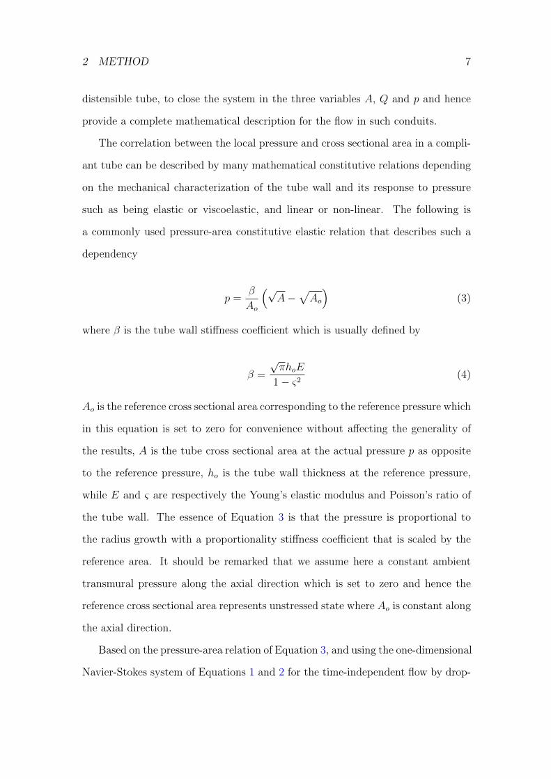
in the current investigation; representative graphic images of these geometries are
shown in Figure 1, while the mathematical relations that describe the dependency
of the tube radius, R, on the tube axial coordinate, x, for these geometries are given
in Table 1. A generic converging-diverging tube profile demonstrating the setting
of the coordinate system for the R–x correlation, as used in Table 1, is shown in
Figure 2. These geometries have been used previously [20, 21] to find flow relations
for Newtonian and power law fluids in rigid tubes. A representative sample of the
flow solutions on distensible converging-diverging tubes are also given in Figures
3-7.
(a) Conic (b) Parabolic
(c) Hyperbolic (d) Hyperbolic Cosine
(e) Sinusoidal
Figure 1: Converging-Diverging tube geometries used in the current investigation.
In all flow simulations, including the ones shown in Figures 3-7, we used a range
of evenly-divided discretization meshes to observe the convergence behavior of the
3 IMPLEMENTATION AND RESULTS 11
→
Rmax
Rmin
↑ R
max
x0
R
−L/2 L/2
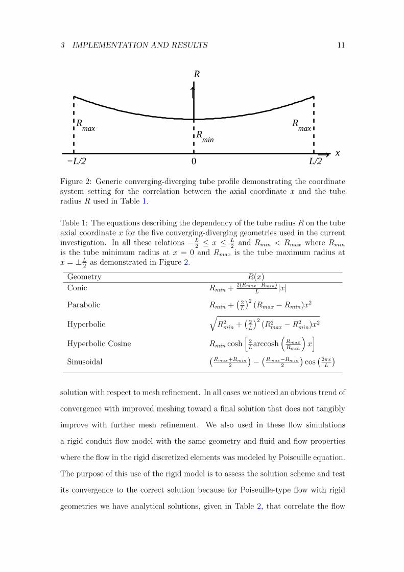
Figure 2: Generic converging-diverging tube profile demonstrating the coordinatesystem setting for the correlation between the axial coordinate x and the tuberadius R used in Table 1.
Table 1: The equations describing the dependency of the tube radius R on the tubeaxial coordinate x for the five converging-diverging geometries used in the currentinvestigation. In all these relations −L
2≤ x ≤ L
2and Rmin < Rmax where Rmin
is the tube minimum radius at x = 0 and Rmax is the tube maximum radius atx = ±L
2as demonstrated in Figure 2.
Geometry R(x)
Conic Rmin + 2(Rmax−Rmin)L
|x|
Parabolic Rmin +(
2L
)2(Rmax −Rmin)x2
Hyperbolic√R2min +
(2L
)2(R2
max −R2min)x2
Hyperbolic Cosine Rmin cosh[
2L
arccosh(Rmax
Rmin
)x]
Sinusoidal(Rmax+Rmin
2
)−(Rmax−Rmin
2
)cos(
2πxL
)solution with respect to mesh refinement. In all cases we noticed an obvious trend of
convergence with improved meshing toward a final solution that does not tangibly
improve with further mesh refinement. We also used in these flow simulations
a rigid conduit flow model with the same geometry and fluid and flow properties
where the flow in the rigid discretized elements was modeled by Poiseuille equation.
The purpose of this use of the rigid model is to assess the solution scheme and test
its convergence to the correct solution because for Poiseuille-type flow with rigid
geometries we have analytical solutions, given in Table 2, that correlate the flow
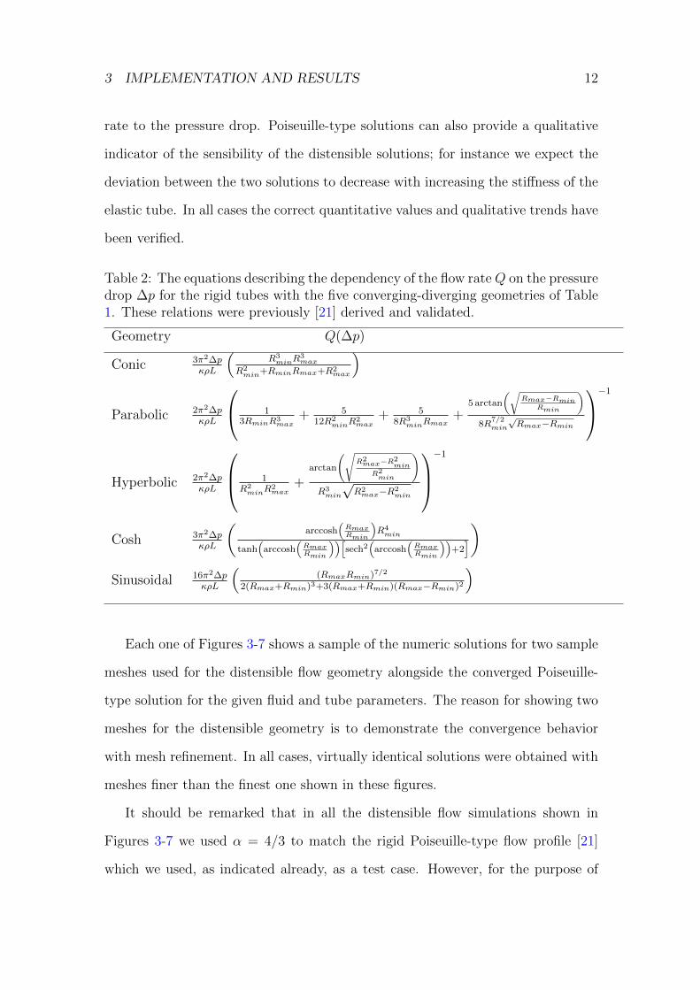
3 IMPLEMENTATION AND RESULTS 12
rate to the pressure drop. Poiseuille-type solutions can also provide a qualitative
indicator of the sensibility of the distensible solutions; for instance we expect the
deviation between the two solutions to decrease with increasing the stiffness of the
elastic tube. In all cases the correct quantitative values and qualitative trends have
been verified.
Table 2: The equations describing the dependency of the flow rate Q on the pressuredrop ∆p for the rigid tubes with the five converging-diverging geometries of Table1. These relations were previously [21] derived and validated.
Geometry Q(∆p)
Conic 3π2∆pκρL
(R3
minR3max
R2min+RminRmax+R2
max
)
Parabolic 2π2∆pκρL
13RminR3
max+ 5
12R2minR
2max
+ 58R3
minRmax+
5 arctan
(√Rmax−Rmin
Rmin
)8R
7/2min
√Rmax−Rmin
−1
Hyperbolic 2π2∆pκρL
1R2
minR2max
+arctan
(√R2max−R2
minR2min
)R3
min
√R2
max−R2min
−1
Cosh 3π2∆pκρL
(arccosh
(RmaxRmin
)R4
min
tanh(
arccosh(
RmaxRmin
))[sech2
(arccosh
(RmaxRmin
))+2])
Sinusoidal 16π2∆pκρL
((RmaxRmin)7/2
2(Rmax+Rmin)3+3(Rmax+Rmin)(Rmax−Rmin)2
)
Each one of Figures 3-7 shows a sample of the numeric solutions for two sample
meshes used for the distensible flow geometry alongside the converged Poiseuille-
type solution for the given fluid and tube parameters. The reason for showing two
meshes for the distensible geometry is to demonstrate the convergence behavior
with mesh refinement. In all cases, virtually identical solutions were obtained with
meshes finer than the finest one shown in these figures.
It should be remarked that in all the distensible flow simulations shown in
Figures 3-7 we used α = 4/3 to match the rigid Poiseuille-type flow profile [21]
which we used, as indicated already, as a test case. However, for the purpose of
3 IMPLEMENTATION AND RESULTS 13
testing and validating the distensible model in general we also used an extensive
range of values greater than and less than 4/3 for α without observing incorrect
convergence or convergence difficulties. In fact using values other than α = 4/3
makes the convergence easier in many cases [11].
An interesting feature that can be seen in Figure 4 is that all the pressure profile
curves are almost identical as well as the flow rates. The reason is that, due to the
high tube stiffness used in this example, the distensible tube solution converged
to the rigid tube Poiseuille-type solution. A more detailed comparison between
the Poiseuille-type rigid tube flow and the Navier-Stokes one-dimensional elastic
tube flow with high stiffness is shown in Figure 8 where the results of Figures 3-7
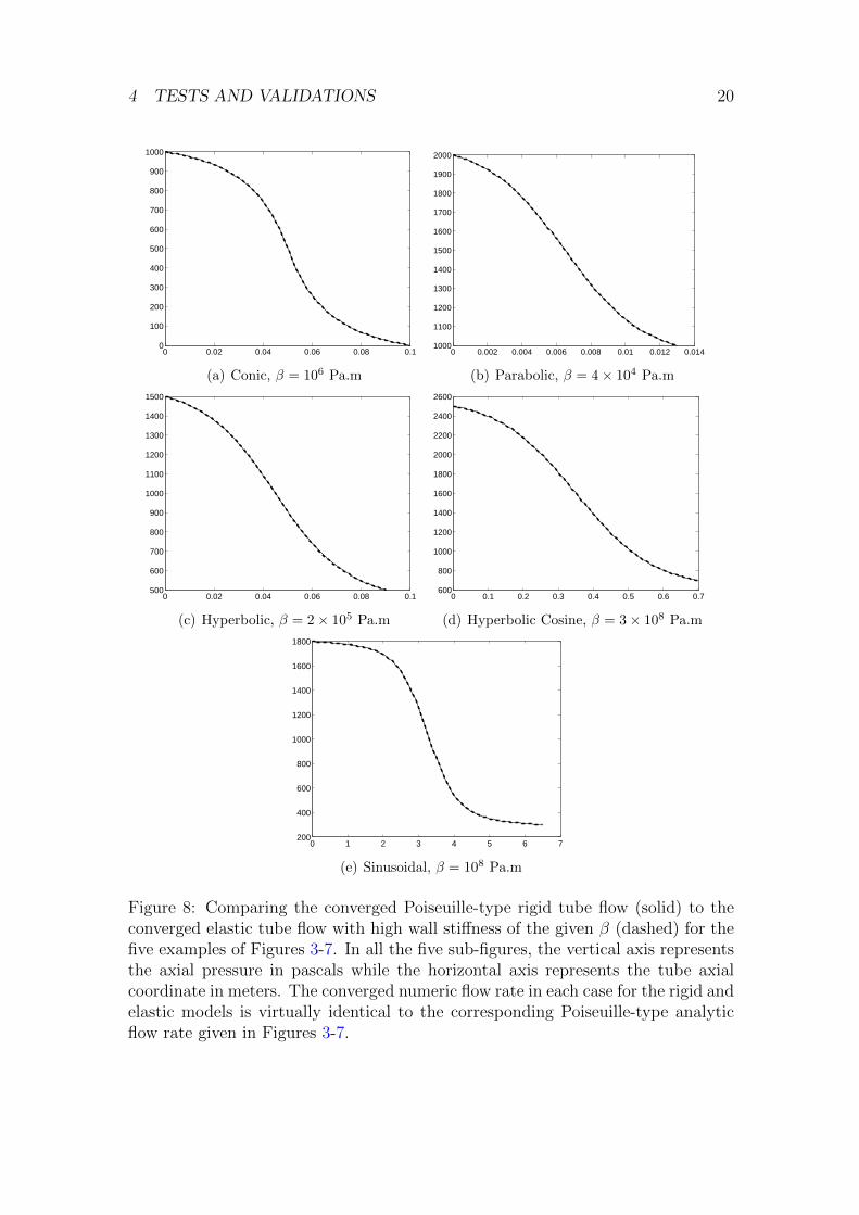
are reproduced using the same fluid, flow and tube parameters but with high tube
stiffness by using large β’s. As seen in Figure 8 the elastic tube flow converges
almost identically to the Poiseuille-type rigid tube flow with increasing the tube
wall stiffness in all cases. This sensible and correct trend can be regarded as
another verification and validation for the residual-based method and the related
computer code. Similar results have also been obtained in [41] in comparing the
rigid and distensible models for the flow in networks of interconnected straight
cylindrical tubes. More detailed comparisons between the rigid and distensible
one-dimensional flow models can be found in the aforementioned reference.
It should be remarked that the critical value of β at which the distensible flow
solution converges to the rigid flow solution depends on several factors such as the
fluid and flow parameters as well as the geometry of the tube and the pressure field
regime characterized by the applied boundary conditions at the inlet and outlet
where their size and the magnitude of their difference play a decisive role. Another
remark is that the shape of the pressure profile curve is highly dependent on the
geometric factors such as LRmin
, LRmax
, and Rmin
Rmaxratios. It also depends on the fluid
and tube mechanical properties, such as fluid viscosity and tube wall stiffness, and
4 TESTS AND VALIDATIONS 14
the magnitude of pressure at the inlet and outlet boundaries.
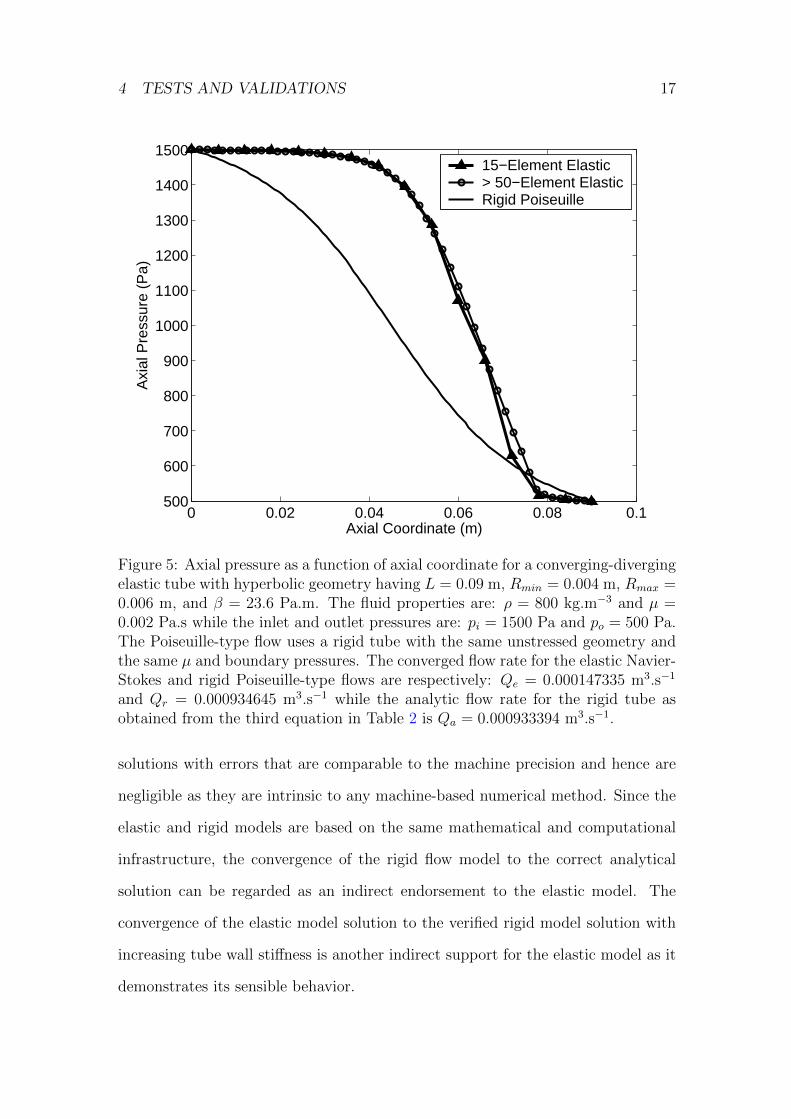
The opposite to what in Figure 4 can be seen in Figure 5 for the hyperbolic
geometry where we used very low stiffness and hence the elastic model deviated
largely from the rigid model. This also affected the dependency of convergence
rate on discretization where the discrepancy between the solutions of the coarse
and fine meshes was more substantial than in the other cases for similar coarse and
fine meshes. In general, the deviation between the rigid and distensible flow models
is maximized by reducing the stiffness, and hence increasing the tube distensibility,
while other parameters are kept fixed.
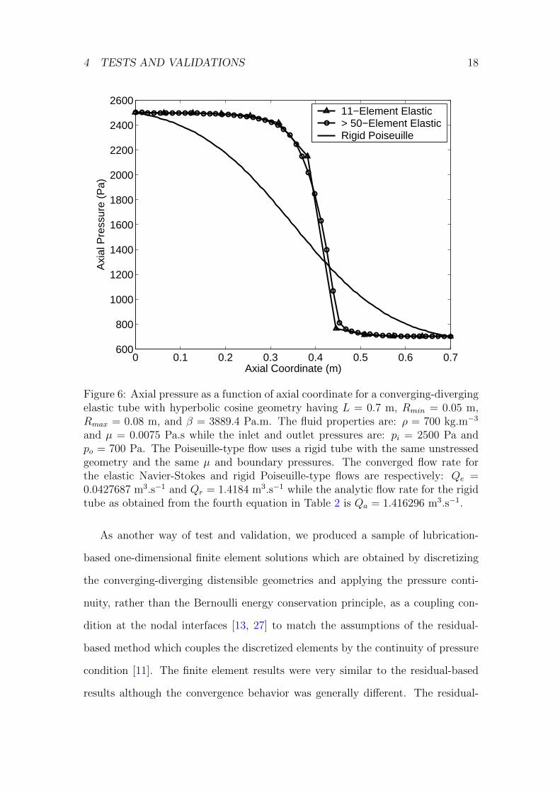
Another interesting feature is that in the flow solution of Figure 6 there is a big
difference between the flow rate of the elastic and rigid tubes. This can be explained
largely by the significant deviation from linearity due to the large values of the inlet
and outlet boundary pressures, as well as the large size of their difference, with a
relatively low stiffness. This indicates that the rigid tube flow model is not a
suitable approximation for simulating and analyzing the flow in distensible tubes
and networks, as it has been done for instance in some hemodynamic studies. More
detailed discussions about this issue can be found in [41].
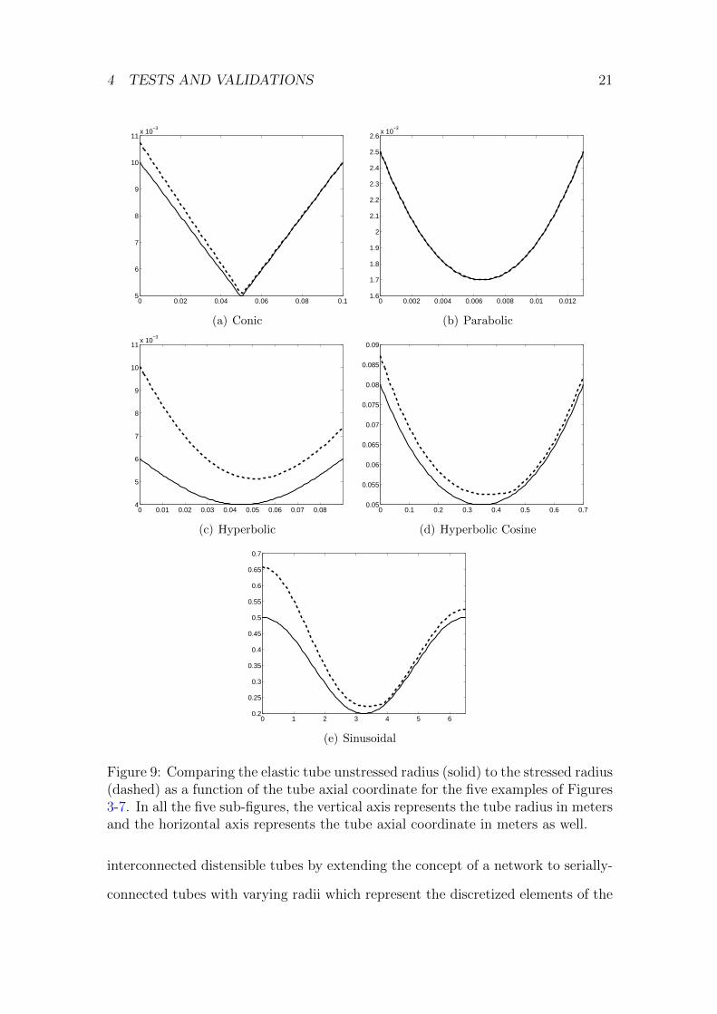
In Figure 9 we draw the geometric profile of the elastic tube for the stressed and
unstressed states for the five examples of Figures 3-7 where we plot the tube radius
versus its axial coordinate for these two states. As seen, these plots show another
sensible qualitative trend in these results and hence provide further endorsement
to the residual-based method. It is needless to say that in Figures 3-9 the inlet
boundary is at x = 0 while the outlet boundary is at the other end.
4 Tests and Validations
We used several metrics to validate the residual-based method and check our com-
puter code and flow solutions. First, we did extensive tests on distensible cylindrical
4 TESTS AND VALIDATIONS 15
0 0.02 0.04 0.06 0.08 0.10
100
200
300
400
500
600
700
800
900
1000
Axial Coordinate (m)
Axi
al P
ress
ure
(Pa)
11−Element Elastic > 50−Element ElasticRigid Poiseuille
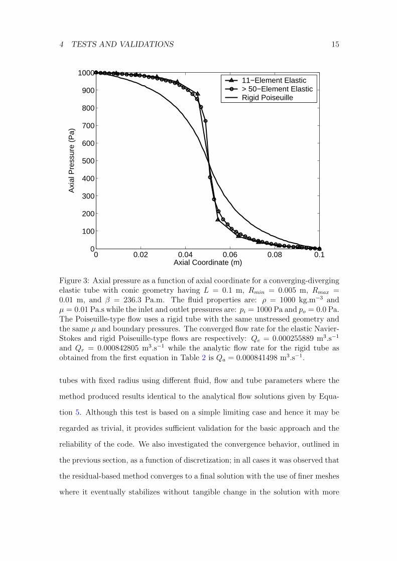
Figure 3: Axial pressure as a function of axial coordinate for a converging-divergingelastic tube with conic geometry having L = 0.1 m, Rmin = 0.005 m, Rmax =0.01 m, and β = 236.3 Pa.m. The fluid properties are: ρ = 1000 kg.m−3 andµ = 0.01 Pa.s while the inlet and outlet pressures are: pi = 1000 Pa and po = 0.0 Pa.The Poiseuille-type flow uses a rigid tube with the same unstressed geometry andthe same µ and boundary pressures. The converged flow rate for the elastic Navier-Stokes and rigid Poiseuille-type flows are respectively: Qe = 0.000255889 m3.s−1
and Qr = 0.000842805 m3.s−1 while the analytic flow rate for the rigid tube asobtained from the first equation in Table 2 is Qa = 0.000841498 m3.s−1.
tubes with fixed radius using different fluid, flow and tube parameters where the
method produced results identical to the analytical flow solutions given by Equa-
tion 5. Although this test is based on a simple limiting case and hence it may be
regarded as trivial, it provides sufficient validation for the basic approach and the
reliability of the code. We also investigated the convergence behavior, outlined in
the previous section, as a function of discretization; in all cases it was observed that
the residual-based method converges to a final solution with the use of finer meshes
where it eventually stabilizes without tangible change in the solution with more
4 TESTS AND VALIDATIONS 16
0 0.002 0.004 0.006 0.008 0.01 0.012 0.0141000
1100
1200
1300
1400
1500
1600
1700
1800
1900
2000
Axial Coordinate (m)
Axi
al P
ress
ure
(Pa)
11−Element Elastic> 50−Element ElasticRigid Poiseuille
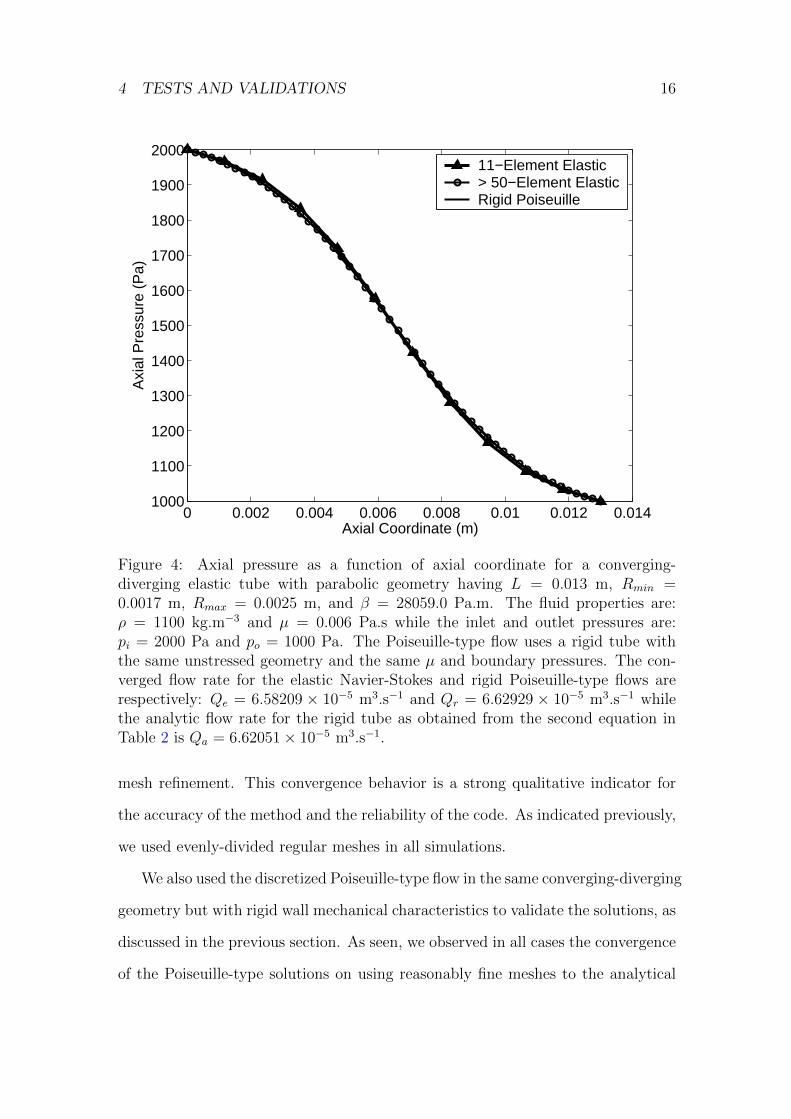
Figure 4: Axial pressure as a function of axial coordinate for a converging-diverging elastic tube with parabolic geometry having L = 0.013 m, Rmin =0.0017 m, Rmax = 0.0025 m, and β = 28059.0 Pa.m. The fluid properties are:ρ = 1100 kg.m−3 and µ = 0.006 Pa.s while the inlet and outlet pressures are:pi = 2000 Pa and po = 1000 Pa. The Poiseuille-type flow uses a rigid tube withthe same unstressed geometry and the same µ and boundary pressures. The con-verged flow rate for the elastic Navier-Stokes and rigid Poiseuille-type flows arerespectively: Qe = 6.58209 × 10⁻⁵ m3.s−1 and Qr = 6.62929 × 10⁻⁵ m3.s−1 whilethe analytic flow rate for the rigid tube as obtained from the second equation inTable 2 is Qa = 6.62051× 10⁻⁵ m3.s−1.
mesh refinement. This convergence behavior is a strong qualitative indicator for
the accuracy of the method and the reliability of the code. As indicated previously,
we used evenly-divided regular meshes in all simulations.
We also used the discretized Poiseuille-type flow in the same converging-diverging
geometry but with rigid wall mechanical characteristics to validate the solutions, as
discussed in the previous section. As seen, we observed in all cases the convergence
of the Poiseuille-type solutions on using reasonably fine meshes to the analytical
4 TESTS AND VALIDATIONS 17
0 0.02 0.04 0.06 0.08 0.1500
600
700
800
900
1000
1100
1200
1300
1400
1500
Axial Coordinate (m)
Axi
al P
ress
ure
(Pa)
15−Element Elastic> 50−Element ElasticRigid Poiseuille
Figure 5: Axial pressure as a function of axial coordinate for a converging-divergingelastic tube with hyperbolic geometry having L = 0.09 m, Rmin = 0.004 m, Rmax =0.006 m, and β = 23.6 Pa.m. The fluid properties are: ρ = 800 kg.m−3 and µ =0.002 Pa.s while the inlet and outlet pressures are: pi = 1500 Pa and po = 500 Pa.The Poiseuille-type flow uses a rigid tube with the same unstressed geometry andthe same µ and boundary pressures. The converged flow rate for the elastic Navier-Stokes and rigid Poiseuille-type flows are respectively: Qe = 0.000147335 m3.s−1
and Qr = 0.000934645 m3.s−1 while the analytic flow rate for the rigid tube asobtained from the third equation in Table 2 is Qa = 0.000933394 m3.s−1.
solutions with errors that are comparable to the machine precision and hence are
negligible as they are intrinsic to any machine-based numerical method. Since the
elastic and rigid models are based on the same mathematical and computational
infrastructure, the convergence of the rigid flow model to the correct analytical
solution can be regarded as an indirect endorsement to the elastic model. The
convergence of the elastic model solution to the verified rigid model solution with
increasing tube wall stiffness is another indirect support for the elastic model as it
demonstrates its sensible behavior.
4 TESTS AND VALIDATIONS 18
0 0.1 0.2 0.3 0.4 0.5 0.6 0.7600
800
1000
1200
1400
1600
1800
2000
2200
2400
2600
Axial Coordinate (m)
Axi
al P
ress
ure
(Pa)
11−Element Elastic> 50−Element ElasticRigid Poiseuille
Figure 6: Axial pressure as a function of axial coordinate for a converging-divergingelastic tube with hyperbolic cosine geometry having L = 0.7 m, Rmin = 0.05 m,Rmax = 0.08 m, and β = 3889.4 Pa.m. The fluid properties are: ρ = 700 kg.m−3
and µ = 0.0075 Pa.s while the inlet and outlet pressures are: pi = 2500 Pa andpo = 700 Pa. The Poiseuille-type flow uses a rigid tube with the same unstressedgeometry and the same µ and boundary pressures. The converged flow rate forthe elastic Navier-Stokes and rigid Poiseuille-type flows are respectively: Qe =0.0427687 m3.s−1 and Qr = 1.4184 m3.s−1 while the analytic flow rate for the rigidtube as obtained from the fourth equation in Table 2 is Qa = 1.416296 m3.s−1.
As another way of test and validation, we produced a sample of lubrication-
based one-dimensional finite element solutions which are obtained by discretizing
the converging-diverging distensible geometries and applying the pressure conti-
nuity, rather than the Bernoulli energy conservation principle, as a coupling con-
dition at the nodal interfaces [13, 27] to match the assumptions of the residual-
based method which couples the discretized elements by the continuity of pressure
condition [11]. The finite element results were very similar to the residual-based
results although the convergence behavior was generally different. The residual-
4 TESTS AND VALIDATIONS 19
0 1 2 3 4 5 6 7200
400
600
800
1000
1200
1400
1600
1800
Axial Coordinate (m)
Axi
al P
ress
ure
(Pa)
31−Element Elastic> 50−Element ElasticRigid Poiseuille
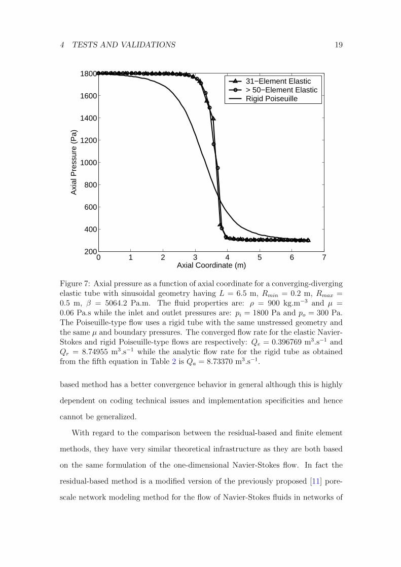
Figure 7: Axial pressure as a function of axial coordinate for a converging-divergingelastic tube with sinusoidal geometry having L = 6.5 m, Rmin = 0.2 m, Rmax =0.5 m, β = 5064.2 Pa.m. The fluid properties are: ρ = 900 kg.m−3 and µ =0.06 Pa.s while the inlet and outlet pressures are: pi = 1800 Pa and po = 300 Pa.The Poiseuille-type flow uses a rigid tube with the same unstressed geometry andthe same µ and boundary pressures. The converged flow rate for the elastic Navier-Stokes and rigid Poiseuille-type flows are respectively: Qe = 0.396769 m3.s−1 andQr = 8.74955 m3.s−1 while the analytic flow rate for the rigid tube as obtainedfrom the fifth equation in Table 2 is Qa = 8.73370 m3.s−1.
based method has a better convergence behavior in general although this is highly
dependent on coding technical issues and implementation specificities and hence
cannot be generalized.
With regard to the comparison between the residual-based and finite element
methods, they have very similar theoretical infrastructure as they are both based
on the same formulation of the one-dimensional Navier-Stokes flow. In fact the
residual-based method is a modified version of the previously proposed [11] pore-
scale network modeling method for the flow of Navier-Stokes fluids in networks of
4 TESTS AND VALIDATIONS 20
0 0.02 0.04 0.06 0.08 0.10
100
200
300
400
500
600
700
800
900
1000
(a) Conic, β = 106 Pa.m
0 0.002 0.004 0.006 0.008 0.01 0.012 0.0141000
1100
1200
1300
1400
1500
1600
1700
1800
1900
2000
(b) Parabolic, β = 4× 10⁴ Pa.m
0 0.02 0.04 0.06 0.08 0.1500
600
700
800
900
1000
1100
1200
1300
1400
1500
(c) Hyperbolic, β = 2× 10⁵ Pa.m
0 0.1 0.2 0.3 0.4 0.5 0.6 0.7600
800
1000
1200
1400
1600
1800
2000
2200
2400
2600
(d) Hyperbolic Cosine, β = 3× 10⁸ Pa.m
0 1 2 3 4 5 6 7200
400
600
800
1000
1200
1400
1600
1800
(e) Sinusoidal, β = 108 Pa.m
Figure 8: Comparing the converged Poiseuille-type rigid tube flow (solid) to theconverged elastic tube flow with high wall stiffness of the given β (dashed) for thefive examples of Figures 3-7. In all the five sub-figures, the vertical axis representsthe axial pressure in pascals while the horizontal axis represents the tube axialcoordinate in meters. The converged numeric flow rate in each case for the rigid andelastic models is virtually identical to the corresponding Poiseuille-type analyticflow rate given in Figures 3-7.
4 TESTS AND VALIDATIONS 21
0 0.02 0.04 0.06 0.08 0.15
6
7
8
9
10
11x 10
−3
(a) Conic
0 0.002 0.004 0.006 0.008 0.01 0.0121.6
1.7
1.8
1.9
2
2.1
2.2
2.3
2.4
2.5
2.6x 10
−3
(b) Parabolic
0 0.01 0.02 0.03 0.04 0.05 0.06 0.07 0.084
5
6
7
8
9
10
11x 10
−3
(c) Hyperbolic
0 0.1 0.2 0.3 0.4 0.5 0.6 0.70.05
0.055
0.06
0.065
0.07
0.075
0.08
0.085
0.09
(d) Hyperbolic Cosine
0 1 2 3 4 5 60.2
0.25
0.3
0.35
0.4
0.45
0.5
0.55
0.6
0.65
0.7
(e) Sinusoidal
Figure 9: Comparing the elastic tube unstressed radius (solid) to the stressed radius(dashed) as a function of the tube axial coordinate for the five examples of Figures3-7. In all the five sub-figures, the vertical axis represents the tube radius in metersand the horizontal axis represents the tube axial coordinate in meters as well.
interconnected distensible tubes by extending the concept of a network to serially-
connected tubes with varying radii which represent the discretized elements of the
5 COMPARISONS 22
converging-diverging tubes. Hence the agreement between the residual-based and
finite element methods may not be regarded as an entirely independent validation
method and that is why we did not do detailed validation by the lubrication-based
one-dimensional finite element.
5 Comparisons
As indicated previously, the advantages of the residual-based method in comparison
to other methods include simplicity, ease of implementation, low computational
costs, and reliability of solutions which are comparable in their accuracy to any
intended analytical solutions based on the given assumptions, as the investigated
limiting cases like rigid and fixed-radius tubes have revealed. These advantages also
apply for the residual-based method in comparison to the lubrication-based one-
dimensional finite element method plus a better overall convergence behavior. The
biggest advantage of the finite element method, however, is its applicability to the
transient time-dependent flow and more suitability for probing other flow-related
one-dimensional transport phenomena such as the reflection and propagation of
pressure waves. Therefore, the lubrication-based one-dimensional finite element
could be the method of choice for investigating transient flow and wave propagation
in distensible geometries until proper modifications are introduced on the residual-
based method to extend it to these modalities. More details about the comparison
between the residual-based and finite element methods can be found in [11].
The residual-based method, as indicated earlier, can also be used for irreg-
ular flow conduits in general with cross sections that vary in size and shape and
even without converging-diverging feature and regardless of being cylindrically axi-
symmetric as long as an analytical, or empirical, or even numerical [37] relation
between the boundary pressures and flow rate on a straight geometry with a sim-
ilar cross sectional shape does exist. Therefore it can be safely claimed that the
6 CONCLUSIONS 23
residual-based method has a wider applicability range than many other methods
whose explicit or implicit underlying assumptions apply only to restricted types of
conduit geometry.
With regard to convergence, each numerical method has its own characteristic
convergence behavior which depends on many factors such as the utilized numerical
solvers and their underlying mathematical and computational theory, the nature
of the physical problem, the employed convergence support techniques, coding
technicalities, and so on. Hence it is not easy to make a definite comparison
for the convergence behavior between different numerical methods. However, we
can say that the residual-based method has in general a better rate and speed
of convergence in comparison to other commonly-used numerical methods. More
details about convergence issues and convergence enhancement techniques can be
found in [11].
On the other hand, the residual-based method has a number of limitations
based on its underlying physical assumptions, as stated in section 2, as well as
limitations rooted in its one-dimensional nature that restricts its applicability to
modeling axially-dependent flow phenomena and hence excludes phenomena related
to other types of dependency. However, most of these limitations are shared by
other comparable methods.
6 Conclusions
A simple and reliable method based on the lubrication approximation in conjunc-
tion with a non-linear simultaneous solution scheme based on the continuity of
pressure and volumetric flow rate with an analytical solution correlating the flow
rate to the boundary pressures in straight cylindrical elastic tubes with constant
radius is used in this paper to find the flow rate and pressure field in distensible
tubes with converging-diverging shapes. Five converging-diverging axi-symmetric
6 CONCLUSIONS 24
geometries were used for demonstrating the applicability of the method and assess-
ing its merit.
The method is validated by its convergence behavior with finer discretization
as well as comparing the equivalent Poiseuille-based flow to the analytical solutions
which were obtained and validated previously. A sample of lubrication-based one-
dimensional finite element solutions have also been obtained and compared to the
residual-based solutions; these results show very good agreement. The method was
also tested on limiting cases of elastic cylindrical tubes with fixed radius, where it
produced results identical to the analytical solutions, as well as the convergence to
the established rigid tube flow with increasing tube wall stiffness.
The method can be extended to geometries other than cylindrically axi-symmetric
converging-diverging shapes as long as a flow characterization relation can be pro-
vided for the discretized elements; whether analytical or empirical or even numer-
ical. The method can also be extended beyond the use in computing the flow in
single tubes to computing the flow in networks of interconnected distensible con-
duits which are, totally or partially, characterized by having converging-diverging
geometries, or variable cross sectional shapes or curving structure in the flow di-
rection to be more general.
Many industrial and medical applications, such as material processing and
stenosis modeling, can benefit from this approach which is easy to implement and
integrate with other flow modeling techniques. Moreover, it produces highly accu-
rate solutions with low computational costs. An initial investigation indicates that
its convergence behavior is generally superior to that of the traditional numerical
techniques such as the one-dimensional finite element especially with the use of
convergence enhancement techniques.
6 CONCLUSIONS 25
Nomenclature
α correction factor for axial momentum flux
β stiffness coefficient in the pressure-area relation
κ viscosity friction coefficient
µ fluid dynamic viscosity
ν fluid kinematic viscosity
ρ fluid mass density
ς Poisson’s ratio of tube wall
A tube cross sectional area at actual pressure
Ain tube cross sectional area at inlet
Ao tube cross sectional area at reference pressure
Aou tube cross sectional area at outlet
E Young’s elastic modulus of the tube wall
f flow continuity residual function
ho tube wall thickness at reference pressure
J Jacobian matrix
L tube length
N number of discretized tube nodes
p pressure
p pressure vector
pi inlet pressure
po outlet pressure
∆p pressure drop
6 CONCLUSIONS 26
∆p pressure perturbation vector
Q volumetric flow rate
Qa analytic flow rate for rigid tube
Qe numeric flow rate for elastic tube
Qr numeric flow rate for rigid tube
r residual vector
R tube radius
Rmax maximum unstressed tube radius
Rmin minimum unstressed tube radius
t time
x tube axial coordinate
REFERENCES 27
References
[1] J.B. Shukla; R.S. Parihar; B.R.P. Rao. Effects of stenosis on non-Newtonian
flow of the blood in an artery. Bulletin of Mathematical Biology, 42(3):283–
294, 1980. 4
[2] C.D. Han (editor). Multiphase Flow in Polymer Processing. Academic Press,
1st edition, 1981. 4
[3] D.W. Ruth; H. Ma. Numerical analysis of viscous, incompressible flow in a
diverging-converging RUC. Transport in Porous Media, 13(2):161–177, 1993.
4
[4] B.B. Dykaar; P.K. Kitanidis. Macrotransport of a Biologically Reacting Solute
Through Porous Media. Water Resources Research, 32(2):307–320, 1996. 4
[5] T. Sochi. Pore-Scale Modeling of Non-Newtonian Flow in Porous Media. PhD
thesis, Imperial College London, 2007. 4
[6] A. Valencia; D. Ledemann; R. Rivera; E. Bravo; M. Galvez. Blood flow
dynamics and fluid-structure interaction in patient-specific bifurcating cere-
bral aneurysms. International Journal for Numerical Methods in Fluids,
58(10):1081–1100, 2008. 4
[7] T. Sochi. Non-Newtonian Flow in Porous Media. Polymer, 51(22):5007–5023,
2010. 4
[8] W.G. Gray; C.T. Miller. Thermodynamically constrained averaging theory
approach for modeling flow and transport phenomena in porous medium sys-
tems: 8. Interface and common curve dynamics. Advances in Water Resources,
33(12):1427–1443, 2010. 4
REFERENCES 28
[9] A. Plappally; A. Soboyejo; N. Fausey; W. Soboyejo; L. Brown. Stochastic Mod-
eling of Filtrate Alkalinity in Water Filtration Devices: Transport Through
Micro/Nano Porous Clay Based Ceramic Materials. Journal of Natural and
Environmental Sciences, 1(2):96–105, 2010. 4
[10] H.O. Balan; M.T. Balhoff; Q.P. Nguyen; W.R. Rossen. Network Modeling of
Gas Trapping and Mobility in Foam Enhanced Oil Recovery. Energy & Fuels,
25(9):3974–3987, 2011. 4
[11] T. Sochi. Pore-Scale Modeling of Navier-Stokes Flow in Distensible Networks
and Porous Media. Submitted, 2013. 4, 9, 13, 18, 19, 22, 23
[12] T. Sochi. Non-Newtonian Rheology in Blood Circulation. Submitted, 2013. 4
[13] T. Sochi. Fluid Flow at Branching Junctions. Submitted, 2013. 4, 18
[14] N. Phan-Thien; C.J. Goh; M.B. Bush. Viscous flow through corrugated tube
by boundary element method. Journal of Applied Mathematics and Physics
(ZAMP), 36(3):475–480, 1985. 4
[15] N. Phan-Thien; M.M.K. Khan. Flow of an Oldroyd-type fluid through a
sinusoidally corrugated tube. Journal of Non-Newtonian Fluid Mechanics,
24(2):203–220, 1987. 4
[16] S.R. Burdette; P.J. Coates; R.C. Armstrong; R.A. Brown. Calculations of
viscoelastic flow through an axisymmetric corrugated tube using the explicitly
elliptic momentum equation formulation (EEME). Journal of Non-Newtonian
Fluid Mechanics, 33(1):1–23, 1989. 4
[17] D.F. James; N. Phan-Thien; M.M.K. Khan; A.N. Beris; S. Pilitsis. Flow of
test fluid M1 in corrugated tubes. Journal of Non-Newtonian Fluid Mechanics,
35(2-3):405–412, 1990. 4
REFERENCES 29
[18] S. Huzarewicz; R.K. Gupta; R.P. Chhabra. Elastic effects in flow of fluids
through sinuous tubes. Journal of Rheology, 35(2):221–235, 1991. 4
[19] T. Sochi. The Flow of Newtonian Fluids in Axisymmetric Corrugated Tubes.
arXiv:1006.1515v1, 2010. 4
[20] T. Sochi. The flow of power-law fluids in axisymmetric corrugated tubes.
Journal of Petroleum Science and Engineering, 78(3-4):582–585, 2011. 4, 10
[21] T. Sochi. Newtonian Flow in Converging-Diverging Capillaries. International
Journal of Modeling, Simulation, and Scientific Computing, 04(03):1350011,
2013. 4, 6, 10, 12
[22] S. Miekisz. The Flow and Pressure in Elastic Tube. Physics in Medicine and
Biology, 8(3):319, 1963. 4
[23] V.C. Rideout; D.E. Dick. Difference-Differential Equations for Fluid Flow in
Distensible Tubes. IEEE Transactions on Biomedical Engineering, 14(3):171–
177, 1967. 4
[24] M. Heil. Stokes flow in an elastic tube – A large-displacement fluid-structure
interaction problem. International Journal for Numerical Methods in Fluids,
28(2):243265, 1998. 4
[25] K. Vajravelu; S. Sreenadh; P. Devaki; K.V. Prasad. Mathematical model for
a Herschel-Bulkley fluid flow in an elastic tube. Central European Journal of
Physics, 9(5):1357–1365, 2011. 4
[26] X. Descovich; G. Pontrelli; S. Melchionna; S. Succi; S. Wassertheurer. Mod-
eling Fluid Flows in Distensible Tubes for Applications in Hemodynamics.
International Journal of Modern Physics C, 24(5):1350030, 2013. 4
REFERENCES 30
[27] T. Sochi. One-Dimensional Navier-Stokes Finite Element Flow Model.
arXiv:1304.2320, 2013. 4, 6, 9, 18
[28] T. Sochi. Flow of Navier-Stokes Fluids in Cylindrical Elastic Tubes. Submitted,
2013. 4, 8
[29] A.J. Greidanus; R. Delfos; J. Westerweel. Drag reduction by surface treat-
ment in turbulent Taylor-Couette flow. Journal of Physics: Conference Series,
318(8):082016, 2011. 4
[30] G.C. Georgiou; G. Kaoullas. Newtonian flow in a triangular duct with slip at
the wall. Meccanica, August 2013. DOI: 10.1007/s11012-013-9787-7. 4
[31] K.D. Housiadas. Viscoelastic Poiseuille flows with total normal stress depen-
dent, nonlinear Navier slip at the wall. Physics of Fluids, 25(4):043105, 2013.
4
[32] A. Ramachandra Rao. Unsteady Flow with Attenuation in a Fluid Filled
Elastic Tube with a Stenosis. Acta Mechanica, 49(3-4):201–208, 1983. 4
[33] A. Ramachandra Rao. Oscillatory flow in an elastic tube of variable cross-
section. Acta Mechanica, 46(1-4):155–165, 1983. 4
[34] J.C. Misra; M.K. Patra. Oscillatory flow of a viscous fluid through converging-
diverging orthotropic tethered tubes. Computers & Mathematics with Appli-
cations, 26(2):87–106, 1993. 4
[35] J. Tambaca; S. Canic; A. Mikelic. Effective model of the fluid flow through
elastic tube with variable radius. Grazer mathematische Berichte, 348:91–112,
2005. 4
[36] A. Bucchi; G.E. Hearn. Predictions of Aneurysm Formation in Distensible
REFERENCES 31
Tubes: Part A - Theoretical Background to Alternative Approaches. Interna-
tional Journal of Mechanical Sciences, 71:1–20, 2013. 4
[37] T. Sochi. Using Euler-Lagrange Variational Principle to Obtain Flow Relations
for Generalized Newtonian Fluids. Rheologica Acta (accepted), 2013. 5, 22
[38] A.C.L. Barnard; W.A. Hunt; W.P. Timlake; E. Varley. A Theory of Fluid
Flow in Compliant Tubes. Biophysical Journal, 6(6):717–724, 1966. 6
[39] T. Sochi. Slip at Fluid-Solid Interface. Polymer Reviews, 51:1–33, 2011. 6
[40] A. Costa; G. Wadge; O. Melnik. Cyclic extrusion of a lava dome based on
a stick-slip mechanism. Earth and Planetary Science Letters, 337338:39–46,
2012. 6
[41] T. Sochi. Comparing Poiseuille with 1D Navier-Stokes Flow in Rigid and
Distensible Tubes and Networks. Submitted, 2013. 6, 13, 14
[42] Y. Damianou; G.C. Georgiou; I. Moulitsas;. Combined effects of compressibil-
ity and slip in flows of a Herschel-Bulkley fluid. Journal of Non-Newtonian
Fluid Mechanics, 193:89–102, 2013. 6
Related Documents