Flow behavior in a dual fracture network

$Page 1: Flow behavior in a dual fracture network$
Flow behavior in a dual fracture network

Herve Jourdea,*, Fabien Cornatonb, Severin Pistrea, Pascal Bidauxa,1

aLaboratoire Hydrosciences, ISTEEM, UMR 5569 du CNRS, Montpellier II University, Place E. Bataillon, 34095 Montpellier Cedex 5, FrancebCHYN, University of Neuchatel, Rue Emile-Argand 11, CH-2007 Neuchatel, Switzerland

Received 18 September 2001; revised 6 May 2002; accepted 16 May 2002

Abstract

A model that incorporates a pseudo-random process controlled by mechanical rules of fracturing is used to generate 3D

orthogonal joint networks in tabular stratified aquifers. The results presented here assume that two sets of fractures, each with

different conductivities, coexist. This is the case in many aquifers or petroleum reservoirs that contain sets of fractures with

distinct hydraulic properties related to each direction of fracturing. Constant rate pump-tests from partially penetrating wells are

simulated in synthetic networks. The transient head response is analyzed using the type curve approach and plots, as a function

of time, of pressure propagation in the synthetic network are shown. The hydrodynamic response can result in a pressure

transient that is similar to a dual-porosity behavior, even though such an assumption was not made a priori. We show in this

paper that this dual porosity like flow behavior is, in fact, related to the major role of the network connectivity, especially around

the well, and to the aperture contrast between the different families of fractures that especially affects the earlier hydrodynamic

response. Flow characteristics that may be interpreted as a dual porosity flow behavior are thus related to a lateral heterogeneity

(large fracture or small fault). Accordingly, when a dual porosity model matches well test data, the resulting reservoir

parameters can be erroneous because of the model assumptions basis that are not necessarily verified. Finally, it is shown both

on simulated data and well test data that such confusion in the interpretation of the flow behavior can easily occur. Well test data

from a single well must therefore be used cautiously to assess the flow properties of fractured reservoirs with lateral

heterogeneities such as large fractures or small faults. q 2002 Published by Elsevier Science B.V.

Keywords: Fractured reservoir; Pumping tests; Pressure transient response; Dual porosity behavior; Heterogeneity; Connectivity

1. Introduction

The hydraulic properties of fractured reservoirs are

of great importance to the management of ground-

water and petroleum resources. Fluid flow related to

connected networks of fractures can influence the

migration of water-soluble wastes and the distribution

of petroleum accumulations. At the scale of the

Earth’s crust, fractures are very frequent tectonic

elements. The most common fracture pattern is

composed of two sets of orthogonal joints perpen-

dicular to the strata. Such fracture systems have been

characterized in the field (Pollard and Aydin, 1988;

Huang and Angelier, 1989; Rives et al., 1994) and

reproduced in experiments (Rives et al., 1994; Wu and

Pollard, 1995). Observations made at different scales

have shown that network patterns are not random, but

rather are controlled by mechanical interactions

between joints during network genesis, which

0022-1694/02/$ - see front matter q 2002 Published by Elsevier Science B.V.

PII: S0 02 2 -1 69 4 (0 2) 00 1 20 -8

Journal of Hydrology 266 (2002) 99–119

www.elsevier.com/locate/jhydrol

1 PERENCO SA 23-25, rue Dumond Durville, 75116 Paris,

France.

* Corresponding author. Fax: þ33-4671-44-774.

E-mail address: [email protected] (H.

Jourde).

http://www.elsevier.com/locate/jhydrol

explains statistical properties (length, spacing, den-

sity, aspect ratio, etc.) and affects network

connectivity.

In the fracture network model considered in this

study, simple mechanical rules of fracturing are taken

into account in an algorithm that uses a pseudo-

random process to generate orthogonal fracture sets in

a stratified aquifer. This model is proposed to simulate

synthetic fracture network in layered rocks and the

pressure transient response induced by pumping test

(Jourde et al., 1998). The hydrodynamic behavior of

the synthetic reservoir is studied by considering a

pump-test of a single-phase fluid from a well that

partially penetrates the simulated network. It is

assumed that flow occurs at intersections between

discontinuities, fractures, or bedding parallel joints,

which are modeled as pipes with various dimensions.

Common testing methods examine the change of

fluid pressure in a well while it is being produced at a

constant rate (drawdown test) or shutin after a

prolonged production period (buildup test). Fluid

flow properties of fracture networks can thus be

estimated from transient well testing (Warren and

Root, 1963; Gringarten et al., 1974; Bourdet et al.,

1983; Horne, 1995; Hamm and Bidaux, 1996). One

must notice that the interpretation of pressure test data

is not an easy task, especially for fractured reservoirs

in which the connectivity of the flow paths network as

Nomenclature

(ij ) indices referring to element joining nodes (i ) and ( j )

Lij length of an element (ij )

kij integrated hydraulic conductivity of an element (ij )

Sij integrated storativity of an element (ij )

xij abscissa along the element (ij )

h0 initial head in the aquifer

hij hydraulic head between nodes i and j

›hij=›xij hydraulic gradient between nodes i and j

qij flow rate through an element (ij )

m kinematic viscosity

g gravity constant

dV elementary volume

b elastic constant

r distance between a piezometer node and the pumping node

rd dimensionless distance between a piezometer node and the pumping node

T thickness of the synthetic network

th average thickness of the strata and length unit

Kh equivalent horizontal conductivity of the synthetic network

Ss equivalent specific storativity of the synthetic network.

Dh equivalent diffusivity of the synthetic network ¼ Kh=Ss

Q flow rate at the pumping well.

sd dimensionless drawdown ¼ ð2pKhT=QÞs

t time

td dimensionless time ¼ Dht=th2

p Laplace parameter

�sij drawdown along the element ij in Laplace domain

�si drawdown at node i in Laplace domain

�sj drawdown at node j in Laplace domain

�qiðpÞ flow rate at node i in Laplace domain

H. Jourde et al. / Journal of Hydrology 266 (2002) 99–119100

well as the hydraulic properties of the different

features are usually unknown and may induce

particular flow behavior. In this paper, the transient

flow response is analyzed by using the derivative of

the drawdown with time multiplied by time (Bourdet

et al., 1983) and the approximation of the generalized

radial flow model (Barker, 1988). The pressure

transient response was found to be very sensitive to

both the connectivity around the well and the aperture

contrast between the different families of fracture that

together can induce a dual porosity-like behavior.

The paper is organized as follows: First, we

describe how we simulate fracture networks and

transient well tests. We present results of simu-

lations while varying hydrodynamic properties of

the network. We then investigate what is the

origin of this dual porosity-like pressure transient

response in the synthetic networks representative

of natural fractured reservoir. We show that this

behavior is related to a connectivity that differs

from the assumptions usually considered for dual

porosity model and how it is sensitive to the

different hydrodynamic properties of the network.

With the example of a fractured reservoir with

identical properties as the modeled network, we

finally show that well test data interpreted as dual

porosity could also correspond to a flow behavior

related to a lateral heterogeneity made of a large

fracture in the vicinity of the well. We conclude

with a discussion of well test interpretations that

are informed by our new results.

2. Three dimensional fracture network model

As this is not the focus of this paper, we will not

give an extended explanation about the model, but

simply remind the reader about the main assumptions.

The model allows the simulation of a network

constituted of two orthogonal generations of joints

in a tabular stratified medium (Fig. 1). Orthogonal

joints perpendicular to bedding constitute one of

the most common patterns of joints found on

superficial outcrops of sedimentary rocks and occur

in many oil reservoirs and aquifer in sedimentary

terrain. Abutting and crosscutting relationships as

well as markedly differing joint orientations seem

to imply that the two sets formed neither at the

same time nor under the same stress conditions

(Bai and Gross, 1999). In our model, we consider

that the second set of fractures is younger than the

first set. We focus on partially crosscutting patterns

in which the first joint set has the longest fractures

that are abutted or crosscut by the second set. The

development of a fracture produces stress relaxation

in its vicinity (Segall and Pollard, 1983). This

relaxation zone affects a small zone around each

fracture in which no new fracture can form (Rives

et al., 1994; Becker and Gross, 1996). This zone of

reduced stress, referred to as the stress reduction

shadow or shadow zone, scales with joint heights

and is responsible for the observed correlation

between joint spacing and bed thickness (Hobbs,

1967; Price and Cosgrove, 1990). The distribution

of spacing between joints of the same set is

negative exponential at the earliest stage of joint

development, then log-normal, and finally becomes

normal when the rock layer is saturated (Rives

et al., 1994; Wu and Pollard, 1995).

Accordingly, the pseudo-random approach, con-

sidered for joint generation and propagation in our

model, is based on the following simple mechanical

descriptions of fracture propagations and mechanical

interactions:

† A random process gives the thickness of the strata

according to a log–normal distribution;

† The joints of the first and second generations grow

from randomly distributed flaws (uniform distri-

bution);

† The joints are controlled by the concept of a

shadow zone and rock layer saturation;

† Second generation joints cross or abut those of the

first generation;

† The joints can cross-cut some strata but will always

be bounded by a stratum interface;

† The joints have a rectangular shape.

The synthetic patterns obtained give good results

from a visual standpoint as well as from a statistical

standpoint approach (Jourde et al., 1998; Jourde,

1999). Indeed, the match between synthetic networks

and different outcrops were demonstrated by various

statistical analyses. The spacing of the first generation

joints in the different layers follows a normal

distribution, as it should in saturated strata. The

H. Jourde et al. / Journal of Hydrology 266 (2002) 99–119 101

length distribution, after all the horizontal interactions

between fractures, remains lognormal, which is in

agreement with field observations in layered fractured

rocks. The relationship between average joint spacing

and bed thickness is determined stratum by stratum

and is nearly linear, which is also a characteristic of

sedimentary rocks (Huang and Angelier, 1989; Wu

and Pollard, 1995).

3. Transient flow model

In flow models for fractured networks, it is

generally assumed that flow is diffuse (between

plate) or homogeneously channelized within each

fracture. However, observations of the channelization

of flow in conduits at intersections between fractures

suggest that intersections may be more important flow

Fig. 1. Orthogonal joint network; (a) Natural example of Devonian sandstone (average thickness of individual layers ¼ 50 cm), Scotland (photo

V. Auzias); (b) Simulated example.


paths, especially in stratified sedimentary rocks

(Drogue and Grillot, 1976; Sanderson and Zhang,

1997; Bruel et al., 1999; Cornaton and Perrochet,

2002).

In limestone, Drogue and Grillot (1976) have

shown direct evidence of flow at the intersection

between fractures and bedding-parallel planes by

temperature and flow-meter measurement. These

authors also identified channeling at these intersec-

tions with video logging. Irrespective of the reservoir

rock and the intersection shape, mineralization is

expected to begin away from the intersection, where

the aperture is narrow. Over time, such mineralization

increasingly concentrates flow at the intersections,

which remain the most important channels until

complete infilling of the system (Drogue and Costa

Almeida, 1984). Sanderson and Zhang (1997) demon-

strated that a change in the stress state might open up

pipes at fracture intersections and result in a sudden

transition from diffuse flow through fracture networks

to highly localized flow. This may be the case in many

aquifers, where pumping or changes in the regional

stress field change the stress state and create such

channelized flow in pipes. Such channeling has also

been identified in deep mines (Bruel et al., 1999) and

the pumping test data presented hereafter come from a

field site where flow matches this particular case.

Accordingly, the stratified fractured reservoir can

be described as a system composed of pipes linking

nodes in which pipes correspond to intersections

between fractures or between fracture and bedding

plane. A sub-horizontal channel (pipe) is generated

when a sub-vertical joint intersects a low dip and flat

bedding plane. A sub-vertical channel (pipe) is

generated when two joints of different sets intersect

each other. In such layered fractured rocks, two types

of intersections can be considered: (1) T-shape

intersections which occur when a joint of the second

set abuts a joint of the first set, or when a joint abuts a

bedding plane; and (2) X-shape intersections which

occur when a joint of the second set crosscuts a joint

of the first set, or when a joint crosses a bedding plane.

In the present study, we consider a reservoir whose

matrix is impermeable and constituted of non-karstic

sedimentary rocks. In this case, the T-shape intersec-

tion between second-set joints and first set joints may

have a larger aperture than X-shape intersections (Fig.

2). Indeed, in T-shape intersections, the first set joint

has an aperture large enough to create a free surface

effect, such that the second set joint abuts the first set

joint. In X-shape intersections, the first set joint must

be close enough for a local contact across the first-set

joint where the second set joint crosscuts. Hence, flow

paths are likely to have lower aperture along X-shape

intersections than along T-shape intersections in such

fractured reservoirs (Bruel et al., 1999).

The aperture of preferred flow paths (pipe

diameter) is chosen on the basis of the type of

intersection (T-shape or X-shape) and the lithology of

the matrix. Radii of horizontal pipes formed by

intersections of second set joints with bedding planes

are always ‘small’ (Fig. 2). Assignment of pipe radii

as a function of joint orientation enables accounting

for hydraulic properties anisotropy, as is observed in

many layered fractured systems (Barthelemy et al.,

1996). This anisotropy reflects the fact that a set of

joints may be hydraulically less efficient for various

reasons such as the regional or local state of stress, the

continuity of the fracture set, or the connectivity of the

network.

For the simulation of pressure transient responses,

we therefore consider a pipe network model repre-

sentative of flow paths in the fracture network with the

following assumptions:

† Flow in the matrix as well as in fracture plane is

neglected;

† The permeable network is composed of mono-

dimensional elements (pipes) that correspond to

intersections between fractures or between fracture

and bedding plane. Different hydraulic properties

can be affected to pipes according to intersections

type and reservoir properties (Jourde et al., 1998;

Jourde, 1999);

† Flow in the pipes is laminar (Poiseuille flow);

† The aquifer is confined with no-flux boundary

conditions imposed at the sides of the pattern.

One large connective cluster of pipes is generally

obtained. Then, the pump-test is modeled while

considering a well producing at a constant rate and

partially penetrating the connective cluster. Fluid flow

in this discrete system is simulated by the traditional

mass conservation approach, which allows a good

resolution of the earlier data.

Flow is thus computed by applying the diffusivity


equation to each pipe, and the principle of continuity

and mass conservation at nodes, assuming that nodes

are not capacitive.

The diffusivity equation, written in terms of the

hydraulic head hij measured along pipe (ij ) of length

Lij [L] joining nodes (i ) and ( j ), is:

kij

Sij

›2hij

›x2ij

¼›hij

›tð1Þ

with kij and Sij; the integrated hydraulic conductivity

[L3T21] and integrated storativity [L] of pipe (ij ),

respectively, xij the abscissa along pipe (ij ) ð0 , xij ,

LijÞ: By definition (Cacas et al., 1990), kij is the ratio

between the flow rate qij through a pipe (ij ) and the

hydraulic head gradient in the pipe:

qij ¼ 2kij

›hij

›xij

ð2Þ

kij ¼ ðpg=8mÞR4 ð3Þ

where m [L2T21] is the kinematic viscosity of the fluid

and R [L] is the radius of the pipe.

Throughout this paper, the integrated hydraulic

conductivity will be referred as conductivity for easier

writing.

By analogy, we defined the integrated storativity of

an element Sij as the volume of fluid released per

length unit of the element for a unit change in

hydraulic head (Jourde et al., 1998):

›qij

›xij

¼ 2Sij

›hij

›tð4Þ

Sij ¼ bpR2 ð5Þ

where b ¼ Bf þ Cw ½1=L� is an elastic constant that

accounts for both the compressibility of the fracture

(Bf) and the fluid (Cw), assuming the matrix

compressibility negligible.

Considering now the principle of continuity at

Fig. 2. Assignment of preferred flow paths aperture (pipe diameter) on the basis of the type of intersection. T-shape intersections have larger

aperture than X-shape intersections for pipes belonging to first set joints. Horizontal pipes formed by intersections of second set joints with

bedding planes are always ‘small’.


node (i ), it can be written as:

hijðxij ¼ 0; tÞ ¼ hikðxik ¼ 0; tÞ ¼ hiðtÞ ð6Þ

with hi (t ) the hydraulic head at node (i ) and time t.

Introducing the diffusivity of an element Dij ¼

kij=Sij; Eq. (1) can be written as:

Dij

›2hij

›x2ij

¼›hij

›tð7Þ

For convenience, the diffusivity equation is written in

terms of drawdown rather than head. Drawdown sij is

defined as sij ¼ h0 2 hij; where h0 is the initial head;

the diffusivity Eq. (7) becomes:

Dij

›2sij

›x2ij

¼›sij

›tð8Þ

Finally, mass conservation at nodes assuming that

nodes are not capacitive gives:

Xi–j

kij

›sij

›xij

!xij¼0

¼ qiðtÞ ð9Þ

where qi (t ) is the flow rate withdrawn from the reservoir

at node i and time t. Assuming that the pumping well

(node w ) produces at a constant rate Q, this implies qw

(t ) ¼ Q at node w and qi ðtÞ ¼ 0 elsewhere.

Barker (1991) established steady flow equations

for pipe networks. In order to solve the problem in

transient-state, Ezzedine (1994) took the same

approach using an analogy to the steady-state problem

in the Laplace domain. Thus, following the procedure

devised by this author, the use of Laplace transforms

in each element leads to an ordinary differential

equation:

Dij

d2�sij

dx2ij

¼ p�sij ð10Þ

where p denotes the Laplace parameter and �sij is the p-

transformed drawdown along the element ij, of length

Lij, in Laplace domain. This formulation allows us to

express

d�sij

dxij

!xij¼0

linearly as a function of �si ¼ �sijðxij ¼ 0Þ and �sj ¼

�sijðxij ¼ LijÞ; and hence to write the Kirschoff

equations in terms of �si and �sj without derivatives.

Therefore, the analytic solution of Eq. (10) (Ezzedine,

1994) reads:

�sijðx; pÞ ¼ �siðpÞ coshðlijxÞ þsinhðlijxÞ

sinhðlijLijÞð�sjðpÞ

2 �siðpÞ coshðlijLijÞÞ ð11Þ

with

l2ij ¼

p

Dij

:

Taking the derivative of Eq. (11) and substituting it

into Eq. (9) we obtain:

Xj

2kijlij

sinhðlijLijÞ½sjðpÞ2 �siðpÞ coshðlijLijÞ� ¼ �qiðpÞ

ð12Þ

where �qiðpÞ ¼ Q=p at the point sink and �qiðpÞ ¼ 0

elsewhere. That is, for any value of the Laplace

variable p, the drawdown at the N nodes is calculated

by solving a linear system of N equations:Xj

aij�sjðpÞ ¼ �qiðpÞ ð13Þ

with

aij ¼ 2kijlij

sinhðlijLijÞ; i – j; and aii

¼Xj–i

kijlij cothðlijLijÞ:

Finally, the real drawdown s is computed from �s by a

numerical inverse Laplace transform (Stehfest, 1970).

4. Transient flow behavior in the synthetic network

Pump-test simulations can be carried out at a

constant rate on a node situated at a stratigraphic

interface (Jourde et al., 1998), which corresponds to

the ideal case of an experimental site in which the well

is equipped with packers that isolate all permeable

levels. In order to represent more realistic near-

wellbore geometry, we consider here a well that

penetrates a finite thickness of the formation (Fig.

3(a)). All of the elements intersected by a cylinder of

defined radius and height (corresponding to the well)


are connected to one unique node virtually present in

all layers intersected by the well (Fig. 3(b)). The

hydraulic head calculated on this node represents the

head that would be measured on a well of infinite

conductivity (without wellbore storage).

The simulated pressure transient response is then

represented for different wells and different network

characteristics, using the dimensionless parameters

defined as follows:

† rd ¼ r=th; the dimensionless distance between an

observation well (node) and the pumping well and

r the Euclidean distance between the latter;

th ¼ T/n (L) is the average thickness of the n

strata constituting the synthetic network of thick-

ness T;

† sd ¼ ð2pKhT=QÞs; the dimensionless drawdown

where Kh [LT21] is the equivalent horizontal

conductivity of the synthetic network, Q [L3T21]

is the flow rate and s is the drawdown at the

pumping well.

† td ¼ Dht=th2 with Dh ¼ Kh=Ss [L2T21] the

equivalent diffusivity, and Ss [L21] the equival-

ent specific storage of the synthetic network.

In most pumping test simulations, when the whole

network is queried (i.e, for large td), the observed flow

Fig. 3. Representation of a well partially penetrating the synthetic network (only the pipes situated on bedding parallel-planes are shown); (a) a

cylinder of defined radius and height represents the well; (b) the well is numerically considered as a unique node (represented in the two bedding

parallel plane in this scheme), that is connected to all the elements intersected by the previous cylinder. It is virtually present in all the strata

containing an intersected element and corresponds to a well without wellbore storage.


behavior is radial. This is why we chose the preceding

dimensionless drawdown. For the same reason, the

equivalent horizontal conductivity is defined as Kh ¼ffiffiffiffiffiffiffiKxKy

p; with Kx [LT21] and Ky [LT21] being the

equivalent conductivities along the x and y axes,

respectively. Kx and Ky are calculated by considering

several cross-sections (more than 100 in general) of

the synthetic network, respectively, orthogonal to x-

and y-directions. For each cross-section, we determine

n1 (the number of pipes of small radius (r1) per

surface unit) and n2 (the number of pipes of high

radius (r2) per surface unit) in order to calculate the

mean values of these parameters referred as mn1

[L22] and mn2 [L22], respectively (with subscript x or

y depending on the direction considered). If we denote

k1 [L3T21] and k2 [L3T21] as the respective pipe

conductivity of element of radius r1 and r2, then:

Kx ¼ mn1x k1 þ mn2x k2; and

Ky ¼ mn1y k1 þ mn2y k2

The equivalent specific storativity S is calculated by

considering l1 [L22] and l2 [L22] as the total length of

pipes of small (r1) and high (r2) radius per volume

unit in the whole network, respectively. If we make S1

[L] and S2 [L] the pipe storage (integrated storativity)

of elements of radius r1 and r2, respectively, then:

S ¼ l1 S1 þ l2 S2

The dimensionless drawdown sd and the derivative

dsd/d log(td) which reflects the dimensionless rate of

pressure change with time multiplied by time

(Bourdet et al., 1983) are plotted in logarithmic

coordinates as a function of dimensionless time td at

the pumping well or td=r2d at an observation well.

The simulated curves are interpreted using an

approximation of the generalized radial flow model of

Barker (1988). This author proposed a model by

considering a generalized diffusivity equation invol-

ving fractional dimension. This generalized radial

flow (GRF) model generalizes the flow dimension to

non-integral values, while retaining the assumptions

of radial flow and homogeneity of the fractured

medium (hydraulic conductivity Kf and specific

storage Ssf). It is assumed that the fluid is injected

into a source that is an n-dimensional sphere of radius

rw and storage capacity Sw. The source has an

infinitesimal skin and defines a surface of exchange

that corresponds to the projection of the n-dimen-

sional sphere through three-dimensional space by an

amount b 32n. This surface is anrn21w b32n; with b 32n

the lateral extent of the flow region in n dimension. If

n ¼ 2 the flow is radial and b 32n corresponds to the

thickness of the reservoir b. an is the area of the unit

sphere in n dimensions:

an ¼ 2pn=2=G ðn=2Þ ð14Þ

where G(x ) is the Gamma function.

Considering the above hypothesis and a constant

rate of production Q0, the diffusivity equation is

formulated and a solution is given in the Laplace

domain. Then, after inversion of the equation to real

domain, the drawdown s(r,t ) in the fracture system

can be expressed as a function of r, the distance

measured in the fractured flow system from the center

of source, and time t:

sðr; tÞ ¼Q0r2n

4p12nKfb32n

Gð2n; uÞ n , 1 ð15Þ

where

n ¼ 1 2 n=2 ð16Þ

u ¼ Ssfr2=4Kf t ð17Þ

Eq. (15) is a generalization of the equation given by

Theis (1935) for radial flow with a line source. For

small values of u (either at the source for small r, or

anywhere else for large t ), Eq. (15) can be

approximate by the asymptotic form:

sðr; tÞ ¼Q0r2n

4p12nKfb32nn

4Kf t

Ssf

� �n2Gð1 2 nÞr2n

� ð18Þ

where G(x,y ) is the incomplete Gamma function and

n – 0 ðn – 2Þ:For a given distance r, Eq. (18) that is a

generalization of the Jacob equation (1946) can thus

be written as:

sðtÞ ¼ Atn 2 B ð19Þ

At late time (large t ) or at the producing well (small

r ), the log–log plot of pressure derivative (dp/

d log(t )) versus time will yield a straight line with

slope n ¼ 1 2 n=2: Eq. (19) can thus be considered as

a diagnostic tool to determine the flow dimension


equal to the dimension n of the source, by considering:

n ¼ 1 2 n=2 ð20Þ

For the following simulations, the hydraulic proper-

ties are calculated while considering water at 20 8C

with kinematic viscosity m ¼ 1:003 £ 1026 m2=s and

compressibility coefficient Cw ¼ 4:8 £ 1026 m21: For

a fissured rock, the compressibility coefficient Bf

varies between 7 £ 1026 m21 and 3 £ 1026 m21

(Domenico and Schwartz, 1990). Accordingly, we

choose the elastic constant b ¼ Bf þ Cw such as b ¼

1025 m21 to estimate the storativity of each element

and the equivalent specific storativity of the whole

network.

4.1. Transient well test signatures obtained from

pumping-test simulation

Pumping test simulations were carried out on the

network shown on Fig. 1(b), the equivalent aperture of

the various channels (pipes) constituting the network

being, respectively, 0.001 and 0.002 m. While con-

sidering the parameters b and m stated above, this

confers to the network the following hydraulic

properties:

Kh ¼ 1:3 £ 1026 m s21; Ss ¼ 1:2 £ 1026 m21;

Dh ¼ 1:08:

Fig. 4 shows the transient flow response on a pumping

well of equivalent radius 0.2 m, and a penetration

ratio of a quarter of the aquifer thickness; it intersects

a pipe related to a second-generation fracture in the

proximity of a long fracture of first generation (Fig. 5).

The hydrodynamic response analyzed with the

derivative might be interpreted as a dual porosity

behavior, which is followed by a quasi-radial flow

ðn ¼ 1:92Þ:The dual porosity behavior corresponds to pressure

transients in reservoirs that have distinct primary and

secondary porosity. These pressure effects are quite

commonly seen in naturally fractured reservoirs. In a

dual porosity reservoir, a porous ‘matrix’ of lower

transmissivity (primary porosity) is adjacent to higher

transmissivity medium (secondary porosity). Dual

porosity model are based on the hypothesis that the

well intersects the secondary porosity (continuum

fracture) which itself drains the primary porosity

(continuum matrix).

As described by Gringarten et al. (1974), it is

possible to define the fracture system (secondary

porosity) hydraulic conductivity as

kf ¼ k0fVf

and the block system (primary porosity) hydraulic

conductivity as

km ¼ k0mVm

where k0f and k0m are the hydraulic conductivities of

representative fissures and matrix rock, respectively,

Vf is the ratio of the total volume of the fissures to the

bulk volume of the rock mass (the sum of the volume

of the fissures and the volume of the matrix), and Vm is

the ratio of the total volume of the matrix rocks to the

bulk volume. Vf and Vm sum to unity.

In like manner, specific storage of the fissure

system can be defined as

Sf ¼ S0fVf

and the specific storage of the blocks can be defined as

Sm ¼ S0mVm

where S0f and S0

m are the specific storages of

representative fissures and matrix rock, respectively.

The main hydraulic parameters specific to dual

porosity model to match well test data are the

transmissivity ratio and the storativity ratio.

The first of the two parameters is the transmissivity

ratio

l ¼ xkm=kf r2w

where rw is the radius at the production well and x is a

factor that depends on the geometry of the inter-

porosity flow between the matrix and the fractures

(Horne, 1995):

x ¼ SA=lV

where SA is the surface area of the matrix block, V is

the matrix volume, and l is a characteristic length that

depends on the shape of the matrix blocks.

The second parameter is the storativity ratio v, that

relates the secondary (or fracture) storativity to that of

the entire system:

v ¼ Sf=ðSf þ SmÞ


In such a dual porosity model, fluid flows to the

wellbore through the fracture alone, although may

feed from the matrix block (Horne, 1995). Due to the

two separate ‘porosities’ in the reservoir, the dual

porosity system has a response that may show

characteristics of both of them. The secondary

porosity (fractures), having the greater transmissivity

and being connected to the wellbore, respond first.

The primary porosity does not flow directly into the

wellbore and is of lower transmissivity, therefore

responds much later. As the pressure change in terms

of time is more meaningful than the pressure itself,

this behavior is clearly seen when we examine the

derivative curve (Bourdarot, 1996) that shows three

distinct flow phases as a function of time (Fig. 6). The

first flow phase corresponds to the fracture flow

(growing of the derivative), the second flow phase

corresponds to a transition period during which matrix

feeds the fracture (decay of the derivative), and the

third flow phase corresponds to both fracture and

matrix production.

Accordingly, the shape of the derivative observed

on Fig. 4 might be characteristic of a dual porosity

behavior. However, in the simulated fracture network

the permeability and storativity of the matrix are not

taken into account. So, if the shape of the derivative is

related to a dual porosity behavior, we can assume that

channels of low hydraulic conductivity provide the

storage function (primary porosity) and that channels

of high conductivity provide the transmissive function

(secondary porosity). In this case, the ‘V shape’ of the

derivative should vary as we change the conductivity

contrast between the elements.

4.2. Effect of aperture contrast between elements on

the hydrodynamic behavior

To understand the implications of a higher aperture

(then conductivity) contrast between the various

elements on the hydrodynamic behavior, we carried

out two other simulations. For the first simulation

(Fig. 7), the equivalent apertures of the channels were

fixed at 0.001 and 0.003 m, respectively, which results

in a conductivity ratio of 81 between the channels and

yields the following hydraulic properties of the

network:

Kh ¼ 1:7 £ 1026 m s21; Ss ¼ 1:6 £ 1026 m21;

Dh ¼ 1:06:

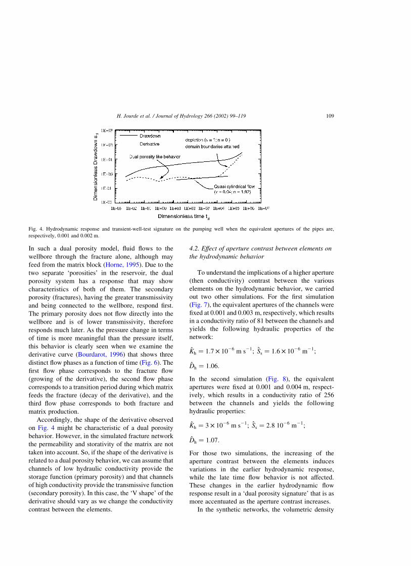
In the second simulation (Fig. 8), the equivalent

apertures were fixed at 0.001 and 0.004 m, respect-

ively, which results in a conductivity ratio of 256

between the channels and yields the following

hydraulic properties:

Kh ¼ 3 £ 1026 m s21; Ss ¼ 2:8 1026 m21;

Dh ¼ 1:07:

For those two simulations, the increasing of the

aperture contrast between the elements induces

variations in the earlier hydrodynamic response,

while the late time flow behavior is not affected.

These changes in the earlier hydrodynamic flow

response result in a ‘dual porosity signature’ that is as

more accentuated as the aperture contrast increases.

In the synthetic networks, the volumetric density

Fig. 4. Hydrodynamic response and transient-well-test signature on the pumping well when the equivalent apertures of the pipes are,

respectively, 0.001 and 0.002 m.


Fig. 5. Map view of bedding with simulated fracture sets. The pumping well intersects a low conductivity pipe of a second-generation fracture;

this fracture is connected to a long and high fracture of first generation (on its right). Large aperture channels are represented by bold lines.


[L/L3] of, respectively, the high and low conductivity

channels are of same order of magnitude. Thus, if we

still assume that channels of low hydraulic conduc-

tivity provide the storage function (primary porosity)

and that channels of high conductivity provide the

transmissive function (secondary porosity), then a

higher aperture contrast between the elements will

generate a high transmissive function of the secondary

porosity (Kf) and a low transmissive function of the

primary porosity (Km). Accordingly, this contrast

should generate a more accentuated dual-porosity

behavior. However, following the same hypothesis,

the storage function of the primary porosity (Sm) will

be lower than the storage function of the secondary

porosity (Sf), which is in disagreement with the

hypothesis required for a dual porosity behavior

analysis.

Furthermore, the well is connected to the primary

porosity (channel of low hydraulic conductivity), which

differs from the assumptions usually considered for dual

porosity model. Thus, this hydrodynamic behavior that

looks like a dual porosity behavior, is related to another

phenomenon since there are major discrepancies

between the assumptions required for a dual porosity

behavior and the well-aquifer properties of the

simulated network.

In addition, if we consider the storativity ratio v ¼

Sf=ðSf þ SmÞ that relates the secondary (or fracture)

storativity to that of the entire system, we observe that

our system reacts in a different manner, as it should

while considering a dual porosity model. Indeed, as

the volumetric density of the high and low conduc-

tivity channels is of same order of magnitude, Sf and

Sm are also of same order of magnitude for a low

conductivity contrast if we keep assuming that

channels of low conductivity correspond to the

primary porosity and that channels of high conduc-

tivity correspond to the secondary porosity. In this

case v would be smaller for a low aperture contrast

between channels (Fig. 4) than for a high aperture

contrast (Figs. 7 and 8), since Sf becomes bigger than

Sm. In a conventional dual porosity model, the ‘V

shape’ of the derivative is as much accentuated, as v

parameter is low. Thus the ‘V shape’ observed on Fig.

4 should be more remarkable than on Fig. 7 that itself

should be more accentuated than on Fig. 8. Instead the

‘V shape’ of the derivative is as much emphasized as

v parameter is high. In a same way, the beginning of

the transition is as much later as v is high in the case

of a dual porosity model. In our case, we observe

exactly the opposite (Figs. 4, 7 and 8). Thus, the

variation of the hydrodynamic behavior with the v

parameter is opposite to what it should be according to

Fig. 6. Drawdown and derivative variations observed for a dual

porosity behavior in a fracture aquifer (modified from Bourdarot

(1996)).

Fig. 7. Hydrodynamic response and transient-well-test signature on the pumping well when the equivalent apertures of the low and high

conductivity pipes are, respectively, 0.001 and 0.003 m.


a dual porosity behavior, while considering that

channels of low hydraulic conductivity provide the

storage function (primary porosity) and that channels

of high conductivity provide the transmissive function

(secondary porosity). Note that the previous consider-

ations induce another major contradiction with the

usual dual porosity model assumption that implies

Sf ! Sm.

This shows that the first intuitive analysis of the

hydrodynamic behavior is not appropriate and that

this analysis might lead to the determination of

inappropriate hydrodynamic parameters. Thus, we

might be in a particular configuration where both high

and low conductivity channels participate to the

storage function of the system while the low

conductivity channel linked to the well would provide

the transmissive function towards the remainder of the

aquifer.

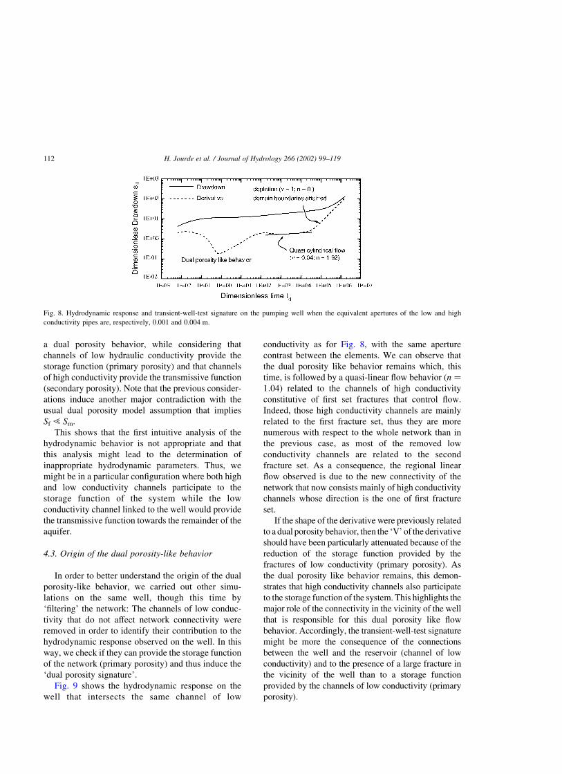
4.3. Origin of the dual porosity-like behavior

In order to better understand the origin of the dual

porosity-like behavior, we carried out other simu-

lations on the same well, though this time by

‘filtering’ the network: The channels of low conduc-

tivity that do not affect network connectivity were

removed in order to identify their contribution to the

hydrodynamic response observed on the well. In this

way, we check if they can provide the storage function

of the network (primary porosity) and thus induce the

‘dual porosity signature’.

Fig. 9 shows the hydrodynamic response on the

well that intersects the same channel of low

conductivity as for Fig. 8, with the same aperture

contrast between the elements. We can observe that

the dual porosity like behavior remains which, this

time, is followed by a quasi-linear flow behavior ðn ¼

1:04Þ related to the channels of high conductivity

constitutive of first set fractures that control flow.

Indeed, those high conductivity channels are mainly

related to the first fracture set, thus they are more

numerous with respect to the whole network than in

the previous case, as most of the removed low

conductivity channels are related to the second

fracture set. As a consequence, the regional linear

flow observed is due to the new connectivity of the

network that now consists mainly of high conductivity

channels whose direction is the one of first fracture

set.

If the shape of the derivative were previously related

to a dual porosity behavior, then the ‘V’ of the derivative

should have been particularly attenuated because of the

reduction of the storage function provided by the

fractures of low conductivity (primary porosity). As

the dual porosity like behavior remains, this demon-

strates that high conductivity channels also participate

to the storage function of the system. This highlights the

major role of the connectivity in the vicinity of the well

that is responsible for this dual porosity like flow

behavior. Accordingly, the transient-well-test signature

might be more the consequence of the connections

between the well and the reservoir (channel of low

conductivity) and to the presence of a large fracture in

the vicinity of the well than to a storage function

provided by the channels of low conductivity (primary

porosity).

Fig. 8. Hydrodynamic response and transient-well-test signature on the pumping well when the equivalent apertures of the low and high

conductivity pipes are, respectively, 0.001 and 0.004 m.


Fig. 9. Hydrodynamic response and transient-well-test signature on the pumping well when the pipes of low hydraulic conductivity that do not

affect network connectivity are removed; the equivalent apertures of the low and high conductivity pipes are, respectively, 0.001 and 0.004 m.

Fig. 10. Dimensionless fluid pressure propagation in the bedding parallel plane intersected by the well, hydrodynamic response and transient-

well-test signature at the corresponding time. Interpolation of calculated drawdowns in pipes was used in order to visualize the signal

propagation, assuming homogeneous parameters between fractures. The ‘box’ corresponds to the central part of the aquifer and has the same

height and half the lateral size of the synthetic network. The long and high fracture in the vicinity of the well is schematically represented. (a)

The pressure front encounters the large fracture, the derivative begins to fall; (b) the pressure front propagates in the large fracture whose

storativity is solicited, the derivative drops; (c) the pressure front propagates around the strike of the large fracture that acts as a relay structure to

fluid drainage, the derivative increases; (d) return to homogeneous behavior (the derivative corresponds almost to radial drawdown) with fluid

drainage mostly controlled by the large fracture.


For a better understanding of the hydrodynamic

behavior, we represented the propagation of pressure

front as a function of time in the synthetic network

(Figs. 10 and 11), for the simulation illustrated by Fig.

8. Fig. 10 shows the propagation, as a function of

time, of isobaric contours (corresponding to pressure

perturbation generated by the pumping test) within a

bedding parallel plane comprising the channel inter-

sected by the well (Fig. 5(a)). Fig. 11 shows the

propagation in terms of time of isobaric surfaces

within the whole network.

When the derivative begins to fall (Figs. 10(a) and

11(a)), the pressure perturbation front encounters a

major fracture of the first set (schematized) con-

stituted of high conductivity pipes (numerically

determined). This fracture initially acts as a barrier

to pressure perturbation propagation (Figs. 10(a) and

11(a)), then fills (the decrease in the derivative

corresponds to the storage solicitation of pipes

making up the fracture, Figs. 10(b) and 11(b)), thus

permitting continued migration of the pressure

perturbation into the remainder of the reservoir

(Figs. 10(c) and 11(c)). Finally, the growth of the

derivative curve corresponds to the return to a

homogeneous flow behavior, nevertheless controlled

by the fracture (Figs. 10(d) and 11(d)). Indeed, this

high permeability fracture is under pressure relative to

the remainder of the reservoir along its strike, such

Fig. 11. Dimensionless fluid pressure propagation in the whole network, hydrodynamic response and transient-well-test signature at the

corresponding time. Interpolation of calculated drawdowns in pipes was used in order to visualize the signal propagation, assuming

homogeneous parameters between fractures. The represented domain is the same as for Fig. 10 and the large fracture is still schematized. (a) The

pressure front encounters the large fracture, the derivative begins to fall; (b) the pressure front propagates in the large fracture whose storativity

is solicited, the derivative drops; (c) the pressure front propagates around the strike of the large fracture that acts as a relay structure to fluid

drainage, the derivative increases; (d) return to homogeneous behavior (the derivative corresponds almost to radial drawdown) with fluid

drainage mostly controlled by the large fracture.


that fluid at a large distance from the well first flows

into the fracture’s channels and then is focused

towards the well. This results in a quasi-radial flow

after the transient-well-test signature (Fig. 8) that

corresponds to fluid drainage towards the large

fracture and not towards the well.

Thus, the ‘V shape’ of the derivative that looks like

a ‘dual porosity signature’ is related to a ‘hydrodyn-

amic barrier’ to pressure propagation. This barrier

corresponds to a large fracture that is composed of

high conductivity channels and acts as a lateral

heterogeneity.

We showed that in a fractured reservoir, a dual

porosity signature may appear during the pressure

transient response although we are in a configuration

different from the hypothesis required for an analysis

with a dual porosity model. Indeed, the well is

connected to a low conductivity fracture (primary

porosity) in our model, although it should be

connected to a high conductivity fracture (secondary

porosity) for a conventional analysis with a dual

porosity model. Furthermore, we have shown that

although we can interpret a pressure transient

response in a fractured aquifer with a dual porosity

model, this corresponds to a different phenomenon

that is not in agreement with the dual porosity model

hypothesis. Thus the interpretation will be erroneous

and the parameters will not be characteristic of the

system, which will induce errors in the estimation of

reservoir parameters and thus in the management of

the resources of the reservoir. This may also point out

clearly the fact, that a dual-porosity like behavior can

also be induced only by a complex fracture network

itself.

5. Application to field data: dual porosity or lateral

heterogeneity?

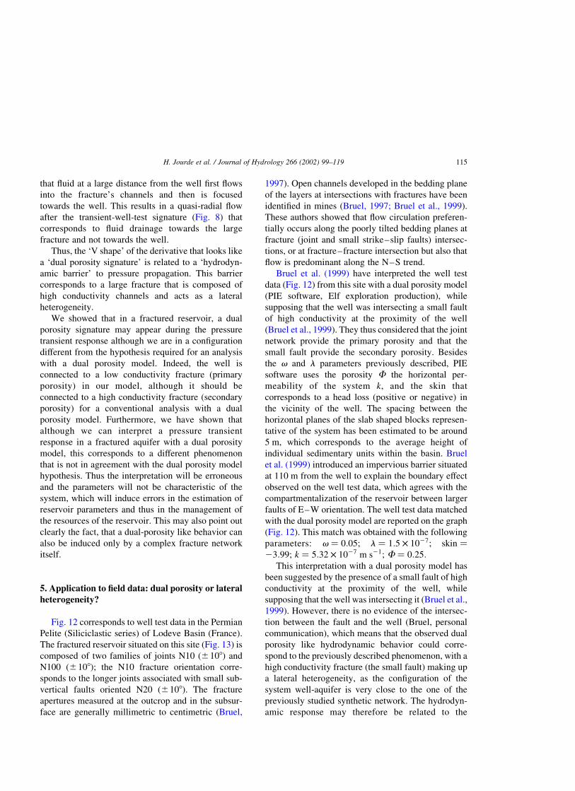
Fig. 12 corresponds to well test data in the Permian

Pelite (Siliciclastic series) of Lodeve Basin (France).

The fractured reservoir situated on this site (Fig. 13) is

composed of two families of joints N10 (^108) and

N100 (^108); the N10 fracture orientation corre-

sponds to the longer joints associated with small sub-

vertical faults oriented N20 (^108). The fracture

apertures measured at the outcrop and in the subsur-

face are generally millimetric to centimetric (Bruel,

1997). Open channels developed in the bedding plane

of the layers at intersections with fractures have been

identified in mines (Bruel, 1997; Bruel et al., 1999).

These authors showed that flow circulation preferen-

tially occurs along the poorly tilted bedding planes at

fracture (joint and small strike–slip faults) intersec-

tions, or at fracture–fracture intersection but also that

flow is predominant along the N–S trend.

Bruel et al. (1999) have interpreted the well test

data (Fig. 12) from this site with a dual porosity model

(PIE software, Elf exploration production), while

supposing that the well was intersecting a small fault

of high conductivity at the proximity of the well

(Bruel et al., 1999). They thus considered that the joint

network provide the primary porosity and that the

small fault provide the secondary porosity. Besides

the v and l parameters previously described, PIE

software uses the porosity F the horizontal per-

meability of the system k, and the skin that

corresponds to a head loss (positive or negative) in

the vicinity of the well. The spacing between the

horizontal planes of the slab shaped blocks represen-

tative of the system has been estimated to be around

5 m, which corresponds to the average height of

individual sedimentary units within the basin. Bruel

et al. (1999) introduced an impervious barrier situated

at 110 m from the well to explain the boundary effect

observed on the well test data, which agrees with the

compartmentalization of the reservoir between larger

faults of E–W orientation. The well test data matched

with the dual porosity model are reported on the graph

(Fig. 12). This match was obtained with the following

parameters: v ¼ 0:05; l ¼ 1:5 £ 1027; skin ¼

23:99; k ¼ 5:32 £ 1027 m s21; F ¼ 0:25:This interpretation with a dual porosity model has

been suggested by the presence of a small fault of high

conductivity at the proximity of the well, while

supposing that the well was intersecting it (Bruel et al.,

1999). However, there is no evidence of the intersec-

tion between the fault and the well (Bruel, personal

communication), which means that the observed dual

porosity like hydrodynamic behavior could corre-

spond to the previously described phenomenon, with a

high conductivity fracture (the small fault) making up

a lateral heterogeneity, as the configuration of the

system well-aquifer is very close to the one of the

previously studied synthetic network. The hydrodyn-

amic response may therefore be related to the


connectivity in the surrounding of the well connected

to the rest of the aquifer by a fracture of low

conductivity linked to a high conductivity fracture

(the small fault in this case).

Thus, our model might be able to reproduce the

observed flow behavior, without considering a dual

porosity behavior. On the field site, the dip is very

low, so that the reservoir can be approximate by a

tabular network; in addition, the ‘useful flow network’

consists of two sub-orthogonal fracture families and

preferred flow paths are located at intersections

between discontinuities. Accordingly, our model

correctly matches the properties of the site that

comprises two principal directions of fracturing with

flow located in channels at fracture intersections,

which induces a hydraulic conductivity anisotropy

related to the two families of fracture. As the normal

offset of the strike–slip fault in the vicinity of the well

is very small, we assume that it can be simulated by a

large fracture with our joint network model.

The match obtained with the dual porosity model is

obtained while using a dimensionless pressure (DP)

although our model considers a dimensionless draw-

down (sd). Accordingly, we attempted to generate

qualitatively and not quantitatively the same flow

behavior. To do so, we ran a pumping test simulation

in a synthetic network while considering the follow-

ing hypothesis: the average thickness of the strata (th)

has been fixed to 5 m and the average spacing between

fractures was fixed to 50 cm, which is in accordance

with field data (Bruel, 1997). To account for the

previous horizontal permeability and porosity deter-

mined with the dual porosity model PIE to match the

data, we chose a horizontal equivalent permeability

Kh ¼ 5 £ 1027 m s21 and an equivalent specific

storativity Ss ¼ 2:5 £ 1026 m21 (while considering

Ss ¼ Fb for the synthetic network. The negative skin

introduced to match the data with the dual porosity

model indicates an improvement in the flow near the

wellbore, which happens when the well intersects one

or many open channels or fractures.

Accordingly, in our model the well is located such

as it intersects a channel of low conductivity and is in

the proximity of the large fracture representative of

the small fault. We chose this configuration as we

Fig. 12. Well test data of a well in proximity to a small fault of trend N15. Data have been interpreted with a dual porosity model (PIE), assuming

that the well intersects the small fault and that the joint network assures the function storage.

Fig. 13. Oblique view of the fractured aquifer constituted of

Permian Pelite (siliciclastic series) found within the Lodeve basin of

France, (photograph: T. Bruel).


have shown that a lateral heterogeneity in proximity

to the well (the small fault in this case) can induce a

dual porosity like flow behavior.

The qualitative match of the well test data with

our model (Fig. 14) is obtained when we consider a

directional permeability ratio such as Ky ¼ 10 £ Kx;

with Ky and Kx, the equivalent permeability along

the direction of the first generation (longer) joints

and the second-generation joints, respectively. The

plot of well test data and simulated data reported

on a same graph with a vertical translation shows

that the fit is qualitatively consistent (Fig. 14).

Accordingly, the simulated transient-well-test sig-

nature related to a lateral heterogeneity, can

qualitatively match the well test data.

Furthermore, the resulting equivalent aperture of

the channels constitutive of the network calculated to

obtain the previous hydrodynamic parameters, are,

respectively, equal to 0.37 and 1.5 mm, which is

consistent with field data (Bruel, 1997) that gave a

measured aperture lower than millimetric for the

joints and millimetric to centimetric for the fault. We

thus qualitatively explained the same flow behavior

with our model while being consistent with field data,

showing that the use of a dual porosity model is not

necessarily appropriate. Instead, this is the connec-

tivity in the vicinity of the well that may induce this

dual porosity like behavior, which can simply result

from the presence of a high conductivity small fault

making up a lateral heterogeneity.

6. Summary and conclusions

The focus of this study was to determine what

confidence can be given to the transient-well-test

signature when pumping is carried out on a unique

wellbore and how a well known flow behavior like

dual porosity can wrongly be used to interpret a

hydrodynamic response related to a different phenom-

enon. We thus propose an alternative deterministic

interpretation with another type of model that

incorporates fracture interactions and conductivity

anisotropy.

In this paper, we showed how the flow behavior is

affected by changing the hydrodynamic properties of

channels constitutive of the dual fracture network and

by modifying its connectivity. We thus observed that

the earlier hydrodynamic response is strongly con-

trolled by the aperture contrast between the flow paths

as well as by the connectivity in the vicinity of the

well. The representation, in terms of time, of the

propagation of isobaric surfaces during a simulated

pumping test revealed that flow characteristics that

may be interpreted as a dual porosity flow behavior

are in fact related to a lateral heterogeneity (large

fracture or small fault). We saw that a large fracture

near the well first acts as a ‘hydrodynamic barrier’ to

pressure propagation then as a relay structure to

drainage since remote fluid first flows in its channels

and then is focused toward the well. Thus the

observed dual porosity like transient-well-test signa-

ture is different of the classical dual porosity behavior

Fig. 14. Well-test data from the experimental site of Lodeve and simulated well-test data obtained from the synthetic network, with a vertical

translation such as the qualitative match is better seen.


for which it is considered that flow first occurs within

fractures that afterwards are fed by the matrix.

We thus showed that when a dual porosity model

matches well test data, the resulting reservoir

parameters can be erroneous because of the model

assumptions basis that are not necessarily verified.

Accordingly a model, like the dual porosity model,

intended to explain complex natural phenomenon

must be used very cautiously. Indeed, the misuse of a

model to interpret well test data can lead to incorrect

analysis. That is why the flow behavior must correctly

be identified in order to determine the hydrodynamic

properties since it is a very important factor in the

strategy not only for the management of an aquifer or

an oil reservoir, but also for the rehabilitation of a

polluted aquifer.

With a field example where the fractured reservoir

comprises such lateral heterogeneity, we have shown

that well test data obtained on this site could also be

related to the connectivity and the presence of a small

fault in the surrounding of the well. Indeed, our model

was found to correctly match the properties of the

experimental site, both from a geometric and

hydrodynamic point of view. We thus showed that

the connectivity in the area immediately surrounding

the pumping well is very important in controlling the

flow and efficient exploitation of this type of fractured

reservoir. These results also indicate that the con-

sideration of fracture interaction mechanisms during

network generation, which allows the representation

of the structure of natural dual fracture networks, is of

great importance since the connectivity that exerts a

strong effect on flow behavior is correctly simulated.

Well test data from a single well must therefore be

used cautiously to assess the flow properties of

fractured reservoirs with lateral heterogeneities such

as large fractures or small faults. It will often be

necessary to consider test responses from multiple

wells to unambiguously determine the hydrodynamic

properties of the fractured reservoirs, in such a

configuration of the pumping well within the aquifer.

Acknowledgements

The authors wish to thank the F.L. Paillet and J.C.

Roegiers for their helpful comments and suggestions,

as well as S. Bottcher for its review of the translation.

The Centre National Universitaire Sud de Calcul

(CNUSC) of Montpellier (France) provided free

access to powerful tools for simulation processes

and 3D visualization (P. Falandry).

References

Bai, T., Gross, M.R., 1999. Theoretical analysis of cross-joint

geometries and their classification. J. Geophys. Res. 104 (B1),

1163–1177.

Barker, J.A., 1988. A generalized radial flow model for hydraulic

tests in fractured rock. Water Resour. Res. 24 (10), 1796–1804.

Barker, J.A., 1991. The reciprocity principle and an analytical

solution for Darcian flow in network. Water Resour. Res. 27 (5),

743–746.

Barthelemy, P., Jacquin, C., Yao, J., Thovert, J.F., Adler, P.M.,

1996. Hierarchical structures and hydraulic properties of

fracture network in the Causse of Larzac. J. Hydrol. 187,

237–258.

Becker, A., Gross, M.R., 1996. Mechanism for joint saturation in

mechanically layered rocks: an example from southern Israel.

Tectonophysics 257, 233–237.

Bourdarot, G., 1996. Essais de puits: methodes d’interpretation,

Editions Technip, Paris, p. 352.

Bourdet, D., Ayoub, J.A., Whittle, T.M., Pirard, Y.M., Kniazeff, V.,

1983. Interpretating well tests in fractured reservoirs. World Oil

1975, 77–87.

Bruel, T., 1997. Caracterisation des circulations de fluides dans un

reseau fracture et role des contraintes in situ, PhD Thesis (in

french), These de l’Universite Montpellier II, p. 402.

Bruel, T., Petit, J.P., Massonnat, G., Guerin, R., Nolf, J.L., 1999.

Relation entre ecoulements et fractures ouvertes dans un

systeme aquifere compartimente par des failles et mise en

evidence d’une double porosite de fractures. Bull. Soc. Geol.

France 170 (3), 401–412.

Cacas, M.C., Ledoux, E., De Marsily, G., Tillie, B., 1990. Modeling

fracture flow with a stochastic discrete fracture network:

calibration and validation-1/the flow model. Water Resour.

Res. 26 (3), 479–489.

Cornaton, F., Perrochet, P., 2002. Analytical 1-D dual-porosity

equivalent solutions to 3-D discrete single-continuum models.

Application to karstic spring hydrograph modeling. J. Hydrol.

262, 164–175.

Domenico, P., Schwartz, F.W., 1990. Physical and Chemical

Hydrogeology, Wiley, New York, p. 824.

Drogue, C., Grillot, J.C., 1976. Structure geologique et premieres

observations piezometriques a la limite du sous systeme

karstique de Terrieu. Geologie 3 (25).

Drogue, C., Costa Almeida, C.A., 1984. Deformations cassantes et

structure de magasin dans la couverture carbonatee mesozoıque

du centre du Portugal (Est du plateau de Fatima). C.R. Acad.

Sci. 299(II) (9), 577–580.

Ezzedine, S., 1994. Modelisation des ecoulements et du transport

dans les milieux fissures. Approches continue et discontinue,


PhD Thesis, These de l’Ecole Nationale Superieure des Mines

de Paris, p. 208.

Gringarten, A.C., Ramey, H.J., Raghavan, R., 1974. Unsteady state

pressure distributions created by a well with a horizontal fracture,

partial penetration, or restricted entry. SPE J., 413–426.

Hamm, S.Y., Bidaux, P., 1996. Dual-Porosity fractal models for

transient flow analysis in fissured rocks. Water Resour. Res. 32,

2733–2745.

Hobbs, D.W., 1967. The formation of tension joints in sedimentary

rocks: an explanation. Geol. Mag. 104, 550–556.

Horne, R.N., 1995. Modern Well Test Analysis: a Computer-Aided

Approach, Petroway Inc, Palo Alto, CA, p. 185.

Huang, Q., Angelier, J., 1989. Fracture spacing and its relation to

bed thickness. Geol. Mag. 126 (4), 355–362.

Jourde, H., 1999. Simulation d’essais de puits en milieu fracture a

partir d’un modele discret base sur les lois mecaniques de

fracturation. Validation sur sites experimentaux, PhD Thesis,

Memoires Geosciences Montpellier, 11, p. 205.

Jourde, H., Bidaux, P., Pistre, S., 1998. Modelisation des

ecoulements en reseaux de fractures orthogonales: influence

de la localisation du puits de pompage sur les rabattements.

Bull. Soc. Geol. France 169 (5), 635–644.

Pollard, D.D., Aydin, A., 1988. Progress in understanding jointing

over the past century. Geol. Soc. Am. Bull. 100, 1181–1204.

Price, N.J., Cosgrove, J.W., 1990. Analysis of Geological

Structures, Cambridge University Press, Cambridge.

Rives, T., Rawnsley, K., Petit, J.P., 1994. Analogue simulation of

orthogonal joint set formation in brittle varnish. J. Struct. Geol.

16 (3), 419–429.

Sanderson, D.J., Zhang, X., 1997. Modeling and prediction of

localized flow in fractured rock-masses. AAPG Bull. 81 (8),

1409–1410.

Segall, P., Pollard, D.D., 1983. Joint formation in granitic rock of

the Sierra Nevada. Geol. Soc. Am. Bull. 94, 563–575.

Stehfest, H., 1970. Commun. ACM 13, 47–49.

Theis, C.V., 1935. The relation between the lowering of the

piezometric surface and the rate and duration of discharge of a

well using groundwater storage. AGU, 16th Annu. Meet.,

519–524.

Warren, J.E., Root, P.J., 1963. The behavior of naturally fractured

reservoirs. SPE J. 3 (2), 245–255.

Wu, H., Pollard, D.D., 1995. An experimental study of the

relationship between joint spacing and layer thickness.

J. Struct. Geol. 17 (6), 887–905.


Flow behavior in a dual fracture network

Documents