UNIVERSIT ` A DEGLI STUDI DI FIRENZE Dipartimento di Sistemi e Informatica Dottorato di Ricerca in Ingegneria Informatica, Multimedialit`a e Telecomunicazioni ING-INF/05 Formal methods in the development life cycle of real-time software Laura Carnevali Dissertation submitted in partial fulfillment of the requirements for the degree of Doctor of Philosophy in Informatics, Multimedia and Telecommunication Engineering Ph.D. Coordinator Prof. Giacomo Bucci Advisors Prof. Enrico Vicario Prof. Giacomo Bucci XXII Ciclo – 2008-2010

Welcome message from author
This document is posted to help you gain knowledge. Please leave a comment to let me know what you think about it! Share it to your friends and learn new things together.
Transcript

UNIVERSITA DEGLI STUDI DI FIRENZEDipartimento di Sistemi e Informatica
Dottorato di Ricerca inIngegneria Informatica, Multimedialita e Telecomunicazioni
ING-INF/05
Formal methods
in the development life cycle
of real-time software
Laura Carnevali
Dissertation submitted in partial fulfillment
of the requirements for the degree of
Doctor of Philosophy
in Informatics, Multimedia and Telecommunication Engineering
Ph.D. Coordinator
Prof. Giacomo Bucci
Advisors
Prof. Enrico Vicario
Prof. Giacomo Bucci
XXII Ciclo – 2008-2010

To my parents and Marco

“The best thing for being sad,” replied Merlyn, beginning
to puff and blow, “is to learn something. That is the only
thing that never fails. You may grow old and trembling
in your anatomies, you may lie awake at night listening
to the disorder of your veins, you may miss your only
love, you may see the world about you devastated by evil
lunatics, or know your honour trampled in the sewers of
baser minds. There is only one thing for it then – to
learn. Learn why the world wags and what wags it. That
is the only thing which the mind can never exhaust, never
alienate, never be tortured by, never fear or distrust, and
never dream of regretting. Learning is the thing for you.
Look at what a lot of things there are to learn.”
Terence Hanbury White
The Once and Future King - The Sword in the Stone

This thesis was reviewed by Prof. Susanna Donatelli (University of Turin),Prof. Giuseppe Lipari (Scuola Superiore Sant’Anna - Pisa), and Prof. TullioVardanega (University of Padua), whom I sincerely thank for their valuablecomments and suggestions.
iii

Acknowledgements
I would like to sincerely thank my advisor Prof. Enrico Vicario, for his guidanceand support during these three years, for his expertise and enthusiasm. I wouldalso like to thank Prof. Giacomo Bucci, for his experience and advice.
A special thank goes to Luigi Sassoli, for his valuable and helpful sugges-tions during the first year of my PhD course, for his patience in answering myfrequent questions, for the time spent in interesting and fruitful discussions.
I am very grateful to Leonardo Grassi, Lorenzo Ridi, and Irene Bicchierai,working with them has been a pleasure to me. I would also like to thankpresent and past people in the Software Technologies Laboratory at the Uni-versity of Florence: Jacopo Torrini, Valeriano Sandrucci, Andrea Tarocchi,Francesco Poli, Fabrizio Baldini, Graziella Magnolfi, Jacopo Baldanzi, LucaRomano. Thanks for your support and for our funny talks about informatics,life, politics, food, and football.
Words cannot express my love and gratitude to my parents, for making mylife so special. Last but certainly not least, thanks to Marco, for what was,what is, and what will be.

Abstract
Preemptive Time Petri Nets (pTPNs) support modeling and analysis ofconcurrent timed software components running under fixed priority preemptivescheduling. The model is supported by a well established theory based onsymbolic state-space analysis through Difference Bounds Matrix (DBM), withspecific contributions on compositional modularization, trace analysis, andefficient over-approximation and clean-up in the management of suspensionderiving from preemptive behavior.
The aim of this dissertation is to devise and implement a framework thatbrings the theory to application. To this end, the theory is cast into an organictailoring of design, coding, and testing activities within a V-Model softwarelife cycle in respect of the principles of regulatory standards applied to theconstruction of safety-critical software components. To implement the tool-chain subtended by the overall approach into a Model Driven Development(MDD) framework, the theory of state-space analysis is complemented withmethods and techniques supporting semi-formal specification and automatedcompilation into pTPN models and real-time code, measurement-based Execu-tion Time estimation, test-case selection and sensitization, coverage evaluation.

Contents
List of Acronyms v
Introduction ix
1 A formal methodology for the development of real-time software 1
1.1 Real-time operating systems . . . . . . . . . . . . . . . . . . . . 11.1.1 Definitions . . . . . . . . . . . . . . . . . . . . . . . . . 31.1.2 Limits and desirable features of RTOSs . . . . . . . . . . 51.1.3 Predictability as a central feature of RTOSs . . . . . . . 81.1.4 Standards for RTOSs . . . . . . . . . . . . . . . . . . . 131.1.5 Commercial and open source real-time kernels . . . . . . 18
1.1.5.1 Commercial RTOSs . . . . . . . . . . . . . . . 181.1.5.2 Linux-based real-time kernels . . . . . . . . . . 201.1.5.3 Research kernels . . . . . . . . . . . . . . . . . 22
1.2 Real-Time Application Interface . . . . . . . . . . . . . . . . . . 241.2.1 RTAI architecture . . . . . . . . . . . . . . . . . . . . . 241.2.2 RTAI schedulers . . . . . . . . . . . . . . . . . . . . . . 271.2.3 RTAI IPC mechanisms . . . . . . . . . . . . . . . . . . . 29
1.3 Software development processes . . . . . . . . . . . . . . . . . . 301.3.1 From the waterfall model to eXtreme Programming . . . 311.3.2 The V-Model software life cycle . . . . . . . . . . . . . . 32
1.4 Mapping the theory of pTPNs onto a V-Model software life cycle 35
2 Design of real-time task-sets through preemptive Time Petri Nets 42
2.1 Preemptive Time Petri Nets . . . . . . . . . . . . . . . . . . . . 422.1.1 Syntax . . . . . . . . . . . . . . . . . . . . . . . . . . . 422.1.2 Semantics . . . . . . . . . . . . . . . . . . . . . . . . . 44
CONTENTS ii

2.2 Modeling real-time task-sets through pTPNs . . . . . . . . . . . 462.2.1 Tasks, jobs, and chunks . . . . . . . . . . . . . . . . . . 462.2.2 Semaphore synchronization and priority ceiling . . . . . . 482.2.3 Message passing and mailbox synchronization . . . . . . . 49
2.2.3.1 RTAI Messages . . . . . . . . . . . . . . . . . 492.2.3.2 RTAI Mailbox . . . . . . . . . . . . . . . . . . 572.2.3.3 Mailbox synchronization in the example case . . 61
2.3 Architectural verification of real-time task-sets through pTPNs . 622.3.1 Simulation of pTPN models . . . . . . . . . . . . . . . . 622.3.2 State-space analysis of pTPN models . . . . . . . . . . . 622.3.3 Application to the example case . . . . . . . . . . . . . . 65
3 Design of real-time task-sets through a semi-formal specification 68
3.1 Specification of real-time task-sets through timeline schemas . . . 693.1.1 Tasks, jobs, and chunks . . . . . . . . . . . . . . . . . . 693.1.2 Semaphore synchronization and priority ceiling . . . . . . 703.1.3 Mailbox synchronization . . . . . . . . . . . . . . . . . . 713.1.4 Example . . . . . . . . . . . . . . . . . . . . . . . . . . 71
3.2 Specification of real-time task-sets through UML-MARTE . . . . 72
4 Coding process and Execution Time profiling 76
4.1 Implementation of the dynamic architecture of a CSCI under RTAI 774.1.1 Implementation of periodic tasks . . . . . . . . . . . . . 794.1.2 Implementation of jittering and sporadic tasks . . . . . . 834.1.3 Observation of reentrant jobs . . . . . . . . . . . . . . . 86
4.2 Executable Architecture of a CSCI . . . . . . . . . . . . . . . . . 884.3 Execution Time profiling . . . . . . . . . . . . . . . . . . . . . . 88
4.3.1 A measurement-based approach through pTPNs . . . . . 894.3.2 Code instrumentation . . . . . . . . . . . . . . . . . . . 914.3.3 Experimental results . . . . . . . . . . . . . . . . . . . . 91
4.4 Timing observability and control . . . . . . . . . . . . . . . . . . 944.4.1 Estimation of the Execution Time of primitives . . . . . . 944.4.2 Estimation of the accuracy of the function busy_sleep . 994.4.3 Estimation of the context switch time . . . . . . . . . . . 1014.4.4 Estimation of the perturbation of time-stamped logging . 104
5 Unit and Integration Testing Processes 106
5.1 Defect and failure model . . . . . . . . . . . . . . . . . . . . . . 1065.2 Test-case selection and coverage analysis . . . . . . . . . . . . . 1075.3 Test-case execution . . . . . . . . . . . . . . . . . . . . . . . . 112
CONTENTS iii

5.3.1 Supporting test-case execution through pTPNs . . . . . . 1145.3.2 Experimental results . . . . . . . . . . . . . . . . . . . . 115
5.4 Oracles verdict . . . . . . . . . . . . . . . . . . . . . . . . . . . 118
6 Summary of the approach 121
Conclusions 134
Bibliography 138
CONTENTS iv

List of Acronyms
ADEOS Adaptive Domain Environment for Operating Systems . . . . . . . . . . . . 26
BCET Best Case Execution Time . . . . . . . . . . . . . . . . . . . . . . . . . . . . . . . . . . . . . . . . .89
CSCI Computer Software Configuration Item . . . . . . . . . . . . . . . . . . . . . . . . . . . . . 37
DBM Difference Bounds Matrix . . . . . . . . . . . . . . . . . . . . . . . . . . . . . . . . . . . . . . . . . . xi
DSML Domain Specific Modeling Language . . . . . . . . . . . . . . . . . . . . . . . . . . . . . . . ix
EDF Earliest Deadline First . . . . . . . . . . . . . . . . . . . . . . . . . . . . . . . . . . . . . . . . . . . . . . 12
FIFO First In First Out . . . . . . . . . . . . . . . . . . . . . . . . . . . . . . . . . . . . . . . . . . . . . . . . . . 28
HCI Hardware Configuration Item . . . . . . . . . . . . . . . . . . . . . . . . . . . . . . . . . . . . . . . . 37
HRTOS Hard Real-Time Operating System . . . . . . . . . . . . . . . . . . . . . . . . . . . . . . . . 4
HS Hierarchical Scheduling . . . . . . . . . . . . . . . . . . . . . . . . . . . . . . . . . . . . . . . . . . . . . . 136
LIST OF ACRONYMS v

IPC Inter Process Communication . . . . . . . . . . . . . . . . . . . . . . . . . . . . . . . . . . . . . . . . . 3
IUT Implementation Under Test . . . . . . . . . . . . . . . . . . . . . . . . . . . . . . . . . . . . . . . . 112
IVSS Intelligent Visual Surveillance System . . . . . . . . . . . . . . . . . . . . . . . . . . . . . . .35
LXRT LinuX Real-Time . . . . . . . . . . . . . . . . . . . . . . . . . . . . . . . . . . . . . . . . . . . . . . . . . . 29
MARTE Modeling and Analysis of Real-Time and Embedded systems . . . . . .35
MDD Model Driven Development . . . . . . . . . . . . . . . . . . . . . . . . . . . . . . . . . . . . . . . . . ix
POSIX Portable Operating System Interface for UniX . . . . . . . . . . . . . . . . . . . . 14
PRS Preemptive ReSume execution policy . . . . . . . . . . . . . . . . . . . . . . . . . . . . . . . . . xi
pTPN preemptive Time Petri Net . . . . . . . . . . . . . . . . . . . . . . . . . . . . . . . . . . . . . . . . . xi
RAMS Reliability, Availability, Maintainability and Safety . . . . . . . . . . . . . . . 136
RM Rate Monotonic Priority Order . . . . . . . . . . . . . . . . . . . . . . . . . . . . . . . . . . . . . . 29
RR Round Robin . . . . . . . . . . . . . . . . . . . . . . . . . . . . . . . . . . . . . . . . . . . . . . . . . . . . . . . . . 12
RTAI Real-Time Application Interface . . . . . . . . . . . . . . . . . . . . . . . . . . . . . . . . . . . . 21
RTHAL Real-Time Hardware Abstraction Layer . . . . . . . . . . . . . . . . . . . . . . . . . . 24
RTOS Real-Time Operating System . . . . . . . . . . . . . . . . . . . . . . . . . . . . . . . . . . . . . . . .x
LIST OF ACRONYMS vi

SCG state class graph . . . . . . . . . . . . . . . . . . . . . . . . . . . . . . . . . . . . . . . . . . . . . . . . . . . . 63
SD System Development . . . . . . . . . . . . . . . . . . . . . . . . . . . . . . . . . . . . . . . . . . . . . . . . . 33
SD1 System Requirements Analysis . . . . . . . . . . . . . . . . . . . . . . . . . . . . . . . . . . . . . . . 33
SD2 System Design . . . . . . . . . . . . . . . . . . . . . . . . . . . . . . . . . . . . . . . . . . . . . . . . . . . . . . 33
SD3 Software/Hardware Requirements Analysis . . . . . . . . . . . . . . . . . . . . . . . . . . . 34
SD4-SW Preliminary Software Design . . . . . . . . . . . . . . . . . . . . . . . . . . . . . . . . . . . . 34
SD5.2-SW Analysis of Resources and Time Requirements . . . . . . . . . . . . . . . . . 34
SD6-SW Software Implementation . . . . . . . . . . . . . . . . . . . . . . . . . . . . . . . . . . . . . . . . 34
SD6.3-SW Self Assessment of the Software Module . . . . . . . . . . . . . . . . . . . . . . . 34
SD7-SW Software Integration . . . . . . . . . . . . . . . . . . . . . . . . . . . . . . . . . . . . . . . . . . . . .34
SD8 System Integration . . . . . . . . . . . . . . . . . . . . . . . . . . . . . . . . . . . . . . . . . . . . . . . . . . 34
SD9 Transition to Utilization . . . . . . . . . . . . . . . . . . . . . . . . . . . . . . . . . . . . . . . . . . . . .34
TPN Time Petri Net . . . . . . . . . . . . . . . . . . . . . . . . . . . . . . . . . . . . . . . . . . . . . . . . . . . . . xi
UML Unified Modeling Language . . . . . . . . . . . . . . . . . . . . . . . . . . . . . . . . . . . . . . . . . 35
UP Unified Process . . . . . . . . . . . . . . . . . . . . . . . . . . . . . . . . . . . . . . . . . . . . . . . . . . . . . . . 32
LIST OF ACRONYMS vii

WCET Worst Case Execution Time . . . . . . . . . . . . . . . . . . . . . . . . . . . . . . . . . . . . . . 11
WCCT Worst Case Completion Time . . . . . . . . . . . . . . . . . . . . . . . . . . . . . . . . . . . . 65
XP eXtreme Programming . . . . . . . . . . . . . . . . . . . . . . . . . . . . . . . . . . . . . . . . . . . . . . . .32
LIST OF ACRONYMS viii

Introduction
Intertwined effects of concurrency and timing comprise one of the most chal-
lenging factors of complexity in the development of safety-critical software
components. Formal methods may provide a crucial help in supporting both
design and verification activities, reducing the effort of development, and pro-
viding a higher degree of confidence in the correctness of products.
Integration of formal methods in the industrial practice is explicitly en-
couraged in certification standards such as RTCA/DO-178B [60], with specific
reference to software with complex behavior deriving from concurrency, syn-
chronization, and distributed processing. The RTCA/DO-178B standard re-
commends that the proposed methods are smoothly integrated with design and
testing activities prescribed by a defined and documented software life cycle.
In particular, this recommendation can be effectively referred to the framework
of the V-Model [42], which is often adopted by process oriented standards ru-
ling the development of safety-critical software subject to explicit certification
requirements, such as airborne systems [60], railway and transport applica-
tions [50], medical control devices [77]. The integration of formal methods
along multiple activities of the software life cycle is also a typical approach
to Model Driven Development (MDD), where Domain Specific Modeling Lan-
guages (DSMLs) enable the formalization of system requirements and design,
and transformation engines support the development of generators of concrete
artifacts that may include code, documentation, complementary models, tests
INTRODUCTION ix

[78], [110]. In this context, the adoption of formal methods may serve to attain
various degrees of rigor, ranging from non ambiguous specification to support
for manual verification and even to automated verification [60].
Various tools [90], [14], [69] have been described and experimented in the
application of the MDD concept, with different goals in the aspects of mo-
del formalization, implementation and verification. Simulink [90] is a tool
for mathematical modeling and simulation of complex control systems, based
on a block diagram paradigm. Integrated within MATLAB environment [88]
and coupled with other facilities such as Real-Time Workshop [89], Simulink
supports automated generation of real-time C-code for a large variety of plat-
forms and Real-Time Operating Systems (RTOSs). The direct translation of
block diagrams into executable code emphasizes performance and signal-flow
optimizations over correctness-related issues while hiding the effect of concur-
rency on resources allocation and usage. Charon [14] is a language for the
specification of interacting hybrid systems and provides a modular description
of both architectural and behavioral aspects. The conformance of the model
with hybrid state machines allows the adoption of formal analysis techniques
for validation purposes [12]. Code generation experiences from Charon models
[13] are mainly focused on the preservation of concurrency correctness and
mathematical constraints (i.e., differential or algebraic equations representing
system dynamics), as this may be jeopardized by the discrepancy between
continuous/concurrent behavior of the model and the discrete/preemptive be-
havior of the target platform. The Giotto Language [69] realizes a separation
of concerns along the orthogonal issues of timing and functionality, through
the introduction of an intermediate layer of abstraction between the mathe-
matical model and the corresponding generated code. This layer defines an
embedded software model, i.e., a solution to a given control problem that takes
into account timing and concurrency constraints while neglecting functiona-
lity concerns and platform-dependent choices such as scheduling or preemption
policies [70]. The actual execution of the generated software components on
a target platform relies on the use of a Virtual Machine (called Embedded
Machine) that accounts for scheduling, preemption, and resource allocation
INTRODUCTION x

policies.
A different approach able to reduce the step of code generation to the syn-
thesis of an on-line controller was proposed in [11], where the state-space of
a discrete time model is enumerated and used to identify and synthesize an
on-line controller that keeps the execution of the system within a range of
correct behavior. A similar approach is reported in a continuous time setting
in [122]. In both the cases, the exhaustive enumeration of the state-space be-
comes a precondition for the implementation stage, and on-line control puts
an overhead on timing resources. Furthermore, the resulting code structure
does not meet consolidated design and implementation practices, thus preven-
ting smooth integration within an existing development software life cycle. In
the Uppaal tool [22] various activities along the life cycle are supported by
relying on the formal nucleus of Timed Automata. This supports state-space
analysis based on Difference Bounds Matrix (DBM) theory, test case selection
and execution [72], [84], and synthesis of a controller that drives the system
along selected behaviors in the state-space [49]. However, the model does not
encompass representation of suspension, thus ruling out the case of real-time
systems running under preemptive scheduling. In the Times tool of Uppaal
[15], the limitation is partially circumvented by resorting to the model of Ti-
med Automata with Tasks (TAT) [59] through the composition of a model
of asynchronous task releases and the usage of the analysis technique of [91],
but this requires Execution Times of tasks to be deterministic integer values,
which comprises an assumption that is not met in a large class of practical
applications [124].
The model of Time Petri Nets (TPNs) is extended by preemptive Time
Petri Nets (pTPNs) [34], [33] with a concept of resource that supports re-
presentation of suspension in the advancement of clocks. This realizes the
so-called Preemptive ReSume execution policy (PRS) [87], providing an ex-
pressivity which compares to stopwatch automata [58] and Petri Nets with
hyper-arcs [106], and which enables convenient modeling of the usual pat-
terns of concurrency encountered in the practice of real-time systems [34], [33].
The analysis technique reported in [36] enumerates an over-approximation of
INTRODUCTION xi

the state state-space that maintains the efficiency of DBM encoding of state
classes, and that supports exact identification of feasible timings of selected
behaviors through a clean-up algorithm. This enables efficient verification of
properties pertaining to reachability under timing constraints and to the sa-
tisfaction of real-time deadlines. Preliminary experimentations on the use of
pTPNs in individual steps of the construction of real-time software were re-
ported in [43], [44], [47], [46], about disciplined manual translation of pTPN
models into code running under RTAI [95], about the execution of timed test-
cases, and about a software framework supporting agile model transformations.
This dissertation develops and integrates the theory of pTPNs in order to
cast it into a comprehensive methodology that comprises an instance (tailo-
ring) of the V-Model framework [42]. To this aim, this work develops the way
how the theory of pTPNs is applied to support in organic manner: semi-formal
specification of real-time software components and automated translation into
the corresponding pTPN model; generation of code running under RTAI [95]
and preserving sequencing and timeliness properties; Execution Time profiling;
test case selection and sensitization, oracle verdict, and coverage evaluation.
Experimentation on a case example is reported to demonstrate the feasibility
and effectiveness of the approach.
The dissertation is organized in five chapters.
• Chapter 1 resumes characteristics and peculiarities of RTOSs, describes
the architecture and the main features of RTAI [95], and devises a for-
mal approach that applies the theory of pTPNs to the construction of
real-time software components, reporting the principles of the V-Model
software life cycle and introducing a running case example.
• Chapter 2 recalls the formal nucleus of pTPNs, devising their expressivity
and state-space analysis techniques, illustrates the application of trace
analysis to a concrete case, and discusses how common patterns of task
concurrency and interaction can be effectively modeled through pTPNs.
INTRODUCTION xii

• Chapters 3 describes two approaches to semi-formal specification of real-
time software components and illustrates how pTPN models can be de-
rived from semi-formal specifications.
• Chapter 4 illustrates how a semi-formal specification can be translated
into code that preserves semantic properties of the corresponding pTPN
model, enabling the definition of a measurement-based approach to Exe-
cution Time profiling based on pTPNs. An experimental assessment is
provided to evaluate the accuracy of measures.
• Chapter 5 discusses how the pTPN model of real-time software supports
test case selection and execution through state-space enumeration and
trace analysis, how it allows the definition of different oracles for the
evaluation of executed tests, and provides a measure of attained coverage.
• Chapter 6 resumes the methodology proposed in this dissertation with
reference to a case example.
INTRODUCTION xiii

Chapter
1A formal methodology for the
development of real-time software
This Chapter resumes the main features of RTOSs and focuses on peculiarities
of RTAI [95], the RTOS employed in the experimentation described in this
work. Then, it provides a brief overview of software development processes
and devises a formal approach that casts the theory of pTPNs within the V-
Model software life cycle [42] in order to support the construction of real-time
software components .
1.1 Real-time operating systems
Real-time systems are computing systems that must reach with precise time
constraints to events in the environment [39]. The correct behavior of these
systems depends not only on the logical result of the computation but also on
the time at which the results are produced. Nowadays, a wide and increasing
spectrum of complex systems relies, in part or completely, on real-time com-
puting capabilities, from industrial automation to robotics, from automotive
A FORMAL METHODOLOGY FOR THE DEVELOPMENT OF REAL-TIME SOFTWARE 1

Real-time operating systems
applications to railway and flight control systems, from military systems to
space missions, from embedded systems to multimedia applications and vir-
tual reality. As a consequence, the domain of real-time systems has become
one of the most active and challenging research areas within computer science.
Despite the large application domain, many researchers, developers, and
technical managers have serious misconceptions about real-time computing
[112]. In fact, real-time systems are often erroneously said to be fast systems
that quickly react to external events, and most real-time control applications
are still designed using ad-hoc methods and heuristic approaches. These tech-
niques often rely on the implementation of large portions of code in assembly
language, on timers programming, on the development of low-level drivers for
device handling, and on the manipulation of task and interrupt priorities. Al-
though this approach produces code that can be optimized to run very fast, it
implies various drawbacks:
• Tedious programming. Implementing complex control applications
in assembly language is much more difficult and time consuming than
using a high-level programming language. Moreover, the efficiency and
the reliability of the code strongly relies on the ability of the programmer.
• Difficult code understanding. Programs written in assembly code
are much more difficult to understand than those developed in high-
level programming languages. In addition, clever hand-coding introduces
additional complexities and makes assembly programs even more cryptic:
the more the program gains in efficiency, the less intelligible it gets.
• Difficult code maintainability. Maintenance of assembly code be-
comes much more difficult as the complexity of the program increases,
even for the original programmer.
• Difficult verification of time constraints. Verification of timing
constraints becomes actually impractical without the support of specific
tools and methodologies for code and schedulability analysis.
A FORMAL METHODOLOGY FOR THE DEVELOPMENT OF REAL-TIME SOFTWARE 2

Real-time operating systems
As a major consequence, software developed following empirical techniques
can be highly unpredictable. Advances in computer hardware technology will
improve system throughput and will increase the computational speed, but
they will not be able to take care of any real-time requirement. In fact, whe-
reas the objective of fast computing is to minimize the average response time
of a given set of tasks, the objective of real-time computing is to meet the
individual timing requirement of each task [112]. Hence, however short the
average response time can be, if no formal methodology is adopted to support
a priori verification of all timing constraints of the application and if the under-
lying operating system does not provide specific features to handle real-time
tasks, then it is impractical to foresee certain rare but possible situations that
lead to a system collapse. This is especially serious in the context of control
applications for critical systems, where a failure can be catastrophic and may
injure people or cause heavy damage to the environment.
A more robust guarantee of the performance of a real-time system under all
workload conditions can be achieved only through more sophisticated design
methodologies, static analysis of the source code, and specific operating sys-
tems mechanisms. The latter are purposely designed to support computation
under timing constraints and they include scheduling algorithms, mutual ex-
clusion and synchronization mechanisms, Inter Process Communication (IPC)
mechanisms, interrupt and memory handling. Moreover, control systems of
critical applications must be capable of handling all anticipated scenarios, and
their design must be driven by pessimistic assumptions on the events generated
by the environment so as to identify the most serious situations.
1.1.1 Definitions
Real-time software comprises a set of concurrent real-time tasks [39], [116].
• A real-time task is an executable entity of work which is subject to strin-
gent timing constraints and consists of an infinite sequence of identical
activities called instances or jobs.
A real-time task is typically constrained by a deadline.
A FORMAL METHODOLOGY FOR THE DEVELOPMENT OF REAL-TIME SOFTWARE 3

Real-time operating systems
• The deadline is a point in time by which a real-time task must complete
its execution without causing any damage to the system.
Real-time tasks are usually distinguished in two classes depending on the
consequences that may occur because of a missed deadline:
• A real-time task is said to be hard if missing its deadline may cause
catastrophic consequences on the environment under control (e.g., sen-
sory data acquisition, detection of critical conditions, actuator serving,
low-level control of critical system components, planning sensory-motor
actions that tightly interact with the environment).
• A real-time task is said to be soft if meeting its deadline is desirable for
performance reasons, but missing it does not cause serious damage to
the environment and does not jeopardize correct system behavior (e.g.,
execution of the command interpreter of the user interface, handling in-
put data from the keyboard, display of messages on the screen, graphical
activities, saving report data).
A Hard Real-Time Operating System (HRTOS) is an RTOS that is capable of
handling hard real-time tasks. Real-time applications typically include both
hard and soft activities, therefore HRTOSs should be designed to handle both
hard and soft tasks using different strategies. Hybrid task-sets are usually
managed by guaranteeing individual timing constraints of hard real-time tasks
while minimizing the average response time of soft real-time tasks.
A real-time task can also be characterized by the following parameters:
• Release time: it is the time at which a task becomes ready to execute; it
is also referred to as arrival time.
• Computation time: it is the time which is necessary to execute a task on
the processor without interruption.
• Start time: it is the time at which a task starts its execution.
• Finishing time: it is the time at which a task finishes its execution.
A FORMAL METHODOLOGY FOR THE DEVELOPMENT OF REAL-TIME SOFTWARE 4

Real-time operating systems
• Lateness: it is the delay of a task completion with respect to its deadline
(it is negative if a task completes the execution before its deadline).
• Laxity: it is the maximum time a task can be delayed on its activation
to complete within its deadline.
Real-time tasks are distinguished in periodic and aperiodic depending on the
regularity of their activations.
• A periodic task consists of an infinite sequence of jobs that are regularly
activated at a constant rate. It is characterized by a period (which is the
constant difference between the activation time of consecutive jobs), a
computation time, and a deadline (which is often considered coincident
with the end of the period).
• An aperiodic task consists of an infinite sequence of jobs that are not
regularly activated at a constant rate. Each job is characterized by an
arrival time, a computation time, and a deadline. An aperiodic task
characterized by a minimum interarrival time between consecutive jobs
is said to be a sporadic task.
1.1.2 Limits and desirable features of RTOSs
Most RTOSs are based on kernels that are modified versions of time-sharing
operating systems and, thus, they exhibit some basic features of these systems
that are not suited to handle real-time tasks. The main characteristics of
time-sharing operating systems include:
• Multitasking. A set of primitives for task management (e.g., system
calls to create, suspend, resume, and terminate real-time tasks) provides
a support for concurrent programming. However, many of these pri-
mitives do not take time into account and, even worse, they introduce
unbounded delays on the Execution Time of tasks. This may cause un-
predictable deadline misses.
A FORMAL METHODOLOGY FOR THE DEVELOPMENT OF REAL-TIME SOFTWARE 5

Real-time operating systems
• Priority-based scheduling. Various strategies for task management
can be developed on priority-based scheduling by changing the rule accor-
ding to which priorities are assigned to tasks. However, timing constraints
of real-time tasks cannot be easily mapped into a set of priorities. This
is even harder in dynamic environments, where the arrival of a task may
require the remapping of the entire set of priorities. Moreover, the veri-
fication of timing constraints is quite impractical without the support of
primitives that explicitly handle time.
• Quick response to external interrupts. This feature is usually ob-
tained by assigning to external interrupts higher priorities than real-time
tasks and by reducing the portions of code that are executed while in-
terrupts are disabled. Quick interrupt handling reduces response time
to external events but introduces unbounded delays on the Execution
Time of tasks. Moreover, the number of interrupts that a process can
experience during its execution cannot be bounded in advance.
• Task communication and synchronization primitives. Inter-task
communication and synchronization mechanisms should be combined
with specific access protocols to avoid undesirable phenomena, such as
priority inversion, chained blocking, and deadlock.
• Small kernel and fast context switch. This feature reduces system
overhead, thus improving the average response time of the task-set. Ho-
wever, this does not provide any guarantee that each task will meet its
deadline. In addition, a small kernel does not support the implementa-
tion of functionalities required to manage real-time tasks.
• Real-time clock as internal time reference. Any real-time kernel
that handles time-critical activities that interact with the environment
requires an internal real-time clock. Nevertheless, in most commercial
real-time kernels this is the only mechanism for time management, and
there is not support for deadline specification and periodic task activa-
tion. Moreover, exception handling is usually performed through ad-hoc
A FORMAL METHODOLOGY FOR THE DEVELOPMENT OF REAL-TIME SOFTWARE 6

Real-time operating systems
alarm and timeout signals, which experience the same drawbacks as in-
terrupt handling.
Basic design paradigms found in classical time-sharing systems must be
radically changed in order to develop real-time kernels for critical control ap-
plications, which require stringent timing constraints that must be met to
ensure safe behavior of the system. Such real-time systems must exhibit some
basic properties, which include [39], [30]:
• Predictability. Both functional and timing behavior of a real-time
system must be deterministic in order to guarantee that real-time re-
quirements are met. To this end, system calls must have a bounded
Execution Time, thus avoiding the introduction of unbounded delays on
the Execution Time of tasks.
• Timeliness. Results produced by a real-time system must be correct
both in their functional value and in the time domain. As a consequence,
the operating system must provide specific kernel mechanisms to manage
time and to handle periodic and aperiodic real-time tasks with explicit
timing constraints and different criticality.
• Reliability. Real-time systems must conform to the specification of
their behavior with an acceptable measure of success.
• Availability. The system should be operable and ready for correct usage
when it needs to be used.
• Maintainability. The system should be designed according to a modu-
lar architecture to ensure that the real-time kernel can be easily modified
and adapted to the needs of real-time applications.
• Safety. Real-time systems must achieve acceptable levels of risk of harm
to people, the environment, or business.
• Fault tolerance. Critical components must be designed to be fault
tolerant so as to prevent failures that cause the system to crash.
A FORMAL METHODOLOGY FOR THE DEVELOPMENT OF REAL-TIME SOFTWARE 7

Real-time operating systems
• Design for peak load. Real-time systems must be designed on the
basis of pessimistic assumptions on the environment in order to manage
all anticipated scenarios and, in particular, peak-load conditions.
1.1.3 Predictability as a central feature of RTOSs
Predictability is one of the most important features that an RTOS should
have [114]. Both functional and timing behavior must be deterministic, so
that the system is able to predict the evolution of tasks and guarantee in
advance that all critical real-time requirements will be met. The reliability of
the guarantee depends on a range of factors, which involve the architectural
features of the hardware, the mechanisms and policies adopted by the kernel,
up to the programming language used to implement the application.
• Direct Memory Access. The Direct Memory Access (DMA) is a
technique that enables peripherals devices to read and write the main
memory independently of the Central Processing Unit (CPU).
Since both the CPU and the I/O devices share the same bus, the CPU
has to be blocked when the DMA device is performing a data transfer.
One of the most common transfer methods is called cycle stealing and
it allows the DMA device to steal a CPU memory cycle in order to
execute a data transfer. During the DMA operation, the I/O transfer
runs in parallel with the CPU program execution. However, in case of a
contemporary bus request, the bus is assigned to the DMA device and
the CPU waits until the DMA cycle is completed. As a consequence, it
is not possible to predict how many times the CPU will have to wait for
the DMA device to finish, and, thus, the response time of a task cannot
be precisely determined.
The time-slice method [113] overcomes the problem by splitting each
memory cycle into two adjacent time slots, one reserved for the CPU
and the other one for the DMA device. This solution is less efficient
than cycle stealing but it is more predictable. In fact, memory accesses
A FORMAL METHODOLOGY FOR THE DEVELOPMENT OF REAL-TIME SOFTWARE 8

Real-time operating systems
performed by the CPU and by the DMA device are disjoint in time and
cannot come into conflict with each other; hence, computations of real-
time tasks are not indefinitely delayed by DMA operations and their
Execution Time can be predicted with higher accuracy.
• Cache. A cache is a temporary storage area between the CPU and
the Random Access Memory (RAM) where frequently used data can be
stored for fast access. This buffering technique speeds up the execution
of programs and it is motivated by the fact that statistically the most
frequent accesses to the main memory are limited to a small address space
(program locality) and the same data are multiply accessed closely in time
(temporal locality). Nevertheless, the use of the cache introduces some
degree of nondeterminism which downgrades predictability. In fact, in
case of a cache miss, the data access time is longer due to the additional
data transfer from RAM to cache; in case of write operations in memory,
any modification made on the cache must be copied to the memory in
order to maintain consistency. According to this, worst-case analysis
should assume a cache fault for each memory access and a higher degree
of predictability can be achieved through processors without cache or
with disabled cache.
In other approaches, the influence of the cache on the Execution Time of
tasks is taken into account through a multiplicative factor, which depends
on an estimated percentage of cache faults. A more precise estimation
of the cache behavior can be achieved by analyzing the code of the tasks
and estimating executions times by using a mathematical model of the
cache.
• Interrupts. Interrupts generated by I/O peripheral devices may cause
unbounded delays on the Execution Time of tasks. Each device is asso-
ciated with a service routine (driver), which is executed at the arrival of
an interrupt signal from the device. In many operating systems, inter-
rupts are served using a fixed priority scheme, according to which each
driver is scheduled based on a static priority, higher than priorities of
A FORMAL METHODOLOGY FOR THE DEVELOPMENT OF REAL-TIME SOFTWARE 9
Real-time operating systems
tasks. This is due to the fact that I/O devices usually have more stringent
real-time constraints than application programs. However, in RTOSs, a
control task could be more urgent than an interrupt handling routine.
Moreover, the interrupt mechanism may introduce unpredictable delays
on the Execution Time of tasks, since the number of interrupts that a
task may experience during its execution cannot be easily bounded a
priori.
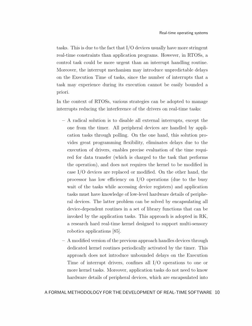
In the context of RTOSs, various strategies can be adopted to manage
interrupts reducing the interference of the drivers on real-time tasks:
– A radical solution is to disable all external interrupts, except the
one from the timer. All peripheral devices are handled by appli-
cation tasks through polling. On the one hand, this solution pro-
vides great programming flexibility, eliminates delays due to the
execution of drivers, enables precise evaluation of the time requi-
red for data transfer (which is charged to the task that performs
the operation), and does not requires the kernel to be modified in
case I/O devices are replaced or modified. On the other hand, the
processor has low efficiency on I/O operations (due to the busy
wait of the tasks while accessing device registers) and application
tasks must have knowledge of low-level hardware details of periphe-
ral devices. The latter problem can be solved by encapsulating all
device-dependent routines in a set of library functions that can be
invoked by the application tasks. This approach is adopted in RK,
a research hard real-time kernel designed to support multi-sensory
robotics applications [85].
– A modified version of the previous approach handles devices through
dedicated kernel routines periodically activated by the timer. This
approach does not introduce unbounded delays on the Execution
Time of interrupt drivers, confines all I/O operations to one or
more kernel tasks. Moreover, application tasks do not need to know
hardware details of peripheral devices, which are encapsulated into
A FORMAL METHODOLOGY FOR THE DEVELOPMENT OF REAL-TIME SOFTWARE 10

Real-time operating systems
kernel procedures. However, the processor has a low efficiency on
I/O operations, with a little higher system overhead with respect to
the previous approach, due to the communication required among
the application tasks and the I/O kernel routines for I/O data ex-
change. Moreover, the kernel needs to be updated when some device
is replaced or added. This approach is adopted in the MARS system
[54], [80].
– A third approach leaves all external interrupts enabled and reduces
the drivers to the least possible size. In fact, each driver activates a
proper task that will actually be the device manager: the dedicated
task executes under the direct control of the operating system, it
is scheduled and guaranteed like any other application task, and it
can be assigned lower priority than those of control tasks. With
respect to the first two solutions, this approach eliminates the busy
wait during I/O operations. Moreover, compared to the traditional
technique, it drastically reduces unbounded delays on the Execution
Time of tasks. The approach is adopted in the ARTS system [119],
[120], in HARTIK [41], [40], and in SPRING [115].
• System calls. Every kernel call should have a bounded Execution Time
and should be preemptable. This permits to achieve a higher precision
in the estimation of the Worst Case Execution Time (WCET) of tasks
and avoids delays on task computations.
• Semaphores. In traditional operating systems, semaphore operations
suffer from priority inversion, which occurs whenever a high priority task
waits for a low priority task to finish its execution for an unbounded
duration. Priority inversion can be avoided through the adoption of
various protocols, which bound the maximum blocking time of tasks
that share a critical section by controlling resource assignment and by
modifying the priority of tasks on the basis of the current resource usage.
• Memory management. Techniques for memory management must
A FORMAL METHODOLOGY FOR THE DEVELOPMENT OF REAL-TIME SOFTWARE 11

Real-time operating systems
not introduce nondeterministic delays on the Execution Time of tasks.
Memory segmentation with fixed-memory management scheme and sta-
tic partitioning are typical solutions adopted in most RTOSs. In gene-
ral, static allocation schemes increase the predictability of the system
but reduce its flexibility, which is a valuable feature in dynamic envi-
ronments. Therefore, the system designer attempts to strike a balance
between predictability and flexibility depending on the requirements of
the applications.
• Programming language. In the context of real-time systems, pro-
gramming languages should permit the specification of certain timing
behavior and realize predictable real-time applications. Unfortunately,
not all programming languages are expressive enough to support these
features.
– The Ada language [75] was developed by the Department of Defence
of the United States. It does not support the definition of explicit
time constraints on the execution of tasks and it embeds nondeter-
ministic statements, thus preventing a reliable worst-case analysis.
Moreover, since it does not provide any protocol for accessing sha-
red resources, a high-priority task may wait for a low priority task
to complete its execution for an unbounded duration.
– The Ravenscar profile [38] is an ISO-level subset of the concur-
rency model of Ada which was specifically conceived to meet design
and implementation requirements of high-integrity real-time sys-
tems, providing the basis for the implementation of deterministic
and time-analyzable real-time applications. It supports the deve-
lopment of single-processor real-time applications, comprised of a
fixed number of tasks which interact only by means of shared data
or protected objects with mutually exclusive access.
– Ada 2005 Real-Time Annex [19] is an update to the Ada language
that includes the Ravenscar profile [38] for high-integrity systems,
further dispatching policies such as Round Robin (RR) and Earliest
A FORMAL METHODOLOGY FOR THE DEVELOPMENT OF REAL-TIME SOFTWARE 12

Real-time operating systems
Deadline First (EDF), support for timing events and for control of
CPU time utilization.
– Real-Time Euclid [79] is a programming language specifically de-
signed to address reliability and guaranteed schedulability issues
in real-time systems. It supports the specification of timing para-
meters (e.g., the timer resolution) and timing constraints of both
periodic and aperiodic tasks (e.g., activation time, period). It pro-
vides a strict semantics that forces the programmer to specify time
bounds and timeout exceptions in all loops, waits, and device acces-
sing statements. Moreover, it addresses static real-time systems. As
a consequence, it does not support dynamic data structures (which
would prevent a correct evaluation of the time required by memory
allocation and deallocation) and recursion (which prevents the de-
termination of the Execution Time of subprograms).
– Real-Time Concurrent C [100] is a high-level programming language
for hard real-time applications that extends Concurrent C [64] by
providing facilities to specify periodicity and deadline constraints.
As characterizing traits, it addresses dynamic systems, where tasks
can be activated at run-time, and it allows the programmer to as-
sociate a deadline with any statement.
1.1.4 Standards for RTOSs
Standards play an important role in the context of operating systems, since
they define syntax and semantics of system calls, thus providing the interface
that the operating system exposes to the application layer. This facilitates
portability of applications from one platform to another and enables the deve-
lopment of a single application on top of kernels supplied by different providers,
thus promoting competition among vendors and increasing the quality of pro-
ducts. Current operating system standards mostly specify portability at the
level of source code, thus requiring the application to be recompiled for every
different platform. There are four main operating system standards available
A FORMAL METHODOLOGY FOR THE DEVELOPMENT OF REAL-TIME SOFTWARE 13

Real-time operating systems
today:
• RT-POSIX. Portable Operating System Interface for UniX (POSIX) is
a family of standards specifically designed to enable source code portabi-
lity of software applications across different operating systems platforms.
POSIX is standardized by IEEE as the IEEE Standard 1003, and also
by ISO/IEC as the international standard ISO/IEC 9945. It defines the
operating system interface by specifying syntax and semantics of core
functions (e.g., file operations, process management, signals, devices),
without indicating how these services should be implemented, so that
system developers can choose their implementation as long as they follow
the specification of the interface. Although POSIX is based on UNIX,
it can be applied to any operating system. An operating system is said
to be POSIX conformant if it implements the standard in its entirety
and this is certified by the Posix Conformance Test Suite; an operating
system is said to be POSIX compliant is it implements only portions of
the standard.
RT-POSIX is the real-time extension of POSIX and it is one of the most
successful and widely adopted standards in the area of RTOSs. It pro-
vides a set of system calls that facilitate concurrent programming and it
supports task synchronization through mutual exclusion resources acces-
sed according to the priority inheritance protocol, task synchronization
by means of condition variables, data sharing among tasks, and prio-
ritized message queues for inter-task communication. RT-POSIX also
defines services that permit to achieve predictable timing behavior, such
as fixed priority preemptive scheduling, sporadic server scheduling, time
management with high resolution, sleep operations, multipurpose timers,
Execution Time budgeting for measuring and limiting task Execution
Times, and virtual memory management.
• OSEK. OSEK/VDX [7] is a standard that specifies the interface of an
operating system for distributed control units in vehicles, supporting ef-
ficient utilization of resources and portability of software applications.
A FORMAL METHODOLOGY FOR THE DEVELOPMENT OF REAL-TIME SOFTWARE 14

Real-time operating systems
OSEK (Offene Systeme und deren Schnittstellen fur die Elektronik in
Kraftfahrzeugen; in English, Open Systems and their Interfaces for the
Electronics in Motor Vehicles) has been founded as a joint project in
the German automotive industry in May 1993. Initial project part-
ners were BMW, Bosch, DaimlerChrysler, Opel, Siemens, Volkswagen
Group, and the University of Karlsruhe. The French car manufacturers
PSA Peugeot Citroen and Renault joined OSEK in 1994 introducing
their VDX (Vehicle Distributed eXecutive) approach, which is a similar
project within the French automotive industry. In October 1995, the
OSEK/VDX group presented the results of the harmonized specification
between OSEK and VDX.
The OSEK/VDX standard addresses safety-critical real-time applica-
tions, allocated to a huge number of units and characterized by tight
timing constraints. For this reason, the standard attempts to reduce the
memory footprint as much as possible in order to enhance the operating
system performance. In order to support a wide range of systems with a
high degree of scalability, modularity, and configurability, the standard
defines four conformance classes that tightly specify the main features of
an operating system and it provides a toolchain where some configura-
tion tools help the designer in tuning the system services and the system
footprint. Moreover, a language called OIL (OSEK Implementation Lan-
guage) is proposed to help the definition of a standardized configuration
information. The operating system defined by the OSEK/VDX standard
does not specify any interface for the Input/Output subsystem: this re-
duces or even prevents the portability of the source code of applications,
since the I/O system quite impacts on the architecture of the application
software; however, the effort is not on achieving full compatibility bet-
ween different application modules, but much more on supporting their
direct portability between compliant operating systems.
The OSEK/VDX standard specifies a uniform communication environ-
ment for automotive control unit application software, called OSEK
Communication (OSEK COM), which provides a standardized API for
A FORMAL METHODOLOGY FOR THE DEVELOPMENT OF REAL-TIME SOFTWARE 15

Real-time operating systems
software communication (between nodes and within a node) that is in-
dependent of the communication media.
OSEK/VDX also includes a standardization of inter-networking inter-
faces, called OSEK Network Management (OSEK NM), which ensures
safety and reliability of communication networks. This is obtained by
implementing access restrictions to each node, by keeping the whole net-
work tolerant to faults, and by implementing diagnostic features capable
of monitoring the status of the network.
• ARINC 653. Avionic Application Standard Software Interface 653
(ARINC 653) [9] is a specification for an application executive used to
integrate avionics systems on modern aircrafts. It supports the imple-
mentation, certification, and execution of analyzable safety-critical real-
time applications for Integrated Modular Avionics architectures.
The ARINC 653 standard defines an APplication EXecutive (APEX) for
space and time partitioning which supports the development of multitas-
king applications. A partition represents a separate application, which
is assigned a dedicated memory space and a time slot; each application
is comprised of a set of tasks, which run under static priority scheduling
within the assigned time slot and communicate with each other through
message buffers, semaphores, and events. Tasks allocated to different
partitions communicate by exchanging messages through ports provided
by the API of the operating system. It is the responsibility of the sys-
tem integrator to ensure that all ports and channels are defined prior to
normal system operation. The mechanism used to write a message on an
API output port depends on whether the message is to be sent to another
partition running on the same processor, a partition running on another
processor, or an interface device. However, the same interface is used
in all the cases, making it relatively easy to move applications between
processors and to substitute software simulations of hardware devices for
testing. Each port may be configured to work in either sampling mode or
queueing mode: in the first case, not yet read messages are overwritten
A FORMAL METHODOLOGY FOR THE DEVELOPMENT OF REAL-TIME SOFTWARE 16

Real-time operating systems
by incoming messages; in the second case, incoming messages are queued
up.
Since each application is isolated from the others, ARINC 653 confor-
mance can be a step towards RTCA/DO-178B certification [60].
• Micro-ITRON. The Real-time Operating system Nucleus (TRON) is
the name of a project started by Dr. Ken Sakamura of the University
of Tokyo in 1984. The goal of the TRON Project has been to create
a concept of a computer architecture and network, in which common
everyday objects are embedded with computer intelligence and are able
to communicate with each other, thus increasing the collaboration of
electronic devices in the environment.
The TRON framework defines a complete architecture for different com-
puting units. Industrial TRON (ITRON) is the specification of an RTOS
for embedded systems which has become a de facto standard in the em-
bedded systems field, especially in Japan, where it is widely used in
mobile phones and other consumer products. Micro-ITRON 3.0 [108]
is a standard for a real-time kernel developed by the ITRON project
and includes the specification of communication features supporting the
implementation of an embedded system within a network. The Micro-
ITRON 4.0 specification [53] is based on the Micro-ITRON 3.0 specifica-
tion and it has been developed to improve compatibility and conformance
level, to increase productivity in software development, to allow reuse of
application software, and to achieve more portability. To this end, Micro-
ITRON 4.0 combines the loose standardization that is typical of ITRON
standards with a strict standardization of kernel functions, called Stan-
dard Profile, that is needed for portability. The Standard profile supports
the association of tasks with priorities, semaphores, message queues, and
mutual exclusion primitives with priority ceiling and priority inheritance
protocols.
A FORMAL METHODOLOGY FOR THE DEVELOPMENT OF REAL-TIME SOFTWARE 17

Real-time operating systems
1.1.5 Commercial and open source real-time kernels
At the present time, there are many commercial and open source RTOSs. This
Section gives a brief overview on some of them and Section 1.2 will provide a
more detailed description of the RTOS employed in the experimentation.
1.1.5.1 Commercial RTOSs
There are more than one hundred commercial RTOSs, from very small ker-
nels with a memory footprint of a few kilobytes to large multiprocessor sys-
tems for complex real-time applications. Most of them support concurrent
programming and static priority preemptive scheduling. Only a small subset
of commercial RTOSs supports dynamic priority scheduling (e.g., deadline-
driven priority scheduling) and implements some form of priority inheritance
to prevent priority inversion while accessing mutually exclusive resources. In
addition to traditional programming tools (e.g., editor, compiler, debugger),
commercial RTOSs usually provide specific tools for the development of real-
time applications (e.g., tools supporting performance profiling, tracing of ker-
nel activities, memory analysis, schedulability analysis, WCET analysis). The
most adopted commercial RTOSs are VxWorks [103], QNX, and OSE.
• VxWorks [103], [104], [105] is produced by Wind River Systems [8] and
it is the most adopted RTOS in embedded industry. It supports fixed
priority preemptive scheduling and RR scheduling; it enables inter-task
communication through shared variables, semaphores (with support for
priority inheritance protocol), message queues, pipes, sockets, and re-
mote procedure calls; it provides a cross-compiler and associated pro-
grams, a performance profiler to estimate the Execution Time of routines,
some utilities to monitor the way how the processor is used by tasks, and
a simulator to emulate the target system along the development process
or during the testing phase.
VxWorks 5.x and 6.x conform to the real-time POSIX 1003.1b standard.
Support for graphics, multiprocessing, memory management, connecti-
A FORMAL METHODOLOGY FOR THE DEVELOPMENT OF REAL-TIME SOFTWARE 18

Real-time operating systems
vity, Java, and file system is provided by separate services. Tornado and
Workbench are the integrated development environments for VxWorks
5.x and 6.x releases, respectively.
• QNX Neutrino [73] is a microkernel RTOS that provides a comprehen-
sive, integrated set of technologies supporting the development of robust
and reliable mission-critical applications. Fundamental operating sys-
tem services (i.e., signals, timers, and scheduling) are implemented in
the microkernel, while the other components (i.e., file systems, drivers,
protocol stacks, applications) run outside the kernel. As a result, a de-
fected component can be automatically restarted without affecting other
components or the kernel. QNX supports the priority inheritance proto-
col in order to avoid priority inversion, and nested interrupts in order to
enable priority-driven interrupt handling. Communication among sys-
tem components is performed through message passing.
The QNX RTOS complies with the POSIX 1003.1-2001 standard and
with its real-time extension, and it includes a module for power manage-
ment that allows the developer to control power consumption of system
components and adopt specific power management strategies.
Since September 2007, QNX offers a licence for non-commercial use.
• OSE [97] is a modular, high-performance, full-featured RTOS, optimized
for complex distributed systems that require the utmost in availability
and reliability. It is produced by ENEA and it is widely used in au-
tomotive and communications industry. It provides three families of
operating systems that implement the OSE API at different levels: OSE
is the portable kernel, OSEck is the compact kernel for Digital Signal
Processors (DSPs), and Epsilon is a set of highly optimized assembly
kernels. It supports both static and dynamic processes, and different
categories of processes which run under different scheduling principles:
interrupt processes and priority-based processes are scheduled according
to their priority; timer interrupt processes are are triggered cyclically;
background processes are scheduled in RR manner; phantom processes
A FORMAL METHODOLOGY FOR THE DEVELOPMENT OF REAL-TIME SOFTWARE 19

Real-time operating systems
are not scheduled at all and they are used to redirect signals. Commu-
nication among processes is performed through message queues.
1.1.5.2 Linux-based real-time kernels
Linux [5] is a free Unix-type operating system kernel, originally conceived and
created by Linus Torvalds in 1991 and then developed with the assistance and
contributions of thousands of programmers around the world.
Linux provides two distinct modes of operation of the CPU: kernel mode
is a privileged mode in which the CPU is assumed to be executing trusted
software and it can reference any memory address; user mode is other than
kernel mode, and it is a non-privileged mode in which each running instance
of a program is not allowed to access those portions of memory that have been
allocated to the kernel or to other programs. The kernel is the core of the
operating system and it is considered trusted software; any other program is
considered untrusted software and must request the use of the kernel by means
of a system call in order to perform privileged instructions (e.g., task creation
and destruction, I/O operations).
The Linux kernel is non-preemptive through version 2.4: while a process
runs in kernel mode, it cannot be suspended and replaced by another process
(i.e., preempted), but it can be suspended only if it voluntarily relinquishes
the control of the CPU or if an interrupt or an exception occurs. According to
this, when a user process runs a portion of the kernel code via a system call,
it temporarily becomes a kernel process and it runs in kernel mode until the
kernel has satisfied the process request, no matter how long that might take.
The Linux kernel version 2.6 (which was introduced in late 2003) is preemptive:
a process running in kernel mode can be suspended in order to run a different
process. This is obtained through the introduction of preemption points, which
are instructions that allow the scheduler to run and possibly block the current
process so as to schedule a higher priority process. Unreasonable delays in
system calls are thus avoided by periodically testing a preemption point. This
can be an important benefit for real-time applications but it is not enough
A FORMAL METHODOLOGY FOR THE DEVELOPMENT OF REAL-TIME SOFTWARE 20

Real-time operating systems
to guarantee strict timing constraints. To this end, the Linux kernel can be
extended in different manners in order to support hard real-time applications.
• RTLinux [126] is a real-time extension for the Linux kernel initially de-
veloped by Victor Yodaiken, Michael Barabanov, and Cort Dougan at
the New Mexico Institute of Mining and Technology. It is distributed by
Finite State Machine Labs [4].
RTLinux works as a small executive with a real-time scheduler that runs
Linux as a completely preemptable thread with lowest priority. RTLinux
real-time threads and Linux processes can communicate by means of a
shared memory space or through a file-like interface. The standard Li-
nux interrupt handler routine and the macros for interrupt enabling and
disabling are modified so that the RTLinux interrupt routine is executed
whenever an interrupt is raised: if the interrupt is related to a real-time
activity, then a real-time thread is notified and RTLinux executes its own
scheduler; otherwise, Linux interrupt service routine is delayed until no
real-time thread is active.
This approach provides a separation of concerns between the Linux ker-
nel and the real-time micro-kernel and permits to execute Linux as a
background activity in the real-time executive, thus reducing the la-
tency on real-time activities. However, real-time tasks execute in the
same address space of the Linux kernel and, thus, a fault in a user task
may crash the kernel. Moreover, there is no direct support for resource
management policies and it is often necessary to re-write drivers for real-
time applications, since real-time threads cannot use the standard Linux
device driver mechanism.
• Real-Time Application Interface (RTAI) [95] is a real-time extension for
the Linux kernel that builds on the original idea of RTLinux [126]. Its
main features will be discussed in Section 1.2.
• Linux Resource/Kernel (Linux/RK) [6], [96] is developed by the Real-
time and Multimedia Systems Laboratory led by Dr. Raj Rajkumar
A FORMAL METHODOLOGY FOR THE DEVELOPMENT OF REAL-TIME SOFTWARE 21

Real-time operating systems
at Carnegie Mellon University. It provides a real-time extension of the
Linux kernel according to a different approach with respect to RTLinux
[126] and RTAI [95], by directly modifying the Linux kernel in order
to supply it with those features that support the development and the
execution of applications with strict timing constraints.
Linux/RK is a resource kernel based on Linux, i.e., a real-time kernel that
provides timely, guaranteed, and enforced access to system resources for
applications. An application can request the reservation of a certain
amount of a resource (e.g., CPU time, physical memory page, network
bandwidth, disk bandwidth) and the kernel can guarantee that the re-
quested amount is available to the application. Such a guarantee of
resource allocation gives an application the knowledge of the amount of
its currently available resources. A Quality of Service (QoS) manager or
an application itself can then optimize system behavior by computing
the best QoS obtained from the available resources.
1.1.5.3 Research kernels
Research kernels are characterized by the ability to associate tasks with explicit
time constraints (e.g., period, deadline) and with additional parameters used
to analyze the dynamic performance of the system, by the possibility to verify
in advance whether timing constraints of an application will be met during the
execution, and by the use of specific resource access protocols not only to avoid
priority inversion but also to limit the blocking time on mutually exclusive
resources. Most of the kernels that exhibit these features are developed by
universities and research centers, such as SHARK, MaRTE and ERIKA.
• Soft and HArd Real-time Kernel (SHARK) [63] is a dynamic configu-
rable kernel architecture developed at the Scuola Superiore S. Anna in
Pisa. It is expressively designed to support the implementation and
testing of new scheduling algorithms and resource management proto-
cols, and it manages hard real-time, soft real-time, and non real-time
A FORMAL METHODOLOGY FOR THE DEVELOPMENT OF REAL-TIME SOFTWARE 22

Real-time operating systems
applications. SHARK comprises a Generic Kernel, which does not im-
plement any particular scheduling algorithm or resource management
protocol, but postpones scheduling decisions and the adoption of access
policies to shared resources to external scheduling modules and resource
modules, respectively. Modules can be registered at initialization, thus
achieving full modularity in scheduling and resource management poli-
cies. According to this, an application can be developed independently
of a particular system configuration, so that new modules can be ad-
ded or replaced in the same application, in order to evaluate the effects
of specific scheduling policies in terms of predictability, overhead, and
performance.
The system is compliant with almost all the POSIX 1003.13 PSE52 spe-
cifications in order to simplify the porting of application code developed
for other POSIX compliant kernels.
• Minimal Real-Time operating system for Embedded applications (MaRTE)
[102] is an HRTOS developed at the University of Cantabria, which pro-
vides an easy to use and controlled environment to develop multi-thread
real-time applications. It follows the Minimal Real-Time POSIX 1003.13
subset and implements the Ada 2005 Real-Time Annex, which includes
the Ravenscar profile [38]. It is available under the GNU General Public
License 2 at http://marte.unican.es/.
MaRTE supports the implementation and cross-development of mixed
language applications in Ada, C, and C++ through the GNU compi-
lers Gnat and Gcc. The kernel has an hardware abstraction layer which
provides an interface to operations for interrupt management, clock and
timer management, and thread context switches, thus facilitating migra-
tion of application code from one platform to another.
• Embedded Real-tIme Kernel Architecture (ERIKA) [2] is a free of charge,
open-source implementation of the OSEK/VDX API [7] distributed by
Evidence s.r.l. [3] under the GNU GPL licence. It provides two ver-
sions: ERIKA Enterprise, which supports new hardware platforms in
A FORMAL METHODOLOGY FOR THE DEVELOPMENT OF REAL-TIME SOFTWARE 23

Real-Time Application Interface
automotive applications, and ERIKA Educational, which is developed
for teaching and didactical purposes.
ERIKA provides a set of modules which implement task management and
real-time scheduling policies. The hardware abstraction layer contains
the hardware dependent code that manages context switches and inter-
rupt handling.
1.2 Real-Time Application Interface
Real-Time Application Interface (RTAI) [95] is a real-time extension for the Li-
nux kernel that supports the development of real-time applications with strict
timing constraints for several architectures (x86, x86 64, PowerPC, ARM).
The project was initially started from the original RTLinux code [126] by
Prof. Paolo Mantegazza from the Dipartimento di Ingegneria Aerospaziale
of Politecnico di Milano and it is now a living open-source project developed
by a wide community. Although the architectures of RTAI and RTLinux are
quite similar, RTAI has considerably built on and enhanced the original idea
of RTLinux and the API of the projects were developed according to oppo-
site principles. The main features and system calls of RTAI are not POSIX
compliant, although RTAI implements a compliant subset of POSIX 1003.1.c.
1.2.1 RTAI architecture
Both RTLinux and RTAI provide a small RTOS that runs the standard Linux
kernel as the lowest priority task, which is allowed to execute whenever no
real-time task is schedulable. While RTLinux applies most changes directly to
the kernel source files, resulting in modifications and additions to numerous
Linux files, RTAI limits the changes to the standard Linux kernel by adding a
layer of virtual hardware between the standard Linux kernel and the hardware
itself. Until RTAI 3.0, this layer relied on the so called Real-Time Hardware
Abstraction Layer (RTHAL), which is comprised of an interrupt dispatcher
A FORMAL METHODOLOGY FOR THE DEVELOPMENT OF REAL-TIME SOFTWARE 24

Real-Time Application Interface
that intercepts, processes, and redirects hardware interrupts (see Fig. 1.1). A
real-time interrupt is immediately served by the real-time kernel through the
invocation of the corresponding real-time handler; a non real-time interrupt is
queued up as a pending interrupt, and it is served by the Linux kernel when
no real-time task is running. In so doing, the RTHAL provides a framework
onto which RTAI is mounted with the ability to fully preempt the Linux kernel.
The RTHAL was implemented by modifying less than 20 lines of existing code,
and by adding about 50 lines of new code, thus minimizing the changes on the
standard Linux kernel and thereby improving the maintainability of RTAI and
the Linux kernel code. The fact that every interrupt is intercepted by the
RTHAL imposes an additional overhead and causes a little increase in the
average value of latency; nevertheless, RTAI ensures much smaller maximum
values of latency than a standard kernel, thus improving determinism and
responsiveness [16], [86].
L i n u x k e r n e l
H a r d w a r e
R T H A L
R e a l - t i m e k e r n e l
i n t e r rup t
rea l - t ime i n t e r rup tp e n d i n g L i n u x i n t e r r u p t s
n o n r e a l - t i m e i n t e r r u p t
K e r n e l s p a c e
Figure 1.1. The RTHAL-based RTAI architecture.
RTLinux is covered by the US Patent 5995745, issued on November 30,
1999 and entitled “Adding Real-Time Support To General Purpose Operating
A FORMAL METHODOLOGY FOR THE DEVELOPMENT OF REAL-TIME SOFTWARE 25

Real-Time Application Interface
Systems”. In order to avoid legacy constraints of this patent and to provide
a more structured and flexible technology to add real-time features to Linux,
the RTAI community has developed the Adaptive Domain Environment for
Operating Systems (ADEOS). The general design of the Adeos nanokernel
[1] has been proposed by Karim Yaghmour and it provides an extensible and
adaptive environment that enables the sharing of hardware resources among
multiple entities called domains, each represented by an operating system or
by an instance of an operating system [125]. In the RTAI architecture, ADEOS
provides a resource virtualization layer between the computer hardware on the
one hand, and Linux and RTAI on the other one, as reported in Fig. 1.2.
R T A I
H a r d w a r e
A D E O S
L i n u x
Figure 1.2. The ADEOS-based RTAI architecture.
Resource sharing among different domains is achieved through an interrupt
pipeline. Each domain is assigned a static priority level, which is used for a
proper dispatch order of events. In fact, domains are queued up according to
their respective priority and hardware interrupts are propagated through the
pipeline, from its head (i.e., the highest priority domain) down to its tail (i.e.,
the lowest priority domain). A domain may:
• accept and handle the interrupt, and then decide whether to propagate
it to the next stage or not;
• ignore and stall the interrupt, handling it in a subsequent moment, and
A FORMAL METHODOLOGY FOR THE DEVELOPMENT OF REAL-TIME SOFTWARE 26

Real-Time Application Interface
then decide whether to propagate it to the next domain or not;
• discard the interrupt and propagate it to the next stage;
• terminate the interrupt without propagating it through the pipeline.
In the ADEOS architecture, RTAI is installed as the highest priority domain,
thus guaranteeing that it always intercepts and handles hardware interrupts
before the standard Linux kernel, as is illustrated in Fig. 1.3.
h a r d w a r e i n t e r r u p t R T A I .. . L i n u x .. .
Figure 1.3. The event pipeline of ADEOS with RTAI and Linux.
1.2.2 RTAI schedulers
RTAI is a full-featured real-time micro-kernel. Both basic services (e.g., the
schedulers) and advanced services (e.g., POSIX compliant functions) are im-
plemented as kernel modules, which can be loaded or unloaded using the stan-
dard Linux insmod and rmmod commands as their respective capabilities are
required or released.
RTAI supports various types of schedulers, each suited to a specific combi-
nation of hardware and task requirements. In particular, RTAI provides three
priority-based preemptive real-time schedulers:
• UniProcessor (UP) scheduler: it is used on uni-processor platforms.
• Symmetric MultiProcessor (SMP) scheduler: it is used on multi-processor
platforms and supports symmetric workload distribution among the va-
rious CPUs. Tasks can run symmetrically on any CPU or on a cluster
of CPUs, or they can be bound to run on a single CPU.
A FORMAL METHODOLOGY FOR THE DEVELOPMENT OF REAL-TIME SOFTWARE 27

Real-Time Application Interface
• Multi-UniProcessor (MUP) scheduler: it is used on multi-processor plat-
forms. Each task is forced to execute on a single CPU, which is assigned
when the task is created. This restricts the flexibility of MUP scheduler
with respect to SMP scheduler, but increases its efficiency.
RTAI provides two scheduler’s operation modes, depending on the way how
the timer is programmed:
• Periodic mode: the timer is programmed to emit interrupts at fixed time
intervals and the scheduler is executed at the end of each period. The
period of a periodic task should be a multiple of the scheduler’s period,
otherwise it is approximated to the nearest multiple of the scheduler’s
period.
• One-shot mode: the timer is re-programmed at each interrupt, according
to the task that is going to execute. It allows a higher flexibility with
respect to periodic mode, but it imposes an additional overhead due to
the necessity to re-program the timer at each interrupt.
RTAI natively supports various scheduling policies:
• First In First Out (FIFO): tasks are statically associated with a priority
level and the CPU is assigned to the task with highest priority until
the task completes its execution or it voluntarily releases the CPU or a
task with higher priority becomes active. Tasks with equal priority are
queued up according to their activation time (i.e., priorities being equal,
the first task queued up is the first to be resumed).
• Round Robin (RR): tasks are statically assigned a priority level and the
CPU is assigned to the highest priority task for a time no longer than
a predefined unit of time, called time slice or quantum. A task can be
preempted if a higher priority task becomes active before the time slice
has elapsed. Tasks with equal priority are queued up according to their
activation time.
A FORMAL METHODOLOGY FOR THE DEVELOPMENT OF REAL-TIME SOFTWARE 28

Real-Time Application Interface
• Rate Monotonic Priority Order (RM): tasks are statically assigned prio-
rities according to their request rates (i.e., the higher the request rate,
the higher the priority level). The request rate of a periodic task is repre-
sented by its period (i.e., the shorter the period, the higher the priority
level). The currently executing task is preempted whenever a task with
shorter period is released.
• Earliest Deadline First (EDF): tasks are dynamically assigned priorities
according to their absolute deadlines (i.e., the earlier the deadline, the
higher the priority level). The currently executing task is preempted
whenever a task with earlier deadline becomes active.
RTAI enables the execution of hard real-time tasks both in the kernel space
and in the user space. Real-time tasks that run in the kernel space are im-
plemented as loadable kernel modules and, thus, they are integral part of the
kernel. As a consequence, they are not bounded by the memory protection
services of Linux and they have the ability to overwrite system-critical areas
of memory.
LinuX Real-Time (LXRT) is an extension of RTAI that enables the de-
velopment of real-time tasks in the user space, where memory protection is
enabled, and allows applications to dynamically switch between real-time and
non real-time operation. This behavior is obtained by associating each task in
the user space that has real-time requirements with a real-time agent in the
kernel space. When the user task enters hard real-time mode, the real-time
agent disables interrupts, takes the task out of the queue of running tasks of
the Linux scheduler and adds it to the queue of the RTAI scheduler. Although
performance under LXRT is quite good, it imposes higher values of latency
with respect to the execution of real-time tasks in the kernel space.
1.2.3 RTAI IPC mechanisms
Real-time tasks are not allowed to use services provided by the standard Linux
kernel. For this reason, RTAI developers implemented various IPC mecha-
A FORMAL METHODOLOGY FOR THE DEVELOPMENT OF REAL-TIME SOFTWARE 29

Software development processes
nisms, which are employed to transfer and share data between tasks in both
the real-time domain and Linux user space domain. IPC mechanisms are im-
plemented as kernel modules, which can be loaded in addition to basic RTAI
and schedulers modules only when they are requested by real-time tasks.
• Real-Time FIFO queues: they provide an asynchronous and unblocking
one-way communication channel, whose size limit is assigned by the pro-
grammer when the queue is created.
• Semaphores: they are data structures associated with a counter and they
enable mutual exclusion and synchronization among tasks.
• Shared Memory: it is a block of memory that can be read and written
by any task in the system. This provides an alternative communication
paradigm with respect to RTAI FIFOs and it is much more suitable when
a big amount of data needs to be transferred.
• Messages and Remote Procedure Calls: they provide a point-to-point
communication mechanism where the sender task and the receiver task
are supposed to know each other.
• Mailboxes: they provide a flexible communication mechanism to ex-
change data among tasks. The size of a mailbox is defined by the
programmer when it is created and multiple senders and receivers are
allowed.
1.3 Software development processes
A software life cycle process comprises all the activities and work products
necessary to develop a software system. In software engineering, various deve-
lopment models have been proposed and applied throughout the years. Section
1.3.1 provides a brief overview of various software life cycle processes and Sec-
tion 1.3.2 focuses on the V-Model framework [42] which is considered as a
reference in this dissertation.
A FORMAL METHODOLOGY FOR THE DEVELOPMENT OF REAL-TIME SOFTWARE 30

Software development processes
1.3.1 From the waterfall model to eXtreme Programming
The waterfall model is a sequential approach to software development, which
was first described by Winston Royce in 1970 [107]. Although the original mo-
del makes provision for feedback loops at the end of each activity, the majority
of organizations that apply this life cycle process treat it as if it were strictly li-
near. The model begins with customer specification of requirements, which are
reviewed and assessed with respect to completeness, consistency, and clarity;
then, it progresses through planning, modeling, construction, and deployment;
finally, it culminates in on-going maintenance of the completed software, which
sustains the useful operation of the system in its target environment by provi-
ding requested functional enhancements, repairs, performance improvements,
and conversions. The main criticism of this model is that each stage of the
process must be completed before moving to the next one, which comprises
an idealized framework that has difficulties in accommodating iterations and
requirements changes. However, real projects rarely follow the sequential flow
that the model proposes, primarily because it is often difficult for the customer
to state all requirements explicitly at the beginning of the project. For this
reason, various modified versions of the waterfall model have been proposed
which may include slight or major variations upon this process.
The spiral model is an iterative software life cycle process proposed by
Barry Boehm in 1986 to address the source of weaknesses in the waterfall mo-
del and accommodate frequent changes during software development [31]. The
approach integrates the phases of the waterfall model with several activities
addressing risk management, reuse, and prototyping. In particular, each deve-
lopment phase corresponds to one cycle or round of the spiral and involves the
same sequence of steps: Determine objectives, alternatives, and constraints,
which define the problem addressed by the current cycle; Evaluate alterna-
tives: identify and resolve risks, which defines the solution space and serves
to identify future problems that may turn out to be highly expensive; Develop
and verify next level product, which is the realization of the cycle; Plan next
phases, which prepares the next cycle.
A FORMAL METHODOLOGY FOR THE DEVELOPMENT OF REAL-TIME SOFTWARE 31

Software development processes
The Unified Process (UP) is an iterative and incremental development pro-
cess proposed by Grady Booch, Ivar Jacobson, and James Rumbaugh in 1999
[76]. Similar to the spiral model, in the UP, a project consists of several
cycles each ending with the delivery of a product to the customer. Each cycle
consists of four phases: Inception, Elaboration, Construction, and Transition.
Each phase includes a number of iterations and each iteration, in turn, results
in an increment, which is a release of the system that contains added or im-
proved functionality compared with the previous release. The Inception phase
provides an initial evaluation of feasibility costs; the Elaboration phase corres-
ponds to the initiation process, during which the project is planned, the system
is defined, and resources are allocated; the Construction phase addresses the
implementation of system components; the Transition phase is responsible for
system installation and post-development processes.
Agile software development refers to a group of software development me-
thodologies based on iterative development, where requirements and solutions
evolve through collaboration between self-organizing cross-functional teams.
The eXtreme Programming (XP) [21] is a form of agile development that fo-
cuses on short development cycles and close interaction with customers. In
traditional system development methods, system requirements are determined
at the beginning of the development project and often fixed in subsequent
phases, which can be extremely costly at later stages of development. Like
other agile software development methods, XP attempts to reduce the cost of
change through multiple short development cycles, rather than a single long
one. In this doctrine, changes are a natural, inescapable, and desirable aspect
of software development projects and they should be planned for, instead of
attempting to define a stable set of requirements.
1.3.2 The V-Model software life cycle
The V-Model [42] is a framework for the organization of development, mainte-
nance and modification processes in the life cycle of software systems, issued as
a standard by the German Federal Administration and widely practiced in the
A FORMAL METHODOLOGY FOR THE DEVELOPMENT OF REAL-TIME SOFTWARE 32

Software development processes
industry of safety-critical software systems. It is a variation of the waterfall
model that builds a V shape sequence of development activities, highlighting
the relationship between each phase of design and its associated phase of tes-
ting and introducing feedback loops between them. Fig. 1.4 reports a scheme
of the System Development (SD) Submodel, emphasizing the relation between
Design and Verification activities (left/right) and the hierarchical decomposi-
tion from System Level to SW Module Level (top/down).
SD1S y s t e m R e q u i r e m e n t s Ana lys is
SD2 S y s t e m D e s i g n
U s e r R e q u i r e m e n t s
S y s t e m A r c h i t e c t u r e
SD3S W / H W R e q u i r e m e n t s Ana lys is
T e c h n i c a l R e q u i r e m e n t s
SD4 -SWP r e l i m i n a r y S o f t w a r e Des ign
S o f t w a r e A r c h i t e c t u r e
S D 5 - S WD e t a i l e d S o f t w a r e Des ign
SD6-SWS W I m p l e m e n t a t i o n
SD7 -SW SW In tegra t ion
SD8 Sys tem In tegra t ion
SD9 T rans i t ion to Ut i l i za t ion
S o f t w a r e D e s i g n
S y s t e m L e v e l
S y s t e m L e v e l
U n i t L e v e l
S W C o m p o n e n t L e v e l
S W M o d u l e L e v e l
Figure 1.4. V-Model: activities of the System Development Submodel.
System Requirements Analysis (SD1) determines the overall system-level
functional and non-functional User Requirements. System Design (SD2) ge-
nerates a possible solution for the technical system structure called System
A FORMAL METHODOLOGY FOR THE DEVELOPMENT OF REAL-TIME SOFTWARE 33

Software development processes
Architecture, identifies its Units and the User Requirements managed by each
of them, and defines the interfaces of the system to the environment and
the interfaces between system Units. Software/Hardware Requirements Ana-
lysis (SD3) decomposes each Unit into SW and HW Components and allocates
Technical Requirements to them. While SD1 and SD2 have system scope, SD3
is repeated for each single Unit.
Preliminary Software Design (SD4-SW) specifies the Software Architecture
of each SW Unit as a set of concurrent and interacting tasks with assigned func-
tional low-level modules, prescribed release times, and deadlines. The Software
Design is completed in the subsequent activity SD5-SW with the allocation of
resources and time requirements to SW Modules. The sub-activity Analysis of
Resources and Time Requirements (SD5.2-SW), not shown in Fig. 1.4, inves-
tigates calculated requirements in order to verify their feasibility. If Software
Design satisfies resources and time requirements with a sufficient margin of
laxity, maintenance and modification measures can be taken without a huge
effort in re-design.
Software Implementation (SD6-SW) translates the Software Design of each
Unit into executable code, which is subject to self-assessment through the unit-
testing of SW Modules in the sub-activity Self Assessment of the Software
Module (SD6.3-SW), not shown in Fig. 1.4.
Software Integration (SD7-SW) verifies the integration of SW Modules wi-
thin each SW Component (SW Component Level in Fig. 1.4) and then the
integration of SW Components within each SW Unit (Unit Level in Fig. 1.4).
Finally, System Integration (SD8) composes units and performs self-assessment
of the system, while Transition to Utilization (SD9) operates the transition
that leads to install the completed system at the intended application site and
to put it into operation.
A FORMAL METHODOLOGY FOR THE DEVELOPMENT OF REAL-TIME SOFTWARE 34

Mapping the theory of pTPNs onto a V-Model software life cycle
1.4 Mapping the theory of pTPNs
onto a V-Model software life cycle
The development of real-time software can largely benefit from the applica-
tion of formal methods, which add rigor to design and verification activities
and reduce the possible gap between the verified abstraction and its actual
implementation. This dissertation devises a formal methodology that casts
the theory of pTPNs in a tailoring of the V-Model life cycle [42], facing the
aspects of concurrency and timing in the construction of real-time software
components and meeting the prescriptions of main regulatory standards [60],
[50], [77] in the integration of formal methods along the development of safety-
critical software. In the literature, various works provide specific contributions
in the application of formal methods to individual phases of software life cycle.
However, none of them devises a comprehensive approach that supports the
development process in systematic and organic manner from software design
through software implementation and testing. For this reason, the comparison
with related works is addressed throughout the dissertation in the Chapters
that illustrate the application of the proposed approach to specific steps of
software life cycle.
The methodology proposed in this dissertation supports software develop-
ment from the activity SD4-SW through the activity SD7-SW, as shown in
Fig. 1.5. The process is illustrated with reference to an example in the field of
Intelligent Visual Surveillance Systems (IVSSs), which will serve as running
case along the treatment. The case study concerns a vision system which per-
forms real-time 3D tracking of multiple people moving over an extended area
by employing a pan-tilt-zoom (PTZ) camera [29]. In the activity SD1, User
Requirements define parameters of the vision system, such as the frame rate
(i.e., 25 frames per second), the image size (i.e., 160 x 120 pixels), the compres-
sion format (i.e., JPEG), the operating temperature (i.e., from 0◦C to 40◦C),
the camera mass (i.e., up to 1.5 Kg). In the activity SD2, System Architecture
is specified through the Unified Modeling Language (UML) profile for Modeling
A FORMAL METHODOLOGY FOR THE DEVELOPMENT OF REAL-TIME SOFTWARE 35

Mapping the theory of pTPNs onto a V-Model software life cycle
SD1S y s t e m R e q u i r e m e n t s Ana lys is
SD2 S y s t e m D e s i g n
U s e r R e q u i r e m e n t s
S y s t e m A r c h i t e c t u r e
SD3S W / H W R e q u i r e m e n t s Ana lys is
T e c h n i c a l R e q u i r e m e n t s
SD4 -SWP r e l i m i n a r y S o f t w a r e Des ign
S o f t w a r e A r c h i t e c t u r e
S D 5 - S WD e t a i l e d S o f t w a r e Des ign
SD6-SWS W I m p l e m e n t a t i o n
SD7 -SW SW In tegra t ion
SD8 Sys tem In tegra t ion
SD9 T rans i t ion to Ut i l i za t ion
S o f t w a r e D e s i g n
S y s t e m L e v e l
S y s t e m L e v e l
U n i t L e v e l
S W C o m p o n e n t L e v e l
S W M o d u l e L e v e l
Figure 1.5. V-Model: activities of the System Development Submodel. Activitiesimpacted by the usage of pTPN theory are highlighted in grey.
and Analysis of Real-Time and Embedded systems (MARTE) [66], which is an
extension of the UML [67], [68] expressively designed to support the specifica-
tion of real-time and embedded systems. The UML-MARTE class diagram of
System Architecture of the case example is reported in Fig. 1.6: the system
consists of a Control Unit, a PTZ Camera, and a Video Processing Unit. The
Control Unit receives images acquired by the PTZ Camera, sends them to the
Video Processing Unit, and receives the elaborated images back. On the basis
of these results, the Control Unit sets parameters of image processing algo-
rithms (e.g., window size of non-linear filters) and parameters at which images
are acquired (e.g., the levels of pan, tilt, and zoom), and sends them to the
A FORMAL METHODOLOGY FOR THE DEVELOPMENT OF REAL-TIME SOFTWARE 36

Mapping the theory of pTPNs onto a V-Model software life cycle
Video Processing Unit and to the PTZ Camera, respectively. In the activity
Figure 1.6. UML-MARTE class diagram of the System Architecture of an IVSS.The ProcessingResource stereotype models an active, protected, executing-typeresource that is allocated to the execution of schedulable resources. The Device-Resource stereotype specializes the concept of processing resource and typicallyrepresents an external device that may be manipulated or invoked by the plat-form and that may require specific services in the platform for its usage and/ormanagement, but whose internal behavior is not a relevant part of the modelunder consideration. A CommunicationMedia represents the mean to transportinformation from one location to another.
SD3, system units are detailed through the UML-MARTE class diagrams re-
ported in Figs. 1.7 and 1.8 and their SW and HW Components are referred
to as Computer Software Configuration Items (CSCIs) and Hardware Configu-
ration Items (HCIs), respectively. The Control Unit communicates with the
PTZ Camera and with the Video Processing Unit through a serial bus; boards
of both the Control Unit and the Video Processing Unit run RTAI operating
system [95]. The Control Unit comprises a CSCI (i.e., System Management
CSCI) and two HCIs (i.e., a board and a battery): the CSCI is mapped on an
RTAI task-set and allocated to the board. The PTZ Camera consists of two
HCIs (i.e., the Image Sensor Unit and the Mechanical PTZ Unit). The Video
Processing Unit comprises three CSCIs (i.e., Images Acquisition CSCI, Basic
Features Extraction CSCI, and Multiple Target Tracking CSCI) and four HCIs
(i.e., three boards and a battery): each CSCI is mapped on a different RTAI
task-set and allocated to a different board.
The methodology that is proposed in this dissertation comes into play with
the activities SD4-SW and SD5-SW, where each CSCI is mapped on a task-set
according to the following model derived from the practice of real-time systems
[39], [116] and described by the UML diagram [67], [68] of Fig. 1.9:
• A task releases jobs in recurrent manner with periodic, sporadic or jit-
A FORMAL METHODOLOGY FOR THE DEVELOPMENT OF REAL-TIME SOFTWARE 37

Mapping the theory of pTPNs onto a V-Model software life cycle
Figure 1.7. UML-MARTE class diagram of the Control Unit and the PTZ Cameraof the IVSS of Fig. 1.6. The rtUnit stereotype models a real-time applicationthat owns one or more schedulable resources. A SchedulableResource is an activeresource able to perform actions using the processing capacity brought from aprocessing resource by the scheduler that manages it. A Hw Card symbolizes aprinted circuit board, which typically comprises other sub-components like chipsand electrical devices. The allocate stereotype identifies an allocation relationbetween elements of the application model, represented through the stereotypeApplicationAllocationEnd, and elements of the execution platform, modeled bythe stereotype ExecutionPlatformAllocationEnd. A Hw PowerSupply is a hard-ware component that supplies the hardware platform with power. The Hw Busstereotype represents a particular wired channel with specific functional proper-ties.
tering policy, depending on whether the release time is deterministic,
bounded by a minimum but not a maximum value, or constrained bet-
ween a minimum and a maximum value, respectively.
• A job is internally structured as a sequence of chunks, each characterized
A FORMAL METHODOLOGY FOR THE DEVELOPMENT OF REAL-TIME SOFTWARE 38

Mapping the theory of pTPNs onto a V-Model software life cycle
Figure 1.8. UML-MARTE class diagram of the Video Processing Unit of theIVSS of Fig. 1.6.
by a non-deterministic Execution Time constrained within a minimum
and a maximum value. Chunks representing a computation are also
associated with an entry-point function for the attachment of functional
behavior to the corresponding low-level module.
A FORMAL METHODOLOGY FOR THE DEVELOPMENT OF REAL-TIME SOFTWARE 39

Mapping the theory of pTPNs onto a V-Model software life cycle
• Chunks belonging to jobs of different tasks may have dependencies (e.g.,
semaphore synchronization, message passing through a mailbox) and
they may require resources (e.g., one or more processors), in which
case they are associated with a priority level and run under static prio-
rity preemptive scheduling. Wait and signal semaphore operations are
constrained to occur at the beginning and at the end of chunks, respecti-
vely, but a semaphore may be held across multiple subsequent chunks of
the same task. Receipt and dispatch mailbox operations are constrained
to occur at the beginning and at the end of chunks, respectively, and
each mailbox is shared between two tasks.
Figure 1.9. UML diagram of the conceptual model of task-set.
The activity SD4-SW defines the structure of the task-set allocated to each
CSCI, identifies minimum release inter-times and deadlines which are directly
issued from Technical Requirements, and assigns task periods which are design
choices. The activity SD5-SW refines the design of each task-set through the
specification of target processors, task priorities, and allowed time-frames of
computation chunks: in the usual practice, the latter design choice is initially
based on analogy with previous realizations and may require iterations along
the development process. In the activities SD4-SW and SD5-SW, task-sets are
represented through a semi-formal specification and automatically translated
A FORMAL METHODOLOGY FOR THE DEVELOPMENT OF REAL-TIME SOFTWARE 40

Mapping the theory of pTPNs onto a V-Model software life cycle
into pTPN models through the Oris Tool [43]. The sub-activity SD5.2-SW is
supported by pTPN theory and the Oris Tool through simulation and state-
space analysis, which drive two nested cycles of feedback on design choice of
temporal parameters until the structure of the dynamic architecture of each
task-set proves to be adequate to meet sequencing and timeliness requirements.
Referring again to the RTCA/DO-178B standard [60], state-space analysis
verifies the design with the level of rigor of full coverage, which is recommended
there with explicit reference to the case of concurrent and timed behavior.
When state-explosion prevents complete enumeration and analysis, the rigor
degree of the approach downgrades to the level of a method that supports
manual verification, but it is in any case able to verify a significant part of
the state-space, by far beyond the limits that could be attained through code
inspection and testing.
The activity SD6-SW automatically derives the implementation of the dy-
namic architecture of each CSCI from its semi-formal specification through
the Oris Tool [43]. The structure of the code closely follows readable patterns
of preemptive real-time programming and relies on conventional RTOS primi-
tives. Again, this meets the RTCA/DO-178B [60] recommendation that the
introduction of formal methods do not change the essential nature of develop-
ment processes and, moreover, avoids legacy constraints on tools for automa-
ted generation, which also has relevance for industrial acceptance. SD6-SW
also includes the implementation of functional code of low-level modules atta-
ched to the entry-points. The sub-activity SD6.3-SW is supported by pTPN
theory in the verification of timing requirements of low-level modules through
a measurement-based approach to Execution Time profiling.
In the activity SD7-SW, the theory of pTPNs impacts on the verification
of the integration at the SW Component Level supporting test-case selection,
test-case sensitization, oracle verdict and coverage evaluation. The activities
SD8 and SD9 are out of the scope of impact of the methodology proposed in
this dissertation.
A FORMAL METHODOLOGY FOR THE DEVELOPMENT OF REAL-TIME SOFTWARE 41

Chapter
2Design of real-time task-sets
through preemptive Time Petri Nets
In the activities SD4-SW and SD5-SW, the representation of the dynamic
architecture of a CSCI through pTPNs enables schedulability analysis and
sequencing verification through simulation and state-space analysis.
2.1 Preemptive Time Petri Nets
PTPNs [33], [34] extend Petri Nets with the timing semantics of TPNs [92],
[25], [122] and with an additional mechanism of resource assignment, that
makes the progress of timed transitions be dependent on the availability of a
set of preemptable resources.
2.1.1 Syntax
A pTPN is a tuple
〈P ; T ; A−; A+; A·; M0; EFT s; LFT s; τ0; Res; Req; Prio〉 (2.1)
DESIGN OF REAL-TIME TASK-SETS THROUGH PREEMPTIVE TIME PETRI NETS 42

Preemptive Time Petri Nets
where:
• P and T are disjoint sets of places and transitions, respectively.
• A−, A+, and A· are sets of precondition, postcondition, and inhibitor arcs,
respectively, connecting places and transitions:
A− ⊆ P × T,
A+ ⊆ T × P,
A· ⊆ P × T.
(2.2)
A place p is said to be an input or output place for a transition t if there
exists a precondition or a postcondition arc from p to t or viceversa (i.e.,
if 〈p, t〉 ∈ A− or 〈t, p〉 ∈ A+, respectively). A place p is said to be an
inhibitor place for a transition t if there exists an inhibitor arc from p to
t (i.e., if 〈p, t〉 ∈ A·).
• M0 is the (initial) marking associating each place with a non-negative
number of tokens:
M0 : P → N. (2.3)
• EFT s and LFT s associate each transition t ∈ T with a static firing
interval made by a static Earliest Firing Time and a (possibly infinite)
static Latest Firing Time:
EFT s : T → R+
0 ,
LFT s : T → R+
0 ∪ {+∞},
EFT s(t) ≤ LFT s(t) ∀ t ∈ T,
(2.4)
where R+
0 denotes the set of non-negative real numbers.
• τ0 associates each transition t ∈ T with an (initial) time to fire:
τ0 : T → R+
0 . (2.5)
• Res is a set of resources disjoint from P and T .
DESIGN OF REAL-TIME TASK-SETS THROUGH PREEMPTIVE TIME PETRI NETS 43

Preemptive Time Petri Nets
• Req associates each transition with a set of requested resources (i.e., a
subset of Res) called resource request:
Req : T → 2Res (2.6)
• Prio associates each transition with a natural number representing the
priority level associated with its resource request:
Prio : T → N. (2.7)
P , T , A−, A+, and A· comprise a bipartite graph: P and T are disjoint classes
of nodes, accounting for conditions and events, respectively; A−, A+, and A·
are relations between nodes. In the graphic representation (see Fig. 2.1),
places are represented as circles, transitions as bars, precondition and post-
condition arcs as directed arcs, inhibitor arcs as dot-terminated arcs; tokens of
the initial marking are represented as dots inside places; static firing intervals,
resource requests, and priority levels are annotated close to their corresponding
transitions.
2.1.2 Semantics
The state of a pTPN is a pair
s = 〈M, τ〉 (2.8)
where M : P → N is a marking and τ : T → R+
0 associates each transition
with a (dynamic) time to fire. The state dynamically evolves according to a
transition rule made by two clauses of firability and firing.
Firability. A transition t0 is enabled if each of its input places contains at least
one token and none of its inhibitor places contains any token (i.e., M(p) ≥
1 ∀ p . 〈p, t0〉 ∈ A− and M(p) = 0 ∀ p . 〈p, t0〉 ∈ A·). An enabled transition
t0 is progressing if and only if every resource it requires is not required by
any other enabled transition with a higher level of priority (i.e., Prio(t0) ≥
DESIGN OF REAL-TIME TASK-SETS THROUGH PREEMPTIVE TIME PETRI NETS 44

Preemptive Time Petri Nets
Prio(ti) ∀ ti ∈ T e(M) . Req(t0) ∩ Req(ti) 6= {∅}, where T e(M) denotes the
set of transitions enabled by marking M). Transitions that are enabled but
not progressing are said to be suspended. A progressing transition t0 is firable
if its time to fire is not higher than the time to fire of any other progressing
transition (i.e., τ(t0) ≤ τ(ti) ∀ ti ∈ T e(M)).
Firing. When a transition t0 fires, the state s = 〈M, τ〉 is replace by a new state
s′ = 〈M ′, τ ′〉. The marking M ′ is derived from M by removing a token from
each input place of t0 and by adding a token to each output place of t0:
Mtmp(p) = M(p) − 1 ∀ p . 〈p, t0〉 ∈ A−,
M ′(p) = Mtmp(p) + 1 ∀ p . 〈t0, p〉 ∈ A+.(2.9)
Transitions that are enabled both by the temporary marking Mtmp and by the
final marking M ′ are said to be persistent, while those that are enabled by M ′
but not by Mtmp are said to be newly enabled. If t0 is still enabled after its own
firing, it is always regarded as newly enabled. The time to fire τ ′ of transitions
enabled by M ′ is computed in different manner depending on whether they
are newly enabled, persistent-progressing, or persistent-suspended.
• The time to fire of any newly enabled transition tx takes a nondetermi-
nistic value within the static firing interval:
EFT s(tx) ≤ τ(tx) ≤ LFT s(tx). (2.10)
• The time to fire of any persistent transition ty that was progressing in
the previous state s is reduced by the time elapsed in s. This is equal to
the time to fire of t0 as it was measured at the entrance in the previous
state s:
τ ′(ty) = τ(ty) − τ(t0). (2.11)
• The time to fire of any persistent transition tz that was suspended in the
previous state s remains unchanged:
τ ′(tz) = τ(tz). (2.12)
DESIGN OF REAL-TIME TASK-SETS THROUGH PREEMPTIVE TIME PETRI NETS 45

Modeling real-time task-sets through pTPNs
Note that the time to fire of any non-enabled transition does not condition
the firability of any transition and thus the future evolution of the net, and it
will be reset to a new value as soon as the transition will be enabled again.
According to this, the state of a pTPN is sufficiently described by the marking
and by the time to fire of enabled transitions.
2.2 Modeling real-time task-sets through pTPNs
The expressivity of pTPN models compares with stopwatch automata [58] and
with TPNs with inhibitor hyperarcs [106], providing a convenient setting for
the representation of the patterns of concurrency and IPC encompassed by the
task-set model presented in Sect. 1.4. The process is illustrated with reference
to the construction of the CSCIs of the Video Processing Unit of the IVSS
example of Fig. 1.6. In particular, Fig. 2.1 reports the pTPN model for the
Software Design of the Basic Features Extraction CSCI of Fig. 1.8. The task-
set is made by five recurrent tasks synchronized by two binary semaphores and
a mailbox: Tsk1 performs noise reduction through a median filter; Tsk2 mani-
pulates parameters employed by the noise reduction algorithm; Tsk3 and Tsk4
accomplish edge and corner detection through Sobel and Moravec operators,
respectively; Tsk5 manipulates parameters employed by edge and corner de-
tection algorithms. In particular, Tsk2 sends values for parameters of the noise
reduction algorithm to Tsk1 by means of a mailbox; Tsk3, Tsk4, and Tsk5 are
synchronized on a binary semaphore in order to access a shared memory space,
where Tsk3 and Tsk4 read values for parameters of edge and corner detection
algorithms written by Tsk5; Tsk3 and Tsk4 are also synchronized on a second
binary semaphore in order to write into a second shared memory space the
results of edge and corner detection algorithms, respectively.
2.2.1 Tasks, jobs, and chunks
Tsk1, Tsk2, Tsk3 and Tsk4 are periodic tasks, with period equal to 40, 40,
80, and 100 time units, respectively; Tsk5 is a sporadic task with minimum
DESIGN OF REAL-TIME TASK-SETS THROUGH PREEMPTIVE TIME PETRI NETS 46

Modeling real-time task-sets through pTPNs
Figure 2.1. The pTPN model for the dynamic architecture of the Basic FeaturesExtraction CSCI of Fig. 1.8, representing a task-set composed of five recurrenttasks synchronized by two binary semaphores and a mailbox.
interarrival time equal to 120 time units. Transitions t10, t20, t30, t40, and t50
model recurrent job releases of Tsk1, Tsk2, Tsk3, Tsk4, and Tsk5, respecti-
vely: they have no input places and do not require any resource, so as to fire
repeatedly with intertimes falling within their respective firing intervals. Job
chunks are modeled by transitions with static firing intervals corresponding
to the min-max range of Execution Time, associated with resource requests
and static priorities (low priority numbers run first). For instance, transition
t12 represents the completion of the unique chunk of each job of Tsk1, which
requires resource cpu with priority 1 for an Execution Time ranging between
5 and 10 time units. In a similar manner, transitions t21 and t22, transitions
DESIGN OF REAL-TIME TASK-SETS THROUGH PREEMPTIVE TIME PETRI NETS 47

Modeling real-time task-sets through pTPNs
t32, t33, and t35, transitions t43, t44, and t47, and transitions t51 and t54 model
the completion of subsequent chunks for jobs of tasks Tsk2, Tsk3, Tsk4, and
Tsk5, respectively. Computations in different jobs may compete for resource
cpu: for instance, both transitions t21 and t51 require resource cpu, with prio-
rity 2 and 5, respectively; if t21 becomes enabled while t51 is progressing, then
t21 preempts t51 and t51 becomes suspended.
2.2.2 Semaphore synchronization and priority ceiling
We assume that the access to shared resources is regulated by the priority
ceiling emulation protocol [111], which raises the priority of any locking chunk
to the highest priority of any chunk that ever uses that lock (i.e., its priority
ceiling). Although the protocol does not require the use of semaphores on
single-core systems, we assume semaphore synchronization in compliance with
the general case of multi-core systems, which are in fact naturally encompassed
in modeling and analysis of the approach proposed in this dissertation.
Semaphores are modeled in a straightforward manner as places initially
marked with a number of tokens equal to the capacity of the semaphore (i.e.,
1 token in case of binary semaphores) and their acquisition operations are
modeled as immediate transitions. In the task-set of Fig. 2.1, place mux1
models a binary semaphore synchronizing the first chunk of Tsk3, the first
chunk of Tsk4, and the second chunk of Tsk5: wait operations are modeled
by transitions t31, t42, and t53; signal operations are represented by transitions
t32, t43, and t54, which also account for the completion of the three synchroni-
zed chunks. In a similar manner, place mux2 represents a binary semaphore
synchronizing the third chunk of Tsk3 with the third chunk of Tsk4: wait ope-
rations are modeled by transitions t34 and t46; signal operations are represented
by transitions t35 and t47, which also account for chunk completions.
According to the priority ceiling emulation protocol, in Fig. 2.1, prio-
rities of tasks Tsk4 and Tsk5 are raised in the sections where they hold a
resource. Priority boost operations are modeled in explicit manner by the im-
mediate transitions t41, t45, and t52, which precede semaphore wait operations.
DESIGN OF REAL-TIME TASK-SETS THROUGH PREEMPTIVE TIME PETRI NETS 48

Modeling real-time task-sets through pTPNs
Conversely, the corresponding deboost operations are allocated to transitions
t43, t47, and t54, which also account for the completion of computation chunks.
In fact, preemption by a different task within the priority ceiling can occur at
the boost operation but not at deboost, and thus the model does not need to
distinguish chunk completion and priority deboost.
2.2.3 Message passing and mailbox synchronization
In real-time programming, semaphores have a well-established and unam-
biguous semantics which lets them be modeled in a straightforward man-
ner; conversely, message passing primitives are strictly tied to the underlying
RTOS. For this reason, this Section refers to a subset of the IPC primitives em-
ployed in kernel-mode programming under RTAI [95] and describes how they
can be represented through pTPN models. The main intent is to illustrate
how pTPNs provide a formal basis for unambiguous specification of the pri-
mitives of an RTOS. To this end, various send/receive primitives for message
queues and mailboxes are considered, taking into account both blocking and
non-blocking communication. Nevertheless, the implementation of message
exchanging through mailboxes encompassed by the task-set model of Sect. 1.4
avoids the use of blocking primitives for the sender task, as this would be not
suitable for a safety-critical real-time environment.
Moreover, this Section takes into account the problem of determinization
of the implementation with respect to the specification due to some mecha-
nisms of the RTAI operating system [47]. This enables the identification of
the subset of behaviors of the specification that are actually feasible in the
implementation, which turns out to have a great importance in the definition
of coverage objectives during the testing phase.
2.2.3.1 RTAI Messages
RTAI Messages provide a point-to-point inter-task facility that enables two
real-time tasks to pass messages to each other. Messages have a dimension of
4 byte and they are queued up according to the priority of the sender task.
DESIGN OF REAL-TIME TASK-SETS THROUGH PREEMPTIVE TIME PETRI NETS 49

Modeling real-time task-sets through pTPNs
The RTAI primitives rt_send and rt_receive
The RTAI primitive rt_send(RT_TASK* task, unsigned int msg) sends
the message msg to the task task: if the receiver task is ready to get the
message, rt_send does not block the caller task, but its execution can be
preempted if the receiver task has a higher priority; otherwise, the caller task
is blocked and queued up in priority order on the receive list of the recei-
ver task. The RTAI primitive rt_receive(RT_TASK* task, unsigned int*
msg) receives a message from the task task and stores it in the 4 byte sized
buffer pointed by msg: if there is a pending message, rt_receive does not
block the caller task, but its execution can be preempted if the task that sent
the just received message has a higher priority; otherwise, the caller task is
blocked waiting for a message to be sent by the sender task. If task is equal
to 0, the receiver task accepts messages from any task: if there is a pending
message, the task receives the first pending message sent by the sender task
with highest priority; otherwise, it is blocked.
Message passing through rt_send and rt_receive
Given two real-time tasks that pass messages to each other, the number
of messages that the sender task attempts to dispatch during a certain time
interval should be equal to the number of messages that the receiver task
tries to get; in particular, two periodic tasks whose jobs send/receive the same
number of messages should have the same period.
Fig. 2.2 reports the pTPN model for two periodic tasks with equal per-
iod and priority that exchange RTAI messages: at each period, Tsk1 invokes
the RTAI primitive rt_send to pass a message to Tsk2, which receives it by
means of the RTAI primitive rt_receive. Transitions t11 and t21 model the
invocation of primitives rt_send and rt_receive by Tsk1 and Tsk2, respecti-
vely, and they are post-conditioned by places msg and msg wait, respectively:
place msg models the message queue and it contains a token if Tsk1 has sent
a message and Tsk2 has not yet received it; place msg wait represents the
DESIGN OF REAL-TIME TASK-SETS THROUGH PREEMPTIVE TIME PETRI NETS 50

Modeling real-time task-sets through pTPNs
waiting queue for jobs of Tsk2 and it contains a token if the current job of
Tsk2 is waiting to receive a message. Transitions t12 and t22 model the return
of control to Tsk1 and Tsk2, respectively, after the completion of message dis-
patch and receipt, respectively: since rt_send and rt_receive are both blo-
cking primitives, t12 and t22 are preconditioned by places msg and msg wait,
respectively.
According to the semantics of pTPNs, transitions t10, t11, t20, and t21 fire
at the same time under the constraint that the firings of t10 and t20 precede the
firings of t11 and t21, respectively; after the firing of t11 and t21, equal-priority
transitions t12 and t22 can fire in any order. However, the implementation of
the task-set of Fig. 2.2 under RTAI restricts the set of possible behaviors:
tasks with equal period and priority are released in reverse order as they are
initially started; tasks with equal period and priority are resumed in reverse
order as they are suspended; a task cannot be obviously preempted by another
task with equal priority. According to this:
• If Tsk1 is the first task to be released, then it blocks on rt_send (since
Tsk2 is not ready to receive a message); then task Tsk2 is released, it
does not block on rt_receive (since Tsk1 has already sent a message),
it cannot be preempted by the equal-priority task Tsk1, and thus it
completes the current job by suspending itself until the next period;
Tsk1 is then unblocked and it completes the current job by suspending
itself until the next period; at the next period, Tsk1 is the first task to be
resumed, since it is the last suspended task, and the execution pattern
of subsequent periods turns out to be the same.
• If Tsk2 is the first task to be released, then it blocks on rt_receive
(since Tsk1 has not sent a message); then task Tsk1 is released, it does
not block on rt_send (since Tsk2 is ready to receive a message), it cannot
be preempted by the equal-priority task Tsk2, and thus it completes
the current job by suspending itself until the next period; Tsk2 is then
unblocked and it completes the current job by suspending itself until the
next period; at the next period, Tsk2 is the first task to be resumed, since
DESIGN OF REAL-TIME TASK-SETS THROUGH PREEMPTIVE TIME PETRI NETS 51

Modeling real-time task-sets through pTPNs
it is the last suspended task, and the execution pattern of subsequent
periods turns out to be the same.
Therefore, in the implementation of the pTPN model of Fig. 2.2 under RTAI,
the only feasible firing sequence is either {t10 → t11 → t20 → t21 → t22 → t12}
or {t20 → t21 → t10 → t11 → t12 → t22}, depending on whether Tsk1 or Tsk2
is released first 1.
Figure 2.2. The pTPN model for two periodic real-time tasks with equal periodand priority that exchange messages through a message queue by means of theRTAI primitives rt_send and rt_receive.
If the sender task Tsk1 has higher priority than the receiver task Tsk2, the
pTPN model of Fig. 2.2 is modified by assigning transitions t11 and t12 higher
priority than that of transitions t21 and t22. According to the semantics of
pTPNs, transitions fire following the same execution pattern of the model of
Fig. 2.2 under the additional constraints that transitions t11 and t12 overtake
transitions t21 and t22, respectively, when they are concurrently enabled. In
the implementation under RTAI, the higher-priority task Tsk1 is the first to
be released and it blocks on rt_send; then task Tsk2 is released, it does not
block on rt_receive but it is preempted by Tsk1, which is thus unblocked and
1The braces denote none or more repetitions of the enclosed sequence according to the
Backus-Naur Form (BNF) notation [20].
DESIGN OF REAL-TIME TASK-SETS THROUGH PREEMPTIVE TIME PETRI NETS 52

Modeling real-time task-sets through pTPNs
completes the current job by suspending itself until the next period; Tsk2 is in
turn unblocked and it completes the current job by suspending itself until the
next period; at the next period, the higher-priority task Tsk1 is the first task
to be resumed and the execution pattern of subsequent periods turns out to
be the same. Therefore, in the implementation under RTAI, the only feasible
firing sequence is t10 → t11 → t20 → t21 → t12 → t22.
The case in which the receiver task has higher priority than the sender task
is modeled in analogous manner and the only feasible firing sequence of the
implementation under RTAI is t20 → t21 → t10 → t11 → t22 → t12.
The RTAI primitives rt_send_if and rt_receive_if
The RTAI primitive rt_send_if(RT_TASK* task, unsigned int msg)
sends the message msg to the task task if the latter is ready to receive, other-
wise it returns with error: the caller task is never blocked, but its execution
can be preempted if the receiver task is ready to receive a message and has
a higher priority. The RTAI primitive rt_receive_if(RT_TASK* task, un-
signed int* msg) tries to get a message from the task task: if there is a
pending message, rt_receive_if stores it in the 4 byte sized buffer pointed
by msg, otherwise it returns with error. The caller task is never blocked but it
can be preempted if the task that sent the just received message has a higher
priority. If task is equal to 0, the caller task accepts messages from any task.
If a task sends messages through rt_send_if to a task that attempts to
receive them by means of rt_receive_if, then neither dispatch nor receipt
will be successfully completed. In fact, on the one hand, if the sender task ar-
rives first, then rt_send_if returns with error without sending the message,
since the receiver task is not ready to receive a message: when the receiver task
arrives, rt_receive_if returns with error too, because no message is pending.
On the other hand, if the receiver task arrives first, then rt_receive_if re-
turns with error without receiving any message, since the sender task has not
yet sent a message: when the sender task arrives, rt_send_if returns with
error too, because the receiver task is not waiting for a message. On the basis
DESIGN OF REAL-TIME TASK-SETS THROUGH PREEMPTIVE TIME PETRI NETS 53

Modeling real-time task-sets through pTPNs
of this, if the sender task invokes rt_send_if then the receiver task should
not invoke rt_receive_if and viceversa.
Message passing through rt_send and rt_receive_if
Fig. 2.3 reports the pTPN model for two periodic tasks with equal period
and priority that exchange RTAI messages: at each period, Tsk1 employs the
RTAI primitive rt_send to pass a message to Tsk2, which attempts to re-
ceive it by means of the RTAI primitive rt_receive_if (the case in which the
sender task invokes rt_send_if and the receiver task invokes rt_receive is
modeled in analogous manner). Transitions t11 and t21 model the invocation of
primitives rt_send and rt_receive_if by Tsk1 and Tsk2, respectively. Tran-
sition t11 is post-conditioned by place msg, which models the message queue
and contains as many tokens as the number of messages sent by Tsk1 and not
yet received by Tsk2; transition t21 is post-conditioned by place msg wait,
which represents the waiting queue for jobs of Tsk2 and it contains a token if
a job of Tsk2 is waiting to receive a message. Transition t12 models the return
of control to Tsk1 after the completion of message dispatch and it is precon-
ditioned by place msg wait, since rt_send is a blocking primitive; transitions
t22 and t23 model the return of control to Tsk2 after the successful and unsuc-
cessful completion of message receipt, respectively. According to the semantics
of rt_receive_if, if the sender task has already sent a message (i.e., if place
msg contains at least one token), then the message will be correctly received
by the caller task; otherwise, if the sender task has not yet sent a message
(i.e., if place msg contains no tokens), the caller task is not blocked and the
primitive returns with error (i.e., a token is removed from place msg wait):
based on this, t22 has msg as input place, and t23 has msg wait as input place
and msg as inhibiting place.
According to the semantics of pTPNs, at the first period, if t11 fires before
or immediately after t21, then t12 and t22 can fire in any order, while t23 is not
enabled (i.e., Tsk2 successfully receives a message); otherwise, t23 fires (i.e.,
Tsk2 fails to receive a message). In the first case, at the end of the period,
DESIGN OF REAL-TIME TASK-SETS THROUGH PREEMPTIVE TIME PETRI NETS 54

Modeling real-time task-sets through pTPNs
each place contains no tokens (i.e., there are no pending jobs) and the next
period is thus characterized by the same execution pattern. In the latter case,
instead, at the end of the period, places p12 and msg contain one token each
(i.e., the job of Tsk1 that sent a message during the first period is waiting
for a job of Tsk2 to receive it) and the next period is thus characterized by a
different execution pattern: the firings of transitions t11 and t21 add a token
to places p12 and msg and to places p22 and msg wait, respectively (note that
places p12 and msg turn out to contain two tokens); this enables the firings
of transitions t12 and t22 (i.e., Tsk2 successfully receives a message); at the
end of the period, places p12 and msg contain one token each and, thus, all
subsequent periods are characterized by this execution pattern (i.e., if a job
of Tsk2 fails to receive a message, then the job of Tsk1 released in the same
period blocks on rt_send after sending a message: in all subsequent periods,
the new job of Tsk2 successfully receives the pending message and the new job
of Tsk1 blocks on rt_send).
The implementation of the task-set of Fig. 2.3 under RTAI restricts the
set of feasible behaviors in the following manner:
• If Tsk1 is the first task to be released, it blocks on rt_send (since Tsk2
is not ready to receive a message); then Tsk2 is released, it successfully
receives the pending message (it cannot be preempted by the equal prio-
rity task Tsk1) and suspends itself until the next period; Tsk1 is then
unblocked and it completes the current job by suspending itself until the
next period; at the next period, Tsk1 is the first task to be resumed, since
it is the last suspended task, and the execution pattern of subsequent
periods turns out to be the same.
• If Tsk2 is the first task to be released, it fails to receive a message (since
there are no pending messages) and completes the current job by sus-
pending itself until the second period; then Tsk1 is released and it blocks
on rt_send (since Tsk2 is not ready to receive a message); at the second
period, Tsk2 successfully receives the pending message (it cannot be
preempted by the equal priority task Tsk1) and it completes the current
DESIGN OF REAL-TIME TASK-SETS THROUGH PREEMPTIVE TIME PETRI NETS 55

Modeling real-time task-sets through pTPNs
job by suspending itself until the third period; Tsk1 is then unblocked
and completes the current job by suspending itself until the second per-
iod, which has just elapsed; thus, Tsk1 is immediately resumed and it
blocks on rt_send; at the third period, Tsk2 successfully receives the
pending message and the execution pattern of all subsequent periods is
the same of the second period.
According to this, in the implementation of the pTPN model of Fig. 2.3 under
RTAI, the only feasible firing sequence is either {t10 → t11 → t20 → t21 →
t22 → t12} or t20 → t21 → t23 → {t10 → t11 → t20 → t21 → t22 → t12},
depending on whether Tsk1 or Tsk2 is released first.
Figure 2.3. The pTPN model for two periodic real-time tasks with equal periodand priority that exchange messages through a message queue by means of theRTAI primitives rt_send and rt_receive_if.
If the sender task Tsk1 has higher priority than the receiver task Tsk2,
the pTPN model of Fig. 2.3 is modified by assigning transitions t11 and t12
higher priority than that of transitions t21, t22, and t23. According to the
semantics of pTPNs, transitions fire following the same execution pattern of
DESIGN OF REAL-TIME TASK-SETS THROUGH PREEMPTIVE TIME PETRI NETS 56

Modeling real-time task-sets through pTPNs
the model of Fig. 2.3, under the additional constraint that transitions t11 and
t12 overtake transitions t21, t22, and t23 when they are concurrently enabled.
In the implementation under RTAI, at the first period, the higher-priority
task Tsk1 is the first to be released and it blocks on rt_send (since Tsk2 is
not ready to receive a message); then Tsk2 is released, it attempts to receive
the pending message and it is preempted by Tsk1, which is unblocked and
completes the current job by suspending itself until the next period; Tsk2 is
then given the control and it completes the current job by suspending itself
until the next period; at the next period, the higher-priority task Tsk1 is the
first to be resumed and the execution pattern of subsequent periods turns
out to be the same. Therefore, in the implementation under RTAI, the only
feasible firing sequence is {t10 → t11 → t20 → t21 → t12 → t22}.
The case in which the receiver task has higher priority than the sender
task is modeled in analogous manner and the only feasible firing sequence
of the implementation under RTAI turns out to be the same of the case in
which the two tasks have equal priority and the receiver task is released first:
t20 → t21 → t23 → {t10 → t11 → t20 → t21 → t22 → t12}.
2.2.3.2 RTAI Mailbox
RTAI Mailboxes provide a flexible method for inter-task communications: real-
time tasks can send arbitrarily sized messages and multiple senders and recei-
vers are allowed.
The RTAI primitives rt_mbx_send and rt_mbx_receive
The RTAI primitive rt_typed_mbx_init(MBX* mbx, int size, int
type) initializes a mailbox mbx of size bytes and type type. The mailbox type
defines the policy according to which tasks are queued up: FIFO_Q, PRIO_Q, and
RES_Q for FIFO queueing, task-priority queuing, and task-priority queueing
with priority inheritance, respectively. The RTAI primitive rt_mbx_send(MBX*
mbx, void* msg, int msg_size) sends a message msg of msg_size bytes to
the mailbox mbx: the caller will be blocked until the whole message is copied
DESIGN OF REAL-TIME TASK-SETS THROUGH PREEMPTIVE TIME PETRI NETS 57

Modeling real-time task-sets through pTPNs
into the mailbox or an error occurs, and its execution can be preempted if
there is a higher-priority task waiting to receive from the mailbox. The RTAI
primitive rt_mbx_receive(MBX* mbx, void* msg, int msg_size) receives
a message of msg_size bytes from the mailbox mbx and stores it in the buffer
pointed by msg: the caller will be blocked until all bytes of the message arrive
or an error occurs.
Mailbox synchronization through rt_mbx_send and rt_mbx_receive
Fig. 2.4 reports the pTPN model for two periodic tasks with equal period
and priority that exchange messages through an RTAI mailbox: at each period,
Tsk1 invokes the RTAI primitive rt_mbx_send to pass a message to Tsk2,
which receives it by means of the RTAI primitive rt_mbx_receive. Transition
t11 models the invocation of rt_mbx_send by Tsk1 and it is post-conditioned by
place mbx, which represents the mailbox and is initially empty (i.e., place mbx
contains a token if Tsk1 has sent a message and Tsk2 has not yet received it);
transition t12 represents the return of control to Tsk1 after the completion of
message dispatch. Transition t21 models the invocation of rt_mbx_receive by
Tsk2; transition t22 represent the return of control to Tsk2 after the completion
of message receipt and it is preconditioned by place mbx since rt_mbx_receive
is a blocking primitive.
According to the semantics of pTPNs, transitions of the model can fire in
any order under the constraints that: the firings of t10 and t20 precede the
firings of t11 and t21, respectively; the firings of t11 and t21 precede the firings
of t12 and t22, respectively; the firing of t12 precedes the firing of t22. In the
implementation of the task-set of Fig. 2.4 under RTAI, the set of feasible
behaviors is restricted in the following manner:
• If Tsk1 is the first task to be released, then it sends a message to the
mailbox and completes the current job by suspending itself until the next
period; then Tsk2 is released, it receives the pending message from the
mailbox and completes the current job by suspending itself until the next
period; at the next period, Tsk2 is the first task to be resumed (since
DESIGN OF REAL-TIME TASK-SETS THROUGH PREEMPTIVE TIME PETRI NETS 58

Modeling real-time task-sets through pTPNs
it is the last suspended task) and it blocks on rt_mbx_receive; Tsk1
is then given the control, it sends a message to the mailbox, it cannot
be preempted by the equal-priority task Tsk2 and thus completes the
current job by suspending itself until the next period; Tsk2 is given the
control again, it receives the pending message from the mailbox and
completes the current job by suspending itself until the next period;
at the next period, Tsk2 is again the first task to be resumed and the
execution pattern of all subsequent periods turns out to be the same of
the second period.
• If Tsk2 is the first task to be released, then it blocks on rt_mbx_receive;
then Tsk1 is released, it sends a message to the mailbox, it cannot be
preempted by the equal-priority task Tsk2 and thus completes the cur-
rent job by suspending itself until the next period; Tsk2 is given the
control again, it receives the pending message from the mailbox and
completes the current job by suspending itself until the next period; at
the next period, Tsk2 is the first task to be resumed and the execution
pattern of all subsequent periods turns out to be the same of the first
period.
According to this, in the implementation of the pTPN model of Fig. 2.4 under
RTAI, the only feasible firing sequence is either t10 → t11 → t12 → t20 → t21 →
t22 → {t20 → t21 → t10 → t11 → t12 → t22} or {t20 → t21 → t10 → t11 → t12 →
t22} depending on whether Tsk1 or Tsk2 is the first task to be released.
If the sender task Tsk1 has higher priority than the receiver task Tsk2, the
pTPN model of Fig. 2.4 is modified by assigning transitions t11 and t12 higher
priority than transitions t21 and t22. According to the semantics of pTPNs,
transitions fire following the same execution pattern of the model of Fig. 2.4,
under the additional constraint that transitions t11 and t12 overtake transitions
t21 and t22 when they are concurrently enabled. In the implementation under
RTAI, at the first period, the higher-priority task Tsk1 is the first task to be
released, it sends a message to the mailbox and completes the current job by
suspending itself until the next period; then Tsk2 is released, it receives the
DESIGN OF REAL-TIME TASK-SETS THROUGH PREEMPTIVE TIME PETRI NETS 59

Modeling real-time task-sets through pTPNs
pending message from the mailbox and completes the current job by suspen-
ding itself until the next period; at the next period, the higher-priority task
Tsk1 is the first to be resumed and the execution pattern of subsequent periods
turns out to be the same. Therefore, in the implementation under RTAI, the
only feasible firing sequence is {t10 → t11 → t12 → t20 → t21 → t22}.
The case in which the receiver task has higher priority than the sender task
is modeled in analogous manner and the only feasible firing sequence of the
implementation under RTAI turns out to be {t20 → t21 → t10 → t11 → t22 →
t12}.
Figure 2.4. The pTPN model for two periodic real-time tasks with equal periodand priority that exchange messages through a mailbox by means of the RTAIprimitives rt_mbx_send and rt_mbx_receive.
Mailbox synchronization with multiple senders/receivers
The pTPN model of Fig. 2.4 can be easily extended to encompass the case
of multiple senders to a single mailbox, by letting mbx be an output place for
each transition that represents the dispatch of a message.
On the contrary, the case of multiple receivers from a single mailbox can-
not be modeled in a straightforward manner through pTPNs and it is thus
not taken into account in this dissertation. In fact, the data structure that
represents an RTAI mailbox embeds a semaphore, which is acquired by the
DESIGN OF REAL-TIME TASK-SETS THROUGH PREEMPTIVE TIME PETRI NETS 60

Modeling real-time task-sets through pTPNs
first task that attempts to receive a message from the mailbox; subsequent
receiver tasks are queued up in FIFO order, priority order, or priority order
with priority inheritance, depending on the policy selected when the mailbox
was initialized. According to this, when multiple tasks are waiting to receive
a message, the first dispatched message is received by the first queued task
and subsequent messages are received by the other queued tasks in the order
defined by the selected policy. This comprises a behavior that cannot be re-
presented by extending the pTPN model of Fig. 2.4 along the same line as the
case of multiple senders, i.e., by letting mbx be an input place for each transi-
tion that represents the receipt of a message. In such a model, in fact, if place
mbx is empty and then receives a token, the transition that becomes firable is
the transition of the task with the highest priority that is waiting to receive
a message, which means that the first dispatched message is received by the
waiting task with the highest priority. For this reason, this dissertation does
not encompass the case of task-sets with multiple receiver tasks synchronized
on the same mailbox.
2.2.3.3 Mailbox synchronization in the example case
In the task-set represented in Fig. 2.1, tasks Tsk1 and Tsk2 are synchro-
nized through a mailbox, modeled by place mbx according to the semantics
of RTAI Mailboxes. In particular, the first chunk of each job of Tsk2 sends
a message to the mailbox according to the semantics of the RTAI primitive
rt_mbx_send, and the unique chunk of each job of Tsk1 attempts to receive
a message from the mailbox according to the semantics of the RTAI primi-
tive rt_mbx_receive. Message dispatch is modeled by transition t21, which
also accounts for the completion of the first chunk of Tsk1; message receipt is
modeled by the immediate transition t11.
DESIGN OF REAL-TIME TASK-SETS THROUGH PREEMPTIVE TIME PETRI NETS 61

Architectural verification of real-time task-sets through pTPNs
2.3 Architectural verification of real-time task-sets
through pTPNs
Simulation and state-space analysis of pTPN models support early verification
of the dynamic architecture of task-sets with respect to correctness require-
ments pertaining the ordering of events and their quantitative timing.
2.3.1 Simulation of pTPN models
Simulation consists in dynamic execution of the specification model, either in
interactive on-line manner (token game animation) or in off-line batch mode.
In the latter case, various heuristic strategies can be devised and easily imple-
mented to enlarge coverage of feasible behaviors. Simulation is implemented
in a straightforward manner by leveraging on the native operational semantics
of pTPNs, without encountering particular limits in the complexity of mana-
geable models. However, while helping in the rapid detection of defects during
the early stages of modeling, simulation is not able to guarantee their absence
neither to detect subtle defects occurring under critical timing and sequencing
conditions. State-space analysis can overcome the limit by attaining complete
symbolic coverage of the state-space of the specification model.
2.3.2 State-space analysis of pTPN models
The transition rule of pTPNs defines the way how the state of the model
evolves owing to the firing of a transition and, thus, implies the notion of a
reachability relation between states. In this relation, the firing of the same
transition with different values of the firing time leads to states having the
same marking but different valuations of timers associated with transitions.
Since the firing time can take values within a dense interval, the set of states
that can be reached through the firing of any transition is, in general, a dense
one. To obtain a discretely enumerable reachability relation, the state-space is
thus partitioned into equivalence classes called state classes, each collecting a
DESIGN OF REAL-TIME TASK-SETS THROUGH PREEMPTIVE TIME PETRI NETS 62

Architectural verification of real-time task-sets through pTPNs
dense variety of states. More specifically, a state classe is comprised of a pair
S = 〈M, D〉, (2.13)
where M is a marking and D is a firing domain encoded as the space of solu-
tions for the set of constraints limiting the times to fire of enabled transitions.
A reachability relation is established among classes:
Definition 2.3.1 A state class S ′ is reachable from class S through transition
t0, and we write St0→ S ′, if and only if S ′ contains all and only the states that
are reachable from some state collected in S through some feasible firing of t0.
This reachability relation, sometimes called AE relation [98], defines a graph
of reachability among classes that is called state class graph (SCG) and turns
out to collect together the states that are reached through the same firing
sequence but with different times [25], [27], [122], [34]. A path in the SCG
thus assumes the meaning of symbolic run, representing the dense variety of
runs that fire a given set of transitions in a given qualitative order with a dense
variety of timings between subsequent firings. A symbolic run is then identified
by a sequence of transitions starting from a state class in the SCG, and it is
associated with a completion interval, calculated over the set of completion
times of the dense variety of runs it represents. Note that the same sequence
of firings may be firable from different starting classes. According to this, a
symbolic execution sequence is the finite set of symbolic runs with the same
sequence of firing but with different starting classes.
If the model does not include preemptive behavior, i.e., if it can be repre-
sented as a TPN, a firing domain can be expressed as a set of linear inequalities
in the form of a DBM constraining the times to fire of enabled transitions [122],
i.e., a set of inequalities constraining the difference between the times to fire
of any two enabled transitions:
D = {τ(ti) − τ(tj) ≤ bij ∀ ti, tj ∈ T e(S) ∪ {t∗}, with ti 6= tj} , (2.14)
where bij ∈ R∪ {±∞}, T e(S) is the set of transitions enabled by the marking
of class S, and t∗ is the fictitious event of entrance into the class (i.e., τ(t∗)
DESIGN OF REAL-TIME TASK-SETS THROUGH PREEMPTIVE TIME PETRI NETS 63

Architectural verification of real-time task-sets through pTPNs
represents the ground time at which the class was entered). A set of inequalities
in DBM form allows for multiple evaluations of coefficients bij which yield the
same space of solutions, and it is associated with a normal form in which each
coefficient bij coincides with the maximum value of the difference τ(ti)− τ(tj)
that yields solutions for D. The normal form uniquely exists and can be
computed in cubic time in the number of timers as the solution of an all
shortest path problem on a complete graph in which each timer τ(ti) is a
vertex and each coefficient bij is the length of the directed edge from τ(tj) to
τ(ti) [55], [122], [10]. A firing domain is in normal form if and only if:
bij ≤ bih + bhj ∀ ti, tj , th ∈ T e(S) ∪ {t∗}. (2.15)
The representation in DBM form of firing domains supports efficient derivation
and encoding of successor classes in time O(|T e(S)|2) [122]. The set of timings
for the transitions fired along a symbolic run can also be encoded as a DBM,
thus providing an effective and compact profile for the range of timings that
let the model run along a given firing sequence [122].
If the model includes preemptive behavior, constraints on timers of suspen-
ded transitions can take the form of any kind of linear inequality and thus break
the DBM structure of firing domains, which take the form of linear convex po-
lyhedra and require exponential complexity for derivation and encoding [33],
[34], [106], [26]. To avoid the complexity, [34] enumerates an approximate
relation of succession among state classes, which replaces underlying firing
domains with their tightest enclosing DBM. This permits to maintain poly-
nomial complexity in the representation and derivation of state classes, but
it does not tightly encompass the constraints deriving from preemptive beha-
vior, thus yielding an over-approximation of the SCG. For any selected path
in the over-approximated SCG, the exact set of constraints limiting the set of
feasible timings can be recovered, thus supporting clean-up of false behaviors
and derivation of exact tightening durational bounds along selected critical
runs. In particular, the algorithm provides a tight bound on the minimum
and maximum time that can be spent along any symbolic run and provides an
encoding of the linear convex polyhedron enclosing all and only the timings
DESIGN OF REAL-TIME TASK-SETS THROUGH PREEMPTIVE TIME PETRI NETS 64

Architectural verification of real-time task-sets through pTPNs
that let the model execute along a symbolic run.
2.3.3 Application to the example case
The Oris Tool [109] supports enumeration of the SCG, selection of symbolic
runs attaining specific sequencing and timing conditions and tight evaluation
of their range of timings. For the pTPN model of Fig. 2.1, the state-space
includes 433 reachable markings, covered by 51079 state classes. For each task,
the analysis of the SCG identifies the paths between release and completion
of each job and the corresponding execution sequences. Specifically, tasks
Tsk1, Tsk2, Tsk3, Tsk4, and Tsk5 have 15295, 10967, 21170, 491703, and
156574 symbolic runs and 497, 113, 935, 25377, and 14044 symbolic execution
sequences, respectively. The analysis provides the Worst Case Completion
Time (WCCT) for each task (12, 14, 30, 58, and 60 time units for Tsk1, Tsk2,
Tsk3, Tsk4, and Tsk5, respectively), thus verifying that all deadlines are met
with minimum laxity of 28, 26, 50, 22, and 60 time units for Tsk1, Tsk2, Tsk3,
Tsk4, and Tsk5, respectively.
As an example, Fig. 2.5 reports the results of trace analysis on a symbolic
run of Tsk4 that was selected through state-space analysis as a case in which
Tsk4 may attain its WCCT of 58 time units. After the initial job release (i.e.,
the firing of transition t40, not shown in the schema of Fig. 2.5), task Tsk4
is suspended until time +30: first, it undergoes preemption by the releases
of tasks Tsk1, Tsk2, and Tsk3; then, it is overtaken by the first chunk of
Tsk2, by the unique chunk of Tsk1, and by the second chunk of Tsk2; next, it
undergoes preemption by the second chunk of Tsk5 and by the three chunks of
Tsk3. Finally, after the completion of its first chunk and before the completion
of its second and third chunks, Tsk4 is overtaken again by the releases of tasks
Tsk1 and Tsk2, by the first chunk of Tsk2, by the unique chunk of Tsk1, and
by the second chunk of Tsk2. Note that Tsk5 is the lowest priority task, but
its priority is raised to the level of Tsk3 before the acquisition of the binary
semaphore mux1.
Trace analysis detects mutual dependencies among transition firing times
DESIGN OF REAL-TIME TASK-SETS THROUGH PREEMPTIVE TIME PETRI NETS 65

Architectural verification of real-time task-sets through pTPNs
Figure 2.5. A schema illustrating the range of feasible timings for the symbolic
run ρ = S5605
t10−→ S5795
t20−→ S6092
t30−→ S6591
t21−→ S7198
t11−→ S7741
t12−→ S8120t22−→ S8406
t54−→ S8711
t31−→ S9030
t32−→ S9313
t33−→ S9521
t34−→ S9687
t35−→ S9873
t41−→
S10121
t42−→ S10396
t43−→ S10670
t20−→ S10969
t10−→ S11322
t21−→ S11729
t11−→ S12164t12−→ S12607
t22−→ S13028
t44−→ S13454
t45−→ S13907
t46−→ S14344
t47−→ S14739 in thestate-space of the pTPN model of Fig. 2.1. The run starts with the releaseof a job of Tsk4 (i.e., the firing of transition t40 that enters state-classe S5605,not shown in the schema) and terminates with its completion (i.e., the firing oftransition t47). Time advances along the horizontal axis. Transition firings arerepresented by arrows and they are positioned at their latest feasible time, whilegrey-filled rectangles indicate their allowed range of variation (e.g., transition t12fires twice along the sequence: the first time it can fire within time +10 and+12 and the second time it can fire within +46 and +52, and the two firings aredisplayed at time +12 and +52, respectively). Transitions enabling-periods aremarked through rectangles that are either black or white whether the transitionis progressing or suspended, respectively (e.g., transition t22 fires twice along thesequence and both the times it is suspended until the firing of transition t12 andit is then progressing until its own firing). Classes entered at transition firingsare listed over the schema (e.g., the firing of transition t12 enters state-classS8120); in case of multiple firings occurring at the same time point, classes areare enlisted from the top according to their order (e.g., the firing of transitiont10 enters state-class S5795, which is left at the firing of transition t20 to enterstate-class S6092).
DESIGN OF REAL-TIME TASK-SETS THROUGH PREEMPTIVE TIME PETRI NETS 66

Architectural verification of real-time task-sets through pTPNs
along the sequence (e.g., transition t44 can fire between +47 and +56 and
transition t47 can fire between +48 and +58, but the assumption that transition
t44 fires at time +56 restricts t47 to fire between +57 and +58). This may serve
to identify the timings that let the system run along that sequence and the
specific values that yield the WCCT. In so doing, anomalies are detected as
the cases where the WCCT along the run requires that some previous firing
occurs before its latest feasible value.
DESIGN OF REAL-TIME TASK-SETS THROUGH PREEMPTIVE TIME PETRI NETS 67

Chapter
3Design of real-time task-sets
through a semi-formal specification
In the activities SD4-SW and SD5-SW, the dynamic architecture of a CSCI is
modeled through a semi-formal specification and subsequently translated into
the corresponding pTPN model. This enables a direct formalization of the
task-set at a higher-level of abstraction, supplying a sort of front-end nota-
tion [18] that smooths the complexities of pTPN domain, provides modeling
convenience, and facilitates industrial acceptance [23], [17]. This Chapter in-
troduces the semi-formal specification of timelines and illustrates in detail how
timeline schemas are translated into pTPN models. An alternative description
of task-sets based on UML-MARTE class diagrams [66] is also presented and
it is illustrated with reference to a case example.
DESIGN OF REAL-TIME TASK-SETS THROUGH A SEMI-FORMAL SPECIFICATION 68

Specification of real-time task-sets through timeline schemas
3.1 Specification of real-time task-sets
through timeline schemas
The dynamic architecture of a CSCI can be specified through a graphical
representation based on the concept of timeline schema. This comprises a
behavioral model which restricts the expressivity of pTPNs in a manner that
gives explicit representation to the structural concepts of task, job, chunk,
deadline, period, and entry-point, defined in Chapter 1. The Oris Tool [109]
supports the specification of a real-time task-set through timelines and enables
its automated translation into the corresponding pTPN model through the
JComposer MDD framework [43].
3.1.1 Tasks, jobs, and chunks
A task is specified by a name Tsk and a release interval [min, max] (see Fig.
3.1 (a)); in the equivalent pTPN model (see Fig. 3.1 (b)), it is accounted by a
transition with no input places. A task can also be associated with a deadline,
which has no counterpart in the pTPN model, being part of the descriptive
requirements rather than of the operational specification of the task-set. When
not specified, the deadline is implicitly assumed to be coincident with the
minimum inter-arrival time of task releases.
[ m i n , m a x ]
T s k
T s k
[ m i n , m a x ]
d e a d l i n e
(a) (b)
Figure 3.1. The timeline schema for a task (a) and the transition modeling itsjob releases in the equivalent pTPN model (b).
A chunk is specified by a name C, an execution interval [bcet, wcet], a set
of resource requests specifying the processors to which the chunk is statically
allocated, and the level of priority of its scheduling (see Fig. 3.2 (a)). The set of
DESIGN OF REAL-TIME TASK-SETS THROUGH A SEMI-FORMAL SPECIFICATION 69

Specification of real-time task-sets through timeline schemas
resource requests is empty in case the chunk accounts for a waiting state rather
than for a computation. In the pTPN model (see Fig. 3.2 (b)), each chunk C
is translated into a transition with an input place Cin. The sequence of chunks
that form a task is represented by chaining input places of individual chunks
with the initial task release transition. Entry-point functions associated with
computation chunks have no counterpart in the pTPN model, but serve in the
later stages of coding and testing to attach functional behavior to low-level
modules.
[ m i n , m a x ]
T s k
[ m i n , m a x ]C [ bce t ,wce t ]1 1 1 C [bce t ,wce t ]2 2 2
{ cpu } : p r i o { cpu } : p r i o1 2
[ bce t ,wce t ]1 1 [ bce t ,wce t ]2 2
C 1 C 2
{ cpu } : p r i o 1 { cpu } : p r i o 2
C 1 _ i n C 2 _ i nT s k
f ()T s k _ 1
f ()T s k _ 2
d e a d l i n e
(a) (b)
Figure 3.2. The timeline schema for a task with two chunks (a) and the equiva-lent pTPN model (b).
3.1.2 Semaphore synchronization and priority ceiling
Semaphore operations are specified by decorating chunks with circles, which
are annotated with a (non-atomic) sequence of semaphore operations, each
referred to a semaphore name mutex, and have different colors depending
on the capacity of the semaphore (see Fig. 3.3 (a)). In the corresponding
pTPN model (see Fig. 3.3 (b)), each semaphore is translated into a place
initially marked with a number of tokens equal to the capacity of the semaphore
(i.e., 1 token in case of binary semaphores); a wait operation is accounted
by an immediate transition preconditioned by the semaphore place, while a
signal operation is collapsed with the completion of the chunk that releases
the semaphore. Note that the translation in the pTPN schema incorporates
the priority ceiling emulation protocol [111], and thus a boost transition is
added, while priority deboost is collapsed with the completion of the chunk
DESIGN OF REAL-TIME TASK-SETS THROUGH A SEMI-FORMAL SPECIFICATION 70

Specification of real-time task-sets through timeline schemas
that releases the semaphore.
(a)
(b) T s k
[ m i n , m a x ] [0 ,0 ][0 ,0 ]
C 1 _ w a i tb o o s t
{ c p u } : p r i o ( m u t e x ){ c p u } : p r i o
wa i t i nb o o s t i nC
{ c p u } : p r i o ( m u t e x )
C 1 _ i n
[ bce t ,wce t ]
m u t e x
[ m i n , m a x ]
T s k
C [ bce t ,wce t ]1 1 1 C [bce t ,wce t ]2 2 2
{ cpu } : p r i o { cpu } : p r i o1 2
f ()T s k _ 1
f ()T s k _ 2
d e a d l i n e
m u t e x . w a i t m u t e x . s i g n a l
1
[ bce t ,wce t ]2 2
C 2
{ cpu } : p r i o 2
C 2 _ i n
1
1 1
Figure 3.3. The timeline schema for a task with two chunks and a binary sema-phore synchronization (a) and the corresponding pTPN model (b).
3.1.3 Mailbox synchronization
Mailbox operations are specified by decorating chunks with rectangles anno-
tated with a (non-atomic) sequence of mailbox operations, each referred to a
mailbox name mbx (see Fig. 3.4 (a)). In the corresponding pTPN model (see
Fig. 3.4 (b)), each mailbox is translated into a place with no tokens; a send
operation is collapsed with the completion of the chunk that dispatches the
message, while a receive operation is accounted by an immediate transition
preconditioned by the mailbox place.
3.1.4 Example
As a final example, Fig. 3.5 reports the timeline schema for the pTPN of Fig.
2.1, which models the task-set of the Basic Features Extraction CSCI of Fig.
1.8. In the example, entry-point f11 performs noise reduction; entry-points f21
and f22 are the routines that manipulate parameters employed by the noise
reduction algorithm; entry-points f31 and f41 acquire values for parameters
employed by the edge and corner detection algorithms, respectively (these
values are written in a memory space shared with task Tsk5); entry-points
DESIGN OF REAL-TIME TASK-SETS THROUGH A SEMI-FORMAL SPECIFICATION 71

Specification of real-time task-sets through UML-MARTE
(a)
(b)
p 1 1
m b x
[m in , max ]
T s k
C [bce t ,wce t ]1 1 1 1 1 1 C [bce t , wce t ]1 2 1 2 1 2
{ cpu } : p r i o { cpu } : p r i o1 1 1 2
f ()T s k _ 1 1
f ()T s k _ 1 2
d e a d l i n e
m b x . s e n d
1 1
1
1
[m in , max ]
T s k
C [bce t ,wce t ]2 1 2 1 2 1 C [bce t , wce t ]2 2 2 2 2 2
{ cpu } : p r i o { cpu } : p r i o2 1 2 2
f ()T s k _ 2 1 f ()
T s k _ 2 2
d e a d l i n e
m b x . r e c e i v e
2 2
2
2
T s k1
[m in , max ]1 1
C 1 1 p 1 2 C 1 2
[ bce t ,wce t ]1 1 1 1 [bce t , wce t ]1 2 1 2
{ cpu } : p r i o1 1 { cpu } : p r i o1 2
p 2 1T s k
2
[m in , max ]2 2
C 2 1 p 2 2
C 2 2
[ bce t ,wce t ]2 1 2 1 [bce t , wce t ]2 2 2 2
{ cpu } : p r i o2 1 { cpu } : p r i o2 2
C 2 1 _ m b x _ r e c e i v e
{ cpu } : p r i o2 1
[ 0 ,0 ]
p 2 1 _ m b x _ r e c e i v e
Figure 3.4. The timeline schema for two tasks composed of two chunks andsynchronized on a mailbox (a) and the corresponding pTPN model (b).
f32 and f42 perform edge and corner detection, respectively, and entry-points
f33 and f43 write the corresponding results on a shared memory space; entry-
point f51 manipulates parameters employed by the edge and corner detection
algorithms, and entry-point f52 writes them on the memory space shared with
tasks Tsk3 and Tsk4.
3.2 Specification of real-time task-sets
through UML-MARTE
The dynamic architecture of a CSCI can also be modeled through UML-
MARTE class diagrams [66], which support the specification of structural ele-
DESIGN OF REAL-TIME TASK-SETS THROUGH A SEMI-FORMAL SPECIFICATION 72

Specification of real-time task-sets through UML-MARTE
Figure 3.5. The timeline schema that generates the pTPN model of Fig. 2.1.
ments of a task-set. The representation is illustrated with reference to the
UML-MARTE class diagram of Fig. 3.6, which models the task-set of the
Basic Features Extraction CSCI of Fig. 1.8. It is worth noting that the UML-
MARTE class diagram comprises a structural representation of the task-set,
which is not sufficient to recover the behavioral semantics of the timeline spe-
cification shown in Fig. 3.5. The translation of UML-MARTE class diagrams
into pTPN models is omitted, since the process is analogous to the case of the
derivation of pTPN models from timeline schemas.
• Each task is represented by an object of class Task, specified through
the stereotype SwSchedulableResource which represents a resource that
executes concurrently with other resources under the supervision of a
scheduler. The class Task supports the definition of a deadline, a priority
DESIGN OF REAL-TIME TASK-SETS THROUGH A SEMI-FORMAL SPECIFICATION 73

Specification of real-time task-sets through UML-MARTE
Figure 3.6. The UML-MARTE class diagram that generates the pTPN model ofFig. 2.1.
level, a resource request, and release policy; in particular, it is specialized
into the classes Periodic Task and Sporadic Task depending on whether
the release policy is periodic or sporadic (note that, in this schema,
the jittering release policy can be considered as a particular case of the
DESIGN OF REAL-TIME TASK-SETS THROUGH A SEMI-FORMAL SPECIFICATION 74

Specification of real-time task-sets through UML-MARTE
sporadic release policy where the maximum interarrival time is bounded).
In Fig. 3.6, the object Tsk1 accounts for a periodic task with period of
40 time units and deadline coincident with its period, which releases jobs
made by chunks which require resource CPU with priority level 1.
• Each chunk is accounted by an object of class Chunk, associated with the
stereotype EntryPoint which supplies a routine to be executed. The class
Chunk also supports the specification of a minimum and a maximum
Execution Time. The task Tskx which a chunk Cxy belongs to is specified
by a dependency from the object Tskx to the object Cxy. In Fig. 3.6,
the object C11 represents the unique chunk of jobs of task Tsk1, having
an Execution Time comprised between 1 and 2 time units.
• Binary semaphores are modeled as objects of class Binary Semaphore,
specified through the stereotype SwMutualExclusionResource which re-
presents a resource used to synchronize access to shared variables. An
operation on a semaphore mux performed by a chunk Cxy belonging to
task Tskx is specified through a dependency from the object Tskx to the
object mux, annotated with the chunk name and with the type of opera-
tion (i.e., wait or signal). In Fig. 3.6, chunk C31 of task Tsk3 performs
a wait and a signal operation on semaphore mux1.
• Mailboxes are represented by objects of class Mailbox, specified through
the stereotype MessageComResource, which models a communication
resource used to exchange messages. An operation on a mailbox mbx
performed by a chunk Cxy belonging to task Tskx is specified through
a dependency from the object Tskx to the object mbx, annotated with
the chunk name and with the type of operation (i.e., send or receive).
In Fig. 3.6, chunk C11 of task Tsk1 performs a receive operation on
mailbox mbx.
DESIGN OF REAL-TIME TASK-SETS THROUGH A SEMI-FORMAL SPECIFICATION 75

Chapter
4Coding process
and Execution Time profiling
In the activity SD6-SW, the implementation of the dynamic architecture of
each CSCI is derived from the timeline model, either in automated manner or
through disciplined manual programming. As a salient trait, in any case the
resulting code has a readable structure, which follows natural and readable
patterns of concurrent programming and which closely mirrors the structure
of the corresponding pTPN model. The translation of a timeline schema into
C-code has been developed and experimented for a single-processor application
for both RTAI [95] versions 3.3 and 3.6 and VxWorks [103] releases 5.5 and
6.2. This Chapter reports the salient aspects of the code produced by the
JComposer MDD framework [43] of the Oris Tool [109] which assumes an
RTAI 3.6 patch on Linux kernel 2.6.25 as target platform.
The correspondence between the pTPN model and the code also enables a
measurement-based approach to Execution Time profiling, supports the assess-
ment of the accuracy of measures and permits to gain insight in the behavior
of the underlying RTOS pertaining ordering and timeliness of events. In parti-
CODING PROCESS AND EXECUTION TIME PROFILING 76

Implementation of the dynamic architecture of a CSCI under RTAI
cular, this Chapter reports results of the experimentation conducted on RTAI
concerning the verification of time-frame requirements of low-level modules,
the evaluation of the Execution Time of various primitives, and the estimation
of the context switch time.
4.1 Implementation of the dynamic architecture
of a CSCI under RTAI
The implementation of the dynamic architecture of a CSCI assumes the follo-
wing responsibilities: release task jobs according to their policies; invoke sema-
phore operations and connected priority handling operations; invoke mailbox
operations; enforce sequenced invocation of entry-point methods. The UML-
MARTE class diagram [61], [66] reported in Fig. 4.1 describes the architecture
of the implementation. Listings 4.1, 4.2, 4.3, and 4.4 report fragments of the
code that implements the dynamic architecture of the Basic Features Extrac-
tion CSCI of Fig. 1.8, specified by the timeline schema of Fig. 3.5 and by
the corresponding pTPN model of Fig. 2.1; Fig. 4.2 illustrates the corres-
pondence of components of the timeline schema, the code, and the underlying
pTPN model with reference to task Tsk4 of Fig. 3.5. Temporal parameters
of the timeline schema and the pTPN model are assumed to be expressed in
milliseconds.
The task-set is implemented as a kernel module, loaded into the kernel
space through the entry-point init_module (class Load Module in Fig. 4.1)
and unloaded at the end of the execution through the exit-point cleanup_mod-
ule (class Unload Module in Fig. 4.1). The entry-point init_module allocates
data structures that are used in the task-set and the exit-point cleanup_module
deletes them: in Listings 4.1 and 4.2, these include two binary semaphores mux1
and mux2 and a mailbox mbx, which are explicitly represented in the timeline
model of Fig. 3.5, a binary semaphore named asynch_mux5 and a shared me-
mory space named ASYNCH_SHM, which are instrumental to the implementation
of the sporadic task Tsk5.
CODING PROCESS AND EXECUTION TIME PROFILING 77

Implementation of the dynamic architecture of a CSCI under RTAI
Figure 4.1. UML-MARTE class diagram for the implementation structure ofthe dynamic architecture of a CSCI under RTAI. The stereotype SwResourcerepresents a software structural entity provided to the user by the executionsupport. SwMutualExclusionResource, MessageComResource, and SharedData-ComResource are subtypes of SwResource and they describe a resource com-monly used to synchronize access to shared variables, a communication resourceused to exchange messages, and a specific resource used to share the same areaof memory among concurrent resources, respectively. The stereotyope SwCon-currentResource specializes SwResource and represents an entity that providesa routine with an executing context; the stereotype SwSchedulableResource, inturn, specializes SwConcurrentResource and describes a resource that executesconcurrently with other resources under the supervision of a scheduler, modeledby the stereotype Scheduler. An EntryPoint supplies a routine executed in thecontext of a SwConcurrentResource and a BehavioralFeature actually representsthe routine to be executed.
CODING PROCESS AND EXECUTION TIME PROFILING 78

Implementation of the dynamic architecture of a CSCI under RTAI
Binary semaphores are implemented as RTAI binary semaphores (class Bi-
nary Semaphore in Fig. 4.1). A semaphore is created through the RTAI primi-
tive rt_typed_sem_init(SEM* sem, int value, int type), which initia-
lizes a semaphore sem of initial value value and type type (the type of a
semaphore is BIN_SEM, CNT_SEM, and RES_SEM for binary, counting, and re-
source semaphores, respectively), and it is deleted by means of the RTAI pri-
mitive rt_sem_delete(SEM* sem). RTAI binary semaphores require explicit
priority handling operations to implement the priority ceiling emulation pro-
tocol [111]. Actually, RTAI resource semaphores natively implement priority
inheritance and they could be encompassed in the model by extending the
semantics of pTPNs with marking-dependent priorities without significantly
impacting on state-space analysis techniques [33]; however, the construct was
not used to facilitate portability across different RTOSs.
Mailboxes are implemented as RTAI Mailboxes (class Mailbox in Fig. 4.1),
created and deleted through the RTAI primitives rt_typed_mbx_init and
rt_mbx_delete described in Section 2.2.3, respectively. A shared memory
space (class Shared Memory Space in Fig. 4.1) is created through the RTAI
primitive void* rtai_kmalloc(unsigned long name, int size), which al-
locates in the kernel space a chunk of memory of size bytes and identifier name
to be shared among kernel modules and Linux tasks, and returns a pointer to
the allocated space on success 1; a shared memory space is deleted by means
of the RTAI primitive rtai_kfree(void* adr), which frees the chunk of me-
mory pointed by adr.
4.1.1 Implementation of periodic tasks
For each task Tskx of the specification, the entry-point init_module creates
a real-time task tskx through the RTAI primitive rt_task_init(RT_TASK*
task, void (*rt_thread)(int), int data, int stack_size, int pri-
ority, int uses_fpu, void (*signal)(void)), which associates a
1The RTAI primitive nam2num(const char* name) converts a 6-characters string name
to its corresponding unsigned long identifier.
CODING PROCESS AND EXECUTION TIME PROFILING 79

Implementation of the dynamic architecture of a CSCI under RTAI
#define MILLISEC 1000000
#define ASYNCH_SHM_SIZE 10000
SEM mux1 , mux2 , asynch_mux5 ;
MBX mbx;
long long* asynch_shared_memory;
int init_module (void)
{
RT_TASK tsk1 , tsk2 , tsk3 , tsk4 , tsk5 , asynch_tsk5 ;
long long start1 , start2 , start3 , start4 , start5 , time;
rt_typed_sem_init (&mux1 , 1, BIN_SEM );
rt_typed_sem_init (&mux2 , 1, BIN_SEM );
rt_typed_sem_init (& asynch_mux5 , 0, BIN_SEM );
rt_typed_mbx_init (&mbx , 1024, PRIO_Q );
asynch_shared_memory = (long long*) rtai_kmalloc(nam2num (ASYNCH_SHM ),
ASYNCH_SHM_SIZE*sizeof (long long));
rt_task_init(&tsk1 , (void*) tsk1_job , 0, 10000 , 1, 0, 0);
rt_task_init(&tsk2 , (void*) tsk2_job , 0, 10000 , 2, 0, 0);
rt_task_init(&tsk3 , (void*) tsk3_job , 0, 10000 , 3, 0, 0);
rt_task_init(&tsk4 , (void*) tsk4_job , 0, 10000 , 4, 0, 0);
rt_task_init(&tsk5 , (void*) tsk5_job , 0, 10000 , 5, 0, 0);
rt_task_init(& asynch_tsk5 , (void *) asynch_tsk5_job , 0, 2000, 0, 0, 0);
rt_set_periodic_mode ();
start_rt_timer(nano2count (500000) );
time = rt_get_cpu_time_ns();
start1 = nano2count (time + 1000* MILLISEC + 40* MILLISEC );
start2 = nano2count (time + 1000* MILLISEC + 40* MILLISEC );
start3 = nano2count (time + 1000* MILLISEC + 80* MILLISEC );
start4 = nano2count (time + 1000* MILLISEC + 100* MILLISEC );
start5 = nano2count (time + 1000* MILLISEC + 120* MILLISEC );
rt_task_make_periodic (&tsk1 , start1 , nano2count (40* MILLISEC );
rt_task_make_periodic (&tsk2 , start2 , nano2count (40* MILLISEC );
rt_task_make_periodic (&tsk3 , start3 , nano2count (80* MILLISEC );
rt_task_make_periodic (&tsk4 , start4 , nano2count (100* MILLISEC );
rt_task_make_periodic (& asynch_tsk5 , start5 , nano2count (120* MILLISEC );
rt_task_resume(&tsk5);
return 1;
}
Listing 4.1. The entry-point init_module of the kernel module implementingthe dynamic architecture of the Basic Features Extraction CSCI of Fig. 1.8.
CODING PROCESS AND EXECUTION TIME PROFILING 80

Implementation of the dynamic architecture of a CSCI under RTAI
void cleanup_module(void)
{
stop_rt_timer();
rt_sem_delete(&mux1);
rt_sem_delete(&mux2);
rt_sem_delete(& asynch_mux5 );
rt_mbx_delete(&mbx);
rt_task_delete(&tsk1);
rt_task_delete(&tsk2);
rt_task_delete(&tsk3);
rt_task_delete(&tsk4);
rt_task_delete(&tsk5);
rt_task_delete(& async_tsk5 );
}
Listing 4.2. The exit-point cleanup_module of the kernel module implementingthe dynamic architecture of the Basic Features Extraction CSCI of Fig. 1.8.
real-time task task with an entry-point function rt_thread, with a priority
level priority, and with a stack of stack_size bytes (class Task in Fig. 4.1).
The exit-point cleanup_module deletes the real-time tasks through the RTAI
primitive rt_task_delete(RT_TASK* task). In Listing 4.1, the entry-point
function associated with a real-time task tskx is named tskx_job and it is
responsible for the execution of task jobs (class Job in Fig. 4.1).
For each periodic task of the specification (tasks Tsk1, Tsk2, Tsk3, and
Tsk4 in the timeline model of Fig. 3.5), init_module also defines a start time
and a period, through the RTAI primitive rt_task_make_periodic(RT_TASK*
task, RTIME start_time, RTIME period)2 (class Periodic Task in Fig. 4.1).
The primitive does not make the real-time task actually recurrent and periodic,
but only guarantees that an invocation of the RTAI primitive rt_task_wait-
_period(void) will suspend the task until the start-time of the next period.
To make the task recurrent, an explicit loop control structure is programmed
in the function tskx_job that performs job executions, and each repetition
of the loop is completed with an invocation of rt_task_wait_period, as re-
2The RTAI primitive nano2count(RTIME nanosecs) converts the time of nanosecs na-
noseconds into internal count units.
CODING PROCESS AND EXECUTION TIME PROFILING 81

Implementation of the dynamic architecture of a CSCI under RTAI
int message1 , message2 ;
static void tsk1_job (int t) {
while (1) {
rt_mbx_receive(&mbx , &message1 , sizeof (int));
f11 ();
rt_task_wait_period ();
}
}
static void tsk2_job (int t) {
while (1) {
f21 ();
rt_mbx_send (&mbx , &message2 , sizeof (int));
f22 ();
rt_task_wait_period ();
}
}
static void tsk3_job (int t) {
while (1) {
rt_sem_wait (&mux1);
f31 ();
rt_sem_signal(& mux1);
f32 ();
rt_sem_wait (&mux2);
f33 ();
rt_sem_signal(& mux2);
rt_task_wait_period ();
}
}
static void tsk4_job (int t) {
while (1) {
rt_change_prio(rt_whoami (), 3);
rt_sem_wait (&mux1);
f41 ();
rt_sem_signal(& mux1);
rt_change_prio(rt_whoami (), 4);
f42 ();
rt_change_prio(rt_whoami (), 3);
rt_sem_wait (&mux2);
f43 ();
rt_sem_signal(& mux2);
rt_change_prio(rt_whoami (), 4);
rt_task_wait_period ();
}
}
Listing 4.3. Implementation of job executions for periodic tasks Tsk1, Tsk2,Tsk3, and Tsk4 of the timeline schema of Fig. 3.5, which models the dynamicarchitecture of the Basic Features Extraction CSCI of Fig. 1.8.
CODING PROCESS AND EXECUTION TIME PROFILING 82

Implementation of the dynamic architecture of a CSCI under RTAI
ported in Listing 4.3. The loop body of tskx_job implements a single job by
performing: invocation of entry-point functions that execute chunk computa-
tions (in Listing 4.3, tsk1_job invokes the entry-point f11 of the unique chunk
of Tsk1; tsk2_job invokes the entry-points f21 and f22 of the two chunks of
Tsk2; tsk3_job invokes the entry-points f31, f32, and f33 of the three chunks
of Tsk3; tsk4_job invokes the entry-points f41, f42, and f43 of the three
chunks of Tsk4); wait and signal semaphore operations (by means of the RTAI
primitives rt_sem_wait(SEM* sem) and rt_sem_signal(SEM* sem), respec-
tively); priority boost and deboost operations according to the priority ceiling
emulation protocol (through the RTAI primitive rt_change_prio(RT_TASK*
task, int priority), which is passed the pointer to the current real-time
task returned by the RTAI primitive RT_TASK* rt_whoami(void)); mailbox
send and receive operations (by means of the RTAI primitives rt_mbx_send
and rt_mbx_receive described in Section 2.2.3).
Before activating any real-time task, the entry-point init_module starts
the timer in periodic mode with a period of 500 µs through the RTAI pri-
mitives rt_set_periodic_mode(void) and start_rt_timer(int period).
The exit-point cleanup_module stops the timer through the RTAI primitive
stop_rt_timer(void).
4.1.2 Implementation of jittering and sporadic tasks
Jittering and sporadic tasks of the specification (the sporadic task Tsk5 in
the timeline model of Fig. 3.5) account for asynchronous jobs that must be
scheduled on reaction to external stimuli, whose timing is not under control
of the task-set but only subject to an expected restriction on the minimum
and maximum time that can elapse between subsequent occurrences (class
Sporadic Task in Fig. 4.1). In the dynamic architecture, they are thus im-
plemented as jobs scheduled on reaction to the arrival of a signal. Syn-
chronization is performed by the way of a semaphore (the binary semaphore
tsk5_mux in Listings 4.1, 4.2, and 4.4) which is supposed to receive a si-
gnal on each release. According to this, each real-time task tskx implemen-
CODING PROCESS AND EXECUTION TIME PROFILING 83

Implementation of the dynamic architecture of a CSCI under RTAI
Figure 4.2. A fragment of the code implementing the dynamic architecture ofthe Basic Features Extraction CSCI of Fig. 1.8, reporting the implementationof job executions for the periodic task Tsk4 and illustrating the correspondencebetween the timeline schema, the code, and the pTPN model.
ting an asynchronous task of the specification (the real-time task tsk5 with
entry-point tsk5_job in Listings 4.1, 4.2, and 4.4) is activated through the
RTAI primitive rt_task_resume(RT_TASK* task), which makes the newly
created task ready to run. The entry-point tskx_job associated with tskx
embeds a while loop and blocks on the semaphore at each repetition. Asyn-
chronous signals of the semaphore are performed by an additional periodic
real-time task that varies its period at each activation through the RTAI pri-
mitive rt_set_period(RT_TASK* task, RTIME new_period) (the real-time
CODING PROCESS AND EXECUTION TIME PROFILING 84

Implementation of the dynamic architecture of a CSCI under RTAI
#define MILLISEC 1000000
#define ASYNCH_SHM_SIZE 10000
long long* asynch_shared_memory;
static void asynch_tsk5_job(int t)
{
int i = 0;
while (1) {
rt_sem_signal(& asynch_mux5 );
rt_set_period(rt_whoami (), nano2count (asynch_shared_memory[i]* MILLISEC );
i = (i + 1)% ASYNCH_SHM_SIZE;
rt_task_wait_period ();
}
}
static void tsk5_job (int t)
{
while (1) {
rt_sem_wait (& asynch_mux5 );
f51 ();
rt_change_prio(rt_whoami (), 3);
rt_sem_wait (&mux2);
f52 ();
rt_sem_signal(& mux2);
rt_change_prio(rt_whoami (), 5);
}
}
Listing 4.4. Implementation of sporadic job releases and job executions for taskTsk5 of the timeline schema of Fig. 3.5, which models the dynamic architectureof the Basic Features Extraction CSCI of Fig. 1.8.
task asynch_tsk5 with entry-point asynch_tsk5_job in Listings 4.1, 4.2, and
4.4). The new period is sampled according to a given probability distribu-
tion within the interval constrained between the minimum and the maximum
inter-arrival time of the asynchronous task of the specification.
Since function double rand() cannot be invoked within a kernel module,
values are pre-calculated by a task in the user space (not represented in Listings
4.1, 4.2, and 4.4) and written in a memory space shared with the kernel module
(the memory space pointed by asynch_shared_memory in Listings 4.1, 4.2,
and 4.2). To ensure that the inter-time between subsequent signals of the
CODING PROCESS AND EXECUTION TIME PROFILING 85

Implementation of the dynamic architecture of a CSCI under RTAI
semaphore actually follows the given probability distribution, the additional
periodic real-time task is given maximum priority (i.e., priority level 0).
4.1.3 Observation of reentrant jobs
Possibly reentrant job releases (which occur whenever the completion time
of a job exceeds the time between subsequent releases) are included by the
semantics of pTPNs, but they are not encompassed by the proposed imple-
mentation architecture. They could be included by employing a separate
task for each job release. As illustrated in Listing 4.5, for each task Tskx
of the specification, init_module would create a real-time task tskx with
entry-point tskx_release and would start it through the RTAI primitive
rt_task_make_periodic or rt_task_resume depending on whether Tskx is
periodic or asynchronous, respectively: at each repetition, the body loop of
tskx_release would spawn a real-time task that performs a task job, using
a mechanism of multiple buffering to associate each real-time task with a dif-
ferent task handler (the buffer tskx_job_array in Listing 4.5). To ensure
that job releases occur timely, tskx is given maximum priority (i.e., priority
level 0). This implementation pattern would keep the Execution Time of each
loop in tskx_release short, thus avoiding the case in which the completion
of a job comes after the task deadline has elapsed, i.e., the case in which the
invocation of rt_task_make_periodic by a periodic real-time task comes af-
ter the end of the task release period or the completion of a loop repetition
by an asynchronous real-time task comes after the end of the task minimum
release intertime. However, this would break the recommendation of main re-
gulatory standards applied to the construction of safety-critical software that
real-time tasks do not create any other task (e.g., the Ravenscar profile [38]),
and it could be adopted in the early implementation stage in order to detect
reentrant job releases until verification guarantees that all jobs are completed
within the minimum release intertime of their respective tasks.
CODING PROCESS AND EXECUTION TIME PROFILING 86

Implementation of the dynamic architecture of a CSCI under RTAI
#define TASK_BUFFER_SIZE 100
int message1 ;
int init_module (void) {
...
rt_task_init(&tsk1 , (void*) tsk1_release , 0, 10000 , 0, 0, 0);
rt_task_init(&tsk5 , (void*) tsk5_release , 0, 10000 , 0, 0, 0);
...
rt_task_make_periodic (&tsk1 , start1 , nano2count (40* MILLISEC );
rt_task_resume(&tsk5);
return 1;
}
static void tsk1_release(int t) {
static RT_TASK tsk1_job_array[ TASK_BUFFER_SIZE];
int i = 0;
while (1) {
rt_task_init(& tsk1_job_array[i], (void*) tsk1_job , 0, 100000 , 1, 0, 0);
rt_task_resume(& tsk1_job_array[i]);
i = (i + 1)% TASK_BUFFER_SIZE;
rt_task_wait_period ();
}
}
static void tsk5_release(int t) {
static RT_TASK tsk5_job_array[ TASK_BUFFER_SIZE];
int i = 0;
while (1) {
rt_sem_wait (& asynch_mux5 );
rt_task_init(& tsk5_job_array[i], (void*) tsk5_job , 0, 100000 , 5, 0, 0);
rt_task_resume(& tsk5_job_array[i]);
i = (i + 1)% TASK_BUFFER_SIZE;
}
}
static void tsk1_job (int t) {
rt_mbx_receive(&mbx , &message1 , sizeof (int ));
f11 ();
rt_task_delete(rt_whoami ());
}
static void tsk5_job (int t) {
f51 ();
rt_change_prio(rt_whoami (), 3);
rt_sem_wait (&mux2);
f52 ();
rt_sem_signal(&mux2);
rt_change_prio(rt_whoami (), 5);
rt_task_delete(rt_whoami ());
}
Listing 4.5. A fragment of the code of the dynamic architecture of the BasicFeatures Extraction CSCI of Fig. 1.8 following a pattern that supports theobservation of reentrant jobs.
CODING PROCESS AND EXECUTION TIME PROFILING 87

Executable Architecture of a CSCI
4.2 Executable Architecture of a CSCI
The code produced in the implementation of the dynamic architecture of a
CSCI provides an opportunity to concretely realize the concept of Executable
Architecture that comprises one of the core principles of UP development [82].
To this end, chunk computations attached to the entry-points and job re-
leases of asynchronous tasks can be replaced through calls to busy-sleep and
wait functions providing a scaffolding implementation conforming with expec-
ted timing requirements: this yields an executable code that implements the
architecture of the task-set before the construction of any of its functional
capabilities. As usual in UP development, this provides a baseline for in-
cremental integration and testing of low-level modules. In particular, in the
activity SD6.3-SW, this supports separate Execution Time measurement and
unit-testing of low-level modules embedded within their expected operation
environment. This has a number of relevant advantages: the scaffolding effort
needed to support unit testing of each module is largely reduced; Execution
Time measurement accounts for pipeline and cache damage induced by the
execution in preemptive interrupted mode; unit testing is carried out under
the general setting of the specification model rather than under a specific in-
tegration scenario where each module implements only a subset of behaviors
accepted by the specification; this anticipates part of integration testing and
confines the effects of changes in individual modules.
4.3 Execution Time profiling
The specification of the task-set allocated to a CSCI includes temporal parame-
ters playing different roles that subtend different hurdles in the development
process: task periods are a design choice that can be easily enforced in the
implementation; minimum release inter-times and deadlines are derived from
high-level requirements and do not have a direct counterpart in the imple-
mentation; whereas, chunk Execution Times account for the time spent by
functions attached to the entry-points of the specification, and thus comprise
CODING PROCESS AND EXECUTION TIME PROFILING 88

Execution Time profiling
requirements for low-level software components, which are not easy at all to
predict and control.
In the early stages of development, Execution Times are determined through
a tentative approach which mainly relies on analogy with previous realizations
of comparable functionalities on comparable platforms. As the development
process advances and functions attached to the entry-points become available,
actual Execution Times must be evaluated, to verify the satisfaction of allo-
cated bounds or to relax/tighten the initial estimates. To this end, the de-
velopment process requires that an agile approach to the estimation of Worst
Case Execution Times (WCETs) and Best Case Execution Times (BCETs) be
integrated in the life cycle. In general, this can be done either through a static
or through a measurement-based method [124]. Static tools (e.g., Heptane
[52], aiT [65], Bound-T [74]) provide lower and upper bounds for Execution
Times by combining control-flow analysis of code structure to a model of the
hardware architecture; measurement-based tools (e.g., RapiTime [24], MTime
[123], Symta/P [32], [117]) derive estimates through the conjoint use of analysis
of the code architecture and measurements of the Execution Time of sections
of code by means of partial/full hardware tracing support or simulation.
4.3.1 A measurement-based approach through pTPNs
In the context of the methodology proposed in this dissertation, imprecise esti-
mates on Execution Times may jeopardize sensitization and coverage analysis;
moreover, verification is in any case supported by the evidence of testing. Pre-
cise estimates thus appear to be more relevant than safe bounds. According
to this, a measurement-based approach is assumed, which can be implemen-
ted in a simple yet effective manner by developing on the formal basis of
pTPNs. In fact, the pTPN model enables the reconstruction of the Execution
Time of chunk computations from a proper sequence of time-stamped logs and
provides estimates for BCETs and WCETs, the distribution of observed Exe-
cution Times, and a measure of coverage of the state-space. In particular, the
approach is independent of the complexity of the code and of the correspon-
CODING PROCESS AND EXECUTION TIME PROFILING 89

Execution Time profiling
ding pTPN model. As a salient trait, unlike RapiTime and MTime tools, in
the proposed method, measurements are carried out by letting chunks run in
the Executable Architecture of the task-set, and thus enabling to account for
possible dataflow dependencies as well as for cache and pipeline damages due
to the execution in interrupted mode within a concurrent preemptive context.
The proposed approach can be efficiently implemented through automated
instrumentation of the task-set architecture code in order to produce a time-
stamped log for each event corresponding to each transition in the pTPN
model of the dynamic architecture. By construction, these are: the release of
a task job; the completion of a chunk; the completion of a wait operation on a
semaphore; the boost of a priority before a semaphore access; the completion
of the receipt of a message from a mailbox. The initial state of an execution
is easily identified, either through the implementation of a reset function, or
though a technique of state identification such as that employed in [62]. The
sequence of time-stamped logs supports reconstruction of the sequence of states
visited during the execution and enables the evaluation of the sojourn time in
each state. In turn, each state also determines which transitions are newly
enabled or persistent and which are progressing or suspended. The Execution
Time of a chunk can thus be evaluated as the time during which the transition
that represents the chunk completion has been enabled and progressing since
it was newly enabled. This can be derived off-line as the sum of sojourn times
in the visited states where the transition is progressing:
ET (tni ) =
Ki,n−1∑
k=n
ci,k · (τk+1 − τk) (4.1)
where: tni is the instance of transition ti newly enabled in the n-th state visited
by the trace; ci,k is either 1 or 0 whether ti is progressing or suspended in the
k-th state visited by the trace; Ki,n is the index (in the trace) of the state
reached through the firing of tni ; τk is the time of entrance into the k-th state
visited by the trace, i.e., the k-th time-stamp in the log.
CODING PROCESS AND EXECUTION TIME PROFILING 90

Execution Time profiling
4.3.2 Code instrumentation
The responsibility of time-stamped logging is conveniently allocated to the im-
plementation of the dynamic architecture, supporting reuse and avoiding the
need to perturb the code of functions attached to chunk entry-points. Listing
4.6 reports a fragment of the instrumented code that implements the dyna-
mic architecture of the Basic Features Extraction CSCI of Fig. 1.8. Since file
operations are not available in the kernel space (and would in any case take
time beyond the acceptable limits), the time-stamped log is written on an
RTAI FIFO queue by the real-time task-set and transferred on a file by a low-
priority task running in the user space (not represented in Listing 4.6). The
FIFO queue is created by the entry-point init_module through the RTAI pri-
mitive rtf_create(unsigned int fifo, int size), which initializes a real-
time fifo queue of size size and assigns it the identifier fifo (LOG_FIFO in Lis-
ting 4.6), and it is destroyed by the exit-point cleanup_module by means of the
RTAI primitive rtf_destroy(unsigned int fifo). Each event is described
by the variable struct Timed_Action, which comprises the action identifier
(i.e., the identifier of the transition which the action corresponds to) and the
time at which the action occurred. Time-stamped actions are logged on the
FIFO queue through the RTAI primitive rtf_put(unsigned int fifo, void
* buf, int count), which writes the block of data of count bytes pointed
by buf on the FIFO queue with identifier fifo. In order to observe the ti-
mely release of jobs, recurrent real-time tasks are given highest priority and
a separate task for each job is used, according to the implementation pattern
described in Section 4.1.3.
4.3.3 Experimental results
The proposed approach to Execution Time profiling is supported by the Oris
Tool and was applied in the development of the Basic Features Extraction
CSCI of Fig. 1.8 in unit-testing of low-level modules. As an example, Fig. 4.3
reports experimental results obtained for an input-data dependent implemen-
tation of the edge detection module, represented by computation chunk C21
CODING PROCESS AND EXECUTION TIME PROFILING 91

Execution Time profiling
#define LOG_FIFO 0
struct Timed_Action {int action ; long long time ;};
int init_module (void) {
rtf_create (LOG_FIFO , 100000)
...
return 1;
}
static void tsk4_release(int t) {
static RT_TASK tsk4_job_array[ TASK_BUFFER_SIZE];
struct Timed_Action ta;
int i = 0;
while (1) {
rt_task_init(& tsk4_job_array[i], (void*) tsk4_job , 0, 100000 , 4, 0, 0);
rt_task_resume(& tsk4_job_array[i]);
i = (i + 1)% TASK_BUFFER_SIZE;
ta.time = (long long) rt_get_cpu_time_ns ();
ta. transition = 40;
rtf_put (LOG_FIFO , &ta , sizeof (struct TimedAction ));
rt_task_wait_period ();
}
}
static void tsk4_job (int t) {
struct Timed_Action ta;
rt_change_prio(rt_whoami (), 3);
ta.time = (long long)rt_get_cpu_time_ns ();
ta.transition = 41;
rtf_put (LOG_FIFO , &ta , sizeof (struct TimedAction ));
rt_sem_wait (&mux1);
ta.time = (long long)rt_get_cpu_time_ns ();
ta.transition = 42;
rtf_put (LOG_FIFO , &ta , sizeof (struct TimedAction ));
...
f43 ();
rt_sem_signal(&mux2);
rt_change_prio(rt_whoami (), 4);
ta.time = (long long)rt_get_cpu_time_ns ();
ta.transition = 47;
rtf_put (LOG_FIFO , &ta , sizeof (struct TimedAction ));
}
void cleanup_module(void) {
rtf_destroy (LOG_FIFO );
...
}
Listing 4.6. A fragment of the instrumented code that implements the dynamicarchitecture of the Basic Features Extraction CSCI of Fig. 1.8.
CODING PROCESS AND EXECUTION TIME PROFILING 92

Execution Time profiling
associated with entry-point f21 in the timeline model of Fig. 3.5. Observed
Execution Times fall in the interval [7.771, 8.620] ms with a peak on 7.955
ms, accomplishing the time-frame requirement of [5, 10] ms. Note that Exe-
cution Times exhibit a quite wide spectrum with various peaks, due to a set of
input-data dependent alternatives in the implementation of the module, and
the distribution of peaks depends on the distribution of input-data.
0%
0.2%
0.4%
0.6%
0.8%
1%
1.2%
1.4%
1.6%
5 6 7 8 9 10
ms
Figure 4.3. Histogram of observed Execution Times for an input-data dependentimplementation of the edge detection module of the Basic Features ExtractionCSCI of Fig. 1.8.
An input-data independent implementation of the edge detection module
was developed and Execution Times observed on the same data-set are repor-
ted in the histogram of Fig. 4.4: they fall in the interval [7.279, 7.371] ms
with a peak on 7.334 ms, showing a thinner spectrum and thus evidencing a
substantial independence from input-data.
CODING PROCESS AND EXECUTION TIME PROFILING 93

Timing observability and control
0%
0.5%
1%
1.5%
2%
2.5%
3%
3.5%
4%
4.5%
5 6 7 8 9 10
ms
Figure 4.4. Histogram of observed Execution Times for a input-data independentimplementation of the edge detection module of the Basic Features ExtractionCSCI of Fig. 1.8.
4.4 Timing observability and control
An experimental assessment was carried out to evaluate the accuracy of mea-
sures and the perturbation induced by time-stamped logging. Reported results
refer to the case of an Intel Core 2 Quad Q6600 desktop processor, without
loss of generality of the methodology which is platform-independent.
4.4.1 Estimation of the Execution Time of primitives
The Execution Time of various RTAI primitives (listed in Table 4.1) was esti-
mated through a periodic real-time task that repeatedly measures time before
and after calling the primitive under test. Timings were measured through
the RTAI primitive rt_get_cpu_time_ns(void), whose overhead was made
negligible through the repetition of multiple calls of the primitive between sub-
sequent timings: this is based on the assumption that the Execution Time of
a primitive is constant and not affected by the repetition of consecutive calls.
CODING PROCESS AND EXECUTION TIME PROFILING 94

Timing observability and control
To support the hypothesis, a preliminary experiment was carried out through
a periodic task that repeatedly observes the completion time of each execution
of the primitive under test: the difference between subsequent observed values
of time represents a coarse estimation of the Execution Time of the primi-
tive, but it is suitable to reveal significant jitters. Fig. 4.5 reports the pTPN
model that specifies the behavior of the task: periodic releases are modeled
by the firings of transition job release; each job repeatedly performs a call of
the primitive under test and a call of the primitive that measures time, which
are accounted by the firings of transitions primitive under test and get time,
respectively, and it finally writes the observed values of time on a FIFO queue,
which corresponds to the firing of transition fifo put; multiple calls of the
primitive under test and related measures of time are modeled by means of
transition loop and place iterations, which prevent transition fifo put from
firing until transitions primitive under test and get time have fired a number
of times equal to the number of tokens in place iterations (one hundred thou-
sand tokens in Fig. 4.5). Temporal parameters of the pTPN model of Fig.
Figure 4.5. The pTPN model for a periodic task that repeatedly logs the com-pletion time of each execution of a given primitive. Temporal parameters areexpressed in milliseconds.
4.5 are expressed in milliseconds and they are directly derived from prelimi-
nary experimental results, which point out that the Execution Time of each of
the RTAI primitives under consideration plus rt_get_cpu_time_ns is lower
than 2 µs: according to this, the completion of a primitive is modeled through
an immediate transition and the task is given a period of 200 ms (since the
repetition of one hundred thousand calls of one of the primitives under test
CODING PROCESS AND EXECUTION TIME PROFILING 95

Timing observability and control
and one hundred thousand calls of rt_get_cpu_time_ns turns out to have an
Execution Time lower than 200 ms).
Listing 4.7 reports the code for the real-time task that implements the
pTPN model of Fig. 4.5 in order to observe the completion time of the primi-
tive rt_get_cpu_time_ns. Values logged on the FIFO queue are processed by
#define ITERATIONS 100000
#define FIFO 0
int init_module (void) {
RT_TASK task;
long long start;
rtf_create (FIFO , 2000000) ;
rt_task_init(&task , (void *)tsk_job , 0, 10000 , 0, 0, 0);
rt_set_periodic_mode ();
start_rt_timer(nano2count (500000) );
start = nano2count (time + 1000* MILLISEC + 100* MILLISEC );
rt_task_make_periodic (&tsk , start , nano2count (100* MILLISEC ));
return 1;
}
void cleanup_module() {
stop_rt_timer();
rtf_destroy (FIFO);
rt_task_delete(&tsk);
}
static void tsk_job (int t) {
long long time[ITERATIONS ];
int count;
while (1) {
for(count =0; count <ITERATIONS ; count ++) {
rt_get_cpu_time_ns();
time[count ] = rt_get_cpu_time_ns ();
}
rtf_put (FIFO , time , sizeof (long long)*ITERATIONS );
rt_task_wait_period ();
}
}
Listing 4.7. Implementation of the periodic real-time task that repeatedly logs thecompletion time of each execution of the RTAI primitives rt_get_cpu_time_ns.
a low priority task running in the user space (not represented in the model of
Fig. 4.5 and in Listing 4.7) which computes the difference between subsequent
CODING PROCESS AND EXECUTION TIME PROFILING 96

Timing observability and control
logged values of time. Experimental results show that the Execution Time of
the RTAI primitives under consideration is not affected by significant jitters
and it is thus assumed to be constant, although it suffers of spurious variations
between a hundred of nanoseconds to a few microseconds. These fluctuations
are quite regularly distributed over time and they can be ascribed to timing
uncertainties due to processor and bus effects, which are reported to cause
jitters on the order of a microsecond to a few tens of microseconds on general
purpose CPUs running an HRTOS [56], [99].
The periodic task specified by the pTPN model of Fig. 4.6 estimates the
Execution Time of a primitive by measuring time before and after multiple
calls to the primitive under test: periodic releases are modeled by the firings
of transition job release; each job measures time, performs multiple calls to
the primitive under test, and then measures time again, which correspond
to the firings of transitions get time 1, primitive under test, and get time 2
respectively; finally, each job writes on a FIFO queue the two measured values
of time, which is represented by the firing transition fifo put; multiple calls
to the primitive under test are modeled by means of transition loop and place
iterations, which prevent transition get time 2 from firing until transition
primitive under test has fired a number of times equal to the number of
tokens in place iterations (one hundred thousand tokens in Fig. 4.6).
Figure 4.6. The pTPN model for a periodic task that estimates the ExecutionTime of a primitive by measuring time before and after multiple calls to theprimitive under test. Temporal parameters are expressed in milliseconds.
Listing 4.8 reports the code for the real-time task that implements the
pTPN model of Fig. 4.6 in order to estimate the Execution Time of the
CODING PROCESS AND EXECUTION TIME PROFILING 97

Timing observability and control
#define ITERATIONS 100000
#define FIFO 0
struct Interval {long long time1 , time2 ;};
int init_module (void) {
RT_TASK tsk;
long long start;
rtf_create (FIFO , 2000000) ;
rt_task_init(&task , (void *)tsk_job , 0, 10000 , 0, 0, 0);
rt_set_periodic_mode ();
start_rt_timer(nano2count (500000) );
start = nano2count (time + 1000* MILLISEC + 100* MILLISEC );
rt_task_make_periodic (&tsk , start , nano2count (100* MILLISEC ));
return 1;
}
void cleanup_module() {
stop_rt_timer();
rtf_destroy (FIFO);
rt_task_delete(&tsk);
}
static void tsk_job (int t) {
struct Interval ti;
int count;
while (1) {
ti.time1 = rt_get_cpu_time_ns();
for(count =0; count <ITERATIONS ; count ++) {
rt_get_cpu_time_ns();
}
ti.time2 = rt_get_cpu_time_ns();
rtf_put (FIFO , &ti, sizeof (ti));
rt_task_wait_period ();
}
}
Listing 4.8. Implementation of the real-time task that performs the estimationof the Execution Time of the RTAI primitive rt_get_cpu_time_ns.
RTAI primitive rt_get_cpu_time_ns. Values logged on the FIFO queue are
processed by a low priority task running in the user space (not represented
in the model of Fig. 4.6 and in Listing 4.8) which computes the Execution
Time of the primitive under test observed by each job, dividing the difference
between the two logged values of time by the number of repetitive calls, and
then derives the mean value and the standard deviation. Table 4.1 reports
CODING PROCESS AND EXECUTION TIME PROFILING 98

Timing observability and control
results of the experimentation on various RTAI primitives, assuming that each
job performs one hundred thousand calls to the primitive under test and that
the number of executed jobs is one thousand. Experimental results evidence
the fact that the Execution Time of the RTAI primitives under test can be
considered negligible with respect to the time-scale of models discussed in this
dissertation, whose temporal parameters are expressed in milliseconds.
RTAI primitive mean std dev
rt_get_cpu_time_ns 61.47 ns 0.08 ns
rt_task_init 1233.41 ns 18.12 ns
rt_task_make_periodic 74.75 ns 0.05 ns
rt_task_resume 16.36 ns 0.99 ns
rt_task_delete 26.97 ns 0.06 ns
rt_whoami 2.51 ns 0.01 ns
rt_change_prio 45.91 ns 1.73 ns
rt_set_period 49.70 ns 1.05 ns
rt_sem_wait + rt_sem_signal 51.96 ns 2.29 ns
rt_mbx_send 145.33 ns 0.32 ns
rt_mbx_receive 145.10 ns 0.48 ns
rtf_put 104.28 ns 0.94 ns
rtf_get 107.64 ns 0.79 ns
Table 4.1. Estimate of the mean Execution Time of various RTAI primitivesand the corresponding standard deviation. Messages sent to and received froma mailbox by the RTAI primitives rt_mbx_send and rt_mbx_receive, respecti-vely, and messages written on and read from a FIFO queue by the RTAI primitivesrtf_put and rtf_get, respectively, consist of a struct variabile comprised ofan int variable and a long long variabile.
4.4.2 Estimation of the accuracy of the function busy_sleep
A busy_sleep function that uses the cpu for a controlled Execution Time was
implemented to support the construction of the Executable Architecture of
the task-set before all entry-points are implemented. Actually, RTAI natively
CODING PROCESS AND EXECUTION TIME PROFILING 99

Timing observability and control
provides a function void rt_busy_sleep(int nanosecs), but this tends to
jam the operating system clock when applied for timings over few hundreds
of microseconds and, concretely, it only controls the completion time. In fact,
rt_busy_sleep embeds a while loop that exits when the current time over-
takes the completion time, which is set equal to the time at which the loop
is entered plus the specified duration; however, if a task is suspended while
executing the loop, the current time may surpass the completion time and,
thus, the actual Execution Time will turn out to be lower than the specified
duration.
A busy_sleep fitting the needs of the application context described in this
dissertation was thus implemented as a simple deterministic loop with trivial
expedients to avoid compiler optimizations, and it was experimentally tuned on
the specific HW platform, assuming that its actual duration is a linear function
with a constant start-up time plus a duration proportional to the number of
iterations. Listing 4.9 reports the code of the static void busy_sleep(long
long volatile time_units) function that operates on timings expressed as
multiples of 1 ms. The Execution Time of function busy_sleep was estimated
as described in Section 4.4.1, by measuring time through the RTAI primitive
rt_get_cpu_time_ns and by performing multiple calls of the function between
subsequent time measures. Fig. 4.7 plots the results of the experimentation,
showing that a linear approximation effectively fits the relation between the
number of iterations of the deterministic loop and its duration.
double volatile m = 239236.173409;
double volatile q = -24.631101;
static void busy_sleep (long long volatile time_units )
{
long long volatile i;
long long volatile x = 0;
long long volatile iterations = m*(( double )time_units ) + q;
for(i=0; i<( iterations ); i++)
x++;
}
Listing 4.9. Implementation of a function busy_sleep that uses the cpu for acontrolled Execution Time.
CODING PROCESS AND EXECUTION TIME PROFILING 100

Timing observability and control
0
1e+07
2e+07
3e+07
4e+07
5e+07
6e+07
7e+07
8e+07
9e+07
1e+08
1.1e+08
0 5e+06 1e+07 1.5e+07 2e+07 2.5e+07
ns
cycles
Figure 4.7. Observed Execution Times of the function busy_sleep and theirlinear approximation.
4.4.3 Estimation of the context switch time
A context switch occurs when the currently executing real-time task is stopped
so that another real-time task can run. The context switch time was estima-
ted by means of two real-time tasks with equal period and different priority,
synchronized on a binary semaphore. Fig. 4.8 reports the pTPN model that
specifies the behavior of the two tasks. At each period:
• Tsk1, which is the high priority task, blocks on a wait operation on the
semaphore, represented by place mux (which is empty at the beginning
of each period), and the low priority task Tsk2 is thus given the control;
• Tsk2 measures time and performs a signal on the semaphore, which
correspond to the firings of transitions tsk2 get time and signal, res-
pectively, and it is then preempted by the high priority task Tsk1;
CODING PROCESS AND EXECUTION TIME PROFILING 101

Timing observability and control
• Tsk1 is thus unblocked and completes semaphore acquisition, it mea-
sures time, and then it logs the observed value on a FIFO queue, which
are accounted by the firings of transitions wait, tsk1 get time, and
tsk1 fifo put, respectively;
• Tsk2 is then given the control and logs on the real-time FIFO queue the
previously measured value of time, which is represented by the firing of
transition tsk2 fifo put.
At each period, the difference between the value of time observed by the Tsk1
and that observed by Tsk2 is an upper bound on the context switch time.
Figure 4.8. The pTPN model for two periodic tasks employed to estimate thecontext switch time. Temporal parameters are expressed in milliseconds.
Listing 4.10 reports the code that implements the pTPN model of Fig.
4.8. Values logged on the FIFO queue are processed by a low priority task in
the user space (not represented in the model of Fig. 4.8 and in Listing 4.10),
which derives minimum and maximum observed values of the context switch
time, the mean value and the standard deviation. The experimentation was
carried out on one hundred thousand observations, i.e., one hundred thousand
jobs were executed for each of the two tasks. Results show that the context
switch time is bounded within 180 ns and 735 ns, with spurious variations
between 2850 ns and 2959 ns, due to timing uncertainties caused by a general
purpose CPU running an HRTOS [56], [99]. Therefore, the context switch
time is assumed to be negligible in the implementation of models discussed in
this dissertation, whose timings are expressed in milliseconds.
CODING PROCESS AND EXECUTION TIME PROFILING 102

Timing observability and control
#define MILLISEC 1000000
#define ITERATIONS 100000
#define FIFO 0
SEM mux;
struct Timed_Action {int action ; long long time ;};
int init_module (void) {
RT_TASK tsk1 , tsk2; long long start , time;
rt_typed_sem_init (&mux , 0, BIN_SEM );
rtf_create (FIFO , 2000000) ;
rt_task_init(&task1 , (void *) tsk1_job , 0, 10000 , 0, 0, 0);
rt_task_init(&task2 , (void *) tsk2_job , 0, 10000 , 1, 0, 0);
rt_set_periodic_mode ();
start_rt_timer(nano2count (500000) );
time = rt_get_cpu_time_ns();
start = nano2count (time + 1000* MILLISEC + 100* MILLISEC );
rt_task_make_periodic (&tsk1 , start , nano2count (100* MILLISEC ));
rt_task_make_periodic (&tsk2 , start , nano2count (100* MILLISEC ));
return 1;
}
void cleanup_module() {
stop_rt_timer();
rt_sem_delete(&mux);
rtf_destroy (FIFO);
rt_task_delete(&tsk1);
rt_task_delete(&tsk2);
}
static void tsk1_job (int t) {
struct Timed_Action ta;
ta.action = 1;
while (1) {
rt_sem_wait (&mux);
ta.time = rt_get_cpu_time_ns ();
rtf_put (FIFO , &ta, sizeof (struct Timed_Action));
rt_task_wait_period ();
}
}
static void tsk2_job (int t) {
struct Timed_Action ta;
ta.action = 2;
while (1) {
ta.time = rt_get_cpu_time_ns ();
rt_sem_signal(&mux );
rtf_put (FIFO , &ta, sizeof (struct Timed_Action));
rt_task_wait_period ();
}
}
Listing 4.10. Implementation of the two real-time tasks that perform theestimation of the context switch time.
CODING PROCESS AND EXECUTION TIME PROFILING 103

Timing observability and control
4.4.4 Estimation of the perturbation of time-stamped logging
An experimentation was carried out in order to evaluate the accuracy and the
confidence that can be attained in logged time-stamps. To this end, a constant
Execution Time was repeatedly applied through the function busy_sleep, log-
ging the completion time of each execution on an RTAI FIFO queue. Experi-
ments were repeated for various values of the nominal Execution Time. Fig.
4.9 plots the histogram of the difference between the nominal value of the
Execution Time and the difference between subsequent logged time-stamps,
for an Execution Time of 25 ms. The figure also reports the minimum and
1
10
100
1000
10000
0 500 1000 1500 2000 2500 3000 3500 4000
ns
214 ns 1120 ns 3174 ns 3710 ns
µ1 = 594 nsσ1 = 119 ns
µ2 = 3280 nsσ2 = 93 ns
Figure 4.9. Error due to finite accuracy and perturbation observed in the appli-cation of a controlled Execution Time of 25 ms.
maximum delay measured with respect to the nominal value, its mean value
and standard deviation. Note that these values of error encompass various fac-
tors: the (variable) overhead due to the acquisition of a time measure through
rt_get_cpu_time_ns; the overhead for the log onto the RTAI FIFO queue;
the finite accuracy of busy_sleep in controlling the applied Execution Time.
Results show that values of error are in the range [214, 1120] ns with spurious
CODING PROCESS AND EXECUTION TIME PROFILING 104

Timing observability and control
variations between 3174 ns and 3710 ns, thus having negligible impact in the
application context of this work where the precision of temporal parameters is
1 ms. Error peaks are regularly distributed over time and, again, they can be
ascribed to timing uncertainties due to the effects of a general purpose CPU
running an HRTOS [56], [99].
CODING PROCESS AND EXECUTION TIME PROFILING 105

Chapter
5Unit and Integration Testing
Processes
In the activity SD7-SW, confidence in the conformance of the implementa-
tion to design specification and to high-level requirements is attained through
testing. This follows the industrial practice, which is reluctant to abandon
consolidated processes, and reflects critical and mature application contexts,
where testing is in any case requested for certification purposes [60], [50].
5.1 Defect and failure model
According to [30], this dissertation distinguishes between defects (i.e., flaws
in a component or system that can cause the component or system to fail to
perform its required function) and failures (i.e., deviations of the component or
system from its expected delivery, service or result). On the one hand, defects
that are observable in the abstraction of pTPNs are:
• task programming defect: a defect in concurrency control and task inter-
actions that may consist in wrong priority assignment, semaphore opera-
UNIT AND INTEGRATION TESTING PROCESSES 106

Test-case selection and coverage analysis
tion not appropriately combined with priority handling, flawed usage of
any IPC mechanism, out-of-turn invocation of entry-point functions, in-
vocation of IPC primitives within entry-point functions without explicit
representation in the task-set architecture;
• cycle stealing: a defect consisting in the presence of additional tasks
and activities that steal computational resources, which may arise from
unexpected overheads of the operating system, tasks intentionally not
represented in the specification as considered not critical for real-time
behavior, exceeding additional overhead induced by the executable ar-
chitecture.
Note that defects in the sequential code of entry-point functions are not en-
compassed as they are not observable in the pTPN abstraction and are more
conveniently addressed at the level of unit-testing [60] through consolidated
control-flow and data-flow strategies [101], [94].
On the other hand, failures that can be observed with respect to the se-
mantics of a pTPN specification are:
• un-sequenced execution: an execution run that breaks sequencing requi-
rements, e.g., a priority inversion;
• time-frame violation: a temporal parameter assuming a value out of its
nominal interval, e.g., the untimely release of a job, a computation chunk
breaking its expected Execution Time interval;
• deadline miss: a job breaking its end-to-end timing requirement.
5.2 Test-case selection and coverage analysis
Formal methods in test-case selection for reactive and real-time systems have
been reported in various experiences, mostly following a functional approach.
In the partial-WpMethod [62], a deterministic Finite State Machine (FSM)
specification is used to derive a test suite, which achieves state identification
UNIT AND INTEGRATION TESTING PROCESSES 107

Test-case selection and coverage analysis
and guarantees full fault coverage under the assumption of a correctly imple-
mented reset function and of an upper bound on the number of states in the
implementation. The approach is extended to real-time systems in [57] where a
test suite is derived by applying the Wp-method on the FSM obtained through
a finite sampling of the Region Graph of a specification model expressed as
a Timed Input Output Automaton (TIOA). The method still guarantees full
fault detection, but the complexity of the test suite tends to explode and the
assumptions on the number of states in the implementation become much less
realistic than in the untimed context. In [93], an untimed system is specified
in a gray-box style as a SW architecture which is supposed to be translatable
into a Labeled Transition System (LTS). A test suite is derived by achieving
some FSM coverage criterion over a bisimulation reduction of the LTS which
hides unobservable events.
In [71], [83], a real-time system is specified as a deterministic and output-
urgent Timed Automaton. Test cases are deterministically timed event se-
quences, which can be selected either as witnesses of real-time logic expressions
capturing specific testing purposes or as elements of a test suite achieving some
coverage over the locations of the specification automaton. In particular, all-
nodes and all-edges criteria [94] are extended with a nice timed interpretation
of dataflow testing principles [101] covering paths between the definition and
the usage of clock variables.
[72] proposes an on-the-fly global algorithm for model-based generation of
test-suites according to a given coverage criterion, in order to support automa-
ted verification of the conformance of an implementation to its specification.
The test generation problem is formulated as a reachability problem, where
a coverage criterion is regarded as a set of items to be covered, called cove-
rage items. Reachability analysis generates and explores the state space of the
model, and returns a set of paths for all reachable coverage items, without
including redundant paths. In particular, knowledge about the total coverage
found in the currently generated state space is used to guide and prune the
remaining exploration.
UNIT AND INTEGRATION TESTING PROCESSES 108
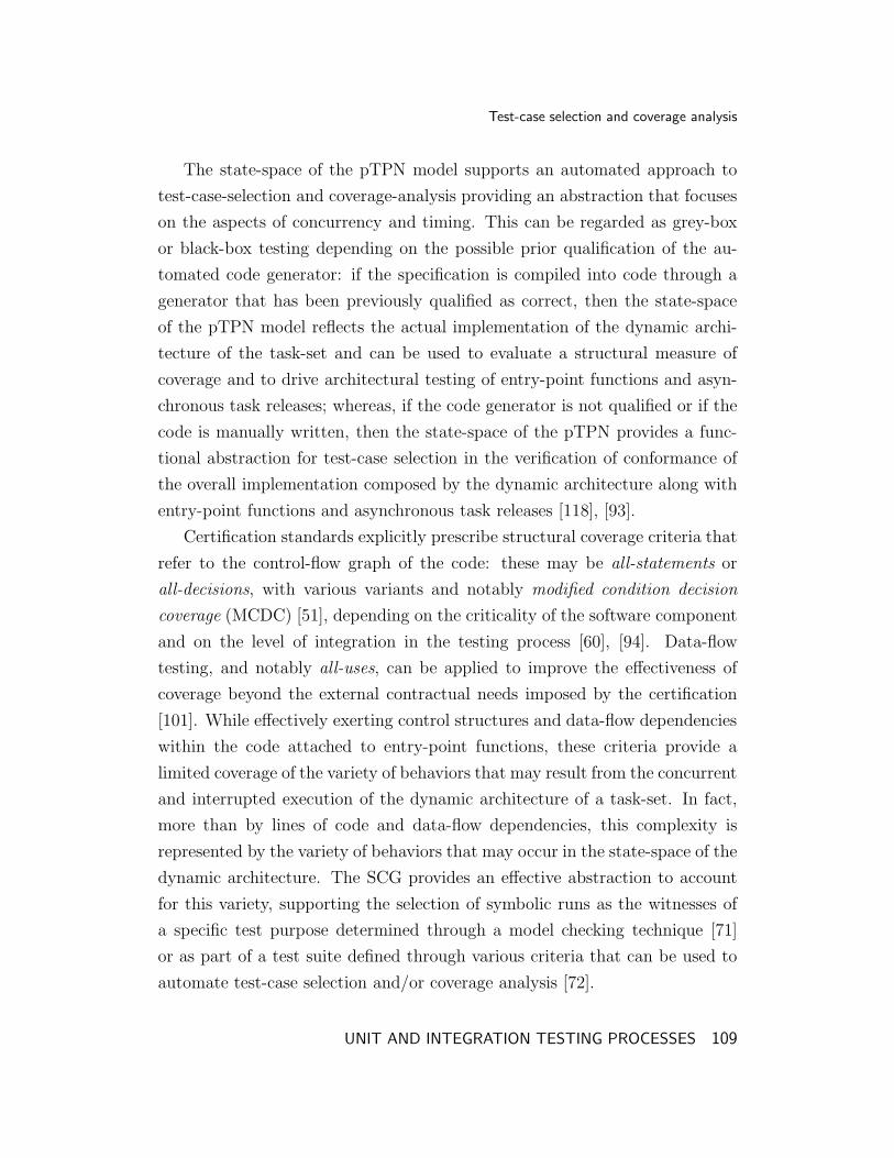
Test-case selection and coverage analysis
The state-space of the pTPN model supports an automated approach to
test-case-selection and coverage-analysis providing an abstraction that focuses
on the aspects of concurrency and timing. This can be regarded as grey-box
or black-box testing depending on the possible prior qualification of the au-
tomated code generator: if the specification is compiled into code through a
generator that has been previously qualified as correct, then the state-space
of the pTPN model reflects the actual implementation of the dynamic archi-
tecture of the task-set and can be used to evaluate a structural measure of
coverage and to drive architectural testing of entry-point functions and asyn-
chronous task releases; whereas, if the code generator is not qualified or if the
code is manually written, then the state-space of the pTPN provides a func-
tional abstraction for test-case selection in the verification of conformance of
the overall implementation composed by the dynamic architecture along with
entry-point functions and asynchronous task releases [118], [93].
Certification standards explicitly prescribe structural coverage criteria that
refer to the control-flow graph of the code: these may be all-statements or
all-decisions, with various variants and notably modified condition decision
coverage (MCDC) [51], depending on the criticality of the software component
and on the level of integration in the testing process [60], [94]. Data-flow
testing, and notably all-uses, can be applied to improve the effectiveness of
coverage beyond the external contractual needs imposed by the certification
[101]. While effectively exerting control structures and data-flow dependencies
within the code attached to entry-point functions, these criteria provide a
limited coverage of the variety of behaviors that may result from the concurrent
and interrupted execution of the dynamic architecture of a task-set. In fact,
more than by lines of code and data-flow dependencies, this complexity is
represented by the variety of behaviors that may occur in the state-space of the
dynamic architecture. The SCG provides an effective abstraction to account
for this variety, supporting the selection of symbolic runs as the witnesses of
a specific test purpose determined through a model checking technique [71]
or as part of a test suite defined through various criteria that can be used to
automate test-case selection and/or coverage analysis [72].
UNIT AND INTEGRATION TESTING PROCESSES 109

Test-case selection and coverage analysis
Without loss of generality a few test-case selection criteria are described
that capture relevant testing goals with reference to the state-space abstrac-
tion.
• All-Markings: is satisfied when each reachable marking has been visi-
ted by at least one test-case. This covers all the acceptable states of
concurrency and thus observes all the possible configurations of the set
of chunks that are concurrently ready/running/blocked (e.g., a state of
priority inversion). The criterion is a kind of all-nodes and its complexity
is thus proportional to the number of reachable markings, and can be
efficiently resolved on the SCG of the pTPN model: for each reachable
marking m, select any class Sm with marking m, and include in the
test-suite any path from a controllable starting point to S.
• All-Marking-Edges: is satisfied when each edge between any two rea-
chable markings has been traversed by at least one test-case. This in-
cludes All-Markings and adds the guarantee to observe the transitions
between subsequent states of concurrency. This notably includes the
events of preemption following to asynchronous releases, chunk comple-
tions, semaphore operations and priority boost/deboost. The criterion is
a kind of all-edges and its complexity is thus proportional to the number
of reachable markings multiplied by the maximum number of events that
may occur within each marking, which in turn is limited by the num-
ber of tasks in the set. As for the all-marking criterion, the selection is
performed on the SCG: for each edge between two markings m1 and m2,
select in the SCG any class S1 with marking m1 that accepts an event
leading to a class S2 with marking m2, and include in the test-suite any
path starting from a controllable starting point and covering the edge.
• All-Markings and All-Marking-Transitions can be refined into All-Classes
and All-Class-Edges, by requiring coverage of all reachable state-classes
and all edges between reachable state-classes, respectively. All-Classes
and All-Class-Edges include their correspondent marking-based criteria
and add the capability to partially account for the difference among
UNIT AND INTEGRATION TESTING PROCESSES 110

Test-case selection and coverage analysis
paths whenever this results in different timing restrictions (e.g., the two
sequences ρ1 = t10, t20, t30, t21, t11, t12, t22, t31, t32, t33, t34, t35, t53, t54,
t41, t42, t43, t20, t10, t30, t21, t11, t12, t22, t44, t45, t46, t47 and ρ2 = t10, t20,
t30, t21, t11, t12, t22, t31, t32, t33, t34, t35, t53, t54, t41, t42, t43, t44, t45, t46,
t0, t47 of the task-set of Fig. 2.1 reach the same state of concurrency,
but they accept different future behaviors due to the different previous
sequencing). However, they also largely increase the actual complexity of
coverage (e.g., in the state-space of the task-set of Fig. 2.1, 433 markings
are refined into 51079 classes).
• All-symbolic-Runs: covers every path in the SCG that starts with a job
release and terminates with the job completion or its deadline miss.
All-Symbolic-Runs properly-includes All-Class-Edges and thus also All-
Marking-Edges, adding the capability to cover all the possible concur-
rency states and transitions within the context of the same job execution.
This can be relevant for instance to account for possible implicit data-
flow and timeliness dependencies among chunks in the same job.
In the usual case in which the deadline of synchronous and asynchro-
nous jobs is not higher than the task period and the minimum release-
intertime, respectively, test-cases can be selected on the SCG in a straight-
forward manner. Under this assumption, releases and completions are
directly represented by specific transitions, while deadline misses can be
identified whenever a release occurs for any task with a job still pending.
The test-suite thus includes every path that starts from any task release
and terminates either with the task completion or with a new release
(which indicates a deadline miss). In the special case in which deadlines
are anticipated with respect to the period or minimum release-intertime,
deadline misses are not directly represented on the SCG, but they can be
made observable by extending the pTPN model with watch transitions
as proposed in [27]).
The resulting number of test-cases is guaranteed to be finite under the
reasonable assumption that all tasks have a finite deadline and that all
UNIT AND INTEGRATION TESTING PROCESSES 111

Test-case execution
tasks require a non-null minimum Execution Time. In fact, if the num-
ber of paths would be infinite, there should be a marking m that can
be visited an infinite number of times between a release and the com-
pletion/deadline of some task T . Since the time between a release and
the completion/deadline is bounded, the Infimum of the time spent bet-
ween two subsequent visits of m should be equal to 0. However, every
sequence between two subsequent visits of m must include an event that
advances the state of a task T ′ 6= T and thus changes the marking in a
place pT ′ belonging to T ′; to bring back the marking of pT ′ to its value in
m, T ′ must complete its execution, restart a new release, and execute all
the steps prior to m, which requires a time not lower than the minimum
Execution Time of the task which is supposed to be strictly higher than
0.
• All-Symbolic-Executions: covers any feasible sequence of events in the
SCG that starts with the release of a job and terminates with its com-
pletion or deadline miss. This reduces the complexity of All-symbolic-
Runs by avoiding to include multiple runs that follow the same event
sequence and are distinguished only by the starting class. This basi-
cally answers the same rational that suggests to prefer All-Markings and
All-Marking-Edges with respect to All-Classes and All-Class-Edges.
5.3 Test-case execution
In the process of testing, sensitization is the activity that identifies the inputs
that let the system run along selected test-cases. In the context of reactive
timed software components, this becomes a matter of determining timed inputs
that force the Implementation Under Test (IUT) to execute selected symbolic
runs.
The problem is considered in various works. In [71], [83], test-cases are
deterministically timed event sequences executed under the assumption that
all events can be observed and that all inputs can be controlled so as to assume
UNIT AND INTEGRATION TESTING PROCESSES 112

Test-case execution
a deterministic value and time. However, not all timers of a real implemen-
tation can be actually managed: periodic and asynchronous release times can
be effectively controlled through conventional primitives of an RTOS; whereas,
computation times are often impractical to handle. Moreover, timers may take
values within a subset of their nominal range of variation due to the determi-
nization of the implementation with respect to the specification [47]. This
causes legal behaviors of the specification model to be unfeasible in the IUT
[28] and arises from various practical factors: i) many abstractions taken in the
specification model cannot exactly correspond to the actual implementation,
e.g., the release of a synchronous task suffers of some jitter, semaphore and
priority handling operations require a non-null Execution Time, preemption
does not occur in zero time and impacts on Execution Times due to cache
and pipeline performances; ii) temporal parameters of the specification are
usually associated with a nondeterministic range of variation, to make the mo-
del robust with respect to possible variations of the implementation; iii) when
a model is developed as the description of an existing implementation (e.g.,
in a re-engineering process), its temporal parameters range within boundaries
which over-approximate those of the actual implementation, to circumvent
the difficulty in obtaining a precise estimate of Execution Times and release
times; iv) specification usually neglects dependencies among Execution Times
of computation chunks, which are difficult to quantify and definitely unreliable
as an assumption for schedulability; v) the operating system may contribute
to the partial determinization of the implementation, e.g., RTAI turns out to
assign a fixed order to the releases of periodic tasks with the same priority at
times multiple of their hyper-period, insensitively to the order in which tasks
are initially started.
Assumptions on deterministic behavior and observability of the IUT are
relaxed in [81], [83]. In particular, [81] proposes a framework for black-box
conformance testing of real-time systems specified as nondeterministic and
partially-observable timed automata, introducing a timed version of the input
output conformance relation of [121]. The execution of test-cases is performed
by means of an adaptive strategy in a game against the IUT and two types
UNIT AND INTEGRATION TESTING PROCESSES 113
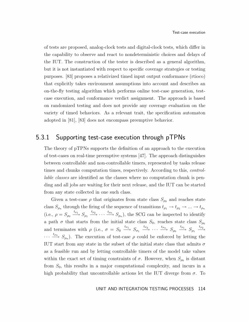
Test-case execution
of tests are proposed, analog-clock tests and digital-clock tests, which differ in
the capability to observe and react to nondeterministic choices and delays of
the IUT. The construction of the tester is described as a general algorithm,
but it is not instantiated with respect to specific coverage strategies or testing
purposes. [83] proposes a relativized timed input output conformance (rtioco)
that explicitly takes environment assumptions into account and describes an
on-the-fly testing algorithm which performs online test-case generation, test-
case execution, and conformance verdict assignment. The approach is based
on randomized testing and does not provide any coverage evaluation on the
variety of timed behaviors. As a relevant trait, the specification automaton
adopted in [81], [83] does not encompass preemptive behavior.
5.3.1 Supporting test-case execution through pTPNs
The theory of pTPNs supports the definition of an approach to the execution
of test-cases on real-time preemptive systems [47]. The approach distinguishes
between controllable and non-controllable timers, represented by tasks release
times and chunks computation times, respectively. According to this, control-
lable classes are identified as the classes where no computation chunk is pen-
ding and all jobs are waiting for their next release, and the IUT can be started
from any state collected in one such class.
Given a test-case ρ that originates from state class Sρ0and reaches state
class Sρnthrough the firing of the sequence of transitions tρ1
→ tρ2→ ... → tρn
(i.e., ρ = Sρ0
tρ1−→ Sρ1
tρ2−→ · · ·tρn−→ Sρn
), the SCG can be inspected to identify
a path σ that starts from the initial state class S0, reaches state class Sρ0
and terminates with ρ (i.e., σ = S0
tσ1−→ Sσ1
tσ2−→ · · ·tσn−→ Sρ0
tρ1−→ Sρ1
tρ2−→
· · ·tρn−→ Sρn
). The execution of test-case ρ could be enforced by letting the
IUT start from any state in the subset of the initial state class that admits σ
as a feasible run and by letting controllable timers of the model take values
within the exact set of timing constraints of σ. However, when Sρ0is distant
from S0, this results in a major computational complexity, and incurs in a
high probability that uncontrollable actions let the IUT diverge from σ. To
UNIT AND INTEGRATION TESTING PROCESSES 114

Test-case execution
reduce the problem, the IUT is not started from the initial state class but
from a controllable class which is suitably selected in the SCG, according to
the following testing procedure:
• The SCG is inspected to identify a path ω that i) starts from a control-
lable class Sc and ii) covers the selected test-case ρ without visiting
any other controllable class (i.e., ω = Sc
tω1−→ Sω1
tω2−→ · · ·tωn−→ Sρ0
tρ1−→
Sρ1
tρ2−→ · · ·tρn−→ Sρn
, where Sωiis a non-controllable class ∀ i ∈ [1, n−1]).
• Trace analysis enables the derivation of the range of feasible timings
for ω, which comprises i) the subset Sc of Sc collecting all and only
the states of Sc that admit ω as a feasible run, and ii) a set of timing
constraints for transitions that are newly enabled in classes visited by the
run. Since values of non-controllable timers are autonomously selected by
the IUT and may let it diverge from the selected test-case, the identified
timing conditions for controllable timers comprise the necessary but not
sufficient condition to execute the path ω. Trace analysis also permits
the derivation of the WCCT of ω.
• The IUT is repeatedly started from a state in Sc and values of control-
lable timers are randomly sampled within the identified range. At each
repetition, the IUT is stopped when time surpasses the WCET of ω,
beyond which either the IUT has covered the selected test-case or it has
diverged.
5.3.2 Experimental results
The application of the proposed sensitization procedure is illustrated in rela-
tion to the execution of a test-case selected as a specific testing purpose [71].
The experimentation was carried out on the Basic Features Extraction CSCI
of Fig. 1.8, whose dynamic architecture is specified by the pTPN model of
Fig. 2.1. The test-case was identified on the SCG as a symbolic run of task
Tsk4 that may attain its WCCT of 58 ms. In particular, the selected test-case
is the symbolic run ρ illustrated in Fig. 2.5, which starts with the release of a
UNIT AND INTEGRATION TESTING PROCESSES 115

Test-case execution
job of Tsk4 (i.e., the firing of transition t40 that enters state-class S5605) and
terminates with its completion (i.e., the firing of transition t47): ρ = S5605
t10−→
S5795
t20−→ S6092
t30−→ S6591
t21−→ S7198
t11−→ S7741
t12−→ S8120
t22−→ S8406
t54−→ S8711
t31−→ S9030
t32−→ S9313
t33−→ S9521
t34−→ S9687
t35−→ S9873
t41−→ S10121
t42−→ S10396
t43−→
S10670
t20−→ S10969
t10−→ S11322
t21−→ S11729
t11−→ S12164
t12−→ S12607
t22−→ S13028
t44−→
S13454
t45−→ S13907
t46−→ S14344
t47−→ S14739.
Following the sensitization strategy described in Sect. 5.3.1, the SCG was
inspected in order to identify a path ω that starts from a controllable class and
covers ρ without visiting any other intermediate controllable class. This was
obtained through the Model Checker of the Oris Tool [35], which provides all
the symbolic paths in the SCG that are witnesses of a branching-time temporal
logic formula, with state and action formulae expressing conditions on both
visited markings and traversed transitions. According to this, the SCG was
checked to identify any symbolic run that: i) starts from a controllable class,
identified by the marking Mc, which assigns a token to places m1 and m2 and
no token to all the other places; ii) reaches any state class that fires t40 without
visiting any intermediate controllable class; iii) terminates with the firing of
t47 after 58 ms since the firing of t40 without including any intermediate firing
of t47. A symbolic run ω that starts from the controllable class S4959 and covers
ρ was thus selected among the witnesses provided by the Model Checker:
ω = S4959
t50−→ S5055
t51−→ S5154
t52−→ S5278
t53−→ S5437
t40−→ ρ
S4959 = 〈Mc, D4959〉 D4959 =
26 ≤ t10 ≤ 33
26 ≤ t20 ≤ 33
26 ≤ t30 ≤ 33
26 ≤ t40 ≤ 33
0 ≤ t50 ≤ ∞
0 ≤ t10 − t20 ≤ 0
0 ≤ t10 − t30 ≤ 0
0 ≤ t10 − t40 ≤ 0
State class S4959 collects states in which periodic tasks Tsk1, Tsk2, Tsk3,
and Tsk4 are constrained to have the same release time within the interval
UNIT AND INTEGRATION TESTING PROCESSES 116

Test-case execution
[26, 33] ms, while no constraints exist on the release time of the sporadic task
Tsk5. The exact timing profile of ω was derived though trace analysis and it
restricts the time to fire of t50 in S4959 to be within 22 ms and 32 ms, which
identifies the subset S4959 of S4959 that admits ω as a feasible run. According
to this, the necessary condition to execute the test-case consists in releasing
the sporadic task Tsk5 within [22, 32] ms and starting the four periodic tasks
Tsk1, Tsk2, Tsk3, and Tsk4 at the same time within [26, 33] ms. Since S4959 is
a controllable class, Tsk5 can be released just after the IUT is started, without
waiting the minimum time of 22 ms: according to this, Tsk5 is released within
[0, 10] ms, and Tsk1, Tsk2, Tsk3, and Tsk4 are contemporary started within
[4, 11] ms. The restart time of the IUT turns out to be equal to 69 ms, being
the WCCT of ω of 91 ms decremented by 22 ms.
The feasibility and effectiveness of the proposed approach to the execution
of test-cases was evaluated with respect to randomized testing.
• Randomized testing: The IUT was run for 1 hour, which corresponds
to 90000 releases of the shortest-period task Tsk1. In a preliminary ex-
periment, the sporadic task Tsk5 was released according to a uniform
distribution within [120, Nmax/106] ms, being Nmax the maximum repre-
sentable integer value. Coverage evaluation evidenced that the test-case
ρ was never covered. Since ρ comprises the execution of a job of Tsk5, a
second experiment was performed by activating jobs of Tsk5 according
to a uniform distribution within [120, 1000] ms. However, also in this
case the test-case ρ was never covered.
• Sensitized testing: The IUT was repeatedly started every 69 ms, re-
leasing Tsk5 within [0, 10] ms and starting Tsk1, Tsk2, Tsk3, and Tsk4
at the same time within [4, 11] ms. One thousand executions were per-
formed, which correspond to an overall Execution Time of a little more
than 1 minute. During the test, ρ was executed 207 times, evidencing
the effectiveness of the approach with respect to randomized testing.
UNIT AND INTEGRATION TESTING PROCESSES 117

Oracles verdict
5.4 Oracles verdict
Logs produced during the testing stage can be analyzed by different oracles
evaluating the conformance between implementation and specification with
different levels of abstraction, each implying a different run-time overhead for
logging and a different off-line complexity for decision.
• The end-to-end Oracle verifies the satisfaction of end-to-end job dead-
lines. The oracle requires time-stamped logging of job releases and com-
pletions, and is implemented in a straightforward manner by comparing
the time elapsed between release and completion of any job against the
deadline of its task (without explicit reference to the structure of the
pTPN model).
• The sequencing Oracle verifies that the qualitative ordering of events
conforms with the specification model, i.e., that there exists at least
one timing that makes the sequencing of the log feasible for the speci-
fication model. This requires logging of all the events corresponding
to a transition in the pTPN model (i.e., job releases, completion of
computation chunks, priority boost operations, semaphore wait opera-
tions, mailbox receipt operations). However, it does not require that
logged events be associated with a time-stamp, thus avoiding the need
for an invocation of the time measuring primitive of the operating system
(rt_get_time_ns() in the case of RTAI).
Decision of the oracle verdict requires state-space analysis, and basically
consists in verifying whether the logged sequence is a symbolic execution
sequence in the SCG of the pTPN model. If all reachable state classes
have been computed, the problem of conformance reduces to verify whe-
ther the SCG contains a path that follows the sequence of logged events.
If the SCG is not finite, or if it does not fit in the available memory,
then conformance can be tested by reconstructing the fragment of the
state-space composed by the classes visited by the logged sequence. To
this end, the logged sequence is assumed to begin with the start-up of
UNIT AND INTEGRATION TESTING PROCESSES 118

Oracles verdict
the task-set. This identifies the initial marking, guarantees that all en-
abled transitions are newly enabled, and thus identifies a reachable state
class that contains the initial state of the logged sequence. Since a state
class is derived in time O(N2) with respect to the number N of enabled
transitions [122], [34], the entire fragment is computed in time O(N2 ·L),
where L is the length of the logged sequence.
• The time-sensitive Oracle verifies the timed trace inclusion relation of
[71], i.e., it verifies that the logged sequence is a feasible execution for the
specification. Verification requires that a time-stamped log is produced
for each event of the implementation that corresponds to a transition
in the pTPN model. Also in this case, to guarantee identification of the
initial state, logging is assumed to start from an initial state with a known
marking where all enabled transitions are newly enabled. This can be the
initial state reached through a reset function that starts-up the task-set.
More generally, the same condition can be attained through an ad-hoc
function that starts-up the task-set from any intermediate controllable
state where no computation is ongoing and all times to the next job
release are known.
The decision algorithm does not require state-space analysis and basi-
cally relies on a simulation of the specification model: starting from the
initial state s0 =< M0, F I0 > accounting for conditions at which the
system is started, the algorithm checks the feasibility of the first timed
action 〈a1, τ1〉 and computes the subsequent state s1; at the n-th step,
the algorithm checks whether tn can be fired at time τn−τn−1 from state
sn−1 and computes the resulting state sn. The Oracle emits a failure ver-
dict as soon as any timed action 〈an, τn〉 is not accepted by the simulator.
A pass verdict is emitted when the run terminates. An inconclusive ver-
dict is emitted when the trace diverges from the sequence of the test-case
with an event that is accepted by the simulator.
The time-sensitive Oracle somehow performs the same function of the
observers proposed in [71], [26]. In [71], an observer is an automaton
UNIT AND INTEGRATION TESTING PROCESSES 119

Oracles verdict
employed online during the testing process to collect auxiliary informa-
tion that is used for coverage evaluation. In [26], an observer is used
to evaluate quantitative properties through state-space enumeration of
the specification model augmented with additional places and transi-
tions. Differently from both the concepts of observer, the time sensitive
Oracle evaluates off-line the execution logs produced by an implementa-
tion. This is accomplished by verifying if the sequence of timed actions is
a subset of the dynamic behavior that the semantics of the specification
model may accept.
All the failures detected by the sequencing Oracle are also detected by the
time-sensitive Oracle, while the vice-versa is of course not true. Besides, failure
detection capability of the end-to-end Oracle are not comparable with those of
the sequencing Oracle and the time-sensitive Oracle. In fact, an execution may
break the expected sequencing and/or an internal time-frame and satisfy the
deadline, and vice-versa. However, if state-space analysis of the specification
model has verified the absence of symbolic runs that break any task deadline,
then all the failures observed by the end-to-end Oracle are also observed by
the sequencing Oracle (and thus also by the time-sensitive Oracle).
Any un-sequenced execution is detected by the sequencing Oracle (and
thus also by the time-sensitive Oracle). Besides, any time frame violation is
detected by the time-sensitive Oracle, but not by the sequencing Oracle unless
timing causes the execution to diverge from the expected sequencing. Cycle
stealing defects are recognized by the time-sensitive Oracle iff the quantity
of stolen time exceeds the laxity between the actual Execution Time and its
expected upper bound.
Coverage metrics can be obtained by mapping on the SCG the sequence of
actions reproduced by the time-sensitive Oracle or by the sequence-sensitive
Oracle. Regardless of the number of identified failures, a metric of coverage is
needed to provide a measure of confidence in the absence of residual defects.
The sequence of actions reproduced by the deadline-sensitive Oracle cannot
be mapped on the SCG because the oracle does not observe all actions.
UNIT AND INTEGRATION TESTING PROCESSES 120

Chapter
6Summary of the approach
For the convenience of the reader, this Chapter resumes the formal metho-
dology for the development of real-time software components proposed in this
dissertation. The approach casts the theory of pTPNs into an organic tailoring
of design, coding, and testing activities within a V-Model software life cycle
[42] and it is summarized by illustrating its application to the development of
the IVSS presented in this work.
The case study described along this dissertation concerns an IVSS which
employs a pan-tilt-zoom (PTZ) camera to perform real-time 3D tracking of
multiple people moving over an extended area [29]. The activity SD1 identifies
User Requirements of the vision system through the definition of parameters
such as the frame rate (i.e., 25 frames per second), the image size (i.e., 160 x
120 pixels), the compression format (i.e., JPEG), the operating temperature
(i.e., from 0◦C to 40◦C), the camera mass (i.e., up to 1.5 Kg). The activity SD2
specifies System Architecture through the UML-MARTE class diagram of Fig.
6.1, identifying a Control Unit, a PTZ Camera, and a Video Processing Unit.
The Control Unit receives images acquired by the PTZ Camera, sends them to
SUMMARY OF THE APPROACH 121

the Video Processing Unit, and receives the elaborated images back. On the
basis of these results, the Control Unit sets parameters of image processing
algorithms (e.g., window size of non-linear filters) and parameters at which
images are acquired (e.g., the levels of pan, tilt, and zoom), and sends them to
the Video Processing Unit and to the PTZ Camera, respectively. The activity
Figure 6.1. UML-MARTE class diagram of the System Architecture of an IVSS.The ProcessingResource stereotype models an active, protected, executing-typeresource that is allocated to the execution of schedulable resources. The Device-Resource stereotype specializes the concept of processing resource and typicallyrepresents an external device that may be manipulated or invoked by the plat-form and that may require specific services in the platform for its usage and/ormanagement, but whose internal behavior is not a relevant part of the modelunder consideration. A CommunicationMedia represents the mean to transportinformation from one location to another.
SD3 details CSCIs and HCIs of each unit through the UML-MARTE class
diagrams shown in Figs. 6.2 and 6.3. The Control Unit communicates with the
PTZ Camera and with the Video Processing Unit through a serial bus; boards
of both the Control Unit and the Video Processing Unit run RTAI operating
system [95]. The Control Unit comprises a CSCI (i.e., System Management
CSCI) and two HCIs (i.e., a board and a battery): the CSCI is mapped on an
RTAI task-set and allocated to the board. The PTZ Camera consists of two
HCIs (i.e., the Image Sensor Unit and the Mechanical PTZ Unit). The Video
Processing Unit comprises three CSCIs (i.e., Images Acquisition CSCI, Basic
Features Extraction CSCI, and Multiple Target Tracking CSCI) and four HCIs
(i.e., three boards and a battery): each CSCI is mapped on a different RTAI
task-set and allocated to a different board.
The approach proposed in this dissertation comes into play with the activi-
ties SD4-SW and SD5-SW through the definition of the dynamic architecture of
the task-set allocated to each CSCI. Each task-set is initially specified through
SUMMARY OF THE APPROACH 122

Figure 6.2. UML-MARTE class diagram of the Control Unit and the PTZ Cameraof the IVSS of Fig. 6.1. The rtUnit stereotype models a real-time applicationthat owns one or more schedulable resources. A SchedulableResource is an activeresource able to perform actions using the processing capacity brought from aprocessing resource by the scheduler that manages it. A Hw Card symbolizes aprinted circuit board, which typically comprises other sub-components like chipsand electrical devices. The allocate stereotype identifies an allocation relationbetween elements of the application model, represented through the stereotypeApplicationAllocationEnd, and elements of the execution platform, modeled bythe stereotype ExecutionPlatformAllocationEnd. A Hw PowerSupply is a hard-ware component that supplies the hardware platform with power. The Hw Busstereotype represents a particular wired channel with specific functional proper-ties.
the identification of minimum release inter-times, periods, and deadlines; then,
it is refined through the definition task priorities and allowed time-frames of
computation chunks. Task-sets are defined through the semi-formal specifi-
cation of timelines, providing modeling convenience and facilitating industrial
SUMMARY OF THE APPROACH 123

Figure 6.3. UML-MARTE class diagram of the Video Processing Unit of theIVSS of Fig. 6.1.
acceptance; then, they are automatically translated into pTPN models through
the Oris Tool [43], enabling schedulability analysis based on state space enu-
meration. Fig. 6.4 reports the timeline schema of the task-set allocated to
the Basic Features Extraction CSCI of Fig. 6.3. The task-set is made by five
SUMMARY OF THE APPROACH 124

recurrent tasks synchronized by two binary semaphores and a mailbox:
• Task Tsk1 performs noise reduction through a median filter. It is a
periodic task with period and deadline of 40 time units. Each job of
Tsk1 consists of the unique chunk C11 which is associated with entry-
point f11, requires resource cpu with priority level 1 (low priority numbers
run first) for an Execution Time constrained within 1 and 2 time units,
and receives a message from mailbox mbx containing parameters for the
noise reduction algorithm at the beginning of its execution.
• Task Tsk2 manipulates parameters employed by the noise reduction al-
gorithm. It is a periodic task with period and deadline of 40 time units.
Each job of Tsk2 consists of two chunks C21 and C22. Chunk C21 is
associated with entry-point f21; it requires resource cpu with priority
level 2 for an Execution Time constrained within 1 and 2 time units; at
the end of its execution, it sends a message to mailbox mbx containing
parameters for the noise reduction algorithm. Chunk C22 is associated
with entry-point f22 and requires resource cpu with priority level 2 for
an Execution Time constrained within 1 and 2 time units.
• Task Tsk3 performs edge detection through Sobel operator. It is a per-
iodic task with period and deadline of 80 time units. Each job of Tsk3
consists of three chunks C31, C32, and C33. Chunk C31 is associated with
entry-point f31, which acquires parameters for the edge detection algo-
rithm from a memory space shared with tasks Tsk4 and Tsk5; it requires
resource cpu with priority level 3 for an Execution Time constrained wi-
thin 1 and 2 time units; it is synchronized on the binary semaphore mux1
to access the memory space shared with tasks Tsk4 and Tsk5. Chunk C32
is associated with entry-point f32, which performs the edge detection al-
gorithm, and requires resource cpu with priority level 3 for an Execution
Time constrained within 5 and 10 time units. Chunk C33 is associated
with entry-point f33, which writes results of the edge detection algorithm
on a memory space shared with task Tsk4; it requires resource cpu with
priority level 3 for an Execution Time constrained within 1 and 2 time
SUMMARY OF THE APPROACH 125

units; it is synchronized on the binary semaphore mux2 to access the
memory space shared with task Tsk4.
• Task Tsk4 performs corner detection through Moravec operator. It is
a periodic task with period and deadline of 100 time units and it has
the same structure as that of task Tsk3: chunk C41 acquires parameters
for the edge detection algorithm from the memory space shared with
tasks Tsk3 and Tsk5; chunk C42 performs the corner detection algorithm;
chunk C43 writes results of the corner detection algorithm on the memory
space shared with task Tsk3.
• Task Tsk5 manipulates parameters employed by edge and corner detec-
tion algorithms. It is a sporadic task with minimum interarrival time and
deadline of 120 time units. Each job of Tsk5 consists of two chunks C51
and C52. Chunk C51 is associated with entry-point f51, which performs
parameters manipulation, and requires resource cpu with priority level
5 for an Execution Time constrained within 1 and 2 time units. Chunk
C52 is associated with entry-point f52, which writes parameters on the
memory space shared with tasks Tsk3 and Tsk4; it requires resource cpu
with priority level 5 for an Execution Time constrained within 1 and 2
time units; it is synchronized on the binary semaphore mux1 to access
the memory space shared with tasks Tsk3 and Tsk4.
The timeline schema of Fig. 6.4 is automatically translated into the pTPN
model of Fig. 6.5. Recurrent job releases are modeled by transitions with nei-
ther input places nor resource request, so as to fire repeatedly with intertimes
falling within their respective firing intervals (e.g., transitions t10, t20, t30, t40,
and t50 model recurrent job releases of tasks Tsk1, Tsk2, Tsk3, Tsk4, and
Tsk5, respectively). Job chunks are modeled by transitions with static firing
intervals corresponding to the min-max range of Execution Time, associated
with resource requests and static priorities (e.g., transition t12 represents the
completion of the unique chunk of each job of Tsk1). Binary semaphores are
modeled in a straightforward manner as places initially marked with 1 to-
ken (e.g., place mux1 models the binary semaphore that synchronizes the first
SUMMARY OF THE APPROACH 126

Figure 6.4. The timeline schema for the dynamic architecture of the Basic Fea-tures Extraction CSCI of Fig. 6.3, representing a task-set composed of fiverecurrent tasks synchronized by two binary semaphores and a mailbox.
chunk of Tsk3, the first chunk of Tsk4, and the second chunk of Tsk5); their ac-
quisition operations are modeled as immediate transitions, while their release
operations are represented by the transitions that also model chunk comple-
tions (e.g., wait operations on semaphore mux1 are modeled by transitions t31,
t42, and t53; signal operations are represented by transitions t32, t43, and t54,
which also account for the completion of the three synchronized chunks). Boost
and deboost operations according to the priority ceiling emulation protocol are
allocated to immediate transitions and to the transitions that also account for
chunk completions, respectively (e.g., transition t52 models priority boost of
task Tsk5, while transition t54 represents the corresponding priority deboost
and also accounts for the completion of the second chunk of task Tsk5). Mail-
SUMMARY OF THE APPROACH 127

boxes are represented by empty places (e.g., place mbx models the mailbox
shared between tasks Tsk1 and Tsk2); message receipt operations are modeled
by immediate transitions (e.g., transition t11 models the receipt of a message
by the unique chunk of task Tsk1); message dispatch operations are modeled
by the transitions that also account for chunk completions (e.g., transition t21
represents both the dispatch of a message to mailbox mbx performed by the
first chunk of task Tsk2 and the completion of that chunk).
Figure 6.5. The pTPN model that corresponds to the timeline schema shown inFig. 6.4.
The pTPN model enables the verification of correctness requirements of the
task-set through the enumeration of the SCG, the selection of symbolic runs
attaining specific sequencing and timing conditions, and the tight evaluation
of their range of timings. For the pTPN model of Fig. 6.5, the Oris Tool
SUMMARY OF THE APPROACH 128

enumerates 51079 state classes and identifies 15295, 10967, 21170, 491703, and
156574 symbolic runs for tasks Tsk1, Tsk2, Tsk3, Tsk4, and Tsk5, respectively.
The analysis of the SCG enables the identification of the WCCT of each task
(12, 14, 30, 58, and 60 time units for Tsk1, Tsk2, Tsk3, Tsk4, and Tsk5,
respectively) and the verification of deadlines (tasks Tsk1, Tsk2, Tsk3, Tsk4,
and Tsk5 meet their respective deadlines with minimum laxity of 28, 26, 50, 22,
and 60 time units, respectively). As an example, Fig. 6.6 reports the results
of trace analysis on a symbolic run of Tsk4 that was selected through state-
space analysis as a case in which Tsk4 may attain its WCCT of 58 time units.
The schema displays the intervals during which each transition is progressing
or suspended, highlighting the range of variability that results from mutual
dependencies among transitions firing times.
The activity SD6-SW implements the dynamic architecture of each CSCI,
providing code that assumes the following responsibilities: release task jobs ac-
cording to their policies; invoke semaphore operations and connected priority
handling operations; invoke mailbox operations; enforce sequenced invocation
of entry-point methods. The implementation of the dynamic architecture of a
CSCI is derived from the timeline specification of its task-set, either through
disciplined manual programming or in automated manner through the Oris
Tool [43]. As a salient trait, the code of the implementation has a readable
structure, which follows natural and readable patterns of concurrent program-
ming and which closely mirrors the structure of the corresponding pTPN mo-
del. Fig. 6.7 illustrates the correspondence of components of the timeline
schema, the code, and the underlying pTPN model with reference to the im-
plementation of task Tsk4 of Fig. 6.4 on RTAI 3.6 [95].
The code of the dynamic architecture can be complemented with busy-sleep
functions, providing an implementation that conforms with expected timing
requirements. This provides an Executable Architecture which enables the
unit testing of low-level modules within their expected operation environment
and supports incremental integration and testing of low-level modules.
The correspondence between the pTPN model of the dynamic architecture
of a CSCI and its implementation enables a measurement-based approach to
SUMMARY OF THE APPROACH 129

Figure 6.6. A schema illustrating the range of feasible timings for the symbolic
run ρ = S5605
t10−→ S5795
t20−→ S6092
t30−→ S6591
t21−→ S7198
t11−→ S7741
t12−→ S8120t22−→ S8406
t54−→ S8711
t31−→ S9030
t32−→ S9313
t33−→ S9521
t34−→ S9687
t35−→ S9873
t41−→
S10121
t42−→ S10396
t43−→ S10670
t20−→ S10969
t10−→ S11322
t21−→ S11729
t11−→ S12164t12−→ S12607
t22−→ S13028
t44−→ S13454
t45−→ S13907
t46−→ S14344
t47−→ S14739 in thestate-space of the pTPN model of Fig. 6.5. The run starts with the releaseof a job of Tsk4 (i.e., the firing of transition t40 that enters state-classe S5605,not shown in the schema) and terminates with its completion (i.e., the firing oftransition t47). Time advances along the horizontal axis. Transition firings arerepresented by arrows and they are positioned at their latest feasible time, whilegrey-filled rectangles indicate their allowed range of variation (e.g., transition t12fires twice along the sequence: the first time it can fire within time +10 and+12 and the second time it can fire within +46 and +52, and the two firings aredisplayed at time +12 and +52, respectively). Transitions enabling-periods aremarked through rectangles that are either black or white whether the transitionis progressing or suspended, respectively (e.g., transition t22 fires twice along thesequence and both the times it is suspended until the firing of transition t12 andit is then progressing until its own firing). Classes entered at transition firingsare listed over the schema (e.g., the firing of transition t12 enters state-classS8120); in case of multiple firings occurring at the same time point, classes areare enlisted from the top according to their order (e.g., the firing of transitiont10 enters state-class S5795, which is left at the firing of transition t20 to enterstate-class S6092).
SUMMARY OF THE APPROACH 130

Figure 6.7. A fragment of the code implementing the dynamic architecture ofthe Basic Features Extraction CSCI of Fig. 6.3, reporting the implementationof job executions for the periodic task Tsk4 and illustrating the correspondencebetween the timeline schema, the code, and the pTPN model.
Execution Time profiling, which reconstructs the Execution Time of chunk
computations from a proper sequence of time-stamped logs. This is supported
by the Oris Tool and applied to the unit-testing of low-level modules. With re-
ference to the Basic Feature Extraction CSCI shown in Fig. 6.3, the histogram
of Fig. 6.8 reports experimental results obtained for an input-data dependent
implementation of the edge detection module, which corresponds to compu-
tation chunk C21 of task Tsk2 in the timeline model of Fig. 6.4. Observed
Execution Times fall in the interval [7.771, 8.620] ms with a peak on 7.955 ms,
SUMMARY OF THE APPROACH 131

accomplishing the time-frame requirement of [5, 10] ms. It is worth noting that
Execution Times exhibit a quite wide spectrum with various peaks, due to a
set of input-data dependent alternatives in the implementation of the module,
and the distribution of peaks depends on the distribution of input-data. An
input-data independent implementation of the edge detection module was de-
veloped and Execution Times observed on the same data-set are reported in
the histogram of Fig. 6.9: they fall in the interval [7.279, 7.371] ms with a peak
on 7.334 ms, showing a thinner spectrum and thus evidencing a substantial
independence from input-data.
0%
0.2%
0.4%
0.6%
0.8%
1%
1.2%
1.4%
1.6%
5 6 7 8 9 10
ms
Figure 6.8. Histogram of observed Execution Times for an input-data dependentimplementation of the edge detection module of the Basic Features ExtractionCSCI of Fig. 6.3.
In the activity SD7-SW, the theory of pTPNs supports both unit and
integration testing processes, contributing to test-case selection, test-case sen-
sitization, oracle verdict and coverage evaluation. In fact, the state-space of
pTPN models provides an abstraction that focuses on the aspects of concur-
rency and timing, supporting the selection of symbolic runs as the witnesses
of a specific test purpose determined through a model checking technique [71]
SUMMARY OF THE APPROACH 132

0%
0.5%
1%
1.5%
2%
2.5%
3%
3.5%
4%
4.5%
5 6 7 8 9 10
ms
Figure 6.9. Histogram of observed Execution Times for a input-data independentimplementation of the edge detection module of the Basic Features ExtractionCSCI of Fig. 6.3.
or as part of a test suite defined through various criteria that can be used to
automate test-case selection and/or coverage analysis [72]. Moreover, the SCG
also supports the definition of a sensitization procedure that optimizes the se-
lection of timed inputs that let the system run along selected test-cases. The
approach distinguishes between controllable and non-controllable timers of the
model, identifies a path starting from a state class composed of controllable
timers and covering the selected test-case, and derives values for controllable
timers that comprise the necessary condition to execute the path. The method
was applied to the development of the Basic Feature Extraction CSCI of Fig.
6.3. Experimental results concerning the sensitization of a symbolic run of
task Tsk4 that may attain its WCCT show the effectiveness of the approach
with respect to randomized testing, where each timer is sampled within its
nominal interval according to a uniform distribution.
SUMMARY OF THE APPROACH 133

Conclusions
This dissertation formalizes a comprehensive methodology for the development
of real-time safety-critical software components, developing and integrating
the theory of pTPNs into a tailoring of the V-Model software life cycle [42]
that covers the activities of design, implementation and verification according
to the principles of main regulatory standards applied to the construction of
safety-critical software [60], [50]. To this end, the theory of state-space analysis
[122], [34] is complemented with formal techniques and methods supporting
automated derivation of pTPN models from a semi-formal specification, au-
tomated compilation of models into real-time code running under RTAI [95],
measurement-based Execution Time evaluation, test-case selection and execu-
tion, and coverage evaluation. To effectively bring the theory to application,
the overall toolchain is implemented within the Oris Tool [109] according to
an MDD approach, and the proposed formal methodology is applied to the
construction of real-time software components for an IVSS.
As a salient trait, the approach proposed in this dissertation has a smooth
impact on the development process, as explicitly recommended by the
RTCA/DO-178B standard [60], and it can be effectively applied in the indus-
trial context. In fact, the main difficulty that the approach brings along is
the need of a specification of the dynamic architecture through pTPNs. This
is largely eased by the use of the semi-formal specification provided by time-
line schemas, which better meet intuitions of the industrial practice, and by
CONCLUSIONS 134

CONCLUSIONS
their automated translation into pTPN models and real-time code. Without
any additional effort on the part of the developer, the pTPN model provides
a formal abstraction that supports verification of the dynamic architecture,
Execution Time profiling of low-level modules, unit and integration testing.
Explosion of the timed state-space of the pTPN model may impair ex-
haustive verification of software design but it does not prevent the overall
development approach: in fact, on the one hand, partial enumeration of the
state-space enables the verification of a significant part of possible behaviors,
reaching the level of rigor that can be attained through simulation; on the
other hand, conformance of the implementation with respect to the specifica-
tion is in any case achieved through testing, which is requested for certification
purposes.
The code of the implementation follows in a straightforward manner the
structure of the pTPN model and preserves its semantic properties. This en-
ables the definition and the implementation of a measurement-based approach
to the reconstruction of the Execution Time of entry-points from a proper se-
quence of time-stamped logs, by leveraging on the formal basis of pTPNs. As a
characterizing trait, measurements are carried out by letting chunks run within
the Executable Architecture of the task-set, thus accounting for pipeline da-
mages consequent to the execution in preemptive interrupted mode. Since each
component of the pTPN specification accepts a context-free translation, the
code can be generated in automated manner by structural induction, thus pro-
viding a full fledged MDD. At the same time, and perhaps more importantly,
the implementation code has a readable structure, which follows common pat-
terns of concurrent programming, leaving the developer full insight and control
over the final code and even allowing a disciplined code programming. This is
a crucial point to support industrial acceptance and avoids legacy constraints
on tools that support editing and translation of timeline schemas and pTPN
models. A clean and readable structure of the code also prevents erroneous
understanding of the semantics of pTPNs and timeline schemas, which in the
industrial practice may be less understood and trusted than conventional pro-
gramming languages and operating system primitives.
CONCLUSIONS 135

CONCLUSIONS
The methodology devised in this dissertation provides an adequate basis to
extend the research in many possible directions regarding the various phases
of software development process. In the design phase, the theory of pTPNs
supports specification and symbolic state space analysis of real-time preemp-
tive systems and enables qualitative verification of correctness requirements
pertaining ordering and timings of events. The main criticism concerned with
qualitative analysis techniques is the problem of state space explosion. Emer-
ging techniques for Hierarchical Scheduling (HS) should provide support to
mitigate the problem, by enabling the application of compositional analysis
methods [37]. In particular, the theory of pTPNs seems to find an application
in modeling and analysis of HS systems with a Time Division Multiplexing
(TDM) global scheduler and Fixed Priority (FP) local schedulers. In fact, the
temporal isolation among different applications permits to conveniently exploit
the expressive power of pTPNs in the representation of preemptive behavior,
allowing the specification of an HS system through a structured representation
where each application and its interface towards the environment are accoun-
ted by a different pTPN model. This would largely reduce the complexity of
the problem, facilitating the scalability of the approach and enabling exhaus-
tive architectural verification of systems that could not be directly analyzed
through a unique flat model.
Following the theory of stochastic state classes developed in [48], [45], the
model of pTPNs could be extended by introducing a stochastic characteri-
zation of non-deterministic timers, which associates the time to fire of each
transition with a probability density function. The SCG would then be ex-
panded into a stochastic SCG where state density functions provide a measure
of probability over the continuous set of states included in each class. The ap-
proach would complement the qualitative identification of feasible behaviors
with a quantitative measure of their probability, enabling the verification of
dependability requirements in dense-timed preemptive systems so as to meet
Reliability, Availability, Maintainability and Safety (RAMS) objectives. This
would also represent a suitable theoretical basis to improve testing activities
through the optimization of both test-case selection and test-case sensitization.
CONCLUSIONS 136

CONCLUSIONS
In particular, quantitative analysis techniques should provide support for the
identification of timed inputs that maximize the probability to let the system
run along selected test-cases.
The development of multi-core systems might contribute to increase the
value of the formal methodology proposed in this dissertation. In fact, the
integration of multiple cores on the same processor for parallel computation
is naturally encompassed in modeling and analysis of pTPNs, thus expanding
the range of application of the proposed approach.
CONCLUSIONS 137

Bibliography
[1] The Adeos Project. http://home.gna.org/adeos.
[2] ERIKA. http://erika.tuxfamily.org.
[3] Evidence s.r.l. http://www.evidence.eu.com.
[4] Finite State Machine Labs. http://www.fsmlabs.com/.
[5] Linux. http://www.linux.org.
[6] Linux/RK. http://www.cs.cmu.edu/ rtmach/.
[7] OSEK/VDX. http://www.osek-vdx.org.
[8] Wind River. http://www.windriver.com/.
[9] Airlines Electronic Engineering Committee (AEEC). Avionics Applica-tion Software Standard Interface (ARINC Specification 653-1). ARINCInc., 2003.
[10] R. K. Ahuja, T. L. Magnanti, and J. B. Orlin. Network Flows: Theory,Algorithms, and Applications. Prentice Hall, 1993.
[11] K. Altisen, G. Goessler, and J. Sifakis. Scheduler Modeling Based onthe Controller Synthesis Paradigm. Real Time Systems, 23:55–84, 2002.
[12] R. Alur, C. Courcoubetis, N. Halbwachs, T. A. Henzinger, P.-H. Ho,X. Nicollin, A. Olivero, J. Sifakis, and S. Yovine. The Algorithmic Ana-lysis of Hybrid Systems. Theoretical Computer Science, 138:3–34, 1995.
BIBLIOGRAPHY 138

[13] R. Alur, F. Ivancic, J. Kim, I. Lee, and O. Sokolsky. Generating embed-ded software from hierarchical hybrid models. In Languages, Compilers,and Tools for Embedded Systems (LCTES), pages 171–182. ACM Press,2003.
[14] R. Alur, I. Lee, and O. Sokolsky. Compositional Refinement for Hierar-chical Hybrid Systems. In Proceedings of the 4th International Workshopon Hybrid Systems: Computation and Control (HSCC), pages 33–48.Springer–Verlag, 2001.
[15] T. Amnell, E. Fersman, L. Mokrushin, P. Pettersson, and W. Yi. TIMES- A Tool for Modelling and Implementation of Embedded Systems. InProceedings of the 8th International Conference on Tools and Algorithmsfor the Construction and Analysis of Systems (TACAS), 2002.
[16] M. P. Andersson and J. H. Lindskov. Real-time linux in an embeddedenvironment. Master’s thesis, Lund University, Lund Institute of Tech-nology, Sweden, January 2003.
[17] Simonetta Balsamo, Antinisca Di Marco, Paola Inverardi, and MartaSimeoni. Model-Based Performance Prediction in Software Development:A Survey. IEEE Transactions on Software Engineering, 30(5):295–310,2004.
[18] Luciano Baresi, Alessandro Orso, and Mauro Pezze. Introducing formalspecification methods in industrial practice. In Proceedings of the 19th
International Conference on Software Engineering (ICSE), pages 56–66.ACM, 1997.
[19] J. Barnes. Rationale for Ada 2005.http://www.adaic.org/standards/05rat/html/Rat-TTL.html.
[20] J. W. Backus F. L. Bauer, J. Green, C. Katz, J. Mccarthy, A. J. Perlis,H. Rutishauser, K. Samelson, B. Vauquois, J. H. Wegstein, A. van Wi-jngaarden, and M. Woodger. Revised report on the algorithm languageALGOL 60. Communications of the ACM, 6(1):1–17, January 1963.
[21] Kent Beck and Cynthia Andres. Extreme Programming Explained: Em-brace Change (2nd Edition). Addison-Wesley Professional, 2004.
[22] G. Behrmann, A. David, and K. G. Larsen. A tutorial on uppaal. InFormal Methods for the Design of Real-Time Systems: 4th InternationalSchool on Formal Methods for the Design of Computer, Communication,
BIBLIOGRAPHY 139

and Software Systems, SFM-RT 2004, number 3185 in LNCS, pages 200–236. Springer–Verlag, September 2004.
[23] Simona Bernardi, Susanna Donatelli, and Jose Merseguer. From UMLsequence diagrams and statecharts to analysable petri net models. InProceedings of the 3rd International Workshop on Software and Perfor-mance (WOSP), pages 35–45. ACM, 2002.
[24] G. Bernat, R. I. Davis, N. Merriam, J. Tuffen, A. Gardner, M. Bennett,and D. Armstrong. Identifying Opportunities for Worst-case ExecutionTime Reduction in an Avionics System. Ada User Journal, 28(3):189–194, Sept. 2007.
[25] B. Berthomieu and M. Diaz. Modeling and Verification of Time De-pendent Systems Using Time Petri Nets. IEEE Transactions on SoftwareEngineering, 17(3), March 1991.
[26] B. Berthomieu, D. Lime, O. H. Roux, and F. Vernadat. Reachability Pro-blems and Abstract State Spaces for Time Petri Nets with Stopwatches.Discrete Event Dynamic Systems, 17(2):133–158, 2007.
[27] B. Berthomieu and M. Menasche. An Enumerative Approach for Ana-lyzing Time Petri Nets. In R. E. A. Mason, editor, Proceedings of theInformation Processing congress (IFIP), volume 9, pages 41–46. ElsevierScience, 1983.
[28] A. Bertolino and M. Marre. Automatic Generation of Path Covers Basedon the Control Flow Analysis of Computer Programs. IEEE Transactionon Software Engineering, 20(12):885–899, 1994.
[29] A. Del Bimbo, G. Lisanti, and F. Pernici. Scale Invariant 3D Multi-Person Tracking using a Base Set of Bundle Adjusted Visual Land-marks. In Proceedings of the IEEE International Workshop on VisualSurveillance (VS), October 2009.
[30] Glossary Working Party International Software Testing QualificationBoard. Standard glossary of terms used in Software Testing - Version2.0 (dd. December, 2nd 2007), 2007.
[31] B. Boehm. A spiral model of software development and enhancement.SIGSOFT Software Engineering Notes, 11(4):14–24, 1986.
BIBLIOGRAPHY 140

[32] Technische Univ. Braunschweig. Symta/P. http://www.ida.ing.tu-bs.de/forschung/projekte/symtap/.
[33] G. Bucci, A. Fedeli, L. Sassoli, and E. Vicario. Modeling Flexible RealTime Systems with Preemptive Time Petri Nets. In Proceedings of the15th Euromicro Conference on Real-Time Systems (ECRTS), July 2003.
[34] G. Bucci, A. Fedeli, L. Sassoli, and E. Vicario. Timed State Space Ana-lysis of Real Time Preemptive Systems. IEEE Transactions on SoftwareEngineering, 30(2):97–111, Feb. 2004.
[35] G. Bucci, L. Sassoli, and E. Vicario. Oris: a tool for state space analysisof real-time preemptive systems. In Proceedings of the 1st InternationalConference on Quantitative Evaluation of Systems (QEST), pages 70–79,2004.
[36] G. Bucci, L. Sassoli, and E. Vicario. Correctness Verification and Perfor-mance Analysis of Real Time Systems Using Stochastic Preemptive TimePetri Nets. IEEE Transaction on Software Engineering, 31(11):913–927,November 2005.
[37] G. Bucci and E. Vicario. Compositional Validation of Time-CriticalSystems Using Communicating Time Petri Nets. IEEE Transaction onSoftware Engineering, 21(12):969–992, 1995.
[38] A. Burns, B. Dobbing, and T. Vardanega. Guide on the use of the AdaRavenscar profile in high integrity systems. ADA Letters, XXIV(2):1–74,2004.
[39] G. Buttazzo. Hard Real-Time Computing Systems. Springer, 2005.
[40] G. C. Buttazzo. HARTIK: A Real-Time Kernel for Robotics Applica-tions. In Proceedings of the IEEE Real-Time Systems Symposium, 1993.
[41] G. C. Buttazzo and M. Di Natale. HARTIK: A Hard Real-Time Ker-nel for Programming Robot Tasks with Explicit Time Constraints andGuaranteed Execution. In IEEE International Conference on Roboticsand Automation (ICRA), pages 404–409, 1993.
[42] BWB - Bundesamt fur Wehrtechnik und Beschaffung Federal Office forMilitary Technology and Procurement of Germany. V-Model 97, Life-cycle Process Model-Developing Standard for IT Systems of the FederalRepublic of Germany. General Directive No. 250, June 1997.
BIBLIOGRAPHY 141

[43] L. Carnevali, D. D’Amico, L. Ridi, and E. Vicario. Automatic CodeGeneration from Real-Time Systems Specifications. In Proceedings ofthe IEEE/IFIP International Symposium on Rapid System Prototyping(RSP), June 2009.
[44] L. Carnevali, L. Grassi, and E. Vicario. A tailored v-model exploiting thetheory of preemptive time petri nets. In Proceedings of the Ada-EuropeInternational Conference on Reliable Software Technologies, pages 87–100, Berlin, Heidelberg, 2008. Springer-Verlag.
[45] L. Carnevali, L. Grassi, and E. Vicario. State-Density Functions overDBM Domains in the Analysis of Non-Markovian Models. IEEE Tran-sactions on Software Engineering, 35(2):178–194, 2009.
[46] L. Carnevali, L. Sassoli, and E. Vicario. Casting Preemptive Time PetriNets in the Development Life Cycle of Real-Time Software. In Procee-dings of the 19th Euromicro Conference on Real-Time Systems (ECRTS),July 2007.
[47] L. Carnevali, L. Sassoli, and E. Vicario. Sensitization of Symbolic Runsin Real-Time Testing Using the ORIS Tool. In Proceedings of the 12th
IEEE International Conference on Emerging Technologies and FactoryAutomation (ETFA), Sept. 2007.
[48] L. Carnevali, L. Sassoli, and E. Vicario. Using Stochastic State Classes inQuantitative Evaluation of Dense-Time Reactive Systems. IEEE Tran-sactions on Software Engineering, 35(5):703–719, 2009.
[49] F. Cassez, A. David, E. Fleury, K. G. Larsen, and D. Lime. EfficientOn-the-fly Algorithms for the Analysis of Timed Games. In CONCUR2005 - Concurrency Theory, pages 66–80. Springer-Verlag, 2005.
[50] CENELEC. EN 50128 - Railway applications: SW for railway controland protection systems. Technical report, CENELEC, 1997.
[51] J. J. Chilenski and S. P. Miller. Applicability of modified condition/-decision coverage to software testing. Software Engineering Journal,29(5):193–200, 1994.
[52] A. Colin and I. Puaut. A Modular and Retargetable Framework for Tree-Based WCET Analysis. In Proceedings of the 13th Euromicro Conferenceon Real-Time Systems (ECRTS), pages 37–44, Delft, The Netherlands,June 2001.
BIBLIOGRAPHY 142
[53] ITRON Commetee. µITRON 4.0 Specification (Ver. 4.00.00). TRONAssociation, http://www.ertl.jp/ITRON/SPEC/mitron4-e.html, 2002.
[54] A. Damm, J. Reisinger, W. Schwabl, and H. Kopetz. The Real-TimeOperating System of MARS. SIGOPS Oper. Syst. Rev., 23(3):141–157,1989.
[55] D. Dill. Timing Assumptions and Verification of Finite-State ConcurrentSystems. Proceedings of the International Workshop on Computer AidedVerification Methods for Finite State Systems, 1989.
[56] L. Dozio and P. Mantegazza. General-purpose processors for active vibro-acoustic control: Discussion and experiences. Control Engineering Prac-tice, 15(2):163–176, February 2007.
[57] A. En-Nouaary, R. Dssouli, and F. Khendek. Timed Wp-Method: Tes-ting Real-Time Systems. IEEE Transactions on Software Engineering,28(11), 2002.
[58] F.Cassez and K.G.Larsen. The Impressive Power of Stopwatches, volume1877. LNCS, August, 2000.
[59] E. Fersman, P. Pettersson, and W. Yi. Timed Automata with Asynchro-nous Processes: Schedulability and Decidability. In Proceedings of the8th International Conference on Tools and Algorithms for the Construc-tion and Analysis of Systems (TACAS), pages 67–82. Springer-Verlag,2002.
[60] Radio Technical Commission for Aeronautics. DO-178B, Software Consi-derations in Airborne Systems and Equipment Certification. Technicalreport, RTCA, 1992.
[61] M. Fowler. UML distilled. A brief guide to the standard object modelinglanguage. Third edition. Addison-Wesley, 2003.
[62] S. Fujiwara, G. V. Bochmann, F. Khendek, M. Amalou, and A. Ghe-damsi. Test Selection Based on Finite-State Models. IEEE Transactionson Software Engineering, 17(2):591–603, 1991.
[63] P. Gai, L. Abeni, M. Giorgi, and G. Buttazzo. A New Kernel Approachfor Modular Real-Time Systems Development. In Proceedings of the13th Euromicro Conference on Real-Time Systems (ECRTS), page 199,Washington, DC, USA, 2001. IEEE Computer Society.
BIBLIOGRAPHY 143

[64] N. Gehani and W. D. Roome. The concurrent C programming language.Silicon Press, Summit, NJ, USA, 1989.
[65] AbsInt Angewandte Informatik GmbH. aiT Worst-Case Execution TimeAnalyzers. http://www.absint.com/ait/.
[66] Object Management Group. UML Profile for MARTE: Modeling andAnalysis of Real-Time Embedded Systems, Version 1.0, November 2009.
[67] Object Management Group. Unified Modeling Language: Infrastructure,Version 2.3, September 2009.
[68] Object Management Group. Unified Modeling Language: Superstructure,Version 2.3, September 2009.
[69] T. A. Henzinger, B. Horowitz, and C. M. Kirsch. Giotto: A time-triggered language for embedded programming. In Proceedings of theIEEE, pages 84–99. IEEE, 2003.
[70] T. A. Henzinger, C. M. Kirsch, M. A. A. Sanvido, and W. Pree. FromControl Models to Real-Time Code Using Giotto. Control Systems Ma-gazine, IEEE, 23(1):50–64, February 2003.
[71] A. Hessel, K. Larsen, B. Nielsen, P. Pettersson, and A. Skou. Time-optimal Real-Time Test Case Generation using UPPAAL. InternationalWorkshop on Formal Approaches to Testing of Software (FATES), 2003.
[72] A. Hessel and P. Pettersson. A Global Algorithm for Model-Based TestSuite Generation. Electronic Notes in Theoretical Computer Science,190(2):47–59, 2007.
[73] D. Hildebrand. An Architectural Overview of QNX. In Proceedings ofthe Workshop on Micro-kernels and Other Kernel Architectures, pages113–126, Berkeley, CA, USA, 1992. USENIX Association.
[74] N. Holsti, T. Langbacka, and S. Saarinen. BoundT Reference Manual.Tidorum Ltd, http://www.tidorum.fi/bound-t/, 2009.
[75] ISO. ISO/IEC DTR 15942. Programming Languages - Guide for theUse of the Ada Programming Language in High Integrity Systems. ISO,2000.
BIBLIOGRAPHY 144

[76] Ivar Jacobson, Grady Booch, and James Rumbaugh. The Unified Soft-ware Development Process. Addison-Wesley Longman Publishing Co.,Inc., Boston, MA, USA, 1999.
[77] P. Jordan. IEC 62304 International Standard Edition 1.0 Medical devicesoftware - Software life cycle processes. The Institution of Engineeringand Technology Seminar on Software for Medical Devices, 2006.
[78] G. Karsai, J. Sztipanovits, A. Ledeczi, and T. Bapty. Model-IntegratedDevelopment of Embedded Software. Proceedings of the IEEE, 91:145–164, January 2003.
[79] E. Kligerman and A. D. Stoyenko. Real-time Euclid: a language forreliable real-time systems. IEEE Transactions on Software Engineering,12(9):941–949, 1986.
[80] H. Kopetz, A. Damm, C. Koza, M. Mulazzani, W. Schwabl, C. Senft,and R. Zainlinger. Distributed Fault-Tolerant Real-Time Systems: TheMars Approach. IEEE Micro, 9(1):25–40, 1989.
[81] M. Krichen and S. Tripakis. Black-Box Conformance Testing for Real–Time Systems. Proceedings of the 11th International SPIN Workshop onModel Checking Software, 2004.
[82] P. Kruchten. The Rational Unified Process: an introduction. Addison–Wesley, 2003.
[83] K.G. Larsen, M. Mikucionis, and B. Nielsen. Online Testing of Real-TimeSystems Using UPPAAL: Status and Future Work. In Ed Brinksma,Wolfgang Grieskamp, and Jan Tretmans, editors, Perspectives of Model-Based Testing, number 04371 in Dagstuhl Seminar Proceedings. Inter-nationales Begegnungs- und Forschungszentrum fuer Informatik (IBFI),Schloss Dagstuhl, Germany, 2005.
[84] Kim G. Larsen, Marius Mikucionis, Brian Nielsen, and Arne Skou. Tes-ting Real-time Embedded Software using UPPAAL-TRON - An Indus-trial Case Study. In The 5th ACM International Conference on EmbeddedSoftware, September 2005.
[85] I. Lee and R. King. Timix: a distributed real-time kernel for multi-sensorrobots. In Proceedings of the IEEE International Conference on Roboticsand Automation, 1988.
BIBLIOGRAPHY 145

[86] G. Lipari and C. Scordino. Linux and Real-Time: Current Approachesand Future Opportinities. In International Congress ANIPLA 2006,November 2006.
[87] M. Ajmone Marsan, G. Balbo, A. Bobbio, G. Chiola, G. Conte, andA. Cumani. The Effect of Execution Policies on the Semantics andAnalysis of Stochastic Petri Nets. IEEE Transactions on Software En-gineering, 15(17):832–846, 1989.
[88] The Mathworks. MATLAB - The Language Of Technical Computing.http://www.mathworks.com/products/matlab/.
[89] The Mathworks. Real-Time Workshop - GenerateC code from Simulink models and MATLAB code.http://www.mathworks.com/products/rtw/.
[90] The Mathworks. Simulink - Simulation and Model-Based Design.http://www.mathworks.com/products/simulink/.
[91] J. McManis and P. Varaiya. Suspension Automata: A Decidable Classof Hybrid Automata. In Proceedings of the 6th International Conferenceon Computer Aided Verification, June 1994.
[92] P. Merlin and D.J. Farber. Recoverability of Communication Protocols.IEEE Transactions on Communications, 24(9), 1976.
[93] H. Muccini, A. Bertolino, and P. Inverardi. Using Software Architec-ture for Code Testing. IEEE Transactions on Software Engineering,30(3):160–171, 2004.
[94] S. C. Ntafos. A Comparison of Some Structural Testing Strategies. IEEETransactions on Software Engineering, 14(6):868–874, 1988.
[95] Dept. of Aerospace Engineering of the Polytechnic of Milan. RTAI: RealTime Application Interface for Linux. https://www.rtai.org.
[96] S. Oikawa and R. Rajkumar. Linux/RK: A Portable Resource Kernel inLinux, 1998.
[97] OSE. OSE Real-Time Operating System. ENEA Embedded Technology,http://www.enea.com.
BIBLIOGRAPHY 146

[98] W. Penczek and A. Polrola. Specification and Model Checking of Tem-poral Properties in Time Petri Nets and Timed Automata. In Proc. ofthe 25th International Conference on Application and Theory of PetriNets (ICATPN), Bologna, Italy, June 2004.
[99] F. M. Proctor and W. P. Shackleford. Real-time Operating System Ti-ming Jitter and its Impact on Motor Control. In Peter E. Orban (Ed.),editor, Proceedings of SPIE, Sensors and Controls for Intelligent Manu-facturing II, volume 4563, pages 10–16, Dec. 2001.
[100] K. Ramamritham. Real-Time Concurrent C: A Language for Program-ming Dynamic Real-Time Systems. Journal of Real-Time Systems,(3):377–405, 1991.
[101] S. Rapps and E.J.Weyuker. Selecting Software Test Data Using DataFlow Information. IEEE Transactions on Software Engineering, 11(8),1985.
[102] M. A. Rivas and M. G. Harbour. Marte OS: An Ada kernel for real-timeembedded applications. Lecture Notes in Computer Science, 2043, 2001.
[103] Wind River. VxWorks. http://www.windriver.com/products/vxworks/.
[104] Wind River. VxWorks 5.5 - Programmer’s Guide.
[105] Wind River. VxWorks 6.2 - Programmer’s Guide.
[106] O. H. Roux and D. Lime. Time Petri Nets with Inhibitor Hyperarcs:Formal Semantics and State Space Computation. Proceedings of the25th International Conference on Theory and Application of Petri nets,3099:371–390, 2004.
[107] W. W. Royce. Managing the development of large software systems:concepts and techniques. In Proceedings of the 9th international confe-rence on Software Engineering (ICSE), pages 328–338. IEEE ComputerSociety Press, 1987.
[108] K. Sakamura. µITRON: An Open and Protable Real-Time OperatingSystem for Embedded Systems: Concept and Specification. IEEE Com-puter Society, April 1998.
[109] L. Sassoli and E. Vicario. Analysis of Real Time Systems through theORIS Tool. In Proceedings of the 3rd International Conference on theQuantitative Evaluation of Systems (QEST), September 2006.
BIBLIOGRAPHY 147

[110] D. C. Schmidt. Model–Driven Engineering. IEEE Computer, pages 1–2,February 2006.
[111] L. Sha, R. Rajkumar, and J. P. Lehoczky. Priority Inheritance Proto-cols: An Approach to Real-Time Synchronization. IEEE Transactionson Computers, 39(9):1175–1185, 1990.
[112] J. A. Stankovic. Misconceptions About Real-Time Computing: A Se-rious Problem for Next-Generation Systems. IEEE Computer, 21, Octo-ber 1988.
[113] J. A. Stankovic and K. Ramamritham, editors. Tutorial: hard real-timesystems. IEEE Computer Society Press, Los Alamitos, CA, USA, 1989.
[114] J. A. Stankovic and K. Ramamritham. What is Predictability for RealTime Systems. Journal of Real Time System, 2, 1990.
[115] J. A. Stankovic and K. Ramamritham. The Spring Kernel: A NewParadigm for Real-Time Systems. IEEE Software, 8(3):62–72, 1991.
[116] J. A. Stankovic, M. Spuri, K. Ramamritham, and G. C. Buttazzo. Dead-line Scheduling for Real-Time Systems: EDF and Related Algorithms.Kluwer Academic Publishers, Norwell, MA, USA, 1998.
[117] J. Staschulat, R. Ernst, A. Schulze, and F. Wolf. Context SensitivePerformance Analysis of Automotive Applications. In Designer’s Forumat Design, Automation and Test in Europe (DATE), March 2005.
[118] I. Stuermer, M. Conrad, H. Doerr, and P. Pepper. Systematic Testingof Model-Based Code Generators. IEEE Transactions on Software En-gineering, 33(9):622–634, Sept. 2007.
[119] H. Tokuda and M. Kotera. A Real-Time Tool Set for the ARTS Kernel.In IEEE Real-Time Systems Symposium, pages 289–299, 1988.
[120] H. Tokuda and C. W. Mercer. ARTS: a distributed real-time kernel.SIGOPS Oper. Syst. Rev., 23(3):29–53, 1989.
[121] J. Tretmans. Test Generation with Inputs, Outputs, and Quiescence. InProceedings of the 2nd International Workshop on Tools and Algorithmsfor the Construction and Analysis of Systems (TACAS), volume 1055of Lecture Notes in Computer Science, pages 127–146. Springer–Verlag,1996.
BIBLIOGRAPHY 148

BIBLIOGRAPHY
[122] E. Vicario. Static Analysis and Dynamic Steering of Time DependentSystems Using Time Petri Nets. IEEE Transactions on Software Engi-neering, August 2001.
[123] I. Wenzel, R. Kirner, B. Rieder, and P. Puschner. Measurement-BasedTiming Analysis. In International Symposium on Leveraging Applica-tions of Formal Methods, Verification and Validation, October 2008.
[124] R. Wilhelm, J. Engblom, A. Ermedahl, N. Holsti, S. Thesing, D. Whal-ley, G. Bernat, C. Ferdinand, R. Heckmann, T. Mitra, F. Mueller,I. Puaut, P. Puschner, J. Statshulat, and P.Stenstroem. Priority In-heritance Protocols: The Worst Case Execution-Time problem: Over-view of methods and survey of tools. ACM Transactions on EmbeddedComputing Systems, 7(3):1–53, 2008.
[125] K. Yaghmour. Adaptive Domain Environment for Operating Systems.http://www.opersys.com/ftp/pub/Adeos/adeos.pdf.
[126] Victor Yodaiken. The RTLinux Manifesto, 1999.
BIBLIOGRAPHY 149
Related Documents