Flexible component analysis for sparse, smooth, nonnegative coding or representation

Flexible Component Analysis for Sparse,

Smooth, Nonnegative Coding or Representation

Andrzej CICHOCKI⋆, Anh Huy PHAN, Rafal ZDUNEK⋆⋆

, and Li-Qing ZHANG⋆ ⋆ ⋆

RIKEN Brain Science Institute, Wako-shi, Saitama, [email protected]

Abstract. In the paper, we present a new approach to multi-way BlindSource Separation (BSS) and corresponding 3D tensor factorization thathas many potential applications in neuroscience and multi-sensory ormultidimensional data analysis, and neural sparse coding. We proposeto use a set of local cost functions with flexible penalty and regularizationterms whose simultaneous or sequential (one by one) minimization viaa projected gradient technique leads to simple Hebbian-like local algo-rithms that work well not only for an over-determined case but also (un-der some weak conditions) for an under-determined case (i.e., a systemwhich has less sensors than sources). The experimental results confirmthe validity and high performance of the developed algorithms, especiallywith usage of the multi-layer hierarchical approach.

1 Introduction - Problem Formulation

Parallel Factor analysis (PARAFAC) or multi-way factorization models withsparsity and/or non-negativity constraints have been proposed as promising andquite efficient tools for processing of signals, images, or general data [1–9]. In thispaper, we propose new hierarchical alternating algorithms referred to as the Flex-ible Component Analysis (FCA) for BSS, including as special cases: NonnegativeMatrix/Tensor Factorization (NMF/NTF), SCA (Sparse Components Analysis),SmoCA (Smooth Component Analysis). The proposed approach can be alsoconsidered as an extension of Morphological Component Analysis (MoCA) [10].By incorporating nonlinear projection or filtering and/or by adding regulariza-tion and penalty terms to the local squared Euclidean distances, we are able toachieve nonnegative and/or sparse and/or smooth representations of the desiredsolution, and to alleviate a problem of getting stuck in local minima.

In this paper, we consider quite a general factorization related to the 3DPARAFAC2 model [1, 5] (see Fig.1)

Y q = ADqXq + Nq = AXq + N q, (q = 1, 2, . . . , Q) (1)

⋆ Dr. A. Cichocki is also with IBS, Polish Academy of Science (PAN), and WarsawUniversity of Technology, Dept. of EE, Warsaw, POLAND

⋆⋆ Dr. R. Zdunek is also with Institute of Telecommunications, Teleinformatics andAcoustics, Wroclaw University of Technology, POLAND

⋆ ⋆ ⋆ Dr. L.-Q. Zhang is with the Shanghai Jiaotong University, CHINA

2 Cichocki, Phan, Zdunek, Zhang

where Y q = [yitq] ∈ RI×T is the q-th frontal slice (matrix) of the observed

(known) 3D tensor data or signals Y ∈ RI×T×Q, Dq ∈ R

J×J+ is a diagonal scal-

ing matrix that holds the q-th row of the matrix D ∈ RQ×J , A = [aij ] =

[a1, a2, . . . , aJ ] ∈ RI×J is a mixing or basis matrix, Xq = [xjtq ] ∈ R

J×T

represents unknown normalized sources or hidden components in q-th slice,

Xq = DqXq = [xjtq ] ∈ RJ×T represents re-normalized (differently scaled)

sources, and Nq = [nitq] ∈ RI×T represents the q-th frontal slice of the tensor

N ∈ RI×T×Q representing noise or errors. Our objective is to estimate the set

of all matrices: A, Dq, Xq, subject to some natural constraints such as non-negativity, sparsity or smoothness. Usually, the common factors, i.e., matrices

A and Xq are normalized to unit length column vectors and rows, respectively,and are often enforced to be as independent and/or as sparse as possible.

The above system of linear equations can be represented in an equivalentscalar form as follows yitq =

∑j aijxjtq +nitq, or equivalently in the vector form

Y q =∑

j aj xjq + Nq, where xjq = [xj1q , xj2q , . . . , xjTq ] are the rows of Xq,and aj are the columns of A (j = 1, 2, . . . , J). Moreover, using the row-wiseunfolding, the model (1) can be represented by one single matrix equation:

Y = AX + N , (2)

where Y = [Y 1, Y 2, . . . , Y Q] ∈ RI×QT , X = [X1, X2, . . . , XQ] ∈ R

J×QT , andN = [N 1, N2, . . . , NQ] ∈ R

I×QT are block row-wise unfolded matrices1. In thespecial case, for Q = 1 the model simplifies to the standard BSS model usedin ICA, NMF, and SCA . The majority of the well-known algorithms for thePARAFAC models work only if the following assumption T >> I ≥ J is held,where J is known or can be estimated using PCA/SVD. In the paper, we pro-pose a family of algorithms that can work also for an under-determined case,i.e., for T >> J > I, if sources are enough sparse and/or smooth. Our pri-mary objective is to estimate the mixing (basis) matrix A and the sources Xq,subject to additional natural constraints such as nonnegativity, sparsity and/orsmoothness constraints. To deal with the factorization problem (1) efficiently, weadopt several approaches from constrained optimization, regularization theory,multi-criteria optimization, and projected gradient techniques. We minimize si-multaneously or sequentially several cost functions with the desired constraintsusing switching between two sets of parameters: A and Xq.

1 It should be noted that the 2D unfolded model, in a general case, is not exactlyequivalent to the PARAFAC2 model (in respect to sources Xq), since we usuallyneed to impose different additional constraints for each slice q. In other words, thePARAFAC2 model should not be considered as a 2-D model with the single 2-Dunfolded matrix X . Profiles of the augmented (row-wise unfolded) X can only betreated as a single profile, while we need to impose individual constraints inde-pendently to each slice Xq or even to each row of Xq. Moreover, the 3D tensorfactorization is considered as a dynamical process or a multi-stage process, wherethe data analysis is performed several times under different conditions (initial esti-mates, selected natural constraints, post-processing) to get full information aboutthe available data and/or discover some inner structures in the data, or to extractphysically meaningful components.

Flexible Component Analysis 3

Q Q

NA

Q

J

I

T T

= +...

...Y

1

i

q

1 Tt

11

1

1

J

D

( )I T Qx x ( )I Jx ( )J T Qx x ( )I T Qx x

JI IT

qX~ QX~

1X~

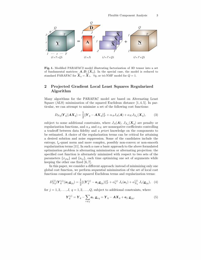
Fig. 1. Modified PARAFAC2 model illustrating factorization of 3D tensor into a setof fundamental matrices: A, D, fXq. In the special case, the model is reduced to

standard PARAFAC for fXq =fX1, ∀q, or tri-NMF model for Q = 1.

2 Projected Gradient Local Least Squares RegularizedAlgorithm

Many algorithms for the PARAFAC model are based on Alternating LeastSquare (ALS) minimization of the squared Euclidean distance [1, 4, 5]. In par-ticular, we can attempt to minimize a set of the following cost functions:

DFq(Y q||AXq) =1

2‖Y q −AXq‖

2F + αAJA(A) + αXJXq

(Xq), (3)

subject to some additional constraints, where JA(A), JXq(Xq) are penalty or

regularization functions, and αA and αX are nonnegative coefficients controllinga tradeoff between data fidelity and a priori knowledge on the components tobe estimated. A choice of the regularization terms can be critical for attaininga desired solution and noise suppression. Some of the candidates include theentropy, lp-quasi norm and more complex, possibly non-convex or non-smoothregularization terms [11]. In such a case a basic approach to the above formulatedoptimization problem is alternating minimization or alternating projection: thespecified cost function is alternately minimized with respect to two sets of theparameters xjtq and aij, each time optimizing one set of arguments whilekeeping the other one fixed [6, 7].

In this paper, we consider a different approach: instead of minimizing only oneglobal cost function, we perform sequential minimization of the set of local costfunctions composed of the squared Euclidean terms and regularization terms:

D(j)Fq(Y

(j)q ||ajxjq) =

1

2‖(Y (j)

q − ajxjq)‖2F + α(j)

a Ja(aj) + α(j)Xq

Jx(xjq), (4)

for j = 1, 2, . . . , J, q = 1, 2, . . . , Q, subject to additional constraints, where

Y(j)q = Y q −

∑

r 6=j

ar xrq = Y q −AXq + aj xjq, (5)


aj ∈ RI×1 are the columns of the basis mixing matrix A, xjq ∈ R

1×T are therows of Xq which represent unknown source signals, Ja(aj) and Jx(xjq) are localpenalty regularization terms which impose specific constraints for the estimated

parameters, and α(j)a ≥ 0 and α

(j)Xq≥ 0 are nonnegative regularization parameters

that control a tradeoff between data-fidelity and the imposed constraints.The construction of such a set of local cost functions follows from the sim-

ple observation that the observed data can be decomposed as follows Y q =∑Jj=1 ajxjq + N q, ∀ q. We motivate the use of such a representation and de-

composition, because xjq have physically meaningful interpretation as sourceswith specific temporal and morphological properties.

The penalty terms may take different forms depending on properties of theestimated sources. For example, if the sources are sparse, we can apply the lp-quasi norm: Jx(xjq) = ||xjq ||

pp = (

∑t |xjtq |

p)1/p with 0 < p ≤ 1, or alternatively

we can use the smooth approximation Jx(xjq) =[∑T

t |xjtq |2 + ε

]p/2

, where

ε ≥ 0 is a small constant. In order to impose local smoothing of signals, we canapply the total variation (TV) Jx(xjq) =

∑T−1t=1 |xj,t+1,q − xj,t,q|, or if we wish

to achieve a smoother solution: Jx(xjq) =∑T−1

t=1

√|xj,t+1,q − xj,t,q|2 + ε, [12].

The gradients of the local cost function (4) with respect to the unknownvectors aj and xjq are expressed by

∂D(j)Fq(Y

(j)q ||aj xjq)

∂xjq

= aTj aj xjq − a

Tj Y

(j)q + α

(j)Xq

Ψx(xjq), (6)

∂D(j)Fq(Y

(j)q ||aj xjq)

∂aj= aj xjq x

Tjq − Y

(j)q x

Tjq + α(j)

a Ψa(aj), (7)

where the matrix functions Ψa(aj) and Ψx(xjq) are defined as2

Ψa(aj) =∂J

(j)a (aj)

∂aj, Ψx(xjq) =

∂J(j)x (xjq)

∂xjq

. (8)

By equating the gradient components to zero, we obtain a new set of locallearning rules:

xjq ←1

aTj aj

(a

Tj Y

(j)q − α

(j)Xq

Ψx(xjq))

, (9)

aj ←1

xjq xTjq

(Y

(j)q x

Tjq − α(j)

a Ψa(aj))

, (10)

for j = 1, 2, . . . , J and q = 1, 2, . . . , Q.However, it should be noted that the above algorithm provides only a reg-

ularized least squares solution, and this is not sufficient to extract the desired

2 If the penalty functions are non-smooth, we can use sub-gradient instead of thegradient.


sources, especially for an under-determined case since the problem may havemany solutions. To solve this problem, we need additionally to impose nonlin-ear projections PΩj

(xjq) or filtering after each iteration or each epoch in orderto enforce that individual estimated sources xjq satisfy the desired constraints.All such projections or filtering can be imposed individually for each source xjq

depending on morphological properties of the source signals. The similar nonlin-ear projection PΩj

(aj) can be applied, if necessary, individually for each vectoraj of the mixing matrix A. Hence, using the projected gradient approach, ouralgorithm can take the following more general and flexible form:

xjq ←1

aTj aj

(aTj Y

(j)q − α

(j)Xq

Ψx(xjq)), xjq ← PΩjxjq, (11)

aj ←1

xjq xTjq

(Y (j)q x

Tjq − α(j)

a Ψa(aj)), aj ← PΩjaj; (12)

where PΩjxjq means generally a nonlinear projection, filtering, transforma-

tion, local interpolation/extrapolation, inpainting, smoothing of the row vectorxjq. Such projections or transformations can take many different forms depend-ing on required properties of the estimated sources (see the next section for moredetails).

Remark 1. In practice, it is necessary to normalize the column vectors aj orthe row vectors xjq to unit length vectors (in the sense of the lp norm (p =1, 2, ...,∞)) in each iterative step. In the special case of the l2 norm, the abovealgorithm can be further simplified by neglecting the denominator in (11) or in

(12), respectively. After estimating the normalized matrices A and Xq (i.e., thenormalized Xq to unit-length rows), we can estimate the diagonal matrices, ifnecessary, as follows:

Dq = diagA+Y q X

+

q , (q = 1, 2, . . . , Q). (13)

3 Flexible Component Analysis (FCA) - PossibleExtensions and Practical Implementations

The above simple algorithm can be further extended or improved (in respect toa convergence rate and performance). First of all, different cost functions can beused for estimating the rows of the matrices Xq (q = 1, 2, . . . , Q) and the columnsof the matrix A. Furthermore, the columns of A can be estimated simultaneously,instead one by one. For example, by minimizing the set of cost functions in (4)with respect to xjq, and simultaneously the cost function (3) with normalizationof the columns aj to an unit l2-norm, we obtain a new FCA learning algorithmin which the individual rows of Xq are updated locally (row by row) and thematrix A is updated globally (all the columns aj simultaneously):

xjq ← aTj Y

(j)q − α

(j)Xq

Ψx(xjq), xjq ← PΩjxjq, (j = 1, . . . , J), (14)

A← (Y qXTq − αAΨA(A))(XqX

Tq )−1, A← PΩ(A), (q = 1, . . . , Q),(15)


with the normalization (scaling) of the columns of A to an unit length in thesense of the l2 norm, where ΨA(A) = ∂JA(A)/∂A.

In order to estimate the basis matrix A, we can use alternatively the followingglobal cost function (see Eq. (2)): DF (Y ||AX) = (1/2)‖Y −AX‖2F +αAJA(A).The minimization of the cost function for a fixed X leads to the updating rule

A←[Y X

T − αAΨA(A)](XX

T )−1. (16)

3.1 Nonnegative Matrix/Tensor Factorization

In order to enforce sparsity and nonnegativity constraints for all the parameters:aij ≥ 0, xjtq ≥ 0, ∀ i, t, q, we can apply the ”half-way rectifying” element-wiseprojection: [x]+ = maxε, x, where ε is a small constant to avoid numericalinstabilities and remove background noise (typically, ε = [10−2 − 10−9]). Si-multaneously, we can impose weak sparsity constriants by using the l1-norm

penalty functions: JA(A) = ||A||1 =∑

ij aij and J(j)x (xjq) = ||xjq||1 =

∑t xjtq .

In such a case, the FCA algorithm for the 3D NTF2 (i.e., the PARAFAC2 withnonnegativity constraints) will take the following form:

xjq ←[a

Tj Y

(j)q − α

(j)Xq

1]+

, (j = 1, . . . , J), (q = 1, . . . , Q), (17)

A←[(Y X

T − αA1)(XXT )−1

]+

, (18)

with normalization of the columns of A in each iterative step to a unit lengthwith the l2 norm, where 1 means a matrix of all ones of appropriate size.

It should be noted the above algorithm can be easily extended to semi-NMFor semi-NTF in which only some sources xjq are nonnegative and/or the mixingmatrix A is bipolar, by simple removing the corresponding ”half-wave rectifying”projections. Moreover, the similar algorithm can be used for arbitrary boundedsources with known lower and/or upper bounds (or supports), i.e ljq ≤ xjtq ≤uiq, ∀t, rather than xjtq ≥ 0, by using suitably chosen nonlinear projectionswhich bound the solutions.

3.2 Smooth Component Analysis (SmoCA)

In order to enforce smooth estimation of the sources xjq for all or some pre-selected indexes j and q, we may apply after each iteration (epoch) the localsmoothing or filtering of the estimated sources, such as the MA (Moving Aver-age), EMA, SAR or ARMA models.

A quite efficient way of smoothing and denoising can be achieved by mini-mizing the following cost function (which satisfies multi-resolution criterion):

J(xjq) =

T∑

t=1

(xjtq − xjtq)2+

T−1∑

t=1

λjtq gt (xj,t+1,q − xjtq) , (19)

where xjtq is a smoothed version of the actually estimated (noisy) xjtq , gt(u) isa convex continuously differentiable function with a global minimum at u = 0,and λjtq are parameters that are data driven and chosen automatically.


3.3 Multi-way Sparse Component Analysis (MSCA)

In the sparse component analysis an objective is to estimate the sources xjq

which are sparse and usually with a prescribed or specified sparsification profile,possibly with additional constraints like local smoothness. In order to enforcethat the estimated sources are sufficiently sparse, we need to apply a suitablenonlinear projection or filtering which allows us adaptively to sparsify the data.The simplest nonlinear projection which enforces some sparsity to the normalizeddata is to apply the following weakly nonlinear element-wise projection:

PΩj(xjtq) = sign(xjtq)|xjtq |

1+αjq (20)

where αjq is a small parameter which controls sparsity. Such nonlinear projectioncan be considered as a simple (trivial) shrinking. Alternatively, we may usemore sophisticated adaptive local soft or hard shrinking in order to sparsifyindividual sources. Usually, we have the three-steps procedure: First, we performthe linear transformation: xw = xW , then, the nonlinear shrinking (adaptivethresholding), e.g., the soft element-wise shrinking: PΩ(xw) = sign(xw) [|xw| −δ]1+δ

+ , and finally the inverse transform: x = PΩ(xw)W−1. The threshold δ > 0is usually not fixed but it is adaptively (data-driven) selected or it graduallydecreases to zero with iterations. The optimal choice for a shrinkage functiondepends on a distribution of data. We have tested various shrinkage functionswith gradually decreasing δ: the hard thresholding rule, soft thresholding rule,non-negative Garrotte rule, n-degree Garotte, and Posterior median shrinkagerule [13]. For all of them, we have obtained the promising results, and usuallythe best performance appears for the simple hard rule.

Our method is somewhat related to the MoCA and SCA algorithms, pro-posed recently by Bobin et al., Daubechies et al., Elad et al., and many others[10, 14, 11]. However, in contrast to these approaches our algorithms are localand more flexible. Moreover, the proposed FCA is more general than the SCA,since it is not limited only to a sparse representation via shrinking and lineartransformation but allows us to impose general and flexible (soft and hard) con-straints, nonlinear projections, transformations, and filtering3. Furthermore, inthe contrast to many alternative algorithms which process the columns of Xq,we process their rows which represent directly the source signals.

We can outline the FCA algorithm as follows:

1. Set the initial values of the matrix A and the matrices Xq, and normalizethe vectors aj to an unit l2-norm length.

2. Calculate the new estimate xjq of the matrices Xq using the iterative formulain (14).

3. If necessary, enforce the nonlinear projection or filtering by imposing naturalconstraints on individual sources (the rows of Xq, (q = 1, 2, . . . , Q)), suchas nonnegativity, boundness, smoothness, and/or sparsity.

3 In this paper, in fact, we use two kinds of constraints: the soft (or weak) constraintsvia penalty and regularization terms in the local cost functions, and the hard (strong)constraints via iteratively adaptive postprocessing using nonlinear projections orfiltering.


4. Calculate the new estimate of A from (16), normalize each column of A toan unit length, and impose the additional constraints on A, if necessary.

5. Repeat the steps (2) and (4) until the convergence criterion is satisfied.

3.4 Multi-layer Blind Identification

In order to improve the performance of the FCA algorithms proposed in this pa-per, especially for ill-conditioned and badly-scaled data and also to reduce therisk of getting stuck in local minima in non-convex alternating minimization,we have developed the simple hierarchical multi-stage procedure [15] combinedtogether with multi-start initializations, in which we perform a sequential de-composition of matrices as follows. In the first step, we perform the basic de-composition (factorization) Y q ≈ A

(1)X

(1)q using any suitable FCA algorithm

presented in this paper. In the second stage, the results obtained from the first

stage are used to build up a new tensor X1 from the estimated frontal slices de-

fined as Y(1)

q = X(1)q , (q = 1, 2, . . . , Q). In the next step, we perform the similar

decomposition for the new available frontal slices: Y(1)

q = X(1)q ≈ A

(2)X

(2)q ,

using the same or different update rules. We continue our decomposition takinginto account only the last achieved components. The process can be repeatedarbitrarily many times until some stopping criteria are satisfied. In each step, weusually obtain gradual improvements of the performance. Thus, our FCA modelhas the following form: Y q ≈ A

(1)A

(2) · · ·A(L)X

(L)q , (q = 1, 2, . . . , Q) with the

final components A = A(1)

A(2) · · ·A(L) and Xq = X

(L)q .

Physically, this means that we build up a system that has many layers orcascade connections of L mixing subsystems. The key point in our approach isthat the learning (update) process to find the matrices X

(l)q and A

(l) is performedsequentially, i.e. layer by layer, where each layer is initialized randomly. In fact,we found that the hierarchical multi-layer approach plays a key role, and it isnecessary to apply in order to achieve satisfactory performance for the proposedalgorithms.

4 Simulation Results

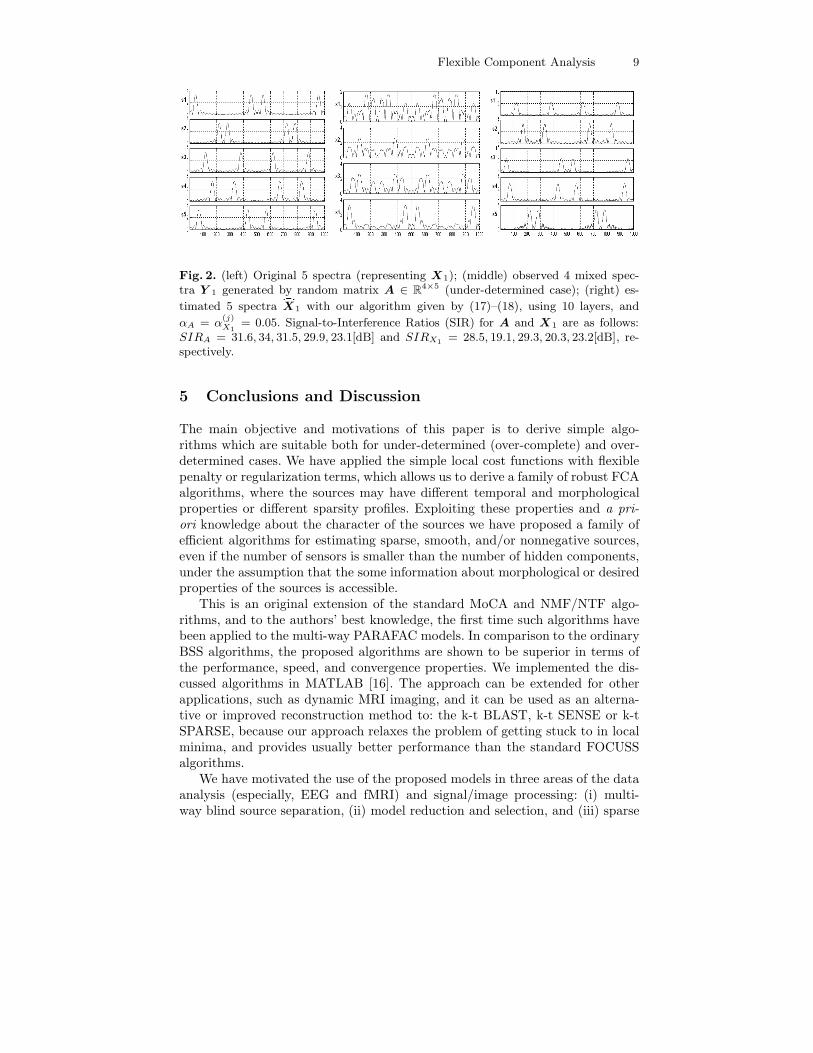
The algorithms presented in this paper have been tested for many difficult bench-marks for signals and images with various temporal and morphological propertiesof signals and additive noise. Due to space limitation we present here only oneillustrative example. The sparse nonnegative signals with different sparsity andsmoothness profiles are collected in with 10 slices Xq (Q = 10) under the formof the tensor X ∈ R

5×1000×10. The observed (mixed) 3D data Y ∈ R4×1000×10

are obtained by multiplying the randomly generated mixing matrix A ∈ R4×5

by X. The simulation results are illustrated in Fig. 2 (only for one frontal sliceq = 1).


Fig. 2. (left) Original 5 spectra (representing X1); (middle) observed 4 mixed spec-tra Y 1 generated by random matrix A ∈ R

4×5 (under-determined case); (right) es-

timated 5 spectra X1 with our algorithm given by (17)–(18), using 10 layers, and

αA = α(j)X1

= 0.05. Signal-to-Interference Ratios (SIR) for A and X1 are as follows:SIRA = 31.6, 34, 31.5, 29.9, 23.1[dB] and SIRX1

= 28.5, 19.1, 29.3, 20.3, 23.2[dB], re-spectively.

5 Conclusions and Discussion

The main objective and motivations of this paper is to derive simple algo-rithms which are suitable both for under-determined (over-complete) and over-determined cases. We have applied the simple local cost functions with flexiblepenalty or regularization terms, which allows us to derive a family of robust FCAalgorithms, where the sources may have different temporal and morphologicalproperties or different sparsity profiles. Exploiting these properties and a pri-

ori knowledge about the character of the sources we have proposed a family ofefficient algorithms for estimating sparse, smooth, and/or nonnegative sources,even if the number of sensors is smaller than the number of hidden components,under the assumption that the some information about morphological or desiredproperties of the sources is accessible.

This is an original extension of the standard MoCA and NMF/NTF algo-rithms, and to the authors’ best knowledge, the first time such algorithms havebeen applied to the multi-way PARAFAC models. In comparison to the ordinaryBSS algorithms, the proposed algorithms are shown to be superior in terms ofthe performance, speed, and convergence properties. We implemented the dis-cussed algorithms in MATLAB [16]. The approach can be extended for otherapplications, such as dynamic MRI imaging, and it can be used as an alterna-tive or improved reconstruction method to: the k-t BLAST, k-t SENSE or k-tSPARSE, because our approach relaxes the problem of getting stuck to in localminima, and provides usually better performance than the standard FOCUSSalgorithms.

We have motivated the use of the proposed models in three areas of the dataanalysis (especially, EEG and fMRI) and signal/image processing: (i) multi-way blind source separation, (ii) model reduction and selection, and (iii) sparse


image coding. Our preliminary experimental results are promising. The modelscan be further extended by imposing additional, natural constraints such asorthogonality, continuity, closure, unimodality, local rank - selectivity, and/orby taking into account a prior knowledge about the specific components.

References

1. Smilde, A., Bro, R., Geladi, P.: Multi-way Analysis: Applications in the ChemicalSciences. John Wiley and Sons, New York (2004)

2. Hazan, T., Polak, S., Shashua, A.: Sparse image coding using a 3D non-negativetensor factorization. In: International Conference of Computer Vision (ICCV).(2005) 50–57

3. Heiler, M., Schnoerr, C.: Controlling sparseness in non-negative tensor factoriza-tion. Springer LNCS 3951 (2006) 56–67

4. Miwakeichi, F., Martnez-Montes, E., Valds-Sosa, P., Nishiyama, N., Mizuhara, H.,Yamaguchi, Y.: Decomposing EEG data into space−time−frequency componentsusing parallel factor analysi. NeuroImage 22 (2004) 1035–1045

5. Mørup, M., Hansen, L.K., Herrmann, C.S., Parnas, J., Arnfred, S.M.: Parallelfactor analysis as an exploratory tool for wavelet transformed event-related EEG.NeuroImage 29 (2006) 938–947

6. Lee, D.D., Seung, H.S.: Learning the parts of objects by nonnegative matrix fac-torization. Nature 401 (1999) 788–791

7. Cichocki, A., Amari, S.: Adaptive Blind Signal and Image Processing (New revisedand improved edition). John Wiley, New York (2003)

8. Dhillon, I., Sra, S.: Generalized nonnegative matrix approximations with Bregmandivergences. In: Neural Information Proc. Systems, Vancouver, Canada (2005)283–290

9. Berry, M., Browne, M., Langville, A., Pauca, P., Plemmons, R.: Algorithms andapplications for approximate nonnegative matrix factorization. ComputationalStatistics and Data Analysis (2006) in press.

10. Bobin, J., Starck, J.L., Fadili, J., Moudden, Y., Donoho, D.L.: Morphologicalcomponent analysis: An adaptive thresholding strategy. IEEE Transactions onImage Processing (2007) in print.

11. Elad, M.: Why simple shrinkage is still relevant for redundant representations?IEEE Trans. On Information Theory 52 (2006) 5559–5569

12. Kovac, A.: Smooth functions and local extreme values. Computational Statisticsand Data Analysis 51 (2007) 5155–5171

13. Tao, T., Vidakovic, B.: Almost everywhere behavior of general wavelet shrinkageoperators. Applied and Computational Harmonic Analysis 9 (2000) 72–82

14. Daubechies, I., Defrrise, M., Mol, C.D.: An iterative thresholding algorithm forlinear inverse problems with a sparsity constraint. Pure and Applied Mathematics57 (2004) 1413–1457

15. Cichocki, A., Zdunek, R.: Multilayer nonnegative matrix factorization. ElectronicsLetters 42 (2006) 947–948

16. Cichocki, A., Zdunek, R.: NTFLAB for Signal Processing. Technical report, Labo-ratory for Advanced Brain Signal Processing, BSI, RIKEN, Saitama, Japan (2006)

Flexible component analysis for sparse, smooth, nonnegative coding or representation

Documents