arXiv:0907.5386v2 [hep-ph] 19 Feb 2010 BNL-90299-2009-BC, CERN-PH-TH-2009-112, FERMILAB-PUB-09-323-T, LAL 09-111, MPP-2009-88, MZ-TH/09-22, MKPH-T-09-14, SLAC-R-926, TUM-HEP-728/09, WSU-HEP-0902 Flavor Physics in the Quark Sector M. Antonelli a D. M. Asner b D. Bauer c T. Becher d M. Beneke e A. J. Bevan f M. Blanke g,h C. Bloise a M. Bona i A. Bondar j C. Bozzi k J. Brod ℓ A.J. Buras g N. Cabibbo m,n A. Carbone o G. Cavoto m V. Cirigliano p M. Ciuchini q J. P. Coleman r D. P. Cronin-Hennessy s J. P. Dalseno t C. H. Davies u F. Di Lodovico f J. Dingfelder v Z. Dolezal w S. Donati x,y W. Dungel z G. Eigen aa U. Egede c R. Faccini m,n T. Feldmann g F. Ferroni m,n J. M. Flynn cf E. Franco m M. Fujikawa ab I. K. Furi´ c cd P. Gambino ac,ad E. Gardi ae T. J. Gershon af S. Giagu m,n E. Golowich ag T. Goto t C. Greub bf C. Grojean i D. Guadagnoli g U. A. Haisch ah R. F. Harr ai A. H. Hoang h T. Hurth i,r G. Isidori a D. E. Jaffe aj A. J¨ uttner ak S. J¨ ager g A. Khodjamirian aℓ P. Koppenburg c R. V. Kowalewski am P. Krokovny t A. S. Kronfeld d J. Laiho an G. Lanfranchi a T. E. Latham af J. Libby ap A. Limosani aq D. Lopes Pegna ar C. D. Lu as V. Lubicz q,at E. Lunghi d V. G. L¨ uth r K. Maltman av W. J. Marciano aj E. C. Martin ao G. Martinelli m,n F. Martinez-Vidal aw A. Masiero ay,az V. Mateu h F. Mescia ba G. Mohanty af ,bb M. Moulson a M. Neubert bc H. Neufeld bd S. Nishida t N. Offen be M. Palutan a P. Paradisi g Z. Parsa aj E. Passemar bf M. Patel i B. D. Pecjak bh A. A. Petrov ai A. Pich aw M. Pierini i B. Plaster bi A. Powell bs S. Prell bj J. Rademaker ce M. Rescigno m S. Ricciardi bk P. Robbe i,bg E. Rodrigues u M. Rotondo ay R. Sacco f C. J. Schilling bℓ O. Schneider bm E. E. Scholz d B. A. Schumm cc C. Schwanda z A. J. Schwartz bn B. Sciascia a J. Serrano bg J. Shigemitsu bo I. J. Shipsey cb A. Sibidanov j,a L. Silvestrini m F. Simonetto az S. Simula q C. Smith bf ,bp A. Soni aj L. Sonnenschein i,bq V. Sordini br M. Sozzi x,y T. Spadaro a P. Spradlin bs A. Stocchi bg N. Tantalo bt C. Tarantino q,at A. V. Telnov ar D. Tonelli d I. S. Towner bu K. Trabelsi t P. Urquijo aq R. S. Van de Water aj R. J. Van Kooten bw J. Virto m,n G. Volpi x,y R. Wanke bx S. Westhoff bp G. Wilkinson bs M. Wingate by Y. Xie ae Preprint submitted to Elsevier 19 February 2010

Welcome message from author
This document is posted to help you gain knowledge. Please leave a comment to let me know what you think about it! Share it to your friends and learn new things together.
Transcript

arX
iv:0
907.
5386
v2 [
hep-
ph]
19
Feb
2010
BNL-90299-2009-BC, CERN-PH-TH-2009-112, FERMILAB-PUB-09-323-T, LAL 09-111,MPP-2009-88, MZ-TH/09-22, MKPH-T-09-14, SLAC-R-926, TUM-HEP-728/09, WSU-HEP-0902
Flavor Physics in the Quark Sector
M. Antonelli a D. M. Asner b D. Bauer c T. Becher d M. Beneke e
A. J. Bevan f M. Blanke g,h C. Bloise a M. Bona i A. Bondar j C. Bozzi k
J. Brod ℓ A.J. Buras g N. Cabibbom,n A. Carbone o G. Cavotom
V. Cirigliano p M. Ciuchini q J. P. Coleman r D. P. Cronin-Hennessy s
J. P. Dalseno t C. H. Davies u F. Di Lodovico f J. Dingfelder v Z. Dolezal w
S. Donati x,y W. Dungel z G. Eigen aa U. Egede c R. Faccinim,n
T. Feldmann g F. Ferronim,n J. M. Flynn cf E. Francom M. Fujikawa ab
I. K. Furic cd P. Gambino ac,ad E. Gardi ae T. J. Gershon af S. Giagum,n
E. Golowich ag T. Goto t C. Greub bf C. Grojean i D. Guadagnoli g
U. A. Haisch ah R. F. Harr ai A. H. Hoang h T. Hurth i,r G. Isidori a
D. E. Jaffe aj A. Juttner ak S. Jager g A. Khodjamirian aℓ P. Koppenburg c
R. V. Kowalewski am P. Krokovny t A. S. Kronfeld d J. Laiho an
G. Lanfranchi a T. E. Latham af J. Libby ap A. Limosani aq
D. Lopes Pegna ar C. D. Lu as V. Lubicz q,at E. Lunghi d V. G. Luth r
K. Maltman av W. J. Marciano aj E. C. Martin ao G. Martinellim,n
F. Martinez-Vidal aw A. Masiero ay,az V. Mateu h F. Mescia ba
G. Mohanty af,bb M. Moulson a M. Neubert bc H. Neufeld bd S. Nishida t
N. Offen be M. Palutan a P. Paradisi g Z. Parsa aj E. Passemar bf M. Patel i
B. D. Pecjak bh A. A. Petrov ai A. Pich aw M. Pierini i B. Plaster bi
A. Powell bs S. Prell bj J. Rademaker ce M. Rescignom S. Ricciardi bk
P. Robbe i,bg E. Rodrigues u M. Rotondo ay R. Sacco f C. J. Schilling bℓ
O. Schneider bm E. E. Scholz d B. A. Schumm cc C. Schwanda z
A. J. Schwartz bn B. Sciascia a J. Serrano bg J. Shigemitsu bo I. J. Shipsey cb
A. Sibidanov j,a L. Silvestrinim F. Simonetto az S. Simula q C. Smith bf,bp
A. Soni aj L. Sonnenschein i,bq V. Sordini br M. Sozzi x,y T. Spadaro a
P. Spradlin bs A. Stocchi bg N. Tantalo bt C. Tarantino q,at A. V. Telnov ar
D. Tonelli d I. S. Towner bu K. Trabelsi t P. Urquijo aq
R. S. Van de Water aj R. J. Van Kooten bw J. Virtom,n G. Volpi x,y
R. Wanke bx S. Westhoff bp G. Wilkinson bs M. Wingate by Y. Xie ae
Preprint submitted to Elsevier 19 February 2010

J. Zupan i,bz,ca
aINFN LNF, Via Enrico Fermi 40, 00044 Frascati, ItalybCarleton University, 1125 Colonel By Drive, Ottawa, ON, Canada K1S 5B6
cImperial College London, London, SW7 2AZ, United KingdomdFermi National Accelerator Laboratory, P.O. Box 500 Batavia, IL 60510-5011, USA
eInstitut fur Theoretische Physik E, RWTH Aachen University, 52056, GermanyfQueen Mary, University of London, E1 4NS, United Kingdom
gTechnische Universitat Munchen, Excellence Cluster Universe, Boltzmannstraße 2, 85748 Garching,Germany
hMax-Planck-Institut fur Physik, Foehringer Ring 6, 80805 Munchen, GermanyiCERN CH-1211 Geneve 23, Switzerland
jBudker Institute of Nuclear Physics, 11, Prosp. Akademika Lavrentieva Novosibirsk 630090, RussianFederation
kINFN Sez. di Ferrara, Polo Scientifico e Tecnologico. Edificio C. Via Saragat, 1. 44100 Ferrara, ItalyℓUniversitat Karlsruhe, Liefer- und Besuchsanschrift: Kaiserstraße 12 - 76131 Karlsruhe Germany
mINFN Sez. di Roma, Piazzale Aldo Moro, 2 00185 Roma, ItalynUniversita di Roma ’Sapienza’, Dipartimento di Fisica, Piazzale Aldo Moro, 5 00185, Roma, Italy
oINFN Sez. di Bologna, Via Irnerio 46, I-40126 Bologna, ItalypLos Alamos National Laboratory, Los Alamos, NM 87545, USA
qINFN Sez. di Roma Tre, Via della Vasca Navale, 84 00146 Roma, ItalyrSLAC National Accelerator Laboratory, 2575 Sand Hill Road, Menlo Park, CA 94025, USA
sUniversity of Minnesota, Minneapolis, Minnesota 55455, USAtHigh Energy Accelerator Research Organization (KEK), 1-1 Oho, Tsukuba, Ibaraki 305-0801 Japan
uUniversity of Glasgow, Glasgow G12 8QQ, United KingdomvPhysikalisches Institut Freiburg, Hermann-Herder-Str.3, 79104 Freiburg, Germany
wIPNP, Charles University in Prague, Faculty of Mathematics and Physics, V Holesovickach 2, 18000 Prague 8, Czech Republic
xDipartimento di Fisica, Universita di Pisa, Largo Pontecorvo 3, 56126 Pisa, ItalyyINFN Sez. di Pisa, Edificio C - Polo Fibonacci Largo B. Pontecorvo, 3 - 56127 Pisa , Italy
zInstitute of High Energy Physics, A-1050 Vienna, AustriaaaDept. of Physics, University of Bergen, Allegaten 55, 5007 Bergen, Norway
abNara Women’s University, Nara, JapanacINFN Sez. di Torino, Via Pietro Giuria 1, 10125 Torino, Italy
adDip. di Fisica Teorica, Univ. di Torino, Via Pietro Giuria 1, 10125 Torino, ItalyaeUniversity of Edinburgh, Edinburgh EH9 3JZ, United Kingdom
afDepartment of Physics, University of Warwick, Coventry CV4 7AL, United KingdomagUniversity of Massachusetts, Amherst, Massachusetts 01003, USA
ahJohannes Gutenberg-Universitat, 55099 Mainz, GermanyaiWayne State University, Detroit, MI 48202, USA
ajBrookhaven National Laboratory, Upton, P.O. Box 5000 Upton, NY 11973-5000, USAakInstitut fur Theoretische Kernphysik, Johannes-Gutenberg Universitat Mainz,
Johann-Joachim-Becher Weg 45, 55099 Mainz, GermanyaℓUniversitat Siegen, Walter Flex Str.3, Emmy Noether Campus, D-57068 Siegen, Germany
amUniversity of Victoria, Victoria, British Columbia, Canada V8W 3P6anWashington University, St. Louis, Missouri 63130, USA
aoUniversity of California at Irvine, Irvine, California 92697, USAapIndian Institute of Technology Madras, IITM Post Office, Chennai, 600032, India
aqThe University of Melbourne, The School of Physics, Victoria 3010, AustraliaarPrinceton University, Princeton, New Jersey 08544, USA
asInstitute of High Energy Physics, Chinese Academy of Sciences, 19B YuquanLu, ShijingshanDistrict, Beijing, 100049, China
atUniversita di Roma Tre, Dipartimento di Fisica ’E. Amaldi’, Via della Vasca Navale 84, 00146Roma, Italy
auStanford University, Stanford, CA 94309, USAavYork University, Toronto, ON M3J 1P3, Canada
2

awIFIC, Universitat de Valencia-CSIC, E-46071 Valencia, SpainayINFN Sez. di Padova, Via F. Marzolo 8, 35131 Padova, Italy
azUniversita di Padova, Dipartimento di Fisica, Via F. Marzolo 8, 35131 Padova, ItalybaUniversitat de Barcelona, Facultat de Fisica, Departament ECM & ICC, E-08028 Barcelona, Spain
bbTata Institute of Fundamental Research, Homi Bhabha Road, Mumbai 400 005, IndiabcInstitut fur Physik, Johannes Gutenberg Universitat, Mainz, Staudingerweg 7, 55128, Germany
bdFaculty of Physics, University of Vienna, Boltzmanngasse 5, A-1090, Wien, AustriabeLaboratoire de Physique Theorique, CNRS/Univ. Paris-Sud 11 (UMR 8627), F-91405 Orsay,
FrancebfInstitute for theoretical physics, University of Bern, Sidlerstrasse 5, 3012 Bern, Switzerland
bgLaboratoire del Accelerateur Lineaire, Universite Paris 11, UMR 8607, Batiment 200 91898 Orsaycedex, France
bhTHEP, Johannes Gutenberg-Universitat, 55099 Mainz, GermanybiUniversity of Kentucky, Lexington, KY 40506, USAbjIowa State University, Ames, Iowa 50011-3160, USA
bkSTFC Rutherford Appleton Laboratory, Chilton, Didcot, OX11 0QX, United KingdombℓUniversity of Texas at Austin, Austin, Texas 78712, USA
bmEcole Polytechnique Federale de Lausanne (EPFL), CH 1015 (Centre Est) Lausanne, SwitzerlandbnUniversity of Cincinnati, P.O. Box 210011, Cincinnati, Ohio 45221, USA
boOhio State University, Columbus, Ohio 43210, USAbpUniversitat Karlsruhe, Institut fur Theoretische Teilchenphysik, D-76128 Karlsruhe, Germany
bqLaboratoire de Physique Nucleaire et de Hautes Energies, LPNHE - Tour 43 Rez-de-chaussoe - 4place Jussieu - 75252 PARIS CEDEX
brETH Zurich, HG Raemistrasse 101 8092 Zurich SwitzerlandbsUniversity of Oxford, Oxford, United Kingdom
btINFN Sezione di Roma ’Tor Vergata’ Via della Ricerca Scientifica, 1 00133 Roma - ItalybuPhysics Department, Queen’s University, Kingston, Ontario K7L 3N6, Canada
bwIndiana University, Bloomington, IN 47405, USAbxUniversitat Mainz, Institut fur Physik, 55099 Mainz, Germany
byUniversity of Cambridge, DAMTP, Wilberforce Road, Cambridge CB3 0WA, United KingdombzJozef Stefan Institute, Jamova cesta 39, 1000 Ljubljana, Slovenia
caUniversity of Ljubljana, Kongresni trg 12, 1000 Ljubljana, SlovenijacbPurdue University, West Lafayette, IN 47907, USA
ccUniversity of California at Santa Cruz, Institute for Particle Physics, Santa Cruz, California 95064,USA
cdUniversity of Florida, Gainesville, FL 32611, USAceUniversity of Bristol, Bristol, BS8 1TL, United Kingdom
cfSchool of Physics & Astronomy, University of Southampton, Southampton SO17 1BJ, UnitedKingdom
Abstract
In the past decade, one of the major challenges of particle physics has been to gain an in-depth
understanding of the role of quark flavor. In this time frame, measurements and the theoretical
interpretation of their results have advanced tremendously. A much broader understanding of
flavor particles has been achieved, apart from their masses and quantum numbers, there now
exist detailed measurements of the characteristics of their interactions allowing stringent tests
of Standard Model predictions. Among the most interesting phenomena of flavor physics is
the violation of the CP symmetry that has been subtle and difficult to explore. In the past,
observations of CP violation were confined to neutral K mesons, but since the early 1990s, a
large number of CP-violating processes have been studied in detail in neutral B mesons. In
parallel, measurements of the couplings of the heavy quarks and the dynamics for their decays
3

in large samples of K,D, and B mesons have been greatly improved in accuracy and the results
are being used as probes in the search for deviations from the Standard Model.
In the near future, there will be a transition from the current to a new generation of experi-
ments, thus a review of the status of quark flavor physics is timely. This report is the result of
the work of the physicists attending the 5th CKM workshop, hosted by the University of Rome
”La Sapienza”, September 9-13, 2008. It summarizes the results of the current generation of
experiments that is about to be completed and it confronts these results with the theoretical
understanding of the field which has greatly improved in the past decade.
Key words:PACS:
Contents
1 Introduction 7
1.1 CKM matrix and the Unitarity Triangle 7
1.1.1 Standard parametrization 8
1.1.2 Wolfenstein parametrization and its generalization 8
1.1.3 Unitarity Triangle 9
1.2 Plan of the report 11
2 Theory Primers 12
2.1 Effective Weak Hamiltonians 12
2.1.1 ∆F = 1 effective weak Hamiltionians 162.1.2 ∆F = 2 effective weak Hamiltionians 19
2.2 Factorization 19
2.3 Lattice QCD 22
2.4 Chiral Perturbation Theory 29
2.5 Beyond the Standard Model 31
2.5.1 Model-independent approaches and the MFV hypothesis 32
2.5.2 The Minimal Supersymmetric extension of the SM (MSSM) 37
2.5.3 Non-supersymmetric extensions of the Standard Model 41
3 Experimental Primers 41
3.1 Overview of experiments 41
3.1.1 Kaon experiments 41
3.1.2 B Factories 45
3.1.3 τ -charm Factories 47
3.1.4 Hadron Colliders 48
3.2 Common experimental tools 51
3.2.1 Time-dependent measurements 51
3.2.2 B Flavor Tagging 52
3.2.3 Vertexing 58
3.2.4 Charged Particle Identification 613.2.5 Background suppression 64
3.2.6 Recoil Tagging Technique 68
3.2.7 Dalitz Plot Analysis 69
4 Determination of |Vud| and |Vus|. 71
4.1 Vud from nuclear decays 72
4.2 Vud from neutron decay 75
4

4.3 Vud from pionic beta decay 78
4.4 Determination of |Vus| from Kℓ2 and Kℓ3 784.4.1 Pℓ2 (P = π,K) rates within the SM 794.4.2 Kℓ3 rates within the SM 80
4.4.3 Kℓ3 form factors 824.4.4 Lattice determinations of f+(0) and fK/fπ 854.4.5 Data Analysis 90
4.5 |Vus| determination from tau decays 984.6 Physics Results 100
4.6.1 Determination of |Vus| × f+(0) and |Vus|/|Vud| × fK/fπ 100
4.6.2 A test of lattice calculation: the Callan-Treiman relation 1014.6.3 Test of Cabibbo Universality or CKM unitarity 1034.6.4 Tests of Lepton Flavor Universality in Kℓ2 decays 108
5 Semileptonic B and D decays: |Vcx| and |Vub| 1095.1 Exclusive semileptonic B and D decays to light mesons π and K 110
5.1.1 Theoretical Background 110
5.1.2 Measurements of D Branching Fractions and q2 Dependence 1155.1.3 Measurements of B branching fractions and q2 dependence 1225.1.4 Determination of |Vcs|, |Vcd|, |Vub| 125
5.2 B → D(∗)ℓν decays for |Vcb| 1285.2.1 Theoretical background: HQS and HQET 1285.2.2 Measurements and Tests 1335.2.3 Determination of Form Factors and |Vcb| 137
5.3 Inclusive CKM-favored B decays 1385.3.1 Theoretical Background 1385.3.2 Measurements of Moments 140
5.3.3 Global Fits for |Vcb| and mb 1425.4 Inclusive CKM-suppressed B decays 143
5.4.1 Theoretical Overview 143
5.4.2 Review of mb determinations 1475.4.3 Measurements and tests 1535.4.4 Determination of |Vub| 156
6 Rare decays and measurements of |Vtd/Vts| 1596.1 Introduction 1596.2 Inclusive B → Xs,dγ 160
6.2.1 Theory of inclusive B → Xs,dγ 1606.2.2 Experimental methods and status of B → Xs,dγ 1636.2.3 Theory of photon energy spectrum and moments 165
6.2.4 Experimental results of photon energy spectrum and moments 1676.3 Exclusive B → V γ decays 168
6.3.1 Theory of exclusive B → V γ decays 168
6.3.2 Experimental results for exclusive B → V γ decays 1706.3.3 Determinations of |Vtd/Vts| from b→ (s, d)γ 173
6.4 Purely leptonic rare decays 174
6.4.1 Theory of purely leptonic rare decays 1746.4.2 Experimental results on purely leptonic rare decays 175
6.5 Semileptonic modes 177
6.5.1 B → Dτν modes 1776.6 Semileptonic neutral currents decays 177
6.6.1 Theory of inclusive B → Xsℓ+ℓ− 177
6.6.2 Experimental results on inclusive B → Xsℓ+ℓ− 1796.6.3 Theory of exclusive b → sℓ+ℓ− modes 1806.6.4 Angular observables in B → K∗ℓ+ℓ− 183
6.6.5 Experimental results on exclusive b → (s, d)ℓ+ℓ− 1856.6.6 Rare K → πνν, ℓ+ℓ− decays in and beyond the SM 1896.6.7 Experimental status of K → πνν and KL → πℓ+ℓ− 192
5

6.7 Rare D meson decays 192
6.7.1 Rare leptonic decays 1926.7.2 D and Ds decay constants from lattice QCD 1946.7.3 Experimental results on fD 197
7 Measurements of Γ, ∆Γ, ∆m and mixing-phases in K, B, and D meson decays 1997.1 The K-meson system 204
7.1.1 Theoretical prediction for ∆MK , εK , and ε′K/εK 204
7.1.2 Experimental methods and results 2057.2 The B-meson system 209
7.2.1 Lifetimes, ∆ΓBq , AqSL
and ∆MBq 209
7.2.2 B meson mixing 2147.2.3 Measurements of the angle β in tree dominated processes 2167.2.4 Measurement of the Bs meson mixing phase 219
7.3 The D-meson system 2237.3.1 Theoretical prediction for ∆MD and CP violation within the SM and beyond 2237.3.2 Experimental results 224
7.4 Future Outlook 2277.4.1 B meson mixing and lifetimes 2277.4.2 Measurements of the Bs meson mixing phase 228
7.4.3 D0 mixing and CP violation 2308 Measurement of the angle γ in tree dominated processes 2338.1 Overview of Theoretically Pristine Approaches to Measure γ 2338.2 Experimental results on γ from B → DK decays 235
8.2.1 GLW analyses 2358.2.2 ADS analyses 2368.2.3 Dalitz plot analyses 238
8.2.4 Other techniques 2418.3 Outlook on the γ measurement 243
8.3.1 Model-independent Method 243
8.3.2 Prospects for LHCb 2469 Measurements of the angles of the unitarity triangle in charmless hadronic B decays 2489.1 Theory estimates for hadronic amplitudes 248
9.1.1 Angles, physical amplitudes, topological amplitudes 2489.1.2 Tree amplitudes: results 2519.1.3 Penguin amplitudes: results 254
9.1.4 Application to angle measurements 2559.1.5 Prospects 256
9.2 Measurement of β 257
9.2.1 Theoretical aspects 2579.2.2 Experimental results 258
9.3 Measurements of α 262
9.3.1 Theoretical aspects 2629.3.2 Experimental measurements 266
9.4 Measurements of γ in charmless hadronic B decays 275
9.4.1 Constraints from B(s) → hh 2759.4.2 Constraints from B → Kππ Dalitz-plot analyses 276
10 Global Fits to the Unitarity Triangle and Constraints on New Physics 280
10.1 Constraints on the Unitarity Triangle Parameters 28110.1.1 Fitting technique 28110.1.2 Inputs to the Unitarity Triangle Analysis 283
10.1.3 Results of Global Fits 28410.1.4 Impact of the Uncertainties on Theoretical Quantities 28610.1.5 Comparison with the Results of CKMfitter 287
10.2 CKM angles in the presence of New Physics 29110.2.1 Model independent constraints on New Physics from global fits 29110.2.2 Impact of flavor physics measurements on grand unified 294
6

10.2.3 New physics in extra-dimension models 297
11 Acknowledgements 300
References 301
1. Introduction
In the past decade, one of the major challenges of particle physics has been to gainan in-depth understanding of the role of quark flavor. In this time frame, measurementsand the theoretical interpretation of their results have advanced tremendously. A muchbroader understanding of flavor particles has been achieved, apart from their masses andquantum numbers, there now exist detailed measurements of the characteristics of theirinteractions allowing stringent tests of Standard Model predictions.Among the most interesting phenomena of flavor physics is the violation of the CP
symmetry that has been subtle and difficult to explore. In the past, observations of CPviolation were confined to neutral K mesons, but since the early 1990s, a large numberof CP-violating processes have been studied in detail in neutral B mesons. In parallel,measurements of the couplings of the heavy quarks and the dynamics for their decays inlarge samples of K,D, and B mesons have been greatly improved in accuracy and theresults are being used as probes in the search for deviations from the Standard Model.In the near future, there will be a transition from the current to a new generation of
experiments, thus a review of the status of quark flavor physics is timely. This reportis the result of the work of the physicists attending the 5th CKM workshop, hosted bythe University of Rome ”La Sapienza”, September 9-13, 2008. It summarizes the resultsof the current generation of experiments that is about to be completed and it confrontsthese results with the theoretical understanding of the field which has greatly improvedin the past decade.In this section the basic formalism of the study of the quark couplings will be introduced
and the relationship between CKM matrix elements and observables will be discussed.The last paragraph will then detail the plan of the report and the content of the rest ofthe sections.
1.1. CKM matrix and the Unitarity Triangle
The unitary CKM matrix [1,2] connects the weak eigenstates (d′, s′, b′) and the corre-sponding mass eigenstates d, s, b (in both basis the up-type mass matrix is diagonal andthe up-type quarks are unaffected by this transformation):
d′
s′
b′
=
Vud Vus Vub
Vcd Vcs Vcb
Vtd Vts Vtb
d
s
b
≡ VCKM
d
s
b
. (1)
The CKM matrix contains all the flavor-changing and CP-violating couplings of theStandard Model.Several parameterizations of the CKM matrix have been proposed in the literature.
This report will use the standard parametrization [3] recommended by the Particle Data
7

Group [4]. We also introduce the generalization of the Wolfenstein parametrization [5]presented in [6] and discuss its connection to the Unitarity Triangle parameters.
1.1.1. Standard parametrizationWith cij = cos θij and sij = sin θij (i, j = 1, 2, 3), the standard parametrization is
given by:
VCKM =
c12c13 s12c13 s13e−iδ
−s12c23 − c12s23s13eiδ c12c23 − s12s23s13e
iδ s23c13
s12s23 − c12c23s13eiδ −s23c12 − s12c23s13e
iδ c23c13
, (2)
where δ is the phase necessary for CP violation. cij and sij can all be chosen to be positiveand δ may vary in the range 0 ≤ δ ≤ 2π. However, measurements of CP violation inK decays force δ to be in the range 0 < δ < π, as the sign of the relevant hadronicparameter is fixed.From phenomenological studies we know that s13 and s23 are small numbers: O(10−3)
and O(10−2), respectively. Consequently, to a very good accuracy,
s12 ≃ |Vus|, s13 ≃ |Vub|, s23 ≃ |Vcb|. (3)
Thus these three parameters can be extracted from tree level decays mediated by thetransitions s→ u, b→ u and b→ c, respectively. The remaining parameter, the phase δ,is responsible for the violation of the CP symmetry. It can clearly be extracted from CP-violating transitions but also from CP-conserving ones using three-generation unitarity,through the construction of the Unitarity Triangle, as discussed below.
1.1.2. Wolfenstein parametrization and its generalizationThe absolute values of the elements of the CKM matrix show a hierarchical pattern
with the diagonal elements being close to unity, the elements |Vus| and |Vcd| being oforder 0.2, the elements |Vcb| and |Vts| of order 4 ·10−2 whereas |Vub| and |Vtd| are of order5 · 10−3. The Wolfenstein parametrization [5] exhibits this hierarchy in a transparentmanner. It is an approximate parametrization of the CKM matrix in which each elementis expanded as a power series in the small parameter λ ∼ |Vus| ≈ 0.22,
V =
1− λ2
2λ Aλ3(− iη)
−λ 1− λ2
2Aλ2
Aλ3(1− − iη) −Aλ2 1
+O(λ4) , (4)
and the set (3) is replaced by
λ, A, , and η . (5)
Because of the smallness of λ and the fact that for each element the expansion parameteris actually λ2, this is a rapidly converging expansion.The Wolfenstein parametrization is certainly more transparent than the standard
parametrization. However, if one requires sufficient level of accuracy, the terms of O(λ4)and O(λ5) have to be included in phenomenological applications. This can be done in
8

many ways [6]. The point is that since (4) is only an approximation the exact definitionof the parameters in (5) is not unique in terms of the neglected order O(λ4). This situa-tion is familiar from any perturbative expansion, where different definitions of expansionparameters (coupling constants) are possible. This is also the reason why in different pa-pers in the literature different O(λ4) terms in (4) can be found. They simply correspondto different definitions of the parameters in (5). Since the physics does not depend ona particular definition, it is useful to make a choice for which the transparency of theoriginal Wolfenstein parametrization is not lost.In this respect a useful definition adopted by most authors in the literature is to go back
to the standard parametrization (2) and to define the parameters (λ,A, , η) through [6]
λ ≡ s12 , Aλ2 ≡ s23 , Aλ3(− iη) ≡ s13e−iδ (6)
to all orders in λ. It follows that
=s13
s12s23cos δ, η =
s13s12s23
sin δ. (7)
The expressions (6) and (7) represent simply the change of variables from (3) to (5). Mak-ing this change of variables in the standard parametrization (2) we find the CKM matrixas a function of (λ,A, , η) which satisfies unitarity exactly. Expanding next each elementin powers of λ we recover the matrix in (4) and in addition find explicit corrections ofO(λ4) and higher order terms. Including O(λ4) and O(λ5) terms we find
V =
1− 1
2λ2 − 1
8λ4 λ+O(λ7) Aλ3(− iη)
−λ+1
2A2λ5[1− 2(+ iη)] 1− 1
2λ2 − 1
8λ4(1 + 4A2) Aλ2 +O(λ8)
Aλ3(1− − iη) −Aλ2 + 1
2Aλ4[1− 2(+ iη)] 1− 1
2A2λ4
(8)
where
≃ (1− λ2
2) +O(λ4), η = η(1− λ2
2) +O(λ4). (9)
An all-order definition of and η will be given in the next section. We emphasize here thatby definition the expression for Vub remains unchanged relative to the original Wolfensteinparametrization and the corrections to Vus and Vcb appear only at O(λ7) and O(λ8),respectively. The advantage of this generalization of the Wolfenstein parametrization isthe absence of relevant corrections to Vus, Vcd, Vub and Vcb and an elegant change inVtd which allows a simple connection to the Unitarity Triangle parameters, as discussedbelow.
1.1.3. Unitarity TriangleThe unitarity of the CKM matrix implies various relations between its elements. In
particular, we have
VudV∗ub + VcdV
∗cb + VtdV
∗tb = 0. (10)
Phenomenologically this relation is very interesting as it involves simultaneously theelements Vub, Vcb and Vtd which are under extensive discussion at present. Other relevantunitarity relations will be presented as we proceed.The relation (10) can be represented as a unitarity triangle in the complex plane.
The invariance of (10) under any phase-transformations implies that the corresponding
9

triangle is rotated in the plane under such transformations. Since the angles and thesides (given by the moduli of the elements of the mixing matrix) in this triangle remainunchanged, they are phase convention independent and are physical observables. Conse-quently they can be measured directly in suitable experiments. One can construct fiveadditional unitarity triangles [7, 8] corresponding to other orthogonality relations, likethe one in (10). Some of them should be useful when the data on rare and CP violatingdecays improve. The areas (A∆) of all unitarity triangles are equal and related to themeasure of CP violation JCP [9]: | JCP |= 2 · A∆.The relation (10) can be represented as the triangle in the complex plane as shown in
Fig. 1, where
+ iη ≡ −→CA = −V
∗ubVudV ∗cbVcd
(11)
and
−→AB = −V ∗
tbVtdV ∗cbVcd
= 1− − iη ,
−→CB = 1 . (12)
ρ+iη 1−ρ−iη
βγ
α
C=(0,0) B=(1,0)
A=(ρ,η)
Fig. 1. Unitarity Triangle.
The parameters and η are the coordinates in the complex plane of the only non-trivialapex of the Unitarity Triangle. Using their definition in Eq. (11), the exact relation tothe parameters and η as given in Eq. (6) can be easily found and reads
+ iη =
√1−A2λ4
1− λ2+ iη
1−A2λ4(+ iη)≃(1 +
λ2
2
)(+ iη) +O(λ4) . (13)
Phenomenological analyses of the Unitarity Triangles constrain the values of andη. These can be translated to constraints on and η using Eq. (13) and then to thestandard parametrization using Eq. (6). All recent analyses determine the VCKM matrixelements in this way, using no expansion whatsoever.Let us collect useful formulae related to the Unitarity Triangle:
– We can express sin(2αi), αi = α, β, γ, in terms of (, η) using simple trigonometricformulae:
sin(2α) =2η(η2 + 2 − )
(2 + η2)((1 − )2 + η2), (14)
sin(2β) =2η(1− )
(1− )2 + η2, (15)
10

sin(2γ) =2η
2 + η2. (16)
– The lengths of AC and AB, denoted by Rb and Rt respectively, are given by
Rb ≡|V ∗ubVud|
|V ∗cbVcd|
=
√2 + η2 ≃ (1 − λ2
2)1
λ
∣∣∣∣VubVcb
∣∣∣∣ , (17)
Rt ≡|V ∗tbVtd|
|V ∗cbVcd|
=√(1− )2 + η2 ≃ 1
λ
∣∣∣∣VtdVcb
∣∣∣∣ . (18)
– The unitarity relation (10) can be rewritten as
Rbeiγ +Rte
−iβ = 1 . (19)
– The angle α can be obtained through the relation
α+ β + γ = π . (20)
– In the standard parametrization, the angles β and γ of the unitarity triangle areapproximately related to the complex phases of the CKM matrix elements Vtd and Vubrespectively. In particular,
Vtd ≃ |Vtd|e−iβ , Vub ≃ |Vub|e−iγ . (21)
1.2. Plan of the report
The goal of the latest generation of flavor experiments has been not only the mea-surement of the angles and sides of the unitarity triangles, but the measurement of asmany redundant observables sensitive to the parameters of the unitarity triangle. Onone side in fact the consistency of this plethora of measurements is a signal that the CP-violation mechanism is fully understood, on the other side possible deviations from theStandard Model would spoil such a consistency. Sensitivity to ”New Physics” is thereforeproportional to the accuracy we are able to achieve on the Unitarity Triangle. Finally,in case New Physics is observed, the Standard Model Unitarity Triangle will have to bemeasured by means of a subset of observables , those that are not influenced by NewPhysics itself, namely tree dominated processes.In this report, we first describe general theoretical (Sec. 2) and experimental (Sec. 3)
tools. Next, the single measurements are described and averaged whenever possible. Inparticular Sec. 4 discusses the measurements of the Cabibbo Angle, Sec. 5 the measure-ment of |Vcx| and |Vub| in semileptonic decays. Rare decays and measurements of |Vtd|and |Vub| are detailed in Sec. 6, while Sec. 7 reports on the mixing and lifetime relatedmeasurements, including the time-dependent measurements of the phases of the mixingdiagram, both for Bd and Bs mesons. All other measurements of angles of the UnitarityTriangle are described in Sec. 8 and 9: the former shows a large number of measurementsof the γ angle in tree dominated processes, while the latter comprises several techniquesto measure α, β, and γ in charmless B decays.These measurements are interpreted altogether in Sec. 10. First the results of global
fits to all observables under the assumption that there is no deviation from the StandardModel is presented. This fit returns a very accurate measurement of the position of theapex of the unitarity triangle. Next, the redundancy of the measurements is exploited totest the possibility of deviations from the Standard Model both in model independentframes and under specific New Physics scenarios.
11

2. Theory Primers
This section contains the description of theretical tools that are common to differentfields of flavor physics and that will therefore be used as starting point in the subsequentsections.
2.1. Effective Weak Hamiltonians
Flavor-changing hadron transitions are multi-scale processes conveniently studied usingthe operator product expansion (OPE) [10,11]. They involve at least two different energyscales: the electroweak scale, given for instance by the W boson mass MW , relevant forthe flavor-changing weak transition, and the scale of strong interactions ΛQCD, related tothe hadron formation. Using the OPE, these processes can be described by effective weakHamiltonians where the W boson and all heavier particles are eliminated as dynamicaldegrees of freedom from the theory [12–16]. These Hamiltonians are given by the firstterm of an expansion in renormalized local operators of increasing dimensions suppressedby inverse powers of the heavy scale.The OPE realizes the scale separation between short-distance (high-energy) and long-
distance (low-energy) physics. The scale µ at which the local operators are renormalizedsets the threshold between the two regimes. The effect of particles heavier than MW
enters only through the Wilson coefficients, namely the effective couplings multiplying theoperators of the Hamiltonian. Short-distance strong-interaction effects are also containedin the Wilson coefficients and can be computed using renormalization-group improvedperturbation theory. Indeed, Wilson coefficients obey a renormalization group equation(RGE) allowing to resum large logs of the form αs(µ)
n+m log(MW /µ)n to all orders
in n. The leading order (LO) resummation corresponds to m = 0, the next-to-leadingorder (NLO) one to m = 1, and so on. Since the Wilson coefficients depend on shortdistance physics only, they behave as effective couplings in the Hamiltonians. They canbe calculated once and for all, i.e. for any external state used to compute the Hamiltonianmatrix elements. Indeed, the complete definition of an effective weak Hamiltonian requiresthe choice of the operators and the computation of the corresponding Wilson coefficients.The dependence on external states, as well as long-distance strong-interaction effects,
is included in the hadronic matrix elements of the local operators and must be evaluatedwith a non-perturbative technique (lattice QCD, QCD sum rules, QCDF, SCET, etc.).As non-perturbative methods can typically compute matrix elements of local operators,this is a major motivation for using the effective weak Hamiltonians.We now illustrate the procedure to define the effective weak Hamiltonians and to com-
pute the Wilson coefficients discussing the case of ∆F = 1 transitions, namely processeswhere the quark flavor quantum numbers change by one unit.The starting point is a generic S matrix element given by the T -product of two weak
charged currents computed in the Standard Model (in the following called full theory todistinguish it from the effective theory defined by the effective weak Hamiltonian)
〈F |S|I〉 =∫d4xDµν (x,MW ) 〈F |T
(Jccµ (x), Jcc †ν (0)
)|I〉 , (22)
where 〈F | and |I〉 are the generic final and initial states and
12

Jccµ (x) =
g√2
3∑
j=1
[(2∑
i=1
Vuidj uiL(x)γµd
jL(x)
)+ ejL(x)γµν
jL(x)
], (23)
where V is the Cabibbo-Kobayashi-Maskawa (CKM) matrix [1, 2], ui = u, c 1 , di =d, s, b, ei = e, µ, τ, νi = νe, νµ, ντ and the subscript L denotes the left-handedcomponent of the field.Given that, using for instance the Feynman gauge,
Dµν (x,MW ) =
∫d4q
(2π)4e−iq·x
−gµνq2 −M2
W + iε= δ(x)
gµν
M2W
+ . . . , (24)
the two weak currents go at short distances in the large MW limit. Thus the S matrixelement can be expanded in terms of local operators and gives
〈F |iS|I〉 = 4GF√2
∑
i
Ci(µ)〈F |Qi(µ)|I〉 + . . . , (25)
where GF is the Fermi constant GF /√2 = g2/8M2
W . The dots represent subdominantterms suppressed by powers of Q2/M2
W where Q is the typical energy scale of the processunder study (ΛQCD for light hadron decays, mb for B decays, etc.).The OPE in Eq. (25) is valid for all possible initial and final states. This allows for the
definition of the effective weak Hamiltonian, given by the operator relation
H∆F=1W = 4
GF√2
∑
i
Ci(µ)Qi(µ) = 4GF√2QT (µ) ·C(µ) . (26)
The Qi(µ) are local, dimension-six operators renormalized at the scale µ and the Ci(µ)are the corresponding Wilson coefficients. The set of operators Qi(µ) forms a completebasis for the OPE. This set contains all the linearly-independent, dimension-six operatorswith the same quantum numbers of the original weak current product, usually reducedby means of the equations of motion (although off-shell basis can also be considered).In practice, the operators generated by the expansion of the full amplitude (in the so-called “matching” procedure described below) must be complemented by the additionaloperators generated by the renormalization procedure. Notice that, in the absence ofQCD (and QED) corrections, the effective Hamiltonian in Eq. (26) reduces to the Fermitheory of weak interactions. For instance, from the leptonic part of the charged currents,one finds
HFermi =GF√2eγµ(1− γ5)νeνµγµ(1− γ5)µ , (27)
i.e. the Fermi Hamiltonian describing the muon decay.For quark transitions, gluonic (and photonic) radiative corrections to amplitudes com-
puted in terms of local operators produce ultraviolet divergences which are not presentin the full theory. This implies that the local operators Qi need to be renormalized anddepend on the renormalization scale µ. Therefore µ-dependent Wilson coefficients mustbe introduced to cancel this dependence.Provided that one choses a large enough renormalization scale µ ≫ ΛQCD, short-
distance QCD (and QED) corrections to the Wilson coefficients can be calculated usinga renormalization-group-improved perturbation theory, resumming classes of large logs
1 The top quark is not included as we are building an effective theory valid for energies below MW .
13

potentially dangerous for the perturbative expansion. All non-perturbative effects areconfined in the matrix elements of the local operators. Their calculation requires a non-perturbative technique able to compute matrix elements of operators renormalized at thescale µ. In the case of leptonic and semi-leptonic hadron decays, the hadronic effects areconfined to the matrix elements of a single current which can be conveniently writtenusing meson decay constants (for matrix elements between one hadron and the vacuum)or form factors (for matrix elements between two hadron states) as for example
〈0|dLγµγ5uL|π+(q)〉 = ifπqµ ,
〈π0(p′)|sLγµdl|K0(p)〉 = f0+(q
2)(p+ p′)µ + f0−(q
2)(p− p′)µ , q2 = (p− p′)2 . (28)
Appearing in different processes, they can be computed using non-perturbative tech-niques or measured in one process and used to predict the others. Predictions for non-leptonic decays, on the other hand, usually require non-perturbative calculations. Data-driven strategies are possible in cases where many measurements related by flavor sym-metries are available.The determination of Wilson coefficients at a given order in perturbation theory re-
quires two steps: (i) the matching between the full theory and the effective Hamiltonianat a scale M ∼ O(MW ) and (ii) the RGE evolution from the matching scale M down tothe renormalization scale µ.Let’s discuss the second point first. Since H∆F=1
W in Eq. (26) is independent of µ, i.e.µ2 d
dµ2H∆F=1W = 0, the Wilson coefficients C(µ) = (C1(µ), C2(µ), . . . ) must satisfy the
RGE
µ2 d
dµ2C(µ) =
1
2γTC(µ) , (29)
which can be conveniently written as(µ2 ∂
∂µ2+ β(αs)
∂
∂αs− 1
2γT (αs)
)C(µ) = 0 , (30)
where
β(αs) = µ2 dαsdµ2
(31)
is the QCD β function and
γ(αs) = 2Z−1µ2 d
dµ2Z (32)
is the operator anomalous dimension matrix. The matrix Z of the renormalization con-stants is defined by the relation connecting the bare operators QB to the renormalizedones Q(µ)
Q(µ) = Z−1(µ, αs)QB . (33)
The solution of the system of linear differential equations (30) is found by introducinga suitable evolution matrix U(µ,MW ) and by imposing an appropriate set of initialconditions, usually called matching conditions. The coefficients C(µ) are given by 2
C(µ) = U(µ,M)C(M) , (34)
2 The problem of the thresholds due to the presence of heavy quarks with a mass MW ≫ mQ ≫ ΛQCD
will be discussed below.
14

with
U(m1,m2) = Tαsexp
(∫ αs(m2)
αs(m1)
dαsβ(αs)
γT (αs)
). (35)
Tαsis the ordered product with increasing couplings from right to left.
The matching conditions are found by imposing that, at µ =M ∼ O(MW ), the matrixelements of the original T -product of the currents coincide, up to terms suppressed byinverse powers of MW , with the corresponding matrix elements of H∆F=1
W . To this end,we introduce the vector T defined by the relation
i〈α|S|β〉 = 4GF√2〈α|QT |β〉0 · T (MW ,mt;αs) + . . . (36)
where 〈α|QT |β〉0 are matrix elements of the operators computed at the tree level and thedots denote power-suppressed terms. The vector T contains the dependence on heavymasses and has a perturbative expansion in αs
3 On dimensional basis, T can onlybe a function of mt/MW and of log(p2/M2
W ) where p generically denotes the externalmomenta.We also introduce the matrix M(µ) such that
〈α|H∆F=1W |β〉= 4
GF√2〈α|QT (µ)|β〉C(µ)
= 4GF√2〈α|QT |β〉0MT (µ;αs)C(µ) . (37)
In terms of T and M , the matching condition
i〈α|S|β〉 = 〈α|H∆F=1W |β〉 (38)
fixes the value of the Wilson coefficients at the scale M as
C(M) = [MT (M ;αs)]−1T (MW ,mt;αs) . (39)
As the full and the effective theories share the same infrared behavior, the dependence onthe external states on which the matching conditions are imposed drops in Eq. (39), sothat any matrix element can be used, even off-shell ones (with some caution), providedthe same external states are used for computing matrix elements in both theories. Noticethat the matching can be imposed at any scale M such that large logs do not appear inthe calculation of the Wilson coefficients at that scale, i.e. αs log(M/MW ) ≪ 1.Equation (34) is correct if no threshold corresponding to a quark mass between µ and
MW is present. Indeed, as αs, γ and β(αs) depend on the number of “active” flavors, itis necessary to change the evolution matrix U defined in Eq. (35), when passing quarkthresholds. The general case then corresponds to a sequence of effective theories with adecreasing number of “active” flavors. By “active” flavor, we mean a dynamical massless(µ ≫ mq) quark field. The theory with k “active” flavors is matched to the one withk + 1 “active” flavors at the threshold. This procedure changes the solution for theWilson coefficients. For instance, if one starts with five “active” flavors at the scale MW
and chooses mc ≪ µ≪ mb, the Wilson coefficients become
C(µ) =W [µ,MW ]C(MW ) = U4(µ,mb)T45U5(mb,MW )C(MW ) . (40)
3 For simplicity, we discuss QCD corrections only. QED corrections can be considered as well and areincluded in a similar way.
15

Fig. 2. One-loop correction to the ∆F = 1 effective weak Hamiltonian.
The matrix T45 matches the four and five flavor theories so that the Wilson coefficientsare continuous across the threshold. The inclusion of the charm threshold proceeds alongthe same lines.So far we have presented the formal solution of the matching and the RGE for the
Wilson coefficients. In practice, we can calculate the relevant functions (β, γ, M , T , etc.)in perturbation theory only. At the LO, one has
β(αs) = −α2s
4πβ0 + . . . , γ =
αs4πγ(0) + . . . T = T (0) + . . . , M = 1 + . . . , (41)
so that the LO Wilson coefficients read
CLO(µ) =
(αs(M)
αs(µ)
)γ(0)T /2β0
T 0 . (42)
The explicit solution can be found in the basis where the LO anomalous dimensionmatrix γ(0) is diagonal. To go beyond the LO, we have to expand the relevant functionsto higher order in αs. Discussing the details on higher order calculations goes beyond thepurpose of this primer. They can be found in the original literature cited in the followingpresentation of the actual effective Hamiltonians for ∆F = 1 and ∆F = 2 transitions.
2.1.1. ∆F = 1 effective weak HamiltioniansEven restricting to processes which change each flavor number by no more than one
unit, namely ∆F = 1 transitions, several effective Hamiltonians can be introduced. Westart considering the Hamiltonian relevant for transtions with ∆B = 1, ∆C = 0, ∆S =−1:
16

H∆B=1 ,∆C=0 ,∆S=−1W = 4
GF√2
(λsc(C1(µ)Q
c1(µ) + C2(µ)Q
c2(µ)
)(43)
+λsu(C1(µ)Q
u1 (µ) + C2(µ)Q
u2 (µ)
)− λst
10∑
i=3
Ci(µ)Qi(µ)),
where the λsq = V ∗qbVqs and the operator basis is given by
Qq1 = bαLγµqαL q
βLγµs
βL Qq2 = bαLγ
µqβL qβLγµs
αL
Q3 = bαLγµsαL
∑
q
qβLγµqβL Q4 = bαLγ
µsβL∑
q
qβLγµqαL
Q5 = bαLγµsαL
∑
q
qβRγµqβR Q6 = bαLγ
µsβL
∑
q
qβRγµqαR
Q7 =3
2bαLγ
µsαL∑
q
eq qβRγµq
βR Q8 =
3
2bαLγ
µsβL∑
q
eq qβRγµq
αR
Q9 =3
2bαLγ
µsαL∑
q
eq qβLγµq
βL Q10 =
3
2bαLγ
µsβL∑
q
eq qβLγµq
αL
(44)
The sum index q runs over the “active” flavors, α, β are color indices and eq is the electriccharge of the quark q. Besides Q1, which come from the matching, the above operatorsare generated by gluon and photon exchanges in the Feynman diagrams of fig. 2. Inparticular, Qq2 is generated by current–current diagrams while Q3–Q6 and Q7–Q10 aregenerated by gluon and photon penguin diagrams respectively. Notice that the choiceof the operator basis in not unique. Different possibilities have been considered in theliterature [17–23].The operators basis includes the ten independent operators in Eq. (44) in the five-flavor
effective theory. Below the bottom threshold, the following relation holds
Q10 −Q9 −Q4 +Q3 = 0 , (45)
so that the independent operators become nine. The basis is further reduced in thethree-flavor theory, i.e. below the charm threshold, due to the additional relations
Q4 −Q3 −Q2 +Q1 = 0 , Q9 −3
2Q1 +
1
2Q3 = 0 . (46)
For b → s transitions with a photon or a lepton pair in the final state, additionaldimension-six operators must be included in the basis, namely
Q7γ =e
16π2mbb
αLσ
µνFµνsαL
Q8g =gs
16π2mbb
αLσ
µνGAµνTAsαL
Q9V =1
2bαLγ
µsαL lγµl
Q10A =1
2bαLγ
µsαL lγµγ5l (47)
where GAµν (Fµν) is the gluon (photon) field strength tensor and TA are the SU(3)generators. They contribute an additional term to the Hamiltonian in Eq. (44) so that,
17

up to doubly Cabibbo-suppressed terms and neglecting the electroweak penguin operatorsQ7–Q10, the effective weak Hamiltonian for these processes reads
HW =−4GF√2λst
( 6∑
i=1
Ci(µ)Qi(µ) + C7γ(µ)Q7γ(µ) + C8g(µ)Q8g(µ)
+C9V (µ)Q9V (µ) + C10A(µ)Q10A(µ)), (48)
with Q1,2 = Qc1,2 defined in Eq. (44).At present, the ∆F = 1 effective weak Hamiltonian in Eq. 44, including electroweak
penguin operators (Q7–Q10 in Eq. (44)), is known at the NNLO in αs [24] and at theNLO in αe [25,26]. The effective Hamiltonian in Eq. (48) has been fully computed at theNNLO in the strong coupling constant [27–30].Effective weak Hamiltonians for other transtions can be obtained by trivial changes
in the quark fields and in the CKM matrix elements entering eqs. (44) and (44). Inparticular
∆B = 1 ,∆C = 0 ,∆S = 0 : s→ d
∆B = 0 ,∆C = 0 ,∆S = 1 : b→ s , s→ d
∆B = 0 ,∆C = 1 ,∆S = 0 : b→ c , s→ u , c→ s , u→ d . (49)
In other cases, for instance ∆B = 1, ∆C = −1, ∆S = 0 transitions, the Hamiltonianhas a simpler structure, namely
H∆B=1,∆C=−1,∆S=0W = 4
GF√2V ∗cbVud
(C1(µ)Q
′1(µ) + C2(µ)Q
′2(µ)
)(50)
withQ′
1 = bαLγµcαL u
βLγµd
βL, Q′
2 = bαLγµcβL u
βLγµd
αL . (51)
Only current–current operators enter this Hamiltonian. Penguin operators are not gener-ated as the considered transitions involve four different flavors. Other Hamiltonians sharethis feature and can be obtained from eqs. (50) and (51) with the following replacements
∆B = 1 ,∆C = 1 ,∆S = 0 : c→ u , u→ c
∆B = 1 ,∆C = −1 ,∆S = −1 : d→ s
∆B = 1 ,∆C = 1 ,∆S = −1 : c→ u , u→ c , d→ s
∆B = 0 ,∆C = −1 ,∆S = 1 : b→ s
∆B = 0 ,∆C = 1 ,∆S = 1 : b→ s , c→ u , u→ c . (52)
Clearly the (omitted) Hermitean-conjugate terms in the Hamiltonians mediate transitionswith opposite ∆F .Notice that physics beyond the SM could change not only the Wilson coefficients
through the matching conditions, but also the operator basis where new spinor and colorstructures may appear. Indeed the most general ∆F = 1 basis contains a large numberof operators making it hardly useful. On the other hand, a possible definition of the classof new physics models with minimal flavor violation is that these models produce onlyreal corrections to the SM Wilson coefficients without changing the operator basis of theeffective weak Hamitonian [31].
18

2.1.2. ∆F = 2 effective weak HamiltioniansThe ∆F = 2 effective weak Hamiltionians are simpler than the ∆F = 1 ones. In the
SM, the operator basis includes one operator only. For example, the ∆S = 2 effectiveHamiltonian is commonly written as
H∆S=2W =
G2F
4π2M2W
(λ2cη1S0(xc) + λ2t η2S0(xt) + λtλcη3S0(xt, xc)
)Qs (53)
where λq = V ∗qsVqd, the functions S0 of xq = m2
q/M2W come from the LO matching
conditions, the coefficents ηi account for the RGE running and NLO effects. Startingfrom the dimension-six operator
Qs = sLγµdL sLγµdL . (54)
Qs is defined as Qs = K(µ)Qs(µ), where K(µ) is the appropriate short-distance factorwhich makes Q independent of µ [32]. The matrix element of this operator between K0
and K0 is parameterised in terms of the RG-invariant bag parameter BK (see Sec. 7).The Hamiltonian in Eq. (53) describes only the short-distance part of the ∆S = 2
amplitude. Long-distance contributions generated by the exchange of hadronic states arealso present. These contributions break the OPE producing additional terms which arediffcult to estimate. This is the case of the K0–K0 mass difference ∆MK which thereforecannot be reliably predicted. On the other hand, the CP-violation parameter ǫK , relatedto Im〈K0|H∆S=2
W |K0〉, is short-distance dominated and thus calculable.Concerning ∆B = 2 transitions, namely the B0
d–B0d and B0
s–B0s mixing amplitudes,
virtual top exchange gives the dominant contributions in the SM. Therefore these ampli-tudes are short-distance dominated and described by matrix elements of the Hamiltonian
H∆B=2W =
G2F
4π2M2W (λqt )
2η2S0(xt)Qqb (55)
whereQqb = bLγµqL bLγ
µqL , q = d, s , (56)
and Qqb is defined similarly to the ∆S = 2 case in terms of the bag-parameter Qqb (seeSec. 7).At present, ∆F = 2 effective Hamiltonians are known at the NLO in the strong
coupling constants [33–35].It is worth noting that, unlike ∆F = 1 Hamiltonians, generic new physics contributions
to ∆F = 2 transitions generate few additional operators allowing for model-independentstudies of ∆F = 2 processes where the Wilson coefficients at the matching scale are usedas new physics parameters [36].Finally, we mention that the absorbtive part of ∆F = 2 amplitudes, related to the
neutral mesons width differences, can also be calculated using an OPE applied to therates rather than to the amplitudes. We refer the interested reader to Sec. 7. for detailson this calculation.
2.2. Factorization
In the previous section it was shown how to integrate out physics at the electroweakscale, resulting in 10 four-fermion operators O1-O10. In order to measure the decay ratesor CP-asymmetries in non-leptonic decays of a B meson to two light pseudoscalar mesons
19

(either π or K), one needs information about the matrix elements of these operatorsbetween the initial B meson and the given final state. The nature of the strong interactionimplies that these matrix elements can not be calculated perturbatively, and one eitherhas to resort to non-perturbative methods to calculate these matrix elements or extractthem from data.In order to determine the required matrix elements from data and still obtain infor-
mation about the electroweak physics requires to have more experimental input thanunknown matrix elements. It has been known for a long time that in the B → ππ systemthere are more measurements than non-perturbative parameters, which allows to mea-sure some fundamental parameters of the CKM matrix [37]. However, of the 8 possiblemeasurements, only 6 have been made to this point, one of which still has very largeuncertaities. Thus, in practice, even in the ππ system some additional information is re-quired in order to have detailed information about the electroweak phases. The situationis worse once we include Kaons in the final state, and without using additional theoreticalinformation, there are more unknown parameters than there are measurements.Factorization utilizes an expansion in ΛQCD/mb in order to simplify the required matrix
elements, resulting in new relations in the limit ΛQCD/mb → 0. Theoretically, this limitcan be taken using diagrammatic factorization techniques (QCD factorization) [38–40] or,equivalently, soft-collinear effective theory (SCET) [41–44], together with heavy quarkeffective theory (HQET). Before detailing how the factorization theorems arise in theeffective field theory approach, we give a simple physical picture of factorization, knownas color transparency.As discussed above, the decay B →M1M2 is described by the matrix elements of local
four-fermion operators, allowing the b quark to decay to three light quarks. Two of thesequarks will form the mesonM1, while the mesonM2 is formed from the third light quarktogether with the spectator quark of the B meson. The dominant contribution to a givendecay arises from operators for which the two light quark forming M1 are in a colorsinglet configuration.These two quarks in a color singlet configuration will only interactnon-perturbatively with the remaining system once their separation is of order 1/ΛQCD.Due to the large energy E ∼ mb/2 of the light mesons, this separation only occurs whenthe two quarks are a distance d ∼ Eπ/Λ
2QCD from the origin of the decay, and therefore
out of the reach d ∼ 1/ΛQCD of the non-perturbative physics of the B meson. Thus, thenon-perturbative dynamics of one of the two mesons is independent of the rest of thesystem. Since the second light meson requires the spectator quark of the B meson, nosuch factorization should be expected.Using effective field theory methods allows to prove this intuitive result rigorously,
while at the same time allowing in principle to go beyond the leading order result inΛQCD/mb. The first step in the factorization proof is to separate the different energyscales in the system, by constructing the correct effective field theory. In the rest frameof the B meson, the two light mesons decay back-to-back with energy mB/2, and welabel the directions of the two mesons by four-vectors n and n. To describe these twoenergetic mesons we require collinear quark and gluon fields which are labeled by thedirection of flight n or n of the meson. We will call the collinear quark fields χn/n andAn/n, respectively. In order to describe the heavy B meson, we require soft heavy quarkand soft light quark and gluon fields, which we call hs, qs and As, respectively. Since itis the two light quarks in the n direction that form the meson M1, we will also writeMn ≡M1 and Mn ≡M2.
20

The important property of SCET/HQET that allows to prove the factorization theoremis that to leading order in ΛQCD/mb the collinear fields in the different directions do notinteract with one another. Furthermore, all interactions between collinear and soft fieldscan be removed from the Lagrangian by redefining the collinear fields to be multiplied bya soft Wilson line Yn, which depends on the direction n of the collinear field it belongsto. Since all interactions between the different sectors disappear at leading order, theLagrangian can be written as
Leff = Ln + Ln + Ls +O(ΛQCD/mb) . (57)
The 4-quark operators Oi describing the decay of the heavy b quark are matched ontooperators in the effective field theory, which are constructed out of the collinear and softfields. This allows to write written as
Oi = Ci ⊗Onni = Ci ⊗[hsΓiYnχn
] [χnY
†nΓiYnχn
]. (58)
Here Ci denotes the Wilson coefficient of the operators and describes the physics occur-ring at the scale mb, and the different operators are distinguished by their Dirac andcolor structure Γi. The symbol ⊗ denotes a convolution between the Wilson coefficientsand operators, which is due to the fact that the Wilson coefficients can depend on thelarge energies of the light quarks. Note that if the two collinear quarks in the n directionform a color singlet (meaning Γi is color singlet), then we can use the unitarity of Wilsonlines Y †
nYn = 1 to write
Oi = Ci ⊗[hsΓiYnχn
] [χnΓiχn
]. (59)
Since the Wilson lines Yn describe the coupling of the collinear fields χn to the rest ofthe system, their cancellation is the field theoretical realization of the physical picturegiven before.The absence of interactions between the fields in the n direction from the rest of the
system can be used to separate the matrix element of the operators Oi as
〈MnMn|Oi|Bs〉=Ci ⊗ 〈MnMn|Onni |Bs〉 = Ci ⊗ 〈Mn|χnΓiχn|0〉 〈Mn|hsΓiYnχn|Bs〉=Ci ⊗ φMn
⊗ ζBMn. (60)
Here φM denotes the light cone distribution function of the mesonM , while ζBM denotesthe matrix element describing the B → M transition. Thus, the matrix element ofthe required operators factor into a convolution of a perturbatively calculable Wilsoncoefficient Ci, a matrix element describing the B → M2 transition, as well as the wavefunction of the meson M1. The wave functions of the light pseudoscalar mesons havebeen measured in the past and are known relatively well, and some of the B → M2
matrix elements can be measured in semileptonic B decays. Thus, much information forthe matrix elements of the operators Oi can be measured in other processes, allowing touse the non-leptonic data on to extract information about the weak scale physics.There are several different approaches to understanding factorization and they go by
the names QCD Factorization (QCDF) [38–40], perturbative QCD (PQCD) [45–50] andsoft-collinear effective theory (SCET) [51–53] in the literature. All three approaches agreewith everything discussed up to this point, and the main differences arises when tryingto factorize the matrix elements ζBM further. This can be achieved by matching onto a
21

Table 1Comparison of the different approaches to Factorization
SCET QCDF PQCD
Expansion in αs(µi) No Yes Yes
Singular convolutions N/A New parameters ”Unphysical” kT
Charm Loop Non-perturbative Perturbative Perturbative
Number of paramterers Most Middle Least
second effective theory which integrates out physics at the scale µi ∼√ΛQCDmb, which
allows to write
ζBM = J ⊗ φB ⊗ φM . (61)
Here J is a matching coefficient that can be calculated perturbatively in an expansion inαs(µi). A naive calculation of this function J unfortunately leads to a singular convolutionwith the wave functions φM and φB, and it is the resolution of this problem that separatesthe different approaches. The SCET approach to factorization simply never performs thesecond step of the factorization theorem and uses directly the results in Eq. (60) butrequiring the most experimental information. The PQCD results regulate the singularconvolution with an unphysical transverse momentum of the light meson. These resultsare therefore on less solid theoretical footing, but require the least amount of experimentalinput. QCDF uses a mixture of both approaches and only uses Eq. (61) in cases whereno singular convolutions are obtained. Note however, that for power corrections includedinto QCDF a different logic is used and a new non-perturbative parameter is included toparameterize singular convolutions.Besides the differences in the treatment of singular convolutions, there are also dif-
ferences in how matrix elements of operators containing charm quarks are treated. Thetheoretical question is whether such contributions can be calculated perturbatively orif they lead to new non-perturbative effects. The SCET approach does not attempt tocalculate these matrix elements perturbatively, while QCDF and PQCD do use perturba-tion theory. The differences between the different approaches are summarized in Tab. 1.
2.3. Lattice QCD
The tools explained in the previous two sections are used to separate the physical scalesof flavor physics into the weak scale, the heavy-quark scale, and the nonperturbative QCDscale. At the short distances of the first two, QCD effects can be treated with perturbationtheory, as part of the evaluation of the Wilson coefficients. At longer distances, whereQCD confines, perturbative QCD breaks down: to obtain the hadronic matrix elementsof the operators, one must tackle nonperturbative QCD.In some cases general features of field theory—symmetry, analyticity and unitarity,
the renormalization group—are enough. For example, using the fact that QCD preservesCP one can show that the nonperturbative hadronic amplitude drops out of the CPasymmetry for a process like B → ψKS. Another set of examples entails using oneprocess to “measure” the hadronic matrix element, and then using this “measurement”in other, more intriguing, processes.
22

In general, however, one would like to compute hadronic matrix elements. The endobjective is to see whether new physics lurks at short distances, so it is essential thatone start with the QCD Lagrangian. Any approach will involve some approximation andcompromise—QCD is too hard otherwise, so it is just as essential that any uncertaintiesbe systematically reducible and under quantifiable control.One method that has these aims is based on lattice gauge theory, which provides a
mathematically sound definition of the gauge theory. In QCD, or any quantum fieldtheory, anything of interest can be related to a correlation function
〈O1(x1)O2(x2) · · ·On(xn)〉 =1
Z
∫ ∏
x,µ
dAµ(x)∏
x
dq(x)dq(x)O1(x1)O2(x2) · · ·On(xn) e−S ,
(62)where the Oi(x) are local, color singlet operators built out of quark fields q, antiquarkfields q, and gluon fields Aµ, and S is the classical action. The normalization factor Z isdefined so that 〈1〉 = 1. For brevity, color, flavor, and (for q, q) Dirac indices are impliedbut not written out. As it stands, Eq. (62) requires a definition of the products overthe continuous spacetime label x. A mathematically sound way to do so is to start witha discrete spacetime variable, labeling the sites of a four-dimensional spacetime lattice.The idea goes back to Heisenberg, but for QCD and other gauge theories, the key camewhen Wilson showed how to incorporate local gauge invariance with the lattice [54]. Ifthe lattice has N3
S ×L4 sites, the spatial size of the finite volume is L = NSa, where a isthe lattice spacing, and temporal extent L4 = N4a.The lattice regulates the ultraviolet divergences that appear in quantum field theory
and reduces the mathematical problem to one similar to statistical mechanics. Familiarperturbation theory can be derived starting with lattice field theory, but many othertheoretical tools from condensed matter theory are available [55]. In the years afterWilson’s paper there were, for example, many attempts to calculate hadron masses withstrong coupling expansions.If the lattice has a finite extent, then the system defined by Eq. (62) has a finite, albeit
large, number of degrees of freedom. That means that the integrals can, in principle, beevaluated on a computer. In the rest of this report all applications of lattice QCD use thisapproach. In this section we provide a summary of the methods and a guide to estimatethe inevitable errors that enter when mounting large-scale computing.To start, let us leave the quarks and antiquarks aside and consider how many gluonic
integration variables are needed. One would like the lattice spacing a to be smaller thana hadron, and the spatial volume should be large enough to contain at least one hadron.A desirable target is then NS = L/a = 32, which is typical by now, and some groups useeven larger lattices. For reasons explained below, the temporal extent N4 is often takento be 2 or 3 times larger than NS . Taking the gluon’s 8 colors and the 4-fold Lorentzindex into account, the functional integral has 8 × 4 × 323 × 64 ∼ 108 dimensions. Thisis practical with Monte Carlo methods, generating an ensemble of random values of thefields and replacing the right-hand side of Eq. (62) with
〈O1(x1)O2(x2) · · ·On(xn)〉 =1
C
∑
c
w(A(c))O1(x1)O2(x2) · · ·On(xn), (63)
where the weight w for the cth configuration is specified below, and C is chosen so that〈1〉 = 1. If the weight e−S in Eq. (62) is real and positive, then the random fields can be
23

generated with distribution e−S, in which case the weights are field independent. This iscalled importance sampling, and without it numerical lattice field theory is impractical.In Minkowski space the weight is actually a phase factor eiSM . That means that
the weight fluctuates wildly, leading to enormous cancellations that are impossible todeal with numerically. For that reason, numerical LQCD calculations are carried out inEuclidean space or, equivalently, with imaginary time. With this restriction it remainsstraightforward to compute hadron masses and many matrix elements. If, however, thecoordinates xi in the original correlation function must have timelike or lightlike separa-tion, then the function lies beyond current computational techniques.Fermions, such as quarks, are special for several reasons. To impose the Pauli exclusion
principle, the quark fields are Grassman numbers, i.e., they anticommute with each other,qiqj = −qjqi(1 − δij). The integration is a formal procedure called Berezin integration.Fortunately, in cases of practical interest, the integration can be carried out by hand.The quark part of the action takes the form
Sqq =∑
ij
qjMjiqi, (64)
where i and j are multi-indices for spacetime, spin, color, and flavor. The matrix M issome lattice version of the Dirac operator. It is easy to show that
∫ ∏
ij
dqjdqie−Sqq = detM. (65)
Similarly, if quark fields appear in the operators, each instance of qiqj is replaced, usingthe Wick contraction, by the quark propagator M−1
ij . The determinant and M−1 bothdepend on the gauge field; we simply carry out the quark and antiquark integration byhand and the gluon integration with the Monte Carlo, now with weight detM e−Sgauge .The computation ofM−1
ij is demanding and the computation of detM is very demanding.Another peculiar feature of fermions is an obstacle to realizing chiral symmetry on
the lattice [56,57], often called the fermion doubling problem, because a simple nearest-neighbor version of the Dirac operator leads to a 16-fold duplication of states. As aconsequence, several formulations of lattice fermions are used in numerical lattice QCD.With staggered fermions [58, 59] some of the doubling remains, but a subset of the chi-ral symmetry is preserved. With Wilson fermions [60] all doubling is removed, but allof the (softly broken) chiral symmetries are explicitly broken. The Ginsparg-Wilson re-lation [61], which is derived from the renormalization group, shows how to preserve aremnant of chiral symmetry. Specific solutions are the fixed-point action [62,63], domain-wall fermions [64–67], and the overlap [68,69]. In the approaches satisfying the Ginsparg-Wilson relation, the chiral transformation turns out to depend on the gauge field [70].From a theoretical perspective these are the most attractive, but from a practical per-spective the staggered and Wilson formulations are numerically faster.To obtain a finite problem, numerical lattice QCD uses a finite spacetime volume, so
one must specify boundary conditions. In most cases, one identifies the field with itself,up to a phase:
q(x+ Lµeµ) = eiθµq(x), (66)
where eµ is a unit vector and Lµ is the total extent, both in the µ direction. If θµ = 0this is called a periodic boundary condition; if θµ = π this is called an antiperiodicboundary condition; and otherwise this is called a twisted boundary condition [71, 72]
24

(although “twisted boundary condition” has other meanings too [73]). In a finite volume,the spectrum is discrete. The allowed 3-momenta are
p =θ
L+
2π
Ln, (67)
where n is a vector of integers. One should bear in mind the discrete momentum fol-lows from the finite volume, not the lattice itself. For one-particle states finite-volumeeffects are exponentially suppressed in periodic and antiperiodic [74], as well as (par-tially) twisted [75], boundary conditions. For multi-particle states the boundary effectsare larger and more interesting [76], as discussed for K → ππ in Ref. [77].To determine the CKM matrix we need the matrix elements of the electroweak Hamil-
tonian derived in Sec. 2.1. In most cases, we are interested in transitions with at mostone hadron in the initial or final state. These quantities are determined from 2- and3-point correlation functions, as follows. A first step is to determine the mass. Let O bean operator with the quantum numbers (JPC , etc.) of the state of interest. For largetemporal extent L4, and temporal separation x4 > 0, the 2-point correlation function
〈O(x)O†(0)〉 = 〈0|O(x)O†(0)|0〉, (68)
where |0〉 is the QCD vacuum state and the hat indicates an operator in Hilbert space.Because these calculations are in Euclidean space, the time dependence of the annihilationoperator is
O(x) = ex4HOe−x4H , (69)
where H is the Hamiltonian. In deriving Eq. (68) the eigenvalue of H in |0〉 is set to zero.Inserting a complete set of eigenstates of H into Eq. (68), one has
〈O(x)O†(0)〉 =∑
n
〈0|Oe−x4H |n〉〈n|O†|0〉 =∑
n
e−x4En |〈n|O†|0〉|2, (70)
where En is the energy of the nth state. If |n〉 is a single-particle state with zero 3-momentum, this energy is the mass. Taking x4 large enough the state with the lowest-lying mass dominates, and this is how masses are computed in lattice QCD: evaluate theleft-hand side of Eq. (70) with Monte Carlo techniques, and fit the right-hand side to asum of exponentials.Now suppose that one would like to consider the case where one is interested in a
simple matrix element, one where an operator from the effective Hamiltonian annihilatesthe hadron. One can obtain the matrix element by computing another 2-point correlationfunction,
〈J(x)O†(0)〉 = 〈0|J(x)O†(0)|0〉 =∑
n
e−x4En〈0|J |n〉〈n|O†|0〉. (71)
With the energies and overlaps 〈n|O†|0〉 from the mass calculation, this calculation yieldsthe transition matrix elements 〈0|J |n〉.Most of the transitions of interest in flavor physics involve mesons, so it is worth
illustrating how the quark propagatorsM−1 come in. For the charged Kaon, for example,we take the operator O = sγ5u, and the 2-point function is computed via
〈sγ5u(x)uγ5s(0)〉 = −〈tr[Gu(x, 0)γ5Gs(0, x)γ5]〉A, (72)
where the trace is over color and Dirac indices, the average on the right-hand side is overgluon fields, and the quark propagator Gf (x, y) is the solution of
25

∑
x
M(w, x)Gf (x, y) = δwy (73)
for flavor f , with color and Dirac indices implied. For the decay of a Kaon to leptons,the transition operator J = sγ4γ5u, and the computation of Eq. (71) simply replaces thefirst γ5 on both sides of Eq. (72) with γ4γ5.In neutral meson mixing and in semileptonic and radiative decays one encounters
hadronic matrix elements with one hadron in both the initial and final states. For theseone computes a 3-point correlation function,
〈Of (x)J(y)O†i (0)〉 =
∑
mn
e−(x4−y4)Efme−y4Ein〈0|Of |fm〉〈fm|J |in〉〈in|O†i |0〉. (74)
The energies Efm, Ein and amplitudes 〈0|Of |fm〉, 〈in|O†i |0〉 are computed from 2-point
functions, so the 3-point function yields 〈fm|J |in〉. As before, for mesons (and baryons)the left-hand side is computed by contracting quark and antiquark fields in favor of quarkpropagators.Hadron masses and decay amplitudes computed with lattice QCD depend on the bare
gauge coupling and the bare quark masses, 1 + nf free parameters, if nf flavors arerelevant to the problem at hand. The bare gauge coupling is related to the lattice spacingvia renormalization. Thus, all dimensional quantities are really ratios of the quantity ofinterest compared to some fiducial quantity with dimensions of mass. This standard massshould be one that is either not very sensitive to the quark masses, such as some of themass splitting in quarkonium, or whose mass dependence is seen to be under good control,such as fπ. The bare quark masses are fixed through the simplest hadron masses: m2
π
and m2K for the light and strange quarks, and the Ds and Bs or ηc and Υ masses for
charmed and bottom quarks.In computational physics it is important to know how to estimate uncertainties. In
lattice QCD uncertainties arise, in principal, from the nonzero lattice spacing and thefinite volume. In practice, the algorithms for computing detM andM−1 slow down as thequark masses are reduced. Consequently, the calculations cited elsewhere in this reportare based on simulations with light quark masses that are higher than those of the upand down quarks in nature. Also in practice, one must be careful with heavy quarks,because the ultraviolet cutoff of currently available lattices, 1/a or π/a, is not (much)higher than the b-quark mass.Fortunately, all these uncertainties may be assessed and quantified with effective field
theories. (For a review of lattice QCD developed from this perspective, see [78].) Forthe so-called chiral extrapolation, lattice practitioners use chiral perturbation theory(χPT) to extend the reach from feasible light quark masses down to the physical up-and down-quark masses. This is the same χPT discussed in Sec. 2.4, although somepractical considerations differ. Often applications of χPT to lattice QCD incorporate theleading discretization effects of the lattice. A chiral extrapolation entails a fit to numericallattice-QCD data, and the associated uncertainty is estimated from a combination ofquantitative measures, like goodness of fit, and qualitative considerations, such as thesmallness of the quark mass and the effect of higher-order terms. In addition, χPTcan be used to estimate finite-size effects, because the largest ones typically stem fromprocesses in which a virtual pion is emitted, traverses the (periodic) boundary, and isthen reabsorbed [74, 79, 80].
26

Discretization effects can be understood and controlled with the Symanzik effectivefield theory [81,82]. The central Ansatz here is that lattice gauge theory is described bya continuum effective field theory. For QCD
LLGT.= LQCD +
∑
i
adimLi−4KiLi, (75)
where the sum runs over operators Li of dimension 5 or higher, and the power of afollows from dimensional analysis. The coefficient Ki subsumes short-distance effects,analogously to the Wilson coefficients in Sec. 2.1. The right-hand side of Eq. (75) is a toolto analyze the left-hand side or, more precisely, numerical data generated with the latticeLagrangian LLGT. If a is small enough, the higher dimensional operators may be treatedas perturbations, leading to two key insights. The first is to justify an extrapolation in ato the continuum limit. More powerfully, if one can show for any (expedient) observablethat, say, all the dimension-5Ki vanish, then one knows that they vanish for all processes.The systematic reduction of the first several Ki is known as the Symanzik improvementprogram. With chirally symmetric actions, the dimension-5 Ki vanish by symmetry, sothese are automatically O(a) improved.For heavy quarks it is often the case that mQa 6≪ 1 and, hence, special care is needed.
It is often said that lattice gauge theory breaks down, but it is more accurate to say thatthe most straightforward application of the Symanzik effective theory breaks down. Formost calculations relevant to the CKM unitarity triangle, it is simpler to use HQET asa theory of cutoff effects [83–85]. This is possible because every (sensible) approach toheavy quarks on the lattice enjoys the same static limit and heavy-quark symmetries. Sothe same set-up as in Sec. 2.2 is possible, just with different short-distance structure—because the lattice changes short distance. Analogously to Symanzik, one can set upan improvement program. Now, however, the approach to the continuum limit is not sosimple as O(a) or O(a2). Nevertheless, most serious calculations with heavy-quarks usethis formalism, or something equivalent, to estimate heavy-quark discretization effects.For further details on techniques for heavy quarks, see [86]. A more recent developmentis to map out the mQa dependence in finite volume [87, 88], where both mQa ≪ 1 andmQa ≈ 1 are feasible (cf. Sec. 5).One uncertainty that is not amenable to effective field theory (and is, therefore, devilish
to quantify) stems from the so-called quenched approximation [89,90]. It corresponds toreplacing the computationally demanding detM in the weight by 1 and attempting tocompensate by shifts in the bare gauge coupling and bare quark masses. Physically thiscorresponds to keeping valence quarks but treating sea quarks as a dielectric medium.This approximation is, by now, a historical artifact. All calculations that aspire to playa role in flavor physics now have either nf = 2 or 2 + 1 flavors of sea quarks. In bothcases the 2 light quarks are taken as light as possible, as a basis for chiral extrapolation.For 2+1 the third flavor is tuned to have the mass of the strange quark, whereas nf = 2means that the strange quark is quenched. A comparison of quenched and 2+1 flavorQCD is shown in Fig. 3, adapted from Ref. [91].The results shown in Fig. 3, and many quoted in the rest of this report, have been
obtained with staggered sea quarks [92,93], which provide the least computationally de-manding method for computing detM [94]. A drawback in this method is that staggeredquarks come in four species, and a single quark flavor is simulated with [det4M ]1/4 [95],where the subscript emphasizes the number of species in the determinant. There are con-
27

0.9 1.0 1.1quenched/experiment
Υ(1P-1S)
Υ(3S-1S)
Υ(2P-1S)
Υ(1D-1S)
ψ(1P-1S)
2mB
s − mΥ
mΩ
3mΞ − mN
fK
fπ
0.9 1.0 1.1(n
f = 2+1)/experiment
Fig. 3. Comparison of quenched and 2+1 flavor lattice QCD, plotting the ratio of calculated resultsto laboratory measurements [91]. The quenched results deviate by as much as 10–15%—not bad for astrongly-coupled field theory, but not good enough for flavor physics. With 2+1 flavors of sea quarks,however, the agreement is at the few-percent level.
cerns whether the fourth root really yields QCD in the continuum limit, although all pub-lished criticisms [96–98] have been refuted [99,100]. The theoretical arguments [101,102]in favor of this procedure are still being digested, although there is a significant body ofsupporting circumstantial evidence [103–105]. Whatever one thinks of the rooted stag-gered sea, it should be clear that these calculations should be confirmed. Other methodsfor sea quarks are accumulating sufficiently high statistics, so one can anticipate compet-itive results not only with staggered sea quarks [106], but also with Symanzik-improvedWilson sea quarks [107, 108], twisted-mass Wilson sea quarks [109], domain-wall seaquarks [110], and overlap sea quarks [111].Calculations with 2 flavors of sea quarks have an uncertainty from quenching the
strange quark. The error incurred may be as large as 3–5%, but is again hard to pindown. In many cases, for example the Ω− mass, no significant effect is seen. When using2-flavor results in this report, we take the original authors’ estimates of the error forquenching the strange quark. If they have omitted this line from the error budget, wethen assign a conservative 5% error.Numerical lattice QCD has developed over the past thirty years, and much of the
literature has aimed to develop numerical methods. Such work is not limited to algo-rithm development, but also to demonstrate how a phenomenologically relevant calcula-tion could or should be carried out. Inevitably, some papers straddle the middle groundbetween development and mature results, with the consequence that some interestingpapers have incomplete error budgets. Where such results are used later in the report,we try to account for omitted uncertainties in a rational way.
28

2.4. Chiral Perturbation Theory
Chiral perturbation theory (ChPT) is the effective field theory describing strong andelectroweak interactions of the light pseudo-scalar mesons (π, K, η) at low energy, ina regime where standard perturbative methods are inapplicable [112–114]. ChPT relieson our understanding of the chiral symmetry of QCD in the limit of massless lightquarks (mu = md = ms = 0), its spontaneous symmetry breaking according to thepattern SU(3)L × SU(3)R → SU(3)V and its explicit breaking due to non-vanishingquark masses.In the massless limit mq = 0, the QCD Lagrangian for light quarks (q⊤ = (u, d, s))
LQCD = −1
4GaµνG
µνa + i qLγ
µDµqL + i qRγµDµqR − qLmq qR − qLmq qL (76)
is invariant under global independent SU(3)L × SU(3)R transformations of the left-and right-handed quarks in flavor space: qL,R → gL,R qL,R , gL,R ∈ SU(3)L,R. Theabsence of SU(3) multiplets of opposite parity in the hadronic spectrum suggests thatthe chiral group G = SU(3)L×SU(3)R is spontaneously broken to the diagonal subgroupH = SU(3)V , i.e. the symmetry is realized a la Nambu-Goldstone [115–117]. Accordingto Goldstone’s theorem [115] then, the spectrum of QCD should contain an octet ofpseudoscalar massless bosons, in one to one correspondence to the broken symmetrygenerators. These are identified with the π, K, and η mesons, which would be masslessin the exact chiral limit of mu,d,s = 0, but acquire a finite mass in the real world dueto explicit chiral symmetry breaking induced by mq 6= 0. Pions, Kaons, and eta remain,however, the lowest lying hadronic excitations. The existence of a gap separating π,K, ηfrom the rest of the spectrum makes it possible to build an effective theory involvingonly Goldstone modes.The basic building blocks of the effective theory are the Goldstone fields ϕ. Intuitively,
the massless Goldstone modes describe excitations of the system along the directionsin field space that connect degenerate vacuum configurations (think about the circle ofminima in a ”Mexican-hat” potential). Mathematically, this means that the Goldstonefields parametrize the elements u(ϕ) of the coset space SU(3)L×SU(3)R/ SU(3)V [118,119]. The transformation of ϕ under G is determined by the action of G on the elementsu(ϕ) of the coset space
u(ϕ) → u(ϕ′) = gRu(ϕ)h(g, ϕ)−1 = h(g, ϕ)u(ϕ)g−1
L (77)
where g = (gL, gR) ∈ G. The explicit form of h(g, ϕ) ∈ SU(3)V will not be needed here.An explicit parametrization of u(ϕ) is given by
u(ϕ) = exp
i√2F
ϕ
, (78)
with
ϕ =
1√2π0 +
1√6η8 π+ K+
π− − 1√2π0 +
1√6η8 K0
K− K0 − 2√6η8
.
29

The structure of the effective Lagrangian Leff is determined by chiral symmetry andthe discrete symmetries of QCD. Leff has to be invariant under chiral transformations,up to explicit symmetry breaking terms that transform like the quark mass term in theQCD Lagrangian (76). As a consequence, Leff is organized as an expansion in powers of(i) derivatives (momenta) of the Goldstone fields and (ii) light quark masses (mq). Sincethe meson masses squared are proportional to the quark masses, the two expansions arerelated (mq ∼ O(M2
M ) ∼ O(p2)) and the mesonic effective chiral Lagrangian takes theform
Leff =∑
n≥1
L2n , L2n ∼ O(p2n) . (79)
The power counting parameter is given by the ratio p2 ∼ p2ext/Λ2χ of a typical external
momentum (or quark mass) over the intrinsic scale Λχ, set by the lightest non-Goldstonestates (Λχ ∼ 1 GeV). To each order in the expansion, the effective Lagrangian contains anumber of low-energy constants (LECs) not fixed by symmetry consideration, encodingunderlying QCD dynamics.The leading order effective Lagrangian reads (in terms of U(ϕ) = u(ϕ)2),
L2 =F 2
4Tr
[∂µU ∂
µU + 2Bmq
(U + U †)
](80)
where mq = diag(mu,md,ms) and the trace is performed over the SU(3) indices. Thedimensionful constants F and B are related to the pion decay constant and the quarkcondensate by Fπ = F (1 +O(mq)) and 〈0|uu|0〉 = −F 2B (1 +O(mq)). L2 contains theGell-Mann-Oaks-Renner [120] and Gell-Mann-Okubo [121,122] mass relations and allowsone to calculate physical processes, such as ππ scattering, to O(p2) in terms of just Fπand M2
M (M2π = B(mu +md), ...).
The power of the effective field theory approach is that it allows to systematicallyimprove the calculations of low-energy processes by considering higher-order terms inthe momentum/light-quark-mass expansion. As shown by Weinberg [112], at any givenorder in this expansion only a finite number of couplings in (79) appear. For instance atO(p4) a given amplitude receives contributions only from: (i) tree-level diagrams with oneinsertion from L4; (ii) one-loop diagrams with all vertices from L2. The loop diagramsperturbatively unitarize the theory and introduce physical infrared singularities due topseudoscalar meson intermediate states (the chiral logs, ∼ mq logmq). However, loopsalso introduce ultraviolet divergences. Using a regularization compatible with chiral sym-metry, the counterterms necessary to absorb the divergences must have the same formas the terms present in L4: thus, one loop divergences simply renormalize the LECs ofO(p4). This argument generalizes to any order in the low-energy expansion: the effectivetheory is renormalizable order by order in the low-energy expansion.The finite parts of the LECs can be fitted to experiment or extracted by matching to
lattice QCD results (or other, less systematic approximations to non-perturbative QCDdynamics). The accuracy of a given calculation is bounded by the size of higher orderterms in the low-energy expansion. State of the art calculations in the strong sector goup to O(p6) [123].To illustrate the general features discussed above, we report here the expression of the
the pion decay constant to O(p4) [114]
30

Fπ = F
[1− 2µπ − µK +
8B
F 2
(m Lr5(µ) + (mu +md +ms)L
r4(µ)
)]. (81)
Here µP = M2P /(32π
2F 2) log(M2P /µ
2), M2π = B(mu + md), MK = B(ms + m), and
m = 1/2(mu +md). Moreover, µ is the renormalization scale and Lr4,5(µ) are two finitescale-dependent LECs. This expression illustrates the appearance of calculable chiral log-arithms (with unambiguous coefficients) as well as polynomial terms in the quark massesmultiplied by a priori unknown coefficients. Expressions of this type are used to extrapo-late lattice QCD results from unphysical quark masses to the physical point. Nowadays,this is one of the most relevant applications of ChPT in CKM physics. An importantrecent development in this area is the use of SU(2) ChPT [110,124], in which Kaons aretreated as external massive fields, to study the extrapolation of Kaon amplitudes in mu,d
(see Sec. 4.4.4 for discussion and applications)
The framework presented above describes the strong interactions of Goldstone modes.It has been extended in several directions, highly relevant to CKM physics, to include:– non-leptonic weak interactions of Goldstone modes (∆S = 1, 2) [125–128];– interactions of soft Goldstone modes with heavy particles (heavy mesons [129,130] andbaryons [131, 132]);
– interaction of Goldstone modes with external electromagnetic fields and weak gaugebosons (this is achieved by adding external sources that couple to quark bilinears inthe QCD Lagrangian [113, 114]);
– other dynamical fields in the low-energy theory, such as photons [133] and light lep-tons [134] (the amplitudes are expanded to O(e2p2n), e being the electromagneticcoupling).
2.5. Beyond the Standard Model
Despite its impressive phenomenological success, the SM should be regarded as a low-energy effective theory. Viewing the SM as an effective theory poses two main questions:which is the energy scale and which are the interactions and symmetries properties of thenew degrees of freedom. So far we have no unambiguous answer for both these questions;however, a strong theoretical prejudice for new degrees of freedom around the TeV scalefollows from a natural stabilization of the mechanism of electroweak symmetry breaking.In this perspective, low-energy flavor physics provide a powerful tool to address the secondquestion, and in particular to explore the symmetries properties of the new degrees offreedom.In order to describe New Physics (NP) effects in flavor physics we can follow two main
strategies, whose virtues and limitations can be summarised as follows:– Generic Effective Field Theory (EFT) approaches.Assuming the new degrees to be heavier than SM fields, we can integrate them outand describe NP effects by means of a generalization of the Fermi Theory: the SMLagrangian becomes the renormalizable part of a more general local Lagrangian whichincludes an infinite tower of higher-dimensional operators, constructed in terms of SMfields and suppressed by inverse powers of an effective scale ΛNP > MW .This general bottom-up approach allows us to analyse all realistic extensions of the SMin terms of a limited number of parameters (the coefficients of the higher-dimensional
31

operators). The drawback of this method is the impossibility to establish correla-tions of NP effects at low and high energies: the scale ΛNP defines the cut-off of theEFT. However, correlations among different low-energy processes can be establishedimplementing specific symmetry properties on the EFT, such as the Minimal FlavorViolation hypothesis (see Sec. 2.5.1). The experimental tests of such correlations allowus to test/establish general features of the new theory which holds independently ofthe dynamical details of the model. In particular, B, D and K decays are extremelyuseful in determining the flavor-symmetry breaking pattern of the NP model.
– Explicit Ultraviolet completions.The generic EFT approach is somehow the opposite of the standard top-down strat-egy, where a given NP theory –and a specific set of parameters– are employed toevaluate possible deviations from the SM. The top-down approach usually allows us toestablish several correlations, both at low energies and between low- and high-energyobservables. In the following we will discuss in some detail this approach in the case ofMinimal Supersymmetric extension of the SM (see Sec. 2.5.2). The price to pay of thisstrategy is the loss of generality. This is quite a high price given our limited knowledgeabout the physics above the electroweak scale.
2.5.1. Model-independent approaches and the MFV hypothesisThe NP contributions should naturally induce large effects in processes which are
severely suppressed in the SM, such as meson-antimeson mixing (∆F = 2 amplitudes) orflavor-changing neutral-current (FCNC) rare decays. Up to now there is no evidence ofdeviations from the SM in these processes and this implies severe bounds on the effectivescale of various dimension-six operators in the EFT approach. For instance, the goodagreement between SM expectations and experimental determinations of K0–K0 mixingleads to bounds above 104 TeV for the effective scale of ∆S = 2 operators, i.e. well abovethe few TeV range suggested by a natural stabilization of the electroweak-symmetrybreaking mechanism.The apparent contradiction between these two determinations of Λ is a manifestation
of what in many specific frameworks (supersymmetry, technicolor, etc.) goes under thename of flavor problem: if we insist on the theoretical prejudice that new physics has toemerge in the TeV region, we have to conclude that the new theory possesses a highlynon-generic flavor structure. Interestingly enough, this structure has not been clearlyidentified yet, mainly because the SM (the low-energy limit of the new theory), doesn’tpossess an exact flavor symmetry. Within a model-independent approach, we shouldtry to deduce this structure from data, using the experimental information on FCNCtransitions to constrain its form.
2.5.1.1. Generic bounds on loop-mediated amplitudes. In several realistic NP models wecan neglect non-standard effects in all cases where the corresponding effective operatoris generated at the tree-level within the SM. This general assumption implies that theexperimental determination of the CKM matrix via tree-level processes is free from thecontamination of NP contributions. Using this determination we can unambiguouslypredict meson-antimeson mixing and FCNC amplitudes within the SM. Comparing thesepredictions with data allows to derive general constraints on NP which holds in a wideclass of models.
32

The most constrained sector is the one of ∆F = 2 transitions, where almost all theinteresting amplitudes have been measured with good accuracy. An updated analysis ofthe present constraints from these measurements will be presented in Sec. 10.2. The mainconclusions that can be drawn form this analysis can be summarized as follows:– In all the three accessible short-distance amplitudes (K0–K0, Bd–Bd, and Bs–Bs)the magnitude of the new-physics amplitude cannot exceed, in size, the SM short-distance contribution. The latter is suppressed both by the GIM mechanism and bythe hierarchical structure of the CKM matrix. As a result, new-physics models withTeV-scale flavored degrees of freedom and O(1) flavor-mixing couplings are essentiallyruled out. For instance, considering a generic ∆F = 2 effective Lagrangian of the form
L∆F=2 =∑
i6=j
cijΛ2
(diLγµdjL)
2 , (82)
where di denotes a generic down-type quark (i = 1, 2, 3) and cij are dimensionlesscouplings, the condition |A∆F=2
NP | < |A∆F=2SM | implies
Λ <3.4 TeV
|V ∗tiVtj |/|cij |1/2
≈
9× 10³ TeV × |csd|1/2
4× 10² TeV × |cbd|1/2
7× 101 TeV × |cbs|1/2(83)
– In the case of Bd–Bd and K0–K0 mixing, which are both well measured, there isstill room for a new-physics contribution comparable to the SM one. However, this ispossible only if the new-physics contribution is aligned in phase with respect to the SMamplitude. The situation is quite different in the case of Bs–Bs mixing, where presentmeasurements allow a large non-standard CP violating phase.
As we will discuss in the following, a natural mechanism to reconcile the stringent boundsin Eq. (83) with the expectation Λ ∼ few TeV is obtained with the Minimal FlavorViolation hypothesis.
2.5.1.2. Minimal Flavor Violation. A very reasonable, although quite pessimistic, so-lution to the flavor problem is the so-called Minimal Flavor Violation (MFV) hypothesis.Under this assumption, flavor-violating interactions are linked to the known structureof Yukawa couplings also beyond the SM. As a result, non-standard contributions inFCNC transitions turn out to be suppressed to a level consistent with experiments evenfor Λ ∼ few TeV. One of the most interesting aspects of the MFV hypothesis is that itcan naturally be implemented within the EFT approach to NP. The effective theoriesbased on this symmetry principle allow us to establish unambiguous correlations amongNP effects in various rare decays. These falsifiable predictions are the key ingredients toidentify in a model-independent way which are the irreducible sources of flavor symmetrybreaking.The MFV hypothesis consists of two ingredients [135]: i) a flavor symmetry and ii) a
set of symmetry-breaking terms. The symmetry is defined from the SM Lagrangian inabsence of Yukawa couplings. This is invariant under a large gbobal symmetry of flavortransformations: Gq ⊗ Gℓ ⊗ U(1)5, where
Gq = SU(3)QL⊗ SU(3)UR
⊗ SU(3)DR, Gℓ = SU(3)LL
⊗ SU(3)ER. (84)
33

The SU(3) groups refer to a rotation in flavor space (or a flavor mixing) among thethree families of basic SM fields: the quark and lepton doublets, QL and LL, and thethree singlets UR, DR and ER. Two of the five U(1) groups can be identified with thetotal baryon and lepton number (not broken by the SM Yukawa interaction), while anindependent U(1) can be associated to the weak hypercharge. Since hypercharge is gaugedand involves also the Higgs field, it is more convenient not to include it in the flavourgroup, which would then be defined as GSM = Gℓ ⊗ U(1)4 [136].Within the SM this large global symmetry, and particularly the SU(3) subgroups
controlling flavor-changing transitions, is explicitly broken by the Yukawa interaction
LY = QLYDDRH + QLYUURHc + LLYEERH + h.c. (85)
The most restrictive hypothesis we can make to protect in a consistent way quark-flavormixing beyond the SM is to assume that YD and YU are the only sources of Gq breakingalso in the NP model. To implement and interpret this hypothesis in a consistent way,we can assume that Gq is a good symmetry, promoting YU,D to be non-dynamical fields(spurions) with non-trivial transformation properties under this symmetry
YU ∼ (3, 3, 1)Gq, YD ∼ (3, 1, 3)Gq
. (86)
If the breaking of the symmetry occurs at very high energy scales at low-energies wewould only be sensitive to the background values of the Y , i.e. to the ordinary SMYukawa couplings. Employing the effective-theory language, we then define that an ef-fective theory satisfies the criterion of Minimal Flavor Violation in the quark sector ifall higher-dimensional operators, constructed from SM and Y fields, are invariant underCP and (formally) under the flavor group Gq [135].According to this criterion one should in principle consider operators with arbitrary
powers of the (dimensionless) Yukawa fields. However, a strong simplification arises bythe observation that all the eigenvalues of the Yukawa matrices are small, but for the topone, and that the off-diagonal elements of the CKM matrix are very suppressed. Y As aconsequence, in the limit where we neglect light quark masses, the leading ∆F = 2 and∆F = 1 FCNC amplitudes get exactly the same CKM suppression as in the SM:
A(di → dj)MFV = (V ∗tiVtj) A(∆F=1)
SM
[1 + a1
16π2M2W
Λ2
], (87)
A(Mij − Mij)MFV = (V ∗tiVtj)
2A(∆F=2)SM
[1 + a2
16π2M2W
Λ2
]. (88)
where the A(i)SM are the SM loop amplitudes and the ai are O(1) real parameters. The ai
depend on the specific operator considered but are flavor independent. This implies thesame relative correction in s→ d, b→ d, and b→ s transitions of the same type.As pointed out in Ref. [31], within the MFV framework several of the constraints used
to determine the CKM matrix (and in particular the unitarity triangle) are not affectedby NP. In this framework, NP effects are negligible not only in tree-level processes butalso in a few clean observables sensitive to loop effects, such as the time-dependent CPVasymmetry in Bd → J/ΨKL,S. Indeed the structure of the basic flavor-changing couplingin Eq. (88) implies that the weak CPV phase of Bd–Bd mixing is arg[(VtdV
∗tb)
2], exactlyas in the SM. This construction provides a natural (a posteriori) justification of why noNP effects have been observed in the quark sector: by construction, most of the cleanobservables measured at B factories are insensitive to NP effects in the MFV framework.
34

Table 2Bounds on the scale of new physics for some representative ∆F = 2 [36] and ∆F = 1 [137] MFV
operators (assuming effective coupling 1/Λ2).
Operator Λi@95% prob. [TeV] Observables
H†(DRλdλFCσµνQL
)(eFµν) 6.1 B → Xsγ, B → Xsℓ+ℓ−
12(QLYUY
†UγµQL)
2 5.9 ǫK , ∆mBd, ∆mBs(
QLλFCγµQL)(ERγµER) 2.7 B → Xsℓ+ℓ−, Bs → µ+µ−
In Tab. 2 we report a few representative examples of the bounds on the higher-dimen-sional operators in the MFV framework. As can be noted, the built-in CKM suppressionleads to bounds on the effective scale of new physics not far from the TeV region. Thesebounds are very similar to the bounds on flavor-conserving operators derived by precisionelectroweak tests. This observation reinforces the conclusion that a deeper study of raredecays is definitely needed in order to clarify the flavor problem: the experimental preci-sion on the clean FCNC observables required to obtain bounds more stringent than thosederived from precision electroweak tests (and possibly discover new physics) is typicallyin the 1%− 10% range.Although the MFV seems to be a natural solution to the flavor problem, it should be
stressed that we are still very far from having proved the validity of this hypothesis fromdata. 4 A proof of the MFV hypothesis can be achieved only with a positive evidence ofphysics beyond the SM exhibiting the flavor-universality pattern (same relative correctionin s → d, b → d, and b → s transitions of the same type) predicted by the MFVassumption.The idea that the CKM matrix rules the strength of FCNC transitions also beyond the
SM has become a very popular concept in the recent literature and has been implementedand discussed in several works. It is worth stressing that the CKM matrix representsonly one part of the problem: a key role in determining the structure of FCNCs isalso played by quark masses, or by the Yukawa eigenvalues. In this respect, the MFVcriterion illustrated above provides the maximal protection of FCNCs (or the minimalviolation of flavor symmetry), since the full structure of Yukawa matrices is preserved.At the same time, this criterion is based on a renormalization-group-invariant symmetryargument, which can be implemented independently of any specific hypothesis aboutthe dynamics of the new-physics framework. The only difference between weakly- andstrongly-iteracting theories at the TeV scale is that in the latter case the expansion inpowers of the Yukawa spurions cannot be truncated to the first non-trivial terms [139,140](leaving more freedom for non-negligible effects also in up-type FCNC amplitudes [140]).This model-independent structure does not hold in most of the alternative definitions ofMFV models that can be found in the literature. For instance, the definition of Ref. [141](denoted constrained MFV, or CMFV) contains the additional requirement that theeffective FCNC operators playing a significant role within the SM are the only relevantones also beyond the SM. This condition is realized only in weakly coupled theories atthe TeV scale with only one light Higgs doublet, such as the MSSM with small tanβ. Itdoes not hold in several other frameworks, such as Higgsless models, or the MSSM withlarge tanβ.
4 In the EFT language we can say that there is still room for sizable new sources of favour symmetrybreaking beside the SM Yukawa couplings [138].
35

2.5.1.3. MFV at large tanβ. If the Yukawa Lagrangian contains only one Higgs field,we can still assume that the Yukawa couplings are the only irreducible breaking sourcesof Gq, but we can change their overall normalization.A particularly interesting scenario is the two-Higgs-doublet model where the two Hig-
gses are coupled separately to up- and down-type quarks:
L2HDMY = QLYDDRHD + QLYUURHU + LLYEERHD + h.c. (89)
This Lagrangian is invariant under an extra U(1) symmetry with respect to the one-Higgs Lagrangian in Eq. (85): a symmetry under which the only charged fields are DR
and ER (charge +1) and HD (charge −1). This symmetry, denoted UPQ, prevents tree-level FCNCs and implies that YU,D are the only sources of Gq breaking appearing inthe Yukawa interaction (similar to the one-Higgs-doublet scenario). Coherently with theMFV hypothesis, we can then assume that YU,D are the only relevant sources of Gqbreaking appearing in all the low-energy effective operators. This is sufficient to ensurethat flavor-mixing is still governed by the CKM matrix, and naturally guarantees a goodagreement with present data in the ∆F = 2 sector. However, the extra symmetry of theYukawa interaction allows us to change the overall normalization of YU,D with interestingphenomenological consequences in specific rare modes.The normalization of the Yukawa couplings is controlled by the ratio of the vacuum
expectation values (vev) of the two Higgs fields, or by the parameter tanβ = 〈HU 〉/〈HD〉.For tanβ >> 1 the smallness of the b quark and τ lepton masses can be attributed to thesmallness of 1/ tanβ rather than to the corresponding Yukawa couplings. As a result, fortanβ >> 1 we cannot anymore neglect the down-type Yukawa coupling. Moreover, theU(1)PQ symmetry cannot be exact: it has to be broken at least in the scalar potentialin order to avoid the presence of a massless pseudoscalar Higgs. Even if the breakingof U(1)PQ and Gq are decoupled, the presence of U(1)PQ breaking sources can haveimportant implications on the structure of the Yukawa interaction, especially if tanβ islarge [135, 142–144]. We can indeed consider new dimension-four operators such as
ǫ QLYDDR(HU )c or ǫ QLYUY
†UYDDR(HU )
c , (90)
where ǫ denotes a generic MFV-invariant U(1)PQ-breaking source. Even if ǫ ≪ 1, theproduct ǫ×tanβ can be O(1), inducing large corrections to the down-type Yukawa sector:
ǫ QLYDDR(HU )c vev−→ ǫ QLYDDR〈HU 〉 = (ǫ × tanβ) QLYDDR〈HD〉 . (91)
Since the b-quark Yukawa coupling becomes O(1), the large-tanβ regime is particularlyinteresting for helicity-suppressed observables in B physics.One of the clearest phenomenological consequences is a suppression (typically in the
10− 50% range) of the B → ℓν decay rate with respect to its SM expectation [145,146].Potentially measurable effects in the 10− 30% range are expected also in B → Xsγ [147,148] and ∆MBs
[149, 150]. The most striking signature could arise from the rare decaysBs,d → ℓ+ℓ− whose rates could be enhanced over the SM expectations by more thanone order of magnitude [151–153]. An enhancement of both Bs → ℓ+ℓ− and Bd → ℓ+ℓ−
respecting the MFV relation Γ(Bs → ℓ+ℓ−)/Γ(Bd → ℓ+ℓ−) ≈ |Vts/Vtd|2 would be anunambiguous signature of MFV at large tanβ [137].
36

2.5.2. The Minimal Supersymmetric extension of the SM (MSSM)The MSSM is one of the most well-motivated and definitely the most studied extension
of the SM at the TeV scale. For a detailed discussion of this model we refer to thespecialised literature (see e.g. Ref. [154]). Here we limit our self to analyse some propertiesof this model relevant to flavor physics.The particle content of the MSSM consist of the SM gauge and fermion fields plus a
scalar partner for each quark and lepton (squarks and sleptons) and a spin-1/2 partnerfor each gauge field (gauginos). The Higgs sector has two Higgs doublets with the corre-sponding spin-1/2 partners (higgsinos) and a Yukawa coupling of the type in Eq. (89).While gauge and Yukawa interactions of the model are completely specified in termsof the corresponding SM couplings, the so-called soft-breaking sector 5 of the theorycontains several new free parameters, most of which are related to flavor-violating ob-servables. For instance the 6 × 6 mass matrix of the up-type squarks, after the up-typeHiggs field gets a vev (HU → 〈HU 〉), has the following structure
M2U =
m2
QLAU 〈HU 〉
A†U 〈HU 〉 m2
UR
+ O (mZ ,mtop) , (92)
where mQL, mUR
, and AU are 3× 3 unknown matrices. Indeed the adjective minimal inthe MSSM acronyms refers to the particle content of the model but does not specify itsflavor structure.Because of this large number of free parameters, we cannot discuss the implications
of the MSSM in flavor physics without specifying in more detail the flavor structure ofthe model. The versions of the MSSM analysed in the literature range from the so-calledConstrained MSSM (CMSSM), where the complete model is specified in terms of onlyfour free parameters (in addition to the SM couplings), to the MSSSM without R parityand generic flavor structure, which contains a few hundreds of new free parameters.Throughout the large amount of work in the past decades it has became clear that
the MSSM with generic flavor structure and squarks in the TeV range is not compatiblewith precision tests in flavor physics. This is true even if we impose R parity, the discretesymmetry which forbids single s-particle production, usually advocated to prevent a toofast proton decay. In this case we have no tree-level FCNC amplitudes, but the loop-induced contributions are still too large compared to the SM ones unless the squarksare highly degenerate or have very small intra-generation mixing angles. This is nothingbut a manifestation in the MSSM context of the general flavor problem illustrated inSec. 2.5.1.The flavor problem of the MSSM is an important clue about the underling mechanism
of supersymmetry breaking. On general grounds, mechanisms of SUSY breaking withflavor universality (such as gauge mediation) or with heavy squarks (especially in thecase of the first two generations) tends to be favoured. However, several options are stillopen. These range from the very restrictive CMSSM case, which is a special case of
5 Supersymmetry must be broken in order to be consistent with obsevations (we do not observe degen-erate spin partners in nature). The soft breaking terms are the most general supersymmetry-breakingterms which prserve the nice ultraviolet properties of the model. They can be divided into two mainclasses: 1) mass terms which break the mass degeneracy of the spin partenrs (e.g. sfermion or gauginomass terms); ii) trilinear couplings among the scalar fields of the theory (e.g. sfermion-sfermion-Higgscouplings).
37

MSSM with MFV, to more general scenarios with new small but non-negligible sourcesof flavor symmetry breaking.
2.5.2.1. Flavor Universality, MFV, and RGE in the MSSM. Since the squark fieldshave well-defined transformation properties under the SM quark-flavor group Gq, theMFV hypothesis can easily be implemented in the MSSM framework following the generalrules outlined in Sec. 2.5.1.2.We need to consider all possible interactions compatible with i) softly-broken super-
symmetry; ii) the breaking of Gq via the spurion fields YU,D. This allows to express thesquark mass terms and the trilinear quark-squark-Higgs couplings as follows [135, 155]:
m2QL
= m2(a11l + b1YUY
†U + b2YDY
†D + b3YDY
†DYUY
†U + b4YUY
†UYDY
†D + . . .
),
m2UR
= m2(a21l + b5Y
†UYU + . . .
), AU = A
(a31l + b6YDY
†D + . . .
)YU , (93)
and similarly for the down-type terms. The dimensionful parameters m and A, expectedto be in the range few 100 GeV – 1 TeV, set the overall scale of the soft-breaking terms.In Eq. (93) we have explicitly shown all independent flavor structures which cannot beabsorbed into a redefinition of the leading terms (up to tiny contributions quadratic inthe Yukawas of the first two families), when tanβ is not too large and the bottom Yukawacoupling is small, the terms quadratic in YD can be dropped.In a bottom-up approach, the dimensionless coefficients ai and bi should be considered
as free parameters of the model. Note that this structure is renormalization-group invari-ant: the values of ai and bi change according to the Renormalization Group (RG) flow,but the general structure of Eq. (93) is unchanged. This is not the case if the bi are set tozero, corresponding to the so-called hypothesis of flavor universality. In several explicitmechanism of supersymmetry breaking, the condition of flavor universality holds at somehigh scale M , such as the scale of Grand Unification in the CMSSM (see below) or themass-scale of the messenger particles in gauge mediation (see Ref. [156]). In this casenon-vanishing bi ∼ (1/4π)2 lnM2/m2 are generated by the RG evolution. As recentlypointed out in Ref. [157, 158], the RG flow in the MSSM-MFV framework exhibit quasiinfra-red fixed points: even if we start with all the bi = O(1) at some high scale, the only
non-negligible terms at the TeV scale are those associated to the YUY†U structures.
If we are interested only in low-energy processes we can integrate out the supersym-metric particles at one loop and project this theory into the general EFT discussed inthe previous sections. In this case the coefficients of the dimension-six effective operatorswritten in terms of SM and Higgs fields (see Tab. 2) are computable in terms of thesupersymmetric soft-breaking parameters. The typical effective scale suppressing theseoperators (assuming an overall coefficient 1/Λ2) is Λ ∼ 4πm. Looking at the boundsin Tab. 2, we then conclude that if MFV holds, the present bounds on FCNCs do notexclude squarks in the few hundred GeV mass range, i.e. well within the LHC reach.
2.5.2.2. The CMSSM framework. The CMSSM, also known as mSUGRA, is the su-persymmetric extension of the SM with the minimal particle content and the maximalnumber of universality conditions on the soft-breaking terms. At the scale of GrandUnification (MGUT ∼ 1016 GeV) it is assumed that there are only three independentsoft-breaking terms: the universal gaugino mass (m1/2), the universal trilinear term (A),
38

and the universal sfermion mass (m0). The model has two additional free parameters inthe Higgs sector (the so-called µ and B terms), which control the vacuum expectationvalues of the two Higgs fields (determined also by the RG running from the unificationscale down to the electroweak scale). Imposing the correctW - and Z-boson masses allowus to eliminate one of these Higgs-sector parameters, the remaining one is usually chosento be tanβ. As a result, the model is fully specified in terms of the three high-energyparameters m1/2, m0, A, and the low-energy parameter tanβ. 6 This constrained ver-sion of the MSSM is an example of a SUSY model with MFV. Note, however, that themodel is much more constrained than the general MSSM with MFV: in addition to beflavor universal, the soft-breaking terms at the unification scale obey various additionalconstraints (e.g. in Eq. (93) we have a1 = a2 and bi = 0).
In the MSSM with R parity we can distinguish five main classes of one-loop diagramscontributing to FCNC and CP violating processes with external down-type quarks. Theyare distinguished according to the virtual particles running inside the loops: W andup-quarks (i.e. the leading SM amplitudes), charged-Higgs and up-quarks, charginosand up-squarks, neutralinos and down-squarks, gluinos and down-squarks. Within theCMSSM, the charged-Higgs and chargino exchanges yield the dominant non-standardcontributions.Given the low number of free parameters, the CMSSM is very predictive and phe-
nomenologically constrained by the precision measurements in flavor physics. The mostpowerful low-energy constraint comes from B → Xsγ. For large values of tanβ, strongconstraints are also obtained from Bs → µ+µ−, ∆Ms and from B(B → τν). If theseobservables are within the present experimental bounds, the constrained nature of themodel implies essentially no observable deviations from the SM in other flavor-changingprocesses. Interestingly enough, the CMSSM satisfy at the same time the flavor con-straints and those from electroweak precision observables for squark masses below 1 TeV(see e.g. [159, 160]).In principle, within the CMSSM the relative phases of the free parameters leads to
two new observable CP-violating phases (beside the CKM phase). However, these phasesare flavor-blind and turn out to be severely constrained by the experimental bounds onthe electric dipole moments. In particular, the combination of neutron and electron edmsforces these phases to be at most of O(10−2) for squark masses masses below 1 TeV.Once this constraints are satisfied, the effects of these new phases in the B, D and Ksystems are negligible.
2.5.2.3. The Mass Insertion Approximation in the general MSSM. Flavor universalityat the GUT scale is not a general property of the MSSM, even if the model is embeddedin a Grand Unified Theory. If this assumption is relaxed, new interesting phenomenacan occur in flavor physics. The most general one is the appearance of gluino-mediatedone-loop contributons to FCNC amplitudes [161, 162].The main problem when going beyond simplifying assumptions, such as flavor univer-
sality of MFV, is the proliferation in the number of free parameters. A useful model-independent parameterization to describe the new phenomena occurring in the gen-
6 More precisely, for each choice of m1/2, m0, A, tan β there is a discrete ambiguity related to the signof the µ term.
39

Table 3Upper bounds at 95% C.L. on the dimensionless down-type mass-insertion parameters (see text) for
squark and gluino masses of 350 GeV (from Ref. [167]).
|(δd12)LL,RR| < 1 · 10−2 |(δd12)LL=RR| < 2 · 10−4 |(δd12)LR| < 5 · 10−4 |(δd12)RL| < 5 · 10−4
|(δd13)LL,RR| < 7 · 10−2 |(δd13)LL=RR| < 5 · 10−3 |(δd13)LR| < 1 · 10−2 |(δd13)RL| < 1 · 10−2
|(δd23)LL| < 2 · 10−1 |(δd23)RR| < 7 · 10−1 |(δd23)LL=RR| < 5 · 10−2 |(δd23)LR,RL| < 5 · 10−3
eral MSSM with R parity conservation is the so-called mass insertion (MI) approxima-tion [163]. Selecting a flavor basis for fermion and sfermion states where all the couplingsof these particles to neutral gauginos are flavor diagonal, the new flavor-violating effectsare parametrized in terms of the non-diagonal entries of the sfermion mass matrices.More precisely, denoting by ∆ the off-diagonal terms in the sfermion mass matrices (i.e.the mass terms relating sfermions of the same electric charge, but different flavor), thesfermion propagators can be expanded in terms of δ = ∆/m2, where m is the averagesfermion mass. As long as ∆ is significantly smaller than m2 (as suggested by the ab-sence of sizable deviations form the SM), one can truncate the series to the first termof this expansion and the experimental information concerning FCNC and CP violatingphenomena translates into upper bounds on these δ’s [164].The major advantage of the MI method is that it is not necessary to perform a full
diagonalization of the sfermion mass matrices, obtaining a substantial simplification inthe comparison of flavor-violating effects in different processes. There exist four type ofmass insertions connecting flavors i and j along a sfermion propagator: (∆ij)LL, (∆ij)RR,(∆ij)LR and (∆ij)RL. The indices L and R refer to the helicity of the fermion partners.In most cases the leading non-standard amplitude is the gluino-exchange one, which
is enhanced by one or two powers of the ratio (αstrong/αweak) with respect to neutralino-or chargino-mediated amplitudes. When analysing the bounds, it is customary to con-sider one non-vanishing MI at a time, barring accidental cancellations. This procedureis justified a posteriori by observing that the MI bounds have typically a strong hierar-chy, making the destructive interference among different MIs rather unlikely. The boundthus obtained from recent measurements in B and K physics 7 are reported in Tab. 3. 8
The bounds mainly depend on the gluino and on the average squark mass, scaling asthe inverse mass (the inverse mass square) for bounds derived from ∆F = 2 (∆F = 1)observables.The only clear pattern emerging from these bounds is that there is no room for siz-
able new sources of flavor-symmetry breaking. However, it is too early to draw definiteconclusions since some of the bounds, especially those in the 2-3 sector, are still ratherweak. As suggested by various authors (see e.g. ), the possibility of sizable deviations
7 The bounds on the 1-2 sector are obtained from the measurements of ∆MK , ε and ε′/ε. In particular∆MK and ε bound the real and imaginary part of the product (δd12δ
d12), while ε′/ε puts a bound
on Im(δd12). The bounds on the 1-3 sector are obtained from ∆MBd(modulus) and the CP violating
asymmetry in B → J/ΨK (phase). The bounds on the 2 − 3 sector are derived mainly from ∆MBs ,B → Xsγ and B → Xsℓ+ℓ−.8 The leading ∆F = 1 and ∆F = 2 gluino-mediated amplitudes in the MI approximation can befound in Ref. [164]. In the ∆F = 2 case also the NLO QCD corrections to effective Hamiltonian areknown [165]. A more complete set of supersymmetric amplitudes in the MI approximation, includingchargino-mediated relevant in the large-tanβ limit, can be found in Ref. [166].
40

from the SM in the 2-3 sector could fit well with the large 2-3 mixing of light neutrinos,in the context of a unification of quark and lepton sectors [168, 169].
2.5.3. Non-supersymmetric extensions of the Standard ModelWe conclude this chapter outlining two of the general features of flavor physics ap-
pearing in non-supersymmetric extensions of the Standard Model, without entering thedetails of specific theories.In models with generic flavor structure, the most stringent constraints on the new
flavor-violating couplings are tipically derived from Kaon physics (as it also happens forthe bounds in Tab. 3). This is a consequence of the high suppression, within the SM, ofshort-distance dominated FCNC amplitudes between the first two families:
A(s→ d)SM = O(λ5) , A(b → d)SM = O(λ3) , A(b→ s)SM = O(λ2) . (94)
As a result, a natural place to look for sizable deviations from the SM are rare decaysK → πνν and KL → π0ℓ+ℓ− (see for instance the expectations for these decays in theLittlest Higgs model without [170] and with [171–174]) T-parity. These decays allow usto explore the sector of ∆F = 1 s→ d transitions, that so far is only loosely tested.An interesting alternative to MFV, which naturally emerges in models with Extra
Space-time Dimensions (or models with strongly interacting dynamics at the TeV scale),is the hypothesis of hierarchical fermion profiles [175–179] (which is equivalent to thehypothesis of hierarchical kinetic terms [180]). Contrary to MFV, this hypothesis (oftendenoted as NMFV or RS-GIM mechanism) is not a symmetry principle but a dynamicalargument: light fermions are weakly coupled to the new TeV dynamics, with a strengthinversely proportional to their Yukawa coupling (or better the square root of their SMYukawa coupling). Also in the case the most significant constraints are derived fromKaon physics. However, in this case the stringent constraints from ǫK and ǫ′K genericallydisfavour visible effects in other observables, although it is still possible to have someeffect, in particular in the phase of the Bs mixing amplitude [181, 182]. In view of thelittle CP problem in the kaon, several modifications of the quark-flavor sector of warpedextra-dimensional models have been proposed. Most of them try to implement the notionof MFV into the RS framework [183–185] by using flavor symmetries. The downside ofthese constructions is that they no longer try to explain the fermion mass hierarchy,but only accommodate it with the least amount of flavor structure, making this class ofmodels hard to probe via flavor precision tests.
3. Experimental Primers
This section contains all the relevant information on experiments and experimentaltechniques which are needed throughout the report.
3.1. Overview of experiments
3.1.1. Kaon experimentsIn recent years, many experiments have been performed to precisely measure many
Kaon decay parameters. Branching ratios (BR’s) for main, subdominant, and rare decays,lifetimes, parameters of decay densities, and charge asymmetries have been measured
41

with unprecedented accuracy for KS, KL, and K±. Different techniques have been used,
often allowing careful checks of the results from experiments with independent sourcesof systematic errors.In the approach of NA48 [186] at the CERN SPS and KTeV [187] at the Fermilab
Tevatron, Kaons were produced by the interactions of intense high-energy proton beamson beryllium targets (see Tab. 4). Both experiments were designed to measure the directCP violation parameter Re(ε′/ε) via the double ratio of branching fractions for KS
and KL decays to π+π− and π0π0 final states. In order to confirm or disprove theconflicting results of the former-generation experiments, NA31 [188] and E-731 [189], thegoal was to reach an uncertainty of a few parts in 104. This not only requires intense KL
beams, so as to guarantee the observation of at least 108 decays of the rarest of the fourmodes, i.e., KL → π0π0; it also made it necessary to achieve a high level of cancelationof the systematic uncertainties for KL and KS detection, separately for neutral andcharged decay modes, as well as rejection of the order of 106 for the most frequent KL
backgrounds, KL → 3π0 and KL → πℓν.In both setups, the target producing the KL beam is the origin of coordinates. KL’s
are transported by a ∼ 100-m long beam line, with magnetic filters to remove unwantedparticles and collimators to better define the Kaon-beam direction, to a fiducial decayvolume (FV). The FV is surrounded by veto detectors, for rejecting decay productsemitted at large angles and therefore with relatively low energy; this is particularlyuseful for the rejection of KL → 3π0 background. The FV is followed by a tracker tomeasure the charge, multiplicity, and momentum of charged decay products, and by a fastscintillator hodoscope to provide the first-level trigger and determine the event time. Thetracking resolution σp/p is (4⊕p[GeV]/11)×10−3 for NA48 and (1.7⊕p[GeV]/14)×10−3
for KTeV. In the downstream (forward) region, both experiments use fine-granularity,high-efficiency calorimeters to accurately measure multiplicity and energy of photons andelectrons for the identification of KL → 2π0. The KTeV calorimeter is made of pure CsI,while the NA48 calorimeter is made of liquid krypton. The energy resolution σE/E is3.2%/
√E[GeV] ⊕ 9%/E[GeV] ⊕ 0.42% for NA48 and 2%
√E[GeV] ⊕ 0.4% for KTeV.
Behind the calorimeter, the detectors are completed by calorimeters for muon detection.Different methods are used for the production of a KS beam. In NA48, a channelingcrystal bends a small and adjustable fraction of protons that do not interact in the KL
target to a dedicated beam line; these protons are then transported and collimated tointeract with a second target located few meters before the FV, thus producing a KS/KL
beam with momentum and direction close to those of the KL beam, so that most of KS
decays are in the FV. KS decays are identified by tagging protons on the secondary beamline using time of flight. In KTeV, two KL beams are produced at the first target, withopposite transverse momenta in the horizontal direction, and a thick regenerator is placedin one of the two beams to produce KS, again a few meters before the FV. KS and KL
decays are distinguished by their different transverse position on the detector. In bothsetups, one measures decays from a KL beam with <∼ 10−6 contamination from KS ,and from an enriched-KS beam contaminated by a KL component, which is determinedvery precisely during analysis.The KTeV experiment at Fermilab underwent different phases. The E-799 KTeV phase-
I used the apparatus of the E-731 experiment [189], upgraded to handle increased KL
fluxes and to study multibody rare KL and π0 decays. In phase-II of E-799, a new beamline and a new detector were used, including a new CsI calorimeter and a new tran-
42

Table 4Typical beam parameters for K production in the NA48, KTeV, ISTRA+, and E787/E949 experiments.
Experiment proton energy (GeV) K, spill/cycle K momentum Beam type
NA48 450 1.5× 10¹², 2.4 s/14.4 s (70–170) GeV KS–KL
NA48/1 400 5× 10¹⁰, 4.8 s/16.2 s (70–170) GeV KS
NA48/2 400 7× 10¹¹, 4.8 s/16.8 s 60 GeV K±
KTeV 450–800 3× 10¹², 20 s/60 s (40–170) GeV KS–KL, KL
ISTRA+ 70 3× 10⁶, 1.9 s/9.7 s 25 GeV K−
E787 24 4–7×10⁶, 1.6 s/3.6 s 710/730/790 MeV, stopped K+
E949 21.5 3.5×10⁶, 2.2 s/5.4 s 710 MeV, stopped K+
sition radiation detector, thus allowing a sensitivity of 10−11 on the BR of many KL
decay channels and improving by large factors the accuracy on the ratio of BR’s of all ofthe main KL channels. Finally, using the E-832 experimental configuration Re(ε′/ε) wasmeasured to few parts in 10−4 [187]. The NA48 program involved different setups as well.After operating to simultaneously produce KL’s and KS’s, the beam parameters wereoptimized in the NA48/1 phase to produce a high-intensity KS beam for the study ofrareKS decays, reaching the sensitivity of 10−10 for some specific channels and especiallyimproving knowledge on those with little background from the accompanying KL decayto the same final state. Subsequent beam and detector upgrades, including the inser-tion of a Cerenkov beam counter (“NA48/2 setup”) allowed production of simultaneousunseparated charged Kaon beams for the measurement of CP violation from the chargeasymmetry in the Dalitz densities for three-pion decays [190]. The NA48/2 phase allowedthe best present sensitivities for many rare K± decays to be reached, with BR’s as lowas 10−8 and improved precision for the ratios of BR’s of the main K± channels. A recentrun made in 2007 by the NA62 collaboration using the NA48/2 setup was dedicated toa precision measurement of the ratio Γ(Ke2)/Γ(Kµ2). A future experiment is foreseen atthe CERN SPS for the measurement of the ultra-rare decay K+ → π+νν with a 10%accuracy [191, 192].An unseparated charged Kaon beam was also exploited for study of charged Kaon
decay parameters with the ISTRA+ detector [193] at the U-70 proton synchrotron inIHEP, Protvino, Russia. A beam (see Tab. 4), with ∼ 3% K− abundance is analyzed bya magnetic spectrometer with four proportional chambers and a particle identification isprovided by three Cerenkov counters. The detector concept is similar to those presentedabove, with the tracking of charged decay products provided by drift chambers, drifttubes, and proportional chambers and with the calorimetry for photon vetoing at largeangle or energy measurement at low angle performed by lead-glass detectors.A different approach for the study of the ultra-rare K → πνν decay and the search
for lepton-flavor violating transitions was taken by the E787 [194–196] and E949 [197]experiments at the Alternating Gradient Synchrotron (AGS) of the Brookhaven NationalLaboratory. Charged Kaons were produced by 24-GeV protons interacting on a fixedtarget. A dedicated beam line transported, purified and momentum selected Kaons. Thebeam (see Tab. 4) had adjustable momenta from 670 MeV to 790 MeV and a ratio ofKaons to pions of ∼ 4/1.The detector design was optimized to reach sensitivities of the order of 10−10 on the
43

BR’s for decays of K± to charged particles, especially lepton-flavor violating decays, suchas K → πµe: for this purpose, redundant and independent measurements for particleidentification and kinematics were provided, as well as efficient vetoing for photons. Thebeam was first analyzed by Cerenkov and wire-chamber detectors, and later slowed downby a passive BeO degrader and an active lead-glass radiator, the Cerenkov light of whichwas used to veto pions and early K decays. Kaons were then stopped inside an activetarget made of scintillating fibers. The charged decay products emitted at large anglewere first analyzed in position, trajectory, and momentum by a drift chamber; their rangeand kinetic energy was then measured in a Range Stack alternating plastic scintillatorwith passive material. The readout of the Range Stack photomultipliers was designed torecord times and shapes of pulses up to 6.4 µs after the trigger, thus allowing the entirechain of π → µ→ e decays to be detected and allowing clean particle identification. Thedetector was surrounded by electromagnetic calorimeters for hermetic photon vetoing: alead/scintillator barrel and two CsI-crystal endcaps. Two lead/scintillating-fiber collarsallowed vetoing of charged particles emitted at small angles. Using this setup, the bestsensitivity to date was obtained for the BR for K → πνν, reaching the 10−10 level.Precision studies of KS, KL, and K
± main and subdominant decays were performedwith a different setup using the KLOE detector at the DAΦNE. DAΦNE, the Frascatiφ factory, is an e+e− collider working at
√s ∼ mφ ∼ 1.02 GeV. φ mesons are produced
essentially at rest with a visible cross section of ∼ 3.1 µb and decay into KSKL andK+K− pairs with BR’s of ∼ 34% and ∼ 49%, respectively. During KLOE data taking,which started in 2001 and concluded in 2006, the peak luminosity of DAΦNE improvedcontinuously, reaching ∼ 2.5×1032 cm−2 s−1 at the end. The total luminosity integratedat the φ peak is ∼ 2.2 fb−1, corresponding to ∼ 2.2 (∼ 3.3) billion K0K0 (K+K−) pairs.Kaons get a momentum of ∼ 100 MeV/c which translates into a low speed, βK ∼ 0.2.
KS and KL can therefore be distinguished by their mean decay lengths: λS ∼ 0.6 cmand λL ∼ 340 cm. K+ and K− decay with a mean length of λ± ∼ 90 cm and can bedistinguished from their decays in flight to one of the two-body final states µν or ππ0.The Kaon pairs from φ decay are produced in a pure JPC = 1−− quantum state, so
that observation of a KL (K+) in an event signals, or tags, the presence of a KS (K−)and vice versa; highly pure and nearly monochromatic KS , KL, and K
± beams can thusbe obtained and exploited to achieve high precision in the measurement of absolute BR’s.The analysis of Kaon decays is performed with the KLOE detector, consisting essen-
tially of a drift chamber, DCH, surrounded by an electromagnetic calorimeter, EMC. Asuperconducting coil provides a 0.52 T magnetic field. The DCH [198] is a cylinder of4 m in diameter and 3.3 m in length, which constitutes a fiducial volume for KL and K±
decays extending for ∼ 0.5λL and ∼ 1λ±. The momentum resolution for tracks at largepolar angle is σp/p ≤ 0.4%. The invariant mass reconstructed from the momenta of thetwo pion tracks of a KS → π+π− decay peaks aroundmK with a resolution of ∼800 keV,thus allowing clean KL tagging. The c.m. momenta reconstructed from identification of1-prong K± → µν, ππ0 decay vertices in the DC peak around the expected values witha resolution of 1–1.5 MeV, thus allowing clean and efficient K∓ tagging.The EMC is a lead/scintillating-fiber sampling calorimeter [199] consisting of a barrel
and two endcaps, with good energy resolution, σE/E ∼ 5.7%/√E(GeV), and excellent
time resolution, σT = 54 ps/√E(GeV)⊕ 50 ps. About 50% of the KL’s produced reach
the EMC, where most interact. A signature of these interactions is the presence of an
44

Table 5Accelerator parameters of the B-Factories. The design parameters are given for PEP-II and KEK-B. The
final running parameters for CESR are given.
CESR KEK-B PEP-II
LER HER LER HER
Energy (GeV) 5.29 3.5 8.0 3.1 9.0
Collision mode 2 mrad 11mrad Head-on
Circumference (m) 768 3018 2199
β∗x/β
∗y ( cm) 100/1.8 100/1 100/1 37.5/1.5 75/3
ξ∗x/ξ∗y 0.03/0.06 0.05/0.05 0.03/0.03
ǫ∗x/ǫ∗y (πrad− nm) 210/1 19/0.19 19/0.19 64/2.6 48.2/1.9
relative energy spread (10−4) 6.0 7.7 7.2 9.5 6.1
Total Current (A) 0.34 2.6 1.1 2.14 0.98
number of bunches 45 5120 1658
RF Frequency (MHz)/ Voltage (MV ) 500/5 508/22 508/48 476/9.5 476/17.5
number of cavities 4 28 60 10 20
high-energy cluster not connected to any charged track, with a time corresponding toa low velocity: the resolution on βK corresponds to a resolution of ∼ 1 MeV on theKL momentum. This allows clean KS tagging. The timing capabilities of the EMC areexploited to precisely reconstruct the position of decay vertices of KL and K± to π0’sfrom the cluster times of the emitted photons, thus allowing a precise measurement ofthe KL and K± lifetimes.With this setup, KLOE reached the best sensitivity for absolute BR’s of the main
K±, KL, and KS channels (dominating world data in the latter case) and improved theknowledge of semileptonic decay rate densities and lifetimes for K± and KL.
3.1.2. B FactoriesThe high statistics required to perform precise flavor physics with B mesons has been
accomplished by B-Factories colliding electrons and positrons at the energy of the Υ (4S)resonance (e+e− → Υ (4S)BB): CESR at LEPP (Cornell, USA), PEP-II [200] at SLAC(Stanford, USA) and KEK-B [201] at KEK (Tsukuba, Japan). Measurements that ex-ploit the evolution of the observables with the decay time of the mesons also requireasymmetric beams in order to ensure a boost to the produced mesons.To this aim PEP-II (KEK-B) collide 3.1 (3.5) GeV positrons on 9.0 (8.0) GeV electrons,
thus achieving a boost βγ = 0.56(0.43). The other design parameters of the B-Factoriesare listed in Tab: 5. The design instantaneous luminosities were 1033, 3 × 1033, and1× 1034 cm−2 s−1 for CESR, PEP-II and KEK-B, respectively.The accelerator performances have actually overcome the design: CESR has ceased its
operations as B-Factory in 1999 with a peak luminosity L = 1.2×1033 cm−2 s−1, PEP-IIhas ended its last run in April 2008 with a peak luminosity of 12 × 1033 cm−2 s−1 andKEK-B, which is still operational and awaits an upgrade (Super-KEK-B), has achieveda luminosity as high as 1.7 × 1034 cm−2 s−1. The total collected luminosities are 15.5,553 and 895 fb−1 for CESR, PEP-II and KEK-B, respectively.
45

The detectors installed on these accelerators, CLEO-II/II.V/III 9 [202–206] at CESR,BaBar [207] at PEP-II and Belle [208] at KEK-B, are multipurpose and require exclusiveand hermetic reconstruction of the decay products of all generated particles. To thisaim the following requirements must be met: (1) accurate reconstruction of charged-particle trajectories; (2) precise measurement of neutral particle energies; and (3) goodidentification of photons, electrons, muons, charged Kaons, K0
Smesons and K0
Lmesons.
The most challenging experimental requirement is the detection of the decay points ofthe short-lived B mesons. CLEO, BaBar and Belle use double-sided silicon-strip detectorsallowing full tracking of low-momentum tracks. Four, three and five cylindrical layers areused at CLEO, Belle and BaBar, respectively. To minimize the contribution of multiplescattering, these detectors are located at small radii close to the interaction point. Fortracking outside the silicon detector, and the measurement of momentum, all experimentsuse conventional drift chambers with a helium-based gas mixture to minimize multiplescattering and synchrotron radiation backgrounds.The other difficult requirement for the detectors is the separation of Kaons from pi-
ons. At high momentum, this is needed to distinguish topologically identical final statessuch as B0 → π+π− and B0 → K+π− from one another. At lower momenta, particleidentification is essential for B flavor tagging.Three different approaches to high-momentum particle identification have been imple-
mented, all of which exploit Cerenkov radiation. At CLEO a proximity focusing RICHwith CH4/TEA as the photosensitive medium and LiF as the radiator. The system relieson an expansion gap between the radiator and photon detector to separate the Cherenkovlight without the use of additional focusing elements. The RICH has good K-π separa-tion for charged tracks above 700 MeV/c; below this momenta dE/dx measurements inthe drift chamber are used for particle identification.At Belle, aerogel is used as a radiator. Blocks of aerogel are read out directly by
fine-mesh phototubes that have high gain and operate reliably in a 1.5-Tesla magneticfield. Because the threshold momentum for pions in the aerogel is 1.5 GeV/c, below thismomentum K/π separation is carried out using high-precision time-of-flight (TOF) scin-tillators with a resolution of 95 ps. The aerogel and TOF counter system is complementedby dE/dx measurements in the central drift chamber. The dE/dx system provides K/πseparation below 0.7 GeV/c and above 2.5 GeV/c in the relativistic rise region.At BaBar, Cerenkov light is produced in quartz bars and then transmitted by total
internal reflection to the outside of the detector through a water tank to a large arrayof phototubes where the ring is imaged. The detector is called DIRC (Detector of In-ternally Reflected Cerenkov light). It provides particle identification for particles above700 MeV/c. Additional particle identification is provided by dE/dx measurements in thedrift chamber and the five-layer silicon detector.To detect photons and electrons, all detectors use large arrays of CsI(Tl) crystals
located inside the coil of the magnet. In BABAR and Belle, another novel feature is theuse of resistive plate chambers (RPC) inserted into the steel return yoke of the magnet.This detector system is used for both muon and K0
Ldetection. At CLEO the iron return
yoke of the solenoid is instrumented with plastic streamer counters to identify muons.
9 The detector went through several major upgrades during its lifetime. In this section only the finalconfiguration, CLEO-III, is described. The size of the Υ (4S) data-sets collected were 4.7 fb−1, 9.0 fb−1,9.1 fb−1 with CLEO-II, CLEO-II.V and CLEO-III, respectively.
46

Table 6Accelerator parameters of τ -charm factories.
BEPC CESR-c BEPC-II
Max. energy (GeV) 2.2 2.08 2.3
Collision mode Head-on ±3.3 mrad 22 mrad
Circumference (m) 240 768 240
β∗x/β
∗y ( cm) 120/5 94/1.2 100/1.5
ξ∗x/ξ∗y (10−4) 350/350 420/280 400/400
ǫ∗x/ǫ∗y(π rad− nm) 660/28 120/3.5 144/2.2
relative energy spread (10−4) 5.8 8.2 5.2
Total Current (A) 0.04 0.072 0.91
number of bunches 1 24 93
RF Frequency (MHz)/ Voltage (MV ) 200/0.6-1.6 500/5 500/1.5
number of cavities 4 4 2
To read out the detectors, BABAR uses electronics based on digital pipelines andincurs little or no dead-time. Belle uses charge-to-time (Q-to-T) converters that are thenread out by multihit time-to-digital counters (TDCs). This allows a uniform treatment oftiming and charge signals. Details of the CLEO data-acquisition system can be found inRef. [204]; the system can handle trigger rates of 1 kHz well above the normal operatingconditions (100 Hz).
3.1.3. τ -charm FactoriesRecently there have been two accelerators that have been operating near the τ -charm
threshold: BEPC at IHEP (Beijing, China) and CESR-c [209] at LEPP (Cornell, USA).The center-of-mass-energy ranges covered are 3.7 − 5.0 GeV and 3.97 − 4.26 GeV byBEPC and CESR-c, respectively. The peak instantaneous luminosities achieved are 12.6×1030 cm−2 s−1 and 76 × 1030 cm−2 s−1. The other parameters of BEPC and CESR-care given in Tab. 6.At CESR-c the CLEO-III detector, described in Sec. 3.1.2, was modified for lower en-
ergy data-taking and renamed CLEO-c [209]. The principal differences were the reductionof the magnetic field from 1.5 T to 1 T and the replacement of the silicon vertex detectorby a six-layer inner drift chamber. Both these modifications improved the reconstruc-tion of low momentum tracks. CLEO-c collected 27 million ψ(2S) events, 818 pb−1 ofintegrated luminosity at the ψ(3770) and 602 pb−1 of integrated luminosity at a center-of-mass energy of 4.17 GeV. The latter data set includes a over half a million DsD
∗s
events.The most recent detector installed on BEPC is BES-II [210, 211]. BES-II collected
samples of 58 million J/ψ and 14 million ψ(2S) events. In addition, an energy scan wasperformed between center-of-mass energies 3.7 to 5.0 GeV to determine both R andthe resonances parameters of the higher-mass charmonium states. BES-II tracking wasperformed by a drift chamber surrounding a straw tube vertex detector. 10 A scintillating
10The vertex detector was originally operated at Mark III.
47

time-of-flight detector with 180 ps resolution is used for particle identification along withdE/dx measurements in the drift chamber. There are sampling electromagnetic-showercounters in the barrel and endcap made from layers of streamer tubes sandwiched betweenlead absorbers. Outside the 0.4 T solenoid the iron flux return is instrumented withproportional tubes to detect muons.BEPC and BES-III have recently undergone significant upgrades (see for example
[212]). The BEPC-II accelerator has a design luminosity 100 times greater than BEPCwith a peak of 1033 cm−2 s−1. The other parameters of BEPC-II are given in Tab. 6. TheBES-III detector has the following components: a He-based drift-chamber, a time-of-flightsystem with ∼100 ps resolution, a CsI(Tl) crystal calorimeter, a 1 T superconductingsolenoid and the return yoke is instrumented with RPCs for muon identification. BES-III began taking data in the summer of 2008 and a ψ(2S) data sample of 10 pb−1 hasalready been collected. The collection of unprecedented samples of J/ψ , ψ(2S) and Dmesons produced just above open-charm threshold are expected in the coming years.
3.1.4. Hadron CollidersHigh energy proton-(anti)proton collisions offer superb opportunities for beauty and
charm physics due to large production cross section and, in contrast to electron-positroncolliders running at the Υ (4S), the possibility of studying all species of b-mesons andbaryons. Present generation experiments, CDF and D0 operate at the Fermilab Tevatronproviding pp collisions at
√s = 1.96TeV in the Run II started in 2002, while experiments
at the soon to be operated LHC collider at CERN will study proton-proton collisionsat
√s = 14TeV. The Tevatron collides pp bunches every 396 ns, corresponding to an
average of 2 inelastic collisions per crossing at a luminosity of L = 1 × 1032 cm−2s−1,typical of the data used to produce the physics results discussed here. More recentlyTevatron provided peak luminosities in excess of 3×1032 cm−2s−1, and delivered in total6.5 fb−1as of this writing.The cross section for centrally produced b-hadrons has been measured with a variety
of techniques at Tevatron and found to be consistent with NLO theoretical calculations:an early measurement using inclusive J/ψ down to PT = 0 in the rapidity range |y| < 0.6found σ(pp→ b+X) = 17.6±0.4(.stat.) +2.5
−2.3(sys.) µb [213], while a more recent one usingfully reconstructed B+ → J/ψK+ measured σ(pp→ B+ +X,PT > 6 GeV/c, |y| ≤ 1) =2.78 ± 0.24 µb [214] which gives more of an idea of the usable cross-section for centraldetectors like CDFII and D0. The fragmentation fraction of b-quarks in Bu,d and Bsmesons has been measured to be consistent at Tevatron and at LEP, with roughly 1 Bsmeson produced every 4 B+ or B0, while the rate of b-baryons has been reported to behigher at Tevatron with a possible mild PT dependence [215].The huge production rate for heavy flavored particles has to be contrasted, however,
with the overwhelming inelastic proton-(anti)proton interaction rate which is typicallythree order of magnitudes higher. This poses a fundamental experimental challenge fordetectors ad hadron colliders, which needs to devise trigger strategies in order to be ableto record as pure a signal as possible while discarding uninteresting events.The Tevatron experiments exploit conceptually similar, multi-purpose central detectors
with a cylindrical symmetry around the beam axis, in contrast the dedicated futureexperiment at LHC collider (LHCb) employs a radically different forward geometry, inorder to exploit the rapidly increasing bb cross section at high rapidity.
48

Key elements in the design of detectors for heavy flavor physics at hadron collidersare: large magnetic spectrometers for charged particle momentum measurements; pre-cision vertex detectors for proper decay time determination and signal separation, lowenergy electron and muon identification for triggering, flavor tagging, and identificationof rare leptonic decays; high rate capability for data acquisition and trigger systems.Additionally π-K identification is crucial for flavor tagging and signal separation, and,thus, a significant part of the design of the dedicated LHCb detector, while in centralmuti-purpose detectors limited particle id is available with the exception of CDF-II whichbenefits from dE/dx and TOF measurements. In the following we will briefly describethe CDF [213] and D0 [216] detectors relevant for the experimental results discussed inthis report.CDF and D0 detectorsThe CDF-II detector spectrometer is built around an axially symmetric Central Outer
Tracker (COT), a open-cell drift chamber that provides charged track identificationand measurement of the momentum transverse to the pp beams (pT ) in the centralregion(|η| ≤ 1.2) for tracks with pT > 400MeV/c. The active volume of the COT coversextends from a radius of 40 to 140 cm, with up to 96 axial and stereo measurement pointsinside a superconducting solenoid that provides a 1.4T axial magnetic field. D0 CentralFiber Tracker fills a significant smaller space inside a 2 T solenoid, 20 to 50 cm, with16000 channel organized in 8 alternating axial and stereo layers each providing a doubletof measurement points. The pT resolution is found to be δpT /pT ∼ 0.001 · pT (GeV/c)in the CDF tracker. This results in precise invariant mass reconstruction which providesexcellent signal-to-background ratio for fully reconstructed B and D decay modes.Tracks found in the central tracker are extrapolated inward and matched to hits in
silicon microvertex detectors in both CDF and D0. The CDF detector (SVX II + ISL)uses double sided silicon microstrip technology providing tracking information in the r-φand r-z planes in the pseudo-rapidity range |η| < 2. The detector has up to 7 layers ofdouble-sided silicon at radial distances ranging from 2.5 cm to 28 cm from the beamline.Within the SVX is the innermost single-sided, radiation hard silicon layer (Layer 00),
which is mounted directly onto the beam pipe at a radius of 1.35 to 1.62 cm [217]. Theimpact parameter resolution of the tracking system with, and without, the inclusion ofLayer 00 is shown in Figure 4. The impact parameter resolution for high pT chargedtracks is ∼ 25µm taking in to account the 32µm contribution from the transverse size ofthe interaction region [217].D0 silicon microstrip tracker (SMT) is composed of cylindrical barrels with 4 layers of
double-sided detectors interspersed with disks in the central part, and complemented withlarge forward disk at both ends, a design optimized for tracking up to |η| < 3. In addition,in 2006 a new innermost layer (Layer 0) was installed inside the existing detector. Thishas improved the impact parameter resolution and will prevent the expected performancedegradation due to radiation damage of the innermost SMT layer during the rest of theTevatron run [218].The silicon vertex detectors are crucial for precise decay length determination of b de-
cays in time dependent measurement. Moreover the 3D vertex reconstruction allowed bythe combined r-φ and r-z measurements provides efficient background rejection againstthe large background of prompt events.Particle identification in CDF is provided by dE/dx in the central drift chamber and a
time-of-flight (TOF) system consisting of 216 scintillator bars located between the COT
49

-600 -400 -200 0 200 400 6000
2000
4000
6000
8000
10000
12000
14000
16000
18000
m)µ (0SVT d
25≤ SVT2χ 2 GeV/c; ≥tP
mµ = 47 dσ
mµtr
acks
per
10
Fig. 4. CDF impact parameter resolution tracking tracks with Layer 00 hits (blue points) and withoutLayer 00 hits (red points.) a) and Silicon Vertex Trigger (SVT) impact parameter distribution for ageneric sample of tracks b).
and the solenoid [219]. The TOF, with a resolution of around 110 ps, provides at least2σ K/π separation for pT < 1.5 GeV/c. For pT > 2.0 GeV/c, the separation provided bydE/dx between pions and Kaons is equivalent to 1.4σ between two Gaussians while theseparation for pions and electrons is 2.5 σ at pT = 1.5 GeV/c.Outside the solenoid are electromagnetic and hadronic calorimeters covering the pseudo-
rapidity region |η| < 3.5 in CDF and up to|η| < 4.0 in D0.Muon detectors are located behind the hadron calorimeters, The CDF muon systems
are segmented into four components, the Central Muon system (CMU) provides coveragefor |η| < 0.6 and pT > 1.5GeV/c and sits behind ∼5.5 interaction lengths (λ) of materialprimarily consisting of the iron of the hadronic calorimeter. The Central Muon upgrade(CMP) sits behind an additional 60 cm, ∼3λ of steel, providing identification for muonswith pT > 3.0GeV/c in |η| < 0.6, with higher purity than muons identified only inthe CMU. The Central Muon extension (CMX) consists of eight layers drift chambersarranged in conic sections and provides coverage for 0.6 < |η| < 1.1 and pT > 2.0 GeV/c,and is located behind absorber material corresponding to ∼ 6 up to ∼ 10 interactionlengths. The D0 muon system sits outside of a thick absorber (> 10 λ), and consists ofa layer of tracking detectors and scintillation trigger counters inside a 1.8T iron toroid,followed by two additional layers outside the toroid. The muon coverage extends to|η| = 2. Magnet polarities are regularly reversed during data collection, thus providingan important way to control charge dependent effects in muon reconstruction that mightaffect semileptonic asymmetry measurement.TriggersData acquisition and trigger system for experiments at hadron colliders have to sustain
an extremely high collision rate, 7.6(40) MHz at Tevatron(LHC), and reduce it to ap-proximately 100-1000 Hz of interesting events that can be saved permanently for physicsanalysis, thus providing rejection factor > 104 against uninteresting proton-(anti)protoncollisions. The most straightforward way to achieve such a goal is to design electron andmuon based triggers, using single or multi-lepton signatures, that allow to select signif-
50

icantly pure samples of heavy flavor decays thanks to the large semileptonic branchingratios, or by isolating final states containing e.g. J/ψ . Rate is controlled primarily withlepton transverse momentum requirement, that has to be kept as low as possible in orderto maximize signal efficiency. Inclusive electron and muon selection with a threshold of6-8 GeV/c are typical at Tevatron. Much lower thresholds are possible for events with twoleptons, approaching the minimum detectable transverse momentum in each detector (2 GeV/c at Tevatron).This strategy has been implemented by all the present and forthcoming experiments
and provided the majority of the result for rare decays and lifetime measurements atTevatron in the last decade. A clear limitation of this approach is that it lacks the abilityto select fully hadronic decays of b-hadrons. In the context of CKM-related physics thelatter are important for the study of either 2 body charmless decays, or B → DK decaysinvolved in the measurement of the angle γ in tree processes, and, most importantly,for selecting large samples of fully reconstructed Bs → D+
s π− and Bs → D+
s π+π−π+
that lead to the first observation of B0s − B
0
s mixing in 2006 [220]. To overcome thislimitation the CDF collaboration pioneered the technique of online reconstruction ofcharged tracks originating from decay vertexes far from the collision point due to thesignificant boost and lifetime of B-mesons produced at high energy hadron colliders. Thekey innovation introduced for Run II in the CDF trigger was in fact the Silicon VertexTrigger (SVT) [221] processor. At the second level of the trigger system, information fromthe silicon vertex detector is combined with tracks reconstructed at the first level triggerin the drift chamber. High resolution SVT-tracks are then provided within the latencyof ≈ 20µs, and are used to select events characterized by two tracks with high impactparameter and vertex decay length greater than 200 µm, thus providing a rejectionfactor of 100-1000 while maintaining a significant efficiency for B decays. The impactparameter resolution of the SVT, shown in Figure 4, is approximately 50µm, whichincludes a contribution of 32µm from the width of the pp interaction region. It has to benoted, however, that selecting events based upon decay length information, introducesan important inefficiency at small values of proper decay time. We will describe how thisbias has been incorporated in the analysis in Section 3.2.3.
3.2. Common experimental tools
In the following the most relevant experimental techniques for flavor physics will bebriefly discussed. Time dependent measurements require excellent vertexing and flavortagging capabilities, crucial in the latter case is particle identification and π-K separation.Finally noise suppression, recoil tagging technique and Dalitz-plot analysis techniques willbe discussed.
3.2.1. Time-dependent measurementsIt is possible to measure phases of the CKM matrix elements, and therefore CP vio-
lating quantities, by exploiting the different time evolution of the two mass eigenstatesof the B0 meson system, BL and BH . At B-Factories, where a B0 meson is producedcoherently with its antiparticle, the probability density function of observing a B decayinto a flavor eigenstate (called Btag) and for whom η = −1(+1) if B0 (B0) and the otherone, called Breco, in a given final state f at times that differ by ∆t is
51

fη(∆t) =Γ
4e−Γ|∆t| 1 + η [S sin∆m∆t− C cos∆m∆t] , (95)
where the decay width difference between the two mass eigenstates is neglected, ∆m isthe mass difference,
S =2Imλ
1 + |λ|2 C =1− |λ|21 + |λ|2 , (96)
and
λ = −|⟨B0∣∣H∆B=2
∣∣B0⟩|
〈B0| H∆B=2
∣∣B0⟩ 〈f |H∆B=1
∣∣B0⟩
〈f |H∆B=1 |B0〉 . (97)
Depending on the choice of the final state f , S can be related to different phases of theCKM matrix elements. In particular if f is a flavor eigenstate then λ = 0 and C = 1 andS = 0, no phase can be measured but there is sensitivity to ∆m; likewise if f is a CPeigenstate, λ is a pure phase and this is usually the cleanest configuration to measureCP violation parameters, although all non-zero values of λ allow such measurements.At hadron colliders the same considerations apply, a part from the fact that ∆t mea-
sures the time between the B meson production and its decay and that η = −1(+1) foran initially produced B0 (B0). The initial B flavor can be measured either by observ-ing the decay products of the other hadron with a b quark in the event, or by utilizinginformation on the jet of particles the B meson is contained into.There are therefore three key ingredients in these measurements: the identification of
the flavor of the meson produced in association with the one reconstructed in the channelf (the so-called B-tagging), the measurement of ∆t which requires the reconstruction ofthe decay vertex of at least one B meson (both mesons in the case of B-factories), andthe reconstruction of the B meson in the final state f with the least possible background.The experimental uncertainties on these quantities alter the probability density func-
tion of the measured quantities, function which is used in the likelihood fits implementedto perform these measurements. Instead of Eq. 95 one can then write
fη(∆t) =Γ
4e−Γ|∆ttrue| 1 + ηD [S sin∆m∆ttrue − C cos∆m∆ttrue]⊗R(∆t−∆ttrue)+f
bkgη (∆t),
(98)where⊗ indicates the convolution,D = 1−pw is the tagging dilution (pw is the probabilityof incorrectly tagging a meson), R is the vertexing resolution function, and f bkgη is theprobability density function for the background.The next sections describe the techniques adopted for tagging, vertexing reconstruction
and background rejection and the means available to estimate the quantities that enterinto Eq. 98.
3.2.2. B Flavor TaggingOne of the key components in the measurement of neutral B meson flavor oscillations
or time dependent CP asymmetries is identifying the flavor of the B meson (containing ab antiquark) or B meson (containing a b quark) at production, in the case of incoherentmixing at hadronic colliders, or at the moment the other b-meson decays in the case ofB0B0 from Υ (4S). We refer to this method of identifying the B hadron flavor as “B flavortagging”. The figure of merit to compare different tagging methods or algorithms is theso-called effective tagging power εD2 = ε(1−2 pW )2, where the efficiency ε represents the
52

L xy
ct = L xymp
B
T
opposite side
K
K
π
π
0sB
D s
+
+
K+
same side (vertexing)
opposite
D meson
fragmentationkaon
−l
side lepton
B hadronB jet
Collision Point
Creation of bbtypically 1 mm
Fig. 5. Sketch of typical bb event indicating several B flavor tagging techniques.
fraction of events for which a flavor tag exists and pW is the mistag probability indicatingthe fraction of events with a wrong flavor tag. The mistag probability is related to thedilution: D = 1 − 2 pW . The experimentally observed mixing or CP asymmetries are, infact, proportional to the dilution D. A flavor tag which always returns the correct taghas a dilution of 1, while a random tag yielding the correct flavor 50% of the time has adilution of zero.Several methods to tag the initial b quark flavor have been used both at B-factories and
hadron collider experiments. The flavor tagging methods can be divided into two groups,those that identify the flavor of the other b-hadron produced in the same event (oppositeside tag - OST), and those that tag the initial flavor of the B candidates itself (sameside tag - SST). The latter, being based on charge correlation between initial b quarkand fragmentation particles is only possible at hadron colliders or Z-pole experiments.Fig. 5 is a sketch of a bb event showing the B and B mesons originating from the
primary pp interaction vertex and decaying at a secondary vertex indicating possibleflavor tags on the decay vertex side (SST) as well as opposite side tags.In the following the main aspects of the opposite side taggers used at both Tevatron
and B-Factories and of the SST used for the B0s -B
0
s oscillation observation and in thefirst φs determination at Tevatron will be briefly discussed.Opposite Side TagsBoth experiments at hadron colliders and B-Factories exploit three feature of B decays
to estimate the flavour of the opposite B meson.The “lepton tagging” looks for an electron or muon from the semileptonic decay of the
opposite side B hadron in the event. The charge of this lepton is correlated with the flavorof the B hadron: an ℓ− comes from a b→ c ℓ−νX transition, while an ℓ+ originates froma b quark. Since the semileptonic B branching fraction is small, B(B → ℓX) ∼ 20%,lepton tags are expected to have low efficiency but high dilution because of the highpurity of lepton identification.The strangeness of Kaons or Λ from the subsequent charm decay c → sX is also
correlated with the B flavor, e.g. a K− results from the decay chain b → c → s whilea K+ signals a b flavor. Searching for a charged Kaon from the opposite side B hadrondecay is referred to as “Kaon tagging”. This method is expected to have high efficiencybut low dilution at hadron colliders since the challenge is to first identify Kaons amonga vast background of pions through particle-id techniques, and then to discriminate theB decay Kaon candidates from all prompt Kaons produced in the collision by relyingon Kaon impact parameter and reconstruction of secondary vertexes in the opposite
53

side [222].Finally all other information carried by the tracks among the decays of the B mesons
constitutes the third large tagging category. On average in fact the most energetic chargeddecay product carries the charge of the original b quark. At Tevatron the “jet chargetagging” exploits the fact that the sign of the momentum weighted sum of the particlecharges of the opposite side secondary vertex from b (D0 [223]) or b jet (CDF [224]) iscorrelated to the charge of the b quark. Jet charge tags can reach very high efficiencybut with low dilution. Furthermore, more than 20% of B decays contain charged D∗
mesons which decay 66% of the times into a soft pion with the same charge. Soft pionscan therefore also have a high charge correlation with the original b quark. The Belleand BaBar experiments input to multivariate tagging algorithms the charge of all tracks,with special treatment for the softest in the event to take into account this effect.The algorithms to combine all the information use multivariate technique either ex-
ploiting directly the available output of the various tagging algorithms or starting byassigning each track candidate of coming from the ”tagging” B meson into one categorybetween lepton, kaon, soft pion (only for B-Factories) or generic track. Each experimentthen has a different approach to exploit the information.The BaBar experiment uses one Neural Network (NN) per category with different
quantities in input depending on the category (see Ref. [225] for details): for instance the”Lepton” category would contain lepton identification quantities and the momentum.The output of these NNs based on single-particle information are themselves combinedinto several event-by-event NNs, that assess the likelihood of the flavor assignment. Thetagging categories are mutually exclusive and for each event only one NN is evaluated.The algorithm of the Belle experiment is similar but exploits likelihood instead of NNsand has a single output (called r). In both cases the algorithms are tuned on MC, butthe mistag probability is estimated on data control samples.The experimental sensitivity is maximized upon using the expected dilution on an event
by event basis, employing parameterizations derived by a combination of simulation andreal data. As an example, the dilution of the lepton tagging is parameterized as a functionof the lepton identification quality and of the prelT of the tagging lepton (CDF [226,227])or of the lepton jet-charge (D0 [223]). The quantity prelT is defined as the magnitudeof the component of the tagging-lepton momentum that is perpendicular to the axis ofthe jet associated with the lepton tag. Variation of the dilution as a function of prelT isshown left side of Fig. 6 for electron tags in CDF. The dilution is lower for low prelTbecause fake leptons and leptons from sequential semileptonic decay (b → c → ℓ+) tendto have relatively low prelT values. Also, to maximize the tagging power the dilutionof the jet charge tags can be calculated separately for different quality of the oppositeside secondary vertex information and parametrized as a linear function in the quantity|Qjet| · Pnn, where Pnn expresses a probability for the jet to be a b jet, as displayedin Fig. 6 for jets containing a well separated secondary vertex in the CDF case. Flavormisidentification can occur because the jet charge does not reflect perfectly the truecharge of the original b quark, due e.g. to mixing. In addition, the selected tagging jetmay contain only a few or no tracks from the actual opposite side B hadron decay.At Tevatron, the typical flavor tagging power of a single tagging algorithm is O(1%).
Limitations in opposite side tagging algorithms arise because the second bottom hadronis inside the detector acceptance in less than 40% of the time or it is possible that thesecond B hadron is a neutral B meson that mixed into its antiparticle. For example, the
54

[GeV/c]relTP
-1 0 1 2 3
Dilu
tion [%
]
-10
0
10
20
30
40
50
60
70
80
Isolated tracks
e+SVT Data
nn|*Pjet
|Q0.0 0.5 1.0
Dilu
tion
[%]
0
10
20
30
40
50
60
70
data pointsσ±linear fit
|=1
jet
jets
with
|Q
e+SVT data
Class 1 jets
Fig. 6. Variation of dilution of the electron tags with prelT (left). Dilution as a function of |Qjet| · Pnn for”jet-charge” tagging algorithm (right).
low efficiency of an opposite side lepton tag of ∼ 20% from the semileptonic B hadronbranching fraction together with a dilution of ∼ 30% results in an estimated εD2 ∼0.4× 0.2× 0.32 ∼ 0.01. At B-factories, better hermeticity of detectors, enhanced particleidentification capability, and the absence of incoherent mixing as a source of dilutionmakes it possible to reach combining all the information together en effective taggingpower εD2 ∼ 0.30 in both Belle and Babar. As an example of tagging performances foreach experiment considered here, the obtained efficiencies ε, effective dilutions 〈D〉, andeffective tagging powers εD2 are shown in Table 7.In the case of opposite side flavor tags, the dilution is expected to be independent of
the type of B meson (B0,B+,Bs) under study, hence can be studied on large inclusivesemileptonic samples (CDF) or on B0 or B+ samples (D0) and then applied in Bs relatedmeasurement. The final calibration of the opposite side tagging methods come from ameasurement of the B0 oscillation frequency ∆md in hadronic and semileptonic samplesof B mesons at both B-factories and Tevatron experiments. A perfectly calibrated taggingmethod applied to a large sample of B0 mesons should result in a precise measurementof ∆md. In turn one can use the well known world average value of ∆md to check andre-calibrate the predicted dilutions of the opposite side tagging algorithms.
Same Side Flavor TaggingThe initial flavor of a B meson can additionally be tagged by exploiting correlations
of the B flavor with the charge of particles produced in association with it (SST). Suchcorrelations arise from b quark hadronization and from B∗∗ decays. In the case of a B−
or B0 mesons, the fragmentation particles are mainly pions while Bs meson are primarilyaccompanied by fragmentation Kaons. In the Bs meson case we thus refer to this methodas “same side Kaon tagging” (SSKT). In the simplest picture, where only pseudo-scalarmesons are produced directly by the fragmentation process, the following charged stablemesons are expected: a B0 will be produced along with π−, a B− will be produced witha π+ or a K+, and a Bs will be produced with a K−. Corresponding relations are truefor the charge conjugated B mesons. The idea of the same side tagging algorithm is to
55

Table 7Tagging performances of the opposite side tagging algorithms at BaBar [228], Belle [229], D0 [223], and
CDF [230]. Note that the individual tagger performance in the latter case are determined in non-exclusivesample so their sum is greater than the neural network (NN) based combined opposite side tagging forCDF. All errors given are statistical.
Category Efficiency ε [%] Effect. dilution 〈D〉 [%] Tagging Power εD2 [%]
BaBar Belle (r ∈) BaBar Belle BaBar Belle BaBar Belle
Lepton 0.875-1 8.96±0.07 14.4±0.9 99.4±0.3 97.0±0.5 7.98±0.11 13.5±0.9
Kaon I 0.75-0.875 10.82±0.07 9.8±0.7 89.4±0.3 78.2±0.9 8.65±0.3 6.0±0.5
Kaon II 0.625-0.75 17.19±0.09 10.7±0.8 71.0±0.4 68.4±1.0 8.68±0.17 5.0±0.5
Kaon-Pion 0.5-0.625 13.67±0.08 10.8±0.8 53.4±0.4 55.0±1.1 3.91±0.12 3.3±0.4
Pion 0.25-0.5 14.18±0.08 14.6±0.9 35.0±0.4 36.0±0.8 1.73±0.09 1.9±0.2
Other 0-0.25 9.54±0.07 39.7±1.5 17.0± 0.5 7.2±0.7 0.27 ±0.04 0.2±0.1
Total Tagging Power 31.2± 0.3 29.9±1.2
CDF D0 CDF D0 CDF D0
Muon 5.5± 0.1 6.6± 0.1 35.3± 1.1 47.3± 2.7 0.68± 0.05 1.48± 0.17
Electron 3.1± 0.1 1.8± 0.1 30.7± 1.1 34.1± 5.8 0.29± 0.01 0.21± 0.07
Jet Charge 90.5± 0.1 2.8± 0.1 9.5± 0.5 42.4± 4.8 0.80± 0.05 0.50± 0.11
Kaon 18.1± 0.1 N/A 11.1± 0.9 N/A 0.23± 0.02 N/A
Total Tagging Power 1.81± 0.10 2.19± 0.22
identify the leading fragmentation track charge and to determine the B initial flavoraccordingly.Several advantages compared to the opposite side tagging algorithms are worth men-
tioning. The SST shows a high efficiency since the leading fragmentation track is in thesame detector region as the signal B hadron, thus, within the detector acceptance, andthere are also no limitations due to branching ratios. The search region for same sidetagging tracks is limited near the signal B direction. Due to this geometrical restriction,the SST is robust against background from the underlying event or multiple interac-tions. Finally neutral meson mixing does not dilute the useful charge correlation. Theseadvantages are reflected in an higher flavor tagging dilution.Unlike the opposite side flavor tagging algorithms, the performance of the same side al-
gorithm cannot easily be quantified using data. Since SST is based on information fromthe signal B fragmentation process, its performance depends on the signal B species.Therefore, B+ and B0 modes can not be used to calibrate the same side tagging per-formance for Bs mesons. Instead, prior to the actual observation of Bs mixing, theexperiments had to rely upon Monte Carlo simulation to quantify the performance ofsame side tagging for Bs mesons. High statistics B+ and B0 modes have been used toverify that specifically tuned Monte Carlo program accurately model the fragmentationprocess.The CDF algorithm [231] starts selecting charged tracks with pT ≥ 450MeV/c, good
momentum and impact parameter resolution as potential tagging tracks. Fragmentationtracks originate from the primary vertex, therefore an impact parameter significanceless than 4 is required. To reject background from multiple interactions, the tracks are
56

required to be close to the Bs candidates both along the beam direction and in ∆R =√∆η2 +∆φ2 ≤ 0.7.About 60% of the tagged events have one and only one tagging track. Of the remaining
events approximately one-third have all tagging tracks with the same charge. Therefore,the subsequent tagging algorithm makes a choice between multiple, oppositely chargedtracks in about one-fourth of all tagged events. Several variables have been employed.The most sensitive was found to be the maximum longitudinal component of the taggingtracks with respect to the B momentum, and after that the largest likelihood to be a Kaonbased on TOF and dE/dx measurements. A neural network is finally used to combinethe available information. Examples of the dependence of the dilution on the variablesdiscussed above are given in Fig. 7 for the subsample with only one tagging track.
Fig. 7. (Left panel) Dilution of the maximum prelL algorithm as a function of tagging track pT . (Middlepanel) Dilution for the Kaon identification based algorithm as function of Kaon likelihood. (Right panel)Dilution of the NN algorithm as a function of NN variable. The dots represent Monte Carlo data, theline is the parametrization, which has been used to determine the event-by-event dilution. Events withonly one tagging track candidate around the Bs meson are displayed.
The performance of the SSKT algorithm has been evaluated for B+, B0 and Bs modeson several decay channels (see Table 8). The agreement between simulation and data inB+ and B0 modes suggests that the simulation can predict the tagger performance acrossall B species. The measured differences are used to evaluate a systematic uncertainty onSSKT for Bs mesons. Since the algorithm rely on the number of Kaons produced in thefragmentation process leading to the production of Bs mesons an additional importantuncertainty is derived by the difference in data and simulation of the number of Kaonsaround the Bs direction of flight. Smaller systematic uncertainties arise considering b-quark production mechanism, fragmentation models, B∗∗ rate and event pile-up.
Table 8Performance of the NN based algorithm in data and Monte Carlo. Only statistical uncertainties arequoted.
[%] B− → D0π− B0 → D+π− Bs → D+s π
−
MC ǫ 55.9 ± 0.1 56.6 ± 0.1 52.1 ± 0.3
〈D〉 26.8 ± 0.2 16.1 ± 0.6 29.2 ± 0.7
data (1 fb−1) ǫ 58.2 ± 0.3 57.2 ± 0.3 49.3 ± 1.3
〈D〉 26.4 ± 0.8 15.2 ± 1.7 —
57

The tagging dilution evaluated for the Bs → D+s π
− sample using the event-by-eventpredicted dilution derived from Monte Carlo yields 〈D〉 = 24.9− 29.3+3.3
−4.3% (for compar-
ison using the maximum prelL only gives 〈D〉 = 23.7+2.6−4.5 %). The overall SSKT tagging
figure of merit is ε 〈D〉2 = 3.1−4.3+1.0−1.4, including statistical and systematic uncertainties
(the given range reflect the performance of the CDF TOF system in different data takingperiods). This result can be compared to the overall OST εD2 = 1.8 ± 0.1% for oppo-site side tagging on the same channel (note the significant channel dependence of themeasured εD2, mostly related to the B meson pT spectrum of the reconstructed decays).Also the D0 experiment recently introduced a same side tagger [232]. The track with
pT > 500MeV/c closest in ∆R to the Bs candidate flight direction is selected for tagging.Dilution is studied as a function of the product of the tagging track charge and ∆R, aswell as forming a same side jet charge from the transverse momentum weighted sum of alltracks within a narrow cone around the Bs flight direction. The combined εD2 from OSTand SST quoted by the D0 collaboration is 4.68± 0.54% to be compared to 2.48± 0.22%from the OST alone.
3.2.3. VertexingFor time dependent measurements determining the elapsed times (∆t in Sec. 3.2.1)
is crucial. This is obtained by first measuring a length L and then computing ∆t =L/(c β γ). The vertexing techniques utilized to measure L are significantly different at B-Factories and hadron colliders because of the different boost and because time dependentmeasurements have two different needs: measure the difference in time between the two Bmesons in an event at the B-Factories and measure the time of flight since the productionof the B meson of insterest at the hadron colliders. The two approaches are thereforedescribed separatetly in the following.Vertex reconstruction at B-Factories
Fig. 8. Schematic view of the vertexing algorithm at B-Factories.
The Breco vertex is reconstructed from charged tracks and photon candidates thatare combined to make up intermediate mesons (e.g., J/ψ, D, K0
S) and then treated as
virtual particles. The trajectory of these virtual particles is computed from those of theirdecay particles, and, when appropriate, mass constraints are imposed to improve theknowledge of the kinematics. In the case of charmonium states such as J/ψK0
S, Belle
uses only the dileptons from the J/ψ decay. In Belle, the vertex of the signal candidateis constrained to come from the beam-spot in the x-y plane and convolved with thefinite B-meson lifetime. BABAR uses the beam-spot information only in the tag vertex
58
reconstruction. The resulting spatial resolution depends on the final state; it is typically65 µm in BABAR and 75µm in Belle.BABAR determines the Btag vertex by exploiting the knowledge of the center-of-
mass four-momentum and an estimate of the interaction point or beam-spot position.This information, along with the measured three-momentum of the fully reconstructedBreco candidate, its decay vertex, and its error matrix, permits calculation of the Btagproduction point and three-momentum, with its associated error matrix (see Fig. 8). Alltracks that are not associated with the Breco reconstruction are considered; K0
Sand Λ
candidates are used as input to the fit in place of their daughters, but tracks consistentwith photon conversions are excluded. To reduce the bias from charm decay products,the track with the largest χ2 vertex contribution if greater than 6 is removed and the fitis iterated until no track fails this requirement.Belle reconstructs the Btag vertex from well-reconstructed tracks that have hits in
the silicon vertex detector and are not assigned to the Breco vertex. Tracks from K0Scandidates and tracks farther than 1.8 mm in z or 500 µm in r from the Breco vertex areexcluded. An iterative fit to these tracks is performed with the constraint that the vertexposition be consistent with the beam spot. If the overall χ2 is poor, the track with theworst χ2 contribution is removed, unless it is identified as a high-momentum lepton. Inthis case, the lepton is retained and the track with the second-largest χ2 is removed.The resolution on ∆z is dominated by the Btag vertex reconstruction and therefore is
nearly independent of the reconstructed CP decay mode. Based on Monte Carlo simula-tion, it is estimated to be 190 µm. The ∆z measurement is converted to a ∆t measure-ment, and the corresponding resolution is 1.1 ps in BABAR and 1.43 ps in Belle becauseof the different center-of-mass boosts.Decay Length Measurements at Tevatron In the Tevatron detectors, with a
central geometry, the decay length is best measured in the transverse plane, the propertime t is computed from the flight distance in the transverse plane, Lxy. Thus, theexpression for t and its resolution are:
t=L
cβγ= Lxy
mB
c pT; σt = σLxy
mB
c pT⊕ σpT
pTt (99)
For fully reconstructed decays, the only significant uncertainty is from the decay dis-tance measurement. Partially reconstructed decays have an additional term from pTuncertainty which grows linearly with t.The transverse flight distance of the B-meson, Lxy, is given by the transverse distance
between the location of pp interaction, the Primary Vertex (PV), and the SecondaryVertex (SV), i.e. the decay point of the B-meson. The position of the PV is determinedfor each event by fitting the tracks in the underlying event to a common origin, exludingthe tracks belonging to the B candidate.The secondary vertex is determined by fitting to a common vertex the B dauther
charged tracks, considering tertiary vertex from charm decay, and mass constraints onintermediate resonances where applicable. The error estimate on Lxy is obtained bycombining the PV uncertainty with that provided by the SV fit. A gaussian resolutionfunction is normally a good approximation but the error estimate from the vertex fit needsto be multiplied by a scale factor for a correct measurement. This rescaling is typicallycalculated from the lifetime distribution of prompt background (e.g. from prompt J/ψand underlying event tracks for decays involving J/ψ , or from prompt charm production
59

and fake leptons for semileptonic decays). A peculiar situation arise when data biased inlifetime, due e.g. to trigger requirements, are used. In this case special samples can bemanufactured combining a prompt charm meson with a randomly selected charged track,consistent with coming from the PV. The pseudo-decay length of this events is expectedto peak at 0 and can be used to measure the decay length resolution scale factor.The proper decay time resolution for fully reconstructed Bs → D+
s π− and Bs →
D+s π
+π−π+ decays with the CDF detector is shown in Fig. 9 (left). The mean properdecay time uncertainty corresponds to 86 fs, which has to be compared with the oscillationperiod for Bs mesons ≈ 350 fs, and shows the ability of the current Tevatron experimentvertex detectors to resolve the fast Bs oscillations.
proper time resolution [cm]0 0.002 0.004 0.006 0.008 0.01
mµpr
obab
ility
per
5
0
0.1
0.2
)-π +π (-π +s D→ 0
sB
mµ> = 25.9 ctσ<
Proper decay time [ps]0 1 2 3
Pro
per
deca
y tim
e re
solu
tion
[fs]
0
200
400
600
800
π s D→ 0sB
ρ s / Dπ *s D→ 0
sB
2 5.1 GeV/c≤ lsD, 4.9 < mν l (*)s D→ 0
sB
2 4.5 GeV/c≤ lsD, 4.3 < mν l (*)s D→ 0
sB
2 3.1 GeV/c≤ lsD, 2.0 < mν l (*)s D→ 0
sB
Fig. 9. The decay time resolution for fully reconstructed Bs decays in CDF (left) and the effectiveresolution for different values of missing (unreconstructed) semileptonic mass, as a function of the properdecay time (right).
For partially reconstructed decays, like semileptonic decays, there is an important addi-tional uncertainty in the decay time due to the incompletely measured pT of the B meson(Eq. 99). The distribution F (k) of the fractional missing momentum k = pobsT /pT (B) isextracted from Monte Carlo simulations and is rather wide with a typical RMS of 10to 20%. The gaussian resolution function has to be convoluted with the distribution ofthis k factor in any time dependent measurement involving partially reconstructed orsemi-leptonic decays. In semileptonic decays the missing neutrino momentum is corre-lated with the visible mass D + ℓ, MDℓ, hence it is useful to divide the data in bins ofMDℓ taking advantage of the narrower width of F (k) for higher MDℓ as shown in Fig. 9(right).An important complication in time dependent measurement is introduced by recon-
struction or trigger bias on proper time (see e.g. section 3.1.4). To take in to account thiseffect a function ξ(t), that describes the acceptance as a function of proper decay timeand is derived from simulations, multiply proper time related terms in the likelihoodfits. To derive it CDF assumes that for each accepted event i, the expected ct distribu-tion without any bias is an exponential smeared by the experimental resolution function,
60

proper decay length [cm]0.0 0.2 0.4
Rel
ativ
e ef
ficie
ncy
0.0
0.5
1.0
1.5
2.0
2.5CDF Run II Monte Carlo
ct (cm)0 0.05 0.1 0.15 0.2 0.25 0.3
Can
dida
tes
/ ( 0
.003
cm
)1
10
210
ct (cm)0 0.05 0.1 0.15 0.2 0.25 0.3
Can
dida
tes
/ ( 0
.003
cm
)1
10
210
Data
Fit Result
πD
otherss
+Bπ+D*ρDK+D
XcΛX, -sD→0X, B-D→-/0B
Bkgd.
-1CDF Run II Preliminary 1.3 fb
Fig. 10. A representative example of the dependence of trigger and selection efficiency on proper decaytime from the displaced track trigger in CDF, vertical scale in arbitrary units (left). Lifetime fit toBs → D+
s π− sample from CDF (right)
where the width is the ct error (σcti) of that event. The denominator is the sum of theN expected distributions without any bias,
ξ(ct)≡ reconstructed ct after trigger + selectionN∑
i=1
1
τexp
(− ct
cτ
)⊗G(ct;σcti)⊗k F(k)
, (100)
where the smearing with the k-factor distribution F(k) has to be included for incom-pletely reconstructed decays. The shape of the proper decay length efficiency curve isparametrized using analytically integrable functions and used to multiply proper timerelated terms in the likelihood fits. Fig. 10 shows a representative example of the propertime efficiency from the CDF experiment. The rapid turn-on of the curve is due tominimum impact parameter and Lxy significance requirements at the trigger and recon-struction level, while the turn-off at larger proper decay length is due to upper cut onimpact parameter at the trigger level. Because each B decay mode has its own kine-matic characteristics and selection requirements, an efficiency curve has to be derivedseparately for each channel.The method has been extensively validated with Tevatron data, measuring B0, B+
and Bs and Λb lifetime a variety of fully adronic modes. As an example, a recent prelim-inary determination of the Bs lifetime in the Bs → D+
s π− channel is shown in Fig. 10
right [233], giving cτ(Bs) = 455.0 ± 12.2st ± 8.2sy µm, in good agreement with PDGaverages.
3.2.4. Charged Particle IdentificationIdentification (ID) of charged particles (e, µ, π, K, p) plays a crucial role in flavor
physics, in many cases π/K separation being both the most important and experimentally
61

challenging. Some of the most important PID techniques are sensitive to the particle’svelocity; working in tandem with tracking, which provides a measurement of the particle’smomentum, they separate the particles by mass. Other techniques exploit the uniqueinteraction properties of specific particles.The purpose of this primer is to describe conceptually the PID techniques employed
in the detector experiments that provided the results included in this report. For amore general discussion, please see Chapters “Passage of particles through matter” and“Particle Detectors” in Ref. [4].At the track momenta relevant to flavor physics, the rate of ionization energy loss,
usually denoted dE/dx, to a good approximation is a constant for e± and a functiononly of the particle’s velocity (but not its type) for the others. Measurements of dE/dxare naturally provided by nearly all types of tracking detectors. The type of informationprovided is either the collected charge or time-over-threshold for each of the detectorelements crossed by the track (which typically number from 8–10 to a few dozen). Thetruncated-mean algorithm, which discards a fixed fraction (typically ∼ 30%) of the sam-ples with the highest dE/dx values, is usually used to mitigate the effect of the long tailof the Landau–Vavilov distribution of the individual dE/dx samples.As a function of particle’s velocity, the dE/dx truncated mean reaches a minimum at
βγ = p/m ≈ 3.5–4.5 and rises rapidly as the particle’s velocity decreases (dE/dx ∝ 1/β2
for βγ . 1). For this reason, dE/dx is the most useful for µ/π/K/p separation at themomenta where for at least one of the particle types being separated p/m . 1.4 (e.g., atp . 0.7 GeV/c for K/π separation). At βγ & 6, the dE/dx truncated mean experiencesa “relativistic rise”, which is mild in gases, allowing weak (1-2 σ) π/K separation atp & 1.4 GeV/c, but nearly non-existent in liquids and solids. Depending on the detec-tor and the environment, measurements of dE/dx can be affected by a large variety ofsizable systematic effects, including aging, and thus development of a dE/dx calibrationtechnique that can reliably predict the dE/dx mean value and resolution for a particleof a given type anywhere in the detector can be a great challenge, particularly when onewishes to exploit for PID the dE/dx “relativistic rise” in a gaseous tracking system.Examples of dE/dx use in PID include the drift chambers in BABAR [207,234], Belle [235],
BESII [211], CDF [236], CLEO-II [203], CLEO-III and CLEO-c [205], and KLOE [237].In BABAR and Belle, dE/dx K/π separation at low momenta is very important to B flavortagging, and in CDF the dE/dx “relativistic rise” is critically important to the studyof B0, Bs, Λb → h+h′− (h = π,K, p) decays. The BABAR silicon vertex tracker [207],with its 5 double-sided Si layers, is unique among Si vertex detectors at e+e− machinesin its ability to provide useful dE/dx information, which is particularly valuable for π/eseparation at p . 0.2GeV/c (e.g., in charm physics).Time-of-flight (TOF) PID systems combine knowledge of the particle’s creation time
and trajectory with a high-precision measurement of its arrival time at the TOF detector,thus proving a measurement of its velocity. Given the time resolution of the currentlydeployed TOF detectors (∼ 100-200 ps), they are limited in π/K separation of at least2σ to p . 1.5 GeV/c. Examples include the TOF systems at Belle [238], BESII [211],CDF [219], and KLOE [237]. Complementarity of TOF and dE/dx measurements isevident from the fact that dE/dx separation in gas vanishes for π/K at 1.1 GeV/c, fore/π at 0.16 GeV/c, for e/K at 0.63 GeV/c, and for e/p at 1.2 GeV/c.Detectors that exploit theCherenkov–Vavilov radiation by charged particles moving
faster than vcrit = c/n, where n is the refraction coefficient of a solid, liquid or gaseous
62

radiator, tend to provide the best velocity-based PID at p & 1GeV/c. The cheapestand most simple are Cherenkov threshold detectors, where the refraction index of theradiator is chosen in such a way that in the kinematic range of interest the lighter ofthe two particle types being distinguished would be superluminal while the other onewould not; additional information may be provided by comparing the observed numberof Cherenkov photons with the one expected for each of the particle types. Belle employssilica aerogel with refraction indices varying from 1.01 to 1.03 [239].Since Cherenkov radiation is emitted in a cone with an opening angle θC = cos−1 1
nβ ,the particle’s velocity can be determined by measuring the cone’s opening angle. The mostcommon, moderately expensive such technology is RICH (Ring-Imaging CHerenkov),where the cone is produced in a transparent solid, liquid or gaseous radiator (LiF inCLEO-III and CLEO-c, [206]) and projected onto a planar photon detector a certain dis-tance away. Another, more expensive but space-saving ring-imaging technology is DIRC,used in BABAR [240], where the cone of Cherenkov light is produced and captured withina bar of synthetic fused silica running the length of the BABAR detector. The π/K separa-tion achieved in B → Xh± decays in BABAR by the DIRC (DCH dE/dx) varies from 13σ(1.0σ) at 1.5 GeV/c to 2.5σ (1.9σ) at 4.5 GeV/c [241]. However, due to the DIRC’s me-chanical complexity about 18% of reconstructed high-momentum tracks in BABAR missthe DIRC; similar coverage limitations are usually suffered by RICH and TOF systemsas well.For dedicated e± ID, the most distinctive and frequently used feature of their in-
teractions with matter is the development of electromagnetic (EM) showers in thickabsorbers. EM calorimeters seek to contain and measure the total shower energy Ecal.For e±, the ratio Ecal/p is close to 1, while for the other charged particles the Ecal/pratio will be either much smaller than 1 (“minimum-ionizing”), have a broad distribu-tion mostly below 1 for those that shower hadronically, or have a poorly defined broaddistribution for the antiprotons that annihilate in the calorimeter. Since the shapes ofthe EM showers produced by high-energy e± and photons are quite similar, the match-ing of calorimeter clusters to tracks extrapolated from the tracking system is of criticalimportance. The materials used in EM calorimeters the most frequently are blocks ofheavy inorganic scintillators with no longitudinal segmentation. Thallium-doped CsI isused in BABAR [207], Belle [208, 242], CLEO [243], and BESIII. Even in the absence oflongitudinal segmentation, limited information on the longitudinal shower shape (whichis different for e/µ/π/K/p) can be obtained for particles of sufficiently low momenta(which enter the calorimeter at an angle sufficiently different from 90) by combiningtracking and lateral cluster-shape information with a technique recently introduced inBABAR [244]. KLOE has a lead–scintillating fiber sampling EM calorimeter [245], which,thanks to its longitudinal segmentation, also provides good muon-hadron separation.Unlike the other long-lived charged particles, muons do not shower. Hence, dedicated
muon ID relies on muons’ long path length in absorber thick enough to stop hadronicshowers (5-8 hadronic interaction lengths is common). Instrumentation of the magnet’siron flux return with several layers of charged-particle detectors is a good approach since itallows monitoring of hadron-shower development (which also enables K0
LID) and precise
matching of tracks with hits in the muon system. This approach is used in BABAR [207],Belle [246], BESII [211], and CLEO [203,247].Response of the detector as a whole, and each of the subdetectors individually, to
the passage of charged particles of a given type can be studied with high-purity, high-
63

statistics calibration samples selected on the basis of the physics and kinematics of certaindecays, with PID applied to the other particles in the decay to further enhance purity. Incalibrating the PID response of a given subdetector, PID information from the rest of thedetector can be used as well. Examples of calibration samples used in e+e− B factoriesinclude protons from Λ → pπ−, pions and Kaons from D∗+ → D0π+ (D0 → K−π+),pions from K0
S→ π+π−, electrons and muons from e+e− → ℓ+ℓ−γ.
The best PID performance is achieved by combining information from all subdetectors.The TOF, dE/dx and ring-imaging Cherenkov measurements can be conveniently repre-sented in the form of probability-distribution functions (PDFs), which makes likelihood-based hadron ID quite close to optimal. On the other hand, the calorimeter and muon-system quantities, which are more numerous and can be highly correlated, are either verydifficult or impossible to adequately describe with PDFs. For this reason, the best PIDperformance can be achieved by advanced multivariate techniques such as neural netsand bagged decision trees.
3.2.5. Background suppressionThe isolation of signal events in the presence of significant sources of backgrounds is
critical for almost all measurements. This usually is achieved by an optimization of theevent selection process designed to maximize the experimental sensitivity by suppressingthe backgrounds effectively while retaining a sizable fraction of the signal. The choiceof the method depends on both the nature of the signal and background events, andcritically on the signal over background ratio which may vary from more than 100 to10−6 or less.The separation of signal and background processes relies both on the detector perfor-
mance as well as kinematics of the final state produced. Large acceptance and the highresolution and efficiencies for the reconstruction of charged and neutral particles and theidentification of leptons and hadrons over a wide range of energies are very important.A low rate of the misidentification of charged hadrons as leptons is critical, in particularfor rare processes involving leptons.Though the cross sections for heavy flavor particle production in hadronic interactions
exceed the cross sections at e+e− colliders by several orders of magnitude, their fractionof the total interaction rate is small. Furthermore, the multiplicity of the final statesis very large, and thus the combinatorial background to charm and beauty particles isextremely large for experiments at hadron colliders and for fixed-target experiments inhigh momentum hadron beams. Typical event triggers rely on the detection of chargedhadrons and leptons of large transverse momentum and in some cases also on the isolationof decay vertices that are displaced from the primary interaction point. The analyses oftenfocus on decays involving two- or three-body decays to intermediate states of narrowwidth, for instance J/ψ , D or D∗ mesons. Because of the very large momenta of theseintermediate states, the identification of particles that do not originate form the primaryinteraction point is a very powerful tool to suppress backgrounds.Background conditions for the detection of charm and beauty particles at e+e− colliders
are markedly different. There are two dominant sources of background, the so-calledcontinuum background and combinatorial background from other particles in the finalstates from decays of resonances under study, for instance J/ψ , ψ(3770), or Υ (nS) mesons.Two types of processes contribute to continuum background, QED processes, e+e− →
64

ℓ+ℓ−(γ) with ℓ = e, µ, or τ , and quark-pair production, e+e− → qq with q = u, d, s, (c).Both of these processes are impacted by energy losses due to initial state radiation.At e+e− colliders operating near kinematic thresholds for pair production of charm or
beauty particles, for instance the B Factories at Υ (4S) and the Charm Factories at theψ(3770) or above, the primary particles pairs are produced at very low momenta, leadingto event topologies that are spherical, not jet-like.Continuum background is characterized by lower multiplicities and higher momenta of
charged and neutral particles. To suppress QED background, selected events are usuallyrequired to have at least three reconstructed charged particles. At sufficiently high c.m.energies, the fragmentation of the light quarks leads to a two-jet topology. Such eventsare characterized by variables that measure the alignment of particles within an eventalong a common axis. Among the variables that show sharply peaked distributions forjet-like events are:– thrust, the maximum sum of the longitudinal momenta of all particles relative to achosen axis; the trust distribution peaks at or just below 1.0 for two-body final statesand two-jet events;
– cos∆θthrust, where ∆θthrust is the angle between the thrust axis of one or the sumof all particles associated with the signal candidate and the thrust axis of the rest ofthe event; this distribution is flat for signal events and peaked near 1.0 for continuumbackground;
– the energy flow in conical shells centered on the thrust axis, typically nine double conesof 10 degrees; for continuum events most of the energy is contained in the inner cones,while for the more spherical signal events the energy is shared more uniformly amongall cones;
– normalized Legendre moments can be viewed as continuous generalizations of the en-ergy cones, typically the first and second of these moments are used, Lj =
∑i pi| cos θi|j
with j = 0 or j = 2, where pi and θi are the momentum and angle of any particles,except those related to the signal decay, relative to the thrust axis of the signal decay.In many cases these moments provide better discrimination of continuum events thanthe energy cones.
– R2 = H2/H0, the ratio of second to zeroth Fox-Wolfram movements, with H2 =∑i,j |pi||pj |L2(cos θij), calculated for all particles in the event, charged and neutral.
The nth Fox-Wolfram moment is the momentum-weighted sum of Legendre polynomialof the nth order, computed for the cosine of the angles between all pairs of particles;the ratio R2 peaks close to 1.0 for jet-like continuum events.
In practice the suppression of the continuum background is achieved by imposing restric-tion on many of these variables, either as sequential individual cuts, or by constructinga multivariable discriminant, a decision tree, or employing a neural network.Fig. 11 shows examples of distributions for two of these variables for selected BB
events.For the isolation of exclusive decays of B orD mesons that are pair-produced at Beauty
or Charm Factories two kinematic variables are commonly used to separate signal frombackground events. These variables make optimum use of the measured beam energiesand are largely uncorrelated. The difference of the reconstructed and expected energyfor the decay of a meson M is defined as ∆E = (qMq0− s/2)/
√s, where
√s = 2E∗
beam isthe total energy of the colliding beams in the c.m. frame, and qM and q0 are the Lorentzvectors representing the momentum of the candidate M and of the e+e− system, q0 =
65

RDEθcos0 0.2 0.4 0.6 0.8 1
Eve
nts
(Nor
mal
ized
)
0
0.05
0.1
(a)
2L-4 -2 0 2 4
Eve
nts
(Nor
mal
ized
)
0
0.02
0.04
(b)
Fig. 11. Distribution of variables used to suppress continuum background in selected candidates forB0 → K−π+π0 decays [248] a) cos∆θthrust, b) the normalized Legendre moments L2. The solid linesshow the expectation for continuum background, the dotted lines represent the background distributions.
qe− + qe+ . In the c.m. system,
∆E = E∗M − E∗
beam, (101)
where E∗M is the energy of the reconstructed meson M .
The second variable is often referred to as the energy-substituted mass, mES . In thelaboratory frame, it can be determined from the measured three-momentum, pM , of thecandidate M , without explicit knowledge of the masses of the decay products, mES =√(s/2 + pM · p0)2/E2
0 − p2M . In the c.m. frame (p0 = 0), this variable takes the familiar
form,
mES =√E∗2beam − p∗2
M , (102)
where p∗M is the c.m. momentum of the mesonM , derived from the momenta of its decay
products, and its energy is substituted by E∗beam.
An example of ∆E and mES distributions is given in Fig. 12 for a selected sampleof rare B decays. ∆E is centered on zero and the mES distribution peaks at the B-meson mass. While resolution in ∆E is dominated by detector resolution, the resolutionin mES is determined by the spread in the energy of the colliding beams, typically afew MeV. The flat background is composed of both continuum and BB events, its sizedepends on the decay mode under study and the overall event selection. There is a smallcomponent of peaking background due to backgrounds with kinematics very similar tothe true decays.For decays that cannot be fully reconstructed because of an undetected neutrino orK0
L,
the separation of signal and backgrounds is more challenging. The energy and momentumof the missing particle can be inferred from the measurement of all other particles in theevent and the total energy and momentum of the colliding beams,
(Emiss,pmiss) = (E0,p0)− (∑
i
Ei,∑
i
pi). (103)
If the only missing particle in the event is a neutrino or K0L, the missing mass should be
close to zero or the Kaon mass and the missing momentum should be non-zero. Fig. 13ashows an example of a missing mass squared distribution, E2
miss − |pmiss|2 for B− →D0ℓ−ν decays, selected in BB events tagged by a hadronic decay of the second B meson
66

E (GeV)∆-0.2 -0.1 0.0 0.1 0.2
Eve
nts
/ 20
MeV
0
20
40
E (GeV)∆-0.2 -0.1 0.0 0.1 0.2
Eve
nts
/ 20
MeV
0
20
40
(GeV)ESm5.25 5.26 5.27 5.28 5.29
Eve
nts
/ 2.5
MeV
0
20
40
60
(GeV)ESm5.25 5.26 5.27 5.28 5.29
Eve
nts
/ 2.5
MeV
0
20
40
60 (a) (b)
Fig. 12. Distributions of a) ∆E and b) mES for a sample of B0 → ωK0S candidates [249]. The solid
line represents the result of the fit to the data, the dotted line marks the background contributions.
in the event. There is a narrow peak at zero for events in which the only missing particleis the neutrino, and a broad enhancement due to B− → D∗0ℓ−ν decays, in which the lowenergy pion or photon from the decay D∗0 → D0π0 or D∗0 → D0γ escaped detection.Since the second B is fully reconstructed, there is very little combinatorial background.
]4/c2Missing Mass Squared [GeV-0.5 0 0.5 1 1.5 2
)4/c2
Eve
nts
/(0.
04 G
eV
0
20
40
60
80
100 ν Dl→B ν D*l→B ν D**l→B
continuum + BBfake lepton
0
2000
4000
-10 -5 0 5cosθBY
Ev
ents
/0.5
Fig. 13. Distributions of the a) the missing mass squared for selected B → Dℓν candidates, in BBevents tagged by a hadronic decay of the second B meson in the event [250], b) cos θBY , for a sampleof B0 → D∗+ℓ−ν candidates [251] Her the unshaded histrogram indicates the signal distribution, ontop of background contributions, mostly from other semileptonic B decays.
For semileptonic B or D decays, M → Hℓν, a variable first introduced by the CLEOCollaboration is used to suppress background,
cos θBY =(2EBEY −M2
M −M2Y )
2|pM ||pY |. (104)
For a true semileptonic decay in which the only missing particle is the neutrino, θBYis the angle between the momentum vectors pM and pY = pH + pℓ, and the condi-tion | cos θBY | ≤ 1.0 should be fulfilled, while for background events or incompletelyreconstructed semileptonic decays the distribution extends to much larger values, thusenabling a clear separation from the signal decays (see Fig. 13b).
67

3.2.6. Recoil Tagging TechniqueAt e+e− colliders charged leptons and heavy flavor particles are produced in pairs, thus
the detection of one member of the pair can be used to tag the presence of the other. Inparticular at Charm and B at B-Factories, operating at or near the threshold for charm orbeauty particles tagging techniques not only identify the second member of the pair, theyalso can be used to measure their momentum and energy and uniquely determine theircharge and flavor quantum numbers. Furthermore, near threshold, there are no otherparticle produced, and therefore the combinatorial background is significantly reduced.In addition, the kinematics of the final state are constrained such that given a fullyreconstructed tag of one decays, the presence of a missing or undetectable particle likeν or K0
Lmeson can be identified from the missing momentum and missing energy of the
whole event (see for example [252]).The tagging technique for ψ(3770) → DD events was first developed by the Mark III
collaboration [253] at SLAC, and has since been exploited in many analyses based ondata from by CLEOc, BES,KLOE, and the B Factories. For ψ(3770) → D0D0 eventsthere are several tag modes, which can be divided into three categories: pure flavor tagssuch as D0 → K−e+νe and D0 → π−µ+νµ; quasi-flavor tags for neutral mesons, such asD0 → K−π+, D0 → K−π+π0 and D0 → K−π+π+π−, for which there is a small doubly-Cabibbo-suppressed contribution, and tags for CP-eigenstates such as D0 → K+K− andK0
Lπ0. The quasi-flavor tags can be used to make precision measurements of branching
fractions [254] and partial rates [255]. The three decays listed correspond to 25% of thetotal branching fraction. Since the ψ(3770) is a C = −1 state, the detection of a tagwith definite CP means that the other D meson in the event must be of opposite CP.Studies combined flavor and CP-tagged samples of Kπ events [256] and K0
Sπ+π− [257]
have resulted in the determination of the strong-phase parameters in D decay. Using low-multiplicity decays, such as D+ → K−π+π+ and D+ → K0
Sπ+ has resulted in extremely
clean samples, even for rare signal decays, and thus precise branching fraction and partialrate measurements.Single-tag efficiencies and purities vary considerably depending on the number of tracks
and neutrals in the decay. For example, D0 → K−π+ and D+ → K0Sπ+π0 tags have
efficiencies of 65% and 22% and sample purities of ∼ 5% and ∼ 50%, respectively. Forfully reconstructed hadronic tags the discriminating variable (shown in Fig. 14) is thebeam-constrained mass (see Sec. 3.2.5 and Eq. 102).The recoil technique has also been used successfully in e+e− → D+
s D∗−s events at
CLEO-c to measure branching fractions ( [258]). Tag decays include D−s → K+K−π−,
D−s → K0
SK−, D−
s → K+K−π−π0 and D−s → π+π−π− and correspond to approxi-
mately 20% of the total D−s branching fraction. The D∗−
s → D−s γ/π
0 candidates areidentified with or without the explicit reconstruction of the photon or π0.At the Υ (4S) resonance, the higher mass of the b mesons lead to much smaller individ-
ual branching fractions for individual decays, which means that the achievable taggingefficiencies are much lower. Nevertheless, both BABAR and Belle have developed and em-ployed several tagging techniques. The cleanest samples are possible for tree-mediatedhadronic decays of the form B → D(∗)X , where X refers a hadronic state of one ormore hadrons, up to five charged mesons (pions or Kaons), up to two neutral pions or a
K0S, and the D0,(∗), D+,(∗)or D+,(∗)
s mesons are reconstructed in many different decaysmodes. The kinematic variables ∆E and mES, introduced in Sec. 3.2.5, are used to iso-
68

late the true tag decays from combinatorial background and to estimate the purity ofthe tag samples. The purity of a given tag mode is used to separate the cleaner samplesfrom those with high background, the actual choice usually depends on the signal modeunder study. The tag efficiency is typically 0.3% and has a signal-to-noise ratio of 0.5(see Fig. 14).Significantly higher tag efficiencies can be obtained for semileptonic B decays, for
instance B → D(∗)ℓν (ℓ = e, µ), with a branching fraction of more than 7% for eachlepton. For D mesons the same decays listed above are used, are reconstructed and forthe D∗ mesons the decays are D∗+ → D0π+, D+π0 and D∗0 → D0π0, D0γ. Due to thevery small mass difference of the D∗ and D mesons, the pions and photons from itsdecay are of low energy, and thus the mass difference ∆M = m(Dπ) − m(D) can bevery well measured. The presence of a neutrino in the decay can be checked using thevariable cosθBY defined in Eq. 104. As for hadronic tags, tag selection and its efficiencyand purity are strongly dependent on the signal decay recoiling against the tag. Typicalefficiencies are of order 0.5-1%.
1.830 1.840 1.850 1.860 1.870 1.880 1.890
mBC (GeV)
20000
40000
60000
Eve
nts
/0.5
MeV
Fig. 14. Distribution of the energy substituted mass for selected hadronic tag decays a) for D mesons inψ(3770) events at CLEO, and b) for B mesons in Υ (4S) decays at BABAR.
The biggest advantage of the hadronic B tags over the semileptonic B tags is thebetter measurement of the reconstructed B momentum. This permits constraints on thesignal decays in the recoil and precise reconstruction of the kinematic variables even indecays with a neutrino or missing neutral Kaon. Otherwise the two tags have similarperformance. They are completely orthogonal samples and thus can be combined .
3.2.7. Dalitz Plot AnalysisThe partial decay rate of a particle into a multi-body final state depends on the square
of a Lorentz invariant matrix element M. Such matrix element can be independent ofthe specific kinematic configuration of the final state or otherwise reveal a non-trivialstructure in the dynamics of the decay. In the case, for instance, of a three-body decayP → 123, invariant masses of pair of particles can be defined as m2
ij = |pi + pj |2 where
pj (j=1,2,3) are the four-momenta of the final states particle. A plot of m2ij versus m2
ik
is commonly referred as Dalitz plot [259].Dalitz plots distributions have been used since several decades to study the strong
interaction dynamics in particle decays or in scattering experiment. In a three body
69

Fig. 15. Dalitz plot distribution of a high purity sample of D0 → KSπ+π−, with m2
− = |pKS+ pπ− |2
and m2+ = |pKS
+ pπ+ |2 from [260]. The most visible features are described by a K∗−(892) resonance(vertical band with two lobes) and a ρ(770) resonance (diagonal band with two lobes). Interferencesbetween resonances are distorting the distribution. The contours (solid red line) represent the kinematiclimits of the decay.
decay of a meson, the underlying dynamics can be therefore represented by intermediateresonances. As an example in Fig.15 a Dalitz plot for the decay D0 → KSπ
+π− is shown:there are several visible structures due to competing and interfering resonances.It is therefore a common practice to parameterize the matrix element as a coherent
sum of two-body amplitudes (subscript r) [261],
M ≡∑
r
areiφrAr(m
213,m
223) (105)
An additional constant ”non-resonant” term aNReiφNR is sometimes included.
The parameters ar and φr are the magnitude and phase of the amplitude for thecomponent r. In the case of a D0 decay the function Ar = FD × Fr × Tr × Wr is aLorentz-invariant expression where FD (Fr) is the Blatt-Weisskopf centrifugal barrierfactor for the D (resonance) decay vertex [262] Tr is the resonance propagator, and Wr
describes the angular distribution in the decay.For Tr a relativistic Breit-Wigner (BW) parameterization with mass-dependent width
is commonly used (for definitions see review in [261]). BW mass and width values areusually taken from scattering experiment or world averages provided by Particle DataGroup.
70

The angular dependence Wr reflects the spin of the resonance and is described usingeither Zemach tensors [263–265] where transversality is enforced or the helicity formal-ism [266,267] when a longitudinal component in the resonance propagator is allowed (seeRef. [261] for a comprehensive summary).Alternative parameterizations have been used especially to represent spin zero (S-wave)
resonances. For this component the presence of several broad and overlapping resonancesmakes a simple BW model not adequate.For instance, K-matrix formalism with the P-vector approximation [268, 269] was used for ππ S-wave components.In the context of flavor physics Dalitz model have been used as effective parameteri-
zations to derive strong phase dependence. The knowledge of strong phases is relevantfor analysis where the extraction of weak phases can be obtained through interferencesbetween different resonances. Moreover, in the case of neutral meson decays the interfer-ence between flavor mixing and decay leads to time-dependent analyses (either for CP orflavor mixing measurements). For this reason Dalitz models have been included in suchanalyses (that are frequently referred for short as time-dependent Dalitz analyses).
4. Determination of |Vud| and |Vus|.
Unitarity of the bare (unrenormalized) CKM [1, 2] 3 × 3 quark mixing matrix V 0ij ,
i = u, c, t j = d, s, b implies the orthonormal tree level relations
∑
i
V 0∗ij V
0ik =
∑
i
V 0∗ji V
0ki = δjk (106)
Standard Model quantum loop effects are important and corrected for such thatEq. (106) continues to hold at the renormalized level [270]. That prescription gener-ally involves normalization of all charged current semileptonic amplitudes relative to theFermi constant
Gµ = 1.166371(6)× 10−5GeV−2 (107)
obtained from the precisely measured (recently improved) muon lifetime [271]
τµ = Γ−1(µ+ → e+νeνµ(γ)) = 2.197019(21)× 10−6sec (108)
In all processes, Standard Model SU(3)C×SU(2)L×U(1)Y radiative corrections areexplicitly accounted for [272].Of particular interest here is the first row constraint
|Vud|2 + |Vus|2 + |Vub|2 = 1 (109)
An experimental deviation from that prediction would be evidence for “new physics”beyond Standard Model expectations in the form of tree or loop level contributions tomuon decay and/or the semileptonic processes from which the Vij are extracted. Ofcourse, if Eq. (109) is respected at a high level of certainty, it implies useful constraintson various “new physics” scenarios.
71

4.1. Vud from nuclear decays
Nuclear beta decays between 0+ states sample only the vector component of thehadronic weak interaction. This is important because the conserved vector current (CVC)hypothesis protects the vector coupling constantGV from renormalization by backgroundstrong interactions. Thus, the GV that occurs in nuclei should be the same as the onethat operates between free up and down quarks. In that case, one can write GV = GFVud,which means that a measurement of GV in nuclei, when combined with a measurementof the Fermi constant GF in muon decay, yields the value of the CKM matrix elementVud. To date, precise measurements of the beta decay between isospin analog states ofspin, Jπ = 0+, and isospin, T = 1, provide the most precise value of Vud.A survey of the relevant experimental data has recently been completed by Hardy
and Towner [273]. Compared to the previous survey [274] in 2005 there are 27 newpublications, many with unprecedented precision. In some cases they have improvedthe average results by tightening their error assignments and in others by changing theircentral values. Penning-trapmeasurements of decay energies have been especially effectivein this regard.For each transition, three experimental quantities have to be determined: the decay
energy, Qec; the half-life of the decaying state, t1/2; and the branching ratio, R, forthe particular transition under study. The decay energy is used to calculate the phasespace integral, f , where it enters as the fifth power. Thus, if f is required to have 0.1%precision then the decay energy must be known to 0.02% – a demand that is currentlybeing surpassed by Penning-trap devices. The partial half-life is defined as t = t1/2/Rand the product ft is
ft =K
G2FV
2ud 〈τ+〉2
, (110)
where K/(~c)6 = 2π3~ ln 2/(mec
2)5 = 8120.2787(11)× 10−10 GeV−4 s. When isospin isan exact symmetry the initial and final states, being isospin analogs, are identical exceptthat a proton has switched to a neutron. Since the operator describing the transition issimply the isospin ladder operator, τ+, its matrix element, 〈τ+〉, is independent of nuclearstructure and is given by an isospin Clebsch-Gordan coefficient, which for isospin T = 1states has the value
√2. Hence,
ft =K
2G2FV
2ud
, (111)
and according to CVC the ft value is a constant independent of the nucleus under study.In practice, however, isospin is always a broken symmetry in nuclei, and beta decayoccurs in the presence of radiative corrections, so a ‘corrected’ ft value is defined by
Ft ≡ ft(1 + δ′R) (1− (δC − δNS)) =K
2G2FV
2ud (1 + ∆V
R); (112)
so it is this corrected Ft that is a constant. Here the radiative correction has beenseparated into three components: (i) ∆V
R is a nucleus-independent part that includesthe universal short-distance component SEW affecting all semi-leptonic decays, definedlater in Eq. (128). Being a constant, ∆V
R is placed on the right-hand-side of Eq. (112);(ii) δ′R is transition dependent, but only in a trivial way, since it just depends on thenuclear charge, Z, and the electron energy, Ee; while δNS is a small nuclear-structure
72

Table 9Experimental ft values for 0+ → 0+ superallowed Fermi beta decays, the trivial nucleus-dependent
component of the radiative correction, δ′R, the nuclear-structure dependent isospin-symmetry-breakingand radiative correction taken together, δC − δNS , and the corrected Ft values. The last line gives theaverage Ft value and the χ2 of the fit.
Parent ft(s) δ′R(%) δC − δNS(%) Ft(s)
10C 3041.7 ± 4.3 1.679 ± 0.004 0.520± 0.039 3076.7 ± 4.6
14O 3042.3 ± 2.7 1.543 ± 0.008 0.575± 0.056 3071.5 ± 3.3
22Mg 3052.0 ± 7.2 1.466 ± 0.017 0.605± 0.030 3078.0 ± 7.4
26Alm 3036.9 ± 0.9 1.478 ± 0.020 0.305± 0.027 3072.4 ± 1.4
34Cl 3049.4 ± 1.2 1.443 ± 0.032 0.735± 0.048 3070.6 ± 2.1
34Ar 3052.7 ± 8.2 1.412 ± 0.035 0.845± 0.058 3069.6 ± 8.5
38Km 3051.9 ± 1.0 1.440 ± 0.039 0.755± 0.060 3072.5 ± 2.4
42Sc 3047.6 ± 1.4 1.453 ± 0.047 0.630± 0.059 3072.4 ± 2.7
46V 3050.3 ± 1.0 1.445 ± 0.054 0.655± 0.063 3074.1 ± 2.7
50Mn 3048.4 ± 1.2 1.444 ± 0.062 0.695± 0.055 3070.9 ± 2.8
54Co 3050.8 ± 1.3 1.443 ± 0.071 0.805± 0.068 3069.9 ± 3.3
62Ga 3074.1 ± 1.5 1.459 ± 0.087 1.52± 0.21 3071.5 ± 7.2
74Rb 3084.9 ± 7.8 1.50± 0.12 1.71± 0.31 3078 ± 13
Average Ft 3072.14 ± 0.79
χ2/ν 0.31
dependent term that requires a shell-model calculation for its evaluation. (iii) Lastly, δCis an isospin-symmetry breaking correction, typically of order 0.5%, that also requires ashell-model calculation for its evaluation.In Tab. 9 are listed the experimental ft values from the survey of Hardy and Towner
[273] for 13 transitions, of which 10 have an accuracy at the 0.1% level, and three atup to the 0.4% level. Also listed are the theoretical corrections, δ′R and δC − δNS , takenfrom Ref. [275], and the corrected Ft values. This data set is sufficient to provide avery demanding test of the CVC assertion that the Ft values should be constant forall nuclear superallowed transitions of this type. In Fig. 16 the uncorrected ft values inthe upper panel show considerable scatter, the lowest and highest points differing by 50parts in 3000. This scatter is completely absent in the corrected Ft values shown in thelower panel of Fig. 16, an outcome principally due to the nuclear-structure-dependentcorrections, δC − δNS , thus validating the theoretical calculations at the level of currentexperimental precision. The data in Tab. 9 and Fig. 16 are clearly satisfying the CVCtest. The weighted average of the 13 data is
Ft = 3072.14± 0.79 s, (113)
with a corresponding chi-square per degree of freedom of χ2/ν = 0.31. Eq. (113) confirmsthe constancy of GV – the CVC hypothesis – at the level of 1.3× 10⁻⁴.
73

Before proceeding to a determination of Vud it has to be noted that the isospin-symmetry-breaking correction, δC , is taken from Towner and Hardy [275] who calculatedproton and neutron radial functions as eigenfunctions of a Saxon-Woods potential. Analternative procedure used in the past by Ormand and Brown [276–278] takes the radialfunctions as eigenfunctions of a Hartree-Fock mean-field potential. The corrections ob-tained by Ormand and Brown were consistently smaller than the Saxon-Woods valuesand this difference was treated as a systematic error in previous surveys. In their mostrecent survey, though, Hardy and Towner [273] repeated the Hartree-Fock calculations,but with a change in the calculational procedure, and obtained results that were closerto the Saxon-Woods values. Even so, when these Hartree-Fock δC values are used inEq. (112) the χ2 of the fit to Ft = constant becomes a factor of three larger. This initself might be sufficient reason to reject the Hartree-Fock values, but to be safe an aver-age of the Hartree-Fock and Saxon-Woods Ft values was adopted and a systematic errorassigned that is half the spread between the two values. This leads to
Ft= 3071.83± 0.79stat ± 0.32syst s
= 3071.83± 0.85 s. (114)
In the second line the two errors have been combined in quadrature.Recently, Miller and Schwenk [279] have explored the formally complete approach to
isospin-symmetry breaking, but produced no numerical results. The Towner-Hardy [273]values quoted here are based on a model whose approximations can be tested for A = 10by comparing with the large no-core shell-model calculation of Caurier et al [280], whichis as close to an exact calculation as is currently possible. The agreement between thetwo suggests that any further systematic error in the isospin-breaking correction is likelyto be small.The CKM matrix element Vud is then obtained from
V 2ud =
K
2G2F (1 + ∆V
R)Ft, (115)
where ∆VR is the nucleus-independent radiative correction taken from Marciano and Sirlin
[281]: viz.∆V
R = (2.631± 0.038)%. (116)
With Ft obtained from Eq. (114), the value of Vud becomes
Vud = 0.97425± 0.00022. (117)
Compared to the Hardy-Towner survey [274] of 2005, which obtained Vud = 0.97380(40),the central value has shifted by about one standard deviation primarily as a result ofPenning-trap decay-energy measurements and a reevaluation of the isospin-symmetrybreaking correction in 2007 [275]. The error is dominated by theoretical uncertainties;experiment only contributes 0.00008 to the error budget. Currently the largest contribu-tion to the error budget comes from the nucleus-independent radiative correction ∆V
R –recently reduced by a factor of two by Marciano and Sirlin [281]. Further improvementshere will need some theoretical breakthroughs. Second in order of significance are thenuclear-structure-dependent corrections δC and δNS . So long as 0+ → 0+ nuclear decaysprovide the best access to Vud, these corrections will need to be tested and honed. Hereis where nuclear experiments will continue to play a critical role.
74

3030
ft
3040
3060
3080
3050
3070
3090
Z of daughter
2010 30 400
3070
3080
3090
3060
Ft
C10
O14
Mg22
Cl34
Al26 mAr34
K38 m
Sc42
V46
Mn50
Co54
Ga62 Rb74
Fig. 16. In the top panel are plotted the uncorrected experimental ft values as a function of the chargeon the daughter nucleus. In the bottom panel, the corresponding Ft values as defined in Eq. (112) aregiven. The horizontal grey band in the bottom panel gives one standard deviation around the averageFt.
4.2. Vud from neutron decay
Although the result is not yet competitive, to extract Vud from neutron β-decay isappealing because it does not require the application of corrections for isospin-symmetrybreaking effects, δC , or nuclear-structure effects, δNS , as defined in the previous sectionon nuclear β-decay. However, it should be noted that the transition-dependent radiativecorrection, δ′R, and the nucleus-independent radiative correction, ∆V
R, must still be ap-plied to neutron β-decay observables; and the latter is, in fact, the largest contributor tothe uncertainty in the nuclear value for Vud.In contrast to nuclear β-decays between 0+ states, which sample only the weak vector
75

interaction, neutron β-decay proceeds via a mixture of the weak vector and axial-vectorinteractions. Consequently, three parameters are required for a description of neutronβ-decay: GF , the fundamental weak interaction constant; λ ≡ gA/gV , the ratio of theweak axial-vector and vector coupling constants; and the parameter of interest, Vud.Thus, measurements of at least two observables (treating GF as an input parameter) arerequired for a determination of Vud.A value for λ can be extracted from measurements of correlation coefficients in po-
larized neutron β-decay. Assuming time-reversal invariance, the differential decay ratedistribution of the electron and neutrino momenta and the electron energy for polarizedβ-decay is of the form [282]
dW
dEedΩedΩν∝ peEe(E0 − Ee)
2
[1 + a
pe · pνEeEν
+ 〈σn〉 ·(ApeEe
+BpνEν
)], (118)
where Ee (Eν) and pe (pν) denote, respectively, the electron (neutrino) energy andmomentum; E0 (= 782 keV + me) denotes the β-decay endpoint energy, with me theelectron mass; and 〈σn〉 denotes the neutron polarization. Neglecting recoil-order correc-tions, the correlation coefficients a (the e-νe-asymmetry), A (the β-asymmetry), and B(the νe-asymmetry) can be expressed in terms of λ as [283, 284]
a =1− λ2
1 + 3λ2, A = −2
λ2 + λ
1 + 3λ2, B = 2
λ2 − λ
1 + 3λ2. (119)
At present, these correlation parameters have values a = −0.103± 0.004, A = −0.1173±0.0013, and B = 0.983 ± 0.004 [285]. Although B has been measured to the highestprecision (0.41%), the sensitivity of B to λ is a factor ∼ 10 less than that of a and A.Thus, the neutron β-asymmetry A yields the most precise result for λ.A second observable is the neutron lifetime, τn, which can be written in terms of the
above parameters as [281, 286, 287]
1
τn=G2Fm
5e
2π3|Vud|2(1 + 3λ2)f(1 + RC). (120)
Here, f = 1.6887 ± 0.00015 is a phase space factor, which includes the Fermi functioncontribution [283], and (1 + RC) = 1.03886 ± 0.00039 denotes the total effect of allelectroweak radiative corrections [281, 286]. After insertion of the numerical factors inEq. (120), a value for Vud can be determined from τn and λ according to [281, 286]
|Vud|2 =4908.7± 1.9 s
τn(1 + 3λ2). (121)
The current status of a neutron-sector result for Vud is summarized in Fig. 17, where |λ|is plotted on the horizontal axis, and Vud on the vertical axis. At present, the Particle DataGroup [285] averages the four most recent measurements of the neutron β-asymmetry,A, performed with beams of polarized cold neutrons [288–291], and one combined mea-surement of A and B [292], to obtain their recommended value of λ = −1.2695± 0.0029(shown as the vertical error band). It should be noted that the error on the PDG averagefor λ (0.23%) is greater than that of the most precise individual result (0.15%) [291],because the error on the average has been increased by a
√χ2/(N − 1) scale factor of
2.0 to account for the spread among the individual data points. Constraints between thevalues for Vud and λ, computed according to Eq. (121) for two different values for theneutron lifetime, are shown as the angled error bands. The band labeled “PDG 2008”
76

represents the PDG’s recommended value for τn = 885.7± 0.8 s, whereas the other bandrelies solely on the most recent result reported for τn of 878.5± 0.7± 0.3 s [293], whichdisagrees by 6σ with the PDG average. Note that the PDG deliberately chose not toinclude this discrepant result in their most recent averaging procedure.
0.97
0.972
0.974
0.976
0.978
0.98
0.982
1.255 1.26 1.265 1.27 1.275 1.28
PDG 2008 λ
0+→ 0+ Vud
PDG 2008 τn
New τn
| λ |
Vud
Fig. 17. Current status of Vud from neutron β-decay. The vertical error band indicates the current PDGerror on λ. The angled error bands show the constraints between Vud and λ for two values of the neutronlifetime: the PDG recommended value, and that from a recent 6σ-discrepant result. For comparison,the horizontal error band denotes the value of Vud from 0+ nuclear β-decays discussed in the previoussection.
The intersection of the error band for λ with the error band defined by the neutronlifetime determines the value for Vud. Assuming the PDG value of τn = 885.7 ± 0.8 syields [285]
Vud = 0.9746± 0.0004τn ± 0.0018λ ± 0.0002RC, (122)
where the subscripts denote the error sources. If the discrepant neutron lifetime result of878.5± 0.7 ± 0.3 s were employed instead, it would suggest a considerably larger value,Vud = 0.9786± 0.0004τn ± 0.0018λ ± 0.0002RC. For comparison, the value for Vud fromnuclear β-decay discussed in the previous section is shown as the horizontal band. Theneutron β-decay result derived from the PDG’s recommended values for τn and λ is seento be in excellent agreement with that from nuclear β-decay, albeit with an error barthat is a factor ∼ 7–8 larger.An ongoing series of precision measurements of neutron β-decay observables aims to
reduce the error on λ and resolve the lifetime discrepancy. The goal of two currentlyrunning experiments, the PERKEO III experiment at the Institut Laue-Langevin [287](using a beam of cold neutrons) and the UCNA experiment at Los Alamos NationalLaboratory [294] (using stored ultracold neutrons), are sub-0.5% measurements of theneutron β-asymmetry, A. Since these two experiments employ different experimentalapproaches, they are sensitive to different systematic uncertainties. The combination oftheir results will reduce the λ-induced uncertainty for Vud by up to a factor of ∼ 3.Finally, although the error on τn is not the dominant uncertainty, the 6σ discrepancy
between the PDG average and the most recent result is clearly unsatisfactory. Indeed,multiple groups are now attempting to measure τn to a level of precision ranging between
77

1 s and 0.1 s. Hence, the next round of experiments should reach sufficient precision todefinitively discriminate between the PDG average and the recent discrepant result.
4.3. Vud from pionic beta decay
Vud can also be obtained from the pion beta decay, π+ → π0e+νe[γ], which is a purevector transition between two spin-zero members of an isospin triplet and is thereforeanalogous to the superallowed nuclear decays. Like neutron decay, it has the advantagethat there are no nuclear-structure dependent corrections to be applied. Its major dis-advantage, however, is that it is a very weak branch, O(10−8), in the decay of the pion.The corresponding decay width can be decomposed as
Γπe3 =G2FM
5π±
64π3SEW
∣∣∣Vudf+(0)∣∣∣2
Iππ0 (1 + δEM) . (123)
In the above equation SEW represents the universal short-distance electroweak correction(Eq. 128), f+(0) is the vector form-factor at zero momentum transfer, Iππ0 the phasespace factor, and δEM the long-distance electromagnetic correction. As far as the stronginteraction is concerned, the Ademollo-Gatto theorem [295] requires the deviation off+(0) from its value 1 in the isospin limit to be quadratic in the quark mass differencemd−mu. This results in a very tiny correction f+(0)−1 = −7×10⁻⁶ at one-loop [296] andleads to the expectation that higher order strong interaction corrections will not disturbthis nice picture. The corrections in (123) are therefore dominated by electromagneticcontributions. The long-distance electromagnetic corrections can be separated into ashift to the phase space integral δIππ/Iππ0 = 1.09×10⁻³ as well as a structure dependentterm [296]
1
2· δEM
∣∣str.dep.
=−4πα
2
3X1 +
1
2Xphys
6 (µ) +1
32π2
(3 + log
m2e
M2π±
+ 3 logM2π±
µ2
)
= (5.11± 0.25)× 10−3 , (124)
where we have used the recent results of [297] for the electromagnetic coupling constantsX1,6 entering in (124) (with a fractional uncertainty of 100%) to update the numericalresult of Ref. [296]. Higher order corrections are expected to be strongly suppressed by∼ (Mπ/4πfπ)
2. Combining the updated theory with the branching fraction BR(π+ →π0e+νe[γ]) = (1.040±0.004(stat±0.004(syst))×10−8 from the PIBETA experiment [298],we find:
Vud = 0.9741(2)th(26)exp. (125)
Vud from pion beta decay is in agreement with the more precise result, Eq. (117), from nu-clear decays. A tenfold improvement on the experimental measurement would be neededto make this extraction competitive with nuclear decays.
4.4. Determination of |Vus| from Kℓ2 and Kℓ3
Here we discuss the determination of |Vus| from the combination of leptonic pion andKaon decay and from semileptonic Kaon decay. We start with the status of the theoreticaldescription of leptonic pion and Kaon decays and of semileptonic Kaon decays within
78

the SM, and the report on the status of the experimental results, particularly for thesemileptonic decay.
4.4.1. Pℓ2 (P = π,K) rates within the SMIncluding all known short- and long-distance electroweak corrections, and parame-
terizing the hadronic effects in terms of a few dimensionless coefficients, the inclusiveP → ℓνℓ(γ) decay rate can be written as [299, 300]
ΓPℓ2(γ)=Γ
(0)Pℓ2SEW
1 +
α
πF (m2
ℓ/M2P )
1− α
π
[3
2log
Mρ
MP+ c
(P )1
+m2ℓ
M2ρ
(c(P )2 log
M2ρ
m2ℓ
+ c(P )3 + c
(P )4 (mℓ/MP )
)
− M2P
M2ρ
c(P )2 log
M2ρ
m2ℓ
], (126)
where the decay rate in the absence of radiative corrections is given by
Γ(0)Pℓ2
=G2F |VP |2f2
P
4πMP m
2ℓ
(1− m2
ℓ
M2P
)2
, Vπ = Vud, VK = Vus . (127)
The factor SEW describes the short-distance electromagnetic correction [301, 302] whichis universal for all semileptonic processes. To leading order it is given by
SEW = 1 +2α
πlog
MZ
Mρ. (128)
Including also the leading QCD corrections [299], it assumes the numerical valueSEW = 1.0232. The first term in curly brackets is the universal long-distance correc-tion for a point-like meson. The explicit form of the one-loop function F (x) can be found
in [299]. The structure dependent coefficients c(P )1 are independent of the lepton mass
mℓ and start at order e2p2 in chiral perturbation theory. The other coefficients appear
only at higher orders in the chiral expansion. The one-loop result (order e2p2) for c(P )1 is
given by [134],
c(π)1 =−4π2Er(Mρ)−
1
2+Z
4
(3 + 2 log
M2π
M2ρ
+ logM2K
M2ρ
), (129)
c(K)1 =−4π2Er(Mρ)−
1
2+Z
4
(3 + 2 log
M2K
M2ρ
+ logM2π
M2ρ
), (130)
where the electromagnetic low-energy coupling Z arising at order e2p0 can be expressedthrough the pion mass difference by the relation
M2π± −M2
π0 = 8παZf2π + . . . . (131)
The quantity Er(Mρ), being a certain linear combination of e2p2 low-energy couplings[134], cancels in the ratio ΓKℓ2(γ)
/Γπℓ2(γ). As suggested by Marciano [303], a determination
of |Vus/Vud| can be obtained by combining the experimental values for the decay rateswith the lattice determination of fK/fπ via
79

|Vus|fK|Vud|fπ
= 0.23872(30)
(ΓKℓ2(γ)
Γπℓ2(γ)
)1/2
. (132)
The small error is an estimate of unknown electromagnetic contributions arising at ordere2p4.
In the standard model, the ratios R(P )e/µ = ΓP→eνe(γ)/ΓP→µνµ(γ) are helicity suppressed
as a consequence of the V − A structure of the charged currents, constituting sensitiveprobes of new physics. In a first systematic calculation to order e2p4, the radiative correc-
tions to R(P )e/µ have been obtained with an unprecedented theoretical accuracy [300,304].
The two-loop effective theory results were complemented with a matching calculation ofan associated counterterm, giving
R(π)e/µ = (1.2352± 0.0001)× 10−4 , R
(K)e/µ = (2.477± 0.001)× 10−5 . (133)
The central value of R(π)e/µ agrees with the results of a previous calculations [299, 305],
pushing the theoretical uncertainty below the 0.1 per mille level. The discrepancy with
a previous determination of R(K)e/µ can be traced back to inconsistencies in the analysis
of [305].
4.4.2. Kℓ3 rates within the SMThe photon-inclusive Kℓ3 decay rates are conveniently decomposed as [285]
ΓKℓ3(γ)=G2FM
5K
192π3C2KSEW
∣∣∣VusfK0π−
+ (0)∣∣∣2
IℓK(λ+,0)(1 + δKℓEM + δKπSU(2)
), (134)
where C2K = 1 (1/2) for the neutral (charged) Kaon decays, SEW is the short distance
electroweak correction, fK0π−
+ (0) is the K → π vector form factor at zero momentumtransfer, and IℓK(λ+,0) is the phase space integral which depends on the (experimentallyaccessible) slopes of the form factors (generically denoted by λ+, 0). Finally, δ
KℓEM represent
channel-dependent long distance radiative corrections and δKπSU(2) is a correction inducedby strong isospin breaking.
Electromagnetic effects in Kℓ3 decaysThe results of the most recent calculation [306] of the four channel-dependent long-
distance electromagnetic corrections δKℓEM are shown in Tab. 10. The values given herewere obtained to leading nontrivial order in chiral effective theory, working with a fullyinclusive prescription of real photon emission. For the electromagnetic low-energy cou-plings appearing in the structure dependent contributions, the recent determinationsof [297,307] were employed. The errors in Tab. 10 are estimates of (only partially known)higher order contributions. The associated correlation matrix was found [306]
1.0 0.081 0.685 −0.147
1.0 −0.147 0.764
1.0 0.081
1.0
. (135)
80

Table 10Summary of the electromagnetic corrections to the fully-inclusive Kℓ3(γ) rate [306].
δKℓEM(%)
K0e3 0.99 ± 0.22
K±e3 0.10 ± 0.25
K0µ3 1.40 ± 0.22
K±µ3 0.016 ± 0.25
It is also useful to record the uncertainties on the linear combinations of δKℓEM that arerelevant for lepton universality and strong isospin-breaking tests [306]:
δK0e
EM − δK0µ
EM = (−0.41± 0.17)% (136)
δK±e
EM − δK±µ
EM = (0.08± 0.17)% (137)
δK±e
EM − δK0e
EM = (−0.89± 0.32)% (138)
δK±µ
EM − δK0µ
EM = (−1.38± 0.32)% . (139)
The corresponding electromagnetic corrections to the Dalitz plot densities can also befound in [306]. It is important to notice that the corrections to the Dalitz distributionscan be locally large (up to ∼ 10%) with considerable cancellations in the integratedelectromagnetic corrections.
Isospin breaking correction in Kℓ3 decaysIn (134), the same form factor fK
0π−
+ (0) (at zero-momentum transfer) is pulled outfor all decay channels, where
δK0π−
SU(2) = 0 , δK±π0
SU(2) =
(fK
±π0
+ (0)
fK0π−
+ (0)
)2
− 1 . (140)
Note that the form factors denote the pure QCD quantities plus the electromagneticcontributions to the meson masses and to π0-η mixing. The isospin breaking parameterδK
±π0
SU(2) is related to the π0-η mixing angle via [308]
δK±π0
SU(2) = 2√3(ε(2) + ε
(4)S + ε
(4)EM + . . .
)(141)
The dominant lowest-order contribution can be expressed in terms of quark masses [309]:
ε(2) =
√3
4
md −mu
ms − m, m =
mu +md
2. (142)
The explicit form of the strong and electromagnetic higher-order corrections in Eq. (141)can be found in [308]. The required determination of the quark mass ratio
R =ms − m
md −mu(143)
uses the fact that the double ratio
Q2 =m2s − m2
m2d −m2
u
= Rms/m+ 1
2(144)
81

can be expressed in terms of pseudoscalar masses and a purely electromagnetic contri-bution [309]:
Q2 =∆KπM
2K
(1 +O(m2
q))
M2π
[∆K0K+ +∆π+π0 − (∆K0K+ +∆π+π0)EM
] , ∆PQ =M2P −M2
Q . (145)
Due to Dashen’s theorem [310], the electromagnetic term vanishes to lowest order e2p0.At next-to-leading order it is given by [133, 311]
(∆K0K+ +∆π+π0)EM = e2M2K
[1
4π2
(3 ln
M2K
µ2− 4 + 2 ln
M2K
µ2
)+
4
3(K5 +K6)
r(µ)
− 8(K10 +K11)r(µ) + 16ZLr5(µ)
]+O(e2M2
π) . (146)
Based on their estimates for the electromagnetic low-energy couplings entering in (146),Ananthanarayan and Moussallam [307] found a rather large deviation from Dashen’slimit, (∆K0K+ + ∆π+π0)EM = −1.5∆π+π0 , which corresponds to [312] Q = 20.7 ± 1.2(the error accounts for the uncertainty due to higher order corrections). Such a small valuefor Q (compared to QDashen = 24.2) is also supported [313–315] by previous studies 11 .Together with [312] ms/m = 24.7 ± 1.1 (see also [317]) one finds R = 33.5 ± 4.3 and
finally, together with a determination of ε(4)S and ε
(4)EM, the result [312]
δK±π0
SU(2) = 0.058(8) . (147)
4.4.3. Kℓ3 form factorsThe hadronic K → π matrix element of the vector current is described by two form
factors (FFs), f+(t) and f−(t)
〈π− (pπ) |sγµu|K0 (pK)〉 = (pK + pπ)µf+(t) + (pK − pπ)
µf−(t) (148)
where t = (pK − pπ)2 = (pℓ + pν)
2. The vector form factor f+(t) represents the P-wave projection of the crossed channel matrix element 〈0|sγµu|Kπ〉 whereas the S-waveprojection is described by the scalar form factor defined as
f0(t) = f+(t) +t
m2K −m2
π
f−(t) . (149)
By construction, f0(0) = f+(0).In order to compute the phase space integrals appearing in Eq. (134) we need exper-
imental or theoretical inputs about the t-dependence of f+,0(t). In principle, chiral per-turbation theory (ChPT) and lattice QCD are useful tools to set theoretical constraints.However, in practice the t-dependence of the FFs at present is better determined bymeasurements and by combining measurements and dispersion relations. To that aim,we introduce the normalized FFs
f+(t) =f+(t)
f+(0), f0(t) =
f0(t)
f0(0), f+(0) = f0(0) = 1 . (150)
11Note however that a recent analysis of η → 3π at the two-loop level [316] favors the value Q = 23.2.
82

Whereas f+(t) is accessible in theKe3 andKµ3 decays, f0(t) is more difficult to measuresince it is only accessible in Kµ3 decays, being kinematically suppressed in Ke3 decays,
and is strongly correlated with f+(t).Moreover, measuring the scalar form factor is of special interest due to the existence
of the Callan-Treiman (CT) theorem [318] which predicts the value of the scalar formfactor at the so-called CT point, namely t ≡ ∆Kπ = m2
K −m2π,
C ≡ f0(∆Kπ) =fKfπ
1
f+(0)+ ∆CT , (151)
where ∆CT ∼ O(mu,d/4πFπ) is a small correction. ChPT at NLO in the isospin limit [309]gives
∆CT = (−3.5± 8)× 10−3 , (152)
where the error is a conservative estimate of the higher order corrections [319]. A completetwo-loop calculation of ∆CT [320], as well as a computation at O(p4, e2p2, (md −mu))[312], consistent with this estimate, have been recently presented.The measurement of C provide a powerful consistency check of the lattice QCD cal-
culations of fK/fπ and f+(0), as will be discussed in Sec. 4.6.2.Another motivation to measure the shape of the scalar form factor very accurately is
that knowing the slope and the curvature of the scalar form factor allows one to performa matching with the 2-loop ChPT calculations [321] and then determine fundamentalconstants of QCD such as f+(0) or the low-energy constants (LECs) C12, C34 whichappear in many ChPT calculations.
Parametrization of the form factors and dispersive approachTo determine the FF shapes, different experimental analyses of Kℓ3 data have been
performed in the last few years, by KTeV, NA48, and KLOE for the neutral mode andby ISTRA+ for the charged mode.Among the different parameterizations available, one can distinguish two classes [322].
The class called class II in this reference contains parameterizations based on mathemat-ical rigorous expansions where the slope, the curvature and all the higher order terms ofthe expansion are free parameters of the fit. In this class, one finds the Taylor expansion
fTayl+,0 (t) = 1 + λ′+,0t
M2π
+1
2λ′′+,0
(t
m2π
)2
+1
6λ′′′+,0
(t
m2π
)3
+ . . . , (153)
where λ′+,0 and λ′′+,0 are the slope and the curvature of the FFs respectively, but also theso-called z-parametrization [323].As for parameterizations belonging to class I, they correspond to parameterizations for
which by using physical inputs, specific relations between the slope, the curvature andall the higher order terms of the Taylor expansion, Eq. (153) are imposed. This allowsto reduce the correlations between the fit parameters since only one parameter is fittedfor each FF. In this class, one finds the pole parametrization
fPole+,0 (t) =M2V,S
M2V,S − t
, (154)
in which dominance of a single resonance is assumed and its mass MV,S is the fit pa-rameter. Whereas for the vector FF a pole parametrization with the dominance of the
83

K∗(892) (MV ∼ 892 MeV) is in good agreement with the data, for the scalar FF thereis no such obvious dominance. One has thus to rely, at least for f0(t), on a dispersiveparametrization. In such a construction, in addition to guarantee the good properties ofanalyticity and unitarity of the FFs, physical inputs such as the low energy Kπ dataand, in the case of the vector form factor, the dominance of K*(892) resonance are used.The vector and scalar form factors are analytic functions in the complex t-plane, except
for a cut along the positive real axis, starting at the first physical threshold where theydevelop discontinuities. They are real for t < tth = (mK + mπ)
2. Cauchy’s theoremimplies that f+,0(t) can be written as a dispersive integral along the physical cut
f+,0(t) =1
π
∞∫
tth
ds′Imf+,0(s
′)
(s′ − t− i0)+ subtractions , (155)
where all the possible on-shell states contribute to its imaginary part Imf+,0(s′). A
number of subtractions is needed to make the integral convergent.A particularly appealing dispersive parametrization for the scalar form factor is the one
proposed in Ref. [324]. Two subtractions are performed, one at t = 0 where by definitionf0(0) = 1, see Eq. (150), and the other one at the CT point. This leads to
fDisp0 (t) = exp[ t
∆Kπ(lnC −G(t))
], (156)
with
G(t) =∆Kπ(∆Kπ − t)
π
∫ ∞
(mK+mπ)2
ds
s
φ0(s)
(s−∆Kπ)(s− t− iǫ), (157)
assuming that the scalar FF has no zero. In this case the only free parameter to bedetermined from a fit to the data is C. φ0(s) represents the phase of the form factor.According to Watson’s theorem [325], this phase can be identified in the elastic regionwith the S-wave, I = 1/2 Kπ scattering phase. The fact that two subtractions havebeen made in writing Eq. (156) allows to minimize the contributions from the unknownhigh-energy phase in the dispersive integral. The resulting function G(t), Eq. (157), doesnot exceed 20% of the expected value of lnC limiting the theoretical uncertainties whichrepresent at most 10% of the value of G(t) [324].A dispersive representation for the vector FF has been built in a similar way [326]. Since
there is no analog of the CT theorem, in this case, the two subtractions are performedat t = 0. Assuming that the vector FF has no zero, one gets
fDisp+ (t) = exp[ t
m2π
(Λ+ +H(t))], H(t) =
m2πt
π
∫ ∞
(mK+mπ)2
ds
s2φ+(s)
(s− t− iǫ). (158)
with Λ+ ≡ m2πdf+(t)/dt|t=0 is the fit parameter and φ+(s) the phase of the vector form
factor. Here, in the elastic region, φ+(t) equals the I = 1/2, P-wave Kπ scattering phaseaccording to Watson’s theorem [325]. Similarly to what happens for G, the two subtrac-tions minimize the contribution coming from the unknown high energy phase resultingin a relatively small uncertainty on H(t). Since the dispersive integral H(t) representsat most 20% of the expected value of Λ+, the latter can then be determined with a highprecision knowing H(t) much less precisely. For more details on the dispersive repre-sentations and a detailed discussion of the different sources of theoretical uncertaintiesentering the dispersive parametrization via the function G and H , see [324] and [326].
84

Using a class II parametrization for the FFs in a fit to Kℓ3 decay distribution, only twoparameters (λ′+ and λ′′+ for a Taylor expansion, Eq. (153)) can be determined for f+(t)
and only one parameter (λ′0 for a Taylor expansion) for f0(t). Moreover these parametersare strongly correlated. It has also been shown in Ref. [324] that in order to describethe FF shapes accurately in the physical region, one has to go at least up to the secondorder in the Taylor expansion. Neglecting the curvature in the parametrization of f0(t)generates a bias in the extraction of λ′0 which is then overestimated [324]. Hence, usinga class II parametrization for f0(t) doesn’t allow it to be extrapolated from the physicalregion (m2
ℓ < t < t0 = (mK − mπ)2) up to the CT point with a reliable precision. To
measure the FF shapes from Kℓ3 decays with the precision demanded in the extractionof |Vus|, it is preferable to use a parametrization in class I.
4.4.4. Lattice determinations of f+(0) and fK/fπIn this section we summarize the status of results of lattice QCD simulations for the
semileptonic Kaon decay form factor f+(0) and for the ratio of Kaon and pion leptonicdecay constants, fK/fπ. For a brief introduction to lattice QCD we refer the reader tosection 2.3.
Theoretical estimates of f+(0)The vector form factor at zero-momentum transfer, f+(0), is the key hadronic quantity
required for the extraction of the CKMmatrix element |Vus| from semileptonicKℓ3 decays(cf. equation (134)). Within SU(3) ChPT one can perform a systematic expansion off+(0) of the type
f+(0) = 1 + f2 + f4 + ... , (159)
where fn = O[MnK,π/(4πfπ)
n] and the first term is equal to unity due to the vector currentconservation in the SU(3) limit. Because of the Ademollo-Gatto (AG) theorem [295], thefirst non-trivial term f2 does not receive contributions from the local operators of theeffective theory and can be computed unambiguously in terms of the Kaon and pionmasses (MK and Mπ) and the pion decay constant fπ. It takes the value f2 = −0.023 atthe physical point [327]. The task is thus reduced to the problem of finding a predictionfor the quantity ∆f , defined as
∆f ≡ f4 + f6 + ... = f+(0)− (1 + f2) , (160)
which depends on the low-energy constants (LECs) of the effective theory and cannot bededuced from other processes.The original estimate made by Leutwyler and Roos [327] was based on the quark
model yielding ∆f = −0.016(8). More recently other analytical approaches have tried todetermine the next-to-next-to-leading order (NNLO) term f4 by writing it as
f4 = L4(µ) + f loc4 (µ) , (161)
where µ is the renormalization scale, L4(µ) is the loop contribution computed in Ref. [328]and f loc4 (µ) is the O(p6) local contribution. For the latter various models have beenadopted, namely the quark model in Ref. [328], the dispersion relations in Ref. [329] andthe 1/Nc expansion in Ref. [330], obtaining ∆f = 0.001(10), − 0.003(11), 0.007(12),respectively. These values are compatible with zero within the uncertainties and are
85

significantly larger than the LR estimate, leading to smaller SU(3)-breaking effects onf+(0).Notice that in principle the next-to-next-to-leading order (NNLO) term f4 may be
obtained from the slope and the curvature of the scalar form factor f0(q2), but present
data from K → πµνµ decays are not precise enough for an accurate determination.A precise evaluation of f+(0), or equivalently ∆f , requires the use of non-perturbative
methods based on the fundamental theory of the strong interaction, such us latticeQCD simulations. Such determinations started recently with the quenched simulations ofRef. [331], where it was shown that f+(0) can be determined at the physical point witha ≃ 1% accuracy. The findings of Ref. [331] triggered various unquenched calculations off+(0), namely those of Refs. [332–334] with Nf = 2 with pion masses above ≃ 500 MeVand two very recent ones from Ref. [335] with Nf = 2 + 1 and Ref. [336] with Nf = 2.In the former the simulated pion masses start from 330 MeV, while in the latter, theystart from 260 MeV. In both cases the error associated with the chiral extrapolation wassignificantly reduced with respect to previous works thanks to the lighter pion masses.In Ref. [336] the chiral extrapolation was performed using both SU(3) and SU(2)
ChPT for f2 (see Ref. [337]). In the latter case the Kaon field is integrated out andthe effects of the strange quark are absorbed into the LECs of the new effective theory.The results obtained using SU(2) and SU(3) ChPT are found to be consistent withinthe uncertainties, giving support to the applicability of chiral perturbation theory atthis order. We note that since no predictions in chiral perturbation theory for ∆f as afunction of the quark masses exists in a closed form, the lattice data for ∆f is currentlyextrapolated to the physical point using phenomenologically motivated ansatze.The results for f+(0) and ∆f are summarized in Tab. 11, together with some relevant
details concerning the various lattice set-ups, and those of f+(0) are shown in Fig. 18. Itcan be seen that:i) all lattice results suggest a negative, sizable value for ∆f in agreement with the LR
estimate, but at variance with the results of the analytical approaches of Refs. [328–330], and
ii) the two recent lattice calculations of Refs. [335, 336] have reached an encouragingprecision of ≃ 0.5% on the determination of f+(0).Since simulations of lattice QCD are carried out in a finite volume, the momentum
transfer q2 for the conventionally used periodic fermion boundary conditions takes valuescorresponding to the Fourier modes of the Kaon or pion. Using a phenomenologicalansatz for the q2-dependence of the form factor one interpolates to q2 = 0 where f+(0) isextracted, thereby introducing a major systematic uncertainty. A new method based onthe use of partially twisted boundary conditions (cf. section 2.3) has been developed [338]which allows this uncertainty to be entirely removed by simulating directly at the desiredkinematic point q2 = 0.Although the impact of discretization effects is expected to be small 12 , we emphasize
that all available lattice calculations have been carried out at a single lattice spacing.A systematic study of the scaling behavior of f+(0), using partially twisted boundary
conditions and the extension of the simulations to lighter pion masses in order to improve
12The analysis from ETM [336], with fixed simulated quark mass, confirms that discretization effectsare small with respect to present uncertainty.
86

Table 11Summary of model and lattice results for f+(0) and ∆f . The lattice errors include both statistical and
systematic uncertainties.
Ref. Model/Lattice f+(0) ∆f Mπ (MeV)MπL a (fm) Nf
[327] LR 0.961 ( 8) −0.016 ( 8)
[328] ChPT + LR 0.978 (10) +0.001 (10)
[329] ChPT + disp. 0.974 (11) −0.003 (11)
[330] ChPT + 1/Nc 0.984 (12) +0.007 (12)
[331] SPQcdR 0.960 ( 9) −0.017 ( 9) & 500 & 5 ≃ 0.07 0
[332] JLQCD 0.967 ( 6) −0.010 ( 6) & 550 & 5 ≃ 0.09 2
[333] RBC 0.968 (12) −0.009 (12) & 490 & 6 ≃ 0.12 2
[334] QCDSF 0.965 ( ?) −0.012 ( ?) & 590 & 6 ≃ 0.08 2
[336] ETMC 0.956 ( 8) −0.021 ( 8) & 260 & 4 ≃ 0.07 2
[335] RBC + UKQCD 0.964 ( 5) −0.013 ( 5) & 330 & 4 ≃ 0.11 2 + 1
LR 1984
ChPT+LR
ChPT+disp.ChPT+1/N
c
SPQCDR 2004
JLQCD 2005
RBC 2006
QCDSF 2007
ETMC 2009
RBC+UKQCD 2008Nf=2+1
Nf=2
Nf=0
latti
ceC
hPT
+...
QM
f+(0)
0.9 0.95 1 1.05
Fig. 18. Results of model (squares) and lattice (dots) calculations of f+(0).
the chiral extrapolation will be the priorities for the upcoming lattice studies of Kℓ3
decays.
Theoretical estimates of fK/fπAs was pointed out in Ref. [303], an alternative to Kℓ3 decays for obtaining a precise
determination of |Vus| is provided by the Kaon(pion) leptonic decays K(π) → µνµ(γ). Inthis case, the key hadronic quantity is the ratio of the Kaon and pion decay constants,fK/fπ.In contrast to f+(0), the pseudoscalar decay constants are not protected by the AG
87

theorem [295] against corrections linear in the SU(3) breaking. Moreover the first non-trivial term (of order O(p4)) in the chiral expansion of fK/fπ depends on the LECs andtherefore it cannot be predicted unambiguously within ChPT. This is the reason whythe most precise determinations of fK/fπ come from lattice QCD simulations.During the recent years various collaborations have provided new results for fK/fπ
using unquenched gauge configurations with both 2 and 2+1 dynamical flavors. Theyare summarized in Tab. 12, together with some relevant details concerning the variouslattice set-ups. They are shown graphically in Fig. 19.
Table 12Summary of lattice results for fK/fπ. The errors include both statistical and systematic uncertainties.
Ref. Collaboration fK/fπ Mπ (MeV)MπL a (fm) Nf
[106, 339] MILC 1.197 + 7−13 & 240 & 4 → 0 2 + 1
[340] HPQCD 1.189 ( 7) & 250 & 4 → 0 2 + 1
[341] BMW 1.185 (15) & 190 & 5 → 0 2 + 1
[342] Aubin et al. 1.191(23) & 240 & 3.8 → 0 2 + 1
[343] ETMC 1.210 (18) & 260 & 4 → 0 2
[344] NPLQCD 1.218 +11−24 & 290 & 4 ≃ 0.13 2 + 1
[110] RBC/UKQCD 1.205 (65) & 330 & 4 ≃ 0.11 2 + 1
[107] PACS − CS 1.189 (20) & 160 & 2 ≃ 0.09 2 + 1
MILC
HPQCD
BMW
AUBIN et al.
ETMC
NPLQCD
RBC/UKQCD
PACS−CS
Nf=2+1
a > 0
Nf=2
a −> 0
Nf=2+1
a −> 0
fK
/fπ
1.1 1.15 1.2 1.25 1.3 1.35
Fig. 19. Results of lattice calculations of fK/fπ.
A few comments are in order:i) finite size effects are kept under good control by the constraint MπL & 4, which is
adopted by all collaborations except Ref. [107];ii) the continuum extrapolation, which allows discretization effects to be safely removed,
has been performed by several collaborations;
88

iii) the convergence of the SU(3) chiral expansion for fK/fπ appears to be questionable,mainly because large NLO corrections are already required to account for the largedifference between the experimental value of fπ and the value of the decay constant inthe massless SU(3) limit;
iv) the convergence of the SU(2) chiral expansion is much better and thanks to the lightpion masses reached in the recent lattice calculations, the uncertainty related to thechiral extrapolation to the physical point is kept to the percent level [110];
v) little is known about the details of the chiral and continuum extrapolation in Ref. [340](HPQCD) which is currently the most precise lattice prediction for fK/fπ; in particularabout the priors on many parameters that have been introduced;
vi) It is worth repeating (cf. section 2.3) that there exist conceptional concerns aboutthe staggered fermion formulation - the results by MILC, HPQCD, Aubin et al. andNPLQCD use staggered fermions and need to be confirmed by conceptually cleanfermion formulations.
Summary of lattice resultsWe note that the Flavia Net Lattice Averaging Group (FLAG) has just started to pe-
riodically compile and publish (web and journal) lattice QCD results for SM observablesand parameters. In addition, averages will be computed where feasible and a classifica-tion of the quality of lattice results by means of a simple color coding will be providedin order to facilitate understanding of lattice results for non-experts. For a first statusreport see [345].Hence, no average over lattice results will be provided here. We merely identify those
results that have a good control over systematic uncertainties and have been publishedin journals and refer the reader to the forthcoming FLAG document for averages.For f+(0) the 2+1 flavor result by the RBC+UKQCD [335] collaboration is the most
advanced calculation,
f+(0) = 0.964(5) Nf = 2 + 1 . (162)
while for 2 flavors it is the result by ETM [336],
f+(0) = 0.956(8) Nf = 2 . (163)
For fK/fπ with Nf = 2 + 1 dynamical quarks, the currently most precise predictionsare by MILC [106]
fK/fπ = 1.197(+7−13) Nf = 2 + 1 , (164)
and HPQCD [340]
fK/fπ = 1.189(7) Nf = 2 + 1 , (165)
both using the same set of staggered sea quark configurations.For illustrative purposes the latter result will be used later in section 4.6. We also
emphasize the currently most precise result with Nf = 2 dynamical quarks by the ETMcollaboration [343]:
fK/fπ = 1.210(18) (Nf = 2) . (166)
89

At the current level of precision the comparison of the Nf = 2 and Nf = 2 + 1 resultindicates a rather small contribution of the strange sea quarks to the ratio of decayconstants.
4.4.5. Data AnalysisWe perform fits to world data on the BRs and lifetimes for the KL and K±, with the
constraint that BRs add to unity. This is the correct way of using the new measurements.A detailed description of the fit is given in Ref [346]. The present version of our fits usesonly published measurements.
KL leading branching ratios and τLNumerous measurements of the principal KL BRs, or of various ratios of these BRs,
have been published recently. For the purposes of evaluating |Vus|f+(0), these data canbe used in a PDG-like fit to the KL BRs and lifetime, so all such measurements areinteresting.KTeV has measured five ratios of the six main KL BRs [347]. The six channels in-
volved account for more than 99.9% of the KL width and KTeV combines the five mea-sured ratios to extract the six BRs. We use the five measured ratios in our analysis:B(Kµ3)/B(Ke3) = 0.6640(26), B(π+π−π0)/B(Ke3) = 0.3078(18), B(π+π−)/B(Ke3) =0.004856(28), B(3π0)/B(Ke3) = 0.4782(55), and B(2π0)/B(3π0) = 0.004446(25). Theerrors on these measurements are correlated; this is taken into account in our fit.NA48 has measured the ratio of the BR for Ke3 decays to the sum of BRs for all decays
to two tracks, giving B(Ke3)/(1− B(3π0)) = 0.4978(35) [348].Using φ → KLKS decays in which the KS decays to π+π−, providing normalization,
KLOE has directly measured the BRs for the four main KL decay channels [349]. Theerrors on the KLOE BR values are dominated by the uncertainty on the KL lifetime τL;since the dependence of the geometrical efficiency on τL is known, KLOE can solve for τLby imposing
∑x B(KL → x) = 1 (using previous averages for the minor BRs), thereby
greatly reducing the uncertainties on the BR values obtained. Our fit makes use of theKLOE BR values before application of this constraint: B(Ke3) = 0.4049(21), B(Kµ3) =0.2726(16), B(3π0) = 0.2018(24), and B(π+π−π0) = 0.1276(15). The dependence of thesevalues on τL and the correlations between the errors are taken into account. KLOE hasalso measured τL directly, by fitting the proper decay time distribution for KL → 3π0
events, for which the reconstruction efficiency is high and uniform over a fiducial volumeof ∼0.4λL. They obtain τL = 50.92(30) ns [350].There are also two recent measurements of B(π+π−)/B(Kℓ3), in addition to the KTeV
measurement of B(π+π−)/B(Ke3) discussed above. The KLOE collaboration obtainsB(π+π−)/B(Kµ3) = 7.275(68) × 10−3 [351], while NA48 obtains B(π+π−)/B(Ke3) =4.826(27) × 10−3 [352]. All measurements are fully inclusive of inner bremsstrahlung.The KLOE measurement is fully inclusive of the direct-emission (DE) component, DEcontributes negligibly to the KTeV measurement, and a residual DE contribution of0.19% has been subtracted from the NA48 value to obtain the number quoted above.We fit the 13 recent measurements listed above, together with eight additional ratios of
the BRs for subdominant decays. The complete list of 21 inputs is given in Table 14. Asfree parameters, our fit has the seven largest KL BRs (those to Ke3, Kµ3, 3π
0, π+π−π0,π+π−, π0 and γγ) and the KL lifetime, as well as two additional parameters necessary for
90

Table 13Results of fit to KL BRs and lifetime.
Parameter Value S
B(Ke3) 0.4056(9) 1.3
B(Kµ3) 0.2704(10) 1.5
B(3π0) 0.1952(9) 1.2
B(π+π−π0) 0.1254(6) 1.1
B(π+π−) 1.967(7) × 10−3 1.1
B(π+π−γ) 4.15(9) × 10−5 1.6
B(π+π−γ) DE 2.84(8) × 10−5 1.3
B(2π0) 8.65(4) × 10−4 1.4
B(γγ) 5.47(4) × 10−4 1.1
τL 51.16(21) ns 1.1
the treatment of the direct emission (DE) component in the radiation-inclusive π+π− de-cay width. Our definition of B(π+π−) is now fully inclusive of inner bremsstrahlung (IB),but exclusive of the DE component. The fit also includes B(π+π−γ) and B(π+π−γDE),the branching ratios for decays to states with a photon with E∗
γ > 20 MeV, and with aphoton from DE with E∗
γ > 20 MeV, respectively. Other parameterizations are possible,but this one most closely represents the input data set and conforms to recent PDGusage. With 21 input measurements, 10 free parameters, and the constraint that the sumof the BRs (except for B(π+π−γ), which is entirely included in the sum of B(π+π−)and B(π+π−γDE)) equal unity, we have 12 degrees of freedom. The fit gives χ2 = 19.8(P = 7.1%).The evolution of the average values of the BRs for KLℓ3 decays and for the important
normalization channels is shown in Fig. 21.
38 40
PDG ’04
PDG ’08
This fit
BR(Ke3) [%]
27 27.5
BR(Kµ3) [%]
20 21
BR(3π0) [%]
2 2.1
BR(π+π-) [%]
Fig. 20. Evolution of average values for main KL BRs.
KS leading branching ratios and τSKLOE has measured the ratio BR(KS → πeν)/BR(KS → π+π−) with 1.3% preci-
sion [353], making possible an independent determination of |Vus| f+(0) to better than0.7%. In [354], KLOE combines the above measurement with their measurement rmB(KS →π+π−)/rmB(KS → π0π0) = 2.2459(54). Using the constraint that the KS BRs sum to
91

Table 14Input data used for the fit to KL BRs and lifetime (all the references refer to PDG08 [285]).
Parameter Value Source
τKL50.92(30) ns Ambrosino 05C
τKL51.54(44) ns Vosburgh 72
BKe3 0.4049(21) Ambrosino 06
BKµ3 0.2726(16) Ambrosino 06
BKµ3/BKe3 0.6640(26) Alexopoulos 04
B3π0 0.2018(24) Ambrosino 06
B3π0/BKe3 0.4782(55) Alexopoulos 04
Bπ+π−π0 0.1276(15) Ambrosino 06
Bπ+π−π0/BKe3 0.3078(18) Alexopoulos 04
Bπ+π−/BKe3 0.004856(29) Alexopoulos 04
Bπ+π−/BKe3 0.004826(27) Lai 07
Bπ+π−/BKµ3 0.007275(68) Ambrosino 06F
BKe3/B2 tracks 0.4978(35) Lai 04B
Bπ0π0/B3π0 0.004446(25) Alexopoulos 04
Bπ0π0/Bπ+π− 0.4391(13) PDG etafit [285]
Bγγ/B3π0 0.00279(3) Adinolfi 03
Bγγ/B3π0 0.00281(2) Lai 03
Bπ+π−/Bπ+π−(γ) 0.0208(3) Alavi-Harati 01B
Bπ+π−γDE/Bπ+π−γ 0.689(21) Abouzaid 06A
Bπ+π−γDE/Bπ+π−γ 0.683(11) Alavi-Harati 01B
Bπ+π−γDE/Bπ+π−γ 0.685(41) Ramberg 93
unity and assuming the universality of lepton couplings, they determine the BRs forπ+π−, π0π0, Ke3, and Kµ3 decays.Our fit is an extension of the analysis in [354]. We perform a fit to the data on the KS
BRs to π+π−, π0π0, and Ke3 that uses, in addition to the above two measurements:– the measurement from NA48, ΓKS → πeν/ΓKL → πeν [355], where the denominatoris obtained from the results of our KL fit;
– the measurement of τS (not assuming CPT ) from NA48 [285], 89.589(70) ps;– the measurement of τS (not assuming CPT ) from KTeV [285], 89.58(13) ps;– the result BRKµ3/BRKe 3 = 0.66100(214), obtained from the assumption of universallepton couplings, the values of the quadratic (vector) and linear (scalar) form-factorparameters from our fit to form-factor data, and the long-distance electromagneticcorrections discussed in Sec. 4.4.2.
The free parameters are the four BRs listed above plus τS . With six inputs and oneconstraint (on the sum of the BRs), the fit has one degree of freedom and gives χ2 =0.0038 (P = 95%). The results of the fit are listed in Table 15.
92

Table 15Results of fit to KS BRs and lifetime
Parameter Value S
Bπ+π− 0.6920(5) 1.0
Bπ0π0 0.3069(5) 1.0
BKe3 7.05(8) × 10−4 1.0
BKµ3 4.66(6) × 10−4 1.0
τS 4.66(6) × 10−4 1.0
K± leading branching ratios and τ±
There are several new results providing information on K±ℓ3 rates. The NA48/2 collab-
oration has published measurements of the three ratios B(Ke3/ππ0), B(Kµ3/ππ
0), andB(Kµ3/Ke3) [356]. These measurements are not independent; in our fit, we use the valuesB(Ke3/ππ
0) = 0.2470(10) and B(Kµ3/ππ0) = 0.1637(7) and take their correlation into
account.KLOE has measured the absolute BRs for the Ke3 and Kµ3 decays [357]. In φ →
K+K− events, K+ decays into µν or ππ0 are used to tag a K− beam, and vice versa.KLOE performs four separate measurements for each Kℓ3 BR, corresponding to thedifferent combinations of Kaon charge and tagging decay. The final averages are B(Ke3) =4.965(53)(38)% and B(Kµ3) = 3.233(29)(26)%. KLOE has also measured the absolutebranching ratio for the ππ0 [358] and µν decay [359].Our fit takes into account the correlation between these values, as well as their de-
pendence on the K± lifetime. The world average value for τ± is nominally quite precise.However, the PDG error is scaled by 2.1; the confidence level for the average is 0.17%.It is important to confirm the value of τ±. The new measurement from KLOE, τ± =12.347(30) ns, agrees with the PDG average.Our fit for the six largest K± branching ratios and lifetime uses the measurements in
Table 17, including the six measurements noted above. We have recently carried out acomprehensive survey of the K± data set, which led to the elimination of 11 measure-ments currently in the 2008 PDG fit. Finally, we note that after the elimination of the1970 measurement of Γ(π±π±π∓) from Ford et al.( Ford70 in Ref. [285]), the input dataset provides no strong constraint on the π±π±π∓ branching ratio, which increases theuncertainties on the resulting BR values. The fit uses 17 input measurements, seven freeparameters, and one constraint, giving 11 degrees of freedom. We obtain the results inTable 16. The fit gives χ2 = 25.8 (P = 0.69%). The comparatively low P -value reflectssome tension between the KLOE and NA48/2 measurements of the Kℓ3 branching ratios.Both the significant evolution of the average values of the Kℓ3 BRs and the effect of
the correlations with B(ππ0) are evident in Fig. 21.
Measurement of BR(Ke2)/BR(Kµ2)Experimental knowledge of Ke2/Kµ2 was poor until recently. The current world aver-
age RK = B(Ke2)/B(Kµ2) = (2.45± 0.11)× 10−5 dates back to three experiments of the1970s [285] and has a precision of about 5%. Two new measurements were reported re-cently by NA62 and KLOE (see Tab. 18). A preliminary result based on about 14,000Ke2
events, was presented at the 2009 winter conferences by the KLOE collaboration [360].
93

Table 16Results of fit to K± BRs and lifetime.
Parameter Value S
B(Kµ2) 63.47(18)% 1.3
B(ππ0) 20.61(8)% 1.1
B(πππ) 5.573(16)% 1.2
B(Ke3) 5.078(31)% 1.3
B(Kµ3) 3.359(32)% 1.9
B(ππ0π0) 1.757(24)% 1.0
τ± 12.384(15) ns 1.2
0.045 0.05
PDG ’04
PDG ’06
PDG ’08
This fit
BR(Ke3)
0.03 0.035
PDG ’04
PDG ’06
PDG ’08
This fit
BR(Kµ3)
0.62 0.63 0.64
PDG ’04
PDG ’06
PDG ’08
This fit
BR(Kµ2)
0.195 0.205 0.215
PDG ’04
PDG ’06
PDG ’08
This fit
BR(Kπ2)
Fig. 21. Evolution of average values for main K± BRs.
Preliminary result from NA62, based on about 50,000 Ke2 events from the 2008 data setwas presented in at KAON 2009 [361]. Both the KLOE and the NA62 measurements areinclusive with respect to final state radiation contribution due to bremsstrahlung. Thesmall contribution of Kl2γ events from direct photon emission from the decay vertex wassubtracted by each of the experiments. Combining these new results with the currentPDG value yields a current world average of
RK = (2.498± 0.014)× 10−5, (167)
in good agreement with the SM expectation [300] and, with a relative error of 0.56%, anorder of magnitude more precise than the previous world average.
Measurements of Kℓ3 slopesFor Ke3 decays, recent measurements of the quadratic slope parameters of the vector
form factor (λ′+, λ′′+), see Eq. 153 are available from KTeV [362], KLOE [363], ISTRA+
[364], and NA48 [365].We show the results of a fit to the KL and K− data in the first column of Tab. 19,
and to only the KL data in the second column. With correlations correctly taken into
94

Table 17Input data used for the fit to K± BRs and lifetime (all the references refer to PDG08 [285]). The two
1995 values of the K± lifetime from Koptev et al. are averaged with S = 1.6 before being included inthe fit as a single value.
Parameter Value Source
τK± 12.368(41) ns Koptev 95 (*)
τK± 12.380(16) ns Ott 71
τK± 12.443(38) ns Fitch 65B
τK± 12.347(30) ns Ambrosino 08
BKµ2 0.6366(17) Ambrosino 06A
Bππ0 0.2066(11) [358]
Bππ0/BKµ2 0.3329(48) Usher 92
Bππ0/BKµ2 0.3355(57) Weissenberg 76
Bππ0/BKµ2 0.3277(65) Auerbach 67
BKe3 0.04965(53) Ambrosino 08A
BKe3/Bππ0+Kµ3 +π2π0 0.1962(36) Sher 03
BKe3/Bππ0 0.2470(10) Batley 07A
BKµ3 0.03233(39) Ambrosino 08A
BKµ3/Bππ0 0.1636(7) Batley 07A
BKµ3/BKe3 0.671(11) Horie 01
Bππ0π0 0.01763(26) Aloisio 04A
Bππ0π0/Bπππ 0.303(9) Bisi 65
Table 18Results and prediction for RK = B(Ke2)/B(Kµ2).
RK [10−5]
PDG 2.45± 0.11
NA48/2 2.500 ± 0.016
KLOE 2.493 ± 0.031
SM prediction 2.477 ± 0.001
account, both fits give good values of χ2/ndf. The significance of the quadratic term is4.2σ from the fit to all data, and 3.5σ from the fit to KL data only.Including or excluding the K− slopes has little impact on the values of λ′+ and λ′′+; in
particular, the values of the phase-space integrals change by just 0.07%. The errors onthe phase-space integrals are significantly smaller when the K− data are included in theaverage.KLOE, KTeV, and NA48 also quote the values shown in Tab. 20 for MV from pole
(see Eq. 154) fits to KL e3 data. The average value of MV from all three experiments isMV = 875±5 MeV with χ2/ndf = 1.8/2. The three values are quite compatible with eachother and reasonably close to the known value of theK±∗(892) mass (891.66±0.26MeV).
95

Table 19Average of quadratic fit results for Ke3 slopes.
KL and K− data KL data only
4 measurements 3 measurements
χ2/ndf = 5.3/6 (51%) χ2/ndf = 4.7/4 (32%)
λ′+ × 103 25.2± 0.9 24.9± 1.1
λ′′+ × 103 1.6± 0.4 1.6± 0.5
ρ(λ′+, λ+′′) −0.94 −0.95
I(K0e3) 0.15463(21) 0.15454(29)
I(K±e3) 0.15900(22) 0.15890(30)
Table 20Pole fit results for K0
e3 slopes.
Experiment MV (MeV) 〈MV 〉 = 875± 5 MeV
KLOE 870 ± 6± 7 χ2/ndf = 1.8/2
KTeV 881.03 ± 7.11 λ′+ × 103 = 25.42(31)
NA48 859 ± 18 λ′′+ = 2× λ′ 2+
I(K0e3) = 0.15470(19)
The values for λ′+ and λ′′+ from expansion of the pole parametrization are qualitativelyin agreement with the average of the quadratic fit results. More importantly, for theevaluation of the phase-space integrals, using the average of quadratic or pole fit resultsgives values of I(K0
e3) that differ by just 0.03%.ForKµ3 decays, recent measurements of the slope parameters (λ′+, λ
′′+, λ0) are available
from KTeV [362], KLOE [366], ISTRA+ [367], and NA48 [368]. We will not use theISTRA+ result for the average because systematic errors have not been provided. Weuse the Ke3 − Kµ3 averages provided by the experiments for KTeV and KLOE. NA48does not provide such an average, so we calculate it for inclusion in the fit.We have studied the statistical sensitivity of the form-factor slope measurements using
Monte Carlo techniques. The conclusions of this study are a) that neglecting a quadraticterm in the parametrization of the scalar form factor when fitting results leads to a shiftof the value of the linear term by about 3.5 times the value of the quadratic term; and b)that because of correlations, it is impossible to measure the quadratic slope parameterfrom quadratic fits to the data at any plausible level of statistics. The use of the linearrepresentation of the scalar form factor is thus inherently unsatisfactory. The effect isrelevant when testing the CT theorem Eq. (151) discussed in section 4.6.2.The results of the combination are listed in Tab. 21.The value of χ2/ndf for all measurements is terrible; we quote the results with scaled
errors. This leads to errors on the phase-space integrals that are ∼60% larger afterinclusion of the new Kµ3 NA48 data.The evaluations of the phase-space integrals for all four modes are listed in each case.
Correlations are fully accounted for, both in the fits and in the evaluation of the integrals.The correlation matrices for the integrals are of the form
96

0
2
4
20 25λ+′ × 10−3
λ +″ ×
10−3
0
2
4
20 25
20
25
10 15λ0 × 10−3
λ +′ ×
10−3
20
25
10 150
2
4
10 15λ0 × 10−3
λ +″ ×
10−3
0
2
4
10 15
Fig. 22. 1-σ contours for λ′+, λ′′+, λ0 determinations from KLOE(blue ellipse), KTeV(red ellipse),NA48(green ellipse), and world average with(filled yellow ellipse) and without(filled cyan ellipse) theNA48 Kµ3 result.
Table 21Averages of quadratic fit results for Ke3 and Kµ3 slopes.
χ2/ndf 29/8 (3× 10⁻⁴)
λ′+ × 103 24.5± 0.9 (S = 1.1)
λ′′+ × 103 1.8± 0.4 (S = 1.3)
λ0 × 103 11.7± 1.4 (S = 1.9)
ρ(λ′+, λ′′+) −0.94
ρ(λ′+, λ0) +0.44
ρ(λ′′+, λ0) −0.52
I(K0e3) 0.15449(20)
I(K±e3) 0.15885(21)
I(K0µ3) 0.10171(32)
I(K±µ3) 0.10467(33)
ρ(Ie3, Iµ3) +0.53
+1 +1 ρ ρ
+1 +1 ρ ρ
ρ ρ +1 +1
ρ ρ +1 +1
where the order of the rows and columns is K0e3, K
±e3, K
0µ3, K
±µ3, and ρ = ρ(Ie3, Iµ3) as
listed in the table.Adding the Kµ3 data to the fit does not cause drastic changes to the values of the
97

phase-space integrals for the Ke3 modes: the values for I(K0e3) and I(K
±e3) in Tab. 21 are
qualitatively in agreement with those in Tab. 19. As in the case of the fits to the Ke3
data only, the significance of the quadratic term in the vector form factor is strong (3.6σfrom the fit to all data).
4.5. |Vus| determination from tau decays
A very precise determination of Vus can be obtained from the semi-inclusive hadronicdecay width of the τ lepton into final states with strangeness [369,370]. The ratio of theCabibbo-suppressed and Cabibbo-allowed τ decay widths directly measures (Vus/Vud)
2,up to very small SU(3)-breaking corrections which can be theoretically estimated withthe needed accuracy.The inclusive character of the total τ hadronic width renders possible an accurate
calculation of the ratio [371–375]
Rτ ≡ Γ[τ− → ντ hadrons (γ)]
Γ[τ− → ντe−νe(γ)]= Rτ,V +Rτ,A +Rτ,S , (168)
using analyticity constraints and the operator product expansion. One can separatelycompute the contributions associated with specific quark currents: Rτ,V and Rτ,A corre-spond to the Cabibbo-allowed decays through the vector and axial-vector currents, whileRτ,S contains the remaining Cabibbo-suppressed contributions.To a first approximation the Cabibbo mixing can be directly obtained from experimen-
tal measurements, without any theoretical input. Neglecting the small SU(3)-breakingcorrections from the ms −md quark-mass difference, one gets:
|Vus|SU(3) = |Vud|(
Rτ,SRτ,V+A
)1/2
= 0.210± 0.003 . (169)
We have used |Vud| = 0.97425 ± 0.00022 (cf. Eq. (117)), Rτ = 3.640 ± 0.010 and thevalue Rτ,S = 0.1617± 0.0040 [370], which results from the recent BaBar [376] and Belle[377] measurements of Cabibbo-suppressed tau decays [378]. The new branching ratiosmeasured by BaBar and Belle are all smaller than the previous world averages, whichtranslates into a smaller value of Rτ,S and |Vus|. For comparison, the previous valueRτ,S = 0.1686± 0.0047 [379] resulted in |Vus|SU(3) = 0.215± 0.003.This rather remarkable determination is only slightly shifted by the small SU(3)-
breaking contributions induced by the strange quark mass. These corrections can betheoretically estimated through a QCD analysis of the difference [369, 370, 380–387]
δRτ ≡ Rτ,V+A
|Vud|2− Rτ,S
|Vus|2. (170)
Since the strong interactions are flavor blind, this quantity vanishes in the SU(3) limit.The only non-zero contributions are proportional to the mass-squared difference m2
s−m2d
or to vacuum expectation values of SU(3)-breaking operators such as δO4 ≡ 〈0|msss−mddd|0〉 = (−1.4 ± 0.4) · 10−3 GeV4 [369, 380]. The dimensions of these operators arecompensated by corresponding powers of m2
τ , which implies a strong suppression of δRτ[380]:
δRτ ≈ 24SEW
m2s(m
2τ )
m2τ
(1− ǫ2d
)∆(αs)− 2π2 δO4
m4τ
Q(αs)
, (171)
98

where ǫd ≡ md/ms = 0.053± 0.002 [317]. The perturbative QCD corrections ∆(αs) andQ(αs) are known to O(α3
s) and O(α2s), respectively [380, 387].
The theoretical analysis of δRτ involves the two-point vector and axial-vector corre-lators, which have transverse (J = 1) and longitudinal (J = 0) components. The J = 0contribution to ∆(αs) shows a rather pathological behavior, with clear signs of being anon-convergent perturbative series. Fortunately, the corresponding longitudinal contribu-tion to δRτ can be estimated phenomenologically with a much better accuracy, δRτ |L =0.1544±0.0037 [369,388], because it is dominated by far by the well-known τ → ντπ andτ → ντK contributions [389]. To estimate the remaining L + T component, one needsan input value for the strange quark mass. Taking the range ms(mτ ) = (100± 10) MeV[ms(2GeV) = (96±10)MeV], which includes the most recent determinations of ms fromQCD sum rules and lattice QCD [388], one gets finally δRτ,th = δRτ |L + δRτ |L+T =0.216± 0.016, which implies [370]
|Vus| =(
Rτ,SRτ,V +A
|Vud|2 − δRτ,th
)1/2
= 0.2165± 0.0026 exp ± 0.0005 th . (172)
A larger central value, |Vus| = 0.2212 ± 0.0031, is obtained with the old world averagefor Rτ,S .Notice that the theoretical input only appears through the quantity δRτ,th, which is
one order of magnitude smaller than the ratio Rτ,V+A/|Vud|2 = 3.665 ± 0.012. Theo-retical uncertainties are thus very suppressed, although a number of issues deserve fur-ther investigation. These include (i) an assessment of the uncertainty due to differentprescriptions (Contour Improved Perturbation Theory versus Fixed Order PerturbationTheory) for the slow-converging D = 2, L+T correlator series, which could shift |Vus| byup to ∼ 0.0020 [390]; (ii) addressing the stability of the extracted |Vus| by using alter-nate sum rules that involve different weights, w(s), and/or spectral integral endpointss0 < mτ2 [384, 391]. With theory errors at the level of Eq. (172), experimental errorswould dominate, in contrast to the situation encountered in Kℓ3 decays.The phenomenological determination of δRτ |L contains a hidden dependence on Vus
through the input value of the Kaon decay constant fK . Although the numerical impact ofthis dependence is negligible, it can be taken explicitly into account. Using the measuredK−/π− → νµµ
− decay widths and the τ lifetime [285], one can determine the Kaon andpion contributions toRτ with better accuracy than the direct τ decay measurements, withthe results Rτ |τ
−→ντK−
= (0.04014±0.00021) and Rτ |τ−→ντπ
−
= (0.6123±0.0025). The
corresponding longitudinal contributions are just given by Rτ |τ−→ντP
−
L≡ Rτ |τ
−→ντP−−
Rτ |τ−→ντP
−
L+T= −2(m2
P /m2τ)Rτ |τ
−→ντP−
(P = K,π).Subtracting the longitudinal contributions from Eq. (172), one gets an improved for-
mula to determine Vus with the best possible accuracy [370]:
|Vus|2 =Rτ,S
Rτ,V +A
|Vud|2 − δRτ,th≡ Rτ,S −Rτ |τ
−→ντK−
L
Rτ,V +A−Rτ |τ−→ντπ−
L
|Vud|2 − δRτ,th
, (173)
where δRτ,th ≡ δRτ |L + δRτ,th|L+T = (0.033± 0.003)+ (0.062± 0.015) = 0.095± 0.015.
The subtracted longitudinal correction δRτ |L is now much smaller because it does notcontain any pion or Kaon contribution. Using the same input values for Rτ,S and Rτ,V+A,one recovers the Vus determination obtained before in Eq. (172), with an error of± 0.0030.
99

Table 22Summary of |Vus| × f+(0) determination from all channels.
mode |Vus| × f+(0) % err BR τ ∆ Int
KL → πeν 0.2165(5) 0.26 0.09 0.20 0.11 0.06
KL → πµν 0.2175(6) 0.32 0.15 0.18 0.15 0.16
KS → πeν 0.2157(13) 0.61 0.60 0.03 0.11 0.06
K± → πeν 0.2162(11) 0.52 0.31 0.09 0.41 0.06
K± → πµν 0.2168(14) 0.65 0.47 0.08 0.42 0.16
average 0.2166(5)
Sizable changes on the experimental determination of Rτ,S are to be expected fromthe full analysis of the huge BaBar and Belle data samples. In particular, the high-multiplicity decay modes are not well known at present and their effect has been justroughly estimated or simply ignored. Thus, the result (172) could easily fluctuate in thenear future. However, it is important to realize that the final error of the Vus determi-nation from τ decay is likely to remain dominated by the experimental uncertainties. IfRτ,S is measured with a 1% precision, the resulting Vus uncertainty will get reduced toaround 0.6%, i.e. ±0.0013, making τ decay the competitive source of information aboutVus.An accurate measurement of the invariant-mass distribution of the final hadrons in
Cabibbo-suppressed τ decays could make possible a simultaneous determination of Vusand the strange quark mass, through a correlated analysis of several SU(3)-breakingobservables constructed with weighted moments of the hadronic distribution [369, 380,381]. However, the extraction of ms suffers from theoretical uncertainties related to theconvergence of the associated perturbative QCD series. A better understanding of theseQCD corrections is needed in order to improve the present determination of ms [369,380, 384–387].
4.6. Physics Results
In this section we summarize the results for |Vus| discussed in the previous sections andbased on these results we give constraints on physics beyond the SM. Instead of averagesfor lattice results for fK/fπ we use fK/fπ = 1.189(7) by HPQCD [340] for illustrativepurposes (cf. the discussion at the end of section 4.4.4).
4.6.1. Determination of |Vus| × f+(0) and |Vus|/|Vud| × fK/fπThis section describes the results that are independent of the theoretical parameters
f+(0) and fK/fπ.
Determination of |Vus| × f+(0)The value of |Vus| × f+(0) has been determined from (134) using the world average
values reported in section 4.4.5 for lifetimes, branching ratios and phase space integrals,and the radiative and SU(2) breaking corrections discussed in section 4.4.2.The results are given in Tab. 22, and are shown in Fig. 23 for KL → πeν, KL → πµν,
KS → πeν, K± → πeν, K± → πµν, and for the combination. The average,
100

0.214 0.216 0.218 0.22
0.214 0.216 0.218 0.22
KLe3
KLµ3
KSe3
K+e3
K+µ3
lavinetKaon WG
Fig. 23. Display of |Vus| × f+(0) for all channels.
|Vus| × f+(0) = 0.2166(5), (174)
has an uncertainty of about of 0.2%. The results from the five modes are in good agree-ment, the fit probability is 55%. In particular, comparing the values of |Vus| × f+(0)obtained from K0
ℓ3 and K±ℓ3 we obtain a value of the SU(2) breaking correction
δKSU(2)exp.= 5.4(8)%
in agreement with the CHPT calculation reported in Eq. 147: δKSU(2) = 5.8(8)%.
4.6.2. A test of lattice calculation: the Callan-Treiman relationAs described in Sec. 4.4.3 the Callan-Treiman relation fixes the value of scalar form
factor at t = m2K −m2
π (the so-called Callan-Treiman point) to the ratio (fK/fπ)/f+(0).The dispersive parametrization for the scalar form factor proposed in [324] and dis-cussed in Sec. 4.4.3 allows the available measurements of the scalar form factor to betransformed into a precise information on (fK/fπ)/f+(0), completely independent of thelattice estimates.Very recently KLOE [392], KTeV [393], ISTRA+ [394], and NA48 [368] have produced
results on the scalar FF behavior using the dispersive parametrization. The results aregiven in Tab. 23 for all four experiments.Fig. 24 shows the values for f+(0) determined from the scalar form factor slope mea-
surements obtained using the Callan-Treiman relation and fK/fπ = 1.189(7). The valueof f+(0) = 0.964(5) from UKQCD/RBC is also shown. As already noted in Sec. 4.4.5,the NA48 result is difficult to accommodate. Here one can see that this results is alsoinconsistent with the theoretical estimates of f+(0). In particular, it violates the Fubini-Furlan bound f+(0) < 1 [395]. For this reason, the NA48 result will be excluded whenusing the Callan-Treiman constraint.
101

Table 23Experimental results for log(C).
Experiment log(C) mode
KTeV 0.195(14) KLµ3
KLOE 0.217(16) KLµ3 and KLe3
NA48 0.144(14) KLµ3
ISTRA+ 0.211(13) K−µ3
0.9 0.95 1 1.05
UKQCD/RBC
KLOE
ISTRA+
NA48
KTeV
f+(0)
laviF AnetKaon WG
Fig. 24. Values for f+(0) determined from the scalar form factor slope using the Callan-Treiman relationand fK/fπ = 1.189(7). The UKQCD/RBC result f+(0) = 0.964(5) is also shown.
We combine the average of the above results, logC = 0.207± 0.008, with the latticedeterminations of fK/fπ = 1.189(7) and f+(0) = 0.964(5) using the constraint given bythe Callan-Treiman relation. The results of the combination are given in Tab. 24. The fit
Table 24Results from the form factor fit.
logC f+(0) fK/fπ
0.204(6) 0.964(4) 1.187(6)
correlation matrix
1. -0.44 0.52
1. 0.28
1.
probability is 99%, confirming the agreement between experimental measurements andlattice determinations. The accuracies of fK/fπ and f+(0) are also slightly improved,
102

0.22
0.225
0.23
0.97 0.975 Vud
Vu
s
0.22
0.225
0.23
0.97 0.975
lavinet Kaon WG
Vud (0+ → 0+)
Vus (Kl3)
fit withunitarity
fit
Vus/Vud (Kµ2)
unitarity
Fig. 25. Results of fits to |Vud|, |Vus|, and |Vus|/|Vud|.
and this effect can be better seen in the ratio f+(0)/(fK/fπ), which is directly relatedto the Callan-Treiman constraint.
Determination of |Vus|/|Vud| × fK/fπAn independent determination of |Vus| is obtained from Kℓ2 decays. The most impor-
tant mode is K+ → µ+ν, which has been measured by KLOE with a relative uncertaintyof about 0.3%. Hadronic uncertainties are minimized by making use of the ratio Γ(K+ →µ+ν)/Γ(π+ → µ+ν).Using the world average values of BR(K± → µ±ν) and of τ± given in Sec. 4.4.5 and
the value of Γ(π± → µ±ν) = 38.408(7) µs−1 from [285] we obtain:
|Vus|/|Vud| × fK/fπ = 0.2758± 0.0007 . (175)
4.6.3. Test of Cabibbo Universality or CKM unitarityTo determine |Vus| and |Vud| we use the value |Vus| × f+(0) = 0.2166(5) reported in
Tab. 22, the result |Vus|/|Vud|fK/fπ = 0.2758(7) discussed in Sec. 4.6.2, f+(0) = 0.964(5),and fK/fπ = 1.189(7). From the above we find:
|Vus|= 0.2246± 0.0012 [Kℓ3 only] , (176)
|Vus|/|Vud|= 0.2319± 0.0015 [Kℓ2 only] . (177)
A slightly less precise determination of |Vus|/|Vud| = 0.2304(+0.0026−0.0015) is obtained using
the value of fK/fπ from MILC [106]. These determinations can be used in a fit togetherwith the the evaluation of |Vud| from 0+ → 0+ nuclear beta decays quoted in section 4.1:|Vud|=0.97425±0.00022. The global fit gives
|Vud| = 0.97425(22) |Vus| = 0.2252(9) [Kℓ3,ℓ2 + 0+ → 0+] , (178)
103

with χ2/ndf = 0.52/1 (47%). This result does not make use of CKM unitarity. If theunitarity constraint is included, the fit gives
|Vus| = sin θC = λ = 0.2253(6) [with unitarity] (179)
Both results are illustrated in Fig. 25.Using the (rather negligible) |Vub|2 ≃ 1.5× 10⁻⁵ in conjunction with the above results
leads to
|Vud|2 + |Vus|2 + |Vub|2 = 0.9999(4)Vud(4)Vus
= 0.9999(6) (180)
The outstanding agreement with unitarity provides an impressive confirmation of Stan-dard Model radiative corrections [281, 286](at about the 60 sigma level!). It can be usedto constrain “new physics” effects which, if present, would manifest themselves as adeviation from 1, i.e. what would appear to be a breakdown of unitarity.We will give several examples of the utility Eq. (180) provides for constraining “new
physics”. Each case is considered in isolation, i.e. it is assumed that there are no accidentalcancellations.
Exotic Muon DecaysIf the muon can undergo decay modes beyond the Standard Model µ+ → e+νeνµ and
its radiative extensions, those exotic decays will contribute to the muon lifetime. Thatwould mean that the “real” Fermi constant, GF , is actually smaller than the value inEq. (107) and we should be finding
|Vud|2 + |Vus|2 + |Vub|2 = 1−BR(exotic muon decays) (181)
A unitarity sum below 1 could be interpreted as possible evidence for such decays.Alternatively, Eq. (180) provides at (one-sided) 95% CL
BR(exotic muon decays) < 0.001 (182)
That is, of course, not competitive with, for example, the direct bound BR(µ+ →e+γ) < 1 × 10⁻¹¹ [285]. However, for decays such as µ+ → e+νeνµ (wrong neutrinos),Eq. (182) is about a factor of 10 better than the direct constraint [285] BR(µ+ →e+νeνµ) < 0.012. That constraint is useful for possible future neutrino factories wherethe neutrino beams originate from muon decays. If such a decay were to exist, it wouldprovide a background to neutrino oscillations.Another way to illustrate the above constraint is to extract the Fermi constant from
nuclear, K and B decays assuming the validity of CKM unitarity without employingmuon decay. Values in Eq. 178 give
GCKMF = 1.166279(261)× 10−5GeV−2 CKM Unitarity (183)
which is in fact the second best determination of GF , after Eq. (107). The comparisonbetween Gµ in Eq. (107) and GCKM
F in Eq. (183) is providing the constraints on “newphysics”, if it affects them differently. So far, they are equal to within errors.
Heavy Quarks and LeptonsAs a second example, consider the case of new heavy quarks or leptons that couple to
the ordinary 3 generations of fermions via mixing [270]. For a generic heavy charge −1/3
104

D quark from a 4th generation, mirror fermions, SU(2)L singlets etc., one finds at theone-sided 95% CL
|VuD| ≤ 0.03 (184)
Considering that |Vub| ≃ 0.004, such an indirect constraint appears not to be verystringent but it can be useful in some models to rule out large loop induced effects frommixing. In the case of heavy neutrinos with mN > mµ, one finds similarly
|VℓN | < 0.03 , ℓ = e, µ (185)
Four Fermion OperatorsIf there are induced dim. 6 four fermion operators of the form
∓i2πΛ2uγµdeLγ
µνe (186)
where Λ is a high effective mass scale due to compositeness, leptoquarks, excited W ∗
bosons (e.g. extra dimensions) or even heavy loop effects, they will interfere with the
Standard Model beta decay amplitudes and give GCKMF = Gµ
(1±
√2π
GµΛ2
). One finds at
90%CL
Λ > 30 TeV (187)
Similar constraints apply to new 4 fermion lepton operators that contribute to µ+ →e+νeνµ. Of course, in some cases there can be a cancellation between semileptonic andpurely leptonic effects and no bound results.The high scale bounds in Eq. (187) apply most directly to compositeness because no
coupling suppression was assumed. For leptoquarks, W ∗ bosons etc. the bounds shouldbe about an order of magnitude smaller due to weak couplings. A mW∗ bound of about4∼6 TeV results if we assume it affects leptonic and semileptonic decays very differently;but that assumption may not be valid and may need to be relaxed (see below). In thecase of new loop effects, those bounds should be further reduced by another order ofmagnitude. For example, we next consider the effect of heavy Z ′ bosons in loops thatenter muon and charged current semileptonic decays differently where a bound of about400 GeV is obtained.
Additional Z ′ Gauge BosonsAs next example, we consider the existence of additional Z ′ bosons that influence
unitarity at the loop level by affecting muon and semi-leptonic beta decays differently[396]. In general, we found that the unitarity sum was predicted to be greater than onein most scenarios. In fact, one expects
|Vud|2 + |Vus|2 + |Vub|2 = 1+ 0.01λℓn X/(X − 1)
X =m2Z′/m2
W (188)
where λ is a model dependent quantity of O(1). It can have either sign, but generallyλ > 0.
105

In the case of SO(10) grand unification Z ′ = Zχ with λ ≃ 0.5, one finds at one-sided90% CL
mZχ> 400GeV (189)
That bound is somewhat smaller than tree level bounds on Z ′ bosons from atomicparity violation and polarized Moller scattering [397, 398] as well as the direct collidersearch bounds [285] mZχ
> 720 GeV.
Charged Higgs BosonsA particularly interesting test is the comparison of the |Vus| value extracted from the
helicity-suppressed Kℓ2 decays with respect to the value extracted from the helicity-allowed Kℓ3 modes. To reduce theoretical uncertainties from fK and electromagneticcorrections in Kℓ2, we exploit the ratio Br(Kℓ2)/Br(πℓ2) and we study the quantity
Rl23 =
∣∣∣∣Vus(Kℓ2)
Vus(Kℓ3)× Vud(0
+ → 0+)
Vud(πℓ2)
∣∣∣∣ . (190)
Within the SM, Rl23 = 1, while deviation from 1 can be induced by non-vanishing scalar-or right-handed currents. Notice that in Rl23 the hadronic uncertainties enter through(fK/fπ)/f+(0).Effects of scalar currents due to a charged Higgs give [346]
Rl23 =
∣∣∣∣1−m2K+
M2H+
(1− md
ms
)tan2 β
1 + ǫ0 tanβ
∣∣∣∣ , (191)
whereas for right-handed currents we have
Rl23 = 1− 2 (ǫs − ǫns) . (192)
In the case of scalar densities (MSSM), the unitarity relation between |Vud| extractedfrom 0+ → 0+ nuclear beta decays and |Vus| extracted from Kℓ3 remains valid as soonas form factors are experimentally determined. This constrain together with the experi-mental information of logCMSSM can be used in the global fit to improve the accuracyof the determination of Rl23, which in this scenario turns to be
Rl23|expscalar = 1.004± 0.007 . (193)
Here (fK/fπ)/f+(0) has been fixed from lattice. This ratio is the key quantity to beimproved in order to reduce present uncertainty on Rl23.The measurement of Rl23 above can be used to set bounds on the charged Higgs mass
and tanβ. Fig. 26 shows the excluded region at 95% CL in the MH–tanβ plane (settingǫ0 = 0.01). The measurement of BR(B → τν) [145, 146, 399] can be also used to set asimilar bound in the MH–tanβ plane. While B → τν can exclude quite an extensiveregion of this plane, there is an uncovered region in the exclusion corresponding to adestructive interference between the charged-Higgs and the SM amplitude. This regionis fully covered by the K → µν result.In the case of right-handed currents [324], Rl23 can be obtained from a global fit to
the values of eqs. (174) and (175). Here logCexp is free of new physics effects and can bealso used to constrain (fK/fπ)/f+(0) together with lattice results (namely the values inTab. 24). The result is
Rl23|expRHcurr. = 1.004± 0.006 . (194)
106

20
40
60
80
100 200 300 400 500
95% CL from B→τν
95% CL from K→µν/π→µν
charged Higgs mass (GeV/c2)
tan
(β)
lavinetKaon WG
Fig. 26. Excluded region in the charged Higgs mass-tanβ plane. The region excluded by B → τν is alsoindicated.
In addition, interesting unitarity constraints can be placed on supersymmetry [400–402]where SUSY loops affect muon and semileptonic decays differently. Again, one expectsconstraints up to mass scales of O(500 GeV), depending on the degree of cancellationbetween squark and slepton effects.In the future, the unitarity constraint could improve from ±0.0006 to ±0.0004 if f+(0)
and fK/fπ errors as well as uncertainties from radiative corrections can be reduced. Suchan improvement will be difficult, but particularly well motivated if an apparent violationstarts to emerge or the LHC makes a relevant “new physics” discovery.As an added comment, we again mention that eqs. (107) and (183) represent our two
best measurements of the Fermi constant. Their agreement reinforces the validity of usingGµ to normalize electroweak charged and neutral current amplitudes in other precisionsearches for “new physics”. In fact, either Gµ or GCKM
F could be used without muchloss of sensitivity, since all other experiments are currently less precise than both. Forexample, one of the next best determinations of the Fermi constant (which is insensitiveto mt) comes from [286]
G(2)F =
πα√2m2
W sin2 θW (mZ)MS(1−∆r(mZ)MS)(195)
where
107

α−1 = 137.035999084(51) (196a)
mW = 80.398(25) GeV (196b)
sin2 θW (mZ)MS = 0.23125(16) (196c)
∆r(mZ)MS = 0.0696(2) (196d)
One finds
G(2)F = 1.165629(1100)× 10−5 GeV−2 (197)
with an uncertainty about 180 times larger than Gµ and about 4 times larger thanGCKMF . The value in Eq. (197) is, nevertheless, very useful for constraining “new physics”
that affects it differently than Gµ or GCKMF . Perhaps the two best examples are the S
parameter [403, 404]
S ≃ 1
6πND (198)
which depends on the number of new heavy SU(2)L doublets (e.g. ND = 4 in the caseof a 4th generation) and a generic W ∗ Kaluza-Klein excitation associated with extradimensions [286] that has the same quark and lepton couplings. Either would contribute
to Gµ or GCKMF but not to G
(2)F . Therefore, one has the relation
Gµ ≃ GCKMF ≃ G
(2)F (1 + 0.0085S +O(1)
m2W
m2W∗
) (199)
The good agreement among all three Fermi constants then suggests mW∗ > 2∼ 3 TeV and S ≃ 0.1 ± 0.1 (consistent with zero). Those constraints are similar towhat is obtained from global fits to all electroweak data. Taken at face value they sug-gest any “new physics” near the TeV scale that we hope to unveil at the LHC is hidingitself quite well from us in precision low energy data. It will be interesting to see whatthe LHC finds.
4.6.4. Tests of Lepton Flavor Universality in Kℓ2 decaysThe ratio RK = Γ(Kµ2)/Γ(Ke2) can be precisely calculated within the Standard
Model. Neglecting radiative corrections, it is given by
R(0)K =
m2e
m2µ
(m2K −m2
e)2
(m2K −m2
µ)2= 2.569× 10⁻⁵, (200)
and reflects the strong helicity suppression of the electron channel. Radiative correctionshave been computed with effective theories [300], yielding the final SM prediction
RSMK =R
(0)K (1 + δRrad.corr.
K )
= 2.569× 10−5 × (0.9622± 0.0004) = (2.477± 0.001)× 10−5 . (201)
Because of the helicity suppression within then SM, the Ke2 amplitude is a prominentcandidate for possible sizable contributions from physics beyond the SM. Moreover, whennormalizing to the Kµ2 rate, we obtain an extremely precise prediction of the Ke2 widthwithin the SM. In order to be visible in the Ke2/Kµ2 ratio, the new physics must violatelepton flavor universality.
108
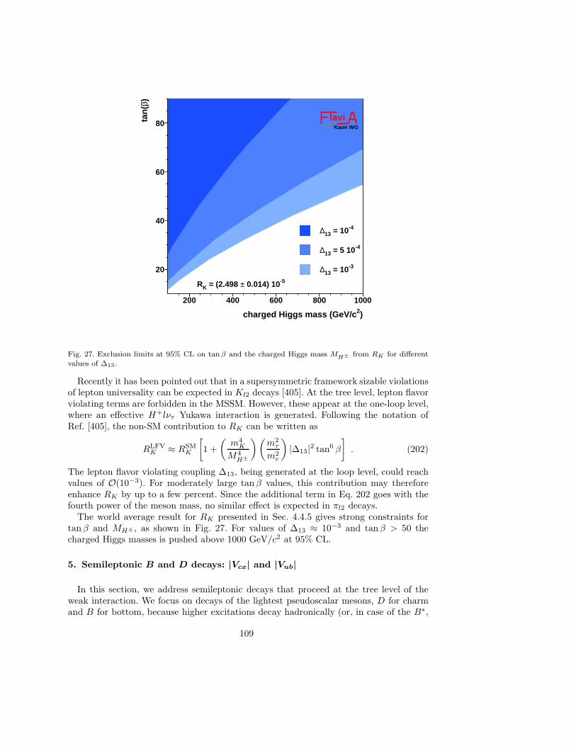
20
40
60
80
200 400 600 800 1000
RK = (2.498 ± 0.014) 10-5
∆13 = 10-3
∆13 = 5 10-4
∆13 = 10-4
charged Higgs mass (GeV/c2)
tan
(β)
lavinetKaon WG
Fig. 27. Exclusion limits at 95% CL on tanβ and the charged Higgs mass MH± from RK for differentvalues of ∆13.
Recently it has been pointed out that in a supersymmetric framework sizable violationsof lepton universality can be expected in Kl2 decays [405]. At the tree level, lepton flavorviolating terms are forbidden in the MSSM. However, these appear at the one-loop level,where an effective H+lντ Yukawa interaction is generated. Following the notation ofRef. [405], the non-SM contribution to RK can be written as
RLFVK ≈ RSM
K
[1 +
(m4K
M4H±
)(m2τ
m2e
)|∆13|2 tan6 β
]. (202)
The lepton flavor violating coupling ∆13, being generated at the loop level, could reachvalues of O(10−3). For moderately large tanβ values, this contribution may thereforeenhance RK by up to a few percent. Since the additional term in Eq. 202 goes with thefourth power of the meson mass, no similar effect is expected in πl2 decays.The world average result for RK presented in Sec. 4.4.5 gives strong constraints for
tanβ and MH± , as shown in Fig. 27. For values of ∆13 ≈ 10−3 and tanβ > 50 thecharged Higgs masses is pushed above 1000 GeV/c2 at 95% CL.
5. Semileptonic B and D decays: |Vcx| and |Vub|
In this section, we address semileptonic decays that proceed at the tree level of theweak interaction. We focus on decays of the lightest pseudoscalar mesons, D for charmand B for bottom, because higher excitations decay hadronically (or, in case of the B∗,
109

radiatively) to the D and B and thus have negligibly small semileptonic partial widths.The amplitude for quark flavor change in these processes is proportional to a CKMmatrixelement, providing a direct way to “measure” the CKM matrix.Purely leptonic decays of pseudoscalars are, of course, also directly sensitive to the
CKM matrix, but they require a spin flip. Their rate is, hence, helicity suppressed bya factor (mℓ/mP )
2, where mP is the pseudoscalar meson mass and mℓ the mass of thedaughter lepton. This suppression makes purely leptonic decays more sensitive to non-Standard processes, and therefore less reliable channels for the determination of CKMmatrix elements than semileptonic decays.As with the determination of |Vus| in the semileptonic decay K → πℓν, discussed in
Sec. 4, one can determine |Vcs| from D → Kℓν, |Vcd| from D → πℓν, |Vub| from B →πℓν, and |Vcb| from B → D(∗)ℓν, by combining measurements of the differential decayrate with lattice-QCD calculations for the hadronic part of the transition, commonlydescribed with form factors. This section starts with the three heavy-to-light decays,and then proceeds to heavy-to-heavy decays for which heavy-quark symmetry plays acrucial role. |Vcb| and |Vub| can also be determined from inclusive semileptonic B decays,because the large energy scale mb and the inclusion of all final-state hadrons makesthese processes amenable to the operator-product expansion (OPE). Within the OPEthe short-distance QCD can be calculated in perturbation theory, and the long-distanceQCD can be measured from kinematic distributions. While this is rather straightforwardfor |Vcb| it is more subtle |Vub| so these two topics are treated in separate subsections.
5.1. Exclusive semileptonic B and D decays to light mesons π and K
5.1.1. Theoretical BackgroundHeavy-to-light semileptonic decays, in which a B or D meson decays into a light
pseudoscalar or vector meson (such as a pion or ρ meson), are sensitive probes of quarkflavor-changing interactions. The decay rate for H → Pℓν semileptonic decay is given by
dΓ
dq2=G2F |VqQ|224π3
(q2 −m2ℓ)
2√E2P −m2
P
q4m2H
(1 +
m2ℓ
2q2
)m2H(E2
P −m2P )[f+(q
2)]2
+3m2
ℓ
8q2(m2
H −m2P )
2[f0(q
2)]2, (203)
where q ≡ pH − pP is the momentum transferred to the lepton pair and |VqQ| is therelevant CKM matrix element. The form factors, f+(q
2) and f0(q2), parametrize the
hadronic matrix element of the heavy-to-light vector current, V µ ≡ iqγµQ:
〈P |V µ|H〉 = f+(q2)
(pµH + pµP − m2
H −m2P
q2qµ)+ f0(q
2)m2H −m2
P
q2qµ, (204)
where EP = (m2H +m2
P − q2)/2mH is the energy of the light meson in the heavy me-son’s rest frame. The kinematics of semileptonic decay require that the form factors areequal at zero momentum-transfer, f+(0) = f0(0). In the limit mℓ → 0, which is a goodapproximation for ℓ = e, µ, the form factor f0(q
2) drops out and the expression for thedecay rate simplifies to
dΓ
dq2=G2F |VqQ|2
192π3m3H
[(m2
H +m2P − q2)2 − 4m2
Hm2P
]3/2 |f+(q2)|2. (205)
110

Using the above expression, a precise experimental measurement of the decay rate, incombination with a controlled theoretical calculation of the form factor, allows for a cleandetermination of the CKM matrix element |VqQ|.Analyticity and unitarityIt is well-established that the general properties of analyticity and unitarity largely
constrain the shapes of heavy-to-light semileptonic form factors [406–410]. All form fac-tors are analytic in q2 except at physical poles and threshold branch points. Becauseanalytic functions can always be expressed as convergent power series, this allows theform factors to be written in a particularly useful manner.Consider a change of variables that maps q2 in the semileptonic region onto a unit
circle:
z(q2, t0) =
√1− q2/t+ −
√1− t0/t+√
1− q2/t+ +√1− t0/t+
, (206)
where t+ ≡ (mH +mP )2, t− ≡ (mH −mP )
2, and t0 is a constant to be discussed later.In terms of this new variable, z, the form factors have a simple form:
P (q2)φ(q2, t0)f(q2) =
∞∑
k=0
ak(t0)z(q2, t0)
k. (207)
In order to preserve the analytic structure of f(q2), the function P (q2) vanishes at polesbelow the H-P pair-production threshold that contribute to H-P pair-production as vir-tual intermediate states. For example, in the case of B → πℓν decay, P (q2) incorporatesthe location of the B∗ pole:
PB→πℓν+ (q2) = z(q2,mB∗). (208)
For the case of D meson semileptonic decays, the mass of the D∗ meson is above theD-π production threshold, but the D∗
s is below D-K production threshold. Hence
PD→πℓν+ (q2) = 1, (209)
PD→Kℓν+ (q2) = z(q2,mD∗
s). (210)
In the expression for f(q2), Eq. (207), φ(q2, t0) is any analytic function. It can be chosen,however, to make the unitarity constraint on the series coefficients have a simple form.The standard choice for φ+(q
2, t0), which enters the expression for f+(q2), is [410]:
φ+(q2, t0) =
√3
96πχ(0)J
(√t+ − q2 +
√t+ − t0
)(√t+ − q2 +
√t+ − t−
)3/2
×(√
t+ − q2 +√t+
)−5 (t+ − q2)
(t+ − t0)1/4, (211)
where χ(0)J is a numerical factor that can be calculated using perturbation theory and
the operator product expansion. A similar function can be derived for the irrelevant formfactor f0(q
2).Given the above choices for P (q2) and φ(q2, t0), unitarity constrains the size of the
series coefficients:N∑
k=0
a2k . 1, (212)
111

Table 25Physical region in terms of the variable z for various semileptonic decays given the choice t0 = 0.65t−.
B → πlν −0.34 < z < 0.22
D → πlν −0.17 < z < 0.16
D → Klν −0.04 < z < 0.06
where this holds for any value of N . In the case of the B → πℓν form factor, the sizesof the series coefficients (aks) turn out to be much less than 1 [411]. Becher and Hillrecently pointed out that this is due to the fact that the b-quark mass is so large, andused heavy-quark power-counting to derive a tighter constraint on the aks:
N∑
k=0
a2k ≤(Λ
mQ
)3
, (213)
where Λ is a typical hadronic scale [412]. The above expression suggests that the seriescoefficients should be larger for D-meson form factors than for B-meson form factors.This, however, has not been tested.In order to accelerate the convergence of the power-series in z, the free parameter
t0 in Eq. (206) can be chosen to make the range of |z| as small as possible. For thevalue t0 = 0.65t− used in Ref. [410], the ranges of |z| for some typical heavy-to-lightsemileptonic decays are given in Tab. 25. The tight heavy-quark constraint on the size ofthe coefficients in the z-expansion, in conjunction with the small value of |z|, ensures thatonly the first few terms in the series are needed to describe heavy-to-light semileptonicform factors to a high accuracy.Other model-independent parameterizations of heavy-to-light semileptonic form fac-
tors base on analyticity and unitarity have been proposed and applied to the case of B →πℓν decay by Bourrely, Caprini, and Lellouch [413] and by Flynn and Nieves [414, 415].Bourrely et al. use the series expansion in z described above, but choose simpler outerfunction, φ(q2, t0) = 1. This leads, however, to a more complicated constraint on theseries coefficients, which is no longer diagonal in the series index k. Flynn and Nieves usemultiply-subtracted Omnes dispersion relations to parametrize the form factor shape interms of the elastic B-π scattering phase shift and the value of f+(q
2) at a few subtractionpoints below the B-π production threshold.Lattice QCDIn lattice-QCD calculations and in heavy-quark effective theory (HQET), it is easier
to work with a different linear combination of the form factors:
〈P |V µ|H〉 =√2mH
[vµf‖(EP ) + pµ⊥f⊥(EP )
], (214)
where vµ = pµH/mH is the velocity of the heavy meson, pµ⊥ = pµP − (pP · v)vµ is thecomponent of the light meson momentum perpendicular to v, and EP = pP · v = (m2
H +m2P − q2)/(2mH) is the energy of the light meson in the heavy meson’s rest frame. In the
heavy meson’s rest frame, the form factors f‖(EP ) and f⊥(EP ) are directly proportionalto the hadronic matrix elements of the temporal and spatial vector current:
112

f‖(EP ) =〈P |V 0|H〉√
2mH(215)
f⊥(EP ) =〈P |V i|H〉√
2mH
1
piP. (216)
Lattice QCD simulations therefore typically determine f‖(EP ) and f⊥(EP ), and then cal-culate the form factors that appear in the heavy-to-light decay width using the followingequations:
f0(q2) =
√2mH
m2H −m2
P
[(mH − EP )f‖(EP ) + (E2
P −m2P )f⊥(EP )
], (217)
f+(q2) =
1√2mH
[f‖(EP ) + (mH − EP )f⊥(EP )
]. (218)
These expressions automatically satisfy the kinematic constraint f+(0) = f0(0).The goal is to evaluate the hadronic matrix elements on the right-hand side of Eqs.(215)
and (216) via numerical simulations in lattice QCD. Such simulations are carried out withoperators, V Lµ , written in terms of the lattice heavy and light quark fields appearing inthe lattice actions. Hence, an important step in any lattice determination of hadronicmatrix elements is the matching between continuum operators such as Vµ and their latticecounterparts. The matching takes the form
〈P |Vµ|H〉 = ZQqVµ〈P |V Lµ |H〉. (219)
For heavy-light currents with dynamical (as opposed to static) heavy quarks, the match-
ing factors ZQqVµhave been obtained to date either through a combination of perturbative
and nonperturbative methods or via straight one-loop perturbation theory. Uncertaintiesin ZQqVµ
can be a major source of systematic error in semileptonic form factor calculationsand methods are being developed for complete nonperturbative determinations in orderto reduce such errors in the future.Another important feature of lattice simulations is that calculations are carried out at
nonzero lattice spacings and with up- and down-quark masses mq that are larger than inthe real world. Results are obtained for several lattice spacings and for a sequence of mq
values and one must then extrapolate to both the continuum and the physical quark masslimits. These two limits are intimately connected to each other, and it is now standardto use chiral perturbation theory (χPT) that has been adapted to include discretizationeffects [416–421].The initial pioneering work on B and D meson semileptonic decays on the lattice
were all carried out in the quenched approximation [422–426]. This approximation whichignores effects of sea quark-antiquark pairs has now been overcome and most recentlattice calculations include vacuum polarization from Nf = 2 + 1 or Nf = 2 dynamicallight quark flavors. Unquenched calculations of B → πℓν semileptonic decays have beencarried out by the Fermilab/MILC and the HPQCD collaborations using the MILCcollaboration Nf = 2+1 configurations [411,427,428]. Both collaborations use improvedstaggered (AsqTad) quarks for light valence and sea quarks. They differ, however, in theirtreatment of the heavy b quark. Fermilab/MILC employs the heavy clover action andHPQCD the nonrelativistic NRQCD action. The dominant errors in both calculations aredue to statistics and the chiral extrapolation. The next most important error stems from
113

discretization corrections for the Fermilab/MILC and operator matching for the HPQCDcollaborations, respectively. It is important that simulations based on other light quarklattice actions be pursued in the future as a cross check.In the case of D → K and D → π semileptonic decays, there exists to-date only one
Nf = 2 + 1 calculation, again based on AsqTad light and clover heavy quarks, by theFermilab Lattice and MILC collaborations [427]. Recently two groups have initiatedNf =2 calculations, and their results are still at a preliminary stage. The ETM collaborationuses “twisted mass” light and charm quarks at maximal twist [429], whereas Becirevic,Haas and Mescia use improved Wilson quarks and configurations created by the QCDSFcollaboration [430, 431]. The latter group employs double ratio methods and twistedboundary conditions to allow more flexibility in picking out many values of q2. There hasalso been a recent exploratory study with improved Wilson quark action which, althoughstill quenched, is at a very small lattice spacing of around 0.04 fm [432]. These authorshave considered both B and D decays.Light-cone QCD Sum RulesLight-cone sum rules (LCSR) [433–435] combine the idea of the original QCD sum
rules [436, 437] with the elements of the theory of hard exclusive processes. LCSR areused in a wide array of applications (for a review, see [438]), in particular, for calculatingB → π,K, η, ρ,K∗ andD → π,K form factors [439–449]. The starting point is a speciallydesigned correlation function where the product of two currents is sandwiched betweenthe vacuum and an on-shell state. In the case of B0 → π+ form factor
Fµ(p, q) = i
∫d4xeiqx〈π+(p) | T uγµb(x),mbbiγ5d(0) | 0〉
=
(2fBf
+Bπ(q
2)m2B
m2B − (p+ q)2
+∑
Bh
2fBhf+Bhπ
(q2)m2Bh
m2Bh
− (p+ q)2
)pµ +O(qµ) , (220)
where the factor proportional to pµ is transformed into a hadronic sum by inserting acomplete set of hadronic states between the currents. This sum also represents, schemat-ically, a dispersion integral over the hadronic spectral density. The lowest-lying B-statecontribution contains the desired B → π form factor multiplied by the B decay constant.At spacelike (p+ q)2 ≪ m2
b and at small and intermediate q2 ≪ m2b , the time ordered
product in Eq. (220) may also be expanded near the light-cone x2 ∼ 0, thereby resumminglocal operators into distribution amplitudes:
F ((p+ q)2, q2) =∑
t=2,3,4
∫Dui
∑
k=0,1
(αsπ
)kT
(t)k ((p+ q)2, q2, ui,mb, µ)ϕ
(t)π (ui, µ) . (221)
This generic expression is a convolution (at the factorization scale µ) of calculable short-
distance coefficient functions T(t)k and universal pion light-cone distribution amplitudes
(DA’s) ϕ(t)π (ui, µ) of twist t ≥ 2. The integration goes over the pion momentum fractions
ui = u1, u2, ... distributed among quarks and gluons. Importantly, the contributionsto Eq. (221) corresponding to higher twist and/or higher multiplicity pion DA’s aresuppressed by inverse powers of the b-quark virtuality ((p + q)2 −m2
b), allowing one toretain a few low twist contributions in this expansion. Currently, analyses of Eq. (220)can include all LO contributions of twist 2,3,4 quark-antiquark and quark-antiquark-gluon DA’s of the pion and the O(αs) NLO corrections to the twist 2 and 3 two-particlecoefficient functions.
114

Furthermore, one uses quark-hadron duality to approximate the sum over excited Bhstates in Eq. (220) by the result from the perturbative QCD calculation introducingthe effective threshold parameter sB0 . The final step involves a Borel transformation(p + q)2 → M2, where the scale of the Borel parameter M2 reflects the characteristicvirtuality at which the correlation function is calculated. The resulting LCSR for theB → π form factor has the following form
f+Bπ(q
2) =em
2B/M
2
2m2BfB
1
π
∫ sB0
m2b
ds ImF (OPE)(s, q2)e−s/M2
, (222)
where ImF (OPE) is directly calculated from the double expansion (221). The intrinsicuncertainty introduced by the quark-hadron duality approximation is minimized by cal-culating the B meson mass using the derivative of the same sum rule. The main inputparameters, apart from αs and b quark mass (taken in the MS scheme), include the non-perturbative normalization constants and nonasymptotic coefficients for each given twistcomponent, e.g., for the twist-2 pion DA ϕπ these are fπ and the Gegenbauer momentsai. For twist-3,4 the recent analysis can be found in Ref. [450]. For the B-meson decayconstant entering LCSR (222) one usually employs the conventional QCD sum rule forthe two-point correlator of biγ5q currents with O(αs) accuracy (the most complete sumrule in MS-scheme is presented in [451]). More details on the numerical results, sourcesof uncertainties and their estimates can be found in the recent update [448]. Furtherimprovement of the LCSR calculation of heavy-to-light form factors is possible, if onegets a better understanding of the quark-hadron duality approximation in B channel,and a more accurate estimation of nonperturbative parameters of pion DA’s.Despite their intrinsically approximate nature, LCSRs represent a useful analytic
method providing a unique possibility to calculate both hard and soft contributions tothe transition form factors. Different versions of LCSR employing B-meson distributionamplitudes [452] as well as the framework of SCET [453,454] have also been introduced.
5.1.2. Measurements of D Branching Fractions and q2 DependenceIn the last few years, a new level of precision has been achieved in measurements of
branching fractions and hadronic form factors for exclusive semileptonic D decays by theBelle, BaBar, and CLEO collaborations. In this section, we focus on semileptonic decays,D → Pℓνℓ, where D represents a D0 or D+, P a pseudoscalar meson, charged or neutral,either π or K, and ℓ a muon or electron. In addition, we also present a BaBar analysisof D+
s → K+K−ℓ+νℓ, which provided first evidence of an S-wave contribution.The results from the B-Factories (Babar and Belle) are based on very large samples of
D mesons produced via the process e+e− → cc recorded at about 10.58 GeV c.m. energy.CLEO-c experiment relies on a sample of ψ(3770) → DD events, which is smaller, butallows for very clean tags and excellent q2 resolution. Two of the four recent analyses tagevents by reconstructing a hadronic decay of one of the D mesons in the event, in additionto the semileptonic decay of the other. The total number of tagged events serves as ameasure of the total sample ofD mesons and thus provides the absolute normalization forthe determination of the semileptonic branching fractions. Untagged analyses typicallyrely on the relative normalization to a sample ofD decays with a well measured branchingfraction. The analyses use sophisticated techniques for background suppression (Fisherdiscriminants) and resolution enhancement (kinematic fits). The neutrino momentum
115

and energy is equated with the reconstructed missing momentum and energy relyingon energy-momentum conservation. The detailed implementation and resolution variessignificantly among the measurements and cannot be presented here in detail.The BaBar Collaboration reports a study of D0 → K−e+νe based on a luminosity of
75 fb−1 [455]. They analyze D∗+ → D0π+ decays, with D0 → K−e+νe. The analysisexploits the two-jet topology of e+e− → cc events. The events are divided by the planeperpendicular to the event thrust axis into two halves, each equivalent to a jet producedby c- or c-quark fragmentation. The energy of each jet is estimated from its measuredmass and the total c.m. energy. To determine the momentum of the D and the energy ofthe neutrino a kinematic fit is performed to the total event, constraining the invariantmass of the K−e+νe candidate to the D0 mass. The D direction is approximated bythe direction opposite the vector sum of the momenta of all other particles in the event,except the Kaon and lepton associated with the signal candidate. The neutrino energy isestimated as the difference between the total energy of the jet containing the Kaon andcharged lepton and the sum of the particle energies in that jet. To suppress combinatorialbackground eachD0 candidate is combined with a π+ of the same charge as the lepton andthe mass difference is required to be small, δM =M(D0π+)−M(D0) < 0.160 GeV. Thebackground-subtracted q2 distribution is corrected for efficiency and detector resolutioneffects.For BaBar’s analysis [455], the normalization of the form factor at q2 = 0 is fK+ (0) =
0.727± 0.007± 0.005± 0.007, where the first error is statistical, the second systematic,and the third due to uncertainties of external input parameters. In addition to the tradi-tional parametrization of the form factors as a function of q2 using pole approximations,BaBar also performed a fit in terms of the expansion in the parameter z. The results arepresented in Fig. 28. A fit to a polynomial shows that data are compatible with a lineardependence, which is fully consistent with the modified pole ansatz for f+(q
2).BaBar also reports the branching fraction for D0 → K−e+νe. To obtain the nor-
malization for the signal sample, they perform a largely identical analysis to isolatea sample of D0 → K−π+ decays, and combine it with the world average B(D0 →K−π+) = (3.80 ± 0.07)%. The result, the ratio of branching fractions, RD = B(D0 →K−e+νe)/B(D0 → K−π+) = 0.927 ± 0.007 ± 0.012, translates to B(D0 → K−e+νe) =(3.522 ± 0.027 ± 0.045 ± 0.065)%, where the last error represents the uncertainty ofB(D0 → K−π+).The Belle Collaboration has analyzed a sample of 282 fb−1, recorded at or just below
the Υ (4S) resonance [456]. They search for the process, e+e− → cc → D(∗)tagD
∗+sigX , with
D∗+sig → D0π+
soft [456]. Here X represents additional particles from c-quark fragmentation.
The Dtag is reconstructed as a D0 or D+, in decay modes D → K(nπ) with n =
1, 2, 3. In events that contain a D∗+sig , the recoil of the D
(∗)tagXπ
+soft provides an estimate
of the signal D0-meson energy and momentum vector. Figure 29 shows the invariant
mass spectrum as derived from the D(∗)tagXπ
+soft system. This distribution determines the
number of D0’s in the candidate sample and provides an absolute normalization. In thissample a search for semileptonic decays D0 → π−ℓ+νℓ or D0 → K−ℓ+νℓ is performed;here the charged lepton is either an electron or muon. Pairs of a hadron and a lepton ofopposite sign are identified and the neutrino four-momentum is obtained from energy-momentum conservation. Fig. 30 shows the distribution for the missing mass squared,M2ν , which for signal events is required to be consistent with zero, < 0.05 GeV2/c4.
116

The resulting branching fractions are B(D0 → K−ℓ+νℓ) = (3.45 ± 0.07 ± 0.20)% andB(D0 → π−ℓ+νℓ) = (0.255± 0.019± 0.016)%. The measured form factors as a functionof q2 are also included in Fig. 33 for both decay modes. The normalization of the formfactors at q2 = 0 are fK+ (0) = 0.695± 0.007± 0.022 and fπ+(0) = 0.624± 0.020± 0.030.The CLEO Collaboration analyzed data recorded at the mass at the ψ(3770) resonance,
which decays exclusively to DD pairs. They report measurements of semileptonic decaysof both D0 and D+, for both untagged and tagged events. For the untagged analysis [458]the normalization of DD pairs is based on a separate analysis [254]. Individual hadrons,π−, π0, K−, or KS, are paired with an electron and the missing momentum and energyof the entire event are used to estimate the neutrino four-momentum. The missing mass
1
1.2
1.4
-0.05 -0.025 0 0.025 0.05
-z
P Φ
f+ (
z) /
P Φ
f+(z
max
) Modif. pole fitBaBar
Fig. 28. Babar analysis of D0 → K−e+νe [455]: Measured values for P ×Φ× f+ versus −z, normalizedto 1.0 at z = zmax. The straight lines represent the expectation from the fit to the modified pole ansatz,the result in the center, as well as the statistical and total uncertainties on either side.
Fig. 29. Belle experiment [456]: Invariant mass distribution for D0sig candidates.
117

squared is required to be consistent with zero. Additionally, the four-momentum of thesignal candidates, i.e., the sum of the hadron, lepton and neutrino energies must beconsistent with the known energy and mass of the D meson. The yield of D mesonsis extracted in five q2 bins. The CLEO Collaboration reports the branching fractions,B(D0 → K− e+ νe) = (3.56±0.03±0.09)%, B(D0 → π− e+ νe) = (0.299±0.011±0.09)%,B(D+ → K0 e+ νe) = (8.53 ± 0.13± 0.23)%, and B(D+ → π0 e+ νe) = (0.373± 0.022±0.013)%. Figure 33 includes the CLEO-c untagged results for f+(q
2) versus q2.Recent results of the CLEO-c tagged analysis [255] were reported for the first time at
this workshop. This analysis is based on a luminosity of 281 pb−1. To tag events, all eventsare required to have a hadronic D decay, fully reconstructed in one of eight channels forD0 and one of six channels for D+. Since the DD system is produced nearly at rest, theD candidate should have an energy consistent with the beam energy. The beam-energysubstituted mass, mES , is required to be consistent with the known D mass. For thissample of events, an electron is paired with a hadron, π−, π0, K−, or KS. In DD eventswith a signal semileptonic decay, the only unidentified particle is the neutrino. Its energyand momentum are derived from the missing energy and momentum. The measureddifference of these two quantities, U = Eν − Pν , is used to discriminate signal frombackground. Fig. 31 shows the U distribution for the four semileptonic decay modes.The requirement of a hadronic tag results in extremely pure samples. For the decayD0 → K− e+ νe the signal-to-noise ratio is about 300. Based on these selected samplesCLEO-c reports the branching fractions, B(D0 → K− e+ νe) = (3.61 ± 0.05 ± 0.05)%,B(D0 → π− e+ νe) = (0.314±0.013±0.004)%,B(D+ → K0 e+ νe) = (8.90±0.17±0.21)%,and B(D+ → π0 e+ νe) = (0.384± 0.027± 0.023)%. Figure 33 shows the CLEO-c resultsfor f+(q
2) versus q2.The CLEO Collaboration has computed the average of the untagged and tagged re-
sults, taking into account all correlations. The results for the branching fractions areshown in Tab. 26. The untagged analysis contains about 2.5 times more events but haslarger backgrounds and different systematic uncertainties. The product of the form fac-tor f+(0) and the CKM matrix element is extracted from the combined measurements,fK+ (0)|Vcs| = 0.744± 0.007± 0.005 and fπ+(0)|Vcd| = 0.143± 0.005± 0.002.Since the time that the above results were reported at CKM2008, CLEO collabora-
tion has completed a new tagged analysis which is based on the entire 818 pb−1 ofdata recorded at the ψ(3770) resonance [459]. The results for the most recent branch-ing fraction measurements are, B(D0 → K− e+ νe) = (3.50 ± 0.03 ± 0.04)%, B(D0 →
0
10
20
30
40
50
-1 -0.5 0 0.5 1
right-sign m2ν / GeV2/c4
evts
/ 0.
02 G
eV2 /c
4
60
0
100
200
300
400
500
-1 -0.5 0 0.5 1
right-sign m2ν / GeV2/c4
evts
/ 0.
02 G
eV2 /c
4
Fig. 30. Belle experiment [456, 457]: Missing mass squared distribution for D0sig candidates. Left:
D0 → π−ℓ+νℓ; right: D0 → K−ℓ+νℓ. The D0 → K−ℓ+νℓ and fake D0 backgrounds are derived from
data and are shown in magenta and yellow respectively. The cyan histogram shows the contribution fromD0 → K∗/ρℓ+νℓ as determined from simulation.
118

Table 26CLEO-c: Absolute branching fractions for tagged, untagged and averaged results.
Tagged Untagged Average
π−e+νe 0.308± 0.013± 0.004 0.299 ± 0.011 ± 0.008 0.304± 0.011± 0.005
π0e+νe 0.379± 0.027± 0.002 0.373 ± 0.022 ± 0.013 0.378± 0.020± 0.012
K−e+νe 3.60± 0.05 ± 0.05 3.56± 0.03± 0.09 3.60 ± 0.03± 0.06
K0e+νe 8.87± 0.17 ± 0.21 8.53± 0.13± 0.23 8.69 ± 0.12± 0.19
π− e+ νe) = (0.288± 0.008± 0.003)%, B(D+ → K0 e+ νe) = (8.83± 0.10± 0.20)%, andB(D+ → π0 e+ νe) = (0.405± 0.016± 0.009)%. The measured form factors as a functionof q2 for this analysis are shown at the bottom of Fig. 33. The product of the form fac-tor f+(0) and the CKM matrix element is extracted from an isospin-combined fit whichyields fK+ (0)|Vcs| = 0.719±0.006±0.005 and fπ+(0)|Vcd| = 0.150±0.004±0.001. The newCLEO-c results are consistent with the previous CLEO-c measurements and supersedethose measurements.At this conference BaBar reported a measurement of D+
s → K+K−ℓ+νℓ decays [460].Events with a K+K− mass in the range 1.01−1.03GeV/c2 are selected, corresponding toφ→ K+K− decays, except for a small S-wave contribution which is observed for the firsttime. Since the final state meson is a vector, the decay rate depends on five variables, themass squared of the K+K− pair, q2 and three decay angles, and on three form factors,A1, A2 and V , for which the q2 dependence is assumed to be dominated by a single pole,
V (q2) =V (0)
1− q2/m2V
, A1,2(q2) =
A1,2(0)
1− q2/m2A
, (223)
with a total of five parameters, the normalizations V (0), A1(0), A2(0) and the pole massesmV and mA. In a data sample of 214 fb−1, the BaBar Collaboration selects about 25,000signal decays, about 50 times more than the earlier analysis by FOCUS [461]. The signalyield and the form factor ratios are extracted from a binned maximum likelihood fit to the
Fig. 31. CLEO-c tagged analysis [255]: Signal distributions (U = Eν − Pν) for the four semileptonic Ddecay channels.
119

four-dimensional decay distribution, r2 = A2(0)/A1(0) = 0.763± 0.071± 0.065 and rV =V (0)/A1(0) = 1.849±0.060±0.095, as well as the pole massmA = 2.28+0.23
−0.18±0.18GeV/c2.The sensitivity to mV is weak and therefore this parameter is fixed to 2.1GeV/c2. Theresult of the fit is shown in Fig. 32. The small S-wave contribution, which can be asso-ciated with f0 → K+K− decays, corresponds to (0.22+0.12
−0.08 ± 0.03)% of the K+K−e+νedecay rate. The D+
s → K+K−e+νe branching fraction is measured relative to the de-cay D+
s → K+K−π+, resulting in B(D+s → K+K−e+νe)/B(D+
s → K+K−π+) =0.558±0.007±0.016, from which the absolute total branching fraction B(D+
s → φe+νe) =(2.61± 0.03± 0.08± 0.15)% is obtained. By comparing this quantity with the predicteddecay rate, using the fitted parameters for the form factors, the absolute normalizationA1(0) = 0.607± 0.011± 0.019± 0.018 was determined for the first time. The third errorstated here refers to the combined uncertainties from various external inputs, namelybranching fractions for D+
s , and φ, the D+s lifetime and |Vcs|. Lattice QCD calculations
for this decay have been performed only in the quenched approximation. They agree withthe experimental results for A1(0), r2 and mA, but are lower than the measured valueof rV . It would be interesting to see if unquenched calculations are in better agreementwith experimental results.In summary, BaBar, Belle and CLEO-c have measured D meson semileptonic branch-
ing fractions and hadronic form factors in a variety of decay modes, using complementaryexperimental approaches. The results from the experiments are highly consistent. Withlattice QCD prediction for the form factors, these results will allow a precise determina-tion of Vcs and Vcd. Fig. 33 shows a compilation of all form factor measurements, f+(q
2)versus q2. All analyses presented here have performed studies of the q2 parameterizations
)2 (GeV2q
0 0.2 0.4 0.6 0.8 1
2E
ntri
es/0
.1 G
eV
0
500
1000
1500
2000
2500
3000
3500
4000
4500
)2 (GeV2q
0 0.2 0.4 0.6 0.8 1
2E
ntri
es/0
.1 G
eV
0
500
1000
1500
2000
2500
3000
3500
4000
4500datafitted signal
BB cc
uds
a)
eθcos-1 -0.5 0 0.5 1
Ent
ries
/0.1
0
500
1000
1500
2000
eθcos-1 -0.5 0 0.5 1
Ent
ries
/0.1
0
500
1000
1500
2000b)
Kθcos-1 -0.5 0 0.5 1
Ent
ries
/0.1
0
500
1000
1500
2000
2500
Kθcos-1 -0.5 0 0.5 1
Ent
ries
/0.1
0
500
1000
1500
2000
2500 c)
χ-3 -2 -1 0 1 2 3
Ent
ries
/0.3
2
0
500
1000
1500
χ-3 -2 -1 0 1 2 3
Ent
ries
/0.3
2
0
500
1000
1500
d)
Fig. 32. BaBar [460]: Projected distributions of the four kinematic variables. The data (points withstatistical errors) are compared to the sum of four contributions: the fitted signal (hatched histograms)and the estimated background contributions (different colored histograms) from BB, cc, and the sum ofuu, dd, and ss events.
120

Table 27Summary of the form factors parameters obtained by the different experiments for D → K semileptonic
decays. The first column gives the simple pole mass, the second the parameter α used in the modifiedpole model, and the third the normalization.
Mpole[ GeV/c2] α f+(0)
Belle [456] 1.82± 0.04 ± 0.03 0.52± 0.08± 0.06 0.695± 0.007± 0.022
BaBar [455] 1.884± 0.012± 0.015 0.38± 0.02± 0.03 0.727± 0.007± 0.005± 0.007
CLEO-c [459] 1.93± 0.02 ± 0.01 0.30± 0.03± 0.01 0.739± 0.007± 0.005
LQCD [463] 0.50± 0.04± 0.07 0.73± 0.03± 0.07
and extractions of the associated parameters. A summary of these measurements is givenin Tabs. 27 and 28, as well as the values obtained by lattice QCD computation [463].The reader is referred to the references for more details.Measurements of D → πℓνℓ and D → V ℓνℓ will benefit from the increased data sam-
ples expected in the near future. Of particular interest is the anticipated ψ(3770) runningof BES-III. The BES-III Collaboration began data accumulation in July of 2008. Theexperiment is comparable to CLEO-c in detector design but has superior muon identifi-cation performance, but worse performance for hadron identification, and is expected to
0 0.05 0.1 0.15 0.2 0.25 0.3 0.35 0.4 0.45
q2/m
Ds*
2
0
0.5
1
1.5
2
2.5
f +(q
2 )
q2
max/m
Ds*
2
lattice QCD [Fermilab/MILC, hep-ph/0408306]experiment [Belle, hep-ex/0510003]experiment [BaBar, 0704.0020 [hep-ex]]experiment [CLEO-c, 0712.0998 [hep-ex]]experiment [CLEO-c, 0810.3878 [hep-ex]]
D → Klν
0 0.1 0.2 0.3 0.4 0.5 0.6 0.7 0.8
q2/m
D*2
0
1
2
3
4
5
f +(q
2 )
q2
max/m
D*2
lattice QCD [Fermilab/MILC, hep-ph/0408306]experiment [Belle, hep-ex/0510003]experiment [CLEO-c, 0712.0998 [hep-ex]]experiment [CLEO-c, 0810.3878 [hep-ex]]
D → πlν
Fig. 33. Compilation of the form factor f+(q2) versus q2 for the semileptonic D decays with a Kaon(left) and pion (right). Top plots, adapted from Ref. [462], include measurements through the end of2008. Bottom plots show results of a recent CLEO-c analysis [459]. In all plots the lines are the LQCDresults of Ref. [463]; the inner band represents statistical uncertainty and the outer band includes thesystematic uncertainty.
121

Table 28Summary of the form factors parameters obtained by the different experiments for D → π semileptonic
decays. The first column gives the simple pole mass, the second the parameter α used in the modifiedpole model, and the third the normalization.
Mpole[ GeV/c2] α f+(0)
Belle [456] 1.97± 0.08 ± 0.04 0.10± 0.21± 0.10 0.624± 0.020± 0.030
CLEO-c [459] 1.91± 0.02 ± 0.01 0.21± 0.07± 0.02 0.666± 0.019± 0.004± 0.003
LQCD [463] 0.44± 0.04± 0.07 0.64± 0.03± 0.06
accumulate at least an order of magnitude more data. The muon identification will allowaccess to all the semileptonic modes covered in this section from a single experiment.
5.1.3. Measurements of B branching fractions and q2 dependenceExclusive semileptonic decays B → Xuℓν, where Xu denotes a charmless hadronic
final state, have been reported by the CLEO, BaBar, and Belle collaborations [464–473]. The specification of the final state provides good kinematic constraints and aneffective background rejection, but results in lower signal yields compared with inclusivemeasurements. Three experimental techniques that differ in the way the second B mesonin the BB event is treated have been employed in these measurements. The second Bmeson is either fully reconstructed in a hadronic decay mode (“hadronic tags”), partiallyreconstructed in a semileptonic decay mode (“semileptonic tags”) or not reconstructedat all (“untagged”). The tagged and untagged methods differ greatly in terms of signalefficiency and purity.B → πℓνThe B → πℓν decay is the most promising decay mode for a precise determination of
|Vub|, both for experiment and for theory. A number of measurements with different tag-ging techniques exist, but at present the untagged analyses, which were first performedby the CLEO collaboration [465], still provide the most precise results. In untagged anal-yses, the momentum of the neutrino is inferred from the missing energy and momentumin the whole event. The neutrino is combined with a charged lepton and a pion to forma B → πℓν candidate. The biggest experimental challenge is the suppression of theB → Xcℓν background. Additional background sources are e+e− → qq (q = u, d, s, c)continuum events, which dominate at low q2, and feed-down from other B → Xuℓνdecays, which dominate at high q2.The BaBar experiment has measured the B → πℓν branching fraction and q2 spec-
trum with a good accuracy [466]. In this analysis, the signal yields are extracted from amaximum-likelihood fit to the two-dimensional ∆E vs. mES distribution of the signal Bmeson in twelve bins of q2 (see Fig. 34). This fit allows for an extraction of the q2 depen-dence of the form factor f+(q
2). The shape of the measured spectrum is compatible withthe ones predicted from LQCD [427,428] and LCSR [444] calculations, but incompatiblewith the ISGW2 quark model [474]. A fit to the q2 spectrum using the Becirevic-Kaidalov(BK) parametrization yields a shape parameter α = 0.52± 0.05± 0.03 with a goodness-of-fit of P (χ2) = 0.65. Other parameterizations, e.g. the z-expansion, have been usedin a simultaneous fit of the BaBar data and LQCD calculations [411]. The measuredpartial branching fractions are extrapolated to the full decay rate and, in combinationwith recent form-factor calculations, used to determine |Vub|
122

The leading experimental systematic uncertainties are associated with the reconstruc-tion of charged and neutral particles, which impact the modeling of the missing momen-tum reconstruction, and with backgrounds from continuum events at low q2 and fromB → Xuℓν decays at high q2. Due to the feed-down from B → ρℓν decays, the uncer-tainties on the branching fraction and form factors for this decay mode contribute to thesystematic uncertainty. A simultaneous measurement of B → πℓν and B → ρℓν decayscan reduce this uncertainty.Recently several tagged measurements have appeared [467, 468, 471, 472]. They have
led to a simpler and more precise reconstruction of the neutrino momentum and have lowbackgrounds and a uniform acceptance in q2. This is achieved, however, at the expense ofmuch smaller signal samples which limit the statistical precision of the form-factor mea-surement. Semileptonic-tag measurements have a signal-to-background ratio of around1–2 and yield ∼ 0.5 signal decays per fb−1. The signal is extracted from the distributionof events in cos2 φB, where φB is the angle between the direction of either B meson andthe plane containing the momentum vectors of the tag-side D∗ℓ system and the signal-side πℓ system [467]. Hadronic-tag measurements reach signal-to-background ratios of upto ∼ 10 and yield ∼ 0.1 signal decays per fb−1. Here the signal is extracted from themissing-mass squared distribution (see Fig. 35).Tab. 29 summarizes all B → πℓν branching-fraction measurements; shown are the
total branching fraction as well as the partial branching fractions for q2 < 16 GeV2 andq2 > 16 GeV2 with statistical and systematic uncertainties. The measurements agree wellamong each other. A combination of all measurements results in an average branchingfraction of 1.34× 10⁻⁴ with a precision of 6% (4% statistical and 4% systematic).B → η/η′/ρ/ωℓνIn addition to B → πℓν, the experiments have measured other semileptonic final states
with a pseudoscalar meson, η [465, 467, 469, 475] or η′ [464, 467, 475], or a vector meson,ρ [464,465,470–472] or ω [469,473]. They are important ingredients to the determination
(GeV)ESm5.19 5.21 5.23 5.25 5.27 5.29
Eve
nts
/ 0.
005
GeV
0
100
200
300
400
500
600
700
2 < 16 GeV20 < q signalνlπ→0B
bkgνul→b
bkgBother Bcontinuum bkgdata
a)
2 < 16 GeV20 < q
(GeV)ESm5.19 5.21 5.23 5.25 5.27 5.290
50
100
150
200
250
300
350
2 < 26.4 GeV216 < q
b)
2 < 26.4 GeV216 < q
E (GeV)∆-1 -0.5 0 0.5 1
Eve
nts
/ 0.
08 G
eV
0
100
200
300
400
500 c)
E (GeV)∆-1 -0.5 0 0.5 10
50
100
150
200
250
300
350 d)
Fig. 34. Untagged B → πℓν measurement from BaBar [466]. Left: ∆E and mES projections forq2 < 16 GeV2 and q2 > 16 GeV2. Right: Measured q2 spectrum compared with a fit of the BKparametrization and with theory predictions from LQCD [427, 428], LCSR [444] and the ISGW2 quarkmodel [474].
123

Table 29Total and partial branching fractions for B0 → π−ℓ+ν with statistical and systematic uncertainties.
Measurements of B(B+ → π0ℓ+ν) have been multiplied by a factor 2τB0/τB+ .
L( fb−1) B × 104 ∆B(q2 < 16) × 104 ∆B(q2 > 16) × 104
BaBar no tag (π−) [466] 206 1.45± 0.07± 0.11 1.08± 0.06± 0.09 0.38± 0.04± 0.05
CLEO no tag (π−,π0) [464] 16 1.38± 0.15± 0.11 0.97± 0.13± 0.09 0.41± 0.08± 0.04
BaBar sl. tag (π−) [467] 348 1.39± 0.21± 0.08 0.92± 0.16± 0.05 0.46± 0.13± 0.03
Belle sl. tag (π−) [471] 253 1.38± 0.19± 0.15 1.02± 0.16± 0.11 0.36± 0.10± 0.04
BaBar sl. tag (π0) [467] 348 1.80± 0.28± 0.15 1.38± 0.23± 0.11 0.45± 0.17± 0.06
Belle sl. tag (π0) [471] 253 1.43± 0.26± 0.15 1.05± 0.23± 0.12 0.37± 0.15± 0.04
BaBar had. tag (π−) [468] 211 1.07± 0.27± 0.19 0.42± 0.18± 0.06 0.65± 0.20± 0.13
Belle had. tag (π−) [472] 605 1.12± 0.18± 0.05 0.85± 0.16± 0.04 0.26± 0.08± 0.01
BaBar had. tag (π0) [468] 211 1.54± 0.41± 0.30 1.05± 0.36± 0.19 0.49± 0.23± 0.12
Belle had. tag (π0) [472] 605 1.24± 0.23± 0.05 0.85± 0.16± 0.04 0.41± 0.11± 0.02
Average 1.36± 0.05± 0.05 0.94± 0.05± 0.04 0.37± 0.03± 0.02
Table 30Total branching fractions for exclusive B → Xuℓν decays with Xu = η, η′, ρ, or ω. †The BaBar collabo-ration reports an upper limit of B(B+ → η′ℓ+ν) < 0.47 at 90% CL [467].
Decay mode B × 104 σstat × 104 σsyst × 104
B+ → ηℓ+ν (BaBar average) [469] 0.37 0.06 0.07
B+ → η′ℓ+ν (CLEO no tag) [464]† 2.66 0.80 0.56
B0 → ρ−ℓ+ν (average) 2.80 0.18 0.16
B+ → ωℓ+ν (BaBar no tag) [469] 1.14 0.16 0.08
of the composition of the inclusive B → Xuℓν rate. They may also help to furtherconstrain theoretical form-factor calculations and provide valuable cross-checks for thedetermination of |Vub| from B → πℓν. The LQCD calculations for these final states arechallenging. For the flavor-neutral final-state mesons, η, η′ and ω, the matrix elementcontains contributions from quark-disconnected diagrams. For the ρ final state, the largewidth of the ρ resonance complicates the calculations.The η and η′ modes have been measured by the CLEO and BaBar collaboration.
The limit on B(B → η′ℓν) published by BaBar [467] agrees only marginally with theCLEO result [464] (at the 2.6σ level). Further measurements are needed to resolve thisdiscrepancy. In the future, a measurement of the ratio Rη′η = B(B → η′ℓν)/B(B → ηℓν)would be interesting to constrain the gluonic singlet contribution to the B → η(′) formfactor, as proposed in [447].The B → ρℓν decay has a larger rate than charmless semileptonic decays into pseu-
doscalar mesons, but one must deal with the non-resonant ππ contribution, which leadsto a sizable systematic uncertainty. The kinematics of decays with vector mesons aredescribed by three form factors. The statistical precision in current analyses is still toolow to measure these form factors. As an example, Fig. 35 shows the missing-mass andq2 spectra of B → ρℓν and B → ωℓν decays measured by the Belle collaboration ina hadronic-tag analysis [472]. Tab. 30 summarizes the most precise branching fractionresults for semileptonic B decays to low-mass charmless hadrons heavier than the pion.Prospects for exclusive charmless decaysThe outlook for further improvements in these measurements for the full B-factory
124

datasets and for a Super B factory is good. It can be expected that for B → πℓνthe untagged measurements will remain the most precise up to integrated luminositiesof several ab−1. To reduce the systematic uncertainties of untagged measurements, abetter knowledge of inclusive B → Xuℓν decays is important, since they are the biggestlimitation in the high-q2 region where LQCD calculations exist. In addition, a significantfraction of the BB background comes from events, where the signal B meson has beenwrongly reconstructed by assigning one or more particles from the decay of the other Bmeson to the signal decay. To reduce this uncertainty, much effort is needed to improvethe simulation of generic B-meson decays. With the full B-factory dataset, a precisionof about 4-5% should be achievable for the total B → πℓν branching fraction.The tagged measurements in particular will improve with larger data samples. The
systematic uncertainties in these measurements have a significant statistical componentand thus the total experimental error is expected to fall as 1/
√N . For the higher-mass
states, the tagged measurements should soon give the most precise branching-fractionresults. However, the larger data samples from untagged analyses will be needed toextract information on the three form factors involved in decays with a vector meson.For an integrated luminosity of 1–2 ab−1, several thousand B → ρℓν and B → ωℓνdecays can be expected. These signal samples will allow us to obtain some informationon the form factors or ratios of form-factors through a simultaneous fit of the q2 spectrumand decay-angle distributions, similar to the study of B → D∗ℓν decays. A measurementof all three form factors will most likely not be feasible with the current B-factory datasamples.
5.1.4. Determination of |Vcs|, |Vcd|, |Vub|Once both the form factor |f+(q2)|2 and the experimental decay width Γ(qmin) are
known, the CKM matrix element |VqQ| can be determined in several ways. We brieflydescribe the two most common methods below.Until recently the standard procedure used to extract CKM matrix elements from
)2Missing mass squared (GeV-1 0 1 2 3 4 5
2E
ven
ts /
0.2
GeV
0
10
20
30
40
50
60
)2Missing mass squared (GeV-1 0 1 2 3 4 5
2E
ven
ts /
0.2
GeV
0
10
20
30
40
50
60
Data+ρ
crossfeedνulOther backgrounds
)2Missing mass squared (GeV-1 0 1 2 3 4 5
2E
ven
ts /
0.2
GeV
0
10
20
30
40
50
60
)2Missing mass squared (GeV-1 0 1 2 3 4 5
2E
ven
ts /
0.2
GeV
0
10
20
30
40
50
60Data
0ρ crossfeedνul
Other backgrounds
)2Missing mass squared (GeV-1 0 1 2 3 4 5
2E
ven
ts /
0.2
GeV
0
5
10
15
20
25
30
)2Missing mass squared (GeV-1 0 1 2 3 4 5
2E
ven
ts /
0.2
GeV
0
5
10
15
20
25
30
Dataω
crossfeedνulOther backgrounds
)2/c2 (GeV2q
0 5 10 15 20 25
]-4
[ 1
0to
tΓ/2
/ d
qΓ
d
0
0.5
1
1.5
2
0ρ DataLCSR (Ball98)
ISGW2
)2/c2 (GeV2q
0 5 10 15 20 25
]-4
[ 1
0to
tΓ/2
/ d
qΓ
d
0
0.5
1
1.5
2+ρ Data
LCSR (Ball98)
ISGW2
)2/c2 (GeV2q
0 5 10 15 20 25
]-4
[ 1
0to
tΓ/2
/ d
qΓ
d
0
0.5
1
1.5
2
ω DataLCSR (Ball98)
ISGW2
Fig. 35. Belle hadronic-tag measurements [472]: Missing-mass squared distributions and q2 spectra forB → ρℓν and B → ωℓν decays.
125

exclusive semileptonic decays has been to integrate the theoretically determined formfactor over a region of q2 and then combine it with the experimentally measured decayrate in this region:
Γ(qmin)
|VqQ|2=
G2F
192π3m3H
∫ q2max
q2min
dq2[(m2
H +m2P − q2)2 − 4m2
Hm2P
]3/2 |f+(q2)|2. (224)
The integration requires a continuous parametrization of the form factor between q2min
and q2max that is typically obtained by fitting the theoretical form factor result to a modelfunction such as the Becirevic-Kaidalov (BK) [476] or Ball-Zwicky (BZ) parametriza-tion [444]. The three-parameter BK Ansatz,
f+(q2) =
f+(0)
(1− q2/m2B∗) (1− α q2/m2
B∗), (225)
f0(q2) =
f+(0)
(1− q2/βm2B∗)
, (226)
incorporates many essential features of the form factor shape such as the kinematicconstraint at q2 = 0, heavy-quark scaling, and the location of the B∗ pole. The four-parameter BZ Ansatz extends the BK expression for f+(q
2) by including an additionalpole to capture the effects of multiparticle states.In general, the use of a model function to parametrize the form factor introduces
assumptions that make it difficult to quantify the agreement between theory and exper-iment and gives rise to a systematic uncertainty in the CKM matrix element |VqQ| thatis hard to estimate. It is likely that this error can be safely neglected when interpolatingbetween data points. Thus the choice of fit function should have only a slight impact onthe exclusive determinations of |Vcs| and |Vcd| because lattice-QCD calculations and ex-perimental measurements possess a large region of overlap in q2. It is less clear, however,how well the BK and BZ Ansatze can be trusted to extrapolate the form factor shapebeyond the reach of the numerical lattice-QCD data or the experimental data. Thus oneshould be cautious in using them for the exclusive determination of |Vub| via Eq. (224),since an extrapolation in q2 is necessary both for lattice QCD, which is most accurateat high q2, and for experimental measurements, which are most precise at low values ofq2. In particular, comparisons of lattice and experimental determinations of BK or BZfit parameters are potentially misleading, because apparent inconsistencies could simplybe due to the inadequacy of the parametrization.Recently, several groups have begun to use model-independent parameterizations for
the exclusive determination of |Vub| [410–415, 477]. This avoids the concerns about theBK and BZ Ansatze outlined above, and should become the standard method for de-termining |Vub| and other CKM matrix elements from semileptonic decays in the nearfuture. For concreteness, here we focus on the z-expansion given in Eq. (207), but theprocedure for determining |Vub| outlined here should apply to other model-independentparameterizations. Because the z-expansion relies only on analyticity and unitarity, it canbe trusted to extrapolate the form factor shape in q2 beyond the reach of the data. Onecan easily check for consistency between theory and experiment using this parametriza-tion by fitting the data separately and comparing the slope (a1/a0), curvature (a2/a0),and so forth. Finally, because as many terms can be added to the convergent series as are
126

-0.3 -0.2 -0.1 0 0.1 0.20.01
0.015
0.02
0.025
0.03
0.035
0.04
χ2/d.o.f. = 0.59
z
P+φ
+f +
simultaneous 4-parameter z-fit
Fermilab-MILC lattice dataBABAR data rescaled by |Vub| from z-fit
Fig. 36. Model-independent determination of |Vub| from a simultaneous fit of lattice and experimen-tal B → πℓν semileptonic form factor data to the z-parametrization [411]. Inclusion of terms in thepower-series through z3 yields the maximum uncertainty in |Vub|; the corresponding 4-parameter z-fitis given by the red curve in both plots. The circles denote the Fermilab-MILC lattice-QCD calcula-tion [411], while the stars indicate the 12-bin Babar data [466], rescaled by the value of |Vub| determinedin the simultaneous z-fit.
needed to describe the B → πℓν form factor to the desired accuracy, the parametrizationcan be systematically improved as theoretical and experimental data get better.Once the shapes of the theoretical and experimental form factor data are determined
to be consistent, the CKM matrix element |Vub| is given simply by the ratio of the nor-malizations, |Vub| = aexp.0 /atheo.0 . The total uncertainty in |Vub| can be reduced, however,by fitting the theoretical and experimental data simultaneously, leaving the relative nor-malization as a free parameter to be determined [411]. The combined fit incorporatesall of the available data, thereby allowing the numerical lattice QCD data primarily todictate the shape at high q2 and the experimental data largely to determine the shape atlow q2. Although the theoretical and experimental data are uncorrelated, it is importantto include the correlations between experiments or between theoretical calculations, de-spite the fact that they can be difficult to ascertain. Fig. 36 shows an example combinedfit to the model-independent z-parametrization that uses 2+1 flavor lattice QCD resultsfrom Fermilab/MILC [411] and experimental data from BABAR [466].Combining the most recent experimental measurements of D → Kℓν and D → πℓν
form factors with the 2+1 flavor lattice QCD calculations from the Fermilab/MILCcollaboration [285, 463], CLEO finds [459]
|Vcd|= 0.234± 0.007± 0.025, (227)
|Vcs|= 0.985± 0.012± 0.103, (228)
where the errors are experimental and theoretical, respectively. These determinationsrely upon the BK parametrization, both to parametrize the theoretical D → πℓν andD → Kℓν form factor shapes for use in Eq. (224) and within the lattice QCD calculationitself. Although this is unlikely to introduce a significant systematic error, use of one ofthe many model-independent functional forms available would be preferable. The largestuncertainties in both |Vcs| and |Vcd| are from discretization errors in the lattice QCD
127

calculation, and can be reduced by simulating at a finer lattice spacing. Because thelattice calculations of the D → πℓν and D → Kℓν form factors can improved in astraightforward manner, without requiring new techniques, we expect the errors in both|Vcd| and |Vcs| to decrease significantly in the near future.Most recent exclusive determinations of |Vub| rely upon the 2+1 flavor lattice QCD
calculations of the B → πℓν form factor of the HPQCD and Fermilab/MILC collabora-tions [285, 427, 428]. Those which use model-independent parameterizations of the formfactor shape often incorporate additional theoretical points from light cone sum rules,soft collinear effective theory, and chiral perturbation theory [410, 412, 413, 415]. All ofthe results for |Vub| are consistent within uncertainties. We show a representative sampleof these results, along with two model-dependent determinations that rely on the BKand BZ parameterizations for comparison, in Fig. 37. Below we quote the most recentcalculation by Fermilab/MILC because this is the only one to use a model-independentparametrization along with the full correlation matrices, derived directly from the data,for both theory and experiment [411]:
|Vub| = (3.38± 36)× 10−3, (229)
where the total uncertainty is the sum of statistical, systematic, and experimental errorsadded in quadrature. The dominant theoretical uncertainty in |Vub| comes from statisticsand the extrapolation to the physical up and down quark masses and to the continuum.The sub-dominant uncertainties, which are of comparable size, are due to the perturbativerenormalization of the heavy-light vector current and heavy-quark discretization errorsin the action and current. All of these errors can be reduced by increasing statistics andsimulating at a finer lattice spacing. We therefore expect the total uncertainty in |Vub|determined from B → πℓν semileptonic decay to decrease in the next few years.
5.2. B → D(∗)ℓν decays for |Vcb|
5.2.1. Theoretical background: HQS and HQETThe matrix elements of semileptonic decays can be related to a set of form factors. In
the conventions of refs. [478–480], the matrix elements relevant for B → D(∗)ℓν decaysare
〈D|Vµ|B〉√mBmD
= (vB + vD)µh+ + (vB − vD)
µh−, (230)
〈D∗α|Vµ|B〉√mBmD∗
= εµνρσvνBvρD∗ǫ
∗σα hV , (231)
〈D∗α|Aµ|B〉√mBmD∗
= iǫ∗να [hA1(1 + w)gµν − (hA2vµB + hA3v
µD∗)v
νB ], (232)
where mB and mD(∗) are the masses of the B and D(∗) mesons, respectively, vB,D(∗) =pB,D(∗)/mB,D(∗) is the 4-velocity of the mesons, εµνρσ is the totally antisymmetric tensorin 4 dimensions, and ǫµα is the polarization vector of D∗
α, with
3∑
α=1
ǫ∗µα ǫνα = −gµν + vµD∗v
νD∗ . (233)
128

0 1 2 3 4 5
|Vub|x103
HFAG + FNAL/MILC (2005)
HFAG + HPQCD (2006)
Flynn-Nieves (2007)
Bourrely et al. (2008)
Model Independent Complete AnalysisBABAR + FNAL/MILC (2008)
Fig. 37. Determinations of |Vub| that rely upon 2+1 flavor lattice QCD calculations. The upper tworesults use the BK and BZ parameterizations, respectively, to describe the the B → πℓν form factor,while the lower three results use different model-independent parameterizations.
The form factors depend on the heavy-light meson masses, and on the velocity transferfrom initial to final state w = vB · vD(∗) . The values of w are constrained by kinematicsto fall in the range
1 ≤ w ≤ m2B +m2
D(∗)
2mBmD(∗)
, (234)
with the largest value ofw around 1.5. The usual invariant q2 = m2B+m
2D(∗)−2wmBmD(∗) .
The differential rate for the decay B → Dℓν is
dΓ(B → Dℓν)
dw=
G2F
48π3m3D(mB +mD)
2(w2 − 1)3/2|Vcb|2|G(w)|2, (235)
with
G(w) = hB→D+ (w) − mB −mD
mB +mDhB→D− (w). (236)
The differential rate for the semileptonic decay B → D∗ℓνℓ is
dΓ(B → D∗ℓν)
dw=G2F
4π3m3D∗(mB −mD∗)2
√w2 − 1|Vcb|2χ(w)|F(w)|2 , (237)
where χ(w)|FB→D∗ (w)|2 contains a combination of four form factors that must be cal-culated nonperturbatively. At zero recoil χ(1) = 1, and F(1) reduces to a single formfactor, hA1(1). At non-zero recoil, all four form factors contribute, yielding
129

χ(w) =w + 1
12
(5w + 1− 8w(w − 1)mBmD∗
(mB −mD∗)2
), (238)
F(w) = hA1(w)1 + w
2
√H2
0 (w) +H2+(w) +H2
−(w)
3χ(w), (239)
with
H0(w) =w −mD∗/mB − (w − 1)R2(w)
1−mD∗/mB, (240)
H±(w) = t(w)
[1∓
√w − 1
w + 1R1(w)
], (241)
t2(w) =m2B − 2wmBmD∗ +m2
D∗
(mB −mD∗)2, (242)
R1(w) =hV (w)
hA1(w), (243)
R2(w) =hA3(w) + (mD∗/mB)hA2(w)
hA1(w). (244)
Eqs. (235) and (237) hold for vanishing lepton mass, and there are corrections analo-gous to those in Eq. (203). For semimuonic decays, these effects are included in recentexperimental analyses.In the limit of infinite heavy-quark mass, all heavy quarks interact in the same way
in heavy light mesons. This phenomenon is known as heavy quark symmetry (HQS).For example, given that a heavy quark has spin quantum number 1/2, the quark hasa chromomagnetic moment g/(2mQ), which vanishes as the heavy quark mQ goes toinfinity. Thus, in a meson, the interaction between the spin of the heavy quark and thelight degrees of freedom is suppressed. The heavy-light meson is then symmetric undera change in the z-component of the heavy-quark spin, and this is known as heavy-quarkspin symmetry.In the heavy-quark limit we have that the velocity of the heavy quark is conserved
in soft processes. Thus, the mass-dependent piece of the momentum operator can beremoved by a field redefinition,
hQ(v, x) =1+ 6v2
eimQv·xQ(x), (245)
where (1+ 6v)/2 is a projection operator, and Q(x) is the conventional quark field in QCD.If the quark has a total momentum Pα, the new field carries a residual momentum kα =Pα−mQv
α. In the limit mQ → ∞, the effective Lagrangian for heavy quarks interactingvia QCD becomes
LHQET = hQiv ·DhQ, (246)
where Dα = ∂α − igstaAαa is the covariant derivative. For large but finite mQ, this
Lagrangian receives corrections from terms of higher-dimension proportional to inversepowers of mQ. These corrections break the HQS of the leading order Lagrangian, butare well-defined at each order of the expansion, and can be included in a systematic way.
130

The resulting Lagrangian is known as the Heavy-Quark Effective Theory (HQET). Thehigher-dimension operators in the HQET come with coefficients that are determined bymatching to the underlying, fundamental theory, namely QCD.In lattice simulations, it is not possible to treat quarks where the mass in lattice units
amQ is large compared to 1 using conventional light-quark methods. All lattice heavy-quark methods make use of HQET in order to avoid the large discretization effects thatwould result from such a naive treatment. For lattices currently in use, amc ∼ 0.5− 1.0and amb ∼ 2−3, so HQETmethods are essential for precision calculations. For a technicalreview of these methods, see Ref. [86].One approach consists in simulating a discrete version of the HQET action, introduced
in Ref. [481], by treating the sub-leading operators as insertions in correlation functions.The matching procedure is particularly complicated on the lattice because of the presenceof power divergences that arise as a consequence of the mixing of operators of lowerdimensions with the observable of interest, but it can be carried out with non-perturbativeaccuracy [482] by means of a finite volume technique (see also [483] for a review of thesubject).The Fermilab approach makes use of the fact that the Wilson fermion action reproduces
the static quark action in the infinite mass limit. Higher dimension operators can thenbe adjusted in a systematic way. Each higher dimension operator has a counterpart inHQET, and once the coefficients of the new operators are tuned to the appropriatevalues, the lattice action gives the continuum result, to a given order in HQET. To orderΛQCD/2mQ, the only new operator is a single dimension 5 term, and this is the sameterm that is added to the Wilson fermion action to improve it in the light quark sector.(The power of 2 is a combinatoric factor appropriate to the HQET expansion.) Thisimproved action is known as the Sheikholeslami- Wohlert action [484], and the tunings ofthe parameters in this action appropriate to heavy quarks is the Fermilab method nowin common use [83, 485]. Higher order improvement to the Fermilab method, includingoperators of even higher dimension, has been proposed in Ref. [486].Another approach to handle with heavy quarks on the lattice is the so-called “step-
scaling method” [487]. Within the step-scaling method the dynamics of the heavy quarksis resolved by making simulations on small volumes (L ≃ 0.5 fm) without recurring toany approximation but introducing, at intermediate stages, finite volume effects. Theseare subsequently accounted for by performing simulations on progressively larger volumesand by relying on the observation that sub-leading operators enter the HQET expansionof finite volume effects multiplied by inverse powers of LmQ. The success of this approachdepends on the possibility of computing the finite volume observable, finite volume effectsand their product with smaller errors and systematics with respect to the ones that wouldbe obtained by a direct calculation. The strength of the method is a great freedom in thedefinition of the observable on finite volumes provided that its physical value is recoveredat the end of the procedure.The Fermilab Lattice Collaboration introduced a double ratio in order to compute h+
at zero-recoil [488]
〈D|cγ4b|B〉〈B|bγ4c|D〉〈D|cγ4c|D〉〈B|bγ4b|B〉
= |h+(1)|2 . (247)
This double ratio has the advantage that the statistical errors and many of the systematicerrors cancel. The discretization errors are suppressed by inverse powers of heavy-quark
131

mass as αs(ΛQCD/2mQ)2 and (ΛQCD/2mQ)
3 [83], and much of the current renormaliza-tion cancels, leaving only a small correction that can be computed perturbatively [85].The extra suppression of discretization errors by a factor of ΛQCD/2mQ occurs at zero-recoil for heavy-to-heavy transitions, and is a consequence of Luke’s Theorem [489].In order to obtain h−, it is necessary to consider non-zero recoil momenta. In this case,
Luke’s theorem does not apply, and the HQET power counting leads to larger heavy-quark discretization errors. However, this is mitigated by the small contribution of h− tothe branching fraction. The form factor h− can be determined from the double ratio [488]
〈D|cγjb|B〉〈D|cγ4c|D〉〈D|cγ4b|B〉〈D|cγjb|D〉 =
[1− h−(w)
h+(w)
] [1 +
h−(w)
2h+(w)(w − 1)
], (248)
which can be extrapolated to the zero-recoil point w = 1. Using the double ratios ofEqs. (247) and (248) the latest (preliminary) unquenched determinations of h+(1) andh−(1) from the Fermilab Lattice and MILC Collaborations combine to give [490]
G(1) = 1.074(18)(16), (249)
where the first error is statistical and the second is the sum of all systematic errors inquadrature.The form factor at zero-recoil needed for B → D∗ℓν has been computed by the Fer-
milab Lattice and MILC Collaborations using the double ratio [491]
〈D∗|cγjγ5b|B〉〈B|bγjγ5c|D∗〉〈D∗|cγ4c|D∗〉〈B|bγ4b|B〉
= |hA1(1)|2 , (250)
where again, the discretization errors are suppressed by inverse powers of heavy-quarkmass as αs(ΛQCD/2mQ)
2 and (ΛQCD/2mQ)3, and much of the current renormalization
cancels, leaving only a small correction that can be computed perturbatively [85]. Theyextrapolate to physical light quark masses using the appropriate rooted staggered chiralperturbation theory [492]. Including a QED correction of 0.7% [302], they obtain [491]
F(1) = 0.927(13)(20), (251)
where the first error is statistical and the second is the sum of systematic errors inquadrature.Because of the kinematic suppression factors (w2 − 1)3/2 and (w2 − 1)1/2 appearing
in Eqs. (235) and (237), respectively, the experimental decay rates at zero recoil mustbe obtained by extrapolation. The extrapolation is guided by theory, where Ref. [493]have used dispersive constraints on the form factor shapes, together with heavy-quarksymmetry to provide simple, few parameter, extrapolation formulas expanded about thezero-recoil point,
hA1(w) = hA1(1)[1− 8ρ2D∗z + (53ρ2D∗ − 15)z2 − (231ρ2D∗ − 91)z3
], (252)
R1(w) = R1(1)− 0.12(w − 1) + 0.05(w − 1)2, (253)
R2(w) = R2(1) + 0.11(w − 1)− 0.06(w − 1)2, (254)
G(w) = G(1)[1− 8ρ2Dz + (51ρ2D − 10)z2 − (252ρ2D − 84)z3
], (255)
with
z =
√w + 1−
√2√
w + 1 +√2. (256)
132

Table 31Quenched results for G(w) and ∆(w) at non zero recoil [478, 479]. The notation “(q)” stays for the
unknown systematics coming from the quenching approximation. QED corrections not included.
w G(w) ∆(w)
1.000 1.026(17)(q) 0.466(26)(q)1.030 1.001(19)(q) 0.465(25)(q)1.050 0.987(15)(q) 0.464(24)(q)1.100 0.943(11)(q) 0.463(24)(q)1.200 0.853(21)(q) 0.463(23)(q)
Table 32Quenched results for F(w) and F(w)/G(w) at non zero recoil [480]. The notation “(q)” stands for theunknown systematics coming from the quenching approximation. QED corrections not included.
w F(w) F(w)/G(w)
1.000 0.917(08)(05)(q) 0.878(10)(04)(q)1.010 0.913(09)(05)(q) 0.883(09)(04)(q)1.025 0.905(10)(05)(q) 0.891(09)(04)(q)1.050 0.892(13)(04)(q) 0.905(10)(04)(q)1.070 0.880(17)(04)(q) 0.914(12)(05)(q)1.075 0.877(18)(04)(q) 0.916(12)(05)(q)1.100 0.861(23)(04)(q) 0.923(16)(05)(q)
This approach is employed below to determine G(1)|Vcb| and F(1)|Vcb|.These extrapolations introduce a systematic error into the extraction of |Vcb| that,
although mild for B → D∗ℓν, can be eliminated by calculating the form factors atnon zero recoil. A first step on this route has been done by applying the step scalingmethod to calculate, in the quenched approximation, G(w) and F(w) for values of wwhere experimental data are directly available. The form factors have been defined onthe lattice entirely in terms of ratios of three-point correlation functions, analogously tothe double ratios discussed above, obtaining in such a way a remarkable statistical and (apart from quenching) systematic accuracy. All the details of the calculations, includingchiral and continuum extrapolations and discussions on the sensitiveness of finite volumeeffects on the heavy quark masses, can be found in refs. [478–480]. The results are shown inTab. 31 and Tab. 32. The quantity ∆(w) appearing in Tab. 31 is required to parametrizethe decay rate B → Dτντ and its knowledge with non perturbative accuracy opens thepossibility to perform lepton-flavor universality checks on the extraction of |Vcb| fromthis channel. On the one hand, the phenomenological relevance of the results of Tab. 31and Tab. 32 is limited by the quenching uncertainty that cannot be reliably quantified.On the other hand, these results shed light on the systematics on |Vcb| coming from theextrapolation of the experimental decay rates at zero recoil. The agreement at zero recoilwith the full QCD results, Eqs. (249) and (251), suggests that the unestimated quenchingerror may be comparable to the present statistical error.
5.2.2. Measurements and TestsMeasurements of the partial decay widths dΓ/dw for the decays B → D(∗)ℓν have been
performed for more than fifteen years on data recorded at the Υ (4S) resonance (CLEO,Babar, Belle), and at LEP. Though this review will cover only the most recent measure-ments, it will offer an almost complete overview of the analysis techniques employed so
133

far.A semileptonic decay is reconstructed by combining a charged lepton, ℓ, either an
electron or a muon, and a charm meson of the appropriate charge and flavor. To rejectnon-BB background, only leptons with momentum pℓ < 2.3 GeV/c are accepted. Tosuppress fake leptons and leptons from secondary decays, a lower bound pℓ is usuallyapplied, in the range from 0.6 to 1.2 GeV/c, depending on the analysis.D mesons are fullyreconstructed in several hadronic decay channels. Charged and neutral D∗ are identifiedby their decays to Dπ. In Υ (4S) decays, the energy and momentum of the B mesons, EBand |pB|, are well known 13 . Since the neutrino escapes detection, the B decay usuallyis not completely reconstructed. However, kinematic constraints can be applied to rejectbackground. In particular, if the massless neutrino is the only unobserved particle, theB-meson direction is constrained to lie on a cone centered along the D(∗)ℓ momentumvector, pD(∗)ℓ, with an opening angle θBY bounded by the condition | cos θBY | ≤ 1 (seeEq. 104 for the exact definition). Background events from randomD(∗)ℓ combinations arespread over a much larger range in cos θBY and decays of the type B → D(∗)ππℓν, wherethe additional pions are not reconstructed, accumulate mainly below cos θBY = −1.The differential decay rate d4Γ/dwd cos θℓd cos θV dχ depends on four variables: w =
vB · vD(∗) , θℓ, the angle between the lepton direction in the virtual W rest frame and theW direction in the B rest frame, θV , the angle between the D-meson direction in theD∗ rest frame and the D∗ direction in the B rest frame, and χ, the angle between theplane determined from the D∗ decay products and the plane defined by the two leptons.In HQET, the decay rate is parametrized in term of four quantities: the normalizationF(1)|Vcb|, the slope ρ2D∗ , and the form-factor ratiosR1(1) and R2(1). Many measurementsof F(1)|Vcb| and ρ2D∗ rely on the differential decay rates, integrated over the three angles,dΓ(B → D∗ℓν)/dw and thus require external knowledge of R1(1) and R2(1).Following the first measurement by CLEO [494], the Babar [251], and Belle [495]
Collaborations have employed much larger samples of reconstructed neutral B mesonsto determine R1(1) and R2(1) from a fit to the four-dimensional differential decay rate.Figure 38 shows a comparison of the data and the fit results from the recent Belleanalysis, for the projections of the four kinematic variables. Tab. 33 lists the results ofthe fully-differential measurements from Babar and Belle.In a recent Babar analysis [496] a sample of about 23,500 B− → D∗0ℓ−ν decays has
been selected from about 2× 10⁷ Υ (4S) → BB events. The signal yield is determined inten bins in w to measure dΓ(B− → D∗0ℓ−ν)/dw with minimal model dependence. Thefitted values of F(1)|Vcb| and ρ2D∗ are given in Tab. 33.The large integrated luminosities and the deeper understanding of B mesons properties
accumulated in recent years have allowed B-factories to perform new measurements ofsemileptonic decays based on innovative approaches. Babar has recently published resultson G(w)|Vcb| and F(w)|Vcb| , based on an inclusive selection of B → DℓνX decays, whereonly the D meson and the charged lepton are reconstructed [497]. To reduce backgroundfrom D∗∗ℓν decays and other background sources, the lepton momentum is restricted
13 In LEP experiments the direction of the B meson is obtained from the vector joining the primaryvertex to the B decay vertex, the neutrino energy is computed from the missing energy in the event.A missing energy technique is also applied by Υ (4S) experiments to improve background rejection inB → Dℓν measurements.
134

Table 33Summary of the B-factories results on form factors and |Vcb| from semileptonic B decays.
Mode Ref. F(1)|Vcb| · 103 ρ2D∗ R1 R2
B− → D∗0ℓ−ν [496] 35.9± 0.6± 1.4 1.16± 0.06± 0.08 - -
B0 → D∗+ℓ−ν [495] 34.4± 0.2± 1.0 1.29± 0.05± 0.03 1.50 ± 0.05± 0.06 0.84± 0.03± 0.03
B0 → D∗+ℓ−ν [251] 34.4± 0.3± 1.1 1.19± 0.05± 0.03 1.43 ± 0.06± 0.04 0.83± 0.04± 0.02
B → D(∗)ℓ−ν [497] 35.9± 0.2± 1.2 1.22± 0.02± 0.07 - -
Mode Ref. G(1)|Vcb| · 103 ρ2D
B → Dℓ−ν [497] 43.1± 0.8± 2.3 1.20± 0.04± 0.07
B → Dℓ−ν [250] 43.0± 1.9± 1.4 1.20± 0.09± 0.04
pℓ > 1.2GeV/c, and the D mesons are reconstructed only in the two simplest and cleanestdecay modes, D0 → K−π+ and D+ → K−π+π+.Signal decays with D and D∗ mesons in the final states are separated from background
processes (mainly semileptonic decays involving higher mass charm mesons, D∗∗) on astatistical basis. The V − A structure of the weak decays favors larger values of pℓ forthe vector meson D∗ than for the scalar D. using the three-dimensional distributions ofthe lepton momentum pℓ, the D momentum pD, and cos θBY .The signal and background yields, the values of ρ2D, ρ
2D∗ , G(1)|Vcb| and F(1)|Vcb|
are obtained from a binned χ2 fit to the three-dimensional distributions of the leptonmomentum pℓ, the D momentum pD, and cos θBY , separately for the D0ℓ and D+ℓ
Fig. 38. Belle [495]: Results of the four-dimensional fit to the B0 → D∗+ℓν decay rate in terms one one-di-mensional projections: w (top-left), cos θℓ (top-right), cos θV (bottom left) and χ (bottom right). Thedata (points) are compared to the sum of the fitted contribution, signal (green) and several backgroundsources (in different colors).
135

Can
did
ates
/100
MeV
10000
20000
30000
Can
did
ates
/100
MeV
10000
20000
30000
(a)
* (GeV/c)l
p1.5 20.9
0.95
1
1.05
1.1
Can
did
ates
/100
MeV
10000
20000
Can
did
ates
/100
MeV
10000
20000
(b)
* (GeV/c)D
p1 1.5 20.9
0.95
1
1.05
1.1
Can
did
ates
/1.0
50
100
310×
Can
did
ates
/1.0
50
100
310×
(c)
B-DlΘcos-2 -1 0 10.9
0.95
1
1.05
1.1
Fig. 39. BaBar [497]: Projected distributions for selected B → D0e−νeX events a) pℓ, (b) pD, and (c)cos θBY . The data (points) are compared to the fit result, showing contributions from Dℓν (red), D∗ℓν(green), D∗∗ℓν (blue) decays, and residual background (taupe).
samples. The contribution from neutral and chargedB decays in each sample are obtainedfrom the ratio of measured branching fractions of Υ (4S) → B+B−, Υ (4S) → B0B0, thebranching fractions for charged and neutral D∗ mesons to D mesons, and by imposingequal semileptonic decay rates for charged and neutral B mesons. As an example, Fig. 39shows the results of the fit in one-dimensional projections for the D0e−νeX sample. Analternative fit with R1(1) and R2(1) as free parameters gives results consistent with thefully differential measurements cited above, albeit with larger statistical and systematicerrors.Since the Dℓν and D∗ℓν decays are measured simultaneously, the comparison of their
form factors to validate the QCD predictions is straightforward. The measured formfactor ratio at zero recoil G(1)/F(1) = 1.23±0.09 confirms the lattice QCD prediction of1.16± 0.04. The difference of the slope parameters ρ2D − ρ2D∗ = 0.01± 0.04 is consistentwith zero, as predicted [498].The large luminosity accumulated in the B-factories permits the use of tagged event
samples, for which one of the two B mesons is fully reconstructed in an hadronic finalstate (more than 1000 modes are considered) and a semileptonic decay of the other Bis reconstructed from the remaining particles in the event. Since the momentum of thetagged B is measured, the kinematic properties of the semileptonic B are fully deter-mined. This technique results in a sizable background reduction and thus a much lowerbound on the lepton momentum (pℓ > 0.6 GeV/c), a much more precise determinationof w, and therefore a remarkable reduction of the systematic error, at the cost of an in-crease in the statistical error (the tagging efficiency does not exceed 0.5%). While severalmeasurements of semileptonic branching fractions exist to date, only BaBar has pre-sented a form factor determination, G(1)|Vcb| and ρ2D, with a tagged sample of B → Dℓνdecays [250].The yield of signal events in ten equal size w bins is obtained from a fit to the distri-
bution of the missing mass squared, M2ν = (PB − PD − Pℓ)
2. An example is shown inFig. 40. A fit to the background-subtracted and efficiency-corrected signal yield, summedover charged and neutral B decays, is used to extract the form-factor parameters, thenormalization G|Vcb|, and the slope, ρ2D. The signal yield and the fitted form factor as a
136

function of w are shown in Fig. 40. The results of this measurement, and of all the othersdiscussed so far, are reported in Tab. 33. There is very good consistency among all of themost recent measurements.By integrating the differential decays rates the branching fractions for B → Dℓν and
B → D∗ℓν decays can be determined with good precision. However, there has been a longstanding problem with the measured semileptonic branching fractions. The sums of thebranching fractions for B → Dℓ−ν, B → D∗ℓ−ν and B → D(∗)πℓ−ν decays [499, 500],9.5 ± 0.3% for B+ and 8.9 ± 0.2)% for B0, are significantly smaller than the measuredinclusive B → Xcℓν branching fractions of 10.89± 0.16% and 10.15± 0.16% for B+ andB0, respectively. Branching fractions for B → D∗∗ℓν decay are still not well known, andfurthermore, the assumption that the four D∗∗ mesons decay exclusively to Dπ and D∗πfinal states is largely untested experimentally. And even among the measured values forthe single largest B branching fraction, B(B → D∗ℓν), there is a spread that exceeds thestated errors significantly.
5.2.3. Determination of Form Factors and |Vcb|Fig. 41 shows the one sigma contour plots for all the measurements of G(w)|Vcb| and
F(w)|Vcb| performed so far. While there is a good agreement among the five measure-ments of B → Dℓν decays, there is less consistency among the ten D∗ results, specificallytwo of the older measurements differ significantly from the recent, more precise measure-ments. Tab. 34 shows the averages of form factor measurements. Using the values of G(1)and F(1) reported in Eqs. (249) and (251) we obtain
Fig. 40. BaBar analysis of tagged B → Dℓµ decays [250] Data (points) compared to fit results, left: M2ν
for w > 1.54, center: signal event yield for the sum of charged and neutral B decays, right: G(w) vs w, asobtained from efficiency-corrected yields (data points) and the result of the form factor fit (solid line).
2ρ0 1 2
]-3
| [10
cb |V×
G(1
)
20
30
40
50
HFAGICHEP08
ALEPHCLEO
BELLEBABAR global fit
BABAR taggedAVERAGE
= 12χ ∆
/dof = 1.2/ 82χ
2ρ0 0.5 1 1.5 2
]-3
| [10
cb |V×
F(1)
30
35
40
45
HFAGICHEP08
ALEPH
CLEO
OPAL(part. reco.)
OPAL(excl.)
DELPHI(part. reco.)
BELLE
DELPHI (excl.)
BABAR (excl.)
BABAR (D*0)
BABAR (Global Fit)
AVERAGE
= 12χ ∆
/dof = 39/212χ
Fig. 41. HFAG: One sigma contour plots for all measurements of G(1)|Vcb| (left), F(1)|Vcb| (center), andF(1)|Vcb| with the two measurements that are least consistent with the average removed (right).
137

Table 34Averages for form factors extrapolations and slopes.
Process G(1)|Vcb|, F(1)|Vcb| ρ2D(∗)
B → Dℓν 42.4 ± 1.6 1.19± 0.05
B → D∗ℓν 35.41 ± 0.52 1.16± 0.05
|Vcb|= (39.4± 1.4± 0.9)× 10−3 from B → Dℓν, (257)
|Vcb|= (38.28± 0.71± 0.99)× 10−3 from B → D∗ℓν, (258)
where the first error is from experiment and the second from unquenched lattice QCD.The two results agree well. It is not straightforward for combine these two results, becausethe correlations between the two sets of measurements and two calculations have notbeen analyzed. Assuming a correlation of 50% for both, we obtain the average valuefrom exclusive decays
|Vcb| = (38.6± 1.1)× 10−3, (259)
where experimental and lattice-QCD errors have been added in quadrature.
5.3. Inclusive CKM-favored B decays
5.3.1. Theoretical BackgroundThe inclusive B → Xcℓν decay rate can be calculated using the operator product
expansion (OPE). Applied to heavy quark decays, the OPE amounts to an expansion ininverse powers of the heavy quark mass and is often referred to as heavy-quark expansion(HQE). Using this technique, the non-perturbative input needed to predict the rate isreduced to a few matrix elements of local operators in HQET. Together with |Vcb|, mb,and mc, these heavy-quark parameters can be extracted from a moment analysis, i.e. byfitting the theoretical predictions for the decay rate and moments of decay spectra to theavailable experimental results.The application of the OPE to semileptonic heavy hadron decays was developed quite
some time ago [501–504]. A detailed discussion of the technique can, for example, befound in the textbook [505]. For a review focusing on the extraction of |Vcb| and the heavyquark parameters, see [506] and the PDG review [285]. In the following, we briefly recallsome of the basic concepts, review recent progress in evaluating higher-order perturbativecorrections, and briefly discuss possible limitations of the approach. After this, we reviewthe available experimental data and the results of the moment analysis.The B → Xcℓν decay is mediated by the effective Hamiltonian
Heff =GF√2Vcb J
µ Jℓµ =GF√2Vcb c γ
µ (1− γ5) b ℓ γµ (1− γ5) ν . (260)
Neglecting electromagnetic corrections, the decay rate factors into a product of a leptonictensor Lµν and a hadronic tensor Wµν , which are given by the matrix elements of twoleptonic and two hadronic currents. Using the optical theorem, the hadronic tensor canbe obtained from the imaginary part of the forward matrix element of the product Tµν oftwo weak currents, 2MBWµν = −2 Im〈B(pB)|Tµν |B(pB)〉. The OPE expands the time-ordered product Tµν into a sum of local HQET operators Oi of increasing dimension
138

Tµν = −i∫d4xe−iqxT
[J†µ(x)Jν(0)
]=∑
i
Ciµν(v · q, q2,mb,mc)Oi(0) . (261)
In order to perform the expansion, a velocity vector vµ, with v2 = 1, is introduced tosplit the b-quark momentum into pµb = mbv
µ+ rµ, where the components of the residualmomentum rµ are independent of the b-quark mass. It is usually chosen to be the mesonvelocity, vµ = pµB/MB. Because Eq. (261) is an operator relation, it holds for arbitrarymatrix elements. To determine the Wilson coefficients Ciµν one considers partonic matrixelements of Eq. (261) in perturbation theory.The OPE separates the physics associated with large scales such as mb, which enter
the Wilson coefficients Ciµν , from the non-perturbative dynamics entering the matrixelements of the operators Oi. In this context, it is important that the operators on theright-hand side of Eq. (261) are defined in HQET so that their matrix elements are inde-pendent of mb up to power corrections and are governed by non-perturbative dynamicsassociated with the scale ΛQCD. Since the Wilson coefficients of higher dimensional op-erators in Eq. (261) contain inverse powers of mb, their contributions to the rate aresuppressed by powers of ΛQCD/mb. The leading operator in Eq. (261) has dimensionthree and is given by a product of two HQET heavy quark fields O3 = hv hv. Up topower corrections, its B-meson matrix element is one. Dimension four operators can beeliminated using the equation of motion and the leading power corrections arise fromtwo dimension five operators: the kinetic operator Okin and the chromomagnetic oper-ator Omag, whose B-meson matrix elements are denoted by λ1 and λ2 [507] or µ2
π andµ2G [503]. Different schemes are used to define these parameters, but to leading order and
leading power they are given by
〈Okin〉 ≡1
2MB〈B(pB)| hv(iD)2hv |B(pB)〉 = −µ2
π = λ1 , (262)
〈Omag〉 ≡1
2MB〈B(pB)|
g
2hvσµνG
µνhv |B(pB)〉 = µ2G = 3λ2 .
In order for the OPE to converge, it is necessary that the scales entering the Wilsoncoefficients are all larger than ΛQCD. This condition is violated in certain regions of phase-space. In order to get reliable predictions, one needs to consider sufficiently inclusivequantities such as the total rate, which takes the form [501–504]
Γ(B → Xcℓν) =G2F |Vcb|2m5
b
192π3
f(ρ) + k(ρ)
µ2π
2m2b
+ g(ρ)µ2G
2m2b
, (263)
up to corrections suppressed by (ΛQCD/mb)3, and with ρ = m2
c/m2b. The Wilson coeffi-
cients f(ρ), k(ρ) and g(ρ) can be calculated in perturbation theory. They are obtainedby taking the imaginary part of Ciµν , contracting with the lepton tensor Lµν and inte-grating over the leptonic phase space. We have written the expansion in inverse powersof mb, but it is the energy release ∆E ∼ mb −mc which dictates the size of higher ordercorrections. Other suitable inclusive observables include the spectral moments
⟨Enℓ E
mX (M2
X)l⟩=
1
Γ0
∫ Emax
E0
dEℓ
∫dEX
∫dM2
X
dΓ
dEX dM2X dEℓ
Enℓ EmX (M2
X)l, (264)
with Γ0 = Γ(Eℓ > E0) for low values of n, m, and l, with a moderate lepton energy cutE0. The OPE for the moments Eq. (264) depends on the same operator matrix elements
139

as the rate Eq. (263), but the calculable Wilson coefficients f(ρ), g(ρ), and k(ρ) will bedifferent for each moment. Note that the coefficient k(ρ) of the kinetic operator is linkedto the leading power coefficient f(ρ), for example k(ρ) = −f(ρ) for the total rate. Thecorresponding relations for the moments are given in [508].By measuring the rate and several spectral moments Eq. (264), and fitting the theo-
retical expressions to the data, one can simultaneously extract |Vcb|, the quark massesmb and mc, as well as the heavy quark parameters such as µπ and µG. Two independentimplementations of this moment analysis are currently used [509, 510] and [511] (basedon [506, 512]). Both groups include terms up to third order in ΛQCD/mb [513] and eval-uate leading order Wilson coefficients to one-loop accuracy [514–520]. In addition, theyalso include the part of the two-loop corrections which is proportional β0 [512,521–526].However, the two fits use different schemes for the masses and heavy quark parameters.The analysis of [511] is performed in the kinetic scheme [527], while [509,510] adopt the1S-scheme [528] as their default choice. Both schemes, as well as others, such as thepotential-subtracted [529] and the shape-function scheme [530], are designed to improvethe perturbative behavior by reducing the large infrared sensitivity inherent in the polescheme. Two-loop formulae for the conversion among the different schemes can be foundin [531].It has been noticed that the two-loop terms appearing in the conversion of mb among
schemes were in some cases larger than the uncertainties quoted after fitting in a givenscheme [532]. This indicates that higher-order corrections to the Wilson coefficients canno longer be neglected. Recently, a number of new perturbative results for the Wilsoncoefficients have become available, however, they have not yet been implemented intothe moment analysis. The Wilson coefficient of the leading order operator O3 has beenevaluated to two-loop accuracy [533, 534]. The numerical technique used in [533] allowsfor the calculation of arbitrary moments and its results are confirmed by an independentanalytical calculation of the rate and the first few Eℓ and EX moments [534]. An earlierestimate of the two-loop corrections [535] needed to be revised in view of the new results[536]. At the same accuracy, one should also include the one-loop corrections to thecoefficients of the kinetic and chromomagnetic operators. So far, only the correctionsfor the kinetic operator are available [508]. Furthermore, the tree-level OPE has beenextended to fourth order in ΛQCD/mb [537].In addition to perturbative and non-perturbative corrections, the hadronic decay rates
will contain terms which are not captured by the OPE. While such terms are expo-nentially suppressed in completely Euclidean situations, they are not guaranteed to benegligible for the semileptonic rate and its moments [538]. These violations of quark-hadron duality are difficult to quantify. Model estimates seem to indicate that the effectson the rate are safely below the 1% level for the total rate [539, 540], but they could belarger for the spectral moments. Other issues studied in the recent literature concern therole of the charm quarks [541, 542] and potential new physics effects [543, 544].
5.3.2. Measurements of MomentsMeasurements of the semileptonic B branching fraction and inclusive observables in
B → Xcℓν decays relevant to the determination of the heavy quark parameters in theOPE have been obtained by the BaBar [545–547], Belle [548,549], CDF [550], CLEO [551]and DELPHI [552] Collaborations. The photon-energy spectrum in B → Xsγ decays,
140

which is particularly sensitive to the b-quark mass, mb, has been studied by BaBar [553,554], Belle [555, 556] and CLEO [557]. In this section, we briefly review new or updatedmeasurements of B → Xcℓν decays.BaBar has updated their previous measurement of the hadronic mass moments 〈M2n
X 〉[546] and obtained preliminary results based on a dataset of 210 fb−1 taken at theΥ (4S) resonance [547]. In this analysis, the hadronic decay of one B meson in Υ (4S) →BB is fully reconstructed (Btag) and the semileptonic decay of the second B is inferredfrom the presence of an identified lepton (e or µ) among the remaining particles in theevent (Bsig). This fully reconstructed tag provides a significant reduction in combinatorialbackgrounds and results in a sample of semileptonic decays with a purity of about 80%.Particles that are not used in the reconstruction of Btag and are not identified as thecharged lepton are assigned to the Xc system, and its mass MX is calculated using somekinematic constraints for the whole event.From the MX spectrum, BaBar calculates the hadronic mass moments 〈Mn
X〉, n =1, . . . , 6 as a function of a lower limit on the lepton momenta in the center-of-mass (c.m.)frame ranging from 0.8 to 1.9 GeV/c. These moments are distorted by acceptance andfinite resolution effects and an event-by-event correction is derived from Monte Carlo(MC) simulated events. These corrections are approximated as linear functions of theobserved mass with coefficients that depend on the lepton momentum, the multiplicityof the Xc system and Emiss − c|pmiss|, where Emiss and pmiss are the missing energy and3-momentum in the event, respectively. Note that in this analysis mixed mass and c.m.energy moments 〈N2n
X 〉, n = 1, 2, 3, with NX = M2Xc
4 − 2ΛEX + Λ2 and Λ = 0.65 GeVare measured in addition to ordinary hadronic mass moments. These mixed momentsare expected to better constrain some heavy quark parameters, though they are not yetused in global fit analyses.Belle has recently measured the c.m. electron energy [548] and the hadronic mass [549]
spectra in B → Xcℓν decays, based on 140 fb−1 of Υ (4S) data. The experimental pro-cedure is very similar to the BaBar analysis, i.e., the hadronic decay of one B mesonin the event is fully reconstructed. The main difference to the BaBar analysis is thatdetector effects in the spectra are removed by unfolding using the Singular Value De-composition (SVD) algorithm [558] with a detector response matrix determined by MCsimulation. The moments are calculated from the unfolded spectra. Belle measures thepartial semileptonic branching fraction and the c.m. electron energy moments 〈Ene 〉, n =1, . . . , 4, for minimum c.m. electron energies ranging from 0.4 to 2.0 GeV. In the hadronicmass analysis [549] the first and second moments ofM2
X are measured for minimum c.m.lepton energies between 0.7 and 1.9 GeV.Another interesting analysis of inclusive B → Xcℓν decays comes from the DELPHI
experiment [552] operating at LEP. In this study, the b-frame lepton energy 〈Enl 〉, n =1, 2, 3, and the hadronic massM2n
X , n = 1, . . . , 5, moments are measured without applyingany selection on the lepton energy in the b-frame. This is possible because DELPHImeasures decays of b-hadrons in Z0 → bb events. b-hadrons are produced with significantkinetic energy in the laboratory frame, so that charged leptons produced at rest in theb-frame can be observed in the detector.
141

Table 35Results of the global fit analyses by BaBar and Belle in terms of |Vcb| and the b-quark massmb, including
the χ2 of the fit over the number of degrees of freedom. Note that the fit results for mb in the kineticand 1S schemes can be compared only after scheme translation.
|Vcb| (10−3) mb (GeV) χ2/ndf.
BaBar kinetic [547] 41.88 ± 0.81 4.552 ± 0.055 8/(27 − 7)
Belle kinetic [555] 41.58 ± 0.90 4.543 ± 0.075 4.7/(25 − 7)
Belle 1S [555] 41.56 ± 0.68 4.723 ± 0.055 7.3/(25 − 7)
Table 36Measurements of the lepton energy 〈Enℓ 〉 and hadronic mass moments 〈M2n
X 〉 in B → Xcℓν and thephoton energy moments 〈Enγ 〉 in B → Xsγ used in the combined HFAG fit.
Experiment 〈Enℓ 〉 〈M2nX 〉 〈Enγ 〉
BaBar n = 0, 1, 2, 3 [545] n = 1, 2 [547] n = 1, 2 [553, 554]
Belle n = 0, 1, 2, 3 [548] n = 1, 2 [549] n = 1, 2 [556]
CDF n = 1, 2 [550]
CLEO n = 1, 2 [551] n = 1 [557]
DELPHI n = 1, 2, 3 [552] n = 1, 2 [552]
5.3.3. Global Fits for |Vcb| and mb
The OPE calculation of the B → Xcℓν weak decay rate depends on a set of heavyquark parameters that contain the soft QCD contributions. These parameters can bedetermined from other inclusive observables in B decays, namely the lepton energy 〈Enℓ 〉and hadronic mass moments 〈M2n
X 〉 in B → Xcℓν and the photon energy moments 〈Enγ 〉in B → Xsγ. Once these parameters are known, |Vcb| can be determined from mea-surements of the semileptonic B branching fraction. This is the principle of the global fitanalyses for |Vcb|. On the theory side, these analyses require OPE predictions of the afore-mentioned inclusive observables, in addition to a calculation of the semileptonic width.At present, two independent sets of theoretical formulae have been derived includingnon-perturbative corrections up to O(1/m3
b), referred to as the kinetic [506,512,559] andthe 1S scheme [510], according to the definition of the b-quark mass used.Tab. 35 summarizes the results of the global fit analyses performed by BaBar [547] and
Belle [555] in terms of |Vcb| and the b-quark mass mb. BaBar uses 27 and Belle 25 mea-surements of the partial B → Xcℓν branching fraction and the moments in B → Xcℓνand B → Xsγ decays. Measurements at different thresholds in the lepton or photonenergy are highly correlated. Correlations between measurements and between their the-oretical predictions must therefore be accounted for in the definition of the χ2 of the fit.The BaBar analysis performs a fit in the kinetic mass scheme only. In this framework,the free parameters are: |Vcb|, mb(µ), mc(µ), µ
2π(µ), µ
2G(µ), ρ
3D(µ) and ρ
3LS(µ), where µ
is the scale taken to be 1 GeV. In addition, Belle fits their data also in the 1S scheme.Here, the free parameters are: |Vcb|, mb, λ1, ρ1, τ1, τ2 and τ3. The only external input inthese analyses is the average B lifetime τB = (1.585± 0.006) ps [560].HFAG has combined the available B → Xcℓν and B → Xsγ data from different
experiments to extract |Vcb| and mb. Using 64 measurements in total (Tab. 36), theanalysis is carried out in the kinetic scheme. The procedure is very similar to the analyses
142

Table 37Combined HFAG fit to all experimental data (Tab. 36). In the last column we quote the χ2 of the fit
over the number of degrees of freedom.
Dataset |Vcb| (10−3) mb (GeV) µ2π (GeV2) χ2/ndf.
Xcℓν and Xsγ 41.54± 0.73 4.620± 0.035 0.424 ± 0.042 26.4/(64 − 7)
Xcℓν only 41.31± 0.76 4.678± 0.051 0.410 ± 0.046 20.3/(53 − 7)
(GeV)bm4.55 4.6 4.65 4.7
|cb
|V
0.04
0.041
0.042
0.043
ν l c Xγ s + Xν l c X
HFAG
ICHEP08
(GeV)bm4.55 4.6 4.65 4.7
)2 (
GeV
π2 µ
0.35
0.4
0.45
0.5 HFAG
ICHEP08
ν l c Xγ s + Xν l c X
Fig. 42. ∆χ2 = 1 contours for the HFAG fit for |Vcb| and mb in the (mb, |Vcb|) and (mb, µ2π) planes, with
and without B → Xsγ data.
of the B-factory datasets described above. The results for |Vcb|, mb and µ2π are quoted
in Tab. 37 and Fig. 42. Recently, concerns have been raised about the inclusion of B →Xsγ moments, because their prediction is not based on pure OPE but involves modelingof non-OPE contributions using a shape function. We therefore also quote the results ofa fit without the B → Xsγ data (53 measurements).The current result for |Vcb| based on fits to lepton-energy, hadronic-mass, and photon-
energy moments by HFAG is
|Vcb| = (41.54± 0.73)× 10−3, (265)
where theoretical and experimental uncertainties have been combined. This value differsfrom the exclusive determination of |Vcb|, Eq. (259), at the 2σ level. Note that the inclusivefits lead to values χ2 that are substantially smaller than should be expected, which maypoint to a problem with the input errors or correlations. The determination of mb andmc will be further discussed in Sec. 5.4.2.
5.4. Inclusive CKM-suppressed B decays
5.4.1. Theoretical OverviewThe inclusive semileptonic B decays into charmless final states are described by the
same local OPE we have considered above for the CKM favored ones. The relevant non-perturbative matrix elements are those measured in the fit to the moments discussed inSec. 5.3. In the total width there is one additional contribution from a four-quark operatorrelated to the Weak Annihilation (WA) between the b quark and a spectator [561],
143

whose analogue in the CKM favored decay is suppressed by the large charm mass. In anarbitrary, properly defined scheme the total semileptonic width is through O(1/m3
b , α2s)
Γ[B → Xueν] =G2F m
5b
192π3|Vub|2
[1 +
αsπp(1)u +
α2s
π2p(2)u − µ2
π
2m2b
− 3µ2G
2m2b
+
(77
6+ 8 ln
µ2WA
m2b
)ρ3Dm3b
+3ρ3LS2m3
b
+32π2
m3b
BWA(µWA)
], (266)
where BWA is the B meson matrix element of the WA operator evaluated at the scaleµWA. Since BWA vanishes in the factorization approximation, WA is phenomenologicallyimportant only to the extent factorization is violated at µWA. We therefore expect itto contribute less than 2-3% to the difference between B0 and B+ widths and, due toits isosinglet component, to the total width of both neutral and charged B [562, 563].The latter and the lnµWA in the coefficient of ρ3D originate in the mixing between WAand Darwin operators [564]. The dominant parametric uncertainty on the total widthcurrently comes from mb, due to the m5
b dependence. The theoretical uncertainty frommissing higher order corrections has been estimated to be at most 2% in the kineticscheme [562]. Assuming 35 MeV precision on mb, |Vub| could presently be extracted fromthe total decay rate with a theoretical error smaller than 2.5%.Unfortunately, most experimental analyses apply severe cuts to avoid the charm back-
ground. The cuts limit the invariant mass of the hadronic final state, X , and destroy theconvergence of the local OPE introducing a sensitivity to the effects of Fermi motion ofthe heavy quark inside the B meson. These effects are not suppressed by powers of 1/mb
in the restricted kinematic regions. The Fermi motion is inherently non-perturbative;within the OPE it can be described by a nonlocal distribution function, called the shapefunction (SF) [565, 566], whose lowest integer moments are given by the same expec-tation values of local operators appearing in Eq.(266). In terms of light-cone momentaP± = EX ∓ pX , a typical event in the SF region has P+ ≪ P− = O(mb), with P
+ notfar above the QCD scale. The emergence of the SF is also evident in perturbation theory:soft-gluon resummation gives rise to a b quark SF when supplemented by an internal re-summation of running coupling corrections, see e.g. [567–570]. This SF has the requiredsupport properties, namely it extends the kinematic ranges by energies of O(ΛQCD), andit is stable under higher order corrections. The quark SF can therefore be predicted undera few assumptions, as we will see below. The inclusion of power corrections related to thedifference between b quark and B meson SFs and the proper matching to the OPE areimportant issues in this context. An alternative possibility is to give up predicting theSF. Since the OPE fixes the first few moments of the SF, one can parametrize it in termsof the known non-perturbative quantities employing an ansatz for its functional form.The uncertainty due to the functional form can be evaluated by varying it, a process thathas been recently systematized [571]. Finally, one can exploit the universality of the SF,up to 1/mb corrections, and extract it from the photon spectrum of B → Xsγ, whichis governed by the same dynamics as inclusive semileptonic decays [565, 566, 572, 573].Notice that rates in restricted phase space regions always show increased sensitivity tomb, up to twice that in Eq.(266).Subleading contributions in 1/mb are an important issue, and acquire a different char-
acter depending on the framework in which they are discussed. For instance, if oneexpands in powers of the heavy quark mass the non-local OPE that gives rise to the
144

SF, the first subleading order sees the emergence of many largely unconstrained sub-leading SFs [574–576] that break the universality noted above. An alternative procedurehas been developed in [577], where the only expansion in 1/mb is at the level of localOPE. A single finite mb distribution function has been introduced for each of the threerelevant structure functions at fixed q2. All power-suppressed terms are taken into ac-count in the OPE relations for the integer moments of the SFs, which are computed, likeEq.(266) through O(Λ3). Finally, in the context of resummed perturbation theory, powercorrections appear in moment space and can be parametrized.Perturbative corrections also modify the physical spectra: the complete O(αs) and
O(β0α2s) corrections to the triple differential spectrum [578,579] are available, while the
O(α2s) have been recently computed in the SF region only [580–583]. There is a clear
interplay between perturbative corrections and the proper definition of the SF beyondlowest order, a problem that has been addressed in different ways, see below.The experimental cuts can aggravate the uncertainty due to WA. Indeed, WA effects
are expected to manifest themselves only at maximal q2 and lead to an uncertainty thatdepends strongly on the cuts employed. In the experimental analyses the high-q2 regioncould therefore either be excluded or used to put additional constraints on the WA matrixelement [564, 584, 585]. Moreover, the high-q2 spectrum is not properly described by theOPE (see [577] and references therein) and should be modeled, while its contribution tothe integrated rate can be parametrized by the WA matrix element BWA. In particular,at µWA = 1GeV, the positivity of the q2 spectrum implies a positive value of BWA(1GeV),leading to a decrease in the extracted |Vub| [577].All the problems outlined above have been extensively discussed in the literature. We
will now consider four practical implementations, briefly discussing their basic features.DGE The approach of Refs. [567–570] uses resummed perturbation theory in moment–
space to compute the on-shell decay spectrum in the entire phase space; non-perturbativeeffects are taken into account as power corrections in moment space. Resummation is ap-plied to both the ‘jet’ and the ‘soft’ (quark distribution or SF) subprocesses at NNLL 14 ,dealing directly with the double hierarchy of scales (Λ ≪ √
Λmb ≪ mb) characterizingthe decay process. Consequently, the shape of the spectrum in the kinematic region wherethe final state is jet-like is largely determined by a calculation, and less by parametriza-tion. The resummation method employed, Dressed Gluon Exponentiation (DGE), is ageneral resummation formalism for inclusive distributions near a threshold [587]. It goesbeyond the standard Sudakov resummation by incorporating an internal resummationof running–coupling corrections (renormalons) in the exponent and has proved effectivein a range of applications [587]. DGE adopts the Principal Value procedure to regularizethe Sudakov exponent and thus define the non-perturbative parameters. In particular,this definition applies to the would-be 1/mb ambiguity of the ‘soft’ Sudakov factor, whichcancels exactly [588] against the pole–mass renormalon when considering the spectrumin physical hadronic variables. The same regularization used in the Sudakov exponent
must be applied in the computation of the regularized b pole mass from the input mMSb .
This makes DGE calculation consistent with the local OPE up to O(Λ2/m2b).
ADFR In this model based on perturbative resummation [589] the integral in theSudakov exponent is regulated by the use of the analytic coupling [590], which is finite in
14The ‘jet’ logarithms are similar to those resummed in the approach of Ref. [586]; there however ‘soft’logarithms are not resummed.
145

the infrared and is meant to account for all non-perturbative effects. The resummation isperformed at NNLL, while the non-logarithmic part of the spectra is computed at O(αs)in the on-shell scheme, setting the pole b mass numerically equal to MB. In contrastwith DGE, this procedure does not enforce the cancellation of the renormalon ambiguityassociated with mb, and thus it violates the local OPE at O(Λ/mb), resulting in anuncontrolled O(Λ) shift of the P+ spectrum. The model reproduces b fragmentationdata and the photon spectrum in B → Xsγ, but does not account for O(Λ/mb) powercorrections relating different processes. The normalization (total rate) is fixed by thetotal width of B → Xcℓν, avoiding the m5
b dependence, but introducing a dependenceon mc.BLNP The SF approach of Ref. [586] employs a modified expansion in inverse powers
of mb, where at each order the dynamical effects associated with soft gluons, k+ ∼ P+ ∼Λ are summed into non-perturbative shape functions. As mentioned above, at leadingpower there is one such function; beyond this order there are several different functions.To extend the calculation beyond this particular region, the expansion is designed tomatch the local OPE when integrated over a significant part of the phase space. In thisway two systematic expansions in inverse powers of the mass are used together. In thismultiscale OPE, developed following SCET methodology (cf. Sec. 2.2), the differentialwidth is given by
dΓ
dP+ dP− dEl= HJ ⊗ S +
1
mbH ′iJi ⊗ S′
i + . . . (267)
where soft (S), jet (J), and hard (H) functions depend on momenta ∼ Λ,√Λmb,mb,
respectively. The jet and hard functions are computed perturbatively at O(αs) in theshape function scheme, resumming Sudakov logs at NNLL, while the soft functions areparametrized at an intermediate scale, µ ∼ 1.5GeV, using the local OPE constraints ontheir first moments computed at O(1/m2
b) and a set of functional forms. Although thesubleading SFs are largely unconstrained, BLNP find that the experimentally-relevantpartial branching fractions remain under good control: the largest uncertainty in thedetermination of |Vub| is due to mb.GGOU The kinetic scheme used in Sec. 5.3 to define the OPE parameters, is employed
in [577] to introduce the distribution functions through a factorization formula for thestructure functions Wi,
Wi(q0, q2) ∝
∫dk+ Fi(k+, q
2, µ)W perti
[q0 −
k+2
(1− q2
mbMB
), q2, µ
], (268)
where the distribution functions Fi(k+, q2, µ) depend on the light-cone momentum k+,
on q2 (through subleading effects) and on the infrared cutoff µ [577]. As the latter inhibitssoft gluon emission, the spectrum has only collinear singularities whose resummation isnumerically irrelevant. The perturbative corrections in W pert
i include O(α2sβ0) contribu-
tions, which alone decrease the value of |Vub| by about 5%. The functions Fi(k+, q2, µ)
are constrained by the local OPE expressions for their first moments at fixed q2 andµ = 1GeV, computed including all 1/m3
b corrections. A vast range of functional forms isexplored, leading to a 1-2% uncertainty on |Vub| [577].Although conceptually quite different, the above approaches generally lead to roughly
consistent results when the same inputs are used and the theoretical errors are taken intoaccount. In Fig. 43(a) we show the normalized electron energy spectrum computed in the
146

Fig. 43. Comparison of different theoretical treatments of inclusive b → u transitions: (a) El spectrum;(b)MX spectrum. Red, magenta, brown and blue lines refer, respectively, to DGE, ADFR, BLNP, GGOUwith a sample of three different functional forms. The actual experimental cuts at El = 1.9, 2.0GeV andMX = 1.55, 1.7GeV are also indicated.
latest implementations of the four approaches. Except in ADFR, the spectrum dependssensitively on mb. An accurate measurement of the electron spectrum can discriminatebetween at least some of the methods. The same applies to the MX spectrum, which isshown in Fig. 43(b) for El > 1GeV.
5.4.2. Review of mb determinationsAs we have just seen, theoretical predictions of inclusive B decays can depend strongly
on mb. Thus, uncertainties in the knowledge of mb can affect the determination of otherparameters. To achieve the high precision in the theoretical predictions required by ex-perimental data it is important to avoid the O(ΛQCD) renormalon ambiguities relatedto the pole mass parameter and to consider the quark masses as renormalization schemedependent couplings of the Standard Model Lagrangian that have to be determined fromprocesses that depend on them. Thus having precise control over the scheme-dependenceof the bottom quark mass parameters is as important as reducing their numerical uncer-tainty.Predictions for B meson decays also suffer from renormalon ambiguities of order
Λ2QCD/mb or smaller. These ambiguities cannot in general be removed solely by a partic-
ular choice of a bottom mass scheme. Additional subtractions in connection with fixingspecific schemes for higher order non-perturbative matrix element in the framework ofthe OPE are required to remove these ambiguities. Some short-distance bottom massschemes have been proposed together with additional subtractions concerning the ki-netic operator λ1 or µ2
π. In the following we briefly review the prevalent perturbativebottom mass definitions which were employed in recent analyses of inclusive B decays.A more detailed review on quark mass definitions including analytic formulae has beengiven in the CKM 2003 Report [591].MS mass: The most common short-distance mass parameter it the MS mass mb(µ),
which is defined by regularizing QCD with dimensional regularization and subtractingthe UV divergences in the MS scheme. As a consequence the MS mass depends on therenormalization scale µ. Since the UV subtractions do not contain any infrared sensitiveterms, the MS mass is only sensitive to scales of order or larger than mb. The MS massis therefore disfavored for direct use in the theoretical description of inclusive B decays.However, it is still useful as a reference mass. The relation between the pole mass and the
147

MS mass is known to O(α3s) [592–594], see Sec. 2.1 of the 2003 report [591] for analytic
formulae.Threshold masses The shortcomings of the MS masses in describing inclusive B
decays can be resolved by so-called threshold masses [595]. The prevalent threshold massdefinitions are the kinetic, the shape function and the 1S mass schemes. They are free ofan ambiguity of order ΛQCD through in general scale-dependent subtractions.The kinetic mass is defined as [596, 597]
mb,kin(µkin) =mb,pole −[Λ(µkin)
]pert
−[µ2π(µkin)
2mb,pole
]
pert
, (269)
where[Λ(µkin)
]pert
and[µ2π(µkin)
]pert
are perturbative evaluations of HQET matrix
elements that describe the difference between the pole and the B meson mass. Theterm µkin is the subtraction scale. To avoid the appearance of large logarithmic termsit should be chosen somewhat close to the typical momentum fluctuations within the Bmeson. The relation between the kinetic mass and the pole mass is known to O(α2
s) andO(α3
sβ20) [598, 599], see the 2002 report [591] for analytic formulae.
The shape function mass [530,531] is defined from the condition that the OPE for thefirst moment of the leading order shape function for the B → Xuℓν and B → Xsγ decaysin the endpoint regions vanishes identically. The relation between the shape function massand the pole mass is known at O(α2
s) and reads
mSFb (µSF, µ) =mb,pole − µSF
CFαs(µ)
π
[1− 2 ln
µSF
µ+αs(µ)
πk1(µSF, µ)
]
− µ2π(µSF, µ)
3µSF
CFαs(µ)
π
[2 ln
µSF
µ+αs(µ)
πk2(µSF, µ)
], (270)
where
k1(µSF, µ) =47
36β0 +
(10
9− π2
12− 9
4ζ3 +
κ
8
)CA +
(−8 +
π2
3+ 4ζ3
)CF
+
[−4
3β0 +
(−2
3+π2
6
)CA +
(8− 2π2
3
)CF
]lnµSF
µ
+
(1
2β0 + 2CF
)ln2
µSF
µ, (271)
k2(µSF, µ) =−k1(µSF, µ) +7
6β0 +
(1
3− π2
12
)CA +
(−5 +
π2
3
)CF
+
(−1
2β0 − CF
)lnµSF
µ. (272)
The relation depends on the momentum cutoff µSF which enters the definition of thefirst moment and on the (non-perturbative and infrared subtracted) kinetic energy matrixelement µ2
π defined from the ratio of the second and zeroth moment of the shape function.Since the shape function is renormalization scale dependent, the shape function massdepends on also on the renormalization scale µ. In practical applications the SF masshas been considered for µ = µSF, m
SFb (µSF) ≡ mSF
b (µSF, µSF).
148

The 1S mass [528,600,601] is defined as one half of the perturbative series for the massof the n = 1, 3S1 bottomonium bound state in the limit mb ≫ mbv ≫ mbv
2 ≫ ΛQCD.In contrast to the kinetic and shape-function masses, the subtraction scale involved inthe 1S mass is tied dynamically to the inverse Bohr radius ∼ mbαs of the bottomoniumground state and therefore does not appear as an explicit parameter. The 1S mass schemeis known completely to O(α3
s), see the 2003 report [591] for analytic formulae.In Tab. 38 the numerical values of the bottom quark kinetic, shape function and 1S
masses are provided for different values for the strong coupling taking the MS massmb(mb) as a the reference input. Each entry corresponds to the mass using the respec-tive 1-loop/2-loop/3-loop relations as far as they are available and employing a commonrenormalization scale for the strong coupling when the pole mass is eliminated. As therenormalization scale we employed µ = mb(mb) to minimize the impact of logarithmicterms involving the cutoff scales µkin,SF and the scale mb(mb) [602]. Numerical approxi-mations for the conversion formulae at the respective highest available order accounting
in particular for the dependence on α(nf=5)s (MZ) and the renormalization scale µ read:
m1Sb = 1.032mkin
b (1 GeV) + 1.9∆αs − 0.003∆µ , (273)
mSFb (1.5 GeV) = 1.005mkin
b (1 GeV) + 0.9∆αs − 0.006∆µ − 0.003∆µ2π , (274)
mSFb (1.5 GeV) = 0.976m1S
b − 0.9∆αs + 0.001∆µ − 0.003∆µ2π , (275)
mb(mb) = 0.917mkinb (1 GeV) − 8.2∆αs + 0.005∆µ , (276)
mb(mb) = 0.888m1Sb − 9.9∆αs + 0.006∆µ , (277)
mb(mb) = 0.916mSFb (1.5 GeV) − 8.0∆αs + 0.017∆µ + 0.003∆µ2
π , (278)
where ∆αs = [α(5)s (MZ) − 0.118] GeV, ∆µ = (µ − 4.2 GeV), ∆µ2
π = [µ2π(1.5 GeV) −
0.15 GeV2] GeV−1. The formulae agree with the respective exact relations to betterthan 10 MeV (for 3.7 GeV < µ < 4.7 GeV). The theoretical uncertainties from missinghigher order terms are reflected in the renormalization scale dependence of the conversionformulae.Bottom quark mass determinationsThere are two major methods to determine the bottom mass with high precision:
spectral sum rules using data for the bottom production rate in e+e− collisions, andfits to moments obtained from distributions of semileptonic B → Xcℓν and radiativeB → Xsγ decays. Both rely on the validity of the operator product expansion and theinput of higher order perturbative corrections. The results obtained from both methodsare compatible. Lattice determinations still have larger uncertainties and suffer fromsystematic effects, which need to be better understood to be competitive to the previoustwo methods. A summary of recent bottom mass determinations is given in Tab. 39.Spectral e+e− sum rulesThe spectral sum rules start from the correlator Π(q2) of two electromagnetic bottom
quark currents and are based on the fact that derivatives of Π at q2 = 0 are related tomoments of the total cross section σ(e+e− → bb),
149

Table 38Numerical values of the bottom quark kinetic, 1S and shape function masses in units of GeV for a given
MS value mb(mb) using µ = mb(mb), nl = 4 and three values of α(5)s (mZ ). Flavor matching was carried
out at µ = mb(mb). For the shape function mass µ2π(1.5 GeV) = 0.15 GeV2 was adopted. Numbers withan asterisk are given in the large-β0 approximation.
mb(mb) mb,kin(1GeV) mb,1S mb,SF(1.5GeV)
α(5)s (mZ ) = 0.116
4.10 4.36/4.42/4.45∗ 4.44/4.56/4.60 4.34/4.44/-
4.15 4.41/4.48/4.50∗ 4.49/4.61/4.65 4.39/4.50/-
4.20 4.46/4.53/4.56∗ 4.54/4.66/4.71 4.45/4.55/-
4.25 4.52/4.59/4.61∗ 4.60/4.72/4.76 4.50/4.61/-
4.30 4.57/4.64/4.67∗ 4.65/4.77/4.81 4.56/4.66/-
α(5)s (mZ ) = 0.118
4.10 4.37/4.44/4.46∗ 4.45/4.57/4.62 4.35/4.46/-
4.15 4.42/4.49/4.52∗ 4.50/4.63/4.67 4.40/4.51/-
4.20 4.47/4.55/4.57∗ 4.55/4.68/4.73 4.46/4.57/-
4.25 4.52/4.60/4.63∗ 4.61/4.73/4.78 4.51/4.62/-
4.30 4.58/4.66/4.69∗ 4.66/4.79/4.84 4.56/4.68/-
α(5)s (mZ ) = 0.120
4.10 4.37/4.45/4.48∗ 4.46/4.59/4.64 4.36/4.48/-
4.15 4.43/4.51/4.54∗ 4.51/4.64/4.70 4.41/4.53/-
4.20 4.48/4.56/4.59∗ 4.56/4.70/4.75 4.47/4.59/-
4.25 4.54/4.62/4.65∗ 4.62/4.75/4.80 4.52/4.64/-
4.30 4.59/4.67/4.71∗ 4.67/4.81/4.86 4.57/4.70/-
Mn =12 π2Q2
b
n!
(d
dq2
)nΠ(q2)
∣∣∣∣q2=0
=
∫ds
sn+1R(s) , (279)
where R = σ(e+e− → bb)/σ(e+e− → µ+µ−). From Eq. (279) it is possible to determinethe bottom quark mass using an operator product expansion [603,604]. One has to restrictthe moments to n . 10 such that the momentum range contributing to the moment issufficient larger than ΛQCD and the perturbative contributions dominate. Here the mostimportant non-perturbative matrix element is the gluon condensate, but its contributionis very small.Nonrelativistic e+e− sum rules: For the large n, 4 . n . 10, the moments are domi-
nated by the bottomonium bound states region and the experimentally unknown partsof the bb continuum cross section are suppressed. Depending on the moment the overallexperimental uncertainties in the b quark mass are between 15 and 20 MeV. Sum ruleanalyses using threshold masses and based on NNLO fixed order computations in theframework of NRQCD [599, 605–607] yield consistent results but suffer from relativelylarge NNLO corrections to the normalization of the moments Mn. Uncertainties in thebottom mass at the level of below 50 to 100 MeV were achieved by making assumptionson the behavior of higher order corrections. The use of renormalization group improved
150

Table 39Collection in historical order in units of GeV of recent bottom quark mass determinations from spectral
sum rules and the Υ (1S) mass. Only results where αs was taken as an input are shown. The uncertaintiesquoted in the respective references have been added quadratically. All numbers have been taken fromthe respective publications.
author mb(mb) other mass comments, Ref.
nonrelativistic spectral sum rules
Melnikov 98 4.20± 0.10M1GeVkin
= 4.56± 0.06 NNLO, mc = 0 [599]
Hoang 99 4.20± 0.06 M1S = 4.71± 0.03 NNLO, mc = 0 [605]
Beneke 99 4.26± 0.09M2GeVPS = 4.60± 0.11 NNLO, mc = 0 [606]
Hoang 00 4.17± 0.05 M1S = 4.69± 0.03 NNLO, mc 6= 0 [607]
Eidemuller 02 4.24± 0.10M2GeVPS = 4.56± 0.11 NNLO + O(α2
s), mc = 0 [608]
Pineda 06 4.19± 0.06M2GeVPS = 4.52± 0.06 NNLL partial, mc = 0 [609]
relativistic spectral sum rules
Kuhn 01 4.19± 0.05 O(α2s) [610]
Bordes 02 4.19± 0.05 O(α2s), finite energ. s.r. [611]
Corcella 02 4.20± 0.09 O(α2s), continuum err.incl. [612]
Hoang 04 4.22± 0.11 O(α2s), contour improved [613]
Boughezal 06 4.21± 0.06 O(α3s) [614]
Kuhn 07 4.16± 0.03 O(α3s) [615]
moments from B → Xcℓν and B → Xsγ distributions
HFAG (ICHEP 08) 08 4.28± 0.07M1GeVkin = 4.66± 0.05 B → Xcℓν, O(α2
sβ0) [560]
4.23± 0.05M1GeVkin
= 4.60± 0.03 B → Xcℓν, B → Xsγ, O(α2sβ0) [560]
4.17± 0.04 M1S = 4.70± 0.03 B → Xcℓν & B → Xsγ, O(α2sβ0) [560]
4.22± 0.07 M1S = 4.75± 0.06 B → Xcℓν, O(α2sβ0) [560]
NRQCD computations in Ref. [609] yields an uncertainty of 60 MeV without makingsuch assumptions. However, the analysis of Ref. [609] neglects known large NNLL ordercontributions to the anomalous dimension of the quark pair production currents [616].Relativistic sum rules: For small n, 1 ≤ n . 4, the experimentally unmeasured parts
of the bb continuum cross section above the Υ resonance region constitute a substantialcontribution to the spectral moments and uncertainties below the 100 MeV level are onlypossible using theory to predict the continuum contributions [612]. For the theoreticaldetermination of the moments usual fixed order perturbation theory can be employed.The most recent bottom quark mass determinations [614, 615] use perturbation theoryat O(α3
s) and obtain mb(mb) with an uncertainty between 25 and 58 MeV.Inclusive B decay momentsAs already discussed in Sec. 5.3 the analysis of moments of lepton energy and hadron
invariant mass moments obtained from spectra in the semileptonic decay B → Xcℓν andof radiative photon energy moments from B → Xsγ allows to determine the bottomquark threshold masses. Currently the theoretical input for the moment computations
151

includes O(αs) and O(α2sβ0) corrections for the partonic contribution and tree-level Wil-
son coefficients for the power corrections [510, 512, 526]; it would be desirable to includethe known full O(α2
s) corrections into the analysis. For what concerns the determinationof mb, the results based on combined B → Xcℓν and B → Xsγ data are in agreementwith the e+e− sum rule determinations, while using only B → Xcℓν data leads to slightlylarger mb with larger error, which are, however, still compatible with the other deter-minations. In fact, the semileptonic moments are mostly sensitive to a combination ofmb and mc, as apparent from Fig.44, where various determinations of mc and mb arecompared.Lattice QCDIn principle, lattice QCD should provide sound ways of determining the quark masses:
each bare mass is adjusted until one particular hadron mass agrees with experiment.In practice, there are several approaches. One is to convert the bare mass of the lat-tice action to a more familiar renormalization scheme. Another is to define the mass viaratios of matrix elements derived from the CVC or PCAC relations. Finally, one cancompute short-distance objects that are sensitive to the (heavy) quark masses, for whichcontinuum perturbation theory can be used [618]. For the first two methods, a matchingprocedure is needed to relate the bare lattice mass, or currents, to a continuum scheme,such as MS. The matching can be done in perturbation theory—the state of the artfor light quarks is two-loop [619]—or via nonperturbative matching [483]. When con-
Fig. 44. Comparison of different determinations of mc and mb in the kinetic scheme. The red ellipserefers to the semileptonic fit discussed in Sec. 5.3, the large green ellipse to the 2007 PDG values, andthe others to various e+e− sum rule determinations listed in Table 39, taking into account the sizabletheoretical error in the change of scheme. Figure updated from [617].
152

sidering nonperturbatively matched results from lattice QCD, one should bear in mindthat the match is to an RI-MOM scheme or to the renormalization-group independent(RGI) mass. Final conversion to the MS scheme always entails perturbation theory, be-cause dimensional regulators, and hence their minimal subtractions, are defined only inperturbation theory.For bottom quarks, light-quark methods do not carry over straightforwardly [86]. Con-
sequently, unquenched determinations ofmb have been limited to one-loop accuracy [620]while nonperturbatively matched determinations remain quenched [621]. They are, thus,not competitive with the other determinations of mb discussed here. For charm the sit-uation is almost the same, except on the finest lattices with the most-improved actions.Then, as discussed below, it is possible to use moments of the charmonium correlatorand continuum O(α3
s) perturbation theory [622], or to employ two-loop matching, whichis still in progress [623].Charm mass determinationsDue to the increased precision in the data and in the theoretical description the charm
quark mass is also an important input parameter in the analysis of inclusive B decays.Due to its low mass the use of threshold masses is not imperative for the charm quark,and the most common scheme is the MS mass. The most precise measurements areobtained from e+e− sum rules. More recently, charm mass measurements with smalluncertainties are also obtained from inclusive B decays. In the e+e− sum rule anal-yses of Refs. [614, 615] based on fixed order perturbation theory at O(α3
s) the resultsmc(mc) = 1.295 ± 0.015 GeV and 1.286 ± 0.013 GeV, respectively, were obtained. Inwas, however, pointed out in Ref. [613] based on an O(α2
s) analysis that carrying outthe analysis in fixed-order perturbation theory might underestimate the theory errordue to a discrepancy of the predictions in fixed-order and in contour-improved pertur-bation theory. In the analysis of Ref. [622] lattice calculations of moments of differentcurrent-current correlators, defined in analogy to Eq. (279), and O(α3
s) fixed-order com-putations of these moments were combined and the result mc(mc) = 1.268± 0.009 GeVwas obtained. This analysis avoids the usually large conversion uncertainties when latticemasses are converted to the MS continuum mass, however, it might also suffer from thetheory issue pointed out in Ref. [613]. Thus this issue certainly deserves further inves-tigation. More recently, measurement of the charm mass with small uncertainties werealso obtained from fits to inclusive B decay spectra. In Refs. [624] and [511] the resultsmc(mc) = 1.22 ± 0.06 GeV and 1.24 ± 0.09 GeV, respectively, were obtained. Theseresults are compatible with the e+e− sum rule analyses.
5.4.3. Measurements and testsThe experimental measurements of inclusive charmless semileptonic B decays are dom-
inated by measurements at the Υ (4S) resonance. They fall into two broad categories: so-called “tagged” measurements, in which the companion B meson is fully reconstructedin a hadronic decay mode (see Sec. 3.2.6), which allows an unambiguous associationof particles with the semileptonic B decay and the determination of the B decay restframe; and untagged measurements, in which only a charged lepton and, in some cases,the missing momentum vector for the event are measured.The untagged measurements tend to have high efficiency but poor signal to noise, and
are sensitive to e+e− → qq continuum background. The main source of background is
153

from b→ cℓν decays. Existing measurements all require the lepton momentum to exceed1.9 GeV in the Υ (4S) rest frame. Those analyses that utilize the missing momentum vec-tor generally have improved background rejection, but also have additional uncertaintiesdue to the modeling of sources of missing momentum, such as imperfect track and clusterreconstruction, the response to neutral hadrons and the presence of additional neutri-nos. The partial branching fraction in a specified kinematic region is determined in someanalyses by a cut-and-count method, and in others by a fit of the measured spectrumto the predicted shapes of the signal and background components. In all cases the fitsuse coarse binning in regions where the differential distributions are highly sensitive todetails of the shape function.The tagged measurements require the presence of an electron or muon with Eℓ >
1.0 GeV amongst the particles not used in the reconstruction of the hadronic B de-cay. These analyses provide measurements of the kinematic variables of the hadronicsystem associated with the semileptonic decay, such as mX and P+, as well as of q2.They also provide additional handles for suppressing background, which comes predom-inantly from the Cabibbo-favored decays b → cℓν; these include charge correlationsbetween the fully-reconstructed B meson and the lepton, the veto of Kaons from thesemileptonically-decaying B, and constraints on the charge sum of reconstructed tracksand on the reconstructed missing mass-squared in the event. This power has a cost; thenet selection efficiency is < 1% relative to an untagged analysis, and is not well under-stood in absolute terms due to incomplete knowledge of the decay modes that contributeto the fully-reconstructed B meson sample. As a result, these analyses measure ratiosof branching fractions, usually relative to the inclusive semileptonic partial branchingfraction for Ee > 1.0 GeV. Examples of measurements from these two categories areshown in Figs. 45 and 46.The large b → cℓν background is reduced in most analyses by making restrictive
kinematic cuts. The measured quantity is then a (sometimes small) fraction of the full b→uℓν rate. As discussed in section 5.4.1, these restrictions introduce sensitivity to the non-perturbative shape function, and significantly increase the sensitivity to mb. The choiceof kinematic cuts is a balance between statistical and systematic uncertainties, whichincrease as kinematic cuts are relaxed, and theoretical and parametric uncertainties,which decrease under these conditions.The best determinations to date of various b→ uℓν partial rates are given in Tab. 40.
The experimental systematic uncertainties affecting all analyses are due to track recon-struction and electron identification. Untagged analyses are relatively more sensitive tobremsstrahlung and radiative corrections. The tagged analyses have additional uncer-tainties due to the determination of event yields via fits to the invariant mass spectra offully-reconstructed B candidates. Uncertainties due to the modeling of b → cℓν decaysare correlated between measurements, but their magnitude varies depending on the cutsapplied and the analysis strategy; most analyses include some data-based evaluation ofthe level of this background. The leading sources of uncertainty arise from uncertaintiesin the form factors for B → D∗ℓν decays and limited knowledge of semileptonic decays tohigher mass charm states. The modeling of b→ uℓν decays is relevant to all analyses tothe extent that the precise mix of exclusive states, which is not well measured, affects theacceptance and reconstruction efficiency. In some analyses an additional sensitivity arisesdue to the use of a b → uℓν component in a fit to the measured kinematic observable;the shape of this component then affects the result. The sensitivity of each analysis to
154

10 5 (a)
10
10 410 5
(b)
0
5000
1.1 1.5 1.9 2.3 2.7 3.1 3.5
(c)
Electron Momentum (GeV/c)
N
umbe
r of
Ele
ctro
ns /
(50
MeV
/c)
Fig. 45. The inclusive electron energy spectrum [625] from BaBar is shown for (a) on-peak data andq2 continuum (histogram); (b) data subtracted for non-BB contributions (points) and the simulatedcontribution fromB decays other than b → uℓν (histogram); and (c) background-subtracted data (points)with a model of the b → uℓν spectrum (histogram).
Mx (GeV/c2)
Eve
nts
/ 120
MeV
/c2
data
b→u MCb→c MC
(a)←signalregion
0
100
200
300
400
500
600
700
800
0 1 2 3 4 5
Mx (GeV/c2)
Eve
nts
/ 120
MeV
/c2
←signalregion (b)
-25
0
25
50
75
100
125
150
0 1 2 3 4 5
Fig. 46. The hadronic invariant mass spectrum [626] in Belle data (points) is shown in (a) with histogramscorresponding to the fitted contributions from b → cℓν and b → uℓν. After subtracting the expectedcontribution from b → cℓν, the data (points) are compared to a model b → uℓν spectrum (histogram)in (b).
weak annihilation varies as a function of the acceptance cuts used.The larger data sets now available allow less restrictive kinematic cuts that encompass
up to 90% or more of the total b → uℓν rate, which significantly reduces the impactof theoretical uncertainties. A preliminary result from Belle [627] uses a multivariateanalysis on a tagged sample to measure the full b → uℓν rate for Eℓ > 1.0 GeV, and
155

quotes an experimental uncertainty of 6% on |Vub| and smaller theoretical uncertaintiesthan measurements made in more restrictive kinematic regions. Given the challengingnature of the measurements that include large regions dominated by b → cℓν decays, itis valuable to have results based on complementary techniques. Untagged measurementsof the fully inclusive electron spectrum can also be pushed further into the region domi-nated by b → cℓν decays; there are prospects for pushing down to Ee > 1.6 GeV whilemaintaining experimental errors at the < 5% level on |Vub|.The availability of measured partial rates in different kinematic regions allows a test of
the theoretical predictions, as ratios of partial rates are independent of |Vub|. One gauge ofthe consistency of the measured and predicted partial rates is the χ2 of the |Vub| averagewithin each theoretical framework. These are given in Tab. 40 In each case a reasonableχ2 probability is obtained. One can also probe directly the ratios of particular partialrates.
5.4.4. Determination of |Vub|As described in the previous section, the large background from the b → cℓν decays
is the chief experimental limitation in the determination of the total branching fractionfor b → uℓν decays.The different analyses are characterized by kinematic cuts appliedon: the lepton energy (Eℓ), the invariant mass of the hadron final state (MX), the light-cone component of the hadronic final state momentum along the jet direction (P+), thetwo dimensional distributions MX -q2 and Eℓ-s
max, where q2 is the squared transferredmomentum to the lepton pair and smax is the maximal MX
2 at fixed q2 and Eℓ. Giventhe large variety of analyses performed, and the differences in background rejection cutsused in the different experimental techniques, each analysis measures a partial rate in adifferent phase-space region. The differential rates needed from the theory to extract |Vub|from the experimental results have been calculated using each theoretical approach. Thechallenge of averaging the |Vub|measurements from the different analyses is due mainly tothe complexity of combining measurements performed with different systematic assump-tions and with potentially-correlated systematic uncertainties. Different analyses oftenuse a different decomposition of their systematic uncertainties, so achieving consistentdefinitions for any potentially correlated contributions requires close coordination withthe experiments. Also, some tagged analyses produce partial rates in several kinematicvariables, like MX , MX-q
2 and P+, based on the same data sample, so the statisticalcorrelation among the analyses needs to be accounted for. As a result, only those analysesfor which the statistical correlation is provided are included in the average. Systematicuncertainties that are uncorrelated with any other sources of uncertainty appearing inan average are lumped with the statistical error. Those systematic errors correlated withat least one other measurement are treated explicitly. Examples of correlated system-atic errors include uncertainties in the branching fractions for exclusive b → cℓν andb → uℓν decay modes, the tracking, particle identification and luminosity uncertaintiesfor analyses performed in the same experiment, etc.The theoretical errors for a given calculation are considered completely correlated
among all the analyses. No uncertainty is assigned for possible duality violations.For BLNP, we have considered theoretical errors due to the HQE parameters mb and
µ2π, the functional form of the shape function, the subleading shape functions, the vari-
ation of the matching scales, and weak annihilation.
156

Table 40Partial branching fraction and |Vub| from inclusive b → uℓν measurements. The values determined
using different theoretical calculations are given along with the corresponding theory uncertainty; theexperimental error on |Vub| is quoted separately. The fu values are from BLNP. The ADFR values forthe endpoint analyses refer to Ee > 2.3GeV.
Method ∆BF×105 fBLNPu (|Vub| × 105)
(GeV) BLNP GGOU DGE ADFR
Ee > 2.1 [628] 33± 2± 7 0.20 383± 45+32−33 368 ± 43+24
−38 358 ± 42+28−25 349± 20+24
−24
Ee-q2 [629] 44± 4± 4 0.20 428± 29+36−37 not avail. 404 ± 27+28
−30 390± 26+23−24
mX -q2 [630] 74± 9± 13 0.35 423± 45+29−30 414 ± 44+33
−34 420 ± 44+23−18 397± 42+23
−23
Ee > 1.9 [631] 85± 4± 15 0.36 464± 43+29−31 453 ± 42+22
−30 456 ± 42+28−24 326± 17+22
−22
Ee > 2.0 [625] 57± 4± 5 0.28 418± 24+29−31 405 ± 23+22
−32 406 ± 27+27−26 346± 14+24
−23
mX < 1.7 [626] 123± 11± 12 0.69 390± 26+24−26 386 ± 26+18
−21 403 ± 27+26−20 393± 26+24
−24
mX < 1.55 [632] 117± 9± 7 0.61 402± 19+27−29 398 ± 19+26
−28 423 ± 20+21−16 404± 19+25
−26
mX -q2 [632] 77± 8± 7 0.35 432± 28+29−31 422 ± 28+33
−35 426 ± 28+23−19 415± 27+24
−24
P+ < 0.66 [632] 94± 9± 8 0.60 365± 24+25−27 343 ± 22+28
−27 370 ± 24+31−24 356± 23+23
−23
Average 406± 15+25−27 403 ± 15+20
−25 425 ± 15+21−17 384± 13+23
−20
χ2/d.f. 13.9/8 9.4/7 7.1/8 16.1/8
For DGE, the theoretical errors are due to the effect of the αs and mb uncertainties onthe prediction of the event fraction and the total rate, weak annihilation and the changeand variation of the scale of the matching scheme.The theoretical errors for GGOU are from the value of αs, mb and non-perturbative
parameters, higher order perturbative and non-perturbative corrections, the modelingof the q2 tail, the weak annihilation matrix element and the functional form of thedistribution functions at fixed q2 and µ = 1GeV.Finally, the theoretical errors considered for ADFR are related to the uncertainties on
αs, |Vcb|, mc, and the semileptonic branching fraction. In addition, a different method toextract |Vub| from the semileptonic rate is used, which does not depend on the inclusivesemileptonic charm rate, and pole quark masses are employed instead of the MS ones.The theoretical errors are all characterized by uncertainties whose size and derivative
as a function of the rate are different, affecting in different ways the |Vub| averages.The methodology and the results provided by the Heavy Flavor Averaging Group
(HFAG) are presented in this section. To meaningfully combine the different analyses, thecentral values and errors are rescaled to a common set of input parameters. Specificallyfor the b → uℓν analyses, the average B lifetime used for the measurements is (1.573±0.009) ps. Moreover, a rescaling factor to account for final state radiation is applied tothe partial branching fractions used for the CLEO and Belle endpoint measurements.The fit performed to obtain the value of the b quark mass is described in Sec. 5.3. The
value of mb from the global fit in the kinetic scheme is used for all the four frameworksfor consistency, translated to the different mass schemes as needed. Note that the modelsdepend strongly on the b quark mass, except for ADFR, so it is very important to use aprecise determination of the b quark mass. The results obtained by these methods andthe corresponding averages are shown in Tab. 40.
157

All the methods are consistent with the current data. Fig. 47 compares |Vub| extractedin each experimental analysis using different frameworks. The results of DGE, BLNP,GGOU agree in all cases within theoretical non-parametric errors. We take as our eval-uation of |Vub| from inclusive semileptonic decays the arithmetic average of the valuesand errors of these three determinations to find
|Vub| = (411+27−28)× 10−5. (280)
Although in these three cases the χ2/d.f. reported in Tab. 40 is good, a small WAcontribution can marginally improve it. Differences among these theory approaches can beuncovered by additional experimental information on the physical spectra. For instance,the endpoint analyses of BABAR and Belle already allow us to extract |Vub| at values ofEcut ranging from 1.9 to 2.3 GeV. The two plots in Fig 48 compare |Vub| extracted inthe four theory frameworks at various Ecut. BABAR’s more precise results lead to stablevalues of |Vub| for Ecut ≤ 2.2GeV in BLNP and GGOU, but it must be stressed thatthe shape of the spectrum strongly depends on mb and no conclusion can presently bedrawn.As mentioned above, the leading shape function can also be measured in b → sγ de-
Fig. 47. Comparison of |Vub| extracted from experiment as in Tab. 40 (with the exception of the secondline) using the color code introduced in Fig. 43 for the four frameworks. The bands correspond to theoryerrors depurated of common parametric errors.
Fig. 48. |Vub| extracted from the lepton endpoint by BABAR and Belle as a function of the cut on thelepton energy. The bands correspond to GGOU theory errors depurated of the parametric and WA errorand to the latter combined with the experimental one.
158

cays, and there are prescriptions that relate directly the partial rates for b → sγ andb → uℓν decays [572, 573, 633, 634], thus avoiding any parametrization of the shapefunction. However, uncertainties due to the sub-leading shape function remain. TheBABAR measurement in Ref. [625] has been analyzed by in Ref. [635] to obtain |Vub|= (4.28± 0.29± 0.29± 0.26± 0.28)× 10−3 and |Vub| = (4.40± 0.30± 0.41± 0.23)× 10−3
using calculations from Refs. [634] and [572,573], respectively. These results are consistentwith the inclusive |Vub| average.Another approach is to measure b→ uℓν transitions over the full phase space, thereby
reducing theoretical uncertainties. In the first measurement of this type, BABAR [636]found |Vub| = (4.43± 0.45± 0.29)× 10−3. A preliminary BELLE measurement of 90% ofthe full b→ uℓν rate quotes |Vub|×105 as follows: [627] 437±26+23
−21 (BLNP), 446±26+15−16
(DGE), 441 ± 26+12−22 (GGOU). The last error in each case combines uncertainties from
theory and mb, and is smaller than in less-inclusive measurements.The inclusive determinations of |Vub| are about ∼ 2σ larger than those obtained from
exclusive B → πℓν. The estimated uncertainty on |Vub| from inclusive decays is presentlysmaller than from exclusive decays. The value of |Vub| predicted from the measured sin 2βvalue is closer to the exclusive result [637].The experimental results and theoretical computations presented in this chapter rep-
resent an enormous effort, and their distillation into determinations of |Vub| and |Vcb|have required close communication among the participants.
6. Rare decays and measurements of |Vtd/Vts|
6.1. Introduction
In this chapter we will discuss a particular subclass of B, K, and D meson decays,so-called rare decays. These transitions have been the subject of a considerable numberof experimental and theoretical investigations. Being rare processes mediated by loopdiagrams in the SM, they all test the flavor structure of the underlying theory at thelevel of quantum corrections and provide information on the couplings and masses ofheavy virtual particles appearing as intermediate states. The resulting sensitivity tonon-standard contributions, such as charged Higgs bosons, SUSY particles, Kaluza-Klein(KK) excitations or other exotics arising in extensions of the SM, allows for an indirectobservation of NP, a strategy complementary to the direct production of new particles.Whereas the latter option is reserved to the Tevatron and the LHC, the indirect searchesperformed by CLEO, BABAR, Belle, and other low-energy experiments already imposesevere restrictions on the parameter space of a plethora of NP scenarios, while they donot exclude the possibility that CDF, D0, or LHCb may find significant deviations fromthe SM expectations in certain rare processes, and thus evidence for NP, prior to a directdiscovery of the associated new states by the high-pT experiments ATLAS and CMS.Among the rare decays, the radiative b → (s, d)γ transitions play a special role. Pro-
ceeding at rates of order G2Fα, they are parametrically enhanced over all other loop-
induced, non-radiative rare decays that are proportional to G2Fα
2. The helicity violat-ing b → (s, d)γ amplitudes are dominated by perturbative QCD effects which replacethe quadratic GIM suppression present in the electroweak vertex by a logarithmic one.This mild suppression of the QCD corrected amplitudes reduces the sensitivity of these
159

processes to high-scale physics, but makes them wonderful laboratories to study bothperturbative and non-perturbative strong-interaction phenomena. Since the b → (s, d)γtransitions receive sizable contributions from top-quark loops involving the couplings |Vts|or |Vtd|, radiative B-meson decays may be in addition used to test the unitarity of theCKM matrix and to over-constrain the Wolfenstein parameters ρ and η. The theoreticaland experimental status of both the inclusive B → Xs,dγ and exclusive B → (K∗, ρ, ω)γmodes is reviewed in Sec.s 6.2 and 6.3.Useful complementary information on the chiral nature of the flavor structure of pos-
sible non-standard interactions can be obtained from the studies of purely leptonic andsemileptonic rare decays. Tree-level processes like B → τν or B → Dτν provide aunique window on scalar interactions induced by charged Higgs bosons exchange, whileloop-induced decays such as Bs,d → µ+µ− and B → (Xs,K,K
∗)ℓ+ℓ− also probe themagnitude and phase of SU(2) breaking effects arising from Z-penguin and electroweakbox amplitudes. The latter contributions lead to a quadratic GIM mechanism in thecorresponding decay amplitudes and therefore to an enhanced sensitivity to the scale ofpossible non-standard interactions. In contrast to the two-body decay modes B → τνand Bs,d → µ+µ−, the three-body decays B → Dτν and B → (Xs,K,K
∗)ℓ+ℓ− allowone to study non-trivial observables beyond the branching fraction by kinematic mea-surements of the decay products. In the presence of large statistics, expected from theLHC and a future super flavor factor, angular analyses of the b → cτν and b → sℓ+ℓ−
channels will admit model-independent extractions of the coupling constants multiply-ing the effective interaction vertices. The recent progress achieved in the field of purelyleptonic and semileptonic rare decays is summarized in Sec.s 6.4 to 6.6.Our survey is rounded off in Sec.s 6.7 and 6.8 with concise discussions of various
rare K and D meson decays. In the former case, the special role of the K → πνν andKL → π0ℓ+ℓ− modes is emphasized, which due to their theoretical cleanness and theirenhanced sensitivity to both non-standard flavor and CP violation, are unique tools todiscover or, if no deviation is found, to set severe constraints on non-MFV physics wherethe hard GIM cancellation present in the SM and MFV is not active.
6.2. Inclusive B → Xs,dγ
6.2.1. Theory of inclusive B → Xs,dγThe inclusive decay B → Xsγ is mediated by a FCNC and is loop suppressed within
the SM. Comparing the experimentally measured branching fraction with that obtainedin the SM puts constraints on all NP models which alter the strength of FCNCs. Theseconstraints are quite stringent, because theory and experiment show good agreementwithin errors that amount to roughly 10% on each side. To reach this accuracy on thetheory prediction requires to include QCD corrections to NNLO in perturbation theory.In this section we describe the SM calculation of the branching fraction to this order,elaborate on some theoretical subtleties related to experimental cuts on the photon en-ergy, and give examples of the implications for NP models. We also summarize the statusof B → Xdγ decays, for which experimental results have recently become available.The calculation of QCD corrections to the B → Xsγ branching fraction is compli-
cated by the presence of widely separated mass scales, ranging from the mass of the topquark and the electroweak gauge bosons to those of the bottom and charm quarks. A
160

straightforward expansion in powers of αs leads to terms of the form αs ln(MW /mb) ∼ 1at each order in perturbation theory, so fixed-order perturbation theory is inappropriate.One uses instead the EFT techniques discussed in Sec. 2.1, to set up an expansion in RGimproved perturbation theory. After integrating out the top quark and the electroweakgauge bosons, the leading-power effective Lagrangian reads
Leff = LQCD×QED +GF√2
∑
q=u,c
V ∗qsVqb
[C1(µ)Q
q1 + C2(µ)Q
q2 +
8∑
i=3
Ci(µ)Qi
]. (281)
The Wilson coefficients Ci are obtained at a high scale µ0 ∼ MW as a series in αs bymatching Green’s functions in the SM with those in the EFT. They are then evolveddown to a low scale µ ∼ mb by means of the RG. Solving the RG equations requiresthe knowledge of the anomalous dimensions of the operators, and the counting in RG-improved perturbation theory is such that the anomalous dimensions must be knownto one order higher in αs than the matching coefficients themselves. The Wilson coeffi-cients and anomalous dimensions to the accuracy needed for the NNLO calculation wereobtained in [27, 28] and [24, 29, 30], respectively.The final step in the calculation consists in the evaluation of the decay rate Γ(B →
Xsγ)Eγ>E0 using the effective Lagrangian (281). The cut on the photon energy is requiredto suppress background in the experimental measurements. The rate is calculated in theheavy-quark expansion, which uses that ΛQCD ≪ mb,mc. The leading-order result canbe written as
Γ(B → Xsγ)Eγ>E0 =G2Fαm
5b
32π4|V ∗tsVtb|2
8∑
i,j=1
Ci(µ)Cj(µ)Gij(E0) , (282)
where we have neglected contributions from Qu1,2, which are CKM suppressed. The func-tions Gij can be calculated in fixed-order perturbation theory as long as ΛQCD ≪mb − 2E0 = ∆. In that case, they are obtained from the partonic matrix elements ofthe b→ Xsγ decay. Results at NLO in αs are known completely [638]. At NNLO, exactresults are available only for G77 [639–641]. Concerning the NNLO corrections to theother elements Gij , it is reasonable to focus on terms where i, j ∈ 1, 2, 7, 8, since theWilson coefficients C3−6 are small. For those terms, the set of NNLO diagrams generatedby inserting a bottom, charm, or light-quark loop into the gluon lines of the NLO dia-grams are also known [642–645], with the exception of G18 and G28. An estimate of theremaining NNLO corrections was performed in [646], by calculating the full correctionsto the elements Gij in the asymptotic limit mc ≫ mb/2, and then interpolating themto three different boundary conditions at mc = 0 to find results at the physical valuemc ≈ mb/4.The results of the various NNLO corrections discussed above lead to the numerical
analysis of [647], which found
B(B → Xsγ)Eγ>1.6GeV = (3.15± 0.23)× 10−4 . (283)
The total error was obtained by adding in quadrature the uncertainties from hadronicpower corrections (5%), parametric dependences (3%), and the interpolation in the charmquark mass (3%). The most significant unknown stems from hadronic power correctionsscaling as αsΛQCD/mb [648]. For the (Q7, Q8) interference, this involve hadronic ma-trix elements of four-quark operators with trilocal light-cone structure, which were esti-mated in the vacuum insertion approximation to change the branching fraction by about
161

−[0.3, 3.0]%. Corrections of similar or larger size may arise from non-local αsΛQCD/mb
corrections due to the (Q1,2, Q7) interference, but these have not yet been estimated.The fixed-order calculation relies on the parametric counting ∆ ∼ mb. However, mea-
surements of the branching fractions are limited to values above a photon energy cutE0 = 1.6GeV, corresponding to ∆ ∼ 1.4GeV, so it can be argued the counting ΛQCD ≪∆ ≪ mb is more appropriate. In that case, to properly account for the photon energy cutrequires to separate contributions from a hard scale µh ∼ mb, the soft scale µs ∼ ∆, andan intermediate scale µi ∼
√mb∆. An EFT approach able to separate these scales and
to resum large logarithms of their ratios was developed in [649], and extended to NNLOin RG-improved perturbation theory in [650–652]. An approach which used the samefactorization of scales, but a different approach to resummation, called dressed gluonexponentiation (DGE), was pursued in [567,569]. Compared to [652], the DGE approachincludes additional effects arising from the resummation of running-coupling correctionsin the power-suppressed ∆/mb contributions.The consistency between the SM prediction (283) and the experimental world average
as given in Tab. 41, provides strong constraints on many extensions of the SM. The primeexample is the bound on the mass of the charged Higgs boson in the 2HDM of type II(2HDM-II) [653–655] that amounts to MH+ > 295GeV at 95% CL [647], essentiallyindependent of tanβ. This is much stronger than other available direct and indirectconstraints on MH+ .The inclusive b→ sγ transition has also received a lot of attention in SUSY extensions
of the SM [147,148,655–657]. In the limit ofMSUSY ≫MW , SUSY effects can be absorbedinto the coupling constants of local operators in an EFT [135]. The Higgs sector of theMSSM is modified by these non-decoupling corrections and can differ notably from thenative 2HDM-II model. Some of the corrections to B → Xsγ in the EFT are enhancedby tanβ, as αs tanβ ∼ 1 for tanβ ≫ 1, and need to be resummed if applicable. In thelarge tanβ regime the relative sign of the chargino contribution is given by −sgn(Atµ).For sgn(Atµ) > 0, the chargino and charged Higgs boson contributions interfere con-structively with the SM amplitude and this tends to rule out large positive values of theproduct of the trilinear soft SUSY breaking coupling At and the Higgsino parameter µ.In the MSSM with generic sources of flavor violation, B → Xsγ implies stringent boundson the flavor-violating entries in the down-squark mass matrix. In particular, for smalland moderate values of tanβ all four mass insertions (δd23)AB with A,B = L,R except for(δd23)RR are determined entirely by B → Xsγ 2.5.2.3. The bounds on |(δd23)AB | amountto 4× 10⁻¹, 6× 10⁻², and 2× 10⁻² for the LL, LR, and RL insertion.In the portion of the SUSY parameter space with inverted scalar mass hierarchy, real-
ized in the class of SUSY GUT scenarios, chargino contributions to b→ sγ are stronglyenhanced. As a result, SUSY GUT models with third generation Yukawa unification anduniversal squark and gaugino masses at the GUT scale are unable to accommodate thevalue of the bottom-quark mass without violating either the constraint from B → Xsγ orBs → µ+µ−, unless the scalar masses are pushed into the few TeV range [658]. A poten-tial remedy consists in relaxing Yukawa to b–τ unification, but even then the predictionsfor B(B → Xsγ) tend to be at the lower end of the range favored by experiment [659].In non-SUSY extensions of the SM, contributions due to Kaluza-Klein (KK) excitations
in models with universal extra dimensions (UEDs) interfere destructively with the SMamplitude, B → Xsγ leads to powerful bounds on the inverse compactification radius1/R [660,661]. Exclusion limits have been obtained in the five- and six-dimensional case
162

and amount to 1/R > 600GeV [662] and 1/R > 650GeV [663] at 95% CL. These boundsexceed the limits that can be derived from any other direct measurement.The discussion so far dealt with B → Xsγ. Recently, a first measurement of the B →
Xdγ branching fraction has been presented [664]. Compared to B → Xsγ, the nominaltheoretical difference is to replace s→ d in the effective Lagrangian (281), in which casethe terms proportional to Qu1,2 are no longer CKM suppressed. The implications of thishave been studied in [665], where it was pointed out that the ratio B(B → Xsγ)/B(B →Xdγ) can be calculated with reduced theoretical uncertainty. This was used along withthe experimental results to determine |Vtd/Vts| in [664]. A possible subtlety is that in [665]the total branching fraction has been calculated, whereas the experimental measurementsare limited to the region MXs
< 1.8GeV of hadronic invariant masses, where “shape-function” effects are expected to be important.
6.2.2. Experimental methods and status of B → Xs,dγThe analysis of the inclusive B → Xsγ decay at the B factories is rather complicated.
The quantities to be measured are the differential decay rate, i.e., the photon energyspectrum as well as the total branching fraction. There are three methods for the inclusiveanalyses: fully inclusive, semi-inclusive, and B recoil.The idea of the fully inclusive method is to subtract the photon energy spectrum of
the on-resonant e+e− → Υ (4S) → BB events by that of the continuum e+e− → qqevents. This method is free from the uncertainty of the final state, and can exploit thewhole available statistics. However, the signal purity is very low, and the backgroundsuppression is a key issue. The photon energy is obtained in the Υ (4S) rest frame andnot in the B rest frame, since the momentum of the B is unknown.Panel (a) of Fig. 49 shows the photon energy spectrum after suppressing the contin-
uum background, using event topology, and vetoing high energy photons from π0 or ηusing the invariant mass of the candidate high energy photon, and of any other photonsin the event. The largest background is from the continuum events, and is subtracted us-ing the continuum data. This subtraction requires correction due to small center-of-massenergy difference for the event selection efficiency, photon energy, and photon multiplic-ity between the on-resonant and continuum sample. As shown in panel (b) of Fig. 49,the subtracted spectrum still suffers from huge backgrounds from B decays, which aresubtracted using the MC sample. Here, the MC sample needs to be calibrated with datausing control samples to reproduce the yields of π0, η, etc. The final photon spectrum, ob-tained with the prescribed procedure, for b→ sγ events, is shown in panel (c) of Fig. 49.It can be seen that the errors increase rapidly for photon energies below 2GeV due tothe very large continuum background in that region. For this reason all measurements ofthe branching ratio introduce a cutoff Emin
γ and then extrapolate to get B(Eγ > 1.6GeV)which is compared to the theory prediction. Measurements by CLEO, BABAR, and Belleusing the fully inclusive method are listed in Tab. 41. The results are consistent with theSM expectation (283).In the semi-inclusive method, also called “sum-of-exclusive” method, the reconstruc-
tion of the B → Xsγ signal is performed by the sum of certain hadronic final states Xs
that are exclusively reconstructed. Typically, Xs is reconstructed from one Kaon plusup to four pions including up to one or two neutral pions, but also modes with threeKaons or an η are used. The advantage of this method is a better signal purity compared
163

Fig. 49. (a) On-resonant data (open circle), scaled continuum data (open square) and continuum back-ground subtracted (filled circle) photon energy spectrum. (b) The spectra of photons from B decays(MC). (c) The extracted photon spectrum for B → Xsγ. The plots are taken from [666].
(a) (b) (c)
(GeV)γc.m.sE
1.5 2 2.5 3 3.5 4
Ph
oto
n c
and
idat
es/(
0.05
GeV
)
1
10
210
310
410
510
610
[GeV]γc.m.sE
1.5 2 2.5 3 3.5-110
1
10
210
310
410
510
610
710 γγ→0πγγ→η
Other decaysBeam bkgdMis-ID eMis-ID hadronSignal
[GeV]γc.m.sE
1.5 2 2.5 3 3.5 4
Ph
oto
ns
/ 50
MeV
-4000
-2000
0
2000
4000
6000
to the fully inclusive method. The background suppression is still important, but thedetailed correction of the MC samples and the precise determination of the luminosity ofthe off-resonance sample, used in the fully inclusive method, are not necessary. Anotheradvantage is that the photon energy in the B rest frame can be measured from the massof the Xs system. However, this method can reconstruct only a part of the Xs system,and suffers from the large uncertainty in the fraction of the total width present in theexclusive modes that are reconstructed. The measurements from BABAR and Belle arelisted in Tab. 41.It is also possible to measure the CP asymmetry, ACP, of B → Xsγ with the semi-
inclusive method, since most of the final states provide flavor information. In the SM, ACP
is predicted to be less than 1% [667,668], but some models beyond the SM predict muchlarger values of ACP [667–670]. The measurement of BABAR leads to ACP = −0.010 ±0.030stat± 0.014syst for MXs
< 2.8GeV [671] while Belle finds ACP = 0.002± 0.050stat±0.030syst for MXs
< 2.1GeV [672].BABAR recently reported a first measurement of B → Xdγ using the semi-inclusive
approach [664]. In this analysis, seven exclusive final states in the range 0.6GeV <MXd
< 1.8GeV are reconstructed. Although the analysis suffers from a large backgroundfrom continuum events, mis-reconstructed B → Xsγ events, and an large uncertainty inmissing modes, BABAR obtained the branching fraction in this mass range to be (7.2 ±2.7stat ± 2.3syst)× 10−6.In the B recoil method, one of the two produced B mesons is fully reconstructed in a
hadronic mode, and an isolated photon is identified in the rest of the event. This methodprovides a very clean signal, and one obtains simultaneously the flavor, charge, andmomentum of the B meson. The drawback is a very low efficiency. In the analysis with210 fb−1 by BABAR [673], 6.8× 10⁵ B mesons are tagged and 119± 27 signal events arefound. The result is limited by statistics and is not competitive with the other methodslisted in Tab. 41. However, this method is promising for a future super flavor factory.
164

Table 41Inclusive branching fractions of radiative B decays. Emin
γ and B(Eγ > Eminγ ) are the minimum energy
and branching fraction reported in the paper, while B(Eγ > 1.6GeV) is the rescaled branching fraction.The size of the data sets is given in units of fb−1 and the branching fractions are in units of 10−6.
Method Data set Eminγ B(Eγ > Emin
γ ) B(Eγ > 1.6GeV) Ref.
CLEO fully inclusive 9 2.0 305 ± 41± 26 329± 53 [557]
BABAR fully inclusive 82 1.9 367 ± 29± 34± 29 392± 56 [553]
BABAR semi-inclusive 82 1.9 327 ± 18+55−40
+4−9 349± 57 [554]
BABAR B-recoil 210 1.9 366 ± 85± 60 391± 111 [673]
Belle semi-inclusive 6 2.24 — 369± 94 [674]
Belle fully inclusive 605 1.7 332± 16± 37± 1 337± 43 [666]
Average – – – 352± 23± 9
Theory prediction – – – 315± 23 [647]
6.2.3. Theory of photon energy spectrum and momentsThe basic motivation to study the photon energy spectrum in B → Xsγ is the fact that
backgrounds prohibit a measurement of the branching fraction for non-hard photons.Despite significant progress, the current measurements still have sizable errors belowEγ ∼ 2GeV. Raising the photon energy cut Eγ > E0 significantly increases the accuracyof the measurements, but requires an larger extrapolation to the “total” width, therebyintroducing some model dependence.In contrast to the branching ratio, the photon energy spectrum is largely insensitive to
NP [675]. It can thus be used for precision studies of perturbative and non-perturbativestrong-interaction effects. In particular, the measured spectrum allows to extract thevalue of the mass of the bottom quark from its first moment 〈Eγ〉 ∼ mb/2, its averagekinetic energy µ2
π from its second moment, and gives direct information on the importanceof the B meson “shape function” for different values of E0. The measurements of mb andµ2π using B → Xsγ are complementary to the determinations using the inclusive moments
of B → Xcℓν. Fits to the measured moments [511, 555] based on the 1S [510] and thekinetic scheme [512,566] have been very useful, and constitute today an important inputto the determination of |Vub| [560].The calculation of the B → Xsγ photon spectrum is a complex theoretical problem.
First of all, there is no unique way to define the total B → Xsγ width owing to boththe soft divergence of the (Q7, Q8) interference term and the possibility of secondaryphoton emission in non-radiative b→ s decays. Furthermore, the local OPE in B → Xsγdoes not apply to contributions from operators other than Q7, in which the photoncouples to light quarks [676, 677]. In the case of the (Q7, Q8) interference, the resultingO(αsΛQCD/mb) corrections to the total rate have been estimated in [648]. A detailedstudy of the impact of these and similar enhanced non-local power-corrections on thephoton energy spectrum is in progress [].Even in the case of the Q7 self-interference, where an local OPE for the total width
exists, the calculation of the spectrum is highly non-trivial. The main difficulty arisesdue to the jet-like structure of the decay process, where an energetic hadronic system,EXs
∼ Eγ ∼ O(mb/2), with a relatively small mass, O(√mbΛQCD), recoils against the
photon.
165

In the endpoint region, the B → Xsγ spectrum can be computed as a convolution be-tween a perturbatively calculable coefficient function and the quark distribution functionS(l+). While the non-perturbative content of S(l+) is in principle clear, a calculation byexisting non-perturbative methods is not possible, so that in practice one must modelthe function S(l+) using a suitable parametrization. Information on the correspondingmodel parameters can be obtained from the experimental measurements of the first fewmoments of inclusive decay spectra, which in turn determine the moments of the “shapefunction”.Significant progress has been made since the first dedicated calculation of the spectrum
[675]. The state-of-the-art calculations are based on the factorization picture of inclusivedecays near the endpoint [678]. Consider for example the measurement of the partialB → Xsγ width with Eγ > E0. The key observation is that near the endpoint, i.e., for∆ ≪ mb, and to leading order in ΛQCD/mb there are three separate dynamical processeswhich are quantum mechanically incoherent. A soft subprocess, S, which is characterizedby soft gluons with momenta of order ∆ = mb − 2Eγ , a jet subprocess, J , summing upcollinear hard radiation with virtualities of order of
√mb∆, and a hard function, H ,
associated with virtual gluons with momenta of order mb. The factorized decay widthtakes the form
Γ(∆) = H(mb)J(√mb∆)⊗ S(∆) + O(ΛQCD/mb) . (284)
This factorization formula, originally proposed in [678], was rederived in the frameworkof SCET [41, 530]. It serves as a basis for a range of approaches, facilitating the re-summation of large Sudakov logarithms associated with the double hierarchy of scalesmb ≫ √
mb∆ ≫ ∆. This includes DGE [567–569, 588, 679] and a multi-scale OPE(MSOPE) [650–652,680].Using SCET, it is possible to systematically define additional non-local operators that
contribute to the decay spectra at subleading powers of ΛQCD/mb [681–683]. Unfortu-nately, the corresponding subleading “shape functions” are not well constrained sincestarting at O(ΛQCD/mb) the number of functions exceeds the number of observables.Thus, estimating non-perturbative corrections to (284) remains a notoriously difficulttask.While (284) only holds for ∆ ≪ mb, its use may vary depending on the extent at
which effects on the lowest scale are described by perturbation theory. If ∆ ≫ ΛQCD itis useful to compute the quark distribution function perturbatively [588,650] rather thanto parametrize it. In contrast, when ∆ ∼ ΛQCD this function becomes non-perturbative.Two different approaches based on SCET have been developed to deal with these tworegimes, MSOPE for the former and a formalism based on parametrization of the shapefunctions for the latter [530]. In contrast, DGE, which is at the outset derived in theregime ∆ ≫ ΛQCD, has been extended to the regime ∆ ∼ ΛQCD by constraining theBorel transform of S(l+) and then parametrizing non-perturbative corrections dependingon the soft scale in moment space.Beyond the conceptual issues discussed so far, much progress has been made on the
calculation side. In particular, the Q7 self-interference part of the spectrum has beencomputed to NNLO accuracy [639, 684]. In addition, all the necessary ingredients forSudakov resummation at NNLO of both the soft and the jet function are in place [588,650,651,685,686]. Some additional higher-order corrections are known, in particular, running-coupling corrections [569,642,679], but unfortunately complete NNLO calculations of the
166

(Q7, Q1,2) and (Q1,2, Q1,2) interference terms are not available at present.Systematic NNLO analysis of the B → Xsγ branching fraction and spectrum have
been performed by three groups [569, 647, 652]. While the first analysis works at fixed-order in perturbation theory, the latter two articles are based on Sudakov resummationutilizing (284). The MSOPE result has been combined with the fixed-order predictionsby computing the fraction of events 1− T that lies in the range E0 = [1.0, 1.6]GeV. Theanalysis [652] finds 1−T = 0.07+0.03
−0.05pert±0.02hard±0.02pars, where the individual errors
are perturbative, hadronic, and parametric. The quoted value is almost twice as large asthe estimate 1−T = 0.04± 0.01pert obtained in fixed-order perturbation theory [647]. Incontrast, in the DGE approach [569] one finds a much thinner tail of the photon energyspectrum at NNLO, 1−T = 0.016±0.003pert, which is consistent with the result obtainedin fixed order perturbation theory.Given the common theoretical basis for the resummation, the opposite conclusions
drawn in [652] and [569] may look surprising. The main qualitative differences between thetwo calculations are as follows. First, the result [652] is plagued by a significant additionaltheoretical error related to low-scale, µ ∼ ∆, perturbative corrections, indicating thepresence of large subleading logarithmic corrections to the soft function. In contrast, theDGE approach [569] supplements Sudakov resummation with internal resummation ofrunning-coupling corrections, which is necessary to cure the endpoint divergence of thefixed-logarithmic-accuracy expansion. Second, the MSOPE approach [652] identified ahigh sensitivity to the matching procedure, dealing with terms that are suppressed bypowers of ∆/mb for Eγ ∼ mb/2, but are not small away from the endpoint [569, 687].The analysis [569], on the other hand, has used additional information on the small Eγbehavior of the different interference terms, which is known to all orders in perturbationtheory, to extend the range of applicability of resummation to the tail region.In conclusion, progress on the theory front, in particular in factorization and resum-
mation of perturbation theory, and in explicit higher order calculations, significantlyimproved our knowledge of the photon energy spectrum in B → Xsγ. Nevertheless,uncertainties of both perturbative and non-perturbative origin remain, which deservefurther theoretical investigations.
6.2.4. Experimental results of photon energy spectrum and momentsIn the case of the semi-inclusive and B recoil methods, the photon energy spectrum
can be measured directly in the B meson rest frame. The semi-inclusive method suffersfrom large uncertainty from the hadronic system, while the B recoil method requiresmuch more statistics. Presently, precise measurements of the photon energy spectrumare therefore provided only with the fully inclusive method.In the fully inclusive method, it is not possible to know the momentum of the B meson
for each photon, so only the photon energy distribution in the Υ (4S) rest frame is directlymeasurable. As a result the raw photon energy spectrum has to be corrected not only forthe photon detection efficiency of the calorimeter and other selection efficiency, but alsofor the smearing effect between the B meson and the Υ (4S) frame. The energy spectrum isalso smeared by the response of the calorimeter. The correction due to smearing, whichis also referred to as “unfolding”, depends on the signal models and its parameters.CLEO [557] uses a signal model by Ali and Greub [688], while a model by Kagan andNeubert [675] is used by both BABAR [553] and Belle [666]. The latter collaboration also
167

considers other models [559, 569, 572, 586].The photon energy spectrum is often represented in terms of the first two moments,
i.e., mean and variance, above a certain energy threshold. For example, BABAR [553] ob-tains 〈Eγ〉 = (2.346±0.032stat±0.011syst)GeV and 〈E2
γ〉−〈Eγ〉2 = (0.0226±0.0066stat±0.0020syst)GeV2 for Eγ > 2.0GeV, while Belle [666] 〈Eγ〉 = (2.281±0.032stat±0.053syst±0.002boos)GeV and 〈E2
γ〉 − 〈Eγ〉2 = (0.0396± 0.0156stat ± 0.0214syst ± 0.0012boos)GeV2
for Eγ > 1.7GeV, where the last errors in the Belle measurements are from the boost cor-rection. In these measurements, branching fractions and moments with different photonenergy thresholds are also obtained. Parameters useful for the |Vcb| and |Vub| determi-nations such as the bottom-quark mass mb or its mean momentum squared µ2
π can beobtained by fitting the theoretical predictions to the measured moments. This is discussedin detail in Sec. 5.3.One of the challenges in the measurement is to lower the energy threshold of the photon.
The contamination of the background from B decays becomes more severe rapidly, asthe threshold is lowered, especially in the region below 2GeV. So far, with growing datasets, measurements with lower photon energy threshold have been performed. However,the results with lower cut on the photon energy tend to give larger systematic, and modelerrors. This raises the question which threshold value is optimal to determine |Vcb| and|Vub|. Another issue is that the uncertainty of mb is included in the signal model error forthe measurements of the moments, but the measured moments themselves are used todetermined mb. The latter issue could probably be avoided by performing a simultaneousdetermination of the parameters in question from the raw photon energy spectrum.
6.3. Exclusive B → V γ decays
6.3.1. Theory of exclusive B → V γ decaysThe exclusive decays B(s) → V γ, with V ∈ K∗, ρ, ω, φ, are mediated by FCNCs
and thus test the flavor sector in and beyond the SM. After matching onto the effec-tive Lagrangian (281), the main theoretical challenge is to evaluate the hadronic matrixelements of the operators Q1−8. QCDF is a model-independent approach based on theheavy-quark expansion [689–691], and the bulk of this section is devoted to describingthis formalism. At the end of the section we briefly mention the “perturbative QCD”(pQCD) approach [692–694]. Although the hadronic uncertainties inherent to the exclu-sive decay modes are a barrier to precise predictions, we shall see that the exclusive decaysnonetheless provide valuable information on the CKM elements |Vtd/Vts| and allow toput constraints on the chiral structure of possible non-standard interactions.QCDF is the statement that in the heavy-quark limit the hadronic matrix element of
each operator in the effective Lagrangian can be written in the form
⟨V γ |Qi| B
⟩= T I
i FB→V⊥ +
∫ ∞
0
dω
ωφB+(ω)
∫ 1
0
du φV⊥(u)TIIi (ω, u) +O
(ΛQCD
mb
). (285)
The form factor FB→V⊥ and the light-cone distribution amplitudes (LCDAs) φB+ , φV⊥ are
non-perturbative, universal objects. The hard-scattering kernels T I,IIi can be calculated as
a perturbative series in αs. The elements T Ii (T II
i ) are referred to as “vertex corrections”(“spectator corrections”). The hard-scattering kernels have been known completely at
168

order αs (NLO) for some time [689–691], and recently some of the α2s (NNLO) corrections
have also been calculated [695].An all orders proof of the QCDF formula (285) was performed in [696], using the
technology of SCET. The EFT approach also allows to separate physics from the twoperturbative scales mb and
√mbΛQCD, and to resum perturbative logarithms of their
ratio using the RG. The numerical impact of this resummation has been investigatedin [695, 696].The predictive power of QCDF is limited by hadronic uncertainties related to the
LCDAs and QCD form factors, as well as by power corrections in ΛQCD/mb. For in-stance, the form factors FB→V⊥ can be calculated with QCD sum rules to an accuracyof about 15%, which implies an uncertainty of roughly 30% on the B → V γ branchingfractions. More troublesome is the issue of power corrections. A naive dimensional esti-mate indicates that these should be on the order of 10%, but this statement is hard toquantify. Since SCET is an effective theory which sets up a systematic expansion in αsand ΛQCD/mb, it has the potential to extend the QCDF formalism to subleading orderin ΛQCD/mb. However, in cases where power corrections have been calculated, the convo-lution integrals over momentum fractions do not always converge [697]. These “endpointdivergences” are at present a principle limitation on the entire formalism.Although a comprehensive theory of power corrections is lacking, it is nonetheless
possible to estimate some of the corrections which are believed to be large, or whichplay an important role in phenomenological applications. One such correction stemsfrom the annihilation topology, which has been shown to factorize at leading order inαs [690]. Annihilation gives the leading contribution to isospin asymmetries, and is alsoimportant for B± → ρ±γ branching fractions, where it is enhanced by a factor of C1,2/C7.The ΛQCD/mb corrections from annihilation have been included in all recent numericalstudies [446, 698–700], and part of the Λ2
QCD/m2b correction, so-called “long-distance
photon emission”, has been calculated in [446]. Some additional αsΛQCD/mb correctionsfrom annihilation and spectator scattering needed to calculate isospin asymmetries weredealt with in [697]. Corrections from three-particle Fock states in the B and V mesons,most significant for indirect CP asymmetries, were estimated in [446].We now give numerical results for some key observables in B → V γ decays, and
compare them with experiment. The ratio of B → K∗γ and B → ργ branching fractionsis useful for the determination of |Vtd/Vts|. To understand why this is the case, considerthe expression
B(B0 → ρ0γ)
B(B0 → K∗0γ)=
1
2ξ2
∣∣∣∣VtdVts
∣∣∣∣2 [
1− 2Rutǫ0 cosα cos θ0 +R2utǫ
20
]. (286)
Analogous expressions hold for charged decays and B → ωγ. The quantities ǫ0 and cos θ0can be calculated in QCDF, and vanish at leading order in ΛQCD/mb and αs. Beyondleading order they are approximately 10%, but the factor inside the brackets remainsclose to unity, due to a additional suppression from the CKM factors cosα ∼ 0.1 andRut = |(VudVub)/(VtdVtb)| ∼ 0.5. Therefore, by far, the dominant theoretical uncertaintyis related to the form factor ratio ξ = FB→K∗
/FB→ρ. The ratio of form factors can becalculated with better accuracy than the form factors themselves and has been estimatedusing light-cone sum rules to be 1.17 ± 0.09 [446]. Extracting |Vtd/Vts| from (286) andaveraging with determinations from the charged mode and the B → ωγ decay yields theresults given in Sec. 6.3.3.
169

Direct and isospin CP asymmetries, ACP and AI, provide useful tests of the SM andthe QCDF approach. In QCDF, direct CP asymmetries in B → V γ decays are suppressedby at least one power of αs and isospin asymmetries by at least one power of ΛQCD/mb,so both of these are predicted to be small. We first consider B → ργ decays. In thatcase the QCDF prediction for the direct CP asymmetry is about −10% [699, 700] andagrees well with the recent experimental results quoted in Sec. 6.3.2. The QCDF resultfor AI depends strongly on cosα, but in the preferred range of α near 90 is roughlybetween zero and −10% [699,700]. Values closer to the central experimental value can begenerated if one assumes a large contribution from non-perturbative charming penguins[701], which would be in contradiction with the power counting of QCDF. Given the largeexperimental errors it is not yet possible to draw a definite conclusion. For B → K∗γdecays, the direct CP asymmetries are strongly suppressed due to the CKM structure ofthe decay amplitude. The isospin asymmetry comes out to be (3 ± 4)% [560], which iscompatible with predictions from QCDF [446,697–699]. This isospin asymmetry is verysensitive to the magnitude and sign of the ratio C6/C7.Finally, we consider indirect CP asymmetries. In the SM, these are suppressed by
powers ofms,d/mb or arise from the presence of three-particle Fock states in the B and Vmesons, which are ΛQCD/mb corrections to the leading order factorization formula [702].A calculation performed in [446] indicates that the corrections from three-particle Fockstates are much smaller than the generic size of a ΛQCD/mb power correction, so that theindirect CP asymmetries are estimated to be below the 3% level for all decay modes. Theasymmetries could be much larger in extensions of the SM with altered chiral structuresuch as left-right symmetric models [446]. The current experimental results are withintheir large errors consistent with zero [703, 704].A modified implementation of the heavy-quark expansion is provided by the pQCD
approach [692–694]. The main difference compared to QCDF is that pQCD attemptsto calculate the QCD form factors perturbatively. The assumptions required for such atreatment have been questioned in [705]. However, numerical results for most observ-ables are in rough agreement with those from QCDF. A recent comparison between thebranching fractions, isospin and CP asymmetries obtained within the two theoreticalsetups can be found in [446].
6.3.2. Experimental results for exclusive B → V γ decaysThe exclusive reconstruction of radiative B → V γ decays or other multi-body decays
such as B → Kπγ is usually straightforward. The dominant background originates fromthe continuum process e+e− → qq, which is experimentally suppressed by means of eventshape variables.Vetoing high energetic photons from π0 or η is also useful. The background from B
decays is small in the low hadronic mass region, but becomes larger for higher hadronicmass, i.e., lower photon energy. Therefore, in the analysis of the exclusive final stateswith more than two particles, it is necessary to apply a cut on the hadronic mass, whichis typically around 2 to 2.5GeV. The contribution of the cross-feed from radiative Bdecays to other final states also becomes a significant background in some modes.The first observation of radiative B decays has been established in 1993 by CLEO [706]
by a measurement of the B → K∗γ mode. They found 13 events in the signal regionin a data sample of 1.4 fb−1, and measured the branching fraction B(B → K∗γ) =
170

Table 42Measured branching fractions of radiative B decays. Only modes with evidence are listed. The size of
the data sets is given in the units of fb−1.
Belle BABAR
Mode B (10−6) Data set Ref. B (10−6) Data set Ref.
B0 → K∗0γ 40.1± 2.1± 1.7 78 [707] 45.8± 1.0± 1.6 347 [708]
B0 → K∗+γ 42.5± 3.1± 2.4 78 [707] 47.3± 1.5± 1.7 347 [708]
B+ → K1(1270)+γ 43 ± 9± 9 140 [709] – – –
B0 → K∗2 (1430)
0γ 13 ± 5± 1 29 [710] 12.2± 2.5± 1.0 81 [711]
B+ → K∗2 (1430)
+γ – – – 14.5± 4.0± 1.5 81 [711]
B+ → K+ηγ 8.4± 1.5+1.2−0.9 253 [712] 7.7± 1.0± 0.4 423 [713]
B0 → K0ηγ 8.7+3.1−2.7
+1.9−1.6 253 [712] 7.1+2.1
−2.0 ± 0.4 423 [713]
B+ → K+η′γ 3.2+1.2−1.1 ± 0.3 605 [714] – – –
B+ → K+φγ 3.4± 0.9± 0.4 90 [715] 3.5± 0.6± 0.4 211 [716]
B+ → pΛγ 2.45+0.44−0.38 ± 0.22 414 [717] – – –
B+ → K+π−π+γ 25.0± 1.8± 2.2 140 [709] 29.5± 1.3± 2.0 211 [718]
B+ → K0π+π0γ – – – 45.6± 4.2± 3.1 211 [718]
B0 → K0π+π−γ 24.0± 4.0± 3.0 140 [709] 18.5± 2.1± 1.2 211 [718]
B0 → K+π−π0γ – – – 40.7± 2.2± 3.1 211 [718]
B0s → φγ 57+18
−15+12−11 24 [719] – – –
B+ → ρ+γ 0.87+0.29−0.27
+0.09−0.11 605 [720] 1.20+0.42
−0.37 ± 0.20 423 [721]
B0 → ρ0γ 0.78+0.17−0.16
+0.09−0.10 605 [720] 0.97+0.24
−0.22 ± 0.06 423 [721]
B0 → ωγ 0.40+0.19−0.17 ± 0.13 605 [720] 0.50+0.27
−0.23 ± 0.09 423 [721]
(45 ± 15stat ± 3syst) × 10−6. Now, the measurements by BABAR and Belle are based ondata set that are more than 100 times larger and start to be dominated by systematics, ascan be seen from Tab. 42. Unfortunately, it is not easy to predict the branching fractionsof exclusive modes precisely, and hence it is difficult to compare the results with theory.What can be predicted more precisely are the direct CP or charge asymmetry ACP
and the isospin asymmetry AI. They are defined as
ACP =Γ(B → K∗γ)− Γ(B → K∗γ)
Γ(B → K∗γ) + Γ(B → K∗γ),
AI =Γ(B0 → K∗0γ)− Γ(B+ → K∗+γ)
Γ(B0 → K∗0γ) + Γ(B+ → K∗+γ),
(287)
and similarly for the other decay modes. In the case of B → K∗γ, BABAR obtained ACP =−0.009±0.017stat±0.011syst and AI = 0.029±0.019stat±0.016syst±0.018prod [708] whilethe results of Belle read ACP = −0.015±0.044stat±0.012syst and AI = 0.034±0.044stat±0.026syst ± 0.025prod [707]. The last errors in AI arise from the production ratio of B0
and B+ for which BABAR and Belle assume the values 1.044± 0.050 and 1.020± 0.034,respectively. The direct CP asymmetry has also been measured in the B → ργ system byBelle which finds ACP = −0.11±0.32stat±0.09syst [720]. The corresponding experimental
171

Table 43Measurements of tCPV of radiative B decays. Only the S terms are shown. The size of the data sets is
given in units of fb−1.
Belle BABAR
Mode S Data set Ref. S Data set Ref.
B0 → K∗0γ −0.32+0.36−0.33 ± 0.05 492 [703] −0.03± 0.29± 0.03 423 [704]
B0 → K0Sπ
0γ† −0.10± 0.31± 0.07 492 [703] – – –
B0 → K0Sπ
0γ‡ – – – −0.78± 0.59± 0.09 423 [704]
B0 → K0Sηγ – – – −0.18+0.49
−0.46 ± 0.12 423 [713]
B0 → K0Sρ
0γ 0.11± 0.33+0.05−0.09 605 [723] – – –
† MKπ < 1.8GeV ‡ 1.1GeV < MKπ < 1.8GeV
results for the isospin asymmetry read AI = −0.43+0.25−0.22stat
± 0.10syst from BABAR [721]
and AI = −0.48+0.21−0.19stat
+0.08−0.09syst
from Belle [720]. Within errors, the measured values of
ACP and AI are consistent with the SM predictions discussed in Sec. 6.3.1.Another important variable is the time-dependent CP asymmetry. In the SM, the
photon from the b→ sγ process is almost polarized. Photons from B0 are right-handed,while photons from B0 are left-handed. So if the photon is completely polarized, B0 andB0 cannot decay into a common final state, and mixing-induced CP violation does nothappen. Indeed, the time-dependent CP violation (tCPV) in radiative B decays B →fCPγ, where fCP denotes a CP eigenstate, is expected to be within a few percent evenwhen we consider the possible enhancement due to the strong interaction. Therefore, themeasurement of tCPV for b→ sγ is a probe of the photon polarization, and large valuesof tCPV would be a signal of the presence of non-standard right-handed interactions.The final state in K∗0 → K0
Sπ0 is a CP eigenstate, but it is not essential whether
the decay goes through K∗0 or not. Actually, final states can be any of the type P1P2γ,where P1 and P2 are pseudoscalar mesons [722]. In consequence, the measurements havebeen performed not only for B → K∗0γ → K0
Sπ0γ but also for the non-resonant mode
B → K0Sπ0γ. In Tab. 43 we list the measured S terms of the various tCPV. Since the
final state K0Sπ0γ does not include charged tracks that come from the B vertex, the B
decay vertex has to be calculated using the K0Strajectory, which causes lower efficiency.
Although the error is still large, the result is consistent with vanishing CP asymmetry.Many other exclusive final states have also been found by BABAR and Belle. Tab. 42
shows the decays with experimental evidence and their branching fractions. Radiativedecays through kaonic resonances are observed for B → K∗
2 (1430)γ and B → K1(1270)γ,in addition to B → K∗γ. The other listed modes are three- or four-body decays. Mea-surements of these branching ratios provide a better understanding of the compositionof b→ sγ final states, and potentially reduce the systematic errors due to hadronizationin the inclusive analysis with the sum of exclusive method. Some exclusive modes canalso be used to study the tCPV. As shown in Tab. 43, BABAR has performed the firstmeasurement of tCPV for B0 → K0
Sηγ, while Belle has reported the first evidence of
B+ → K+η′γ, whose neutral mode is also usable for an tCPV analysis.Belle has recently reported the measurement of tCPV in B0 → K0
Sρ0γ → K0
Sπ+π−γ [723].
The advantage of this mode is that the B decay vertex can be determined from twocharged pions. On the other hand, there exists a contamination from other decays with
172

the same final state such as B0 → K∗+π−γ. Since K1(1270) and K∗(1680) have signifi-
cant branching fractions to Kρ, it is necessary to estimate the fraction of B → K1(1270)γand B → K∗(1680)γ in the entire B → Kππγ decay. Belle uses the charged mode B+ →K+π+π−γ in order to disentangle the composition, and, assuming the isospin relation,estimates the dilution factor to the effective S in the ρ0 mass window. The result listedin Tab. 43 shows that the size of the error is competitive to those for B0 → K∗0γ.Radiative decays of the Bs meson have been studied by Belle using the data taken at
the Υ (5S) center-of-mass energy, and the decay Bs → φγ has been observed as shownin Tab. 42. LHCb is expected to perform the study of the time-dependent asymmetry ofthis mode [724]. With respect to the Bd system, there is an additional observable A∆ inthe formula of the asymmetry:
ACP(t) =S sin(∆mst)− C cos(∆mst)
cosh(∆Γst/2)−A∆ sinh(∆Γs/2). (288)
The extra contribution A∆ parametrizes the fraction of wrongly polarized photons, and issensitive to NP as well as the S term. According to the MC simulation, LHCb is expectedto reach sensitivities of σ(A∆) ∼ 0.22 and σ(S) ∼ 0.11 for 2 fb−1, which demonstratesthat the prospects for a measurement of the photon polarization at LHCb are promising.
6.3.3. Determinations of |Vtd/Vts| from b→ (s, d)γSince the b → dγ process is suppressed by a factor of |Vtd/Vts| compared to b → sγ,
its branching fraction is useful to extract the ratio |Vtd/Vts| by means of (286). Theexclusive modes to be studied in the case of b→ dγ are B → (ρ, ω)γ. Due to their smallbranching fractions, the continuum background suppression is a key issue in the analysis.In addition, the good particle identification of the BABAR and Belle detectors is essentialto separate B → ργ from B → K∗γ. Both BABAR and Belle have observed clear signalsof these modes. The current values of the branching fractions are given in Tab. 42.The input value for the extraction of |Vtd/Vts| is the branching ratio of B → (ρ, ω)γ
and B → K∗γ. One can perform a simultaneous fit to B → (ρ, ω)γ and B → K∗γor calculate the ratio from the individual fits to B → (ρ, ω)γ and B → K∗γ, so as tocancel common systematic errors. In order to obtain the combined branching fractionof B → (ρ, ω)γ, one assumes the isospin relation B(B → (ρ, ω)γ) = B(B+ → ρ+γ) =2 (τB+/τB0)B(B0 → ρ0γ) = 2 (τB+/τB0)B(B0 → ωγ). From the combined branchingfraction of B → ρ+γ, B → ρ0γ, and B → ωγ, BABAR and Belle have extracted thevalues 0.039± 0.008 and 0.0284± 0.0050stat
+0.0027−0.0029syst
for B(B → (ρ, ω)γ)/B(B → K∗γ),
respectively. These measurements translate into |Vtd/Vts| = 0.233+0.025−0.024expr
± 0.021theo
for BABAR [721] and 0.195+0.020−0.019expr
± 0.015theo for Belle [720], where the first (second)
error in |Vtd/Vts| is of experimental (theoretical) nature. The values extracted from theindividual decay modes can also be found in the latter references.Future precise measurements of B → Xdγ also provide a promising way to deter-
mine the ratio |Vtd/Vts|. Using the value of B(B → Xdγ) as given in Sec. 6.2.2 leads to|Vtd/Vts| = 0.177± 0.043expr ± 0.001theo [664]. Although the given theory error is likelyto be underestimated, as it does not take into account an uncertainty due to the exper-imental cut on MXd
, the quoted numbers make clear that determinations of |Vtd/Vts|from B → Xdγ are at the moment essentially only limited by experiment.
173

So far, the central values of |Vtd/Vts| extracted from b → (s, d)γ are compatible withthe ones following from Bd,s mixing [220], although both the experimental and theo-retical uncertainties are significantly larger in the former case. While thus not suitablefor a precise determination of |Vtd/Vts|, the b → (s, d)γ results are complementary tothose from neutral meson mixing, since they could be affected differently by NP. It istherefore worthwhile to try to improve the measurements of b → (s, d)γ with one orderof magnitude larger luminosities.
6.4. Purely leptonic rare decays
6.4.1. Theory of purely leptonic rare decaysThe charged-current processes P → ℓν are the simplest flavor-violating helicity sup-
pressed observables. Both in the SM and models of NP with a extended Higgs sector thesemodes appear already at the tree level. The charged Higgs contribution is proportionalto the Yukawa couplings of quarks and leptons, but it can compete with the contributionarising form W±-boson exchange due to the helicity suppression of P → ℓν [145]. Takinginto account the resummation of the leading tanβ = vu/vd corrections to all orders, theH± contributions to the P → ℓν amplitude within a MFV supersymmetric frameworkleads to the following ratio [146, 399]
RPℓν =BSM(P → ℓν)
BSUSY(P → ℓν)=
[1−
(m2P
m2H±
)tan2 β
1 + ǫ0 tanβ
]2, (289)
where ǫ0 denotes the effective coupling which parametrizes the non-holomorphic correc-tions to the down-type Yukawa interaction. One typically has ǫ0 ∼ 10−2. For a naturalchoice of the MSSM parameters, the relation (289) implies a suppression with respect tothe SM in the B → τν decay of O(10%), but an enhancement is also possible for verylight MH± .Performing a global t of the unitarity triangle, one obtains the following SM prediction
B(B → τν)SM = (0.87± 0.19)× 104]. The major part of the total error stems from theuncertainty due to the B-meson decay constant fB. The latter prediction is 1.7σ belowthe current world average B(B → τν)exp = (1.51 ± 0.33) × 104. However, systematicerrors in the lattice determinations of fB in conjunction with the limited experimentalstatistics do not allow to draw a clear-cut conclusion about the presence of beyond theSM physics in B → τν at the moment.The expression for RKµν is obtained from (289) by replacing m2
B with m2K . Although
the charged Higgs contributions are now suppressed by a factor m2K/m
2B ∼ 1/100, K →
ℓν is competitive with B → τν due to the excellent experimental resolution [346] andthe good theoretical control of the former. The best strategy to fully exploit the NPsensitivity of the Kl2 system is to consider the observable RKµν/Rπµν [146, 346] thatis proportional to (fK/fπ)
2. Once a well established unquenched lattice calculations offK/fπ will be available, RKµν/Rπµν will play a relevant role in both constraining andprobing scenarios with a extended Higgs sector.The SM prediction for the Bs → µ+µ− branching fraction is B(Bs → µ+µ−)SM =
(3.37 ± 0.31) × 10−9 [725] while the current 95% CL upper bound from CDF readsB(Bs → µ+µ−)exp < 5.8 × 10⁻⁸ [726], which still leaves room for enhancements ofthe branching fraction relative to the SM of more than factor of 10. In particular, the
174

MSSM with large tanβ provides a natural framework where large departures from theSM expectations of B(Bs → µ+µ−) are allowed [153].The important role of B(Bs,d → ℓ+ℓ−) in the large tanβ regime of the MSSM has
been widely discussed in the literature. The leading non-SM contribution to B → ℓ+ℓ−
decays is generated by a single tree-level amplitude, i.e., the neutral Higgs exchangeB → A0, H0 → ℓ+ℓ−. Since the effective FCNC coupling of the neutral Higgs bosonsappears only at the quantum level, in this case the amplitude has a strong dependenceon other MSSM parameters of the soft sector in addition to MA0 ∼ MH0 and tanβ. Inparticular, a key role is played by the µ term and the up-type trilinear soft-breaking term,AU , which control the strength of the non-holomorphic terms. The leading parametricdependence of the scalar FCNC amplitude from these parameters is given by
A(Bs → µ+µ−) ∝ mbmµ
M2A0
µAUM2q
tan3 β mb(bRsL)(µLµR) . (290)
More quantitatively, the pure SUSY contributions can be summarized by the approx-imate formula
B(Bs → µ+µ−) ≃ 5× 10⁻⁸
(1 + 0.5
tanβ
50
)4
(tanβ
50
)6 (500GeV
MA0
)4(ǫY
3× 10⁻³
)2
, (291)
where ǫY ∼ 3 × 10⁻³ holds in the limit of all the SUSY masses and AU equal. Theapproximation (291) shows that B(Bs → µ+µ−) already poses interesting constraints onthe MSSM parameter space, especially for light MA0 and large values of tanβ. However,given the specific dependence on µ and AU , the present B(Bs → µ+µ−) bound does notexclude the large tanβ effects in P → ℓν already discussed.
6.4.2. Experimental results on purely leptonic rare decaysTo measure the branching fraction for B → τν is a big challenge as there are at
least three neutrinos in the final state. To get a sufficiently pure signal sample the recoiltechnique discussed in Sec. 3.2.6 is used. On the tagging side a semi-leptonic or a fullyreconstructed hadronic state is required, and on the signal side the visible particles fromthe τ decay. On top of this the most powerful discriminating variable is excess energy inthe calorimeter.The first Belle analysis used fully hadronic tag decays and had a 3.5 σ signal with
449 × 106 BB pairs [727]. BABAR used both hadronic and semileptonic tag decays andhad a 2.6 σ signal with 383 × 106 BB pairs [728, 729]. The latest Belle analysis usessemileptonic tag decays with one prong τ decays and 657× 106 BB pairs. In this samplethey find 154 signal events with a significance of 3.8 σ. This results in a branching fractionof (1.65+0.38
−0.37stat+0.35−0.37syst
)×10−4. All the results are summarized in Tab. 44. Searches have
also been made for the decay B+ → µ+νµ where BABAR has set a 90% CL upper limitof 1.3× 10⁻⁶ [730] and Belle at 1.7× 10⁻⁶ [731].Searches for Bs → µ+µ− are only carried out at hadron machines, whereasBd → µ+µ−
is being searched for at the B-factories as well, even if the measurements are no longercompetitive with the Tevatron results. CDF and D0 build multivariate discriminants thatcombine muon identification with kinematics and lifetime information. This keeps signalefficiency high while rejecting O(106) larger backgrounds including Drell-Yan continuum,
175

Table 44Summary of the B → τντ measurements.
Experiment Tagging method Data set Significance B(10−4) Ref.
Belle Hadronic 449M 3.5σ 1.79+0.56−0.49
+0.46−0.51 [727]
BABAR Semileptonic 383M - 0.9± 0.6± 0.1 [728]
BABAR Hadronic 383M 2.2σ 1.8+0.9−0.8 ± 0.4 [729]
Belle Semileptonic 657M 3.8σ 1.65+0.38−0.37
+0.35−0.37 [732]
Average 1.51± 0.33
Table 45An overview of the limits set on the decays of the type B → ℓ+ℓ−.
Experiment Decay Data set 90% CL Limit (×108) Ref.
D0 Bs → µ+µ− 1.3 fb−1 9.4 [735]
CDF Bs → µ+µ− 2.0 fb−1 4.7 [726]
CDF Bs → e±µ∓ 2.0 fb−1 20 [736]
CDF Bs → e+e− 2.0 fb−1 28 [736]
CDF Bd → µ+µ− 2.0 fb−1 1.5 [726]
CDF Bd → e±µ∓ 2.0 fb−1 6.4 [736]
CDF Bd → e+e− 2.0 fb−1 8.3 [736]
BABAR Bd → µ+µ− 384M 11.3 [737]
BABAR Bd → e+e− 384M 5.2 [737]
BABAR Bd → e±µ∓ 384M 9.2 [737]
Belle Bd → µ+µ− 85M 16 [738]
Belle Bd → e+e− 85M 19 [738]
Belle Bd → e±µ∓ 85M 17 [738]
sequential b → c → s decays, bb → µ+µ− + X decays, and hadrons faking muons.Background estimates are checked in multiple control regions, and then the signal-likeregion of the discriminant output is inspected for excess of events clustering at the Bmass. The overlap between Bs and Bd search regions, due to limited mass resolution, issmaller at CDF allowing independent results on each mode. There is no evidence of asignal and the best limit at 90% CL is B(Bs → µ+µ−) < 4.7× 10⁻⁸ [726].In the near future it is expected that both CDF and D0 will reach a limit of B(Bs →
µ+µ−) at 2×10⁻⁸ with 8 fb−1 of data. This is just a factor six above the SM expectationand will set serious constraints on NP as outlined in the previous section. Assuming nosignal, LHCb will be able to exclude B(Bs → µ+µ−) to be above the SM level with just2 fb−1 of data corresponding to one nominal year of data taking. A 5 σ discovery at theSM level will require several years of data taking and all three LHC experiments arecompetitive for this [733, 734].Other rare leptonic decay modes have been searched for including rare D0 decays and
the LFV decay B → eµ. All of these results are summarized in Tab. 45.
176

6.5. Semileptonic modes
6.5.1. B → Dτν modesIn the framework of the 2HDM-II, charged Higgs boson exchange contributes sig-
nificantly not only to B → τν but also to B → Dτν decays already at tree level, iftanβ = O(50). Due to the recent data accumulated at the B factories, these channelsbecome a standard tool to constrain the effective coupling gS of a charged Higgs bosonto right-handed down-type fermions [739–741].While B(B → τν) is more sensitive to charged-Higgs effects than B(B → Dτν), the
latter branching fraction has a much smaller theoretical uncertainty. The prediction forB(B → τν) involves the B-meson decay constant fB, which is obtained from latticecalculations, and the CKM element |Vub|, both suffering from large errors, δ(|Vub|fB) ∼20%. In contrast, the vector and scalar form factors FV and FS in B → Dτν are wellunder control, δ(|Vcb|FV ) < 4% and δ(|Vcb|FS) < 7%. First, |Vcb|FV (q2) is extracted fromthe measured q2 spectrum in B → Dℓν [560]. Second, FS(q
2) is constrained by FV atq2 = (pB−pD)2 = 0 and by heavy-quark symmetry at maximal q2. Since two parametersare sufficient to describe the B → D form factors, FS(q
2) is thus fixed [739,742]. Thanksto this good precision, present data on B(B → Dτν) can almost completely exclude thewindow around gS = 2 left by B(B → τν) at 95% CL [742].Since charged-Higgs effects exhibit a q2 dependence distinct from longitudinal W±-
boson exchange, the differential distribution dΓ(B → Dτν)/dq2 is more sensitive than thebranching ratio B(B → Dτν) [743]. Notice that in the differential distribution charged-Higgs effects can be detected not only from the normalization of the decay mode, butalso from the shape of the spectrum.To further increase the sensitivity to charged Higgs boson exchange, one can include
information on the polarization of the τ lepton. Though the latter is not directly accessibleat the B factories, in the decay chain B → Dν[τ → πν] the τ spin is directly correlatedwith the direction of the pion in the final state. To combine this correlation with thesensitivity from the q2 distribution, an unbinned fit to the triple-differential distributiondΓ(B → Dν[τ− → π−ν])/(dED dEπ d cos θDπ) should be performed [739]. Here ED, Eπ,denote the energies of the mesons and θDπ is the angle between D and π− in the B restframe. The exploration of both differential distributions in a comprehensive experimentalanalysis makes the B → Dτν mode particularly well-suited to detect charged-Higgseffects and to distinguish them from other possible NP contributions.
6.6. Semileptonic neutral currents decays
6.6.1. Theory of inclusive B → Xsℓ+ℓ−
The study of b→ sℓ+ℓ− transitions can yield useful complementary information, whenconfronted with the less rare b→ sγ decays, in testing the flavor sector of the SM. In par-ticular, a precise measurement of the inclusive B → Xsℓ
+ℓ− decay distributions would bewelcome in view of NP searches, because they are amenable to clean theoretical descrip-tions for dilepton invariant masses in the ranges q2 ∈ [1, 6]GeV2 and q2 > 14.4GeV2.The inclusive B → Xsℓ
+ℓ− rate can be written as follows
177

d2Γ
dq2 d cos θl=
3
8
[(1 + cos2 θl)HT (q
2) + 2 cos θlHA(q2) + 2 (1− cos2 θl)HL(q
2)],
(292)where q2 = (p+ℓ + p−ℓ )
2 and θl is the angle between the negatively charged lepton andthe B meson in the center-of-mass frame of the lepton pair. At leading order and up toan overall (m2
b − q2)2 factor one has
HT (q2) ∝ 2q2
[(C9 + 2C7
m2b
q2
)2
+ C210
],
HA(q2) ∝ −4q2C10
(C9 + 2C7
m2b
q2
),
HL(q2) ∝
[(C9 + 2C7)
2 + C210
].
The coefficients Hi(q2) are three independent functions of the Wilson coefficients of
the effective Hamiltonian (281). Hence separate measurements of these three quantitieslead to better constraints on the coefficients C7, C9, and C10. In terms of the functionsHi(q
2) the total rate and the forward-backward asymmetry (FBA) are given by dΓ/dq2 =HT (q
2)+HL(q2) and dAFB/dq
2 = 3/4HA(q2). The double differential rate (292) is known
at NNLO in QCD [24,27, 744–751] and at NLO in QED [750,752, 753]. In addition non-perturbative corrections scaling as Λ2
QCD/m2b, Λ
3QCD/m
3b , or Λ
2QCD/m
2c [754–760] have
been calculated.A comment on QED corrections is necessary. After inclusion of the NLO QED ma-
trix elements, the electron and muon channels receive contributions proportional toln(m2
b/m2ℓ). These results correspond to the process B → Xsℓ
+ℓ− in which QED ra-diation is included in the Xs system and the dilepton invariant mass does not containany photon. In the BABAR and Belle experiments the inclusive decay is measured as asum over exclusive states. As a consequence the log-enhanced QED corrections are notdirectly applicable to the present experimental results and have to be modified [761]. Wealso add that potentially large corrections to RK = Γ(B → Xsµ
+µ−)q2∈[q20 ,q21 ]/Γ(B →
Xse+e−)q2∈[q20,q
21 ], which in the SM is to an excellent approximation equal to 1, can arise
from collinear photon emission. Since the actual net effect of these corrections dependson the experimental cuts, an good understanding of this issue is crucial to put reliablebounds on possible NP effects from a measurement of RK .Cuts on the dilepton and hadronic invariant masses are necessary to reject backgrounds
from resonant charmonium production, B → Xsψ(cc) → Xsℓ+ℓ−, and double semilep-
tonic decays, B → Xcℓ−ν → Xsℓ
+ℓ−νν, respectively. The first cut, in particular, forcesus to consider separately the low- and high-q2 regions corresponding to dilepton invari-ant masses of q2 ∈ [1, 6] GeV2 and q2 > 14.4 GeV2, respectively. In the low-q2 regionthe OPE is well behaved and power corrections are small, but the effect of the MXs
cutis quite important. The present experimental analyses correct for this effect utilizing aFermi motion model [762]. In the high-q2 region MXs
cuts are irrelevant but the OPEitself breaks down, resulting in large ΛQCD/mb power corrections. Both these problemscan be addressed as discussed at the very end of this subsection.The most up-to-date SM predictions in the case of muons in the final state read
178

Bq2∈[1,6]GeV2 = (1.59± 0.11)× 10−6 ,
Bq2>14 GeV2 = (2.42± 0.66)× 10−7 ,
q20 = (3.50± 0.12)GeV2 ,
Aq2∈[1,3.5]GeV2 = (−9.09± 0.91)% ,
Aq2∈[3.5,6]GeV2 = (7.80± 0.76)% ,
(293)
where q20 denotes the location of the zero in the FBA spectrum and Abin are the integratedFBA in the q2 ∈ [1, 3.5]GeV2 and q2 ∈ [3.5, 6]GeV2 bins. We emphasize that the quotederrors do not take into account uncertainties related to the presence of enhanced localpower corrections scaling as αsΛQCD/mb. Based on simple dimensional reasons theseunknown corrections can be estimated to induce errors at the order of 5%.Finally, let us mention three possible improvements in the experimental analyses. First,
a measurement of the low-q2 rate normalized to the semileptonic B → Xuℓν rate withthe same MXs
cut would have a much reduced sensitivity to the actual MXscut em-
ployed [763]. Second, the convergence of the OPE is greatly enhanced for the high-q2 ratenormalized to the semileptonic B → Xuℓν rate with the same q2 cut [760], as can be seenby comparing the relative error in (293) with the SM prediction for this new ratio whichreads Rq2>14 GeV2 = (2.29± 0.30)× 10−3 [753]. Third, the angular decomposition of therate and the separate extraction of HT (q
2) and HA(q2) would result in much stronger
constraints on the Wilson coefficients [764].
6.6.2. Experimental results on inclusive B → Xsℓ+ℓ−
In a fully inclusive analysis of the rare electroweak penguin decay B → Xsℓ+ℓ−, where
ℓ+ℓ− is either e+e− or µ+µ−, some difficulties arise, since an abundant source of leptonsis produced in semileptonic B and D decays. For example, the branching fraction fortwo semileptonic B decays, B(B → Xcℓν) = (10.64± 0.11)% [560], is about four ordersof magnitude larger than that of the signal. Since standard kinematic constraints likethe the beam-energy-substituted mass, mES, or the difference between the reconstructedB meson energy in the center-of-mass frame and its known value, ∆E, cannot be usedhere, one needs to develop other analysis strategies. So far two alternative methods weredeveloped that allows one to reduce these backgrounds. The first so-called recoil methodis based on kinematic constraints of the Υ (4S) → BB decays. By performing a completereconstruction of the other B meson in a hadronic final state plus requiring a lepton pairthe residual background consists of two consecutive semileptonic decays of the signal Bcandidate. This is reduced by requirements on missing energy in the whole events, eventshapes, and vertex information. Since the B reconstruction efficiency is of the order of0.1%, the present BB sample are not sufficiently large to use this method. The secondso-called semi-inclusive method consists of summing up exclusive final states.Both BABAR and Belle focused on the second method. Using 89 (152) million BB
events BABAR (Belle) reconstructed final states from a K+ or a K0S and up to two (four)
pions recoiling against the lepton pair, where at most one π0 was accepted [765, 766].In both analyses, event shape variables, kinematic variables, and vertex informationare combined into likelihood functions for signal, BB backgrounds, and e+e− → qqcontinuum backgrounds. The likelihood ratios are optimized to enhance signal-like events.The signal is extracted from an extended maximum likelihood fit to the mES distribution
179

Table 46BABAR and Belle measurements of the partial branching fractions for the B → Xsℓ+ℓ− decay in different
bins of q2. The J/ψ and ψ(2S) veto regions differ for the e+e− and µ+µ− modes. The latter are shownin parentheses.
Experiment q2 [GeV2] B [10−7]
BaBar [765] 0.04–1.0 0.8± 3.6+0.7−0.4
1.0–4.0 16± 6± 5
4.0–7.29 (7.84) 18± 8± 4
10.56 (10.24)–11.90 (12.60) 10± 8± 2
14.44–25.0 6.4± 3.2+1.2−0.9
Belle [766] 0.04–1.0 11.34± 4.83+4.60−2.71
1.0–6.0 14.93± 5.04+4.11−3.21
6.0–7.27 (7.55) & 10.54 (10.22)– 11.81 (12.50) & 14.33 (14.33)–14.4 7.32± 6.14+1.84−1.91
14.4–25.0 4.18± 1.17+0.61−0.68
after selecting a signal-like region in ∆E. Both analyses found significant event yields,measuring branching fractions of
B(B → Xsℓ+ℓ−) = (5.6± 1.5stat ± 0.6syst ± 1.1mode)× 10−6 ,
B(B → Xsℓ+ℓ−) =
(4.11± 0.83stat
+0.85−0.81syst
)× 10−6 ,
(294)
where the J/ψ and ψ(2S) veto regions have been excluded and the third error of theBABAR number corresponds to the uncertainty induced by the Fermi motion model [762].The partial branching fractions in bins of q2 as measured by BABAR and Belle are summa-rized in Tab. 46. BABAR also measured the direct CP asymmetry (NB−NB)/(NB+NB) =−0.22± 0.26± 0.02, where NB(B) are the signal yields for B(B) → Xsℓ
+ℓ−. All resultsare consistent with the SM predictions discussed in Sec. 6.6.1.
6.6.3. Theory of exclusive b→ sℓ+ℓ− modesThe theoretical calculation of exclusive b → sℓ+ℓ− amplitudes is complicated by the
fact that one encounters non-factorizable QCD dynamics. Some of these effects can beestimated using perturbative methods based on the heavy-quark expansion. To be con-crete, we focus on the decays B → K∗ℓ+ℓ− and comment on other decay modes at theend of this section.Assuming the K∗ to be on the mass shell, the decay B0 → K∗0(→ K−π+)ℓ+ℓ− is
completely described by four independent kinematic variables; namely, the lepton-pairinvariant mass, q2, and the three angles θl, θK∗ , φ. The sign of the angles for the B decayshow great variation in the literature. Therefore we present here an explicit definition.p denote three momentum vectors in the B rest frame, q the same in the di-muon restframe, and r in the K∗0 rest frame, the z-axis is defined as as the direction of the K∗0
in the B rest frame. Three unit vectors are given in the following way: the first one isin the direction of the z-axis where the θ angles are measured with respect to, and theother two are perpendicular to the di-muon and K∗0 decay planes.
ez =pK− + pπ+
|pK− + pπ+ | , el =pµ− × pµ+
|pµ− × pµ+ | , eK =pK− × pπ+
|pK− × pπ+ | . (295)
180

It follows for the B
cos θl =qµ+ · ez|qµ+ | , cos θK =
rK− · ez|rK− | (296)
andsinφ = (el × eK) · ez , cosφ = eK · el . (297)
The angles are defined in the intervals
−1 6 cos θl 6 1 , −1 6 cos θK 6 1 , −π 6 φ < π , (298)
where in particular it should be noted that the φ angle is signed.In words, for the B the angle θl is measured as the angle between the ℓ+ and the z-axis
in the dimuon rest frame. As the B flies in the direction of the z-axis in the dimuon restframe this is equivalent to measuring θl as the angle between the ℓ+ and the B in thedi-lepton rest frame. The angle θK is measured as the angle between the Kaon and thez-axis measured in the K∗0 rest frame. Finally φ is the angle between the normals tothe planes defined by the Kπ system and the µ+µ− system in the rest frame of the Bmeson.For the B the definition is such that the angular distributions will stay the same as
for the B in the absence of CP violation. This means that for all the definitions above,ℓ− is interchanged with ℓ+, K+ with K− and and π+ with π−.Following [764], the doubly differential decay rate for B → K∗ℓ+ℓ− can be decom-
posed as in the inclusive case (292). Here the helicity amplitude HT (q2) determines the
rate for transversely polarized K∗ mesons, HL(q2) the longitudinal rate, and HA(q
2) isresponsible for the lepton FBA. In terms of transversity amplitudes, which are relevantfor the angular analysis of B → K∗(Kπ)ℓ+ℓ−, these functions read [767]
HT (q2) = |A⊥L|2 + |A⊥R|2 + |A‖L|2 + |A‖R|2 ,
HL(q2) = |A0L|2 + |A0R|2 ,
HA(q2) = 2Re
[A‖RA
∗⊥R −A‖LA
∗⊥L
].
(299)
The transversity amplitudes themselves can be written as [689, 699, 767]
A⊥L,R ∝[(C9 ∓ C10)
V (q2)
mB +mK∗
+2mb
q2T1(q2)
],
A‖L,R ∝[(C9 ∓ C10)
A1(q2)
mB −mK∗
+2mb
q2T2(q2)
],
A0L,R ∝[(C9 ∓ C10)
A1(q
2)
mB −mK∗
− m2B − q2
m2B
A2(q2)
mB +mK∗
+2mb
m2B
T2(q2)−
m2B − q2
m2B
T3(q2)]
.
(300)
Here we neglected some terms of order m2K∗/m2
B, and did not show the kinematic nor-malization factors which can be found in [767]. The ingredients in (300) are: first, theSM short-distance Wilson coefficients C9,10 of the b → sℓ+ℓ− operators in the weak ef-fective Lagrangian (281), which are to be tested against NP. 15 Second, the vector- and
15NP contributions to the operators Q′7−10, that are obtained from Q7−10 by exchanging left- by right-
handed fields everywhere, can easily be included [767].
181

axial-vector B → K∗ transition form factors V,A1,2 which have to be estimated by non-perturbative methods. Third, the q2-dependent functions Ti(q2) that contain factorizableand non-factorizable effects from virtual photons via the operators Q1−8 in (281). In the“naive factorization approximation”, the functions Ti(q2) are again expressed in terms ofshort-distance Wilson coefficients, B → K∗ transition form factors, and quark-loop func-tions, which are perturbative if q2 lies outside the vector-resonance region. Corrections to“naive factorization” can and should be systematically computed in the mb → ∞ limit,if we restrict ourselves 16 to the window q2 ∈ [1, 6]GeV2. The QCDF theorem [689,699]which can be further justified in SCET, takes the schematic form
T1(q2) ≃m2B
m2B − q2
T2(q2)
T3(q2)−m2B
m2B − q2
T2(q2)≃
ξ⊥(q2)C⊥(q
2) + φ±B(ω)⊗ φ⊥K∗(u)⊗ T⊥(ω, u) ,
ξ‖(q2)C‖(q
2) + φ±B(ω)⊗ φ‖K∗(u)⊗ T‖(ω, u) ,
(301)
where ξ⊥,‖ are universal form factors arising in the combined heavy-quark-mass andlarge-recoil-energy limit [769, 770], C⊥,‖ and T⊥,‖ are perturbative coefficient functionsincluding vertex corrections and spectator effects, respectively, and φB and φK∗ denotehadronic LCDAs which again have to be estimated from non-perturbative methods. Onthe one hand, the reduction of form factors in the symmetry limit is a crucial ingredientto obtain a precise estimate of the FBA [770–772]. On the other hand, observables likethe isospin asymmetry between charged and neutral decays are sensitive to ΛQCD/mb
corrections to (301), which generally are small but difficult to estimate very precisely[699, 773, 774].To be concrete, let us quote some theoretical predictions for individual SM rates and
asymmetries in the low-q2 region, following the numerical analysis in [699] but usingupdated values for the B lifetimes. We first note that the hadronic uncertainties for thepartial rates in that region are dominated by the form factor uncertainties, and thereforeshould be considered as less useful for precision tests of the SM. These uncertainties dropout to a large extent in the prediction for the FBA in particular in the vicinity of thezero of the FBA 17 . This is illustrated in panel (a) of Fig. 50. For the zero of the FBAone obtains
q20(B0 → K∗0ℓ+ℓ−) =
(4.36+0.33
−0.31
)GeV2 ,
q20(B± → K∗±ℓ+ℓ−) =
(4.15+0.27
−0.27
)GeV2 .
(302)
Considering the FBA for the partially integrated rates
AFB =
∫ 1
0dΓ
d cos θldθl −
∫ 0
−1dΓ
d cos θldθl
∫ 1
0dΓ
d cos θldθl +
∫ 0
−1dΓ
d cos θldθl
(303)
one obtains
Alow-q2
FB =
−0.033+0.014−0.016 , for B0 → K∗0ℓ+ℓ− ,
−0.062+0.018−0.023 , for B± → K∗±ℓ+ℓ− .
(304)
16 In principle, the region 4m2c ≪ q2 ≤ m2
b can be treated in heavy hadron chiral perturbation theory[768].17The form factor dependence could be further reduced by normalizing the FBA to the transverse rate,instead of the full rate.
182

(a) 1 2 3 4 5 6 7-0.2
-0.1
0.0
0.1
0.2
(b) 0 1 2 3 4 5 6 7-0.10
-0.08
-0.06
-0.04
-0.02
0.00
0.02
Fig. 50. (a) Theoretical estimate for differential FBA in B0 → K∗0ℓ+ℓ−. (b) Estimate for differentialisospin asymmetry. The dashed line denotes the LO result. The solid line with the error band the NLOprediction with parametric uncertainties.
The corresponding predictions for the isospin asymmetry are shown in panel (a) ofFig. 50, and the partially integrated isospin asymmetry is estimated as
Alow-q2
I =
∫dΓ0 −
∫dΓ±
∫dΓ0 +
∫dΓ± = 0.007+0.003
−0.003 . (305)
Notice that the perturbative errors can be reduced by resummation of large logarithmsin SCET [775] or the computation of higher-order corrections, but irreducible systematicuncertainties from both higher-order ΛQCD/mb corrections, and the restricted precisionof the form factor estimates from LCSR or LQCD remain.Let us finally consider further exclusive decay modes that can be used to test the
b → sℓ+ℓ− transition. The decay into a pseudoscalar Kaon, B → Kℓ+ℓ−, is similarto the decay into a longitudinal vector meson [689, 776]. An interesting observable forthe identification of NP is the ratio RK already mentioned in Sec. 6.6.1. One should alsomention the decay Bs → φℓ+ℓ−, where a recent model-independent analysis of NP effectsbased on “naive” factorization has been given [777]. A SM analysis including NLO effectsis straightforward and will be discussed elsewhere [778].A related process is B → ρℓ+ℓ− which probes the b→ dℓ+ℓ− transition in and beyond
the SM. Due to the different CKM hierarchy it may show potentially larger isospin andCP -violating effects than its counterparts in b → sℓ+ℓ− [689]. It is also useful as across-check for the factorization approach.
6.6.4. Angular observables in B → K∗ℓ+ℓ−
Besides the branching fractions, the FBA and CP-violating observables, the exclusivedecay B0 → K∗0ℓ+ℓ− with an angular analysis of the subsequent K∗0 → K−π+ decayoffers the possibility to further constrain NP [767,774, 779–782]. The decay is describedby 4 independent kinematic variables: the lepton-pair invariant mass squared, q2, and thethree angles θl, θK , φ. Summing over final-state spins, the differential decay distributioncan be expressed in terms of 9 independent functions [783–787], which are related to thetransversity amplitudes 18 discussed around (299) and (300), and which are invariantunder the following symmetry transformations [782]
18Another transversity amplitude At does not contribute for massless leptons.
183

Ai L → cos θ e+iφL Ai L − sin θ e−iφR A∗i R ,
Ai R → sin θ e−iφL A∗i L + cos θ e+iφR Ai R ,
A⊥L → +cos θ e+iφL A⊥L + sin θ e−iφR A∗⊥R ,
A⊥R → − sin θ e−iφL A∗⊥L + cos θ e+iφR A⊥R .
(306)
Here i = ‖, 0. Any experimental observable constructed from the transversity amplitudesthus has to be invariant under these symmetries or would require to measure the helicityof the decay products which is not possible at LHCb or a super flavor factory. For
instance, this excludes the asymmetry A(1)T defined in [784], despite its very attractive
NP sensitivity [767, 780].As it has been emphasized in [782], one can construct angular observables which simul-
taneously fulfill a number of requirements, namely: i) small theoretical uncertainties dueto cancellations of form-factor dependencies, ii) good experimental resolution at LHCband/or super flavor factory, iii) high sensitivity to NP effects, including contributionsfrom new operators in the weak effective Hamiltonian. Focusing on the sensitivity toright-handed operator Q′
7, where one would encounter the combination of Wilson coeffi-cients (C7+C
′7) in A⊥L,R and (C7−C′
7) in A‖L,R and A0L,R, the authors of [782] identifythe following three observables to satisfy the above criteria
A(2)T =
|A⊥|2 − |A‖|2|A⊥|2 + |A‖|2
, A(3)T =
|A0A∗‖|
|A0| |A⊥|, A
(4)T =
|A0LA∗⊥L −A∗
0RA⊥R||A0A∗
‖|, (307)
where AiA∗j = AiLA
∗jL+AiRA
∗jR. In particular, the dependence on the form factors ξ⊥,‖
drops out to first approximation if one neglects αs and ΛQCD/mb corrections.
In Fig. 51, the theoretical estimates and experimental sensitivity for A(2)T , A
(3)T , and
A(4)T are plotted as a function of q2. In each theoretical plot on the left-hand side the
thin dark line is the central NLO result for the SM and the narrow inner dark (orange)band corresponds to the related uncertainties due to both input parameters and per-turbative scale dependence. Light gray (green) bands refer to ΛQCD/mb = ±5% correc-tions considered for each spin amplitude, while for the darker gray (green) one considersΛQCD/mb = ±10% corrections. The curves labeled (a) to (d) correspond to four differentbenchmark points in the MSSM. For more details we refer to [782]. The experimentalsensitivity for a data set corresponding to 10 fb−1 of integrated luminosity at LHCb isgiven in each figure on the right, assuming SM rates. Here the solid (red) line shows themedian extracted from the fit to the ensemble of data, and the dashed (black) line showsthe theoretical input distribution. The inner and outer bands correspond to 1σ and 2σexperimental errors.
The observablesA(3)T and A
(4)T offer sensitivity to the longitudinal spin amplitude A0L,R
in a controlled way, i.e., the theoretical uncertainties from NLO corrections turn out tobe very small. Concerning the sensitivity to right-handed currents, one observes sizable
deviations from the SM for A(2)T , A
(3)T , and A
(4)T in the 4 SUSY benchmark scenarios
studied in [782]. For a recent discussion of other NP scenarios we refer to [774]. Comparing
the theoretical and experimental figures, it can be seen that in particular A(3)T offers great
promise to distinguish between such NP models.
184

1 2 3 4 5 6-1.0
-0.5
0.0
0.5
1.0
q2 IGeV2 M
ATH2L
1 2 3 4 5 60.0
0.5
1.0
1.5
2.0
2.5
q2 IGeV2 M
ATH3L
1 2 3 4 5 60
1
2
3
4
5
6
7
q2 IGeV2 M
ATH4L
Fig. 51. The asymmetries A(2)T
, A(3)T
, and A(4)T
as a function of q2, with theoretical errors (left panels),and experimental errors (right panels). See text for details. Fig.s taken from [782].
6.6.5. Experimental results on exclusive b→ (s, d)ℓ+ℓ−
The exclusive electroweak decay B → Kℓ+ℓ− is a b → s transition that was firstobserved by Belle [788] in a sample of 31 million BB events. Using 123 million BBevents BABAR confirmed the observation and reported first evidence for B → K∗ℓ+ℓ−
[789] which was confirmed later by Belle [790]. In the most recent studies BABAR andBelle have reconstructed ten final states consisting of K∓, K0
S(→ π+π−), K∓π±, K∓π0
or K0S(→ π+π−)π∓ besides the lepton pair using 384 million and 657 million BB events,
respectively [791–793]. The signal yields in individual final states are extracted fromthe mES and ∆E distributions. The main background arises from random combinationsof leptons from B and D decays. As in the semi-inclusive analysis this combinatorialbackground is suppressed by using event shape variables, kinematic variables, and vertexinformation that are combined into a neural network (BABAR) or a likelihood ratio (Belle).The multivariate observables are optimized separately for each mode, for each type ofbackground, BB or e+e− → qq, and each q2 region.Total branching fractions measured by BABAR, Belle, and CDF are in agreement with
each other and the SM predictions [772,794]. The interest, however, has shifted towardsrate asymmetries, since many uncertainties in both predictions and measurements cancel
185

as explained in Sec. 6.6.3. BABAR and Belle so far studied isospin asymmetries, AK(∗)
I ,
direct CP asymmetries,AK(∗)
CP , and lepton forward-backward asymmetries,AFB, as well astheK∗ longitudinal polarization, FL, and the ratio of rates to µ+µ− and e+e− final states,RK(∗) . With increased statistics both experiments started to explore the q2 dependenceof these observables.The CP-averaged isospin asymmetry and direct CP asymmetry are defined by
AK(∗)
I =B(B0 → K(∗)0ℓ+ℓ−)− (τ0/τ+)B(B± → K(∗)±ℓ+ℓ−)
B(B0 → K(∗)0ℓ+ℓ−) + (τ0/τ+)B(B± → K(∗)±ℓ+ℓ−),
AK(∗)
CP =B(B → K
(∗)ℓ+ℓ−)− B(B → K(∗)ℓ+ℓ−)
B(B → K(∗)ℓ+ℓ−) + B(B → K(∗)ℓ+ℓ−)
,
(308)
where τ0 and τ+ are the B0 and B+ lifetimes, respectively. ACP is predicted to beO(10−3) in the SM. NP at the electroweak scale, however, could produce a significantenhancement [781]. The ratiosRK(∗) are sensitive to the presence of a neutral SUSY Higgsboson [795]. In the SM, RK is expected to be unity modulo a small correction accountingfor differences in phase space [796] and possibly QED radiation. For mℓ+ℓ− ≥ 2mµ,RK∗ should be also close to unity. Due to the 1/q2 dependence of the photon penguincontribution, however, there is a significant rate enhancement in the B → K∗e+e−
mode for me+e− < 2mµ decreasing the SM expectation of RK∗ to 0.75. New scalar andpseudoscalar contributions may modify this prediction. The possible size of these effectsis however already bounded severely by the Tevatron limits on Bs → µ+µ−.Present results of branching fractions, rate-based asymmetries, and lepton-flavor ratios
are summarized in Tab.s 47 and 48. At the present level of precision branching fractions,RK(∗) , and ACP are in good agreement with the SM. While AI agrees with the SM forlarge values of q2, the BABAR measurement of AI in the low-q2 region deviates from theSM expectation [773] by almost 4 σ for the combination of the B → Kℓ+ℓ− and B →K∗ℓ+ℓ− modes. Though consistent with the SM expectation the Belle results supportthe BABAR observations at low q2.The angular distribution of B → K∗ℓ+ℓ− depends on the three angles defined in
eqs. 296 and 297. The one-dimensional angular distributions in cos θK and cos θℓ simplyare
W (θK) =3
2FL cos2 θK +
3
4(1− FL)(1 − cos2 θK) ,
W (θℓ) =3
4FL(1− cos2 θℓ) +
3
8(1− FL)(1 + cos2 θℓ) +AFB cos θℓ .
(309)
While W (θK) depends only on FL, W (θℓ) depends both on FL and AFB. The FBAis proportional to the difference of two interference terms that include products of theWilson coefficients C9C10 and C7C10. In the first term the main q2 dependence originatesfrom the q2 dependence of C9 while in the second term it results from the 1/q2 dependenceof the photon penguin contribution.BABAR and Belle measured FL and AFB in different bins of q2. After extracting the
event yield from the mES distribution, FL is determined first from a fit to W (θK). ThenAFB is determined from a fit toW (θℓ) for fixed signal yields and fixed FL. The results aresummarized in Tab. 49. The BABAR and Belle results for FL and AFB in comparison totheir SM predictions and three scenarios, that result from changing the sign of the Wilsoncoefficients C7, or C9C10, or both combinations with respect to the SM values are shown
186

Table 47Measurements of the partial branching fractions and isospin asymmetries for the B → Kℓ+ℓ− and
B → K∗ℓ+ℓ− decays in different bins of q2.
Experiment Mode q2 [GeV2] B [10−7] AI
BABAR [792] B → Kℓ+ℓ− 0.1–7.02 0.181+0.39−0.36 ± 0.008 −1.43+0.56
−0.85 ± 0.05
10.24–12.96 or >14.06 0.135+0.040−0.037 ± 0.007 0.28+0.24
−0.30 ± 0.03
B → K∗ℓ+ℓ− 0.1–7.02 0.43+0.11−0.10 ± 0.03 −0.56+0.17
−0.15 ± 0.03
10.24–12.96 or >14.06 0.42+0.10−0.10 ± 0.03 0.18+0.36
−0.28 ± 0.04
Belle [793] B → Kℓ+ℓ− 0.0–2.0 0.81+0.18−0.16 ± 0.05 −0.33+0.33
−0.25 ± 0.05
2.0–5.0 0.58+0.16−0.14 ± 0.04 −0.49+0.45
−0.34 ± 0.04
5.0–8.86 0.86+0.18−0.16 ± 0.05 −0.19+0.26
−0.22 ± 0.05
10.09–12.86 0.55+0.16−0.14 ± 0.03 −0.29+0.37
−0.29 ± 0.05
14.18–16.0 0.38+0.19−0.12 ± 0.02 −0.40+0.61
−0.69 ± 0.04
> 16.0 0.98+0.20−0.18 ± 0.06 0.11+0.24
−0.21 ± 0.05
1.0–6.0 1.36+0.23−0.21 ± 0.08 −0.41+0.25
−0.20 ± 0.04
B → K∗ℓ+ℓ− 0.0–2.0 1.46+0.40−0.35 ± 0.12 −0.67+0.18
−0.16 ± 0.03
2.0–5.0 1.29+0.38−0.34 ± 0.10 1.17+0.72
−0.82 ± 0.02
5.0–8.86 0.99+0.41−0.36 ± 0.08 −0.47+0.31
−0.29 ± 0.04
10.09–12.86 2.24+0.44−0.40 ± 0.18 0.00+0.20
−0.21 ± 0.05
14.18–16.0 1.05+0.29−0.26 ± 0.08 0.16+0.30
−0.35 ± 0.05
> 16.0 2.04+0.27−0.24 ± 0.16 −0.02+0.20
−0.21 ± 0.05
1.0–6.0 1.49+0.45−0.40 ± 0.12
CDF [797] B+ → K+ℓ+ℓ− <8.4 or 10.2–13.0 or >14.1 5.9± 1.5± 0.4 −0.33+0.33−0.25 ± 0.05
CDF [797] B0 → K∗+ℓ+ℓ− <8.4 or 10.2–13.0 or >14.1 8.1± 3.0± 1.0
Table 48BABAR and Belle measurements of total branching fractions, CP asymmetries, and lepton flavor ratiosfor the B → Kℓ+ℓ− and B → K∗ℓ+ℓ− decays. For B → K∗ℓ+ℓ− the pole region, q2 < m2
µ, is includedin RK∗ . The CP asymmetries are given for B → K+ℓ+ℓ− and the combined B → K∗ℓ+ℓ− modes.
Experiment Mode B [10−7] ACP RK(∗)
BABAR [792] B → Kℓ+ℓ− 3.9+0.7−0.7 ± 0.2 −0.18+0.18
−0.18 ± 0.01 0.96+0.44−0.34 ± 0.05
B → K∗ℓ+ℓ− 11.1+1.9−1.8 ± 0.7 0.01+0.16
−0.15 ± 0.01 1.1+0.42−0.32 ± 0.07
Belle [793] B → Kℓ+ℓ− 4.8+0.5−0.4 ± 0.3 −0.04+0.1
−0.1 ± 0.02 1.03+0.19−0.19 ± 0.06
B → K∗ℓ+ℓ− 10.8+1.1−1.0 ± 0.9 −0.10+0.10
−0.10 ± 0.01 0.83+0.17−0.17 ± 0.08
in Fig. 52. At the present level of precision both FL and AFB are consistent with theSM expectations. For B → Kℓ+ℓ−, the measurement of AFB is consistent with zero asexpected in the SM. It is important to emphasize, that models in which the sign of C7 isreversed while C9,10 receive only small non-standard corrections are disfavored at the 3σlevel by the combination of the B(B → Xsγ) and B(B → Xsℓ
+ℓ−) measurements [798].The hypothetical NP scenario corresponding to the green dashed curves in Fig. 52 is
187

Table 49BABAR and Belle measurements of the K∗ longitudinal polarizations and the lepton FBAs for the B →K∗ℓ+ℓ− decays in different bins of q2.
Experiment q2 [GeV2] FL AFB
BABAR [791] 0.1–6.25 0.35+0.16−0.16 ± 0.04 0.24+0.18
−0.23 ± 0.05
10.24–12.96 or >14.06 0.71+0.20−0.22 ± 0.04 0.76+0.52
−0.32 ± 0.07
Belle [793] 0.0–2.0 0.29+0.21−0.18 ± 0.02 0.47+0.26
−0.32 ± 0.03
2.0–5.0 0.75+0.21−0.22 ± 0.05 0.14+0.20
−0.26 ± 0.07
5.0–8.86 0.65+0.26−0.27 ± 0.06 0.47+0.16
−0.25 ± 0.14
10.09–12.86 0.17+0.17−0.15 ± 0.03 0.43+0.18
−0.20 ± 0.03
14.18–16.0 −0.15+0.27−0.23 ± 0.07 0.70+0.16
−0.22 ± 0.10
> 16.0 0.12+0.15−0.13 ± 0.02 0.66+0.11
−0.16 ± 0.04
1.0–6.0 0.67+0.23−0.23 ± 0.05 0.26+0.27
−0.30 ± 0.07
]4/c2q^2 [GeV0 2 4 6 8 10 12 14 16 18 20
LF
-0.4
-0.2
0
0.2
0.4
0.6
0.8
1
(2S
)ψ
ψJ/
]4/c2q^2 [GeV0 2 4 6 8 10 12 14 16 18 20
FB
A
-0.6
-0.4
-0.2
0
0.2
0.4
0.6
0.8
1
1.2
(2S
)ψψJ/
Fig. 52. Measurements of FL (left) and of AFB (right) as a function of q2 for B → K∗ℓ+ℓ− from BABAR
(black points) and Belle (cyan points). The curves show predictions for four cases, the SM (blue solidcurve), the flipped-sign C7 case (green dashed curve), the case of flipped-sign C9C10 (magenta dottedcurve), and the case with both flipped-sign C7 and C9C10 (red dash-dotted curve).
thus in variance with the available data on the inclusive b → sγ, ℓ+ℓ− transitions. Thisobservation makes clear that to bound the values of the various Wilson coefficients oneshould exploit all the experimental information in the b → sγ and b → sℓ+ℓ− sectorcombining both inclusive and exclusive channels.The exclusive decays B → π(ρ)ℓ+ℓ− are the corresponding b → d transitions that are
suppressed with respect to the b → s transitions by |Vtd/Vts|2. BABAR [799] searchedfor B → πℓ+ℓ− events using 230 million BB events while Belle [800] searched for B →(π, ρ, ω)ℓ+ℓ− modes using 657 million BB events. The lowest branching fraction upperlimit is set for the B → πℓ+ℓ− mode by Belle yielding B(B → πℓ+ℓ−) < 4.9 × 10⁻⁸ at90% CL which just lies a factor of around 1.5 above the central value of the SM predictionwhich reads B(B → πℓ+ℓ−) = (3.3± 1.0)× 10−8 [801].The LHCb experiment will collect ∼ 7 × 10³ fully reconstructed B0 → K∗0µ+µ−
events per 2 fb−1 integrated luminosity [802]. At the LHC design luminosity, such andata-set will be acquired in a single year of data-taking. Before such conditions areachieved, with even the data from the LHC pilot run, a 0.1 fb−1 integrated luminositywould therefore give a comparable number of events to the final dataset expected from
188

the B-factory experiments [791, 793] and CDF [797]. The branching ratio for this decayis already measured with a precision comparable to the level of theoretical uncertainties.LHCb’s experimental exploration will therefore focus on angular observables such as theforward-backward asymmetry AFB.Given the background expected from simulation studies [802], LHCb will be able to
determine the zero-crossing point of this asymmetry by counting forward- and backward-events with a statistical precision of 0.5GeV2 with 2 fb−1 integrated luminosity [803].Additional systematic contributions to this precision from e.g. the determination of ac-ceptance and trigger efficiencies are under study. A measurement with a statistical un-certainty at the level of present theoretical uncertainties on the zero-crossing point (seeSec. 6.6.3) will therefore require a 10 fb−1 integrated luminosity. However, using infor-mation from the θK angular distribution, in particular, by making a simultaneous fit forboth the AFB and FL observables, a factor ∼ 2 increase in the statistical precision canbe obtained [804]. Adding the information from the angle φ, a full angular fit will givea further ∼ 30% increase in the precision [805]. More significantly, such a full angularfit will give access to the underlying amplitudes, from which any observable can then beformed. As detailed in Sec. 6.6.4, LHCb will be able to measure, with good precision,
other theoretically well controlled observables such as A(2,3,4)T (see Eq 307), which will
give very different new physics sensitivity to AFB. Studies indicate that full angular fitscan be made to converge with data-sets in excess of the expectation from 2 fb−1 inte-grated luminosity. In practise, performing such a fit will require excellent understandingof the trigger and detector efficiencies and will be a later LHCb measurement.
6.6.6. Rare K → πνν, ℓ+ℓ− decays in and beyond the SMThe rare decays KL → π0νν, K+ → π+νν, and KL → π0ℓ+ℓ− proceed dominantly
through heavy-quark induced FCNC. Since their rates in the SM are predicted with highprecision, they offer the cleanest and clearest window into the sector of s→ d transitions.Their study is thus complementary to B physics in searching for NP, and constrainingthe possible models.
6.6.6.1. Prediction within the SM. The electroweak processes inducing the rare K de-cays are of three types: Z penguin and W± boxes, single- and double-photon penguin.The former as well as the CP-violating single-photon penguin, are always dominated byshort-distance physics, i.e., the top- and charm-quark contribution. On the other hand,the CP-conserving photon penguins are fully dominated by the long-distance up-quarkcontribution, in which case they get further enhanced by the ∆I = 1/2 rule. Thesecontributions are to be evaluated in χPT, by relating them to other, well-measured ob-servables.For KL → π0νν and K+ → π+νν, short-distance physics dominates because of the
absence of photon penguins and the quadratic GIM breaking exhibited in the Z pen-guin. The calculation of the branching ratios can be split into several pieces. First, thetop quark contribution Xt is known including NLO QCD effects [806, 807]. While NLOelectroweak effects have been estimated in the large top-quark mass limit [808]. In thecharm-quark sector, the NNLO QCD [809, 810] and electroweak [811] corrections havebeen computed, significantly reducing the scheme and scale ambiguities in the corre-sponding quantity Pc. For both these contributions, the matrix elements of the resulting
189

dimension-six operator, encoded in κL and κ+, are obtained from the full set of Kℓ3 data,including isospin-breaking and long-distance QED corrections [812]. Higher-dimensionalcontributions for the charm quark, which are negligible in the case of the top quarksince they are suppressed by m2
K/m2t , as well as the residual up-quark contributions are
parametrized by δPu,c, which has been estimated using χPT [813]. The error on δPu,cmay be reduced through LQCD studies [814]. Finally, the rate forK1 ≈ KS andK2 ≈ KL
are similar, and thus indirect CP-violation, KL → εK2 → π0νν, is below the percentlevel since the smallness of εK ∼ 10−3 cannot be compensated [815]. Putting all thesepieces together, the K → πνν rates are predicted with a high level of accuracy in theSM
B(KL → π0νν
)= (2.54± 0.35)× 10−11 ,
B(K+ → π+νν
)= (8.51± 0.73)× 10−11 .
(310)
The composition of the quoted errors is as follows 69%CKM, 12%para, 15%Xt, 4%κL
and 52%CKM, 17%para, 12%Xt, 12%δPu,c
, 5%Pc, 2%κ+ , where the parametric uncertainty
combines the errors on mt, mc, and αs.For the K → πℓ+ℓ− modes, besides the short-distance top- and charm-quark contri-
butions, some long-distance effects arise due to the photon penguins. For the CP-oddK2, the single-photon penguin is CP-violating, hence still short-distance dominated, andis known precisely [816]. On the other hand, the double-photon penguin is a purelylong-distance CP-conserving contribution. It has been evaluated from KL → π0γγ data,and turns out to be competitive in the muon case [817, 818]. For the K+ and the CP-even K1, the CP-conserving single-photon penguin completely dominates, hence thesemodes do not give us access to the short-distance physics. Further, this photon penguinis large enough to compensate for εK ∼ 10−3 in the indirect CP-violating KL → εK1 →π0γ∗ → π0ℓ+ℓ− contribution [819]. This piece can be brought under control thanks tothe B(KS → π0ℓ+ℓ−) measurements, up to its interference sign [817,820–822]. Neverthe-less, the current experimental accuracy for B(KS → π0ℓ+ℓ−) still represents the largestsource of uncertainty in the B(KL → π0ℓ+ℓ−) predictions, which are
B(KL → π0e+e−) = 3.54+0.98−0.85
(1.56+0.62
−0.49
)× 10−11 ,
B(KL → π0µ+µ−) = 1.41+0.28−0.26
(0.95+0.22
−0.21
)× 10−11 ,
(311)
for constructive (destructive) interference.For the KL → ℓ+ℓ− modes, though the short-distance top- and charm-quark contri-
butions are predicted with excellent accuracy [823], it is the long-distance two-photonpenguin which dominates. Its theoretical estimation is problematic because, contrary toKL → π0γγ → π0ℓ+ℓ−, it i) diverges in χPT [824] and ii) produces the final leptonpair in the same state as the short-distance processes, and hence interferes with themwith an unknown sign. Better measurements of KS → π0γγ and K+ → π+γγ couldsettle this issue [825]. These two problems have, up to now, upset attempts to extractthe subleading short-distance top- and charm-quark components from the well-measuredB(KL → µ+µ−).
6.6.6.2. Sensitivity to NP effects. Rare K decays are ideally suited to search for NPeffects. Indeed, besides the loop suppression of the underlying FCNC processes, they are
190

significantly CKM suppressed. Compared to A(b → s, d), the amplitudes in the s → dsector scale as
A(s → d) ∼ |V ∗tdVts| ∼ λ5 ,
A(b→ d) ∼ |V ∗tdVtb| ∼ λ3 ,
A(b→ s) ∼ |V ∗tsVtb| ∼ λ2 ,
(312)
with λ ∼ 0.22. If NP is generic, i.e., it does not follow the CKM scaling (312), it isclear that the constraints from rare K decays are typically the most stringent. Stateddifferently, a measurement of KL → π0νν close to its SM prediction is the most difficultto reconcile with the existence of generic NP at a reasonably low scale around a TeV.NP models in which the CKM scalings (312) are preserved are referred to as of MFV
type [135]. When this is the case, NP can show up at a low scale without violatingexperimental bounds, including those from rare K decays. In addition, when MFV isenforced within a particular model like the MSSM, the effects are expected to be rathersmall, often beyond the experimental sensitivity. This has been analyzed at moderate[826] or large tanβ [144, 827, 828], without R-parity [829], or with MFV imposed atthe GUT scale [157, 158]. Turning this around, the rare K decays emerge as one of thebest places to look for deviations of the MFV hypothesis [137, 830, 831]. If the flavor-breaking transitions induced by the NP particles are not precisely aligned with those ofthe SM, large effects can show up. This is true even given the current measurement ofthe K+ → π+νν mode. The model-independent bound it implies on the KL → π0ννmode is still about 30 times higher that the SM prediction [832].Each NP model affects the basic electroweak FCNC differently. If it enters into the Z
penguin, the two K → πνν modes exhibit the best sensitivity. This happens for examplein the MSSM from chargino-squark loops at moderate tanβ [833–837] or charged-Higgs-quark loops at large tanβ [828], with R-parity violation [838–840], in little Higgs modelswithout [170] and with [171–173, 841] T-parity, and in the presence of extra-dimensions[181, 663, 842]. In most of these models, correlated changes to the short-distance photonpenguin are induced [843,844], and these could then be probed and disentangled using theKL → π0ℓ+ℓ− modes. Combined measurements of all the rareK decay modes can serve asa powerful discriminator among models [818,822]. Further, purely electromagnetic effectscould also be present, as in the electromagnetic operators, for which the KL → π0ℓ+ℓ−
modes are clean probes while ε′ is problematic [845].In addition, NP could occur with helicity-suppressed couplings proportional to the
fermion mass. Typical examples are the neutral Higgs-induced FCNC, as generated inthe MSSM at large tanβ [142, 144, 153, 827]. Obviously, the KL → π0µ+µ− and KL →µ+µ− modes are the only available windows for such helicity-suppressed effects in thes→ d sector. Therefore, these effects can in principle be disentangled from NP in the Zor photon penguins by a combined analysis of all the rare K decay modes [822].In conclusion, the K → πνν modes offer one of the best opportunities to find a ir-
refutable signal of NP in the field of flavor physics. Furthermore, combining informationon the different K → πνν and KL → π0ℓ+ℓ− channels allows one to probe and disen-tangle NP effects in most of the different types of FCNC interactions. Being either freeof hadronic uncertainties, or these being under sufficiently good theoretical control, thestage is set for a complete and detailed study of s→ d transitions.
191

6.6.7. Experimental status of K → πνν and KL → πℓ+ℓ−
The E787 and E949 experiments have established the feasibility of observing theK+ →π+νν decay using a stopped Kaon beam [197]. Observation of seven candidate events byE787 and E949 yields B(K+ → π+νν) =
(1.73+1.15
−1.05
)×10−10 when the relative acceptance
and measured background are taken into account with a likelihood method [846]. Ithas been estimated that, assuming the SM decay rate, a stopped K+ experiment couldaccumulate hundreds of K+ → π+νν events, using a copious proton source such asProject-X at FNAL [847]. The NA62 experiment at CERN seeks to observe on the orderof a hundred K+ → π+νν decays using a decay-in-flight technique in an unseparated 75GeV beam.The experiment E391a has set a limit of B(KL → π0νν) < 670× 10−10 at 90% CL in
a sample of 5.1 × 10⁹ KL decays [848]. The experimental result is still larger than themodel-independent limit [832] of B(KL → π0νν) < 14.6 × 10⁻¹⁰ at 90% CL implied bythe K+ → π+νν results. E391a is currently analyzing an additional 3.6× 10⁹ KL decaysand plans to implement an upgraded detector in the experiment E14 at JPARC thatwould have a sensitivity comparable to the expected SM KL → π0νν decay rate.The experimental limits on KL → π0e+e− and KL → π0µ+µ− are 2.8 × 10⁻¹⁰ and
3.8× 10⁻¹⁰ at 90% CL by the KTeV collaboration [4]. The KL → π0e+e− mode suffersfrom an irreducible background from KL → γγe+e− decays, B(KL → γγe+e−) = (5.95±0.33) × 10−7, that can be suppressed by a precise diphoton mass resolution. There arecurrently no experiments planned to continue the search for these decays.
6.7. Rare D meson decays
6.7.1. Rare leptonic decaysIn the Standard Model (SM) flavor-changing neutral current (FCNC) decays of charm
hadrons are highly suppressed by the GIMmechanism [849]. In the processD0 → Xuℓ+ℓ−
this leads to branching fractions of O(10−8) [850]. However, this process can be enhancedby the presence of long-distance contributions, increasing the branching fractions byseveral orders of magnitude [850]. The effect of these long distance contributions fromintermediate resonances can be separated by examining the invariant mass of the lep-ton pair (e.g. φ → ℓ+ℓ−). In radiative charm decays (e.g. c → uγ), the long distancecontributions are not so easily determined, making it increasingly difficult to study theshort-distance effects. The branching fractions of the D0 → ℓ+ℓ− final state are predictedto be O(10−13) [850], including contributions from long distance processes.Lepton family-number violating (LFV), and lepton-number violating (LV) decays are
strictly forbidden in the SM. The processes are allowed in extensions to the SM withnon-zero neutrino mass but at a very low level [850]. A large impact is expected to comefrom R-parity violating super-symmetry. Depending on the size of the R-parity violatingcouplings, branching fractions for these processes can be enhanced up to the O(10−6)level for differing c→ uℓ+ℓ− processes.The search for FCNC processes in charm decays has not received the attention that
the K and B meson sectors have attracted. The current measurements of these decays(Tab. 50-52) agree with SM predictions, and there are ongoing efforts to improve boththeoretical predictions and experimental limits. There is also ongoing effort to measurenew effects such as CP violation in these processes.
192

Table 5090% confidence limits on Flavor-changing neutral current, (FCNC), lepton family-number (LFV) violat-
ing, or lepton-number (LV) violating decay modes of the D+ (left) and the D+s (right) [285].
Process Decay type Upper limit Reference
π+ e+e− FCNC < 7.4 ×10⁻⁶ [851]
π+ µ+µ− FCNC < 3.9 ×10⁻⁶ [852]
ρ+µ+µ− FCNC < 5.6 ×10⁻⁴ [853]
K+ e+e− N/A a < 6.2 ×10⁻⁶ [851]
K+ µ+µ− N/Aa < 9.2 ×10⁻⁶ [854]
π+ e± µ∓ LFV < 3.4 ×10⁻⁵ [855]
K+ e± µ∓ LFV < 6.8 ×10⁻⁵ [855]
π− e+ e+ LV < 3.6 ×10⁻⁶ [851]
π− µ+ µ+ LV < 4.8 ×10⁻⁶ [854]
π− e+ µ+ LV < 5.0 ×10⁻⁵ [855]
ρ−µ+ µ+ LV < 5.6 ×10⁻⁴ [853]
K− e+ e+ LV < 4.5 ×10⁻⁶ [851]
K− µ+ µ+ LV < 1.3 ×10⁻⁵ [854]
K− e+ µ+ LV < 1.3 ×10⁻⁴ [856]
K∗− µ+ µ+ LV < 8.5 ×10⁻⁴ [853]
a These modes are not a useful test for FCNC,because both quarks must change flavor.
Process Decay type Upper limit Reference
π+ e+e− N/Aa < 2.7 ×10⁻⁴ [855]
π+ µ+µ− N/Aa < 2.6 ×10⁻⁵ [854]
K+ e+e− FCNC < 1.6 ×10⁻³ [855]
K+ µ+µ− FCNC < 3.6 ×10⁻⁵ [854]
K∗− µ+µ− FCNC < 1.4 ×10⁻³ [853]
π+ e± µ∓ LFV < 6.1 ×10⁻⁴ [855]
K+ e± µ∓ LFV < 6.3 ×10⁻⁴ [855]
π− e+ e+ LV < 6.9 ×10⁻⁴ [855]
π− µ+ µ+ LV < 2.9 ×10⁻⁵ [854]
π− e+ µ+ LV < 7.3 ×10⁻⁴ [855]
K− e+ e+ LV < 6.3 ×10⁻⁴ [855]
K− µ+ µ+ LV < 1.3 ×10⁻⁵ [854]
K− e+ µ+ LV < 6.8 ×10⁻⁴ [855]
K∗− µ+ µ+ LV < 1.4 ×10⁻³ [853]
Table 5190% confidence limits on flavor-changing neutral current (FCNC), or lepton-number (LV) violating decaymodes of the Λc [285].
Process Decay type Upper limit Reference
pµ+µ− FCNC < 3.4 ×10⁻⁴ [853]
Σ−µ+ µ+ LV < 7.0 ×10⁻⁴ [853]
Therefore, searching for FCNC, LFV, or LV modes in the charm sector is a relativelyinviting place to investigate new physics in the SM. Similar arguments hold for raredecays in the K and B sector. However, the charm system is unique in that it couplesan up-type quark to new physics.It is clear that due to the relatively little experimental progress in this area within the
last decade and the large data sets from the flavor factories, that there is a several ordersof magnitude in precision to be gained from re-reanalyzing these measurements withmeaningful limits to be derived which may have the potential to constrain parameterspace for many new physics models. At present the upper limits for branching fractionsfor those modes more recently measured [851,852,858] are starting to confine the allowedparameter space of R-parity violating super-symmetric models.
193

Table 5290% confidence limits on flavor-changing neutral current (FCNC), lepton family-number (LFV) violating,
or lepton-number (LV) violating decay modes of the D0 [285].
Process Decay type Upper limit Reference
γγ FCNC < 2.7 ×10⁻⁵ [857]
e+e− FCNC < 1.2 ×10⁻⁶ [858]
µ+µ− FCNC < 1.3 ×10⁻⁶ [858]
π0 e+e− FCNC < 4.5 ×10⁻⁵ [859]
π0 µ+µ− FCNC < 1.8 ×10⁻⁴ [853]
ηe+e− FCNC < 1.1 ×10⁻⁴ [859]
ηµ+µ− FCNC < 5.3 ×10⁻⁴ [859]
π+π− e+e− FCNC < 3.73 ×10⁻⁴ [860]
ρ0e+e− FCNC < 1.0 ×10⁻⁴ [859]
π+π− µ+µ− FCNC < 3.0 ×10⁻⁵ [860]
ρ0µ+µ− FCNC < 2.2 ×10⁻⁵ [860]
ωe+e− FCNC < 1.8 ×10⁻⁴ [859]
ωµ+µ− FCNC < 8.3 ×10⁻⁴ [859]
K+K− e+e− FCNC < 3.15 ×10⁻⁴ [860]
φe+e− FCNC < 5.2 ×10⁻⁵ [859]
K+K− µ+µ− FCNC < 3.3 ×10⁻⁵ [860]
φµ+µ− FCNC < 3.1 ×10⁻⁵ [860]
K0 e+e− N/A a < 1.1 ×10⁻⁴ [859]
K0 µ+µ− N/Aa < 2.6 ×10⁻⁴ [853]
K− π+ e+e− FCNC < 3.85 ×10⁻⁴ [860]
K∗0 e+e− N/Aa < 4.7 ×10⁻⁵ [860]
K+ π+ µ+µ− FCNC < 3.59 ×10⁻⁴ [860]
a These modes are not a useful test for FCNC,because both quarks must change flavor.
Process Decay type Upper limit Reference
K∗0 µ+µ− N/Aa < 2.4 ×10⁻⁵ [860]
π+π− π0 µ+µ− FCNC < 8.1 ×10⁻⁴ [853]
e± µ∓ LFV < 8.1 ×10⁻⁷ [858]
π0 e± µ∓ LFV < 8.6 ×10⁻⁵ [859]
ηe± µ∓ LFV < 1.0 ×10⁻⁴ [859]
π+π− e± µ∓ LFV < 1.5 ×10⁻⁵ [860]
ρ0e± µ∓ LFV < 4.9 ×10⁻⁵ [859]
ωe± µ∓ LFV < 1.2 ×10⁻⁴ [859]
K−K+ e± µ∓ LFV < 1.8 ×10⁻⁴ [860]
φe± µ∓ LFV < 3.4 ×10⁻⁵ [859]
K0 e± µ∓ LFV < 1.0 ×10⁻⁴ [859]
K− π+ e± µ∓ LFV < 5.53 ×10⁻⁴ [859]
K∗0 e± µ∓ LFV < 8.3 ×10⁻⁵ [860]
π− π− e+ e+ + c.c LV < 1.12 ×10⁻⁴ [860]
π− π− µ+ µ+ + c.c LV < 2.9 ×10⁻⁵ [860]
K− π− e+ e+ + c.c LV < 2.06 ×10⁻⁴ [860]
K− π− µ+ µ+ + c.c LV < 3.9 ×10⁻⁴ [860]
K− K− e+ e+ + c.c LV < 1.52 ×10⁻⁴ [860]
K− K− µ+ µ+ + c.c LV < 9.4 ×10⁻⁵ [860]
π− π− e+ µ+ + c.c LV < 7.9 ×10⁻⁵ [860]
K− π− e+ µ+ + c.c LV < 2.18 ×10⁻⁴ [860]
K− K− e+ µ+ + c.c LV < 5.7 ×10⁻⁵ [860]
6.7.2. D and Ds decay constants from lattice QCDQuark confinement inside hadrons makes the direct experimental determination of how
quarks change from one flavor to another via the weak interactions impossible. Instead wemust study experimentally the decay of a hadron, calculate the effect of the strong forceon the quarks in the hadron and then correct for this to expose the quark interaction withthe W boson. The simplest such hadron decay is annihilation of a charged pseudoscalarinto a W and thence into a lepton and an antineutrino. The leptonic width of such apseudoscalar meson, P , of quark content ab (or ab) is given by:
Γ(P → lνl(γ)) =G2F |Vab|28π
f2Pm
2lmP
(1− m2
l
m2P
)2
. (313)
194

Vab is from the Cabibbo-Kobayashi-Maskawa (CKM) matrix element which encapsulatesthe Standard Model description of quark coupling to the W . fP , the decay constant,parametrizes the amplitude for the meson annihilation to a W and is basically the prob-ability for the quark and antiquark to be in the same place. It is defined by:
fPmP =< 0|ψ(x)γ0γ5ψ(x)|P (p = 0) > (314)
Note that fP is a property of the meson in pure QCD. In the real world there is also elec-tromagnetism and so the experimental rate must be corrected for this. It is a small (1-2%)effect, except for very heavy mesons (Bs) decaying to very light leptons (electrons) [261].If Vab is known from elsewhere an experimental value for Γ gives fP , to be compared totheory. If not, an accurate theoretical value for fP , combined with experiment, can yielda value of Vab.Accuracy in both experiment and theory is important for useful tests of the Standard
Model. Here the numerical techniques of lattice QCD come to the fore for the theoreticalcalculation because it is now possible to do such calculations accurately [91] and thepseudoscalar decay constant is one of the simplest quantities to calculate in lattice QCD.A lattice QCD calculation proceeds by splitting space-time up into a lattice of points
(with spacing a) and generating sets of gluon fields on the lattice that are ‘typical snap-shots of the vacuum’. For accurate calculations these snapshots need to include the effectof quark-antiquark pairs, known as ‘sea’ quarks, generated by energy fluctuations in thevacuum. The important sea quarks are those which cost little energy to make i.e. thelight u, d and s. Unfortunately in lattice QCD it is numerically expensive to work withsea u and d masses that are close to their physical values and we have to extrapolate tothe physical point from heavier values using chiral perturbation theory. Valence quarksthat make up a hadron are propagated through these gluon fields, allowing any numberof interactions. We tie together appropriate valence quark and antiquark propagators tomake, for example, a meson correlator which is then printed out as a function of latticetime, t (we sum on spatial lattice sites to project on to zero spatial momentum). We fitas a function of t to a multi-exponential form:
< 0|H†(0)H(t)|0 >=∑
i
Ai(e−Eit + e−Ei(T−t)) (315)
where T is the time extent of the lattice. The smallest value of Ei (corresponding tothe state that survives to large t) is the ground state mass in that channel, and Ai isthe square of the matrix element between the vacuum and P of the operator H used tocreate and destroy the hadron. If H is the local temporal axial current of equation 314(and this is the operator used if the valence quark and antiquark are simply tied togetherat the same start and end points matching colors and spins) then A0 will be directlyrelated to the decay constant of the ground state pseudoscalar.For K and π mesons several very accurate decay constant determinations have been
done now in lattice QCD including the full effect of u, d and s quarks in the sea, and atseveral values of the lattice spacing. Extrapolations to the physical point in the u/d massand a = 0 have been done with a full error budget. The lattice value of fK/fπ can beused to determine Vus to 1% accuracy. (* This is presumably described in the subsectionon strange physics, so you only need a reference to that here *).For the charged charmed mesons Dd and Ds the lattice determination of the decay
constant can be compared to an experimental one derived from the leptonic decay rate if
195

Fig. 53. A comparison of lattice results for the D and Ds decay constant [340,429,861] and experimentalresults obtained from the leptonic decay rate using CKM elements Vcs and Vcd from elsewhere [457,862–865]. There is agreement between lattice and experiment for fD , but not for fDs .
values of Vcd and Vcs are assumed (usually Vus = Vcd and Vud = Vcs). This is an importanttest of modern lattice techniques, that can be used to calibrate lattice errors. The errorsexpected in the D/Ds case are similar to those for K/π. The statistical errors on the rawlattice numbers are similar, and the extrapolations that must be done in the u/d massare less of an issue than for π. Indeed for the Ds, which has no valence u/d quark, thereis very little dependence on the (sea) u/d mass and so very little extrapolation.The extrapolations to a = 0 are worse for D/Ds than for K/π and the reason is that
the charm quark mass in lattice units, mca, is relatively large. Typically a lattice result atnon-zero lattice spacing will have a power series dependence on the lattice spacing withthe scale of the a-dependent terms set by a typical momentum inside the bound state.Extrapolations to a = 0 can then be done using this functional form, and the resultingerror will depend on the size of the extrapolation. For charm physics the scale of thea-dependent terms is set by mc and we expect
m = ma=0(1 +A(mca)2 +B(mca)
4 + . . .). (316)
The extrapolation can then be quite severe, and will determine the final error, if we donot take steps to control or eliminate terms in this series by improving the action.The Highly Improved Staggered Quark (HISQ) action for charm quarks [866] elimi-
nates the (mca)2 term and results at three values of the lattice spacing then give an
accurate extrapolation to a = 0 with a 2% final error [340]. Alternatives to this are the‘Fermilab interpretation’ of improved Wilson quarks [861] and the twisted mass formal-ism [429]. Both have larger errors than for HISQ at present. Improved Wilson quarkshave discretization errors at αs(mca) in principle but the Fermilab interpretation re-moves the leading errors that come from the kinetic energy, and experience has shownthat a-dependence is small in this formalism. However, relativity is given up and thismeans, for example, that the masses of mesons cannot be as accurately tuned and arenormalisation factor is needed to relate the decay constant on the lattice to a resultappropriate to the real world (at a = 0). The twisted mass formalism uses a relativistic
196

framework with errors appearing first at mca)2. It has so far been applied at two values
of the lattice spacing for gluon field configurations that do not include s sea quarks, soare not completely realistic.Fig. 53 shows a comparison of these lattice calculations to new experimental results
from CLEO-c for both fD and fDs(which appeared after [340,861]) and older results for
fDsfrom BaBar [865]. The good agreement between lattice and experiment for fD (and
fK and fπ) contrasts with the 3σ disagreement for fDsand it has been suggested that
this is a harbinger of new physics [867]. Improved experimental errors for fDswill shed
light on this. Meanwhile, lattice calculations and their systematic errors are also beingtested against other quantities in charm physics [868].
6.7.3. Experimental results on fDFully leptonic decays of D+
(s) mesons depend upon both the weak and strong inter-
actions. The weak part is straightforward to describe in terms of the annihilation ofthe quark antiquark pair to a W+ boson. The strong interaction is required to describethe gluon exchange between the quark and antiquark. The strong interaction effects areparametrized by the decay constant, fD+
(s), such that the total decay rate is given by
Γ(D+(s) → l+ν) =
G2F
8πf2D+
(s)
m2lMD+
(s)[1− m2
l
M2D+
(s)
]2|Vcd(s)|2 ,
where GF is the Fermi coupling constant, MD+(s)
and ml are the D+(s) meson and final
state lepton masses, respectively, and Vcd(s) is a Cabibbo-Kobayashi-Maskawa (CKM)matrix element. The values of Vcd and Vcs can be equated Vus and Vud, which are wellknown. Therefore, within the standard model, measurements of the fully leptonic decayrates allow a determination of fD+
(s).
Measurements of fD+(s)
can be compared to calculations from theories of QCD, the most
precise of which use unquenched lattice techniques (see for example Ref. [340].) Similarcalculations of strong parameters in B meson decay are relied upon to extract CKMmatrix elements, such as |Vtd|/|Vts| from the rates of B mixing. Therefore, comparingpredictions for fD+
(s)to measurements is important for validating the QCD calculation
techniques. Deviations of experimental measurements from theoretical predictions maybe a consequence of non-SM physics (see for example Ref. [867]).CLEO-c provides the most precise experimental determinations of fD+ [863] and fD+
s
[258,869] to date. All measurements at CLEO-c exploit the recoil technique described inSec. 3.2.6.The determination of fD+ uses six hadronic decays of the D− as tags: K+π−π−,
K+π−π−π0, K0Sπ
−, K0Sπ
−π−π+, K0Sπ
−π0 and K+K−π−. The analysis is performed on818 pb−1 of e+e− → ψ(3770) → DD data. 460,000 tagged events are reconstructed. Thefully leptonic decay reconstructed is D+ → µ+νµ, Events are considered as signal if theycontain a single additional charged track of opposite charge to the fully reconstructedtag decay. Events with additional neutral energy deposits in the calorimeter are vetoed.The beam-energy constrained missing-mass squared, MM2 is computed:
MM2 = (Ebeam − Eµ+)2 − (−pD− − pµ+)2 ,
197

where Ebeam is the beam energy, pD− is the three-momentum of the fully reconstructedD− decay and Eµ+ (pµ+) is the energy (three-momentum) of the µ+ candidate. Forsignal events the measured MM2 will be close to zero (the ν mass).The sample of events is then divided depending upon whether the energy the µ+
candidate deposits in the electromagnetic calorimeter is more or less than 300MeV;98.8% of µ+ deposit less than 300 MeV. The yield of D+ → µ+ν events is extracted bya fit to the MM2 distribution of µ candidates depositing less than 300MeV.The fit to data produces the following results:
B(D+ → µ+ν) = (3.82± 0.32± 0.09)× 10−4 ,
andfD+ = (205.8± 8.5± 2.5)MeV ,
where first uncertainty is statistical and the second uncertainty is systematic. Further-more, the ratio between µν and the smallD+ → τ+(π+ν)ν contribution has been fixed tothe SM expectation. The systematic uncertainty contains significant contributions fromradiative corrections, particle identification efficiency and background assumptions. Themeasurement is in good agreement with the theoretical prediction of Follana et al. [340]of fD+ = (207± 4) MeV.The CLEO-c measurements of fD+
sare made with a data set corresponding to 600 pb−1
of integrated luminosity collected at a center-of-mass energy of 4.170GeV, which is closeto the maximum of the D+
s D∗−s production cross-section. One analysis reconstructs
D+s → µ+ν and D+
s → τ+(π+ν)ν events [258] and the other reconstructs D+s →
τ+(e+νν)ν events [869]. These are briefly reviewed in turn.The analysis of D+
s → µ+ν and D+s → τ+(π+ν)ν reconstructs D−∗
s → D−s γ tags
in nine hadronic D+s decay modes. The number of tags reconstructed is approximately
44,000. Signal candidates are reconstructed in an almost identical fashion to the mea-surements of fD+ and the resulting MM2 distribution and fit are shown in Fig. 54 (a).The principal results from this analysis are:
B(D+s → µ+ν) = (0.591± 0.037± 0.018)% ,
B(D+s → τ+ν) = (6.42± 0.81± 0.18)% ,
andfD+
s= (263.3± 8.2± 3.9) MeV.
The main systematic uncertainty is from the D∗+s tag yields.
The selection of D+s → τ+(e+νν)ν only uses three of the purest D−
s tags: φπ−, K∗0K−
and K−K0S . There are 26,300 tagged events reconstructed. Events with a single charged
track of opposite sign, which is compatible with being an electron, are selected as signalcandidates. The distribution of extra energy, Eextra, in these events, with the backgroundevaluated in the tag D−
s mass sidebands subtracted, is shown in Fig. 54 (a). The signalpeaks close to 150MeV, which is the energy of the photon in D∗+
s → D+s γ decays. A
binned fit to this distribution gives the following results:
B(D+s → τ+ν) = (0.530± 0.47± 0.22)%
andfD+
s= (252.5± 11.1± 5.2) MeV.
198

(a) (b)
Fig. 54. Fits to the (a)MM2 and (b) Eextra distributions used to extract the D+s → lν yields at CLEO-c.
In (a) the solid line is the total fit result, the dashed line is the µν component, the dot-dashed line isthe τν component and the dotted line is background.
The main systematic uncertainty is from the estimation of the D+s → K0
Le+ν peaking
backgrounds.The two results for fD+
sgive an average value of
fD+s= (259.5± 6.6± 3.1) MeV ,
which is 2.3σ larger than the recent lattice calculation fD+s= (241± 3) MeV [340].
BABAR [865] and Belle [456] have also measured fD+s, but the results are much less
precise than those from CLEO-c. However, these results were made with a fraction oftheir data sets and will be updated. be
7. Measurements of Γ, ∆Γ, ∆m and mixing-phases in K, B, and D mesondecays
The phenomenon of meson-antimeson oscillation, being a flavor changing neutral cur-rent (FCNC) process, is very sensitive to heavy degrees of freedom propagating in themixing amplitude and, therefore, it represents one of the most powerful probes of NewPhysics (NP). In K and Bd,s systems the comparison of observed meson mixing with theStandard Model (SM) prediction has achieved a good accuracy and plays a fundamentalrole in constraining not only the Unitarity Triangle (UT) but also possible extensions ofthe SM. Very recently the evidence for flavor oscillation in the D system has been alsorevealed, providing complementary information with respect to the K and Bd,s systems,since it involves mesons with up-type quarks.We recall here the basic formalism of meson-antimeson mixing, starting from the K
system. In principle, one could describe neutral meson mixing with a unique formalism.
199

W
W
s d
d s
u,c,t u,c,t
(a)
u,c,t
u,c,t
s d
d s
W W
(b)
Fig. 55. Box diagrams contributing to K0 − K0 mixing in the SM.
However, we present different formalisms for K, B, and D mixing to make contact withprevious literature, considering also that different approximations are used.The neutral Kaons K0 = (sd) and K0 = (sd) are flavor eigenstates which in the SM
can mix via weak interactions through the box diagrams shown in Fig. 55. In the presenceof flavor mixing the time evolution of the K0-K0 system is described by
id
dt
K0(t)
K0(t)
= H
K0(t)
K0(t)
, (317)
where the the Hamiltonian H is a 2× 2 non-hermitian matrix which can be decomposedas H = M − iΓ/2. The matrices M and Γ are hermitian and their elements respectivelydescribe the dispersive and absorptive part of the time evolution of the Kaon states.We note that, in terms of K0 and K0, the CP eigenstates are given by 19
K± =1√2(K0 ± K0) , CP |K±〉 = ±|K±〉 . (318)
The Hamiltonian eigenstates, called short and long due to the significant differencebetween their decay time, can be written as
KS =K+ + ǫ K−√(1 + |ǫ|2)
, KL =K− + ǫ K+√(1 + |ǫ|2)
. (319)
They coincide with CP eigenstates but for a small admixture governed by a small complexparameter ǫ, defined as
1− ǫ
1 + ǫ= −
√M∗
12 − iΓ∗12/2
M12 − iΓ12/2. (320)
In theK system, the smallness of ǫ ≃ O(10−3) implies ImM12 ≪ReM12 and ImΓ12 ≪ ReΓ12.Consequently, the mass difference between the mass eigenstates KL and KS can be wellapproximated by the simple expression:
∆MK ≡MKL−MKS
= −2ReM12 , (321)
where the off-diagonal element M12 is given by
M12 = 〈K0|H∆S=2eff |K0〉 , (322)
19The phase convention is chosen so that CP |K0〉 = |K0〉 and CP |K0〉 = |K0〉.
200

with H∆S=2eff being the effective Hamiltonian that describes ∆S = 2 transitions, defined in
Sec. 2.1. Notice that Eq. (321) only gives the short-distance part of ∆MK . Long-distancecontributions, however, are present due to the exchange of light meson states and aredifficult to estimate. On the other hand, the imaginary part of the amplitudes discussedbelow are not affected by these contributions, which have Cabibbo-suppressed imaginarypart.We now discuss the parameters εK and ε′K/εK . which are used to measure indirect
and direct CP violatons in the K system. Since a two pion final state is CP even while athree pion final state is CP odd, KS and KL preferably decay to 2π and 3π respectively,via the following CP conserving decay modes: KL → 3π (via K2), KS → 2π (via K1).Given how KL and KS are not CP eigenstates, they can also decay, with small branchingfractions, as follows: KL → 2π (via K1), KS → 3π (via K2). This CP violation is calledindirect as it does not proceed via explicit breaking of the CP symmetry in the decayitself, but via the mixing of the CP state with opposite CP parity to the dominant one.We note that ǫ depends on the phase convention of the K meson states and hence it isnot measurable by itself. A phase-independent parameter which provides a measure ofthe indirect CP violation is
εK =A(KL → (ππ)I=0)
A(KS → (ππ)I=0), (323)
which, using the already-mentioned approximations as well as ∆M ≃ −∆Γ and Γ12 ≃(A∗
0)2, is related to ǫ by
εK = ǫ+ iξ =
(ImM12
2ReM12+ ξ
)exp(iφǫ) sinφǫ , with ξ =
ImA0
ReA0, (324)
where the phase φǫ is measured to be (43.51± 0.05) [4]. The amplitude A0 appearingin Eq. (324) is defined through
A(K0 → π+π−) =
√2
3A0e
iδ0 +
√1
3A2e
iδ2 ,
A(K0 → π0π0) =
√2
3A0e
iδ0 − 2
√1
3A2e
iδ2 , (325)
where the subscript I = 0, 2 denotes states with isospin 0, 2. Hence, δ0,2 are the corre-sponding strong phases, and the weak CKM phases are contained in A0 and A2. IndirectCP violation reflects the fact that the mass eigenstates are not CP eigenstates. Direct CPviolation, on the other hand, is realized via a direct transition of a CP odd to a CP evenstate or vice-versa. A measure of the direct CP violation in KL → ππ is characterizedby a complex parameter ε′K defined as 20
ε′K =1√2Im
(A2
A0
)eiΦ, Φ = π/2 + δ2 − δ0, (326)
with amplitudes A0,2 defined in Eq. (325). Extracting the strong phases δ0,2 from ππ scat-tering yields Φ ≈ π/4. Experimentally, the ratio ε′K/εK can be determined by measuringthe ratios
η00 =A(KL → π0π0)
A(KS → π0π0), η+− =
A(KL → π+π−)
A(KS → π+π−). (327)
20Actually direct CP violation is accounted for by Re(ε′K).
201

In fact, from Eqs. (327) and (325), one finds
η00 ≃ εK − 2ε′K , η+− ≃ εK + ε′K , (328)
by exploiting the smallness of εK and ε′K , using ImAi ≪ReAi and ω = ReA2/ReA0 =0.045 ≪ 1, which corresponds to the ∆I = 1/2 rule. The ratio ε′K/εK can then bemeasured from ∣∣∣∣
η00η+−
∣∣∣∣2
≃ 1− 6 Re
(ε′KεK
). (329)
The formalism recalled in the case of the K system is basically the same for the Bdand Bs systems. There is however a notation difference for the neutral mass eigenstates,which are denoted heavy and light and are expressed in terms of the flavor eigenstates as
BL,Hq =1√
(1 + |(q/p)q|2)(Bq ± (q/p)qBq) , (q = d, s) (330)
with (q/p)q parameterizing indirect CP violation. This parameter is similar to ǫ forKaons. Comparing Eqs. (319) and (330), one finds q/p = (1− ǫ)/(1 + ǫ).Similar to the Kaon case, the phase of (q/p)q depends on the phase convention of the
B meson states, but the absolute value |(q/p)q| can be measured. Further interestingexperimental observables in the Bd and Bs systems are the mass and width differences:∆MBq
≡ MBH−MBL
and ∆ΓBq≡ ΓBL
− ΓBH. They can be written in terms of the
dispersive, M q12, and absorptive, Γq12, matrix elements as
(∆MBq)2 − 1
4(∆ΓBq
)2 = 4|M q12|2 − |Γq12|2 ,
∆MBq∆ΓBq
= −4Re(M q12Γ
q∗12) , |(q/p)q| =
∣∣∣∣∣
√2M q∗
12 − iΓq∗122M q
12 − iΓq12
∣∣∣∣∣ . (331)
The dispersive element M q12 is related to the matrix element of the effective ∆B = 2
Hamiltonian, defined in Sec. 2.1, as it can be straightforwardly derived from Eq. (322).The absorptive matrix element Γq12 can be written as
Γq12 =1
2MBq
Disc〈Bq|i∫d4xT (H∆B=1
eff (x)H∆B=1eff (0))|Bq〉 , (332)
where “Disc” picks up the discontinuities across the physical cut in the time-orderedproduct of the ∆B = 1 Hamiltonians, defined in Sec. 2.1. The relations in Eq. (331)can be simplified by exploiting the smallness of the ratio Γq12/M
q12 ∼ O(m2
b/m2t ) ∼ 10−3,
which allows neglecting O(m4b/m
4t ) terms, so that one can write
∆MBq= 2|M q
12| , ∆ΓBq= −∆MBq
Re
(Γq12M q
12
), |(q/p)q| = 1− 1
2Im
(Γq12M q
12
).
(333)Other important CP-violating observables, associated in the CKM phase convention
to the phases of the Bq mixing amplitudes, are the CKM angles
β = arg
(−V
∗cbVcdV ∗tbVtd
), βs = arg
(− V ∗
tbVtsV ∗cbVcs
). (334)
Note that V ∗cbVcd and V ∗
cbVcs are approximately real in the CKM phase convention sothat Md
12 ≃ |Md12|e2iβ and M s
12 ≃ |M s12|e−2iβs . Moreover, the two angles have different
size: β ∼ 1 and βs ∼ λ2 ∼ O(10−2).
202

The angle β can be measured, for instance, in the time-dependent CP asymmetry ofb → ccs transitions. In particular, for the golden channel Bd → J/ψKS and neglectingdoubly Cabibbo-suppressed contributions to the decay amplitudes, one obtains
aB→J/ψKS
CP (t) = sin(2β) sin(∆MBdt) . (335)
We refer the reader to Sec. 7.2.3 for more details. The extraction of the angle βs is moreproblematic. In analogy to the previous case, the decay Bs → J/ψ φ is sensitive to thephase of the Bs mixing amplitude. In this case, a time-dependent angular analysis isrequired to separate CP-odd and CP-even contributions. This analysis provides a jointmeasurement of Γs, ∆Γs and φs, where φs = arg(λJ/ψ φ) with λJ/ψ φ = (q/p)sA(Bs →(J/ψ φ)f )/A(Bs → (J/ψ φ)f ) with f = 0, ‖,⊥ (details on the experimental measure-ments can be found in Sec. 7.2.4). Discarding doubly Cabibbo-suppressed terms, theratios A/A are real, so that φs could give access to the mixing phase. In the same ap-proximation, the SM mixing phase βs vanishes. Therefore, a measurement of the Bsmixing phase as small as the SM one requires controlling the Cabibbo-suppressed termsin the decay amplitudes. For an attempt see Ref. [870]. On the other hand, an unsup-pressed Bs mixing phase generated by NP can be measured using Bs → J/ψ φ with goodaccuracy. Another angle related to the Bs mixing phase is φ′s = arg(−M s
12/Γs12), from
which one can write
∆ΓBs= 2|Γs12| cosφ′s, asfs =
|Γs12||M s
12|sinφ′s . (336)
Similar to φs, φ′s coincides with the phase of the Bs mixing amplitude up to doubly
Cabibbo-suppressed terms. Therefore, φ′s ≃ φs is a sensitive probe of large NP contribu-tions to the Bs mixing phase, but cannot be used to determine βs. Indeed, φ
′s turns out
to be very small in the SM, as the leading term in Γs12 has the same phase of M s12 while
the corrections are both Cabibbo and GIM suppressed.Finally, the study of mixing and CP violation in the D system is based on the same
formalism as for B mesons. A peculiarity of D mesons is that CP violation in mixing isstrongly suppressed within the SM by the CKM combination VcbV
∗ub, so that the matrix
elements MD12 and ΓD12 of the ∆C = 2 effective Hamiltonian (see Sec. 2.1) are real to a
good approximation. Long-distance contributions which cannot be accounted for by theeffective Hamiltonian plague computations of D-D mixing observables, even more thanin the case of ∆MK . The short-distance (SD) part of the mass and width differences canbe computed. They are given by:
∆MSDD =MDH
−MDL= 2Re
√(MD
12 −i
2ΓD12)(M
D∗12 − i
2ΓD∗12 ) ,
∆ΓSDD =ΓDH
− ΓDL= −4Im
√(MD
12 −i
2ΓD12)(M
D∗12 − i
2ΓD∗12 ) . (337)
For the D system, the experimental information on the mass and width differences isprovided by the time-integrated observables
xD =∆MD
ΓD, yD =
∆ΓD2ΓD
. (338)
203

7.1. The K-meson system
7.1.1. Theoretical prediction for ∆MK , εK , and ε′K/εKThe expression for the mass difference ∆mK has been given in Eq. (321). The short-
distance contributions, which are represented by the real parts of the box diagrams (seeFig. 55) with charm quark and top quark exchanges, are known at NLO in QCD [34].The dominant contribution is represented by charm exchanges, due to the smallness ofthe real parts of the CKM top quark couplings, which is not compensated by the effectof having heavier quarks running in the loop. Non-negligible contribution comes fromthe box diagrams with simultaneous charm and top exchanges. In spite of the accuracyachieved in the short-distance part, a reliable theoretical prediction of ∆mK is preventedby relevant long-distance contributions which are difficult to estimate. The calculatedshort-distance part leads in fact to a value of ∼ 80% [871] of the experimentally observedmass difference between the neutral Kaon states of ∆mK = (3.483±0.006)·10−12MeV [4].Theoretical predictions for the parameter of indirect CP violation εK have been sofar
obtained from the expression (324) by neglecting the term ξ, which constitutes a smallcontribution, and approximating the phase φǫ to π/4, so that |εK | can be written as:
|εK | = CεBKA2λ6η−η1S0(xc)(1−
λ2
2) + η3S0(xc, xt) + η2S0(xt)A
2λ4(1 − ρ) , (339)
where Cε =G2
F f2KMKM
2W
6√2π2∆mK
. However, it has been recently pointed out [872] that the
adopted approximations might no longer be justified, due to the improved theoretical ac-curacy in both perturbative and non-perturbative contributions. In Eq. (339) the Inami-Lim functions S0(xc,t) and S0(xc, xt) [873] contain the box-contributions from the charmand top-quark exchange with xi = m2
i /M2W , while ηi (i = 1, 2, 3) describe (perturbative)
short-distance QCD-corrections [33–35]. The Kaon bag parameter BK measures the de-viation of the ∆S = 2 hadronic matrix element from its value in the vacuum saturationapproach:
BK =〈K0|Q∆S=2|K0〉
83f
2Km
2K
. (340)
Therefore, BK contains all the non-perturbative QCD contributions for εK . Currently thebest determination of this parameter is available from lattice simulations of QCD witheither 2+1 or 2 dynamical quark flavors, which avoid the systematic uncertainty due to“quenching” in earlier lattice studies done without dynamical quarks (cf. Sec. 2.3). Atthis time, the most accurate results (obtained independently with 2+1 dynamical quarkflavors) by RBC/UKQCD [874] and Aubin et al. [875] quote a combined statistical andsystematic uncertainty of 5.4 and 4.0 per cent for BK , respectively. That means that thecontribution from BK to the total uncertainty in εK is now comparable to the secondbiggest contribution, which originates from |Vcb|. This CKM-matrix element is nowadaysknown with 2.3 per cent accuracy [4] but enters εK in the fourth power.In most current lattice calculations, due to algorithmic and computational limitations,
the simulated up- and down-quark masses are heavier than their physical values, thusrequiring an extrapolation for BK to those light quark masses guided by chiral pertur-bation theory (ChPT, see Sec. 2.4). Fig. 56 summarizes the currently available latticeresults with either Nf = 2+ 1 or 2 dynamical quarks. The RBC/UKQCD [110,874] andthe HPQCD [876] results both were obtained with Nf = 2 + 1, where the former used
204

the domain-wall and the latter the staggered fermion formulation. The work by Aubin etal. [875] used a mixed action approach, where domain-wall valence fermions have beencalculated on a 2+1 flavor background of dynamical staggered quarks. In case of theRBC/UKQCD result, crucial ingredients for obtaining a small uncertainty in the finalnumber were the use of Kaon SU(2)-ChPT to extrapolate to light physical quark massesand the use of a non-perturbative renormalization technique. The HPQCD result wasobtained using degenerate Kaons (made of two quarks of mass ms/2) and used a pertur-bative renormalization technique. Results with Nf = 2 are available from JLQCD [877]using dynamical overlap fermions and from ETMC [878] using twisted mass fermions 21 ,both with non-perturbative renormalization. While ETMC also used Kaon SU(2)-ChPT,the JLQCD result was extrapolated using NLO SU(3)-ChPT with analytic NNLO-termsadded. All these dynamical results except the one from Aubin et al. were obtained at asingle value for the finite lattice spacing a (values indicated in Fig. 56), meaning that acontinuum extrapolation is still missing. But the RBC/UKQCD and the HPQCD resultsaccount for this fact in the systematic error estimate. For the near future, one shouldexpect updates to these results, containing, e.g. simulations at finer lattice spacings andlighter dynamical quark masses and therefore further increasing the accuracy of the valueBK obtained from lattice calculations.Estimates of the Kaon bag parameter in the chiral limit (mu,md,ms → 0) are available
from lattice simulations [110], large NC approximation [879–881] or the QCD-hadronicduality [882].As far as indirect CP violation is concerned, the parameter ε′K/εK can be written
by using the operator-product expansion (OPE) as an expression involving the hadronicK → (ππ) operatorsQ6 and Q8 given in Eq. (44) of Sec. 2.1, see e.g. [889]. Here ε′K can beexpressed in terms of isospin amplitudes and is an experimentally measurable (complex)parameter. The hadronic matrix elements Q6, Q8 contribute most to the uncertainties inthe theoretical prediction for ε′K/εK . On the lattice, usually an indirect approach [890]is pursued, which measures K → π and K → vacuum operators instead and relatesthose via chiral perturbation to the wanted K → (ππ) operators. For quenched studiessee [891,892], for recent work using dynamical domain-wall fermions see [893]. The latterwork raises some doubts about the applicability of this approach, which is based onSU(3)-ChPT to be valid around the strange quark mass. A different technique, based onthe calculation of finite volume correlation functions, is described in [77], which mightturn out to be more successful in the future. See also [894] for an alternative approach,i.e. to study ε′K/εK in the small box approach (ǫ-regime).
7.1.2. Experimental methods and resultsThe Kaon system was the first playground for the understanding of the violation of the
CP symmetry. In the years before the B system was investigated, all forms of CP violationhad been observed in the Kaon system. These are CP violation in the Kaon mixing, withthe measurement of Re(εK), in the direct decay, providing a non-null result onRe(ε′K/εK)and in the interference between mixing and decay, through the determination of the η+−phase, φ+−. CP violation has been observed in the KL decay to the CP-even eigenstate oftwo pions, in the time-integrated charge asymmetry of the KL semileptonic decay rates,
21The ETMC result is still preliminary. No systematic errors are included yet.
205

CP-PACS ’08Nf=0, a→0
RBC ’06Nf=0, a→0
JLQCD 97Nf=0, a→0
JLQCD ’08Nf=2, a=0.12fm
ETMC ’08Nf=2, a=0.09fm
HPQCD ’06Nf=2+1, a=0.13fm
RBC/UKQCD ’08Nf=2+1, a=0.11fm
Aubin et al. ’09Nf=2+1, a→0
LubiczIFAE 08
LellouchLATTICE 08
DawsonLATTICE 05
0.6 0.65 0.7 0.75 0.8 0.85 0.9 0.95 1
0.782±0.005stat±0.007syst±0.079quench
†
0.786±0.031stat±0.054syst±0.042quench
0.845±0.057stat+syst±0.085quench
†
0.758±0.006stat±0.056syst±0.038quench
†
0.770±0.030±0.039quench†
0.830±0.180total
0.720±0.013stat±0.037syst
0.724±0.008stat±0.028syst
0.750±0.070total
0.723±0.011stat±0.035syst
0.791±0.040syst±0.079quench
BK(RGI)
average
dynamical
Nf=2
Nf=2+1
quenched
PRELIM. syst. err.?
Fig. 56. Summary of lattice results for BK : included are recent results from dynamical Nf = 2 + 1[110, 874–876] and Nf = 2 [877, 878] simulations. Also shown are quenched (Nf = 0) results fromJLQCD [883], RBC [884], and CP-PACS [885]. For comparison, the figure includes the old lattice averagefrom the Lattice 2005 conference [886] and two recently published averages [887,888], too. Solid errorbarsdo not include the error due to quenching, which is added in the dashed errorbars.† A (conservative) quenching error of 5% or 10% has been assigned to Nf = 2 or quenched results,respectively, where no estimate for this systematic error has been provided (see Sec. 2.3).
in the KL → π+π−γ channel, and in the angular asymmetry of the KL → e+e−π+π−
decays.Direct CP violation through ∆S= 1 processes has been measured as a tiny difference
in the ratios of the branching ratios of the KL to the CP-even eigenstates, KL → π+π−
and KL → π0π0, normalized to the KS branching ratio for the same final state (Eq. 329).Precise measurements in the Kaon sector have been obtained with different techniquesby the present generation of experiments (KTeV, NA48 and KLOE). Results on all ofthe major branching ratios, lifetimes and the KL mass are summarized in Sec. 4.4.5,where analyses of interest for the |Vus| determination are discussed. Several of these newmeasurements are not in good agreement with the average of older data. This is thecase of the CP-violating decays, KL → π+π−, KL → π0π0, whose branching ratios asmeasured by KTeV [347] in year 2004 are 5% and 8% lower, respectively, than previousworld averages. KLOE and NA48 recently confirmed [351, 352] the KTeV result on theBR(KL → π+π−).KTeV has measured the BR(KL → π+π−) and the BR(KL → π0π0) [347] from the
analysis of all of the mainKL decay channels, as described in Sec. 4.4.5. The CP-violatingcharged channel was selected among events not satisfying the criteria for semileptonic
206

and π+π−π0 decays, by imposing cuts on the mππ invariant mass and on the two-tracktransverse momentum-squared. The KL → π0π0 events are identified by the reconstruc-tion of exactly four clusters in the calorimeter. The photons are paired to have two pionspointing to a single decay vertex and the pion invariant mass is required to be consis-tent with the Kaon mass. Major systematic uncertainties come from the precision on theknowledge of the efficiency reconstruction and to a less extent from radiative correctionsto charged modes, Monte Carlo statistics and background subtraction.The KLOE measurement [351] has been obtained from the relative ratio of KL →
π+π− and KL → πµν decays, the absolute semileptonic branching ratio BR(KL → πµν)being previously determined [349] from the measurement of all the major decay modes,using the tagging technique to obtain the absolute branching fractions and imposing theconstraint on the sum of the branching fractions to solve the dependence on the KL
lifetime. The KL sample at KLOE, operating at the Frascati φ factory, is tagged bythe reconstruction of the KS → π+π− decays, giving a precise determination of the KL
momentum. In order to minimize the difference on trigger efficiency between the twoselected channels, the pions from KS decay are requested to release in the calorimeterenergy enough to trigger the data acquisition system.The CP-violating channel was selected by a fit with a linear combination of Monte
Carlo shapes for signal and background to the√E2miss + |p2miss| distribution, where
Emiss is the missing energy in the hypothesis of the two charged pion decay. The preci-sion is dominated by the accuracy on tagging and tracking efficiency, which depend oncorrections applied to the Monte Carlo sample, necessary to resolve small discrepanciesbetween the Monte Carlo-predicted distributions and those obtained from data controlsamples.NA48 measured the relative decay widths Γ(KL → π+π−)/Γ(KL → πeν) [352] from
a sample of two-track events selected for the analysis, which results in the semileptonicKe3 branching ratio normalized to all of the two-track modes [348]. The CP-violatingchannel was selected by analysis requirements on the mππ invariant mass, the Kaontransverse momentum-squared, the ratio of the reconstructed energy and the particlemomentum, E/P ( which is very effective in separating electrons from µ and π ), andfinally using the muon veto system for Kµ3 rejection. Systematic uncertainties are dueto the knowledge of Kaon spectrum, background contamination from Kµ3 decays, andto a less extent radiative corrections, trigger efficiencies and Monte Carlo statistics. Theobtained branching fractions are summarized in Tab. 53, together with the CP-violationparameter |η+−|, defined in Eq. 327, and Re(εK).
Table 53KL → π+π− branching ratios as measured by KTeV [347], KLOE [351] and NA48 [352]. compared withprevious world average [895]. For Re(εK), the average value of φ+− = (43.4 ± 0.7) and Re(ε′K/εK) =(16.5±2.6)×10−4 have been used.
Source BR(KL → π+π−) |η+−| Re(εK)
PDG 04 (20.90 ± 0.25)10−4 [895] (22.88± 0.14)10−4 (16.6± 0.2)10−4
KTeV 04 (19.75 ± 0.12)10−4 [347] (22.28± 0.10)10−4 (16.1± 0.2)10−4
KLOE 06 (19.63 ± 0.21)10−4 [351] (22.19± 0.13)10−4 (16.1± 0.2)10−4
NA48 07 (19.69 ± 0.19)10−4 [352] (22.23± 0.12)10−4 (16.1± 0.2)10−4
207

Direct CP violation has been established by precision measurements from NA48 [896]and KTeV [187], giving Re(ε′K/εK) = (14.7±2.2)×10−4 and Re(ε′K/εK) = (20.7±2.8)×10−4, respectively. The measurements hitherto summarized are used in the fit proceduredescribed in the “CP violation in Klong decays” Review [285], which obtains the valueof
|ǫK | = (2·|η+−|+ |η00|)/3 = (2.229± 0.012)× 10−3 (341)
The KTeV collaboration recently announced the final result on Re(ε′K/εK), obtainedwith an improved analysis of the entire data set [897, 898]. The systematic error wasreduced from 2.4 ×10⁻⁴ to 1.8 ×10⁻⁴ and the statistical uncertainty from 1.5 ×10⁻⁴ to1.1 ×10−4, giving Re(ε′K/εK) = (19.2±1.1stat±1.8syst)× 10−4. The results from the twoexperiments are consistent within 1.7 σ. The new average, after scaling uncertainties totake into account the consistency level of the measurements, and including contributionsfrom ∆I=3/2 amplitudes [899], not present in Eq.323, is Re(ε′K/εK) = (16.4±1.9)×10−4.The KTeV experiment also measured the phase of the CP-violating decays. They used
simultaneous measurements of events from two nearly parallel Kaon beams, with one ofthe beams passing through a thick regenerator, for precise determination of acceptancesand contamination for both the charged (π+π−) and neutral (π0π0) modes. To reduce sys-tematic uncertainties, the regenerator positions were alternated between the two beamsonce per minute. Re(ε′K/εK) has been obtained by a fit to the vacuum-to-regeneratorratio for charged and neutral modes, taking into account the KL-KS interference pat-tern in the regenerator sample [187]. Together with Re(ε′K/εK), the fit provides the bestresults on φ00 − φ+− = (0.29± 0.31), ∆MK =MKL
−MKS= 3.465(7)10−12 MeV and
the KS lifetime, τS = 89.62(5)10−12 s.The unitarity relation applied to time evolution of the neutral Kaon state leads to the
Bell-Steinberger relation expressing CP and CPT violation parameters in terms of Kaondecay widths.
[ΓS + ΓLΓS − ΓL
+ i tanφSW
]×[
Re(ǫ)
1 + |ǫ|2 − iIm(δ)
]
=1
ΓS − ΓL
∑
f
AL(f)A∗S(f), (342)
where
φSW = arctan
(2∆MK
ΓS − ΓL
). (343)
Besides testing CPT symmetry, the unitarity constraint for the neutral Kaon system,which receives relevant contributions only from few final states, really improves the pre-cision on the Re(εK) parameter. The measurements of the KL , KS branching fractionsand lifetimes, together with the KLOE upper limits on the KS → π0π0π0 mode [900], onthe time-integrated charge asymmetry of the KS semileptonic decay [353], and the newresult on φ+− announced by KTeV [897,898], have improved the accuracy on both CP-and CPT-violation parameters, Re(εK) and Im(δ). The results published in Ref. [901]were mostly based on the KLOE measurements. These have been revised for the “CPTinvariance tests in neutral Kaon decay” Review [285] using the entire set of publisheddata from KTeV and NA48, and then updated by the FlaviaNet Kaon Working Group toinclude the preliminary results on the ηππ phases from the KTeV experiment [897, 898].The results are summarized in Tab. 54.
208

Table 54CP and CPT violation parameters from the unitarity constraint (Bell-Steinberger relation).
Source Re(εK) Im(δ) Ref.
KLOE 06 (15.96 ± 0.13)10−4 (0.04± 0.21)10−4 [901]
PDG 08 (16.12 ± 0.06)10−4 (−0.06 ± 0.19)10−4 [285]
FlaviaNet 08 (16.12 ± 0.06)10−4 (−0.01 ± 0.14)10−4
Overall, the measurements in the Kaon sector to date constitute a precise data set con-sistent with CPT symmetry and unitarity. The comparison with CP-violation parametersin the B sector confirms that the CKM mechanism is the major source of CP-violation inmeson decays. Still, Kaon physics has to meet the challenging experimental program onCP violation in very rare, and especially KL → πνν, decays which is extremely promisingfor constraining the CKM parameters and the physics beyond the SM as discussed inSec. 6.6.6.
7.2. The B-meson system
7.2.1. Lifetimes, ∆ΓBq, AqSL and ∆MBq
Heavy meson mixing plays a particularly important role in placing constraints on NP,since this loop process can be computed quite reliably using the heavy-quark expansion(HQE). Similarly, the hierarchy of lifetimes of heavy hadrons can be understood in theHQE, which makes use of the disparity of scales present in the decays of hadrons con-taining b-quarks. HQE predicts the ratios of lifetimes of beauty mesons [902–905], whichnow agree with the experimental observations within experimental and theoretical uncer-tainties. The most recent theoretical predictions show evidence of excellent agreement oftheoretical and experimental results [906–911]. This agreement also provides us with someconfidence that quark-hadron duality, which states that smeared partonic amplitudes canbe replaced by the hadronic ones, is expected to hold in inclusive decays of heavy flavors.It should be pointed out that the low experimental value of the ratio τ(Λb)/τ(Bd) haslong been a puzzle for the theory. Only recent next-to-leading order (NLO) calculationsof perturbative QCD [906–908] and 1/mb corrections [909–911] to spectator effects aswell as recent Tevatron measurements practically eliminated this discrepancy.The inclusive decay rate of a heavy hadron Hb and B-meson mixing parameters can
be most conveniently computed by employing the optical theorem to relate the decaywidth to the imaginary part of the forward matrix element of the transition operator:
Γ(Hb) =1
2MHb
Disc〈Hb|i∫d4xT (H∆B=1
eff (x)H∆B=1eff (0))|Hb〉 , (344)
where H∆B=1eff represents the effective ∆B = 1 Hamiltonian, given in Sec. 2.1.
In the heavy-quark limit, the energy release is large, so that the correlator in Eq. (344)is dominated by short-distance physics. The OPE can be applied as explained in Sec. 2.1,leading to a prediction for the decay widths of Eq. (344) as a series of local operators ofincreasing dimension suppressed by powers of 1/mb:
Γ(Hb) =1
2MHb
∑
k
〈Hb|Tk|Hb〉 =∑
k
Ck(µ)
mkb
〈Hb|O∆B=0k (µ)|Hb〉, (345)
209

with the scale dependence of the Wilson coefficients compensated by the scale dependenceof the matrix elements.It is customary to make predictions for the ratios of lifetimes (widths), as many theo-
retical uncertainties cancel out in the ratio. Since the differences of lifetimes should comefrom the differences in the light sectors of heavy hadrons, at the leading order in HQE allbeauty hadrons with light spectators have the same lifetime. The difference between me-son and baryon lifetimes first occurs at order 1/m2
b and is essentially due to the differentstructure of mesons and baryons, amounting to at most 1− 2% [904].The main effect appears at the 1/m3
b level and comes from dimension-six four-quarkoperators, whose contribution is enhanced due to the phase-space factor 16π2. They arethus capable of inducing corrections of order 16π2(ΛQCD/mb)
3 = O(5 − 10%). Theseoperators introduce through the so-called Weak Annihilation (WA) and Pauli Interfer-ence (PI) diagrams, a difference in lifetimes for both heavy mesons and baryons. Theireffects have been computed [502, 904, 912–916] including NLO perturbative QCD cor-rections [906–908] and 1/mb corrections [909–911]. The non-perturbative contribution isenclosed in the matrix elements of the mentioned operators, which are the following four
Oq1 = biγµ(1 − γ5)biqjγµ(1− γ5)qj , O
q2 = biγ
µγ5biqjγµ(1− γ5)qj ,
Oq1 = biγµ(1 − γ5)bj qiγµ(1− γ5)qj , O
q2 = biγ
µγ5bj qiγµ(1− γ5)qj . (346)
The matrix elements of these operators are parameterized in a different way depending onwhether or not the light quark q of the operator enters as a valence quark in the externalhadronic state [906]. In this way one can distinguish the contribution of the contraction ofthe light quark in the operator with the light quark in the hadron, which is the only onecalculated in lattice QCD [917–920]. Computing the contribution of the contraction oftwo light quarks in the operator, which vanishes in the vacuum saturation approximation,has been so far prevented by the difficult problem of subtracting power divergences. Bycombining the results for the perturbative and non-perturbative contributions discussedabove, the theoretical predictions for the lifetime ratios read
τ(B+)/τ(B0) = 1.06± 0.02 , τ(Bs)/τ(B0) = 1.00± 0.01 , τ(Λb)/τ(B
0) = 0.91± 0.04 .
(347)
Similar calculations yield B-mixing parameters presented in the form of expansion in1/mn
b . The width difference is related the matrix elements M q12 and Γq12 as in Eq. (333)
and by using the HQE it can be written as
∆ΓBq=
G2Fm
2b
6π(2MBq)(V ∗cbVcq)
2 · (348)
[F (z) + P (z)] 〈Q〉+ [FS(z) + PS(z)] 〈QS〉+ δ1/m + δ1/m2
,
where z = m2c/m
2b and the two ∆B = 2 operators are defined as
Q = (biqi)V−A(bjqj)V−A, QS = (biqi)S−P (bjqj)S−P . (349)
The matrix elements for Q and QS are known to be
210

〈Q〉 ≡ 〈Bq|Q|Bq〉 = f2BqM2Bq
2
(1 +
1
Nc
)BBq
,
〈QS〉 ≡ 〈Bq|QS |Bq〉 = −f2BqM2Bq
M2Bq
(mb +ms)2
(2− 1
Nc
)BSBq
,
A theoretical prediction for the Bd,s width differences then requires to calculate non-perturbatively the decay constants fBd,s
and the bag parametersBBd,sand BSBd,s
. Severalunquenched lattice calculations of the decay constants have been performed with Nf = 2or Nf = 2+ 1 dynamical fermions [921–928]. They have been obtained by treating the bquark on the lattice with two different approaches, either FNAL [485] or non-relativisticQCD. A collection of these results is provided in Ref. [887], where the following averagesare estimated
fBd= (200± 20)MeV , fBs
= (245± 25)MeV . (350)
The average for fBstakes into account all the existing Nf = 2 and Nf = 2 + 1 results.
For fBdthe lattice determination is more delicate, because its value is enhanced by chiral
logs effects relevant at low quark masses. In order to properly account for these effects,simulations at light values of the quark mass (typically mud < ms/2) are required. Forthis reason, the fBd
average provided in Ref. [887] and given in Eq. (350) is derived bytaking into account only the results obtained by the HPQCD [926] and FNAL/MILC [928]collaborations, by using the MILC gauge field configurations generated at light quarkmasses as low as ms/8. A more recent HPQCD calculation [927] of fBd
and fBs, as well
as of the bag parameters BBdand BBs
, came out after the averages in Ref. [887] wereperformed. Since the new results are consistent with the old ones, the averages [887] canbe considered up to date.Also for the bag parameters, a collection of quenched [929–931] and unquenched (Nf =
2 and Nf = 2+1) [924,927,932,933] results can be found in Ref. [887]. A first observationis that the dependence on the light quark mass, that should allow to distinguish betweenBd and Bs mesons, is practically invisible. For the BBd,s
bag parameters, the unquenchedresults tend to be slightly lower than the quenched determinations, though still wellcompatible within the errors, and lead to the averages [887]
BMSBd
(mb) = BMSBs
(mb) = 0.80± 0.08 , (351)
in the MS scheme at the renormalization scale µ = mb, which correspond to the renor-malization group invariant parameters
BBd= BBs
= 1.22± 0.12 . (352)
The bag parameters BSBd,shave been recently calculated without the unquenched approx-
imation only by one lattice collaboration [932], finding no evidence of quenching effects.The averages given in Ref. [887], include also previous quenched lattice results, and inthe MS scheme at the renormalization scale µ = mb they read
BSBd= BSBs
= 0.85± 0.10 . (353)
The Wilson coefficients of these operators have been computed at NLO in QCD [934–936] and, together with 1/mb-suppressed effects [937], lead to the theoretical predic-tions [938]
∆ΓBd
ΓBd
= (4.1± 0.9± 1.2) · 10−3 ,∆ΓBs
ΓBs
= (13± 2± 4) · 10−2 . (354)
211

We observe that the theoretical predictions above are obtained by expressing the ratio∆Γ/Γ as (∆Γ/∆M)th./(∆M/Γ)exp., i.e. by using the available accurate experimentalmeasurements for the lifetimes and the mass differences. Moreover, they are obtainedin a different operator basis Q, Qs, with QS = (biqj)S−P (bjqi)S−P , where there donot appear strong cancelations due to NLO and 1/mb-suppressed contributions [938].The differences between the central values of ∆ΓBq
/ΓBqcomputed in the “old” and
“new” bases, which come from uncalculated αs/mb and α2s corrections, turn out to be
quite large. A conservative 30% uncertainty is taken into account by the second errorsin Eq. (354).The experimental observable |(q/p)q|, whose deviation from unity describes CP vi-
olation due to mixing, is related to M q12 and Γq12, through Eq. (333). The theoretical
prediction of |(q/p)q| is therefore based on the same perturbative and non-perturbativecalculation discussed for the width differences, while the CKM contribution to |(q/p)q|is different from that in ∆ΓBq
/ΓBq. The updated theoretical predictions are [934–936]
|(q/p)d| − 1 = (2.96± 0.67) · 10−4 , |(q/p)s| − 1 = (1.28± 0.28) · 10−5 . (355)
Experimentally, information on the CP violation parameter |(q/p)q| is provided by themeasurement of the semileptonic CP asymmetry, defined as
AqSL =Γ(B0(t) → l−νX)− Γ(B0(t) → l+νX)
Γ(B0(t) → l−νX)− Γ(B0(t) → l+νX)(356)
which is related to |(q/p)q| throughAqSL = 2(1− |(q/p)q|) . (357)
We conclude this section on B mesons by discussing the mass difference. In contrastto ∆MK , in this case the long-distance contributions are estimated to be very small and∆MBd,s
is very well approximated by the relevant box diagrams, which are analogous tothose shown in Fig. 55 for Kaons. Moreover, due to mu,c ≪ mt, only the top sector cancontribute significantly, whereas the charm sector and the mixed top-charm contribu-tions are entirely negligible. Thus, the theoretical expression for M q
12, to which the massdifference is related through Eq. (333), can be written as
M q12 =
G2FMBq
M2W
12π2
(VtbV
∗tq
)2ηBS0(xt)f
2BqBBq
, (q = d, s) , (358)
where S0(xt) is the Inami-Lim function and ηB ≈ 0.551 represents the NLO QCD cor-rection [33].The mass differences in the Bd and Bs systems are proportional to |Vtd|2 and |Vts|2,
respectively, thus representing important constraints on the UT, provided that the mul-tiplied hadronic matrix elements are calculated. In order to involve reduced hadronicuncertainties, it is convenient to use as experimental constraints the ratio ∆MBs
/∆MBd
and ∆MBs, since the strange-bottom sector is not affected by the uncertainty due to
the chiral extrapolation. On the other hand the UT analysis, being overconstrained, canbe performed without using some inputs. In this way, the mass difference ∆MBs
can bepredicted with an accuracy of approximately 10%, as shown in Sec. 10 where the wholeUT analysis is discussed.Experiments have published measurements of all flavors of B hadrons. The B factories
have produced precision measurements of the B+ and B0 lifetimes. In addition to the light
212

mesons, the Tevatron experiments have also measured B0s , Λb and Bc lifetimes. Selected
measurements and the agreement of the world average fit with theoretical prediction arelisted in Table 55.A typical lifetime measurement consists of two steps: signal isolation and lifetime
fitting. In the signal isolation step one tries to obtain the cleanest signal without cuttingon lifetime-related variables (impact parameter, vertex displacement etc). Fitting thelifetime distribution is usually done with a log likelihood fit (binned or unbinned) inwhich the signal lifetime distribution is a convolution of an exponential and the detectorlifetime resolution function, while the background lifetime distribution is typically anad-hoc parametrization based on a sample in which the signal was anti-selected (e.g.mass sidebands).The B factory experiments have measured B+ and B0 lifetimes in fully reconstructed
hadronic decays as well as semileptonic B0 → lD∗ν and partially reconstructed hadronicB0 → D∗−π+ and B0 → D∗−ρ+ decays. The common element of all B factory mea-surements is the reconstruction of the lifetime exploiting the boost in the z directionfrom asymmetric colliding beams. As discussed in Section 3.2.3, the time measurementcomes from correcting the displacement, L by the boost factor: ∆t = L/cβγ. The decaytime ∆t is the decay time between two vertices in the z direction. The B mesons arealways pair produced in the B factory environment, and the decays of each of the Bmesons is a completely independent event from the other. Therefore, one can measurethe lifetime of a B meson by starting the time interval ∆t with the decay time of oneof the B mesons and ending it with the decay of the other B meson. For measurementsutilizing partially reconstructed (e.g. D∗+) decays, many handles specific to the B fac-tory environment are used. In the particular example of semileptonic decays involvingthe, D∗+, the D∗+ → π+D0 the D0 decay is not explicitely reconstructed. Instead, thesmall phase space for the D∗ decay is exploited to infer the direction and energy of theD∗ from that of the soft pion. The momenta of the D+, the lepton, and the center ofmass energy are used to infer the momentum of the neutrino. The invariant mass of theneutrino computed from the same variables provides a powerful variable which eliminatesa large fraction of the BB combinatorial background.Tevatron experiments have access to B0, B+ as well as B0
s , Λb and Bc decays andhave reported lifetime measurements for all of them. The B0 and B+ lifetimes are mea-sured both in semileptonic and fully reconstructed hadronic decays. The corrections forsemileptonic decays are different than in B factory experiments. Samples are gatheredby triggering on a lepton; CDF also requires a displaced track to further increase the Bfraction of the sample. Lacking the initial energy of the B meson, inclusive reconstruc-tion is not possible. The D/D∗ meson has to be reconstructed explicitely, incurring alarge branching ratio penalty. As discussed in more detail in Section 3.2.3, the energyof the neutrino is also unknown, so the computation of the decay proper time incurresa K-factor correction which has to be derived from Monte Carlo simulation of B mesondecays. The D0 experiment directly measures the ratio of B+ and B0 lifetimes by fittingthe ratio of observed B+ and B0 decay times (no K factor correction is applied) to apredicted distribution which depends on the lifetime ratio. B0, B+, B0
s , and Λb lifetimesare also measured with fully reconstructed hadronic final states. For the B0, B+ and B0
s
mesons the most common final state is B → Dπ. Data samples for these analyses aregathered by triggering on displaced vertices, as described in Section 3.2.3. This triggersculpts the lifetime distribution. This effect and the correction techniques used in the
213

analyses are discussed in detail in Section 3.2.3. The lifetime ratio of τ(Λb)/τ(B0) has
been of considerable interest. There has been a long standing disagreement between the-oretical predictions and experimental results. The Λb lifetime has been measured bothin the Λb → J/ψΛ and Λb → Λcπ decays. Data for the first decay channel is gatheredwith dimuon triggers which are not lifetime biased. Data for the second channel is gath-ered through the displaced track trigger and requires similar corrections to those appliedto fully hadronic B meson decays. The Bc meson occupies a special place amongst theB-hadrons as it can decay weakly via the b or c quark, making its lifetime considerablyshorter than those of light B mesons. Due to its relatively large branching fraction, Teva-tron experiments measure the Bc lifetime in semileptonic decays (Bc → J/Ψlν). The Bcmass is measured in hadronic decays, where lifetime cuts are used to reject background.Similar to semileptonic light B decays, the Bc momentum cannot be fully reconstructed;K-factor corrections based on Monte Carlo simulation are necessary.Table 55 lists representative measurements from the different experiments and cur-
rent world average results. Most of the B hadron lifetimes are now in good agreementwith theoretical predictions [939] [940], except for the B0
s lifetime which is currentlysignificantly lower than the predicted value.As discussed in Section 7.2.1, additional information can be extracted from the mea-
surement of lifetime differences between the heavy and light eigenstates. At the Tevatronthe lifetime difference in the Bs system is accessible in the decay Bs → J/ψφ whichgives rise to both CP-even and CP-odd final states. It is possible to separate the two CPcomponents of the decay and measure the lifetime difference through a simultaneous fitto the time evolution and angular distributions of the decay products of the J/ψ andφ mesons. Fig. 57 shows the lifetime projections for the ∆Γ measurements at CDF andD0 with the CP even and CP odd components fitted separatly. Both experiments haveso far analysed 2.8 fb−1 of data. The results [232, 941] are still compatible with a ∆Γ ofzero. It should be noted that if ∆Γ is not zero, the flavor specific (equal mix of BHs andBLs at t=0) and CP specific Bs lifetimes will be distinct.
ct (cm)-0.1 0 0.1 0.2 0.3 0.4 0.5
mµC
and
idat
es p
er 2
5.0
-110
1
10
210
310
410DataTotal FitTotal Signal
CP-evenCP-oddBackground
-1DØ , 2.8 fb
φ ψ J/→ 0sB
Mass 5.26 - 5.46 GeV
) [cm]φ ψ (J/τc-0.2 -0.1 0 0.1 0.2 0.3
mµev
ents
/50
1
10
210
310
-1CDF Run II Preliminary 2.8 fb
DataFitSignalLightHeavyBackground
-1CDF Run II Preliminary 2.8 fb
Fig. 57. Lifetime projection for B0s → J/ψφ decay candiates in the signal region. In the left panel, the
projection of the D0 fit. In the right panel, the corresponding projection by the CDF collaboration.
7.2.2. B meson mixingMixing measurements utilize lifetime and flavor tagging information, as described in
Section 3.2.2. As discussed in Section 3.2.1, the time evolution of the probability density
214

Table 55Representative measurements from different experiments and world average lifetimes. The ratios of world
average hadron lifetimes to the B0 lifetime are compared to theoretical predictions.
Hadron Source Result [ps] Ratio τ(Bx)/τ(B0) Theory Pred. Ratio
B0
BABAR 1.504 ± 0.013+0.018−0.013
Belle 1.534 ± 0.008± 0.010
CDF 1.524 ± 0.030± 0.016
D0 1.414 ± 0.018± 0.034
PDG 1.525± 0.009
B+ 1.04− 1.08
Belle 1.635 ± 0.011± 0.011
BABAR 1.673 ± 0.032± 0.023
CDF 1.630 ± 0.016± 0.011
D0 −−− 1.080 +−0.016 +−0.014
PDG 1.638± 0.011 1.07± 0.01
B0s 0.99− 1.01
CDF 1.36± 0.09+0.06−0.05
D0 1.3980.044+0.028−0.025
PDG 1.425± 0.041 0.934± 0.027
Λb 0.87− 0.95
D0 1.218+0.130−0.115 ± 0.0427
CDF 1.593+0.083−0.078 ± 0.0337
PDG 1.383+0.049−0.048 0.91± 0.03
B+c 0.31− 0.36
CDF 0.475+0.053−0.049 ± 0.018
D0 0.448+0.038−0.036 ± 0.032
PDG 0.453± 0.041 0.29± 0.03
function for a B meson tagged with flavor η to decay with flavor f is given by Equation98. The relevant experimental parameters that come into play are the effective taggingpower (ǫD2), proper time resolution and signal. These differ significantly between the Bfactory experiments and hadron colliders. Opposite side flavor tagger properties for thedifferent experiments are compared in Table 7. The main difficulty with flavor taggingin hadron colliders is that the opposite side B meson is not in the detector acceptancemost of the time. This is not the case with B factories due to the coherent productionand controlled boost of the BB meson pair.Mixing in the Bd meson sector was established 25 years ago by the Argus Collab-
oration [942] and precision measurements where available since the beginning of theasymmetric B-Factory program, since they can exploit both the large luminosity and theboost of the center-of-mass frame. A compilation of measurements from all contributing
215

experiments is shown in Figure Fig. 58. The most accurate measurements come fromBelle and BABAR, where one of the two B mesons is fully via in their semileptonic decayand the other B tagged as B0 or B0.The most significant contribution of the Tevatron experiments to B mixing is the obser-
vation of B0s oscillations. The analysis layout is very similar to that for B0 mixing. Clean
signal reconstruction, proper time resolution and flavor tagger dilution are essential. Theprobability density function for tagged decays also follows the formalism of Equation98. The significant difference with respect to B0 mixing is the high expected oscillationfrequency (∼ 18 ps−1). The high frequency makes excellent proper time reconstructionessential; in order to resolve the oscillation frequency, the detector resolution has to bebetter than one oscillation period. The now-standard way of interpreting and combiningresults was first proposed by Moser and Roussarie [943] and is called an amplitude scan.Mathematically very similar to a Fourier transformation of the tagged lifetime distri-bution, this method involves re-fitting the data with different probe frequencies, whilefloating the oscillation amplitude. The amplitudes are then reported as a function ofprobe frequency. An amplitude significantly different from zero indicates the presence ofan oscillation signal. Figure 59 shows the most recent results from CDF and D0. TheCDF result [220] is consistent with oscillations at ∆MBs
= 17.77 ± 0.10 (stat) ± 0.07(syst) ps−1. The signal significance is found to be 5.4σ. The D0 result [944] shows con-sistency with an oscillation signal at ∆MBs
= 18.53 ± 0.93 (stat) ± 0.30 (sys) ps−1.The significance of the signal corresponds to 2.9σ and supersedes the original two-sidedbound 17 < ∆MBs
< 21ps−1 at 90% CL [945].
7.2.3. Measurements of the angle β in tree dominated processesThe Standard Model (SM) of electroweak interactions describes charge conjugation-
parity (CP ) violation as a consequence of an irreducible complex phase in the three-generation Cabibbo-Kobayashi-Maskawa (CKM) quark-mixing matrix [1,2]. In this frame-work, neutral B decays to CP eigenstates containing a charmonium and K0 meson pro-vide a direct measurement of sin2β [946, 947]. The unitarity triangle angle β (or Φ1) isarg [−VcdV ∗
cb/VtdV∗tb ] where the Vij are CKM matrix elements.
B0 → J/ψπ0 proceeds instead via a Cabibbo-suppressed b → ccd transition: the treeamplitude has the same weak phase as the b → ccs transition, therefore we expectthe corresponding values of S and C to be − sin2β and 0 respectively, unless penguinamplitudes or other contributions are significant.The current status of measurements of sin2β from charmonium decays are presented in
what follows and cover b→ ccs and b→ ccd transitions. Additional results on determiningthe sign of β are also mentioned using the measurement of cos2β in b→ ccsdecays.Most of the measurements presented here are based on data collected by the BABAR
and the Belle experiments. The difference between the proper decay times of the signalB meson (Brec) and of the other B meson (Btag) is used to measure the time-dependentCP -asymmmetries, ACP . The initial flavor of Brec is identified by using information fromBtag. ACP is defined as
ACP (t) ≡N(B0(t) → f)−N(B0(t) → f)
N(B0(t) → f) +N(B0(t) → f)= S sin(∆mdt)− C cos(∆mdt), (359)
where N(B0(t) → f) is the number of B0 that decay into the CP-eigenstate f after a
216

0.35 0.4 0.45 0.5 0.55 0.6 0.65
∆md (ps-1)
World averagefor PDG 2009
0.507 ±0.005 ps-1
CLEO+ARGUS(χd measurements)
0.496 ±0.032 ps-1
Average of 28 above 0.508 ±0.005 ps-1
BABAR D*lν/l,K,NN(23M BB
−)
0.492 ±0.018 ±0.013 ps-1
BABAR D*lν(part)/l(88M BB
−)
0.511 ±0.007 ±0.007 ps-1
BELLE B0d(full)+D*lν/comb
(152M BB−
)0.511 ±0.005 ±0.006 ps-1
BELLE l/l(32M BB
−)
0.503 ±0.008 ±0.010 ps-1
BELLE D*π(part)/l(31M BB
−)
0.509 ±0.017 ±0.020 ps-1
BABAR l/l(23M BB
−)
0.493 ±0.012 ±0.009 ps-1
BABAR B0d(full)/l,K,NN
(32M BB−
)0.516 ±0.016 ±0.010 ps-1
D0 D(*)µ/OST(02-05)
0.506 ±0.020 ±0.016 ps-1
CDF1 D*l/l(92-95)
0.516 ±0.099 +0.029 ps-10.516 ±0.099 -0.035
CDF1 l/l,Qjet(94-95)
0.500 ±0.052 ±0.043 ps-1
CDF1 µ/µ(92-95)
0.503 ±0.064 ±0.071 ps-1
CDF1 Dl/SST(92-95)
0.471 +0.078 ±0.034 ps-10.471 -0.068
OPAL π*l/Qjet(91-00)
0.497 ±0.024 ±0.025 ps-1
OPAL D*/l(90-94)
0.567 ±0.089 +0.029 ps-10.567 ±0.089 -0.023
OPAL D*l/Qjet(90-94)
0.539 ±0.060 ±0.024 ps-1
OPAL l/Qjet(91-94)
0.444 ±0.029 +0.020 ps-10.444 ±0.029 -0.017
OPAL l/l(91-94)
0.430 ±0.043 +0.028 ps-10.430 ±0.043 -0.030
L3 l/l(IP)(94-95)
0.472 ±0.049 ±0.053 ps-1
L3 l/Qjet(94-95)
0.437 ±0.043 ±0.044 ps-1
L3 l/l(94-95)
0.458 ±0.046 ±0.032 ps-1
DELPHI vtx(94-00)
0.531 ±0.025 ±0.007 ps-1
DELPHI D*/Qjet(91-94)
0.523 ±0.072 ±0.043 ps-1
DELPHI l/l(91-94)
0.480 ±0.040 ±0.051 ps-1
DELPHI π*l/Qjet(91-94)
0.499 ±0.053 ±0.015 ps-1
DELPHI l/Qjet(91-94)
0.493 ±0.042 ±0.027 ps-1
ALEPH l/l(91-94)
0.452 ±0.039 ±0.044 ps-1
ALEPH l/Qjet(91-94)
0.404 ±0.045 ±0.027 ps-1
ALEPH D*/l,Qjet(91-94)
0.482 ±0.044 ±0.024 ps-1
Heavy FlavourAveraging Group
Fig. 58. Summary and average of ∆MBdmeasurements. See [560] for the full list of references.
time t and ∆md is the difference between the B mass eigenstates. Belle reports resultsusing the variable A ≡ −C.
217

]-1 [pssm∆
0 5 10 15 20 25 30 35
Am
plitu
de
-2
-1.5
-1
-0.5
0
0.5
1
1.5
2σ 1 ± data
σ 1.645
σ 1.645 ± data
(stat. only)σ 1.645 ± data
95% CL limit
sensitivity
-117.2 ps-131.3 ps
CDF Run II Preliminary -1L = 1.0 fb
)-1 (pssm∆0 5 10 15 20 25 30
Am
plit
ud
e
-2.5
-2
-1.5
-1
-0.5
0
0.5
1
1.5
2
2.5 (tot)σ 1 ±data
(stat)σ 1.645 ±data
(tot)σ 1.645 ±data
(tot)-1sensitivity: 27.3 ps
-1 L dt = 2.4 fb∫ RunII Preliminary: ∅DMarch 5, 2008
Fig. 59. Amplitude scans for the Bs oscillation fits. CDF and D0 results are shown in the left and rightpanel, respectively.
In the SM, direct CP violation in b→ ccs decays is negligible. Under this assumption,the CP violation parameters S and C are given by Sb→ccs = −ηf sin2β and Cb→ccs = 0,where ηf is −1 for (cc)K0
Sdecays (e.g. J/ψK0
S, ψ(2S)K0
S, χc1K
0S, ηcK
0S
22 ) and ηf is +1for the (cc)K0
L(e.g. J/ψK0
L) state. The J/ψK∗0(K∗0 → K0
Sπ0) final state is an admixture
of CP even and CP odd amplitudes for which we use ηf = 0.504±0.033. To be consistentwith other time-dependent CP measurements, we show the results in terms of Cf = ηfCand Sf = ηfS. Using 425.7fb−1 of integrated luminosity, the BABAR experiment measuredthe time-dependent CP asymmetry parameters for the J/ψK0
S, ψ(2S)K0
S, χc1K
0S, ηcK
0S
and J/ψK0Lmodes combined [948] 23 :
Cf = 0.026± 0.020(stat)± 0.016(syst), Sf = 0.691± 0.029(stat)± 0.014(syst).
Cf and Sf for each of the decay modes within the CP sample and of the J/ψK0(K0S+K0
L)
sample were also measured [948]. These results are preliminary. The Belle experimentmeasured these parameters from J/ψK0
Sand J/ψK0
Ldecays using a data sample of
492fb−1 and found [949]:
Cf = −0.018± 0.021(stat)± 0.014(syst), Sf = 0.642± 0.031(stat)± 0.017(syst).
Belle also reported results from the ψ(2S)K0Sdecay using 605fb−1 [950]:
Cf = −0.039± 0.069(stat)± 0.049(syst), Sf = 0.718± 0.090(stat)± 0.033(syst).
The analysis of b → ccs decay modes imposes a constraint on sin2β only, but a four-fold ambiguity in the determination of the angle β remains. It is possible to reducethis ambiguity by measuring cos2β using the angular and time-dependent asymmetry inB0 → J/ψK∗0(K∗0 → K0
Sπ0) decays. The results of the fit treating sin2β and cos2β as
independent variables give cos2β = +3.32+0.76−0.96±0.27 [951] for BABAR. Using the outcome
of fits to simulated samples, the sign of cos 2β is determined to be positive at the 86%confidence level. Belle reported cos2β = +0.56 ± 0.11 ± 0.27 [952]. These results are
22Charge-conjugate reactions are included implicitly unless otherwise specified.23Unless otherwise stated, all results are quoted with the first error being statistical and the secondsystematic.
218

compatible with the Standard Model expectations. Other measurements also contributeto reduce the ambiguity.The time-dependent CP asymmetry parameters were measured in the B0 → J/ψπ0
decay and are also consistent with the SM. Using a dataset of 425fb−1, the BABAR ex-periment measured [953]:
Cf = −0.20± 0.19(stat)± 0.03(syst), Sf = −1.23± 0.21(stat)± 0.04(syst).
This is evidence for CP violation as S and C are measured to have non-zero values at a4σ confidence level. The results reported by the Belle experiment using 492fb−1 are [954]:
Cf = −0.08± 0.16(stat)± 0.05(syst), Sf = −0.65± 0.21(stat)± 0.05(syst).
The measurements of sin2β in charmonium decays are in excellent agreement with theSM expectations [955]. The results presented above are summarized in Fig. 60. Highprecision measurements using larger datasets are anticipated in the next few years.
sin(2β) ≡ sin(2φ1)
-2 -1 0 1 2 3
BaBararXiv:0808.1903
0.69 ± 0.03 ± 0.01
Belle J/ψ K0
PRL 98 (2007) 0318020.64 ± 0.03 ± 0.02
Belle ψ(2S) KSPRD 77 (2008) 091103(R)
0.72 ± 0.09 ± 0.03
ALEPHPLB 492, 259 (2000)
0.84 +-01..8024 ± 0.16
OPALEPJ C5, 379 (1998)
3.20 +-12..8000 ± 0.50
CDFPRD 61, 072005 (2000)
0.79 +-00..4414
AverageHFAG
0.67 ± 0.02
H F A GH F A GICHEP 2008
PRELIMINARY
J/ψ π0 SCP vs CCP
Contours give -2∆(ln L) = ∆χ2 = 1, corresponding to 60.7% CL for 2 dof
-1 -0.8 -0.6 -0.4 -0.2 0
-0.6
-0.4
-0.2
0
0.2
0.4
0.6
SCP
CCP
BaBarBelleAverage
H F A GH F A GICHEP 2008
PRELIMINARY
Fig. 60. HFAG averages. In the left panel, the average of sin2β from all experiments. In the right panel,the summary plot of S versus C for B0 → J/ψπ0.
7.2.4. Measurement of the Bs meson mixing phaseThe Bs mixing phase is accessible through the time-evolution of Bs → J/ψφ decays,
which is sensitive to the relative phase between the mixing and the b → ccs quark-
level transition, βJ/ψφs = βSM
s + βNPs . This phase is responsible for CP -violation. In the
Standard Model it equals to βSMs = arg(−VtsV ∗
tb/VcsV∗cb) ≈ 0.02 [637, 956]. Any sizeable
deviation from this value would be unambiguous evidence of new physics [957]. If new
physics contributes a phase (βNPs ), this would also enter φ
J/ψφs = φSMs −2βNP
s , which is thephase difference between mixing and decay into final states common to Bs and Bs, and is
tiny in the SM: φSMs = arg(−M12/Γ12) ≈ 0.004 [938]. The phase φJ/ψφs enters the decay-
width difference between light and heavy states, ∆Γ = ΓL − ΓH = 2|Γ12| cos(φJ/ψφs )and equals ∆ΓSM ≈ 2|Γ12| = 0.096 ± 0.036 ps−1 in the Standard Model [938], thus
playing a role in Bs → J/ψφ decays. Since the SM values for βJ/ψφs and φ
J/ψφs cannot be
219

resolved with the resolution of current experiments, the following approximation is used:
φJ/ψφs ≈ −2βNP
s ≈ −2βJ/ψφs , which holds in case of sizable NP contributions.
The measurement of βJ/ψφs is analogous to the determination of the phase β =
arg(−VcdV ∗cb/VtdV
∗tb) in B
0 → J/ψK0Sdecays, except for a few additional complications.
The oscillation frequency in the Bs system is about 35 times higher than in B0 mesons,requiring excellent decay-time resolution. The decay of a pseudoscalar meson (Bs) intotwo vector mesons (J/ψ and φ) produces two CP -even states (orbital angular momen-tum L = 0, 2), and one CP -odd state (L = 1), which need to be separated for maximum
sensitivity. Finally, the value of the SM expectation for βJ/ψφs is approximately 30 times
smaller [946] than β.Both Tevatron experiments have performed measurements of the time-evolution of
flavor-tagged Bs → J/ψ (→ µ+µ−)φ(→ K+K−) decays [958]. The CDF analysis isdescribed in the following, a similar analysis is performed by D0. Events enriched inJ/ψ decays are selected by a trigger that requires the spatial matching between a pairof two-dimensional, oppositely-curved, tracks in the multi-wire drift chamber (coverage|η| < 1) and their extrapolation outward to track-segments reconstructed in the muondetectors (drift chambers and scintillating fibers). In the offline analysis, a kinematicfit to a common space-point is applied between the candidate J/ψ and another pair oftracks consistent with being Kaons originated from a φ meson decay. An artificial neu-ral network trained on simulated events (to identify signal, S) and Bs mass sidebands(for background, B) is used for an unbiased optimization of the selection. The quantityS/
√S +B is maximized using kinematic and particle identification (PID) information.
Discriminating observables include Kaon-likelihood from the combination of dE/dx andTOF information, transverse momenta of the Bs and φ mesons, the K+K− mass, andthe quality of the vertex fit.The sensitivity to the mixing phase is enhanced if the evolution of CP -even eigenstates,
CP -odd eigenstates, and their interference is separated. This is done by using the angulardistributions of final state particles to statistically determine the CP -composition of thesignal. The angular distributions are studied in the transversity basis, which allows aconvenient separation between CP -odd and CP -even terms in the equations of the time-evolution.Sensitivity to the phase increases if the evolution of bottom-strange mesonsproduced as Bs or Bs are studied independently. The time development of flavor-tagged
decays contains terms proportional to sin(2βJ/ψφs ), reducing the ambiguity with respect
to the untagged case (∝ | sin(2βJ/ψφs )|). Building on techniques used in the Bs mix-ing frequency measurement [220], the production flavor is inferred using flavor taggingtechniques discussed in Sec. 3.2.2The tagging power, ǫD2 ≈ 4.5%, is the product of an efficiency ǫ, the fraction of
candidates with a flavor tag, and the square of the dilution D = 1 − 2w, where w isthe mistag probability. The proper time of the decay and its resolution are known on aper-candidate basis from the position of the decay vertex, which is determined with anaverage resolution of approximately 27 µm (90 fs−1) in Bs → J/ψφ decays. Informationon Bs candidate mass and its uncertainty, angles between final state particles’ trajectories(to extract the CP -composition), production flavor, and decay length and its resolutionare used as observables in a multivariate unbinned maximum likelihood fit of the timeevolution. The fit accounts for direct decay amplitude, mixing followed by the decay,and their interference. Direct CP -violation is expected to be small and is not considered.
220

The outputs of the fit are the phase βJ/ψφs , the decay-width difference ∆Γ, and 25 other
“nuisance” parameters (ν). These include the mean Bs decay-width (Γ = (ΓL +ΓH)/2),the squared magnitudes of linear polarization amplitudes (|A0|2, |A‖|2, |A2
⊥|), the CP -conserving (“strong”) phases (δ‖ = arg(A‖A
∗0), δ⊥ = arg(A⊥A∗
0)), and others.The acceptance of the detector is calculated from a Monte Carlo simulation and found
to be consistent with observed angular distributions of random combinations of fourtracks in data. CDF also validated the angular-mass-lifetime model by measuring life-time and polarization amplitudes in 7800 B0 → J/ψ K∗ decays, which show angu-lar features similar to the Bs sample: cτ(B0) = 456 ± 6(stat) ± 6(syst)µm, |A0|2 =0.569±0.009(stat)±0.009(syst), |A‖|2 = 0.211±0.012(stat)±0.006(syst), δ‖ = −2.96±0.08(stat)± 0.03(syst), and δ⊥ = 2.97± 0.06(stat)± 0.01(syst). The results, consistentand competitive with most recent B–factories’ results [959], support the reliability ofthe model. Additional confidence is provided by the precise measurement of lifetime andwidth-difference in untagged Bs → J/ψφ decays [960].Tests of the fit on simulated samples show biased, non-Gaussian distributions of esti-
mates and multiple maxima, because the likelihood is invariant under the transformation
T = (2βJ/ψφs → π − 2β
J/ψφs ,∆Γ → −∆Γ, δ‖ → 2π − δ‖, δ⊥ → π − δ⊥), and the resolu-
tion on βJ/ψφs was found to depend crucially on the true values of β
J/ψφs and ∆Γ. CDF
quotes therefore a frequentist confidence region in the (βJ/ψφs ,∆Γ) plane rather than
point-estimates for these parameters. Obtaining a correct and meaningful region requires
projecting the full 27-dimensional region into the (βJ/ψφs ,∆Γ) plane. A common approxi-
mate method is the profile likelihood approach. For every point in the (βJ/ψφs ,∆Γ) plane,
ν are the values of nuisance parameters that maximize the likelihood. Then −2∆ ln(Lp)is typically used as a χ2 variable to derive confidence regions in the two-dimensional
space (βJ/ψφs ,∆Γ). Simulations show that in the present case the approximation fails.
The resulting regions contain the true values with lower probability than the nominalconfidence level (C.L.) because the −2∆ ln(Lp) distribution has longer tails than a χ2. Afull confidence region construction is therefore needed, using simulation of a large numberof pseudo-experiments to derive the actual distribution of −2∆ ln(Lp), with a potentialfor an excessive weakening of the results from systematic uncertainties. However, in afull confidence limit construction, the use of −2∆ ln(Lp) as ordering function is close tooptimal for limiting the impact of systematic uncertainties [961,962]. With this method,it is possible to account for the effect of systematic uncertainties just by randomly sam-pling a limited number of points in the space of all nuisance parameters: a specific value
(βJ/ψφs ,∆Γ) is excluded only if it can be excluded for any assumed value of the nuisance
parameters within 5σ of their estimate on data. Fig. 61 shows the confidence regionsobtained by the two experiments with 2.8 fb−1 of Tevatron data.A separate handle on CP violation is available through semileptonic Bs decays and has
been performed by the D0 collaboration on 2.8 fb−1 of Tevatron data. The flavor of the Bsmeson in the final state is determined by the muon charge in the decay Bs → D−
s µ+νX
with D−s → φπ− and φ→ K+K−. A combined tagging method is then used to determine
the initial state flavor. A time-dependent fit to Bs candidate distributions yields the CPviolation parameter
Assl = −0.0024± 0.0117 (stat)+0.0015−0.0024 (syst). (360)
This is the first direct measurement [953] of the time integrated flavor untagged charge
221

(rad) s
β-1 0 1
)
-1
(ps
Γ∆
-0.6
-0.4
-0.2
0.0
0.2
0.4
0.6
-1CDF Run II Preliminary L = 2.8 fb
95% C.L.68% C.L.
SM prediction
New Physics
68% CL95% CL99% CL99.7% CL
HFAG2008
-3 -2 -1 0 1 2 3-0.6
-0.4
-0.2
0.0
0.2
0.4
0.6
p-value = 0.0851.72σ from SM
SM
D 2.8 fb—1
Fig. 61. Confidence region in the (βJ/ψφs ,∆Γ) plane obtained with 2.8 fb−1 of CDF (left panel) and
D0(right panel) data. The green band is the region allowed by any NP contribution not entering |Γ12|,and assuming 2|Γ12| = 0.096 ± 0.036 ps−1 [938].
asymmetry in semileptonic B0s decays. As,unt.SL has also been obtained from a data sam-
ple corresponding to an integrated luminosity of 1.3 fb−1 in comparing the decay rateBs → µ+D−
s νX , D−s → φπ−, φ → K+K− with its charge conjugated decay rate. The
asymmetry amounts to
As,unt.SL = [1.23± 0.97 (stat)± 0.17 (syst)]× 10−2, (361)
assuming that ∆ms/Γs ≫ 1. The result can be further related to the CP-violating phasein B0
s mixing via
∆Γs∆ms
tanφs = [2.45± 1.93 (stat)± 0.35 (syst)]× 10−2. (362)
-0.6
-0.4
-0.2
0.0
0.2
0.4
0.6
68% CL95% CL99% CL99.7% CL
HFAG2008
2.2σ from SM
SM
p-value = 0.031
-3 -2 -1 0 1 2 3
CDF 1.35 fb—1
+ D 2.8 fb—1
(a)
-0.6
-0.4
-0.2
0.0
0.2
0.4
0.6
68% CL95% CL99% CL99.7% CL
HFAG2008
SM
-3 -2 -1 0 1 2 3
+ constraintsCDF 1.35 fb—1
+ D 2.8 fb—1
(b)
Fig. 62. Contour plots of D0and CDF combined results in the (∆Γs, φs) plane for different confidencelevels. In the left panel, the combination of two results without constraints. In the right panel, constraintsof the measured charge asymmetry AsSL and B0
s lifetime are taken into account.
222

The world best knowledge on the Bs mixing phase at this time comes from combiningthe two Tevatron results and applying all available constraints to the calculation. Fig.62 shows the combination of the results from the two Tevatron experiments. The currentcombined result is based on the 1.35 fb−1 dataset from CDF and the 2.8 fb−1 dataset fromD0. The unconstrained result is consistent with the Standard Model prediction within2.2σ. Adding constraints from AsSL and the Bs flavor specific lifetime measurements, thediscrepancy betwen the Standard Model prediction and the combined result increases to2.3σ.
7.3. The D-meson system
7.3.1. Theoretical prediction for ∆MD and CP violation within the SM and beyondThe SM calculation of ∆MD is plagued by long-distance contributions, responsible for
very large theoretical uncertainties. The short-distance contribution in ∆MD [963, 964],indeed, is highly suppressed both by a factor (m2
s − m2d)/M
2W generated by the GIM
mechanism and by a further factor (m2s − m2
d)/m2c due to the fact that the external
momentum, of the order of mc, is communicated to the internal light quarks in box-diagrams. These factors explain why the box-diagrams are so small for D mesons relativeto K and Bd,s mesons where the GIM mechanism enters as m2
c/M2W and m2
t /M2W and
external momenta can be neglected.Theoretical estimates of charm mixing in the SM have been performed using either
quarks or hadrons as basic degrees of freedom. The former method, like that used inBd,s mixing, consists in analyzing the mixing by using a sum of local operators orderedby dimension according to OPE [965]. Roughly speaking, the result at the leading or-der in the OPE (where operators of dimension D = 6 contribute) and in QCD fromthe ss intermediate state yields the result [966] yD ∼ F (z)(|Vus|/|Vcs|)2 ∼ 0.01 whereF (z) = 1/2 + O(z) with z ≡ (ms/mc)
2 ≃ 0.006. This seems to reproduce the correctmagnitude. Such is, however, not the case, as severe flavor cancellations with the dd,sd, ds intermediate states occur (the leading terms in the z-expansion for xD and yDrespectively become z2 and z3 at order α0
s and just z2 at order α1s). The result through
O(αs) is tiny, xD ≃ yD ∼ 10−6 [966]. Evidently the OPE for charm is slowly convergent,although higher orders of the OPE do contain terms in which the z-suppression is less se-vere [967,968]. The problem is that the number of local operators increases sharply withthe operator dimension D (e.g. D = 6 has two operators, D = 9 has fifteen, and so on).To make matters worse, the matrix elements of the various local operators are unknownand can be only roughly approximated in model calculations. QCD lattice determinationswould be of great use, but are currently unavailable.The other method, which considers hadronic degrees of freedom, is based on the fol-
lowing relation between the width difference and the absorptive matrix element given inEq. (337), with
ΓD12 =1
2MDDisc〈D0|i
∫d4xT (H∆C=1
eff (x)H∆C=1eff (0))|D0〉 , (363)
To get yD, defined in Eq. (338), one inserts intermediate states between the ∆C = 1effective Hamiltonians (see Sec. 2.1). This method yielded an early estimate for yBs
(where the dominant contributions are few in number [969]), but for charm mixing manymatrix elements contribute. The result of using a theoretical model [970] gives yD ∼ 10−3,
223

which is too small. This shows how delicate the sum over many contributions seems tobe.Another approach is to rely more on charm decay data and less on the underlying
theory [971,972]. Given that SU(3) breaking occurs at second order in charmmixing [973],perhaps all two-particle and three-particle sectors contribute very little. However, thiscannot happen for the four-particle intermediate states because the decay of D0 into four-Kaon states is kinematically forbidden. In fact, Ref. [974] claims that these multiparticlesectors can generate yD ∼ 10−2. The complicate picture is worsened by the fact that adispersion relation calculation [974] using charm decay widths as input predicts a negativevalue for xD, i.e. of opposite sign with respect to the experimental measurement. Thedetermination of xD in the SM is certainly subtle enough to deserve further study and,at the same time, to strengthen the motivation for studying NP models of D0 mixing.NP contributions to charm mixing can affect yD as well as xD. We do not consider the
former here, instead refering the reader to refs. [975, 976]. The study of xD in Ref. [977]considers 21 New Physics models, arranged in terms of extra gauge bosons (LR models,etc), extra scalars (multi-Higgs models, etc), extra fermions (little Higgs models, etc),extra dimensions (split fermion models, etc), and extra global symmetries (SUSY, etc).The strategy for calculating the effect of NP on D0 mixing is, for the most part, straight-forward. One considers a particular NP model and calculates the mixing amplitude as afunction of the model parameters. If the mixing signal is sufficiently large, constraints onthe parameters are obtained. Of these 21 NP models, only four (split SUSY, universalextra dimensions, left-right symmetric and flavor-changing two-higgs doublet) are inef-fective in producing charm mixing at the observed level. This has several causes, e.g.the NP mass scale is too large, severe cancellations occur in the mixing signal, etc. Thismeans that 17 of the NP models can produce charm mixing. We refer to Ref. [977] fordetails.Finally, we observe that for a deeper understanding of D0 − D0 mixing, there remain
additional avenues to explore, among them correlating NP contributions between charmmixing and rare charm decays and providing a comprehensive account of CP violations(both SM and NP) in D0 − D0 mixing.
7.3.2. Experimental resultsRecent studies have shown evidence for mixing in theD0-D0 system at the 1% level [978–
981]. The measured values can be accommodated by the Standard Model (SM) [968,971–974] where the largest predictions for xD and yD are of O(10−2). These measurementsprovide strong constraints on new physics models [977, 982, 983]. An observation of CPviolation in D0-D0 mixing with the present experimental sensitivity would provide evi-dence for physics beyond the SM [984], and a search for this effect in the charm system isconsidered elsewhere [985]. Presented here is an overview of recent mixing measurements.The first evidence analysis studies right-sign (RS), Cabibbo-favored (CF) decay D0 →
K−π+ and the wrong-sign (WS) decay D0 → K+π−. The latter can be produced viathe doubly Cabibbo-suppressed (DCS) decay D0 → K+π− or via mixing followed by aCF decay D0 → K+π−. The DCS decay has a small rate RD of order tan4 θC ≈ 0.3%relative to CF decay. D0 and D0 are distinguished by their production in the decayD∗+ → π+
s D0 where the π+
s is referred to as the “slow pion”. In RS decays the π+s and
Kaon have opposite charges, while in WS decays the charges are the same.
224

The time dependence of the WS decay rate is used to separate the contributions ofDCS decays from D0-D0 mixing. For the WS decay of a meson produced as a D0 attime t = 0 in the limit of small mixing (|xD|, |yD| ≪ 1) and CP conservation this isapproximated as
TWS(t)
e−Γt∝ RD +
√RDy
′f Γt+
x′2f + y′2f4
(Γt)2 , (364)
where x′f = xD cos δf + yD sin δf , y′f = −xD sin δf + yD cos δf , where f is the final state
accessible to both D0 and D0 decays, and δf is the relative strong phase between theDCS and CF amplitudes. This makes it possible to measure the quantities xD and yD, ifthe strong phase difference δf is known. To search for CP violation, Eq. (364) is appliedto D0 and D0 samples separately.Evidence forD0-D0 mixing inD0 → K+π− decays has been reported by the BABAR col-
laboration [978]. The mixing parameters were found to be x′2Kπ = [−0.22±0.30 (stat.)±0.21 (syst.)]× 10−3 and y′Kπ = [9.7 ± 4.4 (stat.) ± 3.1 (syst.)]× 10−3, and a correlationbetween them of −0.94. This result is inconsistent with the no-mixing hypothesis with asignificance of 3.9 σ, with no evidence for CP violation.The quantum coherence between pair-produced D0 and D0 in ψ(3770) decays can be
used to study charm mixing and to make a determination of the relative strong phaseδKπ [988]. Using data collected with the CLEO-c detector at Ecm = 3.77 GeV, as wellas branching fraction input from other experiments a value of cos δKπ = 1.03+0.31
−0.17± 0.06was found, where the uncertainties are statistical and systematic, respectively. In addi-tion, by further including external measurements of charm mixing parameters, anothermeasurement of cos δKπ = 1.10±0.35±0.07, as well as xD sin δKπ = (4.4+2.7
−1.8±2.9)×10−3
and (δKπ = 22+11 +9−12 −11)
, was made.The initial evidence by the BABAR experiment was first confirmed by the CDF col-
laboration [986, 987]. The CDF analysis was performed on a signal sample of 12.7× 10³
D0 → K+π− decays gathered with the displaced track trigger. This corresponds to anintegrated luminosity of 1.5 fb−1,. The analysis considers D0 decays with proper decaytimes between 0.75 and 10 mean D0 lifetimes. The mixing parameters are measured tobe RD = 3.04± 0.55(×10−3), y′ = 8.54± 7.55(×10−3), x′2 = −0.12± 0.35(×10−3). The
data are inconsistent with the no mixing hypothesis (y′ = x′2 = 0) with a probabilityequivalent to 3.8 Gaussian standard deviations.Further evidence for mixing was reported by the BABAR collaboration using a time-
dependent Dalitz plot analysis of the WS D0 → K+π−π0 decays [981]. The advantageof an amplitude analysis across the Dalitz plot is that the interference term in Eq. 364,produces a variation in average decay time as a function of position in the Dalitz plotthat is sensitive to the complex amplitudes of the resonant isobars as well as the mixingparameters. In this study, the change in the average decay time and the interferencebetween the D0 → K∗+π− and D0 → ρ−K+ amplitudes are the origin of the sensitivityto mixing. Assuming CP conservation, the mixing parameters x′Kππ0 = [2.61 +0.57
−0.68 (stat.)
± 0.39 (syst.)]%, and y′Kππ0 = [-0.06 +0.55−0.64 (stat.) ± 0.34 (syst.)]% were extracted. This
result is inconsistent with the no-mixing hypothesis with a significance of 3.2 σ. Noevidence of CP violation in mixing was observed.The CLEO collaboration pioneered an analysis of D0 → K0
Sπ+π− decays using a
time-dependent Dalitz plot analysis [989], allowing for a direct determination of xD and
225

yD. Due to the presence of CP -eigenstates in the final state, the amplitudes of D0 andD0 are entangled, so that the analysis is free of unknown phases. The Belle collabora-tion has repeated this analysis [990], first assuming CP conservation and subsequentlyallowing for CP violation. Assuming negligible CP violation, the mixing parametersxD = (0.80± 0.29+0.09+0.10
−0.07−0.14)% and yD = (0.33± 0.24+0.08+0.06−0.12−0.08)% were measured, where
the errors are statistical, experimental systematic, and systematic due to the amplitudemodel uncertainties, respectively. This corresponds to a deviation of 2.4 σ significancefrom the no-mixing hypothesis. Allowing for CP violation, the CPV parameters |q/p| =0.86+0.30+0.06
−0.29−0.03 ± 0.08 and arg(q/p) = (−14+16+5+2−18−3−4)
have been obtained.
One consequence of D0-D0 mixing is that the D0 decay time distribution can bedifferent for decays to different CP eigenstates [991]. Using the ratios of lifetimes extractedfrom a sample of D0 mesons produced through the process D∗+ → D0π+, that decayto K−π+, K−K+, or π+π−, the lifetimes of the CP-even, Cabibbo-suppressed modesK−K+ and π+π− are compared to that of the CP-mixed, Cabibbo-favored mode K−π+
to obtain a measurement of yCP , which in the limit of CP conservation corresponds to themixing parameter yD. Both Belle [979] and BABAR [980] have produced measurements ofD0-D0 mixing parameters, at 3.2 and 3.0 σ from the no mixing expectation, respectively.All current results are shown in Fig. 63. No evidence for a CP asymmetry between D0
and D0 decays has been found.
-4 -3 -2 -1 0 1 2 3 4 5
yCP (%)
World average 1.072 ± 0.257 %
Belle 2008 0.210 ± 0.630 ± 0.780 %
BaBar 2007 1.030 ± 0.330 ± 0.190 %
Belle 2007 1.310 ± 0.320 ± 0.250 %
Belle 2002 -0.500 ± 1.000 ± 0.800 %
CLEO 2002 -1.200 ± 2.500 ± 1.400 %
FOCUS 2000 3.420 ± 1.390 ± 0.740 %
E791 1999 0.732 ± 2.890 ± 1.030 %
HFAG-charm
ICHEP 2008
Fig. 63. Current measurements of yCP . The mean yCP ≈ 1 % differs significantly from zero [560].
226

The mixing parameter yCP has also been measured by the Belle Collaboration, using aflavor-untagged sample of D0 → K0
SK+K− decays [992]. By measuring the difference in
lifetimes between D0 mesons decaying to K0SK+K− in two different m(K+K−) regions
with different contributions of CP even and odd eigenstates they determine yCP = (0.21±0.63± 0.78± 0.01(model))%. This result, is also included in Fig. 63.
x (%)
-1 -0.5 0 0.5 1 1.5 2
y (%
)
-1
-0.5
0
0.5
1
1.5
2 CPV allowed
σ 1 σ 2 σ 3 σ 4 σ 5
HFAG-charm
ICHEP 2008
|q/p|
0.2 0.4 0.6 0.8 1 1.2 1.4 1.6 1.8
Arg
(q/p
)
-1.5
-1
-0.5
0
0.5
1
1.5 σ 1 σ 2 σ 3 σ 4 σ 5
HFAG-charm
ICHEP 2008
Fig. 64. World averages from the Heavy Flavor Averaging Group (HFAG): χ2 contours for xD vs. yD,and |q/p| vs. Arg(q/p).
A global average has been constructed from 28 mixing variables (including those men-tioned above), by the Heavy Flavor Averaging Group (HFAG) [560], as shown in Fig. 64.The no-mixing point xD = y = 0 is excluded at 9.8 σ, and the values xD ≈ y ≈ 1 % arefavored, but to date no single measurement exceeds 5 σ.
7.4. Future Outlook
With planned data taking coming to an end for some of the main experiments con-tributing to lifetime and mixing results, attention is now turning to the flavor program ofthe Large Hadron Collider. With a dedicated heavy flavor experiment (LHCb), two pow-erful multi-purpose detectors (ATLAS and CMS), and plans for tremendous integratedluminosity samples, expectations of precision results are very high. In this chapter wereview expected performance for some of the most interesting results that are expectedto come from the LHC.
7.4.1. B meson mixing and lifetimesThe first B meson lifetime measurements at LHC experiments will be used as calibra-
tion measurements to understand detector effects on time-dependant analyses. Very largesamples of fully reconstructed B+ and B0 candidates will be available very early afterthe LHC starts, and will allow comparison with existing precise lifetime measurements.For example, at ATLAS, 1024 reconstructed B0 → J/ψK∗0 are expected after 10 pb−1 ofdata, which will allow a lifetime measurement with 10% precision after approximatively
227

one month of data taking. Similarly, the LHCb experiment will reconstruct 1.735 millionB+ → J/ψK+ candidates for 2 fb−1 of data, with a small background over signal ratio,allowing not to use any lifetime selection criteria and thus to determine lifetime resolu-tion functions. Hadronic decay modes will also be reconstructed with large samples. TheLHCb experiment will reconstruct 1.34 million B0 → D−(K−π+π−)π+ decays in 2 fb−1
of data. The expected proper time resolution of 33.9 fs will allow LHCb to reach thecurrent B0 lifetime precision (0.009 ps) with 60000 events, considering only statisticalerrors.Measurements of Λb lifetimes are expected to improve significantly with LHC results.
LHCb expects to reconstruct 2.3 × 10⁴ events for 2 fb−1 of data in the decay modeΛb → Jψ(µ+µ−)Λ(pπ). The anticipated proper time resolution for these decays is 41.5fs, yielding to a lifetime measurement with a statistical precision of 0.027 ps. The ATLASexperiment will reconstruct 4500 events in the same decay mode with 10 fb−1 of data.LHC experiments plan on precisely measuring the B+
c lifetime. The B+c production
cross-section is roughly 20 times larger at the LHC than at the Tevatron. About 109
B±c will be produced per year in LHCb. Measurement of the B+
c lifetime will be aninteresting window on the proportions of its three decay mechanisms: b decay, c decayand anihilation. The most promising decay chanel that will be used for the analysisis B+
c → J/ψπ+. Assuming a B+c production cross-section of 0.4 µb and a branching
fraction for B+c → J/ψπ+ equal to 1.3 × 10⁻³, 700 events are expected for 2 fb−1 of
data at LHCb, and 80 events for 10 fb−1 at CMS, leading to a statistical precision onthe lifetime measurement of 0.026 ps at LHCb and 0.055 ps at CMS.The reconstruction of the flavor specific decay modeB0
s → D+s π
− withD+s → K+K−π+
will allow the measurement of the B0s mixing frequency ∆ms together with the B0
s widthdifference, ∆Γs. 155000 reconstructed candidates are expected at LHCb in 2 fb−1 of data,with a small background over signal ratio B
S ∈ [0.06; 0.4] at 90% confidence level. Themass resolution is expected to be 17 MeV/c2 and a proper time resolution of 33 fs isanticipated. This implies measurements of the B0
s lifetime to a precision of 0.013 ps. Theexpected uncertainty on ∆ms is 0.008 ps−1. ∆Γs will be measured to 0.03 ps−1 precision,assuming a central value of ∆Γs equal to 0.068 ps−1. A more precise ∆Γs determinationis expected to be obtained from the time-dependant angular analysis of the decay modeB0s → J/ψφ. Preliminary studies show that a precision of 0.021 ps−1 can be reached at
ATLAS with 10 fb−1 of data, 0.010 ps−1 at CMS with 10 fb−1 of data assuming perfecttagging, and 0.008 ps−1 at LHCb with 2 ps−1 of data.In summary, very precise lifetime measurements of the B0 and B+ mesons will be
available very soon after LHC starts and will be used to calibrate LHC detectors forfurther lifetime measurements. Parameters of the B0
s hadron (τs, ∆ms) will reach similarprecisions to those currently available for B0 and B+. These measurements are expectedto rapidly become limited by systematics uncertainties. Precision studies of other Bhadrons, such as the lifetime of the B+
c and Λb, will be conducted at the CMS, ATLAS,and LHCb experiments.
7.4.2. Measurements of the Bs meson mixing phaseAs discussed in Sec. 7.2.4 and [993], the most precise measurement of βs can be ob-
tained via a tagged time-dependent angular analysis of the Bs → J/ψφ decay mode.In order to disentangle the two CP eigenstates, the three amplitudes are statistically
228

Fig. 65. LHCb toy Monte Carlo simulation of the proper time distribution of right-sign taggedB0s → D+
s π− decays. The toy simulation is based on resolutions, efficiencies, and tagging power es-
timated from full detector simulation.
separated through an angular analysis. The oscillation amplitude of the time-dependentangular distributions is proportional to the CP-violation phase βs. In the following textwe compare the key performance parameters for this measurement between the threeexperiments.Offline selections for the three experiments are based on basic quantities like particle
identification, pT of the decay products, vertex quality and, only for ATLAS and CMS,b-vertex displacement. The MuonID capability is similar for the three experiments (muonefficiency of ∼ 90 % for a misidentification rate of ∼ 1%, but dependent with pT , η forcentral detectors). Hadron identification capability is higher for LHCb due to the powerfulRICH system [994] which allows to Kaon identification with an efficiency of ∼ 88%. Thepion misidentification rate of ∼ 3%.The expected momentum resolution is σp/p = (0.3 − 0.5)% for LHCb and σpT /pT =
1− 2% for ATLAS/CMS. This provides a Bs mass resolution of ∼ 17 MeV/c2 for LHCbwithout use of a J/Ψ mass constraint in the fit. CMS and ATLAS predict Bs massresolutions of ∼ 14− 16 MeV /c2, using a J/Ψ mass constraint in the fit. LHCb does notmake use of the J/Ψ mass constraint because this requirement modifies the proper timeacceptance of the decaying Bs.ATLAS/CMS use an offline selection with Bs lifetime selection cuts. This selection
gets rid of most of the prompt combinatorial background but also modifies heavily theproper time acceptance that must be corrected afterwards. LHCb will optimize the Bssignal selection by minimizing the bias on the proper time and angular acceptances.For the time being, LHCb and ATLAS are developing tagged analyses, while CMS
is currently reporting an untagged one. ATLAS will use several taggers mainly basedon leptons and vertex charge. The combined tag gives an effective tagging power ofǫeff = ǫtag(1− 2ω)2 = 4.6%. LHCb expects excellent hadron identification and thereforecan profit also from both same side and opposite side Kaon taggers. The combined tag isexpected to have an effective tagging power of ǫeff = 6.2%. Tagging calibration will beperformed at LHCb using flavor specific decays, namely B0 → J/ψ K∗ and B+ to J/ψ
229

K+ for calibration of OS taggers, and Bs → Dsπ for calibration of the same side tagger.The last key ingredient is the proper time resolution, στ . Expected average proper timeresolutions are 83 fs, 77 fs and 40 fs, for ATLAS, CMS and LHCb, respectively. At thetime of this report, Monte Carlo samples with full simulation which were available forstudies have limited statistics: ∼ 7 pb−1 of inclusive J/Ψ → µ+ mu− were available forthe LHCb studies, and 20 - 50 pb−1 of b → J/Ψ(µµ)X for ATLAS/CMS. The MonteCarlo with full detector simulation cannot be used to perform a full analysis evaluation.However, these samples can be used to estimate yield, background fractions, mass, propertime and angle distributions, resolutions, and acceptances. The extracted quantities arethen used in toy Monte Carlo ensembles in order to estimate the sensitivity to 2βs (andother parameters) via results of unbinned maximum likelihood fits.Tab. 56 summarizes the expected precision for 2βs and ∆Γs after 1/4 of a nominal
year of running. The estimated event yield, background contamination, effective taggingefficiency ǫD2 and proper time resolutions σ(τ) are also listed per experiment. Thesestudies assumed values of 2βs ∼ 0.04 for βs and ∆Γs and ∆Γs/Γs ∼ 0.1. ATLAS, CMSand LHCb have a strong potential to increase the precision of the measurements of theBs CP violating phase well beyond the present CDF and D0 results. These precisionmeasurements will open opportunities to probe for effects beyond the Standard Model.
Table 56Summary table for ATLAS, CMS and LHCb. We show the untagged signal yield for a luminosity corre-sponding to a 1/4 year of running at nominal luminosity, the B/S ratio, the effective tagging efficienc y,the proper time resolution and the sensitivity on 2βs and ∆Γs/Γs.
ATLAS CMS LHCb
L[fb−1] 2.5 2.5 0.5
signal yield [untagged] 22.5 k 27 k 28.5 k
B/S 0.18 0.25 2
dominant background long-lived long-lived prompt
ǫD2 4.6 % N/A 6.2 %
σ(τ) 83 fs 77 fs 40 fs
σ(2βs) 0.16 N/A 0.06
σ(∆Γs/Γs)/(∆Γs/Γs) 0.45 0.28 0.17
7.4.3. D0 mixing and CP violationAs the dedicated flavor experiment at CERN’s Large Hadron Collider (LHC), LHCb is
the only LHC experiment currently planning measurements of D0-D0 mixing and charmCP violation. The following studies document the expected performance of the LHCbexperiment.Many of the features that make LHCb an excellent B physics laboratory also make
LHCb well-suited for many charm physics studies at unprecedented levels of preci-sion [995]. The silicon Vertex Locator (VELO) will provide the excellent vertex resolutionsnecessary for time dependent measurements: an estimated 45 fs proper time resolution isexpected for D0 → K−π+ decays where the D0 mesons are produced in b-hadron decays.The LHCb tracking system will supply precise momentum measurements The projectedmass resolution for two body decays of D0 mesons is estimated to be 6MeV/c2 The
230

LHCb Ring Imaging Cherenkov (RICH) detectors will provide excellent K–π discrimina-tion over a wide momentum range from 2GeV/c to 100GeV/c. Finally, the LHCb triggersystem will have a high statistics charm stream, so that the large charm production inLHC collisions can be exploited for precision measurements.LHCb will perform both time-dependent and time-integrated CP violation searches.
Each time-dependent D0-D0 mixing measurement will be analyzed in charge conjugatesubsets to measure possible CP violating effects. Measurements with promptly producedcharm mesons and with charm mesons produced in b-hadron decays will be pursued.Analysis methods for both sources are under development. Preliminary studies for mea-surements with secondary charm are currently more complete. Initial studies have focusedon D∗+–tagged two-body D0 → h−h′+ decays. Multi-body decays to charged productsand up to one K0
S are suitable for precision measurements at LHCb and will be inves-tigated. In four body hadronic decays, plans for CP violation searches include completeamplitude analyses and analyses of quantities that are odd under time reversal.Simulated events from a full interaction and LHCb detector simulation have been used
to estimate LHCb’s potential performance in charm mixing analyses. Preliminary eventselection studies on these simulated events indicate a yield of approximately 8 millionD∗+–tagged D0 → K−K+ decays in 10fb−1 of collisions. The D∗+ was produced in ab-hadron decay in these studies. [996]. This yield estimate includes the expected effectsof both the L0 and the HLT triggers. This corresponds to a statistical precision of ap-proximately 4× 10⁻⁴ for the CP asymmetry search. The selection used in the study wasoptimized for the wrong sign (WS) D0 → Kπ decays. Reoptimizing for D0 → KK isexpected to result in even higher yields. Similar studies predict approximately 1.2 billionD∗+–tagged D0 → KK decays in 10 fb−1 after the L0 trigger, before the HLT trigger.Efficient strategies to select these events in the HLT are under investigation.LHCb will measure D0-D0 mixing in as many channels as it can efficiently reconstruct.
Initial studies have focused on the two main mixing measurements possible with D∗+–tagged two-body D0 → h−h′+ decays—mixing from analysis of WS Kπ decays, and theratio of lifetimes of singly Cabibbo suppressed (SCS) and right sign (RS) decays.Time-dependent analyses require precise measurements of the creation and decay ver-
tices of the D0 mesons. The scale of the required precision is set by the approximately4 mm mean laboratory flight distance for a 60GeV/c D0 (the mean momentum of sec-ondary D∗+–tagged D0 decays). The decay vertex of a two-body D0 decay can be de-termined precisely from its products with a resolution of ∼ 260 µm along the beam axis.For promptly produced D0 decays, the precisely measured primary interaction vertex(resolution ∼ 60 µm along the beam axis [995]) is the creation vertex.For secondary charm decays, the additional charged tracks must come from the b-
hadron decay that produced the D∗+. LHCb has been developing techniques to partiallyreconstruct the parent b-hadron that produced the D∗+ [996]. Initial results from thesedevelopments are promising. As shown in the Bpart column of Tab. 57, using a partialreconstruction dramatically improves the precision of the estimated D0 creation vertexand, consequently, the measured D0 proper time. Fig. 66 shows that this process pro-duces precisely measured proper times that closely reproduce the generated proper timedistribution. The b-hadron partial reconstruction is approximately 60% efficient withrespect to all selected secondary D∗+–tagged D0 → h−h′+ decays.Toy Monte Carlo studies have been used to estimate LHCb’s statistical sensitivities
to the mixing parameters x′2 and y′ in a two-body WS mixing study and to the mixing
231

Table 57Estimated resolutions of D0, D∗+, and Bpart vertices, and of D0 proper time in simulated LHCb data.
The D0 proper time, τD0 , is estimated both using the D∗+ vertex as the creation vertex in the firstcolumn, and using the Bpart vertex as the creation vertex in the last column.
D0 D∗+ Bpart
x 22 µm 190 µm 18 µm
y 17 µm 140 µm 18 µm
z 260 µm 4200 µm 240 µm
τD0 0.47 ps 0.045 ps
lifetime (ps)0D-1 0 1 2
can
d /
0.06
ps
bin
0
20
40
60
80
100
120
140
160 lifetime, reconstructed0D
lifetime, generated0D
2x’-0.1 0 0.1 0.2
-310×
y’
0.004
0.0045
0.005
0.0055
0.006
0.0065
0.007
0.0075
0.008
0.0085
0.009
2x’-0.1 0 0.1 0.2
-310×
y’
0.004
0.0045
0.005
0.0055
0.006
0.0065
0.007
0.0075
0.008
0.0085
0.009 Central ValueWS 1 SigmaWS 2 SigmaWS 3 Sigma
1 sigmaCP
y 2 sigma
CPy
3 sigmaCP
y
Fig. 66. In the left panel, the distribution of the proper times for simulated D0 mesons from B → D∗+Xdecays. The solid lines are the generated proper times and the points are the estimated D0 propertimes using the estimated parent B decay vertex as the D0 production vertex. In the right panel, thesensitivities in 10 fb−1 from the WS study and the yCP study. Contours correspond to 1σ, 2σ, and 3σconfidence levels from the WS study. Horizontal bands correspond to 1σ, 2σ, and 3σ confidence levelsfrom the yCP study.
parameter yCP in a two-body lifetime ratio study.Selection studies in fully simulated LHCb events predict a yield of roughly 230, 000
D∗+–tagged WS decays 10 fb−1 of LHCb data. Again, the D∗+ mesons originate in thedecays of b-hadrons in this study. The 10 fb−1 signal and background yields, proper timeresolution, and proper time acceptance of this selection were used in a toy Monte Carlostudy to estimate the LHCb statistical sensitivity to x′2 and y′:
σstat(x′2) = ±0.064× 10⁻³; σstat(y
′) = ±0.87× 10⁻³ [996].
The same selection studies referred to in Sec. 7.4.3 estimate that a lifetime ratio anal-ysis on 10 fb−1 of LHCb data would incorporate approximately 8 million D∗+–taggedD0 → K−K+ decays from b-hadron decays. The 10 fb−1 signal and background yields,the proper time resolution, and the proper time acceptance of this selection were used ina toy Monte Carlo study to estimate the LHCb statistical sensitivity to yCP:
σstat(yCP) = ±0.5× 10⁻³ [996].
Strategies to reduce the systematic uncertainties to commensurate precision are in de-velopment. While systematic uncertainties are still under study, but LHCb will certainly
232

D0us Ku
B b W B b u
KD0
u su WFig. 67. Leading Feynman diagrams contributing to the B+ → DK+ decay. From [260].
have the statistical power to make precision measurements in charm CP violation andD0-D0 mixing.
8. Measurement of the angle γ in tree dominated processes
8.1. Overview of Theoretically Pristine Approaches to Measure γ
Among the fundamental parameters of the Standard Model of particle physics, theangle γ = arg (−VudV ∗
ub/VcdV∗cb) of the Unitarity Triangle formed from elements of the
Cabibbo-Kobayashi-Maskawa quark mixing matrix [1, 2] has a particular importance. Itis the only CP violating parameter that can be measured using only tree-level decays, andthus it provides an essential benchmark in any effort to understand the baryon asymmetryof the Universe. Strategies to measure fundamental parameters of the Standard Modeland to search for New Physics by overconstraining the Unitarity Triangle inevitablyrequire a precise measurement of γ.Fortunately, there is a theoretically pristine approach to measure γ using tree-dominated
B → DK decays [997–999]. The approach exploits the interference between D0 and D0
amplitudes that occurs when the neutral D meson is reconstructed in decay that is ac-cessible to both flavor states. Feynman diagrams for the relevant B decays are shownin Fig. 67. The original approach uses D decays to CP eigenstates [998, 999], but vari-ants using doubly-Cabibbo-suppressed decays [1000,1001], singly-Cabibbo-suppressed de-cays [1002] and multibody final states such asK0
Sπ+π− [257,1003,1004], and many others
besides, have been proposed.Considering D decays to CP eigenstates (CP even and odd denoted by D1 and D2
respectively), and defining
rBeiδB =
A(B+ → D0K+
)
A(B+ → D
0K+
) , (365)
the dependence on γ of the decay rates is found to be as follows (as illustrated in Fig. 68).
233

K−)
D0K−)
0
γγ
δ
δ
(B− DCP2A
(B−
(B− D K−)
A
A
Fig. 68. Illustration of the sensitivity to γ that arises from the interference of B+ → D0K+ and
B+ → D0K+ decay amplitudes.
A(B− → D1K
−) ∝ 1
2
(1 + rBe
i(δB−γ))−→ (366)
Γ(B− → D1K
−) ∝ 1 + r2B + 2rB cos (δB − γ)
A(B− → D2K
−) ∝ 1
2
(1− rBe
i(δB−γ))−→ (367)
Γ(B− → D2K
−) ∝ 1 + r2B − 2rB cos (δB − γ)
A(B+ → D1K
+)∝ 1
2
(1 + rBe
i(δB+γ))−→ (368)
Γ(B+ → D1K
+)∝ 1 + r2B + 2rB cos (δB + γ)
A(B+ → D2K
+)∝ 1
2
(1− rBe
i(δB+γ))−→ (369)
Γ(B+ → D2K
+)∝ 1 + r2B − 2rB cos (δB + γ)
From the above expressions it is clear that CP violation effects will be enhanced forvalues of rB close to unity. It can also be seen that measurements of rates (and rateasymmetries) alone yield information on x± = rB cos(δB ± γ). This leads to ambiguitiesin the extraction of γ. These can be resolved, and the overall precision improved, wheninformation on y± = rB sin(δB ± γ) is obtained, as can be achieved from Dalitz plotanalyses, for example.To avoid relying on theoretical estimates of the hadronic parameters rB and δB, these
parameters must also be determined from the data. Once that is done, the underlyingmethod has essentially zero theoretical uncertainty. The largest effects are due to charmmixing and possible CP violation effects in the D decays [1005]. However, once measuredit is possible to take these effects into account in the analysis. Similarly, when decays of
neutral B mesons are used, there is a potential systematic effect if the possible B0(s)–B
0
(s)
width difference is neglected [1006,1007].As already mentioned above, many different decays in the “B → DK” family can
be used to gain sensitivity to γ. Not only charged but also neutral B decays can be
used. Any decay of the neutral D meson that is accessible to both D0 and D0can be
used. Furthermore decays with excited D and/or K states not only provide additionalstatistics. In the former case there is an effective strong phase difference of π between thecases that the D∗ is reconstructed as Dπ0 and Dγ that is particularly beneficial when Ddecays to doubly-Cabibbo-suppressed final states are analyzed [1008]. When K∗ mesonsare used, their natural width can be handled by the introduction of effective hadronicparameters [1009]; alternatively a Dalitz plot analysis of the B → DKπ decay removesthis problem and maximizes the sensitivity to γ [1010]. Ultimately it is clear that the
234

best sensitivity to γ will be obtained by combining as many statistically independentmeasurements as possible.
8.2. Experimental results on γ from B → DK decays
8.2.1. GLW analysesThe technique of measuring γ proposed by Gronau, London and Wyler (and called
GLW) [998,999] makes use of D0 decays to CP eigenstates, such as K+K−, π+π− (CP -even) or K0
Sπ0, K0
Sφ (CP -odd). Since both D0 and D0 can decay into the same CPeigenstate (DCP , or D1 for a CP-even state and D2 for a CP-odd state), the b → cand b → u processes shown in Fig. 67 interfere in the B± → DCPK
± decay channel.This interference may lead to direct CP violation. To measure D meson decays to CPeigenstates a large number of B meson decays is required since the branching fractionsto these modes are of order 1%. To extract γ using the GLW method, the followingobservables sensitive to CP violation are used: the asymmetries
A1,2 ≡ B(B− → D1,2K−)− B(B+ → D1,2K
+)
B(B− → D1,2K−) + B(B+ → D1,2K+)
=2rB sin δ′ sin γ
1 + r2B + 2rB cos δ′ cos γ
(370)
and the double ratios
R1,2 ≡ B(B− → D1,2K−) + B(B+ → D1,2K
+)
B(B− → D0K−) + B(B+ → D0K+)
= 1 + r2B + 2rB cos δ′ cos γ,
(371)
where
δ′ =
δB for D1
δB + π for D2
, (372)
and rB and δB were defined in the previous section. The value of rB is given by the ratioof the CKM matrix elements |V ∗
ubVcs|/|V ∗cbVus| ∼ 0.38 times a color suppression factor.
Here we assume that mixing and CP violation in the neutral D meson system can beneglected.Instead of four observables R1,2 and A1,2, only three of which are independent (since
A1R1 = −A2R2), an alternative set of three parameters can be used:
x± = rB cos(δB ± γ) =R1(1∓A1)−R2(1∓A2)
4, (373)
and
r2B =R1 +R2 − 2
2. (374)
The use of these observables allows for a direct comparison with the methods involvinganalyses of the Dalitz plot distributions of multibody D0 decays (see Sec. 8.2.3), wherethe same parameters x± are obtained.Measurements of B → DCPK decays have been performed by both the BaBar [1011]
and Belle [1012] collaborations, while CDF has recently made measurements using CP-even decays only [1013]. The most recent update is BaBar’s analysis using a data sample
235

Table 58Results of the GLW analysis by BaBar [1011].
R1 1.06± 0.10 ± 0.05
R2 1.03± 0.10 ± 0.05
A1 +0.27± 0.09 ± 0.04
A2 −0.09± 0.09 ± 0.02
x+ −0.09± 0.05 ± 0.02
x− +0.10± 0.05 ± 0.03
r2B 0.05± 0.07± 0.03
of 382M BB pairs [1011]. The analysis uses D0 decays to K+K− and π+π− as CP-evenmodes, K0
Sπ0 and K0
Sω as CP-odd modes.The results of the analysis (both in terms of asymmetries and double ratios, and the
alternative x±, r2B set of parameters) are shown in Tab. 58. As follows from (370) and(372), the signs of the A1 and A2 asymmetries should be opposite, which is confirmed bythe experiment. The x± values are in good agreement with those obtained by the Dalitzplot analysis technique (see 8.2.3). Note that the measurement of A1 deviates from zeroby 2.8 standard deviations.A summary of measurements of observables with the GLW method is given in Fig. 69.
As well as the results using B → DCPK decays, this compilation also includes measure-ments from the decay channels B → D∗
CPK and B → DCPK∗.
8.2.2. ADS analysesThe difficulties in the application of the GLW methods are primarily due to the small
magnitude of the CP asymmetry of the B± → DCPK± decay probabilities, which
may lead to significant systematic uncertainties in the measurement of CP violation.An alternative approach was proposed by Atwood, Dunietz and Soni [1000, 1001]. In-stead of using D0 decays to CP eigenstates, the ADS method uses Cabibbo-favored
and doubly Cabibbo-suppressed decays: D0 → K−π+ and D0 → K−π+. In the decays
B+ → [K−π+]DK+ and B− → [K+π−]DK−, the suppressed B decay corresponds to
the Cabibbo-allowed D0 decay, and vice versa. Therefore, the interfering amplitudes areof similar magnitudes, and one can expect significant CP asymmetry.The observable that is measured in the ADS method is the fraction of the suppressed
and allowed branching ratios:
RADS =B(B± → [K∓π±]DK±)
B(B± → [K±π∓]DK±)
= r2B + r2D + 2rBrD cos γ cos δ,
(375)
where rD is the ratio of the doubly Cabibbo-suppressed and Cabibbo-allowed D0 decayamplitudes [560]:
rD =
∣∣∣∣A(D0 → K+π−)
A(D0 → K−π+)
∣∣∣∣ = 0.058± 0.001, (376)
and δ is the sum of strong phase differences in B and D decays: δ = δB + δD. Once asignificant signal is seen, the direct CP asymmetry must be measured,
236

RCP+ Averages
HF
AG
CK
M20
08H
FA
GC
KM
2008
HF
AG
CK
M20
08
DC
P K
D* C
P K
DC
P K
*
-1 0 1 2 3
BaBarPRD 77, 111102 (2008)
1.06 ± 0.10 ± 0.05
BellePRD 73, 051106 (2006)
1.13 ± 0.16 ± 0.08
CDFarXiv:0809.4809
1.30 ± 0.24 ± 0.12
AverageHFAG
1.10 ± 0.09
BaBarPRD 78, 092002 (2008)
1.31 ± 0.13 ± 0.03
BellePRD 73, 051106 (2006)
1.41 ± 0.25 ± 0.06
AverageHFAG
1.33 ± 0.12
BaBarCKM2008 preliminary
2.17 ± 0.35 ± 0.09
AverageHFAG
2.17 ± 0.36
H F A GH F A GCKM2008
PRELIMINARY RCP- Averages
HF
AG
CK
M20
08H
FA
GC
KM
2008
HF
AG
CK
M20
08
DC
P K
D* C
P K
DC
P K
*
-1 0 1 2
BaBarPRD 77, 111102 (2008)
1.03 ± 0.10 ± 0.05
BellePRD 73, 051106 (2006)
1.17 ± 0.14 ± 0.14
AverageHFAG
1.06 ± 0.10
BaBarPRD 78, 092002 (2008)
1.09 ± 0.12 ± 0.04
BellePRD 73, 051106 (2006)
1.15 ± 0.31 ± 0.12
AverageHFAG
1.10 ± 0.12
BaBarCKM2008 preliminary
1.03 ± 0.27 ± 0.13
AverageHFAG
1.03 ± 0.30
H F A GH F A GCKM2008
PRELIMINARY
ACP+ Averages
HF
AG
CK
M20
08
HF
AG
CK
M20
08H
FA
GC
KM
2008
DC
P K
D* C
P K
DC
P K
*
-1.4 -1.2 -1 -0.8 -0.6 -0.4 -0.2 0 0.2 0.4 0.6 0.8 1 1.2
BaBarPRD 77, 111102 (2008)
0.27 ± 0.09 ± 0.04
BellePRD 73, 051106 (2006)
0.06 ± 0.14 ± 0.05
CDFarXiv:0809.4809
0.39 ± 0.17 ± 0.04
AverageHFAG
0.24 ± 0.07
BaBarPRD 78, 092002 (2008)
-0.11 ± 0.09 ± 0.01
BellePRD 73, 051106 (2006)
-0.20 ± 0.22 ± 0.04
AverageHFAG
-0.12 ± 0.08
BaBarCKM2008 preliminary
0.09 ± 0.13 ± 0.05
AverageHFAG
0.09 ± 0.14
H F A GH F A GCKM2008
PRELIMINARY ACP- Averages
HF
AG
CK
M20
08H
FA
GC
KM
2008
HF
AG
CK
M20
08
DC
P K
D* C
P K
DC
P K
*
-1.4 -1.2 -1 -0.8 -0.6 -0.4 -0.2 0 0.2 0.4 0.6 0.8 1 1.2
BaBarPRD 77, 111102 (2008)
-0.09 ± 0.09 ± 0.02
BellePRD 73, 051106 (2006)
-0.12 ± 0.14 ± 0.05
AverageHFAG
-0.10 ± 0.08
BaBarPRD 78, 092002 (2008)
0.06 ± 0.10 ± 0.02
BellePRD 73, 051106 (2006)
0.13 ± 0.30 ± 0.08
AverageHFAG
0.07 ± 0.10
BaBarCKM2008 preliminary
-0.23 ± 0.21 ± 0.07
AverageHFAG
-0.23 ± 0.22
H F A GH F A GCKM2008
PRELIMINARY
Fig. 69. Compilations and world averages of measurements of observables using the GLW method. Topleft: R1; top right: R2; bottom left: A1; bottom right: A2.
AADS =B(B− → [K+π−]DK−)− B(B+ → [K−π+]DK
+)
B(B− → [K+π−]DK−) + B(B+ → [K−π+]DK+)
=2rBrD sin γ sin δ
r2B + r2D + 2rBrD cos γ cos δ.
(377)
Studies of ADS channels have been performed by both BaBar [1014] and Belle [1015].Unfortunately, the product branching ratios into the final states of interest are so smallthat they cannot be observed using the current experimental statistics. The most recentupdate of the ADS analysis is that from Belle using 657M BB pairs [1015]. The analysisuses B± → DK± decays with D0 decaying to K+π− and K−π+ modes (and theircharge-conjugated partners). The ratio of suppressed and allowed modes is found to be
RADS = (8.0+6.3−5.7
+2.0−2.8)× 10−3. (378)
Since the signal in the suppressed modes is not significant, the CP asymmetry is in-evitably consistent with zero:
AADS = −0.13+0.98−0.88 ± 0.26. (379)
237

RADS Averages
HF
AG
CK
M20
08
HF
AG
CK
M20
08H
FA
G
CK
M20
08
HF
AG
CK
M20
08
HF
AG
CK
M20
08
D_K
π K
D*_
Dπ0 _K
π K
D*_
Dγ_
Kπ
K
D_K
π K
*
D_K
ππ0 K
-0.08 -0.06 -0.04 -0.02 0 0.02 0.04 0.06 0.08 0.1
BaBarPRD 72 (2005) 032004
0.013 +-00..001019
BellePRD 78 (2008) 071901
0.008 ± 0.006 +-00..000023
AverageHFAG
0.010 ± 0.005
BaBarPRD 72 (2005) 032004
-0.002 +-00..001006
AverageHFAG
-0.002 +-00..001006
BaBarPRD 72 (2005) 032004
0.011 +-00..001183
AverageHFAG
0.011 +-00..001183
BaBarCKM2008 preliminary
0.066 ± 0.029 ± 0.010
AverageHFAG
0.066 ± 0.031
BaBarPRD 76 (2007) 111101
0.012 ± 0.012 ± 0.009
AverageHFAG
0.012 ± 0.015
H F A GH F A GCKM2008
PRELIMINARY
Fig. 70. Compilations and world averages of measurements of observables using the ADS method.
A summary of measurements of observables with the ADS method is given in Fig. 70.As well as the results using the decays B → DK with D → Kπ, this compilation alsoincludes measurements from the decay channels B → D∗K with D → Kπ and thedecays D∗ → Dπ0 and D∗ → Dγ treated distinctly [1008], B → DK∗ with D → Kπand B → DK with D → Kππ0.The ADS analysis currently does not give a significant constraint on γ, but it pro-
vides important information on the value of rB. Using the conservative assumptioncos γ cos δ = −1 one obtains the upper limit rB < 0.19 at 90% CL. A somewhat tighterconstraint can be obtained by using the γ and δB measurements from the Dalitz plotanalyses (see Sec. 8.2.3), and the recent CLEO-c measurement of the strong phase δD =(22+11
−12+9−11)
[988, 1016].
8.2.3. Dalitz plot analysesA Dalitz plot analysis of a three-body final state of the D meson allows one to obtain
all the information required for determination of γ in a single decay mode. The use ofa Dalitz plot analysis for the extraction of γ was first discussed in the context of theADS method [1000,1001]. This technique uses the interference of Cabibbo-favored D0 →K−π+π0 and doubly Cabibbo-suppressed D0 → K−π+π0 decays. However, the smallrate for the doubly Cabibbo-suppressed decay limits the sensitivity of this technique.Three body final states such as K0
Sπ+π− [257,1003] have been suggested as promising
modes for the extraction of γ. Like in the GLW or ADS method, the two amplitudesinterfere as the D0 and D0 mesons decay into the same final state K0
Sπ+π−; we denote
the admixed state as D+. Assuming no CP asymmetry in neutralD decays, the amplitudeof the D+ decay as a function of Dalitz plot variables m2
+ = m2K0
Sπ+ and m2
− = m2K0
Sπ−
is
fB+ = fD(m2+,m
2−) + rBe
i(δB+γ)fD(m2−,m
2+) , (380)
where fD(m2+,m
2−) is the amplitude of the D0 → K0
Sπ+π− decay.
Similarly, the amplitude of the D− decay from B− → DK− process is
238

fB− = fD(m2−,m
2+) + rBe
i(δB−γ)fD(m2+,m
2−) . (381)
The D0 → K0Sπ
+π− decay amplitude can be determined at the B factories from thelarge samples of flavor-tagged D0 → K0
Sπ+π− decays produced in continuum e+e−
annihilation. [In fact, only |fD|2 can be determined from flavor tagged data, but a modelassumption can be made to describe the variation of the strong phase across the Dalitzplot. Approaches to avoid such model-dependence are discussed in more detail below.]Once fD is known, a simultaneous fit of B+ and B− data allows the contributions of rB ,γ and δB to be separated. The method has only a two-fold ambiguity: the solutions at(γ, δB) and (γ + 180, δB + 180) cannot be distinguished. References [257] and [1017]give more detailed descriptions of the technique.Both Belle and BaBar collaborations recently reported updates of their γ measure-
ments using Dalitz plot analysis. The preliminary result from Belle [1018] uses a datasample of 657M BB pairs and two modes, B± → DK± and B± → D∗K± with D∗ →Dπ0. The neutral D meson is reconstructed in the K0
Sπ+π− final state in both cases.
To determine the decay amplitude, D∗± mesons produced via the e+e− → cc con-tinuum process are used, which then decay to a neutral D meson and a charged pion.The flavor of the neutral D meson is tagged by the charge of the pion in the decayD∗− → D0π−. B factories offer large sets of such charm data: 290.9 × 10³ events areused in the Belle analysis with only 1.0% background.The description of the D0 → K0
Sπ+π− decay amplitude is based on the isobar model.
The amplitude fD is represented by a coherent sum of two-body decay amplitudes and onenonresonant decay amplitude. The model includes a set of 18 two-body amplitudes: fiveCabibbo-allowed amplitudes: K∗(892)+π−, K∗(1410)+π−, K∗
0 (1430)+π−, K∗
2 (1430)+π−
and K∗(1680)+π−; their doubly Cabibbo-suppressed partners; eight amplitudes with K0S
and a ππ resonance:K0Sρ, K
0Sω, K
0Sf0(980), K
0Sf2(1270),K
0Sf0(1370), K
0Sρ(1450), K
0Sσ1
and K0Sσ2; and a flat nonresonant term.
The selection of B± → D(∗)K± decays is based on the CM energy difference ∆E =∑Ei−Ebeam and the beam-constrainedB meson massMbc =
√E2
beam − (∑
pi)2, whereEbeam is the CM beam energy, and Ei and pi are the CM energies and momenta of theB candidate decay products. To suppress background from e+e− → qq (q = u, d, s, c)continuum events, variables that characterize the event shape are used. At the first stageof the analysis, when the (Mbc,∆E) distribution is fitted in order to obtain the fractionsof the background components, a requirement on the event shape is imposed to suppressthe continuum events. The number of such “clean” events is 756 for B± → DK± modewith 29% background, and 149 events for B± → D∗K± mode with 20% background. Inthe Dalitz plot fit, events are not rejected based on event shape variables, these are usedin the likelihood function to better separate signal and background events.The Dalitz distributions of the B+ and B− samples are fitted separately, using Carte-
sian parameters x± = r± cos(δB ± γ) and y± = r± sin(δB ± γ), where the indices “+”and “−” correspond to B+ and B− decays, respectively. In this approach the amplituderatios (r+ and r−) are not constrained to be equal for the B+ and B− samples. Confi-dence intervals in rB , γ and δB are then obtained from the (x±, y±) using a frequentisttechnique.The values of the parameters rB, γ and δB obtained from the combination of B± →
DK± and B± → D∗K± modes are presented in Tab. 59. Note that in addition to thedetector-related systematic error which is caused by the uncertainties of the background
239

Table 59Results of the combination of B+ → DK+ and B+ → D∗K+ modes by Belle [1018].
Parameter 1σ interval 2σ interval Systematic error Model uncertainty
φ3 76 +12
−1349 < φ3 < 99 4 9
rDK 0.16 ± 0.04 0.08 < rDK < 0.24 0.01 0.05
rD∗K 0.21 ± 0.08 0.05 < rD∗K < 0.39 0.02 0.05
δDK 136 +14
−16100 < δDK < 163 4 23
δD∗K 343 +20
−22293 < δDK < 389 4 23
Table 60Signal yields of different modes used for Dalitz analysis by BaBar collaboration [260].
B decay D decay Yield
B± → DK± D0 → K0Sπ
+π− 600 ± 31
D0 → K0SK
+K− 112 ± 13
B± → [Dπ0]D∗K± D0 → K0Sπ
+π− 133 ± 15
D0 → K0SK
+K− 32 ± 7
B± → [Dγ]D∗K± D0 → K0Sπ
+π− 129 ± 16
D0 → K0SK
+K− 21 ± 7
B± → DK∗± D0 → K0Sπ
+π− 118 ± 18
description, imperfect simulation, etc., the result suffers from the uncertainty of theD decay amplitude description. The statistical confidence level of CP violation for thecombined result is (1− 5.5× 10⁻⁴), corresponding to 3.5 standard deviations.In contrast to the Belle analysis, the BaBar analysis based on a data sample of 383M
BB pairs [260] includes seven different decay modes: B± → DK±, B± → D∗K± withD0 → Dπ0 and Dγ, and B± → DK∗±, where the neutral D meson is reconstructed inK0Sπ
+π− and K0SK
+K− (except for B± → DK∗± mode) final states. The signal yieldsfor these modes are shown in Tab. 60.The differences from the Belle model of D0 → K0
Sπ+π− decay are as follows: the K-
matrix formalism [268,269,1019] is used to describe the ππ S-wave, while the Kπ S-waveis parametrized usingK∗
0 (1430) resonances and an effective range nonresonant componentwith a phase shift [1020]. The description of D0 → K0
SK+K− decay amplitude uses an
isobar model that includes eight two-body decays: K0Sa0(980)
0, K0Sφ(1020), K
0Sf0(1370),
K0Sf2(1270)
0, K0Sa0(1450)
0, K−a0(980)+, K+a0(980)−, and K−a0(1450)+.
The fit to signal samples is performed in a similar way to the Belle analysis, usingan unbinned likelihood function that includes Dalitz plot variables and in addition Bmeson invariant mass and event-shape variables to better separate signal and backgroundevents. From the combination of all modes, BaBar obtains γ = (76+23
−24 ± 5 ± 5) (mod180), where the first error is statistical, the second is experimental systematic, andthe third is the D0 model uncertainty. The values of the amplitude ratios are rB =0.086 ± 0.035 ± 0.010 ± 0.011 for B± → DK±, r∗B = 0.135 ± 0.051 ± 0.011 ± 0.005 forB± → D∗K±, and κrs = 0.163+0.088
−0.105 ± 0.037± 0.021 for B± → DK∗± (here κ accountsfor possible nonresonant B± → DK0
Sπ± contribution). The combined significance of
direct CP violation is 99.7%, or 3.0 standard deviations.
240

DDalitzK± x± vs y±
Contours give -2∆(ln L) = ∆χ2 = 1, corresponding to 60.7% CL for 2 dof
-0.2 -0.1 0 0.1 0.2
-0.2
-0.1
0
0.1
0.2
x
y
BaBar B+
Belle B+
BaBar B-
Belle B-
Averages
H F A GH F A GICHEP 2008
PRELIMINARY
D*DalitzK
± x± vs y±
Contours give -2∆(ln L) = ∆χ2 = 1, corresponding to 60.7% CL for 2 dof
-0.4 -0.2 0 0.2 0.4
-0.4
-0.2
0
0.2
0.4
x
y
BaBar B+
Belle B+
BaBar B-
Belle B-
Averages
H F A GH F A GICHEP 2008
PRELIMINARY
DDalitzK*± x± vs y±
Contours give -2∆(ln L) = ∆χ2 = 1, corresponding to 60.7% CL for 2 dof
-0.8 -0.4 0 0.4 0.8
-0.8
-0.4
0
0.4
0.8
x+
y+
BaBar B+
Belle B+
BaBar B-
Belle B-
Averages
H F A GH F A GICHEP 2008
PRELIMINARY
Fig. 71. World averages of measurements of observables in the Cartesian parametrization of the Dalitzmethod. Left: (x±, y±) for B → DK; (middle): (x±, y±) for B → D∗K (D∗ → Dπ0 and D∗ → Dγcombined); (right): (x±, y±) for B → DK∗. The Belle results use only D → K0
Sπ+π−, while the BaBar
results include also D → K0SK
+K−. The averages do not include model uncertainities.
Summaries of measurements of observables with the Dalitz plot method are given inFigs. 71 and 72.
8.2.4. Other techniquesIn decays of neutral B mesons to final states such as DK both amplitudes involvingD0
and D0 are color-suppressed. Consequently, the value of rB is larger, with naıve estimatesgiving rB ∼ 0.4. In the decay B0 → DK∗(892)0 the flavor of the B meson is tagged bythe charge of the Kaon produced in the K∗(892)0 decay (K+π− or K−π+) [1021], sothat a time-dependent analysis is not necessary.Searches for doubly Cabibbo-suppressed decays have not yet yielded a significant sig-
nal, but allow limits to be put on rB . The most recent results are from BaBar using adata sample of 465M BB pairs [1022]. BaBar has studied D → Kπ, D → Kππ0 andD → Kπππ, and has found RADS(Kπ) < 0.244 at the 95% confidence level. The resultscan be combined using external information from CLEO-c [988, 1016, 1023] to obtainrS ∈ [0.07, 0.41] at the 95% confidence level, where rS is the equivalent of the parameterrB modified due to the finite width of the K∗0 resonance [1009].BaBar have also performed a Dalitz plot analysis of the three-body decay D0 →
K0Sπ
+π− decay in B0 → DK∗(892)0 [1024]. The technique, and the decay model aresimilar to that used for B± → DK∗± decays (see Sec. 8.2.3). The analysis is based on371M BB pairs, and yields the following constraints: γ = (162 ± 56), rB < 0.55 with90% CL.It is also possible to measure γ by exploiting the interference between b→ c and b→ u
decays that occurs due to B0–B0 mixing using a time-dependent analysis. Since the in-terference occurs via oscillations, the mixing phase is also involved and the analysis issensitive to the combination of angles sin(2β+γ). In this approach, the abundant decayssuch as B → Dπ and B → D∗π can be used; however the size of the CP violation effectdepends on the magnitude of the ratio of the b → u over b → c amplitudes, usually de-noted R, which is naıvely expected to take values R ∼ 0.02 for these decays. Consequentlythese measurements are still statistics limited, as well as being potentially sensitive tosystematics caused by any mismodelling of the large CP-conserving component. The sta-
241

DD(
a*
l)itzK
(*) x+ Averages
HF
AG
ICH
EP
200
8
HF
AG
ICH
EP
200
8
HF
AG
ICH
EP
200
8
D_D
alitz
KD
*_D
alitz
KD
_Dal
itz K
*
-1 -0.8 -0.6 -0.4 -0.2 0 0.2 0.4 0.6 0.8 1
BaBarPRD 78 (2008) 034023
-0.067 ± 0.043 ± 0.014
BellearXiv:0803.3375
-0.107 ± 0.043 ± 0.011
AverageHFAG correlated average
-0.087 ± 0.032
BaBarPRD 78 (2008) 034023
0.137 ± 0.068 ± 0.014
BellearXiv:0803.3375
0.133 ± 0.083 ± 0.018
AverageHFAG correlated average
0.136 ± 0.054
BaBarPRD 78 (2008) 034023
-0.113 ± 0.107 ± 0.028
BellePRD 73, 112009 (2006)
-0.105 +-00..117677 ± 0.006
AverageHFAG correlated average
-0.117 ± 0.092
H F A GH F A GICHEP 2008
PRELIMINARY
DD(
a*
l)itzK
(*) x- Averages
HF
AG
ICH
EP
200
8
HF
AG
ICH
EP
200
8
HF
AG
ICH
EP
200
8
D_D
alitz
KD
*_D
alitz
KD
_Dal
itz K
*
-1 -0.8 -0.6 -0.4 -0.2 0 0.2 0.4 0.6 0.8 1
BaBarPRD 78 (2008) 034023
0.090 ± 0.043 ± 0.015
BellearXiv:0803.3375
0.105 ± 0.047 ± 0.011
AverageHFAG correlated average
0.104 ± 0.033
BaBarPRD 78 (2008) 034023
-0.111 ± 0.069 ± 0.014
BellearXiv:0803.3375
0.024 ± 0.140 ± 0.018
AverageHFAG correlated average
-0.061 ± 0.061
BaBarPRD 78 (2008) 034023
0.115 ± 0.138 ± 0.039
BellePRD 73, 112009 (2006)
-0.784 +-00..224995 ± 0.029
AverageHFAG correlated average
-0.097 ± 0.127
H F A GH F A GICHEP 2008
PRELIMINARY
DD(
a*
l)itzK
(*) y+ Averages
HF
AG
ICH
EP
200
8H
FA
GIC
HE
P 2
008
HF
AG
ICH
EP
200
8
D_D
alitz
KD
*_D
alitz
KD
_Dal
itz K
*
-1 -0.8 -0.6 -0.4 -0.2 0 0.2 0.4 0.6 0.8 1
BaBarPRD 78 (2008) 034023
-0.015 ± 0.055 ± 0.006
BellearXiv:0803.3375
-0.067 ± 0.059 ± 0.018
AverageHFAG correlated average
-0.037 ± 0.041
BaBarPRD 78 (2008) 034023
0.080 ± 0.102 ± 0.010
BellearXiv:0803.3375
0.130 ± 0.120 ± 0.022
AverageHFAG correlated average
0.100 ± 0.078
BaBarPRD 78 (2008) 034023
0.125 ± 0.139 ± 0.051
BellePRD 73, 112009 (2006)
-0.004 +-00..116546 ± 0.013
AverageHFAG correlated average
0.067 ± 0.108
H F A GH F A GICHEP 2008
PRELIMINARY
DD(
a*
l)itzK
(*) y- Averages
HF
AG
ICH
EP
200
8
HF
AG
ICH
EP
200
8
HF
AG
ICH
EP
200
8
D_D
alitz
KD
*_D
alitz
KD
_Dal
itz K
*
-1 -0.8 -0.6 -0.4 -0.2 0 0.2 0.4 0.6 0.8 1
BaBarPRD 78 (2008) 034023
0.053 ± 0.056 ± 0.007
BellearXiv:0803.3375
0.177 ± 0.060 ± 0.018
AverageHFAG correlated average
0.111 ± 0.042
BaBarPRD 78 (2008) 034023
-0.051 ± 0.080 ± 0.009
BellearXiv:0803.3375
-0.243 ± 0.137 ± 0.022
AverageHFAG correlated average
-0.122 ± 0.067
BaBarPRD 78 (2008) 034023
0.226 ± 0.142 ± 0.058
BellePRD 73, 112009 (2006)
-0.281 +-00..434305 ± 0.046
AverageHFAG correlated average
0.161 ± 0.143
H F A GH F A GICHEP 2008
PRELIMINARY
Fig. 72. World averages of measurements of observables in the Cartesian parametrization of the Dalitzmethod from HFAG [560]. Top left: x+; top right: x−; bottom left: y+; bottom right: y−. The data isdescribed in the caption to Fig. 71.
tistical precision can be improved by using partial reconstruction for B → D∗π decaysas well as the more conventional “full” reconstruction. A summary of measurements ofthese modes from BaBar [1025,1026] and Belle [1027,1028] is given in Fig. 73.Another similar neutral B decay mode is B0 → D∓K0π±, where time-dependent
Dalitz plot analysis is sensitive to 2β + γ [1029, 1030]. One advantage of this techniquecompared to the methods based on B0 → D(∗)π decays is that, since both b → c andb → u diagrams involved in this decay are color-suppressed, the expected value of theratio of their magnitudes R is larger. Secondly, 2β + γ is measured with only a two-fold ambiguity (compared to four-fold in B0 → D(∗)π decays). In addition, all strongamplitudes and phases can be, in principle, measured in the same data sample.The BaBar collaboration has performed the analysis based on 347M BB pairs data
sample [1031]. The B0 → D∓K0π± Dalitz plot is found to be dominated by B0 →D∗∗0K0
S (both b → u and b → c transitions) and B0 → D−K∗+ (b → c only) states.From an unbinned maximum likelihood fit to the time-dependent Dalitz distribution, thevalue of 2β+γ as a function of R is obtained. The value of R cannot be determined withthe current data sample, therefore, the value R = 0.3 is used, and its uncertainty is taken
242

a parameters
HF
AG
ICH
EP
200
8
HF
AG
ICH
EP
200
8H
FA
GIC
HE
P 2
008
HF
AG
ICH
EP
200
8
Dπ
D*π
full
D*π
par
tial
Dρ
-0.3 -0.2 -0.1 0 0.1 0.2
BaBarPRD 73 (2006) 111101
-0.010 ± 0.023 ± 0.007
BellePRD 73 (2006) 092003
-0.050 ± 0.021 ± 0.012
AverageHFAG
-0.030 ± 0.017
BaBarPRD 73 (2006) 111101
-0.040 ± 0.023 ± 0.010
BellePRD 73 (2006) 092003
-0.039 ± 0.020 ± 0.013
AverageHFAG
-0.039 ± 0.017
BaBarPRD 71 (2005) 112003
-0.034 ± 0.014 ± 0.009
BellearXiv:0809.3203
-0.047 ± 0.014 ± 0.012
AverageHFAG
-0.040 ± 0.012
BaBarPRD 73 (2006) 111101
-0.024 ± 0.031 ± 0.009
AverageHFAG
-0.024 ± 0.032
H F A GH F A GICHEP 2008
PRELIMINARY
c parameters
HF
AG
ICH
EP
200
8H
FA
GIC
HE
P 2
008
HF
AG
ICH
EP
200
8
HF
AG
ICH
EP
200
8
Dπ
D*π
full
D*π
par
tial
Dρ
-0.5 -0.4 -0.3 -0.2 -0.1 0 0.1 0.2 0.3 0.4
BaBarPRD 73 (2006) 111101
-0.033 ± 0.042 ± 0.012
BellePRD 73 (2006) 092003
-0.019 ± 0.021 ± 0.012
AverageHFAG
-0.022 ± 0.021
BaBarPRD 73 (2006) 111101
0.049 ± 0.042 ± 0.015
BellePRD 73 (2006) 092003
-0.011 ± 0.020 ± 0.013
AverageHFAG
0.002 ± 0.021
BaBarPRD 71 (2005) 112003
-0.019 ± 0.022 ± 0.013
BellearXiv:0809.3203
-0.009 ± 0.014 ± 0.012
AverageHFAG
-0.012 ± 0.015
BaBarPRD 73 (2006) 111101
-0.098 ± 0.055 ± 0.018
AverageHFAG
-0.098 ± 0.058
H F A GH F A GICHEP 2008
PRELIMINARY
Fig. 73. Measurements of observables in B → Dπ and similar final states. The parameters used in thesecompilations are a = (−1)L+12R sin(2β + γ) cos(δ) and c = (−1)L+12R cos(2β + γ) sin(δ), where L isthe angular momentum in the decay (+1 for Dπ and −1 for D∗π and Dρ), R is the magnitude of theratio of the b→ u and b → c amplitudes and δ is their relative phase.
into account in the systematic error. This results in the value 2β + γ = (83 ± 53 ± 20)
or (263± 53± 20).
8.3. Outlook on the γ measurement
The world average values that include the latest measurements presented in 2008 arereported in Sec. 10.For an evaluation of the prospect of γ measurement, it is essential to note the fact
that for the first time the value of rB is shown to be significantly non-zero. In previousmeasurements, poor constraints on rB caused significantly non-gaussian errors for γ,and made it difficult to predict the future sensitivity of this parameter. Now that rB isconstrained to be of the order 0.1, one can confidently extrapolate the current precisionto future measurements at LHCb and Super-B facilities.The γ precision is mainly dominated by Dalitz analyses. These analyses currently
suffer from a hard-to-control uncertainty due to the D0 decay amplitude description,which is estimated to be 5–10. At the current level of statistical precision this errorstarts to influence the total γ uncertainty. A solution to this problem can be the useof quantum-correlated DD decays at ψ(3770) resonance available currently at CLEO-cexperiment, where the missing information about the strong phase in D0 decay can beobtained experimentally.
8.3.1. Model-independent MethodGiri et al. proposed [257] a model-independent procedure for obtaining γ, as follows.
The Dalitz plot is divided into 2N bins, symmetrically about the line m2+ = m2
−. Thebins are indexed from −i to i, excluding zero. The coordinate transformation m2
+ ↔ m2−
thus corresponds to the exchange of bins i ↔ −i. The number of events in the i-th bin
243

of a flavor-tagged D0 decay K0Sπ
+π− Dalitz plot is then expressed as:
Ki = AD
∫
i
|fD(m2+,m
2−)|2dm2
+dm2− = ADFi, (382)
where AD is a normalization factor. The coefficients Ki can be obtained precisely froma very large sample of D0 decays reconstructed in flavor eigenstate, which is accessi-ble at B-factories, for example. The interference between the D0 and D0 amplitudes isparametrized by the quantities ci and si:
ci ≡1√FiF−i
∫
i
|fD(m2+,m
2−)||fD(m2
−,m2+)| cos[∆δD(m2
+,m2−)]dm
2+dm
2−, (383)
si ≡1√FiF−i
∫
i
|fD(m2+,m
2−)||fD(m2
+,m2−)| sin[∆δD(m2
+,m2−)]dm
2+dm
2−, (384)
where the integral is performed over a single bin. The quantities ci and si are theamplitude-weighted averages of cos∆δD and sin∆δD over each Dalitz-plot bin. The ex-pected number of events in the bins of the Dalitz plot of the D decay from B± → DK±
is
〈Ni〉 = AB[Ki + r2BK−i + 2√KiK−i(x±ci + y ± si)], (385)
where AB is the normalization constant. As soon as the ci and si coefficients are known,one can obtain x± and y± values (and hence γ and other related quantities) by a max-imum likelihood fit using equation (385). In principle, ci and si can be left as free pa-rameters in a D0 → K0
Sπ+π− Dalitz-plot analysis from B± decays. However, it has been
shown [1032] that almost infinite statistics of B decays is necessary in that case.It is important to note that ci and si depend only on the D0 decay, not the B decay,
and therefore these quantities can be measured using the quantum-correlatedDD decaysof the ψ(3770) resonance. For example, the expected number of events in a bin of theDalitz plot of DCP tagged decays equals
〈Mi〉± = A±CP [Ki +K−i ± 2
√KiK−ici], (386)
where the ± indicates whether the CP tag is CP-even or CP-odd. This relation can beused to obtain the ci coefficients, but obtaining si remains a problem. If the binningis fine enough, so that both the phase difference ∆δD and the amplitude |fD| remainconstant across the area of each bin, the expressions (383,384) reduce to ci = cos(∆δD)and si = sin(∆δD). The si coefficients can be obtained as si = ±
√1− c2i . Using this
equality if the amplitude varies across a bin will lead to bias in the x±, y± fit results.Since ci is obtained directly, and the absolute value of si is overestimated, the bias willmainly affect y± determination, resulting in lower absolute values of y±.A unique possibility to find si independent of ci is available in a sample where both
D mesons from the ψ(3770) decay into the K0Sπ
+π− state [1033]. Since the ψ(3770) is avector, the two D mesons are produced in a P -wave, and the wave function of the twomesons is antisymmetric. Then the four-dimensional density of the two correlated Dalitzplots is given by:
〈M〉ij = Acorr[KiK−j +K−iKj−2√KiK−iKjK−j(cicj + sisj)].
(387)
244

Fig. 74. Phase binning of the D0 → K0Sπ
+π− Dalitz plot.
The indices i, j correspond to the two D mesons from ψ(3770) decay. This decay issensitive to both ci and si for the price of having to deal with the four-dimensional phasespace.The original idea of Giri et al. was to divide the Dalitz plot into square bins [257]. In
case of limited statistics unavoidably the number of the bins could be relatively small.Consequently, a large loss of sensitivity can be expected due to variation of amplitude andphase over the bin. Bondar et al. noted [1033] that increased sensitivity can be obtainedif the bins are chosen to minimize the variation in ∆δD over each bin. One can dividethe Dalitz phase space into N bins of equal size with respect to ∆δD as predicted, forexample, by the BaBar isobar model [260]. In the half of the Dalitz plot m2
+ < m2−, the
ith bin is defined by the condition
2π(i− 3/2)/N < ∆δD(m2+,m
2−) < 2π(i− 1/2)/N , (388)
The −ith bin is defined symmetrically in the lower portion of the Dalitz plot. Such abinning with N = 8 is shown in Fig. 74. One might suspect that, since we are using amodel to determine our bins, we are not free of model dependence. In fact any binningis acceptable in that it will give a correct, unbiased answer for γ, at the cost of largeruncertainties compared to an optimal binning with respect to ∆δD.Using 818 pb−1 of e+e− collisions produced at the ψ(3770), the CLEO-c collaboration
has made a first determination [1034] of the strong phase parameters, ci and si, whichare listed in Tab. 61. From a toy Monte Carlo study with a large sample of B± → D0K±
data generated with γ = 60, δB = 130 and rB = 0.1, CLEO found that the decaymodel uncertainty on γ is reduced to about 1.7 due to these new measurements. As aresult, the precision of the γ measurement using B+ → D0K+ decays will not be limitedby model-dependent assumptions on strong phase behavior in the D0 → K0
Sπ+π− decay.
245

Table 61Fit results for ci and si. The first error is statistical, the second error is the systematic uncertainty, the
third error is the model uncertainty due to including K0Lπ
+π− events in the analysis.
i ci si
0 0.743± 0.037± 0.022± 0.013 0.014 ± 0.160 ± 0.077 ± 0.045
1 0.611± 0.071± 0.037± 0.009 0.014 ± 0.215 ± 0.055 ± 0.017
2 0.059± 0.063± 0.031± 0.057 0.609 ± 0.190 ± 0.076 ± 0.037
3 −0.495± 0.101± 0.052± 0.045 0.151 ± 0.217 ± 0.069 ± 0.048
4 −0.911± 0.049± 0.032± 0.021 −0.050 ± 0.183 ± 0.045 ± 0.036
5 −0.736± 0.066± 0.030± 0.018 −0.340 ± 0.187 ± 0.052 ± 0.047
6 0.157± 0.074± 0.042± 0.051 −0.827 ± 0.185 ± 0.060 ± 0.036
7 0.403± 0.046± 0.021± 0.002 −0.409 ± 0.158 ± 0.050 ± 0.002
8.3.2. Prospects for LHCbThe measurement of the CKM angle γ in tree dominated processes is one of the
principal goals of LHCb. Extensive simulation studies have been conducted in a varietyof channels. The results summarized here derive from [1035] and references therein.LHCb will measure γ in tree dominated processes using two main approaches:(i) Time-dependent measurements The extraction of γ has been studied using
both B0 → D∓π± and Bs → D∓s K
±. Although the CP-asymmetries in thesemodes involve a contribution arising from the mixing diagram, this contributioncan be subtracted using the result from complementary measurements in otherprocesses, allowing for a pure tree-level γ determination.
(ii) B → DK strategies The modes that have so far been investigated which havesignificant weight in the γ measurement include B∓ → DK∓, with the neutralD reconstructed in the K+K−, π+π−, K∓π±, K∓π±π+π− and K0
Sπ+π− final
states, and B0 → D(K±π±,K+K−, π+π−)K∗0(K−π+) (+c.c.). The fact that noinitial-state flavor tagging is required means that the relative sensitivity of theB → DK method is particularly high at LHCb compared with time-dependentmeasurements, in which the tagging power is in general lower than is the case atΥ (4S) experiments.
The expected yields in 2 fb−1 of data taking in these channels are given in Tab. 62.Note that the goal of the baseline LHCb experiment is to accumulate around 10 fb−1 ofintegrated luminosity. In all modes the selection benefits from the good performance ofthe π −K separation provided by the LHCb RICH system.The physics processes underlying the event rates and kinematic distributions in the
B → DK channels have many parameters in common. This means that the observablesfor these channels may be combined in a global fit to achieve the best possible sensitivityto these parameters, most notably γ itself. The power of such a fit has been investigatedin a toy Monte Carlo study, taking as input the expected sensitivities on the observ-ables arising from the full simulation. For the two and four body D decay modes theobservables are the event rates in each mode; for the D → K0
Sπ+π− decay they are the
populations of bins in Dalitz space, as defined by the expected strong-phase difference.
246

Table 62Summary of expected LHCb signal and background yields for 2 fb−1. In those rows where more than one
channel is specified (eg. B± → D(K±π∓)K± or B+ → D(K+K− + π+π−)K+), the yields correspondto the sum over all indicated modes. The physics parameters assumed in calculating these numbers canbe found in [1035].
Channel Signal Background
B± → D(K±π∓)K± 56k 35k
B+ → D(K−π+)K+ 680 780
B− → D(K+π−)K− 400 780
B+ → D(K+K− + π+π−)K+ 3.3k 7.2k
B− → D(K+K− + π+π−)K− 4.4k 7.2k
B± → D(K±π∓π+π−)K± 61k 40k
B+ → D(K−π+π+π−)K+ 470 1.2k
B− → D(K+π−π+π−)K− 350 1.2k
B0 → D(K+π−)K∗0, B0 → D(K−π+)K∗0 3.4k 1.7k
B0 → D(K−π+)K∗0 350 850
B0 → D(K+π−)K∗0 230 850
B0 → D(K+K− + π+π−)K∗0 150 500
B0 → D(K+K− + π+π−)K∗0 550 500
B± → D(K0Sπ
+π−)K± 5k 4.7k
Bs, Bs → D∓s K
± 6.2k 4.3k
B0, B0 → D∓π± 1,300k 290k
Important components of this fit are the external constraints which come from the Ddecay properties from the quantum-correlated measurements at CLEO-c. These are themeasured strong phase difference in D → Kπ decays [988, 1016], the measured coher-ence factor [1036] and average strong phase difference in D → Kπππ decays [1023], andthe expected sensitivity on the cosine and sine of the strong phase differences in theD → K0
Sπ+π− Dalitz plot bins [1034]. 24 The results of this fit have a dependence on
the assumed values of the physics parameters; the least well known of these is δB0 , thestrong phase difference between the interfering diagrams in B0 → DK∗0 decays, and soin Tab. 63 the expected sensitivity on γ is shown as a function of this phase. The CLEO-cinputs allow for a significant improvement on the overall precision.The results from the global B → DK fit may be combined with the expected uncer-
tainty on γ from the time-dependent measurements, the most important of which is theanalysis of Bs → D∓
s K± decays. The expected precision on γ from all of these measure-
ments is shown in Tab. 64. It can be seen that with the modes under consideration asensitivity of 2− 3 is expected in the lifetime of the experiment.
24Note that the results shown here take as input preliminary estimates of the CLEO-c sensitivity to theD-meson decay properties for both D → Kπππ and D → K0
Sπ+π−.
247

Table 63Expected LHCb sensitivity to γ from B → DK strategies for data sets corresponding to integrated
luminosities of 0.5, 2 and 10 fb−1, with and without CLEO-c constraints.
δB0 () 0 45 90 135 180
0.5 fb−1
σγ without CLEO-c constraints () 11.5 12.9 13.1 12.5 9.7
σγ with CLEO-c constraints () 9.0 12.0 10.7 11.1 8.6
2 fb−1
σγ without CLEO-c constraints () 5.8 8.3 7.8 8.4 5.0
σγ with CLEO-c constraints () 4.6 6.1 5.7 6.0 4.3
10 fb−1
σγ without CLEO-c constraints () 2.6 5.4 3.5 4.8 2.4
σγ with CLEO-c constraints () 2.3 3.5 2.9 3.2 2.2
Table 64Expected LHCb combined sensitivity to γ from B → DK and time-dependent measurements for datasets corresponding to integrated luminosities of 0.5, 2 and 10 fb−1.
δB0 () 0 45 90 135 180
σγ for 0.5 fb−1 () 8.1 10.1 9.3 9.5 7.8
σγ for 2 fb−1 () 4.1 5.1 4.8 5.1 3.9
σγ for 10 fb−1 () 2.0 2.7 2.4 2.6 1.9
9. Measurements of the angles of the unitarity triangle in charmlesshadronic B decays
9.1. Theory estimates for hadronic amplitudes
9.1.1. Angles, physical amplitudes, topological amplitudesAny standard-model (SM) amplitude for a decay B → f can be written, by integrating
out the weak interactions to lowest order in GF (Sec. 2.1), as a linear combination
A(B → f) =∑
i,U
CiVUDV∗Ub〈f |Qi|B〉 (389)
of matrix elements of local operators Qi in QCD × QED. Here D = d, s and U =u, c, t. By CKM unitarity, one term in the sum over U can be removed. This gives adecomposition into (physical) tree and penguin amplitudes (the names are motivated byWick contractions of the operators Qi contributing to them),
A(B → f) = TfeiθT + Pf e
iθP ,
A(B → f) = Tfe−iθT + Pf e
−iθP , (390)
where Tf and Pf (“strong amplitudes”) and θT and θP (“weak phases”) have definiteCP transformation properties. For decays into two light mesons, conventionally U = c
248

(or U = t) is eliminated, giving θP = β (θP = 0), and θT = γ. For decays involvingcharmonium, the tree is associated with U = c (θT = 0), and one of U = u, t is eliminated(both are expected to be negligible). The prototypical angle measurement derives fromthe time-dependent CP asymmetry
ACP(f ; t) ≡Γ(B(t) → f)− Γ(B(t) → f)
Γ(B(t) → f) + Γ(B(t) → f)≡ −Cf cos∆mt+ Sf sin∆mt, (391)
where f is a CP eigenstate of eigenvalue ηCP(f), ∆m is the absolute value of the massdifference between the two mass eigenstates in the B0–B0 system, and
Cf =1− |ξ|21 + |ξ|2 , Sf =
2Imξ
1 + |ξ|2 , ξ = e−i2βA(B → f)
A(B → f). (392)
(We assume CPT conservation, and neglect lifetime differences and CP violation inmixing throughout.) If Pf can be neglected, |ξ| = 1, Cf = 0, and Sf gives a clean mea-surement of sin 2(β + θT ). This is true to very good approximation for decays into finalstates containing charmonium such as B → J/ψKS (θT = 0, −ηCP(f)Sf = sin 2β). Itholds less accurately for b → d transitions like B → (π+π−, ρ+π−, ρ+ρ−), where theCKM hierarchy is [Pf/Tf ]CKM = O(1), but some suppression of penguin amplitudes fol-lows from theoretical arguments reviewed below. In these modes, one has approximately−ηCP(f)Sf ≈ sin 2(β + γ) = − sin 2α. Conversely, penguin-dominated b → s modesB → (πK, φK, η(′)K, . . . ), where [Tf/Pf ]CKM = O(λ2), probe sin2β.In view of these considerations, it is clear that the interpretation of the time-dependent
CP asymmetries (and more generally, the many charmless B and B decay rates) in termsof CKM parameters and possible new-physics contributions requires some information onat least the amplitude ratios P/T , hence on the hadronic matrix elements 〈f |Qi|B〉. Inprinciple, the latter are determined by the QCD and electromagnetic coupling and quarkmasses via (for the case of a two-particle final state) four-point correlation functionsinvolving three operators destroying the B-meson and creating the final-state mesons, aswell as one insertion of the operator Qi. Formally, they are expressible in terms of a pathintegral
〈M1M2|Qi|B〉 ∼∫dA
∫dψ dψ jµB(x)j
νM1
(y)jρM2(z)Qi(w)e
i(SQCD+QED). (393)
The currents jB, jM1 , jM2 must have the correct quantum numbers to create/destroythe initial- and final-state particles, for instance jµB = bγµγ5d for a B0 decay, but areotherwise arbitrary. In practice, this path integral cannot be evaluated; however, theinner (fermionic) path integral can be represented as a sum of Wick contractions whichprovide a nonperturbative definition of “topological” amplitudes (Fig. 75). We stressthat no expansion of any kind has been made; the lines represent the full inverse Diracoperators, rather than perturbative (“free”) propagators, averaged over arbitrary gluonbackgrounds by the outer (gluonic) path integral. A complete list has been given in [1037].Topological amplitudes can also be defined equivalently (and were originally) as matrixelements of the SU(3) decomposition of the weak Hamiltonian [1038,1039].Each physical amplitude decomposes into several topological ones. For a tree, in the
notation of [1040],
249

B
b q2
q3
M2
M1
q1
Qi B
M2
M1
q1
q2Qi
q3
b
Fig. 75. Examples of Wick contractions. Left: Tree contraction. Right: Penguin contraction. Thescheme-independent topological amplitudes correspond to certain sums of contractions of several opera-tors in the weak Hamiltonian. The lines are “dressed” propagators, depending on the gluonic background.Arbitrarily many gluons not shown. From [1037].
TM1M2 = |VubVuD|[AM1M2(α1(M1M2) + α2(M1M2) + αu4 (M1M2))
+BM1M2(b1(M1M2) + b2(M1M2) + bu3 (M1M2) + bu4 (M1M2))
+O(α)] + (M1 ↔M2) . (394)
The first two terms on the first line are known as the color-allowed and color-suppressedtrees, while the third term is due to a set of penguin contractions. The terms on thesecond lines are due to annihilation topologies, where both fields in the current jB arecontracted with the weak vertex. We have not spelled out O(α) terms, which include theelectroweak penguin terms, as well as long-distance QED effects. 25 Not all topologicalamplitudes are present for every final state. 26 On the other hand, if both ai(M1M2) andai(M2M1) are present, they must be summed. For instance [1040],
Tπ0ρ0 =i
2|VubVud|
GF√2m2B
[fBπ+ (0)fρ(α2(π
0ρ0)− αu4 (π0ρ0))− fBfπfρb1(π
0ρ0)
+ABρ0 (0)fπ(α2(ρ0π0)− αu4 (ρ
0π0))− fBfπfρb1(ρ0π0) +O(α)
], (395)
where we have also spelled out the normalization factors AM1M2 , which like BM1M2
consists of form factors, decay constants, GF , etc. as a convention (and in anticipation ofthe heavy-quark expansion), neglecting terms O(mπ/mB,mρ/mB). Moreover, for flavor-singlet mesons M1 or M2 there are additional amplitudes.Similarly, for a penguin, we have the decomposition
PM1M1 = |VcbVcD|[AM1M2αc4(M1M2) +BM1M2(b
c3(M1M2) + bc4(M1M2))]
+(M1 ↔M2) . (396)
The parametrization are general, but we have now fixed a convention where V ∗tbVtD has
been eliminated.Present theoretical knowledge on the topological amplitudes derives from expansions
(i) in the Wolfenstein parameter λ (see above discussion), (ii) around the SU(3) flavorsymmetry limit (i.e., in ms/Λ), (iii) in the inverse number of colors 1/Nc, and (iv) theheavy-quark expansion in Λ/mb and αs, where Λ ≡ ΛQCD is the QCD scale parameter.The counting for the various topological amplitudes is shown in Tab. 65. The λ and
25These effects include emissions of soft photons from the final-state particles [1041] and are modeled inextracting the two-body rates and asymmetries (which are not infrared safe if soft photons are included)from data.26More precisely, one would write αi(M1M2) → ci(M1M2)αi(M1M2) where ci(M1M2) = 0 if theamplitude is not present and a Clebsch-Gordan coefficient otherwise [1040].
250

Table 65Hierarchies among topological amplitudes from expansions in the Cabibbo angle λ, in 1/Nc, and in
ΛQCD/mb. Some multiply suppressed amplitudes (e.g. EW penguin amplitudes that are CKM suppressedin b → s transitions) are omitted.
T/a1 C/a2 Put/αu4 Pct/αc4 PEW /α3EW PC
EW /α4EW bc3 bc4 E/b1 A/b2
Cabibbo (b → d) all amplitudes are O(λ3)
Cabibbo (b → s) λ4 λ4 λ4 λ2 λ2 λ2 λ2 λ2 λ4 λ4
1/N 1 1N
1N
1N
1 1N
1N
1N
1N
1
Λ/mb 1 1 1 1 1 1 Λ/mb Λ/mb Λ/mb Λ/mb
1/Nc counting provide only (rough) hierarchies. Existing SU(3) analyses work at zerothorder, providing relations between topological amplitudes for different final states. (Inthe case of π+π−, ρ+ρ−, isospin alone provides useful relations. This is the basis for theα determinations reviewed in Sec. 9.3 below.) The virtue is the possibility to completelyeliminate some of the theoretically difficult amplitudes from the analysis, removing theneed for their theoretical computation. This comes of the expense of eliminating someof the experimental information that is in principle sensitive to short-distance physics(SM and beyond) from the analysis, as well. For instance, in the α determinations, sixobservables are needed to determine one parameter.Both the 1/Nc expansion and the heavy-quark expansion rely on an expansion in Feyn-
man diagrams. The virtue of the heavy-quark expansion is that, to lowest order in theexpansion parameter Λ/mb, and in some cases to subleading order, the amplitudes them-selves are calculable in perturbation theory. More precisely, they factorize into productsof form factors and of convolution of a perturbative expression with non-perturbative me-son wave functions. Moreover, all the bi (annihilation) amplitudes are power-suppressed.The theoretical basis of the 1/mb expansion is discussed in Sec. 2.2. The rest of thissection is devoted to quantitative results and phenomenology of the topological (andphysical) amplitudes.
9.1.2. Tree amplitudes: resultsThe most complete results are available for the topological tree amplitudes, whose
factorization at leading power in the 1/mb expansion is pictured in Fig. 76. The grayblobs and the violet ‘spring’ lines contain the soft and collinear gluon degrees of freedom(virtualities <
√Λmb). The hard subgraph, formed by the remaining gluon lines and
the pieces of quark lines between their attachments and the weak vertex, connects thequark legs of the weak operators Q1 and Q2 with valence quark lines for the externalstates but not with each other, hence the name ”tree”. For either operator, the hardscale mb (wavy lines) can be matched onto two operators OI,II in SCETI (see Sec. 2.2).At leading power, all terms at O(αs) (NLO) [38–40] and O(α2
s) (NNLO) [1042–1046]have been computed. In particular, these results establish the validity of factorizationand the good behavior of the perturbation expansion up to NNLO. The hard-collinearscale
√Λmb can also be factorized. This has been performed for the operators of type II
in [1044, 1047–1049]. Again, a stable perturbation expansion is observed. Depending onthe flavor of the valence quark lines, color factors differ, giving rise to a “color-allowed”amplitude α1 and a “color-suppressed” one α2. The type-II (hard-spectator-scattering)contributions then take the form
251

b
QiB
M1
M2
Fig. 76. Factorization of the tree amplitudes. Left: Matrix element of a weak Hamiltonian current-currentoperator Q1,2 in the effective 5-flavor QCD×QED theory. The red, wavy lines close to the vertex havevirtualities of order m2
b; the system of green ‘cut-spring’ lines connecting to the spectator, of order Λmb.
The purple ‘spring’ lines entering the mesons indicate the soft gluon background in which the hardsubprocess takes place. Middle: Factorization into a product of a wave function and a form factor (to beconvoluted with a hard kernel HI or HII). Right: The B-type bilocal form factor (convoluted with HII)factorizes further into wave functions. (According to the pQCD framework, this is also true for the soft(A-type) form factor.)
AM1M2αII1,2 ∝ [HII ∗ φM2 ] ∗ [φB ∗ J ∗ φM1 ] (397)
of a convolution of hard and hard-collinear scattering kernels HII and J with meson wavefunctions. An alternative is not to perform the hard-collinear factorization and define anon-local form factor ζJ = φB ∗ J ∗ φM , information on which has to be extracted fromexperiment. This works in practice to zeroth order in αs(mb) [51]. At higher orders,the kernel HII acquires a dependence on how the momentum is shared between the M1
valence quarks, i.e. the convolution HII ∗ζJ becomes nontrivial. No higher-order analyseshave been performed. 27
For the type-I operators, in the collinear expansion one encounters divergent convo-lutions in factorizing the hard-collinear scale already at the leading power, indicatinga soft overlap breaking (perturbative) factorization of soft and collinear physics. In thiscase, however, not performing this factorization is more feasible, as it leaves a single formfactor (which can be taken to be an ordinary QCD form factor or the SCET soft formfactor) multiplying a convolution of a hard-scattering kernel with one light-meson wavefunction,
AM1M2αI1,2 ∝ fBM1(0)HI ∗ φM2 . (398)
[By convention, the form factor is factored out into AM1M2 .] An alternative treatmentis kT factorization (“pQCD”) [48], where a transverse-momentum-dependent B-mesonwave function is introduced, which regularizes the endpoint divergence. In this case, aconvergent convolution arises (at lowest order), and within the uncertainties on the wavefunction it is generally possible to accommodate the observed data. 28
Finally, certain power corrections were identified as potentially large in [40]. One class,which is only relevant for final states containing pseudoscalars, consists of “chirally en-
27Strictly speaking, the convolution of the ζJ factor with HII might diverge at the endpoint. Correspond-ingly, to such a convolution in general a non-perturbative soft rescattering phase should be associated.An endpoint divergence indeed appears in the attempt to perturbatively factorize ζJ at first subleadingpower, see below.28 Independently of the convergence issue, a perturbative calculation in the kT (or any other) factorizationscheme must demonstrate that the result is dominated by modes which are perturbative.
252

hanced” terms, which are proportional to the ratio rPχ = m2P /(mbmq), where P is a pion
or Kaon and mq an average of light quark masses; another class of certain annihilationtopologies with large color factors (first pointed out in [48]) is discussed in Sec. 9.1.3below. Power corrections are of phenomenological relevance in αII
2 , which contains achirally-enhanced power correction involving the large Wilson coefficient C1, where theconvolution of HII with the power-suppressed analogue ζtw3
J of ζJ is divergent. Thesepower corrections are therefore not dominated by perturbative gluon exchange. Theyhave been modeled in [40] by introducing an IR cutoff O(500MeV) on the convolutionsand associating an arbitrary rescattering phase with the soft dynamics.Quantitatively, combining the phenomenological analysis in [1050] (where values for
hadronic parameters are specified) with the results of [1045, 1046] gives
α1(ππ) = 1.015 + [0.025 + 0.012i]V + [0.024 + 0.026i]V V
−[ rsp0.485
][0.020]LO + [0.034 + 0.029i]HV + [0.012]tw3
= 0.999+0.034−0.072 + (0.009+0.024
−0.051)i, (399)
α2(ππ) = 0.184− [0.153 + 0.077i]V − [0.030 + 0.042i]V V
+[ rsp0.485
][0.122]LO + [0.050 + 0.053i]HV + [0.071]tw3
= 0.245+0.228−0.135 + (−0.066+0.115
−0.081)i. (400)
In each amplitude, the terms on the first and second lines correspond to the type-I andtype-II contributions. These are further split into terms O(1), O(αs) (V, LO), and O(α2
s)(VV, HV), and an estimate of a chirally enhanced power correction following a modeldefined in [40] (“tw3”). The relative normalization factor of the spectator-scatteringcontributions, rsp = (9fπfB)/(mbf
Bπ+ (0)λB), contains the bulk of the parametric uncer-
tainty of that term. We observe that the color-allowed tree is perturbatively stable andhas small uncertainties resulting from the poor knowledge of hadronic input parameters.Moreover, the spectator-scattering contribution is small, including a weak dependenceon endpoint-divergent power corrections (labeled “tw3”).Conversely, the color-suppressed tree amplitude is dominated by the type-II contri-
bution, and it exhibits large sensitivity to a chirally enhanced, non-factorizable powercorrection. It is important to keep in mind that the estimate for the latter, unlike allother pieces, is based on a model. Several phenomenological analyses of the B → ππdata favor large values α2(ππ) = O(1), which is sometimes called a puzzle. In the Stan-dard Model, a large value can come from a large rsp, for instance through the momentλ−1B ≡
∫dωφB+(ω)/ω of the relevant B-meson wave function. Information on λB can
be obtained by operator product expansions in HQET [1051, 1052] and from QCD sumrules [1053,1054], but with considerable uncertainties. An interesting possibility is to de-termine λB more directly from radiative semileptonic decay, discussed in Sec. 9.1.5 below.Second, is not inconceivable that a large value originates from the presently incalculabletwist-three spectator scattering. Such an interpretation would be consistent with the factthat data suggest a small value of α2(ρρ), which is not sensitive to chiral enhancement.In the treatment advocated in [51], ζJ is not factorized. The generic prediction is
argα2/α1 = O(αs) (this is set to zero in the analysis). A prediction on the magnituderequires knowledge on ζ and ζJ from outside sources, in analogy with the results described
253

above. For more details, see [51, 53, 1055].In the pQCD approach, the issue of a large α2/α1 (possibly with a large phase) has
been addressed in [1056] and again in [1057]. The latter paper augments the structure inthe original approach by an extra soft rescattering factor which represents an additionalnon-perturbative parameter that has to be adjusted to experimental data. We note thatthe computation in [1056] uses the hard (type-I) vertex from [38–40] as a building blockto estimate NLO effects in the pQCD approach. Taking, for the sake of the argument,the asymptotic form of the distribution amplitude φM2 , the contribution is proportionalto
C2(µ) +C1(µ)
Nc
[1 +
αs(µ)CF4π
(−37
2− 3 i π + 12 ln
mb
µ
)], (401)
where C1(µ) is the large current-current Wilson coefficient. In order to obtain both alarge magnitude and phase, one would need to evaluate this expression at a low scaleµ≪ mb, where perturbation theory is questionable. 29 In the pQCD approach the aboveexpression appears inside a convolution integral, where the scale µ is fixed by the internalkinematics of the spectator scattering. The enhancement and the large phase of the color-suppressed tree amplitude found in [1056] therefore has to be associated to a rather loweffective renormalization scale (see also the discussion in [1058]). Correspondingly, scalevariations or alternative scale-setting procedures in the pQCD approach represent anadditional source of potentially large theoretical uncertainties associated to this kind ofNLO effects.Finally, the (physical) tree amplitudes receive contributions from penguin and anni-
hilation contractions as discussed above. The factorization properties of the former arevery similar to those of the penguin amplitudes discussed in the following section andgive rise to corrections that are subleading with respect to α1, α2. For the annihilationamplitudes b1 and b2 there is no factorization in the collinear expansion. Both the modelof [40] and the kT factorization of [48] result in small numerical values. 30
9.1.3. Penguin amplitudes: resultsThe penguin contraction αc4(M1M2) entering the physical penguin amplitude PM1M2
decomposes in the heavy-quark expansion as
αc4 = ac4 + rχa6 + higher powers and terms not chirally enhanced. (402)
Factorization of ac4 (as defined here) to leading power has been argued (to one loop) andthe hard kernels computed in [38–40] but has been the subject of some controversy overthe existence of an extra leading-power long-distance nonrelativistic “charming-penguin”contribution [51, 1060, 1061]. Such an incalculable extra term would, in practice, implythat no prediction for penguin amplitudes can be made. It appears that this theoreticalissue has recently been resolved [1062] (in favor of calculability in the sense of [38–40]).
29More precisely, the apparent µ-dependence is formally a NNLO effect.30 In [1037] it has been noted that b2 is leading in the 1/Nc counting. On the other hand, the diagramsthat are leading in the 1/Nc counting combine to the product of a decay constant and the matrix elementof the divergence of a current that is conserved in the limit ms,d,u → 0. A hard-scattering approachthen implies bN=∞
2 = O(ms,d,u/mb). This suppression is also found in the QCD light-cone sum rulestreatment in [1059]. Nevertheless we do not know a rigorous argument why this amplitude could not beas large as O(ms/Λ) in B → πK decays.
254

Again, there are two contributions, labeled I and II as in the case of the trees. The compu-tation of the spectator scattering term aII4 has been performed to O(α2
s) [1050,1055]. The“scalar-penguin” term rχa
c6 is again a chirally enhanced power correction, which however
is calculable. At O(αs) [38–40] it dominates over ac4 whenM2 is a pseudoscalar (otherwiseit is negligible). Finally, the physical penguin amplitudes contain a penguin annihilationterm with a large color factor that is not chirally enhanced. Twist-three spectator scatter-ing is unlikely to be very important, as the type-I contributions are significant (similarlyto the color-allowed tree). Because the perturbative results for the penguin amplitudes, incomparison to the tree amplitudes, are rather incomplete at this time (only one piece atO(α2
s) has been computed, as discussed above), we refrain from giving numerical results;for an exhaustive compendium of O(αs) results we refer to [1040]. Rather, we recall thefollowing “anatomy”. As just mentioned, physical penguin amplitudes are approximatelydescribed in terms of a leading-power piece, a chirally enhanced power correction, andan annihilation term:
PM1M2 ∝ ac4(M1M2)± rM2χ ac6(M1M2) +
BM1M2
AM1M2
bc3(M1M2). (403)
The sign in front of a6 provides for constructive interference in the case of a PP final stateand destructive one for a V P final state; moreover the enhancement factor rχ is absent(or small) for PV final states. This results in a particular pattern for the magnitudesand phases of penguin amplitudes (and P/T ratios) that can be compared to data in∆B = ∆S = 1 decays [1040, 1050], with a reasonable agreement within uncertainties.The comparison also indicates the presence of substantial annihilation contributions (asincluded in the ‘S4’ scenario favored in [1040]). For instance, a complex annihilation termis essential to account for the observed sign of CP asymmetries in B0 → K+π− and B0 →π+π−. (A caveat to this is that the O(α2
s) contribution to a6 is currently not known; as itinvolves the large coefficient C1 it might make a non-negligible contribution to the phaseof P/T .) As with the endpoint divergent twist-three spectator scattering (and with thesame caveats) the annihilation term is rendered finite in pQCD (kT factorization) andone can obtain the “correct” sign of the penguin amplitudes through the annihilationamplitude. A treatment based on the approach of [51], but extended by an a6 term anda real annihilation amplitude, can be found in [1055]. The phenomenologically requiredphase is assigned there to a nonperturbative charming-penguin parameter.
9.1.4. Application to angle measurementsAs explained in Sec. 9.1.1, various time-dependent CP asymmetries measure CKM
angles via their S-parameter in the limit of vanishing T or P . The predictions obtainedfrom the heavy-quark expansion can be directly applied to correct for non-vanishingsubleading amplitudes. For the case of the angle β in b→ s penguin transition, where
∆Sf = −ηCP(f)Sf − sin(2β) ≈ 2 cos(2β) sin γ ReTfPf, (404)
such analyses have been performed in [53,1063–1066], following the different treatment ofhadronic inputs and (divergent) power corrections outlined above. Results are comparedin Tab. 66.Analogous expressions hold for b → d transitions. This allows a measurement of
Sπ+π−,π+ρ−,ρ+ρ− to be directly turned into one of γ. These determinations are com-
255

Table 66Predictions for ∆S defined in the text for several penguin-dominated modes. Note: For the QCDF results,
we quote the result of a scan over input parameters (conservative). For the SCET results, double resultscorrespond to two solutions of a fit of hadronic parameters, and errors are combined in quadrature.Results for PP final states are from [53], for PV from [1065]; both papers assume SU(3) to reduce thenumber of theory papers but differ over the inclusion of certain chirally enhanced terms.
mode QCDF/BBNS [1063] SCET/BPRS [53, 1065] pQCD [1066] experiment
φKS 0.01 . . . 0.05 0 / 0 0.01 . . . 0.03 −0.23± 0.18
ωKS 0.01 . . . 0.21 −0.25 . . .−0.14 / 0.09 . . . 0.13 0.08 . . . 0.18 −0.22± 0.24
ρ0KS −0.29 . . . 0.02 0.11 . . . 0.20 / −0.16 . . .−0.11 −0.25 . . .−0.09 −0.13± 0.20
ηKS −1.67 . . . 0.27 −0.20 . . . 0.13 / −0.07 . . . 0.21
η′KS 0.00 . . . 0.03 −0.06 . . . 0.10 / −0.09 . . . 0.11 −0.08± 0.07
π0KS 0.02 . . . 0.15 0.04 . . . 0.10 −0.10± 0.17
petitive with the average of isospin-triangle “α” determinations, and in fact even ofthe global unitarity triangle fit: γππ = (70+13
−10), γπρ = (69 ± 7) [1058], and γρLρL =
(73.2+7.6−7.7)
[1067]. (These involve QCDF calculations of P/T ; we have not updated ex-perimental inputs.) For a combination of heavy-quark expansion and SU(3) flavor argu-ments, see [1068].
9.1.5. ProspectsThe discovery that predictions for hadronic two-body decay amplitudes can be made in
perturbation theory in an expansion in Λ/mb has led to a lot of activity at the conceptual,technical, and phenomenological level. At the former, it provides a highly nontrivialapplication of soft-collinear effective theory, while at the latter it bore the promise todiscuss many more observables separately than is possible based on isospin and flavor-SU(3) arguments alone. So far, the available technical results are between the NLOand NNLO stage, where they show a good behavior of the perturbation series. TheNNLO computations should be completed also for the (topological) penguins, includingchirally enhanced power corrections. This means one-loop corrections to aII6 and two-loopcorrections to aI4 and aII6 , and analogous electroweak amplitudes. Not before then will itbe really possible to compare to data (preferably from new-physics-insensitive channels)to assess the importance of certain incalculable power corrections, which will then likelydominate the uncertainties on all amplitudes. A related issue is the status of requirednonperturbative inputs – foremost, form factors and moments of the B-meson wavefunctions. While some progress on the former is expected from improved lattice results,the latter has to be obtained in other ways, such as from QCD light-cone sum rules orfrom data itself. Most important are the first inverse moments λ−1
B and λ−1Bs
. They areintimately related to the size of spectator-scattering terms, hence to the color-suppressedtree (and electroweak-penguin) amplitudes. Interestingly, in the case of Bd mesons thisparameter can already be constrained from the search for the radiative semileptonic decayB+ → γℓ+ν [1069]. Here, a more sophisticated theoretical analysis taking into accountknown higher-order and power corrections in that mode would be interesting.For the non-factorizable power corrections themselves, significant conceptual progress
would be necessary before one might gain quantitative control. The fate of soft-collinearfactorization is a hard problem but is important. Meanwhile, a comparison of data with
256

refined theory predictions may give us more (or less) confidence in present models of thepower corrections.
9.2. Measurement of β
9.2.1. Theoretical aspectsMeasurements of time-dependent CP violation in hadronic b → s penguin dominated
decay modes provide an interesting method to test the SM. Naively, decays to CP eigen-state final states f (with CP eigenvalues ηf ) which are dominated by VtbV
∗ts amplitudes
should have small values of ∆Sf ≡ −ηfSf − SJ/ψK0Ssince, in the SM, arg (VtbV
∗ts) ≈
arg (VcbV∗cs). Although one expects hadronic corrections in these modes to be only of
O(λ2) ≈ 5% [1070, 1071], this is difficult to confirm rigorously. In fact in the past fewyears many theoretical studies [1063, 1064, 1066, 1072, 1073] of the “pollution” from theamplitude proportional to VubV
∗us to these modes have been undertaken. Recall that the
amplitude can be written as
A(B → f) = VcbV∗cs a
cf + VubV
∗us a
uf ∝ 1 + e−iγ df , (405)
where schematically the hadronic amplitude ratio is given by
df ∼∣∣∣∣VubV
∗us
VcbV ∗cs
∣∣∣∣Pu, C, . . .P c + . . .
. (406)
Since for small df , the correction ∆Sf ≈ 2Re(df ) cos(2β) sin γ, these contributions haveto be negligibly small for time-dependent CP asymmetry measurements in b → s tran-sitions to provide a clean and viable test of the SM, or df has to be under very goodtheoretical control. The problem is that precise model independent estimates are ratherdifficult to make. Most theoretical calculations suggest that the two penguin amplitudesP c, Pu are similar resulting in a universal positive contribution 0.03 to Sf , while thefinal-state dependence results mainly from the interference of the color-suppressed treeamplitude C with the dominant penguin amplitude, Re(C/P c). For more detailed re-views, see Refs. [1074, 1075].In fact, it is important to note that there are actually (at least) three ways to determine
sin2β in the SM:– First, the gold-plated method via B0 → J/ψK0
S,
– Via the b→ s penguin-dominated decay modes,– From the “predicted” value of sin2β, based on the SM CKM Unitarity Triangle fit.Unlike the previous two, which are directly measured values of sin2β, the predictedvalue is typically obtained by using hadronic matrix elements, primarily from latticecalculations, along with experimental information on CP violating and CP conservingparameters ǫK , ∆ms/∆md and Vub/Vcb. In fact, recently it has been shown that theprecision in one hadronic matrix element (BK) has improved so that even withoutusing Vub/Vcb a non-trivial constraint can be obtained for the predicted value of sin2βin the SM [1076]. This is important since there is an appreciable disagreement betweeninclusive and exclusive determinations of Vub [261].
Differences in the resulting three values of sin2β may imply new physics and need to becarefully understood.In the discussion of experimental results below, we see that ten b → s penguin dom-
inated decay modes have been identified so far. Several theoretical studies find that
257

three of the modes: φK0S, η′K0
Sand K0
SK0
SK0
Sare the cleanest with SM predictions of
∆Sf . 0.05, since either there is no pollution from the color-suppressed tree ampli-tude, or the penguin amplitude is large, in which case df is estimated to be only a fewpercent; this also generally means that the uncertainties on these estimates are small.On the other hand, theoretical calculations find appreciably larger tree contributions(with large uncertainties) in several of the other modes, such as ηK0
S, ρK0
S, ωK0
S. It
therefore no longer seems useful to average the CP asymmetry over all of the penguinmodes. Factorization-based calculations suggest that the uncertainty in the case of π0K0
S
is intermediate between the two sets of final states above. However, for π0K0Sadditional
information is available: a general amplitude parametrization of the entire set of πK finalstates together with SU(3) flavor symmetry allows to constrain Sπ0K0
Sby other πK and
ππ observables [1077–1079]. At present this method yields Sπ0K0S≃ 0.8–1, if one allows
for an anomalously large color-suppressed tree amplitude that is suggested by the currentπK branching fractions and direct CP asymmetries. Hence improved measurements ofthe direct and time-dependent asymmetries may still provide useful tests of the SM.Finally, we note that the current experimental errors of 0.07 (η′K0
S) and 0.17 (φK0
S
and K0SK0
SK0
S), as shown in Fig. 80, are statistics dominated and are also still large
compared to the expected theory uncertainties. At a Super Flavor Factory (≈ 50–75 ab−1
of data) the experimental errors will get significantly reduced down to around 0.01–0.03 [167, 1074, 1080–1082]. Looking to the future, another interesting channel is Bs →φφ [1070,1083], where the naıve Standard Model expectation for Sf is zero, and which willbe measured by LHCb. As mentioned above, in the SM it is theoretically quite difficultto explain ∆Sf larger than 0.05 in these modes. Therefore if improved experimentalmeasurements show ∆S & 0.1 then that would be an unambiguous sign of a CP -oddphase beyond the SM-CKM paradigm.
9.2.2. Experimental resultsB0 → η′K0 and B0 → ωK0
S
Both the BaBar and Belle experiments reconstruct seven decay channels ofB0 → η′K0,B0 → η′(ργ, ηγγπ+π−, η3ππ+π−)K0
S(π+π−),
B0 → η′(ργ, ηγγπ+π−)K0S(π0π0) and
B0 → η′(ηγγπ+π−, η3ππ+π−)K0L.
BaBar identifies the decays with a K0Susing mES, ∆E and a Fisher discriminant which
separates continuum fromBB events [249]. Similarly, Belle usesMbc, ∆E and a likelihoodratio, RS/B, which performs the same task of qq discrimination [949]. For K0
Lmodes,
only the K0Ldirection is measured, so either mES or ∆E is calculated. BaBar uses ∆E
while Belle chooses Mbc. Fig. 77 shows ∆t and asymmetry projections for B0 → η′K0.For B0 → ωK0
S, the only useful decay channel is, B0 → ω(π+π−π0)K0
S(π+π−). BaBar
uses mES, ∆E, a Fisher discriminant, the ω mass and its helicity to discriminate betweensignal and background [249] while Belle usesMbc, ∆E, RS/B and the ω mass [1084]. Thefit results are summarized in Tab. 67 and Fig. 80.In these modes there is no evidence for direct CP violation while mixing-induced
CP violation is consistent with charmonium. The significance of the mixing-induced CPviolation effect in B0 → η′K0 is greater than 5σ in both BaBar and Belle analyses.
B0 → K0π0, B0 → K0SK0
SK0
Sand B0 → K0
Sπ0π0
258

0
50
100
150
0
50
100
150
t (ps) ∆-6 -4 -2 0 2 4 6
Asy
mm
etry
-1
-0.5
0
0.5
1
t (ps) ∆-6 -4 -2 0 2 4 6
Asy
mm
etry
-1
-0.5
0
0.5
1
(a)
(b)
(c)
Eve
nts
/ ps
t (ps)∆-6 -4 -2 0 2 4 6
Asy
mm
etry
-1
-0.5
0
0.5
1 (c)
t (ps)∆-6 -4 -2 0 2 4 6
Asy
mm
etry
-1
-0.5
0
0.5
1-6 -4 -2 0 2 4 60
50
100
(b)
-6 -4 -2 0 2 4 60
50
100
-6 -4 -2 0 2 4 60
50
100
(a)
-6 -4 -2 0 2 4 60
50
100
Eve
nts
/ ps (a) B0 → η′K0
0
50
100
150 q=+1q=−1
Entr
ies / 1
.5 p
s
-0.5
0
0.5
-7.5 -5 -2.5 0 2.5 5 7.5-ξf∆t(ps)
Asym
metr
y
B0 tags B0 tags
B0 tags B0 tags
Fig. 77. Signal enhanced ∆t projections and asymmetry plots for B0 → η′K0. The left (middle) plotshows BaBar’s fit results for B0 → η′K0
S (B0 → η′K0L) and the right plot shows Belle’s combined fit
result.
Table 67Summary of B0 → η′K0 and B0 → ωK0
S .
BaBar Belle
B0 → η′K0
Yield (N(BB)× 106) 2515 ± 69 (467) 1875 ± 60 (535)
B0 → ωK0
Yield (N(BB)× 106) 163± 18 (467) 118± 18 (535)
These modes are distinguished by the lack of a primary track coming from the recon-structed B vertex. In such cases, the B vertex is determined by extrapolating the K0
S
pseudo-track back to the interaction point. However, due to the relatively long lifetimeof the K0
Smeson, the vertex reconstruction efficiency is less than 100% as the charged
pion daughters may not be able to register hits in the innermost sub-detector.For B0 → K0π0, BaBar describes signal events with the reconstructed B mass and
the mass of the tag-side B calculated from the known beam energy and reconstructedB momentum constrained with the nominal B mass. In addition, the cosine of the polarangle of the B candidate in the Υ (4S) frame and ratio of angular moments, L2/L0, whichdiscriminate against continuum are also used [249]. Belle uses Mbc, ∆E, and RS/B todescribe signal events and additionally considers the B0 → K0
Lπ0 channel for which ∆E
cannot be calculated [1085]. Fig. 78 shows ∆t and asymmetry projections forB0 → K0π0.For B0 → K0
SK0
SK0
Sand B0 → K0
Sπ0π0 [1086], BaBar uses mES, ∆E and a neural
network (NN) which distinguishes BB from qq events to describe signal [1087, 1088]and similarly, Belle uses Mbc, ∆E and RS/B [949, 1089]. For B0 → K0
SK0
SK0
S, both
experiments include the case where one K0Sdecays to a neutral pion pair. The fit results
are summarized in Tab. 68 and Fig. 80.
259

T [ps]∆-6 -4 -2 0 2 4 6
0
20
40
T [ps]∆-6 -4 -2 0 2 4 6
0
20
40(a)
T [ps]∆-6 -4 -2 0 2 4 6
0
20
40
T [ps]∆-6 -4 -2 0 2 4 6
0
20
40(b)
t (ps)∆-6 -4 -2 0 2 4 6
Asy
mm
etry
-1
-0.5
0
0.5
1
t (ps)∆-6 -4 -2 0 2 4 6
Asy
mm
etry
-1
-0.5
0
0.5
1 (c)
Eve
nts
/ ps
t (ps)∆-6 -4 -2 0 2 4 6
Eve
nts
/ (2
.5 p
s)
0
10
20
30
40
50 Tags0B Tags
0 B
t (ps)∆-6 -4 -2 0 2 4 6
Raw
Asy
mm
etry
-1-0.8-0.6-0.4-0.2
00.20.40.60.8
1
B0 tags
B0 tags
Fig. 78. Signal enhanced and background subtracted ∆t projections and asymmetry plots forB0 → K0π0. The left plot shows BaBar’s fit result and the right plot shows Belle fit result.
Table 68Summary of B0 → K0 π0, B0 → K0
S K0S K0
S and B0 → K0S π0 π0.
BaBar Belle
B0 → K0π0
Yield (N(BB)× 106) 556 ± 32 (467) 657± 37 (657)
B0 → K0SK
0SK
0S
Yield (N(BB)× 106) 274 ± 20 (467) 185± 17 (535)
B0 → K0Sπ
0π0
Yield (N(BB)× 106) 117 ± 27 (227) 307± 32 (657)
In these modes the direct CP components are all consistent with Standard Modelexpectations and the mixing-induced parameters are consistent with charmonium withcurrent statistics. The largest discrepancy, which is not statistically significant, is in themixing-induced CP violation parameter in B0 → K0
Sπ0π0, which appears to have the
wrong sign.
B0 → K0Sπ+π− and B0 → K0
SK+K−
To extract CP violation parameters of modes such as B0 → K0Sρ0 (ρ0 → π+π−)
or B0 → K0Sφ (φ → K+K−), it is necessary to perform a time-dependent Dalitz plot
analysis as interfering resonances in the three-body final states make the results of quasi-two-body analyses difficult to interpret. As the relative amplitudes and phases of eachdecay channel in the Dalitz plot are determined in such an analysis, the angle βeff canbe directly obtained, rather than measuring Seff
CP .
260

For B0 → K0Sπ+π−, the signal model contains the K∗+(892), K∗+
0 (1430), ρ0(770),f0(980), f2(1270), fX(1300) states and a nonresonant component. BaBar describes signalevents with mES, ∆E and the output of a neutral network [1090] while Belle just uses∆E [1091]. Belle finds two solutions given in Tab. 69 with consistent CP parameters butdifferent K∗+
0 (1430)π− relative fractions due to the interference between K∗+0 (1430) and
the non-resonant component. The high K∗+π− fraction of Solution 1 is in agreementwith some phenomenological estimates [1092] and may also be qualitatively favored bythe total K–π S-wave phase shift as a function of m(Kπ) when compared with thatmeasured by the LASS collaboration [1020]. The fit results for both experiments aresummarized in Tab. 71 and Fig. 79, which includes the preferred solution from Belle.
Table 69Multiple solutions in B0 → K0
Sπ+π− at Belle where the first error is statistical, the second systematic
and the third is the model uncertainty.
Sol. 1 Sol. 2
βeff (ρ0(770)K0S) (20.0+8.6
−8.5 ± 3.2± 3.5) (22.8± 7.5± 3.3± 3.5)
βeff (f0(980)K0S) (12.7+6.9
−6.5 ± 2.8± 3.3) (14.8+7.3−6.7 ± 2.7± 3.3)
The decay B0 → K0SK+K− is also studied with a time-dependent Dalitz plot analysis.
The signal model contains the f0(980), φ(1020), fX(1500) and χc0 states and a nonres-onant component. The BaBar collaboration additionally uses the K0
Sdecay channel to
neutral pions and describes signal events with mES and ∆E [1093]. Similarly, Belle usesMbc and ∆E [1094].
π+ π- KS β(ρKS)
HF
AG
CK
M20
08
-0 10 20 30 40
BaBar
arXiv:0708.2097
19.0 +-190..0 ± 3.0 ± 3.0
Belle
ICHEP 2008 preliminary
20.0 +-88..65 ± 3.2 ± 3.5
Average
HFAG
19.5 ± 7.1
H F A GH F A GCKM2008
PRELIMINARY
π+ π- KS β(f0KS)
HF
AG
CK
M20
08
-20 -10 0 10 20 30 40 50 60
BaBar
arXiv:0708.2097
44.0 +-1110..00 ± 3.0 ± 4.0
Belle
ICHEP 2008 preliminary
12.7 +-66..95 ± 2.8 ± 3.3
Average
HFAG
23.6 ± 6.6
H F A GH F A GCKM2008
PRELIMINARY
K+ K- KS β(f0KS)
HF
AG
ICH
EP
200
8
-10 0 10 20 30 40
BaBar
arXiv:0808.0700
8.5 ± 7.5 ± 1.8
Belle
ICHEP 2008 preliminary
28.2 +-99..98 ± 2.0 ± 2.0
Average
HFAG correlated average
16.3 ± 6.0
H F A GH F A GICHEP 2008
PRELIMINARY
K+ K- KS β(φKS)
HF
AG
ICH
EP
200
8
-10 0 10 20 30 40
BaBar
arXiv:0808.0700
7.7 ± 7.7 ± 0.9
Belle
ICHEP 2008 preliminary
21.2 +-91.08. ± 2.0 ± 2.0
Average
HFAG correlated average
12.9 ± 5.6
H F A GH F A GICHEP 2008
PRELIMINARY
Fig. 79. CP parameters of B0 → K0Sπ
+π− and B0 → K0SK
+K−.
261

Belle finds four solutions as shown in Tab. 70 due to the interference between f0(980),fX(1500) and the non-resonant component. Using external information from B0 →K0
Sπ+π−, if the fX(1500) is the f0(1500) for both B
0 → K0Sπ+π− and B0 → K0
SK+K−,
the ratio of branching fractions, B(f0(1500) → π+π−)/B(f0(1500) → K+K−), prefersthe solution with the low fX(1500)K0
Sfraction. Similarly other measurements of the rela-
tive magnitudes of the f0(980) → π+π and f0(980) → K+K− widths prefer the solutionwith the low f0(980)K
0Sfraction. The fit results for both experiments are summarized
in Tab. 71 and Fig. 79, which includes the preferred solution from Belle, while Fig. 80gives a summary of these results together with those from other charmless hadronic Bdecays. In the time-dependent CP violation analyses, there is no evidence for direct CPviolation and βeff is consistent with charmonium.
Table 70Multiple solutions in B0 → K0
SK+K− at Belle where the error is statistical only.
Sol. 1 Sol. 2 Sol. 3 Sol. 4
βeff (f0(980)K0S ) (28.2+9.8
−9.9) (64.1+7.6
−8.0) (61.5+6.5
−6.5) (36.9+10.9
−9.6 )
βeff (φ(1020)K0S ) (21.2+9.8
−10.4) (62.1+8.3
−8.8) (65.1+8.7
−8.7) (44.9+13.2
−13.6)
Table 71Summary of B0 → K0
Sπ+π− and B0 → K0
SK+K−.
BaBar Belle
B0 → K0Sπ
+π−
Yield (N(BB)× 106) 2172 ± 70 (383) 1944 ± 98 (657)
B0 → K0SK
+K−
Yield (N(BB)× 106) 1428 ± 47 (467) 1269 ± 51 (657)
9.3. Measurements of α
9.3.1. Theoretical aspectsThe b→ u tree amplitude (Fig. 81(a)) is proportional to Vub and, in the usual conven-
tion, carries the weak phase γ. Since B0B0 mixing carries the weak phase 2β, at the treelevel the time-dependent CP -violation measurements in the B0 → π+π− and B0 → ρ+ρ−
decays are sensitive to 2β + 2γ = 2π − 2α.The decay-time distribution for B0 → π+π− is given by
dN
d∆t=e−|∆t|/τ
4τ×1− qtag[Cππ cos(∆md∆t)− Sππ sin(∆md∆t)]
, (407)
where τ is the neutral B lifetime, ∆md is the B0–B0 mixing frequency, ∆t is the difference
in decay times tππ − ttag, and the parameter qtag equals +1 (−1) when the tag-side B
decays as a B0(B0). The parameter Cππ characterizes direct CP violation and is alsoreferred to in the literature as −Aππ. At the tree level, the CP -violating asymmetriesSππ = sin 2α (α ≡ arg [−VtdV ∗
tb/VudV∗ub]) and Cππ ≡ −Aππ = 0. However, since the
leading higher-order b→ d contribution to the B0 → π+π− decay amplitude (Fig. 81(b))is sizable and carries the weak phase −β, direct CP violation Cππ 6= 0 becomes possible
262

Cf = -Af
HF
AG
CK
M20
08H
FA
GC
KM
2008
HF
AG
CK
M20
08H
FA
GC
KM
2008
HF
AG
CK
M20
08
HF
AG
CK
M20
08
HF
AG
CK
M20
08H
FA
G
CK
M20
08
HF
AG
CK
M20
08H
FA
GC
KM
2008
φ K
0
η′ K
0
KS K
S K
S
π0 K0
ρ0 KS
ω K
S
f 0 K
S
π0 π0 K
S
φ π0 K
S
K+ K
- K0
-1.8 -1.6 -1.4 -1.2 -1 -0.8 -0.6 -0.4 -0.2 0 0.2 0.4 0.6 0.8 1 1.2 1.4 1.6 1.8
BaBar -0.14 ± 0.19 ± 0.02Belle -0.31 +-
00
.
.22
13 ± 0.04 ± 0.09
Average -0.23 ± 0.15BaBar -0.08 ± 0.06 ± 0.02Belle 0.01 ± 0.07 ± 0.05Average -0.05 ± 0.05BaBar -0.16 ± 0.17 ± 0.03Belle -0.31 ± 0.20 ± 0.07Average -0.23 ± 0.13BaBar 0.13 ± 0.13 ± 0.03Belle -0.14 ± 0.13 ± 0.06Average 0.01 ± 0.10BaBar 0.02 ± 0.27 ± 0.08 ± 0.06Belle -0.03 +-
00
.
.22
43 ± 0.11 ± 0.11
Average -0.01 ± 0.20BaBar -0.52 +-
00
.
.22
20 ± 0.03
Belle 0.09 ± 0.29 ± 0.06Average -0.32 ± 0.17BaBar 0.16 ± 0.19Belle 0.05 ± 0.18Average 0.10 ± 0.13BaBar 0.23 ± 0.52 ± 0.13Belle 0.17 ± 0.24 ± 0.06Average 0.18 ± 0.22BaBar -0.20 ± 0.14 ± 0.06Average -0.20 ± 0.15BaBar -0.05 ± 0.09 ± 0.04Belle 0.09 ± 0.10 ± 0.05Average 0.01 ± 0.07
H F A GH F A GCKM2008
PRELIMINARY
sin(2βeff) ≡ sin(2φe1ff)
HF
AG
CK
M20
08
HF
AG
CK
M20
08H
FA
GC
KM
2008
HF
AG
CK
M20
08
HF
AG
CK
M20
08H
FA
GC
KM
2008
HF
AG
CK
M20
08H
FA
GC
KM
2008
HF
AG
CK
M20
08
HF
AG
CK
M20
08
HF
AG
CK
M20
08
b→ccs
φ K
0
η′ K
0
KS K
S K
S
π0 K0
ρ0 KS
ω K
S
f 0 K
S
π0 π0 K
S
φ π0 K
S
K+ K
- K0
-2 -1 0 1 2
World Average 0.67 ± 0.02BaBar 0.26 ± 0.26 ± 0.03Belle 0.67 +-
00..2322
Average 0.44 +-00..1178
BaBar 0.57 ± 0.08 ± 0.02Belle 0.64 ± 0.10 ± 0.04Average 0.59 ± 0.07BaBar 0.90 +-
00..1280
+-00..0034
Belle 0.30 ± 0.32 ± 0.08Average 0.74 ± 0.17BaBar 0.55 ± 0.20 ± 0.03Belle 0.67 ± 0.31 ± 0.08Average 0.57 ± 0.17BaBar 0.61 +-
00..2224 ± 0.09 ± 0.08
Belle 0.64 +-00..1295 ± 0.09 ± 0.10
Average 0.63 +-00..1271
BaBar 0.55 +-00..2269 ± 0.02
Belle 0.11 ± 0.46 ± 0.07Average 0.45 ± 0.24BaBar 0.64 +-
00..1158
Belle 0.60 +-00..1169
Average 0.62 +-00..1113
BaBar -0.72 ± 0.71 ± 0.08Belle -0.43 ± 0.49 ± 0.09Average -0.52 ± 0.41BaBar 0.97 +-
00..0532
Average 0.97 +-00..0532
BaBar 0.86 ± 0.08 ± 0.03Belle 0.68 ± 0.15 ± 0.03 +-
00..2113
Average 0.82 ± 0.07
H F A GH F A GCKM2008
PRELIMINARY
Fig. 80. CP parameters of charmless hadronic B decays.
263

and Sππ = sin 2αeff
√1− C2
ππ , where, in general, the phase difference α−αeff = ∆α ≡ δ 6=0. Contributions from physics beyond the Standard Model could affect the CP -violatingasymmetries Sππ and Cππ primarily through additional penguin amplitudes.The value of δ can be extracted through a model-independent analysis that uses the
SU(2) isospin-related decays B± → π±π0 and B0 → π0π0 [37]. Let us denote the Bij →πiπj and Bij → πiπj decay amplitudes Aij and Aij , respectively. Assuming isospinsymmetry, these amplitudes are related by the equations
A+−/√2 +A00 = A+0, A+−/
√2 +A00 = A−0, (408)
which can be represented graphically in the form of “isospin triangles” (Fig. 81(c)).Neglecting electroweak penguins, |A+0| = |A−0| (evidence of direct CP violation in B± →π±π0 would show that such contributions cannot be neglected, and would be a signalfor new physics contributions). If the (arbitrary) global phase of all Aij amplitudes ischosen such that A+0 = A−0, it can be shown that the phase difference between A+−
and A+− is 2δ. Note that the value of δ extracted in this manner carries an eightfoldambiguity. Moreover, the value of α that is obtained is insensitive to new physics effects,unless they violate isospin. In the B → ππ system (as in the B → ρρ case, discussedbelow), knowledge of A00 and A00 is the limiting factor in the extraction of δ.For B → ρρ decays, the same formalism applies separately to each helicity amplitude
(where CP = +1 (L = 0, 2) and CP = −1 (L = 1)). Thus, the extraction of α requiresknowledge of the polarization. In practise, the fraction of longitudinal polarization (fL)is measured by fitting the ρ helicity angle distribution. The probability density function(PDF) used is
d2N
d cos θ1 d cos θ2= 4fL cos
2 θ1 cos2 θ2 + (1 − fL) sin
2 θ1 sin2 θ2 , (409)
where θ1 (θ2) is the angle between the daughter π0 and direction opposite the ρ− (ρ+)direction in the ρ+ (ρ−) rest frame (see Fig. 82). B0 → ρ+ρ− is found to be almostpurely fL= 1, which implies that the CP -odd L=1 component is negligible. This highpolarization is fortunate, as it gives a larger CP asymmetry and thus greater sensitivityto α. (Conversely, the possibility to resolve some of the ambiguities in the solution for αfrom the interference between different helicity amplitudes is precluded.) Moreover, thecontributions from penguin amplitudes (Fig. 81b) are found to be small for B → ρρ,allowing a determination of α with small theoretical uncertainty.A second complication in B → ρρ decays is that the final state ρ mesons have non-zero
decay width, and thus their masses are not necessarily equal. As a consequence, Bose-Einstein symmetry no longer holds, and the I=1 isospin state is allowed [1095]. In thiscase the isospin relations needed to extract α (Fig. 81c) do not hold. The problem canbe studied by restricting the ππ invariant mass window used to select ρ→ ππ candidates
(a) (b) (c)
Fig. 81. (a) Tree and (b) gluonic-penguin contributions to B0 → (π/ρ)+(π/ρ)−. (c) London–Gronauisospin triangles for B → ππ, B → ρρ [37].
264

ρφ
θ
θ
π
π
π
π
+
−
0
0
1
2−
+ρ
Fig. 82. Definition of helicity angles θ1 and θ2 used to fit for fL, the fraction of longitudinal polarization.
to a narrow range and checking whether the fitted value of sin2α shifts. No such shifthas been observed, and hence possible isospin violation is below the sensitivity of currentmeasurements.The decays B0 → ρ+π−, B0 → ρ−π+, and B0 → ρ0π0 (collectively referred to as
B0 → ρπ) are also mediated by the b→ uud transition, and thus the interference betweenB0 → ρπ and B0 → ρπ is also sensitive to α. However, these modes have an advantageover B → ππ and B → ρρ decays, as pointed out in Ref. [1096]: the three-body π+π−π0
final state yields a Dalitz plot that can be analyzed to measure all three B0 → (ρπ)0
modes simultaneously. The decay-time distributions of these three states allows one toresolve the penguin contribution and determine α with very little theoretical uncertaintyand only a single unresolvable ambiguity (α −→ α + π). In addition, one can use thebranching fractions for the charged modes B+ → ρ+π0 and B+ → ρ0π+ along withisospin relations to improve the determination of α [1097, 1098].The Dalitz plot has a time dependence
|A(t, s+, s−)|2 ∝ e−Γ|t|(|A3π |2 + |A3π|2) −
qtag · (|A3π |2 − |A3π|2) cos(∆m∆t) +
qtag · 2 · Im(q
pA∗
3πA3π
)sin(∆m∆t)
, (410)
where A3π = A(B0 → πππ), A3π = A(B0 → πππ), s+ = (p++p0)2, s− = (p−+p0)
2, andp+, p−, and p0 are the four-momenta of the π+, π−, and π0, respectively. The parameter
qtag equals +1 (−1) when the tag-side B decays as a B0(B0), and q/p is the ratio of
complex coefficients relating the B0 and B0 flavor eigenstates to the mass eigenstates.The amplitudes A3π and A3π are further decomposed into
265

A3π(s+, s−) = f+(s+, s−)A+ + f−(s+, s−)A− + f0(s+, s−)A0 (411)(q
p
)A3π(s+, s−) = f+(s+, s−)A+ + f−(s+, s−)A− + f0(s+, s−)A0 , (412)
where the subscript “+” represents ρ+π−, “−” is for ρ−π+, and “0” is for ρ0π0. Thekinematic functions fi and fi are the products of Breit-Wigner functions to describe theππ lineshape and an angular function to describe the helicity distribution. The goal ofthe analysis is to fit the time-dependence of the Dalitz plot to determine the six complexamplitudes Ai and Ai; from these one determines α via the relationship
ei2α =A+ +A− + 2A0
A+ +A− + 2A0
. (413)
Note that the description of the ππ lineshape introduces some systematic error in theDalitz plot analysis. This can be checked by changing the lineshape in within a reasonablerange or by using an alternative SU(3)-based method to extract α that does not use thetails of ππ lineshapes [1099].All the above methods use isospin to estimate the penguin pollution. They are thus
theoretically limited by isospin breaking. While hard to compute these corrections areexpected to be at the degree level, with the smallest impact expected in the B → ρπextraction [1100–1102].
9.3.2. Experimental measurementsB → ππHigh-quality separation of charged Kaons and pions is a distinctive experimental chal-
lenge in the B0 → π+π− and B± → π±π0 analyses. Indeed, B(B0 → K+π−)/B(B0 →π+π−) ≈ 3.8 and B(B± → K±π0)/B(B± → π±π0) ≈ 2.3 [560], and the separation be-tween the Kπ and ππ candidates in the kinematic quantity ∆E at e+e− B-meson facto-ries is only about 1.5σ. Both Belle and BABAR employ sophisticated likelihood-based pion-Kaon separation in the branching-fraction and CP -violation analyses in these modes. Inaddition to the B factories, the CDF experiment, thanks to its 1.4σ dE/dx-based Kaon-pion separation, aided by the invariant-mass separation of the K±π∓ and π+π− candi-dates, is able to provide a competitive measurement of the B(B0 → K+π−)/B(B0 →π+π−) ratio, and thus of the less-well-known B(B0 → π+π−).The most up-to-date measurements in the B → ππ modes, along with the September
2008 HFAG averages, are quoted in Tab. 72. With the exception of Cπ0π0 , the sensitiv-ities of the BABAR and Belle measurements are very similar. Plots of B0 → π+π− ∆t
0
100
200
300q = +1q = −1
(a)
No
. of
π+ π- eve
nts
-1
0
1
-5 0 5∆t (ps)
AC
P
(b)
t (ps)∆-6 -4 -2 0 2 4 6
Eve
nts
/ ps
0
20
40
60
80
100
120
140
160
t (ps)∆-6 -4 -2 0 2 4 6
Eve
nts
/ ps
0
20
40
60
80
100
120
140
160
BABARPreliminary
t (ps)∆-6 -4 -2 0 2 4 6
Eve
nts
/ ps
0
20
40
60
80
100
120
140
160
t (ps)∆-6 -4 -2 0 2 4 6
Eve
nts
/ ps
0
20
40
60
80
100
120
140
160
BABARPreliminary
t (ps)∆-6 -4 -2 0 2 4 6
Asy
mm
etry
-1-0.8-0.6-0.4-0.2
00.20.40.60.8
1
t (ps)∆-6 -4 -2 0 2 4 6-1
-0.8-0.6-0.4-0.2
00.20.40.60.8
1
BABARPreliminary
(c) (d) (e)
Fig. 83. (a) Distributions of ∆t for B0 (q = +1) and B0 (q = −1) tags and (b) their CP -violatingasymmetry in B0 → π+π− signal events reported by Belle [1105]. Distributions of ∆t for (c) B0 and (d)B0 tags and (e) their CP -violating asymmetry in B0 → π+π− signal events reported by BABAR [1104].
266

Table 72Branching fractions and CP asymmetries in B → ππ. First error is statistical and second systematic.
Please note that Belle quotes A ≡ −C. The April 2008 online update of the preliminary CDF result isB(π+π−) = (5.02± 0.33± 0.35)× 10−6 [1103]. Values given in parentheses are the numbers of BB pairsin the datasets used in the analyses, where appropriate.
BABAR Belle HFAG avg.
Sππ −0.68± 0.10± 0.03 [1104] (467M) −0.61 ± 0.10± 0.04 [1105] (535M) −0.65± 0.07
Cππ −0.25± 0.08± 0.02 [1104] (467M) −0.55 ± 0.08± 0.05 [1105] (535M) −0.38± 0.06
B(π+π−)× 106 5.5± 0.4± 0.3 [1106] (227M) 5.1± 0.2± 0.2 [1107] (449M) 5.16± 0.22
B(π+π0)× 106 5.02± 0.46± 0.29 [1108] (383M) 6.5± 0.4+0.4−0.5 [1107] (449M) 5.59+0.41
−0.40
A(π+π0) 0.030 ± 0.039 ± 0.010 [1108] (383M) 0.07 ± 0.03± 0.01 [1109] (535M) 0.050± 0.025
B(π0π0)× 106 1.83± 0.21± 0.13 [1104] (467M) 1.1± 0.3± 0.1 [1110] (535M) 1.55± 0.19
Cπ0π0 −0.43± 0.26± 0.05 [1104] (467M) −0.44+0.62−0.73
+0.06−0.04 [1110] (535M) −0.43+0.24
−0.25
ππS-1 -0.5 0 0.5 1
ππC
-1
-0.5
0
0.5
1 BABARPreliminary
BelleBelle
σ1σ2σ3σ4σ5σ6σ7
-1110×1-C.L. = 2
-1
-0.5
0
0.5
1
-1 -0.5 0 0.5 1Sππ
Aπ
π
π+ π- SCP vs CCP
Contours give -2∆(ln L) = ∆χ2 = 1, corresponding to 60.7% CL for 2 dof
-0.8 -0.6 -0.4 -0.2 0
-0.8
-0.6
-0.4
-0.2
0
SCP
CCP
BaBarBelleAverage
H F A GH F A GICHEP 2008
PRELIMINARY(a) (b)
(c)
Fig. 84. Sππ and Cππ ≡ −Aππ in B0 → π+π−: central values, uncertainties, and confidence-level (C.L.)contours for 1 − C.L. = 0.317 (1σ), 4.55 × 10⁻² (2σ), 2.70 × 10⁻³ (3σ), 6.33 × 10⁻⁵ (4σ), 5.73 × 10⁻⁷
(5σ), 1.97 × 10⁻⁹ (6σ) and 2.56 × 10⁻¹² (7σ): (a) BABAR [1104], (b) Belle [1105]. (c) BABAR and Belle∆χ2 = 1 (Sππ , Cππ) contours, corresponding to 60.7% C.L., and their HFAG correlated average. BABARand Belle results are consistent at 0.055 (1.9σ) C.L.
(degrees)α0 50 100 150
1 -
C.L
.
0
0.2
0.4
0.6
0.8
1
1.2 BABARPreliminary
0
0.2
0.4
0.6
0.8
1
0 30 60 90 120 150 180φ2 (degrees)
1 -
C.L
.
(a) (b)
Fig. 85. Constraints on the CKM angle α: (a) from BABAR [1104] using only the B → ππ results fromBABAR; (b) from Belle [1105], using Belle’s measurements of Sπ+π− and Cπ+π− and the Summer 2006HFAG world averages for the branching fractions and CP -violating asymmetries in B+ → π+π0 andB0 → π0π0.
267

distributions for the B0 and B0 tags and their CP -violating asymmetries are shown inFig. 83, and the (Sππ, Cππ) confidence-level contours are shown in Fig. 84. Interpreta-tion of the latest BABAR and Belle B → ππ results in terms of constraints on the angleα is shown in Fig. 85. Only the isospin-triangle relations are used in these constraints.Values of α near 0 or π can be excluded with additional physics input [1108,1111]. Thekey point is that the isospin analysis requires no knowledge about either the magnitudeor phase of the penguin contribution. However, using CKM unitarity the relative phasebetween penguin and tree can be chosen to be α, so that the direct CP violation param-eter Cππ ∝ α. Consequently, the observation Cππ 6= 0 requires α 6= 0 (or alternativelyhadronic parameters must unphysically tend to infinity).Both Belle and BABAR observe a non-zero CP -violating asymmetry Sππ in the time
distribution of B0 → π+π− decays, with significances of 5.3σ and 6.3σ, respectively.Belle observes, with a significance of 5.5σ, direct CP violation (Cππ 6= 0) in B0 → π+π−;BABAR sees 3.0σ evidence of Cππ 6= 0.
B → ρρ
The decay B0 → ρ+ρ− has been measured by Belle and BABAR several times withincreasingly larger data samples. Both experiments measure the branching fraction, fL,and the CP -violating parameters Aρρ and Sρρ. The most recent results are listed inTab. 73. The measured values of Aρρ and Sρρ are consistent with zero, i.e., there is noevidence for CP violation. The decay-time distributions and CP asymmetry distribution(ACP in bins of ∆t) are shown in Figs. 86 and 87. From the same analysis, Belle has alsoset a limit on the nonresonant B0 → ρ0π+π− contribution at Γ(ρ±π∓π0)/Γ(ρ+ρ−) =0.063 ± 0.067.
Table 73Belle and BABAR results for B0 → ρ+ρ− decays [1112–1114].
Data Branching fL Aρρ Sρρ
( fb−1) fraction ×10−6
Belle 253/492 22.8 ± 3.8+2.3−2.6 0.941+0.034
−0.040 ± 0.030 0.16 ± 0.21 ± 0.08 0.19 ± 0.30 ± 0.08
BABAR 349 25.5 ± 2.1+3.6−3.9 0.992 ± 0.024+0.026
−0.013 −0.01 ± 0.15 ± 0.06 −0.17 ± 0.20+0.05−0.06
The most recent results from Belle [1115] and BABAR [1116] on the decay B+ → ρ+ρ0
are listed in Tab. 74. Both measured values of ACP are consistent with zero, implyingthat a possible electroweak penguin contribution is small. Belle has also set a limit onthe nonresonant B+ → (ρππ)+ contribution of Γ[(ρππ)+]/Γ(ρ+ρ0) < 0.17 at 90% C.L.
Table 74Belle and BABAR results for B+ → ρ+ρ0 decays, from Refs. [1115, 1116].
Data Branching fL ACP
( fb−1) fraction ×10−6
Belle 78 31.7 ± 7.1+3.8−6.7 0.95 ± 0.11 ± 0.02 −0.12 ± 0.13 ± 0.10
BABAR 211 16.8 ± 2.2 ± 2.3 0.905 ± 0.042+0.023−0.027 0.00 ± 0.22 ± 0.03
The decay B0 → ρ0ρ0 has proved difficult to measure due to its small branchingfraction, and has only recently been observed. Measurements from BABAR [1117] and
268

0
10
20
30
40
50
60
70
-5 0 5∆t (ps)
Eve
nts
/ (1.
25 p
s)
(a)
0
10
20
30
40
50
60
70
-5 0 5∆t (ps)
(b)
∆t (ps)
Eve
nts
/ (1.
25 p
s)
-0.8
-0.6
-0.4
-0.2
0
0.2
0.4
0.6
-6 -4 -2 0 2 4 6
(c)
∆t (ps)
Raw
Asy
mm
etry
/ (2
.5 p
s)
Fig. 86. Decay time distributions from Belle [1112]. (a) B0 → ρ+ρ− decays (b) B0 → ρ+ρ− decays, and(c) the raw asymmetry (N −N)/(N +N), where N (N) is the number of B0 (B0) candidates includingbackground. The hatched region shows the fit result for the signal component, and the solid curve showsthe fit result for the total.
Eve
nts
/ 2 p
s
10
20
30
Eve
nts
/ 2 p
s
10
20
30(a)
Eve
nts
/ 2 p
s
10
20
30
Eve
nts
/ 2 p
s
10
20
30(b)
t (ps)∆-6 -4 -2 0 2 4 6
Asy
mm
etry
-1
-0.5
0
0.5
1
t (ps)∆-6 -4 -2 0 2 4 6
Asy
mm
etry
-1
-0.5
0
0.5
1(c)
Fig. 87. Decay time distributions from BABAR [1113]. (a) B0 → ρ+ρ− decays (b) B0 → ρ+ρ− decays, and(c) the asymmetry (N −N)/(N +N), where N (N) is the number of signal B0 → ρ+ρ− (B0 → ρ+ρ−)decays. The dashed curve shows the fit result for all backgrounds, and the solid curve shows the fit resultfor the total.
269

Belle [1118] are listed in Tab. 75. Both experiments obtain the signal yield from unbinnedmaximum likelihood fits to Mbc (or mES ≡ Mbc), ∆E, and Mππ. The fit is complicatedby possible contributions from ρ0f0(980), f0f0, f0π
+π−, and a1π final states, as well asfrom B0 → ρ0π+π− and B0 → π+π−π+π−.The BABAR experiment requires that Mππ ∈ (0.50, 1.05)GeV/c2; they subsequently fit
to variables mES, ∆E, helicity angles cos θ1, cos θ2, and the decay time difference ∆t.Including the helicity angles in the fit yields a measurement of fL, and including ∆tyields a measurement of Aρρ and Sρρ. BABAR observes an excess of signal events with3.1σ significance, and no significant nonresonant contributions. The measured values ofAρρ and Sρρ are consistent with zero, i.e., there is no evidence for CP violation.The Belle experiment requires Mππ ∈ (0.55, 1.70)GeV/c2– a wider window than that
used by BABAR (see Fig. 88). Belle observes a higher rate of nonresonant ρππ and 4πcomponents than BABAR does, and the significance of Belle’s ρ0ρ0 signal is only 1.0σ.
0.6
0.8
1
1.2
1.4
1.6
0.6 0.8 1 1.2 1.4 1.6
M1(ππ) vs. M2(ππ) (ρ0ρ0)0.55
0.55
1.71.7
1.7
0.6
0.8
1
1.2
1.4
1.6
0.6 0.8 1 1.2 1.4 1.6
M1(ππ) vs. M2(ππ) (ρ0ππ)0.55
0.55
1.71.7
1.7
0.6
0.8
1
1.2
1.4
1.6
0.6 0.8 1 1.2 1.4 1.6
M1(ππ) vs. M2(ππ) (4π)0.55
0.55
1.71.7
1.7
Fig. 88. Monte Carlo simulated Mππ distributions for (a) B0 → ρ0ρ0, (b) B0 → ρ0π+π−, and (b)B0 → π+π−π+π− decays, from Belle. The plots are symmetrized by randomly choosing the masscombination plotted against the horizontal axis. The fitted region for Belle isMππ ∈ (0.55, 1.70)GeV/c2,whereas that for BABAR is Mππ ∈ (0.55, 1.05)GeV/c2.
Table 75Belle and BABAR results for B0 → ρ0ρ0 decays [1117, 1118].
Mode Branching fL Aρρ Sρρ
fraction (10−6)
Belle (605 fb−1)
ρ0ρ0 0.4 ± 0.4+0.2−0.3 − − −
ρ0π+π− 5.9+3.5−3.4 ± 2.7 − − −
π+π−π+π− 12.4+4.7−4.6
+2.1−1.9 − − −
BABAR (423 fb−1)
ρ0ρ0 0.92 ± 0.32 ± 0.14 0.75+0.11−0.14 ± 0.05 −0.2 ± 0.8 ± 0.3 0.3 ± 0.7 ± 0.2
ρ0π+π− −1.6+5.0−4.5 ± 2.2 − − −
π+π−π+π− 3.0+11.6−9.9 ± 4.1 − − −
270

Both Belle and BABAR constrain α using isospin analysis [37]. The fitted observablesare the branching fractions and fractions of longitudinal polarization for B+ → ρ+ρ0,B0 → ρ+ρ−, and B0 → ρ0ρ0, the coefficients Aρρ and Sρρ for B0 → ρ+ρ− decays,and Aρρ for B0 → ρ0ρ0 decays. The fitted parameters are the magnitudes |A(B0 →ρ+ρ0)|, |A(B0 → ρ+ρ−)|, and |A(B0 → ρ0ρ0)|, the average phase of, and phase differencebetween, amplitudes A(B0 → ρ+ρ−) and A(B0 → ρ+ρ−), and α. To obtain a confidenceinterval for α, the experiments scan values of α and, for each value, fit the measuredobservables. The resulting χ2 is input into the cumulative χ2 distribution to obtain aconfidence level (p-value) for that value of α. Plotting this confidence level (C.L.) versusα allows one to read off a confidence interval.The most recent Belle result [1118], obtained using world average values [560] for all
observables except B(B0 → ρ0ρ0) for which only the Belle result is used, is shown inFig. 89 (top). The “flat-top” region results from the fact that no measurement of Aρρfor B0 → ρ0ρ0 decays is used. From the plot one reads off three disjoint 68.3% C.L.intervals; the interval consistent with unitarity (α + β + γ = 180) is (75.8, 106.2).Requiring symmetric errors gives α = (91.7± 14.9).The most recent BABAR result [1117], made using BABAR results exclusively, is shown in
Fig. 89 (bottom). The dotted contour is the nominal solution; however, including in the fitthe parameter Sρρ from B0 → ρ0ρ0 decays reduces the four-fold ambiguity for α to threesolutions (solid contour). The final result is expressed in terms of the shift δ ≡ α − αeff
that results from the penguin contribution (recall that Sρρ = −√1−A2
ρρ sin 2αeff , see
Eq. 407). The upper limit is |δ| < 17.6 at 90% C.L.
B0 → ρπ
The time-dependent Dalitz plot analysis of B0 → π+π−π0 has been performed byBABAR using 346 fb−1 of data [1119] and by Belle using 414 fb−1 [1120]. In principle,one inserts the parametrization (411) and (412) into (410) to obtain the PDF for fit-ting. However, the resulting PDF is nonlinear in the amplitudes Ai and Ai, and thefit is not well-behaved for current statistics. To stabilize the fit, one defines new fittingparameters [1121]
U±i = |Ai|2 ± |Ai|2 (414)
U±ij = AiA
∗j ± AiA
∗j (415)
Ii = Im(AiA∗i ) (416)
Re(Iij) = Re(AiA∗j − Aj A
∗i ) (417)
Im(Iij) = Im(AiA∗j + Aj A
∗i ) . (418)
Eqs. (414)-(418) define 27 real parameters from six complex amplitudes, and thus theseparameters are not all independent. The overall normalization is fixed by setting U+
+ = 1,and then there are 26 free parameters in the fit. The fit results for BABAR and Belle arelisted in Tab. 76.To constrain α, a χ2 fit is performed to the 27 measured observables listed in Tab. 76.
The χ2 statistic takes into account all correlations between the observables. There are inprinciple 12 free parameters in the fit, corresponding to the six complex amplitudes Aiand Ai. However, the additional parameter α is included along with the (complex) isospin
271

(deg)effα-α-20 -10 0 10 20 30
1-C
L
0
0.2
0.4
0.6
0.8
1
Fig. 89. Plot of 1−CL versus α from Belle [1118] (top), and 1−CL versus α − αeff from BABAR [1117](bottom). From these plots one reads off confidence intervals. In the top plot, the flat-top region resultsfrom not using Aρρ from B0 → ρ0ρ0 in the fit; in the bottom plot, the solid curve results from usingboth Aρρ and Sρρ from B0 → ρ0ρ0.
relation (413); together these reduce the number of free parameters to 11. The constraintU++ = 1 fixes the overall normalization, and a global phase factor can be neglected; thus
the final number of free parameters is nine. A scan is performed over values of α, wherefor each value the other eight parameters are floated in order to minimize the χ2. Theresulting change in the χ2 from the minimum value is converted into a confidence level(CL) either by using the cumulative χ2 distribution for one degree of freedom, or byfinding the p-value from an ensemble of toy MC experiments.The resulting plots of 1−CL versus α for BABAR and Belle are shown in Fig. 90. The
values of α that have (1−CL) > 0.317 determine 1σ confidence intervals for α. As can beseen from the plots, the 1−CL contour has large variations that result in multiple regions,i.e., non-simply-connected intervals. Typically, the experiments quote only the intervalconsistent with unitarity. Belle obtains a second 1−CL contour by including additionalobservables: the branching fractions for B0 → ρ+π−, ρ−π+, ρ0π0 obtained from theiranalysis, and world average values [560] for the branching fractions and CP asymmetriesmeasured for the charged modes B± → ρ±π0 and B± → ρ0π±. With these four newobservables, two additional isospin relations are used; the final number of parametersfloated in the fit is 12. The resulting 1− CL contour is also shown in Fig. 90. The finalresult from BABAR is α = (87+45
−13), whereas the final result from Belle is α ∈ (68, 95)
at 68.3% CL.
272

Table 76Fit results for the U and I coefficients from Refs. [1119] (BABAR) and [1120] (Belle). The first error listed
is statistical, and the second is systematic.
Parameter BABAR Belle
U++ 1.0 (fixed) +1 (fixed)
U+− 1.32± 0.12± 0.05 +1.27± 0.13± 0.09
U+0 0.28± 0.07± 0.04 +0.29± 0.05± 0.04
U+,Re+− 0.17± 0.49± 0.31 +0.49± 0.86± 0.52
U+,Re+0 −1.08± 0.48± 0.20 +0.29± 0.50± 0.35
U+,Re−0 −0.36± 0.38± 0.08 +0.25± 0.60± 0.33
U+,Im+− −0.07± 0.71± 0.73 +1.18± 0.86± 0.34
U+,Im+0 −0.16± 0.57± 0.14 −0.57± 0.35± 0.51
U+,Im−0 −0.17± 0.50± 0.23 −1.34± 0.60± 0.47
U−+ 0.54± 0.15± 0.05 +0.23± 0.15± 0.07
U−− −0.32± 0.14± 0.05 −0.62± 0.16± 0.08
U−0 −0.03± 0.11± 0.09 +0.15± 0.11± 0.08
U−,Re+− 2.23± 1.00± 0.43 −1.18± 1.61± 0.72
U−,Re+0 −0.18± 0.88± 0.35 −2.37± 1.36± 0.60
U−,Re−0 −0.63± 0.72± 0.32 −0.53± 1.44± 0.65
U−,Im+− −0.38± 1.06± 0.36 −2.32± 1.74± 0.91
U−,Im+0 −1.66± 0.94± 0.25 −0.41± 1.00± 0.47
U−,Im−0 0.12± 0.75± 0.22 −0.02± 1.31± 0.83
I+ −0.02± 0.10± 0.03 −0.01± 0.11± 0.04
I− −0.01± 0.10± 0.02 +0.09± 0.10± 0.04
I0 0.01± 0.06± 0.01 +0.02± 0.09± 0.05
IRe+− 1.90± 2.03± 0.65 +1.21± 2.59± 0.98
IRe+0 0.41± 1.30± 0.41 +1.15± 2.26± 0.92
IRe−0 0.41± 1.30± 0.21 −0.92± 1.34± 0.80
IIm+− −1.99± 1.25± 0.34 −1.93± 2.39± 0.89
IIm+0 −0.21± 1.06± 0.25 −0.40± 1.86± 0.85
IIm−0 1.23± 1.07± 0.29 −2.03± 1.62± 0.81
B0 → a±1 π∓
As proposed by Gronau and Zupan [1122], the ∆t distribution for B0 → a±1 π∓ decays
can be fit to determine α. However, there can be a penguin amplitude that substantiallyshifts the measured α value from the true value, as found for B → ππ decays. Thus, todetermine α from B0 → a±1 π
∓ requires external input, e.g., assuming SU(3) symmetryand using measurements of B → a1K [1123] and B0 → K1Aπ [1124] decays. This methodhas uncertainties arising from SU(3)-breaking corrections and unknown decay constantsfa1 and fK1
.
273

α (deg)
1-C
.L.
0
0.25
0.5
0.75
1
0 50 100 150 0
0.2
0.4
0.6
0.8
1
0 30 60 90 120 150 180
1−C
.L.
φ2 (degrees)
C.L.=68.3%
Fig. 90. 1 − CL versus α resulting from χ2 fits to the 27 observables listed in Tab. 76. The left plotis from BABAR [1119], and the right plot is from Belle [1120]. The horizontal line at 1 − CL = 0.317corresponds to 68.3% CL and is used to determine 1σ confidence intervals for α. For Belle, the dashedcontour corresponds to a nine-parameter fit, and the solid contour corresponds to a twelve parameter fit(see text).
Experimentally, one simultaneously fits the four distributions B0 → a±1 π∓ and B0 →
a±1 π∓ to the PDF
dN(a±1 π∓)
d∆t= (1±ACP )
e−|∆t|/τ
8τ×
1− qtag
[(C ±∆C) cos(∆m∆t)− (S ±∆S) sin(∆m∆t)
], (419)
where qtag =+1 (−1) when the tag-side B decays as a B0 (B0). The parameters ACP ,C, and S are CP -violating, and the parameters ∆C and ∆S are CP -conserving. BABARhas performed this fit using 349 fb−1 of data [1125]; the results are listed in Tab. 77.The values obtained are subsequently used to determine αeff = α− δ within a four-foldambiguity. The solution closest to the α value favored by B → ρρ and B → ππ decays isαeff =(78.6± 7.3). This result differs from α by the unknown penguin contribution δ.
Table 77BABAR results for B0 → a±1 π∓ decays, from Ref. [1125].
Parameter Value
ACP −0.07 ± 0.07 ± 0.02
C −0.10 ± 0.15 ± 0.09
S 0.37 ± 0.21 ± 0.07
∆C 0.26 ± 0.15 ± 0.07
∆S −0.14 ± 0.21 ± 0.06
274

9.4. Measurements of γ in charmless hadronic B decays
In this subsection we review the methods to determine the weak phase in the CKMmatrix using ∆S = 1 charmless hadronic B decays: B → Kπ, B → Kππ. Conventionallythis is rewritten as a constraint on γ, but in many instances it also involves the knowledgeof the B0B0 mixing phase. This is taken to be well known as it is measured precisely inB0 → J/ψK0
S. The B → Kπ and B → Kππ decays are dominated by QCD penguins
and are as such sensitive to new physics effects from virtual corrections entering at 1-loop. Comparing the extracted value of γ with that from a tree level determination usingB → DK constitutes a test of Standard Model.
9.4.1. Constraints from B(s) → hhWe can write any amplitude as a sum of two terms
A(B → f) = PeiδP + TeiγeiδT , (420)
where the “penguin” P carries only a strong phase δP , while the “tree” T has both strongphase δT and a weak phase γ. The latter flips signs for the CP conjugated amplitudeA(B → f)). The sensitivity to γ comes from the interference of the two contributions. In∆S = 1 decays the tree contribution is doubly CKM suppressed — it carries the CKMfactor |V ∗
ubVus| – while the penguin contribution has a CKM factor |V ∗cbVcs| that is ∼ 1/λ2
times larger. We can thus expand in T/P , which gives for the direct CP asymmetry andbranching fraction respectively
ACP = 2T
Psin(δP − δT ) sin γ +O
((TP
)2),
B = P 2[1 + 2
T
Pcos(δP − δT ) cos γ +O
((TP
)2)].
(421)
Using the above expression for B(B0 → K+π−) one can get a very simple geometricbound on γ, if P is known. Obtaining P from B(B+ → π+K0) — neglecting verysmall color suppressed electroweak penguins — one has | cos γ| >
√1−R valid for R <
1 [1126,1127] (R is defined in Eq. 422 below). At present this gives γ < 77 at 1σ.The extraction of γ requires more theoretical input. One needs to determine the strong
phase difference δP − δT and the ratio T/P . This can be achieved either by relating T/Pto ∆S = 0 decays using SU(3) [1077, 1128–1137] or by using the 1/mb expansion andfactorization theorems to calculate the T/P ratio [40, 51, 52, 1040,1056,1138].The methods that use SU(3) flavor symmetries exploit the fact that ∆S = 0 decays
such as B → ππ are tree dominated. The CKM factors multiplying the “tree” (V ∗ubVud)
and “penguin” terms (V ∗cbVcd) are of comparable size (unlike ∆S = 1 decays where
the “tree” is CKM suppressed). From these decays one can then determine the size ofT/P and feed it into ∆S = 1 decays to extract γ. In doing this quite often some 1/mb
suppressed annihilation or exchange amplitudes need to be neglected. These methodsare hard to improve systematically, while already at present the determined value of γis dominated by theoretical errors due to SU(3) breaking and the neglected amplitudes.These were estimated to be of order 8 − 10 in [1132] for the extraction of γ from B →ππ and B → πK. Some improvement can be expected, if one does not need to neglectannihilation amplitudes but rely only on flavor symmetry. One interesting method ofthis type uses Bs → K+K− and B → π+π− decays [1137, 1139]. In this analysis, the
275

theoretical error on the extracted value of γ due to SU(3) breaking was estimated tobe of the order of 5 [1136]. This is a promising avenue of investigation for the LHCbexperiment.If instead of extracting γ the goal is to make a precision test of the Standard Model, one
can rather take as an input the value of γ determined from B → DK or from global fits.A theoretically clean prediction of SK0
Sπ0 is then possible using isospin relations, while
theoretical calculations based on the 1/mb expansion are used only for SU(3) breakingterms [1078] (see also [1079]).If the 1/mb expansion is used to determine γ, a number of different observables can
be used, since in principle all the observables are now calculable. At present in the1/mb expansion calculations γ is taken as an input, but it could of course be extractedfrom data instead. Different groups treat differently various terms in the expansion, forinstance expanding or not expanding in αS(
√Λmb), including different 1/mb suppressed
terms in the expansion, etc., and this may lead to slightly different extracted values of γ(but the estimated theoretical errors should account for the differences). The importantpoint is that the expansion is systematically improvable so that the errors could at leastin principle be reduced in the future. For instance, the theoretical errors on the value ofγ extracted from Sρπ are about 5 and about 10 if extracted from Sππ [1040]. Muchlarger errors can be expected for γ extracted from ∆S = 1 decays, since the interferenceis CKM suppressed.As an example let us consider the ratios
R =B(B0 → π∓K±)τB+
B(B± → π±K0)τB0
, Rc =2B(B± → π0K±)
B(B± → π±K0), Rn =
B(B0 → π∓K±)
2B(B0 → π0K0), (422)
for which part of the theoretical and experimental uncertainties cancel [1140]. Tab. 78summarizes the current experimental measurements of the B → Kπ branching frac-tions and CP asymmetries [560, 1104, 1106–1108, 1141, 1142], while τB+/τB0 = 1.073 ±0.008 [560]. In Tab. 78 we also quote the resulting world averages for the ratios, ignoringthe correlations between the individual branching fraction measurements. These translateinto the following bounds on γ at 68% confidence level [1056]
R ⇒ 55 < γ < 95, Rc ⇒ 55 < γ < 80, Rn ⇒ 40 < γ < 75. (423)
The measurements of Bs decays to two light hadrons can provide further constraints onγ [1133]. Following its earlier discovery of Bs → K+K− [1143], the CDF collaboration hasrecently produced updated measurements of the branching fraction and CP asymmetryof the decay Bs → K−π+ [1144, 1145]:
B(Bs → K−π+) = (5.0± 0.7± 0.8)× 10−6 , (424)
ACP (Bs → K−π+) = (39± 15± 8)% . (425)
It has been recently pointed out that these results have implications for SU(3) and QCDfactorization [1146], which prefer a larger value of the branching fraction for the StandardModel value of γ.
9.4.2. Constraints from B → Kππ Dalitz-plot analysesThree-body decays have an added benefit that quasi-two-body decays such as B →
K∗π and B → Kρ can interfere through the same final Kππ state. Measuring the
276

Table 78Summary of B → Kπ experimental measurements.
Quantity BaBar Value Belle Value World Average Value
B(B± → π±K0) (23.9± 1.1± 1.0) × 10−6 (22.8+0.8−0.7 ± 1.3)× 10−6 (23.1 ± 1.0)× 10−6
B(B± → π0K±) (13.6± 0.6± 0.7) × 10−6 (12.4 ± 0.5± 0.6)× 10−6 (12.9 ± 0.6)× 10−6
B(B0 → π∓K±) (19.1± 0.6± 0.6) × 10−6 (19.9 ± 0.4± 0.8)× 10−6 (19.4 ± 0.6)× 10−6
B(B0 → π0K0) (10.1± 0.6± 0.4) × 10−6 (9.7± 0.7+0.6−0.7)× 10−6 (9.8± 0.6)× 10−6
ACP (B± → π±K0) (−2.9± 3.9± 1.0)% (+3± 3± 1)% (+0.9± 2.5)%
ACP (B± → π0K±) (+3.0± 3.9± 1.0)% (+7± 3± 1)% (+5.0± 2.5)%
ACP (B0 → π∓K±) (−10.7± 1.6+0.6
−0.4)% (−9.4 ± 1.8± 0.8)% (−9.8+1.2−1.1)%
ACP (B0 → π0K0) (−13 ± 13 ± 3)% (+14± 13± 6)% (−1± 10)%
R · · · · · · 0.90± 0.05
Rc · · · · · · 1.12± 0.07
Rn · · · · · · 0.99± 0.07
interference pattern in the Dalitz plot then allows to determine not only the magnitudesof the amplitudes as in the two body decays, but also the relative phases between theamplitudes. This can then be used either to check 1/mb predictions or as an additionalinput for the determination of the CKM weak phase using flavor symmetries. We willreview such a method below [1147, 1148]. The cleanest method requires measurementsfrom the B0 → K+π−π0 and B0 → K0
Sπ+π− Dalitz plots [1147–1149]. Other methods
also use B+ → K0Sπ+π0 [1147], B+ → K+π+π− and B0 → K0
Sπ+π− [1150], and Bs →
K+π−π0 and Bs → K0Sπ+π− [1151].
The main idea of the method [1147, 1148] is that by using isospin decomposition onecan cancel the QCD penguin contributions (∆I = 0 reduced amplitudes) in B → K∗πdecays. The I = 3/2 (∆I = 1) final state, is for instance given by
3A3/2 = A(B0 → K∗+π−) +√2A(B0 → K∗0π0) , (426)
with an equivalent definition for the amplitude for charge-conjugated states, A3/2. Sinceboth magnitudes and relative phases of amplitudes are measurables, this is now an ob-servable quantity — up to an overall phase. In the absence of electroweak penguin (EWP)terms A3/2 carries a weak phase γ, so that in this limit
γ = Φ3/2 ≡ −1
2arg(R3/2
), where R3/2 ≡ A3/2
A3/2. (427)
The constraint in ρ− η plane in the absence of EWP is a straight line, η = ρ tanΦ3/2.The inclusion of EWP shifts this constraint to [1148]
η = tanΦ3/2
[ρ+ C[1− 2Re(r3/2)] +O(r23/2)
], (428)
where C is a quantity that depends only on electroweak physics and is well known, witha theoretical error below 1% (λ = 0.227)
C ≡ 3
2
C9 + C10
C1 + C2
1− λ2/2
λ2= −0.27 , (429)
277

00
3/2
2Φ3/2
3A3/2
_Α_
−+
_
Α+−Α00
Α
3A
√
√2
2
φ
φ
_
∆φ
Fig. 91. Geometry for Eq. (426) and its charge-conjugate, using notations A+− ≡ A(B0 → K∗+π−),A00 = A(B0 → K∗0π0) and similar notations for charge-conjugated modes [1148].
while the nonperturbative QCD effects enter only through a complex parameter
r3/2 ≡ (C1 − C2)〈(K∗π)I=3/2|O1 −O2|B0〉(C1 + C2)〈(K∗π)I=3/2|O1 +O2|B0〉 . (430)
Here O1 ≡ (bs)V−A(uu)V−A and O2 ≡ (bu)V−A(us)V−A are the V-A current-currentoperators. In naive factorization r3/2 is found to be real and small, r3/2 ≤ 0.05 [1147].This is in agreement with the estimate using flavor SU(3) from B → ρπ, r3/2 = 0.054±0.045± 0.023 [1148], where the first error is experimental and the second an estimate oftheoretical errors. This then gives the constraint
η = tanΦ3/2 [ρ− 0.24± 0.03] . (431)
The phase Φ3/2 can be determined by measuring the magnitudes and relative phasesof the B0 → K∗+π−, B0 → K∗0π0 amplitudes and their charge-conjugates. A graph-ical representation of the triangle relation Eq. (426) and its charge conjugate is givenin Fig. 91. The above four magnitudes of amplitudes and the two relative phases, φ ≡arg[A(B0 → K∗0π0)/A(B0 → K∗+π−)] and φ ≡ arg[A(B0 → K∗0π0)/A(B0 → K∗−π+)],determine the two triangles separately. Their relative orientation is fixed by the phasedifference ∆φ ≡ arg[A(B0 → K∗+π−)/A(B0 → K∗−π+)].A similar analysis is possible using B → ρK decays. Although each ρ meson has only
a single dipion decay, the relative phase between the amplitudes in Eq. (426) can bedetermined exploiting the fact that the K∗π amplitudes appear in both Kππ Dalitzplots and therefore can be used as a common reference. The same approach could alsobe applied to B → K∗ρ decays.The B+ → K+π+π− Dalitz plot provides the highest signal event yield of the Kππ
Dalitz plots and so can be used to establish a working isobar model. This informa-tion can be used by the other analyses, leading to smaller systematic uncertainties. TheK+π+π− Dalitz plot also contains the intermediate state ρ0(770)K+, which is predictedto have a large direct CP asymmetry ∼ 40%. Measuring this asymmetry, interesting inits own right, tells us that the tree and penguin contributions are of similar order andthat we do indeed have sensitivity to γ in these decays. BaBar [1152] and Belle [1153]have recently updated their analyses of this Dalitz plot and both see strong evidenceof direct CP violation in B+ → ρ0(770)K+. The results are in excellent agreement
278

and are summarized in Tab. 79. The signal Dalitz-plot model used in these analyses con-tains contributions fromK∗0(892)π+,K∗0
0 (1430)π+, ρ0(770)K+, ω(782)K+, f0(980)K+,
f2(1270)K+, fX(1300)K
+, χc0K+, and a nonresonant component; the BaBar model also
contains K∗02 (1430)π+. The main difference between the approaches of the two experi-
ments concerns the nonresonant model. Belle uses two e−αs distributions, where α is afree parameter, one with s = m2
K+π− and one with s = m2π+π− . BaBar uses a phase-space
component in addition to a parametrization of the low-mass K+π− S-wave that followsthat of the LASS experiment [1020].
Table 79Summary of results for ACP of B+ → ρ0(770)K+. The uncertainties are statistical, systematic andmodel-dependent respectively.
Experiment ACP (ρ0(770)K+)
BaBar (+44 ± 10± 4+5−13)%
Belle (+41 ± 10 ± 3+3−7)%
HFAG Average (+42+8−10)%
The B0 → K0Sπ+π− Dalitz plot is an extremely rich physics environment. As well
as providing measurements of the B0B0 mixing phase 2β, discussed in Sec. 9.2.2, it ispossible to measure the phase difference ∆φ between B0 → K∗+π− and B0 → K∗−π+,one of the crucial ingredients in the determination of γ with the method of Refs. [1147–1149]. Both BaBar [1090] and Belle [1094] have performed time-dependent Dalitz-plotanalyses of this mode. Details of the analyses are discussed in Sec. 9.2.2. Belle findtwo fit solutions that correspond to different interference between the K∗+
0 (1430) andnonresonant components. These two solutions prefer different values of ∆φ. The resultsfor ∆φ are illustrated in Fig. 92 and summarized in Tab. 80. There is some disagreementbetween the BaBar and Belle results. The experimentally measured values of ∆φ includethe B0B0 mixing phase since they come from time-dependent analyses. This has to beremoved before the values can be used in the extraction of γ.
)π(892)*(Kφ∆-250 -200 -150 -100 -50 0 50 100
2 χ
0
5
10
15
20
25
CL > 32%-30.1+30.9-163.5
CL > 5%-60.9+61.5-163.5 BABAR
preliminary
φ∆-100 -75 -50 -25 0 25 50 75 100
log
L∆
-2
05
101520253035
-30.9+31.3) = -0.7-π *+(Kφ∆
φ∆-100 -75 -50 -25 0 25 50 75 100
log
L∆
-2
05
101520253035
-29.0+28.4) = +14.6-π *+(Kφ∆
Fig. 92. Likelihood scans of ∆φ from Dalitz-plot analyses of B0 → K0Sπ
+π−. The left plot is from BaBar,the middle and right plots are from Belle and represent the scans of the two different solutions.
The other two parameters required to determine γ are φ and φ. These are the relativephases of B0 → K∗+π− and B0 → K∗0π0 and B0 → K∗−π+ and B0 → K∗0π0,respectively. Both of these quantities can be determined from a time-integrated Dalitz-plot analysis of B0 → K+π−π0 (and its charge conjugate). Such an analysis has notyet been performed by Belle but BaBar has published results based on 232 × 106 BBpairs [1154] and has preliminary results based on the full BaBar dataset of 454×106 BB
279

Table 80Summary of results for ∆φ(K∗+π−) from time-dependent Dalitz-plot analyses of B0 → K0
Sπ+π−. The
uncertainties are statistical, systematic and model-dependent respectively.
Experiment ∆φ(K∗+π−)
BaBar (−164 ± 24 ± 12± 15)
Belle Soln. 1 (−1+24−23 ± 11± 18)
Belle Soln. 2 (+15+19−20 ± 11 ± 18)
pairs [248]. The published analysis includes contributions from ρ−(770)K+,K∗+(892)π−,K∗0(892)π0, K∗+
0 (1430)π− and K∗00 (1430)π0. The higher K∗ resonances are modeled
by the LASS parametrization, which also includes a slowly varying nonresonant term.The fit exhibits multiple solutions that are not well separated. This can be seen in thelikelihood scans in Fig. 93 and unfortunately leads to a weaker constraint on γ. BaBar’spreliminary results on the larger data sample indicate much better separation betweensolutions, however likelihood scans of φ and φ are not yet completed.
) (degrees)-π(892)*+(Kφ) - 0π(892)*0(Kφ = φ-150 -100 -50 0 50 100 150
log
L∆
-2
0
0.5
1
1.5
2
2.5
3
3.5
4
(a)
) (degrees)+π(892)*-(Kφ)-0π(892)*0
K(φ = φ-150 -100 -50 0 50 100 150
log
L∆
-2
0
0.5
1
1.5
2
2.5
3
3.5
4
(b)
Fig. 93. Likelihood scans of φ (left) and φ (right) from BaBar Dalitz-plot analysis of B0 → K+π−π0.
The BaBar results on ∆φ [1090], φ and φ [1154] have been combined [1149] to createa constraint
39 < Φ3/2 < 112 (68%CL) , (432)
which can be converted to a constraint on the ρ− η plane, using the relation (431). Bothof these constraints are shown in Fig. 94.
10. Global Fits to the Unitarity Triangle and Constraints on New Physics
The large variety of precise measurements reported so far can be used to place con-straints on theoretical models of flavor particles and their interactions. The impact ofthese constraints has been studied using global fits to the predictions of the StandardModel and other theoretical models.In this section, results of such studies will be presented. First, the results described in
this report are interpreted within the Standard Model (Sec. 10.1). Next, Sec. 10.2 sum-marizes the constraints imposed by these measurements on deviations from the StandardModel. Discussions of constraints, first in a model independent approach, then for GrandUnified Theories, and for models with Extra Dimensions conclude the report.
280

Fig. 94. Constraint on the angle Φ3/2 (left) from combined information from Kππ Dalitz plot analyses.
The dashed purple line is for the case when∣∣R3/2
∣∣ is unconstrained while the solid blue line is for the case
when 0.8 <∣∣R3/2
∣∣ < 1.2. Constraint on the ρ − η plane (right) from combined information from KππDalitz plot analyses. The dark shaded region corresponds to the experimental 1σ range while the lightshaded region includes the theoretical error on the contributions from electroweak penguin processes.
10.1. Constraints on the Unitarity Triangle Parameters
The measured quantities reported so far are sensitive to different combinations of theparameters of the CKM matrix (see Sec. 1.1.3 for details). Their relations to the anglesand sides of the Unitarity Triangle (UT) place constraints on the coordinates of its apex(ρ, η) and thus can be used to test the predictions of the Standard Model or any othertheory describing flavor physics. The most powerful way to make such tests is to performglobal fits comparing the data to theoretical predictions.To combine a large number of measurements of different quantities performed with
different methods and data samples, widely different in size and composition, and thuswith different statistical and systematic errors, not all of them Gaussian in nature, isa non-trivial task. Theoretical predictions have uncertainties that are very difficult toassess and that are usually not expected to adhere to Gaussian distributions. Two groupshave independently developed global analysis tools to determine the CKM parametersin the framework of the Standard Model and its extensions. The two approaches differsignificantly, in particular in the treatment of uncertainties of data and of the theorypredictions. The results of this report have been analyzed by the UTfit group. Mostof this section therefore discusses their Bayesian approach in detail, the work of theCKMfitter group being summarized for comparison in Sec. 10.1.5.
10.1.1. Fitting techniqueThe Unitarity Triangle analysis developed by the UTfit group relies on the Bayes
Theorem. Its specific application is briefly described in the following, more details canbe found in elsewhere [1155].A given constraint cj relates the coordinates of the apex of the Unitarity Triangle
(ρ, η) to quantities that have been experimentally determined or theoretically calculated(x = x1, x2, ..., xN), through functional dependencies that are prescribed by the theorythat is being tested, cj = cj(ρ, η,x).In the case of perfect knowledge of cj and xi, each of the constraints would represent a
well defined curve in the (ρ, η) plane. In the presence of uncertainties, the constraints arerepresented by distributions of curves, each weighted according to the probability density
281

derived from the error distributions. Based on Bayes Theorem, the UTfit group derivesfor M constraints cj and N free parameters xi, a pdf or probability density function,
f(ρ, η,x|c1, ..., ˆcM ) ∝∏
j=1,M
fj(cj | ρ, η,x)×∏
i=1,N
fi(xi)× f(ρ, η). (433)
By integrating Eq. (433) over x, one obtains,
f(ρ, η | c, f) ∝ L(c | ρ, η, f)× f(ρ, η) , (434)
where c stands for the set of measured constraints, and
L(c | ρ, η, f) =∫ ∏
j=1,M
fj(cj | ρ, η,x)∏
i=1,N
fi(xi) dxi (435)
is the effective overall likelihood function which takes into account all possible valuesof xj and their weights based on their associated error distributions. This expressionunderlines the dependence of the likelihood on the best knowledge of all xi, described byf(x). Assuming a flat a priori distribution for ρ and η, i.e. all values are equally likely,the final (unnormalized) pdf is,
f(ρ, η) ∝∫ ∏
j=1,M
fj(cj | ρ, η,x)∏
i=1,N
fi(xi) dxi . (436)
The integration is done by Monte Carlo methods, in which a large sample is extractedfor the free parameters and a weight is assigned for each extraction . In this way ana posteriori pdf for each parameter is obtained, generally different from the a priori one,because of the weighting procedure. The result of each extraction is considered more orless likely, depending on the agreement of the corresponding measured quantities with theactual experimental results or theoretical calculation. The UTfit group treats theoreticaland experimental parameters in a uniform way, adopting the error distributions, Gaussianor non-Gaussian, directly as a priori probability density functions.The a posteriori pdfs depend by construction on the choice of the a priori ones, which
are based on - to a certain degree subjective - assessments of systematic uncertainties,experimental and theoretical, on theoretical approximations and assumptions. In manyUnitarity Triangle analyses, the precise and abundant measurements and theoreticalinputs represent very stringent constraints and the results are not very sensitive to theparticular choice of the a priori distributions for the parameters. If this is not the case,an assessment of the sensitivity of the result to variations of the prior is required.As part of theUTfit analysis, the agreement of the measured quantities is quantified in
the so-called compatibility plots [1156]. An indirect determination of a particular quantityis obtained from a global fit including all the available constraints, except those fromthe direct measurement of the quantity of interest. This indirectly determined valuerepresents the prediction by the Standard Model or any other theory from which theconstraints are derived. The comparison of the prediction and the direct measurement,including their respective uncertainties, can be used to assess the compatibility with theunderlying theoretical calculations or model.Specifically, if f(xth) and f(xfit) are the pdfs for the predicted and the measured
values, respectively, their compatibility is evaluated by constructing the pdf for the dif-ference, xth − xfit, and by estimating the distance of its most probable value from zero,
282

in units of standard deviations. In the compatibility plots, contours of constant distanceare shown in two dimensions, σ(xfit) versus xfit. The compatibility between xth andxfit can be directly estimated, for any central value and error on xfit. In this way, thecompatibility of constraints with the measurements is simply assessed by comparing twodifferent pdfs, without any assumption about their shapes. Examples of compatibilityplots are shown in section 10.1.3.
10.1.2. Inputs to the Unitarity Triangle AnalysisNot all measurements have sensitivity to the Unitarity Triangle parameters and there
are determinations of the same observable that are equivalent but not identical. A choicehas to be made. The best selection of experimental results discussed in this report hasbeen used as input to the CKM analysis using UT fits. They are summarized in Tab. 81.The set of lattice inputs (see Ref. [887] for details) chosen for UT fits is summarized in
Table 81Most relevant experimental inputs to the UT fits. Internal references with the details of the choice ofthe inputs are also included.
Input Source Value Reference
|Vud| Nuclear decays 0.97425 ± 0.00022 Eq. 117
|Vus| SL Kaon decays 0.2259 ± 0.0009 Eq 178
|Vcb|incl. SL charmed B decays (41.54 ± 0.73)× 10−3 Eq. 265
|Vcb|excl. SL charmed B decays (38.6 ± 1.1)× 10−3 Eq. 259
|Vub| incl. SL charmless B decays (4.11+0.27−0.28)× 10−3 Eq. 280
|Vub| excl. SL charmless B decays (3.38± 0.36) × 10−3 Eq. 229
B(B+ → τ+ν) Leptonic B decays (1.51± 0.33) × 10−4 Tab. 44
∆md BdBd mixing (0.507 ± 0.005) ps−1 Fig. 58
∆ms BsBs mixing (17.77 ± 0.12) ps−1 Sec. 7.2.2
|ǫK | KK mixing (2.229± 0.012) × 10−3 Eq. 341
sin 2β Charmonium B decays 0.671± 0.023 Fig. 60
B & CP parameters B → ππ, ρρ, ρπ decays Sec. 9
(x±, y±), B & A B → D(∗)0K(∗)± (GGSZ, GLW, ADS) Sec. 8
Tab. 82.
Table 82Phenomenological inputs obtained from Lattice QCD calculations
Input Value
fBs (MeV) 245± 25
BBs 1.22 ± 0.12
fBs/fBd1.21 ± 0.04
BBs/BBd1.00 ± 0.03
BK 0.75 ± 0.07
283

10.1.3. Results of Global FitsFigure 95 displays the results of the global fit in the (ρ, η) plane. A summary of the
fitted parameters of the CKM matrix (see Sec. 1 for definitions) is presented in Table 83.The global fits also result in improved determinations of the measured quantities, the
Table 83Results of the global fit for the parameters of the CKM matrix. Parameters obtained with the CKMfitterapproach (see Sec. 10.1.5) are also shown for comparison.
Parameter Result CKMfitter
ρ 0.158 ± 0.021 0.139+0.025−0.027
η 0.343 ± 0.013 0.341+0.016−0.015
A 0.802 ± 0.015 0.812+0.010−0.024
λ 0.2259 ± 0.0016 0.2252 ± 0.0008
ρ-1 -0.5 0 0.5 1
η
-1
-0.5
0
0.5
1γ
β
α
γ+β2
sm∆dm∆ dm∆
KεcbVubV
ρ-1 -0.5 0 0.5 1
η
-1
-0.5
0
0.5
1
Fig. 95. Individual and global constraints in the (ρ, η) plane from the global UT fits. The shaded areasindicate the individual constraints at 95% CL. The contours of the overall constraints defining the apexof the UT triangle correspond to 68% and 95% C.L. .
angles and sides of the Unitarity Triangle which are listed in Tab. 84.
Table 84Improved measurements of angles and sides of the Unitarity Triangle obtained from the global fits.Results obtained with the CKMfitter approach (see Sec. 10.1.5) are also shown for comparison.
Parameter Results CKMfitter
α(o) 92.6± 3.2 90.6+3.8−4.2
sin2β 0.698± 0.019 0.684+0.023−0.021
γ(o) 65.4± 3.1 67.8+4.2−3.9
|Vub| 0.00359 ± 0.0012 0.00350+0.00015−0.00014
|Vcb| 0.0409± 0.0005 0.04117+0.00038−0.00115
|Vtd| 0.00842 ± 0.00021 0.00859+0.00027−0.00029
The increasing precision of the measurements and of the theoretical calculations havesignificantly improved the knowledge of the allowed region for the apex position (ρ, η).
284

Good overall consistency between the various measurements at 95 % C.L. is observed,thus establishing the CKM mechanism as the dominant source of CP violation in B-meson decays.Furthermore, measurements of CP -violating quantities from the B-factories are now
so abundant and precise that the CKM parameters can be constrained by the angles ofthe Unitarity Triangle alone, as shown in Fig. 96. In addition, (ρ, η) can be determinedindependently using experimental information from CP -conserving processes, |Vub|/|Vcb|from semileptonic B decays, ∆md and ∆ms from the Bd − Bd and Bs − Bs oscillations)and the direct CP violation measurements in the Kaon sector, ǫK (see Fig. 96). Priorto the precise BABAR and Belle measurements this was the strategy used to predict thevalue of sin 2β [1157].
ρ-1 -0.5 0 0.5 1
η
-1
-0.5
0
0.5
1
sm∆dm∆ dm∆
KεcbVubV
ρ-1 -0.5 0 0.5 1
η
-1
-0.5
0
0.5
1
ρ-1 -0.5 0 0.5 1
η
-1
-0.5
0
0.5
1γ
β
α
γ+β2
ρ-1 -0.5 0 0.5 1
η
-1
-0.5
0
0.5
1
Fig. 96. Allowed regions for (ρ, η), as constrained by the measurement of |Vub|/|Vcb|, ∆md, ∆ms andǫK (left) and of the angles α, sin 2β, γ, 2β + γ, β and cos 2β (right) . The closed contours indicate theregions of 68% and 95% C.L. for the triangle apex, while the colored zones mark the 95% C.L. for eachconstraint.
Although the global fits show very good agreement overall, there are some measure-ments for which the agreement is less convincing. As described in Sec. 10.1.1,UTfit quan-tifies the overall agreement of individual measurements with predictions of the global fitby means of compatibility plots. Such plots for α, sin 2β, γ and ∆ms are shown in Fig.97. The direct measurements for α and ∆ms are in excellent agreement with the indirectdetermination from the global fits, although for ∆ms the effectiveness of the comparisonis limited by the precision on the theoretical inputs, resulting in sizable uncertainties(compared to the experimental one) for the prediction extracted from the fit. The directmeasurement of γ yields a slightly higher value of (78± 12)o than the indirect one fromthe overall fit, (65 ± 3)o, though they are compatible within 1σ. The measurement ofsin 2β based on the CP asymmetry in B0 → J/ψK0 is slightly shifted with respect tothe indirect determination, but compatible to within 2σ.It has been observed for several years that the direct measurement of sin 2β favors a
value of |Vub| that is more compatible with the direct determination of |Vub| based onexclusive rather than inclusive charmless semileptonic decays. The problem is illustratedin Fig. 98 and reflects the great challenge that the extraction of |Vub| from charmlesssemileptonic decays represents. Experimentally, these charmless decays are impacted by
285

very large backgrounds which are difficult to understand in detail and difficult to suppressdue to the presence of a neutrino in the final state. Theoretically, the required normal-ization and corrections for hadronic effects based on QCD calculations are dominatingthe uncertainties. The QCD calculations and models are different for the two processesand their uncertainties are impacted by the selection of the experimental data. Whilethere are now several calculations available, it remains very difficult to assess the overalltheoretical uncertainties for the extraction of |Vub|. The fact that the current values of|Vub| from exclusive and inclusive decays are only marginally consistent could be takenas an indication that the uncertainties are larger than stated.
]o[α0 20 40 60 80 100 120 140 160 180
])o [α(σ
0
2
4
6
8
10
12
14
0
1
2
3
4
5
6 σ
βsin20.5 0.6 0.7 0.8 0.9 1
)β(s
in2
σ
0
0.01
0.02
0.03
0.04
0.05
0.06
0.07
0
1
2
3
4
5
6 σ
]o[γ0 20 40 60 80 100 120 140 160 180
])o [γ(σ
0
5
10
15
20
25
0
1
2
3
4
5
6 σ
]-1[pss m∆0 5 10 15 20 25 30 35 40
])-1
[ps
s m∆(σ
0
0.1
0.2
0.3
0.4
0.5
0.6
0.7
0.8
0.9
1
0
1
2
3
4
5
6 σ
Fig. 97. Compatibility plots for α, sin 2β sin 2β from the measurement of the CP asymmetry inB0 → J/ψK0, γ and ∆ms. The color code indicates the compatibility between direct and indirectdeterminations, given in terms of standard deviations, as a function of the measured value and the ex-perimental uncertainty. The crosses indicate the world averages and errors of the direct measurements.
Given the present experimental measurements, no significant deviation from the CKMpicture has been observed. Of course, this statement does not apply to observables thathave no or very small impact on ρ and η (for instance the Bs mixing phase).
10.1.4. Impact of the Uncertainties on Theoretical QuantitiesGiven the abundance of constraints now available for the determination of the UT
Triangle, ρ and η, one can perform the global fit without the hadronic parameters derived
286

ls ρ-1 -0.5 0 0.5 1
η
-1
-0.5
0
0.5
1γ
β
α
γ+β2
ρ-1 -0.5 0 0.5 1
η
-1
-0.5
0
0.5
1
ubV0.003 0.0035 0.004 0.0045 0.005
)u
b(Vσ
0
0.05
0.1
0.15
0.2
0.25
0.3
0.35
0.4
0.45
0.5-310×
0
1
2
3
4
5
6 σ
Fig. 98. Left: Allowed regions for ρ and η obtained by using the measurements of |Vub|/|Vcb|, ∆md,∆ms, ǫK , The colored zones indicate the 68% and 95% probability regions for the angle measurements,which are not included in the fit. Right: Compatibility plot for Vub. The cross and the star indicate theexclusive and inclusive measurements, respectively.
from lattice calculations as input. In this way, one can quantify the impact that futureimprovements in the lattice QCD calculation will have on the UT analysis.Figure 99, shows the 68% and 95% probability regions for different lattice quanti-
ties, obtained from a UT fit using the measurements of angles and the constraints fromsemileptonic B decays. The relations between observables and theoretical quantities usedin this fit are obtained assuming the validity of the SM. Numerical results are given inTable 85.
ξ0.5 0.6 0.7 0.8 0.9 1 1.1 1.2 1.3 1.4 1.5
K
B
0
0.2
0.4
0.6
0.8
1
1.2
1.4
1.6
1.8
2
ξ0.5 0.6 0.7 0.8 0.9 1 1.1 1.2 1.3 1.4 1.5
K
B
0
0.2
0.4
0.6
0.8
1
1.2
1.4
1.6
1.8
2
ξ0.5 0.6 0.7 0.8 0.9 1 1.1 1.2 1.3 1.4 1.5
[GeV
] s
BB
dBF
0.22
0.23
0.24
0.25
0.26
0.27
0.28
0.29
0.3
0.31
0.32
ξ0.5 0.6 0.7 0.8 0.9 1 1.1 1.2 1.3 1.4 1.5
[GeV
] s
BB
dBF
0.22
0.23
0.24
0.25
0.26
0.27
0.28
0.29
0.3
0.31
0.32
Fig. 99. Comparison of the current lattice calculations (data points) with prediction of the global fit,
left: ξ versus BK and right: fBs
√BBs versus ξ. The dark and light colored areas show the 68% and
95% probability regions.
10.1.5. Comparison with the Results of CKMfitterExtracting Standard Model best values of parameters from the very large number of
different measurements is difficult. It is not trivial to combine measurements with verydifferent statistical errors and extract the best the information. However, it is much more
287

Table 85The values obtained for the theoretical parameters from a UT analysis using the angles and Vub/Vcbmeasurements are compared with the results of lattice calculations.
Parameter UT (angles+Vub/Vcb) Lattice QCD results
BK 0.78± 0.05 0.75± 0.07
fBs
√BBs [MeV] 266.8± 4.1 270 ± 30
ξ =fBs
√BBs
fBd
√BBd
1.23± 0.03 1.21± 0.04
fBd[MeV] 195 ± 11 200 ± 20
difficult to combine measurements with widely different sources and estimations of thesystematic errors, in many cases there is need for case-to-case judgment and margin forinterpretation.For these reasons, it has been extremely important to have more than one approach
to fits of the UT Triangle. In this section the results obtained by the UTfit groupare compared with the most recent results of the CKMfitter group as summarized inhttp://ckmfitter.in2p3.fr/. The inputs to the two fitting methods are different, and thechoice of the lattice parameters differs and experimental inputs are taken from a slightlydifferent sets of measurements, some of them taken from earlier publications. Nonetheless,the comparison is important, because it shows that different approaches lead to somewhatdifferent results.Statistical methodThe CKMfitter was developed in parallel to UTfit to perform global UT analyses. The
most significant difference to theUTfit approach is the treatment of non-Gaussian errors.In particular, the CKMFitter group introduced RangeF it [956], a special procedure todeal with uncertainties of theoretical predictions.The CKMfitter method is described briefly as follows. The experimental input is a set of
Nexp measurements, xexp, related to a set of theoretical expressions or constraints, xtheo.The theoretical expressions are model-dependent functions of of Nmod parameters ymod.A subset of Ntheo parameters in ymod are considered fundamental and free parametersof the theory, e.g. the four Wolfenstein parameters in the SM or the top quark mass.These parameters are denoted as ytheo. The remaining NQCD = Nmod − Ntheo inputparameters, which currently are less well known due to the difficulty of computing stronginteraction effects, e.g. fbd , Bd,... are denoted as yQCD.The fit is set up to minimize the quantity, χ2 = −2 lnL(ymod), with the likelihood
function L(ymod), defined as a product two types of contributions,
L(ymod) = Lexp(xexp − xtheo(ymod))× Ltheo(yQCD). (437)
Lexp depends on the experimental measurements xexp, with errors that are Gaussiandistributed in general (and correlations, if known, are taken into account), and theirtheoretical predictions xtheo, which are functions of the model parameters ymod. In thecase of a non-Gaussian experimental errors, the exact description of the associated like-lihood is used in the fit. Ltheo describes the imperfect knowledge of the QCD parametersyQCD ∈ ymod, where the theoretical uncertainties σsyst are considered to be bound bya range, [yQCD −σsyst,yQCD +σsyst]. In RangeF it the theoretical likelihood functionsLtheo(i) do not contribute to the χ2 of the fit, as long as the yQCD values are within
288

their range. With these constraints, all results should be understood as valid only if theallowed ranges contain the true values of the ymod.The minimization is performed in two steps. First, the global minimum, χ2
min,global,is determined with respect to all Nmod parameters. Due to the systematic uncertaintiesfrom experiment and theory, this minimum does in general not correspond to a uniqueymod . Second, a selected subspace of the parameter space, e.g. a = (ρ, η) is scanned,to determine the local minimum χ2, χ2
min,local(a), for each fixed point on a grid in the
parameter space a, with respect to the remaining parameters. The offset-corrected χ2 iscalculated as, ∆χ2(a) = χ2
min,local(a) − χ2min,global, where its minimum is equal to zero
by construction.Finally, a confidence level (C.L.) for a is obtained, assuming Gaussian distributions,
by using the cumulative χ2 distribution:
1− CL = Prob(∆χ2(a),Ndof) (438)
=1√
2NdofΓ(Ndof/2)
∫ ∞
χ2(ymod)
e−t/2tNdof/2−1dt. (439)
InputsThe inputs to the fits performed by the CKMfitter group differ slightly from the results
of this report and different choices of parameters estimated with lattice QCD calculationshave been made. The latter difference is mostly due to the difference in the treatment ofsystematic errors. These differences are presented in Tables 86 and 87 to be comparedwith Tables 81 and 82. Identical input values are not included in these tables. The
Table 86Most relevant experimental inputs used by CKMfitter for the global UT fit that are different fromthose used by UT fit. The numbers marked in bold are theoretical uncertainties treated using Rfit (flatlikelihood).
Input Source Value Reference
|Vud| Nuclear decays 0.97418 ± 0.00026 [275]
|Vus| SL Kaon decays 0.2246 ± 0.0012 [346]
|Vcb| SL charmed B decays (40.59 ± 0.38± 0.58)× 10−3 [560] 31
|Vub| SL charmless B decays (3.87 ± 0.09± 0.46) × 10−3 [560]
B(B+ → τ+ν) Leptonic B decays (1.73 ± 0.35) × 10−4 Tab. 44 combined with [1158]
Table 87Phenomenological inputs from Lattice QCD calculations as adopted by the CKMfitter group. The errorstreated according to the Rfit (see text) prescription are highlighted in bold.
fBs (MeV) 228± 3± 17
BBs 1.196± 0.008± 0.023
fBs/fBd1.23± 0.03± 0.05
BBs/BBd1.05± 0.02± 0.05
BK 0.721± 0.005± 0.040
sources of the experimental inputs are given in Tables 86, the different choices of latticeparameter are justified in the following.
289

First of all, only unquenched lattice calculations with 2 or 2+1 dynamical fermions,published in journals or proceedings are taken into account. The Gaussian and flat com-ponents of the errors are separated and the latter is treated according to Rfit prescrip-tion [956].The Gaussian errors comprise purely statistical errors as well as systematic uncertain-
ties that are expected to also have normal error distributions (e.g.interpolation errors).The remaining systematic uncertainties are handled as Rfit errors. If there are severalerror sources in the Rfit category, they are added linearly.If Rfit is taken stricto sensu and the individual likelihood functions are combined by
multiplication, the resulting overall uncertainty might be underestimated. This effect iscorrected for by adopting the following procedure: first, the likelihood functions for theGaussian uncertainties are combined; next this combination is assigned the smallest of theindividual Rfit errors. The underlying idea is as follows: The estimated error should notbe smaller than the best of all estimates, but this best estimate should not be impactedby less precise methods, as would be the case if one took the dispersion of the individualcentral values as a guess of the combined theoretical uncertainty. All this underlines thefact that theoretical uncertainties are often ill-defined, and procedures to combine sucherrors should be judged critically. The CKMFitter approach is only one among severalthe alternatives that can be found in the literature.Results of CKM FitterFigure 100 displays the result of global fits performed with the CKMfitter, together
with the 96% C.L. contours of the individual constraints. For comparison with UT fit,the results are listed in Tables 83 and 84). The two global fit procedures give comparableresults, although they arrive at somewhat different contours for the individual constraints.The results are an excellent proof of robustness of the fit methods, indicating that atpresent precision the different choices for the treatment of errors do not impact theconclusions significantly.
γ
γ
α
α
dm∆Kε
Kε
sm∆ & dm∆
ubV
βsin 2
(excl. at CL > 0.95) < 0βsol. w/ cos 2
excluded at CL > 0.95
α
βγ
ρ−1.0 −0.5 0.0 0.5 1.0 1.5 2.0
η
−1.5
−1.0
−0.5
0.0
0.5
1.0
1.5excluded area has CL > 0.95
Moriond 09
CKMf i t t e r
Fig. 100. Individual and global constraints in the (ρ, η) plane obtained by the CKMfitter group. Theshaded areas indicate the individual constraints at 95% CL. The contours of the overall constraintsdefining the apex of the UT triangle correspond to 68% and 95% C.L. .
290

10.2. CKM angles in the presence of New Physics
10.2.1. Model independent constraints on New Physics from global fitsThe Standard Model (SM) of electroweak and strong interactions works beautifully
up to the highest energies presently explored at colliders. However, there are severalindications that it must be embedded as an effective theory into a more complete modelthat should, among other things, contain gravity, allow for gauge coupling unificationand provide a dark matter candidate and an efficient mechanism for baryogenesis. Asdiscussed in Sec. 2.5, this effective theory can be described by a Lagrangian of the form
L(MW ) = Λ2H†H + LSM +1
ΛL5 +
1
Λ2L6 + . . . ,
where the logarithmic dependence on the cutoff Λ has been neglected. Barring the possi-bility of a conspiracy between physics at scales below and above Λ to give an electroweaksymmetry breaking scale Mw ≪ Λ, we assume that the cutoff lies close to Mw. Then thepower suppression of higher dimensional operators is not too severe for L5,6 to producesizable effects in low-energy processes, provided that they do not compete with tree-levelSM contributions. Therefore, we should look for new physics effects in quantities that arezero at the tree level in the SM and are finite and calculable at the quantum level. Withinthe SM, such quantities fall in two categories: i) electroweak precision observables (pro-tected by the electroweak symmetry) and ii) Flavor Changing Neutral Currents (FCNC)(protected by the GIM mechanism). In the SM, all FCNC and CP violating processesare computable in terms of quark masses and of the elements of the Cabibbo-Kobayashi-Maskawa (CKM) matrix [1, 2]. This implies very strong correlations among observablesin the flavor sector. NP contributions, or equivalently the operators in L5,6, violate ingeneral these correlations, so that NP can be strongly constrained by combining all theavailable experimental information on flavor and CP violation.A very useful tool to combine the available experimental data in the quark sector is
the Unitarity Triangle (UT) analysis [956, 1156]. Thanks to the measurements of theUnitarity Triangle (UT) angles recently performed at B factories, the UT fit is over-constrained. Therefore, it has become possible to add NP contributions to all quantitiesentering the UT analysis and to perform a combined fit of both NP and SM parameters.In general, NP models introduce a large number of new parameters: flavor changingcouplings, short distance coefficients and matrix elements of new local operators. Thespecific list and the actual values of these parameters can only be determined within agiven model. Nevertheless, each of the meson-antimeson mixing processes is described bya single amplitude and can be parametrized, without loss of generality, in terms of twoparameters, which quantify the difference between the full amplitude and the SM one.Thus, for instance, in the case of B0
q − B0q mixing we define [36]:
CBqe2iφBq =
〈B0q |H full
eff |B0q 〉
〈B0q |HSM
eff |B0q 〉
; C∆mK=
Re[〈K0|H fulleff |K0〉]
Re[〈K0|HSMeff |K0〉] ; CǫK =
Im[〈K0|H fulleff |K0〉]
Im[〈K0|HSMeff |K0〉](440)
where q = d, s, HSMeff includes only the SM box diagrams, while H full
eff includes also the NPcontributions. For theK0−K0 mixing, we find it convenient to introduce two parametersrelated to the real and imaginary parts of the total amplitude to the SM one. In summary,
291

all NP effects in ∆F = 2 transitions are parametrized in terms of six real quantities, CǫK ,C∆mK
, CBd, φBd
, CBsand φBs
[1155].To further improve the NP parameter determination in the Bs sector, mainly uncon-
strained in the classical UT analysis, we include in the NP fit recent results from theTevatron. We use the following experimental inputs: the semileptonic asymmetry in Bsdecays AsSL, the dimuon charge asymmetry AµµSL from CDF and D0, the measurementof the Bs lifetime from flavor-specific final states, and the two-dimensional likelihoodratio for ∆Γs and φs = 2(βs − φBs
) from the time-dependent tagged angular analysis ofBs → J/ψφ decays by CDF and D0 32 . The new input parameters used in our analysisare given in Ref. [36] and continuously updated in [1159]. The relevant NLO formulas for∆Γs and for the semileptonic asymmetries in the presence of NP have been discussed inRefs. [36, 1160,1161].
mK∆C0 0.5 1 1.5 2 2.5 3 3.5 4 4.5 5
KεC
-3
-2
-1
0
1
2
3
mK∆C0 0.5 1 1.5 2 2.5 3 3.5 4 4.5 5
KεC
-3
-2
-1
0
1
2
3
dBC0 1 2 3 4 5 6
]o [ dBφ
-80
-60
-40
-20
0
20
40
60
80
dBC0 1 2 3 4 5 6
]o [ dBφ
-80
-60
-40
-20
0
20
40
60
80
]o[NPd
φ0 20 40 60 80 100 120 140 160 180
SM
d/A
NP
dA
0
0.2
0.4
0.6
0.8
1
1.2
1.4
]o[NPd
φ0 20 40 60 80 100 120 140 160 180
SM
d/A
NP
dA
0
0.2
0.4
0.6
0.8
1
1.2
1.4
ρ-1 -0.5 0 0.5 1
η
-1
-0.5
0
0.5
1γ
cbVubV
ρ-1 -0.5 0 0.5 1
η
-1
-0.5
0
0.5
1
Fig. 101. From left to right, CǫK vs. C∆mK, φBd
vs. CBd, (ANP/ASM) vs. φNP for NP in the Bd sector
and the resulting selected region on the ρ− η plane obtained from the NP analysis [36].
sBC0 2 4 6
Pro
bab
ility
den
sity
0
0.0005
0.001
0.0015
0.002
sBC0 2 4 6
Pro
bab
ility
den
sity
0
0.0005
0.001
0.0015
0.002
sBC0 2 4 6
Pro
bab
ility
den
sity
0
0.0005
0.001
0.0015
0.002
sBφ
-50 0 50
Pro
bab
ility
den
sity
0
0.1
0.2
0.3
-310×
sBφ
-50 0 50
Pro
bab
ility
den
sity
0
0.1
0.2
0.3
-310×
sBφ
-50 0 50
Pro
bab
ility
den
sity
0
0.1
0.2
0.3
-310×
sBC0 1 2 3 4 5 6
]o [ sBφ
-80
-60
-40
-20
0
20
40
60
80
sBC0 1 2 3 4 5 6
]o [ sBφ
-80
-60
-40
-20
0
20
40
60
80
]o[NPs
φ0 20 40 60 80 100 120 140 160 180
SM
s/A
NP
sA
0
0.5
1
1.5
2
2.5
3
3.5
]o[NPs
φ0 20 40 60 80 100 120 140 160 180
SM
s/A
NP
sA
0
0.5
1
1.5
2
2.5
3
3.5
Fig. 102. From left to right, p.d.f.’s for CBs , φBs , φBs vs. CBs and (ANP/ASM) vs. φNP for NP in theBs sector [1162].
We also include in the fit NP effects in ∆B = 1 transitions that can also affect someof the measurements entering the UT analysis, in particular the measurements of α, ASL
and ∆Γs [36, 1160,1161].The results obtained in a global fit for the six NP parameters are shown in Fig. 101,
together with the corresponding regions in the ρ–η plane. More details on the analysiscan be found in Ref. [1161] (see Ref. [956, 1160] for previous analyses).Writing CBq
e2iφBq = (ASMe2iβq +ANPe
2i(βq+φNP))/(ASMe2iβq ) and given the p.d.f. for
CBqand φBq
, we can derive the p.d.f. in the (ANP/ASM) vs. φNP plane as seen in Fig. 101.
32We use the latest D0 results without assumptions on the strong phases
292

We see that in the Bd system, the NP contribution can be substantial if its phase is closeto the SM phase, while for arbitrary phases its magnitude has to be much smaller thanthe SM one. Notice that, with the latest data, the SM (φBd
= 0) is disfavored at 68%probability due to the slight disagreement between sin 2β and |Vub/Vcb|. This requiresANP 6= 0 and φNP 6= 0. For the same reason, φNP > 90 at 68% probability and the plotis not symmetric around φNP = 90. Assuming that the small but non-vanishing valuefor φBd
we obtained is just due to a statistical fluctuation, the result of our analysispoints either towards models with no new source of flavor and CP violation beyond theones present in the SM (Minimal Flavor Violation, MFV), or towards models in whichnew sources of flavor and CP violation are only present in b→ s transitions.Conversely, from the results of our analysis in the Bs system, we see that the phase
φBsdeviates from zero at ∼ 3.0σ. The solution around φBs
∼ −20 corresponds toφNPs ∼ −50 and ANP
s /ASMs ∼ 75%. The second solution is much more distant from the
SM and it requires a dominant NP contribution (ANPs /ASM
s ∼ 190%). In this case theNP phase is thus very well determined. The strong phase ambiguity affects the sign ofcosφs and thus Re ANP
s /ASMs , while Im ANP
s /ASMs ∼ −0.74 in any case.
This result shows an hint of discrepancy with respect to the SM expectation in the BsCP-violating phase. We are eager to see updated measurements using larger data setsfrom both the Tevatron experiments in order to strengthen the present evidence, waitingfor the advent of LHCb for a high-precision measurement of the NP phase.It is remarkable that to explain the result obtained for φs, new sources of CP violation
beyond the CKM phase are required, strongly disfavoring the MFV hypothesis. Thesenew phases will in general produce correlated effects in ∆B = 2 processes and in b → sdecays. These correlations cannot be studied in a model-independent way, but it will beinteresting to analyze them in specific extensions of the SM. In this respect, improvingthe results on CP violation in b→ s penguins at present and future experimental facilitiesis of the utmost importance.If we now consider the most general effective Hamiltonian for ∆F = 2 processes
(H∆F=2eff [36]), we can translate the experimental constraints into allowed ranges for
the Wilson coefficients of H∆F=2eff . These coefficients in general have the form
Ci(Λ) =FiLiΛ2
(441)
where Fi is a function of the (complex) NP flavor couplings, Li is a loop factor thatis present in models with no tree-level Flavor Changing Neutral Currents (FCNC), andΛ is the scale of NP, i.e. the typical mass of the new particles mediating ∆F = 2transitions. For a generic strongly-interacting theory with arbitrary flavor structure, oneexpects Fi ∼ Li ∼ 1 so that the allowed range for each of the Ci(Λ) can be immediatelytranslated into a lower bound on Λ. Specific assumptions on the flavor structure of NP,for example Minimal or Next-to-Minimal Flavor Violation (see Sec. 2.5), correspond toparticular choices of the Fi functions. To obtain the p.d.f. for the Wilson coefficients atthe NP scale Λ, we switch on one coefficient at a time in each sector and calculate itsvalue from the result of the NP analysis presented above.The connection between the Ci(Λ) and the NP scale Λ depends on the general prop-
erties of the NP model, and in particular on the flavor structure of the Fi. Assumingstrongly interacting new particles, we have
293

Λ =
√FiCi
. (442)
In deriving the lower bounds on the NP scale Λ, we assume Li = 1, corresponding tostrongly-interacting and/or tree-level NP. Two other interesting possibilities are given byloop-mediated NP contributions proportional to α2
s or α2W .
Assuming strongly interacting and/or tree-level NP contributions with generic flavorstructure (i.e. Li = |Fi| = 1), we can translate the upper bounds on Ci into the lowerbounds on the NP scale Λ. Conversely, in case of hints of NP effects, an upper boundson the NP scale Λ is extracted.
Table 8895% probability lower bounds on the NP scale Λ (inTeV) for several possible flavor structures and loopsuppressions from the K and Bd systems.
Scenario strong/tree αs loop αW loop
MFV 5.5 0.5 0.2
NMFV 62 6.2 2
General 240000 24000 8000
Table 8995% probability upper bounds on the NP scale Λ (inTeV) for several possible flavor structures and loopsuppressions from the Bs system.
Scenario strong/tree αs loop αW loop
NMFV 35 4 2
General 800 80 30
From the lower bound Tab. 88, we could conclude that any model with strongly inter-acting NP and/or tree-level contributions is beyond the reach of direct searches at theLHC. Flavor and CP violation remain the main tool to constrain (or detect) such NPmodels. Weakly-interacting extensions of the SM can be accessible at the LHC providedthat they enjoy a MFV-like suppression of ∆F = 2 processes, or at least a NMFV-likesuppression with an additional depletion of the NP contribution to ǫK .If we consider the current effect in the Bs mixing, we obtain the upper bound Tab. 89
and we notice that the general model is strongly problematic being the upper bound ata much lower scale with respect to the corresponding lower bound resulting from theK and Bd systems. NMFV models are less problematic, but they can hardly reproducewith the current size of the NP effect in the Bs system while keeping small effects in theBd and even smaller effects in the K system. Finally, MFV models would have possiblesolutions in this scheme but they cannot generate the effect in the Bs phase. So thecurrent hint suggests some hierarchy in NP mixing which is stronger that the SM one.
10.2.2. Impact of flavor physics measurements on grand unifiedIn a model of physics beyond the Standard Model, it is expected that observables in
the flavor physics are affected by the contributions from new particles which couple to thequarks and leptons. Comparing measured values of flavor observables with the StandardModel predictions enables us to obtain information on the new physics contributions. Ifthe measured value of certain observable differs from the Standard Model prediction, thedifference shows the magnitude of the new physics contribution. If the measured valueis consistent with the Standard Model prediction, that measurement is still useful as aconstraint on the new physics.Here we focus on the cases of supersymmetric grand unified models. For general reviews
of supersymmetric models, see Refs. [154, 1163,1164] and references therein.In supersymmetric extensions of the Standard Model, there exist superpartners of the
Standard Model particles, namely squarks, sleptons, gauginos and higgsinos. Supersym-
294

metrized interactions include quark-squark-gaugino and quark-squark-higgsino couplings.The mass matrices of the superparticles are different from corresponding ones of the Stan-dard Model particles because of the supersymmetry breaking. Therefore the flavor mixingamong the squarks depend on flavor structure of the supersymmetry breaking mecha-nism. The mismatch between the flavor bases of quarks and squarks generates mixingmatrices at the quark-squark-gaugino(higgsino) interactions. These mixing matrices arenot necessarily the same as the CKM matrix and affect the flavor changing amplitudesthrough loop diagrams with squarks in the internal lines.Importance of the flavor physics in supersymmetric models have been recognized since
early 1980’s [161, 162]. It was pointed out that squarks of the first and second gener-ations must be almost degenerate in mass, since otherwise too large contribution tothe K − K mixing would be given by squark-gaugino loops. This requirement, whichis known as “SUSY flavor problem”, motivates us to build a model of supersymmetrybreaking mechanism that controls the squark mass matrices. The minimal supergravity(mSUGRA) model is one of those models. In mSUGRA, it is assumed that the supersym-metry breaking occurs in a hidden sector and its effect is transferred to the observablesector by (super-)gravitational interactions. Consequently, the supersymmetry breakingmasses and interactions of the superparticles are generated near the Planck scale andflavor-blind. Mass differences and flavor mixings of the squarks are induced by the (su-persymmetrized) Yukawa interactions through radiative corrections. Therefore the de-generacy of the first and the second generation squarks is explained by the smallness ofthe Yukawa couplings of the light quarks. On the other hand, masses of the third gen-eration squarks, particularly stop, receive significant corrections from large top Yukawacoupling. Squark flavor mixing occurs in left-handed squarks and the mixing matrix isapproximately the same as the CKM matrix [1165–1167].Effects of the superparticles on flavor observables have been studied in the past decades
[1168–1170], and it turns out that deviations from the Standard Model predictions aresmall in the simplest mSUGRA scenario, under the improved constraints from directsearches for the superparticles and the Higgs bosons at LEP and Tevatron experiments.An exception is the b → s γ decay. b → s γ in supersymmetric models has been studiedintensively in 1990’s [1171–1174]. It is shown that the contributions from the suparpar-ticle loops can be as large as the Standard Model one, thus the agreement between themeasured value of B(b → s γ) and its Standard Model prediction gives us an importantconstraint on the parameter space of a supersymmetric model.After the existence of the neutrino masses is established by neutrino oscillation experi-
ments, flavor mixing in the lepton sector has been also taken into account. Althoughthe the neutrino masses are very small compared to the quark and charged leptonmasses, Yukawa couplings of the neutrinos need not to be small. If the see-saw mech-anism [1175–1177] works and the Majorana masses of the right-handed neutrinos aresufficiently large, the Yukawa coupling constants of the neutrinos may be O(1). In themSUGRA scenario, the neutrino Yukawa coupling generates the flavor mixing in theslepton mass matrices through radiative corrections. The flavor mixing in the sleptonseventually induces the lepton flavor violating processes such as µ→ e γ [1178, 1179].In the supersymmetric grand unified models, the Yukawa interactions of quarks and
leptons are unified at the energy scale of the grand unification. Therefore both squarkand slepton mass matrices receive flavor off-diagonal contributions due to the unifiedYukawa interactions above the GUT scale. In a SU(5) unification model, flavor mixings
295

Fig. 103. Mixing-induced CP asymmetry in Bd → K∗ γ decay as a function of the lightest down-typesquark mass in the SU(5) SUSY GUT with right-handed neutrinos [1186].
of the left-handed squarks and the right-handed charged sleptons are governed by theYukawa coupling matrix of the up-type quarks that consists of the top Yukawa coupling[1180,1181]. On the other hand, the right-handed down-type squarks and the left-handedsleptons receive contributions form the neutrino Yukawa coupling matrix, which is relatedto the Maki-Nakagawa-Sakata neutrino mixing matrix [1182]. Since the neutrino mixingangle between the second and the third generations is known to be large, it is expectedthat significant bR − sR mixing is induced when the magnitudes of the neutrino Yukawacouplings are sufficiently large [1183–1185].The squark flavor mixings, which are generated by the (grand-unified) neutrino Yukawa
interactions, contribute to the quark flavor changing amplitudes. Since these additionalcontributions are independent of the CKM matrix, it is possible that deviations from theStandard Model predictions of the flavor observables in the B decays are sizably largewhile those in K decays are suppressed. Fig. 103 [1186] shows the mixing-induced CPasymmetry in Bd → K∗ γ decay as a function of the lightest down-type squark mass inthe SU(5) SUSY GUT with right-handed neutrinos. Each dot in the plot correspondsto a different choice of supersymmetry breaking parameters in the mSUGRA scenario.CKM matrix elements and neutrino parameters are fixed. The neutrino Yukawa couplingmatrix is chosen so that the flavor mixing between the second and the third generationsis large, whereas the mixing between the first and the second generations is suppressed.With this choice, SUSY contributions to the K − K mixing (εK) and µ → e γ aresmall enough. It is seen that there exist parameter regions where the asymmetry is as
296

Fig. 104. Correlation between the mixing-induced CP asymmetry in Bd → K∗ γ and the branchingfraction of τ → µγ [1186].
large as ±20% for the squark mass ∼ 1TeV satisfying other experimental constraints.Other observables in b → s transition, such as the time-dependent CP asymmetries inBd → φKS and Bs → J/ψ φ are also affected significantly in the same parameter region.Another characteristic feature is that the SUSY flavor signals in the quark and lepton
sectors are correlated with each other [1186]. As can be seen in Fig. 104, the branchingfraction of τ → µ γ can be as large as 10−8 in the parameter region with large correctionsto b→ s observables.The pattern of deviations from the Standard Model predictions depends on the flavor
structure of the masses and interactions of the squarks and sleptons. Therefore a com-bined analysis of many flavor observables provides us with important clue on physicsdetermining the structure of the SUSY breaking sector.
10.2.3. New physics in extra-dimension modelsIn recent years a lot of interest was dedicated to extensions of the Standard Model
involving one or more extra dimensions (ED), motivated by the possibility to find anatural solution, in this context, of the hierarchy between the electroweak and the Planckscale. ED models can be grouped basically into three classes according to the space-timegeometry of the ED and the localization properties of SM fields. In ADD [1187, 1188]models the space-time is extended by one or more large (sub-millimeter) EDs with flatgeometry. Only gravity is allowed to propagate in the higher-dimensional bulk, whileall gauge and matter fields are confined to a 4d brane. In a different class of models,
297

2.6 2.8 3.0 3.2 3.4
0.10
0.15
0.20
0.25
0.30
0.35
0.40
0.30.40.50.71.0
> 1.5 TeV
B(B → Xsγ)SM [10−4]
∆B
(B→
Xsγ) S
M[1
0−
4]
Fig. 105. 95 % C.L. limits on 1/R as a function of the SM central value and error on B(B → Xsγ) forthe minimal UED5 [662] and UED6 [663] models.
dubbed Universal Extra Dimensions (UED) [1189], the EDs have flat geometry and arecompactified, but now the SM fields are free to propagate in the bulk. Finally, in RS [1190,1191] models, a 5d warped space-time is considered. Nowadays, in most phenomenologicalapplications modifications of the original RS1 setup [1190] are considered, where gaugeand matter fields propagate in the 5d bulk [176, 1192, 1193] and only the Higgs bosonis confined on or near the IR brane. In the following we will summarize flavor physicsconstraints on UED and warped models.
10.2.3.1. Universal extra dimensions (UED). For what concerns UEDs we consider theso called minimal UED5 [1189] and minimal UED6 [1194–1196] models, characterized byone ED compactified on S1/Z2 and two EDs compactified on T 2/Z2, respectively. Theminimality refers to the absence of flavor non-universal boundary terms that would lead tounacceptably large flavor changing neutral currents. With these assumptions the Kaluza-Klein (KK) modes of the SM fields induce new contributions to flavor violating processes.As the models are minimal flavor violating (see Sec. 2.5), those interactions are entirelycontrolled by the CKM matrix and the relevant free parameters of the models are thecompactification radiusR and the cut-off scale Λ at which the full (5d/6d) theory becomesnon-perturbative. Detailed analyses of FCNC processes in UED5 and UED6 have beenpresented in [660–662,842,1197–1206] and [660,663], respectively. Lower bounds on 1/Rcome from oblique corrections, Z → bb, (g−2)µ and b→ sγ, with the latter providing byfar the strongest constraint. It is interesting to note that UED contributions to b → sγtend always to decrease the branching ratio and, within the 5d (6d) theory, have anegligible (logarithmic) dependence on the cut-off Λ. Utilizing the world average B(B →Xsγ)exp = (3.55± 0.24+0.09
−0.10± 0.03) ·10−4 the authors of Refs. [662,663] find that in bothmodels the inverse compactification radius has to be larger than about 600GeV, withthe exact bound depending quite sensitively on the theoretical prediction for the centralvalue. Their findings are summarized in Fig. 105. A discussion of these models in thecontext of dark matter and accelerator searches can be found, for instance, in Ref. [1207].
10.2.3.2. Bulk fermions in a warped ED. The case of bulk fermions in a warped EDis more interesting from the flavor physics point of view, as the localization of fermionzero modes along the 5th dimension provides an intrinsic explanation of the observed
298

-1 -0.5 0 0.5 1-150
-75
0
75
150
-1 -0.5 0 0.5 1
-150
-75
0
75
150
SΨΦ
As SLH
As SLL SM
Fig. 106. left: Required Barbieri-Giudice [1224] fine-tuning ∆BG(εK) as a function of εK in the cus-todially protected RS model. The blue curve displays the average fine-tuning [182]. right: Correlationbetween the CP-asymmetries AsSL and Sψφ in the custodially protected RS model, fulfilling all available∆F = 2 constraints [182].
Fig. 107. left: Br(KL → π0νν) as a function of Br(K+ → π+νν) in the custodially protectedRS model [181]. The shaded area represents the experimental 1σ-range for Br(K+ → π+νν). right:Br(KL → µ+µ−) versus Br(Bs → µ+µ−) in the custodially protected RS model [181].
hierarchies in fermion masses and mixings [176, 1193, 1208]. Due to the absence of KKparity, here new physics contributions to FCNC observables appear already at the treelevel, however they are strongly suppressed thanks to the so-called RS-GIM mechanism[178]. In contrast to the UED models, this class of models goes beyond MFV and manynew flavor violating parameters and CP phases are present, in addition to new flavorviolating operators beyond the SM ones.In order to obtain agreement with the electroweak T parameter, usually an enlarged
gauge sector SU(2)L × SU(2)R × U(1)X is considered [1209,1210], together with custo-dially protected fermion representations that avoid large anomalous ZbLbL [1211–1214]and at the same time also ZdiLd
jL [181, 182, 1215] couplings. Consequently the KK mass
scale can be as low as MKK ≃ (2 − 3)TeV and therefore in the reach of direct LHCsearches.The impact of RS bulk matter on quark flavor violating observables has been dis-
cussed extensively in the literature, see e.g. [178, 181, 182, 1216–1223] for details. Herewe focus only on the most stringent constraint, coming from the εK observable, thatmeasures indirect CP-violation in the neutral K meson sector, and on implications forflavor observables that have not yet been measured with high precision.In contrast to the SM, the tree level exchange of KK gauge bosons induces amongst
others the presence of left-right operators QLR contributing to ∆F = 2 processes. These
299

operators receive large renormalisation group corrections and are in the case of K0− K0
mixing in addition chirally enhanced. It turns out then that the otherwise so powerfulRS-GIM mechanism in this case is not sufficient to suppress the new physics contributionbelow the experimental limits, so that assuming completely anarchic 5d Yukawa couplingsa lower bound on the KK mass scaleMKK ≃ 20TeV is obtained [182,1221]. In [182] it hasbeen shown however that allowing for modest hierarchies in the 5d Yukawas agreementwith εK can be obtained even without significant fine-tuning (see Fig. 106), so thata natural solution to the “εK-problem” even for low KK scales cannot be excluded.Imposing then all available ∆F = 2 constraints on the RS parameter space, large newCP-violating effects in Bs−Bs mixing can still be found in this model [182], offering a neatexplanation of the recent CDF and D0 data [232, 958, 1225]. In addition slight tensionsbetween CP-violation in K and Bd observables [872,1076] could easily be resolved thanksto the presence of non-MFV interactions [182]. An interesting pattern of deviations fromthe SM can also be found in the case of rare K and Bd,s decays (see Fig. 107) [181]. Asthe dominant contribution stems from tree level flavor changing couplings of the Z bosonto right-handed down-type quarks, generally larger effects are to be expected in rare Kdecays, e. g. Br(KL → π0νν) can be enhanced by up to a factor 5. While the effects inBd,s decays are much more modest (e. g. ±20% in Br(Bd,s → µ+µ−)), flavor universalitycan be strongly violated, so that interesting deviations from the MFV predictions appear.Striking correlations arise not only between various rare K decays, but also between Kand Bd,s physics observables, thus allowing to distinguish this framework from other newphysics scenarios.Alternative solutions to solve the “εK-problem”, based on flavor symmetries, have
as well been discussed in the recent literature. One approach is to protect the modelfrom all tree level FCNCs by incorporating a full 5d GIM mechanism [183], in whichthe bulk respects a full U(3)3 flavor symmetry. Although this model is safe, since itseffective theory is MFV, it leaves the origin of the large hierarchies in the flavor sectorunanswered. More recent proposals therefore seek to suppress dangerous FCNCs andsimultaneously try to explain the hierarchical structure of the flavor sector. One of themis the so called “5d MFV” model [1226]. Here one postulates that the only sources offlavor breaking are two anarchic Yukawa spurions. The low-energy limit is not MFV, andthe additional assumption, that brane and bulk terms in the down sector are effectivelyaligned, is needed to suppress dangerous FCNCs. Recently, an economical model hasbeen proposed [1227] in which one assumes a U(3) flavor symmetry for the 5D fieldscontaining the right handed down quarks. Dangerous contributions to QLR are thenonly generated by suppressed mass insertions on the IR brane where the symmetry isnecessarily broken. Another recent approach [184] presents a simple model where the keyingredient are two horizontal U(1) symmetries which induce an alignment of bulk massesand down Yukawas, thus strongly suppressing FCNCs in the down sector. FCNCs in theup sector, however, can be close to experimental limits.
11. Acknowledgements
We would like to thank the Universita ”Sapienza” of Rome and in particular its De-partment of Physics for the hospitality during the days of the workshop (9-13 September2008). For the finantial and organizational support to the workshop itself we would like
300

to thank INFN and in particular its Roma1 Section and the Local Organizing Committee(D. Anzellotti, C. Bulfon, G. Bucci, E. Di Silvestro, R. Faccini, M. Mancini, G. Piredda,and R. Soldatelli) respectively.The program of the workshop was elaborated by the Programm Committee (P. Ball,
G. Cavoto, M. Ciuchini, R. Faccini – chair, R. Forty, S. Giagu, P. Gambino, B. Grinstein,S. Hashimoto, T. Iijima, G. Isidori, V. Luth, G. Piredda, M. Rescigno, and A. Stocchi)under consultation of the International Advisory Committee (I. I. Bigi, C. Bloise, A.Buras, N. Cabibbo, A. Ceccucci, P. Chang, F. Ferroni, A. Golutvin, A. Jawahery, A.S. Kronfeld, Y. Kwon, M. Mangano, W. J. Marciano, G. Martinelli, A. Masiero, T.Nakada, M. Neubert, P. Roudeau, A. I. Sanda, M. D. Shapiro, I. P.J. Shipsey, A. Soni,W. J. Taylor, N. G. Uraltsev, and M. Yamauchi).This work is supported by Australian Research Council and the Australian Department
of Industry Innovation, Science and Research, the Natural Sciences and EngineeringResearch Council (Canada), the National Science Fundation of China, the Commissariata l’Energie Atomique and Institut National de Physique Nucleaire et de Physique desParticules (France), the Bundesministerium fur Bildung und Forschung and DeutscheForschungsgemeinschaft (Germany), the Department of Science and Technology of Indiathe Istituto Nazionale di Fisica Nucleare (Italy), the Ministry of Education Culture,Sports, Science, and Technology (Japan), the Japan Society of Promotion of Science, theBK21 program of the Ministry of Education of Korea, the Research Council of Norway,the Ministry of Education and Science of the Russian Federation, the Slovenian ResearchAgency, Ministerio de Educacion y Ciencia (Spain), the Science and Technology FacilitiesCouncil (United Kingdom), and the US Department of Energy and National ScienceFoundation .Individuals have received support from European Community’s Marie-Curie Research
Training Networks under contracts MRTN-CT-2006-035505 (‘Tools and Precision Calcu-lations for Physics Discoveries at Colliders’) and MRTN-CT-2006-035482 (’FLAVIAnet’),from the National Science Fundation of China (grants 10735080 and 10625525), the DFGCluster of Excellence ’Origin and Structure of the Universe’ (grant BU 706/2-1), theJpan Society for the Promotion of Science (grant 20244037), and the A. von HumboldtStiftung, from MICINN, Spain (grant FPA2007-60323), from the ITP at University ofZurich, from the US National Science Fundation (grant PHY-0555304) and Departmentof Energy (grants DE-FG02-96ER41005 and DE-AC02-07CH11359 – Fermi Research Al-liance, LLC), and from Generalitat Valenciana (grant PROMETEO/2008/069).
References
[1] N. Cabibbo, Unitary Symmetry and Leptonic Decays, Phys. Rev. Lett. 10 (1963) 531–533.[2] M. Kobayashi, T. Maskawa, CP Violation in the Renormalizable Theory of Weak Interaction,
Prog. Theor. Phys. 49 (1973) 652–657.[3] L.-L. Chau, W.-Y. Keung, Comments on the Parametrization of the Kobayashi-Maskawa Matrix,
Phys. Rev. Lett. 53 (1984) 1802.[4] C. Amsler, A. Masoni, The η(1405), η(1475), f1(1420), and f1(1510).[5] L. Wolfenstein, Parametrization of the Kobayashi-Maskawa Matrix, Phys. Rev. Lett. 51 (1983)
1945.[6] A. J. Buras, M. E. Lautenbacher, G. Ostermaier, Waiting for the top quark mass, K+ → pi+
neutrino anti-neutrino, B(s)0 - anti-B(s)0 mixing and CP asymmetries in B decays, Phys. Rev.D50 (1994) 3433–3446.
301

[7] R. Aleksan, B. Kayser, D. London, Determining the quark mixing matrix from CP violatingasymmetries, Phys. Rev. Lett. 73 (1994) 18–20.
[8] J. P. Silva, L. Wolfenstein, Detecting new physics from CP-violating phase measurements in Bdecays, Phys. Rev. D55 (1997) 5331–5333.
[9] C. Jarlskog, Commutator of the Quark Mass Matrices in the Standard Electroweak Model and aMeasure of Maximal CP Violation, Phys. Rev. Lett. 55 (1985) 1039.
[10] K. G. Wilson, Nonlagrangian models of current algebra, Phys. Rev. 179 (1969) 1499–1512.[11] K. G. Wilson, The Renormalization Group and Strong Interactions, Phys. Rev. D3 (1971) 1818.[12] M. K. Gaillard, B. W. Lee, ∆I = 1/2 Rule for Nonleptonic Decays in Asymptotically Free Field
Theories, Phys. Rev. Lett. 33 (1974) 108.[13] G. Altarelli, L. Maiani, Octet Enhancement of Nonleptonic Weak Interactions in Asymptotically
Free Gauge Theories, Phys. Lett. B52 (1974) 351–354.[14] E. Witten, Short Distance Analysis of Weak Interactions, Nucl. Phys. B122 (1977) 109.[15] F. J. Gilman, M. B. Wise, Effective Hamiltonian for ∆S = 1 Weak Nonleptonic Decays in the Six
Quark Model, Phys. Rev. D20 (1979) 2392.[16] B. Guberina, R. D. Peccei, Quantum Chromodynamic Effects and CP Violation in the Kobayashi-
Maskawa Model, Nucl. Phys. B163 (1980) 289.[17] A. I. Vainshtein, V. I. Zakharov, M. A. Shifman, A Possible mechanism for the ∆T = 1/2 rule in
nonleptonic decays of strange particles, JETP Lett. 22 (1975) 55–56.[18] M. A. Shifman, A. I. Vainshtein, V. I. Zakharov, Light Quarks and the Origin of the ∆I = 1/2
Rule in the Nonleptonic Decays of Strange Particles, Nucl. Phys. B120 (1977) 316.[19] M. A. Shifman, A. I. Vainshtein, V. I. Zakharov, Nonleptonic Decays of K Mesons and Hyperons,
Sov. Phys. JETP 45 (1977) 670.[20] F. J. Gilman, M. B. Wise, K0 anti-K0 Mixing in the Six Quark Model, Phys. Rev. D27 (1983)
1128.[21] J. Bijnens, M. B. Wise, Electromagnetic Contribution to Epsilon-prime/Epsilon, Phys. Lett. B137
(1984) 245.[22] M. Lusignoli, Electromagnetic corrections to the effective hamiltonian for strangeness changing
decays and ǫ′/ǫ, Nucl. Phys. B325 (1989) 33.[23] K. G. Chetyrkin, M. Misiak, M. Munz, Weak radiative B-meson decay beyond leading logarithms,
Phys. Lett. B400 (1997) 206–219.[24] M. Gorbahn, U. Haisch, Effective Hamiltonian for non-leptonic |∆F | = 1 decays at NNLO in
QCD, Nucl. Phys. B713 (2005) 291–332.[25] A. J. Buras, M. Jamin, M. E. Lautenbacher, Two loop anomalous dimension matrix for ∆S = 1
weak nonleptonic decays. 2. O(alpha-alpha-s), Nucl. Phys. B400 (1993) 75–102.[26] M. Ciuchini, E. Franco, G. Martinelli, L. Reina, The ∆S = 1 effective Hamiltonian including
next-to- leading order QCD and QED corrections, Nucl. Phys. B415 (1994) 403–462.[27] C. Bobeth, M. Misiak, J. Urban, Photonic penguins at two loops and m(t)-dependence of BR(B →
X(s)ℓ+ℓ−), Nucl. Phys. B574 (2000) 291–330.[28] M. Misiak, M. Steinhauser, Three-loop matching of the dipole operators for b → sγ and b → sg,
Nucl. Phys. B683 (2004) 277–305.[29] M. Gorbahn, U. Haisch, M. Misiak, Three-loop mixing of dipole operators, Phys. Rev. Lett. 95
(2005) 102004.[30] M. Czakon, U. Haisch, M. Misiak, Four-loop anomalous dimensions for radiative flavour- changing
decays, JHEP 03 (2007) 008.[31] A. J. Buras, P. Gambino, M. Gorbahn, S. Jager, L. Silvestrini, Universal unitarity triangle and
physics beyond the standard model, Phys. Lett. B500 (2001) 161–167.[32] A. J. Buras, W. Slominski, H. Steger, B Meson Decay, CP Violation, Mixing Angles and the Top
Quark Mass, Nucl. Phys. B238 (1984) 529.[33] A. J. Buras, M. Jamin, P. H. Weisz, Leading and next-to-leading QCD corrections to ǫ parameter
and B0 − B0 mixing in the presence of a heavy top quark, Nucl. Phys. B347 (1990) 491–536.[34] S. Herrlich, U. Nierste, Enhancement of the K(L) - K(S) mass difference by short distance QCD
corrections beyond leading logarithms, Nucl. Phys. B419 (1994) 292–322.[35] S. Herrlich, U. Nierste, The Complete |∆S| = 2 Hamiltonian in the Next-To- Leading Order,
Nucl. Phys. B476 (1996) 27–88.[36] M. Bona, et al., Model-independent constraints on ∆F = 2 operators and the scale of new physics,
JHEP 03 (2008) 049.
302

[37] M. Gronau, D. London, Isospin analysis of CP asymmetries in B decays, Phys. Rev. Lett. 65(1990) 3381–3384.
[38] M. Beneke, G. Buchalla, M. Neubert, C. T. Sachrajda, QCD factorization for B → ππ decays:Strong phases and CP violation in the heavy quark limit, Phys. Rev. Lett. 83 (1999) 1914–1917.
[39] M. Beneke, G. Buchalla, M. Neubert, C. T. Sachrajda, QCD factorization for exclusive, non-leptonic B meson decays: General arguments and the case of heavy-light final states, Nucl. Phys.B591 (2000) 313–418.
[40] M. Beneke, G. Buchalla, M. Neubert, C. T. Sachrajda, QCD factorization in B → πK, ππ decaysand extraction of Wolfenstein parameters, Nucl. Phys. B606 (2001) 245–321.
[41] C. W. Bauer, S. Fleming, M. E. Luke, Summing Sudakov logarithms in B → Xs + γ in effectivefield theory, Phys. Rev. D63 (2000) 014006.
[42] C. W. Bauer, S. Fleming, D. Pirjol, I. W. Stewart, An effective field theory for collinear and softgluons: Heavy to light decays, Phys. Rev. D63 (2001) 114020.
[43] C. W. Bauer, I. W. Stewart, Invariant operators in collinear effective theory, Phys. Lett. B516(2001) 134–142.
[44] C. W. Bauer, D. Pirjol, I. W. Stewart, Soft-Collinear Factorization in Effective Field Theory,Phys. Rev. D65 (2002) 054022.
[45] H.-n. Li, H.-L. Yu, Perturbative QCD analysis of B meson decays, Phys. Rev. D53 (1996) 2480–2490.
[46] H.-N. Li, H.-L. Yu, PQCD analysis of exclusive charmless B meson decay spectra, Phys. Lett.B353 (1995) 301–305.
[47] T.-W. Yeh, H.-n. Li, Factorization theorems, effective field theory, and nonleptonic heavy mesondecays, Phys. Rev. D56 (1997) 1615–1631.
[48] Y.-Y. Keum, H.-n. Li, A. I. Sanda, Fat penguins and imaginary penguins in perturbative QCD,Phys. Lett. B504 (2001) 6–14.
[49] Y. Y. Keum, H.-N. Li, A. I. Sanda, Penguin enhancement and B → Kπ decays in perturbativeQCD, Phys. Rev. D63 (2001) 054008.
[50] C.-H. Chen, Y.-Y. Keum, H.-n. Li, Perturbative QCD analysis of B → φK decays, Phys. Rev.D64 (2001) 112002.
[51] C. W. Bauer, D. Pirjol, I. Z. Rothstein, I. W. Stewart, B → M1M2: Factorization, charmingpenguins, strong phases, and polarization, Phys. Rev. D70 (2004) 054015.
[52] C. W. Bauer, I. Z. Rothstein, I. W. Stewart, SCET analysis of B → Kπ, B → KK, and B → ππdecays, Phys. Rev. D74 (2006) 034010.
[53] A. R. Williamson, J. Zupan, Two body B decays with isosinglet final states in SCET, Phys. Rev.D74 (2006) 014003.
[54] K. G. Wilson, Confinement of Quarks, Phys. Rev. D10 (1974) 2445–2459.[55] J. B. Kogut, A Review of the Lattice Gauge Theory Approach to Quantum Chromodynamics,
Rev. Mod. Phys. 55 (1983) 775.
[56] D. Friedan, A proof of the Nielsen-Ninomiya theorem, Commun. Math. Phys. 85 (1982) 481–490.[57] H. B. Nielsen, M. Ninomiya, Absence of Neutrinos on a Lattice. 1. Proof by Homotopy Theory,
Nucl. Phys. B185 (1981) 20.
[58] T. Banks, L. Susskind, J. B. Kogut, Strong Coupling Calculations of Lattice Gauge Theories:(1+1)-Dimensional Exercises, Phys. Rev. D13 (1976) 1043.
[59] L. Susskind, Lattice Fermions, Phys. Rev. D16 (1977) 3031–3039.
[60] K. G. Wilson, Quarks: From Paradox to Myth, Subnucl. Ser. 13 (1977) 13–32.
[61] P. H. Ginsparg, K. G. Wilson, A Remnant of Chiral Symmetry on the Lattice, Phys. Rev. D25(1982) 2649.
[62] U. J. Wiese, Fixed point actions for Wilson fermions, Phys. Lett. B315 (1993) 417–424.
[63] P. Hasenfratz, V. Laliena, F. Niedermayer, The index theorem in QCD with a finite cut-off, Phys.Lett. B427 (1998) 125–131.
[64] D. B. Kaplan, A Method for simulating chiral fermions on the lattice, Phys. Lett. B288 (1992)342–347.
[65] Y. Shamir, Chiral fermions from lattice boundaries, Nucl. Phys. B406 (1993) 90–106.
[66] V. Furman, Y. Shamir, Axial symmetries in lattice QCD with Kaplan fermions, Nucl. Phys. B439(1995) 54–78.
[67] T. Blum, A. Soni, QCD with domain wall quarks, Phys. Rev. D56 (1997) 174–178.
303

[68] H. Neuberger, Exactly massless quarks on the lattice, Phys. Lett. B417 (1998) 141–144.
[69] H. Neuberger, More about exactly massless quarks on the lattice, Phys. Lett. B427 (1998) 353–355.
[70] M. Luscher, Exact chiral symmetry on the lattice and the Ginsparg- Wilson relation, Phys. Lett.B428 (1998) 342–345.
[71] P. F. Bedaque, Aharonov-Bohm effect and nucleon nucleon phase shifts on the lattice, Phys. Lett.B593 (2004) 82–88.
[72] G. M. de Divitiis, R. Petronzio, N. Tantalo, On the discretization of physical momenta in latticeQCD, Phys. Lett. B595 (2004) 408–413.
[73] G. ’t Hooft, A Property of Electric and Magnetic Flux in Nonabelian Gauge Theories, Nucl. Phys.B153 (1979) 141.
[74] M. Luscher, Volume Dependence of the Energy Spectrum in Massive Quantum Field Theories. 1.Stable Particle States, Commun. Math. Phys. 104 (1986) 177.
[75] C. T. Sachrajda, G. Villadoro, Twisted boundary conditions in lattice simulations, Phys. Lett.B609 (2005) 73–85.
[76] M. Luscher, Signatures of unstable particles in finite volume, Nucl. Phys. B364 (1991) 237–254.
[77] L. Lellouch, M. Luscher, Weak transition matrix elements from finite-volume correlation functions,Commun. Math. Phys. 219 (2001) 31–44.
[78] A. S. Kronfeld, Uses of effective field theory in lattice QCD. arXiv:hep-lat/0205021.
[79] J. Gasser, H. Leutwyler, Spontaneously Broken Symmetries: Eeffective Lagrangians at FiniteVolume, Nucl. Phys. B307 (1988) 763.
[80] G. Colangelo, C. Haefeli, Finite volume effects for the pion mass at two loops, Nucl. Phys. B744(2006) 14–33.
[81] K. Symanzik, Continuum Limit and Improved Action in Lattice Theories. 1. Principles and phi**4Theory, Nucl. Phys. B226 (1983) 187.
[82] K. Symanzik, Continuum Limit and Improved Action in Lattice Theories. 2. O(N) NonlinearSigma Model in Perturbation Theory, Nucl. Phys. B226 (1983) 205.
[83] A. S. Kronfeld, Application of heavy-quark effective theory to lattice QCD. I: Power corrections,Phys. Rev. D62 (2000) 014505.
[84] J. Harada, et al., Application of heavy-quark effective theory to lattice QCD. II: Radiativecorrections to heavy-light currents, Phys. Rev. D65 (2002) 094513.
[85] J. Harada, S. Hashimoto, A. S. Kronfeld, T. Onogi, Application of heavy-quark effective theory tolattice QCD. III: Radiative corrections to heavy-heavy currents, Phys. Rev. D65 (2002) 094514.
[86] A. S. Kronfeld, Heavy quarks and lattice QCD, Nucl. Phys. Proc. Suppl. 129 (2004) 46–59.[87] G. M. de Divitiis, M. Guagnelli, F. Palombi, R. Petronzio, N. Tantalo, Heavy-light decay constants
in the continuum limit of lattice QCD, Nucl. Phys. B672 (2003) 372–386.
[88] H.-W. Lin, N. Christ, Non-perturbatively determined relativistic heavy quark action, Phys. Rev.D76 (2007) 074506.
[89] E. Marinari, G. Parisi, C. Rebbi, Monte Carlo Simulation of the Massive Schwinger Model, Nucl.Phys. B190 (1981) 734.
[90] D. Weingarten, Monte Carlo Evaluation of Hadron Masses in Lattice Gauge Theories withFermions, Phys. Lett. B109 (1982) 57.
[91] C. T. H. Davies, et al., High-precision lattice QCD confronts experiment, Phys. Rev. Lett. 92(2004) 022001.
[92] C. W. Bernard, et al., The QCD spectrum with three quark flavors, Phys. Rev. D64 (2001) 054506.
[93] C. Aubin, et al., Light hadrons with improved staggered quarks: Approaching the continuumlimit, Phys. Rev. D70 (2004) 094505.
[94] K. Jansen, Lattice QCD: a critical status report. arXiv:0810.5634.
[95] H. W. Hamber, E. Marinari, G. Parisi, C. Rebbi, Numerical simulations of QuantumChromodynamics, Phys. Lett. B124 (1983) 99.
[96] M. Creutz, The evil that is rooting, Phys. Lett. B649 (2007) 230–234.
[97] M. Creutz, The author replies. (Chiral anomalies and rooted staggered fermions), Phys. Lett.B649 (2007) 241–242.
[98] M. Creutz, Why rooting fails, PoS LAT2007 (2007) 007.[99] C. Bernard, M. Golterman, Y. Shamir, S. R. Sharpe, Comment on ’Chiral anomalies and rooted
staggered fermions’, Phys. Lett. B649 (2007) 235–240.
304

[100] C. Bernard, M. Golterman, Y. Shamir, S. R. Sharpe, ’t Hooft vertices, partial quenching, androoted staggered QCD, Phys. Rev. D77 (2008) 114504.
[101] Y. Shamir, Locality of the fourth root of the staggered-fermion determinant: Renormalization-group approach, Phys. Rev. D71 (2005) 034509.
[102] Y. Shamir, Renormalization-group analysis of the validity of staggered-fermion QCD with thefourth-root recipe, Phys. Rev. D75 (2007) 054503.
[103] S. Durr, Theoretical issues with staggered fermion simulations, PoS LAT2005 (2006) 021.
[104] S. R. Sharpe, Rooted staggered fermions: Good, bad or ugly?, PoS LAT2006 (2006) 022.[105] A. S. Kronfeld, Lattice gauge theory with staggered fermions: how, where, and why (not), PoS
LAT2007 (2007) 016.
[106] A. Bazavov, et al., Full nonperturbative QCD simulations with 2+1 flavors of improved staggeredquarks. arXiv:0903.3598.
[107] S. Aoki, et al., 2+1 Flavor Lattice QCD toward the Physical Point. arXiv:0807.1661.
[108] S. Durr, et al., Ab Initio Determination of Light Hadron Masses, Science 322 (2008) 1224–1227.[109] P. Boucaud, et al., Dynamical twisted mass fermions with light quarks, Phys. Lett. B650 (2007)
304–311.
[110] C. Allton, et al., Physical Results from 2+1 Flavor Domain Wall QCD and SU(2) ChiralPerturbation Theory, Phys. Rev. D78 (2008) 114509.
[111] S. Aoki, et al., Two-flavor QCD simulation with exact chiral symmetry, Phys. Rev. D78 (2008)014508.
[112] S. Weinberg, Phenomenological Lagrangians, Physica A96 (1979) 327.[113] J. Gasser, H. Leutwyler, Chiral Perturbation Theory to One Loop, Ann. Phys. 158 (1984) 142.
[114] J. Gasser, H. Leutwyler, Chiral Perturbation Theory: Expansions in the Mass of the StrangeQuark, Nucl. Phys. B250 (1985) 465.
[115] J. Goldstone, Field Theories with Superconductor Solutions, Nuovo Cim. 19 (1961) 154–164.
[116] Y. Nambu, D. Lurie, Chirality conservation and soft pion production, Phys. Rev. 125 (1962)1429–1436.
[117] S. Weinberg, Nonlinear realizations of chiral symmetry, Phys. Rev. 166 (1968) 1568–1577.[118] S. R. Coleman, J. Wess, B. Zumino, Structure of phenomenological Lagrangians. 1, Phys. Rev.
177 (1969) 2239–2247.
[119] J. Callan, Curtis G., S. R. Coleman, J. Wess, B. Zumino, Structure of phenomenologicalLagrangians. 2, Phys. Rev. 177 (1969) 2247–2250.
[120] M. Gell-Mann, R. J. Oakes, B. Renner, Behavior of current divergences under SU(3) x SU(3),Phys. Rev. 175 (1968) 2195–2199.
[121] M. Gell-Mann, Symmetries of baryons and mesons, Phys. Rev. 125 (1962) 1067–1084.[122] S. Okubo, Note on Unitary Symmetry in Strong Interaction. II Excited States of Baryons, Prog.
Theor. Phys. 28 (1962) 24–32.
[123] J. Bijnens, Chiral meson physics at two loops, AIP Conf. Proc. 768 (2005) 153–159.[124] A. Roessl, Pion kaon scattering near the threshold in chiral SU(2) perturbation theory, Nucl.
Phys. B555 (1999) 507–539.
[125] J. A. Cronin, Phenomenological model of strong and weak interactions in chiral U(3) x U(3),Phys. Rev. 161 (1967) 1483–1494.
[126] J. Kambor, J. H. Missimer, D. Wyler, The Chiral Loop Expansion of the Nonleptonic WeakInteractions of Mesons, Nucl. Phys. B346 (1990) 17–64.
[127] V. Cirigliano, J. F. Donoghue, E. Golowich, Electromagnetic corrections to K → ππ. I: Chiralperturbation theory, Phys. Rev. D61 (2000) 093001.
[128] G. Ecker, G. Isidori, G. Muller, H. Neufeld, A. Pich, Electromagnetism in nonleptonic weakinteractions, Nucl. Phys. B591 (2000) 419–434.
[129] M. B. Wise, Chiral perturbation theory for hadrons containing a heavy quark, Phys. Rev. D45(1992) 2188–2191.
[130] G. Burdman, J. F. Donoghue, Union of chiral and heavy quark symmetries, Phys. Lett. B280(1992) 287–291.
[131] J. Gasser, M. E. Sainio, A. Svarc, Nucleons with Chiral Loops, Nucl. Phys. B307 (1988) 779.
[132] E. E. Jenkins, A. V. Manohar, Baryon chiral perturbation theory using a heavy fermionLagrangian, Phys. Lett. B255 (1991) 558–562.
[133] R. Urech, Virtual photons in chiral perturbation theory, Nucl. Phys. B433 (1995) 234–254.
305

[134] M. Knecht, H. Neufeld, H. Rupertsberger, P. Talavera, Chiral perturbation theory with virtualphotons and leptons, Eur. Phys. J. C12 (2000) 469–478.
[135] G. D’Ambrosio, G. F. Giudice, G. Isidori, A. Strumia, Minimal flavour violation: An effective fieldtheory approach, Nucl. Phys. B645 (2002) 155–187.
[136] T. Feldmann, M. Jung, T. Mannel, Sequential Flavour Symmetry Breaking. arXiv:0906.1523.[137] T. Hurth, G. Isidori, J. F. Kamenik, F. Mescia, Constraints on New Physics in MFV models: A
Model- independent analysis of ∆F = 1 processes, Nucl. Phys. B808 (2009) 326–346.[138] T. Feldmann, T. Mannel, Minimal Flavour Violation and Beyond, JHEP 02 (2007) 067.[139] T. Feldmann, T. Mannel, Large Top Mass and Non-Linear Representation of Flavour Symmetry,
Phys. Rev. Lett. 100 (2008) 171601.[140] A. L. Kagan, G. Perez, T. Volansky, J. Zupan, General Minimal Flavor Violation. arXiv:0903.1794.[141] A. J. Buras, Minimal flavor violation, Acta Phys. Polon. B34 (2003) 5615–5668.[142] L. J. Hall, R. Rattazzi, U. Sarid, The Top quark mass in supersymmetric SO(10) unification,
Phys. Rev. D50 (1994) 7048–7065.[143] T. Blazek, S. Raby, S. Pokorski, Finite supersymmetric threshold corrections to CKM matrix
elements in the large tan Beta regime, Phys. Rev. D52 (1995) 4151–4158.[144] G. Isidori, A. Retico, Scalar flavor changing neutral currents in the large tan beta limit, JHEP 11
(2001) 001.[145] W.-S. Hou, Enhanced charged Higgs boson effects in B- → tau anti- neutrino, mu anti-neutrino
and b → tau anti-neutrino + X, Phys. Rev. D48 (1993) 2342–2344.[146] G. Isidori, P. Paradisi, Hints of large tan(beta) in flavour physics, Phys. Lett. B639 (2006) 499–
507.[147] G. Degrassi, P. Gambino, G. F. Giudice, B → Xsγ in supersymmetry: Large contributions beyond
the leading order, JHEP 12 (2000) 009.[148] M. S. Carena, D. Garcia, U. Nierste, C. E. M. Wagner, b → sγ and supersymmetry with large
tan(β), Phys. Lett. B499 (2001) 141–146.[149] A. J. Buras, P. H. Chankowski, J. Rosiek, L. Slawianowska, ∆Md,s, B
0d,s
→ µ+µ− and B → Xsγ
in supersymmetry at large tan β, Nucl. Phys. B659 (2003) 3.[150] A. J. Buras, P. H. Chankowski, J. Rosiek, L. Slawianowska, ∆ M(s) / ∆ M(d), sin 2 Beta and
the angle γ in the presence of new ∆F = 2 operators, Nucl. Phys. B619 (2001) 434–466.[151] C. Hamzaoui, M. Pospelov, M. Toharia, Higgs-mediated FCNC in supersymmetric models with
large tan(beta), Phys. Rev. D59 (1999) 095005.[152] S. R. Choudhury, N. Gaur, Dileptonic decay of Bs meson in SUSY models with large tan(beta),
Phys. Lett. B451 (1999) 86–92.[153] K. S. Babu, C. F. Kolda, Higgs mediated B0 → µ+µ− in minimal supersymmetry, Phys. Rev.
Lett. 84 (2000) 228–231.[154] S. P. Martin, A Supersymmetry Primer. arXiv:hep-ph/9709356.[155] L. J. Hall, L. Randall, Weak scale effective supersymmetry, Phys. Rev. Lett. 65 (1990) 2939–2942.[156] G. F. Giudice, R. Rattazzi, Theories with gauge-mediated supersymmetry breaking, Phys. Rept.
322 (1999) 419–499.[157] P. Paradisi, M. Ratz, R. Schieren, C. Simonetto, Running minimal flavor violation, Phys. Lett.
B668 (2008) 202–209.[158] G. Colangelo, E. Nikolidakis, C. Smith, Supersymmetric models with minimal flavour violation
and their running, Eur. Phys. J. C59 (2009) 75–98.[159] O. Buchmueller, et al., Predictions for Supersymmetric Particle Masses in the CMSSM using
Indirect Experimental and Cosmological Constraints, JHEP 09 (2008) 117.[160] O. Buchmueller, et al., Prediction for the Lightest Higgs Boson Mass in the CMSSM using Indirect
Experimental Constraints, Phys. Lett. B657 (2007) 87–94.[161] J. R. Ellis, D. V. Nanopoulos, Flavor Changing Neutral Interactions in Broken Supersymmetric
Theories, Phys. Lett. B110 (1982) 44.[162] R. Barbieri, R. Gatto, Conservation Laws for Neutral Currents in Spontaneously Broken
Supersymmetric Theories, Phys. Lett. B110 (1982) 211.[163] L. J. Hall, V. A. Kostelecky, S. Raby, New Flavor Violations in Supergravity Models, Nucl. Phys.
B267 (1986) 415.[164] F. Gabbiani, E. Gabrielli, A. Masiero, L. Silvestrini, A complete analysis of FCNC and CP
constraints in general SUSY extensions of the standard model, Nucl. Phys. B477 (1996) 321–352.
306

[165] M. Ciuchini, et al., Next-to-leading order strong interaction corrections to the ∆F = 2 effectivehamiltonian in the MSSM, JHEP 09 (2006) 013.
[166] J. Foster, K.-i. Okumura, L. Roszkowski, Probing the flavour structure of supersymmetry breakingwith rare B-processes: A beyond leading order analysis, JHEP 08 (2005) 094.
[167] M. Artuso, et al., B, D and K decays, Eur. Phys. J. C57 (2008) 309–492.[168] D. Chang, A. Masiero, H. Murayama, Neutrino mixing and large CP violation in B physics, Phys.
Rev. D67 (2003) 075013.[169] M. Ciuchini, et al., Soft SUSY breaking grand unification: Leptons versus quarks on the flavor
playground, Nucl. Phys. B783 (2007) 112–142.[170] A. J. Buras, A. Poschenrieder, S. Uhlig, W. A. Bardeen, Rare K and B Decays in the Littlest
Higgs Model without T-Parity, JHEP 11 (2006) 062.[171] M. Blanke, et al., Rare and CP-Violating K and B Decays in the Littlest Higgs Model with
T-Parity, JHEP 01 (2007) 066.[172] M. Blanke, A. J. Buras, S. Recksiegel, C. Tarantino, S. Uhlig, Correlations between ǫ′/ǫ and rare
K decays in the littlest Higgs model with T-parity, JHEP 06 (2007) 082.[173] T. Goto, Y. Okada, Y. Yamamoto, Ultraviolet divergences of flavor changing amplitudes in the
littlest Higgs model with T-parity, Phys. Lett. B670 (2009) 378–382.[174] M. Blanke, A. J. Buras, B. Duling, S. Recksiegel, C. Tarantino, FCNC processes in the Littlest
Higgs model with T-parity: a 2009 LookIn preparation.[175] N. Arkani-Hamed, M. Schmaltz, Hierarchies without symmetries from extra dimensions, Phys.
Rev. D61 (2000) 033005.[176] T. Gherghetta, A. Pomarol, Bulk fields and supersymmetry in a slice of AdS, Nucl. Phys. B586
(2000) 141–162.[177] S. J. Huber, Q. Shafi, Fermion Masses, Mixings and Proton Decay in a Randall- Sundrum Model,
Phys. Lett. B498 (2001) 256–262.[178] K. Agashe, G. Perez, A. Soni, Flavor structure of warped extra dimension models, Phys. Rev.
D71 (2005) 016002.[179] K. Agashe, M. Papucci, G. Perez, D. Pirjol, Next to minimal flavor violation. arXiv:hep-
ph/0509117.[180] S. Davidson, G. Isidori, S. Uhlig, Solving the flavour problem with hierarchical fermion wave
functions, Phys. Lett. B663 (2008) 73–79.[181] M. Blanke, A. J. Buras, B. Duling, K. Gemmler, S. Gori, Rare K and B Decays in a Warped
Extra Dimension with Custodial Protection, JHEP 03 (2009) 108.[182] M. Blanke, A. J. Buras, B. Duling, S. Gori, A. Weiler, ∆F = 2 Observables and Fine-Tuning in
a Warped Extra Dimension with Custodial Protection, JHEP 03 (2009) 001.[183] G. Cacciapaglia, et al., A GIM Mechanism from Extra Dimensions, JHEP 04 (2008) 006.[184] C. Csaki, A. Falkowski, A. Weiler, A Simple Flavor Protection for RS. arXiv:0806.3757.[185] C. Csaki, G. Perez, Z. Surujon, A. Weiler, Flavor Alignment via Shining in RS. arXiv:0907.0474.[186] V. Fanti, et al., The Beam and detector for the NA48 neutral kaon CP violations experiment at
CERN, Nucl. Instrum. Meth. A574 (2007) 433–471.[187] A. Alavi-Harati, et al., Measurements of Direct CP Violation, CPT Symmetry, and Other
Parameters in the Neutral Kaon System, Phys. Rev. D67 (2003) 012005.[188] G. D. Barr, et al., A New measurement of direct CP violation in the neutral kaon system, Phys.
Lett. B317 (1993) 233–242.[189] L. K. Gibbons, et al., Measurement of the CP violation parameter Re(ǫ′/ epsilon), Phys. Rev.
Lett. 70 (1993) 1203–1206.[190] J. R. Batley, et al., Measurement of the Dalitz plot slope parameters of the K± → π±π+π−
decay, Phys. Lett. B649 (2007) 349–358.[191] G. Anelli, et al., Proposal to measure the rare decay K+ → π+νν at the CERN SPSCERN-SPSC-
2005-013.[192] G. Anelli, et al., NA62/P-326 Status reportCERN-SPSC-2007-035.[193] I. V. Ajinenko, et al., Study of the K− → π0e−ν decay, Phys. Atom. Nucl. 65 (2002) 2064–2069.[194] S. C. Adler, et al., Evidence for the Decay K+ → π+νν, Phys. Rev. Lett. 79 (1997) 2204–2207.[195] S. C. Adler, et al., Further Search for the Decay K+ → π+νν, Phys. Rev. Lett. 84 (2000) 3768–
3770.[196] S. S. Adler, et al., Further search for the decay K+ → π+νν in the momentum region P ¡ 195
MeV/c, Phys. Rev. D70 (2004) 037102.
307

[197] S. Adler, et al., Measurement of theK+ → π+νν Branching Ratio, Phys. Rev. D77 (2008) 052003.
[198] M. Adinolfi, et al., The tracking detector of the KLOE experiment, Nucl. Instrum. Meth. A488(2002) 51–73.
[199] M. Adinolfi, et al., The KLOE electromagnetic calorimeter, Nucl. Instrum. Meth. A482 (2002)364–386.
[200] PEP-II: An Asymmetric B Factory. Conceptual Design Report. June 1993SLAC-418.[201] A. E. Bondar, KEKB performance, Nucl. Instrum. Meth. A462 (2001) 139–145.
[202] D. Andrews, et al., The CLEO Detector, Nucl. Instr. Meth. 211 (1983) 47.[203] Y. Kubota, et al., The CLEO-II detector, Nucl. Instrum. Meth. A320 (1992) 66–113.
[204] G. Viehhauser, CLEO III operation, Nucl. Instrum. Meth. A462 (2001) 146–151.[205] D. Peterson, et al., The CLEO III drift chamber, Nucl. Instrum. Meth. A478 (2002) 142–146.
[206] M. Artuso, et al., The CLEO RICH detector, Nucl. Instrum. Meth. A554 (2005) 147–194.[207] B. Aubert, et al., The BaBar detector, Nucl. Instrum. Meth. A479 (2002) 1–116.
[208] A. Abashian, et al., The Belle detector, Nucl. Instrum. Meth. A479 (2002) 117–232.[209] R. A. Briere, et al., CLEO-c and CESR-c: A New Frontier of Weak and Strong Interactions, LEPP
Report No. CLNS 01/1742.
[210] J. Z. Bai, et al., The BES detector, Nucl. Instrum. Meth. A344 (1994) 319–334.[211] J. Z. Bai, et al., The BES upgrade, Nucl. Instrum. Meth. A458 (2001) 627–637.[212] F. A. Harris, Bepcii and Besiii, Int. J. Mod. Phys. A24 (2009) 377–384.
[213] D. E. Acosta, et al., Measurement of the J/ψ meson and b−hadron production cross sections inpp collisions at
√s = 1960 GeV, Phys. Rev. D71 (2005) 032001.
[214] T. Aaltonen, et al., Measurement of the b-Hadron Production Cross Section Using Decays to mu−
D0 X Final States in pp Collisions at sqrt s = 1.96 TeV, Phys. Rev. D79 (2009) 092003.
[215] T. Aaltonen, et al., Measurement of Ratios of Fragmentation Fractions for Bottom Hadrons in ppCollisions at
√s = 1.96-TeV, Phys. Rev. D77 (2008) 072003.
[216] V. M. Abazov, et al., The Upgraded D0 Detector, Nucl. Instrum. Meth. A565 (2006) 463–537.
[217] C. S. Hill, Operational experience and performance of the CDFII silicon detector, Nucl. Instrum.Meth. A530 (2004) 1–6.
[218] D. Tsybychev, Status and performance of the new innermost layer of silicon detector at D0, Nucl.Instrum. Meth. A582 (2007) 701–704.
[219] S. Cabrera, et al., The CDF-II time-of-flight detector, Nucl. Instrum. Meth. A494 (2002) 416–423.[220] A. Abulencia, et al., Observation of B0
s − B0s oscillations, Phys. Rev. Lett. 97 (2006) 242003.
[221] B. Ashmanskas, et al., The CDF silicon vertex trigger, Nucl. Instrum. Meth. A518 (2004) 532–536.[222] G. Salamanna, Study of Bs mixing at the CDFII experiment with a newly developed opposite
side b flavour tagging algorithm using kaonsFERMILAB-THESIS-2006-21.
[223] V. M. Abazov, et al., Measurement of Bd mixing using opposite-side flavor tagging, Phys. Rev.D74 (2006) 112002.
[224] C. Lecci, A neural jet charge tagger for the measurement of the B/s0 B/ s0 oscillation frequencyat CDFFERMILAB-THESIS-2005-89.
[225] B. Aubert, et al., A study of time dependent CP-violating asymmetries and flavor oscillations inneutral B decays at the Υ (4S), Phys. Rev. D66 (2002) 032003.
[226] G. A. Giurgiu, B Flavor Tagging Calibration and Search for Bs Oscillations in SemileptonicDecays with the CDF Detector at FermilabFERMILAB-THESIS-2005-41.
[227] V. Tiwari, Measurement of the Bs Bs oscillation frequency using semileptonic decaysFERMILAB-THESIS-2007-09.
[228] B. Aubert, et al., Measurement of Time-Dependent CP Asymmetry in B0-¿ccbar K(*)0 Decays.arXiv:0902.1708.
[229] K. F. Chen, et al., Time-dependent CP-violating asymmetries in b –¿ s anti-q q transitions, Phys.Rev. D72 (2005) 012004.
[230] T. C. Collaboration, CDF Notes 8235,8241,8460 (2006).
[231] A. Belloni, Observation of Bs0 - anti-Bs0 oscillations and the development and application ofsame-side-kaon flavor tagging FERMILAB-THESIS-2007-36.
[232] V. M. Abazov, et al., Measurement of B0s mixing parameters from the flavor-tagged decay B0
s →J/ψφ, Phys. Rev. Lett. 101 (2008) 241801.
[233] T. C. Collaboration, CDF Note 9203 (2008).[234] G. Sciolla, et al., The BaBar drift chamber, Nucl. Instrum. Meth. A419 (1998) 310–314.
308

[235] H. Hirano, et al., A high resolution cylindrical drift chamber for the KEK B- factory, Nucl.Instrum. Meth. A455 (2000) 294–304.
[236] A. A. Affolder, et al., CDF central outer tracker, Nucl. Instrum. Meth. A526 (2004) 249–299.
[237] F. Ambrosino, et al., Data handling, reconstruction, and simulation for the KLOE experiment,Nucl. Instrum. Meth. A534 (2004) 403–433.
[238] H. Kichimi, et al., The BELLE TOF system, Nucl. Instrum. Meth. A453 (2000) 315–320.
[239] T. Iijima, et al., Aerogel Cherenkov counter for the BELLE detector, Nucl. Instrum. Meth. A453(2000) 321–325.
[240] I. Adam, et al., The DIRC particle identification system for the BaBar experiment, Nucl. Instrum.Meth. A538 (2005) 281–357.
[241] B. Aubert, et al., Observation of CP violation in B0 → K+π− and B0 → π+π−, Phys. Rev. Lett.99 (2007) 021603.
[242] K. Hanagaki, H. Kakuno, H. Ikeda, T. Iijima, T. Tsukamoto, Electron identification in Belle,Nucl. Instrum. Meth. A485 (2002) 490–503.
[243] C. Bebek, A Cesium Iodide calorimeter with photodiode readout for CLEO-II, Nucl. Instrum.Meth. A265 (1988) 258–265.
[244] D. N. Brown, J. Ilic, G. B. Mohanty, Extracting longitudinal shower development informationfrom crystal calorimetry plus tracking, Nucl. Instrum. Meth. A592 (2008) 254–260.
[245] M. Adinolfi, et al., The KLOE electromagnetic calorimeter, Nucl. Instrum. Meth. A494 (2002)326–331.
[246] A. Abashian, et al., Muon identification in the Belle experiment at KEKB, Nucl. Instrum. Meth.A491 (2002) 69–82.
[247] D. Bortoletto, et al., A Muon identification detector for B physics near e+ e- → B anti-B threshold,Nucl. Instrum. Meth. A320 (1992) 114–127.
[248] B. Aubert, et al., Amplitude Analysis of the Decay B0 → K+π−π0. arXiv:0807.4567.[249] B. Aubert, et al., Measurement of time dependent CP asymmetry parameters in B0 meson decays
to ωK0S , η
′K0, and π0K0S , Phys. Rev. D79 (2009) 052003.
[250] B. Aubert, et al., Measurement of |Vcb| and the form-factor slope for B → Dℓ−νℓ decays on therecoil of fully reconstructed B mesons. arXiv:0807.4978.
[251] B. Aubert, et al., Determination of the form-factors for the decay B0 → D∗−ℓ+νl and of theCKM matrix element |Vcb|, Phys. Rev. D77 (2008) 032002.
[252] Q. He, et al., Comparison of D → K0spi and D → K0
Lπ Decay Rates, Phys. Rev. Lett. 100 (2008)091801.
[253] J. Adler, et al., Measurement of the Branching Fractions for D0 → π−e+νe and D0 → K−e+νeand determination of (Vcd/Vcs)
2, Phys. Rev. Lett. 62 (1989) 1821.[254] S. Dobbs, et al., Measurement of Absolute Hadronic Branching Fractions of D Mesons and e+e− →
DD Cross Sections at the psi(3770), Phys. Rev. D76 (2007) 112001.
[255] J. Y. Ge, et al., Study of D0 → π−e+νe, D+ → π0e+νe, D0 → K−e+νe, and D+ → K0e+νe inTagged Decays of the ψ(3770) Resonance. arXiv:0810.3878.
[256] D. M. Asner, W. M. Sun, Time-Independent Measurements of D0 − D0 Mixing and RelativeStrong Phases Using Quantum Correlations, Phys. Rev. D73 (2006) 034024.
[257] A. Giri, Y. Grossman, A. Soffer, J. Zupan, Determining gamma using B± → DK± with multibodyD decays, Phys. Rev. D68 (2003) 054018.
[258] J. P. Alexander, et al., Measurement of BD+s → ℓ+ν and the Decay Constant fD+
s From 600/pb−1 of e± Annihilation Data Near 4170 MeV, Phys. Rev. D79 (2009) 052001.
[259] R. H. Dalitz, , Phyl. Mag. 44 (1953) 1068.
[260] B. Aubert, et al., Improved measurement of the CKM angle γ in B∓ → D(∗)K(∗∓) decays witha Dalitz plot analysis of D decays to K0
Sπ+π−) and K0
SK+K−), Phys. Rev. D78 (2008) 034023.
[261] W. M. Yao, et al., Review of particle physics, J. Phys. G33 (2006) 1–1232.
[262] J. M. Blatt, V. F. Weisskopf, Theoretical Nuclear Physics, John Wiley & Sons, New York.[263] C. Zemach, Three pion decays of unstable particles, Phys. Rev. 133 (1964) B1201.
[264] C. Zemach, Determination of the Spins and Parities of Resonances, Phys. Rev. 140 (1965) B109–B124.
[265] V. Filippini, A. Fontana, A. Rotondi, Covariant spin tensors in meson spectroscopy, Phys. Rev.D51 (1995) 2247–2261.
[266] M. Jacob, G. C. Wick, Annals Phys. 7 (1959) 404.
309

[267] S. U. Chung, Helicity coupling amplitudes in tensor formalism, Phys. Rev. D48 (1993) 1225–1239.
[268] E. P. Wigner, Resonance Reactions and Anomalous Scattering, Phys. Rev. 70 (1946) 15–33.
[269] I. J. R. Aitchison, K-Matrix formalism for overlapping resonances, Nucl. Phys. A189 (1972) 417–423.
[270] W. J. Marciano, A. Sirlin, On the Renormalization of the Charm Quartet Model, Nucl. Phys. B93(1975) 303.
[271] D. B. Chitwood, et al., Improved Measurement of the Positive Muon Lifetime and Determinationof the Fermi Constant, Phys. Rev. Lett. 99 (2007) 032001.
[272] W. J. Marciano, A. Sirlin, Radiative Corrections to beta Decay and the Possibility of a FourthGeneration, Phys. Rev. Lett. 56 (1986) 22.
[273] J. C. Hardy, I. S. Towner, Superallowed 0+ to 0+ nuclear beta decays: A new survey with precisiontests of the conserved vector current hypothesis and the standard model. arXiv:0812.1202.
[274] I. S. Towner, J. C. Hardy, A new analysis of 14O beta decay: branching ratios and CVC consistency,Phys. Rev. C72 (2005) 055501.
[275] I. S. Towner, J. C. Hardy, An improved calculation of the isospin-symmetry-breaking correctionsto superallowed Fermi beta decay, Phys. Rev. C77 (2008) 025501.
[276] W. E. Ormand, B. A. Brown, Calculated isospin-mixing corrections to Fermi β- decays in 1s0d-shell nuclei with emphasis on A = 34, Nucl. Phys. A440 (1985) 274–300.
[277] W. E. Ormand, B. A. Brown, Corrections to the Fermi matrix element for superallowed betadecay, Phys. Rev. Lett. 62 (1989) 866–869.
[278] W. E. Ormand, B. A. Brown, Isospin-mixing corrections for fp-shell Fermi transitions, Phys. Rev.C52 (1995) 2455–2460.
[279] G. A. Miller, A. Schwenk, Isospin-symmetry-breaking corrections to superallowed Fermi betadecay: Formalism and schematic models, Phys. Rev. 78 (2008) 035501.
[280] E. Caurier, P. Navratil, W. E. Ormand, J. P. Vary, Ab initio shell model for A=10 nuclei, Phys.Rev. C66 (2002) 024314.
[281] W. J. Marciano, A. Sirlin, Improved calculation of electroweak radiative corrections and the valueof Vud, Phys. Rev. Lett. 96 (2006) 032002.
[282] J. D. Jackson, S. B. Treiman, H. W. Wyld, Possible tests of time reversal invariance in Beta decay,Phys. Rev. 106 (1957) 517–521.
[283] D. H. Wilkinson, Analysis of neutron beta decay, Nucl. Phys. A377 (1982) 474–504.[284] S. Gardner, C. Zhang, Sharpening low-energy, standard-model tests via correlation coefficients in
neutron beta-decay, Phys. Rev. Lett. 86 (2001) 5666–5669.
[285] C. Amsler, et al., Review of particle physics, Phys. Lett. B667 (2008) 1.[286] A. Czarnecki, W. J. Marciano, A. Sirlin, Precision measurements and CKM unitarity, Phys. Rev.
D70 (2004) 093006.
[287] H. Abele, The neutron. Its properties and basic interactions, Prog. Part. Nucl. Phys. 60 (2008)1–81.
[288] P. Bopp, et al., The beta decay asymmetry of the neutron and gA/gV , Phys. Rev. Lett. 56 (1986)919.
[289] B. Erozolimsky, I. Kuznetsov, I. Stepanenko, Y. A. Mostovoi, Corrigendum: Corrected value ofthe beta-emission asymmetry in the decay of polarized neutrons measured in 1990, Phys. Lett.B412 (1997) 240–241.
[290] P. Liaud, et al., The measurement of the beta asymmetry in the decay of polarized neutrons,Nucl. Phys. A612 (1997) 53–81.
[291] H. Abele, et al., Is the Unitarity of the quark-mixing-CKM-matrix violated in neutron β-decay?,Phys. Rev. Lett. 88 (2002) 211801.
[292] Y. A. Mostovoi, I. A. Kuznetsov, A. P. Serebrov, B. G. Erozolimsky, Effect of taking into accountthe radiative decay mode in measurements of the antineutrino-spin correlation in neutron decay,Phys. Atom. Nucl. 64 (2001) 151–152.
[293] A. Serebrov, et al., Measurement of the neutron lifetime using a gravitational trap and a low-temperature Fomblin coating, Phys. Lett. B605 (2005) 72–78.
[294] R. W. Pattie, et al., First Measurement of the Neutron β-Asymmetry with Ultracold Neutrons,Phys. Rev. Lett. 102 (2009) 012301.
[295] M. Ademollo, R. Gatto, Nonrenormalization Theorem for the Strangeness Violating VectorCurrents, Phys. Rev. Lett. 13 (1964) 264–265.
310

[296] V. Cirigliano, M. Knecht, H. Neufeld, H. Pichl, The pionic beta decay in chiral perturbationtheory, Eur. Phys. J. C27 (2003) 255–262.
[297] S. Descotes-Genon, B. Moussallam, Radiative corrections in weak semi-leptonic processes at lowenergy: A two-step matching determination, Eur. Phys. J. C42 (2005) 403–417.
[298] D. Pocanic, et al., Precise Measurement of the π+ → π0e+ν Branching Ratio, Phys. Rev. Lett.93 (2004) 181803.
[299] W. J. Marciano, A. Sirlin, Radiative corrections to pi(lepton 2) decays, Phys. Rev. Lett. 71 (1993)3629–3632.
[300] V. Cirigliano, I. Rosell, π/K → eν branching ratios to O(e2 p4) in Chiral Perturbation Theory,JHEP 10 (2007) 005.
[301] A. Sirlin, Current Algebra Formulation of Radiative Corrections in Gauge Theories and theUniversality of the Weak Interactions, Rev. Mod. Phys. 50 (1978) 573.
[302] A. Sirlin, Large m(W), m(Z) Behavior of the O(alpha) Corrections to Semileptonic ProcessesMediated by W, Nucl. Phys. B196 (1982) 83.
[303] W. J. Marciano, Precise determination of |Vus| from lattice calculations of pseudoscalar decayconstants, Phys. Rev. Lett. 93 (2004) 231803.
[304] V. Cirigliano, I. Rosell, Two-loop effective theory analysis of pi (K) → e anti- nu/e [gamma]branching ratios, Phys. Rev. Lett. 99 (2007) 231801.
[305] M. Finkemeier, Radiative corrections to pi(l2) and K(l2) decays, Phys. Lett. B387 (1996) 391–394.[306] V. Cirigliano, M. Giannotti, H. Neufeld, Electromagnetic effects in Kl3 decays, JHEP 11 (2008)
006.[307] B. Ananthanarayan, B. Moussallam, Four-point correlator constraints on electromagnetic chiral
parameters and resonance effective Lagrangians, JHEP 06 (2004) 047.[308] V. Cirigliano, M. Knecht, H. Neufeld, H. Rupertsberger, P. Talavera, Radiative corrections to Kl3
decays, Eur. Phys. J. C23 (2002) 121–133.[309] J. Gasser, H. Leutwyler, Low-Energy Expansion of Meson Form-Factors, Nucl. Phys. B250 (1985)
517–538.[310] R. F. Dashen, Chiral SU(3) x SU(3) as a symmetry of the strong interactions, Phys. Rev. 183
(1969) 1245–1260.[311] H. Neufeld, H. Rupertsberger, Isospin breaking in chiral perturbation theory and the decays eta
→ pi lepton neutrino and tau → eta pi neutrino, Z. Phys. C68 (1995) 91–102.[312] A. Kastner, H. Neufeld, The Kl3 scalar form factors in the standard model, Eur. Phys. J. C57
(2008) 541–556.[313] J. F. Donoghue, A. F. Perez, The electromagnetic mass differences of pions and kaons, Phys. Rev.
D55 (1997) 7075–7092.[314] J. Bijnens, J. Prades, Electromagnetic corrections for pions and kaons: Masses and polarizabilities,
Nucl. Phys. B490 (1997) 239–271.[315] G. Amoros, J. Bijnens, P. Talavera, QCD isospin breaking in meson masses, decay constants and
quark mass ratios, Nucl. Phys. B602 (2001) 87–108.[316] J. Bijnens, K. Ghorbani, η → 3π at Two Loops In Chiral Perturbation Theory, JHEP 11 (2007)
030.[317] H. Leutwyler, The ratios of the light quark masses, Phys. Lett. B378 (1996) 313–318.[318] C. G. Callan, S. B. Treiman, Equal Time Commutators and K Meson Decays, Phys. Rev. Lett.
16 (1966) 153–157.[319] H. Leutwyler, private communication.[320] J. Bijnens, K. Ghorbani, Isospin breaking in Kπ vector form-factors for the weak and rare decays
Kℓ3, K → πνν and K → πℓ+ℓ−. arXiv:0711.0148.[321] V. Bernard, E. Passemar, Matching Chiral Perturbation Theory and the Dispersive Representation
of the Scalar Kpi Form Factor, Phys. Lett. B661 (2008) 95–102.[322] V. Bernard, M. Oertel, E. Passemar, J. Stern, Dispersive representation and shape of the Kl3
form factors: robustness. arXiv:0903.1654.[323] R. J. Hill, Constraints on the form factors for K → πlν and implications for |Vus|, Phys. Rev.
D74 (2006) 096006.[324] V. Bernard, M. Oertel, E. Passemar, J. Stern, K(L)(mu3) decay: A stringent test of right-handed
quark currents, Phys. Lett. B638 (2006) 480.[325] K. M. Watson, The Effect of final state interactions on reaction cross- sections, Phys. Rev. 88
(1952) 1163–1171.
311

[326] E. Passemar, Dispersive representation and shape of Kl3 form factors, PoS KAON (2008) 012.[327] H. Leutwyler, M. Roos, Determination of the Elements V(us) and V(ud) of the Kobayashi-
Maskawa Matrix, Z. Phys. C25 (1984) 91.[328] J. Bijnens, P. Talavera, K(l3) decays in chiral perturbation theory, Nucl. Phys. B669 (2003) 341–
362.[329] M. Jamin, J. A. Oller, A. Pich, Order p6 chiral couplings from the scalar Kπ form-factor, JHEP
02 (2004) 047.[330] V. Cirigliano, et al., The ¡S P P¿ Green function and SU(3) breaking in K(l3) decays, JHEP 04
(2005) 006.[331] D. Becirevic, et al., The K → π vector form factor at zero momentum transfer on the lattice,
Nucl. Phys. B705 (2005) 339–362.[332] N. Tsutsui, et al., Kaon semileptonic decay form factors in two-flavor QCD, PoS LAT2005 (2006)
357.[333] C. Dawson, T. Izubuchi, T. Kaneko, S. Sasaki, A. Soni, Vector form factor in Kl3 semileptonic
decay with two flavors of dynamical domain-wall quarks, Phys. Rev. D74 (2006) 114502.[334] D. Brommel, et al., Kaon semileptonic decay form factors from Nf = 2 non- perturbatively
O(a)-improved Wilson fermions, PoS LAT2007 (2007) 364.[335] P. A. Boyle, et al., Kl3 semileptonic form factor from 2+1 flavour lattice QCD, Phys. Rev. Lett.
100 (2008) 141601.[336] V. Lubicz, F. Mescia, S. Simula, C. Tarantino, f. t. E. Collaboration, K → π Semileptonic Form
Factors from Two-Flavor Lattice QCD. arXiv:0906.4728.[337] J. M. Flynn, C. T. Sachrajda, SU(2) chiral prturbation theory for Kl3 decay amplitudes, Nucl.
Phys. B812 (2009) 64–80.[338] P. A. Boyle, J. M. Flynn, A. Juttner, C. T. Sachrajda, J. M. Zanotti, Hadronic form factors in
lattice QCD at small and vanishing momentum transfer, JHEP 05 (2007) 016.[339] C. Aubin, et al., Light pseudoscalar decay constants, quark masses, and low energy constants
from three-flavor lattice QCD, Phys. Rev. D70 (2004) 114501.[340] E. Follana, C. T. H. Davies, G. P. Lepage, J. Shigemitsu, High Precision determination of the π,
K, D and Ds decay constants from lattice QCD, Phys. Rev. Lett. 100 (2008) 062002.[341] S. Durr, fK/fπ in full QCD, Talk at The XXVI International Symposium on Lattice Field Theory,
2008.[342] C. Aubin, J. Laiho, R. S. Van de Water, Light pseudoscalar meson masses and decay constants
from mixed action lattice QCD. arXiv:0810.4328.[343] B. Blossier, et al., Pseudoscalar decay constants of kaon and D-mesons from Nf=2 twisted mass
Lattice QCD. arXiv:0904.0954.[344] S. R. Beane, P. F. Bedaque, K. Orginos, M. J. Savage, fK/fπ in Full QCD with Domain Wall
Valence Quarks, Phys. Rev. D75 (2007) 094501.[345] G. Colangelo, et al., The FLAG working group: making lattice results accessible to
phenomenologists Kaon09 http://kaon09.kek.jp/program.html.[346] M. Antonelli, et al., Precision tests of the Standard Model with leptonic and semileptonic kaon
decays. arXiv:0801.1817.[347] T. Alexopoulos, et al., Measurements of KL Branching Fractions and the CP Violation Parameter
—eta+-—, Phys. Rev. D70 (2004) 092006.[348] A. Lai, et al., Measurement of the branching ratio of the decay KL → πeν and extraction of the
CKM parameter |Vus|, Phys. Lett. B602 (2004) 41–51.[349] F. Ambrosino, et al., Measurements of the absolute branching ratios for the dominant K(L) decays,
the K(L) lifetime, and V(us) with the KLOE detector, Phys. Lett. B632 (2006) 43–50.[350] F. Ambrosino, et al., Measurement of the K(L) meson lifetime with the KLOE detector, Phys.
Lett. B626 (2005) 15–23.[351] F. Ambrosino, et al., Measurement of the branching ratio of the KL → π+π− decay with the
KLOE detector, Phys. Lett. B638 (2006) 140–145.[352] A. Lai, et al., Measurement of the ratio Γ(KL → π+π−)/Γ(KL → π±e∓ν) and extraction of the
CP violation parameter |η±|, Phys. Lett. B645 (2007) 26–35.[353] F. Ambrosino, et al., Measurement of the branching fraction and charge asymmetry for the decay
KS → πeν with the KLOE detector, Phys. Lett. B636 (2006) 173–182.[354] F. Ambrosino, et al., Precise measurement of Γ(KS → π+π−(γ))/Γ(KS → π0π0) with the KLOE
detector at DAFNE, Eur. Phys. J. C48 (2006) 767–780.
312

[355] J. R. Batley, et al., Determination of the relative decay rate K(S) → pi e nu / K(L) → pi e nu,Phys. Lett. B653 (2007) 145–150.
[356] J. R. Batley, et al., Measurements of Charged Kaon Semileptonic Decay Branching FractionsK± → pi0mu± nu and K± → pi0e± nu and Their Ratio, Eur. Phys. J. C50 (2007) 329–340.
[357] F. Ambrosino, et al., Measurement of the absolute branching ratios for semileptonic K+/- decayswith the KLOE detector, JHEP 02 (2008) 098.
[358] F. Ambrosino, et al., The measurement of the absolute branching ratio of the K+ to pi+ pi0(gamma) decay at KLOE. arXiv:0707.2654.
[359] F. Ambrosino, et al., Measurement of the absolute branching ratio for the K+ → µ+ν(γ) decaywith the KLOE detector, Phys. Lett. B632 (2006) 76–80.
[360] M. Antonelli presenatation at La Thuile ’09; M. Moulson, communication to FlaviaNet Kaon WG.[361] E. Goudzovski presenatation at KAON09; M. Sozzi, communication to FlaviaNet Kaon WG.[362] T. Alexopoulos, et al., Measurements of Semileptonic KL Decay Form Factors, Phys. Rev. D70
(2004) 092007.[363] F. Ambrosino, et al., Measurement of the form-factor slopes for the decay KL → π±e∓ν with the
KLOE detector, Phys. Lett. B636 (2006) 166–172.[364] O. P. Yushchenko, et al., High statistic measurement of the K− → π0e−ν decay form-factors,
Phys. Lett. B589 (2004) 111–117.[365] A. Lai, et al., Measurement of K0
e3 form factors, Phys. Lett. B604 (2004) 1–10.[366] F. Ambrosino, et al., Measurement of the KL → πµν form factor parameters with the KLOE
detector, JHEP 12 (2007) 105.[367] O. P. Yushchenko, et al., High statistic study of the K− → π0µ−ν decay, Phys. Lett. B581 (2004)
31–38.[368] A. Lai, et al., Measurement of K0
µ3 form factors, Phys. Lett. B647 (2007) 341–350.[369] E. Gamiz, M. Jamin, A. Pich, J. Prades, F. Schwab, Vus and ms from hadronic tau decays, Phys.
Rev. Lett. 94 (2005) 011803.[370] E. Gamiz, M. Jamin, A. Pich, J. Prades, F. Schwab, Theoretical progress on the Vus determination
from tau decays, PoS KAON (2008) 008.[371] E. Braaten, QCD Predictions for the Decay of the tau Lepton, Phys. Rev. Lett. 60 (1988) 1606–
1609.[372] S. Narison, A. Pich, QCD Formulation of the tau Decay and Determination of ΛMS , Phys. Lett.
B211 (1988) 183.[373] E. Braaten, S. Narison, A. Pich, QCD analysis of the tau hadronic width, Nucl. Phys. B373 (1992)
581–612.[374] F. Le Diberder, A. Pich, The perturbative QCD prediction to R(tau) revisited, Phys. Lett. B286
(1992) 147–152.[375] A. Pich, QCD predictions for the tau hadronic width: Determination of αs(M2
τ ), Nucl. Phys.Proc. Suppl. 39BC (1995) 326.
[376] B. Aubert, et al., Exclusive branching fraction measurements of semileptonic tau decays into threecharged hadrons, τ− → φπ−ντ and τ− → φK−ντ , Phys. Rev. Lett. 100 (2008) 011801.
[377] D. Epifanov, et al., Study of τ− → KSπ−ντ decay at Belle, Phys. Lett. B654 (2007) 65–73.
[378] S. Banerjee, Measurement of |Vus| using hadronic tau decays from BaBar and Belle, PoS KAON(2008) 009.
[379] M. Davier, A. Hocker, Z. Zhang, The physics of hadronic tau decays, Rev. Mod. Phys. 78 (2006)1043–1109.
[380] A. Pich, J. Prades, Strange quark mass determination from Cabibbo-suppressed tau decays, JHEP10 (1999) 004.
[381] S. Chen, et al., Strange quark mass from the invariant mass distribution of Cabibbo-suppressedtau decays, Eur. Phys. J. C22 (2001) 31–38.
[382] K. G. Chetyrkin, J. H. Kuhn, A. A. Pivovarov, Determining the Strange Quark Mass in CabibboSuppressed Tau Lepton Decays, Nucl. Phys. B533 (1998) 473–493.
[383] J. G. Korner, F. Krajewski, A. A. Pivovarov, Determination of the strange quark mass fromCabibbo suppressed tau decays with resummed perturbation theory in an effective scheme, Eur.Phys. J. C20 (2001) 259–269.
[384] K. Maltman, C. E. Wolfe, Vus from hadronic tau decays, Phys. Lett. B639 (2006) 283–289.[385] J. Kambor, K. Maltman, The strange quark mass from flavor breaking in hadronic tau decays,
Phys. Rev. D62 (2000) 093023.
313

[386] K. Maltman, Problems with extracting m(s) from flavor breaking in hadronic tau decays, Phys.Rev. D58 (1998) 093015.
[387] P. A. Baikov, K. G. Chetyrkin, J. H. Kuhn, Strange quark mass from tau lepton decays withO(α3
s) accuracy, Phys. Rev. Lett. 95 (2005) 012003.[388] M. Jamin, J. A. Oller, A. Pich, Scalar K pi form factor and light quark masses, Phys. Rev. D74
(2006) 074009.[389] K. Maltman, J. Kambor, Decay constants, light quark masses and quark mass bounds from light
quark pseudoscalar sum rules, Phys. Rev. D65 (2002) 074013.[390] K. Maltman, A Mixed Tau-Electroproduction Sum Rule for Vus, Phys. Lett. B672 (2009) 257–263.[391] K. Maltman, C. E. Wolfe, S. Banerjee, I. M. Nugent, J. M. Roney, Status of the Hadronic tau
Decay Determination of |Vus|, Nucl. Phys. Proc. Suppl. 189 (2009) 175–180.[392] M. Testa, Recent results from KLOE. arXiv:0805.1969.[393] E. Passemar and S. Glazov, communication to FlaviaNet Kaon WG.[394] O. Yushchenko, communication to FlaviaNet Kaon WG.[395] S. Fubini, G. Furlan, On the algebraization of some dispersion sum rules, Lett. Nuovo Cim. 3S1
(1970) 168–172.[396] W. J. Marciano, A. Sirlin, Constraint on additional neutral gauge bosons from electroweak
radiative corrections, Phys. Rev. D35 (1987) 1672–1676.[397] P. L. Anthony, et al., Precision measurement of the weak mixing angle in Moeller scattering, Phys.
Rev. Lett. 95 (2005) 081601.[398] A. Czarnecki, W. J. Marciano, Electrons are not ambidextrous, Nature 435 (2005) 437–438.[399] A. G. Akeroyd, S. Recksiegel, The effect of H± on B± → τ±ντ and B± → µ±νµ, J. Phys. G29
(2003) 2311–2317.[400] R. Barbieri, C. Bouchiat, A. Georges, P. Le Doussal, Quark-lepton nonuniversality in
supersymmetric models, Phys. Lett. B156 (1985) 348.[401] K. Hagiwara, S. Matsumoto, Y. Yamada, Supersymmetric contribution to the quark - lepton
universality violation in charged currents, Phys. Rev. Lett. 75 (1995) 3605–3608.[402] A. Kurylov, M. J. Ramsey-Musolf, Charged current universality in the MSSM, Phys. Rev. Lett.
88 (2002) 071804.[403] M. E. Peskin, T. Takeuchi, A New constraint on a strongly interacting Higgs sector, Phys. Rev.
Lett. 65 (1990) 964–967.[404] W. J. Marciano, J. L. Rosner, Atomic parity violation as a probe of new physics, Phys. Rev. Lett.
65 (1990) 2963–2966.[405] A. Masiero, P. Paradisi, R. Petronzio, Probing new physics through µ− e universality in K → lν,
Phys. Rev. D74 (2006) 011701.[406] C. Bourrely, B. Machet, E. de Rafael, Semileptonic decays of pseudoscalar particles (M →M ′ℓνℓ)
and short distance behavior of Quantum Chromodynamics, Nucl. Phys. B189 (1981) 157.[407] C. G. Boyd, B. Grinstein, R. F. Lebed, Constraints on form-factors for exclusive semileptonic
heavy to light meson decays, Phys. Rev. Lett. 74 (1995) 4603–4606.[408] L. Lellouch, Lattice-Constrained Unitarity Bounds for B0 → π+ℓ−νℓ Decays, Nucl. Phys. B479
(1996) 353–391.[409] C. G. Boyd, M. J. Savage, Analyticity, shapes of semileptonic form factors, and B → πℓν, Phys.
Rev. D56 (1997) 303–311.[410] M. C. Arnesen, B. Grinstein, I. Z. Rothstein, I. W. Stewart, A precision model independent
determination of |Vub| from B → πeν, Phys. Rev. Lett. 95 (2005) 071802.[411] J. Bailey, et al., The B → πℓν semileptonic form factor from three- flavor lattice QCD: A model-
independent determination of |Vub|, Phys. Rev. D79 (2009) 054507.[412] T. Becher, R. J. Hill, Comment on form factor shape and extraction of |Vub| from B → πℓν, Phys.
Lett. B633 (2006) 61–69.[413] C. Bourrely, I. Caprini, L. Lellouch, Model-independent description of B → πℓν decays and a
determination of |Vub|, Phys. Rev. D79 (2009) 013008.[414] J. M. Flynn, J. Nieves, Extracting |Vub| from B → πℓν decays using a multiply-subtracted Omnes
dispersion relation, Phys. Rev. D75 (2007) 013008.[415] J. M. Flynn, J. Nieves, |Vub| from exclusive semileptonic B to π decays revisited, Phys. Rev. D76
(2007) 031302.[416] W.-J. Lee, S. R. Sharpe, Partial Flavor Symmetry Restoration for Chiral Staggered Fermions,
Phys. Rev. D60 (1999) 114503.
314

[417] C. Aubin, C. Bernard, Pion and Kaon masses in Staggered Chiral Perturbation Theory, Phys.Rev. D68 (2003) 034014.
[418] O. Bar, G. Rupak, N. Shoresh, Chiral perturbation theory at O(α2) for lattice QCD, Phys. Rev.D70 (2004) 034508.
[419] S. R. Sharpe, J. M. S. Wu, Twisted mass chiral perturbation theory at next-to-leading order,Phys. Rev. D71 (2005) 074501.
[420] O. Bar, C. Bernard, G. Rupak, N. Shoresh, Chiral perturbation theory for staggered sea quarksand Ginsparg-Wilson valence quarks, Phys. Rev. D72 (2005) 054502.
[421] C. Aubin, C. Bernard, Heavy-Light Semileptonic Decays in Staggered Chiral Perturbation Theory,Phys. Rev. D76 (2007) 014002.
[422] K. C. Bowler, et al., Improved B → πℓνℓ form factors from the lattice, Phys. Lett. B486 (2000)111–117.
[423] A. Abada, et al., Heavy → light semileptonic decays of pseudoscalar mesons from lattice QCD,Nucl. Phys. B619 (2001) 565–587.
[424] S. Aoki, et al., Differential decay rate of B → πℓν semileptonic decay with lattice NRQCD, Phys.Rev. D64 (2001) 114505.
[425] A. X. El-Khadra, A. S. Kronfeld, P. B. Mackenzie, S. M. Ryan, J. N. Simone, The semileptonicdecays B → πℓν and D → πℓν from lattice QCD, Phys. Rev. D64 (2001) 014502.
[426] J. Shigemitsu, et al., Semileptonic B decays from an NRQCD/D234 action, Phys. Rev. D66 (2002)074506.
[427] M. Okamoto, et al., Semileptonic D → π/K and B → π/D decays in 2+1 flavor lattice QCD,Nucl. Phys. Proc. Suppl. 140 (2005) 461–463.
[428] E. Dalgic, et al., B Meson Semileptonic Form Factors from Unquenched Lattice QCD, Phys. Rev.D73 (2006) 074502.
[429] B. Blossier, V. Lubicz, C. Tarantino, S. Simula, Pseudoscalar meson decay constants fK , fD andfDs , from Nf = 2 twisted mass Lattice QCD. arXiv:0810.3145.
[430] D. Becirevic, B. Haas, F. Mescia, Semileptonic D-decays and Lattice QCD, PoS LAT2007 (2007)355.
[431] B. Haas, D-decays with unquenched Lattice QCD. arXiv:0805.2392.[432] A. A. Khan, et al., Decays of mesons with charm quarks on the lattice, PoS LAT2007 (2007) 343.[433] I. I. Balitsky, V. M. Braun, A. V. Kolesnichenko, Radiative Decay Sigma+ → p gamma in
Quantum Chromodynamics, Nucl. Phys. B312 (1989) 509–550.[434] V. M. Braun, I. E. Filyanov, QCD Sum Rules in Exclusive Kinematics and Pion Wave Function,
Z. Phys. C44 (1989) 157.[435] V. L. Chernyak, I. R. Zhitnitsky, B meson exclusive decays into baryons, Nucl. Phys. B345 (1990)
137–172.[436] M. A. Shifman, A. I. Vainshtein, V. I. Zakharov, QCD and Resonance Physics. Sum Rules, Nucl.
Phys. B147 (1979) 385–447.[437] M. A. Shifman, A. I. Vainshtein, V. I. Zakharov, QCD and Resonance Physics: Applications, Nucl.
Phys. B147 (1979) 448–518.[438] P. Colangelo, A. Khodjamirian, QCD sum rules, a modern perspective. arXiv:hep-ph/0010175.[439] V. M. Belyaev, A. Khodjamirian, R. Ruckl, QCD calculation of the B → pi, K form-factors, Z.
Phys. C60 (1993) 349–356.[440] V. M. Belyaev, V. M. Braun, A. Khodjamirian, R. Ruckl, D∗ D π and B∗ B π couplings in QCD,
Phys. Rev. D51 (1995) 6177–6195.[441] A. Khodjamirian, R. Ruckl, S. Weinzierl, O. I. Yakovlev, Perturbative QCD correction to the
B → π transition form factor, Phys. Lett. B410 (1997) 275–284.[442] E. Bagan, P. Ball, V. M. Braun, Radiative corrections to the decay B → πeν and the heavy quark
limit, Phys. Lett. B417 (1998) 154–162.[443] A. Khodjamirian, R. Ruckl, S. Weinzierl, C. W. Winhart, O. I. Yakovlev, Predictions on B → πℓνℓ,
D → πℓνℓ and D → Kℓνℓ from QCD light-cone sum rules, Phys. Rev. D62 (2000) 114002.[444] P. Ball, R. Zwicky, New results on B → π,K, η decay form factors from light-cone sum rules,
Phys. Rev. D71 (2005) 014015.[445] P. Ball, Testing QCD sum rules on the light-cone in D → (π,K)ℓν decays, Phys. Lett. B641
(2006) 50–56.[446] P. Ball, G. W. Jones, R. Zwicky, B → V γ beyond QCD factorisation, Phys. Rev. D75 (2007)
054004.
315

[447] P. Ball, G. W. Jones, B → η(′) Form Factors in QCD, JHEP 08 (2007) 025.
[448] G. Duplancic, A. Khodjamirian, T. Mannel, B. Melic, N. Offen, Light-cone sum rules for B → πform factors revisited, JHEP 04 (2008) 014.
[449] G. Duplancic, B. Melic, B, Bs → K form factors: an update of light-cone sum rule results, Phys.Rev. D78 (2008) 054015.
[450] P. Ball, V. M. Braun, A. Lenz, Twist-4 Distribution Amplitudes of the K∗ and φMesons in QCD,JHEP 08 (2007) 090.
[451] M. Jamin, B. O. Lange, fB and fBs from QCD sum rules, Phys. Rev. D65 (2002) 056005.[452] A. Khodjamirian, T. Mannel, N. Offen, Form factors from light-cone sum rules with B-meson
distribution amplitudes, Phys. Rev. D75 (2007) 054013.[453] F. De Fazio, T. Feldmann, T. Hurth, Light-cone sum rules in soft-collinear effective theory, Nucl.
Phys. B733 (2006) 1–30.[454] F. De Fazio, T. Feldmann, T. Hurth, SCET sum rules for B → P and B → V transition form
factors, JHEP 02 (2008) 031.[455] B. Aubert, et al., Measurement of the q2 dependence of the Hadronic Form Factor in D0 →
K−e+νe decays, Phys. Rev. D76 (2007) 052005.[456] L. Widhalm, et al., Measurement of D0 → πℓν(Kℓν) form factors and absolute branching
fractions, Phys. Rev. Lett. 97 (2006) 061804.[457] L. Widhalm, Leptonic and semileptonic D and Ds decays at B- factories. arXiv:0710.0420.[458] S. Dobbs, et al., A Study of the Semileptonic Charm Decays D0 → π−e+νe, D+ → π0e+νe,
D0 → K−e+νe, and D+ → K0e+νe, Phys. Rev. D77 (2008) 112005.[459] . D. Besson, Improved measurements of D meson semileptonic decays to pi and K mesons.
arXiv:0906.2983.[460] B. Aubert, et al., Study of the decay D+
s → K+K−e+νe, Phys. Rev. D78 (2008) 051101.[461] J. M. Link, et al., New measurements of the D+
s → φµ+ν form factor ratios, Phys. Lett. B586(2004) 183–190.
[462] C. Bernard, et al., Visualization of semileptonic form factors from lattice QCD. arXiv:0906.2498.[463] C. Aubin, et al., Semileptonic decays of D mesons in three-flavor lattice QCD, Phys. Rev. Lett.
94 (2005) 011601.[464] N. E. Adam, et al., A Study of Exclusive Charmless Semileptonic B Decay and |Vub|, Phys. Rev.
Lett. 99 (2007) 041802.[465] S. B. Athar, et al., Study of the q2 dependence of B → πℓν and B → ρ(ω)ℓν decay and extraction
of |Vub|, Phys. Rev. D68 (2003) 072003.[466] B. Aubert, et al., Measurement of the B0 → π−ℓ+ν form- factor shape and branching fraction,
and determination of |Vub| with a loose neutrino reconstruction technique, Phys. Rev. Lett. 98(2007) 091801.
[467] B. Aubert, et al., Measurements of B → π, η, η′ℓνℓ Branching Fractions and Determination of|Vub| with Semileptonically Tagged B Mesons, Phys. Rev. Lett. 101 (2008) 081801.
[468] B. Aubert, et al., Measurement of the B → πℓν Branching Fraction and Determination of |Vub|with Tagged B Mesons, Phys. Rev. Lett. 97 (2006) 211801.
[469] B. Aubert, et al., Measurement of the B+ → ωℓ+ν and B+ – → ηℓ+ν Branching Fractions.arXiv:0808.3524.
[470] B. Aubert, et al., Study of B → πℓν and B → ρℓν decays and determination of |Vub|, Phys. Rev.D72 (2005) 051102.
[471] T. Hokuue, et al., Measurements of branching fractions and q2 distributions for B → πℓν andB → ρℓν Decays with B → D(∗)ℓν Decay Tagging, Phys. Lett. B648 (2007) 139–148.
[472] I. Adachi, et al., Measurement of exclusive B → Xuℓν decays using full- reconstruction taggingat Belle. arXiv:0812.1414.
[473] K. Abe, et al., Evidence for B+ → ωℓ+ν. arXiv:hep-ex/0307075.[474] D. Scora, N. Isgur, Semileptonic meson decays in the quark model: An update, Phys. Rev. D52
(1995) 2783–2812.[475] B. Aubert, et al., Measurement of the B+ → ηℓ+ν and B+ → η′ℓ+ν branching fractions using
υ4S → BB events tagged by a fully reconstructed B meson. arXiv:hep-ex/0607066.[476] D. Becirevic, A. B. Kaidalov, Comment on the heavy → light form factors, Phys. Lett. B478
(2000) 417–423.[477] R. S. Van de Water, P. B. Mackenzie, Unitarity and the heavy quark expansion in the
determination of semileptonic form factors, PoS LAT2006 (2006) 097.
316

[478] G. M. de Divitiis, E. Molinaro, R. Petronzio, N. Tantalo, Quenched lattice calculation of theB → Dℓν decay rate, Phys. Lett. B655 (2007) 45–49.
[479] G. M. de Divitiis, R. Petronzio, N. Tantalo, Quenched lattice calculation of semileptonic heavy-light meson form factors, JHEP 10 (2007) 062.
[480] G. M. de Divitiis, R. Petronzio, N. Tantalo, Quenched lattice calculation of the vector channelB → D∗ℓν decay rate, Nucl. Phys. B807 (2009) 373–395.
[481] E. Eichten, B. R. Hill, An Effective Field Theory for the Calculation of Matrix Elements InvolvingHeavy Quarks, Phys. Lett. B234 (1990) 511.
[482] J. Heitger, R. Sommer, Non-perturbative heavy quark effective theory, JHEP 02 (2004) 022.
[483] R. Sommer, Non-perturbative QCD: Renormalization, O(a)-improvement and matching to heavyquark effective theory. arXiv:hep-lat/0611020.
[484] B. Sheikholeslami, R. Wohlert, Improved Continuum Limit Lattice Action for QCD with WilsonFermions, Nucl. Phys. B259 (1985) 572.
[485] A. X. El-Khadra, A. S. Kronfeld, P. B. Mackenzie, Massive Fermions in Lattice Gauge Theory,Phys. Rev. D55 (1997) 3933–3957.
[486] M. B. Oktay, A. S. Kronfeld, New lattice action for heavy quarks, Phys. Rev. D78 (2008) 014504.
[487] M. Guagnelli, F. Palombi, R. Petronzio, N. Tantalo, fB and two scales problems in lattice QCD,Phys. Lett. B546 (2002) 237–246.
[488] S. Hashimoto, et al., Lattice QCD calculation of B → Dℓν decay form factors at zero recoil, Phys.Rev. D61 (1999) 014502.
[489] M. E. Luke, Effects of subleading operators in the heavy quark effective theory, Phys. Lett. B252(1990) 447–455.
[490] M. Okamoto, Full determination of the CKM matrix using recent results from lattice QCD, PoSLAT2005 (2006) 013.
[491] C. Bernard, et al., The B → D∗ℓν form factor at zero recoil from three-flavor lattice QCD: AModel independent determination of |Vcb|, Phys. Rev. D78 (2008) 094505.
[492] J. Laiho, R. S. Van de Water, B → D∗ℓν and B → Dℓν form factors in staggered chiralperturbation theory, Phys. Rev. D73 (2006) 054501.
[493] I. Caprini, L. Lellouch, M. Neubert, Dispersive bounds on the shape of B → D(∗)ℓν form factors,Nucl. Phys. B530 (1998) 153–181.
[494] J. E. Duboscq, et al., Measurement of the form-factors for B0 → D∗+ℓ−ν, Phys. Rev. Lett. 76(1996) 3898–3902.
[495] . I. Adachi, Measurement of the form factors of the decay B0 → D∗−l+νl and determination ofthe CKM matrix element |Vcb|. arXiv:0810.1657.
[496] B. Aubert, et al., Measurement of the Decay B− → D*0 e−ν( e), Phys. Rev. Lett. 100 (2008)231803.
[497] B. Aubert, et al., Measurements of the Semileptonic Decays B → Dℓν and B → D∗ℓν Using aGlobal Fit to DXℓν Final States, Phys. Rev. D79 (2009) 012002.
[498] B. Grinstein, Z. Ligeti, Heavy quark symmetry in B → D(∗)lν spectra, Phys. Lett. B526 (2002)345–354.
[499] D. Liventsev, et al., Study of B → D∗∗ℓν with full reconstruction tagging, Phys. Rev. D77 (2008)091503.
[500] B. Aubert, et al., A Measurement of the branching fractions of exclusive B → D(∗) (π) ℓ−ν( ℓ)
decays in events with a fully reconstructed B meson, Phys. Rev. Lett. 100 (2008) 151802.
[501] J. Chay, H. Georgi, B. Grinstein, Lepton energy distributions in heavy meson decays from QCD,Phys. Lett. B247 (1990) 399–405.
[502] I. I. Y. Bigi, M. A. Shifman, N. G. Uraltsev, A. I. Vainshtein, QCD predictions for lepton spectrain inclusive heavy flavor decays, Phys. Rev. Lett. 71 (1993) 496–499.
[503] B. Blok, L. Koyrakh, M. A. Shifman, A. I. Vainshtein, Differential distributions in semileptonicdecays of the heavy flavors in QCD, Phys. Rev. D49 (1994) 3356–3366.
[504] A. V. Manohar, M. B. Wise, Inclusive semileptonic B and polarized Λb decays from QCD, Phys.Rev. D49 (1994) 1310–1329.
[505] A. V. Manohar, M. B.Wise, Heavy quark physics, Camb. Monogr. Part. Phys. Nucl. Phys. Cosmol.10 (2000) 1–191.
[506] D. Benson, I. I. Bigi, T. Mannel, N. Uraltsev, Imprecated, yet impeccable: On the theoreticalevaluation of Γ(B → Xcℓν), Nucl. Phys. B665 (2003) 367–401.
317

[507] A. F. Falk, M. Neubert, Second order power corrections in the heavy quark effective theory. 1.Formalism and meson form-factors, Phys. Rev. D47 (1993) 2965–2981.
[508] T. Becher, H. Boos, E. Lunghi, Kinetic corrections to B → Xcℓν at one loop, JHEP 12 (2007)062.
[509] C. W. Bauer, Z. Ligeti, M. Luke, A. V. Manohar, B decay shape variables and the precisiondetermination of |Vcb| and mb, Phys. Rev. D67 (2003) 054012.
[510] C. W. Bauer, Z. Ligeti, M. Luke, A. V. Manohar, M. Trott, Global analysis of inclusive B decays,Phys. Rev. D70 (2004) 094017.
[511] O. Buchmuller, H. Flacher, Fits to moment measurements from B → Xcℓν and B → Xsγ decaysusing heavy quark expansions in the kinetic scheme, Phys. Rev. D73 (2006) 073008.
[512] P. Gambino, N. Uraltsev, Moments of semileptonic B decay distributions in the 1/mb expansion,Eur. Phys. J. C34 (2004) 181–189.
[513] M. Gremm, A. Kapustin, Order 1/mb 3 corrections to inclusive semileptonic B decay, Phys. Rev.D55 (1997) 6924–6932.
[514] M. Jezabek, J. H. Kuhn, QCD Corrections to Semileptonic Decays of Heavy Quarks, Nucl. Phys.B314 (1989) 1.
[515] M. Jezabek, J. H. Kuhn, Lepton Spectra from Heavy Quark Decay, Nucl. Phys. B320 (1989) 20.[516] A. Czarnecki, M. Jezabek, J. H. Kuhn, Hadron spectra from semileptonic decays of heavy quarks,
Acta Phys. Polon. B20 (1989) 961.[517] A. Czarnecki, M. Jezabek, Distributions of leptons in decays of polarized heavy quarks, Nucl.
Phys. B427 (1994) 3–21.[518] M. B. Voloshin, Moments of lepton spectrum in B decays and the m(b) - m(c) quark mass
difference, Phys. Rev. D51 (1995) 4934–4938.[519] M. Trott, Improving extractions of —V(cb)— and m(b) from the hadronic invariant mass moments
of semileptonic inclusive B decay, Phys. Rev. D70 (2004) 073003.[520] A. F. Falk, M. E. Luke, M. J. Savage, Hadron spectra for semileptonic heavy quark decay, Phys.
Rev. D53 (1996) 2491–2505.[521] M. E. Luke, M. J. Savage, M. B. Wise, Perturbative strong interaction corrections to the heavy
quark semileptonic decay rate, Phys. Lett. B343 (1995) 329–332.[522] P. Ball, M. Beneke, V. M. Braun, Resummation of running coupling effects in semileptonic B
meson decays and extraction of |Vcb|, Phys. Rev. D52 (1995) 3929–3948.[523] M. Gremm, I. W. Stewart, Order α2
sβ0 correction to the charged lepton spectrum in b → cℓνℓdecays, Phys. Rev. D55 (1997) 1226–1232.
[524] A. F. Falk, M. E. Luke, Hadronic spectral moments in semileptonic B decays with a lepton energycut, Phys. Rev. D57 (1998) 424–430.
[525] N. Uraltsev, Perturbative corrections to the semileptonic b-decay moments: Eℓcut dependence andrunning-αs effects in the OPE approach, Int. J. Mod. Phys. A20 (2005) 2099–2118.
[526] V. Aquila, P. Gambino, G. Ridolfi, N. Uraltsev, Perturbative corrections to semileptonic b decaydistributions, Nucl. Phys. B719 (2005) 77–102.
[527] N. Uraltsev, BLM-resummation and OPE in heavy flavor transitions, Nucl. Phys. B491 (1997)303–322.
[528] A. H. Hoang, Z. Ligeti, A. V. Manohar, B decays in the Upsilon expansion, Phys. Rev. D59 (1999)074017.
[529] M. Beneke, A quark mass definition adequate for threshold problems, Phys. Lett. B434 (1998)115–125.
[530] S. W. Bosch, B. O. Lange, M. Neubert, G. Paz, Factorization and shape-function effects in inclusiveB- meson decays, Nucl. Phys. B699 (2004) 335–386.
[531] M. Neubert, Two-loop relations for heavy-quark parameters in the shape-function scheme, Phys.Lett. B612 (2005) 13–20.
[532] M. Neubert, QCD Calculations of Decays of Heavy Flavor Hadrons. arXiv:0801.0675.[533] K. Melnikov, O(α2
s) corrections to semileptonic decay b → clνl. arXiv:0803.0951.[534] A. Pak, A. Czarnecki, Mass effects in muon and semileptonic b → c decays, Phys. Rev. Lett. 100
(2008) 241807.[535] A. Czarnecki, K. Melnikov, Two-loop QCD corrections to semileptonic b decays at an intermediate
recoil, Phys. Rev. D59 (1999) 014036.[536] M. Dowling, A. Pak, A. Czarnecki, Semi-Leptonic b-decay at Intermediate Recoil, Phys. Rev. D78
(2008) 074029.
318

[537] B. M. Dassinger, T. Mannel, S. Turczyk, Inclusive semi-leptonic B decays to order 1/m4b, JHEP
03 (2007) 087.
[538] M. A. Shifman, Quark-hadron duality. arXiv:hep-ph/0009131.
[539] I. I. Y. Bigi, N. Uraltsev, A vademecum on quark hadron duality, Int. J. Mod. Phys. A16 (2001)5201–5248.
[540] I. I. Bigi, T. Mannel, Parton hadron duality in B meson decays. arXiv:hep-ph/0212021.
[541] I. I. Bigi, N. Uraltsev, R. Zwicky, On the nonperturbative charm effects in inclusive B → Xcℓνdecays, Eur. Phys. J. C50 (2007) 539–556.
[542] C. Breidenbach, T. Feldmann, T. Mannel, S. Turczyk, On the Role of ’Intrinsic Charm’ in Semi-Leptonic B-Meson Decays, Phys. Rev. D78 (2008) 014022.
[543] B. M. Dassinger, R. Feger, T. Mannel, Testing the left-handedness of the b → c transition, Phys.Rev. D75 (2007) 095007.
[544] B. Dassinger, R. Feger, T. Mannel, Complete Michel Parameter Analysis of inclusive semileptonicb → c transition. arXiv:0803.3561.
[545] B. Aubert, et al., Measurement of the electron energy spectrum and its moments in inclusiveB → Xeν decays, Phys. Rev. D69 (2004) 111104.
[546] B. Aubert, et al., Measurements of moments of the hadronic mass distribution in semileptonic Bdecays, Phys. Rev. D69 (2004) 111103.
[547] B. Aubert, et al., Measurement of Moments of the Hadronic-Mass and -Energy Spectrum inInclusive Semileptonic B → Xcℓ−ν Decays. arXiv:0707.2670.
[548] P. Urquijo, et al., Moments of the electron energy spectrum and partial branching fraction ofB → Xceν decays at Belle, Phys. Rev. D75 (2007) 032001.
[549] C. Schwanda, et al., Moments of the hadronic invariant mass spectrum in B → Xcℓν decays atBelle, Phys. Rev. D75 (2007) 032005.
[550] D. E. Acosta, et al., Measurement of the moments of the hadronic invariant mass distribution insemileptonic B decays, Phys. Rev. D71 (2005) 051103.
[551] S. E. Csorna, et al., Moments of the B meson inclusive semileptonic decay rate using neutrinoreconstruction, Phys. Rev. D70 (2004) 032002.
[552] J. Abdallah, et al., Determination of heavy quark non-perturbative parameters from spectralmoments in semileptonic B decays, Eur. Phys. J. C45 (2006) 35–59.
[553] B. Aubert, et al., Measurement of the branching fraction and photon energy moments of B → Xsγand ACP (B → Xs+dγ), Phys. Rev. Lett. 97 (2006) 171803.
[554] B. Aubert, et al., Measurements of the B → Xsγ branching fraction and photon spectrum froma sum of exclusive final states, Phys. Rev. D72 (2005) 052004.
[555] C. Schwanda, et al., Measurement of the Moments of the Photon Energy Spectrum in B → XsγDecays and Determination of |Vcb| and mb at Belle, Phys. Rev. D78 (2008) 032016.
[556] K. Abe, et al., Improved Measurement of Inclusive Radiative B-meson decays, AIP Conf. Proc.1078 (2009) 342–344.
[557] S. Chen, et al., Branching fraction and photon energy spectrum for b → sγ, Phys. Rev. Lett. 87(2001) 251807.
[558] A. Hocker, V. Kartvelishvili, SVD Approach to Data Unfolding, Nucl. Instrum. Meth. A372 (1996)469–481.
[559] D. Benson, I. I. Bigi, N. Uraltsev, On the photon energy moments and their ‘bias’ corrections inB → Xs + γ, Nucl. Phys. B710 (2005) 371–401.
[560] E. Barberio, et al., Averages of b−hadron and c−hadron Properties at the End of 2007.arXiv:0808.1297.
[561] I. I. Y. Bigi, N. G. Uraltsev, Weak annihilation and the endpoint spectrum in semileptonic Bdecays, Nucl. Phys. B423 (1994) 33–55.
[562] N. Uraltsev, Theoretical uncertainties in Gamma(sl)(b → u), Int. J. Mod. Phys. A14 (1999)4641–4652.
[563] M. B. Voloshin, Nonfactorization effects in heavy mesons and determination of |Vub| from inclusivesemileptonic B decays, Phys. Lett. B515 (2001) 74–80.
[564] P. Gambino, G. Ossola, N. Uraltsev, Hadronic mass and q2 moments of charmless semileptonic Bdecay distributions, JHEP 09 (2005) 010.
[565] M. Neubert, QCD based interpretation of the lepton spectrum in inclusive anti-B → X(u) leptonanti-neutrino decays, Phys. Rev. D49 (1994) 3392–3398.
319

[566] I. I. Y. Bigi, M. A. Shifman, N. G. Uraltsev, A. I. Vainshtein, On the motion of heavy quarks insidehadrons: Universal distributions and inclusive decays, Int. J. Mod. Phys. A9 (1994) 2467–2504.
[567] J. R. Andersen, E. Gardi, Taming the B → Xsγ spectrum by dressed gluon exponentiation, JHEP06 (2005) 030.
[568] J. R. Andersen, E. Gardi, Inclusive spectra in charmless semileptonic B decays by dressed gluonexponentiation, JHEP 01 (2006) 097.
[569] J. R. Andersen, E. Gardi, Radiative B decay spectrum: DGE at NNLO, JHEP 01 (2007) 029.
[570] E. Gardi, Inclusive B decays from resummed perturbation theory. arXiv:hep-ph/0703036.[571] Z. Ligeti, I. W. Stewart, F. J. Tackmann, Treating the b quark distribution function with reliable
uncertainties, Phys. Rev. D78 (2008) 114014.
[572] B. O. Lange, M. Neubert, G. Paz, A two-loop relation between inclusive radiative and semileptonicB decay spectra, JHEP 10 (2005) 084.
[573] B. O. Lange, Shape-function independent relations of charmless inclusive B-decay spectra, JHEP01 (2006) 104.
[574] A. K. Leibovich, Z. Ligeti, M. B. Wise, Enhanced subleading structure functions in semileptonicB decay, Phys. Lett. B539 (2002) 242–248.
[575] C. W. Bauer, M. Luke, T. Mannel, Subleading shape functions in B → Xuℓν and thedetermination of |Vub|, Phys. Lett. B543 (2002) 261–268.
[576] S. W. Bosch, M. Neubert, G. Paz, Subleading shape functions in inclusive B decays, JHEP 11
(2004) 073.[577] P. Gambino, P. Giordano, G. Ossola, N. Uraltsev, Inclusive semileptonic B decays and the
determination of |Vub|, JHEP 10 (2007) 058.
[578] F. De Fazio, M. Neubert, B → Xuℓνℓ decay distributions to order αs, JHEP 06 (1999) 017.[579] P. Gambino, E. Gardi, G. Ridolfi, Running-coupling effects in the triple-differential charmless
semileptonic decay width, JHEP 12 (2006) 036.
[580] R. Bonciani, A. Ferroglia, Two-Loop QCD Corrections to the Heavy-to-Light Quark Decay, JHEP11 (2008) 065.
[581] H. M. Asatrian, C. Greub, B. D. Pecjak, NNLO corrections to B → Xulν in the shape-functionregion, Phys. Rev. D78 (2008) 114028.
[582] M. Beneke, T. Huber, X. Q. Li, Two-loop QCD correction to differential semi-leptonic b → udecays in the shape-function region, Nucl. Phys. B811 (2009) 77–97.
[583] G. Bell, NNLO corrections to inclusive semileptonic B decays in the shape-function region, Nucl.Phys. B812 (2009) 264–289.
[584] J. L. Rosner, et al., Experimental limits on weak annihilation contributions to b → uℓν decay,Phys. Rev. Lett. 96 (2006) 121801.
[585] B. Aubert, et al., Measurement of the B0 → X−u ℓ
+νℓ decays near the kinematic endpoint of thelepton spectrum and search for violation of isospin symmetry. arXiv:0708.1753.
[586] B. O. Lange, M. Neubert, G. Paz, Theory of charmless inclusive B decays and the extraction ofVub, Phys. Rev. D72 (2005) 073006.
[587] E. Gardi, Inclusive distributions near kinematic thresholds. arXiv:hep-ph/0606080.
[588] E. Gardi, Radiative and semi-leptonic B-meson decay spectra: Sudakov resummation beyondlogarithmic accuracy and the pole mass, JHEP 04 (2004) 049.
[589] U. Aglietti, F. Di Lodovico, G. Ferrera, G. Ricciardi, Inclusive Measure of |Vub| with the AnalyticCoupling Model, Eur. Phys. J. C59 (2009) 831–840.
[590] D. V. Shirkov, I. L. Solovtsov, Analytic model for the QCD running coupling with universalalpha(s)-bar(0) value, Phys. Rev. Lett. 79 (1997) 1209–1212.
[591] M. Battaglia, et al., The CKM matrix and the unitarity triangle. Workshop, CERN, Geneva,Switzerland, 13-16 Feb 2002: Proceedings. arXiv:hep-ph/0304132.
[592] N. Gray, D. J. Broadhurst, W. Grafe, K. Schilcher, Three loop relation of quark MS and polemasses, Z. Phys. C48 (1990) 673–680.
[593] K. Melnikov, T. v. Ritbergen, The three-loop relation between the MS-bar and the pole quarkmasses, Phys. Lett. B482 (2000) 99–108.
[594] K. G. Chetyrkin, M. Steinhauser, The relation between the MS-bar and the on-shell quark massat order α3
s , Nucl. Phys. B573 (2000) 617–651.[595] A. H. Hoang, et al., Top-antitop pair production close to threshold: Synopsis of recent NNLO
results, Eur. Phys. J. direct C2 (2000) 1.
320

[596] I. I. Y. Bigi, M. A. Shifman, N. Uraltsev, A. I. Vainshtein, High power n of m(b) in beauty widthsand n = 5 → infinity limit, Phys. Rev. D56 (1997) 4017–4030.
[597] I. I. Y. Bigi, M. A. Shifman, N. G. Uraltsev, A. I. Vainshtein, Sum rules for heavy flavor transitionsin the SV limit, Phys. Rev. D52 (1995) 196–235.
[598] A. Czarnecki, K. Melnikov, N. Uraltsev, Non-Abelian dipole radiation and the heavy quarkexpansion, Phys. Rev. Lett. 80 (1998) 3189–3192.
[599] K. Melnikov, A. Yelkhovsky, The b quark low-scale running mass from Upsilon sum rules, Phys.Rev. D59 (1999) 114009.
[600] A. H. Hoang, Z. Ligeti, A. V. Manohar, B decay and the Upsilon mass, Phys. Rev. Lett. 82 (1999)277–280.
[601] A. H. Hoang, T. Teubner, Top quark pair production close to threshold: Top mass, width andmomentum distribution, Phys. Rev. D60 (1999) 114027.
[602] A. H. Hoang, A. Jain, I. Scimemi, I. W. Stewart, Infrared Renormalization Group Flow for HeavyQuark Masses, Phys. Rev. Lett. 101 (2008) 151602.
[603] V. A. Novikov, et al., Sum Rules for Charmonium and Charmed Mesons Decay Rates in QuantumChromodynamics, Phys. Rev. Lett. 38 (1977) 626.
[604] L. J. Reinders, H. Rubinstein, S. Yazaki, Hadron Properties from QCD Sum Rules, Phys. Rept.127 (1985) 1.
[605] A. H. Hoang, 1S and MSbar Bottom Quark Masses from Upsilon Sum Rules, Phys. Rev. D61(2000) 034005.
[606] M. Beneke, A. Signer, The bottom MS quark mass from sum rules at next-to-next-to-leadingorder, Phys. Lett. B471 (1999) 233–243.
[607] A. H. Hoang, Bottom quark mass from Upsilon mesons: Charm mass effects. arXiv:hep-ph/0008102.
[608] M. Eidemuller, QCD moment sum rules for Coulomb systems: the charm and bottom quarkmasses, Phys. Rev. D67 (2003) 113002.
[609] A. Pineda, A. Signer, Renormalization Group Improved Sum Rule Analysis for the Bottom QuarkMass, Phys. Rev. D73 (2006) 111501.
[610] J. H. Kuhn, M. Steinhauser, Determination of αs and heavy quark masses from recentmeasurements of R(s), Nucl. Phys. B619 (2001) 588–602.
[611] J. Bordes, J. Penarrocha, K. Schilcher, Bottom quark mass and QCD duality, Phys. Lett. B562(2003) 81–86.
[612] G. Corcella, A. H. Hoang, Uncertainties in the MSbar bottom quark mass from relativistic sumrules, Phys. Lett. B554 (2003) 133–140.
[613] A. H. Hoang, M. Jamin, MSbar Charm Mass from Charmonium Sum Rules with ContourImprovement, Phys. Lett. B594 (2004) 127–134.
[614] R. Boughezal, M. Czakon, T. Schutzmeier, Charm and bottom quark masses from perturbativeQCD, Phys. Rev. D74 (2006) 074006.
[615] J. H. Kuhn, M. Steinhauser, C. Sturm, Heavy quark masses from sum rules in four-loopapproximation, Nucl. Phys. B778 (2007) 192–215.
[616] A. H. Hoang, Three-loop anomalous dimension of the heavy quark pair production current innon-relativistic QCD, Phys. Rev. D69 (2004) 034009.
[617] P. Gambino, P. Giordano, Normalizing inclusive rare B decays, Phys. Lett. B669 (2008) 69–73.[618] A. Bochkarev, P. de Forcrand, Determination of the renormalized heavy quark mass in lattice
QCD, Nucl. Phys. B477 (1996) 489–520.
[619] Q. Mason, H. D. Trottier, R. Horgan, C. T. H. Davies, G. P. Lepage, High-precision determinationof the light-quark masses from realistic lattice QCD, Phys. Rev. D73 (2006) 114501.
[620] A. Gray, et al., The Upsilon spectrum and mb from full lattice QCD, Phys. Rev. D72 (2005)094507.
[621] J. Heitger, Heavy quark masses from lattice QCD, Nucl. Phys. Proc. Suppl. 181+182 (2008) 156.
[622] I. Allison, et al., High-Precision Charm-Quark Mass from Current-Current Correlators in Latticeand Continuum QCD, Phys. Rev. D78 (2008) 054513.
[623] I. F. Allison, et al., Matching the Bare and MSbar Charm Quark Masses Using Weak CouplingSimulations. arXiv:0810.0285.
[624] A. H. Hoang, A. V. Manohar, Charm Quark Mass from Inclusive Semileptonic B Decays, Phys.Lett. B633 (2006) 526–532.
321

[625] B. Aubert, et al., Measurement of the inclusive electron spectrum in charmless semileptonic Bdecays near the kinematic endpoint and determination of |Vub|, Phys. Rev. D73 (2006) 012006.
[626] I. Bizjak, et al., Measurement of the inclusive charmless semileptonic partial branching fraction ofB mesons and determination of |Vub| using the full reconstruction tag, Phys. Rev. Lett. 95 (2005)241801.
[627] B. CollaborationPreliminary result shown at CKM2008.[628] A. Bornheim, et al., Improved Measurement of |Vub| with Inclusive Semileptonic B Decays, Phys.
Rev. Lett. 88 (2002) 231803.[629] B. Aubert, et al., Determination of |Vub| from measurements of the electron and neutrino momenta
in inclusive semileptonic B decays, Phys. Rev. Lett. 95 (2005) 111801.[630] H. Kakuno, et al., Measurement of |Vub| using inclusive B → Xuℓν decays with a novel Xu
reconstruction method, Phys. Rev. Lett. 92 (2004) 101801.[631] A. Limosani, et al., Measurement of inclusive charmless semileptonic B-meson decays at the
endpoint of the electron momentum spectrum, Phys. Lett. B621 (2005) 28–40.[632] B. Aubert, et al., Measurements of Partial Branching Fractions for B → Xuℓν and Determination
of |Vub|, Phys. Rev. Lett. 100 (2008) 171802.[633] M. Neubert, Analysis of the photon spectrum in inclusive B → Xs + γ decays, Phys. Rev. D49
(1994) 4623–4633.[634] A. K. Leibovich, I. Low, I. Z. Rothstein, Extracting Vub without recourse to structure functions,
Phys. Rev. D61 (2000) 053006.[635] V. B. Golubev, Y. I. Skovpen, V. G. Luth, Extraction of |Vub| with Reduced Dependence on
Shape Functions, Phys. Rev. D76 (2007) 114003.[636] B. Aubert, et al., Determinations of |Vub| from inclusive semileptonic B decays with reduced model
dependence, Phys. Rev. Lett. 96 (2006) 221801.[637] M. Bona, et al., The unitarity triangle fit in the standard model and hadronic parameters from
lattice QCD: A reappraisal after the measurements of ∆ms and BR(B → τντ ), JHEP 10 (2006)081.
[638] A. J. Buras, A. Czarnecki, M. Misiak, J. Urban, Completing the NLO QCD calculation of B →Xsγ, Nucl. Phys. B631 (2002) 219–238.
[639] K. Melnikov, A. Mitov, The photon energy spectrum in B → Xs+γ in perturbative QCD throughO(α2
s), Phys. Lett. B620 (2005) 69–79.[640] I. R. Blokland, A. Czarnecki, M. Misiak, M. Slusarczyk, F. Tkachov, The electromagnetic dipole
operator effect on B → Xsγ at O(α2s), Phys. Rev. D72 (2005) 033014.
[641] H. M. Asatrian, et al., NNLL QCD contribution of the electromagnetic dipole operator to Γ(B →Xsγ), Nucl. Phys. B749 (2006) 325–337.
[642] Z. Ligeti, M. E. Luke, A. V. Manohar, M. B. Wise, The B → Xsγ photon spectrum, Phys. Rev.D60 (1999) 034019.
[643] K. Bieri, C. Greub, M. Steinhauser, Fermionic NNLL corrections to b → sγ, Phys. Rev. D67(2003) 114019.
[644] R. Boughezal, M. Czakon, T. Schutzmeier, NNLO fermionic corrections to the charm quark mass
dependent matrix elements in B → Xsγ, JHEP 09 (2007) 072.[645] T. Ewerth, Fermionic corrections to the interference of the electro- and chromomagnetic dipole
operators in B → Xsγ at O(α2s), Phys. Lett. B669 (2008) 167–172.
[646] M. Misiak, M. Steinhauser, NNLO QCD corrections to the B → Xsγ matrix elements usinginterpolation in mc, Nucl. Phys. B764 (2007) 62–82.
[647] M. Misiak, et al., The first estimate of BR(B → Xsγ) at O(α2s), Phys. Rev. Lett. 98 (2007)
022002.[648] S. J. Lee, M. Neubert, G. Paz, Enhanced non-local power corrections to the B → Xs + γ decay
rate, Phys. Rev. D75 (2007) 114005.[649] M. Neubert, Renormalization-group improved calculation of the B → Xs + γ branching ratio,
Eur. Phys. J. C40 (2005) 165–186.[650] T. Becher, M. Neubert, Toward a NNLO calculation of the B → Xs + γ decay rate with a cut on
photon energy. I: Two-loop result for the soft function, Phys. Lett. B633 (2006) 739–747.[651] T. Becher, M. Neubert, Toward a NNLO calculation of the B → Xsγ decay rate with a cut on
photon energy. II: Two-loop result for the jet function, Phys. Lett. B637 (2006) 251–259.[652] T. Becher, M. Neubert, Analysis of BR(B → Xs + γ) at NNLO with a cut on photon energy,
Phys. Rev. Lett. 98 (2007) 022003.
322

[653] M. Ciuchini, G. Degrassi, P. Gambino, G. F. Giudice, Next-to-leading QCD corrections to B →Xs + γ: Standard model and two-Higgs doublet model, Nucl. Phys. B527 (1998) 21–43.
[654] F. Borzumati, C. Greub, 2HDMs predictions for B → Xs + γ in NLO QCD, Phys. Rev. D58(1998) 074004.
[655] C. Bobeth, M. Misiak, J. Urban, Matching conditions for b → sγ and b→ sg in extensions of thestandard model, Nucl. Phys. B567 (2000) 153–185.
[656] M. Ciuchini, G. Degrassi, P. Gambino, G. F. Giudice, Next-to-leading QCD corrections to B →Xsγ in supersymmetry, Nucl. Phys. B534 (1998) 3–20.
[657] G. Degrassi, P. Gambino, P. Slavich, QCD corrections to radiative B decays in the MSSM withminimal flavor violation, Phys. Lett. B635 (2006) 335–342.
[658] M. Albrecht, W. Altmannshofer, A. J. Buras, D. Guadagnoli, D. M. Straub, Challenging SO(10)SUSY GUTs with family symmetries through FCNC processes, JHEP 10 (2007) 055.
[659] W. Altmannshofer, D. Guadagnoli, S. Raby, D. M. Straub, SUSY GUTs with Yukawa unification:A Go/no-go study using FCNC processes, Phys. Lett. B668 (2008) 385–391.
[660] K. Agashe, N. G. Deshpande, G. H. Wu, Universal extra dimensions and b → sγ, Phys. Lett.B514 (2001) 309–314.
[661] A. J. Buras, A. Poschenrieder, M. Spranger, A. Weiler, The impact of universal extra dimensionson B → Xsγ, B → Xsg, B → Xsµ+µ−, KL → π0e+e−, and ǫ′/ǫ, Nucl. Phys. B678 (2004)455–490.
[662] U. Haisch, A. Weiler, Bound on minimal universal extra dimensions from B → Xsγ, Phys. Rev.D76 (2007) 034014.
[663] A. Freitas, U. Haisch, B → Xsγ in two universal extra dimensions, Phys. Rev. D77 (2008) 093008.[664] B. Aubert, et al., Measurement of B → Xγ Decays and Determination of |Vtd/Vts|.
arXiv:0807.4975.[665] A. Ali, H. Asatrian, C. Greub, Inclusive decay rate for B → Xd+γ in next-to- leading logarithmic
order and CP asymmetry in the standard model, Phys. Lett. B429 (1998) 87–98.[666] H. Abe, K.-S. Choi, T. Kobayashi, H. Ohki, Three generation magnetized orbifold models, Nucl.
Phys. B814 (2009) 265–292.[667] A. L. Kagan, M. Neubert, Direct CP violation in B → Xsγ decays as a signature of new physics,
Phys. Rev. D58 (1998) 094012.[668] T. Hurth, E. Lunghi, W. Porod, Untagged B → Xs+dγ CP asymmetry as a probe for new physics,
Nucl. Phys. B704 (2005) 56–74.[669] S. Baek, P. Ko, Probing SUSY-induced CP violations at B factories, Phys. Rev. Lett. 83 (1999)
488–491.[670] K. Kiers, A. Soni, G.-H. Wu, Direct CP violation in radiative b decays in and beyond the standard
model, Phys. Rev. D62 (2000) 116004.[671] B. Aubert, et al., A Measurement of CP Asymmetry in b → sγ using a Sum of Exclusive Final
States, Phys. Rev. Lett. 101 (2008) 171804.[672] S. Nishida, et al., Measurement of the CP asymmetry in B → Xs + γ, Phys. Rev. Lett. 93 (2004)
031803.[673] B. Aubert, et al., Measurement of the B → Xs gamma Branching Fraction and Photon Energy
Spectrum using the Recoil Method, Phys. Rev. D77 (2008) 051103.[674] K. Abe, et al., A measurement of the branching fraction for the inclusive B → Xs+γ decays with
Belle, Phys. Lett. B511 (2001) 151–158.[675] A. L. Kagan, M. Neubert, QCD anatomy of B → Xs + γ decays, Eur. Phys. J. C7 (1999) 5–27.[676] A. Kapustin, Z. Ligeti, H. D. Politzer, Leading logarithms of the b quark mass in inclusive B →
Xs + γ decay, Phys. Lett. B357 (1995) 653–658.[677] Z. Ligeti, L. Randall, M. B. Wise, Comment on nonperturbative effects in B → Xs + γ, Phys.
Lett. B402 (1997) 178–182.[678] G. P. Korchemsky, G. Sterman, Infrared factorization in inclusive B meson decays, Phys. Lett.
B340 (1994) 96–108.[679] E. Gardi, On the quark distribution in an on-shell heavy quark and its all-order relations with
the perturbative fragmentation function, JHEP 02 (2005) 053.[680] M. Neubert, Advanced predictions for moments of the B → Xsγ photon spectrum, Phys. Rev.
D72 (2005) 074025.[681] C. W. Bauer, M. E. Luke, T. Mannel, Light-cone distribution functions for B decays at subleading
order in 1/mb, Phys. Rev. D68 (2003) 094001.
323

[682] K. S. M. Lee, I. W. Stewart, Factorization for power corrections to B → Xsγ and B → Xuℓν,Nucl. Phys. B721 (2005) 325–406.
[683] M. Beneke, F. Campanario, T. Mannel, B. D. Pecjak, Power corrections to B → Xuℓν(Xsγ) decayspectra in the ’shape-function’ region, JHEP 06 (2005) 071.
[684] H. M. Asatrian, T. Ewerth, A. Ferroglia, P. Gambino, C. Greub, Magnetic dipole operatorcontributions to the photon energy spectrum in B → Xs + γ at O(alpha(s)**2), Nucl. Phys.B762 (2007) 212–228.
[685] G. P. Korchemsky, G. Marchesini, Structure function for large x and renormalization of Wilsonloop, Nucl. Phys. B406 (1993) 225–258.
[686] S. Moch, J. A. M. Vermaseren, A. Vogt, The three-loop splitting functions in QCD: The non-singlet case, Nucl. Phys. B688 (2004) 101–134.
[687] M. Misiak, QCD Calculations of Radiative B Decays. arXiv:0808.3134.[688] A. Ali, C. Greub, Photon energy spectrum in B → Xs+ γ and comparison with data, Phys. Lett.
B361 (1995) 146–154.
[689] M. Beneke, T. Feldmann, D. Seidel, Systematic approach to exclusive B → V ℓ+ℓ−, V γ decays,Nucl. Phys. B612 (2001) 25–58.
[690] S. W. Bosch, G. Buchalla, The radiative decays B → V γ at next-to-leading order in QCD, Nucl.Phys. B621 (2002) 459–478.
[691] A. Ali, A. Y. Parkhomenko, Branching ratios for B → ργ decays in next-to- leading order in αsincluding hard spectator corrections, Eur. Phys. J. C23 (2002) 89–112.
[692] Y. Y. Keum, M. Matsumori, A. I. Sanda, CP asymmetry, branching ratios and isospin breakingeffects of B → K∗γ with perturbative QCD approach, Phys. Rev. D72 (2005) 014013.
[693] C.-D. Lu, M. Matsumori, A. I. Sanda, M.-Z. Yang, CP asymmetry, branching ratios and isospinbreaking effects in B → ργ and B → ωγ decays with the pQCD approach, Phys. Rev. D72 (2005)094005.
[694] M. Matsumori, A. I. Sanda, The mixing-induced CP asymmetry in B → K ∗ γ decays withperturbative QCD approach, Phys. Rev. D73 (2006) 114022.
[695] A. Ali, B. D. Pecjak, C. Greub, B → V γ Decays at NNLO in SCET, Eur. Phys. J. C55 (2008)577–595.
[696] T. Becher, R. J. Hill, M. Neubert, Factorization in B → V γ decays, Phys. Rev. D72 (2005)094017.
[697] A. L. Kagan, M. Neubert, Isospin breaking in B → K∗γ decays, Phys. Lett. B539 (2002) 227–234.
[698] S. W. Bosch, G. Buchalla, Constraining the unitarity triangle with B → V γ, JHEP 01 (2005)035.
[699] M. Beneke, T. Feldmann, D. Seidel, Exclusive radiative and electroweak b → d and b→ s penguindecays at NLO, Eur. Phys. J. C41 (2005) 173–188.
[700] A. Ali, A. Parkhomenko, B → (ρ, ω)γ decays and CKM phenomenology. arXiv:hep-ph/0610149.[701] C. Kim, A. K. Leibovich, T. Mehen, Nonperturbative Charming Penguin Contributions to Isospin
Asymmetries in Radiative B decays, Phys. Rev. D78 (2008) 054024.
[702] B. Grinstein, Y. Grossman, Z. Ligeti, D. Pirjol, The photon polarization in B → Xs + γ in thestandard model, Phys. Rev. D71 (2005) 011504.
[703] Y. Ushiroda, et al., Time-dependent CP asymmetries in B0 → K0Sπ
0γ transitions, Phys. Rev.D74 (2006) 111104.
[704] B. Aubert, et al., Measurement of Time-Dependent CP Asymmetry in B0 → K0Sπ
0γ Decays,Phys. Rev. D78 (2008) 071102.
[705] S. Descotes-Genon, C. T. Sachrajda, Sudakov effects in B → πℓνℓ form factors, Nucl. Phys. B625(2002) 239–278.
[706] R. Ammar, et al., Evidence for penguins: First observation of B → K∗(892)γ, Phys. Rev. Lett.71 (1993) 674–678.
[707] M. Nakao, et al., Measurement of the B → K∗γ branching fractions and asymmetries, Phys. Rev.D69 (2004) 112001.
[708] B. Aubert, et al., Measurement of Branching Fractions and CP and Isospin Asymmetries inB → K∗γ. arXiv:0808.1915.
[709] H. Yang, et al., Observation of B+ → K1(1270)+γ, Phys. Rev. Lett. 94 (2005) 111802.[710] S. Nishida, et al., Radiative B meson decays into K pi gamma and K pi pi gamma final states,
Phys. Rev. Lett. 89 (2002) 231801.
324

[711] B. Aubert, et al., Measurement of the B0 → K∗2 (1430)0γ and B+ → K∗
2 (1430)+γ branching
fractions, Phys. Rev. D70 (2004) 091105.
[712] S. Nishida, et al., Observation of B+ → K+ηγ, Phys. Lett. B610 (2005) 23–30.[713] B. Aubert, et al., Branching Fractions and CP-Violating Asymmetries in Radiative B Decays to
eta K gamma, Phys. Rev. D79 (2009) 011102.
[714] I. Adachi, et al., Evidence for B to K eta’ gamma Decays at Belle. arXiv:0810.0804.
[715] A. Drutskoy, et al., Observation of radiative B → φKγ decays, Phys. Rev. Lett. 92 (2004) 051801.[716] B. Aubert, et al., Measurement of B decays to Phi K gamma, Phys. Rev. D75 (2007) 051102.
[717] M. Z. Wang, et al., Study of B+ → pΛγ, pΛπ0 and B0 → pΛπ−, Phys. Rev. D76 (2007) 052004.[718] B. Aubert, et al., Measurement of branching fractions and mass spectra of B → Kππγ, Phys.
Rev. Lett. 98 (2007) 211804.
[719] J. Wicht, et al., Observation of B0s → φγ and Search for B0
s → γγ Decays at Belle, Phys. Rev.Lett. 100 (2008) 121801.
[720] N. Taniguchi, et al., Measurement of branching fractions, isospin and CP- violating asymmetriesfor exclusive b→ dγ modes, Phys. Rev. Lett. 101 (2008) 111801.
[721] B. Aubert, et al., Measurements of Branching Fractions for B+ → ρ+γ, B0 → ρ0γ, and B0 → ωγ,Phys. Rev. D78 (2008) 112001.
[722] D. Atwood, T. Gershon, M. Hazumi, A. Soni, Mixing-induced CP violation in B → P1P2γ insearch of clean new physics signals, Phys. Rev. D71 (2005) 076003.
[723] Q.-f. Li, J. Steinheimer, H. Petersen, M. Bleicher, H. Stocker, Effects of a phase transition on HBTcorrelations in an integrated Boltzmann+Hydrodynamics approach, Phys. Lett. B674 (2009) 111–116.
[724] F. Muheim, Y. Xie, R. Zwicky, Exploiting the width difference in Bs → φγ, Phys. Lett. B664(2008) 174–179.
[725] A. J. Buras, Relations between ∆Ms,d and Bs,d → µµ in models with minimal flavor violation,Phys. Lett. B566 (2003) 115–119.
[726] T. Aaltonen, et al., Search for B0s → µ+µ− and B0
d → µ+µ− decays with 2fb−1 of pp collisions,Phys. Rev. Lett. 100 (2008) 101802.
[727] K. Ikado, et al., Evidence of the purely leptonic decay B− → τ ντ , Phys. Rev. Lett. 97 (2006)251802.
[728] B. Aubert, et al., A Search for B+ → τ+ν, Phys. Rev. D76 (2007) 052002.[729] B. Aubert, et al., A Search for B+ → τ+ν with Hadronic B tags, Phys. Rev. D77 (2008) 011107.
[730] B. Aubert, et al., Search for B+ → µ+νµ with inclusive reconstruction at BaBar. arXiv:0807.4187.[731] N. Satoyama, et al., A search for the rare leptonic decays B+ → µ+ν and B+ → e+ν, Phys. Lett.
B647 (2007) 67–73.
[732] I. Adachi, et al., Measurement of B− → τ−νtau Decay With a Semileptonic Tagging Method.arXiv:0809.3834.
[733] D. Martinez, J. A. Hernando, F. Teubert, LHCb potential to measure / exclude the branchingratio of the decay Bs → µ+µ−CERN-LHCB-2007-033.
[734] G. Aad, et al., Expected Performance of the ATLAS Experiment - Detector, Trigger and Physics.arXiv:0901.0512.
[735] V. M. Abazov, et al., Search for Bs → µ+µ− at D0, Phys. Rev. D76 (2007) 092001.[736] T. Aaltonen, et al., Search for the Decays B0(s) → e+µ− and B0(s) → e+e− in CDF Run. II,
Phys. Rev. Lett. 102 (2009) 201801.
[737] B. Aubert, et al., Search for decays of B0 → mesons into e+e−, µ+µ−, and e±µ∓ final states,Phys. Rev. D77 (2008) 032007.
[738] M. C. Chang, et al., Search for B0 → ℓ+ℓ− at BELLE, Phys. Rev. D68 (2003) 111101.
[739] U. Nierste, S. Trine, S. Westhoff, Charged-Higgs effects in a new B → Dτν differential decaydistribution, Phys. Rev. D78 (2008) 015006.
[740] J. F. Kamenik, F. Mescia, B → Dτν Branching Ratios: Opportunity for Lattice QCD and Hadron
Colliders, Phys. Rev. D78 (2008) 014003.[741] D. Eriksson, F. Mahmoudi, O. Stal, Charged Higgs bosons in Minimal Supersymmetry: Updated
constraints and experimental prospects, JHEP 11 (2008) 035.
[742] S. Trine, Charged-Higgs effects in B → Dτν decays. arXiv:0810.3633.[743] K. Kiers, A. Soni, Improving constraints on tan β/mH using B → Dτν, Phys. Rev. D56 (1997)
5786–5793.
325

[744] H. H. Asatryan, H. M. Asatrian, C. Greub, M. Walker, Calculation of two loop virtual correctionsto b→ sl+l− in the standard model, Phys. Rev. D65 (2002) 074004.
[745] H. H. Asatryan, H. M. Asatrian, C. Greub, M. Walker, Complete gluon bremsstrahlung correctionsto the process b → sl+l−, Phys. Rev. D66 (2002) 034009.
[746] A. Ghinculov, T. Hurth, G. Isidori, Y. P. Yao, Forward-backward asymmetry in B → Xsl+l− atthe NNLL level, Nucl. Phys. B648 (2003) 254–276.
[747] H. M. Asatrian, K. Bieri, C. Greub, A. Hovhannisyan, NNLL corrections to the angulardistribution and to the forward-backward asymmetries in b → Xsl+l−, Phys. Rev. D66 (2002)094013.
[748] A. Ghinculov, T. Hurth, G. Isidori, Y. P. Yao, New NNLL QCD results on the decay B → Xsl+l−,Eur. Phys. J. C33 (2004) s288–s290.
[749] A. Ghinculov, T. Hurth, G. Isidori, Y. P. Yao, The rare decay B → Xsl+l− to NNLL precisionfor arbitrary dilepton invariant mass, Nucl. Phys. B685 (2004) 351–392.
[750] C. Bobeth, P. Gambino, M. Gorbahn, U. Haisch, Complete NNLO QCD analysis of B → Xsℓ+ℓ−
and higher order electroweak effects, JHEP 04 (2004) 071.[751] H. M. Asatrian, H. H. Asatryan, A. Hovhannisyan, V. Poghosyan, Complete bremsstrahlung
corrections to the forward- backward asymmetries in b → Xsl+l−, Mod. Phys. Lett. A19 (2004)603–614.
[752] T. Huber, E. Lunghi, M. Misiak, D. Wyler, Electromagnetic logarithms in B → Xsℓ+ℓ−, Nucl.Phys. B740 (2006) 105–137.
[753] T. Huber, T. Hurth, E. Lunghi, Logarithmically Enhanced Corrections to the Decay Rate andForward Backward Asymmetry in B → Xsℓ+ℓ−, Nucl. Phys. B802 (2008) 40–62.
[754] A. F. Falk, M. E. Luke, M. J. Savage, Nonperturbative contributions to the inclusive rare decaysB → X(s) gamma and B → X(s) lepton+ lepton-, Phys. Rev. D49 (1994) 3367–3378.
[755] A. Ali, G. Hiller, L. T. Handoko, T. Morozumi, Power corrections in the decay rate anddistributions in B → Xsl+l− in the standard model, Phys. Rev. D55 (1997) 4105–4128.
[756] J.-W. Chen, G. Rupak, M. J. Savage, Non-1/mnb power suppressed contributions to inclusiveB → Xsl+l− decays, Phys. Lett. B410 (1997) 285–289.
[757] G. Buchalla, G. Isidori, S. J. Rey, Corrections of order Λ2QCD/m
2c to inclusive rare B decays, Nucl.
Phys. B511 (1998) 594–610.[758] G. Buchalla, G. Isidori, Nonperturbative effects in B → Xsl+l− for large dilepton invariant mass,
Nucl. Phys. B525 (1998) 333–349.[759] C. W. Bauer, C. N. Burrell, Nonperturbative corrections to moments of the decay B → Xsℓ+ℓ−,
Phys. Rev. D62 (2000) 114028.
[760] Z. Ligeti, F. J. Tackmann, Precise predictions for B → Xsℓ+ℓ− in the large q2 region, Phys. Lett.B653 (2007) 404–410.
[761] T. Huber, T. Hurth, E. Lunghi, The Role of Collinear Photons in the Rare Decay B → Xsℓ+ℓ−.arXiv:0807.1940.
[762] A. Ali, G. Hiller, Perturbative QCD- and power-corrected hadron spectra and spectral momentsin the decay B → Xsℓ+ℓ−, Phys. Rev. D58 (1998) 074001.
[763] K. S. M. Lee, Z. Ligeti, I. W. Stewart, F. J. Tackmann, Universality and mX cut effects inB → Xsℓ+ℓ−, Phys. Rev. D74 (2006) 011501.
[764] K. S. M. Lee, Z. Ligeti, I. W. Stewart, F. J. Tackmann, Extracting short distance informationfrom b → sℓ+ℓ− effectively, Phys. Rev. D75 (2007) 034016.
[765] B. Aubert, et al., Measurement of the B → Xsℓ+ℓ− branching fraction with a sum over exclusivemodes, Phys. Rev. Lett. 93 (2004) 081802.
[766] M. Iwasaki, et al., Improved measurement of the electroweak penguin process B → Xsℓ+ℓ−, Phys.Rev. D72 (2005) 092005.
[767] F. Kruger, J. Matias, Probing new physics via the transverse amplitudes of B0 → K∗0(→K−π+)ℓ+ℓ− at large recoil, Phys. Rev. D71 (2005) 094009.
[768] B. Grinstein, D. Pirjol, Precise —V(ub)— determination from exclusive B decays: Controlling thelong-distance effects, Phys. Rev. D70 (2004) 114005.
[769] J. Charles, A. Le Yaouanc, L. Oliver, O. Pene, J. C. Raynal, Heavy-to-light form factors in theheavy mass to large energy limit of QCD, Phys. Rev. D60 (1999) 014001.
[770] M. Beneke, T. Feldmann, Symmetry-breaking corrections to heavy-to-light B meson form factorsat large recoil, Nucl. Phys. B592 (2001) 3–34.
326

[771] G. Burdman, Short distance coefficients and the vanishing of the lepton asymmetry in B → V ℓ+
lepton-, Phys. Rev. D57 (1998) 4254–4257.
[772] A. Ali, P. Ball, L. T. Handoko, G. Hiller, A Comparative study of the decays B → (K, K∗)ℓ+ℓ−
in standard model and supersymmetric theories, Phys. Rev. D61 (2000) 074024.
[773] T. Feldmann, J. Matias, Forward-backward and isospin asymmetry for B → K∗ℓ+ℓ− decay inthe standard model and in supersymmetry, JHEP 01 (2003) 074.
[774] W. Altmannshofer, et al., Symmetries and Asymmetries of B → K∗µ+µ− Decays in the StandardModel and Beyond, JHEP 01 (2009) 019.
[775] A. Ali, G. Kramer, G.-h. Zhu, B → K∗ℓ+ℓ− in soft-collinear effective theory, Eur. Phys. J. C47(2006) 625–641.
[776] C. Bobeth, G. Hiller, G. Piranishvili, Angular Distributions of B → Kℓℓ Decays, JHEP 12 (2007)040.
[777] U. O. Yilmaz, Analysis of Bs → φℓ+ℓ− decay with new physics effects, Eur. Phys. J. C58 (2008)555–568.
[778] M. Beneke, T. Feldmann, D. SeidelIn preparation.[779] F. KrugerChapter 2.17 of Ref. [1228].
[780] E. Lunghi, J. Matias, Huge right-handed current effects in B → K∗(Kπ)ℓ+ℓ− in supersymmetry,JHEP 04 (2007) 058.
[781] C. Bobeth, G. Hiller, G. Piranishvili, CP Asymmetries in bar B → K∗(→ Kπ)ℓℓ and Untagged
Bs, Bs → φ(→ K+K−)ℓℓ Decays at NLO, JHEP 07 (2008) 106.[782] U. Egede, T. Hurth, J. Matias, M. Ramon, W. Reece, New observables in the decay mode B →
K∗0ℓ+ℓ−, JHEP 11 (2008) 032.
[783] F. Kruger, L. M. Sehgal, N. Sinha, R. Sinha, Angular distribution and CP asymmetries in thedecays B → K−π+e−e+ and B → π−π+e−e+, Phys. Rev. D61 (2000) 114028.
[784] D. Melikhov, N. Nikitin, S. Simula, Probing right-handed currents in B → K∗ℓ+ℓ− transitions,Phys. Lett. B442 (1998) 381–389.
[785] C. S. Kim, Y. G. Kim, C.-D. Lu, T. Morozumi, Azimuthal angle distribution in B → K∗(→Kπ)l+l− at low invariant ml+l− region, Phys. Rev. D62 (2000) 034013.
[786] C. S. Kim, Y. G. Kim, C.-D. Lu, Possible supersymmetric effects on angular distributions inB → K∗(→ Kπ)l+l− decays, Phys. Rev. D64 (2001) 094014.
[787] A. Faessler, T. Gutsche, M. A. Ivanov, J. G. Korner, V. E. Lyubovitskij, The Exclusive rare decaysB → K(K*) ℓℓ and Bc → D(D∗)ℓℓ in a relativistic quark model, Eur. Phys. J. direct C4 (2002)18.
[788] K. Abe, et al., Observation of the decay B → Kℓ+ℓ−, Phys. Rev. Lett. 88 (2002) 021801.[789] B. Aubert, et al., Evidence for the rare decay B → K∗ℓ+ℓ− and measurement of the B → Kℓ+ℓ−
branching fraction, Phys. Rev. Lett. 91 (2003) 221802.
[790] A. Ishikawa, et al., Observation of the electroweak penguin decay B → K∗ℓ+ℓ−, Phys. Rev. Lett.91 (2003) 261601.
[791] B. Aubert, et al., Angular Distributions in the Decays B → K∗ℓ+ℓ−, Phys. Rev. D79 (2009)031102.
[792] B. Aubert, et al., Direct CP, Lepton Flavor and Isospin Asymmetries in the Decays B →K(∗)ℓ+ℓ−, Phys. Rev. Lett. 102 (2009) 091803.
[793] and others, Measurement of the Differential Branching Fraction and Forward-BackwordAsymmetry for B → K∗ℓ+ℓ−. arXiv:0904.0770.
[794] A. Ali, E. Lunghi, C. Greub, G. Hiller, Improved model independent analysis of semileptonic andradiative rare B decays, Phys. Rev. D66 (2002) 034002.
[795] Q.-S. Yan, C.-S. Huang, W. Liao, S.-H. Zhu, Exclusive semileptonic rare decays B → (K,K∗)ℓ+ℓ−
in supersymmetric theories, Phys. Rev. D62 (2000) 094023.
[796] G. Hiller, F. Kruger, More model independent analysis of b → s processes, Phys. Rev. D69 (2004)074020.
[797] T. Aaltonen, et al., Search for the Rare Decays B+ → µ+µ−K+, B0 → µ+µ−K∗0(892), andB0s → µ+µ−φ at CDF, Phys. Rev. D79 (2009) 011104.
[798] P. Gambino, U. Haisch, M. Misiak, Determining the sign of the b → sγ amplitude, Phys. Rev.Lett. 94 (2005) 061803.
[799] B. Aubert, et al., Search for the rare decay B → πℓ+ℓ−, Phys. Rev. Lett. 99 (2007) 051801.[800] J. T. Wei, et al., Search for B → πℓ+ℓ− Decays at Belle, Phys. Rev. D78 (2008) 011101.
327

[801] T. M. Aliev, M. Savci, Exclusive B → πℓ+ℓ− and B → ρℓ+ℓ− decays in two Higgs doublet model,Phys. Rev. D60 (1999) 014005.
[802] J. Dickens, V. Gibson, C. Lazzeroni, M. Patel, Selection of the decay bd → k∗Oµ+µ− at lhcb,Tech. Rep. LHCb-2007-038. CERN-LHCb-2007-038, CERN, Geneva (Apr 2007).
[803] J. Dickens, V. Gibson, C. Lazzeroni, M. Patel, A study of the sensitivity to the forward-backwardasymmetry in bd → k∗µ+mu− decays at lhcb, Tech. Rep. LHCb-2007-039. CERN-LHCb-2007-039, CERN, Geneva (Jul 2007).
[804] W. Reece, Extracting angular correlations from the rare decay overlineBd → K∗0µ+µ− at lhcb,
Tech. Rep. LHCb-2008-021. CERN-LHCb-2008-021, CERN, Geneva (May 2008).
[805] U. Egede, W. Reece, Performing the full angular analysis of Bd → K∗0µ+µ− at lhcb, Tech. Rep.
LHCb-2008-041. CERN-LHCb-2008-041, CERN, Geneva (Nov 2008).[806] G. Buchalla, A. J. Buras, QCD corrections to rare K and B decays for arbitrary top quark mass,
Nucl. Phys. B400 (1993) 225–239.[807] M. Misiak, J. Urban, QCD corrections to FCNC decays mediated by Z-penguins and W-boxes,
Phys. Lett. B451 (1999) 161–169.[808] G. Buchalla, A. J. Buras, Two-loop large-m(t) electroweak corrections to K → pi nu anti-nu for
arbitrary Higgs boson mass, Phys. Rev. D57 (1998) 216–223.[809] A. J. Buras, M. Gorbahn, U. Haisch, U. Nierste, The rare decay K+ → π+νν at the next-to-next-
to-leading order in QCD, Phys. Rev. Lett. 95 (2005) 261805.[810] A. J. Buras, M. Gorbahn, U. Haisch, U. Nierste, Charm quark contribution to K+ → π+νν at
next-to-next-to-leading order, JHEP 11 (2006) 002.[811] J. Brod, M. Gorbahn, Electroweak Corrections to the Charm Quark Contribution toK+ → π+νν,
Phys. Rev. D78 (2008) 034006.[812] F. Mescia, C. Smith, Improved estimates of rare K decay matrix-elements from K(l3) decays,
Phys. Rev. D76 (2007) 034017.[813] G. Isidori, F. Mescia, C. Smith, Light-quark loops inK → πνν, Nucl. Phys. B718 (2005) 319–338.[814] G. Isidori, G. Martinelli, P. Turchetti, Rare kaon decays on the lattice, Phys. Lett. B633 (2006)
75–83.[815] G. Buchalla, A. J. Buras, K → πνν and high precision determinations of the CKM matrix, Phys.
Rev. D54 (1996) 6782–6789.[816] G. Buchalla, A. J. Buras, M. E. Lautenbacher, Weak decays beyond leading logarithms, Rev.
Mod. Phys. 68 (1996) 1125–1144.[817] G. Buchalla, G. D’Ambrosio, G. Isidori, Extracting short-distance physics from KL,S → π0e+e−
decays, Nucl. Phys. B672 (2003) 387–408.[818] G. Isidori, C. Smith, R. Unterdorfer, The rare decay KL → π0µ+µ− within the SM, Eur. Phys.
J. C36 (2004) 57–66.[819] G. D’Ambrosio, G. Ecker, G. Isidori, J. Portoles, The decays K → πl+l− beyond leading order
in the chiral expansion, JHEP 08 (1998) 004.[820] C. Bruno, J. Prades, Rare Kaon Decays in the 1/Nc-Expansion, Z. Phys. C57 (1993) 585–594.[821] S. Friot, D. Greynat, E. De Rafael, Rare kaon decays revisited, Phys. Lett. B595 (2004) 301–308.[822] F. Mescia, C. Smith, S. Trine, KL → π0e+e− and KL → π0µ+µ−: A binary star on the stage of
flavor physics, JHEP 08 (2006) 088.[823] M. Gorbahn, U. Haisch, Charm quark contribution to KL → µ+µ− at next-to- next-to-leading
order, Phys. Rev. Lett. 97 (2006) 122002.[824] G. Isidori, R. Unterdorfer, On the short-distance constraints from KL,S → µ+µ− , JHEP 01
(2004) 009.[825] J.-M. Gerard, C. Smith, S. Trine, Radiative kaon decays and the penguin contribution to the
∆I = 1/2 rule, Nucl. Phys. B730 (2005) 1–36.[826] G. Isidori, F. Mescia, P. Paradisi, C. Smith, S. Trine, Exploring the flavour structure of the MSSM
with rare K decays, JHEP 08 (2006) 064.[827] G. Isidori, A. Retico, Bs,d → ℓ+ℓ− and KL → ℓ+ℓ− in SUSY models with nonminimal sources
of flavor mixing, JHEP 09 (2002) 063.[828] G. Isidori, P. Paradisi, Higgs-mediated K → πνν in the MSSM at large tan(β), Phys. Rev. D73
(2006) 055017.[829] E. Nikolidakis, C. Smith, Minimal Flavor Violation, Seesaw, and R-parity, Phys. Rev. D77 (2008)
015021.
328

[830] C. Bobeth, et al., Upper bounds on rare K and B decays from minimal flavor violation, Nucl.Phys. B726 (2005) 252–274.
[831] U. Haisch, A. Weiler, Determining the Sign of the Z− Penguin Amplitude, Phys. Rev. D76 (2007)074027.
[832] Y. Grossman, Y. Nir, KL → π0νν beyond the standard model, Phys. Lett. B398 (1997) 163–168.[833] Y. Nir, M. P. Worah, Probing the flavor and CP structure of supersymmetric models with K →
πνν decays, Phys. Lett. B423 (1998) 319–326.[834] A. J. Buras, A. Romanino, L. Silvestrini, K → πνν: A model independent analysis and
supersymmetry, Nucl. Phys. B520 (1998) 3–30.[835] G. Colangelo, G. Isidori, Supersymmetric contributions to rare kaon decays: Beyond the single
mass-insertion approximation, JHEP 09 (1998) 009.[836] A. J. Buras, P. Gambino, M. Gorbahn, S. Jager, L. Silvestrini, epsilon’/epsilon and Rare K and
B Decays in the MSSM, Nucl. Phys. B592 (2001) 55–91.[837] A. J. Buras, T. Ewerth, S. Jager, J. Rosiek, K+ → π+νν and KL → π0νν decays in the general
MSSM, Nucl. Phys. B714 (2005) 103–136.[838] Y. Grossman, G. Isidori, H. Murayama, Lepton flavor mixing and K → πνν decays, Phys. Lett.
B588 (2004) 74–80.[839] N. G. Deshpande, D. K. Ghosh, X.-G. He, Constraints on new physics from K → πνν, Phys. Rev.
D70 (2004) 093003.[840] A. Deandrea, J. Welzel, M. Oertel, K → πνν from standard to new physics, JHEP 10 (2004) 038.[841] M. Blanke, A. J. Buras, B. Duling, S. Recksiegel, C. Tarantino, FCNC Processes in the Littlest
Higgs Model with T-Parity: a 2009 Look. arXiv:0906.5454.[842] A. J. Buras, M. Spranger, A. Weiler, The Impact of Universal Extra Dimensions on the Unitarity
Triangle and Rare K and B Decays, Nucl. Phys. B660 (2003) 225–268.[843] P. L. Cho, M. Misiak, D. Wyler, KL → π 0e+e− and B → Xsℓ+ℓ− Decay in the MSSM, Phys.
Rev. D54 (1996) 3329–3344.[844] C. Bobeth, A. J. Buras, F. Kruger, J. Urban, QCD corrections to B → Xd,sνν, Bd,s → ℓ+ℓ−,
K → πνν and KL → µ+µ− in the MSSM, Nucl. Phys. B630 (2002) 87–131.[845] A. J. Buras, G. Colangelo, G. Isidori, A. Romanino, L. Silvestrini, Connections between
epsilon’/epsilon and rare kaon decays in supersymmetry, Nucl. Phys. B566 (2000) 3–32.[846] A. V. Artamonov, et al., New measurement of the K+ → π+νν branching ratio, Phys. Rev. Lett.
101 (2008) 191802.[847] J. Appel, et al., Physics with a High Intensity Proton Source at Fermilab
http://www.fnal.gov/directorate/Longrange/Steering Public/P5/GoldenBook-2008-02-03.pdf.[848] J. K. Ahn, et al., Search for the Decay K0
L → π0νν, Phys. Rev. Lett. 100 (2008) 201802.[849] S. L. Glashow, J. Iliopoulos, L. Maiani, Weak Interactions with Lepton-Hadron Symmetry, Phys.
Rev. D2 (1970) 1285–1292.[850] G. Burdman, E. Golowich, J. L. Hewett, S. Pakvasa, Rare Charm Decays in the Standard Model
and Beyond, Phys. Rev. D66 (2002) 014009.[851] Q. He, et al., Search for Rare and Forbidden Decays D+ → h±e∓e+, Phys. Rev. Lett. 95 (2005)
221802.[852] V. M. Abazov, et al., Measurement of the tt production cross section in pp collisions at
√s =
1.96-TeV using kinematic characteristics of lepton + jets events, Phys. Rev. D76 (2007) 092007.[853] K. Kodama, et al., Upper limits of charm hadron decays to two muons plus hadrons, Phys. Lett.
B345 (1995) 85–92.[854] J. M. Link, et al., Search for rare and forbidden 3-body di-muon decays of the charmed mesons
D+ and D+s , Phys. Lett. B572 (2003) 21–31.
[855] E. M. Aitala, et al., Search for rare and forbidden dilepton decays of the D+, D+s , and D0 charmed
mesons, Phys. Lett. B462 (1999) 401–409.[856] P. L. Frabetti, et al., Search for rare and forbidden decays of the charmed meson D+, Phys. Lett.
B398 (1997) 239–244.[857] T. E. Coan, et al., First search for the flavor changing neutral current decay D0 → γγ, Phys. Rev.
Lett. 90 (2003) 101801.[858] B. Aubert, et al., Search for flavor-changing neutral current and lepton flavor violating decays of
D0 → ℓ+ℓ−, Phys. Rev. Lett. 93 (2004) 191801.[859] A. Freyberger, et al., Limits on flavor changing neutral currents in D0 meson decays, Phys. Rev.
Lett. 76 (1996) 3065–3069.
329

[860] E. M. Aitala, et al., Search for rare and forbidden charm meson decays D0 → V ℓ+ℓ− and hhℓℓ,Phys. Rev. Lett. 86 (2001) 3969–3972.
[861] C. Aubin, et al., Charmed meson decay constants in three-flavor lattice QCD, Phys. Rev. Lett.95 (2005) 122002.
[862] K. M. Ecklund, et al., Measurement of the Absolute Branching Fraction of D+s → τ+ντ Decay,
Phys. Rev. Lett. 100 (2008) 161801.[863] B. I. Eisenstein, et al., Precision Measurement of BR(D+ → µ+ν) and the Pseudoscalar Decay
Constant fD+ , Phys. Rev. D78 (2008) 052003.[864] L. Zhang, Measurements of D and Ds decay constants at CLEO. arXiv:0810.2328.[865] B. Aubert, et al., Measurement of the pseudoscalar decay constant fDs using charm-tagged events
in e+ e- collisions at s1/2 = 10.58-GeV, Phys. Rev. Lett. 98 (2007) 141801.[866] E. Follana, et al., Highly Improved Staggered Quarks on the Lattice, with Applications to Charm
Physics, Phys. Rev. D75 (2007) 054502.[867] B. A. Dobrescu, A. S. Kronfeld, Accumulating evidence for nonstandard leptonic decays of Ds
mesons, Phys. Rev. Lett. 100 (2008) 241802.[868] C. T. H. Davies, et al., Precision charm physics, mc and αs from lattice QCD. arXiv:0810.3548.[869] P. U. E. Onyisi, et al., Improved Measurement of Absolute Branching Fraction of Ds to tau nu,
Phys. Rev. D79 (2009) 052002.[870] S. Faller, R. Fleischer, T. Mannel, Precision Physics with B0
s → J/ψφ at the LHC: The Quest forNew Physics, Phys. Rev. D79 (2009) 014005.
[871] J. Bijnens, J. M. Gerard, G. Klein, The K(L) - K(S) mass difference, Phys. Lett. B257 (1991)191–195.
[872] A. J. Buras, D. Guadagnoli, Correlations among new CP violating effects in ∆F = 2 observables,Phys. Rev. D78 (2008) 033005.
[873] T. Inami, C. S. Lim, Effects of Superheavy Quarks and Leptons in Low-Energy Weak ProcessesK(L) → mu anti-mu, K+ → pi+ Neutrino anti-neutrino and K0 ↔ anti-K0, Prog. Theor. Phys.65 (1981) 297.
[874] D. J. Antonio, et al., Neutral kaon mixing from 2+1 flavor domain wall QCD, Phys. Rev. Lett.100 (2008) 032001.
[875] C. Aubin, J. Laiho, R. S. Van de Water, The neutral kaon mixing parameter BK from unquenchedmixed-action lattice QCD. arXiv:0905.3947.
[876] E. Gamiz, et al., Unquenched determination of the kaon parameter BK from improved staggeredfermions, Phys. Rev. D73 (2006) 114502.
[877] S. Aoki, et al., BK with two flavors of dynamical overlap fermions, Phys. Rev. D77 (2008) 094503.[878] P. Dimopoulos, et al., K-meson vector and tensor decay constants and BK-parameter from Nf=2
tmQCD, PoS LATTICE2008 (2008) 271.[879] W. A. Bardeen, A. J. Buras, J. M. Gerard, The B Parameter Beyond the Leading Order of 1/n
Expansion, Phys. Lett. B211 (1988) 343.[880] J. Bijnens, J. Prades, The B(K) parameter in the 1/N(c) expansion, Nucl. Phys. B444 (1995)
523–562.[881] J. Bijnens, E. Gamiz, J. Prades, The B(K) kaon parameter in the chiral limit, JHEP 03 (2006)
048.[882] J. Prades, C. A. Dominguez, J. A. Penarrocha, A. Pich, E. de Rafael, The K0 - anti-K0 B factor
in the QCD hadronic duality approach, Z. Phys. C51 (1991) 287–296.[883] S. Aoki, et al., Kaon B parameter from quenched lattice QCD, Phys. Rev. Lett. 80 (1998) 5271–
5274.[884] Y. Aoki, et al., The kaon B-parameter from quenched domain-wall QCD, Phys. Rev. D73 (2006)
094507.[885] Y. Nakamura, S. Aoki, Y. Taniguchi, T. Yoshie, Precise determination of BK and right quark
masses in quenched domain-wall QCD, Phys. Rev. D78 (2008) 034502.[886] C. Dawson, progress in kaon phenomenology from lattice QCD, PoS LAT2005 (2006) 007.[887] V. Lubicz, C. Tarantino, Flavour physics and Lattice QCD: averages of lattice inputs for the
Unitarity Triangle Analysis, Nuovo Cim. 123B (2008) 674–688.[888] L. Lellouch, Kaon physics: a lattice perspective. arXiv:0902.4545.[889] A. J. Buras, Weak Hamiltonian, CP violation and rare decays. arXiv:hep-ph/9806471.[890] C. W. Bernard, T. Draper, A. Soni, H. D. Politzer, M. B. Wise, Application of Chiral Perturbation
Theory to K → 2 pi Decays, Phys. Rev. D32 (1985) 2343–2347.
330

[891] J. I. Noaki, et al., Calculation of non-leptonic kaon decay amplitudes from K → π matrix elementsin quenched domain-wall QCD, Phys. Rev. D68 (2003) 014501.
[892] T. Blum, et al., Kaon Matrix Elements and CP-violation from Quenched Lattice QCD: (I) the3-flavor case, Phys. Rev. D68 (2003) 114506.
[893] S. Li, N. H. Christ, Chiral perturbation theory, K to pi pi decays and 2+1 flavor domain wallQCD. arXiv:0812.1368.
[894] L. Giusti, et al., On K → ππ amplitudes with a light charm quark, Phys. Rev. Lett. 98 (2007)082003.
[895] K. Hagiwara, et al., Review of particle physics, Phys. Rev. D66 (2002) 010001.[896] J. R. Batley, et al., A precision measurement of direct CP violation in the decay of neutral kaons
into two pions, Phys. Lett. B544 (2002) 97–112.[897] T. Yamanaka, Review on epsilon’/epsilon. arXiv:0807.1418.[898] E. T. Worcester, Measurements of Direct CP Violation, CPT Symmetry, and Other Parameters
in the Neutral Kaon SystemFERMILAB-THESIS-2007-51.[899] M. S. Sozzi, On the direct CP violation parameter epsilon prime, Eur. Phys. J. C36 (2004) 37–42.[900] F. Ambrosino, et al., A direct search for the CP-violating decay KS → 3π0 with the KLOE
detector at DAPHNE, Phys. Lett. B619 (2005) 61–70.[901] F. Ambrosino, et al., Determination of CP and CPT violation parameters in the neutral kaon
system using the Bell-Steinberger relation and data from the KLOE experiment, JHEP 12 (2006)011.
[902] I. I. Y. Bigi, B. Blok, M. A. Shifman, N. Uraltsev, A. I. Vainshtein, Nonleptonic decays of beautyhadrons: From phenomenology to theory. arXiv:hep-ph/9401298.
[903] M. B. Voloshin, Inclusive weak decay rates of heavy hadrons. arXiv:hep-ph/0004257.[904] M. Neubert, C. T. Sachrajda, Spectator effects in inclusive decays of beauty hadrons, Nucl. Phys.
B483 (1997) 339–370.[905] J. L. Rosner, Enhancement of the Λb decay rate, Phys. Lett. B379 (1996) 267–271.[906] M. Ciuchini, E. Franco, V. Lubicz, F. Mescia, Next-to-leading order QCD corrections to spectator
effects in lifetimes of beauty hadrons, Nucl. Phys. B625 (2002) 211–238.[907] E. Franco, V. Lubicz, F. Mescia, C. Tarantino, Lifetime ratios of beauty hadrons at the next-to-
leading order in QCD, Nucl. Phys. B633 (2002) 212–236.[908] M. Beneke, G. Buchalla, C. Greub, A. Lenz, U. Nierste, The B+ - B/d0 lifetime difference beyond
leading logarithms, Nucl. Phys. B639 (2002) 389–407.[909] F. Gabbiani, A. I. Onishchenko, A. A. Petrov, Λb lifetime puzzle in heavy-quark expansion, Phys.
Rev. D68 (2003) 114006.[910] F. Gabbiani, A. I. Onishchenko, A. A. Petrov, Spectator effects and lifetimes of heavy hadrons,
Phys. Rev. D70 (2004) 094031.[911] A. Badin, F. Gabbiani, A. A. Petrov, Lifetime difference in Bs mixing: Standard model and
beyond, Phys. Lett. B653 (2007) 230–240.[912] M. A. Shifman, M. B. Voloshin, Preasymptotic Effects in Inclusive Weak Decays of Charmed
Particles, Sov. J. Nucl. Phys. 41 (1985) 120.[913] B. Guberina, S. Nussinov, R. D. Peccei, R. Ruckl, D Meson Lifetimes and Decays, Phys. Lett.
B89 (1979) 111.[914] N. Bilic, B. Guberina, J. Trampetic, Pauli Interference Effect in D+ Lifetime, Nucl. Phys. B248
(1984) 261.[915] B. Guberina, R. Ruckl, J. Trampetic, Charmed Baryon Lifetime Differences, Z. Phys. C33 (1986)
297.[916] B. Guberina, B. Melic, H. Stefancic, Lifetime-difference pattern of heavy hadrons, Phys. Lett.
B484 (2000) 43–50.[917] M. Di Pierro, C. T. Sachrajda, A lattice study of spectator effects in inclusive decays of B mesons,
Nucl. Phys. B534 (1998) 373–391.[918] M. Di Pierro, C. T. Sachrajda, C. Michael, An exploratory lattice study of spectator effects in
inclusive decays of the Λb baryon, Phys. Lett. B468 (1999) 143.[919] M. Di Pierro, C. T. Sachrajda, Spectator effects in inclusive decays of beauty hadrons, Nucl. Phys.
Proc. Suppl. 73 (1999) 384–386.[920] D. Becirevic, Theoretical progress in describing the B meson lifetimes. arXiv:hep-ph/0110124.[921] A. Ali Khan, et al., Decay constants of B and D mesons from improved relativistic lattice QCD
with two flavours of sea quarks, Phys. Rev. D64 (2001) 034505.
331

[922] A. Ali Khan, et al., B meson decay constant from two-flavor lattice QCD with non-relativisticheavy quarks, Phys. Rev. D64 (2001) 054504.
[923] C. Bernard, et al., Lattice calculation of heavy-light decay constants with two flavors of dynamicalquarks, Phys. Rev. D66 (2002) 094501.
[924] S. Aoki, et al., B0 − B0 mixing in unquenched lattice QCD, Phys. Rev. Lett. 91 (2003) 212001.[925] M. Wingate, C. T. H. Davies, A. Gray, G. P. Lepage, J. Shigemitsu, The B/s and D/s decay
constants in 3 flavor lattice QCD, Phys. Rev. Lett. 92 (2004) 162001.[926] A. Gray, et al., The B Meson Decay Constant from Unquenched Lattice QCD, Phys. Rev. Lett.
95 (2005) 212001.[927] E. Gamiz, C. T. H. Davies, G. P. Lepage, J. Shigemitsu, M. Wingate, Neutral B Meson Mixing
in Unquenched Lattice QCD. arXiv:0902.1815.[928] C. Bernard, et al., The decay constants fB and fD+ from three-flavor lattice QCD, PoS LAT2007
(2007) 370.[929] L. Lellouch, C. J. D. Lin, Standard model matrix elements for neutral B meson mixing and
associated decay constants, Phys. Rev. D64 (2001) 094501.[930] D. Becirevic, V. Gimenez, G. Martinelli, M. Papinutto, J. Reyes, B-parameters of the complete
set of matrix elements of ∆B = 2 operators from the lattice, JHEP 04 (2002) 025.[931] S. Aoki, et al., B0 − B0 mixing in quenched lattice QCD. ((U)) ((W)), Phys. Rev. D67 (2003)
014506.[932] E. Dalgic, et al., B0
s − B0s mixing parameters from unquenched lattice QCD, Phys. Rev. D76
(2007) 011501.[933] C. Albertus, et al., B - B mixing with domain wall fermions in the static approximation, PoS
LAT2007 (2007) 376.[934] M. Beneke, G. Buchalla, C. Greub, A. Lenz, U. Nierste, Next-to-leading order QCD corrections
to the lifetime difference of Bs mesons, Phys. Lett. B459 (1999) 631–640.[935] M. Beneke, G. Buchalla, A. Lenz, U. Nierste, CP asymmetry in flavour-specific B decays beyond
leading logarithms, Phys. Lett. B576 (2003) 173–183.[936] M. Ciuchini, E. Franco, V. Lubicz, F. Mescia, C. Tarantino, Lifetime differences and CP violation
parameters of neutral B mesons at the next-to-leading order in QCD, JHEP 08 (2003) 031.[937] M. Beneke, G. Buchalla, I. Dunietz, Width Difference in the Bs − Bs System, Phys. Rev. D54
(1996) 4419–4431.[938] A. Lenz, U. Nierste, Theoretical update of Bs − Bs mixing, JHEP 06 (2007) 072.[939] C. Tarantino, B-meson mixing and lifetimes, Nucl. Phys. Proc. Suppl. 156 (2006) 33–37.[940] V. V. Kiselev, Decays of the Bc meson. arXiv:hep-ph/0308214.[941] T. C. Collaboration, CDF Note 9458 (2008).[942] H. Albrecht, et al., Observation of B0 - anti-B0 Mixing, Phys. Lett. B192 (1987) 245.[943] H. G. Moser, A. Roussarie, Mathematical methods for B0 anti-B0 oscillation analyses, Nucl.
Instrum. Meth. A384 (1997) 491–505.[944] D0 Bs oscillation combination for summer 2007.D0 note 5618
http://www-d0.fnal.gov/Run2Physics/WWW/results/prelim/B/B54/B54.pdf.[945] V. M. Abazov, et al., First direct two-sided bound on the B0
s oscillation frequency, Phys. Rev.Lett. 97 (2006) 021802.
[946] I. I. Y. Bigi, A. I. Sanda, Notes on the Observability of CP Violations in B Decays, Nucl. Phys.B193 (1981) 85.
[947] A. B. Carter, A. I. Sanda, CP Violation in B Meson Decays, Phys. Rev. D23 (1981) 1567.[948] B. Aubert, et al., Update of Time-Dependent CP Asymmetry Measurements in b → ccs Decays.
arXiv:0808.1903.[949] K. F. Chen, et al., Observation of time-dependent CP violation in B0 → η′K0 decays and
improved measurements of CP asymmetries in B0 → φK0, K0SK
0SK
0S and B0 → J/ψK0 decays,
Phys. Rev. Lett. 98 (2007) 031802.[950] H. Sahoo, et al., Measurements of time-dependent CP violation in B0 → ψ(2S)KS decays, Phys.
Rev. D77 (2008) 091103.[951] B. Aubert, et al., Ambiguity-free measurement of cos(2β): Time- integrated and time-dependent
angular analyses of B → J/ψKπ, Phys. Rev. D71 (2005) 032005.[952] R. Itoh, et al., Studies of CP violation in B → J/ψK∗ decays, Phys. Rev. Lett. 95 (2005) 091601.[953] B. Aubert, et al., Evidence for CP violation in B0 → J/ψπ0 decays, Phys. Rev. Lett. 101 (2008)
021801.
332

[954] S. E. Lee, et al., Improved measurement of time-dependent CP violation in B0 → J/ψπ0 decays,Phys. Rev. D77 (2008) 071101.
[955] M. Ciuchini, E. Franco, G. Martinelli, L. Reina, L. Silvestrini, An Upgraded analysis of epsilon-prime epsilon at the next- to-leading order, Z. Phys. C68 (1995) 239–256.
[956] J. Charles, et al., CP violation and the CKM matrix: Assessing the impact of the asymmetric Bfactories, Eur. Phys. J. C41 (2005) 1–131.
[957] I. Dunietz, R. Fleischer, U. Nierste, In pursuit of new physics with Bs decays, Phys. Rev. D63(2001) 114015.
[958] T. Aaltonen, et al., First Flavor-Tagged Determination of Bounds on Mixing- Induced CPViolation in B0
s → J/ψφ Decays, Phys. Rev. Lett. 100 (2008) 161802.[959] B. Aubert, et al., Measurement of decay amplitudes of B → J/ψK∗, ψ(2S)K∗, and χc1K∗ with
an angular analysis, Phys. Rev. D76 (2007) 031102.
[960] T. Aaltonen, et al., Measurement of lifetime and decay-width difference in B0s → J/ψφ decays,
Phys. Rev. Lett. 100 (2008) 121803.
[961] K. S. Cranmer, Frequentist hypothesis testing with background uncertainty.arXiv:physics/0310108.
[962] G. Punzi, Ordering algorithms and confidence intervals in the presence of nuisance parameters.arXiv:physics/0511202.
[963] H.-Y. Cheng, CP Violating Effects in Heavy Meson Systems, Phys. Rev. D26 (1982) 143.
[964] A. Datta, D. Kumbhakar, D0 − D0 Mixing: A Possible Test of Physics Beyond the StandardModel, Z. Phys. C27 (1985) 515.
[965] H. Georgi, D - anti-D mixing in heavy quark effective field theory, Phys. Lett. B297 (1992) 353–357.
[966] E. Golowich, A. A. Petrov, Short distance analysis of D0 − D0 mixing, Phys. Lett. B625 (2005)53–62.
[967] T. Ohl, G. Ricciardi, E. H. Simmons, D - anti-D mixing in heavy quark effective field theory: TheSequel, Nucl. Phys. B403 (1993) 605–632.
[968] I. I. Y. Bigi, N. G. Uraltsev, D0 − D0 oscillations as a probe of quark-hadron duality, Nucl. Phys.B592 (2001) 92–106.
[969] R. Aleksan, A. Le Yaouanc, L. Oliver, O. Pene, J. C. Raynal, Estimation of ∆Γ for the Bs − Bssystem: Exclusive decays and the parton model, Phys. Lett. B316 (1993) 567–577.
[970] F. Buccella, M. Lusignoli, G. Miele, A. Pugliese, P. Santorelli, Nonleptonic weak decays of charmedmesons, Phys. Rev. D51 (1995) 3478–3486.
[971] J. F. Donoghue, E. Golowich, B. R. Holstein, J. Trampetic, Dispersive Effects in D0− D0 Mixing,Phys. Rev. D33 (1986) 179.
[972] L. Wolfenstein, D0 − D0 Mixing, Phys. Lett. B164 (1985) 170.
[973] A. F. Falk, Y. Grossman, Z. Ligeti, A. A. Petrov, SU(3) breaking and D0 − D0 mixing, Phys.Rev. D65 (2002) 054034.
[974] A. F. Falk, Y. Grossman, Z. Ligeti, Y. Nir, A. A. Petrov, The D0 − D0 mass difference from adispersion relation, Phys. Rev. D69 (2004) 114021.
[975] E. Golowich, S. Pakvasa, A. A. Petrov, New physics contributions to the lifetime difference inD0 − D0 mixing, Phys. Rev. Lett. 98 (2007) 181801.
[976] A. A. Petrov, G. K. Yeghiyan, Lifetime difference in D0 - D0 mixing within R- parity-violatingSUSY, Phys. Rev. D77 (2008) 034018.
[977] E. Golowich, J. Hewett, S. Pakvasa, A. A. Petrov, Implications of D0 − D0 Mixing for NewPhysics, Phys. Rev. D76 (2007) 095009.
[978] B. Aubert, et al., Evidence for D0 − D0 Mixing, Phys. Rev. Lett. 98 (2007) 211802.
[979] M. Staric, et al., Evidence for D0 − D0 Mixing, Phys. Rev. Lett. 98 (2007) 211803.[980] B. Aubert, et al., Measurement of D0 − D0 mixing using the ratio of lifetimes for the decays
D0 → K−π+, K−K+, and π−π+, Phys. Rev. D78 (2008) 011105.
[981] B. Aubert, et al., Measurement of D0 − D0 mixing from a time- dependent amplitude analysis ofD0 → K+π−π0 decays. arXiv:0807.4544.
[982] G. Burdman, I. Shipsey, D0 − D0 mixing and rare charm decays, Ann. Rev. Nucl. Part. Sci. 53(2003) 431–499.
[983] A. A. Petrov, Charm mixing in the Standard Model and beyond, Int. J. Mod. Phys. A21 (2006)5686–5693.
333
[984] G. Blaylock, A. Seiden, Y. Nir, The Role of CP violation in D0 − D0 mixing, Phys. Lett. B355(1995) 555–560.
[985] Staric, Marko, CP violation from B factories, this workshop.
[986] T. Aaltonen, et al., Evidence for D0 − D0 mixing using the CDF II Detector, Phys. Rev. Lett.100 (2008) 121802.
[987] Donati, Simone, D0 −D0 mixing and CP violation from Hadron Colliders, this workshop.
[988] D. M. Asner, et al., Determination of the D0 → K+π− Relative Strong Phase Using Quantum-Correlated Measurements in e+e− → D0D0 bar at CLEO, Phys. Rev. D78 (2008) 012001.
[989] D. M. Asner, et al., Search for D0 - D0 Mixing in the Dalitz Plot Analysis of D0 → K0Sπ
+π−,Phys. Rev. D72 (2005) 012001.
[990] K. Abe, et al., Measurement of D0 − D0 mixing in D0 → Ksπ+π− decays, Phys. Rev. Lett. 99(2007) 131803.
[991] T.-h. T. Liu, The D0 − D0 mixing search: Current status and future prospects. arXiv:hep-ph/9408330.
[992] I. Adachi, et al., Measurement of yCP in D meson decays to CP eigenstates. arXiv:0808.0074.
[993] A. S. Dighe, I. Dunietz, R. Fleischer, Extracting CKM phases and Bs − Bs mixing parametersfrom angular distributions of nonleptonic B decays, Eur. Phys. J. C6 (1999) 647–662.
[994] T. L. Collaboration, The lhcb rich tdr, CERN/LHCC 2000-037.
[995] A. A. Alves, et al., The LHCb Detector at the LHC, JINST 3 (2008) S08005.[996] P. M. Spradlin, G. Wilkinson, F. Xing, Selection of tagged wrong sign D0 → π−K+ candidates
for D0D0 mixing measurementsCERN-LHCB-2007-049.
[997] I. I. Y. Bigi, A. I. Sanda, On direct CP violation in B → D0(D0)Kπ′s versus B → D0(D0)Kπ′sdecays, Phys. Lett. B211 (1988) 213.
[998] M. Gronau, D. London., How to determine all the angles of the unitarity triangle from B0d→ DKS
and B0s → D0, Phys. Lett. B253 (1991) 483–488.
[999] M. Gronau, D. Wyler, On determining a weak phase from CP asymmetries in charged B decays,Phys. Lett. B265 (1991) 172–176.
[1000] D. Atwood, I. Dunietz, A. Soni, Enhanced CP violation with B → KD0(D0) modes and extractionof the CKM angle γ, Phys. Rev. Lett. 78 (1997) 3257–3260.
[1001] D. Atwood, I. Dunietz, A. Soni, Improved methods for observing CP violation in B± → KD andmeasuring the CKM phase gamma, Phys. Rev. D63 (2001) 036005.
[1002] Y. Grossman, Z. Ligeti, A. Soffer, Measuring γ in B± → Kpm(KK∗)(D) decays, Phys. Rev. D67(2003) 071301.
[1003] A. Bondar, proceedings of BINP Special Analysis Meeting on Dalitz Analysis (2002).
[1004] A. Poluektov, et al., Measurement of φ3 with Dalitz plot analysis of B± → D(∗)K± decay, Phys.Rev. D70 (2004) 072003.
[1005] Y. Grossman, A. Soffer, J. Zupan, The effect of D anti-D mixing on the measurement of gammain B → DK decays, Phys. Rev. D72 (2005) 031501.
[1006] M. Gronau, Y. Grossman, N. Shuhmaher, A. Soffer, J. Zupan, Using untagged B0 → DKS todetermine γ, Phys. Rev. D69 (2004) 113003.
[1007] M. Gronau, Y. Grossman, Z. Surujon, J. Zupan, Enhanced effects on extracting γ from untaggedB0 and Bs decays, Phys. Lett. B649 (2007) 61–66.
[1008] A. Bondar, T. Gershon, On φ3 measurements using B− → D∗K− decays, Phys. Rev. D70 (2004)091503.
[1009] M. Gronau, Improving bounds on gamma in B± → DK± and B±,0 → DX±,0s , Phys. Lett. B557
(2003) 198–206.[1010] T. Gershon, On the Measurement of the Unitarity Triangle Angle γ from B0 → DK∗0 Decays,
Phys. Rev. D79 (2009) 051301.
[1011] B. Aubert, et al., Measurement of CP observables in B± → D0CPK
± decays, Phys. Rev. D77(2008) 111102.
[1012] K. Abe, et al., Study of B± → DCPK± and D∗
CPK± decays, Phys. Rev. D73 (2006) 051106.
[1013] K. Gibson, Measurement of CP Observables in B− → D0K− Decays at CDF. arXiv:0809.4809.
[1014] B. Aubert, et al., Search for b → u transitions in B− → D0K− and B− → D∗0K−, Phys. Rev.D72 (2005) 032004.
[1015] Y. Horii, et al., Study of the Suppressed B meson Decay B− → DK−, D → K+π−, Phys. Rev.D78 (2008) 071901.
334

[1016] J. L. Rosner, et al., Determination of the Strong Phase in D0 → K+π− Using Quantum-Correlated Measurements, Phys. Rev. Lett. 100 (2008) 221801.
[1017] A. Poluektov, et al., Measurement of φ3 with Dalitz plot analysis of B+ → D(∗)K(∗)+ decay,Phys. Rev. D73 (2006) 112009.
[1018] K. Abe, et al., Updated Measurement of phi3 with a Dalitz Plot Analysis of B → D(∗)K Decay.arXiv:0803.3375.
[1019] V. V. Anisovich, A. V. Sarantsev, K-matrix analysis of the (IJPC = 00++)-wave in the massregion below 1900 MeV, Eur. Phys. J. A16 (2003) 229–258.
[1020] D. Aston, et al., A Study of K- pi+ Scattering in the Reaction K- p → K- pi+ n at 11-GeV/c,Nucl. Phys. B296 (1988) 493.
[1021] I. Dunietz, CP violation with selftagging B(d) modes, Phys. Lett. B270 (1991) 75–80.[1022] B. Aubert, et al., Search for b → u transitions in B0 → D0K∗0 decays. arXiv:0904.2112.[1023] N. Lowrey, et al., Determination of the D0 → K−π+π0 and D0 → K−π+π+π− Coherence
Factors and Average Strong-Phase Differences Using Quantum-Correlated Measurements.arXiv:0903.4853.
[1024] B. Aubert, et al., Measurement of the CKM angle gamma in B0 → D0(D0)K∗0 with a Dalitzanalysis of D0 → KSπ
+π−. arXiv:0805.2001.[1025] B. Aubert, et al., Measurement of time-dependent CP-violating asymmetries and constraints on
sin(2β + γ) with partial reconstruction of B → D∗∓π± decays, Phys. Rev. D71 (2005) 112003.[1026] B. Aubert, et al., Measurement of time-dependent CP asymmetries in B0 → D(∗) +- π∓ and
B0 → D±ρ∓ decays, Phys. Rev. D73 (2006) 111101.[1027] I. Adachi, et al., Measurements of time-dependent CP Asymmetries in B → D∗∓π± decays using
a partial reconstruction technique. arXiv:0809.3203.[1028] F. J. Ronga, et al., Measurements of CP violation in B0 → D∗−π+ and B0 → D−π+ decays,
Phys. Rev. D73 (2006) 092003.[1029] R. Aleksan, T. C. Petersen, A. Soffer, Measuring the weak phase gamma in color allowed B →
DKπ decays, Phys. Rev. D67 (2003) 096002.[1030] F. Polci, M. H. Schune, A. Stocchi, Feasibility study for a model independent measurement of
2β + γ in B0 decays using D−K0π+ final states. arXiv:hep-ph/0605129.[1031] B. Aubert, et al., Time-dependent Dalitz plot analysis of B0 → D∓K0π± decays, Phys. Rev.
D77 (2008) 071102.[1032] A. Bondar, A. Poluektov, Feasibility study of model-independent approach to φ3 measurement
using Dalitz plot analysis, Eur. Phys. J. C47 (2006) 347–353.[1033] A. Bondar, A. Poluektov, The use of quantum-correlated D0 decays for φ3 measurement, Eur.
Phys. J. JC55 (2008) 51.[1034] R. A. Briere, First model-independent determination of the relative strong phase between D0 and
D0 → KSπ+π− and its impact on the CKM Angle gamma/phi3 measurement. arXiv:0903.1681.
[1035] K. Akiba, et al., Determination of the CKM-angle gamma with tree-level processes atLHCbCERN-LHCB-2008-031.
[1036] D. Atwood, A. Soni, Role of charm factory in extracting CKM-phase information via B → DK,Phys. Rev. D68 (2003) 033003.
[1037] A. J. Buras, L. Silvestrini, Non-leptonic two-body B decays beyond factorization, Nucl. Phys.B569 (2000) 3–52.
[1038] D. Zeppenfeld, SU(3) Relations for B Meson Decays, Zeit. Phys. C8 (1981) 77.[1039] M. Gronau, O. F. Hernandez, D. London, J. L. Rosner, Decays of B mesons to two light
pseudoscalars, Phys. Rev. D50 (1994) 4529–4543.[1040] M. Beneke, M. Neubert, QCD factorization for B → PP and B → PV decays, Nucl. Phys. B675
(2003) 333–415.[1041] E. Baracchini, G. Isidori, Electromagnetic corrections to non-leptonic two-body B and D decays,
Phys. Lett. B633 (2006) 309–313.[1042] M. Beneke, S. Jager, Spectator scattering at NLO in non-leptonic B decays: Tree amplitudes,
Nucl. Phys. B751 (2006) 160–185.[1043] N. Kivel, Radiative corrections to hard spectator scattering in B → ππ decays, JHEP 05 (2007)
019.[1044] V. Pilipp, Hard spectator interactions in B → ππ at order α2
s , Nucl. Phys. B794 (2008) 154–188.[1045] G. Bell, NNLO Vertex Corrections in charmless hadronic B decays: Imaginary part, Nucl. Phys.
B795 (2008) 1–26.
335

[1046] G. Bell, NNLO vertex corrections in charmless hadronic B decays: Real part. arXiv:0902.1915.
[1047] T. Becher, R. J. Hill, Loop corrections to heavy-to-light form factors and evanescent operators inSCET, JHEP 10 (2004) 055.
[1048] M. Beneke, D. Yang, Heavy-to-light B meson form factors at large recoil energy: Spectatorscattering corrections, Nucl. Phys. B736 (2006) 34–81.
[1049] G. G. Kirilin, Loop corrections to the form factors in B → πℓν decay. arXiv:hep-ph/0508235.
[1050] M. Beneke, S. Jager, Spectator scattering at NLO in non-leptonic B decays: Leading penguinamplitudes, Nucl. Phys. B768 (2007) 51–84.
[1051] S. J. Lee, M. Neubert, Model-independent properties of the B-meson distribution amplitude, Phys.Rev. D72 (2005) 094028.
[1052] H. Kawamura, K. Tanaka, Operator product expansion for B-meson distribution amplitude anddimension-5 HQET operators, Phys. Lett. B673 (2009) 201–207.
[1053] P. Ball, E. Kou, B → γeν transitions from QCD sum rules on the light-cone, JHEP 04 (2003)029.
[1054] V. M. Braun, D. Y. Ivanov, G. P. Korchemsky, The B-Meson Distribution Amplitude in QCD,Phys. Rev. D69 (2004) 034014.
[1055] A. Jain, I. Z. Rothstein, I. W. Stewart, Penguin Loops for Nonleptonic B-Decays in the StandardModel: Is there a Penguin Puzzle?. arXiv:0706.3399.
[1056] H.-n. Li, S. Mishima, A. I. Sanda, Resolution to the B → πK puzzle, Phys. Rev. D72 (2005)114005.
[1057] H.-n. Li, S. Mishima, Resolution of the B → ππ, πK puzzles. arXiv:0901.1272.
[1058] M. Beneke, Hadronic B decays, ECONF C0610161 (2006) 030.
[1059] A. Khodjamirian, T. Mannel, M. Melcher, B. Melic, Annihilation effects in B → ππ from QCDlight-cone sum rules, Phys. Rev. D72 (2005) 094012.
[1060] M. Beneke, G. Buchalla, M. Neubert, C. T. Sachrajda, Comment on ’B →M1M2: Factorization,charming penguins, strong phases, and polarization’, Phys. Rev. D72 (2005) 098501.
[1061] C. W. Bauer, D. Pirjol, I. Z. Rothstein, I. W. Stewart, On differences between SCET and QCDFfor B → ππ decays, Phys. Rev. D72 (2005) 098502.
[1062] M. Beneke, G. Buchalla, M. Neubert, C. T. Sachrajda, Penguins with Charm and Quark-HadronDuality. arXiv:0902.4446.
[1063] M. Beneke, Corrections to sin(2β) from CP asymmetries in B0 → (π0, ρ0, η, η′, ω, φ)KS decays,Phys. Lett. B620 (2005) 143–150.
[1064] H.-Y. Cheng, C.-K. Chua, A. Soni, Effects of Final-state Interactions on Mixing-induced CPViolation in Penguin-dominated B Decays, Phys. Rev. D72 (2005) 014006.
[1065] W. Wang, Y.-M. Wang, D.-S. Yang, C.-D. Lu, Charmless Two-body B(Bs) → V P decays In Soft-Collinear-Effective-Theory, Phys. Rev. D78 (2008) 034011.
[1066] H.-n. Li, S. Mishima, Penguin-dominated B → PV decays in NLO perturbative QCD, Phys. Rev.D74 (2006) 094020.
[1067] M. Beneke, J. Rohrer, D. Yang, Branching fractions, polarisation and asymmetries of B → V Vdecays, Nucl. Phys. B774 (2007) 64–101.
[1068] M. Beneke, M. Gronau, J. Rohrer, M. Spranger, A precise determination of α using B0 → ρ+ρ−
and B+ → K∗0ρ+, Phys. Lett. B638 (2006) 68–73.
[1069] B. Aubert, et al., Search for the radiative leptonic decay B+ → γℓ+νl. arXiv:0704.1478.
[1070] Y. Grossman, M. P. Worah, CP asymmetries in B decays with new physics in decay amplitudes,Phys. Lett. B395 (1997) 241–249.
[1071] D. London, A. Soni, Measuring the CP angle beta in hadronic b → s penguin decays, Phys. Lett.B407 (1997) 61–65.
[1072] G. Buchalla, G. Hiller, Y. Nir, G. Raz, The pattern of CP asymmetries in b → s transitions, JHEP09 (2005) 074.
[1073] H.-Y. Cheng, C.-K. Chua, A. Soni, CP-violating asymmetries in B0 decays to K+K−K0(S,L)
and
K0SK
0SK
0(S,L)
, Phys. Rev. D72 (2005) 094003.
[1074] T. E. Browder, T. Gershon, D. Pirjol, A. Soni, J. Zupan, New Physics at a Super Flavor Factory.arXiv:0802.3201.
[1075] L. Silvestrini, Searching for new physics in b → s hadronic penguin decays, Ann. Rev. Nucl. Part.Sci. 57 (2007) 405–440.
336

[1076] E. Lunghi, A. Soni, Possible Indications of New Physics in Bd -mixing and in sin(2β)Determinations, Phys. Lett. B666 (2008) 162–165.
[1077] M. Ciuchini, E. Franco, G. Martinelli, M. Pierini, L. Silvestrini, Searching For New Physics WithB to K pi Decays, Phys. Lett. B674 (2009) 197–203.
[1078] R. Fleischer, S. Jager, D. Pirjol, J. Zupan, Benchmarks for the New-Physics Search through CPViolation in B0 → π0KS , Phys. Rev. D78 (2008) 111501.
[1079] M. Gronau, J. L. Rosner, Implications for CP asymmetries of improved data on B → K0π0, Phys.Lett. B666 (2008) 467–471.
[1080] e. . Hashimoto, S., et al., Letter of intent for KEK Super B FactoryKEK-REPORT-2004-4.[1081] M. Bona, et al., Superb: A high-luminosity heavy flavour factory. conceptual design reportPisa,
Italy: INFN (2007) 453 p. www.pi.infn.it/SuperB/?q=CDR.[1082] T. Browder, et al., On the Physics Case of a Super Flavour Factory, JHEP 02 (2008) 110.[1083] M. Raidal, CP asymmetry in B –¿ Phi K(S) decays in left-right models and its implications on
B/s decays, Phys. Rev. Lett. 89 (2002) 231803.[1084] K. Abe, et al., Measurements of time-dependent CP violation in B0 → ωK0
S , f0(980)K0S , K
0Sπ
0
and K+K−K0S decays, Phys. Rev. D76 (2007) 091103.
[1085] I. Adachi, et al., Measurement of CP asymmetries in B0 → K0π0 decays. arXiv:0809.4366.[1086] T. Gershon, M. Hazumi, Time-dependent CP violation in B0 → P 0P 0X0 decays, Phys. Lett.
B596 (2004) 163–172.[1087] B. Aubert, et al., cKM Preliminary (2008).[1088] B. Aubert, et al., Measurement of CP Asymmetry in B0 → Ksπ0π0 Decays, Phys. Rev. D76
(2007) 071101.[1089] K. Abe, et al., Measurements of CP Violation Parameters in B0 → KSπ
0π0 and B0 → KSKSDecays. arXiv:0708.1845.
[1090] B. Aubert, et al., Time-dependent Dalitz Plot Analysis of B0 → K0sπ
+π−. arXiv:0708.2097.[1091] J. Dalseno, et al., Time-dependent Dalitz Plot Measurement of CP Parameters in B0 → Ksπ+π−
Decays. arXiv:0811.3665.[1092] V. Chernyak, Estimates of flavoured scalar production in B decays, Phys. Lett. B509 (2001)
273–276.[1093] B. Aubert, et al., Measurement of CP-Violating Asymmetries in the B0 → K+K−K0
s Dalitz Plot.arXiv:0808.0700.
[1094] J. Dalseno, Measurements of CKM angle phi1 with charmless penguins at Belle. arXiv:0810.2628.[1095] A. F. Falk, Z. Ligeti, Y. Nir, H. Quinn, Comment on extracting alpha from B → ρρ, Phys. Rev.
D69 (2004) 011502.[1096] A. E. Snyder, H. R. Quinn, Measuring CP asymmetry in B → ρπ decays without ambiguities,
Phys. Rev. D48 (1993) 2139–2144.[1097] H. J. Lipkin, Y. Nir, H. R. Quinn, A. Snyder, Penguin trapping with isospin analysis and CP
asymmetries in B decays, Phys. Rev. D44 (1991) 1454–1460.[1098] M. Gronau, Elimination of penguin contributions to CP asymmetries in B decays through isospin
analysis, Phys. Lett. B265 (1991) 389–394.[1099] M. Gronau, J. Zupan, On measuring alpha in B(t) → ρ±π∓, Phys. Rev. D70 (2004) 074031.[1100] S. Gardner, How isospin violation mocks *new* physics: π0 − η, η′ mixing in B → ππ decays,
Phys. Rev. D59 (1999) 077502.[1101] M. Gronau, J. Zupan, Isospin-breaking effects on alpha extracted in B → ππ, ρρ, ρπ, Phys. Rev.
D71 (2005) 074017.[1102] J. Zupan, Penguin pollution estimates relevant for φ2/α extraction, Nucl. Phys. Proc. Suppl. 170
(2007) 33–38.[1103] M. Morello, Branching fractions and direct CP asymmetries of charmless decay modes at the
Tevatron, Nucl. Phys. Proc. Suppl. 170 (2007) 39–45.[1104] B. Aubert, et al., Measurement of CP Asymmetries and Branching Fractions in B0 →→ π+π−,
B0 → K+π−, B0 → π0π0, B0 → K0π0 and Isospin Analysis of B → ππ Decays. arXiv:0807.4226.[1105] H. Ishino, et al., Observation of Direct CP-Violation in B0 → π+π− Decays and Model-
Independent Constraints on φ2, Phys. Rev. Lett. 98 (2007) 211801.[1106] B. Aubert, et al., Improved Measurements of the Branching Fractions for B0 → π+π− and
B0 → K+π−, and a Search for B0 → K+K−, Phys. Rev. D75 (2007) 012008.[1107] K. Abe, et al., Measurements of branching fractions for B → Kπ and B → ππ decays with 449
million B anti-B pairs, Phys. Rev. Lett. 99 (2007) 121601.
337

[1108] B. Aubert, et al., Study of B0 → π0π0, B± → π±π0, and B± → K±π0 Decays, and IsospinAnalysis of B → ππ Decays, Phys. Rev. D76 (2007) 091102.
[1109] Difference in direct charge-parity violation between charged and neutral B meson decays, Nature452 (2008) 332–335.
[1110] K. Abe, et al., Improved measurement of B0 → π0π0. arXiv:hep-ex/0610065.[1111] M. Bona, et al., Improved determination of the CKM angle α from B → ππ decays, Phys. Rev.
D76 (2007) 014015.
[1112] A. Somov, et al., Improved measurement of CP-violating parameters in ρ+ρ− decays, Phys. Rev.D76 (2007) 011104.
[1113] B. Aubert, et al., A Study of B0 → ρ+ρ− Decays and Constraints on the CKM Angle alpha,Phys. Rev. D76 (2007) 052007.
[1114] A. Somov, et al., Measurement of the branching fraction, polarization, and CP asymmetry forB0 → ρ+ρ− decays, and determination of the CKM phase phi(2), Phys. Rev. Lett. 96 (2006)171801.
[1115] J. Zhang, et al., Observation of B+ → ρ+ρ0, Phys. Rev. Lett. 91 (2003) 221801.[1116] B. Aubert, et al., Measurements of branching fraction, polarization, and charge asymmetry of
B± → ρ±ρ0 and a search for B± → ρ± f0(980), Phys. Rev. Lett. 97 (2006) 261801.
[1117] B. Aubert, et al., Measurement of the Branching Fraction, Polarization, and CP Asymmetries inB0 → ρ0ρ0 Decay, and Implications for the CKM Angle alpha, Phys. Rev. D78 (2008) 071104.
[1118] C. C. Chiang, et al., Measurement of B0 → π+π−π+π− Decays and Search for B0 → ρ0ρ0, Phys.Rev. D78 (2008) 111102.
[1119] B. Aubert, et al., Measurement of CP-violating asymmetries in B0 → ρπ0 using a time-dependentDalitz plot analysis, Phys. Rev. D76 (2007) 012004.
[1120] A. Kusaka, et al., Measurement of CP Asymmetries and Branching Fractions in a Time-DependentDalitz Analysis of B0 → (ρπ)0 and a Constraint on the Quark Mixing Angle φ2, Phys. Rev. D77(2008) 072001.
[1121] H. R. Quinn, J. P. Silva, The Use of early data on B → ρπ decays, Phys. Rev. D62 (2000) 054002.[1122] M. Gronau, J. Zupan, Weak phase α from B0 → a1(1260)±π∓, Phys. Rev. D73 (2006) 057502.
[1123] B. Aubert, et al., Observation of B+ Meson Decays to a1(1260)+K0 and B0 to a1(1260) −K+,Phys. Rev. Lett. 100 (2008) 051803.
[1124] B. Aubert, et al., Measurement of branching fractions of B0 decays to K1(1270)+π− andK1(1400)+π−. arXiv:0807.4760.
[1125] B. Aubert, et al., Measurements of CP-Violating Asymmetries in B0 → a1 ± (1260)π∓ decays,Phys. Rev. Lett. 98 (2007) 181803.
[1126] R. Fleischer, T. Mannel, Constraining the CKM angle gamma and penguin contributions throughcombined B → πK branching ratios, Phys. Rev. D57 (1998) 2752–2759.
[1127] M. Neubert, J. L. Rosner, New bound on gamma from B± → πK decays, Phys. Lett. B441 (1998)403–409.
[1128] M. Neubert, J. L. Rosner, Determination of the weak phase gamma from rate measurements inB± → πK, ππ decays, Phys. Rev. Lett. 81 (1998) 5076–5079.
[1129] A. J. Buras, R. Fleischer, A general analysis of gamma determinations from B → πK decays,Eur. Phys. J. C11 (1999) 93–109.
[1130] A. J. Buras, R. Fleischer, Constraints on the CKM Angle γ and Strong Phases from B → πKDecays, Eur. Phys. J. C16 (2000) 97–104.
[1131] A. J. Buras, R. Fleischer, S. Recksiegel, F. Schwab, Anatomy of prominent B and K decays andsignatures of CP- violating new physics in the electroweak penguin sector, Nucl. Phys. B697 (2004)133–206.
[1132] M. Gronau, J. L. Rosner, Systematic Error on Weak Phase γ from B → π+π− and B → Kπ,Phys. Lett. B651 (2007) 166–170.
[1133] M. Gronau, J. L. Rosner, The Role of Bs → Kπ in determining the weak phase γ, Phys. Lett.B482 (2000) 71–76.
[1134] C.-W. Chiang, M. Gronau, J. L. Rosner, D. A. Suprun, Charmless B → PP decays using flavorSU(3) symmetry, Phys. Rev. D70 (2004) 034020.
[1135] C.-W. Chiang, M. Gronau, Z. Luo, J. L. Rosner, D. A. Suprun, Charmless B → V P decays usingflavor SU(3) symmetry, Phys. Rev. D69 (2004) 034001.
[1136] R. Fleischer, Bs,d → ππ, πK,KK: Status and Prospects, Eur. Phys. J. C52 (2007) 267–281.
338

[1137] R. Fleischer, New strategies to extract beta and gamma from Bd → π+π− and Bs → K+K−,Phys. Lett. B459 (1999) 306–320.
[1138] C. W. Bauer, I. Z. Rothstein, I. W. Stewart, A new method for determining gamma from B → ππdecays, Phys. Rev. Lett. 94 (2005) 231802.
[1139] I. Dunietz, Extracting CKM parameters from B decaysPresented at Summer Workshop on BPhysics at Hadron Accelerators, Snowmass, CO, 21 Jun - 2 Jul 1993.
[1140] A. J. Buras, R. Fleischer, S. Recksiegel, F. Schwab, The B → ππ, πK puzzles in the light of newdata: Implications for the standard model, new physics and rare decays, Acta Phys. Polon. B36(2005) 2015–2050.
[1141] B. Aubert, et al., Observation of B+ → K0K+ and B0 → K0K0, Phys. Rev. Lett. 97 (2006)171805.
[1142] K. Abe, et al., Observation of B decays to two kaons, Phys. Rev. Lett. 98 (2007) 181804.[1143] A. Abulencia, et al., Observation of B0 (s) → K+K− and Measurements of Branching Fractions
of Charmless Two-body Decays of B0 and B0s Mesons in pp Collisions at
√s = 1.96-TeV, Phys.
Rev. Lett. 97 (2006) 211802.[1144] T. Aaltonen, et al., Observation of New Charmless Decays of Bottom Hadrons. arXiv:0812.4271.[1145] M. J. Morello, Charmless b−hadrons decays at CDF. arXiv:0810.3258.[1146] C.-W. Chiang, M. Gronau, J. L. Rosner, Examination of Flavor SU(3) in B, Bs → Kπ Decays,
Phys. Lett. B664 (2008) 169–173.[1147] M. Ciuchini, M. Pierini, L. Silvestrini, New bounds on the CKM matrix from B → Kππ Dalitz
plot analyses, Phys. Rev. D74 (2006) 051301.[1148] M. Gronau, D. Pirjol, A. Soni, J. Zupan, Improved method for CKM constraints in charmless
three- body B and Bs decays, Phys. Rev. D75 (2007) 014002.[1149] M. Gronau, D. Pirjol, A. Soni, J. Zupan, Constraint on rho-bar, eta-bar from B to K*pi, Phys.
Rev. D77 (2008) 057504.[1150] I. Bediaga, G. Guerrer, J. M. de Miranda, Extracting the quark mixing phase gamma from B± →
K±π+π−, B0 → KSπ+π−, and B0 → KSπ
+π−, Phys. Rev. D76 (2007) 073011.[1151] M. Ciuchini, M. Pierini, L. Silvestrini, Hunting the CKM weak phase with time-integrated Dalitz
analyses of Bs → KKπ and Bs → Kππ decays, Phys. Lett. B645 (2007) 201–203.[1152] B. Aubert, et al., Evidence for Direct CP Violation from Dalitz-plot analysis of B± → K±π∓π±,
Phys. Rev. D78 (2008) 012004.[1153] A. Garmash, et al., bELLE-CONF-0827.[1154] B. Aubert, et al., Dalitz Plot Analysis of the Decay B0(B0) → K±π∓π0, Phys. Rev. D78 (2008)
052005.[1155] M. Ciuchini, et al., 2000 CKM triangle analysis: A Critical review with updated experimental
inputs and theoretical parameters, JHEP 07 (2001) 013.[1156] M. Bona, et al., The 2004 UTfit Collaboration report on the status of the unitarity triangle in
the standard model, JHEP 07 (2005) 028.[1157] F. Parodi, P. Roudeau, A. Stocchi, Constraints on the parameters of the V(CKM) matrix by end
1998, Nuovo Cim. A112 (1999) 833–854.[1158] B. Aubert, et al., A Search for B+ → ℓ+νℓ Recoiling Against B− → D0ℓ−ν. arXiv:0809.4027.[1159] M. Bona, et al., www.utfit.org web site.[1160] M. Bona, et al., The UTfit collaboration report on the status of the unitarity triangle beyond the
standard model. I: Model- independent analysis and minimal flavour violation, JHEP 03 (2006)080.
[1161] M. Bona, et al., Constraints on new physics from the quark mixing unitarity triangle, Phys. Rev.Lett. 97 (2006) 151803.
[1162] M. Bona, et al., First Evidence of New Physics in b→ s Transitions. arXiv:0803.0659.[1163] H. P. Nilles, Supersymmetry, Supergravity and Particle Physics, Phys. Rept. 110 (1984) 1–162.[1164] D. J. H. Chung, et al., The soft supersymmetry-breaking Lagrangian: Theory and applications,
Phys. Rept. 407 (2005) 1–203.[1165] J. F. Donoghue, H. P. Nilles, D. Wyler, Flavor Changes in Locally Supersymmetric Theories,
Phys. Lett. B128 (1983) 55.[1166] A. Bouquet, J. Kaplan, C. A. Savoy, On Flavor Mixing in Broken Supergravity, Phys. Lett. B148
(1984) 69.[1167] A. Bouquet, J. Kaplan, C. A. Savoy, Low-Energy Constraints on Supergravity Parameters, Nucl.
Phys. B262 (1985) 299.
339

[1168] F. Gabbiani, A. Masiero, FCNC in Generalized Supersymmetric Theories, Nucl. Phys. B322 (1989)235.
[1169] I. I. Y. Bigi, F. Gabbiani, Impact of different classes of supersymmetric models on rare B decays,B0 − B0 mixing and CP violation, Nucl. Phys. B352 (1991) 309–341.
[1170] S. Bertolini, F. Borzumati, A. Masiero, G. Ridolfi, Effects of supergravity induced electroweakbreaking on rare B decays and mixings, Nucl. Phys. B353 (1991) 591–649.
[1171] N. Oshimo, Radiative B meson decay in supersymmetric models, Nucl. Phys. B404 (1993) 20–41.
[1172] J. L. Hewett, Can b→ sγ close the supersymmetric Higgs production window?, Phys. Rev. Lett.70 (1993) 1045–1048.
[1173] V. D. Barger, M. S. Berger, R. J. N. Phillips, Implications of b → s gamma decay measurementsin testing the MSSM Higgs sector, Phys. Rev. Lett. 70 (1993) 1368–1371.
[1174] R. Barbieri, G. F. Giudice, b → s gamma decay and supersymmetry, Phys. Lett. B309 (1993)86–90.
[1175] P. Minkowski, µ → eγ at a Rate of One Out of 1-Billion Muon Decays?, Phys. Lett. B67 (1977)421.
[1176] T. Yanagida, Horizontal gauge symmetry and masses of neutrinosIn Proceedings of the Workshopon the Baryon Number of the Universe and Unified Theories, Tsukuba, Japan, 13-14 Feb 1979.
[1177] M. Gell-Mann, P. Ramond, R. Slansky, Complex spinors and unified theoriesPrint-80-0576(CERN).
[1178] J. Hisano, D. Nomura, T. Yanagida, Atmospheric neutrino oscillation and large lepton flavourviolation in the SUSY SU(5) GUT, Phys. Lett. B437 (1998) 351–358.
[1179] J. Hisano, D. Nomura, Solar and atmospheric neutrino oscillations and lepton flavor violation insupersymmetric models with the right- handed neutrinos, Phys. Rev. D59 (1999) 116005.
[1180] R. Barbieri, L. J. Hall, Signals for supersymmetric unification, Phys. Lett. B338 (1994) 212–218.
[1181] R. Barbieri, L. J. Hall, A. Strumia, Violations of lepton flavor and CP in supersymmetric unifiedtheories, Nucl. Phys. B445 (1995) 219–251.
[1182] Z. Maki, M. Nakagawa, S. Sakata, Remarks on the unified model of elementary particles, Prog.Theor. Phys. 28 (1962) 870.
[1183] S. Baek, T. Goto, Y. Okada, K.-i. Okumura, Neutrino oscillation, SUSY GUT and B decay, Phys.Rev. D63 (2001) 051701.
[1184] T. Moroi, Effects of the right-handed neutrinos on ∆S = 2 and ∆B = 2 processes insupersymmetric SU(5) model, JHEP 03 (2000) 019.
[1185] T. Moroi, CP violation in Bd → φKS in SUSY GUT with right- handed neutrinos, Phys. Lett.B493 (2000) 366–374.
[1186] T. Goto, Y. Okada, T. Shindou, M. Tanaka, Patterns of flavor signals in supersymmetric models,Phys. Rev. D77 (2008) 095010.
[1187] N. Arkani-Hamed, S. Dimopoulos, G. R. Dvali, The hierarchy problem and new dimensions at amillimeter, Phys. Lett. B429 (1998) 263–272.
[1188] N. Arkani-Hamed, S. Dimopoulos, G. R. Dvali, Phenomenology, astrophysics and cosmology oftheories with sub-millimeter dimensions and TeV scale quantum gravity, Phys. Rev. D59 (1999)086004.
[1189] T. Appelquist, H.-C. Cheng, B. A. Dobrescu, Bounds on universal extra dimensions, Phys. Rev.D64 (2001) 035002.
[1190] L. Randall, R. Sundrum, A large mass hierarchy from a small extra dimension, Phys. Rev. Lett.83 (1999) 3370–3373.
[1191] L. Randall, R. Sundrum, An alternative to compactification, Phys. Rev. Lett. 83 (1999) 4690–4693.
[1192] S. Chang, J. Hisano, H. Nakano, N. Okada, M. Yamaguchi, Bulk standard model in the Randall-Sundrum background, Phys. Rev. D62 (2000) 084025.
[1193] Y. Grossman, M. Neubert, Neutrino masses and mixings in non-factorizable geometry, Phys. Lett.B474 (2000) 361–371.
[1194] B. A. Dobrescu, E. Ponton, Chiral compactification on a square, JHEP 03 (2004) 071.
[1195] M. Hashimoto, D. K. Hong, Topcolor breaking through boundary conditions, Phys. Rev. D71(2005) 056004.
[1196] B. A. Dobrescu, D. Hooper, K. Kong, R. Mahbubani, Spinless photon dark matter from twouniversal extra dimensions, JCAP 0710 (2007) 012.
340

[1197] D. Chakraverty, K. Huitu, A. Kundu, Effects of Universal Extra Dimensions on B0 − B0 Mixing,Phys. Lett. B558 (2003) 173–181.
[1198] G. Devidze, A. Liparteliani, U.-G. Meissner, Bs,d → γγ decay in the model with one universalextra dimension, Phys. Lett. B634 (2006) 59–62.
[1199] P. Colangelo, F. De Fazio, R. Ferrandes, T. N. Pham, Exclusive B → K(∗)l+l−, B → K(∗)ννand B → K∗γ transitions in a scenario with a single universal extra dimension, Phys. Rev. D73(2006) 115006.
[1200] P. Colangelo, F. De Fazio, R. Ferrandes, T. N. Pham, Spin effects in rare B → Xsτ+τ− andB → K∗τ+τ− decays in a single universal extra dimension scenario, Phys. Rev. D74 (2006)115006.
[1201] R. Mohanta, A. K. Giri, Study of FCNC mediated rare Bs decays in a single universal extradimension scenario, Phys. Rev. D75 (2007) 035008.
[1202] P. Colangelo, F. De Fazio, R. Ferrandes, T. N. Pham, FCNC Bs and Λb transitions: Standardmodel versus a single universal extra dimension scenario, Phys. Rev. D77 (2008) 055019.
[1203] R. Ferrandes, B → K∗ℓ+ℓ− as a probe of Universal Extra Dimensions. arXiv:0710.2040.
[1204] I. Ahmed, M. A. Paracha, M. J. Aslam, Exclusive B → K1l+l− decay in model with singleuniversal extra dimension, Eur. Phys. J. C54 (2008) 591–599.
[1205] V. Bashiry, K. Zeynali, Exclusive B → πℓ+ℓ− and B → ρℓ+ℓ− Decays in the Universal ExtraDimension, Phys. Rev. D79 (2009) 033006.
[1206] I. I. Bigi, G. G. Devidze, A. G. Liparteliani, U. G. Meissner, B → γγ in an ACD model, Phys.Rev. D78 (2008) 097501.
[1207] D. Hooper, S. Profumo, Dark matter and collider phenomenology of universal extra dimensions,Phys. Rept. 453 (2007) 29–115.
[1208] S. J. Huber, Flavor violation and warped geometry, Nucl. Phys. B666 (2003) 269–288.[1209] K. Agashe, A. Delgado, M. J. May, R. Sundrum, RS1, custodial isospin and precision tests, JHEP
08 (2003) 050.
[1210] C. Csaki, C. Grojean, L. Pilo, J. Terning, Towards a realistic model of Higgsless electroweaksymmetry breaking, Phys. Rev. Lett. 92 (2004) 101802.
[1211] K. Agashe, R. Contino, L. Da Rold, A. Pomarol, A custodial symmetry for Z b anti-b, Phys. Lett.B641 (2006) 62–66.
[1212] R. Contino, L. Da Rold, A. Pomarol, Light custodians in natural composite Higgs models, Phys.Rev. D75 (2007) 055014.
[1213] G. Cacciapaglia, C. Csaki, G. Marandella, J. Terning, A New Custodian for a Realistic HiggslessModel, Phys. Rev. D75 (2007) 015003.
[1214] M. S. Carena, E. Ponton, J. Santiago, C. E. M. Wagner, Electroweak constraints on warped modelswith custodial symmetry, Phys. Rev. D76 (2007) 035006.
[1215] A. J. Buras, B. Duling, S. Gori, The Impact of Kaluza-Klein Fermions on Standard Model FermionCouplings in a RS Model with Custodial Protection. arXiv:0905.2318.
[1216] G. Burdman, Constraints on the bulk standard model in the Randall- Sundrum scenario, Phys.Rev. D66 (2002) 076003.
[1217] G. Burdman, Flavor violation in warped extra dimensions and CP asymmetries in B decays, Phys.Lett. B590 (2004) 86–94.
[1218] K. Agashe, G. Perez, A. Soni, B-factory signals for a warped extra dimension, Phys. Rev. Lett.93 (2004) 201804.
[1219] G. Moreau, J. I. Silva-Marcos, Flavour physics of the RS model with KK masses reachable atLHC, JHEP 03 (2006) 090.
[1220] S. Chang, C. S. Kim, J. Song, Constraint of Bd,s − Bd,s mixing on warped extra- dimensionmodel, JHEP 02 (2007) 087.
[1221] C. Csaki, A. Falkowski, A. Weiler, The Flavor of the Composite Pseudo-Goldstone Higgs, JHEP09 (2008) 008.
[1222] K. Agashe, A. Azatov, L. Zhu, Flavor Violation Tests of Warped/Composite SM in the Two- SiteApproach. arXiv:0810.1016.
[1223] M. E. Albrecht, M. Blanke, A. J. Buras, B. Duling, K. Gemmler, Electroweak and FlavourStructure of a Warped Extra Dimension with Custodial Protection. arXiv:0903.2415.
[1224] R. Barbieri, G. F. Giudice, Upper Bounds on Supersymmetric Particle Masses, Nucl. Phys. B306(1988) 63.
341

[1225] G. Brooijmans, Mixing and CP Violation at the Tevatron. arXiv:0808.0726.[1226] A. L. Fitzpatrick, G. Perez, L. Randall, Flavor from Minimal Flavor Violation and a Viable
Randall- Sundrum Model. arXiv:0710.1869.[1227] J. Santiago, Minimal Flavor Protection: A New Flavor Paradigm in Warped Models, JHEP 12
(2008) 046.[1228] E. . Hewett, Joanne L., et al., The Discovery potential of a Super B Factory. Proceedings, SLAC
Workshops, Stanford, USA, 2003. arXiv:hep-ph/0503261.
342
Related Documents