Flat-Top Line-Shaped Beam Shaping and System Design

Citation: Liu, C.; Guo, Y. Flat-Top

Line-Shaped Beam Shaping and

System Design. Sensors 2022, 22, 4199.

https://doi.org/10.3390/s22114199

Academic Editor: Amir Arbabi

Received: 8 May 2022

Accepted: 30 May 2022

Published: 31 May 2022

Publisher’s Note: MDPI stays neutral

with regard to jurisdictional claims in

published maps and institutional affil-

iations.

Copyright: © 2022 by the authors.

Licensee MDPI, Basel, Switzerland.

This article is an open access article

distributed under the terms and

conditions of the Creative Commons

Attribution (CC BY) license (https://

creativecommons.org/licenses/by/

4.0/).

sensors

Article

Flat-Top Line-Shaped Beam Shaping and System DesignChe Liu and Yanling Guo *

College of Mechanical and Electrical Engineering, Northeast Forestry University, Harbin 150040, China;[email protected]* Correspondence: [email protected]

Abstract: In this study, the circular Gaussian spot emitted by a laser light source is shaped into arectangular flat-top beam to improve the scanning efficiency of a selective laser sintering scanningsystem. A CO2 laser with a power of 200 W, wavelength of 10.6 µm, and spot diameter of 9 mm isshaped into a flat-top spot with a length and width of 0.5 × 0.1 mm, and the mapping function andflat-top Lorentzian function are calculated. We utilize ZEMAX to optimize the aspherical cylindricallens of the shaping system and the cylindrical lens of the focusing system. We then calculate theenergy uniformity of the flat-top line-shaped beam at distances from 500 to 535 mm and study thezoom displacement of the focusing lens system. The results indicated that the energy uniformity ofthe flat-top beam was greater than 80% at the distances considered, and the focusing system mustprecisely control the displacement of the cylindrical lens in the Y-direction to achieve precise zooming.

Keywords: selective laser sintering; flat-top line beam; dynamic focus

1. Introduction

In a selective laser sintering 3D-printing system, the emitted laser beam has a Gaus-sian energy distribution and circular spot. It also has a point-shaped Gaussian energydistribution after focusing; therefore, direct applications typically result in uneven heatingand low-sintering-molding efficiency. To mitigate this limitation in practical applications,a laser beam with a circular spot and Gaussian energy distribution must be shaped intoa rectangular spot with a flat-top energy distribution, and it should have a linear flat-topenergy distribution after focusing [1–3]. This type of line-shaped laser irradiation sintering(line-shaped sintering) is equivalent to multiple lasers working simultaneously, and theresultant heating is uniform. This method can improve sintering quality and shortenthe sintering time of molded parts. Moreover, in the process of laser shaping, the laserdivergence angle is compressed to reduce the diffraction of the laser beam and obtain athinner focusing line-shaped spot.

Current beam-shaping methods mainly include aspherical-lens systems [4–7], diffrac-tive optical elements [8], liquid-crystal spatial light modulators [9,10], and metasurfaces andmetamaterials [11,12]. Aspherical cylindrical lenses are the most effective beam-shapingmethod for an intense laser beam-shaping system. This method has the advantages ofa good shaping effect, low energy loss, and a simple structure. Additionally, only twoaspherical cylindrical lenses are typically required to realize laser-beam expansion andshaping, and many previous studies have extensively investigated these applications. AGaussian beam can effectively be shaped into a flat-top beam [13–16]; however, the shapeof the beam spot cannot be changed.

This study proposes a beam-shaping system based on aspherical cylindrical lenses. Theproposed system uses the principle of the equivalent optical length of any beam betweentwo aspherical lenses and the law of conservation of energy of the incident and outgoinglaser beams to shape a circular laser spot with a Gaussian light-intensity distribution intoa quasi-rectangular spot with a uniform intensity distribution. We introduce the designprinciple and method used for the shaping system through an example and analyze theeffectiveness of the proposed method via a practical application.

Sensors 2022, 22, 4199. https://doi.org/10.3390/s22114199 https://www.mdpi.com/journal/sensors

Sensors 2022, 22, 4199 2 of 14

2. Physical Model and Mapping Function of Flat-Top Beam

The simple physical model of the flat-top beam is represented by a circle function,which has the advantage of a simple form. However, it can only describe the uniform energydistribution of a flat-top beam and is unsuitable for calculating the beam transmissioncharacteristics. Compared to other physical flat-top-beam models, the flat-top Lorentz modelis the simplest for calculation. Therefore, the flat-top Lorentz model is selected as the physicalmodel of the flat-top beam in this study to reduce the calculation complexity [17–19].

The light intensity function distribution of the laser beam is shown in Equation (1):

I(r) = I0 exp(−2r2

r20

) (1)

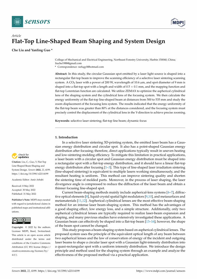
In Equation (1), r0 is the laser beam radius (mm) and I0 is the maximum light intensity(cd) of the laser beam. The light-field intensity distribution of the laser beam is shown inFigure 1.

Sensors 2022, 22, x FOR PEER REVIEW 2 of 15

distribution into a quasi-rectangular spot with a uniform intensity distribution. We intro-

duce the design principle and method used for the shaping system through an example

and analyze the effectiveness of the proposed method via a practical application.

2. Physical Model and Mapping Function of Flat-Top Beam

The simple physical model of the flat-top beam is represented by a circle function,

which has the advantage of a simple form. However, it can only describe the uniform

energy distribution of a flat-top beam and is unsuitable for calculating the beam transmis-

sion characteristics. Compared to other physical flat-top-beam models, the flat-top Lo-

rentz model is the simplest for calculation. Therefore, the flat-top Lorentz model is se-

lected as the physical model of the flat-top beam in this study to reduce the calculation

complexity [17–19].

The light intensity function distribution of the laser beam is shown in Equation (1):

2

0 2

0

2( ) exp( )

rI r I

r

−= (1)

In Equation (1), r0 is the laser beam radius (mm) and I0 is the maximum light intensity

(cd) of the laser beam. The light-field intensity distribution of the laser beam is shown in

Figure 1.

I0

ω0

I0/e2

r0

I

0

Figure 1. Intensity distribution of gaussian laser beams.

In Figure 1, ω0 is the waist radius of the Gaussian laser beam, defined as the radius

of the laser beam when the peak light intensity drops to I0/e2.

Since only the flat-top Lorentz beam can obtain the analytical solution, the flat-top

Lorentz function is used as the shaping objective. The shaping model of the flat-top Lo-

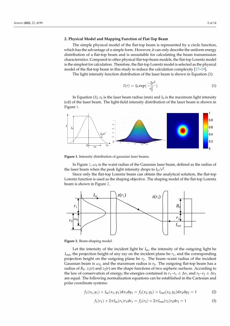
rentz beam is shown in Figure 2.

z(r2)

R0

r2

Iout

z(r1)Iin

r1

ω0r0

Figure 2. Beam-shaping model.

Let the intensity of the incident light be 𝐼in , the intensity of the outgoing light be 𝐼out ,

the projection height of any ray on the incident plane be r1, and the corresponding projec-

tion height on the outgoing plane be r2. The beam–waist radius of the incident Gaussian

beam is ω0, and the maximum radius is r0. The outgoing flat-top beam has a radius of R0.

z1(r) and z2(r) are the shape functions of two aspheric surfaces. According to the law of

Figure 1. Intensity distribution of gaussian laser beams.

In Figure 1, ω0 is the waist radius of the Gaussian laser beam, defined as the radius ofthe laser beam when the peak light intensity drops to I0/e2.

Since only the flat-top Lorentz beam can obtain the analytical solution, the flat-topLorentz function is used as the shaping objective. The shaping model of the flat-top Lorentzbeam is shown in Figure 2.

Sensors 2022, 22, x FOR PEER REVIEW 2 of 15

distribution into a quasi-rectangular spot with a uniform intensity distribution. We intro-

duce the design principle and method used for the shaping system through an example

and analyze the effectiveness of the proposed method via a practical application.

2. Physical Model and Mapping Function of Flat-Top Beam

The simple physical model of the flat-top beam is represented by a circle function,

which has the advantage of a simple form. However, it can only describe the uniform

energy distribution of a flat-top beam and is unsuitable for calculating the beam transmis-

sion characteristics. Compared to other physical flat-top-beam models, the flat-top Lo-

rentz model is the simplest for calculation. Therefore, the flat-top Lorentz model is se-

lected as the physical model of the flat-top beam in this study to reduce the calculation

complexity [17–19].

The light intensity function distribution of the laser beam is shown in Equation (1):

2

0 2

0

2( ) exp( )

rI r I

r

−= (1)

In Equation (1), r0 is the laser beam radius (mm) and I0 is the maximum light intensity

(cd) of the laser beam. The light-field intensity distribution of the laser beam is shown in

Figure 1.

I0

ω0

I0/e2

r0

I

0

Figure 1. Intensity distribution of gaussian laser beams.

In Figure 1, ω0 is the waist radius of the Gaussian laser beam, defined as the radius

of the laser beam when the peak light intensity drops to I0/e2.

Since only the flat-top Lorentz beam can obtain the analytical solution, the flat-top

Lorentz function is used as the shaping objective. The shaping model of the flat-top Lo-

rentz beam is shown in Figure 2.

z(r2)

R0

r2

Iout

z(r1)Iin

r1

ω0r0

Figure 2. Beam-shaping model.

Let the intensity of the incident light be 𝐼in , the intensity of the outgoing light be 𝐼out ,

the projection height of any ray on the incident plane be r1, and the corresponding projec-

tion height on the outgoing plane be r2. The beam–waist radius of the incident Gaussian

beam is ω0, and the maximum radius is r0. The outgoing flat-top beam has a radius of R0.

z1(r) and z2(r) are the shape functions of two aspheric surfaces. According to the law of

Figure 2. Beam-shaping model.

Let the intensity of the incident light be Iin, the intensity of the outgoing light beIout, the projection height of any ray on the incident plane be r1, and the correspondingprojection height on the outgoing plane be r2. The beam–waist radius of the incidentGaussian beam is ω0, and the maximum radius is r0. The outgoing flat-top beam has aradius of R0. z1(r) and z2(r) are the shape functions of two aspheric surfaces. According tothe law of conservation of energy, the energies contained in r1~r1 ± ∆r1 and r2~r2 ± ∆r2are equal. The following normalization equations can be established in the Cartesian andpolar coordinate systems:

f1(x1, y1)× Iin(x1, y1)dx1dy1 = f2(x2, y2)× Iout(x2, y2)dx2dy2 = 1 (2)

f1(r1)× 2π Iin(r1)r1dr1 = f2(r2)× 2π Iout(r2)r2dr2 = 1 (3)

Sensors 2022, 22, 4199 3 of 14

where f1 is the entrance pupil function and f2 is the exit pupil function, which are shownas follows:

f (r1) =

{10≤ r0> r0

f (r2) =

{10≤ R0> R0

The intensity distribution of the incident Gaussian beam is

IG (r) =2

πω20

exp

[−2(

rω0

)2]

. (4)

Considering the integrability of the outgoing flat-top beam, the flat-top Lorentzianfunction is used to express the intensity distribution as follows:

IL(R) =1

πR20

[1 +

(RR0

)q]1+ 2q

(5)

where q is the order of the flat-top Lorentzian function.After substituting the function expressions of the Gaussian and flat-top Lorentzian

beams into Equation (3), the mapping function can be obtained as follows:

1− exp

[−2

(r2

ω20

)]=

[1 +

(R0

R

)q]− 2q

(6)

The mapping function between R and r is

R = h(r) =R0

√1− exp

[−2(

rω0

)]√

1−{

1− exp[−2(

rω0

)2]}q/2

(7)

r = h(r) = ±ω0

√√√√√−12

ln

1−[

1 +(

RR0

)−q]− 2

q (8)

In particular, when q→∞, Equation (7) can be written as

R = R0

√1− exp

[−2(

rω0

)](9)

Equation (9) shows that when the flat-top Lorentzian function is used as a flat-topbeam distribution function, its mapping function has an analytical solution, which canfacilitate ray tracing and significantly simplify the numerical calculation process. For aGalilean-type aspheric system [20], there exists

R = −R0

√√√√1− exp

[−2(

rω0

)2]

(10)

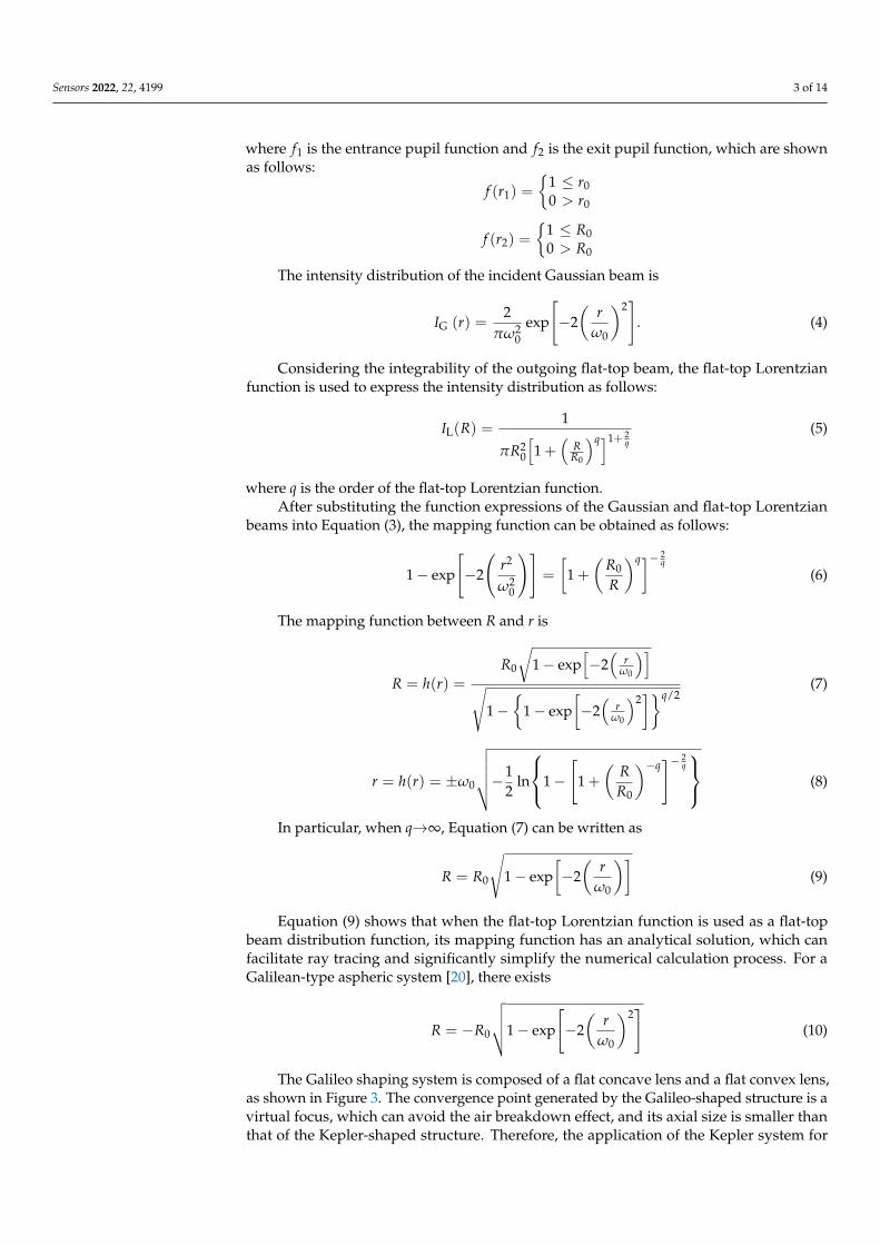
The Galileo shaping system is composed of a flat concave lens and a flat convex lens,as shown in Figure 3. The convergence point generated by the Galileo-shaped structure is avirtual focus, which can avoid the air breakdown effect, and its axial size is smaller thanthat of the Kepler-shaped structure. Therefore, the application of the Kepler system for

Sensors 2022, 22, 4199 4 of 14

beam shaping requires laser power that is not too high, and the Galileo aspheric lens groupcan be applied to larger power.

Sensors 2022, 22, x FOR PEER REVIEW 4 of 15

The Galileo shaping system is composed of a flat concave lens and a flat convex lens,

as shown in Figure 3. The convergence point generated by the Galileo-shaped structure is

a virtual focus, which can avoid the air breakdown effect, and its axial size is smaller than

that of the Kepler-shaped structure. Therefore, the application of the Kepler system for

beam shaping requires laser power that is not too high, and the Galileo aspheric lens

group can be applied to larger power.

The magnification β = f2/f1, where f1 is the focal length of flat-concave lens and f2 is the

focal length of flat-convex lens.

Figure 3. Galileo Beam-Shaping System.

Along the cross-section of the Gaussian beam, the energy is concentrated around the

spot center. To obtain a flat-top beam with uniform illumination, it is necessary to diverge

the rays that pass through a small aperture and concentrate the rays that pass through a

large aperture. Therefore, it is necessary to obtain the relationship between the coordi-

nates of the rays on the entrance-pupil plane and those on the image plane, which is called

the mapping function.

3. System Design of Laser Beam Expansion and Shaping

The optical beam expansion and shaping system based on aspherical cylindrical

lenses can simultaneously adjust the intensity distribution and spot shape of the laser

beam. The parameters of the incident light of the shaping object used in the system design

are as follows: a CO2 laser is used with a power of 200 W, wavelength of 10.6 μm, and spot

diameter of 9 mm. The Gaussian beam is shaped into a rectangular flat-top beam with a

size of 15 × 60 mm using the aspherical cylindrical lenses. The working distance is 500

mm, and the glass material is ZnSe.

3.1. Design of Aspherical Cylindrical Lenses

The Y-direction is consistent with the default coordinate setting in ZEMAX, and all

coordinate systems in this study are the same as the default setting in ZEMAX. First, we

set the wavelength and aperture. The aperture was set to 13.5 mm, and the field of view

was set to 0.

Three surfaces were inserted into the lens data editor (LDE). The second surface was

set as a cylindrical surface, the glass material was set as ZnSe, and the thickness was set

to 6 mm. The radius of the third surface was set to infinity. The radius of the second sur-

face, conic, 4th, 6th, 8th, and 10th order coefficients, and the thickness of the third surface

was set as optimization variables. The 2nd order system was omitted to reduce the pro-

cessing complexity. The 4th, 6th, 8th, and 10th order coefficients were 𝑎4 = −1.279 × 105,

𝑎6 = 2.878 × 107, 𝑎8 = −2.878 × 109, and 𝑎10 = 1.25 × 1011, respectively.

The aperture, field of view, and wavelength were set similarly to the Y-direction, and

a macro program was used to generate the evaluation function. In the macro program, the

radius of the flat-top beam was changed (from 7.5 to 30 mm), and the operand was

changed accordingly (from REAY to REAX). The rays converged in the X-direction; there-

fore, a coordinate-break surface was added to the LDE to rotate the cylindrical lens by 90°

Figure 3. Galileo Beam-Shaping System.

The magnification β = f 2/f 1, where f 1 is the focal length of flat-concave lens and f 2 isthe focal length of flat-convex lens.

Along the cross-section of the Gaussian beam, the energy is concentrated around thespot center. To obtain a flat-top beam with uniform illumination, it is necessary to divergethe rays that pass through a small aperture and concentrate the rays that pass through alarge aperture. Therefore, it is necessary to obtain the relationship between the coordinatesof the rays on the entrance-pupil plane and those on the image plane, which is called themapping function.

3. System Design of Laser Beam Expansion and Shaping

The optical beam expansion and shaping system based on aspherical cylindrical lensescan simultaneously adjust the intensity distribution and spot shape of the laser beam. Theparameters of the incident light of the shaping object used in the system design are asfollows: a CO2 laser is used with a power of 200 W, wavelength of 10.6 µm, and spotdiameter of 9 mm. The Gaussian beam is shaped into a rectangular flat-top beam with asize of 15 × 60 mm using the aspherical cylindrical lenses. The working distance is 500 mm,and the glass material is ZnSe.

3.1. Design of Aspherical Cylindrical Lenses

The Y-direction is consistent with the default coordinate setting in ZEMAX, and allcoordinate systems in this study are the same as the default setting in ZEMAX. First, we setthe wavelength and aperture. The aperture was set to 13.5 mm, and the field of view wasset to 0.

Three surfaces were inserted into the lens data editor (LDE). The second surface wasset as a cylindrical surface, the glass material was set as ZnSe, and the thickness was setto 6 mm. The radius of the third surface was set to infinity. The radius of the secondsurface, conic, 4th, 6th, 8th, and 10th order coefficients, and the thickness of the thirdsurface was set as optimization variables. The 2nd order system was omitted to reduce theprocessing complexity. The 4th, 6th, 8th, and 10th order coefficients were a4 = −1.279× 105,a6 = 2.878× 107, a8 = −2.878× 109, and a10 = 1.25× 1011, respectively.

The aperture, field of view, and wavelength were set similarly to the Y-direction, anda macro program was used to generate the evaluation function. In the macro program,the radius of the flat-top beam was changed (from 7.5 to 30 mm), and the operand waschanged accordingly (from REAY to REAX). The rays converged in the X-direction; there-fore, a coordinate-break surface was added to the LDE to rotate the cylindrical lens by 90◦

around the Z-axis. The 4th, 6th, 8th, and 10th order coefficients were a4 = −4.816× 105,a6 = 9.016× 107, a8 = −8.964× 109, and a10 = 3.913× 1011, respectively.

Two cylindrical lenses were used to shape the X and Y directions, and the lensesdid not interfere with each other. Thus, after the two cylindrical lenses were individuallydesigned, they could simply be stacked. The refraction–surface radius, air thickness,

Sensors 2022, 22, 4199 5 of 14

nonlinear coefficient of the aspheric surface, and 4th–10th order coefficients were set as theoptimization variables for the system. The distance between the shaping lenses for the X-and Y-directions was set to 142 mm. The optimized system structure is shown in Table 1.

Table 1. Structural parameters of the combination optical system.

Surface Type Radius (mm) Thickness (mm) Glass Diameter (mm) Conic

Stop 0 5 Air 0 03 56.132 6 ZNSE 6.75 −112.6034 Infinity 139.271 Air 6.75 06 Infinity 0 Air 6.75 07 123.491 6 ZNSE 6.75 −495.168 Infinity 317.448 Air 6.641 0

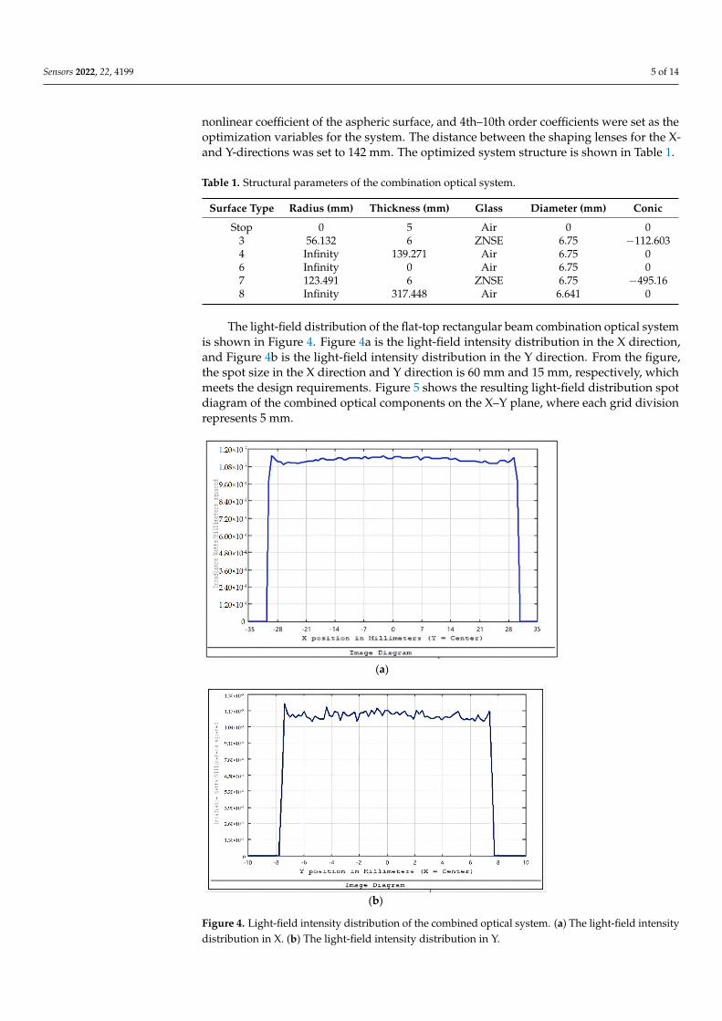
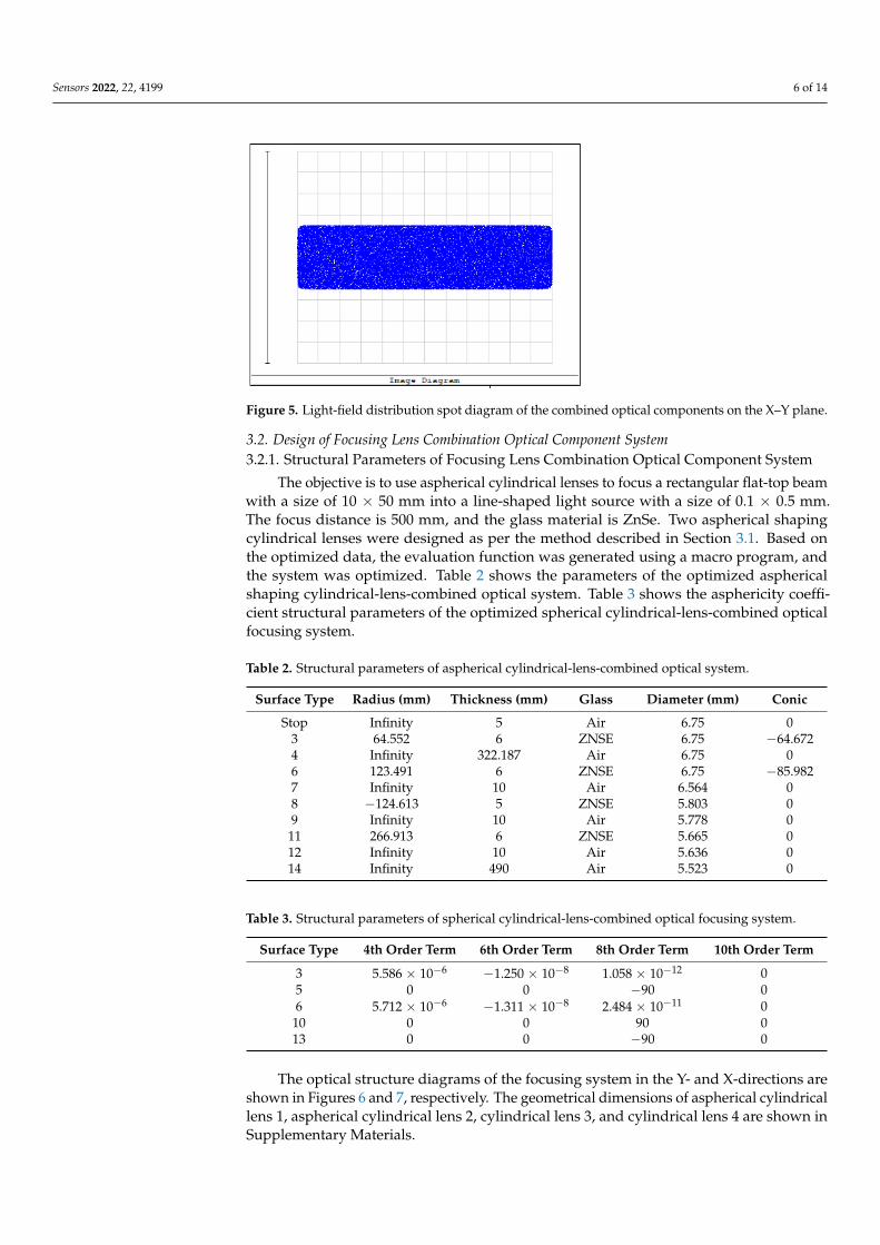
The light-field distribution of the flat-top rectangular beam combination optical systemis shown in Figure 4. Figure 4a is the light-field intensity distribution in the X direction,and Figure 4b is the light-field intensity distribution in the Y direction. From the figure,the spot size in the X direction and Y direction is 60 mm and 15 mm, respectively, whichmeets the design requirements. Figure 5 shows the resulting light-field distribution spotdiagram of the combined optical components on the X–Y plane, where each grid divisionrepresents 5 mm.

Sensors 2022, 22, x FOR PEER REVIEW 5 of 15

around the Z-axis. The 4th, 6th, 8th, and 10th order coefficients were 𝑎4 = −4.816 × 105,

𝑎6 = 9.016 × 107, 𝑎8 = −8.964 × 109, and 𝑎10 = 3.913 × 1011, respectively.

Two cylindrical lenses were used to shape the X and Y directions, and the lenses did

not interfere with each other. Thus, after the two cylindrical lenses were individually de-

signed, they could simply be stacked. The refraction–surface radius, air thickness, nonlin-

ear coefficient of the aspheric surface, and 4th–10th order coefficients were set as the op-

timization variables for the system. The distance between the shaping lenses for the X-

and Y-directions was set to 142 mm. The optimized system structure is shown in Table 1.

Table 1. Structural parameters of the combination optical system.

Surface Type Radius (mm) Thickness (mm) Glass Diameter (mm) Conic

Stop 0 5 Air 0 0

3 56.132 6 ZNSE 6.75 −112.603

4 Infinity 139.271 Air 6.75 0

6 Infinity 0 Air 6.75 0

7 123.491 6 ZNSE 6.75 −495.16

8 Infinity 317.448 Air 6.641 0

The light-field distribution of the flat-top rectangular beam combination optical sys-

tem is shown in Figure 4. Figure 4a is the light-field intensity distribution in the X direc-

tion, and Figure 4b is the light-field intensity distribution in the Y direction. From the

figure, the spot size in the X direction and Y direction is 60 mm and 15 mm, respectively,

which meets the design requirements. Figure 5 shows the resulting light-field distribution

spot diagram of the combined optical components on the X–Y plane, where each grid di-

vision represents 5 mm.

(a)

Sensors 2022, 22, x FOR PEER REVIEW 6 of 15

(b)

Figure 4. Light-field intensity distribution of the combined optical system. (a) The light-field inten-

sity distribution in X. (b) The light-field intensity distribution in Y.

Figure 5. Light-field distribution spot diagram of the combined optical components on the X–Y

plane.

3.2. Design of Focusing Lens Combination Optical Component System

3.2.1. Structural Parameters of Focusing Lens Combination Optical Component System

The objective is to use aspherical cylindrical lenses to focus a rectangular flat-top

beam with a size of 10 × 50 mm into a line-shaped light source with a size of 0.1 × 0.5 mm.

The focus distance is 500 mm, and the glass material is ZnSe. Two aspherical shaping

cylindrical lenses were designed as per the method described in Section 3.1. Based on the

optimized data, the evaluation function was generated using a macro program, and the

system was optimized. Table 2 shows the parameters of the optimized aspherical shaping

cylindrical-lens-combined optical system. Table 3 shows the asphericity coefficient struc-

tural parameters of the optimized spherical cylindrical-lens-combined optical focusing

system.

Figure 4. Light-field intensity distribution of the combined optical system. (a) The light-field intensitydistribution in X. (b) The light-field intensity distribution in Y.

Sensors 2022, 22, 4199 6 of 14

Sensors 2022, 22, x FOR PEER REVIEW 6 of 15

(b)

Figure 4. Light-field intensity distribution of the combined optical system. (a) The light-field inten-

sity distribution in X. (b) The light-field intensity distribution in Y.

Figure 5. Light-field distribution spot diagram of the combined optical components on the X–Y

plane.

3.2. Design of Focusing Lens Combination Optical Component System

3.2.1. Structural Parameters of Focusing Lens Combination Optical Component System

The objective is to use aspherical cylindrical lenses to focus a rectangular flat-top

beam with a size of 10 × 50 mm into a line-shaped light source with a size of 0.1 × 0.5 mm.

The focus distance is 500 mm, and the glass material is ZnSe. Two aspherical shaping

cylindrical lenses were designed as per the method described in Section 3.1. Based on the

optimized data, the evaluation function was generated using a macro program, and the

system was optimized. Table 2 shows the parameters of the optimized aspherical shaping

cylindrical-lens-combined optical system. Table 3 shows the asphericity coefficient struc-

tural parameters of the optimized spherical cylindrical-lens-combined optical focusing

system.

Figure 5. Light-field distribution spot diagram of the combined optical components on the X–Y plane.

3.2. Design of Focusing Lens Combination Optical Component System3.2.1. Structural Parameters of Focusing Lens Combination Optical Component System

The objective is to use aspherical cylindrical lenses to focus a rectangular flat-top beamwith a size of 10 × 50 mm into a line-shaped light source with a size of 0.1 × 0.5 mm.The focus distance is 500 mm, and the glass material is ZnSe. Two aspherical shapingcylindrical lenses were designed as per the method described in Section 3.1. Based onthe optimized data, the evaluation function was generated using a macro program, andthe system was optimized. Table 2 shows the parameters of the optimized asphericalshaping cylindrical-lens-combined optical system. Table 3 shows the asphericity coeffi-cient structural parameters of the optimized spherical cylindrical-lens-combined opticalfocusing system.

Table 2. Structural parameters of aspherical cylindrical-lens-combined optical system.

Surface Type Radius (mm) Thickness (mm) Glass Diameter (mm) Conic

Stop Infinity 5 Air 6.75 03 64.552 6 ZNSE 6.75 −64.6724 Infinity 322.187 Air 6.75 06 123.491 6 ZNSE 6.75 −85.9827 Infinity 10 Air 6.564 08 −124.613 5 ZNSE 5.803 09 Infinity 10 Air 5.778 0

11 266.913 6 ZNSE 5.665 012 Infinity 10 Air 5.636 014 Infinity 490 Air 5.523 0

Table 3. Structural parameters of spherical cylindrical-lens-combined optical focusing system.

Surface Type 4th Order Term 6th Order Term 8th Order Term 10th Order Term

3 5.586 × 10−6 −1.250 × 10−8 1.058 × 10−12 05 0 0 −90 06 5.712 × 10−6 −1.311 × 10−8 2.484 × 10−11 0

10 0 0 90 013 0 0 −90 0

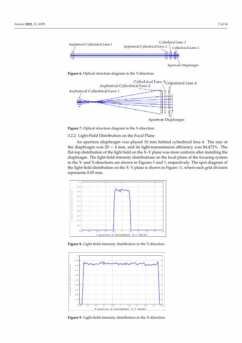
The optical structure diagrams of the focusing system in the Y- and X-directions areshown in Figures 6 and 7, respectively. The geometrical dimensions of aspherical cylindricallens 1, aspherical cylindrical lens 2, cylindrical lens 3, and cylindrical lens 4 are shown inSupplementary Materials.

Sensors 2022, 22, 4199 7 of 14

Sensors 2022, 22, x FOR PEER REVIEW 7 of 15

Table 2. Structural parameters of aspherical cylindrical-lens-combined optical system.

Surface Type Radius (mm) Thickness (mm) Glass Diameter (mm) Conic

Stop Infinity 5 Air 6.75 0

3 64.552 6 ZNSE 6.75 −64.672

4 Infinity 322.187 Air 6.75 0

6 123.491 6 ZNSE 6.75 −85.982

7 Infinity 10 Air 6.564 0

8 −124.613 5 ZNSE 5.803 0

9 Infinity 10 Air 5.778 0

11 266.913 6 ZNSE 5.665 0

12 Infinity 10 Air 5.636 0

14 Infinity 490 Air 5.523 0

Table 3. Structural parameters of spherical cylindrical-lens-combined optical focusing system.

Surface Type 4th Order Term 6th Order Term 8th Order Term 10th Order Term

3 5.586 × 10−6 −1.250 × 10−8 1.058 × 10−12 0

5 0 0 −90 0

6 5.712 × 10−6 −1.311 × 10−8 2.484 × 10−11 0

10 0 0 90 0

13 0 0 −90 0

The optical structure diagrams of the focusing system in the Y- and X-directions are

shown in Figures 6 and 7, respectively. The geometrical dimensions of aspherical cylin-

drical lens 1, aspherical cylindrical lens 2, cylindrical lens 3, and cylindrical lens 4 are

shown in Supplementary Materials.

Figure 6. Optical structure diagram in the Y-direction.

Figure 7. Optical structure diagram in the X-direction.

3.2.2. Light-Field Distribution on the Focal Plane

An aperture diaphragm was placed 10 mm behind cylindrical lens 4. The size of the

diaphragm was 20 × 4 mm, and its light-transmission efficiency was 84.472%. The flat-top

distribution of the light field on the X–Y plane was more uniform after installing the dia-

phragm. The light-field-intensity distributions on the focal plane of the focusing system

in the Y- and X-directions are shown in Figures 8 and 9, respectively. The spot diagram of

Figure 6. Optical structure diagram in the Y-direction.

Sensors 2022, 22, x FOR PEER REVIEW 7 of 15

Table 2. Structural parameters of aspherical cylindrical-lens-combined optical system.

Surface Type Radius (mm) Thickness (mm) Glass Diameter (mm) Conic

Stop Infinity 5 Air 6.75 0

3 64.552 6 ZNSE 6.75 −64.672

4 Infinity 322.187 Air 6.75 0

6 123.491 6 ZNSE 6.75 −85.982

7 Infinity 10 Air 6.564 0

8 −124.613 5 ZNSE 5.803 0

9 Infinity 10 Air 5.778 0

11 266.913 6 ZNSE 5.665 0

12 Infinity 10 Air 5.636 0

14 Infinity 490 Air 5.523 0

Table 3. Structural parameters of spherical cylindrical-lens-combined optical focusing system.

Surface Type 4th Order Term 6th Order Term 8th Order Term 10th Order Term

3 5.586 × 10−6 −1.250 × 10−8 1.058 × 10−12 0

5 0 0 −90 0

6 5.712 × 10−6 −1.311 × 10−8 2.484 × 10−11 0

10 0 0 90 0

13 0 0 −90 0

The optical structure diagrams of the focusing system in the Y- and X-directions are

shown in Figures 6 and 7, respectively. The geometrical dimensions of aspherical cylin-

drical lens 1, aspherical cylindrical lens 2, cylindrical lens 3, and cylindrical lens 4 are

shown in Supplementary Materials.

Figure 6. Optical structure diagram in the Y-direction.

Figure 7. Optical structure diagram in the X-direction.

3.2.2. Light-Field Distribution on the Focal Plane

An aperture diaphragm was placed 10 mm behind cylindrical lens 4. The size of the

diaphragm was 20 × 4 mm, and its light-transmission efficiency was 84.472%. The flat-top

distribution of the light field on the X–Y plane was more uniform after installing the dia-

phragm. The light-field-intensity distributions on the focal plane of the focusing system

in the Y- and X-directions are shown in Figures 8 and 9, respectively. The spot diagram of

Figure 7. Optical structure diagram in the X-direction.

3.2.2. Light-Field Distribution on the Focal Plane

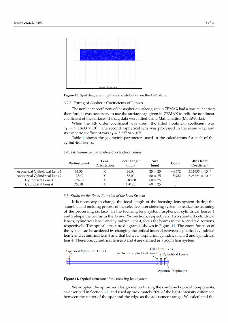
An aperture diaphragm was placed 10 mm behind cylindrical lens 4. The size ofthe diaphragm was 20 × 4 mm, and its light-transmission efficiency was 84.472%. Theflat-top distribution of the light field on the X–Y plane was more uniform after installing thediaphragm. The light-field-intensity distributions on the focal plane of the focusing systemin the Y- and X-directions are shown in Figures 8 and 9, respectively. The spot diagram ofthe light-field distribution on the X–Y plane is shown in Figure 10, where each grid divisionrepresents 0.05 mm.

Sensors 2022, 22, x FOR PEER REVIEW 8 of 15

the light-field distribution on the X–Y plane is shown in Figure 10, where each grid divi-

sion represents 0.05 mm.

Figure 8. Light-field-intensity distribution in the Y-direction.

Figure 9. Light-field-intensity distribution in the X-direction.

Figure 10. Spot diagram of light-field distribution on the X–Y plane.

3.2.3. Fitting of Aspheric Coefficients of Lenses

The nonlinear coefficient of the aspheric surface given in ZEMAX had a particular

error; therefore, it was necessary to use the surface sag given in ZEMAX to refit the non-

linear coefficient of the surface. The sag data were fitted using Mathematica (MathWorks).

When the 4th order coefficient was used, the fitted nonlinear coefficient was 𝑎4 =

5.11633 × 106. The second aspherical lens was processed in the same way, and its aspheric

coefficient was 𝑎4 = 5.25724 × 106.

Table 4 shows the geometric parameters used in the calculations for each of the cy-

lindrical lenses.

Figure 8. Light-field-intensity distribution in the Y-direction.

Sensors 2022, 22, x FOR PEER REVIEW 8 of 15

the light-field distribution on the X–Y plane is shown in Figure 10, where each grid divi-

sion represents 0.05 mm.

Figure 8. Light-field-intensity distribution in the Y-direction.

Figure 9. Light-field-intensity distribution in the X-direction.

Figure 10. Spot diagram of light-field distribution on the X–Y plane.

3.2.3. Fitting of Aspheric Coefficients of Lenses

The nonlinear coefficient of the aspheric surface given in ZEMAX had a particular

error; therefore, it was necessary to use the surface sag given in ZEMAX to refit the non-

linear coefficient of the surface. The sag data were fitted using Mathematica (MathWorks).

When the 4th order coefficient was used, the fitted nonlinear coefficient was 𝑎4 =

5.11633 × 106. The second aspherical lens was processed in the same way, and its aspheric

coefficient was 𝑎4 = 5.25724 × 106.

Table 4 shows the geometric parameters used in the calculations for each of the cy-

lindrical lenses.

Figure 9. Light-field-intensity distribution in the X-direction.

Sensors 2022, 22, 4199 8 of 14

Sensors 2022, 22, x FOR PEER REVIEW 8 of 15

the light-field distribution on the X–Y plane is shown in Figure 10, where each grid divi-

sion represents 0.05 mm.

Figure 8. Light-field-intensity distribution in the Y-direction.

Figure 9. Light-field-intensity distribution in the X-direction.

Figure 10. Spot diagram of light-field distribution on the X–Y plane.

3.2.3. Fitting of Aspheric Coefficients of Lenses

The nonlinear coefficient of the aspheric surface given in ZEMAX had a particular

error; therefore, it was necessary to use the surface sag given in ZEMAX to refit the non-

linear coefficient of the surface. The sag data were fitted using Mathematica (MathWorks).

When the 4th order coefficient was used, the fitted nonlinear coefficient was 𝑎4 =

5.11633 × 106. The second aspherical lens was processed in the same way, and its aspheric

coefficient was 𝑎4 = 5.25724 × 106.

Table 4 shows the geometric parameters used in the calculations for each of the cy-

lindrical lenses.

Figure 10. Spot diagram of light-field distribution on the X–Y plane.

3.2.3. Fitting of Aspheric Coefficients of Lenses

The nonlinear coefficient of the aspheric surface given in ZEMAX had a particular error;therefore, it was necessary to use the surface sag given in ZEMAX to refit the nonlinearcoefficient of the surface. The sag data were fitted using Mathematica (MathWorks).

When the 4th order coefficient was used, the fitted nonlinear coefficient wasa4 = 5.11633 × 106. The second aspherical lens was processed in the same way, andits aspheric coefficient was a4 = 5.25724× 106.

Table 4 shows the geometric parameters used in the calculations for each of thecylindrical lenses.

Table 4. Geometric parameters of cylindrical lenses.

Radius (mm) LensOrientation

Focal Length(mm)

Size(mm) Conic 4th Order

Coefficient

Aspherical Cylindrical Lens 1 64.55 X 46.00 25 × 25 −4.672 5.11633 × 10−6

Aspherical Cylindrical Lens 2 123.49 Y 88.00 60 × 25 −5.982 5.25724 × 10−6

Cylindrical Lens 3 −24.91 Y −88.00 60 × 25 0Cylindrical Lens 4 266.91 X 190.20 60 × 25 0

3.3. Study on the Zoom Function of the Lens System

It is necessary to change the focal length of the focusing lens system during thescanning and molding process of the selective laser sintering system to realize the scanningof the processing surface. In the focusing lens system, aspherical cylindrical lenses 1and 2 shape the beams in the X- and Y-directions, respectively. Two standard cylindricallenses, cylindrical lens 3 and cylindrical lens 4, focus the beams in the X- and Y-directions,respectively. The optical-structure diagram is shown in Figure 11. The zoom function ofthe system can be achieved by changing the optical interval between aspherical cylindricallens 2 and cylindrical lens 3 and that between aspherical cylindrical lens 2 and cylindricallens 4. Therefore, cylindrical lenses 3 and 4 are defined as a zoom lens system.

Sensors 2022, 22, x FOR PEER REVIEW 9 of 15

Table 4. Geometric parameters of cylindrical lenses.

Radius (mm) Lens Orientation Focal Length (mm) Size (mm) Conic 4th Order Coefficient

Aspherical Cylindrical Lens 1 64.55 X 46.00 25 × 25 −4.672 5.11633 × 10−6

Aspherical Cylindrical Lens 2 123.49 Y 88.00 60 × 25 −5.982 5.25724 × 10−6

Cylindrical Lens 3 −24.91 Y −88.00 60 × 25 0

Cylindrical Lens 4 266.91 X 190.20 60 × 25 0

3.3. Study on the Zoom Function of the Lens System

It is necessary to change the focal length of the focusing lens system during the scan-

ning and molding process of the selective laser sintering system to realize the scanning of

the processing surface. In the focusing lens system, aspherical cylindrical lenses 1 and 2

shape the beams in the X- and Y-directions, respectively. Two standard cylindrical lenses,

cylindrical lens 3 and cylindrical lens 4, focus the beams in the X- and Y-directions, re-

spectively. The optical-structure diagram is shown in Figure 11. The zoom function of the

system can be achieved by changing the optical interval between aspherical cylindrical

lens 2 and cylindrical lens 3 and that between aspherical cylindrical lens 2 and cylindrical

lens 4. Therefore, cylindrical lenses 3 and 4 are defined as a zoom lens system.

Figure 11. Optical structure of the focusing lens system.

We adopted the optimized design method using the combined optical components,

as described in Section 3.2, and used approximately 20% of the light-intensity difference

between the center of the spot and the edge as the adjustment range. We calculated the

intensity distribution of the light field and the displacement parameters of the zoom lens

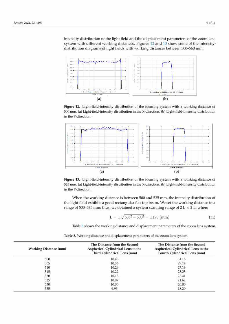
system with different working distances. Figures 12 and 13 show some of the intensity-

distribution diagrams of light fields with working distances between 500–560 mm.

(a) (b)

Figure 12. Light-field-intensity distribution of the focusing system with a working distance of 500

mm. (a) Light-field-intensity distribution in the X-direction. (b) Light-field-intensity distribution in

the Y-direction.

Figure 11. Optical structure of the focusing lens system.

We adopted the optimized design method using the combined optical components,as described in Section 3.2, and used approximately 20% of the light-intensity differencebetween the center of the spot and the edge as the adjustment range. We calculated the

Sensors 2022, 22, 4199 9 of 14

intensity distribution of the light field and the displacement parameters of the zoom lenssystem with different working distances. Figures 12 and 13 show some of the intensity-distribution diagrams of light fields with working distances between 500–560 mm.

Sensors 2022, 22, x FOR PEER REVIEW 9 of 15

Table 4. Geometric parameters of cylindrical lenses.

Radius (mm) Lens Orientation Focal Length (mm) Size (mm) Conic 4th Order Coefficient

Aspherical Cylindrical Lens 1 64.55 X 46.00 25 × 25 −4.672 5.11633 × 10−6

Aspherical Cylindrical Lens 2 123.49 Y 88.00 60 × 25 −5.982 5.25724 × 10−6

Cylindrical Lens 3 −24.91 Y −88.00 60 × 25 0

Cylindrical Lens 4 266.91 X 190.20 60 × 25 0

3.3. Study on the Zoom Function of the Lens System

It is necessary to change the focal length of the focusing lens system during the scan-

ning and molding process of the selective laser sintering system to realize the scanning of

the processing surface. In the focusing lens system, aspherical cylindrical lenses 1 and 2

shape the beams in the X- and Y-directions, respectively. Two standard cylindrical lenses,

cylindrical lens 3 and cylindrical lens 4, focus the beams in the X- and Y-directions, re-

spectively. The optical-structure diagram is shown in Figure 11. The zoom function of the

system can be achieved by changing the optical interval between aspherical cylindrical

lens 2 and cylindrical lens 3 and that between aspherical cylindrical lens 2 and cylindrical

lens 4. Therefore, cylindrical lenses 3 and 4 are defined as a zoom lens system.

Figure 11. Optical structure of the focusing lens system.

We adopted the optimized design method using the combined optical components,

as described in Section 3.2, and used approximately 20% of the light-intensity difference

between the center of the spot and the edge as the adjustment range. We calculated the

intensity distribution of the light field and the displacement parameters of the zoom lens

system with different working distances. Figures 12 and 13 show some of the intensity-

distribution diagrams of light fields with working distances between 500–560 mm.

(a) (b)

Figure 12. Light-field-intensity distribution of the focusing system with a working distance of 500

mm. (a) Light-field-intensity distribution in the X-direction. (b) Light-field-intensity distribution in

the Y-direction.

Figure 12. Light-field-intensity distribution of the focusing system with a working distance of500 mm. (a) Light-field-intensity distribution in the X-direction. (b) Light-field-intensity distributionin the Y-direction.

Sensors 2022, 22, x FOR PEER REVIEW 10 of 15

(a) (b)

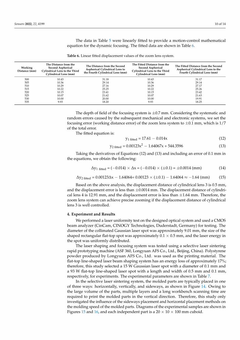
Figure 13. Light-field-intensity distribution of the focusing system with a working distance of 535

mm. (a) Light-field-intensity distribution in the X-direction. (b) Light-field-intensity distribution in

the Y-direction.

When the working distance is between 500 and 535 mm, the intensity distribution of

the light field exhibits a good rectangular flat-top beam. We set the working distance to a

range of 500–535 mm; thus, we obtained a system scanning range of 2 L × 2 L, where

L = 2 2535 500 190 (mm) − = (11)

Table 5 shows the working distance and displacement parameters of the zoom lens

system.

Table 5. Working distance and displacement parameters of the zoom lens system.

Working Distance (mm)

The Distance from the Second Aspheri-

cal Cylindrical Lens to the Third Cylin-

drical Lens (mm)

The Distance from the Second Aspherical Cy-

lindrical Lens to the Fourth Cylindrical Lens

(mm)

500 10.43 31.18

505 10.36 29.14

510 10.29 27.16

515 10.22 25.25

520 10.15 23.41

525 10.07 21.62

530 10.00 20.00

535 9.93 18.20

The data in Table 5 were linearly fitted to provide a motion-control mathematical

equation for the dynamic focusing. The fitted data are shown in Table 6.

The depth of field of the focusing system is ±0.7 mm. Considering the systematic and

random errors caused by the subsequent mechanical and electronic systems, we set the

focusing error (working distance error) of the zoom lens system to ±0.1 mm, which is 1/7

of the total error.

Table 6. Linear fitted displacement values of the zoom lens system.

Working Dis-

tance (mm)

The Distance from the

Second Aspherical Cy-

lindrical Lens to the

Third Cylindrical Lens

(mm)

The Distance from the

Second Aspherical Cy-

lindrical Lens to the

Fourth Cylindrical

Lens (mm)

The Fitted Distance

from the Second As-

pherical Cylindrical

Lens to the Third Cy-

lindrical Lens (mm)

The Fitted Distance from

the Second Aspherical Cy-

lindrical Lens to the

Fourth Cylindrical Lens

(mm)

500 10.43 31.18 10.43 31.17

505 10.36 29.14 10.36 29.14

510 10.29 27.16 10.29 27.17

Figure 13. Light-field-intensity distribution of the focusing system with a working distance of535 mm. (a) Light-field-intensity distribution in the X-direction. (b) Light-field-intensity distributionin the Y-direction.

When the working distance is between 500 and 535 mm, the intensity distribution ofthe light field exhibits a good rectangular flat-top beam. We set the working distance to arange of 500–535 mm; thus, we obtained a system scanning range of 2 L × 2 L, where

L = ±√

5352 − 5002 = ±190 (mm) (11)

Table 5 shows the working distance and displacement parameters of the zoom lens system.

Table 5. Working distance and displacement parameters of the zoom lens system.

Working Distance (mm)The Distance from the Second

Aspherical Cylindrical Lens to theThird Cylindrical Lens (mm)

The Distance from the SecondAspherical Cylindrical Lens to the

Fourth Cylindrical Lens (mm)

500 10.43 31.18505 10.36 29.14510 10.29 27.16515 10.22 25.25520 10.15 23.41525 10.07 21.62530 10.00 20.00535 9.93 18.20

Sensors 2022, 22, 4199 10 of 14

The data in Table 5 were linearly fitted to provide a motion-control mathematicalequation for the dynamic focusing. The fitted data are shown in Table 6.

Table 6. Linear fitted displacement values of the zoom lens system.

WorkingDistance (mm)

The Distance from theSecond Aspherical

Cylindrical Lens to the ThirdCylindrical Lens (mm)

The Distance from the SecondAspherical Cylindrical Lens to

the Fourth Cylindrical Lens (mm)

The Fitted Distance from theSecond Aspherical

Cylindrical Lens to the ThirdCylindrical Lens (mm)

The Fitted Distance from the SecondAspherical Cylindrical Lens to the

Fourth Cylindrical Lens (mm)

500 10.43 31.18 10.43 31.17505 10.36 29.14 10.36 29.14510 10.29 27.16 10.29 27.17515 10.22 25.25 10.22 25.26520 10.15 23.41 10.15 23.42525 10.07 21.62 10.07 21.63530 10.00 20.00 10.00 19.91535 9.93 18.20 9.93 18.25

The depth of field of the focusing system is ±0.7 mm. Considering the systematic andrandom errors caused by the subsequent mechanical and electronic systems, we set thefocusing error (working distance error) of the zoom lens system to ±0.1 mm, which is 1/7of the total error.

The fitted equation is:y1 fitted = 17.61 − 0.014x (12)

y2 fitted = 0.00123x2 − 1.64067x + 544.3596 (13)

Taking the derivatives of Equations (12) and (13) and including an error of 0.1 mm inthe equations, we obtain the following:

∆y1 fitted = (−0.014) × ∆x = (−0.014) × (±0.1) = ±0.0014 (mm) (14)

∆y2 fitted = 0.00123∆x − 1.64064= 0.00123 × (±0.1) − 1.64064 ≈ −1.64 (mm) (15)

Based on the above analysis, the displacement distance of cylindrical lens 3 is 0.5 mm,and the displacement error is less than ±0.0014 mm. The displacement distance of cylindri-cal lens 4 is 12.91 mm, and the displacement error is less than ±1.64 mm. Therefore, thezoom lens system can achieve precise zooming if the displacement distance of cylindricallens 3 is well controlled.

4. Experiment and Results

We performed a laser uniformity test on the designed optical system and used a CMOSbeam analyzer (CinCam, CINOGY Technologies, Duderstadt, Germany) for testing. Thediameter of the collimated Gaussian laser spot was approximately 9.01 mm, the size of theshaped rectangular flat-top spot was approximately 0.1 × 0.5 mm, and the laser energy inthe spot was uniformly distributed.

The laser shaping and focusing system was tested using a selective laser sinteringrapid prototyping machine (ASF 360, Longyuan AFS Co., Ltd., Beijing, China). Polystyrenepowder produced by Longyuan AFS Co., Ltd. was used as the printing material. Theflat-top line-shaped laser beam shaping system has an energy loss of approximately 17%;therefore, this study selected a 15 W Gaussian laser spot with a diameter of 0.1 mm anda 93 W flat-top line-shaped laser spot with a length and width of 0.5 mm and 0.1 mm,respectively, for experiments. The experimental parameters are shown in Table 7.

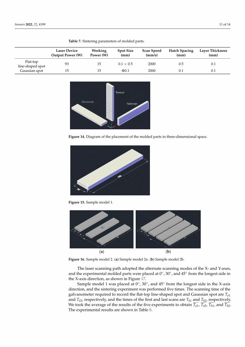
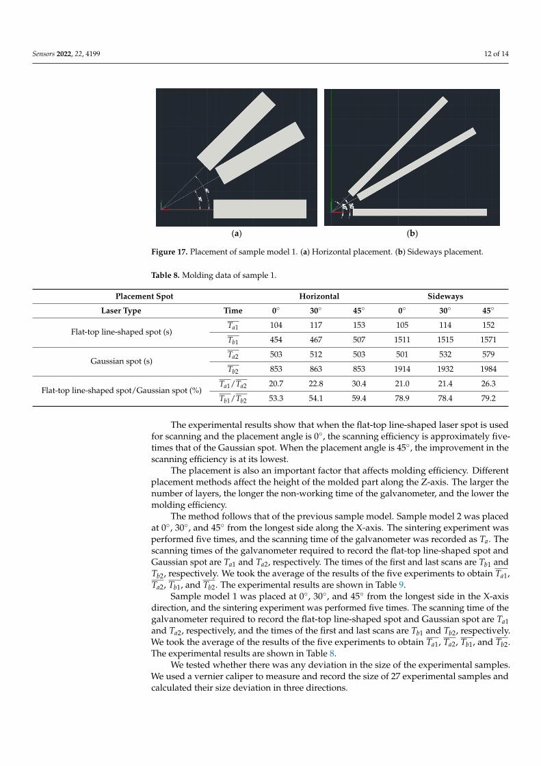
In the selective laser sintering system, the molded parts are typically placed in oneof three ways: horizontally, vertically, and sideways, as shown in Figure 14. Owing tothe large volume of the parts, multiple layers and a long workbench scanning time arerequired to print the molded parts in the vertical direction. Therefore, this study onlyinvestigated the influence of the sideways placement and horizontal placement methods onthe molding speed of the molded parts. Diagrams of the experimental samples are shown inFigures 15 and 16, and each independent part is a 20 × 10 × 100 mm cuboid.

Sensors 2022, 22, 4199 11 of 14

Table 7. Sintering parameters of molded parts.

Laser DeviceOutput Power (W)

WorkingPower (W)

Spot Size(mm)

Scan Speed(mm/s)

Hatch Spacing(mm)

Layer Thickness(mm)

Flat-topline-shaped spot 93 15 0.1 × 0.5 2000 0.5 0.1

Gaussian spot 15 15 Φ0.1 2000 0.1 0.1Sensors 2022, 22, x FOR PEER REVIEW 12 of 15

Figure 14. Diagram of the placement of the molded parts in three-dimensional space.

Figure 15. Sample model 1.

(a) (b)

Figure 16. Sample model 2. (a) Sample model 2a. (b) Sample model 2b.

The laser scanning path adopted the alternate scanning modes of the X- and Y-axes,

and the experimental molded parts were placed at 0°, 30°, and 45° from the longest side

in the X-axis direction, as shown in Figure 17.

(a) (b)

Figure 17. Placement of sample model 1. (a) Horizontal placement. (b) Sideways placement.

Figure 14. Diagram of the placement of the molded parts in three-dimensional space.

Sensors 2022, 22, x FOR PEER REVIEW 12 of 15

Figure 14. Diagram of the placement of the molded parts in three-dimensional space.

Figure 15. Sample model 1.

(a) (b)

Figure 16. Sample model 2. (a) Sample model 2a. (b) Sample model 2b.

The laser scanning path adopted the alternate scanning modes of the X- and Y-axes,

and the experimental molded parts were placed at 0°, 30°, and 45° from the longest side

in the X-axis direction, as shown in Figure 17.

(a) (b)

Figure 17. Placement of sample model 1. (a) Horizontal placement. (b) Sideways placement.

Figure 15. Sample model 1.

Sensors 2022, 22, x FOR PEER REVIEW 12 of 15

Figure 14. Diagram of the placement of the molded parts in three-dimensional space.

Figure 15. Sample model 1.

(a) (b)

Figure 16. Sample model 2. (a) Sample model 2a. (b) Sample model 2b.

The laser scanning path adopted the alternate scanning modes of the X- and Y-axes,

and the experimental molded parts were placed at 0°, 30°, and 45° from the longest side

in the X-axis direction, as shown in Figure 17.

(a) (b)

Figure 17. Placement of sample model 1. (a) Horizontal placement. (b) Sideways placement.

Figure 16. Sample model 2. (a) Sample model 2a. (b) Sample model 2b.

The laser scanning path adopted the alternate scanning modes of the X- and Y-axes,and the experimental molded parts were placed at 0◦, 30◦, and 45◦ from the longest side inthe X-axis direction, as shown in Figure 17.

Sample model 1 was placed at 0◦, 30◦, and 45◦ from the longest side in the X-axisdirection, and the sintering experiment was performed five times. The scanning time of thegalvanometer required to record the flat-top line-shaped spot and Gaussian spot are Ta1and Ta2, respectively, and the times of the first and last scans are Tb1 and Tb2, respectively.We took the average of the results of the five experiments to obtain Ta1, Ta2, Tb1, and Tb2.The experimental results are shown in Table 8.

Sensors 2022, 22, 4199 12 of 14

Sensors 2022, 22, x FOR PEER REVIEW 12 of 15

Figure 14. Diagram of the placement of the molded parts in three-dimensional space.

Figure 15. Sample model 1.

(a) (b)

Figure 16. Sample model 2. (a) Sample model 2a. (b) Sample model 2b.

The laser scanning path adopted the alternate scanning modes of the X- and Y-axes,

and the experimental molded parts were placed at 0°, 30°, and 45° from the longest side

in the X-axis direction, as shown in Figure 17.

(a) (b)

Figure 17. Placement of sample model 1. (a) Horizontal placement. (b) Sideways placement. Figure 17. Placement of sample model 1. (a) Horizontal placement. (b) Sideways placement.

Table 8. Molding data of sample 1.

Placement Spot Horizontal Sideways

Laser Type Time 0◦ 30◦ 45◦ 0◦ 30◦ 45◦

Flat-top line-shaped spot (s)Ta1 104 117 153 105 114 152

Tb1 454 467 507 1511 1515 1571

Gaussian spot (s)Ta2 503 512 503 501 532 579

Tb2 853 863 853 1914 1932 1984

Flat-top line-shaped spot/Gaussian spot (%)Ta1/Ta2 20.7 22.8 30.4 21.0 21.4 26.3

Tb1/Tb2 53.3 54.1 59.4 78.9 78.4 79.2

The experimental results show that when the flat-top line-shaped laser spot is usedfor scanning and the placement angle is 0◦, the scanning efficiency is approximately five-times that of the Gaussian spot. When the placement angle is 45◦, the improvement in thescanning efficiency is at its lowest.

The placement is also an important factor that affects molding efficiency. Differentplacement methods affect the height of the molded part along the Z-axis. The larger thenumber of layers, the longer the non-working time of the galvanometer, and the lower themolding efficiency.

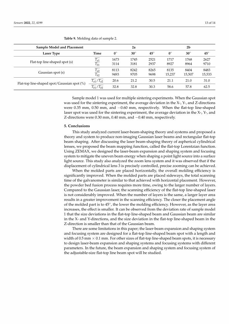
The method follows that of the previous sample model. Sample model 2 was placedat 0◦, 30◦, and 45◦ from the longest side along the X-axis. The sintering experiment wasperformed five times, and the scanning time of the galvanometer was recorded as Ta. Thescanning times of the galvanometer required to record the flat-top line-shaped spot andGaussian spot are Ta1 and Ta2, respectively. The times of the first and last scans are Tb1 andTb2, respectively. We took the average of the results of the five experiments to obtain Ta1,Ta2, Tb1, and Tb2. The experimental results are shown in Table 9.

Sample model 1 was placed at 0◦, 30◦, and 45◦ from the longest side in the X-axisdirection, and the sintering experiment was performed five times. The scanning time of thegalvanometer required to record the flat-top line-shaped spot and Gaussian spot are Ta1and Ta2, respectively, and the times of the first and last scans are Tb1 and Tb2, respectively.We took the average of the results of the five experiments to obtain Ta1, Ta2, Tb1, and Tb2.The experimental results are shown in Table 8.

We tested whether there was any deviation in the size of the experimental samples.We used a vernier caliper to measure and record the size of 27 experimental samples andcalculated their size deviation in three directions.

Sensors 2022, 22, 4199 13 of 14

Table 9. Molding data of sample 2.

Sample Model and Placement 2a 2b

Laser Type Time 0◦ 30◦ 45◦ 0◦ 30◦ 45◦

Flat-top line-shaped spot (s)Ta1 1673 1745 2521 1717 1768 2627Tb1 3114 3181 2937 8927 8964 9710

Gaussian spot (s)Ta2 8113 8242 8265 8135 8404 8483Tb2 9493 9705 9698 15,237 15,507 15,533

Flat-top line-shaped spot/Gaussian spot (%)Ta1/Ta2 20.6 21.2 30.5 21.1 21.0 31.0

Tb1/Tb2 32.8 32.8 30.3 58.6 57.8 62.5

Sample model 1 was used for multiple sintering experiments. When the Gaussian spotwas used for the sintering experiment, the average deviation in the X-, Y-, and Z-directionswere 0.35 mm, 0.50 mm, and −0.60 mm, respectively. When the flat-top line-shapedlaser spot was used for the sintering experiment, the average deviation in the X-, Y-, andZ-directions were 0.30 mm, 0.40 mm, and −0.40 mm, respectively.

5. Conclusions

This study analyzed current laser-beam-shaping theory and systems and proposed atheory and system to produce non-imaging Gaussian laser beams and rectangular flat-topbeam shaping. After discussing the laser beam-shaping theory of aspherical cylindricallenses, we proposed the beam mapping function, called the flat-top Lorentzian function.Using ZEMAX, we designed the laser-beam expansion and shaping system and focusingsystem to mitigate the uneven beam energy when shaping a point light source into a surfacelight source. This study also analyzed the zoom lens system and it was observed that if thedisplacement of cylindrical lens 3 is precisely controlled, precise zooming can be achieved.

When the molded parts are placed horizontally, the overall molding efficiency issignificantly improved. When the molded parts are placed sideways, the total scanningtime of the galvanometer is similar to that achieved with horizontal placement. However,the powder bed fusion process requires more time, owing to the larger number of layers.Compared to the Gaussian laser, the scanning efficiency of the flat-top line-shaped laseris not considerably improved. When the number of layers is the same, a larger layer arearesults in a greater improvement in the scanning efficiency. The closer the placement angleof the molded part is to 45◦, the lower the molding efficiency. However, as the layer areaincreases, the effect is smaller. It can be observed from the deviation rate of sample model1 that the size deviations in the flat-top line-shaped beam and Gaussian beam are similarin the X- and Y-directions, and the size deviation in the flat-top line-shaped beam in theZ-direction is smaller than that of the Gaussian beam.

There are some limitations in this paper; the laser-beam expansion and shaping systemand focusing system are designed for a flat-top line-shaped beam spot with a length andwidth of 0.5 mm× 0.1 mm. For other sizes of flat-top line-shaped beam spots, it is necessaryto design laser-beam expansion and shaping systems and focusing systems with differentparameters. In the future, the beam expansion and shaping system and focusing system ofthe adjustable-size flat-top line beam spot will be studied.

Sensors 2022, 22, 4199 14 of 14

Supplementary Materials: The following supporting information can be downloaded at: https://www.mdpi.com/article/10.3390/s22114199/s1, Figure S1: Geometrical dimensions of aspherical cylindricallens 1; Figure S2: Geometrical dimensions of aspherical cylindrical lens 2; Figure S3: Geometricaldimensions of cylindrical lens 3; Figure S4: Geometrical dimensions of cylindrical lens 4.

Author Contributions: Conceptualization, C.L. and Y.G.; methodology, C.L.; software, C.L.; vali-dation, C.L. and Y.G.; formal analysis, C.L.; investigation, C.L.; resources, Y.G.; writing—originaldraft preparation, C.L.; writing—review and editing, C.L. and Y.G.; visualization, C.L.; supervision,Y.G.; project administration, Y.G.; funding acquisition, Y.G. All authors have read and agreed to thepublished version of the manuscript.

Funding: This research was funded by the Natural Science Foundation of Heilongjiang Province,grant number ZD2017009. This research was funded by the National Key Research and DevelopmentProgram of China, grant number 2017YFD0601004.

Institutional Review Board Statement: Not applicable.

Informed Consent Statement: Not applicable.

Data Availability Statement: Not applicable.

Conflicts of Interest: The authors declare no conflict of interest. The founding sponsors had no rolein the design of the study; in the collection, analyses, or interpretation of data; in the writing of themanuscript, and in the decision to publish the results.

References1. Shealy, D.L. Historical perspective of laser beam shaping. Laser Beam Shaping III. Int. Soc. Opt. Photonics 2002, 4770, 28–47.2. Kaszei, K.; Boone, C. Flat-top laser beams: Their uses and benefits. Laser Focus World Photonics Technol. Solut. Tech. Prof. Worldw.

2021, 57, 123–132.3. Wang, Y.; Shi, J. Developing very strong texture in a nickel-based superalloy by selective laser melting with an ultra-high power

and flat-top laser beam. Mater. Charact. 2020, 165, 148–156. [CrossRef]4. Ma, H.-T.; Liu, Z.-J.; Jiang, P.-Z. Improvement of Galilean refractive beam shaping system for accurately generating near-

diffraction-limited flattop beam with arbitrary beam size. Opt. Express 2011, 19, 13105–13117. [CrossRef] [PubMed]5. Shang, J.; Zhu, X.; Chen, P.; Zhu, G.; Yan, Q. Refractive optical reshaper that converts a laser Gaussian beam to a flat-top beam.

Chin. J. Lasers 2010, 37, 2543. [CrossRef]6. Hoffnagle, J.A.; Jefferson, C.M. Design and performance of a refractive optical system that converts a Gaussian to a flattop beam.

Appl. Opt. 2000, 39, 5488–5499. [CrossRef] [PubMed]7. Piskunov, T.S.; Baryshnikov, N.V.; Zhivotovskii, I.V.; Sakharov, A.A.; Sokolovskii, V.A. A Methodology for Measuring the

Parameters of Large Concave Aspherical Mirrors by Means of a Wavefront Sensor. Opt. Spectrosc. 2019, 127, 639–646. [CrossRef]8. Pang, H.; Ying, C.; Fab, C.; Lin, P.; Wu, H. Design Diffractive Optical Elements for Beam Shaping with Hybrid Algorithm. Acta

Photonica Sin. 2010, 39, 977. (In Chinese) [CrossRef]9. Yu, X.-C.; Hu, J.-S.; Wang, L.-B. Laser beam shaping based on liquid-crystal spatial light modulator. Acta Opt. Sin. 2012,

32, 0514001–0514006.10. Yu, X.-C.; Hu, J.-S.; Wang, L.-B. New methods for improving the quality of laser beam. Chin. J. Lasers 2012, 39, 0116001–0116006.11. Dănilă, O. Spectroscopic assessment of a simple hybrid Si-Au cell metasurface-based sensor in the mid-infrared domain. J. Quant.

Spectrosc. Radiat. Transf. 2020, 254, 107209. [CrossRef]12. Karvounis, A.; Gholipour, B.; MacDonald, K.F.; Zheludev, N.I. All-dielectric phase-change reconfigurable metasurface. Appl. Phys.

Lett. 2016, 109, 051103. [CrossRef]13. Zhao, T.; Fan, Z.; Xiao, H.; Huang, K.; Bai, Z.; Ge, W.; Zhang, H. Realizing Gaussian to flat-top beam shaping in traveling-wave

amplification. Opt. Express 2017, 25, 33226–33235. [CrossRef]14. Gao, Y.; An, Z.; Li, N.; Zhao, W.; Wang, J. Optical design of Gaussian beam shaping. Opt. Precis. Eng. 2011, 19, 1464. (In Chinese)

[CrossRef]15. Nie, S.; Yu, J.; Liu, Y.; Fan, Z. Design and Analysis of Flat-Top Beam Produced by Diffractive Optical Element. Appl. Mech. Mater.

2015, 3862, 743.16. Laskin, V.; Laskin, A. Shaper-Refractive Beam Shaping Optics for Advanced Laser Technologies. J. Phys. Conf. Ser. 2013,

8, 12171–12178.17. Shealy, D.L.; Hoffnagle, J.A. Laser beam shaping profiles and progration. Appl. Opt. 2006, 45, 5118–5130. [CrossRef] [PubMed]18. Zhang, S. A simple bi-convex refractive laser beam shaper. J. Opt. A Pure Appl. Opt. 2007, 9, 945. [CrossRef]19. Luo, S.-R.; Lyu, B.-D.; Zhang, B. Propagation Characteristics of Flattened Gaussian Beams. Acta Opt. Sin. 2000, 20, 1213. (In Chinese)20. Shi, G.-Y.; Li, S.; Huang, K.; Yi, H.; Yang, J.-L. Gaussian beam shaping based on aspheric cylindrical lenses. Optoelectron. Lett.

2014, 10, 439–442. [CrossRef]