Flame propagation and autoignition in a high pressure optical engine by Zhengyang Ling BEng MSc Submitted in accordance with the requirements for the degree of Doctor of Philosophy School of Mechanical Engineering September 2014 The candidate confirms that the work submitted is his own and that the appropriate credit has been given where reference has been made to the work of others. This copy has been supplied on the understanding that it is copyright material and that no quotation from this thesis may be published without proper acknowledgement.

Welcome message from author
This document is posted to help you gain knowledge. Please leave a comment to let me know what you think about it! Share it to your friends and learn new things together.
Transcript
Flame propagation and autoignition in ahigh pressure optical engine
by
Zhengyang LingBEng MSc
Submitted in accordance with the requirements
for the degree of Doctor of Philosophy
School of Mechanical Engineering
September 2014
The candidate confirms that the work submitted is his own and that the appropriatecredit has been given where reference has been made to the work of others. This copy
has been supplied on the understanding that it is copyright material and that noquotation from this thesis may be published without proper acknowledgement.

To Mom and Dad
Intellectual Property and Publication Statements
The candidate confirms that the work submitted is his/her own, except where work
which has formed part of jointly authored publications has been included. The contri-
bution of the candidate and the other authors to this work has been explicitly indicated
below. The candidate confirms that appropriate credit has been given within the thesis
where reference has been made to the work of others.
In the following three papers, the candidate completed all experimental studies, evalua-
tion of data and preparation of publications. All authors contributed to proof reading of
the articles prior to publication.
Part of Chapter 6 of the thesis is based on a jointly-authored conference extended ab-
stract paper: Zhengyang Ling, A.A. Burluka. Effect of increased initial pressure onpremixed turbulent flame development in SI Engines, in the 7th Biennial Meeting for theScandinavian-Nordic Section, Cambridge, England, March 27-28, 2014.
Part of Chapter 7 of the thesis is based on a jointly-authored conference paper: Zhengyang
Ling, A.A. Burluka. Self-ignition and knock in normally aspirated and strongly chargedSI engine, in European Combustion Meeting 2013, Lund, Sweden, June 25-28, 2013.
Appendix C contains: a jointly-authored paper: Zhengyang Ling, A.A. Burluka, U. Azi-
mov. Knock Properties of Oxygenated Blends in Strongly Charged and Variable Com-pression Ratio Engines, in SAE 2014 international Powertrain, Fuels&Lubricants Meeting,
Birmingham, UK, October 20-30, 2014. SAE Technical Paper, 2014-01-2608.
The candidate undertook part of PIV data analysis, in particular, probability distribution
function and integral length scales calculation in the jointly-authored journal paper:
Burluka, A.A.; El-Dein Hussin, A.M.T.A.; Ling, Z. Y.; and Sheppard, C.G.W., 2012, Effectsof large-scale turbulence on cyclic variability in spark-ignition engine, ExperimentalThermal and Fluid Science 43, 13-22.
This copy has been supplied on the understanding that it is copyright material and that
no quotation from the thesis may be published without proper acknowledgement
c⃝2014 University of Leeds and Zhengyang Ling
i

Acknowledgements
It is unlikely to complete a doctoral dissertation without the help and support of many
people. The acknowledgments resulted the hardest part to write, because it was not
simple to find the right words to express my gratitude for those people, who support
and accompany me throughout these years.
First and foremost, I am grateful to my supervisor, Dr. Alexey Burluka, for his patience
and guidance during the writing process and through the period of research. At many
stages I have benefited from his advices, especially in the lab for exploring new ideas,
and giving me the freedom to pursue my interests in the combustion group.
I would like to thank Dr. Kexin Liu, who introduced me to this exciting group, and Prof.
Derek Bradley for valuable advises.
I would like to thank the technical staff in the Thermodynamics Laboratory: Paul Banks,
Brian Leach, Mark Batchelor, for the help during the preparation of the experiment.
My gratitude also goes to my PhD colleagues: Graham Conway, Ahmed Faraz, Nini
Chen, Dominic Moffat, Richard Mumby. Former research fellows: Dr. Junfeng Yang, Dr.
Ulugbek Azimov, Dr. Jin Xiao, for providing me insightful discussions and ideas, and
the pleasure of working together. Thanks in particular to Ahmed M. T. A. E. Hussin, who
helped me to ”survive” in the first year in Leeds and take care of me as a member of
family.
I am also grateful to Prof. Heng Cao, and Prof. Qi An at East China University of Science
and Technology, for their encouragements throughout my doctoral research. I would not
start my PhD study without the fundamental knowledge and skills I learned from them.
I also want to thank many friends: Xianwei Meng, Mingfu Guan, Wei Jiang, Xijin Hua,
Yue Zhang, Jun Zhu, Nicolas Delbosc and all members in the Office 2.47. My warmest
grateful to Leigang Cao, who is the one I could always call if I need any help.
I wish to thank China Scholarship Council for financial support which enabled me to
pursue my studies at University of Leeds.
At last, I will be forever thankful to my parents, Chengzu Ling and Yan Cheng, who
always believe in me and give me the best care. Thanks to my love, Rossella Sorte for her
love and for the happiness she has brought to my life. Things always become easy when
they are around me.
ii
Abstract
”Downsizing” engines with a turbo-charger is considered a promising way to realize the
reduction of CO2 emissions and the improvement of fuel efficiency. Understanding high
pressure engine combustion and knock is a prerequisite of developing any ”Downsiz-
ing” Spark Ignition (SI) engine. Nevertheless, the lack or inconsistent of experimental
data about dynamic behaviours of premixed flame and autoignition at elevated pressure
hinder further research. The aims of this study are developing an optical experimental
boosted spark-ignition engine, and applying advanced diagnostic tools for investigation
of flame propagation and autoignition.
In this study, the optical engine LUPOE (Leeds University Ported Optical Engine)
was employed, which was supercharged using electronically controlled exhaust valves.
The controlled exhaust valves can increase the back pressure and extend the inlet boost-
ing time, to raise the initial pressure without changing the inlet flow rate. This new exper-
imental boosting configuration enables the intake mass flow rate and the initial pressure
to be independently varied. New engine control and data acquisition systems also were
developed to fulfill the requirements of the high pressure experiments.
This new boosting method has further been deployed to investigate the influence of
a highly boosted initial environment (inlet pressure was up to 2.5 bar) on the flame devel-
opment. These studies have been conducted at almost the same conditions of turbulence
intensity. The turbulence intensities, and the integral length scales, were measured by us-
ing two dimensional Particle Image Velocimetry (PIV). The turbulent flame development
was recorded with high speed CH* chemiluminescence. In addition to the image analy-
sis, ”reverse” thermodynamic analysis was applied to derive the in-cylinder charge state
and mass burning rate. The results show that an inlet pressure rise from 1.6 bar to 2.0 bar
decreases the flame burning velocity weakly. However, it has different effects upon the
flame acceleration at the early stage, and flame deceleration when the flame approaches
the side walls. Burning velocity still shows a slight raise with the pressure increasing at
the ”fully developed” stage. The structure of the flame at high pressure and its response
to pressure effects also were investigated. A laser sheet visualization technique was ap-
plied, and a new image processing algorithm was developed to derive the detailed cross
section flame front topology. Wrinkle and curvature of the flame front were character-
ized to compare the flame shapes under different boosted initial pressures. ”Self-similar”
properties of flames were evaluated with mean progress variables. The results show that
the initial pressure has only a slight effect on the flame structure. Flames at high pressure
have the same ”self-similar” properties as that observed at low pressure.
Further analysis and modelling of turbulent combustion requires information on
the laminar flame speed. In order to gain the iso-octane laminar flame speed at high igni-
iii
tion temperatures and pressures up to 600 K and 15 bar, the LUPOE engine was operated
at extremely low engine speeds, i.e. at an engine speed of 100 rpm. A turbulent-free
condition was attained and confirmed by PIV measurement, the flame speeds in engine-
relevant conditions were collected. By comparing these data with the laminar burning
velocities from the correlations calculation and chemical mechanisms simulation, the
measured burning velocities could be twice faster than that of unstretched and stable
flame. This is possibly caused by flame surface wrinkling, induced by hydrodynamic
instabilities at high pressure.
Finally, knock characteristics were examined in the strongly boosted SI engine. Im-
ages of different knock development processes provide a detailed understanding of the
pressure oscillation in relation to in-cylinder phenomena. It was found that the extreme
knock events, observed during the strongly charged operation, occurred at lower pres-
sures, and larger mass fractions burned compared with knock at the normally aspirated
operation. The gas dynamics of autoignition, and flame-autoignition interaction played
an important role for the pressure oscillations. The reaction front initiated by the au-
toignition events propagated at velocities much lower than the speed of sound at the
extreme knock onset.
iv
Contents
Contents v
List of Figures ix
List of Tables xxii
1 Topic introduction and scope of thesis 1
1.1 Motivation . . . . . . . . . . . . . . . . . . . . . . . . . . . . . . . . . . . . . 1
1.2 Scope of the current work . . . . . . . . . . . . . . . . . . . . . . . . . . . . 3
1.3 Thesis outline . . . . . . . . . . . . . . . . . . . . . . . . . . . . . . . . . . . 4
2 Background to SI engine combustion 6
2.1 Turbulence . . . . . . . . . . . . . . . . . . . . . . . . . . . . . . . . . . . . . 6
2.1.1 Reynolds decomposition of velocity . . . . . . . . . . . . . . . . . . 7
2.1.2 Turbulent length scales . . . . . . . . . . . . . . . . . . . . . . . . . . 10
2.1.3 The spectrum of turbulence . . . . . . . . . . . . . . . . . . . . . . . 12
2.1.4 Influence of pressure on turbulence . . . . . . . . . . . . . . . . . . 14
2.2 Combustion . . . . . . . . . . . . . . . . . . . . . . . . . . . . . . . . . . . . 15
2.2.1 Laminar premixed flames . . . . . . . . . . . . . . . . . . . . . . . . 15
2.2.1.1 Laminar burning velocity . . . . . . . . . . . . . . . . . . . 17
2.2.1.2 Flame stretch . . . . . . . . . . . . . . . . . . . . . . . . . . 20
2.2.1.3 Flame instability . . . . . . . . . . . . . . . . . . . . . . . . 22
2.2.2 Turbulent premixed flames . . . . . . . . . . . . . . . . . . . . . . . 24
2.2.2.1 Flamelet concept and flame brush thickness . . . . . . . . 24
2.2.2.2 Combustion diagram . . . . . . . . . . . . . . . . . . . . . 24
2.2.2.3 Flame development and turbulent burning velocity . . . 27
2.2.2.4 Influence of pressure on flame propagation . . . . . . . . 29
2.2.2.5 Flame Chemiluminescence . . . . . . . . . . . . . . . . . . 32
2.3 Autoignition and knock . . . . . . . . . . . . . . . . . . . . . . . . . . . . . 33
v
CONTENTS
2.3.1 Types of abnormal combustion . . . . . . . . . . . . . . . . . . . . . 33
2.3.2 Autoignition chemistry and the octane number of fuel . . . . . . . 36
2.3.3 Reaction front development from autoignition sites . . . . . . . . . 38
2.4 Optical experimental engines . . . . . . . . . . . . . . . . . . . . . . . . . . 40
3 Experimental engine and boosting system 43
3.1 LUPOE 2D research engine . . . . . . . . . . . . . . . . . . . . . . . . . . . 44
3.2 Air and fuel system . . . . . . . . . . . . . . . . . . . . . . . . . . . . . . . . 46
3.3 Boosting system . . . . . . . . . . . . . . . . . . . . . . . . . . . . . . . . . . 48
3.3.1 Initial design of boosting system . . . . . . . . . . . . . . . . . . . . 48
3.3.2 Supercharging system with intake and exhaust valves . . . . . . . 50
3.3.3 Selection of the exhaust system valve . . . . . . . . . . . . . . . . . 52
3.4 Engine control and data acquisition system . . . . . . . . . . . . . . . . . . 54
3.4.1 Input signals . . . . . . . . . . . . . . . . . . . . . . . . . . . . . . . 56
3.4.2 Exhaust valve control scheme . . . . . . . . . . . . . . . . . . . . . . 57
3.4.3 Micro-control code structure . . . . . . . . . . . . . . . . . . . . . . 58
3.4.4 Data acquisition system timing . . . . . . . . . . . . . . . . . . . . . 60
3.5 Pressure data processing and analysis . . . . . . . . . . . . . . . . . . . . . 61
3.5.1 Re-sample of pressure data . . . . . . . . . . . . . . . . . . . . . . . 61
3.5.2 LUSIEDA reverse thermodynamic analysis . . . . . . . . . . . . . . 61
4 Optical measurements and data processing 66
4.1 Flow field measurement . . . . . . . . . . . . . . . . . . . . . . . . . . . . . 66
4.1.1 PIV experimental setup . . . . . . . . . . . . . . . . . . . . . . . . . 67
4.1.2 Image evaluation . . . . . . . . . . . . . . . . . . . . . . . . . . . . . 71
4.1.3 Data post processing . . . . . . . . . . . . . . . . . . . . . . . . . . . 73
4.2 Flame imaging . . . . . . . . . . . . . . . . . . . . . . . . . . . . . . . . . . . 75
4.2.1 CH* chemiluminescence imaging . . . . . . . . . . . . . . . . . . . . 77
4.2.1.1 Luminescent flame image processing . . . . . . . . . . . . 82
4.2.2 Two-dimensional laser sheet visualization . . . . . . . . . . . . . . 86
4.2.2.1 Flame front detection . . . . . . . . . . . . . . . . . . . . . 86
4.2.2.2 Flame contour processing . . . . . . . . . . . . . . . . . . . 90
5 Iso-octane burning velocity in SI engine 93
5.1 Effects of engine speeds on turbulence . . . . . . . . . . . . . . . . . . . . . 94
5.2 Direct measurement of burning velocities . . . . . . . . . . . . . . . . . . . 100
5.2.1 Pressure results . . . . . . . . . . . . . . . . . . . . . . . . . . . . . . 100
5.2.2 Laser sheet visualization results . . . . . . . . . . . . . . . . . . . . 100
vi
CONTENTS
5.2.3 CH* chemiluminescence image results . . . . . . . . . . . . . . . . . 102
5.2.4 Experimental conditions . . . . . . . . . . . . . . . . . . . . . . . . . 105
5.2.5 Burning velocities . . . . . . . . . . . . . . . . . . . . . . . . . . . . 107
5.3 On a turbulence free burning velocity in engines . . . . . . . . . . . . . . . 109
5.4 Laminar flame speed correlations and simulation . . . . . . . . . . . . . . 115
5.4.1 Experimental data review . . . . . . . . . . . . . . . . . . . . . . . . 115
5.4.2 Evaluation of modelling methods . . . . . . . . . . . . . . . . . . . 117
5.5 Comparison of experimental and numerical results . . . . . . . . . . . . . 123
6 Flame development in a boosted engine 126
6.1 Engine operation condition . . . . . . . . . . . . . . . . . . . . . . . . . . . 127
6.2 Flow characteristics in boosted LUPOE 2D engine . . . . . . . . . . . . . . 129
6.2.1 Individual cycle . . . . . . . . . . . . . . . . . . . . . . . . . . . . . . 129
6.2.2 Compression stroke process . . . . . . . . . . . . . . . . . . . . . . . 130
6.2.3 Effects of inlet flow rate and pressure . . . . . . . . . . . . . . . . . 134
6.3 Engine combustion experimental results . . . . . . . . . . . . . . . . . . . . 140
6.3.1 Observations of turbulent flame propagation . . . . . . . . . . . . . 140
6.3.2 Pressure traces and mean flame radius . . . . . . . . . . . . . . . . 143
6.4 Combustion regime . . . . . . . . . . . . . . . . . . . . . . . . . . . . . . . . 147
6.5 Effect of initial pressure on flame development . . . . . . . . . . . . . . . . 149
6.5.1 Experimental observation on burning velocity . . . . . . . . . . . . 150
6.5.2 Burning rate and flame thickness . . . . . . . . . . . . . . . . . . . . 155
6.5.3 Further discussion on flame development . . . . . . . . . . . . . . . 157
6.6 Effect of initial pressure on flame structure . . . . . . . . . . . . . . . . . . 161
6.6.1 Mean progress value and self-similar structure . . . . . . . . . . . . 162
6.6.2 Flame wrinkle and curvature . . . . . . . . . . . . . . . . . . . . . . 164
7 Autoignition in a boosted SI engine 170
7.1 Knock map of LUPOE 2D boosted engine . . . . . . . . . . . . . . . . . . . 170
7.2 Observations of autoignition . . . . . . . . . . . . . . . . . . . . . . . . . . . 174
7.2.1 End gas self-ignition . . . . . . . . . . . . . . . . . . . . . . . . . . . 174
7.2.2 Extreme knock . . . . . . . . . . . . . . . . . . . . . . . . . . . . . . 176
7.2.3 Abnormal combustion in a skip-fired cycle . . . . . . . . . . . . . . 180
7.3 Knock onset and intensity . . . . . . . . . . . . . . . . . . . . . . . . . . . . 182
7.4 Influence of intake pressure on the knock characteristics . . . . . . . . . . 186
7.5 Comparison of self-ignition and extreme knock . . . . . . . . . . . . . . . . 191
8 Conclusions and Recommendations 199
vii
CONTENTS
8.1 Introduction . . . . . . . . . . . . . . . . . . . . . . . . . . . . . . . . . . . . 199
8.1.1 Conclusions of Iso-octane flame speed experiments . . . . . . . . . 200
8.1.2 Conclusions of high pressure turbulent flame experiments . . . . . 202
8.1.3 Conclusions of autoignition and extreme knock experiments . . . . 204
8.1.4 Recommendations for future work . . . . . . . . . . . . . . . . . . . 206
Appendix A: Photograph of the LUPOE 2D engine 209
Appendix B: Equation 3.1 derivation 210
Appendix C 211
References 212
viii
List of Figures
2.1 Reynolds decomposition for time dependent flow. . . . . . . . . . . . . . . 9
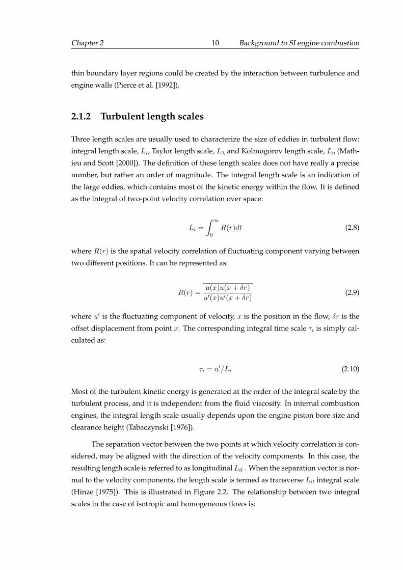
2.2 Transversal and longitudinal spatial velocity correlations. . . . . . . . . . . 11
2.3 Energy spectrum of homogeneous isotropic turbulence using generalized
PSD function 2.18 for stoichiometric octane-air based on Kolmogorov length
scale. . . . . . . . . . . . . . . . . . . . . . . . . . . . . . . . . . . . . . . . . 13
2.4 Schematic representation of structure of a one dimensional premixed flame. 16
2.5 Infinitely thin flame model and finite flame thickness model for a one di-
mensional unstretched flame propagating from left to right. . . . . . . . . 18
2.6 Strain and curvature effects on a stretched propagating flame. . . . . . . . 21
2.7 Illustration of hydrodynamic flame instability. . . . . . . . . . . . . . . . . 23
2.8 Illustration of effects of thermo-diffusion flame instability on laminar prop-
agating flame speeds. . . . . . . . . . . . . . . . . . . . . . . . . . . . . . . . 23
2.9 Flamelet concept: the turbulent premixed flame consists an array of lami-
nar flame sheets, subjected to stretch and wrinkling in a turbulent flow. . . 25
2.10 Borghi combustion regime diagram with possible engine combustion region. 26
2.11 The influence of various physical mechanisms on the turbulent burning
velocity with root mean square (rms) velocity and the Lewis number Le,
reproduced after Lipatnikov [2013]. . . . . . . . . . . . . . . . . . . . . . . . 28
2.12 Emission spectrum detected at the SI engine (Merola et al. [2009]). . . . . . 33
2.13 Autoignition at a solid surface (cylinder wall) or in the gas phase (unburnt
mixture). . . . . . . . . . . . . . . . . . . . . . . . . . . . . . . . . . . . . . . 34
2.14 Illustration of pressure curves of pre-ignition, extreme knock, knock, and
normal combustion, in the LUPOE 2D boosted engine running at speed
of 750 rpm and spark timing 2o bTDC, stoichiometric iso-octane fuel. The
intake and head temperature was kept at 323 K. Initial pressure was 2.0 bar. 35
ix
LIST OF FIGURES
2.15 Ignition delay time of heptane (MON=RON=0) and iso-octane (MON=ROM=100)
at different pressure and temperature. The data are calculated using CHEMKIN
II package (Robert [1989]) with chemical reaction mechanism from Jerzem-
beck et al. [2009]. . . . . . . . . . . . . . . . . . . . . . . . . . . . . . . . . . 37
2.16 Conditions for the occurrence of developing detonations in terms of ξ, and
ε. Supersonic and subsonic autoignitive deflagrations occur in the regions
marked P and B respectively. Cited from (Kalghatgi and Bradley [2012]). . 39
2.17 Two kinds of configuration of optical engines: optical access through the
cylinder head (Hicks et al. [1994]), optical access through the piston (Stone
[1999]) . . . . . . . . . . . . . . . . . . . . . . . . . . . . . . . . . . . . . . . 41
2.18 Peak motoring pressure and maximum engine speed achieved in this study
comparison with previously spark ignition optical engines. . . . . . . . . . 42
3.1 3D view of the LUPOE 2D engine layout with the details of the optical head. 45
3.2 Schematic diagram the LUPOE 2D engine modified from Roberts [2010]. . 45
3.3 Schematic diagram of the LUPOE 2D engine air/fuel flow system modified
from Roberts [2010]. . . . . . . . . . . . . . . . . . . . . . . . . . . . . . . . . 47
3.4 Schematic diagram of the LUPOE 2D seeding system, cited from Wu [2006]. 48
3.5 3D view of the LUPOE 2D engine breathing system with liners and its
position (The liners are modified from Conway [2013]). . . . . . . . . . . . 49
3.6 Illustration of two methods to super-charge an engine: (a) Increasing the
inlet flow rate, (b) increasing the air charging time. The black line is the
increasing of the initial inlet pressure measured without piston movement. 50
3.7 Illustration of the initial pressure calculation model with piston movement 51
3.8 (a) Photograph of the installed exhaust system valve on the LUPOE 2D
boosted engine. (b) The result of response time test of the selected solenoid
valve. . . . . . . . . . . . . . . . . . . . . . . . . . . . . . . . . . . . . . . . . 53
3.9 Schematic diagram of the LUPOE 2D boosted engine control and data ac-
quisition system. . . . . . . . . . . . . . . . . . . . . . . . . . . . . . . . . . 55
3.10 Schematic diagram of the engine skip firing and multi-trigger sequence. . 55
3.11 Dynamic pressure re-alignment using the absolute pressure signal. . . . . 57
3.12 Illustration of exhaust vale control scheme. . . . . . . . . . . . . . . . . . . 58
3.13 Flow chart for the micro-controller code for exhaust valve control. . . . . . 59
3.14 The LUPOE 2D boosted engine timing captured by the data acquisition
system. EVC: Exhaust valve close, EVO: Exhaust valve open; FVC: Fuel
valve close. . . . . . . . . . . . . . . . . . . . . . . . . . . . . . . . . . . . . . 60
3.15 Flow chart of pressure signal processing . . . . . . . . . . . . . . . . . . . . 62
x
LIST OF FIGURES
3.16 Illustration of engine combustion models in the LUSIEDA . . . . . . . . . 63
3.17 Flowchart showing the sequence of events during a firing cycle analysis in
LUSIEDA, reproduced from Roberts [2010]. . . . . . . . . . . . . . . . . . . 64
3.18 Samples of the flame radii derived from LUSIEDA and CH* chemilumines-
cence image (left), and the flame thickness calculated using the difference
between these two flame radii. The data are from the LUPOE 2D boosted
engine running at a speed of 750 rpm and a spark timing 2o bTDC, stoi-
chiometric iso-octane fuel. . . . . . . . . . . . . . . . . . . . . . . . . . . . . 65
4.1 A schematic diagram of PIV experiment setup, image evaluation process,
and a 2D velocity vector field from LUPOE 2D engine running at 750 rpm. 68
4.2 The configuration of lens for laser sheet generation. . . . . . . . . . . . . . 70
4.3 Experiment set up of high speed flame imaging acquisition system. . . . . 78
4.4 Structure of IRO intensifier adopted from Lavision [2012], CMOS sensor
camera was used in this study. . . . . . . . . . . . . . . . . . . . . . . . . . 79
4.5 Calibration grid plate imposed by a generated uniform grid plate (green
square points) based on three selected points. . . . . . . . . . . . . . . . . . 79
4.6 Typical images of different flame imaging methods: (A) 430 nm filter, (B)
470 nm filter, (C) 560 nm filter, (D) Natural light (E) Laser sheet method (F)
Schlieren: the images of (A-F) are from LUPOE 2D boosted engine running
at a speed of 750 rpm and spark timing 2o bTDC, stoichiometric iso-octane
fuel, (F) is taken from Mandilas [2008]. . . . . . . . . . . . . . . . . . . . . . 81
4.7 A developing flame captured in the optical LUPOE 2D boosted engine via
CH* chemiluminescence technique. The engine was run at a speed of 750
rpm and spark timing 2o bTDC, with stoichiometric iso-octane fuel. Initial
pressure was 2.0 bar. . . . . . . . . . . . . . . . . . . . . . . . . . . . . . . . 83
4.8 Flame front propagation trace derived from Figure 4.7 (left), definition of
mean flame radius and entrainment burning velocity calculation (right). . 83
4.9 Left: Pseudo-colour image of local CH* chemiluminescence flame taken
from square region of a weakly wrinkled flame from the LUPOE 2D boosted
engine running at a speed of 100 rpm and spark timing 10obTDC, stoichio-
metric iso-octane fuel. Right: Normalized luminous intensity distribution
along the flame radius direction indicated as a line in the left image. . . . 85
xi
LIST OF FIGURES
4.10 Left: Pseudo-colour image of local CH* chemiluminescence flame taken
from square region of a moderate turbulent flame in the LUPOE 2D boosted
engine running at a speed of 750 rpm and spark timing 2o bTDC, stoichio-
metric iso-octane fuel. Right: Normalized luminous intensity distribution
along the flame radius direction indicated as a line in the left image. . . . 85
4.11 Experimental setup of laser sheet method with a snapshot image from top
view of the engine head . . . . . . . . . . . . . . . . . . . . . . . . . . . . . . 87
4.12 Right: Pseudo-colour image of the laser sheet method taken from square
region of a turbulent flame (Left) from LUPOE 2D boosted engine running
at a speed of 750 rpm and spark timing 2o bTDC, stoichiometric iso-octane
fuel. . . . . . . . . . . . . . . . . . . . . . . . . . . . . . . . . . . . . . . . . . 88
4.13 Luminous intensity along the flame radius direction taken as a line in the
Figure 4.12. . . . . . . . . . . . . . . . . . . . . . . . . . . . . . . . . . . . . . 89
4.14 Laser sheet image processing: Step 1 is to find approximate flame front
position, Step 2: local image process including: (1) Chop image; (2) Bina-
rization; (3) Image expansion; (4) Binarization and flame front detection. . 89
4.15 Illustration of flame contour sampling using a cumulative angle. The global
flame shape with chopped region position is shown in this figure, the ar-
rows are normal directions of local fitted curves using third order polyno-
mials. . . . . . . . . . . . . . . . . . . . . . . . . . . . . . . . . . . . . . . . . 91
5.1 A snapshot of the flow velocity field captured by PIV at 2o bTDC position
at an engine speed of 100 rpm, illustrated in the form of vector (left) and
scalar (right) maps. . . . . . . . . . . . . . . . . . . . . . . . . . . . . . . . . 95
5.2 The velocity probability density functions (pdf) of the flow velocity field
shown in Figure 5.1. The inlet and exhaust pipe positions and their coor-
dinates were plotted in the corner. . . . . . . . . . . . . . . . . . . . . . . . 95
5.3 Flow fields of the mean velocity magnitude from PIV measurements at 2o
bTDC for different engine speeds from 100 rpm to 300 rpm. . . . . . . . . 96
5.4 Flow fields of the RMS velocity from PIV measurement at 2o bTDC for
different engine speeds from 100 rpm to 300 rpm. . . . . . . . . . . . . . . 97
5.5 Mean and standard deviation (represented as error bar) of the mean veloc-
ity fields shown in Figure 5.3. Ux: mean velocity in X direction, Uy: mean
velocity in Y direction, S: velocity magnitude. Ux and Uy are at the same
speed, shifted for illustration only. . . . . . . . . . . . . . . . . . . . . . . . 98
xii
LIST OF FIGURES
5.6 Mean and standard deviation (represented as error bar) of the RMS veloc-
ity fields shown in Figure 5.4. u’x: RMS velocity in X direction, u’y: RMS
velocity in Y direction, S: RMS velocity magnitude. u’x and u’y are at the
same speed, shifted for illustration only. . . . . . . . . . . . . . . . . . . . . 98
5.7 Longitudinal and transverse integral length scales based on spatial analy-
sis at 2o bTDC with engine speed increasing. . . . . . . . . . . . . . . . . . 99
5.8 Pressure cycles from one engine run at a speed of 100 rpm for different
equivalence ratios. . . . . . . . . . . . . . . . . . . . . . . . . . . . . . . . . 101
5.9 Comparison of flame contours at engine speeds of 100 rpm and 750 rpm,
these flame contours were derived from laser sheet images at the 2oCA and
10oCA after ignition, respectively, with stoichiometric iso-octane fuel. . . . 101
5.10 Typical CH* chemiluminescence images (colour inverse) at different equiv-
alence ratios at the engine speed of 100 rpm, pressure is 12 bar and the
temperature was estimated 600 K at the spark timing. The dotted circle
has the same area as the flame. . . . . . . . . . . . . . . . . . . . . . . . . . 103
5.11 Local flame propagation with image intensities as magnitude derived from
Figure 5.10 at the third direction in Figure 5.12. . . . . . . . . . . . . . . . . 104
5.12 Local flame thickness development at 5 directions along the flame radius
derived from 5.10 at different equivalence ratios. . . . . . . . . . . . . . . . 104
5.13 Pressure change with crank angle (left) and flame radius (right) at spark
timing 10o bTDC and an engine speed of 100 rpm with different equiva-
lence ratios. . . . . . . . . . . . . . . . . . . . . . . . . . . . . . . . . . . . . 106
5.14 Engine volume change with crank angle and flame radius. . . . . . . . . . 106
5.15 The flame speed as a function of stretch rate for a stoichiometric flame at
an engine speed of 100 rpm. . . . . . . . . . . . . . . . . . . . . . . . . . . . 106
5.16 Flame radii development at different equivalence ratios at an engine speed
of 100 rpm. . . . . . . . . . . . . . . . . . . . . . . . . . . . . . . . . . . . . . 108
5.17 Mean burning velocities of iso-octane-air mixture at an engine speed of
100 rpm, the initial pressure is 12 bar and temperature is 600 K at the spark
moment. . . . . . . . . . . . . . . . . . . . . . . . . . . . . . . . . . . . . . . 108
5.18 Mean pressure trace at different engine speeds and equivalence ratios with
the same pressure at spark timing. The histories of pressure and tempera-
ture at these engine conditions are shown in (d). . . . . . . . . . . . . . . . 110
5.19 Typical CH* chemiluminescence images (colour inverse) captured at stoi-
chiometric equivalence ratio at different engine speeds. . . . . . . . . . . . 111
5.20 Typical CH* chemiluminescence images (colour inverse) captured at equiv-
alence ratio 1.2 at different engine speeds. . . . . . . . . . . . . . . . . . . . 112
xiii
LIST OF FIGURES
5.21 Extrapolation of flame speeds using mean burning velocities from different
engine speeds at equivalence ratios 0.8, 1.0 and 1.2. The error bar is the
standard deviation of burning velocities at each condition. . . . . . . . . . 113
5.22 Comparison of flame brush thickness derived from Figure 5.19 for stoi-
chiometric ϕ = 1.0 and Figure 5.20 for rich mixture ϕ = 1.2. . . . . . . . . . 114
5.23 Comparison of experimental conditions in this study with available exper-
iment data of iso-octane laminar burning velocity from bomb experiments
in the literature (Bradley et al. [1998]; Galmiche et al. [2012]; Jerzembeck
et al. [2009]; Kelley et al. [2011]). . . . . . . . . . . . . . . . . . . . . . . . . . 116
5.24 Laminar burning velocity correlations and experimental data compared at
1 bar and 353 K across a range of equivalence ratios. . . . . . . . . . . . . . 120
5.25 Laminar burning velocity correlations and experimental data compared at
10 bar and 353 K across a range of equivalence ratios. . . . . . . . . . . . . 120
5.26 Laminar burning velocity correlations and experimental data compared at
10 bar and equivalence ratio 1 across a range of temperatures. . . . . . . . 122
5.27 Laminar burning velocity correlations and experimental data compared at
373 K and equivalence ratio 1 across a range of pressures. . . . . . . . . . . 122
5.28 Laminar burning velocity expressions and experimental data compared at
15 bar and 600 K across a range of equivalence ratios. . . . . . . . . . . . . 124
6.1 Initial inlet pressure map with different inlet flow rates and exhaust valve
operation times. . . . . . . . . . . . . . . . . . . . . . . . . . . . . . . . . . . 128
6.2 A snapshot of flow velocity field captured by PIV for the condition Pi20,
illustrated in the form of vector (left) and scalar (right) maps. . . . . . . . . 131
6.3 The velocity probability density functions (pdf) of the flow velocity field
shown in Figure 6.2. The inlet and exhaust pipe positions and their coor-
dinates are plotted in the corner. . . . . . . . . . . . . . . . . . . . . . . . . 131
6.4 The energy density spectrum of turbulent flow shown in Figure 6.2 with
the position of engine bore size, integral length scale Li, and Taylor length
scale Lλ. . . . . . . . . . . . . . . . . . . . . . . . . . . . . . . . . . . . . . . 132
6.5 Flow fields of mean (left) and RMS (right) velocity during compression
stroke at 40o bTDC, 20o bTDC, 10o bTDC, 2o bTDC (from top to bottom),
in the LUPOE 2D boosted engine running at a speed of 750 rpm, the inlet
initial pressure was 1.6 bar. . . . . . . . . . . . . . . . . . . . . . . . . . . . 133
xiv
LIST OF FIGURES
6.6 Flow fields of mean velocity at 2o bTDC in the LUPOE 2D boosted engine
running at a speed of 750 rpm, the initial pressure for the test cases Pi20,
Pi20ref are 2.0 bar; Pi18, Pi18ref are 1.8 bar, Pi16 is 1.6 bar. Air mass flow
rate for the three cases Pi16, Pi18, Pi20 equals 5.2 g/s, for the case Pi18ref,
it is 6.48 g/s, and Pi20ref equals 7.77 g/s. . . . . . . . . . . . . . . . . . . . 135
6.7 Flow fields of RMS velocity at 2o bTDC in the LUPOE 2D boosted engine
running at a speed of 750 rpm, the initial pressure for the test cases Pi20,
Pi20ref are 2.0 bar; Pi18, Pi18ref are 1.8 bar, Pi16 is 1.6 bar. Air mass flow
rate for the three cases Pi16, Pi18, Pi20 equals 5.2 g/s, for the case Pi18ref,
it is 6.48 g/s, and Pi20ref equals 7.77 g/s. . . . . . . . . . . . . . . . . . . . 136
6.8 Mean and standard deviation (represented as error bar) of mean velocity
fields shown in Figure 6.6. Ux: mean velocity in X direction, Uy: mean
velocity in Y direction, S: velocity magnitude. Ux and Uy are at the same
speed, shifted for illustration only. . . . . . . . . . . . . . . . . . . . . . . . 138
6.9 Mean and standard deviation (represented as error bar) of RMS velocity
fields shown in Figure 6.7. u’x: RMS velocity in X direction, u’y: RMS
velocity in Y direction, S: RMS velocity magnitude. u’x and u’y are at the
same speed, shifted for illustration only. . . . . . . . . . . . . . . . . . . . . 138
6.10 Influence of intake air mass flow rate on the averaged RMS (root mean
square) velocity during the compression stroke measured at 2o bTDC, in
the LUPOE 2D boosted engine running at a speed of 750 rpm, the initial
pressure for the test cases Pi20, Pi20ref are 2.0 bar; Pi18, Pi18ref are 1.8 bar,
Pi16 is 1.6 bar. Air mass flow rate for the three test cases Pi16, Pi18, Pi20
equals 5.2 g/s, for the case Pi18ref, it is 6.48 g/s and Pi20ref equals 7.77 g/s. 139
6.11 Longitudinal and transverse integral length scales based on spatial anal-
ysis at 2o bTDC, in the LUPOE 2D boosted engine running at a speed of
750 rpm, the initial pressure for the test cases Pi20, Pi20ref are 2.0 bar; Pi18,
Pi18ref are 1.8 bar, Pi16 is 1.6 bar. Air mass flow rate for the three test cases
Pi16, Pi18, Pi20 equals 5.2 g/s, for the case Pi18ref, it is 6.48 g/s and Pi20ref
equals 7.77 g/s. . . . . . . . . . . . . . . . . . . . . . . . . . . . . . . . . . . 139
6.12 Development of turbulent flame at different conditions from CH* chemi-
luminescence imaging (colour-reverse), in the LUPOE 2D boosted engine,
the intake and head temperature were kept at 323 K, the other main oper-
ation parameters are listed in the Figure. . . . . . . . . . . . . . . . . . . . . 141
6.13 Local flame propagation with image intensities as magnitude derived from
Figure 6.12 at the first direction in Figure 6.14. . . . . . . . . . . . . . . . . 142
xv
LIST OF FIGURES
6.14 Local flame brush thickness development at 5 directions along flame ra-
dius with image intensity as magnitude, these data are derived from 6.13. 142
6.15 Pressure-crank angle diagrams of Pi16, Pi18, Pi20, Pi18ref and Pi20ref, col-
lected in the LUPOE 2D boosted engine running at a speed of 750 rpm and
a spark timing 2o bTDC, stoichiometric iso-octane fuel. The cycles were
split into three categories depending on their average rate of combustion;
the fast cycles were shown in red, medium in blue and slow in green col-
ors, respectively. . . . . . . . . . . . . . . . . . . . . . . . . . . . . . . . . . . 144
6.16 Crank-angle based ensemble average pressure for Pi16, Pi18, Pi20, Pi18ref
and Pi20ref, in the LUPOE 2D boosted engine running at a speed of 750
rpm and a spark timing 2obTDC, stoichiometric iso-octane fuel. . . . . . . 145
6.17 Peak pressure versus corresponding crank angle for its occurrence at ex-
perimental conditions: Pi16, Pi18, Pi20, Pi18ref and Pi20ref, in the LUPOE
2D boosted engine running at a speed of 750 rpm and a spark timing 2o
bTDC, stoichiometric iso-octane fuel. . . . . . . . . . . . . . . . . . . . . . . 145
6.18 Mean flame radius versus crank angle for experimental conditions: Pi16,
Pi18, Pi20, Pi18ref and Pi20ref, in the LUPOE 2D boosted engine running at
a speed of 750 rpm and a spark timing 2o bTDC, stoichiometric iso-octane
fuel. The cycles are split into three categories depending on their pressure
trace; the fast cycles are shown in red, medium in blue and slow in green
colors, respectively. . . . . . . . . . . . . . . . . . . . . . . . . . . . . . . . . 146
6.19 Calculated laminar flame speed and temperature after ignition at three ini-
tial pressure conditions: Pi16, Pi18 and Pi20, in the LUPOE 2D boosted
engine running at a speed of 750 rpm and a spark timing 2o bTDC, stoi-
chiometric iso-octane fuel. . . . . . . . . . . . . . . . . . . . . . . . . . . . . 148
6.20 Borghi diagram for the turbulent flames for the conditions: Pi16, Pi18, Pi20,
Pi18ref and Pi20ref, in the LUPOE 2D boosted engine running at a speed
of 750 rpm and a spark timing 2 deg bTDC, stoichiometric iso-octane fuel. 148
6.21 Conditions of in-cylinder pressure and engine volume change in three
flame development stages: flame acceleration, fully developed and flame
deceleration. . . . . . . . . . . . . . . . . . . . . . . . . . . . . . . . . . . . . 152
6.22 Illustration of burning velocity calculated from Figure 6.21 during flame
development: flame acceleration, fully developed stage and flame deceler-
ation. . . . . . . . . . . . . . . . . . . . . . . . . . . . . . . . . . . . . . . . . 152
xvi
LIST OF FIGURES
6.23 Histogram of flame development for the experimental conditions: Pi16,
Pi18, Pi18ref, Pi20 and Pi20ref, in the LUPOE 2D boosted engine running at
a speed of 750 rpm and a spark timing 2o bTDC, stoichiometric iso-octane
fuel. The red line shows the mean value. . . . . . . . . . . . . . . . . . . . . 153
6.24 Correlation between pressure at the beginning of the fully developed stage
and burning velocity for the experimental conditions: Pi16, Pi18, Pi18, Pi20
and Pi20ref, in the LUPOE 2D boosted engine running at a speed of 750
rpm and a spark timing 2o bTDC, stoichiometric iso-octane fuel. . . . . . . 154
6.25 Correlation between pressure change at flame deceleration stage and burn-
ing velocity, for the three initial conditions: Pi16, Pi18 and Pi20, in the
LUPOE 2D boosted engine running at a speed of 750 rpm and a spark tim-
ing 2o bTDC, stoichiometric iso-octane fuel. . . . . . . . . . . . . . . . . . . 154
6.26 (a) The Burn rate of the mixture derived from LUSIEDA, (b) Flame brush
thickness calculated from the difference between entrainment flame radius
and burnt gas flame radius, for the three initial conditions: Pi16, Pi18 and
Pi20, in the LUPOE 2D boosted engine running at a speed of 750 rpm and
a spark timing 2o bTDC, stoichiometric iso-octane fuel. . . . . . . . . . . . 156
6.27 Comparison of modelling (Zimont model) and measured turbulent burn-
ing velocities for the three initial conditions: Pi16, Pi18 and Pi20, in the
LUPOE 2D boosted engine running at a speed of 750 rpm and a spark tim-
ing 2o bTDC, with stoichiometric iso-octane fuel. . . . . . . . . . . . . . . . 158
6.28 (a) Fitted curves of flame acceleration and (b) deceleration compared against
the experimental data (points) in terms of fast, medium and slow cycles,
for Pi16, Pi18 and Pi20 in the LUPOE 2D boosted engine running at a speed
of 750 rpm and a spark timing 2o bTDC, stoichiometric iso-octane fuel. . . 160
6.29 (a) Mean progress variable maps, (b) corresponding sliced mean progress
variable profiles along the flame radius direction with 10o angle interval,
for the three initial pressure conditions Pi16, Pi18 anf Pi20 in the LUPOE
2D boosted engine running at a speed of 750 rpm and a spark timing 2o
bTDC, stoichiometric iso-octane fuel. . . . . . . . . . . . . . . . . . . . . . . 163
6.30 Flame contours of fast, medium and slow cycles selected from three condi-
tions: Pi16, Pi20 and Pi20ref, in the LUPOE 2D boosted engine running at
a speed of 750 rpm and a spark timing 2o bTDC, stoichiometric iso-octane
fuel. . . . . . . . . . . . . . . . . . . . . . . . . . . . . . . . . . . . . . . . . . 165
xvii
LIST OF FIGURES
6.31 Comparison of flame radius deviation along the flame contour of fast,
medium and slow cycles for three conditions: Pi16, Pi20 and Pi20ref, in
the LUPOE 2D boosted engine running at 750 rpm, spark timing 2obTDC,
stoichiometric iso-octane fuel. . . . . . . . . . . . . . . . . . . . . . . . . . . 167
6.32 Mean curvature distribution of flames from the three conditions: Pi16, Pi20
and Pi20ref, in the LUPOE 2D boosted engine running at a speed of 750
rpm and a spark timing 2o bTDC, stoichiometric iso-octane fuel. . . . . . . 167
6.33 Comparison of autocorrelation along the flame contour of fast, medium
and slow cycles for the three conditions: Pi16, Pi20 and Pi20ref, in the
LUPOE 2D boosted engine running at a speed of 750 rpm and a spark
timing 2obTDC, stoichiometric iso-octane fuel. . . . . . . . . . . . . . . . . 168
6.34 The energy density spectrum (PDS) of flame contour of fast, medium and
slow cycles for the three conditions: Pi16, Pi20 and Pi20ref, in the LUPOE
2D boosted engine running at a speed of 750 rpm and a spark timing 2o
bTDC, stoichiometric iso-octane fuel. . . . . . . . . . . . . . . . . . . . . . . 168
7.1 Pressure traces near the knock boundary at initial pressure 1.6 bar: (a)
slight knocking, (b) ”average” knocking, (c) severe knocking. Other op-
eration parameters are listed in the Figures. . . . . . . . . . . . . . . . . . . 172
7.2 Engine knock map of the LUPOE 2D boosted engine at a speed of 750 rpm,
the temperature of engine intake and head were kept at 323K. The numbers
in the square bracket are coordinates. . . . . . . . . . . . . . . . . . . . . . . 173
7.3 End gas self-ignition, the operating condition and the corresponding pres-
sure trace can be seen in the Figure 7.4. The times shown are the time
elapsed from the spark discharge. . . . . . . . . . . . . . . . . . . . . . . . . 175
7.4 Pressure trace of a self-ignition cycle in Figure 7.3, the number of the im-
ages in Figure 7.3 are shown next to the pressure points at which the im-
ages were taken. . . . . . . . . . . . . . . . . . . . . . . . . . . . . . . . . . . 175
7.5 Extreme knock, the operating condition and the corresponding pressure
trace can be seen in the Figure 7.6. The times shown are the time elapsed
from the spark discharge. . . . . . . . . . . . . . . . . . . . . . . . . . . . . 177
7.6 Pressure trace of an extreme knock cycle in Figure 7.5, the number of the
images in Figure 7.5 are shown next to the pressure points at which the
images were taken. . . . . . . . . . . . . . . . . . . . . . . . . . . . . . . . . 177
7.7 An extreme knock with high speed imaging 25 kfps. The operating con-
dition and the corresponding pressure trace can be seen in the Figure 7.8.
The times shown are the time elapsed from the spark discharge. . . . . . . 179
xviii
LIST OF FIGURES
7.8 Pressure trace of an extreme knock cycle in Figure 7.7, the number of the
images in Figure 7.7 are shown next to the pressure points at which the
images were taken. . . . . . . . . . . . . . . . . . . . . . . . . . . . . . . . . 179
7.9 Autoignition process captured in a misfire cycle. The operating condition
and the corresponding pressure trace can be seen in the Figure 7.10. The
times shown are the time elapsed from the spark discharge. The red circles
indicate the onset moment of two autoignition sites. . . . . . . . . . . . . . 181
7.10 Pressure trace of an autoignition cycle in Figure 7.9, the number of the
images in Figure 7.9 are shown next to the pressure points at which the
images were taken. . . . . . . . . . . . . . . . . . . . . . . . . . . . . . . . . 181
7.11 Illustration of the definitions of knock parameters. . . . . . . . . . . . . . . 183
7.12 Comparison of (a) detected autoignition onset, and (b) knock onset from
pressure and images. The cycles number 1 to 4 are from the PRF95 fuel
experiment in Section 7.5, while the cycles number 5, 6 and 7 correspond to
the cycles: self-ignition, and two extreme knock cycles described in Section
7.2. . . . . . . . . . . . . . . . . . . . . . . . . . . . . . . . . . . . . . . . . . 184
7.13 (a) Comparison of knock intensity and MAPO, (b) The relationship be-
tween knock onset and knock intensity of 7 sample cycles. The cycles
number 1 to 4 are from the PRF95 fuel experiment in Section 7.5, while
the cycles number 5,6 and 7 correspond to the cycles: self-ignition, two
extreme knock cycles described in Section 7.2. . . . . . . . . . . . . . . . . 185
7.14 Knock pressure traces for the naturally aspirated (a) and charged (b) oper-
ation of LUPOE 2D. The fast cycles are shown in red, medium in blue and
slow in green colors, respectively. ”Pinit mean” means the inlet pressure. . 187
7.15 Maximum pressure as a function of the crank angle at which it is achieved
for the naturally aspirated (a) and charged (b) operation of LUPOE 2D.
”Std 2nd” means the two standard deviations. . . . . . . . . . . . . . . . . 187
7.16 Knock onset distribution for the naturally aspirated (a) and charged (b)
operation of LUPOE 2D engine. The operation parameters are listed in the
Figure 7.14. . . . . . . . . . . . . . . . . . . . . . . . . . . . . . . . . . . . . . 188
7.17 Knock intensity distribution for the naturally aspirated (a) and charged (b)
operation of LUPOE 2D engine. The operation parameters are listed in the
Figure 7.14. . . . . . . . . . . . . . . . . . . . . . . . . . . . . . . . . . . . . . 188
7.18 Autoignition onset versus knock intensity (MAPO) for the naturally aspi-
rated (a) and charged (b) operation of LUPOE 2D engine. The operation
parameters are listed in the Figure 7.14. . . . . . . . . . . . . . . . . . . . . 189
xix
LIST OF FIGURES
7.19 Pressure at the moment of autoignition onset versus knock intensity (MAPO)
for the naturally aspirated (a) and charged (b) operation of LUPOE 2D en-
gine. The operation parameters are listed in the Figure 7.14. . . . . . . . . 189
7.20 The pressure and temperature history of the end gas for the naturally as-
pirated (NA) and the boosted LUPOE 2D engines with the potential au-
toignition regions. The reverse cycle software LUSIEDA was used to pre-
dict the unburnt gas temperatures based on experimentally gathered cylin-
der pressure data. . . . . . . . . . . . . . . . . . . . . . . . . . . . . . . . . . 190
7.21 Pressure traces of four different knock intensity cycles selected from the
same engine operation condition, in the LUPOE 2D boosted engine run-
ning at a speed of 750 rpm and a spark timing 2o bTDC, stoichiometric
PRF95 fuel. The numbers are time (ms) of the autoignition onset after ig-
nition. . . . . . . . . . . . . . . . . . . . . . . . . . . . . . . . . . . . . . . . . 192
7.22 Band pass filter pressure traces of four different knock intensity cycles se-
lected from the same engine operation condition, in the LUPOE 2D boosted
engine running at a speed of 750 rpm and a spark timing 2o bTDC, stoichio-
metric PRF95 fuel. . . . . . . . . . . . . . . . . . . . . . . . . . . . . . . . . . 192
7.23 FFT transform of four different knock intensity cycles selected from the
same engine operation condition, in the LUPOE 2D boosted engine run-
ning at a speed of 750 rpm and a spark timing 2o bTDC, stoichiometric
PRF95 fuel. . . . . . . . . . . . . . . . . . . . . . . . . . . . . . . . . . . . . . 193
7.24 Temperature and pressure histories of four different knock intensity cy-
cles selected from the same engine operation condition, in the LUPOE 2D
boosted engine running at speed of 750 rpm and spark timing 2o bTDC,
stoichiometric PRF95 fuel. . . . . . . . . . . . . . . . . . . . . . . . . . . . . 194
7.25 Images of autoignition development for four different knock intensity cy-
cles selected from the same engine operation condition, in the LUPOE 2D
boosted engine running at a speed of 750 rpm and a spark timing 2o bTDC,
stoichiometric PRF95 fuel. The cycle numbers are the same as shown in
Figure 7.21. . . . . . . . . . . . . . . . . . . . . . . . . . . . . . . . . . . . . . 195
7.26 Flame radius development of four different knock intensity cycles selected
from the same engine operation condition, in the LUPOE 2D boosted en-
gine running at a speed of 750 rpm and a spark timing 2o bTDC, with
stoichiometric PRF95 fuel. . . . . . . . . . . . . . . . . . . . . . . . . . . . . 196
xx

LIST OF FIGURES
7.27 A narrow horizontal section taken from the full-bore image for derivation
of flame displacement speed under extreme knock case shown in Figure
7.5, the blue line is derived ignited flame front, the red line is the autoigni-
tion reaction front, the yellow line is an extrapolation line to predict the
flame position without autoigntion effect. . . . . . . . . . . . . . . . . . . . 198
7.28 Local ignited flame velocity and the reaction front velocity developed from
an autoignition site, calculated from Figure 7.27. . . . . . . . . . . . . . . . 198
xxi
List of Tables
3.1 A comparison of the main engine parameters between the LUPOE 2D and
LUPOE 2D boosted engines. . . . . . . . . . . . . . . . . . . . . . . . . . . . 46
3.2 Various effective compression ratios. . . . . . . . . . . . . . . . . . . . . . . 46
3.3 A comparison of the specifications between desired valve and selected valve. 53
4.1 Specifications of PIV setting . . . . . . . . . . . . . . . . . . . . . . . . . . . 72
5.1 Previous high pressure iso-octane air laminar burning velocity studies. . . 116
5.2 The range of applicability and data resource of different correlations. . . . 118
5.3 Constants for Equation 5.1 for iso-octane-air mixtures. . . . . . . . . . . . . 118
5.4 Constants for Equations 5.2, 5.3 and 5.4 for iso-octane-air mixtures. . . . . 119
6.1 Selected LUPOE 2D engine operation conditions. . . . . . . . . . . . . . . . 128
xxii

Nomenclature
Roman and Greek SymbolsSymbol Units Description
A m2, Area
A – Zimont burning velocity model constant
a m/s Speed of sound in a gas
α 1/s Stretch rate
α m2/s Thermal diffusivity
c – Mean progress variable
δL mm Laminar flame thickness
d m Diameter
D m Engine bore
D m2/s Mass diffusivity
Da – Damkholer number
ϵ – The rate of dissipation of the kinetic energy
fd – Flame acceleration coefficient
fw – Flame deceleration coefficient
I0 – Stretch factor
I – Image intensity
Ka – Karlovitz number
k m 2/s2 Turbulent kinetic energy
κ m−1 Wave number
κc m−1 Curvature rate
Lb – Markstein length
Le – Lewis number
Li mm Turbulent integral length scale
Lλ mm Turbulent Taylor length scale
xxiii
NOMENCLATURE
Lη mm Turbulent Kolmogorov length scale
La mm Flame integral length scale
Ma – Markstein number
M – Image magnification
P Pa Pressure
ϕ – Equivalence Ratio
m kg Mass
m kg/s Mass flow rate
ρ kg / m3 Density
R J/(mol*K) gas constant
Re mm Flame entrainment radius
Re - Reynolds Number
S0l m/s Unstretched laminar flame speed
Sf m/s Flame speed
St m/s Turbulent flame speed
S m/s velocity magnitude
T K Temperature
θ o Crank angle
t s Time
τi s Integral time scale
τλ s Taylor time scale
τη s Kolmogorov time scale
υ m2/s kinematic viscosity
V m/s Flow velocity
Ul m/s Laminar burning velocity
Ue m/s Entraiment buring velocity
u m/s Burning Velocity
u′ m/s Rms turbulent velocity
u′k m/s Effective rms turbulent velocity
x m distance
AbbreviationsaTDC After top dead centre
bTDC Before top dead centre
xxiv
NOMENCLATURE
oCA Degrees of crank angle rotation
CRstatic Static compression ratio
CRdynamic Dynamic compression ratio
CCD Charge coupled device
CMOS Complementary metaloxide semiconductor
DAQ Data acquisition
DNS Direct numerical simulation
ECU Electronic control unit
EGR Exhaust gas recirculation
EPC/EVC Exhaust port closure / exhaust valve closure
FFT Fast fourier transform
fps Frames per second
HCCI Homogeneous charge compression ignition
HWA Hot wire anemometry
IMEP Indicated mean effective pressure
IPC/IVC Intake port closure / intake valve closure
K Kalghatgi octane index correction factor
LDV Laser doppler velocimetry
LSPI Low speed pre-ignition
LUPOE 2D Leeds university ported optical engine (Mk II) disc con-
figuration
LUSIE Leeds university spark ignition engine (simulation soft-
ware)
LUSIEDA Leeds university spark ignition engine data analysis
MATLAB Matrix Laboratory
MON Motor octane number
NTC Negative temperature coefficient
NA Naturally Aspirated
ON Octane Number
PIV Particle image velocimetry
POD Proper Orthogonal Decomposition
PLIF Planar Laser Induced Fluoresence
PRF Primary reference fuel
rev / min Revolutions per minute
rms Root mean square
xxv
NOMENCLATURE
RON Research octane number
SI Spark ignition
TDC Top dead centre
WOT Wide open throttle
Subscriptsb – Burnt
i – Intake
l – Laminar
t – Turbulent
r – Reaction (burnt)
u – Unburnt
xxvi
Chapter 1
Topic introduction and scope of
thesis
1.1 Motivation
Internal combustion (IC) engines, the core part of vehicles, have been developed for more
than a century. At present, the energy crisis and environmental pollution are two major
challenges for their further development. The price of fuel is expected to continue to rise
owing to the limitation of crude oil reserves, which will be consumed in a few decades
(DoE [2014]). Governments have also strictly legislated the emissions of pollutants from
IC engines such as nitrogen oxides, NOx, carbon dioxide, CO2, and unburned hydro-
carbons, UHC (Sounasis [2013]). Under these financial and political pressures, engine
researchers and manufacturers are seeking cost-effective solutions to increase engine effi-
ciency and reduce pollution emissions. More compact engines, which consume less fuel
is a direct way to achieve these targets, especially for reducing the CO2 generation. This
is the concept of ”Downsizing” engine (Lake et al. [2004]), designed to reduce the engine
displacement volume while keeping the same power performance as compared with the
initial larger engine. Such decrease of swept volume leads to an improvement in engine
efficiency as well as a reduction in CO2 emissions. Boosting system, such as a turbo-
charger, is usually employed in the process of engine downsizing to increase the density
of the fluid in the inlet above ambient conditions, in order to achieve high specific engine
Chapter 1 2 Topic introduction and scope of thesis
power output. A reduction in the number, or size, of cylinders also reduces pumping,
friction, and heat transfer losses. In the short to medium term, ”Downsizing” engine is
an efficient way to improve fuel economy with a good cost to benefit ratio (Fraser et al.
[2009]).
Flame propagation directly affects the heat release and pressure development in
the combustion process in Spark Ignition (SI) engines. A smaller capacity engine with
external boosting system means an increase of the in-cylinder pressure during the com-
bustion process 1. Therefore, demands for improvements in ”Downsizing” Spark Ignition
engines require major efforts for understanding the fundamental principles of combus-
tion at elevated pressure environments. This includes the aspects of premixed laminar
flames and turbulent flames. Although laminar and turbulent premixed flames have been
investigated very extensively in the fundamental combustion experiments, such as ones
using a constant volume vessel, most of these studies concern combustion at atmospheric
or low pressure range (1-10 bar), while combustion phenomena at high pressures, about
20 bar or above related to supercharged SI engines condition are still poorly understood.
The previous experimental works concluded that laminar flame speeds were reduced
by pressure for typical hydrocarbon-air mixtures, while turbulent flame speeds were in-
creased by pressure (Lipatnikov and Chomiak [2002]). However, these results obtained
from various experiments are not consistent, and there are not sufficient data of high
pressure flame speeds in supercharged SI engines condition.
Another important area in engine studies is to characterise auto-ignition in SI en-
gines. The further development of a higher compression ratio, boosted engine is limited
by abnormal combustion phenomena, such as knock and pre-ignition, which in turn limit
the maximum efficiency of the engine. A random heavy knock has been observed in re-
cently strongly supercharged engine experiments (Dahnz and Spicher [2010]), this could
cause severe engine damage. With the increasing of initial inlet pressure at low speed,
the maximum amplitude of knock pressure tends to be extremely high, compared to the
knock combustion pressure in a naturally aspirated engine. Although, these extreme
knock events2 have been recorded in a number of ”Downsizing” engine experiments, the
mechanism of it is still an open subject.
1It may also increase temperature and turbulence intensity.2Previous works referred to these abnormal ignition events as Super Knock (Inoue et al.
[2012], Mega Knock (Attard et al. [2010]), or Extreme knock (Dahnz and Spicher [2010]). Theterm ”Extreme knock” was adopted in this study.
Chapter 1 3 Topic introduction and scope of thesis
1.2 Scope of the current work
This study aims at contributing to the knowledge of the flame propagation and autoigni-
tion process in highly supercharged Spark Ignition engines. Although some prototype
”Downsizing” Spark Ignition engines have been tested (Attard et al. [2010]; Lecointe and
Monnier [2003]; Shahed and Bauer [2009]), and significant amount of data were gen-
erated to analyze engine performance, the information on the detailed flame structure
and development at elevated pressure in a strongly supercharged engine environment is
deficient. For this reason, a study for applying advanced flow visualization and high
speed flame imaging methods into an optical boosted experimental SI engine is con-
ducted here, in order to acquire a view inside the combustion and knock phenomena
in a supercharged engine.
The first objective of the present work is to develop a new optical boosted engine
apparatus. It is based on the single cylinder Leeds University Ported Optical Engine 2D
(LUPOE 2D), which could provide a full-bore optical access and a well-controlled mix-
ture composition preparation. LUPOE 2D gas exchange system was designed to avoid
complex turbulence flows, in such a way that a growing flame sees a homogeneous flow
field, in order to simplify the effects of turbulence on flame growth and put more empha-
sis on the combustion process.
In order to achieve high pressures in the engine cylinder and avoid complex cou-
pling between the turbocharging and combustion processes, a simulated boosting method
is developed to increase the inlet pressure. In the majority of experiments with boosted
engines, a high pressure is accompanied by an increase of the inlet flow rate, thus simul-
taneously high pressure and stronger turbulence may arise at highly boosted conditions.
This results in the flame development being affected by both high pressure and turbu-
lence. In order to overcome this problem, a new supercharging method should yield the
mean and root-mean-square (rms) flow velocities in the cylinder at the spark timing at
the same level while only the pressure increases. Ideally, the supercharged optical engine
will also achieve a high peak motoring pressure value, higher than most current optical
spark ignition engines.
Consequently, turbulent burning velocities at high pressures with different ini-
tial inlet pressure are measured. Under the similar turbulence conditions, effects of
highly boosted initial pressure on flame unsteady development, flame structure, and
flame brush thickness can be studied. These effects need to be assessed at the different
combustion phases i.e. initiation, main phase, and termination phase.
Chapter 1 4 Topic introduction and scope of thesis
The experimental data derived from the LUPOE 2D engine also can be an ideal test-
bed for the validation of advanced turbulent combustion models. For the latter, laminar
flame speed is required as an important input parameter. Corresponding experimen-
tal values at boosted engine-relevant conditions are not available in the literature. As a
consequence, experimental investigations on premixed iso-octane flames are conducted
in the LUPOE 2D engine with an extremely low engine speed. It is of interest to see
whether or not the optical engine in a turbulence-free environment allows one accurately
to measure the laminar flame speed at higher pressures.
Autoignition is also investigated in the LUPOE 2D boosted engine. The high speed
images of different modes of auto-ignition with corresponding in-cylinder pressure data
provide clues to the onset and development of abnormal combustion in the engines.
These observed autoignition phenomena also can be used to deduce those knock events
with the similar pressure curve shapes without images from other engines. Further data
analysis try to gain insight into the effects of boosted inlet pressure on knock character-
istics in strongly supercharged spark ignition engines, in particular, to understand the
extreme knock.
1.3 Thesis outline
• Chapter 2 - A literature review includes basic concepts of turbulence, combustion
and autoignition in Spark Ignition engines related to this study. The emphases
are put on the methods to characterize turbulence flow, the definition of laminar,
turbulent flame burning velocities with their measurement issues and a discussion
of experimental results in the literature about pressure effects on flame propagation
and autoignition.
• Chapter 3 - A detailed description of the developed boosted Leeds University
Ported Optical Engine. Two kinds of boosting methods were compared and an
exhaust valve design scheme was presented. A new micro-controller based engine
control system was also developed. In addition, a brief introduction of LUSIEDA
(Leeds University Spark Ignition Engine Data Analysis), a reverse thermodynamic
code used to derive the unburned pressure/temperature history from experimen-
tal pressure trace is given.
• Chapter 4 - Flow velocities and flame development measurement methods inside
the engine cylinder are presented in this chapter. The basic principles of Particle
Image Velocimetry (PIV), flame chemiluminescence, and laser sheet visualization
Chapter 1 5 Topic introduction and scope of thesis
techniques are described, with a description of their experimental operation and
data process details.
• Chapter 5 - An attempt to direct measurement of the laminar flame speed from
an optical engine with extremely low engine speed is presented in this chapter.
The nearly turbulence-free condition was validated by using PIV technique. By
comparing the existing laminar flame speed data and correlation equations in the
literature to the current experimental data, the accuracy of laminar flame speed
measurement in a turbulence-free engine chamber is discussed.
• Chapter 6 - Results of the turbulence flame measurement are presented in this chap-
ter. The performance of designed boosted system was evaluated by using PIV mea-
surement. 5 experimental conditions were selected to compare the effects of pres-
sure on different flame development stages. The detailed flame structures derived
from laser sheet images also were investigated.
• Chapter 7 - A number of different autoignition development processes were ob-
served and shown in this Chapter. The reaction front velocities were calculated to
clarify if detonation could be generated from a hot spot directly. 4 typical autoigni-
tion cycles representing the transition from weakly self-ignition to strong knock
were analyzed, based on simultaneously images and pressure data. At last, corre-
lations between knock characteristic parameters were conducted to show the dif-
ferent knock properties in naturally aspirated and strongly boosted engine.
• Chapter 8 - The conclusions of the present work are summarized, together with
recommendations for future studies.
Chapter 2
Background to SI engine combustion
Presented in this Chapter is the literature review of basic concepts of turbulence, pre-
mixed flame, and autoignition. Following, the prior optical spark ignition engines for
characterization of combustion are compared. Autoignition and knock in a spark igni-
tion engine are influenced by the pressure and temperature in the end portion of the
unburned gas, these are governed by the turbulent flame propagation. Therefore, a deep
understanding of combustion processes in-cylinder, such as the flow structures, laminar
and turbulent flame propagation, and stability of flame, is a prerequisite to the under-
standing of autoignition and knock phenomena. In this Chapter, the above-mentioned
concepts are discussed with a particular emphasis on the processes at elevated pressure
related to supercharged engines.
2.1 Turbulence
The knowledge of turbulence is a starting point to understand turbulent combustion.
Turbulence itself is one of the remaining few unresolved and important problems in clas-
sical physics. Turbulent flow is a complex natural phenomenon containing a wide range
of vortice scales; they are chaotic in nature (Tennekes and Lumley [1972]). According to
Kolomogorov′s theory on eddy cascade hypothesis for homogeneous and isotropic tur-
bulence (Mathieu and Scott [2000]), turbulence might be characterized by a wide range of
size of eddies which are generated from large eddies and broken up into smaller eddies.
The smallest eddies dissipating during this process are dominated by the viscous forces.
Chapter 2 7 Background to SI engine combustion
Turbulent flow is referred to as homogeneous when its mean properties do not
vary with position. This means that measurements taken at one position are statistically
equivalent to measurements taken at any other position. Isotropic turbulence is when the
turbulence has no preferential direction. This implies that measurements taken with one
particular probe orientation are statistically indistinguishable from measurements taken
with any other probe orientation (Mathieu and Scott [2000]).
The turbulence in an engine is greatly determined by the engine geometry and
breathing system design (Tabaczynski [1976]). During engine air charging process, the
inlet system usually generates two types of large scale turbulent flow: swirl and tumble
(Heywood [1988]). The swirl is a rotation of the bulk air around the cylinder axis, while
the tumble is a rotation of the air charge around the axis which is normal to the cylinder
axis. Thereafter, these large bulk air structures are decaying and dissipating into small
scale eddies during the compression stroke. These eddies have a major influence on early
flame kernel growth and flame propagation. Strong turbulence can lead to an increase
of flame speed, resulting in faster burning velocity and reduction of the cyclic variability
(Hill and Zhang [1994]). It also can benefit for the extension of lean combustion operation
range. Nevertheless, excessively strong turbulence can quench the flame ([Bradley et al.,
1992]). In some experimental engines, the breathing system was designed to eliminate
the significant bulk flow motion, e.g. swirl or tumble, as well as the flow was nearly
isotropic and homogeneous near the end of compression process (Atashkari [1997]).
This section briefly describes and introduces measures of turbulence. Turbulent
flow velocity changes continuously in a wide range of length and time scales. Methods
using statistics are therefore required to describe and characterize the turbulent flow,
including mean velocity, root mean square (rms) turbulent velocity, and various length
or time scales.
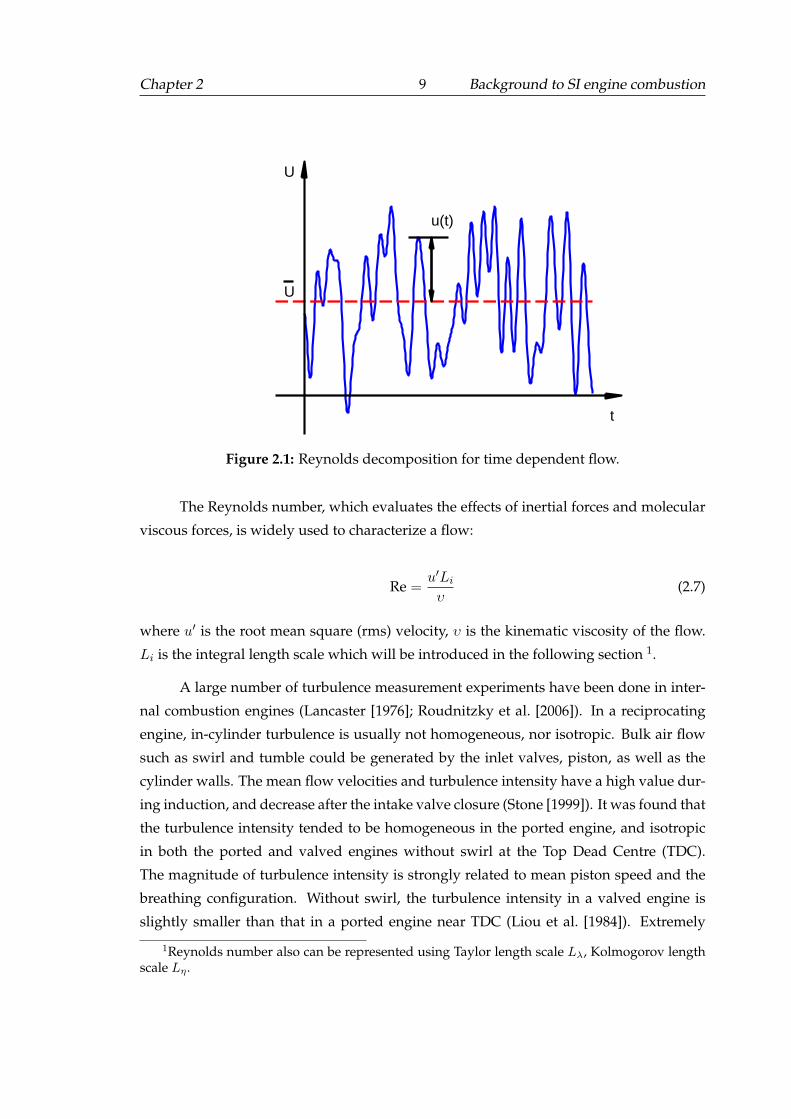
2.1.1 Reynolds decomposition of velocity
The instantaneous fluid velocity U(t), can be split into mean U(t) and fluctuating com-
ponent u(t) in what known as Reynolds decomposition as follows:
U(t) = U(t) + u(t) (2.1)
Chapter 2 8 Background to SI engine combustion
The mean velocity can be calculated in a number of different ways. If the flow is consid-
ered steady, the mean velocity is time independent and is described as follow:
U = limτ→∞
1
τ
∫ to+τ
to
Udt (2.2)
The fluctuating component can be calculated as root-mean-square quantities:
u′ = limτ→∞
[1
τ
∫ to+τ
to
(U − U)2dt
]1/2(2.3)
u′ usually is defined as ”turbulent intensity”1. By summing the square of turbulent in-
tensities from each of the orthogonal components, turbulent kinetic energy per unit mass
of fluid can be obtained:
k =1
2
(u′
2x + u′
2y + u′
2z
)(2.4)
An illustration of the Reynolds decomposition is shown in Figure 2.1. Nevertheless, it is
hard to find a steady or isotropic flow in the reciprocated engines because of additional
nearly periodic motion introduced by valves and piston movement. A discrete average
process can be adopted in this situation (Heywood [1988]; Stone [1999]). An instanta-
neous turbulence velocity in the ith cycle at crank angle θ can be decomposed as follows:
U(θ, i) = U(θ, i) + u(θ, i) (2.5)
where U(θ, i) and u(θ, i) are the mean and fluctuating components of the instantaneous
velocity. The ensemble-averaged velocity is defined as:
UEA(θ) =1
Nc
Nc∑i=1
U(θ, i) (2.6)
where Nc is the total number of cycles used in the average calculation.
1Strictly speaking, the term of ”turbulence intensity” should be u′/U . However, this definitioncannot be applied in the flow where mean velocity tends to be zero.
Chapter 2 9 Background to SI engine combustion
t
U
U
u(t)
Figure 2.1: Reynolds decomposition for time dependent flow.
The Reynolds number, which evaluates the effects of inertial forces and molecular
viscous forces, is widely used to characterize a flow:
Re =u′Li
υ(2.7)
where u′ is the root mean square (rms) velocity, υ is the kinematic viscosity of the flow.
Li is the integral length scale which will be introduced in the following section 1.
A large number of turbulence measurement experiments have been done in inter-
nal combustion engines (Lancaster [1976]; Roudnitzky et al. [2006]). In a reciprocating
engine, in-cylinder turbulence is usually not homogeneous, nor isotropic. Bulk air flow
such as swirl and tumble could be generated by the inlet valves, piston, as well as the
cylinder walls. The mean flow velocities and turbulence intensity have a high value dur-
ing induction, and decrease after the intake valve closure (Stone [1999]). It was found that
the turbulence intensity tended to be homogeneous in the ported engine, and isotropic
in both the ported and valved engines without swirl at the Top Dead Centre (TDC).
The magnitude of turbulence intensity is strongly related to mean piston speed and the
breathing configuration. Without swirl, the turbulence intensity in a valved engine is
slightly smaller than that in a ported engine near TDC (Liou et al. [1984]). Extremely
1Reynolds number also can be represented using Taylor length scale Lλ, Kolmogorov lengthscale Lη.
Chapter 2 10 Background to SI engine combustion
thin boundary layer regions could be created by the interaction between turbulence and
engine walls (Pierce et al. [1992]).
2.1.2 Turbulent length scales
Three length scales are usually used to characterize the size of eddies in turbulent flow:
integral length scale, Li, Taylor length scale, Lλ and Kolmogorov length scale, Lη (Math-
ieu and Scott [2000]). The definition of these length scales does not have really a precise
number, but rather an order of magnitude. The integral length scale is an indication of
the large eddies, which contains most of the kinetic energy within the flow. It is defined
as the integral of two-point velocity correlation over space:
Li =
∫ ∞
0R(r)dt (2.8)
where R(r) is the spatial velocity correlation of fluctuating component varying between
two different positions. It can be represented as:
R(r) =u(x)u(x+ δr)
u′(x)u′(x+ δr)(2.9)
where u′ is the fluctuating component of velocity, x is the position in the flow, δr is the
offset displacement from point x. The corresponding integral time scale τi is simply cal-
culated as:
τi = u′/Li (2.10)
Most of the turbulent kinetic energy is generated at the order of the integral scale by the
turbulent process, and it is independent from the fluid viscosity. In internal combustion
engines, the integral length scale usually depends upon the engine piston bore size and
clearance height (Tabaczynski [1976]).
The separation vector between the two points at which velocity correlation is con-
sidered, may be aligned with the direction of the velocity components. In this case, the
resulting length scale is referred to as longitudinal Lil . When the separation vector is nor-
mal to the velocity components, the length scale is termed as transverse Lit integral scale
(Hinze [1975]). This is illustrated in Figure 2.2. The relationship between two integral
scales in the case of isotropic and homogeneous flows is:
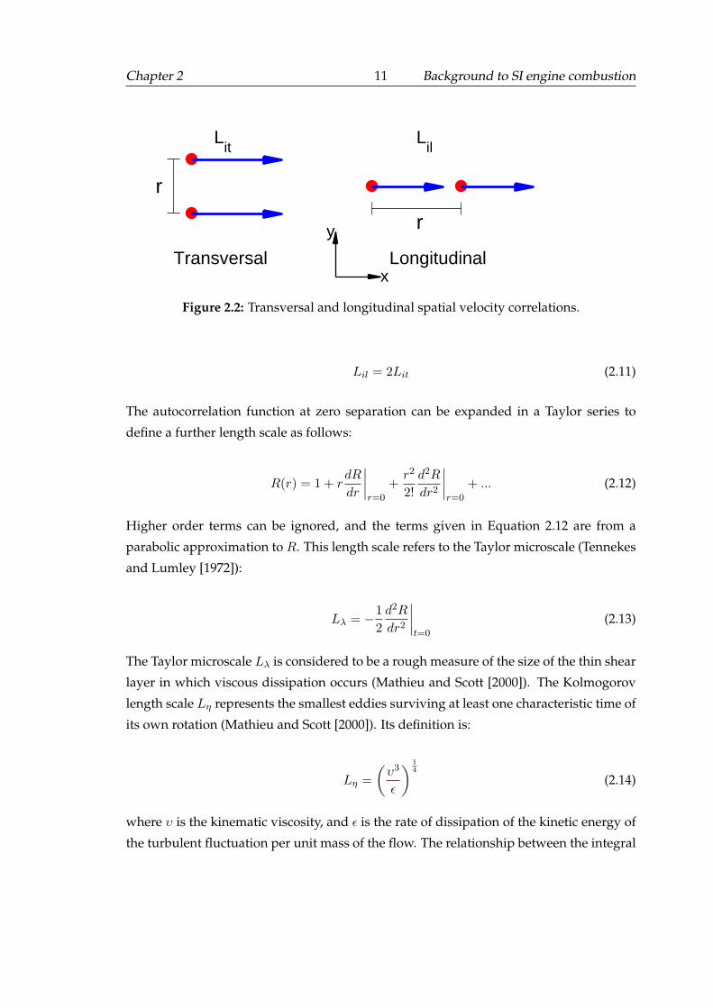
Chapter 2 11 Background to SI engine combustion
y
x
r
r
Lit
Lil
Transversal Longitudinal
Figure 2.2: Transversal and longitudinal spatial velocity correlations.
Lil = 2Lit (2.11)
The autocorrelation function at zero separation can be expanded in a Taylor series to
define a further length scale as follows:
R(r) = 1 + rdR
dr
∣∣∣∣r=0
+r2
2!
d2R
dr2
∣∣∣∣r=0
+ ... (2.12)
Higher order terms can be ignored, and the terms given in Equation 2.12 are from a
parabolic approximation to R. This length scale refers to the Taylor microscale (Tennekes
and Lumley [1972]):
Lλ = −1
2
d2R
dr2
∣∣∣∣t=0
(2.13)
The Taylor microscale Lλ is considered to be a rough measure of the size of the thin shear
layer in which viscous dissipation occurs (Mathieu and Scott [2000]). The Kolmogorov
length scale Lη represents the smallest eddies surviving at least one characteristic time of
its own rotation (Mathieu and Scott [2000]). Its definition is:
Lη =
(υ3
ϵ
) 14
(2.14)
where υ is the kinematic viscosity, and ϵ is the rate of dissipation of the kinetic energy of
the turbulent fluctuation per unit mass of the flow. The relationship between the integral
Chapter 2 12 Background to SI engine combustion
scales and Taylor, Kolmogorov length scales, can be represented by using the Reynolds
number based on the integral length scale (Law [2006]):
Li
Lλ= Re
12 (2.15)
Li
Lη= Re
34 (2.16)
2.1.3 The spectrum of turbulence
Turbulence can be analyzed using Fourier method to decompose the turbulent fluctua-
tions into sinusoidal components (Mathieu and Scott [2000]). Fourier transform translates
the correlation function into a kinetic energy spectrum S(k), representing distribution of
a turbulent energy among the different wavelengths and different scales of turbulence.
The outcome of Fourier transformation is the density of kinetic energy per unit wave
number k. The wave number k is the inverse of the eddy size. The one dimensional
frequency power spectral density is defined as:
S(k) =1
2π
∫ ∞
−∞exp(−itf)R(t)dt (2.17)
A dimensionless power spectrum was suggested by Abdel-Gayed et al. [1987], and later
improved by Scott [1992] as a function of Kolmogorov length scales by interpolating a
large number of data from Laser Doppler Anemometer (LDA) measurements in the Leeds
fan stirred bomb vessel for a stoichiometric octane-air mixture. A homogeneous and
isotropic turbulence energy spectrum can be calculated by using the following equation:
S(kη) =0.01668Re2.5λ + 3.74Re0.9λ − 70Re−0.1
λ
1 + (0.127Re1.5λ kη)5/3 + (1.15Re0.623λ kη)4 + (1.27Re0.35λ kη)7(2.18)
An example of this energy spectrum for a turbulent flow of stoichiometric octane-air mix-
ture at Reλ = 500 was plotted in the log-log Figure 2.3 using the Equation 2.18. The small
wave numbers are related to large scale eddies, which contain most of the energy and
contribute most to the transport of momentum, mass and heat. These large scale eddies
correspond to the integral scale, and are caused by the boundary conditions of the flow,
such as bulk flow in the engine. In the inertial sub-range, the energy spectrum decreases
following a slope of −5/3, which can be observed in the energy spectrum Figure 2.3.
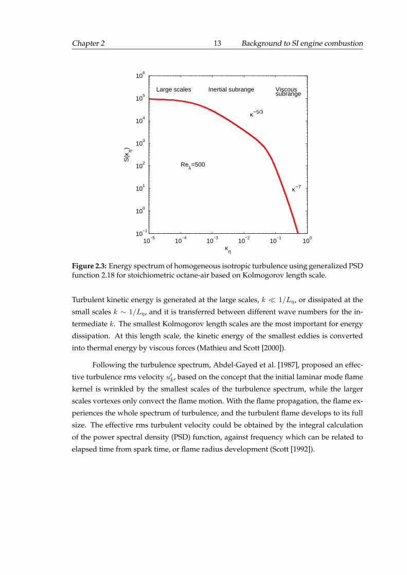
Chapter 2 13 Background to SI engine combustion
10−5
10−4
10−3
10−2
10−1
100
10−1
100
101
102
103
104
105
106
Large scales Inertial subrange Viscoussubrange
Reλ=500
κ−5/3
κ−7
κη
S(κ
η)
Figure 2.3: Energy spectrum of homogeneous isotropic turbulence using generalized PSDfunction 2.18 for stoichiometric octane-air based on Kolmogorov length scale.
Turbulent kinetic energy is generated at the large scales, k ≪ 1/Lη, or dissipated at the
small scales k ∼ 1/Lη, and it is transferred between different wave numbers for the in-
termediate k. The smallest Kolmogorov length scales are the most important for energy
dissipation. At this length scale, the kinetic energy of the smallest eddies is converted
into thermal energy by viscous forces (Mathieu and Scott [2000]).
Following the turbulence spectrum, Abdel-Gayed et al. [1987], proposed an effec-
tive turbulence rms velocity u′k, based on the concept that the initial laminar mode flame
kernel is wrinkled by the smallest scales of the turbulence spectrum, while the larger
scales vortexes only convect the flame motion. With the flame propagation, the flame ex-
periences the whole spectrum of turbulence, and the turbulent flame develops to its full
size. The effective rms turbulent velocity could be obtained by the integral calculation
of the power spectral density (PSD) function, against frequency which can be related to
elapsed time from spark time, or flame radius development (Scott [1992]).
Chapter 2 14 Background to SI engine combustion
2.1.4 Influence of pressure on turbulence
Turbulent flow in an engine is usually produced by the breathing system and piston mo-
tion. The flow structure and intensity are related to the geometry of the inlet valves for 4
stroke engines and the inlet pipes configuration for 2 stroke engines. Before investigating
the pressure effects on turbulence, it is necessary to clarify whether the turbulence is in-
creased by stronger supercharged inlet flow rate, or by pressure. Cruz et al. [2003] found a
10% rise in turbulence intensity when the engine inlet pressure was boosted from 1 bar to
1.5 bar by using calibrated anemometer measurements. Landry et al. [2008] applied Par-
ticle Imaging Velocimetry to measure the flow field in an optical single cylinder research
engine, and used Proper Orthogonal Decomposition to derive the turbulence intensi-
ties and length scales. Both values show a tendency to increase weakly with pressure.
However, the observed effects were not strong enough to draw a relationship between
turbulence properties and the inlet pressure. Although these researchers have reported
that supercharged engines had a higher turbulence intensity, it was not clearly identified
whether the increase was generated by the turbocharger or by the raised initial pressure.
The effect of intake charge mass flow rate on the turbulent flow was investigated
by Dawood [2010] in a single cylinder two-stroke ported engine. This engine has a sim-
ilar structure and geometry size with the engine that is used in this study. The results
from PIV measurements showed that the inlet flow velocity had greater influence at low
engine speed. A 50% increase of inlet flow rate corresponded a 50% increase in mean
velocity, and a 25% in Root Mean Square (RMS) velocity. These velocities were measured
at TDC position at an engine speed of 750 rpm. This means that the increased turbulence
intensity, generated by stronger inlet flow, should be taken into account when the super-
charged engine is applied to investigate the pressure effects, especially, if this is a two
stroke engine with jet type intakes.
The main pressure effect on turbulence is a decrease of the flow kinematic viscosity
ν ∝ P−1. This results in an increase of Reynolds number Rel = u′Li/ν ∝ P , and in
the extension of the energy spectrum to a higher frequency region with smaller eddies,
described by the Taylor length scale Lλ ∝ Li · Re−1/2l and the Kolmogorov length scale
Lη ∝ Li · Re−3/4l (Soika et al. [2003]). An example of this spectra widening was shown
in the experiment of Kobayashi et al. [1997], performed with a nozzle-type burner in a
high-pressure chamber. The mean flow rate (U = 2.0 m/s), and the turbulent intensity
were maintained the same during measurements. It was found that the integral scale
tended to remain the same at elevated pressure. Pressure and turbulence intensity u′
(rms velocity) had not a linear relationship. Initially, the turbulent intensity decreased
Chapter 2 15 Background to SI engine combustion
with the pressure, until the latter reached about 1.0 MPa, at which point a further raise of
pressure increased u′.
This trend was also observed by Soika et al. [2003]. A premixed bluff-body sta-
bilized burner flame in a high pressure cylindrical chamber was investigated. The inlet
flow conditions were well controlled. The premixed flame was ignited at an atmospheric
pressure, then an exhaust throttle valve was closed, and the flow mass was increased
until the pressure in the chamber reached a desired value. The inlet flow velocity was
kept constant during the experiment, thus both the mean flow velocity and turbulent in-
tensity could be thought to be constant when the pressure increased. The flow field was
characterized with Laser Doppler Anemometry (LDA). Soika et al. [2003] found that the
global flow features were only weakly dependent on pressure. The integral length scale
was decreasing when pressure was increased below 0.7 MPa, beyond which it grow with
the increased pressure.
In conclusion, it has been shown that the effects of pressure on turbulence are likely
to be weak. However,the turbulent flow in a supercharged engine could be affected by
both inlet flow rate and pressure. In order to study the pressure effects, the turbulence
modification caused by the boosting process, rather than pressure needs to receive atten-
tion. This, in particular means the mean velocity and turbulence in the intake flow into
the cylinder, plus the pattern of the flow inside the cylinder induced by the intake.
2.2 Combustion
Even though the flame in SI engines is a turbulent flame, laminar premixed flames play
a crucial role for turbulent burning velocities. Therefore, this section will introduce the
laminar flame phenomena, and a description of turbulent premixed flames. Some con-
cepts such as flame speed, burning velocity, and flame thickness, can be equally applied
to explain the turbulent flame.
2.2.1 Laminar premixed flames
A laminar premixed flame is a traveling wave of chemical transformation of fresh gas into
combustion products. A simplified structure of unstretched laminar premixed flames can
be identified as the preheat zone, the reaction zone, and the product zone, as shown in
Figure 2.4 (Griffiths and Barnard [1995]). The unstretched laminar flame speed S0l is
usually defined as the velocity of flame front relative to a stationary observer, where
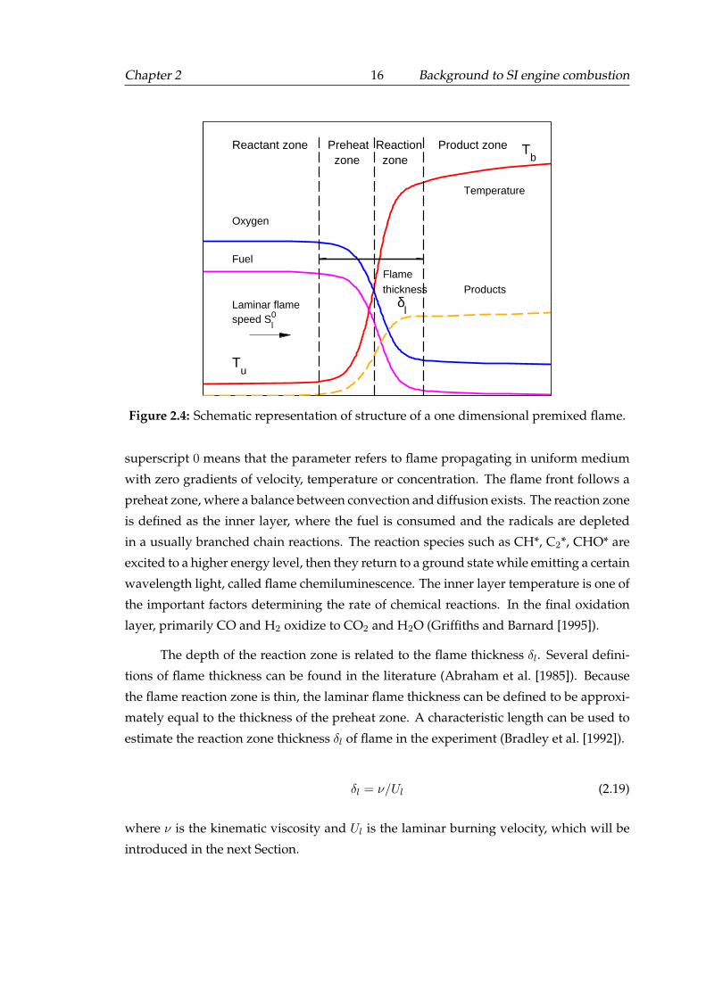
Chapter 2 16 Background to SI engine combustion
Oxygen
Fuel
Temperature
ProductsLaminar flamespeed S
l0
Reactant zone Preheat zone
Reaction zone
Product zone
Tu
Tb
Flamethickness
δl
Figure 2.4: Schematic representation of structure of a one dimensional premixed flame.
superscript 0 means that the parameter refers to flame propagating in uniform medium
with zero gradients of velocity, temperature or concentration. The flame front follows a
preheat zone, where a balance between convection and diffusion exists. The reaction zone
is defined as the inner layer, where the fuel is consumed and the radicals are depleted
in a usually branched chain reactions. The reaction species such as CH*, C2*, CHO* are
excited to a higher energy level, then they return to a ground state while emitting a certain
wavelength light, called flame chemiluminescence. The inner layer temperature is one of
the important factors determining the rate of chemical reactions. In the final oxidation
layer, primarily CO and H2 oxidize to CO2 and H2O (Griffiths and Barnard [1995]).
The depth of the reaction zone is related to the flame thickness δl. Several defini-
tions of flame thickness can be found in the literature (Abraham et al. [1985]). Because
the flame reaction zone is thin, the laminar flame thickness can be defined to be approxi-
mately equal to the thickness of the preheat zone. A characteristic length can be used to
estimate the reaction zone thickness δl of flame in the experiment (Bradley et al. [1992]).
δl = ν/Ul (2.19)
where ν is the kinematic viscosity and Ul is the laminar burning velocity, which will be
introduced in the next Section.
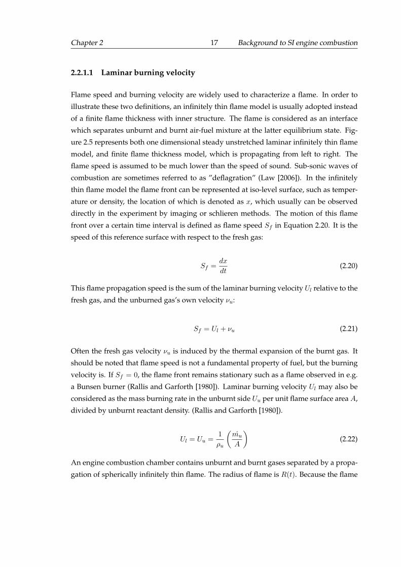
Chapter 2 17 Background to SI engine combustion
2.2.1.1 Laminar burning velocity
Flame speed and burning velocity are widely used to characterize a flame. In order to
illustrate these two definitions, an infinitely thin flame model is usually adopted instead
of a finite flame thickness with inner structure. The flame is considered as an interface
which separates unburnt and burnt air-fuel mixture at the latter equilibrium state. Fig-
ure 2.5 represents both one dimensional steady unstretched laminar infinitely thin flame
model, and finite flame thickness model, which is propagating from left to right. The
flame speed is assumed to be much lower than the speed of sound. Sub-sonic waves of
combustion are sometimes referred to as ”deflagration” (Law [2006]). In the infinitely
thin flame model the flame front can be represented at iso-level surface, such as temper-
ature or density, the location of which is denoted as x, which usually can be observed
directly in the experiment by imaging or schlieren methods. The motion of this flame
front over a certain time interval is defined as flame speed Sf in Equation 2.20. It is the
speed of this reference surface with respect to the fresh gas:
Sf =dx
dt(2.20)
This flame propagation speed is the sum of the laminar burning velocity Ul relative to the
fresh gas, and the unburned gas’s own velocity νu:
Sf = Ul + νu (2.21)
Often the fresh gas velocity νu is induced by the thermal expansion of the burnt gas. It
should be noted that flame speed is not a fundamental property of fuel, but the burning
velocity is. If Sf = 0, the flame front remains stationary such as a flame observed in e.g.
a Bunsen burner (Rallis and Garforth [1980]). Laminar burning velocity Ul may also be
considered as the mass burning rate in the unburnt side Uu per unit flame surface area A,
divided by unburnt reactant density. (Rallis and Garforth [1980]).
Ul = Uu =1
ρu
(mu
A
)(2.22)
An engine combustion chamber contains unburnt and burnt gases separated by a propa-
gation of spherically infinitely thin flame. The radius of flame is R(t). Because the flame
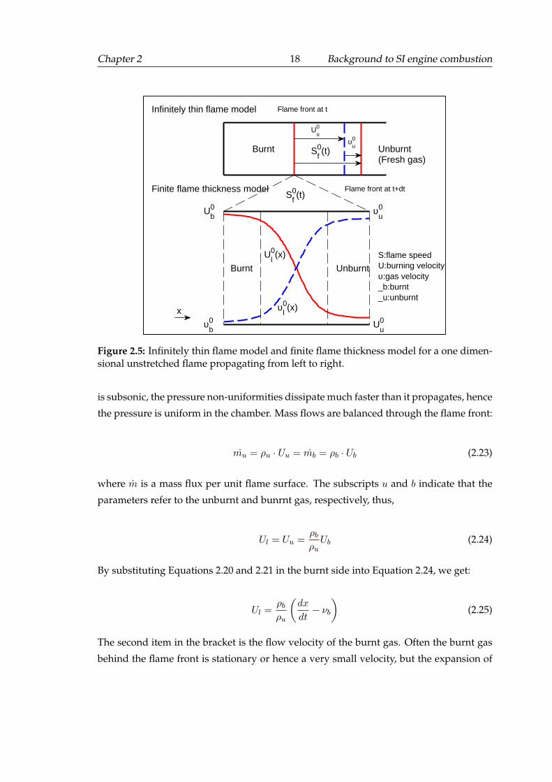
Chapter 2 18 Background to SI engine combustion
Burnt Unburnt
Burnt Unburnt(Fresh gas)
Ub0
υb0 U
u0
υu0
Ul0(x)
υl0(x)
Sf0(t)
υu0
Uu0
Sf0(t)
Flame front at t
Flame front at t+dt
S:flame speedU:burning velocityυ:gas velocity_b:burnt_u:unburnt
Infinitely thin flame model
Finite flame thickness model
x
Figure 2.5: Infinitely thin flame model and finite flame thickness model for a one dimen-sional unstretched flame propagating from left to right.
is subsonic, the pressure non-uniformities dissipate much faster than it propagates, hence
the pressure is uniform in the chamber. Mass flows are balanced through the flame front:
mu = ρu · Uu = mb = ρb · Ub (2.23)
where m is a mass flux per unit flame surface. The subscripts u and b indicate that the
parameters refer to the unburnt and bunrnt gas, respectively, thus,
Ul = Uu =ρbρu
Ub (2.24)
By substituting Equations 2.20 and 2.21 in the burnt side into Equation 2.24, we get:
Ul =ρbρu
(dx
dt− νb
)(2.25)
The second item in the bracket is the flow velocity of the burnt gas. Often the burnt gas
behind the flame front is stationary or hence a very small velocity, but the expansion of
Chapter 2 19 Background to SI engine combustion
hot products induces considerable motion of the fresh gas ahead of the flame. Therefore,
Equation 2.25 can be simplified with flame radius R(t) as follow:
Ul =ρbρu
(dR(t)
dt
)=
ρbρu
Sb (2.26)
The exact definition of the laminar burning velocity is important before applying
any measurement in the experiment. Equation 2.26 is one possible illustration of how to
derive burning velocity from flame radius R(t) recorded by an image acquisition system.
Usually, imaging measurement of flame development is employed in constant pressure
conditions where pressure change is negligible. An engine burning velocity, can also be
calculated from pressure signal, e.g. assuming a linear relationship between the mass
fraction of the burnt gas and the pressure rise. Then, a computer model can be used
to calculate the burning velocity from pressure information (Marshall et al. [2011]; Met-
ghalchi and Keck [1982]). Generally, pressure rather than images is a direct measurement
for burning velocity. However, complexity of models, and a number of input parameters,
influenced the accuracy of the final results. In practice, optical techniques are preferred,
in fact, image method can provide the geometry information of the flame front and record
the initial flame propagation, which is hardly detected by pressure transducer due to the
small pressure increase at the beginning.
The another way to measure burning velocity is to make use of Equation 2.21. The
second item in Equation 2.21 is the flow velocity in the unburnt side in front of flame,
which is usually a large value and can not be neglected. The flow measurement method
has been applied to measure directly the gas velocity in front of a flame (Vagelopoulos
and Egolfopoulos [1998]), and derive the burning velocity from Equation 2.21. However,
the gas velocity is a function of distance from the flame, as shown in the finite flame thick-
ness model, behavior of the burning velocity Ul(s), gas velocity νl(s), and flame propaga-
tion velocity Sf (s), is schematically represented as a function of the position in different
unstretched flames. Moreover, the spatial resolution of the flow measurement may be not
sufficiently high to obtain an accurate velocity. The value of fresh gas velocity is a major
part of Equation 2.21, so any imprecise measured of flow velocities would bring a large
error in the burning velocity. Therefore, the imaging measurement based on Equation
2.26 will be adopted in this study for both laminar and turbulent flame measurements.
The density of unburnt and burnt gas could be calculated from thermodynamic analysis
equations with chemical reaction components (Abdi Aghdam [2003]).
Chapter 2 20 Background to SI engine combustion
2.2.1.2 Flame stretch
One-dimensional flames, described in the previous section, cannot be achieved in prac-
tical experimental configurations (Rallis and Garforth [1980]). For example, real flames
are often affected by the stretch effects. The stretch rate α can be defined as the time
derivative of the flame surface area A and further divided by the area A:
α =1
A
(dA
dt
)(2.27)
For example, for a cylindrical flame of a unit height with radius R, this becomes:
α =1
A
(dA
dt
)=
1
2πR
d(2πR)
dt=
1
RSf (2.28)
The equation which relates the stretch rate to flow velocity u has been derived in the
following form (Law [2006]):
α = (n · (n · ∇)u+∇ · u) + Sl∇ · n
= (δij − ninj)∂ui∂xj
+ Sl∂ni
xi
= ατ + αn + κc
(2.29)
where n is a unit normal outward. α is strain item due to the gradient velocities at the
flame surface, and it can be further split into normal straining αn and tangential straining
ατ . The final item κc is the curvature caused by the flame area change during propaga-
tion of the curved surface. Sl is the flame speed. The propagating flame surface can be
expanded or contracted by the strain and curvature effects under different conditions of
curvature, as shown in Figure 2.6.
In the experiment, stretch rate can be obtained from equation 2.28 using flame ra-
dius information. It can also be directly measured based on the equation 2.29, where flow
field information can be measured. However, 2D flow field measurement will shift the
results to a lower value (Lauer and Sattelmayer [2010]), and in order to detect the velocity
gradients at the flame front, very high spatial resolution of the velocity measurement is
required.
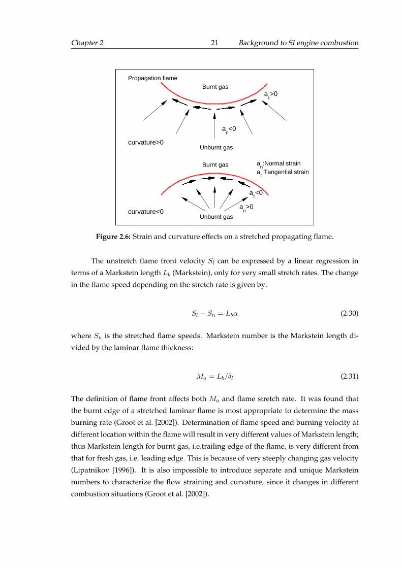
Chapter 2 21 Background to SI engine combustion
curvature<0
curvature>0
Burnt gas
Unburnt gas
Burnt gas
Unburnt gas
an<0
an>0
aτ>0
aτ<0
an:Normal strain
aτ:Tangential strain
Propagation flame
Figure 2.6: Strain and curvature effects on a stretched propagating flame.
The unstretch flame front velocity Sl can be expressed by a linear regression in
terms of a Markstein length Lb (Markstein), only for very small stretch rates. The change
in the flame speed depending on the stretch rate is given by:
Sl − Sn = Lbα (2.30)
where Sn is the stretched flame speeds. Markstein number is the Markstein length di-
vided by the laminar flame thickness:
Ma = Lb/δl (2.31)
The definition of flame front affects both Ma and flame stretch rate. It was found that
the burnt edge of a stretched laminar flame is most appropriate to determine the mass
burning rate (Groot et al. [2002]). Determination of flame speed and burning velocity at
different location within the flame will result in very different values of Markstein length;
thus Markstein length for burnt gas, i.e.trailing edge of the flame, is very different from
that for fresh gas, i.e. leading edge. This is because of very steeply changing gas velocity
(Lipatnikov [1996]). It is also impossible to introduce separate and unique Markstein
numbers to characterize the flow straining and curvature, since it changes in different
combustion situations (Groot et al. [2002]).
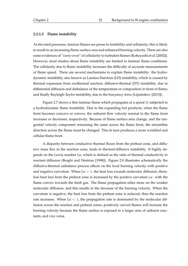
Chapter 2 22 Background to SI engine combustion
2.2.1.3 Flame instability
At elevated pressures, laminar flames are prone to instability and cellularity; this is likely
to result in an increasing flame surface area and enhanced burning velocity. There are also
some evidences of ”carry-over” of cellularity to turbulent flames (Kobayashi et al. [2002]).
However, most studies about flame instability are limited to laminar flame conditions.
The cellularity due to flame instability increases the difficulty of accurate measurements
of flame speed. There are several mechanisms to explain flame instability: the hydro-
dynamic instability, also known as Landau-Darrieus (LD) instability, which is caused by
thermal expansion from exothermal reaction; diffusive-thermal (DT) instability, due to
differential diffusion and disbalance of the temperature or composition in front of flame;
and finally Rayleigh-Taylor instability, due to the buoyancy force (Lipatnikov [2013]).
Figure 2.7 shows a thin laminar flame which propagates at a speed Sl subjected to
a hydrodynamic flame instability. Due to the expanding hot products, when the flame
front becomes concave or convex, the unburnt flow velocity normal to the flame front
increases or decreases, respectively. Because of flame surface area change, and the tan-
gential velocity component remaining the same across the flame front, the streamline
direction across the flame must be changed. This in turn produces a more wrinkled and
cellular flame front.
A disparity between conductive thermal fluxes from the preheat zone, and diffu-
sive mass flux in the reaction zone, leads to thermal-diffusive instability. It highly de-
pends on the Lewis number Le, which is defined as the ratio of thermal conductivity to
reactant diffusion (Borghi and Destriau [1998]). Figure 2.8 illustrates schematically the
diffusive-thermal unbalance process effects on the local burning velocity with positive
and negative curvature. When Le > 1, the heat loss exceeds molecular diffusion, there-
fore heat loss from the preheat zone is increased by the positive curvature i.e. with the
flame convex towards the fresh gas. The flame propagation relies more on the weaker
molecular diffusion, and this results in the decrease of the burning velocity. When the
curvature is negative, the heat loss from the preheat zone is reduced, thus the reaction
rate increases. When Le < 1, the propagation rate is dominated by the molecular dif-
fusion across the reaction and preheat zones, positively curved flames will increase the
burning velocity because the flame surface is exposed to a larger area of unburnt reac-
tants, and vice versa.
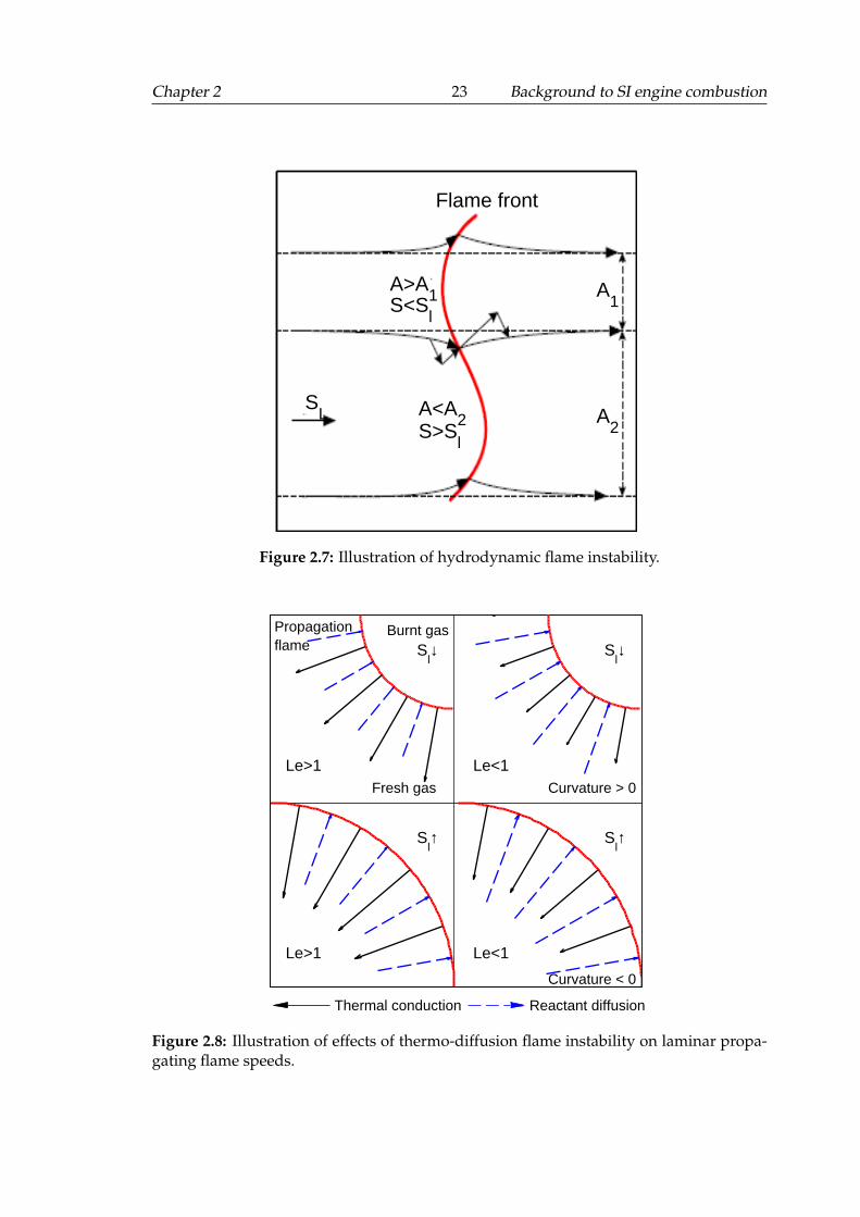
Chapter 2 23 Background to SI engine combustion
Flame front
SL
A>A1S<Sl
A<A2
S>Sl
A1
A2
Figure 2.7: Illustration of hydrodynamic flame instability.
Le>1
Le>1
Le<1
Le<1
Sl↓
Sl↑ S
l↑
Sl↓
Propagationflame
Burnt gas
Fresh gas Curvature > 0
Curvature < 0
Thermal conduction Reactant diffusion
Figure 2.8: Illustration of effects of thermo-diffusion flame instability on laminar propa-gating flame speeds.
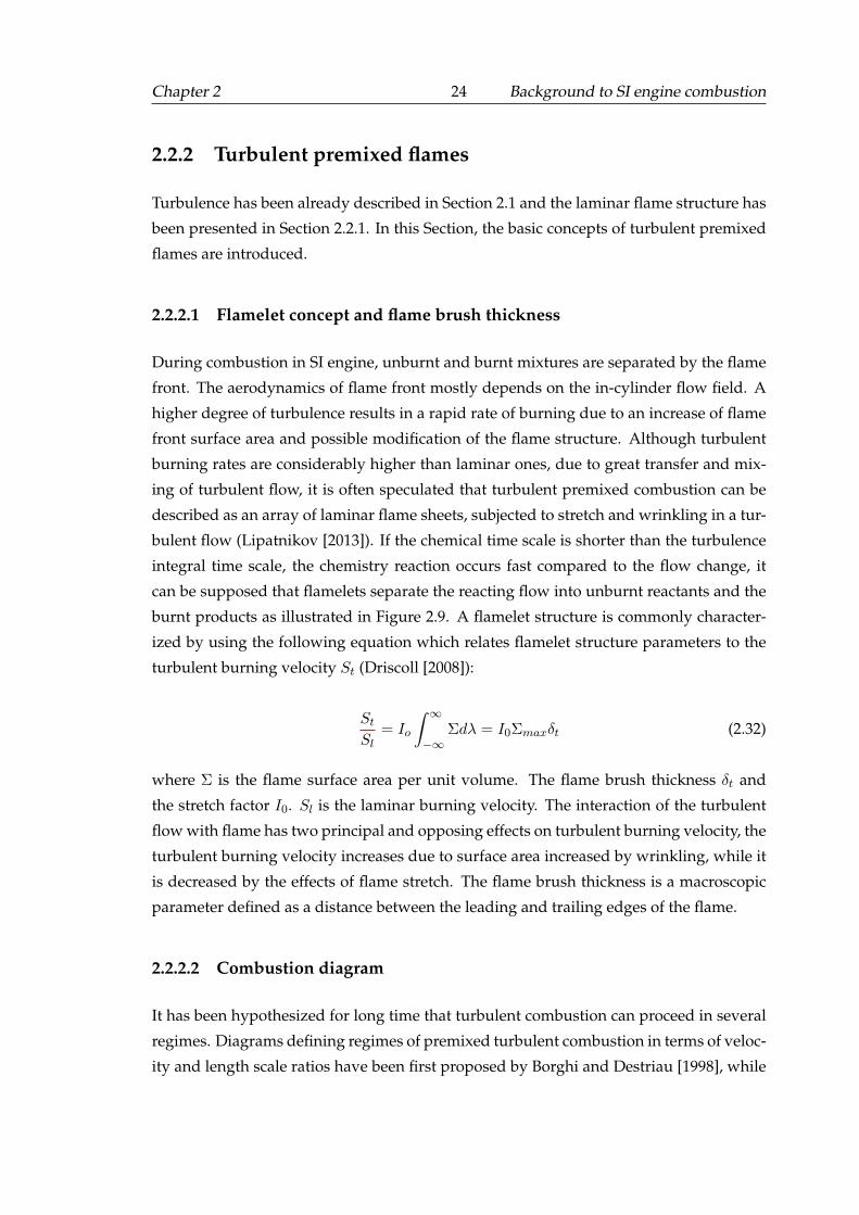
Chapter 2 24 Background to SI engine combustion
2.2.2 Turbulent premixed flames
Turbulence has been already described in Section 2.1 and the laminar flame structure has
been presented in Section 2.2.1. In this Section, the basic concepts of turbulent premixed
flames are introduced.
2.2.2.1 Flamelet concept and flame brush thickness
During combustion in SI engine, unburnt and burnt mixtures are separated by the flame
front. The aerodynamics of flame front mostly depends on the in-cylinder flow field. A
higher degree of turbulence results in a rapid rate of burning due to an increase of flame
front surface area and possible modification of the flame structure. Although turbulent
burning rates are considerably higher than laminar ones, due to great transfer and mix-
ing of turbulent flow, it is often speculated that turbulent premixed combustion can be
described as an array of laminar flame sheets, subjected to stretch and wrinkling in a tur-
bulent flow (Lipatnikov [2013]). If the chemical time scale is shorter than the turbulence
integral time scale, the chemistry reaction occurs fast compared to the flow change, it
can be supposed that flamelets separate the reacting flow into unburnt reactants and the
burnt products as illustrated in Figure 2.9. A flamelet structure is commonly character-
ized by using the following equation which relates flamelet structure parameters to the
turbulent burning velocity St (Driscoll [2008]):
St
Sl= Io
∫ ∞
−∞Σdλ = I0Σmaxδt (2.32)
where Σ is the flame surface area per unit volume. The flame brush thickness δt and
the stretch factor I0. Sl is the laminar burning velocity. The interaction of the turbulent
flow with flame has two principal and opposing effects on turbulent burning velocity, the
turbulent burning velocity increases due to surface area increased by wrinkling, while it
is decreased by the effects of flame stretch. The flame brush thickness is a macroscopic
parameter defined as a distance between the leading and trailing edges of the flame.
2.2.2.2 Combustion diagram
It has been hypothesized for long time that turbulent combustion can proceed in several
regimes. Diagrams defining regimes of premixed turbulent combustion in terms of veloc-
ity and length scale ratios have been first proposed by Borghi and Destriau [1998], while
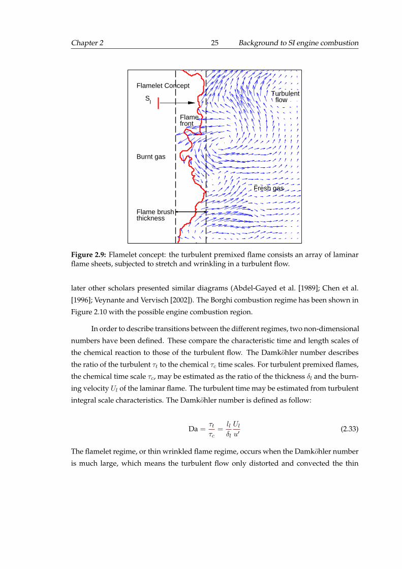
Chapter 2 25 Background to SI engine combustion
Flame brushthickness
Burnt gas
Fresh gas
Turbulentflow
Flamefront
Sl
Flamelet Concept
Figure 2.9: Flamelet concept: the turbulent premixed flame consists an array of laminarflame sheets, subjected to stretch and wrinkling in a turbulent flow.
later other scholars presented similar diagrams (Abdel-Gayed et al. [1989]; Chen et al.
[1996]; Veynante and Vervisch [2002]). The Borghi combustion regime has been shown in
Figure 2.10 with the possible engine combustion region.
In order to describe transitions between the different regimes, two non-dimensional
numbers have been defined. These compare the characteristic time and length scales of
the chemical reaction to those of the turbulent flow. The Damkohler number describes
the ratio of the turbulent τt to the chemical τc time scales. For turbulent premixed flames,
the chemical time scale τc, may be estimated as the ratio of the thickness δl and the burn-
ing velocity Ul of the laminar flame. The turbulent time may be estimated from turbulent
integral scale characteristics. The Damkohler number is defined as follow:
Da =τtτc
=llδl
Ul
u′(2.33)
The flamelet regime, or thin wrinkled flame regime, occurs when the Damkohler number
is much large, which means the turbulent flow only distorted and convected the thin
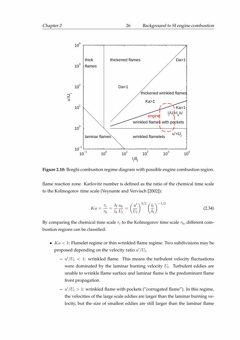
Chapter 2 26 Background to SI engine combustion
10−1
100
101
102
103
104
10−1
100
101
102
103
104
thick
flames
laminar flames
thickened flames
wrinkled flames with pockets
wrinkled flamelets
thickened wrinkled flames
Da<1
Da=1
Ka=1
Ka>1
u’=Ul
li/U
l=lλ/u’
li/δ
l
u’/U
l
engine
Figure 2.10: Borghi combustion regime diagram with possible engine combustion region.
flame reaction zone. Karlovitz number is defined as the ratio of the chemical time scale
to the Kolmogorov time scale (Veynante and Vervisch [2002]):
Ka =τcτk
=δllk
ukUl
=
(u′
Ul
)3/2( llδl
)−1/2
(2.34)
By comparing the chemical time scale τc to the Kolmogorov time scale τk, different com-
bustion regions can be classified:
• Ka < 1: Flamelet regime or thin wrinkled flame regime. Two subdivisions may be
proposed depending on the velocity ratio u′/Ul.
– u′/Ul < 1: wrinkled flame. This means the turbulent velocity fluctuations
were dominated by the laminar burning velocity Ul. Turbulent eddies are
unable to wrinkle flame surface and laminar flame is the predominant flame
front propagation.
– u′/Ul > 1: wrinkled flame with pockets (”corrugated flame”). In this regime,
the velocities of the large scale eddies are larger than the laminar burning ve-
locity, but the size of smallest eddies are still larger than the laminar flame
Chapter 2 27 Background to SI engine combustion
thickness, so that eddies are unable to penetrate into the laminar flame struc-
ture, leaving chemical and transport processes within the flame structure es-
sentially unchanged.
• 1 < Ka ≤ 100: Thickened wrinkled flame regime or thin reaction zone. In this
regime, the smallest eddies are smaller than the laminar flame thickness so that
eddies are able to penetrate into the laminar flame structure. But, the smallest
eddies are still larger than the thickness of the inner layer so that eddies cannot
change the reaction zone.
• Ka > 100: Thickened flame regime or well-stirred reactor. In this situation, the
smallest eddies are small enough to penetrate into the inner layer, affecting chem-
ical reactions. The premixed flame structure cannot be preserved and local extinc-
tion will occur.
2.2.2.3 Flame development and turbulent burning velocity
Combustion in a spark ignition engine is a transient process, both burning velocity and
flame brush thickness develop with time after ignition and are influenced by several
mechanisms, this process is called flame development (Lipatnikov [2013]).
After spark ignition, a laminar flame would propagate in a smooth spherical man-
ner from the point of ignition. The diffusion mechanism governs the flame propaga-
tion and only small eddies can affect it. With the flame developing, the flame surface is
wrinkled and distorted by the turbulence, increasing its propagation velocity and brush
thickness. The constant burning rate may be observed in a short period before the flame
reaches the cylinder walls. This phenomena could be attributed to the flame attaining a
”fully developed” state or a balance between flame initial acceleration and the deceler-
ation caused by the interaction of flame and walls (Liu et al. [2013]). At last, the flame
speed become slow and quenches when it is approaching the cylinder wall.
Usually, turbulent burning velocities in an engine are referred to the burning ve-
locity at the ”fully developed” state. Two definitions of flame burning velocity have been
considered by Groff and Matekunas [1980]. One is based on mass rate of entrainment of
unburned mixture into the flame (Ue), usually derived from photographic observations
(Beretta et al. [1983]). The second definition is related to the rate of production of burnt
gas, which is obtained from pressure rise; this may be named mass burning velocity, Un.
The turbulent burning velocity is the result of the interaction of turbulence and
the flame. It is increased by the turbulent wrinkling of the flame, resulting in an en-
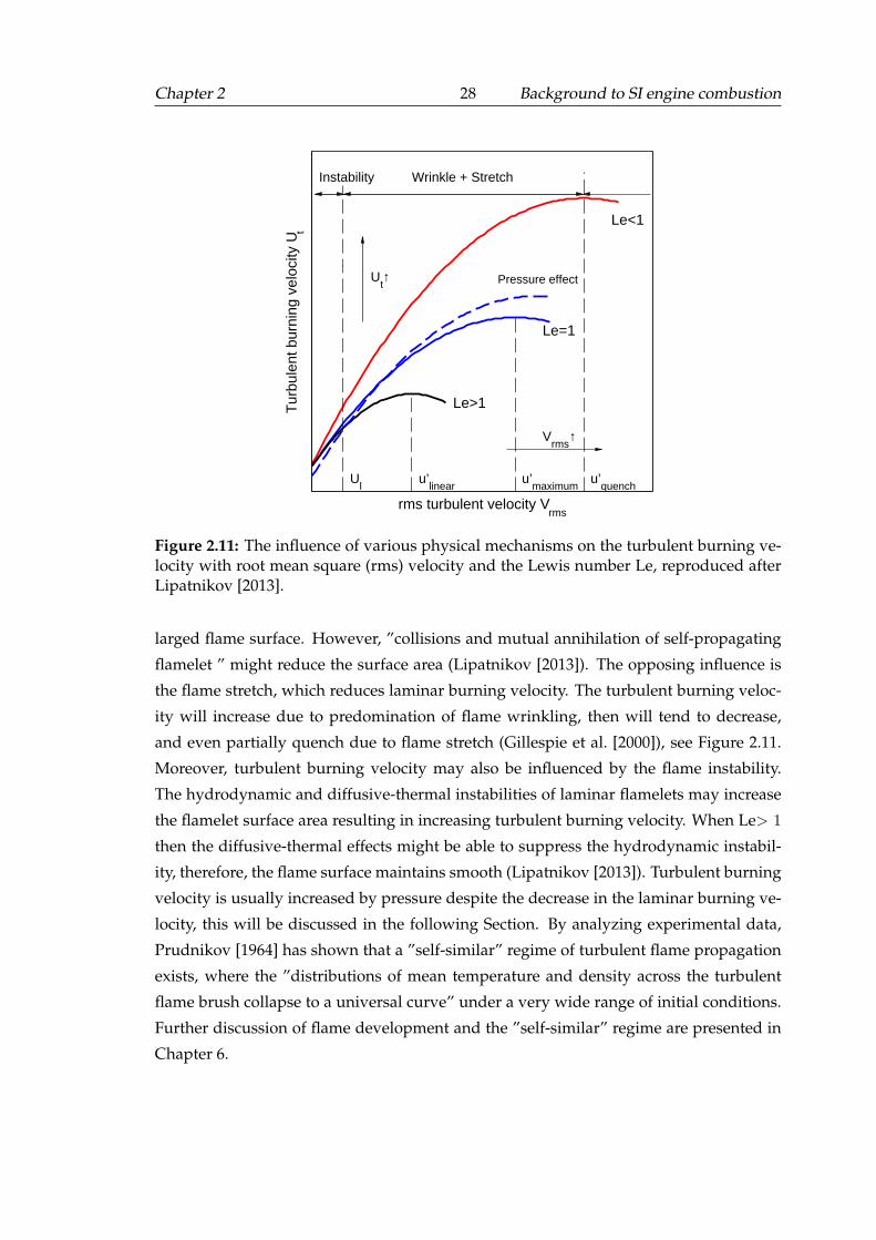
Chapter 2 28 Background to SI engine combustion
Pressure effect
Vrms
↑
Ut↑
Le>1
Le=1
Le<1
Instability Wrinkle + Stretch
Ul u’
linear u’
maximum u’
quench
rms turbulent velocity Vrms
Tur
bule
nt b
urni
ng v
eloc
ity U
t
Figure 2.11: The influence of various physical mechanisms on the turbulent burning ve-locity with root mean square (rms) velocity and the Lewis number Le, reproduced afterLipatnikov [2013].
larged flame surface. However, ”collisions and mutual annihilation of self-propagating
flamelet ” might reduce the surface area (Lipatnikov [2013]). The opposing influence is
the flame stretch, which reduces laminar burning velocity. The turbulent burning veloc-
ity will increase due to predomination of flame wrinkling, then will tend to decrease,
and even partially quench due to flame stretch (Gillespie et al. [2000]), see Figure 2.11.
Moreover, turbulent burning velocity may also be influenced by the flame instability.
The hydrodynamic and diffusive-thermal instabilities of laminar flamelets may increase
the flamelet surface area resulting in increasing turbulent burning velocity. When Le> 1
then the diffusive-thermal effects might be able to suppress the hydrodynamic instabil-
ity, therefore, the flame surface maintains smooth (Lipatnikov [2013]). Turbulent burning
velocity is usually increased by pressure despite the decrease in the laminar burning ve-
locity, this will be discussed in the following Section. By analyzing experimental data,
Prudnikov [1964] has shown that a ”self-similar” regime of turbulent flame propagation
exists, where the ”distributions of mean temperature and density across the turbulent
flame brush collapse to a universal curve” under a very wide range of initial conditions.
Further discussion of flame development and the ”self-similar” regime are presented in
Chapter 6.
Chapter 2 29 Background to SI engine combustion
2.2.2.4 Influence of pressure on flame propagation
It has been widely observed that pressure has a negative effect on laminar burning ve-
locity from both computation (Soika et al. [2003]) and experiments (Bradley et al. [1998]).
Detailed one-dimensional flame calculations using CHEMKIN for a methane/air flame
show an approximate relationship ul ∝ P−0.5 (Soika et al. [2003]). Experimental results
also confirmed that the unstretched laminar burning velocities decrease as P−0.52 (Liu
et al. [2011]). In addition, the flame thickness is not significantly changed by pressure.
A comprehensive review of pressure effects on laminar flame speed and structure
has been done by Law [2006]. It has been shown that effects of pressure on laminar
flames can be attributed to several aspects: when the pressure increases, the density of
reactant gases at the same temperature increases, consequently higher concentrations of
the species are achieved. Diffusion coefficient and thermal diffusivity are inversely pro-
portional to pressure. Strong nonlinearly chemical kinetics may play a key role, especially
those pressure-dependent chain mechanisms whose reaction rate can be varied by pres-
sure, through the reaction order, or the pressure exponent (Law [2006]). Detailed descrip-
tion of effects on chemical reaction mechanisms is out of the aims of this study. However,
the application of the chemical mechanism validated only at low pressure should be con-
sidered cautiously to calculate the burning velocity at high pressure. The adiabatic flame
temperature is increased by elevated pressure i.e. adiabatic flame temperature can be
increased from 50 to over 100 K by pressure increase from 1 to 100 bar (Law [2006]).
Apart from understanding the pressure effects on a laminar flame, it may be more
important gaining accurate laminar burning velocity, since it is a key parameter for study-
ing turbulent combustion. Laminar burning velocities measurements have been made at
high pressure, e.g. as demonstrated in the work of Metghalchi and Keck [1982], in which
data at high pressure were extracted from pressure rise measurements in a constant vol-
ume bomb. A laminar burning velocity correlation equation was proposed based on their
experiments with a wide range of temperature and pressure. More details of the corre-
lation equations are presented in Chapter 5. However, the data at elevated pressures are
still limited, although there is a rapid growth of the measurements in this area (Jerzem-
beck et al. [2009]; Marshall et al. [2011]). Recently, the initial pressure in a constant volume
bomb experiment was increased to 25 bar in the experiment of Jerzembeck et al. [2009]
with schlieren methods. The cellular structure on the flame surface, due to flame insta-
bility at elevated pressure, brings the difficulties in the accurate measurement of burning
velocity (Lawes et al. [2012]). The onset of cellularity is shifted towards a small flame ra-
dius by increased pressure. Cellular shape flame surface induced by instabilities causes
Chapter 2 30 Background to SI engine combustion
an acceleration of the flame front. How the flame speed is accelerated by the instability
in the engine relevant condition, and whether flame instability effects should be included
into turbulent combustion modelling, still remains an open question.
The laminar flame speeds under engine relevant conditions (pressure > 15 bar and
temperature > 500 K) are difficult to measure directly in the constant volume vessel.
Landry et al. [2008] calculated the laminar burning velocity by using detailed chemical
mechanisms under engine-like conditions. The results show a decrease of laminar burn-
ing velocity with elevated pressure, which might be compensated for by an increase in
the temperature. Consequently, the laminar burning velocity remains nearly constant.
Hence, it is different between the results observed from steady state experiments and
engine experiment, where temperature and pressure are changed together during com-
pression stroke.
For turbulent premixed flames, most experimental results show an increase in tur-
bulent flame speeds and burning velocities by pressure. Kobayashi et al. [2002, 1997]
have investigated turbulent premixed flames at a high-pressure environment up to 3.0
MPa. In order to stabilize the flame at high pressure, a bunsen-type burner was used to
overcome the unsteady and short duration of flame propagation in combustion vessels.
Turbulent burning velocity was measured, and St/Sl was also found to be considerably
affected by pressure. A power law expression of St/Sl with (P/P0)(u′/Sl) was deduced,
and the exponent ratio was found to be 0.4. A finer and more wrinkled structure of the
flame with increasing of pressure was found. This is consistent to the observation of
Soika et al. [2003]. They found that the flame front contour of high-pressure methane/air
flames became strongly wrinkled when the pressure was increased in a bluff-body sta-
bilized burner. However, the results from Griebel et al. [2007] experiment showed that
there was no influence of pressure on the mean flame front position, on the flame brush
thickness, or on the turbulent burning velocity under the pressure range of 0.5-1.44 MPa.
In his work, turbulent flame speeds and flow field of lean premixed methane/air flames
were measured by using Particle Image Velocimetry (PIV) and Planar Laser Induced Flu-
orescence of the OH radical (OH-PLIF) in a high pressure combustor.
In comparison with the results from stationary flames, information for freely prop-
agating turbulent flames may be more relevant to internal combustion engines. Bradley
et al. [1998] have investigated turbulent burning velocities for a wide range of initial con-
ditions using a fan-stirred bomb up to 1.2 MPa for turbulent flames. The results showed
that the flame curvature and wrinkling were increased due to the onset of instability at
high pressure, which made the turbulent burning velocity increase with pressure. The
implosion technique (Al-Shahrany et al. [2005]) was developed to measure burning ve-
Chapter 2 31 Background to SI engine combustion
locities at the final stage of two opposite inward propagation flames, where the pressure
can reach 3.0 MPa. A comprehensive measurement of the turbulent burning velocity of
iso-octane/air mixtures has been conducted by Lawes et al. [2012]. It was found that the
turbulent burning velocity did not change significantly with pressure at a low turbulent
intensity (u′ = 1 m/s), while at u′ = 4 m/s, the increased pressure resulted in an observ-
able rise in turbulent burning velocity in a constant volume combustion bomb from 0.1-1
MPa. In these tests, the pressure was increased while turbulence intensity was kept con-
stant. Liu et al. [2012] argued that the increase of pressure raised the Reynolds number,
which caused the increasing of the turbulent burning velocity. Under constant Reynolds
number conditions, they found that turbulent burning velocities decreased with increas-
ing of pressure, which was similar to laminar burning velocities. The data were collected
from a double-chamber, fan-stirred large premixed turbulent combustion facility at ele-
vated pressure up to 1.2 MPa. However, the turbulent burning velocity increased at any
elevated pressure with an increase of Reynolds number.
The results from constant combustion vessel still can not provide all the informa-
tion about combustion in SI engines due to a number of factors, including piston mo-
tion, which leads to higher pressure and temperature before spark ignition and also the
flame shape is confined by the geometry of the engine chamber. Only a few studies pro-
vided the information about combustion characteristic in a real boosted engine condition.
Mounaım-Rousselle et al. [2013] undertook an investigation into the effect of pressure
and dilution on the turbulent burning velocity with intake pressures between 0.7 to 1.5
bar. The turbulent burning velocity was estimated from the mean flame front displace-
ment velocity and the mean flow field velocity, which were determined from the laser
tomography images and Particle Image Velocimetry (PIV). It was found that the intake
initial pressure, which ranged from 1.0-1.5 bar, seemed to have no effect on turbulence. At
the same condition, the turbulent flame speed increased slightly, while the laminar flame
speed remained constant. Merola et al. [2007] investigated the flame development and
found that the trajectory scope of flame kernel decreased when increasing of the boost
pressure, while the path length and speed of it was increased. The initial speed of flame
propagation was increased for boosted conditions and it decreased after it reached a max-
imum speed, due to the increase of pressure in the end gas. The last stage of flame-wall
contact information is absent because of the limit of engine’s optical access structure.
Chapter 2 32 Background to SI engine combustion
2.2.2.5 Flame Chemiluminescence
The knowledge of flame chemiluminescence is important for flame imaging measure-
ment. Flame chemiluminescence is a kind of light emission of radicals during their return
from an electronically excited state to the ground state (Gaydon [1957]). Chemilumines-
cence techniques have been applied in a wide combustion research areas, e.g. monitoring
fuel-air ratio (Aleiferis et al. [2004]), detecting range of flame position, shape, and struc-
ture (Ikeda et al. [2001]), and can also be employed to measure heat release fluctuations
(Hardalupas and Orain [2004]). Usually, the excited species are generated by chemical
reactions in the flame reaction zone. Thus in typical hydrocarbon-air flames, chemilu-
minescence intensity from radicals, like CH* and C2*, can provide information about
conditions in the reaction zone. A typical chemiluminescence spectrum in the ultraviolet
and visible part of combustion in a spark ignition was shown in Figure 2.12 (Merola et al.
[2009]). It can be seen that C2* has several band systems. The Swan band consists of
wavelength near 473.71 nm, 516.52 nm and 563.55 nm. The formation of C2* is owing to
the reactions (Gaydon [1957]):
CH2 + C− > H2 + C2∗ (2.35)
CH + C− > H + C2∗ (2.36)
The CH is detected at 430 nm, 290 nm, 314 nm. The strongest is at 430 nm. The
formation of excited CH in the flames has been debated for long time (Gaydon [1957]). It
was suggested that it might be generated from C2:
C2 + OH− > CO + CH∗ (2.37)
C2 + O− > CO + CH∗ (2.38)
However, it is difficult to interpret the chemiluminescence signals because of the
integrated line of sight information acquired. Furthermore, it is affected by many factors
such as pressure, temperature, strain, equivalence ratio and fuel.
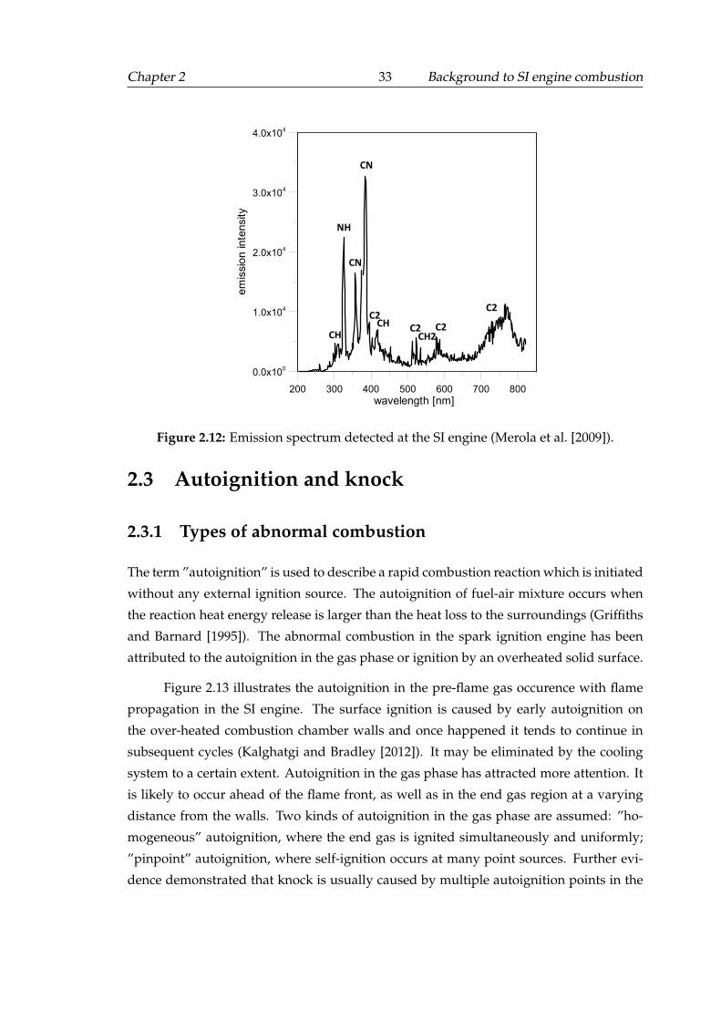
Chapter 2 33 Background to SI engine combustion
200 300 400 500 600 700 800
wavelength [nm]
0.0x100
1.0x10⁴
2.0x10⁴
3.0x10⁴
4.0x10⁴
em
issio
n inte
nsity
CH
CN
NH
CN
C2 C2
C2
CH2
C2
CH
Figure 9. UV-near IR emission spectrum detected at the
Issue 11622
Figure 2.12: Emission spectrum detected at the SI engine (Merola et al. [2009]).
2.3 Autoignition and knock
2.3.1 Types of abnormal combustion
The term ”autoignition” is used to describe a rapid combustion reaction which is initiated
without any external ignition source. The autoignition of fuel-air mixture occurs when
the reaction heat energy release is larger than the heat loss to the surroundings (Griffiths
and Barnard [1995]). The abnormal combustion in the spark ignition engine has been
attributed to the autoignition in the gas phase or ignition by an overheated solid surface.
Figure 2.13 illustrates the autoignition in the pre-flame gas occurence with flame
propagation in the SI engine. The surface ignition is caused by early autoignition on
the over-heated combustion chamber walls and once happened it tends to continue in
subsequent cycles (Kalghatgi and Bradley [2012]). It may be eliminated by the cooling
system to a certain extent. Autoignition in the gas phase has attracted more attention. It
is likely to occur ahead of the flame front, as well as in the end gas region at a varying
distance from the walls. Two kinds of autoignition in the gas phase are assumed: ”ho-
mogeneous” autoignition, where the end gas is ignited simultaneously and uniformly;
”pinpoint” autoignition, where self-ignition occurs at many point sources. Further evi-
dence demonstrated that knock is usually caused by multiple autoignition points in the
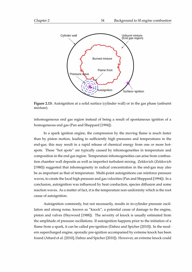
Chapter 2 34 Background to SI engine combustion
Autoignition
Pressure wave
Surface−ignition
Flame front
Burned mixture
Unburnt mixture(End gas region)
Cylinder wall
Figure 2.13: Autoignition at a solid surface (cylinder wall) or in the gas phase (unburntmixture).
inhomogeneous end gas region instead of being a result of spontaneous ignition of a
homogeneous end gas (Pan and Sheppard [1994]).
In a spark ignition engine, the compression by the moving flame is much faster
than by piston motion, leading to sufficiently high pressures and temperatures in the
end-gas; this may result in a rapid release of chemical energy from one or more hot-
spots. These ”hot spots” are typically caused by inhomogeneities in temperature and
composition in the end gas region. Temperature inhomogeneities can arise from combus-
tion chamber wall deposits as well as imperfect turbulent mixing. Zeldovich (Zeldovich
[1980]) suggested that inhomogeneity in radical concentration in the end-gas may also
be as important as that of temperature. Multi-point autoignitions can reinforce pressure
waves, to create the local high pressure and gas velocities (Pan and Sheppard [1994]). In a
conclusion, autoignition was influenced by heat conduction, species diffusion and some
reaction waves. As a matter of fact, it is the temperature non-uniformity which is the root
cause of autoignition.
Autoignition commonly, but not necessarily, results in in-cylinder pressure oscil-
lation and strong noise, known as ”knock”, a potential cause of damage to the engine,
piston and valves (Heywood [1988]). The severity of knock is usually estimated from
the amplitude of pressure oscillations. If autoignition happens prior to the initiation of a
flame from a spark, it can be called pre-ignition (Dahnz and Spicher [2010]). In the mod-
ern supercharged engine, sporadic pre-ignition accompanied by extreme knock has been
found (Attard et al. [2010]; Dahnz and Spicher [2010]). However, an extreme knock could
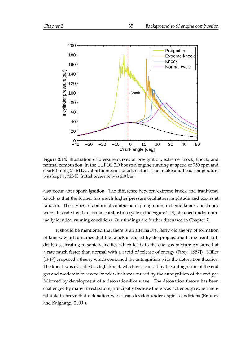
Chapter 2 35 Background to SI engine combustion
−40 −30 −20 −10 0 10 20 30 40 500
20
40
60
80
100
120
140
160
180
200
Crank angle [deg]
Incy
linde
r pr
essu
re[b
ar]
Spark
PreignitionExtreme knockKnockNormal cycle
Figure 2.14: Illustration of pressure curves of pre-ignition, extreme knock, knock, andnormal combustion, in the LUPOE 2D boosted engine running at speed of 750 rpm andspark timing 2o bTDC, stoichiometric iso-octane fuel. The intake and head temperaturewas kept at 323 K. Initial pressure was 2.0 bar.
also occur after spark ignition. The difference between extreme knock and traditional
knock is that the former has much higher pressure oscillation amplitude and occurs at
random. Thee types of abnormal combustion: pre-ignition, extreme knock and knock
were illustrated with a normal combustion cycle in the Figure 2.14, obtained under nom-
inally identical running conditions. Our findings are further discussed in Chapter 7.
It should be mentioned that there is an alternative, fairly old theory of formation
of knock, which assumes that the knock is caused by the propagating flame front sud-
denly accelerating to sonic velocities which leads to the end gas mixture consumed at
a rate much faster than normal with a rapid of release of energy (Firey [1957]). Miller
[1947] proposed a theory which combined the autoignition with the detonation theories.
The knock was classified as light knock which was caused by the autoignition of the end
gas and moderate to severe knock which was caused by the autoignition of the end gas
followed by development of a detonation-like wave. The detonation theory has been
challenged by many investigators, principally because there was not enough experimen-
tal data to prove that detonation waves can develop under engine conditions (Bradley
and Kalghatgi [2009]).
Chapter 2 36 Background to SI engine combustion
2.3.2 Autoignition chemistry and the octane number of fuel
The end gas auto- (or self-) igniton originates from a rapid heat release at a single or
multiple discrete exothermic centres or hot spots. These appear when the induction time
for the end-gas autoignition is less than the time required for the spark-initiated flame
to propagate through the cylinder. The chemical induction time is related to fuels igni-
tion behaviour which is mostly governed by the complex chemical mechanisms of fuel
oxidation.
Hydrocarbon oxidation generally consists of four steps; initiation, propagation,
degenerated branching and termination (Griffiths and Barnard [1995]). The path of the
autoignition reaction is related to the history of the unburned gaseous mixture pressure
and temperature. There exist three main paths: a ”cool” flame reaction at temperatures
in the range of 500-800 K, two stage ignition region in which the ”cool” flame proceeds
to a hot flame (800-1100 K) and a single stage ”hot-temperature” ignition (> 1100K).
In the low or intermediate temperature region (500-860 K), Reaction R+O2 RO2 is
reversible, so synthesis and decomposition occur simultaneously. The Reaction is gener-
ally in forward mode and produces the alkylperoxy radicals RO2. When temperature is
increased to enter the Negative Temperature Coefficient regime (NTC), RO2 −→ R+O2
reaction is predominately reversed and produces RO2 radicals. At the high tempera-
ture, decomposition of branching agent (hydrogen peroxide: H2O2 OH +OH) be-
comes the key reaction. Therefore, at low temperatures, ROOH radicals into a single
hydroxyl (OH) radical and partial fuel oxidation dominate the oxidation process while
at high temperatures; the HOOH radical becomes the main branching agent. In the Neg-
ative Temperature Coefficient (NTC) regime, high temperatures shutdown the pathway
of low temperature oxidation and shifting to the hydrogen decomposition and the tem-
perature is not high enough to activate hydrogen peroxide decomposition (Curran et al.
[2002]). In engine research using spectroscopic investigations, weak OH* radicals and
very weak HCHO* radicals were obtained before autoignition occurred which confirms
low-temperature chemical reaction of auto-ignition in the engine (Kawahara et al. [2007]).
Since practical fuels contain many hundreds of components coming from all types
of hydrocarbons e.g. alkanes, alkenes, napthenes and aromatics, this makes it difficult to
develop an accurate chemical mechanism to explain the knock phenomena. In order to
obtain a direct comparison of different fuel tendencies to produce knock, a method for
correlating the chemical structure of a species with its octane number was proposed (Hey-
wood [1988]). The Cooperative Fuel Research Committee defined a standard procedure
to measure a fuel’s octane number (ON). Regardless of how complex the autoignition
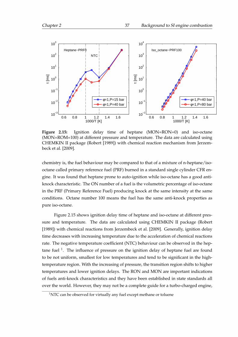
Chapter 2 37 Background to SI engine combustion
0.6 0.8 1 1.2 1.4 1.610
−3
10−2
10−1
100
101
102
103
1000/T [K]
τ [m
s]
Heptane−PRF0
NTC
φ=1,P=15 barφ=1,P=40 bar
0.6 0.8 1 1.2 1.4 1.610
−2
10−1
100
101
102
103
104
1000/T [K]
τ [m
s]
Iso_octane−PRF100
φ=1,P=40 barφ=1,P=80 bar
Figure 2.15: Ignition delay time of heptane (MON=RON=0) and iso-octane(MON=ROM=100) at different pressure and temperature. The data are calculated usingCHEMKIN II package (Robert [1989]) with chemical reaction mechanism from Jerzem-beck et al. [2009].
chemistry is, the fuel behaviour may be compared to that of a mixture of n-heptane/iso-
octane called primary reference fuel (PRF) burned in a standard single cylinder CFR en-
gine. It was found that heptane prone to auto-ignition while iso-octane has a good anti-
knock characteristic. The ON number of a fuel is the volumetric percentage of iso-octane
in the PRF (Primary Reference Fuel) producing knock at the same intensity at the same
conditions. Octane number 100 means the fuel has the same anti-knock properties as
pure iso-octane.
Figure 2.15 shows ignition delay time of heptane and iso-octane at different pres-
sure and temperature. The data are calculated using CHEMKIN II package (Robert
[1989]) with chemical reactions from Jerzembeck et al. [2009]. Generally, ignition delay
time decreases with increasing temperature due to the acceleration of chemical reactions
rate. The negative temperature coefficient (NTC) behaviour can be observed in the hep-
tane fuel 1. The influence of pressure on the ignition delay of heptane fuel are found
to be not uniform, smallest for low temperatures and tend to be significant in the high-
temperature region. With the increasing of pressure, the transition region shifts to higher
temperatures and lower ignition delays. The RON and MON are important indications
of fuels anti-knock characteristics and they have been established in state standards all
over the world. However, they may not be a complete guide for a turbo-charged engine,
1NTC can be observed for virtually any fuel except methane or toluene
Chapter 2 38 Background to SI engine combustion
because of the wider range of operational regimes which may exceed the reference engine
(Bradley and Head [2006]).
The calculated ignition delay time for the PRF fuel is often much too long to cause
pre-ignition (Dahnz and Spicher [2010]). Recent investigation of pre-ignition in a turbo-
charged engine by Dahnz and Spicher [2010] has highlighted effects of lubricant oil droplets
released from the cylinder liner promoting autoignition under certain conditions. A fur-
ther study of Kalghatgi and Bradley [2012] related the autoignition on the engine surface
to the minimum critical size of a hot spot for a flame to propagate. It was found the the
minimum critical size of a hot spot decreased with the increasing of the initial pressure.
The gas-phase autoignition, which is considered as the dominant mode of pre-ignition in
modern SI engines, may originate from the hot spot containing long-chain lubricating oil,
and this process could possibly be enhanced by small solid particles acting as a catalyst.
These conclusions may imply that while the main cause of end-gas ignition is
the homogeneous gas-phase chemistry under naturally aspirated conditions, analysis of
auto-ignition under boosted conditions should take into account the role of the lubri-
cant as well. However, such assumptions have not been convincingly validated and the
mechanism of lubricant oil droplets inducing pre-ignition is still far from clear, perhaps
to some extent because of lack of understanding of autoignition delay times in the pres-
ence of lubricating oil mists. Therefore, no attempt is made in this work study potential
effects of the lubricant on the abnormal combustion.
2.3.3 Reaction front development from autoignition sites
Three modes of reaction front propagation from hot spots have been proposed to describe
the transition from autoignition to knock using modelling method (Gu et al. [2003]). A
thermal explosion or homogeneous autoignition would be created when the temperature
gradient is small. Although, this is unlikely to be the case in an engine. As the magni-
tude of temperature gradient increases, weak pressure waves are created from exother-
mic centres, propagating away from the centre and transiting to deflagration. The end
gas is consumed by a reaction front, propagating at subsonic speed, O(10-100) m/s at
engine conditions. Knock tends to be moderate in this case. If the temperature gradient
of the end gas reaches to some critical value between the deflagration and thermal explo-
sion modes, a stronger shock is formed with a super-sonic reaction front velocity. Intense
chemical reaction will be initiated and sustained by this shock and ultimately leads to
the development of a detonation. The speed of detonation can reach O(1000) m/s (Gu
et al. [2003]). In this mode, severe knock occurs and will damage the engine (Konig and
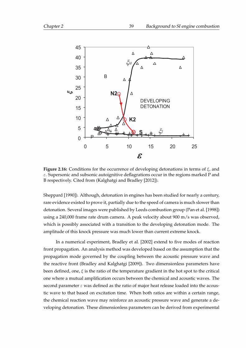
Chapter 2 39 Background to SI engine combustion
0
5
10
15
20
25
30
35
40
45
0 5 10 15 20 25
xB
DEVELOPING
DETONATION
P
e
xu
xl
N2
K2
S
Figure 2.16: Conditions for the occurrence of developing detonations in terms of ξ, andε. Supersonic and subsonic autoignitive deflagrations occur in the regions marked P andB respectively. Cited from (Kalghatgi and Bradley [2012]).
Sheppard [1990]). Although, detonation in engines has been studied for nearly a century,
rare evidence existed to prove it, partially due to the speed of camera is much slower than
detonation. Several images were published by Leeds combustion group (Pan et al. [1998])
using a 240,000 frame rate drum camera. A peak velocity about 900 m/s was observed,
which is possibly associated with a transition to the developing detonation mode. The
amplitude of this knock pressure was much lower than current extreme knock.
In a numerical experiment, Bradley et al. [2002] extend to five modes of reaction
front propagation. An analysis method was developed based on the assumption that the
propagation mode governed by the coupling between the acoustic pressure wave and
the reactive front (Bradley and Kalghatgi [2009]). Two dimensionless parameters have
been defined, one, ξ is the ratio of the temperature gradient in the hot spot to the critical
one where a mutual amplification occurs between the chemical and acoustic waves. The
second parameter ε was defined as the ratio of major heat release loaded into the acous-
tic wave to that based on excitation time. When both ratios are within a certain range,
the chemical reaction wave may reinforce an acoustic pressure wave and generate a de-
veloping detonation. These dimensionless parameters can be derived from experimental
Chapter 2 40 Background to SI engine combustion
ignition delay time τ(T, p) (Bradley and Kalghatgi [2009]). Kalghatgi and Bradley [2012]
investigated several pressure traces of extreme knock, and registered these conditions on
the (ξ and ε) coordinates as shown in Figure 2.16, it was found that extreme knock was
located in the developing detonation regime and the high knock intensities could be at-
tributed to autoigniton induced further detonation. By using this method, the detonation
mode has also been recognized by Rudloff et al. [2013]. However, these conclusions rely
on the assumption that the detonation was generated from the hot spot directly and the
map used for recognizing detonation and deflagration was based on the DNS calculation
using H2 (Gu et al. [2003]), which has a different ignition delay time with commercial fuel.
To identify the extreme knock caused by the huge unburnt mass fraction due to advance
of auto-ignition time or the occurrence of developing detonation is one of objectives of
this study.
2.4 Optical experimental engines
Pressure signals from an experimental engine only yield the information averaged over
the entire combustion chamber. Detailed flow and combustion processes can be acquired
from partially transparent engines with optical measurements. Although additional opti-
cal windows within an engine may change heat transfer intensity, optical access is useful
for fundamental combustion research related to reciprocating engines. Two main kinds
of optical engines are described in the literature as shown in Figure 2.17: optical access
through the cylinder head, and the optical access through the piston (Zhao and Ladom-
matos [2001]), in the so-called Bowditch arrangement.
The optical access through the piston engines are more widely used (Beretta et al.
[1983]; Foucher and Mounaım-Rousselle [2005]; Gatowski et al. [1984]; Knaus et al. [1999]),
especially in the last twenty years. Mounting an optical window in the piston is compat-
ible with the overhead valves configuration. Fuel injection spray and mixture in mod-
ern Gasoline Direct Injector (GDI) engines, which are strongly affected by flow structure
generated by lifted valves, can be investigated (Aleiferis et al. [2010, 2004]; Chen et al.
[2012]). Ignition and initial flame development can be observed (Peterson et al. [2014]).
In order to apply diagnostics to engine, another window in the side of engine, or a totally
transparent cylinder body, may need to be used. But above all, the optical access can
be employed to observe the combustion phenomena (Aleiferis et al. [2013]; Bates [1991];
Buschbeck et al. [2012]; Ziegler et al. [1988]).
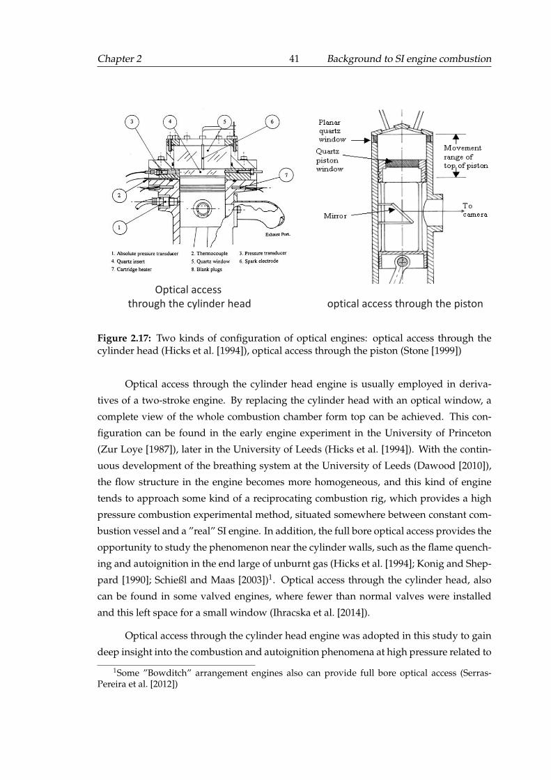
Chapter 2 41 Background to SI engine combustion
Optical access
through the cylinder head optical access through the piston
Figure 2.17: Two kinds of configuration of optical engines: optical access through thecylinder head (Hicks et al. [1994]), optical access through the piston (Stone [1999])
Optical access through the cylinder head engine is usually employed in deriva-
tives of a two-stroke engine. By replacing the cylinder head with an optical window, a
complete view of the whole combustion chamber form top can be achieved. This con-
figuration can be found in the early engine experiment in the University of Princeton
(Zur Loye [1987]), later in the University of Leeds (Hicks et al. [1994]). With the contin-
uous development of the breathing system at the University of Leeds (Dawood [2010]),
the flow structure in the engine becomes more homogeneous, and this kind of engine
tends to approach some kind of a reciprocating combustion rig, which provides a high
pressure combustion experimental method, situated somewhere between constant com-
bustion vessel and a ”real” SI engine. In addition, the full bore optical access provides the
opportunity to study the phenomenon near the cylinder walls, such as the flame quench-
ing and autoignition in the end large of unburnt gas (Hicks et al. [1994]; Konig and Shep-
pard [1990]; Schießl and Maas [2003])1. Optical access through the cylinder head, also
can be found in some valved engines, where fewer than normal valves were installed
and this left space for a small window (Ihracska et al. [2014]).
Optical access through the cylinder head engine was adopted in this study to gain
deep insight into the combustion and autoignition phenomena at high pressure related to
1Some ”Bowditch” arrangement engines also can provide full bore optical access (Serras-Pereira et al. [2012])
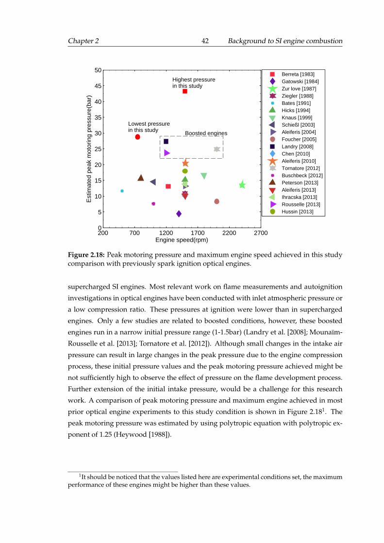
Chapter 2 42 Background to SI engine combustion
200 700 1200 1700 2200 27000
5
10
15
20
25
30
35
40
45
50
Engine speed(rpm)
Est
imat
ed p
eak
mot
orin
g pr
essu
re(b
ar)
Lowest pressurein this study
Highest pressurein this study
Boosted engines
Berreta [1983]Gatowski [1984]Zur love [1987]Ziegler [1988]Bates [1991]Hicks [1994]Knaus [1999]Schießl [2003]Aleiferis [2004]Foucher [2005]Landry [2008]Chen [2010]Aleiferis [2010]Tornatore [2012]Buschbeck [2012]Peterson [2013]Aleiferis [2013]Ihracska [2013]Rousselle [2013]Hussin [2013]
Figure 2.18: Peak motoring pressure and maximum engine speed achieved in this studycomparison with previously spark ignition optical engines.
supercharged SI engines. Most relevant work on flame measurements and autoignition
investigations in optical engines have been conducted with inlet atmospheric pressure or
a low compression ratio. These pressures at ignition were lower than in supercharged
engines. Only a few studies are related to boosted conditions, however, these boosted
engines run in a narrow initial pressure range (1-1.5bar) (Landry et al. [2008]; Mounaım-
Rousselle et al. [2013]; Tornatore et al. [2012]). Although small changes in the intake air
pressure can result in large changes in the peak pressure due to the engine compression
process, these initial pressure values and the peak motoring pressure achieved might be
not sufficiently high to observe the effect of pressure on the flame development process.
Further extension of the initial intake pressure, would be a challenge for this research
work. A comparison of peak motoring pressure and maximum engine achieved in most
prior optical engine experiments to this study condition is shown in Figure 2.181. The
peak motoring pressure was estimated by using polytropic equation with polytropic ex-
ponent of 1.25 (Heywood [1988]).
1It should be noticed that the values listed here are experimental conditions set, the maximumperformance of these engines might be higher than these values.
Chapter 3
Experimental engine and boosting
system
In recent years, a large number of excellent naturally aspirated engine experiments have
been conducted by the Leeds combustion research group using the Leeds University
Ported Optical Engine (LUPOE) (Muard [2006]; Roberts [2010]; Smallbone [2004]). The
objective of the current study is to investigate the engine combustion at elevated pres-
sures. With this aim, the naturally aspirated LUPOE 2D engine was modified into a
boosted engine. The breathing system of LUPOE 2D was redesigned for the purpose of
simulating turbo-charged engine operation condition. The challenge was not only to in-
crease the initial pressure of the engine, but also to control the turbulence in the engine
at a certain desired level. Various methods have been applied to increase the initial pres-
sure, including exchanging the position of the intake and exhaust ports, installing intake
and exhaust system valves, and increasing the air supply pressure directly. These meth-
ods were tested and compared to find an efficient and accurate way to control the inlet
pressure. This Chapter also includes the description of LUPOE 2D engine design along
with its basic components. The engine controller and data acquisition system were re-
designed and are described here. At last, the pressure data process and analysis methods
were introduced with a reverse thermodynamic simulation software LUSIEDA (Leeds
University Spark Ignition Engine Data Analysis).
Chapter 3 44 Experimental engine and boosting system
3.1 LUPOE 2D research engine
Leeds University Ported Optical Engine, Version 2, Disc-head (LUPOE 2D) was devel-
oped on the base of a commercially available Lister Petter-PH1 single cylinder diesel
engine, of which the cylinder head, the breathing system were replaced with bespoke
components. An overview of the engine setup can be seen in Figure 3.1, and a detailed
drawing of the schematic diagram of the LUPOE 2D and optical head have been shown
in Figure 3.2. A photograph of the LUPOE 2D engine can be found in Appendix A.
The LUPOE 2D engine is similar to a two-stroke engine, in that it has a disc-shaped
combustion chamber with a full-bore overhead optical access. It replaces the overhead
valves by side ports to avoid obstructing the full-bore optical access, provided by one
top and two opposite side windows. A custom built compact spark plug was located
in the center of the cylinder bore; it consists of a 0.5 mm diameter steel anode housed
inside a sheathed 3 mm alumina tube. A L-shaped length of brazing rod was connected
to the outer brass tube to act as the cathode. The quartz optical window was used in
normal combustion experiments, in most cases, but it was replaced by a more robust
metal blanking plate to avoid the damage to the quartz window under strongly knocking
conditions.
The LUPOE 2D engine has two diametrically opposed intake ports of rectangular
cross section and an exhaust passage consisting of either two or four rings of circular ex-
haust holes drilled in the liner, communicating with a void between a liner and a barrel,
leading to one exhaust duct. The liner of the boosted LUPOE 2D engine has 2 rows of ex-
haust holes, while naturally aspirated version has 4 rows, the reason of this configuration
will be explained in the Section ”Boosting system”. The timings of the port holes opening
and closing were controlled by the movement of piston. The specifications of the natu-
rally aspirated LUPOE 2D engine and boosted LUPOE 2D engine are compared in Table
3.1. The employed ported breathing arrangement, in particular the ports dimensions
and inclination, allows one to eliminate swirl and tumble motion often existing in valves
engines, and to generate in-cylinder flow field uniform in both average and root-mean
square properties, thus LUPOE 2D can be considered as a featureless flow engine.
Compression ratio can be adjusted by using a series of metal shims, placed between
the top of the engine block and the cylinder head. The specifications of these are detailed
in Table 3.2. The shim thickness of 4 mm was only used during initial stage of engine
tests to ensure that the engine operation was safe. The shim thickness of 1 mm was
mainly used in this study, in order to obtain a similar compression ratio as the naturally
aspirated LUPOE 2D engine.
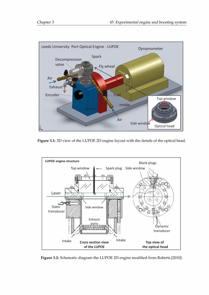
Chapter 3 45 Experimental engine and boosting system
Optical headSide window
Top window
Dynamometer
Spark
Fly wheel
Fuel
Intake
Encoder
Decompression
valve
Exhaust
Leeds University Port Optical Engine - LUPOE
Air
Air
Heater
Figure 3.1: 3D view of the LUPOE 2D engine layout with the details of the optical head.
Top window Spark plug
Side window
Exhaust
ports
IntakeIntake
Side window
Blank plugs
Dynamic
transducer
Static
transducer
Cross section view
of the LUPOE
Top view of
the optical head
LUPOE engine structure
Laser
Figure 3.2: Schematic diagram the LUPOE 2D engine modified from Roberts [2010].
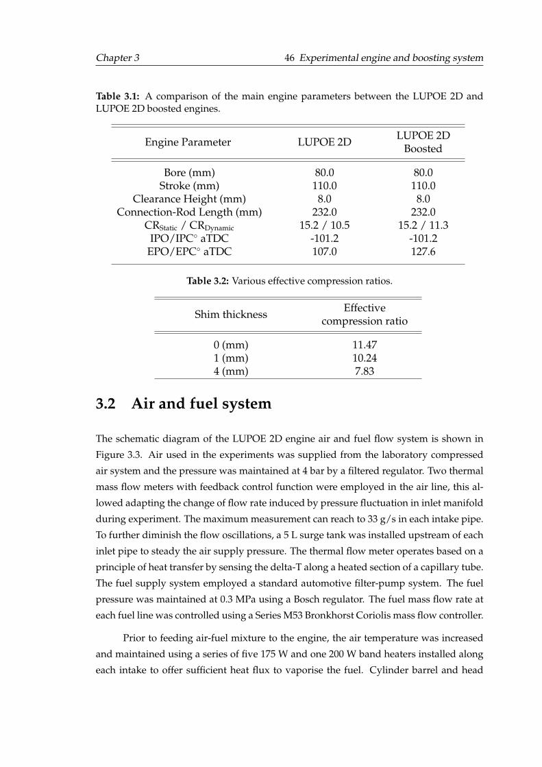
Chapter 3 46 Experimental engine and boosting system
Table 3.1: A comparison of the main engine parameters between the LUPOE 2D andLUPOE 2D boosted engines.
Engine Parameter LUPOE 2D LUPOE 2DBoosted
Bore (mm) 80.0 80.0Stroke (mm) 110.0 110.0
Clearance Height (mm) 8.0 8.0Connection-Rod Length (mm) 232.0 232.0
CRStatic / CRDynamic 15.2 / 10.5 15.2 / 11.3IPO/IPC◦ aTDC -101.2 -101.2
EPO/EPC◦ aTDC 107.0 127.6
Table 3.2: Various effective compression ratios.
Shim thickness Effectivecompression ratio
0 (mm) 11.471 (mm) 10.244 (mm) 7.83
3.2 Air and fuel system
The schematic diagram of the LUPOE 2D engine air and fuel flow system is shown in
Figure 3.3. Air used in the experiments was supplied from the laboratory compressed
air system and the pressure was maintained at 4 bar by a filtered regulator. Two thermal
mass flow meters with feedback control function were employed in the air line, this al-
lowed adapting the change of flow rate induced by pressure fluctuation in inlet manifold
during experiment. The maximum measurement can reach to 33 g/s in each intake pipe.
To further diminish the flow oscillations, a 5 L surge tank was installed upstream of each
inlet pipe to steady the air supply pressure. The thermal flow meter operates based on a
principle of heat transfer by sensing the delta-T along a heated section of a capillary tube.
The fuel supply system employed a standard automotive filter-pump system. The fuel
pressure was maintained at 0.3 MPa using a Bosch regulator. The fuel mass flow rate at
each fuel line was controlled using a Series M53 Bronkhorst Coriolis mass flow controller.
Prior to feeding air-fuel mixture to the engine, the air temperature was increased
and maintained using a series of five 175 W and one 200 W band heaters installed along
each intake to offer sufficient heat flux to vaporise the fuel. Cylinder barrel and head
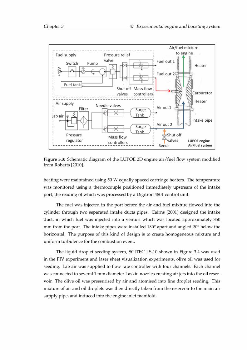
Chapter 3 47 Experimental engine and boosting system
Fuel tank
Switch Pump
Pressure relief
valve
Shut off
valves
Mass flow
controllers
Mass flow
controllers
Surge
Tank
Surge
TankLab air
Pressure
regulator
FilterNeedle valves
Fuel out 1
Fuel out 2
Air out1
Air out 2
Air/fuel mixture
to engine
Carburetor
Heater
Heater
Intake pipe
Fuel supply
Air supply
LUPOE engine
Air/fuel systemSeeds
Shut off
valves
Figure 3.3: Schematic diagram of the LUPOE 2D engine air/fuel flow system modifiedfrom Roberts [2010].
heating were maintained using 50 W equally spaced cartridge heaters. The temperature
was monitored using a thermocouple positioned immediately upstream of the intake
port, the reading of which was processed by a Digitron 4801 control unit.
The fuel was injected in the port before the air and fuel mixture flowed into the
cylinder through two separated intake ducts pipes. Cairns [2001] designed the intake
duct, in which fuel was injected into a venturi which was located approximately 350
mm from the port. The intake pipes were installed 180o apart and angled 20o below the
horizontal. The purpose of this kind of design is to create homogeneous mixture and
uniform turbulence for the combustion event.
The liquid droplet seeding system, SCITEC LS-10 shown in Figure 3.4 was used
in the PIV experiment and laser sheet visualization experiments, olive oil was used for
seeding. Lab air was supplied to flow rate controller with four channels. Each channel
was connected to several 1 mm diameter Laskin nozzles creating air jets into the oil reser-
voir. The olive oil was pressurised by air and atomised into fine droplet seeding. This
mixture of air and oil droplets was then directly taken from the reservoir to the main air
supply pipe, and induced into the engine inlet manifold.
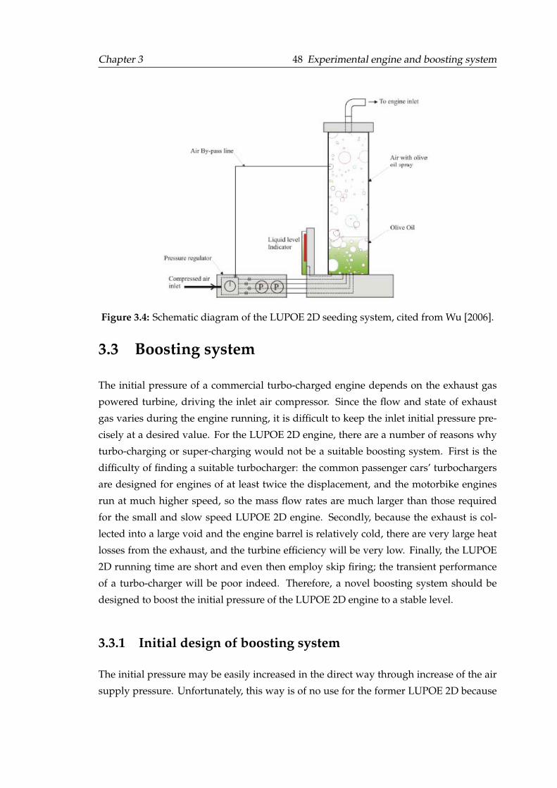
Chapter 3 48 Experimental engine and boosting system
Figure 3.4: Schematic diagram of the LUPOE 2D seeding system, cited from Wu [2006].
3.3 Boosting system
The initial pressure of a commercial turbo-charged engine depends on the exhaust gas
powered turbine, driving the inlet air compressor. Since the flow and state of exhaust
gas varies during the engine running, it is difficult to keep the inlet initial pressure pre-
cisely at a desired value. For the LUPOE 2D engine, there are a number of reasons why
turbo-charging or super-charging would not be a suitable boosting system. First is the
difficulty of finding a suitable turbocharger: the common passenger cars’ turbochargers
are designed for engines of at least twice the displacement, and the motorbike engines
run at much higher speed, so the mass flow rates are much larger than those required
for the small and slow speed LUPOE 2D engine. Secondly, because the exhaust is col-
lected into a large void and the engine barrel is relatively cold, there are very large heat
losses from the exhaust, and the turbine efficiency will be very low. Finally, the LUPOE
2D running time are short and even then employ skip firing; the transient performance
of a turbo-charger will be poor indeed. Therefore, a novel boosting system should be
designed to boost the initial pressure of the LUPOE 2D engine to a stable level.
3.3.1 Initial design of boosting system
The initial pressure may be easily increased in the direct way through increase of the air
supply pressure. Unfortunately, this way is of no use for the former LUPOE 2D because
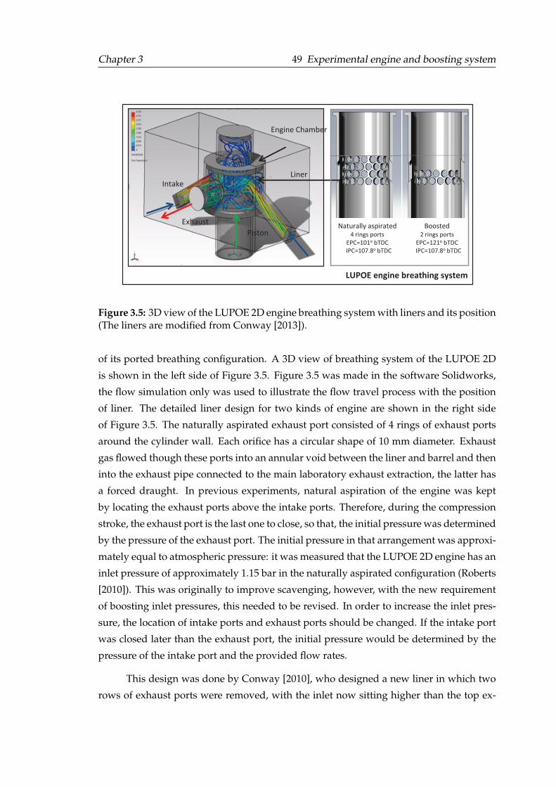
Chapter 3 49 Experimental engine and boosting system
Intake
Exhaust
Piston
Engine Chamber
Liner
Naturally aspirated
4 rings ports
EPC=101o bTDC
IPC=107.8o bTDC
Boosted
2 rings ports
EPC=121o bTDC
IPC=107.8o bTDC
LUPOE engine breathing system
Figure 3.5: 3D view of the LUPOE 2D engine breathing system with liners and its position(The liners are modified from Conway [2013]).
of its ported breathing configuration. A 3D view of breathing system of the LUPOE 2D
is shown in the left side of Figure 3.5. Figure 3.5 was made in the software Solidworks,
the flow simulation only was used to illustrate the flow travel process with the position
of liner. The detailed liner design for two kinds of engine are shown in the right side
of Figure 3.5. The naturally aspirated exhaust port consisted of 4 rings of exhaust ports
around the cylinder wall. Each orifice has a circular shape of 10 mm diameter. Exhaust
gas flowed though these ports into an annular void between the liner and barrel and then
into the exhaust pipe connected to the main laboratory exhaust extraction, the latter has
a forced draught. In previous experiments, natural aspiration of the engine was kept
by locating the exhaust ports above the intake ports. Therefore, during the compression
stroke, the exhaust port is the last one to close, so that, the initial pressure was determined
by the pressure of the exhaust port. The initial pressure in that arrangement was approxi-
mately equal to atmospheric pressure: it was measured that the LUPOE 2D engine has an
inlet pressure of approximately 1.15 bar in the naturally aspirated configuration (Roberts
[2010]). This was originally to improve scavenging, however, with the new requirement
of boosting inlet pressures, this needed to be revised. In order to increase the inlet pres-
sure, the location of intake ports and exhaust ports should be changed. If the intake port
was closed later than the exhaust port, the initial pressure would be determined by the
pressure of the intake port and the provided flow rates.
This design was done by Conway [2010], who designed a new liner in which two
rows of exhaust ports were removed, with the inlet now sitting higher than the top ex-
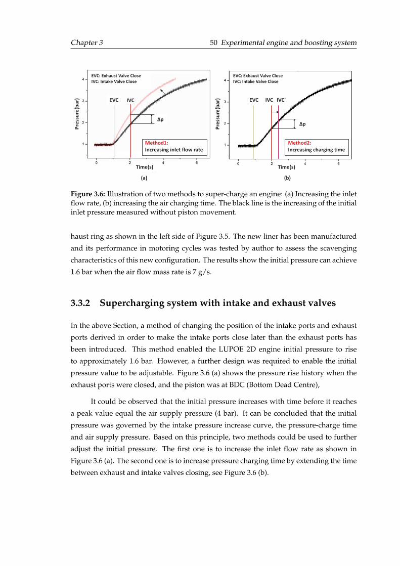
Chapter 3 50 Experimental engine and boosting system
EVC: Exhaust Valve Close
IVC: Intake Valve Close
Time(s)
(a)
Method1:
Increasing inlet flow rate
∆p
EVC IVC
Pre
ssu
re(b
ar)
Time(s)
(b)
EVC: Exhaust Valve Close
IVC: Intake Valve Close
Method2:
Increasing charging time
∆p
EVC IVC IVC'
Pre
ssu
re(b
ar)
Figure 3.6: Illustration of two methods to super-charge an engine: (a) Increasing the inletflow rate, (b) increasing the air charging time. The black line is the increasing of the initialinlet pressure measured without piston movement.
haust ring as shown in the left side of Figure 3.5. The new liner has been manufactured
and its performance in motoring cycles was tested by author to assess the scavenging
characteristics of this new configuration. The results show the initial pressure can achieve
1.6 bar when the air flow mass rate is 7 g/s.
3.3.2 Supercharging system with intake and exhaust valves
In the above Section, a method of changing the position of the intake ports and exhaust
ports derived in order to make the intake ports close later than the exhaust ports has
been introduced. This method enabled the LUPOE 2D engine initial pressure to rise
to approximately 1.6 bar. However, a further design was required to enable the initial
pressure value to be adjustable. Figure 3.6 (a) shows the pressure rise history when the
exhaust ports were closed, and the piston was at BDC (Bottom Dead Centre),
It could be observed that the initial pressure increases with time before it reaches
a peak value equal the air supply pressure (4 bar). It can be concluded that the initial
pressure was governed by the intake pressure increase curve, the pressure-charge time
and air supply pressure. Based on this principle, two methods could be used to further
adjust the initial pressure. The first one is to increase the inlet flow rate as shown in
Figure 3.6 (a). The second one is to increase pressure charging time by extending the time
between exhaust and intake valves closing, see Figure 3.6 (b).
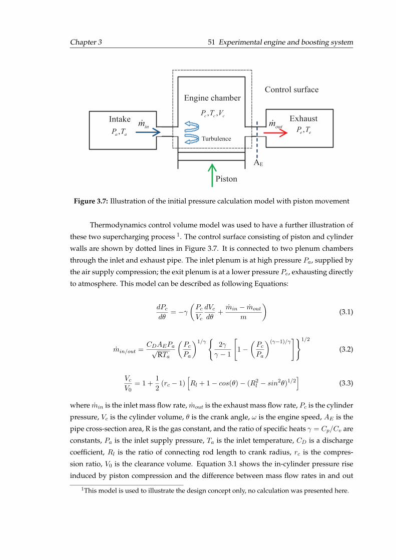
Chapter 3 51 Experimental engine and boosting system
, ,c c cP T V
,a aP T
,e eP T
Control surface
outm&
inm&
Piston
Exhaust Intake
Engine chamber
Turbulence
AE
Figure 3.7: Illustration of the initial pressure calculation model with piston movement
Thermodynamics control volume model was used to have a further illustration of
these two supercharging process 1. The control surface consisting of piston and cylinder
walls are shown by dotted lines in Figure 3.7. It is connected to two plenum chambers
through the inlet and exhaust pipe. The inlet plenum is at high pressure Pa, supplied by
the air supply compression; the exit plenum is at a lower pressure Pe, exhausting directly
to atmosphere. This model can be described as following Equations:
dPc
dθ= −γ
(Pc
Vc
dVc
dθ+
min − mout
m
)(3.1)
min/out =CDAEPa√
RTa
(Pc
Pa
)1/γ{
2γ
γ − 1
[1−
(Pc
Pa
)(γ−1)/γ]}1/2
(3.2)
Vc
V0= 1 +
1
2(rc − 1)
[Rl + 1− cos(θ)− (R2
l − sin2θ)1/2]
(3.3)
where min is the inlet mass flow rate, mout is the exhaust mass flow rate, Pc is the cylinder
pressure, Vc is the cylinder volume, θ is the crank angle, ω is the engine speed, AE is the
pipe cross-section area, R is the gas constant, and the ratio of specific heats γ = Cp/Cv are
constants, Pa is the inlet supply pressure, Ta is the inlet temperature, CD is a discharge
coefficient, Rl is the ratio of connecting rod length to crank radius, rc is the compres-
sion ratio, V0 is the clearance volume. Equation 3.1 shows the in-cylinder pressure rise
induced by piston compression and the difference between mass flow rates in and out
1This model is used to illustrate the design concept only, no calculation was presented here.
Chapter 3 52 Experimental engine and boosting system
under assumption of adiabatic compression process, see Appendix B. Equation 3.2 is for
one-dimensional steady compressible isotropic flow through an orifice or flow restriction
of effective area AE . Equation 3.3 is the engine volume change (Heywood [1988]). It can
be seen that the first method is to increase the min essentially. In order to obtain a higher
boosted pressure, the air flow rate has to be increased, it is not an efficient way and a
potential drawback is that the large mass flow rate may increase the turbulence in jet-
type intake LUPOE 2D engine and further to interfere the observation of pressure effects
on flame. The second way to increase the pressure charge time is essentially try to con-
trol the mout by adjusting the AE , the most efficiency way is to reduce the AE , this can
be realized by installing a controllable exhaust system valve. This configuration enables
the intake mass flow rate min and the initial pressure to be independently varied. The
turbulence quantities, which are heavily influenced by inlet flow velocities in the ported
engine, can be controlled to the greatest extent. From these reasons, an exhaust system
valve was selected to it developed for controlling the boosted initial pressure.
3.3.3 Selection of the exhaust system valve
The challenge for the exhaust valve design is that a contradiction exists between require-
ments of high flow rate and fast response time. The moving parts of the valve have to
be accelerated within a very short period of time to provide a prompt response. Thus
the weight of the moving parts that cover the orifice must be kept to a minimum. This
reduces the stroke, and flow rate across the valve. Furthermore, the high pressure and
temperature of the working fluid also should be taken into account. After a full com-
parison of different types of valves, a solenoid valve was selected (Ling [2011]). The
solenoid valve is controlled by an electric current through a solenoid. The solenoid con-
verts electrical energy into mechanical energy which, in turn, opens or closes the valve
mechanically. The pulse signal is very steep which will be enough for fulfilling the re-
quirement of response time. The limitation of solenoid valve is that the flow rate may
decrease if the stroke is short. The problem can be solved by using more motoring cycles
in an experiment, which means that there will be enough time to allow the fully premixed
homogeneous charge from the intake to displace completely the contents of the cylinder.
A commercial solenoid valve with a 12 mm orifice area has been chosen . A test-bed
was established to test the air flow rate through the valve, the details have been reported
in Ling [2011]. The solenoid valve was installed between the air supply source and the
engine intake pipe. A thermal mass flow meter was used to record the flow rate. The
solenoid valve opened when it was connected to 24 V power which was controlled by an
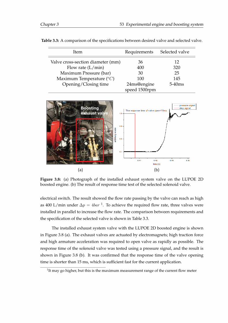
Chapter 3 53 Experimental engine and boosting system
Table 3.3: A comparison of the specifications between desired valve and selected valve.
Item Requirements Selected valve
Valve cross-section diameter (mm) 36 12Flow rate (L/min) 400 320
Maximum Pressure (bar) 30 25Maximum Temperature (oC) 100 145
Opening/Closing time 24ms@engine 5-40msspeed 1500rpm
Boosting
exhaust valve
(a) (b)
Figure 3.8: (a) Photograph of the installed exhaust system valve on the LUPOE 2Dboosted engine. (b) The result of response time test of the selected solenoid valve.
electrical switch. The result showed the flow rate passing by the valve can reach as high
as 400 L/min under ∆p = 4bar 1. To achieve the required flow rate, three valves were
installed in parallel to increase the flow rate. The comparison between requirements and
the specification of the selected valve is shown in Table 3.3.
The installed exhaust system valve with the LUPOE 2D boosted engine is shown
in Figure 3.8 (a). The exhaust valves are actuated by electromagnets; high traction force
and high armature acceleration was required to open valve as rapidly as possible. The
response time of the solenoid valve was tested using a pressure signal, and the result is
shown in Figure 3.8 (b). It was confirmed that the response time of the valve opening
time is shorter than 15 ms, which is sufficient fast for the current application.
1It may go higher, but this is the maximum measurement range of the current flow meter
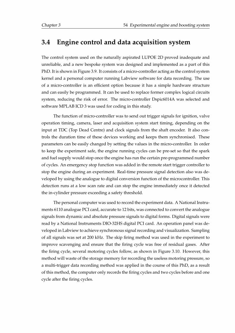
Chapter 3 54 Experimental engine and boosting system
3.4 Engine control and data acquisition system
The control system used on the naturally aspirated LUPOE 2D proved inadequate and
unreliable, and a new bespoke system was designed and implemented as a part of this
PhD. It is shown in Figure 3.9. It consists of a micro-controller acting as the control system
kernel and a personal computer running Labview software for data recording. The use
of a micro-controller is an efficient option because it has a simple hardware structure
and can easily be programmed. It can be used to replace former complex logical circuits
system, reducing the risk of error. The micro-controller Dspic6014A was selected and
software MPLAB ICD 3 was used for coding in this study.
The function of micro-controller was to send out trigger signals for ignition, valve
operation timing, camera, laser and acquisition system start timing, depending on the
input at TDC (Top Dead Centre) and clock signals from the shaft encoder. It also con-
trols the duration time of these devices working and keeps them synchronised. These
parameters can be easily changed by setting the values in the micro-controller. In order
to keep the experiment safe, the engine running cycles can be pre-set so that the spark
and fuel supply would stop once the engine has run the certain pre-programmed number
of cycles. An emergency stop function was added in the remote start trigger controller to
stop the engine during an experiment. Real-time pressure signal detection also was de-
veloped by using the analogue to digital conversion function of the microcontroller. This
detection runs at a low scan rate and can stop the engine immediately once it detected
the in-cylinder pressure exceeding a safety threshold.
The personal computer was used to record the experiment data. A National Instru-
ments 6110 analogue PCI card, accurate to 12 bits, was connected to convert the analogue
signals from dynamic and absolute pressure signals to digital forms. Digital signals were
read by a National Instruments DIO-32HS digital PCI card. An operation panel was de-
veloped in Labview to achieve synchronous signal recording and visualization. Sampling
of all signals was set at 200 kHz. The skip firing method was used in the experiment to
improve scavenging and ensure that the firing cycle was free of residual gases. After
the firing cycle, several motoring cycles follow, as shown in Figure 3.10. However, this
method will waste of the storage memory for recording the useless motoring pressure, so
a multi-trigger data recording method was applied in the course of this PhD, as a result
of this method, the computer only records the firing cycles and two cycles before and one
cycle after the firing cycles.
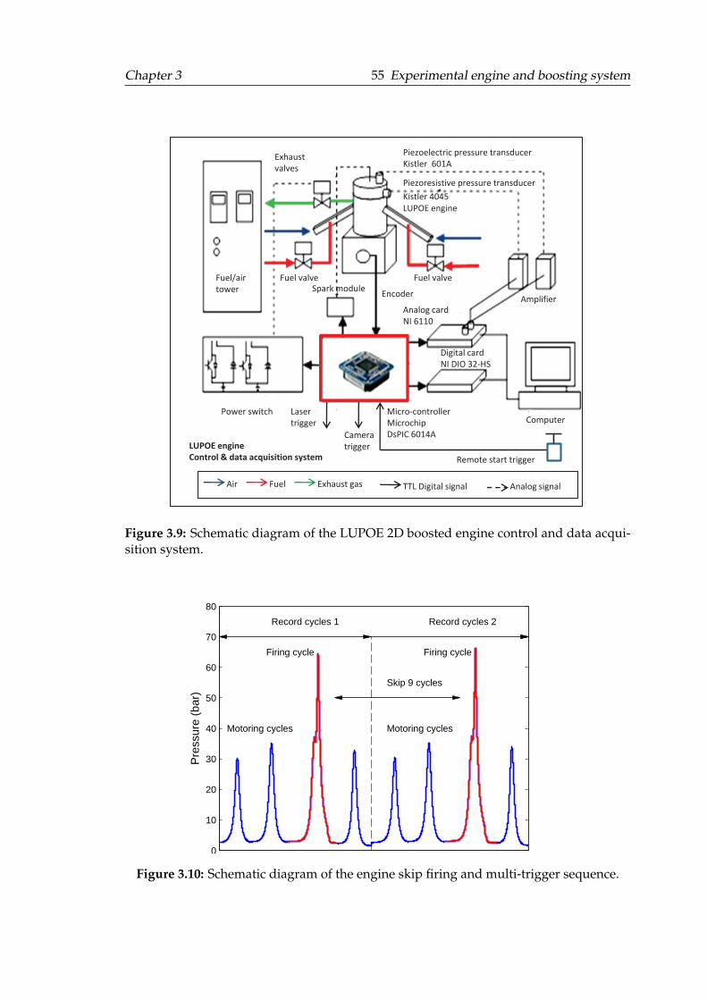
Chapter 3 55 Experimental engine and boosting system
Exhaust
valves
Fuel/air
tower Spark module
Piezoelectric pressure transducer
Kistler 601A
Piezoresistive pressure transducer
Kistler 4045
Fuel valve Fuel valve
Power switch Micro-controller
Microchip
DsPIC 6014A
Analog card
NI 6110
Digital card
NI DIO 32-HS
Amplifier
Computer
LUPOE engine
Encoder
Remote start trigger
Laser
trigger
Camera
trigger
Air Fuel Exhaust gas TTL Digital signal Analog signal
LUPOE engine
Control & data acquisition system
Figure 3.9: Schematic diagram of the LUPOE 2D boosted engine control and data acqui-sition system.
0
10
20
30
40
50
60
70
80
Record cycles 1 Record cycles 2
Firing cycle Firing cycle
Motoring cycles Motoring cycles
Skip 9 cycles
Pre
ssur
e (b
ar)
Figure 3.10: Schematic diagram of the engine skip firing and multi-trigger sequence.
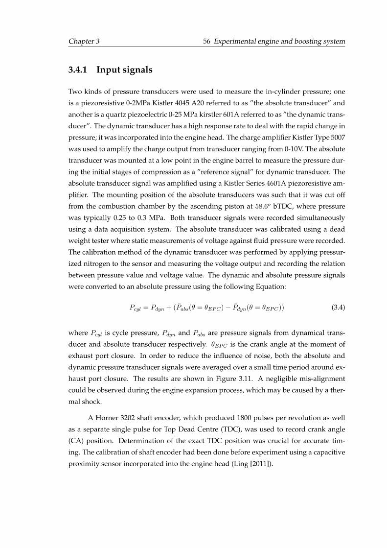
Chapter 3 56 Experimental engine and boosting system
3.4.1 Input signals
Two kinds of pressure transducers were used to measure the in-cylinder pressure; one
is a piezoresistive 0-2MPa Kistler 4045 A20 referred to as ”the absolute transducer” and
another is a quartz piezoelectric 0-25 MPa kirstler 601A referred to as ”the dynamic trans-
ducer”. The dynamic transducer has a high response rate to deal with the rapid change in
pressure; it was incorporated into the engine head. The charge amplifier Kistler Type 5007
was used to amplify the charge output from transducer ranging from 0-10V. The absolute
transducer was mounted at a low point in the engine barrel to measure the pressure dur-
ing the initial stages of compression as a ”reference signal” for dynamic transducer. The
absolute transducer signal was amplified using a Kistler Series 4601A piezoresistive am-
plifier. The mounting position of the absolute transducers was such that it was cut off
from the combustion chamber by the ascending piston at 58.6o bTDC, where pressure
was typically 0.25 to 0.3 MPa. Both transducer signals were recorded simultaneously
using a data acquisition system. The absolute transducer was calibrated using a dead
weight tester where static measurements of voltage against fluid pressure were recorded.
The calibration method of the dynamic transducer was performed by applying pressur-
ized nitrogen to the sensor and measuring the voltage output and recording the relation
between pressure value and voltage value. The dynamic and absolute pressure signals
were converted to an absolute pressure using the following Equation:
Pcyl = Pdyn + (Pabs(θ = θEPC)− Pdyn(θ = θEPC)) (3.4)
where Pcyl is cycle pressure, Pdyn and Pabs are pressure signals from dynamical trans-
ducer and absolute transducer respectively. θEPC is the crank angle at the moment of
exhaust port closure. In order to reduce the influence of noise, both the absolute and
dynamic pressure transducer signals were averaged over a small time period around ex-
haust port closure. The results are shown in Figure 3.11. A negligible mis-alignment
could be observed during the engine expansion process, which may be caused by a ther-
mal shock.
A Horner 3202 shaft encoder, which produced 1800 pulses per revolution as well
as a separate single pulse for Top Dead Centre (TDC), was used to record crank angle
(CA) position. Determination of the exact TDC position was crucial for accurate tim-
ing. The calibration of shaft encoder had been done before experiment using a capacitive
proximity sensor incorporated into the engine head (Ling [2011]).
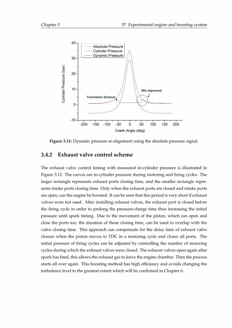
Chapter 3 57 Experimental engine and boosting system
Mis-alignment
Translation distance
Figure 3.11: Dynamic pressure re-alignment using the absolute pressure signal.
3.4.2 Exhaust valve control scheme
The exhaust valve control timing with measured in-cylinder pressure is illustrated in
Figure 3.12. The curves are in-cylinder pressure during motoring and firing cycles. The
larger rectangle represents exhaust ports closing time, and the smaller rectangle repre-
sents intake ports closing time. Only when the exhaust ports are closed and intake ports
are open, can the engine be boosted. It can be seen that this period is very short if exhaust
valves were not used. After installing exhaust valves, the exhaust port is closed before
the firing cycle in order to prolong the pressure-charge time thus increasing the initial
pressure until spark timing. Due to the movement of the piston, which can open and
close the ports too, the duration of these closing time, can be used to overlap with the
valve closing time. This approach can compensate for the delay time of exhaust valve
closure when the piston moves to TDC in a motoring cycle and closes all ports. The
initial pressure of firing cycles can be adjusted by controlling the number of motoring
cycles during which the exhaust valves were closed. The exhaust valves open again after
spark has fired, this allows the exhaust gas to leave the engine chamber. Then the process
starts all over again. This boosting method has high efficiency and avoids changing the
turbulence level to the greatest extent which will be confirmed in Chapter 6.
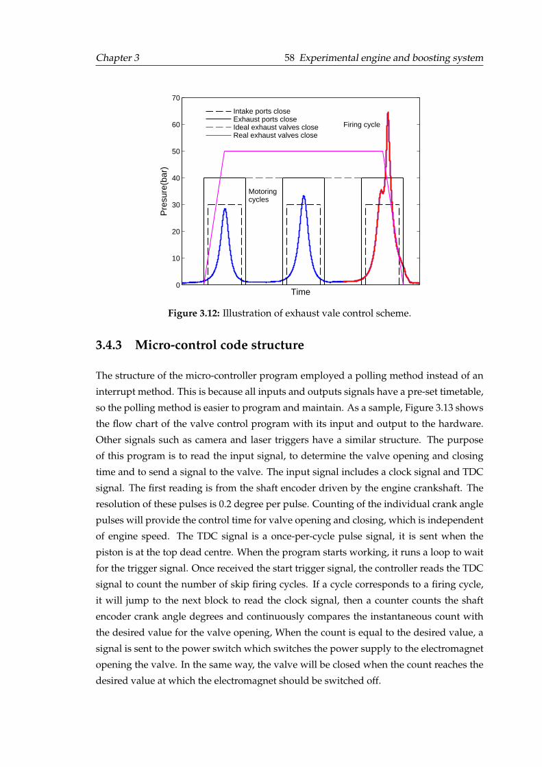
Chapter 3 58 Experimental engine and boosting system
0
10
20
30
40
50
60
70
Motoringcycles
Firing cycle
Intake ports closeExhaust ports closeIdeal exhaust valves closeReal exhaust valves close
Pre
sure
(bar
)
Time
Figure 3.12: Illustration of exhaust vale control scheme.
3.4.3 Micro-control code structure
The structure of the micro-controller program employed a polling method instead of an
interrupt method. This is because all inputs and outputs signals have a pre-set timetable,
so the polling method is easier to program and maintain. As a sample, Figure 3.13 shows
the flow chart of the valve control program with its input and output to the hardware.
Other signals such as camera and laser triggers have a similar structure. The purpose
of this program is to read the input signal, to determine the valve opening and closing
time and to send a signal to the valve. The input signal includes a clock signal and TDC
signal. The first reading is from the shaft encoder driven by the engine crankshaft. The
resolution of these pulses is 0.2 degree per pulse. Counting of the individual crank angle
pulses will provide the control time for valve opening and closing, which is independent
of engine speed. The TDC signal is a once-per-cycle pulse signal, it is sent when the
piston is at the top dead centre. When the program starts working, it runs a loop to wait
for the trigger signal. Once received the start trigger signal, the controller reads the TDC
signal to count the number of skip firing cycles. If a cycle corresponds to a firing cycle,
it will jump to the next block to read the clock signal, then a counter counts the shaft
encoder crank angle degrees and continuously compares the instantaneous count with
the desired value for the valve opening, When the count is equal to the desired value, a
signal is sent to the power switch which switches the power supply to the electromagnet
opening the valve. In the same way, the valve will be closed when the count reaches the
desired value at which the electromagnet should be switched off.
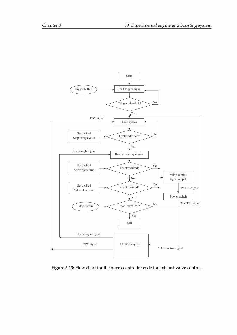
Chapter 3 59 Experimental engine and boosting system
Read cycles
Read crank angle pulse
Start
Trigger_signal=1?
Read trigger signal
Set desired
Skip firing cycles
Yes
No
Set desired
Valve open time
Cycles=desired?
count=desired?
Stop_signal =1?
Set desired
Valve close time
No
count=desired?
No
End
Valve control
signal output
Trigger button
Stop button
Yes
Yes
Yes
Power switch
TDC signal
Crank angle signal
Crank angle signal
TDC signal
5V TTL signal
24V TTL signal
LUPOE engine
No
Yes
No
Valve control signal
Figure 3.13: Flow chart for the micro-controller code for exhaust valve control.
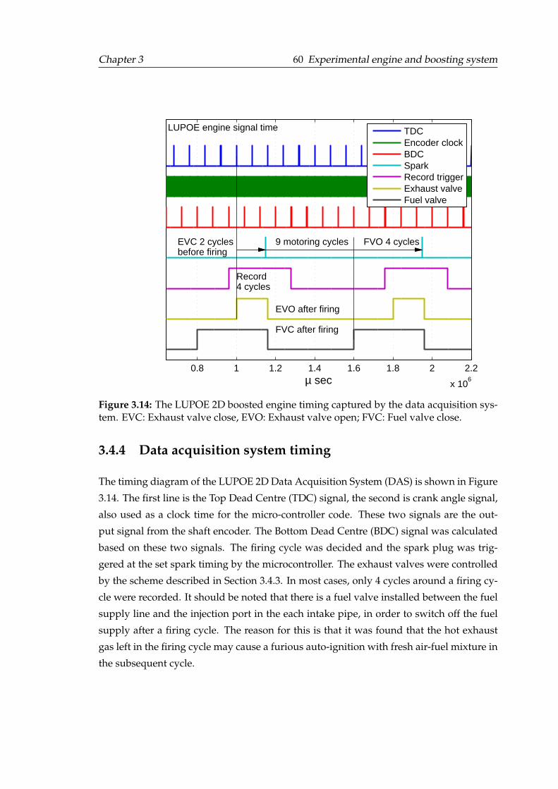
Chapter 3 60 Experimental engine and boosting system
0.8 1 1.2 1.4 1.6 1.8 2 2.2
x 106µ sec
EVC 2 cycles FVO 4 cyclesbefore firing
9 motoring cycles
EVO after firing
FVC after firing
Record4 cycles
LUPOE engine signal time TDCEncoder clockBDCSparkRecord triggerExhaust valveFuel valve
Figure 3.14: The LUPOE 2D boosted engine timing captured by the data acquisition sys-tem. EVC: Exhaust valve close, EVO: Exhaust valve open; FVC: Fuel valve close.
3.4.4 Data acquisition system timing
The timing diagram of the LUPOE 2D Data Acquisition System (DAS) is shown in Figure
3.14. The first line is the Top Dead Centre (TDC) signal, the second is crank angle signal,
also used as a clock time for the micro-controller code. These two signals are the out-
put signal from the shaft encoder. The Bottom Dead Centre (BDC) signal was calculated
based on these two signals. The firing cycle was decided and the spark plug was trig-
gered at the set spark timing by the microcontroller. The exhaust valves were controlled
by the scheme described in Section 3.4.3. In most cases, only 4 cycles around a firing cy-
cle were recorded. It should be noted that there is a fuel valve installed between the fuel
supply line and the injection port in the each intake pipe, in order to switch off the fuel
supply after a firing cycle. The reason for this is that it was found that the hot exhaust
gas left in the firing cycle may cause a furious auto-ignition with fresh air-fuel mixture in
the subsequent cycle.
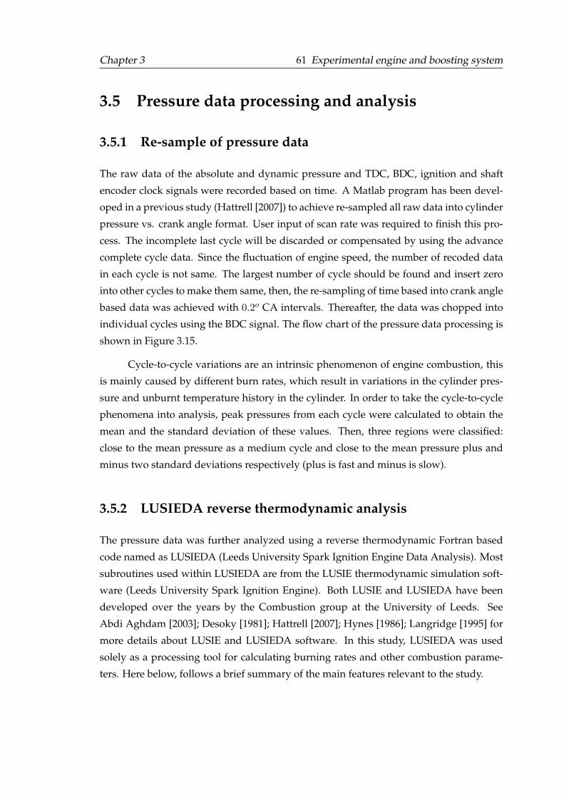
Chapter 3 61 Experimental engine and boosting system
3.5 Pressure data processing and analysis
3.5.1 Re-sample of pressure data
The raw data of the absolute and dynamic pressure and TDC, BDC, ignition and shaft
encoder clock signals were recorded based on time. A Matlab program has been devel-
oped in a previous study (Hattrell [2007]) to achieve re-sampled all raw data into cylinder
pressure vs. crank angle format. User input of scan rate was required to finish this pro-
cess. The incomplete last cycle will be discarded or compensated by using the advance
complete cycle data. Since the fluctuation of engine speed, the number of recoded data
in each cycle is not same. The largest number of cycle should be found and insert zero
into other cycles to make them same, then, the re-sampling of time based into crank angle
based data was achieved with 0.2o CA intervals. Thereafter, the data was chopped into
individual cycles using the BDC signal. The flow chart of the pressure data processing is
shown in Figure 3.15.
Cycle-to-cycle variations are an intrinsic phenomenon of engine combustion, this
is mainly caused by different burn rates, which result in variations in the cylinder pres-
sure and unburnt temperature history in the cylinder. In order to take the cycle-to-cycle
phenomena into analysis, peak pressures from each cycle were calculated to obtain the
mean and the standard deviation of these values. Then, three regions were classified:
close to the mean pressure as a medium cycle and close to the mean pressure plus and
minus two standard deviations respectively (plus is fast and minus is slow).
3.5.2 LUSIEDA reverse thermodynamic analysis
The pressure data was further analyzed using a reverse thermodynamic Fortran based
code named as LUSIEDA (Leeds University Spark Ignition Engine Data Analysis). Most
subroutines used within LUSIEDA are from the LUSIE thermodynamic simulation soft-
ware (Leeds University Spark Ignition Engine). Both LUSIE and LUSIEDA have been
developed over the years by the Combustion group at the University of Leeds. See
Abdi Aghdam [2003]; Desoky [1981]; Hattrell [2007]; Hynes [1986]; Langridge [1995] for
more details about LUSIE and LUSIEDA software. In this study, LUSIEDA was used
solely as a processing tool for calculating burning rates and other combustion parame-
ters. Here below, follows a brief summary of the main features relevant to the study.
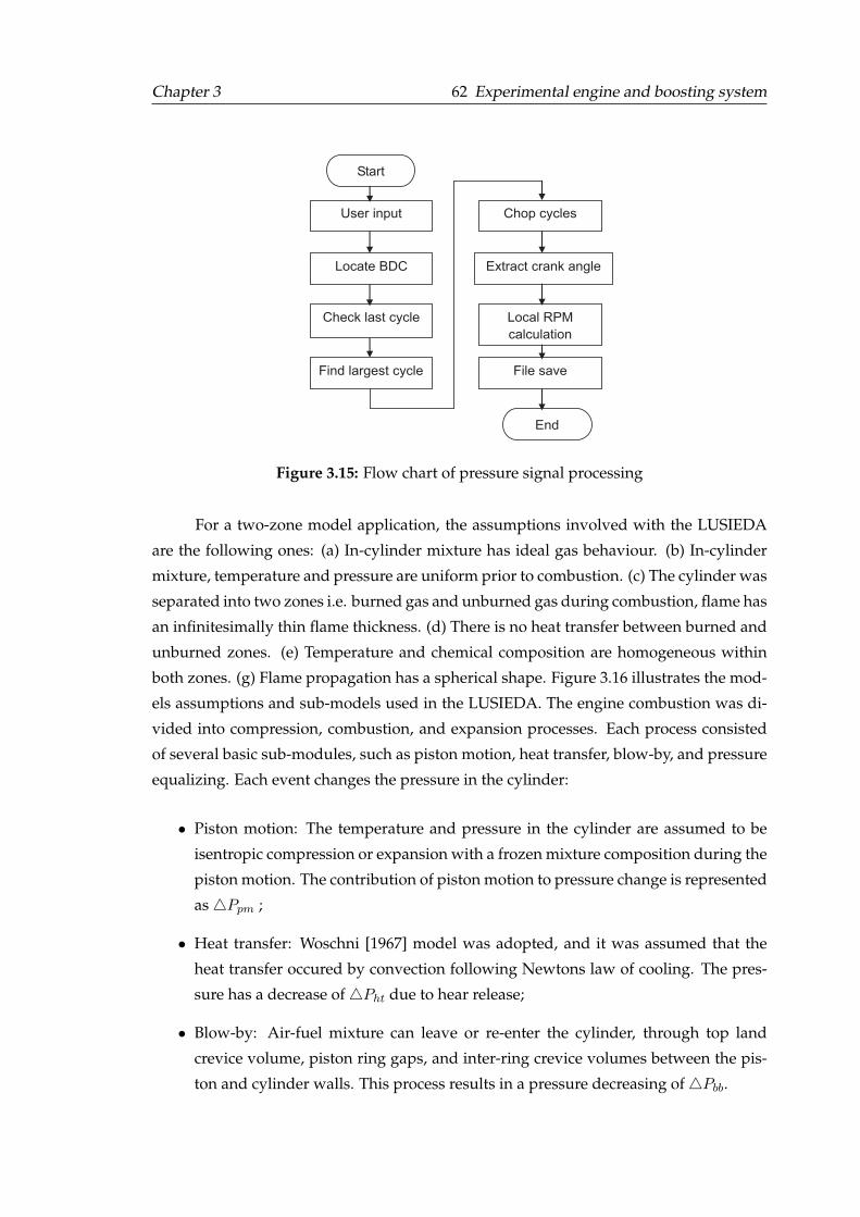
Chapter 3 62 Experimental engine and boosting system
Locate BDC
User input
Check last cycle
Find largest cycle
Chop cycles
Extract crank angle
Local RPM
calculation
File save
End
Start
Figure 3.15: Flow chart of pressure signal processing
For a two-zone model application, the assumptions involved with the LUSIEDA
are the following ones: (a) In-cylinder mixture has ideal gas behaviour. (b) In-cylinder
mixture, temperature and pressure are uniform prior to combustion. (c) The cylinder was
separated into two zones i.e. burned gas and unburned gas during combustion, flame has
an infinitesimally thin flame thickness. (d) There is no heat transfer between burned and
unburned zones. (e) Temperature and chemical composition are homogeneous within
both zones. (g) Flame propagation has a spherical shape. Figure 3.16 illustrates the mod-
els assumptions and sub-models used in the LUSIEDA. The engine combustion was di-
vided into compression, combustion, and expansion processes. Each process consisted
of several basic sub-modules, such as piston motion, heat transfer, blow-by, and pressure
equalizing. Each event changes the pressure in the cylinder:
• Piston motion: The temperature and pressure in the cylinder are assumed to be
isentropic compression or expansion with a frozen mixture composition during the
piston motion. The contribution of piston motion to pressure change is represented
as △Ppm ;
• Heat transfer: Woschni [1967] model was adopted, and it was assumed that the
heat transfer occured by convection following Newtons law of cooling. The pres-
sure has a decrease of △Pht due to hear release;
• Blow-by: Air-fuel mixture can leave or re-enter the cylinder, through top land
crevice volume, piston ring gaps, and inter-ring crevice volumes between the pis-
ton and cylinder walls. This process results in a pressure decreasing of △Pbb.
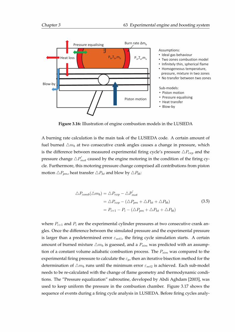
Chapter 3 63 Experimental engine and boosting system
Pb,Tb,mb Pu,Tu,mu
Piston motion
Burn rate ∆mb
Heat loss
Blow-by
Pressure equalising
Assumptions:
• Ideal gas behaviour
• Two zones combustion model
• Infinitely thin, spherical flame
• Homogeneous temperature,
pressure, mixture in two zones
• No transfer between two zones
Sub-models:
• Piston motion
• Pressure equalising
• Heat transfer
• Blow-by
Figure 3.16: Illustration of engine combustion models in the LUSIEDA
A burning rate calculation is the main task of the LUSIEDA code. A certain amount of
fuel burned △mb at two consecutive crank angles causes a change in pressure, which
is the difference between measured experimental firing cycle’s pressure △Pexp and the
pressure change △P′mot caused by the engine motoring in the condition of the firing cy-
cle. Furthermore, this motoring pressure change comprised all contributions from piston
motion △Ppm, heat transfer △Pht and blow by △Pbb:
△Pcomb(△mb) = △Pexp −△P′mot
= △Pexp − (△Ppm +△Pht +△Pbb)
= Pi+1 − Pi − (△Ppm +△Pht +△Pbb)
(3.5)
where Pi+1 and Pi are the experimental cylinder pressures at two consecutive crank an-
gles. Once the difference between the simulated pressure and the experimental pressure
is larger than a predetermined error εset1, the firing cycle simulation starts. A certain
amount of burned mixture △mb is guessed, and a Psim was predicted with an assump-
tion of a constant volume adiabatic combustion process. The Psim was compared to the
experimental firing pressure to calculate the εp, then an iterative bisection method for the
determination of △mb runs until the minimum error εset2 is achieved. Each sub-model
needs to be re-calculated with the change of flame geometry and thermodynamic condi-
tions. The ”Pressure equalization” subroutine, developed by Abdi Aghdam [2003], was
used to keep uniform the pressure in the combustion chamber. Figure 3.17 shows the
sequence of events during a firing cycle analysis in LUSIEDA. Before firing cycles analy-
Chapter 3 64 Experimental engine and boosting system
Blowby
Heat tranfer
Pressure equalisation
Guess pmD
Adiabatic flame
temperature
Calculate simP
Start
exp
exp
motP P
Pe
-=
Store bmD
0pmD =
Initial conditions
2p sete e<
1p sete e<
exp
exp
simP P
Pe
-=
Last CA?
End
N
N
Y
Y
Y
N
Firing cycle
Figure 3.17: Flowchart showing the sequence of events during a firing cycle analysis inLUSIEDA, reproduced from Roberts [2010].
sis, a motoring simulation was required to validate the heat transfer, blow-by, and other
engine operation initial conditions parameters setting. Decoupling of the cylinder pres-
sure and temperature rise due to piston motion from that due to combustion have been
shown to be vital for a successful LUSIEDA calculation (Roberts [2010]).
Thermodynamic analysis of measured cylinder pressure in LUSIEDA gives a flame
radius which lies between the entrainment and end of combustion radius. An example of
the burned gas radius calculated from the pressure trace processed by LUSIEDA is shown
in the left side of Figure 3.18, where the entrainment flame radius derived from the same
cycle’s CH*images is also presented. A small radius about 5 mm at the spark timing
existed due to the error between the experimental pressure and simulated pressure, only
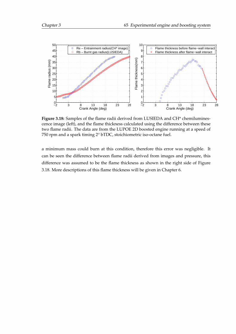
Chapter 3 65 Experimental engine and boosting system
−2 3 8 13 18 23 280
5
10
15
20
25
30
35
40
45
50
Crank Angle (deg)
Fla
me
radi
us (
mm
)
Re – Entrainment radius(CH* image)Rb – Burnt gas radius(LUSIEDA)
−2 3 8 13 18 23 280
1
2
3
4
5
6
7
8
9
10
Crank Angle (deg)
Fla
me
thic
knes
s(m
m)
Flame thickness before flame−wall interactFlame thickness after flame−wall interact
Figure 3.18: Samples of the flame radii derived from LUSIEDA and CH* chemilumines-cence image (left), and the flame thickness calculated using the difference between thesetwo flame radii. The data are from the LUPOE 2D boosted engine running at a speed of750 rpm and a spark timing 2o bTDC, stoichiometric iso-octane fuel.
a minimum mass could burn at this condition, therefore this error was negligible. It
can be seen the difference between flame radii derived from images and pressure, this
difference was assumed to be the flame thickness as shown in the right side of Figure
3.18. More descriptions of this flame thickness will be given in Chapter 6.
Chapter 4
Optical measurements and data
processing
This Chapter presents the optical measurement techniques and their data processing
methods to characterize the flow field and flame propagation process. Firstly, the prin-
ciples and relevant experimental considerations in the Particle Image Velocimetry (PIV)
measurement are introduced. Secondly, two flame imaging methods are described: the
CH* chemiluminescence imaging, and a two-dimensional laser sheet visualization tech-
nique 1. Data processing methods for these optical measurements are also developed.
4.1 Flow field measurement
Time-averaged single-point measurements using Laser Doppler Velocimetry (LDV), and
Hot Wire Anemometry (HWA), have been applied to the study of in-cylinder flow in
internal combustion engines (Witze [1980]), which provided a wealth of useful informa-
tion. However, flows in-cylinder are highly complex, unsteady, and exhibit cycle-to-cycle
variations, hence, single point measurements are not sufficient for the investigation of
in-cylinder flows in detail. Therefore, the measurement techniques of the two dimen-
sional flow fields have been developed, such as Particle Image Velocimetry (PIV). This
1It was also called ”laser tomography” or ”Mie scattering” in the literature, the term ”lasersheet method” was adopted in this study.
Chapter 4 67Optical measurements and data processing
technique provides new insights into flow processes within internal combustion engine
cylinders.
Particle Image Velocimetry was first applied to investigate the high axial swirl in an
internal combustion engine by Reuss and Rosalik [2000]. This work showed the method
to calculate instantaneous vorticity and strain rate fields ahead of the flame front, the
resolution achieved was of the order of 1 mm. Subsequently, Reuss and Rosalik [2000]
examined the cyclic variability in a semi quantitative manner by capturing the flow field
in each cycle. Towers and Towers [2004] applied a high speed PIV system with a framing
rate of 13.5 kHz and a spatial resolution of 128 x 128 pixels to study cyclic variability
of in-cylinder flows using an optical engine with a head having two inlet valves. The
results showed that changing the axial swirl level has a significant influence on the cyclic
variability of the flow in the latter half of the compression stroke. The whole field had
a maximum velocity of nearly 10 m/s. Fajardo and Sick [2009] developed a high-speed
PIV technique using two high-repetition rate diode-pumped Nd:YAG lasers operated at
355 nm and a CMOS camera with a framing rate of 12 kHz and a spatial resolution of 480
x 480 pixels to measurements of velocity fields near the spark plug in a firing engine at a
rate of 6 kHz for 500 consecutive cycles.
For a Particle Image Velocimetry system, a continuous or pulsed laser light source
is used to illuminate flow mixing particles in a thin measurement plane, traces of the par-
ticles are recorded and a comparison between two pictures is conducted using a statistical
correlation technique to calculate the velocity of the particles. Significant interpolation or
ensemble averaging of many data sets is required to re-construct the information of two
dimensional velocities. Since individual particle images do not need to be identified, a
high particle seeding density can be used to gain a high resolution two dimensional flow
velocity map (Raffel et al. [2007]). Owing to these advantages, PIV was chosen as the
two-dimensional flow visualization technique in this research.
4.1.1 PIV experimental setup
The PIV experiment consists of several subsystems: the proper tracer particles, a double-
pulse laser, a camera and image evaluation process. Figure 4.1 illustrates the PIV exper-
iment setup for the in-cylinder flows measurement in the LUPOE 2D engine in a two-
dimensional horizontal plane, with its data process. In this section, the setup of PIV
system is described firstly.
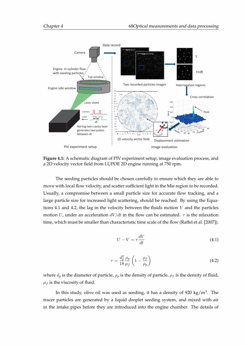
Chapter 4 68Optical measurements and data processing
.
. . . .. .. ... ..
Engine in-cylinder flow
with seeding particles
Laser sheet
dt
Nd-Yag twin cavity laser
generates two pulses
between dt
Camera
Two recorded particles images
t
t+dt
Interrogation regions
Cross correlation
Displacement estimation2D velocity vector field
Engine side window
Top window
Peak
PIV experiment setup Image evaluation
Laser
Camera
Data record
Figure 4.1: A schematic diagram of PIV experiment setup, image evaluation process, anda 2D velocity vector field from LUPOE 2D engine running at 750 rpm.
The seeding particles should be chosen carefully to ensure which they are able to
move with local flow velocity, and scatter sufficient light in the Mie region to be recorded.
Usually, a compromise between a small particle size for accurate flow tracking, and a
large particle size for increased light scattering, should be reached. By using the Equa-
tions 4.1 and 4.2, the lag in the velocity between the fluids motion V and the particles
motion U , under an acceleration dV/dt in the flow can be estimated. τ is the relaxation
time, which must be smaller than characteristic time scale of the flow (Raffel et al. [2007]).
U − V = τdV
dt(4.1)
τ =d2p18
ρpµf
(1− ρf
ρp
)(4.2)
where dp is the diameter of particle, ρp is the density of particle, ρf is the density of fluid,
µf is the viscosity of fluid.
In this study, olive oil was used as seeding, it has a density of 920 kg/m3. The
tracer particles are generated by a liquid droplet seeding system, and mixed with air
in the intake pipes before they are introduced into the engine chamber. The details of
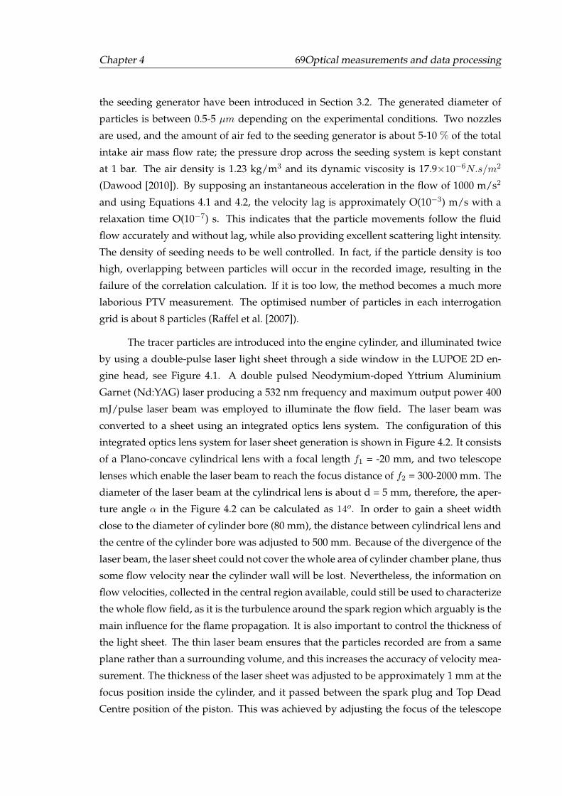
Chapter 4 69Optical measurements and data processing
the seeding generator have been introduced in Section 3.2. The generated diameter of
particles is between 0.5-5 µm depending on the experimental conditions. Two nozzles
are used, and the amount of air fed to the seeding generator is about 5-10 % of the total
intake air mass flow rate; the pressure drop across the seeding system is kept constant
at 1 bar. The air density is 1.23 kg/m3 and its dynamic viscosity is 17.9×10⁻⁶N.s/m2
(Dawood [2010]). By supposing an instantaneous acceleration in the flow of 1000 m/s2
and using Equations 4.1 and 4.2, the velocity lag is approximately O(10−3) m/s with a
relaxation time O(10−7) s. This indicates that the particle movements follow the fluid
flow accurately and without lag, while also providing excellent scattering light intensity.
The density of seeding needs to be well controlled. In fact, if the particle density is too
high, overlapping between particles will occur in the recorded image, resulting in the
failure of the correlation calculation. If it is too low, the method becomes a much more
laborious PTV measurement. The optimised number of particles in each interrogation
grid is about 8 particles (Raffel et al. [2007]).
The tracer particles are introduced into the engine cylinder, and illuminated twice
by using a double-pulse laser light sheet through a side window in the LUPOE 2D en-
gine head, see Figure 4.1. A double pulsed Neodymium-doped Yttrium Aluminium
Garnet (Nd:YAG) laser producing a 532 nm frequency and maximum output power 400
mJ/pulse laser beam was employed to illuminate the flow field. The laser beam was
converted to a sheet using an integrated optics lens system. The configuration of this
integrated optics lens system for laser sheet generation is shown in Figure 4.2. It consists
of a Plano-concave cylindrical lens with a focal length f1 = -20 mm, and two telescope
lenses which enable the laser beam to reach the focus distance of f2 = 300-2000 mm. The
diameter of the laser beam at the cylindrical lens is about d = 5 mm, therefore, the aper-
ture angle α in the Figure 4.2 can be calculated as 14o. In order to gain a sheet width
close to the diameter of cylinder bore (80 mm), the distance between cylindrical lens and
the centre of the cylinder bore was adjusted to 500 mm. Because of the divergence of the
laser beam, the laser sheet could not cover the whole area of cylinder chamber plane, thus
some flow velocity near the cylinder wall will be lost. Nevertheless, the information on
flow velocities, collected in the central region available, could still be used to characterize
the whole flow field, as it is the turbulence around the spark region which arguably is the
main influence for the flame propagation. It is also important to control the thickness of
the light sheet. The thin laser beam ensures that the particles recorded are from a same
plane rather than a surrounding volume, and this increases the accuracy of velocity mea-
surement. The thickness of the laser sheet was adjusted to be approximately 1 mm at the
focus position inside the cylinder, and it passed between the spark plug and Top Dead
Centre position of the piston. This was achieved by adjusting the focus of the telescope
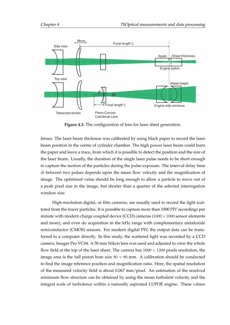
Chapter 4 70Optical measurements and data processing
Engine side windows
Engine piston
Focal length f2
Sheet thicknessSpark
Plano-Convex
Cylindrical LensTelescope lenses
Focal length f1
d
Top view
Side view
Sheet height
Move
a
Figure 4.2: The configuration of lens for laser sheet generation.
lenses. The laser beam thickness was calibrated by using black paper to record the laser
beam position in the centre of cylinder chamber. The high power laser beam could burn
the paper and leave a trace, from which it is possible to detect the position and the size of
the laser beam. Usually, the duration of the single laser pulse needs to be short enough
to capture the motion of the particles during the pulse exposure. The interval delay time
dt between two pulses depends upon the mean flow velocity and the magnification of
image. The optimised value should be long enough to allow a particle to move out of
a peak pixel size in the image, but shorter than a quarter of the selected interrogation
window size.
High-resolution digital, or film cameras, are usually used to record the light scat-
tered from the tracer particles. It is possible to capture more than 1000 PIV recordings per
minute with modern charge coupled device (CCD) cameras (1000×1000 sensor elements
and more), and even do acquisition in the kHz range with complementary metaloxide
semiconductor (CMOS) sensors. For modern digital PIV, the output data can be trans-
ferred to a computer directly. In this study, the scattered light was recorded by a CCD
camera, Imager Pro VC04. A 50 mm Nikon lens was used and adjusted to view the whole
flow field at the top of the laser sheet. The camera has 1600 × 1200 pixels resolution, the
image area is the full piston bore size 80 × 80 mm. A calibration should be conducted
to find the image reference position and magnification ratio. Here, the spatial resolution
of the measured velocity field is about 0.067 mm/pixel. An estimation of the resolved
minimum flow structure can be obtained by using the mean turbulent velocity and the
integral scale of turbulence within a naturally aspirated LUPOE engine. These values
Chapter 4 71Optical measurements and data processing
have been measured as about U = 1 - 5 m/s, Li = 10 mm by Hussin [2012]. The Taylor
microscale and Kolmogorov length scale can be estimated as O(0.1) mm from Equations
2.15, and O(0.01) mm from Equation 2.16, respectively. The minimum interrogation size
that can be used without accuracy loss is 16 pixels square, with 50% overlap. Thus, the
minimum resolution of a vector velocity is about O(0.5) mm. Therefore, it is impossible
to study the turbulence structures smaller than Taylor and Kolmogorov length scales.
However, for investigating the bulk flow behaviour with the new boosting system, this
experimental setup still has sufficient spatial resolution to detect the large flow structures.
There are two images recorded for each engine cycle. The first image shows the ini-
tial positions of the particles, and the second records the final positions after the particles
movement in the flow. These two trigger signals for the camera are synchronized with
the laser pulse, as shown in the Figure 4.1. The software was set up in such a way that
the first frame of the PIV image pair was exposed for microseconds and then the second
image was exposed for a longer period of time to record the image (Dawood [2010]). The
noise could be reduced using a mechanical shutter or preventing external light to reach
the camera during the experiment. A low pass optical filter attached to the camera was
used to allow the passage of the scattered laser light whilst prevent any illumination pro-
duced by the flame. The lab lights should be switched off during the experiment, and
black plates covered the space around the engine to reduce the light reflection from the
surroundings.
4.1.2 Image evaluation
After the digital PIV images are recorded, interrogation areas are created by dividing the
image into many small subareas. It is assumed that all the particles within one inter-
rogation area have homogeneous movements between the two illuminations. Statistical
methods, such as auto and cross correlation, are implemented to derive the local dis-
placement vector from each two sets of interrogation regions. In most commercial PIV
software, correlation plane calculation is achieved in the frequency domain by using Fast
Fourier Transforms (FFT) (Raffel et al. [2007]), it can be represented as:
RII ⇔ I · I ′∗ (4.3)
where I and I ′ are the Fourier transforms of the function I and I ′, respectively. The
location of the peak in the correlation plane corresponds to the average particle displace-
ment, see Figure 4.1. Then, a single average particle displacement and velocity could be
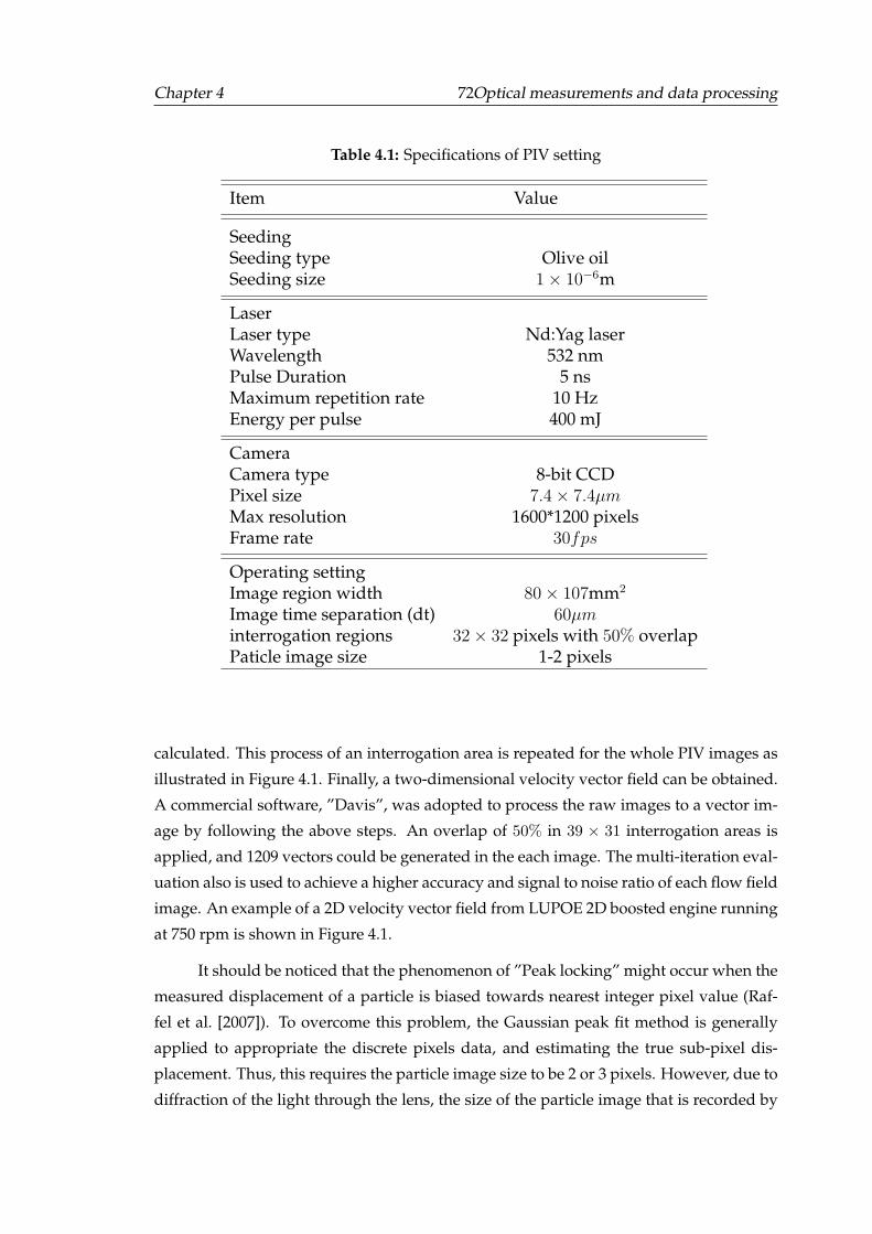
Chapter 4 72Optical measurements and data processing
Table 4.1: Specifications of PIV setting
Item Value
SeedingSeeding type Olive oilSeeding size 1× 10⁻⁶m
LaserLaser type Nd:Yag laserWavelength 532 nmPulse Duration 5 nsMaximum repetition rate 10 HzEnergy per pulse 400 mJ
CameraCamera type 8-bit CCDPixel size 7.4× 7.4µmMax resolution 1600*1200 pixelsFrame rate 30fps
Operating settingImage region width 80× 107mm2
Image time separation (dt) 60µminterrogation regions 32× 32 pixels with 50% overlapPaticle image size 1-2 pixels
calculated. This process of an interrogation area is repeated for the whole PIV images as
illustrated in Figure 4.1. Finally, a two-dimensional velocity vector field can be obtained.
A commercial software, ”Davis”, was adopted to process the raw images to a vector im-
age by following the above steps. An overlap of 50% in 39 × 31 interrogation areas is
applied, and 1209 vectors could be generated in the each image. The multi-iteration eval-
uation also is used to achieve a higher accuracy and signal to noise ratio of each flow field
image. An example of a 2D velocity vector field from LUPOE 2D boosted engine running
at 750 rpm is shown in Figure 4.1.
It should be noticed that the phenomenon of ”Peak locking” might occur when the
measured displacement of a particle is biased towards nearest integer pixel value (Raf-
fel et al. [2007]). To overcome this problem, the Gaussian peak fit method is generally
applied to appropriate the discrete pixels data, and estimating the true sub-pixel dis-
placement. Thus, this requires the particle image size to be 2 or 3 pixels. However, due to
diffraction of the light through the lens, the size of the particle image that is recorded by
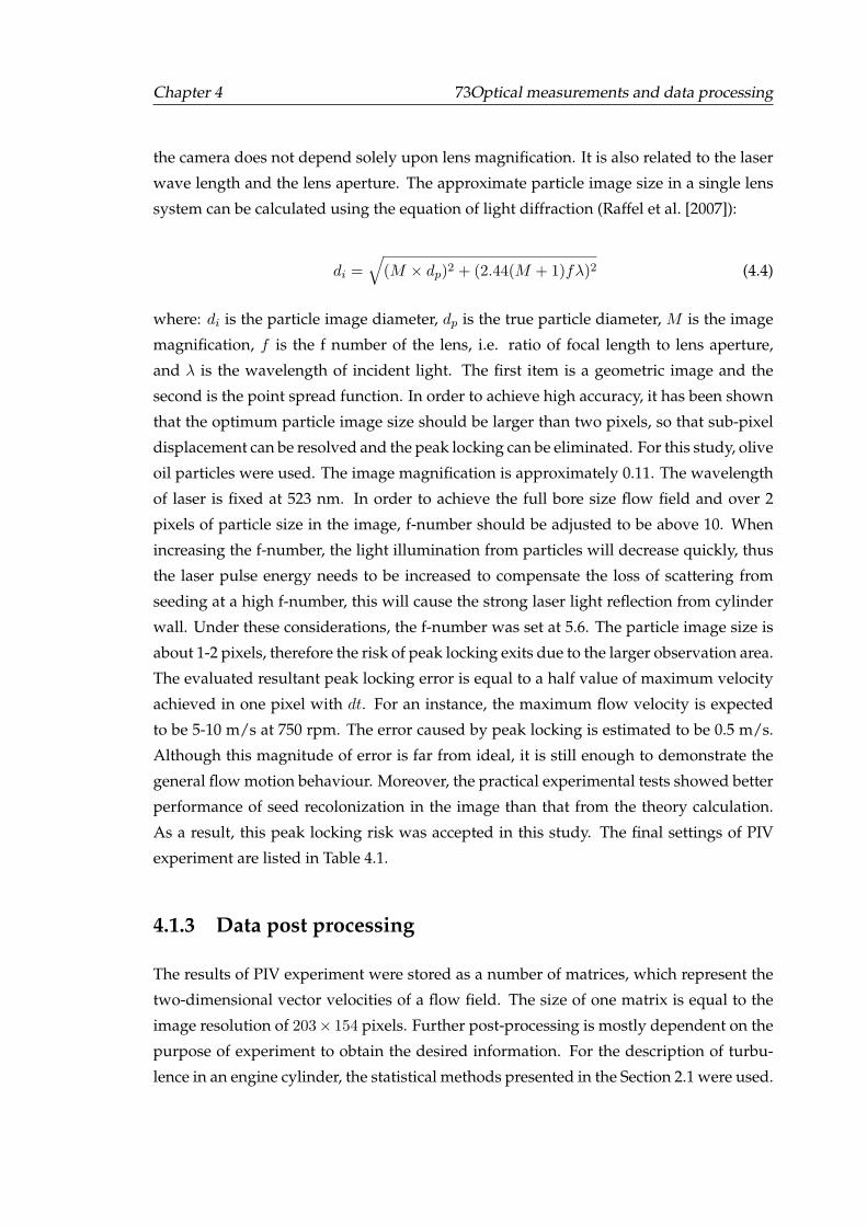
Chapter 4 73Optical measurements and data processing
the camera does not depend solely upon lens magnification. It is also related to the laser
wave length and the lens aperture. The approximate particle image size in a single lens
system can be calculated using the equation of light diffraction (Raffel et al. [2007]):
di =√
(M × dp)2 + (2.44(M + 1)fλ)2 (4.4)
where: di is the particle image diameter, dp is the true particle diameter, M is the image
magnification, f is the f number of the lens, i.e. ratio of focal length to lens aperture,
and λ is the wavelength of incident light. The first item is a geometric image and the
second is the point spread function. In order to achieve high accuracy, it has been shown
that the optimum particle image size should be larger than two pixels, so that sub-pixel
displacement can be resolved and the peak locking can be eliminated. For this study, olive
oil particles were used. The image magnification is approximately 0.11. The wavelength
of laser is fixed at 523 nm. In order to achieve the full bore size flow field and over 2
pixels of particle size in the image, f-number should be adjusted to be above 10. When
increasing the f-number, the light illumination from particles will decrease quickly, thus
the laser pulse energy needs to be increased to compensate the loss of scattering from
seeding at a high f-number, this will cause the strong laser light reflection from cylinder
wall. Under these considerations, the f-number was set at 5.6. The particle image size is
about 1-2 pixels, therefore the risk of peak locking exits due to the larger observation area.
The evaluated resultant peak locking error is equal to a half value of maximum velocity
achieved in one pixel with dt. For an instance, the maximum flow velocity is expected
to be 5-10 m/s at 750 rpm. The error caused by peak locking is estimated to be 0.5 m/s.
Although this magnitude of error is far from ideal, it is still enough to demonstrate the
general flow motion behaviour. Moreover, the practical experimental tests showed better
performance of seed recolonization in the image than that from the theory calculation.
As a result, this peak locking risk was accepted in this study. The final settings of PIV
experiment are listed in Table 4.1.
4.1.3 Data post processing
The results of PIV experiment were stored as a number of matrices, which represent the
two-dimensional vector velocities of a flow field. The size of one matrix is equal to the
image resolution of 203× 154 pixels. Further post-processing is mostly dependent on the
purpose of experiment to obtain the desired information. For the description of turbu-
lence in an engine cylinder, the statistical methods presented in the Section 2.1 were used.
Chapter 4 74Optical measurements and data processing
In general, the mean velocity varies with time and position, thus there are two methods
to evaluate flow field variables: ensemble and spatial averaging (Larsson [2009]). In this
study, the ensemble averaging method was adopted. The data calculations have been
programmed using Matlab with some functions from an open source package PIVMAT
(Moisy [2007]). The ensemble average velocity was calculated at each point on the inter-
rogation grid, and hence the results were often presented as maps, such processing was
mostly used to establish the flow properties of the engine. The ensemble mean velocities
were calculated as:
Ux(x, y) =1
Nim
Nim∑i=1
Ux(x, y, i) (4.5)
Uy(x, y) =1
Nim
Nim∑i=1
Uy(x, y, i) (4.6)
where Ux(x, y, i), Uy(x, y, i) are the instantaneous velocities at the grid point (x, y) in the
x and y direction respectively. i indicates the number of vector flow fields, and the total
number of images is Nim. Ensemble averaging removed the large-scale flow variation
due to turbulence and cyclic variation present in the velocity fields for individual cycles.
While the formulation above is written for Cartesian coordinates, it was also possible to
use polar coordinates. The velocity magnitude S is defined as:
S =√
U2x + U2
y (4.7)
The time-average fluctuation components, ux, uy are calculated as:
ux(x, y, i) = Ux(x, y, i)− Ux(x, y) (4.8)
uy(x, y, i) = Uy(x, y, i)− Uy(x, y) (4.9)
from which the RMS turbulent velocity,u′x and u
′y are calculated as:
u′x(x, y) =
{1
Nim
Nim∑i=1
[ux(x, y, i)]2
} 12
(4.10)
Chapter 4 75Optical measurements and data processing
u′y(x, y) =
{1
Nim
Nim∑i=1
[uy(x, y, i)]2
} 12
(4.11)
as was shown in the introduction in Section 2.1, there exist four kinds of integral length
scales depending on velocity direction ux or uy, and correlation direction ”transverse” or
”longitudinal” (Hussin [2012]). The corresponding correlation coefficients can be repre-
sented as Rxl, Rxt, Ryl, Ryt, they are calculated from the fluctuating velocity values at
two separated positions (x, y) and (x + ζ, y) in X-direction or (x, y) and (x, y + β) in Y -
direction. β and ζ are the variable separation distances. Here, only the equations based
on ux are given:
Rxl(x, x+ ζ) =1
(Nim − 1)
Nim∑i=1
ux(x, y, i)ux(x+ ζ, y, i)
[u′x(x, y)u
′x(x+ ζ, y)]
(4.12)
Rxt(y, y + β) =1
(Nim − 1)
Nim∑i=1
ux(x, y, i)ux(x, y + β, i)
[u′x(x, y)u
′x(x, y + β)]
(4.13)
Then the longitudinal integral length scale Lxl and transverse integral length scale Lxt
which have been illustrated in Figure 2.2, are calculated from:
Lxl(x, y) =
∫ ζ=0
0Rxl(x, x+ ζ)dζ (4.14)
Lxt(x, y) =
∫ β=0
0Rxt(y, y + β)dβ (4.15)
4.2 Flame imaging
Flame imaging experiments have been applied in optical spark ignition research engines
for many years with methods including natural light, schlieren, shadowgraph, laser sheet
Mie scatter imaging and Planar Laser Induced Fluorescence (PLIF). Early investigations
used the schlieren technique or natural light imaging (Gatowski et al. [1984]) to investi-
gate the combustion phenomena in cylinder.
Shadowgraph and schlieren techniques depend on a refraction index change caused
by density gradients in the combustion mixture to generate an image on a screen. A light
Chapter 4 76Optical measurements and data processing
source and optical lens are required to generate a parallel beam of light. The entrain-
ment flame front can be obtained from the image due to substantial difference between
burnt and unburnt gas densities instead of flame luminosity, the sensitive requirement
of camera might be not important. The difficulties of applying the shadowgraphy and
schlieren techniques are the requirement of optical access through the cylinder. In an en-
gine, configuration of a mirror installed on the top of the piston crown with an optical
head access is often adopted. However, the vibration of mirror during engine running
would bring errors into measurement, and the mirror surface degradation caused by
combustion makes this method very risky for a supercharged engine.
In natural light imaging, the chemiluminescence, i.e. the emitted light from flame
species is the only source for detection. This method has many advantages of application
with the exception of low luminosity which is not always sufficient for fast imaging, par-
ticularly in the case of lean flames (Dawood [2010]). Different wavelength filters can be
used to isolate the light of a certain wavelength. The flame front position and brush thick-
ness can be detected by tracing flame chemiluminescence generated from certain species
such as CH*, C2* in the reaction zone (Ikeda et al. [2001]). However, this is also limited
by the low level of luminosity, most applicants only are single-shot image. Modern high
speed digital cameras are extremely light sensitive and are capable of using just natural
light to detect the flame positions with short exposure times. Muard [2006] has shown
little difference in flame front images generated in simultaneous high speed schlieren and
natural light photography in an engine.
These techniques are useful for understanding the dynamic behaviour of flames,
but they yielded only little insight into the structure of the turbulent flames, because these
methods averaged the flame over the line of sight. One of the developments in the laser
diagnostics was Mie scattered light images (laser sheet visualization) of flames, which
will be introduced in the following Section 4.2.2; this method essentially produce images
of ”slice” sections of a flame, allowing more detailed characterization of the flame front
structure (Cairns [2001]). It is also possible to reconstruct a 3D flame with a number of
images taken in a range of planar sheets at a short time (Hattrell [2007]).
Another two-dimensional planar measurement method to trace the flame front is
Planar Laser Induced Fluorescence (PLIF). The principle of PLIF is to collect the spon-
taneous emission of photons when a molecule state moving from an excited electronic
level to a ground level. There is an energy loss associated with this process. There-
fore, detected emission light should be at a longer wavelength than the excitation laser
source ((Eckbreth [1996])). This technique also can be used to detect the flame reaction
zone when the excited species are CH*, C2*. Planar Laser Induced Fluorescence (PLIF)
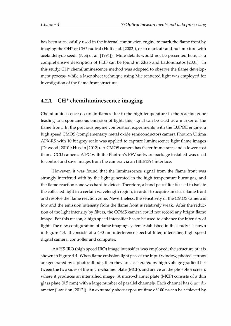
Chapter 4 77Optical measurements and data processing
has been successfully used in the internal combustion engine to mark the flame front by
imaging the OH* or CH* radical (Hult et al. [2002]), or to mark air and fuel mixture with
acetaldehyde seeds (Neij et al. [1994]). More details would not be presented here, as a
comprehensive description of PLIF can be found in Zhao and Ladommatos [2001]. In
this study, CH* chemiluminescence method was adopted to observe the flame develop-
ment process, while a laser sheet technique using Mie scattered light was employed for
investigation of the flame front structure.
4.2.1 CH* chemiluminescence imaging
Chemiluminescence occurs in flames due to the high temperature in the reaction zone
leading to a spontaneous emission of light, this signal can be used as a marker of the
flame front. In the previous engine combustion experiments with the LUPOE engine, a
high speed CMOS (complementary metal oxide semiconductor) camera Photron Ultima
APX-RS with 10 bit grey scale was applied to capture luminescence light flame images
(Dawood [2010]; Hussin [2012]). A CMOS camera has faster frame rates and a lower cost
than a CCD camera. A PC with the Photron’s PFV software package installed was used
to control and save images from the camera via an IEEE1394 interface.
However, it was found that the luminescence signal from the flame front was
strongly interfered with by the light generated in the high temperature burnt gas, and
the flame reaction zone was hard to detect. Therefore, a band pass filter is used to isolate
the collected light in a certain wavelength region, in order to acquire an clear flame front
and resolve the flame reaction zone. Nevertheless, the sensitivity of the CMOS camera is
low and the emission intensity from the flame front is relatively weak. After the reduc-
tion of the light intensity by filters, the COMS camera could not record any bright flame
image. For this reason, a high speed intensifier has to be used to enhance the intensity of
light. The new configuration of flame imaging system established in this study is shown
in Figure 4.3. It consists of a 430 nm interference spectral filter, intensifier, high speed
digital camera, controller and computer.
An HS-IRO (high speed IRO) image intensifier was employed, the structure of it is
shown in Figure 4.4. When flame emission light passes the input window, photoelectrons
are generated by a photocathode, then they are accelerated by high voltage gradient be-
tween the two sides of the micro-channel plate (MCP), and arrive on the phosphor screen,
where it produces an intensified image. A micro-channel plate (MCP) consists of a thin
glass plate (0.5 mm) with a large number of parallel channels. Each channel has 6 µm di-
ameter (Lavision [2012]). An extremely short exposure time of 100 ns can be achieved by
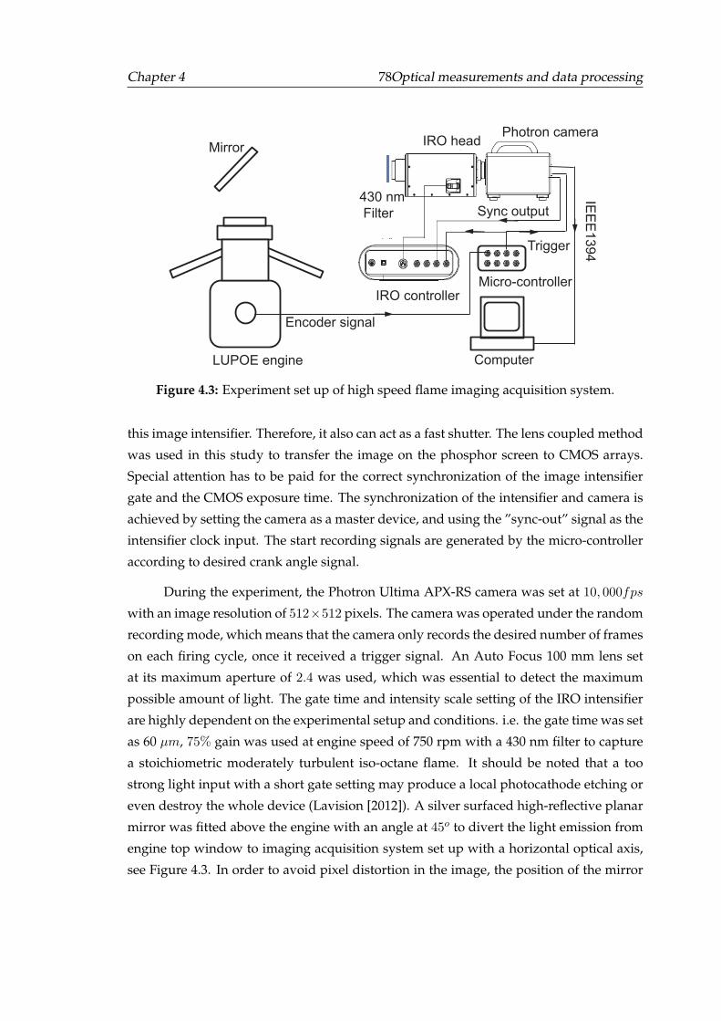
Chapter 4 78Optical measurements and data processing
Mirror
LUPOE engine
430 nm
Filter
IRO headPhotron camera
IRO controller
Computer
IEE
E1394
Sync output
Trigger
Micro-controller
Encoder signal
Figure 4.3: Experiment set up of high speed flame imaging acquisition system.
this image intensifier. Therefore, it also can act as a fast shutter. The lens coupled method
was used in this study to transfer the image on the phosphor screen to CMOS arrays.
Special attention has to be paid for the correct synchronization of the image intensifier
gate and the CMOS exposure time. The synchronization of the intensifier and camera is
achieved by setting the camera as a master device, and using the ”sync-out” signal as the
intensifier clock input. The start recording signals are generated by the micro-controller
according to desired crank angle signal.
During the experiment, the Photron Ultima APX-RS camera was set at 10, 000fps
with an image resolution of 512×512 pixels. The camera was operated under the random
recording mode, which means that the camera only records the desired number of frames
on each firing cycle, once it received a trigger signal. An Auto Focus 100 mm lens set
at its maximum aperture of 2.4 was used, which was essential to detect the maximum
possible amount of light. The gate time and intensity scale setting of the IRO intensifier
are highly dependent on the experimental setup and conditions. i.e. the gate time was set
as 60 µm, 75% gain was used at engine speed of 750 rpm with a 430 nm filter to capture
a stoichiometric moderately turbulent iso-octane flame. It should be noted that a too
strong light input with a short gate setting may produce a local photocathode etching or
even destroy the whole device (Lavision [2012]). A silver surfaced high-reflective planar
mirror was fitted above the engine with an angle at 45o to divert the light emission from
engine top window to imaging acquisition system set up with a horizontal optical axis,
see Figure 4.3. In order to avoid pixel distortion in the image, the position of the mirror
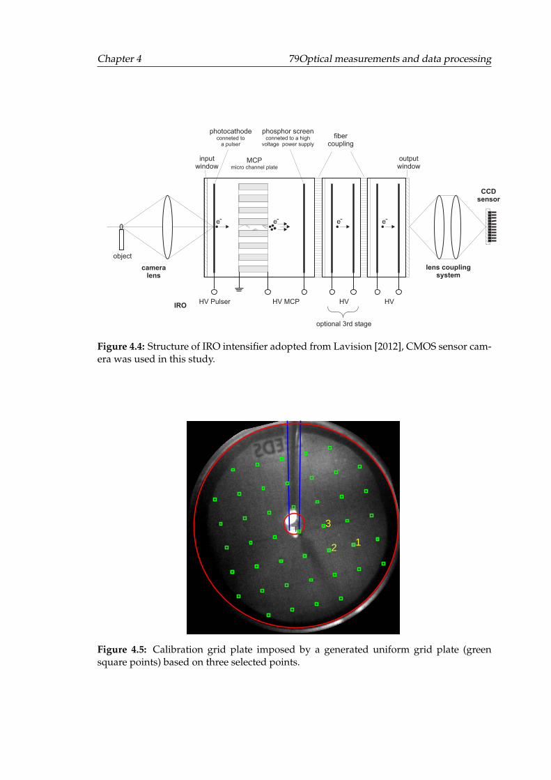
Chapter 4 79Optical measurements and data processing
e- e-
cameralens
inputwindow
object
photocathodeconneted to
a pulser
phosphor screenconneted to a high
voltage power supply
MCPmicro channel plate
lens couplingsystem
CCDsensor
HV MCPHV PulserIRO
e-
HV
outputwindow
e-
HV
fibercoupling
optional 3rd stage
Figure 4.4: Structure of IRO intensifier adopted from Lavision [2012], CMOS sensor cam-era was used in this study.
12
3
Figure 4.5: Calibration grid plate imposed by a generated uniform grid plate (greensquare points) based on three selected points.
Chapter 4 80Optical measurements and data processing
and imaging system needs to be adjusted carefully. This can be checked by the following
calibration method.
A calibration grid plate was used before the experiment, to evaluate the image dis-
tortion, as well as the magnification ratio of the image acquisition system. Figure 4.5 is a
snapshot image of the calibration grid plate put on the piston surface and covered with
the optical head. Three points in the corners of one grid are randomly and manually se-
lected. Based on these three points, a uniform grid plate shown in green square points
was generated by the computer. Comparing new grid positions to that on the original cal-
ibration grid plate, the image distortion can be evaluated. The pixel resolution also can be
estimated by dividing the distance between two points on the calibration grid plate to the
number of pixels of the recorded image. Errors exist when a large difference between the
calibration grid plate and the uniform grid plate is found. These errors usually are caused
by a shift of the optical path or refraction of light though a concave or convex window.
The error of optical path can be reduced to a negligible value by adjusting the position
of the mirror and camera acquisition system. However, to correct the optical distortion
induced by a non-planar window or imaging acquisition system, the image registration
method needs to be applied. This method calculates a spatial transformation map, which
can be used to correct distorted images. By looking at the Figure 4.5, it can be considered
that the distortion of the recorded image is negligible, after a careful adjustment of the
light path. Low distortion also comes from the fact that the top of the engine head is a flat
high-transparency quartz window. Furthermore, the acquisition system has a high image
recording performance. Therefore, the image registration method was not engaged here.
The accurate magnification ratio was obtained by using grid plate calibration before each
set of experiment. The resolution of each pixel is approximately 156 µm, which is lower
than the CCD camera used in the PIV system.
During the experiment, black spots were found on the inner surface of the top
window; there might be associated with soot particles or unburnt oil droplets left from
previous or current firing cycles. Hence, the engine top window was cleaned before
each engine running set, about 15 firing cycles. The amount of lubrication oil used in
the engine also was carefully controlled to minimize their effects on the image quality.
Moreover, the laboratory has no windows; therefore it guarantees a condition of nearly
complete darkness for the tests once the light is turned off. Thus, errors arising from
scattering, and interference from other light sources could be neglected.
A series of flame images were taken in the LUPOE 2D boosted engine running at a
speed of 750 rpm and a spark timing 2o bTDC, with stoichiometric iso-octane fuel, except
the image taken from Mandilas [2008] which used a different imaging method. Typical
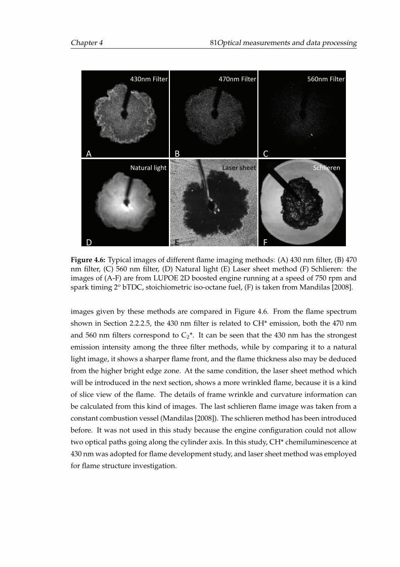
Chapter 4 81Optical measurements and data processing
430nm Filter 470nm Filter
Natural light Laser sheet Schlieren
560nm Filter
A B C
D E F
Figure 4.6: Typical images of different flame imaging methods: (A) 430 nm filter, (B) 470nm filter, (C) 560 nm filter, (D) Natural light (E) Laser sheet method (F) Schlieren: theimages of (A-F) are from LUPOE 2D boosted engine running at a speed of 750 rpm andspark timing 2o bTDC, stoichiometric iso-octane fuel, (F) is taken from Mandilas [2008].
images given by these methods are compared in Figure 4.6. From the flame spectrum
shown in Section 2.2.2.5, the 430 nm filter is related to CH* emission, both the 470 nm
and 560 nm filters correspond to C2*. It can be seen that the 430 nm has the strongest
emission intensity among the three filter methods, while by comparing it to a natural
light image, it shows a sharper flame front, and the flame thickness also may be deduced
from the higher bright edge zone. At the same condition, the laser sheet method which
will be introduced in the next section, shows a more wrinkled flame, because it is a kind
of slice view of the flame. The details of frame wrinkle and curvature information can
be calculated from this kind of images. The last schlieren flame image was taken from a
constant combustion vessel (Mandilas [2008]). The schlieren method has been introduced
before. It was not used in this study because the engine configuration could not allow
two optical paths going along the cylinder axis. In this study, CH* chemiluminescence at
430 nm was adopted for flame development study, and laser sheet method was employed
for flame structure investigation.
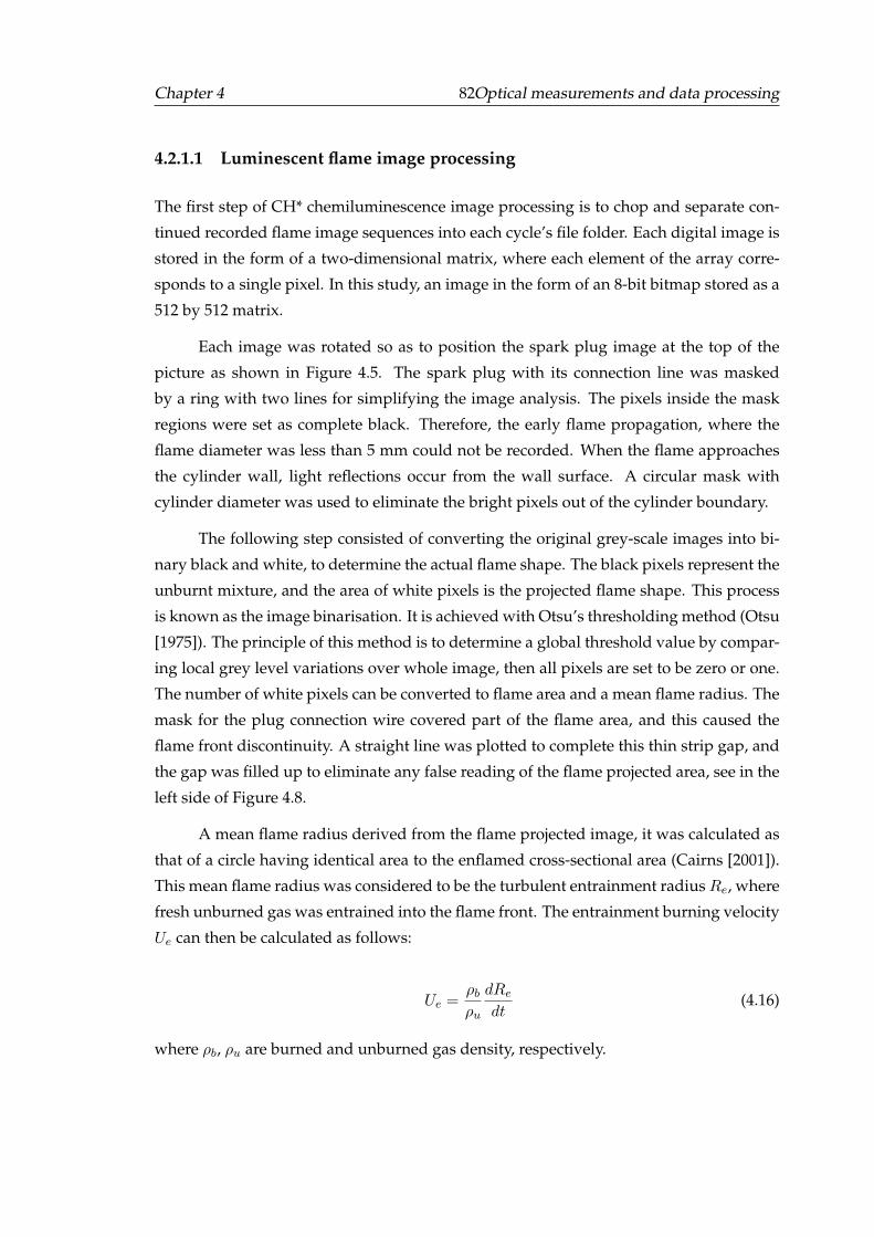
Chapter 4 82Optical measurements and data processing
4.2.1.1 Luminescent flame image processing
The first step of CH* chemiluminescence image processing is to chop and separate con-
tinued recorded flame image sequences into each cycle’s file folder. Each digital image is
stored in the form of a two-dimensional matrix, where each element of the array corre-
sponds to a single pixel. In this study, an image in the form of an 8-bit bitmap stored as a
512 by 512 matrix.
Each image was rotated so as to position the spark plug image at the top of the
picture as shown in Figure 4.5. The spark plug with its connection line was masked
by a ring with two lines for simplifying the image analysis. The pixels inside the mask
regions were set as complete black. Therefore, the early flame propagation, where the
flame diameter was less than 5 mm could not be recorded. When the flame approaches
the cylinder wall, light reflections occur from the wall surface. A circular mask with
cylinder diameter was used to eliminate the bright pixels out of the cylinder boundary.
The following step consisted of converting the original grey-scale images into bi-
nary black and white, to determine the actual flame shape. The black pixels represent the
unburnt mixture, and the area of white pixels is the projected flame shape. This process
is known as the image binarisation. It is achieved with Otsu’s thresholding method (Otsu
[1975]). The principle of this method is to determine a global threshold value by compar-
ing local grey level variations over whole image, then all pixels are set to be zero or one.
The number of white pixels can be converted to flame area and a mean flame radius. The
mask for the plug connection wire covered part of the flame area, and this caused the
flame front discontinuity. A straight line was plotted to complete this thin strip gap, and
the gap was filled up to eliminate any false reading of the flame projected area, see in the
left side of Figure 4.8.
A mean flame radius derived from the flame projected image, it was calculated as
that of a circle having identical area to the enflamed cross-sectional area (Cairns [2001]).
This mean flame radius was considered to be the turbulent entrainment radius Re, where
fresh unburned gas was entrained into the flame front. The entrainment burning velocity
Ue can then be calculated as follows:
Ue =ρbρu
dRe
dt(4.16)
where ρb, ρu are burned and unburned gas density, respectively.
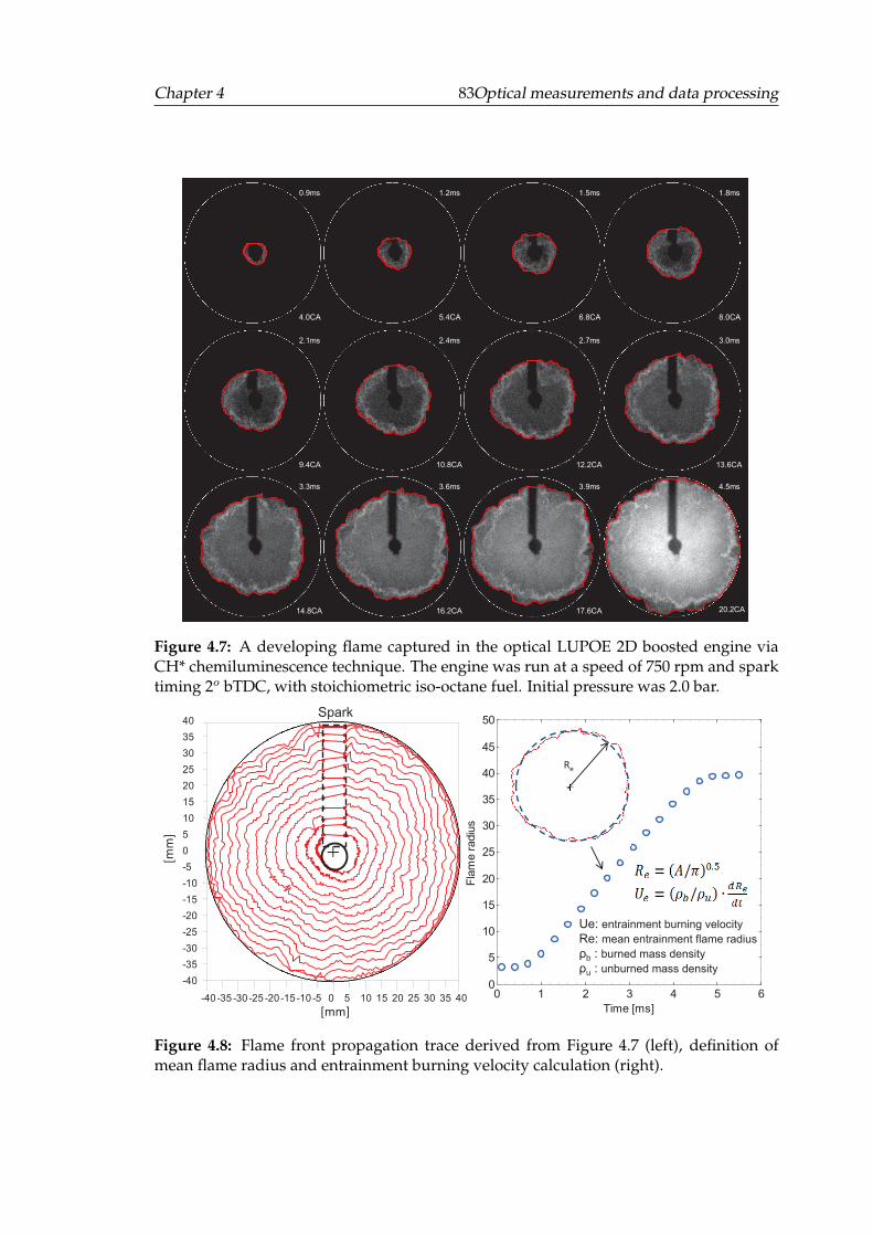
Chapter 4 83Optical measurements and data processing
4.0CA
0.9ms
5.4CA
1.2ms
6.8CA
1.5ms
8.0CA
1.8ms
9.4CA
2.1ms
10.8CA
2.4ms
12.2CA
2.7ms
13.6CA
3.0ms
14.8CA
3.3ms
16.2CA
3.6ms
17.6CA
3.9ms
20.2CA
4.5ms
Figure 4.7: A developing flame captured in the optical LUPOE 2D boosted engine viaCH* chemiluminescence technique. The engine was run at a speed of 750 rpm and sparktiming 2o bTDC, with stoichiometric iso-octane fuel. Initial pressure was 2.0 bar.
21.6CA
4.8ms
-40
-40
-35
-35
-30
-30
-25
-25
-20
-20
-15
-15
-10
-10
-5
-5
0
0
5
5
10
10
15
15
20
20
25
25
30
30
35
35
40
40
(mm)
0 1 2 3 4 5 60
5
10
15
20
25
30
35
40
45
50
Time [ms]
Fla
me r
adiu
s
Re
[mm]
[mm]
Spark
Ue: entrainment burning velocity
Re: mean entrainment flame radius
ρb : burned mass density
ρu : unburned mass density
Figure 4.8: Flame front propagation trace derived from Figure 4.7 (left), definition ofmean flame radius and entrainment burning velocity calculation (right).
Chapter 4 84Optical measurements and data processing
A sequence of flame propagation images with their derived flame fronts is shown
in Figure 4.7, the corresponding flame radius is shown in Figure 4.8, the mean flame ra-
dius calculation method is also illustrated. It can be seen that the flame front is the max-
imum radius along the projected sight line, especially at the end of flame propagation
stage. Hence, these images could not provide reliable information on flame front wrin-
kling; however, it is still a good method to investigate the flame development process by
using mean turbulent entrainment flame burning velocity.
It is also well considered that high CH* exists only in the main reaction zone (Gay-
don [1957]), thus the resulting images provide a good indication of the instantaneous
flame reaction zone location. Flame brush thickness may be derived from the intensities
of the pixels in the flame image. However, the convolutions of the flame front existing
in a highly turbulent flow may make it difficult to interpret the flame properties. This is
because the signal is an integral value equal to the depth of field of the collection optics.
In this study, the flame is weakly wrinkled, so that the errors caused by the line-of-sight
technique are hopefully small.
Images of local CH* chemiluminescence collected in laminar and moderate turbu-
lent iso-octane flames are plotted with pseudo-colour in the left side of Figures 4.9 and
4.10, and the global flame shape with chopped region position are shown in the right bot-
tom corner in the each image. A significant difference between these two kinds of flames
can be observed. Strong light emission zones can be found in both flame front regions.
These high intensity pixels can be used as an indication of the flame reaction zone. In
order to characterize the flame thickness, a line along the flame radius, across the flame
front versus normalized luminous intensity, are plotted and shown in the right sides of
Figures 4.9 and 4.10. As observed in the spatial space, the flame luminous intensity has
a peak value close to the flame front. The radius position, with 10% luminous intensity,
was defined as the flame front. Usually, the flame thickness can be defined as 1/|dwdx |, a
straight line between peak position and the flame front can be fitted very well. In order
to simplify the data processing. In this study, the distance between flame front and 90%
luminous intensity inside the flame was considered as the flame brush thickness.
It has been mentioned that flame chemiluminescence as a line-of-sight technique
is not an ideal way to investigate flame structure because the flame front derived from
the image is a projected shape. A detailed cross-section of flame front structure can be
acquired by cutting the flame into slices. This can be achieved by applying laser sheet
visualization technique in the following Section.
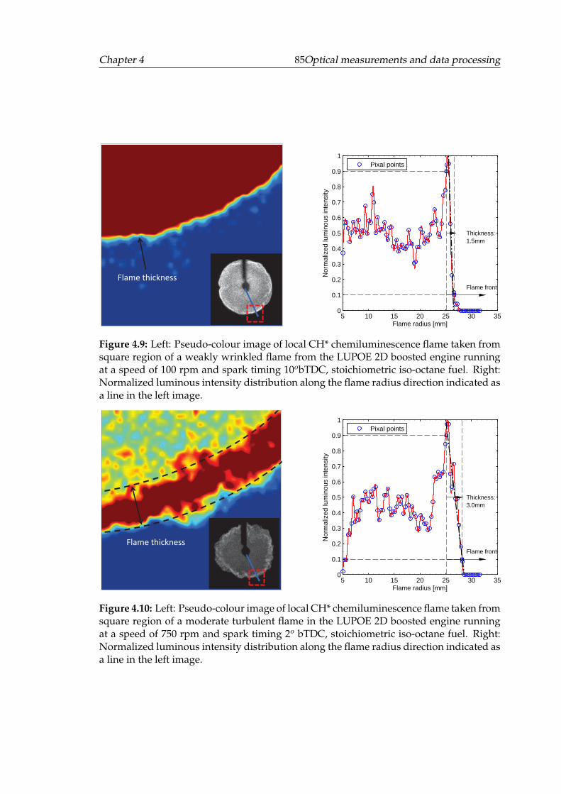
Chapter 4 85Optical measurements and data processing
Flame thickness
5 10 15 20 25 30 350
0.1
0.2
0.3
0.4
0.5
0.6
0.7
0.8
0.9
1
Flame radius [mm]N
orm
aliz
ed lu
min
ous
inte
nsity
Thickness:1.5mm
Flame front
Pixal points
Figure 4.9: Left: Pseudo-colour image of local CH* chemiluminescence flame taken fromsquare region of a weakly wrinkled flame from the LUPOE 2D boosted engine runningat a speed of 100 rpm and spark timing 10obTDC, stoichiometric iso-octane fuel. Right:Normalized luminous intensity distribution along the flame radius direction indicated asa line in the left image.
Flame thickness
5 10 15 20 25 30 350
0.1
0.2
0.3
0.4
0.5
0.6
0.7
0.8
0.9
1
Flame radius [mm]
Nor
mal
ized
lum
inou
s in
tens
ity
Thickness:3.0mm
Flame front
Pixal points
Figure 4.10: Left: Pseudo-colour image of local CH* chemiluminescence flame taken fromsquare region of a moderate turbulent flame in the LUPOE 2D boosted engine runningat a speed of 750 rpm and spark timing 2o bTDC, stoichiometric iso-octane fuel. Right:Normalized luminous intensity distribution along the flame radius direction indicated asa line in the left image.
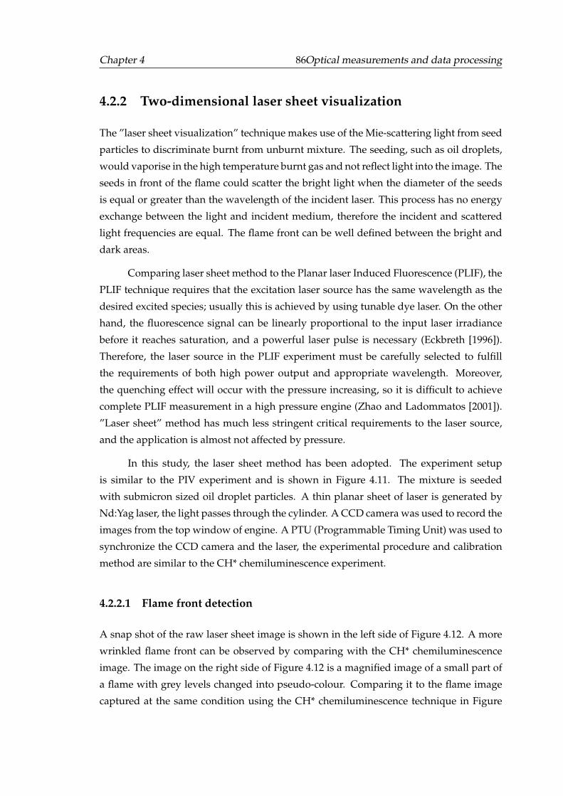
Chapter 4 86Optical measurements and data processing
4.2.2 Two-dimensional laser sheet visualization
The ”laser sheet visualization” technique makes use of the Mie-scattering light from seed
particles to discriminate burnt from unburnt mixture. The seeding, such as oil droplets,
would vaporise in the high temperature burnt gas and not reflect light into the image. The
seeds in front of the flame could scatter the bright light when the diameter of the seeds
is equal or greater than the wavelength of the incident laser. This process has no energy
exchange between the light and incident medium, therefore the incident and scattered
light frequencies are equal. The flame front can be well defined between the bright and
dark areas.
Comparing laser sheet method to the Planar laser Induced Fluorescence (PLIF), the
PLIF technique requires that the excitation laser source has the same wavelength as the
desired excited species; usually this is achieved by using tunable dye laser. On the other
hand, the fluorescence signal can be linearly proportional to the input laser irradiance
before it reaches saturation, and a powerful laser pulse is necessary (Eckbreth [1996]).
Therefore, the laser source in the PLIF experiment must be carefully selected to fulfill
the requirements of both high power output and appropriate wavelength. Moreover,
the quenching effect will occur with the pressure increasing, so it is difficult to achieve
complete PLIF measurement in a high pressure engine (Zhao and Ladommatos [2001]).
”Laser sheet” method has much less stringent critical requirements to the laser source,
and the application is almost not affected by pressure.
In this study, the laser sheet method has been adopted. The experiment setup
is similar to the PIV experiment and is shown in Figure 4.11. The mixture is seeded
with submicron sized oil droplet particles. A thin planar sheet of laser is generated by
Nd:Yag laser, the light passes through the cylinder. A CCD camera was used to record the
images from the top window of engine. A PTU (Programmable Timing Unit) was used to
synchronize the CCD camera and the laser, the experimental procedure and calibration
method are similar to the CH* chemiluminescence experiment.
4.2.2.1 Flame front detection
A snap shot of the raw laser sheet image is shown in the left side of Figure 4.12. A more
wrinkled flame front can be observed by comparing with the CH* chemiluminescence
image. The image on the right side of Figure 4.12 is a magnified image of a small part of
a flame with grey levels changed into pseudo-colour. Comparing it to the flame image
captured at the same condition using the CH* chemiluminescence technique in Figure
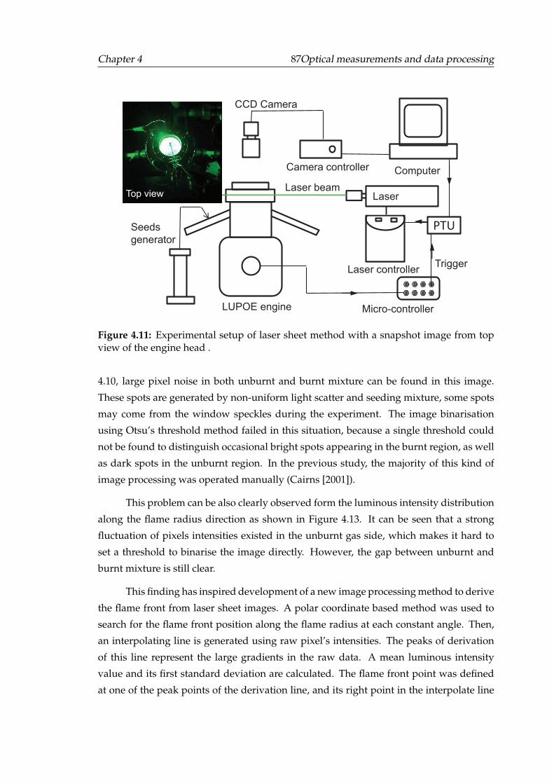
Chapter 4 87Optical measurements and data processing
LUPOE engine
CCD Camera
Laser controller
Computer
Trigger
Micro-controller
Laser
PTU
Camera controller
Laser beam
Seeds
generator
Top view
Figure 4.11: Experimental setup of laser sheet method with a snapshot image from topview of the engine head .
4.10, large pixel noise in both unburnt and burnt mixture can be found in this image.
These spots are generated by non-uniform light scatter and seeding mixture, some spots
may come from the window speckles during the experiment. The image binarisation
using Otsu’s threshold method failed in this situation, because a single threshold could
not be found to distinguish occasional bright spots appearing in the burnt region, as well
as dark spots in the unburnt region. In the previous study, the majority of this kind of
image processing was operated manually (Cairns [2001]).
This problem can be also clearly observed form the luminous intensity distribution
along the flame radius direction as shown in Figure 4.13. It can be seen that a strong
fluctuation of pixels intensities existed in the unburnt gas side, which makes it hard to
set a threshold to binarise the image directly. However, the gap between unburnt and
burnt mixture is still clear.
This finding has inspired development of a new image processing method to derive
the flame front from laser sheet images. A polar coordinate based method was used to
search for the flame front position along the flame radius at each constant angle. Then,
an interpolating line is generated using raw pixel’s intensities. The peaks of derivation
of this line represent the large gradients in the raw data. A mean luminous intensity
value and its first standard deviation are calculated. The flame front point was defined
at one of the peak points of the derivation line, and its right point in the interpolate line
Chapter 4 88Optical measurements and data processing
Burnt gas
Figure 4.12: Right: Pseudo-colour image of the laser sheet method taken from squareregion of a turbulent flame (Left) from LUPOE 2D boosted engine running at a speed of750 rpm and spark timing 2o bTDC, stoichiometric iso-octane fuel.
is larger than mean value, while its left point in the interpolate line is lower than mean
value minus first standard deviation. Finally, an approximate flame possible front can
be distinguished, an example is shown in Figure 4.14, the blue line is the flame front
searched by using this method. However, this method still has two issues. First, the
defined flame front is not in the burnt gas side, where the luminous intensity of pixels
should tend to zero due to the high temperature. Second, it could not recognize the more
than one flame front point in the one direction of flame radius, which was caused by
strong flame front wrinkling.
Therefore, a second step of local flame front searching was designed. Firstly, a
small square region was acquired with a 10o angle step along the flame front defined in
the first step. Image binarisation using Otsu’s thresholding method was used, this makes
use of the intensity information from a local region, the light emissions in a small area
are assumed to be more uniform than that from a whole image. Secondly, a 3× 3 spatial
Gaussian filter was applied to smooth and further enhance each image. A low threshold
was set at 20%, where seeds are vaporised by the high temperature in the burnt gas, to
achieve the edge detection. The final flame contour was detected using a search algorithm
by checking each pixel; the pixel on the flame edge is the one whose neighbour’s have
the reverse colour. The processing of laser sheet image is illustrated in Figure 4.14. The
final detected flame front was shown in red colour. This method can solve the difficulty
of direct binarisation of raw images, caused by non-uniform of seeding and laser light
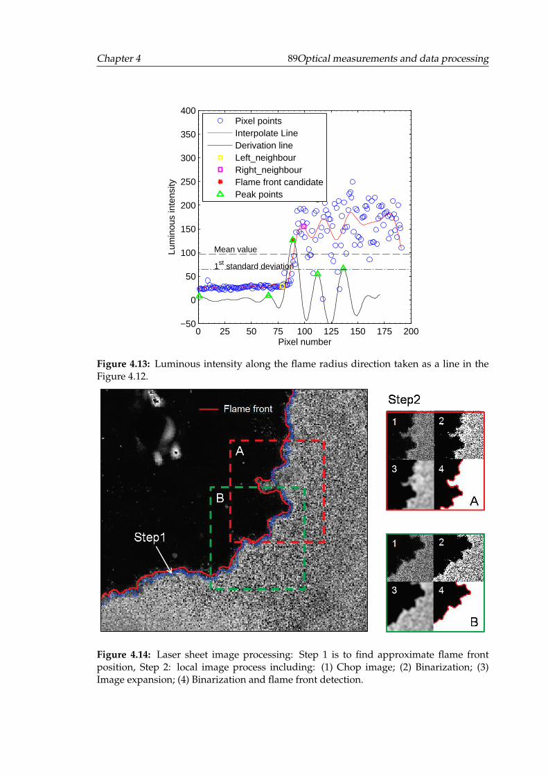
Chapter 4 89Optical measurements and data processing
0 25 50 75 100 125 150 175 200−50
0
50
100
150
200
250
300
350
400
Pixel number
Lum
inou
s in
tens
ity
Mean value
1st standard deviation
Pixel pointsInterpolate LineDerivation lineLeft_neighbourRight_neighbourFlame front candidatePeak points
Figure 4.13: Luminous intensity along the flame radius direction taken as a line in theFigure 4.12.
Figure 4.14: Laser sheet image processing: Step 1 is to find approximate flame frontposition, Step 2: local image process including: (1) Chop image; (2) Binarization; (3)Image expansion; (4) Binarization and flame front detection.
Chapter 4 90Optical measurements and data processing
intensity. Furthermore, based on this local image processing strategy, more sophisticated
filter algorithms and edge detection methods can be applied to obtain higher resolution
edge detection results. Since this image processing method can deal with the image with
large pixel noise. The PIV images with low seeding density also could be processed as a
laser sheet image, this provides a way to investigate the interaction between flame and
flow using the same experimental setup.
4.2.2.2 Flame contour processing
The flame contour data derived from the laser sheet images are stored in a series orthog-
onal coordinates (x,y). In order to characterize the flame wrinkle level, a mean flame
radius r is calculated using minimum least square algorithm to acquire an ”equivalent”
flame radius. Therefore, the wrinkled flame structure induced by the eddies, which are
larger than the flame itself, could be cut off. The deviation of the flame contour d(s) from
the mean radius at the length s along the contour could be calculated as:
d(s) = r(s)− r (4.17)
where r(s) is the instantaneous flame radius at s length along the flame contour. The
mean ¯d(s) and the root mean square d(s)′ values of the flame edge fluctuation can be
defined as:
¯d(s) =1
Ltot
∫ Ltot
0d(s)ds (4.18)
d(s)′2 =1
Ltot
∫ Ltot
0(d(s)− ¯d(s))2ds (4.19)
where Ltot is the total length of flame contour. This value can be considered a parameter
to characterize the flame wrinkle level.
For the calculation of the flame front curvature, firstly, the flame front was sampled
using a cumulative angle approximating 2o between two digitized points (Hicks et al.
[1994]), see Figure 4.15. Secondly, third order polynomials were fitted to represent local
flame contours as two functions x(s) and y(s) using 2 neighboring points. Then the local
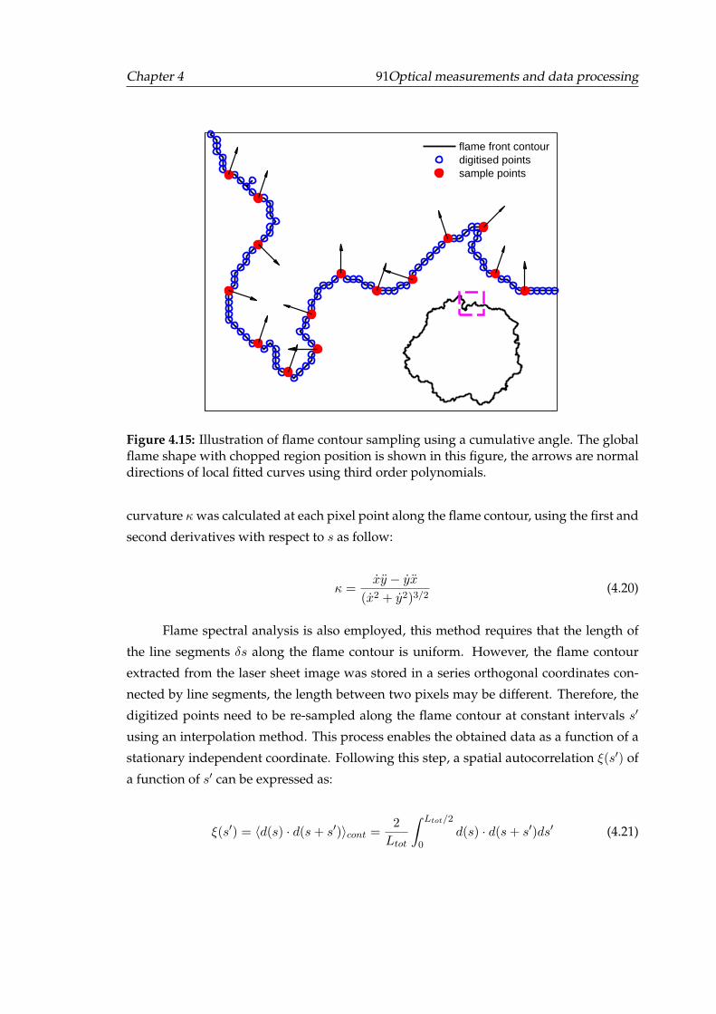
Chapter 4 91Optical measurements and data processing
flame front contourdigitised pointssample points
Figure 4.15: Illustration of flame contour sampling using a cumulative angle. The globalflame shape with chopped region position is shown in this figure, the arrows are normaldirections of local fitted curves using third order polynomials.
curvature κ was calculated at each pixel point along the flame contour, using the first and
second derivatives with respect to s as follow:
κ =xy − yx
(x2 + y2)3/2(4.20)
Flame spectral analysis is also employed, this method requires that the length of
the line segments δs along the flame contour is uniform. However, the flame contour
extracted from the laser sheet image was stored in a series orthogonal coordinates con-
nected by line segments, the length between two pixels may be different. Therefore, the
digitized points need to be re-sampled along the flame contour at constant intervals s′
using an interpolation method. This process enables the obtained data as a function of a
stationary independent coordinate. Following this step, a spatial autocorrelation ξ(s′) of
a function of s′ can be expressed as:
ξ(s′) = ⟨d(s) · d(s+ s′)⟩cont =2
Ltot
∫ Ltot/2
0d(s) · d(s+ s′)ds′ (4.21)
Chapter 4 92Optical measurements and data processing
An integral length of flame wrinkle La could be defined as follow:
La =
∫ ξ=0
0ξ(s′)ds′ (4.22)
The Fourier analysis of the ξ(s′) can then be solved as:
Φξ(k) =
∫ Ltot/2
0cos(k · s′)ξ(s′)ds′ (4.23)
The laser sheet imaging and data processing method presented here will be applied to
investigate the pressure influences on the turbulent flame structure in the boosted LUPOE
2D engine in Chapter 6.
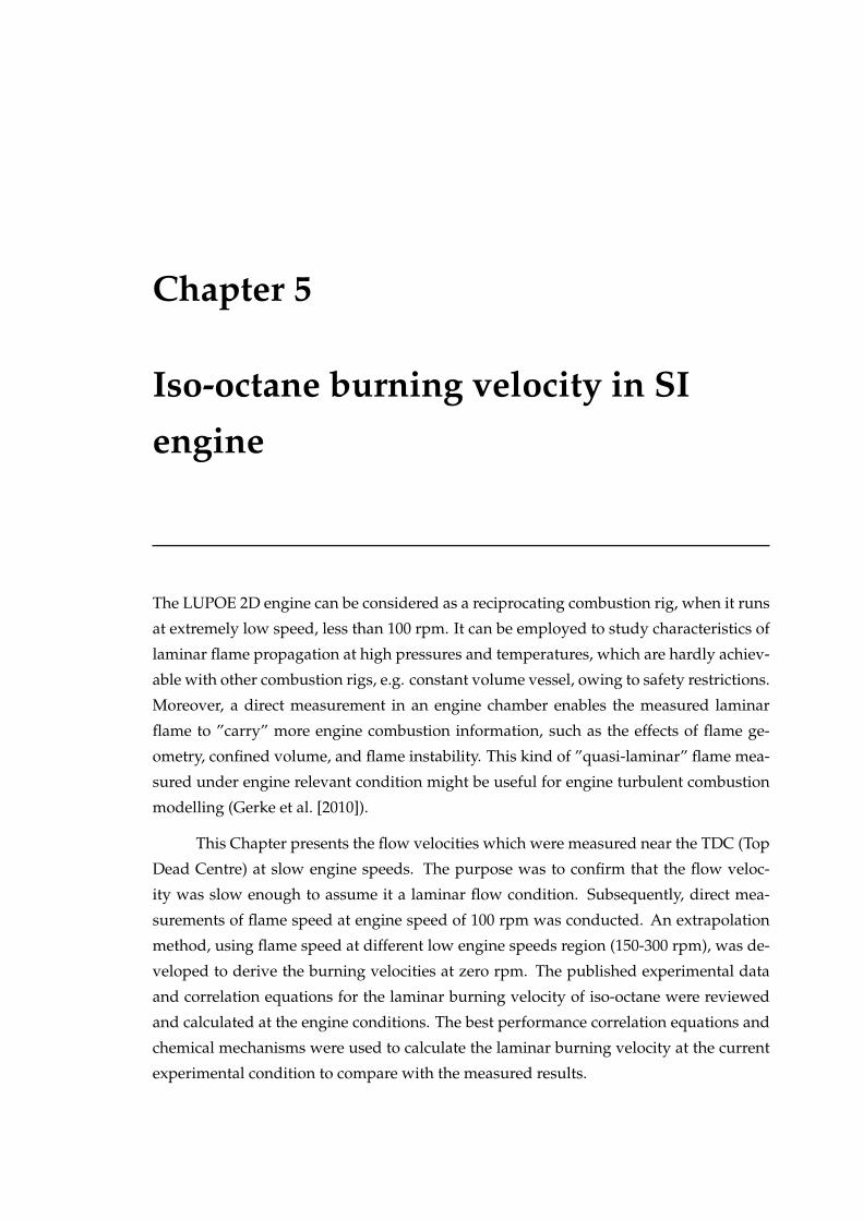
Chapter 5
Iso-octane burning velocity in SI
engine
The LUPOE 2D engine can be considered as a reciprocating combustion rig, when it runs
at extremely low speed, less than 100 rpm. It can be employed to study characteristics of
laminar flame propagation at high pressures and temperatures, which are hardly achiev-
able with other combustion rigs, e.g. constant volume vessel, owing to safety restrictions.
Moreover, a direct measurement in an engine chamber enables the measured laminar
flame to ”carry” more engine combustion information, such as the effects of flame ge-
ometry, confined volume, and flame instability. This kind of ”quasi-laminar” flame mea-
sured under engine relevant condition might be useful for engine turbulent combustion
modelling (Gerke et al. [2010]).
This Chapter presents the flow velocities which were measured near the TDC (Top
Dead Centre) at slow engine speeds. The purpose was to confirm that the flow veloc-
ity was slow enough to assume it a laminar flow condition. Subsequently, direct mea-
surements of flame speed at engine speed of 100 rpm was conducted. An extrapolation
method, using flame speed at different low engine speeds region (150-300 rpm), was de-
veloped to derive the burning velocities at zero rpm. The published experimental data
and correlation equations for the laminar burning velocity of iso-octane were reviewed
and calculated at the engine conditions. The best performance correlation equations and
chemical mechanisms were used to calculate the laminar burning velocity at the current
experimental condition to compare with the measured results.
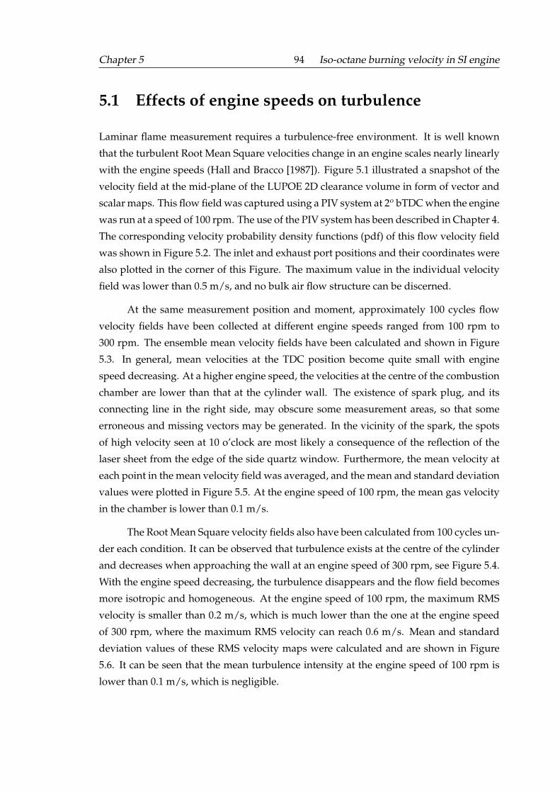
Chapter 5 94 Iso-octane burning velocity in SI engine
5.1 Effects of engine speeds on turbulence
Laminar flame measurement requires a turbulence-free environment. It is well known
that the turbulent Root Mean Square velocities change in an engine scales nearly linearly
with the engine speeds (Hall and Bracco [1987]). Figure 5.1 illustrated a snapshot of the
velocity field at the mid-plane of the LUPOE 2D clearance volume in form of vector and
scalar maps. This flow field was captured using a PIV system at 2o bTDC when the engine
was run at a speed of 100 rpm. The use of the PIV system has been described in Chapter 4.
The corresponding velocity probability density functions (pdf) of this flow velocity field
was shown in Figure 5.2. The inlet and exhaust port positions and their coordinates were
also plotted in the corner of this Figure. The maximum value in the individual velocity
field was lower than 0.5 m/s, and no bulk air flow structure can be discerned.
At the same measurement position and moment, approximately 100 cycles flow
velocity fields have been collected at different engine speeds ranged from 100 rpm to
300 rpm. The ensemble mean velocity fields have been calculated and shown in Figure
5.3. In general, mean velocities at the TDC position become quite small with engine
speed decreasing. At a higher engine speed, the velocities at the centre of the combustion
chamber are lower than that at the cylinder wall. The existence of spark plug, and its
connecting line in the right side, may obscure some measurement areas, so that some
erroneous and missing vectors may be generated. In the vicinity of the spark, the spots
of high velocity seen at 10 o’clock are most likely a consequence of the reflection of the
laser sheet from the edge of the side quartz window. Furthermore, the mean velocity at
each point in the mean velocity field was averaged, and the mean and standard deviation
values were plotted in Figure 5.5. At the engine speed of 100 rpm, the mean gas velocity
in the chamber is lower than 0.1 m/s.
The Root Mean Square velocity fields also have been calculated from 100 cycles un-
der each condition. It can be observed that turbulence exists at the centre of the cylinder
and decreases when approaching the wall at an engine speed of 300 rpm, see Figure 5.4.
With the engine speed decreasing, the turbulence disappears and the flow field becomes
more isotropic and homogeneous. At the engine speed of 100 rpm, the maximum RMS
velocity is smaller than 0.2 m/s, which is much lower than the one at the engine speed
of 300 rpm, where the maximum RMS velocity can reach 0.6 m/s. Mean and standard
deviation values of these RMS velocity maps were calculated and are shown in Figure
5.6. It can be seen that the mean turbulence intensity at the engine speed of 100 rpm is
lower than 0.1 m/s, which is negligible.
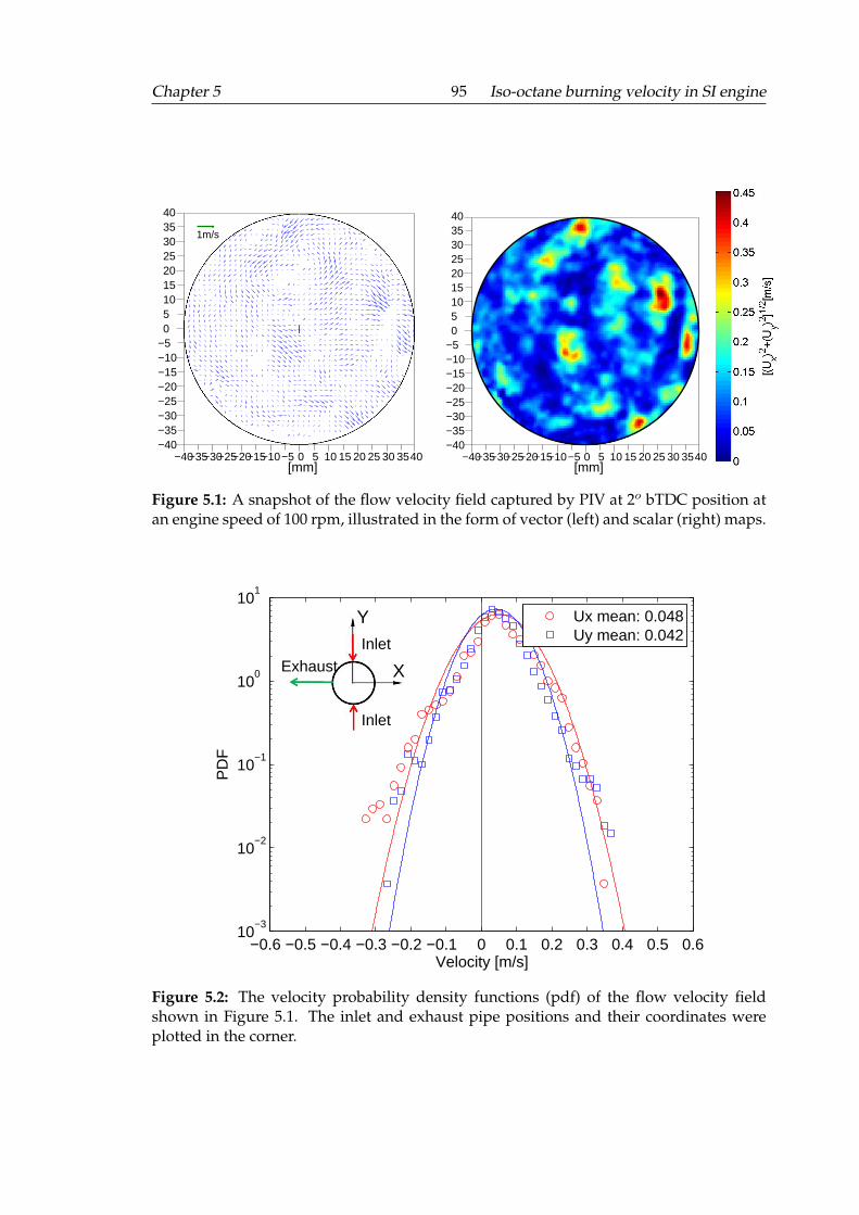
Chapter 5 95 Iso-octane burning velocity in SI engine
1m/s
−40−40
−35
−35
−30
−30
−25
−25
−20
−20
−15
−15
−10
−10
−5
−5
0
0
5
5
10
10
15
15
20
20
25
25
30
30
35
35
40
40
[mm]−40
−40−35
−35
−30
−30
−25
−25
−20
−20
−15
−15
−10
−10
−5
−5
0
0
5
5
10
10
15
15
20
20
25
25
30
30
35
35
40
40
[mm]
Figure 5.1: A snapshot of the flow velocity field captured by PIV at 2o bTDC position atan engine speed of 100 rpm, illustrated in the form of vector (left) and scalar (right) maps.
−0.6 −0.5 −0.4 −0.3 −0.2 −0.1 0 0.1 0.2 0.3 0.4 0.5 0.610
−3
10−2
10−1
100
101
Velocity [m/s]
PD
F
Ux mean: 0.048Uy mean: 0.042Inlet
Inlet
Exhaust X
Y
Figure 5.2: The velocity probability density functions (pdf) of the flow velocity fieldshown in Figure 5.1. The inlet and exhaust pipe positions and their coordinates wereplotted in the corner.
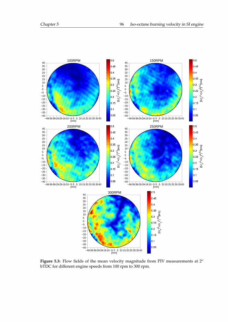
Chapter 5 96 Iso-octane burning velocity in SI engine
−40−40
−35
−35
−30
−30
−25
−25
−20
−20
−15
−15
−10
−10
−5
−5
0
0
5
5
10
10
15
15
20
20
25
25
30
30
35
35
40
40
[mm]
100RPM
−40−40
−35
−35
−30
−30
−25
−25
−20
−20
−15
−15
−10
−10
−5
−5
0
0
5
5
10
10
15
15
20
20
25
25
30
30
35
35
40
40
[mm]
150RPM
−40−40
−35
−35
−30
−30
−25
−25
−20
−20
−15
−15
−10
−10
−5
−5
0
0
5
5
10
10
15
15
20
20
25
25
30
30
35
35
40
40
[mm]
200RPM
−40−40
−35
−35
−30
−30
−25
−25
−20
−20
−15
−15
−10
−10
−5
−5
0
0
5
5
10
10
15
15
20
20
25
25
30
30
35
35
40
40
[mm]
250RPM
−40−40
−35
−35
−30
−30
−25
−25
−20
−20
−15
−15
−10
−10
−5
−5
0
0
5
5
10
10
15
15
20
20
25
25
30
30
35
35
40
40
[mm]
300RPM
Figure 5.3: Flow fields of the mean velocity magnitude from PIV measurements at 2o
bTDC for different engine speeds from 100 rpm to 300 rpm.
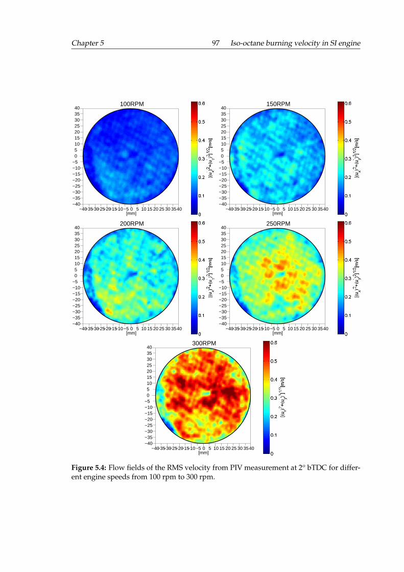
Chapter 5 97 Iso-octane burning velocity in SI engine
−40−40
−35
−35
−30
−30
−25
−25
−20
−20
−15
−15
−10
−10
−5
−5
0
0
5
5
10
10
15
15
20
20
25
25
30
30
35
35
40
40
[mm]
100RPM
−40−40
−35
−35
−30
−30
−25
−25
−20
−20
−15
−15
−10
−10
−5
−5
0
0
5
5
10
10
15
15
20
20
25
25
30
30
35
35
40
40
[mm]
150RPM
−40−40
−35
−35
−30
−30
−25
−25
−20
−20
−15
−15
−10
−10
−5
−5
0
0
5
5
10
10
15
15
20
20
25
25
30
30
35
35
40
40
[mm]
200RPM
−40−40
−35
−35
−30
−30
−25
−25
−20
−20
−15
−15
−10
−10
−5
−5
0
0
5
5
10
10
15
15
20
20
25
25
30
30
35
35
40
40
[mm]
250RPM
−40−40
−35
−35
−30
−30
−25
−25
−20
−20
−15
−15
−10
−10
−5
−5
0
0
5
5
10
10
15
15
20
20
25
25
30
30
35
35
40
40
[mm]
300RPM
Figure 5.4: Flow fields of the RMS velocity from PIV measurement at 2o bTDC for differ-ent engine speeds from 100 rpm to 300 rpm.
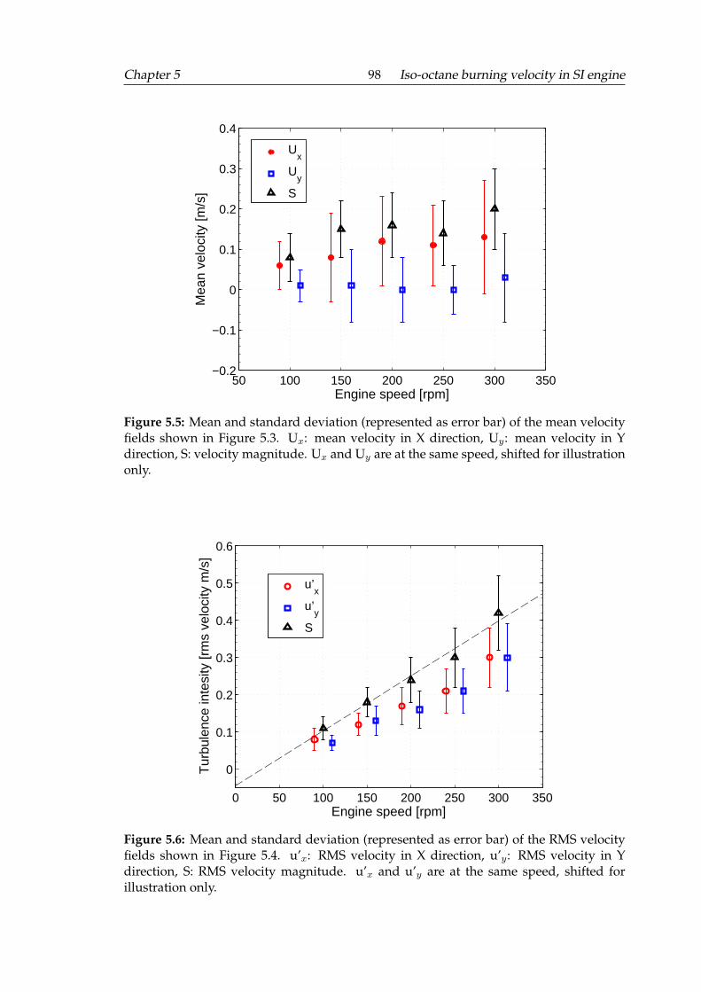
Chapter 5 98 Iso-octane burning velocity in SI engine
50 100 150 200 250 300 350−0.2
−0.1
0
0.1
0.2
0.3
0.4
Engine speed [rpm]
Mea
n ve
loci
ty [m
/s]
Ux
Uy
S
Figure 5.5: Mean and standard deviation (represented as error bar) of the mean velocityfields shown in Figure 5.3. Ux: mean velocity in X direction, Uy: mean velocity in Ydirection, S: velocity magnitude. Ux and Uy are at the same speed, shifted for illustrationonly.
0 50 100 150 200 250 300 350
0
0.1
0.2
0.3
0.4
0.5
0.6
Engine speed [rpm]
Tur
bule
nce
inte
sity
[rm
s ve
loci
ty m
/s]
u’x
u’y
S
Figure 5.6: Mean and standard deviation (represented as error bar) of the RMS velocityfields shown in Figure 5.4. u’x: RMS velocity in X direction, u’y: RMS velocity in Ydirection, S: RMS velocity magnitude. u’x and u’y are at the same speed, shifted forillustration only.
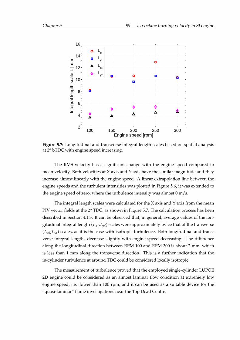
Chapter 5 99 Iso-octane burning velocity in SI engine
100 150 200 250 3002
4
6
8
10
12
14
16
Engine speed [rpm]
Inte
gral
leng
th s
cale
L [m
m]
Lxl
Lyl
Lxt
Lyt
Figure 5.7: Longitudinal and transverse integral length scales based on spatial analysisat 2o bTDC with engine speed increasing.
The RMS velocity has a significant change with the engine speed compared to
mean velocity. Both velocities at X axis and Y axis have the similar magnitude and they
increase almost linearly with the engine speed. A linear extrapolation line between the
engine speeds and the turbulent intensities was plotted in Figure 5.6, it was extended to
the engine speed of zero, where the turbulence intensity was almost 0 m/s.
The integral length scales were calculated for the X axis and Y axis from the mean
PIV vector fields at the 2o TDC, as shown in Figure 5.7. The calculation process has been
described in Section 4.1.3. It can be observed that, in general, average values of the lon-
gitudinal integral length (Lxl,Lyl) scales were approximately twice that of the transverse
(Lxt,Lyt) scales, as it is the case with isotropic turbulence. Both longitudinal and trans-
verse integral lengths decrease slightly with engine speed decreasing. The difference
along the longitudinal direction between RPM 100 and RPM 300 is about 2 mm, which
is less than 1 mm along the transverse direction. This is a further indication that the
in-cylinder turbulence at around TDC could be considered locally isotropic.
The measurement of turbulence proved that the employed single-cylinder LUPOE
2D engine could be considered as an almost laminar flow condition at extremely low
engine speed, i.e. lower than 100 rpm, and it can be used as a suitable device for the
”quasi-laminar” flame investigations near the Top Dead Centre.
Chapter 5 100 Iso-octane burning velocity in SI engine
5.2 Direct measurement of burning velocities
As shown in PIV results, both averaged mean and RMS flow velocities at the engine
speed of 100 rpm are lower than 0.1 m/s. Under this condition, the flame propagation in
the cylinder might be considered as a laminar flame. Pressure and imaging measurement
methods have been applied in this Section to measure the stretched laminar flame at el-
evated pressure. The measurement was conducted near TDC to reduce further influence
of the flow velocities on the flame propagation.
5.2.1 Pressure results
For all the tests presented below, the engine speed was set at 100 rev/min, intakes and
wall temperature were kept at 323 K, the same as for the high speed engine experiment in
Chapter 6. The spark timing was 10o bTDC (before Top Dead Centre). The temperature
at spark timing can reach about 600 K, calculated from LUSIEDA. The spark energy was
adjusted to be at a minimum, at such that a stable ignition can be achieved in order
to avoid a high energy spark discharge disturbing the initial flame development. Each
firing cycle was followed by 10 motoring cycles with skipped ignition. Only 6 cycles
could have been recorded during each engine run with a data scan rate of 50 kHz. Figure
5.8 shows the 5 pressure cycles collected for varied equivalence ratios from 0.6 to 1.2.
Both the pressure rise rate and the peak pressure increase with the equivalence ratios
increasing. The cycle variability becomes significant with equivalence ratio decreasing,
and the engine operation at equivalence ratio 1.2 has the lowest cycle variability. These
tests proved that the experimental results were repeatable, and the effect of turbulence on
flame propagation was negligible at this low engine speed. The pressure at spark timing
for all cases was approximately 12 bar.
5.2.2 Laser sheet visualization results
The laser sheet visualization method was applied in order to investigate the detailed
flame shape and its variability. The flame contour is determined from an image created
by a laser sheet passing through a seeded medium, see Section 4.2.2. About 30 flame
contours were collected at 2o CA after ignition at the engine speed of 100 rpm, and at 10o
CA after ignition at the engine speed of 750 rpm, respectively, approximate 1.2 ms elapsed
since the spark timing for stochiometric charge. Figure 5.9 shows the flame front of each
firing cycle at two engine speeds with the cylinder wall. Although a slightly wrinkled
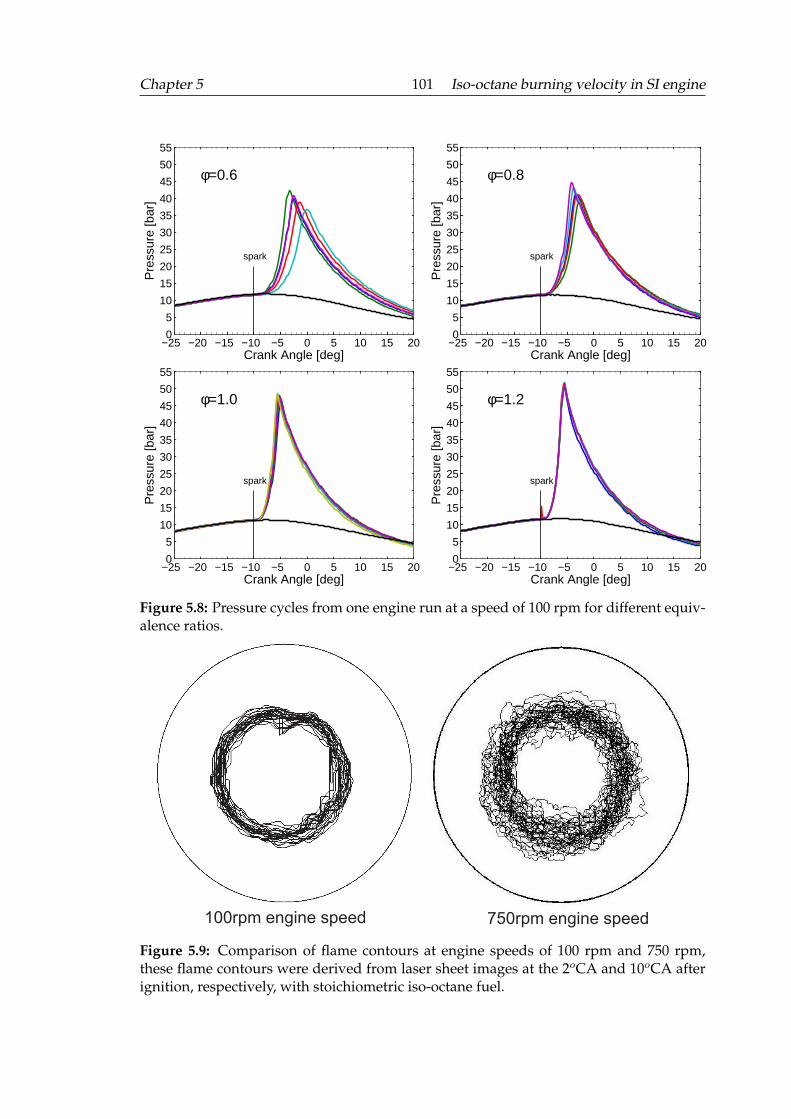
Chapter 5 101 Iso-octane burning velocity in SI engine
−25 −20 −15 −10 −5 0 5 10 15 200
5
10
15
20
25
30
35
40
45
50
55
spark
φ=0.6
Crank Angle [deg]
Pre
ssur
e [b
ar]
−25 −20 −15 −10 −5 0 5 10 15 200
5
10
15
20
25
30
35
40
45
50
55
spark
φ=0.8
Crank Angle [deg]
Pre
ssur
e [b
ar]
−25 −20 −15 −10 −5 0 5 10 15 200
5
10
15
20
25
30
35
40
45
50
55
spark
φ=1.0
Crank Angle [deg]
Pre
ssur
e [b
ar]
−25 −20 −15 −10 −5 0 5 10 15 200
5
10
15
20
25
30
35
40
45
50
55
spark
φ=1.2
Crank Angle [deg]
Pre
ssur
e [b
ar]
Figure 5.8: Pressure cycles from one engine run at a speed of 100 rpm for different equiv-alence ratios.
100rpm engine speed 750rpm engine speed
Figure 5.9: Comparison of flame contours at engine speeds of 100 rpm and 750 rpm,these flame contours were derived from laser sheet images at the 2oCA and 10oCA afterignition, respectively, with stoichiometric iso-octane fuel.
Chapter 5 102 Iso-octane burning velocity in SI engine
flame front still can be observed at the engine speed of 100 rpm, they are relatively small
compared to the turbulent flame at the engine speed of 750 rpm, and the differences of
flame radius between each firing cycle at the low engine speed are also much lower than
that of a turbulent flame at the high engine speed.
5.2.3 CH* chemiluminescence image results
The CH* chemiluminescence image method, i.e. flame photographs taken with an in-
terference filter for 470 nm, see Section 4.2.1, was used to obtain the flame development
information. Shown in Figure 5.10 are 4 typical examples of sequential CH* imaging of
developing iso-octane flames for lean, ϕ = 0.6 and 0.8, stoichiometric, ϕ = 1.0, and rich
mixtures ϕ=1.2. Intakes and wall temperature were kept at 323 K, and the spark timing
was set at 10o bTDC. The pressure and temperature at the spark discharge are 12 bar and
600 K, as derived from LUSIEDA simulation. The dotted circle, which has the same area
as the flame, is also shown in each flame image to compare with the instantaneous flame
front shape.
The moments of nearly equal flame areas were selected in each row to compare the
effect of equivalence ratio on the flame front. The time and crank angle of each flame
were listed on the top left corner and bottom left corner. There was a large difference in
the time that flame radius took to reach a similar size, between 0.6, 0.8, and 1.0, while
the stoichiometric and rich flames look more similar. This observation agrees with the
pressure traces shown in Figure 5.8.
The high ignition energy from spark disturbed the initial flame shape. The lean
flame retained the ”cracks” caused by the spark and growing, became more wrinkled.
However, the flame surface still attained an almost spherical shape with large scale dis-
tortions. Stoichiometric and rich flame spread more uniformly during the initial stage
and had an ability to ”recover” from the spark-induced ”cracks”. The flame kept a spher-
ical shape until the flame developed to a radius of approximately half of the engine cylin-
der diameter (20 mm). Small scale wrinkles started to appear, and quickly covered the
whole flame surface. It was the same for the lean flame.
These regular curved small shapes are similar to the cellularity structure caused
by a hydrodynamic instability. Although the detailed structure observation is limited by
the 2D measurement method, the observed structures were significantly different from
those observed at high turbulent flow conditions, where flame showed very irregular
wrinkled shapes that occurred quickly after ignition. Flame deceleration happens when
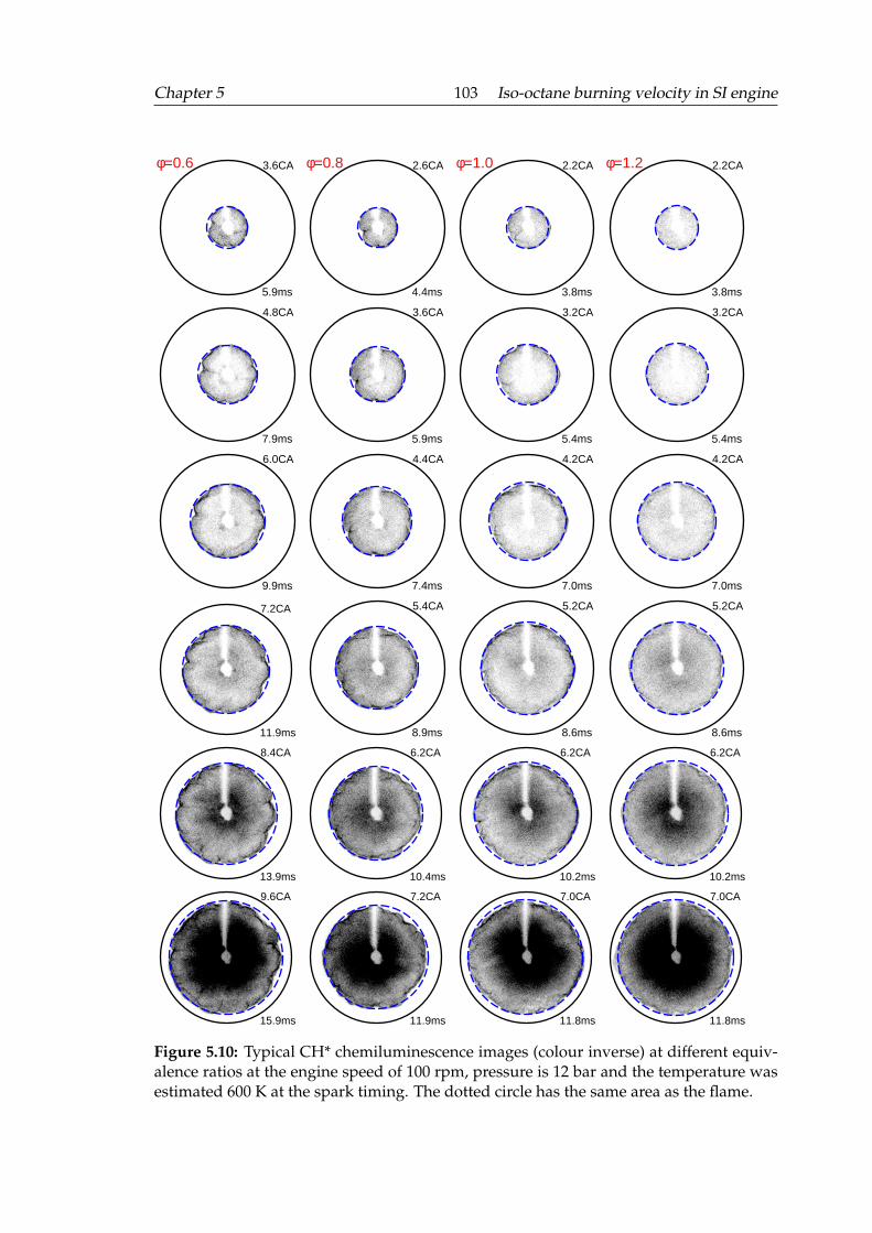
Chapter 5 103 Iso-octane burning velocity in SI engine
3.6CA
5.9ms
φ=0.6 2.6CA
4.4ms
φ=0.8 2.2CA
3.8ms
φ=1.0 2.2CA
3.8ms
φ=1.2
4.8CA
7.9ms
3.6CA
5.9ms
3.2CA
5.4ms
3.2CA
5.4ms
6.0CA
9.9ms
4.4CA
7.4ms
4.2CA
7.0ms
4.2CA
7.0ms
7.2CA
11.9ms
5.4CA
8.9ms
5.2CA
8.6ms
5.2CA
8.6ms
8.4CA
13.9ms
6.2CA
10.4ms
6.2CA
10.2ms
6.2CA
10.2ms
9.6CA
15.9ms
7.2CA
11.9ms
7.0CA
11.8ms
7.0CA
11.8ms
Figure 5.10: Typical CH* chemiluminescence images (colour inverse) at different equiv-alence ratios at the engine speed of 100 rpm, pressure is 12 bar and the temperature wasestimated 600 K at the spark timing. The dotted circle has the same area as the flame.
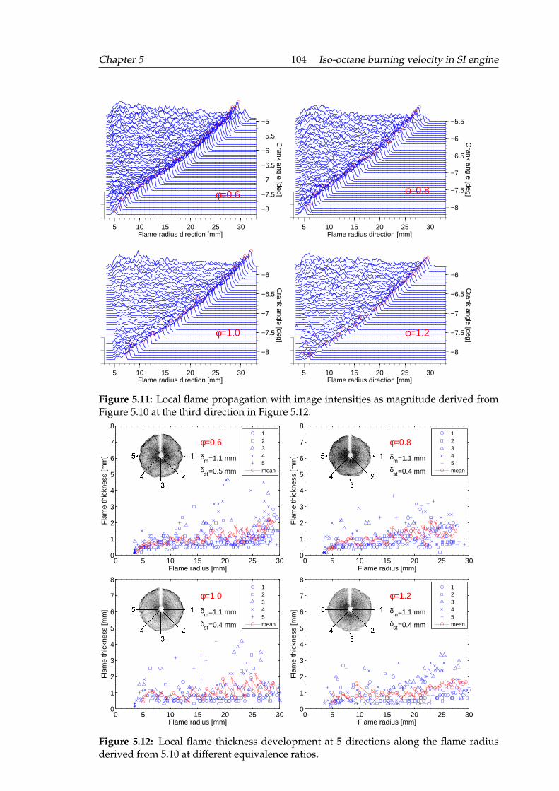
Chapter 5 104 Iso-octane burning velocity in SI engine
5 10 15 20 25 30
−8
−7.5
−7
−6.5
−6
−5.5
−5
Crank angle [deg]φ=0.6
Flame radius direction [mm]5 10 15 20 25 30
−8
−7.5
−7
−6.5
−6
−5.5
Crank angle [deg]φ=0.8
Flame radius direction [mm]
5 10 15 20 25 30
−8
−7.5
−7
−6.5
−6C
rank angle [deg]
φ=1.0
Flame radius direction [mm]5 10 15 20 25 30
−8
−7.5
−7
−6.5
−6
Crank angle [deg]
φ=1.2
Flame radius direction [mm]
Figure 5.11: Local flame propagation with image intensities as magnitude derived fromFigure 5.10 at the third direction in Figure 5.12.
0 5 10 15 20 25 300
1
2
3
4
5
6
7
8
Flame radius [mm]
Fla
me
thic
knes
s [m
m]
δm
δst
=1.1 mm
=0.5 mm
φ=0.612345mean
0 5 10 15 20 25 300
1
2
3
4
5
6
7
8
Flame radius [mm]
Fla
me
thic
knes
s [m
m]
δm
δst
=1.1 mm
=0.4 mm
φ=0.812345mean
0 5 10 15 20 25 300
1
2
3
4
5
6
7
8
Flame radius [mm]
Fla
me
thic
knes
s [m
m]
δm
δst
=1.1 mm
=0.4 mm
φ=1.012345mean
0 5 10 15 20 25 300
1
2
3
4
5
6
7
8
Flame radius [mm]
Fla
me
thic
knes
s [m
m]
δm
δst
=1.1 mm
=0.4 mm
φ=1.212345mean
Figure 5.12: Local flame thickness development at 5 directions along the flame radiusderived from 5.10 at different equivalence ratios.
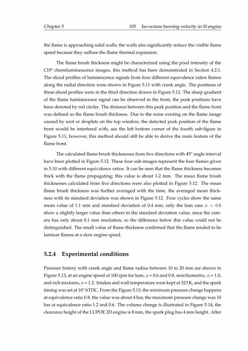
Chapter 5 105 Iso-octane burning velocity in SI engine
the flame is approaching solid walls; the walls also significantly reduce the visible flame
speed because they suffuse the flame thermal expansion.
The flame brush thickness might be characterized using the pixel intensity of the
CH* chemiluminescence images, this method has been demonstrated in Section 4.2.1.
The sliced profiles of luminescence signals from four different equivalence ratios flames
along the radial direction were shown in Figure 5.11 with crank angle. The positions of
these sliced profiles were in the third direction drawn in Figure 5.12. The sharp gradient
of the flame luminescence signal can be observed in the front, the peak positions have
been denoted by red circles. The distance between this peak position and the flame front
was defined as the flame brush thickness. Due to the noise existing on the flame image
caused by soot or droplets on the top window, the detected peak position of the flame
front would be interfered with, see the left bottom corner of the fourth sub-figure in
Figure 5.11, however, this method should still be able to derive the main feature of the
flame front.
The calculated flame brush thicknesses from five directions with 45o angle interval
have been plotted in Figure 5.12. These four sub-images represent the four flames given
in 5.10 with different equivalence ratios. It can be seen that the flame thickness becomes
thick with the flame propagating; this value is about 1-2 mm. The mean flame brush
thicknesses calculated from five directions were also plotted in Figure 5.12. The mean
flame brush thickness was further averaged with the time, the averaged mean thick-
ness with its standard deviation was shown in Figure 5.12. Four cycles show the same
mean value of 1.1 mm and standard deviation of 0.4 mm, only the lean case ϕ = 0.6
show a slightly larger value than others in the standard deviation value, since the cam-
era has only about 0.1 mm resolution, so the difference below this value could not be
distinguished. The small value of flame thickness confirmed that the flame tended to be
laminar flames at a slow engine speed.
5.2.4 Experimental conditions
Pressure history with crank angle and flame radius between 10 to 20 mm are shown in
Figure 5.13, at an engine speed of 100 rpm for lean, ϕ = 0.6 and 0.8, stoichiometric, ϕ = 1.0,
and rich mixtures, ϕ = 1.2. Intakes and wall temperature were kept at 323 K, and the spark
timing was set at 10o bTDC. From the Figure 5.13, the minimum pressure change happens
at equivalence ratio 0.8, the value was about 4 bar, the maximum pressure change was 10
bar at equivalence ratio 1.2 and 0.6. The volume change is illustrated in Figure 5.14, the
clearance height of the LUPOE 2D engine is 8 mm, the spark plug has 4 mm height. After
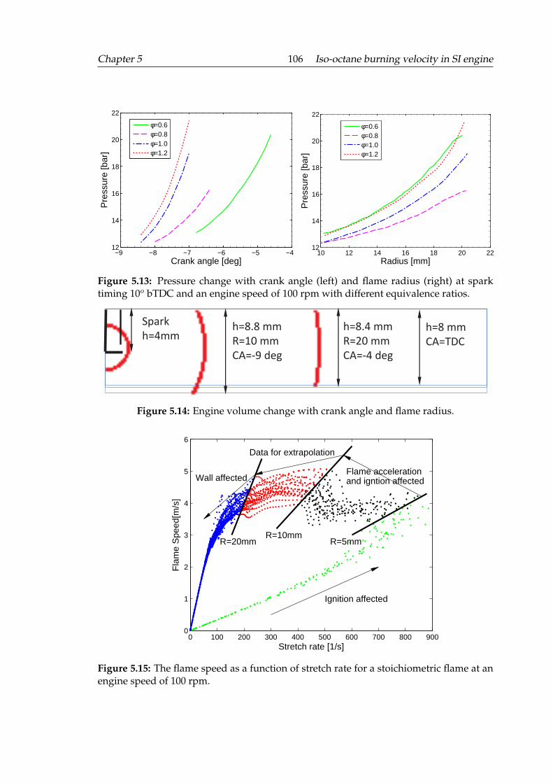
Chapter 5 106 Iso-octane burning velocity in SI engine
−9 −8 −7 −6 −5 −412
14
16
18
20
22
Crank angle [deg]
Pre
ssur
e [b
ar]
φ=0.6φ=0.8φ=1.0φ=1.2
10 12 14 16 18 20 2212
14
16
18
20
22
Radius [mm]
Pre
ssur
e [b
ar]
φ=0.6φ=0.8φ=1.0φ=1.2
Figure 5.13: Pressure change with crank angle (left) and flame radius (right) at sparktiming 10o bTDC and an engine speed of 100 rpm with different equivalence ratios.
h=8.8 mm
R=10 mm
CA=-9 deg
h=8.4 mm
R=20 mm
CA=-4 deg
h=8 mm
CA=TDC
Spark
h=4mm
Figure 5.14: Engine volume change with crank angle and flame radius.
0 100 200 300 400 500 600 700 800 9000
1
2
3
4
5
6
Stretch rate [1/s]
Fla
me
Spe
ed[m
/s]
Ignition affected
Flame accelerationand igntion affected
Data for extrapolation
Wall affected
R=5mmR=10mm
R=20mm
Figure 5.15: The flame speed as a function of stretch rate for a stoichiometric flame at anengine speed of 100 rpm.
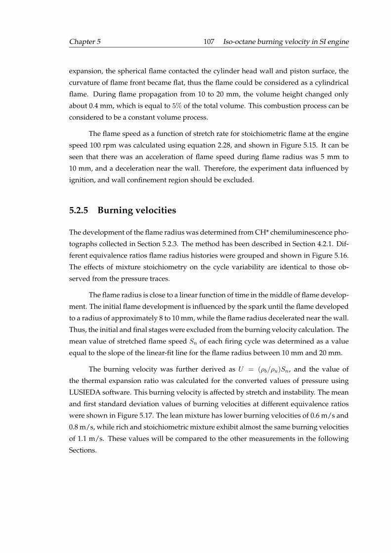
Chapter 5 107 Iso-octane burning velocity in SI engine
expansion, the spherical flame contacted the cylinder head wall and piston surface, the
curvature of flame front became flat, thus the flame could be considered as a cylindrical
flame. During flame propagation from 10 to 20 mm, the volume height changed only
about 0.4 mm, which is equal to 5% of the total volume. This combustion process can be
considered to be a constant volume process.
The flame speed as a function of stretch rate for stoichiometric flame at the engine
speed 100 rpm was calculated using equation 2.28, and shown in Figure 5.15. It can be
seen that there was an acceleration of flame speed during flame radius was 5 mm to
10 mm, and a deceleration near the wall. Therefore, the experiment data influenced by
ignition, and wall confinement region should be excluded.
5.2.5 Burning velocities
The development of the flame radius was determined from CH* chemiluminescence pho-
tographs collected in Section 5.2.3. The method has been described in Section 4.2.1. Dif-
ferent equivalence ratios flame radius histories were grouped and shown in Figure 5.16.
The effects of mixture stoichiometry on the cycle variability are identical to those ob-
served from the pressure traces.
The flame radius is close to a linear function of time in the middle of flame develop-
ment. The initial flame development is influenced by the spark until the flame developed
to a radius of approximately 8 to 10 mm, while the flame radius decelerated near the wall.
Thus, the initial and final stages were excluded from the burning velocity calculation. The
mean value of stretched flame speed Sn of each firing cycle was determined as a value
equal to the slope of the linear-fit line for the flame radius between 10 mm and 20 mm.
The burning velocity was further derived as U = (ρb/ρu)Sn, and the value of
the thermal expansion ratio was calculated for the converted values of pressure using
LUSIEDA software. This burning velocity is affected by stretch and instability. The mean
and first standard deviation values of burning velocities at different equivalence ratios
were shown in Figure 5.17. The lean mixture has lower burning velocities of 0.6 m/s and
0.8 m/s, while rich and stoichiometric mixture exhibit almost the same burning velocities
of 1.1 m/s. These values will be compared to the other measurements in the following
Sections.
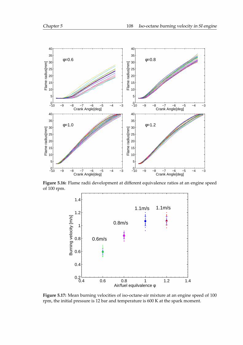
Chapter 5 108 Iso-octane burning velocity in SI engine
−10 −9 −8 −7 −6 −5 −4 −30
5
10
15
20
25
30
35
40
Crank Angle[deg]
Fla
me
radi
us[m
m] φ=0.6
−10 −9 −8 −7 −6 −5 −4 −30
5
10
15
20
25
30
35
40
Crank Angle[deg]
Fla
me
radi
us[m
m] φ=0.8
−10 −9 −8 −7 −6 −5 −4 −30
5
10
15
20
25
30
35
40
Crank Angle[deg]
Fla
me
radi
us[m
m] φ=1.0
−10 −9 −8 −7 −6 −5 −4 −30
5
10
15
20
25
30
35
40
Crank Angle[deg]
Fla
me
radi
us[m
m] φ=1.2
Figure 5.16: Flame radii development at different equivalence ratios at an engine speedof 100 rpm.
0.4 0.6 0.8 1 1.2 1.40.2
0.4
0.6
0.8
1
1.2
1.4
0.6m/s
0.8m/s
1.1m/s 1.1m/s
Air/fuel equilvalence φ
Bur
ning
vel
ocity
[m/s
]
Figure 5.17: Mean burning velocities of iso-octane-air mixture at an engine speed of 100rpm, the initial pressure is 12 bar and temperature is 600 K at the spark moment.

Chapter 5 109 Iso-octane burning velocity in SI engine
5.3 On a turbulence free burning velocity in engines
It has been shown in Section 5.1 that there exists an almost linear relationship between
the engine speed and RMS flow velocities in the cylinder. Turbulence-free flow can be
assumed at a zero engine speed. Here, we explore a new method of measuring a laminar
burning velocity at turbulence-free conditions, the method is based on extrapolating the
burning velocities from different engine speeds. In order to maintain the same initial
pressure and temperature conditions, the spark ignition timing has to be adjusted.
Because of knock occurrence at early advanced spark timing, for this new method,
the spark timing was generally set after the Top Dead Centre. The spark timing, at which
in-cylinder pressure attains 15 bar, was chosen. With increasing the engine speed, the in-
cylinder peak motoring pressure also increases, thus the spark timing has to be retarded
into the expansion stroke. Four engine speeds have been selected: 150 rpm, 200 rpm, 250
rpm, and 300 rpm. The peak pressure at 100 rpm was lower than 15 bar, so this speed
was excluded from the extrapolation and used only for comparison analysis.
The pressure selected for ignition, P0=15 bar, was slightly below the peak motoring
pressure and it could have been achieved at either 6oCA bTDC or at slightly differing
times after TDC, see the annotated lines in Figure 5.18. Obviously, the peak pressure
is very sensitive to the spark timing around the TDC. In order to match not only the
pressure but also the temperature for different engine speeds, a set of calculations was
undertaken using LUSIEDA, and the resulting pressure-temperature history is shown in
Figure 5.18 (d), together with the indication of the in-cylinder charge state at the spark
timing. Although the difference of temperature exists at TDC, the temperatures of the 4
conditions are similar at the spark timing with a high value 606 K.
Shown in Figure 5.19 are CH* images of growing flame at stoichiometric equiva-
lence ratio at engine speeds from 150 rpm to 300 rpm. With increasing the engine speed,
the mean and RMS flow velocities increase, shown in the Section 5.1. Although the flame
kernels for 4 engine speeds look similar for a short while after ignition, the flame quickly
becomes wrinkled, presumably because of turbulence at higher engine speed. Mean-
while, the flame also travels at a faster speed. This can be seen from Figure 5.19 which
shows the flame shape taken at approximately the same flame size while the time re-
quired to reach this stage is shown in the annotations. It is appropriate to notice that,
even though a higher engine speed means faster flame, the increase is not linear. At a
low engine speed, the flames show a small regular curved flame structure during the
flame propagation, while with stronger turbulence they have irregularly and strongly
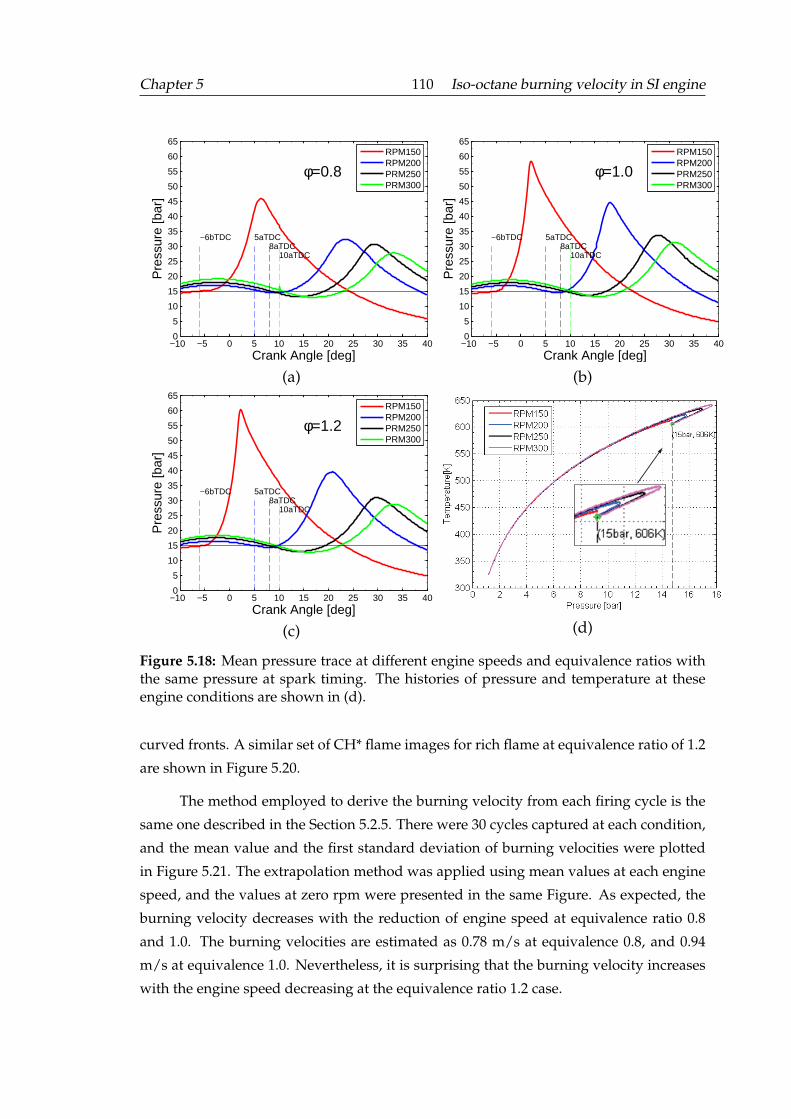
Chapter 5 110 Iso-octane burning velocity in SI engine
−10 −5 0 5 10 15 20 25 30 35 400
5
10
15
20
25
30
35
40
45
50
55
60
65
−6bTDC 5aTDC8aTDC
10aTDC
Crank Angle [deg]
Pre
ssur
e [b
ar]
φ=0.8RPM150RPM200PRM250PRM300
(a)
−10 −5 0 5 10 15 20 25 30 35 400
5
10
15
20
25
30
35
40
45
50
55
60
65
−6bTDC 5aTDC8aTDC
10aTDC
Crank Angle [deg]
Pre
ssur
e [b
ar]
φ=1.0RPM150RPM200PRM250PRM300
(b)
−10 −5 0 5 10 15 20 25 30 35 400
5
10
15
20
25
30
35
40
45
50
55
60
65
−6bTDC 5aTDC8aTDC
10aTDC
Crank Angle [deg]
Pre
ssur
e [b
ar]
φ=1.2RPM150RPM200PRM250PRM300
(c) (d)
Figure 5.18: Mean pressure trace at different engine speeds and equivalence ratios withthe same pressure at spark timing. The histories of pressure and temperature at theseengine conditions are shown in (d).
curved fronts. A similar set of CH* flame images for rich flame at equivalence ratio of 1.2
are shown in Figure 5.20.
The method employed to derive the burning velocity from each firing cycle is the
same one described in the Section 5.2.5. There were 30 cycles captured at each condition,
and the mean value and the first standard deviation of burning velocities were plotted
in Figure 5.21. The extrapolation method was applied using mean values at each engine
speed, and the values at zero rpm were presented in the same Figure. As expected, the
burning velocity decreases with the reduction of engine speed at equivalence ratio 0.8
and 1.0. The burning velocities are estimated as 0.78 m/s at equivalence 0.8, and 0.94
m/s at equivalence 1.0. Nevertheless, it is surprising that the burning velocity increases
with the engine speed decreasing at the equivalence ratio 1.2 case.
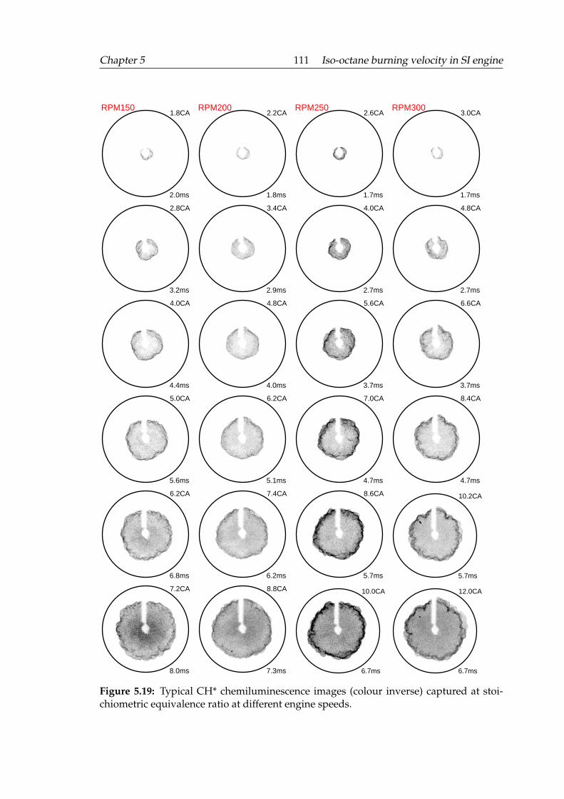
Chapter 5 111 Iso-octane burning velocity in SI engine
1.8CA
2.0ms
RPM1502.2CA
1.8ms
RPM2002.6CA
1.7ms
RPM2503.0CA
1.7ms
RPM300
2.8CA
3.2ms
3.4CA
2.9ms
4.0CA
2.7ms
4.8CA
2.7ms
4.0CA
4.4ms
4.8CA
4.0ms
5.6CA
3.7ms
6.6CA
3.7ms
5.0CA
5.6ms
6.2CA
5.1ms
7.0CA
4.7ms
8.4CA
4.7ms
6.2CA
6.8ms
7.4CA
6.2ms
8.6CA
5.7ms
10.2CA
5.7ms
7.2CA
8.0ms
8.8CA
7.3ms
10.0CA
6.7ms
12.0CA
6.7ms
Figure 5.19: Typical CH* chemiluminescence images (colour inverse) captured at stoi-chiometric equivalence ratio at different engine speeds.
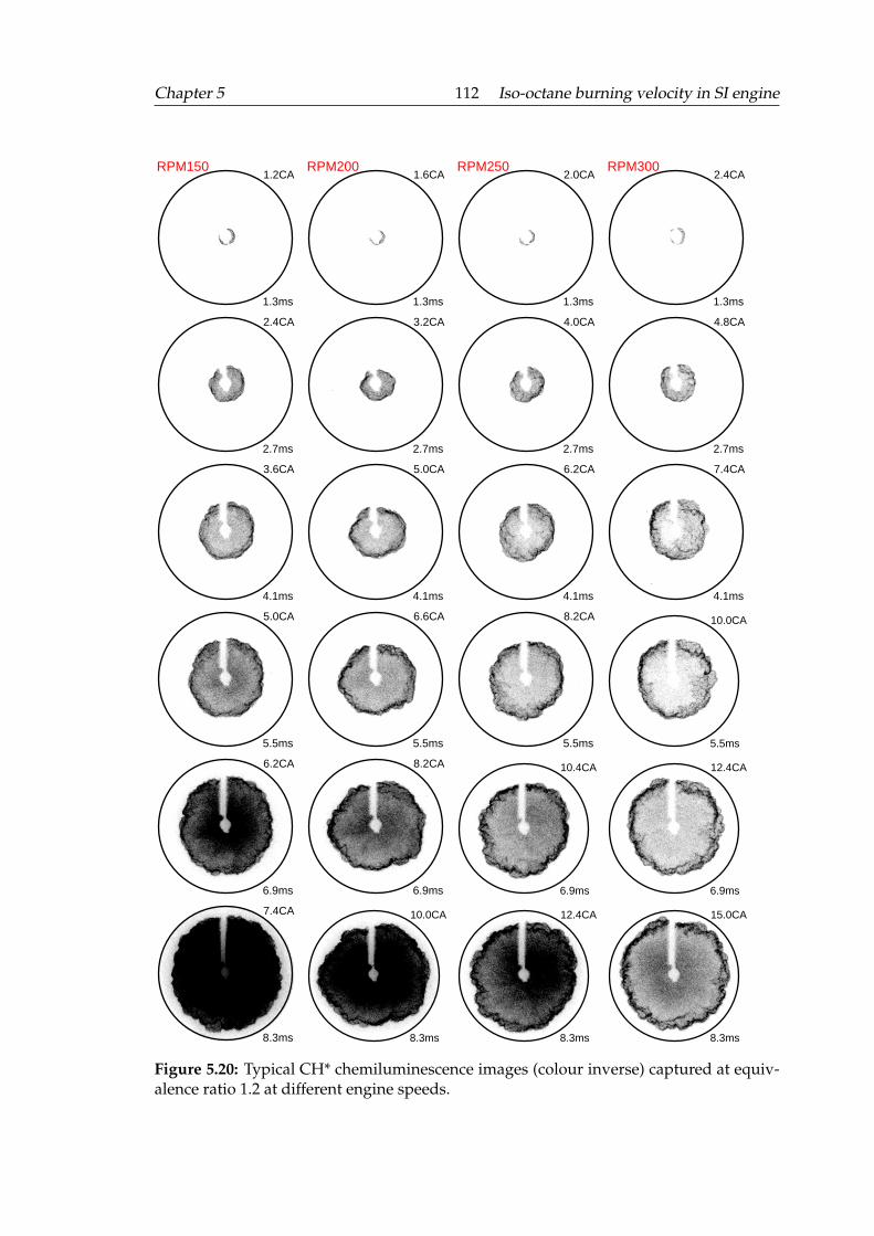
Chapter 5 112 Iso-octane burning velocity in SI engine
1.2CA
1.3ms
RPM1501.6CA
1.3ms
RPM2002.0CA
1.3ms
RPM2502.4CA
1.3ms
RPM300
2.4CA
2.7ms
3.2CA
2.7ms
4.0CA
2.7ms
4.8CA
2.7ms
3.6CA
4.1ms
5.0CA
4.1ms
6.2CA
4.1ms
7.4CA
4.1ms
5.0CA
5.5ms
6.6CA
5.5ms
8.2CA
5.5ms
10.0CA
5.5ms
6.2CA
6.9ms
8.2CA
6.9ms
10.4CA
6.9ms
12.4CA
6.9ms
7.4CA
8.3ms
10.0CA
8.3ms
12.4CA
8.3ms
15.0CA
8.3ms
Figure 5.20: Typical CH* chemiluminescence images (colour inverse) captured at equiv-alence ratio 1.2 at different engine speeds.
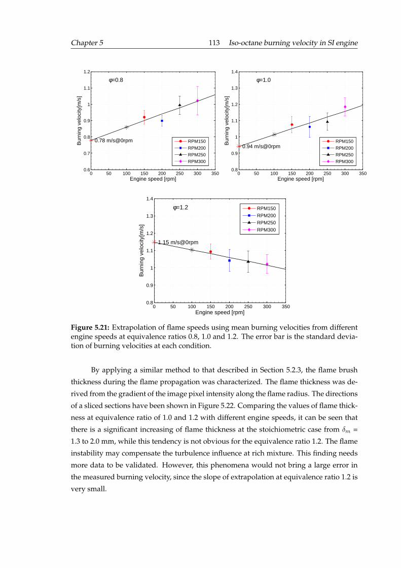
Chapter 5 113 Iso-octane burning velocity in SI engine
0 50 100 150 200 250 300 3500.6
0.7
0.8
0.9
1
1.1
1.2
Engine speed [rpm]
Bur
ning
vel
ocity
[m/s
]
0.78 m/s@0rpm
φ=0.8
RPM150
RPM200
RPM250
RPM300
0 50 100 150 200 250 300 3500.8
0.9
1
1.1
1.2
1.3
1.4
Engine speed [rpm]
Bur
ning
vel
ocity
[m/s
]
0.94 m/s@0rpm
φ=1.0
RPM150
RPM200
RPM250
RPM300
0 50 100 150 200 250 300 3500.8
0.9
1
1.1
1.2
1.3
1.4
Engine speed [rpm]
Bur
ning
vel
ocity
[m/s
]
1.15 m/s@0rpm
φ=1.2 RPM150
RPM200
RPM250
RPM300
Figure 5.21: Extrapolation of flame speeds using mean burning velocities from differentengine speeds at equivalence ratios 0.8, 1.0 and 1.2. The error bar is the standard devia-tion of burning velocities at each condition.
By applying a similar method to that described in Section 5.2.3, the flame brush
thickness during the flame propagation was characterized. The flame thickness was de-
rived from the gradient of the image pixel intensity along the flame radius. The directions
of a sliced sections have been shown in Figure 5.22. Comparing the values of flame thick-
ness at equivalence ratio of 1.0 and 1.2 with different engine speeds, it can be seen that
there is a significant increasing of flame thickness at the stoichiometric case from δm =
1.3 to 2.0 mm, while this tendency is not obvious for the equivalence ratio 1.2. The flame
instability may compensate the turbulence influence at rich mixture. This finding needs
more data to be validated. However, this phenomena would not bring a large error in
the measured burning velocity, since the slope of extrapolation at equivalence ratio 1.2 is
very small.
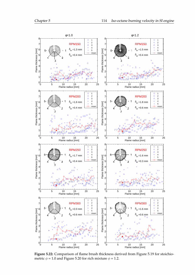
Chapter 5 114 Iso-octane burning velocity in SI engine
0 5 10 15 20 250
1
2
3
4
5
6
7
8
Flame radius [mm]
Fla
me
thic
knes
s [m
m]
φ=1.0
δm
δst
=1.3 mm
=0.4 mm
RPM150
12345mean
0 5 10 15 20 250
1
2
3
4
5
6
7
8
Flame radius [mm]
Fla
me
thic
knes
s [m
m]
φ=1.2
δm
δst
=1.5 mm
=0.4 mm
RPM150
12345mean
0 5 10 15 20 250
1
2
3
4
5
6
7
8
Flame radius [mm]
Fla
me
thic
knes
s [m
m]
δm
δst
=1.6 mm
=0.4 mm
RPM20012345mean
0 5 10 15 20 250
1
2
3
4
5
6
7
8
Flame radius [mm]
Fla
me
thic
knes
s [m
m]
δm
δst
=1.8 mm
=0.6 mm
RPM20012345mean
0 5 10 15 20 250
1
2
3
4
5
6
7
8
Flame radius [mm]
Fla
me
thic
knes
s [m
m]
δm
δst
=1.7 mm
=0.4 mm
RPM25012345mean
0 5 10 15 20 250
1
2
3
4
5
6
7
8
Flame radius [mm]
Fla
me
thic
knes
s [m
m]
δm
δst
=1.6 mm
=0.3 mm
RPM25012345mean
0 5 10 15 20 250
1
2
3
4
5
6
7
8
Flame radius [mm]
Fla
me
thic
knes
s [m
m]
δm
δst
=2.0 mm
=0.6 mm
RPM30012345mean
0 5 10 15 20 250
1
2
3
4
5
6
7
8
Flame radius [mm]
Fla
me
thic
knes
s [m
m]
δm
δst
=1.6 mm
=0.6 mm
RPM30012345mean
Figure 5.22: Comparison of flame brush thickness derived from Figure 5.19 for stoichio-metric ϕ = 1.0 and Figure 5.20 for rich mixture ϕ = 1.2.
Chapter 5 115 Iso-octane burning velocity in SI engine
5.4 Laminar flame speed correlations and simulation
The laminar burning velocity of iso-octane fuel has been widely measured in constant
volume combustion vessels (Bradley et al. [1998]; Galmiche et al. [2012]; Jerzembeck et al.
[2009]; Metghalchi and Keck [1982]. Nevertheless, the current measurement pressure and
temperature conditions are outside the range that can be obtained in these bomb exper-
iments as shown in Figure 5.23. The available experiment data from the literature also
could not cover the real boosted engine operation region, used in this work. In order to
validate the measurement results, correlation equations and computer modelling method
were used. First, various correlation equations for laminar flame speed and a chemical
reaction mechanism were evaluated by the experimental data from bomb at the low pres-
sure and temperature range in this Section. Then the calculated data were extended to
the current high pressure and temperature experimental conditions to compare the mea-
sured data in the next Section.
5.4.1 Experimental data review
Outwardly propagating flame configuration has been proven to be the most suitable for
high pressure flame speed measurements. Iso-octane burning velocities of laminar flame
at elevated pressures are often measured in a constant volume vessel. Early works in-
clude those of Metghalchi and Keck [1982], and Ryan and Lestz [1980]. They derived the
burning velocities from thermodynamic analysis of the pressure rise in a bomb. Even
though effects of flame stretch and hydrodynamic instabilities might be included in these
measurements, they were neglected for a long time. Recent works, e.g. Bradley et al.
[1998], and Jerzembeck et al. [2009], applied optical methods to record the flame propa-
gation process, hence it can be considered to be the direct measurement of the stretched
laminar flame propagation speed. Here, four sets of experimental data for iso-octane
laminar burning velocities were used to validate the correlation equations and chemical
reaction simulation at the low pressure, these experimental data are from four research
groups, and they are listed in Table 5.1.
All reviewed experiments were conducted in constant volume combustion ves-
sels or bombs, of different sizes and shapes. The spherical stainless steel bomb in Leeds
(Bradley et al. [1998]) has the large inner diameter of 380 mm and optical windows of
150 mm diameter, and it is capable of withstanding initial pressures of up to 15 bar and
initial temperatures of up to 500 K. The air and fuel were mixed using four fans driven
by electric motors. Galmiche et al. [2012], carried out experiment in a similar spherical
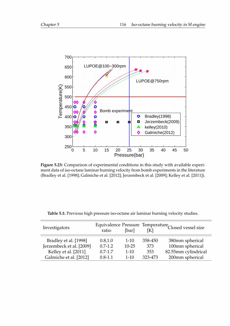
Chapter 5 116 Iso-octane burning velocity in SI engine
0 5 10 15 20 25 30 35 40 45 50250
300
350
400
450
500
550
600
650
700
LUPOE@100−300rpm
LUPOE@750rpm
Bomb experiment
Pressure(bar)
Tem
pera
ture
(K)
Bradley(1998)Jerzembeck(2009)kelley(2010)Galmiche(2012)
Figure 5.23: Comparison of experimental conditions in this study with available experi-ment data of iso-octane laminar burning velocity from bomb experiments in the literature(Bradley et al. [1998]; Galmiche et al. [2012]; Jerzembeck et al. [2009]; Kelley et al. [2011]).
Table 5.1: Previous high pressure iso-octane air laminar burning velocity studies.
Investigators Equivalenceratio
Pressure[bar]
Temperature[K] Closed vessel size
Bradley et al. [1998] 0.8,1.0 1-10 358-450 380mm sphericalJerzembeck et al. [2009] 0.7-1.2 10-25 373 100mm spherical
Kelley et al. [2011] 0.7-1.7 1-10 353 82.55mm cylindricalGalmiche et al. [2012] 0.8-1.1 1-10 323-473 200mm spherical
Chapter 5 117 Iso-octane burning velocity in SI engine
combustion bomb relying on molecular diffusion for mixture preparation. The inner di-
ameter of the bomb used in his experiment was 200 mm, and the initial pressure inside
the combustion chamber was limited to 10 bar. Jerzembeck et al. [2009], used a small
bomb with inner diameter 100 mm, and optical windows 50 mm. The maximum initial
pressure achieved in his experiment was up to 25 bar. Kelley et al. [2011], developed
a dual-chamber cylindrical vessel. The outer chamber has 273 mm inner diameter and
304.8 mm length, the inner chamber was 82 mm inner diameter and 127 mm length. Two
quartz windows (114 mm diameter) were installed at the both end sides. The maximum
pressure was claimed to achieve 60 bar, however the data for iso-octane presented in their
published work was at 10 bar.
During experiments at the constant volume vessel, fuel and air mixture were ig-
nited at the centre, and schlieren photography was applied to record the progress of
flame development. The mean flame radius was derived from each schlieren image. The
laminar flame speed could be calculated as the rate of change of flame radius with time.
Only images of laminar flame propagation without ignition effect and captured before
the onset of flame instability were used (Bradley et al. [1998]). Bradley et al. [1998] ap-
plied a first order least-squares fit through four adjacent radii to obtain a flame speed,
then derived an unstretched laminar burning velocity using a first-order fitted Markstein
length as described in Section 2.2.1.2. Jerzembeck et al. [2009] adopted the similar way
to process the data. Both Kelley et al. [2011] and Galmiche et al. [2012] used a nonlinear
extrapolation method to obtain the unstretched laminar burning velocities.
5.4.2 Evaluation of modelling methods
A widely used laminar flame speed correlation expression has been proposed by Met-
ghalchi and Keck [1982], which is a simple power law equation with reference temper-
ature T0 and pressure P0 with two exponents α and β. these parameters were obtained
using pressure traces recorded in a bomb.
ul = (Bm +B2(ϕ− ϕm)2)
(Tu
T0
)α( P
P0
)β
(5.1)
where ul is the laminar burning velocity, Tu is the unburnt gas temperature (K) and P
is the pressure (bar). ϕ is the equivalence ratio. Similar expression was proposed by Al-
Shahrany et al. [2005] using schlieren images recorded from two opposite propagating
flames in a constant volume bomb. For an iso-octane-air mixture, the input parameters
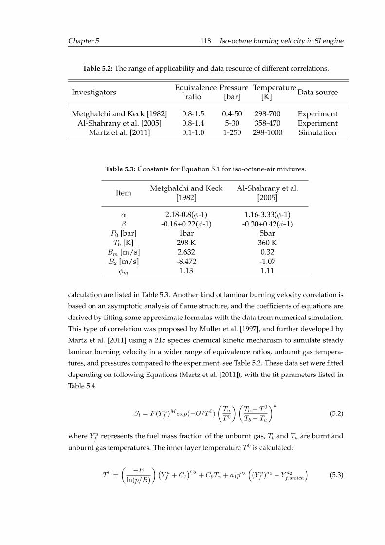
Chapter 5 118 Iso-octane burning velocity in SI engine
Table 5.2: The range of applicability and data resource of different correlations.
Investigators Equivalenceratio
Pressure[bar]
Temperature[K] Data source
Metghalchi and Keck [1982] 0.8-1.5 0.4-50 298-700 ExperimentAl-Shahrany et al. [2005] 0.8-1.4 5-30 358-470 Experiment
Martz et al. [2011] 0.1-1.0 1-250 298-1000 Simulation
Table 5.3: Constants for Equation 5.1 for iso-octane-air mixtures.
Item Metghalchi and Keck[1982]
Al-Shahrany et al.[2005]
α 2.18-0.8(ϕ-1) 1.16-3.33(ϕ-1)β -0.16+0.22(ϕ-1) -0.30+0.42(ϕ-1)
P0 [bar] 1bar 5barT0 [K] 298 K 360 K
Bm [m/s] 2.632 0.32B2 [m/s] -8.472 -1.07
ϕm 1.13 1.11
calculation are listed in Table 5.3. Another kind of laminar burning velocity correlation is
based on an asymptotic analysis of flame structure, and the coefficients of equations are
derived by fitting some approximate formulas with the data from numerical simulation.
This type of correlation was proposed by Muller et al. [1997], and further developed by
Martz et al. [2011] using a 215 species chemical kinetic mechanism to simulate steady
laminar burning velocity in a wider range of equivalence ratios, unburnt gas tempera-
tures, and pressures compared to the experiment, see Table 5.2. These data set were fitted
depending on following Equations (Martz et al. [2011]), with the fit parameters listed in
Table 5.4.
Sl = F (Y uf )Mexp(−G/T 0)
(Tu
T 0
)(Tb − T 0
Tb − Tu
)n
(5.2)
where Y uf represents the fuel mass fraction of the unburnt gas, Tb and Tu are burnt and
unburnt gas temperatures. The inner layer temperature T 0 is calculated:
T 0 =
(−E
ln(p/B)
)(Y uf + C7
)C8 + C9Tu + a1pa3
((Y u
f )a2 − Y a2f,stoich
)(5.3)
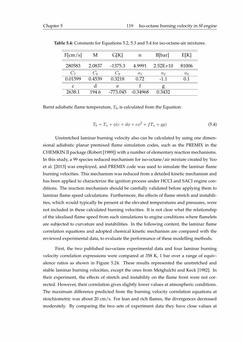
Chapter 5 119 Iso-octane burning velocity in SI engine
Table 5.4: Constants for Equations 5.2, 5.3 and 5.4 for iso-octane-air mixtures.
F[cm/s] M G[K] n B[bar] E[K]
280583 2.0837 -1375.3 4.9991 2.52E+10 81006C7 C8 C9 a1 a2 a3
0.01599 0.4539 0.3218 0.72 -1.1 0.1c d e f g
2638.1 194.6 -773.045 -0.34968 0.3432
Burnt adiabatic flame temperature, Tb, is calculated from the Equation:
Tb = Tu + ϕ(c+ dϕ+ eϕ2 + fTu + gp) (5.4)
Unstretched laminar burning velocity also can be calculated by using one dimen-
sional adiabatic planar premixed flame simulation codes, such as the PREMIX in the
CHEMKIN II package (Robert [1989]) with a number of elementary reaction mechanisms.
In this study, a 99 species reduced mechanism for iso-octane/air mixture created by Yoo
et al. [2013] was employed, and PREMIX code was used to simulate the laminar flame
burning velocities. This mechanism was reduced from a detailed kinetic mechanism and
has been applied to characterize the ignition process under HCCI and SACI engine con-
ditions. The reaction mechanism should be carefully validated before applying them to
laminar flame speed calculations. Furthermore, the effects of flame stretch and instabili-
ties, which would typically be present at the elevated temperatures and pressures, were
not included in these calculated burning velocities. It is not clear what the relationship
of the idealised flame speed from such simulations to engine conditions where flamelets
are subjected to curvature and instabilities. In the following content, the laminar flame
correlation equations and adopted chemical kinetic mechanism are compared with the
reviewed experimental data, to evaluate the performance of these modelling methods.
First, the two published iso-octane experimental data and four laminar burning
velocity correlation expressions were compared at 358 K, 1 bar over a range of equiv-
alence ratios as shown in Figure 5.24. These results represented the unstretched and
stable laminar burning velocities, except the ones from Metghalchi and Keck [1982]. In
their experiment, the effects of stretch and instability on the flame front were not cor-
rected. However, their correlation gives slightly lower values at atmospheric conditions.
The maximum difference predicted from the burning velocity correlation equations at
stoichiometric was about 20 cm/s. For lean and rich flames, the divergences decreased
moderately. By comparing the two sets of experiment data they have close values at
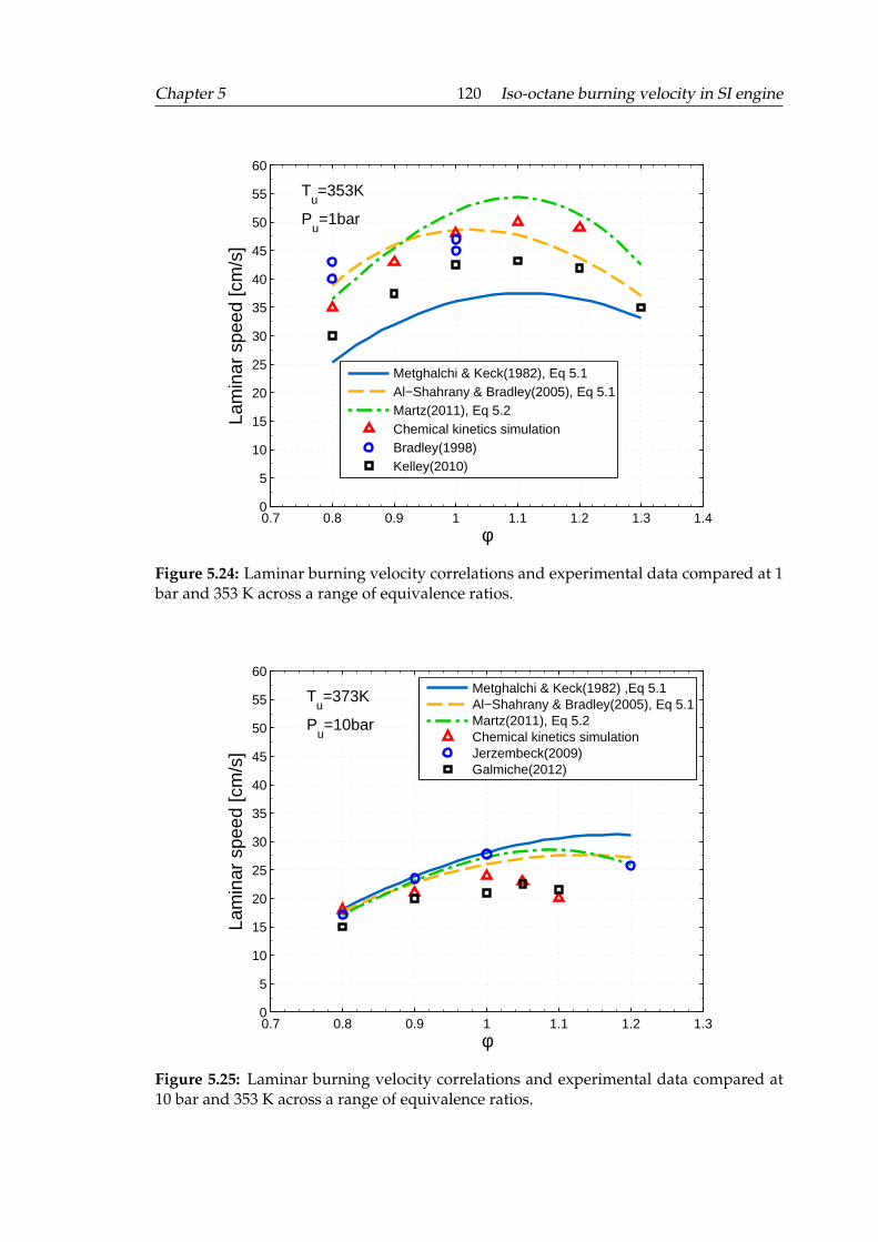
Chapter 5 120 Iso-octane burning velocity in SI engine
0.7 0.8 0.9 1 1.1 1.2 1.3 1.40
5
10
15
20
25
30
35
40
45
50
55
60
φ
Lam
inar
spe
ed [c
m/s
]
Tu=353K
Pu=1bar
Metghalchi & Keck(1982), Eq 5.1Al−Shahrany & Bradley(2005), Eq 5.1Martz(2011), Eq 5.2Chemical kinetics simulationBradley(1998)Kelley(2010)
Figure 5.24: Laminar burning velocity correlations and experimental data compared at 1bar and 353 K across a range of equivalence ratios.
0.7 0.8 0.9 1 1.1 1.2 1.30
5
10
15
20
25
30
35
40
45
50
55
60
φ
Lam
inar
spe
ed [c
m/s
]
Tu=373K
Pu=10bar
Metghalchi & Keck(1982) ,Eq 5.1Al−Shahrany & Bradley(2005), Eq 5.1Martz(2011), Eq 5.2Chemical kinetics simulationJerzembeck(2009)Galmiche(2012)
Figure 5.25: Laminar burning velocity correlations and experimental data compared at10 bar and 353 K across a range of equivalence ratios.
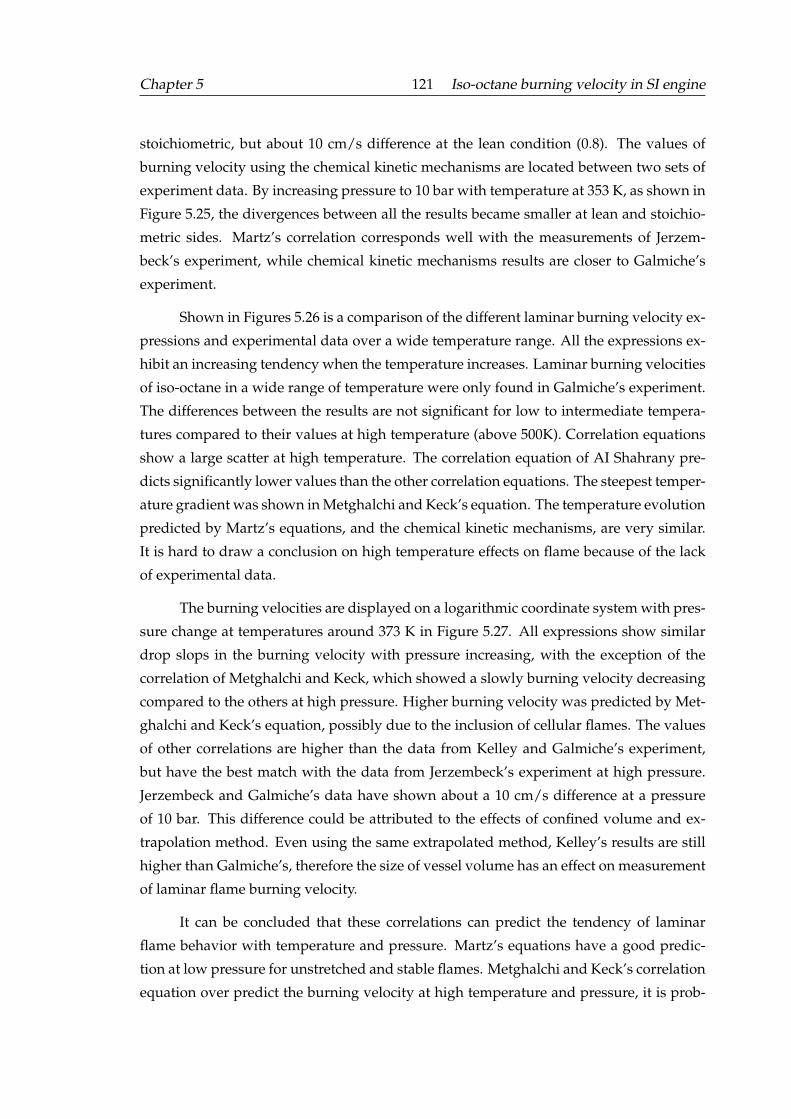
Chapter 5 121 Iso-octane burning velocity in SI engine
stoichiometric, but about 10 cm/s difference at the lean condition (0.8). The values of
burning velocity using the chemical kinetic mechanisms are located between two sets of
experiment data. By increasing pressure to 10 bar with temperature at 353 K, as shown in
Figure 5.25, the divergences between all the results became smaller at lean and stoichio-
metric sides. Martz’s correlation corresponds well with the measurements of Jerzem-
beck’s experiment, while chemical kinetic mechanisms results are closer to Galmiche’s
experiment.
Shown in Figures 5.26 is a comparison of the different laminar burning velocity ex-
pressions and experimental data over a wide temperature range. All the expressions ex-
hibit an increasing tendency when the temperature increases. Laminar burning velocities
of iso-octane in a wide range of temperature were only found in Galmiche’s experiment.
The differences between the results are not significant for low to intermediate tempera-
tures compared to their values at high temperature (above 500K). Correlation equations
show a large scatter at high temperature. The correlation equation of AI Shahrany pre-
dicts significantly lower values than the other correlation equations. The steepest temper-
ature gradient was shown in Metghalchi and Keck’s equation. The temperature evolution
predicted by Martz’s equations, and the chemical kinetic mechanisms, are very similar.
It is hard to draw a conclusion on high temperature effects on flame because of the lack
of experimental data.
The burning velocities are displayed on a logarithmic coordinate system with pres-
sure change at temperatures around 373 K in Figure 5.27. All expressions show similar
drop slops in the burning velocity with pressure increasing, with the exception of the
correlation of Metghalchi and Keck, which showed a slowly burning velocity decreasing
compared to the others at high pressure. Higher burning velocity was predicted by Met-
ghalchi and Keck’s equation, possibly due to the inclusion of cellular flames. The values
of other correlations are higher than the data from Kelley and Galmiche’s experiment,
but have the best match with the data from Jerzembeck’s experiment at high pressure.
Jerzembeck and Galmiche’s data have shown about a 10 cm/s difference at a pressure
of 10 bar. This difference could be attributed to the effects of confined volume and ex-
trapolation method. Even using the same extrapolated method, Kelley’s results are still
higher than Galmiche’s, therefore the size of vessel volume has an effect on measurement
of laminar flame burning velocity.
It can be concluded that these correlations can predict the tendency of laminar
flame behavior with temperature and pressure. Martz’s equations have a good predic-
tion at low pressure for unstretched and stable flames. Metghalchi and Keck’s correlation
equation over predict the burning velocity at high temperature and pressure, it is prob-
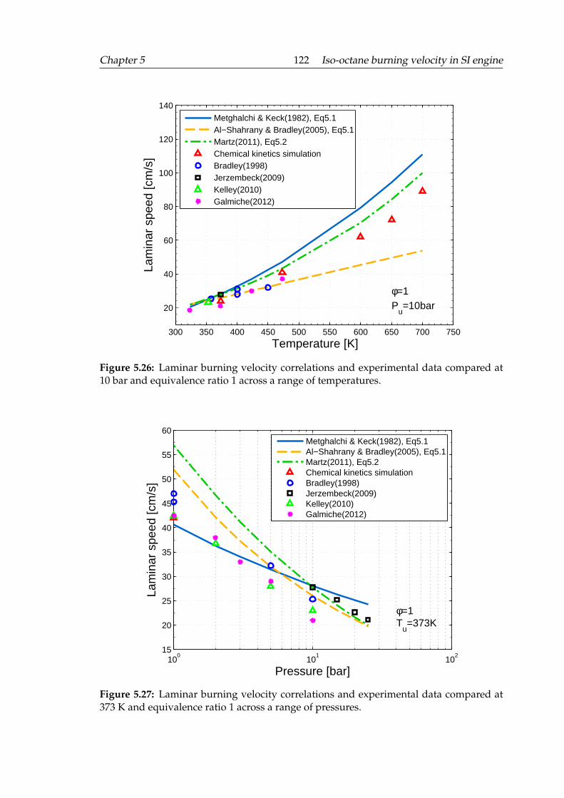
Chapter 5 122 Iso-octane burning velocity in SI engine
300 350 400 450 500 550 600 650 700 750
20
40
60
80
100
120
140
Temperature [K]
Lam
inar
spe
ed [c
m/s
]
φ=1P
u=10bar
Metghalchi & Keck(1982), Eq5.1Al−Shahrany & Bradley(2005), Eq5.1Martz(2011), Eq5.2Chemical kinetics simulationBradley(1998)Jerzembeck(2009)Kelley(2010)Galmiche(2012)
Figure 5.26: Laminar burning velocity correlations and experimental data compared at10 bar and equivalence ratio 1 across a range of temperatures.
100
101
102
15
20
25
30
35
40
45
50
55
60
Pressure [bar]
Lam
inar
spe
ed [c
m/s
]
φ=1T
u=373K
Metghalchi & Keck(1982), Eq5.1Al−Shahrany & Bradley(2005), Eq5.1Martz(2011), Eq5.2Chemical kinetics simulationBradley(1998)Jerzembeck(2009)Kelley(2010)Galmiche(2012)
Figure 5.27: Laminar burning velocity correlations and experimental data compared at373 K and equivalence ratio 1 across a range of pressures.
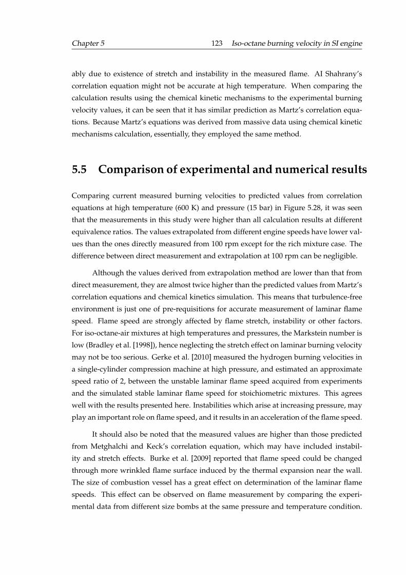
Chapter 5 123 Iso-octane burning velocity in SI engine
ably due to existence of stretch and instability in the measured flame. AI Shahrany’s
correlation equation might not be accurate at high temperature. When comparing the
calculation results using the chemical kinetic mechanisms to the experimental burning
velocity values, it can be seen that it has similar prediction as Martz’s correlation equa-
tions. Because Martz’s equations was derived from massive data using chemical kinetic
mechanisms calculation, essentially, they employed the same method.
5.5 Comparison of experimental and numerical results
Comparing current measured burning velocities to predicted values from correlation
equations at high temperature (600 K) and pressure (15 bar) in Figure 5.28, it was seen
that the measurements in this study were higher than all calculation results at different
equivalence ratios. The values extrapolated from different engine speeds have lower val-
ues than the ones directly measured from 100 rpm except for the rich mixture case. The
difference between direct measurement and extrapolation at 100 rpm can be negligible.
Although the values derived from extrapolation method are lower than that from
direct measurement, they are almost twice higher than the predicted values from Martz’s
correlation equations and chemical kinetics simulation. This means that turbulence-free
environment is just one of pre-requisitions for accurate measurement of laminar flame
speed. Flame speed are strongly affected by flame stretch, instability or other factors.
For iso-octane-air mixtures at high temperatures and pressures, the Markstein number is
low (Bradley et al. [1998]), hence neglecting the stretch effect on laminar burning velocity
may not be too serious. Gerke et al. [2010] measured the hydrogen burning velocities in
a single-cylinder compression machine at high pressure, and estimated an approximate
speed ratio of 2, between the unstable laminar flame speed acquired from experiments
and the simulated stable laminar flame speed for stoichiometric mixtures. This agrees
well with the results presented here. Instabilities which arise at increasing pressure, may
play an important role on flame speed, and it results in an acceleration of the flame speed.
It should also be noted that the measured values are higher than those predicted
from Metghalchi and Keck’s correlation equation, which may have included instabil-
ity and stretch effects. Burke et al. [2009] reported that flame speed could be changed
through more wrinkled flame surface induced by the thermal expansion near the wall.
The size of combustion vessel has a great effect on determination of the laminar flame
speeds. This effect can be observed on flame measurement by comparing the experi-
mental data from different size bombs at the same pressure and temperature condition.
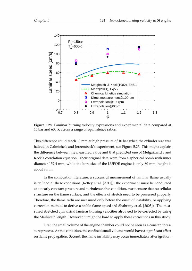
Chapter 5 124 Iso-octane burning velocity in SI engine
0.7 0.8 0.9 1 1.1 1.2 1.3−20
0
20
40
60
80
100
120
140
φ
Lam
inar
spe
ed [c
m/s
]
Pu=15bar
Tu=600K
Metghalchi & Keck(1982), Eq5.1Martz(2011), Eq5.2Chemical kinetics simulationDirect measurement@100rpmExtrapolation@100rpmExtrapolation@0rpm
Figure 5.28: Laminar burning velocity expressions and experimental data compared at15 bar and 600 K across a range of equivalence ratios.
This difference could reach 10 mm at high pressure of 10 bar when the cylinder size was
halved in Galmiche’s and Jerzembeck’s experiment, see Figure 5.27. This might explain
the difference between the measured value and that predicted one of Metgakhatchi and
Keck’s correlation equation. Their original data were from a spherical bomb with inner
diameter 152.4 mm, while the bore size of the LUPOE engine is only 80 mm, height is
about 8 mm.
In the combustion literature, a successful measurement of laminar flame usually
is defined at these conditions (Kelley et al. [2011]): the experiment must be conducted
at a nearly constant pressure and turbulence-free condition, must ensure that no cellular
structure on the flame surface, and the effects of stretch need to be processed properly.
Therefore, the flame radii are measured only before the onset of instability, or applying
correction method to derive a stable flame speed (Al-Shahrany et al. [2005]). The mea-
sured stretched cylindrical laminar burning velocities also need to be corrected by using
the Markstein length. However, it might be hard to apply these corrections in this study.
First, the small volume of the engine chamber could not be seen as a constant pres-
sure process. At this condition, the confined small volume would have a significant effect
on flame propagation. Second, the flame instability may occur immediately after ignition,
Chapter 5 125 Iso-octane burning velocity in SI engine
which can accelerate the flame speed. At the same time, ignition had similar influence on
the flame speed. Therefore, it was hard to determine if the flame speed was accelerated
by the flame instability or ignition in the initial stage, see Figure 5.15. Lastly, the cylindri-
cal flame would have a large area contacting with the cylinder head and piston surface
during flame propagation. The expansion gas in front of the flame front may push the
air-fuel mixture, and the viscous boundary conditions can lead to velocity variations be-
tween flame front in the middle plane of chamber and the walls. The flame front may be
bent in the contact places under these effects. This can accelerate the flame speed. How
large the effects will be induced by this phenomenon has not been studied for the engine
condition.
In conclusion, it has been shown that the flame speed, measured at a turbulence-
free engine environment, can reach high values compared to that measured from con-
stant volume combustion vessels. This is mainly due to flame instability and small con-
fined volume. It is unreliable to apply the correction methods to correct the current
measured ”quasi-laminar” burning velocity to unstretched and stable burning velocity
directly. However, since there existed a large difference of burning velocity between sta-
ble and unstable flames at engine relevant pressure and temperature conditions, it worth
considering whether the influence of flame front instabilities should be included in lam-
inar burning velocity, before putting it into a turbulent combustion model. This requires
further investigation with the turbulent flame studies.
Chapter 6
Flame development in a boosted
engine
Understanding the influences of high pressure on the flame dynamics and structure are
crucial for designing new efficient ”Downsizing” spark ignition engines. The effects of
highly boosted initial pressure on unsteady flame development, turbulent burning veloc-
ity and flame structure at the same condition of turbulence intensity have been investi-
gated experimentally in this Chapter. The measurements were performed in the boosted
optical engine LUPOE 2D with an independently controlled exhaust system valve de-
tailed in Chapter 3. The turbulent intensity and the integral length scale were character-
ized by two-dimensional Particle Image Velocimetry (PIV). High speed CH* chemilumi-
nescence imaging method was applied to record the flame front position, combined with
a ”reverse” thermodynamic analysis engine model, burning rate and flame brush thick-
ness can be obtained. The structure of the flame front at high pressure and its response to
pressure effects have been further investigated using a laser sheet visualization method.
The detailed cross section flame front topology was observed. Wrinkle and curvature of
the flame front were characterized to compare the flame shapes under different boosted
initial pressures.
Chapter 6 127 Flame development in a boosted engine
6.1 Engine operation condition
The LUPOE 2D boosted engine can be boosted by two methods. The first method is to
increase the inlet flow mass rate. It is widely used in most boosted engine experiments
(Landry et al. [2008]; Merola et al. [2007]). Compared with the lifted valves engine, the
turbulence generated by the jet-type intake of LUPOE 2D engine shall be more sensitive
to the inlet flow velocity. Increasing the inlet flow velocity may result in the turbulence
intensity increasing. The second method is to use the exhaust valve described in the
previous Chapter 3; the LUPOE 2D engine can gain the higher initial pressure at the
same flow rate setting through extending the time during which the exhaust valve closed
before a firing cycle.
An initial inlet pressure map for the boosted LUPOE 2D engine has been developed
and it is shown in Figure 6.1 for different combinations of inlet flow rate and exhaust
valve closing time. The engine was fired at a speed of 750 rpm. At this speed, each
cycle lasts 80 ms. It can be seen that the initial pressure does not change significantly
when the exhaust valve closes one cycle before firing. This is because of the small flow
rate and delay time of exhaust valve, about 15 ms. Due to the skip firing cycles, the the
exhaust valves closing time can be advanced further before the firing cycles. Under the
same condition of valve closing time, the initial pressure increases rapidly with the flow
rate. However, the flow rate has to be increased up to 50% in order to increase the initial
pressure 1.6 to 2.0 bar. Such a change might affect the turbulence intensity at the same
time.
The maximum initial pressure shown in the map is approximately 4 bar, see Figure
6.1. Analysis of this Figure shows that when the mass flow rate is changed at a constant
number of cycles before the firing one during which the exhaust valve is closed, it will
change at the same time the turbulence and the initial pressure. However, by a simultane-
ous variation of the time of the exhaust valve closure and the flow rate, one may achieve
the same inlet pressure at different turbulence strengths. This has been attempted in the
present work. These assumptions are confirmed by using Particle Image Velocimetry
(PIV) in the following Section.
Most experiments in this work have been done with conditions shown in the first
column of the map, the initial pressures of these points are 1.6 bar, 1.8 bar and 2.0 bar,
respectively, these cases are denoted as Pi16, Pi18, Pi20. In order to test the flow rate
effects, other two conditions were also used, which have almost same initial pressure,
but higher inlet flow rates, these are denoted as Pi18ref, Pi20ref. These five conditions are
listed in Table 6.1.
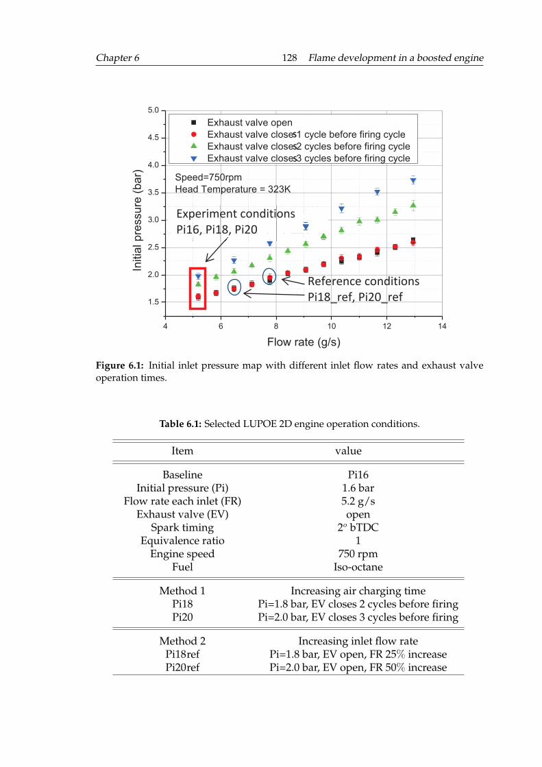
Chapter 6 128 Flame development in a boosted engine
4 6 8 10 12 14
1.5
2.0
2.5
3.0
3.5
4.0
4.5
5.0
Initia
l pre
ssure
(bar)
Flow rate (g/s)
Exhaust valve open
Exhaust valve close 1 cycle before firing cycle
Exhaust valve close 2 cycles before firing cycle
Exhaust valve close 3 cycles before firing cycle
Speed=750rpm
Head Temperature = 323K
Experiment conditions
Pi16, Pi18, Pi20
Reference conditions
Pi18_ref, Pi20_ref
S
S
S
Figure 6.1: Initial inlet pressure map with different inlet flow rates and exhaust valveoperation times.
Table 6.1: Selected LUPOE 2D engine operation conditions.
Item value
Baseline Pi16Initial pressure (Pi) 1.6 bar
Flow rate each inlet (FR) 5.2 g/sExhaust valve (EV) open
Spark timing 2o bTDCEquivalence ratio 1
Engine speed 750 rpmFuel Iso-octane
Method 1 Increasing air charging timePi18 Pi=1.8 bar, EV closes 2 cycles before firingPi20 Pi=2.0 bar, EV closes 3 cycles before firing
Method 2 Increasing inlet flow ratePi18ref Pi=1.8 bar, EV open, FR 25% increasePi20ref Pi=2.0 bar, EV open, FR 50% increase
Chapter 6 129 Flame development in a boosted engine
The LUPOE 2D engine was set to run at the following reference conditions: equiv-
alence ratio was 1, engine speed was 750 rev/min, sparking timing was 2o bTDC (before
Top Dead Centre). The tested fuel was 100% iso-octance. All conditions were selected
in the non-knocking region, in order to avoid the abnormal combustion affecting on the
flame propagation. Pi20ref is the condition which is the closest to the knock boundary.
The knock boundary map of the LUPOE 2D boosted engine is presented in Chapter 7.
100 cycles have been recorded in each experimental condition for statistical analysis. The
number of cycles required to compare the variance of engine pressure cycles has been
investigated by Hussin [2012]. He found there was not a significant change of statistical
results when more than N/7.5 cycles were used for the LUPOE 2D engine, N is the engine
speed. Intake and cylinder head temperature were all kept at 323 K. When the temper-
atures were set below 40oC, an unsteady air fuel mixture strength would happen due to
condensation of fuel on the wall surface of the intake pips (Dawood [2010]), while these
temperatures were set above 60oC, high initial temperature would cause occurrence of
knock and increase the risk of the optical window damage. For all engine experiments,
its skip-fire ratio was set at 20, sufficient for effective exhaust scavenging with no occur-
rence of the run-on phenomenon.
6.2 Flow characteristics in boosted LUPOE 2D engine
This Section examines whether the installed exhaust valve has the ability to boost the
initial pressure and control the turbulence at the same time. Increasing the pressure by
flow rate was also tested to validate the assumption that the inlet flow rate might change
the turbulent flow significantly in the LUPOE 2D boosted engine.
6.2.1 Individual cycle
A snapshot of the flow velocity field captured using PIV system at the condition Pi20 is
shown in Figure 6.2 in the form of vector and scalar maps. The measurement was taken at
2o bTDC in the mid plane of the clearance volume. The flow structure changes from cycle
to cycle, as mentioned in Chapter 3, the engine was designed to eliminate the strong bulk
flow and make the flow uniform. It is clearly shown in this Figure that there does not
exist a swirl structure, and no significant flow direction could be observed. The large and
small vortices distribute all over the field homogeneously. These vortices have a spatial
dimension of order of 5-10 mm. The flow velocity decreases near the wall. The accuracy
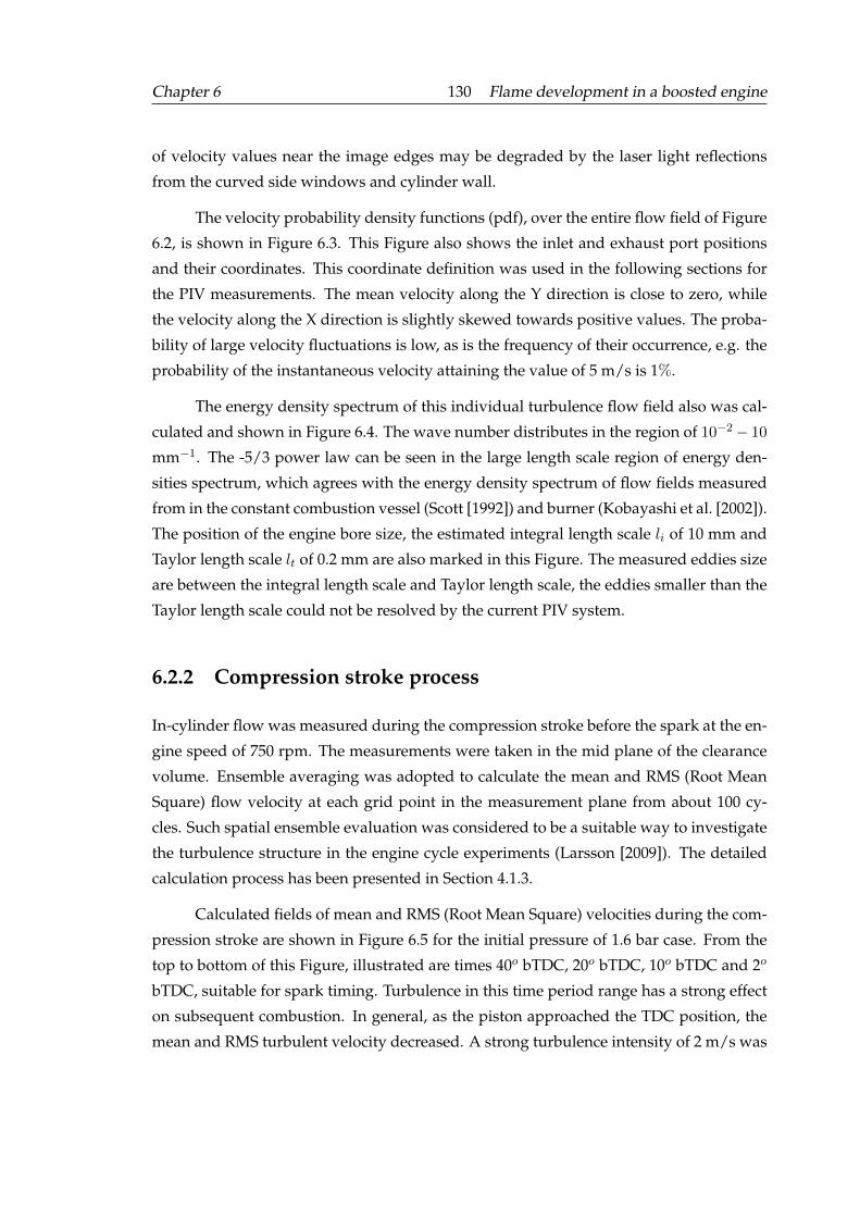
Chapter 6 130 Flame development in a boosted engine
of velocity values near the image edges may be degraded by the laser light reflections
from the curved side windows and cylinder wall.
The velocity probability density functions (pdf), over the entire flow field of Figure
6.2, is shown in Figure 6.3. This Figure also shows the inlet and exhaust port positions
and their coordinates. This coordinate definition was used in the following sections for
the PIV measurements. The mean velocity along the Y direction is close to zero, while
the velocity along the X direction is slightly skewed towards positive values. The proba-
bility of large velocity fluctuations is low, as is the frequency of their occurrence, e.g. the
probability of the instantaneous velocity attaining the value of 5 m/s is 1%.
The energy density spectrum of this individual turbulence flow field also was cal-
culated and shown in Figure 6.4. The wave number distributes in the region of 10−2 − 10
mm−1. The -5/3 power law can be seen in the large length scale region of energy den-
sities spectrum, which agrees with the energy density spectrum of flow fields measured
from in the constant combustion vessel (Scott [1992]) and burner (Kobayashi et al. [2002]).
The position of the engine bore size, the estimated integral length scale li of 10 mm and
Taylor length scale lt of 0.2 mm are also marked in this Figure. The measured eddies size
are between the integral length scale and Taylor length scale, the eddies smaller than the
Taylor length scale could not be resolved by the current PIV system.
6.2.2 Compression stroke process
In-cylinder flow was measured during the compression stroke before the spark at the en-
gine speed of 750 rpm. The measurements were taken in the mid plane of the clearance
volume. Ensemble averaging was adopted to calculate the mean and RMS (Root Mean
Square) flow velocity at each grid point in the measurement plane from about 100 cy-
cles. Such spatial ensemble evaluation was considered to be a suitable way to investigate
the turbulence structure in the engine cycle experiments (Larsson [2009]). The detailed
calculation process has been presented in Section 4.1.3.
Calculated fields of mean and RMS (Root Mean Square) velocities during the com-
pression stroke are shown in Figure 6.5 for the initial pressure of 1.6 bar case. From the
top to bottom of this Figure, illustrated are times 40o bTDC, 20o bTDC, 10o bTDC and 2o
bTDC, suitable for spark timing. Turbulence in this time period range has a strong effect
on subsequent combustion. In general, as the piston approached the TDC position, the
mean and RMS turbulent velocity decreased. A strong turbulence intensity of 2 m/s was
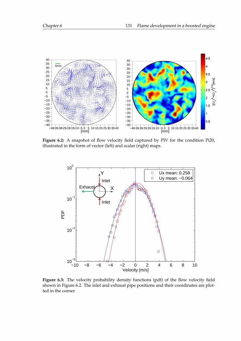
Chapter 6 131 Flame development in a boosted engine
5m/s
−40−40
−35
−35
−30
−30
−25
−25
−20
−20
−15
−15
−10
−10
−5
−5
0
0
5
5
10
10
15
15
20
20
25
25
30
30
35
35
40
40
[mm]−40
−40−35
−35
−30
−30
−25
−25
−20
−20
−15
−15
−10
−10
−5
−5
0
0
5
5
10
10
15
15
20
20
25
25
30
30
35
35
40
40
[mm]
Figure 6.2: A snapshot of flow velocity field captured by PIV for the condition Pi20,illustrated in the form of vector (left) and scalar (right) maps.
−10 −8 −6 −4 −2 0 2 4 6 8 1010
−3
10−2
10−1
100
Velocity [m/s]
PD
F
Ux mean: 0.258Uy mean: −0.064Inlet
Inlet
Exhaust X
Y
Figure 6.3: The velocity probability density functions (pdf) of the flow velocity fieldshown in Figure 6.2. The inlet and exhaust pipe positions and their coordinates are plot-ted in the corner.
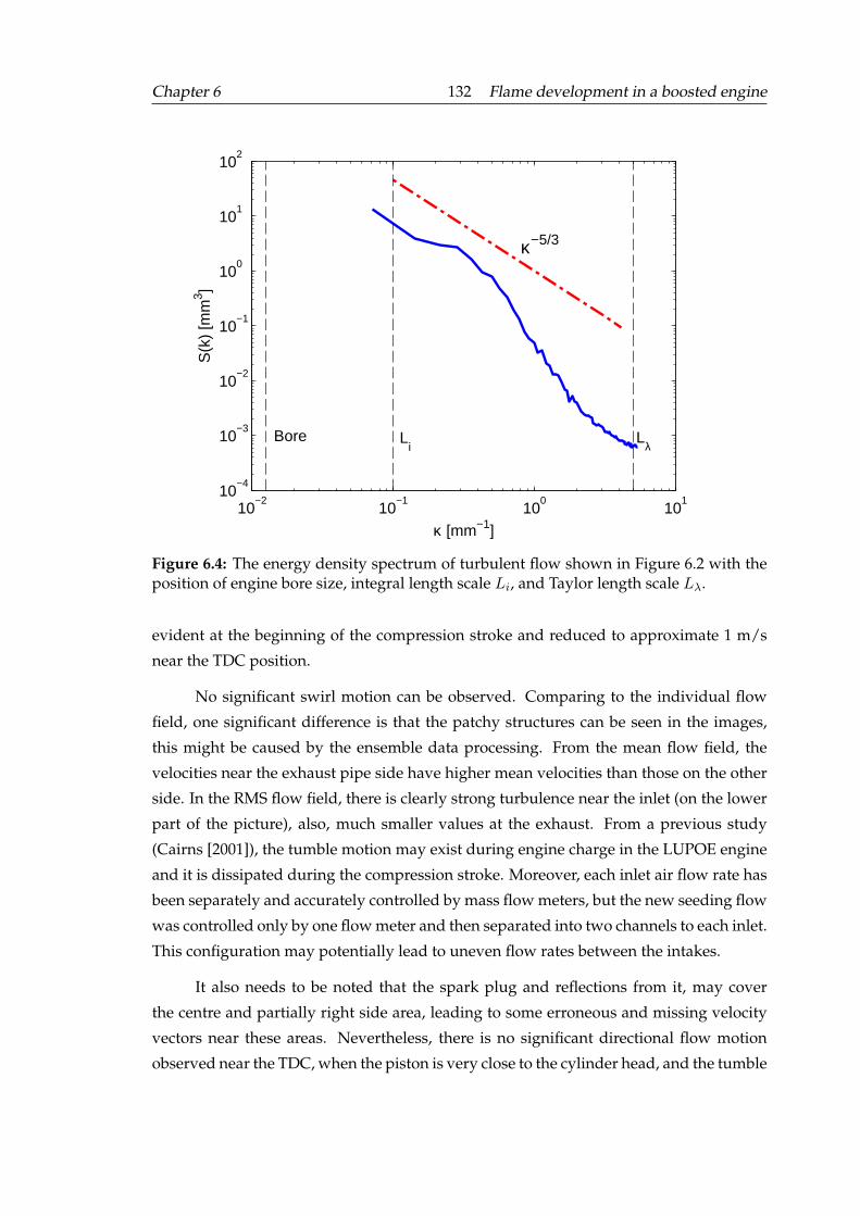
Chapter 6 132 Flame development in a boosted engine
10−2
10−1
100
101
10−4
10−3
10−2
10−1
100
101
102
κ [mm−1]
S(k
) [m
m3 ]
Bore Li
Lλ
κ−5/3
Figure 6.4: The energy density spectrum of turbulent flow shown in Figure 6.2 with theposition of engine bore size, integral length scale Li, and Taylor length scale Lλ.
evident at the beginning of the compression stroke and reduced to approximate 1 m/s
near the TDC position.
No significant swirl motion can be observed. Comparing to the individual flow
field, one significant difference is that the patchy structures can be seen in the images,
this might be caused by the ensemble data processing. From the mean flow field, the
velocities near the exhaust pipe side have higher mean velocities than those on the other
side. In the RMS flow field, there is clearly strong turbulence near the inlet (on the lower
part of the picture), also, much smaller values at the exhaust. From a previous study
(Cairns [2001]), the tumble motion may exist during engine charge in the LUPOE engine
and it is dissipated during the compression stroke. Moreover, each inlet air flow rate has
been separately and accurately controlled by mass flow meters, but the new seeding flow
was controlled only by one flow meter and then separated into two channels to each inlet.
This configuration may potentially lead to uneven flow rates between the intakes.
It also needs to be noted that the spark plug and reflections from it, may cover
the centre and partially right side area, leading to some erroneous and missing velocity
vectors near these areas. Nevertheless, there is no significant directional flow motion
observed near the TDC, when the piston is very close to the cylinder head, and the tumble
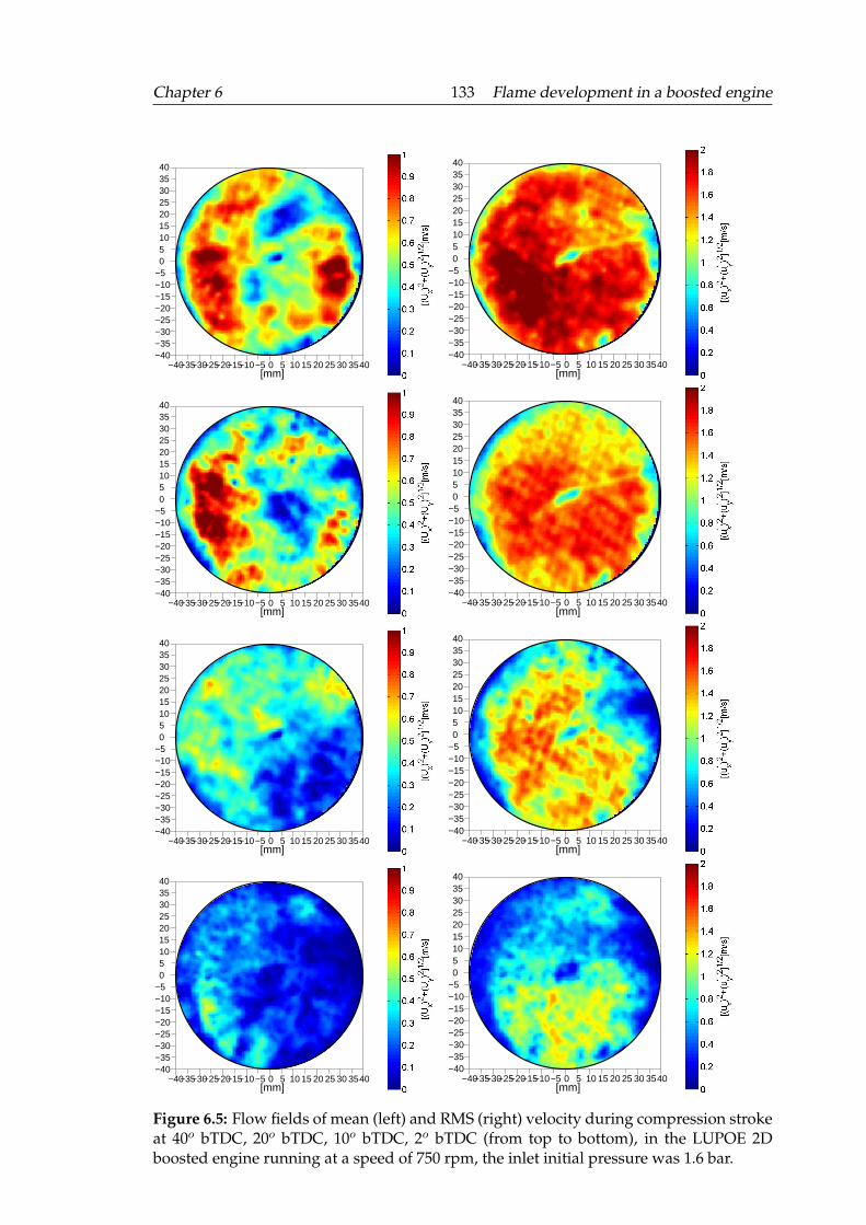
Chapter 6 133 Flame development in a boosted engine
−40−40
−35
−35
−30
−30
−25
−25
−20
−20
−15
−15
−10
−10
−5
−5
0
0
5
5
10
10
15
15
20
20
25
25
30
30
35
35
40
40
[mm]−40
−40−35
−35
−30
−30
−25
−25
−20
−20
−15
−15
−10
−10
−5
−5
0
0
5
5
10
10
15
15
20
20
25
25
30
30
35
35
40
40
[mm]
−40−40
−35
−35
−30
−30
−25
−25
−20
−20
−15
−15
−10
−10
−5
−5
0
0
5
5
10
10
15
15
20
20
25
25
30
30
35
35
40
40
[mm]−40
−40−35
−35
−30
−30
−25
−25
−20
−20
−15
−15
−10
−10
−5
−5
0
0
5
5
10
10
15
15
20
20
25
25
30
30
35
35
40
40
[mm]
−40−40
−35
−35
−30
−30
−25
−25
−20
−20
−15
−15
−10
−10
−5
−5
0
0
5
5
10
10
15
15
20
20
25
25
30
30
35
35
40
40
[mm]−40
−40−35
−35
−30
−30
−25
−25
−20
−20
−15
−15
−10
−10
−5
−5
0
0
5
5
10
10
15
15
20
20
25
25
30
30
35
35
40
40
[mm]
−40−40
−35
−35
−30
−30
−25
−25
−20
−20
−15
−15
−10
−10
−5
−5
0
0
5
5
10
10
15
15
20
20
25
25
30
30
35
35
40
40
[mm]−40
−40−35
−35
−30
−30
−25
−25
−20
−20
−15
−15
−10
−10
−5
−5
0
0
5
5
10
10
15
15
20
20
25
25
30
30
35
35
40
40
[mm]
Figure 6.5: Flow fields of mean (left) and RMS (right) velocity during compression strokeat 40o bTDC, 20o bTDC, 10o bTDC, 2o bTDC (from top to bottom), in the LUPOE 2Dboosted engine running at a speed of 750 rpm, the inlet initial pressure was 1.6 bar.
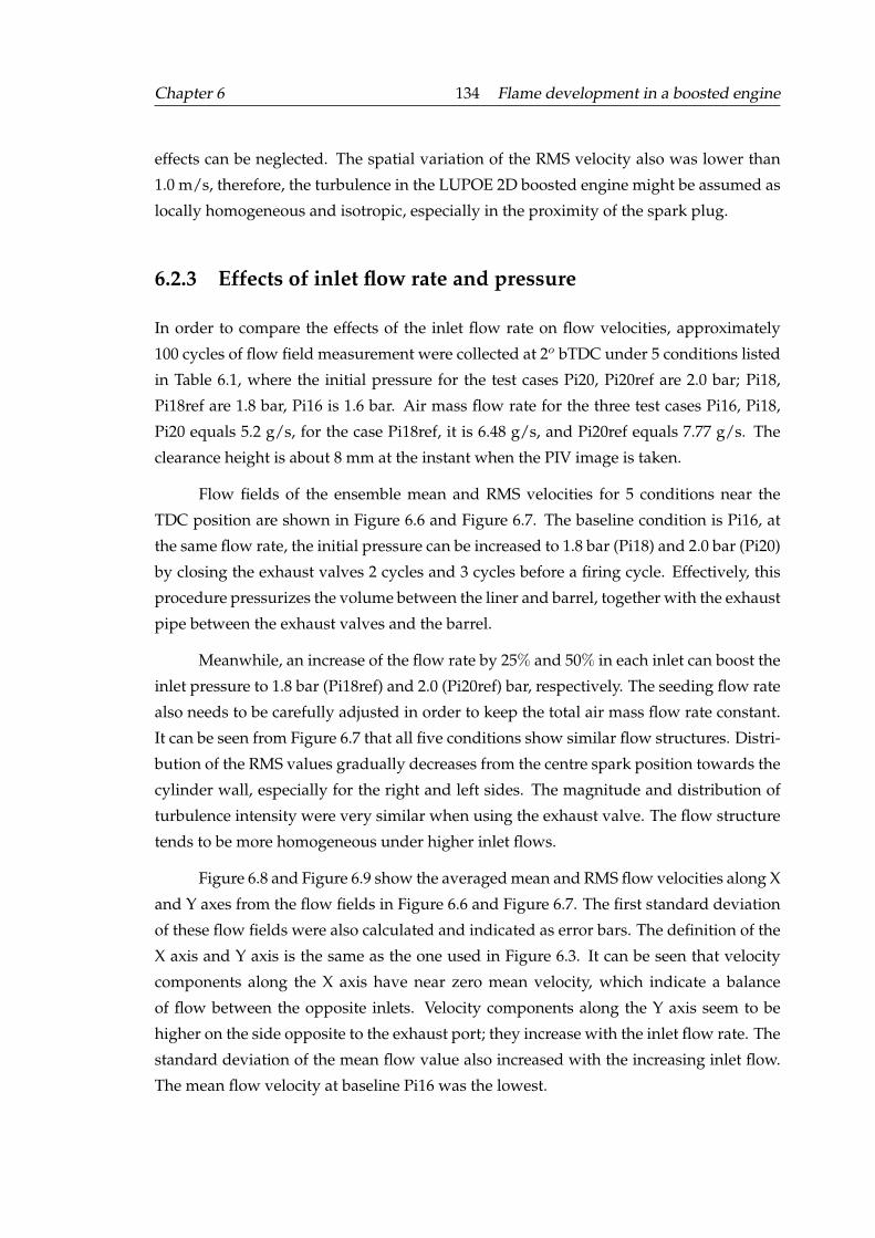
Chapter 6 134 Flame development in a boosted engine
effects can be neglected. The spatial variation of the RMS velocity also was lower than
1.0 m/s, therefore, the turbulence in the LUPOE 2D boosted engine might be assumed as
locally homogeneous and isotropic, especially in the proximity of the spark plug.
6.2.3 Effects of inlet flow rate and pressure
In order to compare the effects of the inlet flow rate on flow velocities, approximately
100 cycles of flow field measurement were collected at 2o bTDC under 5 conditions listed
in Table 6.1, where the initial pressure for the test cases Pi20, Pi20ref are 2.0 bar; Pi18,
Pi18ref are 1.8 bar, Pi16 is 1.6 bar. Air mass flow rate for the three test cases Pi16, Pi18,
Pi20 equals 5.2 g/s, for the case Pi18ref, it is 6.48 g/s, and Pi20ref equals 7.77 g/s. The
clearance height is about 8 mm at the instant when the PIV image is taken.
Flow fields of the ensemble mean and RMS velocities for 5 conditions near the
TDC position are shown in Figure 6.6 and Figure 6.7. The baseline condition is Pi16, at
the same flow rate, the initial pressure can be increased to 1.8 bar (Pi18) and 2.0 bar (Pi20)
by closing the exhaust valves 2 cycles and 3 cycles before a firing cycle. Effectively, this
procedure pressurizes the volume between the liner and barrel, together with the exhaust
pipe between the exhaust valves and the barrel.
Meanwhile, an increase of the flow rate by 25% and 50% in each inlet can boost the
inlet pressure to 1.8 bar (Pi18ref) and 2.0 (Pi20ref) bar, respectively. The seeding flow rate
also needs to be carefully adjusted in order to keep the total air mass flow rate constant.
It can be seen from Figure 6.7 that all five conditions show similar flow structures. Distri-
bution of the RMS values gradually decreases from the centre spark position towards the
cylinder wall, especially for the right and left sides. The magnitude and distribution of
turbulence intensity were very similar when using the exhaust valve. The flow structure
tends to be more homogeneous under higher inlet flows.
Figure 6.8 and Figure 6.9 show the averaged mean and RMS flow velocities along X
and Y axes from the flow fields in Figure 6.6 and Figure 6.7. The first standard deviation
of these flow fields were also calculated and indicated as error bars. The definition of the
X axis and Y axis is the same as the one used in Figure 6.3. It can be seen that velocity
components along the X axis have near zero mean velocity, which indicate a balance
of flow between the opposite inlets. Velocity components along the Y axis seem to be
higher on the side opposite to the exhaust port; they increase with the inlet flow rate. The
standard deviation of the mean flow value also increased with the increasing inlet flow.
The mean flow velocity at baseline Pi16 was the lowest.
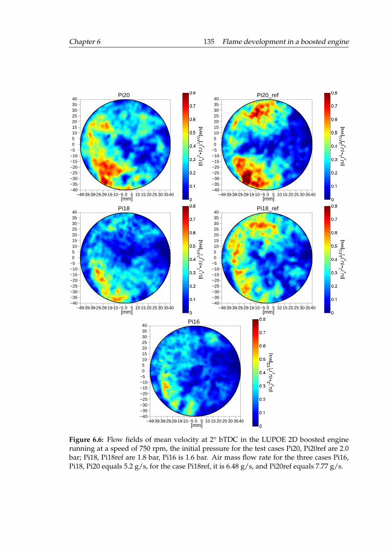
Chapter 6 135 Flame development in a boosted engine
−40−40
−35
−35
−30
−30
−25
−25
−20
−20
−15
−15
−10
−10
−5
−5
0
0
5
5
10
10
15
15
20
20
25
25
30
30
35
35
40
40
[mm]
Pi20
−40−40
−35
−35
−30
−30
−25
−25
−20
−20
−15
−15
−10
−10
−5
−5
0
0
5
5
10
10
15
15
20
20
25
25
30
30
35
35
40
40
[mm]
Pi20_ref
−40−40
−35
−35
−30
−30
−25
−25
−20
−20
−15
−15
−10
−10
−5
−5
0
0
5
5
10
10
15
15
20
20
25
25
30
30
35
35
40
40
[mm]
Pi18
−40−40
−35
−35
−30
−30
−25
−25
−20
−20
−15
−15
−10
−10
−5
−5
0
0
5
5
10
10
15
15
20
20
25
25
30
30
35
35
40
40
[mm]
Pi18_ref
−40−40
−35
−35
−30
−30
−25
−25
−20
−20
−15
−15
−10
−10
−5
−5
0
0
5
5
10
10
15
15
20
20
25
25
30
30
35
35
40
40
[mm]
Pi16
Figure 6.6: Flow fields of mean velocity at 2o bTDC in the LUPOE 2D boosted enginerunning at a speed of 750 rpm, the initial pressure for the test cases Pi20, Pi20ref are 2.0bar; Pi18, Pi18ref are 1.8 bar, Pi16 is 1.6 bar. Air mass flow rate for the three cases Pi16,Pi18, Pi20 equals 5.2 g/s, for the case Pi18ref, it is 6.48 g/s, and Pi20ref equals 7.77 g/s.
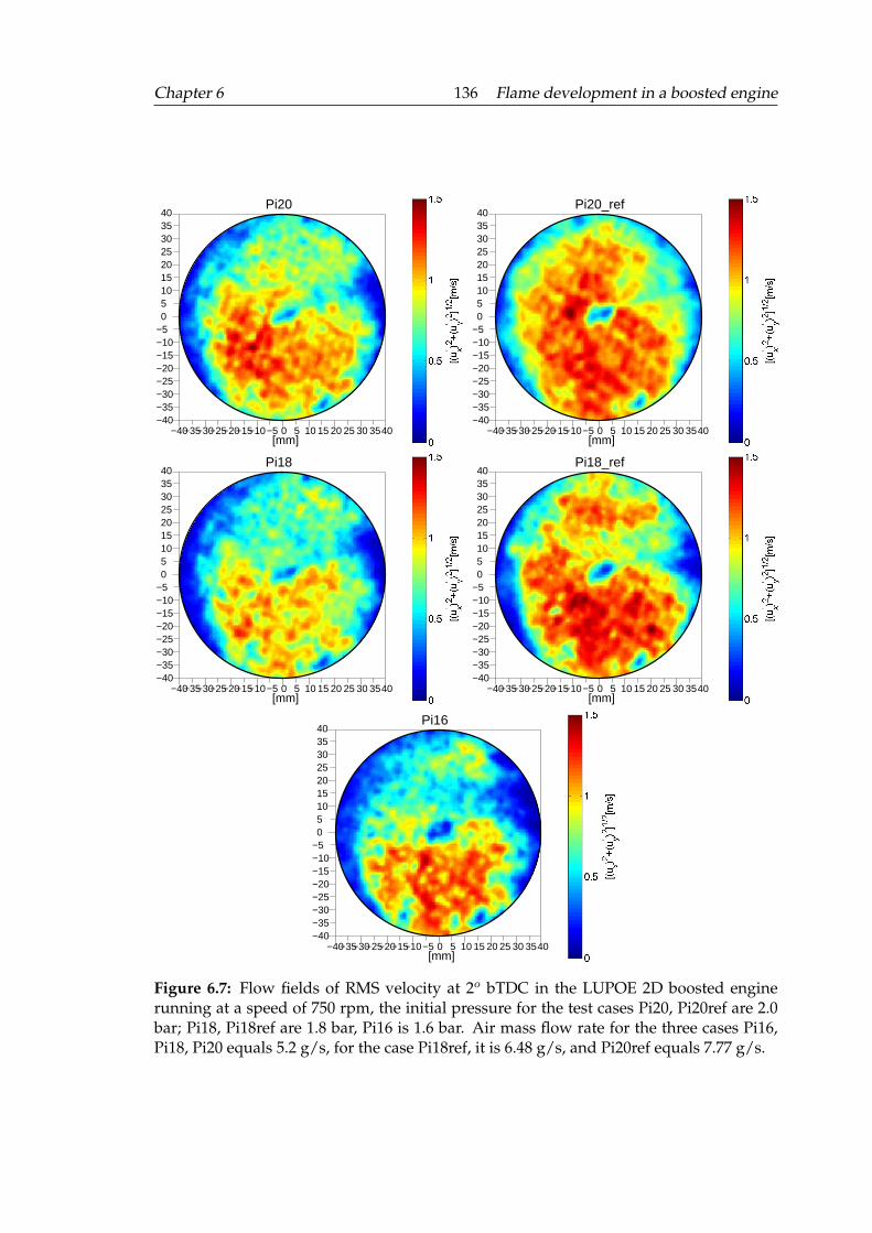
Chapter 6 136 Flame development in a boosted engine
−40−40
−35
−35
−30
−30
−25
−25
−20
−20
−15
−15
−10
−10
−5
−5
0
0
5
5
10
10
15
15
20
20
25
25
30
30
35
35
40
40
[mm]
Pi20
−40−40
−35
−35
−30
−30
−25
−25
−20
−20
−15
−15
−10
−10
−5
−5
0
0
5
5
10
10
15
15
20
20
25
25
30
30
35
35
40
40
[mm]
Pi20_ref
−40−40
−35
−35
−30
−30
−25
−25
−20
−20
−15
−15
−10
−10
−5
−5
0
0
5
5
10
10
15
15
20
20
25
25
30
30
35
35
40
40
[mm]
Pi18
−40−40
−35
−35
−30
−30
−25
−25
−20
−20
−15
−15
−10
−10
−5
−5
0
0
5
5
10
10
15
15
20
20
25
25
30
30
35
35
40
40
[mm]
Pi18_ref
−40−40
−35
−35
−30
−30
−25
−25
−20
−20
−15
−15
−10
−10
−5
−5
0
0
5
5
10
10
15
15
20
20
25
25
30
30
35
35
40
40
[mm]
Pi16
Figure 6.7: Flow fields of RMS velocity at 2o bTDC in the LUPOE 2D boosted enginerunning at a speed of 750 rpm, the initial pressure for the test cases Pi20, Pi20ref are 2.0bar; Pi18, Pi18ref are 1.8 bar, Pi16 is 1.6 bar. Air mass flow rate for the three cases Pi16,Pi18, Pi20 equals 5.2 g/s, for the case Pi18ref, it is 6.48 g/s, and Pi20ref equals 7.77 g/s.
Chapter 6 137 Flame development in a boosted engine
A similar tendency also was observed in the RMS velocities in Figure 6.9. Increas-
ing the inlet flow rate can cause a stronger turbulence intensity. The averaged RMS ve-
locity at Pi16 was 0.65 m/s, then it changed to 0.9 m/s at the Pi20ref case after the intake
flow rate was increased by 50%. While the exhaust valve can keep the RMS velocity at the
almost same level. For the highest and lowest levels of tested mass flow rate, both the X
axis and Y axis have the similar mean and standard deviation values. These observations
were in agreement with the flow field map results.
The turbulence intensity changes during the compression process at different en-
gine inlet air mass flow rates with different exhaust valve closing timing, as shown in
Figure 6.10. It can be observed that the effect of inlet mass flow rate on the RMS in-
cylinder flow velocity is very significant in the early stage of the compression stroke, but
reduces towards TDC. Increasing each inlet flow rate 25-50% can raise the turbulence
intensity by 20-40% near the TDC position, while the exhaust valve can keep the differ-
ence of RMS velocity in a minimum range when the initial pressure was increased. These
observations confirmed that the new boosting configuration using the exhaust valve en-
abled the intake mass flow rate and the initial pressure to be independently varied. The
turbulence quantities, which were heavily influenced by the inlet flow velocities in the
ported engine, can be controlled to the greatest extent.
Dawood [2010] performed PIV measurement in the aspirated naturally LUPOE
engine with a liner having four rows of exhaust orifice at 750 rpm. The measured mean
velocity magnitude was about 0.2 m/s and the RMS velocity was 1.5 m/s at TDC. In this
study, the exhaust gas leaving the cylinder chamber might be blocked to a certain extent
due to the small orifice section of the installed exhaust valves. This resulted in a lower
flow velocity compared to the value measured in the naturally aspirated LUPOE engine.
Landry et al. [2008] investigated the turbulence in a four stroke boosted optical engine,
and the turbulence intensity was measured as 1.15 m/s at 10o bTDC at the engine speed
of 1200 rpm. Since the turbulence intensity decreases with engine speed decreasing, mean
velocity magnitude was 0.1 m/s and RMS velocity was 0.65 m/s at the LUPOE 2D engine
baseline condition Pi16, which can provide a good approximation to conditions in real
commercial lifted valves engines at a low engine speed.
The longitudinal integral length scales along the X axis Lxl, along the Y axis Lyl,
and transverse length scales along the X axis Lxt, along the Y axis Lyt were calculated
following the procedure described in Section 4.1.3 using the mean PIV vector fields and
have shown in Figure 6.11. It can be observed that, in general, average values of the
longitudinal integral length scales are between 8-10 mm, which was approximately twice
that of the transverse integral length scales 4 mm. This is a further indication that the
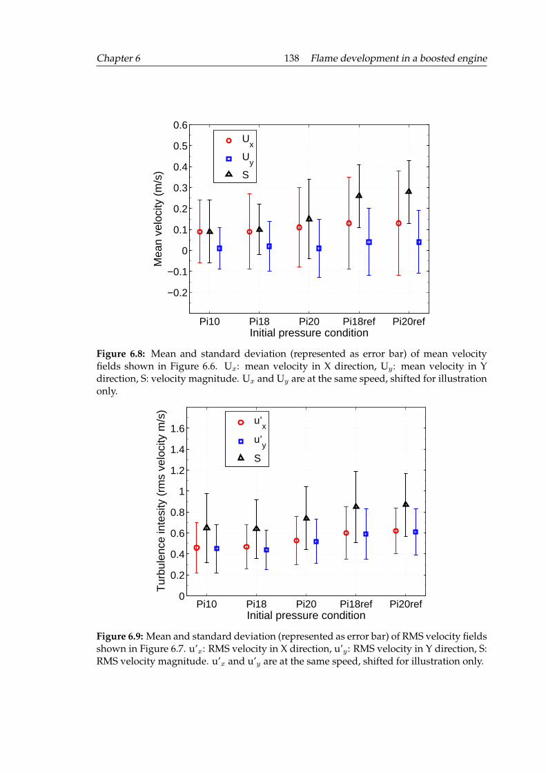
Chapter 6 138 Flame development in a boosted engine
Pi10 Pi18 Pi20 Pi18ref Pi20ref
−0.2
−0.1
0
0.1
0.2
0.3
0.4
0.5
0.6
Initial pressure condition
Mea
n ve
loci
ty (
m/s
)
Ux
Uy
S
Figure 6.8: Mean and standard deviation (represented as error bar) of mean velocityfields shown in Figure 6.6. Ux: mean velocity in X direction, Uy: mean velocity in Ydirection, S: velocity magnitude. Ux and Uy are at the same speed, shifted for illustrationonly.
Pi10 Pi18 Pi20 Pi18ref Pi20ref0
0.2
0.4
0.6
0.8
1
1.2
1.4
1.6
Initial pressure condition
Tur
bule
nce
inte
sity
(rm
s ve
loci
ty m
/s)
u’x
u’y
S
Figure 6.9: Mean and standard deviation (represented as error bar) of RMS velocity fieldsshown in Figure 6.7. u’x: RMS velocity in X direction, u’y: RMS velocity in Y direction, S:RMS velocity magnitude. u’x and u’y are at the same speed, shifted for illustration only.
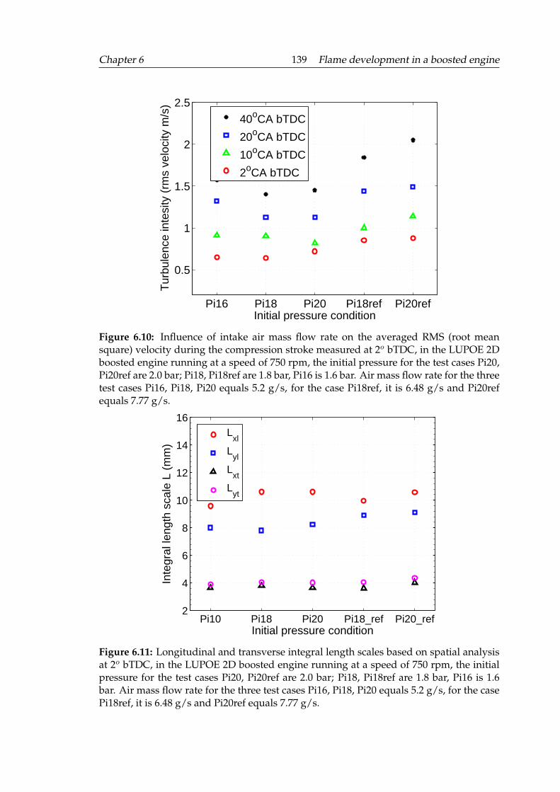
Chapter 6 139 Flame development in a boosted engine
Pi16 Pi18 Pi20 Pi18ref Pi20ref
0.5
1
1.5
2
2.5
Initial pressure condition
Tur
bule
nce
inte
sity
(rm
s ve
loci
ty m
/s)
40oCA bTDC
20oCA bTDC
10oCA bTDC
2oCA bTDC
Figure 6.10: Influence of intake air mass flow rate on the averaged RMS (root meansquare) velocity during the compression stroke measured at 2o bTDC, in the LUPOE 2Dboosted engine running at a speed of 750 rpm, the initial pressure for the test cases Pi20,Pi20ref are 2.0 bar; Pi18, Pi18ref are 1.8 bar, Pi16 is 1.6 bar. Air mass flow rate for the threetest cases Pi16, Pi18, Pi20 equals 5.2 g/s, for the case Pi18ref, it is 6.48 g/s and Pi20refequals 7.77 g/s.
Pi10 Pi18 Pi20 Pi18_ref Pi20_ref2
4
6
8
10
12
14
16
Initial pressure condition
Inte
gral
leng
th s
cale
L (
mm
)
Lxl
Lyl
Lxt
Lyt
Figure 6.11: Longitudinal and transverse integral length scales based on spatial analysisat 2o bTDC, in the LUPOE 2D boosted engine running at a speed of 750 rpm, the initialpressure for the test cases Pi20, Pi20ref are 2.0 bar; Pi18, Pi18ref are 1.8 bar, Pi16 is 1.6bar. Air mass flow rate for the three test cases Pi16, Pi18, Pi20 equals 5.2 g/s, for the casePi18ref, it is 6.48 g/s and Pi20ref equals 7.77 g/s.
Chapter 6 140 Flame development in a boosted engine
in-cylinder turbulence at 2o bTDC could be considered locally isotropic. There is a small
difference in the mean values of the longitudinal scales for X and Y velocity components.
Hussin [2012] measured the transverse length scale to be about 3.5 and 7 mm at TDC
with turbulence intensity at about 1.5 m/s at a speed of 750 rpm in the natural aspirated
LUPOE engine, thus the length scales decreased slightly with the decreasing of the tur-
bulence intensity.
6.3 Engine combustion experimental results
Following the investigation of the engine flow, combustion experiments were conducted
and the results are presented in this Section.
6.3.1 Observations of turbulent flame propagation
Before studying the pressure effects on flame propagation, several images of flame de-
velopment with different equivalence ratios and engine speeds were obtained, and they
are shown in Figure 6.12, to provide a general observation of the turbulent flame charac-
teristics. These images were captured from the LUPOE 2D boosted engine using a CH*
chemiluminescence imaging method, and the main experimental operation parameters
were listed on the left-up insert. The head and intake temperature were kept at 323K,
and the spark timing was fixed at 2o bTDC for all cycles. The second cycle was the Pi16,
which has the initial pressure of 1.6 bar. On the left of Pi16 was the case which had the
similar operation conditions as Pi16, except that the equivalence ratio was reduced to 0.8.
The third column was cycle Pi20ref, which had a higher initial pressure of 2.0 bar and
turbulence than Pi16. The last cycle had almost the same operational conditions as cycle
3, except that the engine speed was increased to 1500 rpm.
From these images, it was clearly shown that the flame speed of lean cycle 1 had the
slowest flame propagation speed compared to the stoichiomtric one (cycle 2), when the
other operational parameters were kept the same. There was not significant difference
between cycle 2 and cycle 3 from image observation for the flame speed. Under the same
initial pressure of 2.0 bar, the flame speed at the high engine speed achieved a faster
burning velocity and more wrinkled flame front, see last column in Figure 6.12.
These flame images were analyzed using the method described in Section 4.2.1,
the flame thickness values were estimated from the gradient of image intensity along
the flame radius at several angles. The positions of the sliced section of the flame are
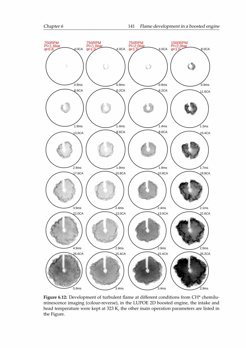
Chapter 6 141 Flame development in a boosted engine
4.0CA
0.9ms
750RPMPi=1.6barφ=0.8 4.0CA
0.9ms
750RPMPi=1.6barφ=1.0 4.0CA
0.9ms
750RPMPi=2.0barφ=1.0 8.0CA
0.9ms
1500RPMPi=2.0barφ=1.0
8.6CA
1.9ms
6.2CA
1.4ms
6.2CA
1.4ms
11.6CA
1.3ms
13.0CA
2.9ms
8.6CA
1.9ms
8.6CA
1.9ms
15.4CA
1.7ms
17.6CA
3.9ms
10.8CA
2.4ms
10.8CA
2.4ms
18.8CA
2.1ms
22.0CA
4.9ms
13.0CA
2.9ms
13.0CA
2.9ms
22.6CA
2.5ms
26.6CA
5.9ms
15.4CA
3.4ms
15.4CA
3.4ms
26.2CA
2.9ms
Figure 6.12: Development of turbulent flame at different conditions from CH* chemilu-minescence imaging (colour-reverse), in the LUPOE 2D boosted engine, the intake andhead temperature were kept at 323 K, the other main operation parameters are listed inthe Figure.
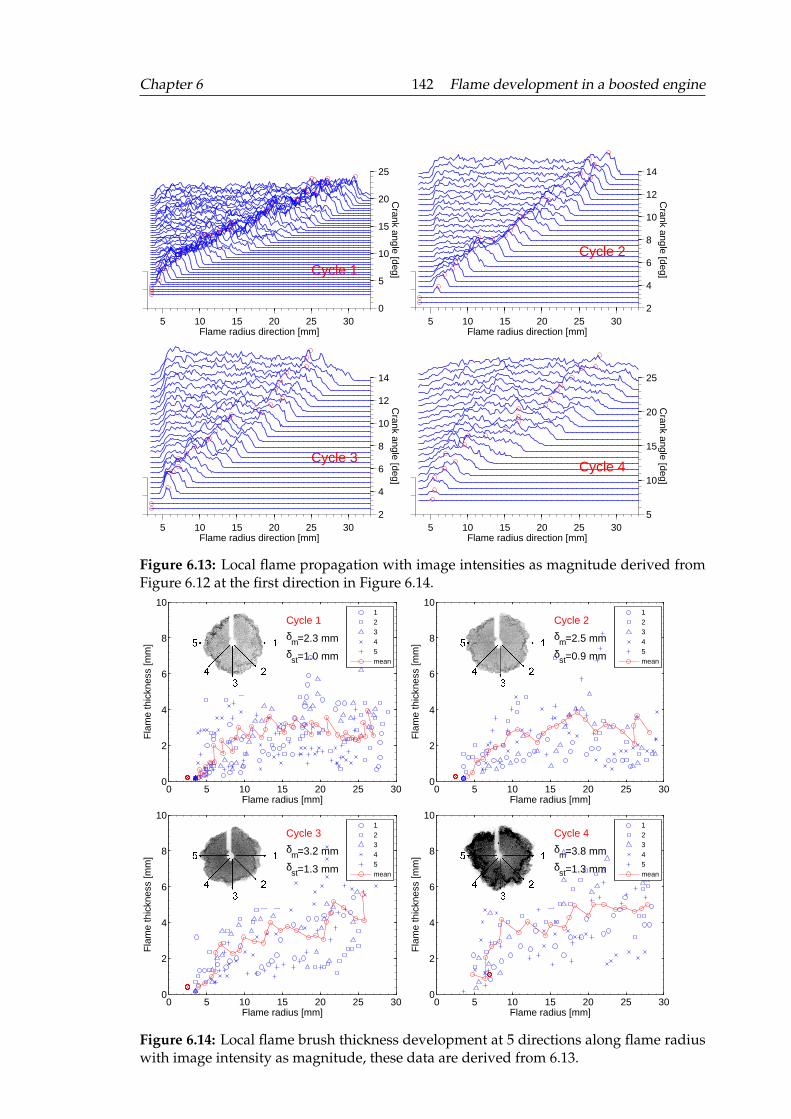
Chapter 6 142 Flame development in a boosted engine
5 10 15 20 25 300
5
10
15
20
25
Crank angle [deg]Cycle 1
Flame radius direction [mm]5 10 15 20 25 30
2
4
6
8
10
12
14
Crank angle [deg]
Cycle 2
Flame radius direction [mm]
5 10 15 20 25 302
4
6
8
10
12
14
Crank angle [deg]
Cycle 3
Flame radius direction [mm]5 10 15 20 25 30
5
10
15
20
25
Crank angle [deg]
Cycle 4
Flame radius direction [mm]
Figure 6.13: Local flame propagation with image intensities as magnitude derived fromFigure 6.12 at the first direction in Figure 6.14.
0 5 10 15 20 25 300
2
4
6
8
10
Flame radius [mm]
Fla
me
thic
knes
s [m
m]
δm
δst
=2.3 mm
=1.0 mm
Cycle 112345mean
0 5 10 15 20 25 300
2
4
6
8
10
Flame radius [mm]
Fla
me
thic
knes
s [m
m]
δm
δst
=2.5 mm
=0.9 mm
Cycle 212345mean
0 5 10 15 20 25 300
2
4
6
8
10
Flame radius [mm]
Fla
me
thic
knes
s [m
m]
δm
δst
=3.2 mm
=1.3 mm
Cycle 312345mean
0 5 10 15 20 25 300
2
4
6
8
10
Flame radius [mm]
Fla
me
thic
knes
s [m
m]
δm
δst
=3.8 mm
=1.3 mm
Cycle 412345mean
Figure 6.14: Local flame brush thickness development at 5 directions along flame radiuswith image intensity as magnitude, these data are derived from 6.13.
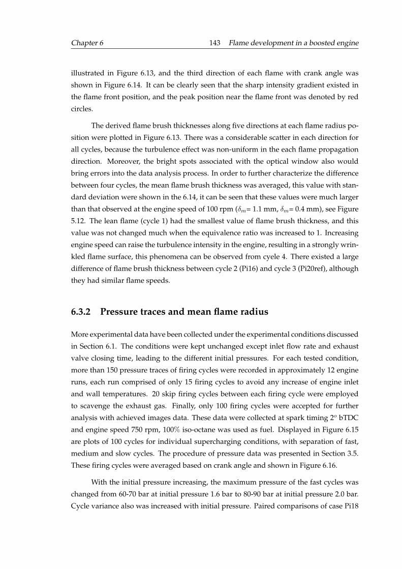
Chapter 6 143 Flame development in a boosted engine
illustrated in Figure 6.13, and the third direction of each flame with crank angle was
shown in Figure 6.14. It can be clearly seen that the sharp intensity gradient existed in
the flame front position, and the peak position near the flame front was denoted by red
circles.
The derived flame brush thicknesses along five directions at each flame radius po-
sition were plotted in Figure 6.13. There was a considerable scatter in each direction for
all cycles, because the turbulence effect was non-uniform in the each flame propagation
direction. Moreover, the bright spots associated with the optical window also would
bring errors into the data analysis process. In order to further characterize the difference
between four cycles, the mean flame brush thickness was averaged, this value with stan-
dard deviation were shown in the 6.14, it can be seen that these values were much larger
than that observed at the engine speed of 100 rpm (δm= 1.1 mm, δm= 0.4 mm), see Figure
5.12. The lean flame (cycle 1) had the smallest value of flame brush thickness, and this
value was not changed much when the equivalence ratio was increased to 1. Increasing
engine speed can raise the turbulence intensity in the engine, resulting in a strongly wrin-
kled flame surface, this phenomena can be observed from cyele 4. There existed a large
difference of flame brush thickness between cycle 2 (Pi16) and cycle 3 (Pi20ref), although
they had similar flame speeds.
6.3.2 Pressure traces and mean flame radius
More experimental data have been collected under the experimental conditions discussed
in Section 6.1. The conditions were kept unchanged except inlet flow rate and exhaust
valve closing time, leading to the different initial pressures. For each tested condition,
more than 150 pressure traces of firing cycles were recorded in approximately 12 engine
runs, each run comprised of only 15 firing cycles to avoid any increase of engine inlet
and wall temperatures. 20 skip firing cycles between each firing cycle were employed
to scavenge the exhaust gas. Finally, only 100 firing cycles were accepted for further
analysis with achieved images data. These data were collected at spark timing 2o bTDC
and engine speed 750 rpm, 100% iso-octane was used as fuel. Displayed in Figure 6.15
are plots of 100 cycles for individual supercharging conditions, with separation of fast,
medium and slow cycles. The procedure of pressure data was presented in Section 3.5.
These firing cycles were averaged based on crank angle and shown in Figure 6.16.
With the initial pressure increasing, the maximum pressure of the fast cycles was
changed from 60-70 bar at initial pressure 1.6 bar to 80-90 bar at initial pressure 2.0 bar.
Cycle variance also was increased with initial pressure. Paired comparisons of case Pi18
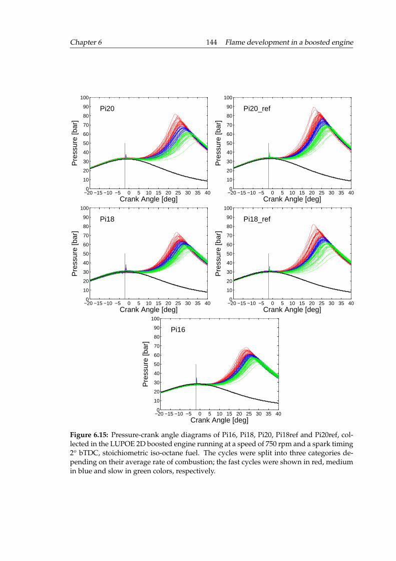
Chapter 6 144 Flame development in a boosted engine
−20 −15 −10 −5 0 5 10 15 20 25 30 35 400
10
20
30
40
50
60
70
80
90
100
Crank Angle [deg]
Pre
ssur
e [b
ar]
Pi20
−20 −15 −10 −5 0 5 10 15 20 25 30 35 400
10
20
30
40
50
60
70
80
90
100
Crank Angle [deg]
Pre
ssur
e [b
ar]
Pi20_ref
−20 −15 −10 −5 0 5 10 15 20 25 30 35 400
10
20
30
40
50
60
70
80
90
100
Crank Angle [deg]
Pre
ssur
e [b
ar]
Pi18
−20 −15 −10 −5 0 5 10 15 20 25 30 35 400
10
20
30
40
50
60
70
80
90
100
Crank Angle [deg]
Pre
ssur
e [b
ar]
Pi18_ref
−20 −15 −10 −5 0 5 10 15 20 25 30 35 400
10
20
30
40
50
60
70
80
90
100
Crank Angle [deg]
Pre
ssur
e [b
ar]
Pi16
Figure 6.15: Pressure-crank angle diagrams of Pi16, Pi18, Pi20, Pi18ref and Pi20ref, col-lected in the LUPOE 2D boosted engine running at a speed of 750 rpm and a spark timing2o bTDC, stoichiometric iso-octane fuel. The cycles were split into three categories de-pending on their average rate of combustion; the fast cycles were shown in red, mediumin blue and slow in green colors, respectively.
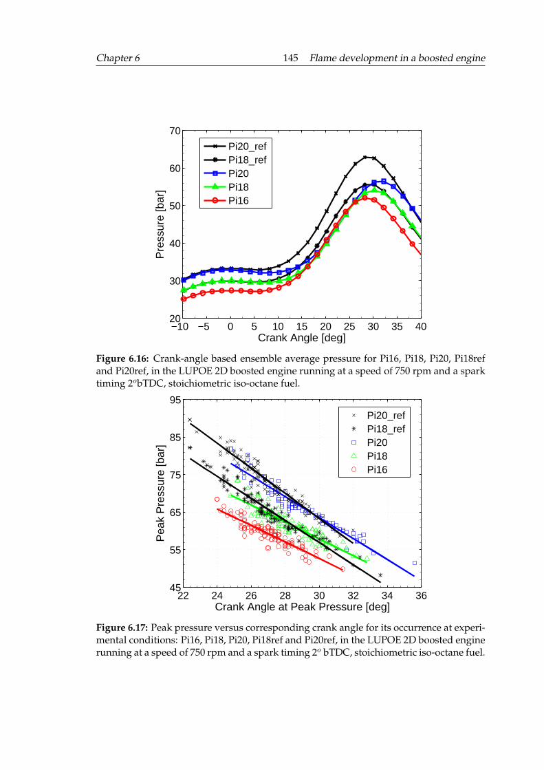
Chapter 6 145 Flame development in a boosted engine
−10 −5 0 5 10 15 20 25 30 35 4020
30
40
50
60
70
Crank Angle [deg]
Pre
ssur
e [b
ar]
Pi20_refPi18_refPi20Pi18Pi16
Figure 6.16: Crank-angle based ensemble average pressure for Pi16, Pi18, Pi20, Pi18refand Pi20ref, in the LUPOE 2D boosted engine running at a speed of 750 rpm and a sparktiming 2obTDC, stoichiometric iso-octane fuel.
22 24 26 28 30 32 34 3645
55
65
75
85
95
Crank Angle at Peak Pressure [deg]
Pea
k P
ress
ure
[bar
]
Pi20_refPi18_refPi20Pi18Pi16
Figure 6.17: Peak pressure versus corresponding crank angle for its occurrence at experi-mental conditions: Pi16, Pi18, Pi20, Pi18ref and Pi20ref, in the LUPOE 2D boosted enginerunning at a speed of 750 rpm and a spark timing 2o bTDC, stoichiometric iso-octane fuel.
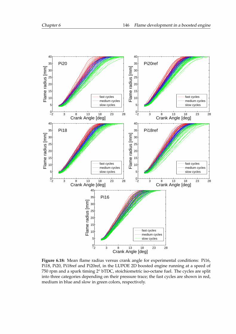
Chapter 6 146 Flame development in a boosted engine
−2 3 8 13 18 23 280
5
10
15
20
25
30
35
40
Crank Angle [deg]
Fla
me
radi
us [m
m]
Pi20
fast cyclesmedium cyclesslow cycles
−2 3 8 13 18 23 280
5
10
15
20
25
30
35
40
Crank Angle [deg]
Fla
me
radi
us [m
m]
Pi20ref
fast cyclesmedium cyclesslow cycles
−2 3 8 13 18 23 280
5
10
15
20
25
30
35
40
Crank Angle [deg]
Fla
me
radi
us [m
m]
Pi18
fast cyclesmedium cyclesslow cycles
−2 3 8 13 18 23 280
5
10
15
20
25
30
35
40
Crank Angle [deg]
Fla
me
radi
us [m
m]
Pi18ref
fast cyclesmedium cyclesslow cycles
−2 3 8 13 18 23 280
5
10
15
20
25
30
35
40
Crank Angle [deg]
Fla
me
radi
us [m
m]
Pi16
fast cyclesmedium cyclesslow cycles
Figure 6.18: Mean flame radius versus crank angle for experimental conditions: Pi16,Pi18, Pi20, Pi18ref and Pi20ref, in the LUPOE 2D boosted engine running at a speed of750 rpm and a spark timing 2o bTDC, stoichiometric iso-octane fuel. The cycles are splitinto three categories depending on their pressure trace; the fast cycles are shown in red,medium in blue and slow in green colors, respectively.
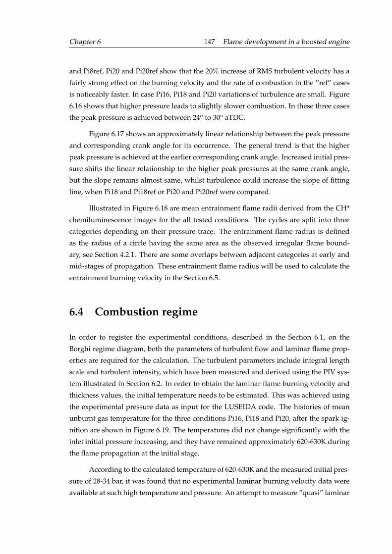
Chapter 6 147 Flame development in a boosted engine
and Pi8ref, Pi20 and Pi20ref show that the 20% increase of RMS turbulent velocity has a
fairly strong effect on the burning velocity and the rate of combustion in the ”ref” cases
is noticeably faster. In case Pi16, Pi18 and Pi20 variations of turbulence are small. Figure
6.16 shows that higher pressure leads to slightly slower combustion. In these three cases
the peak pressure is achieved between 24o to 30o aTDC.
Figure 6.17 shows an approximately linear relationship between the peak pressure
and corresponding crank angle for its occurrence. The general trend is that the higher
peak pressure is achieved at the earlier corresponding crank angle. Increased initial pres-
sure shifts the linear relationship to the higher peak pressures at the same crank angle,
but the slope remains almost same, whilst turbulence could increase the slope of fitting
line, when Pi18 and Pi18ref or Pi20 and Pi20ref were compared.
Illustrated in Figure 6.18 are mean entrainment flame radii derived from the CH*
chemiluminescence images for the all tested conditions. The cycles are split into three
categories depending on their pressure trace. The entrainment flame radius is defined
as the radius of a circle having the same area as the observed irregular flame bound-
ary, see Section 4.2.1. There are some overlaps between adjacent categories at early and
mid-stages of propagation. These entrainment flame radius will be used to calculate the
entrainment burning velocity in the Section 6.5.
6.4 Combustion regime
In order to register the experimental conditions, described in the Section 6.1, on the
Borghi regime diagram, both the parameters of turbulent flow and laminar flame prop-
erties are required for the calculation. The turbulent parameters include integral length
scale and turbulent intensity, which have been measured and derived using the PIV sys-
tem illustrated in Section 6.2. In order to obtain the laminar flame burning velocity and
thickness values, the initial temperature needs to be estimated. This was achieved using
the experimental pressure data as input for the LUSEIDA code. The histories of mean
unburnt gas temperature for the three conditions Pi16, Pi18 and Pi20, after the spark ig-
nition are shown in Figure 6.19. The temperatures did not change significantly with the
inlet initial pressure increasing, and they have remained approximately 620-630K during
the flame propagation at the initial stage.
According to the calculated temperature of 620-630K and the measured initial pres-
sure of 28-34 bar, it was found that no experimental laminar burning velocity data were
available at such high temperature and pressure. An attempt to measure ”quasi” laminar
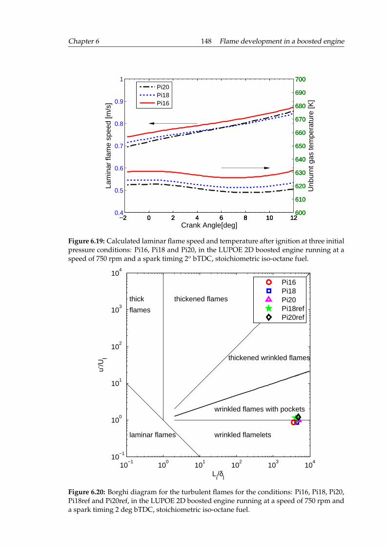
Chapter 6 148 Flame development in a boosted engine
−2 0 2 4 6 8 10 120.4
0.5
0.6
0.7
0.8
0.9
1
Lam
inar
flam
e sp
eed
[m/s
]
−2 0 2 4 6 8 10 12600
610
620
630
640
650
660
670
680
690
700
Unb
urnt
gas
tem
pera
ture
[K]
Crank Angle[deg]−2 0 2 4 6 8 10 12
600
610
620
630
640
650
660
670
680
690
700
−2 0 2 4 6 8 10 12600
610
620
630
640
650
660
670
680
690
700Pi20Pi18Pi16
Figure 6.19: Calculated laminar flame speed and temperature after ignition at three initialpressure conditions: Pi16, Pi18 and Pi20, in the LUPOE 2D boosted engine running at aspeed of 750 rpm and a spark timing 2o bTDC, stoichiometric iso-octane fuel.
10−1
100
101
102
103
104
10−1
100
101
102
103
104
Li/δ
l
u’/U
l
thick
flames
laminar flames
thickened flames
wrinkled flames with pockets
wrinkled flamelets
thickened wrinkled flames
Pi16Pi18Pi20Pi18refPi20ref
Figure 6.20: Borghi diagram for the turbulent flames for the conditions: Pi16, Pi18, Pi20,Pi18ref and Pi20ref, in the LUPOE 2D boosted engine running at a speed of 750 rpm anda spark timing 2 deg bTDC, stoichiometric iso-octane fuel.
Chapter 6 149 Flame development in a boosted engine
iso-octane flame has been described in Chapter 5. Nevertheless, the peak pressure of 15
bar, achieved at the slow engine speed of 100 rpm, was still lower than 30 bar at the high
engine speed of 750 rpm, owing to the strong blow-by effect. The results in Chapter 5
have shown the ”power law” equation proposed by Metghalchi and Keck [1982] has a
predicted value between the measured ”quasi” stretched laminar burning velocity and
the one dimensional unstretched flame simulation. Flame stretch and instability effects
were not excluded in this equation. Therefore, this equation was adopted to calculate
the laminar burning velocity, which has been inserted into the LUSEIDA code. The cal-
culated laminar burning velocities after the spark ignition for the three conditions have
been plotted in Figure 6.19. Pi16 condition has the highest laminar burning velocity at
around 0.75 m/s, while the Pi20 has the lowest value of 0.7 m/s. This tendency did not
change at the initial flame propagation stage. The laminar flame thickness was calculated
from the Equation 2.19, the kinematic viscosity was acquired using the Gaseq chemical
equilibrium code developed by Morley [2005]. The estimated experimental conditions
on the Borghi regime diagram are plotted in Figure 6.20. Five selected conditions in
Section 6.1 are located across the wrinkled flamelets and wrinkled flames with pockets,
since the turbulence intensity is very close to the value of the laminar flame speed. Un-
der the similar turbulent intensity conditions, the calculated laminar flame thicknesses
become thinner, resulting in the operation regime horizontal shift to the right hand side,
see conditions Pi16, Pi18 and Pi20. At the wrinkle flamelet regime, moderate turbulent
flow wrinkled the flame front weakly, thus the effects of flame instability induced by high
pressure might become significant. At the same initial pressure, stronger turbulence in-
tensity leads the operation regime to enter into the wrinkled flame with pockets regime,
see Pi18ref and Pi20ref, where the flame front could be strongly wrinkled by the turbulent
eddies, and flame pockets or islands will appear in the flame front.
6.5 Effect of initial pressure on flame development
This Section presents the investigation of the degree of supercharging on flame devel-
opment, and emphasizes the pressure effects on different flame development phases i.e.
initiation, main phase, and termination phase. These analysis and discussions are based
on the image and pressure data collected in Section 6.3. The experimental conditions
have been presented in Section 6.1.
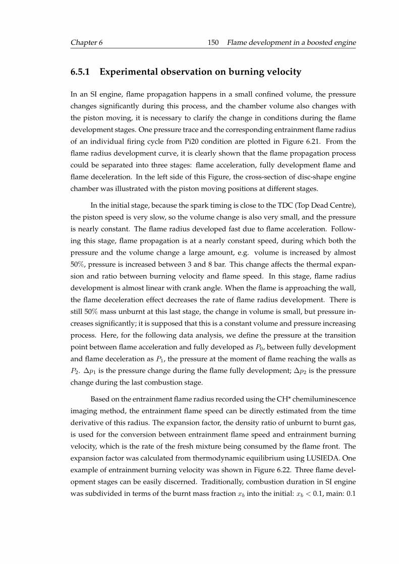
Chapter 6 150 Flame development in a boosted engine
6.5.1 Experimental observation on burning velocity
In an SI engine, flame propagation happens in a small confined volume, the pressure
changes significantly during this process, and the chamber volume also changes with
the piston moving, it is necessary to clarify the change in conditions during the flame
development stages. One pressure trace and the corresponding entrainment flame radius
of an individual firing cycle from Pi20 condition are plotted in Figure 6.21. From the
flame radius development curve, it is clearly shown that the flame propagation process
could be separated into three stages: flame acceleration, fully development flame and
flame deceleration. In the left side of this Figure, the cross-section of disc-shape engine
chamber was illustrated with the piston moving positions at different stages.
In the initial stage, because the spark timing is close to the TDC (Top Dead Centre),
the piston speed is very slow, so the volume change is also very small, and the pressure
is nearly constant. The flame radius developed fast due to flame acceleration. Follow-
ing this stage, flame propagation is at a nearly constant speed, during which both the
pressure and the volume change a large amount, e.g. volume is increased by almost
50%, pressure is increased between 3 and 8 bar. This change affects the thermal expan-
sion and ratio between burning velocity and flame speed. In this stage, flame radius
development is almost linear with crank angle. When the flame is approaching the wall,
the flame deceleration effect decreases the rate of flame radius development. There is
still 50% mass unburnt at this last stage, the change in volume is small, but pressure in-
creases significantly; it is supposed that this is a constant volume and pressure increasing
process. Here, for the following data analysis, we define the pressure at the transition
point between flame acceleration and fully developed as P0, between fully development
and flame deceleration as P1, the pressure at the moment of flame reaching the walls as
P2. ∆p1 is the pressure change during the flame fully development; ∆p2 is the pressure
change during the last combustion stage.
Based on the entrainment flame radius recorded using the CH* chemiluminescence
imaging method, the entrainment flame speed can be directly estimated from the time
derivative of this radius. The expansion factor, the density ratio of unburnt to burnt gas,
is used for the conversion between entrainment flame speed and entrainment burning
velocity, which is the rate of the fresh mixture being consumed by the flame front. The
expansion factor was calculated from thermodynamic equilibrium using LUSIEDA. One
example of entrainment burning velocity was shown in Figure 6.22. Three flame devel-
opment stages can be easily discerned. Traditionally, combustion duration in SI engine
was subdivided in terms of the burnt mass fraction xb into the initial: xb < 0.1, main: 0.1
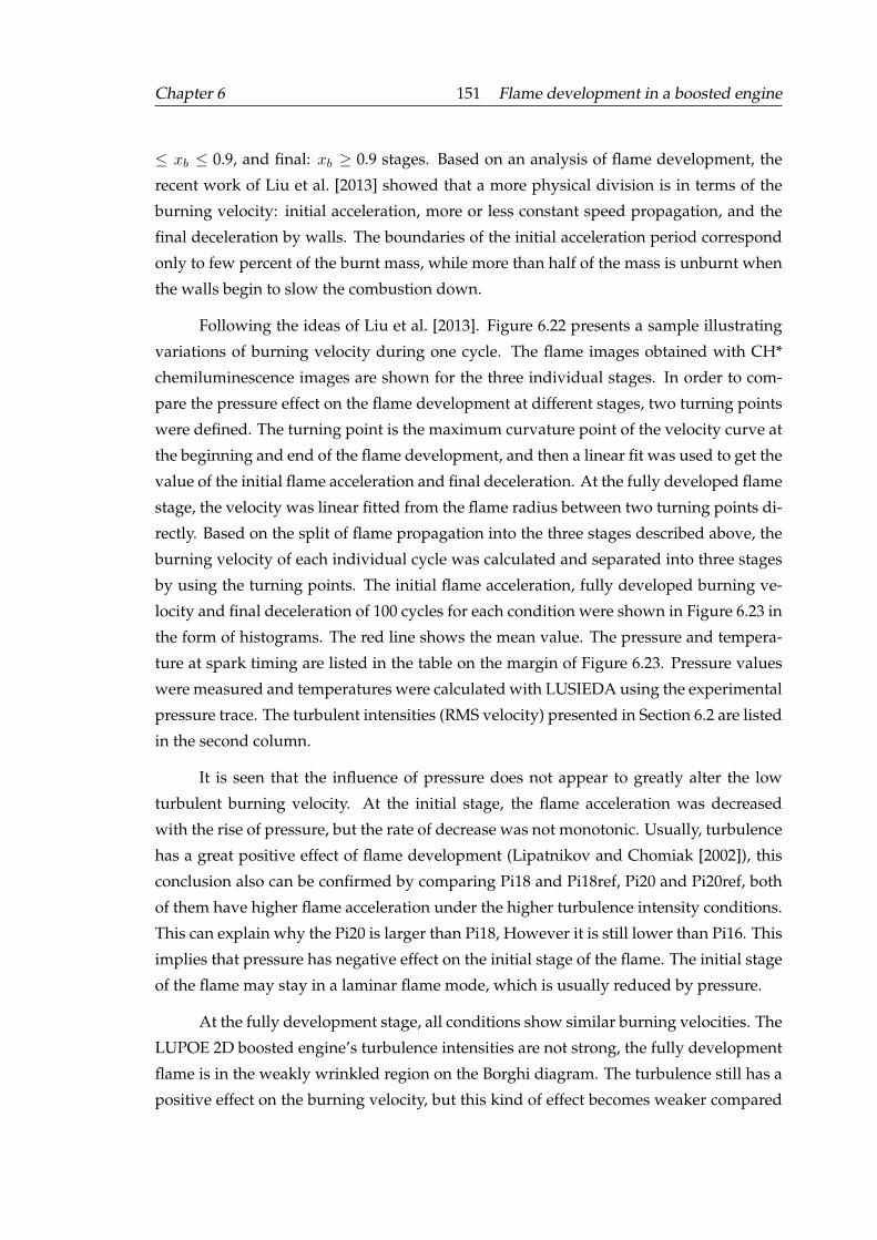
Chapter 6 151 Flame development in a boosted engine
≤ xb ≤ 0.9, and final: xb ≥ 0.9 stages. Based on an analysis of flame development, the
recent work of Liu et al. [2013] showed that a more physical division is in terms of the
burning velocity: initial acceleration, more or less constant speed propagation, and the
final deceleration by walls. The boundaries of the initial acceleration period correspond
only to few percent of the burnt mass, while more than half of the mass is unburnt when
the walls begin to slow the combustion down.
Following the ideas of Liu et al. [2013]. Figure 6.22 presents a sample illustrating
variations of burning velocity during one cycle. The flame images obtained with CH*
chemiluminescence images are shown for the three individual stages. In order to com-
pare the pressure effect on the flame development at different stages, two turning points
were defined. The turning point is the maximum curvature point of the velocity curve at
the beginning and end of the flame development, and then a linear fit was used to get the
value of the initial flame acceleration and final deceleration. At the fully developed flame
stage, the velocity was linear fitted from the flame radius between two turning points di-
rectly. Based on the split of flame propagation into the three stages described above, the
burning velocity of each individual cycle was calculated and separated into three stages
by using the turning points. The initial flame acceleration, fully developed burning ve-
locity and final deceleration of 100 cycles for each condition were shown in Figure 6.23 in
the form of histograms. The red line shows the mean value. The pressure and tempera-
ture at spark timing are listed in the table on the margin of Figure 6.23. Pressure values
were measured and temperatures were calculated with LUSIEDA using the experimental
pressure trace. The turbulent intensities (RMS velocity) presented in Section 6.2 are listed
in the second column.
It is seen that the influence of pressure does not appear to greatly alter the low
turbulent burning velocity. At the initial stage, the flame acceleration was decreased
with the rise of pressure, but the rate of decrease was not monotonic. Usually, turbulence
has a great positive effect of flame development (Lipatnikov and Chomiak [2002]), this
conclusion also can be confirmed by comparing Pi18 and Pi18ref, Pi20 and Pi20ref, both
of them have higher flame acceleration under the higher turbulence intensity conditions.
This can explain why the Pi20 is larger than Pi18, However it is still lower than Pi16. This
implies that pressure has negative effect on the initial stage of the flame. The initial stage
of the flame may stay in a laminar flame mode, which is usually reduced by pressure.
At the fully development stage, all conditions show similar burning velocities. The
LUPOE 2D boosted engine’s turbulence intensities are not strong, the fully development
flame is in the weakly wrinkled region on the Borghi diagram. The turbulence still has a
positive effect on the burning velocity, but this kind of effect becomes weaker compared
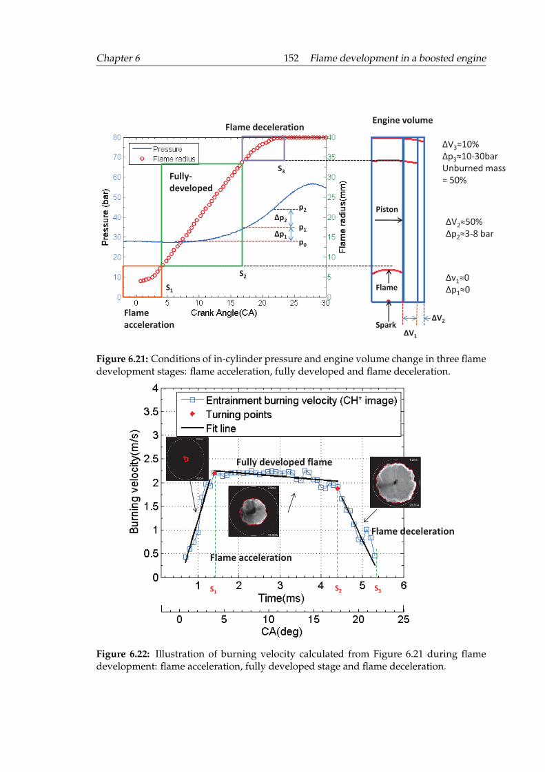
Chapter 6 152 Flame development in a boosted engine
Piston
Engine volume
Flame
Spark
∆V3≈10%
∆p3≈10-30bar
Unburned mass
≈ 50%
∆V2≈50%
∆p2≈3-8 bar
∆v1≈0
∆p1≈0
∆V1
∆V2
∆p1
∆p2
p1
p2
S1
S2
S3
p0
Flame
acceleration
Fully-
developed
Flame deceleration
Figure 6.21: Conditions of in-cylinder pressure and engine volume change in three flamedevelopment stages: flame acceleration, fully developed and flame deceleration.
20.2CA
4.5ms
13.0CA
2.9ms
Flame acceleration
Fully developed flame
Flame deceleration
S1S2 S3
4.0CA
0.9ms
Figure 6.22: Illustration of burning velocity calculated from Figure 6.21 during flamedevelopment: flame acceleration, fully developed stage and flame deceleration.

Chapter 6 153 Flame development in a boosted engine
Figure 6.23: Histogram of flame development for the experimental conditions: Pi16, Pi18,Pi18ref, Pi20 and Pi20ref, in the LUPOE 2D boosted engine running at a speed of 750 rpmand a spark timing 2o bTDC, stoichiometric iso-octane fuel. The red line shows the meanvalue.
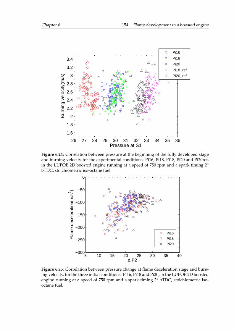
Chapter 6 154 Flame development in a boosted engine
26 27 28 29 30 31 32 33 34 35 36
1.6
1.8
2
2.2
2.4
2.6
2.8
3
3.2
3.4
Pressure at S1
Bur
ning
vel
ocity
(m/s
)
Pi16
Pi18
Pi20
Pi18_ref
Pi20_ref
Figure 6.24: Correlation between pressure at the beginning of the fully developed stageand burning velocity for the experimental conditions: Pi16, Pi18, Pi18, Pi20 and Pi20ref,in the LUPOE 2D boosted engine running at a speed of 750 rpm and a spark timing 2o
bTDC, stoichiometric iso-octane fuel.
5 10 15 20 25 30 35 40−300
−250
−200
−150
−100
−50
0
∆ P2
Fla
me
dece
lera
tion(
m/s
2 )
Pi16
Pi18
Pi20
Figure 6.25: Correlation between pressure change at flame deceleration stage and burn-ing velocity, for the three initial conditions: Pi16, Pi18 and Pi20, in the LUPOE 2D boostedengine running at a speed of 750 rpm and a spark timing 2o bTDC, stoichiometric iso-octane fuel.
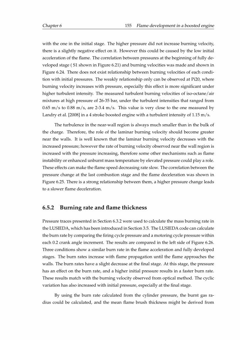
Chapter 6 155 Flame development in a boosted engine
with the one in the initial stage. The higher pressure did not increase burning velocity,
there is a slightly negative effect on it. However this could be caused by the low initial
acceleration of the flame. The correlation between pressures at the beginning of fully de-
veloped stage ( S1 shown in Figure 6.21) and burning velocities was made and shown in
Figure 6.24. There does not exist relationship between burning velocities of each condi-
tion with initial pressures. The weakly relationship only can be observed at Pi20, where
burning velocity increases with pressure, especially this effect is more significant under
higher turbulent intensity. The measured turbulent burning velocities of iso-octane/air
mixtures at high pressure of 26-35 bar, under the turbulent intensities that ranged from
0.65 m/s to 0.88 m/s, are 2-3.4 m/s. This value is very close to the one measured by
Landry et al. [2008] in a 4 stroke boosted engine with a turbulent intensity of 1.15 m/s.
The turbulence in the near-wall region is always much smaller than in the bulk of
the charge. Therefore, the role of the laminar burning velocity should become greater
near the walls. It is well known that the laminar burning velocity decreases with the
increased pressure; however the rate of burning velocity observed near the wall region is
increased with the pressure increasing, therefore some other mechanisms such as flame
instability or enhanced unburnt mass temperature by elevated pressure could play a role.
These effects can make the flame speed decreasing rate slow. The correlation between the
pressure change at the last combustion stage and the flame deceleration was shown in
Figure 6.25. There is a strong relationship between them, a higher pressure change leads
to a slower flame deceleration.
6.5.2 Burning rate and flame thickness
Pressure traces presented in Section 6.3.2 were used to calculate the mass burning rate in
the LUSIEDA, which has been introduced in Section 3.5. The LUSIEDA code can calculate
the burn rate by comparing the firing cycle pressure and a motoring cycle pressure within
each 0.2 crank angle increment. The results are compared in the left side of Figure 6.26.
Three conditions show a similar burn rate in the flame acceleration and fully developed
stages. The burn rates increase with flame propagation until the flame approaches the
walls. The burn rates have a slight decrease at the final stage. At this stage, the pressure
has an effect on the burn rate, and a higher initial pressure results in a faster burn rate.
These results match with the burning velocity observed from optical method. The cyclic
variation has also increased with initial pressure, especially at the final stage.
By using the burn rate calculated from the cylinder pressure, the burnt gas ra-
dius could be calculated, and the mean flame brush thickness might be derived from
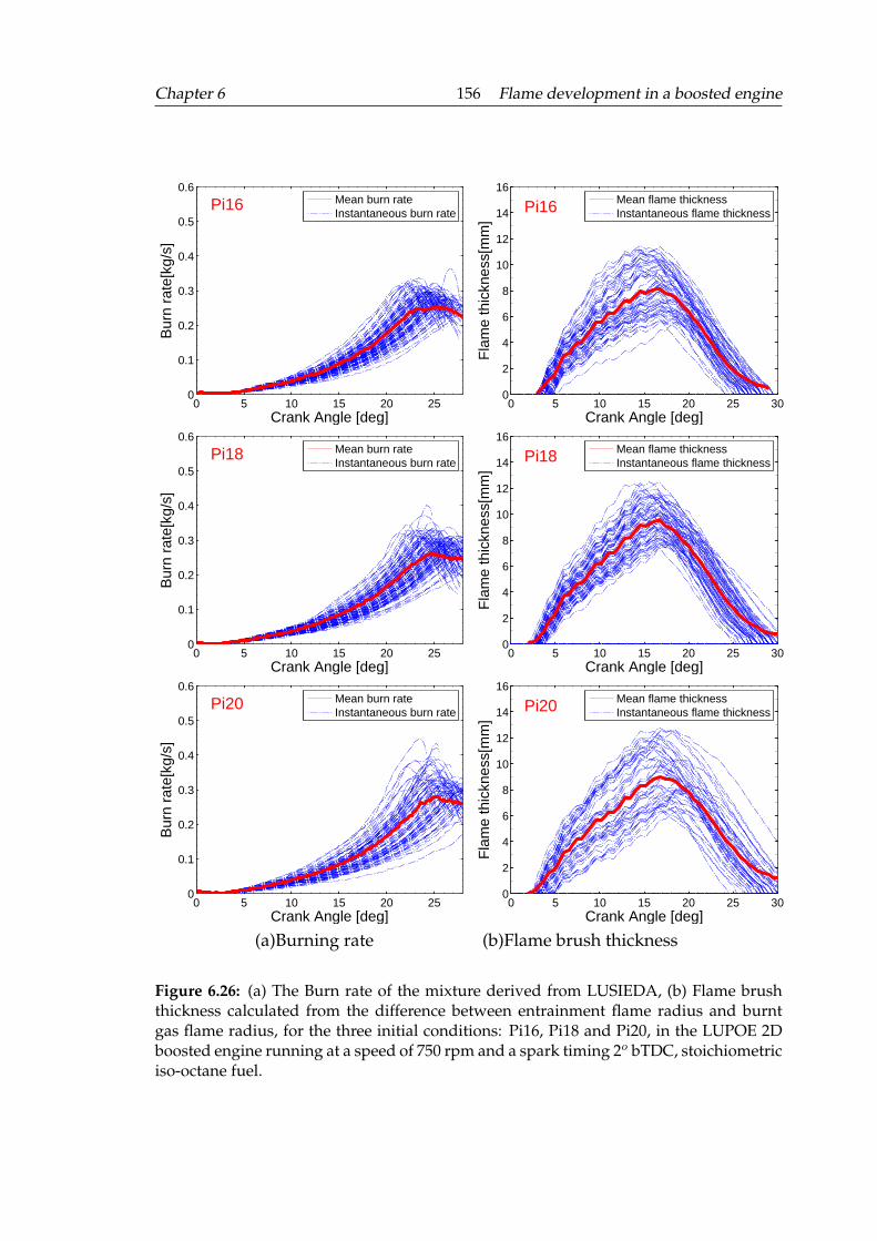
Chapter 6 156 Flame development in a boosted engine
0 5 10 15 20 250
0.1
0.2
0.3
0.4
0.5
0.6
Crank Angle [deg]
Bur
n ra
te[k
g/s]
Pi16 Mean burn rateInstantaneous burn rate
0 5 10 15 20 25 300
2
4
6
8
10
12
14
16
Crank Angle [deg]
Fla
me
thic
knes
s[m
m]
Pi16 Mean flame thicknessInstantaneous flame thickness
0 5 10 15 20 250
0.1
0.2
0.3
0.4
0.5
0.6
Crank Angle [deg]
Bur
n ra
te[k
g/s]
Pi18 Mean burn rateInstantaneous burn rate
0 5 10 15 20 25 300
2
4
6
8
10
12
14
16
Crank Angle [deg]
Fla
me
thic
knes
s[m
m]
Pi18 Mean flame thicknessInstantaneous flame thickness
0 5 10 15 20 250
0.1
0.2
0.3
0.4
0.5
0.6
Crank Angle [deg]
Bur
n ra
te[k
g/s]
Pi20 Mean burn rateInstantaneous burn rate
0 5 10 15 20 25 300
2
4
6
8
10
12
14
16
Crank Angle [deg]
Fla
me
thic
knes
s[m
m]
Pi20 Mean flame thicknessInstantaneous flame thickness
(a)Burning rate (b)Flame brush thickness
Figure 6.26: (a) The Burn rate of the mixture derived from LUSIEDA, (b) Flame brushthickness calculated from the difference between entrainment flame radius and burntgas flame radius, for the three initial conditions: Pi16, Pi18 and Pi20, in the LUPOE 2Dboosted engine running at a speed of 750 rpm and a spark timing 2o bTDC, stoichiometriciso-octane fuel.
Chapter 6 157 Flame development in a boosted engine
the difference between this burnt flame radius and the entrainment flame radius which
are measured from the same cycle’s CH* chemiluminescence images. The details of this
method have been introduced in Section 3.5, and this method was applied to process each
individual cycle for the three initial conditions. The instantaneous flame brush thickness
at the different initial pressures were compared and they are shown in the right side of
Figure 6.26. It can be observed that the flame brush thickness increases with the flame
development. The peak values of flame brush thickness for the three initial pressure con-
ditions are approximately 8-10 mm, which are achieved when the flame speed starts to
decelerate after 15o crank angles after ignition, about 10 mm far from the engine wall.
This value agrees well with the one observed from the CH* chmeiluminescence images
shown in Section 6.3.1. The flame brush thickness increases slightly with the rise of the
initial pressure when the flame is near the walls, the variance of thickness is also ampli-
fied by the increased initial pressure.
6.5.3 Further discussion on flame development
Based on data from experiments, many models and correlations have been developed
to express turbulent burning velocity. Abdi Aghdam [2003] investigated performance of
three turbulent burning velocity correlation methods: the Leeds Ka and KaLe correlations
(Abdel-Gayed et al. [1987]) and the Zimont model (Lipatnikov and Chomiak [2002]). It
was found that the Zimont model was the most promising tool for engineering applica-
tion. Here the Zimont model is validated by current data collected at high pressure, more
details about Leeds Ka and KaLe correlations can be found in Abdi Aghdam [2003]. The
turbulent combustion model developed by Zimont [1979] based on an assumption that
the rate of the turbulent entrainment of fresh mixture into the flame brush is equal to
the consumption of this mixture in the thickened reaction zone. The turbulent steady
burning velocity is given by:
Ut,0 = Au′Da1/4 = Au′3/4Ulk−1/4L1/4 (6.1)
Where Ut,0 is the developed turbulent burning velocity, A is a constant value of 0.5, u′
is the root mean square (rms) turbulent velocity, Ul laminar burning velocity, Da is the
Damkholer number, Da = τl/τc where τl = Li/u′ is the integral time scale, and τc = U2
l /k
is the characteristic laminar chemical time, k is the characteristic laminar chemical time
scale.
Chapter 6 158 Flame development in a boosted engine
4 5 6 7 8 9 10 112.1
2.2
2.3
2.4
2.5
2.6
2.7
2.8
2.9
3
Crank Angle (deg)
Bur
ning
vel
ocity
(m
/s)
Pi16_predictPi16_expPi18_predictPi18_expPi20_predictPi20_exp
Figure 6.27: Comparison of modelling (Zimont model) and measured turbulent burningvelocities for the three initial conditions: Pi16, Pi18 and Pi20, in the LUPOE 2D boostedengine running at a speed of 750 rpm and a spark timing 2o bTDC, with stoichiometriciso-octane fuel.
The Zimont turbulent burning velocity model has been implanted into the LUSIEDA
code. The thermodynamic conditions could be estimated from the input pressure trace.
The laminar burning velocity and the temperature used to calculate the molecular trans-
port coefficient have been shown in Section 6.4. The turbulent parameters were measured
using the PIV system, then input into the code. The predicted mean turbulent burning ve-
locities at the fully developed stage for the three initial pressure conditions are compared
with the corresponding measured entrainment burning velocities derived from the CH*
chemiluminescence images in Figure 6.27. The results show a good agreement in the
values of burning velocities, the maximum error between the measured and predicted
values is approximately less than 0.3 m/s, and it occurred at the strongest boosted condi-
tion Pi20. With the pressure rise, the predicted burning velocity increases. This tendency
contrasts with the measured values. This may be attributed to the fact that the model
does not include the effect of flame transient phenomenon.
There have been so far several models of flame acceleration proposed, e.g. an ex-
pression based fractal combustion models (Baratta et al. [2006]), integral of the dimen-
sionless turbulence PSD by Abdel-Gayed et al. [1987]; and the one proposed by Lipat-
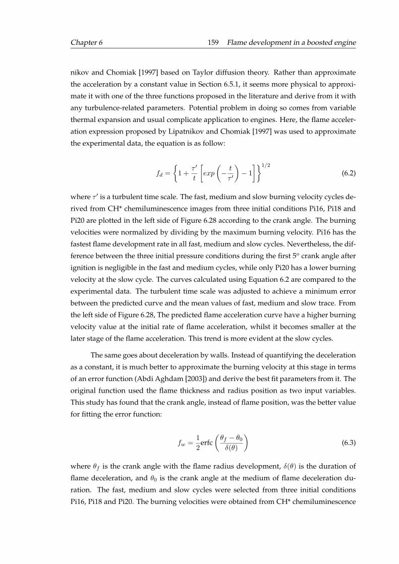
Chapter 6 159 Flame development in a boosted engine
nikov and Chomiak [1997] based on Taylor diffusion theory. Rather than approximate
the acceleration by a constant value in Section 6.5.1, it seems more physical to approxi-
mate it with one of the three functions proposed in the literature and derive from it with
any turbulence-related parameters. Potential problem in doing so comes from variable
thermal expansion and usual complicate application to engines. Here, the flame acceler-
ation expression proposed by Lipatnikov and Chomiak [1997] was used to approximate
the experimental data, the equation is as follow:
fd =
{1 +
τ ′
t
[exp
(− t
τ ′
)− 1
]}1/2
(6.2)
where τ ′ is a turbulent time scale. The fast, medium and slow burning velocity cycles de-
rived from CH* chemiluminescence images from three initial conditions Pi16, Pi18 and
Pi20 are plotted in the left side of Figure 6.28 according to the crank angle. The burning
velocities were normalized by dividing by the maximum burning velocity. Pi16 has the
fastest flame development rate in all fast, medium and slow cycles. Nevertheless, the dif-
ference between the three initial pressure conditions during the first 5o crank angle after
ignition is negligible in the fast and medium cycles, while only Pi20 has a lower burning
velocity at the slow cycle. The curves calculated using Equation 6.2 are compared to the
experimental data. The turbulent time scale was adjusted to achieve a minimum error
between the predicted curve and the mean values of fast, medium and slow trace. From
the left side of Figure 6.28, The predicted flame acceleration curve have a higher burning
velocity value at the initial rate of flame acceleration, whilst it becomes smaller at the
later stage of the flame acceleration. This trend is more evident at the slow cycles.
The same goes about deceleration by walls. Instead of quantifying the deceleration
as a constant, it is much better to approximate the burning velocity at this stage in terms
of an error function (Abdi Aghdam [2003]) and derive the best fit parameters from it. The
original function used the flame thickness and radius position as two input variables.
This study has found that the crank angle, instead of flame position, was the better value
for fitting the error function:
fw =1
2erfc
(θf − θ0δ(θ)
)(6.3)
where θf is the crank angle with the flame radius development, δ(θ) is the duration of
flame deceleration, and θ0 is the crank angle at the medium of flame deceleration du-
ration. The fast, medium and slow cycles were selected from three initial conditions
Pi16, Pi18 and Pi20. The burning velocities were obtained from CH* chemiluminescence
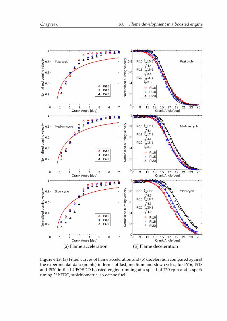
Chapter 6 160 Flame development in a boosted engine
0 1 2 3 4 5 6 70
0.2
0.4
0.6
0.8
1
Crank Angle [deg]
Nor
mal
ized
bur
ning
vel
ocity
Fast cycle
Pi16Pi18Pi20
7 9 11 13 15 17 19 21 23 250
0.2
0.4
0.6
0.8
1
Pi16 θ0:
θf:15.8
4.4Pi18 θ
0:
θf:15.5
3.4Pi20 θ
0:
θf:16.1
3.5
Crank Angle[deg]
Nor
mal
ized
bur
ning
vel
ocity
Fast cycle
Pi16Pi18Pi20
0 1 2 3 4 5 6 70
0.2
0.4
0.6
0.8
1
Crank Angle [deg]
Nor
mal
ized
bur
ning
vel
ocity
Medium cycle
Pi16Pi18Pi20
7 9 11 13 15 17 19 21 23 250
0.2
0.4
0.6
0.8
1
Pi16 θ0:
θf:17.1
4.4Pi18 θ
0:
θf:17.1
3.8Pi20 θ
0:
θf:18.1
3.9
Crank Angle[deg]
Nor
mal
ized
bur
ning
vel
ocity
Medium cycle
Pi16Pi18Pi20
0 1 2 3 4 5 6 70
0.2
0.4
0.6
0.8
1
Crank Angle [deg]
Nor
mal
ized
bur
ning
vel
ocity
Slow cycle
Pi16Pi18Pi20
7 9 11 13 15 17 19 21 23 250
0.2
0.4
0.6
0.8
1
Pi16 θ0:
θf:17.8
4.7Pi18 θ
0:
θf:18.7
4.3Pi20 θ
0:
θf:20.2
4.9
Crank Angle[deg]
Nor
mal
ized
bur
ning
vel
ocity
Slow cycle
Pi16Pi18Pi20
(a) Flame acceleration (b) Flame deceleration
Figure 6.28: (a) Fitted curves of flame acceleration and (b) deceleration compared againstthe experimental data (points) in terms of fast, medium and slow cycles, for Pi16, Pi18and Pi20 in the LUPOE 2D boosted engine running at a speed of 750 rpm and a sparktiming 2o bTDC, stoichiometric iso-octane fuel.
Chapter 6 161 Flame development in a boosted engine
images at the engine speed of 750 rpm and normalized using the maximum burning ve-
locity. The differences between the three conditions are only obvious for the slow cycles,
the higher pressure has the faster burning velocity than the lower one at the same crank
angle. Since the fast, medium and slow cycles were mainly affected by the turbulent
intensity (Hussin [2012]), this implied that the pressure effect might become significant
at the low turbulent conditions. The least-squares method was applied to fit the non-
linear flame deceleration curve using the error function Equation 6.3. The fitting curves
are plotted in the left side of Figure 6.28. The calculated values of θ0 and δ(θ) were also
presented. The duration of flame deceleration δ(θ) does not seem to have a direct rela-
tionship with the time at the medium of flame deceleration duration θ0. It is clear that
the θ0 will be short if the flame develops faster. Thus, all fast cycles show lower values
of θ0 than that of the slow cycles. In general, The θ0 of Pi16 is smaller than the other two
cases. Nevertheless, for the duration time of flame deceleration δ(θ), Pi16 has the highest
value. For the fast cycle, the flame deceleration crank angle δ(θ) is the main value which
is adjusted to fit the curve shape, whilst for the slow cycle, the θ0 value becomes more
important.
6.6 Effect of initial pressure on flame structure
In this section, the structure of flame at high pressure and its response to pressure effects
were further investigated. The laser sheet visualization method was applied to observe
the detailed cross section of the flame front topology. Wrinkle and curvature of the flame
front were characterized to compare the flame shapes under different boosted initial pres-
sure and turbulence. Flame spectral analysis also was applied.
Three conditions have been selected: Pi16, Pi20 and Pi20ref. The details of these
condition operation have been presented in Table 6.1. Pi20 has a higher initial pressure
than Pi16, while the rms velocities at spark timing are similar. The pressure effects can be
seen by comparing these two conditions. Pi20 and Pi20ref have the same initial pressure,
while the rms velocity of Pi20ref is higher than Pi20, turbulence effects may be obtained
by comparing these two conditions. The other engine operation parameters were main-
tained the same for all the conditions: the engine speed was 750rpm, spark timing was
2o bTDC, images were taken at 10 degrees after spark, and iso-octane was used as fuel.
Chapter 6 162 Flame development in a boosted engine
6.6.1 Mean progress value and self-similar structure
A map of mean combustion reaction progress variable, which represents the probability
of finding the burnt gas at a particular position, can be calculated on the amount of flame
contour derived from laser sheet images. The mean progress variable cij at each pixel (i,j)
is the average value of intensities of all binary images at the same position. This leads to
the equation:
cij =1
n
n∑k=1
Ii,j,k (6.4)
where n is the number of images. The calculated c contours become stable when the
number of images tend to be infinite. Nevertheless, it is only possible to collect a finite
number of images in the experiment. Hattrell [2007] found that the required number
of images to obtain a stable contours of c was less than the estimated one from error
analysis, there was little difference between the c values produced by averaging 50 and
100 images. In this study, about 40 to 50 laser sheet images have been collected for each
conditions, some low quality images have been discarded during the image processing.
Limited by the low repetition laser (15 Hz), only one image could be captured
during a firing cycle. The laser sheet also caused a strong light reflection near the engine
wall region, thus only the flame structure at one crank angle during the flame fully-
developed stage was studied here. The c field for the three initial pressure conditions
Pi16, Pi18 and Pi20 are illustrated in the left side of Figure 6.29. These contours were
obtained by averaging the binarised flames of 40-50 cycles for each condition at the crank
angle 8o bTDC (10o CA after ignition). The lower limit of the scale (blue) represents 0%
probability, whilst the upper (red) is 100%. The black circle represents the position of the
engine cylinder walls. The three c fields show similar distributions. The largest flame size
was observed in Pi16. Based on the map of progress variable c field, progress variable
values along the flame radius direction could be sliced in each 10o angle, and plotted in
the right side of Figure 6.29. The measured profiles of the mean progress variable could be
collapsed by a universal curve. This curve can be well approximated by complementary
error function (Lipatnikov and Chomiak [2000]):
c(x) =1
2erfc
(x− x0δt(t)
)(6.5)
where x0 is the position of the value of c(x) = 0.5. δt(t) is the flame brush thickness.
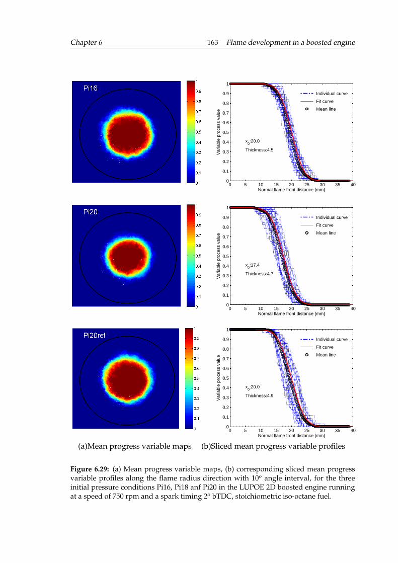
Chapter 6 163 Flame development in a boosted engine
0 5 10 15 20 25 30 35 400
0.1
0.2
0.3
0.4
0.5
0.6
0.7
0.8
0.9
1
Normal flame front distance [mm]
Var
iabl
e pr
oces
s va
lue
Individual curve
Fit curve
Mean line
x0:20.0
Thickness:4.5
0 5 10 15 20 25 30 35 400
0.1
0.2
0.3
0.4
0.5
0.6
0.7
0.8
0.9
1
Normal flame front distance [mm]
Var
iabl
e pr
oces
s va
lue
Individual curve
Fit curve
Mean line
x0:17.4
Thickness:4.7
0 5 10 15 20 25 30 35 400
0.1
0.2
0.3
0.4
0.5
0.6
0.7
0.8
0.9
1
Normal flame front distance [mm]
Var
iabl
e pr
oces
s va
lue
Individual curve
Fit curve
Mean line
x0:20.0
Thickness:4.9
(a)Mean progress variable maps (b)Sliced mean progress variable profiles
Figure 6.29: (a) Mean progress variable maps, (b) corresponding sliced mean progressvariable profiles along the flame radius direction with 10o angle interval, for the threeinitial pressure conditions Pi16, Pi18 anf Pi20 in the LUPOE 2D boosted engine runningat a speed of 750 rpm and a spark timing 2o bTDC, stoichiometric iso-octane fuel.
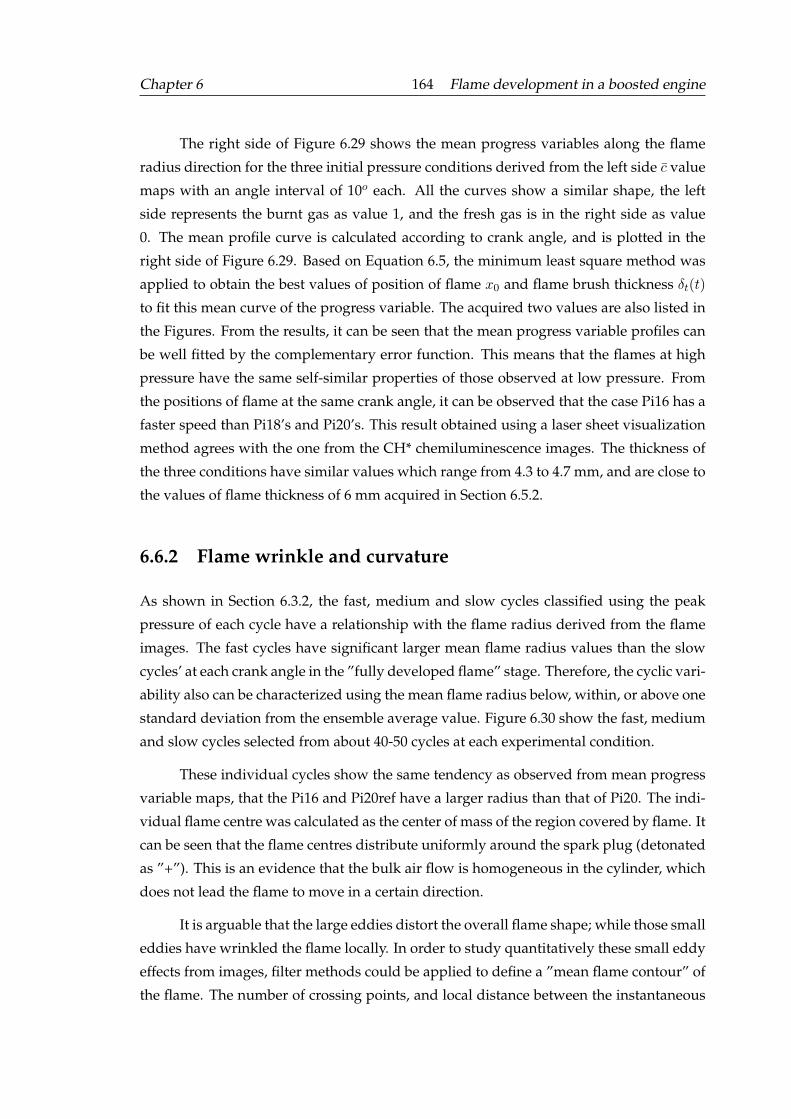
Chapter 6 164 Flame development in a boosted engine
The right side of Figure 6.29 shows the mean progress variables along the flame
radius direction for the three initial pressure conditions derived from the left side c value
maps with an angle interval of 10o each. All the curves show a similar shape, the left
side represents the burnt gas as value 1, and the fresh gas is in the right side as value
0. The mean profile curve is calculated according to crank angle, and is plotted in the
right side of Figure 6.29. Based on Equation 6.5, the minimum least square method was
applied to obtain the best values of position of flame x0 and flame brush thickness δt(t)
to fit this mean curve of the progress variable. The acquired two values are also listed in
the Figures. From the results, it can be seen that the mean progress variable profiles can
be well fitted by the complementary error function. This means that the flames at high
pressure have the same self-similar properties of those observed at low pressure. From
the positions of flame at the same crank angle, it can be observed that the case Pi16 has a
faster speed than Pi18’s and Pi20’s. This result obtained using a laser sheet visualization
method agrees with the one from the CH* chemiluminescence images. The thickness of
the three conditions have similar values which range from 4.3 to 4.7 mm, and are close to
the values of flame thickness of 6 mm acquired in Section 6.5.2.
6.6.2 Flame wrinkle and curvature
As shown in Section 6.3.2, the fast, medium and slow cycles classified using the peak
pressure of each cycle have a relationship with the flame radius derived from the flame
images. The fast cycles have significant larger mean flame radius values than the slow
cycles’ at each crank angle in the ”fully developed flame” stage. Therefore, the cyclic vari-
ability also can be characterized using the mean flame radius below, within, or above one
standard deviation from the ensemble average value. Figure 6.30 show the fast, medium
and slow cycles selected from about 40-50 cycles at each experimental condition.
These individual cycles show the same tendency as observed from mean progress
variable maps, that the Pi16 and Pi20ref have a larger radius than that of Pi20. The indi-
vidual flame centre was calculated as the center of mass of the region covered by flame. It
can be seen that the flame centres distribute uniformly around the spark plug (detonated
as ”+”). This is an evidence that the bulk air flow is homogeneous in the cylinder, which
does not lead the flame to move in a certain direction.
It is arguable that the large eddies distort the overall flame shape; while those small
eddies have wrinkled the flame locally. In order to study quantitatively these small eddy
effects from images, filter methods could be applied to define a ”mean flame contour” of
the flame. The number of crossing points, and local distance between the instantaneous
Chapter 6 165 Flame development in a boosted engine
−40 −30 −20 −10 0 10 20 30 40−40
−30
−20
−10
0
10
20
30
40
X [mm]
Y [m
m]
Pi16 fast cyclemedium cycleslow cycle
−40 −30 −20 −10 0 10 20 30 40−40
−30
−20
−10
0
10
20
30
40
X [mm]
Y [m
m]
Pi20 fast cyclemedium cycleslow cycle
−40 −30 −20 −10 0 10 20 30 40−40
−30
−20
−10
0
10
20
30
40
X [mm]
Y [m
m]
Pi20ref fast cyclemedium cycleslow cycle
Figure 6.30: Flame contours of fast, medium and slow cycles selected from three condi-tions: Pi16, Pi20 and Pi20ref, in the LUPOE 2D boosted engine running at a speed of 750rpm and a spark timing 2o bTDC, stoichiometric iso-octane fuel.
and filtered contours could be further defined to qualify the flame wrinkle (Aleiferis et al.
[2004]; Cairns [2001]). In this study, a ”flame radius” was calculated using minimum least
square algorithm. Thereafter, the wrinkle structure of a flame contour was characterized
using the deviation between the flame contour and the mean radius at the sample points
along the contour. The detailed calculation equation has been presented in Section 4.2.2.2.
The deviation values have been calculated for the three conditions: Pi16, Pi20 and
Pi20ref, and the results are shown in Figure 6.31. The mean and standard deviation val-
ues are also listed in Figure 6.31. Generally, larger flame radius have longer flame contour
lengths. By comparing Pi16 and Pi20, the wrinkle level of flame Pi16 is stronger than that
of Pi20 at all fast, medium and slow cycles. These two conditions have the similar tur-
Chapter 6 166 Flame development in a boosted engine
bulence intensities and different pressure above 6 bar, see Figure 6.24. This observation
implies that the pressure decreases the wrinkle effect under moderate turbulence, which
contrasts to the knowledge that flame front tends to be cellular under flame instability.
The Le number was estimated approximate 2.0 in these conditions, thus, the diffusive-
thermal effects may suppress the hydrodynamic instability, therefore, the flame surface
retains a smooth shape. Stronger turbulence leads to severe flame front wrinkle, this
can be observed when the Pi20 and Pi20ref were compared in medium and slow cycles,
except that one in the fast cycle.
The mean flame curvature was also examined, because the geometry of the flame
front also was influenced by the wrinkled flame structure. The calculation method has
been introduced in Section 4.2.2.2. The curvature values of each individual flame front
were combined together at each condition. The probability distribution curves for the
three conditions are plotted in Figure 6.32. The curvature values are between -5 to 5
(1/m), similar to the measured values from a burner flame at 1 to 10 bar (Soika et al.
[2003]). With the pressure increased by up 6 bar, no discernible systematic difference in
either length-scales or shapes of the probability distribution can be observed.
Figure 6.33 show the normalized spatial autocorrelation curves of fast, medium
and slow cycles at the three conditions: Pi16, Pi20 and Pi20ref. The La obtained from the
Equation 4.21 are listed in the Figure 6.33. Pi20ref has the largest values of 6-8 mm in
the medium and slow cycles, whilst, the values of Pi20 are smallest at the same group
of Pi20ref. This means the turbulence effects on the flame contour happens in the large
scales. By comparing the Pi16 and Pi20, it can be observed the decrease of La by increas-
ing pressure, the value of Pi20 is about 1-3 mm, thus, the influence of pressure on flame
wrinkle occurs in the small scales. In the fast cycle, the Pi20ref seems to have an abnor-
mal small value if it was compared to the medium and slow ones. The same problem
was also seen in the results shown in Figure 6.31. This may be due to the fact that using
the flame radius to select the fast, medium and slow cycles is not the best way to choose
a typical cycle. Ensemble averaging of all cycles’ parameters may be better to represent a
turbulent flame’s characteristic.
Power spectral density (PSD) S(k) was estimated based on the Equation 4.22. The
results of 9 flame contours are plotted in Figure 6.34 against the logarithms of the associ-
ated wavenumber,κ. No great difference can be distinguished, only a small spread in the
values in the end of the spectrum. Thus, the shape of PSD is not affected by the pressure
or turbulence increasing at the large scales. At the fully developed stage, the flame front
experiences the full spectrum of wrinkle length scales. The PSD deceases with a almost
constant slop as κ−2.4, this value is steeper than that observed from the isotropic turbu-
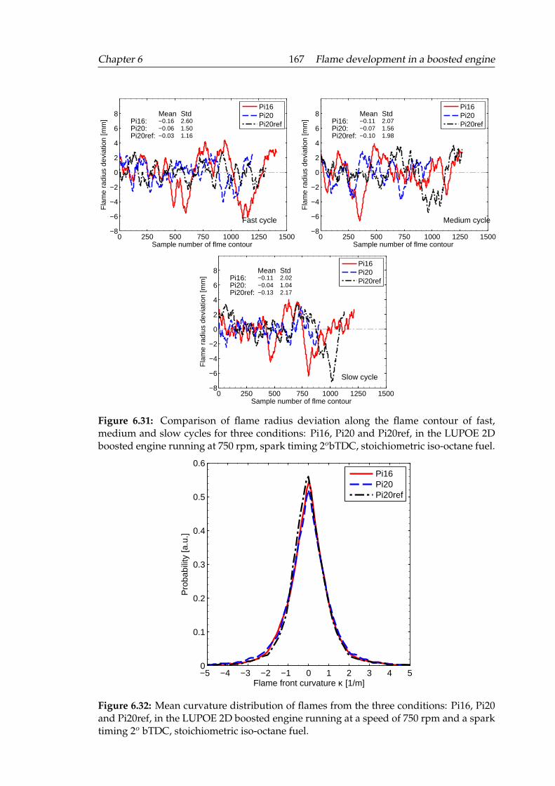
Chapter 6 167 Flame development in a boosted engine
0 250 500 750 1000 1250 1500−8
−6
−4
−2
0
2
4
6
8Pi16: −0.16 2.60Pi20: −0.06 1.50Pi20ref: −0.03 1.16
Sample number of flme contour
Fla
me
radi
us d
evia
tion
[mm
]
Mean Std
Fast cycle
Pi16Pi20Pi20ref
0 250 500 750 1000 1250 1500−8
−6
−4
−2
0
2
4
6
8Pi16: −0.11 2.07Pi20: −0.07 1.56Pi20ref: −0.10 1.98
Sample number of flme contour
Fla
me
radi
us d
evia
tion
[mm
]
Mean Std
Medium cycle
Pi16Pi20Pi20ref
0 250 500 750 1000 1250 1500−8
−6
−4
−2
0
2
4
6
8Pi16: −0.11 2.02Pi20: −0.04 1.04Pi20ref: −0.13 2.17
Sample number of flme contour
Fla
me
radi
us d
evia
tion
[mm
]
Mean Std
Slow cycle
Pi16Pi20Pi20ref
Figure 6.31: Comparison of flame radius deviation along the flame contour of fast,medium and slow cycles for three conditions: Pi16, Pi20 and Pi20ref, in the LUPOE 2Dboosted engine running at 750 rpm, spark timing 2obTDC, stoichiometric iso-octane fuel.
−5 −4 −3 −2 −1 0 1 2 3 4 50
0.1
0.2
0.3
0.4
0.5
0.6
Flame front curvature κ [1/m]
Pro
babi
lity
[a.u
.]
Pi16Pi20Pi20ref
Figure 6.32: Mean curvature distribution of flames from the three conditions: Pi16, Pi20and Pi20ref, in the LUPOE 2D boosted engine running at a speed of 750 rpm and a sparktiming 2o bTDC, stoichiometric iso-octane fuel.
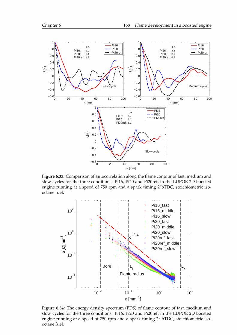
Chapter 6 168 Flame development in a boosted engine
0 20 40 60 80 100−0.6
−0.4
−0.2
0
0.2
0.4
0.6
0.8
1
Pi16: 9.0Pi20: 2.4Pi20ref: 1.3
La
Fast cycle
s’ [mm]
ξ(s’ )
Pi16Pi20Pi20ref
0 20 40 60 80 100−0.6
−0.4
−0.2
0
0.2
0.4
0.6
0.8
1
Pi16: 4.8Pi20: 2.6Pi20ref: 6.8
La
Medium cycle
s’ [mm]
ξ(s’ )
Pi16Pi20Pi20ref
0 20 40 60 80 100−0.6
−0.4
−0.2
0
0.2
0.4
0.6
0.8
1
Pi16: 4.7Pi20: 1.1Pi20ref: 6.1
La
Slow cycle
s’ [mm]
ξ(s’ )
Pi16Pi20Pi20ref
Figure 6.33: Comparison of autocorrelation along the flame contour of fast, medium andslow cycles for the three conditions: Pi16, Pi20 and Pi20ref, in the LUPOE 2D boostedengine running at a speed of 750 rpm and a spark timing 2obTDC, stoichiometric iso-octane fuel.
10−2
10−1
100
101
10−4
10−2
100
102
κ [mm−1]
S(k
)[m
m3 ]
κ−2.4
Bore Li
Lλ
Flame radius
Pi16_fastPi16_middlePi16_slowPi20_fastPi20_middlePi20_slowPi20ref_fastPi20ref_middlePi20ref_slow
Figure 6.34: The energy density spectrum (PDS) of flame contour of fast, medium andslow cycles for the three conditions: Pi16, Pi20 and Pi20ref, in the LUPOE 2D boostedengine running at a speed of 750 rpm and a spark timing 2o bTDC, stoichiometric iso-octane fuel.

Chapter 6 169 Flame development in a boosted engine
lence flow κ−5/3 in the LUPOE 2D engine shown in the Figure 6.4. This gradient of the
PSD curve agrees with the measurement of Kheirkhah and Gulder [2013] and Hicks et al.
[1994]. Several characteristic length scales also were labelled in Figure 6.34. The largest
wavelength of PSD is close to the engine bore size, while the smallest wavelength is cut
off above the estimated Taylor length scale (0.2mm), this is mainly caused by the restric-
tion of the resolution of the images. The flame can be influenced by the eddies which are
significantly larger (10 to 20 times) than the turbulence integral length scale Li (10 mm).
Chapter 7
Autoignition in a boosted SI engine
This Chapter presents the effects of increased inlet pressure on knock characteristics stud-
ied in the strongly supercharged spark ignition engine, with a particular emphasis on
understanding the occurrence of extreme knock. The knock images with different pres-
sure oscillation amplitudes were obtained from the LUPOE 2D boosted engine. Based
on these knock images and their corresponding pressure data, the development of au-
toignition sites and subsequently produced combustion waves were described, and the
definitions of knock characteristic parameters, i.e. knock onset and knock intensity, were
also evaluated. These defined knock parameters were used to understand the difference
of cyclic variability and knock properties under naturally aspirated and strongly boosted
engine running modes. Furthermore, several individual imaging knock cycles with grad-
ually increased knock intensities from the same engine operation condition were selected.
The effects of thermodynamics state of the end gas condition, unburnt gas mass fraction,
and burning velocity on knock intensity were analyzed. The speed of the reaction front
generated by autoignition site was calculated to check whether detonation exists in the
extreme knock cycles.
7.1 Knock map of LUPOE 2D boosted engine
As a starting point, a series of experiments with different inlet initial pressure and spark
timing at engine speed of 750 rpm have been conducted in the LUPOE 2D boosted engine
to discriminate between knock and ”no knock” regions of operation regimes. The knock
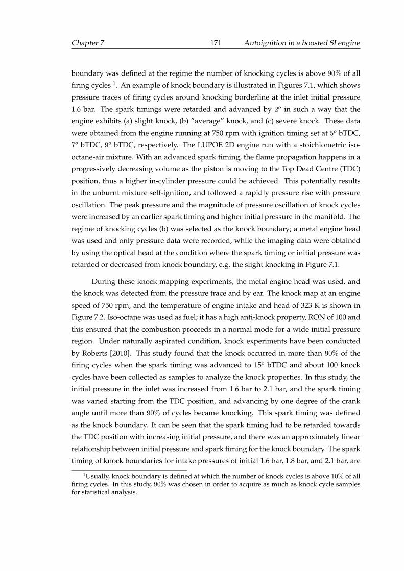
Chapter 7 171 Autoignition in a boosted SI engine
boundary was defined at the regime the number of knocking cycles is above 90% of all
firing cycles 1. An example of knock boundary is illustrated in Figures 7.1, which shows
pressure traces of firing cycles around knocking borderline at the inlet initial pressure
1.6 bar. The spark timings were retarded and advanced by 2o in such a way that the
engine exhibits (a) slight knock, (b) ”average” knock, and (c) severe knock. These data
were obtained from the engine running at 750 rpm with ignition timing set at 5o bTDC,
7o bTDC, 9o bTDC, respectively. The LUPOE 2D engine run with a stoichiometric iso-
octane-air mixture. With an advanced spark timing, the flame propagation happens in a
progressively decreasing volume as the piston is moving to the Top Dead Centre (TDC)
position, thus a higher in-cylinder pressure could be achieved. This potentially results
in the unburnt mixture self-ignition, and followed a rapidly pressure rise with pressure
oscillation. The peak pressure and the magnitude of pressure oscillation of knock cycles
were increased by an earlier spark timing and higher initial pressure in the manifold. The
regime of knocking cycles (b) was selected as the knock boundary; a metal engine head
was used and only pressure data were recorded, while the imaging data were obtained
by using the optical head at the condition where the spark timing or initial pressure was
retarded or decreased from knock boundary, e.g. the slight knocking in Figure 7.1.
During these knock mapping experiments, the metal engine head was used, and
the knock was detected from the pressure trace and by ear. The knock map at an engine
speed of 750 rpm, and the temperature of engine intake and head of 323 K is shown in
Figure 7.2. Iso-octane was used as fuel; it has a high anti-knock property, RON of 100 and
this ensured that the combustion proceeds in a normal mode for a wide initial pressure
region. Under naturally aspirated condition, knock experiments have been conducted
by Roberts [2010]. This study found that the knock occurred in more than 90% of the
firing cycles when the spark timing was advanced to 15o bTDC and about 100 knock
cycles have been collected as samples to analyze the knock properties. In this study, the
initial pressure in the inlet was increased from 1.6 bar to 2.1 bar, and the spark timing
was varied starting from the TDC position, and advancing by one degree of the crank
angle until more than 90% of cycles became knocking. This spark timing was defined
as the knock boundary. It can be seen that the spark timing had to be retarded towards
the TDC position with increasing initial pressure, and there was an approximately linear
relationship between initial pressure and spark timing for the knock boundary. The spark
timing of knock boundaries for intake pressures of initial 1.6 bar, 1.8 bar, and 2.1 bar, are
1Usually, knock boundary is defined at which the number of knock cycles is above 10% of allfiring cycles. In this study, 90% was chosen in order to acquire as much as knock cycle samplesfor statistical analysis.
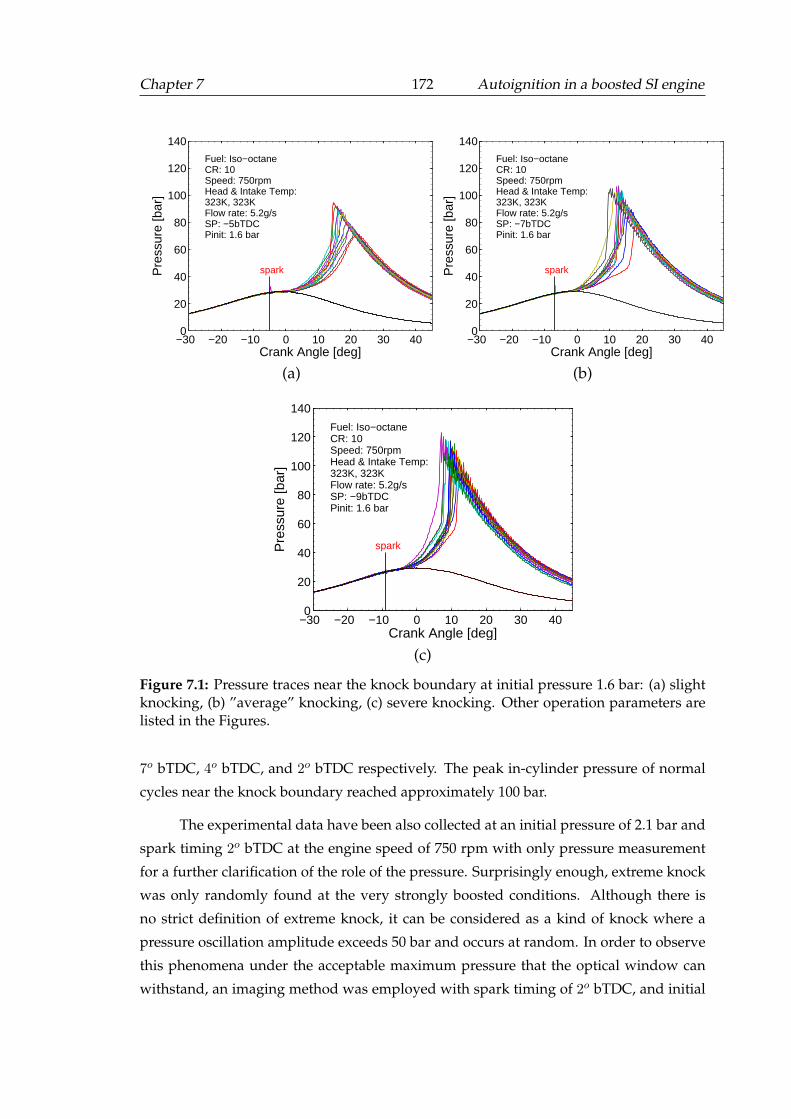
Chapter 7 172 Autoignition in a boosted SI engine
−30 −20 −10 0 10 20 30 400
20
40
60
80
100
120
140
spark
Crank Angle [deg]
Pre
ssur
e [b
ar]
Fuel: Iso−octaneCR: 10Speed: 750rpmHead & Intake Temp:323K, 323KFlow rate: 5.2g/sSP: −5bTDCPinit: 1.6 bar
(a)
−30 −20 −10 0 10 20 30 400
20
40
60
80
100
120
140
spark
Crank Angle [deg]
Pre
ssur
e [b
ar]
Fuel: Iso−octaneCR: 10Speed: 750rpmHead & Intake Temp:323K, 323KFlow rate: 5.2g/sSP: −7bTDCPinit: 1.6 bar
(b)
−30 −20 −10 0 10 20 30 400
20
40
60
80
100
120
140
spark
Crank Angle [deg]
Pre
ssur
e [b
ar]
Fuel: Iso−octaneCR: 10Speed: 750rpmHead & Intake Temp:323K, 323KFlow rate: 5.2g/sSP: −9bTDCPinit: 1.6 bar
(c)
Figure 7.1: Pressure traces near the knock boundary at initial pressure 1.6 bar: (a) slightknocking, (b) ”average” knocking, (c) severe knocking. Other operation parameters arelisted in the Figures.
7o bTDC, 4o bTDC, and 2o bTDC respectively. The peak in-cylinder pressure of normal
cycles near the knock boundary reached approximately 100 bar.
The experimental data have been also collected at an initial pressure of 2.1 bar and
spark timing 2o bTDC at the engine speed of 750 rpm with only pressure measurement
for a further clarification of the role of the pressure. Surprisingly enough, extreme knock
was only randomly found at the very strongly boosted conditions. Although there is
no strict definition of extreme knock, it can be considered as a kind of knock where a
pressure oscillation amplitude exceeds 50 bar and occurs at random. In order to observe
this phenomena under the acceptable maximum pressure that the optical window can
withstand, an imaging method was employed with spark timing of 2o bTDC, and initial
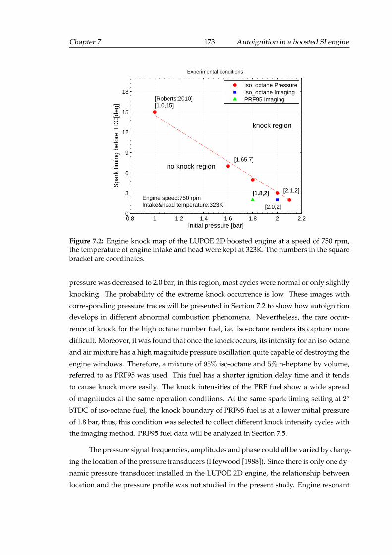
Chapter 7 173 Autoignition in a boosted SI engine
0.8 1 1.2 1.4 1.6 1.8 2 2.20
3
6
9
12
15
18
Experimental conditions
Initial pressure [bar]
Spa
rk ti
min
g be
fore
TD
C[d
eg]
[1.8,2]
[1.0,15]
[1.65,7]
[2.1,2]
[2.0,2]
[1.8,2]
[Roberts:2010]
Engine speed:750 rpmIntake&head temperature:323K
no knock region
knock region
Iso_octane PressureIso_octane ImagingPRF95 Imaging
Figure 7.2: Engine knock map of the LUPOE 2D boosted engine at a speed of 750 rpm,the temperature of engine intake and head were kept at 323K. The numbers in the squarebracket are coordinates.
pressure was decreased to 2.0 bar; in this region, most cycles were normal or only slightly
knocking. The probability of the extreme knock occurrence is low. These images with
corresponding pressure traces will be presented in Section 7.2 to show how autoignition
develops in different abnormal combustion phenomena. Nevertheless, the rare occur-
rence of knock for the high octane number fuel, i.e. iso-octane renders its capture more
difficult. Moreover, it was found that once the knock occurs, its intensity for an iso-octane
and air mixture has a high magnitude pressure oscillation quite capable of destroying the
engine windows. Therefore, a mixture of 95% iso-octane and 5% n-heptane by volume,
referred to as PRF95 was used. This fuel has a shorter ignition delay time and it tends
to cause knock more easily. The knock intensities of the PRF fuel show a wide spread
of magnitudes at the same operation conditions. At the same spark timing setting at 2o
bTDC of iso-octane fuel, the knock boundary of PRF95 fuel is at a lower initial pressure
of 1.8 bar, thus, this condition was selected to collect different knock intensity cycles with
the imaging method. PRF95 fuel data will be analyzed in Section 7.5.
The pressure signal frequencies, amplitudes and phase could all be varied by chang-
ing the location of the pressure transducers (Heywood [1988]). Since there is only one dy-
namic pressure transducer installed in the LUPOE 2D engine, the relationship between
location and the pressure profile was not studied in the present study. Engine resonant
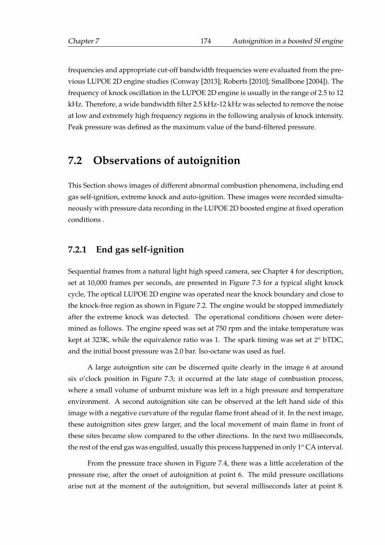
Chapter 7 174 Autoignition in a boosted SI engine
frequencies and appropriate cut-off bandwidth frequencies were evaluated from the pre-
vious LUPOE 2D engine studies (Conway [2013]; Roberts [2010]; Smallbone [2004]). The
frequency of knock oscillation in the LUPOE 2D engine is usually in the range of 2.5 to 12
kHz. Therefore, a wide bandwidth filter 2.5 kHz-12 kHz was selected to remove the noise
at low and extremely high frequency regions in the following analysis of knock intensity.
Peak pressure was defined as the maximum value of the band-filtered pressure.
7.2 Observations of autoignition
This Section shows images of different abnormal combustion phenomena, including end
gas self-ignition, extreme knock and auto-ignition. These images were recorded simulta-
neously with pressure data recording in the LUPOE 2D boosted engine at fixed operation
conditions .
7.2.1 End gas self-ignition
Sequential frames from a natural light high speed camera, see Chapter 4 for description,
set at 10,000 frames per seconds, are presented in Figure 7.3 for a typical slight knock
cycle, The optical LUPOE 2D engine was operated near the knock boundary and close to
the knock-free region as shown in Figure 7.2. The engine would be stopped immediately
after the extreme knock was detected. The operational conditions chosen were deter-
mined as follows. The engine speed was set at 750 rpm and the intake temperature was
kept at 323K, while the equivalence ratio was 1. The spark timing was set at 2o bTDC,
and the initial boost pressure was 2.0 bar. Iso-octane was used as fuel.
A large autoigntion site can be discerned quite clearly in the image 6 at around
six o’clock position in Figure 7.3; it occurred at the late stage of combustion process,
where a small volume of unburnt mixture was left in a high pressure and temperature
environment. A second autoignition site can be observed at the left hand side of this
image with a negative curvature of the regular flame front ahead of it. In the next image,
these autoignition sites grew larger, and the local movement of main flame in front of
these sites became slow compared to the other directions. In the next two milliseconds,
the rest of the end gas was engulfed, usually this process happened in only 1o CA interval.
From the pressure trace shown in Figure 7.4, there was a little acceleration of the
pressure rise, after the onset of autoignition at point 6. The mild pressure oscillations
arise not at the moment of the autoignition, but several milliseconds later at point 8.
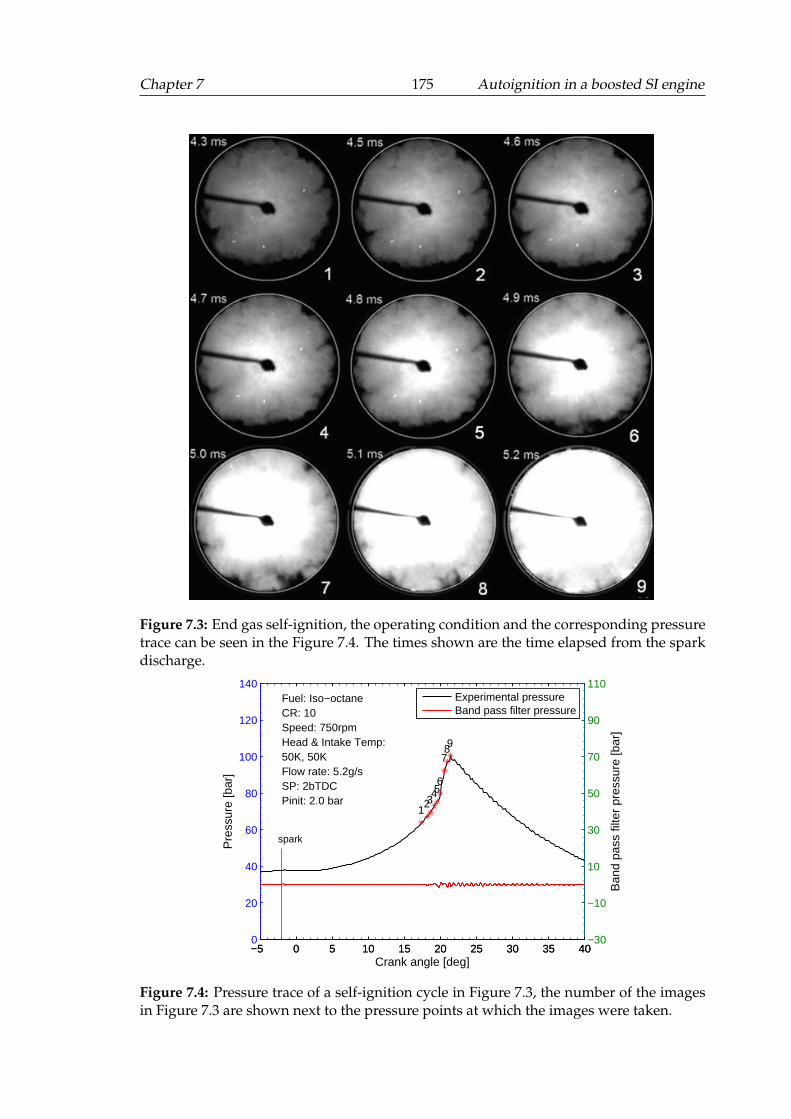
Chapter 7 175 Autoignition in a boosted SI engine
Figure 7.3: End gas self-ignition, the operating condition and the corresponding pressuretrace can be seen in the Figure 7.4. The times shown are the time elapsed from the sparkdischarge.
−5 0 5 10 15 20 25 30 35 400
20
40
60
80
100
120
140
spark
123
456
789
Pre
ssur
e [b
ar]
Fuel: Iso−octaneCR: 10Speed: 750rpmHead & Intake Temp:50K, 50KFlow rate: 5.2g/sSP: 2bTDCPinit: 2.0 bar
−5 0 5 10 15 20 25 30 35 40−30
−10
10
30
50
70
90
110
Ban
d pa
ss fi
lter
pres
sure
[bar
]
Crank angle [deg]
Experimental pressureBand pass filter pressure
Figure 7.4: Pressure trace of a self-ignition cycle in Figure 7.3, the number of the imagesin Figure 7.3 are shown next to the pressure points at which the images were taken.
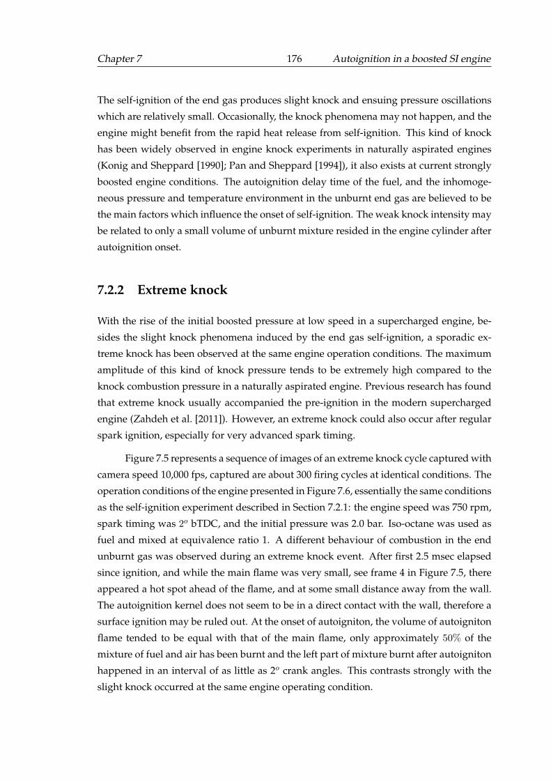
Chapter 7 176 Autoignition in a boosted SI engine
The self-ignition of the end gas produces slight knock and ensuing pressure oscillations
which are relatively small. Occasionally, the knock phenomena may not happen, and the
engine might benefit from the rapid heat release from self-ignition. This kind of knock
has been widely observed in engine knock experiments in naturally aspirated engines
(Konig and Sheppard [1990]; Pan and Sheppard [1994]), it also exists at current strongly
boosted engine conditions. The autoignition delay time of the fuel, and the inhomoge-
neous pressure and temperature environment in the unburnt end gas are believed to be
the main factors which influence the onset of self-ignition. The weak knock intensity may
be related to only a small volume of unburnt mixture resided in the engine cylinder after
autoignition onset.
7.2.2 Extreme knock
With the rise of the initial boosted pressure at low speed in a supercharged engine, be-
sides the slight knock phenomena induced by the end gas self-ignition, a sporadic ex-
treme knock has been observed at the same engine operation conditions. The maximum
amplitude of this kind of knock pressure tends to be extremely high compared to the
knock combustion pressure in a naturally aspirated engine. Previous research has found
that extreme knock usually accompanied the pre-ignition in the modern supercharged
engine (Zahdeh et al. [2011]). However, an extreme knock could also occur after regular
spark ignition, especially for very advanced spark timing.
Figure 7.5 represents a sequence of images of an extreme knock cycle captured with
camera speed 10,000 fps, captured are about 300 firing cycles at identical conditions. The
operation conditions of the engine presented in Figure 7.6, essentially the same conditions
as the self-ignition experiment described in Section 7.2.1: the engine speed was 750 rpm,
spark timing was 2o bTDC, and the initial pressure was 2.0 bar. Iso-octane was used as
fuel and mixed at equivalence ratio 1. A different behaviour of combustion in the end
unburnt gas was observed during an extreme knock event. After first 2.5 msec elapsed
since ignition, and while the main flame was very small, see frame 4 in Figure 7.5, there
appeared a hot spot ahead of the flame, and at some small distance away from the wall.
The autoignition kernel does not seem to be in a direct contact with the wall, therefore a
surface ignition may be ruled out. At the onset of autoigniton, the volume of autoigniton
flame tended to be equal with that of the main flame, only approximately 50% of the
mixture of fuel and air has been burnt and the left part of mixture burnt after autoigniton
happened in an interval of as little as 2o crank angles. This contrasts strongly with the
slight knock occurred at the same engine operating condition.
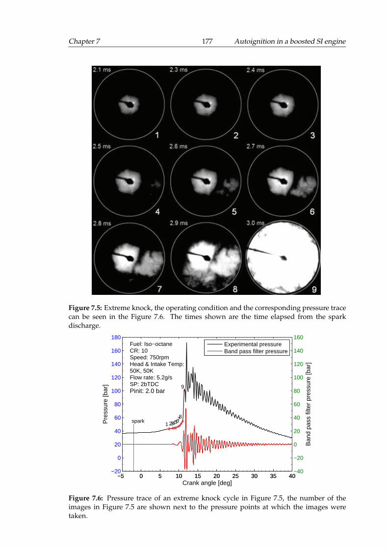
Chapter 7 177 Autoignition in a boosted SI engine
Figure 7.5: Extreme knock, the operating condition and the corresponding pressure tracecan be seen in the Figure 7.6. The times shown are the time elapsed from the sparkdischarge.
−5 0 5 10 15 20 25 30 35 40−20
0
20
40
60
80
100
120
140
160
180
spark1 234567
8
9
Pre
ssur
e [b
ar]
Fuel: Iso−octaneCR: 10Speed: 750rpmHead & Intake Temp:50K, 50KFlow rate: 5.2g/sSP: 2bTDCPinit: 2.0 bar
−5 0 5 10 15 20 25 30 35 40−40
−20
0
20
40
60
80
100
120
140
160
Ban
d pa
ss fi
lter
pres
sure
[bar
]
Crank angle [deg]
Experimental pressureBand pass filter pressure
Figure 7.6: Pressure trace of an extreme knock cycle in Figure 7.5, the number of theimages in Figure 7.5 are shown next to the pressure points at which the images weretaken.
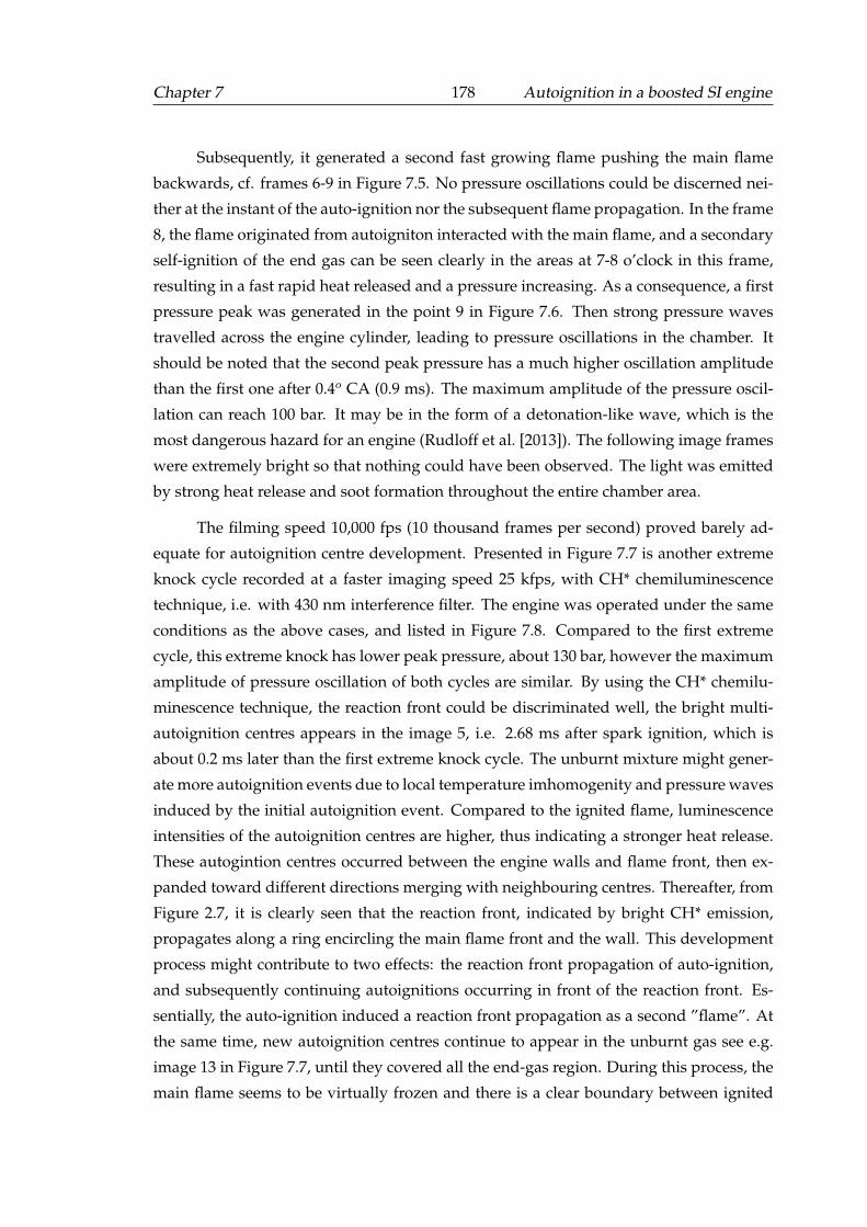
Chapter 7 178 Autoignition in a boosted SI engine
Subsequently, it generated a second fast growing flame pushing the main flame
backwards, cf. frames 6-9 in Figure 7.5. No pressure oscillations could be discerned nei-
ther at the instant of the auto-ignition nor the subsequent flame propagation. In the frame
8, the flame originated from autoigniton interacted with the main flame, and a secondary
self-ignition of the end gas can be seen clearly in the areas at 7-8 o’clock in this frame,
resulting in a fast rapid heat released and a pressure increasing. As a consequence, a first
pressure peak was generated in the point 9 in Figure 7.6. Then strong pressure waves
travelled across the engine cylinder, leading to pressure oscillations in the chamber. It
should be noted that the second peak pressure has a much higher oscillation amplitude
than the first one after 0.4o CA (0.9 ms). The maximum amplitude of the pressure oscil-
lation can reach 100 bar. It may be in the form of a detonation-like wave, which is the
most dangerous hazard for an engine (Rudloff et al. [2013]). The following image frames
were extremely bright so that nothing could have been observed. The light was emitted
by strong heat release and soot formation throughout the entire chamber area.
The filming speed 10,000 fps (10 thousand frames per second) proved barely ad-
equate for autoignition centre development. Presented in Figure 7.7 is another extreme
knock cycle recorded at a faster imaging speed 25 kfps, with CH* chemiluminescence
technique, i.e. with 430 nm interference filter. The engine was operated under the same
conditions as the above cases, and listed in Figure 7.8. Compared to the first extreme
cycle, this extreme knock has lower peak pressure, about 130 bar, however the maximum
amplitude of pressure oscillation of both cycles are similar. By using the CH* chemilu-
minescence technique, the reaction front could be discriminated well, the bright multi-
autoignition centres appears in the image 5, i.e. 2.68 ms after spark ignition, which is
about 0.2 ms later than the first extreme knock cycle. The unburnt mixture might gener-
ate more autoignition events due to local temperature imhomogenity and pressure waves
induced by the initial autoignition event. Compared to the ignited flame, luminescence
intensities of the autoignition centres are higher, thus indicating a stronger heat release.
These autogintion centres occurred between the engine walls and flame front, then ex-
panded toward different directions merging with neighbouring centres. Thereafter, from
Figure 2.7, it is clearly seen that the reaction front, indicated by bright CH* emission,
propagates along a ring encircling the main flame front and the wall. This development
process might contribute to two effects: the reaction front propagation of auto-ignition,
and subsequently continuing autoignitions occurring in front of the reaction front. Es-
sentially, the auto-ignition induced a reaction front propagation as a second ”flame”. At
the same time, new autoignition centres continue to appear in the unburnt gas see e.g.
image 13 in Figure 7.7, until they covered all the end-gas region. During this process, the
main flame seems to be virtually frozen and there is a clear boundary between ignited
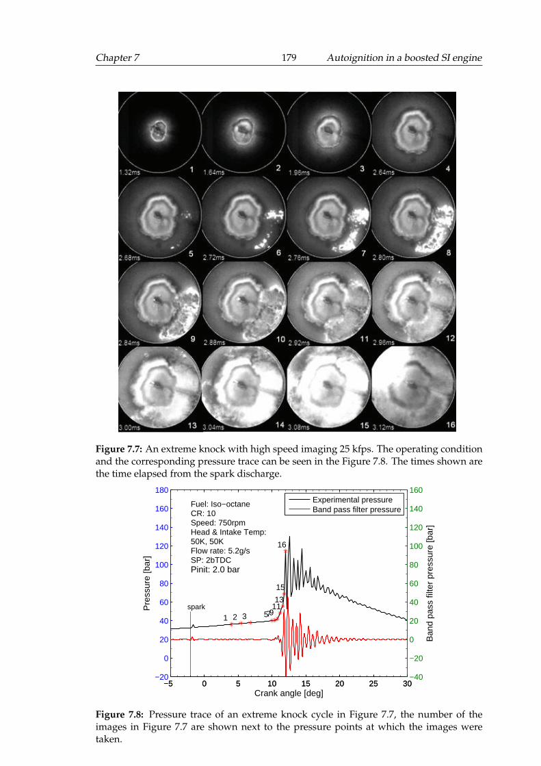
Chapter 7 179 Autoignition in a boosted SI engine
Figure 7.7: An extreme knock with high speed imaging 25 kfps. The operating conditionand the corresponding pressure trace can be seen in the Figure 7.8. The times shown arethe time elapsed from the spark discharge.
−5 0 5 10 15 20 25 30−20
0
20
40
60
80
100
120
140
160
180
spark
1 2 3 5791113
15
16
Pre
ssur
e [b
ar]
Fuel: Iso−octaneCR: 10Speed: 750rpmHead & Intake Temp:50K, 50KFlow rate: 5.2g/sSP: 2bTDCPinit: 2.0 bar
−5 0 5 10 15 20 25 30−40
−20
0
20
40
60
80
100
120
140
160
Ban
d pa
ss fi
lter
pres
sure
[bar
]
Crank angle [deg]
Experimental pressureBand pass filter pressure
Figure 7.8: Pressure trace of an extreme knock cycle in Figure 7.7, the number of theimages in Figure 7.7 are shown next to the pressure points at which the images weretaken.
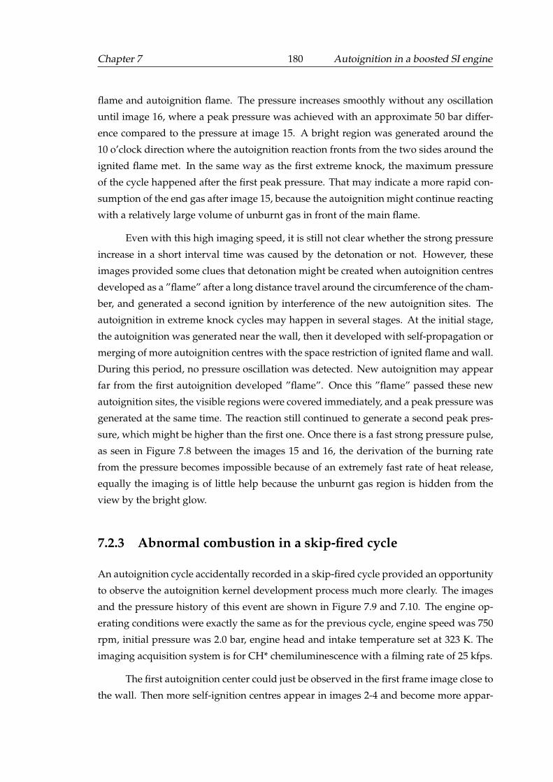
Chapter 7 180 Autoignition in a boosted SI engine
flame and autoignition flame. The pressure increases smoothly without any oscillation
until image 16, where a peak pressure was achieved with an approximate 50 bar differ-
ence compared to the pressure at image 15. A bright region was generated around the
10 o’clock direction where the autoignition reaction fronts from the two sides around the
ignited flame met. In the same way as the first extreme knock, the maximum pressure
of the cycle happened after the first peak pressure. That may indicate a more rapid con-
sumption of the end gas after image 15, because the autoignition might continue reacting
with a relatively large volume of unburnt gas in front of the main flame.
Even with this high imaging speed, it is still not clear whether the strong pressure
increase in a short interval time was caused by the detonation or not. However, these
images provided some clues that detonation might be created when autoignition centres
developed as a ”flame” after a long distance travel around the circumference of the cham-
ber, and generated a second ignition by interference of the new autoignition sites. The
autoignition in extreme knock cycles may happen in several stages. At the initial stage,
the autoignition was generated near the wall, then it developed with self-propagation or
merging of more autoignition centres with the space restriction of ignited flame and wall.
During this period, no pressure oscillation was detected. New autoignition may appear
far from the first autoignition developed ”flame”. Once this ”flame” passed these new
autoignition sites, the visible regions were covered immediately, and a peak pressure was
generated at the same time. The reaction still continued to generate a second peak pres-
sure, which might be higher than the first one. Once there is a fast strong pressure pulse,
as seen in Figure 7.8 between the images 15 and 16, the derivation of the burning rate
from the pressure becomes impossible because of an extremely fast rate of heat release,
equally the imaging is of little help because the unburnt gas region is hidden from the
view by the bright glow.
7.2.3 Abnormal combustion in a skip-fired cycle
An autoignition cycle accidentally recorded in a skip-fired cycle provided an opportunity
to observe the autoignition kernel development process much more clearly. The images
and the pressure history of this event are shown in Figure 7.9 and 7.10. The engine op-
erating conditions were exactly the same as for the previous cycle, engine speed was 750
rpm, initial pressure was 2.0 bar, engine head and intake temperature set at 323 K. The
imaging acquisition system is for CH* chemiluminescence with a filming rate of 25 kfps.
The first autoignition center could just be observed in the first frame image close to
the wall. Then more self-ignition centres appear in images 2-4 and become more appar-
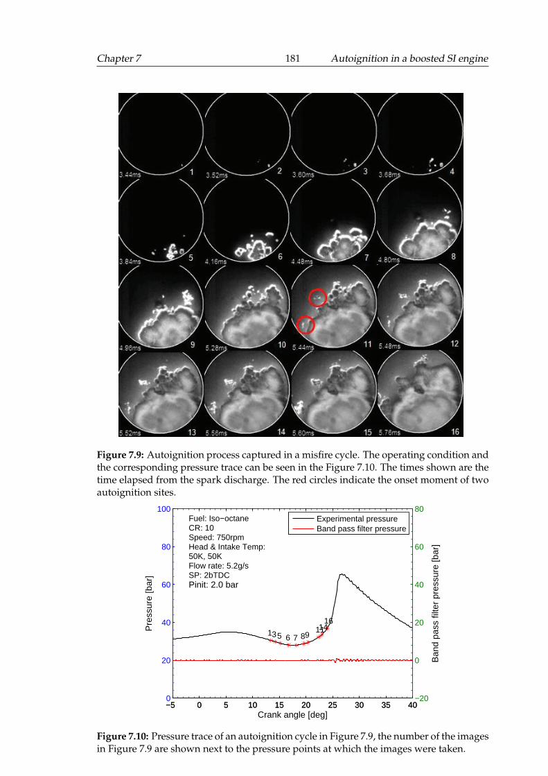
Chapter 7 181 Autoignition in a boosted SI engine
Figure 7.9: Autoignition process captured in a misfire cycle. The operating condition andthe corresponding pressure trace can be seen in the Figure 7.10. The times shown are thetime elapsed from the spark discharge. The red circles indicate the onset moment of twoautoignition sites.
−5 0 5 10 15 20 25 30 35 400
20
40
60
80
100
135 6 7 891114
16
Pre
ssur
e [b
ar]
Fuel: Iso−octaneCR: 10Speed: 750rpmHead & Intake Temp:50K, 50KFlow rate: 5.2g/sSP: 2bTDCPinit: 2.0 bar
−5 0 5 10 15 20 25 30 35 40−20
0
20
40
60
80
Ban
d pa
ss fi
lter
pres
sure
[bar
]
Crank angle [deg]
Experimental pressureBand pass filter pressure
Figure 7.10: Pressure trace of an autoignition cycle in Figure 7.9, the number of the imagesin Figure 7.9 are shown next to the pressure points at which the images were taken.
Chapter 7 182 Autoignition in a boosted SI engine
ent in the vicinity of the first one. They are bright and associated with rapid consumption
of the unburnt gas. After these autoignition sites merged together, they form a propagat-
ing flame front, indicated by CH* luminescence. Flame propagation is accompanied by
appearance of new self-ignition centres ahead of it. A process of autoignition geneated
in front of the ”flame front” can be observed in the sequence of images 11 to 14: the
shape of one close to the wall was affected by the compression of the burnt gas, while
the one in the center area of chamber developed more freely, later they are engulfed by
the flame. In the following frame, the whole end gas is engulfed by the flame, and no
pressure oscillation was detected in this cycle. In a sense, this sequence is very similar to
HCCI combustion with an important distinction that the charge is stoichiometric without
dilution.
7.3 Knock onset and intensity
Knock onset and intensity are usually the two main parameters to characterize the knock
properties (Heywood [1988]). From previous knock images, the knock onset can be fur-
ther discriminated as an autoignition onset, where the autoignition sites appear and only
cause a slight pressure increase. Yet, the knock onset is usually the starting point of
strong pressure oscillations, at which the autoignition sites have been developed across
the entire cylinder in the visible image. The pressure trace of the extreme knock shown
in Section 7.2 is selected here to illustrate the definitions of autoignition and knock onset
in this study. The knock cycle pressure trace was separated into a low band pass part
and a high pass part firstly as shown in Figure 7.11. The high band pass filtered pressure
represents the pressure oscillations induced by knock; the signal shown in Figure 7.11
corresponds to the cut-off frequency bandwidth of 2.5-12 kHz. Some weak oscillations
can be observed after the autoignition sites appear before the detected knock onset, and
then the amplitude of pressure increases progressively until knock occurs. At the knock
onset time, the amplitude of pressure increased steeply and then reached a peak value
in a short time. After this, the amplitude of the pressure decreased and the oscillations
lasted for few milliseconds, slowly decaying.
A threshold value was adopted to determine the autoignition onset, that is the fil-
tered pressure oscillations were scanned until a certain threshold value was exceeded
(Worret et al. [2002]). The threshold was usually set below the maximum amplitude
of the knock-related oscillations and above that of the noise signals. However, a uni-
versal threshold setting for all engine operation conditions does not exist. Even for the
same operation condition, it was found that decreasing the threshold leads to mark incor-
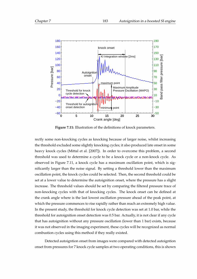
Chapter 7 183 Autoignition in a boosted SI engine
0 5 10 15 20 25 30−60
−40
−20
0
20
40
60
80
100
120
140
160
180
Pre
ssur
e [b
ar]
Autoigntiononset
knock onset
maximum point
minimum point
Maximum AmplitudePressure Oscillation (MAPO)
KI Integration window [2ms]
Threshold for autoignitiononset detection
Threshold for knockcycle detection
0 5 10 15 20 25 30−50
−30
−10
10
30
50
70
90
110
130
150
170
190
Ban
d pa
ss fi
lter
pres
sure
[bar
]
Crank angle [deg]
Figure 7.11: Illustration of the definitions of knock parameters.
rectly some non-knocking cycles as knocking because of larger noise, whilst increasing
the threshold excluded some slightly knocking cycles; it also produced late onset in some
heavy knock cycles (Mittal et al. [2007]). In order to overcome this problem, a second
threshold was used to determine a cycle to be a knock cycle or a non-knock cycle. As
observed in Figure 7.11, a knock cycle has a maximum oscillation point, which is sig-
nificantly larger than the noise signal. By setting a threshold lower than the maximum
oscillation point, the knock cycles could be selected. Then, the second threshold could be
set at a lower value to determine the autoignition onset, where the pressure has a slight
increase. The threshold values should be set by comparing the filtered pressure trace of
non-knocking cycles with that of knocking cycles. The knock onset can be defined at
the crank angle where is the last lowest oscillation pressure ahead of the peak point, at
which the pressure commences to rise rapidly rather than reach an extremely high value.
In the present study, the threshold for knock cycle detection was set at 1.0 bar, while the
threshold for autoignition onset detection was 0.5 bar. Actually, it is not clear if any cycle
that has autoignition without any pressure oscillation (lower than 1 bar) exists, because
it was not observed in the imaging experiment, these cycles will be recognized as normal
combustion cycles using this method if they really existed.
Detected autoigntion onset from images were compared with detected autoigntion
onset from pressures for 7 knock cycle samples at two operating conditions, this is shown
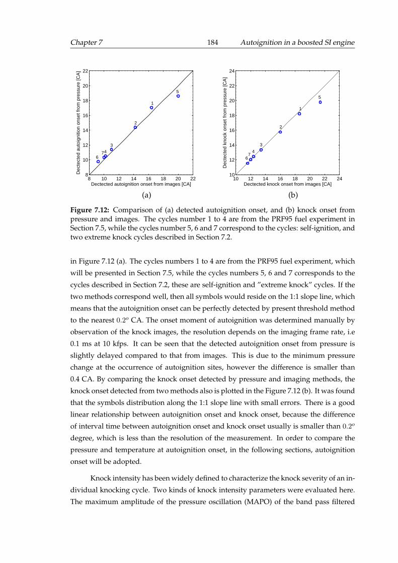
Chapter 7 184 Autoignition in a boosted SI engine
8 10 12 14 16 18 20 228
10
12
14
16
18
20
22
1
2
3
4
5
67
Dectected autoignition onset from images [CA]
Dec
tect
ed a
utoi
gniti
on o
nset
from
pre
ssur
e [C
A]
(a)
10 12 14 16 18 20 22 2410
12
14
16
18
20
22
24
1
2
3
4
5
67
Dectected knock onset from images [CA]
Dec
tect
ed k
nock
ons
et fr
om p
ress
ure
[CA
]
(b)
Figure 7.12: Comparison of (a) detected autoignition onset, and (b) knock onset frompressure and images. The cycles number 1 to 4 are from the PRF95 fuel experiment inSection 7.5, while the cycles number 5, 6 and 7 correspond to the cycles: self-ignition, andtwo extreme knock cycles described in Section 7.2.
in Figure 7.12 (a). The cycles numbers 1 to 4 are from the PRF95 fuel experiment, which
will be presented in Section 7.5, while the cycles numbers 5, 6 and 7 corresponds to the
cycles described in Section 7.2, these are self-ignition and ”extreme knock” cycles. If the
two methods correspond well, then all symbols would reside on the 1:1 slope line, which
means that the autoignition onset can be perfectly detected by present threshold method
to the nearest 0.2o CA. The onset moment of autoignition was determined manually by
observation of the knock images, the resolution depends on the imaging frame rate, i.e
0.1 ms at 10 kfps. It can be seen that the detected autoignition onset from pressure is
slightly delayed compared to that from images. This is due to the minimum pressure
change at the occurrence of autoignition sites, however the difference is smaller than
0.4 CA. By comparing the knock onset detected by pressure and imaging methods, the
knock onset detected from two methods also is plotted in the Figure 7.12 (b). It was found
that the symbols distribution along the 1:1 slope line with small errors. There is a good
linear relationship between autoignition onset and knock onset, because the difference
of interval time between autoignition onset and knock onset usually is smaller than 0.2o
degree, which is less than the resolution of the measurement. In order to compare the
pressure and temperature at autoignition onset, in the following sections, autoignition
onset will be adopted.
Knock intensity has been widely defined to characterize the knock severity of an in-
dividual knocking cycle. Two kinds of knock intensity parameters were evaluated here.
The maximum amplitude of the pressure oscillation (MAPO) of the band pass filtered
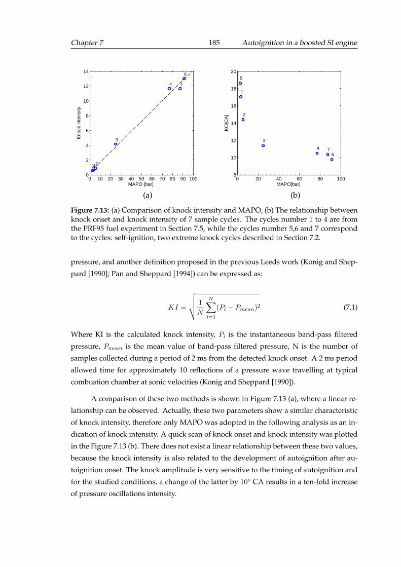
Chapter 7 185 Autoignition in a boosted SI engine
0 10 20 30 40 50 60 70 80 90 1000
2
4
6
8
10
12
14
12
3
4
5
6
7
MAPO [bar]
Kno
ck in
tens
ity
(a)
0 20 40 60 80 1008
10
12
14
16
18
20
1
2
3
4
5
67
MAPO[bar]
KO
[CA
]
(b)
Figure 7.13: (a) Comparison of knock intensity and MAPO, (b) The relationship betweenknock onset and knock intensity of 7 sample cycles. The cycles number 1 to 4 are fromthe PRF95 fuel experiment in Section 7.5, while the cycles number 5,6 and 7 correspondto the cycles: self-ignition, two extreme knock cycles described in Section 7.2.
pressure, and another definition proposed in the previous Leeds work (Konig and Shep-
pard [1990]; Pan and Sheppard [1994]) can be expressed as:
KI =
√√√√ 1
N
N∑i=1
(Pi − Pmean)2 (7.1)
Where KI is the calculated knock intensity, Pi is the instantaneous band-pass filtered
pressure, Pmean is the mean value of band-pass filtered pressure, N is the number of
samples collected during a period of 2 ms from the detected knock onset. A 2 ms period
allowed time for approximately 10 reflections of a pressure wave travelling at typical
combustion chamber at sonic velocities (Konig and Sheppard [1990]).
A comparison of these two methods is shown in Figure 7.13 (a), where a linear re-
lationship can be observed. Actually, these two parameters show a similar characteristic
of knock intensity, therefore only MAPO was adopted in the following analysis as an in-
dication of knock intensity. A quick scan of knock onset and knock intensity was plotted
in the Figure 7.13 (b). There does not exist a linear relationship between these two values,
because the knock intensity is also related to the development of autoignition after au-
toignition onset. The knock amplitude is very sensitive to the timing of autoignition and
for the studied conditions, a change of the latter by 10o CA results in a ten-fold increase
of pressure oscillations intensity.
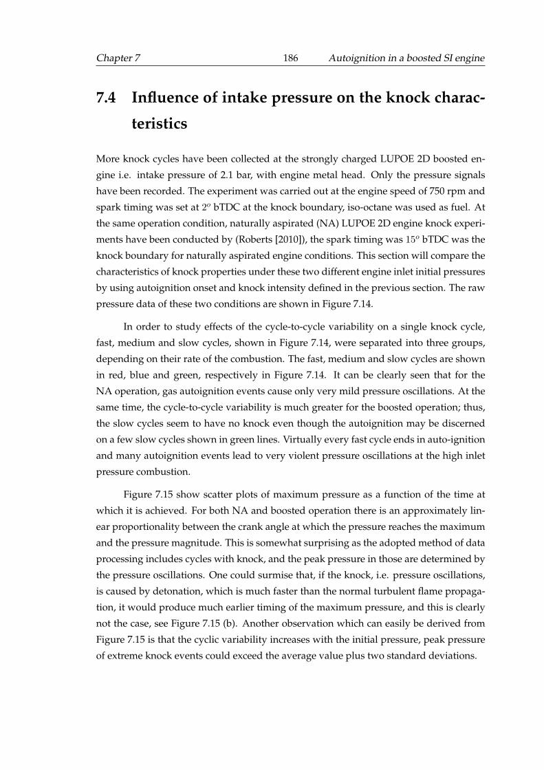
Chapter 7 186 Autoignition in a boosted SI engine
7.4 Influence of intake pressure on the knock charac-
teristics
More knock cycles have been collected at the strongly charged LUPOE 2D boosted en-
gine i.e. intake pressure of 2.1 bar, with engine metal head. Only the pressure signals
have been recorded. The experiment was carried out at the engine speed of 750 rpm and
spark timing was set at 2o bTDC at the knock boundary, iso-octane was used as fuel. At
the same operation condition, naturally aspirated (NA) LUPOE 2D engine knock experi-
ments have been conducted by (Roberts [2010]), the spark timing was 15o bTDC was the
knock boundary for naturally aspirated engine conditions. This section will compare the
characteristics of knock properties under these two different engine inlet initial pressures
by using autoignition onset and knock intensity defined in the previous section. The raw
pressure data of these two conditions are shown in Figure 7.14.
In order to study effects of the cycle-to-cycle variability on a single knock cycle,
fast, medium and slow cycles, shown in Figure 7.14, were separated into three groups,
depending on their rate of the combustion. The fast, medium and slow cycles are shown
in red, blue and green, respectively in Figure 7.14. It can be clearly seen that for the
NA operation, gas autoignition events cause only very mild pressure oscillations. At the
same time, the cycle-to-cycle variability is much greater for the boosted operation; thus,
the slow cycles seem to have no knock even though the autoignition may be discerned
on a few slow cycles shown in green lines. Virtually every fast cycle ends in auto-ignition
and many autoignition events lead to very violent pressure oscillations at the high inlet
pressure combustion.
Figure 7.15 show scatter plots of maximum pressure as a function of the time at
which it is achieved. For both NA and boosted operation there is an approximately lin-
ear proportionality between the crank angle at which the pressure reaches the maximum
and the pressure magnitude. This is somewhat surprising as the adopted method of data
processing includes cycles with knock, and the peak pressure in those are determined by
the pressure oscillations. One could surmise that, if the knock, i.e. pressure oscillations,
is caused by detonation, which is much faster than the normal turbulent flame propaga-
tion, it would produce much earlier timing of the maximum pressure, and this is clearly
not the case, see Figure 7.15 (b). Another observation which can easily be derived from
Figure 7.15 is that the cyclic variability increases with the initial pressure, peak pressure
of extreme knock events could exceed the average value plus two standard deviations.
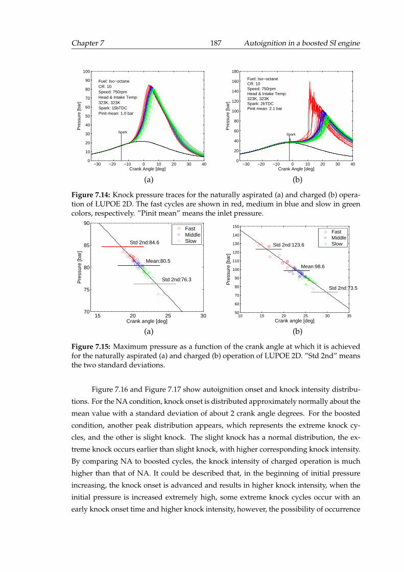
Chapter 7 187 Autoignition in a boosted SI engine
−30 −20 −10 0 10 20 30 400
10
20
30
40
50
60
70
80
90
100
Spark
Crank Angle [deg]
Pre
ssur
e [b
ar]
Fuel: Iso−octaneCR: 10Speed: 750rpmHead & Intake Temp:323K, 323KSpark: 15bTDCPinit mean: 1.0 bar
(a)
−30 −20 −10 0 10 20 30 400
20
40
60
80
100
120
140
160
180
Spark
Crank Angle [deg]
Pre
ssur
e [b
ar]
Fuel: Iso−octaneCR: 10Speed: 750rpmHead & Intake Temp:323K, 323KSpark: 2bTDCPinit mean: 2.1 bar
(b)
Figure 7.14: Knock pressure traces for the naturally aspirated (a) and charged (b) opera-tion of LUPOE 2D. The fast cycles are shown in red, medium in blue and slow in greencolors, respectively. ”Pinit mean” means the inlet pressure.
15 20 25 3070
75
80
85
90
Crank angle [deg]
Pre
ssur
e [b
ar]
Mean:80.5
Std 2nd:84.6
Std 2nd:76.3
FastMiddleSlow
(a)
10 15 20 25 30 3550
60
70
80
90
100
110
120
130
140
150
Crank angle [deg]
Pre
ssur
e [b
ar]
Mean:98.6
Std 2nd:123.6
Std 2nd:73.5
FastMiddleSlow
(b)
Figure 7.15: Maximum pressure as a function of the crank angle at which it is achievedfor the naturally aspirated (a) and charged (b) operation of LUPOE 2D. ”Std 2nd” meansthe two standard deviations.
Figure 7.16 and Figure 7.17 show autoignition onset and knock intensity distribu-
tions. For the NA condition, knock onset is distributed approximately normally about the
mean value with a standard deviation of about 2 crank angle degrees. For the boosted
condition, another peak distribution appears, which represents the extreme knock cy-
cles, and the other is slight knock. The slight knock has a normal distribution, the ex-
treme knock occurs earlier than slight knock, with higher corresponding knock intensity.
By comparing NA to boosted cycles, the knock intensity of charged operation is much
higher than that of NA. It could be described that, in the beginning of initial pressure
increasing, the knock onset is advanced and results in higher knock intensity, when the
initial pressure is increased extremely high, some extreme knock cycles occur with an
early knock onset time and higher knock intensity, however, the possibility of occurrence
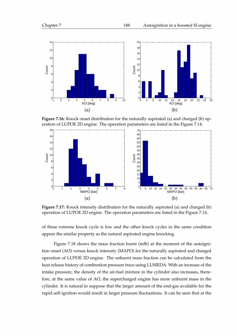
Chapter 7 188 Autoignition in a boosted SI engine
1 2 3 4 5 6 7 8 9 100
2
4
6
8
10
12
14
KO [deg]
Cou
nt
(a)
4 6 8 10 12 14 16 18 20 22 24 260
2
4
6
8
10
12
14
16
18
20
KO [deg]
Cou
nt
(b)
Figure 7.16: Knock onset distribution for the naturally aspirated (a) and charged (b) op-eration of LUPOE 2D engine. The operation parameters are listed in the Figure 7.14.
0 1 2 3 4 5 6 7 80
2
4
6
8
10
12
14
16
18
MAPO [bar]
Cou
nt
(a)
0 5 10 15 20 25 30 35 40 45 50 55 60 65 700
5
10
15
20
25
30
35
40
45
50
55
60
65
70
MAPO [bar]
Cou
nt
(b)
Figure 7.17: Knock intensity distribution for the naturally aspirated (a) and charged (b)operation of LUPOE 2D engine. The operation parameters are listed in the Figure 7.14.
of these extreme knock cycle is low and the other knock cycles in the same condition
appear the similar property as the natural aspirated engine knocking.
Figure 7.18 shows the mass fraction burnt (mfb) at the moment of the autoigni-
tion onset (AO) versus knock intensity (MAPO) for the naturally aspirated and charged
operation of LUPOE 2D engine. The unburnt mass fraction can be calculated from the
heat release history of combustion pressure trace using LUSIEDA. With an increase of the
intake pressure, the density of the air-fuel mixture in the cylinder also increases, there-
fore, at the same value of AO, the supercharged engine has more unburnt mass in the
cylinder. It is natural to suppose that the larger amount of the end-gas available for the
rapid self-ignition would result in larger pressure fluctuations. It can be seen that at the
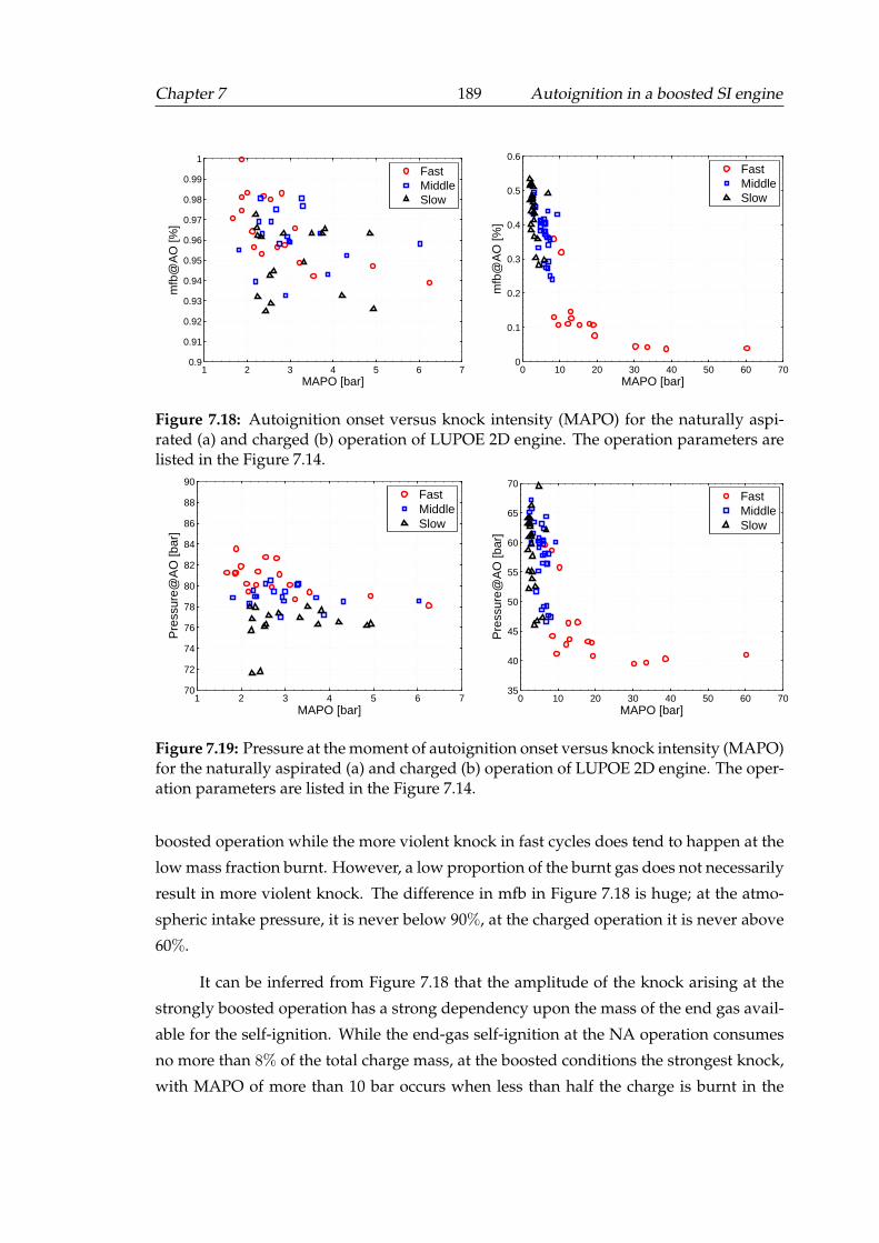
Chapter 7 189 Autoignition in a boosted SI engine
1 2 3 4 5 6 70.9
0.91
0.92
0.93
0.94
0.95
0.96
0.97
0.98
0.99
1
MAPO [bar]
mfb
@A
O [%
]
FastMiddleSlow
0 10 20 30 40 50 60 700
0.1
0.2
0.3
0.4
0.5
0.6
MAPO [bar]
mfb
@A
O [%
]
FastMiddleSlow
Figure 7.18: Autoignition onset versus knock intensity (MAPO) for the naturally aspi-rated (a) and charged (b) operation of LUPOE 2D engine. The operation parameters arelisted in the Figure 7.14.
1 2 3 4 5 6 770
72
74
76
78
80
82
84
86
88
90
MAPO [bar]
Pre
ssur
e@A
O [b
ar]
FastMiddleSlow
0 10 20 30 40 50 60 7035
40
45
50
55
60
65
70
MAPO [bar]
Pre
ssur
e@A
O [b
ar]
FastMiddleSlow
Figure 7.19: Pressure at the moment of autoignition onset versus knock intensity (MAPO)for the naturally aspirated (a) and charged (b) operation of LUPOE 2D engine. The oper-ation parameters are listed in the Figure 7.14.
boosted operation while the more violent knock in fast cycles does tend to happen at the
low mass fraction burnt. However, a low proportion of the burnt gas does not necessarily
result in more violent knock. The difference in mfb in Figure 7.18 is huge; at the atmo-
spheric intake pressure, it is never below 90%, at the charged operation it is never above
60%.
It can be inferred from Figure 7.18 that the amplitude of the knock arising at the
strongly boosted operation has a strong dependency upon the mass of the end gas avail-
able for the self-ignition. While the end-gas self-ignition at the NA operation consumes
no more than 8% of the total charge mass, at the boosted conditions the strongest knock,
with MAPO of more than 10 bar occurs when less than half the charge is burnt in the
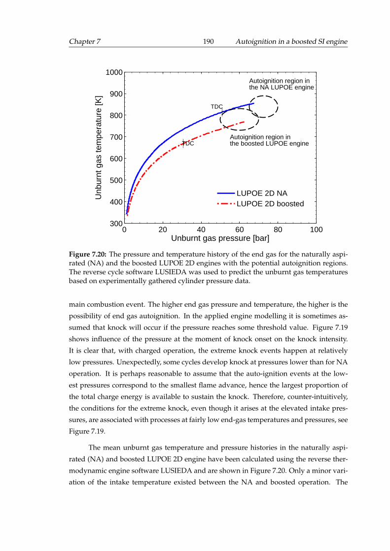
Chapter 7 190 Autoignition in a boosted SI engine
0 20 40 60 80 100300
400
500
600
700
800
900
1000
TDC
TDC
Unburnt gas pressure [bar]
Unb
urnt
gas
tem
pera
ture
[K]
Autoignition region inthe NA LUPOE engine
Autoignition region inthe boosted LUPOE engine
LUPOE 2D NALUPOE 2D boosted
Figure 7.20: The pressure and temperature history of the end gas for the naturally aspi-rated (NA) and the boosted LUPOE 2D engines with the potential autoignition regions.The reverse cycle software LUSIEDA was used to predict the unburnt gas temperaturesbased on experimentally gathered cylinder pressure data.
main combustion event. The higher end gas pressure and temperature, the higher is the
possibility of end gas autoignition. In the applied engine modelling it is sometimes as-
sumed that knock will occur if the pressure reaches some threshold value. Figure 7.19
shows influence of the pressure at the moment of knock onset on the knock intensity.
It is clear that, with charged operation, the extreme knock events happen at relatively
low pressures. Unexpectedly, some cycles develop knock at pressures lower than for NA
operation. It is perhaps reasonable to assume that the auto-ignition events at the low-
est pressures correspond to the smallest flame advance, hence the largest proportion of
the total charge energy is available to sustain the knock. Therefore, counter-intuitively,
the conditions for the extreme knock, even though it arises at the elevated intake pres-
sures, are associated with processes at fairly low end-gas temperatures and pressures, see
Figure 7.19.
The mean unburnt gas temperature and pressure histories in the naturally aspi-
rated (NA) and boosted LUPOE 2D engine have been calculated using the reverse ther-
modynamic engine software LUSIEDA and are shown in Figure 7.20. Only a minor vari-
ation of the intake temperature existed between the NA and boosted operation. The
Chapter 7 191 Autoignition in a boosted SI engine
calculated results show the temperature of the boosted LUPOE 2D engine is lower than
that of the NA engine at the TDC position and the potential autoignition region. How-
ever, the spark timing of the boosted engine is closer to TDC than that of NA engine, thus
the difference of the temperature at the spark timing is not large for two conditions. This
implied that extreme knock occurrence may be not governed by auto-igniton of unburnt
end gas, which is sensitive to the pressure and temperature. Since there does not exist
valves or spray injection deposits in the LUPOE 2D engine, the lubrication oil released
from piston crevice could be a potential reason for the extreme knock.
7.5 Comparison of self-ignition and extreme knock
Several knock cycles selected from the same boosted condition will be used for a further
study on the difference between self-ignition and extreme knock. Although the number
of knock cycles with image recording is too small to derive reliable statistical results, an
attempt at establishing a relationship of knock development process with knock inten-
sity could still be undertaken. Here, knock cycles with different knock intensities are
analyzed, the engine was operated at 750 rpm, and fuelled with a mixture of 95% iso-
octane and 5% n-heptane by volume (PRF95). Due to the short ignition delay time of
PRF95, at the same spark timing, the knock boundary occurred at a lower initial pressure
of 1.8 bar compared to iso-octane at the spark timing 2o bTDC. Four knock cycles are
selected, representing a transition from a slight knock to an extreme knock. The pressure
traces and filtered pressure oscillations are compared in Figure 7.21 and Figure 7.22.
It can be seen that there existed a small pressure deviation at spark timing; the
cycle 1 has the lowest pressure at that moment, and it also shows the lowest rate of com-
bustion and a weakest barely detectable knock. Cycle 3 has much smaller pressure at
the spark timing and, yet, it shows very similar fast burning rate and onset of knock to
the cycle 4 which has the highest pressure at the spark instance. Cycle 2 and 4 have the
same ignition pressure but the subsequent combustion is very different. The autoigni-
tion onsets detected from the images are marked in the pressure traces, with the advance
of autoigniton onset time, the peak pressure raised and the pressure oscillation become
more violent. The amplitude of pressure oscillation can be seen in Figure 7.22, which
clearly show a gradually increase of the magnitude of the pressure oscillations.
These pressure traces were transformed into the frequency domain by using Fast
Fourier Transform (FFT) in Matlab. The FFT results are plotted in Figure 7.23. Generally,
the position of the maximum frequency does not change much with the knock intensity
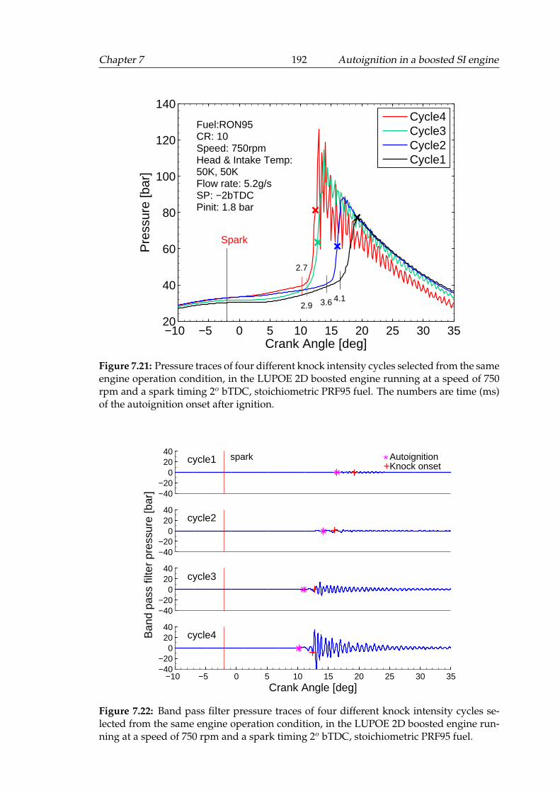
Chapter 7 192 Autoignition in a boosted SI engine
−10 −5 0 5 10 15 20 25 30 3520
40
60
80
100
120
140
Crank Angle [deg]
Pre
ssur
e [b
ar]
2.7
2.9 3.6 4.1
Spark
Fuel:RON95CR: 10Speed: 750rpmHead & Intake Temp:50K, 50KFlow rate: 5.2g/sSP: −2bTDCPinit: 1.8 bar
Cycle4Cycle3Cycle2Cycle1
Figure 7.21: Pressure traces of four different knock intensity cycles selected from the sameengine operation condition, in the LUPOE 2D boosted engine running at a speed of 750rpm and a spark timing 2o bTDC, stoichiometric PRF95 fuel. The numbers are time (ms)of the autoignition onset after ignition.
−40−20
02040
cycle1 spark *+
AutoignitionKnock onset
−40−20
02040
cycle2
−40−20
02040
cycle3
B
and
pass
filte
r pr
essu
re [b
ar]
−10 −5 0 5 10 15 20 25 30 35−40−20
02040
cycle4
Crank Angle [deg]
Figure 7.22: Band pass filter pressure traces of four different knock intensity cycles se-lected from the same engine operation condition, in the LUPOE 2D boosted engine run-ning at a speed of 750 rpm and a spark timing 2o bTDC, stoichiometric PRF95 fuel.
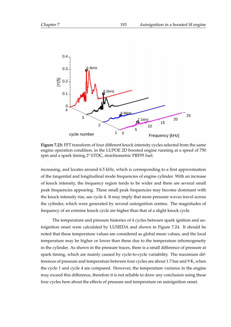
Chapter 7 193 Autoignition in a boosted SI engine
05
1015
2025
1
2
3
40
0.1
0.2
0.3
0.4
Frequency [kHz]
7.1kHz
6.8kHz
6.5kHz
cycle number
6.3kHz
|Y(f
)|
Figure 7.23: FFT transform of four different knock intensity cycles selected from the sameengine operation condition, in the LUPOE 2D boosted engine running at a speed of 750rpm and a spark timing 2o bTDC, stoichiometric PRF95 fuel.
increasing, and locates around 6.5 kHz, which is corresponding to a first approximation
of the tangential and longitudinal mode frequencies of engine cylinder. With an increase
of knock intensity, the frequency region tends to be wider and there are several small
peak frequencies appearing. These small peak frequencies may become dominant with
the knock intensity rise, see cycle 4. It may imply that more pressure waves travel across
the cylinder, which were generated by several autoignition centres. The magnitudes of
frequency of an extreme knock cycle are higher than that of a slight knock cycle.
The temperature and pressure histories of 4 cycles between spark ignition and au-
toignition onset were calculated by LUSIEDA and shown in Figure 7.24. It should be
noted that these temperature values are considered as global mean values, and the local
temperature may be higher or lower than these due to the temperature inhomogeneity
in the cylinder. As shown in the pressure traces, there is a small difference of pressure at
spark timing, which are mainly caused by cycle-to-cycle variability. The maximum dif-
ferences of pressure and temperature between four cycles are about 1.7 bar and 9 K, when
the cycle 1 and cycle 4 are compared. However, the temperature variance in the engine
may exceed this difference, therefore it is not reliable to draw any conclusion using these
four cycles here about the effects of pressure and temperature on autoignition onset.
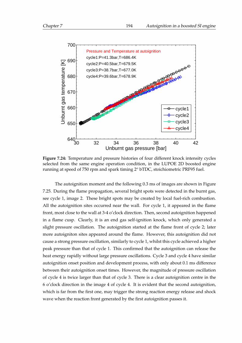
Chapter 7 194 Autoignition in a boosted SI engine
30 32 34 36 38 40 42640
650
660
670
680
690
700
cycle1:P=41.3bar,T=686.4K
cycle2:P=40.5bar,T=679.5K
cycle3:P=38.7bar,T=677.0K
cycle4:P=39.6bar,T=678.9K
Pressure and Temperature at autoignition
Unburnt gas pressure [bar]
Unb
urnt
gas
tem
pera
ture
[K]
cycle1cycle2cycle3cycle4
Figure 7.24: Temperature and pressure histories of four different knock intensity cyclesselected from the same engine operation condition, in the LUPOE 2D boosted enginerunning at speed of 750 rpm and spark timing 2o bTDC, stoichiometric PRF95 fuel.
The autoignition moment and the following 0.3 ms of images are shown in Figure
7.25. During the flame propagation, several bright spots were detected in the burnt gas,
see cycle 1, image 2. These bright spots may be created by local fuel-rich combustion.
All the autoignition sites occurred near the wall. For cycle 1, it appeared in the flame
front, most close to the wall at 3-4 o’clock direction. Then, second autoignition happened
in a flame cusp. Clearly, it is an end gas self-ignition knock, which only generated a
slight pressure oscillation. The autoignition started at the flame front of cycle 2; later
more autoigniton sites appeared around the flame. However, this autoignition did not
cause a strong pressure oscillation, similarly to cycle 1, whilst this cycle achieved a higher
peak pressure than that of cycle 1. This confirmed that the autoignition can release the
heat energy rapidly without large pressure oscillations. Cycle 3 and cycle 4 have similar
autoignition onset position and development process, with only about 0.1 ms difference
between their autoignition onset times. However, the magnitude of pressure oscillation
of cycle 4 is twice larger than that of cycle 3. There is a clear autoignition centre in the
6 o’clock direction in the image 4 of cycle 4. It is evident that the second autoignition,
which is far from the first one, may trigger the strong reaction energy release and shock
wave when the reaction front generated by the first autoignition passes it.
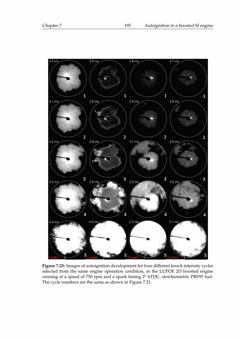
Chapter 7 195 Autoignition in a boosted SI engine
Cycle1 Cycle2 Cycle3 Cycle4
Figure 7.25: Images of autoignition development for four different knock intensity cyclesselected from the same engine operation condition, in the LUPOE 2D boosted enginerunning at a speed of 750 rpm and a spark timing 2o bTDC, stoichiometric PRF95 fuel.The cycle numbers are the same as shown in Figure 7.21.
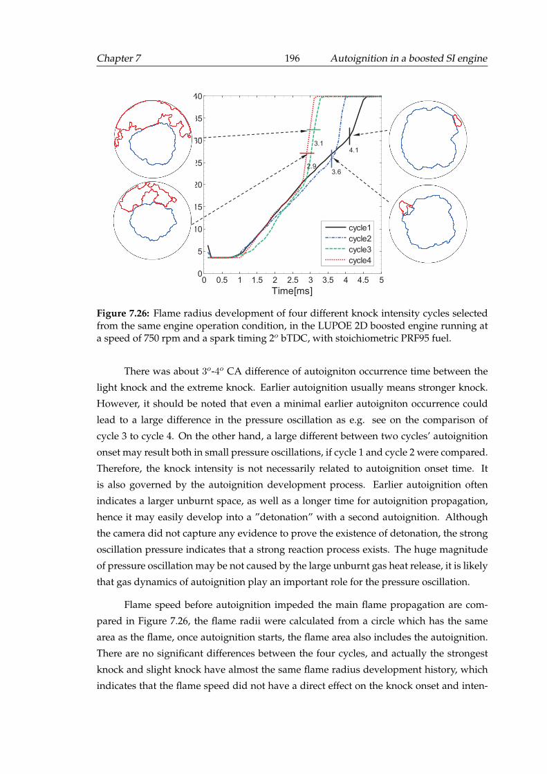
Chapter 7 196 Autoignition in a boosted SI engine
0 0.5 1 1.5 2 2.5 3 3.5 4 4.5 50
5
10
15
20
25
30
35
40
Time[ms]
Fla
me
ra
diu
s[m
m]
4.1
3.6
3.1
2.9
cycle1
cycle2
cycle3
cycle4
Figure 7.26: Flame radius development of four different knock intensity cycles selectedfrom the same engine operation condition, in the LUPOE 2D boosted engine running ata speed of 750 rpm and a spark timing 2o bTDC, with stoichiometric PRF95 fuel.
There was about 3o-4o CA difference of autoigniton occurrence time between the
light knock and the extreme knock. Earlier autoignition usually means stronger knock.
However, it should be noted that even a minimal earlier autoigniton occurrence could
lead to a large difference in the pressure oscillation as e.g. see on the comparison of
cycle 3 to cycle 4. On the other hand, a large different between two cycles’ autoignition
onset may result both in small pressure oscillations, if cycle 1 and cycle 2 were compared.
Therefore, the knock intensity is not necessarily related to autoignition onset time. It
is also governed by the autoignition development process. Earlier autoignition often
indicates a larger unburnt space, as well as a longer time for autoignition propagation,
hence it may easily develop into a ”detonation” with a second autoignition. Although
the camera did not capture any evidence to prove the existence of detonation, the strong
oscillation pressure indicates that a strong reaction process exists. The huge magnitude
of pressure oscillation may be not caused by the large unburnt gas heat release, it is likely
that gas dynamics of autoignition play an important role for the pressure oscillation.
Flame speed before autoignition impeded the main flame propagation are com-
pared in Figure 7.26, the flame radii were calculated from a circle which has the same
area as the flame, once autoignition starts, the flame area also includes the autoignition.
There are no significant differences between the four cycles, and actually the strongest
knock and slight knock have almost the same flame radius development history, which
indicates that the flame speed did not have a direct effect on the knock onset and inten-
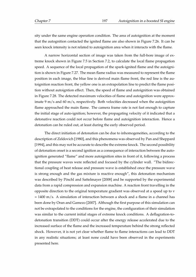
Chapter 7 197 Autoignition in a boosted SI engine
sity under the same engine operation condition. The area of autoignition at the moment
that the autognition contacted the ignited flame are also shown in Figure 7.26. It can be
seen knock intensity is not related to autoignition area when it interacts with the flame.
A narrow horizontal section of image was taken from the full-bore image of ex-
treme knock shown in Figure 7.5 in Section 7.2, to calculate the local flame propagation
speed. A sequence of the local propagation of the spark-ignited flame and the autoigni-
tion is shown in Figure 7.27. The mean flame radius was measured to represent the flame
position in each image, the blue line is derived main flame front, the red line is the au-
toignition reaction front, the yellow one is an extrapolation line to predict the flame posi-
tion without autoigntion effect. Then, the speed of flame and autoignition was obtained
in Figure 7.28. The detected maximum velocities of flame and autoignition were approx-
imate 9 m/s and 60 m/s, respectively. Both velocities decreased when the autoignition
flame approached the main flame. The camera frame rate is not fast enough to capture
the initial stage of auto-ignition; however, the propagating velocity of it indicated that a
detonative reaction could not occur before flame and autoignition interaction. Hence a
detonation can be ruled out, at least during the early observed period.
The direct initiation of detonation can be due to inhomogeneities, according to the
description of Zeldovich [1980], and this phenomena was observed by Pan and Sheppard
[1994], and this may not be accurate to describe the extreme knock. The second possibility
of detonation onset is a second ignition as a consequence of interaction between the auto-
ignition generated ”flame” and more autoignition sites in front of it, following a process
that the pressure waves were reflected and focused by the cylinder wall. ”The bidirec-
tional coupling of heat release and pressure wave is established once the pressure wave
is strong enough and the gas mixture is reactive enough”, this detonation mechanism
was described by Poschl and Sattelmayer [2008] and be supported by the experimental
data from a rapid compression and expansion machine. A reaction front travelling in the
opposite direction to the original temperature gradient was observed at a speed up to v
= 1400 m/s. A simulation of interaction between a shock and a flame in a channel has
been done by Oran and Gamezo [2007]. Although the first purpose of this simulation can
not be extrapolated to the conditions for the engine, the configuration of their simulation
was similar to the current initial stages of extreme knock conditions. A deflagration-to-
detonation transition (DDT) could occur after the energy release accelerated due to the
increased surface of the flame and the increased temperature behind the strong reflected
shock. However, it is not yet clear whether flame to flame interactions can lead to DDT
in any realistic situations; at least none could have been observed in the experiments
presented here.
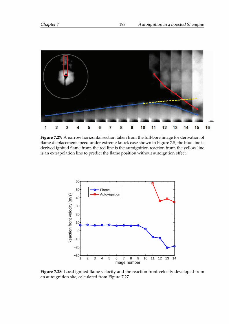
Chapter 7 198 Autoignition in a boosted SI engine
Figure 7.27: A narrow horizontal section taken from the full-bore image for derivation offlame displacement speed under extreme knock case shown in Figure 7.5, the blue line isderived ignited flame front, the red line is the autoignition reaction front, the yellow lineis an extrapolation line to predict the flame position without autoigntion effect.
1 2 3 4 5 6 7 8 9 10 11 12 13 14−30
−20
−10
0
10
20
30
40
50
60
Image number
Rea
ctio
n fr
ont v
eloc
ity (
m/s
)
FlameAuto−ignition
Figure 7.28: Local ignited flame velocity and the reaction front velocity developed froman autoignition site, calculated from Figure 7.27.
Chapter 8
Conclusions and Recommendations
8.1 Introduction
This thesis aimed an investigation of the flame propagation and autoignition in a high
pressure single-cylinder optical research engine used here. The LUPOE 2D boosted en-
gine has a disc-shaped combustion chamber with full-bore overhead optical access. A
new boosting method with control system has been developed to increase the inlet pres-
sure while maintaining well-controlled turbulence intensity under safe operating condi-
tions. Subsequently, three main groups of experiments have been conducted:
• Measurement of iso-octane flame speed in a turbulence-free engine relevant envi-
ronment;
• Study of turbulent flame development at supercharged engine conditions, empha-
sizing on the pressure effects on different flame development stages and flame
structure;
• Investigation of characteristics of auto-ignition and extreme knock in a strongly
boosted engine.
In these experiments, in-cylinder pressure signals were recorded, and have been
analyzed using the Leeds University Spark Ignition Data Analysis (LUSIEDA) reverse
Chapter 8 200 Conclusions and Recommendations
thermodynamic code. Various optical diagnostic methods have been applied. The Parti-
cle image velocimetry (PIV) was employed to investigate effects of engine speed, intake
flow rate, and pressure on the turbulent flow in the engine. Flame chemiluminescence
signals were captured with a high speed imaging acquisition system with an interference
filter; flame propagation speeds under different conditions were derived from these im-
ages. The detailed flame structure was obtained by laser sheet visualization technique,
where the cross section of a 3D flame has been visualized by cross-cuuting it with a laser
sheet. These data collected under well controlled conditions yielded a comprehensive
database for engine combustion theory validation, and also for modelling work by col-
leagues in the School of Mechanical Engineering at Leeds University. Conclusions drawn
from the previous Chapters of this thesis are presented here. Furthermore, some sugges-
tions arising from this study are proposed for future works.
8.1.1 Conclusions of Iso-octane flame speed experiments
Presented in the current section are conclusions from the measurements of iso-octane
flame speed in a turbulence-free engine-relevant environment.
• The engine flow fields at the mid plane of the clearance volume of LUPOE-2D en-
gine were measured using a PIV system near the TDC position, at engine speeds of
100, 150, 200, and 250 rpm. There was no significant swirl motion detected in the
bulk flow, and the flow tends to be homogeneous and uniform near the TDC posi-
tion. The ensemble mean velocity decreased when the engine speed was reduced.
At the engine speed of 100 rpm, the mean gas velocity in the chamber was lower
than 0.1 m/s. The RMS turbulent velocity near TDC was linearly proportional to
the engine speed, and declined to approximately zero when the engine speed de-
creased to zero. At the same time, the integral length scale at TDC also decreased
with the engine speed; the longitudinal integral length scales were approximately
twice larger than the transverse integral length scales. These results confirmed that
LUPOE engine could generate an almost homogeneous and turbulence-free envi-
ronment when it runs at extremely low speed, i.e. less than 100 rpm, and so it
could be used as a reciprocating combustion rig for laminar flame speed measure-
ment under engine relevant conditions.
• Pressure traces recorded in the LUPOE engine at an engine speed of 100 rpm, with
various equivalence ratios, show that the cycle variability was extremely small
at the stoichiometric and rich conditions. These observations further support the
Chapter 8 201 Conclusions and Recommendations
claim that the LUPOE engine can provide minimum turbulence intensity and ho-
mogeneous mixture conditions. The spark timing was set at 10 deg bTDC, where a
high pressure of 12 bar and high temperature of 600k (calculated from LUSEIDA)
could be achieved.
• Laser sheet visualization measurements provided the cross-section information of
flame shape. Comparing the results from engine speeds at 150 rpm and 750 rpm,
it was shown clearly that the flame contour was closer to a circle at the low engine
speed. The variability of mean flame radius at the same crank angle also had a
significant drop with the engine speed decreasing.
• After a comprehensive assessment of experimental conditions, direct measurement
of flame propagation in a turbulent-free environment has been conducted using
CH* chemiluminescience. The sequence of images captured at various equiva-
lence ratios show the development process of flame. A smooth flame front was
observed after ignition, and it became wrinkled as the flame was approaching the
wall. However, the flame front attained more regular cellular shapes, which was
different from the randomly wrinkled flame front induced by turbulence. These
cellular structures could be generated by a flame instability at the high pressure.
• In order to eliminate effects exerted by the ignition and engine side walls on the
flame speed measurement, only the flame radius range from 10 to 22 mm was
chosen for the burning velocity calculation. During this stage, the volume height
changed only about 0.4 mm at the engine speed of 100 rpm, which is equal to 5%
of the total volume. This combustion duration could be considered as a constant
volume process. The visible flame speed Sn was derived from the slope of the fit-
ting line of flame radius from 10 to 22 mm, the burning velocity was calculated as
U = ρb/ρuSn, and the value of the thermal expansion ratio was calculated using
LUSIEDA. The burning velocity of iso-octane had a similar value of 1.1 m/s for
stoichiometric and rich mixtures of equivalence ratio, while 0.6 m/s and 0.8 m/s
were for lean mixture 0.6 and 0.8 respectively.
• Since the rms velocity was linearly proportional to the engine speed, and decreased
to approximately zero if the engine was stopped, a new method of measuring a
laminar burning velocity at turbulence-free conditions was explored. This method
is based on extrapolating the burning velocities from different engine speeds from
300 rpm to 150 rpm. In order to keep the pressures and temperatures similar at
spark timing, different spark timings have been selected, at a high pressure of 15
bar and a high temperature of 600K. Flame speeds with equivalence ratios 0.8, 1
Chapter 8 202 Conclusions and Recommendations
and 1.2 under four engine speeds have been measured. The results show that the
burning velocity has linearly decreased with the reduction of the engine speed for
lean and stoichiometric mixture, while the rich flame speed shows an opposite
tendency. The extrapolated burning velocity for three equivalence ratios are 0.78
m/s for the lean mixture, 0.94 m/s for the stoichiometric and 1.15 m/s for the rich
mixture. The difference between the values from the direct measurement at engine
speed 100 rpm and that derived from extrapolation from engine speed 150 to 300
rpm is small.
• It is very difficult to measure the laminar burning velocity of iso-octane at a high
pressure of 15 bar, and high temperature of 600K at constant pressure in a constant
volume combustion vessel. The experimental data which can be used to validate
the current measurement results are not available in the literature. For this reason,
correlations for laminar flame speed and reaction mechanism computations have
been adopted. Nevertheless, these equations and a reaction mechanism need to be
evaluated using the available experimental data before applying them to calculate
burning velocity at high pressure. 4 sets of experimental data of iso-octane burning
velocity, 3 correlation equations and a chemical reaction mechanism were selected
and evaluated comprehensively.
• Comparing current measured burning velocities to values derived from correlation
equations at high temperature and pressure, a difference between the magnitude
of measured and computed results was observed. The measured flame speed is
about 1.5-2 times larger than that from calculation. This may be attributed to the
acceleration of the flame front due to flame instabilities and stretch effects. Since the
Markstein number of iso-octane-air mixtures at high temperatures and pressures
was low, instabilities which arise at increasing pressure, may play a more important
role on flame speed, and result in an acceleration of the flame speed.
8.1.2 Conclusions of high pressure turbulent flame experiments
The following conclusions could be derived from the investigation of turbulent flame
development at supercharged engine conditions.
• The boosting methods were tested by using exhaust valve installed in the exhaust
system and increasing the inlet flow rate, and a map of initial pressure with these
two methods was realized. Based on the map, a reference condition was decided
as a starting point for subsequent inlet pressure increasing before the knock cycle
Chapter 8 203 Conclusions and Recommendations
happened. Two conditions for each boosting method were selected as the following
test conditions.
• The effects of increasing inlet flow rate on the turbulence intensity in the LUPOE 2D
engine was investigated using a PIV system. The measurements were conducted
at the mid plane of the clearance volume of LUPOE-2D engine near the TDC posi-
tion, at engine speeds of 750 rpm. The maximum flow speed in the LUPOE engine
was about 4m/s, where no significant bulk flow, e.g. swirl motion, was detected.
Increasing the inlet flow rate by 50% caused stronger turbulence intensity by up
to 40%, while the exhaust valve closing could keep the RMS velocity at almost the
same level. For the highest and lowest levels of tested mass flow rate, the mean
velocity of an engine flow field had a similar mean value and standard deviation
along both the X and Y axes. These results confirmed that the new boosting con-
figuration using the exhaust valve enabled the intake mass flow rate and the initial
pressure to be independently controlled.
• The integral length scales were calculated from the mean PIV vector fields at 2
degrees before TDC. It could be observed that, in general, average values of the
longitudinal integral length scales were between 8-10 mm, approximately twice
the transverse integral length scales 4 mm. The flow field near the TDC could thus
be considered as a homogeneous turbulence flow.
• Pressure traces and images of flame propagation of 100 cycles have been recorded
at the selected conditions. The entrainment flame radius was defined as the ra-
dius of a circle having the same area as the observed irregular flame boundary. In
order to take the cycle variability effect into analysis, the recorded pressure traces
and flame radius were separated into fast, middle and slow cycles. The cycle was
classified by using peak pressure below, within, or above two standard deviations
from the ensemble average value.
• The experimental conditions were plotted on the Borghi diagram, the turbulence
intensity and integral length scales were measured by the PIV system, the laminar
flame speeds were calculated with Metghalchi and Keck’s power law correlation
equation. The selected conditions were located in the boundary between wrinkled
flamelets and wrinkled flamelets with pockets. Molecular transport parameters
were calculated at initial temperature estimated with the LUSEIDA, and its value
was around 620K.
• The effects of pressure on flame development were assessed at the different com-
bustion phases i.e. initiation, main phase, and termination phase. Overall, the re-
Chapter 8 204 Conclusions and Recommendations
sults show that the pressure rise decreased the flame burning velocity very weakly.
However, it had different effects upon the acceleration at early stages, and decel-
eration at final stages. Increasing the initial pressure had slightly negative effects
on the flame acceleration; turbulence was the main factor at the initial stage. In-
creasing initial pressure could decrease slightly the burning velocity in the fully
developed stage. Yet, this decrease may mainly be caused by decreasing flame
acceleration. The burning velocity was slightly rising with pressure increasing.
Pressure decreased the flame deceleration near the walls, resulting in longer com-
bustion duration. However, the burning rate increased with higher pressure in this
region.
• The flame acceleration speed curves for fast, middle, and slow cycles at three ini-
tial pressure conditions have been compared with the flame acceleration model
proposed by Lipatnikov and Chomiak, which was characterized by two turbulent
parameters. The models predicted a faster initial rate of flame acceleration than the
measured value, and slower rate at the later stage of the flame acceleration.
• The flame deceleration speed curves of fast, middle, and slow cycles at three ini-
tial pressure conditions are well fitted by the error functions erfc(x), which was
characterized by two parameters: the flame radius time, and flame deceleration
duration. For the fast cycle, the flame deceleration duration value of the equation
is the main value to be adjusted to fit the curve shape, whilst for the slow cycle, the
flame radius time value is more important.
• Under the same experimental conditions, the structure of the flame at high pres-
sure and its response to pressure effects were also investigated. A Laser sheet vi-
sualization method was applied, and a new algorithm for image processing was
developed to derive the detailed cross section flame front topology. Self-similar
properties of flames were evaluated with mean progress variable maps. The re-
sults show that the initial pressure has only a slightly effect on the flame structure
in the aspects of flame wrinkle and curvature. The mean progress variable profiles
could be collapsed by the error function well. Flames at high pressure have the
same ”self-similar” properties as those observed at low pressure.
8.1.3 Conclusions of autoignition and extreme knock experiments
The following conclusions may be drawn from the experimental investigation of auto-
ignition and extreme knock in a strongly boosted engine.
Chapter 8 205 Conclusions and Recommendations
• An engine knocking map was made for the LUPOE 2D boosted engine at an engine
speed of 750 rpm. The intake and cylinder head temperature were kept at 323K.
When the initial pressure was increased from 1.0 bar to 2.1bar, the spark timing had
to be retarded from 15oCA bTDC to 2oCA bTDC. At these spark timings, above 90%
of the cycles were knocking cycles and this spark timing was defined as the knock
boundary.
• A rise of the initial pressure promoted appearance of the extreme knock character-
ized with very large pressure oscillations and low probability of appearance. In
this study, the extreme knock was defined as a kind of knock, where the pressure
oscillation amplitude exceeded 50 bar and occurred at random.
• Images of self-ignition and the extreme knock process have been obtained; the end
gas self-ignition happened at the late stage of combustion, and produced slight
pressure oscillations. In contrast, the extreme knock was caused by earlier au-
toignition sites and following strong pressure oscillation. The development process
of autoignition in an extreme knock event can generate a new ”flame”, which could
be a result of the reaction front propagation of auto-ignition, or subsequently con-
tinuing from the autoignition occurring in front of the reaction front. This process
was restricted by the main flame and engine walls.
• Knock onset and autoignition onset have been discriminated using an accurate de-
tection of pressure oscillation, and be validated by the collected knocking images.
The raw knock pressure trace was filtered with a bandwidth of 2.5-12 kHz to de-
rive the pressure oscillations induced by knock. Two knock intensity characteristic
methods, the MAPO maximum amplitude of the pressure oscillation of band pass
filtered pressure, and the one developed by previous workers in Leeds were com-
pared. These methods produced similar results.
• Effects of cyclic variability on knock onset and intensity were strongly amplified by
engine charging. In particular, the magnitude of cyclic variability of the maximum
pressure within a cycle increased with the initial pressure.
• At the initial stage, the autoignition was generated at some small distance away
from the wall. The autoignition kernel did not seem to be in direct contact with the
wall, therefore surface ignition may be ruled out.
• Compared with slight knock, the extreme knock occurred at a lower pressure and
larger mass fraction burnt. Since the LUPOE engine does not have valves or spray
injection deposits, the lubrication oil from piston crevice could be a potential reason
for the extreme knock.
Chapter 8 206 Conclusions and Recommendations
• It was not observed that the flame speed had a direct effect on the knock onset and
intensity under the same engine operation condition. Knock intensity also did not
relate to autoignition area when it interacted with the main flame.
• In the frequency domain, the frequency of the most intense pressure oscillations
did not change upon a transition to extreme knock, and this might be only related
to engine chamber size. However, the width of the frequency distribution tended
to be longer and showed more harmonics when the knock became stronger.
• The knock intensity was not necessarily related to the autoignition onset time. The
gas dynamics of autoignition, and flame-autoignition interaction played an impor-
tant role for the pressure oscillations. The earlier autoignition occurrence provided
more time and space for autoignition sites to propagate, achieved a higher speed to
impede the main flame, and generated a second ignition by interference from the
new autoignition sites. This could result in strong pressure oscillations.
• From measurements of the local speed of the reaction front developed from an au-
toignition site it was found that the velocity remained subsonic. Thus a direct det-
onation did not exist in the observed extreme knocks. However, an extremely fast
rate of heat release could be observed from the pressure in the several milliseconds
which followed the autoignition onset.
8.1.4 Recommendations for future work
Listed below are pointed some empirical observations related to the possibility to extend
further this study to explore related areas. I am articulating a series of suggestions in or-
der to address some of these empirical and theoretical issues that remain unsorted within
the temporal and logistic conditions, as well as the equipment limitations of this research.
• The direct measurement of laminar flame in a disc-shape engine chamber could be
affected by the heat release and the flame geometry restricted by the engine walls,
the effects of these factors on the burning velocity measurement need to be taken
into account and corrected.
• The quasi-laminar flame speed measured in the current study is twice faster than
the one expected from the existing literature; flame instability could be the main
factor accelerating the flame speed, according to the image observation and exclu-
sive method. Nevertheless, the mechanism behind this is still not clear, and the
method to characterise this flame instability effect also needs to be developed to
Chapter 8 207 Conclusions and Recommendations
derive the ”real” flame burning velocity. Furthermore, whether the flame speed
carrying the flame instability information is suitable for the turbulent flame speed
modelling, also requires additional discussions.
• The engine temperature was calculated by using reverse thermodynamic models,
the accuracy of the results relays on the models and input parameters. Direct tem-
perature measurement could be applied by using advanced laser diagnostics such
as PLIF. This is useful for current models validation and investigation of the tem-
perature imhomogeities in the engine chamber. Spatial temperature measurement
is also important for the further studies of autoignition and knock.
• Laminar flame speed measurement in this experiment can be explored in a wider
range of experimental conditions. The maximum pressure could be increased by
changing the engine compression ratio, while the temperature could also be varied
by setting different heater values for the engine body.
• The exhaust valve used in the current study consisted of three solenoid valves.
Although it can fulfill the requirements of increasing the inlet pressure at the engine
speed of 750 rpm very well, the response time of exhaust valves is still slow if the
engine speed is increased above 1500 rpm. The iris diaphragm and butterfly valve
actuated by a brushless DC motor could be a solution to achieve a faster response
time with large flow rate across. Thereafter, the engine speed could be further
increased to study the high pressure combustion behaviour at high engine speeds.
• The Particle Image Velocimetry (PIV) system used in this study has the low rep-
etition rate of 15 Hz, hence, only one flow field could be captured in each engine
cycle. The dynamic flow field with flame propagation could be evaluated by using
a fast PIV system i.e. repetition rate is larger than 5 kHz. Furthermore, the burning
velocity might also be directly derived from the flow information in front of the
flame front.
• With a fast PIV system, the relationship between turbulence and autoignition sites
generation could be studied. It is also interesting to see how the turbulence flow
field changes with the autoignition sites development. The local flow speed around
the autoignition sites also can derived from PIV images.
• The flame development near the engine walls could be further studied, the accu-
racy of the measurement is strongly compromised by the light refection from the
engine walls. New measurement methods should be developed to observe this
process with a higher resolution.
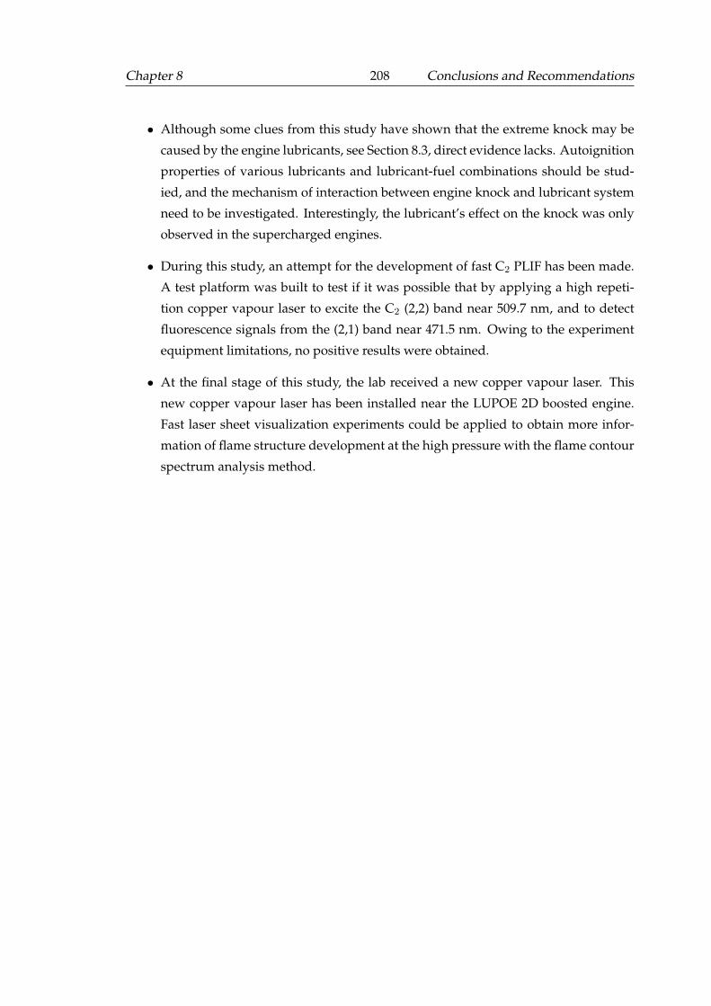
Chapter 8 208 Conclusions and Recommendations
• Although some clues from this study have shown that the extreme knock may be
caused by the engine lubricants, see Section 8.3, direct evidence lacks. Autoignition
properties of various lubricants and lubricant-fuel combinations should be stud-
ied, and the mechanism of interaction between engine knock and lubricant system
need to be investigated. Interestingly, the lubricant’s effect on the knock was only
observed in the supercharged engines.
• During this study, an attempt for the development of fast C2 PLIF has been made.
A test platform was built to test if it was possible that by applying a high repeti-
tion copper vapour laser to excite the C2 (2,2) band near 509.7 nm, and to detect
fluorescence signals from the (2,1) band near 471.5 nm. Owing to the experiment
equipment limitations, no positive results were obtained.
• At the final stage of this study, the lab received a new copper vapour laser. This
new copper vapour laser has been installed near the LUPOE 2D boosted engine.
Fast laser sheet visualization experiments could be applied to obtain more infor-
mation of flame structure development at the high pressure with the flame contour
spectrum analysis method.
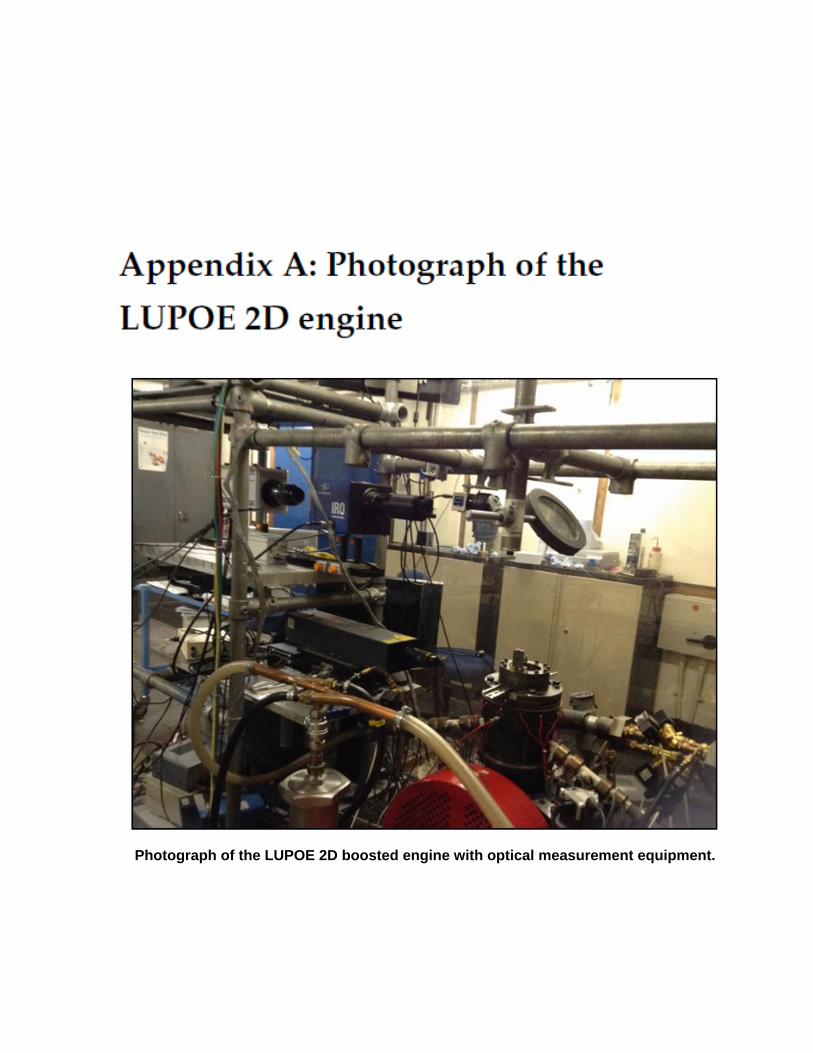
Photograph of the LUPOE 2D boosted engine with optical measurement equipment.
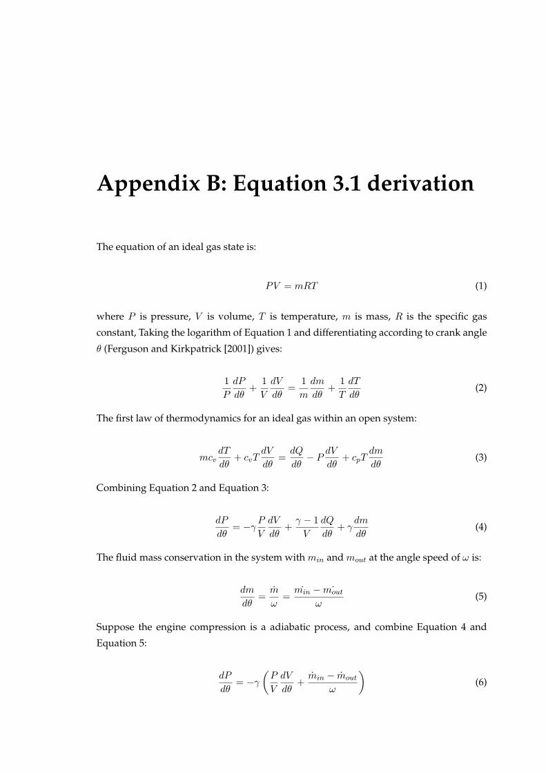
Appendix B: Equation 3.1 derivation
The equation of an ideal gas state is:
PV = mRT (1)
where P is pressure, V is volume, T is temperature, m is mass, R is the specific gas
constant, Taking the logarithm of Equation 1 and differentiating according to crank angle
θ (Ferguson and Kirkpatrick [2001]) gives:
1
P
dP
dθ+
1
V
dV
dθ=
1
m
dm
dθ+
1
T
dT
dθ(2)
The first law of thermodynamics for an ideal gas within an open system:
mcvdT
dθ+ cvT
dV
dθ=
dQ
dθ− P
dV
dθ+ cpT
dm
dθ(3)
Combining Equation 2 and Equation 3:
dP
dθ= −γ
P
V
dV
dθ+
γ − 1
V
dQ
dθ+ γ
dm
dθ(4)
The fluid mass conservation in the system with min and mout at the angle speed of ω is:
dm
dθ=
m
ω=
min − ˙mout
ω(5)
Suppose the engine compression is a adiabatic process, and combine Equation 4 and
Equation 5:
dP
dθ= −γ
(P
V
dV
dθ+
min − mout
ω
)(6)
Appendix C
Zhengyang Ling, A.A. Burluka, U. Azimov. Knock Properties of Oxygenated Blends in
Strongly Charged and Variable Compression Ratio Engines, in SAE 2014 international
Powertrain, Fuels&Lubricants Meeting, Birmingham, UK, October 20-30, 2014. SAE Techni-
cal Paper, 2014-01-2608.
Page 1 of 14
14FFL-0202/2014-01-2608
Knock properties of oxygenated blends in strongly charged and variable compression ratio engines
Zhengyang Ling1, A. A. Burluka1, Ulugbed Azimov2
1.University of Leeds, 2.Northumbria University
Copyright © 2014 SAE International
Abstract
Replacing the conventional fossil fuel totally or partially with alcohols or ethers in spark-ignition (SI) engine is a promising way to reduce pollutant emissions. A large number of studies on alcohol-containing blends in SI engines could be found in the literature. Nonetheless, investigations of ether-containing blends are by far much less numerous, especially for modern boosted engines. Blending with ether compounds might change the burning rate at high pressure, which consequently changes the anti-knock properties of these fuels and leads to a deterioration in the vehicle drivability.
This work reports experiments carried out in two one-cylinder engines: one is a naturally aspirated, variable compression ratio engine, and the other is a strongly charged optical engine. Three fuels with different RON and MON numbers were tested: Iso-octane, a blend Ethyl Tert Butyl Ether (ETBE) with a primary reference fuel, and a commercial gasoline fuel containing 5% by volume of ethanol (E05).
The experimental results show a significant difference of knock boundaries of three fuels in the boosted engine at the initial, i.e. equivalent of the intake manifold, pressure of 1.6bar, and almost similar knock boundaries under different compression ratios in the naturally aspirated engine. The fuel sensitivity upon the knock boundary of oxygenated blends was identified in order to compare the fuels’ performance in different engines. The burning rate was determined at the same compression ratio for the two engines from the high speed flame imaging and a reverse-thermodynamic analysis, in order to clarify the effects of the burning rate on the anti-knock behaviour.
Introduction
Raising concentration of carbon dioxide (CO2) in the air is one of the main causes of environmental concerns. Automotive companies are under political pressures, and they are taking seriously this issue by seeking cost-effective solutions which combine an eco-friendly approach with the reduced costs of fuel [1]. One such solution is a wider use of bio-derived petrol substitutes, such as ethanol or alkyl ter-butyl ethers, e.g. ETBE. Oxygenated fuel admixtures also allow the gasoline in vehicles to burn more completely, resulting in reducing air pollution such as carbon monoxide emission and smog.
The idea of using alcohol as an alternative fuel is not new, but only recently ethanol has become the additive of choice for oxygenated fuel in many places around the world. Alcohols are more competitive among the other alternatives, because they are compatible with existing fuelling distribution infrastructure and are easily stored in a vehicle [2]. Blending ethanol to gasoline has another beneficial effect of improving inherent or chemical resistance to engine knock owing to their high octane numbers (RON 109). Auto-ignition delay time also is further increased by the high sensitivity, i.e. difference between the research (RON) and motor (MON) octane number of ethanol, resulting in greater knock resistance as combustion phasing is retarded due to reduced unburned gas temperature [3]. In general, compared to "standard" gasoline, oxygenated fuels have high Motor Octane Number (MON) and Research Octane Number (RON) which results in high anti-knock Index. In contrast, the sensitivity of the gasoline increases with increasing the oxygenates content, which may cause difficulties in the operation under different engine operation conditions.
Furthermore, the alcohols have a higher latent heat of evaporation compared to gasoline; this reduces the temperature of the inlet manifold and increases the volumetric efficiency [4]. Especially, it is beneficial in supercharged engines, where, by injecting the alcohol-gasoline blends into a supercharger inlet, both the cooling effect and the compressor efficiency are enhanced [5].
For many years, MTBE was another common additive for oxygenated fuel. However, MTBE can easily foul up water in artesian wells because of its low sorption into soils and high water solubility. As a result, legislative efforts have been made by some governments to phase out the use of MTBE [6]. Possible alternative to MTBE, Ethyl Tert-Butyl Ether (ETBE), has much smaller impact on our water supply due to its lower water solubility [7]. ETBE is synthesised from mixtures of ethanol with isobutylene in an endothermic catalytic reaction [2]. ETBE is considered as a biofuel thus having the potential to play a significant role in the future of alternative biofuels [8]. One of advantages of ETBE as a blending component compared to ethanol is that it does not increase the volatility of gasoline. It has higher octane boost than MTBE, and a higher MON than ethanol [9, 10]. Its saturated vapour pressure is lower than that of either MTBE or ethanol. ETBE has better sensitivity compared to other alcohols [11].
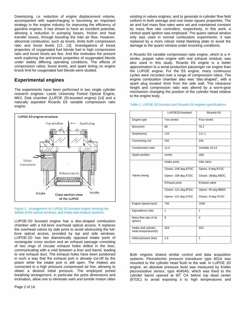
Page 2 of 14
Downsizing, i.e. reduction of engine displacement volume, accompanied with supercharging is becoming an important strategy in the engine industry for improving the efficiency of gasoline engines. It has shown to have an excellent potential, allowing a reduction in pumping losses, friction and heat transfer losses, through boosting the inlet air flow. However, abnormal combustion, such as knock, limits both compression ratio and boost levels [12, 13]. Investigations of knock properties of oxygenated fuel blends fuel in high compression ratio and boost levels are few. And this motivates the present work exploring the anti-knock properties of oxygenated blends under widely differing operating conditions. The effects of compression ratios, boost levels, and spark timing on engine knock limit for oxygenated fuel blends were studied.
Experimental engines
The experiments have been performed in two single cylinder research engines: Leeds University Ported Optical Engine, MK2, Disk chamber (LUPOE 2D-boosted engine) [14] and a naturally aspirated Ricardo E6 variable compression ratio engine.
Figure 1. Arrangement of LUPOE-2D boosted engine showing the details of the optical windows, and intake and exhaust systems.
LUPOE-2D boosted engine has a disc-shaped combustion chamber with a full-bore overhead optical access. It replaces the overhead valves by side ports to avoid obstructing the full-bore optical access, provided by top and side windows. LUPOE-2D has two diametrically opposed intake ports of rectangular cross section and an exhaust passage consisting of two rings of circular exhaust holes drilled in the liner, communicating with a void between a liner and barrel, leading to one exhaust duct. The exhaust holes have been positioned in such a way that the exhaust port is already cut-off by the piston while the intake port is still open. The intakes are connected to a high pressure compressed air line, allowing to obtain a desired initial pressure. The employed ported breathing arrangement, in particular the ports dimensions and inclination, allow one to eliminate swirl and tumble motion often
existing in valves engines, and to generate in-cylinder flow field uniform in both average and root mean square properties. The air and fuel mass flow rates were set and maintained constant by mass flow rate controllers, respectively. In this work, a central spark ignition was employed. The quartz optical window only was used in normal combustion experiments; it was replaced by a more robust metal blanking plate to avoid the damage to the quartz window under knocking conditions.
A Ricardo E6 variable compression ratio engine, which is a 4-stroke, poppet valve engine with real exhaust residual, was also used in this study. Ricardo E6 engine is a better approximation to a serial production passenger car engine than the LUPOE engine. For the E6 engine, many continuous cycles were recorded over a range of compression ratios. The engine combustion chamber also was “disc-shaped”, with a spark plug located 4mm from the side wall. The clearance height and compression ratio was altered by a worm-gear mechanism changing the position of the cylinder head relative to the engine body.
Table 1. LUPOE-2D boosted and Ricardo E6 engines specifications.
LUPOE2D-boosted Ricardo E6
Engine type Two-stroke Four-stroke
Bore(mm) 80 76.2
Stroke(mm) 110 111.1
Connecting rod 232 244
Compression ratio 11.5 Variable 10-14
Spark position center side
Valves timing
Intake ports Inlet valve
Closes -108 deg BTDC
Opens -108 deg ATDC
Opens -9 deg BTDC
Closes -38deg ABDC
Exhaust ports Exhaust valve
Closes -121 deg BTDC
Opens -121 deg ATDC
Opens -45 deg BBDC
Closes -9 deg ATDC
Engine Speed (rpm) 750 1500
Equivalence ratio 1 1
Mass flow rate of air (g/sec)
9 4
Intake and cylinder head temperature(K)
323 323
Initial pressure (bar) 1.6 1
Both engines shared similar control and data acquisition systems. Piezoelectric pressure transducer type 601A was mounted to the cylinder head flush to the wall. In LUPOE 2D engine, an absolute pressure level was measured by Kistler piezoresistive sensor, type 4045A5, which was fixed to the cylinder barrel opened at 60
o CA before top dead center
(bTDC) to avoid exposing it to high temperatures and
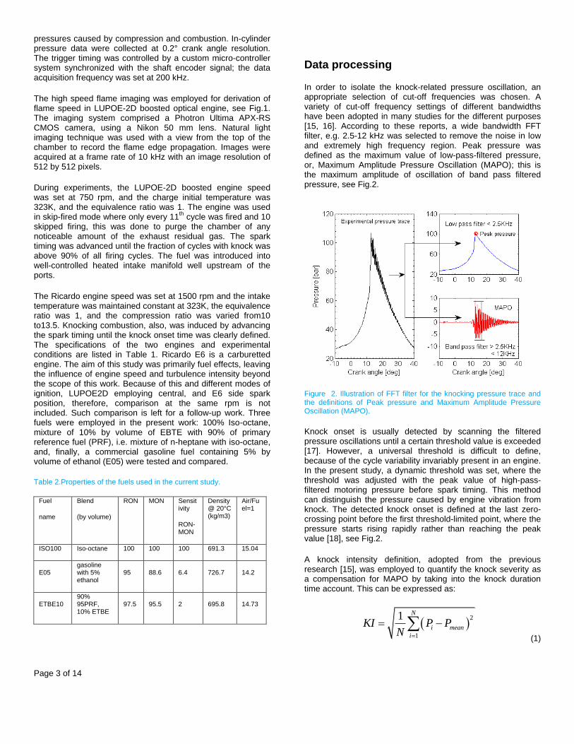
Page 3 of 14
pressures caused by compression and combustion. In-cylinder pressure data were collected at 0.2° crank angle resolution. The trigger timing was controlled by a custom micro-controller system synchronized with the shaft encoder signal; the data acquisition frequency was set at 200 kHz.
The high speed flame imaging was employed for derivation of flame speed in LUPOE-2D boosted optical engine, see Fig.1. The imaging system comprised a Photron Ultima APX-RS CMOS camera, using a Nikon 50 mm lens. Natural light imaging technique was used with a view from the top of the chamber to record the flame edge propagation. Images were acquired at a frame rate of 10 kHz with an image resolution of 512 by 512 pixels.
During experiments, the LUPOE-2D boosted engine speed was set at 750 rpm, and the charge initial temperature was 323K, and the equivalence ratio was 1. The engine was used in skip-fired mode where only every 11
th cycle was fired and 10
skipped firing, this was done to purge the chamber of any noticeable amount of the exhaust residual gas. The spark timing was advanced until the fraction of cycles with knock was above 90% of all firing cycles. The fuel was introduced into well-controlled heated intake manifold well upstream of the ports.
The Ricardo engine speed was set at 1500 rpm and the intake temperature was maintained constant at 323K, the equivalence ratio was 1, and the compression ratio was varied from10 to13.5. Knocking combustion, also, was induced by advancing the spark timing until the knock onset time was clearly defined. The specifications of the two engines and experimental conditions are listed in Table 1. Ricardo E6 is a carburetted engine. The aim of this study was primarily fuel effects, leaving the influence of engine speed and turbulence intensity beyond the scope of this work. Because of this and different modes of ignition, LUPOE2D employing central, and E6 side spark position, therefore, comparison at the same rpm is not included. Such comparison is left for a follow-up work. Three fuels were employed in the present work: 100% Iso-octane, mixture of 10% by volume of EBTE with 90% of primary reference fuel (PRF), i.e. mixture of n-heptane with iso-octane, and, finally, a commercial gasoline fuel containing 5% by volume of ethanol (E05) were tested and compared.
Table 2.Properties of the fuels used in the current study.
Fuel
name
Blend
(by volume)
RON MON Sensitivity
RON-MON
Density @ 20°C (kg/m3)
Air/Fuel=1
ISO100 Iso-octane 100 100 100 691.3 15.04
E05 gasoline with 5% ethanol
95 88.6 6.4 726.7 14.2
ETBE10 90% 95PRF, 10% ETBE
97.5 95.5 2 695.8 14.73
Data processing
In order to isolate the knock-related pressure oscillation, an appropriate selection of cut-off frequencies was chosen. A variety of cut-off frequency settings of different bandwidths have been adopted in many studies for the different purposes [15, 16]. According to these reports, a wide bandwidth FFT filter, e.g. 2.5-12 kHz was selected to remove the noise in low and extremely high frequency region. Peak pressure was defined as the maximum value of low-pass-filtered pressure, or, Maximum Amplitude Pressure Oscillation (MAPO); this is the maximum amplitude of oscillation of band pass filtered pressure, see Fig.2.
Figure 2. Illustration of FFT filter for the knocking pressure trace and the definitions of Peak pressure and Maximum Amplitude Pressure Oscillation (MAPO).
Knock onset is usually detected by scanning the filtered pressure oscillations until a certain threshold value is exceeded [17]. However, a universal threshold is difficult to define, because of the cycle variability invariably present in an engine. In the present study, a dynamic threshold was set, where the threshold was adjusted with the peak value of high-pass-filtered motoring pressure before spark timing. This method can distinguish the pressure caused by engine vibration from knock. The detected knock onset is defined at the last zero-crossing point before the first threshold-limited point, where the pressure starts rising rapidly rather than reaching the peak value [18], see Fig.2.
A knock intensity definition, adopted from the previous research [15], was employed to quantify the knock severity as a compensation for MAPO by taking into the knock duration time account. This can be expressed as:
2
1
1 N
i mean
i
KI P PN
(1)
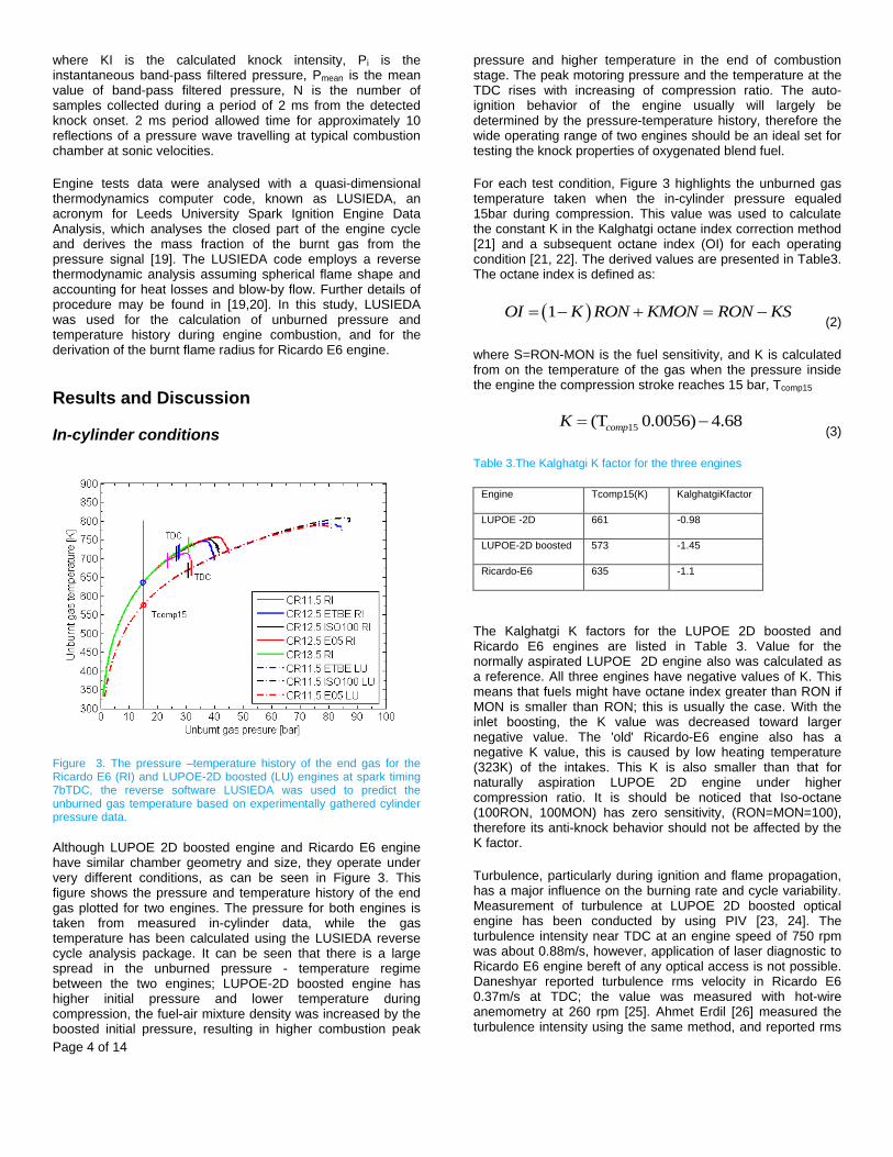
Page 4 of 14
where KI is the calculated knock intensity, Pi is the instantaneous band-pass filtered pressure, Pmean is the mean value of band-pass filtered pressure, N is the number of samples collected during a period of 2 ms from the detected knock onset. 2 ms period allowed time for approximately 10 reflections of a pressure wave travelling at typical combustion chamber at sonic velocities.
Engine tests data were analysed with a quasi-dimensional thermodynamics computer code, known as LUSIEDA, an acronym for Leeds University Spark Ignition Engine Data Analysis, which analyses the closed part of the engine cycle and derives the mass fraction of the burnt gas from the pressure signal [19]. The LUSIEDA code employs a reverse thermodynamic analysis assuming spherical flame shape and accounting for heat losses and blow-by flow. Further details of procedure may be found in [19,20]. In this study, LUSIEDA was used for the calculation of unburned pressure and temperature history during engine combustion, and for the derivation of the burnt flame radius for Ricardo E6 engine.
Results and Discussion
In-cylinder conditions
Figure 3. The pressure –temperature history of the end gas for the Ricardo E6 (RI) and LUPOE-2D boosted (LU) engines at spark timing 7bTDC, the reverse software LUSIEDA was used to predict the unburned gas temperature based on experimentally gathered cylinder pressure data.
Although LUPOE 2D boosted engine and Ricardo E6 engine have similar chamber geometry and size, they operate under very different conditions, as can be seen in Figure 3. This figure shows the pressure and temperature history of the end gas plotted for two engines. The pressure for both engines is taken from measured in-cylinder data, while the gas temperature has been calculated using the LUSIEDA reverse cycle analysis package. It can be seen that there is a large spread in the unburned pressure - temperature regime between the two engines; LUPOE-2D boosted engine has higher initial pressure and lower temperature during compression, the fuel-air mixture density was increased by the boosted initial pressure, resulting in higher combustion peak
pressure and higher temperature in the end of combustion stage. The peak motoring pressure and the temperature at the TDC rises with increasing of compression ratio. The auto-ignition behavior of the engine usually will largely be determined by the pressure-temperature history, therefore the wide operating range of two engines should be an ideal set for testing the knock properties of oxygenated blend fuel.
For each test condition, Figure 3 highlights the unburned gas temperature taken when the in-cylinder pressure equaled 15bar during compression. This value was used to calculate the constant K in the Kalghatgi octane index correction method [21] and a subsequent octane index (OI) for each operating condition [21, 22]. The derived values are presented in Table3. The octane index is defined as:
1OI K RON KMON RON KS (2)
where S=RON-MON is the fuel sensitivity, and K is calculated from on the temperature of the gas when the pressure inside the engine the compression stroke reaches 15 bar, Tcomp15
15(T 0.0056) 4.68compK (3)
Table 3.The Kalghatgi K factor for the three engines
Engine Tcomp15(K) KalghatgiKfactor
LUPOE -2D 661 -0.98
LUPOE-2D boosted 573 -1.45
Ricardo-E6 635 -1.1
The Kalghatgi K factors for the LUPOE 2D boosted and Ricardo E6 engines are listed in Table 3. Value for the normally aspirated LUPOE 2D engine also was calculated as a reference. All three engines have negative values of K. This means that fuels might have octane index greater than RON if MON is smaller than RON; this is usually the case. With the inlet boosting, the K value was decreased toward larger negative value. The 'old' Ricardo-E6 engine also has a negative K value, this is caused by low heating temperature (323K) of the intakes. This K is also smaller than that for naturally aspiration LUPOE 2D engine under higher compression ratio. It is should be noticed that Iso-octane (100RON, 100MON) has zero sensitivity, (RON=MON=100), therefore its anti-knock behavior should not be affected by the K factor.
Turbulence, particularly during ignition and flame propagation, has a major influence on the burning rate and cycle variability. Measurement of turbulence at LUPOE 2D boosted optical engine has been conducted by using PIV [23, 24]. The turbulence intensity near TDC at an engine speed of 750 rpm was about 0.88m/s, however, application of laser diagnostic to Ricardo E6 engine bereft of any optical access is not possible. Daneshyar reported turbulence rms velocity in Ricardo E6 0.37m/s at TDC; the value was measured with hot-wire anemometry at 260 rpm [25]. Ahmet Erdil [26] measured the turbulence intensity using the same method, and reported rms
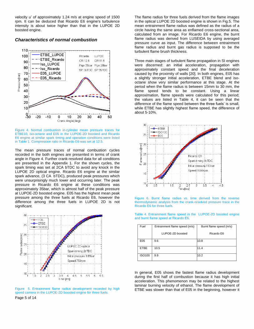
Page 5 of 14
velocity u’ of approximately 1.24 m/s at engine speed of 1500 rpm. It can be deduced that Ricardo E6 engine's turbulence intensity is about twice higher than that in the LUPOE 2D boosted engine.
Characteristics of normal combustion
Figure 4. Normal combustion in-cylinder mean pressure traces for ETBE10, iso-octane and E05 in the LUPOE-2D boosted and Ricardo E6 engine at similar spark timing and operation conditions were listed in Table 1. Compression ratio in Ricardo E6 was set at 12.5.
The mean pressure traces of normal combustion cycles recorded in the both engines are presented in terms of crank angle in Figure 4. Further crank-resolved data for all conditions are presented in the Appendix 1. For the shown cycles, the spark timing was set at 2CA bTDC to avoid any knock in the LUPOE 2D optical engine. Ricardo E6 engine at the similar spark advance, (3 CA bTDC), produced peak pressures which were unsurprisingly much lower and occurring later. The peak pressure in Ricardo E6 engine at these conditions was approximately 35bar, which is almost half of the peak pressure at LUPOE-2D boosted engine. E05 has the highest mean peak pressure among the three fuels at Ricardo E6, however the difference among the three fuels in LUPOE 2D is not significant.
Figure 5. Entrainment flame radius development recorded by high speed camera in the LUPOE-2D boosted engine for three fuels.
The flame radius for three fuels derived from the flame images in the optical LUPOE 2D boosted engine is shown in Fig.5. The mean entrainment flame radius was defined as the radius of a circle having the same area as enflamed cross-sectional area, calculated from an image. For Ricardo E6 engine, the burnt flame radius was derived from LUSEIDA by using averaged pressure curve as input. The difference between entrainment flame radius and burnt gas radius is supposed to be the turbulent flame brush thickness.
Three main stages of turbulent flame propagation in SI engines were discerned: an initial acceleration, propagation with approximately constant speed and the final deceleration caused by the proximity of walls [20]. In both engines, E05 has a slightly stronger initial acceleration, ETBE blend and iso-octane show very similar performance at this stage. At the period when the flame radius is between 15mm to 30 mm, the flame speed tends to be constant. Using a linear approximation, flame speeds were calculated for this period; the values are listed in Table 4, it can be seen that the difference of the flame speed between the three fuels’ is small, while ETBE has slightly highest flame speed, the difference of about 5-10%.
Figure 6. Burnt flame radius vs. time derived from the reverse thermodynamic analysis from the crank-resolved pressure trace in the Ricardo E6 for three fuels.
Table 4. Entrainment flame speed in the LUPOE-2D boosted engine and burnt flame speed at Ricardo E6.
Fuel Entrainment flame speed (m/s)
LUPOE-2D boosted
Burnt flame speed (m/s)
Ricardo E6
E05 9.6 10.8
ETBE 10.5 11.4
ISO100 9.9 10.2
In general, E05 shows the fastest flame radius development during the first half of combustion because it has high initial acceleration. This phenomenon may be related to the highest laminar burning velocity of ethanol. The flame development of ETBE was slower than that of E05 in the beginning, however it

Page 6 of 14
has slightly larger “developed” turbulent flame speed. At some point, when the flame is approximately half-way to the wall, ETBE blend flames reach the same radius as E05 owing to its faster entrainment flame speed. Isooctane was the slowest fuel of the three. These results derived from optical observation are corroborated by the results derived from the mean pressure signal.
Despite the turbulence being approximately twice stronger in Ricardo E6, the time required for the flame to grow from 15 to 35mm in size was slightly larger, circa 2.5 msec, in Ricardo E6 as compared to approximately 2 msec in LUPOE 2D, see Figs. 5 and 6. It may indicate a possible greater role of the flame instabilities at the higher pressures in LUPOE 2D, however, detailed investigation of this effect is beyond the scope of this paper. Nonetheless, it is worth noticing that, the combustion duration times are very similar in the two engines, the combustion duration angle in Ricardo E6 is almost double the one in the LUPOE 2D boosted engine, because the former runs at 1500 rpm. The spark timing was set close to TDC, therefore, combustion happened in the expansion stroke, with a strong drop of the peak combustion pressure with the increasing chamber volume. Moreover, Ricardo E6 engine has the side spark plug configuration. These factors result in much lower and later observed peak pressures in the Ricardo E6 engine.
Slow flame speeds weakened the linear relationship between maximum pressure, and crank angle at which the maximum pressures achieved. The linear relationship have been widely observed in several engines [19] . In Fig 7, the fastest fuel E05 still show a somewhat proportional relationship, while the slowest fuel Iso-octane may have the higher peak pressure in the late combustion angle. According to these figures, coefficient of variation of peak pressure COV-pmax was calculated for cyclic variability comparison, it is presented in Table 5. The cyclic variation of peak pressure for E05 is lower than that for iso-octane and EBTE10 at the LUPOE engine. However it becomes the highest one in Ricardo E6 engine.
Figure 7. Peak pressure versus corresponding crank angle for its occurrence for ISO100, E05 and ETBE at LUPOE -2D boosted engine.
Figure 8. Peak pressure versus corresponding crank angle for its occurrence for ISO100, E05 and ETBE at Ricardo-E6.
Table 5. Coefficient of variation (COV) in peak pressure in the two engines for the three fuels.
Fuel COV-pmax
LUPOE-2Dboosted
COV-pmax
Ricardo-E6
E05 12.2 12.3
ETBE 12.4 10.4
ISO100 13.2 11.0
Characteristics of knocking combustion
Figure 9. Knock combustion in-cylinder mean pressure traces for ETBE10, iso-octane and E05 in the LUPOE-2D boosted and Ricardo E6 engine at spark timing 7bTDC and operation conditions were listed in Table 1.
Under the same operational conditions as the normal combustion discussed above, the spark time was advanced to 7
o bTDC, at which point a larger proportion of the cycles was
knocking. The mean low-pass filtered pressures for three fuels in the two engines are presented in Figure 9 and the individual
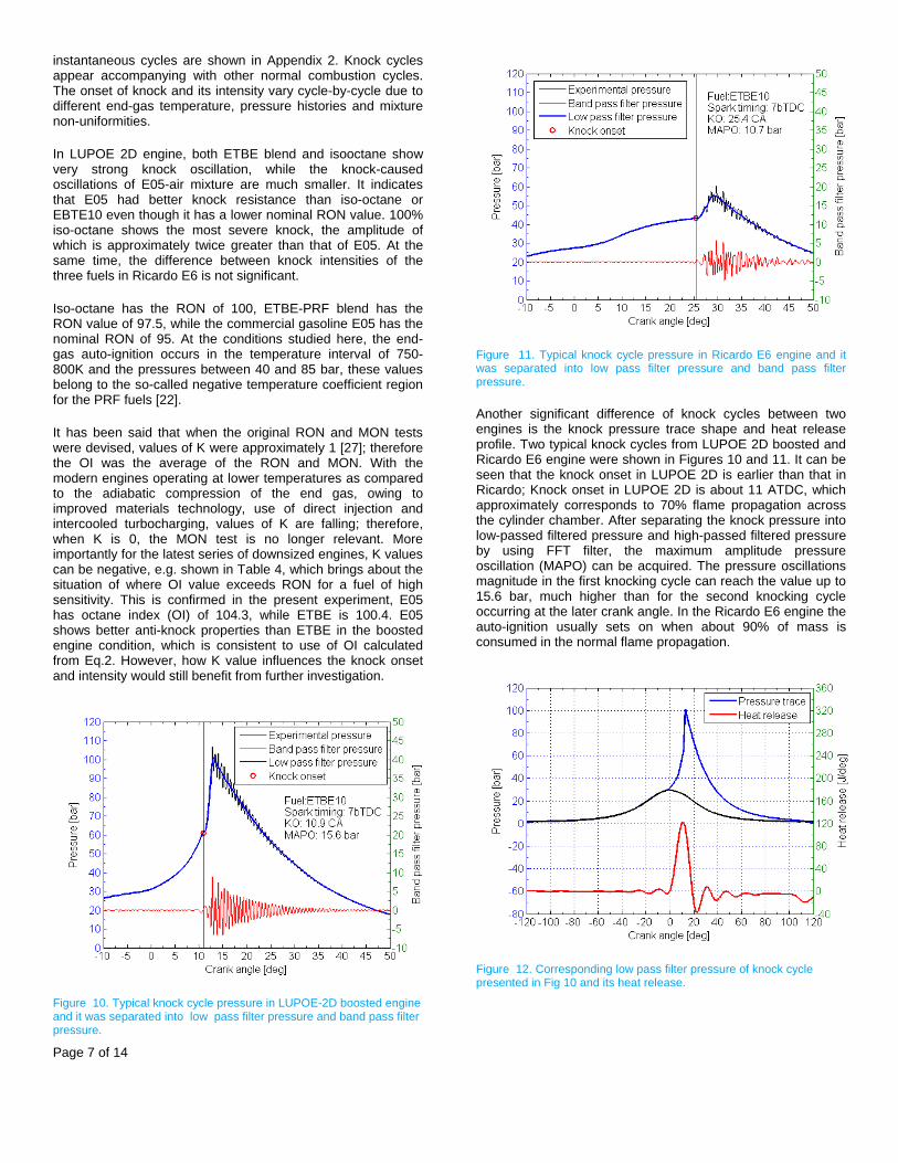
Page 7 of 14
instantaneous cycles are shown in Appendix 2. Knock cycles appear accompanying with other normal combustion cycles. The onset of knock and its intensity vary cycle-by-cycle due to different end-gas temperature, pressure histories and mixture non-uniformities.
In LUPOE 2D engine, both ETBE blend and isooctane show very strong knock oscillation, while the knock-caused oscillations of E05-air mixture are much smaller. It indicates that E05 had better knock resistance than iso-octane or EBTE10 even though it has a lower nominal RON value. 100% iso-octane shows the most severe knock, the amplitude of which is approximately twice greater than that of E05. At the same time, the difference between knock intensities of the three fuels in Ricardo E6 is not significant.
Iso-octane has the RON of 100, ETBE-PRF blend has the RON value of 97.5, while the commercial gasoline E05 has the nominal RON of 95. At the conditions studied here, the end-gas auto-ignition occurs in the temperature interval of 750-800K and the pressures between 40 and 85 bar, these values belong to the so-called negative temperature coefficient region for the PRF fuels [22].
It has been said that when the original RON and MON tests were devised, values of K were approximately 1 [27]; therefore the OI was the average of the RON and MON. With the modern engines operating at lower temperatures as compared to the adiabatic compression of the end gas, owing to improved materials technology, use of direct injection and intercooled turbocharging, values of K are falling; therefore, when K is 0, the MON test is no longer relevant. More importantly for the latest series of downsized engines, K values can be negative, e.g. shown in Table 4, which brings about the situation of where OI value exceeds RON for a fuel of high sensitivity. This is confirmed in the present experiment, E05 has octane index (OI) of 104.3, while ETBE is 100.4. E05 shows better anti-knock properties than ETBE in the boosted engine condition, which is consistent to use of OI calculated from Eq.2. However, how K value influences the knock onset and intensity would still benefit from further investigation.
Figure 10. Typical knock cycle pressure in LUPOE-2D boosted engine and it was separated into low pass filter pressure and band pass filter pressure.
Figure 11. Typical knock cycle pressure in Ricardo E6 engine and it was separated into low pass filter pressure and band pass filter pressure.
Another significant difference of knock cycles between two engines is the knock pressure trace shape and heat release profile. Two typical knock cycles from LUPOE 2D boosted and Ricardo E6 engine were shown in Figures 10 and 11. It can be seen that the knock onset in LUPOE 2D is earlier than that in Ricardo; Knock onset in LUPOE 2D is about 11 ATDC, which approximately corresponds to 70% flame propagation across the cylinder chamber. After separating the knock pressure into low-passed filtered pressure and high-passed filtered pressure by using FFT filter, the maximum amplitude pressure oscillation (MAPO) can be acquired. The pressure oscillations magnitude in the first knocking cycle can reach the value up to 15.6 bar, much higher than for the second knocking cycle occurring at the later crank angle. In the Ricardo E6 engine the auto-ignition usually sets on when about 90% of mass is consumed in the normal flame propagation.
Figure 12. Corresponding low pass filter pressure of knock cycle presented in Fig 10 and its heat release.
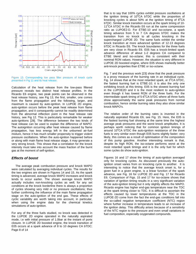
Page 8 of 14
Figure 13. Corresponding low pass filter pressure of knock cycle presented in Fig 11 and its heat release.
Calculation of the heat release from the low-pass filtered pressure reveals two distinct heat release profiles. In the Ricardo E6 engine, two peak points can be observed in the heat release history, see Fig 13, the first, smaller, one comes from the flame propagation and the following, larger, and maximum is caused by auto-ignition. In LUPOE 2D engine, auto-ignition occurs before the peak heat release from flame propagation, and it consequently cannot be readily determined from the abnormal inflection point in the heat release rate history, see Fig 12. This is particularly remarkable for weaker auto-ignitions [28]. The difference between the two kinds of heat release can be used to explain the difference of MAPO. The autoignition occurring after heat release caused by flame propagation, has less energy left in the unburned air-fuel mixture, hence it has much smaller propensity to trigger violent pressure oscillations. When the auto-ignition happened before or along with main flame heat release stage, it may generate a very strong knock. This shows that a correlation for the knock intensity must take into account the mass fraction of the burnt gas at the moment of self-ignition.
Effects of boost
The average peak combustion pressure and knock MAPO were calculated by averaging individual cycles. The results for the two engines are shown in Figures 14 and 15. As the spark timing is advanced, average knock MAPO increases and knock tends to occur earlier. The shown average knock MAPO actually includes non-knocking cycles as well; for any set conditions at the knock borderline there is always a proportion of cycles showing very mild or no pressure oscillations; thus further confirming the influence of the main flame propagation stage on the auto-ignition of the end gas. These effects of cyclic variability are worth taking into account, in particular, when using the engine data for the chemical kinetics simulations of auto-ignition.
For any of the three fuels studied, no knock was detected in the LUPOE 2D engine operated in the naturally aspirated mode, i.e with initial pressure of 1.0bar at the instant of ports closure. In LUPOE 2D boosted engine, the knock transition of E05 occurs at a spark advance of 8 to 10 degrees CA bTDC;
that is to say that 100% cycles exhibit pressure oscillations at the ignition timing of 10
0CA bTDC while the proportion of
knocking cycles is about 50% at the ignition timing of 80CA
bTDC. Similar knock transition occurs at the spark timing of 10-11
0CA bTDC in the Ricardo E6 run at the same compression
ratio as LUPOE2-D. For ETBE-10 and iso-octane, a spark timing advance from 5 to 7 CA degrees bTDC makes the transition from no knock to all cycles knocking in the supercharged LUPOE 2D. The same fuels exhibit the similar knock transition at more advanced ignition of 12-13 degrees bTDC in Ricardo E6. The knock boundaries for the three fuels are very close in Ricardo E6. E05 has a knock-limited spark advance difference of about 1-2 degrees CA compared to ETBE blend and iso-octane; this is consistent with their nominal RON values. However, the situation is very different in LUPOE 2D boosted engine, where E05 shows markedly better anti-knock properties than ETBE or iso-octane.
Fig. 7 and the previous work [23] show that the peak pressure is a proxy measure of the burning rate in an individual cycle. Fig. 14 shows that at the most retarded spark, at 3
0CA bTDC,
the fastest burning fuel is ETBE-10; it is also the only one exhibiting knock at this timing. E05 is the slowest burning fuel in the LUPOE2D and it is the most resilient to auto-ignition even though it has lowest RON of the three fuels. For the intermediate spark timing of 5-6
0CA bTDC where all three fuels
show approximately the same peak pressures from normal combustion, hence similar burning rates they also show similar knock MAPO's.
The relative order of the burning rates is inverted in the naturally aspirated Ricardo E6, see Fig. 15. Here, the E05 is the fastest burning fuel showing at the same time the highest average peak pressures and the worst knock amplitudes. It is perhaps worth noticing that for common ignition timings of around 10
0CA bTDC the auto-ignition resistance of the three
fuels is very similar even though E05 burns slightly faster; very likely, this comes as a result of optimisation of the composition of this pump gasoline. Another interesting remark is that, despite its high RON, the iso-octane performs worst at the most retarded spark timings and it is the only fuel for which some cycles do show auto-ignition.
Figures 16 and 17 show the timing of auto-ignition averaged only for knocking cycles. As discussed previously the auto-ignition onset varies from on knocking cycle to another. It is interesting to notice that the average knock onset is, for a given fuel in a given engine, is a linear function of the spark advance, see Fig. 16 for LUPOE 2D and Fig. 17 for Ricardo E6. Comparison of Figs. 15 and 17 for iso-octane shows that variation of ignition timing results in a very significant variation of the auto-ignition timing but it only slightly affects the MAPO. Ricardo engine has higher end-gas temperature near the TDC at the spark timing closer to TDC. It is difficult to ascertain the effects caused by lower temperatures at the TDC in the LUPOE-2D come from the fact the end-gas conditions fall into the so-called negative temperature coefficient (NTC) region where further increase in temperature leads to an increase of the ignition delay. This difficulty arises because of a sensitivity of the NTC region to the pressure and even small variations in fuel composition, especially oxygenated compounds.
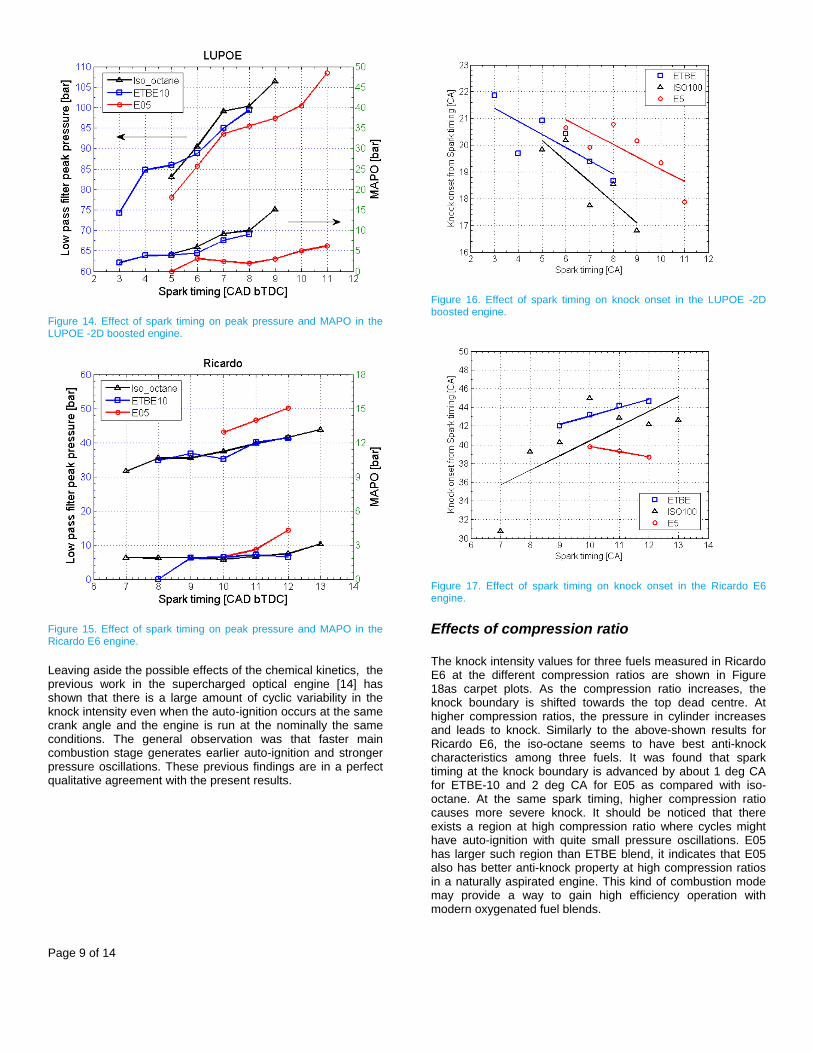
Page 9 of 14
Figure 14. Effect of spark timing on peak pressure and MAPO in the LUPOE -2D boosted engine.
Figure 15. Effect of spark timing on peak pressure and MAPO in the Ricardo E6 engine.
Leaving aside the possible effects of the chemical kinetics, the previous work in the supercharged optical engine [14] has shown that there is a large amount of cyclic variability in the knock intensity even when the auto-ignition occurs at the same crank angle and the engine is run at the nominally the same conditions. The general observation was that faster main combustion stage generates earlier auto-ignition and stronger pressure oscillations. These previous findings are in a perfect qualitative agreement with the present results.
Figure 16. Effect of spark timing on knock onset in the LUPOE -2D boosted engine.
Figure 17. Effect of spark timing on knock onset in the Ricardo E6 engine.
Effects of compression ratio
The knock intensity values for three fuels measured in Ricardo E6 at the different compression ratios are shown in Figure 18as carpet plots. As the compression ratio increases, the knock boundary is shifted towards the top dead centre. At higher compression ratios, the pressure in cylinder increases and leads to knock. Similarly to the above-shown results for Ricardo E6, the iso-octane seems to have best anti-knock characteristics among three fuels. It was found that spark timing at the knock boundary is advanced by about 1 deg CA for ETBE-10 and 2 deg CA for E05 as compared with iso-octane. At the same spark timing, higher compression ratio causes more severe knock. It should be noticed that there exists a region at high compression ratio where cycles might have auto-ignition with quite small pressure oscillations. E05 has larger such region than ETBE blend, it indicates that E05 also has better anti-knock property at high compression ratios in a naturally aspirated engine. This kind of combustion mode may provide a way to gain high efficiency operation with modern oxygenated fuel blends.
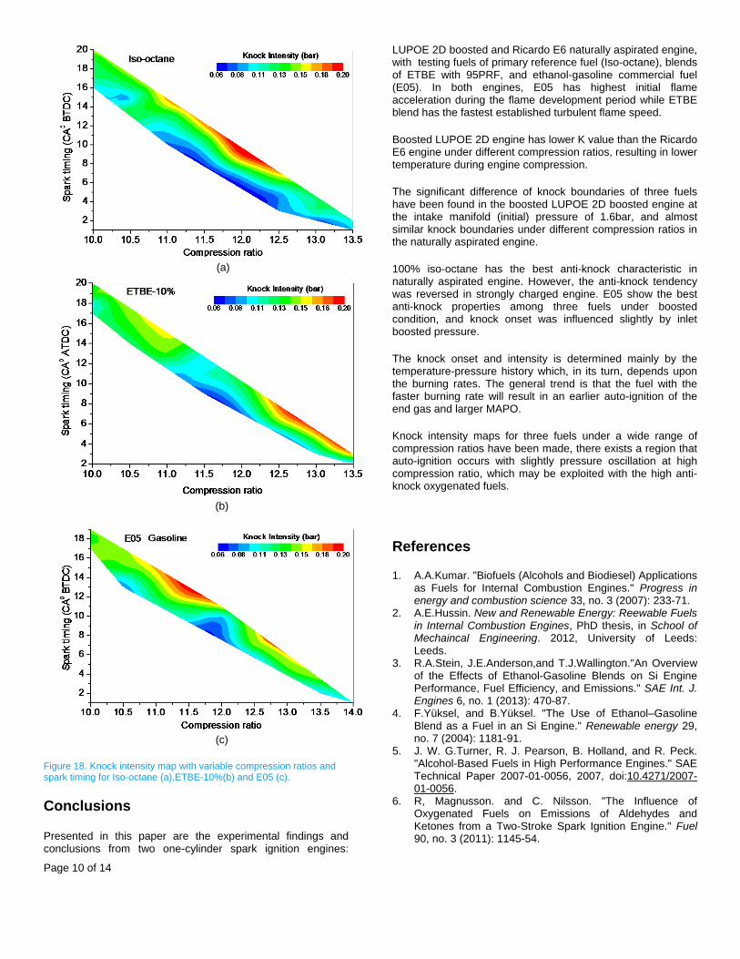
Page 10 of 14
(a)
(b)
(c)
Figure 18. Knock intensity map with variable compression ratios and spark timing for Iso-octane (a),ETBE-10%(b) and E05 (c).
Conclusions
Presented in this paper are the experimental findings and conclusions from two one-cylinder spark ignition engines:
LUPOE 2D boosted and Ricardo E6 naturally aspirated engine, with testing fuels of primary reference fuel (Iso-octane), blends of ETBE with 95PRF, and ethanol-gasoline commercial fuel (E05). In both engines, E05 has highest initial flame acceleration during the flame development period while ETBE blend has the fastest established turbulent flame speed.
Boosted LUPOE 2D engine has lower K value than the Ricardo E6 engine under different compression ratios, resulting in lower temperature during engine compression.
The significant difference of knock boundaries of three fuels have been found in the boosted LUPOE 2D boosted engine at the intake manifold (initial) pressure of 1.6bar, and almost similar knock boundaries under different compression ratios in the naturally aspirated engine.
100% iso-octane has the best anti-knock characteristic in naturally aspirated engine. However, the anti-knock tendency was reversed in strongly charged engine. E05 show the best anti-knock properties among three fuels under boosted condition, and knock onset was influenced slightly by inlet boosted pressure.
The knock onset and intensity is determined mainly by the temperature-pressure history which, in its turn, depends upon the burning rates. The general trend is that the fuel with the faster burning rate will result in an earlier auto-ignition of the end gas and larger MAPO.
Knock intensity maps for three fuels under a wide range of compression ratios have been made, there exists a region that auto-ignition occurs with slightly pressure oscillation at high compression ratio, which may be exploited with the high anti-knock oxygenated fuels.
References
1. A.A.Kumar. "Biofuels (Alcohols and Biodiesel) Applications as Fuels for Internal Combustion Engines." Progress in energy and combustion science 33, no. 3 (2007): 233-71.
2. A.E.Hussin. New and Renewable Energy: Reewable Fuels in Internal Combustion Engines, PhD thesis, in School of Mechaincal Engineering. 2012, University of Leeds: Leeds.
3. R.A.Stein, J.E.Anderson,and T.J.Wallington."An Overview of the Effects of Ethanol-Gasoline Blends on Si Engine Performance, Fuel Efficiency, and Emissions." SAE Int. J. Engines 6, no. 1 (2013): 470-87.
4. F.Yüksel, and B.Yüksel. "The Use of Ethanol–Gasoline Blend as a Fuel in an Si Engine." Renewable energy 29, no. 7 (2004): 1181-91.
5. J. W. G.Turner, R. J. Pearson, B. Holland, and R. Peck. "Alcohol-Based Fuels in High Performance Engines." SAE Technical Paper 2007-01-0056, 2007, doi:10.4271/2007-01-0056.
6. R, Magnusson. and C. Nilsson. "The Influence of Oxygenated Fuels on Emissions of Aldehydes and Ketones from a Two-Stroke Spark Ignition Engine." Fuel 90, no. 3 (2011): 1145-54.
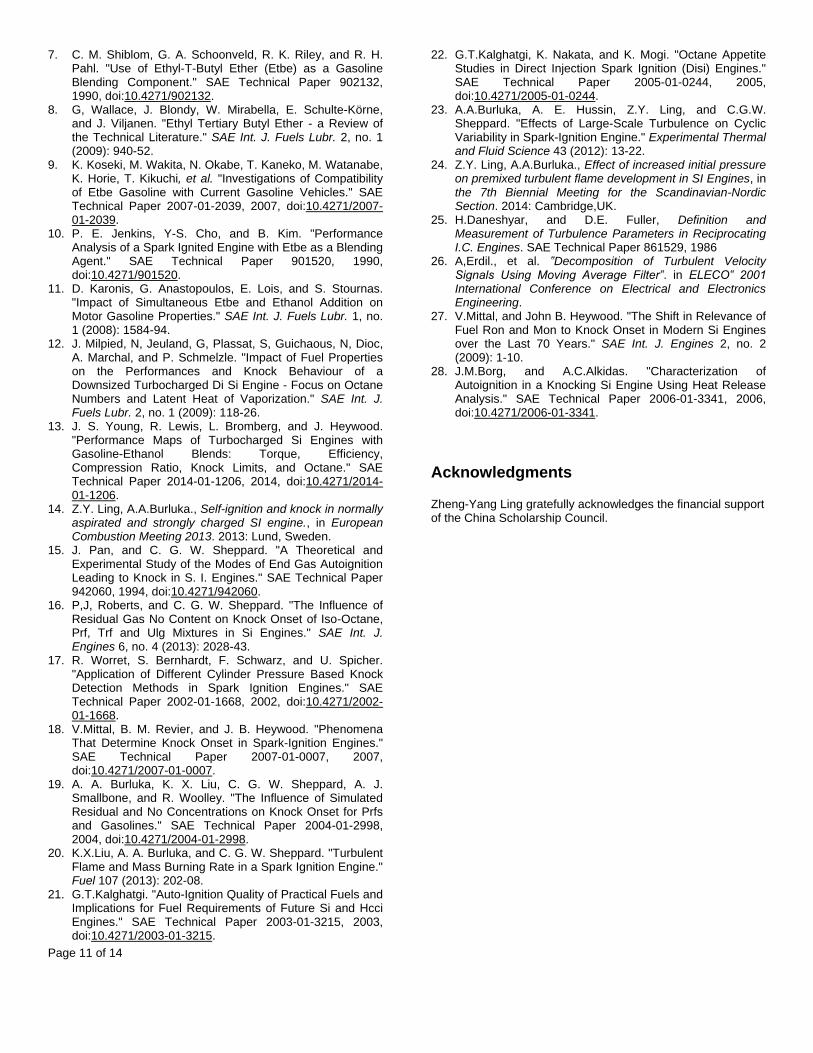
Page 11 of 14
7. C. M. Shiblom, G. A. Schoonveld, R. K. Riley, and R. H. Pahl. "Use of Ethyl-T-Butyl Ether (Etbe) as a Gasoline Blending Component." SAE Technical Paper 902132, 1990, doi:10.4271/902132.
8. G, Wallace, J. Blondy, W. Mirabella, E. Schulte-Körne, and J. Viljanen. "Ethyl Tertiary Butyl Ether - a Review of the Technical Literature." SAE Int. J. Fuels Lubr. 2, no. 1 (2009): 940-52.
9. K. Koseki, M. Wakita, N. Okabe, T. Kaneko, M. Watanabe, K. Horie, T. Kikuchi, et al. "Investigations of Compatibility of Etbe Gasoline with Current Gasoline Vehicles." SAE Technical Paper 2007-01-2039, 2007, doi:10.4271/2007-01-2039.
10. P. E. Jenkins, Y-S. Cho, and B. Kim. "Performance Analysis of a Spark Ignited Engine with Etbe as a Blending Agent." SAE Technical Paper 901520, 1990, doi:10.4271/901520.
11. D. Karonis, G. Anastopoulos, E. Lois, and S. Stournas. "Impact of Simultaneous Etbe and Ethanol Addition on Motor Gasoline Properties." SAE Int. J. Fuels Lubr. 1, no. 1 (2008): 1584-94.
12. J. Milpied, N, Jeuland, G, Plassat, S, Guichaous, N, Dioc, A. Marchal, and P. Schmelzle. "Impact of Fuel Properties on the Performances and Knock Behaviour of a Downsized Turbocharged Di Si Engine - Focus on Octane Numbers and Latent Heat of Vaporization." SAE Int. J. Fuels Lubr. 2, no. 1 (2009): 118-26.
13. J. S. Young, R. Lewis, L. Bromberg, and J. Heywood. "Performance Maps of Turbocharged Si Engines with Gasoline-Ethanol Blends: Torque, Efficiency, Compression Ratio, Knock Limits, and Octane." SAE Technical Paper 2014-01-1206, 2014, doi:10.4271/2014-01-1206.
14. Z.Y. Ling, A.A.Burluka., Self-ignition and knock in normally aspirated and strongly charged SI engine., in European Combustion Meeting 2013. 2013: Lund, Sweden.
15. J. Pan, and C. G. W. Sheppard. "A Theoretical and Experimental Study of the Modes of End Gas Autoignition Leading to Knock in S. I. Engines." SAE Technical Paper 942060, 1994, doi:10.4271/942060.
16. P,J, Roberts, and C. G. W. Sheppard. "The Influence of Residual Gas No Content on Knock Onset of Iso-Octane, Prf, Trf and Ulg Mixtures in Si Engines." SAE Int. J. Engines 6, no. 4 (2013): 2028-43.
17. R. Worret, S. Bernhardt, F. Schwarz, and U. Spicher. "Application of Different Cylinder Pressure Based Knock Detection Methods in Spark Ignition Engines." SAE Technical Paper 2002-01-1668, 2002, doi:10.4271/2002-01-1668.
18. V.Mittal, B. M. Revier, and J. B. Heywood. "Phenomena That Determine Knock Onset in Spark-Ignition Engines." SAE Technical Paper 2007-01-0007, 2007, doi:10.4271/2007-01-0007.
19. A. A. Burluka, K. X. Liu, C. G. W. Sheppard, A. J. Smallbone, and R. Woolley. "The Influence of Simulated Residual and No Concentrations on Knock Onset for Prfs and Gasolines." SAE Technical Paper 2004-01-2998, 2004, doi:10.4271/2004-01-2998.
20. K.X.Liu, A. A. Burluka, and C. G. W. Sheppard. "Turbulent Flame and Mass Burning Rate in a Spark Ignition Engine." Fuel 107 (2013): 202-08.
21. G.T.Kalghatgi. "Auto-Ignition Quality of Practical Fuels and Implications for Fuel Requirements of Future Si and Hcci Engines." SAE Technical Paper 2003-01-3215, 2003, doi:10.4271/2003-01-3215.
22. G.T.Kalghatgi, K. Nakata, and K. Mogi. "Octane Appetite Studies in Direct Injection Spark Ignition (Disi) Engines." SAE Technical Paper 2005-01-0244, 2005, doi:10.4271/2005-01-0244.
23. A.A.Burluka, A. E. Hussin, Z.Y. Ling, and C.G.W. Sheppard. "Effects of Large-Scale Turbulence on Cyclic Variability in Spark-Ignition Engine." Experimental Thermal and Fluid Science 43 (2012): 13-22.
24. Z.Y. Ling, A.A.Burluka., Effect of increased initial pressure on premixed turbulent flame development in SI Engines, in the 7th Biennial Meeting for the Scandinavian-Nordic Section. 2014: Cambridge,UK.
25. H.Daneshyar, and D.E. Fuller, Definition and Measurement of Turbulence Parameters in Reciprocating I.C. Engines. SAE Technical Paper 861529, 1986
26. A,Erdil., et al. ‟Decomposition of Turbulent Velocity Signals Using Moving Average Filter‟. in ELECO‟ 2001 International Conference on Electrical and Electronics Engineering.
27. V.Mittal, and John B. Heywood. "The Shift in Relevance of Fuel Ron and Mon to Knock Onset in Modern Si Engines over the Last 70 Years." SAE Int. J. Engines 2, no. 2 (2009): 1-10.
28. J.M.Borg, and A.C.Alkidas. "Characterization of Autoignition in a Knocking Si Engine Using Heat Release Analysis." SAE Technical Paper 2006-01-3341, 2006, doi:10.4271/2006-01-3341.
Acknowledgments
Zheng-Yang Ling gratefully acknowledges the financial support of the China Scholarship Council.

Page 12 of 14
Definitions/Abbreviations CR Compression Ratio
bTDC Before Top Dead Center
aTDC After Top Dead Center
KO Knock Onset
KI Knock Intensity
MAPO Maximum Amplitude Pressure Oscillation
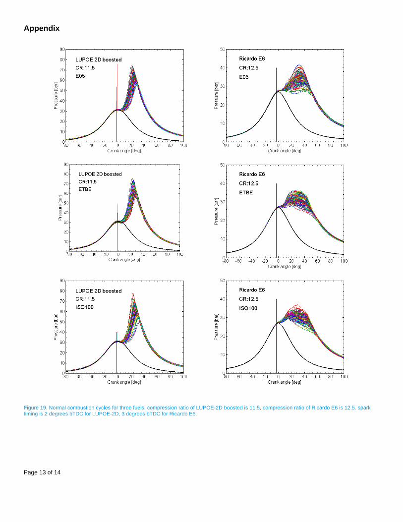
Page 13 of 14
Appendix
Figure 19. Normal combustion cycles for three fuels, compression ratio of LUPOE-2D boosted is 11.5, compression ratio of Ricardo E6 is 12.5. spark timing is 2 degrees bTDC for LUPOE-2D, 3 degrees bTDC for Ricardo E6.
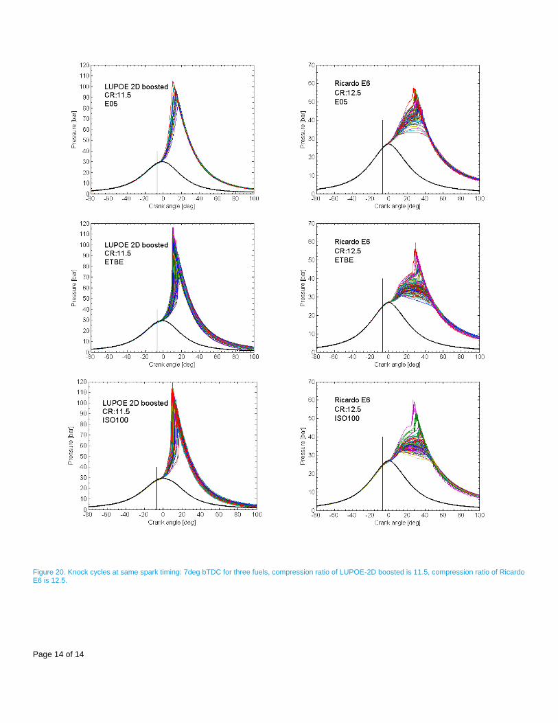
Page 14 of 14
Figure 20. Knock cycles at same spark timing: 7deg bTDC for three fuels, compression ratio of LUPOE-2D boosted is 11.5, compression ratio of Ricardo E6 is 12.5.
References
Abdel-Gayed, R., Bradley, D., and Lung, F.-K. (1989). Combustion regimes and the strain-
ing of turbulent premixed flames. Combustion and Flame, 76(2):213–218. 25
Abdel-Gayed, R. G., Bradley, D., and Lawes, M. (1987). Turbulent burning velocities: A
general correlation in terms of straining rates. Proceedings of the Royal Society of London.
A. Mathematical and Physical Sciences, 414:389–413. 12, 13, 157, 158
Abdi Aghdam, E. (2003). Improvement and Validation of a Thermodynamic S.I. Engine Sim-
ulation Code. PhD thesis, Department of Mechanical Engineering, The University of
Leeds. 19, 61, 63, 157, 159
Abraham, J., Williams, F. A., and Bracco, F. V. (1985). A discussion of turbulent flame
structure in premixed charges. Society of Automotive Engineers, SAE Technical Paper
850345. 16
Al-Shahrany, A. S., Bradley, D., Lawes, M., and Woolley, R. (2005). Measurement of un-
stable burning velocities of iso-octane-air mixtures at high pressure and the derivation
of laminar burning velocities. Proceedings of the Combustion Institute, 30:225–232. 30,
117, 118, 124
Aleiferis, P., Serras-Pereira, J., and Richardson, D. (2013). Characterisation of flame de-
velopment with ethanol, butanol, iso-octane, gasoline and methane in a direct-injection
spark-ignition engine. Fuel, 109:256–278. 40
Aleiferis, P., Serras-Pereira, J., Van Romunde, Z., Caine, J., and Wirth, M. (2010). Mech-
anisms of spray formation and combustion from a multi-hole injector with e85 and
gasoline. Combustion and Flame, 157(4):735–756. 40
Aleiferis, P., Taylor, A., Ishii, K., and Urata, Y. (2004). The nature of early flame devel-
opment in a lean-burn stratified-charge spark-ignition engine. Combustion and Flame,
136(3):283–302. 32, 40, 165
213 REFERENCES
Atashkari, K. (1997). Laser Diagnostics in Combustion and In-Cylinder Flow. PhD thesis,
Department of Mechanical Engineering, The University of Leeds. 7
Attard, W. P., Toulson, E., Watson, H., and Hamori, F. (2010). Abnormal combustion
including mega knock in a 60% downsized highly turbocharged PFI engine. Society of
Automotive Engineers, SAE Technical Paper 2010-01-1456. 2, 3, 34
Baratta, M., Catania, A. E., Spessa, E., and Vassallo, A. (2006). Development and assess-
ment of a multizone combustion simulation code for SI engines based on a novel fractal
model. Society of Automotive Engineers, SAE Technical Paper 2006-01-0048. 158
Bates, S. C. (1991). Further insights into SI four-stroke combustion using flame imaging.
Combustion and Flame, 85(3):331–352. 40
Beretta, G., Rashidi, M., and Keck, J. (1983). Turbulent flame propagation and combustion
in spark ignition engines. Combustion and Flame, 52:217–245. 27, 40
Borghi, R. and Destriau, M. (1998). Combustion and flames: chemical and physical principles.
Editions Technip, Paris, 1st edition. 22, 24
Bradley, D. and Head, R. (2006). Engine autoignition: The relationship between octane
numbers and autoignition delay times. Combustion and flame, 147(3):171–184. 38
Bradley, D., Hicks, R. A., Lawes, M., and Sheppard, C. G. W. (1998). The measurement of
laminar burning velocities and markstein numbers for iso-octane-air and iso-octane-
n-heptane-air mixtures at elevated temperatures and pressures in an explosion bomb.
Combustion and Flame, 115:126–144. xiv, 29, 30, 115, 116, 117, 123
Bradley, D. and Kalghatgi, G. (2009). Influence of autoignition delay time characteristics
of different fuels on pressure waves and knock in reciprocating engines. Combustion
and flame, 156(12):2307–2318. 35, 39, 40
Bradley, D., Lau, A. K. C., and Lawes, M. (1992). Flame stretch rate as a determinant of
turbulent burning velocity. Philosophical Transactions of the Royal Society : Physical and
Engineering Sciences, 338(1650):359–387. 7, 16
Bradley, D., Morley, C., Gu, X., and Emerson, D. (2002). Amplified pressure waves during
autoignition: relevance to cai engines. Society of Automotive Engineers, SAE Technical
Paper 2002-01-2868. 39
Burke, M. P., Chen, Z., Ju, Y., and Dryer, F. L. (2009). Effect of cylindrical confinement
on the determination of laminar flame speeds using outwardly propagating flames.
Combustion and Flame, 156(4):771–779. 123
214 REFERENCES
Buschbeck, M., Bittner, N., Halfmann, T., and Arndt, S. (2012). Dependence of com-
bustion dynamics in a gasoline engine upon the in-cylinder flow field, determined by
high-speed PIV. Experiments in fluids, 53(6):1701–1712. 40
Cairns, A. (2001). Turbulent Flame Development in a Spark Ignition Engine. PhD thesis,
Department of Mechanical Engineering, The University of Leeds. 47, 76, 82, 87, 132,
165
Chen, L., Stone, R., and Richardson, D. (2012). A study of mixture preparation and pm
emissions using a direct injection engine fuelled with stoichiometric gasoline/ethanol
blends. fuel, 96:120–130. 40
Chen, Y.-C., Peters, N., Schneemann, G., Wruck, N., Renz, U., and Mansour, M. S.
(1996). The detailed flame structure of highly stretched turbulent premixed methane-
air flames. Combustion and flame, 107(3):223–IN2. 25
Conway, G. (2010). High pressure autoignition modelling in S.I. engines - transfer report.
Department of Mechanical Engineering, The University of Leeds. 49
Conway, G. T. (2013). Cyclic variability of flame propagation and autoignition in supercharged
and naturally aspirated SI engines. PhD thesis, Department of Mechanical Engineering,
The University of Leeds. x, 49, 174
Cruz, P., Vianna, J., and Moreira, C. S. (2003). Study of the turbulence intensity varia-
tion within the combustion chamber of an S.I engine due to turbocharging. Society of
Automotive Engineers, SAE Technical Paper 2003-01-3687. 14
Curran, H. J., Gaffuri, P., Pitz, W., and Westbrook, C. (2002). A comprehensive modeling
study of iso-octane oxidation. Combustion and flame, 129(3):253–280. 36
Dahnz, C. and Spicher, U. (2010). Irregular combustion in supercharged spark ignition
engines- pre-ignition and other phenomena. International Journal of Engine Research,
11:485–499. 2, 34, 38
Dawood, A. (2010). Combustion and Flow Characteristics in a Disc-Shaped Spark Ignition
Engine. PhD thesis, Department of Mechanical Engineering, The University of Leeds.
14, 41, 69, 71, 76, 77, 129, 137
Desoky, A. (1981). An experiental and theoretical study of the combustion process in a divided
chamber spark ignition engine. PhD thesis, Department of Mechanical Engineering, The
University of Leeds. 61
215 REFERENCES
DoE, U. (2014). International energy outlook 2014. In: Energy Information Administration
Office of Integrated Analysis and Forecasting U.S. Department of Energy Washington, D.
(Ed.). http://www.eia.gov/forecasts/ieo/. 1
Driscoll, J. F. (2008). Turbulent premixed combustion: Flamelet structure and its effect on
turbulent burning velocities. Progress in Energy and Combustion Science, 34(1):91–134.
24
Eckbreth, A. C. (1996). Laser diagnostics for combustion temperature and species. CRC Press.
76, 86
Fajardo, C. and Sick, V. (2009). Development of a high-speed uv particle image velocime-
try technique and application for measurements in internal combustion engines. Ex-
periments in Fluids, 46(1):43–53. 67
Ferguson, R. C. and Kirkpatrick, T. A. (2001). Internal Combustion Engines: Applied Ther-
mosciences. John Wiley & Sons, New York, 2nd edition. 210
Firey, J. (1957). A detonation wave theory of gasoline engine knock. Symposium (Interna-
tional) on Combustion, 6(1):878–886. 35
Foucher, F. and Mounaım-Rousselle, C. (2005). Fractal approach to the evaluation of
burning rates in the vicinity of the piston in a spark-ignition engine. Combustion and
flame, 143(3):323–332. 40
Fraser, N., Blaxill, H., Lumsden, G., and Bassett, M. (2009). Challenges for increased
efficiency through gasoline engine downsizing. Society of Automotive Engineers, SAE
Technical Paper 2009-01-1053. 2
Galmiche, B., Halter, F., and Foucher, F. (2012). Effects of high pressure, high temperature
and dilution on laminar burning velocities and markstein lengths of iso-octane/air
mixtures. Combustion and Flame, 159(11):3286–3299. xiv, 115, 116, 117
Gatowski, J. A., Heywood, J. B., and Deleplace, C. (1984). Flame photographs in a spark-
ignition engine. Combustion and flame, 56(1):71–81. 40, 75
Gaydon, A. G. (1957). The spectroscopy of flames. Chapman and Hall London. 32, 84
Gerke, U., Steurs, K., Rebecchi, P., and Boulouchos, K. (2010). Derivation of burning ve-
locities of premixed hydrogen/air flames at engine-relevant conditions using a single-
cylinder compression machine with optical access. International Journal of Hydrogen
Energy, 35(6):2566–2577. 93, 123
216 REFERENCES
Gillespie, L., Lawes, M., Sheppard, C. G. W., and Woolley, R. (2000). Aspects of laminar
and turbulent burning velocity relevant to SI engines. Society of Automotive Engineers,
SAE Technical Paper 2000-01-0192. 28
Griebel, P., Siewert, P., and Jansohn, P. (2007). Flame characteristics of turbulent lean
premixed methane/air flames at high pressure: Turbulent flame speed and flame brush
thickness. proceedings of the Combustion Institute, 31(2):3083–3090. 30
Griffiths, J. F. and Barnard, J. A. (1995). Flame and Combustion. Blackie Academic & Pro-
fessional, Glasgow, 3rd edition. 15, 16, 33, 36
Groff, E. G. and Matekunas, F. A. (1980). The nature of turbulent flame propagation in
a homogeneous spark-ignited engine. Society of Automotive Engineers, SAE Technical
Paper 800133. 27
Groot, G., Van Oijen, J., De Goey, L., Seshadri, K., and Peters, N. (2002). The effects of
strain and curvature on the mass burning rate of premixed laminar flames. Combustion
Theory and Modelling, 6(4):675–695. 21
Gu, X., Emerson, D., and Bradley, D. (2003). Modes of reaction front propagation from
hot spots. Combustion and flame, 133(1):63–74. 38, 40
Hall, M. J. and Bracco, F. V. (1987). A study of velocities and turbulence intensities mea-
sured in firing and motored engines. Society of Automotive Engineers, SAE Technical
Paper 870453. 94
Hardalupas, Y. and Orain, M. (2004). Local measurements of the time-dependent heat re-
lease rate and equivalence ratio using chemiluminescent emission from a flame. Com-
bustion and Flame, 139(3):188–207. 32
Hattrell, T. (2007). A Computational and Experimental Study of Spark Ignition Combustion.
PhD thesis, Department of Mechanical Engineering, The University of Leeds. 61, 76,
162
Heywood, J. B. (1988). Internal Combustion Engine Fundamentals. McGraw-Hill, New York,
international edition edition. 7, 8, 34, 36, 42, 52, 173, 182
Hicks, R., Lawes, M., Sheppard, C., and Whitaker, B. (1994). Multiple laser sheet imaging
investigation of turbulent flame structure in a spark ignition engine. Society of Automo-
tive Engineers, SAE Technical Paper 941992. x, 41, 90, 169
Hill, P. and Zhang, D. (1994). The effects of swirl and tumble on combustion in spark-
ignition engines. Progress in energy and combustion science, 20(5):373–429. 7
217 REFERENCES
Hinze, J. (1975). Turbulence: an introduction to its mechanism and theory. McGraw-Hill, New
York, 2nd edition. 10
Hult, J., Richter, M., Nygren, J., Alden, M., Hultqvist, A., Christensen, M., and Johansson,
B. (2002). Application of a high-repetition-rate laser diagnostic system for single-cycle-
resolved imaging in internal combustion engines. Applied optics, 41(24):5002–5014. 77
Hussin, A. (2012). New and Renewable Energy:Renewable Fuels in Internal Combustion En-
gines. PhD thesis, Department of Mechanical Engineering, The University of Leeds. 71,
75, 77, 129, 140, 161
Hynes, J. (1986). A Computational and Experimental Study of Spark Ignition Combustion. PhD
thesis, Department of Mechanical Engineering, The University of Leeds. 61
Ihracska, B., Korakianitis, T., Ruiz, P., Emberson, D. R., Crookes, R. J., Diez, A., and Wen,
D. (2014). Assessment of elliptic flame front propagation characteristics of iso-octane,
gasoline, M85 and E85 in an optical engine. Combustion and Flame, 161(3):696–710. 41
Ikeda, Y., Nishihara, H., and Nakajima, T. (2001). Measurement of flame front structure
and its thickness by planar and local chemiluminescence of OH*, CH* and C2*. Society
of Automotive Engineers, SAE Technical Paper 2001-01-0920. 32, 76
Inoue, T., Inoue, Y., and Ishikawa, M. (2012). Abnormal combustion in a highly boosted
SI engine-the occurrence of super knock. Society of Automotive Engineers, SAE Technical
Paper 2012-01-1141. 2
Jerzembeck, S., Peters, N., Pepiot-Desjarins, P., and Pitsch, H. (2009). Laminar burning
velocities at high pressure for primary reference fuels and gasoline: Experimental and
numerical investigation. Combustion and Flame, 156:292–301. x, xiv, 29, 37, 115, 116, 117
Kalghatgi, G. and Bradley, D. (2012). Pre-ignition and ’super-knock’ in turbo-charged
spark-ignition engines. International Journal of Engine Research, 0:1–16. x, 33, 38, 39, 40
Kawahara, N., Tomita, E., and Sakata, Y. (2007). Auto-ignited kernels during knocking
combustion in a spark-ignition engine. Combustion Institute, pages 2999–3006. 36
Kelley, A., Smallbone, A., Zhu, D., and Law, C. (2011). Laminar flame speeds of C5 to
C8n-alkanes at elevated pressures: Experimental determination, fuel similarity, and
stretch sensitivity. Proceedings of the Combustion Institute, 33(1):963–970. xiv, 116, 117,
124
Kheirkhah, S. and Gulder, O. (2013). Turbulent premixed combustion in v-shaped flames:
Characteristics of flame front. Physics of Fluids (1994-present), 25(5):055107. 169
218 REFERENCES
Knaus, D. A., Gouldin, F. C., Hinze, P. C., and Miles, P. C. (1999). Measurement of in-
stantaneous flamelet surface normals and the burning rate in a SI engine. Society of
Automotive Engineers, SAE Technical Paper 1999-01-3543. 40
Kobayashi, H., Kawahata, T., Seyama, K., Fujimari, T., and Kim, J.-S. (2002). Relationship
between the smallest scale of flame wrinkles and turbulence characteristics of high-
pressure, high-temperature turbulent premixed flames. Proceedings of the Combustion
Institute, 29(2):1793–1800. 22, 30, 130
Kobayashi, H., Nakashina, T., Tamura, T., Maruta, K., and Niioka, T. (1997). Turbulence
measurements and observations of turbulent premixed flames at elevated pressure up
to 3.0mpa. Combustion Institute, 108(1-2):104–110. 14, 30
Konig, G. and Sheppard, C. G. W. (1990). End gas autoignition and knock in a spark
ignition engine. Society of Automotive Engineers, SAE Technical Paper 902135. 38, 41,
176, 185
Lake, T., Stokes, J., Murphy, R., Osborne, R., and Schamel, A. (2004). Turbocharging con-
cepts for downsized D.I gasoline engines. Society of Automotive Engineers, SAE Techni-
cal Paper 2004-01-0036. 1
Lancaster, D. R. (1976). Effects of engine variables on turbulence in a spark-ignition en-
gine. Society of Automotive Engineers, SAE Technical Paper 760159. 9
Landry, L., Halter, F., Foucher, F., Samson, E., and Rousselle, C. (2008). Effect of pressure
and dilution on flame front displacement in boosted spark-ignition engine combustion.
Society of Automotive Engineers, SAE Technical Paper 2008-01-1625. 14, 30, 42, 127, 137,
155
Langridge, S. (1995). Imaging and thermodynamic analysis of autoignition and knock in SI
engines. PhD thesis, Department of Mechanical Engineering, The University of Leeds.
61
Larsson, G. (2009). Turbulence Related Cyclic Variation in Combustion. PhD thesis, Depart-
ment of Mechanical Engineering, The University of Leeds. 74, 130
Lauer, M. and Sattelmayer, T. (2010). On the adequacy of chemiluminescence as a mea-
sure for heat release in turbulent flames with mixture gradients. Journal of Engineering
for Gas Turbines and Power, 132(6):061502. 20
Lavision (2012). High-speed IRO. Technical report, Lavision. xi, 77, 78, 79
219 REFERENCES
Law, C. K. (2006). Combustion physics. Cambridge University Press. 12, 17, 20, 29
Lawes, M., Ormsby, M. P., Sheppard, C. G. W., and Woolley, R. (2012). The turbulent
burning velocities of iso-octane/air mixtures. Combustion and Flame, 159:19491959. 29,
31
Lecointe, B. and Monnier, G. (2003). Downsizing a gasoline engine using turbocharging
with direct injection. Progress in Energy and Combustion Science, 28:1–74. 3
Ling, Z. (2011). Characterization of knock and autoignition in a boosted spark ignition
engine- transfer report. Department of Mechanical Engineering, The University of Leeds.
52, 56
Liou, T.-M., Hall, M., Santavicca, D., and Bracco, F. (1984). Laser doppler velocimetry
measurements in valved and ported engines. Society of Automotive Engineers, SAE Tech-
nical Paper 840375. 9
Lipatnikov, A. N. (1996). Some issues of using markstein number for modeling premixed
turbulent combustion. Combustion science and technology, 119(1-6):131–154. 21
Lipatnikov, A. N. (2013). Fundamentals of Premixed Turbulent Combustion. CRC Press, Boca
Raton, Florida, 1st edition. ix, 22, 24, 27, 28
Lipatnikov, A. N. and Chomiak, J. (1997). A simple model of unsteady turbulent flame
propagation. Society of Automotive Engineers, SAE Technical Paper 972993. 158, 159
Lipatnikov, A. N. and Chomiak, J. (2000). Modeling of pressure and non-stationary effects
in spark-ignition engine combustion: A comparison of different approaches. Society of
Automotive Engineers, SAE Technical Paper 2000-01-2034. 162
Lipatnikov, A. N. and Chomiak, J. (2002). Turbulent flame speed and thickness: phe-
nomenology, evaluation and application in multi-dimensional applications. Progress
in Energy and Combustion Science, 28:1–74. 2, 151, 157
Liu, C.-C., Shy, S., Chen, H.-C., and Peng, M.-W. (2011). On interaction of centrally-
ignited, outwardly-propagating premixed flames with fully-developed isotropic tur-
bulence at elevated pressure. Proceedings of the Combustion Institute, 33(1):1293–1299.
29
Liu, C.-C., Shy, S. S., Peng, M.-W., Chiu, C.-W., and Dong, Y.-C. (2012). High-pressure
burning velocities measurements for centrally-ignited premixed methane/air flames
interacting with intense near-isotropic turbulence at constant reynolds numbers. Com-
bustion and Flame, 159(8):2608–2619. 31
220 REFERENCES
Liu, K., Burluka, A., and Sheppard, C. (2013). Turbulent flame and mass burning rate in
a spark ignition engine. Fuel, 107:202–208. 27, 151
Mandilas, C. (2008). Laminar and Turbulent Burning Characteristics of Hydrocarbon Fuels.
PhD thesis, Department of Mechanical Engineering, The University of Leeds. xi, 80, 81
Markstein, G. Non-steady flame propagation,(1964). McMillan Publication, New York. 21
Marshall, S., Taylor, S., Stone, C., Davies, T., and Cracknell, R. (2011). Laminar burning
velocity measurements of liquid fuels at elevated pressures and temperatures with
combustion residuals. Combustion and Flame, 158(10):1920–1932. 19, 29
Martz, J., Middleton, R., Lavoie, G., Babajimopoulos, A., and Assanis, D. (2011). A
computational study and correlation of premixed isooctane–air laminar reaction front
properties under spark ignited and spark assisted compression ignition engine condi-
tions. Combustion and Flame, 158(6):1089–1096. 118
Mathieu, J. and Scott, J. (2000). An introduction to turbulent flow. Cambridge University
Press, Cambridge, 1st edition. 6, 7, 10, 11, 12, 13
Merola, S., Sementa, P., Tornatore, C., and Vaglieco, B. (2009). Spectroscopic investiga-
tions and high resolution visualization of the combustion phenomena in a boosted PFI
SI engine. Society of Automotive Engineers, SAE Technical Paper 2009-01-1814. ix, 32, 33
Merola, S., Vaglieco, B., Formisano, G., Lucignano, G., and Mastrangelo, G. (2007). Flame
diagnostics in the combustion chamber of boosted PFI SI engine. Society of Automotive
Engineers, SAE Technical Paper 2007-24-0003. 31, 127
Metghalchi, M. and Keck, J. C. (1982). Burning velocities of mixtures of air with methanol,
isooctane, and indolene at high pressure and temperature. Combustion and Flame,
48:191–210. 19, 29, 115, 117, 118, 119, 149
Miller, C. D. (1947). Roles of detonation waves and autoignition in spark-ignition engine
knock as shown by photographs taken at 40,000 and 200,000 frames per sec. Society of
Automotive Engineers, SAE Technical Paper 470207. 35
Mittal, V., Revier, B. M., and Heywood, J. B. (2007). Phenomena that determine knock
onset in spark-ignition engines. Society of Automotive Engineers, SAE Technical Paper
2007-01-0007. 183
Moisy, F. (2007). PIVMat: A PIV post-processing and data analysis toolbox for matlab.
http://www.fast.u-psud.fr/pivmat/. 74
221 REFERENCES
Morley, C. (2005). Gaseq: a chemical equilibrium program for windows. http:// www.
gaseq. co. uk. 149
Mounaım-Rousselle, C., Landry, L., Halter, F., and Foucher, F. (2013). Experimental char-
acteristics of turbulent premixed flame in a boosted spark-ignition engine. Proceedings
of the Combustion Institute, 34(2):2941–2949. 31, 42
Muard, A. E. M. A. (2006). Flow and combustion in disc and pent roof SI engines. PhD thesis,
Department of Mechanical Engineering, The University of Leeds. 43, 76
Muller, U. C., Bollig, M., and Peters, N. (1997). Approximations for burning velocities
and markstein numbers for lean hydrocarbon and methanol flames. Combustion and
Flame, 108:349–356. 118
Neij, H., Johansson, B., and Alden, M. (1994). Development and demonstration of 2D-LIF
for studies of mixture preparation in SI engines. Combustion and Flame, 99(2):449–457.
77
Oran, E. S. and Gamezo, V. N. (2007). Origins of the deflagration-to-detonation transition
in gas-phase combustion. Combustion and Flame, 148(1):4–47. 197
Otsu, N. (1975). A threshold selection method from gray-level histograms. Automatica,
11(285-296):23–27. 82
Pan, J., Sheppard, C., Tindall, A., Berzins, M., Pennington, S., and Ware, J. (1998). End gas
inhomogeneity, autoignition and knock. Society of Automotive Engineers, SAE Technical
Paper 982616. 39
Pan, J. and Sheppard, C. G. W. (1994). A theoretical and experimental study of the modes
of end gas autoignition leading to knock in s.i. engines. Society of Automotive Engineers,
SAETechnical Paper 942060. 34, 176, 185, 197
Peterson, B., Reuss, D. L., and Sick, V. (2014). On the ignition and flame development in a
spray-guided direct-injection spark-ignition engine. Combustion and Flame, 161(1):240–
255. 40
Pierce, P. H., Ghandhi, J. B., and Martin, J. K. (1992). Near-wall velocity characteristics
in valved and ported motored engines. Society of Automotive Engineers, SAE Technical
Paper 920152. 10
Poschl, M. and Sattelmayer, T. (2008). Influence of temperature inhomogeneities on
knocking combustion. Combustion and Flame, 153(4):562–573. 197
222 REFERENCES
Prudnikov, A. (1964). Combustion of homogeneous fuel-air mixtures in turbulent
flows. Physical basis of processes in combustion chambers of airbreathing engines. Moscow:
Mashinostroenie, pages 255–347. 28
Raffel, M., Willert, C., and Kompenhans, J. (2007). Particle Image Velocimetry: a practical
guide. Springer. 67, 68, 69, 71, 72, 73
Rallis, C. J. and Garforth, A. M. (1980). The determination of laminar burning velocity.
Progress in Energy and Combustion Science, 6(4):303–329. 17, 20
Reuss, D. and Rosalik, M. (2000). PIV measurements during combustion in a reciprocat-
ing internal combustion engine. In Laser Techniques Applied to Fluid Mechanics, pages
441–456. Springer. 67
Robert, J. (1989). Chemkin-II: A fortran chemical kinetics package for the analysis of gas-
phase chemical kinetics. Sandia National Laboratories Report, pages SAND89–8009B. x,
37, 119
Roberts, P. (2010). Fuel and Exhaust Residual Effects in Spark Ignition and HCCI engines. PhD
thesis, Department of Mechanical Engineering, The University of Leeds. x, xi, 43, 45,
47, 49, 64, 171, 174, 186
Roudnitzky, S., Druault, P., and Guibert, P. (2006). Proper orthogonal decomposition of
in-cylinder engine flow into mean component, coherent structures and random gaus-
sian fluctuations. Journal of Turbulence, (7). 9
Rudloff, J., Zaccardi, J.-M., Richard, S., and Anderlohr, J. (2013). Analysis of pre-ignition
in highly charged SI engines: Emphasis on the auto-ignition mode. Proceedings of the
Combustion Institute, 34(2):2959–2967. 40, 178
Ryan, T. W. and Lestz, S. S. (1980). The laminar burning velocity of isooctane, n-heptane,
methanol, methane, and propane at elevated temperature and pressures in the pres-
ence of a diluent. Society of Automotive Engineers, SAE Technical Paper 800103. 115
Schießl, R. and Maas, U. (2003). Analysis of endgas temperature fluctuations in an SI
engine by laser-induced fluorescence. Combustion and flame, 133(1):19–27. 41
Scott, M, J. (1992). Distributions of strain rate and temperature in turbulent combustion. PhD
thesis, Department of Mechanical Engineering, The University of Leeds. 12, 13, 130
Serras-Pereira, J., Aleiferis, P., and Richardson, D. (2012). Imaging and heat flux mea-
surements of wall impinging sprays of hydrocarbons and alcohols in a direct-injection
spark-ignition engine. Fuel, 91(1):264–297. 41
223 REFERENCES
Shahed, S. M. and Bauer, K. H. (2009). Parametric studies of the impact of turbocharging
on gasoline engine downsizing. Society of Automotive Engineers, SAE Technical Paper
2009-01-1472. 3
Smallbone, A. (2004). Fuel and Residual Effects in Spark Ignition Engines. PhD thesis, De-
partment of Mechanical Engineering, The University of Leeds. 43, 174
Soika, A., Dinkelacker, F., and Leipertz, A. (2003). Pressure influence on the flame front
curvature of turbulent premixed flames: comparison between experiment and theory.
Combustion and flame, 132(3):451–462. 14, 15, 29, 30, 166
Sounasis, J. (Accessed 23 June 2013). World vehicle population tops 1 billion units.
http://wardsauto.com/ar/world_vehicle_population_110815. 1
Stone, C. R. (1999). Introduction to Internal Combustion Engines. Palgrave Macmillan, New
York, 3rd edition. x, 8, 9, 41
Tabaczynski, R. J. (1976). Turbulence and turbulent combustion in spark-ignition engines.
Progress in Energy and Combustion Science, pages 143–165. 7, 10
Tennekes, H. and Lumley, J. L. (1972). A First Course in Turbulence. MIT, Cambridge, MA,
1st edition. 6, 11
Tornatore, C., Marchitto, L., Valentino, G., Esposito Corcione, F., and Merola, S. S. (2012).
Optical diagnostics of the combustion process in a PFI SI boosted engine fueled with
butanol–gasoline blend. Energy, 45(1):277–287. 42
Towers, D. and Towers, C. (2004). Cyclic variability measurements of in-cylinder engine
flows using high-speed particle image velocimetry. Measurement Science and Technology,
15(9):1917. 67
Vagelopoulos, C. M. and Egolfopoulos, F. N. (1998). Direct experimental determination
of laminar flame speeds. 27(1):513–519. 19
Veynante, D. and Vervisch, L. (2002). Turbulent combustion modeling. Progress in energy
and combustion science, 28(3):193–266. 25, 26
Witze, P. O. (1980). A critical comparison of hot-wire anemometry and laser doppler
velocimetry for IC engine applications. Society of Automotive Engineers, SAE Technical
Paper 800132. 66
224 REFERENCES
Worret, R., Bernhardt, S., Schwarz, F., and Spicher, U. (2002). Application of different
cylinder pressure based knock detection methods in spark ignition engines. Society of
Automotive Engineers, SAE Technical Paper 2002-01-1668. 182
Woschni, G. (1967). A universally applicable equation for the instantaneous heat trans-
fer coefficient in the internal combustion engine. Society of Automotive Engineers, SAE
Technical Paper 670931. 62
Wu, C.-H. (2006). Turbulence and Combustion Studies in a Naturally Aspirated and Pressure
Charged Spark Ignition Engine. PhD thesis, Department of Mechanical Engineering, The
University of Leeds. x, 48
Yoo, C. S., Luo, Z., Lu, T., Kim, H., and Chen, J. H. (2013). A DNS study of ignition charac-
teristics of a lean iso-octane/air mixture under HCCI and SACI conditions. Proceedings
of the Combustion Institute, 34(2):2985–2993. 119
Zahdeh, A., Rothenberger, P., Nguyen, W., Anbarasu, M., Schmuch-Solda, S., Schaefer,
J., and T., G. (2011). Fundamental approach to investigate pre-ignition in boosted SI
engines. Society of Automotive Engineers, SAE Technical Paper 2011-01-0340. 176
Zeldovich, Y. B. (1980). Regime classification of an exothermic reaction with nonuniform
initial conditions. Combustion and Flame, 39(2):211–214. 34, 197
Zhao, H. and Ladommatos, N. (2001). Engine combustion instrumentation and diagnostics.
Warrendale, PA: Society of Automotive Engineers, 2001. 842. 40, 77, 86
Ziegler, G., Zettlitz, A., Meinhardt, P., Herweg, R., Maly, R., and Pfister, W. (1988). Cycle-
resolved two-dimensional flame visualization in a spark-ignition engine. Society of
Automotive Engineers, SAE Technical Paper 881634. 40
Zimont, V. L. (1979). Theory of turbulent combustion on a homogeneous fuel mixture at
high reynolds numbers. Combustion, Explosions & Shockwaves, 15:305–311. 157
Zur Loye, A. O. (1987). Two-dimensional visualization of premixed charge flame struc-
ture in an IC engine. Society of Automotive Engineers, SAE Technical Paper 870454. 41
Related Documents


![Analytical investigation of temperature distribution and flame ...studies on the mechanisms of flame propagation through particle clouds [12,13], the mechanisms off lame propagation](https://static.cupdf.com/doc/110x72/60f818fab52ab3304c316549/analytical-investigation-of-temperature-distribution-and-flame-studies-on-the.jpg)


