Fixed Versus Random Effects Models for Multilevel and Longitudinal Data Analysis Ashley H. Schempf, PhD MCH Epidemiology Training Course June 1, 2012

Fixed Versus Random Effects Models for Multilevel and Longitudinal Data Analysis Ashley H. Schempf, PhD MCH Epidemiology Training Course June 1, 2012.
Dec 17, 2015
Welcome message from author
This document is posted to help you gain knowledge. Please leave a comment to let me know what you think about it! Share it to your friends and learn new things together.
Transcript

Fixed Versus Random Effects Models for Multilevel and Longitudinal Data Analysis
Ashley H. Schempf, PhDMCH Epidemiology Training Course
June 1, 2012

Outline
• Clustered Data• Fixed Effects Models• Random Effects Models• GEE Models• Hybrid Models• Applied Examples• Homework Assignment

Clustered Data
• Involves nesting/clustering of observations or data points
• Multilevel—clustering over space
• Panel/Longitudinal—clustering over time
A B C D Neighborhood j
1 2 3 4 5 6 7 8 9 10 11 12 Individual i
Time t repeated measurementsA 1 2 3
Individual/ B 1 2 3Unit i C 1 2 3 D 1 2 3

Unique features• Correlation of data within clusters
– Violation of independence; as a modeling assumption errors must be independent
– Complexity/redundancy must be accounted for
• Variation at multiple levels allows richer examination and distinction of effects– Neighborhood/family versus individual effects– Cross-sectional (selection) versus longitudinal (causation)
• A lot of bias can be introduced with single-level data (omitted variables, selection) – Racial disparities when contextual differences aren’t examined
(neighborhood level data omitted)– Association between dieting and weight (longitudinal data omitted)

Between versus Within Cluster Effects
• Factors that only vary between clusters are cluster level effects – Multilevel: walkability, crime level– Longitudinal: race/ethnicity, sex
• However, any factor that varies within cluster can also vary between cluster– Multilevel: income/poverty, race
• Individual-level and neighborhood aggregated (e.g. % poverty, % black)
– Longitudinal: smoking, activity, diet• At each time point but also averaged for an individual (e.g. average activity level over time)

Between versus Within Cluster Effects
• In multilevel cases, we may care about both between and within-cluster effects– Contextual effect of living in more versus less segregated
neighborhoods (% Black)– Individual effect of race/ethnicity
• In longitudinal cases, the between-cluster effects of within-cluster variables tend to represent confounded cross-sectional inference– Comparing a person who smokes to one who doesn’t – Comparing outcomes within a person when they smoke
and after they quit

Handling Clustered Data
• Many ways of accounting for complex errors and violation of non-independence– Robust SEs, random effects, GEE, survey analysis
• Many ways of disentangling between and within-cluster effects– Fixed effects, hybrid models
• The correct choice lies in your purpose

Applied Data Example• To demonstrate these options, I’ll use a dataset of
birth certificate information from two counties in North Carolina– Multilevel data structure: births nested within
neighborhoods (Census block groups)– Covariate of interest: race (Black-White)– Continuous and dichotomous outcome: gestational age
and preterm birth (<37 weeks)
Schempf AH, Kaufman JS. Accounting for context in studies of health inequalities: a review and comparison of approaches. Ann Epidemiol. forthcoming
Schempf AH, Kaufman JS, Messer LC, Mendola P. The neighborhood contribution to black-white perinatal disparities: an example from two north Carolina counties, 1999-2001. Am J Epidemiol. 2011;174(6):744-52.
Fixed Effects• Account for all cluster-level variation by holding
cluster constant
• All inference is therefore within-cluster
• Can be implemented either by – entering dummy variables for n-1 clusters
– conditional approach• Continuous outcome: “de-meaning” or subtracting the cluster
means from all variables before running model
• Binary outcome: conditional logistic regression

reg ga_clean race i.b_group
i.b_group _Ib_group_1-392 (_Ib_group_1 for b_g~p==370630001011 omitted)note: _Ib_group_51 omitted because of collinearitynote: _Ib_group_155 omitted because of collinearity
Source | SS df MS Number of obs = 31489-------------+------------------------------ F(390, 31098) = 2.86 Model | 5064.7562 390 12.9865543 Prob > F = 0.0000 Residual | 141130.634 31098 4.53825437 R-squared = 0.0346-------------+------------------------------ Adj R-squared = 0.0225 Total | 146195.391 31488 4.64289223 Root MSE = 2.1303
------------------------------------------------------------------------------ ga_clean | Coef. Std. Err. t P>|t| [95% Conf. Interval]-------------+---------------------------------------------------------------- race | -.4692281 .032978 -14.23 0.000 -.5338663 -.40459 _Ib_group_2 | .0241545 .3980305 0.06 0.952 -.7560012 .8043102 _Ib_group_3 | .5450826 .3702998 1.47 0.141 -.1807199 1.270885 _Ib_group_4 | -.1346887 .4903915 -0.27 0.784 -1.095876 .8264983 _Ib_group_5 | .435551 .4606856 0.95 0.344 -.4674114 1.338513 _Ib_group_6 | -.2657666 .5106346 -0.52 0.603 -1.266631 .7350977 _Ib_group_7 | .3649276 .4704894 0.78 0.438 -.5572506 1.287106 _Ib_group_8 | -.6098332 .5706181 -1.07 0.285 -1.728268 .5086011 _Ib_group_9 | .30786 .6502678 0.47 0.636 -.9666911 1.582411_Ib_group_10 | .1086299 .5707573 0.19 0.849 -1.010077 1.227337….↓
Accounting for neighborhood differences (within-neighborhood inference), Black infants are delivered -.47 weeks earlier than White infants

proc glm data=nc.data_final;class b_group ;model ga_clean= race b_group /clparm solution;quit; R-Square Coeff Var Root MSE ga_clean Mean 0.034644 5.476830 2.130318 38.89692
Source DF Type I SS Mean Square F Value Pr > F race 1 2585.192623 2585.192623 569.64 <.0001 b_group 389 2479.563572 6.374199 1.40 <.0001
Source DF Type III SS Mean Square F Value Pr > F race 1 918.775440 918.775440 202.45 <.0001 b_group 389 2479.563572 6.374199 1.40 <.0001
Standard Parameter Estimate Error t Value Pr > |t|
Intercept 39.45939128 B 0.32492837 121.44 <.0001 race -0.46922813 0.03297796 -14.23 <.0001 b_group 370630001011 -0.67109834 B 0.45201887 -1.48 0.1376 b_group 370630001012 -0.64694387 B 0.40694049 -1.59 0.1119 b_group 370630001021 -0.12601570 B 0.37957976 -0.33 0.7399 b_group 370630002001 -0.80578708 B 0.49753595 -1.62 0.1053 b_group 370630002002 -0.23554737 B 0.46848328 -0.50 0.6151
Parameter 95% Confidence Limits
Intercept 38.82251860 40.09626396 race -0.53386626 -0.40459000 b_group 370630001011 -1.55707353 0.21487684 b_group 370630001012 -1.44456361 0.15067587 b_group 370630001021 -0.87000731 0.61797592 b_group 370630002001 -1.78097758 0.16940342
Accounting for neighborhood differences (within-neighborhood inference), Black infants are delivered -.47 weeks earlier than White infants

xtreg ga_clean race, i(b_group) fe
Fixed-effects (within) regression Number of obs = 31489Group variable: b_group Number of groups = 390
R-sq: within = 0.0065 Obs per group: min = 1 between = 0.3141 avg = 80.7 overall = 0.0177 max = 652
F(1,31098) = 202.45corr(u_i, Xb) = 0.2308 Prob > F = 0.0000
------------------------------------------------------------------------------ ga_clean | Coef. Std. Err. t P>|t| [95% Conf. Interval]-------------+---------------------------------------------------------------- race | -.4692281 .032978 -14.23 0.000 -.5338663 -.40459 _cons | 39.04992 .0161171 2422.89 0.000 39.01833 39.08151-------------+---------------------------------------------------------------- sigma_u | .39512117 sigma_e | 2.1303179 rho | .03325698 (fraction of variance due to u_i)------------------------------------------------------------------------------F test that all u_i=0: F(389, 31098) = 1.40 Prob > F = 0.0000
Same result without the fixed coefficient output for all the clusters

proc glm data=nc.data_final;absorb b_group;model ga_clean = race;quit;
The GLM ProcedureDependent Variable: ga_clean Sum of Source DF Squares Mean Square F Value Pr > F Model 390 5064.7562 12.9866 2.86 <.0001 Error 31098 141130.6344 4.5383 Corrected Total 31488 146195.3906
R-Square Coeff Var Root MSE ga_clean Mean 0.034644 5.476830 2.130318 38.89692
Source DF Type I SS Mean Square F Value Pr > F
b_group 389 4145.980755 10.658048 2.35 <.0001 race 1 918.775440 918.775440 202.45 <.0001
Source DF Type III SS Mean Square F Value Pr > F
race 1 918.7754401 918.7754401 202.45 <.0001
Standard Parameter Estimate Error t Value Pr > |t|
race -.4692281302 0.03297796 -14.23 <.0001
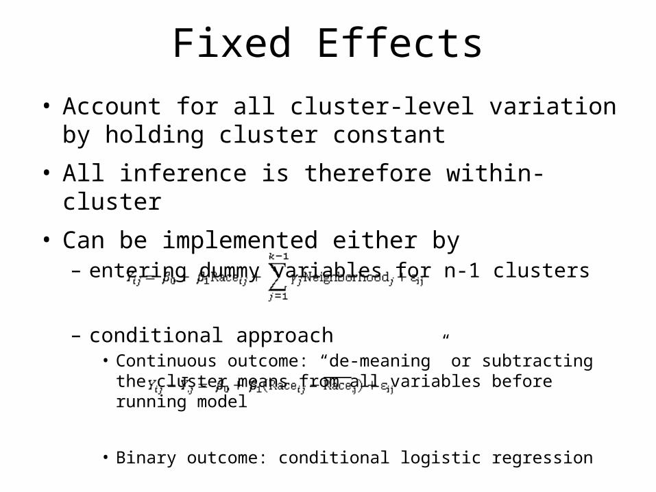
Comparison to Conventional RegressionUse cluster-robust SEs to account for complex error (individual and cluster)
reg ga_clean race, vce(cl b_group)
Linear regression Number of obs = 31489 F( 1, 389) = 351.42 Prob > F = 0.0000 R-squared = 0.0177 Root MSE = 2.1356
(Std. Err. adjusted for 390 clusters in b_group)------------------------------------------------------------------------------ | Robust ga_clean | Coef. Std. Err. t P>|t| [95% Conf. Interval]-------------+---------------------------------------------------------------- race | -.6112235 .0326053 -18.75 0.000 -.6753281 -.5471189 _cons | 39.09623 .014152 2762.59 0.000 39.0684 39.12405------------------------------------------------------------------------------
Crude effect: -0.61 weeksAdjusting for neighborhood: -0.47 weeks
Neighborhood explained 23% of the racial disparity (assuming there are no confounders of neighborhood)

Can use surveyreg for cluster-robust SEs in SAS
proc surveyreg data=nc.data_final;cluster b_group;class b_group ;model ga_clean= race /clparm solution;run;
The SURVEYREG Procedure
Regression Analysis for Dependent Variable ga_clean
Estimated Regression Coefficients
Standard 95% Confidence Parameter Estimate Error t Value Pr > |t| Interval
Intercept 39.0962254 0.01415202 2762.59 <.0001 39.0684014 39.1240495 race -0.6112235 0.03260526 -18.75 <.0001 -0.6753281 -0.5471189
NOTE: The denominator degrees of freedom for the t tests is 389.

Logistic Model for Binary Outcome
logit ptb_total i.race i.b_group, or
Logistic regression Number of obs = 31157 LR chi2(367) = 687.08 Prob > chi2 = 0.0000Log likelihood = -9091.5835 Pseudo R2 = 0.0364
------------------------------------------------------------------------------ ptb_total | Odds Ratio Std. Err. z P>|z| [95% Conf. Interval]-------------+---------------------------------------------------------------- race | 1.614217 .0849715 9.10 0.000 1.455979 1.789652 _Ib_group_2 | .7499313 .4644189 -0.46 0.642 .2227859 2.524383 _Ib_group_3 | .7817543 .4527046 -0.43 0.671 .2512752 2.432154 _Ib_group_4 | 1.837389 1.208127 0.93 0.355 .506426 6.66632 _Ib_group_5 | 1.012978 .6832426 0.02 0.985 .2700685 3.799497 _Ib_group_6 | 1.871619 1.284711 0.91 0.361 .4874589 7.186159 _Ib_group_7 | .6577316 .504969 -0.55 0.585 .1460644 2.961781 _Ib_group_8 | 4.113144 2.752025 2.11 0.035 1.108285 15.26498 _Ib_group_9 | .6818469 .7794273 -0.34 0.738 .0725551 6.407749_Ib_group_10 | 1.130029 1.000033 0.14 0.890 .1994381 6.40281
Accounting for neighborhood differences (within-neighborhood inference), the odds of PTB are 1.61 times greater for Black than White infants
23 clusters with 322 observations were dropped because of non-varying outcomes—all 0 or 1—division by 0 for an OR

margins race, vce(unconditional) post
Predictive margins Number of obs = 31157
Expression : Pr(ptb_total), predict()
(Std. Err. adjusted for 367 clusters in b_group2)------------------------------------------------------------------------------ | Unconditional | Margin Std. Err. z P>|z| [95% Conf. Interval]-------------+---------------------------------------------------------------- race | 0 | .0753146 .0021845 34.48 0.000 .071033 .0795962 1 | .1154796 .0039339 29.35 0.000 .1077693 .12319------------------------------------------------------------------------------
. lincom _b[1.race] - _b[0.race] Risk Difference
( 1) - 0bn.race + 1.race = 0
------------------------------------------------------------------------------ | Coef. Std. Err. z P>|z| [95% Conf. Interval]-------------+---------------------------------------------------------------- (1) | .040165 .0046569 8.62 0.000 .0310377 .0492924------------------------------------------------------------------------------
. nlcom _b[1.race] / _b[0.race] Risk Ratio
_nl_1: _b[1.race] / _b[0.race]
------------------------------------------------------------------------------ | Coef. Std. Err. z P>|z| [95% Conf. Interval]-------------+---------------------------------------------------------------- _nl_1 | 1.533297 .0713801 21.48 0.000 1.393394 1.673199------------------------------------------------------------------------------

proc logistic data=nc.data_final;class b_group ;model ptb_total (desc)= race b_group;run;
Odds Ratio Estimates
Point 95% Wald Effect Estimate Confidence Limits
race 1.614 1.456 1.790 b_group 370630001011 vs 371830544023 2.118 0.387 11.580 b_group 370630001012 vs 371830544023 1.588 0.314 8.034 b_group 370630001021 vs 371830544023 1.656 0.347 7.897 b_group 370630002001 vs 371830544023 3.891 0.727 20.828 b_group 370630002002 vs 371830544023 2.145 0.390 11.787 b_group 370630002003 vs 371830544023 3.964 0.709 22.160 b_group 370630003011 vs 371830544023 1.393 0.219 8.850 b_group 370630003012 vs 371830544023 8.710 1.599 47.453 b_group 370630003013 vs 371830544023 1.444 0.120 17.316 b_group 370630003021 vs 371830544023 2.393 0.311 18.388 b_group 370630003022 vs 371830544023 1.250 0.198 7.881 b_group 370630003023 vs 371830544023 2.515 0.431 14.684 b_group 370630004011 vs 371830544023 1.409 0.187 10.615 b_group 370630004012 vs 371830544023 2.206 0.347 14.033
…↓
Would need to use SUDAAN or binomial/poisson models for RD or RR in SAS
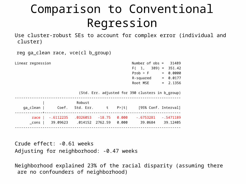
xtlogit ptb_total race, i(b_group) fe orclogit ptb_total race, group(b_group) vce(cl b_group) or
note: multiple positive outcomes within groups encountered.note: 23 groups (332 obs) dropped because of all positive or all negative outcomes.
Iteration 0: log pseudolikelihood = -8466.3107 Iteration 1: log pseudolikelihood = -8456.9979 Iteration 2: log pseudolikelihood = -8456.9975
Conditional (fixed-effects) logistic regression Number of obs = 31157 Wald chi2(1) = 84.25 Prob > chi2 = 0.0000Log pseudolikelihood = -8456.9975 Pseudo R2 = 0.0047
(Std. Err. adjusted for 367 clusters in b_group)------------------------------------------------------------------------------ | Robust ptb_total | Odds Ratio Std. Err. z P>|z| [95% Conf. Interval]-------------+---------------------------------------------------------------- 1.race | 1.604089 .0825837 9.18 0.000 1.450126 1.774398------------------------------------------------------------------------------
The conditional approach is recommended for non-linear models because of the incidental parameters problem with dummy variables, leading to upward bias. Mainly a problem for small clusters so not too different in this sample (avg cluster size ~80)
1.61 versus 1.60

proc logistic data=nc.data_final;strata b_group;model ptb_total (desc) = race;run;
The LOGISTIC Procedure
Conditional Analysis
Model Fit Statistics
Without With Criterion Covariates Covariates AIC 16994.399 16915.995 SC 16994.399 16924.352 -2 Log L 16994.399 16913.995
Testing Global Null Hypothesis: BETA=0
Test Chi-Square DF Pr > ChiSq Likelihood Ratio 80.4035 1 <.0001 Score 82.2342 1 <.0001 Wald 81.7008 1 <.0001
Analysis of Maximum Likelihood Estimates Standard Wald Parameter DF Estimate Error Chi-Square Pr > ChiSq race 1 0.4726 0.0523 81.7008 <.0001
Odds Ratio Estimates
Point 95% Wald Effect Estimate Confidence Limits
race 1.604 1.448 1.777

Comparison to Conventional Regressionlogit ptb_total race, vce(cl b_group) or
Logistic regression Number of obs = 31489 Wald chi2(1) = 278.47 Prob > chi2 = 0.0000Log pseudolikelihood = -9312.2722 Pseudo R2 = 0.0163
(Std. Err. adjusted for 390 clusters in b_group)------------------------------------------------------------------------------ | Robust ptb_total | Odds Ratio Std. Err. z P>|z| [95% Conf. Interval]-------------+---------------------------------------------------------------- race | 2.02922 .0860517 16.69 0.000 1.86738 2.205085------------------------------------------------------------------------------
Crude OR: 2.03Adjusting for neighborhood: 1.60
Neighborhood explained ~40% of the racial disparity in PTB (assuming there are no confounders of neighborhood)
N.B. For percent change in OR, you always need to subtract the null (1.0) first(0.6-1.03)/1.03 = -.41 or a drop of 41% after controlling for contextual differences

proc surveylogistic data=nc.data_final;cluster b_group;model ptb_total (desc)= race;run;
Testing Global Null Hypothesis: BETA=0
Test Chi-Square DF Pr > ChiSq
Likelihood Ratio 308.0644 1 <.0001 Score 324.9556 1 <.0001 Wald 278.4631 1 <.0001
Analysis of Maximum Likelihood Estimates
Standard Wald Parameter DF Estimate Error Chi-Square Pr > ChiSq
Intercept 1 -2.6016 0.0285 8352.0534 <.0001 race 1 0.7077 0.0424 278.4631 <.0001
Odds Ratio Estimates
Point 95% Wald Effect Estimate Confidence Limits
race 2.029 1.867 2.205
Association of Predicted Probabilities and Observed Responses
Percent Concordant 32.9 Somers' D 0.167 Percent Discordant 16.2 Gamma 0.340 Percent Tied 50.8 Tau-a 0.027 Pairs 80536248 c 0.584
Fixed Effects: Benefits & Disadvantages
• Benefits: – Provides within-cluster effects that are not confounded by
cluster-level factors because all cluster variation is removed (accounts for unobservable confounding)
– No minimum number of clusters
• Disadvantages: – Does not allow estimation of observable cluster-level
effects so often seen more in longitudinal analyses where between-cluster effects may not be of interest
– Can be inefficient/less precise due to less degrees of freedom (each cluster counts as parameter) and it only exploits one level of variation

Random Effects• Alternative to fixed effects that models only one
additional parameter (instead of k-1) by making greater assumptions
• More efficient but vulnerable to bias• Average cluster-specific intercept with the cluster-level
variance estimated (τ₀2)
• Accounts for variability in the outcome across neighborhoods but not for covariates (corr μoj, xi = 0)
• Allows estimates of variance at both levels and of cluster-level covariates because the cluster-level variance isn’t completely removed from model

xtreg ga_clean race, i(b_group) re mle
Random-effects ML regression Number of obs = 31489Group variable: b_group Number of groups = 390
Random effects u_i ~ Gaussian Obs per group: min = 1 avg = 80.7 max = 652
LR chi2(1) = 389.27Log likelihood = -68563.638 Prob > chi2 = 0.0000
------------------------------------------------------------------------------ ga_clean | Coef. Std. Err. z P>|z| [95% Conf. Interval]-------------+---------------------------------------------------------------- race | -.5883143 .027936 -21.06 0.000 -.6430679 -.5335606 _cons | 39.07689 .0180206 2168.46 0.000 39.04157 39.11221-------------+---------------------------------------------------------------- /sigma_u | .1364134 .021792 .0997419 .1865676 /sigma_e | 2.131475 .0085433 2.114796 2.148285 rho | .0040792 .0013011 .0021387 .0074679------------------------------------------------------------------------------Likelihood-ratio test of sigma_u=0: chibar2(01)= 18.07 Prob>=chibar2 = 0.000
Cluster-specific, within-neighborhood interpretation but significantly higher than FE estimate of -0.47
Intracluster Correlation = 0.004 (proportion of variance that occurs at neighborhood level)0.1362/(0.1362+2.132) = 0.004- Significant neighborhood variation but a small fraction of overall variability (0.4%)

proc glimmix data=nc.data_final method=quad;class b_group;model ga_clean = race /solution ;random intercept/ subject=b_group;run; The GLIMMIX Procedure Optimization Information
Optimization Technique Dual Quasi-Newton Parameters in Optimization 4 Lower Boundaries 2 Upper Boundaries 0 Fixed Effects Not Profiled Starting From GLM estimates Quadrature Points 1
Covariance Parameter Estimates Standard Cov Parm Subject Estimate Error
Intercept b_group 0.01861 0.005946 Residual 4.5432 0.03642
Solutions for Fixed Effects
Standard Effect Estimate Error DF t Value Pr > |t|
Intercept 39.0769 0.01802 389 2168.69 <.0001 race -0.5883 0.02793 31098 -21.06 <.0001
Type III Tests of Fixed Effects
Num Den Effect DF DF F Value Pr > F
race 1 31098 443.54 <.0001

xtlogit ptb_total race, i(b_group) re or
Random-effects logistic regression Number of obs = 31489Group variable: b_group Number of groups = 390
Random effects u_i ~ Gaussian Obs per group: min = 1 avg = 80.7 max = 652
Wald chi2(1) = 265.00Log likelihood = -9310.5391 Prob > chi2 = 0.0000
------------------------------------------------------------------------------ ptb_total | OR Std. Err. z P>|z| [95% Conf. Interval]-------------+---------------------------------------------------------------- race | 1.992814 .0844133 16.28 0.000 1.834049 2.165323-------------+---------------------------------------------------------------- /lnsig2u | -4.059262 .6231052 -5.280526 -2.837999-------------+---------------------------------------------------------------- sigma_u | .131384 .040933 .0713425 .241956 rho | .0052196 .0032354 .0015447 .0174837------------------------------------------------------------------------------Likelihood-ratio test of rho=0: chibar2(01) = 3.47 Prob >= chibar2 = 0.031
Cluster-specific, within-neighborhood interpretation but significantly higher than FE estimate of 1.60
Intracluster Correlation = 0.005 (most of variance occurs within neighborhood at the individual level, 99.5%, rather than between neighborhoods at neighborhood level, 0.5%)0.1314/(0.1314 + π2/3) = 0.005

proc glimmix data=nc.data_final method=quad;class b_group;model ptb_total (descending) = race /solution dist=bin link=logit oddsratio;random intercept / subject=b_group;run; Covariance Parameter Estimates Standard Cov Parm Subject Estimate Error
Intercept b_group 0.01746 0.01081
Solutions for Fixed Effects
Standard Effect Estimate Error DF t Value Pr > |t|
Intercept -2.5945 0.02907 389 -89.26 <.0001 race 0.6894 0.04238 31098 16.27 <.0001
Odds Ratio Estimates 95% Confidence race _race Estimate DF Limits
1.3261 0.3261 1.992 31098 1.834 2.165
Type III Tests of Fixed Effects
Num Den Effect DF DF F Value Pr > F
race 1 31098 264.60 <.0001

Random Intercept + Slope • Also possible to allow random normal variation in covariate effect across neighborhood, e.g. allowing
racial disparity to vary by neighborhood
xtmixed ga_clean race || b_group: race, mle
Mixed-effects ML regression Number of obs = 31489Group variable: b_group Number of groups = 390 Obs per group: min = 1 avg = 80.7 max = 652 Wald chi2(1) = 304.72Log likelihood = -68537.949 Prob > chi2 = 0.0000------------------------------------------------------------------------------ ga_clean | Coef. Std. Err. z P>|z| [95% Conf. Interval]-------------+---------------------------------------------------------------- race | -.6060449 .0347181 -17.46 0.000 -.6740911 -.5379988 _cons | 39.09577 .0147177 2656.37 0.000 39.06693 39.12462------------------------------------------------------------------------------------------------------------------------------------------------------------ Random-effects Parameters | Estimate Std. Err. [95% Conf. Interval]-----------------------------+------------------------------------------------b_group: Independent | sd(race) | .3447168 .0374273 .2786404 .4264626 sd(_cons) | .0221739 .0600709 .0001096 4.485535-----------------------------+------------------------------------------------ sd(Residual) | 2.127355 .0085317 2.110699 2.144143------------------------------------------------------------------------------LR test vs. linear regression: chi2(2) = 69.45 Prob > chi2 = 0.0000Note: LR test is conservative and provided only for reference.
• Appears to be significant variation across neighborhoods but the point estimate or average within-neighborhood disparity is not correct based on comparisons to FE models (-0.47)

proc glimmix data=nc.data_final method=quad;class b_group;model ga_clean = race /solution ;random intercept race/ subject=b_group;Run; The GLIMMIX Procedure
Covariance Parameter Estimates
Standard Cov Parm Subject Estimate Error
Intercept b_group 0.000494 0.003077 race b_group 0.1188 0.02584 Residual 4.5256 0.03631
Solutions for Fixed Effects
Standard Effect Estimate Error DF t Value Pr > |t|
Intercept 39.0958 0.01498 389 2609.64 <.0001 race -0.6060 0.03488 352 -17.38 <.0001
Type III Tests of Fixed Effects
Num Den Effect DF DF F Value Pr > F
race 1 352 301.93 <.0001

xtmelogit ptb_total race || b_group: race, or
Mixed-effects logistic regression Number of obs = 31489Group variable: b_group Number of groups = 390
Obs per group: min = 1 avg = 80.7 max = 652
Integration points = 7 Wald chi2(1) = 255.50Log likelihood = -9310.2914 Prob > chi2 = 0.0000
------------------------------------------------------------------------------ ptb_total | Odds Ratio Std. Err. z P>|z| [95% Conf. Interval]-------------+---------------------------------------------------------------- race | 1.991382 .0858163 15.98 0.000 1.830093 2.166887------------------------------------------------------------------------------
------------------------------------------------------------------------------ Random-effects Parameters | Estimate Std. Err. [95% Conf. Interval]-----------------------------+------------------------------------------------b_group: Independent | sd(race) | .1218997 .0899226 .0287138 .5175045 sd(_cons) | .1101542 .0562791 .040468 .2998403------------------------------------------------------------------------------LR test vs. logistic regression: chi2(2) = 3.96 Prob > chi2 = 0.1380
Note: LR test is conservative and provided only for reference.
No indication of significant neighborhood variation in the PTB racial disparity; average neighborhood-specific disparity is biased relative to FE (1.60)

proc glimmix data=nc.data_final method=quad;class b_group;model ptb_total (descending) = race /solution dist=bin link=logit oddsratio;random intercept race/ subject=b_group;run; Covariance Parameter Estimates
Standard Cov Parm Subject Estimate Error
Intercept b_group 0.01230 0.01248 race b_group 0.01495 0.02201
Solutions for Fixed Effects
Standard Effect Estimate Error DF t Value Pr > |t|
Intercept -2.5967 0.02875 389 -90.31 <.0001 race 0.6886 0.04312 352 15.97 <.0001
Odds Ratio Estimates 95% Confidence race _race Estimate DF Limits
1.3261 0.3261 1.991 352 1.829 2.167
Type III Tests of Fixed Effects
Num Den Effect DF DF F Value Pr > F
race 1 352 255.04 <.0001

When will RE approximate FE?
• When there is no between-cluster confounding– No clustering of X – No variation in outcome by cluster
• Even when confounding is present, RE can still approximate FE under certain conditions– Normally, a composite of within and between
effects but weighted toward the within-effect when it is more precise• Large cluster size • High ICC

Example• Most of variation
is between rather than within cluster (ICC=0.99) so within-effect is going to be very precise (little variability)5
0100
150
200
15 20 25 30 35x
---------------------------------------------------------------- Variable | ols olsc gee fe re -------------+-------------------------------------------------- x | -2.2152 -2.2152 2.0552 2.0563 2.0503 | 0.799 1.189 0.044 0.045 0.054 _cons | 166.0880 166.0880 67.3646 67.3404 67.4793 | 18.868 28.958 13.615 1.049 7.058 ---------------------------------------------------------------- legend: b/se

• For most multilevel neighborhood studies, ICC is quite low (<10%) so only a huge cluster size could compensate to get valid within-cluster estimates in the presence of neighborhood confounding
• We can also control for observable cluster-level factors but there are many factors that may not be measured or imperfectly measured• e.g. built environment, air quality/toxins, health care
access/quality, fresh foods, social cohesion
• So it can be rare to get the FE estimate, which controls for all factors--observed and unobserved, by controlling only for a few observed factors in a RE model

xtreg ga_clean race poverty, i(b_group) re mle
Random-effects ML regression Number of obs = 31489Group variable: b_group Number of groups = 390
Random effects u_i ~ Gaussian Obs per group: min = 1 avg = 80.7 max = 652
LR chi2(2) = 407.38Log likelihood = -68554.58 Prob > chi2 = 0.0000
------------------------------------------------------------------------------ ga_clean | Coef. Std. Err. z P>|z| [95% Conf. Interval]-------------+---------------------------------------------------------------- race | -.5368362 .030145 -17.81 0.000 -.5959193 -.477753 poverty | -.0064216 .0015111 -4.25 0.000 -.0093832 -.0034599 _cons | 39.1246 .0205574 1903.19 0.000 39.08431 39.16489-------------+---------------------------------------------------------------- /sigma_u | .1304851 .0218083 .0940368 .1810607 /sigma_e | 2.131108 .0085401 2.114436 2.147913 rho | .003735 .0012466 .0018992 .007028------------------------------------------------------------------------------Likelihood-ratio test of sigma_u=0: chibar2(01)= 15.89 Prob>=chibar2 = 0.000
So controlling for poverty moves us closer to the within-cluster effect but doesn’t control for all important neighborhood factorsCrude: -0.61 FE: -0.47 Controlling for neighborhood poverty: -0.54Explains about half of the neighborhood contribution (0.07/0.14)And 11.5% of overall disparity (0.07/-0.61)

Hausman test for consistency in estimates from FE and RE models
hausman ga_clean_fe ga_clean_re_poverty
---- Coefficients ---- | (b) (B) (b-B) sqrt(diag(V_b-V_B)) | ga_clean_fe ga_clean_r~y Difference S.E.-------------+---------------------------------------------------------------- race | -.4692281 -.5500752 .080847 .0156404------------------------------------------------------------------------------ b = consistent under Ho and Ha; obtained from xtreg B = inconsistent under Ha, efficient under Ho; obtained from xtreg
Test: Ho: difference in coefficients not systematic
chi2(1) = (b-B)'[(V_b-V_B)^(-1)](b-B) = 26.72 Prob>chi2 = 0.0000
Rejects the null of equivalence between the FE and RE estimator
**From a RE model that is based on generalized least squares, not maximum likelihood

xtlogit ptb_total race poverty, i(b_group) re or
Random-effects logistic regression Number of obs = 31489Group variable: b_group Number of groups = 390
Random effects u_i ~ Gaussian Obs per group: min = 1 avg = 80.7 max = 652
Wald chi2(2) = 316.05Log likelihood = -9297.2331 Prob > chi2 = 0.0000
------------------------------------------------------------------------------ ptb_total | OR Std. Err. z P>|z| [95% Conf. Interval]-------------+---------------------------------------------------------------- race | 1.804966 .0834998 12.77 0.000 1.64851 1.976272 poverty | 1.010437 .0020192 5.20 0.000 1.006487 1.014403-------------+---------------------------------------------------------------- /lnsig2u | -4.32276 .7583429 -5.809085 -2.836435-------------+---------------------------------------------------------------- sigma_u | .1151661 .0436677 .0547739 .2421452 rho | .0040153 .0030328 .0009111 .0175106------------------------------------------------------------------------------Likelihood-ratio test of rho=0: chibar2(01) = 2.21 Prob >= chibar2 = 0.068
So controlling for poverty moves us closer to the within-cluster effect but doesn’t control for all important neighborhood factorsCrude: 2.03 FE: 1.60 Controlling for neighborhood poverty: 1.80Explains about half of the neighborhood contribution (0.2/0.43)And 20% of overall disparity (0.2/1.03)

Hausman test for consistency in estimates from FE and RE models
hausman ptb_fe ptb_re_poverty
---- Coefficients ---- | (b) (B) (b-B) sqrt(diag(V_b-V_B)) | ptb_fe ptb_re_pov~y Difference S.E.-------------+---------------------------------------------------------------- race | .4725559 .590542 -.1179861 .0243549------------------------------------------------------------------------------ b = consistent under Ho and Ha; obtained from xtlogit B = inconsistent under Ha, efficient under Ho; obtained from xtlogit
Test: Ho: difference in coefficients not systematic
chi2(1) = (b-B)'[(V_b-V_B)^(-1)](b-B) = 23.47 Prob>chi2 = 0.0000
Rejects the null of equivalence between the FE and RE estimator

Random Effects: Benefits & Disadvantages
• Benefits: – Ability to estimate covariates both within and
between cluster (level 1 and 2 effects)– Ability to partition variance at multiple levels– Examine variation in effects across cluster– Efficient/parsimonious
• Disadvantages: – Within-cluster effects can be significantly biased– Requires ~30 clusters for estimation of cluster
variance with random normal assumption

GEE• Handles clustered data with complex error
treated as a nuisance rather than explicitly controlled (FE) or modeled as an interest (RE)
• Within-cluster correlation specified as – Independent (robust SEs, point estimates unchanged)– Exchangeable (similar to RE point estimates)– Unstructured (allows variation in correlation)
• Inference is population-averaged rather than cluster-specific (only difference is for odds ratio since the average of each cluster-specific OR ≠ overall OR; not collapsible)

xtreg ga_clean race, i(b_group) pa corr(ind) vce(robust)xtgee ga_clean race, corr(ind) vce(robust)
Iteration 1: tolerance = 6.133e-15
GEE population-averaged model Number of obs = 31489Group variable: b_group Number of groups = 390Link: identity Obs per group: min = 1Family: Gaussian avg = 80.7Correlation: independent max = 652 Wald chi2(1) = 351.43Scale parameter: 4.560647 Prob > chi2 = 0.0000
Pearson chi2(31489): 143610.20 Deviance = 143610.20Dispersion (Pearson): 4.560647 Dispersion = 4.560647
(Std. Err. adjusted for clustering on b_group)------------------------------------------------------------------------------ | Semirobust ga_clean | Coef. Std. Err. z P>|z| [95% Conf. Interval]-------------+---------------------------------------------------------------- race | -.6112235 .0326047 -18.75 0.000 -.6751276 -.5473194 _cons | 39.09623 .0141518 2762.63 0.000 39.06849 39.12396------------------------------------------------------------------------------
Results are very similar to OLS regression with cluster-robust SEs

xtreg ga_clean race, i(b_group) pa corr(exc)xtgee ga_clean race, corr(exc) vce(robust)
Iteration 1: tolerance = .00997269Iteration 2: tolerance = .00071555Iteration 3: tolerance = .00004882Iteration 4: tolerance = 3.319e-06Iteration 5: tolerance = 2.256e-07
GEE population-averaged model Number of obs = 31489Group variable: b_group Number of groups = 390Link: identity Obs per group: min = 1Family: Gaussian avg = 80.7Correlation: exchangeable max = 652 Wald chi2(1) = 350.49Scale parameter: 4.560803 Prob > chi2 = 0.0000
(Std. Err. adjusted for clustering on b_group)------------------------------------------------------------------------------ | Semirobust ga_clean | Coef. Std. Err. z P>|z| [95% Conf. Interval]-------------+---------------------------------------------------------------- race | -.5939304 .0317245 -18.72 0.000 -.6561093 -.5317514 _cons | 39.08105 .013988 2793.91 0.000 39.05364 39.10847------------------------------------------------------------------------------
Results are very similar to the random intercept model with cluster-robust SEs

proc genmod data=nc.data_final;class b_group;model ga_clean = race;repeated subject=b_group /corr=ind;run;
Analysis Of GEE Parameter Estimates Empirical Standard Error Estimates
Standard 95% Confidence Parameter Estimate Error Limits Z Pr > |Z|
Intercept 39.0962 0.0141 39.0685 39.1239 2766.18 <.0001 race -0.6112 0.0326 -0.6750 -0.5474 -18.77 <.0001
proc genmod data=nc.data_final;class b_group;model ga_clean = race;repeated subject=b_group /corr=exc;run; Exchangeable Working Correlation Correlation 0.0028899011
Analysis Of GEE Parameter Estimates Empirical Standard Error Estimates
Standard 95% Confidence Parameter Estimate Error Limits Z Pr > |Z|
Intercept 39.0811 0.0140 39.0537 39.1084 2797.50 <.0001 race -0.5939 0.0317 -0.6560 -0.5318 -18.75 <.0001

xtlogit ptb_total race, i(b_group) pa corr(ind) vce(robust) orxtgee ptb_total race, fam(bin) link(logit) corr(ind) vce(robust) eform
Iteration 1: tolerance = 1.545e-07
GEE population-averaged model Number of obs = 31489Group variable: b_group Number of groups = 390Link: logit Obs per group: min = 1Family: binomial avg = 80.7Correlation: independent max = 652 Wald chi2(1) = 278.47Scale parameter: 1 Prob > chi2 = 0.0000
Pearson chi2(31489): 31489.00 Deviance = 18624.54Dispersion (Pearson): 1 Dispersion = .5914619
(Std. Err. adjusted for clustering on b_group)------------------------------------------------------------------------------ | Semirobust ptb_total | Odds Ratio Std. Err. z P>|z| [95% Conf. Interval]-------------+---------------------------------------------------------------- race | 2.02922 .0860517 16.69 0.000 1.867381 2.205086------------------------------------------------------------------------------
Results are very similar to logistic regression with cluster-robust SEs

xtlogit ptb_total race, i(b_group) pa corr(exc) vce(robust) orxtgee ptb_total race, fam(bin) link(logit) corr(exc) vce(robust) eform
Iteration 1: tolerance = .00895091Iteration 2: tolerance = .00071972Iteration 3: tolerance = .00006077Iteration 4: tolerance = 5.223e-06Iteration 5: tolerance = 4.495e-07
GEE population-averaged model Number of obs = 31489Group variable: b_group Number of groups = 390Link: logit Obs per group: min = 1Family: binomial avg = 80.7Correlation: exchangeable max = 652 Wald chi2(1) = 269.83Scale parameter: 1 Prob > chi2 = 0.0000
(Std. Err. adjusted for clustering on b_group)------------------------------------------------------------------------------ | Semirobust ptb_total | Odds Ratio Std. Err. z P>|z| [95% Conf. Interval]-------------+---------------------------------------------------------------- race | 1.995782 .0839587 16.43 0.000 1.837828 2.167313------------------------------------------------------------------------------
Results are very similar to RE logistic regression with cluster-robust SEsICC is so low that marginal OR ≈ cluster-specific OR

proc genmod data=nc.data_final;class b_group;model ptb_total = race /dist=bin link=logit;repeated subject=b_group/corr=ind;estimate 'race or' race -1 1 /exp;run; Contrast Estimate Results
Mean Mean L'Beta Standard L'Beta Label Estimate Confidence Limits Estimate Error Alpha Confidence Limits
race or 0.6699 0.6513 0.6880 0.7077 0.0424 0.05 0.6246 0.7907 Exp(race or) 2.0292 0.0859 0.05 1.8676 2.2049
proc genmod data=nc.data_final;class b_group;model ptb_total = race /dist=bin link=logit;repeated subject=b_group/corr=exc;estimate 'race or' race -1 1 /exp;run; Contrast Estimate Results
Mean Mean L'Beta Standard L'Beta Label Estimate Confidence Limits Estimate Error Alpha Confidence Limits
race or 0.6662 0.6476 0.6843 0.6910 0.0420 0.05 0.6087 0.7734 Exp(race or) 1.9958 0.0839 0.05 1.8380 2.1671

GEE: Benefits & Disadvantages
• Benefits:– Ability to estimate both within and between-
cluster effects and adjust SEs for clustering– Examine cross-level interaction
• Disadvantages: – Within-cluster effects can be significantly biased – Marginal inference leads to effect estimates closer
to the null in logistic models (depending on ICC)– No variance components

Hybrid Models• Obtain the appropriate within-neighborhood effect in
random effects, GEE, or general cluster-robust models• Contain the advantages of RE or GEE models without
the bias in the within-cluster effects• Incorporate the cluster-mean of the covariate to
account for all between-cluster variation related to the covariate (aggregated variable, % Black)– Centering (subtracting cluster-mean)
– Centering + cluster-mean covariate adjustment
– Cluster-mean covariate adjustment

egen race_bgc=mean(race), by(b_group)gen race_c=race-race_bgcxtreg ga_clean race_c, i(b_group) re mle
Random-effects ML regression Number of obs = 31489Group variable: b_group Number of groups = 390Random effects u_i ~ Gaussian Obs per group: min = 1 avg = 80.7 max = 652
LR chi2(1) = 201.73Log likelihood = -68657.406 Prob > chi2 = 0.0000------------------------------------------------------------------------------ ga_clean | Coef. Std. Err. z P>|z| [95% Conf. Interval]-------------+---------------------------------------------------------------- race_c | -.4692281 .0329833 -14.23 0.000 -.5338742 -.404582 _cons | 38.85962 .0206466 1882.13 0.000 38.81915 38.90008-------------+---------------------------------------------------------------- /sigma_u | .291513 .0203577 .2542229 .3342729 /sigma_e | 2.130663 .0085431 2.113985 2.147473 rho | .0183752 .0025312 .0139516 .0239413------------------------------------------------------------------------------Likelihood-ratio test of sigma_u=0: chibar2(01)= 193.82 Prob>=chibar2 = 0.000
Estimate now corresponds to within-neighborhood effect of race obtained in FE model (-0.47)
-Note that the ICC is now much larger than in the RE model (0.004 0.018)-Neighborhood variance increased because centering removed the association between race and neighborhood before estimation so this refers to the ICC from a null model-No other variables in the model (including random intercept) will be adjusted for

PROC SUMMARY NWAY DATA=nc.data;VAR race;CLASS b_group;OUTPUT OUT=cluster MEAN=race_bgc;RUN;
DATA nc.data_final;MERGE nc.data cluster;BY b_group;race_c=race-race_bgc;RUN;
proc glimmix data=nc.data_final method=quad;class b_group;model ga_clean = race_c /solution ;random intercept / subject=b_group;run; Covariance Parameter Estimates
Standard Cov Parm Subject Estimate Error
Intercept b_group 0.08497 0.01187 Residual 4.5397 0.03641
Solutions for Fixed Effects Standard Effect Estimate Error DF t Value Pr > |t|
Intercept 38.8596 0.02065 389 1882.23 <.0001 race_c -0.4692 0.03298 31098 -14.23 <.0001

xtlogit ptb_total race_c, i(b_group) re or
Random-effects logistic regression Number of obs = 31489Group variable: b_group Number of groups = 390
Random effects u_i ~ Gaussian Obs per group: min = 1 avg = 80.7 max = 652
Wald chi2(1) = 83.13Log likelihood = -9384.2229 Prob > chi2 = 0.0000
------------------------------------------------------------------------------ ptb_total | OR Std. Err. z P>|z| [95% Conf. Interval]-------------+---------------------------------------------------------------- race_c | 1.610407 .0841611 9.12 0.000 1.453621 1.784104-------------+---------------------------------------------------------------- /lnsig2u | -2.192009 .1819926 -2.548708 -1.83531-------------+---------------------------------------------------------------- sigma_u | .3342037 .0304113 .2796115 .3994546 rho | .0328355 .0057796 .023213 .046258------------------------------------------------------------------------------Likelihood-ratio test of rho=0: chibar2(01) = 83.11 Prob >= chibar2 = 0.000
OR now corresponds to within-neighborhood effect of race obtained in FE model (1.61)
ICC is now much larger than in the RE model (0.005 0.032) because it is not adjusted for racial clustering/segregation across neighborhoods

PROC SUMMARY NWAY DATA=nc.data;VAR race;CLASS b_group;OUTPUT OUT=cluster MEAN=race_bgc;RUN;
DATA nc.data_final;MERGE nc.data cluster;BY b_group;race_c=race-race_bgc;RUN;
proc glimmix data=nc.data_final method=quad;class b_group;model ptb_total (descending) = race_c /solution dist=bin link=logit oddsratio;random intercept / subject=b_group;run; Covariance Parameter Estimates Standard Cov Parm Subject Estimate Error Intercept b_group 0.1113 0.02016
Solutions for Fixed Effects Standard Effect Estimate Error DF t Value Pr > |t|
Intercept -2.3408 0.02861 389 -81.82 <.0001 race_c 0.4764 0.05226 31098 9.12 <.0001
Odds Ratio Estimates 95% Confidence race_c _race_c Estimate DF Limits
1 -1E-9 1.610 31098 1.454 1.784
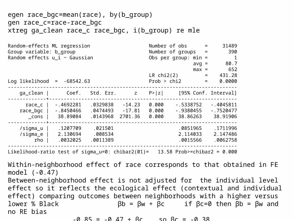
egen race_bgc=mean(race), by(b_group)gen race_c=race-race_bgcxtreg ga_clean race_c race_bgc, i(b_group) re mle
Random-effects ML regression Number of obs = 31489Group variable: b_group Number of groups = 390Random effects u_i ~ Gaussian Obs per group: min = 1 avg = 80.7 max = 652 LR chi2(2) = 431.28Log likelihood = -68542.63 Prob > chi2 = 0.0000------------------------------------------------------------------------------ ga_clean | Coef. Std. Err. z P>|z| [95% Conf. Interval]-------------+---------------------------------------------------------------- race_c | -.4692281 .0329838 -14.23 0.000 -.5338752 -.4045811 race_bgc | -.8450466 .0474493 -17.81 0.000 -.9380455 -.7520477 _cons | 38.89084 .0143968 2701.36 0.000 38.86263 38.91906-------------+---------------------------------------------------------------- /sigma_u | .1207709 .021501 .0851965 .1711996 /sigma_e | 2.130694 .008534 2.114033 2.147486 rho | .0032025 .0011389 .0015566 .0062758------------------------------------------------------------------------------Likelihood-ratio test of sigma_u=0: chibar2(01)= 13.58 Prob>=chibar2 = 0.000
Within-neighborhood effect of race corresponds to that obtained in FE model (-0.47)Between-neighborhood effect is not adjusted for the individual level effect so it reflects the ecological effect (contextual and individual effect) comparing outcomes between neighborhoods with a higher versus lower % Black βb = βw + βc if βc=0 then βb = βw and no RE bias
-0.85 = -0.47 + βc so βc = -0.38-Note that the ICC is now small again because it’s adjusted for cluster mean of race (composition/segregation)

egen race_bgc=mean(race), by(b_group)xtreg ga_clean race race_bgc, i(b_group) re mle
Random-effects ML regression Number of obs = 31489Group variable: b_group Number of groups = 390Random effects u_i ~ Gaussian Obs per group: min = 1 avg = 80.7 max = 652 LR chi2(2) = 431.28Log likelihood = -68542.63 Prob > chi2 = 0.0000
------------------------------------------------------------------------------ ga_clean | Coef. Std. Err. z P>|z| [95% Conf. Interval]-------------+---------------------------------------------------------------- race | -.4692281 .0329838 -14.23 0.000 -.5338752 -.4045811 race_bgc | -.3758185 .0577872 -6.50 0.000 -.4890794 -.2625576 _cons | 39.04385 .0179707 2172.64 0.000 39.00863 39.07907-------------+---------------------------------------------------------------- /sigma_u | .1207709 .021501 .0851965 .1711996 /sigma_e | 2.130694 .008534 2.114033 2.147486 rho | .0032025 .0011389 .0015566 .0062758------------------------------------------------------------------------------Likelihood-ratio test of sigma_u=0: chibar2(01)= 13.58 Prob>=chibar2 = 0.000
Without cluster –mean centering , the cluster mean variable now refers to the contextual effect of racial segregation because it is now correlated with and can be adjusted for the individual effect
Refers to the effect of living in a more segregated neighborhood regardless of whether you are black or white βc = βb - βw = -0.38 Because it is significantly different from zero, there is evidence of a contextual effect , βw ≠ βb
corr μoj, xi ≠ 0

Caveats
• Cluster-mean adjustment is a convenient way to account for cluster-level confounding but there are some important considerations– Cluster mean must always come from sample (not
external population, e.g. census % Black)– Other covariates may also require cluster-mean
adjustment if they’re confounders of the principal covariate and also vary by cluster
– Should always compare to FE estimates– For complex survey data, weights may need to be
scaled for multilevel models and the hybrid approach may only work if there is minimal sampling bias

Examples
Multilevel data structure• Neighborhood models• Sibling studies
Longitudinal data structure• Policy evaluation (state panels)

Neighborhood Contribution to Black White Perinatal Disparities
• Used hybrid models (cluster-mean adjustment) to evaluate the impact of neighborhood inequalities to racial disparities
• Adjusted for individual-level factors that could influence neighborhood selection (age, education, marital status, gravidity)
• Neighborhoods made a significant contribution to PTB (~15% disparity reduction)
• Effect of neighborhood segregation wasn’t fully explained by neighborhood poverty
• May need to consider context across the life courseSchempf AH, Kaufman JS, Messer LC, Mendola P. The neighborhood contribution to black-white perinatal disparities: an example from two north Carolina counties, 1999-2001. Am J Epidemiol. 2011;174(6):744-52.

Neighborhood Contribution to Hypertension Disparities
• Used cluster-mean centering for all covariates compared to RE model with neighborhood-level covariates
• Neighborhood differences helped to entirely explain the residual black-white hypertension disparity after adjustment for individual-level factors– OR 1.5 1.0
• Measured neighborhood variables (poverty/affluence, Hispanic, age composition) accounted for entire neighborhood contribution– OR still 1.0 without cluster-mean centering
Morenoff JD, House JS, Hansen BB, et al. Understanding social disparities in hypertension prevalence, awareness, treatment, and control: the role of neighborhood context. Soc Sci Med. 2007;65(9):1853-1866.

Gestational Weight Gain and Child BMI• Siblings nested within mothers (CPP)• Used FE models to account for unobserved family
level factors (environmental/genetic) that may be associated with both GWG and child BMI
• GEE (independent) models showed associations between GWG and child BMI
• FE models, comparing only changes in GWG between pregnancies within the same mother, showed no effect on child BMI
• May be nothing deterministic about in-utero exposures
Branum AM, Parker JD, Keim SA, Schempf AH. Prepregnancy body mass index and gestational weight gain in relation to child body mass index among siblings. Am J Epidemiol. 2011 Nov 15;174(10):1159-65.

Breastfeeding and Child BMI
• Breastfeeding is often associated with many positive health outcomes but it’s unclear whether this is due to confounding by selection (unobserved characteristics)
• Siblings nested within mother (add-health)• Used FE models to contrast outcomes for discordant
siblings (one breastfed, one formula fed)• No effect of different breastfeeding exposure on
adolescent overweight within siblings to the same mother
• Changing a woman’s breastfeeding behavior is not likely to change child BMI; many benefits of breastfeeding but reducing obesity may not be oneNelson MC, Gordon-Larsen P, Adair LS. Are adolescents who were breast-fed less likely to be overweight?
Analyses of sibling pairs to reduce confounding. Epidemiology. 2005 Mar;16(2):247-53.

Policy Evaluation
• Cross sectional analyses comparing jurisdictions with a policy to those without can be severely biased (between-cluster)
• States/counties/hospitals may institute policies in response to a problem (reverse causality)
• States/counties/hospitals may institute policies if they are more progressive; already healthier (selection, omitted variable bias)
• Need longitudinal inference, comparing outcomes before and after policy change within a given unit to contemporaneous controls for time trend irrespective of policy change

Difference in Difference
T=Treatment C=Control B=Before A=AfterDiD 1) (YT – YC, A) – (YT – YC, B) = 1
2) (YA – YB, T) – (YA – YB, C) = 1
Cross-sectional: (YT – YC, A) = 3
Pre-Post: (YA – YB, T) = 3
Could be an example of selection for a positive health indicatore.g. breastfeeding laws
Before After012345
TreatmentControl

Difference in Difference
T=Treatment C=Control B=Before A=AfterDiD 1) (YT – YC, A) – (YT – YC, B) = -1
2) (YA – YB, T) – (YA – YB, C) = -1
Cross-sectional: (YT – YC, A) = 1
Pre-Post: (YA – YB, T) = 1
Could be an example of reverse causality for a negative indicatore.g. school nutrition/activity policies and obesity
Before After012345
TreatmentControl

Fixed Effects Panel Analysis
Design- Same as Difference in Difference but extends beyond
two periods and requires multiple units Yjt = βo + βPjt + βj + βt + βXjt + ejt
- Within-unit contrasts with between-unit contemporaneous controls are achieved by entering unit level dummy variables (βj) along with time indicator (βt)
- 3+ time points can control for unit-specific trends that may be simultaneous to policy changes

Sample Software Code
SASProc reg; *Proc logistic;Class state year;Model Y= x state year;Run;
Proc logistic;Class state year;Model Y= x year;Strata state;Run;
STATAxi: reg y x i.year i.statexi: logit y x i.year i.state
xi: xtreg y x i.year, i(state) fexi: xtlogit y x i.year, i(state) fexi: clogit y x i.year, group(state)
Applied Example Objective
• To evaluate and compare the impact of state-specific changes in smoking-related policies on childhood asthma prevalence & severity

Data• Individual-level outcome data come from available
waves of NSCH (2003 & 2007)– Parent-reported current asthma– Severity of current asthma (mild v. moderate/severe)– Chronic ear infection (3+ in past year)– Control factors: child age, sex, race/ethnicity, primary language, family
structure, insurance status/type, household poverty, and parental education
• Longitudinal state policy data from CDC – Cigarette Taxes– Clean air legislation– Medicaid coverage of cessation services

Data Steps
• Append both years of survey data– Set statement in SAS– Append in STATA– Need to assign unique ID numbers
• Merge policy level detail by state and year– If exploring lags, create in policy database prior to merging
(manually or with lag function)
State Year Tax Tax_Lag1 Tax_Lag2
CT 2003 0.59 0.34 0.34
CT 2007 2.00 1.51 1.51

Model Specification
• Used OLS instead of logistic because output is interpretable as probabilities
Y = β0 + βsex + βage + βrace + βlanguage + βfam_structure + βeducation + βpoverty + βinsurance + βyear + βstate + βtax

Results
• Cigarette taxes– Asthma prevalence: ↓16% per $1 increase, p=0.09
– Moderate/severe asthma: ↓29% per $1 increase, p=0.04
• Clean air legislation– No significant effects
• Medicaid coverage for cessation therapy– Chronic ear infection: ↓60% with expansion, p<0.01

Effects for a $1 increase in cigarette taxes, relative decrease from 2003 outcome level 3.1%
InterpretationFixed effects: On average, states that increase their tax by $1 see a significant ~30% drop in moderate/severe asthmaCross-sectional: On average, tax differences between states are not associated with moderate/severe asthma
Comparison of Model Inference
Outcome Fixed Effects Panel Analysis
Cross-Sectional
Moderate/Severe Asthma Prevalence
-29.8%(-57.7% , -1.9%)
3.8%(-4.4%, 12%)

State-Specific InferenceKentucky 2003 2007 ∆
Moderate/Severe Asthma 4.3% 3.2% -1.1%
Cigarette Taxes 3¢ 30¢ 27¢
Predicted effect = 0.27 * -0.9% pts = -0.24% pts so the tax hike was responsible for 22% of the decline in moderate/severe asthma (-.24%/-1.1%)
If state had increased taxes by $1 (73¢ more than actual), decline would have been greater by 0.73 * -0.9% = -0.66% -- translates to a relative drop of 41% instead of 26% (absolute change of -1.76% instead of -1.1% relative to baseline of 4.3%)

Smoking Legislation and Children’s Secondhand Smoke Exposure
• Cross-sectional models showed that clean air legislation was associated with reduced exposure
• Fixed effect (longitudinal models) showed no association so it appears that more progressive states enacted legislation
• However, there was an impact of cigarette taxes that served to reduce racial/ethnic and income disparities– Greater effects for White and low-income children
Hawkins SS, Chandra A, Berkman L. The Impact of Tobacco Control Policies on Disparities in Children's Secondhand Smoke Exposure: A Comparison of Methods. Matern Child Health J. 2012 Mar 29. [Epub ahead of print]

Medical Marijuana Laws and Adolescent Use
• RE models showed marijuana laws to be associated with greater use
• FE models showed no association between medical marijuana laws and use
• Likely a reverse causal association that states with greater use among the constituency are more likely to pass legislation
Harper S, Strumpf EC, Kaufman JS. Do medical marijuana laws increase marijuana use? Replication study and extension. Ann Epidemiol. 2012 Mar;22(3):207-12.

Summary
• For multilevel analyses, you typically want to examine effects at both levels so you need models that allow variation at multiple levels– Generally want to use RE or GEE models– Use hybrid models incorporating cluster means to
account for cluster-level confounding and achieve “true” within-cluster effects
• For panel/longitudinal analyses, you typically only care about the within-unit inference obtained from FE models– Generally want to use conventional FE models

Homework Assignment
• Dataset of births matched to same mother (momid)• Use this to compare inference and interpret the effects of
smoking on birthweight (birwt is continuous and LBW, <2500 g) from these models– Conventional regression with cluster robust SEs– Random intercept– GEE (exchangeable)– Fixed effects– Hybrid fixed effects (cluster mean adjusting)
• Include smoke and the covariates of mage, male, married, hsgrad, somecoll, collgrad, black, pretri2, pretri3, novisit
• Describe the benefits and disadvantages of the above models

Conventional regression with cluster robust SEsproc surveyreg data=new;cluster momid;model birwt = smoke mage male black pretri2 pretri3 novisit married hsgrad somecoll collgrad;run; Number of Observations 8604 Mean of birwt 3469.9 Sum of birwt 29855287
Design Summary
Number of Clusters 3978
Fit Statistics
R-square 0.09307 Root MSE 502.33 Denominator DF 3977
Estimated Regression Coefficients
Standard Parameter Estimate Error t Value Pr > |t|
black -222.62920 28.9780315 -7.68 <.0001 pretri2 15.16062 17.9602368 0.84 0.3987 pretri3 48.01495 38.4015782 1.25 0.2112 novisit -192.22265 85.1568122 -2.26 0.0240 married 50.13834 26.7366384 1.88 0.0608 hsgrad 58.16388 25.6906615 2.26 0.0236 somecoll 87.25244 28.3130890 3.08 0.0021 collgrad 102.54592 29.1243183 3.52 0.0004
NOTE: The denominator degrees of freedom for the t tests is 3977.

Random Interceptproc glimmix data=new method=quad(initpl=5) noinitglm;class momid;model birwt = smoke mage male black pretri2 pretri3 novisit married hsgrad somecoll collgrad /solution ;random intercept / subject=momid;run;
Covariance Parameter Estimates
Standard Cov Parm Subject Estimate Error
Intercept momid 114042 4252.84 Residual 138531 2904.36
Solutions for Fixed Effects
Standard Effect Estimate Error DF t Value Pr > |t|
Intercept 3106.48 40.9177 3972 75.92 <.0001 smoke -219.73 18.2327 4620 -12.05 <.0001 mage 7.8386 1.3469 4620 5.82 <.0001 male 120.67 9.5870 4620 12.59 <.0001 black -216.99 28.2373 4620 -7.68 <.0001 pretri2 8.1155 15.5535 4620 0.52 0.6018 pretri3 43.7332 34.5642 4620 1.27 0.2058 novisit -158.13 54.7582 4620 -2.89 0.0039 married 53.1767 25.4802 4620 2.09 0.0369 hsgrad 62.9070 24.9831 4620 2.52 0.0118 somecoll 88.8345 27.2365 4620 3.26 0.0011 collgrad 100.40 27.9142 4620 3.60 0.0003

GEE (Exchangeable)proc genmod data=new;class momid;model birwt=smoke mage male black pretri2 pretri3 novisit married hsgrad somecoll collgrad ;repeated subject=momid /corr=exc;run;
Exchangeable Working Correlation
Correlation 0.4428629745
GEE Fit Criteria
QIC 8624.9632 QICu 8616.0000
Analysis Of GEE Parameter Estimates Empirical Standard Error Estimates
Standard 95% Confidence Parameter Estimate Error Limits Z Pr > |Z|
Intercept 3108.079 42.6106 3024.564 3191.594 72.94 <.0001 smoke -220.554 19.1370 -258.062 -183.046 -11.53 <.0001 mage 7.7884 1.4092 5.0264 10.5504 5.53 <.0001 male 120.5962 9.6715 101.6403 139.5521 12.47 <.0001 black -217.102 29.2310 -274.394 -159.810 -7.43 <.0001 pretri2 8.2117 15.7123 -22.5838 39.0073 0.52 0.6012 pretri3 43.7602 36.4548 -27.6899 115.2103 1.20 0.2300 novisit -158.761 73.4419 -302.705 -14.8177 -2.16 0.0306 married 53.1095 26.6567 0.8632 105.3557 1.99 0.0463 hsgrad 62.8929 25.7679 12.3887 113.3971 2.44 0.0147 somecoll 88.8847 28.3292 33.3604 144.4089 3.14 0.0017 collgrad 100.5458 29.0306 43.6469 157.4447 3.46 0.0005

Fixed Effectsproc glm data=new;absorb momid;model birwt=smoke mage male black pretri2 pretri3 novisit married hsgrad somecoll collgrad ;run;quit;
Dependent Variable: birwt
Standard Parameter Estimate Error t Value Pr > |t|
smoke -104.2849992 29.14818572 -3.58 0.0004 mage 22.7041539 3.00947000 7.54 <.0001 male 125.3693243 10.93838681 11.46 <.0001 black 0.0000000 B . . . pretri2 2.0485058 18.62282276 0.11 0.9124 pretri3 45.4074853 41.48998267 1.09 0.2738 novisit -99.1457340 67.59271486 -1.47 0.1425 married 0.0000000 B . . . hsgrad 0.0000000 B . . . somecoll 0.0000000 B . . . collgrad 0.0000000 B . . .
NOTE: The X'X matrix has been found to be singular, and a generalized inverse was used to solve the normal equations. Terms whose estimates are followed by the letter 'B' are not uniquely estimable.

Hybrid Fixed Effects in RE ModelPROC SUMMARY NWAY DATA=mla.smoking2;VAR smoke mage male pretri2 pretri3 novisit;CLASS momid;OUTPUT OUT=cluster MEAN=m_smoke m_age m_male m_pretri2 m_pretri3 m_novisit;RUN;DATA new;MERGE mla.smoking2 cluster;BY momid;RUN;
proc glimmix data=new method=quad(initpl=5) noinitglm;class momid;model birwt = smoke m_smoke mage male black pretri2 pretri3 novisit married hsgrad somecoll collgrad m_age m_male m_pretri2 m_pretri3 m_novisit/solution ;random intercept / subject=momid;run;
Covariance Parameter Estimates Standard Cov Parm Subject Estimate Error
Intercept momid 114019 4219.03 Residual 137212 2867.98
Solutions for Fixed Effects
Standard Effect Estimate Error DF t Value Pr > |t|
Intercept 3227.63 45.8709 3966 70.36 <.0001 smoke -104.28 29.2192 4620 -3.57 0.0004 m_smoke -184.57 37.2826 4620 -4.95 <.0001 mage 22.7041 3.0168 4620 7.53 <.0001 male 125.37 10.9651 4620 11.43 <.0001 black -224.76 28.3522 4620 -7.93 <.0001 pretri2 2.0485 18.6682 4620 0.11 0.9126 pretri3 45.4075 41.5911 4620 1.09 0.2750 novisit -99.1457 67.7575 4620 -1.46 0.1435 married 44.0668 26.0170 4620 1.69 0.0904 hsgrad 63.3957 25.2540 4620 2.51 0.0121 somecoll 91.8638 27.8175 4620 3.30 0.0010 collgrad 108.02 28.9992 4620 3.73 0.0002 m_age -18.3473 3.3681 4620 -5.45 <.0001 m_male -20.9414 22.3241 4620 -0.94 0.3483 m_pretri2 22.7864 33.7079 4620 0.68 0.4991 m_pretri3 2.4144 74.8960 4620 0.03 0.9743 m_novisit -154.42 114.85 4620 -1.34 0.1788
Related Documents