FIXED-POINT IMAGE ORTHORECTIFICATION ALGORITHMS ...

FIXED-POINT IMAGE ORTHORECTIFICATION ALGORITHMS

FOR REDUCED COMPUTATIONAL COST

Dissertation

Submitted to

The School of Engineering of the

UNIVERSITY OF DAYTON

In Partial Fulfillment of the Requirements for

The Degree of

Doctor of Philosophy in Engineering

By

Joseph Clinton French

UNIVERSITY OF DAYTON

Dayton, Ohio

May, 2016

FIXED-POINT IMAGE ORTHORECTIFICATION ALGORITHMS FOR

REDUCED COMPUTATIONAL COST

Name: French, Joseph Clinton

APPROVED BY:

Eric J. Balster, Ph.D.Advisor Committee ChairmanAssociate ProfessorElectrical & Computer Engineering

Russell C. Hardie, Ph.D.Committee MemberProfessorElectrical and Computer Engineering

Vijayan K. Asari, Ph.D.Committee MemberProfessor & Ohio Research ScholarsChair Wide Area SurveillanceElectrical & Computer Engineering

Kenneth J. Barnard, Ph.D.Committee MemberPrincipal Electronics EngineerSensors DirectorateAir Force Research Laboratory

John G. Weber, Ph.D.Associate DeanSchool of Engineering

Eddy Rojas, Ph.D., M.A., P.E.DeanSchool of Engineering

ii

c© Copyright by

Joseph Clinton French

All rights reserved

2016

ABSTRACT

FIXED-POINT IMAGE ORTHORECTIFICATION ALGORITHMS FOR REDUCED

COMPUTATIONAL COST

Name: French, Joseph Clinton

University of Dayton

Advisor: Dr. Eric J. Balster

Imaging systems have been applied to many new applications in recent yearss. With

the advent of low-cost, low-power focal planes and more powerful, lower cost computers,

remote sensing applications have become more wide spread. Many of these applications

require some form of geolocation, especially when relative distances are desired. However,

when greater global positional accuracy is needed, orthorectification becomes necessary. Or-

thorectification is the process of projecting an image onto a Digital Elevation Map (DEM),

which removes terrain distortions and corrects the perspective distortion by changing the

viewing angle to be perpendicular to the projection plane. Orthorectification is used in

disaster tracking, landscape management, wildlife monitoring and many other applications.

However, orthorectification is a computationally expensive process due to floating point

operations and divisions in the algorithm. To reduce the computational cost of on-board

processing, two novel algorithm modifications are proposed. One modification is projec-

tion utilizing fixed-point arithmetic. Fixed point arithmetic removes the floating point

operations and reduces the processing time by operating only on integers. The second

iii

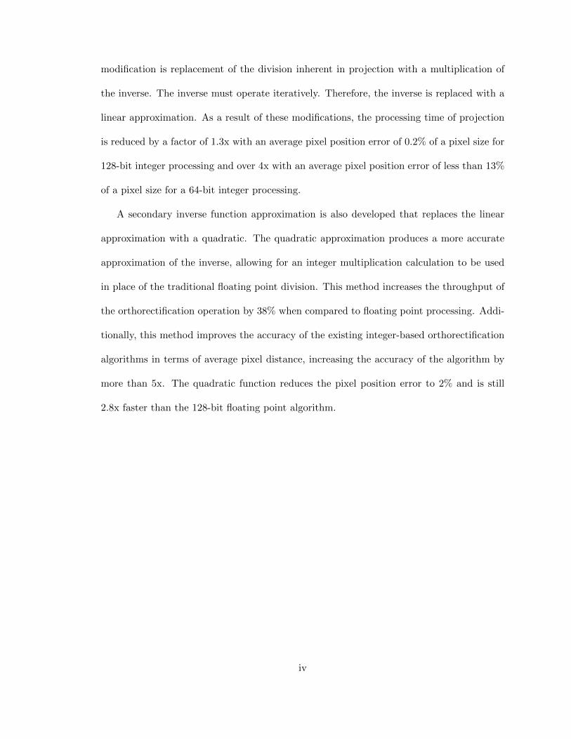
modification is replacement of the division inherent in projection with a multiplication of

the inverse. The inverse must operate iteratively. Therefore, the inverse is replaced with a

linear approximation. As a result of these modifications, the processing time of projection

is reduced by a factor of 1.3x with an average pixel position error of 0.2% of a pixel size for

128-bit integer processing and over 4x with an average pixel position error of less than 13%

of a pixel size for a 64-bit integer processing.

A secondary inverse function approximation is also developed that replaces the linear

approximation with a quadratic. The quadratic approximation produces a more accurate

approximation of the inverse, allowing for an integer multiplication calculation to be used

in place of the traditional floating point division. This method increases the throughput of

the orthorectification operation by 38% when compared to floating point processing. Addi-

tionally, this method improves the accuracy of the existing integer-based orthorectification

algorithms in terms of average pixel distance, increasing the accuracy of the algorithm by

more than 5x. The quadratic function reduces the pixel position error to 2% and is still

2.8x faster than the 128-bit floating point algorithm.

iv

For my family, Pınar and Koray.

v

ACKNOWLEDGMENTS

This research was partially funded with the help of the Air Force Research Laboratory.

I would also like to thank the University of Dayton Electrical and Computer Engineering

Department faculty for their expertise and insight. A special thanks my advisor, Dr. Eric

Balster and committee members, Dr. Russell Hardie, Dr. Vijay Asari, and Dr. Kenneth

Barnard for their guidance.

A special thanks to my current employer Lightstorm Research, as well as the University

of Dayton Research Institute for their support and encouragement.

vi

TABLE OF CONTENTS

ABSTRACT . . . . . . . . . . . . . . . . . . . . . . . . . . . . . . . . . . . . . . . . iii

DEDICATION . . . . . . . . . . . . . . . . . . . . . . . . . . . . . . . . . . . . . . . v

ACKNOWLEDGMENTS . . . . . . . . . . . . . . . . . . . . . . . . . . . . . . . . . vi

LIST OF FIGURES . . . . . . . . . . . . . . . . . . . . . . . . . . . . . . . . . . . . ix

LIST OF TABLES . . . . . . . . . . . . . . . . . . . . . . . . . . . . . . . . . . . . . xii

I. INTRODUCTION . . . . . . . . . . . . . . . . . . . . . . . . . . . . . . . . . . 1

II. BACKGROUND . . . . . . . . . . . . . . . . . . . . . . . . . . . . . . . . . . . 7

2.1 Image Projection . . . . . . . . . . . . . . . . . . . . . . . . . . . . . . . . 7

2.2 Forward Projection . . . . . . . . . . . . . . . . . . . . . . . . . . . . . . 11

2.2.1 Back Projection . . . . . . . . . . . . . . . . . . . . . . . . . . . . 12

2.3 Camera Model . . . . . . . . . . . . . . . . . . . . . . . . . . . . . . . . . 13

2.4 Projection Plane . . . . . . . . . . . . . . . . . . . . . . . . . . . . . . . . 14

2.5 Orthorectification . . . . . . . . . . . . . . . . . . . . . . . . . . . . . . . 18

2.6 Fixed-Point Arithmetic . . . . . . . . . . . . . . . . . . . . . . . . . . . . 19

III. REVIEW OF SELECT PAPERS . . . . . . . . . . . . . . . . . . . . . . . . . . 22

3.1 Aerial Imagery Processing . . . . . . . . . . . . . . . . . . . . . . . . . . . 22

3.2 Orthorectification . . . . . . . . . . . . . . . . . . . . . . . . . . . . . . . 25

3.3 Fixed-Point Processing and FPGAs . . . . . . . . . . . . . . . . . . . . . 29

IV. RESEARCH SETUP . . . . . . . . . . . . . . . . . . . . . . . . . . . . . . . . . 34

4.1 Data Set . . . . . . . . . . . . . . . . . . . . . . . . . . . . . . . . . . . . 34

4.2 Equipment . . . . . . . . . . . . . . . . . . . . . . . . . . . . . . . . . . . 37

4.3 Floating-Point Back Projection Method . . . . . . . . . . . . . . . . . . . 38

vii

4.3.1 Back Projection Method . . . . . . . . . . . . . . . . . . . . . . . 38

4.3.2 DEM Interpolation . . . . . . . . . . . . . . . . . . . . . . . . . . 42

4.3.3 Algorithm Implementation . . . . . . . . . . . . . . . . . . . . . . 44

V. FIXED-POINT PROJECTION ALGORITHM WITH LINEAR APPROXIMA-

TION [26] . . . . . . . . . . . . . . . . . . . . . . . . . . . . . . . . . . . . . . . 47

5.1 Algorithm Description of [26] . . . . . . . . . . . . . . . . . . . . . . . . . 47

5.2 Metrics . . . . . . . . . . . . . . . . . . . . . . . . . . . . . . . . . . . . . 53

5.3 Results from [26] . . . . . . . . . . . . . . . . . . . . . . . . . . . . . . . . 56

5.3.1 128-bit Algorithm with Linear Approximation Results . . . . . . . 56

5.3.2 64-bit Algorithm with Linear Approximation Results . . . . . . . 61

VI. FIXED-POINT PROJECTION ALGORITHM WITH QUADRATIC APPROX-

IMATION [27] . . . . . . . . . . . . . . . . . . . . . . . . . . . . . . . . . . . . 65

6.1 Algorithm Description of [27] . . . . . . . . . . . . . . . . . . . . . . . . . 66

6.2 Metrics . . . . . . . . . . . . . . . . . . . . . . . . . . . . . . . . . . . . . 72

6.3 Results from [27] . . . . . . . . . . . . . . . . . . . . . . . . . . . . . . . . 74

6.3.1 128-bit Algorithm with Quadratic Approximation Training Results 74

6.3.2 64-bit Algorithm with Quadratic Approximation Training Results 75

6.3.3 Algorithm Results, Comparison, and Discussion . . . . . . . . . . 77

VII. CONCLUSION . . . . . . . . . . . . . . . . . . . . . . . . . . . . . . . . . . . . 82

APPENDICES. . . . . . . . . . . . . . . . . . . . . . . . . . . . . . . . . . . . . . . . 84

APPENDIX A: DERIVATION OF EQUATION 6.2 . . . . . . . . . . . . . . 84

APPENDIX B: CURRENT JOURNAL PUBLICATIONS . . . . . . . . . . 86

APPENDIX C: CURRENT CONFERENCE PUBLICATIONS . . . . . . . 87

BIBLIOGRAPHY . . . . . . . . . . . . . . . . . . . . . . . . . . . . . . . . . . . . . 88

viii

LIST OF FIGURES

2.1 Projection Geometry. . . . . . . . . . . . . . . . . . . . . . . . . . . . . . . . 10

2.2 Pin-hole camera model. . . . . . . . . . . . . . . . . . . . . . . . . . . . . . 13

2.3 The CAHV camera model. . . . . . . . . . . . . . . . . . . . . . . . . . . . . 14

2.4 East, North, Up (ENU) and Earth-Centered Earth-Fixed reference coordi-

nates with respect to the Earth. (source Wikipedia: Mike1024) . . . . . . . 16

2.5 The difference between (a) geo-location, (b) georectification, and (c) or-

thorectification . . . . . . . . . . . . . . . . . . . . . . . . . . . . . . . . . . 19

2.6 32-bit floating point conversion from binary to decimal . . . . . . . . . . . . 21

4.1 LAIR Data set Collection Orbit of Training Data. . . . . . . . . . . . . . . 35

4.2 Example of the individual images captured using the sensor system from the

LAIR data set. . . . . . . . . . . . . . . . . . . . . . . . . . . . . . . . . . . 35

4.3 Combined images from Figure 4.2. . . . . . . . . . . . . . . . . . . . . . . . 36

4.4 Orthrectified image using the same images from Figure 4.2, overlayed on

Google Earth for context. . . . . . . . . . . . . . . . . . . . . . . . . . . . . 37

4.5 Orientation of the Novatel IMU Orientation for the LAIR data set collection. 38

4.6 Earth coordinate variable definitions (a) top view; (b) side view. . . . . . . 40

4.7 DEM of the Dayton, Ohio area used for with the LAIR data set. . . . . . . 42

4.8 Bilinear interpolation of the DEM. . . . . . . . . . . . . . . . . . . . . . . . 43

ix

5.1 Flow diagram for the proposed projection method. . . . . . . . . . . . . . . 54

5.2 Average pixel offset surface per set of scale factors over 100 training images. 57

5.3 Average pixel offset profile highlighting peak and plateau. . . . . . . . . . . 58

5.4 Histogram for the difference image shown in Figure 5.5 (c). . . . . . . . . . 60

5.5 Sub-region of the projected image using the [68] algorithm, left (a), and

the integer algorithm, center (b), the difference between the two (contrast

enhanced), right (c). . . . . . . . . . . . . . . . . . . . . . . . . . . . . . . . 60

5.6 Average pixel offset surface per set of scale factors over 100 training images,

limited to 64-bit integers. . . . . . . . . . . . . . . . . . . . . . . . . . . . . 62

5.7 Results of the algorithm described in [68], left (a), and the 64-bit integer

algorithm, right (b). . . . . . . . . . . . . . . . . . . . . . . . . . . . . . . . 63

5.8 Histogram for the difference image shown in Figure 5.9 (c). . . . . . . . . . 63

5.9 Results orthorectification on a sub-image using the algorithm described in

[68], left (a), and the 64-bit integer algorithm, center (b), the difference

between the two (contrast enhanced), right (c). . . . . . . . . . . . . . . . . 64

6.1 Difference Image (C) between the truth image (A) and the 64-bit linear

approximation algorithm (B) . . . . . . . . . . . . . . . . . . . . . . . . . . 66

6.2 Difference between the linear estimate (blue) and the quadratic estimate

(green) to the inversion function . . . . . . . . . . . . . . . . . . . . . . . . 68

6.3 Percent Difference between target floating point value and the integer ap-

proximation as a function of scale factor. . . . . . . . . . . . . . . . . . . . . 70

6.4 Average pixel offset surface per set of scale factors over 100 training images. 75

6.5 Average pixel offset surface per set of scale factors over 100 training images. 76

6.6 Profile over λ3 with a fixed λ1 and different λ2 samples. . . . . . . . . . . . 77

6.7 Comparison of the average pixel projection distance from the F128 algorithm

among the different projection algorithms. . . . . . . . . . . . . . . . . . . . 79

x

6.8 Comparison of the speed increase as compared to the F128 algorithm among

the different projection algorithms. . . . . . . . . . . . . . . . . . . . . . . . 79

6.9 Full frame projection result from the F128 algorithm with highlighted selec-

tion for comparison to other algorithms. . . . . . . . . . . . . . . . . . . . . 80

6.10 Comparison of the algorithm projections from the F128 projection algorithm;

(A) F64, (B) I128LA, (C) I64LA, (D) I128QA, and (E) I64QA. . . . . . . . . . . 81

xi

LIST OF TABLES

4.1 Test bench computer specifications. . . . . . . . . . . . . . . . . . . . . . . . 37

5.1 Integer variables and scale factors. . . . . . . . . . . . . . . . . . . . . . . . 49

5.2 Projection Comparison between floating point and integer algorithm for λ1

= 28 and λ2 = 39 of the Testing Data. . . . . . . . . . . . . . . . . . . . . . 59

5.3 Projection Comparison between floating point and 64-bit integer algorithms

for λ1 = 17 and λ2 = 32 of the Testing Data. . . . . . . . . . . . . . . . . . 64

6.1 Projection algorithm comparison showing the results from the testing data

compared to the F128 algorithm. . . . . . . . . . . . . . . . . . . . . . . . . 78

xii

CHAPTER I

INTRODUCTION

Imaging systems have become a more prominent feature in many new applications as

the acquisition cost has decreased and the quality has increased. Along with the price and

quality of digital cameras, computers have become smaller and more powerful. Therefore,

more computation can now be performed in real-time with quicker response for disaster

relief, threat detection, traffic monitoring, or any number of situations. Different image

processing techniques have been developed (i.e. filtering [24], image compression [37], and

noise reduction [30]) and modified to run efficiently on low-power processing units. However,

many of these applications require orthorectification to easily identify and interpret resource

allocation.

Orthorectification is the process of projecting an image onto a Digital Elevation Map

(DEM) and changing the perspective to be perpendicular to the projection surface. Aerial

imagery is converted to more of a map-like environment with distance correctly scaled

and oriented toward the North. Orthorectification is a computationally expensive process

that can hamper image collection rates and therefore, the overall system effectiveness. In

order to combat the computationally prohibitive orthorectification we propose an efficient

fixed-point back projection algorithm.

1

Aerial imagery has been used on many remote sensing applications including managing

natural disasters [23, 47], observing ecological changes [49], tracking declines in foundation

species [21], monitoring traffic [62], monitoring natural events like glaciation [6], natural

resources [65], and monitoring wetland restoration sites [38]. Other applications include

automated UAV navigation as described in [22], or mapping archeological sites [52]. As the

proliferation of unmanned aerial vehicles (UAVs) continues, more applications will become

apparent. Each of these applications require geographical knowledge of where the images

are captured. A common Earth-based projection plane across images has the benefit of

being able to pool multiple images from multiple sensors into a common intuitive space.

To overcome the computational complexity of orthorectification, several methods have

been developed to reduce processing time. Most of these methods use a form of distributed

computing such as grid computing, cloud computing, or Graphics Processing Units (GPUs).

A distributed computing paradigm is possible because each pixel is independent of the other

pixels through the orthorectification process. In other words, the projection of one pixel

does not depend on any of the other pixels. However, distributed systems can be prohibitive

due to size, weight and power constraints.

Grid computing is a task oriented collection of computers that distribute computational

loads to increase system throughput. Grid computing has also been utilized to perform

orthorectification such as [69] which demonstrates a grid computing architecture that helps

maximize the computational throughput of an orthorectification process using Moderate

Resolution Imaging SpectroRadiometer (MODIS) satellite imagery. Another task for grid

computers is monitoring disaster areas as demonstrated by [7], which proposes a method of

a grid computing architecture for fast disaster response using orthorectification.

2

Cloud computing, a method of using several non-local computers for processing, has

been used for orthorectification in glacier [57], ocean [28], and soil monitoring [18] as well as

natural disaster damage analysis [7]. One drawback of cloud computing is the security issues

that can arise. If the image or location is sensitive, then cloud computing may not be a good

solution. Cloud computing requires the image to be offloaded to a remote computer prior

to processing. Orthorectification systems have used cloud computing [43], but it becomes

difficult for real-time operations. Another disadvantage of cloud computing is the added

overhead of breaking up of the processes and the recombination of the result.

Some of the current research with GPUs concentrate on parallel implementation, and

coding methods. The method covered by [70] describes traffic monitoring using a GPU-

based image processing system, and is able to keep up with a 3 Hz frame rate of a 3K

imaging system. GPUs are also used to orthorectify an aerial pushbroom system onto a

digital terrain model (DTM) [58], which is able to orthorectify the sensor’s pixels at over

500 lines per second; much faster than the sensor was originally collecting.

Another technique for increasing the system throughput combines the GPU and CPU to

have them work in cooperatively, or share the computational load between a CPU and GPU.

A processing architecture and data flow is detailed in [10]. The problem of implementing

image processing techniques on a GPU when the image size is not a power of 2, or is too

large to store on a GPU is covered by [11]. [11] uses an open source image processing tool

box with CUDA implementations to compare the computational costs between using the

GPU or multi-core CPU for different image sizes. [11] also mentions that the selection of

the image processing algorithms is a major factor in speed increases as well as the decreases

in double precision calculations.

3

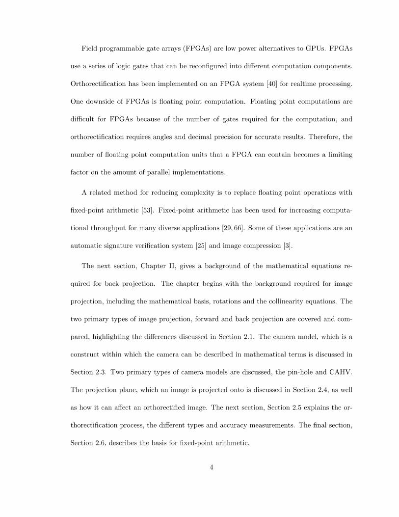
Field programmable gate arrays (FPGAs) are low power alternatives to GPUs. FPGAs

use a series of logic gates that can be reconfigured into different computation components.

Orthorectification has been implemented on an FPGA system [40] for realtime processing.

One downside of FPGAs is floating point computation. Floating point computations are

difficult for FPGAs because of the number of gates required for the computation, and

orthorectification requires angles and decimal precision for accurate results. Therefore, the

number of floating point computation units that a FPGA can contain becomes a limiting

factor on the amount of parallel implementations.

A related method for reducing complexity is to replace floating point operations with

fixed-point arithmetic [53]. Fixed-point arithmetic has been used for increasing computa-

tional throughput for many diverse applications [29, 66]. Some of these applications are an

automatic signature verification system [25] and image compression [3].

The next section, Chapter II, gives a background of the mathematical equations re-

quired for back projection. The chapter begins with the background required for image

projection, including the mathematical basis, rotations and the collinearity equations. The

two primary types of image projection, forward and back projection are covered and com-

pared, highlighting the differences discussed in Section 2.1. The camera model, which is a

construct within which the camera can be described in mathematical terms is discussed in

Section 2.3. Two primary types of camera models are discussed, the pin-hole and CAHV.

The projection plane, which an image is projected onto is discussed in Section 2.4, as well

as how it can affect an orthorectified image. The next section, Section 2.5 explains the or-

thorectification process, the different types and accuracy measurements. The final section,

Section 2.6, describes the basis for fixed-point arithmetic.

4

Chapter III discusses a selection of papers that highlight the applications along with the

benefits and some of the challenges encountered in researching aerial imagery and efficient

code implementations. The first section, Section 3.1, covers some of the current research on

applications that require aerial image processing from remote systems. Current methods

and applications for orthorectification is discussed in Section 3.2. The final section, Section

3.3, reviews the different applications where efficient fixed-point processing and FPGA

implementations have been used and discribes the benefits and detriments inherent therein.

Chapter IV, details the experimental setup, data and fixed-point projection algorithms.

the first section, Section 4.1, describes the data set, which consists of the imagery, position

and attitude data, as well as a discussion on the preprocessing required to successfully

implement the fixed-point algorithms. Section 4.2 lists the experimental equipment used

during the image collection, algorithm programming and processing. Section 4.3 describes

the floating-point orthorectification algorithm as described in [68]. Beginning with the

basic back projection method (Section 4.3.1), the DEM interpolation (Section 4.3.2) and

the implementation of the orthorectification algorithm (Section 4.3.3).

The fixed-point orthorectification algorithm as described in [26] is covered in Chapter V.

The algorithm and equations are shown in Section 5.1. The algorithm uses two scale factors

for integer conversion and fixed-point computations to increase the system throughput.

There are two versions of the algorithm, 128-bit and 64-bit integer versions. Section 5.2

discusses the metrics used for training and comparison. The results of the testing and

training of the two different versions is shown in Section 5.3. Section 5.3.1 reviews the

results of the training and testing of the 128-bit integer version. The training and testing

of the 64-bit integer version is covered in Section 5.3.2.

5

While [26] uses a linear approximation, Chapter VI describes a quadratic approxima-

tion proposed in [27]. Section 5.1 describes the algorithm and corresponding equations.

The metrics used for scale factor optimization training and performance comparisons are

described in Section 6.2. As with Chapter V, there are training and testing components as

well as two different versions, also 128-bit and 64-bit integer, of the algorithm. The first

two subsections, Sections 6.3.1 and 6.3.2, cover the training of the algorithms to determine

the optimal scale factors. The final subsection, Section 6.3.3 discusses the comparison of

the results of the different algorithms.

The final chapter, Chapter VII, closes with a review of the results of the different ap-

proximation techniques implemented. It concludes with a brief discussion of future research

topics that may improve performance or modular implementations for commercial usage.

6

CHAPTER II

BACKGROUND

This chapter gives a brief background on a few subjects required for the understanding of

the research topic. The first section, Section 2.1, discusses image projection beginning with

the rotation matrices and then covering forward and back projection. Camera models are

modeling constructs that characterize the imaging camera and the camera’s relationship

to the real world and is covered in Section 2.3. Section 2.4 covers the different types of

Earth based projection planes. Orthorectification, described in Section 2.5, is the most

accurate type of geo-location where perspective and terrain distortions are removed. The

final section, Section 2.6, describes fixed point arithmetic and the relationship between

floating point variables and the integer representations.

2.1 Image Projection

Image projection has become more important in the last several years as the ability

to capture digital imagery has become more cost effective. Projection is the process of

transforming objects to different spaces. For instance, in ancient times a sun dial indicated

the time of day by casting a shadow of the needle in the middle of the dial onto the dial

itself to indicate the time of day. In effect, this is what projection does, an object is located

7

in a certain reference frame, projection can transform the object to a different frame usually

with some warping or distortion.

IAn image, which is in the image plane, can be modified by adding a rotation, thereby

placing the image out of the image plane, and into a different projection plane. Projection

is typically performed with a rotation matrix, as shown in Equation 2.1, where x and y are

the original coordinates, x0 and y0 are the offsets in the original coordinates, i and j are the

transformed coordinates, and i0 and j0 are the transformed coordinate offsets [41].

i− i0

j − j0

=

cos(θ) − sin(θ)

sin(θ) cos(θ)

x− x0

y − y0

(2.1)

Image projection can be a more complicated process. An image is really a 2D represen-

tation of a 3D space. An image is physically the result of a projection from a 3D world into

a 2D Focal Plane Array (FPA). During this transformation, a real-world object is projected

through a lens and then onto the focal plane. The question then becomes, is it possible to

recreate the 3D space from the imagery?

Part of the answer is that a more complex rotation matrix is required. In a 3D coordinate

system, each axis needs to have a different rotation. A set of rotation angles are used which

correspond to each axis in a 3D space, as shown in Equations 2.2, 2.3, and 2.4, where θ

is the rotation about the x-axis, φ is the rotation about the y-axis, and ω is the rotation

about the z-axis [32].

These rotations can be combined to give a similar result as Equation 2.1, only in three

dimensions, by multiplying the matrices together where the order of operation does matter.

The system transform about three axes is shown in equation 2.6. However, often during

8

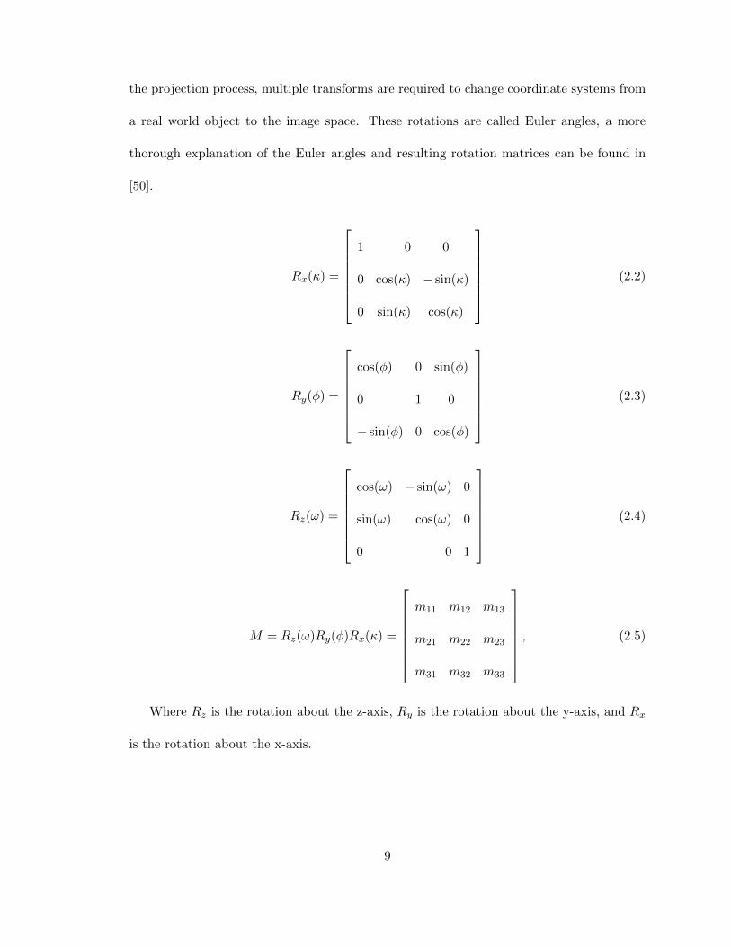
the projection process, multiple transforms are required to change coordinate systems from

a real world object to the image space. These rotations are called Euler angles, a more

thorough explanation of the Euler angles and resulting rotation matrices can be found in

[50].

Rx(κ) =

1 0 0

0 cos(κ) − sin(κ)

0 sin(κ) cos(κ)

(2.2)

Ry(φ) =

cos(φ) 0 sin(φ)

0 1 0

− sin(φ) 0 cos(φ)

(2.3)

Rz(ω) =

cos(ω) − sin(ω) 0

sin(ω) cos(ω) 0

0 0 1

(2.4)

M = Rz(ω)Ry(φ)Rx(κ) =

m11 m12 m13

m21 m22 m23

m31 m32 m33

, (2.5)

Where Rz is the rotation about the z-axis, Ry is the rotation about the y-axis, and Rx

is the rotation about the x-axis.

9

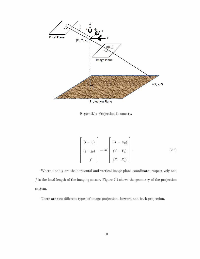
Figure 2.1: Projection Geometry.

(i− i0)

(j − j0)

−f

= M

(X −X0)

(Y − Y0)

(Z − Z0)

. (2.6)

Where i and j are the horizontal and vertical image plane coordinates respectively and

f is the focal length of the imaging sensor. Figure 2.1 shows the geometry of the projection

system.

There are two different types of image projection, forward and back projection.

10

2.2 Forward Projection

Equation 2.6 can be modified to transform image coordinates [i,j, -f ] to world coordi-

nates [X, Y, Z], as shown in Equation 2.7.

(X −X0)

(Y − Y0)

(Z − Z0)

= MT

(i− i0)

(j − j0)

(−f)

, (2.7)

Where the T operand is the transpose of the transform matrix. The collinearity equations

are a set of equations based on the assumption that the world coordinate, focal point, and

image pixel lie on the same line. The collinearity equations that are derived from the

coordinate transform shown in Equation 2.7. Equation 2.8 is for the horizontal coordinates

and 2.9 is for the vertical. The collinearity equations are widely used for orthorectification

[68].

X = X0 + (Z − Z0)m11(i− i0) +m21(j − j0) +m31(−f)

m13(i− i0) +m23(j − j0) +m33(−f)(2.8)

Y = Y0 + (Z − Z0)m12(i− i0) +m22(j − j0) +m32(−f)

m13(i− i0) +m23(j − j0) +m33(−f)(2.9)

However, with forward projection, the result isn’t a uniform grid. When an image is

forward projected, a square pixel is projected onto the projection plane into a trapezoidal

shape. The difference in shape will have to be modified to fit into a uniform DEM grid.

Another complication arises when the size of the DEM pixel is different than the native

11

projected image pixel size. When this happens, some DEM pixels that are surrounded by

projected image data, are missed and results in a distracting blank pixel in the orthorectified

image. For aerial imagery, the projected image pixel size changes throughout the projection

plane. To avoid missing or blank pixels, the largest projected pixel size would need to be

used. If the largest projected pixel size is used, then part of the image is degraded and a

loss of resolution occurs. If the smallest projected pixel size is chosen, the probability of

missed or blank projection plane pixels increases.

These missing or non-projected pixels become a distraction and can harm the appearance

and can negatively effect image processing techniques. To remove the non-projected pixels,

a secondary interpolation is required, increasing the computational requirements.

2.2.1 Back Projection

Back projection does not require the secondary interpolation step. In back projection,

the world coordinates are projected into the image plane of the camera system (Figure 2.1).

In back projection the collinearity equations can be simplified to Equation 2.10 for the

horizontal component in the image plane and Equation 2.11 for the vertical component.

i = −f m11(X −Xc) +m12(Y − Yc) +m13(Z − Zc)m31(X −Xc) +m32(Y − Yc) +m33(Z − Zc)

, (2.10)

j = −f m21(X −Xc) +m22(Y − Yc) +m23(Z − Zc)m31(X −Xc) +m32(Y − Yc) +m33(Z − Zc)

. (2.11)

Back projection has the advantage in that the interpolation ”gridding” step can be

accomplished during the projection process.

12

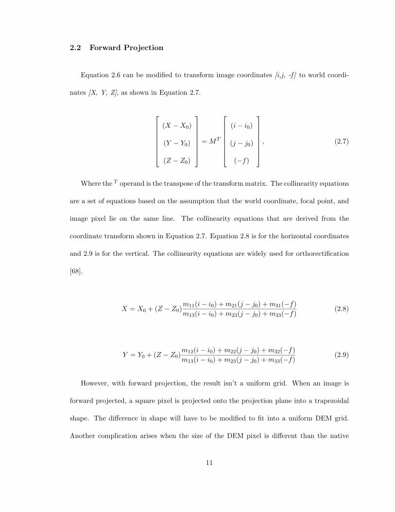
Figure 2.2: Pin-hole camera model.

2.3 Camera Model

Equations 2.8, 2.9, and 2.10, 2.11 define the mathematical relationship between a pixel in

the image plane, and a location on the Earth for a pin-hole camera [32]. The pin-hole camera

model is the simplest camera model, where no image distortion is assumed, as illustrated

by Figure 2.2. Where, (Xc, Yc, Zc) is the camera center with repect to the real world. The

pinhold operates as an aperture or pupil. P(X, Y, Z) is the world coordinate intersection

between the line formed from the camera center through the image plane intersection, p(i,j),

and the digital elevation sample.

Another method for describing the relationship between the earth and the image plane

is known as the CAHV camera model [76]. The CAHV camera model also assumes no

image distortion, and is directly related to the collinearity equations. This model consists

of the center of the focal plane ”C” in Earth coordinates, ”A” is the pointing vector in of

the principal axis, ”H’” is the horizontal direction vector, and ”V’” is the vertical direction

vector, as shown in Figure 2.3. The CAHV camera model relates distance and direction

on the focal plane to the corresponding distance and direction in the world coordinate

13

Figure 2.3: The CAHV camera model.

system. The CAHV model also creates an efficient construct for projecting between the

image coordinates and world coordinates in that all of the information required for the

projection is contained within the model.

The CAHV model is closely related to the collinearity equations only with the focal

length multiplied through the equation.

2.4 Projection Plane

With the rotation and projection applied, the next element is the projection plane. The

projection plane is where the pixels are projected onto (forward projection), as in Equations

2.8 and 2.9 where the projection plane locations are denoted by [X, Y, Z]. The projection

14

plane can also be projected from (backward projection), as in Equations 2.10 and 2.11. The

projection plane is typically a flat surface because changes in projection distance can add

distortions.

One solution is to use the Earth as the projection plane. Several different models of the

Earth ellipsoid have been developed. The most commonly used Earth model is the WGS84

ellipsoid model, which is used by the GPS satellites [71]. However, trying to project directly

onto the WGS84 geodiod is computationally intensive and often leads to systemic errors

[8]. A different reference frame is developed to both simplify the process and reduce errors.

Georectification is the process of projecting an aerial image onto an Earth based projection

plane (e.g. local tangential plane [31] or Earth-Centered, Earth Fixed (ECEF)[2]) so that

the image pixels are tied to Earth coordinates. The different Earth based coordinate systems

are shown below in Figure 2.4

The ECEF coordinate system measures everything from the center of the Earth. It

does, however, provide a uniform grid in three dimensions, which allows easier computation

for projection. The ECEF coordinates are related to the geodedic coordinates by equations

2.12, 2.13, and 2.14, where φ is the geodedic latitude, θ is the geodedic longitude, h is the

height above ellipsoid, and α is the semi-major axis of the ellipsoid model, and e is the first

eccentricity of the ellipsoid model.

X = (α√

1− e2 sin2(φ)+ h) cos(φ)cos(θ) (2.12)

Y = (α√

1− e2 sin2(φ)+ h) cos(φ)sin(θ) (2.13)

15

Figure 2.4: East, North, Up (ENU) and Earth-Centered Earth-Fixed reference coordinateswith respect to the Earth. (source Wikipedia: Mike1024)

Z = (α√

1− e2 sin2(φ)(1− e2) + h)sin(φ) (2.14)

A derivative of the ECEF coordinate frame is the local tangent or east, north, up (ENU)

coordinate frame. One of the issues with the ECEF coordinate frame is that everything

is measured from the center of the earth, so all of the computations will work with large

values. However, since it is really only the surface that we are usually worried about,

the ENU coordinate frame references everything from a user defined center on the Earth’s

surface. This helps reduce the size of the values involved, and with the ECEF coordinate

frame, each direction is orthogonal to the other directions. The equation for converting

between ECEF and ENU is shown below in equation 2.15. The variables Xp, Yp, and Zp

16

are the ECEF coordinates of the platform. The variables Xt, Yt, and Zt are the ECEF

coordinates at the desired center of the tangent plane. Again the relationship between

geodedic, ECEF and ENU is shown below in figure 2.4

X

Y

Z

=

− sin(φ) cos(φ) 0

− sin(θ) cos(φ) − sin(φ) sin(θ) cos(φ)

cos(θ)cos(φ) cos(θ)sin(θ) sin(θ)

Xp −Xr

Yp − Yr

Zp − Zr

(2.15)

Another addition to the different ground planes is the digital elevation map (DEM).

Many techniques use a DEM during the projection process such as [50], [78], and [61].

DEMs are used to increase the accuracy of an image projection. The WGS84 ellipsoid,

for instance, is typically several meters below the actual elevation of the land. A DEM

helps to give a more accurate surface on top of the coordinate system to improve accuracy.

However, when capturing aerial imagery, the image projection vectors aren’t from a 2D

surface, the differences in elevation complicates the orthorectification process. To mitigate

this effect, an approximation of the terrain is required. There are elevation maps available

from government agencies such as the United States Geological Survey (USGS) [73] and

NASA [51]. These typically have Ground Sample Distances (GSD) of 1 to 10 square meters.

Many aerial images will have a finer GSD than those specified by the elevation map.

Therefore, an interpolation step is performed to match the expected nominal projected GSD

with the digital elevation map.

17

2.5 Orthorectification

The process described in previous sections can be combined to produce an orthorectified

image. There are different processing methods for attaching earth coordinates to image

pixels. They are geo-location, georectification, and orthorectification. The definition of

each process type is listed below.

Geo-location is simply attaching an earth coordinate to an image pixel, no other pro-

cessing needs to be performed. There are different types of geo-location such as projecting

the image footprints thereby finding the Earth coordinates of the corners of the image.

Another method is to match known features to the same features on Earth. Geo-location

does not need to perform projection, or remove perspective or terrain distortions.

Georectification adds the projection process to geo-location. With Georectification,

each image pixel gets attached to an Earth coordinate, however, the projection is on an

Earth-model surface and does not necessarily remove terrain distortions. The perspective

distortions are also removed through projection, changing the viewing angle orthogonal to

the projection plane. Georectification can be sufficient for many purposes, but as figure 2.5

shows, the accuracy may not be enough for some applications.

Orthorectification is a similar process, but instead of projection onto a flat surface, the

image is projected onto a DEM to remove the terrain distortions. It is the most accurate

Earth-based projection. It is commonly performed for mapping purposes [7, 10, 36, 42, 47,

49, 60, 62, 69]. Figure 2.5 shows the difference between the three types of Earth based image

processes.

18

Figure 2.5: The difference between (a) geo-location, (b) georectification, and (c) orthorec-tification

Many of the most accurate orthorectification algorithms rely on Ground Control Points

(GCP). GCPs are locations on the ground that are detectable in the imagery and have

known Earth coordinates. Typically the algorithms rely on several GCPs depending on the

spacing within the image. Once the GCPs have been located, corrections can be made to

the camera model or navigation data to increase the absolute accuracy of the projection.

However, in some instances, no GCPs are known. In this case the accuracy depends solely

on the camera model, position and attitude measurements of the platform.

2.6 Fixed-Point Arithmetic

Fixed-point processing is a method for increasing the speed of calculation [3, 25, 29]. In

order to convert between a floating point variable and a fixed-point variable a multiplication

by a constant is required to preserve precision as shown by Equation 2.16.

19

F =⌊2λF

⌋, (2.16)

where F is a floating point number, F is the fixed-point representation, and λ is a

scale factor. If the constant is restricted to a power of two then manipulating the resulting

integers becomes easier since scaling of the fixed-point result can be performed using bit

shifts. The scale factor determines the accuracy of the resulting integer representation. A

larger scale factor results in a higher degree of accuracy.

Fixed-point arithmetic is a more efficient computation compared to floating-point com-

putation, because of the simplification of the binary operations. A fixed-point binary word

consists only of the scaled numeric value, the significand. A floating-point binary word

consists of the significand or mantissa and exponent. Figure 2.6 shows the composition and

different stages of conversion from a binary word (top) to a decimal value (bottom).

While the floating point values can represent a wider range of values, any computation

must account for the exponent which adds more computations.

20

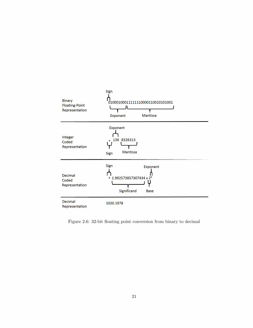
Figure 2.6: 32-bit floating point conversion from binary to decimal

21

CHAPTER III

REVIEW OF SELECT PAPERS

This chapter gives an overview on some of the recent research. The first section covers

some topics on aerial image processing, including different aerial imaging applications. The

next section deals exclusively with orthorectification and some of the applications and ben-

efits. Section 3.3 discusses some of the current topics in Fixed-point processing and FPGA

algorithms and applications.

3.1 Aerial Imagery Processing

Aerial imagery can provide a cost effective method for monitoring remote or large areas

on a more routine basis. There is, therefore, a significant amount of research conducted on

applications using aerial imagery. One application estimates the height and canopy density

of trees using data from a low cost passive sensor and a UAV [80]. The UAV is flown over a

forest. The data collected is then forward projected onto a 3D model of the forest canopy.

One issue confronted in this paper is the discontinuous nature of the canopy and processing

the imagery in a way that allows the algorithm to determine where the discontinuities are

located. The feedback loop between the 3D surface and the information from the sensor

allows the tree heights to be estimated. The accuracy of the height estimate is compared

22

for over 100 trees. Multiple flights are used with criss-crossing patterns over the forest at

different altitudes. The change in altitude also changes the projected pixel size on the 3D

model. The change in pixel size shows the degradation of the tree height estimate as the

projected pixel size increases. This research is relevant because it highlights the problems

due to the pixel size and shape and these problems are compounded by the discontinuities

in forest canopies. It also discusses the uncertainty built into the projection process when

projected pixel size varies.

Along with monitoring tree health, farming and pest/weed control also uses UAVs to

monitor health as in [35]. The application proposed in [35] uses small UAVs with a high

resolution camera to determine weed type and density. The UAV flies over a field of interest

and then uses a series of image filters which allow specific features to be extracted. The

features are then processed through a learning algorithm to differentiate between weed and

background features. This paper focuses on three weeds common to Australia. Once the

classifier has learned the weed features, the UAV can make the determination of a learned

weed type and concentration of a given weed type per area. This paper highlights the

benefit of real-time monitoring for agricultural and horticulture purposes.

In the scientific realm, remote and non-destructive testing has many benefits for fragile

or susceptible areas like the moss fields of Antarctica. The research described in [46] uses a

small rotor UAV to monitor the moss beds in Antarctica. The moss beds in Antarctica are in

a precarious situation with melting snow and glacier runoff. Monitoring the health and area

of the moss becomes an issue because going to the moss beds and taking measurements on

a regular basis can damage the moss. However, using a low-altitude UAV, a high resolution

projection plane, and statistical modelling, the moss beds are monitored remotely and in a

23

non-destructive method. The algorithm used is a Structure From Motion (SFM) algorithm

[39] to estimate the moss bed underlying structure. The accuracy of the underlying structure

and associated runoff is determined using the monte carlo simulations with 400 realizations.

The combination of the finely sampled ground plane and using statistics to estimate the

underlying structure emphasizes the multi-faceted process that is required for accurate

orthorectification. Orthorectification inherently relies on data fusion to produce an accurate

result.

Aerial imagery is also used in urban traffic monitoring as in [9], where a small low-

altitude UAV is used to detect vehicles. The complexity of the scene, including changes

in brightness, motion within the scene, and motion of the sensing platform make real-time

processing difficult. To compensate for these difficulties, a processing chain is developed

that uses an intensity boosting, that masks shaded areas for better matching, and image

resolution pyramid. The pyramid processing still allows efficient global feature extraction

and matching. The vehicles are matched using a spatio-temporal appearance related metric.

One issue that this paper covered is the effort to optimize the computation on UAV platform

and still achieve near real-time results. Many applications are moving toward a stand-alone

UAV with onboard image processing techniques. However, the complications that arise from

such an implementation, such as low-power and limited computational resources, show the

necessity of efficient and parallel programming.

Aerial imagery has also been used in the preservation [75] and identification [13, 63] of

archeological sites and artifacts. Many archeological sites are corrupted due to digs, or

vandalism, which makes post-inspection difficult or impossible. The proposed solution in

[17] uses 3D reconstruction of the archeological sites to be preserved prior to intervention or

24

destruction. The proposed system contains a UAV with a visible camera and the PhotoScan

software to determine a digital surface map of the area. High portability is a driving factor

as the system needs to be easy to carry and ship. The increased accuracy of the system

over existing site log methods, as well as the increase in public awareness make this system

a desirable alternative.

All of the applications discussed above for aerial imagery use a UAV controlled by a

user, however automated takeoff and landing can also be performed using image process-

ing on the UAV platforms. For takeoff and landing, real-time feedback becomes a more

pressing concern. A possible solution is proposed in [77] which uses an onboard monocular

camera for automatic takeoff and landing of a Micro Aerial Vehicle (MAV). For this task,

a typical landing pad is used, with a H in a circle. The system uses pictures of the circle

and perspective projection to estimate the attitude of the MAV. The algorithm determines

the position, altitude, and attitude with six degrees of freedom. Real-time automatic nav-

igation, especially from small UAVs operate in a power scarce environment where efficient

computation becomes imperative.

3.2 Orthorectification

A subset of aerial image processing is orthorectification. Orthorectification is used pri-

marily when location and distance are important for analysis. One application for real-time

monitoring is presented in [72] which proposes an orthorectification method for monitoring

active landslides. The system is implemented on a ground based system, mounted on a pil-

lar overlooking the Super-Suaze landslide in France from 2008 to 2009. A cross-correlation

25

metric is used to find the land displacements. After the displacements are found the dis-

placement fields are orthorectified using the collinearity equations onto a DEM. Some of

the drawbacks are illumination and small movements of the imaging system. Despite these

drawbacks, this system is developed to operate as an early warning system. One aspect of

the proposed system that makes orthorectification easier is that the viewing angle, distance,

and region imaged are fixed. Fixed angles and distances allow more pre-computed variables

for faster computation. However, this system finds even small movements of the platform

causes problems with accuracy. The positional measurement accuracy issue highlights the

sensitivity of the orthorectification process to measurement error.

When the platform isn’t in a fixed location and the viewing angle changes significantly

across the field of view (FOV), orthorectification becomes more difficult to process in real-

time. Moving sensor platforms also create difficulties in assessing system accuracy. One

method for determining absolute accuracy is proposed in [1], which discusses methods for

determining the absolute accuracy of the orthorectification process from two commercial

satellites, GeoEye-1 and WorldView-2. Both of these satellites are very high resolution

systems and all of the processing and comparisons are targeted to the panchromatic images.

The orthorectification algorithm for this paper uses rational functions [67] to map from

image coordinates to Earth coordinates and finds that a 3rd order polynomial in each

direction with 7 GPCs achieves the overall best result. The number of factors that influence

the assessed accuracy of the system contains, but are not limited to: sensor type, orientation

(parallel or perpendicular to orbit), number of ground control points, maximum viewing

angle with respect to nadir, and altitude accuracy. The number of variables that influence

the system accuracy, indicates the sensitivity of the orthorectification process.

26

The method of assessing accuracy presented in [1] uses Ground Control Point (GCP).

Since GCPs are used as a measure of accuracy, they are also used to update the orthorec-

tification parameters. For instance, a fully automated approach for orthorectification of a

satellite pushbroom sensor is discussed in [48]. The method uses the onboard attitude and

position measurements as well as an automated GCP detection and extraction. The GCP

extraction consists of finding geo-referenced road vectors, then building a set of GCPs based

on these roads. The collinearity equations are used to generate the initial camera model

from the position and attitude measurements. The GCPs are then used to update the

camera model for more accurate projections. The results are verified using the RapidEye

satellite collected over three different regions. The accuracy of the orthorectified images is

around 1 pixel. Using GCPs and orthorectification in a feedback loop to improve accuracy

adds another level of complexity for image processing algorithms, but are required for the

most accurate implementations. However, most of these types of feedback optimization

techniques are too slow to be considered real-time.

Different algorithms for optimizing the accuracy of the orthorectification processes have

been implemented. Particle swarm algorithms used in conjunction with GCPs is proposed

in [59] where the orthorectification of pushbroom imagery is optimized. Particle swarm

algorithms use several candidate solutions and optimize based on a set of metrics and the

other candidates movement to converge to a common minima. These algorithms use the

projected locations of GCPs to optimize the orthorectified frame. The system also uses

the parallel nature of graphics processing unit (GPU) to increase the throughput of the

system. The particle swarm algorithm is used to match features that are then fed back

into the navigation data and sensor camera model. This paper highlights the parallel

27

nature of the orthorectification process. Since orthorectification operates on each pixel

independently, each pixel can be processed in parallel. GPUs are also used because of

their parallel nature and capability to operate on floating point values. In this case, the

GPU performs orthorectification, feature extraction and matching, and optimization of the

projection. However, this application is not designed to perform in real-time. The reliance

on the optimization process and requirement of a ground station GPU for processing limit

the real-time capability. This paper does, however, show the possibilities of improving

orthorectification accuracy in a parallel implementation.

All of the applications mentioned previously either use a ground station for real-time

processing or do not operate in real-time. Performing orthorectification in real-time is re-

quired for some situations, for instance in disaster monitoring. Due to the difficulties in

real-time orthorectification, [45] discusses the time issues in imaging and processing sys-

tems required for quick response needs in generating orthorectified imagery. The primary

areas that the research covers are identification of problem areas within the image capture,

preprocessing and orthorectification processes. There were two foci of the research. The

first focus is on a generic work-flow for an efficient overall system. The second was opera-

tional work-flow to minimize the computations required for orthorectification and building

a mosaic from the result. For this particular case, most of the time saving is realized by

limiting the image overlap to achieve a more efficient system. Real-time orthorectification

requires an overall efficient imaging and processing system. The processing efficiency can be

obtained by using parallel processing on any number of computational platforms, multi-core

CPUs, GPUs, or FPGAs. It becomes difficult in real-time aerial systems to maintain the

high power consumption of CPUs and GPUs, however, FPGAs require low power.

28

3.3 Fixed-Point Processing and FPGAs

A possible first step in efficient image processing is to remove floating point calcula-

tions. As mentioned in Section 2.6, floating-point calculations require more computations

per variable than an integer computation of the same size. However, fixed point implemen-

tations can be difficult. For instance, [15] proposes a fixed-point method to approximate the

logarithmic base two (log2) function. Many hardware approximations for the log function

rely on look up tables (LUTs) [64] or piecewise polynomial approximations with uniform

segments [16]. The proposed method uses fixed-point piecewise linear approximation from

non-uniform segments. There are two ”types” of segments: coarse and fine. The fine seg-

ments are designated to the critical points of x=1 and x=0, and the coarse segments are for

everywhere else. The input to the approximated log function is limited to integer values.

One of the main contributions of this paper is the non-uniform sampling of the log func-

tion for better approximation and faster pipelining. Removing floating-point operations

in approximations of non-linear functions is a proven method for increasing computational

throughput.

Fixed-point arithmetic can also be used to increase the efficiency of select image pro-

cessing algorithms. As an example, [54] presents a method to efficiently estimate integral

histograms using fixed-point arithmetic. The method propagates an aggregate histogram

through the scan lines and updates the histogram. While this method is primarily focused

on 2D and 3D data sets, the implementation allows for any dimension data to be pro-

cessed. Both a floating point and fixed point algorithm are implemented. The fixed point

algorithm is significantly more efficient than the floating point method. The fixed point

method is used for data sets that begin with integer values, such as 8-bit imagery. The

29

floating point method is used for 3D wavefront data where the data is already in floating

point variables. This paper highlights some aspects of image processing that lends itself to

fixed point processing and the resulting increase in efficiency as compared to floating point

implementation. Fixed-point arithmetic alone increases the throughput of a system, but

the efficiency can be lost due to inefficient programming or hardware implementations.

Another possibility to increase the system throughput is to streamline the data through

the processing chain. One method of streamlining the data is with a programming language

and compiler [33, 56]. An example of a programming language and compiler that eases the

development of efficient high-speed image processing techniques for specialized hardware

implementations is proposed in [33]. Darkroom, the proposed programming language, com-

piles directly to buffer line pipelines and removes some of the complexities of local buffer

storage. Another aspect of the Darkroom compiler for optimally scheduling memory trans-

fers to and from DRAM. The compiler is formulated for operation with ASIC, FPGA or

fast CPU code. Using the compiler, the processing system is able to attain gigapixel/sec.

throughput. While moving data around in an efficient way as designed for a particular

image processing method is certainly beneficial and does increase the throughput of the

system, it can still lose some of the efficiency due to the image processing algorithm imple-

mentation and floating-point calculations. Another place loss of efficiency can arise is the

capability to be compiled on multiple hardware designs. Being able to compile on multiple

languages decreases development time, but it can negatively impact the throughput of the

system.

30

A development language that has been developed for efficient image processing is pro-

posed in [20] and named, Single Assignment C (SA-C). SA-C is a language specifically de-

signed to port image processing algorithms to an FPGA architecture. A targeted language

can typically achieve more efficient results as compared to a general language. Different

algorithms are implemented using SA-C and compared against a general purpose proces-

sor. These algorithms consist of scaler addition, edge detection, Cohen-Daubechies-Feuveau

wavelet filter [12], dilation, and probing [5]. The results are between an 8 fold increase for

scaler addition, and 800x speed increase for probing. All of the image processing algorithms

that are implemented performs faster than the corresponding CPU implementation. One

drawback is that the efficient use of pipelined memory as described in [33] is not used. An-

other drawback is that the algorithms only operate on the image processing techniques that

have an integer implementation, more sophisticated or complex algorithm will probably still

struggle using SA-C.

Many image processing algorithms are difficult to implement as integer only operations

while maintaining real-time computation. Converting floating point variables to fixed-point

values is more complex, but ultimately allows more flexibility in the development process.

For instance, [74] implements a real-time fast Fourier Transform (FFT) algorithm on an

FPGA. FFT is an algorithm that is typically implemented using floating point variables.

However, for an FPGA parallel implementation, a fixed-point version is developed. Two

types of FFT algorithms are used, the Radix-2 [14] FFT and Radix-4 discrete FFT algo-

rithms [79]. The results show the improved computational throughput of the fixed-point

implementations over the floating point versions. While the research shows the feasibility of

31

a fixed point FFT algorithm on an FPGA and the improved throughput, there is no com-

parison for results. How does the floating point implementation compare to the fixed-point

implementation?

In general, fixed-point implementations are not as accurate as floating-point implemen-

tations of image processing algorithms. As an example, [55] discusses the tradeoff between

hardware pipeline benefits of 3D ray trace renderings of objects, and software versions using

CPUs. A fixed-point ray tracing algorithm is developed and implemented in programmable

graphics hardware. There are four primary functions involved in ray tracing for 3D re-

construction: point-of-view (POV) Ray initialization, traverser, intersector, and shader.

The first function, POV Ray initialization sets up the viewing angles and initial processing

parameters. The traverser stage sets up the ray projection from the POV ”eye” and the

initial surface mesh as well as finding the where the voxels are pierced by the ray trace.

Once the ray and voxel pairs are determined, the data is passed to the intersector, which

determines if a ”hit” occurs between a ray-voxel pair and a triangle surface pixel. If a hit

occurs the ray-voxel pair is converted to a ray-triangle pair and sent to the last stage, the

shader. The shader determines the color contribution of each contributing ray trace to a

triangle. The fixed-point implementation outperforms the CPU implementation in speed.

However, the fixed-point implementation also struggles with the aspects of the process that

require a higher resolution in calculation. For instance, the ”hit” points may be shifted in

location from the floating-point implementation due to the smaller range of values that can

be represented, the shift then influences the shading of the result. While the solution offers

an efficient fixed-point algorithm for a low-power environment, it still does not operate in

real-time.

32

The combination between hardware, data pipelining, efficient programming and algo-

rithm selection offers the best results for real-time image processing on remote platforms.

The final paper reviewed [19], proposes an FPGA implementation for a real-time pipelined

optical flow algorithm for motion detection. A sensor part of the implementation is a ”vir-

tual sensor” which consists of a camera model and a 30 Hz frame rate of images to be

pipelined, as if it is coming directly from a camera. The optical flow algorithm being imple-

mented is based on a method first described in [44] and modified for hardware by [4]. The

system once implemented is able to detect motion of imagery of a moving car, however, the

results do not have the precision of the floating point implementation due to limitations of

the fixed point arithmetic. This is one of the first stand-alone real-time implementations of

an image processing algorithm. The goal is to create a system that can be implemented on

a number of remote sensing systems for traffic monitoring or search and detect applications.

33

CHAPTER IV

RESEARCH SETUP

This chapter discusses the experimental setup used in conducting this research. The

first section, Section 4.1, describes the LAIR data set which was collected by the Air Force

Research Laboratory in October of 2009. Section 4.2, covers the equipment used for data

collection, algorithm development and processing platform. The floating point orthorectifi-

cation algorithm [68] is covered in Section 4.3.

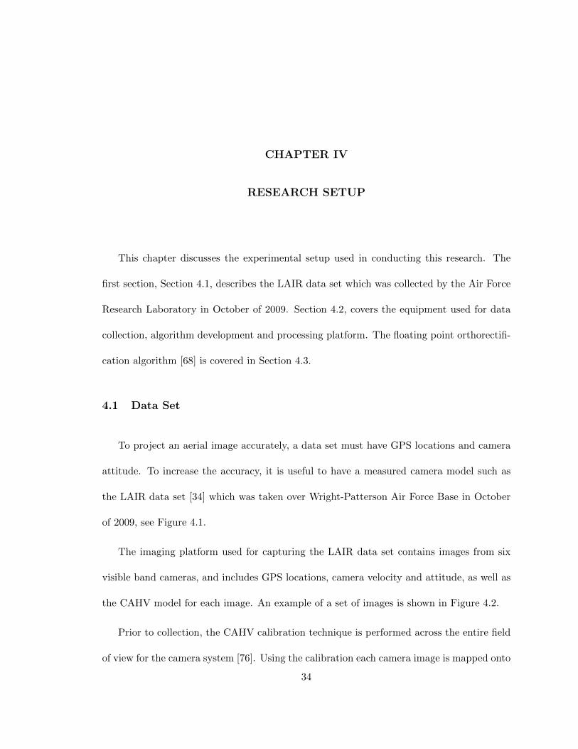
4.1 Data Set

To project an aerial image accurately, a data set must have GPS locations and camera

attitude. To increase the accuracy, it is useful to have a measured camera model such as

the LAIR data set [34] which was taken over Wright-Patterson Air Force Base in October

of 2009, see Figure 4.1.

The imaging platform used for capturing the LAIR data set contains images from six

visible band cameras, and includes GPS locations, camera velocity and attitude, as well as

the CAHV model for each image. An example of a set of images is shown in Figure 4.2.

Prior to collection, the CAHV calibration technique is performed across the entire field

of view for the camera system [76]. Using the calibration each camera image is mapped onto

34

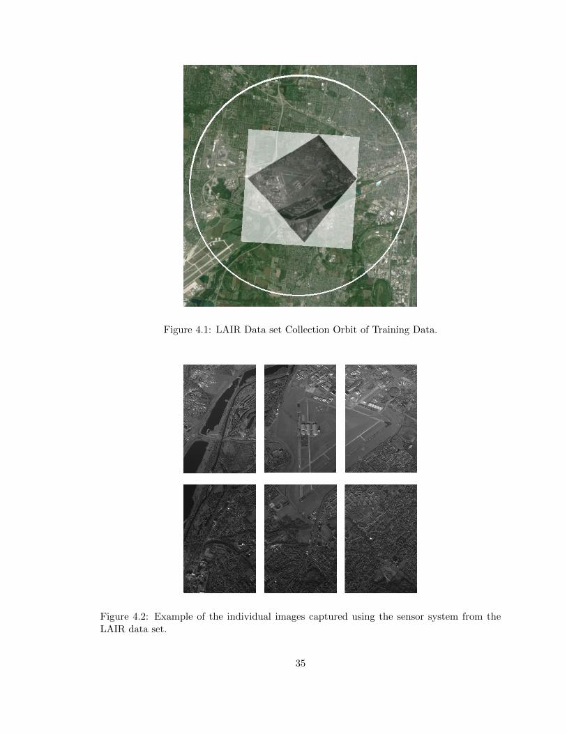
Figure 4.1: LAIR Data set Collection Orbit of Training Data.

Figure 4.2: Example of the individual images captured using the sensor system from theLAIR data set.

35

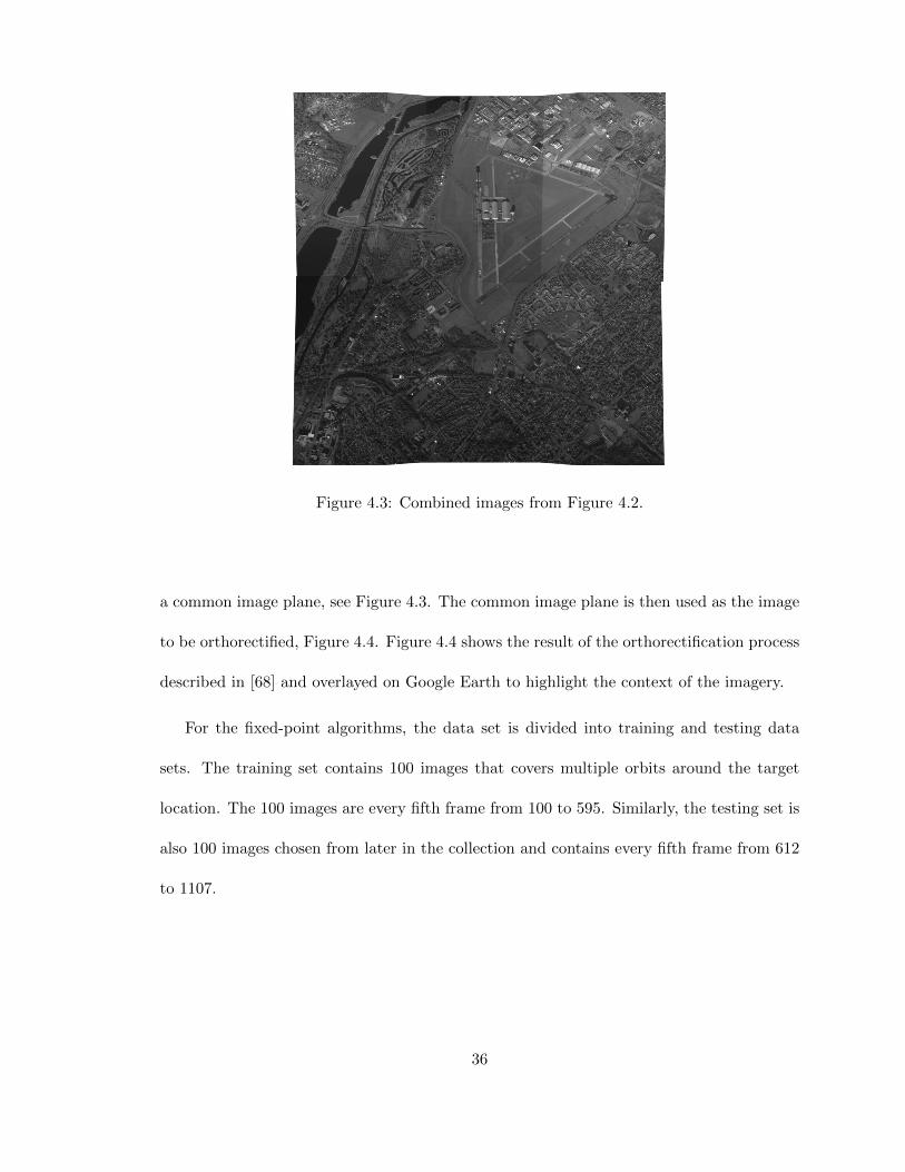
Figure 4.3: Combined images from Figure 4.2.

a common image plane, see Figure 4.3. The common image plane is then used as the image

to be orthorectified, Figure 4.4. Figure 4.4 shows the result of the orthorectification process

described in [68] and overlayed on Google Earth to highlight the context of the imagery.

For the fixed-point algorithms, the data set is divided into training and testing data

sets. The training set contains 100 images that covers multiple orbits around the target

location. The 100 images are every fifth frame from 100 to 595. Similarly, the testing set is

also 100 images chosen from later in the collection and contains every fifth frame from 612

to 1107.

36

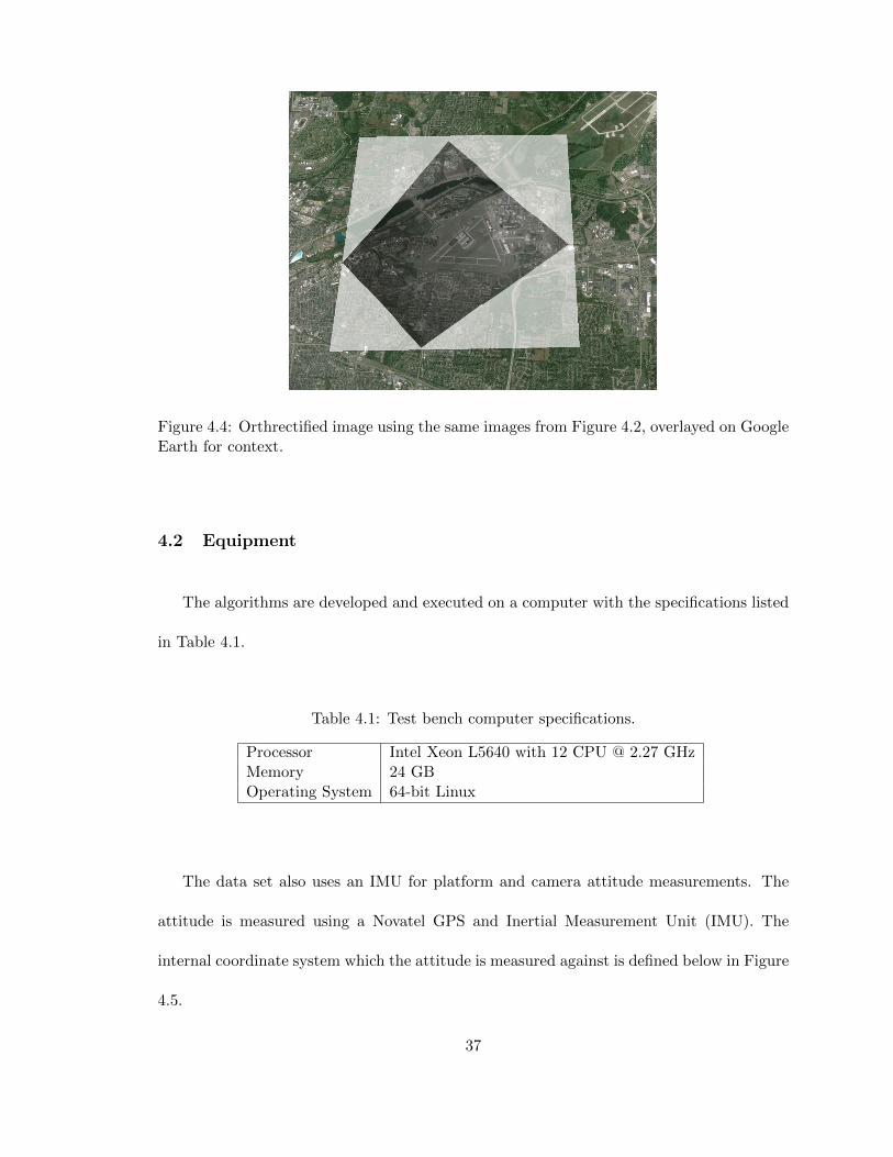
Figure 4.4: Orthrectified image using the same images from Figure 4.2, overlayed on GoogleEarth for context.

4.2 Equipment

The algorithms are developed and executed on a computer with the specifications listed

in Table 4.1.

Table 4.1: Test bench computer specifications.

Processor Intel Xeon L5640 with 12 CPU @ 2.27 GHzMemory 24 GBOperating System 64-bit Linux

The data set also uses an IMU for platform and camera attitude measurements. The

attitude is measured using a Novatel GPS and Inertial Measurement Unit (IMU). The

internal coordinate system which the attitude is measured against is defined below in Figure

4.5.

37

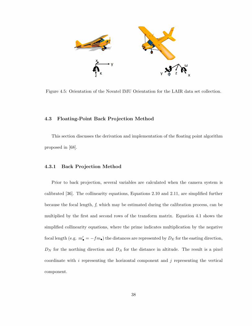
Figure 4.5: Orientation of the Novatel IMU Orientation for the LAIR data set collection.

4.3 Floating-Point Back Projection Method

This section discusses the derivation and implementation of the floating point algorithm

proposed in [68].

4.3.1 Back Projection Method

Prior to back projection, several variables are calculated when the camera system is

calibrated [36]. The collinearity equations, Equations 2.10 and 2.11, are simplified further

because the focal length, f, which may be estimated during the calibration process, can be

multiplied by the first and second rows of the transform matrix. Equation 4.1 shows the

simplified collinearity equations, where the prime indicates multiplication by the negative

focal length (e.g. m′• = −fm•) the distances are represented by DE for the easting direction,

DN for the northing direction and DA for the distance in altitude. The result is a pixel

coordinate with i representing the horizontal component and j representing the vertical

component.

38

i =m′11DE+m′12DN+m′13DAm31DE+m32DN+m33DA

j =m′21DE+m′22DN+m′23DAm31DE+m32DN+m33DA

. (4.1)

The projection plane which is projected onto the image plane can be defined as a the-

oretical flat surface, or as a Digital Elevation Map (DEM). A DEM has terrain altitudes

at associated earth coordinates and is used to obtain more accurate results over a flat pro-

jection surface. The DEM has a Ground Sample Distance (GSD) in the easting, ∆E , and

northing, ∆N , directions respectively. The DEM GSD’s are, typically, too coarse for the

size of an image pixel projection. Therefore, an interpolation factor, I, is typically used to

more densely represent the DEM, and is chosen to critically sample the image focal plane.

The interpolated GSD’s, δE for the easting direction and δN for the northing direction, are

given by

δE = ∆EI , δN = ∆N

I. (4.2)

A visual representation of the projection variables and their relationship to the DEM is

shown in Figure 2, where (X,Y,Z) is the Earth location being projected, (Xc, Yc, Zc) is the

current location of the imaging sensor, and δA is the interpolated altitude differential unit.

The DEM, Z(x, y), is natively sampled with indices x,y, corresponding to the two planar

dimensions easting and northing respectively. The interpolated indices are given by

x′ = Ix+ χ; χε[0, I)

y′ = Iy + γ; γε[0, I)

, (4.3)

39

Figure 4.6: Earth coordinate variable definitions (a) top view; (b) side view.

Where χ is the iterative variable in the easting direction, and γ is the iterative variable

in the northing direction. The DEM is interpolated using a bilinear interpolation technique

and is represented as ζ(x′, y′).

In order to use the collinearity equations for georectification, a few remaining variables

need definition. Three distance variables, DN , DE , and DA, which correspond to the

distances in the northing, easting and altitude respectively and are given by

DE [x′] = X0 + x′δE −Xc

DN [y′] = Y0 + y′δN − Yc

DA[x′, y′] = ζ[x′, y′]− Zc

. (4.4)

40

Where X0 and Y0 are the initial easting and northing values respectively for the projec-

tion plane being used. The indices x′, y′ denote the dependencies of the distances with the

corresponding DEM directions. DN is only dependent in the northing direction, and DE is

only dependent in the easting direction.

The collinearity equations require an interpolated numerator and denominator given by,

i[x′, y′] = in[x′,y′]rd[x′,y′]

j[x′, y′] = jn[x′,y′]rd[x′,y′]

. (4.5)

Back projection of an image requires an iterative process of updating all three distance

variables, DE , DN , and DA, using Equation 4.4. Solving for the numerators in Equation

4.5, in[x′, y′], jn[x′, y′], results in

in[x′, y′] = m′11DE [x′] +m′12DN [y′] +m′13DA[x′, y′]

jn[x′, y′] = m′21DE [x′] +m′22DN [y′] +m′23DA[x′, y′]

, (4.6)

and the denominator, rd[x′, y′], is given by

rd[x′, y′] = m31DE [x′] +m32DN [y′] +m33DA[x′, y′] . (4.7)

The division in Equation 4.5 produces the corresponding pixel location in the image

plane from the world coordinate. This process is repeated through all samples of the

interpolated DEM, ζ[x′, y′].

41

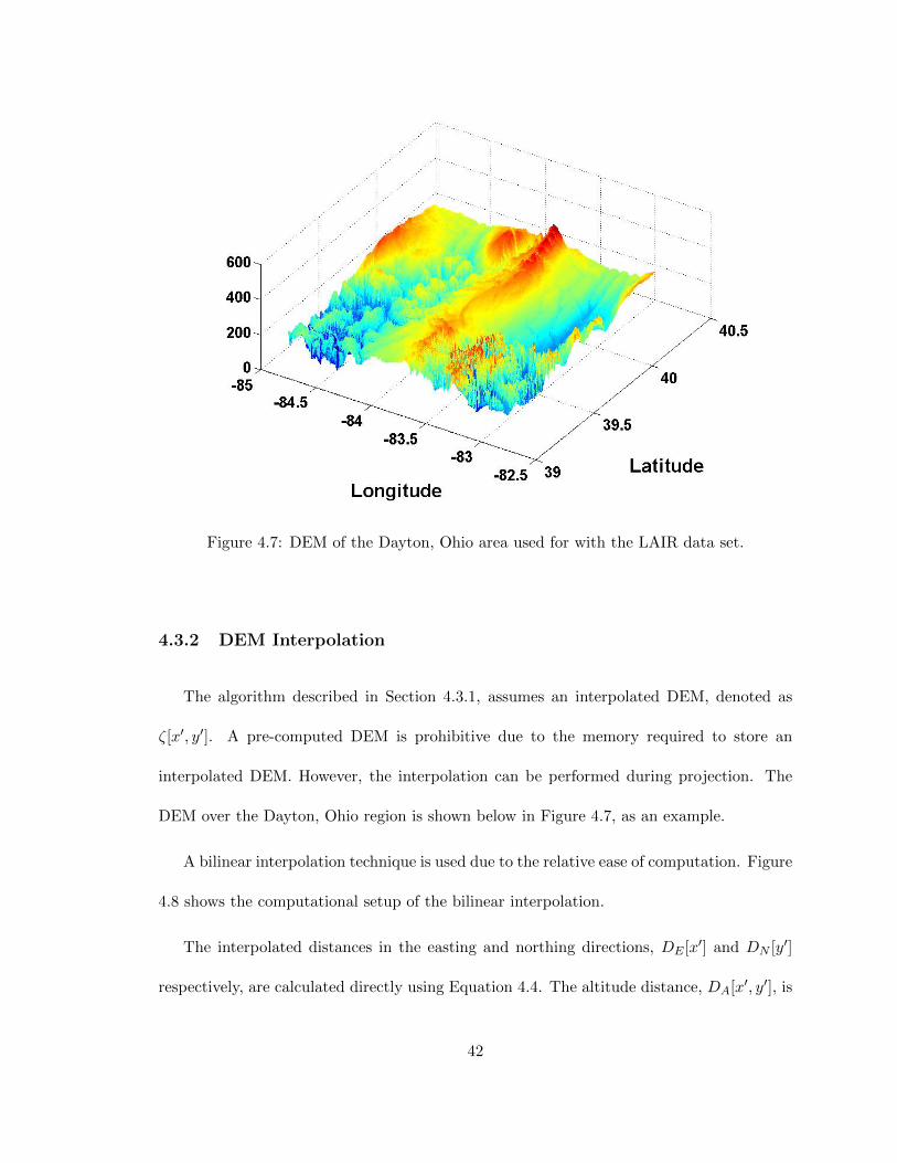
Figure 4.7: DEM of the Dayton, Ohio area used for with the LAIR data set.

4.3.2 DEM Interpolation

The algorithm described in Section 4.3.1, assumes an interpolated DEM, denoted as

ζ[x′, y′]. A pre-computed DEM is prohibitive due to the memory required to store an

interpolated DEM. However, the interpolation can be performed during projection. The

DEM over the Dayton, Ohio region is shown below in Figure 4.7, as an example.

A bilinear interpolation technique is used due to the relative ease of computation. Figure

4.8 shows the computational setup of the bilinear interpolation.

The interpolated distances in the easting and northing directions, DE [x′] and DN [y′]

respectively, are calculated directly using Equation 4.4. The altitude distance, DA[x′, y′], is

42

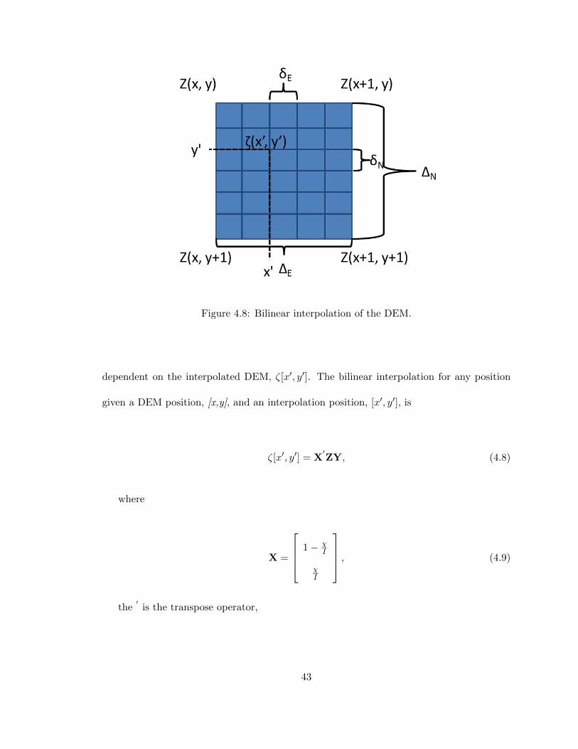
Figure 4.8: Bilinear interpolation of the DEM.

dependent on the interpolated DEM, ζ[x′, y′]. The bilinear interpolation for any position

given a DEM position, [x,y], and an interpolation position, [x′, y′], is

ζ[x′, y′] = X′ZY, (4.8)

where

X =

1− χI

χI

, (4.9)

the′

is the transpose operator,

43

Z =

Z[x, y] Z[x+ 1, y]

Z[x, y + 1] Z[x+ 1, y + 1]

, (4.10)

and

Y =

1− γI

γI

. (4.11)

With these equations, the interpolated altitude distance, DA[x′, y′], from Equation 4.4,

can be calculated within the projection algorithm without a separate DEM interpolation

step.

4.3.3 Algorithm Implementation

The implementation of the algorithm in Section 4.3.1 as described in [68] is to perform

the interpolation and projection simultaneously. If one direction is held constant during an

iteration, then the collinearity equation numerator and denominator can be incremented in

the other two directions.

The interpolated numerators, Equation 4.6, and denominator, Equation 4.7 can be

rewritten incorporating an iterative differential unit as shown in Equation 4.12.

in[x′, y′] = m′11(DE [Ix] + χδE) +m′12(DN [Iy] + γδN ) +m′13(DA[Ix, Iy] + χδAE + γδAN )

jn[x′, y′] = m′21(DE [Ix] + χδE) +m′22(DN [Iy] + γδN ) +m′23(DA[Ix, Iy] + χδAE + γδAN )

rd[x′, y′] = m31(DE [Ix] + χδE) +m32(DN [Iy] + γδN ) +m33(DA[Ix, Iy] + χδAE + γδAN )

,

(4.12)

44

Where δAE and δAN are the differential units for the altitude of the DEM in the east-

ing and northing directions respectively. If the interpolation is performed in the northing

direction and the value is held constant for the interpolation in the easting direction, the

new equations are shown in Equation 4.13, where the value for the interpolated y direction

is based on the DEM interpolation in Equation 4.11

in[x′, y′] = m′11(DE [Ix] + χδE) +m′12DN [y′] +m′13(DA[Ix, y′] + χδAE )

jn[x′, y′] = m′21(DE [Ix] + χδE) +m′22DN [y′] +m′23(DA[Ix, y′] + χδAE )

rd[x′, y′] = m31(DE [Ix] + χδE) +m32DN [y′] +m33(DA[Ix, y′] + χδAE )

, (4.13)

The differential unit for the altitude in the easting direction is found using a linear

interpolation by Equation 4.14

δAE =Z[I(x+ 1), y′]− Z[Ix, y′]

I. (4.14)

Each component of the collinearity equations is a function of χ and can be divided into

an initial value and an iterative variable. The initial values are shown in Equation 4.15.

in[Ix, y′] = (m′11DE [Ix] +m′12DN [y′] +m′13DA[Ix, y′])

jn[Ix, y′] = (m′21DE [Ix] +m′22DN [y′] +m′23DA[Ix, y′])

rd[Ix, y′] = m31DE [Ix] +m32DN [y′] +m33DA[Ix, y′]

, (4.15)

and the iterative variables are shown in Equation 4.16

45

δin = m′11δE +m′13δAE

δjn = m′21δE +m′23δAE

δrd = m31δE +m33δAE

. (4.16)

The iterative collinearity equation components becomes

in[x′, y′] = in[Ix, y′] + χδin

jn[x′, y′] = jn[Ix, y′] + χδjn

rd[x′, y′] = rd[Ix, y

′] + χδrd

. (4.17)

The floating-point algorithm psuedo-code is shown in Algorithm 1.

Algorithm 1 Floating Point Algorithm

1: Load Calibration Parameters2: m•, Z3: Xc, Yc Equation 4.44: ∆E ,∆N

5: Calculate More Parameters6: I, δE , δN Equations 4.27: for y = I(yinitial : yfinal)8: DN [Iy] - Equation 4.49: for x = I(xinitial : xfinal)

10: DE [Ix] - Equation 4.411: for γ = 1 : I12: ζ[Ix, y′] - Equation 4.913: DZ [Ix, y′] - Equation 4.414: in[Ix, y′], jn[Ix, y′], rd[Ix, y

′] - Equation 4.1515: δin , δjn , δrd - Equation 4.1616: for χ = 1 : I17: i[x′, y′], j[x′, y′] - Equation 4.518: in[x′, y′], jn[x′, y′], rd[x

′, y′] - Equation 4.17

19: end20: DN [y′] - Equation 4.4

21: end22: end23: end

46

CHAPTER V

FIXED-POINT PROJECTION ALGORITHM WITH LINEAR

APPROXIMATION [26]

This chapter covers the development, implementation, and results of algorithm proposed

in [26].

5.1 Algorithm Description of [26]

All of the components required for calculating the image plane pixel positions, Equation

4.5 are described in Section 4.3, . However, a division is required for the projection cal-

culation, which is computationally inefficient. To remove the division from the collinearity

equation, the denominator, rd[x′, y′], can be inverted beforehand.

However, the inversion is computationally inefficient when performed for every interpo-

lated pixel. To increase the throughput the inversion is computed fewer times by imple-

menting a linear approximation of the denominator. The denominator can be broken down

into an initial value and a differential value, where Ix and Iy are the interpolated positions

of known DEM values (i.e. χ = γ = 0), such as

r−1d [x′, y′] =

1

rd[Ix, Iy] + δrdE [χ] + δrdN [γ]. (5.1)

47

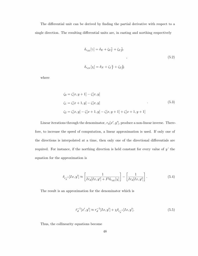
The differential unit can be derived by finding the partial derivative with respect to a

single direction. The resulting differential units are, in easting and northing respectively

δrdE [γ] = δE + ζ0γI + ζ2

γI2

δrdN [χ] = δN + ζ1χI + ζ2

χI2

, (5.2)

where

ζ0 = ζ[x, y + 1]− ζ[x, y]

ζ1 = ζ[x+ 1, y]− ζ[x, y]

ζ2 = ζ[x, y]− ζ[x+ 1, y]− ζ[x, y + 1] + ζ[x+ 1, y + 1]

. (5.3)

Linear iterations through the denominator, rd[x′, y′], produce a non-linear inverse. There-

fore, to increase the speed of computation, a linear approximation is used. If only one of

the directions is interpolated at a time, then only one of the directional differentials are

required. For instance, if the northing direction is held constant for every value of y’ the

equation for the approximation is

δr−1d

[Ix, y′] ≈[

1

Ird[Ix, y′] + I2δrdE [χ]

]−[

1

Ird[Ix, y′]

]. (5.4)

The result is an approximation for the denominator which is

r−1d [x′, y′] ≈ r−1

d [Ix, y′] + χδr−1d

[Ix, y′]. (5.5)

Thus, the collinearity equations become

48

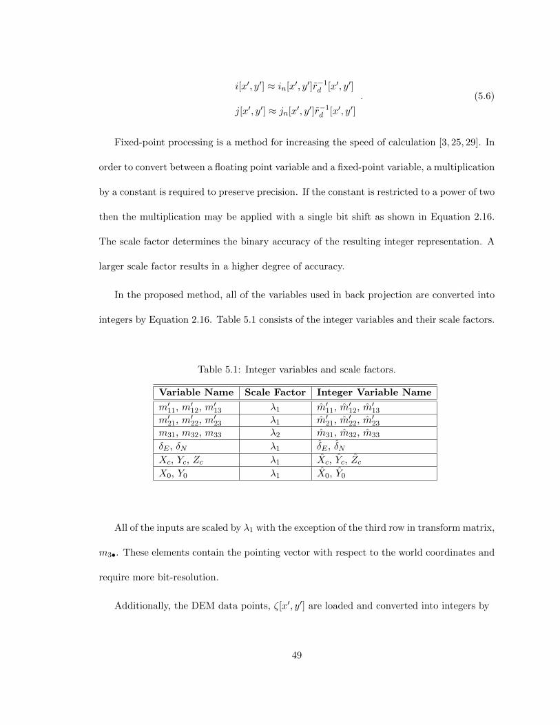
i[x′, y′] ≈ in[x′, y′]r−1d [x′, y′]

j[x′, y′] ≈ jn[x′, y′]r−1d [x′, y′]

. (5.6)

Fixed-point processing is a method for increasing the speed of calculation [3, 25, 29]. In

order to convert between a floating point variable and a fixed-point variable, a multiplication

by a constant is required to preserve precision. If the constant is restricted to a power of two

then the multiplication may be applied with a single bit shift as shown in Equation 2.16.

The scale factor determines the binary accuracy of the resulting integer representation. A

larger scale factor results in a higher degree of accuracy.

In the proposed method, all of the variables used in back projection are converted into

integers by Equation 2.16. Table 5.1 consists of the integer variables and their scale factors.

Table 5.1: Integer variables and scale factors.

Variable Name Scale Factor Integer Variable Name

m′11, m′12, m′13 λ1 m′11, m′12, m′13

m′21, m′22, m′23 λ1 m′21, m′22, m′23

m31, m32, m33 λ2 m31, m32, m33

δE , δN λ1 δE , δNXc, Yc, Zc λ1 Xc, Yc, ZcX0, Y0 λ1 X0, Y0

All of the inputs are scaled by λ1 with the exception of the third row in transform matrix,

m3•. These elements contain the pointing vector with respect to the world coordinates and

require more bit-resolution.

Additionally, the DEM data points, ζ[x′, y′] are loaded and converted into integers by

49

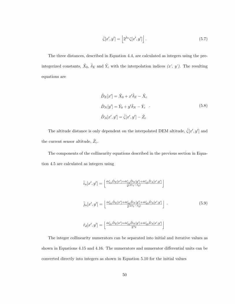
ζ[x′, y′] =⌊2λ1ζ[x′, y′]

⌋. (5.7)

The three distances, described in Equation 4.4, are calculated as integers using the pre-

integerized constants, X0, δE and Yc with the interpolation indices (x’, y’). The resulting

equations are

DE [x′] = X0 + x′δE − Xc

DN [y′] = Y0 + y′δN − Yc

DA[x′, y′] = ζ[x′, y′]− Zc

. (5.8)

The altitude distance is only dependent on the interpolated DEM altitude, ζ[x′, y′] and

the current sensor altitude, Zc.

The components of the collinearity equations described in the previous section in Equa-

tion 4.5 are calculated as integers using

in[x′, y′] =⌊m′11DE [x′]+m′12DN [y′]+m′13DA[x′,y′]

2(2λ1−λ2)

⌋

jn[x′, y′] =⌊m′21DE [x′]+m′22DN [y′]+m′23DA[x′,y′]

2(2λ1−λ2)

⌋

rd[x′, y′] =

⌊m′31DE [x′]+m′32DN [y′]+m′33DA[x′,y′]

2λ2

⌋. (5.9)

The integer collinearity numerators can be separated into initial and iterative values as

shown in Equations 4.15 and 4.16. The numerators and numerator differential units can be

converted directly into integers as shown in Equation 5.10 for the initial values

50

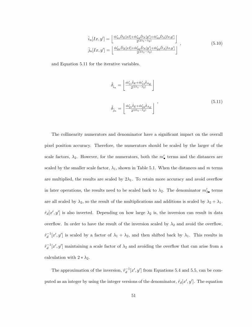
in[Ix, y′] =⌊m′11DE [xI]+m′12DN [y′]+m′13DA[Ix,y′]

2(2λ1−λ2)

⌋jn[Ix, y′] =

⌊m′21DE [xI]+m′22DN [y′]+m′23DA[Ix,y′]

2(2λ1−λ2)

⌋ , (5.10)

and Equation 5.11 for the iterative variables.

δin =

⌊m′11δE+m′13δAE

2(2λ1−λ2)

⌋

δjn =

⌊m′21δE+m′23δAE

2(2λ1−λ2)

⌋ , (5.11)

The collinearity numerators and denominator have a significant impact on the overall

pixel position accuracy. Therefore, the numerators should be scaled by the larger of the

scale factors, λ2. However, for the numerators, both the m′• terms and the distances are

scaled by the smaller scale factor, λ1, shown in Table 5.1. When the distances and m terms

are multiplied, the results are scaled by 2λ1. To retain more accuracy and avoid overflow

in later operations, the results need to be scaled back to λ2. The denominator m′3• terms

are all scaled by λ2, so the result of the multiplications and additions is scaled by λ2 + λ1.

rd[x′, y′] is also inverted. Depending on how large λ2 is, the inversion can result in data

overflow. In order to have the result of the inversion scaled by λ2 and avoid the overflow,

r−1d [x′, y′] is scaled by a factor of λ1 + λ2, and then shifted back by λ1. This results in

r−1d [x′, y′] maintaining a scale factor of λ2 and avoiding the overflow that can arise from a

calculation with 2 ∗ λ2.

The approximation of the inversion, r−1d [x′, y′] from Equations 5.4 and 5.5, can be com-

puted as an integer by using the integer versions of the denominator, rd[x′, y′]. The equation

51

for the integer computations for the inversion and differential approximation is scaled by

λ2. The differential unit and inversion approximation are

δr−1d

[Ix, y′] =(r−1d [Ix+ I, y′]− r−1

d [Ix, y′])I−1

ˆr−1d [x′, y′] ≈ r−1

d [Ix, y′] + χδr−1d

[Ix, y′]

, (5.12)

where

r−1d [Ix, y′] =

⌊2λ1+λ2

rd[Ix, y′]

⌋, (5.13)

and

I−1 =

⌊2λ1

I

⌋. (5.14)

The image plane pixel positions for the proposed method can now be calculated by

i[x′, y′] =

⌊in[x′,y′]ˆr−1

d [x′,y′]

2λ2

⌋

j[x′, y′] =

⌊jn[x′,y′]ˆr−1

d [x′,y′]

2λ2

⌋ , (5.15)

and

i[x′, y′] ∼=⌊i[x′,y′]

2λ1

⌋

j[x′, y′] ∼=⌊j[x′,y′]

2λ1

⌋ . (5.16)

52

The flow diagram for the proposed projection method is shown below in Figure 5.1

The pseudo code for the fixed-point algorithm with the linear approximation is shown

below in Algorithm 2

Algorithm 2 Fixed-Point Algorithm with Linear Approximation

1: Load Calibration Parameters2: m•, Z3: Xc, Yc Equation 5.84: ∆E , ∆N

5: Calculate More Parameters6: I, δE , δN Equations 4.27: for y = I(yinitial : yfinal)

8: DN [Iy] - Equation 5.89: for x = I(xinitial : xfinal)

10: DE [Ix] - Equation 5.811: for γ = 1 : I12: ζ[x′, y′] - Equation 5.713: DA[Ix, y′] - Equation 5.814: in[Ix, y′], jn[Ix, y′] - Equation 5.1015: δin , δjn - Equation 5.11

16: ˆr−1d [Ix, y′], δr−1

d[Ix, y′] - Equation 5.12

17: for χ = 1 : I18: i[x′, y′], j[x′, y′] - Equation 5.1519: in[x′, y′], jn[x′, y′] - Equation 5.1220: r−1

d [x′, y′] - Equation 5.12

21: end22: DN [y′] - Equation 5.8

23: end24: end25: end

5.2 Metrics

For comparison, a back projection algorithm [68] is used where all of the necessary

variables are 64-bit floating point data types, along with the proposed integer based algo-

rithm. Each of the algorithms are executed on the same Linux based 16 core computer

53

Figure 5.1: Flow diagram for the proposed projection method.

54

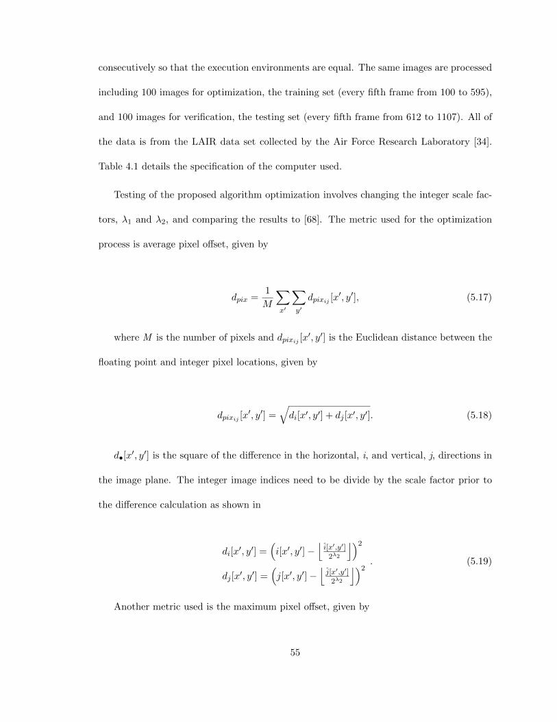
consecutively so that the execution environments are equal. The same images are processed

including 100 images for optimization, the training set (every fifth frame from 100 to 595),

and 100 images for verification, the testing set (every fifth frame from 612 to 1107). All of

the data is from the LAIR data set collected by the Air Force Research Laboratory [34].

Table 4.1 details the specification of the computer used.

Testing of the proposed algorithm optimization involves changing the integer scale fac-

tors, λ1 and λ2, and comparing the results to [68]. The metric used for the optimization

process is average pixel offset, given by

dpix =1

M

∑x′

∑y′

dpixij [x′, y′], (5.17)

where M is the number of pixels and dpixij [x′, y′] is the Euclidean distance between the

floating point and integer pixel locations, given by

dpixij [x′, y′] =

√di[x′, y′] + dj [x′, y′]. (5.18)

d•[x′, y′] is the square of the difference in the horizontal, i, and vertical, j, directions in

the image plane. The integer image indices need to be divide by the scale factor prior to

the difference calculation as shown in

di[x′, y′] =

(i[x′, y′]−

⌊i[x′,y′]

2λ2

⌋)2

dj [x′, y′] =

(j[x′, y′]−

⌊j[x′,y′]

2λ2

⌋)2. (5.19)

Another metric used is the maximum pixel offset, given by

55

dmax = maxx′,y′

dpixij [x′, y′] (5.20)

The maximum pixel offset is recorded for each image, and is combined over the training

set by keeping the maximum pixel offset error for each set of scale factors across all of

training images. The maximum pixel offset is important because the average can show a

small difference, but if a few pixels overflow the data type then, the image will be impacted.

The maximum error indicates whether a data overflow occurred.

5.3 Results from [26]

This section presents and discusses the results from the fixed-point orthorectification

algorithm with a linear approximation methods published in [26].

5.3.1 128-bit Algorithm with Linear Approximation Results

The first set of results are for 128-bit integers, which show how accurate the proposed

method can be and limit overflow. Equation 5.17 indicates the average pixel offset from

the floating point within an image. dpix is calculated and averaged over the 100 training

images. Figure 5.2 shows the results over several values of λ1 and λ2. The range of results,

due to loss of too much resolution and data type overrun is large, therefore, a log function is

employed to highlight the small changes for the most accurate result as well as to compress

the large errors.

The range for λ1 and λ2 are from 0 to 63. Figure 5.2 shows that the errors are large

but consistent until enough information is maintained that the projection results begin to

56

Figure 5.2: Average pixel offset surface per set of scale factors over 100 training images.

approach the floating point version. The variables scaled by λ1 require less resolution to

begin convergence. There is a valley, which is the best performing sets of scale factors which

extends across the viable region along the λ2 axis. A profile plot is shown in Figure 5.3

which shows the minimum pixel offset error and plateau as λ2 varies.

There is an area of good performance with small pixel offset area around the valley. This

is beneficial as it allows flexibility to withstand large terrain variance and still maintain an

acceptable level of accuracy. However, after the floor of the results, the pixel offset error

jumps to a large value. The jump in error is due to a bit overflow from one or more of the

multiplication operations with the scale factors.

57

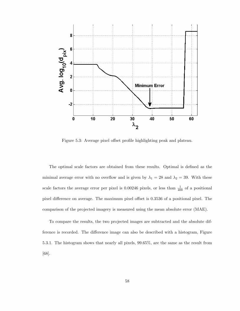
Figure 5.3: Average pixel offset profile highlighting peak and plateau.

The optimal scale factors are obtained from these results. Optimal is defined as the

minimal average error with no overflow and is given by λ1 = 28 and λ2 = 39. With these

scale factors the average error per pixel is 0.00246 pixels, or less than 1400 of a positional

pixel difference on average. The maximum pixel offset is 0.3536 of a positional pixel. The

comparison of the projected imagery is measured using the mean absolute error (MAE).

To compare the results, the two projected images are subtracted and the absolute dif-

ference is recorded. The difference image can also be described with a histogram, Figure

5.3.1. The histogram shows that nearly all pixels, 99.65%, are the same as the result from

[68].

58

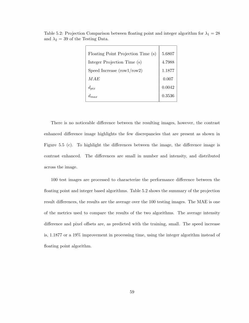
Table 5.2: Projection Comparison between floating point and integer algorithm for λ1 = 28and λ2 = 39 of the Testing Data.

Floating Point Projection Time (s) 5.6807

Integer Projection Time (s) 4.7988

Speed Increase (row1/row2) 1.1877

MAE 0.007

dpix 0.0042

dmax 0.3536

There is no noticeable difference between the resulting images, however, the contrast

enhanced difference image highlights the few discrepancies that are present as shown in

Figure 5.5 (c). To highlight the differences between the image, the difference image is

contrast enhanced. The differences are small in number and intensity, and distributed

across the image.

100 test images are processed to characterize the performance difference between the

floating point and integer based algorithms. Table 5.2 shows the summary of the projection

result differences, the results are the average over the 100 testing images. The MAE is one

of the metrics used to compare the results of the two algorithms. The average intensity

difference and pixel offsets are, as predicted with the training, small. The speed increase

is, 1.1877 or a 19% improvement in processing time, using the integer algorithm instead of

floating point algorithm.

59

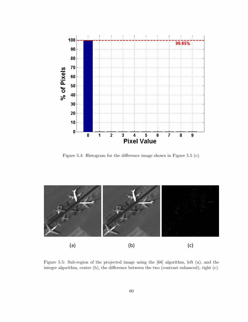
Figure 5.4: Histogram for the difference image shown in Figure 5.5 (c).

Figure 5.5: Sub-region of the projected image using the [68] algorithm, left (a), and theinteger algorithm, center (b), the difference between the two (contrast enhanced), right (c).

60

5.3.2 64-bit Algorithm with Linear Approximation Results

Since 64-bit processors are becoming more commonplace, it is helpful if the scale factors

operate within a 64-bit value to obtain maximum performance. To find the optimal scale

factors for a 64-bit integer, another test is run which limits all data-types to 64-bits. a

subset of scale factor values are optimized and the pixel offset surface is shown below in

Figure 5.6. The difference between the two surfaces shown in Figures 5.2 and 5.6 is where

data overflow occurs.

To determine the optimal scale factors with the integers limited to 64-bits, a sub-range

of the scale factor region is optimized over, namely λ1 = 12 to 20 and λ2 = 26 to 34. These

ranges are found by determining how much of a scale factor is required to maintain data,

i.e. finding where the 128-bit surface, Figure 5.2, begins to converge for each scale factor.

Then calculating the average pixel difference and checking for data overflow. Figure 5.6

shows the sub-range of scale factors over the training images, after being limited to a 64-bit

depth. The difference between Figure 5.6 and 5.2 is where the overflow occurs due the the

64-bit limit.

For the 64-bit limited algorithm, the optimal scale factors are λ1 = 17 and λ2 = 32.

The resulting average pixel offset error is 0.1464, and a maximum pixel offset of 1.0607.

Therefore, in general, nearly all pixels are under a half pixel offset, from the targeted

position. At the maximum error, a pixel is shifted by a full pixel size.

The summary for the testing data for the 64-bit limited integer algorithm is shown in

Table 5.3. As with the previous results, all of the values are averaged over the 100 testing

images. The speed increase is more than double with the optimal scale factors, and does

61

Figure 5.6: Average pixel offset surface per set of scale factors over 100 training images,limited to 64-bit integers.

not overflow in any of the images. The average intensity difference between the algorithms

is sufficiently small as to not cause noticeable artifacts.

Figure 5.3.2 shows the resulting orthorectified images from a test image for the different

algorithms. The difference image has more pixels that are different, but most of these

differences are small, as shown by the histogram of the difference image in Figure 5.8 along

with the statistics for the individual test image.

A zoomed in section of the image is shown in Figure 5.9. The difference image indicates

many pixels that are not the same, however, by inspection the two orthorectified images are

not visually different. Another artifact of the algorithm change becomes apparent in the

difference image, the graduations along the easting direction. These graduations are the

induced error from the linear approximation of the inverse function described in Section 5.1.

62

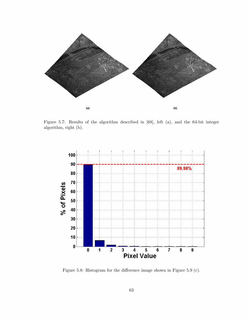
Figure 5.7: Results of the algorithm described in [68], left (a), and the 64-bit integeralgorithm, right (b).

Figure 5.8: Histogram for the difference image shown in Figure 5.9 (c).

63

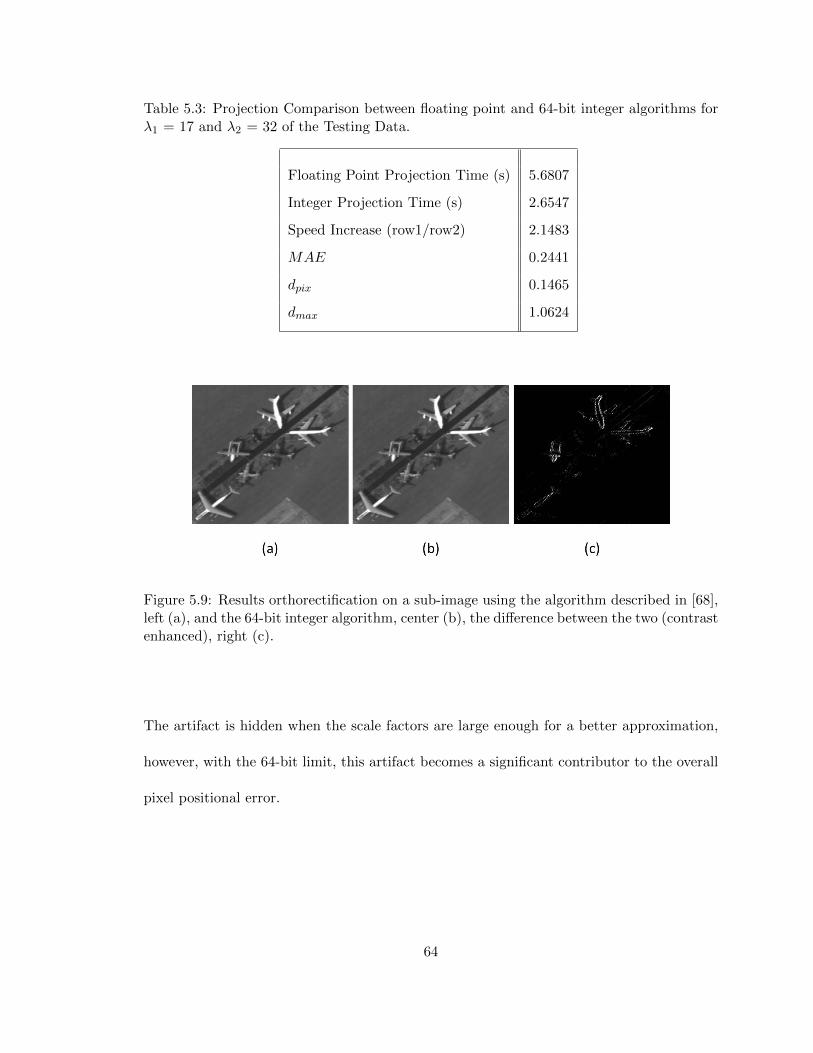
Table 5.3: Projection Comparison between floating point and 64-bit integer algorithms forλ1 = 17 and λ2 = 32 of the Testing Data.

Floating Point Projection Time (s) 5.6807

Integer Projection Time (s) 2.6547

Speed Increase (row1/row2) 2.1483

MAE 0.2441

dpix 0.1465

dmax 1.0624

Figure 5.9: Results orthorectification on a sub-image using the algorithm described in [68],left (a), and the 64-bit integer algorithm, center (b), the difference between the two (contrastenhanced), right (c).

The artifact is hidden when the scale factors are large enough for a better approximation,

however, with the 64-bit limit, this artifact becomes a significant contributor to the overall

pixel positional error.

64

CHAPTER VI

FIXED-POINT PROJECTION ALGORITHM WITH QUADRATIC

APPROXIMATION [27]

This chapter covers the quadratic approach for approximating an inverse function pro-

posed in [27]. The results of the quadratic approach are compared to the different algorithms

and versions. The first algorithm [68] has two versions. The first version is a 128-bit floating-

point algorithm denoted as F128, and used as the truth values for comparisons to the other

algorithms. There are two methods for determining a standard ”truth”, one method is to

use control points in the imagery with known absolute location and compare the projected

position to the control point’s position. Another method, given that control points aren’t

always available, the projection is dependent solely on location and attitude measurement

accuracy. The second method is used for this section, where the measurement accuracy

determines the accuracy of the projection. The control point method is useful for absolute

accuracy, but the measurement accuracy method is applicable to more platforms. The other

version of the [68] algorithm uses a 64-bit floating point data type and is denoted as F64.

The integer algorithm described in Chapter V uses a linear function to approximate

the inverse function. There are also two versions of the linear algorithm, a 128-bit integer

65

Figure 6.1: Difference Image (C) between the truth image (A) and the 64-bit linear approx-imation algorithm (B)

version, I128LA, and a 64-bit integer version I64LA. The quadratic version described below

also has the 128-bit version, I128QA and the 64-bit version I64QA.

6.1 Algorithm Description of [27]

The previous chapter, Chapter , describes a linear approximation for fixed-point image

orthorectification. However, the pixel offset, especially for the I64LA version, is significantly

higher than the F64 method. The difference image gives an indication of the likely reason;

the linear approximation of the inverse function coupled with the limited resolution of the

64-bit integer. Figure 6.1 (C) shows the difference between the result of F128 algorithm (A)

and the I64LA algorithm (B). Note the additional difference structure (vertical lines) in the

difference image.

The purpose of this paper is to develop a fixed-point orthorectification algorithm that

generates a more accurate result. The proposed modifications replace the linear approxi-

mation of the inverse function with a quadratic approximation. Using the results from [26],

66

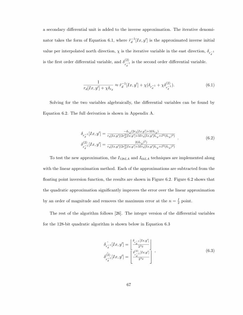
a secondary differential unit is added to the inverse approximation. The iterative denomi-

nator takes the form of Equation 6.1, where r−1d [Ix, y′] is the approximated inverse initial

value per interpolated north direction, χ is the iterative variable in the east direction, δr−1d

is the first order differential variable, and δ(2)

r−1d

is the second order differential variable.

1

rd[Ix, y′] + χδrd≈ r−1

d [Ix, y′] + χ(δr−1d

+ χδ(2)

r−1d

). (6.1)

Solving for the two variables algebraically, the differential variables can be found by

Equation 6.2. The full derivation is shown in Appendix A.

δr−1d

[Ix, y′] =−δrd (2rd[Ix,y′]+3Iδrd )

rd[Ix,y′](2r2d[Ix,y′]+3Ird[Ix,y′]δrd+I2(δrd )2)

δ(2)

r−1d

[Ix, y′] =2(δrd )2)

rd[Ix,y′](2r2d[Ix,y′]+3Ird[Ix,y′]δrd+I2(δrd )2)

. (6.2)

To test the new approximation, the I128LA and I64LA techniques are implemented along

with the linear approximation method. Each of the approximations are subtracted from the

floating point inversion function, the results are shown in Figure 6.2. Figure 6.2 shows that

the quadratic approximation significantly improves the error over the linear approximation

by an order of magnitude and removes the maximum error at the n = I2 point.

The rest of the algorithm follows [26]. The integer version of the differential variables

for the 128-bit quadratic algorithm is shown below in Equation 6.3

ˆδr−1d

[Ix, y′] =

⌊δr−1d

[Ix,y′]

2λ2

⌋ˆδ

(2)

r−1d

[Ix, y′] =

⌊δ(2)

r−1d

[Ix,y′]

2λ2

⌋ , (6.3)

67

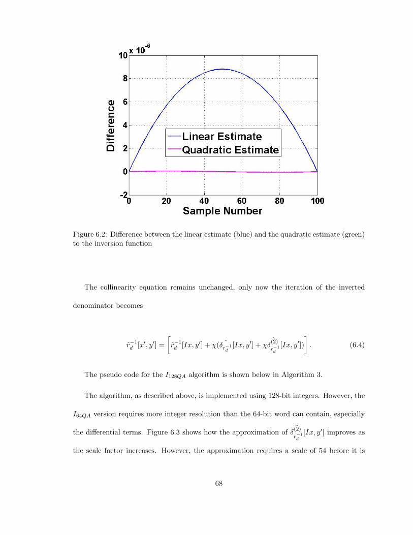
Figure 6.2: Difference between the linear estimate (blue) and the quadratic estimate (green)to the inversion function

The collinearity equation remains unchanged, only now the iteration of the inverted

denominator becomes

r−1d [x′, y′] =

[r−1d [Ix, y′] + χ( ˆδr−1

d[Ix, y′] + χ

ˆδ

(2)

r−1d

[Ix, y′])

]. (6.4)

The pseudo code for the I128QA algorithm is shown below in Algorithm 3.

The algorithm, as described above, is implemented using 128-bit integers. However, the

I64QA version requires more integer resolution than the 64-bit word can contain, especially

the differential terms. Figure 6.3 shows how the approximation ofˆδ

(2)

r−1d

[Ix, y′] improves as

the scale factor increases. However, the approximation requires a scale of 54 before it is

68

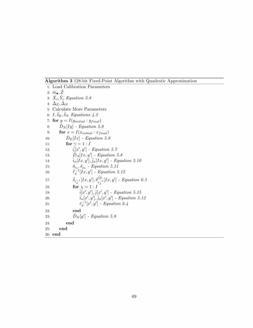
Algorithm 3 128-bit Fixed-Point Algorithm with Quadratic Approximation

1: Load Calibration Parameters2: m•, Z3: Xc, Yc Equation 5.84: ∆E , ∆N

5: Calculate More Parameters6: I, δE , δN Equations 4.27: for y = I(yinitial : yfinal)

8: DN [Iy] - Equation 5.89: for x = I(xinitial : xfinal)

10: DE [Ix] - Equation 5.811: for γ = 1 : I12: ζ[x′, y′] - Equation 5.713: DA[Ix, y′] - Equation 5.814: in[Ix, y′], jn[Ix, y′] - Equation 5.1015: δin , δjn - Equation 5.1116: ˆr−1

d [Ix, y′] - Equation 5.12

17: δr−1d

[Ix, y′],ˆδ

(2)

r−1d

[Ix, y′] - Equation 6.3

18: for χ = 1 : I19: i[x′, y′], j[x′, y′] - Equation 5.1520: in[x′, y′], jn[x′, y′] - Equation 5.1221: r−1

d [x′, y′] - Equation 6.4

22: end23: DN [y′] - Equation 5.8

24: end25: end26: end

69

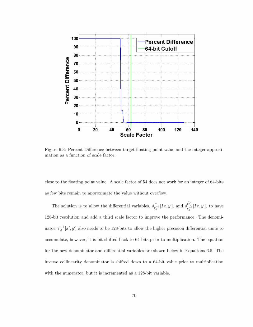
Figure 6.3: Percent Difference between target floating point value and the integer approxi-mation as a function of scale factor.

close to the floating point value. A scale factor of 54 does not work for an integer of 64-bits

as few bits remain to approximate the value without overflow.

The solution is to allow the differential variables, ˆδr−1d

[Ix, y′], andˆδ

(2)

r−1d

[Ix, y′], to have

128-bit resolution and add a third scale factor to improve the performance. The denomi-

nator, r−1d [x′, y′] also needs to be 128-bits to allow the higher precision differential units to

accumulate, however, it is bit shifted back to 64-bits prior to multiplication. The equation

for the new denominator and differential variables are shown below in Equations 6.5. The

inverse collinearity denominator is shifted down to a 64-bit value prior to multiplication

with the numerator, but it is incremented as a 128-bit variable.

70

r−1d [x′, y′] =

⌊m′31DE [x′]+m′32DN [y′]+m′33DA[x′,y′]

2λ2+λ3

⌋ˆδr−1d

[Ix, y′] =

⌊δr−1d

[Ix,y′]

2λ2+λ3

⌋ˆδ

(2)

r−1d

[Ix, y′] =

⌊δ(2)

r−1d

[Ix,y′]

2λ2+λ3

⌋ , (6.5)

The pseudo code for the I64QA version is shown below in Algorithm 4.

Algorithm 4 64-bit Fixed-Point Algorithm with Quadratic Approximation

1: Load Calibration Parameters2: m•, Z3: Xc, Yc Equation 5.84: ∆E , ∆N

5: Calculate More Parameters6: I, δE , δN Equations 4.27: for y = I(yinitial : yfinal)

8: DN [Iy] - Equation 5.89: for x = I(xinitial : xfinal)

10: DE [Ix] - Equation 5.811: for γ = 1 : I12: ζ[x′, y′] - Equation 5.713: DA[Ix, y′] - Equation 5.814: in[Ix, y′], jn[Ix, y′] - Equation 5.1015: δin , δjn - Equation 5.11

16: ˆr−1d [Ix, y′], δr−1

d[Ix, y′],

ˆδ

(2)

r−1d

[Ix, y′] - Equation 6.5

17: for χ = 1 : I18: i[x′, y′], j[x′, y′] - Equation 5.1519: in[x′, y′], jn[x′, y′] - Equation 5.1220: r−1

d [x′, y′] - Equation 6.4

21: end22: DN [y′] - Equation 5.8

23: end24: end25: end

71

6.2 Metrics

The quadratic approximated orthorectification algorithm is implemented with 128 and

64-bit data types, and compared to [68] and [26]. For comparison between the different

algorithm versions, each of the versions are developed and executed on the same Linux

based 16 core computer with specification listed below in table 4.1.

Two data sets are used one for training and the other for testing. All imagery in the

training and testing data sets are from the LAIR II data set collected by Air Force Research

Laboratory [34]. The training data set is 100 frames from the beginning of the data set to

frame 595, with every fifth frame used. The platform used for the data collection flies an

orbit around a location, by using every fifth frame the full orbit is sampled with enough

angle variation to avoid over-training to a specific a specific set of look angles and distances.

The testing data set is also 100 images, but from later in the collection (every fifth frame

from 612 to 1107).

For the floating point algorithms, no training is required because there are no scale

factors. Only the integer algorithms that have the quadratic approximation are trained to

determine the scale factors. The F128 algorithm, considered to be truth, is used to determine

the scale factors.

Once all training has been completed, the testing data set is processed using the different

algorithms. There are two steps to testing the results. The first step consists of processing

all versions and comparing the average projected pixel distances, 6.6, with respect to the

F128 algorithm.

72

dpix =1

M

∑x′

∑y′

dpix[x′, y′], (6.6)

where M is the number of projected pixels and dpix[x′, y′] is the Euclidean distance

between the F128 point pixel location and the other algorithms. The equation for the

Euclidean distance between two pixel locations is shown in Equation 6.7 where ild[x′, y′],

and jld[x′, y′] are the resulting pixel locations from the F128 algorithm using Equation 4.5

(i-horizontal, j-vertical), and j•[x′, y′], and j•[x

′, y′] are the pixel locations for one of the

other algorithms that are being tested.

dpix[x′, y′] =√

(ild[x′, y′]− i•[x′, y′])2 + ((jld[x′, y′]− j•[x′, y′])2. (6.7)

The maximum pixel offset, given by Equation 6.8, is a measure that can indicate if the

projection ever overflowed the number of allotted bits.

dmax = maxx′,y′

dpix[x′, y′]. (6.8)

The next step, consists of each stand-alone implementation where the time and orthorec-

tified imagery is produced and new metrics are used. One of the new metrics include the

mean absolute error of the projected imagery, shown in Equation 6.9, where Qld[x′, y′] is

the projected pixel intensity value from the F128 algorithm and Q•[x′, y′] is the projected

pixel value from the algorithm being tested. The absolute pixel value differences are then

summed and a mean value is calculated from all test images.

73

MAE =1

M

∑x′

∑y′

|Qld[x′, y′]−Q•[x′, y′]|. (6.9)

Computational time as well as the speed increase as shown by Equation 6.10, where the

time for projection from the F128 algorithm (Tld) is divided by the computational time of

the other projection algorithms (T•).

S =TldT•

(6.10)

The final metric is the percentage, with respect to the total number of projected pixels,

of the number of non-zero elements remaining after the difference from the F128 algorithm,

denoted as P , and shown in Equation 6.11. P is another estimate of how well the orthorec-

tification algorithm performed.

P =

1

M

∑x′

∑y′

1, |Qld[x′, y′]−Q•[x′, y′]| > 0

0, else

. (6.11)

6.3 Results from [27]

This section presents the results from the fixed-point orthorectification algorithm with

a quadratic approximation pending published in [27].

6.3.1 128-bit Algorithm with Quadratic Approximation Training Results

The 128-bit Integer algorithm with the quadratic approximation, I128QA, is trained. The

training consists of calculating the average pixel difference between the I128QA algorithm

74

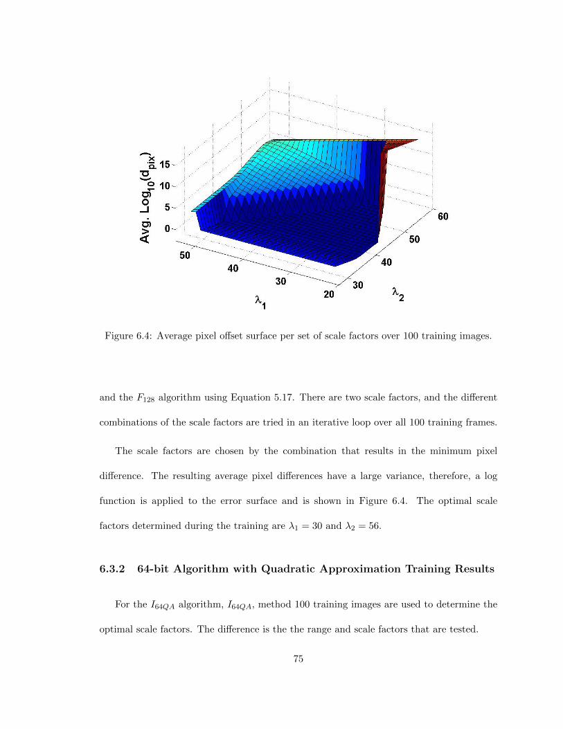
Figure 6.4: Average pixel offset surface per set of scale factors over 100 training images.

and the F128 algorithm using Equation 5.17. There are two scale factors, and the different

combinations of the scale factors are tried in an iterative loop over all 100 training frames.

The scale factors are chosen by the combination that results in the minimum pixel

difference. The resulting average pixel differences have a large variance, therefore, a log

function is applied to the error surface and is shown in Figure 6.4. The optimal scale

factors determined during the training are λ1 = 30 and λ2 = 56.

6.3.2 64-bit Algorithm with Quadratic Approximation Training Results

For the I64QA algorithm, I64QA, method 100 training images are used to determine the

optimal scale factors. The difference is the the range and scale factors that are tested.

75

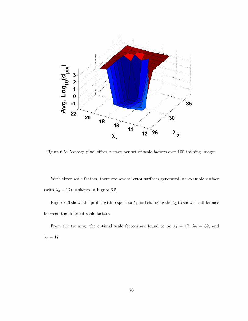
Figure 6.5: Average pixel offset surface per set of scale factors over 100 training images.

With three scale factors, there are several error surfaces generated, an example surface

(with λ3 = 17) is shown in Figure 6.5.

Figure 6.6 shows the profile with respect to λ3 and changing the λ2 to show the difference

between the different scale factors.

From the training, the optimal scale factors are found to be λ1 = 17, λ2 = 32, and

λ3 = 17.

76

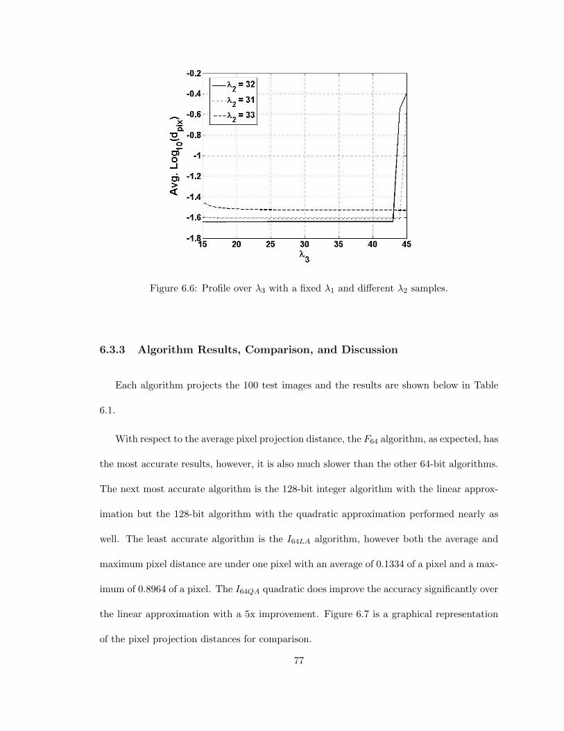
Figure 6.6: Profile over λ3 with a fixed λ1 and different λ2 samples.

6.3.3 Algorithm Results, Comparison, and Discussion

Each algorithm projects the 100 test images and the results are shown below in Table

6.1.

With respect to the average pixel projection distance, the F64 algorithm, as expected, has

the most accurate results, however, it is also much slower than the other 64-bit algorithms.

The next most accurate algorithm is the 128-bit integer algorithm with the linear approx-

imation but the 128-bit algorithm with the quadratic approximation performed nearly as

well. The least accurate algorithm is the I64LA algorithm, however both the average and

maximum pixel distance are under one pixel with an average of 0.1334 of a pixel and a max-

imum of 0.8964 of a pixel. The I64QA quadratic does improve the accuracy significantly over

the linear approximation with a 5x improvement. Figure 6.7 is a graphical representation

of the pixel projection distances for comparison.

77

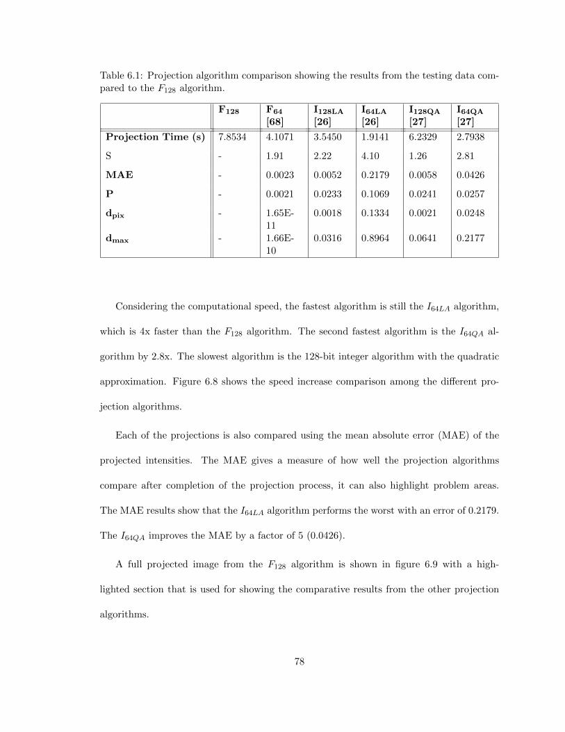
Table 6.1: Projection algorithm comparison showing the results from the testing data com-pared to the F128 algorithm.

F128 F64

[68]I128LA[26]

I64LA[26]

I128QA

[27]I64QA

[27]

Projection Time (s) 7.8534 4.1071 3.5450 1.9141 6.2329 2.7938

S - 1.91 2.22 4.10 1.26 2.81

MAE - 0.0023 0.0052 0.2179 0.0058 0.0426

P - 0.0021 0.0233 0.1069 0.0241 0.0257

dpix - 1.65E-11

0.0018 0.1334 0.0021 0.0248

dmax - 1.66E-10

0.0316 0.8964 0.0641 0.2177

Considering the computational speed, the fastest algorithm is still the I64LA algorithm,

which is 4x faster than the F128 algorithm. The second fastest algorithm is the I64QA al-

gorithm by 2.8x. The slowest algorithm is the 128-bit integer algorithm with the quadratic

approximation. Figure 6.8 shows the speed increase comparison among the different pro-

jection algorithms.

Each of the projections is also compared using the mean absolute error (MAE) of the

projected intensities. The MAE gives a measure of how well the projection algorithms

compare after completion of the projection process, it can also highlight problem areas.

The MAE results show that the I64LA algorithm performs the worst with an error of 0.2179.

The I64QA improves the MAE by a factor of 5 (0.0426).

A full projected image from the F128 algorithm is shown in figure 6.9 with a high-

lighted section that is used for showing the comparative results from the other projection

algorithms.

78

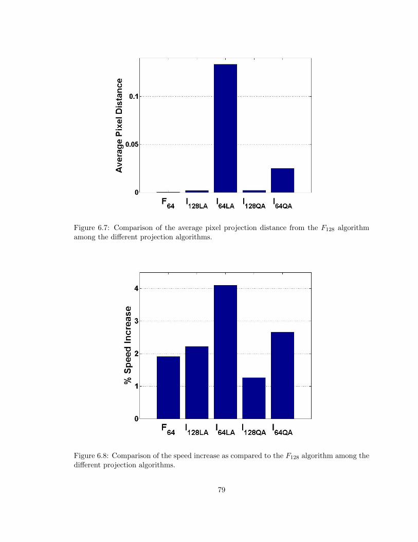
Figure 6.7: Comparison of the average pixel projection distance from the F128 algorithmamong the different projection algorithms.

Figure 6.8: Comparison of the speed increase as compared to the F128 algorithm among thedifferent projection algorithms.

79

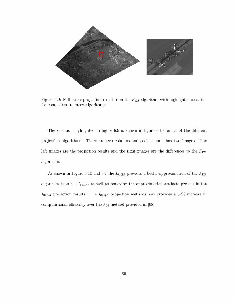
Figure 6.9: Full frame projection result from the F128 algorithm with highlighted selectionfor comparison to other algorithms.

The selection highlighted in figure 6.9 is shown in figure 6.10 for all of the different

projection algorithms. There are two columns and each column has two images. The

left images are the projection results and the right images are the differences to the F128

algorithm.

As shown in Figure 6.10 and 6.7 the I64QA provides a better approximation of the F128

algorithm than the I64LA, as well as removing the approximation artifacts present in the

I64LA projection results. The I64QA projection methods also provides a 32% increase in

computational efficiency over the F64 method provided in [68].

80

Figure 6.10: Comparison of the algorithm projections from the F128 projection algorithm;(A) F64, (B) I128LA, (C) I64LA, (D) I128QA, and (E) I64QA.

81

CHAPTER VII

CONCLUSION

This paper describes two new integer orthorectification algorithms. The first algorithm is

a fixed-point integer algorithm with a linear inverse approximation to remove division. The

algorithm uses two scale factors that are determined through orthorectifying 100 training

images and measuring the average pixel distance from the 64-bit floating point algorithm

described in [68]. After the scale factors are determined, 100 test images are orthorectified

to compare with the 64-bit floating point algorithm. The results show that the processing

time improved by more than 2x with a pixel position difference of less than 15% of a pixel

size for 64-bit integer processing. The 128-bit integer processing results are more accurate,

with a 0.5% pixel position difference, but the computational speed is slower than the 64-bit

algorithm at a 1.2x speed increase over [68].

The second algorithm uses a quadratic collinearity inverse approximation utilizing two

different data types (128-bit and 64-bit integer). The quadratic integer algorithms are also

trained using 100 training images, and then verified using 100 testing images. Each of the

algorithms are compared to the F128 orthorectification algorithm, used as truth. The I64QA

algorithm shows a 5x improvement in projected pixel distance as compared to the I64LA

82

algorithm. The I64QA algorithm is also nearly 3x faster than the F128 algorithm and 1.5x

faster than any of the floating point implementations.

To increase the processing speed in software, the next step could be to combine the

numerator and denominator into an iterative function. All of the researched methods solely

approximate the inverse function, the numerator is never taken into account in the approx-

imations. However, there are major advantages to including the numerator. First, it may

result in a better approximation even if the approximation is limited to a linear function.

If the linear approximation also includes the numerator it may decrease the decrease the

scale factors and allow more bit-depth to represent the value. However, a non-linear ap-

proximation would probably still give more accurate results. The second advantage is that

it will remove two multiplication steps in the inner most loop. As mentioned in Chapter

IV, the pixel location calculation (Equation 5.6) still requires the numerator multiplied by

the approximated inverted denominator. If the numerator is included in the approximation

then the pixel location would be calculated by an iterative addition.

One purpose of this research is to show the feasibility of an FPGA implementation of

the orthorectification algorithm. As mentioned earlier, FPGA is a useful tool for systems

where power consumption is a concern. The new 64-bit integer algorithm with the quadratic

approximation increases the accuracy over the linear implementation and removed the ar-

tifacts. Thereby making it a good candidate for implementation on an FPGA without

losing much accuracy in the floating point to fixed-point conversion or the inverse function

approximation.

83

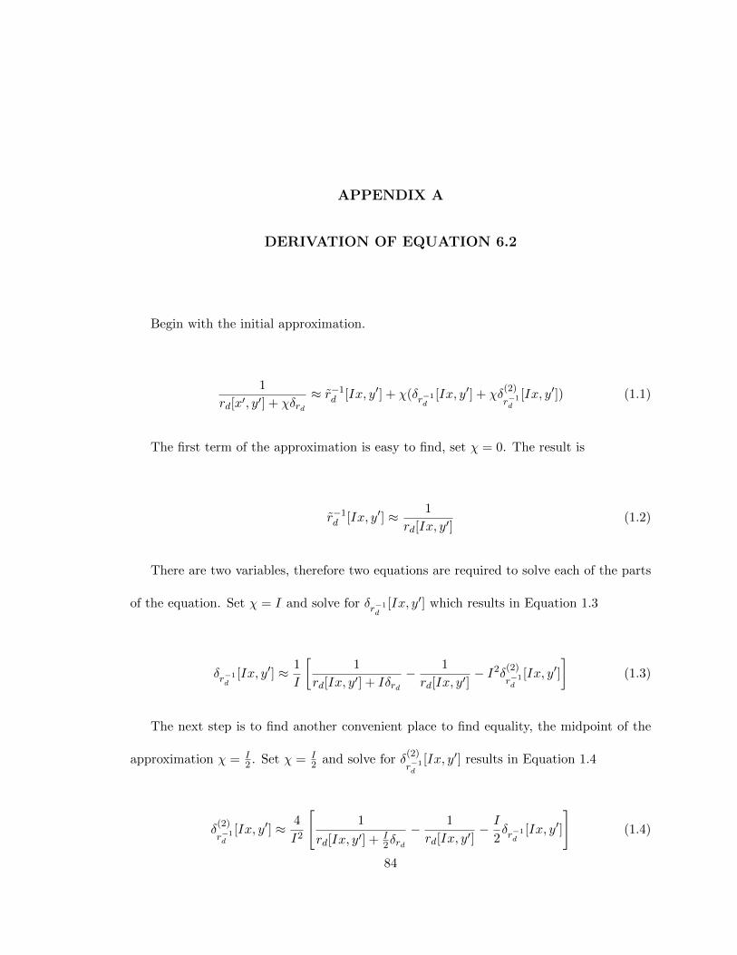
APPENDIX A

DERIVATION OF EQUATION 6.2

Begin with the initial approximation.

1

rd[x′, y′] + χδrd≈ r−1

d [Ix, y′] + χ(δr−1d

[Ix, y′] + χδ(2)

r−1d

[Ix, y′]) (1.1)

The first term of the approximation is easy to find, set χ = 0. The result is

r−1d [Ix, y′] ≈ 1

rd[Ix, y′](1.2)

There are two variables, therefore two equations are required to solve each of the parts

of the equation. Set χ = I and solve for δr−1d

[Ix, y′] which results in Equation 1.3

δr−1d

[Ix, y′] ≈ 1

I

[1

rd[Ix, y′] + Iδrd− 1

rd[Ix, y′]− I2δ

(2)

r−1d

[Ix, y′]

](1.3)

The next step is to find another convenient place to find equality, the midpoint of the

approximation χ = I2 . Set χ = I

2 and solve for δ(2)

r−1d

[Ix, y′] results in Equation 1.4

δ(2)

r−1d

[Ix, y′] ≈ 4

I2

[1

rd[Ix, y′] + I2δrd

− 1

rd[Ix, y′]− I

2δr−1d

[Ix, y′]

](1.4)

84

Substitute Equation 1.3 into Equation 1.4 and simplify results in

δ(2)

r−1d

[Ix, y′] ≈ 4

I2

[1

rd[Ix, y′] + I2δrd

− 1

2rd[Ix, y′]− 1

2rd[Ix, y′] + Iδrd

](1.5)

Equation 1.5 can be simplified further into

δ(2)

r−1d

[Ix, y′] =2(δrd)

2)

rd[Ix, y′](2r2d[Ix, y

′] + 3Ird[Ix, y′]δrd + I2(δrd)2)

(1.6)

Next substitute Equation 1.6 into Equation 1.3 and simplify

δr−1d

[Ix, y′] =−δrd(2rd[Ix, y′] + 3Iδrd)

rd[Ix, y′](2r2d[Ix, y

′] + 3Ird[Ix, y′]δrd + I2(δrd)2)

(1.7)

85

APPENDIX B

CURRENT JOURNAL PUBLICATIONS

[1] Joseph C French and Eric J Balster. A fast and accurate orthorectification algorithm

of aerial imagery using integer arithmetic. Journal of Selected Topics in Applied Earth

Observations and Remote Sensing, 2013.

[2] Joseph C French and Eric J Balster. A quadratic approximation for an integer or-

thorectification algorithm. Journal of Selected Topics in Applied Earth Observations

and Remote Sensing, (Pending).

86

APPENDIX C

CURRENT CONFERENCE PUBLICATIONS

[1] Joseph French, William Turri, Joseph Fernando, and Eric Balster. Gpu accelerated ele-

vation map based registration of aerial images. In High Performance Extreme Computing

Conference (HPEC), 2013 IEEE, pages 1–6. IEEE, 2013.

[2] Joseph C French, Eric J Balster, and William F Turri. A 64-bit orthorectification

algorithm using fixed-point arithmetic. In Society of Photo-Optical Instrumentation

Engineers (SPIE) Conference Series, volume 8895, 2013.

[3] Patrick C Hytla, Joseph C French, Frank O Baxley, Kenneth J Barnard, Mark A Bick-

nell, Russell C Hardie, Eric J Balster, and Nicholas P Vicen. Dynamic range manage-

ment and image compression emphasizing dismount targets in midwave infrared per-

sistent surveillance systems. In Military Sensing Symposium 2010 PF07. SENSIAC,

2010.

[4] Patrick C Hytla, Joseph C French, Nicholas P Vicen, Russell C Hardie, Eric J Balster,

Frank O Baxley, Kenneth J Barnard, and Mark A Bicknell. Image compression empha-

sizing pixel size objects in midwave infrared persistent surveillance systems. In Aerospace

and Electronics Conference (NAECON), Proceedings of the IEEE 2010 National, pages

296–301. IEEE, 2010.

[5] Paul Sundlie, Joseph French, and Eric Balster. Integer computation of image orthorec-

tification for high speed throughput. In International Conference of Image Processing

and Computer Vision. WorldCom, July 2011.

87

BIBLIOGRAPHY

[1] Manuel A Aguilar, Marıa del Mar Saldana, and Fernando J Aguilar. Assessing geomet-

ric accuracy of the orthorectification process from geoeye-1 and worldview-2 panchro-

matic images. International Journal of Applied Earth Observation and Geoinformation,

21:427–435, 2013.

[2] E.F. Arias, P. Charlot, M. Feissel, and J.-F. Lestrade. The extragalactic reference

system of the international earth rotation service, icrs. Astronomy and Astrophysics,

(303):604–608, March 1995.

[3] Eric J. Balster, Benjamin T. Fortener, and William F. Turri. Integer computation of

lossy jpeg2000 compression. IEEE Transactions on Image Processing, 20(8):2386–2391,

August 2011.

[4] John L Barron, David J Fleet, and Steven S Beauchemin. Performance of optical flow

techniques. International journal of computer vision, 12(1):43–77, 1994.

[5] James E Bevington. Laser radar atr algorithms: Phase iii final report. Alliant Techsys-

tems, Inc, 1992.

[6] Anshuman Bhardwaj, Lydia Sam, F Javier Martın-Torres, Rajesh Kumar, et al. Uavs

as remote sensing platform in glaciology: Present applications and future prospects.

Remote Sensing of Environment, 175:196–204, 2016.

[7] Conrad Bielski, Simone Gentilini, and Marco Papparlardo. Post-disaster image pro-

cessing for damage analysis using genesi-dr, wps and grid computing. Remote Sensing,

3:1234–1250, June 2011.

[8] Samuel S. Blackman and Rober Popoli. Design and analysis of modern tracking systems,

volume 685. Artech House, Norwood, MA, 1999.

[9] Xianbin Cao, Changxia Wu, Jinhe Lan, Pingkun Yan, and Xuelong Li. Vehicle detection

and motion analysis in low-altitude airborne video under urban environment. Circuits

and Systems for Video Technology, IEEE Transactions on, 21(10):1522–1533, 2011.

88

[10] Dai Chenguang and Yang Jingyu. Research on orthorectification of remote sensing

images using gpu-cpu cooperative processing. In 2011 International Symposium on

Image and Data Fusion (ISIDF), volume 1 of 4, pages 9–11. IEEE, August 2011.

[11] Emmanuel Christophe, Julien Michel, and Jordi Inglada. Remote sensing processing:

From multicore to gpu. IEEE Journal of Selected Topics in Applied Earth Observations

and Remote Sensing, 4(3):643–652, September 2011.

[12] Albert Cohen, Ingrid Daubechies, and J-C Feauveau. Biorthogonal bases of compactly

supported wavelets. Communications on pure and applied mathematics, 45(5):485–560,

1992.

[13] Douglas C Comer and Michael J Harrower. Mapping archaeological landscapes from

space, volume 5. Springer Science & Business Media, 2013.

[14] James W Cooley and John W Tukey. An algorithm for the machine calculation of

complex fourier series. Mathematics of computation, 19(90):297–301, 1965.

[15] Davide De Caro, Marco Genovese, Ettore Napoli, Nicola Petra, and Antonio

Giuseppe Maria Strollo. Accurate fixed-point logarithmic converter. Circuits and Sys-

tems II: Express Briefs, IEEE Transactions on, 61(7):526–530, 2014.

[16] Davide De Caro, Nicola Petra, and Antonio GM Strollo. Efficient logarithmic converters

for digital signal processing applications. Circuits and Systems II: Express Briefs, IEEE

Transactions on, 58(10):667–671, 2011.

[17] Jeroen De Reu, Gertjan Plets, Geert Verhoeven, Philippe De Smedt, Machteld Bats,

Bart Cherrette, Wouter De Maeyer, Jasper Deconynck, Davy Herremans, Pieter Laloo,

et al. Towards a three-dimensional cost-effective registration of the archaeological her-

itage. Journal of Archaeological Science, 40(2):1108–1121, 2013.

[18] Stephen D DeGloria, Dylan E Beaudette, James R Irons, Zamir Libohova, Peggy E

O’Neill, Phillip R Owens, Philip J Schoeneberger, Larry T West, and Douglas A

Wysocki. Emergent imaging and geospatial technologies for soil investigations. 2014.

[19] Javier Dıaz, Eduardo Ros, Francisco Pelayo, Eva M Ortigosa, and Sonia Mota. Fpga-

based real-time optical-flow system. Circuits and Systems for Video Technology, IEEE

Transactions on, 16(2):274–279, 2006.

[20] Bruce A Draper, J Ross Beveridge, AP Willem Bohm, Charles Ross, and Monica

Chawathe. Accelerated image processing on fpgas. Image Processing, IEEE Transactions

on, 12(12):1543–1551, 2003.

[21] Aaron M Ellison, Michael S. Bank, Barton D. Clinton, Elizabeth A. Colburn,

Katherine Elliott, Chelcy R. Ford, David R. Foster, Brian D. Kloeppel, Jennifer D.

Knoepp, Gary M. Lovett, Jacqueline Mohan, David A. Orwig, Nicholas L. Rodenhouse,

William V. Sobczak, Kristina A. Stinson, Jeffrey K. Stone, Cristopher M. Swan, Jill

89

Thompson, Betsy Von Holle, and Jackson R. Webster. Loss of foundation species: Con-

sequences for the structure and dynamics of forested ecosystems. Frontiers in Ecology

and the Environment, 3(9):479–486, 2005.

[22] Jakob Engel, Jurgen Sturm, and Daniel Cremers. Scale-aware navigation of a low-

cost quadrocopter with a monocular camera. Robotics and Autonomous Systems,

62(11):1646–1656, 2014.

[23] Carlos Alphonso F Ezequiel, Matthew Cua, Nathaniel C Libatique, Gregory L Tango-

nan, Raphael Alampay, Rollyn T Labuguen, Chrisandro M Favila, Jaime Luis E Hon-

rado, Vinni Canos, Charles Devaney, et al. Uav aerial imaging applications for post-

disaster assessment, environmental management and infrastructure development. In

Unmanned Aircraft Systems (ICUAS), 2014 International Conference on, pages 274–

283. IEEE, 2014.

[24] Suhaib A Fahmy, Peter YK Cheung, and Wayne Luk. Novel fpga-based implementation

of median and weighted median filters for image processing. In Field Programmable Logic

and Applications, 2005. International Conference on, pages 142–147. IEEE, 2005.

[25] Miguel A. Ferrer, Jesus B. Alonso, and Carlos M. Travieso. Offline geometric parame-

ters for automatic signature verification using fixed point arithmetic. IEEE Transactions

on Pattern Analysis and Machine Intelligence, 27(6):993–997, June 2005.

[26] Joseph C French and Eric J Balster. A fast and accurate orthorectification algorithm of

aerial imagery using integer arithmetic. Selected Topics in Applied Earth Observations

and Remote Sensing, IEEE Journal of, 7(5):1826–1834, 2014.

[27] Joseph C French and Eric J Balster. A quadratic approximation for an integer or-

thorectification algorithm. Selected Topics in Applied Earth Observations and Remote

Sensing, IEEE Journal of, (Pending).

[28] Diego Fustes, Diego Cantorna, Carlos Dafonte, Alfonso Iglesias, and Bernardino Arcay.

Applications of cloud computing and gis for ocean monitoring through remote sensing.

In Smart Sensing Technology for Agriculture and Environmental Monitoring, pages 303–

321. Springer, 2012.

[29] Jason George, Bo Marr, Aniruddha Dasgupta, and David V. Anderson. Fixed-point

arithmetic on a budget: Comparing probabilistic and reduced-precision addition. In

Circuits and Systems (MWSCAS), 2010 53rd IEE International Midwest Symposium,

pages 1258–1261. IEEE, 2010.

[30] MC Hanumantharaju, M Ravishankar, DR Rameshbabu, and SB Satish. An efficient

vlsi architecture for adaptive rank order filter for image noise removal. International

Journal of Information and Electronics Engineering, 1(1), 2011.

[31] M. A. Hapgood. Space physics coordinate tranformations: A user guide. Planetary

Space Science, 40(5):711–717, 1992.

90

[32] Richard Hartley and Andrew Zisserman. Multiple View Geometry in Computer Vision,

volume 2. Cambridge, 2000.

[33] James Hegarty, John Brunhaver, Zachary DeVito, Jonathan Ragan-Kelley, Noy Cohen,

Steven Bell, Artem Vasilyev, Mark Horowitz, and Pat Hanrahan. Darkroom: compil-

ing high-level image processing code into hardware pipelines. ACM Trans. Graph.,

33(4):144–1, 2014.

[34] http://www.wpafb.af.mil/afrl. Lair data set. Website.

[35] Calvin Hung, Zhe Xu, and Salah Sukkarieh. Feature learning based approach for weed

classification using high resolution aerial images from a digital camera mounted on a

uav. Remote Sensing, 6(12):12037–12054, 2014.

[36] Veljko M Jovanovic, Michael M. Smyth, Jia Zong, Robert Ando, and Graham W.

Bothwell. Misr photogrammetric data reduction for geophysical retrievals. IEEE Trans-

actions on Geoscience and Remote Sensing, 36(4):1290–1301, July 1998.

[37] Med Lassaad Kaddachi, Leila Makkaoui, Adel Soudani, Vincent Lecuire, and

J Moureaux. Fpga-based image compression for low-power wireless camera sensor net-

works. In Next Generation Networks and Services (NGNS), 2011 3rd International

Conference on, pages 68–71. IEEE, 2011.

[38] Christian KNOTH, Birte KLEIN, Torsten PRINZ, and Till KLEINEBECKER. Un-

manned aerial vehicles as innovative remote sensing platforms for high-resolution in-

frared imagery to support restoration monitoring in cut-over bogs. Applied vegetation

science, 16(3):509–517, 2013.

[39] Jan J Koenderink and Andrea J Van Doorn. Affine structure from motion. JOSA A,

8(2):377–385, 1991.

[40] David Kuo and Don Gordon. Real-time orthorectification by fpga-based hardware

acceleration. In Remote Sensing, pages 78300Y–78300Y. International Society for Optics

and Photonics, 2010.

[41] David C. Lay. Linear Algebra and Its Applications, second edition. Addison-Wesley,

1998.

[42] Changno Lee and James Bethel. Georegistration of airborne hyperspectral image data.

IEEE Transactions on Geoscience and Remote Sensing, 39(7):1347–1351, July 2001.

[43] Craig A. Lee, Samuel D. Gasster, Antonio Plaza, Chein-I Chang, and Bormin Huang.

Recent developments in high performance computing for remote sensing: A review.

IEEE Journal of Selected Topics in Applied Earth Observations and Remote Sensing,

4(3):508–527, September 2011.

[44] Bruce D Lucas, Takeo Kanade, et al. An iterative image registration technique with

an application to stereo vision. In IJCAI, volume 81, pages 674–679, 1981.

91

[45] G Lucas. Considering time in orthophotography production: from a general workflow

to a shortened workflow for a faster disaster response. The International Archives of

Photogrammetry, Remote Sensing and Spatial Information Sciences, 40(3):249, 2015.

[46] Arko Lucieer, Darren Turner, Diana H King, and Sharon A Robinson. Using an un-

manned aerial vehicle (uav) to capture micro-topography of antarctic moss beds. Inter-

national Journal of Applied Earth Observation and Geoinformation, 27:53–62, 2014.

[47] Luiz A. Manfre, Eliane Hirata, Janaina B. Silva, Eduardo J. Shinohara, Mariana A.

Giannotti, Ana Paula C. Larocca, and Jose A. Quintanilha. An analysis of geospatial

technologies for risk and natural disaster management. ISPRS International Journal of

Geo-Information, 1:166–185, August 2012.

[48] Ales Marsetic, Kristof Ostir, and Mojca Kosmatin Fras. Automatic orthorectification

of high-resolution optical satellite images using vector roads. Geoscience and Remote

Sensing, IEEE Transactions on, 53(11):6035–6047, 2015.

[49] Jessica L. Morgan, Sarah E. Gergel, and Nicholas C. Coops. Aerial photography: A

rapidly evolving tool for ecological management. BioScience, 60(1):47–59, January 2010.

[50] M. Mostafa and K-P Schwarz. Digital image georeferencing from a multiple camera

system by gps/ins. ISPRS Journal of Photogrammetry and Remote Sensing, 56:1–12,

2001.

[51] NASA. National aeronautics and space administration. Website.

[52] Brandon R Olson, Ryan A Placchetti, Jamie Quartermaine, and Ann E Killebrew. The

tel akko total archaeology project (akko, israel): Assessing the suitability of multi-scale

3d field recording in archaeology. Journal of Field Archaeology, 38(3):244–262, 2013.

[53] B. Parhami. Computer Arithmetic: Algorithms and Hardware Designs. Oxford Uni-

versity Press, inc, New York, NY, USA, 2nd edition, 2009.

[54] Fatih Porikli. Integral histogram: A fast way to extract histograms in cartesian spaces.

In Computer Vision and Pattern Recognition, 2005. CVPR 2005. IEEE Computer So-

ciety Conference on, volume 1, pages 829–836. IEEE, 2005.

[55] Timothy J Purcell, Ian Buck, William R Mark, and Pat Hanrahan. Ray tracing on pro-

grammable graphics hardware. In ACM Transactions on Graphics (TOG), volume 21,

pages 703–712. ACM, 2002.

[56] Jonathan Ragan-Kelley, Connelly Barnes, Andrew Adams, Sylvain Paris, Fredo Du-

rand, and Saman Amarasinghe. Halide: a language and compiler for optimizing par-

allelism, locality, and recomputation in image processing pipelines. ACM SIGPLAN

Notices, 48(6):519–530, 2013.

92

[57] Elisabeth Ranisavljevic, Florent Devin, Dominique Laffly, and Yannick Le Nir. A

dynamic and generic cloud computing model for glaciological image processing. Inter-

national Journal of Applied Earth Observation and Geoinformation, 27:109–115, 2014.

[58] Javier Reguera-Salgado and Julio Martin-Herrero. Real time orthorectification of high

resolution airborne pushbroom imagery. In Proc. SPIE 8183 - High Performance Com-

puting in Remote Sensing, volume 81830J. SPIE, October 2011.

[59] Javier Reguera-Salgado and Julio Martın-Herrero. High performance gcp-based particle

swarm optimization of orthorectification of airborne pushbroom imagery. In Geoscience

and Remote Sensing Symposium (IGARSS), 2012 IEEE International, pages 4086–4089.

IEEE, 2012.

[60] M. Rieke, T. Foerster, J. Geipel, and T. Prinz. High-precision positioning and real-

time data processing of uav systems. The International Archives of the Photogrammetry,

Remote Sensing and Spatial Information Sciences, 38:1–C22, September 2011.

[61] Branko Ristic and Nickens Okello. Sensor registration in ecef coordinates using the

mlr algorithm. Proc. 6th international Conference for Information Fusion, 2003.

[62] D. Rosenbaum, J. Leitloff, F. Kurz, O. Meynberg, and T. Reize. Real-time image

processing for road traffic data extraction from aerial images. In Technical Commission

VII Symposium, 2010.

[63] Apostolos Sarris, Nikos Papadopoulos, Athos Agapiou, Maria Cristina Salvi, Diofan-

tos G Hadjimitsis, William A Parkinson, Richard W Yerkes, Attila Gyucha, and Paul R

Duffy. Integration of geophysical surveys, ground hyperspectral measurements, aerial

and satellite imagery for archaeological prospection of prehistoric sites: the case study

of veszto-magor tell, hungary. Journal of Archaeological Science, 40(3):1454–1470, 2013.

[64] Michael J Schulte and James E Stine. Approximating elementary functions with sym-

metric bipartite tables. Computers, IEEE Transactions on, 48(8):842–847, 1999.

[65] Mozhdeh Shahbazi, Jerome Theau, and Patrick Menard. Recent applications of un-

manned aerial imagery in natural resource management. GIScience & Remote Sensing,

51(4):339–365, 2014.

[66] Paul Sundlie, Joseph French, and Eric Balster. Integer computation of image orthorec-

tification for high speed throughput. In International Conference of Image Processing

and Computer Vision. WorldCom, July 2011.

[67] C Vincent Tao and Yong Hu. A comprehensive study of the rational function model

for photogrammetric processing. Photogrammetric engineering and remote sensing,

67(12):1347–1358, 2001.

[68] MISR Science Team. Algorithm theoretical basis documents. Website.

93

[69] Y. M. Teo, S. C. Tay, and J. P. Gozali. Distributed georectification of satellite im-

ages using grid computing. In Proceedings of the International Parallel and Distributed

Processing Symposium, Nice, France, April 2003. IEEE, IEEE Computer Society Press.

[70] U. Thomas, F. Kurz, R. Mueller D. Rosenbaum, and Reinartz. Gpu-based orthorec-

tification of digital airborne camera images in real time. In ISPRS, editor, The In-

ternational Archives of the Photogrammetry, Remote Sensing and Spatial Information

Sciences, volume 37, pages 589–594, 2008.

[71] NIMA Technical Report TR8350.2. Department of defense world geodetic system 1984,

its definition and relationships with local geodetic systems. Technical report, National

Geospatial Intelligence Agency, July 1997.

[72] Julien Travelletti, Christophe Delacourt, Pascal Allemand, J-P Malet, Jean Schmit-

tbuhl, Renaud Toussaint, and Mickael Bastard. Correlation of multi-temporal ground-

based optical images for landslide monitoring: Application, potential and limitations.

ISPRS Journal of Photogrammetry and Remote Sensing, 70:39–55, 2012.

[73] USGS. United states geological survey. Website.

[74] Isa Servan Uzun, Abbes Amira, and Ahmed Bouridane. Fpga implementations of fast

fourier transforms for real-time signal and image processing. In Vision, Image and Signal

Processing, IEE Proceedings-, volume 152, pages 283–296. IET, 2005.

[75] Geert Verhoeven, Michael Doneus, Ch Briese, and Frank Vermeulen. Mapping by

matching: a computer vision-based approach to fast and accurate georeferencing of

archaeological aerial photographs. Journal of Archaeological Science, 39(7):2060–2070,

2012.

[76] Y. Yakimovsky and R. Cunningham. A system for extracting three-dimensional mea-

surements from a stereo pair of tv cameras. Computer Graphics Image Processing,

7:195–210, 1978.

[77] Shaowu Yang, Sebastian A Scherer, and Andreas Zell. An onboard monocular vision

system for autonomous takeoff, hovering and landing of a micro aerial vehicle. Journal

of Intelligent & Robotic Systems, 69(1-4):499–515, 2013.

[78] W. Yang and L. Di. An accurate and automated approach to georectification of hdf-eos

swath data. Photogrammetric Engineering and Remote Sensing, 70(4):397–404, 2004.

[79] R Yavne. An economical method for calculating the discrete fourier transform. In

Proceedings of the December 9-11, 1968, fall joint computer conference, part I, pages

115–125. ACM, 1968.

[80] Pablo J Zarco-Tejada, R Diaz-Varela, V Angileri, and P Loudjani. Tree height quan-

tification using very high resolution imagery acquired from an unmanned aerial vehicle

(uav) and automatic 3d photo-reconstruction methods. European journal of agronomy,

55:89–99, 2014.

94