Five-Number Summary 1 Smallest Value Smallest Value First Quartile First Quartile Median Median Third Quartile Third Quartile Largest Value Largest Value.

Five-Number Summary11 Smallest ValueSmallest Value

First QuartileFirst Quartile

MedianMedian

Third QuartileThird Quartile

Largest ValueLargest Value

22

33

44

55

Five-Number Summary

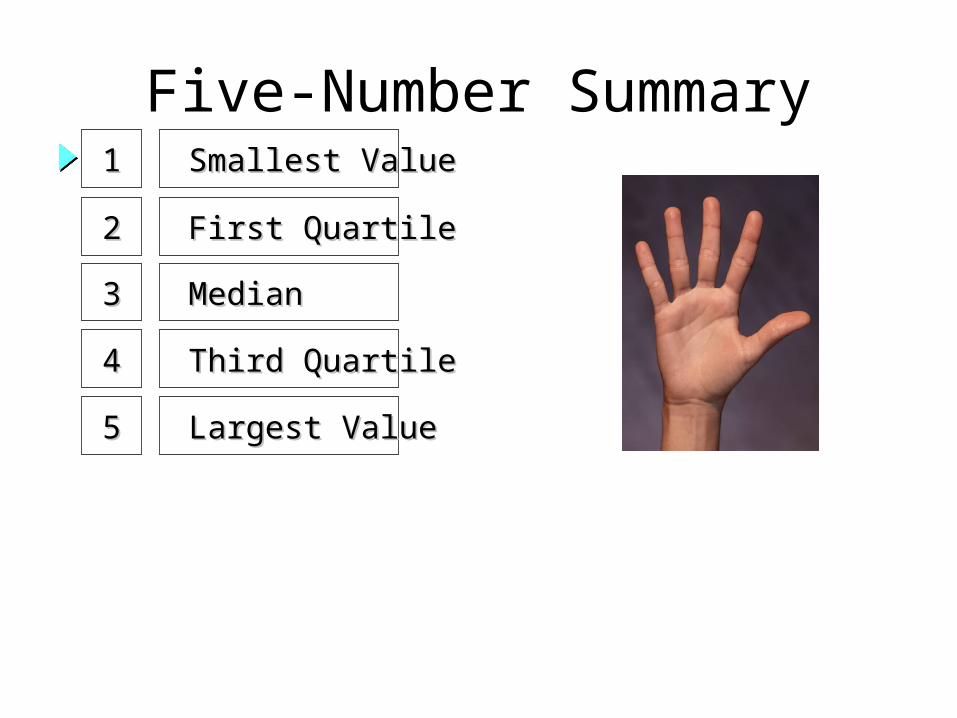
425 430 430 435 435 435 435 435 440 440440 440 440 445 445 445 445 445 450 450450 450 450 450 450 460 460 460 465 465465 470 470 472 475 475 475 480 480 480480 485 490 490 490 500 500 500 500 510510 515 525 525 525 535 549 550 570 570575 575 580 590 600 600 600 600 615 615

425 430 430 435 435 435 435 435 440 440440 440 440 445 445 445 445 445 450 450450 450 450 450 450 460 460 460 465 465465 470 470 472 475 475 475 480 480 480480 485 490 490 490 500 500 500 500 510510 515 525 525 525 535 549 550 570 570575 575 580 590 600 600 600 600 615 615

Lowest Value = 425Lowest Value = 425 First Quartile = 445First Quartile = 445

Median = 475Median = 475

Third Quartile = 525Third Quartile = 525Largest Value = 615Largest Value = 615

375375

400400

425425

450450

475475

500500

525525

550550

575575

600600

625625

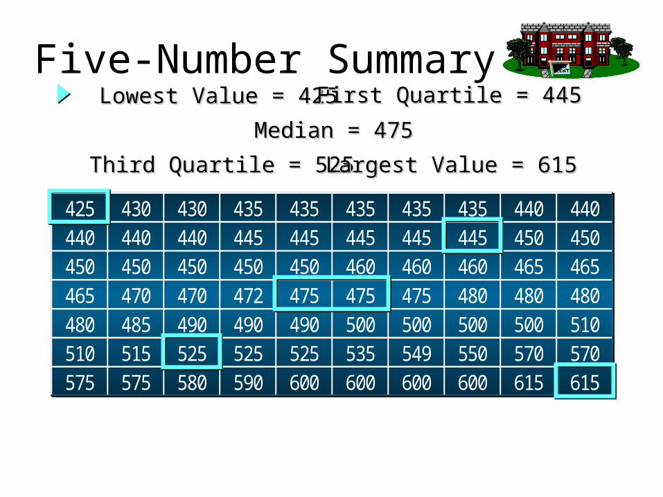
A box is drawn with its ends located at the first andA box is drawn with its ends located at the first and third quartiles.third quartiles.

Box PlotBox Plot

A vertical line is drawn in the box at the location ofA vertical line is drawn in the box at the location of the median (second quartile).the median (second quartile).

Q1 = 445Q1 = 445 Q3 = 525Q3 = 525

Q2 = 475Q2 = 475

Box PlotBox Plot

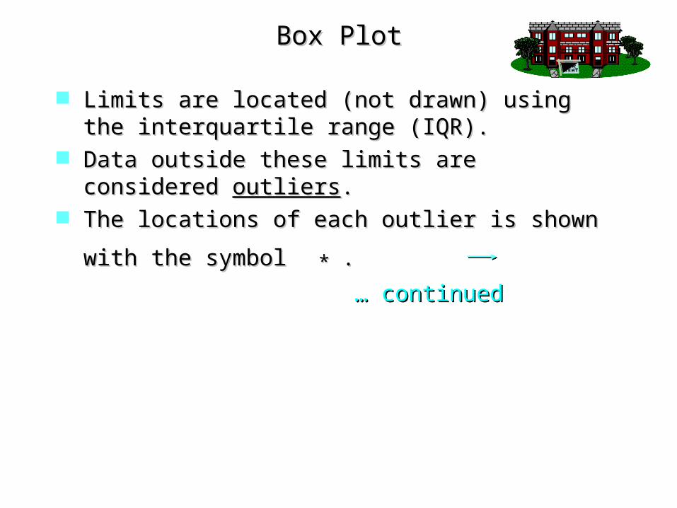
Limits are located (not drawn) using the Limits are located (not drawn) using the interquartile range (IQR).interquartile range (IQR).

Data outside these limits are considered Data outside these limits are considered outliersoutliers..

The locations of each outlier is shown with the The locations of each outlier is shown with the

symbolsymbol * * ..

… … continuedcontinued

Box PlotBox Plot

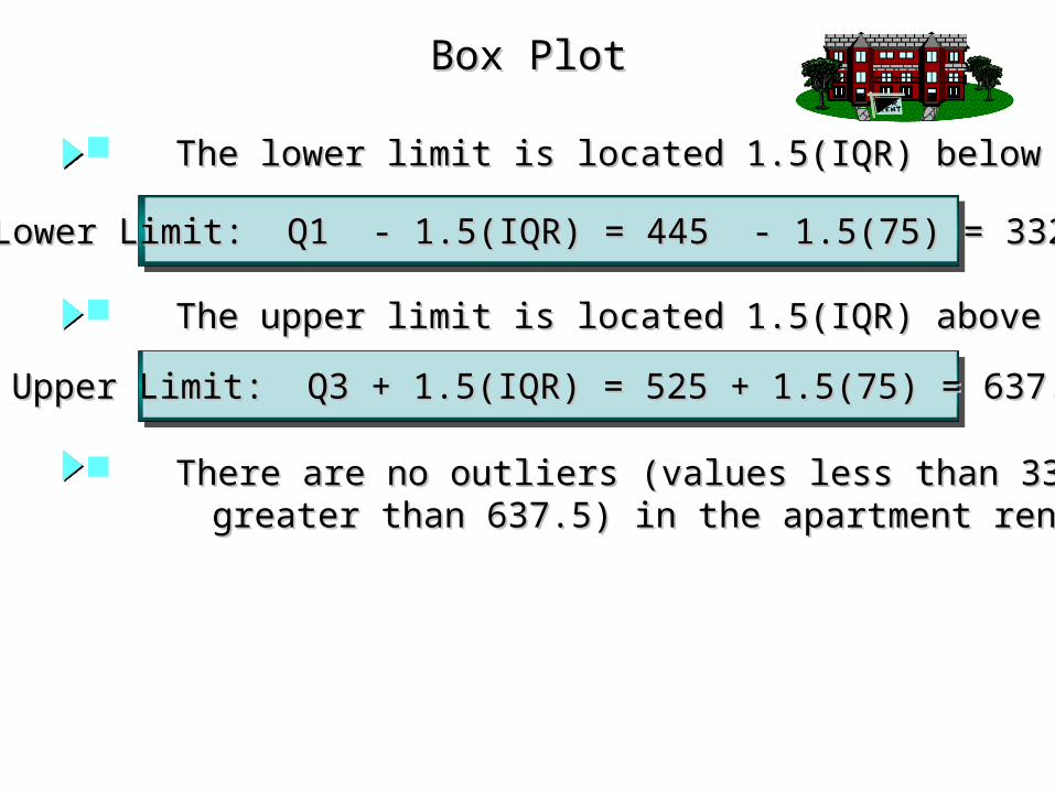
Lower Limit: Q1 - 1.5(IQR) = 445 - 1.5(75) = 332.5Lower Limit: Q1 - 1.5(IQR) = 445 - 1.5(75) = 332.5

Upper Limit: Q3 + 1.5(IQR) = 525 + 1.5(75) = 637.5Upper Limit: Q3 + 1.5(IQR) = 525 + 1.5(75) = 637.5

The lower limit is located 1.5(IQR) below The lower limit is located 1.5(IQR) below QQ1.1.

The upper limit is located 1.5(IQR) above The upper limit is located 1.5(IQR) above QQ3.3.

There are no outliers (values less than 332.5 orThere are no outliers (values less than 332.5 or greater than 637.5) in the apartment rent data.greater than 637.5) in the apartment rent data.

Box Plot

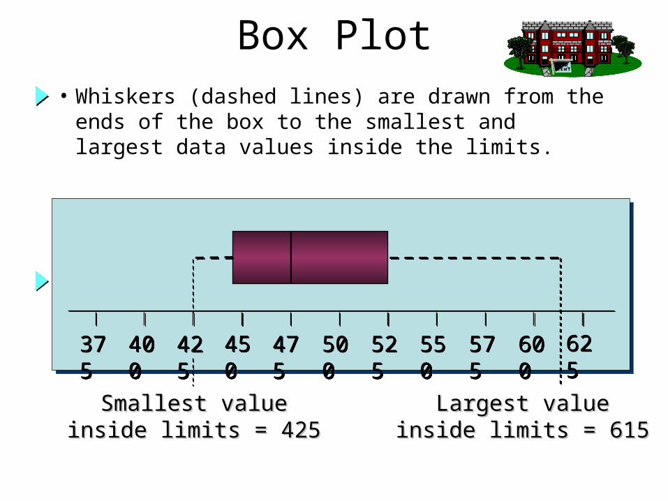
• Whiskers (dashed lines) are drawn from the ends of the box to the smallest and largest data values inside the limits.

375375

400400

425425

450450

475475

500500

525525

550550

575575

600600

625625

Smallest valueSmallest valueinside limits = 425inside limits = 425

Largest valueLargest valueinside limits = 615inside limits = 615

Measures of AssociationBetween two Variables

•Covariance

•Correlation coefficient

Covariance

• Covariance is a measure of linear association between variables.

• Positive values indicate a positive correlation between variables.

• Negative values indicate a negative correlation between variables.

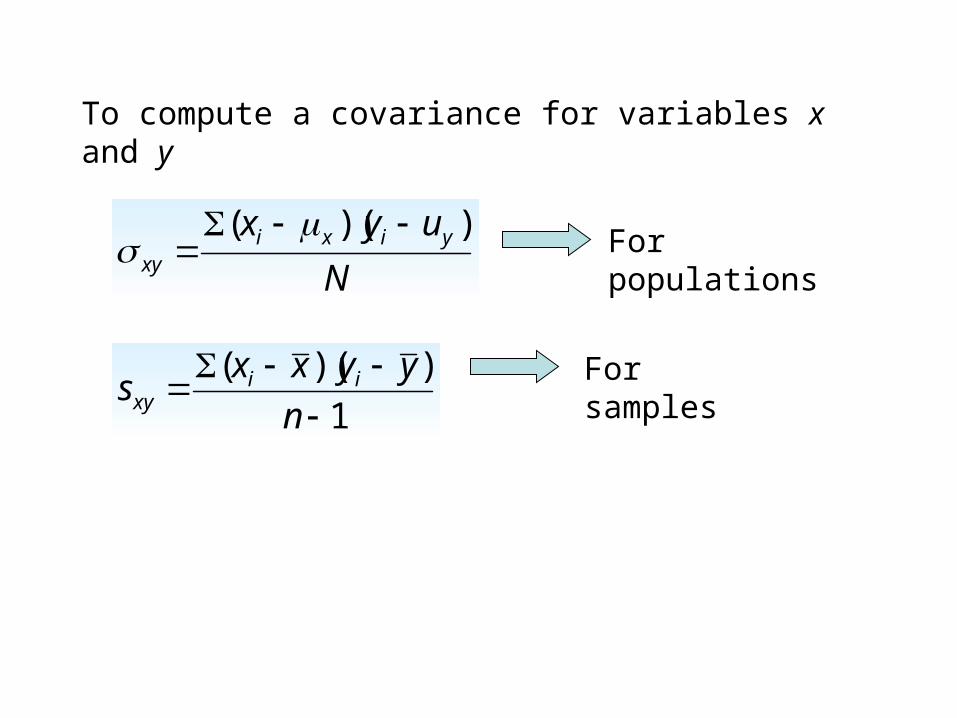
To compute a covariance for variables x and y

N

uyx yixixy

))((

For populations

1

))((

n

yyxxs iixy

For samples

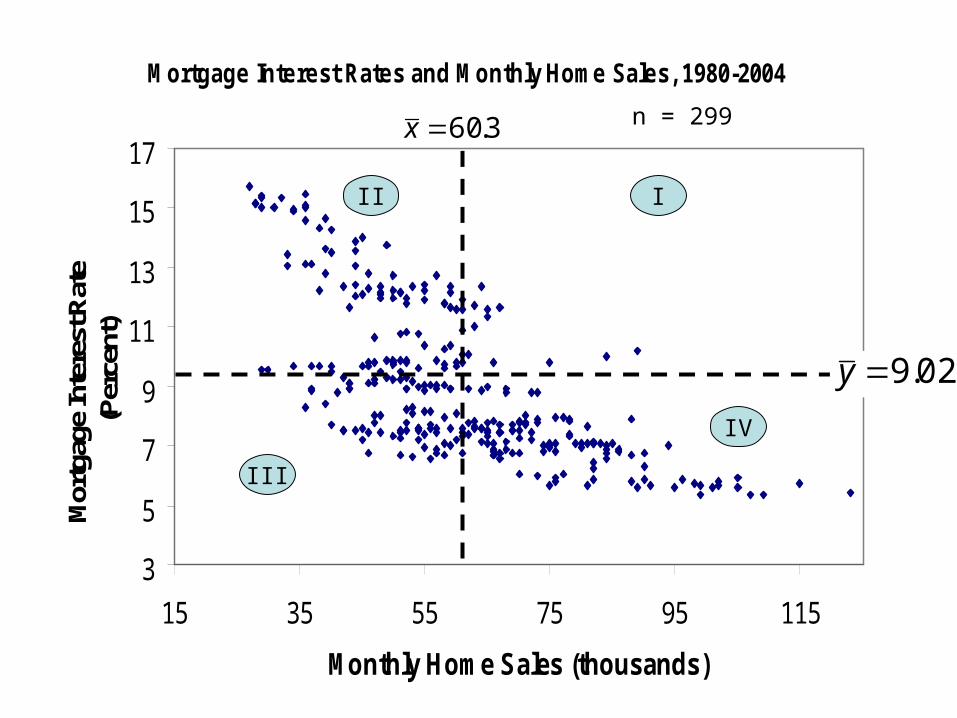
Mortgage Interest Rates and Monthly Home Sales, 1980-2004

3

5

7

9

11

13

15

17

15 35 55 75 95 115

Monthly Home Sales (thousands)

Mor

tgag

e In

tere

st R

ate

(Per

cent

)3.60x

02.9y

n = 299

II I

III

IV

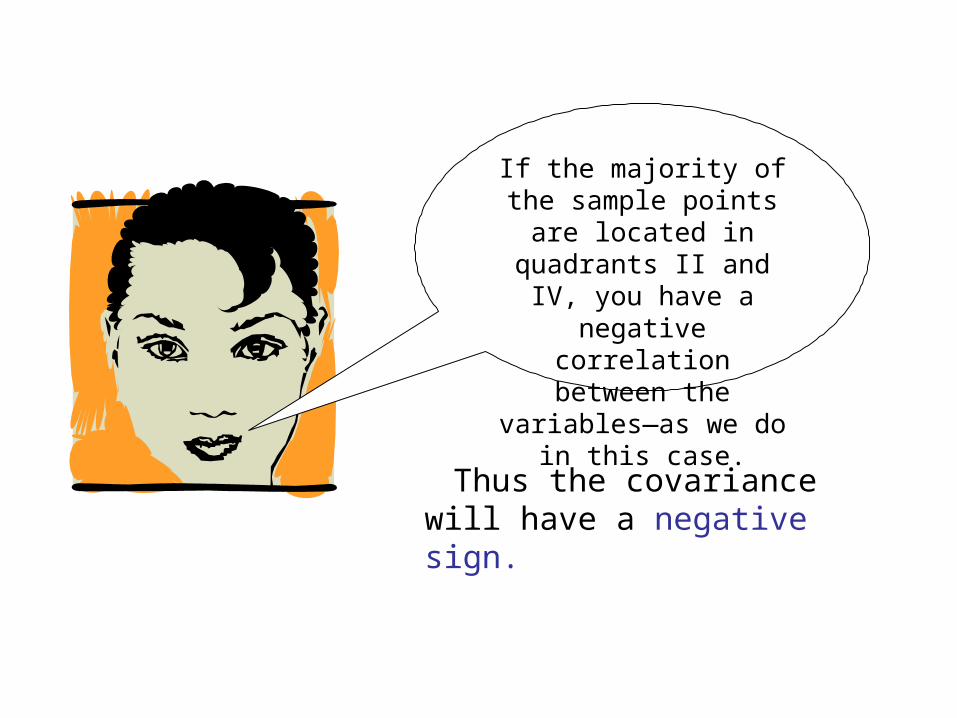
If the majority of the sample points are

located in quadrants II and IV, you have a negative correlation

between the variables—as we do in this case.

Thus the covariance will have a negative sign.

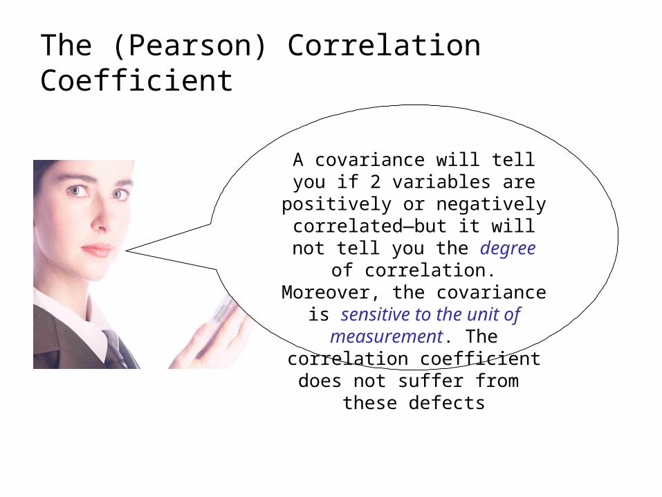
The (Pearson) Correlation Coefficient

A covariance will tell you if 2 variables are positively or

negatively correlated—but it will not tell you the degree of correlation. Moreover, the

covariance is sensitive to the unit of measurement. The correlation coefficient does not suffer from

these defects

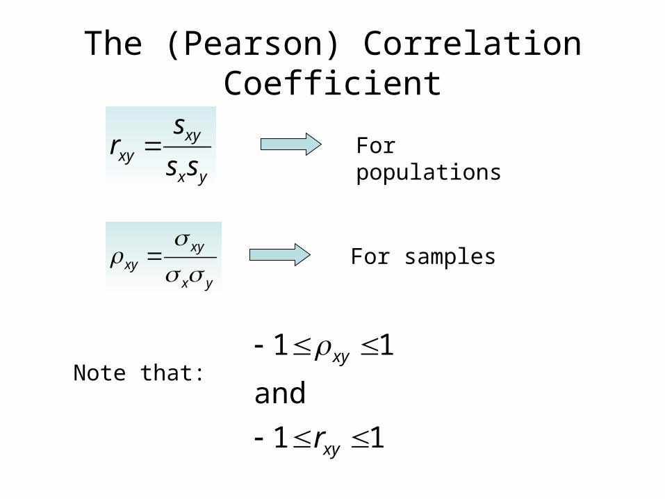
The (Pearson) Correlation Coefficient

yx

xyxy

yx

xyxy ss

sr For populations

For samples

Note that:

11

and

11

xy

xy

r

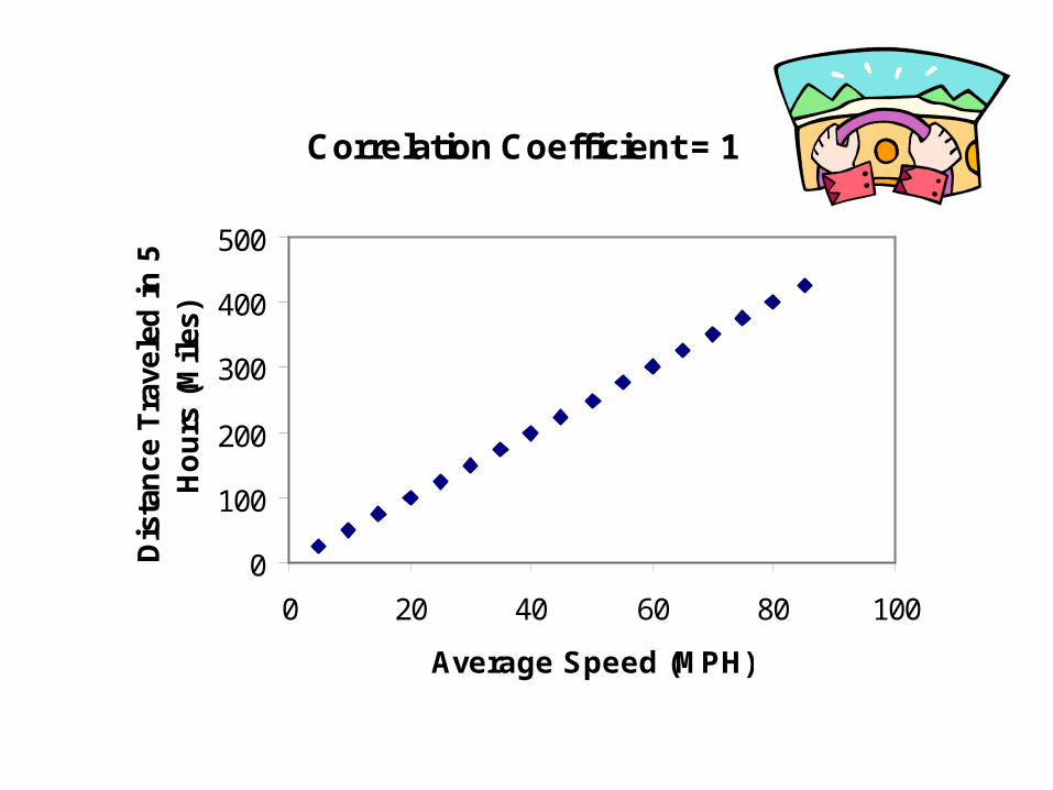
Correlation Coefficient = 1

0

100

200

300

400

500

0 20 40 60 80 100

Average Speed (MPH)

Dis

tan

ce T

rave

led

in

5

Ho

urs

(M

iles

)

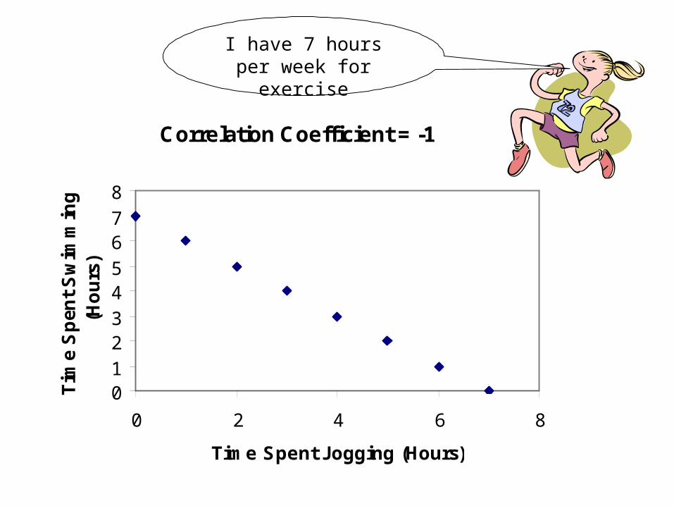
Correlation Coefficient = -1

012345678

0 2 4 6 8

Time Spent Jogging (Hours)

Tim

e S

pen

t S

wim

min

g

(Ho

urs

)

I have 7 hours per week for exercise

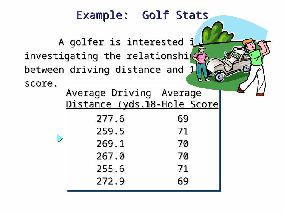
A golfer is interested inA golfer is interested in

investigating the relationship, if any,investigating the relationship, if any,

between driving distance and 18-holebetween driving distance and 18-hole

score.score.

277.6277.6259.5259.5269.1269.1267.0267.0255.6255.6272.9272.9

696971717070707071716969

Average DrivingAverage DrivingDistance (yds.)Distance (yds.)

AverageAverage18-Hole Score18-Hole Score

Example: Golf StatsExample: Golf Stats

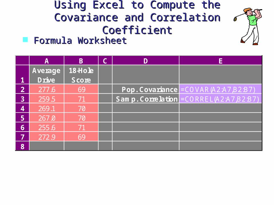
Using Excel to Compute theUsing Excel to Compute theCovariance and Correlation CoefficientCovariance and Correlation Coefficient

Formula WorksheetFormula Worksheet

A B C D E

1Average

Drive18-Hole Score

2 277.6 69 Pop. Covariance =COVAR(A2:A7,B2:B7)3 259.5 71 Samp. Correlation =CORREL(A2:A7,B2:B7)4 269.1 705 267.0 706 255.6 717 272.9 698

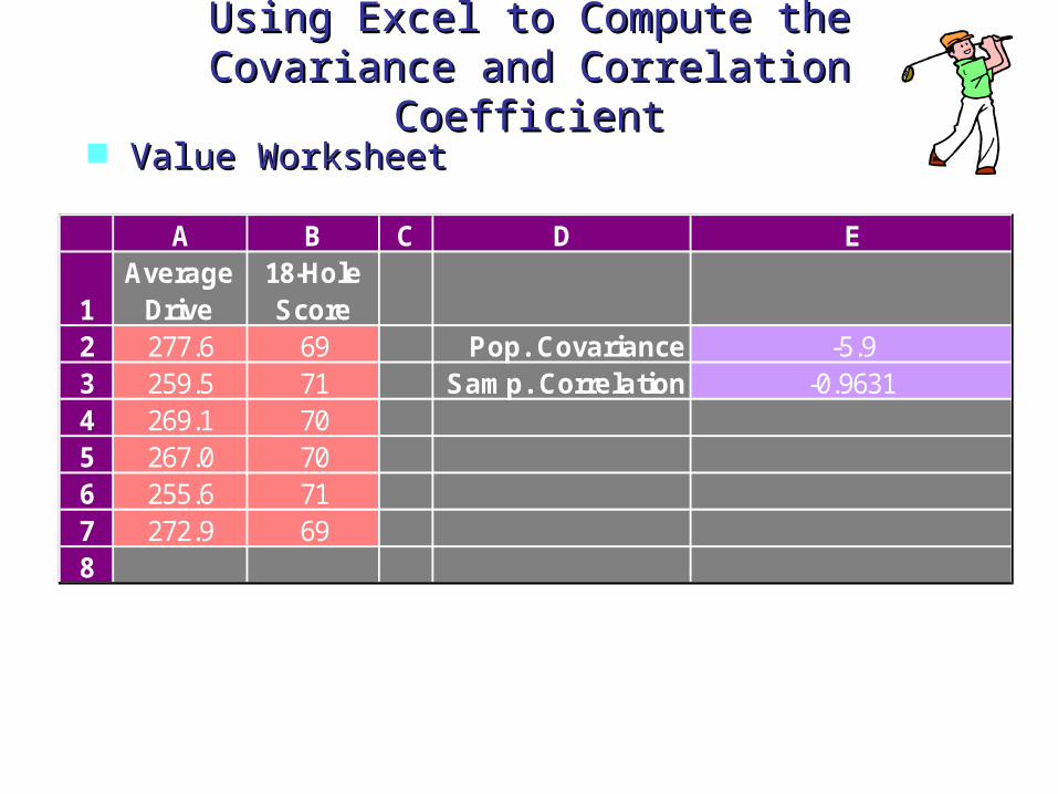
Value WorksheetValue Worksheet

Using Excel to Compute theUsing Excel to Compute theCovariance and Correlation CoefficientCovariance and Correlation Coefficient

A B C D E

1Average

Drive18-Hole Score

2 277.6 69 Pop. Covariance -5.93 259.5 71 Samp. Correlation -0.96314 269.1 705 267.0 706 255.6 717 272.9 698

The Weighted Mean and Working with Grouped Data

• Weighted mean• Mean for grouped data• Variance for grouped data• Standard deviation for grouped data.

GPA Example

A grade point average is a weighted-mean. That is, 4- hour courses are weighted more than 3- hour courses

when computing a GPA

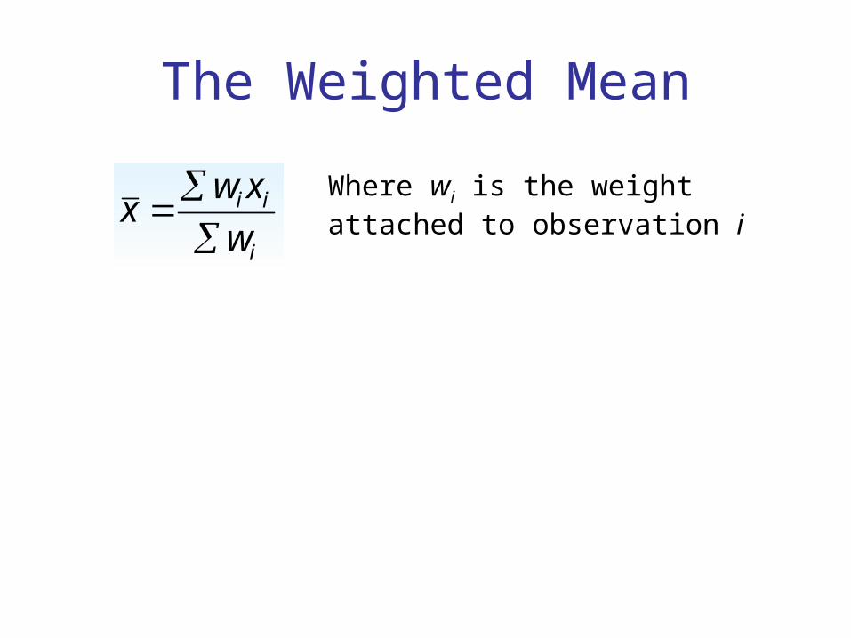
The Weighted Mean

i

ii

w

xwx

Where wi is the weight attached to observation i

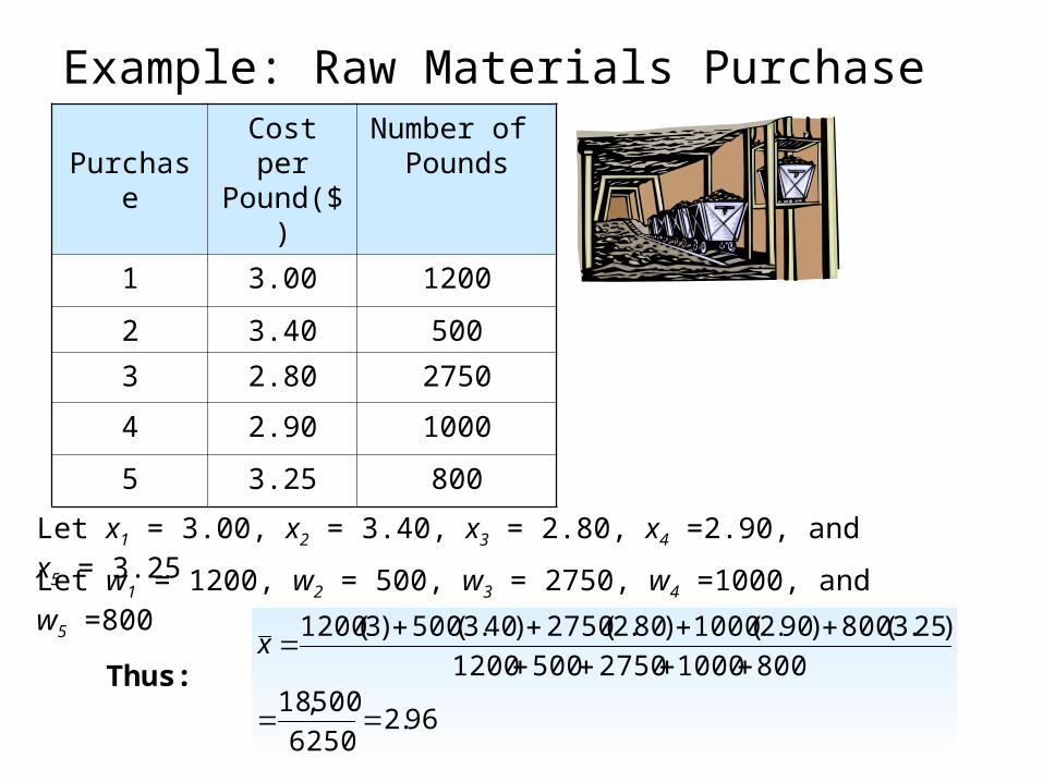
Example: Raw Materials Purchase

PurchaseCost per Pound($)

Number of Pounds

1 3.00 1200

2 3.40 500

3 2.80 2750

4 2.90 1000

5 3.25 800

Let x1 = 3.00, x2 = 3.40, x3 = 2.80, x4 =2.90, and x5 = 3.25

Let w1 = 1200, w2 = 500, w3 = 2750, w4 =1000, and w5 =800

Thus:

96.26250

500,18800100027505001200

)25.3(800)90.2(1000)80.2(2750)40.3(500)3(1200

x

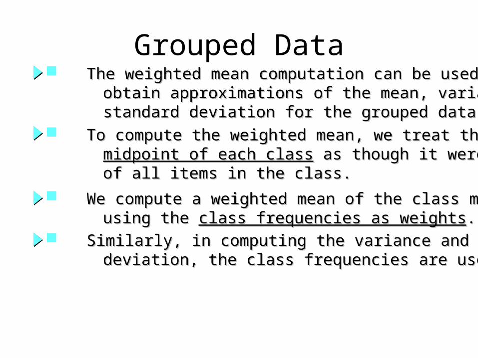
Grouped Data The weighted mean computation can be used toThe weighted mean computation can be used to obtain approximations of the mean, variance, andobtain approximations of the mean, variance, and standard deviation for the grouped data.standard deviation for the grouped data. To compute the weighted mean, we treat theTo compute the weighted mean, we treat the midpoint of each classmidpoint of each class as though it were the mean as though it were the mean of all items in the class.of all items in the class. We compute a weighted mean of the class midpointsWe compute a weighted mean of the class midpoints using the using the class frequencies as weightsclass frequencies as weights.. Similarly, in computing the variance and standardSimilarly, in computing the variance and standard deviation, the class frequencies are used as weights.deviation, the class frequencies are used as weights.

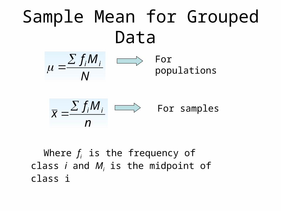
Sample Mean for Grouped Data

n

Mfx ii

Where fi is the frequency of class i and Mi is the midpoint of class i

N

Mf ii

For populations

For samples

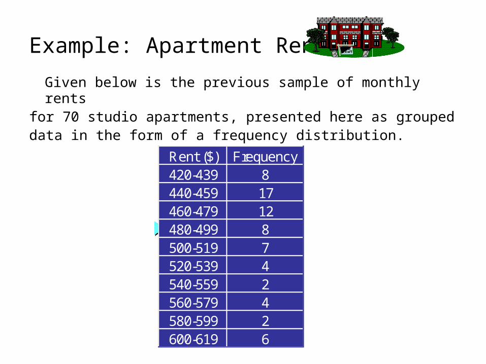
Example: Apartment Rents

Given below is the previous sample of monthly rents

for 70 studio apartments, presented here as groupeddata in the form of a frequency distribution.

Rent ($) Frequency420-439 8440-459 17460-479 12480-499 8500-519 7520-539 4540-559 2560-579 4580-599 2600-619 6

Rent ($) Frequency420-439 8440-459 17460-479 12480-499 8500-519 7520-539 4540-559 2560-579 4580-599 2600-619 6

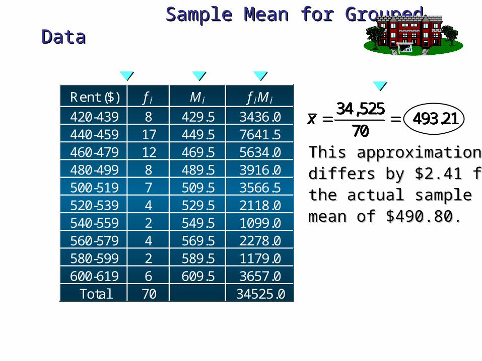
Sample Mean for Grouped DataSample Mean for Grouped Data

This approximationThis approximationdiffers by $2.41 fromdiffers by $2.41 fromthe actual samplethe actual samplemean of $490.80.mean of $490.80.

34,525 493.21

70x

34,525 493.21

70x

Rent ($) f i

420-439 8440-459 17460-479 12480-499 8500-519 7520-539 4540-559 2560-579 4580-599 2600-619 6

Total 70

M i

429.5449.5469.5489.5509.5529.5549.5569.5589.5609.5

f iM i

3436.07641.55634.03916.03566.52118.01099.02278.01179.03657.034525.0

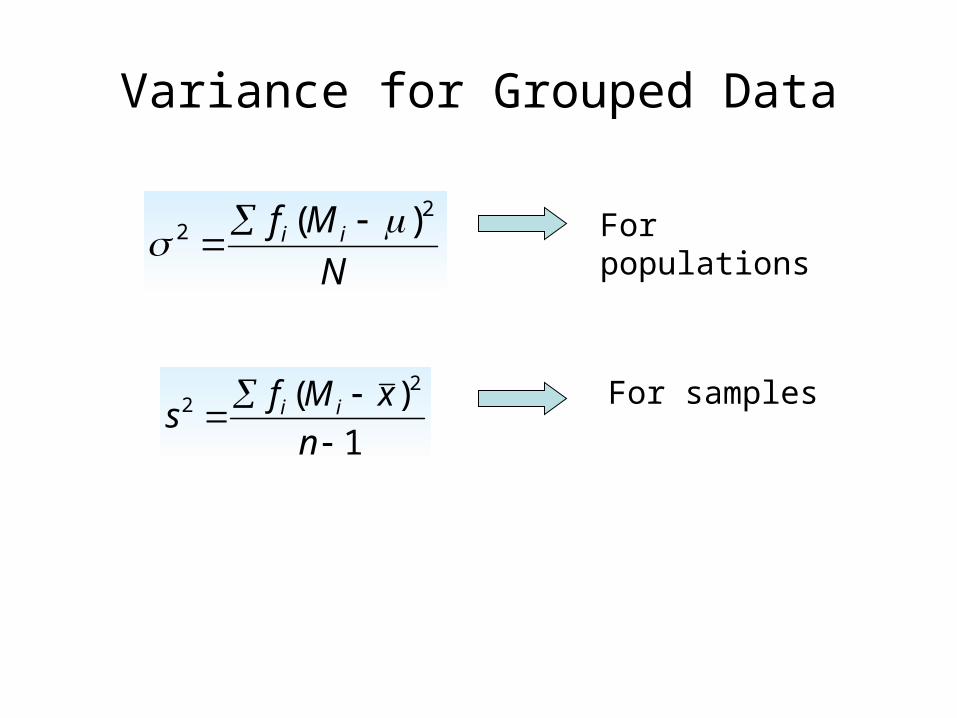
Variance for Grouped Data

N

Mf ii2

2 )(

1

)( 22

n

xMfs ii

For populations

For samples

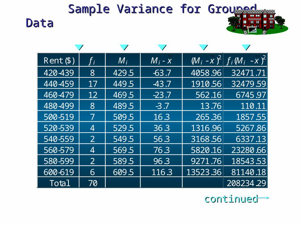
Rent ($) f i

420-439 8440-459 17460-479 12480-499 8500-519 7520-539 4540-559 2560-579 4580-599 2600-619 6

Total 70

M i

429.5449.5469.5489.5509.5529.5549.5569.5589.5609.5

Sample Variance for Grouped DataSample Variance for Grouped Data

M i - x

-63.7-43.7-23.7-3.716.336.356.376.396.3116.3

f i(M i - x )2

32471.7132479.596745.97110.11

1857.555267.866337.13

23280.6618543.5381140.18

208234.29

(M i - x )2

4058.961910.56562.1613.76

265.361316.963168.565820.169271.76

13523.36

continuedcontinued

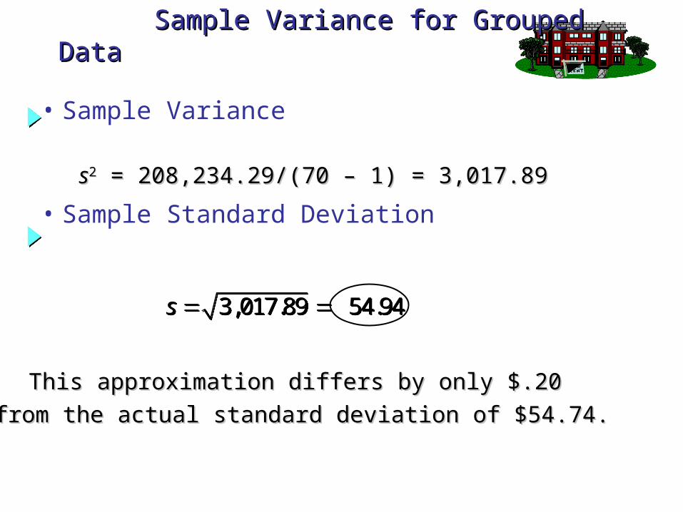
• Sample Variance

• Sample Standard Deviation

3,017.89 54.94s 3,017.89 54.94s

ss22 = 208,234.29/(70 – 1) = 3,017.89 = 208,234.29/(70 – 1) = 3,017.89

This approximation differs by only $.20 This approximation differs by only $.20

from the actual standard deviation of $54.74.from the actual standard deviation of $54.74.

Sample Variance for Grouped DataSample Variance for Grouped Data