U.U.D.M. Project Report 2021:45 Examensarbete i matematik, 30 hp Handledare: Yukai Yang Ämnesgranskare: Rolf Larsson Examinator: Magnus Jacobsson Juni 2021 Department of Mathematics Uppsala University Fitting Yield Curve with Dynamic Nelson-Siegel Models: Evidence from Sweden Zhe Huang

Welcome message from author
This document is posted to help you gain knowledge. Please leave a comment to let me know what you think about it! Share it to your friends and learn new things together.
Transcript
U.U.D.M. Project Report 2021:45
Examensarbete i matematik, 30 hpHandledare: Yukai Yang Ämnesgranskare: Rolf LarssonExaminator: Magnus JacobssonJuni 2021
Department of MathematicsUppsala University
Fitting Yield Curve with DynamicNelson-Siegel Models: Evidence from Sweden
Zhe Huang

Abstract
In this thesis, the yield curve of the Swedish treasury bill andgovernment bond is modelled by five dynamic Nelson-Siegel mod-els separately. Estimations of the latent factors are given by theKalman filter optimization. According to the estimation results, thedynamic Nelson-Siegel model is the most stable and convenient modelto fit the yields with all maturities. The arbitrage-free Nelson-Siegelmodel makes good performance on the short-term yields. The dy-namic generalized Nelson-Siegel model has the advantage for estimat-ing medium-term and long-term yields.
Acknowledgement
I would like to extend my sincerest and deepest thanks to my supervisor YukaiYang for offering me this exciting topic, for his patient guidance, constantencouragement and support. I learnt a lot from his supervision. I believethat will be the fortune in my life. I would like to thank my subject reviewerRolf Larsson for giving me comments to improve my thesis. I would liketo acknowledge Jens Christensen for explaining his idea on AFNS models. Iwould also like to give my thanks to Yuqiong Wang for helping me understandthe arbitrage theory.
In addition, I would like to thank my parents and my friends for theircompany during this tough period.
Contents
1 Introduction 1
2 Financial Preliminaries 22.1 Interest Rates . . . . . . . . . . . . . . . . . . . . . . . . . . . 22.2 Zero-Coupon bond Yields . . . . . . . . . . . . . . . . . . . . 32.3 Yield Curve Factors . . . . . . . . . . . . . . . . . . . . . . . . 3
3 State Space Models and Kalman Filter 43.1 State Space Models . . . . . . . . . . . . . . . . . . . . . . . . 43.2 Kalman Filter . . . . . . . . . . . . . . . . . . . . . . . . . . . 5
4 The Nelson-Siegel Term Structure Models 64.1 Nelson-Siegel Model . . . . . . . . . . . . . . . . . . . . . . . . 64.2 Dynamic Nelson-Siegel Model(DNS) . . . . . . . . . . . . . . . 74.3 Arbitrage-free Nelson-Siegel Model(AFNS) . . . . . . . . . . . 94.4 Dynamic Generalized Nelson-Siegel Model(DGNS) . . . . . . . 14
5 Empirical Study 155.1 Data . . . . . . . . . . . . . . . . . . . . . . . . . . . . . . . . 165.2 Estimation Framework . . . . . . . . . . . . . . . . . . . . . . 17
5.2.1 DNS Model . . . . . . . . . . . . . . . . . . . . . . . . 185.2.2 AFNS Model . . . . . . . . . . . . . . . . . . . . . . . 195.2.3 DGNS Model . . . . . . . . . . . . . . . . . . . . . . . 205.2.4 Out-of-sample Forecast Method . . . . . . . . . . . . . 20
5.3 Estimation Results . . . . . . . . . . . . . . . . . . . . . . . . 205.3.1 DNS Model Estimation . . . . . . . . . . . . . . . . . . 205.3.2 AFNS Model Estimation . . . . . . . . . . . . . . . . . 245.3.3 DGNS Model Estimation . . . . . . . . . . . . . . . . . 28
5.4 Out-of-sample Forecasts . . . . . . . . . . . . . . . . . . . . . 30
6 Conclusion 31
Bibliography 32
A Figures 33
1 Introduction
In many financial areas, it is important to get a good estimation of the yieldcurve. From the last century, economists attempt to develop plenty of modelsto fit the yield curve with different forms. One class of the most widely usedmodels are the Nelson-Siegel models.
Nelson and Siegel [1987] suggest a simple static model with three latentfactors to fit the yield curve of the bond market. The most significant con-tribution of the Nelson-Siegel model is using only three variables to describea complex curve with great performance. The three factors can be inter-preted as the level, the slope and the curvature of the yield curve. Since thenmany different versions of Nelson-Siegel model have been offered for buildingzero-coupon yield curves by researchers.
To study the dynamic evolution of the yield curve, Diebold and Li [2006]offer a dynamic version of the three-factor Nelson-Siegel model, which isnamed as dynamic Nelson-Siegel model. In this model, Diebold and Lidevelop the three Nelson-Siegel factors to latent time-varying parameters.Diebold et al. [2006] use the Kalman filter maximum log-likelihood optimiza-tion method to estimate the Nelson-Siegel parameters, which has become thecommon method to deal with this kind of problems now.
Empirically, the dynamic Nelson-Siegel model has good achievement onin-sample fit, but it does not set the restrictions necessary for the absenceof arbitrage. To solve the theoretical restrictions, Christensen et al. [2011]develop the affine arbitrage-free class of dynamic Nelson-Siegel term structuremodels, referred to as the Arbitrage-free Nelson-Siegel model.
Besides the traditional three-factor model, Diebold and Rudebusch [2013]collect some extended Nelson-Siegel models with additional factors. For ex-ample, the four-factor Svensson model developed by Svensson [1995], thefive-factor dynamic generalized Nelson-Siegel model created by Christensenet al. [2009] and so on. Following the study of Christensen et al. [2009], theextra factors can improve the fitting performance on long-term bond yields.
Although there is a vast of papers about the Nelson-Siegel model andits empirical study, they seldom focus on Swedish data. While in my the-sis, I investigate Nelson-Siegel models and figure out appropriate modelsfor the Swedish treasury bill and government bond yields. I mainly ap-ply three versions of the Nelson-Siegel model in this thesis, the dynamicNelson-Siegel model, the arbitrage-free Nelson-Siegel model and the dynamicgeneralized Nelson-Siegel model. In the following section, I review somefinancial concepts that are related to this thesis. In Section 3, I intro-duce the state space models and the Kalman filter. In Section 4, I ex-
1

plain the Nelson-Siegel term structure models, because they are the keymodels for estimations in next section. Section 5 is the most importantin my thesis, all the estimation results are contained in this section andI provide in-sample fit and out-of-sample forecast tests on different mod-els. The R Codes of my thesis can be founded on my GitHub page https:
//github.com/ZheHuang96/Master-Thesis-Code.
2 Financial Preliminaries
In this section, I follow Diebold and Rudebusch [2013] and introduce somefinancial facts as a basis of my thesis. The facts are interest rates, the zero-coupon bond yields, and the factor structure of a yield curve.
2.1 Interest Rates
There are three interest rates in the bond market, the discount rate, theforward rate and the yield. The discount rate of a bond is the interestfor calculating bond prices with the present value. The yield to maturityis the interest rate that represents the total return when the bond reachesmaturity. The forward rate is the future yield of the bond. Following Dieboldand Rudebusch [2013], there are three definitions.
Definition 2.1. The relationship between the discount rate and the yield isdefined as:
P (τ) = e−τy(τ) (2.1)
where P (τ) is the price of a τ -period discount bond and y(τ) is the continu-ously compound yield to maturity of this bond.
Definition 2.2. The relationship between the discount rate and the forwardrate is defined as:
f(τ) = −P′(τ)
P (τ)(2.2)
where f(τ) is the forward rate of a bond.
It is easy to get the connection between the yield and the forward rateby inserting Equation (2.1) into Equation (2.2).
2
Definition 2.3. The relationship between the yield and the forward rate isdefined as:
y(τ) =1
τ
τ∫0
f(u)du (2.3)
Hence, researchers construct the unobserved yield with two different ap-proaches, the forward rate and the discount rate.
2.2 Zero-Coupon bond Yields
A zero-coupon bond, as named, is a kind of bond without any coupons orinterest payments during the bond holding period. When the bond attainsmaturity, the bondholder can obtain the face value of the bond. Hence thezero-coupon bond is the simplest bond in the bond market. In general, thegovernment bonds of countries are zero-coupon bonds. The most commonexample is the US Treasury Bills, which is widely used in vast papers.
Definition 2.4. The relationship between the price and yield of a zero-couponbond is defined by
y = [F
p]1n − 1 (2.4)
where y represents the yield of a zero-coupon bond, F represents the facevalue, p stands for the current price, and n is the compounding period tomaturity.
Practically, the yields are not observed and need to be estimated by theprices of zero-coupon bonds. The most popular way to construct yields isusing the estimated forward rates at related maturities. Following Dieboldand Rudebusch [2013], the zero-coupon yield is an equally-weighted averageof forward rates.
2.3 Yield Curve Factors
A yield curve, also called term structure, is a curve that graphs many differentyields to different maturities at any time. The evolution of the yield curveis supposed to be dynamic. To describe the yield curve better, many studiessuggest the imposition of ”factors”.
Normally, the bond market yields are described by multivariate models.According to many pieces of evidence shown, the financial asset returns canbe modelled by a typical restricted vector autoregressive process, illustrated
3
as a factor structure. The basic method behind the factor structure is usinga set of limited latent objects (”factors”) to drive a large set of objects, e.g.,the bond yields in this thesis. Hence, the complicated observations can beexplained by easy dynamic variables. Researchers think the term structuredata can have various factors in the real world. They also prove that thedynamic factor models can fit the observed yield data with high accuracy asa whole.
The difficulty of fitting the yield curve is how to figure out the dynamicevolution of latent models. To build and estimate the unknown dynamicfactor models from observations, state space models and the Kalman Filtermethod are necessary. Hence they will be introduced in details in the nextsection.
3 State Space Models and Kalman Filter
This section considers how to fit the yield curve with latent factor models.Dynamic models are widely used to describe the evolution of the financialmarket. In this section, I introduce some methods to build and estimatedynamic models.
3.1 State Space Models
In many economic applications, the evolution of input and output variablescannot be measured directly. To study the evolution of the internal variables,the common way is to apply state space models, suggested by Kunst [2007].
A state space model is a time series model that describes an observed timeseries, Yt, by the unobserved state vector, Xt. Usually, the dynamic systemof Xt is a Markov process, which means Xt only depends on the history ofXt−1. Hence, a linear state space model has two equations: the measurementequation
Yt = BXt + εt (3.1)
and the state transition equation
Xt = AXt−1 + Cµt−1 + ηt (3.2)
where µ is the mean vector and the measurement error εt and the state errorηt are i.i.d white noise. Normally, εt is assumed to be a zero-mean Guassianwith the covariance H, i.e. εt ∼ N(0, H) and ηt is assumed to be a zero-meanGuassian with the covariance Q, i.e. ηt ∼ N(0, Q).
The measurement equation illustrates the relationship between the ob-served time series Yt and the unobserved state Xt. The state transition
4
equation illustrates the evolution of the state vector from time t− 1 to timet. As the equations show, several latent variables need to be estimated. Tosolve this problem, researchers have created an effective method, called theKalman filter.
3.2 Kalman Filter
In practical utilization, the Kalman filter is a useful way to estimate thelatent variables of the linear state space model. The Kalman filter can helpto construct the log-likelihood function related to the state space model. Theoptimal predictions can be obtained by using the maximum log-likelihoodmethod.
The procedure of the Kalman filter is to estimate Xt, given the initialestimate of X0, the observed series of measurement Yt, and the informationof the system described by A, B, C, H and Q.
According to Kim and Bang [2018], the Kalman filter algorithm includestwo steps: prediction and update. Consider the period t−1 and suppose thestate update Xt−1 and its covariance matrix Σt−1, and the update step is intime t. The Kalman filter algorithm is briefed as follows:
Prediction:
Xt|t−1 = AXt−1 + Cµt−1 predicted state estimate (3.3)
Σt|t−1 = AΣt−1A′ +Q predicted error covariance (3.4)
Update:
Xt|t = Xt|t−1 +Ktvt updated state estimate (3.5)
Σt|t = (I −KtB)Σt|t−1 updated error covariance (3.6)
where vt = yt−BXt|t−1 is the measurement residual and Kt = Σt|t−1B′(H +
BΣt|t−1B′)−1 is called the Kalman gain.
Because the Kalman filter is a recursive procedure, initialization is needed.The initial guess of the state estimate and the error covariance matrix can bethe initial values, with Q and H. Finally, a Kalman filter can be completedby implementing the prediction and update steps for each time step after theinitialization.
Kalman filter offers all the parameters to construct the log-likelihoodfunction for the observations. But the maximization of the log-likelihood
5
function is complicated. Prediction error decomposition is a common for-mat of log-likelihood function to simply the problem. The prediction errordecomposition of the log-likelihood is
log l(YT |ϕ) =T∑t=1
log l(yt|Yt−1, ϕ) (3.7)
= −T∑t=1
(N
2log 2π +
1
2log |Ωt|t−1|+
1
2v′
tΩ−1t|t−1vt) (3.8)
where N is the number of observations, ϕ represents the unknown parameters,YT = (y1, . . . , yT ), vt = yt − yt−1 = yt −Bxt|t−1, and Ωt|t−1 = BΣt|t−1B
′ +H.It is easy to maximize the log-likelihood function and get the optimizationof unknown parameters by this decomposition.
Up to now, I have proposed the general methods to build and estimatelatent factor models. I will introduce the specific dynamic models for yieldsin the next section.
4 The Nelson-Siegel Term Structure Models
This section introduces the important underlying models used in the thesis.To make everything clear, I start this part with the original Nelson-Siegelmodel created by Nelson and Siegel [1987], then move to three dynamicmodels, the dynamic Nelson-Siegel model defined by Diebold and Li [2006],the arbitrage-free Nelson-Siegel model illustrated by Christensen et al. [2011]and the dynamic generalized Nelson-Siegel model designed by Christensenet al. [2009].
4.1 Nelson-Siegel Model
The Nelson-Siegel model is a three-factor exponential parametric model foundedby Nelson and Siegel [1987]. They discover that the classic yield curve shapefunctions follow the solutions to differential and difference equations and theforward rates are the solutions to the differential equations generated by spotrates. Hence, they give the function to fit the forward rate curve as follows:
f(τ) = β1 + β2e−λτ + β3λe
−λτ (4.1)
The zero-coupon yield curve is equal to the average of the forward rates, itcan be implied as:
6
y(τ) = β1 + β2(1− e−λτ
λτ) + β3(
1− e−λτ
λτ− e−λτ ) (4.2)
where y(τ) is the zero-coupon yield with τ months to maturity, λ is a constantthe controls the decay rate and β1, β2, β3 are latent parameters. For the yieldcurve, β1 is the long-term factor and imposes the level of it, β2 is the short-term factor and interprets the slope, β3 is the medium-term factor and isrelated to the curvature.
The Nelson-Siegel model is the basic model for the DNS model, the AFNSmodel and the DGNS model.
4.2 Dynamic Nelson-Siegel Model(DNS)
In order to find the progression of the bond market time by time, Dieboldand Li [2006] improve the Nelson-Siegel model by adding dynamic behaviourto the factors of the model. The new model is:
yt(τ) = Lt + St(1− e−λτ
λτ) + Ct(
1− e−λτ
λτ− e−λτ ) (4.3)
where Lt, St, Ct are latent time-varying parameters which have the sameinterpretation as β1, β2, β3 in the original Nelson-Siegel model. Lt, St, Ctrepresent level, slope and curvature of the yield curve. The factor loadingis shown as Figure 4.1. The dynamic movements of the latent parametersfollow the time series process. For example, independent AR(1) processesand a VAR(1) process.
The dynamic Nelson-Siegel model is a state-space model and the pa-rameters are state variables. In this thesis, two versions of the DNS modelare considered, the independent-factor DNS model and the correlated-factorDNS model.
For the independent-factor DNS model, the three latent factors follow in-dependent first-order auto-regressive processes (AR(1)). The state transitionequation isLt − µLSt − µS
Ct − µC
=
a11 0 00 a22 00 0 a33
Lt−1 − µLSt−1 − µSCt−1 − µC
+
ηt(L)ηt(S)ηt(C)
(4.4)
where the stochastic shocks ηt(L), ηt(S) and ηt(C) have diagonal covariancematrix
Q =
q211 0 00 q2
22 00 0 q2
33
(4.5)
7
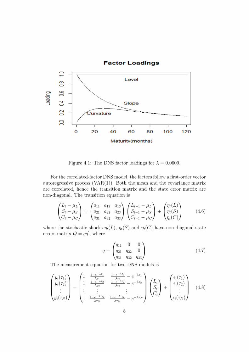
Figure 4.1: The DNS factor loadings for λ = 0.0609.
For the correlated-factor DNS model, the factors follow a first-order vectorautoregressive process (VAR(1)). Both the mean and the covariance matrixare correlated, hence the transition matrix and the state error matrix arenon-diagonal. The transition equation isLt − µLSt − µS
Ct − µC
=
a11 a12 a13
a21 a22 a23
a31 a32 a33
Lt−1 − µLSt−1 − µSCt−1 − µC
+
ηt(L)ηt(S)ηt(C)
(4.6)
where the stochastic shocks ηt(L), ηt(S) and ηt(C) have non-diagonal stateerrors matrix Q = qq
′, where
q =
q11 0 0q21 q22 0q31 q32 q33
(4.7)
The measurement equation for two DNS models isyt(τ1)yt(τ2)
...yt(τN)
=
1 1−e−λτ1
λτ11−e−λτ1λτ1
− e−λτ11 1−e−λτ2
λτ21−e−λτ2λτ2
− e−λτ2...
......
1 1−e−λτNλτN
1−e−λτNλτN
− e−λτN
LtStCt
+
εt(τ1)εt(τ2)
...εt(τN)
(4.8)
8
where the measurement errors εt(τi) are i.i.d. white noise.
4.3 Arbitrage-free Nelson-Siegel Model(AFNS)
Christensen et al. [2011] develop the Arbitrage-free Nelson-Siegel (AFNS)model by imposing the affine arbitrage-free term structure into the DNSmodel.
Here I briefly introduce the affine arbitrage-free term structure by follow-ing Bjork [2009] and Duffie and Kan [1996].
Definition 4.1. A stochastic process W is named a Wiener process when itsatisfies the conditions as follows:
• W (0) = 0
• The process has independent increments.
• For s < t, the stochastic variable W (t) −W (s) has the Gaussian dis-tribution N [0,
√t− s].
• W has continuous trajectories.
Proposition 4.1. For a multidimensional stochastic process Xt, the shortrate rt is a deterministic function of Xt.
rt = ρ0(t) + ρ1(t)′Xt (4.9)
where ρ0 : [0, T ]→ R and ρ0 : [0, T ]→ Rn are continuous bounded functions.If the bond market is arbitrage-free, there is a risk-neutral measure Q, and
the zero-coupon bond prices with an affine term structure can be representedas follows:
P (t, T ) = EQ[exp(−T∫t
rudu)] (4.10)
= exp(A(t, T )−B(t, T )′Xt) (4.11)
where the Q-dynamics of the process Xt are given by
dXt = KQ(t)[θQ(t)−Xt]dt+ Σ(t)D(Xt, t)dWQt (4.12)
In Equation (4.12), WQt is a Q-Wiener process, KQ, θQ, Σ are continuous
bounded functions. D is a diagonal matrix and the ith diagonal elementis√γi(t) + δi1(t)X1
t + · · ·+ δin(t)Xnt , where γ and δ are continuous bounded
functions.
9
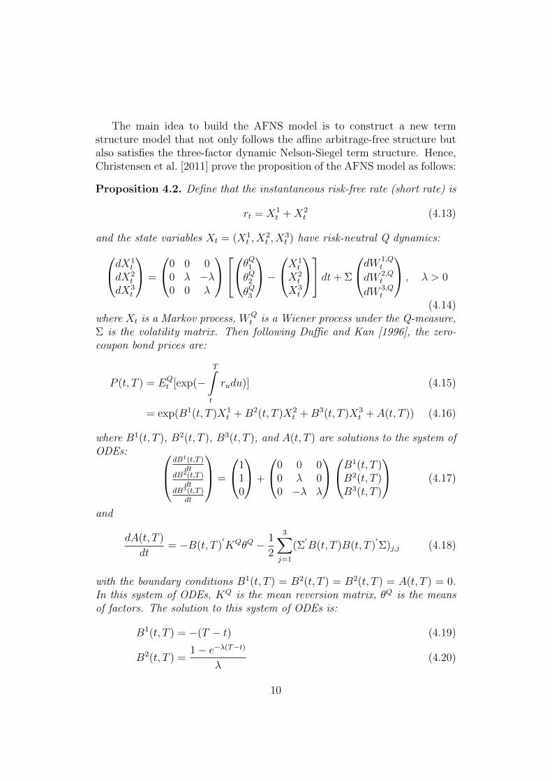
The main idea to build the AFNS model is to construct a new termstructure model that not only follows the affine arbitrage-free structure butalso satisfies the three-factor dynamic Nelson-Siegel term structure. Hence,Christensen et al. [2011] prove the proposition of the AFNS model as follows:
Proposition 4.2. Define that the instantaneous risk-free rate (short rate) is
rt = X1t +X2
t (4.13)
and the state variables Xt = (X1t , X
2t , X
3t ) have risk-neutral Q dynamics:dX1
t
dX2t
dX3t
=
0 0 00 λ −λ0 0 λ
θQ1θQ2θQ3
−X1
t
X2t
X3t
dt+ Σ
dW 1,Qt
dW 2,Qt
dW 3,Qt
, λ > 0
(4.14)where Xt is a Markov process, WQ
t is a Wiener process under the Q-measure,Σ is the volatility matrix. Then following Duffie and Kan [1996], the zero-coupon bond prices are:
P (t, T ) = EQt [exp(−
T∫t
rudu)] (4.15)
= exp(B1(t, T )X1t +B2(t, T )X2
t +B3(t, T )X3t + A(t, T )) (4.16)
where B1(t, T ), B2(t, T ), B3(t, T ), and A(t, T ) are solutions to the system ofODEs:
dB1(t,T )dt
dB2(t,T )dt
dB3(t,T )dt
=
110
+
0 0 00 λ 00 −λ λ
B1(t, T )B2(t, T )B3(t, T )
(4.17)
and
dA(t, T )
dt= −B(t, T )
′KQθQ − 1
2
3∑j=1
(Σ′B(t, T )B(t, T )
′Σ)j,j (4.18)
with the boundary conditions B1(t, T ) = B2(t, T ) = B2(t, T ) = A(t, T ) = 0.In this system of ODEs, KQ is the mean reversion matrix, θQ is the meansof factors. The solution to this system of ODEs is:
B1(t, T ) = −(T − t) (4.19)
B2(t, T ) =1− e−λ(T−t)
λ(4.20)
10
B3(t, T ) = (T − t)e−λ(T−t) − 1− e−λ(T−t)
λ(4.21)
A(t, T ) = (KQθQ)2
T∫t
B2(s, T )ds+ (KQθQ)3
T∫t
B3(s, T )ds
+1
2
3∑j=1
T∫t
(Σ′B(t, T )B(t, T )
′Σ)j,jds. (4.22)
Finally, zero-coupon bound yields are:
y(t, T ) = X1t +
1− e−λ(T−t)
λ(T − t)X2t +
[1− e−λ(T−t)
λ(T − t)− e−λ(T−t)
]X3t −
A(t, T )
T − t(4.23)
where X1t represents the level factor, X2
t represents the slope factor, X3t rep-
resents the curvature factor, and λ is the decay parameter.
From Proposition 4.2, the instantaneous interest rate is the sum of leveland slope factors in the yield function. Comparing (4.23) with (4.3), it isclear to find that both the AFNS model and the DNS model have the samefactor loadings in their yield functions. The key difference between the AFNSmodel and the DNS model is the −A(t,T )
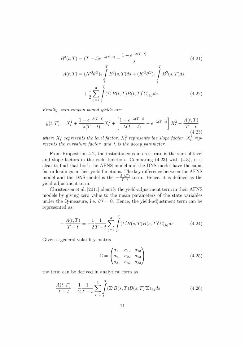
T−t term. Hence, it is defined as theyield-adjustment term.
Christensen et al. [2011] identify the yield-adjustment term in their AFNSmodels by giving zero value to the mean parameters of the state variablesunder the Q-measure, i.e. θQ = 0. Hence, the yield-adjustment term can berepresented as:
− A(t, T )
T − t= −1
2
1
T − t
3∑j=1
T∫t
(Σ′B(s, T )B(s, T )′Σ)j,jds (4.24)
Given a general volatility matrix
Σ =
σ11 σ12 σ13
σ21 σ22 σ23
σ31 σ32 σ33
(4.25)
the term can be derived in analytical form as
A(t, T )
T − t=
1
2
1
T − t
3∑j=1
T∫t
(Σ′B(s, T )B(s, T )′Σ)j,jds (4.26)
11
= A(T − t)2
6
+B
[1
2λ2− 1
λ3
1− e−λ(T−t)
T − t+
1
4λ3
1− e−2λ(T−t)
T − t
]+ C
[1
2λ2+
1
λ2e−λ(T−t) − 1
4λ(T − t)e−2λ(T−t)
− 3
4λ2e−2λ(T−t) − 2
λ3
1− e−λ(T−t)
T − t+
5
8λ3
1− e−2λ(T−t)
T − t
]+D
[1
2λ(T − t) +
1
λ2e−λ(T−t) − 1
λ3
1− e−λ(T−t)
T − t
]+ E
[1
2λ(T − t) +
3
λ2e−λ(T−t) +
1
λ(T − t)e−λ(T−t)
− 3
λ3
1− e−λ(T−t)
T − t
]+ F
[1
λ2+
1
λ2e−λ(T−t) − 1
2λ2e−2λ(T−t)
− 3
λ3
1− e−λ(T−t)
T − t+
3
4λ3
1− e−2λ(T−t)
T − t
](4.27)
where
A = σ211 + σ2
12 + σ213
B = σ221 + σ2
22 + σ223
C = σ231 + σ2
32 + σ233
D = σ11σ21 + σ12σ22 + σ13σ23
E = σ11σ31 + σ12σ32 + σ13σ33
F = σ21σ31 + σ22σ32 + σ23σ33
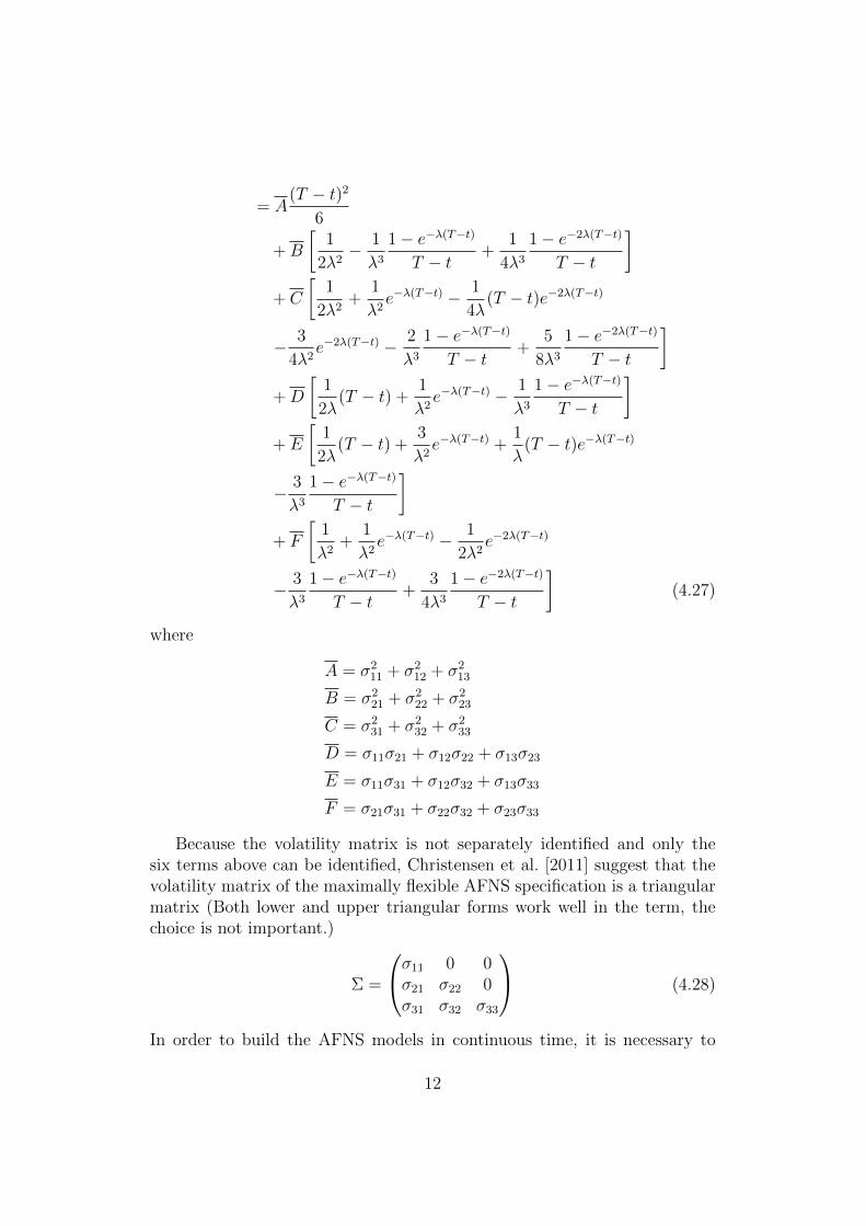
Because the volatility matrix is not separately identified and only thesix terms above can be identified, Christensen et al. [2011] suggest that thevolatility matrix of the maximally flexible AFNS specification is a triangularmatrix (Both lower and upper triangular forms work well in the term, thechoice is not important.)
Σ =
σ11 0 0σ21 σ22 0σ31 σ32 σ33
(4.28)
In order to build the AFNS models in continuous time, it is necessary to
12
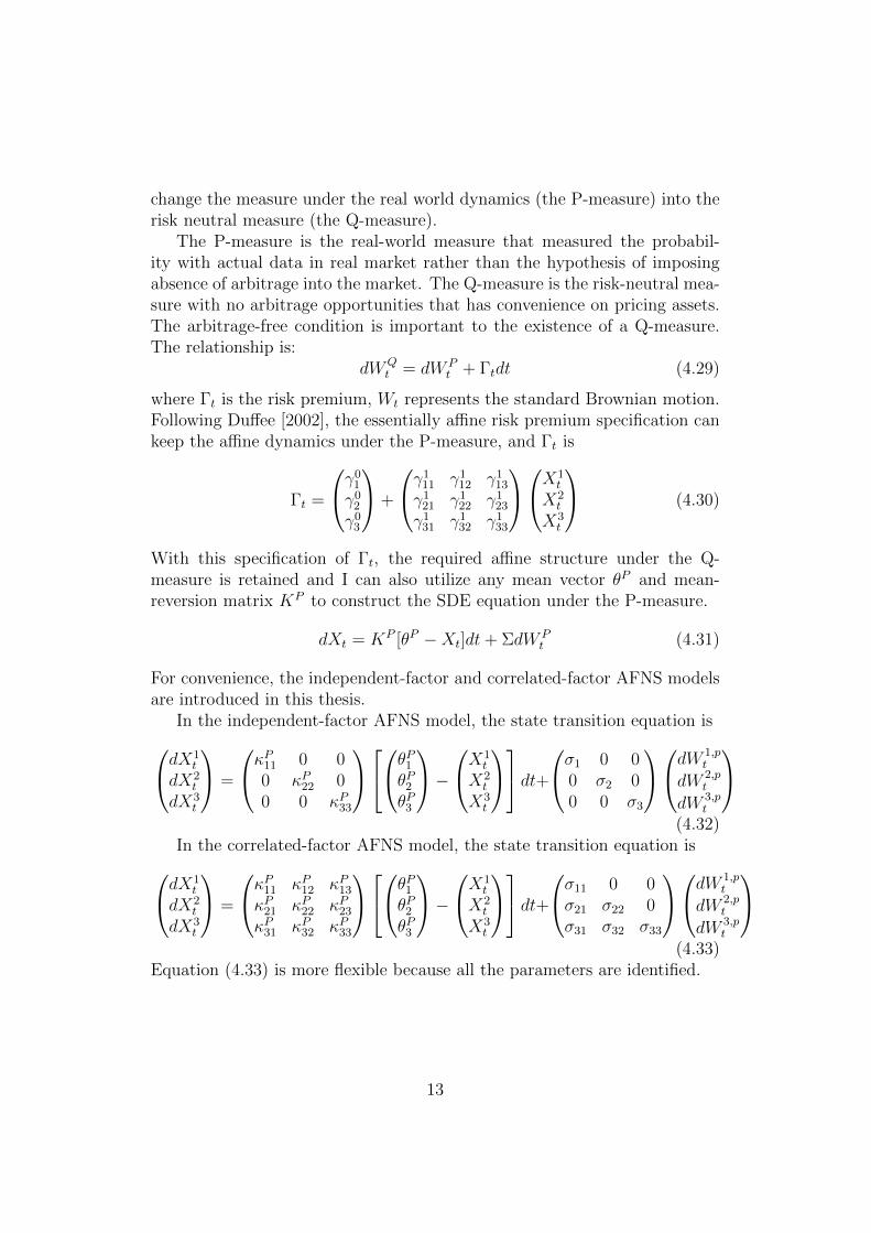
change the measure under the real world dynamics (the P-measure) into therisk neutral measure (the Q-measure).
The P-measure is the real-world measure that measured the probabil-ity with actual data in real market rather than the hypothesis of imposingabsence of arbitrage into the market. The Q-measure is the risk-neutral mea-sure with no arbitrage opportunities that has convenience on pricing assets.The arbitrage-free condition is important to the existence of a Q-measure.The relationship is:
dWQt = dW P
t + Γtdt (4.29)
where Γt is the risk premium, Wt represents the standard Brownian motion.Following Duffee [2002], the essentially affine risk premium specification cankeep the affine dynamics under the P-measure, and Γt is
Γt =
γ01
γ02
γ03
+
γ111 γ1
12 γ113
γ121 γ1
22 γ123
γ131 γ1
32 γ133
X1t
X2t
X3t
(4.30)
With this specification of Γt, the required affine structure under the Q-measure is retained and I can also utilize any mean vector θP and mean-reversion matrix KP to construct the SDE equation under the P-measure.
dXt = KP [θP −Xt]dt+ ΣdW Pt (4.31)
For convenience, the independent-factor and correlated-factor AFNS modelsare introduced in this thesis.
In the independent-factor AFNS model, the state transition equation isdX1t
dX2t
dX3t
=
κP11 0 00 κP22 00 0 κP33
θP1θP2θP3
−X1
t
X2t
X3t
dt+σ1 0 0
0 σ2 00 0 σ3
dW 1,pt
dW 2,pt
dW 3,pt
(4.32)
In the correlated-factor AFNS model, the state transition equation isdX1t
dX2t
dX3t
=
κP11 κP12 κP13
κP21 κP22 κP23
κP31 κP32 κP33
θP1θP2θP3
−X1
t
X2t
X3t
dt+σ11 0 0σ21 σ22 0σ31 σ32 σ33
dW 1,pt
dW 2,pt
dW 3,pt
(4.33)
Equation (4.33) is more flexible because all the parameters are identified.
13
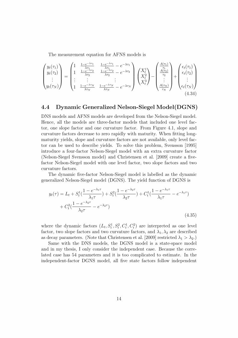
The measurement equation for AFNS models isyt(τ1)yt(τ2)
...yt(τN)
=
1 1−e−λτ1
λτ11−e−λτ1λτ1
− e−λτ11 1−e−λτ2
λτ21−e−λτ2λτ2
− e−λτ2...
......
1 1−e−λτNλτN
1−e−λτNλτN
− e−λτN
X1
t
X2t
X3t
−
A(τ1)τ1
A(τ2)τ2...
A(τN )τN
+
εt(τ1)εt(τ2)
...εt(τN)
(4.34)
4.4 Dynamic Generalized Nelson-Siegel Model(DGNS)
DNS models and AFNS models are developed from the Nelson-Siegel model.Hence, all the models are three-factor models that included one level fac-tor, one slope factor and one curvature factor. From Figure 4.1, slope andcurvature factors decrease to zero rapidly with maturity. When fitting long-maturity yields, slope and curvature factors are not available, only level fac-tor can be used to describe yields. To solve this problem, Svensson [1995]introduce a four-factor Nelson-Siegel model with an extra curvature factor(Nelson-Siegel Svensson model) and Christensen et al. [2009] create a five-factor Nelson-Siegel model with one level factor, two slope factors and twocurvature factors.
The dynamic five-factor Nelson-Siegel model is labelled as the dynamicgeneralized Nelson-Siegel model (DGNS). The yield function of DGNS is
yt(τ) = Lt + S1t (
1− e−λ1τ
λ1τ) + S2
t (1− e−λ2τ
λ2τ) + C1
t (1− e−λ1τ
λ1τ− e−λ1τ )
+ C2t (
1− e−λ2τ
λ2τ− e−λ2τ )
(4.35)
where the dynamic factors (Lt, S1t , S
2t , C
1t , C
2t ) are interpreted as one level
factor, two slope factors and two curvature factors, and λ1, λ2 are describedas decay parameters. (Note that Christensen et al. [2009] restricted λ1 > λ2.)
Same with the DNS models, the DGNS model is a state-space modeland in my thesis, I only consider the independent case. Because the corre-lated case has 54 parameters and it is too complicated to estimate. In theindependent-factor DGNS model, all five state factors follow independent
14
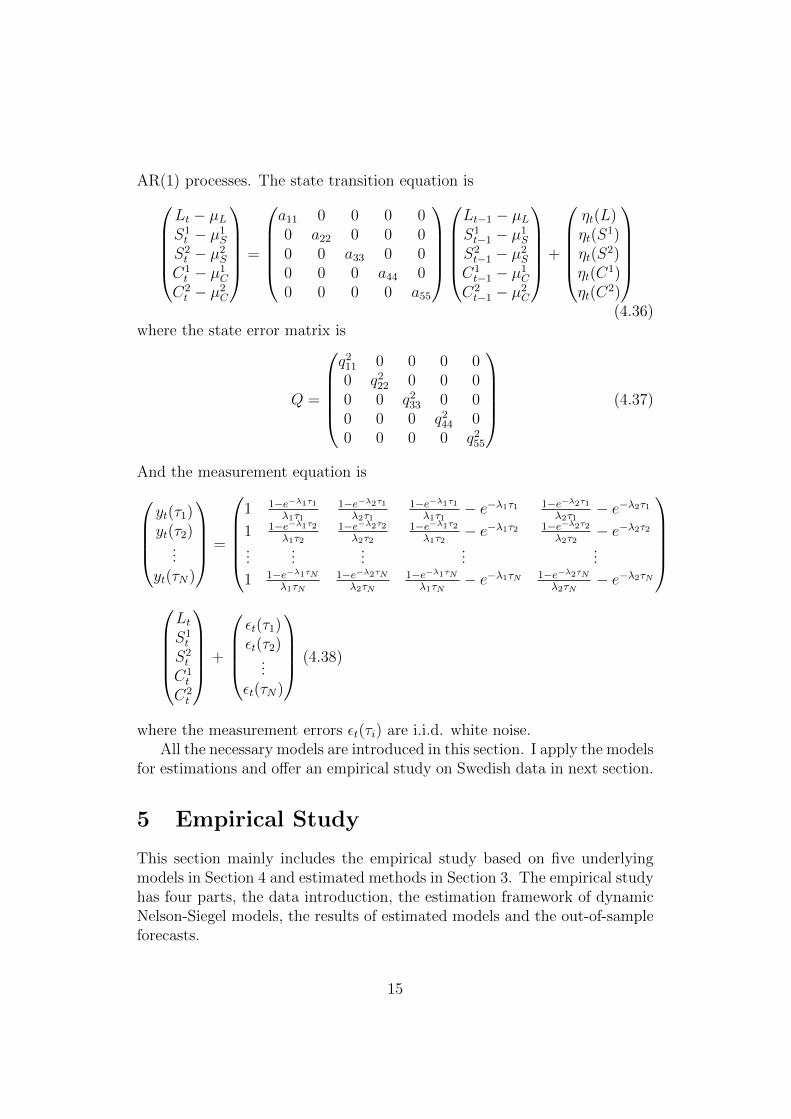
AR(1) processes. The state transition equation isLt − µLS1t − µ1
S
S2t − µ2
S
C1t − µ1
C
C2t − µ2
C
=
a11 0 0 0 00 a22 0 0 00 0 a33 0 00 0 0 a44 00 0 0 0 a55
Lt−1 − µLS1t−1 − µ1
S
S2t−1 − µ2
S
C1t−1 − µ1
C
C2t−1 − µ2
C
+
ηt(L)ηt(S
1)ηt(S
2)ηt(C
1)ηt(C
2)
(4.36)
where the state error matrix is
Q =
q2
11 0 0 0 00 q2
22 0 0 00 0 q2
33 0 00 0 0 q2
44 00 0 0 0 q2
55
(4.37)
And the measurement equation isyt(τ1)yt(τ2)
...yt(τN)
=
1 1−e−λ1τ1
λ1τ11−e−λ2τ1λ2τ1
1−e−λ1τ1λ1τ1
− e−λ1τ1 1−e−λ2τ1λ2τ1
− e−λ2τ11 1−e−λ1τ2
λ1τ21−e−λ2τ2λ2τ2
1−e−λ1τ2λ1τ2
− e−λ1τ2 1−e−λ2τ2λ2τ2
− e−λ2τ2...
......
......
1 1−e−λ1τNλ1τN
1−e−λ2τNλ2τN
1−e−λ1τNλ1τN
− e−λ1τN 1−e−λ2τNλ2τN
− e−λ2τN
LtS1t
S2t
C1t
C2t
+
εt(τ1)εt(τ2)
...εt(τN)
(4.38)
where the measurement errors εt(τi) are i.i.d. white noise.All the necessary models are introduced in this section. I apply the models
for estimations and offer an empirical study on Swedish data in next section.
5 Empirical Study
This section mainly includes the empirical study based on five underlyingmodels in Section 4 and estimated methods in Section 3. The empirical studyhas four parts, the data introduction, the estimation framework of dynamicNelson-Siegel models, the results of estimated models and the out-of-sampleforecasts.
15
5.1 Data
The estimates in my thesis are based on monthly Swedish treasury bill andgovernment bond yields. Treasury bills are short-term debt tools with ma-turities of less than one year. The treasury bills in Sweden include fourdurations: one month, three months, six months and one year. However, theone-year treasury bill is discontinued in October 2010. So I do not collect itinto my data set. Swedish government bonds are long-term debt tools withfour maturities: two years, five years, seven years and ten years. Treasurybills and government bonds are issued by the Swedish National Debt Office.
The final data are zero-coupon yields from January 1996 to December2011 and at seven maturities: one month, three months, six months, twoyears, five years, seven years and ten years. The data are directly downloadedfrom the Swedish Central Bank website.
Notice that, in Diebold et al. [2006], Christensen et al. [2011] and otherpapers, they estimate and test dynamic Nelson-Siegel models by using themonthly US Treasury bill and bond yields with a wide range of maturitiesand get good performances. The data are zero-coupon yields with sixteenmaturities: 3, 6, 9, 12, 18, 24, 36, 48, 60, 84, 96, 108, 120, 180, 240, and 360months. Compared with the US data, I do not have so many observationsat different maturities for my thesis. But it is also fascinating to investigatethe performances of the models under this situation.
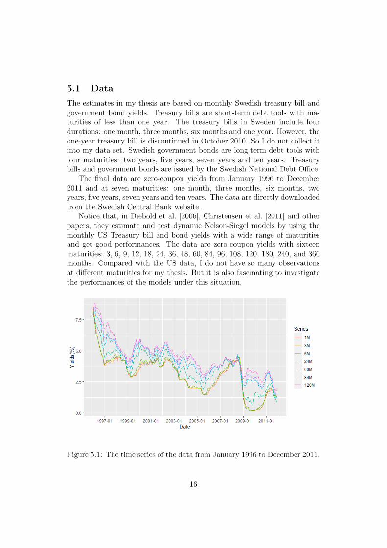
Figure 5.1: The time series of the data from January 1996 to December 2011.
16
From Figure 5.1, I observe the Swedish yields have a general descendingtrend from January 1996 to December 2011. Usually, the yields at longmaturity are higher than the yields at short maturity. In this figure, the10-year yield curve (the pink line) is over other yield curves. Under thiscurve, there are the 7-year yield curve, the 5-year yield curve and so on. Butthe difference between the yields is not obvious when the yields are at shortmaturity (less than one year). Another interesting thing is that the yields atseven different maturities become quite close and go down sharply from 2008to 2009 because of the global financial crisis in 2008. Especially, the crisishas a serious influence on the short-term bonds, which made the bond yieldsclose to zero in nearly two years (2009-2010). But the long-term bonds arenot as deeply affected as the short-term bonds.
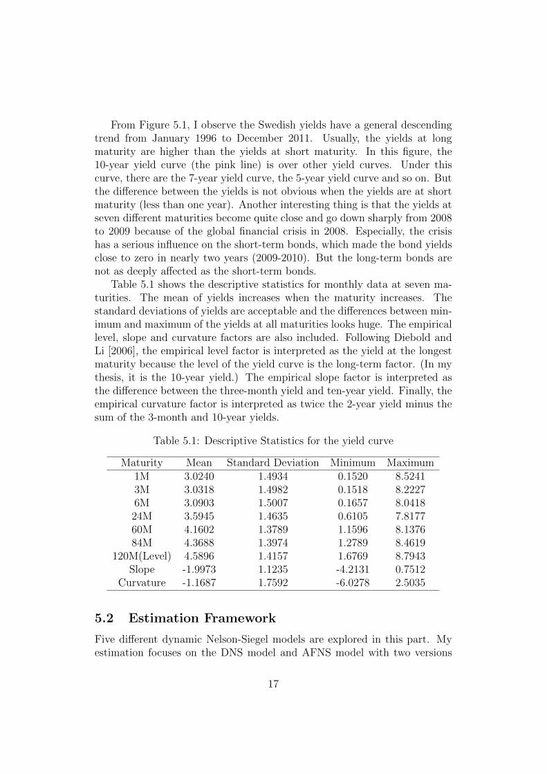
Table 5.1 shows the descriptive statistics for monthly data at seven ma-turities. The mean of yields increases when the maturity increases. Thestandard deviations of yields are acceptable and the differences between min-imum and maximum of the yields at all maturities looks huge. The empiricallevel, slope and curvature factors are also included. Following Diebold andLi [2006], the empirical level factor is interpreted as the yield at the longestmaturity because the level of the yield curve is the long-term factor. (In mythesis, it is the 10-year yield.) The empirical slope factor is interpreted asthe difference between the three-month yield and ten-year yield. Finally, theempirical curvature factor is interpreted as twice the 2-year yield minus thesum of the 3-month and 10-year yields.
Table 5.1: Descriptive Statistics for the yield curve
Maturity Mean Standard Deviation Minimum Maximum1M 3.0240 1.4934 0.1520 8.52413M 3.0318 1.4982 0.1518 8.22276M 3.0903 1.5007 0.1657 8.041824M 3.5945 1.4635 0.6105 7.817760M 4.1602 1.3789 1.1596 8.137684M 4.3688 1.3974 1.2789 8.4619
120M(Level) 4.5896 1.4157 1.6769 8.7943Slope -1.9973 1.1235 -4.2131 0.7512
Curvature -1.1687 1.7592 -6.0278 2.5035
5.2 Estimation Framework
Five different dynamic Nelson-Siegel models are explored in this part. Myestimation focuses on the DNS model and AFNS model with two versions
17
(independent-factor and correlated-factor), and the independent-factor DGNSmodel. In this part, I introduce the framework to estimate and forecastSwedish data with dynamic Nelson-Siegel models.
5.2.1 DNS Model
For the DNS models, the state-space representations can be written as fol-lows:
Xt = (I − A)µ+ AXt−1 + ηt (5.1)
Yt = BXt + εt (5.2)
where Xt = (Lt, St, Ct), I is the identity matrix, µ is a vector of factor means,the matrices A and B are constant. B is the factor-loading matrix for thedecay parameter λ. The error structure is(
ηtεt
)∼ N
[(00
),
(Q 00 H
)], (5.3)
According to (4.5) and (4.7), the matrix Q in the independent-factor DNSmodel is diagonal and in the correlated-factor DNS model is not diagonal.Following Diebold and Li [2006], the matrix H is diagonal.
Now the Kalman filter is applied to estimate the parameters. In theindependent-factor DNS model, there are 17 parameters, and in the correlated-factor DNS model, there are 26 parameters. Following Diebold et al. [2006],X0 = µ and Σ0 = V , where V solves V = AV A′ +Q. The prediction step oftime t− 1 is:
Xt|t−1 = (I − A)µ+ AXt−1 (5.4)
Σt|t−1 = AΣt−1A′ +Q (5.5)
The update step of time t is:
Xtt = Xt|t−1 + Σt|t−1B′F−1t vt (5.6)
Σtt = (I − Σt|t−1B′F−1t B)Σt|t−1 (5.7)
where measurement residual vt = yt−A−BXt|t−1, Ft = cov(vt) = BΣt|t−1B′+
H, H = diag(σ2ε (τ1), ..., σ2
ε (τN)).Given all parameters from the Kalman filter, the log-likelihood function
can be classified, the prediction error decomposition of the function is
logL = −TN2log(2π)−
T∑t=1
(v′tF
−1t vt + log|Ft|
2) (5.8)
18
where N is the number of observed yields. The maximum log-likelihoodestimates are obtained by optimizing the parameters and the decay parameterλ. In this thesis, N = 192, and λ for initialling Kalman filter is 0.6915,which is chosen by the mean of the time series of empirical λ parameters.The empirical λ parameters are the results of fixing the basic Nelson-Siegelmodel with the data.
Here I do not choose the common decay parameter λ = 0.0609 that isrecommended by Diebold et al. [2006], because I think that for different termstructure data, the decay parameter is different. Instead, I use the mean ofthe empirical parameters as the constant initial λ parameter.
5.2.2 AFNS Model
Following Christensen et al. [2011], the state-space representations of theAFNS models can be written as:
Xt = (I − exp(−KP∆t))θP + exp(−KP∆t)Xt−1 + ηt (5.9)
Yt = BXt − A+ εt (5.10)
where ∆t is the time difference between the data. The error structure is sameas (5.3), only the matrix Qt in AFNS models is different.
Qt =
∆t∫0
e−KP sΣΣ′e−(KP )′sds (5.11)
Notice that the matrix Q is equal to the conditional covariance matrix.The Kalman filter-based maximum-likelihood method for AFNS models
is similar with the method for DNS models. But I initialize the Kalmanfilter with the unconditional mean and covariance matrix in AFNS models,X0 = θP and Σ0 =
∫∞0e−K
P sΣΣ′e−(KP )′sds. Hence the prediction step is
Xt|t−1 = EP [Xt|Yt−1] = (I − exp(−KP∆t))θP + exp(−KP∆t)Xt−1 (5.12)
Σt|t−1 = exp(−KP∆t)Σt−1[exp(−KP∆t)]′+Qt (5.13)
Other steps can be found in the DNS model estimation. To keep thecovariance stationary under the P-measure, Christensen et al. restrict theeigenvalues of A to be less than 1 in DNS and DGNS models and the realcomponent of each eigenvalue of KP to be positive.
19
5.2.3 DGNS Model
The independent-factor DGNS model has the same representations and theerror structure as the independent-factor DNS model, the only difference isthe size of matrices, e.g. the matrix A and the state error matrix Q are 5× 5matrices, and the factor Xt = (Lt, S
1t , S
2t , C
1t , C
2t ). There are 24 parameters in
this model. To avoid collinearity between the factors, the difference of initialλ1, λ2 parameters can be set as big as possible. Here I use the optimized λ forthe independent-factor DNS model as the first decay parameter, λ1 = 0.7144,and set λ2 = 0.0144.
5.2.4 Out-of-sample Forecast Method
The out-of-sample forecast is a common and important way to test the per-formance of financial estimators and models. To check dynamic Nelson-Siegelmodels, I splice the observations in two parts with forecasting period h. I usethe first part to get the forecast yields with h months ahead Yt+h(τ), where τis the maturity and t is the time, and compare forecast yields with observedyields. Following Christensen et al. [2011], the forecast error is defined aset+h(τ) = Yt+h(τ) − Yt+h(τ), and forecast performances are decided by theroot mean squared forecast error (RMSFE).
5.3 Estimation Results
This section is the summary of all the estimation results involved in mythesis. The results are illustrated separately by different models.
5.3.1 DNS Model Estimation
The results of the estimates for DNS models are shown below.
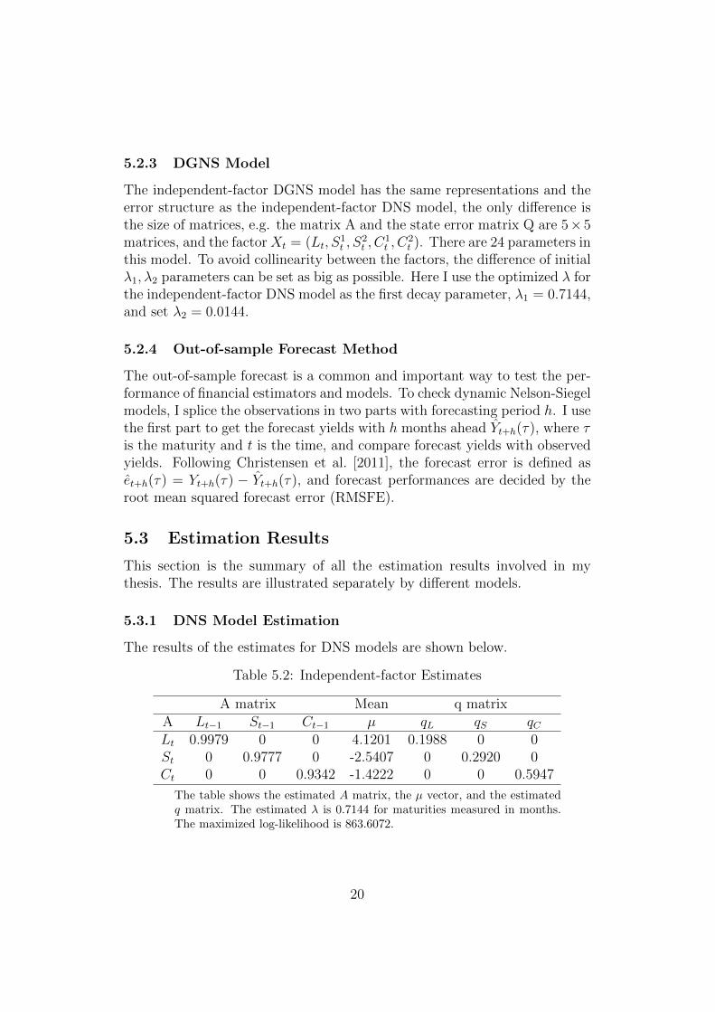
Table 5.2: Independent-factor Estimates
A matrix Mean q matrixA Lt−1 St−1 Ct−1 µ qL qS qCLt 0.9979 0 0 4.1201 0.1988 0 0St 0 0.9777 0 -2.5407 0 0.2920 0Ct 0 0 0.9342 -1.4222 0 0 0.5947
The table shows the estimated A matrix, the µ vector, and the estimatedq matrix. The estimated λ is 0.7144 for maturities measured in months.The maximized log-likelihood is 863.6072.
20
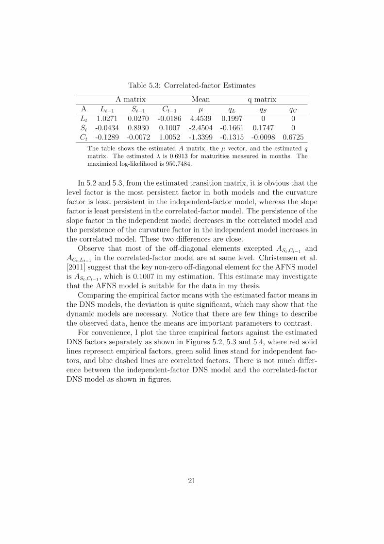
Table 5.3: Correlated-factor Estimates
A matrix Mean q matrixA Lt−1 St−1 Ct−1 µ qL qS qCLt 1.0271 0.0270 -0.0186 4.4539 0.1997 0 0St -0.0434 0.8930 0.1007 -2.4504 -0.1661 0.1747 0Ct -0.1289 -0.0072 1.0052 -1.3399 -0.1315 -0.0098 0.6725
The table shows the estimated A matrix, the µ vector, and the estimated qmatrix. The estimated λ is 0.6913 for maturities measured in months. Themaximized log-likelihood is 950.7484.
In 5.2 and 5.3, from the estimated transition matrix, it is obvious that thelevel factor is the most persistent factor in both models and the curvaturefactor is least persistent in the independent-factor model, whereas the slopefactor is least persistent in the correlated-factor model. The persistence of theslope factor in the independent model decreases in the correlated model andthe persistence of the curvature factor in the independent model increases inthe correlated model. These two differences are close.
Observe that most of the off-diagonal elements excepted ASt,Ct−1 andACt,Lt−1 in the correlated-factor model are at same level. Christensen et al.[2011] suggest that the key non-zero off-diagonal element for the AFNS modelis ASt,Ct−1 , which is 0.1007 in my estimation. This estimate may investigatethat the AFNS model is suitable for the data in my thesis.
Comparing the empirical factor means with the estimated factor means inthe DNS models, the deviation is quite significant, which may show that thedynamic models are necessary. Notice that there are few things to describethe observed data, hence the means are important parameters to contrast.
For convenience, I plot the three empirical factors against the estimatedDNS factors separately as shown in Figures 5.2, 5.3 and 5.4, where red solidlines represent empirical factors, green solid lines stand for independent fac-tors, and blue dashed lines are correlated factors. There is not much differ-ence between the independent-factor DNS model and the correlated-factorDNS model as shown in figures.
21
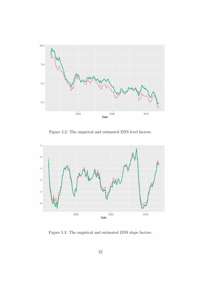
Figure 5.2: The empirical and estimated DNS level factors.
Figure 5.3: The empirical and estimated DNS slope factors.
22
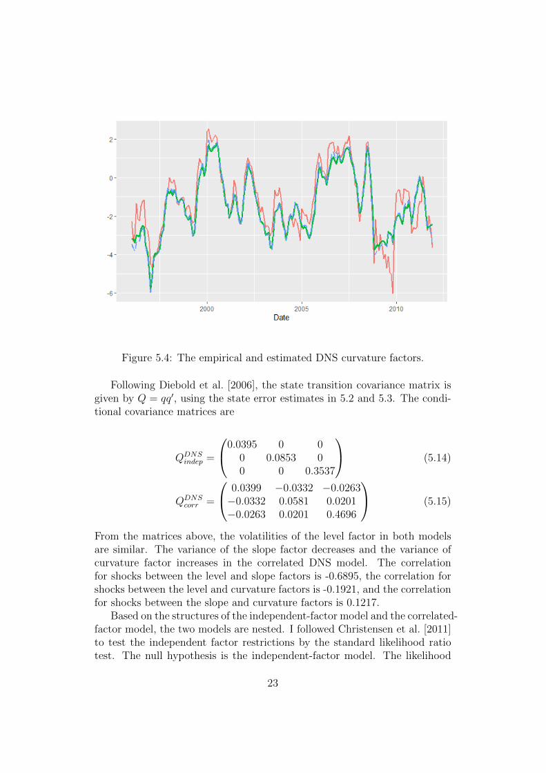
Figure 5.4: The empirical and estimated DNS curvature factors.
Following Diebold et al. [2006], the state transition covariance matrix isgiven by Q = qq′, using the state error estimates in 5.2 and 5.3. The condi-tional covariance matrices are
QDNSindep =
0.0395 0 00 0.0853 00 0 0.3537
(5.14)
QDNScorr =
0.0399 −0.0332 −0.0263−0.0332 0.0581 0.0201−0.0263 0.0201 0.4696
(5.15)
From the matrices above, the volatilities of the level factor in both modelsare similar. The variance of the slope factor decreases and the variance ofcurvature factor increases in the correlated DNS model. The correlationfor shocks between the level and slope factors is -0.6895, the correlation forshocks between the level and curvature factors is -0.1921, and the correlationfor shocks between the slope and curvature factors is 0.1217.
Based on the structures of the independent-factor model and the correlated-factor model, the two models are nested. I followed Christensen et al. [2011]to test the independent factor restrictions by the standard likelihood ratiotest. The null hypothesis is the independent-factor model. The likelihood
23
ratio is given by
LR = 2[logL(θcorr)− logL(θindep)] ∼ χ2(9) (5.16)
I obtain LR = 174.2824 and the associated p-value less than 0.0001.Hence, the restrictions established in the independent-factor model are re-jected.
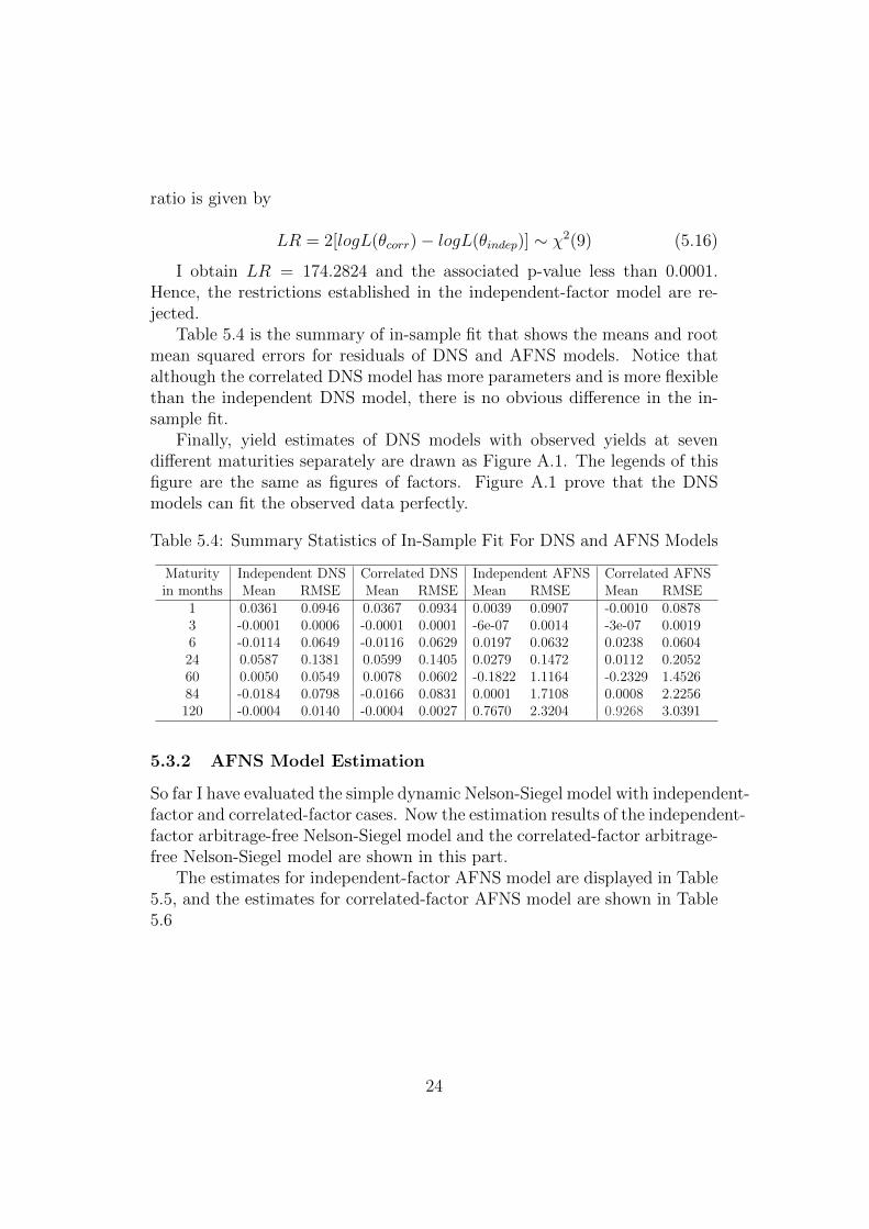
Table 5.4 is the summary of in-sample fit that shows the means and rootmean squared errors for residuals of DNS and AFNS models. Notice thatalthough the correlated DNS model has more parameters and is more flexiblethan the independent DNS model, there is no obvious difference in the in-sample fit.
Finally, yield estimates of DNS models with observed yields at sevendifferent maturities separately are drawn as Figure A.1. The legends of thisfigure are the same as figures of factors. Figure A.1 prove that the DNSmodels can fit the observed data perfectly.
Table 5.4: Summary Statistics of In-Sample Fit For DNS and AFNS Models
Independent DNS Correlated DNS Independent AFNS Correlated AFNSMaturityin months Mean RMSE Mean RMSE Mean RMSE Mean RMSE
1 0.0361 0.0946 0.0367 0.0934 0.0039 0.0907 -0.0010 0.08783 -0.0001 0.0006 -0.0001 0.0001 -6e-07 0.0014 -3e-07 0.00196 -0.0114 0.0649 -0.0116 0.0629 0.0197 0.0632 0.0238 0.060424 0.0587 0.1381 0.0599 0.1405 0.0279 0.1472 0.0112 0.205260 0.0050 0.0549 0.0078 0.0602 -0.1822 1.1164 -0.2329 1.452684 -0.0184 0.0798 -0.0166 0.0831 0.0001 1.7108 0.0008 2.2256120 -0.0004 0.0140 -0.0004 0.0027 0.7670 2.3204 0.9268 3.0391
5.3.2 AFNS Model Estimation
So far I have evaluated the simple dynamic Nelson-Siegel model with independent-factor and correlated-factor cases. Now the estimation results of the independent-factor arbitrage-free Nelson-Siegel model and the correlated-factor arbitrage-free Nelson-Siegel model are shown in this part.
The estimates for independent-factor AFNS model are displayed in Table5.5, and the estimates for correlated-factor AFNS model are shown in Table5.6
24
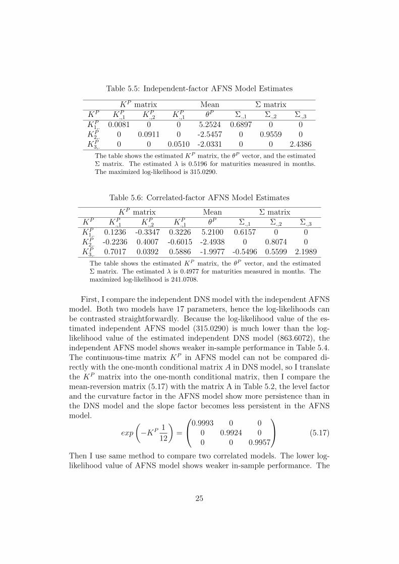
Table 5.5: Independent-factor AFNS Model Estimates
KP matrix Mean Σ matrixKP KP
.,1 KP.,2 KP
.,1 θP Σ.,1 Σ.,2 Σ.,3
KP1,. 0.0081 0 0 5.2524 0.6897 0 0
KP2,. 0 0.0911 0 -2.5457 0 0.9559 0
KP3,. 0 0 0.0510 -2.0331 0 0 2.4386
The table shows the estimated KP matrix, the θP vector, and the estimatedΣ matrix. The estimated λ is 0.5196 for maturities measured in months.The maximized log-likelihood is 315.0290.
Table 5.6: Correlated-factor AFNS Model Estimates
KP matrix Mean Σ matrixKP KP
.,1 KP.,2 KP
.,1 θP Σ.,1 Σ.,2 Σ.,3
KP1,. 0.1236 -0.3347 0.3226 5.2100 0.6157 0 0
KP2,. -0.2236 0.4007 -0.6015 -2.4938 0 0.8074 0
KP3,. 0.7017 0.0392 0.5886 -1.9977 -0.5496 0.5599 2.1989
The table shows the estimated KP matrix, the θP vector, and the estimatedΣ matrix. The estimated λ is 0.4977 for maturities measured in months. Themaximized log-likelihood is 241.0708.
First, I compare the independent DNS model with the independent AFNSmodel. Both two models have 17 parameters, hence the log-likelihoods canbe contrasted straightforwardly. Because the log-likelihood value of the es-timated independent AFNS model (315.0290) is much lower than the log-likelihood value of the estimated independent DNS model (863.6072), theindependent AFNS model shows weaker in-sample performance in Table 5.4.The continuous-time matrix KP in AFNS model can not be compared di-rectly with the one-month conditional matrix A in DNS model, so I translatethe KP matrix into the one-month conditional matrix, then I compare themean-reversion matrix (5.17) with the matrix A in Table 5.2, the level factorand the curvature factor in the AFNS model show more persistence than inthe DNS model and the slope factor becomes less persistent in the AFNSmodel.
exp
(−KP 1
12
)=
0.9993 0 00 0.9924 00 0 0.9957
(5.17)
Then I use same method to compare two correlated models. The lower log-likelihood value of AFNS model shows weaker in-sample performance. The
25
one-month conditional matrix is
exp
(−KP 1
12
)=
0.9898 0.0283 −0.02650.0012 0.9366 0.0008−0.0008 −0.0010 0.9430
(5.18)
In the correlated-factor case, the level factor and the curvature factor in theAFNS model show less persistence than in the DNS model and the slope fac-tor becomes more persistent in the AFNS model. Here the result is differentfrom the result of the independent-factor case.
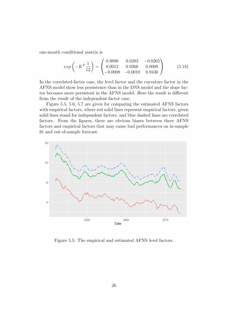
Figure 5.5, 5.6, 5.7 are given for comparing the estimated AFNS factorswith empirical factors, where red solid lines represent empirical factors, greensolid lines stand for independent factors, and blue dashed lines are correlatedfactors. From the figures, there are obvious biases between three AFNSfactors and empirical factors that may cause bad performances on in-samplefit and out-of-sample forecast.
Figure 5.5: The empirical and estimated AFNS level factors.
26
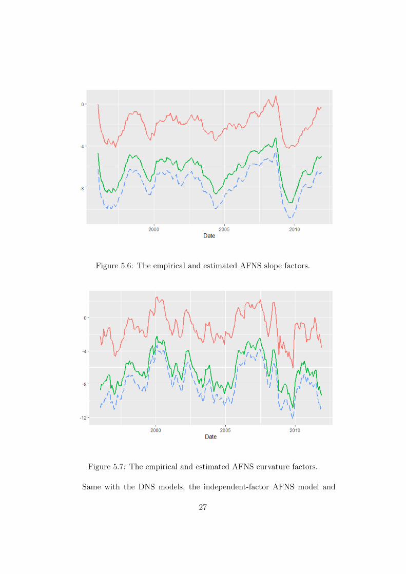
Figure 5.6: The empirical and estimated AFNS slope factors.
Figure 5.7: The empirical and estimated AFNS curvature factors.
Same with the DNS models, the independent-factor AFNS model and
27
the correlated-factor AFNS model are nested. Applying the equation (5.16),LR = 147.9164 and the associated p-value less than 0.0001. The restric-tions established in the independent-factor model are rejected. Hence, theindependent-factor cases are enough to fit the data set in DNS and AFNSmodels.
Observing the factor means from Table 5.5 and 5.6, the AFNS modelsfactor means estimates are higher than the estimated factor means in DNSmodels, especially, the estimated level factors in AFNS models are nearly20% higher than the level factors in DNS models. In Nelson-Siegel models,the level factor is the long-term factor that influenced yields at long matu-rities. Hence, higher level factors might indicate that AFNS models are notsuitable for long-maturity yields. Meanwhile, from Table 5.4, the residualsand RMSEs are quite big when the maturity equals 120 months. To figure outthis problem straightforwardly, I plot yield estimates with observed yields atseven different maturities separately as Figure A.2, the legends of this figureare the same as in previous figures. There are obvious biases between theestimated data and observations when the maturities are five years, sevenyears and ten years. The AFNS models can fit the yields with maturities lessthan or equal to 2 years. Hence, AFNS models have poor performance whenfitting the long-maturity yields.
Based on the results I get, for my data set, it is no significant differencebetween DNS models and AFNS models when the maturities are short. Forlong-maturity yields, DNS models might be a good choice. However, sincemy data set only has 1344 samples and seven maturities, we need to testmore data to get a general conclusion.
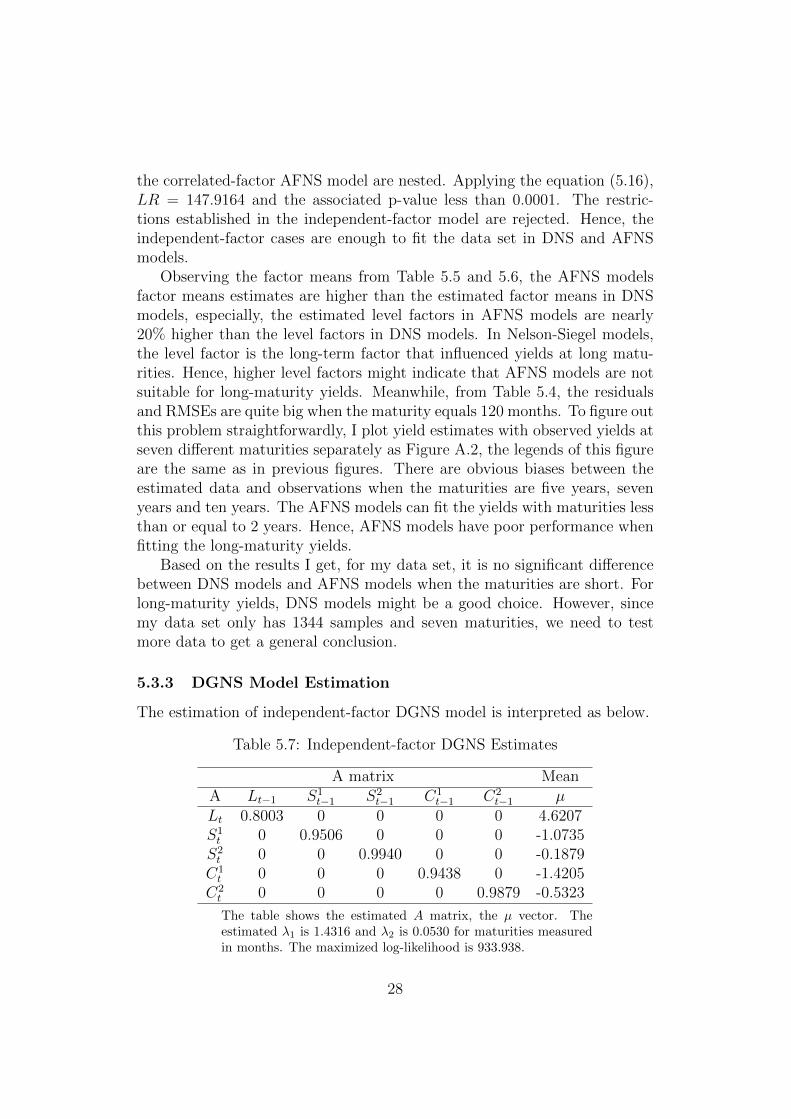
5.3.3 DGNS Model Estimation
The estimation of independent-factor DGNS model is interpreted as below.
Table 5.7: Independent-factor DGNS Estimates
A matrix MeanA Lt−1 S1
t−1 S2t−1 C1
t−1 C2t−1 µ
Lt 0.8003 0 0 0 0 4.6207S1t 0 0.9506 0 0 0 -1.0735S2t 0 0 0.9940 0 0 -0.1879
C1t 0 0 0 0.9438 0 -1.4205
C2t 0 0 0 0 0.9879 -0.5323
The table shows the estimated A matrix, the µ vector. Theestimated λ1 is 1.4316 and λ2 is 0.0530 for maturities measuredin months. The maximized log-likelihood is 933.938.
28
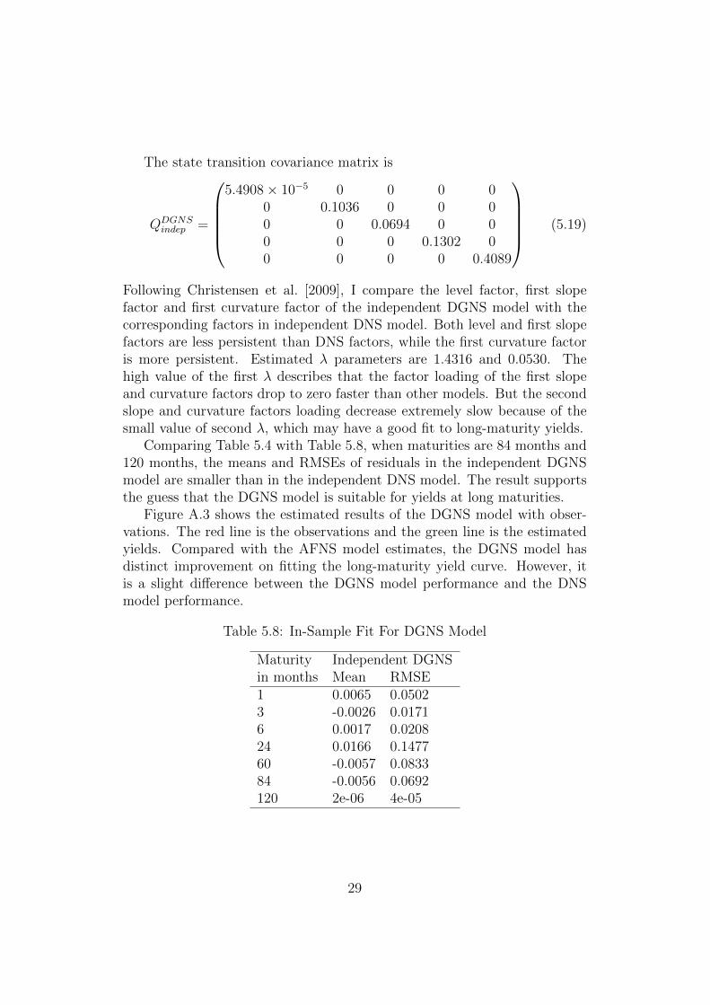
The state transition covariance matrix is
QDGNSindep =
5.4908× 10⁻⁵ 0 0 0 0
0 0.1036 0 0 00 0 0.0694 0 00 0 0 0.1302 00 0 0 0 0.4089
(5.19)
Following Christensen et al. [2009], I compare the level factor, first slopefactor and first curvature factor of the independent DGNS model with thecorresponding factors in independent DNS model. Both level and first slopefactors are less persistent than DNS factors, while the first curvature factoris more persistent. Estimated λ parameters are 1.4316 and 0.0530. Thehigh value of the first λ describes that the factor loading of the first slopeand curvature factors drop to zero faster than other models. But the secondslope and curvature factors loading decrease extremely slow because of thesmall value of second λ, which may have a good fit to long-maturity yields.
Comparing Table 5.4 with Table 5.8, when maturities are 84 months and120 months, the means and RMSEs of residuals in the independent DGNSmodel are smaller than in the independent DNS model. The result supportsthe guess that the DGNS model is suitable for yields at long maturities.
Figure A.3 shows the estimated results of the DGNS model with obser-vations. The red line is the observations and the green line is the estimatedyields. Compared with the AFNS model estimates, the DGNS model hasdistinct improvement on fitting the long-maturity yield curve. However, itis a slight difference between the DGNS model performance and the DNSmodel performance.
Table 5.8: In-Sample Fit For DGNS Model
Maturityin months
Independent DGNSMean RMSE
1 0.0065 0.05023 -0.0026 0.01716 0.0017 0.020824 0.0166 0.147760 -0.0057 0.083384 -0.0056 0.0692120 2e-06 4e-05
29
5.4 Out-of-sample Forecasts
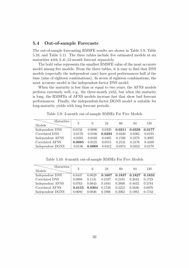
The out-of-sample forecasting RMSFE results are shown in Table 5.9, Table5.10, and Table 5.11. The three tables include five estimated models at sixmaturities with 3-,6-,12-month forecast separately.
The bold value represents the smallest RMSFE value of the most accuratemodel among five models. From the three tables, it is easy to find that DNSmodels (especially the independent case) have good performances half of thetime (nine of eighteen combinations). In seven of eighteen combinations, themost accurate model is the independent-factor DNS model.
When the maturity is less than or equal to two years, the AFNS modelsperform extremely well, e.g., the three-month yield, but when the maturityis long, the RMSFEs of AFNS models increase fast that show bad forecastperformances. Finally, the independent-factor DGNS model is suitable forlong-maturity yields with long forecast periods.
Table 5.9: 3-month out-of-sample RMSEs For Five Models
ModelsMaturities
3 6 24 60 84 120
Independent DNS 0.0156 0.0090 0.0320 0.0311 0.0339 0.0177Correlated DNS 0.0170 0.0166 0.0293 0.0340 0.0365 0.0195Independent AFNS 0.0285 0.0168 0.0485 0.1586 0.2378 0.3095Correlated AFNS 0.0085 0.0125 0.0515 0.2131 0.3176 0.4169Independent DGNS 0.0136 0.0069 0.0412 0.0374 0.0352 0.0179
Table 5.10: 6-month out-of-sample RMSEs For Five Models
ModelsMaturities
3 6 24 60 84 120
Independent DNS 0.0447 0.0629 0.1607 0.1837 0.1827 0.1633Correlated DNS 0.0894 0.1131 0.2187 0.2185 0.2043 0.1723Independent AFNS 0.0763 0.0843 0.1944 0.3800 0.4832 0.5784Correlated AFNS 0.0155 0.0304 0.1726 0.4252 0.5636 0.6976Independent DGNS 0.0680 0.0846 0.1906 0.2063 0.1983 0.1742
30
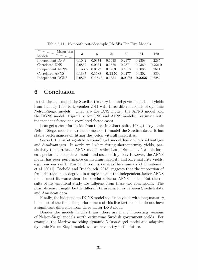
Table 5.11: 12-month out-of-sample RMSEs For Five Models
ModelsMaturities
3 6 24 60 84 120
Independent DNS 0.1002 0.0974 0.1438 0.2177 0.2308 0.2285Correlated DNS 0.0852 0.0954 0.1878 0.2371 0.2369 0.2210Independent AFNS 0.0778 0.0877 0.1953 0.4513 0.6086 0.7611Correlated AFNS 0.1837 0.1688 0.1150 0.4277 0.6302 0.8309Independent DGNS 0.0826 0.0843 0.1554 0.2172 0.2256 0.2282
6 Conclusion
In this thesis, I model the Swedish treasury bill and government bond yieldsfrom January 1996 to December 2011 with three different kinds of dynamicNelson-Siegel models. They are the DNS model, the AFNS model andthe DGNS model. Especially, for DNS and AFNS models, I estimate withindependent-factor and correlated-factor cases.
I can get some information from the estimation results. First, the dynamicNelson-Siegel model is a reliable method to model the Swedish data. It hasstable performances on fitting the yields with all maturities.
Second, the arbitrage-free Nelson-Siegel model has obvious advantagesand disadvantages. It works well when fitting short-maturity yields, par-ticularly the correlated AFNS model, which has perfect out-of-sample fore-cast performance on three-month and six-month yields. However, the AFNSmodel has poor performance on medium-maturity and long-maturity yields,e.g., ten-year yield. This conclusion is same as the summary of Christensenet al. [2011]. Diebold and Rudebusch [2013] suggests that the imposition offree-arbitrage must degrade in-sample fit and the independent-factor AFNSmodel must fit worse than the correlated-factor AFNS model. But the re-sults of my empirical study are different from these two conclusions. Thepossible reason might be the different term structures between Swedish dataand American data.
Finally, the independent DGNS model can fix on yields with long-maturity,but most of the time, the performances of this five-factor model do not havea significant difference from three-factor DNS model.
Besides the models in this thesis, there are many interesting versionsof Nelson-Siegel models worth estimating Swedish government yields. Forexample, the Markov switching dynamic Nelson-Siegel model and adaptivedynamic Nelson-Siegel model. we can have a try in the future.
31
Bibliography
Charles R Nelson and Andrew F Siegel. Parsimonious modeling of yieldcurves. Journal of Business, pages 473–489, 1987.
Francis X. Diebold and Canlin Li. Forecasting the term structure of govern-ment bond yields. Journal of Econometrics, 130(2):337–364, 2006.
Francis X Diebold, Glenn D Rudebusch, and S Boragan Aruoba. The macroe-conomy and the yield curve: a dynamic latent factor approach. Journal ofEconometrics, 131(1-2):309–338, 2006.
Jens HE Christensen, Francis X Diebold, and Glenn D Rudebusch. Theaffine arbitrage-free class of nelson-siegel term structure models. Journalof Econometrics, 164(1):4–20, 2011.
Francis X Diebold and Glenn D Rudebusch. Yield curve modeling and fore-casting: the dynamic Nelson-Siegel approach. Princeton University Press,2013.
Lars EO Svensson. Estimating forward interest rates with the extendednelson& siegel method. Sveriges Riksbank Quarterly Review, 3(1):13–26,1995.
Jens HE Christensen, Francis X Diebold, and Glenn D Rudebusch. Anarbitrage-free generalized nelson-siegel term structure model, 2009.
Robert Kunst. State space models and the kalman filter. VektorautoregressiveMethoden, 2007.
Youngjoo Kim and Hyochoong Bang. Introduction to kalman filter and itsapplications. Introduction and Implementations of the Kalman Filter, 1:1–16, 2018.
Tomas Bjork. Arbitrage theory in continuous time. Oxford university press,2009.
Darrell Duffie and Rui Kan. A yield-factor model of interest rates. Mathe-matical finance, 6(4):379–406, 1996.
Gregory R Duffee. Term premia and interest rate forecasts in affine models.The Journal of Finance, 57(1):405–443, 2002.
32
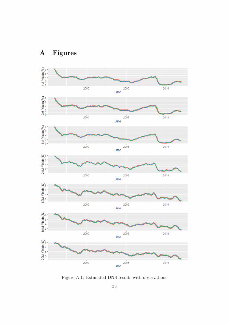
A Figures
Figure A.1: Estimated DNS results with observations
33
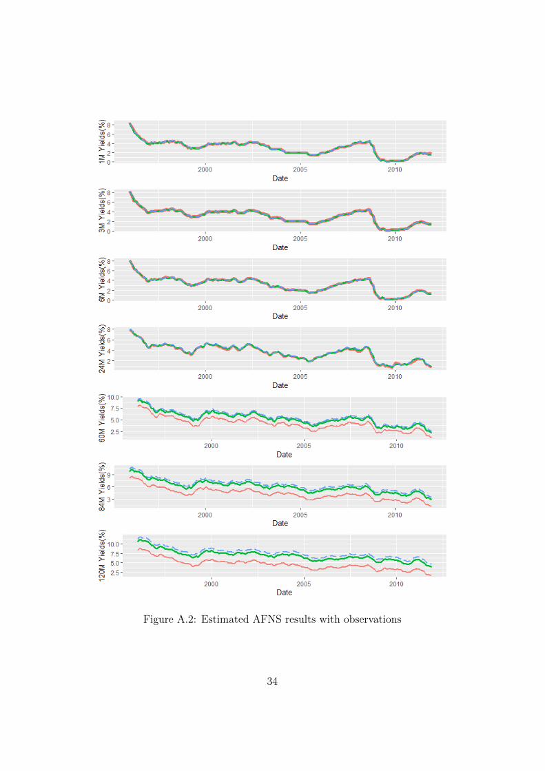
Figure A.2: Estimated AFNS results with observations
34
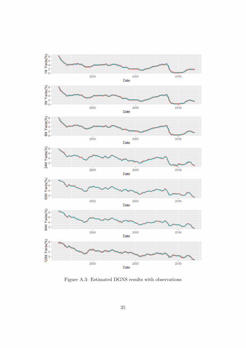
Figure A.3: Estimated DGNS results with observations
35
Related Documents