Fitting a single active appearance model simultaneously to multiple images

Fitting a Single Active Appearance ModelSimultaneously to Multiple Images

Changbo Hu, Jing Xiao, Iain Matthews,Simon Baker, Jeff Cohn, and Takeo Kanade

The Robotics Institute, Carnegie Mellon University5000 Forbes Avenue, Pittsburgh, PA 15213, USA

Abstract

Active Appearance Models (AAMs) are a well studied 2D deformable model.One recently proposed extension of AAMs to multiple images is the Coupled-View AAM. Coupled-View AAMs model the 2D shape and appearance of aface in two or more views simultaneously. The major limitation of Coupled-View AAMs, however, is that they are specific to a particular set of cameras,both in geometry and the photometric responses. In this paper, we describehow a single AAM can be fit to multiple images, captured simultaneouslyby cameras with arbitrary geometry and response functions. Our algorithmretains the major benefits of Coupled-View AAMs: the integration of infor-mation from multiple images into a single model, and improved fitting ro-bustness.

1 Introduction

Active Appearance Models (AAMs) are a well studied model [3] which have a wide va-riety of applications, including face recognition, pose estimation, expression recognition,and lip-reading [7,9].

One recently proposed extension of AAMs is the Coupled-View AAM (CVAAM) [4].CVAAMs model the 2D shape and appearance of a face in two or more views simultane-ously. The main motivation for CVAAMs is to take advantage of multiple cameras. Forexample, a CVAAM that is fit to a frontal and a profile view of a face integrates the datafrom the two images into a single set of model parameters. As shown in [5] (albeit usinga slightly different technique), combining information from multiple images can improveface recognition performance.

The major limitation of CVAAMs is that they are specific to a particular set of cam-eras. A CVAAM can only be used with the same camera setup used to collect the trainingdata. If a different number of cameras are used, the cameras are moved, or cameras withdifferent photometric responses are used, the CVAAM cannot be re-used.

In this paper, we describe how a single AAM can be fit to multiple images, captured si-multaneously by cameras with arbitrary geometry and response functions. Our algorithmremoves the restriction on the cameras, but retains the major benefits of Coupled-ViewAAMs: the integration of information from multiple images into a single set of modelparameters, and improved fitting robustness.

The main technical challenge is relating the 2D AAM shape parameters in one viewwith the corresponding parameters in the other views. This relationship is particularlycomplex because shape is modelled in 2D. It would be far easier if we had a 3D shapemodel. Fortunately, AAMs have recently been extended to 2D+3D AAMs [11]. A 2D+3DAAM containsboth a 2D shape model and a 3D shape model. The 2D+3D AAM is fitusing an extension of the inverse compositional algorithm [8]. As the algorithm runs, the2D shape model is fit in the usual manner, but subject to the constraint that the 2D shapeis a valid projection of the 3D shape model. The 2D+3D algorithm recovers the 2D shapeparameters, the appearance parameters, the 3D shape parameters, and the camera param-eters (which include 3D pose). Because it uses a fundamentally 2D fitting algorithm, the2D+3D AAM can be fit very efficiently in real-time.

To generalise the 2D+3D fitting algorithm to multiple images, we use a separate set of2D shape parameters for each image, but just a single, global set of 3D shape parameters.We impose the constraints that for each view separately, the 2D shape model for that viewmust approximately equal the projection of the single 3D shape model. Imposing theseconstraints indirectly couples the 2D shape parameters for each view in a physically con-sistent manner. Our algorithm can use any number of cameras, positioned arbitrarily. Thecameras can be moved and replaced with different cameras without any retraining. Thecomputational cost of the multi-view 2D+3D algorithm is only approximatelyN timesmore than the single-view algorithm whereN is the number of cameras.

2 2D+3D Active Appearance Models

2.1 2D Active Appearance Models

The2D shapes of an AAM is a 2D triangulated mesh, and in particular the vertex loca-tions of the mesh. AAMs allow linear shape variation. This means that the shapescan beexpressed as a base shapes0 plus a linear combination ofmshape matricessi :

s = s0 +m

∑i=1

pi si (1)

where the coefficientspi are the shape parameters. AAMs are normally computed fromtraining data consisting of a set of images with the shape mesh (hand) marked on them [3].The Procrustes alignment algorithm and Principal Component Analysis (PCA) are thenapplied to compute the the base shapes0 and the shape variationsi .

Theappearanceof an AAM is defined within the base meshs0. Let s0 also denote theset of pixelsu = (u,v)T that lie inside the base meshs0, a convenient abuse of terminology.The appearance of the AAM is then an imageA(u) defined over the pixelsu ∈ s0. AAMsallow linear appearance variation. This means that the appearanceA(u) can be expressedas a base appearanceA0(u) plus a linear combination ofl appearance imagesAi(u):

A(u) = A0(u)+l

∑i=1

λi Ai(u) (2)

where the coefficientsλi are the appearance parameters. The base (mean) appearanceA0 and appearance imagesAi are usually computed by applying Principal ComponentsAnalysis to the (shape normalised) training images [3].

Although Equations (1) and (2) describe the AAM shape and appearance variation,they do not describe how to generate amodel instance.The AAM model instance withshape parametersp and appearance parametersλi is created by warping the appearanceAfrom the base meshs0 to the model shape meshs. In particular, the pair of meshess0 ands define a piecewise affine warp froms0 to s denotedW(u;p).

Note that for ease of presentation we have omitted any mention of the 2D similaritytransformation that is used with an AAM to normalise the shape [3]. In this paper weinclude the normalising warp inW(u;p) and the similarity normalisation parameters inp. See [8] for a description of how to include the normalising warp inW(u;p) and alsohow to fit an AAM with such a normalising warp.

2.2 3D Active Appearance Models

The 3D shapes of a 3D AAM is a 3D triangulated mesh and in particular the vertexlocations of the mesh. 3D AAMs also allow linear shape variation. The shape matrixscan be expressed as a base shapes0 plus a linear combination ofmshape matricessi :

s = s0 +m

∑i=1

pi si (3)

where the coefficientspi are the shape parameters. 3D AAMs are normally computedfrom training data consisting of a number of3D range images with the mesh vertices(hand) marked in them [2]. Note that there is no difference between the definition of a 3DAAM in this section and a 3D Morphable Model (3DMM) as described in [2].

The appearance of a 3D AAM is an imageA(u) just like the appearance of a 2D AAM.The appearance variation of a 3D AAM is also governed by Equation (2) and is computedin a similar manner by applying Principal Components Analysis to the input texture maps.

To generate a 3D AAMmodel instance, an image formation model is needed to con-vert the 3D shapes into a 2D mesh, onto which the appearance is warped. In [10] thefollowing weak perspective imaging model was used:

u = Px =(

ix iy izjx jy jz

)x+(

ox

oy

). (4)

where(ox,oy) is an offset to the origin and the projection axesi = (ix, iy, iz) and j =( jx, jy, jz) are equal length and orthogonal:i · i = j · j ; i · j = 0, andx = (x,y,z) is a 3Dvertex location. The model instance is then computed by projecting every 3D shape vertexonto a 2D vertex using Equation (4). The appearanceA(u) is finally warped onto the 2Dmesh (taking into account visibility.)

2.3 2D+3D Active Appearance Models

A 2D+3D AAM [11] consists of the 2D shape variationsi of a 2D AAM governed byEquation (1), the appearance variationAi(u) of a 2D AAM governed by Equation (2), andthe 3D shape variationsi of a 3D AAM governed by Equation (3). The 2D shape variationsi and the appearance variationAi(u) of the 2D+3D AAM are constructed exactly as fora 2D AAM. The 3D shape variationsi we use is automatically constructed from the 2Dshape variationsi using a non-rigid structure-from-motion algorithm [11].

3 Fitting Algorithms

Our algorithm to fit a 2D+3D AAM to multiple images is an extension of the algorithmto fit a 2D+3D AAM to a single image [11] which itself is an extension to the algorithmto fit a 2D AAM to a single image [8]. To describe our algorithm, we first need to reviewthe algorithms on which it is based.

3.1 Fitting a 2D AAM to a Single Image

The goal of fitting a 2D AAM to an imageI [8] is to minimise:

∑u∈s0

[A0(u)+

l

∑i=1

λiAi(u)− I(W(u;p))

]2

=

∥∥∥∥∥A0(u)+l

∑i=1

λiAi(u)− I(W(u;p))

∥∥∥∥∥2

(5)

with respect to the 2D shapep and appearanceλi parameters. In [8] it was shown thatthe inverse compositional algorithm [1] can be used to optimise the expression in Equa-tion (5). The algorithm uses the “project out” algorithm [6, 8] to break the optimisationinto two steps. The first step consists of optimising:

‖A0(u)− I(W(u;p))‖2span(Ai)⊥(6)

with respect to the shape parametersp where the subscript span(Ai)⊥ means project thevector into the subspace orthogonal to the subspace spanned byAi , i = 1, . . . , l . The secondstep consists of solving for the appearance parameters:

λi = − ∑u∈s0

Ai(u) [A0(u)− I(W(u;p)] (7)

where the appearance vectorsAi have been orthonormalised. Optimising Equation (6)itself can be performed by iterating the following two steps. Step 1 consists of computing:

∆p = −H−12D ∆pSD where ∆pSD = ∑

u∈s0

[SD2D(u)]T [A0(u)− I(W(u;p)] (8)

and the following two terms can be pre-computed to achieve high efficiency:

SD2D(u) =[

∇A0∂W∂p

]span(Ai)⊥

, H2D = ∑u∈s0

[SD2D(u)]T SD2D(u). (9)

Step 2 consists of updating the warp:

W(u;p) ← W(u;p)◦W(u;∆p)−1. (10)

3.2 Fitting a 2D+3D AAM to a Single Image

The goal of fitting a 2D+3D AAM to an imageI [11] is to minimise:∥∥∥∥∥A0(u)+l

∑i=1

λiAi(u)− I(W(u;p))

∥∥∥∥∥2

+ K ·

∥∥∥∥∥s0 +m

∑i=1

pi si−P

(s0 +

m

∑i=1

pi si

)∥∥∥∥∥2

(11)

with respect top, λi , P, andp whereK is a large constant weight. Equation (11) shouldbe interpreted as follows. The first term in Equation (11) is the 2D AAM fitting criterion.The second term enforces the (heavily weighted, soft) constraints that the 2D shapesequals the projection of the 3D shapes with projection matrixP. See Equation (4).

In [11] it was shown that the 2D AAM fitting algorithm [8] can be extended to a2D+3D AAM. The resulting algorithm only requires approximately 20% more computa-tion per iteration to process the second term in Equation (11). Empirically, however, the3D constraints in the second term result in the algorithm requiring approximately 40%fewer iterations.

As with the 2D AAM algorithm, the “project out” algorithm [8] is used to break theoptimisation into two steps, the first optimising:

‖A0(u)− I(W(u;p))‖2span(Ai)⊥+ K ·∑

iF2

i (p;P;p) (12)

with respect top, P, andp, whereFi(p;P;p) is the error inside the L2 norm in the secondterm in Equation (11) for each of the meshx andy vertices. The second step solves forthe appearance parameters using Equation (7). The 2D+3D has more unknowns to solvefor than the 2D algorithm. As a notational convenience, concatenate all the unknownsinto one vectorq = (p;P;p). Optimising Equation (12) is then performed by iterating thefollowing two steps. Step 1 consists of computing1:

∆q = −H−13D ∆qSD = −H−1

3D

[(∆pSD

0

)+K ·∑

i

(∂Fi

∂q

)T

Fi(q)

](13)

where:

H3D =(

H2D 00 0

)+K ·∑

i

(∂Fi

∂q

)T∂Fi

∂q. (14)

Step 2 consists of first extracting the parametersp, P, andp from q, and then updating thewarp using Equation (10), and the other two sets of parametersP andp additively.

3.3 Fitting a Single 2D+3D AAM to Multiple Images

Suppose that we haveN imagesIn : n = 1, . . . ,N of a face that we wish to fit the 2D+3DAAM to. We assume that the images are capturedsimultaneouslyby synchronised, butuncalibrated cameras. The naive algorithm is to fit the 2D+3D AAMindependentlytoeach of the images. This algorithm can be improved upon, however, by noticing that,since the imagesIn are captured simultaneously, the 3D shape of the face should be thesame whichever image it is computed in. We therefore pose fitting a single 2D+3D AAMto multiple images as minimising:

N

∑n=1

∥∥∥∥∥A0(u)+l

∑i=1

λni Ai(u)− In(W(u;pn))

∥∥∥∥∥2

+

K ·

∥∥∥∥∥s0 +m

∑i=1

pni si−Pn

(s0 +

m

∑i=1

pi si

)∥∥∥∥∥2 (15)

1For ease of presentation, in this paper we omit any mention of the additional correction that needs to bemade toFi(p;P;p) to use the inverse compositional algorithm. See [11] for more details.

simultaneously with respect to theN sets of 2D shape parameterspn, theN sets of appear-ance parametersλ n

i (the appearance may be different in different images due to differentcamera response functions), theN sets of camera matricesPn, and the one, global set of3D shape parametersp. Note that the 2D shape parameters in each image are not inde-pendent, but are coupled in a physically consistent2 manner through the single set of 3Dshape parametersp. Optimising Equation (15) therefore cannot be decomposed intoNindependent optimisations. The appearance parametersλ n

i can, however, be dealt withusing the “project out” algorithm in the usual way; i.e. we first optimise:

N

∑n=1

‖A0(u)− In(W(u;pn))‖2span(Ai)⊥+ K ·

∥∥∥∥∥s0 +m

∑i=1

pni si−Pn

(s0 +

m

∑i=1

pi si

)∥∥∥∥∥2(16)

with respect topn, Pn, andp, and then solve for the appearance parameters:

λni = − ∑

u∈s0

Ai(u) · [A0(u)− In(W(u;pn))] . (17)

Organise the unknowns in Equation (16) into a single vectorr = (p1;P1; . . . ;pN;PN;p).Also, split the single-view 2D+3D AAM terms into parts that correspond to the 2D imageparameters (pn andPn) and the 3D shape parameters (p):

∆qnSD =

(∆qn

SD,2D∆qn

SD,p

)and Hn

3D =(

Hn3D,2D,2D Hn

3D,2D,pHn

3D,p,2D Hn3D,p,p

). (18)

Optimising Equation (16) can then be performed by iterating the following two steps.Step 1 consists of computing:

∆r = −H−1MV ∆rSD = −H−1

MV

∆q1

SD,2D...

∆qNSD,2D

∑Nn=1 ∆qn

SD,p

(19)

where:

HMV =

H1

3D,2D,2D 0 . . . 0 H13D,2D,p

0 H23D,2D,2D . . . 0 H2

3D,2D,p...

......

......

0 . . . 0 HN3D,2D,2D HN

3D,2D,pH1

3D,p,2D H23D,p,2D . . . HN

3D,p,2D ∑Nn=1Hn

3D,p,p

. (20)

Step 2 consists of extracting the parameterspn, Pn, andp from r , and updating the warpparameterspn using Equation (10), and the other parametersPn andp additively.

The N image algorithm is very similar toN copies of the single image algorithm.Almost all of the computation is just replicatedN times, one copy for each image. The

2Note that directly coupling the 2D shape models would be difficult due to the complex relationship betweenthe 2D shape in one image and another. Multi-view face model fitting is best achieved with a 3D model. Asimilar algorithm could be derived for 3D AAMs such as 3D Morphable Models [2]. The main advantage ofusing a 2D+3D AAM [11] is the far greater fitting speed.

Initi

alis

atio

nA

fter

5Ite

ratio

nsC

onve

rged

Left Camera Centre Camera Right Camera

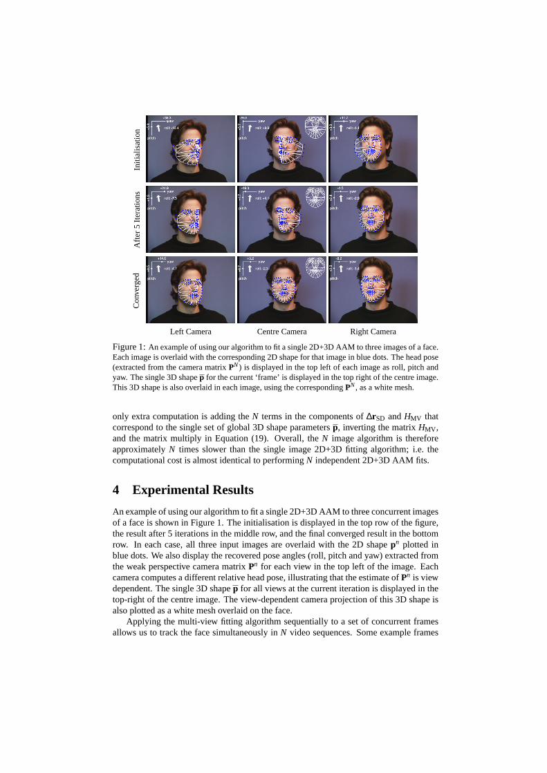
Figure 1:An example of using our algorithm to fit a single 2D+3D AAM to three images of a face.Each image is overlaid with the corresponding 2D shape for that image in blue dots. The head pose(extracted from the camera matrixPN) is displayed in the top left of each image as roll, pitch andyaw. The single 3D shapep for the current ‘frame’ is displayed in the top right of the centre image.This 3D shape is also overlaid in each image, using the correspondingPN, as a white mesh.

only extra computation is adding theN terms in the components of∆rSD andHMV thatcorrespond to the single set of global 3D shape parametersp, inverting the matrixHMV ,and the matrix multiply in Equation (19). Overall, theN image algorithm is thereforeapproximatelyN times slower than the single image 2D+3D fitting algorithm; i.e. thecomputational cost is almost identical to performingN independent 2D+3D AAM fits.

4 Experimental Results

An example of using our algorithm to fit a single 2D+3D AAM to three concurrent imagesof a face is shown in Figure 1. The initialisation is displayed in the top row of the figure,the result after 5 iterations in the middle row, and the final converged result in the bottomrow. In each case, all three input images are overlaid with the 2D shapepn plotted inblue dots. We also display the recovered pose angles (roll, pitch and yaw) extracted fromthe weak perspective camera matrixPn for each view in the top left of the image. Eachcamera computes a different relative head pose, illustrating that the estimate ofPn is viewdependent. The single 3D shapep for all views at the current iteration is displayed in thetop-right of the centre image. The view-dependent camera projection of this 3D shape isalso plotted as a white mesh overlaid on the face.

Applying the multi-view fitting algorithm sequentially to a set of concurrent framesallows us to track the face simultaneously inN video sequences. Some example frames

Fra

me

1F

ram

e12

0F

ram

e20

0

Left Camera Centre Camera Right Camera

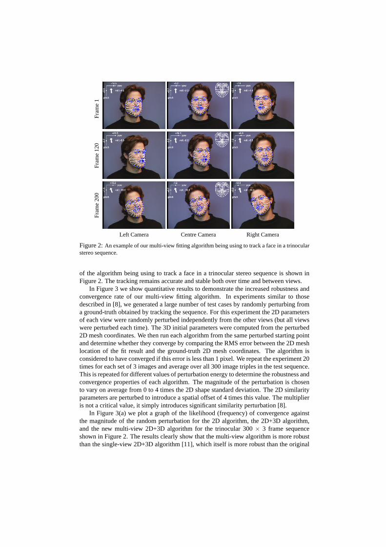
Figure 2:An example of our multi-view fitting algorithm being using to track a face in a trinocularstereo sequence.

of the algorithm being using to track a face in a trinocular stereo sequence is shown inFigure 2. The tracking remains accurate and stable both over time and between views.

In Figure 3 we show quantitative results to demonstrate the increased robustness andconvergence rate of our multi-view fitting algorithm. In experiments similar to thosedescribed in [8], we generated a large number of test cases by randomly perturbing froma ground-truth obtained by tracking the sequence. For this experiment the 2D parametersof each view were randomly perturbed independently from the other views (but all viewswere perturbed each time). The 3D initial parameters were computed from the perturbed2D mesh coordinates. We then run each algorithm from the same perturbed starting pointand determine whether they converge by comparing the RMS error between the 2D meshlocation of the fit result and the ground-truth 2D mesh coordinates. The algorithm isconsidered to have converged if this error is less than 1 pixel. We repeat the experiment 20times for each set of 3 images and average over all 300 image triples in the test sequence.This is repeated for different values of perturbation energy to determine the robustness andconvergence properties of each algorithm. The magnitude of the perturbation is chosento vary on average from 0 to 4 times the 2D shape standard deviation. The 2D similarityparameters are perturbed to introduce a spatial offset of 4 times this value. The multiplieris not a critical value, it simply introduces significant similarity perturbation [8].

In Figure 3(a) we plot a graph of the likelihood (frequency) of convergence againstthe magnitude of the random perturbation for the 2D algorithm, the 2D+3D algorithm,and the new multi-view 2D+3D algorithm for the trinocular 300× 3 frame sequenceshown in Figure 2. The results clearly show that the multi-view algorithm is more robustthan the single-view 2D+3D algorithm [11], which itself is more robust than the original

0 0.4 0.8 1.2 1.6 2 2.4 2.8 3.2 3.6 40

10

20

30

40

50

60

70

80

90

100P

erce

ntag

e of

tria

ls c

onve

rged

Average shape eigenvector sigma + 4.0 × point location sigma

2D2D+3D2D+3D MV

0 2 4 6 8 10 12 14 16 18 200

2

4

6

8

10

12

Iteration

RM

S p

oint

loca

tion

erro

r

2D2D+3D2D+3D MV

(a) Frequency of Convergence (b) Rate of Convergence

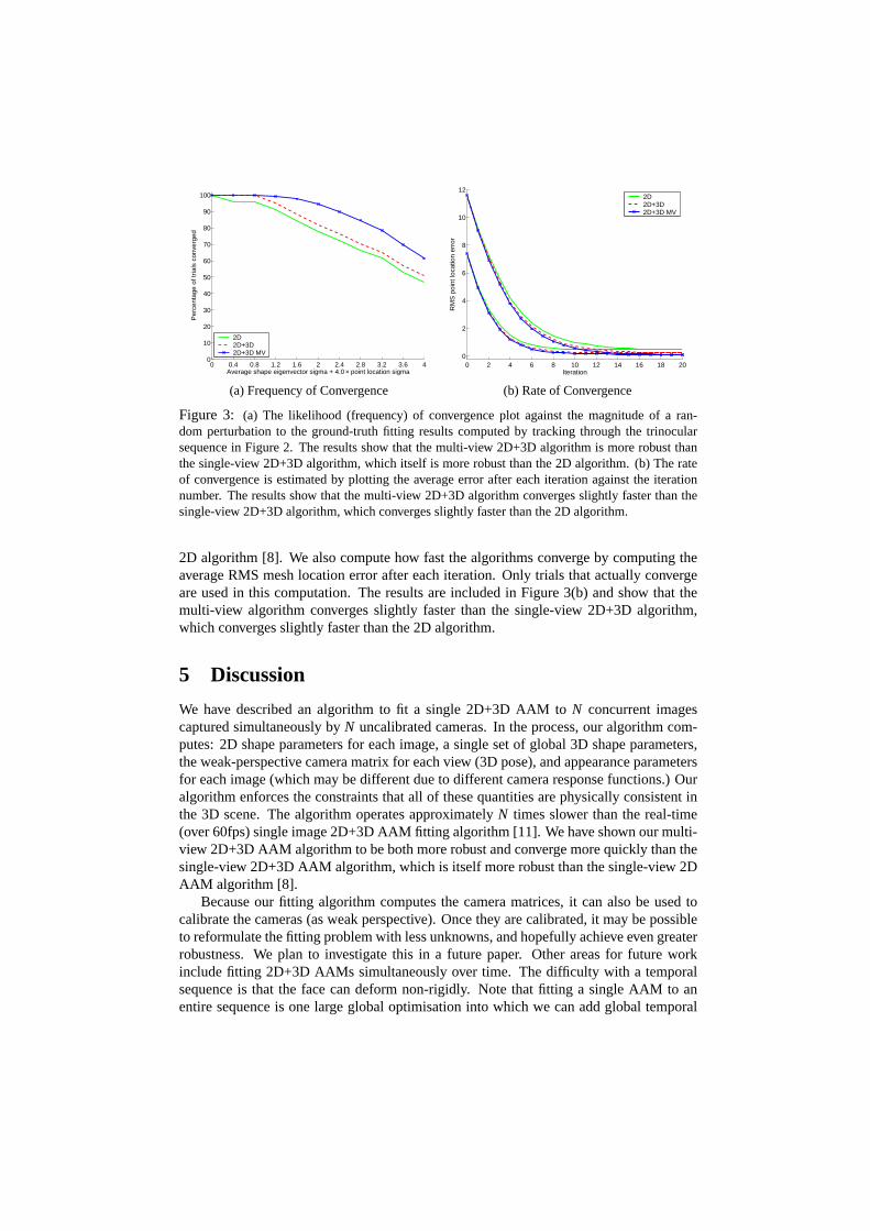
Figure 3: (a) The likelihood (frequency) of convergence plot against the magnitude of a ran-dom perturbation to the ground-truth fitting results computed by tracking through the trinocularsequence in Figure 2. The results show that the multi-view 2D+3D algorithm is more robust thanthe single-view 2D+3D algorithm, which itself is more robust than the 2D algorithm. (b) The rateof convergence is estimated by plotting the average error after each iteration against the iterationnumber. The results show that the multi-view 2D+3D algorithm converges slightly faster than thesingle-view 2D+3D algorithm, which converges slightly faster than the 2D algorithm.

2D algorithm [8]. We also compute how fast the algorithms converge by computing theaverage RMS mesh location error after each iteration. Only trials that actually convergeare used in this computation. The results are included in Figure 3(b) and show that themulti-view algorithm converges slightly faster than the single-view 2D+3D algorithm,which converges slightly faster than the 2D algorithm.

5 Discussion

We have described an algorithm to fit a single 2D+3D AAM toN concurrent imagescaptured simultaneously byN uncalibrated cameras. In the process, our algorithm com-putes: 2D shape parameters for each image, a single set of global 3D shape parameters,the weak-perspective camera matrix for each view (3D pose), and appearance parametersfor each image (which may be different due to different camera response functions.) Ouralgorithm enforces the constraints that all of these quantities are physically consistent inthe 3D scene. The algorithm operates approximatelyN times slower than the real-time(over 60fps) single image 2D+3D AAM fitting algorithm [11]. We have shown our multi-view 2D+3D AAM algorithm to be both more robust and converge more quickly than thesingle-view 2D+3D AAM algorithm, which is itself more robust than the single-view 2DAAM algorithm [8].

Because our fitting algorithm computes the camera matrices, it can also be used tocalibrate the cameras (as weak perspective). Once they are calibrated, it may be possibleto reformulate the fitting problem with less unknowns, and hopefully achieve even greaterrobustness. We plan to investigate this in a future paper. Other areas for future workinclude fitting 2D+3D AAMs simultaneously over time. The difficulty with a temporalsequence is that the face can deform non-rigidly. Note that fitting a single AAM to anentire sequence is one large global optimisation into which we can add global temporal

smoothness constraints which may improve fitting performance, whereas tracking a headthrough a video is a sequence of independent optimisations that may yield inconsistentresults at each frame. The best way to do this is an interesting research question.

Acknowledgments

The research described in this paper was supported by U.S. DoD contract N41756-03-C4024, NIMH grant R01 MH51435, and DENSO Corporation.

References

[1] S. Baker and I. Matthews. Lucas-Kanade 20 years on: A unifying framework.In-ternational Journal of Computer Vision, 56(3):221 – 255, 2004.

[2] V. Blanz and T. Vetter. A morphable model for the synthesis of 3D faces. InCom-puter Graphics, Annual Conference Series, pages 187–194, 1999.

[3] T. Cootes, G. Edwards, and C. Taylor. Active appearance models.IEEE Trans. onPattern Analysis and Machine Intelligence, 23(6):681–685, 2001.

[4] T. Cootes, G. Wheeler, K. Walker, and C. Taylor. Coupled-view active appearancemodels. InProceedings of the British Machine Vision Conference, volume 1, pages52–61, 2000.

[5] R. Gross, I. Matthews, and S. Baker. Appearance-based face recognition and light-fields. IEEE Transactions on Pattern Analysis and Machine Intelligence, 26(4):449– 465, 2004.

[6] G. Hager and P. Belhumeur. Efficient region tracking with parametric models ofgeometry and illumination.IEEE Transactions on Pattern Analysis and MachineIntelligence, 20:1025–1039, 1998.

[7] A. Lanitis, C. J. Taylor, and T. F. Cootes. Automatic interpretation and coding of faceimages using flexible models.IEEE Transactions on Pattern Analysis and MachineIntelligence, 19(7):742–756, 1997.

[8] I. Matthews and S. Baker. Active Appearance Models revisited.International Jour-nal of Computer Vision, 60(2):135–164, 2004. In Press. Also appeared as CarnegieMellon University Robotics Institute Technical Report CMU-RI-TR-03-02.

[9] I. Matthews, T. Cootes, J. Bangham, S. Cox, and R. Harvey. Extraction of visualfeatures for lipreading.IEEE Transactions on Pattern Analysis and Machine Intel-ligence, 24(2):198–213, 2002.

[10] S. Romdhani and T. Vetter. Efficient, robust and accurate fitting of a 3D morphablemodel. InProceedings of the IEEE International Conference on Computer Vision,pages 59–66, 2003.

[11] J. Xiao, S. Baker, I. Matthews, and T. Kanade. Real-time combined 2D+3D activeappearance models. InProceedings of the IEEE Conference on Computer Visionand Pattern Recognition, volume II, pages 535–542, 2004.