Fiscal Devaluations - Princeton Universityitskhoki/FiscalDevaluations.pdf · Fiscal Devaluations Emmanuel Farhi HarvardUniversity ... Veronica Rappoport, Ricardo Reis, Richard Rogerson,

Fiscal Devaluations∗

Emmanuel FarhiHarvard University

Gita GopinathHarvard University

Oleg ItskhokiPrinceton University

First Draft: June 3, 2011This Draft: April 6, 2013

Abstract

We show that even when the exchange rate cannot be devalued, a small set of con-ventional fiscal instruments can robustly replicate the real allocations attained under anominal exchange rate devaluation in a dynamic New Keynesian open economy envi-ronment. We perform the analysis under alternative pricing assumptions—producer orlocal currency pricing, along with nominal wage stickiness; under arbitrary degrees ofasset market completeness and for general stochastic sequences of devaluations. Thereare two types of fiscal policies equivalent to an exchange rate devaluation—one, a uni-form increase in import tariff and export subsidy, and two, a value-added tax increaseand a uniform payroll tax reduction. When the devaluations are anticipated, thesepolicies need to be supplemented with a consumption tax reduction and an income taxincrease. These policies are revenue neutral. In certain cases equivalence requires, inaddition, a partial default on foreign bond holders. We discuss the issues of implemen-tation of these policies, in particular, under the circumstances of a currency union.

∗We thank Andrew Abel, Philippe Aghion, Alberto Alesina, Pol Antràs, Mark Aguiar, Gianluca Benigno,Raj Chetty, Arnaud Costinot, Michael Devereux, Charles Engel, Francesco Franco, Xavier Gabaix, EtienneGagnon, Fabio Ghironi, Elhanan Helpman, Olivier Jeanne, Urban Jermann, Mike Golosov, João Gomes,Gene Grossman, John Leahy, Elias Papaioannou, Veronica Rappoport, Ricardo Reis, Richard Rogerson,Martín Uribe, Adrien Verdelhan, Michael Woodford and seminar/conference participants at NES-HSE, ECB,Frankfurt, Princeton, Federal Reserve Board, Columbia, NBER IFM, Wharton, NYU, Harvard, MIT, NYFed, LSE for their comments, and Eduard Talamas for excellent research assistance.

Published in the Review of Economic Studies, April 2014, 81(2): 725-760http://dx.doi.org/10.1093/restud/rdt036

1 Introduction

Exchange rate devaluations have long been proposed as a desirable policy response to macroe-

conomic shocks that impair a country’s competitiveness in the presence of price and wage

rigidities. Milton Friedman famously argued for flexible exchange rates on these grounds.

Yet countries that wish to or have to maintain a fixed exchange rate cannot resort to ex-

change rate devaluations. In this paper we show how a country can use unilateral fiscal policy

to generate the same real outcomes as those following a nominal exchange rate devaluation,

while keeping the nominal exchange rate fixed.

This question about fiscal devaluations dates back to the period of the gold standard when

countries could not devalue their currencies. At that time, Keynes (1931) had proposed that

a uniform ad valorem tariff on all imports plus a uniform subsidy on all exports would have

the same impact as an exchange rate devaluation. Recently, it has also been conjectured

that a similar outcome could be achieved by increasing value-added taxes and cutting payroll

taxes (e.g., social security contributions).

The current crisis in the Euro area has brought fiscal devaluations to the forefront of

policy. The Euro has been blamed for the inability of countries like Greece, Portugal, Spain,

Italy and even France to devalue their exchange rates and restore their competitiveness in

international markets.1 Faced with the dramatic alternatives of austerity-ridden internal

devaluation and exit from the Euro, countries in the Eurozone are considering the option

of fiscal devaluations. Indeed, in 2012, France has implemented a fiscal devaluation. Pre-

vious examples include Denmark in 1988, Sweden in 1993, and Germany in 2006. Fiscal

devaluations have clearly become a serious policy option.

Despite discussions in policy circles, there is little formal analysis of fiscal devaluations.2

This is an area where the policy debate is ahead of academic knowledge. This paper is

intended to bridge this gap, by providing the first formal analysis of fiscal devaluations in

a stochastic dynamic general equilibrium New Keynesian open economy environment.3 In1For popular policy writings on the topic see, for example, Feldstein in the Financial

Times in February 2010 (http://www.nber.org/feldstein/ft02172010.html), Krugman in theNew York Times in May 2010 (http://krugman.blogs.nytimes.com/2010/05/01/why-devalue/),Roubini in the Financial Times in June 2011 (http://www.economonitor.com/nouriel/2011/06/13/the-eurozone-heads-for-break-up/).

2For policy discussions, see for example Farhi and Werning (http://web.mit.edu/iwerning/Public/VAT.pdf); Cavallo and Cottani on VoxEU (http://www.voxeu.org/index.php?q=node/4666); IMF PressRelease on Portugal (http://www.imf.org/external/np/sec/pr/2011/pr11160.htm) and IMF’s Septem-ber 2011 Fiscal Monitor (http://www.imf.org/external/pubs/ft/fm/2011/02/fmindex.htm).

3We adopt the New Keynesian framework with nominal rigidities as it provides the most natural labora-tory for studying the real consequences of a nominal devaluation, however, our equivalence results betweennominal and fiscal devaluations generalize beyond the models with nominal frictions.

1

doing so, we learn under what circumstances the tariff-cum-subsidy and VAT-cum-payroll

fiscal interventions suffice to attain equivalence and when they need to be supplemented with

additional policy adjustments.

We define a fiscal devaluation of size δt at date t to be a set of unilateral fiscal polices that

implements the same real allocation as under a nominal exchange rate devaluation of size δt,

but holding the nominal exchange rate fixed. We explore a general path of δt, including both

expected and unexpected devaluations. Since the nature of price rigidity—whether prices

are set in the currency of the producers or in local currency—is central for the real effects of

nominal devaluations (see, for example, Lane, 2001; Corsetti, 2008), we allow for both the

cases of producer (PCP) and local currency pricing (LCP) and for nominal wage rigidity.4

Additionally, we allow for a wide range of alternative international asset market structures,

including complete markets, and various degrees of incompleteness such as international

trade in risk-free nominal bonds only or international trade in equities.

We find that, first, despite the fact that the actual allocations induced by devaluations in

New Keynesian environments are sensitive to the details of the environment, there exists a

small set of fiscal instruments that can robustly replicate the effects—both on real variables

and nominal prices—of nominal exchange rate devaluations across all specifications. The

exact details of which instruments need to be used depend on the extent of completeness of

asset markets, the currency denomination of bonds and the expected or unexpected nature

of devaluations. Second, the required adjustment in taxes is only a function of δt, the

size of the required devaluation, and is independent of all details of the environment, such

as for example the degree of wage and price stickiness, and the type of pricing (local or

producer currency). Third, when all proposed tax instruments are used a fiscal devaluation

is government revenue neutral. Otherwise, we show that these policies generate additional

government revenue in periods of trade deficits.

We study both types of fiscal devaluations—a uniform increase in import tariffs and

export subsidies and a uniform increase in value-added taxes and reduction in payroll taxes.

The dynamic analysis reveals that both of these policies, in general, need to be accompanied

by a uniform reduction in consumption taxes and an increase in income taxes.5 However,

under some circumstances, changes in consumption and income taxes can be dispensed

with. Whether this latter option is possible depends on the extent of completeness of asset4PCP refers to the case when prices are sticky in the currency of the producer (exporter), while LCP is

the case when prices are sticky in the currency of the consumer (importer) of the good.5A consumption tax is equivalent to a sales tax that is applied only to final goods, and not to intermediate

goods. In our setup all goods are final, and hence consumption and sales taxes are always equivalent. Further,under the tariff-based policy, an increase in income tax should extend to both wage income and dividendincome, while under the VAT-based policy, the dividend-income tax should be left unchanged.

2

markets and whether the exchange rate movements that are being mimicked are anticipated

or unanticipated.

To provide intuition for the underlying mechanisms, consider the case of producer cur-

rency pricing (PCP). One of the channels through which a nominal devaluation raises relative

output at home is through a depreciation of home’s terms of trade that makes home goods

cheaper relative to foreign goods. This movement in the terms of trade can be mimicked

either through a combination of import tariff and export subsidy or through an increase in

the value-added tax (which is reimbursed to exporters and levied on importers). Addition-

ally, to ensure that prices at home are the same as under a nominal devaluation, an increase

in the value-added tax needs to be offset with a reduction in the payroll tax. The relative

prices of all goods then respond identically under a fiscal and nominal devaluation.

When is a reduction in consumption taxes and an increase in income taxes required?

Without a reduction in consumption taxes, fiscal devaluations result in an appreciated real

exchange rate relative to a nominal devaluation. This is because fiscal devaluations, despite

having the same effect on the terms of trade, lead to an increase in the relative price of the

home consumption bundle—an effect absent under nominal devaluation. This difference is

of no consequence for the real allocation when trade is balanced or when the devaluation is

unexpected and asset markets are incomplete, as neither risk-sharing nor saving decisions

are affected under these circumstances. As a result, precisely in these two cases, we can

dispense with the adjustment in consumption taxes.

By contrast, with expected devaluations, in the absence of an adjustment in consumption

taxes, the different behavior of the real exchange rate under nominal and fiscal devaluations

induces different savings and portfolio decisions. These effects then need to be undone with a

reduction in consumption taxes. This allows to fully mimic the behavior of the real exchange

rate under a nominal devaluation. When the consumption tax is used, an offsetting increase

in income taxes is required so as not to distort the labor supply decision of households.

In the case of incomplete markets we highlight the role of the currency denomination of

debt. When bonds are denominated in the foreign currency or in the case of equities, no

additional instruments are required for a fiscal devaluation. By contrast when international

bonds are denominated in the home currency, the proposed set of tax instruments does not

suffice. Equivalence then requires a partial default by the home country. Specifically, a

nominal devaluation depletes the foreign-currency value of home’s external debt if it was

denominated in home currency. The proposed limited set of fiscal instruments cannot repli-

cate this effect on home’s foreign obligations. This is why a fiscal devaluation under these

circumstances must be accompanied by a partial default on home-currency debt of the home

3

country.

Importantly, when all four taxes (e.g., VAT, payroll, consumption and income taxes)

are used, the policy is revenue-neutral for the government. That is the direct effects of tax

changes on the fiscal deficit add up to zero as the revenue earned from the VAT and income

tax increases exactly offset the revenue declines that follow the payroll and consumption tax

cuts. The indirect effects on revenue that arise from the stimulative effects of a fiscal deval-

uation on output, however, remain exactly as in the case of an exchange rate devaluation.

When only a reduced set of tax instruments is used, such as VAT and payroll tax only, a

fiscal devaluation generates positive fiscal revenues in states when the country runs a trade

deficit.

We consider a series of extensions that are important for implementation. We first

examine the implementation of fiscal devaluations by individual countries in a currency

union in a multi-country environment. We show that equivalence is retained for effects on

countries both within and outside the union across nominal and fiscal devaluations. We also

show that when the devaluing country is small relative to the overall size of the currency

union and/or where seigniorage income constitutes a negligible share of a country’s GDP, a

country within a currency union can engineer a fiscal devaluation unilaterally without any

coordination with the union central bank.

We then discuss fiscal devaluations in an economy with capital. When production capital

is a variable input the VAT-based fiscal devaluation requires a reduction in capital taxes to

firms. Without it firms would have an incentive to substitute labor for capital, an effect

absent under a nominal devaluation.

We also investigate the consequence of non-symmetric short-run pass-through of VAT

and payroll taxes into prices. Under these circumstances a fiscal devaluation requires a non-

uniform adjustment in the taxes. Specifically, if the short-run pass-through of VAT is larger

than that of a payroll tax, then a one-time devaluation can be replicated with the same

increase in VAT as in the benchmark model, but with a larger reduction in the payroll tax,

with the difference gradually phased out as prices adjust over time.

Finally, we provide a numerical illustration of fiscal devaluations and compare across

various cases of complete and incomplete fiscal devaluations. We calibrate the example

to the recent experience of Spain. We allow for capital and adjustment costs in capital

accumulation and realistic taxes in an environment with wage rigidity. The 2008 crisis

is modeled as the outcome of a borrowing cost shock that generates a decline in output,

consumption and investment similar to those observed in Spain. We show that a nominal

devaluation of 10% eliminates the output decline and essentially replicates the flexible wage

4

allocation. We then compare welfare changes across various cases of complete and incomplete

fiscal devaluation. Specifically, we consider the case when only a VAT-payroll tax swap is

used with no change in capital taxes, the case of an anticipated fiscal devaluation, the case

of smaller fiscal devaluation, and the case when seignorage revenues are set to zero. We show

that the welfare gains from even an incomplete fiscal devaluation are significant.

The outline of the paper is as follows. Section 2 outlines the model. Section 3 presents the

main equivalence results. Section 4 analyzes several extensions, such as implementation in

the currency union, capital inputs, and asymmetric pass-through of taxes. Section 5 provides

a numerical illustration of the equilibrium dynamics under nominal and fiscal devaluations

against that under fixed exchange rates and passive fiscal policy. Section 6 concludes.

Related literature Our paper contributes to a long literature, both positive and nor-

mative, that analyzes how to replicate the effects of exchange rate devaluations with fiscal

instruments. The tariff-cum-export subsidy and the VAT increase-cum-payroll tax reduction

are intuitive fiscal policies to replicate the effects of a nominal devaluations on international

relative prices, and accordingly have been discussed before in the policy and academic liter-

ature. Poterba, Rotemberg, and Summers (1986) emphasize the fact that tax changes that

would otherwise be neutral if prices and wages were flexible have short-run macroeconomic

effects when prices or wages are sticky. Most recently, Staiger and Sykes (2010) explore

the equivalence using import tariffs and export subsidies in a partial equilibrium static en-

vironment with sticky or flexible prices, and under balanced trade. While the equivalence

between a uniform tariff-cum-subsidy and a devaluation has a long tradition in the literature

(as surveyed in Staiger and Sykes, 2010), most of the earlier analysis was conducted in static

endowment economies (or with fixed labor supply). Berglas (1974) provides an equivalence

argument for nominal devaluations, using VAT and tariff-based policies, in a reduced-form

model without micro-foundations, no labor supply and without specifying the nature of asset

markets.6

Our departure from this literature is to perform a dynamic general equilibrium analysis

with varying degrees of price rigidity, alternative asset market assumptions and for expected

and unexpected devaluations. In contrast to the earlier literature, we allow for dynamic price

setting as in the New Keynesian literature, endogenous labor supply, savings and portfolio

choice decisions, as well as interest-elastic money demand. In doing so, we learn that the

tariff-cum-subsidy and VAT-cum-payroll fiscal interventions do not generally suffice to attain6The VAT policy with border adjustment has been the focus of Grossman (1980) and Feldstein and

Krugman (1990), however, in an environment with flexible exchange rates and prices. Calmfors (1998)provides a policy discussion of the potential role of VAT and payroll taxes in impacting allocations in acurrency union.

5

equivalence. In addition we find that only a small number of additional instruments are

required to robustly implement fiscal devaluation under the fairly rich set of specifications

we explore.

This paper is complementary to Adao, Correia, and Teles (2009) who show that the

allocation in the flexible price, flexible exchange rate economy can be implemented with

fiscal and monetary policies that induce stable producer prices and constant exchange rates.7

This general implementation principle however does not help answer the question of whether

there is a robust and small set of conventional fiscal instruments that can replicate the effect

of a nominal devaluation which is the focus of our paper.

We perform the analysis in a more general environment, with different types of price

and wage stickiness, under a rich array of asset market structures and for expected and

unanticipated devaluations. Importantly, in Adao, Correia, and Teles (2009) since optimal

policy is sensitive to the details of the environment the fiscal instruments used will vary

across environments and in general will require flexibly time-varying and firm-varying taxes,

in contrast to the main result in our paper. In addition, their implementation requires taxes

both at Home and in Foreign. By contrast, ours requires only adjusting taxes at Home.

This is an important advantage because it can be implemented unilaterally. Moreover, their

implementation relies on income taxes and differential consumption taxes for local versus

imported goods. These taxes are less conventional than payroll and value-added taxes—tax

instruments that have been proposed as potential candidates in policy circles (e.g., see IMF,

2011).

The paper is also related to Schmitt-Grohé and Uribe (2011), who show that in their

environment with downward wage rigidity and inelastic labor supply, the effects of a nominal

devaluation can be replicated with a payroll subside alone. Our paper complements their

analysis by considering a more general environment and showing that in general, a payroll

subsidy alone does not suffice to replicate the effects of a nominal devaluation.

This paper is also related to Lipińska and von Thadden (2009) and Franco (2011) who

quantitatively evaluate the effects of a tax swap from direct (payroll) taxes to indirect taxes

(VAT) under a fixed exchange rate.8 Neither of these studies however explores exact equiva-

lence with a nominal devaluation, as we do in this paper. Lastly, this paper is similar in spirit

to Correia, Farhi, Nicolini, and Teles (2011) who, building on the general implementation

results of Correia, Nicolini, and Teles (2008), use fiscal instruments to replicate the effects of

the optimal monetary policy when the zero-lower bound on nominal interest rate is binding.7Eggertsson (2004) makes a similar observation in a simplified log-linearized model.8Other quantitative analysis includes Boscam, Diaz, Domenech, Ferri, Perez, and Puch (2011) for Spain.

6

2 ModelThe model economy features two countries, home H and foreign F . There are three types

of agents in each economy: consumers, producers and the government, and we describe each

in turn. We then discuss which assumptions of our setup can be further relaxed.

2.1 Consumers

The home country is populated with a continuum of symmetric households. Households are

indexed by h ∈ [0, 1], but we often omit the index h to simplify exposition. In each period,

each household h chooses consumption Ct, money Mt and holdings of assets Bjt+1j∈Jt ,

where Jt is the set of assets Jt available to the households. Each household also sets a wage

rate Wt(h) and supplies labor Nt(h) in order to satisfy demand at this wage rate.

The household h maximizes expected lifetime utility, E0

∑∞t=0 β

tU(Ct, Nt,mt), subject to

the flow budget constraint:PtCt

1 + ςct+Mt +

∑j∈Jt

QjtB

jt+1 ≤

∑j∈Jt−1

(Qjt +Dj

t )Bjt +Mt−1 +

WtNt

1 + τnt+

Πt

1 + τ dt+ Tt,

where Pt is the consumer price index before consumption subsidy ςct and mt = Mt(1 + ςct )/Pt

denotes real money balances. Πt is aggregate profits of the home firms assumed (without loss

of generality) to be held by the representative domestic consumer; τnt is the labor-income tax,

τ dt is the profit (dividend-income) tax, and Tt is the lump-sum transfer from the government.

An asset j is characterized by its price Qjt and effective payout Dj

t reflecting possible defaults

and haircuts on the asset.

For convenience of exposition we adopt the following standard utility specification:

U (Ct, Nt,mt) =1

1− σC1−σt − κ

1 + ϕN1+ϕt +

χ

1− νm1−νt .

Consumption Ct is an aggregator of home and foreign goods:

Ct =

[γ

1ζ

HC1−ζζ

Ht + γ1ζ

FC1−ζζ

Ft

] ζζ−1

, ζ ≥ 0,

that allows for a home bias, γH = 1 − γF ∈ [1/2, 1]. The consumption of both home and

foreign goods is given by CES aggregators of individual varieties i ∈ [0, 1] with elasticity of

substitution ρ > 1: Ckt =[´ 1

0Ckt(i)

(ρ−1)/ρdi]ρ/(ρ−1)

for k ∈ H,F.

We now discuss some of the relevant equilibrium conditions associated with consumers’

optimal decisions. Given the CES structure of consumption aggregators, consumer good

demand is characterized by:

Ckt(i) =

(Pkt(i)

Pkt

)−ρCkt, Ckt = γk

(PktPt

)−ρCt, (1)

7

where i is the variety of the home or foreign good (k ∈ H,F). Pkt(i), Pkt and Pt are

respectively the price of variety i of good k, the price index for good k and the overall

consumer price index. As is well known, CES price indexes are defined by

Pt =[γHP

1−ζHt + γFP

1−ζF t

] 11−ζ and Pkt =

[´ 1

0Pkt(i)

1−ρdi] 1

1−ρ, k ∈ H,F, (2)

and the aggregate consumer expenditure is given by PtCt = PHtCHt +PFtCFt with PktCkt =´ 1

0Pkt(i)Ckt(i)di.

It is useful to define the nominal stochastic discount factor of a household:

Θt,s ≡ βs−t(Ct+sCt

)−σPtPt+s

1 + ςct+s1 + ςct

, s ≥ t, (3)

and we use Θt+1 ≡ Θt,t+1 for brevity. This discount factor prices available assets:

Qjt = Et

Θt+1

(Qjt+1 +Dj

t+1

), ∀j ∈ Jt. (4)

Finally, money demand is given by

χCσt

(Mt

Pt/(1 + ςct )

)−ν= 1− EtΘt+1, (5)

where the right-hand side is an increasing function of the nominal risk-free interest rate

which satisfies 1 + it+1 = 1/EtΘt+1.

Foreign households We assume that foreign households face a symmetric problem with

the exception that the foreign government imposes no taxes or subsidies and foreign con-

sumers have a home bias towards foreign-produced goods. We denote foreign variables with

an asterisk. For brevity we omit listing all equilibrium conditions for foreign given the sym-

metry with home. Define J∗t to be the set of assets available to foreign households and

Ωt ⊂ Jt ∩ J∗t to be the set of assets traded internationally by both domestic and foreign

households. The equilibrium in the world asset market requires Bjt + B∗jt = 0 for all j ∈ Ωt

since we assume all assets are in zero net supply.

The foreign-currency nominal stochastic discount factor is given by

Θ∗t,s = βs−t(C∗sC∗t

)−σP ∗tP ∗s

(6)

Since the Euler equations (4) for assets j ∈ Ωt are satisfied for both countries, we can write

international risk sharing conditions as:

Et

Qjt+1 +Dj

t+1

Qjt

[Θt+1 −Θ∗t+1

EtEt+1

]= 0 ∀j ∈ Ωt, (7)

8

where Et is the nominal exchange rate, and the foreign currency depreciation rate (Et/Et+1)

converts the home-currency asset returns into foreign-currency returns. The risk sharing

condition (7) states that domestic and foreign stochastic discount factors agree in pricing

the internationally-traded assets. It also implicitly assumes that any default or haircut is

uniform for domestic and foreign holders of the assets, and that the adopted fiscal policies

do not act as capital controls.

2.2 Producers

In each country there is a continuum i ∈ [0, 1] of firms producing different varieties of goods

using a technology with labor as the only input. Specifically, firm i produces according to

Yt(i) = AtZt(i)Nt(i)α, 0 < α ≤ 1, (8)

where At is the aggregate country-wide level of productivity, Zt(i) is idiosyncratic firm

productivity shock, and Nt(i) is the firm’s labor input. Productivity At, Zt(i) and their

foreign counterparts follow arbitrary stochastic processes over time.

The firm sells to both the home and foreign market. Specifically, it must satisfy de-

mand (1) for its good in each market given its price PHt(i) at home and P ∗Ht(i) abroad in

the foreign currency. Therefore, we can write the market clearing for variety i as:9

Yt(i) = CHt(i) + C∗Ht(i), (9)

where C∗Ht(i) is foreign-market demand for variety i of the home good. The profit of firm i

is given by

Πit = (1− τ vt )PHt(i)CHt(i) + (1 + ςxt )EtP ∗Ht(i)C∗Ht(i)− (1− ςpt )WtNt(i), (10)

where τ vt is the value-added tax (VAT), ςxt is the export subsidy and ςpt is the payroll subsidy.

Note that this equation makes it explicit that exports are not subject to the VAT, or more

specifically VAT is rebated back to the firms upon exporting.10 We define the prices to be

inclusive of the VAT, export subsidy and import tariff, but exclusive of the consumption

subsidy ςct . Aggregate profits of the home firms are given by Πt ≡´ 1

0Πitdi and aggregate

labor demand is Nt =´ 1

0Nt(i)di.

9Note that overall demand for good i results from aggregation of demands across all consumers h ∈ [0, 1]

in the home and foreign markets respectively, e.g. CHt(i) =´ 1

0CHt(i;h)dh.

10The profit of the foreign firm is Πi∗t = P ∗Ft(i)C

∗Ft(i)+

1−τvt(1+τmt )EtPFt(i)C

∗Ft(i)−W ∗t N∗t (i) in foreign currency,

and its exports are subject to both the VAT and the import tariff τmt paid at the border.

9

2.3 Price and wage setting

Firms set prices subject to a Calvo friction: in any given period, a firm can adjust its prices

with probability 1 − θp, and maintains its previous-period price otherwise. The firm sets

prices to maximize the expected net present value of profits conditional on no price change,∑∞s=t θ

s−tp Et

Θt,sΠ

is/(1 + τ ds )

, subject to the production technology and demand equations

given above, and where τ ds is the dividend-income (or profit) tax payed by stock holders.

We now need to make an assumption regarding the currency of price-setting. We assume

that domestic prices are always set in the currency of the consumer and inclusive of the VAT

tax. We denote the domestic period t reset price of firm i by PHt(i), so that firm’s i current

price is given by

PHt(i) =

PH,t−1(i), w/prob θp,

PHt(i), w/prob 1− θp.(11)

The foreign price can be set either in the producer currency, often referred to as producer

currency pricing (PCP), or in the local currency, referred to as local currency pricing (LCP).

Producer currency pricing Consistent with the standard definition of PCP we assume

that the firm chooses the home-currency reset price PHt, while the foreign-market price

satisfies the law of one price:

P ∗Ht(i) = PHt(i)1

Et1− τ vt1 + ςxt

, (12)

where Et is the nominal exchange rate defined as the price of one unit of foreign currency

in terms of units of home currency, hence higher values of Et correspond to home currency

depreciation. In words, the firm sets a common price PHt(i) for both markets, and its

foreign-market price equals this price converted into foreign currency and adjusted for border

taxes—the export subsidy and the VAT reimbursement. The reset price satisfies the following

condition (see Appendix A.1):

Et∞∑s=t

θs−tp Θt,sP ρHs(CHs + C∗Hs)

1 + τ ds

[(1− τ vs )PHt(i)−

ρ

ρ− 1

(1− ςps )Ws

αAsZs(i)Ns(i)α−1

]= 0. (13)

This implies that the preset price PHt(i) is a constant markup over the weighted-average

expected future marginal costs during the period for which the price is in effect. Equations

(11)–(13) together with the definition of the price index in (2), describe the evolution of

home firms’ prices in the home and foreign markets under PCP.

Local currency pricing Under LCP the firm sets both a home-market price PHt(i) in

home currency and a foreign-market price P ∗Ht(i) in foreign currency. During periods of

10

non-adjustment, the foreign-market price remains constant in foreign currency, therefore

movements in the nominal exchange rates and border taxes directly affect the relative price

of the firm in the home and foreign markets. As a result, the law of one price (12) is violated

in general. Profit maximization with respect to PHt(i) and P ∗Ht(i) leads to two optimality

conditions, one for the home-market price and the other for the foreign-market price (see

Appendix A.1):

Et∞∑s=t

θs−tp Θt,sP ρHsCHs

1 + τ ds

[(1− τ vs )PHt(i)−

ρ

ρ− 1

(1− ςps )Ws

αAsZs(i)Ns(i)α−1

]= 0, (14)

Et∞∑s=t

θs−tp Θt,s(P ∗Hs)

ρC∗Hs1 + τ ds

[(1 + ςxs )EsP ∗Ht(i)−

ρ

ρ− 1

(1− ςps )Ws

αAsZs(i)Ns(i)α−1

]= 0, (15)

describing the evolution of prices (combined with (11), now for both markets) under LCP.

Foreign firms As for price setting by foreign firms, the reset prices of each foreign variety

in the foreign market P ∗Ft(i) and in the home market PFt(i) are characterized in a symmetric

manner to that of the home economy, with the exception that all foreign tax rates are kept

at zero. Under PCP, the law of one price holds for all foreign varieties:

PFt(i) = P ∗Ft(i)Et1 + τmt1− τ vt

, (16)

where τmt is home’s import tariff charged at the border together with the home’s VAT τ vt

imposed on the foreign imports. Under LCP, foreign firms set their home-market price in

home currency according to:

Et∞∑s=t

θs−tp Θ∗t,sPρFsCFs

[1− τ vs1 + τms

1

EsPFt(i)−

ρ

ρ− 1

W ∗s

αA∗sZ∗s (i)N∗s (i)α−1

]= 0. (17)

Labor demand and wage setting Tha labor input Nt is a CES aggregator of the in-

dividual varieties supplied by each household, Nt =[´ 1

0Nt(h)(η−1)/ηdh

]η/(η−1)

with η > 1.

Therefore, aggregate demand for each variety of labor is given by

Nt(h) =

(Wt(h)

Wt

)−ηNt, (18)

where Nt is aggregate labor demand in the economy, Wt(h) is the wage rate charged by

household h for its variety of labor services and Wt =[´ 1

0Wt(h)1−ηdh

]1/(1−η)

is the wage

for a unit of aggregate labor input in the home economy. The aggregate wage bill in the

economy is given by WtNt =´ 1

0Wt(h)Nt(h)dh.

Households are subject to a Calvo friction when setting wages: in any given period, they

may adjust their wage with probability 1 − θw, and maintain the previous-period nominal

11

wage otherwise. The optimality condition for wage setting is given by (see Appendix A.1):

Et∞∑s=t

θs−tw Θt,sNsWη(1+ϕ)s

[η

η − 1

1

1 + ςcsκPsC

σsN

ϕs −

1

1 + τns

Wt(h)1+ηϕ

W ηϕs

]= 0. (19)

This implies that the wage Wt(h) is preset as a constant markup over the expected weighted-

average between future marginal rates of substitution between labor and consumption and

aggregate wage rates, during the duration of the wage. This is a standard result in the New

Keynesian literature, as derived, for example, in Galí (2008). Wage setting (19), together

with the wage evolution analogous to (11), characterize equilibrium wage dynamics.

2.4 Government and country budget constraint

We assume that the government must balance its budget each period, returning all seignior-

age and tax revenues in the form of lump-sum transfers to the households (Tt). This is

without loss of generality since Ricardian equivalence holds in this model. The government

budget constraint in period t is

Mt −Mt−1 + TRt = Tt, (20)

where Mt −Mt−1 is seigniorage income from money supply. The tax revenues from distor-

tionary taxes TRt are given by

TRt =

(τnt

1 + τntWtNt +

τ dt1 + τ dt

Πt −ςct

1 + ςctPtCt

)(21)

+(τ vt PHtCHt − ς

ptWtNt

)+

(τ vt + τmt1 + τmt

PFtCFt − ςxt EtP ∗HtC∗Ht),

where the first bracket contains income taxes levied on and the consumption subsidy paid

to home households; the next two terms are the value-added tax paid by and the payroll

subsidy received by home firms; the last two terms are the import tariff and the VAT paid

by foreign exporters and the export subsidies to domestic firms.

Combining this together with the household budget constraint and aggregate profits, we

arrive at the aggregate country budget constraint:∑j∈Ωt

QjtB

jt+1 −

∑j∈Ωt−1

(Qjt +Dj

t )Bjt = EtP ∗HtC∗Ht − PFtCFt

1− τ vt1 + τmt

, (22)

where the right-hand side is the trade surplus of the home country and the left-hand side is

the change in the international asset position of the home country.11

11Formally, Bjt =´ 1

0Bjt (h)dh is the aggregate net foreign asset-j position of home households.

12

This completes the description of the setup of the model. Given initial conditions and

home and foreign government policies—taxes and money supply—the equations above char-

acterize equilibrium price and wage dynamics in the economy. Given prices firms satisfy

product demand in domestic and foreign markets, and given wages households satisfy labor

demand of firms. Asset prices are such that asset markets are in equilibrium given asset de-

mand by home and foreign households, and consumer money demand equals money supply

in both markets.

2.5 Assumptions

Before turning to the results of our analysis, we highlight that several of the assumptions

made in the model setup to ease exposition can be generalized without impacting our results.

These include assumptions on:

Functional forms We assume CES consumption aggregators and monopolistic compe-

tition, but the results hold under more general environments. For instance, our results

generalize to the case of monopolistic competition with non-constant desired markups (e.g.,

as under Kimball, 1995, demand), as well as to the case of oligopolistic competition with

strategic complementarities (e.g., as in Atkeson and Burstein, 2008). Departing from CES

consumption aggregators and monopolistic competition substantially increases the nota-

tional burden, but leaves the analysis largely unchanged. We can also allow for a general

non-separable utility function in consumption and labor without altering conclusions. We

have assumed home bias in preferences, but no non-tradable goods or trade costs, yet our

results immediately extend to these more general economies.12 Similarly, we have adopted a

money-in-the-utility framework where real money balances are separable from consumption

and leisure, but all results are unchanged when money is introduced via a cash-in-advance

constraint.

Government policy instruments We formulate our model using money supply as the

instrument of monetary policy (money supply rule) in both countries. We could alterna-

tively have performed our analysis using interest rate rules or exchange rate rules without

any alterations to our equivalence results.13 As in the New Keynesian literature, in our

environment, the nominal interest rate is the only money market variable relevant for the

rest of the allocation. Consequently, we could also focus on the cashless limit, to which our12Note that non-tradable goods are equivalent in our analysis to domestic goods produced for domestic

market, and require no special treatment in the design of a fiscal devaluation.13See Benigno, Benigno, and Ghironi (2007) for the design of an interest rate rule to maintain a fixed

exchange rate.

13

equivalence results also apply. We further discuss some of these issue in Section 4.1. For

simplicity, we start from a situation where initial taxes are zero and characterize the required

changes in taxes, but all the results generalize to a situation where initial taxes are not zero

(see footnote 22).

Price setting frictions Our results generalize to departures from Calvo price and wage

setting. Any model of time-contingent price adjustment with arbitrary heterogeneity in price

adjustment hazard rates would deliver similar results. It can also be generalized to a menu

cost model in which the menu cost is given in real units, e.g. in labor, as is commonly assumed,

since in this case the decision to adjust prices will depend only on real variables (including

relative prices) which stay unchanged across nominal and fiscal devaluations. Furthermore,

our equivalence results also apply in other environments where devaluations have real effects

without nominal frictions, as for example in the neoclassical model of Feenstra (1985) with

cash-in-advance constraints in home and foreign currency.14 In Section 4.3 we discuss further

extensions to our price-setting assumptions.

3 Fiscal Devaluations

In this section we formally define the concept of a fiscal devaluation and present our main

results on the equivalence between nominal and fiscal devaluations, first for complete and

then for incomplete asset markets, as well as for the special case of a one-time unanticipated

devaluation. We complete the section with the discussion of government revenue neutrality

of fiscal devaluations.

Definition Consider an equilibrium path of the model economy described above, along

which the nominal exchange rate follows

Et = E0(1 + δt) for t ≥ 0,

for some (stochastic) sequence δtt≥0. Here δt denotes the percent nominal devaluation of

the home currency relative to period 0. We refer to such an equilibrium path as a nominal

δt-devaluation. Denote by Mt the path of home money supply that is associated with the

nominal devaluation. A fiscal δt-devaluation is a sequence M ′t , τ

mt , ς

xt , τ

vt , ς

pt , ς

ct , τ

nt , τ

dt t≥0

of money supply and taxes that achieves the same equilibrium allocation of consumption,

output and labor supply, but for which the equilibrium exchange rate is fixed, E ′t ≡ E0 for14In this environment Feenstra (1985) studied how the tariff policy could improve over a nominal

devaluation.

14

all t ≥ 0. Note that, in general, we do not restrict the path of the exchange rate under a

nominal devaluation.15

Before formulating and proving our main results, we manipulate the two equilibrium

conditions which play the central role in our analysis. First, we divide the home country

budget constraint (22) by P ∗t Et to obtain:∑j∈Ωt

qj∗t Bjt+1 −

∑j∈Ωt−1

(qj∗t + dj∗t )Bjt =

P ∗HtP ∗t

[C∗Ht − CFtSt

], (23)

where qj∗t = Qjt/(P

∗t Et) and dj∗t = Dj

t/(P∗t Et) are real prices and payouts of assets in units of

the foreign final good; and

St ≡PFtP ∗Ht

1

Et1− τ vt1 + τmt

(24)

is the home’s terms of trade—the ratio of the import price index to the export price index

adjusted for border taxes. Second, we rewrite the international risk sharing conditions (7)

using the definitions of the home and foreign stochastic discount factors (3) and (6):

Et

qj∗t+1 + dj∗t+1

qj∗t

[(Ct+1

Ct

)−σ Qt+1

Qt−(C∗t+1

C∗t

)−σ]= 0 ∀j ∈ Ωt, (25)

where

Qt ≡P ∗t Et

Pt/(1 + ςct )(26)

is the consumer-price real exchange rate.

These conditions highlight the role of the two international relative prices—the terms

of trade St in shaping the trade balance on the right-hand side of the country budget con-

straint (23) and the real exchange rate Qt in the international risk sharing condition (25).

The exact roles of these two relative prices changes as we consider different asset market

structures. But a fiscal devaluation will, in general, need to mimic the behavior of these two

relative prices to replicate the equilibrium allocation resulting from a nominal devaluation.

3.1 Complete asset markets

In this case we assume that countries have access to a full set of one-period Arrow securities

and there is perfect risk sharing across countries.

15For example, one can examine simple one-time devaluations with δt = 0 for t < T and δt = δ for t ≥ Twith some stochastic or deterministic T ≥ 0.

15

Proposition 1 Under complete international asset markets, and for both producer and local

currency pricing, a fiscal δt-devaluation can be achieved by one of the two policies:

τmt = ςxt = ςct = τnt = τ dt = δt, or (FD′)

τ vt = ςpt =δt

1 + δt, ςct = τnt = δt and τ dt = 0, (FD′′)

as well as a suitable choice of M ′t, for t ≥ 0.

The formal proof, contained in Appendix A.2, demonstrates that both fiscal devaluation

options E ′t, τmt , ςxt , τ vt , ςpt , ς

ct , τ

nt , τ

dt and a nominal devaluation Et,0 satisfy the equilibrium

system under the same allocation of output, consumption and labor supply. This means

that taxes in both the tariff-based (FD′) and VAT-based (FD′′) policies affect the equilibrium

conditions exactly in the same way as changes in the exchange rate, and in particular, cancel

each other out from the equilibrium conditions not directly affected by the exchange rate.

The reason the combinations of taxes in (FD′) and (FD′′) support a fiscal devaluation is

that they ensure that all reset prices and wages remain the same, and given unchanged prices

the rest of the allocation also remains unchanged. Indeed, to leave the wage setting in (19)

unchanged requires the parity between the labor income tax and the consumption subsidy

(τnt = ςct ), a policy change that keeps the labor wedge unaltered. Analogously, domestic

price setting in (13) requires the parity between the VAT and the payroll subsidy (τ vt = ςpt ).

Now consider international price setting, where the VAT or the border taxes need to mimic

the effects of an exchange rate movement on both export and import prices:

1 + ςxt1− τ vt

=1 + τmt1− τ vt

=EtE0

= 1 + δt. (27)

Indeed, tax policies satisfying (27) result in the same international prices under both PCP

(see (12) and (16)) and LCP (see (15) and (17)). The taxes described so far are sufficient to

replicate the path of all nominal prices and wages, as well as the terms of trade in (24), but

not the real exchange rate in (26), which additionally requires the use of the consumption

subsidy, ςct = δt. This summarizes the logic behind the policies in (FD′) and (FD′′).16

Under complete markets, the international risk sharing condition (25) becomes the fa-

miliar Backus-Smith condition: (CtC∗t

)σ= λQt, (28)

which ties the relative consumptions of the two countries to the real exchange rate, and

where the constant λ is recovered from the intertemporal budget constraint of the country,16Under complete markets, the use of the profit tax τdt is merely needed to avoid second-order distortions

in price setting under the tariff-based policy (FD′).

16

which depends on relative prices and in particular the evolution of the terms of trade (see

Appendix A.2). This implies that the consumption allocation also remains unchanged under

(FD′) and (FD′′) relative to a nominal devaluation, given that, as we established, these

policies leave unchanged all prices, including the terms of trade and the real exchange rate.

And once we have established that Ct, C∗t follows the same path, consumptions and outputs

of every variety, as well as labor demand and supply, must also follow the same path to satisfy

good and labor demand conditions given unchanged wages and prices.

For a more intuitive narrative, let us consider a particular price setting environment,

namely PCP. In this case an exchange rate devaluation at home depreciates home’s terms

of trade. As home’s import price rises relative to its export price, there is an expenditure

switching effect that reallocates home and foreign demand towards home goods. This is the

standard channel through which exchange rate depreciations have expansionary effects on

the economy. A fiscal devaluation mimics the same movement in the terms of trade (24),

which under PCP we rewrite using the law of one price conditions (12) and (16) as:

St =P ∗FtPHtEt

1 + ςxt1− τ vt

,

Given the producer currency prices PHt and P ∗Ft, a fiscal devaluation requires either τ vt =

δt/(1 + δt) or ςxt = τmt = δt. That is, an exchange rate depreciation given producer prices

raises the relative price of home imports to home exports. A fiscal devaluation generates the

same relative price adjustment by means of either an increase in VAT or imposition of an

import tariff and export subsidy. The VAT affects international relative prices because it is

both reimbursed to home exporters and imposed at the border on home importers of foreign

goods, and hence no additional border tax (import tariff or export subsidy) is required when

the VAT is used. An increased VAT must be coupled with a payroll subsidy ςpt = τ vt in

order to avoid a negative wedge in the home price setting and good supply, absent under a

nominal devaluation.

The use of the consumption subsidy ςct is important for replicating the behavior of the real

exchange rate, which depreciates under a nominal devaluation with sticky prices. Indeed,

without the use of the consumption subsidy, both the import tariff and the VAT policies,

despite mimicking the terms of trade movement, raise the home price level by making foreign

goods more expansive. This results in an appreciated real exchange rate which needs to be

undone by the consumption subsidy. The use of the consumption subsidy however distorts

the wage setting and labor supply decision, which needs to be offset using a proportional

labor income tax, τnt = ςct = δt. In the presence of international risk sharing, the movement

in the real exchange rate matters for the relative consumption allocation across countries,

17

and consequently the consumption subsidy is essential. However, there are two cases when

mimicking the real exchange rate, and hence using the consumption subsidy and income tax,

is not essential for the equivalence. The first is the case of financial autarky and balanced

trade which we discuss in Appendix A.3; the second is the case of incomplete international

asset markets under an unanticipated devaluation which we study in detail in Section 3.3.

Discussion We now highlight some interesting features about our equivalence result. First,

a surprising finding is that the same policies work under both LCP and PCP, independently

of whether the law of one price holds. This is because the policies replicate not only the

terms of trade, but also the deviations from the law of one price, whenever they exist under

LCP, and all relative prices more generally. Note however that despite the equivalence result

holding independently of pricing assumptions, the allocations under LCP and PCP can be

substantially different (as discussed, for example, in Lane, 2001). In particular, under PCP

the terms of trade depreciates with a devaluation, while under LCP it appreciates on impact

(see Obstfeld and Rogoff, 2000).

Secondly, fiscal devaluations mimic not only real variables and relative prices, but also

nominal prices. This is because under the staggered price setting environment replicating

the path of nominal prices is essential in order not to distort relative prices, and hence

relative output, across firms that do and do not adjust prices. As a consequence, since fiscal

devaluations mimic all nominal prices, the standard redistribution concerns associated with

inflation are identical across fiscal and nominal devaluations.

Third, the fiscal devaluation policies depend only on δt, the desired devaluation se-

quence, and not directly on the details of the model economy. In this sense, fiscal devaluation

policies are robust—they are insensitive to the micro structure of the economy and require

little information about it. The optimal size of the devaluation, however, depends on model

details.

Finally, we emphasize that a fiscal devaluation requires no active adjustment to money

supply, and the path of home money supply is determined endogenously by equilibrium

money demand in (5) given the decision of the home central bank to implement a particular

path of the exchange rate under respectively a nominal and a fiscal devaluation.17 We return

to the discussion of monetary policy rules sustaining a fiscal devaluation in Section 4.1.17The path of the money supply under a fiscal devaluation is, in general, different from that under a

nominal devaluation, which however is not consequential for the rest of the allocation when money entersthe utility function separably. Under the alternative assumption, or if we additionally required to replicatethe path of the real money holdings, the equivalence requires the use of an additional tax on money holdingsto mimic the reduced money demand under an expected nominal devaluation (see Appendix A.2).

18

3.2 Incomplete asset markets

We now consider the case of incomplete asset markets. The equivalence result follows closely

that of Proposition 1 under complete markets, and in general terms can be stated as follows:

Lemma 1 Under arbitrary asset markets, both (FD′) and (FD′′) constitute δt-fiscal de-valuation policies as long as the foreign-currency payoffs of all internationally-traded assets

Dj∗t are unchanged.

Proof: As we show in the proof of Proposition 1, (FD′) and (FD′′) replicate changes in all

relative prices including the terms of trade and the real exchange rate. The same arguments

go through in the case of incomplete markets as the relevant equilibrium conditions are the

same. The main difference with the complete markets case is that now the general versions of

the country budget constraint and international risk sharing conditions (23) and (25) apply.

As long as real asset payoffs and prices dj∗t , qj∗t are unchanged in terms of the foreign final

good, conditions (23) and (25) are satisfied under the original allocation Ct, C∗t and the

original asset demand Bjt . Since under these policies P ∗t is unchanged, it is enough to

require that Dj∗t , Q

j∗t are unchanged where Dj∗

t = dj∗t P∗t is the foreign-currency nominal

payoff of an asset. Finally, the fundamental price of the asset satisfies

Qj∗t =

∑s≥t

Et

Θ∗t,sDj∗s

= P ∗t

∑s≥t

Et

βs−t

(C∗sC∗t

)−σDj∗s

P ∗s

,

hence under no-bubble asset pricing we only need to require that the path of foreign-currency

nominal asset payoffs Dj∗t is unchanged.

Our equivalence results therefore apply to settings with arbitrarily rich, albeit incomplete,

financial markets. Solving for international portfolio choice under these settings is notori-

ously complicated (e.g., see discussion in Devereux and Sutherland, 2008). Nevertheless,

our analysis goes through as we do not need to characterize the solution, but merely verify

whether an allocation that is an equilibrium outcome under one set of policies remains an

equilibrium allocation under another set of policies.

We next can consider a variety of asset market structures in view of Lemma 1. First

consider one-period risk-free foreign-currency nominal bond. This bond pays Df∗t+1 ≡ 1 in

foreign currency and its foreign-currency price is Qf∗t = Et

Θ∗t+1

= 1/(1 + i∗t+1), where i∗t+1

is the foreign-currency risk-free nominal interest rate. This asset satisfies requirements in

Lemma 1, and hence (FD′) and (FD′′) constitute fiscal devaluation policies without additional

instruments. The same applies to long-term foreign-currency debt as well.

19

Next consider one-period home-currency risk-free bond with a payoff of Dht+1 = 1 in

home currency, and hence Dh∗t+1 = 1/Et+1 in foreign-currency. This asset does not satisfy

Lemma 1, and hence we need to introduce partial default (haircut τht ) to make its foreign-

currency payoff the same as under a nominal devaluation. A haircut policy on one-period

home-currency debt that is required for equivalence satisfies:

1− τht+1 ≡EtEt+1

⇔ τht+1 =δt+1 − δt1 + δt+1

, (29)

i.e., the haircut at t + 1 equals the incremental percent devaluation in that period. With

this haircut, the equilibrium payoff of the home-currency debt under a fiscal devaluation is

Dh∗t+1 = 1− τht+1 =

1 + δt1 + δt+1

,

and hence its foreign-currency price becomes

Qh∗t = Et

Θ∗t+1(1− τht+1)

= (1 + δt)Et

Θ∗t+1/(1 + δt+1)

.

This haircut keeps the returns on the bond (Dh∗t+1/Q

h∗t ) unchanged in the foreign currency

across nominal and fiscal devaluations, which is sufficient to ensure the rest of the equivalence.

Note that the partial default in (29) exactly replicates the valuation effects on home-currency

assets associated with exchange rate movements (e.g., see Gourinchas and Rey, 2007).18

As the last example, we consider international trade in equities, for which:19

Dhe∗t =

Πt

(1 + τ dt )Etand Dfe∗

t = Π∗t .

From equations (10) for profits and its foreign counterpart, we observe that both (FD′) and

(FD′′) keep both Πt/[(1 + τ dt )Et] and Π∗t unchanged relative to a nominal devaluation, and

hence the conditions of Lemma 1 are satisfied without additional instruments. Indeed, the

VAT-cum-payroll subsidy under (FD′′) reduces the foreign-currency profits of home firms,

just like a nominal devaluation. Similarly, the profit (dividend-income) tax does the same

under a tariff-based devaluation (FD′). This, in particular, replicates the distributional and

balance-sheet effects of a nominal devaluation.

We summarize the results above in:18Under a representative agent economy, it is sufficient to require a partial default (haircut) only on

all internationally held home-currency bonds; in a heterogeneous-agent economy exact equivalence requirespartial default on all outstanding home-currency debt, including the within-country holdings across agents,otherwise fiscal devaluations will introduce additional distributions effects beyond those under a nominaldevaluation. Further note that for long-term home-currency debt, the partial default should also extend tothe principal of the debt outstanding.

19The value of the equities are given by Qhe∗t =∑s≥t Et

Θ∗t,s

Πs(1+τdt )Et

and Qfe∗t =

∑s≥t EtΘ∗t,sΠ∗s.

20

Proposition 2 Under trade in foreign-currency risk-free bonds and international trade in

equities, a fiscal δt-devaluation can be achieved by the same polices (FD′) and (FD′′) as

under complete markets; with trade in home-currency bonds, (FD′) and (FD′′) need to be

complemented with a partial default (haircut) equal to τht = (δt − δt−1)/(1 + δt) on all out-

standing home-currency debt.

Full policies (FD′) and (FD′′) robustly engineer fiscal devaluations under both complete

and incomplete markets.20 We next study one special case under which the set of policy

instruments needed to implement a fiscal devaluation can be substantially reduced.

3.3 One-time unanticipated devaluation

Consider the case of a one-time unanticipated δ-devaluation at t = 0. Under these circum-

stances, prior to t = 0, the devaluation is completely unexpected (i.e., a zero probability

event), while at t = 0 the exchange rate devalues by δ once and for all future periods and

states. As we now show, a fiscal devaluation under these circumstances imposes a substan-

tially weaker requirement on the set of fiscal instruments—in particular, the consumption

subsidy and the income tax can be dispensed with—as long as asset markets are incomplete

in the sense that they do not allow for international transfers targeted specifically to the

zero-probability event of an unanticipated devaluation.

Proposition 3 Under incomplete markets, a one-time unanticipated fiscal δ-devaluation

may be attained with one of the two reduced policies:

τmt = ςxt = τ dt = δ and ςct = τnt = 0, or (FD′R)

τ vt = ςpt =δ

1 + δand ςct = τnt = τ dt = 0, (FD′′R)

coupled with a partial default (haircut) τh0 = δ/(1 + δ) on home-currency debt and an un-

changed path of money supply M ′t = Mt, for t ≥ 0.

See Appendix A.4 for the formal proof of this proposition. The main difference of the

reduced policies (FD′R) and (FD′′R) from the full policies in Propositions 1 and 2, is that

the consumption subsidy and income tax can be dispensed with. This is because under

an unanticipated devaluation we have one less relative price to replicate and that is the

real exchange rate. Note that international risk sharing (25) is unaffected by a one-time

unanticipated jump in the real exchange rate in the event of a devaluation, provided that20As Benigno and Kucuk-Tuger (2012) highlight, the real allocations are very sensitive to small changes

in the number of assets traded. Despite this, the fiscal equivalence propositions remain the same acrossarbitrary degrees of asset market completeness.

21

international asset markets are incomplete. As a result, only the path of the terms of trade,

but not of the real exchange rate, has to be mimicked in this case.

Intuitively, the terms of trade is the relative price affecting the terms of exchange in a

given state, as reflected in the flow budget constraint (23). In contrast, the real exchange rate

is the relative price affecting savings (trade across time) and portfolio choice (risk-sharing

across states of the world), as reflected in (25). Since the devaluation is unanticipated,

savings and portfolio choice decisions are unaffected prior to the devaluation (for t < 0).

Furthermore, as it is a one-time permanent devaluation, after it happens at t = 0 the

future dynamics of the real exchange rate, Qt+1/Qt for t ≥ 0, remains the same under a

reduced fiscal devaluation as under a nominal devaluation. Consequently, the savings and

portfolio choice decisions are also unaffected for t ≥ 0, and the jump in Qt at t = 0 remains

inconsequential for the equilibrium allocation. This is why the consumption subsidy can be

dispensed with, and by consequence the income tax is also not needed since there is no labor

supply wedge to offset.21

Implementability Arguably, the reduced VAT-based policy (FD′′R) under a one-time

unanticipated devaluation is the most practical from a policy perspective. Indeed, it re-

quires only a one-time change in two widely used tax rates—an increase in the value-added

tax and a reduction in the payroll tax. The requirement, however, is that these tax changes

are equally unanticipated, and in Section 5 we study numerically the departures from equiv-

alence when the fiscal adjustment happens with a lag.

It might appear that while the size of a nominal devaluation is unrestricted with δ ∈(0,+∞), even in theory the size of the tax adjustment is limited as it cannot exceed 100%.

This is actually not the case. Theoretically a fiscal devaluation of arbitrary size δ ≥ 0 is

also possible. For example, under (FD′′R), a δ-devaluation requires setting VAT and payroll

subsidy at δ/(1 + δ) ∈ (0, 1).22 We further consider the issue of the plausible magnitude of

a fiscal devaluation in Section 5.21Note that consumption subsidy and income tax do not affect the country budget constraint (23) directly,

but they do lead to distributional consequences between the home government and the home households, aswe discuss in Section 3.4 (cf. parts (i) and (ii) of Proposition 4).

22If there were initial non-zero VAT and payroll taxes in place, one can verify that the required new taxesunder a fiscal δ-devaluation are:

τv =τv + δ

1 + δand τp =

τp − δ1 + δ

,

where τv and τp are the pre-devaluation levels of VAT and payroll taxes. Note that for any size of devalua-tion δ, we still have τv < 1 and ςp ≡ −τp < 1. The larger is the initial level of VAT, the smaller is a requiredfurther increase in the VAT to achieve a given level of devaluation.

22

3.4 Government revenue neutrality

We now study how fiscal devaluations affect government revenues over and above the effects

of a nominal devaluation. We first show that the full fiscal devaluation policies (FD′) and

(FD′′) are exactly revenue neutral, state-by-state and period-by-period, that is lead to exactly

the same effects on the government budget as a nominal devaluation. We then analyze the

one-time unanticipated policies (FD′R) and (FD′′R) which do not utilize consumption and

income taxes, and show that these policies generate additional tax revenues in periods (and

states of the world) when the country runs trade deficits.

It is convenient to introduce the following notation:

τmt = ςxt = τ dt = δmt , τ vt = ςpt =δvt

1 + δvt, ςct = τnt = εt.

Under (FD′), δmt = εt = δt and δvt = 0; under (FD′′), δmt = 0 and δvt = εt = δt. The

one-time policies, (FD′R) and (FD′′R) differ only in that εt = 0 and δt ≡ δ for t ≥ 0. With

this notation, we can rewrite incremental government tax revenues (21) generated from fiscal

devaluations as:23

TRt =

[δvt

1 + δvt+

δmt1 + δmt

− εt1 + εt

](PtCt −WtNt

), (30)

Given this, we prove:

Proposition 4 (i) The full fiscal devaluation policies, (FD′) and (FD′′), are exactly gov-

ernment revenue neutral state-by-state and in every time period. (ii) Under reduced fiscal

devaluation policies, (FD′R) and (FD′′R), additional government revenues over and above that

from a one-time unanticipated nominal devaluation equal

TRt = − δt1 + δt

NXt +δtΠt

1 + τ dt, (31)

where NXt = (1 + δt)E0P∗HtC

∗Ht − PFtCFt is the trade balance of the country.

The formal prove of this proposition is contained in Appendix A.5. The first part of the

proposition follows immediately from (30) when we substitute in the full fiscal devaluation

policies (FD′) or (FD′′) which results in TRt ≡ 0. The more involved case is when the

reduced policies (FD′R) or (FD′′R) are used, which when substituted into (30) result in TRt =

δ/(1 + δ) · (PtCt −WtNt). This suggests that the additional government revenues from a

reduced fiscal devaluation are proportional to the difference between total consumption and

total production expenditure (equal in our case to the wage bill). The former exceeds the23We used the fact that PHtCHt + PFtCFt = PtCt, as well as the expression for firm profits (10).

23

latter when either the country runs a trade deficit or earns aggregate profits, as formally

reflected in (31).24 To summarize, a one-time unanticipated fiscal devaluation policy will

generate additional fiscal revenues in the periods in which the country runs a trade deficit,

as long as aggregate profits in the economy are non-negative. This is an appealing feature

of this policy from a practical point of view.25

4 Extensions

In this section we discuss four extensions to the benchmark environment discussed in previous

sections. First, we describe how to engineer a fiscal devaluation in a currency union. Second,

we allow for capital as a variable input in production besides labor. Third, we discuss our

tax pass-through assumptions and evaluate the case of asymmetric pass-through of VAT and

payroll taxes into prices. Fourth, we allow for labor mobility.

4.1 Fiscal devaluations in a currency union

We now consider the implementation of a fiscal devaluation in a monetary union, where the

member-countries give up their monetary policy independence and adopt a common currency

hence abandoning the possibility of a nominal devaluation.26 We consider a general multi-

country world economy in which a subset of countries forms a currency union, while the

remaining countries maintain their own currencies and independent monetary policy.

In general, as we discussed above, a nominal devaluation requires a change in the home

money supply. The distinctive feature of a currency union is that the money supply to

individual member-countries becomes an endogenous variable, and the relative money supply

between the countries adjusts in order to satisfy the fixed nominal value of the currency across

member-countries. The union-wide central bank controls only the overall money supply to

all country members, or alternatively a union-wide nominal interest rate. The questions we

ask in this section are whether the same policies we studied before still constitute a fiscal

devaluation and whether a coordinated policy action from the union central bank is required.

To summarize our findings up front, the same fiscal devaluation policies proposed earlier24Indeed, the VAT-cum-payroll subsidy taxes all goods supplied for consumption in the domestic market

(PtCt) and subsidizes production expenditure (WtNt). The tariff-cum-export-subsidy is a tax on net imports(−NXt), while the additional dividend tax under this policy taxes profits (Πt). As Proposition 4 shows, thetwo policies lead to the same government revenues.

25This also implies, as we show in Appendix A.5, that the net present value of additional fiscal surplusesfrom an unanticipated fiscal devaluation is non-negative when the value of the country’s business sector(stock market capitalization plus the value of unincorporated business) exceeds its net foreign liabilities,which is easily satisfied for the majority of developed countries.

26For a recent survey of the literature on currency unions see Silva and Tenreyro (2010).

24

are still effective in a currency union. Furthermore, in a cashless world in which monetary

authorities follow interest rate rules, any member of a currency union can implement a fiscal

devaluation unilaterally without coordination from the union central bank. However, more

generally, away from the cashless limit, a fiscal devaluation by a member of a currency union

needs to be accommodated by an increase in money supply by the union central bank (au-

tomatic under an interest-rate rule) and a corresponding transfer of the extra seigniorage

revenues from the union central bank to the country-member implementing a fiscal devalua-

tion. In Section 5 we show in a calibrated model that the effects of these seigniorage transfers

are negligible, and the unilateral fiscal policy comes very close to replicating a devaluation.

In the case of multiple countries, two clarifications need to be made. First, the equivalence

now refers to the following two counterfactual scenarios: in one, a country is a member of

a larger currency union and implements a fiscal devaluation; and in the other, the country

is not part of the union (e.g., leaves the union) and implements a nominal devaluation

against the currency of the union, while all other members of the union remain a part of

it.27 Second, the equivalence result allows for arbitrary monetary policy rules in countries

outside the currency union. In particular, the equivalence extends to the equilibrium path in

countries outside the currency union and among other things holds for the nominal exchange

rate of these countries against the currency union. Pinning down the specific equilibrium

path of the nominal exchange rates between the currency union and the outside countries

requires details of the micro environment and the policy rules used, which we do not need

for our equivalence result.28

We now provide the formal extension of the model environment to the case of multiple

countries and the generalization of the fiscal devaluation results.

Setup and additional notation Consider a world consisting of NU + NF + 1 countries

which we denote by k ∈ 0, . . . , NU + NF ≡ W, where NU ≥ 1 and NF ≥ 1. We denote

by Ek,k′

t a bilateral nominal exchange rate between countries k, k′ ∈ W in units of currency

k for one unit of currency k′. NU countries form a currency union U = 1, . . . , NU and

hence have Ek,k′

t ≡ 1 for all k, k′ ∈ U. We denote the exchange rate between the union

currency and a country k ∈ W\U outside the currency union by EU,kt . NF countries, k ∈NU +1, . . . , NU +NF ≡ F, follow independent monetary policies (money supply or interest

27The alternative scenario is when all countries leave the union, which we do not consider here since itresults in a large number of possible counterfactual equilibrium pathes depending on the monetary policyadopted by each country leaving the currency union.

28The union central bank can always target its (average) nominal exchange rate with a given (set of) tradepartner(s), in which case a fiscal devaluation by a member of the currency union results in an equivalentdevaluation against this (set of) trade partner(s).

25

rate rules) and hence have floating currencies. The remaining country, k = 0, chooses

between two regimes. First, it may choose to manage its exchange rate against the currency

union, E0,Ut , in particular carry out a dynamic devaluation δt = E0,U

t , where we normalize

for simplicity E0,U0 = 1. Second, it may choose to be part of the currency union (hence have

E0,Ut ≡ 1) and carry out a fiscal δt-devaluation. We denote by U ≡ U ∪ 0 the extended

currency union in this case, and U = U in the alternative case when country 0 has an

independent monetary policy.

In terms of notation relative to Section 2, we now use country index k ∈W on all country

specific variables (previously we had no identifier for home and star for foreign). We only

need to generalize the expression for the consumption of the imported goods, which now

becomes an index:

CkFt =

∑k′∈W\k

γ1/ζ∗

k,k′

(Ck,k′

F,t

) 1−ζ∗ζ∗

ζ∗

1−ζ∗

,∑

k′∈W\i

γk,k′ = 1,

where ζ∗ is the elasticity of substitution between foreign varieties of the good, which in

general can be different from both ζ and ρ. Each of the Ck,k′

F,t is a CES aggregator of

individual country-k′ varieties with elasticity of substitution ρ, a natural generalization to

the two-country setup. The price indexes P kF,t are generalized appropriately.

The remaining equilibrium conditions are largely unchanged, in particular, this concerns

the consumer and country budget constraints, risk sharing conditions, money demand, price

and wage setting, as well as the expressions for the terms of trade and the CPI-based real

exchange rate. Each country has a stochastic discount factor Θkt,s, and now the risk sharing

conditions (7) must be satisfied for each pair of countries and for each internationally traded

asset.

What is different now, is the role of the union central bank that provides money supply

MUt to satisfy money demands Mk

t in the member-countries:

MUt =

∑k∈U

Mkt .

The central bank collects seigniorage revenues from money supply and redistributes it back

to the member-countries:

MUt −MU

t−1 =∑k∈U

Ωkt ,

where Ωkt is the transfer to country k.

Consequently, the government budget constraint of country k ∈ U instead of (20) becomes

Ωkt + TRk

t = T kt ,

26

where TRkt ≡ 0 when the country does not attempt a fiscal devaluation. That is, when

part of a currency union, the revenues of the government from seigniorage under an in-

dependent monetary policy are replaced with the transfers of a share in the union-wide

seigniorage revenues. The government budget constraint for countries outside the currency

union stays unchanged. We assume that these countries follow independent monetary policy

rules—formulated in terms of money supply, interest rate or exchange rate—which can be

conditioned on any variable, nominal or real, with the exception of the bilateral nominal

exchange rate with country 0, which is not well-defined when it is part of a currency union.

The rules can, however, condition on the exchange rate with the currency union.

Fiscal devaluations in a currency union Consider an equilibrium in this economy,

when country 0 is not part of the currency union. In this case, we have an equilibrium path

for exchange rates EU,kt , E0,kt k∈F and E0,U

t = δt (with initial normalization E0,U0 = δ0 = 1)

which satisfy the no arbitrage relation:

E0,kt = δt · EU,kt .

Therefore, a nominal δt-devaluation against the currency union results in a devalua-

tion of size δt · EU,kt /EU,k0 against country k, which depends on the movement of union–

country-k exchange rate EU,kt /EU,k0 . This equilibrium path is associated with an allocation

Ckt , Y

kt , N

kt k∈W supported by prices, asset values and money.

We now define a fiscal devaluation by country 0 when it is a part of the currency union

and hence EU,0t ≡ 1. In this case, a fiscal devaluation policy involves the same set of fiscal

instruments as in Section 3 used by country 0, as well as the money supply and seigniorage

transfers by the union central bank, MU ′t ,Ω

k′t t≥0,k∈U, which result in the same equilibrium

path Ckt , Y

kt , N

kt k∈W as a nominal δt-devaluation against the currency union. We prove

the following generalization:

Proposition 5 The fiscal devaluation policies in Propositions 1–3 still constitute a fiscal

δt-devaluation in a currency union, provided that the union central bank follows

MU ′t = M0′

t +∑k∈U

Mkt and Ω0′

t = ∆M0′t ,

whereM0′t is the money supply under a fiscal devaluation, as in Propositions 1–3 respectively.

Money supply in all other countries (Mkt , k ∈W\0) and seigniorage transfers to the other

members of the currency union (Ωkt , k ∈ U) are the same as under the nominal devaluation.

We omit the proof of this proposition for brevity, as it follows the same steps as the proof

of Proposition 1 and Lemma 1 by noting that the country budget constraints (23) and

27

international risk sharing conditions (25) generalize directly to the multi-country case, as

well as the country’s terms of trade (24) and real exchange rate (26).29 Note that the

fiscal devaluation policy must affect international transactions symmetrically vis-à-vis all

trade partners of the country, both inside and outside the currency union. For example,

an increase in the VAT needs to be applied to all imports (reimbursed on all exporters)

independently of the country of origin (destination).

The distinctive feature of a fiscal devaluation in a currency union is that now the union

central bank needs to increase the money supply exactly to accommodate the increase in

money demand in country 0 triggered by the fiscal devaluation policy, as well as transfer the

additional seigniorage revenues to country 0. The union central bank does not need to worry

about the distribution of the money supply between the members of the currency union, as

this happens endogenously given the fixed exchange rate (common currency) between the

member-countries.30

The same outcome can be obtained with a union-wide interest rate rule, by setting a

path for iUt+1. In this case, the equivalence requires no active monetary policy response from

the union central bank, but merely that it follows the same iUt+1-policy rule as under the

alternative scenario of the nominal devaluation, which endogenously results in the path of

money supply MU ′t supporting a fiscal devaluation.31 This is, of course, a more practical

case, which also better fits the reality of monetary policy in the world.

The transfer of additional seigniorage revenues is, in general, needed even under an inter-

est rate policy rule, to keep unchanged the budget constraint of the country implementing

a fiscal devaluation relative to the alternative scenario of a nominal devaluation. We now

provide a limiting result where the seigniorage transfers are not needed. Specifically, consider

the limiting case of a cashless economy by letting χ → 0 in the utility function so that the

money demand (5) shrinks to zero independently of consumption and interest rate. In this

case seigniorage revenues are also arbitrary small, and consequently seigniorage transfers29The additional requirement of Lemma 1 that the payoffs of all assets remain the same in the foreign

currency is now modified to allow for any country’s currency foreign to the devaluing country. Therefore,under incomplete markets, debt in any currency other than country 0 does not require additional instruments,while debt in home currency of country 0 still requires a partial default.

30In the case when country 0 is small, in the particular sense thatM0t /M

Ut → 0, the changes inM0

t do notaffect MU

t . Therefore, the union central bank does not need to move MUt when a small member of the union

implements a fiscal devaluation. In this case, given MUt , the money supply relocates towards the devaluing

member without affecting the rest of the currency union as the devaluing country is small.31From Lemma 1 we know that the union-currency nominal interest rate follows the same path under

a nominal and a fiscal devaluation, which in particular implies that a zero-lower-bound constraint on theunion interest rate policy will be binding to the same extent under a nominal and a fiscal devaluation. It isimportant for equivalence, however, that the union central bank follows exactly the same policy rule under anominal and a fiscal devaluation, and does not change its objective or target across the two counterfactuals.

28

become inessential. We then have:

Proposition 6 Consider a cashless economy (χ = 0), in which the union central bank

follows a monetary policy rule resulting in a given equilibrium path of the nominal interest

rate, iUt+1. Then a member-country of the currency union can attain a fiscal devaluation

unilaterally without coordination from the union central bank, by means of fiscal policies

described in Propositions 1–3.

In Section 5 we study the importance of violating the seigniorage transfer requirement in a

calibrated model with χ > 0, and find its quantitative importance negligible for the equiv-

alence result. This suggests that Proposition 6 provides a relevant point of approximation

for our analysis.32

To summarize, the fiscal devaluation policies considered earlier in a two-country world

where both countries preserve their monetary policy independence, extend directly to a much

richer setup with multiple countries a subset of which form a currency union. With these

policies, a country within a currency union can replicate the equilibrium path it could have

attained by being outside the currency union and devaluing against the currency of the union.

Finally, under the circumstances likely to be relevant empirically, a fiscal devaluation inside

a currency union can be implemented unilaterally by any country-member of the currency

union without coordination from the union central bank.

4.2 Capital

In this sub-section, we discuss how our characterization of fiscal devaluations change when

we introduce capital into the model as an additional variable input in production. With

capital, additional tax instruments are required to implement a fiscal devaluation, and we

introduce these instruments below. In Section 5, we study the performance of an incomplete

fiscal devaluation policy without these additional instruments in a calibrated model economy

with capital and adjustment costs.

We adopt a formalization where firms frictionlessly rent the services of labor and capital

on centralized spot markets, at prices Wt and Rt, and capital is accumulated by households.

The full model setup is described in Appendix A.6, while here we present the two central new

equilibrium conditions. Given these two conditions, the remaining equilibrium conditions

including price setting, country budget constraint and international risk sharing conditions

are not affected.32Indeed, seigniorage plays a small role as a source of government revenues in most developed countries,

which motives the focus on the cashless limit in a large part of the New Keynesian literature (e.g., seeWoodford, 2003).

29

The first of these conditions is the firm’s choice of production inputs:

MRTit(Nt(i), Kt(i)

)=

(1− ςRt )Rt

(1− ςpt )Wt

,

where MRTit(Nt(i), Kt(i)

)is the marginal rate of transformation of one unit of capital for

one unit of labor in the production of firm i, ςpt is the payroll subsidy as before, and now ςRt

is a capital subsidy (or, a subsidy on the firm capital rental expenses). Whenever the payroll

subsidy is used (e.g., as in the VAT-payroll subsidy policy (FD′′)), it has to be complemented

with a uniform capital subsidy:

ςRt ≡ ςpt ,

otherwise firms would have an incentive to substitute labor for capital in production under

a fiscal devaluation—an effect absent in a nominal devaluation.

The second new condition is household optimality with respect to capital accumulation

(see Appendix A.6):

Et

(Ct+1

Ct

)−σPtPt+1

1 + ςIt1 + ςct

[Rt+1

1 + ςct+1

1 + τKt+1

+ (1− d)1 + ςct+1

1 + ςIt+1

]= 1,

where d is the capital depreciation rate, ςct is the consumption subsidy as before, and now ςIt

is the investment subsidy (investment tax credit) and τKt is the capital-income tax. The

condition above states that the return on an additional unit of physical capital discounted

with the home stochastic discount factor equals one. It is derived under the assumption

that, without taxes, one unit of the consumption good can be frictionlessly converted into

one unit of the investment good.

As can be seen from this optimality condition, in general, a fiscal devaluation policy will

require

τKt ≡ ςIt ≡ ςct ,

i.e., a capital-income tax and an investment subsidy both equal to the consumption subsidy

involved. If the investment subsidy is not used together with the consumption subsidy, a fiscal

devaluation distorts the household’s allocation of expenditure in favor of consumption goods

and away from investment goods since the relative price of the investment good increases. If

the capital-income tax is not used together with the consumption subsidy, a fiscal devaluation

distorts the consumption-savings decision in favor of greater capital accumulation due to

increased after-tax returns on capital. Importantly, whenever the consumption subsidy is

not used as part of a fiscal devaluation policy, the capital-income tax and the investment

subsidy will not be used as well. We now summarize these results in the context of fiscal

devaluation policies studied in Section 3:

30

Proposition 7 In an economy with capital as a variable input in production, (i) full fiscal

devaluation policies (FD′) and (FD′′) of Propositions 1–2 need to be extended with a capital-

income tax and investment subsidy, τKt ≡ ςIt ≡ δt, while τKt ≡ ςIt ≡ 0 under reduced

fiscal devaluation policies (FD′R) and (FD′′R) of Proposition 3; (ii) in addition, VAT-based

fiscal devaluation policies (FD′′) and (FD′′R) need to be complemented with a capital subsidy,

ςRt ≡ δt/(1 + δt), while tariff-based policies (FD′) and (FD′R) need not.

If we focus on the reduced VAT-based fiscal devaluation (FD′′R) as the most practical policy,

the only additional tax instrument required is the capital subsidy to firms. The general

principle is that all value added inputs of the firm need to be subsidized at the same rate in

order not to distort the equilibrium mix of the factors of production.

4.3 Tax pass-through

We now turn to the discussion of our assumptions on the sensitivity of prices to exchange

rate and tax changes, relate it to existing empirical evidence and analytically evaluate a

departure from the pass-through assumptions in the main text. For concreteness, we restrict

attention to the VAT-based reduced fiscal devaluation policy (FD′′R) replicating a one-time

unanticipated devaluation (Proposition 3), due to its greater implementability. The propo-

sitions on equivalence rely on two sets of assumptions that would be normal to impose in a

standard new Keynesian environment: One, foreign firms pass-through of exchange rate and

VAT changes into the prices at which they sell to the domestic market is the same, all else

equal, that is conditional on the foreign wage. Two, domestic firms pass-through of VAT

and payroll tax to domestic prices is the same, conditional on the domestic wage.

In the medium and long-run, when firms adjust their prices, these assumptions are nat-

ural. When the exchange rate and tax changes are large the long-run can be attained very

quickly since firms will choose to adjust prices immediately. The question then is about the

short-run, when as a large body of evidence suggests, prices adjust infrequently and respond

sluggishly to shocks.

We now survey what empirical evidence exists on the short-run response of prices to ex-

change rate and tax policy changes. The first assumption requires symmetry of pass-through

of exchange rate shocks and VAT shocks into foreign firms prices to the domestic market.

Since existing papers in the literature do not directly address this question, one is necessarily

comparing evidence across different data sets and more importantly comparing cases where

the tax shocks and exchange rate shocks are not necessarily similarly unanticipated or an-

ticipated. Nevertheless, what evidence exists appears to support the assumption of similar

31

pass-through rates. For instance, Campa, Goldberg, and González-Mínguez (2005) estimate

that short-run (one month) pass-through into import prices in the Euro Area is 66% (and

81% in the long-run, after four months). Andrade, Carré, and Bénassy-Quéré (2010) exam-

ine data on French exports to the Euro zone over the 1996–2005 period and document that

median pass-through of VAT shocks that occurred in eleven EMU12 partner countries over

this period is 70–82% at a one year horizon. While they lack higher frequency data they

conclude that the evidence is consistent with similar pass-through behavior for exchange rate

and VAT shocks over a year. The evidence also appears consistent with producer currency

pricing.

Evidence on the second assumption on responses of domestic prices to VAT and payroll

is even harder to come by. First, while there exist some studies on VAT pass-through at

various horizons there are very few equivalent studies for payroll taxes. Carbonnier (2007)

studies two French reforms that involved steep decreases in VAT in 1987 and then in 1999

and finds that the pass-through into domestic prices, almost immediately, was 57% in the

new car sales market and 77% in the household repair services market. The extent of pass-

through therefore varies by market. There is however no similar evidence for payroll tax

changes in these markets. Further, the tax changes were of a very large magnitude and

consequently more revealing of long-run pass-through.33 The one case study that involved

both a VAT increase and a payroll tax cut is the German VAT increase of 3 percentage

points and a cut in employer and employee payroll contributions by 2.3 percentage points

in 2007. Carare and Danninger (2008) examine the effect of these policy changes on core

inflation. They find evidence of staggered price adjustment to tax shocks. The tax policies

were announced 13 months ahead of actual implementation and, consistent with infrequent

price adjustment, they find that prices adjusted upward prior to implementation. They

conclude that overall pass-through from VAT was 73% with about half of this occurring

in the run-up to implementation and the other half at the time of implementation. This

evidence however cannot be directly used to shed light on the symmetry assumption. Firstly,

they focus on core inflation and do not distinguish between domestic and foreign price pass-

through. Secondly, they provide no evidence on pass-through of the payroll tax. Given

that their identification relies on comparing VAT-effected goods with non-VAT goods, they

isolate only the VAT pass-through component. This evidence also does not shed light on

unanticipated tax changes.

The existing evidence therefore does not shed much light on the second assumption.33In September 1987, the VAT rate on car sales went down from the luxury-rate of 33.3% to the full-rate

of 18.6%. In September 1999, the VAT rate on housing repair services went down from the full-rate of 20.6%to the reduced-rate of 5.5%

32

Consequently, we briefly discuss how the equivalence proposition is impacted in the case

of short-run asymmetry in pass-through rates between VAT and payroll tax. Again, for

concreteness, we focus on the case of a one-time unanticipated VAT-based δ-devaluation at

t = 0, in a PCP economy with international trade in foreign-currency bonds only. We now

assume that firms during the period of price non-adjustment mechanically index their price

changes to changes in VAT and payroll taxes, with arbitrary index rates.

Formally, the evolution of the firm’s price satisfies:

PHt(i) =

PHt(i), if adjusts, w/prob 1− θ,(1−τvt

1−τvt−1

)−ξv ( 1−ςpt1−ςpt−1

)ξpPH,t−1(i), if does not adjusts, w/prob θ,

(32)

where ξv, ξp ∈ [0, 1] are short-run tax pass-through (index) rates. Our baseline analysis of

Sections 2–3 was done under the assumption ξv = ξp = 0. However, since our policies always

involve a uniform adjustment in VAT and payroll subsidy (τ vt = ςpt ), the baseline results

immediately extend to the case of symmetric short-run pass-through, that is ξv = ξp ∈[0, 1]. We now analyze the asymmetric pass-through case, for concreteness specializing to

0 ≤ ξp < ξv ≤ 1, that is a higher short-run pass-through on VAT changes relative to payroll

tax changes.

Under PCP, the law of one price (12) and (16) still holds for international prices, hence

requiring that the VAT adjusts exactly as in Proposition 3 (τ vt ≡ δ/(1 + δ) for t ≥ 0).

Therefore, we need to choose a suitable dynamic path for the payroll subsidy in order to

mimic the behavior of the price index for the home good in the home market, PHt.34 In

Appendix A.7, we prove the following:

Proposition 8 In a PCP economy with international trade in foreign-currency bond and

asymmetric short-run pass-through on VAT and payroll tax, a one-time unanticipated δ-

devaluation can be first-order implemented with τ vt = δ/(1+δ) for all t ≥ 0 and the following

payroll subsidy:

if ξp = 0 : ςp0 = 1−(

1

1 + δ

)1+ ξvλ

and ςpt =δ

1 + δfor t > 0,

if ξp > 0 : ςpt = 1−(

1

1 + δ

)1+ξv−ξpξp

ρ1+t

for t ≥ 0,

where ρ ∈ (0, 1) is the smaller root of βx2− (1+β+λ/ξp)x+1 = 0, λ = (1−θp)(1−βθp)/θp.34Note that exact equivalence is no longer feasible, since now firms that happen to adjust and that did

not adjust after the tax change will have different relative prices as compared to the case of a nominaldevaluation. This can be seen from (32), where tax changes affect the evolution of prices when firms do notadjust, while changes in the exchange rate do not. Mimicking, however, the aggregate behavior of the homeprice index PHt is sufficient for the first-order equivalence. This is because, given PHt, all other aggregaterelative prices, including the terms of trade, are replicated.

33

Note a number of differences in Proposition 8 from our results in Section 3. First, a

static δ-devaluation requires a dynamic fiscal policy to replicate it, with the payroll subsidy

overshooting in the short run its long-run level of δ. This is required since short-run pass-

through of VAT is larger than that of the payroll tax, and hence the payroll subsidy should

overshoot the level of the VAT in the short run to compensate for this difference. Second,

the equivalence is only first-order and not exact. This is because under fiscal devaluations

the firms adjusting prices end up with lower prices relative to non-adjusters, as compared

to the nominal devaluation; yet, the overall price index follows the same path. Third,

implementation relies on information about the micro structure of the economy, in particular

the short-run pass-through rates ξp and ξv, and the measure of price stickiness λ. Finally,

this proposition only applies to PCP, but not LCP, economies. Furthermore, in general these

two instruments are insufficient to implement a fiscal devaluation in an LCP economy with

arbitrary tax pass-through, since in this case we are one instrument short to replicate the

dynamics of P ∗Ht.

4.4 Labor mobility

Our baseline setup does not allow for labor mobility across countries, however, the analyzed

fiscal devaluation policies can be extended to economies with labor mobility. Labor mobility

can be introduced into the model in different ways. Consider the case in which the home

workers have the option to be employed in the foreign country, but still have their consump-

tion at home.35 In this case, the no arbitrage condition for workers requires the equalization

of nominal payoffs in the two locations:

Wt

1 + τnt= EtW ∗

t .

Since as we have discussed, a fiscal devaluation needs to replicate the path of Wt,W∗t , the

use of income tax becomes essential under labor mobility. Indeed, the full policies (FD′) and

(FD′′) of Propositions 1 and 2 do satisfy this requirement, and continue to implement fiscal

devaluation even with labor mobility of this type.36 An important qualification in this case

is that income taxes need to be based on the source of income rather than the residency of

the worker.35An alternative case is when workers can only choose to migrate fully, moving the location of both their

employment and consumption. Since fiscal devaluations replicate all real variables and relative prices, theequivalence extends immediately to this case.

36In contrast, fiscal implementation of the first best allocation in Adao, Correia, and Teles (2009) requiresadditional fiscal instruments under labor mobility.

34

5 Numerical IllustrationIn this section we numerically evaluate the impact of fiscal devaluations. We compare al-

locations and welfare across various cases of complete and incomplete fiscal devaluations.

Specifically, we consider the case when only a VAT-payroll tax swap is used with no change

in capital taxes, the case of an anticipated fiscal devaluation, the case of smaller than optimal

fiscal devaluation, and the case without seignorage transfer in a currency union.

To do this we calibrate a small open economy to some features of Spain and its recent

experience during the crisis. This is a variant of the model in Section 2, retaining the

functional forms and extended to include capital (Section 4.2). Wages are assume to be

sticky and prices flexible.

The production function is Cobb-Douglas, Yt = AtNαt K

1−αt . We in addition incorporate

adjustment costs to capital and the accumulation equation for capital is given by:

It = Kt+1 − (1− δ)Kt +φI2

(Kt+1

Kt

− δ)2

Kt,

where φI controls the magnitude of adjustment costs to capital.

We focus on incomplete markets with only bonds denominated in the foreign currency

(that is in euros) and impose that the world interest rate facing domestic households depends

on the amount the country as a whole borrows. Specifically,

i∗t+1 = i∗ + ψ(eB∗−Bt+1 − 1

)+ εr,t,

where B∗ is the steady state debt level, i∗ = (1/β) − 1. This assumption ensures that

the model is stationary: in the long run, debt returns to its steady state level following a

shock. The shock to borrowing costs εr,t is assumed to follow an AR(1) with autocorrelation

coefficient ρr.

We incorporate nonzero initial taxes. The economy is initially at a steady state with

constant positive value added, payroll, capital and labor income taxes. The revenues from

these taxes are rebated to households in the form of a lump-sum transfer/tax. We set all

other taxes to zero. The exchange rate is pegged at 1.

Parameter values The parameter values used in the simulation are listed in Table 1. The

time period is a quarter. Several parameters take values standard in the literature (see e.g.

Galí, 2008). Except when considering the flexible wage case, we follow Christiano, Eichen-

baum, and Rebelo (2011) and set the wage stickiness parameter θw = 0.85 corresponding

roughly to a year and a half average duration of wages. The elasticity of substitution across

35

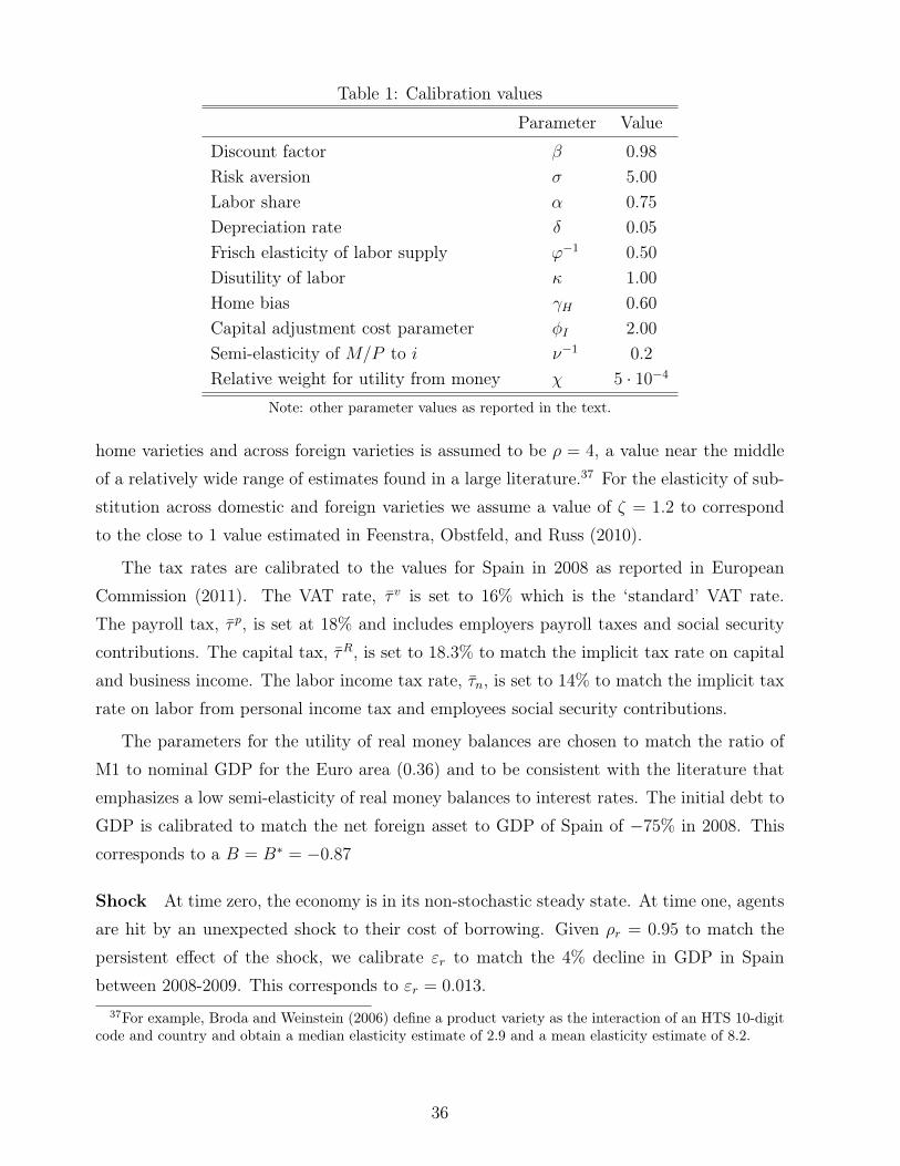
Table 1: Calibration values

Parameter Value

Discount factor β 0.98Risk aversion σ 5.00Labor share α 0.75Depreciation rate δ 0.05Frisch elasticity of labor supply ϕ−1 0.50Disutility of labor κ 1.00Home bias γH 0.60Capital adjustment cost parameter φI 2.00Semi-elasticity of M/P to i ν−1 0.2Relative weight for utility from money χ 5 · 10−4

Note: other parameter values as reported in the text.

home varieties and across foreign varieties is assumed to be ρ = 4, a value near the middle

of a relatively wide range of estimates found in a large literature.37 For the elasticity of sub-

stitution across domestic and foreign varieties we assume a value of ζ = 1.2 to correspond

to the close to 1 value estimated in Feenstra, Obstfeld, and Russ (2010).

The tax rates are calibrated to the values for Spain in 2008 as reported in European

Commission (2011). The VAT rate, τ v is set to 16% which is the ‘standard’ VAT rate.

The payroll tax, τ p, is set at 18% and includes employers payroll taxes and social security

contributions. The capital tax, τR, is set to 18.3% to match the implicit tax rate on capital

and business income. The labor income tax rate, τn, is set to 14% to match the implicit tax

rate on labor from personal income tax and employees social security contributions.

The parameters for the utility of real money balances are chosen to match the ratio of

M1 to nominal GDP for the Euro area (0.36) and to be consistent with the literature that

emphasizes a low semi-elasticity of real money balances to interest rates. The initial debt to

GDP is calibrated to match the net foreign asset to GDP of Spain of −75% in 2008. This

corresponds to a B = B∗ = −0.87

Shock At time zero, the economy is in its non-stochastic steady state. At time one, agents

are hit by an unexpected shock to their cost of borrowing. Given ρr = 0.95 to match the

persistent effect of the shock, we calibrate εr to match the 4% decline in GDP in Spain

between 2008-2009. This corresponds to εr = 0.013.37For example, Broda and Weinstein (2006) define a product variety as the interaction of an HTS 10-digit

code and country and obtain a median elasticity estimate of 2.9 and a mean elasticity estimate of 8.2.

36

Results Figure 1 plots the impulse response of the economy to the interest rate shock for

three cases: flexible wages (F), sticky wages (S) and sticky wages with a 10% fiscal devalu-

ation (FD). This magnitude of devaluation mimics closely the movement in consumption in

the flexible wage case.38 According to the formula in footnote 22, a 10% fiscal devaluation

translates into an increase in VAT of 7.6 percentage points (to 23.6%), a payroll tax cut of

10.7 percentage points (to 7.3%) and a capital tax cut of 10.8 percentage points (to 7.5%).

Note that the initial non-stochastic steady state is identical across all cases. All reported

variables are in percent deviation from their steady state values.

The increase in interest rates makes borrowing costly and leads to a substitution away

from consumption to savings. Since Spain is a net debtor in the initial steady state the

increase in interest rates has a negative income effect that reinforces the substitution effect

and further reduces consumption. The increase in interest rates leads to an increase in the

required rate of return on capital (consistent with the no-arbitrage condition between saving

in foreign bonds and in capital) and a decline in investment. The increase in savings and

decline in investment translates into an improvement in the trade balance. The extent of the

decline in consumption and investment and the impact on output and labor varies across

the three specifications and is tied to differential relative price movements.

In the case when wages are flexible (F), the decline in relative demand for home goods

(given home-bias) induces a decline in the demand for labor and capital services. At the

same time the decline in consumption, through the wealth effect, generates an increase in

labor supply for given real wages. The combined effect is a decline in real wages (5%) and

a decline in wages relative to rental rates of capital. In our calibration the net effect is an

increase in labor employment and an increase in output of 2.5%. The decline in relative

demand for home goods is associated with a sharp terms of trade depreciation of close to

10%, consistent with the decline in wages and rental rates of capital.

When wages are sticky (S), the relative price movements are distorted because of the slow

downward adjustment in wages as seen in Figure 1. The price of home goods declines by a

small amount and the terms of trade therefore depreciates by a little over 1% as compared to

the 10% depreciation in the flexible price case. Since the terms-of-trade is over-appreciated

relative to the flexible wage case the demand for domestic goods is too low. Similarly, real

wages decline gradually and the ratio of wages to the rental rate of capital increases in the

short-run, as opposed to decreasing as in the flexible price case. The combined effect is a38A one-time devaluation (nominal or fiscal) does not perfectly replicate the flexible-wage equilibrium due

to the dynamics associated with adjustment in capital. Note that, as is well known, in the presence ofmark-ups and distortionary taxes, the flexible price equilibrium is not first best. Welfare under an exchangerate devaluation can therefore be higher than in the flexible price allocation.

37

0 4 8−0.05

0

0.05GDP

0 4 8

−0.4

−0.2

0Investment

0 4 8−0.04

−0.03

−0.02

−0.01

0Consumption

0 4 8

−0.1

−0.05

0

0.05Nominal Wages

0 4 8−0.1

0

0.1Price of Home good

0 4 80

0.05

0.1Terms of Trade

0 4 80

0.02

0.04Trade Balance/GDP

0 4 8−0.05

0

0.05

0.1Employment/Capital

0 4 8−0.05

0

0.05Labor

0 4 8−0.05

0

0.05

0.1Consumer Price Level

0 4 8−0.06

−0.03

0

Real wage

F: Flexible wage S: Sticky wage FD: 10% Fiscal devaluation, sticky wage

0 4 8−0.1

−0.05

0

0.05Wage/Rental Rate

Figure 1: Impulse response to an interest rate shock

4.5% drop in labor, a 4% decline in output and a decline in the employment of labor relative

to capital. The direction of movement of labor and output differs both qualitatively and

quantitatively from the flexible price case.39

The impulse responses in the sticky wage case line up qualitatively quite well with what

was observed in Spain following the crisis. The decline in output, consumption, labor,

investment and the improvement in the trade balance accord well with the facts for Spain.

The model generated decline in consumption is 3.8% , while in the data it is 4.9% between39It is useful to compare the sticky wage outcome to papers that have used interest rate shocks but with

flexible prices. For instance, Neumeyer and Perri (2005) highlight the importance of attenuating wealtheffects on labor supply to generate a negative comovement between interest rates and output. Further,they require working capital to generate the required correlation. As is evident here, with pricing powerand wage rigidity, even without working capital and with preferences that allow for wealth effects on laborsupply interest rate shocks can generate negative co-movement. An important difference is that wage rigiditygenerates inefficient relative price movements in the hiring of labor versus capital.

38

Table 2: Welfare loss under alternative policies

Consumption loss

Permanent 10 quarters

No intervention (S) −0.64% −3.65%10% nominal devaluation −0.45% −2.55%

Of this gap

— 10% fiscal devaluation (FD) 100%— FD w/out capital tax cut (FDK) 68%— Anticipated fiscal devaluation (FDA) 79%— 5% fiscal devaluation 53%

Note: welfare-equivalent steady state consumption loss (relative to welfare under no shock).

2008–09. The trade balance as a ratio of GDP improves by 3.6% in the model generated data,

while empirically the improvement was 4.1%. The model generates a decline in investment

of 43% which is larger than in the data, where investment declined by 30% from its peak in

2007 to 2010.

The FD case is where under sticky wages, in the period when the interest rate shock hits,

the country implements a one-time (unexpected) permanent 10% fiscal devaluation (FD).

This intervention targets both the too-high real wage and the under-depreciated terms of

trade. The devaluation raises the domestic price of imported goods and reduces the foreign

price of exported goods, thus generating a larger depreciation of the terms of trade (8%)

than the case without the intervention (1.5%). The associated increase in the home price

level also brings about the relevant decline in real wages, close to the level in the flexible

price case. While this one-time exchange rate intervention cannot replicate the flexible price

allocations perfectly, it does quite well, as seen in the figures. The decline in consumption,

investment, improvement in the trade balance to GDP, and the increase in labor, output

and the ratio of employment to capital are quite close to the flexible price case.

Lastly, we evaluate the welfare impact of a 10% devaluation (FD) relative to the case

without the fiscal devaluation (S). We perform a calculation à la Lucas (1987). That is

we compute the permanent per-period decline in consumption in the non-stochastic steady

state required to match the welfare following the interest rate shock, with and without the

fiscal devaluation. As is well known, in standard business cycle models the level effects are

quite small. The relevant number is therefore the comparison across the different cases.

The certainty equivalent consumption decline in the case of FD is 0.45%. Without the FD

intervention the certainty equivalent consumption decline is around 50% higher, at 0.64%. A

39

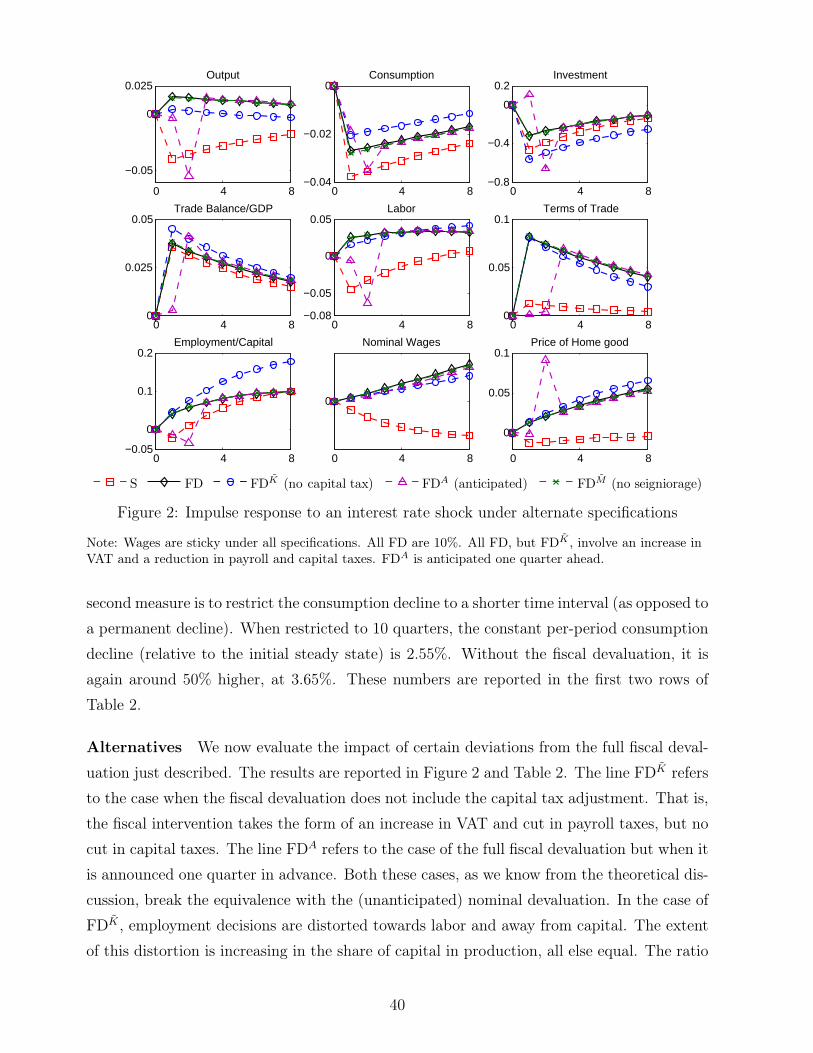
0 4 8

−0.05

0

0.025Output

0 4 8−0.8

−0.4

0

0.2Investment

0 4 8−0.04

−0.02

0Consumption

0 4 8

0

Nominal Wages

0 4 8

0

0.05

0.1Price of Home good

0 4 80

0.05

0.1Terms of Trade

0 4 80

0.025

0.05Trade Balance/GDP

0 4 8−0.05

0

0.1

0.2Employment/Capital

0 4 8−0.08

−0.05

0

0.05Labor

S FD FDK (no capital tax) FDA (anticipated) FDM (no seigniorage)

Figure 2: Impulse response to an interest rate shock under alternate specifications

Note: Wages are sticky under all specifications. All FD are 10%. All FD, but FDK , involve an increase inVAT and a reduction in payroll and capital taxes. FDA is anticipated one quarter ahead.

second measure is to restrict the consumption decline to a shorter time interval (as opposed to

a permanent decline). When restricted to 10 quarters, the constant per-period consumption

decline (relative to the initial steady state) is 2.55%. Without the fiscal devaluation, it is

again around 50% higher, at 3.65%. These numbers are reported in the first two rows of

Table 2.

Alternatives We now evaluate the impact of certain deviations from the full fiscal deval-

uation just described. The results are reported in Figure 2 and Table 2. The line FDK refers

to the case when the fiscal devaluation does not include the capital tax adjustment. That is,

the fiscal intervention takes the form of an increase in VAT and cut in payroll taxes, but no

cut in capital taxes. The line FDA refers to the case of the full fiscal devaluation but when it

is announced one quarter in advance. Both these cases, as we know from the theoretical dis-

cussion, break the equivalence with the (unanticipated) nominal devaluation. In the case of

FDK , employment decisions are distorted towards labor and away from capital. The extent

of this distortion is increasing in the share of capital in production, all else equal. The ratio

40

0.85 0.9 0.950

0.2

0.4

0.6

0.8

Wage stickiness, θW

Con

sumptionloss

(%)equivalent

S

FD

FDK (no capital tax)

FDA (anticipated)

Figure 3: Welfare loss as function of wage rigidity

of employment to capital therefore rises more than in the case of FD. The decline in returns

to investing generates a larger drop in investment and a larger improvement in the trade

balance. In the case FDA when the fiscal intervention is anticipated, the anticipated future

decline in real wages generates a decline in labor employment and output in the quarter

before the implementation of the fiscal devaluation. There is quick convergence to the case

of an unexpected FD in the following periods.

Lastly, the FDM line represents the case when we exclude the seignorage revenues asso-

ciated with a fiscal devaluation from the country budget constraint to capture the case of

a fiscal devaluation in a currency union without the transfer of seigniorage from the union

central bank to the devaluing country (see discussion in Section 4.1). Recall that this is a

policy that can be implemented unilaterally by the country. When calibrated to match the

ratio of M1 to nominal GDP for the Euro Area, the impact from the missing seigniorage

transfers is negligible. One way to see this is that the present discounted value of seignorage

associated with the fiscal devaluation is about 2% of steady state net foreign assets. Re-

versing the impact of the seignorage will be equivalent to a 2% decline in net foreign assets

for Spain alongside the interest rate increase. This has a negligible effect on all variables as

depicted in Figure 2. The path of the variables for the case of FDM is indistinguishable from

that for FD, the full fiscal devaluation.

The welfare implications of incomplete FD are reported in Table 2. Even when the fiscal

devaluation is imperfect it significantly closes the gap between the no intervention and the

full implementation welfare. In the case when only a VAT-payroll tax swap is used without

any adjustment for capital taxes the gap is closed by 68%. In the case when the fiscal

devaluation is anticipated it is closed by 79%. In the case when the devaluation is halved in

size, to 5%, it still covers 53% of the welfare gap.

41

In September 2012 Spain raised the standard VAT from 18% to 21% and for several lower

tax bracket items the tax increases were even bigger, for instance, the taxes on schoolbooks

rose from 4% to 21%, for haircuts, cinema tickets and other entertainment items from 8%

to 21%. This VAT increase was not accompanied with payroll and capital tax cuts as would

be called for in a fiscal devaluation. When we simulate the impact of a 5% VAT tax increase

alongside the interest rate increase, without any other tax changes, welfare is estimated to

decline by more than the case without any intervention. In the absence of intervention welfare

declines by −0.64%. The VAT tax increase instead reduces it by −0.88%, emphasizing the

essential role of a payroll tax cut alongside the VAT increase to capture the benefits of a

devaluation.

The welfare gap between no intervention and a fiscal devaluation (even if imperfect) grows

with the degree of wage rigidity. In Figure 3 we plot the certainty equivalent consumption

decline (permanent) under four alternative policy regimes as a function of the wage rigidity

parameter θw. As is to be expected, the higher the wage rigidity the more beneficial the

fiscal devaluation, either full or incomplete, relative to no-intervention.

6 Conclusion

In this paper we propose two types of fiscal policies that can robustly implement allocations

stemming from a nominal devaluation, but in an economy with a fixed exchange rate. Our

proposed fiscal devaluations have a number of appealing features. First, they can be imple-

mented unilaterally by one country using a small set of conventional fiscal instruments. In

particular, a one-time unanticipated fiscal devaluation can be implemented adjusting solely

the value-added and payroll taxes. Second, they are robust in the sense that they work

across a number of economic environments and require virtually no information about the

details of the microeconomic environment, in particular about the extent and nature of nom-

inal price and wage rigidity. Third, they are government revenue neutral. Clearly, there are

political economy constraints to the size of a feasible fiscal devaluation including tax evasion

considerations. An area that we leave for future research is the impact of these factors on

implementation. Nevertheless, our results suggest that fiscal devaluations offer a partial but

attractive relaxation of Mundell’s impossible trinity, allowing for essentially the same out-

comes as under an active monetary policy while maintaining a fixed exchange rate and free

capital flows.

42

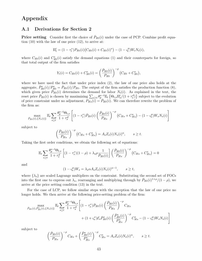
Appendix

A.1 Derivations for Section 2

Price setting Consider first the choice of PHt(i) under the case of PCP. Combine profit equa-tion (10) with the law of one price (12), to arrive at:

Πit = (1− τvt )PHt(i)

(CHt(i) + CHt(i)

∗)− (1− ςpt )WtNt(i),

where CHt(i) and C∗Ht(i) satisfy the demand equations (1) and their counterparts for foreign, sothat total output of the firm satisfies

Yt(i) = CHt(i) + C∗Ht(i) =

(PHt(i)

PHt

)−ρ (CHt + C∗Ht

),

where we have used the fact that under price index (2), the law of one price also holds at theaggregate, P ∗Ht(i)/P

∗Ht = PHt(i)/PHt. The output of the firm satisfies the production function (8),

which given price PHt(i) determines the demand for labor Nt(i). As explained in the text, thereset price PHt(i) is chosen by maximizing

∑s≥t θ

s−tp Et

Θt,sΠ

is/(1 + τds )

subject to the evolution

of price constraint under no adjustment, PHs(i) = PHt(i). We can therefore rewrite the problem ofthe firm as:

maxPHt(i),Ns(i)

Et∑s≥t

θs−tp Θt,s

1 + τds

[(1− τvs )PHt(i)

(PHt(i)

PHs

)−ρ (CHs + C∗Hs

)− (1− ςps )WsNs(i)

]

subject to (PHt(i)

PHs

)−ρ (CHs + C∗Hs

)= AsZs(i)Ns(i)

α, s ≥ t.

Taking the first order conditions, we obtain the following set of equations:

Et∑s≥t

θs−tp Θt,s

1 + τds

[(1− τvs )(1− ρ) + λsρ

1

PHt(i)

](PHt(i)

PHs

)−ρ (CHs + C∗Hs

)= 0

and(1− ςps )Ws = λsαAsZs(i)Ns(i)

α−1, s ≥ t,

where λs are scaled Lagrange multipliers on the constraint. Substituting the second set of FOCsinto the first one to express out λs, rearranging and multiplying through by PHt(i)1+ρ/(1− ρ), wearrive at the price setting condition (13) in the text.

For the case of LCP, we follow similar steps with the exception that the law of one price nolonger holds. We then arrive at the following price-setting problem of the firm:

maxPHt(i),P

∗Ht(i),Ns(i)

Et∑s≥t

θs−tp Θt,s

1 + τds

[(1− τvs )PHt(i)

(PHt(i)

PHs

)−ρCHs

+ (1 + ςxs )EsP ∗Ht(i)(P ∗Ht(i)

P ∗Hs

)−ρC∗Hs − (1− ςps )WsNs(i)

]

subject to (PHt(i)

PHs

)−ρCHs +

(P ∗Ht(i)

P ∗Hs

)−ρC∗Hs = AsZs(i)Ns(i)

α, s ≥ t.

43

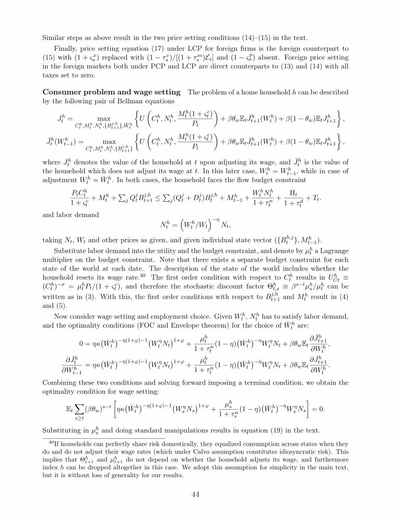
Similar steps as above result in the two price setting conditions (14)–(15) in the text.Finally, price setting equation (17) under LCP for foreign firms is the foreign counterpart to

(15) with (1 + ςxs ) replaced with (1 − τvs )/[(1 + τms )Es] and (1 − ςps ) absent. Foreign price settingin the foreign markets both under PCP and LCP are direct counterparts to (13) and (14) with alltaxes set to zero.

Consumer problem and wage setting The problem of a home household h can be describedby the following pair of Bellman equations

Jht = maxCht ,M

ht ,N

ht ,B

j,ht+1,Wh

t

U

(Cht , N

ht ,Mht (1 + ςct )

Pt

)+ βθwEtJht+1(W h

t ) + β(1− θw)EtJht+1

,

Jht (W ht−1) = max

Cht ,Mht ,N

ht ,B

j,ht+1

U

(Cht , N

ht ,Mht (1 + ςct )

Pt

)+ βθwEtJht+1(W h

t ) + β(1− θw)EtJht+1

,

where Jht denotes the value of the household at t upon adjusting its wage, and Jht is the value ofthe household which does not adjust its wage at t. In this later case, W h

t = W ht−1, while in case of

adjustment W ht = W h

t . In both cases, the household faces the flow budget constraint

PtCht

1 + ςct+Mh

t +∑

j QjtB

j,ht+1 ≤

∑j(Q

jt +Dj

t )Bj,ht +Mh

t−1 +W ht N

ht

1 + τnt+

Πt

1 + τdt+ Tt.

and labor demandNht =

(W ht /Wt

)−ηNt,

taking Nt, Wt and other prices as given, and given individual state vector (Bh,jt ,Mh

t−1).Substitute labor demand into the utility and the budget constraint, and denote by µht a Lagrange

multiplier on the budget constraint. Note that there exists a separate budget constraint for eachstate of the world at each date. The description of the state of the world includes whether thehousehold resets its wage rate.40 The first order condition with respect to Cht results in UhCt ≡(Cht )−σ = µht Pt/(1 + ςct ), and therefore the stochastic discount factor Θh

t,s ≡ βs−tµhs/µht can be

written as in (3). With this, the first order conditions with respect to Bj,ht+1 and Mh

t result in (4)and (5).

Now consider wage setting and employment choice. GivenW ht , Nh

t has to satisfy labor demand,and the optimality conditions (FOC and Envelope theorem) for the choice of W h

t are:

0 = ηκ(W ht

)−η(1+ϕ)−1(W ηt Nt

)1+ϕ+

µht1 + τnt

(1− η)(W ht

)−ηW ηt Nt + βθwEt

∂Jht+1

∂W ht

,

∂Jht∂W h

t−1

= ηκ(W ht

)−η(1+ϕ)−1(W ηt Nt

)1+ϕ+

µht1 + τnt

(1− η)(W ht

)−ηW ηt Nt + βθwEt

∂Jht+1

∂W ht

.

Combining these two conditions and solving forward imposing a terminal condition, we obtain theoptimality condition for wage setting:

Et∑s≥t

(βθw)s−t[ηκ(W ht

)−η(1+ϕ)−1(W ηs Ns

)1+ϕ+

µhs1 + τns

(1− η)(W ht

)−ηW ηs Ns

]= 0.

Substituting in µhs and doing standard manipulations results in equation (19) in the text.40If households can perfectly share risk domestically, they equalized consumption across states when they

do and do not adjust their wage rates (which under Calvo assumption constitutes idiosyncratic risk). Thisimplies that Θh

t+1 and µht+1 do not depend on whether the household adjusts its wage, and furthermoreindex h can be dropped altogether in this case. We adopt this assumption for simplicity in the main text,but it is without loss of generality for our results.

44

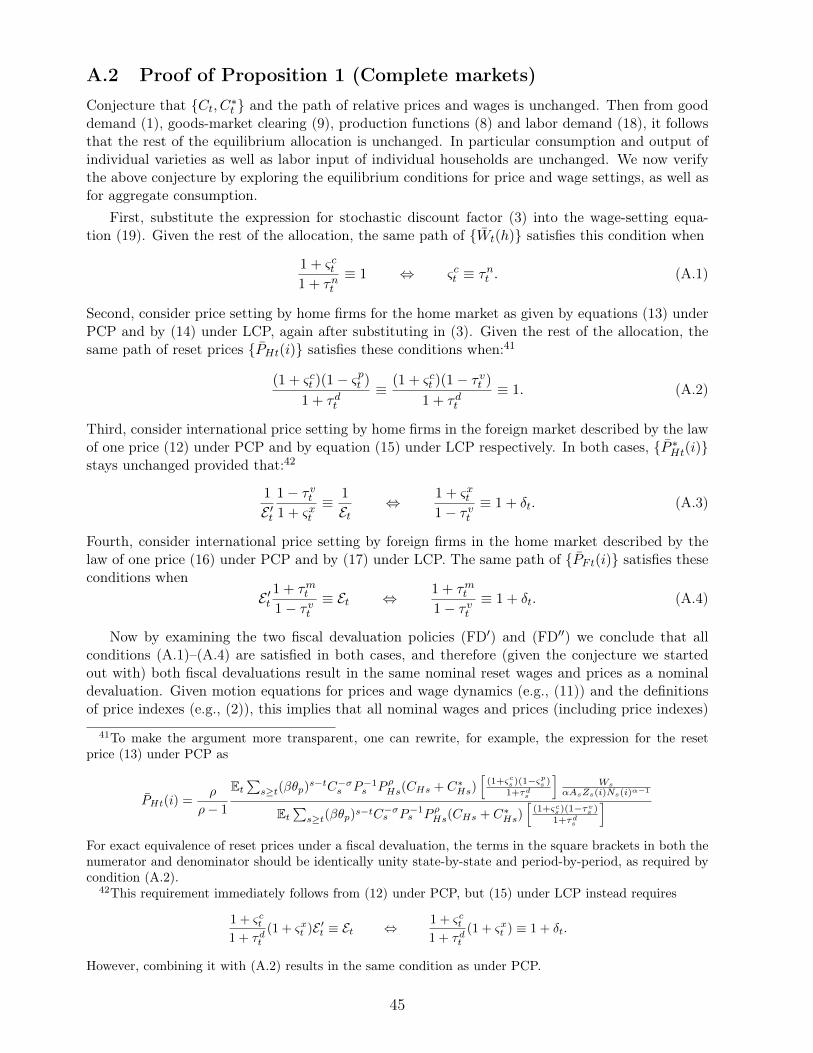
A.2 Proof of Proposition 1 (Complete markets)Conjecture that Ct, C∗t and the path of relative prices and wages is unchanged. Then from gooddemand (1), goods-market clearing (9), production functions (8) and labor demand (18), it followsthat the rest of the equilibrium allocation is unchanged. In particular consumption and output ofindividual varieties as well as labor input of individual households are unchanged. We now verifythe above conjecture by exploring the equilibrium conditions for price and wage settings, as well asfor aggregate consumption.

First, substitute the expression for stochastic discount factor (3) into the wage-setting equa-tion (19). Given the rest of the allocation, the same path of Wt(h) satisfies this condition when

1 + ςct1 + τnt

≡ 1 ⇔ ςct ≡ τnt . (A.1)

Second, consider price setting by home firms for the home market as given by equations (13) underPCP and by (14) under LCP, again after substituting in (3). Given the rest of the allocation, thesame path of reset prices PHt(i) satisfies these conditions when:41

(1 + ςct )(1− ςpt )

1 + τdt≡ (1 + ςct )(1− τvt )

1 + τdt≡ 1. (A.2)

Third, consider international price setting by home firms in the foreign market described by the lawof one price (12) under PCP and by equation (15) under LCP respectively. In both cases, P ∗Ht(i)stays unchanged provided that:42

1

E ′t1− τvt1 + ςxt

≡ 1

Et⇔ 1 + ςxt

1− τvt≡ 1 + δt. (A.3)

Fourth, consider international price setting by foreign firms in the home market described by thelaw of one price (16) under PCP and by (17) under LCP. The same path of PFt(i) satisfies theseconditions when

E ′t1 + τmt1− τvt

≡ Et ⇔ 1 + τmt1− τvt

≡ 1 + δt. (A.4)

Now by examining the two fiscal devaluation policies (FD′) and (FD′′) we conclude that allconditions (A.1)–(A.4) are satisfied in both cases, and therefore (given the conjecture we startedout with) both fiscal devaluations result in the same nominal reset wages and prices as a nominaldevaluation. Given motion equations for prices and wage dynamics (e.g., (11)) and the definitionsof price indexes (e.g., (2)), this implies that all nominal wages and prices (including price indexes)

41To make the argument more transparent, one can rewrite, for example, the expression for the resetprice (13) under PCP as

PHt(i) =ρ

ρ− 1

Et∑s≥t(βθp)

s−tC−σs P−1s P ρHs(CHs + C∗Hs)

[(1+ςcs)(1−ςps )

1+τds

]Ws

αAsZs(i)Ns(i)α−1

Et∑s≥t(βθp)

s−tC−σs P−1s P ρHs(CHs + C∗Hs)

[(1+ςcs)(1−τvs )

1+τds

]For exact equivalence of reset prices under a fiscal devaluation, the terms in the square brackets in both thenumerator and denominator should be identically unity state-by-state and period-by-period, as required bycondition (A.2).

42This requirement immediately follows from (12) under PCP, but (15) under LCP instead requires

1 + ςct1 + τdt

(1 + ςxt )E ′t ≡ Et ⇔ 1 + ςct1 + τdt

(1 + ςxt ) ≡ 1 + δt.

However, combining it with (A.2) results in the same condition as under PCP.

45

are mimicked under both fiscal devaluation policies. This, in turn, implies in view of (A.3)–(A.4)that the terms of trade defined in (24) are also mimicked. To additionally mimic the behavior of thereal exchange rate in (26), we need to require E ′t(1 + ςct ) ≡ Et, which together with (A.1) results in:

ςct ≡ τnt ≡ δt, (A.5)

also satisfied by (FD′) and (FD′′).We finally verify that the equilibrium values of Ct, C∗t associated with a nominal devaluation

are also equilibrium values under our fiscal devaluation policies. Under complete markets, theinternational risk-sharing condition (25) becomes the familiar Backus-Smith condition (28), wherethe constant of proportionality λ is recovered from the intertemporal budget constraint of thecountry and stays unchanged across nominal and fiscal devaluations provided that relative prices andterms of trade follow the same path.43 As long as we have equivalence in all relative prices, includingthe real exchange rate, from (28) we obtain equivalence in the relative consumption allocation. Thelevels of consumption must also be equivalent under nominal and fiscal devaluations to satisfy theaggregate resource constraint (aggregating (9)).

This completes the loop and verifies that the conjecture we started out with is internally con-sistent. That is, the equilibrium allocations of consumption, labor and output associated with anominal devaluation and both fiscal devaluations in (FD′) and (FD′′) coincide.

Finally, under separable utility in money balances, money demand (5) is a side equation, andhence imposes no additional constraints on implementation.44 Switching from nominal to fiscaldevaluation in general changes the path of the (shadow) nominal interest rate, and hence requiresan adjustment in money supply in order to satisfy the altered money demand. The required path ofthe money supply under a fiscal devaluation policy M ′t can be recovered directly from (5) giventhe rest of the allocation.

A.3 Fiscal devaluations in financial autarky

We provide a brief discussion of the case of financial autarky (closed capital account), where theset of risk sharing conditions (25) becomes empty (Ωt ≡ ∅), and the flow budget constraint (23)becomes a balanced trade requirement:

C∗Ht = CFtSt ⇔ C∗tCt

=γFγ∗H

(P ∗HtP ∗t

)ζ (PFtPt

)−ζSt,

43Integrating forward the country flow budget constraint (23) using the foreign stochastic discount factoras weights, we arrive at the intertemporal budget constraint of the country

B0

P ∗0 E0+ E0

∞∑t=0

βt(C∗tC∗0

)−σP ∗HtP ∗t

[C∗Ht − CFtSt

]= 0,

where B0 is the home-currency initial net foreign asset position of the home country, and the second termis the sum of all future trade surpluses of the home country discounted by state prices. Note from gooddemand condition (1) that home and foreign consumption of imports, CFt and C∗Ht, are functions of aggregateconsumption Ct and C∗t , as well as relative price PFt/PHt and P ∗Ft/P

∗Ht respectively.

44Separability of real money balances in the utility function is a standard assumption in the literature andimplies that holdings of real money balances have no affect on the marginal utility of consumption. Henceour equivalence results do not require replicating the equilibrium path of real money balances. If on theother hand we had non-separable utility, equivalence would require the use of an additional tax on moneyholdings in order to reduce money demand under a fiscal devaluation. This is because expected nominaldevaluations result in an increased nominal interest rate and depressed money demand. Replicating anunexpected devaluation, however, does not require an extra instrument even under non-separable utility.

46

where we used demand conditions (1) to substitute in for C∗Ht and CFt. As a result, the real exchangerate plays no role for the allocation as it shows up in no equilibrium condition, and therefore onlyconditions (A.1)–(A.4) are needed to be satisfied by fiscal devaluation policies.45 Note that thereduced fiscal devaluation policies (FD′R) and (FD′′R) of Proposition 3 satisfy these requirements,but under autarky we need not require that the devaluation is unanticipated.

A.4 Proof of Proposition 3 (Unanticipated devaluations)Following the steps of the proof of Proposition 1 (in Appendix A.2), the conditions to mimic thepath of wages and prices instead of (A.1)–(A.4) become simply:

1 + ςct1 + τnt

≡ 1 and1 + ςxt1− τvt

≡ 1 + τmt1− τvt

≡ 1 + δt, (A.6)

which are satisfied under both reduced devaluation policies (FD′R) and (FD′′R). These conditionsdo not impose a requirement on the use of profit tax τdt , because under a one-time unexpecteddevaluation policy it no longer affects price setting in (13)–(15). Indeed, for price setting beforet = 0, no nominal or fiscal policy change is anticipated, so it does not affect price setting; for t ≥ 0,the change in either nominal or fiscal regime happens once and for all, and hence all taxes can bemoved outside the expectation in (13)–(15) and canceled out (also see the expression in footnote 41).

We still need to use profit tax τdt if domestic equity is traded internationally in order to replicatethe effects on the budget constraint (23) and international risk sharing (25), as shown in Lemma 1.In particular, the path of Dhe∗

t = Πt/[(1 + τdt )Et] must be replicated under a fiscal devaluation,which from the equation for profits (10) requires τdt ≡ δ for t ≥ 0 under (FD′R) and τdt ≡ 0 under(FD′′R). Whenever a home-currency debt is traded, a partial default (haircut) τh0 = δ/(1 + δ) isneeded in the event (state-period) of a fiscal devaluation in order to replicate the valuation effectsin the country budget constraint (23).

Since devaluation is one-time unanticipated, the path of the home nominal risk-free interest rateis unaffected (and in fact, UIP holds in this case as interest parity, it+1 = i∗t+1, in every period), andtherefore money demand in (5) is not affected. As a result, with ςct = 0, the same money supply asunder a nominal devaluation would also support the fiscal devaluation (M ′t = Mt), and hence realbalances are also unchanged.

Finally, with ςct = 0, the path of the real exchange rate is not exactly mimicked relative to anominal devaluation, however this does not affect the international risk sharing conditions (25).This is because for t < 0 no policy change is anticipated (zero-probability event), and for t ≥ 0 thepolicy change is once and for all, therefore leaving saving and portfolio choice decisions unaffectedbefore, after and at t = 0. Consequently, the same consumption allocation Ct, C∗t satisfies boththe country budget constraint (23) and the international risk sharing conditions (25) under bothreduced fiscal devaluation policies (FD′R) and (FD′′R) as under a nominal devaluation.

A.5 Proof of Proposition 4 (Revenue neutrality)Part (i) follows immediately from (30) after substituting in εt = δmt under (FD′) and εt = δvtunder (FD′′). To prove Part (ii), note that under both (FD′R) and (FD′′R) we can rewrite

PtCt −WtNt =(PFtCFt − (1 + δt)E0P

∗HtC

∗Ht

)+(PHtCHt + (1 + δt)E0P

∗HtC

∗Ht −WtNt

),

45Note that the domestic Euler equations (4) now become side equations and determine the intertemporalasset prices given the home stochastic discount factor in (3) which need not follow the same path under anominal and a fiscal devaluation in this case.

47

where the first term is trade deficit (−NXt) and the second term is profits without taking intoaccount VAT and payroll subsidy (i.e., Π/(1− τvt ), since τvt = ςpt under fiscal devaluations). We candivide and multiple the second term by the dividend tax (1 + τdt ) to obtain:

PtCt −WtNt = −NXt + (1 + δt)Πt

1 + τdt, (A.7)

since under both (FD′R) and (FD′′R) we have (1 + τdt )/(1− τvt ) ≡ 1 + δt. Finally, substituting (A.7)this resulting equation into (30), and imposing εt = 0 and δmt = δt or δvt = δt under the two reducedfiscal devaluations respectively, we obtain (31).

We now prove an additional result that under one-time unanticipated fiscal devaluations the netpresent value of additional government revenues is non-negative when the stock market capitalization(plus the value of unincorporated business) exceeds the net foreign liabilities of a country:

Lemma A.1 Under (FD′R) and (FD′′R), the net present value of the additional government revenuesequals δ times the sum of net foreign assets and the capitalization of the business sector of the homecountry at the time of the devaluation.

Proof: We make use of the budget constraint of the home country (23):

1

EtEt

Θt,t+1Et+1B∗t+1

− B∗t = P ∗HtC

∗Ht − PFtCFt

1

Et1− τvt1 + τmt

,

where now B∗t =∑

j∈Jt−1(Qj∗t + Dj∗

t )Bjt is the foreign-currency equilibrium payoff of the home

country international asset portfolio at t (in a given state of the world), or equivalently the foreign-currency net foreign assets (inclusive of period t returns) of the home country in the beginning ofperiod t.46

Using the NXt notation, we can rewrite

1

EtEt

Θt,t+1Et+1B∗t+1

− B∗t =

NXt

(1 + δt)E0,

where we have used the fact that Et(1 + τmt )/(1 − τvt ) = E0(1 + δt) under both nominal and fiscaldevaluations. In the case of a one-time unanticipated devaluation (with δt = δ for t ≥ 0), we solvethe above equation forward starting from t = 0:

B0 = E0B∗0 = −∞∑t=0

E0

Θ0,t

NXt

1 + δ

,

where we have imposed the transversality condition for the country international portfolio. Ex-pressing out NXt/(1 + δ) from (31) and substituting it into the intertemporal budget constraint,we obtain

B0 =∞∑t=0

E0

Θ0,t

TRtδ

−Qhe0 , where Qhe0 =

∞∑t=0

E0

Θ0,t

Πt

1 + τdt

is the (shadow) value of the home business sector (stock market capitalization plus the value ofunincorporated businesses). Combining and multiplying through by δ results in

∞∑t=0

E0 Θ0,tTRt = δ ·(B0 +Qhe0

).

46Note that 1EtEt

Θt,t+1Et+1B∗t+1

= Et

Θ∗t,t+1B∗t+1

is the period t foreign-currency value of holding a

state-contingent net foreign asset position B∗t+1 in period t+ 1, where the equality holds in view of the risksharing conditions (25).

48

A.6 Model with capitalWe adopt a formalization where firms rent the services from labor and capital on centralized markets,at prices Wt and Rt, and capital is accumulated by households according to

Kt+1 = (1− δ)Kt + It,

where gross investment It combines the different goods in the exact same way as the consumptionbundle Ct.

Households face the following sequence of budget constraints:

PtCt1 + ςct

+Mt +∑j∈Jt

QjtBjt+1 +

PtIt

1 + ςIt≤∑

j∈Jt−1

(Qjt +Djt )B

jt +Mt−1 +

RtKt

1 + τKt+WtNt

1 + τnt+

Πt

1 + τdt+Tt.

where ςIt is an investment tax credit and τKt is a tax on capital income.The households first-order conditions are the same as in the model without capital with the

addition of one more first-order condition for capital accumulation:

C−σt (1 + ςct )(1 + ςIt

) = βEtC−σt+1

[Rt+1

Pt+1

(1 + ςct+1

)(1 + τKt+1

) + (1− δ)(1 + ςct+1

)(1 + ςIt+1

)] ,corresponding to the Euler equation in the text.

On the production side we assume that each firm operates a neoclassical production function,which for concreteness takes a Cobb-Douglas form:

Yt (i) = AtZt(i)Nt (i)αKt (i)1−α ,

where Kt (i) is the firm’s capital input. Profits are given by:

Πit = (1− τvt )PHt(i)Yt(i)− (1− ςpt )WtNt(i)− (1− ςRt )RtKt(i),

where ςRt is the capital subsidy. The pricing equations are symmetric to the ones previously describedwith the difference that marginal cost is now equal to[

((1− ςps )Ws)α (

(1− ςRs )Rs)1−α

αα (1− α)1−αAsZs(i)

]

instead of (1 − ςps )Ws/[αAsZs(i)Ns(i)α−1], and hence price setting imposes exactly the same re-

quirements on fiscal devaluation policies as in the economy without capital.In addition, the firm’s optimal mix of labor and capital use is given by:

Nt

Kt=

α

1− α(1− ςRs )Rt(1− ςps )Wt

,

which is the special case of the equation in the text under the Cobb-Douglas production function.A fiscal δt-devaluation in this economy can be engineered exactly as in Proposition 1, Lemma 1

and Proposition 2 supplemented with the following tax adjustments. For (FD′) an investmentsubsidy and a tax on capital income ςIt = τKt = ςct = δt are needed. For (FD′′), a subsidy onthe rental rate of capital ςRt = ςpt = δt/ (1 + δt) is also needed. In the case where the fiscaldevaluation is one-time unanticipated, exactly as in Proposition 3, one can dispense with the useof the consumption subsidy and income tax, as well as with the use of the investment subsidy andthe tax on capital income (ςct = τnt = ςIt = τKt = 0 for all t ≥ 0).

49

A.7 Asymmetric tax pass-through

We specialize right away to the case of a one-time unanticipated devaluation and the VAT-basedpolicy, that is we set τmt = ςxt = ςct = τnt = τdt = 0 and only allow for non-zero τvt and ςpt .

In case of partial indexation to tax changes defined in (32), the price setting problem of the firmunder PCP becomes:

maxPHt(i),Ns(i)

Et∑s≥t

θs−tp Θt,s

[(1− τvs )PHs(i)

(PHs(i)

PHs

)−ρ (CHs + C∗Hs

)− (1− ςps )WsNs(i)

]

subject to (PHs(i)

PHs

)−ρ (CHs + C∗Hs

)= AsZs(i)Ns(i)

α, s ≥ t,

where

PHs(i) =

(1− τvs1− τvt

)−ξv (1− ςps1− ςpt

)ξpPHt

is the price of the firm in period s condition on the last price adjustment of the firm being at t ≤ s.Following the same steps as in Appendix A.1, we derive the price setting optimality condition:

Et∑s≥t

θs−tp Θt,s

[(1− τvs )

(1− τvs1− τvt

)−ξv (1− ςps1− ςpt

)ξpPHt(i)−

ρρ−1 (1− ςps )Ws

αAsZs(i)Ns(i)α−1

](PHs(i)

PHs

)−ρ(CHs + C∗Hs

)= 0.

Using (2) and the Calvo assumption, the evolution of the price index is given by

PHt =

θp(( 1− τvt1− τvt−1

)−ξv ( 1− ςpt1− ςpt−1

)ξpPH,t−1

)1−ρ

+

ˆ 1

θp

PHt(i)1−ρdi

1/(1−ρ)

,

where we sorted the firms so that the first θp of them do not adjust prices at t.As discussed in the text, exact fiscal implementation is impossibly with asymmetric pass-

through, and therefore we focus on the first-order accurate implementation by which we ensurethat the first-order dynamics of all aggregate prices, in particular PHt, is unchanged under a nom-inal and a fiscal devaluation.47 To this end, we log linearize the price setting and the price indexevolution equations above:

pHt = (1− βθ)∑

s≥t(βθp)s−tEt

τvt − ς

pt − ξv(τvs − τvt ) + ξp(ς

ps − ςpt ) + mcs

,

pHt = θp(pH,t−1 + ξv∆τ

vt − ξp∆ς

pt

)+ (1− θp)pHt,

where small letters denote logs of respective variables, τvt = − log(1− τvt ), ςpt = − log(1− ςpt ), pHt isthe average reset price across all adjusting firms, mcs = log[ρ/(ρ− 1)] +ws− logα− as + (1−α)nsis the average marginal cost in the cross-section of firms (averaging out idiosyncratic productivityshocks) adjusted by markup.

Following the conventional steps in the New Keynesian literature (see Galí, 2008), we can solvethis system to obtain a dynamic equation for aggregate price index (an analog to the New KeynesianPhillips curve):(

∆pHt − ξv∆τvt + ξp∆ςpt

)= βEt

∆pH,t+1 − ξv∆τvt+1 + ξp∆ς

pt+1

+ λ(τvt − ς

pt + mct

), (A.8)

47In fact, one could mimic price indexes exactly, but not the whole distribution of individual prices. Thepolicy that exactly replicates the aggregate prices is, however, non-analytic and solves a dynamic non-lineardifference equation.

50

where λ = (1 − θp)(1 − βθp)/θp. Under a fiscal devaluation, the dynamics of both pHt and mctreplicates those under a nominal devaluation, which satisfy (A.8) with all taxes set to zero. Thisimplies that the path of taxes must satisfy the following difference equation:(

ξv∆τvt − ξp∆ς

pt

)− β

ξv∆τ

vt+1 − ξp∆ς

pt+1

= λ

(ςpt − τvt

), (A.9)

where we have dropped the expectation as we are looking for a non-stochastic implementation of aone-time fiscal devaluation for t ≥ 0.

In this PCP economy, the law of one price equations (12)–(16) are satisfied, and therefore aVAT-based fiscal devaluation policy requires τvt = δ/(1 + δ), or equivalently τvt = log(1 + δ) ≡ δ, fort ≥ 0. This implies that ∆τvt = 0 for t ≥ 1 and ∆τv0 = δ. Combining this information with (A.9),we obtain a dynamic equation for ςt:48

∆ςpt − β∆ςpt+1 =ξvξpδ It=0 −

λ

ξp

(ςpt − δ

).

The initial condition for this dynamic equation is ςp−1 = 0, and the stationarity of ςt implies aterminal condition limt→∞ ς

pt = δ.

To solve this dynamic equation, rewrite it as:(1 + β +

λ

ξp

)(ςpt − δ

)−(ςpt−1 − δ

)− β

(ςpt+1 − δ

)=ξvξpδ It=0.

Note that it can be further rewritten using lag-operator as:

ρ2

(1− ρ1L

−1)(1− ρ−1

2 L)(ςpt − δ

)=ξvξpδ It=0,

where Lςpt = ςpt−1 is the lag operator, and 0 < ρ1 < 1 < ρ2 are the two roots of x2 − (1 + β +λ/ξp)x− β = 0. Inverting the first bracket with the lead operator, we arrive at:

(ςpt − δ

)− ρ−1

2

(ςpt−1 − δ

)= ρ−1

2

ξvξpδ It=0,

which, taking into account the initial condition, has the solution:

ςp0 − δ = ρ−12

ξv − ξpξp

and ςpt − δ = ρ−t2

(ςp0 − δ

).

This can be simplified to:

ςpt = δ

(1 + ρ

−(t+1)2

ξv − ξpξp

).

Finally, note that ρ = ρ−12 ∈ (0, 1) is also one of the roots of 1 − (1 + β + λ/ξp)x − βx2 = 0.

Exponentiating this solution results in the expression in Propostion 8.Note that under this fiscal devaluation, we first-order replicate the aggregate prices, PHt, P ∗Ht, PFt, P ∗Ft,

and therefore also terms of trade. Given prices, the rest of the allocation is unchanged provided thatthe relative consumption is the same, which is ensured by the unchanged country budget constraintand risk-sharing condition.

48These calculations are done under the assumption ξp > 0. In the case of ξp = 0, the solution to (A.9) isimmediately characterized by ςpt = δ for t > 0 and ςp0 = δ

(1 + λ/ξv

).

51

References

Adao, B., I. Correia, and P. Teles (2009): “On the relevance of exchange rate regimesfor stabilization policy,” Journal of Economic Theory, 144(4), 1468–1488.

Andrade, P., M. Carré, and A. Bénassy-Quéré (2010): “Competition and pass-through on international markets: Firm-level evidence from VAT shocks,” CEPII.

Atkeson, A., and A. Burstein (2008): “Pricing-to-Market, Trade Costs, and Interna-tional Relative Prices,” American Economic Review, 98(5), 1998–2031.

Benigno, G., P. Benigno, and F. Ghironi (2007): “Interest rate rules for fixed exchangerate regimes,” Journal of Economic Dynamics and Control, 31(7), 2196–2211.

Benigno, G., and H. Kucuk-Tuger (2012): “Portfolio allocation and International RiskSharing,” Canadian Journal of Economics, 45(2), 535–565.

Berglas, E. (1974): “Devaluation, Monetary Policy, and Border Tax Adjustment,” Cana-dian Journal of Economics, 7(1), 1–11.

Boscam, J. E., A. Diaz, R. Domenech, J. Ferri, E. Perez, and L. Puch (2011):“REMS: A Rational Expectations Model for Simulation and Policy Evaluation of theSpanish Economy,” in The Spanish Economy: A General Equilibrium Perspective, ed. byJ. Bosca, R. Domenech, J. Ferri, and J. Varela. Palgrave Macmillan.

Broda, C., and D. Weinstein (2006): “Globalization and the Gains from Variety,” Quar-terly Journal of Economics.

Calmfors, L. (1998): “Macroeconomic Policy, Wage Setting and Employment-What dif-ference does the EMU make?,” Oxford Review of Economic Policy, 14(3), 125–151.

Campa, J. M., L. S. Goldberg, and J. M. González-Mínguez (2005): “Exchange-RatePass-Through to Import Prices in the Euro Area,” NBER Working Papers No. 11632.

Carare, A., and S. Danninger (2008): “Inflation Smoothing and the Modest Effect ofVAT in Germany,” IMF Working Papers No. 08/175.

Carbonnier, C. (2007): “Who pays sales taxes? Evidence from French VAT reforms,1987–1999,” Journal of Public Economics, 91(5–6), 1219–1229.

Christiano, L., M. Eichenbaum, and S. Rebelo (2011): “When Is the GovernmentSpending Multiplier Large?,” Journal of Political Economy, 119(1), 78 – 121.

Correia, I., E. Farhi, J. P. Nicolini, and P. Teles (2011): “Unconventional FiscalPolicy at the Zero Bound,” NBER Working Papers No. 16758.

Correia, I., J. P. Nicolini, and P. Teles (2008): “Optimal Fiscal and Monetary Policy:Equivalence Results,” Journal of Political Economy, 116(1), 141–170.

Corsetti, G. (2008): “New Open Economy Macroeconomics,” in The New Palgrave Dic-tionary of Economics, ed. by S. N. Durlauf, and L. E. Blume. Palgrave Macmillan, Bas-ingstoke.

Devereux, M. B., and A. Sutherland (2008): “Country Portfolios in Open EconomyMacro Models,” NBER Working Papers No. 14372.

Eggertsson, G. (2004): “Comment on How Do Monetary and Fiscal Policy Interact inthe European Monetary Union?,” NBER International Seminar on Macroeconomics, pp.241–325.

52

European Commission (2011): Taxation trends in the European Union. European Com-mission.

Feenstra, R., M. Obstfeld, and K. Russ (2010): “In Search of the Armington Elastic-ity,” Working Paper.

Feenstra, R. C. (1985): “Anticipated Devaluations, Currency Flight, and Direct TradeControls in a Monetary Economy,” American Economic Review, 75(3), 386–401.

Feldstein, M. S., and P. R. Krugman (1990): “International Trade Effects of Value-Added Taxation,” in Taxation in the Global Economy, NBER Chapters, pp. 263–282.National Bureau of Economic Research, Inc.

Franco, F. (2011): “Improving competitiveness through fiscal devaluation, the case ofPortugal,” Universidade Nova de Lisboa.

Galí, J. (2008): Monetary Policy, Inflation and the Business Cycle: An Introduction to theNew Keynesian Framework. Princeton University Press.

Gourinchas, P.-O., and H. Rey (2007): “From World Banker to World Venture Capi-talist: U.S. External Adjustment and the Exorbitant Privilege,” in G7 Current AccountImbalances: Sustainability and Adjustment, NBER Chapters, pp. 11–66. National Bureauof Economic Research, Inc.

Grossman, G. M. (1980): “Border tax adjustments: Do they distort trade?,” Journal ofInternational Economics, 10(1), 117–128.

IMF (2011): Fiscal Monitor: Addressing Fiscal Challenges to Reduce Economic Risks. In-ternational Monetary Fund.

Kimball, M. (1995): “The Quantitative Analytics of the Basic Neomonetarist Model,”Journal of Money, Credit and Banking, 27, 1241–77.

Lane, P. R. (2001): “The new open economy macroeconomics: a survey,” Journal of Inter-national Economics, 54(2), 235–266.

Lipińska, A., and L. von Thadden (2009): “Monetart and Fiscal Policy Aspects ofIndirect Tax Changes in a Monetaty Union,” ECB Working Papers No. 1097.

Lucas, R. (1987): Models of Business Cycles. Basil Blackwell, Oxford.Neumeyer, P. A., and F. Perri (2005): “Business cycles in emerging economies: the roleof interest rates,” Journal of Monetary Economics, 52(2), 345–380.

Obstfeld, M., and K. Rogoff (2000): “New Directions for Stochastic Open EconomyModels,” Journal of International Economics, 50, 117–153.

Poterba, J. M., J. J. Rotemberg, and L. H. Summers (1986): “A Tax-Based Test forNominal Rigidities,” American Economic Review, 76(4), 659–75.

Schmitt-Grohé, S., and M. Uribe (2011): “Pegs and Pain,” Columbia Univeristy.Silva, S. J., and S. Tenreyro (2010): “Currency Unions in Prospect and Retrospect,”Annual Review of Economics, 2, 51–74.

Staiger, R. W., and A. O. Sykes (2010): “ ‘Currency manipulation’ and world trade,”World Trade Review, 9(4), 583–627.

Woodford, M. (2003): Interest and Prices: Foundations of a Theory of Monetary Policy.Princeton University Press.

53