First-Order Differential Equations We begin our study of differential equations (DEs) with first-order equations. In this chapter we illustrate the three different ways DEs can be studied: qualitatively (Section 2.1), analytically (Sections 2.2–2.5), and numerically (Section 2.6). The chapter ends with an introduction to mathematical modeling with DEs (Sections 2.7–2.9). 2 CHAPTER 2.1 Solution Curves Without a Solution 2.2 Separable Equations 2.3 Linear Equations 2.4 Exact Equations 2.5 Solutions by Substitutions 2.6 A Numerical Method 2.7 Linear Models 2.8 Nonlinear Models 2.9 Modeling with Systems of First-Order DEs Chapter 2 in Review © Jones & Bartlett Learning LLC, an Ascend Learning Company. NOT FOR SALE OR DISTRIBUTION.

Welcome message from author
This document is posted to help you gain knowledge. Please leave a comment to let me know what you think about it! Share it to your friends and learn new things together.
Transcript
First-Order Differential Equations
We begin our study of differential equations (DEs) with first-order equations. In this chapter we illustrate the three different ways DEs can be studied: qualitatively (Section 2.1), analytically (Sections 2.2–2.5), and numerically (Section 2.6). The chapter ends with an introduction to mathematical modeling with DEs (Sections 2.7–2.9).
2CHAPTER
2.1 Solution Curves Without a Solution
2.2 Separable Equations
2.3 Linear Equations
2.4 Exact Equations
2.5 Solutions by Substitutions
2.6 A Numerical Method
2.7 Linear Models
2.8 Nonlinear Models
2.9 Modeling with Systems of First-Order DEs
Chapter 2 in Review
© Jones & Bartlett Learning LLC, an Ascend Learning Company. NOT FOR SALE OR DISTRIBUTION.
© Jones & Bartlett Learning, LLCNOT FOR SALE OR DISTRIBUTION
© Jones & Bartlett Learning, LLCNOT FOR SALE OR DISTRIBUTION
© Jones & Bartlett Learning, LLCNOT FOR SALE OR DISTRIBUTION
© Jones & Bartlett Learning, LLCNOT FOR SALE OR DISTRIBUTION
© Jones & Bartlett Learning, LLCNOT FOR SALE OR DISTRIBUTION
© Jones & Bartlett Learning, LLCNOT FOR SALE OR DISTRIBUTION
© Jones & Bartlett Learning, LLCNOT FOR SALE OR DISTRIBUTION
© Jones & Bartlett Learning, LLCNOT FOR SALE OR DISTRIBUTION
© Jones & Bartlett Learning, LLCNOT FOR SALE OR DISTRIBUTION
© Jones & Bartlett Learning, LLCNOT FOR SALE OR DISTRIBUTION
© Jones & Bartlett Learning, LLCNOT FOR SALE OR DISTRIBUTION
© Jones & Bartlett Learning, LLCNOT FOR SALE OR DISTRIBUTION
© Jones & Bartlett Learning, LLCNOT FOR SALE OR DISTRIBUTION
© Jones & Bartlett Learning, LLCNOT FOR SALE OR DISTRIBUTION
© Jones & Bartlett Learning, LLCNOT FOR SALE OR DISTRIBUTION
© Jones & Bartlett Learning, LLCNOT FOR SALE OR DISTRIBUTION
© Jones & Bartlett Learning, LLCNOT FOR SALE OR DISTRIBUTION
© Jones & Bartlett Learning, LLCNOT FOR SALE OR DISTRIBUTION
© Jones & Bartlett Learning, LLCNOT FOR SALE OR DISTRIBUTION
© Jones & Bartlett Learning, LLCNOT FOR SALE OR DISTRIBUTION
2.1 Solution Curves Without a Solution
INTRODUCTION Some differential equations do not possess any solutions. For example, there is no real function that satisfies (y9) 2 1 1 5 0. Some differential equations possess solu-tions that can be found analytically, that is, solutions in explicit or implicit form found by implementing an equation-specific method of solution. These solution methods may involve certain manipulations, such as a substitution, and procedures, such as integration. Some dif-ferential equations possess solutions, but the differential equation cannot be solved analytically. In other words, when we say that a solution of a DE exists, we do not mean that there also exists a method of solution that will produce explicit or implicit solutions. Over a time span of centu-ries, mathematicians have devised ingenious procedures for solving some very specialized equa-tions, so there are, not surprisingly, a large number of differential equations that can be solved analytically. Although we shall study some of these methods of solution for first-order equations in the subsequent sections of this chapter, let us imagine for the moment that we have in front of us a first-order differential equation in normal form dy/dx 5 f (x, y), and let us further imag-ine that we can neither find nor invent a method for solving it analytically. This is not as bad a predicament as one might think, since the differential equation itself can sometimes “tell” us specifics about how its solutions “behave.” We have seen in Section 1.2 that whenever f (x, y) and 0f/0y satisfy certain continuity conditions, qualitative questions about existence and unique-ness of solutions can be answered. In this section we shall see that other qualitative questions about properties of solutions—such as, How does a solution behave near a certain point? or How does a solution behave as x S q?—can often be answered when the function f depends solely on the variable y.
We begin our study of first-order differential equations with two ways of analyzing a DE qualitatively. Both these ways enable us to determine, in an approximate sense, what a solution curve must look like without actually solving the equation.
2.1.1 Direction Fields
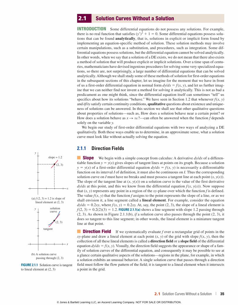
Slope We begin with a simple concept from calculus: A derivative dy/dx of a differen-tiable function y 5 y(x) gives slopes of tangent lines at points on its graph. Because a solution y 5 y(x) of a first-order differential equation dy/dx 5 f (x, y) is necessarily a differentiable function on its interval I of definition, it must also be continuous on I. Thus the corresponding solution curve on I must have no breaks and must possess a tangent line at each point (x, y(x)). The slope of the tangent line at (x, y(x)) on a solution curve is the value of the first derivative dy/dx at this point, and this we know from the differential equation f (x, y(x)). Now suppose that (x, y) represents any point in a region of the xy-plane over which the function f is defined. The value f (x, y) that the function f assigns to the point represents the slope of a line, or as we shall envision it, a line segment called a lineal element. For example, consider the equation dy/dx 5 0.2xy, where f (x, y) 5 0.2xy. At, say, the point (2, 3), the slope of a lineal element is f (2, 3) 5 0.2(2)(3) 5 1.2. FIGURE 2.1.1(a) shows a line segment with slope 1.2 passing through (2, 3). As shown in Figure 2.1.1(b), if a solution curve also passes through the point (2, 3), it does so tangent to this line segment; in other words, the lineal element is a miniature tangent line at that point.
Direction Field If we systematically evaluate f over a rectangular grid of points in the xy-plane and draw a lineal element at each point (x, y) of the grid with slope f (x, y), then the collection of all these lineal elements is called a direction field or a slope field of the differential equation dy/dx 5 f (x, y). Visually, the direction field suggests the appearance or shape of a fam-ily of solution curves of the differential equation, and consequently it may be possible to see at a glance certain qualitative aspects of the solutions—regions in the plane, for example, in which a solution exhibits an unusual behavior. A single solution curve that passes through a direction field must follow the flow pattern of the field; it is tangent to a lineal element when it intersects a point in the grid.
FIGURE 2.1.1 Solution curve is tangent to lineal element at (2, 3)
x
y
(a) f (2, 3) = 1.2 is slope of lineal element at (2, 3)
(2, 3)
slope = 1.2
x
y
(b) A solution curve passing through (2, 3)
(2, 3)
solutioncurve
tangent
2.1 Solution Curves Without a Solution | 35
© Jones & Bartlett Learning LLC, an Ascend Learning Company. NOT FOR SALE OR DISTRIBUTION.
© Jones & Bartlett Learning, LLCNOT FOR SALE OR DISTRIBUTION
© Jones & Bartlett Learning, LLCNOT FOR SALE OR DISTRIBUTION
© Jones & Bartlett Learning, LLCNOT FOR SALE OR DISTRIBUTION
© Jones & Bartlett Learning, LLCNOT FOR SALE OR DISTRIBUTION
© Jones & Bartlett Learning, LLCNOT FOR SALE OR DISTRIBUTION
© Jones & Bartlett Learning, LLCNOT FOR SALE OR DISTRIBUTION
© Jones & Bartlett Learning, LLCNOT FOR SALE OR DISTRIBUTION
© Jones & Bartlett Learning, LLCNOT FOR SALE OR DISTRIBUTION
© Jones & Bartlett Learning, LLCNOT FOR SALE OR DISTRIBUTION
© Jones & Bartlett Learning, LLCNOT FOR SALE OR DISTRIBUTION
© Jones & Bartlett Learning, LLCNOT FOR SALE OR DISTRIBUTION
© Jones & Bartlett Learning, LLCNOT FOR SALE OR DISTRIBUTION
© Jones & Bartlett Learning, LLCNOT FOR SALE OR DISTRIBUTION
© Jones & Bartlett Learning, LLCNOT FOR SALE OR DISTRIBUTION
© Jones & Bartlett Learning, LLCNOT FOR SALE OR DISTRIBUTION
© Jones & Bartlett Learning, LLCNOT FOR SALE OR DISTRIBUTION
© Jones & Bartlett Learning, LLCNOT FOR SALE OR DISTRIBUTION
© Jones & Bartlett Learning, LLCNOT FOR SALE OR DISTRIBUTION
© Jones & Bartlett Learning, LLCNOT FOR SALE OR DISTRIBUTION
© Jones & Bartlett Learning, LLCNOT FOR SALE OR DISTRIBUTION
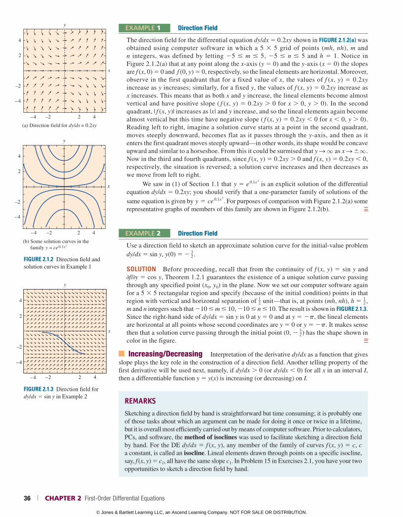
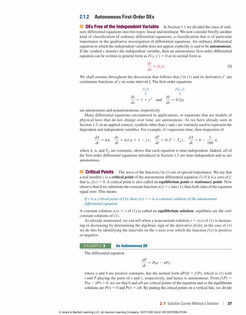
EXAMPLE 1 Direction Field
The direction field for the differential equation dy/dx 5 0.2xy shown in FIGURE 2.1.2(a) was obtained using computer software in which a 5 3 5 grid of points (mh, nh), m and n integers, was defined by letting 25 # m # 5, 25 # n # 5 and h 5 1. Notice in Figure 2.1.2(a) that at any point along the x-axis (y 5 0) and the y-axis (x 5 0) the slopes are f (x, 0) 5 0 and f (0, y) 5 0, respectively, so the lineal elements are horizontal. Moreover, observe in the first quadrant that for a fixed value of x, the values of f (x, y) 5 0.2xy increase as y increases; similarly, for a fixed y, the values of f (x, y) 5 0.2xy increase as x increases. This means that as both x and y increase, the lineal elements become almost vertical and have positive slope ( f (x, y) 5 0.2xy 0 for x 0, y 0). In the second quadrant, | f (x, y)| increases as |x| and y increase, and so the lineal elements again become almost vertical but this time have negative slope ( f (x, y) 5 0.2xy 0 for x 0, y 0). Reading left to right, imagine a solution curve starts at a point in the second quadrant, moves steeply downward, becomes flat as it passes through the y-axis, and then as it enters the first quadrant moves steeply upward—in other words, its shape would be concave upward and similar to a horseshoe. From this it could be surmised that y S q as x S 6q . Now in the third and fourth quadrants, since f (x, y) 5 0.2xy 0 and f (x, y) 5 0.2xy 0, respectively, the situation is reversed; a solution curve increases and then decreases as we move from left to right.
We saw in (1) of Section 1.1 that y 5 e 0.1x
2
is an explicit solution of the differential equation dy/dx 5 0.2xy; you should verify that a one-parameter family of solutions of the
same equation is given by y 5 ce 0.1x
2
. For purposes of comparison with Fig ure 2.1.2(a) some representative graphs of members of this family are shown in Figure 2.1.2(b).
EXAMPLE 2 Direction Field
Use a direction field to sketch an approximate solution curve for the initial-value problem dy/dx 5 sin y, y(0) 5 2 32 .
SOLUTION Before proceeding, recall that from the continuity of f (x, y) 5 sin y and 0f/0y 5 cos y, Theorem 1.2.1 guarantees the existence of a unique solution curve passing through any specified point (x0, y0) in the plane. Now we set our computer software again for a 5 3 5 rectangular region and specify (because of the initial condition) points in that region with vertical and horizontal separation of 1
2 unit—that is, at points (mh, nh), h 5 12 ,
m and n integers such that 210 # m # 10, 210 # n # 10. The result is shown in FIGURE 2.1.3. Since the right-hand side of dy/dx 5 sin y is 0 at y 5 0 and at y 5 2p, the lineal elements are horizontal at all points whose second coordinates are y 5 0 or y 5 2p. It makes sense then that a solution curve passing through the initial point (0, 2 32) has the shape shown in color in the figure.
Increasing/Decreasing Interpretation of the derivative dy/dx as a function that gives slope plays the key role in the construction of a direction field. Another telling property of the first derivative will be used next, namely, if dy/dx 0 (or dy/dx 0) for all x in an interval I, then a differentiable function y 5 y(x) is increasing (or decreasing) on I.
REMARKSSketching a direction field by hand is straightforward but time consuming; it is probably one of those tasks about which an argument can be made for doing it once or twice in a lifetime, but it is overall most efficiently carried out by means of computer software. Prior to calculators, PCs, and software, the method of isoclines was used to facilitate sketching a direction field by hand. For the DE dy/dx 5 f (x, y), any member of the family of curves f (x, y) 5 c, c a constant, is called an isocline. Lineal elements drawn through points on a specific isocline, say, f (x, y) 5 c1, all have the same slope c1. In Problem 15 in Exercises 2.1, you have your two opportunities to sketch a direction field by hand.
FIGURE 2.1.2 Direction field and solution curves in Example 1
y
4
2
42
x
(b) Some solution curves in thefamily y = ce0.1x2
4
2
–4
–4
–4
–4
–2
–2
–2
–2
42
y
x
(a) Direction field for dy/dx = 0.2xy
FIGURE 2.1.3 Direction field for dy/dx 5 sin y in Example 2
4
2
–4
–4 –2 42
y
x
–2
36 | CHAPTER 2 First-Order Differential Equations
© Jones & Bartlett Learning LLC, an Ascend Learning Company. NOT FOR SALE OR DISTRIBUTION.
© Jones & Bartlett Learning, LLCNOT FOR SALE OR DISTRIBUTION
© Jones & Bartlett Learning, LLCNOT FOR SALE OR DISTRIBUTION
© Jones & Bartlett Learning, LLCNOT FOR SALE OR DISTRIBUTION
© Jones & Bartlett Learning, LLCNOT FOR SALE OR DISTRIBUTION
© Jones & Bartlett Learning, LLCNOT FOR SALE OR DISTRIBUTION
© Jones & Bartlett Learning, LLCNOT FOR SALE OR DISTRIBUTION
© Jones & Bartlett Learning, LLCNOT FOR SALE OR DISTRIBUTION
© Jones & Bartlett Learning, LLCNOT FOR SALE OR DISTRIBUTION
© Jones & Bartlett Learning, LLCNOT FOR SALE OR DISTRIBUTION
© Jones & Bartlett Learning, LLCNOT FOR SALE OR DISTRIBUTION
© Jones & Bartlett Learning, LLCNOT FOR SALE OR DISTRIBUTION
© Jones & Bartlett Learning, LLCNOT FOR SALE OR DISTRIBUTION
© Jones & Bartlett Learning, LLCNOT FOR SALE OR DISTRIBUTION
© Jones & Bartlett Learning, LLCNOT FOR SALE OR DISTRIBUTION
© Jones & Bartlett Learning, LLCNOT FOR SALE OR DISTRIBUTION
© Jones & Bartlett Learning, LLCNOT FOR SALE OR DISTRIBUTION
© Jones & Bartlett Learning, LLCNOT FOR SALE OR DISTRIBUTION
© Jones & Bartlett Learning, LLCNOT FOR SALE OR DISTRIBUTION
© Jones & Bartlett Learning, LLCNOT FOR SALE OR DISTRIBUTION
© Jones & Bartlett Learning, LLCNOT FOR SALE OR DISTRIBUTION
2.1.2 Autonomous First-Order DEs
DEs Free of the Independent Variable In Section 1.1 we divided the class of ordi-nary differential equations into two types: linear and nonlinear. We now consider briefly another kind of classification of ordinary differential equations, a classification that is of particular importance in the qualitative investigation of differential equations. An ordinary differential equation in which the independent variable does not appear explicitly is said to be autonomous. If the symbol x denotes the independent variable, then an autonomous first-order differential equation can be written in general form as F(y, y9) 5 0 or in normal form as
dy
dx5 f ( y). (1)
We shall assume throughout the discussion that follows that f in (1) and its derivative f 9 are continuous functions of y on some interval I. The first-order equations
f ( y) f (x, y) T T
dy
dx5 1 1 y
2 and dydx
5 0.2xy
are autonomous and nonautonomous, respectively.Many differential equations encountered in applications, or equations that are models of
physical laws that do not change over time, are autonomous. As we have already seen in Section 1.3, in an applied context, symbols other than y and x are routinely used to represent the dependent and independent variables. For example, if t represents time, then inspection of
dAdt
5 kA, dxdt
5 kx(n 1 1 2 x) , dTdt
5 k(T 2 Tm ) , dAdt
5 6 21
100 A,
where k, n, and Tm are constants, shows that each equation is time-independent. Indeed, all of the first-order differential equations introduced in Section 1.3 are time-independent and so are autonomous.
Critical Points The zeros of the function f in (1) are of special importance. We say that a real number c is a critical point of the autonomous differential equation (1) if it is a zero of f , that is, f (c) 5 0. A critical point is also called an equilibrium point or stationary point. Now observe that if we substitute the constant function y(x) 5 c into (1), then both sides of the equation equal zero. This means
If c is a critical point of (1), then y (x) 5 c is a constant solution of the autonomous differential equation.
A constant solution y(x) 5 c of (1) is called an equilibrium solution; equilibria are the only constant solutions of (1).
As already mentioned, we can tell when a nonconstant solution y 5 y(x) of (1) is increas-ing or decreasing by determining the algebraic sign of the derivative dy/dx; in the case of (1) we do this by identifying the intervals on the y-axis over which the function f (y) is positive or negative.
EXAMPLE 3 An Autonomous DE
The differential equation
dP
dt5 P(a 2 bP),
where a and b are positive constants, has the normal form dP/dt 5 f (P), which is (1) with t and P playing the parts of x and y, respectively, and hence is autonomous. From f (P) 5 P(a 2 bP) 5 0, we see that 0 and a/b are critical points of the equation and so the equilibrium solutions are P(t) 5 0 and P(t) 5 a/b. By putting the critical points on a vertical line, we divide
2.1 Solution Curves Without a Solution | 37
© Jones & Bartlett Learning LLC, an Ascend Learning Company. NOT FOR SALE OR DISTRIBUTION.
© Jones & Bartlett Learning, LLCNOT FOR SALE OR DISTRIBUTION
© Jones & Bartlett Learning, LLCNOT FOR SALE OR DISTRIBUTION
© Jones & Bartlett Learning, LLCNOT FOR SALE OR DISTRIBUTION
© Jones & Bartlett Learning, LLCNOT FOR SALE OR DISTRIBUTION
© Jones & Bartlett Learning, LLCNOT FOR SALE OR DISTRIBUTION
© Jones & Bartlett Learning, LLCNOT FOR SALE OR DISTRIBUTION
© Jones & Bartlett Learning, LLCNOT FOR SALE OR DISTRIBUTION
© Jones & Bartlett Learning, LLCNOT FOR SALE OR DISTRIBUTION
© Jones & Bartlett Learning, LLCNOT FOR SALE OR DISTRIBUTION
© Jones & Bartlett Learning, LLCNOT FOR SALE OR DISTRIBUTION
© Jones & Bartlett Learning, LLCNOT FOR SALE OR DISTRIBUTION
© Jones & Bartlett Learning, LLCNOT FOR SALE OR DISTRIBUTION
© Jones & Bartlett Learning, LLCNOT FOR SALE OR DISTRIBUTION
© Jones & Bartlett Learning, LLCNOT FOR SALE OR DISTRIBUTION
© Jones & Bartlett Learning, LLCNOT FOR SALE OR DISTRIBUTION
© Jones & Bartlett Learning, LLCNOT FOR SALE OR DISTRIBUTION
© Jones & Bartlett Learning, LLCNOT FOR SALE OR DISTRIBUTION
© Jones & Bartlett Learning, LLCNOT FOR SALE OR DISTRIBUTION
© Jones & Bartlett Learning, LLCNOT FOR SALE OR DISTRIBUTION
© Jones & Bartlett Learning, LLCNOT FOR SALE OR DISTRIBUTION
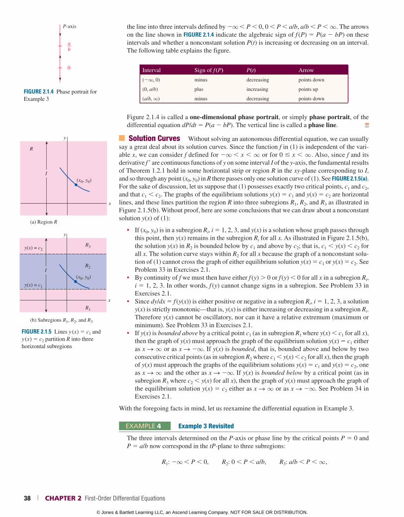
FIGURE 2.1.4 Phase portrait for Example 3
P-axis
ab
0
FIGURE 2.1.5 Lines y (x ) 5 c1 and y (x ) 5 c2 partition R into three horizontal subregions
x
y
R
I
(a) Region R
x
I
(b) Subregions R1, R2, and R3
y
(x0, y0)
(x0, y0)
R3
R2
R1
y(x) = c2
y(x) = c1
the line into three intervals defined by 2q P 0, 0 P a/b, a/b P q . The arrows on the line shown in FIGURE 2.1.4 indicate the algebraic sign of f (P) 5 P(a 2 bP) on these intervals and whether a nonconstant solution P(t) is increasing or decreasing on an interval. The following table explains the figure.
Interval Sign of f (P) P(t) Arrow
(2q, 0) minus decreasing points down
(0, a/b) plus increasing points up
(a/b, q) minus decreasing points down
Figure 2.1.4 is called a one-dimensional phase portrait, or simply phase portrait, of the differential equation dP/dt 5 P(a 2 bP). The vertical line is called a phase line.
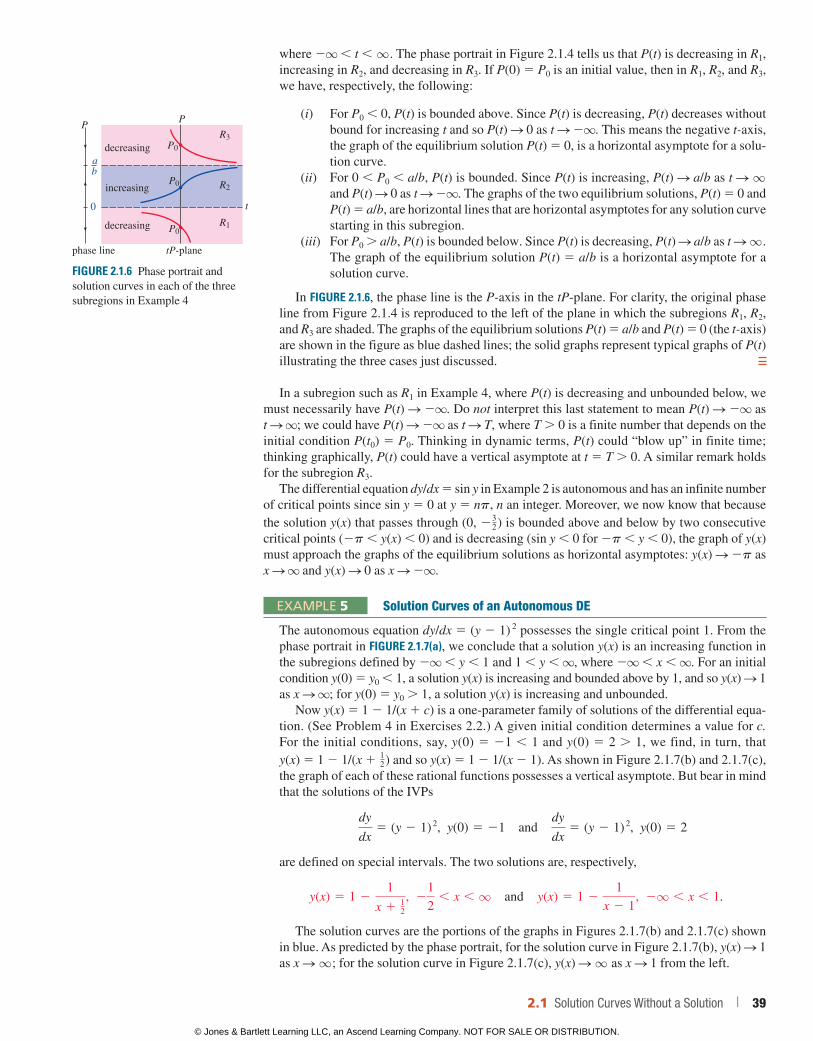
Solution Curves Without solving an autonomous differential equation, we can usually say a great deal about its solution curves. Since the function f in (1) is independent of the vari-able x, we can consider f defined for 2q x q or for 0 # x q . Also, since f and its derivative f 9 are continuous functions of y on some interval I of the y-axis, the fundamental results of Theorem 1.2.1 hold in some horizontal strip or region R in the xy-plane corresponding to I, and so through any point (x0, y0) in R there passes only one solution curve of (1). See FIGURE 2.1.5 (a). For the sake of discussion, let us suppose that (1) possesses exactly two critical points, c1 and c2, and that c1 c2. The graphs of the equilibrium solutions y(x) 5 c1 and y(x) 5 c2 are horizontal lines, and these lines partition the region R into three subregions R1, R2, and R3 as illustrated in Figure 2.1.5(b). Without proof, here are some conclusions that we can draw about a nonconstant solution y(x) of (1):
• If (x0, y0) is in a subregion Ri, i 5 1, 2, 3, and y(x) is a solution whose graph passes through this point, then y(x) remains in the subregion Ri for all x. As illustrated in Figure 2.1.5(b), the solution y(x) in R2 is bounded below by c1 and above by c2; that is, c1 y(x) c2 for all x. The solution curve stays within R2 for all x because the graph of a nonconstant solu-tion of (1) cannot cross the graph of either equilibrium solution y(x) 5 c1 or y(x) 5 c2. See Problem 33 in Exercises 2.1.
• By continuity of f we must then have either f (y) 0 or f (y) 0 for all x in a subregion Ri, i 5 1, 2, 3. In other words, f (y) cannot change signs in a subregion. See Problem 33 in Exercises 2.1.
• Since dy/dx 5 f (y(x)) is either positive or negative in a subregion Ri, i 5 1, 2, 3, a solution y(x) is strictly monotonic—that is, y(x) is either increasing or decreasing in a subregion Ri. Therefore y(x) cannot be oscillatory, nor can it have a relative extremum (maximum or minimum). See Problem 33 in Exercises 2.1.
• If y(x) is bounded above by a critical point c1 (as in subregion R1 where y(x) c1 for all x), then the graph of y(x) must approach the graph of the equilibrium solution y(x) 5 c1 either as x S q or as x S 2q. If y(x) is bounded, that is, bounded above and below by two consecutive critical points (as in subregion R2 where c1 y(x) c2 for all x), then the graph of y(x) must approach the graphs of the equilibrium solutions y(x) 5 c1 and y(x) 5 c2, one as x S q and the other as x S 2q. If y(x) is bounded below by a critical point (as in subregion R3 where c2 y(x) for all x), then the graph of y(x) must approach the graph of the equilibrium solution y(x) 5 c2 either as x S q or as x S 2q. See Problem 34 in Exercises 2.1.
With the foregoing facts in mind, let us reexamine the differential equation in Example 3.
EXAMPLE 4 Example 3 Revisited
The three intervals determined on the P-axis or phase line by the critical points P 5 0 and P 5 a/b now correspond in the tP-plane to three subregions:
R1: 2q P 0, R2: 0 P a/b, R3: a/b P q ,
38 | CHAPTER 2 First-Order Differential Equations
© Jones & Bartlett Learning LLC, an Ascend Learning Company. NOT FOR SALE OR DISTRIBUTION.
© Jones & Bartlett Learning, LLCNOT FOR SALE OR DISTRIBUTION
© Jones & Bartlett Learning, LLCNOT FOR SALE OR DISTRIBUTION
© Jones & Bartlett Learning, LLCNOT FOR SALE OR DISTRIBUTION
© Jones & Bartlett Learning, LLCNOT FOR SALE OR DISTRIBUTION
© Jones & Bartlett Learning, LLCNOT FOR SALE OR DISTRIBUTION
© Jones & Bartlett Learning, LLCNOT FOR SALE OR DISTRIBUTION
© Jones & Bartlett Learning, LLCNOT FOR SALE OR DISTRIBUTION
© Jones & Bartlett Learning, LLCNOT FOR SALE OR DISTRIBUTION
© Jones & Bartlett Learning, LLCNOT FOR SALE OR DISTRIBUTION
© Jones & Bartlett Learning, LLCNOT FOR SALE OR DISTRIBUTION
© Jones & Bartlett Learning, LLCNOT FOR SALE OR DISTRIBUTION
© Jones & Bartlett Learning, LLCNOT FOR SALE OR DISTRIBUTION
© Jones & Bartlett Learning, LLCNOT FOR SALE OR DISTRIBUTION
© Jones & Bartlett Learning, LLCNOT FOR SALE OR DISTRIBUTION
© Jones & Bartlett Learning, LLCNOT FOR SALE OR DISTRIBUTION
© Jones & Bartlett Learning, LLCNOT FOR SALE OR DISTRIBUTION
© Jones & Bartlett Learning, LLCNOT FOR SALE OR DISTRIBUTION
© Jones & Bartlett Learning, LLCNOT FOR SALE OR DISTRIBUTION
© Jones & Bartlett Learning, LLCNOT FOR SALE OR DISTRIBUTION
© Jones & Bartlett Learning, LLCNOT FOR SALE OR DISTRIBUTION
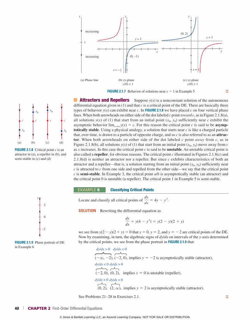
where 2q t q . The phase portrait in Figure 2.1.4 tells us that P(t) is decreasing in R1, increasing in R2, and decreasing in R3. If P(0) 5 P0 is an initial value, then in R1, R2, and R3, we have, respectively, the following:
(i) For P0 0, P(t) is bounded above. Since P(t) is decreasing, P(t) decreases without bound for increasing t and so P(t) S 0 as t S 2q. This means the negative t-axis, the graph of the equilibrium solution P(t) 5 0, is a horizontal asymptote for a solu-tion curve.
(ii) For 0 P0 a/b, P(t) is bounded. Since P(t) is increasing, P(t) S a/b as t S q and P(t) S 0 as t S 2q. The graphs of the two equilibrium solutions, P(t) 5 0 and P(t) 5 a/b, are horizontal lines that are horizontal asymptotes for any solution curve starting in this subregion.
(iii) For P0 a/b, P(t) is bounded below. Since P(t) is decreasing, P(t) S a/b as t S q . The graph of the equilibrium solution P(t) 5 a/b is a horizontal asymptote for a solution curve.
In FIGURE 2.1.6, the phase line is the P-axis in the tP-plane. For clarity, the original phase line from Figure 2.1.4 is reproduced to the left of the plane in which the subregions R1, R2, and R3 are shaded. The graphs of the equilibrium solutions P(t) 5 a/b and P(t) 5 0 (the t-axis) are shown in the figure as blue dashed lines; the solid graphs represent typical graphs of P(t) illustrating the three cases just discussed.
In a subregion such as R1 in Example 4, where P(t) is decreasing and unbounded below, we must necessarily have P(t) S 2q. Do not interpret this last statement to mean P(t) S 2q as t S q; we could have P(t) S 2q as t S T, where T 0 is a finite number that depends on the initial condition P(t0) 5 P0. Thinking in dynamic terms, P(t) could “blow up” in finite time; thinking graphically, P(t) could have a vertical asymptote at t 5 T 0. A similar remark holds for the subregion R3.
The differential equation dy/dx 5 sin y in Example 2 is autonomous and has an infinite number of critical points since sin y 5 0 at y 5 np, n an integer. Moreover, we now know that because the solution y(x) that passes through (0, 23
2) is bounded above and below by two consecutive critical points (2p y(x) 0) and is decreasing (sin y 0 for 2p y 0), the graph of y(x) must approach the graphs of the equilibrium solutions as horizontal asymptotes: y(x) S 2p as x S q and y(x) S 0 as x S 2q.
EXAMPLE 5 Solution Curves of an Autonomous DE
The autonomous equation dy/dx 5 (y 2 1) 2 possesses the single critical point 1. From the phase portrait in FIGURE 2.1.7(a), we conclude that a solution y(x) is an increasing function in the subregions defined by 2q y 1 and 1 y q, where 2q x q. For an initial condition y(0) 5 y0 1, a solution y(x) is increasing and bounded above by 1, and so y(x) S 1 as x S q; for y(0) 5 y0 1, a solution y(x) is increasing and unbounded.
Now y(x) 5 1 2 1/(x 1 c) is a one-parameter family of solutions of the differential equa-tion. (See Problem 4 in Exercises 2.2.) A given initial condition determines a value for c. For the initial conditions, say, y(0) 5 21 1 and y(0) 5 2 1, we find, in turn, that y(x) 5 1 2 1/(x 1 1
2) and so y(x) 5 1 2 1/(x 2 1). As shown in Figure 2.1.7(b) and 2.1.7(c), the graph of each of these rational functions possesses a vertical asymptote. But bear in mind that the solutions of the IVPs
dy
dx5 (y 2 1)
2, y(0) 5 21 and dy
dx5 (y 2 1)
2, y(0) 5 2
are defined on special intervals. The two solutions are, respectively,
y(x) 5 1 21
x 1 12
, 21
2, x , q and y(x) 5 1 2
1
x 2 1, 2q , x , 1.
The solution curves are the portions of the graphs in Figures 2.1.7(b) and 2.1.7(c) shown in blue. As predicted by the phase portrait, for the solution curve in Figure 2.1.7(b), y(x) S 1 as x S q ; for the solution curve in Figure 2.1.7(c), y(x) S q as x S 1 from the left.
FIGURE 2.1.6 Phase portrait and solution curves in each of the three subregions in Example 4
P
ab
0
decreasing
increasing
decreasing
phase line tP-plane
P0
P0
P0
P
R1
R2
R3
t
2.1 Solution Curves Without a Solution | 39
© Jones & Bartlett Learning LLC, an Ascend Learning Company. NOT FOR SALE OR DISTRIBUTION.
© Jones & Bartlett Learning, LLCNOT FOR SALE OR DISTRIBUTION
© Jones & Bartlett Learning, LLCNOT FOR SALE OR DISTRIBUTION
© Jones & Bartlett Learning, LLCNOT FOR SALE OR DISTRIBUTION
© Jones & Bartlett Learning, LLCNOT FOR SALE OR DISTRIBUTION
© Jones & Bartlett Learning, LLCNOT FOR SALE OR DISTRIBUTION
© Jones & Bartlett Learning, LLCNOT FOR SALE OR DISTRIBUTION
© Jones & Bartlett Learning, LLCNOT FOR SALE OR DISTRIBUTION
© Jones & Bartlett Learning, LLCNOT FOR SALE OR DISTRIBUTION
© Jones & Bartlett Learning, LLCNOT FOR SALE OR DISTRIBUTION
© Jones & Bartlett Learning, LLCNOT FOR SALE OR DISTRIBUTION
© Jones & Bartlett Learning, LLCNOT FOR SALE OR DISTRIBUTION
© Jones & Bartlett Learning, LLCNOT FOR SALE OR DISTRIBUTION
© Jones & Bartlett Learning, LLCNOT FOR SALE OR DISTRIBUTION
© Jones & Bartlett Learning, LLCNOT FOR SALE OR DISTRIBUTION
© Jones & Bartlett Learning, LLCNOT FOR SALE OR DISTRIBUTION
© Jones & Bartlett Learning, LLCNOT FOR SALE OR DISTRIBUTION
© Jones & Bartlett Learning, LLCNOT FOR SALE OR DISTRIBUTION
© Jones & Bartlett Learning, LLCNOT FOR SALE OR DISTRIBUTION
© Jones & Bartlett Learning, LLCNOT FOR SALE OR DISTRIBUTION
© Jones & Bartlett Learning, LLCNOT FOR SALE OR DISTRIBUTION
1
y
increasing
increasing
y
(0, 2)y = 1
x = 1
y
x = –
y = 1
(0, –1)
x x
(a) Phase line (b) xy-plane y (0) < 1
(c) xy-plane y (0) > 1
12
FIGURE 2.1.7 Behavior of solutions near y 5 1 in Example 5
Attractors and Repellers Suppose y(x) is a nonconstant solution of the autonomous differential equation given in (1) and that c is a critical point of the DE. There are basically three types of behavior y(x) can exhibit near c. In FIGURE 2.1.8 we have placed c on four vertical phase lines. When both arrowheads on either side of the dot labeled c point toward c, as in Figure 2.1.8(a), all solutions y(x) of (1) that start from an initial point (x0, y0) sufficiently near c exhibit the asymptotic behavior limxSq y(x) 5 c. For this reason the critical point c is said to be asymp-totically stable. Using a physical analogy, a solution that starts near c is like a charged particle that, over time, is drawn to a particle of opposite charge, and so c is also referred to as an attrac-tor. When both arrowheads on either side of the dot labeled c point away from c, as in Figure 2.1.8(b), all solutions y(x) of (1) that start from an initial point (x0, y0) move away from c as x increases. In this case the critical point c is said to be unstable. An unstable critical point is also called a repeller, for obvious reasons. The critical point c illustrated in Figures 2.1.8(c) and 2.1.8(d) is neither an attractor nor a repeller. But since c exhibits characteristics of both an attractor and a repeller—that is, a solution starting from an initial point (x0, y0) sufficiently near c is attracted to c from one side and repelled from the other side—we say that the critical point c is semi-stable. In Example 3, the critical point a/b is asymptotically stable (an attractor) and the critical point 0 is unstable (a repeller). The critical point 1 in Example 5 is semi-stable.
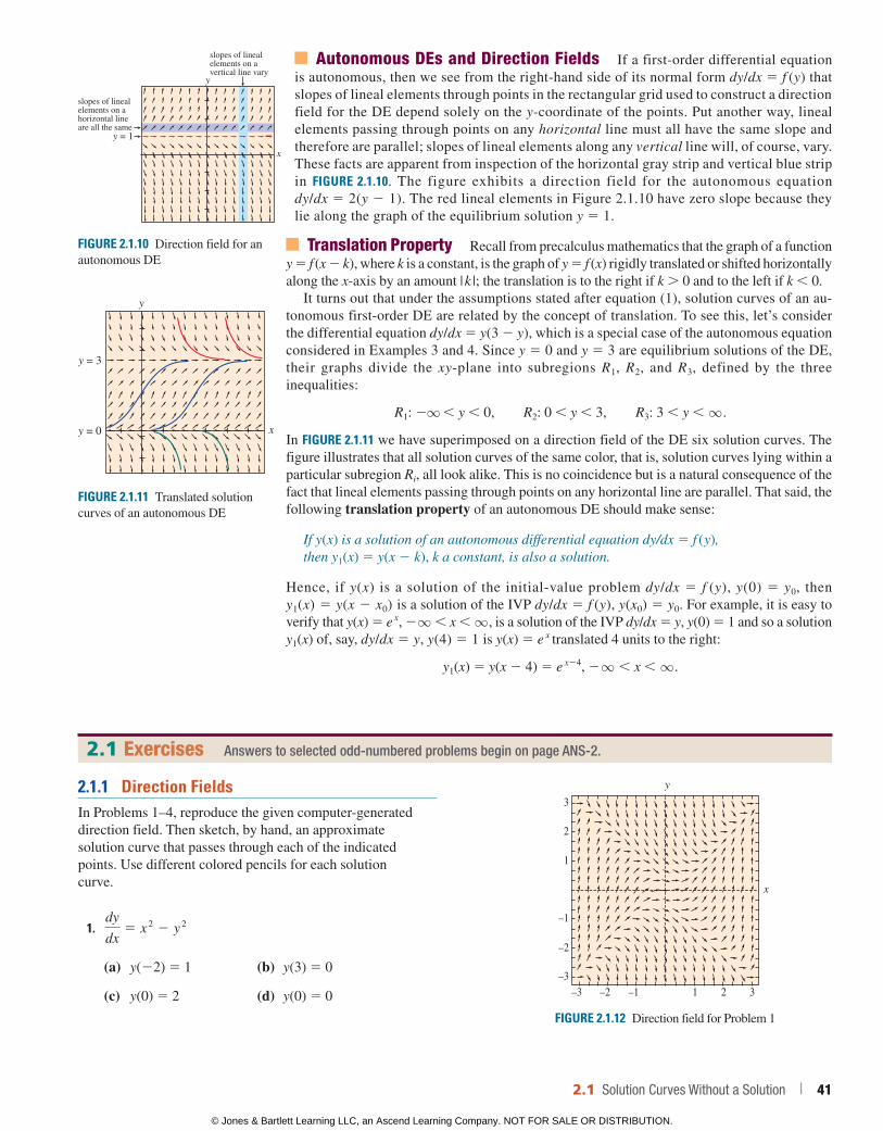
EXAMPLE 6 Classifying Critical Points
Locate and classify all critical points of dy
dx5 4y 2 y
3.
SOLUTION Rewriting the differential equation as
dy
dx5 y(4 2 y
2) 5 y(2 2 y)(2 1 y)
we see from y(2 2 y)(2 1 y) 5 0 that y 5 0, y 5 2, and y 5 2 2 are critical points of the DE.Now by examining, in turn, the algebraic signs of dy/dx on intervals of the y-axis determined by the critical points, we see from the phase portrait in FIGURE 2.1.9 that:
(2q, 22), (22, 0)
dy/dx > 0 dy/dx < 0
, implies y 5 22 is asymptotically stable (attractor),
(22, 0), (0, 2),
dy/dx < 0 dy/dx > 0
implies y 5 0 is unstable (repeller),
(0, 2), (2, q),
dy/dx > 0 dy/dx < 0
implies y 5 2 is asymptotically stable (attractor).
See Problems 21–28 in Exercises 2.1.
FIGURE 2.1.8 Critical point c is an attractor in (a), a repeller in (b), and semi-stable in (c) and (d)
(a) (b) (c) (d)
y0
y0y0
y0
c c c c
y
2
0
–2
FIGURE 2.1.9 Phase portrait of DE in Example 6
40 | CHAPTER 2 First-Order Differential Equations
© Jones & Bartlett Learning LLC, an Ascend Learning Company. NOT FOR SALE OR DISTRIBUTION.
© Jones & Bartlett Learning, LLCNOT FOR SALE OR DISTRIBUTION
© Jones & Bartlett Learning, LLCNOT FOR SALE OR DISTRIBUTION
© Jones & Bartlett Learning, LLCNOT FOR SALE OR DISTRIBUTION
© Jones & Bartlett Learning, LLCNOT FOR SALE OR DISTRIBUTION
© Jones & Bartlett Learning, LLCNOT FOR SALE OR DISTRIBUTION
© Jones & Bartlett Learning, LLCNOT FOR SALE OR DISTRIBUTION
© Jones & Bartlett Learning, LLCNOT FOR SALE OR DISTRIBUTION
© Jones & Bartlett Learning, LLCNOT FOR SALE OR DISTRIBUTION
© Jones & Bartlett Learning, LLCNOT FOR SALE OR DISTRIBUTION
© Jones & Bartlett Learning, LLCNOT FOR SALE OR DISTRIBUTION
© Jones & Bartlett Learning, LLCNOT FOR SALE OR DISTRIBUTION
© Jones & Bartlett Learning, LLCNOT FOR SALE OR DISTRIBUTION
© Jones & Bartlett Learning, LLCNOT FOR SALE OR DISTRIBUTION
© Jones & Bartlett Learning, LLCNOT FOR SALE OR DISTRIBUTION
© Jones & Bartlett Learning, LLCNOT FOR SALE OR DISTRIBUTION
© Jones & Bartlett Learning, LLCNOT FOR SALE OR DISTRIBUTION
© Jones & Bartlett Learning, LLCNOT FOR SALE OR DISTRIBUTION
© Jones & Bartlett Learning, LLCNOT FOR SALE OR DISTRIBUTION
© Jones & Bartlett Learning, LLCNOT FOR SALE OR DISTRIBUTION
© Jones & Bartlett Learning, LLCNOT FOR SALE OR DISTRIBUTION
Autonomous DEs and Direction Fields If a first-order differential equation is autonomous, then we see from the right-hand side of its normal form dy/dx 5 f (y) that slopes of lineal elements through points in the rectangular grid used to construct a direction field for the DE depend solely on the y-coordinate of the points. Put another way, lineal elements passing through points on any horizontal line must all have the same slope and therefore are parallel; slopes of lineal elements along any vertical line will, of course, vary. These facts are apparent from inspection of the horizontal gray strip and vertical blue strip in FIGURE 2.1.10. The figure exhibits a direction field for the autonomous equation dy/dx 5 2(y 2 1). The red lineal elements in Figure 2.1.10 have zero slope because they lie along the graph of the equilibrium solution y 5 1.
Translation Property Recall from precalculus mathematics that the graph of a function y 5 f (x 2 k), where k is a constant, is the graph of y 5 f (x) rigidly translated or shifted horizontally along the x-axis by an amount | k |; the translation is to the right if k . 0 and to the left if k , 0.
It turns out that under the assumptions stated after equation (1), solution curves of an au-tonomous first-order DE are related by the concept of translation. To see this, let’s consider the differential equation dy/dx 5 y(3 2 y), which is a special case of the autonomous equation considered in Examples 3 and 4. Since y 5 0 and y 5 3 are equilibrium solutions of the DE, their graphs divide the xy-plane into subregions R1, R2, and R3, defined by the three inequalities:
R1: 2q y 0, R2: 0 y 3, R3: 3 y q .
In FIGURE 2.1.11 we have superimposed on a direction field of the DE six solution curves. The figure illustrates that all solution curves of the same color, that is, solution curves lying within a particular subregion Ri, all look alike. This is no coincidence but is a natural consequence of the fact that lineal elements passing through points on any horizontal line are parallel. That said, the following translation property of an autonomous DE should make sense:
If y(x) is a solution of an autonomous differential equation dy/dx 5 f ( y), then y1(x) 5 y(x 2 k), k a constant, is also a solution.
Hence, if y(x) is a solution of the initial-value problem dy/dx 5 f (y), y(0) 5 y0, then y1(x) 5 y(x 2 x0) is a solution of the IVP dy/dx 5 f (y), y(x0) 5 y0. For example, it is easy to verify that y(x) 5 e x, 2q x q , is a solution of the IVP dy/dx 5 y, y(0) 5 1 and so a solution y1(x) of, say, dy/dx 5 y, y(4) 5 1 is y(x) 5 e x translated 4 units to the right:
y1(x) 5 y(x 2 4) 5 e x24, 2q x q .
2.1.1 Direction FieldsIn Problems 1–4, reproduce the given computer-generated direction field. Then sketch, by hand, an approximate solution curve that passes through each of the indicated points. Use different colored pencils for each solution curve.
1. dy
dx5 x
2 2 y 2
(a) y(22) 5 1 (b) y(3) 5 0
(c) y(0) 5 2 (d) y(0) 5 0
FIGURE 2.1.12 Direction field for Problem 1
y
x
3
2
1
–1
–2
–3–3 –2 –1 1 2 3
FIGURE 2.1.11 Translated solution curves of an autonomous DE
y = 3
y = 0
y
x
FIGURE 2.1.10 Direction field for an autonomous DE
slopes of linealelements on avertical line vary
slopes of linealelements on ahorizontal lineare all the same
y = 1
y
x
2.1 Exercises Answers to selected odd-numbered problems begin on page ANS-2.
2.1 Solution Curves Without a Solution | 41
© Jones & Bartlett Learning LLC, an Ascend Learning Company. NOT FOR SALE OR DISTRIBUTION.
© Jones & Bartlett Learning, LLCNOT FOR SALE OR DISTRIBUTION
© Jones & Bartlett Learning, LLCNOT FOR SALE OR DISTRIBUTION
© Jones & Bartlett Learning, LLCNOT FOR SALE OR DISTRIBUTION
© Jones & Bartlett Learning, LLCNOT FOR SALE OR DISTRIBUTION
© Jones & Bartlett Learning, LLCNOT FOR SALE OR DISTRIBUTION
© Jones & Bartlett Learning, LLCNOT FOR SALE OR DISTRIBUTION
© Jones & Bartlett Learning, LLCNOT FOR SALE OR DISTRIBUTION
© Jones & Bartlett Learning, LLCNOT FOR SALE OR DISTRIBUTION
© Jones & Bartlett Learning, LLCNOT FOR SALE OR DISTRIBUTION
© Jones & Bartlett Learning, LLCNOT FOR SALE OR DISTRIBUTION
© Jones & Bartlett Learning, LLCNOT FOR SALE OR DISTRIBUTION
© Jones & Bartlett Learning, LLCNOT FOR SALE OR DISTRIBUTION
© Jones & Bartlett Learning, LLCNOT FOR SALE OR DISTRIBUTION
© Jones & Bartlett Learning, LLCNOT FOR SALE OR DISTRIBUTION
© Jones & Bartlett Learning, LLCNOT FOR SALE OR DISTRIBUTION
© Jones & Bartlett Learning, LLCNOT FOR SALE OR DISTRIBUTION
© Jones & Bartlett Learning, LLCNOT FOR SALE OR DISTRIBUTION
© Jones & Bartlett Learning, LLCNOT FOR SALE OR DISTRIBUTION
© Jones & Bartlett Learning, LLCNOT FOR SALE OR DISTRIBUTION
© Jones & Bartlett Learning, LLCNOT FOR SALE OR DISTRIBUTION
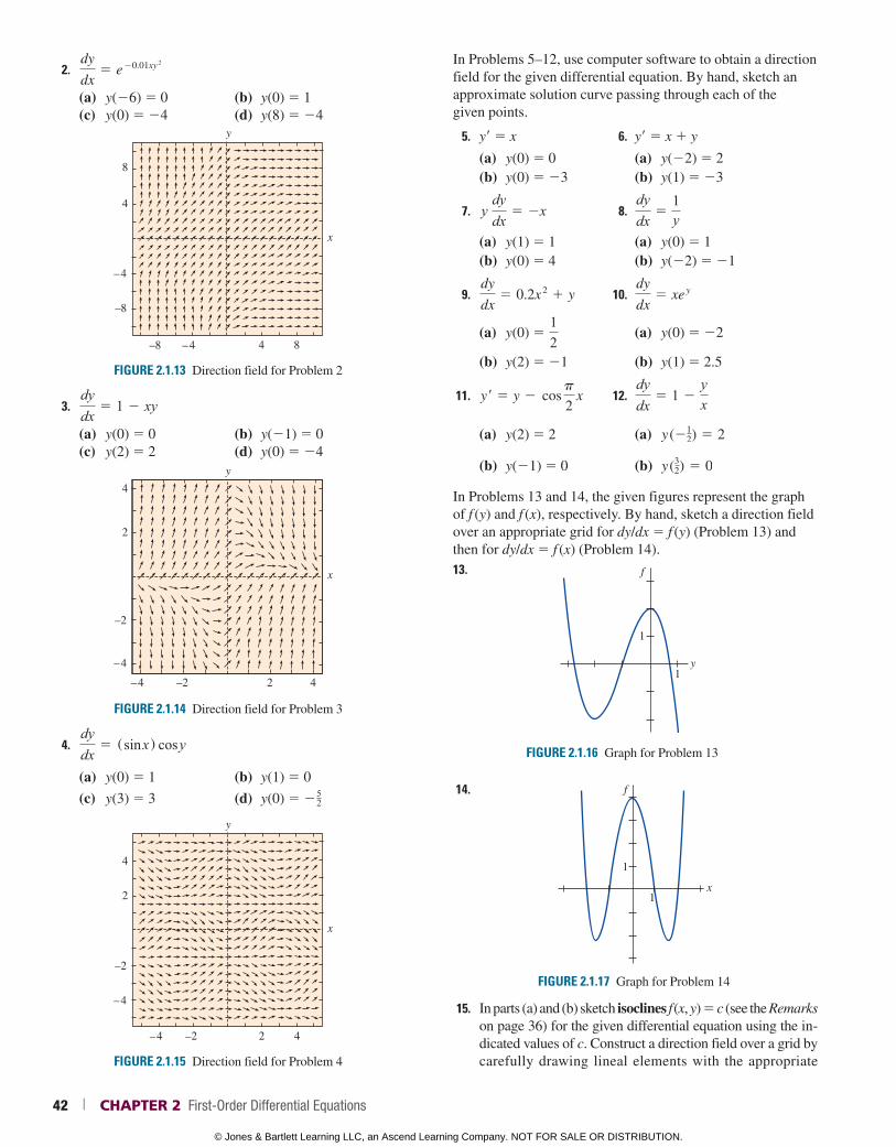
2. dy
dx5 e
20.01xy 2
(a) y(26) 5 0 (b) y(0) 5 1(c) y(0) 5 24 (d) y(8) 5 24
FIGURE 2.1.13 Direction field for Problem 2
4 8
8
4
x
y
–4
–4
–8
–8
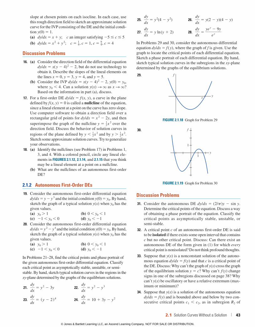
3. dydx
5 1 2 xy
(a) y(0) 5 0 (b) y(21) 5 0(c) y(2) 5 2 (d) y(0) 5 24
FIGURE 2.1.14 Direction field for Problem 3
42
2
4
x
y
–2
–2
–4
–4
4. dydx
5 (sin x) cos y
(a) y(0) 5 1 (b) y(1) 5 0
(c) y(3) 5 3 (d) y(0) 5 252
FIGURE 2.1.15 Direction field for Problem 4
42
2
4
x
y
–2
–2
–4
–4
In Problems 5–12, use computer software to obtain a direction field for the given differential equation. By hand, sketch an approximate solution curve passing through each of the given points.
5. y9 5 x 6. y9 5 x 1 y
(a) y(0) 5 0 (a) y(22) 5 2(b) y(0) 5 23 (b) y(1) 5 23
7. y dydx
5 2x 8. dydx
51y
(a) y(1) 5 1 (a) y(0) 5 1(b) y(0) 5 4 (b) y(22) 5 21
9. dy
dx5 0.2x
2 1 y 10. dy
dx5 xe
y
(a) y(0) 5 12
(a) y(0) 5 22
(b) y(2) 5 21 (b) y(1) 5 2.5
11. y r 5 y 2 cos
p
2 x 12.
dydx
5 1 2yx
(a) y(2) 5 2 (a) y (212) 5 2
(b) y(21) 5 0 (b) y (32) 5 0
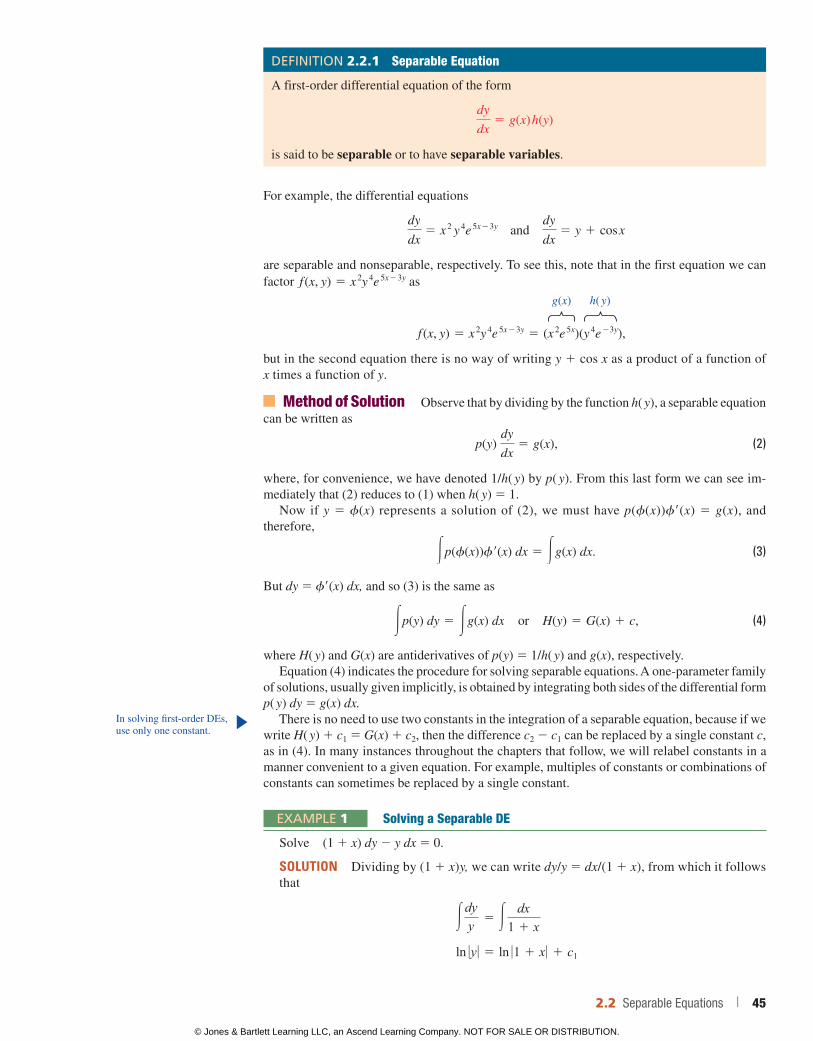
In Problems 13 and 14, the given figures represent the graph of f (y) and f (x), respectively. By hand, sketch a direction field over an appropriate grid for dy/dx 5 f (y) (Problem 13) and then for dy/dx 5 f (x) (Problem 14). 13.
y
f
1
1
FIGURE 2.1.16 Graph for Problem 13
14.
x
f
1
1
FIGURE 2.1.17 Graph for Problem 14
15. In parts (a) and (b) sketch isoclines f (x, y) 5 c (see the Remarks on page 36) for the given differential equation using the in-dicated values of c. Construct a direction field over a grid by carefully drawing lineal elements with the appropriate
42 | CHAPTER 2 First-Order Differential Equations
© Jones & Bartlett Learning LLC, an Ascend Learning Company. NOT FOR SALE OR DISTRIBUTION.
© Jones & Bartlett Learning, LLCNOT FOR SALE OR DISTRIBUTION
© Jones & Bartlett Learning, LLCNOT FOR SALE OR DISTRIBUTION
© Jones & Bartlett Learning, LLCNOT FOR SALE OR DISTRIBUTION
© Jones & Bartlett Learning, LLCNOT FOR SALE OR DISTRIBUTION
© Jones & Bartlett Learning, LLCNOT FOR SALE OR DISTRIBUTION
© Jones & Bartlett Learning, LLCNOT FOR SALE OR DISTRIBUTION
© Jones & Bartlett Learning, LLCNOT FOR SALE OR DISTRIBUTION
© Jones & Bartlett Learning, LLCNOT FOR SALE OR DISTRIBUTION
© Jones & Bartlett Learning, LLCNOT FOR SALE OR DISTRIBUTION
© Jones & Bartlett Learning, LLCNOT FOR SALE OR DISTRIBUTION
© Jones & Bartlett Learning, LLCNOT FOR SALE OR DISTRIBUTION
© Jones & Bartlett Learning, LLCNOT FOR SALE OR DISTRIBUTION
© Jones & Bartlett Learning, LLCNOT FOR SALE OR DISTRIBUTION
© Jones & Bartlett Learning, LLCNOT FOR SALE OR DISTRIBUTION
© Jones & Bartlett Learning, LLCNOT FOR SALE OR DISTRIBUTION
© Jones & Bartlett Learning, LLCNOT FOR SALE OR DISTRIBUTION
© Jones & Bartlett Learning, LLCNOT FOR SALE OR DISTRIBUTION
© Jones & Bartlett Learning, LLCNOT FOR SALE OR DISTRIBUTION
© Jones & Bartlett Learning, LLCNOT FOR SALE OR DISTRIBUTION
© Jones & Bartlett Learning, LLCNOT FOR SALE OR DISTRIBUTION
slope at chosen points on each isocline. In each case, use this rough direction field to sketch an approximate solution curve for the IVP consisting of the DE and the initial condi-tion y(0) 5 1.(a) dy/dx 5 x 1 y; c an integer satisfying 25 # c # 5
(b) dy/dx 5 x 2 1 y 2; c 5 14 , c 5 1, c 5 9
4 , c 5 4
Discussion Problems
16. (a) Consider the direction field of the differential equation dy/dx 5 x( y 2 4) 2 2 2, but do not use technology to obtain it. Describe the slopes of the lineal elements on the lines x 5 0, y 5 3, y 5 4, and y 5 5.
(b) Consider the IVP dy/dx 5 x(y 2 4) 2 2 2, y(0) 5 y0, where y0 4. Can a solution y(x) S q as x S q? Based on the information in part (a), discuss.
17. For a first-order DE dy/dx 5 f (x, y), a curve in the plane defined by f (x, y) 5 0 is called a nullcline of the equation, since a lineal element at a point on the curve has zero slope. Use computer software to obtain a direction field over a rectangular grid of points for dy/dx 5 x 2 2 2y, and then superimpose the graph of the nullcline y 5 1
2x 2 over the direction field. Discuss the behavior of solution curves in regions of the plane defined by y 1
2x 2 and by y 12x 2.
Sketch some approximate solution curves. Try to generalize your observations.
18. (a) Identify the nullclines (see Problem 17) in Prob lems 1, 3, and 4. With a colored pencil, circle any lineal ele-ments in FIGURES 2.1.12, 2.1.14, and 2.1.15 that you think may be a lineal element at a point on a nullcline.
(b) What are the nullclines of an autonomous first-order DE?
2.1.2 Autonomous First-Order DEs
19. Consider the autonomous first-order differential equation dy/dx 5 y 2 y 3 and the initial condition y(0) 5 y0. By hand, sketch the graph of a typical solution y(x) when y0 has the given values.(a) y0 1 (b) 0 y0 1(c) 21 y0 0 (d) y0 21
20. Consider the autonomous first-order differential equation dy/dx 5 y 2 2 y 4 and the initial condition y(0) 5 y0. By hand, sketch the graph of a typical solution y(x) when y0 has the given values.(a) y0 1 (b) 0 y0 1(c) 21 y0 0 (d) y0 21
In Problems 21–28, find the critical points and phase portrait of the given autonomous first-order differential equation. Classify each critical point as asymptotically stable, unstable, or semi- stable. By hand, sketch typical solution curves in the regions in the xy-plane determined by the graphs of the equilibrium solutions.
21. dy
dx5 y
2 2 3y 22. dy
dx5 y
2 2 y 3
23. dydx
5 (y 2 2) 4 24. dy
dx5 10 1 3y 2 y
2
25. dy
dx5 y
2(4 2 y 2) 26.
dy
dx5 y(2 2 y)(4 2 y)
27. dy
dx5 y ln (y 1 2) 28.
dy
dx5
ye y 2 9y
e y
In Problems 29 and 30, consider the autonomous differential equation dy/dx 5 f ( y), where the graph of f is given. Use the graph to locate the critical points of each differential equation. Sketch a phase portrait of each differential equation. By hand, sketch typical solution curves in the subregions in the xy-plane determined by the graphs of the equilibrium solutions.
29.
FIGURE 2.1.18 Graph for Problem 29
yc
f
30.
FIGURE 2.1.19 Graph for Problem 30
1
f
1
y
Discussion Problems
31. Consider the autonomous DE dy/dx 5 (2/p)y 2 sin y. Determine the critical points of the equation. Discuss a way of obtaining a phase portrait of the equation. Classify the critical points as asymptotically stable, unstable, or semi-stable.
32. A critical point c of an autonomous first-order DE is said to be isolated if there exists some open interval that contains c but no other critical point. Discuss: Can there exist an autonomous DE of the form given in (1) for which every critical point is nonisolated? Do not think profound thoughts.
33. Suppose that y(x) is a nonconstant solution of the autono-mous equation dy/dx 5 f (y) and that c is a critical point of the DE. Discuss: Why can’t the graph of y(x) cross the graph of the equilibrium solution y 5 c? Why can’t f (y) change signs in one of the subregions discussed on page 38? Why can’t y(x) be oscillatory or have a relative extremum (max-imum or minimum)?
34. Suppose that y(x) is a solution of the autonomous equation dy/dx 5 f (y) and is bounded above and below by two con-secutive critical points c1 c2, as in subregion R2 of
2.1 Solution Curves Without a Solution | 43
© Jones & Bartlett Learning LLC, an Ascend Learning Company. NOT FOR SALE OR DISTRIBUTION.
© Jones & Bartlett Learning, LLCNOT FOR SALE OR DISTRIBUTION
© Jones & Bartlett Learning, LLCNOT FOR SALE OR DISTRIBUTION
© Jones & Bartlett Learning, LLCNOT FOR SALE OR DISTRIBUTION
© Jones & Bartlett Learning, LLCNOT FOR SALE OR DISTRIBUTION
© Jones & Bartlett Learning, LLCNOT FOR SALE OR DISTRIBUTION
© Jones & Bartlett Learning, LLCNOT FOR SALE OR DISTRIBUTION
© Jones & Bartlett Learning, LLCNOT FOR SALE OR DISTRIBUTION
© Jones & Bartlett Learning, LLCNOT FOR SALE OR DISTRIBUTION
© Jones & Bartlett Learning, LLCNOT FOR SALE OR DISTRIBUTION
© Jones & Bartlett Learning, LLCNOT FOR SALE OR DISTRIBUTION
© Jones & Bartlett Learning, LLCNOT FOR SALE OR DISTRIBUTION
© Jones & Bartlett Learning, LLCNOT FOR SALE OR DISTRIBUTION
© Jones & Bartlett Learning, LLCNOT FOR SALE OR DISTRIBUTION
© Jones & Bartlett Learning, LLCNOT FOR SALE OR DISTRIBUTION
© Jones & Bartlett Learning, LLCNOT FOR SALE OR DISTRIBUTION
© Jones & Bartlett Learning, LLCNOT FOR SALE OR DISTRIBUTION
© Jones & Bartlett Learning, LLCNOT FOR SALE OR DISTRIBUTION
© Jones & Bartlett Learning, LLCNOT FOR SALE OR DISTRIBUTION
© Jones & Bartlett Learning, LLCNOT FOR SALE OR DISTRIBUTION
© Jones & Bartlett Learning, LLCNOT FOR SALE OR DISTRIBUTION
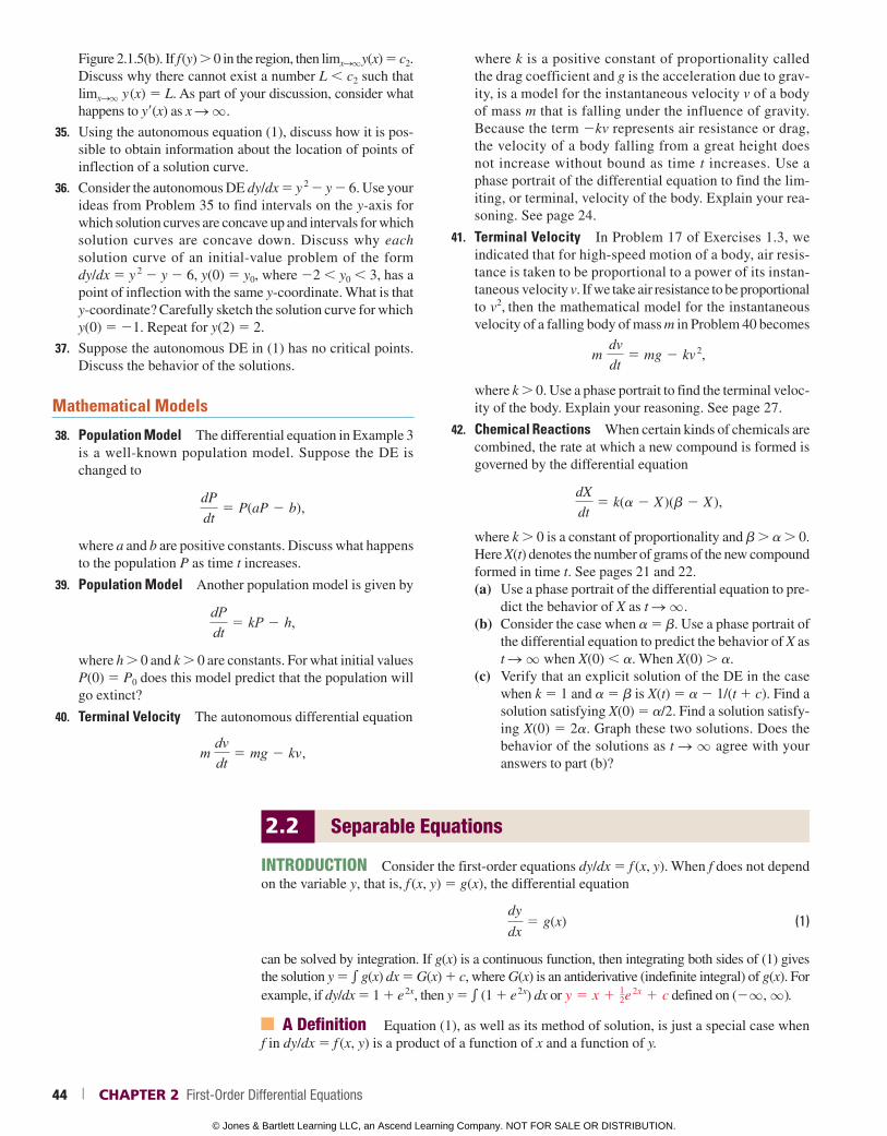
Figure 2.1.5(b). If f (y) 0 in the region, then limxSq y(x) 5 c2. Discuss why there cannot exist a number L c2 such that limxSq y (x) 5 L. As part of your discussion, consider what happens to y9(x) as x S q .
35. Using the autonomous equation (1), discuss how it is pos-sible to obtain information about the location of points of inflection of a solution curve.
36. Consider the autonomous DE dy/dx 5 y 2 2 y 2 6. Use your ideas from Problem 35 to find intervals on the y-axis for which solution curves are concave up and intervals for which solution curves are concave down. Discuss why each solution curve of an initial-value problem of the form dy/dx 5 y 2 2 y 2 6, y(0) 5 y0, where 22 y0 3, has a point of inflection with the same y-coordinate. What is that y-coordinate? Carefully sketch the solution curve for which y(0) 5 21. Repeat for y(2) 5 2.
37. Suppose the autonomous DE in (1) has no critical points. Discuss the behavior of the solutions.
Mathematical Models
38. Population Model The differential equation in Example 3 is a well-known population model. Suppose the DE is changed to
dP
dt5 P(aP 2 b),
where a and b are positive constants. Discuss what happens to the population P as time t increases.
39. Population Model Another population model is given by
dPdt
5 kP 2 h,
where h 0 and k 0 are constants. For what initial values P(0) 5 P0 does this model predict that the population will go extinct?
40. Terminal Velocity The autonomous differential equation
m dvdt
5 mg 2 kv,
where k is a positive constant of proportionality called the drag coefficient and g is the acceleration due to grav-ity, is a model for the instantaneous velocity v of a body of mass m that is falling under the influence of gravity. Because the term 2kv represents air resistance or drag, the velocity of a body falling from a great height does not increase without bound as time t increases. Use a phase portrait of the differential equation to find the lim-iting, or terminal, velocity of the body. Explain your rea-soning. See page 24.
41. Terminal Velocity In Problem 17 of Exercises 1.3, we indicated that for high-speed motion of a body, air resis-tance is taken to be proportional to a power of its instan-taneous velocity v. If we take air resistance to be proportional to v2, then the mathematical model for the instantaneous velocity of a falling body of mass m in Problem 40 becomes
m
dv
dt5 mg 2 kv
2,
where k 0. Use a phase portrait to find the terminal veloc-ity of the body. Explain your reasoning. See page 27.
42. Chemical Reactions When certain kinds of chemicals are combined, the rate at which a new compound is formed is governed by the differential equation
dX
dt5 k(a 2 X )(b 2 X ),
where k 0 is a constant of proportionality and b a 0. Here X(t) denotes the number of grams of the new compound formed in time t. See pages 21 and 22.(a) Use a phase portrait of the differential equation to pre-
dict the behavior of X as t S q .(b) Consider the case when a 5 b. Use a phase portrait of
the differential equation to predict the behavior of X as t S q when X(0) a. When X(0) a.
(c) Verify that an explicit solution of the DE in the case when k 5 1 and a 5 b is X(t) 5 a 2 1/(t 1 c). Find a solution satisfying X(0) 5 a/2. Find a solution satisfy-ing X(0) 5 2a. Graph these two solutions. Does the behavior of the solutions as t S q agree with your answers to part (b)?
2.2 Separable Equations
INTRODUCTION Consider the first-order equations dy/dx 5 f (x, y). When f does not depend on the variable y, that is, f (x, y) 5 g(x), the differential equation
dy
dx5 g(x) (1)
can be solved by integration. If g(x) is a continuous function, then integrating both sides of (1) gives the solution y 5 e g(x) dx 5 G(x) 1 c, where G(x) is an anti derivative (indefinite integral) of g(x). For example, if dy/dx 5 1 1 e 2x, then y 5 e (1 1 e 2x) dx or y 5 x 1 1
2e 2x 1 c defined on (2q , q).
A Definition Equation (1), as well as its method of solution, is just a special case when f in dy/dx 5 f (x, y) is a product of a function of x and a function of y.
44 | CHAPTER 2 First-Order Differential Equations
© Jones & Bartlett Learning LLC, an Ascend Learning Company. NOT FOR SALE OR DISTRIBUTION.
© Jones & Bartlett Learning, LLCNOT FOR SALE OR DISTRIBUTION
© Jones & Bartlett Learning, LLCNOT FOR SALE OR DISTRIBUTION
© Jones & Bartlett Learning, LLCNOT FOR SALE OR DISTRIBUTION
© Jones & Bartlett Learning, LLCNOT FOR SALE OR DISTRIBUTION
© Jones & Bartlett Learning, LLCNOT FOR SALE OR DISTRIBUTION
© Jones & Bartlett Learning, LLCNOT FOR SALE OR DISTRIBUTION
© Jones & Bartlett Learning, LLCNOT FOR SALE OR DISTRIBUTION
© Jones & Bartlett Learning, LLCNOT FOR SALE OR DISTRIBUTION
© Jones & Bartlett Learning, LLCNOT FOR SALE OR DISTRIBUTION
© Jones & Bartlett Learning, LLCNOT FOR SALE OR DISTRIBUTION
© Jones & Bartlett Learning, LLCNOT FOR SALE OR DISTRIBUTION
© Jones & Bartlett Learning, LLCNOT FOR SALE OR DISTRIBUTION
© Jones & Bartlett Learning, LLCNOT FOR SALE OR DISTRIBUTION
© Jones & Bartlett Learning, LLCNOT FOR SALE OR DISTRIBUTION
© Jones & Bartlett Learning, LLCNOT FOR SALE OR DISTRIBUTION
© Jones & Bartlett Learning, LLCNOT FOR SALE OR DISTRIBUTION
© Jones & Bartlett Learning, LLCNOT FOR SALE OR DISTRIBUTION
© Jones & Bartlett Learning, LLCNOT FOR SALE OR DISTRIBUTION
© Jones & Bartlett Learning, LLCNOT FOR SALE OR DISTRIBUTION
© Jones & Bartlett Learning, LLCNOT FOR SALE OR DISTRIBUTION
DEFINITION 2.2.1 Separable Equation
A first-order differential equation of the form
dy
dx5 g(x) h(y)
is said to be separable or to have separable variables.
For example, the differential equations
dy
dx5 x
2 y 4e
5x23y and dy
dx5 y 1 cos x
are separable and nonseparable, respectively. To see this, note that in the first equation we can factor f (x, y) 5 x
2y 4e
5x23y as
g(x) h( y)
f (x, y) 5 x
2y 4e
5x23y 5 (x 2e
5x)(y 4e
23y),
but in the second equation there is no way of writing y 1 cos x as a product of a function of x times a function of y.
Method of Solution Observe that by dividing by the function h( y), a separable equation can be written as
p(y) dy
dx5 g(x), (2)
where, for convenience, we have denoted 1/h( y) by p( y). From this last form we can see im-mediately that (2) reduces to (1) when h( y) 5 1.
Now if y 5 f(x) represents a solution of (2), we must have p(f(x))f9(x) 5 g(x), and therefore,
3p(f(x))f r(x) dx 5 3g(x) dx. (3)
But dy 5 f9(x) dx, and so (3) is the same as
#p(y) dy 5 #g(x) dx or H(y) 5 G(x) 1 c, (4)
where H( y) and G(x) are antiderivatives of p(y) 5 1/h( y) and g(x), respectively.Equation (4) indicates the procedure for solving separable equations. A one-parameter family
of solutions, usually given implicitly, is obtained by integrating both sides of the differential form p( y) dy 5 g(x) dx.
There is no need to use two constants in the integration of a separable equation, because if we write H( y) 1 c1 5 G(x) 1 c2, then the difference c2 2 c1 can be replaced by a single constant c, as in (4). In many instances throughout the chapters that follow, we will relabel constants in a manner convenient to a given equation. For example, multiples of constants or combinations of constants can sometimes be replaced by a single constant.
EXAMPLE 1 Solving a Separable DE
Solve (1 1 x) dy 2 y dx 5 0.
SOLUTION Dividing by (1 1 x)y, we can write dy/y 5 dx/(1 1 x), from which it follows that
3dyy 5 3
dx1 1 x
ln 0y 0 5 ln 01 1 x 0 1 c1
In solving first-order DEs, use only one constant.
2.2 Separable Equations | 45
© Jones & Bartlett Learning LLC, an Ascend Learning Company. NOT FOR SALE OR DISTRIBUTION.
© Jones & Bartlett Learning, LLCNOT FOR SALE OR DISTRIBUTION
© Jones & Bartlett Learning, LLCNOT FOR SALE OR DISTRIBUTION
© Jones & Bartlett Learning, LLCNOT FOR SALE OR DISTRIBUTION
© Jones & Bartlett Learning, LLCNOT FOR SALE OR DISTRIBUTION
© Jones & Bartlett Learning, LLCNOT FOR SALE OR DISTRIBUTION
© Jones & Bartlett Learning, LLCNOT FOR SALE OR DISTRIBUTION
© Jones & Bartlett Learning, LLCNOT FOR SALE OR DISTRIBUTION
© Jones & Bartlett Learning, LLCNOT FOR SALE OR DISTRIBUTION
© Jones & Bartlett Learning, LLCNOT FOR SALE OR DISTRIBUTION
© Jones & Bartlett Learning, LLCNOT FOR SALE OR DISTRIBUTION
© Jones & Bartlett Learning, LLCNOT FOR SALE OR DISTRIBUTION
© Jones & Bartlett Learning, LLCNOT FOR SALE OR DISTRIBUTION
© Jones & Bartlett Learning, LLCNOT FOR SALE OR DISTRIBUTION
© Jones & Bartlett Learning, LLCNOT FOR SALE OR DISTRIBUTION
© Jones & Bartlett Learning, LLCNOT FOR SALE OR DISTRIBUTION
© Jones & Bartlett Learning, LLCNOT FOR SALE OR DISTRIBUTION
© Jones & Bartlett Learning, LLCNOT FOR SALE OR DISTRIBUTION
© Jones & Bartlett Learning, LLCNOT FOR SALE OR DISTRIBUTION
© Jones & Bartlett Learning, LLCNOT FOR SALE OR DISTRIBUTION
© Jones & Bartlett Learning, LLCNOT FOR SALE OR DISTRIBUTION
0y 0 5 e ln 011x 01c1 5 e
ln 011x 0 # ec1
5 01 1 x 0ec1
and so y 5 6 ec1(1 1 x).
Relabeling 6e c1 by c then gives y 5 c(1 1 x) defined on (2q , q ).
In the solution of Example 1, because each integral results in a logarithm, a judicious choice for the constant of integration is ln | c | rather than c. Rewriting the second line of the solution as ln | y | 5 ln | 1 1 x | 1 ln | c | enables us to combine the terms on the right-hand side by the proper-ties of logarithms. From ln | y | 5 ln | c(1 1 x) |, we immediately get y 5 c(1 1 x). Even if the indefinite integrals are not all logarithms, it may still be advantageous to use ln | c |. However, no firm rule can be given.
In Section 1.1 we have already seen that a solution curve may be only a segment or an arc of the graph of an implicit solution G(x, y) 5 0.
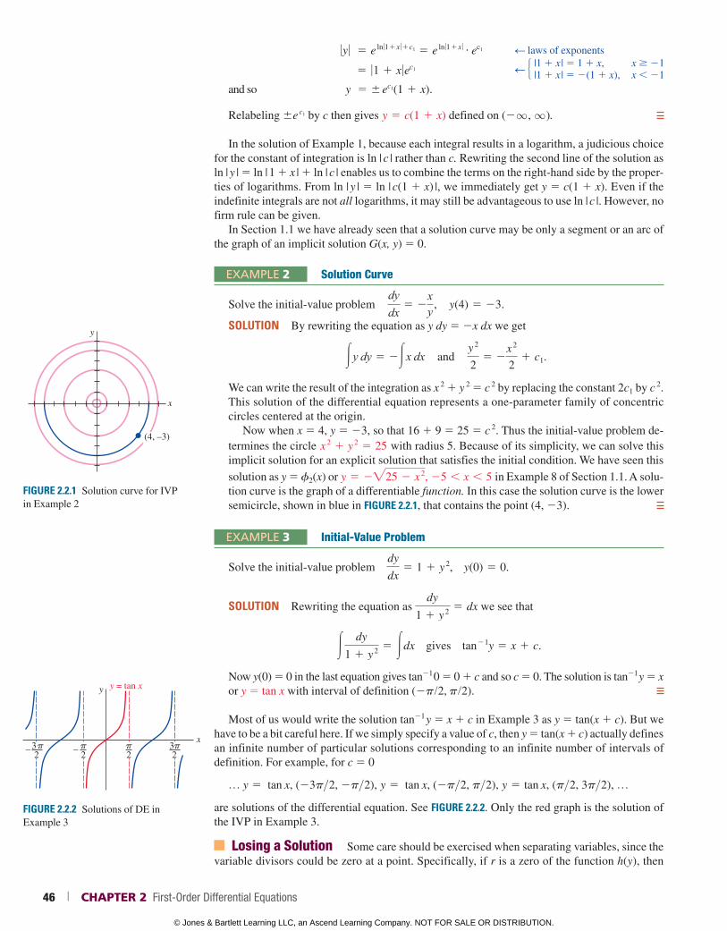
EXAMPLE 2 Solution Curve
Solve the initial-value problem dydx
5 2xy , y(4) 5 23.
SOLUTION By rewriting the equation as y dy 5 2x dx we get
3y dy 5 23x dx and y
2
25 2
x 2
21 c1.
We can write the result of the integration as x 2 1 y 2 5 c 2 by replacing the constant 2c1 by c 2. This solution of the differential equation represents a one-parameter family of concentric circles centered at the origin.
Now when x 5 4, y 5 23, so that 16 1 9 5 25 5 c 2. Thus the initial-value problem de-termines the circle x
2 1 y 2 5 25 with radius 5. Because of its simplicity, we can solve this
implicit solution for an explicit solution that satisfies the initial condition. We have seen this
solution as y 5 f2(x) or y 5 2"25 2 x 2, 25 , x , 5 in Example 8 of Section 1.1. A solu-
tion curve is the graph of a differentiable function. In this case the solution curve is the lower semicircle, shown in blue in FIGURE 2.2.1, that contains the point (4, 23).
EXAMPLE 3 Initial-Value Problem
Solve the initial-value problem dy
dx5 1 1 y
2, y(0) 5 0.
SOLUTION Rewriting the equation as dy
1 1 y 2 5 dx we see that
#dy
1 1 y 2 5 #dx gives tan21y 5 x 1 c.
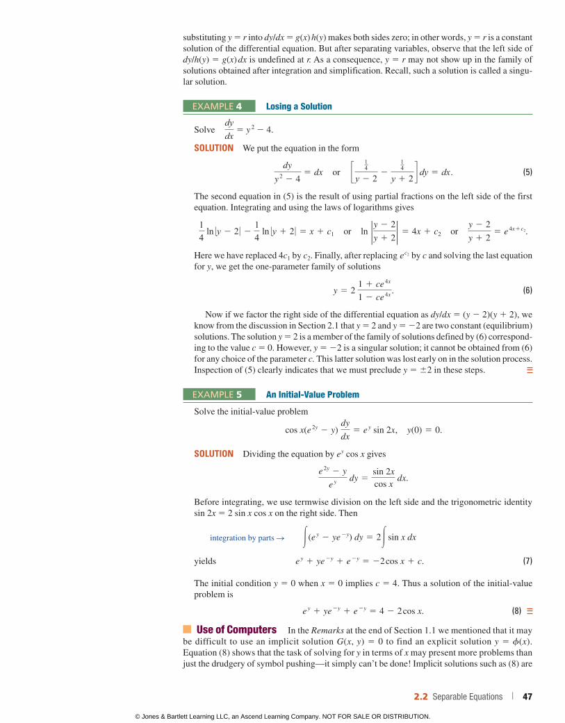
Now y(0) 5 0 in the last equation gives tan21 0 5 0 1 c and so c 5 0. The solution is tan21 y 5 x or y 5 tan x with interval of definition (2p/2, p/2).
Most of us would write the solution tan21 y 5 x 1 c in Example 3 as y 5 tan(x 1 c). But we have to be a bit careful here. If we simply specify a value of c, then y 5 tan(x 1 c) actually defines an infinite number of particular solutions corresponding to an infinite number of intervals of definition. For example, for c 5 0
p y 5 tan x, (23p>2, 2p>2), y 5 tan x, (2p>2, p>2), y 5 tan x, (p>2, 3p>2), p
are solutions of the differential equation. See FIGURE 2.2.2. Only the red graph is the solution of the IVP in Example 3.
Losing a Solution Some care should be exercised when separating variables, since the variable divisors could be zero at a point. Specifically, if r is a zero of the function h(y), then
d laws of exponents
d 5 |1 1 x | 5 1 1 x, x 21
|1 1 x | 5 2(1 1 x), x 21
FIGURE 2.2.1 Solution curve for IVP in Example 2
x
y
(4, –3)
FIGURE 2.2.2 Solutions of DE in Example 3
x
y = tan xy
– 32� –
2� 3
2�
2�
46 | CHAPTER 2 First-Order Differential Equations
© Jones & Bartlett Learning LLC, an Ascend Learning Company. NOT FOR SALE OR DISTRIBUTION.
© Jones & Bartlett Learning, LLCNOT FOR SALE OR DISTRIBUTION
© Jones & Bartlett Learning, LLCNOT FOR SALE OR DISTRIBUTION
© Jones & Bartlett Learning, LLCNOT FOR SALE OR DISTRIBUTION
© Jones & Bartlett Learning, LLCNOT FOR SALE OR DISTRIBUTION
© Jones & Bartlett Learning, LLCNOT FOR SALE OR DISTRIBUTION
© Jones & Bartlett Learning, LLCNOT FOR SALE OR DISTRIBUTION
© Jones & Bartlett Learning, LLCNOT FOR SALE OR DISTRIBUTION
© Jones & Bartlett Learning, LLCNOT FOR SALE OR DISTRIBUTION
© Jones & Bartlett Learning, LLCNOT FOR SALE OR DISTRIBUTION
© Jones & Bartlett Learning, LLCNOT FOR SALE OR DISTRIBUTION
© Jones & Bartlett Learning, LLCNOT FOR SALE OR DISTRIBUTION
© Jones & Bartlett Learning, LLCNOT FOR SALE OR DISTRIBUTION
© Jones & Bartlett Learning, LLCNOT FOR SALE OR DISTRIBUTION
© Jones & Bartlett Learning, LLCNOT FOR SALE OR DISTRIBUTION
© Jones & Bartlett Learning, LLCNOT FOR SALE OR DISTRIBUTION
© Jones & Bartlett Learning, LLCNOT FOR SALE OR DISTRIBUTION
© Jones & Bartlett Learning, LLCNOT FOR SALE OR DISTRIBUTION
© Jones & Bartlett Learning, LLCNOT FOR SALE OR DISTRIBUTION
© Jones & Bartlett Learning, LLCNOT FOR SALE OR DISTRIBUTION
© Jones & Bartlett Learning, LLCNOT FOR SALE OR DISTRIBUTION
substituting y 5 r into dy/dx 5 g(x) h(y) makes both sides zero; in other words, y 5 r is a constant solution of the differential equation. But after separating variables, observe that the left side of dy/h(y) 5 g(x) dx is undefined at r. As a consequence, y 5 r may not show up in the family of solutions obtained after integration and simplification. Recall, such a solution is called a singu-lar solution.
EXAMPLE 4 Losing a Solution
Solve dydx
5 y 2 2 4.
SOLUTION We put the equation in the form
dy
y 2 2 4
5 dx or c14
y 2 22
14
y 1 2d dy 5 dx. (5)
The second equation in (5) is the result of using partial fractions on the left side of the first equation. Integrating and using the laws of logarithms gives
14
ln 0y 2 2 0 214
ln 0y 1 2 0 5 x 1 c1 or ln 2y 2 2
y 1 22 5 4x 1 c2 or
y 2 2
y 1 25 e
4x1c2.
Here we have replaced 4c1 by c2. Finally, after replacing ec2 by c and solving the last equation for y, we get the one-parameter family of solutions
y 5 2 1 1 ce
4x
1 2 ce 4x . (6)
Now if we factor the right side of the differential equation as dy/dx 5 (y 2 2)(y 1 2), we know from the discussion in Section 2.1 that y 5 2 and y 5 22 are two constant (equilibrium) solutions. The solution y 5 2 is a member of the family of solutions defined by (6) correspond-ing to the value c 5 0. However, y 5 22 is a singular solution; it cannot be obtained from (6) for any choice of the parameter c. This latter solution was lost early on in the solution process. Inspection of (5) clearly indicates that we must preclude y 5 62 in these steps.
EXAMPLE 5 An Initial-Value Problem
Solve the initial-value problem
cos x(e 2y 2 y)
dy
dx5 e
y sin 2x, y(0) 5 0.
SOLUTION Dividing the equation by e y cos x gives
e
2y 2 y
e y dy 5
sin 2x cos x
dx.
Before integrating, we use termwise division on the left side and the trigonometric identity sin 2x 5 2 sin x cos x on the right side. Then
#(e y 2 ye
2y) dy 5 2# sin x dx
yields e y 1 ye
2y 1 e 2y 5 22 cos x 1 c. (7)
The initial condition y 5 0 when x 5 0 implies c 5 4. Thus a solution of the initial-value problem is
e y 1 ye
2y 1 e 2y 5 4 2 2 cos x. (8)
Use of Computers In the Remarks at the end of Section 1.1 we mentioned that it may be difficult to use an implicit solution G(x, y) 5 0 to find an explicit solution y 5 f(x). Equation (8) shows that the task of solving for y in terms of x may present more problems than just the drudgery of symbol pushing—it simply can’t be done! Implicit solutions such as (8) are
integration by parts S
2.2 Separable Equations | 47
© Jones & Bartlett Learning LLC, an Ascend Learning Company. NOT FOR SALE OR DISTRIBUTION.
© Jones & Bartlett Learning, LLCNOT FOR SALE OR DISTRIBUTION
© Jones & Bartlett Learning, LLCNOT FOR SALE OR DISTRIBUTION
© Jones & Bartlett Learning, LLCNOT FOR SALE OR DISTRIBUTION
© Jones & Bartlett Learning, LLCNOT FOR SALE OR DISTRIBUTION
© Jones & Bartlett Learning, LLCNOT FOR SALE OR DISTRIBUTION
© Jones & Bartlett Learning, LLCNOT FOR SALE OR DISTRIBUTION
© Jones & Bartlett Learning, LLCNOT FOR SALE OR DISTRIBUTION
© Jones & Bartlett Learning, LLCNOT FOR SALE OR DISTRIBUTION
© Jones & Bartlett Learning, LLCNOT FOR SALE OR DISTRIBUTION
© Jones & Bartlett Learning, LLCNOT FOR SALE OR DISTRIBUTION
© Jones & Bartlett Learning, LLCNOT FOR SALE OR DISTRIBUTION
© Jones & Bartlett Learning, LLCNOT FOR SALE OR DISTRIBUTION
© Jones & Bartlett Learning, LLCNOT FOR SALE OR DISTRIBUTION
© Jones & Bartlett Learning, LLCNOT FOR SALE OR DISTRIBUTION
© Jones & Bartlett Learning, LLCNOT FOR SALE OR DISTRIBUTION
© Jones & Bartlett Learning, LLCNOT FOR SALE OR DISTRIBUTION
© Jones & Bartlett Learning, LLCNOT FOR SALE OR DISTRIBUTION
© Jones & Bartlett Learning, LLCNOT FOR SALE OR DISTRIBUTION
© Jones & Bartlett Learning, LLCNOT FOR SALE OR DISTRIBUTION
© Jones & Bartlett Learning, LLCNOT FOR SALE OR DISTRIBUTION
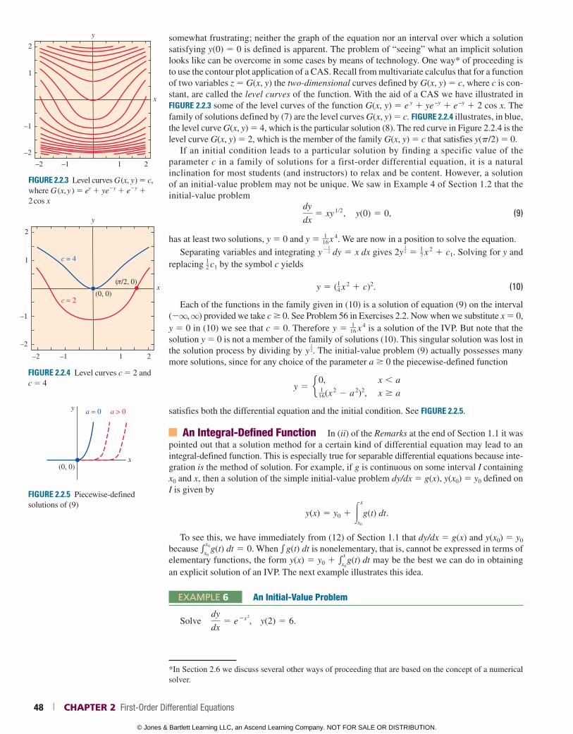
somewhat frustrating; neither the graph of the equation nor an interval over which a solution satisfying y(0) 5 0 is defined is apparent. The problem of “seeing” what an implicit solution looks like can be overcome in some cases by means of technology. One way* of proceeding is to use the contour plot application of a CAS. Recall from multivariate calculus that for a function of two variables z 5 G(x, y) the two-dimensional curves defined by G(x, y) 5 c, where c is con-stant, are called the level curves of the function. With the aid of a CAS we have illustrated in FIGURE 2.2.3 some of the level curves of the function G(x, y) 5 e y 1 ye –y 1 e –y 1 2 cos x. The family of solutions defined by (7) are the level curves G(x, y) 5 c. FIGURE 2.2.4 illustrates, in blue, the level curve G(x, y) 5 4, which is the particular solution (8). The red curve in Figure 2.2.4 is the level curve G(x, y) 5 2, which is the member of the family G(x, y) 5 c that satisfies y(p/2) 5 0.
If an initial condition leads to a particular solution by finding a specific value of the parameter c in a family of solutions for a first-order differential equation, it is a natural inclination for most students (and instructors) to relax and be content. However, a solution of an initial-value problem may not be unique. We saw in Example 4 of Section 1.2 that the initial-value problem
dy
dx5 xy
1/2, y(0) 5 0, (9)
has at least two solutions, y 5 0 and y 5 116x 4. We are now in a position to solve the equation.
Separating variables and integrating y 21
2 dy 5 x dx gives 2y
12 5 1
2 x 2 1 c1. Solving for y and
replacing 12 c1 by the symbol c yields
y 5 (14 x
2 1 c)2. (10)
Each of the functions in the family given in (10) is a solution of equation (9) on the interval (2q, q) provided we take c 0. See Problem 56 in Exercises 2.2. Now when we substitute x 5 0, y 5 0 in (10) we see that c 5 0. Therefore y 5 1
16 x 4 is a solution of the IVP. But note that the
solution y 5 0 is not a member of the family of solutions (10). This singular solution was lost in the solution process by dividing by y
12. The initial-value problem (9) actually possesses many
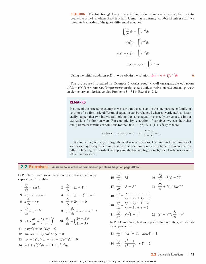
more solutions, since for any choice of the parameter a 0 the piecewise-defined function
y 5 e0, x , a1
16(x 2 2 a
2)2, x $ a
satisfies both the differential equation and the initial condition. See FIGURE 2.2.5.
An Integral-Defined Function In (ii) of the Remarks at the end of Section 1.1 it was pointed out that a solution method for a certain kind of differential equation may lead to an integral-defined function. This is especially true for separable differential equations because inte-gration is the method of solution. For example, if g is continuous on some interval I containing x0 and x, then a solution of the simple initial-value problem dy/dx 5 g(x), y(x0) 5 y0 defined on I is given by
y(x) 5 y0 1 #x
x0
g(t) dt.
To see this, we have immediately from (12) of Section 1.1 that dy/dx 5 g(x) and y(x0) 5 y0 because e
x0
x0 g(t) dt 5 0. When e g(t) dt is nonelementary, that is, cannot be expressed in terms of
elementary functions, the form y(x) 5 y0 1 ex
x0 g(t) dt may be the best we can do in obtaining
an explicit solution of an IVP. The next example illustrates this idea.
EXAMPLE 6 An Initial-Value Problem
Solve dy
dx5 e
2x 2
, y(2) 5 6.
FIGURE 2.2.3 Level curves G (x, y ) 5 c, where G (x, y ) 5 ey 1 ye2y 1 e2y 1 2 cos x
x
y
2
1
–1
–2
–2 –1 1 2
FIGURE 2.2.4 Level curves c 5 2 and c 5 4
–1
–2
x
y
2
1
–2 –1 1 2
c = 2
c = 4
(0, 0)
( /2, 0)π
y
x(0, 0)
a = 0 a > 0
FIGURE 2.2.5 Piecewise-defined solutions of (9)
*In Section 2.6 we discuss several other ways of proceeding that are based on the concept of a numerical solver.
48 | CHAPTER 2 First-Order Differential Equations
© Jones & Bartlett Learning LLC, an Ascend Learning Company. NOT FOR SALE OR DISTRIBUTION.
© Jones & Bartlett Learning, LLCNOT FOR SALE OR DISTRIBUTION
© Jones & Bartlett Learning, LLCNOT FOR SALE OR DISTRIBUTION
© Jones & Bartlett Learning, LLCNOT FOR SALE OR DISTRIBUTION
© Jones & Bartlett Learning, LLCNOT FOR SALE OR DISTRIBUTION
© Jones & Bartlett Learning, LLCNOT FOR SALE OR DISTRIBUTION
© Jones & Bartlett Learning, LLCNOT FOR SALE OR DISTRIBUTION
© Jones & Bartlett Learning, LLCNOT FOR SALE OR DISTRIBUTION
© Jones & Bartlett Learning, LLCNOT FOR SALE OR DISTRIBUTION
© Jones & Bartlett Learning, LLCNOT FOR SALE OR DISTRIBUTION
© Jones & Bartlett Learning, LLCNOT FOR SALE OR DISTRIBUTION
© Jones & Bartlett Learning, LLCNOT FOR SALE OR DISTRIBUTION
© Jones & Bartlett Learning, LLCNOT FOR SALE OR DISTRIBUTION
© Jones & Bartlett Learning, LLCNOT FOR SALE OR DISTRIBUTION
© Jones & Bartlett Learning, LLCNOT FOR SALE OR DISTRIBUTION
© Jones & Bartlett Learning, LLCNOT FOR SALE OR DISTRIBUTION
© Jones & Bartlett Learning, LLCNOT FOR SALE OR DISTRIBUTION
© Jones & Bartlett Learning, LLCNOT FOR SALE OR DISTRIBUTION
© Jones & Bartlett Learning, LLCNOT FOR SALE OR DISTRIBUTION
© Jones & Bartlett Learning, LLCNOT FOR SALE OR DISTRIBUTION
© Jones & Bartlett Learning, LLCNOT FOR SALE OR DISTRIBUTION
SOLUTION The function g(x) 5 e 2x
2
is continuous on the interval (2q, q) but its anti-derivative is not an elementary function. Using t as a dummy variable of integration, we integrate both sides of the given differential equation:
#x
2
dy
dt dt 5 #
x
2e
2t 2
dt
y(t)T x2
5 #x
2e
2t 2
dt
y(x) 2 y(2) 5 #x
2e
2t 2
dt
y(x) 5 y(2) 1 #x
2e
2t 2
dt.
Using the initial condition y(2) 5 6 we obtain the solution y(x) 5 6 1 e x
2 e 2t
2 dt.
The procedure illustrated in Example 6 works equally well on separable equations dy/dx 5 g(x) f (y) where, say, f (y) possesses an elementary antiderivative but g(x) does not possess an elementary antiderivative. See Problems 31–34 in Exercises 2.2.
REMARKSIn some of the preceding examples we saw that the constant in the one-parameter family of solutions for a first-order differential equation can be relabeled when convenient. Also, it can easily happen that two individuals solving the same equation correctly arrive at dissimilar expressions for their answers. For example, by separation of variables, we can show that one-parameter families of solutions for the DE (1 1 y 2) dx 1 (1 1 x 2) dy 5 0 are
arctan x 1 arctan y 5 c or x 1 y1 2 xy
5 c.
As you work your way through the next several sections, keep in mind that families of solutions may be equivalent in the sense that one family may be obtained from another by either relabeling the constant or applying algebra and trigonometry. See Problems 27 and 28 in Exercises 2.2.
In Problems 1–22, solve the given differential equation by separation of variables.
1. dydx
5 sin 5x 2. dy
dx5 (x 1 1)2
3. dx 1 e 3x dy 5 0 4. dy 2 (y 2 1)
2 dx 5 0
5. x dydx
5 4y 6. dy
dx1 2xy
2 5 0
7. dy
dx5 e
3x12y 8. e xy
dy
dx5 e2y 1 e22x2y
9. y ln x dxdy
5 ay 1 1x b
2
10. dydx
5 a2y 1 34x 1 5
b2
11. csc y dx 1 sec 2x dy 5 0
12. sin 3x dx 1 2y cos 33x dy 5 0
13. (e y 1 1)2 e
2y dx 1 (e x 1 1)3e
2x dy 5 0
14. x (1 1 y 2)1/2 dx 5 y(1 1 x
2)1/2 dy
15. dSdr
5 kS 16. dQ
dt5 k(Q 2 70)
17. dP
dt5 P 2 P
2 18. dN
dt1 N 5 Nte
t12
19. dy
dx5
xy 1 3x 2 y 2 3
xy 2 2x 1 4y 2 8
20. dy
dx5
xy 1 2y 2 x 2 2
xy 2 3y 1 x 2 3
21. dy
dx5 x"1 2 y
2 22. (e x 1 e2x)
dy
dx5 y
2
In Problems 23–30, find an explicit solution of the given initial- value problem.
23. dx
dt5 4(x
2 1 1), x(p/4) 5 1
24. dy
dx5
y 2 2 1
x 2 2 1
, y(2) 5 2
2.2 Exercises Answers to selected odd-numbered problems begin on page ANS-2.
2.2 Separable Equations | 49
© Jones & Bartlett Learning LLC, an Ascend Learning Company. NOT FOR SALE OR DISTRIBUTION.
© Jones & Bartlett Learning, LLCNOT FOR SALE OR DISTRIBUTION
© Jones & Bartlett Learning, LLCNOT FOR SALE OR DISTRIBUTION
© Jones & Bartlett Learning, LLCNOT FOR SALE OR DISTRIBUTION
© Jones & Bartlett Learning, LLCNOT FOR SALE OR DISTRIBUTION
© Jones & Bartlett Learning, LLCNOT FOR SALE OR DISTRIBUTION
© Jones & Bartlett Learning, LLCNOT FOR SALE OR DISTRIBUTION
© Jones & Bartlett Learning, LLCNOT FOR SALE OR DISTRIBUTION
© Jones & Bartlett Learning, LLCNOT FOR SALE OR DISTRIBUTION
© Jones & Bartlett Learning, LLCNOT FOR SALE OR DISTRIBUTION
© Jones & Bartlett Learning, LLCNOT FOR SALE OR DISTRIBUTION
© Jones & Bartlett Learning, LLCNOT FOR SALE OR DISTRIBUTION
© Jones & Bartlett Learning, LLCNOT FOR SALE OR DISTRIBUTION
© Jones & Bartlett Learning, LLCNOT FOR SALE OR DISTRIBUTION
© Jones & Bartlett Learning, LLCNOT FOR SALE OR DISTRIBUTION
© Jones & Bartlett Learning, LLCNOT FOR SALE OR DISTRIBUTION
© Jones & Bartlett Learning, LLCNOT FOR SALE OR DISTRIBUTION
© Jones & Bartlett Learning, LLCNOT FOR SALE OR DISTRIBUTION
© Jones & Bartlett Learning, LLCNOT FOR SALE OR DISTRIBUTION
© Jones & Bartlett Learning, LLCNOT FOR SALE OR DISTRIBUTION
© Jones & Bartlett Learning, LLCNOT FOR SALE OR DISTRIBUTION
25. x 2 dy
dx5 y 2 xy, y(21) 5 21
26. dy
dt1 2y 5 1, y(0) 5 5
2
27. "1 2 y 2
dx 2 "1 2 x 2
dy 5 0, y(0) 5 "3/2
28. (1 1 x 4) dy 1 x(1 1 4y 2) dx 5 0, y(1) 5 0
29. dy
dx5 2y ln y, y(0) 5 e
30. x sinh y
dy
dx5 cosh y, y(1) 5 0
In Problems 31–34, proceed as in Example 6 and find an explicit solution of the given initial-value problem.
31. dy
dx5 ye2x
2
, y(4) 5 1
32. dy
dx5 y
2 sin x 2, y(22) 5 1
3
33. dy
dx5 (1 1 y
2)"1 1 cos x 3, y(1) 5 1
34. dy
dx5
e22y sin x
1 1 x 2 , y(0) 5 0
In Problems 35–38, find an explicit solution of the given initial-value problem. Determine the exact interval I of defini-tion of each solution by analytical methods. Use a graphing utility to plot the graph of each solution.
35. dy
dx5
2x 1 1
2y, y(22) 5 21
36. (2y 2 2)
dy
dx5 3x
2 1 4x 1 2, y(1) 5 22
37. e y dx 2 e2x dy 5 0, y(0) 5 0
38. sin x dx 1 y dy 5 0, y(0) 5 1
39. (a) Find a solution of the initial-value problem consisting of the differential equation in Example 4 and the initial conditions y(0) 5 2, y(0) 5 22, y(1
4) 5 1.(b) Find the solution of the differential equation in
Example 4 when ln c1 is used as the constant of integra-tion on the left-hand side in the solution and 4 ln c1 is replaced by ln c. Then solve the same initial-value problems in part (a).
40. Find a solution of x dy
dx5 y
2 2 y that passes through the indicated points.
(a) (0, 1) (b) (0, 0) (c) (12 , 1
2) (d) (2, 14)
41. Find a singular solution of Problem 21. Of Problem 22.
42. Show that an implicit solution of
2x sin 2 y dx 2 (x 2 1 10) cos y dy 5 0
is given by ln(x 2 1 10) csc y 5 c. Find the constant solutions, if any, that were lost in the solution of the differential equation.
Often a radical change in the form of the solution of a differ-ential equation corresponds to a very small change in either the initial condition or the equation itself. In Problems 43–46, find an explicit solution of the given initial-value problem. Use a graphing utility to plot the graph of each solution. Compare each solution curve in a neighborhood of (0, 1).
43. dy
dx5 ( y 2 1)2, y(0) 5 1
44. dy
dx5 ( y 2 1)2, y(0) 5 1.01
45. dy
dx5 ( y 2 1)2 1 0.01, y(0) 5 1
46. dy
dx5 ( y 2 1)2 2 0.01, y(0) 5 1
47. Every autonomous first-order equation dy/dx 5 f (y) is separable. Find explicit solutions y1(x), y2(x), y3(x), and y4(x) of the differential equation dy/dx 5 y 2 y 3 that satisfy, in turn, the initial conditions y1(0) 5 2, y2(0) 5 1
2, y3(0) 5 212,
and y4(0) 5 22. Use a graphing utility to plot the graphs of each solution. Compare these graphs with those predicted in Problem 19 of Exercises 2.1. Give the exact interval of definition for each solution.
48. (a) The autonomous first-order differential equation dy/dx 5 1/(y 2 3) has no critical points. Nevertheless, place 3 on a phase line and obtain a phase portrait of the equation. Com pute d 2y/dx 2 to determine where solution curves are concave up and where they are con-cave down (see Problems 35 and 36 in Exercises 2.1). Use the phase portrait and concavity to sketch, by hand, some typical solution curves.
(b) Find explicit solutions y1(x), y2(x), y3(x), and y4(x) of the differential equation in part (a) that satisfy, in turn, the initial conditions y1(0) 5 4, y2(0) 5 2, y3(1) 5 2, and y4(21) 5 4. Graph each solution and compare with your sketches in part (a). Give the exact interval of definition for each solution.
In Problems 49–54, use a technique of integration or a substi-tution to find an explicit solution of the given differential equation or initial-value problem.
49. dy
dx5
1
1 1 sin x
50. dy
dx5
sin "x
"y
51. ("x 1 x)
dy
dx5 "y 1 y
52. dy
dx5 y
2>3 2 y
53. dy
dx5
e"x
y, y(1) 5 4
54. dy
dx5
x tan 21x
y, y(0) 5 3
50 | CHAPTER 2 First-Order Differential Equations
© Jones & Bartlett Learning LLC, an Ascend Learning Company. NOT FOR SALE OR DISTRIBUTION.
© Jones & Bartlett Learning, LLCNOT FOR SALE OR DISTRIBUTION
© Jones & Bartlett Learning, LLCNOT FOR SALE OR DISTRIBUTION
© Jones & Bartlett Learning, LLCNOT FOR SALE OR DISTRIBUTION
© Jones & Bartlett Learning, LLCNOT FOR SALE OR DISTRIBUTION
© Jones & Bartlett Learning, LLCNOT FOR SALE OR DISTRIBUTION
© Jones & Bartlett Learning, LLCNOT FOR SALE OR DISTRIBUTION
© Jones & Bartlett Learning, LLCNOT FOR SALE OR DISTRIBUTION
© Jones & Bartlett Learning, LLCNOT FOR SALE OR DISTRIBUTION
© Jones & Bartlett Learning, LLCNOT FOR SALE OR DISTRIBUTION
© Jones & Bartlett Learning, LLCNOT FOR SALE OR DISTRIBUTION
© Jones & Bartlett Learning, LLCNOT FOR SALE OR DISTRIBUTION
© Jones & Bartlett Learning, LLCNOT FOR SALE OR DISTRIBUTION
© Jones & Bartlett Learning, LLCNOT FOR SALE OR DISTRIBUTION
© Jones & Bartlett Learning, LLCNOT FOR SALE OR DISTRIBUTION
© Jones & Bartlett Learning, LLCNOT FOR SALE OR DISTRIBUTION
© Jones & Bartlett Learning, LLCNOT FOR SALE OR DISTRIBUTION
© Jones & Bartlett Learning, LLCNOT FOR SALE OR DISTRIBUTION
© Jones & Bartlett Learning, LLCNOT FOR SALE OR DISTRIBUTION
© Jones & Bartlett Learning, LLCNOT FOR SALE OR DISTRIBUTION
© Jones & Bartlett Learning, LLCNOT FOR SALE OR DISTRIBUTION
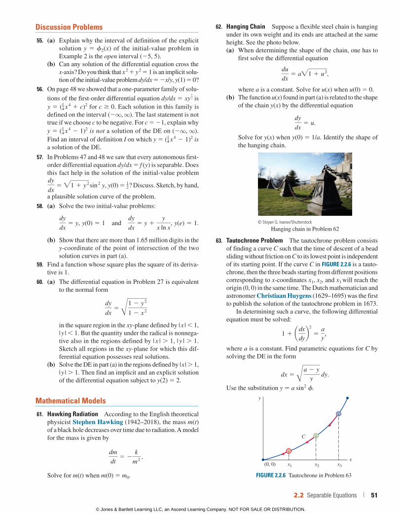
Discussion Problems
55. (a) Explain why the interval of definition of the explicit solution y 5 f2(x) of the initial-value problem in Example 2 is the open interval (25, 5).
(b) Can any solution of the differential equation cross the x-axis? Do you think that x 2 1 y 2 5 1 is an implicit solu-tion of the initial-value problem dy/dx 5 2x/y, y(1) 5 0?
56. On page 48 we showed that a one-parameter family of solu-
tions of the first-order differential equation dy/dx 5 xy
12 is
y 5 (14 x
4 1 c)2 for c 0. Each solution in this family is defined on the interval (2q, q). The last statement is not true if we choose c to be negative. For c 5 21, explain why y 5 (1
4 x 4 2 1)2 is not a solution of the DE on (2q, q).
Find an interval of definition I on which y 5 (14 x
4 2 1)2 is a solution of the DE.
57. In Problems 47 and 48 we saw that every autonomous first-order differential equation dy/dx 5 f (y) is separable. Does this fact help in the solution of the initial-value problem dy
dx5 "1 1 y
2 sin
2 y, y(0) 5 12? Discuss. Sketch, by hand,
a plausible solution curve of the problem.
58. (a) Solve the two initial-value problems:
dy
dx5 y, y(0) 5 1 and
dy
dx5 y 1
y
x ln x, y(e) 5 1.
(b) Show that there are more than 1.65 million digits in the y-coordinate of the point of intersection of the two solution curves in part (a).
59. Find a function whose square plus the square of its deriva-tive is 1.
60. (a) The differential equation in Problem 27 is equivalent to the normal form
dy
dx5 Å
1 2 y 2
1 2 x 2
in the square region in the xy-plane defined by | x | 1, | y | 1. But the quantity under the radical is nonnega-tive also in the regions defined by | x | 1, | y | 1. Sketch all regions in the xy-plane for which this dif-ferential equation possesses real solutions.
(b) Solve the DE in part (a) in the regions defined by | x | 1, | y | 1. Then find an implicit and an explicit solution of the differential equation subject to y(2) 5 2.
Mathematical Models
61. Hawking Radiation According to the English theoretical physicist Stephen Hawking (1942–2018), the mass m(t) of a black hole decreases over time due to radiation. A model for the mass is given by
dm
dt5 2
k
m 2 .
Solve for m(t) when m(0) 5 m0.
62. Hanging Chain Suppose a flexible steel chain is hanging under its own weight and its ends are attached at the same height. See the photo below.(a) When determining the shape of the chain, one has to
first solve the differential equation
du
dx5 a"1 1 u
2,
where a is a constant. Solve for u(x) when u(0) 5 0.(b) The function u(x) found in part (a) is related to the shape
of the chain y(x) by the differential equation
dy
dx5 u.
Solve for y(x) when y(0) 5 1/a. Identify the shape of the hanging chain.
© Stoyan G. Ivanov/Shutterstock
Hanging chain in Problem 62
63. Tautochrone Problem The tautochrone problem consists of finding a curve C such that the time of descent of a bead sliding without friction on C to its lowest point is independent of its starting point. If the curve C in FIGURE 2.2.6 is a tauto-chrone, then the three beads starting from different positions corresponding to x-coordinates x1, x2, and x3 will reach the origin (0, 0) in the same time. The Dutch mathematician and astronomer Christiaan Huygens (1629–1695) was the first to publish the solution of the tautochrone problem in 1673.
In determining such a curve, the following differential equation must be solved:
1 1 adxdy
b2
5ay ,
where a is a constant. Find parametric equations for C by solving the DE in the form
dx 5 Åa 2 y
y dy.
Use the substitution y 5 a sin 2 .
x1 x2 x3
y
x(0, 0)
C
FIGURE 2.2.6 Tautochrone in Problem 63
2.2 Separable Equations | 51
© Jones & Bartlett Learning LLC, an Ascend Learning Company. NOT FOR SALE OR DISTRIBUTION.
© Jones & Bartlett Learning, LLCNOT FOR SALE OR DISTRIBUTION
© Jones & Bartlett Learning, LLCNOT FOR SALE OR DISTRIBUTION
© Jones & Bartlett Learning, LLCNOT FOR SALE OR DISTRIBUTION
© Jones & Bartlett Learning, LLCNOT FOR SALE OR DISTRIBUTION
© Jones & Bartlett Learning, LLCNOT FOR SALE OR DISTRIBUTION
© Jones & Bartlett Learning, LLCNOT FOR SALE OR DISTRIBUTION
© Jones & Bartlett Learning, LLCNOT FOR SALE OR DISTRIBUTION
© Jones & Bartlett Learning, LLCNOT FOR SALE OR DISTRIBUTION
© Jones & Bartlett Learning, LLCNOT FOR SALE OR DISTRIBUTION
© Jones & Bartlett Learning, LLCNOT FOR SALE OR DISTRIBUTION
© Jones & Bartlett Learning, LLCNOT FOR SALE OR DISTRIBUTION
© Jones & Bartlett Learning, LLCNOT FOR SALE OR DISTRIBUTION
© Jones & Bartlett Learning, LLCNOT FOR SALE OR DISTRIBUTION
© Jones & Bartlett Learning, LLCNOT FOR SALE OR DISTRIBUTION
© Jones & Bartlett Learning, LLCNOT FOR SALE OR DISTRIBUTION
© Jones & Bartlett Learning, LLCNOT FOR SALE OR DISTRIBUTION
© Jones & Bartlett Learning, LLCNOT FOR SALE OR DISTRIBUTION
© Jones & Bartlett Learning, LLCNOT FOR SALE OR DISTRIBUTION
© Jones & Bartlett Learning, LLCNOT FOR SALE OR DISTRIBUTION
© Jones & Bartlett Learning, LLCNOT FOR SALE OR DISTRIBUTION
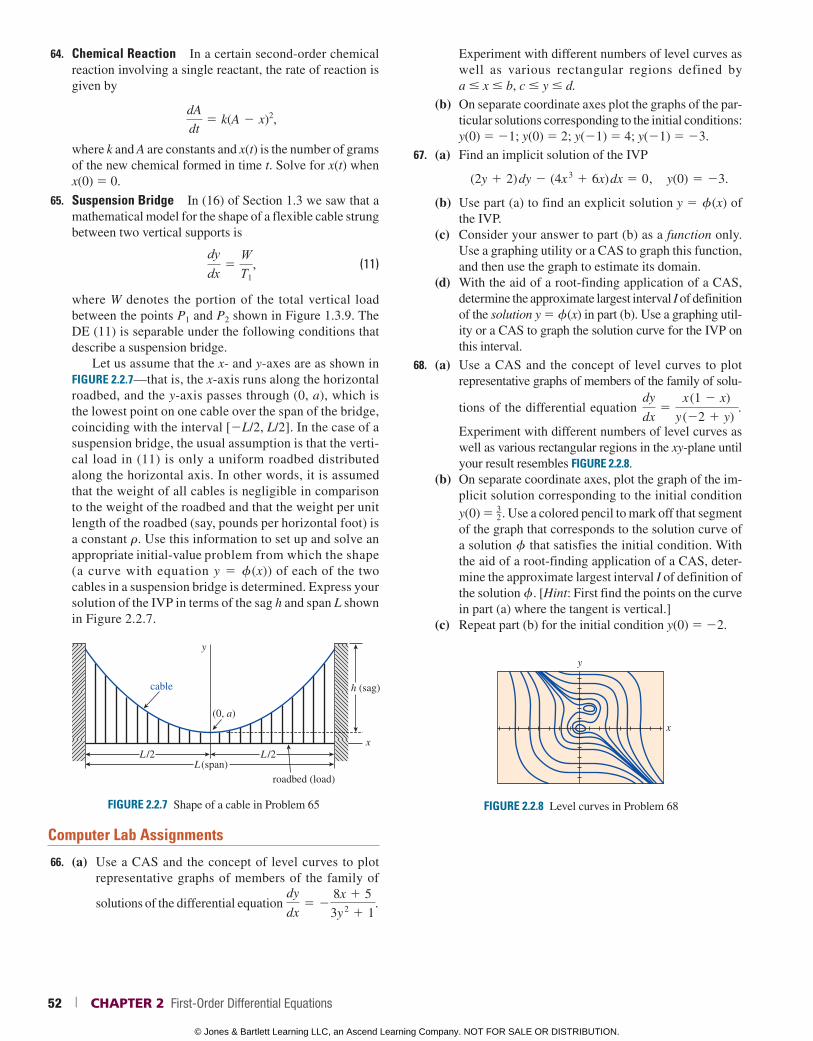
64. Chemical Reaction In a certain second-order chemical reaction involving a single reactant, the rate of reaction is given by
dA
dt5 k(A 2 x)2,
where k and A are constants and x(t) is the number of grams of the new chemical formed in time t. Solve for x(t) when x(0) 5 0.
65. Suspension Bridge In (16) of Section 1.3 we saw that a mathematical model for the shape of a flexible cable strung between two vertical supports is
dydx
5WT1
, (11)
where W denotes the portion of the total vertical load between the points P1 and P2 shown in Figure 1.3.9. The DE (11) is separable under the following conditions that describe a suspension bridge.
Let us assume that the x- and y-axes are as shown in FIGURE 2.2.7—that is, the x-axis runs along the horizontal roadbed, and the y-axis passes through (0, a), which is the lowest point on one cable over the span of the bridge, coinciding with the interval [2L/2, L/2]. In the case of a suspension bridge, the usual assumption is that the verti-cal load in (11) is only a uniform roadbed distributed along the horizontal axis. In other words, it is assumed that the weight of all cables is negligible in comparison to the weight of the roadbed and that the weight per unit length of the roadbed (say, pounds per horizontal foot) is a constant r. Use this information to set up and solve an appropriate initial-value problem from which the shape (a curve with equation y 5 f(x)) of each of the two cables in a suspension bridge is determined. Express your solution of the IVP in terms of the sag h and span L shown in Figure 2.2.7.
FIGURE 2.2.7 Shape of a cable in Problem 65
(0, a)
roadbed (load)
y
x
h (sag)
L /2 L /2L (span)
cable
Computer Lab Assignments
66. (a) Use a CAS and the concept of level curves to plot representative graphs of members of the family of
solutions of the differential equation dy
dx5 2
8x 1 5
3y 2 1 1
.
Experiment with different numbers of level curves as well as various rectangular regions defined by a # x # b, c # y # d.
(b) On separate coordinate axes plot the graphs of the par-ticular solutions corresponding to the initial conditions: y(0) 5 21; y(0) 5 2; y(21) 5 4; y(21) 5 23.
67. (a) Find an implicit solution of the IVP
(2y 1 2) dy 2 (4x 3 1 6x) dx 5 0, y(0) 5 23.
(b) Use part (a) to find an explicit solution y 5 f(x) of the IVP.
(c) Consider your answer to part (b) as a function only. Use a graphing utility or a CAS to graph this function, and then use the graph to estimate its domain.
(d) With the aid of a root-finding application of a CAS, determine the approximate largest interval I of definition of the solution y 5 f(x) in part (b). Use a graphing util-ity or a CAS to graph the solution curve for the IVP on this interval.
68. (a) Use a CAS and the concept of level curves to plot representative graphs of members of the family of solu-
tions of the differential equation dy
dx5
x (1 2 x)
y (22 1 y) .
Experiment with different numbers of level curves as well as various rectangular regions in the xy-plane until your result resembles FIGURE 2.2.8.
(b) On separate coordinate axes, plot the graph of the im-plicit solution corresponding to the initial condition y(0) 5 32 . Use a colored pencil to mark off that segment of the graph that corresponds to the solution curve of a solution f that satisfies the initial condition. With the aid of a root-finding application of a CAS, deter-mine the approximate largest interval I of definition of the solution f. [Hint: First find the points on the curve in part (a) where the tangent is vertical.]
(c) Repeat part (b) for the initial condition y(0) 5 22.
FIGURE 2.2.8 Level curves in Problem 68
y
x
52 | CHAPTER 2 First-Order Differential Equations
© Jones & Bartlett Learning LLC, an Ascend Learning Company. NOT FOR SALE OR DISTRIBUTION.
© Jones & Bartlett Learning, LLCNOT FOR SALE OR DISTRIBUTION
© Jones & Bartlett Learning, LLCNOT FOR SALE OR DISTRIBUTION
© Jones & Bartlett Learning, LLCNOT FOR SALE OR DISTRIBUTION
© Jones & Bartlett Learning, LLCNOT FOR SALE OR DISTRIBUTION
© Jones & Bartlett Learning, LLCNOT FOR SALE OR DISTRIBUTION
© Jones & Bartlett Learning, LLCNOT FOR SALE OR DISTRIBUTION
© Jones & Bartlett Learning, LLCNOT FOR SALE OR DISTRIBUTION
© Jones & Bartlett Learning, LLCNOT FOR SALE OR DISTRIBUTION
© Jones & Bartlett Learning, LLCNOT FOR SALE OR DISTRIBUTION
© Jones & Bartlett Learning, LLCNOT FOR SALE OR DISTRIBUTION
© Jones & Bartlett Learning, LLCNOT FOR SALE OR DISTRIBUTION
© Jones & Bartlett Learning, LLCNOT FOR SALE OR DISTRIBUTION
© Jones & Bartlett Learning, LLCNOT FOR SALE OR DISTRIBUTION
© Jones & Bartlett Learning, LLCNOT FOR SALE OR DISTRIBUTION
© Jones & Bartlett Learning, LLCNOT FOR SALE OR DISTRIBUTION
© Jones & Bartlett Learning, LLCNOT FOR SALE OR DISTRIBUTION
© Jones & Bartlett Learning, LLCNOT FOR SALE OR DISTRIBUTION
© Jones & Bartlett Learning, LLCNOT FOR SALE OR DISTRIBUTION
© Jones & Bartlett Learning, LLCNOT FOR SALE OR DISTRIBUTION
© Jones & Bartlett Learning, LLCNOT FOR SALE OR DISTRIBUTION
2.3 Linear Equations
INTRODUCTION We continue our search for solutions of first-order DEs by next examining linear equations. Linear differential equations are an especially “friendly” family of differential equations in that, given a linear equation, whether first-order or a higher-order kin, there is always a good possibility that we can find some sort of solution of the equation that we can look at.
A Definition The form of a linear first-order DE was given in (7) of Section 1.1. This form, the case when n 5 1 in (6) of that section, is reproduced here for convenience.
DEFINITION 2.3.1 Linear Equation
A first-order differential equation of the form
a1(x) dy
dx1 a0(x)y 5 g(x) (1)
is said to be a linear equation in the dependent variable y.
When g(x) 5 0, the linear equation (1) is said to be homogeneous; otherwise, it is nonhomogeneous.
Standard Form By dividing both sides of (1) by the lead coefficient a1(x) we obtain a more useful form, the standard form, of a linear first-order equation
dy
dx1 P(x)y 5 f (x). (2)
We seek a solution of (2) on an interval I for which both functions P and f are continuous.In the discussion that follows, we illustrate a property and a procedure and end up with a
formula representing the form that every solution of (2) must have. But more than the formula, the property and the procedure are important, because these two concepts carry over to linear equations of higher order.
The Property The differential equation (2) has the property that its solution is the sum of the two solutions, y 5 yc 1 yp, where yc is a solution of the associated homogeneous equation
dy
dx1 P(x)y 5 0 (3)
and yp is a particular solution of the nonhomogeneous equation (2). To see this, observe
d
dx 3yc 1 yp 4 1 P(x) 3yc 1 yp 4 5 cdyc
dx1 P(x)yc d 1 c
dyp
dx1 P(x)yp d 5 f ( x).
0 f (x)
The Homogeneous DE The homogeneous equation (3) is also separable. This fact enables us to find yc by writing (3) as
dy
y1 P(x) dx 5 0
and integrating. Solving for y gives yc 5 ce –eP(x) dx. For convenience let us write yc 5 cy1(x), where y1 5 e –eP(x) dx. The fact that dy1/dx 1 P(x)y1 5 0 will be used next to determine yp.
The Nonhomogeneous DE We can now find a particular solution of equation (2) by a procedure known as variation of parameters. The basic idea here is to find a function u so that yp 5 u(x)y1(x) 5 u(x) e –eP(x) dx is a solution of (2). In other words, our assumption for yp is the same as yc 5 cy1(x) except that c is replaced by the “variable parameter” u. Substituting yp 5 uy1 into (2) gives
2.3 Linear Equations | 53
© Jones & Bartlett Learning LLC, an Ascend Learning Company. NOT FOR SALE OR DISTRIBUTION.
© Jones & Bartlett Learning, LLCNOT FOR SALE OR DISTRIBUTION
© Jones & Bartlett Learning, LLCNOT FOR SALE OR DISTRIBUTION
© Jones & Bartlett Learning, LLCNOT FOR SALE OR DISTRIBUTION
© Jones & Bartlett Learning, LLCNOT FOR SALE OR DISTRIBUTION
© Jones & Bartlett Learning, LLCNOT FOR SALE OR DISTRIBUTION
© Jones & Bartlett Learning, LLCNOT FOR SALE OR DISTRIBUTION
© Jones & Bartlett Learning, LLCNOT FOR SALE OR DISTRIBUTION
© Jones & Bartlett Learning, LLCNOT FOR SALE OR DISTRIBUTION
© Jones & Bartlett Learning, LLCNOT FOR SALE OR DISTRIBUTION
© Jones & Bartlett Learning, LLCNOT FOR SALE OR DISTRIBUTION
© Jones & Bartlett Learning, LLCNOT FOR SALE OR DISTRIBUTION
© Jones & Bartlett Learning, LLCNOT FOR SALE OR DISTRIBUTION
© Jones & Bartlett Learning, LLCNOT FOR SALE OR DISTRIBUTION
© Jones & Bartlett Learning, LLCNOT FOR SALE OR DISTRIBUTION
© Jones & Bartlett Learning, LLCNOT FOR SALE OR DISTRIBUTION
© Jones & Bartlett Learning, LLCNOT FOR SALE OR DISTRIBUTION
© Jones & Bartlett Learning, LLCNOT FOR SALE OR DISTRIBUTION
© Jones & Bartlett Learning, LLCNOT FOR SALE OR DISTRIBUTION
© Jones & Bartlett Learning, LLCNOT FOR SALE OR DISTRIBUTION
© Jones & Bartlett Learning, LLCNOT FOR SALE OR DISTRIBUTION
Product Rule zero T T
u dy1
dx1 y1
du
dx1 P(x)uy1 5 f ( x) or u cdy1
dx1 P(x)y1 d 1 y1
du
dx5 f ( x)
so that y1 du
dx5 f ( x).
Separating variables and integrating then gives
du 5f (x)
y1(x) dx and u 5 3
f (x)
y1(x) dx.
From the definition of y1(x), we see 1/y1(x) 5 e eP(x) dx. Therefore
yp 5 uy1 5 a#f (x)
y1(x) dxb e2eP(x) dx 5 e2eP(x) dx#e
eP (x) dx f (x) dx,
and y 5 yc 1 yp 5 ce 2eP(x) dx 1 e2eP(x) dx#e
eP(x) dx f (x) dx. (4)
Hence if (2) has a solution, it must be of form (4). Conversely, it is a straightforward exercise in differentiation to verify that (4) constitutes a one-parameter family of solutions of equation (2).
You should not memorize the formula given in (4). There is an equivalent but easier way of solving (2). If (4) is multiplied by
e eP(x) dx (5)
and then e eP(x) dx y 5 c 1 #e
eP(x) dx f ( x) dx (6)
is differentiated, d
dx [e
eP(x) dxy] 5 e eP(x) dx
f ( x), (7)
we get e eP(x) dx
dy
dx1 P(x) e
eP(x) dxy 5 e eP(x) dx
f ( x). (8)
Dividing the last result by e eP(x) dx gives (2).
Method of Solution The recommended method of solving (2) actually consists of (6)–(8) worked in reverse order. In other words, if (2) is multiplied by (5), we get (8). The left side of (8) is recognized as the derivative of the product of e eP(x) dx and y. This gets us to (7). We then integrate both sides of (7) to get the solution (6). Because we can solve (2) by integration after multiplication by e
eP(x) dx, we call this function an integrating factor for the differential equation. For convenience we summarize these results. We again emphasize that you should not memorize formula (4) but work through the following two-step procedure each time.
Guidelines for Solving a Linear First-Order Equation
(i) Put a linear first-order equation of form (1) into standard form (2) and then determine P(x) and the integrating factor e eP(x) dx.
(ii) Multiply (2) by the integrating factor. The left side of the resulting equation is auto-matically the derivative of the product of the integrating factor and y. Write
d
dx [e
eP(x) dxy] 5 e eP(x) dx f ( x)
and then integrate both sides of this equation.
54 | CHAPTER 2 First-Order Differential Equations
© Jones & Bartlett Learning LLC, an Ascend Learning Company. NOT FOR SALE OR DISTRIBUTION.
© Jones & Bartlett Learning, LLCNOT FOR SALE OR DISTRIBUTION
© Jones & Bartlett Learning, LLCNOT FOR SALE OR DISTRIBUTION
© Jones & Bartlett Learning, LLCNOT FOR SALE OR DISTRIBUTION
© Jones & Bartlett Learning, LLCNOT FOR SALE OR DISTRIBUTION
© Jones & Bartlett Learning, LLCNOT FOR SALE OR DISTRIBUTION
© Jones & Bartlett Learning, LLCNOT FOR SALE OR DISTRIBUTION
© Jones & Bartlett Learning, LLCNOT FOR SALE OR DISTRIBUTION
© Jones & Bartlett Learning, LLCNOT FOR SALE OR DISTRIBUTION
© Jones & Bartlett Learning, LLCNOT FOR SALE OR DISTRIBUTION
© Jones & Bartlett Learning, LLCNOT FOR SALE OR DISTRIBUTION
© Jones & Bartlett Learning, LLCNOT FOR SALE OR DISTRIBUTION
© Jones & Bartlett Learning, LLCNOT FOR SALE OR DISTRIBUTION
© Jones & Bartlett Learning, LLCNOT FOR SALE OR DISTRIBUTION
© Jones & Bartlett Learning, LLCNOT FOR SALE OR DISTRIBUTION
© Jones & Bartlett Learning, LLCNOT FOR SALE OR DISTRIBUTION
© Jones & Bartlett Learning, LLCNOT FOR SALE OR DISTRIBUTION
© Jones & Bartlett Learning, LLCNOT FOR SALE OR DISTRIBUTION
© Jones & Bartlett Learning, LLCNOT FOR SALE OR DISTRIBUTION
© Jones & Bartlett Learning, LLCNOT FOR SALE OR DISTRIBUTION
© Jones & Bartlett Learning, LLCNOT FOR SALE OR DISTRIBUTION
EXAMPLE 1 Solving a Linear DE
Solve dy
dx2 3y 5 6.
SOLUTION This linear equation can be solved by separation of variables. Alternatively, since the equation is already in the standard form (2), we see that the integrating factor is ee(–3) dx 5 e –3x. We multiply the equation by this factor and recognize that
e 23x
dy
dx2 3e
23x y 5 6e 23x is the same as
d
dx 3e
23x y 4 5 6e 23x.
Integrating both sides of the last equation,
#d
dx [e
23x y] 5 #6e23x dx
gives e –3x y 5 22e –3x 1 c. Thus a solution of the differential equation is y 5 22 1 ce 3x,
2q , x , q .
When a1, a0, and g in (1) are constants, the differential equation is autonomous. In Example 1, you can verify from the normal form dy/dx 5 3(y 1 2) that 22 is a critical point and that it is unstable and a repeller. Thus a solution curve with an initial point either above or below the graph of the equilibrium solution y 5 22 pushes away from this horizontal line as x increases.
Constant of Integration Notice in the general discussion and in Example 1 we disre-garded a constant of integration in the evaluation of the indefinite integral in the exponent of e eP(x) dx. If you think about the laws of exponents and the fact that the integrating factor multiplies both sides of the differential equation, you should be able to answer why writing eP(x) dx 1 c is unnecessary. See Problem 55 in Exercises 2.3.
General Solution Suppose again that the functions P and f in (2) are continuous on a common interval I. In the steps leading to (4) we showed that if (2) has a solution on I, then it must be of the form given in (4). Conversely, it is a straightforward exercise in differentiation to verify that any function of the form given in (4) is a solution of the differential equation (2) on I. In other words, (4) is a one-parameter family of solutions of equation (2), and every solution of (2) defined on I is a member of this family. Consequently, we are justified in calling (4) the general solution of the differential equation on the interval I. Now by writing (2) in the normal form y9 5 F(x, y) we can identify F(x, y) 5 2P(x)y 1 f (x) and 0F/0y 5 2P(x). From the continuity of P and f on the interval I, we see that F and 0F/0y are also continuous on I. With Theorem 1.2.1 as our justification, we conclude that there exists one and only one solution of the first-order initial-value problem
dy
dx1 P(x)y 5 f (x), y(x0) 5 y0 (9)
defined on some interval I0 containing x0. But when x0 is in I, finding a solution of (9) is just a matter of finding an appropriate value of c in (4); that is, for each x0 in I there corresponds a distinct c. In other words, the interval I0 of existence and uniqueness in Theorem 1.2.1 for the initial-value problem (9) is the entire interval I.
EXAMPLE 2 General Solution
Solve x dy
dx2 4y 5 x
6e x.
SOLUTION By dividing by x we get the standard form
dy
dx2
4x
y 5 x 5e
x. (10)
From this form we identify P(x) 5 24/x and f (x) 5 x 5e x and observe that P and f are con-tinuous on the interval (0, q ). Hence the integrating factor is
2.3 Linear Equations | 55
© Jones & Bartlett Learning LLC, an Ascend Learning Company. NOT FOR SALE OR DISTRIBUTION.
© Jones & Bartlett Learning, LLCNOT FOR SALE OR DISTRIBUTION
© Jones & Bartlett Learning, LLCNOT FOR SALE OR DISTRIBUTION
© Jones & Bartlett Learning, LLCNOT FOR SALE OR DISTRIBUTION
© Jones & Bartlett Learning, LLCNOT FOR SALE OR DISTRIBUTION
© Jones & Bartlett Learning, LLCNOT FOR SALE OR DISTRIBUTION
© Jones & Bartlett Learning, LLCNOT FOR SALE OR DISTRIBUTION
© Jones & Bartlett Learning, LLCNOT FOR SALE OR DISTRIBUTION
© Jones & Bartlett Learning, LLCNOT FOR SALE OR DISTRIBUTION
© Jones & Bartlett Learning, LLCNOT FOR SALE OR DISTRIBUTION
© Jones & Bartlett Learning, LLCNOT FOR SALE OR DISTRIBUTION
© Jones & Bartlett Learning, LLCNOT FOR SALE OR DISTRIBUTION
© Jones & Bartlett Learning, LLCNOT FOR SALE OR DISTRIBUTION
© Jones & Bartlett Learning, LLCNOT FOR SALE OR DISTRIBUTION
© Jones & Bartlett Learning, LLCNOT FOR SALE OR DISTRIBUTION
© Jones & Bartlett Learning, LLCNOT FOR SALE OR DISTRIBUTION
© Jones & Bartlett Learning, LLCNOT FOR SALE OR DISTRIBUTION
© Jones & Bartlett Learning, LLCNOT FOR SALE OR DISTRIBUTION
© Jones & Bartlett Learning, LLCNOT FOR SALE OR DISTRIBUTION
© Jones & Bartlett Learning, LLCNOT FOR SALE OR DISTRIBUTION
© Jones & Bartlett Learning, LLCNOT FOR SALE OR DISTRIBUTION
we can use ln x instead of ln | x | since x 0 T
e24edx>x 5 e24 ln x 5 e ln x24
5 x24.
Here we have used the basic identity b log b N 5 N, N 0. Now we multiply (10) by x –4,
x 24
dy
dx2 4x
25y 5 xe x, and obtain
d
dx 3x
24y 4 5 xe x.
It follows from integration by parts that 3xe xdx 5 xe
x 2 e x and so
#d
dx [x
24y] 5 #xe x dx
gives x –4y 5 xe x 2 e x 1 c. Thus the general solution defined on (0, q ) is y 5 x
5e x 2 x
4e x 1 cx
4.
Singular Points Except in the case when the lead coefficient is 1, the recasting of equa-tion (1) into the standard form (2) requires division by a1(x). Values of x for which a1(x) 5 0 are called singular points of the equation. Singular points are potentially troublesome. Specifically in (2), if P(x) (formed by dividing a0(x) by a1(x)) is discontinuous at a point, the discontinuity may carry over to functions in the general solution of the differential equation.
EXAMPLE 3 General Solution
Find the general solution of (x 2 2 9)
dy
dx1 xy 5 0.
SOLUTION We write the differential equation in standard form
dydx
1x
x 2 2 9 y 5 0 (11)
and identify P(x) 5 x/(x 2 2 9). Although P is continuous on (2q, 23), on (23, 3), and on (3, q ), we shall solve the equation on the first and third intervals. On these intervals the integrating factor is
e ex dx>(x
229) 5 e
12e2x dx>(x
229) 5 e
12 ln | x229 | 5 "x
2 2 9.
After multiplying the standard form (11) by this factor, we get
d
dx 3"x
2 2 9 y 4 5 0 and integrating gives "x 2 2 9 y 5 c.
Thus on either (2q, 23) or (3, q), the general solution of the equation is y 5 c/"x 2 2 9.
Notice in the preceding example that x 5 3 and x 5 23 are singular points of the equation and that every function in the general solution y 5 c/"x
2 2 9 is discontinuous at these points. On the other hand, x 5 0 is a singular point of the differential equation in Example 2, but the general solution y 5 x 5e x 2 x 4e x 1 cx 4 is noteworthy in that every function in this one-parameter family is continuous at x 5 0 and is defined on the interval (2q, q ) and not just on (0, q ) as stated in the solution. However, the family y 5 x 5e x 2 x 4e x 1 cx 4 defined on (2q, q ) cannot be considered the general solution of the DE, since the singular point x 5 0 still causes a problem. See Problems 50 and 51 in Exercises 2.3. We will study singular points for linear differential equations in greater depth in Section 5.2.
EXAMPLE 4 An Initial-Value Problem
Solve the initial-value problem dy
dx1 y 5 x, y(0) 5 4.
SOLUTION The equation is in standard form, and P(x) 5 1 and f (x) 5 x are continuous on the interval (2q, q ). The integrating factor is eedx 5 e x, and so integrating
56 | CHAPTER 2 First-Order Differential Equations
© Jones & Bartlett Learning LLC, an Ascend Learning Company. NOT FOR SALE OR DISTRIBUTION.
© Jones & Bartlett Learning, LLCNOT FOR SALE OR DISTRIBUTION
© Jones & Bartlett Learning, LLCNOT FOR SALE OR DISTRIBUTION
© Jones & Bartlett Learning, LLCNOT FOR SALE OR DISTRIBUTION
© Jones & Bartlett Learning, LLCNOT FOR SALE OR DISTRIBUTION
© Jones & Bartlett Learning, LLCNOT FOR SALE OR DISTRIBUTION
© Jones & Bartlett Learning, LLCNOT FOR SALE OR DISTRIBUTION
© Jones & Bartlett Learning, LLCNOT FOR SALE OR DISTRIBUTION
© Jones & Bartlett Learning, LLCNOT FOR SALE OR DISTRIBUTION
© Jones & Bartlett Learning, LLCNOT FOR SALE OR DISTRIBUTION
© Jones & Bartlett Learning, LLCNOT FOR SALE OR DISTRIBUTION
© Jones & Bartlett Learning, LLCNOT FOR SALE OR DISTRIBUTION
© Jones & Bartlett Learning, LLCNOT FOR SALE OR DISTRIBUTION
© Jones & Bartlett Learning, LLCNOT FOR SALE OR DISTRIBUTION
© Jones & Bartlett Learning, LLCNOT FOR SALE OR DISTRIBUTION
© Jones & Bartlett Learning, LLCNOT FOR SALE OR DISTRIBUTION
© Jones & Bartlett Learning, LLCNOT FOR SALE OR DISTRIBUTION
© Jones & Bartlett Learning, LLCNOT FOR SALE OR DISTRIBUTION
© Jones & Bartlett Learning, LLCNOT FOR SALE OR DISTRIBUTION
© Jones & Bartlett Learning, LLCNOT FOR SALE OR DISTRIBUTION
© Jones & Bartlett Learning, LLCNOT FOR SALE OR DISTRIBUTION
d
dx 3e
xy 4 5 xe x
gives e xy 5 xe x 2 e x 1 c. Solving this last equation for y yields the general solution y 5 x 2 1 1 ce – x. But from the initial condition we know that y 5 4 when x 5 0. Substituting these values in the general solution implies c 5 5. Hence the solution of the problem on the interval (2q, q) is
y 5 x 2 1 1 5e – x. (12)
Recall that the general solution of every linear first-order differential equation is a sum of two special solutions: yc , the general solution of the associated homogeneous equation (3), and yp , a particular solution of the nonhomogeneous equation (2). In Example 4 we identify yc 5 ce – x and yp 5 x 2 1. FIGURE 2.3.1, obtained with the aid of a graphing utility, shows (12) in blue along with other representative solutions in the family y 5 x 2 1 1 ce – x. It is interesting to observe that as x gets large, the graphs of all members of the family are close to the graph of yp 5 x 2 1, which is shown in green in Figure 2.3.1. This is because the contribution of yc 5 ce – x to the values of a solution becomes negligible for increasing values of x. We say that yc 5 ce–x is a transient term since yc S 0 as x S q . While this behavior is not a characteristic of all general solu-tions of linear equations (see Example 2), the notion of a transient is often important in applied problems.
Piecewise-Linear Differential Equation In the construction of mathematical mod-els (especially in the biological sciences and engineering) it can happen that one or more coef-ficients in a differential equation is a piecewise-defined function. In particular, when either P(x) or f(x) in (2) is a piecewise-defined function the equation is then referred to as a piecewise-linear differential equation. In the next example, f (x) is piecewise continuous on the interval [0, q ) with a single jump discontinuity at x 5 1. The basic idea is to solve the initial-value problem in two parts corresponding to the two intervals over which f (x) is defined; each part consists of a linear equation solvable by the method of this section. As we will see, it is then possible to piece the two solutions together at x 5 1 so that y(x) is continuous on [0, q ). See Problems 33–38 in Exercises 2.3.
EXAMPLE 5 An Initial-Value Problem
Solve dy
dx1 y 5 f (x), y(0) 5 0 where f (x) 5 e1, 0 # x # 1
0, x . 1.
SOLUTION The graph of the discontinuous function f is shown in FIGURE 2.3.2. We solve the DE for y(x) first on the interval [0, 1] and then on the interval (1, q ). For 0 # x # 1 we have
dydx
1 y 5 1 or, equivalently, d
dx 3e
xy 4 5 e x.
Integrating this last equation and solving for y gives y 5 1 1 c1e – x. Since y(0) 5 0, we must have c1 5 21, and therefore y 5 1 2 e – x, 0 # x # 1. Then for x 1, the equation
dydx
1 y 5 0
leads to y 5 c2e – x. Hence we can write
y 5 e1 2 e2x, 0 # x # 1c2e2x, x . 1.
By appealing to the definition of continuity at a point it is possible to determine c2 so that the foregoing function is continuous at x 5 1. The requirement that limxS11 y(x) 5 y(1) implies that c2e – 1 5 1 2 e – 1 or c2 5 e 2 1. As seen in FIGURE 2.3.3, the piecewise defined function
y 5 e1 2 e2x, 0 # x # 1
(e 2 1) e2x, x . 1 (13)
is continuous on the interval [0, q ).
FIGURE 2.3.2 Discontinuous f (x) in Example 5
1
1
y
x
FIGURE 2.3.3 Graph of function in (13) of Example 5
y
1
1
x
FIGURE 2.3.1 Some solutions of the DE in Example 4
4
2
0
0 2 4
x
c = 0
c > 0
c< 0
y
0
–2
–2
–4
–4
2.3 Linear Equations | 57
© Jones & Bartlett Learning LLC, an Ascend Learning Company. NOT FOR SALE OR DISTRIBUTION.
© Jones & Bartlett Learning, LLCNOT FOR SALE OR DISTRIBUTION
© Jones & Bartlett Learning, LLCNOT FOR SALE OR DISTRIBUTION
© Jones & Bartlett Learning, LLCNOT FOR SALE OR DISTRIBUTION
© Jones & Bartlett Learning, LLCNOT FOR SALE OR DISTRIBUTION
© Jones & Bartlett Learning, LLCNOT FOR SALE OR DISTRIBUTION
© Jones & Bartlett Learning, LLCNOT FOR SALE OR DISTRIBUTION
© Jones & Bartlett Learning, LLCNOT FOR SALE OR DISTRIBUTION
© Jones & Bartlett Learning, LLCNOT FOR SALE OR DISTRIBUTION
© Jones & Bartlett Learning, LLCNOT FOR SALE OR DISTRIBUTION
© Jones & Bartlett Learning, LLCNOT FOR SALE OR DISTRIBUTION
© Jones & Bartlett Learning, LLCNOT FOR SALE OR DISTRIBUTION
© Jones & Bartlett Learning, LLCNOT FOR SALE OR DISTRIBUTION
© Jones & Bartlett Learning, LLCNOT FOR SALE OR DISTRIBUTION
© Jones & Bartlett Learning, LLCNOT FOR SALE OR DISTRIBUTION
© Jones & Bartlett Learning, LLCNOT FOR SALE OR DISTRIBUTION
© Jones & Bartlett Learning, LLCNOT FOR SALE OR DISTRIBUTION
© Jones & Bartlett Learning, LLCNOT FOR SALE OR DISTRIBUTION
© Jones & Bartlett Learning, LLCNOT FOR SALE OR DISTRIBUTION
© Jones & Bartlett Learning, LLCNOT FOR SALE OR DISTRIBUTION
© Jones & Bartlett Learning, LLCNOT FOR SALE OR DISTRIBUTION
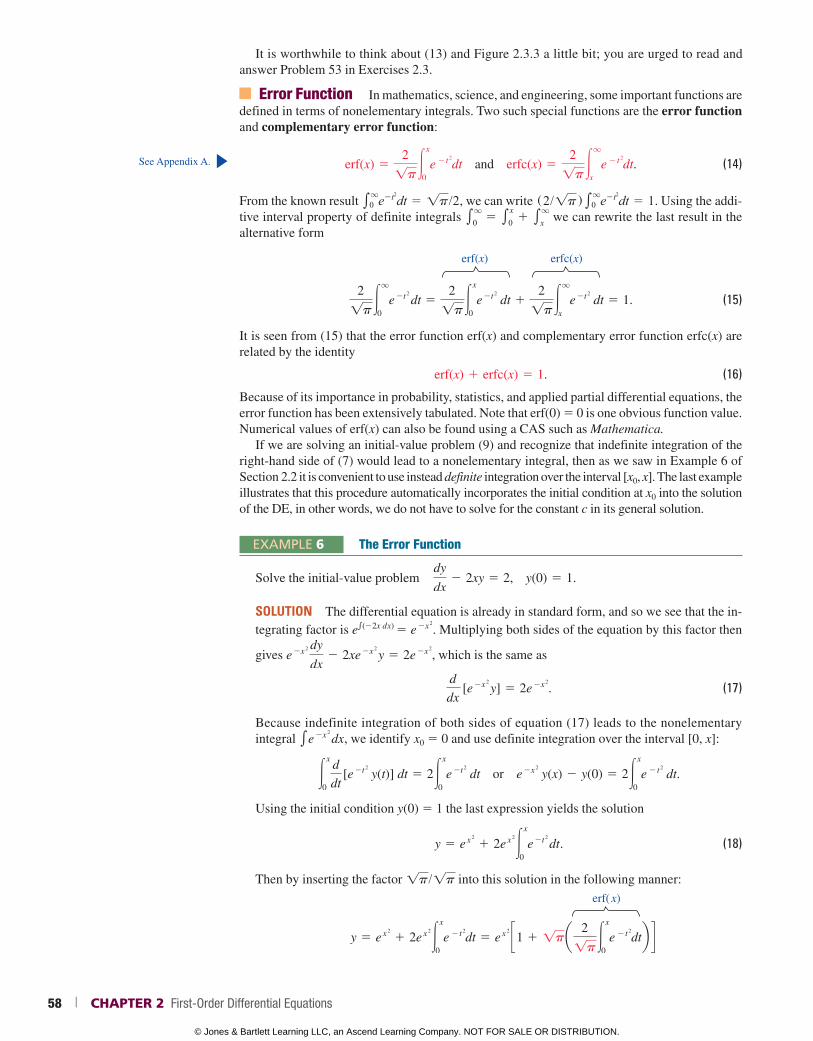
It is worthwhile to think about (13) and Figure 2.3.3 a little bit; you are urged to read and answer Problem 53 in Exercises 2.3.
Error Function In mathematics, science, and engineering, some important functions are defined in terms of nonelementary integrals. Two such special functions are the error function and complementary error function:
erf(x) 52
!p#x
0e
2 t 2
dt and erfc(x) 52
!p#q
x
e 2 t
2
dt. (14)
From the known result eq
0 e2t2dt 5 !p/2, we can write (2/!p) eq
0 e2t2dt 5 1. Using the addi-tive interval property of definite integrals e
q
0 5 ex0 1 e
q
x we can rewrite the last result in the alternative form
erf(x) erfc(x)
2
!p#q
0e
2t 2
dt 52
!p#x
0e
2t 2
dt 12
!p#q
x
e 2t
2
dt 5 1. (15)
It is seen from (15) that the error function erf(x) and complementary error function erfc(x) are related by the identity
erf(x) 1 erfc(x) 5 1. (16)
Because of its importance in probability, statistics, and applied partial differential equations, the error function has been extensively tabulated. Note that erf(0) 5 0 is one obvious function value. Numerical values of erf(x) can also be found using a CAS such as Mathematica.
If we are solving an initial-value problem (9) and recognize that indefinite integration of the right-hand side of (7) would lead to a nonelementary integral, then as we saw in Example 6 of Section 2.2 it is convenient to use instead definite integration over the interval [x0, x]. The last example illustrates that this procedure automatically incorporates the initial condition at x0 into the solution of the DE, in other words, we do not have to solve for the constant c in its general solution.
EXAMPLE 6 The Error Function
Solve the initial-value problem dy
dx2 2xy 5 2, y(0) 5 1.
SOLUTION The differential equation is already in standard form, and so we see that the in-tegrating factor is ee(22x dx) 5 e
2x 2
. Multiplying both sides of the equation by this factor then
gives e 2x
2
dy
dx2 2xe
2x 2
y 5 2e 2x
2
, which is the same as
d
dx [e
2x 2
y] 5 2e 2x
2
. (17)
Because indefinite integration of both sides of equation (17) leads to the nonelementary integral ee
2x 2
dx, we identify x0 5 0 and use definite integration over the interval [0, x]:
#x
0
d
dt [e
2t 2
y(t)] dt 5 2#x
0e
2t 2
dt or e 2x
2
y(x) 2 y(0) 5 2#x
0e
2 t 2
dt.
Using the initial condition y(0) 5 1 the last expression yields the solution
y 5 e x
2
1 2e x
2
#x
0e
2t 2
dt. (18)
Then by inserting the factor !p/!p into this solution in the following manner:
erf( x)
y 5 e x
2
1 2e x
2
#x
0e
2 t 2
dt 5 e x
2 c1 1 !pa 2
!p#x
0e
2 t 2
dtb d
See Appendix A.
58 | CHAPTER 2 First-Order Differential Equations
© Jones & Bartlett Learning LLC, an Ascend Learning Company. NOT FOR SALE OR DISTRIBUTION.
© Jones & Bartlett Learning, LLCNOT FOR SALE OR DISTRIBUTION
© Jones & Bartlett Learning, LLCNOT FOR SALE OR DISTRIBUTION
© Jones & Bartlett Learning, LLCNOT FOR SALE OR DISTRIBUTION
© Jones & Bartlett Learning, LLCNOT FOR SALE OR DISTRIBUTION
© Jones & Bartlett Learning, LLCNOT FOR SALE OR DISTRIBUTION
© Jones & Bartlett Learning, LLCNOT FOR SALE OR DISTRIBUTION
© Jones & Bartlett Learning, LLCNOT FOR SALE OR DISTRIBUTION
© Jones & Bartlett Learning, LLCNOT FOR SALE OR DISTRIBUTION
© Jones & Bartlett Learning, LLCNOT FOR SALE OR DISTRIBUTION
© Jones & Bartlett Learning, LLCNOT FOR SALE OR DISTRIBUTION
© Jones & Bartlett Learning, LLCNOT FOR SALE OR DISTRIBUTION
© Jones & Bartlett Learning, LLCNOT FOR SALE OR DISTRIBUTION
© Jones & Bartlett Learning, LLCNOT FOR SALE OR DISTRIBUTION
© Jones & Bartlett Learning, LLCNOT FOR SALE OR DISTRIBUTION
© Jones & Bartlett Learning, LLCNOT FOR SALE OR DISTRIBUTION
© Jones & Bartlett Learning, LLCNOT FOR SALE OR DISTRIBUTION
© Jones & Bartlett Learning, LLCNOT FOR SALE OR DISTRIBUTION
© Jones & Bartlett Learning, LLCNOT FOR SALE OR DISTRIBUTION
© Jones & Bartlett Learning, LLCNOT FOR SALE OR DISTRIBUTION
© Jones & Bartlett Learning, LLCNOT FOR SALE OR DISTRIBUTION
we see from (14) that (18) can be rewritten in terms of the error function as
y 5 e x
2
[1 1 !p erf(x)]. (19)
The graph of solution (19), shown in FIGURE 2.3.4, was obtained with the aid of a CAS.
See Problems 41–48 in Exercises 2.3.
Use of Computers Some computer algebra systems are capable of producing explicit solutions for some kinds of differential equations. For example, to solve the equation y9 1 2y 5 x, we use the input commands
DSolve[y9[x] + 2 y[x] 55 x, y[x], x] (in Mathematica)and dsolve(diff(y(x), x) + 2*y(x) 5 x, y(x)); (in Maple)
Translated into standard symbols, the output of each program is y 5 214 1 1
2x 1 ce22x.
REMARKS(i) Occasionally a first-order differential equation is not linear in one variable but is linear in the other variable. For example, the differential equation
dy
dx5
1
x 1 y 2
is not linear in the variable y. But its reciprocal
dx
dy5 x 1 y
2 or dx
dy2 x 5 y
2
is recognized as linear in the variable x. You should verify that the integrating factor ee(–1)dy 5 e – y and integration by parts yield an implicit solution of the first equation: x 5 2y 2 2 2y 2 2 1 ce y.(ii) Because mathematicians thought they were appropriately descriptive, certain words were “adopted” from engineering and made their own. The word transient, used earlier, is one of these terms. In future discussions the words input and output will occasionally pop up. The function f in (2) is called the input or driving function; a solution of the differential equa-tion for a given input is called the output or response.(iii) The term special functions mentioned in conjunction with the error function on page 58 also applies to the sine integral function and the Fresnel sine integral function introduced in Problems 47 and 48 in Exercises 2.3. “Special Functions” is actually a well-defined field of study in mathematics. The Fresnel sine integral function is one of two such special integral functions that the French engineer/physicist Augustin-Jean Fresnel (1788–1827) encoun-tered in his study of optics. More special functions are studied in Section 5.3.
x
y
−3 −2 −1 1
1
−1
−2
2
2 3
(0, 1)
FIGURE 2.3.4 Graph of (19) in Example 6
2.3 Exercises Answers to selected odd-numbered problems begin on page ANS-2.
In Problems 1–24, find the general solution of the given dif-ferential equation. Give the largest interval over which the general solution is defined. Determine whether there are any transient terms in the general solution.
1. dydx
5 5y 2. dydx
1 2y 5 0
3. dy
dx1 y 5 e
3x 4. 3 dy
dx1 12y 5 4
5. y r 1 3x 2y 5 x
2 6. y r 1 2xy 5 x 3
7. x 2y r 1 xy 5 1 8. y r 5 2y 1 x
2 1 5
9. x dy
dx2 y 5 x
2 sin x 10. x
dy
dx1 2y 5 3
11. x dy
dx1 4y 5 x
3 2 x 12. (1 1 x) dy
dx2 xy 5 x 1 x
2
13. x 2y r 1 x(x 1 2)y 5 e
x
14. xy r 1 (1 1 x)y 5 e 2x
sin 2x
15. y dx 2 4(x 1 y 6) dy 5 0
16. y dx 5 (ye y 2 2x) dy
17. cos x
dy
dx1 (sin x)y 5 1
2.3 Linear Equations | 59
© Jones & Bartlett Learning LLC, an Ascend Learning Company. NOT FOR SALE OR DISTRIBUTION.
© Jones & Bartlett Learning, LLCNOT FOR SALE OR DISTRIBUTION
© Jones & Bartlett Learning, LLCNOT FOR SALE OR DISTRIBUTION
© Jones & Bartlett Learning, LLCNOT FOR SALE OR DISTRIBUTION
© Jones & Bartlett Learning, LLCNOT FOR SALE OR DISTRIBUTION
© Jones & Bartlett Learning, LLCNOT FOR SALE OR DISTRIBUTION
© Jones & Bartlett Learning, LLCNOT FOR SALE OR DISTRIBUTION
© Jones & Bartlett Learning, LLCNOT FOR SALE OR DISTRIBUTION
© Jones & Bartlett Learning, LLCNOT FOR SALE OR DISTRIBUTION
© Jones & Bartlett Learning, LLCNOT FOR SALE OR DISTRIBUTION
© Jones & Bartlett Learning, LLCNOT FOR SALE OR DISTRIBUTION
© Jones & Bartlett Learning, LLCNOT FOR SALE OR DISTRIBUTION
© Jones & Bartlett Learning, LLCNOT FOR SALE OR DISTRIBUTION
© Jones & Bartlett Learning, LLCNOT FOR SALE OR DISTRIBUTION
© Jones & Bartlett Learning, LLCNOT FOR SALE OR DISTRIBUTION
© Jones & Bartlett Learning, LLCNOT FOR SALE OR DISTRIBUTION
© Jones & Bartlett Learning, LLCNOT FOR SALE OR DISTRIBUTION
© Jones & Bartlett Learning, LLCNOT FOR SALE OR DISTRIBUTION
© Jones & Bartlett Learning, LLCNOT FOR SALE OR DISTRIBUTION
© Jones & Bartlett Learning, LLCNOT FOR SALE OR DISTRIBUTION
© Jones & Bartlett Learning, LLCNOT FOR SALE OR DISTRIBUTION
18. cos2x sin x
dy
dx1 ( cos3x)y 5 1
19. (x 1 1)
dy
dx1 (x 1 2)y 5 2xe
2x
20. (x 1 2)2
dy
dx5 5 2 8y 2 4xy
21. dr
du1 r sec u 5 cos u
22. dP
dt1 2tP 5 P 1 4t 2 2
23. x
dy
dx1 (3x 1 1)y 5 e
23x
24. (x2 2 1)
dy
dx1 2y 5 (x 1 1)2
In Problems 25–32, solve the given initial-value problem. Give the largest interval I over which the solution is defined.
25. xy r 1 y 5 e x, y(1) 5 2
26. y
dx
dy2 x 5 2y
2, y(1) 5 5
27. L
di
dt1 Ri 5 E; i(0) 5 i0, L, R, E, and i0 constants
28. dT
dt5 k(T 2 Tm); T(0) 5 T0, K, Tm , and T0 constants
29. (x 1 1)
dy
dx1 y 5 ln x, y(1) 5 10
30. y r 1 ( tan x)y 5 cos2x, y(0) 5 21
31. ae 22"x 2 y
"xb
dx
dy5 1, y(1) 5 1
32. (1 1 t 2)
dx
dt1 x 5 tan
21t, x(0) 5 4
[Hint: In your solution let u 5 tan 21t.]
In Problems 33–36, proceed as in Example 5 to solve the given initial-value problem. Use a graphing utility to graph the continuous function y(x).
33. dy
dx1 2y 5 f (x), y(0) 5 0, where
f (x) 5 e1, 0 # x # 3
0, x . 3
34. dy
dx1 y 5 f (x), y(0) 5 1, where
f (x) 5 e1,
21,
0 # x # 1
x . 1
35. dy
dx1 2xy 5 f (x), y(0) 5 2, where
f (x) 5 e x, 0 # x , 1
0, x $ 1
36. (1 1 x 2)
dy
dx1 2xy 5 f (x), y(0) 5 0, where
f (x) 5 e x, 0 # x , 1
2x, x $ 1
In Problems 37 and 38, proceed as in Example 5 to solve the given initial-value problem. Use a graphing utility to graph the continuous function y(x).
37. dy
dx1 P(x)y 5 4x, y(0) 5 3, where
P(x) 5 •2, 0 # x # 1
22x
, x . 1
38. dy
dx1 P(x)y 5 0, y(0) 5 4, where
P(x) 5 e1, 0 # x # 2
5, x . 2
In Problems 39 and 40, the given differential equation is not linear in y. Nevertheless, find a general solution of the equation.
39. dx 5 (x 1 y 2) dy
40. y dx 1 (2x 1 xy 2 3) dy 5 0
In Problems 41 and 42, proceed as in Example 6 and express the solution of the given initial-value problem in terms of erf(x) (Problem 41) and erfc(x) (Problem 42).
41. dy
dx2 2xy 5 1, y(1) 5 1
42. dy
dx2 2xy 5 1, y(0) 5 !p>2
In Problems 43–46, proceed as in Example 6 and express the solution of the given initial-value problem in terms of an integral-defined function.
43. dy
dx1 e
xy 5 1, y(0) 5 1
44. x 2
dy
dx2 y 5 x
3, y(1) 5 0
45. dy
dx1 xy 5 cos x, y(0) 5 2
46. dy
dx1 (sin x)y 5 10x, y(0) 5 0
47. The sine integral function is defined as
Si(x) 5 #x
0
sin t
t dt,
where the integrand is defined to be 1 at x 5 0. Express the solution of the initial-value problem
x 3
dy
dx1 2x
2y 5 10 sin x, y(1) 5 0
in terms of Si(x).
60 | CHAPTER 2 First-Order Differential Equations
© Jones & Bartlett Learning LLC, an Ascend Learning Company. NOT FOR SALE OR DISTRIBUTION.
© Jones & Bartlett Learning, LLCNOT FOR SALE OR DISTRIBUTION
© Jones & Bartlett Learning, LLCNOT FOR SALE OR DISTRIBUTION
© Jones & Bartlett Learning, LLCNOT FOR SALE OR DISTRIBUTION
© Jones & Bartlett Learning, LLCNOT FOR SALE OR DISTRIBUTION
© Jones & Bartlett Learning, LLCNOT FOR SALE OR DISTRIBUTION
© Jones & Bartlett Learning, LLCNOT FOR SALE OR DISTRIBUTION
© Jones & Bartlett Learning, LLCNOT FOR SALE OR DISTRIBUTION
© Jones & Bartlett Learning, LLCNOT FOR SALE OR DISTRIBUTION
© Jones & Bartlett Learning, LLCNOT FOR SALE OR DISTRIBUTION
© Jones & Bartlett Learning, LLCNOT FOR SALE OR DISTRIBUTION
© Jones & Bartlett Learning, LLCNOT FOR SALE OR DISTRIBUTION
© Jones & Bartlett Learning, LLCNOT FOR SALE OR DISTRIBUTION
© Jones & Bartlett Learning, LLCNOT FOR SALE OR DISTRIBUTION
© Jones & Bartlett Learning, LLCNOT FOR SALE OR DISTRIBUTION
© Jones & Bartlett Learning, LLCNOT FOR SALE OR DISTRIBUTION
© Jones & Bartlett Learning, LLCNOT FOR SALE OR DISTRIBUTION
© Jones & Bartlett Learning, LLCNOT FOR SALE OR DISTRIBUTION
© Jones & Bartlett Learning, LLCNOT FOR SALE OR DISTRIBUTION
© Jones & Bartlett Learning, LLCNOT FOR SALE OR DISTRIBUTION
© Jones & Bartlett Learning, LLCNOT FOR SALE OR DISTRIBUTION
48. The Fresnel sine integral function is defined as
S(x) 5 #x
0sinap
2 t
2b
dt.
Express the solution of the initial-value problem
dy
dx2 (sin x
2)y 5 0, y(0) 5 5
in terms of S(x).
Discussion Problems
49. Reread the discussion following Example 1. Construct a linear first-order differential equation for which all noncon-stant solutions approach the horizontal asymptote y 5 4 as x S q .
50. Reread Example 2 and then discuss, with reference to Theorem 1.2.1, the existence and uniqueness of a solution of the initial-value problem consisting of xy9 2 4y 5 x 6e x and the given initial condition.(a) y(0) 5 0(b) y(0) 5 y0, y0 0(c) y(x0) 5 y0, x0 0, y0 0
51. Reread Example 3 and then find the general solution of the differential equation on the interval (23, 3).
52. Reread the discussion following Example 4. Construct a linear first-order differential equation for which all solutions are asymptotic to the line y 5 3x 2 5 as x S q .
53. Reread Example 5 and then discuss why it is technically incorrect to say that the function in (13) is a solution of the IVP on the interval [0, q ).
54. (a) Construct a linear first-order differential equation of the form xy9 1 a0(x)y 5 g(x) for which yc 5 c/x 3 and yp 5 x 3. Give an interval on which y 5 x 3 1 c/x 3 is the general solution of the DE.
(b) Give an initial condition y(x0) 5 y0 for the DE found in part (a) so that the solution of the IVP is y 5 x 3 2 1/x 3. Repeat if the solution is y 5 x 3 1 2/x 3. Give an interval I of definition of each of these solutions. Graph the solution curves. Is there an initial-value problem whose solution is defined on the interval (2q, q)?
(c) Is each IVP found in part (b) unique? That is, can there be more than one IVP for which, say, y 5 x 3 2 1/x 3, x in some interval I is the solution?
55. In determining the integrating factor (5), there is no need to use a constant of integration in the evaluation of eP(x) dx. Explain why using eP(x) dx 1 c has no effect on the solution of (2).
Mathematical Models
56. Radioactive Decay Series The following system of dif-ferential equations is encountered in the study of the decay of a special type of radioactive series of elements:
dxdt
5 2l1x,
dydt
5 l1x 2 l2 y,
where l1 and l2 are constants. Discuss how to solve this system subject to x(0) 5 x0, y(0) 5 y0. Carry out your ideas.
57. Heart Pacemaker A heart pacemaker consists of a switch, a battery of constant voltage E0, a capacitor with constant capacitance C, and the heart as a resistor with constant re-sistance R. When the switch is closed, the capacitor charges; when the switch is open, the capacitor discharges, sending an electrical stimulus to the heart. During the time the heart is being stimulated, the voltage E across the heart satisfies the linear differential equation
dE
dt5 2
1
RC E.
Solve the DE subject to E(4) 5 E0.
Computer Lab Assignments 58. (a) Use a CAS to graph the solution curve of the initial-
value problem in Problem 42 on the interval (2q, q).(b) Use tables or a CAS to find the value y(2).
59. (a) Use a CAS to graph the solution curve of the initial-value problem in Problem 47 on the interval [0, q).
(b) Use a CAS to find the value of the absolute maximum of the solution y(x) on the interval.
60. (a) Use a CAS to graph the solution curve of the initial-value problem in Problem 48 on the interval (2q, q).
(b) It is known that Fresnel sine integral S(x) S12 as x S q
and S(x) S 212 as x S 2q. What does the solution
y(x) approach as x S q? As x S 2q?(c) Use a CAS to find the values of the absolute maximum
and the absolute minimum of the solution y(x) on the interval.
2.4 Exact Equations
INTRODUCTION Although the simple differential equation y dx 1 x dy 5 0 is separable, we can solve it in an alternative manner by recognizing that the left-hand side is equivalent to the differential of the product of x and y; that is, y dx 1 x dy 5 d(xy). By integrating both sides of the equation we immediately obtain the implicit solution xy 5 c.
2.4 Exact Equations | 61
© Jones & Bartlett Learning LLC, an Ascend Learning Company. NOT FOR SALE OR DISTRIBUTION.
© Jones & Bartlett Learning, LLCNOT FOR SALE OR DISTRIBUTION
© Jones & Bartlett Learning, LLCNOT FOR SALE OR DISTRIBUTION
© Jones & Bartlett Learning, LLCNOT FOR SALE OR DISTRIBUTION
© Jones & Bartlett Learning, LLCNOT FOR SALE OR DISTRIBUTION
© Jones & Bartlett Learning, LLCNOT FOR SALE OR DISTRIBUTION
© Jones & Bartlett Learning, LLCNOT FOR SALE OR DISTRIBUTION
© Jones & Bartlett Learning, LLCNOT FOR SALE OR DISTRIBUTION
© Jones & Bartlett Learning, LLCNOT FOR SALE OR DISTRIBUTION
© Jones & Bartlett Learning, LLCNOT FOR SALE OR DISTRIBUTION
© Jones & Bartlett Learning, LLCNOT FOR SALE OR DISTRIBUTION
© Jones & Bartlett Learning, LLCNOT FOR SALE OR DISTRIBUTION
© Jones & Bartlett Learning, LLCNOT FOR SALE OR DISTRIBUTION
© Jones & Bartlett Learning, LLCNOT FOR SALE OR DISTRIBUTION
© Jones & Bartlett Learning, LLCNOT FOR SALE OR DISTRIBUTION
© Jones & Bartlett Learning, LLCNOT FOR SALE OR DISTRIBUTION
© Jones & Bartlett Learning, LLCNOT FOR SALE OR DISTRIBUTION
© Jones & Bartlett Learning, LLCNOT FOR SALE OR DISTRIBUTION
© Jones & Bartlett Learning, LLCNOT FOR SALE OR DISTRIBUTION
© Jones & Bartlett Learning, LLCNOT FOR SALE OR DISTRIBUTION
© Jones & Bartlett Learning, LLCNOT FOR SALE OR DISTRIBUTION
Differential of a Function of Two Variables If z 5 f (x, y) is a function of two variables with continuous first partial derivatives in a region R of the xy-plane, then its differential (also called the total differential) is
dz 50f
0x dx 1
0f
0y dy. (1)
Now if f (x, y) 5 c, it follows from (1) that
0f
0x dx 1
0f
0y dy 5 0. (2)
In other words, given a one-parameter family of curves f (x, y) 5 c, we can generate a first-order dif-ferential equation by computing the differential. For example, if x 2 2 5xy 1 y 3 5 c, then (2) gives
(2x 2 5y) dx 1 (25x 1 3y 2) dy 5 0. (3)
For our purposes it is more important to turn the problem around; namely, given a first-order DE such as (3), can we recognize that it is equivalent to the differential d(x 2 2 5xy 1 y 3) 5 0?
DEFINITION 2.4.1 Exact Equation
A differential expression M(x, y) dx 1 N(x, y) dy is an exact differential in a region R of the xy-plane if it corresponds to the differential of some function f (x, y). A first-order differential equation of the form
M(x, y) dx 1 N(x, y) dy 5 0
is said to be an exact equation if the expression on the left side is an exact differential.
For example, the equation x 2y 3 dx 1 x 3y 2 dy 5 0 is exact, because the left side is d(13x 3y 3) 5
x 2y 3 dx 1 x 3y 2 dy. Notice that if M(x, y) 5 x 2y 3 and N(x, y) 5 x 3y 2, then 0M/0y 5 3x 2y 2 5 0N/0x. Theorem 2.4.1 shows that the equality of these partial derivatives is no coincidence.
THEOREM 2.4.1 Criterion for an Exact Differential
Let M(x, y) and N(x, y) be continuous and have continuous first partial derivatives in a rect-angular region R defined by a x b, c y d. Then a necessary and sufficient condition that M(x, y) dx 1 N(x, y) dy be an exact differential is
'M'y
5'N'x
. (4)
PROOF: (Proof of the Necessity) For simplicity let us assume that M(x, y) and N(x, y) have continuous first partial derivatives for all (x, y). Now if the expression M(x, y) dx 1 N(x, y) dy is exact, there exists some function f such that for all x in R,
M(x, y) dx 1 N(x, y) dy 50f
0x dx 1
0f
0y dy.
Therefore, M(x, y) 5'f
'x, N(x, y) 5
'f
'y,
and 'M
'y5
'
'y a 'f
'xb 5
' 2f
'y 'x5
'
'x a 'f
'yb 5
'N
'x.
The equality of the mixed partials is a consequence of the continuity of the first partial derivatives of M(x, y) and N(x, y).
62 | CHAPTER 2 First-Order Differential Equations
© Jones & Bartlett Learning LLC, an Ascend Learning Company. NOT FOR SALE OR DISTRIBUTION.
© Jones & Bartlett Learning, LLCNOT FOR SALE OR DISTRIBUTION
© Jones & Bartlett Learning, LLCNOT FOR SALE OR DISTRIBUTION
© Jones & Bartlett Learning, LLCNOT FOR SALE OR DISTRIBUTION
© Jones & Bartlett Learning, LLCNOT FOR SALE OR DISTRIBUTION
© Jones & Bartlett Learning, LLCNOT FOR SALE OR DISTRIBUTION
© Jones & Bartlett Learning, LLCNOT FOR SALE OR DISTRIBUTION
© Jones & Bartlett Learning, LLCNOT FOR SALE OR DISTRIBUTION
© Jones & Bartlett Learning, LLCNOT FOR SALE OR DISTRIBUTION
© Jones & Bartlett Learning, LLCNOT FOR SALE OR DISTRIBUTION
© Jones & Bartlett Learning, LLCNOT FOR SALE OR DISTRIBUTION
© Jones & Bartlett Learning, LLCNOT FOR SALE OR DISTRIBUTION
© Jones & Bartlett Learning, LLCNOT FOR SALE OR DISTRIBUTION
© Jones & Bartlett Learning, LLCNOT FOR SALE OR DISTRIBUTION
© Jones & Bartlett Learning, LLCNOT FOR SALE OR DISTRIBUTION
© Jones & Bartlett Learning, LLCNOT FOR SALE OR DISTRIBUTION
© Jones & Bartlett Learning, LLCNOT FOR SALE OR DISTRIBUTION
© Jones & Bartlett Learning, LLCNOT FOR SALE OR DISTRIBUTION
© Jones & Bartlett Learning, LLCNOT FOR SALE OR DISTRIBUTION
© Jones & Bartlett Learning, LLCNOT FOR SALE OR DISTRIBUTION
© Jones & Bartlett Learning, LLCNOT FOR SALE OR DISTRIBUTION
The sufficiency part of Theorem 2.4.1 consists of showing that there exists a function f for which 0f/0x 5 M(x, y) and 0f/0y 5 N(x, y) whenever (4) holds. The construction of the function f actually reflects a basic procedure for solving exact equations.
Method of Solution Given an equation of the form M(x, y) dx 1 N(x, y) dy 5 0, deter-mine whether the equality in (4) holds. If it does, then there exists a function f for which
'f
'x5 M(x, y).
We can find f by integrating M(x, y) with respect to x, while holding y constant:
f (x, y) 5 #M(x, y) dx 1 g(y), (5)
where the arbitrary function g(y) is the “constant” of integration. Now differentiate (5) with re-spect to y and assume 0f/0y 5 N(x, y):
0f
0y5
0
0y#M(x, y) dx 1 g r(y) 5 N(x, y).
This gives g r(y) 5 N(x, y) 20
0y#M(x, y) dx. (6)
Finally, integrate (6) with respect to y and substitute the result in (5). The implicit solution of the equation is f (x, y) 5 c.
Some observations are in order. First, it is important to realize that the expression N(x, y) 2 (0/0 y) e M(x, y) dx in (6) is independent of x, because
0
0xcN(x, y) 2
0
0y#M(x, y) dx d 50N
0x2
0
0y a 0
0x#M(x, y) dxb 50N
0x2
0M
0y5 0.
Second, we could just as well start the foregoing procedure with the assumption that 0f/0y 5 N(x, y). After integrating N with respect to y and then differentiating that result, we would find the analogues of (5) and (6) to be, respectively,
f (x, y) 5 #N(x, y) dy 1 h(x) and h r(x) 5 M(x, y) 20
0x#N(x, y) dy.
If you find that integration of 0f/0 x 5 M(x, y) with respect to x is difficult, then try integrating 0f/0y 5 N(x, y) with respect to y. In either case none of these formulas should be memorized.
EXAMPLE 1 Solving an Exact DE
Solve 2xy dx 1 (x 2 2 1) dy 5 0.
SOLUTION With M(x, y) 5 2xy and N(x, y) 5 x 2 2 1 we have
'M
'y5 2x 5
'N
'x.
Thus the equation is exact, and so, by Theorem 2.4.1, there exists a function f (x, y) such that
'f
'x5 2xy and
'f
'y5 x
2 2 1.
From the first of these equations we obtain, after integrating,
f (x, y) 5 x 2y 1 g(y).
Taking the partial derivative of the last expression with respect to y and setting the result equal to N(x, y) gives
2.4 Exact Equations | 63
© Jones & Bartlett Learning LLC, an Ascend Learning Company. NOT FOR SALE OR DISTRIBUTION.
© Jones & Bartlett Learning, LLCNOT FOR SALE OR DISTRIBUTION
© Jones & Bartlett Learning, LLCNOT FOR SALE OR DISTRIBUTION
© Jones & Bartlett Learning, LLCNOT FOR SALE OR DISTRIBUTION
© Jones & Bartlett Learning, LLCNOT FOR SALE OR DISTRIBUTION
© Jones & Bartlett Learning, LLCNOT FOR SALE OR DISTRIBUTION
© Jones & Bartlett Learning, LLCNOT FOR SALE OR DISTRIBUTION
© Jones & Bartlett Learning, LLCNOT FOR SALE OR DISTRIBUTION
© Jones & Bartlett Learning, LLCNOT FOR SALE OR DISTRIBUTION
© Jones & Bartlett Learning, LLCNOT FOR SALE OR DISTRIBUTION
© Jones & Bartlett Learning, LLCNOT FOR SALE OR DISTRIBUTION
© Jones & Bartlett Learning, LLCNOT FOR SALE OR DISTRIBUTION
© Jones & Bartlett Learning, LLCNOT FOR SALE OR DISTRIBUTION
© Jones & Bartlett Learning, LLCNOT FOR SALE OR DISTRIBUTION
© Jones & Bartlett Learning, LLCNOT FOR SALE OR DISTRIBUTION
© Jones & Bartlett Learning, LLCNOT FOR SALE OR DISTRIBUTION
© Jones & Bartlett Learning, LLCNOT FOR SALE OR DISTRIBUTION
© Jones & Bartlett Learning, LLCNOT FOR SALE OR DISTRIBUTION
© Jones & Bartlett Learning, LLCNOT FOR SALE OR DISTRIBUTION
© Jones & Bartlett Learning, LLCNOT FOR SALE OR DISTRIBUTION
© Jones & Bartlett Learning, LLCNOT FOR SALE OR DISTRIBUTION
'f
'y5 x
2 1 g r(y) 5 x 2 2 1. d N(x, y)
It follows that g9(y) 5 21 and g(y) 5 2y.
Hence, f (x, y) 5 x 2y 2 y, and so the solution of the equation in implicit form is x 2y 2 y 5 c. The explicit form of the solution is easily seen to be y 5 c/(x 2 2 1) and is defined on any interval not containing either x 5 1 or x 5 21.
The solution of the DE in Example 1 is not f (x, y) 5 x 2y 2 y. Rather it is f (x, y) 5 c, or if a constant is used in the integration of g9(y), we can then write the solution as f (x, y) 5 0. Note, too, that the equation could be solved by separation of variables.
EXAMPLE 2 Solving an Exact DE
Solve (e 2y 2 y cos xy) dx 1 (2xe 2y 2 x cos xy 1 2y) dy 5 0.
SOLUTION The equation is exact because
'M
'y5 2e
2y 1 xy sin xy 2 cos xy 5'N
'x.
Hence a function f (x, y) exists for which
M(x, y) 5'f
'x and N(x, y) 5
'f
'y.
Now for variety we shall start with the assumption that 0f/0y 5 N(x, y);
that is, 'f
'y5 2xe
2y 2 x cos xy 1 2y
f (x, y) 5 2x#e 2y
dy 2 x# cos xy dy 1 2#y dy 1 h(x)
Remember, the reason x can come out in front of the symbol e is that in the integration with respect to y, x is treated as an ordinary constant. It follows that
f (x, y) 5 xe 2y 2 sin xy 1 y
2 1 h(x)
'f
'x5 e
2y 2 y cos xy 1 h r(x) 5 e 2y 2 y cos xy d M(x, y)
and so h9(x) 5 0 or h(x) 5 c. A family of solutions is xe 2y 2 sin xy 1 y 2 1 c 5 0.
EXAMPLE 3 An Initial-Value Problem
Solve the initial-value problem dy
dx5
xy 2 2 cos x sin x
y(1 2 x 2)
, y(0) 5 2.
SOLUTION By writing the differential equation in the form
(cos x sin x 2 xy 2) dx 1 y(1 2 x 2) dy 5 0
we recognize that the equation is exact because
'M
'y5 22xy 5
'N
'x.
Now 'f
'y5 y(1 2 x
2)
f (x, y) 5y
2
2 (1 2 x
2) 1 h(x)
'f
'x5 2xy
2 1 h r(x) 5 cos x sin x 2 xy 2.
Note the form of the solution. It is f (x, y) 5 c.
64 | CHAPTER 2 First-Order Differential Equations
© Jones & Bartlett Learning LLC, an Ascend Learning Company. NOT FOR SALE OR DISTRIBUTION.
© Jones & Bartlett Learning, LLCNOT FOR SALE OR DISTRIBUTION
© Jones & Bartlett Learning, LLCNOT FOR SALE OR DISTRIBUTION
© Jones & Bartlett Learning, LLCNOT FOR SALE OR DISTRIBUTION
© Jones & Bartlett Learning, LLCNOT FOR SALE OR DISTRIBUTION
© Jones & Bartlett Learning, LLCNOT FOR SALE OR DISTRIBUTION
© Jones & Bartlett Learning, LLCNOT FOR SALE OR DISTRIBUTION
© Jones & Bartlett Learning, LLCNOT FOR SALE OR DISTRIBUTION
© Jones & Bartlett Learning, LLCNOT FOR SALE OR DISTRIBUTION
© Jones & Bartlett Learning, LLCNOT FOR SALE OR DISTRIBUTION
© Jones & Bartlett Learning, LLCNOT FOR SALE OR DISTRIBUTION
© Jones & Bartlett Learning, LLCNOT FOR SALE OR DISTRIBUTION
© Jones & Bartlett Learning, LLCNOT FOR SALE OR DISTRIBUTION
© Jones & Bartlett Learning, LLCNOT FOR SALE OR DISTRIBUTION
© Jones & Bartlett Learning, LLCNOT FOR SALE OR DISTRIBUTION
© Jones & Bartlett Learning, LLCNOT FOR SALE OR DISTRIBUTION
© Jones & Bartlett Learning, LLCNOT FOR SALE OR DISTRIBUTION
© Jones & Bartlett Learning, LLCNOT FOR SALE OR DISTRIBUTION
© Jones & Bartlett Learning, LLCNOT FOR SALE OR DISTRIBUTION
© Jones & Bartlett Learning, LLCNOT FOR SALE OR DISTRIBUTION
© Jones & Bartlett Learning, LLCNOT FOR SALE OR DISTRIBUTION
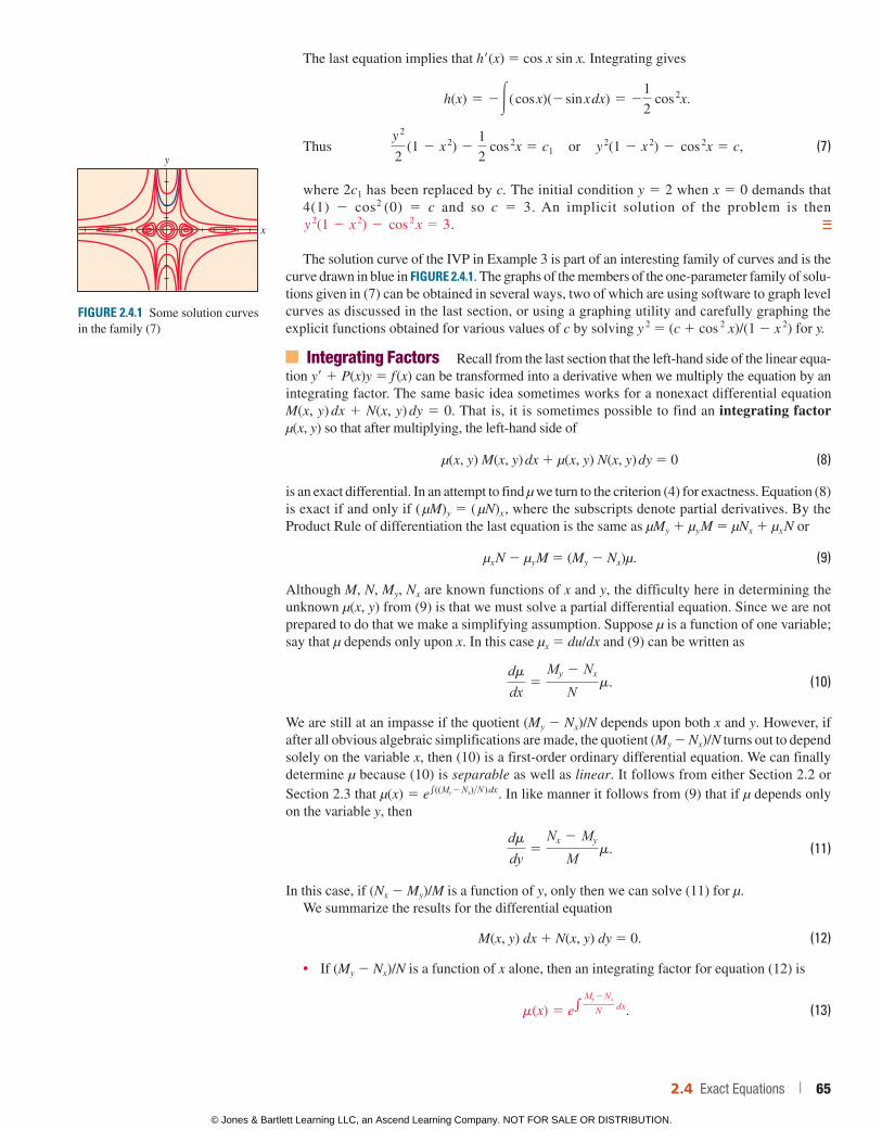
The last equation implies that h9(x) 5 cos x sin x. Integrating gives
h(x) 5 2#( cos x)(2 sin x dx) 5 21
2 cos
2x.
Thus y
2
2 (1 2 x
2) 21
2 cos
2x 5 c1 or y 2(1 2 x
2) 2 cos 2x 5 c, (7)
where 2c1 has been replaced by c. The initial condition y 5 2 when x 5 0 demands that 4(1) 2 cos2 (0) 5 c and so c 5 3. An implicit solution of the problem is then y
2(1 2 x 2) 2 cos
2 x 5 3.
The solution curve of the IVP in Example 3 is part of an interesting family of curves and is the curve drawn in blue in FIGURE 2.4.1. The graphs of the members of the one-parameter family of solu-tions given in (7) can be obtained in several ways, two of which are using software to graph level curves as discussed in the last section, or using a graphing utility and carefully graphing the explicit functions obtained for various values of c by solving y 2 5 (c 1 cos 2 x)/(1 2 x 2) for y.
Integrating Factors Recall from the last section that the left-hand side of the linear equa-tion y9 1 P(x)y 5 f (x) can be transformed into a derivative when we multiply the equation by an integrating factor. The same basic idea sometimes works for a nonexact differential equation M(x, y) dx 1 N(x, y) dy 5 0. That is, it is sometimes possible to find an integrating factor µ(x, y) so that after multiplying, the left-hand side of
µ(x, y) M(x, y) dx 1 µ(x, y) N(x, y) dy 5 0 (8)
is an exact differential. In an attempt to find µ we turn to the criterion (4) for exactness. Equation (8) is exact if and only if ( µM)y 5 ( µN)x, where the subscripts denote partial derivatives. By the Product Rule of differentiation the last equation is the same as µMy 1 µy M 5 µNx 1 µx N or
µxN 2 µyM 5 (My 2 Nx)µ. (9)
Although M, N, My, Nx are known functions of x and y, the difficulty here in determining the unknown µ(x, y) from (9) is that we must solve a partial differential equation. Since we are not prepared to do that we make a simplifying assumption. Suppose µ is a function of one variable; say that µ depends only upon x. In this case µx 5 du/dx and (9) can be written as
dm
dx5
My 2 Nx
N m. (10)
We are still at an impasse if the quotient (My 2 Nx)/N depends upon both x and y. However, if after all obvious algebraic simplifications are made, the quotient (My 2 Nx)/N turns out to depend solely on the variable x, then (10) is a first-order ordinary differential equation. We can finally determine µ because (10) is separable as well as linear. It follows from either Section 2.2 or Section 2.3 that µ(x) 5 ee((My2Nx)>N ) dx. In like manner it follows from (9) that if µ depends only on the variable y, then
dm
dy5
Nx 2 My
M m. (11)
In this case, if (Nx 2 My)/M is a function of y, only then we can solve (11) for µ.We summarize the results for the differential equation
M(x, y) dx 1 N(x, y) dy 5 0. (12)
• If (My 2 Nx)/N is a function of x alone, then an integrating factor for equation (12) is
m(x) 5 ee
My2Nx
N dx. (13)
FIGURE 2.4.1 Some solution curves in the family (7)
y
x
2.4 Exact Equations | 65
© Jones & Bartlett Learning LLC, an Ascend Learning Company. NOT FOR SALE OR DISTRIBUTION.
© Jones & Bartlett Learning, LLCNOT FOR SALE OR DISTRIBUTION
© Jones & Bartlett Learning, LLCNOT FOR SALE OR DISTRIBUTION
© Jones & Bartlett Learning, LLCNOT FOR SALE OR DISTRIBUTION
© Jones & Bartlett Learning, LLCNOT FOR SALE OR DISTRIBUTION
© Jones & Bartlett Learning, LLCNOT FOR SALE OR DISTRIBUTION
© Jones & Bartlett Learning, LLCNOT FOR SALE OR DISTRIBUTION
© Jones & Bartlett Learning, LLCNOT FOR SALE OR DISTRIBUTION
© Jones & Bartlett Learning, LLCNOT FOR SALE OR DISTRIBUTION
© Jones & Bartlett Learning, LLCNOT FOR SALE OR DISTRIBUTION
© Jones & Bartlett Learning, LLCNOT FOR SALE OR DISTRIBUTION
© Jones & Bartlett Learning, LLCNOT FOR SALE OR DISTRIBUTION
© Jones & Bartlett Learning, LLCNOT FOR SALE OR DISTRIBUTION
© Jones & Bartlett Learning, LLCNOT FOR SALE OR DISTRIBUTION
© Jones & Bartlett Learning, LLCNOT FOR SALE OR DISTRIBUTION
© Jones & Bartlett Learning, LLCNOT FOR SALE OR DISTRIBUTION
© Jones & Bartlett Learning, LLCNOT FOR SALE OR DISTRIBUTION
© Jones & Bartlett Learning, LLCNOT FOR SALE OR DISTRIBUTION
© Jones & Bartlett Learning, LLCNOT FOR SALE OR DISTRIBUTION
© Jones & Bartlett Learning, LLCNOT FOR SALE OR DISTRIBUTION
© Jones & Bartlett Learning, LLCNOT FOR SALE OR DISTRIBUTION
• If (Nx 2 My)/M is a function of y alone, then an integrating factor for equation (12) is
m( y) 5 ee
Nx2My
M dy
. (14)
EXAMPLE 4 A Nonexact DE Made Exact
The nonlinear first-order differential equation xy dx 1 (2x 2 1 3y 2 2 20) dy 5 0 is not exact. With the identifications M 5 xy, N 5 2x 2 1 3y 2 2 20 we find the partial derivatives My 5 x and Nx 5 4x. The first quotient from (13) gets us nowhere since
My 2 Nx
N5
x 2 4x
2x 2 1 3y
2 2 205
23x
2x 2 1 3y
2 2 20
depends on x and y. However (14) yields a quotient that depends only on y:
Nx 2 My
M5
4x 2 xxy
53xxy
53y
.
The integrating factor is then e e3 dy/y 5 e 3 ln y 5 e ln y
3
5 y 3. After multiplying the given DE by µ(y) 5 y 3 the resulting equation is
xy 4 dx 1 (2x 2y 3 1 3y 5 2 20y 3) dy 5 0.
You should verify that the last equation is now exact as well as show, using the method of this section, that a family of solutions is 12x
2y 4 1 1
2y 6 2 5y
4 5 c.
REMARKS(i) When testing an equation for exactness, make sure it is of the precise form M(x, y) dx 1 N(x, y) dy 5 0. Sometimes a differential equation is written G(x, y) dx 5 H(x, y) dy. In this case, first rewrite it as G(x, y) dx 2 H(x, y) dy 5 0, and then identify M(x, y) 5 G(x, y) and N(x, y) 5 2H(x, y) before using (4).(ii) In some texts on differential equations the study of exact equations precedes that of linear DEs. If this were so, the method for finding integrating factors just discussed can be used to derive an integrating factor for y9 1 P(x)y 5 f (x). By rewriting the last equation in the differential form (P(x)y 2 f (x)) dx 1 dy 5 0 we see that
My 2 Nx
N5 P(x).
From (13) we arrive at the already familiar integrating factor e eP(x) dx used in Section 2.3.
2.4 Exercises Answers to selected odd-numbered problems begin on page ANS-2.
In Problems 1–20, determine whether the given differential equation is exact. If it is exact, solve it.
1. (2x 2 1) dx 1 (3y 1 7) dy 5 0
2. (2x 1 y) dx 2 (x 1 6y) dy 5 0
3. (5x 1 4y) dx 1 (4x 2 8y 3) dy 5 0
4. (sin y 2 y sin x) dx 1 (cos x 1 x cos y 2 y) dy 5 0
5. (2xy 2 2 3) dx 1 (2x 2y 1 4) dy 5 0
6. a2y 21x
1 cos 3xb
dy
dx1
y
x 2 2 4x
3 1 3y sin 3x 5 0
7. (x 2 2 y 2) dx 1 (x 2 2 2xy) dy 5 0
8. a1 1 ln x 1y
xb dx 5 (1 2 ln x) dy
9. (x 2 y 3 1 y 2 sin x) dx 5 (3xy 2 1 2y cos x) dy
10. (x 3 1 y 3) dx 1 3xy 2 dy 5 0
11. (y ln y 2 e2xy) dx 1 a1y
1 x ln yb dy 5 0
12. (3x 2y 1 e y) dx 1 (x 3 1 xe y 2 2y) dy 5 0
13. x
dy
dx5 2xe
x 2 y 1 6x 2
14. a1 23y 1 xb
dydx
1 y 53x 2 1
66 | CHAPTER 2 First-Order Differential Equations
© Jones & Bartlett Learning LLC, an Ascend Learning Company. NOT FOR SALE OR DISTRIBUTION.
© Jones & Bartlett Learning, LLCNOT FOR SALE OR DISTRIBUTION
© Jones & Bartlett Learning, LLCNOT FOR SALE OR DISTRIBUTION
© Jones & Bartlett Learning, LLCNOT FOR SALE OR DISTRIBUTION
© Jones & Bartlett Learning, LLCNOT FOR SALE OR DISTRIBUTION
© Jones & Bartlett Learning, LLCNOT FOR SALE OR DISTRIBUTION
© Jones & Bartlett Learning, LLCNOT FOR SALE OR DISTRIBUTION
© Jones & Bartlett Learning, LLCNOT FOR SALE OR DISTRIBUTION
© Jones & Bartlett Learning, LLCNOT FOR SALE OR DISTRIBUTION
© Jones & Bartlett Learning, LLCNOT FOR SALE OR DISTRIBUTION
© Jones & Bartlett Learning, LLCNOT FOR SALE OR DISTRIBUTION
© Jones & Bartlett Learning, LLCNOT FOR SALE OR DISTRIBUTION
© Jones & Bartlett Learning, LLCNOT FOR SALE OR DISTRIBUTION
© Jones & Bartlett Learning, LLCNOT FOR SALE OR DISTRIBUTION
© Jones & Bartlett Learning, LLCNOT FOR SALE OR DISTRIBUTION
© Jones & Bartlett Learning, LLCNOT FOR SALE OR DISTRIBUTION
© Jones & Bartlett Learning, LLCNOT FOR SALE OR DISTRIBUTION
© Jones & Bartlett Learning, LLCNOT FOR SALE OR DISTRIBUTION
© Jones & Bartlett Learning, LLCNOT FOR SALE OR DISTRIBUTION
© Jones & Bartlett Learning, LLCNOT FOR SALE OR DISTRIBUTION
© Jones & Bartlett Learning, LLCNOT FOR SALE OR DISTRIBUTION
15. ax 2y
3 21
1 1 9x 2b
dx
dy1 x
3y 2 5 0
16. (5y 2 2x)y9 2 2y 5 0
17. (tan x 2 sin x sin y) dx 1 cos x cos y dy 5 0
18. (2y sin x cos x 2 y 1 2y 2e xy
2
) dx 5 (x 2 sin 2 x 2 4xye xy
2
) dy
19. (4t 3y 2 15t 2 2 y) dt 1 (t 4 1 3y 2 2 t) dy 5 0
20. a1
t1
1
t 2 2
y
t 2 1 y
2b dt 1 aye y 1
1
t 2 1 y
2b dy 5 0
In Problems 21–26, solve the given initial-value problem.
21. (x 1 y) 2 dx 1 (2xy 1 x 2 2 1) dy 5 0, y(1) 5 1
22. (e x 1 y) dx 1 (2 1 x 1 ye y) dy 5 0, y(0) 5 1
23. (4y 1 2t 2 5) dt 1 (6y 1 4t 2 1) dy 5 0, y(21) 5 2
24. a3y 2 2 t
2
y 5 b
dy
dt1
t
2y 4 5 0, y(1) 5 1
25. ( y 2 cos x 2 3x 2y 2 2x) dx 1 (2y sin x 2 x 3 1 ln y) dy 5 0, y(0) 5 e
26. a 1
1 1 y 2 1 cos x 2 2xyb
dy
dx5 y( y 1 sin x), y(0) 5 1
In Problems 27 and 28, find the value of k so that the given differential equation is exact.
27. ( y 3 1 kxy 4 2 2x) dx 1 (3xy 2 1 20x 2y 3) dy 5 0
28. (6xy 3 1 cos y) dx 1 (2kx 2y 2 2 x sin y) dy 5 0
In Problems 29–32, verify that the given differential equation is not exact. Multiply the given differential equation by the indicated integrating factor µ(x, y) and verify that the new equation is exact. Solve.
29. (2xy sin x 1 2y cos x) dx 1 2x cos x dy 5 0; µ(x, y) 5 xy
30. (x 2 1 2xy 2 y 2) dx 1 (y 2 1 2xy 2 x 2) dy 5 0; µ(x, y) 5 (x 1 y) –2
31. (x 3y 2 1 y) dx 1 x dy 5 0; µ(x, y) 5 1/x 2y 2
32. x dx 1 (y 2 x 2 2 y 2) dy 5 0; µ(x, y) 5 1/(x 2 1 y 2)
In Problems 33–38, solve the given differential equation by finding, as in Example 4, an appropriate integrating factor.
33. (2y 2 1 3x) dx 1 2xy dy 5 0
34. y(x 1 y 1 1) dx 1 (x 1 2y) dy 5 0
35. 6xy dx 1 (4y 1 9x 2) dy 5 0
36. cos x dx 1 a1 12yb sin x dy 5 0
37. (10 2 6y 1 e –3x) dx 2 2 dy 5 0
38. (y 2 1 xy 3) dx 1 (5y 2 2 xy 1 y 3 sin y) dy 5 0
In Problems 39 and 40, solve the given initial-value problem by finding, as in Example 4, an appropriate integrating factor.
39. x dx 1 (x 2y 1 4y) dy 5 0, y(4) 5 0
40. (x 2 1 y 2 2 5) dx 5 (y 1 xy) dy, y(0) 5 1
41. (a) Show that a one-parameter family of solutions of the equation
(4xy 1 3x 2) dx 1 (2y 1 2x 2) dy 5 0
is x 3 1 2x 2y 1 y 2 5 c.(b) Show that the initial conditions y(0) 5 22 and y(1) 5 1
determine the same implicit solution.(c) Find explicit solutions y1(x) and y2(x) of the differential
equation in part (a) such that y1(0) 5 22 and y2(1) 5 1. Use a graphing utility to graph y1(x) and y2(x).
Discussion Problems
42. Consider the concept of an integrating factor used in Problems 29–40. Are the two equations
M dx 1 N dy 5 0 and µM dx 1 µN dy 5 0
necessarily equivalent in the sense that a solution of one is also a solution of the other? Discuss.
43. Reread Example 3 and then discuss why we can conclude that the interval of definition of the explicit solution of the IVP (the blue curve in Figure 2.4.1) is (21, 1).
44. Discuss how the functions M(x, y) and N(x, y) can be found so that each differential equation is exact. Carry out your ideas.
(a) M(x, y) dx 1 axe xy 1 2xy 1
1xb dy 5 0
(b) ax 21>2 y
1>2 1x
x 2 1 y
b dx 1 N(x, y) dy 5 0
45. Differential equations are sometimes solved by having a clever idea. Here is a little exercise in clever ness: Although the differential equation
(x 2 "x 2 1 y
2) dx 1 y dy 5 0
is not exact, show how the rearrangement
x dx 1 y dy
"x 2 1 y
25 dx
and the observation 12 d(x 2 1 y 2) 5 x dx 1 y dy can lead
to a solution.
46. True or False: Every separable first-order equation dy/dx 5 g(x)h(y) is exact.
Mathematical Model
47. Falling Chain A portion of a uniform chain of length 8 ft is loosely coiled around a peg at the edge of a high horizon-tal platform and the remaining portion of the chain hangs at rest over the edge of the platform. See FIGURE 2.4.2. Suppose the length of the overhang is 3 ft, that the chain weighs 2 lb/ft, and that the positive direction is downward. Starting at t 5 0 seconds, the weight of the overhanging portion causes the chain on the table to uncoil smoothly and fall to the floor. If x(t) denotes the length of the chain overhanging the table at time t . 0, then v 5 dx/dt is its
2.4 Exact Equations | 67
© Jones & Bartlett Learning LLC, an Ascend Learning Company. NOT FOR SALE OR DISTRIBUTION.
© Jones & Bartlett Learning, LLCNOT FOR SALE OR DISTRIBUTION
© Jones & Bartlett Learning, LLCNOT FOR SALE OR DISTRIBUTION
© Jones & Bartlett Learning, LLCNOT FOR SALE OR DISTRIBUTION
© Jones & Bartlett Learning, LLCNOT FOR SALE OR DISTRIBUTION
© Jones & Bartlett Learning, LLCNOT FOR SALE OR DISTRIBUTION
© Jones & Bartlett Learning, LLCNOT FOR SALE OR DISTRIBUTION
© Jones & Bartlett Learning, LLCNOT FOR SALE OR DISTRIBUTION
© Jones & Bartlett Learning, LLCNOT FOR SALE OR DISTRIBUTION
© Jones & Bartlett Learning, LLCNOT FOR SALE OR DISTRIBUTION
© Jones & Bartlett Learning, LLCNOT FOR SALE OR DISTRIBUTION
© Jones & Bartlett Learning, LLCNOT FOR SALE OR DISTRIBUTION
© Jones & Bartlett Learning, LLCNOT FOR SALE OR DISTRIBUTION
© Jones & Bartlett Learning, LLCNOT FOR SALE OR DISTRIBUTION
© Jones & Bartlett Learning, LLCNOT FOR SALE OR DISTRIBUTION
© Jones & Bartlett Learning, LLCNOT FOR SALE OR DISTRIBUTION
© Jones & Bartlett Learning, LLCNOT FOR SALE OR DISTRIBUTION
© Jones & Bartlett Learning, LLCNOT FOR SALE OR DISTRIBUTION
© Jones & Bartlett Learning, LLCNOT FOR SALE OR DISTRIBUTION
© Jones & Bartlett Learning, LLCNOT FOR SALE OR DISTRIBUTION
© Jones & Bartlett Learning, LLCNOT FOR SALE OR DISTRIBUTION
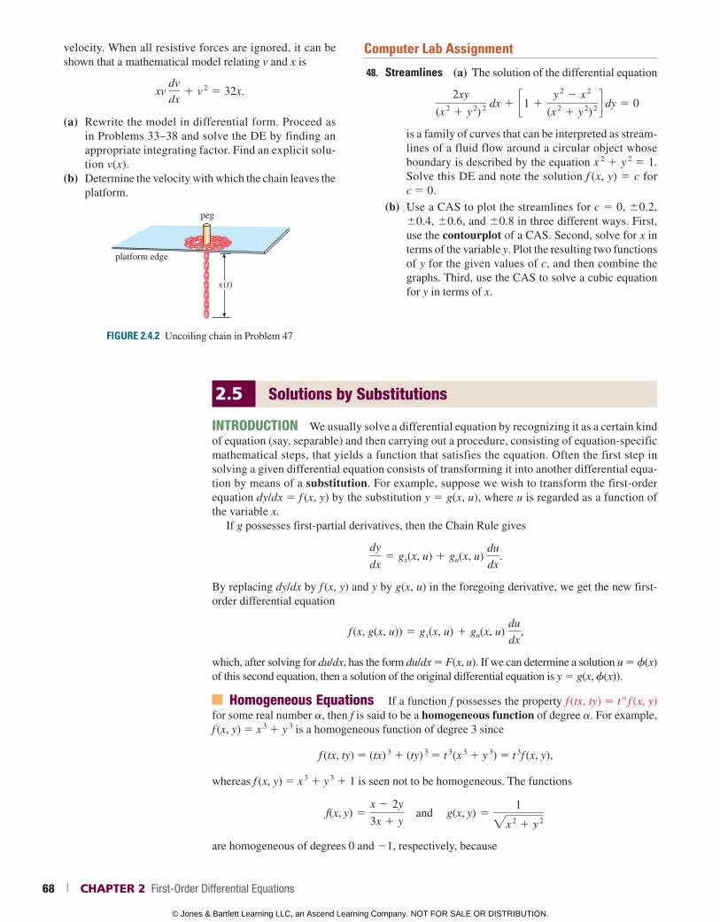
velocity. When all resistive forces are ignored, it can be shown that a mathematical model relating v and x is
xv
dv
dx1 v
2 5 32x.
(a) Rewrite the model in differential form. Proceed as in Problems 33–38 and solve the DE by finding an appropriate integrating factor. Find an explicit solu-tion v(x).
(b) Determine the velocity with which the chain leaves the platform.
FIGURE 2.4.2 Uncoiling chain in Problem 47
x (t)
peg
platform edge
Computer Lab Assignment
48. Streamlines (a) The solution of the differential equation
2xy
(x 2 1 y
2) 2 dx 1 c1 1
y 2 2 x
2
(x 2 1 y
2) 2 d dy 5 0
is a family of curves that can be interpreted as stream-lines of a fluid flow around a circular object whose boundary is described by the equation x 2 1 y 2 5 1. Solve this DE and note the solution f (x, y) 5 c for c 5 0.
(b) Use a CAS to plot the streamlines for c 5 0, 60.2, 60.4, 60.6, and 60.8 in three different ways. First, use the contourplot of a CAS. Second, solve for x in terms of the variable y. Plot the resulting two functions of y for the given values of c, and then combine the graphs. Third, use the CAS to solve a cubic equation for y in terms of x.
2.5 Solutions by Substitutions
INTRODUCTION We usually solve a differential equation by recognizing it as a certain kind of equation (say, separable) and then carrying out a procedure, consisting of equation-specific mathematical steps, that yields a function that satisfies the equation. Often the first step in solving a given differential equation consists of transforming it into another differential equa-tion by means of a substitution. For example, suppose we wish to transform the first-order equation dy/dx 5 f (x, y) by the substitution y 5 g(x, u), where u is regarded as a function of the variable x.
If g possesses first-partial derivatives, then the Chain Rule gives
dy
dx5 gx(x, u) 1 gu(x, u)
du
dx.
By replacing dy/dx by f (x, y) and y by g(x, u) in the foregoing derivative, we get the new first-order differential equation
f (x, g(x, u)) 5 gx(x, u) 1 gu(x, u) du
dx,
which, after solving for du/dx, has the form du/dx 5 F(x, u). If we can determine a solution u 5 f(x) of this second equation, then a solution of the original differential equation is y 5 g(x, f(x)).
Homogeneous Equations If a function f possesses the property f (tx, ty) 5 t a f (x, y) for some real number a, then f is said to be a homogeneous function of degree a. For example, f (x, y) 5 x 3 1 y 3 is a homogeneous function of degree 3 since
f (tx, ty) 5 (tx) 3 1 (ty) 3 5 t 3(x 3 1 y 3) 5 t 3f (x, y),
whereas f (x, y) 5 x 3 1 y 3 1 1 is seen not to be homogeneous. The functions
f(x, y) 5x 2 2y
3x 1 y and g(x, y) 5
1
"x 2 1 y
2
are homogeneous of degrees 0 and 21, respectively, because
68 | CHAPTER 2 First-Order Differential Equations
© Jones & Bartlett Learning LLC, an Ascend Learning Company. NOT FOR SALE OR DISTRIBUTION.
© Jones & Bartlett Learning, LLCNOT FOR SALE OR DISTRIBUTION
© Jones & Bartlett Learning, LLCNOT FOR SALE OR DISTRIBUTION
© Jones & Bartlett Learning, LLCNOT FOR SALE OR DISTRIBUTION
© Jones & Bartlett Learning, LLCNOT FOR SALE OR DISTRIBUTION
© Jones & Bartlett Learning, LLCNOT FOR SALE OR DISTRIBUTION
© Jones & Bartlett Learning, LLCNOT FOR SALE OR DISTRIBUTION
© Jones & Bartlett Learning, LLCNOT FOR SALE OR DISTRIBUTION
© Jones & Bartlett Learning, LLCNOT FOR SALE OR DISTRIBUTION
© Jones & Bartlett Learning, LLCNOT FOR SALE OR DISTRIBUTION
© Jones & Bartlett Learning, LLCNOT FOR SALE OR DISTRIBUTION
© Jones & Bartlett Learning, LLCNOT FOR SALE OR DISTRIBUTION
© Jones & Bartlett Learning, LLCNOT FOR SALE OR DISTRIBUTION
© Jones & Bartlett Learning, LLCNOT FOR SALE OR DISTRIBUTION
© Jones & Bartlett Learning, LLCNOT FOR SALE OR DISTRIBUTION
© Jones & Bartlett Learning, LLCNOT FOR SALE OR DISTRIBUTION
© Jones & Bartlett Learning, LLCNOT FOR SALE OR DISTRIBUTION
© Jones & Bartlett Learning, LLCNOT FOR SALE OR DISTRIBUTION
© Jones & Bartlett Learning, LLCNOT FOR SALE OR DISTRIBUTION
© Jones & Bartlett Learning, LLCNOT FOR SALE OR DISTRIBUTION
© Jones & Bartlett Learning, LLCNOT FOR SALE OR DISTRIBUTION
f (tx, ty) 5tx 2 2ty
3tx 1 ty5
t(x 2 2y)
t(3x 1 y)5
x 2 2y
3x 1 y5 t
0f (x, y)
g(tx, ty) 51
"t 2x
2 1 t 2y
2 5
1
t"x 2 1 y
25 t
21 1
"x 2 1 y
25 t
21g(x, y).
A first-order DE written in differential form
M(x, y) dx 1 N(x, y) dy 5 0 (1)
is said to be a homogeneous equation if the coefficient functions M(x, y) and N(x, y) are homo-geneous functions of the same degree. In other words, (1) is a homogeneous equation if
M(tx, ty) 5 t aM(x, y) and N(tx, ty) 5 t aN(x, y).
The word homogeneous as used here does not mean the same as it does when applied to linear differential equations. See Sections 2.3 and 3.1.
If M and N are homogeneous functions of degree a, we can also write
M(x, y) 5 x aM(1, u) and N(x, y) 5 x aN(1, u) where u 5 y/x, (2)
and M(x, y) 5 y aM(v, 1) and N(x, y) 5 y aN(v, 1) where v 5 x/y. (3)
See Problem 33 in Exercises 2.5. Properties (2) and (3) suggest the substitutions that can be used to solve a homogeneous differential equation. Specifically, either of the substitutions y 5 ux or x 5 vy, where u and v are new dependent variables, will reduce a homogeneous equa-tion to a separable first-order differential equation. To show this, observe that as a consequence of (2) a homogeneous equation M(x, y) dx 1 N(x, y) dy 5 0 can be rewritten as
x a M(1, u) dx 1 x a N(1, u) dy 5 0 or M(1, u) dx 1 N(1, u) dy 5 0,
where u 5 y/x or y 5 ux. By substituting the differential dy 5 u dx 1 x du into the last equation and gathering terms, we obtain a separable DE in the variables u and x:
M(1, u) dx 1 N(1, u)[u dx 1 x du] 5 0
[M(1, u) 1 uN(1, u)] dx 1 xN(1, u) du 5 0
or dxx
1N(1, u) du
M(1, u) 1 uN(1, u)5 0.
We hasten to point out that the preceding formula should not be memorized; rather, the procedure should be worked through each time. The proof that the substitutions x 5 vy and dx 5 v dy 1 y dv also lead to a separable equation follows in an analogous manner from (3).
EXAMPLE 1 Solving a Homogeneous DE
Solve (x 2 1 y 2) dx 1 (x 2 2 xy) dy 5 0.
SOLUTION Inspection of M(x, y) 5 x 2 1 y 2 and N(x, y) 5 x 2 2 xy shows that these coef-ficients are homogeneous functions of degree 2. If we let y 5 ux, then dy 5 u dx 1 x du so that, after substituting, the given equation becomes
(x 2 1 u 2x 2) dx 1 (x 2 2 ux 2)[u dx 1 x du] 5 0
x 2(1 1 u) dx 1 x 3(1 2 u) du 5 0
1 2 u
1 1 u du 1
dxx
5 0
c21 12
1 1 ud du 1
dxx 5 0. d long division
A linear first-order DE a1y9 1 a0 y 5 g(x) is homogeneous when g(x) = 0.
2.5 Solutions by Substitutions | 69
© Jones & Bartlett Learning LLC, an Ascend Learning Company. NOT FOR SALE OR DISTRIBUTION.
© Jones & Bartlett Learning, LLCNOT FOR SALE OR DISTRIBUTION
© Jones & Bartlett Learning, LLCNOT FOR SALE OR DISTRIBUTION
© Jones & Bartlett Learning, LLCNOT FOR SALE OR DISTRIBUTION
© Jones & Bartlett Learning, LLCNOT FOR SALE OR DISTRIBUTION
© Jones & Bartlett Learning, LLCNOT FOR SALE OR DISTRIBUTION
© Jones & Bartlett Learning, LLCNOT FOR SALE OR DISTRIBUTION
© Jones & Bartlett Learning, LLCNOT FOR SALE OR DISTRIBUTION
© Jones & Bartlett Learning, LLCNOT FOR SALE OR DISTRIBUTION
© Jones & Bartlett Learning, LLCNOT FOR SALE OR DISTRIBUTION
© Jones & Bartlett Learning, LLCNOT FOR SALE OR DISTRIBUTION
© Jones & Bartlett Learning, LLCNOT FOR SALE OR DISTRIBUTION
© Jones & Bartlett Learning, LLCNOT FOR SALE OR DISTRIBUTION
© Jones & Bartlett Learning, LLCNOT FOR SALE OR DISTRIBUTION
© Jones & Bartlett Learning, LLCNOT FOR SALE OR DISTRIBUTION
© Jones & Bartlett Learning, LLCNOT FOR SALE OR DISTRIBUTION
© Jones & Bartlett Learning, LLCNOT FOR SALE OR DISTRIBUTION
© Jones & Bartlett Learning, LLCNOT FOR SALE OR DISTRIBUTION
© Jones & Bartlett Learning, LLCNOT FOR SALE OR DISTRIBUTION
© Jones & Bartlett Learning, LLCNOT FOR SALE OR DISTRIBUTION
© Jones & Bartlett Learning, LLCNOT FOR SALE OR DISTRIBUTION
After integration the last line gives
– u 1 2 ln 0 1 1 u 0 1 ln ZxZ 5 ln ZcZ
2
y
x1 2 ln 21 1
y
x2 1 ln ZxZ 5 ln ZcZ. d resubstituting u 5 y/x
Using the properties of logarithms, we can write the preceding solution as
ln 2(x 1 y) 2
cx2 5
y
x or (x 1 y)2 5 cxe
y/x.
Although either of the indicated substitutions can be used for every homogeneous differ-ential equation, in practice we try x 5 vy whenever the function M(x, y) is simpler than N(x, y). Also it could happen that after using one substitution, we may encounter integrals that are difficult or impossible to evaluate in closed form; switching substitutions may result in an easier problem.
Bernoulli’s Equation The differential equation
dy
dx1 P(x)y 5 f (x)y
n, (4)
where n is any real number, is called Bernoulli’s equation after the Swiss mathematician Jacob Bernoulli (1654–1705), who studied the equation around 1695. Note that for n 5 0 equation (4) is linear, and for n 5 1 equation (4) is separable and linear. In 1696 the German polymath Gottfried Wilhelm Leibniz (1646–1716) showed that for n 0 and n 1, any differential equation of the form given in (4) can be reduced to a linear equation by means of the substitu-tion u 5 y
12n. The next example illustrates this substitution method.
EXAMPLE 2 Solving a Bernoulli DE
Solve x
dy
dx1 y 5 x
2y 2.
SOLUTION We begin by rewriting the differential equation in the form given in (4) by dividing by x:
dy
dx1
1x
y 5 xy 2.
With n 5 2 and u 5 y21, we next substitute y 5 u –1 and
dy
dx5 2u
22
du
dx
into the given equation and simplify. The result is
du
dx2
1x
u 5 2x.
The integrating factor for this linear equation on, say, (0, q ) is
e –e dx/x 5 e –ln x 5 e ln x
21
5 x –1.
Integrating d
dx 3x
21u 4 5 21
gives x –1u 5 2x 1 c or u 5 2x 2 1 cx. Since u 5 y –1 we have y 5 1/u, and so a solution of the given equation is y 5 1/(2x 2 1 cx).
Note that we have not obtained the general solution of the original nonlinear differential equa-tion in Example 2, since y 5 0 is a singular solution of the equation.
d Chain Rule
70 | CHAPTER 2 First-Order Differential Equations
© Jones & Bartlett Learning LLC, an Ascend Learning Company. NOT FOR SALE OR DISTRIBUTION.
© Jones & Bartlett Learning, LLCNOT FOR SALE OR DISTRIBUTION
© Jones & Bartlett Learning, LLCNOT FOR SALE OR DISTRIBUTION
© Jones & Bartlett Learning, LLCNOT FOR SALE OR DISTRIBUTION
© Jones & Bartlett Learning, LLCNOT FOR SALE OR DISTRIBUTION
© Jones & Bartlett Learning, LLCNOT FOR SALE OR DISTRIBUTION
© Jones & Bartlett Learning, LLCNOT FOR SALE OR DISTRIBUTION
© Jones & Bartlett Learning, LLCNOT FOR SALE OR DISTRIBUTION
© Jones & Bartlett Learning, LLCNOT FOR SALE OR DISTRIBUTION
© Jones & Bartlett Learning, LLCNOT FOR SALE OR DISTRIBUTION
© Jones & Bartlett Learning, LLCNOT FOR SALE OR DISTRIBUTION
© Jones & Bartlett Learning, LLCNOT FOR SALE OR DISTRIBUTION
© Jones & Bartlett Learning, LLCNOT FOR SALE OR DISTRIBUTION
© Jones & Bartlett Learning, LLCNOT FOR SALE OR DISTRIBUTION
© Jones & Bartlett Learning, LLCNOT FOR SALE OR DISTRIBUTION
© Jones & Bartlett Learning, LLCNOT FOR SALE OR DISTRIBUTION
© Jones & Bartlett Learning, LLCNOT FOR SALE OR DISTRIBUTION
© Jones & Bartlett Learning, LLCNOT FOR SALE OR DISTRIBUTION
© Jones & Bartlett Learning, LLCNOT FOR SALE OR DISTRIBUTION
© Jones & Bartlett Learning, LLCNOT FOR SALE OR DISTRIBUTION
© Jones & Bartlett Learning, LLCNOT FOR SALE OR DISTRIBUTION
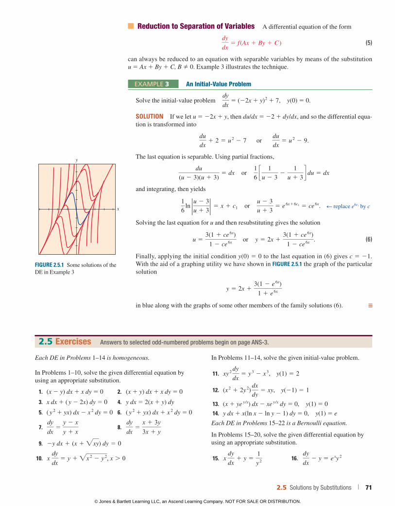
Reduction to Separation of Variables A differential equation of the form
dy
dx5 f (Ax 1 By 1 C ) (5)
can always be reduced to an equation with separable variables by means of the substitution u 5 Ax 1 By 1 C, B 0. Example 3 illustrates the technique.
EXAMPLE 3 An Initial-Value Problem
Solve the initial-value problem dydx
5 (22x 1 y) 2 1 7, y(0) 5 0.
SOLUTION If we let u 5 22x 1 y, then du/dx 5 22 1 dy/dx, and so the differential equa-tion is transformed into
du
dx1 2 5 u
2 2 7 or du
dx5 u
2 2 9.
The last equation is separable. Using partial fractions,
du
(u 2 3)(u 1 3)5 dx or
1
6 c 1
u 2 32
1
u 1 3d du 5 dx
and integrating, then yields
1
6 ln 2u 2 3
u 1 32 5 x 1 c1 or
u 2 3
u 1 35 e
6x16c1 5 ce 6x.
Solving the last equation for u and then resubstituting gives the solution
u 53(1 1 ce
6x)
1 2 ce 6x or y 5 2x 1
3(1 1 ce 6x)
1 2 ce 6x . (6)
Finally, applying the initial condition y(0) 5 0 to the last equation in (6) gives c 5 21. With the aid of a graphing utility we have shown in FIGURE 2.5.1 the graph of the particular solution
y 5 2x 13(1 2 e
6x)
1 1 e 6x
in blue along with the graphs of some other members of the family solutions (6).
d replace e6c1 by c
FIGURE 2.5.1 Some solutions of the DE in Example 3
x
y
Each DE in Problems 1–14 is homogeneous.
In Problems 1–10, solve the given differential equation by using an appropriate substitution.
1. (x 2 y) dx 1 x dy 5 0 2. (x 1 y) dx 1 x dy 5 0
3. x dx 1 ( y 2 2x) dy 5 0 4. y dx 5 2(x 1 y) dy
5. ( y 2 1 yx) dx 2 x 2 dy 5 0 6. ( y 2 1 yx) dx 1 x 2 dy 5 0
7. dydx
5y 2 xy 1 x
8. dydx
5x 1 3y3x 1 y
9. 2y dx 1 (x 1 "xy) dy 5 0
10. x dydx
5 y 1 "x 2 2 y
2, x . 0
In Problems 11–14, solve the given initial-value problem.
11. xy 2
dy
dx5 y
3 2 x 3, y(1) 5 2
12. (x 2 1 2y
2)
dx
dy5 xy, y(21) 5 1
13. (x 1 ye y/x) dx 2 xe y/x dy 5 0, y(1) 5 0
14. y dx 1 x(ln x 2 ln y 2 1) dy 5 0, y(1) 5 e
Each DE in Problems 15–22 is a Bernoulli equation.
In Problems 15–20, solve the given differential equation by using an appropriate substitution.
15. x
dy
dx1 y 5
1
y 2 16.
dy
dx2 y 5 e
xy 2
2.5 Exercises Answers to selected odd-numbered problems begin on page ANS-3.
2.5 Solutions by Substitutions | 71
© Jones & Bartlett Learning LLC, an Ascend Learning Company. NOT FOR SALE OR DISTRIBUTION.
© Jones & Bartlett Learning, LLCNOT FOR SALE OR DISTRIBUTION
© Jones & Bartlett Learning, LLCNOT FOR SALE OR DISTRIBUTION
© Jones & Bartlett Learning, LLCNOT FOR SALE OR DISTRIBUTION
© Jones & Bartlett Learning, LLCNOT FOR SALE OR DISTRIBUTION
© Jones & Bartlett Learning, LLCNOT FOR SALE OR DISTRIBUTION
© Jones & Bartlett Learning, LLCNOT FOR SALE OR DISTRIBUTION
© Jones & Bartlett Learning, LLCNOT FOR SALE OR DISTRIBUTION
© Jones & Bartlett Learning, LLCNOT FOR SALE OR DISTRIBUTION
© Jones & Bartlett Learning, LLCNOT FOR SALE OR DISTRIBUTION
© Jones & Bartlett Learning, LLCNOT FOR SALE OR DISTRIBUTION
© Jones & Bartlett Learning, LLCNOT FOR SALE OR DISTRIBUTION
© Jones & Bartlett Learning, LLCNOT FOR SALE OR DISTRIBUTION
© Jones & Bartlett Learning, LLCNOT FOR SALE OR DISTRIBUTION
© Jones & Bartlett Learning, LLCNOT FOR SALE OR DISTRIBUTION
© Jones & Bartlett Learning, LLCNOT FOR SALE OR DISTRIBUTION
© Jones & Bartlett Learning, LLCNOT FOR SALE OR DISTRIBUTION
© Jones & Bartlett Learning, LLCNOT FOR SALE OR DISTRIBUTION
© Jones & Bartlett Learning, LLCNOT FOR SALE OR DISTRIBUTION
© Jones & Bartlett Learning, LLCNOT FOR SALE OR DISTRIBUTION
© Jones & Bartlett Learning, LLCNOT FOR SALE OR DISTRIBUTION
17. dy
dx5 y(xy
3 2 1) 18. x
dy
dx2 (1 1 x)y 5 xy
2
19. t 2
dy
dt1 y
2 5 ty 20. 3(1 1 t 2)
dy
dt5 2ty (y
3 2 1)
In Problems 21 and 22, solve the given initial-value problem.
21. x 2
dy
dx2 2xy 5 3y
4, y(1) 5 12
22. y 1>2
dy
dx1 y
3>2 5 1, y(0) 5 4
Each DE in Problems 23–30 is of the form given in (5).
In Problems 23–28, solve the given differential equation by using an appropriate substitution.
23. dy
dx5 (x 1 y 1 1)2 24.
dy
dx5
1 2 x 2 y
x 1 y
25. dy
dx5 tan
2(x 1 y) 26. dy
dx5 sin (x 1 y)
27. dy
dx5 2 1 "y 2 2x 1 3
28. dy
dx5 1 1 e
y2x15
In Problems 29 and 30, solve the given initial-value problem.
29. dy
dx5 cos (x 1 y) , y(0) 5 p/4
30. dy
dx5
3x 1 2y
3x 1 2y 1 2, y(21) 5 21
Discussion Problems
Some second-order differential equations can be reduced to a first-order equation by means of a substitution. In Problems 31 and 32, use the substitution u 5 y9 to reduce the given differential equation to a first-order equation, and then solve that equation by a method discussed in this section. Then use u 5 y9 again to find the solution y of the given equation.
31. y 1 (y 9)2 5 0 32. y 2 2y 9 5 4x
33. (a) Show that it is always possible to express any homoge-neous differential equation M(x, y) dx 1 N(x, y) dy 5 0 in the form
dy
dx5 F ay
xb .
(b) Show that the substitution u 5 y/x in the last differen-tial equation in part (a) yields a separable equation.
34. Put the homogeneous differential equation
(5x 2 1 2y 2) dx 2 xy dy 5 0
in the form dy/dx 5 F(y/x) given in part (a) of Problem 33. Then solve the equation using the substitution u 5 y/x.
35. (a) Determine two singular solutions of the DE in Problem 10.
(b) If the initial condition y(5) 5 0 is as prescribed in Problem 10, then what is the largest interval I over which the solution is defined? Use a graphing utility to plot the solution curve for the IVP.
36. In Example 3, the solution y(x) becomes unbounded as x S 6q . Nevertheless y(x) is asymptotic to a curve as x S 2q and to a different curve as x S q . Find the equa-tions of these curves.
37. The differential equation
dy
dx5 P(x) 1 Q(x)y 1 R(x)y
2
is called a Riccati equation after the Venetian jurist and mathematician Jacopo Francesco Riccati (1676–1754) who was able to solve several DEs of this type.(a) A Riccati equation can be solved by a succession
of two substitutions provided we know a particular solution y1 of the equation. Show that the substitution y 5 y1 1 u reduces Riccati’s equation to a Bernoulli equation (4) with n 5 2. The Bernoulli equation can then be reduced to a linear equation by the substitution w 5 u –1.
(b) Find a one-parameter family of solutions for the dif-ferential equation
dy
dx5 2
4
x 2 2
1x
y 1 y 2,
where y1 5 2/x is a known solution of the equation.
38. Devise an appropriate substitution to solve
xy9 5 y ln(xy).
Mathematical Models
39. Population Growth In the study of population dynamics one of the most famous models for a growing but bounded population is the logistic equation
dP
dt5 P(a 2 bP) ,
where a and b are positive constants. Although we will come back to this equation and solve it by an alternative method in Section 2.8, solve the DE this first time using the fact that it is a Bernoulli equation.
40. Falling Chain In Problem 47 in Exercises 2.4 we saw that a mathematical model for the velocity v of a chain slipping off the edge of a high horizontal platform is
xv
dv
dx1 v
2 5 32x.
In that problem you were asked to solve the DE by convert-ing it into an exact equation using an integrating factor. This time solve the DE using the fact that it is a Bernoulli equation.
72 | CHAPTER 2 First-Order Differential Equations
© Jones & Bartlett Learning LLC, an Ascend Learning Company. NOT FOR SALE OR DISTRIBUTION.
© Jones & Bartlett Learning, LLCNOT FOR SALE OR DISTRIBUTION
© Jones & Bartlett Learning, LLCNOT FOR SALE OR DISTRIBUTION
© Jones & Bartlett Learning, LLCNOT FOR SALE OR DISTRIBUTION
© Jones & Bartlett Learning, LLCNOT FOR SALE OR DISTRIBUTION
© Jones & Bartlett Learning, LLCNOT FOR SALE OR DISTRIBUTION
© Jones & Bartlett Learning, LLCNOT FOR SALE OR DISTRIBUTION
© Jones & Bartlett Learning, LLCNOT FOR SALE OR DISTRIBUTION
© Jones & Bartlett Learning, LLCNOT FOR SALE OR DISTRIBUTION
© Jones & Bartlett Learning, LLCNOT FOR SALE OR DISTRIBUTION
© Jones & Bartlett Learning, LLCNOT FOR SALE OR DISTRIBUTION
© Jones & Bartlett Learning, LLCNOT FOR SALE OR DISTRIBUTION
© Jones & Bartlett Learning, LLCNOT FOR SALE OR DISTRIBUTION
© Jones & Bartlett Learning, LLCNOT FOR SALE OR DISTRIBUTION
© Jones & Bartlett Learning, LLCNOT FOR SALE OR DISTRIBUTION
© Jones & Bartlett Learning, LLCNOT FOR SALE OR DISTRIBUTION
© Jones & Bartlett Learning, LLCNOT FOR SALE OR DISTRIBUTION
© Jones & Bartlett Learning, LLCNOT FOR SALE OR DISTRIBUTION
© Jones & Bartlett Learning, LLCNOT FOR SALE OR DISTRIBUTION
© Jones & Bartlett Learning, LLCNOT FOR SALE OR DISTRIBUTION
© Jones & Bartlett Learning, LLCNOT FOR SALE OR DISTRIBUTION
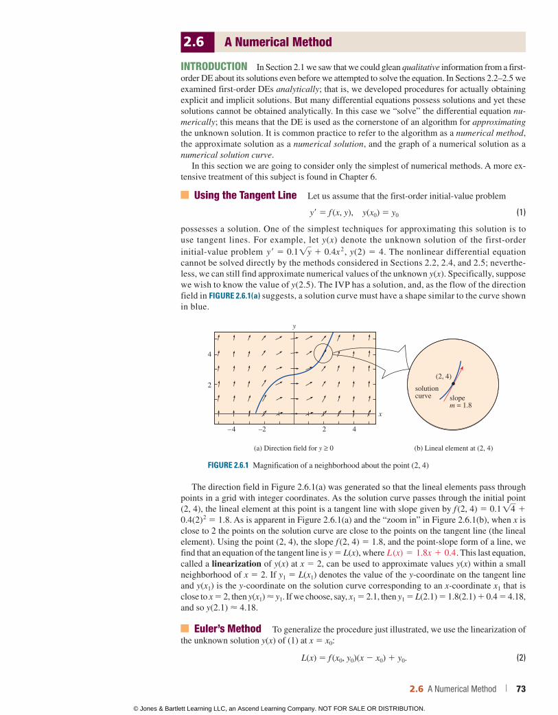
2.6 A Numerical Method
INTRODUCTION In Section 2.1 we saw that we could glean qualitative information from a first-order DE about its solutions even before we attempted to solve the equation. In Sections 2.2–2.5 we examined first-order DEs analytically; that is, we developed procedures for actually obtaining explicit and implicit solutions. But many differential equations possess solutions and yet these solutions cannot be obtained analytically. In this case we “solve” the differential equation nu-merically; this means that the DE is used as the cornerstone of an algorithm for approximating the unknown solution. It is common practice to refer to the algorithm as a numerical method, the approximate solution as a numerical solution, and the graph of a numerical solution as a numerical solution curve.
In this section we are going to consider only the simplest of numerical methods. A more ex-tensive treatment of this subject is found in Chapter 6.
Using the Tangent Line Let us assume that the first-order initial-value problem
y9 5 f (x, y), y(x0) 5 y0 (1)
possesses a solution. One of the simplest techniques for approximating this solution is to use tangent lines. For example, let y(x) denote the unknown solution of the first-order initial-value problem y r 5 0.1!y 1 0.4x
2, y(2) 5 4. The nonlinear differential equation cannot be solved directly by the methods considered in Sections 2.2, 2.4, and 2.5; neverthe-less, we can still find approximate numerical values of the unknown y(x). Specifically, suppose we wish to know the value of y(2.5). The IVP has a solution, and, as the flow of the direction field in FIGURE 2.6.1(a) suggests, a solution curve must have a shape similar to the curve shown in blue.
FIGURE 2.6.1 Magnification of a neighborhood about the point (2, 4)
4
2
2 4
x
y
(a) Direction field for y ≥ 0
solutioncurve slope
m = 1.8
(2, 4)
(b) Lineal element at (2, 4)
–2–4
The direction field in Figure 2.6.1(a) was generated so that the lineal elements pass through points in a grid with integer coordinates. As the solution curve passes through the initial point (2, 4), the lineal element at this point is a tangent line with slope given by f (2, 4) 5 0.1!4 1 0.4(2) 2 5 1.8. As is apparent in Figure 2.6.1(a) and the “zoom in” in Figure 2.6.1(b), when x is close to 2 the points on the solution curve are close to the points on the tangent line (the lineal element). Using the point (2, 4), the slope f (2, 4) 5 1.8, and the point-slope form of a line, we find that an equation of the tangent line is y 5 L(x), where L (x) 5 1.8x 1 0.4. This last equation, called a linearization of y(x) at x 5 2, can be used to approximate values y(x) within a small neighborhood of x 5 2. If y1 5 L(x1) denotes the value of the y-coordinate on the tangent line and y(x1) is the y-coordinate on the solution curve corresponding to an x-coordinate x1 that is close to x 5 2, then y(x1) < y1. If we choose, say, x1 5 2.1, then y1 5 L(2.1) 5 1.8(2.1) 1 0.4 5 4.18, and so y(2.1) < 4.18.
Euler’s Method To generalize the procedure just illustrated, we use the linearization of the unknown solution y(x) of (1) at x 5 x0:
L(x) 5 f (x0, y0)(x 2 x0) 1 y0. (2)
2.6 A Numerical Method | 73
© Jones & Bartlett Learning LLC, an Ascend Learning Company. NOT FOR SALE OR DISTRIBUTION.
© Jones & Bartlett Learning, LLCNOT FOR SALE OR DISTRIBUTION
© Jones & Bartlett Learning, LLCNOT FOR SALE OR DISTRIBUTION
© Jones & Bartlett Learning, LLCNOT FOR SALE OR DISTRIBUTION
© Jones & Bartlett Learning, LLCNOT FOR SALE OR DISTRIBUTION
© Jones & Bartlett Learning, LLCNOT FOR SALE OR DISTRIBUTION
© Jones & Bartlett Learning, LLCNOT FOR SALE OR DISTRIBUTION
© Jones & Bartlett Learning, LLCNOT FOR SALE OR DISTRIBUTION
© Jones & Bartlett Learning, LLCNOT FOR SALE OR DISTRIBUTION
© Jones & Bartlett Learning, LLCNOT FOR SALE OR DISTRIBUTION
© Jones & Bartlett Learning, LLCNOT FOR SALE OR DISTRIBUTION
© Jones & Bartlett Learning, LLCNOT FOR SALE OR DISTRIBUTION
© Jones & Bartlett Learning, LLCNOT FOR SALE OR DISTRIBUTION
© Jones & Bartlett Learning, LLCNOT FOR SALE OR DISTRIBUTION
© Jones & Bartlett Learning, LLCNOT FOR SALE OR DISTRIBUTION
© Jones & Bartlett Learning, LLCNOT FOR SALE OR DISTRIBUTION
© Jones & Bartlett Learning, LLCNOT FOR SALE OR DISTRIBUTION
© Jones & Bartlett Learning, LLCNOT FOR SALE OR DISTRIBUTION
© Jones & Bartlett Learning, LLCNOT FOR SALE OR DISTRIBUTION
© Jones & Bartlett Learning, LLCNOT FOR SALE OR DISTRIBUTION
© Jones & Bartlett Learning, LLCNOT FOR SALE OR DISTRIBUTION
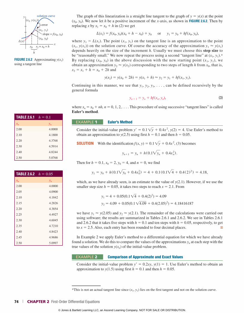
FIGURE 2.6.2 Approximating y(x1) using a tangent line
slope = f(x0, y0)
h
y
x
error
solution curve
L(x)
x0 x1 = x0 + h
(x0, y0)
(x1, y1)
(x1, y(x1))The graph of this linearization is a straight line tangent to the graph of y 5 y(x) at the point
(x0, y0). We now let h be a positive increment of the x-axis, as shown in FIGURE 2.6.2. Then by replacing x by x1 5 x0 1 h in (2) we get
L(x1) 5 f (x0, y0)(x0 1 h 2 x0) 1 y0 or y1 5 y0 1 hf (x0, y0),
where y1 5 L(x1). The point (x1, y1) on the tangent line is an approximation to the point (x1, y(x1)) on the solution curve. Of course the accuracy of the approximation y1 < y(x1) depends heavily on the size of the increment h. Usually we must choose this step size to be “reasonably small.” We now repeat the process using a second “tangent line” at (x1, y1).* By replacing (x0, y0) in the above discussion with the new starting point (x1, y1), we obtain an approximation y2 < y(x2) corresponding to two steps of length h from x0, that is, x2 5 x1 1 h 5 x0 1 2h and
y(x2) 5 y(x0 1 2h) 5 y(x1 1 h) y2 5 y1 1 hf (x1, y1).
Continuing in this manner, we see that y1, y2, y3, . . . , can be defined recursively by the general formula
yn 1 1 5 yn 1 hf (xn, yn), (3)
where xn 5 x0 1 nh, n 5 0, 1, 2, . . . . This procedure of using successive “tangent lines” is called Euler’s method.
EXAMPLE 1 Euler’s Method
Consider the initial-value problem y9 5 0.1!y 1 0.4x 2, y(2) 5 4. Use Euler’s method to obtain an approximation to y(2.5) using first h 5 0.1 and then h 5 0.05.
SOLUTION With the identification f (x, y) 5 0.1!y 1 0.4x 2, (3) becomes
yn11 5 yn 1 h(0.1"yn 1 0.4x 2n ) .
Then for h 5 0.1, x0 5 2, y0 5 4, and n 5 0, we find
y1 5 y0 1 h(0.1"y0 1 0.4x 20 ) 5 4 1 0.1(0.1"4 1 0.4(2)2) 5 4.18,
which, as we have already seen, is an estimate to the value of y(2.1). However, if we use the smaller step size h 5 0.05, it takes two steps to reach x 5 2.1. From
y1 5 4 1 0.05(0.1!4 1 0.4(2) 2) 5 4.09
y2 5 4.09 1 0.05(0.1!4.09 1 0.4(2.05) 2) 5 4.18416187
we have y1 y(2.05) and y2 y(2.1). The remainder of the calculations were carried out using software; the results are summarized in Tables 2.6.1 and 2.6.2. We see in Tables 2.6.1 and 2.6.2 that it takes five steps with h 5 0.1 and ten steps with h 5 0.05, respectively, to get to x 5 2.5. Also, each entry has been rounded to four decimal places.
In Example 2 we apply Euler’s method to a differential equation for which we have already found a solution. We do this to compare the values of the approximations yn at each step with the true values of the solution y(xn) of the initial-value problem.
EXAMPLE 2 Comparison of Approximate and Exact Values
Consider the initial-value problem y9 5 0.2xy, y(1) 5 1. Use Euler’s method to obtain an approximation to y(1.5) using first h 5 0.1 and then h 5 0.05.
*This is not an actual tangent line since (x1, y1) lies on the first tangent and not on the solution curve.
TABLE 2.6.1 h 5 0.1
xn yn
2.00 4.0000
2.10 4.1800
2.20 4.3768
2.30 4.5914
2.40 4.8244
2.50 5.0768
TABLE 2.6.2 h 5 0.05
xn yn
2.00 4.0000
2.05 4.0900
2.10 4.1842
2.15 4.2826
2.20 4.3854
2.25 4.4927
2.30 4.6045
2.35 4.7210
2.40 4.8423
2.45 4.9686
2.50 5.0997
74 | CHAPTER 2 First-Order Differential Equations
© Jones & Bartlett Learning LLC, an Ascend Learning Company. NOT FOR SALE OR DISTRIBUTION.
© Jones & Bartlett Learning, LLCNOT FOR SALE OR DISTRIBUTION
© Jones & Bartlett Learning, LLCNOT FOR SALE OR DISTRIBUTION
© Jones & Bartlett Learning, LLCNOT FOR SALE OR DISTRIBUTION
© Jones & Bartlett Learning, LLCNOT FOR SALE OR DISTRIBUTION
© Jones & Bartlett Learning, LLCNOT FOR SALE OR DISTRIBUTION
© Jones & Bartlett Learning, LLCNOT FOR SALE OR DISTRIBUTION
© Jones & Bartlett Learning, LLCNOT FOR SALE OR DISTRIBUTION
© Jones & Bartlett Learning, LLCNOT FOR SALE OR DISTRIBUTION
© Jones & Bartlett Learning, LLCNOT FOR SALE OR DISTRIBUTION
© Jones & Bartlett Learning, LLCNOT FOR SALE OR DISTRIBUTION
© Jones & Bartlett Learning, LLCNOT FOR SALE OR DISTRIBUTION
© Jones & Bartlett Learning, LLCNOT FOR SALE OR DISTRIBUTION
© Jones & Bartlett Learning, LLCNOT FOR SALE OR DISTRIBUTION
© Jones & Bartlett Learning, LLCNOT FOR SALE OR DISTRIBUTION
© Jones & Bartlett Learning, LLCNOT FOR SALE OR DISTRIBUTION
© Jones & Bartlett Learning, LLCNOT FOR SALE OR DISTRIBUTION
© Jones & Bartlett Learning, LLCNOT FOR SALE OR DISTRIBUTION
© Jones & Bartlett Learning, LLCNOT FOR SALE OR DISTRIBUTION
© Jones & Bartlett Learning, LLCNOT FOR SALE OR DISTRIBUTION
© Jones & Bartlett Learning, LLCNOT FOR SALE OR DISTRIBUTION
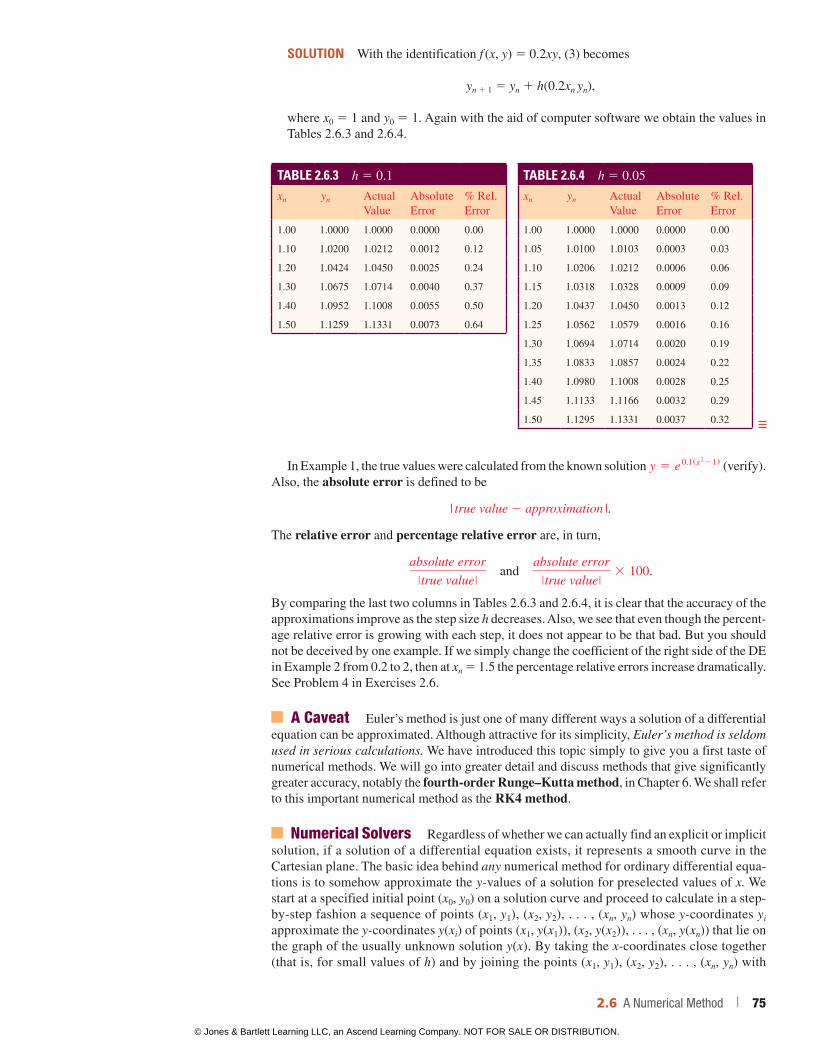
SOLUTION With the identification f (x, y) 5 0.2xy, (3) becomes
yn 1 1 5 yn 1 h(0.2xn yn),
where x0 5 1 and y0 5 1. Again with the aid of computer software we obtain the values in Tables 2.6.3 and 2.6.4.
TABLE 2.6.3 h 5 0.1
xn yn Actual Value
Absolute Error
% Rel. Error
1.00 1.0000 1.0000 0.0000 0.00
1.10 1.0200 1.0212 0.0012 0.12
1.20 1.0424 1.0450 0.0025 0.24
1.30 1.0675 1.0714 0.0040 0.37
1.40 1.0952 1.1008 0.0055 0.50
1.50 1.1259 1.1331 0.0073 0.64
TABLE 2.6.4 h 5 0.05
xn yn Actual Value
Absolute Error
% Rel. Error
1.00 1.0000 1.0000 0.0000 0.00
1.05 1.0100 1.0103 0.0003 0.03
1.10 1.0206 1.0212 0.0006 0.06
1.15 1.0318 1.0328 0.0009 0.09
1.20 1.0437 1.0450 0.0013 0.12
1.25 1.0562 1.0579 0.0016 0.16
1.30 1.0694 1.0714 0.0020 0.19
1.35 1.0833 1.0857 0.0024 0.22
1.40 1.0980 1.1008 0.0028 0.25
1.45 1.1133 1.1166 0.0032 0.29
1.50 1.1295 1.1331 0.0037 0.32
In Example 1, the true values were calculated from the known solution y 5 e 0.1(x
221) (verify). Also, the absolute error is defined to be
| true value 2 approximation |.
The relative error and percentage relative error are, in turn,
absolute error
|true value| and
absolute error
|true value|3 100.
By comparing the last two columns in Tables 2.6.3 and 2.6.4, it is clear that the accuracy of the approximations improve as the step size h decreases. Also, we see that even though the percent-age relative error is growing with each step, it does not appear to be that bad. But you should not be deceived by one example. If we simply change the coefficient of the right side of the DE in Example 2 from 0.2 to 2, then at xn 5 1.5 the percentage relative errors increase dramatically. See Problem 4 in Exercises 2.6.
A Caveat Euler’s method is just one of many different ways a solution of a differential equation can be approximated. Although attractive for its simplicity, Euler’s method is seldom used in serious calculations. We have introduced this topic simply to give you a first taste of numerical methods. We will go into greater detail and discuss methods that give significantly greater accuracy, notably the fourth-order Runge–Kutta method, in Chapter 6. We shall refer to this important numerical method as the RK4 method.
Numerical Solvers Regardless of whether we can actually find an explicit or implicit solution, if a solution of a differential equation exists, it represents a smooth curve in the Cartesian plane. The basic idea behind any numerical method for ordinary differential equa-tions is to somehow approximate the y-values of a solution for preselected values of x. We start at a specified initial point (x0, y0) on a solution curve and proceed to calculate in a step-by-step fashion a sequence of points (x1, y1), (x2, y2), . . . , (xn, yn) whose y-coordinates yi approximate the y-coordinates y(xi) of points (x1, y(x1)), (x2, y(x2)), . . . , (xn, y(xn)) that lie on the graph of the usually unknown solution y(x). By taking the x-coordinates close together (that is, for small values of h) and by joining the points (x1, y1), (x2, y2), . . . , (xn, yn) with
2.6 A Numerical Method | 75
© Jones & Bartlett Learning LLC, an Ascend Learning Company. NOT FOR SALE OR DISTRIBUTION.
© Jones & Bartlett Learning, LLCNOT FOR SALE OR DISTRIBUTION
© Jones & Bartlett Learning, LLCNOT FOR SALE OR DISTRIBUTION
© Jones & Bartlett Learning, LLCNOT FOR SALE OR DISTRIBUTION
© Jones & Bartlett Learning, LLCNOT FOR SALE OR DISTRIBUTION
© Jones & Bartlett Learning, LLCNOT FOR SALE OR DISTRIBUTION
© Jones & Bartlett Learning, LLCNOT FOR SALE OR DISTRIBUTION
© Jones & Bartlett Learning, LLCNOT FOR SALE OR DISTRIBUTION
© Jones & Bartlett Learning, LLCNOT FOR SALE OR DISTRIBUTION
© Jones & Bartlett Learning, LLCNOT FOR SALE OR DISTRIBUTION
© Jones & Bartlett Learning, LLCNOT FOR SALE OR DISTRIBUTION
© Jones & Bartlett Learning, LLCNOT FOR SALE OR DISTRIBUTION
© Jones & Bartlett Learning, LLCNOT FOR SALE OR DISTRIBUTION
© Jones & Bartlett Learning, LLCNOT FOR SALE OR DISTRIBUTION
© Jones & Bartlett Learning, LLCNOT FOR SALE OR DISTRIBUTION
© Jones & Bartlett Learning, LLCNOT FOR SALE OR DISTRIBUTION
© Jones & Bartlett Learning, LLCNOT FOR SALE OR DISTRIBUTION
© Jones & Bartlett Learning, LLCNOT FOR SALE OR DISTRIBUTION
© Jones & Bartlett Learning, LLCNOT FOR SALE OR DISTRIBUTION
© Jones & Bartlett Learning, LLCNOT FOR SALE OR DISTRIBUTION
© Jones & Bartlett Learning, LLCNOT FOR SALE OR DISTRIBUTION
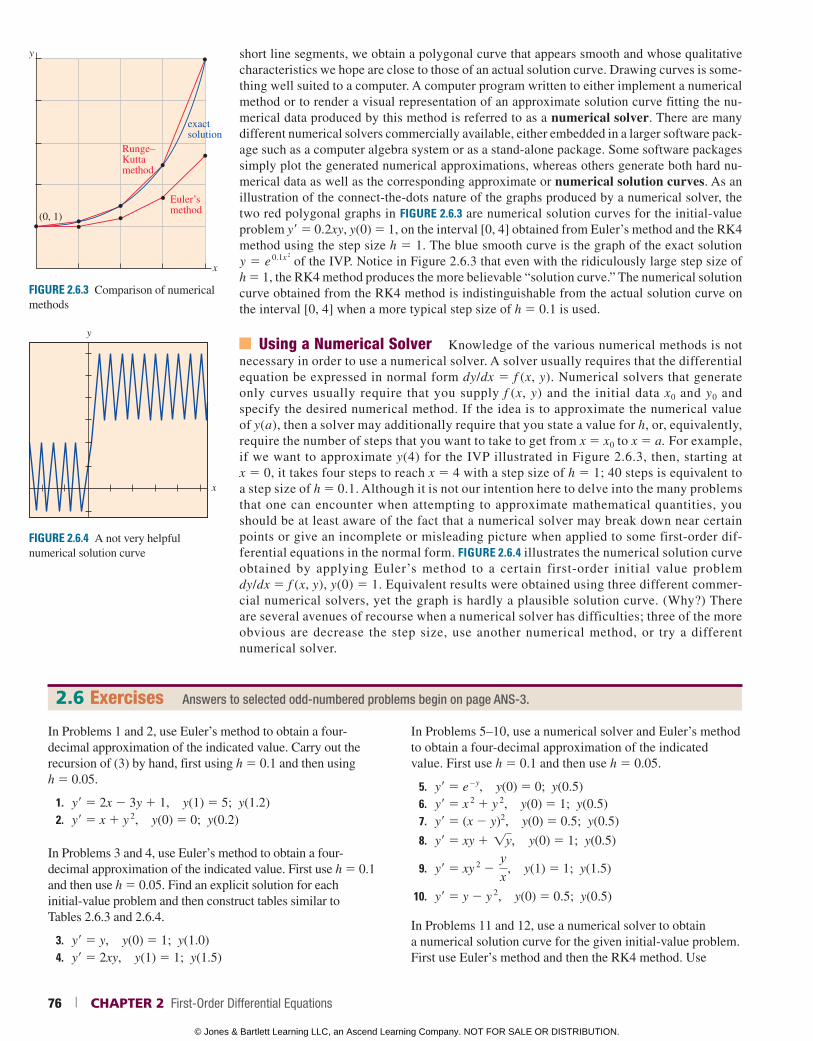
short line segments, we obtain a polygonal curve that appears smooth and whose qualitative characteristics we hope are close to those of an actual solution curve. Drawing curves is some-thing well suited to a computer. A computer program written to either implement a numerical method or to render a visual representation of an approximate solution curve fitting the nu-merical data produced by this method is referred to as a numerical solver. There are many different numerical solvers commercially available, either embedded in a larger software pack-age such as a computer algebra system or as a stand-alone package. Some software packages simply plot the generated numerical approximations, whereas others generate both hard nu-merical data as well as the corresponding approximate or numerical solution curves. As an illustration of the connect-the-dots nature of the graphs produced by a numerical solver, the two red polygonal graphs in FIGURE 2.6.3 are numerical solution curves for the initial-value problem y9 5 0.2xy, y(0) 5 1, on the interval [0, 4] obtained from Euler’s method and the RK4 method using the step size h 5 1. The blue smooth curve is the graph of the exact solution y 5 e
0.1x 2
of the IVP. Notice in Figure 2.6.3 that even with the ridiculously large step size of h 5 1, the RK4 method produces the more believable “solution curve.” The numerical solution curve obtained from the RK4 method is indistinguishable from the actual solution curve on the interval [0, 4] when a more typical step size of h 5 0.1 is used.
Using a Numerical Solver Knowledge of the various numerical methods is not necessary in order to use a numerical solver. A solver usually requires that the differential equation be expressed in normal form dy/dx 5 f (x, y). Numerical solvers that generate only curves usually require that you supply f (x, y) and the initial data x0 and y0 and specify the desired numerical method. If the idea is to approximate the numerical value of y(a), then a solver may additionally require that you state a value for h, or, equivalently, require the number of steps that you want to take to get from x 5 x0 to x 5 a. For example, if we want to approximate y(4) for the IVP illustrated in Figure 2.6.3, then, starting at x 5 0, it takes four steps to reach x 5 4 with a step size of h 5 1; 40 steps is equivalent to a step size of h 5 0.1. Although it is not our intention here to delve into the many problems that one can encounter when attempting to approximate mathematical quantities, you should be at least aware of the fact that a numerical solver may break down near certain points or give an incomplete or misleading picture when applied to some first-order dif-ferential equations in the normal form. FIGURE 2.6.4 illustrates the numerical solution curve obtained by applying Euler’s method to a certain first-order initial value problem dy/dx 5 f (x, y), y(0) 5 1. Equivalent results were obtained using three different commer-cial numerical solvers, yet the graph is hardly a plausible solution curve. (Why?) There are several avenues of recourse when a numerical solver has difficulties; three of the more obvious are decrease the step size, use another numerical method, or try a different numerical solver.
FIGURE 2.6.3 Comparison of numerical methods
exactsolution
Runge–Kuttamethod
(0, 1)
Euler’smethod
x
y
FIGURE 2.6.4 A not very helpful numerical solution curve
x
y
2.6 Exercises Answers to selected odd-numbered problems begin on page ANS-3.
In Problems 1 and 2, use Euler’s method to obtain a four- decimal approximation of the indicated value. Carry out the recursion of (3) by hand, first using h 5 0.1 and then using h 5 0.05.
1. y9 5 2x 2 3y 1 1, y(1) 5 5; y(1.2) 2. y9 5 x 1 y 2, y(0) 5 0; y(0.2)
In Problems 3 and 4, use Euler’s method to obtain a four-decimal approximation of the indicated value. First use h 5 0.1 and then use h 5 0.05. Find an explicit solution for each initial-value problem and then construct tables similar to Tables 2.6.3 and 2.6.4.
3. y9 5 y, y(0) 5 1; y(1.0) 4. y9 5 2xy, y(1) 5 1; y(1.5)
In Problems 5–10, use a numerical solver and Euler’s method to obtain a four-decimal approximation of the indicated value. First use h 5 0.1 and then use h 5 0.05.
5. y9 5 e – y, y(0) 5 0; y(0.5) 6. y9 5 x 2 1 y 2, y(0) 5 1; y(0.5) 7. y9 5 (x 2 y)2, y(0) 5 0.5; y(0.5)
8. y9 5 xy 1 !y, y(0) 5 1; y(0.5)
9. y9 5 xy 2 2 yx , y(1) 5 1; y(1.5)
10. y9 5 y 2 y 2, y(0) 5 0.5; y(0.5)
In Problems 11 and 12, use a numerical solver to obtain a numerical solution curve for the given initial-value problem. First use Euler’s method and then the RK4 method. Use
76 | CHAPTER 2 First-Order Differential Equations
© Jones & Bartlett Learning LLC, an Ascend Learning Company. NOT FOR SALE OR DISTRIBUTION.
© Jones & Bartlett Learning, LLCNOT FOR SALE OR DISTRIBUTION
© Jones & Bartlett Learning, LLCNOT FOR SALE OR DISTRIBUTION
© Jones & Bartlett Learning, LLCNOT FOR SALE OR DISTRIBUTION
© Jones & Bartlett Learning, LLCNOT FOR SALE OR DISTRIBUTION
© Jones & Bartlett Learning, LLCNOT FOR SALE OR DISTRIBUTION
© Jones & Bartlett Learning, LLCNOT FOR SALE OR DISTRIBUTION
© Jones & Bartlett Learning, LLCNOT FOR SALE OR DISTRIBUTION
© Jones & Bartlett Learning, LLCNOT FOR SALE OR DISTRIBUTION
© Jones & Bartlett Learning, LLCNOT FOR SALE OR DISTRIBUTION
© Jones & Bartlett Learning, LLCNOT FOR SALE OR DISTRIBUTION
© Jones & Bartlett Learning, LLCNOT FOR SALE OR DISTRIBUTION
© Jones & Bartlett Learning, LLCNOT FOR SALE OR DISTRIBUTION
© Jones & Bartlett Learning, LLCNOT FOR SALE OR DISTRIBUTION
© Jones & Bartlett Learning, LLCNOT FOR SALE OR DISTRIBUTION
© Jones & Bartlett Learning, LLCNOT FOR SALE OR DISTRIBUTION
© Jones & Bartlett Learning, LLCNOT FOR SALE OR DISTRIBUTION
© Jones & Bartlett Learning, LLCNOT FOR SALE OR DISTRIBUTION
© Jones & Bartlett Learning, LLCNOT FOR SALE OR DISTRIBUTION
© Jones & Bartlett Learning, LLCNOT FOR SALE OR DISTRIBUTION
© Jones & Bartlett Learning, LLCNOT FOR SALE OR DISTRIBUTION
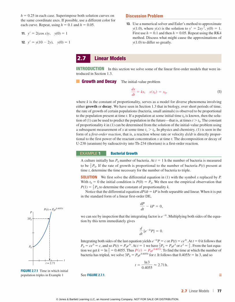
h 5 0.25 in each case. Superimpose both solution curves on the same co ordinate axes. If possible, use a different color for each curve. Repeat, using h 5 0.1 and h 5 0.05.
11. y9 5 2(cos x)y, y(0) 5 1
12. y9 5 y(10 2 2y), y(0) 5 1
Discussion Problem
13. Use a numerical solver and Euler’s method to approximate y(1.0), where y(x) is the solution to y9 5 2xy 2, y(0) 5 1. First use h 5 0.1 and then h 5 0.05. Repeat using the RK4 method. Discuss what might cause the approximations of y(1.0) to differ so greatly.
2.7 Linear Models
INTRODUCTION In this section we solve some of the linear first-order models that were in-troduced in Section 1.3.
Growth and Decay The initial-value problem
dx
dt5 kx, x( t0 ) 5 x0, (1)
where k is the constant of proportionality, serves as a model for diverse phenomena involving either growth or decay. We have seen in Section 1.3 that in biology, over short periods of time, the rate of growth of certain populations (bacteria, small animals) is observed to be proportional to the population present at time t. If a population at some initial time t0 is known, then the solu-tion of (1) can be used to predict the population in the future—that is, at times t t0. The constant of proportionality k in (1) can be determined from the solution of the initial-value problem using a subsequent measurement of x at some time t1 t0. In physics and chemistry, (1) is seen in the form of a first-order reaction, that is, a reaction whose rate or velocity dx/dt is directly propor-tional to the first power of the reactant concentration x at time t. The decomposition or decay of U-238 (uranium) by radioactivity into Th-234 (thorium) is a first-order reaction.
EXAMPLE 1 Bacterial Growth
A culture initially has P0 number of bacteria. At t 5 1 h the number of bacteria is measured to be 3
2 P0. If the rate of growth is proportional to the number of bacteria P(t) present at time t, determine the time necessary for the number of bacteria to triple.
SOLUTION We first solve the differential equation in (1) with the symbol x replaced by P. With t0 5 0 the initial condition is P(0) 5 P0. We then use the empirical observation that P(1) 5 3
2 P0 to determine the constant of proportionality k.Notice that the differential equation dP/dt 5 kP is both separable and linear. When it is put
in the standard form of a linear first-order DE,
dP
dt2 kP 5 0,
we can see by inspection that the integrating factor is e – kt. Multiplying both sides of the equa-tion by this term immediately gives
d
dt [e
2ktP] 5 0.
Integrating both sides of the last equation yields e – ktP 5 c or P(t) 5 ce kt. At t 5 0 it follows that P0 5 ce 0 5 c, and so P(t) 5 P0e kt. At t 5 1 we have 3
2P0 5 P0e k or e k 5 32 . From the last equa-
tion we get k 5 ln 32 5 0.4055. Thus P( t) 5 P0e 0.4055t. To find the time at which the number of
bacteria has tripled, we solve 3P0 5 P0e 0.4055t for t. It follows that 0.4055t 5 ln 3, and so
t 5ln 3
0.4055< 2.71 h.
See FIGURE 2.7.1.FIGURE 2.7.1 Time in which initial population triples in Example 1
t = 2.71 t
P
P0
3P0
P(t) = P0e0.4055t
2.7 Linear Models | 77
© Jones & Bartlett Learning LLC, an Ascend Learning Company. NOT FOR SALE OR DISTRIBUTION.
© Jones & Bartlett Learning, LLCNOT FOR SALE OR DISTRIBUTION
© Jones & Bartlett Learning, LLCNOT FOR SALE OR DISTRIBUTION
© Jones & Bartlett Learning, LLCNOT FOR SALE OR DISTRIBUTION
© Jones & Bartlett Learning, LLCNOT FOR SALE OR DISTRIBUTION
© Jones & Bartlett Learning, LLCNOT FOR SALE OR DISTRIBUTION
© Jones & Bartlett Learning, LLCNOT FOR SALE OR DISTRIBUTION
© Jones & Bartlett Learning, LLCNOT FOR SALE OR DISTRIBUTION
© Jones & Bartlett Learning, LLCNOT FOR SALE OR DISTRIBUTION
© Jones & Bartlett Learning, LLCNOT FOR SALE OR DISTRIBUTION
© Jones & Bartlett Learning, LLCNOT FOR SALE OR DISTRIBUTION
© Jones & Bartlett Learning, LLCNOT FOR SALE OR DISTRIBUTION
© Jones & Bartlett Learning, LLCNOT FOR SALE OR DISTRIBUTION
© Jones & Bartlett Learning, LLCNOT FOR SALE OR DISTRIBUTION
© Jones & Bartlett Learning, LLCNOT FOR SALE OR DISTRIBUTION
© Jones & Bartlett Learning, LLCNOT FOR SALE OR DISTRIBUTION
© Jones & Bartlett Learning, LLCNOT FOR SALE OR DISTRIBUTION
© Jones & Bartlett Learning, LLCNOT FOR SALE OR DISTRIBUTION
© Jones & Bartlett Learning, LLCNOT FOR SALE OR DISTRIBUTION
© Jones & Bartlett Learning, LLCNOT FOR SALE OR DISTRIBUTION
© Jones & Bartlett Learning, LLCNOT FOR SALE OR DISTRIBUTION
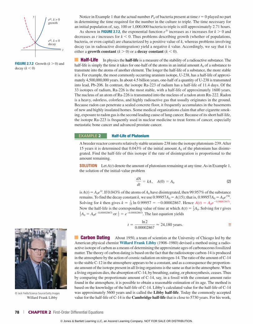
Notice in Example 1 that the actual number P0 of bacteria present at time t 5 0 played no part in determining the time required for the number in the culture to triple. The time necessary for an initial population of, say, 100 or 1,000,000 bacteria to triple is still approximately 2.71 hours.
As shown in FIGURE 2.7.2, the exponential function e kt increases as t increases for k 0 and decreases as t increases for k 0. Thus problems describing growth (whether of populations, bacteria, or even capital) are characterized by a positive value of k, whereas problems involving decay (as in radioactive disintegration) yield a negative k value. Accordingly, we say that k is either a growth constant (k 0) or a decay constant (k 0).
Half-Life In physics the half-life is a measure of the stability of a radioactive substance. The half-life is simply the time it takes for one-half of the atoms in an initial amount A0 of a substance to transmute into the atoms of another element. The longer the half-life of a substance, the more stable it is. For example, the most commonly occurring uranium isotope, U-238, has a half-life of approxi-mately 4,500,000,000 years. In about 4.5 billion years, one-half of a quantity of U-238 is transmuted into lead, Pb-206. In contrast, the isotope Ra-223 of radium has a half-life of 11.4 days. Of the 33 isotopes of radium, Ra-226 is the most stable, with a half-life of approximately 1600 years. The nucleus of an atom of Ra-226 is transmuted into the nucleus of a radon atom Rn-222. Radon is a heavy, odorless, colorless, and highly radioactive gas that usually originates in the ground. Because radon can penetrate a sealed concrete floor, it frequently accumulates in the basements of new and highly insulated homes. Some medical organizations claim that after cigarette smok-ing, exposure to radon gas is the second leading cause of lung cancer. Because of its short half-life, the isotope Ra-223 is frequently used in nuclear medicine to treat forms of cancer, especially metastatic bone cancer and advanced prostate cancer.
EXAMPLE 2 Half-Life of Plutonium
A breeder reactor converts relatively stable uranium-238 into the isotope plutonium-239. After 15 years it is determined that 0.043% of the initial amount A0 of the plutonium has disinte-grated. Find the half-life of this isotope if the rate of disintegration is proportional to the amount remaining.
SOLUTION Let A(t) denote the amount of plutonium remaining at any time. As in Example 1, the solution of the initial-value problem
dA
dt5 kA, A(0) 5 A0 (2)
is A(t) 5 A0e kt. If 0.043% of the atoms of A0 have disintegrated, then 99.957% of the substance remains. To find the decay constant k, we use 0.99957A0 5 A(15); that is, 0.99957A0 5 A0e 15k. Solving for k then gives k 5 1
15 ln 0.99957 5 20.00002867. Hence A(t) 5 A0e 20.00002867t.
Now the half-life is the corresponding value of time at which A(t) 5 12A0. Solving for t gives
12A0 5 A0e –0.00002867t or 1
2 5 e –0.00002867t. The last equation yields
t 5ln 2
0.00002867< 24,180 years.
Carbon Dating About 1950, a team of scientists at the University of Chicago led by the American physical chemist Willard Frank Libby (1908–1980) devised a method using a radio-active isotope of carbon as a means of determining the approximate ages of carbonaceous fossilized matter. The theory of carbon dating is based on the fact that the radioisotope carbon-14 is produced in the atmosphere by the action of cosmic radiation on nitrogen-14. The ratio of the amount of C-14 to the stable C-12 in the atmosphere appears to be a constant, and as a consequence the proportion-ate amount of the isotope present in all living organisms is the same as that in the atmosphere. When a living organism dies, the absorption of C-14, by breathing, eating, or photosynthesis, ceases. Thus by comparing the proportionate amount of C-14, say, in a fossil with the constant amount ratio found in the atmosphere, it is possible to obtain a reasonable estimation of its age. The method is based on the knowledge of the half-life of C-14. Libby’s calculated value for the half-life of C-14 was approximately 5600 years and is called the Libby half-life. Today the commonly accepted value for the half-life of C-14 is the Cambridge half-life that is close to 5730 years. For his work,
FIGURE 2.7.2 Growth (k 0) and decay (k 0)
t
yekt, k > 0growth
ekt, k < 0decay
© Jack Fields/Science Source/Getty Images
Willard Frank Libby
78 | CHAPTER 2 First-Order Differential Equations
© Jones & Bartlett Learning LLC, an Ascend Learning Company. NOT FOR SALE OR DISTRIBUTION.
© Jones & Bartlett Learning, LLCNOT FOR SALE OR DISTRIBUTION
© Jones & Bartlett Learning, LLCNOT FOR SALE OR DISTRIBUTION
© Jones & Bartlett Learning, LLCNOT FOR SALE OR DISTRIBUTION
© Jones & Bartlett Learning, LLCNOT FOR SALE OR DISTRIBUTION
© Jones & Bartlett Learning, LLCNOT FOR SALE OR DISTRIBUTION
© Jones & Bartlett Learning, LLCNOT FOR SALE OR DISTRIBUTION
© Jones & Bartlett Learning, LLCNOT FOR SALE OR DISTRIBUTION
© Jones & Bartlett Learning, LLCNOT FOR SALE OR DISTRIBUTION
© Jones & Bartlett Learning, LLCNOT FOR SALE OR DISTRIBUTION
© Jones & Bartlett Learning, LLCNOT FOR SALE OR DISTRIBUTION
© Jones & Bartlett Learning, LLCNOT FOR SALE OR DISTRIBUTION
© Jones & Bartlett Learning, LLCNOT FOR SALE OR DISTRIBUTION
© Jones & Bartlett Learning, LLCNOT FOR SALE OR DISTRIBUTION
© Jones & Bartlett Learning, LLCNOT FOR SALE OR DISTRIBUTION
© Jones & Bartlett Learning, LLCNOT FOR SALE OR DISTRIBUTION
© Jones & Bartlett Learning, LLCNOT FOR SALE OR DISTRIBUTION
© Jones & Bartlett Learning, LLCNOT FOR SALE OR DISTRIBUTION
© Jones & Bartlett Learning, LLCNOT FOR SALE OR DISTRIBUTION
© Jones & Bartlett Learning, LLCNOT FOR SALE OR DISTRIBUTION
© Jones & Bartlett Learning, LLCNOT FOR SALE OR DISTRIBUTION
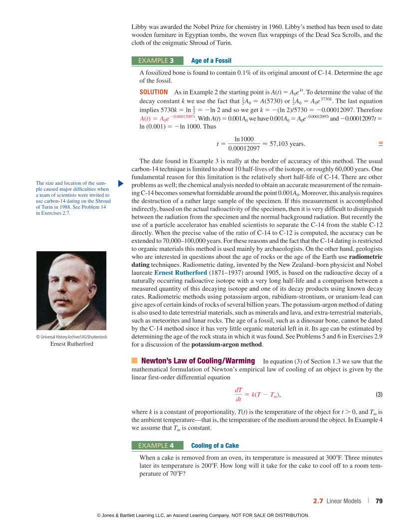
Libby was awarded the Nobel Prize for chemistry in 1960. Libby’s method has been used to date wooden furniture in Egyptian tombs, the woven flax wrappings of the Dead Sea Scrolls, and the cloth of the enigmatic Shroud of Turin.
EXAMPLE 3 Age of a Fossil
A fossilized bone is found to contain 0.1% of its original amount of C-14. Determine the age of the fossil.
SOLUTION As in Example 2 the starting point is A(t) 5 A0e kt. To determine the value of the decay constant k we use the fact that 1
2A0 5 A(5730) or 12A0 5 A0e 5730k. The last equation
implies 5730k 5 ln 12 5 2ln 2 and so we get k 5 2(ln 2)/5730 5 20.00012097. Therefore
A(t) 5 A0e 20.00012097t. With A(t) 5 0.001A0 we have 0.001A0 5 A0e – 0.00012097t and 20.00012097t 5
ln (0.001) 5 2ln 1000. Thus
t 5ln 1000
0.00012097< 57,103 years.
The date found in Example 3 is really at the border of accuracy of this method. The usual carbon-14 technique is limited to about 10 half-lives of the isotope, or roughly 60,000 years. One fundamental reason for this limitation is the relatively short half-life of C-14. There are other problems as well; the chemical analysis needed to obtain an accurate measurement of the remain-ing C-14 becomes somewhat formidable around the point 0.001A0. Moreover, this analysis requires the destruction of a rather large sample of the specimen. If this measurement is accomplished indirectly, based on the actual radioactivity of the specimen, then it is very difficult to distinguish between the radiation from the specimen and the normal background radiation. But recently the use of a particle accelerator has enabled scientists to separate the C-14 from the stable C-12 directly. When the precise value of the ratio of C-14 to C-12 is computed, the accuracy can be extended to 70,000–100,000 years. For these reasons and the fact that the C-14 dating is restricted to organic materials this method is used mainly by archaeologists. On the other hand, geologists who are interested in questions about the age of rocks or the age of the Earth use radiometric dating techniques. Radiometric dating, invented by the New Zealand–born physicist and Nobel laureate Ernest Rutherford (1871–1937) around 1905, is based on the radioactive decay of a naturally occurring radioactive isotope with a very long half-life and a comparison between a measured quantity of this decaying isotope and one of its decay products using known decay rates. Radiometric methods using potassium-argon, rubidium-strontium, or uranium-lead can give ages of certain kinds of rocks of several billion years. The potassium-argon method of dating is also used to date terrestrial materials, such as minerals and lava, and extra-terrestrial materials, such as meteorites and lunar rocks. The age of a fossil, such as a dinosaur bone, cannot be dated by the C-14 method since it has very little organic material left in it. Its age can be estimated by determining the age of the rock strata in which it was found. See Problems 5 and 6 in Exercises 2.9 for a discussion of the potassium-argon method.
Newton’s Law of Cooling / Warming In equation (3) of Section 1.3 we saw that the mathematical formulation of Newton’s empirical law of cooling of an object is given by the linear first-order differential equation
dT
dt5 k(T 2 Tm), (3)
where k is a constant of proportionality, T(t) is the temperature of the object for t 0, and Tm is the ambient temperature—that is, the temperature of the medium around the object. In Example 4 we assume that Tm is constant.
EXAMPLE 4 Cooling of a Cake
When a cake is removed from an oven, its temperature is measured at 3008F. Three minutes later its temperature is 2008F. How long will it take for the cake to cool off to a room tem-perature of 708F?
The size and location of the sam-ple caused major difficulties when a team of scientists were invited to use carbon-14 dating on the Shroud of Turin in 1988. See Problem 14 in Exercises 2.7.
© Universal History Archive/UIG/Shutterstock
Ernest Rutherford
2.7 Linear Models | 79
© Jones & Bartlett Learning LLC, an Ascend Learning Company. NOT FOR SALE OR DISTRIBUTION.
© Jones & Bartlett Learning, LLCNOT FOR SALE OR DISTRIBUTION
© Jones & Bartlett Learning, LLCNOT FOR SALE OR DISTRIBUTION
© Jones & Bartlett Learning, LLCNOT FOR SALE OR DISTRIBUTION
© Jones & Bartlett Learning, LLCNOT FOR SALE OR DISTRIBUTION
© Jones & Bartlett Learning, LLCNOT FOR SALE OR DISTRIBUTION
© Jones & Bartlett Learning, LLCNOT FOR SALE OR DISTRIBUTION
© Jones & Bartlett Learning, LLCNOT FOR SALE OR DISTRIBUTION
© Jones & Bartlett Learning, LLCNOT FOR SALE OR DISTRIBUTION
© Jones & Bartlett Learning, LLCNOT FOR SALE OR DISTRIBUTION
© Jones & Bartlett Learning, LLCNOT FOR SALE OR DISTRIBUTION
© Jones & Bartlett Learning, LLCNOT FOR SALE OR DISTRIBUTION
© Jones & Bartlett Learning, LLCNOT FOR SALE OR DISTRIBUTION
© Jones & Bartlett Learning, LLCNOT FOR SALE OR DISTRIBUTION
© Jones & Bartlett Learning, LLCNOT FOR SALE OR DISTRIBUTION
© Jones & Bartlett Learning, LLCNOT FOR SALE OR DISTRIBUTION
© Jones & Bartlett Learning, LLCNOT FOR SALE OR DISTRIBUTION
© Jones & Bartlett Learning, LLCNOT FOR SALE OR DISTRIBUTION
© Jones & Bartlett Learning, LLCNOT FOR SALE OR DISTRIBUTION
© Jones & Bartlett Learning, LLCNOT FOR SALE OR DISTRIBUTION
© Jones & Bartlett Learning, LLCNOT FOR SALE OR DISTRIBUTION
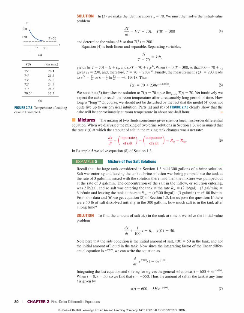
SOLUTION In (3) we make the identification Tm 5 70. We must then solve the initial-value problem
dT
dt5 k(T 2 70), T(0) 5 300 (4)
and determine the value of k so that T(3) 5 200.Equation (4) is both linear and separable. Separating variables,
dT
T 2 705 k dt,
yields ln | T 2 70 | 5 kt 1 c1, and so T 5 70 1 c2e kt. When t 5 0, T 5 300, so that 300 5 70 1 c2 gives c2 5 230, and, therefore, T 5 70 1 230e kt. Finally, the measurement T(3) 5 200 leads to e 3k 5 13
23 or k 5 13 ln 13
23 5 20.19018. Thus
T(t) 5 70 1 230e – 0.19018t. (5)
We note that (5) furnishes no solution to T(t) 5 70 since limt S q T(t) 5 70. Yet intuitively we expect the cake to reach the room temperature after a reasonably long period of time. How long is “long”? Of course, we should not be disturbed by the fact that the model (4) does not quite live up to our physical intuition. Parts (a) and (b) of FIGURE 2.7.3 clearly show that the cake will be approximately at room temperature in about one-half hour.
Mixtures The mixing of two fluids sometimes gives rise to a linear first-order differential equation. When we discussed the mixing of two brine solutions in Section 1.3, we assumed that the rate x9(t) at which the amount of salt in the mixing tank changes was a net rate:
dx
dt5 ainput rate
of saltb 2 aoutput rate
of saltb 5 Rin 2 Rout. (6)
In Example 5 we solve equation (8) of Section 1.3.
EXAMPLE 5 Mixture of Two Salt Solutions
Recall that the large tank considered in Section 1.3 held 300 gallons of a brine solution. Salt was entering and leaving the tank; a brine solution was being pumped into the tank at the rate of 3 gal/min, mixed with the solution there, and then the mixture was pumped out at the rate of 3 gal/min. The concentration of the salt in the inflow, or solution entering, was 2 lb/gal, and so salt was entering the tank at the rate Rin 5 (2 lb/gal) ? (3 gal/min) 5 6 lb/min and leaving the tank at the rate Rout 5 (x/300 lb/gal) ? (3 gal/min) 5 x/100 lb/min. From this data and (6) we get equation (8) of Section 1.3. Let us pose the question: If there were 50 lb of salt dissolved initially in the 300 gallons, how much salt is in the tank after a long time?
SOLUTION To find the amount of salt x(t) in the tank at time t, we solve the initial-value problem
dx
dt1
1
100 x 5 6, x(0) 5 50.
Note here that the side condition is the initial amount of salt, x(0) 5 50 in the tank, and not the initial amount of liquid in the tank. Now since the integrating factor of the linear differ-ential equation is e t/100, we can write the equation as
d
dt [e
t>100x] 5 6e t>100.
Integrating the last equation and solving for x gives the general solution x(t) 5 600 1 ce – t/100. When t 5 0, x 5 50, so we find that c 5 2550. Thus the amount of salt in the tank at any time t is given by
x(t) 5 600 2 550e – t/100. (7)
FIGURE 2.7.3 Temperature of cooling cake in Example 4
T
t15 30
(a)
T =70
300
150
T(t) t (in min.)
(b)
75°74°73°72°71°70.5°
20.121.322.824.928.632.3
80 | CHAPTER 2 First-Order Differential Equations
© Jones & Bartlett Learning LLC, an Ascend Learning Company. NOT FOR SALE OR DISTRIBUTION.
© Jones & Bartlett Learning, LLCNOT FOR SALE OR DISTRIBUTION
© Jones & Bartlett Learning, LLCNOT FOR SALE OR DISTRIBUTION
© Jones & Bartlett Learning, LLCNOT FOR SALE OR DISTRIBUTION
© Jones & Bartlett Learning, LLCNOT FOR SALE OR DISTRIBUTION
© Jones & Bartlett Learning, LLCNOT FOR SALE OR DISTRIBUTION
© Jones & Bartlett Learning, LLCNOT FOR SALE OR DISTRIBUTION
© Jones & Bartlett Learning, LLCNOT FOR SALE OR DISTRIBUTION
© Jones & Bartlett Learning, LLCNOT FOR SALE OR DISTRIBUTION
© Jones & Bartlett Learning, LLCNOT FOR SALE OR DISTRIBUTION
© Jones & Bartlett Learning, LLCNOT FOR SALE OR DISTRIBUTION
© Jones & Bartlett Learning, LLCNOT FOR SALE OR DISTRIBUTION
© Jones & Bartlett Learning, LLCNOT FOR SALE OR DISTRIBUTION
© Jones & Bartlett Learning, LLCNOT FOR SALE OR DISTRIBUTION
© Jones & Bartlett Learning, LLCNOT FOR SALE OR DISTRIBUTION
© Jones & Bartlett Learning, LLCNOT FOR SALE OR DISTRIBUTION
© Jones & Bartlett Learning, LLCNOT FOR SALE OR DISTRIBUTION
© Jones & Bartlett Learning, LLCNOT FOR SALE OR DISTRIBUTION
© Jones & Bartlett Learning, LLCNOT FOR SALE OR DISTRIBUTION
© Jones & Bartlett Learning, LLCNOT FOR SALE OR DISTRIBUTION
© Jones & Bartlett Learning, LLCNOT FOR SALE OR DISTRIBUTION
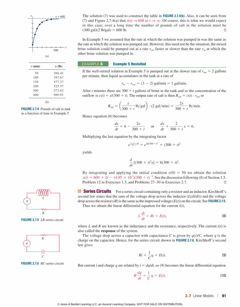
The solution (7) was used to construct the table in FIGURE 2.7.4 (b). Also, it can be seen from (7) and Figure 2.7.4(a) that x(t) S 600 as t S q . Of course, this is what we would expect in this case; over a long time the number of pounds of salt in the solution must be (300 gal)(2 lb/gal) 5 600 lb.
In Example 5 we assumed that the rate at which the solution was pumped in was the same as the rate at which the solution was pumped out. However, this need not be the situation; the mixed brine solution could be pumped out at a rate rout faster or slower than the rate rin at which the other brine solution was pumped in.
EXAMPLE 6 Example 5 Revisited
If the well-stirred solution in Example 5 is pumped out at the slower rate of rout 5 2 gallons per minute, then liquid accumulates in the tank at a rate of
rin 2 rout 5 (3 2 2) gal/min 5 1 gal/min.
After t minutes there are 300 1 t gallons of brine in the tank and so the concentration of the outflow is c(t) 5 x/(300 1 t). The output rate of salt is then Rout 5 c(t) ? rout or
Rout 5 a x
300 1 t lb>galb ? (2 gal>min) 5
2x
300 1 t lb>min.
Hence equation (6) becomes
dx
dt5 6 2
2x
300 1 t or
dx
dt1
2
300 1 t x 5 6.
Multiplying the last equation by the integrating factor
e e
2300 1 t
dt 5 e ln(3001 t)
2
5 (300 1 t)2
yields
d
dt [(300 1 t)2x] 5 6(300 1 t)2.
By integrating and applying the initial condition x(0) 5 50 we obtain the solution x(t) 5 600 1 2t 2 (4.95 3 10
7)(300 1 t)22. See the discussion following (8) of Section 1.3, Problem 12 in Exercises 1.3, and Problems 27–30 in Exercises 2.7.
Series Circuits For a series circuit containing only a resistor and an inductor, Kirchhoff’s second law states that the sum of the voltage drop across the inductor (L(di/dt)) and the voltage drop across the resistor (iR) is the same as the impressed voltage (E(t)) on the circuit. See FIGURE 2.7.5.
Thus we obtain the linear differential equation for the current i(t),
L di
dt1 Ri 5 E(t), (8)
where L and R are known as the inductance and the resistance, respectively. The current i(t) is also called the response of the system.
The voltage drop across a capacitor with capacitance C is given by q(t)/C, where q is the charge on the capacitor. Hence, for the series circuit shown in FIGURE 2.7.6, Kirchhoff’s second law gives
Ri 11
C q 5 E(t). (9)
But current i and charge q are related by i 5 dq/dt, so (9) becomes the linear differential equation
R dq
dt1
1
C q 5 E(t). (10)
FIGURE 2.7.4 Pounds of salt in tank as a function of time in Example 5
x
t500
(a)
x = 600
x (lb)t (min)
(b)
50100150200300400
266.41397.67477.27525.57572.62589.93
FIGURE 2.7.5 LR-series circuit
L
R
E
FIGURE 2.7.6 RC-series circuit
R
C
E
2.7 Linear Models | 81
© Jones & Bartlett Learning LLC, an Ascend Learning Company. NOT FOR SALE OR DISTRIBUTION.
© Jones & Bartlett Learning, LLCNOT FOR SALE OR DISTRIBUTION
© Jones & Bartlett Learning, LLCNOT FOR SALE OR DISTRIBUTION
© Jones & Bartlett Learning, LLCNOT FOR SALE OR DISTRIBUTION
© Jones & Bartlett Learning, LLCNOT FOR SALE OR DISTRIBUTION
© Jones & Bartlett Learning, LLCNOT FOR SALE OR DISTRIBUTION
© Jones & Bartlett Learning, LLCNOT FOR SALE OR DISTRIBUTION
© Jones & Bartlett Learning, LLCNOT FOR SALE OR DISTRIBUTION
© Jones & Bartlett Learning, LLCNOT FOR SALE OR DISTRIBUTION
© Jones & Bartlett Learning, LLCNOT FOR SALE OR DISTRIBUTION
© Jones & Bartlett Learning, LLCNOT FOR SALE OR DISTRIBUTION
© Jones & Bartlett Learning, LLCNOT FOR SALE OR DISTRIBUTION
© Jones & Bartlett Learning, LLCNOT FOR SALE OR DISTRIBUTION
© Jones & Bartlett Learning, LLCNOT FOR SALE OR DISTRIBUTION
© Jones & Bartlett Learning, LLCNOT FOR SALE OR DISTRIBUTION
© Jones & Bartlett Learning, LLCNOT FOR SALE OR DISTRIBUTION
© Jones & Bartlett Learning, LLCNOT FOR SALE OR DISTRIBUTION
© Jones & Bartlett Learning, LLCNOT FOR SALE OR DISTRIBUTION
© Jones & Bartlett Learning, LLCNOT FOR SALE OR DISTRIBUTION
© Jones & Bartlett Learning, LLCNOT FOR SALE OR DISTRIBUTION
© Jones & Bartlett Learning, LLCNOT FOR SALE OR DISTRIBUTION
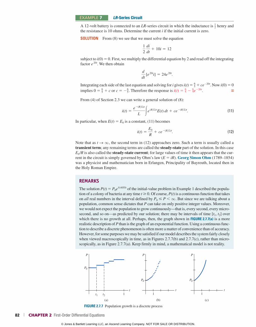
EXAMPLE 7 LR-Series Circuit
A 12-volt battery is connected to an LR-series circuit in which the inductance is 12 henry and
the resistance is 10 ohms. Determine the current i if the initial current is zero.
SOLUTION From (8) we see that we must solve the equation
1
2 di
dt1 10i 5 12
subject to i(0) 5 0. First, we multiply the differential equation by 2 and read off the integrating factor e 20t. We then obtain
d
dt [e
20ti] 5 24e 20t.
Integrating each side of the last equation and solving for i gives i(t) 5 65 1 ce – 20t. Now i(0) 5 0 implies 0 5 6
5 1 c or c 5 265. Therefore the response is i(t) 5 6
5 2 65e
220t.
From (4) of Section 2.3 we can write a general solution of (8):
i(t) 5e
2(R>L)t
L #e (R>L)t
E(t) dt 1 ce 2(R>L)t. (11)
In particular, when E(t) 5 E0 is a constant, (11) becomes
i(t) 5E0
R1 ce
2(R>L)t. (12)
Note that as t S q , the second term in (12) approaches zero. Such a term is usually called a transient term; any remaining terms are called the steady-state part of the solution. In this case E0 /R is also called the steady-state current; for large values of time it then appears that the cur-rent in the circuit is simply governed by Ohm’s law (E 5 iR). Georg Simon Ohm (1789–1854) was a physicist and mathematician born in Erlangen, Principality of Bayreuth, located then in the Holy Roman Empire.
REMARKSThe solution P(t) 5 P0e 0.4055t of the initial-value problem in Example 1 described the popula-tion of a colony of bacteria at any time t 0. Of course, P(t) is a continuous function that takes on all real numbers in the interval defined by P0 # P q . But since we are talking about a population, common sense dictates that P can take on only positive integer values. Moreover, we would not expect the population to grow continuously—that is, every second, every micro-second, and so on—as predicted by our solution; there may be intervals of time [t1, t2] over which there is no growth at all. Perhaps, then, the graph shown in FIGURE 2.7.7(a) is a more realistic description of P than is the graph of an exponential function. Using a continuous func-tion to describe a discrete phenomenon is often more a matter of convenience than of accuracy. However, for some purposes we may be satisfied if our model describes the system fairly closely when viewed macroscopically in time, as in Figures 2.7.7(b) and 2.7.7(c), rather than micro-scopically, as in Figure 2.7.7(a). Keep firmly in mind, a mathematical model is not reality.
(c)
P
1t
P0
(b)
P
1t
P0
(a)
P
t1t2t1
P0
FIGURE 2.7.7 Population growth is a discrete process
82 | CHAPTER 2 First-Order Differential Equations
© Jones & Bartlett Learning LLC, an Ascend Learning Company. NOT FOR SALE OR DISTRIBUTION.
© Jones & Bartlett Learning, LLCNOT FOR SALE OR DISTRIBUTION
© Jones & Bartlett Learning, LLCNOT FOR SALE OR DISTRIBUTION
© Jones & Bartlett Learning, LLCNOT FOR SALE OR DISTRIBUTION
© Jones & Bartlett Learning, LLCNOT FOR SALE OR DISTRIBUTION
© Jones & Bartlett Learning, LLCNOT FOR SALE OR DISTRIBUTION
© Jones & Bartlett Learning, LLCNOT FOR SALE OR DISTRIBUTION
© Jones & Bartlett Learning, LLCNOT FOR SALE OR DISTRIBUTION
© Jones & Bartlett Learning, LLCNOT FOR SALE OR DISTRIBUTION
© Jones & Bartlett Learning, LLCNOT FOR SALE OR DISTRIBUTION
© Jones & Bartlett Learning, LLCNOT FOR SALE OR DISTRIBUTION
© Jones & Bartlett Learning, LLCNOT FOR SALE OR DISTRIBUTION
© Jones & Bartlett Learning, LLCNOT FOR SALE OR DISTRIBUTION
© Jones & Bartlett Learning, LLCNOT FOR SALE OR DISTRIBUTION
© Jones & Bartlett Learning, LLCNOT FOR SALE OR DISTRIBUTION
© Jones & Bartlett Learning, LLCNOT FOR SALE OR DISTRIBUTION
© Jones & Bartlett Learning, LLCNOT FOR SALE OR DISTRIBUTION
© Jones & Bartlett Learning, LLCNOT FOR SALE OR DISTRIBUTION
© Jones & Bartlett Learning, LLCNOT FOR SALE OR DISTRIBUTION
© Jones & Bartlett Learning, LLCNOT FOR SALE OR DISTRIBUTION
© Jones & Bartlett Learning, LLCNOT FOR SALE OR DISTRIBUTION
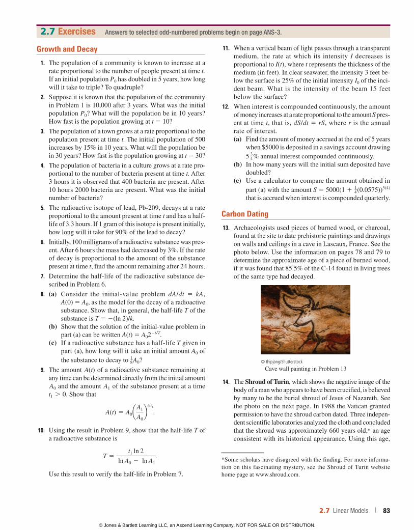
2.7 Exercises Answers to selected odd-numbered problems begin on page ANS-3.
Growth and Decay
1. The population of a community is known to increase at a rate proportional to the number of people present at time t. If an initial population P0 has doubled in 5 years, how long will it take to triple? To quadruple?
2. Suppose it is known that the population of the community in Problem 1 is 10,000 after 3 years. What was the initial population P0? What will the population be in 10 years? How fast is the population growing at t 5 10?
3. The population of a town grows at a rate proportional to the population present at time t. The initial population of 500 increases by 15% in 10 years. What will the population be in 30 years? How fast is the population growing at t 5 30?
4. The population of bacteria in a culture grows at a rate pro-portional to the number of bacteria present at time t. After 3 hours it is observed that 400 bacteria are present. After 10 hours 2000 bacteria are present. What was the initial number of bacteria?
5. The radioactive isotope of lead, Pb-209, decays at a rate proportional to the amount present at time t and has a half-life of 3.3 hours. If 1 gram of this isotope is present initially, how long will it take for 90% of the lead to decay?
6. Initially, 100 milligrams of a radioactive substance was pres-ent. After 6 hours the mass had decreased by 3%. If the rate of decay is proportional to the amount of the substance present at time t, find the amount remaining after 24 hours.
7. Determine the half-life of the radioactive substance de-scribed in Problem 6.
8. (a) Consider the initial-value problem dA/dt 5 kA, A(0) 5 A0, as the model for the decay of a radio active substance. Show that, in general, the half-life T of the substance is T 5 2(ln 2)/k.
(b) Show that the solution of the initial-value problem in part (a) can be written A(t) 5 A02 – t/T.
(c) If a radioactive substance has a half-life T given in part (a), how long will it take an initial amount A0 of the substance to decay to 1
8A0?
9. The amount A(t) of a radioactive substance remaining at any time can be determined directly from the initial amount A0 and the amount A1 of the substance present at a time t1 . 0. Show that
A(t) 5 A0aA1
A0b
t>t1
.
10. Using the result in Problem 9, show that the half-life T of a radioactive substance is
T 5t1 ln 2
ln A0 2 ln A1.
Use this result to verify the half-life in Problem 7.
11. When a vertical beam of light passes through a transparent medium, the rate at which its intensity I decreases is proportional to I(t), where t represents the thickness of the medium (in feet). In clear seawater, the intensity 3 feet be-low the surface is 25% of the initial intensity I0 of the inci-dent beam. What is the intensity of the beam 15 feet below the surface?
12. When interest is compounded continuously, the amount of money increases at a rate proportional to the amount S pres-ent at time t, that is, dS/dt 5 rS, where r is the annual rate of interest.(a) Find the amount of money accrued at the end of 5 years
when $5000 is deposited in a savings account drawing 5 34% annual interest compounded continuously.
(b) In how many years will the initial sum deposited have doubled?
(c) Use a calculator to compare the amount obtained in part (a) with the amount S 5 5000(1 1 1
4(0.0575))5(4) that is accrued when interest is compounded quarterly.
Carbon Dating
13. Archaeologists used pieces of burned wood, or charcoal, found at the site to date prehistoric paintings and drawings on walls and ceilings in a cave in Lascaux, France. See the photo below. Use the information on pages 78 and 79 to determine the approximate age of a piece of burned wood, if it was found that 85.5% of the C-14 found in living trees of the same type had decayed.
© thipjang/Shutterstock
Cave wall painting in Problem 13
14. The Shroud of Turin, which shows the negative image of the body of a man who appears to have been crucified, is believed by many to be the burial shroud of Jesus of Nazareth. See the photo on the next page. In 1988 the Vatican granted permission to have the shroud carbon dated. Three indepen-dent scientific laboratories analyzed the cloth and concluded that the shroud was approximately 660 years old,* an age consistent with its historical appearance. Using this age,
*Some scholars have disagreed with the finding. For more informa-tion on this fascinating mystery, see the Shroud of Turin website home page at www.shroud.com.
2.7 Linear Models | 83
© Jones & Bartlett Learning LLC, an Ascend Learning Company. NOT FOR SALE OR DISTRIBUTION.
© Jones & Bartlett Learning, LLCNOT FOR SALE OR DISTRIBUTION
© Jones & Bartlett Learning, LLCNOT FOR SALE OR DISTRIBUTION
© Jones & Bartlett Learning, LLCNOT FOR SALE OR DISTRIBUTION
© Jones & Bartlett Learning, LLCNOT FOR SALE OR DISTRIBUTION
© Jones & Bartlett Learning, LLCNOT FOR SALE OR DISTRIBUTION
© Jones & Bartlett Learning, LLCNOT FOR SALE OR DISTRIBUTION
© Jones & Bartlett Learning, LLCNOT FOR SALE OR DISTRIBUTION
© Jones & Bartlett Learning, LLCNOT FOR SALE OR DISTRIBUTION
© Jones & Bartlett Learning, LLCNOT FOR SALE OR DISTRIBUTION
© Jones & Bartlett Learning, LLCNOT FOR SALE OR DISTRIBUTION
© Jones & Bartlett Learning, LLCNOT FOR SALE OR DISTRIBUTION
© Jones & Bartlett Learning, LLCNOT FOR SALE OR DISTRIBUTION
© Jones & Bartlett Learning, LLCNOT FOR SALE OR DISTRIBUTION
© Jones & Bartlett Learning, LLCNOT FOR SALE OR DISTRIBUTION
© Jones & Bartlett Learning, LLCNOT FOR SALE OR DISTRIBUTION
© Jones & Bartlett Learning, LLCNOT FOR SALE OR DISTRIBUTION
© Jones & Bartlett Learning, LLCNOT FOR SALE OR DISTRIBUTION
© Jones & Bartlett Learning, LLCNOT FOR SALE OR DISTRIBUTION
© Jones & Bartlett Learning, LLCNOT FOR SALE OR DISTRIBUTION
© Jones & Bartlett Learning, LLCNOT FOR SALE OR DISTRIBUTION
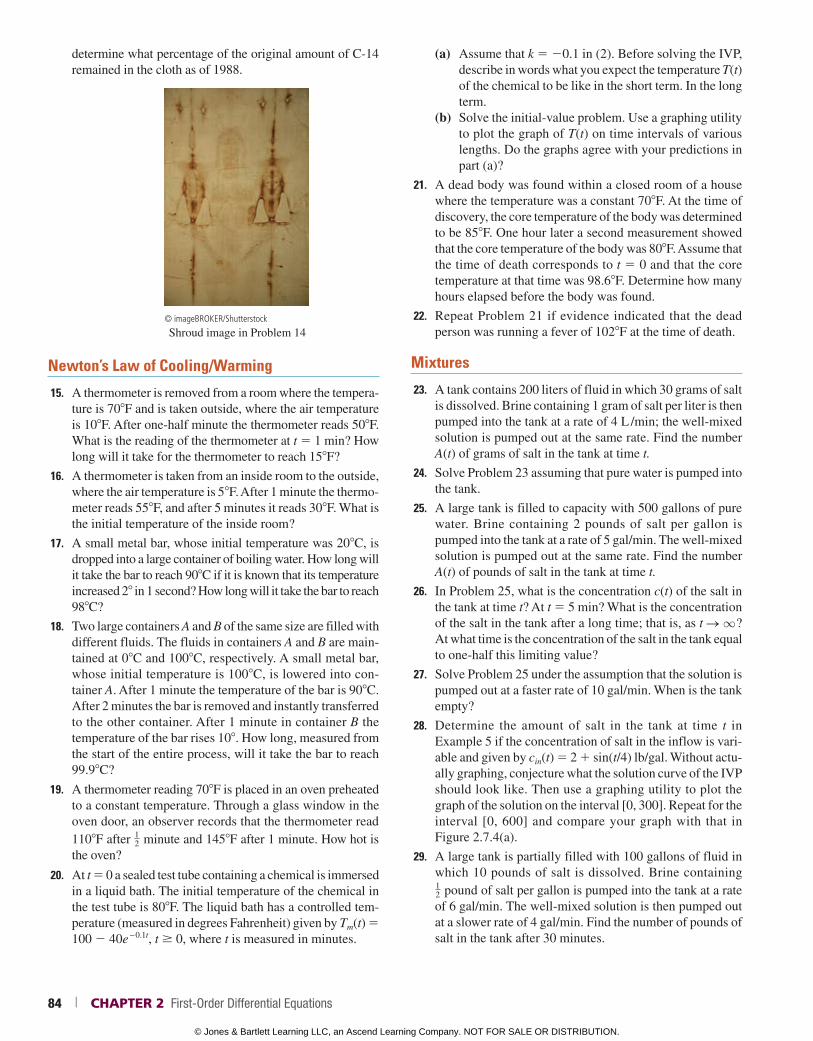
determine what percentage of the original amount of C-14 remained in the cloth as of 1988.
© imageBROKER/Shutterstock
Shroud image in Problem 14
Newton’s Law of Cooling/Warming
15. A thermometer is removed from a room where the tempera-ture is 708F and is taken outside, where the air temperature is 108F. After one-half minute the thermometer reads 508F. What is the reading of the thermometer at t 5 1 min? How long will it take for the thermometer to reach 158F?
16. A thermometer is taken from an inside room to the outside, where the air temperature is 58F. After 1 minute the thermo-meter reads 558F, and after 5 minutes it reads 308F. What is the initial temperature of the inside room?
17. A small metal bar, whose initial temperature was 208C, is dropped into a large container of boiling water. How long will it take the bar to reach 908C if it is known that its temperature increased 28 in 1 second? How long will it take the bar to reach 988C?
18. Two large containers A and B of the same size are filled with different fluids. The fluids in containers A and B are main-tained at 08C and 1008C, respectively. A small metal bar, whose initial temperature is 1008C, is lowered into con-tainer A. After 1 minute the temperature of the bar is 908C. After 2 minutes the bar is removed and instantly transferred to the other container. After 1 minute in container B the temperature of the bar rises 108. How long, measured from the start of the entire process, will it take the bar to reach 99.98C?
19. A thermometer reading 708F is placed in an oven preheated to a constant temperature. Through a glass window in the oven door, an observer records that the thermometer read 1108F after 1
2 minute and 1458F after 1 minute. How hot is the oven?
20. At t 5 0 a sealed test tube containing a chemical is immersed in a liquid bath. The initial temperature of the chemical in the test tube is 808F. The liquid bath has a controlled tem-perature (measured in degrees Fahrenheit) given by Tm(t) 5 100 2 40e – 0.1t, t 0, where t is measured in minutes.
(a) Assume that k 5 20.1 in (2). Before solving the IVP, describe in words what you expect the temperature T(t) of the chemical to be like in the short term. In the long term.
(b) Solve the initial-value problem. Use a graphing utility to plot the graph of T(t) on time intervals of various lengths. Do the graphs agree with your predictions in part (a)?
21. A dead body was found within a closed room of a house where the temperature was a constant 708F. At the time of discovery, the core temperature of the body was determined to be 858F. One hour later a second measurement showed that the core temperature of the body was 808F. Assume that the time of death corresponds to t 5 0 and that the core temperature at that time was 98.68F. Determine how many hours elapsed before the body was found.
22. Repeat Problem 21 if evidence indicated that the dead person was running a fever of 1028F at the time of death.
Mixtures
23. A tank contains 200 liters of fluid in which 30 grams of salt is dissolved. Brine containing 1 gram of salt per liter is then pumped into the tank at a rate of 4 L /min; the well-mixed solution is pumped out at the same rate. Find the number A(t) of grams of salt in the tank at time t.
24. Solve Problem 23 assuming that pure water is pumped into the tank.
25. A large tank is filled to capacity with 500 gallons of pure water. Brine containing 2 pounds of salt per gallon is pumped into the tank at a rate of 5 gal/min. The well-mixed solution is pumped out at the same rate. Find the number A(t) of pounds of salt in the tank at time t.
26. In Problem 25, what is the concentration c(t) of the salt in the tank at time t? At t 5 5 min? What is the concentration of the salt in the tank after a long time; that is, as t S q? At what time is the concentration of the salt in the tank equal to one-half this limiting value?
27. Solve Problem 25 under the assumption that the solution is pumped out at a faster rate of 10 gal/min. When is the tank empty?
28. Determine the amount of salt in the tank at time t in Example 5 if the concentration of salt in the inflow is vari-able and given by cin(t) 5 2 1 sin(t/4) lb/gal. Without actu-ally graphing, conjecture what the solution curve of the IVP should look like. Then use a graphing utility to plot the graph of the solution on the interval [0, 300]. Repeat for the interval [0, 600] and compare your graph with that in Figure 2.7.4(a).
29. A large tank is partially filled with 100 gallons of fluid in which 10 pounds of salt is dissolved. Brine containing 12 pound of salt per gallon is pumped into the tank at a rate of 6 gal/min. The well-mixed solution is then pumped out at a slower rate of 4 gal/min. Find the number of pounds of salt in the tank after 30 minutes.
84 | CHAPTER 2 First-Order Differential Equations
© Jones & Bartlett Learning LLC, an Ascend Learning Company. NOT FOR SALE OR DISTRIBUTION.
© Jones & Bartlett Learning, LLCNOT FOR SALE OR DISTRIBUTION
© Jones & Bartlett Learning, LLCNOT FOR SALE OR DISTRIBUTION
© Jones & Bartlett Learning, LLCNOT FOR SALE OR DISTRIBUTION
© Jones & Bartlett Learning, LLCNOT FOR SALE OR DISTRIBUTION
© Jones & Bartlett Learning, LLCNOT FOR SALE OR DISTRIBUTION
© Jones & Bartlett Learning, LLCNOT FOR SALE OR DISTRIBUTION
© Jones & Bartlett Learning, LLCNOT FOR SALE OR DISTRIBUTION
© Jones & Bartlett Learning, LLCNOT FOR SALE OR DISTRIBUTION
© Jones & Bartlett Learning, LLCNOT FOR SALE OR DISTRIBUTION
© Jones & Bartlett Learning, LLCNOT FOR SALE OR DISTRIBUTION
© Jones & Bartlett Learning, LLCNOT FOR SALE OR DISTRIBUTION
© Jones & Bartlett Learning, LLCNOT FOR SALE OR DISTRIBUTION
© Jones & Bartlett Learning, LLCNOT FOR SALE OR DISTRIBUTION
© Jones & Bartlett Learning, LLCNOT FOR SALE OR DISTRIBUTION
© Jones & Bartlett Learning, LLCNOT FOR SALE OR DISTRIBUTION
© Jones & Bartlett Learning, LLCNOT FOR SALE OR DISTRIBUTION
© Jones & Bartlett Learning, LLCNOT FOR SALE OR DISTRIBUTION
© Jones & Bartlett Learning, LLCNOT FOR SALE OR DISTRIBUTION
© Jones & Bartlett Learning, LLCNOT FOR SALE OR DISTRIBUTION
© Jones & Bartlett Learning, LLCNOT FOR SALE OR DISTRIBUTION
30. In Example 5 the size of the tank containing the salt mixture was not given. Suppose, as in the discussion following Example 5, that the rate at which brine is pumped into the tank is 3 gal/min but that the well-stirred solution is pumped out at a rate of 2 gal/min. It stands to reason that since brine is accumulating in the tank at the rate of 1 gal/min, any finite tank must eventually overflow. Now suppose that the tank has an open top and has a total capacity of 400 gallons.(a) When will the tank overflow?(b) What will be the number of pounds of salt in the tank
at the instant it overflows?(c) Assume that, although the tank is overflowing, the brine
solution continues to be pumped in at a rate of 3 gal/min and the well-stirred solution continues to be pumped out at a rate of 2 gal/min. Devise a method for deter-mining the number of pounds of salt in the tank at t 5 150 min.
(d) Determine the number of pounds of salt in the tank as t S q . Does your answer agree with your intuition?
(e) Use a graphing utility to plot the graph A(t) on the inter-val [0, 500).
Series Circuits
31. A 30-volt electromotive force is applied to an LR-series circuit in which the inductance is 0.1 henry and the resis-tance is 50 ohms. Find the current i(t) if i(0) 5 0. Determine the current as t S q .
32. Solve equation (8) under the assumption that E(t) 5 E0 sin vt and i(0) 5 i0.
33. A 100-volt electromotive force is applied to an RC-series circuit in which the resistance is 200 ohms and the capaci-tance is 10 – 4 farad. Find the charge q(t) on the capacitor if q(0) 5 0. Find the current i(t).
34. A 200-volt electromotive force is applied to an RC-series circuit in which the resistance is 1000 ohms and the ca-pacitance is 5 3 10 – 6 farad. Find the charge q(t) on the capacitor if i(0) 5 0.4. Determine the charge and current at t 5 0.005 s. Determine the charge as t S q .
35. An electromotive force
E(t) 5 e120, 0 # t # 20
0, t . 20
is applied to an LR-series circuit in which the inductance is 20 henries and the resistance is 2 ohms. Find the current i(t) if i(0) 5 0.
36. An LR-series circuit has a variable inductor with the induc-tance defined by
L(t) 5 e1 2 110t, 0 # t , 10
0, t . 10.
Find the current i(t) if the resistance is 0.2 ohm, the im-pressed voltage is E(t) 5 4, and i(0) 5 0. Graph i(t).
Additional Linear Models
37. Air Resistance In (14) of Section 1.3 we saw that a differential equation describing the velocity v of a falling mass subject to air resistance proportional to the instanta-neous velocity is
m
dv
dt5 mg 2 kv,
where k 0 is a constant of proportionality called the drag coefficient. The positive direction is downward.(a) Solve the equation subject to the initial condition
v(0) 5 v0.(b) Use the solution in part (a) to determine the limiting,
or terminal, velocity of the mass. We saw how to de-termine the terminal velocity without solving the DE in Problem 40 in Exercises 2.1.
(c) If the distance s, measured from the point where the mass was released above ground, is related to velocity v by ds/dt 5 v, find an explicit expression for s(t) if s(0) 5 0.
38. How High?—No Air Resistance Suppose a small cannon-ball weighing 16 pounds is shot vertically upward with an initial velocity v0 5 300 ft/s. The answer to the question, “How high does the cannonball go?” depends on whether we take air resistance into account.(a) Suppose air resistance is ignored. If the positive
direction is upward, then a model for the state of the cannonball is given by d 2s/dt 2 5 2g (equation (12) of Section 1.3). Since ds/dt 5 v(t) the last differential equation is the same as dv/dt 5 2g, where we take g 5 32 ft /s 2. Find the velocity v(t) of the cannonball at time t.
(b) Use the result obtained in part (a) to determine the height s(t) of the cannonball measured from ground level. Find the maximum height attained by the cannonball.
39. How High?—Linear Air Resistance Repeat Problem 38, but this time assume that air resistance is proportional to instantaneous velocity. It stands to reason that the maximum height attained by the cannonball must be less than that in part (b) of Problem 38. Show this by supposing that the drag coefficient is k 5 0.0025. [Hint: Slightly modify the DE in Problem 37.]
40. Skydiving A skydiver weighs 125 pounds, and her para-chute and equipment combined weigh another 35 pounds. After exiting from a plane at an altitude of 15,000 feet, she waits 15 seconds and opens her parachute. See FIGURE 2.7.8. Assume the constant of proportionality in the model in Problem 37 has the value k 5 0.5 during free fall and k 5 10 after the parachute is opened. Assume that her initial velocity on leaving the plane is zero. What is her velocity and how far has she traveled 20 seconds after leaving the plane? How does her velocity at 20 seconds compare with
2.7 Linear Models | 85
© Jones & Bartlett Learning LLC, an Ascend Learning Company. NOT FOR SALE OR DISTRIBUTION.
© Jones & Bartlett Learning, LLCNOT FOR SALE OR DISTRIBUTION
© Jones & Bartlett Learning, LLCNOT FOR SALE OR DISTRIBUTION
© Jones & Bartlett Learning, LLCNOT FOR SALE OR DISTRIBUTION
© Jones & Bartlett Learning, LLCNOT FOR SALE OR DISTRIBUTION
© Jones & Bartlett Learning, LLCNOT FOR SALE OR DISTRIBUTION
© Jones & Bartlett Learning, LLCNOT FOR SALE OR DISTRIBUTION
© Jones & Bartlett Learning, LLCNOT FOR SALE OR DISTRIBUTION
© Jones & Bartlett Learning, LLCNOT FOR SALE OR DISTRIBUTION
© Jones & Bartlett Learning, LLCNOT FOR SALE OR DISTRIBUTION
© Jones & Bartlett Learning, LLCNOT FOR SALE OR DISTRIBUTION
© Jones & Bartlett Learning, LLCNOT FOR SALE OR DISTRIBUTION
© Jones & Bartlett Learning, LLCNOT FOR SALE OR DISTRIBUTION
© Jones & Bartlett Learning, LLCNOT FOR SALE OR DISTRIBUTION
© Jones & Bartlett Learning, LLCNOT FOR SALE OR DISTRIBUTION
© Jones & Bartlett Learning, LLCNOT FOR SALE OR DISTRIBUTION
© Jones & Bartlett Learning, LLCNOT FOR SALE OR DISTRIBUTION
© Jones & Bartlett Learning, LLCNOT FOR SALE OR DISTRIBUTION
© Jones & Bartlett Learning, LLCNOT FOR SALE OR DISTRIBUTION
© Jones & Bartlett Learning, LLCNOT FOR SALE OR DISTRIBUTION
© Jones & Bartlett Learning, LLCNOT FOR SALE OR DISTRIBUTION
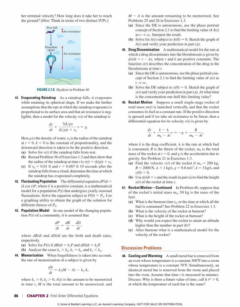
her terminal velocity? How long does it take her to reach the ground? [Hint: Think in terms of two distinct IVPs.]
FIGURE 2.7.8 Skydiver in Problem 40
Parachuteopens
Free fall
Air resistance
Air resistance
41. Evaporating Raindrop As a raindrop falls, it evaporates while retaining its spherical shape. If we make the further assumptions that the rate at which the raindrop evaporates is proportional to its surface area and that air resistance is neg-ligible, then a model for the velocity v(t) of the raindrop is
dv
dt1
3(k>r)
(k>r)t 1 r0 v 5 g.
Here r is the density of water, r0 is the radius of the raindrop at t 5 0, k 0 is the constant of proportionality, and the downward direction is taken to be the positive direction.(a) Solve for v(t) if the raindrop falls from rest.(b) Reread Problem 36 of Exercises 1.3 and then show that
the radius of the raindrop at time t is r(t) 5 (k/r)t 1 r0.(c) If r0 5 0.01 ft and r 5 0.007 ft 10 seconds after the
raindrop falls from a cloud, determine the time at which the raindrop has evaporated completely.
42. Fluctuating Population The differential equation dP/dt 5 (k cos t)P, where k is a positive constant, is a mathematical model for a population P(t) that undergoes yearly seasonal fluctuations. Solve the equation subject to P(0) 5 P0. Use a graphing utility to obtain the graph of the solution for different choices of P0.
43. Population Model In one model of the changing popula-tion P(t) of a community, it is assumed that
dP
dt5
dB
dt2
dD
dt,
where dB/dt and dD/dt are the birth and death rates, respectively.(a) Solve for P(t) if dB/dt 5 k1P and dD/dt 5 k2P.(b) Analyze the cases k1 k2, k1 5 k2, and k1 k2.
44. Memorization When forgetfulness is taken into account, the rate of memorization of a subject is given by
dA
dt5 k1(M 2 A) 2 k2 A,
where k1 0, k2 0, A(t) is the amount to be memorized in time t, M is the total amount to be memorized, and
M 2 A is the amount remaining to be memorized. See Problems 25 and 26 in Exercises 1.3.(a) Since the DE is autonomous, use the phase portrait
concept of Section 2.1 to find the limiting value of A(t) as t S q . Interpret the result.
(b) Solve for A(t) subject to A(0) 5 0. Sketch the graph of A(t) and verify your prediction in part (a).
45. Drug Dissemination A mathematical model for the rate at which a drug disseminates into the bloodstream is given by dx/dt 5 r 2 kx, where r and k are positive constants. The function x(t) describes the concentration of the drug in the bloodstream at time t.(a) Since the DE is autonomous, use the phase portrait con-
cept of Section 2.1 to find the limiting value of x(t) as t S q .
(b) Solve the DE subject to x(0) 5 0. Sketch the graph of x(t) and verify your prediction in part (a). At what time is the concentration one-half this limiting value?
46. Rocket Motion Suppose a small single-stage rocket of total mass m(t) is launched vertically and that the rocket consumes its fuel at a constant rate. If the positive direction is upward and if we take air resistance to be linear, then a differential equation for its velocity v(t) is given by
dv
dt1
k 2 l
m0 2 lt v 5 2g 1
R
m0 2 lt,
where k is the drag coefficient, l is the rate at which fuel is consumed, R is the thrust of the rocket, m0 is the total mass of the rocket at t 5 0, and g is the acceleration due to gravity. See Problem 21 in Exercises 1.3.(a) Find the velocity v(t) of the rocket if m0 5 200 kg,
R 5 2000 N, l 5 1 kg/s, g 5 9.8 m/s 2, k 5 3 kg/s, and v(0) 5 0.
(b) Use ds/dt 5 v and the result in part (a) to find the height s(t) of the rocket at time t.
47. Rocket Motion—Continued In Problem 46, suppose that of the rocket’s initial mass m0, 50 kg is the mass of the fuel.(a) What is the burnout time tb, or the time at which all the
fuel is consumed? See Problem 22 in Exercises 1.3.(b) What is the velocity of the rocket at burnout?(c) What is the height of the rocket at burnout?(d) Why would you expect the rocket to attain an altitude
higher than the number in part (b)?(e) After burnout what is a mathematical model for the
velocity of the rocket?
Discussion Problems
48. Cooling and Warming A small metal bar is removed from an oven whose temperature is a constant 3008F into a room whose temperature is a constant 708F. Simultaneously, an identical metal bar is removed from the room and placed into the oven. Assume that time t is measured in minutes. Discuss: Why is there a future value of time, call it t* 0, at which the temperature of each bar is the same?
86 | CHAPTER 2 First-Order Differential Equations
© Jones & Bartlett Learning LLC, an Ascend Learning Company. NOT FOR SALE OR DISTRIBUTION.
© Jones & Bartlett Learning, LLCNOT FOR SALE OR DISTRIBUTION
© Jones & Bartlett Learning, LLCNOT FOR SALE OR DISTRIBUTION
© Jones & Bartlett Learning, LLCNOT FOR SALE OR DISTRIBUTION
© Jones & Bartlett Learning, LLCNOT FOR SALE OR DISTRIBUTION
© Jones & Bartlett Learning, LLCNOT FOR SALE OR DISTRIBUTION
© Jones & Bartlett Learning, LLCNOT FOR SALE OR DISTRIBUTION
© Jones & Bartlett Learning, LLCNOT FOR SALE OR DISTRIBUTION
© Jones & Bartlett Learning, LLCNOT FOR SALE OR DISTRIBUTION
© Jones & Bartlett Learning, LLCNOT FOR SALE OR DISTRIBUTION
© Jones & Bartlett Learning, LLCNOT FOR SALE OR DISTRIBUTION
© Jones & Bartlett Learning, LLCNOT FOR SALE OR DISTRIBUTION
© Jones & Bartlett Learning, LLCNOT FOR SALE OR DISTRIBUTION
© Jones & Bartlett Learning, LLCNOT FOR SALE OR DISTRIBUTION
© Jones & Bartlett Learning, LLCNOT FOR SALE OR DISTRIBUTION
© Jones & Bartlett Learning, LLCNOT FOR SALE OR DISTRIBUTION
© Jones & Bartlett Learning, LLCNOT FOR SALE OR DISTRIBUTION
© Jones & Bartlett Learning, LLCNOT FOR SALE OR DISTRIBUTION
© Jones & Bartlett Learning, LLCNOT FOR SALE OR DISTRIBUTION
© Jones & Bartlett Learning, LLCNOT FOR SALE OR DISTRIBUTION
© Jones & Bartlett Learning, LLCNOT FOR SALE OR DISTRIBUTION
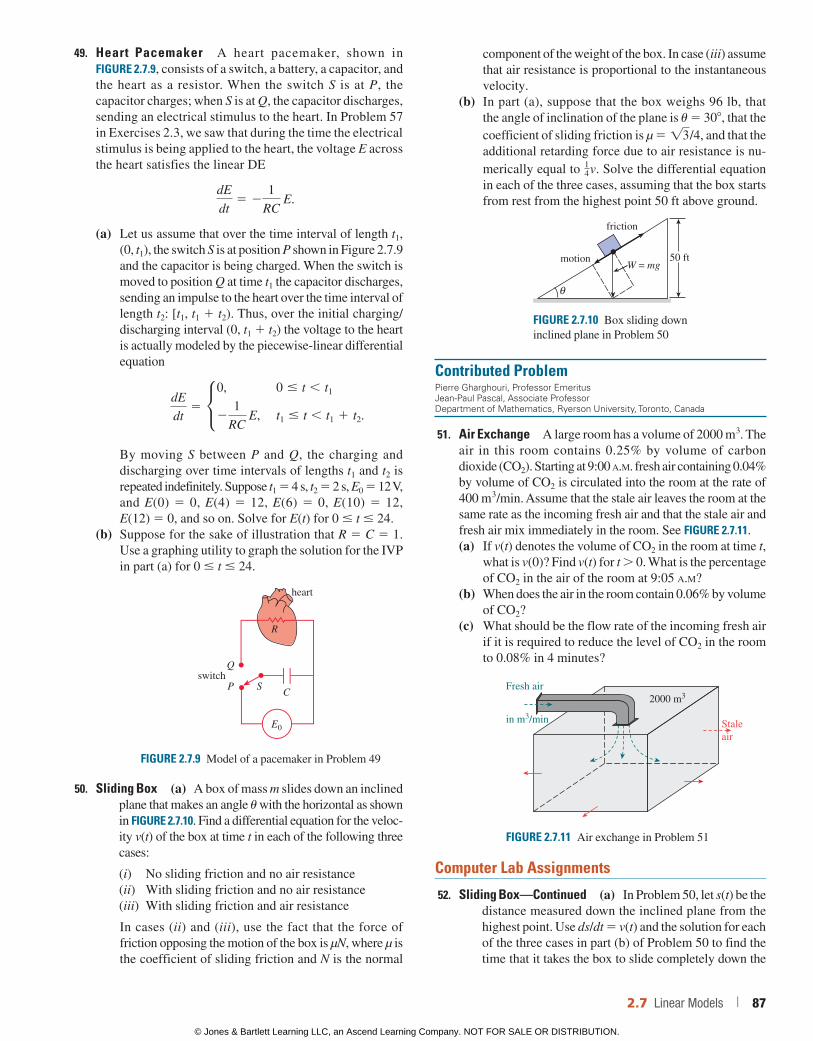
49. Heart Pacemaker A heart pacemaker, shown in FIGURE 2.7.9, consists of a switch, a battery, a capacitor, and the heart as a resistor. When the switch S is at P, the capacitor charges; when S is at Q, the capacitor discharges, sending an electrical stimulus to the heart. In Problem 57 in Exercises 2.3, we saw that during the time the electrical stimulus is being applied to the heart, the voltage E across the heart satisfies the linear DE
dE
dt5 2
1
RC E.
(a) Let us assume that over the time interval of length t1, (0, t1), the switch S is at position P shown in Figure 2.7.9 and the capacitor is being charged. When the switch is moved to position Q at time t1 the capacitor discharges, sending an impulse to the heart over the time interval of length t2: [t1, t1 1 t2). Thus, over the initial charging/discharging interval (0, t1 1 t2) the voltage to the heart is actually modeled by the piecewise-linear differential equation
dE
dt5 •
0, 0 # t , t1
21
RC E, t1 # t , t1 1 t2.
By moving S between P and Q, the charging and discharging over time intervals of lengths t1 and t2 is repeated indefinitely. Suppose t1 5 4 s, t2 5 2 s, E0 5 12 V, and E(0) 5 0, E(4) 5 12, E(6) 5 0, E(10) 5 12, E(12) 5 0, and so on. Solve for E(t) for 0 # t # 24.
(b) Suppose for the sake of illustration that R 5 C 5 1. Use a graphing utility to graph the solution for the IVP in part (a) for 0 # t # 24.
FIGURE 2.7.9 Model of a pacemaker in Problem 49
heart
switchQ
P SC
R
E0
50. Sliding Box (a) A box of mass m slides down an inclinedplane that makes an angle u with the horizontal as shown in FIGURE 2.7.10. Find a differential equation for the veloc-ity v(t) of the box at time t in each of the following three cases:
(i) No sliding friction and no air resistance (ii) With sliding friction and no air resistance (iii) With sliding friction and air resistance
In cases (ii) and (iii), use the fact that the force of friction opposing the motion of the box is µN, where µ is the coefficient of sliding friction and N is the normal
component of the weight of the box. In case (iii) assume that air resistance is proportional to the instantaneous velocity.
(b) In part (a), suppose that the box weighs 96 lb, that the angle of inclination of the plane is u 5 308, that the coefficient of sliding friction is µ 5 !3/4, and that the additional retarding force due to air resistance is nu-merically equal to 1
4v. Solve the differential equation in each of the three cases, assuming that the box starts from rest from the highest point 50 ft above ground.
FIGURE 2.7.10 Box sliding down inclined plane in Problem 50
friction
motionW = mg
θ
50 ft
Contributed ProblemPierre Gharghouri, Professor Emeritus Jean-Paul Pascal, Associate Professor Department of Mathematics, Ryerson University, Toronto, Canada
51. Air Exchange A large room has a volume of 2000 m 3. The air in this room contains 0.25% by volume of carbon dioxide (CO2). Starting at 9:00 a.m. fresh air containing 0.04% by volume of CO2 is circulated into the room at the rate of 400 m 3/min. Assume that the stale air leaves the room at the same rate as the incoming fresh air and that the stale air and fresh air mix immediately in the room. See FIGURE 2.7.11.(a) If v(t) denotes the volume of CO2 in the room at time t,
what is v(0)? Find v(t) for t 0. What is the percentage of CO2 in the air of the room at 9:05 a.m?
(b) When does the air in the room contain 0.06% by volume of CO2?
(c) What should be the flow rate of the incoming fresh air if it is required to reduce the level of CO2 in the room to 0.08% in 4 minutes?
FIGURE 2.7.11 Air exchange in Problem 51
in m3/min
Fresh air2000 m3
Staleair
Computer Lab Assignments
52. Sliding Box—Continued (a) In Problem 50, let s(t) be thedistance measured down the inclined plane from the highest point. Use ds/dt 5 v(t) and the solution for each of the three cases in part (b) of Problem 50 to find the time that it takes the box to slide completely down the
2.7 Linear Models | 87
© Jones & Bartlett Learning LLC, an Ascend Learning Company. NOT FOR SALE OR DISTRIBUTION.
© Jones & Bartlett Learning, LLCNOT FOR SALE OR DISTRIBUTION
© Jones & Bartlett Learning, LLCNOT FOR SALE OR DISTRIBUTION
© Jones & Bartlett Learning, LLCNOT FOR SALE OR DISTRIBUTION
© Jones & Bartlett Learning, LLCNOT FOR SALE OR DISTRIBUTION
© Jones & Bartlett Learning, LLCNOT FOR SALE OR DISTRIBUTION
© Jones & Bartlett Learning, LLCNOT FOR SALE OR DISTRIBUTION
© Jones & Bartlett Learning, LLCNOT FOR SALE OR DISTRIBUTION
© Jones & Bartlett Learning, LLCNOT FOR SALE OR DISTRIBUTION
© Jones & Bartlett Learning, LLCNOT FOR SALE OR DISTRIBUTION
© Jones & Bartlett Learning, LLCNOT FOR SALE OR DISTRIBUTION
© Jones & Bartlett Learning, LLCNOT FOR SALE OR DISTRIBUTION
© Jones & Bartlett Learning, LLCNOT FOR SALE OR DISTRIBUTION
© Jones & Bartlett Learning, LLCNOT FOR SALE OR DISTRIBUTION
© Jones & Bartlett Learning, LLCNOT FOR SALE OR DISTRIBUTION
© Jones & Bartlett Learning, LLCNOT FOR SALE OR DISTRIBUTION
© Jones & Bartlett Learning, LLCNOT FOR SALE OR DISTRIBUTION
© Jones & Bartlett Learning, LLCNOT FOR SALE OR DISTRIBUTION
© Jones & Bartlett Learning, LLCNOT FOR SALE OR DISTRIBUTION
© Jones & Bartlett Learning, LLCNOT FOR SALE OR DISTRIBUTION
© Jones & Bartlett Learning, LLCNOT FOR SALE OR DISTRIBUTION
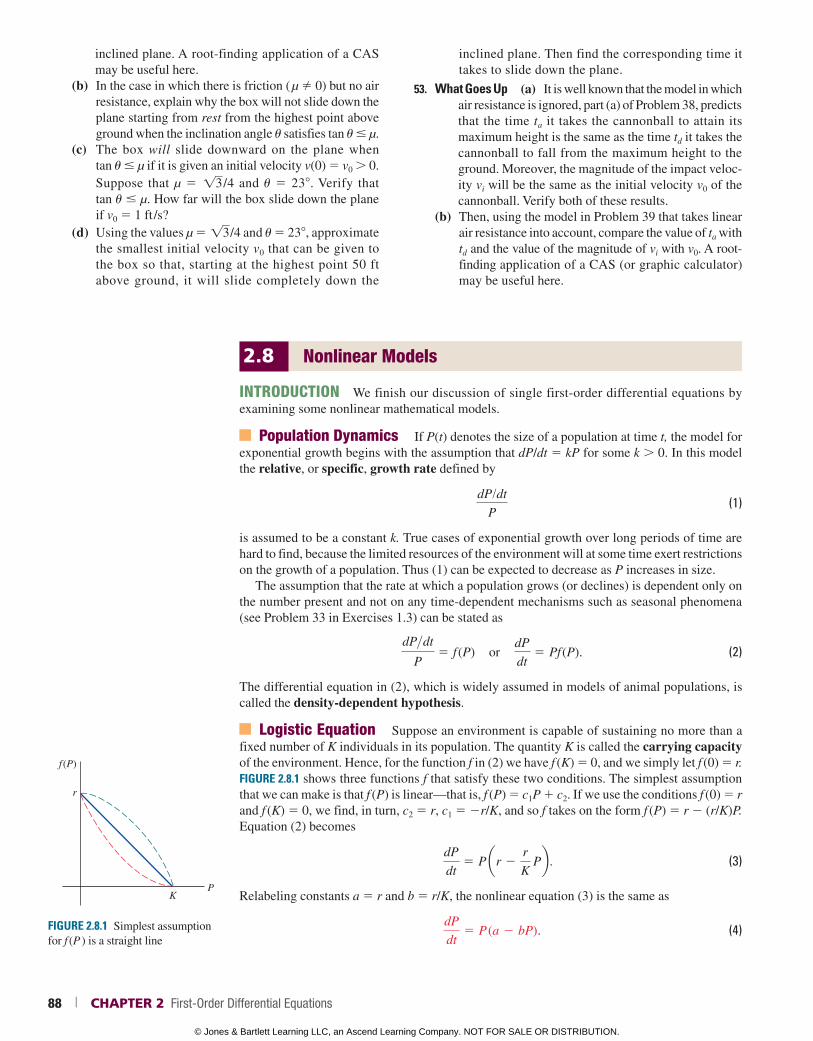
2.8 Nonlinear Models
INTRODUCTION We finish our discussion of single first-order differential equations by examining some nonlinear mathematical models.
Population Dynamics If P(t) denotes the size of a population at time t, the model for exponential growth begins with the assumption that dP/dt 5 kP for some k 0. In this model the relative, or specific, growth rate defined by
dP/dt
P (1)
is assumed to be a constant k. True cases of exponential growth over long periods of time are hard to find, because the limited resources of the environment will at some time exert restrictions on the growth of a population. Thus (1) can be expected to decrease as P increases in size.
The assumption that the rate at which a population grows (or declines) is dependent only on the number present and not on any time-dependent mechanisms such as seasonal phenomena (see Problem 33 in Exercises 1.3) can be stated as
dP>dt
P5 f (P) or
dP
dt5 Pf (P). (2)
The differential equation in (2), which is widely assumed in models of animal populations, is called the density-dependent hypothesis.
Logistic Equation Suppose an environment is capable of sustaining no more than a fixed number of K individuals in its population. The quantity K is called the carrying capacity of the environment. Hence, for the function f in (2) we have f (K) 5 0, and we simply let f (0) 5 r. FIGURE 2.8.1 shows three functions f that satisfy these two conditions. The simplest assumption that we can make is that f (P) is linear—that is, f (P) 5 c1P 1 c2. If we use the conditions f (0) 5 r and f (K) 5 0, we find, in turn, c2 5 r, c1 5 2r/K, and so f takes on the form f (P) 5 r 2 (r/K)P. Equation (2) becomes
dP
dt5 P ar 2
r
K Pb . (3)
Relabeling constants a 5 r and b 5 r/K, the nonlinear equation (3) is the same as
dP
dt5 P (a 2 bP). (4)
inclined plane. A root-finding application of a CAS may be useful here.
(b) In the case in which there is friction ( µ 0) but no air resistance, explain why the box will not slide down the plane starting from rest from the highest point above ground when the inclination angle u satisfies tan u # µ.
(c) The box will slide downward on the plane when tan u # µ if it is given an initial velocity v(0) 5 v0 0. Suppose that µ 5 !3/4 and u 5 238. Verify that tan u # µ. How far will the box slide down the plane if v0 5 1 ft /s?
(d) Using the values µ 5 !3/4 and u 5 238, approximate the smallest initial velocity v0 that can be given to the box so that, starting at the highest point 50 ft above ground, it will slide completely down the
inclined plane. Then find the corresponding time it takes to slide down the plane.
53. What Goes Up (a) It is well known that the model in whichair resistance is ignored, part (a) of Problem 38, predicts that the time ta it takes the cannonball to attain its maximum height is the same as the time td it takes the cannonball to fall from the maximum height to the ground. Moreover, the magnitude of the impact veloc-ity vi will be the same as the initial velocity v0 of the cannonball. Verify both of these results.
(b) Then, using the model in Problem 39 that takes linear air resistance into account, compare the value of ta with td and the value of the magnitude of vi with v0. A root-finding application of a CAS (or graphic calculator) may be useful here.
r
KP
f (P)
FIGURE 2.8.1 Simplest assumption for f (P ) is a straight line
88 | CHAPTER 2 First-Order Differential Equations
© Jones & Bartlett Learning LLC, an Ascend Learning Company. NOT FOR SALE OR DISTRIBUTION.
© Jones & Bartlett Learning, LLCNOT FOR SALE OR DISTRIBUTION
© Jones & Bartlett Learning, LLCNOT FOR SALE OR DISTRIBUTION
© Jones & Bartlett Learning, LLCNOT FOR SALE OR DISTRIBUTION
© Jones & Bartlett Learning, LLCNOT FOR SALE OR DISTRIBUTION
© Jones & Bartlett Learning, LLCNOT FOR SALE OR DISTRIBUTION
© Jones & Bartlett Learning, LLCNOT FOR SALE OR DISTRIBUTION
© Jones & Bartlett Learning, LLCNOT FOR SALE OR DISTRIBUTION
© Jones & Bartlett Learning, LLCNOT FOR SALE OR DISTRIBUTION
© Jones & Bartlett Learning, LLCNOT FOR SALE OR DISTRIBUTION
© Jones & Bartlett Learning, LLCNOT FOR SALE OR DISTRIBUTION
© Jones & Bartlett Learning, LLCNOT FOR SALE OR DISTRIBUTION
© Jones & Bartlett Learning, LLCNOT FOR SALE OR DISTRIBUTION
© Jones & Bartlett Learning, LLCNOT FOR SALE OR DISTRIBUTION
© Jones & Bartlett Learning, LLCNOT FOR SALE OR DISTRIBUTION
© Jones & Bartlett Learning, LLCNOT FOR SALE OR DISTRIBUTION
© Jones & Bartlett Learning, LLCNOT FOR SALE OR DISTRIBUTION
© Jones & Bartlett Learning, LLCNOT FOR SALE OR DISTRIBUTION
© Jones & Bartlett Learning, LLCNOT FOR SALE OR DISTRIBUTION
© Jones & Bartlett Learning, LLCNOT FOR SALE OR DISTRIBUTION
© Jones & Bartlett Learning, LLCNOT FOR SALE OR DISTRIBUTION
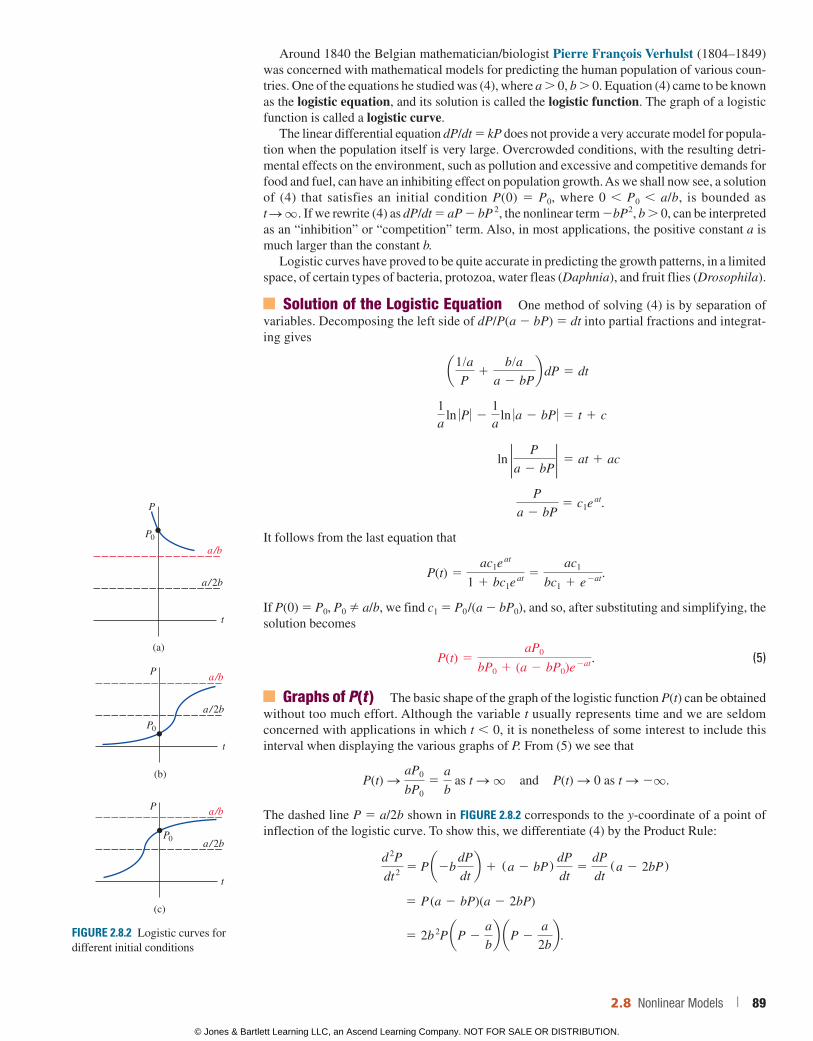
Around 1840 the Belgian mathematician/biologist Pierre François Verhulst (1804–1849) was concerned with mathematical models for predicting the human population of various coun-tries. One of the equations he studied was (4), where a 0, b 0. Equation (4) came to be known as the logistic equation, and its solution is called the logistic function. The graph of a logistic function is called a logistic curve.
The linear differential equation dP/dt 5 kP does not provide a very accurate model for popula-tion when the population itself is very large. Overcrowded conditions, with the resulting detri-mental effects on the environment, such as pollution and excessive and competitive demands for food and fuel, can have an inhibiting effect on population growth. As we shall now see, a solution of (4) that satisfies an initial condition P(0) 5 P0, where 0 P0 a/b, is bounded as t S q . If we rewrite (4) as dP/dt 5 aP 2 bP 2, the nonlinear term 2bP 2, b 0, can be interpreted as an “inhibition” or “competition” term. Also, in most applications, the positive constant a is much larger than the constant b.
Logistic curves have proved to be quite accurate in predicting the growth patterns, in a limited space, of certain types of bacteria, protozoa, water fleas (Daphnia), and fruit flies (Drosophila).
Solution of the Logistic Equation One method of solving (4) is by separation of variables. Decomposing the left side of dP/P(a 2 bP) 5 dt into partial fractions and integrat-ing gives
a1/aP
1b/a
a 2 bPb dP 5 dt
1a
ln 0P 0 21a
ln 0a 2 bP 0 5 t 1 c
ln 2 P
a 2 bP2 5 at 1 ac
P
a 2 bP5 c1e
at.
It follows from the last equation that
P(t) 5ac1e
at
1 1 bc1e at 5
ac1
bc1 1 e 2at.
If P(0) 5 P0, P0 a/b, we find c1 5 P0 /(a 2 bP0), and so, after substituting and simplifying, the solution becomes
P(t) 5aP0
bP0 1 (a 2 bP0)e 2at. (5)
Graphs of P(t ) The basic shape of the graph of the logistic function P(t) can be obtained without too much effort. Although the variable t usually represents time and we are seldom concerned with applications in which t 0, it is nonetheless of some interest to include this interval when displaying the various graphs of P. From (5) we see that
P(t) SaP0
bP05
a
b as t S q and P(t) S 0 as t S 2q.
The dashed line P 5 a/2b shown in FIGURE 2.8.2 corresponds to the y-coordinate of a point of inflection of the logistic curve. To show this, we differentiate (4) by the Product Rule:
d
2P
dt 2 5 P a2b
dP
dtb 1 (a 2 bP)
dP
dt5
dP
dt (a 2 2bP)
5 P (a 2 bP)(a 2 2bP)
5 2b 2P aP 2
a
bb aP 2
a
2bb .
P0
P0
P
(b)
t
P
(c)
t
a/b
a/2b
P0
P
(a)
t
a/b
a/2b
a/b
a/2b
FIGURE 2.8.2 Logistic curves for different initial conditions
2.8 Nonlinear Models | 89
© Jones & Bartlett Learning LLC, an Ascend Learning Company. NOT FOR SALE OR DISTRIBUTION.
© Jones & Bartlett Learning, LLCNOT FOR SALE OR DISTRIBUTION
© Jones & Bartlett Learning, LLCNOT FOR SALE OR DISTRIBUTION
© Jones & Bartlett Learning, LLCNOT FOR SALE OR DISTRIBUTION
© Jones & Bartlett Learning, LLCNOT FOR SALE OR DISTRIBUTION
© Jones & Bartlett Learning, LLCNOT FOR SALE OR DISTRIBUTION
© Jones & Bartlett Learning, LLCNOT FOR SALE OR DISTRIBUTION
© Jones & Bartlett Learning, LLCNOT FOR SALE OR DISTRIBUTION
© Jones & Bartlett Learning, LLCNOT FOR SALE OR DISTRIBUTION
© Jones & Bartlett Learning, LLCNOT FOR SALE OR DISTRIBUTION
© Jones & Bartlett Learning, LLCNOT FOR SALE OR DISTRIBUTION
© Jones & Bartlett Learning, LLCNOT FOR SALE OR DISTRIBUTION
© Jones & Bartlett Learning, LLCNOT FOR SALE OR DISTRIBUTION
© Jones & Bartlett Learning, LLCNOT FOR SALE OR DISTRIBUTION
© Jones & Bartlett Learning, LLCNOT FOR SALE OR DISTRIBUTION
© Jones & Bartlett Learning, LLCNOT FOR SALE OR DISTRIBUTION
© Jones & Bartlett Learning, LLCNOT FOR SALE OR DISTRIBUTION
© Jones & Bartlett Learning, LLCNOT FOR SALE OR DISTRIBUTION
© Jones & Bartlett Learning, LLCNOT FOR SALE OR DISTRIBUTION
© Jones & Bartlett Learning, LLCNOT FOR SALE OR DISTRIBUTION
© Jones & Bartlett Learning, LLCNOT FOR SALE OR DISTRIBUTION
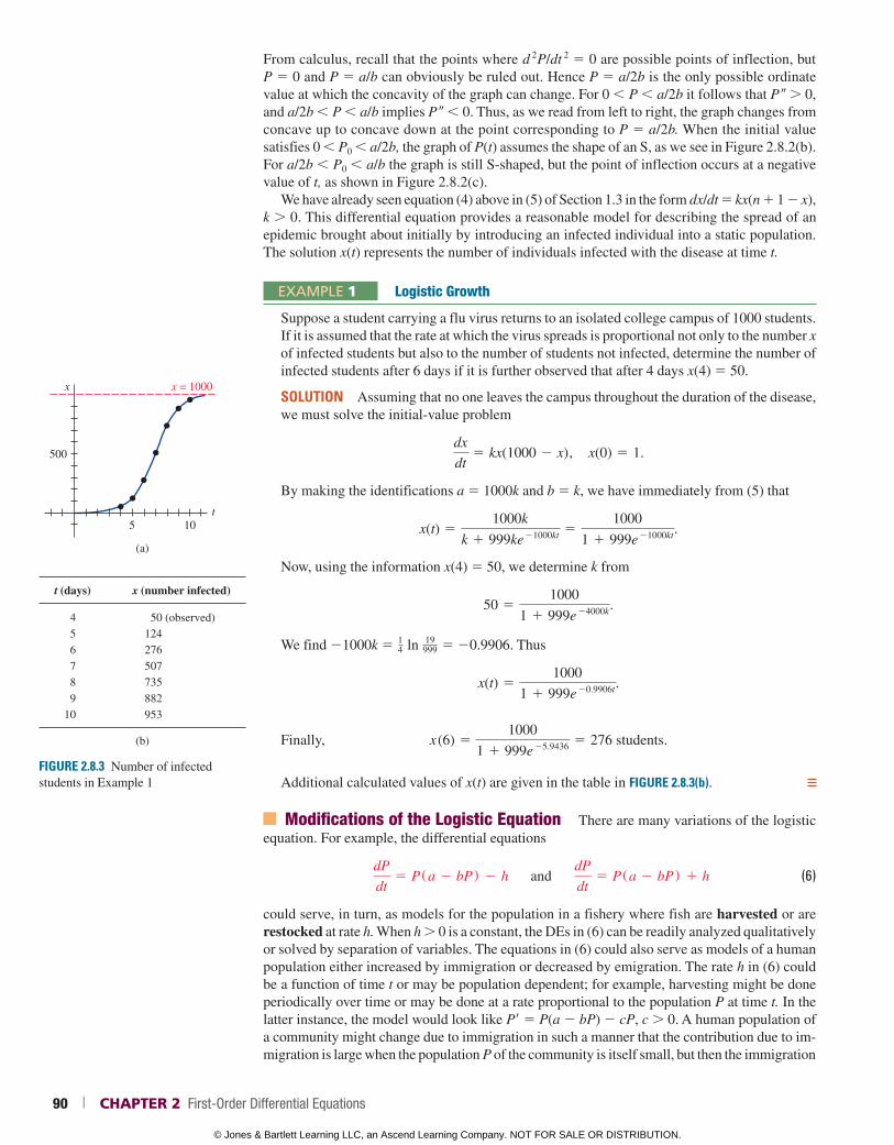
From calculus, recall that the points where d 2P/dt 2 5 0 are possible points of inflection, but P 5 0 and P 5 a/b can obviously be ruled out. Hence P 5 a/2b is the only possible ordinate value at which the concavity of the graph can change. For 0 P a/2b it follows that P 0, and a/2b P a/b implies P 0. Thus, as we read from left to right, the graph changes from concave up to concave down at the point corresponding to P 5 a/2b. When the initial value satisfies 0 P0 a/2b, the graph of P(t) assumes the shape of an S, as we see in Figure 2.8.2(b). For a/2b P0 a/b the graph is still S-shaped, but the point of inflection occurs at a negative value of t, as shown in Figure 2.8.2(c).
We have already seen equation (4) above in (5) of Section 1.3 in the form dx/dt 5 kx(n 1 1 2 x), k 0. This differential equation provides a reasonable model for describing the spread of an epidemic brought about initially by introducing an infected individual into a static population. The solution x(t) represents the number of individuals infected with the disease at time t.
EXAMPLE 1 Logistic Growth
Suppose a student carrying a flu virus returns to an isolated college campus of 1000 students. If it is assumed that the rate at which the virus spreads is proportional not only to the number x of infected students but also to the number of students not infected, determine the number of infected students after 6 days if it is further observed that after 4 days x(4) 5 50.
SOLUTION Assuming that no one leaves the campus throughout the duration of the disease, we must solve the initial-value problem
dx
dt5 kx(1000 2 x), x(0) 5 1.
By making the identifications a 5 1000k and b 5 k, we have immediately from (5) that
x(t) 51000k
k 1 999ke 21000kt 5
1000
1 1 999e 21000kt.
Now, using the information x(4) 5 50, we determine k from
50 51000
1 1 999e 24000k.
We find 21000k 5 14 ln 19
999 5 20.9906. Thus
x(t) 51000
1 1 999e 20.9906t.
Finally, x (6) 51000
1 1 999e 25.9436 5 276 students.
Additional calculated values of x(t) are given in the table in FIGURE 2.8.3(b).
Modifications of the Logistic Equation There are many variations of the logistic equation. For example, the differential equations
dP
dt5 P(a 2 bP) 2 h and
dP
dt5 P(a 2 bP) 1 h (6)
could serve, in turn, as models for the population in a fishery where fish are harvested or are restocked at rate h. When h 0 is a constant, the DEs in (6) can be readily analyzed qualitatively or solved by separation of variables. The equations in (6) could also serve as models of a human population either increased by immigration or decreased by emigration. The rate h in (6) could be a function of time t or may be population dependent; for example, harvesting might be done periodically over time or may be done at a rate pro portional to the population P at time t. In the latter instance, the model would look like P9 5 P(a 2 bP) 2 cP, c 0. A human population of a community might change due to immigration in such a manner that the contribution due to im-migration is large when the population P of the community is itself small, but then the immigration
FIGURE 2.8.3 Number of infected students in Example 1
(b)
t (days) x (number infected)
456789
10
50 (observed)124276507735882953
t
(a)
x x = 1000
500
5 10
90 | CHAPTER 2 First-Order Differential Equations
© Jones & Bartlett Learning LLC, an Ascend Learning Company. NOT FOR SALE OR DISTRIBUTION.
© Jones & Bartlett Learning, LLCNOT FOR SALE OR DISTRIBUTION
© Jones & Bartlett Learning, LLCNOT FOR SALE OR DISTRIBUTION
© Jones & Bartlett Learning, LLCNOT FOR SALE OR DISTRIBUTION
© Jones & Bartlett Learning, LLCNOT FOR SALE OR DISTRIBUTION
© Jones & Bartlett Learning, LLCNOT FOR SALE OR DISTRIBUTION
© Jones & Bartlett Learning, LLCNOT FOR SALE OR DISTRIBUTION
© Jones & Bartlett Learning, LLCNOT FOR SALE OR DISTRIBUTION
© Jones & Bartlett Learning, LLCNOT FOR SALE OR DISTRIBUTION
© Jones & Bartlett Learning, LLCNOT FOR SALE OR DISTRIBUTION
© Jones & Bartlett Learning, LLCNOT FOR SALE OR DISTRIBUTION
© Jones & Bartlett Learning, LLCNOT FOR SALE OR DISTRIBUTION
© Jones & Bartlett Learning, LLCNOT FOR SALE OR DISTRIBUTION
© Jones & Bartlett Learning, LLCNOT FOR SALE OR DISTRIBUTION
© Jones & Bartlett Learning, LLCNOT FOR SALE OR DISTRIBUTION
© Jones & Bartlett Learning, LLCNOT FOR SALE OR DISTRIBUTION
© Jones & Bartlett Learning, LLCNOT FOR SALE OR DISTRIBUTION
© Jones & Bartlett Learning, LLCNOT FOR SALE OR DISTRIBUTION
© Jones & Bartlett Learning, LLCNOT FOR SALE OR DISTRIBUTION
© Jones & Bartlett Learning, LLCNOT FOR SALE OR DISTRIBUTION
© Jones & Bartlett Learning, LLCNOT FOR SALE OR DISTRIBUTION
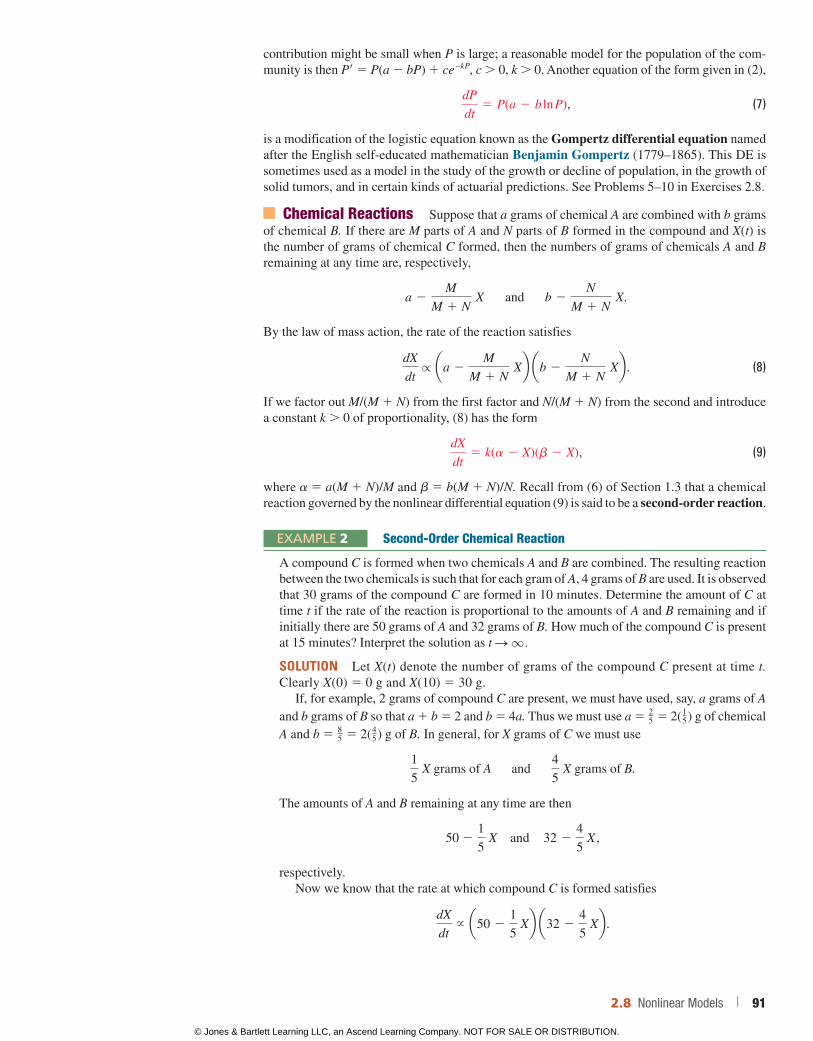
contribution might be small when P is large; a reasonable model for the population of the com-munity is then P9 5 P(a 2 bP) 1 ce –kP, c 0, k 0. Another equation of the form given in (2),
dP
dt5 P(a 2 b ln P), (7)
is a modification of the logistic equation known as the Gompertz differential equation named after the English self-educated mathematician Benjamin Gompertz (1779–1865). This DE is sometimes used as a model in the study of the growth or decline of population, in the growth of solid tumors, and in certain kinds of actuarial predictions. See Problems 5–10 in Exercises 2.8.
Chemical Reactions Suppose that a grams of chemical A are combined with b grams of chemical B. If there are M parts of A and N parts of B formed in the compound and X(t) is the number of grams of chemical C formed, then the numbers of grams of chemicals A and B remaining at any time are, respectively,
a 2M
M 1 N X and b 2
N
M 1 N X.
By the law of mass action, the rate of the reaction satisfies
dX
dtr aa 2
M
M 1 N Xb ab 2
N
M 1 N Xb . (8)
If we factor out M/(M 1 N) from the first factor and N/(M 1 N) from the second and introduce a constant k 0 of proportionality, (8) has the form
dX
dt5 k(a 2 X)(b 2 X), (9)
where a 5 a(M 1 N)/M and b 5 b(M 1 N)/N. Recall from (6) of Section 1.3 that a chemical reaction governed by the nonlinear differential equation (9) is said to be a second-order reaction.
EXAMPLE 2 Second-Order Chemical Reaction
A compound C is formed when two chemicals A and B are combined. The resulting reaction between the two chemicals is such that for each gram of A, 4 grams of B are used. It is observed that 30 grams of the compound C are formed in 10 minutes. Determine the amount of C at time t if the rate of the reaction is proportional to the amounts of A and B remaining and if initially there are 50 grams of A and 32 grams of B. How much of the compound C is present at 15 minutes? Interpret the solution as t S q .
SOLUTION Let X(t) denote the number of grams of the compound C present at time t. Clearly X(0) 5 0 g and X(10) 5 30 g.
If, for example, 2 grams of compound C are present, we must have used, say, a grams of A and b grams of B so that a 1 b 5 2 and b 5 4a. Thus we must use a 5 25 5 2(1
5) g of chemical A and b 5 8
5 5 2(45) g of B. In general, for X grams of C we must use
1
5 X grams of A and
4
5 X grams of B.
The amounts of A and B remaining at any time are then
50 2 1
5 X and 32 2
4
5 X ,
respectively.Now we know that the rate at which compound C is formed satisfies
dX
dt~ a50 2
1
5 Xb a32 2
4
5 Xb .
2.8 Nonlinear Models | 91
© Jones & Bartlett Learning LLC, an Ascend Learning Company. NOT FOR SALE OR DISTRIBUTION.
© Jones & Bartlett Learning, LLCNOT FOR SALE OR DISTRIBUTION
© Jones & Bartlett Learning, LLCNOT FOR SALE OR DISTRIBUTION
© Jones & Bartlett Learning, LLCNOT FOR SALE OR DISTRIBUTION
© Jones & Bartlett Learning, LLCNOT FOR SALE OR DISTRIBUTION
© Jones & Bartlett Learning, LLCNOT FOR SALE OR DISTRIBUTION
© Jones & Bartlett Learning, LLCNOT FOR SALE OR DISTRIBUTION
© Jones & Bartlett Learning, LLCNOT FOR SALE OR DISTRIBUTION
© Jones & Bartlett Learning, LLCNOT FOR SALE OR DISTRIBUTION
© Jones & Bartlett Learning, LLCNOT FOR SALE OR DISTRIBUTION
© Jones & Bartlett Learning, LLCNOT FOR SALE OR DISTRIBUTION
© Jones & Bartlett Learning, LLCNOT FOR SALE OR DISTRIBUTION
© Jones & Bartlett Learning, LLCNOT FOR SALE OR DISTRIBUTION
© Jones & Bartlett Learning, LLCNOT FOR SALE OR DISTRIBUTION
© Jones & Bartlett Learning, LLCNOT FOR SALE OR DISTRIBUTION
© Jones & Bartlett Learning, LLCNOT FOR SALE OR DISTRIBUTION
© Jones & Bartlett Learning, LLCNOT FOR SALE OR DISTRIBUTION
© Jones & Bartlett Learning, LLCNOT FOR SALE OR DISTRIBUTION
© Jones & Bartlett Learning, LLCNOT FOR SALE OR DISTRIBUTION
© Jones & Bartlett Learning, LLCNOT FOR SALE OR DISTRIBUTION
© Jones & Bartlett Learning, LLCNOT FOR SALE OR DISTRIBUTION
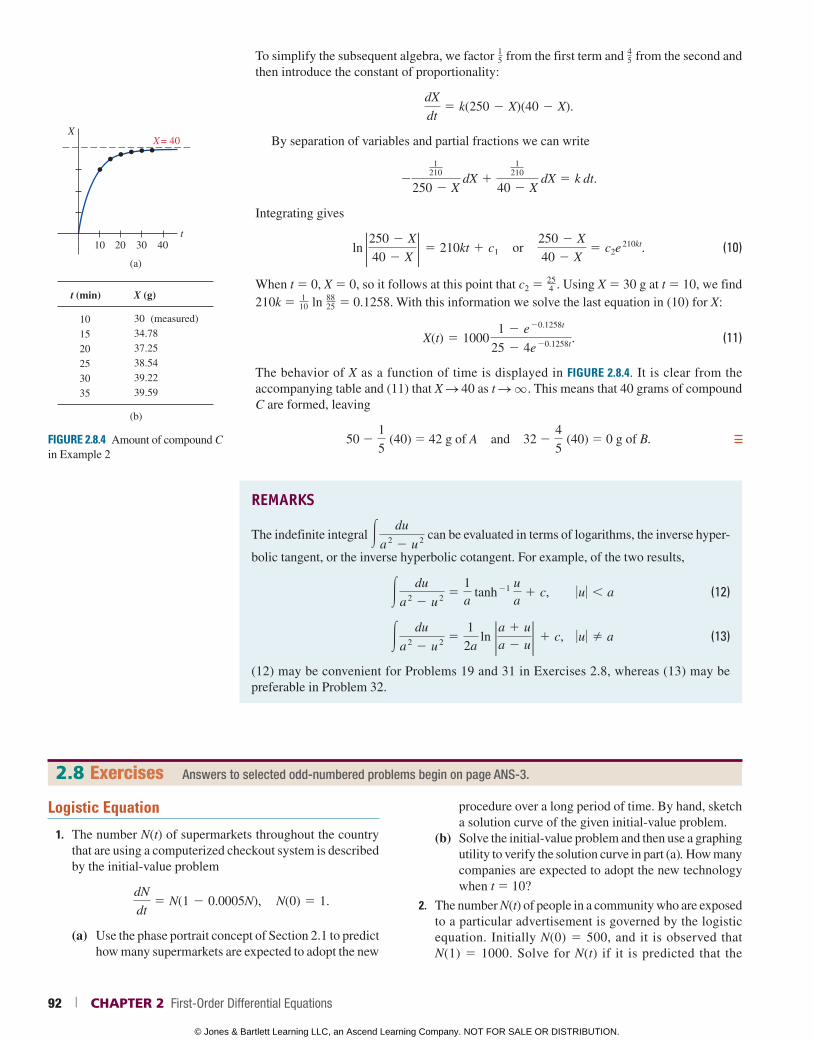
To simplify the subsequent algebra, we factor 15 from the first term and 45 from the second and then introduce the constant of proportionality:
dX
dt5 k(250 2 X)(40 2 X).
By separation of variables and partial fractions we can write
21
210
250 2 X dX 1
1210
40 2 X dX 5 k dt.
Integrating gives
ln 2250 2 X
40 2 X2 5 210kt 1 c1 or
250 2 X
40 2 X5 c2e
210kt. (10)
When t 5 0, X 5 0, so it follows at this point that c2 5 254 . Using X 5 30 g at t 5 10, we find
210k 5 110 ln 88
25 5 0.1258. With this information we solve the last equation in (10) for X:
X(t) 5 1000
1 2 e 20.1258t
25 2 4e 20.1258t. (11)
The behavior of X as a function of time is displayed in FIGURE 2.8.4. It is clear from the accompanying table and (11) that X S 40 as t S q . This means that 40 grams of compound C are formed, leaving
50 2 1
5 (40) 5 42 g of A and 32 2
4
5 (40) 5 0 g of B.
REMARKS
The indefinite integral 3du
a 2 2 u
2 can be evaluated in terms of logarithms, the inverse hyper-
bolic tangent, or the inverse hyperbolic cotangent. For example, of the two results,
#du
a 2 2 u
2 51a
tanh 21
ua
1 c, 0u 0 , a (12)
#du
a 2 2 u
2 51
2a ln 2a 1 u
a 2 u2 1 c, 0u 0 a (13)
(12) may be convenient for Problems 19 and 31 in Exercises 2.8, whereas (13) may be preferable in Problem 32.
FIGURE 2.8.4 Amount of compound C in Example 2
X
t40
(a)
X= 40
t (min)
101520253035
30 (measured)34.7837.2538.5439.2239.59
302010
X (g)
(b)
Logistic Equation
1. The number N(t) of supermarkets throughout the country that are using a computerized checkout system is described by the initial-value problem
dN
dt5 N(1 2 0.0005N), N(0) 5 1.
(a) Use the phase portrait concept of Section 2.1 to predict how many supermarkets are expected to adopt the new
procedure over a long period of time. By hand, sketch a solution curve of the given initial-value problem.
(b) Solve the initial-value problem and then use a graphing utility to verify the solution curve in part (a). How many companies are expected to adopt the new technology when t 5 10?
2. The number N(t) of people in a community who are exposed to a particular advertisement is governed by the logistic equation. Initially N(0) 5 500, and it is observed that N(1) 5 1000. Solve for N(t) if it is predicted that the
2.8 Exercises Answers to selected odd-numbered problems begin on page ANS-3.
92 | CHAPTER 2 First-Order Differential Equations
© Jones & Bartlett Learning LLC, an Ascend Learning Company. NOT FOR SALE OR DISTRIBUTION.
© Jones & Bartlett Learning, LLCNOT FOR SALE OR DISTRIBUTION
© Jones & Bartlett Learning, LLCNOT FOR SALE OR DISTRIBUTION
© Jones & Bartlett Learning, LLCNOT FOR SALE OR DISTRIBUTION
© Jones & Bartlett Learning, LLCNOT FOR SALE OR DISTRIBUTION
© Jones & Bartlett Learning, LLCNOT FOR SALE OR DISTRIBUTION
© Jones & Bartlett Learning, LLCNOT FOR SALE OR DISTRIBUTION
© Jones & Bartlett Learning, LLCNOT FOR SALE OR DISTRIBUTION
© Jones & Bartlett Learning, LLCNOT FOR SALE OR DISTRIBUTION
© Jones & Bartlett Learning, LLCNOT FOR SALE OR DISTRIBUTION
© Jones & Bartlett Learning, LLCNOT FOR SALE OR DISTRIBUTION
© Jones & Bartlett Learning, LLCNOT FOR SALE OR DISTRIBUTION
© Jones & Bartlett Learning, LLCNOT FOR SALE OR DISTRIBUTION
© Jones & Bartlett Learning, LLCNOT FOR SALE OR DISTRIBUTION
© Jones & Bartlett Learning, LLCNOT FOR SALE OR DISTRIBUTION
© Jones & Bartlett Learning, LLCNOT FOR SALE OR DISTRIBUTION
© Jones & Bartlett Learning, LLCNOT FOR SALE OR DISTRIBUTION
© Jones & Bartlett Learning, LLCNOT FOR SALE OR DISTRIBUTION
© Jones & Bartlett Learning, LLCNOT FOR SALE OR DISTRIBUTION
© Jones & Bartlett Learning, LLCNOT FOR SALE OR DISTRIBUTION
© Jones & Bartlett Learning, LLCNOT FOR SALE OR DISTRIBUTION
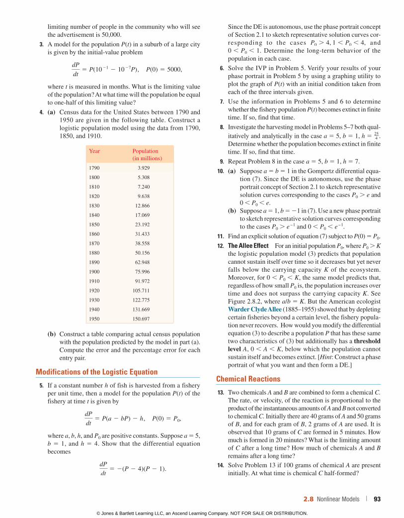
limiting number of people in the community who will see the advertisement is 50,000.
3. A model for the population P(t) in a suburb of a large city is given by the initial-value problem
dP
dt5 P(10
21 2 10 27P), P(0) 5 5000,
where t is measured in months. What is the limiting value of the population? At what time will the population be equal to one-half of this limiting value?
4. (a) Census data for the United States between 1790 and 1950 are given in the following table. Construct a logistic population model using the data from 1790, 1850, and 1910.
Year Population (in millions)
1790 3.929
1800 5.308
1810 7.240
1820 9.638
1830 12.866
1840 17.069
1850 23.192
1860 31.433
1870 38.558
1880 50.156
1890 62.948
1900 75.996
1910 91.972
1920 105.711
1930 122.775
1940 131.669
1950 150.697
(b) Construct a table comparing actual census population with the population predicted by the model in part (a). Compute the error and the percentage error for each entry pair.
Modifications of the Logistic Equation
5. If a constant number h of fish is harvested from a fishery per unit time, then a model for the population P(t) of the fishery at time t is given by
dP
dt5 P(a 2 bP) 2 h, P(0) 5 P0,
where a, b, h, and P0 are positive constants. Suppose a 5 5, b 5 1, and h 5 4. Show that the differential equation becomes
dP
dt5 2(P 2 4)(P 2 1).
Since the DE is autonomous, use the phase portrait concept of Section 2.1 to sketch representative solution curves cor-responding to the cases P0 . 4, 1 , P0 , 4, and 0 , P0 , 1. Determine the long-term behavior of the population in each case.
6. Solve the IVP in Problem 5. Verify your results of your phase portrait in Problem 5 by using a graphing utility to plot the graph of P(t) with an initial condition taken from each of the three intervals given.
7. Use the information in Problems 5 and 6 to determine whether the fishery population P(t) becomes extinct in finite time. If so, find that time.
8. Investigate the harvesting model in Problems 5–7 both qual-itatively and analytically in the case a 5 5, b 5 1, h 5 25
4 . Determine whether the population becomes extinct in finite time. If so, find that time.
9. Repeat Problem 8 in the case a 5 5, b 5 1, h 5 7.
10. (a) Suppose a 5 b 5 1 in the Gompertz differential equa-tion (7). Since the DE is autonomous, use the phase portrait concept of Section 2.1 to sketch representative solution curves corresponding to the cases P0 e and 0 P0 e.
(b) Suppose a 5 1, b 5 21 in (7). Use a new phase portrait to sketch representative solution curves corresponding to the cases P0 e – 1 and 0 P0 e – 1.
11. Find an explicit solution of equation (7) subject to P(0) 5 P0.
12. The Allee Effect For an initial population P0, where P0 K the logistic population model (3) predicts that population cannot sustain itself over time so it decreases but yet never falls below the carrying capacity K of the ecosystem. Moreover, for 0 P0 K, the same model predicts that, regardless of how small P0 is, the population increases over time and does not surpass the carrying capacity K. See Figure 2.8.2, where a/b 5 K. But the American ecologist Warder Clyde Allee (1885–1955) showed that by depleting certain fisheries beyond a certain level, the fishery popula-tion never recovers. How would you modify the differential equation (3) to describe a population P that has these same two characteristics of (3) but additionally has a threshold level A, 0 A K, below which the population cannot sustain itself and becomes extinct. [Hint: Construct a phase portrait of what you want and then form a DE.]
Chemical Reactions
13. Two chemicals A and B are combined to form a chemical C. The rate, or velocity, of the reaction is proportional to the product of the instantaneous amounts of A and B not converted to chemical C. Initially there are 40 grams of A and 50 grams of B, and for each gram of B, 2 grams of A are used. It is observed that 10 grams of C are formed in 5 minutes. How much is formed in 20 minutes? What is the limiting amount of C after a long time? How much of chemicals A and B remains after a long time?
14. Solve Problem 13 if 100 grams of chemical A are present initially. At what time is chemical C half-formed?
2.8 Nonlinear Models | 93
© Jones & Bartlett Learning LLC, an Ascend Learning Company. NOT FOR SALE OR DISTRIBUTION.
© Jones & Bartlett Learning, LLCNOT FOR SALE OR DISTRIBUTION
© Jones & Bartlett Learning, LLCNOT FOR SALE OR DISTRIBUTION
© Jones & Bartlett Learning, LLCNOT FOR SALE OR DISTRIBUTION
© Jones & Bartlett Learning, LLCNOT FOR SALE OR DISTRIBUTION
© Jones & Bartlett Learning, LLCNOT FOR SALE OR DISTRIBUTION
© Jones & Bartlett Learning, LLCNOT FOR SALE OR DISTRIBUTION
© Jones & Bartlett Learning, LLCNOT FOR SALE OR DISTRIBUTION
© Jones & Bartlett Learning, LLCNOT FOR SALE OR DISTRIBUTION
© Jones & Bartlett Learning, LLCNOT FOR SALE OR DISTRIBUTION
© Jones & Bartlett Learning, LLCNOT FOR SALE OR DISTRIBUTION
© Jones & Bartlett Learning, LLCNOT FOR SALE OR DISTRIBUTION
© Jones & Bartlett Learning, LLCNOT FOR SALE OR DISTRIBUTION
© Jones & Bartlett Learning, LLCNOT FOR SALE OR DISTRIBUTION
© Jones & Bartlett Learning, LLCNOT FOR SALE OR DISTRIBUTION
© Jones & Bartlett Learning, LLCNOT FOR SALE OR DISTRIBUTION
© Jones & Bartlett Learning, LLCNOT FOR SALE OR DISTRIBUTION
© Jones & Bartlett Learning, LLCNOT FOR SALE OR DISTRIBUTION
© Jones & Bartlett Learning, LLCNOT FOR SALE OR DISTRIBUTION
© Jones & Bartlett Learning, LLCNOT FOR SALE OR DISTRIBUTION
© Jones & Bartlett Learning, LLCNOT FOR SALE OR DISTRIBUTION
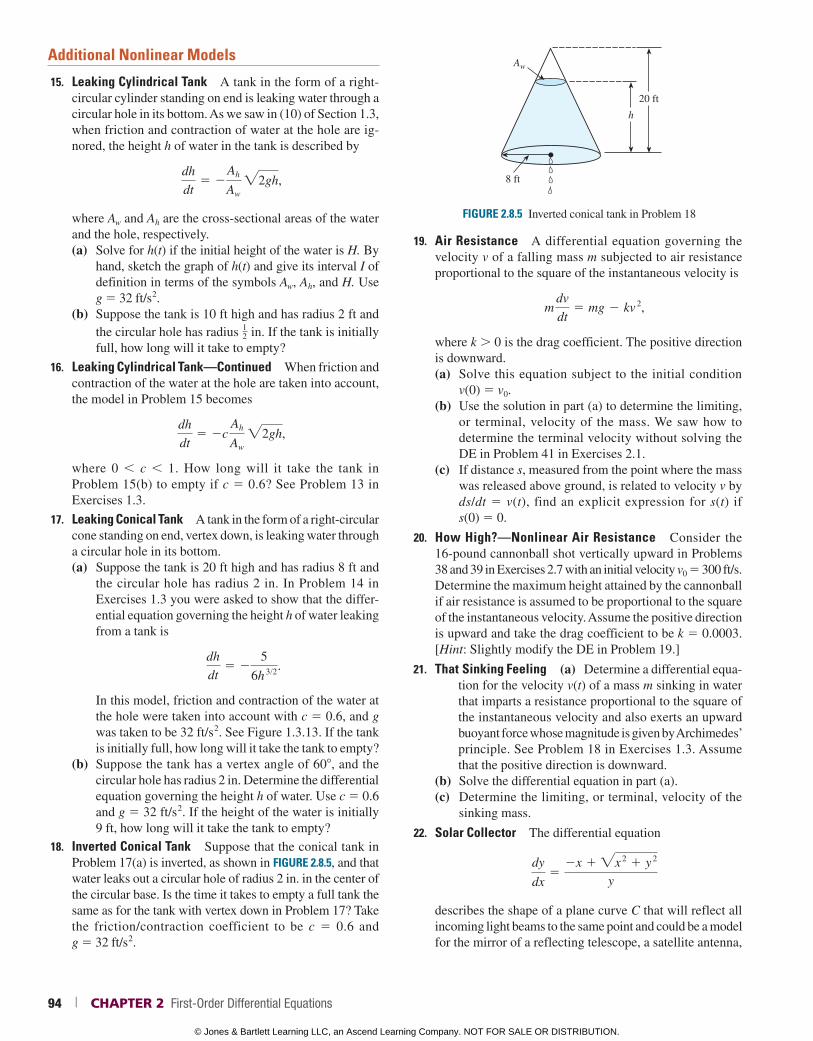
Additional Nonlinear Models
15. Leaking Cylindrical Tank A tank in the form of a right- circular cylinder standing on end is leaking water through a circular hole in its bottom. As we saw in (10) of Section 1.3, when friction and contraction of water at the hole are ig-nored, the height h of water in the tank is described by
dh
dt5 2
Ah
Aw
"2gh,
where Aw and Ah are the cross-sectional areas of the water and the hole, respectively.(a) Solve for h(t) if the initial height of the water is H. By
hand, sketch the graph of h(t) and give its interval I of definition in terms of the symbols Aw, Ah, and H. Use g 5 32 ft/s 2.
(b) Suppose the tank is 10 ft high and has radius 2 ft and the circular hole has radius 1
2 in. If the tank is initially full, how long will it take to empty?
16. Leaking Cylindrical Tank—Continued When friction and contraction of the water at the hole are taken into account, the model in Problem 15 becomes
dh
dt5 2c
Ah
Aw
"2gh,
where 0 c 1. How long will it take the tank in Problem 15(b) to empty if c 5 0.6? See Problem 13 in Exercises 1.3.
17. Leaking Conical Tank A tank in the form of a right-circular cone standing on end, vertex down, is leaking water through a circular hole in its bottom.(a) Suppose the tank is 20 ft high and has radius 8 ft and
the circular hole has radius 2 in. In Problem 14 in Exercises 1.3 you were asked to show that the differ-ential equation governing the height h of water leaking from a tank is
dh
dt5 2
5
6h 3/2.
In this model, friction and contraction of the water at the hole were taken into account with c 5 0.6, and g was taken to be 32 ft/s 2. See Figure 1.3.13. If the tank is initially full, how long will it take the tank to empty?
(b) Suppose the tank has a vertex angle of 608, and the circular hole has radius 2 in. Determine the differential equation governing the height h of water. Use c 5 0.6 and g 5 32 ft/s 2. If the height of the water is initially 9 ft, how long will it take the tank to empty?
18. Inverted Conical Tank Suppose that the conical tank in Problem 17(a) is inverted, as shown in FIGURE 2.8.5, and that water leaks out a circular hole of radius 2 in. in the center of the circular base. Is the time it takes to empty a full tank the same as for the tank with vertex down in Problem 17? Take the friction/contraction coefficient to be c 5 0.6 and g 5 32 ft/s 2.
FIGURE 2.8.5 Inverted conical tank in Problem 18
8 ft
h
20 ft
Aw
19. Air Resistance A differential equation governing the velocity v of a falling mass m subjected to air resistance proportional to the square of the instantaneous velocity is
m
dv
dt5 mg 2 kv
2,
where k 0 is the drag coefficient. The positive direction is downward.(a) Solve this equation subject to the initial condition
v(0) 5 v0.(b) Use the solution in part (a) to determine the limiting,
or terminal, velocity of the mass. We saw how to determine the terminal velocity without solving the DE in Problem 41 in Exercises 2.1.
(c) If distance s, measured from the point where the mass was released above ground, is related to velocity v by ds/dt 5 v(t), find an explicit expression for s(t) if s(0) 5 0.
20. How High?—Nonlinear Air Resistance Consider the 16-pound cannonball shot vertically upward in Problems 38 and 39 in Exercises 2.7 with an initial velocity v0 5 300 ft/s. Determine the maximum height attained by the cannonball if air resistance is assumed to be proportional to the square of the instantaneous velocity. Assume the positive direction is upward and take the drag coefficient to be k 5 0.0003. [Hint: Slightly modify the DE in Problem 19.]
21. That Sinking Feeling (a) Determine a differential equa-tion for the velocity v(t) of a mass m sinking in water that imparts a resistance proportional to the square of the instantaneous velocity and also exerts an upward buoyant force whose magnitude is given by Archimedes’ principle. See Problem 18 in Exercises 1.3. Assume that the positive direction is downward.
(b) Solve the differential equation in part (a).(c) Determine the limiting, or terminal, velocity of the
sinking mass.
22. Solar Collector The differential equation
dy
dx5
2x 1 "x 2 1 y
2
y
describes the shape of a plane curve C that will reflect all incoming light beams to the same point and could be a model for the mirror of a reflecting telescope, a satellite antenna,
94 | CHAPTER 2 First-Order Differential Equations
© Jones & Bartlett Learning LLC, an Ascend Learning Company. NOT FOR SALE OR DISTRIBUTION.
© Jones & Bartlett Learning, LLCNOT FOR SALE OR DISTRIBUTION
© Jones & Bartlett Learning, LLCNOT FOR SALE OR DISTRIBUTION
© Jones & Bartlett Learning, LLCNOT FOR SALE OR DISTRIBUTION
© Jones & Bartlett Learning, LLCNOT FOR SALE OR DISTRIBUTION
© Jones & Bartlett Learning, LLCNOT FOR SALE OR DISTRIBUTION
© Jones & Bartlett Learning, LLCNOT FOR SALE OR DISTRIBUTION
© Jones & Bartlett Learning, LLCNOT FOR SALE OR DISTRIBUTION
© Jones & Bartlett Learning, LLCNOT FOR SALE OR DISTRIBUTION
© Jones & Bartlett Learning, LLCNOT FOR SALE OR DISTRIBUTION
© Jones & Bartlett Learning, LLCNOT FOR SALE OR DISTRIBUTION
© Jones & Bartlett Learning, LLCNOT FOR SALE OR DISTRIBUTION
© Jones & Bartlett Learning, LLCNOT FOR SALE OR DISTRIBUTION
© Jones & Bartlett Learning, LLCNOT FOR SALE OR DISTRIBUTION
© Jones & Bartlett Learning, LLCNOT FOR SALE OR DISTRIBUTION
© Jones & Bartlett Learning, LLCNOT FOR SALE OR DISTRIBUTION
© Jones & Bartlett Learning, LLCNOT FOR SALE OR DISTRIBUTION
© Jones & Bartlett Learning, LLCNOT FOR SALE OR DISTRIBUTION
© Jones & Bartlett Learning, LLCNOT FOR SALE OR DISTRIBUTION
© Jones & Bartlett Learning, LLCNOT FOR SALE OR DISTRIBUTION
© Jones & Bartlett Learning, LLCNOT FOR SALE OR DISTRIBUTION
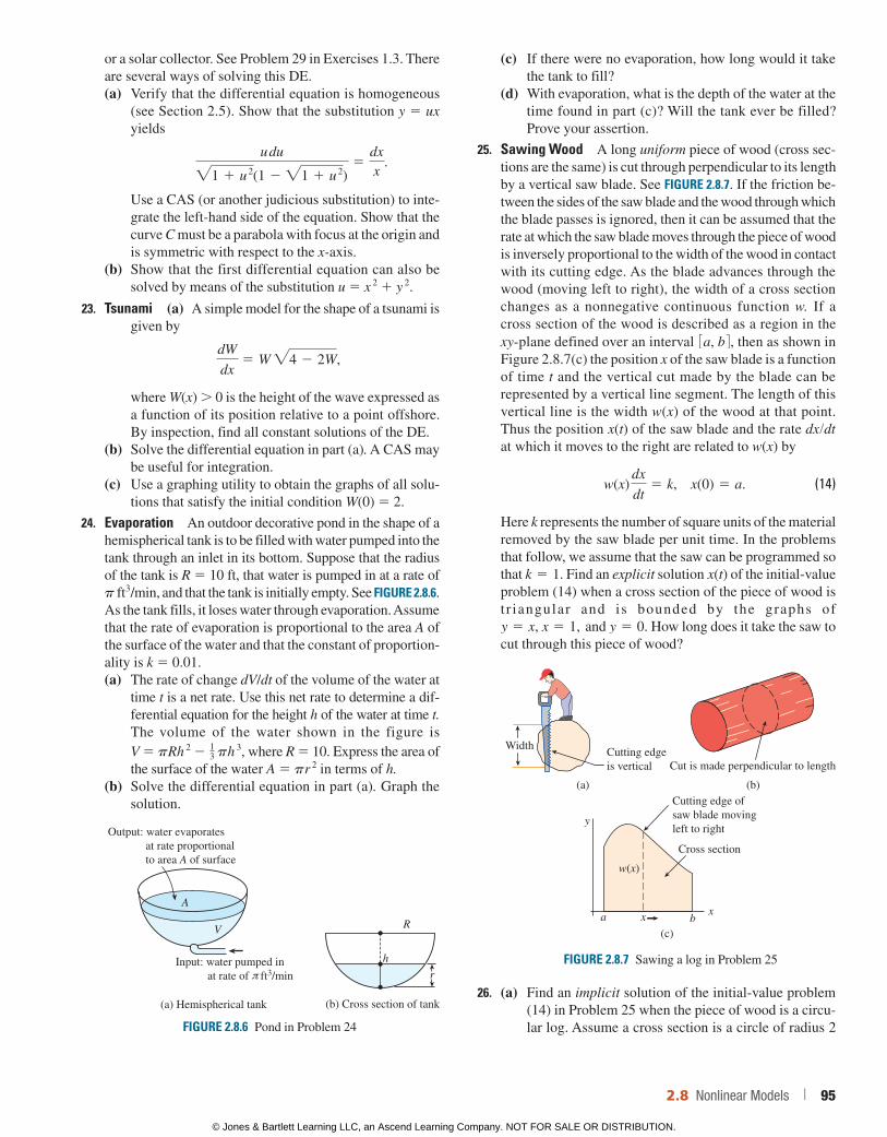
or a solar collector. See Problem 29 in Exercises 1.3. There are several ways of solving this DE.(a) Verify that the differential equation is homogeneous
(see Section 2.5). Show that the substitution y 5 ux yields
u du
"1 1 u 2(1 2 "1 1 u
2)5
dxx
.
Use a CAS (or another judicious substitution) to inte-grate the left-hand side of the equation. Show that the curve C must be a parabola with focus at the origin and is symmetric with respect to the x-axis.
(b) Show that the first differential equation can also be solved by means of the substitution u 5 x 2 1 y 2.
23. Tsunami (a) A simple model for the shape of a tsunami is given by
dW
dx5 W "4 2 2W,
where W(x) 0 is the height of the wave expressed as a function of its position relative to a point offshore. By inspection, find all constant solutions of the DE.
(b) Solve the differential equation in part (a). A CAS may be useful for integration.
(c) Use a graphing utility to obtain the graphs of all solu-tions that satisfy the initial condition W(0) 5 2.
24. Evaporation An outdoor decorative pond in the shape of a hemispherical tank is to be filled with water pumped into the tank through an inlet in its bottom. Suppose that the radius of the tank is R 5 10 ft, that water is pumped in at a rate of p ft 3/min, and that the tank is initially empty. See FIGURE 2.8.6. As the tank fills, it loses water through evaporation. Assume that the rate of evaporation is proportional to the area A of the surface of the water and that the constant of proportion-ality is k 5 0.01.(a) The rate of change dV/dt of the volume of the water at
time t is a net rate. Use this net rate to determine a dif-ferential equation for the height h of the water at time t. The vol ume of the water shown in the figure is V 5 pRh 2 2 1
3 ph 3, where R 5 10. Express the area of the surface of the water A 5 pr 2 in terms of h.
(b) Solve the differential equation in part (a). Graph the solution.
FIGURE 2.8.6 Pond in Problem 24
(a) Hemispherical tank
A
V R
r
h
(b) Cross section of tank
π
Output: water evaporates at rate proportional to area A of surface
Input: water pumped in at rate of ft3/min
(c) If there were no evaporation, how long would it take the tank to fill?
(d) With evaporation, what is the depth of the water at the time found in part (c)? Will the tank ever be filled? Prove your assertion.
25. Sawing Wood A long uniform piece of wood (cross sec-tions are the same) is cut through perpendicular to its length by a vertical saw blade. See FIGURE 2.8.7. If the friction be-tween the sides of the saw blade and the wood through which the blade passes is ignored, then it can be assumed that the rate at which the saw blade moves through the piece of wood is inversely proportional to the width of the wood in contact with its cutting edge. As the blade advances through the wood (moving left to right), the width of a cross section changes as a nonnegative continuous function w. If a cross section of the wood is described as a region in the xy-plane defined over an interval 3a, b 4, then as shown in Figure 2.8.7(c) the position x of the saw blade is a function of time t and the vertical cut made by the blade can be represented by a vertical line segment. The length of this vertical line is the width w(x) of the wood at that point. Thus the position x(t) of the saw blade and the rate dx/dt at which it moves to the right are related to w(x) by
w(x)
dx
dt5 k, x(0) 5 a. (14)
Here k represents the number of square units of the material removed by the saw blade per unit time. In the problems that follow, we assume that the saw can be programmed so that k 5 1. Find an explicit solution x(t) of the initial-value problem (14) when a cross section of the piece of wood is t r iangular and is bounded by the graphs of y 5 x, x 5 1, and y 5 0. How long does it take the saw to cut through this piece of wood?
(c)
xbx
w(x)
a
y
Cutting edge ofsaw blade movingleft to right
Cross section
(a) (b)
Cut is made perpendicular to lengthCutting edgeis vertical
Width
FIGURE 2.8.7 Sawing a log in Problem 25
26. (a) Find an implicit solution of the initial-value problem (14) in Problem 25 when the piece of wood is a circu-lar log. Assume a cross section is a circle of radius 2
2.8 Nonlinear Models | 95
© Jones & Bartlett Learning LLC, an Ascend Learning Company. NOT FOR SALE OR DISTRIBUTION.
© Jones & Bartlett Learning, LLCNOT FOR SALE OR DISTRIBUTION
© Jones & Bartlett Learning, LLCNOT FOR SALE OR DISTRIBUTION
© Jones & Bartlett Learning, LLCNOT FOR SALE OR DISTRIBUTION
© Jones & Bartlett Learning, LLCNOT FOR SALE OR DISTRIBUTION
© Jones & Bartlett Learning, LLCNOT FOR SALE OR DISTRIBUTION
© Jones & Bartlett Learning, LLCNOT FOR SALE OR DISTRIBUTION
© Jones & Bartlett Learning, LLCNOT FOR SALE OR DISTRIBUTION
© Jones & Bartlett Learning, LLCNOT FOR SALE OR DISTRIBUTION
© Jones & Bartlett Learning, LLCNOT FOR SALE OR DISTRIBUTION
© Jones & Bartlett Learning, LLCNOT FOR SALE OR DISTRIBUTION
© Jones & Bartlett Learning, LLCNOT FOR SALE OR DISTRIBUTION
© Jones & Bartlett Learning, LLCNOT FOR SALE OR DISTRIBUTION
© Jones & Bartlett Learning, LLCNOT FOR SALE OR DISTRIBUTION
© Jones & Bartlett Learning, LLCNOT FOR SALE OR DISTRIBUTION
© Jones & Bartlett Learning, LLCNOT FOR SALE OR DISTRIBUTION
© Jones & Bartlett Learning, LLCNOT FOR SALE OR DISTRIBUTION
© Jones & Bartlett Learning, LLCNOT FOR SALE OR DISTRIBUTION
© Jones & Bartlett Learning, LLCNOT FOR SALE OR DISTRIBUTION
© Jones & Bartlett Learning, LLCNOT FOR SALE OR DISTRIBUTION
© Jones & Bartlett Learning, LLCNOT FOR SALE OR DISTRIBUTION
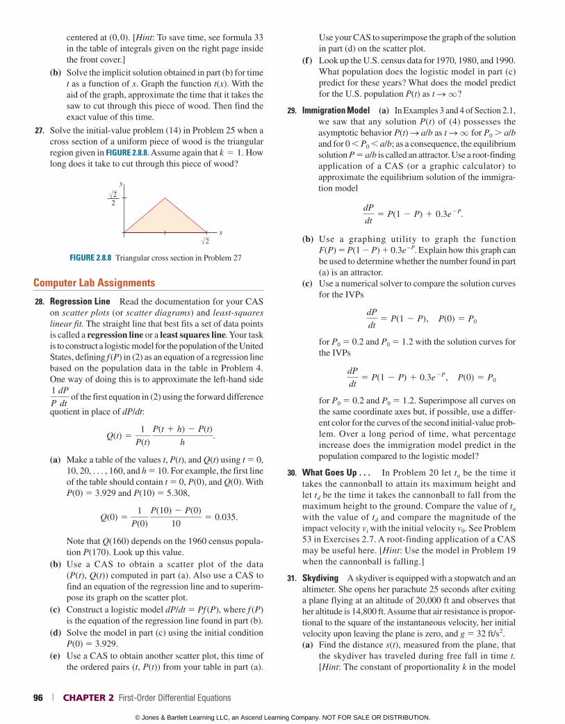
centered at (0, 0). [Hint: To save time, see formula 33 in the table of integrals given on the right page inside the front cover.]
(b) Solve the implicit solution obtained in part (b) for time t as a function of x. Graph the function t(x). With the aid of the graph, approximate the time that it takes the saw to cut through this piece of wood. Then find the exact value of this time.
27. Solve the initial-value problem (14) in Problem 25 when a cross section of a uniform piece of wood is the triangular region given in FIGURE 2.8.8. Assume again that k 5 1. How long does it take to cut through this piece of wood?
FIGURE 2.8.8 Triangular cross section in Problem 27
x
y
2
22
Computer Lab Assignments
28. Regression Line Read the documentation for your CAS on scatter plots (or scatter diagrams) and least-squares linear fit. The straight line that best fits a set of data points is called a regression line or a least squares line. Your task is to construct a logistic model for the population of the United States, defining f (P) in (2) as an equation of a regression line based on the population data in the table in Problem 4. One way of doing this is to approximate the left-hand side 1
P
dP
dt of the first equation in (2) using the forward difference
quotient in place of dP/dt:
Q(t) 51
P(t)
P(t 1 h) 2 P(t)
h.
(a) Make a table of the values t, P(t), and Q(t) using t 5 0, 10, 20, . . . , 160, and h 5 10. For example, the first line of the table should contain t 5 0, P(0), and Q(0). With P(0) 5 3.929 and P(10) 5 5.308,
Q(0) 51
P(0)
P(10) 2 P(0)
105 0.035.
Note that Q(160) depends on the 1960 census popula-tion P(170). Look up this value.
(b) Use a CAS to obtain a scatter plot of the data (P(t), Q(t)) computed in part (a). Also use a CAS to find an equation of the regression line and to superim-pose its graph on the scatter plot.
(c) Construct a logistic model dP/dt 5 Pf (P), where f (P) is the equation of the regression line found in part (b).
(d) Solve the model in part (c) using the initial condition P(0) 5 3.929.
(e) Use a CAS to obtain another scatter plot, this time of the ordered pairs (t, P(t)) from your table in part (a).
Use your CAS to superimpose the graph of the solution in part (d) on the scatter plot.
(f ) Look up the U.S. census data for 1970, 1980, and 1990. What population does the logistic model in part (c) predict for these years? What does the model predict for the U.S. population P(t) as t S q?
29. Immigration Model (a) In Examples 3 and 4 of Section 2.1, we saw that any solution P(t) of (4) possesses the
asymptotic behavior P(t) S a/b as t S q for P0 a/b and for 0 P0 a/b; as a consequence, the equilibrium solution P 5 a/b is called an attractor. Use a root-finding application of a CAS (or a graphic calculator) to approximate the equilibrium solution of the immigra-tion model
dP
dt5 P(1 2 P) 1 0.3e
2P.
(b) Use a graphing utility to graph the function F(P) 5 P(1 2 P) 1 0.3e – P. Explain how this graph can be used to determine whether the number found in part (a) is an attractor.
(c) Use a numerical solver to compare the solution curves for the IVPs
dP
dt5 P(1 2 P), P(0) 5 P0
for P0 5 0.2 and P0 5 1.2 with the solution curves for the IVPs
dP
dt5 P(1 2 P) 1 0.3e
2P, P(0) 5 P0
for P0 5 0.2 and P0 5 1.2. Superimpose all curves on the same coordinate axes but, if possible, use a differ-ent color for the curves of the second initial-value prob-lem. Over a long period of time, what percentage increase does the immigration model predict in the population compared to the logistic model?
30. What Goes Up . . . In Problem 20 let ta be the time it takes the cannonball to attain its maximum height and let td be the time it takes the cannonball to fall from the maximum height to the ground. Compare the value of ta with the value of td and compare the magnitude of the impact velocity vi with the initial velocity v0. See Problem 53 in Exercises 2.7. A root-finding application of a CAS may be useful here. [Hint: Use the model in Problem 19 when the cannonball is falling.]
31. Skydiving A skydiver is equipped with a stopwatch and an altimeter. She opens her parachute 25 seconds after exiting a plane flying at an altitude of 20,000 ft and observes that her altitude is 14,800 ft. Assume that air resistance is propor-tional to the square of the instantaneous velocity, her initial velocity upon leaving the plane is zero, and g 5 32 ft/s 2.(a) Find the distance s(t), measured from the plane, that
the skydiver has traveled during free fall in time t. [Hint: The constant of proportionality k in the model
96 | CHAPTER 2 First-Order Differential Equations
© Jones & Bartlett Learning LLC, an Ascend Learning Company. NOT FOR SALE OR DISTRIBUTION.
© Jones & Bartlett Learning, LLCNOT FOR SALE OR DISTRIBUTION
© Jones & Bartlett Learning, LLCNOT FOR SALE OR DISTRIBUTION
© Jones & Bartlett Learning, LLCNOT FOR SALE OR DISTRIBUTION
© Jones & Bartlett Learning, LLCNOT FOR SALE OR DISTRIBUTION
© Jones & Bartlett Learning, LLCNOT FOR SALE OR DISTRIBUTION
© Jones & Bartlett Learning, LLCNOT FOR SALE OR DISTRIBUTION
© Jones & Bartlett Learning, LLCNOT FOR SALE OR DISTRIBUTION
© Jones & Bartlett Learning, LLCNOT FOR SALE OR DISTRIBUTION
© Jones & Bartlett Learning, LLCNOT FOR SALE OR DISTRIBUTION
© Jones & Bartlett Learning, LLCNOT FOR SALE OR DISTRIBUTION
© Jones & Bartlett Learning, LLCNOT FOR SALE OR DISTRIBUTION
© Jones & Bartlett Learning, LLCNOT FOR SALE OR DISTRIBUTION
© Jones & Bartlett Learning, LLCNOT FOR SALE OR DISTRIBUTION
© Jones & Bartlett Learning, LLCNOT FOR SALE OR DISTRIBUTION
© Jones & Bartlett Learning, LLCNOT FOR SALE OR DISTRIBUTION
© Jones & Bartlett Learning, LLCNOT FOR SALE OR DISTRIBUTION
© Jones & Bartlett Learning, LLCNOT FOR SALE OR DISTRIBUTION
© Jones & Bartlett Learning, LLCNOT FOR SALE OR DISTRIBUTION
© Jones & Bartlett Learning, LLCNOT FOR SALE OR DISTRIBUTION
© Jones & Bartlett Learning, LLCNOT FOR SALE OR DISTRIBUTION
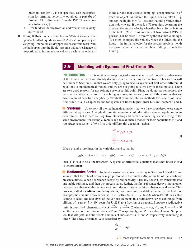
given in Problem 19 is not specified. Use the expres-sion for terminal velocity vt obtained in part (b) of Problem 19 to eliminate k from the IVP. Then eventu-ally solve for vt.]
(b) How far does the skydiver fall and what is her velocity at t 5 15 s?
32. Hitting Bottom A helicopter hovers 500 feet above a large open tank full of liquid (not water). A dense compact object weighing 160 pounds is dropped (released from rest) from the helicopter into the liquid. Assume that air resistance is proportional to instantaneous velocity v while the object is
in the air and that viscous damping is proportional to v 2 after the object has entered the liquid. For air, take k 5 1
4, and for the liquid, k 5 0.1. Assume that the positive direc-tion is downward. If the tank is 75 feet high, determine the time and the impact velocity when the object hits the bottom of the tank. [Hint: Think in terms of two distinct IVPs. If you use (13), be careful in removing the absolute value sign. You might compare the velocity when the object hits the liquid—the initial velocity for the second problem—with the terminal velocity vt of the object falling through the liquid.]
2.9 Modeling with Systems of First-Order DEs
INTRODUCTION In this section we are going to discuss mathematical models based on some of the topics that we have already discussed in the preceding two sections. This section will be similar to Section 1.3 in that we are only going to discuss systems of first-order differential equations as mathematical models and we are not going to solve any of these models. There are two good reasons for not solving systems at this point: First, we do not as yet possess the necessary mathematical tools for solving systems, and second, some of the systems that we discuss cannot be solved analytically. We shall examine solution methods for systems of linear first-order DEs in Chapter 10 and for systems of linear higher-order DEs in Chapters 3 and 4.
Systems Up to now all the mathematical models that we have considered were single differential equations. A single differential equation could describe a single population in an environment, but if there are, say, two interacting and perhaps competing species living in the same environment (for example, rabbits and foxes), then a model for their populations x(t) and y(t) might be a system of two first-order differential equations such as
dx
dt5 g1(t, x, y)
dy
dt5 g2(t, x, y).
(1)
When g1 and g2 are linear in the variables x and y, that is,
g1(t, x, y) 5 c1x 1 c2 y 1 f1(t) and g2(t, x, y) 5 c3x 1 c4 y 1 f2(t),
then (1) is said to be a linear system. A system of differential equations that is not linear is said to be nonlinear.
Radioactive Series In the discussion of radioactive decay in Sections 1.3 and 2.7, we assumed that the rate of decay was proportional to the number A(t) of nuclei of the substance present at time t. When a substance decays by radioactivity, it usually doesn’t just transmute into one stable substance and then the process stops. Rather, the first substance decays into another radioactive substance, this substance in turn decays into yet a third substance, and so on. This process, called a radioactive decay series, continues until a stable element is reached. For example, the uranium decay series is U-238 S Th-234 S . . . S Pb-206, where Pb-206 is a stable isotope of lead. The half-lives of the various elements in a radioactive series can range from billions of years (4.5 3 10 9 years for U-238) to a fraction of a second. Suppose a radioactive
series is described schematically by X h2l1 Y h
2l2 Z, where k1 5 2l1 0 and k2 5 2l2 0 are the decay constants for substances X and Y, respectively, and Z is a stable element. Suppose too, that x(t), y(t), and z(t) denote amounts of substances X, Y, and Z, respectively, remaining at time t. The decay of element X is described by
dx
dt5 2l1x,
2.9 Modeling with Systems of First-Order DEs | 97
© Jones & Bartlett Learning LLC, an Ascend Learning Company. NOT FOR SALE OR DISTRIBUTION.
© Jones & Bartlett Learning, LLCNOT FOR SALE OR DISTRIBUTION
© Jones & Bartlett Learning, LLCNOT FOR SALE OR DISTRIBUTION
© Jones & Bartlett Learning, LLCNOT FOR SALE OR DISTRIBUTION
© Jones & Bartlett Learning, LLCNOT FOR SALE OR DISTRIBUTION
© Jones & Bartlett Learning, LLCNOT FOR SALE OR DISTRIBUTION
© Jones & Bartlett Learning, LLCNOT FOR SALE OR DISTRIBUTION
© Jones & Bartlett Learning, LLCNOT FOR SALE OR DISTRIBUTION
© Jones & Bartlett Learning, LLCNOT FOR SALE OR DISTRIBUTION
© Jones & Bartlett Learning, LLCNOT FOR SALE OR DISTRIBUTION
© Jones & Bartlett Learning, LLCNOT FOR SALE OR DISTRIBUTION
© Jones & Bartlett Learning, LLCNOT FOR SALE OR DISTRIBUTION
© Jones & Bartlett Learning, LLCNOT FOR SALE OR DISTRIBUTION
© Jones & Bartlett Learning, LLCNOT FOR SALE OR DISTRIBUTION
© Jones & Bartlett Learning, LLCNOT FOR SALE OR DISTRIBUTION
© Jones & Bartlett Learning, LLCNOT FOR SALE OR DISTRIBUTION
© Jones & Bartlett Learning, LLCNOT FOR SALE OR DISTRIBUTION
© Jones & Bartlett Learning, LLCNOT FOR SALE OR DISTRIBUTION
© Jones & Bartlett Learning, LLCNOT FOR SALE OR DISTRIBUTION
© Jones & Bartlett Learning, LLCNOT FOR SALE OR DISTRIBUTION
© Jones & Bartlett Learning, LLCNOT FOR SALE OR DISTRIBUTION
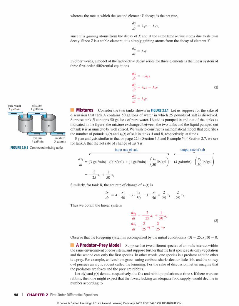
whereas the rate at which the second element Y decays is the net rate,
dy
dt5 l1x 2 l2 y,
since it is gaining atoms from the decay of X and at the same time losing atoms due to its own decay. Since Z is a stable element, it is simply gaining atoms from the decay of element Y:
dz
dt5 l2y.
In other words, a model of the radioactive decay series for three elements is the linear system of three first-order differential equations
dx
dt5 2l1x
dy
dt5 l1x 2 l2y (2)
dz
dt5 l2y.
Mixtures Consider the two tanks shown in FIGURE 2.9.1. Let us suppose for the sake of discussion that tank A contains 50 gallons of water in which 25 pounds of salt is dissolved. Suppose tank B contains 50 gallons of pure water. Liquid is pumped in and out of the tanks as indicated in the figure; the mixture exchanged between the two tanks and the liquid pumped out of tank B is assumed to be well stirred. We wish to construct a mathematical model that describes the number of pounds x1(t) and x2(t) of salt in tanks A and B, respectively, at time t.
By an analysis similar to that on page 22 in Section 1.3 and Example 5 of Section 2.7, we see for tank A that the net rate of change of x1(t) is
input rate of salt output rate of salt
dx1
dt 5 (3 gal/min) ? (0 lb/gal) 1 (1 gal/min) ? a x2
50 lb/galb 2 (4 gal/min) ? a x1
50 lb/galb
5 22
25 x1 1
1
50 x2.
Similarly, for tank B, the net rate of change of x2(t) is
dx2
dt5 4 ?
x1
502 3 ?
x2
502 1 ?
x2
505
2
25 x1 2
2
25 x2.
Thus we obtain the linear system
dx1
dt5 2
2
25 x1 1
1
50 x2
dx2
dt5
2
25 x1 2
2
25 x2.
(3)
Observe that the foregoing system is accompanied by the initial conditions x1(0) 5 25, x2(0) 5 0.
A Predator–Prey Model Suppose that two different species of animals interact within the same environment or ecosystem, and suppose further that the first species eats only vegetation and the second eats only the first species. In other words, one species is a predator and the other is a prey. For example, wolves hunt grass-eating caribou, sharks devour little fish, and the snowy owl pursues an arctic rodent called the lemming. For the sake of discussion, let us imagine that the predators are foxes and the prey are rabbits.
Let x(t) and y(t) denote, respectively, the fox and rabbit populations at time t. If there were no rabbits, then one might expect that the foxes, lacking an adequate food supply, would decline in number according to
A B
pure water3 gal/min
mixture1 gal/min
mixture4 gal/min
mixture3 gal/min
FIGURE 2.9.1 Connected mixing tanks
98 | CHAPTER 2 First-Order Differential Equations
© Jones & Bartlett Learning LLC, an Ascend Learning Company. NOT FOR SALE OR DISTRIBUTION.
© Jones & Bartlett Learning, LLCNOT FOR SALE OR DISTRIBUTION
© Jones & Bartlett Learning, LLCNOT FOR SALE OR DISTRIBUTION
© Jones & Bartlett Learning, LLCNOT FOR SALE OR DISTRIBUTION
© Jones & Bartlett Learning, LLCNOT FOR SALE OR DISTRIBUTION
© Jones & Bartlett Learning, LLCNOT FOR SALE OR DISTRIBUTION
© Jones & Bartlett Learning, LLCNOT FOR SALE OR DISTRIBUTION
© Jones & Bartlett Learning, LLCNOT FOR SALE OR DISTRIBUTION
© Jones & Bartlett Learning, LLCNOT FOR SALE OR DISTRIBUTION
© Jones & Bartlett Learning, LLCNOT FOR SALE OR DISTRIBUTION
© Jones & Bartlett Learning, LLCNOT FOR SALE OR DISTRIBUTION
© Jones & Bartlett Learning, LLCNOT FOR SALE OR DISTRIBUTION
© Jones & Bartlett Learning, LLCNOT FOR SALE OR DISTRIBUTION
© Jones & Bartlett Learning, LLCNOT FOR SALE OR DISTRIBUTION
© Jones & Bartlett Learning, LLCNOT FOR SALE OR DISTRIBUTION
© Jones & Bartlett Learning, LLCNOT FOR SALE OR DISTRIBUTION
© Jones & Bartlett Learning, LLCNOT FOR SALE OR DISTRIBUTION
© Jones & Bartlett Learning, LLCNOT FOR SALE OR DISTRIBUTION
© Jones & Bartlett Learning, LLCNOT FOR SALE OR DISTRIBUTION
© Jones & Bartlett Learning, LLCNOT FOR SALE OR DISTRIBUTION
© Jones & Bartlett Learning, LLCNOT FOR SALE OR DISTRIBUTION
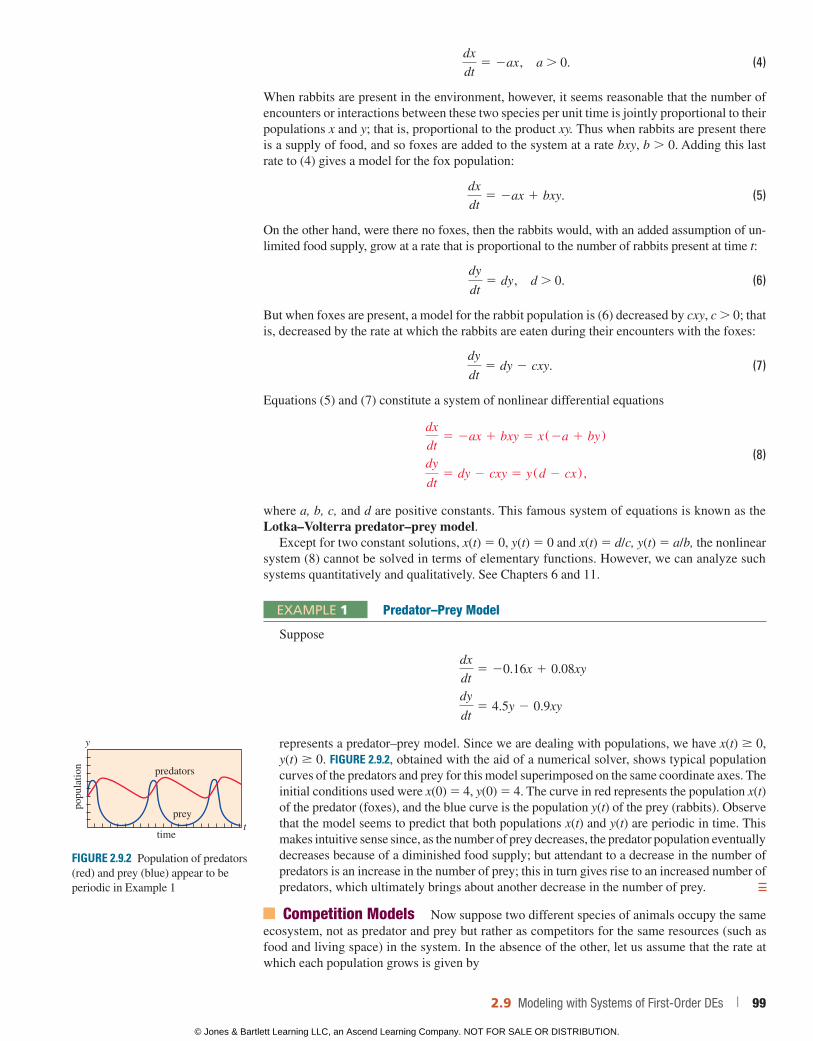
dx
dt5 2ax, a 0. (4)
When rabbits are present in the environment, however, it seems reasonable that the number of encounters or interactions between these two species per unit time is jointly proportional to their populations x and y; that is, proportional to the product xy. Thus when rabbits are present there is a supply of food, and so foxes are added to the system at a rate bxy, b 0. Adding this last rate to (4) gives a model for the fox population:
dx
dt5 2ax 1 bxy. (5)
On the other hand, were there no foxes, then the rabbits would, with an added assumption of un-limited food supply, grow at a rate that is proportional to the number of rabbits present at time t:
dy
dt5 dy, d 0. (6)
But when foxes are present, a model for the rabbit population is (6) decreased by cxy, c 0; that is, decreased by the rate at which the rabbits are eaten during their encounters with the foxes:
dy
dt5 dy 2 cxy. (7)
Equations (5) and (7) constitute a system of nonlinear differential equations
dx
dt5 2ax 1 bxy 5 x(2a 1 by)
dy
dt5 dy 2 cxy 5 y(d 2 cx) ,
(8)
where a, b, c, and d are positive constants. This famous system of equations is known as the Lotka–Volterra predator–prey model.
Except for two constant solutions, x(t) 5 0, y(t) 5 0 and x(t) 5 d/c, y(t) 5 a/b, the nonlinear system (8) cannot be solved in terms of elementary functions. However, we can analyze such systems quantitatively and qualitatively. See Chapters 6 and 11.
EXAMPLE 1 Predator–Prey Model
Suppose
dx
dt5 20.16x 1 0.08xy
dy
dt5 4.5y 2 0.9xy
represents a predator–prey model. Since we are dealing with populations, we have x(t) 0, y(t) 0. FIGURE 2.9.2, obtained with the aid of a numerical solver, shows typical population curves of the predators and prey for this model superimposed on the same coordinate axes. The initial conditions used were x(0) 5 4, y(0) 5 4. The curve in red represents the population x(t) of the predator (foxes), and the blue curve is the population y(t) of the prey (rabbits). Observe that the model seems to predict that both populations x(t) and y(t) are periodic in time. This makes intuitive sense since, as the number of prey decreases, the predator population eventually decreases because of a diminished food supply; but attendant to a decrease in the number of predators is an increase in the number of prey; this in turn gives rise to an increased number of predators, which ultimately brings about another decrease in the number of prey.
Competition Models Now suppose two different species of animals occupy the same ecosystem, not as predator and prey but rather as competitors for the same resources (such as food and living space) in the system. In the absence of the other, let us assume that the rate at which each population grows is given by
FIGURE 2.9.2 Population of predators (red) and prey (blue) appear to be periodic in Example 1
popu
latio
n predators
y
tprey
time
2.9 Modeling with Systems of First-Order DEs | 99
© Jones & Bartlett Learning LLC, an Ascend Learning Company. NOT FOR SALE OR DISTRIBUTION.
© Jones & Bartlett Learning, LLCNOT FOR SALE OR DISTRIBUTION
© Jones & Bartlett Learning, LLCNOT FOR SALE OR DISTRIBUTION
© Jones & Bartlett Learning, LLCNOT FOR SALE OR DISTRIBUTION
© Jones & Bartlett Learning, LLCNOT FOR SALE OR DISTRIBUTION
© Jones & Bartlett Learning, LLCNOT FOR SALE OR DISTRIBUTION
© Jones & Bartlett Learning, LLCNOT FOR SALE OR DISTRIBUTION
© Jones & Bartlett Learning, LLCNOT FOR SALE OR DISTRIBUTION
© Jones & Bartlett Learning, LLCNOT FOR SALE OR DISTRIBUTION
© Jones & Bartlett Learning, LLCNOT FOR SALE OR DISTRIBUTION
© Jones & Bartlett Learning, LLCNOT FOR SALE OR DISTRIBUTION
© Jones & Bartlett Learning, LLCNOT FOR SALE OR DISTRIBUTION
© Jones & Bartlett Learning, LLCNOT FOR SALE OR DISTRIBUTION
© Jones & Bartlett Learning, LLCNOT FOR SALE OR DISTRIBUTION
© Jones & Bartlett Learning, LLCNOT FOR SALE OR DISTRIBUTION
© Jones & Bartlett Learning, LLCNOT FOR SALE OR DISTRIBUTION
© Jones & Bartlett Learning, LLCNOT FOR SALE OR DISTRIBUTION
© Jones & Bartlett Learning, LLCNOT FOR SALE OR DISTRIBUTION
© Jones & Bartlett Learning, LLCNOT FOR SALE OR DISTRIBUTION
© Jones & Bartlett Learning, LLCNOT FOR SALE OR DISTRIBUTION
© Jones & Bartlett Learning, LLCNOT FOR SALE OR DISTRIBUTION
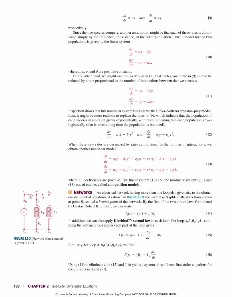
dx
dt5 ax and
dy
dt5 cy, (9)
respectively.Since the two species compete, another assumption might be that each of these rates is dimin-
ished simply by the influence, or existence, of the other population. Thus a model for the two populations is given by the linear system
dx
dt5 ax 2 by
dy
dt5 cy 2 dx,
(10)
where a, b, c, and d are positive constants.On the other hand, we might assume, as we did in (5), that each growth rate in (9) should be
reduced by a rate proportional to the number of interactions between the two species:
dx
dt5 ax 2 bxy
dy
dt5 cy 2 dxy.
(11)
Inspection shows that this nonlinear system is similar to the Lotka–Volterra predator–prey model. Last, it might be more realistic to replace the rates in (9), which indicate that the population of each species in isolation grows exponentially, with rates indicating that each population grows logistically (that is, over a long time the population is bounded):
dx
dt5 a1x 2 b1x
2 and dy
dt5 a2y 2 b2 y
2. (12)
When these new rates are decreased by rates proportional to the number of interactions, we obtain another nonlinear model
dx
dt5 a1x 2 b1x
2 2 c1xy 5 x (a1 2 b1x 2 c1y)
dy
dt5 a2y 2 b2y
2 2 c2xy 5 y (a2 2 b2y 2 c2x) ,
(13)
where all coefficients are positive. The linear system (10) and the nonlinear systems (11) and (13) are, of course, called competition models.
Networks An electrical network having more than one loop also gives rise to simultane-ous differential equations. As shown in FIGURE 2.9.3, the current i1(t) splits in the directions shown at point B1, called a branch point of the network. By the first of the two circuit laws formulated by Gustav Robert Kirchhoff, we can write
i1(t) 5 i2(t) 1 i3(t). (14)
In addition, we can also apply Kirchhoff’s second law to each loop. For loop A1B1B2A2A1, sum-ming the voltage drops across each part of the loop gives
E(t) 5 i1R1 1 L1 di2
dt1 i2R2. (15)
Similarly, for loop A1B1C1C2B2A2A1 we find
E(t) 5 i1R1 1 L2 di3
dt. (16)
Using (14) to eliminate i1 in (15) and (16) yields a system of two linear first-order equations for the currents i2(t) and i3(t):
FIGURE 2.9.3 Network whose model is given in (17)
E
A1
R1
R2
i1 i2
i3
B1 C1
A2 B2 C2
L2L1
100 | CHAPTER 2 First-Order Differential Equations
© Jones & Bartlett Learning LLC, an Ascend Learning Company. NOT FOR SALE OR DISTRIBUTION.
© Jones & Bartlett Learning, LLCNOT FOR SALE OR DISTRIBUTION
© Jones & Bartlett Learning, LLCNOT FOR SALE OR DISTRIBUTION
© Jones & Bartlett Learning, LLCNOT FOR SALE OR DISTRIBUTION
© Jones & Bartlett Learning, LLCNOT FOR SALE OR DISTRIBUTION
© Jones & Bartlett Learning, LLCNOT FOR SALE OR DISTRIBUTION
© Jones & Bartlett Learning, LLCNOT FOR SALE OR DISTRIBUTION
© Jones & Bartlett Learning, LLCNOT FOR SALE OR DISTRIBUTION
© Jones & Bartlett Learning, LLCNOT FOR SALE OR DISTRIBUTION
© Jones & Bartlett Learning, LLCNOT FOR SALE OR DISTRIBUTION
© Jones & Bartlett Learning, LLCNOT FOR SALE OR DISTRIBUTION
© Jones & Bartlett Learning, LLCNOT FOR SALE OR DISTRIBUTION
© Jones & Bartlett Learning, LLCNOT FOR SALE OR DISTRIBUTION
© Jones & Bartlett Learning, LLCNOT FOR SALE OR DISTRIBUTION
© Jones & Bartlett Learning, LLCNOT FOR SALE OR DISTRIBUTION
© Jones & Bartlett Learning, LLCNOT FOR SALE OR DISTRIBUTION
© Jones & Bartlett Learning, LLCNOT FOR SALE OR DISTRIBUTION
© Jones & Bartlett Learning, LLCNOT FOR SALE OR DISTRIBUTION
© Jones & Bartlett Learning, LLCNOT FOR SALE OR DISTRIBUTION
© Jones & Bartlett Learning, LLCNOT FOR SALE OR DISTRIBUTION
© Jones & Bartlett Learning, LLCNOT FOR SALE OR DISTRIBUTION
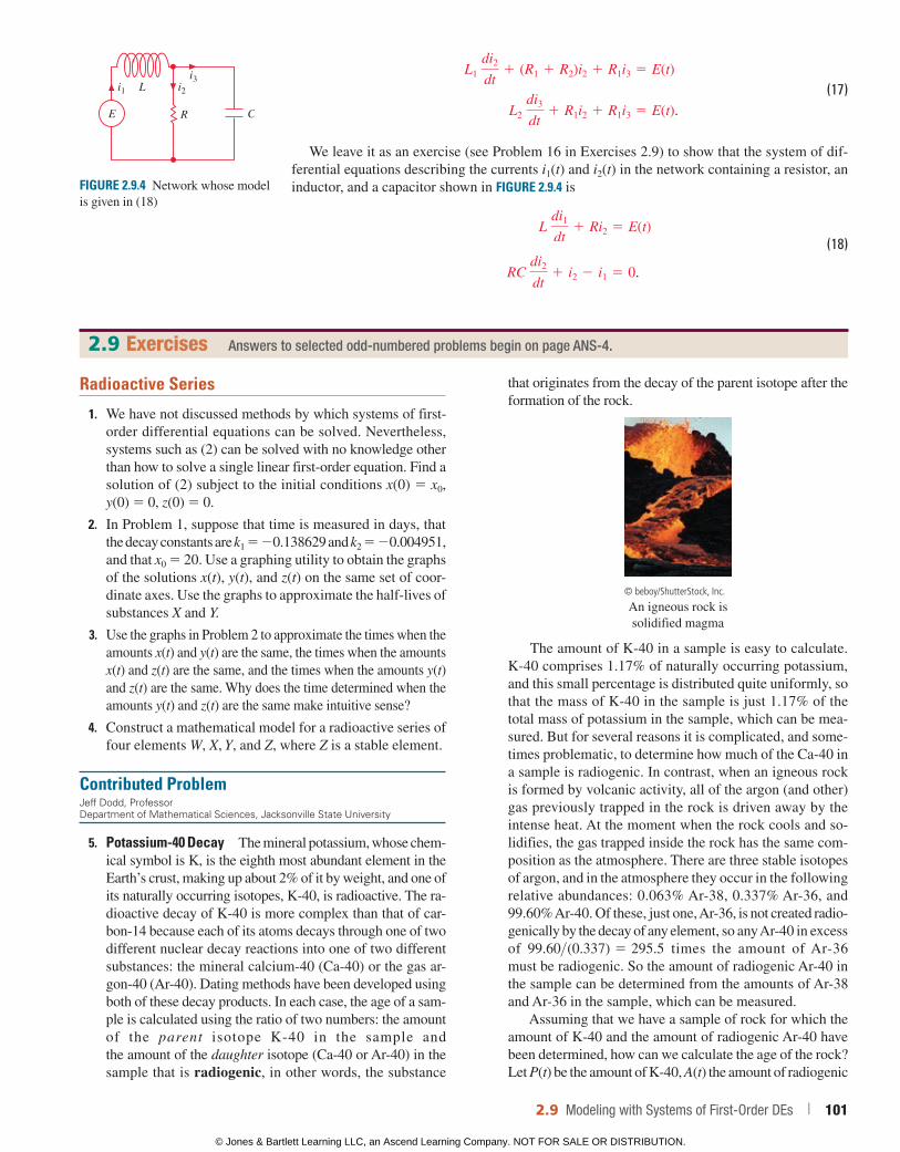
L1 di2
dt1 (R1 1 R2)i2 1 R1i3 5 E(t)
L2 di3
dt1 R1i2 1 R1i3 5 E(t).
(17)
We leave it as an exercise (see Problem 16 in Exercises 2.9) to show that the system of dif-ferential equations describing the currents i1(t) and i2(t) in the network containing a resistor, an inductor, and a capacitor shown in FIGURE 2.9.4 is
L di1
dt1 Ri2 5 E(t)
(18)
RC di2
dt1 i2 2 i1 5 0.
FIGURE 2.9.4 Network whose model is given in (18)
RE
L
C
i1 i2i3
Radioactive Series
1. We have not discussed methods by which systems of first-order differential equations can be solved. Nevertheless, systems such as (2) can be solved with no knowledge other than how to solve a single linear first-order equation. Find a solution of (2) subject to the initial conditions x(0) 5 x0, y(0) 5 0, z(0) 5 0.
2. In Problem 1, suppose that time is measured in days, that the decay constants are k1 5 20.138629 and k2 5 20.004951, and that x0 5 20. Use a graphing utility to obtain the graphs of the solutions x(t), y(t), and z(t) on the same set of coor-dinate axes. Use the graphs to approximate the half-lives of substances X and Y.
3. Use the graphs in Problem 2 to approximate the times when the amounts x(t) and y(t) are the same, the times when the amounts x(t) and z(t) are the same, and the times when the amounts y(t) and z(t) are the same. Why does the time determined when the amounts y(t) and z(t) are the same make intuitive sense?
4. Construct a mathematical model for a radioactive series of four elements W, X, Y, and Z, where Z is a stable element.
Contributed ProblemJeff Dodd, Professor Department of Mathematical Sciences, Jacksonville State University
5. Potassium-40 Decay The mineral potassium, whose chem-ical symbol is K, is the eighth most abundant element in the Earth’s crust, making up about 2% of it by weight, and one of its naturally occurring isotopes, K-40, is radioactive. The ra-dioactive decay of K-40 is more complex than that of car-bon-14 because each of its atoms decays through one of two different nuclear decay reactions into one of two different substances: the mineral calcium-40 (Ca-40) or the gas ar-gon-40 (Ar-40). Dating methods have been developed using both of these decay products. In each case, the age of a sam-ple is calculated using the ratio of two numbers: the amount of the parent isotope K-40 in the sample and the amount of the daughter isotope (Ca-40 or Ar-40) in the sample that is radiogenic, in other words, the substance
that originates from the decay of the parent isotope after the formation of the rock.
© beboy/ShutterStock, Inc.
An igneous rock is solidified magma
The amount of K-40 in a sample is easy to calculate. K-40 comprises 1.17% of naturally occurring potassium, and this small percentage is distributed quite uniformly, so that the mass of K-40 in the sample is just 1.17% of the total mass of potassium in the sample, which can be mea-sured. But for several reasons it is complicated, and some-times problematic, to determine how much of the Ca-40 in a sample is radiogenic. In contrast, when an igneous rock is formed by volcanic activity, all of the argon (and other) gas previously trapped in the rock is driven away by the intense heat. At the moment when the rock cools and so-lidifies, the gas trapped inside the rock has the same com-position as the atmosphere. There are three stable isotopes of argon, and in the atmosphere they occur in the following relative abundances: 0.063% Ar-38, 0.337% Ar-36, and 99.60% Ar-40. Of these, just one, Ar-36, is not created radio-genically by the decay of any element, so any Ar-40 in excess of 99.60>(0.337) 5 295.5 times the amount of Ar-36 must be radiogenic. So the amount of radiogenic Ar-40 in the sample can be determined from the amounts of Ar-38 and Ar-36 in the sample, which can be measured.
Assuming that we have a sample of rock for which the amount of K-40 and the amount of radiogenic Ar-40 have been determined, how can we calculate the age of the rock? Let P(t) be the amount of K-40, A(t) the amount of radiogenic
2.9 Exercises Answers to selected odd-numbered problems begin on page ANS-4.
2.9 Modeling with Systems of First-Order DEs | 101
© Jones & Bartlett Learning LLC, an Ascend Learning Company. NOT FOR SALE OR DISTRIBUTION.
© Jones & Bartlett Learning, LLCNOT FOR SALE OR DISTRIBUTION
© Jones & Bartlett Learning, LLCNOT FOR SALE OR DISTRIBUTION
© Jones & Bartlett Learning, LLCNOT FOR SALE OR DISTRIBUTION
© Jones & Bartlett Learning, LLCNOT FOR SALE OR DISTRIBUTION
© Jones & Bartlett Learning, LLCNOT FOR SALE OR DISTRIBUTION
© Jones & Bartlett Learning, LLCNOT FOR SALE OR DISTRIBUTION
© Jones & Bartlett Learning, LLCNOT FOR SALE OR DISTRIBUTION
© Jones & Bartlett Learning, LLCNOT FOR SALE OR DISTRIBUTION
© Jones & Bartlett Learning, LLCNOT FOR SALE OR DISTRIBUTION
© Jones & Bartlett Learning, LLCNOT FOR SALE OR DISTRIBUTION
© Jones & Bartlett Learning, LLCNOT FOR SALE OR DISTRIBUTION
© Jones & Bartlett Learning, LLCNOT FOR SALE OR DISTRIBUTION
© Jones & Bartlett Learning, LLCNOT FOR SALE OR DISTRIBUTION
© Jones & Bartlett Learning, LLCNOT FOR SALE OR DISTRIBUTION
© Jones & Bartlett Learning, LLCNOT FOR SALE OR DISTRIBUTION
© Jones & Bartlett Learning, LLCNOT FOR SALE OR DISTRIBUTION
© Jones & Bartlett Learning, LLCNOT FOR SALE OR DISTRIBUTION
© Jones & Bartlett Learning, LLCNOT FOR SALE OR DISTRIBUTION
© Jones & Bartlett Learning, LLCNOT FOR SALE OR DISTRIBUTION
© Jones & Bartlett Learning, LLCNOT FOR SALE OR DISTRIBUTION
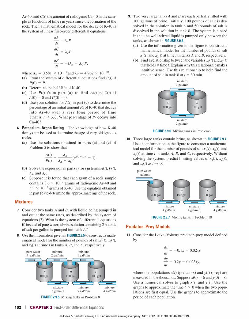
Ar-40, and C(t) the amount of radiogenic Ca-40 in the sam-ple as functions of time t in years since the formation of the rock. Then a mathematical model for the decay of K-40 is the system of linear first-order differential equations
dA
dt5 lAP
dC
dt5 lCP
dP
dt5 2(lA 1 lC)P,
where lA 5 0.581 3 10 21 0
and lC 5 4.962 3 10 21 0.
(a) From the system of differential equations find P(t) if P(0) 5 P0.
(b) Determine the half-life of K-40. (c) Use P(t) from part (a) to find A(t) and C(t) if
A(0) 5 0 and C(0) 5 0.(d) Use your solution for A(t) in part (c) to determine the
percentage of an initial amount P0 of K-40 that decays into Ar-40 over a very long period of time ( that is, t S q ) . What percentage of P0 decays into Ca-40?
6. Potassium–Argon Dating The knowledge of how K-40 decays can be used to determine the age of very old igneous rocks.(a) Use the solutions obtained in parts (a) and (c) of
Problem 5 to show that
A(t)
P(t)5
lA
lA 1 lC
[e (lA1lC)t 2 1].
(b) Solve the expression in part (a) for t in terms A(t), P(t), lA, and lC.
(c) Suppose it is found that each gram of a rock sample contains 8.6 3 10
27 grams of radiogenic Ar-40 and 5.3 3 10
26 grams of K-40. Use the equation obtained in part (b) to determine the approximate age of the rock.
Mixtures
7. Consider two tanks A and B, with liquid being pumped in and out at the same rates, as described by the system of equations (3). What is the system of differential equations if, instead of pure water, a brine solution containing 2 pounds of salt per gallon is pumped into tank A?
8. Use the information given in FIGURE 2.9.5 to construct a math-ematical model for the number of pounds of salt x1(t), x2(t), and x3(t) at time t in tanks A, B, and C, respectively.
FIGURE 2.9.5 Mixing tanks in Problem 8
A100 gal
B100 gal
C100 gal
mixture2 gal/min
pure water4 gal/min
mixture1 gal/min
mixture6 gal/min
mixture5 gal/min
mixture4 gal/min
9. Two very large tanks A and B are each partially filled with 100 gallons of brine. Initially, 100 pounds of salt is dis-solved in the solution in tank A and 50 pounds of salt is dissolved in the solution in tank B. The system is closed in that the well-stirred liquid is pumped only between the tanks, as shown in FIGURE 2.9.6.(a) Use the information given in the figure to construct a
mathematical model for the number of pounds of salt x1(t) and x2(t) at time t in tanks A and B, respectively.
(b) Find a relationship between the variables x1(t) and x2(t) that holds at time t. Explain why this relationship makes intuitive sense. Use this relationship to help find the amount of salt in tank B at t 5 30 min.
FIGURE 2.9.6 Mixing tanks in Problem 9
mixture3 gal/min
mixture2 gal/min
A100 gal
B100 gal
10. Three large tanks contain brine, as shown in FIGURE 2.9.7. Use the information in the figure to construct a mathemat-ical model for the number of pounds of salt x1(t), x2(t), and x3(t) at time t in tanks A, B, and C, respectively. Without solving the system, predict limiting values of x1(t), x2(t), and x3(t) as t S q .
FIGURE 2.9.7 Mixing tanks in Problem 10
pure water4 gal/min
mixture4 gal/min
mixture4 gal/min
mixture4 gal/min
B150 gal
A200 gal
C100 gal
Predator–Prey Models
11. Consider the Lotka–Volterra predator–prey model defined by
dx
dt5 20.1x 1 0.02xy
dy
dt5 0.2y 2 0.025xy,
where the populations x(t) (predators) and y(t) (prey) are measured in the thousands. Suppose x(0) 5 6 and y(0) 5 6. Use a numerical solver to graph x(t) and y(t). Use the graphs to approximate the time t 0 when the two popu-lations are first equal. Use the graphs to approximate the period of each population.
102 | CHAPTER 2 First-Order Differential Equations
© Jones & Bartlett Learning LLC, an Ascend Learning Company. NOT FOR SALE OR DISTRIBUTION.
© Jones & Bartlett Learning, LLCNOT FOR SALE OR DISTRIBUTION
© Jones & Bartlett Learning, LLCNOT FOR SALE OR DISTRIBUTION
© Jones & Bartlett Learning, LLCNOT FOR SALE OR DISTRIBUTION
© Jones & Bartlett Learning, LLCNOT FOR SALE OR DISTRIBUTION
© Jones & Bartlett Learning, LLCNOT FOR SALE OR DISTRIBUTION
© Jones & Bartlett Learning, LLCNOT FOR SALE OR DISTRIBUTION
© Jones & Bartlett Learning, LLCNOT FOR SALE OR DISTRIBUTION
© Jones & Bartlett Learning, LLCNOT FOR SALE OR DISTRIBUTION
© Jones & Bartlett Learning, LLCNOT FOR SALE OR DISTRIBUTION
© Jones & Bartlett Learning, LLCNOT FOR SALE OR DISTRIBUTION
© Jones & Bartlett Learning, LLCNOT FOR SALE OR DISTRIBUTION
© Jones & Bartlett Learning, LLCNOT FOR SALE OR DISTRIBUTION
© Jones & Bartlett Learning, LLCNOT FOR SALE OR DISTRIBUTION
© Jones & Bartlett Learning, LLCNOT FOR SALE OR DISTRIBUTION
© Jones & Bartlett Learning, LLCNOT FOR SALE OR DISTRIBUTION
© Jones & Bartlett Learning, LLCNOT FOR SALE OR DISTRIBUTION
© Jones & Bartlett Learning, LLCNOT FOR SALE OR DISTRIBUTION
© Jones & Bartlett Learning, LLCNOT FOR SALE OR DISTRIBUTION
© Jones & Bartlett Learning, LLCNOT FOR SALE OR DISTRIBUTION
© Jones & Bartlett Learning, LLCNOT FOR SALE OR DISTRIBUTION
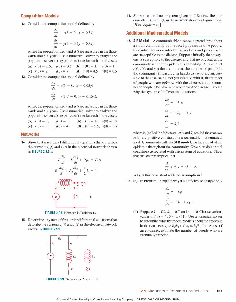
Competition Models
12. Consider the competition model defined by
dx
dt5 x(2 2 0.4x 2 0.3y)
dy
dt5 y(1 2 0.1y 2 0.3x),
where the populations x(t) and y(t) are measured in the thou-sands and t in years. Use a numerical solver to analyze the populations over a long period of time for each of the cases:
(a) x(0) 5 1.5, y(0) 5 3.5 (b) x(0) 5 1, y(0) 5 1(c) x(0) 5 2, y(0) 5 7 (d) x(0) 5 4.5, y(0) 5 0.5
13. Consider the competition model defined by
dx
dt5 x(1 2 0.1x 2 0.05y)
dy
dt5 y(1.7 2 0.1y 2 0.15x),
where the populations x(t) and y(t) are measured in the thou-sands and t in years. Use a numerical solver to analyze the populations over a long period of time for each of the cases:
(a) x(0) 5 1, y(0) 5 1 (b) x(0) 5 4, y(0) 5 10(c) x(0) 5 9, y(0) 5 4 (d) x(0) 5 5.5, y(0) 5 3.5
Networks
14. Show that a system of differential equations that describes the currents i2(t) and i3(t) in the electrical network shown in FIGURE 2.9.8 is
L
di2
dt1 L
di3
dt1 R1i2 5 E(t)
2R1
di2
dt1 R2
di3
dt1
1
C i3 5 0.
FIGURE 2.9.8 Network in Problem 14
E
L
C
i1 i2
i3 R2
R1
15. Determine a system of first-order differential equations that describe the currents i2(t) and i3(t) in the electrical network shown in FIGURE 2.9.9.
FIGURE 2.9.9 Network in Problem 15
E
i3
i2i1
R2
L2L1
R1
R3
16. Show that the linear system given in (18) describes the currents i1(t) and i2(t) in the network shown in Figure 2.9.4. [Hint: dq/dt 5 i3.]
Additional Mathematical Models
17. SIR Model A communicable disease is spread throughout a small community, with a fixed population of n people, by contact between infected individuals and people who are susceptible to the disease. Suppose initially that every-one is susceptible to the disease and that no one leaves the community while the epidemic is spreading. At time t, let s(t), i(t), and r(t) denote, in turn, the number of people in the community (measured in hundreds) who are suscep-tible to the disease but not yet infected with it, the number of people who are infected with the disease, and the num-ber of people who have recovered from the disease. Explain why the system of differential equations
ds
dt5 2k1si
di
dt5 2k2i 1 k1si
dr
dt5 k2i,
where k1 (called the infection rate) and k2 (called the removal rate) are positive constants, is a reasonable mathematical model, commonly called a SIR model, for the spread of the epidemic throughout the community. Give plausible initial conditions associated with this system of equations. Show that the system implies that
d
dt (s 1 i 1 r ) 5 0.
Why is this consistent with the assumptions?
18. (a) In Problem 17 explain why it is sufficient to analyze only
ds
dt5 2k1si
di
dt5 2k2i 1 k1si.
(b) Suppose k1 5 0.2, k2 5 0.7, and n 5 10. Choose various values of i(0) 5 i0, 0 i0 10. Use a numerical solver to determine what the model predicts about the epidemic in the two cases s0 k2/k1 and s0 # k2/k1. In the case of an epidemic, estimate the number of people who are eventually infected.
2.9 Modeling with Systems of First-Order DEs | 103
© Jones & Bartlett Learning LLC, an Ascend Learning Company. NOT FOR SALE OR DISTRIBUTION.
© Jones & Bartlett Learning, LLCNOT FOR SALE OR DISTRIBUTION
© Jones & Bartlett Learning, LLCNOT FOR SALE OR DISTRIBUTION
© Jones & Bartlett Learning, LLCNOT FOR SALE OR DISTRIBUTION
© Jones & Bartlett Learning, LLCNOT FOR SALE OR DISTRIBUTION
© Jones & Bartlett Learning, LLCNOT FOR SALE OR DISTRIBUTION
© Jones & Bartlett Learning, LLCNOT FOR SALE OR DISTRIBUTION
© Jones & Bartlett Learning, LLCNOT FOR SALE OR DISTRIBUTION
© Jones & Bartlett Learning, LLCNOT FOR SALE OR DISTRIBUTION
© Jones & Bartlett Learning, LLCNOT FOR SALE OR DISTRIBUTION
© Jones & Bartlett Learning, LLCNOT FOR SALE OR DISTRIBUTION
© Jones & Bartlett Learning, LLCNOT FOR SALE OR DISTRIBUTION
© Jones & Bartlett Learning, LLCNOT FOR SALE OR DISTRIBUTION
© Jones & Bartlett Learning, LLCNOT FOR SALE OR DISTRIBUTION
© Jones & Bartlett Learning, LLCNOT FOR SALE OR DISTRIBUTION
© Jones & Bartlett Learning, LLCNOT FOR SALE OR DISTRIBUTION
© Jones & Bartlett Learning, LLCNOT FOR SALE OR DISTRIBUTION
© Jones & Bartlett Learning, LLCNOT FOR SALE OR DISTRIBUTION
© Jones & Bartlett Learning, LLCNOT FOR SALE OR DISTRIBUTION
© Jones & Bartlett Learning, LLCNOT FOR SALE OR DISTRIBUTION
© Jones & Bartlett Learning, LLCNOT FOR SALE OR DISTRIBUTION
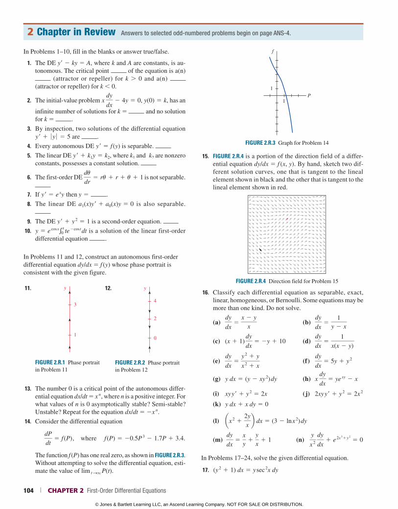
In Problems 1–10, fill in the blanks or answer true/false.
1. The DE y9 2 ky 5 A, where k and A are constants, is au-tonomous. The critical point of the equation is a(n) (attractor or repeller) for k 0 and a(n) (attractor or repeller) for k 0.
2. The initial-value problem x
dy
dx2 4y 5 0, y(0) 5 k, has an
infinite number of solutions for k 5 and no solution for k 5 .
3. By inspection, two solutions of the differential equation y r 1 0 y 0 5 5 are .
4. Every autonomous DE y r 5 f (y) is separable. 5. The linear DE y r 1 k1y 5 k2, where k1 and k2 are nonzero
constants, possesses a constant solution.
6. The first-order DE du
dr5 ru 1 r 1 u 1 1 is not separable.
7. If y r 5 e
xy then y 5 .
8. The linear DE a1(x)y r 1 a0(x)y 5 0 is also separable.
9. The DE y r 1 y 2 5 1 is a second-order equation.
10. y 5 e cos xe
x0 te
2cos t dt is a solution of the linear first-order
differential equation .
In Problems 11 and 12, construct an autonomous first-order differential equation dy/dx 5 f (y) whose phase portrait is consistent with the given figure.
11.
FIGURE 2.R.1 Phase portrait in Problem 11
y
3
1
12.
FIGURE 2.R.2 Phase portrait in Problem 12
y
4
0
2
13. The number 0 is a critical point of the autonomous differ-ential equation dx/dt 5 x n, where n is a positive integer. For what values of n is 0 asymptotically stable? Semi-stable? Unstable? Repeat for the equation dx/dt 5 2x n.
14. Consider the differential equation
dP
dt5 f (P), where f (P) 5 20.5P
3 2 1.7P 1 3.4.
The function f (P) has one real zero, as shown in FIGURE 2.R.3. Without attempting to solve the differential equation, esti-mate the value of lim t Sq P(t).
FIGURE 2.R.3 Graph for Problem 14
f
1P
1
15. FIGURE 2.R.4 is a portion of the direction field of a differ-ential equation dy/dx 5 f (x, y). By hand, sketch two dif-ferent solution curves, one that is tangent to the lineal element shown in black and the other that is tangent to the lineal element shown in red.
FIGURE 2.R.4 Direction field for Problem 15
16. Classify each differential equation as separable, exact, linear, homogeneous, or Bernoulli. Some equations may be more than one kind. Do not solve.
(a) dy
dx5
x 2 y
x (b)
dy
dx5
1y 2 x
(c) (x 1 1)
dy
dx5 2y 1 10 (d)
dy
dx5
1
x(x 2 y)
(e) dy
dx5
y 2 1 y
x 2 1 x
(f ) dy
dx5 5y 1 y
2
(g) y dx 5 (y 2 xy 2) dy (h) x
dy
dx5 ye
xy 2 x
(i) xy y r 1 y 2 5 2x ( j) 2xy y r 1 y
2 5 2x 2
(k) y dx 1 x dy 5 0
(l) ax 2 1
2y
xb dx 5 (3 2 ln x
2) dy
(m) dy
dx5
xy
1y
x1 1 (n)
y
x 2
dy
dx1 e
2x 31y
2
5 0
In Problems 17–24, solve the given differential equation.
17. (y 2 1 1) dx 5 y sec
2x dy
2 Chapter in Review Answers to selected odd-numbered problems begin on page ANS-4.
104 | CHAPTER 2 First-Order Differential Equations
© Jones & Bartlett Learning LLC, an Ascend Learning Company. NOT FOR SALE OR DISTRIBUTION.
© Jones & Bartlett Learning, LLCNOT FOR SALE OR DISTRIBUTION
© Jones & Bartlett Learning, LLCNOT FOR SALE OR DISTRIBUTION
© Jones & Bartlett Learning, LLCNOT FOR SALE OR DISTRIBUTION
© Jones & Bartlett Learning, LLCNOT FOR SALE OR DISTRIBUTION
© Jones & Bartlett Learning, LLCNOT FOR SALE OR DISTRIBUTION
© Jones & Bartlett Learning, LLCNOT FOR SALE OR DISTRIBUTION
© Jones & Bartlett Learning, LLCNOT FOR SALE OR DISTRIBUTION
© Jones & Bartlett Learning, LLCNOT FOR SALE OR DISTRIBUTION
© Jones & Bartlett Learning, LLCNOT FOR SALE OR DISTRIBUTION
© Jones & Bartlett Learning, LLCNOT FOR SALE OR DISTRIBUTION
© Jones & Bartlett Learning, LLCNOT FOR SALE OR DISTRIBUTION
© Jones & Bartlett Learning, LLCNOT FOR SALE OR DISTRIBUTION
© Jones & Bartlett Learning, LLCNOT FOR SALE OR DISTRIBUTION
© Jones & Bartlett Learning, LLCNOT FOR SALE OR DISTRIBUTION
© Jones & Bartlett Learning, LLCNOT FOR SALE OR DISTRIBUTION
© Jones & Bartlett Learning, LLCNOT FOR SALE OR DISTRIBUTION
© Jones & Bartlett Learning, LLCNOT FOR SALE OR DISTRIBUTION
© Jones & Bartlett Learning, LLCNOT FOR SALE OR DISTRIBUTION
© Jones & Bartlett Learning, LLCNOT FOR SALE OR DISTRIBUTION
© Jones & Bartlett Learning, LLCNOT FOR SALE OR DISTRIBUTION
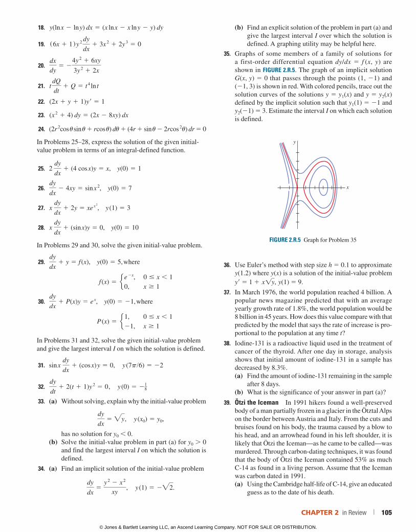
18. y(ln x 2 ln y) dx 5 (x ln x 2 x ln y 2 y) dy
19. (6x 1 1)y 2
dy
dx1 3x
2 1 2y 3 5 0
20. dx
dy5 2
4y 2 1 6xy
3y 2 1 2x
21. t
dQ
dt1 Q 5 t
4 ln t
22. (2x 1 y 1 1)y r 5 1
23. (x 2 1 4) dy 5 (2x 2 8xy) dx
24. (2r 2cos u sin u 1 r cos u) du 1 (4r 1 sin u 2 2r cos 2u) dr 5 0
In Problems 25–28, express the solution of the given initial-value problem in terms of an integral-defined function.
25. 2 dy
dx1 (4 cos x)y 5 x, y(0) 5 1
26. dy
dx2 4xy 5 sin x
2, y(0) 5 7
27. x dy
dx1 2y 5 xe
x 2
, y (1) 5 3
28. x dy
dx1 (sin x)y 5 0, y(0) 5 10
In Problems 29 and 30, solve the given initial-value problem.
29. dy
dx1 y 5 f (x), y(0) 5 5, where
f (x) 5 e e 2x, 0 # x , 1
0, x $ 1
30. dy
dx1 P(x)y 5 e
x, y(0) 5 21, where
P (x) 5 e1, 0 # x , 1
21, x $ 1
In Problems 31 and 32, solve the given initial-value problem and give the largest interval I on which the solution is defined.
31. sin x dy
dx1 (cos x) y 5 0, y (7p/6) 5 22
32. dy
dt1 2(t 1 1)y
2 5 0, y (0) 5 218
33. (a) Without solving, explain why the initial-value problem
dy
dx5 "y, y (x0) 5 y0,
has no solution for y0 0.(b) Solve the initial-value problem in part (a) for y0 0
and find the largest interval I on which the solution is defined.
34. (a) Find an implicit solution of the initial-value problem
dy
dx5
y 2 2 x
2
xy, y (1) 5 2"2.
(b) Find an explicit solution of the problem in part (a) and give the largest interval I over which the solution is defined. A graphing utility may be helpful here.
35. Graphs of some members of a family of solutions for a first-order differential equation dy/dx 5 f (x, y) are shown in FIGURE 2.R.5. The graph of an implicit solution G(x, y) 5 0 that passes through the points (1, 21) and (21, 3) is shown in red. With colored pencils, trace out the solution curves of the solutions y 5 y1(x) and y 5 y2(x) defined by the implicit solution such that y1(1) 5 21 and y2(21) 5 3. Estimate the interval I on which each solution is defined.
FIGURE 2.R.5 Graph for Problem 35
y
x
36. Use Euler’s method with step size h 5 0.1 to approximate y(1.2) where y(x) is a solution of the initial-value problem y9 5 1 1 x!y, y(1) 5 9.
37. In March 1976, the world population reached 4 billion. A popular news magazine predicted that with an average yearly growth rate of 1.8%, the world population would be 8 billion in 45 years. How does this value compare with that predicted by the model that says the rate of increase is pro-portional to the population at any time t?
38. Iodine-131 is a radioactive liquid used in the treatment of cancer of the thyroid. After one day in storage, analysis shows that initial amount of iodine-131 in a sample has decreased by 8.3%.(a) Find the amount of iodine-131 remaining in the sample
after 8 days.(b) What is the significance of your answer in part (a)?
39. Ötzi the Iceman In 1991 hikers found a well-preserved body of a man partially frozen in a glacier in the Ötztal Alps on the border between Austria and Italy. From the cuts and bruises found on his body, the trauma caused by a blow to his head, and an arrowhead found in his left shoulder, it is likely that Ötzi the Iceman—as he came to be called—was murdered. Through carbon-dating techniques, it was found that the body of Ötzi the Iceman contained 53% as much C-14 as found in a living person. Assume that the Iceman was carbon dated in 1991.(a) Using the Cambridge half-life of C-14, give an educated
guess as to the date of his death.
CHAPTER 2 in Review | 105
© Jones & Bartlett Learning LLC, an Ascend Learning Company. NOT FOR SALE OR DISTRIBUTION.
© Jones & Bartlett Learning, LLCNOT FOR SALE OR DISTRIBUTION
© Jones & Bartlett Learning, LLCNOT FOR SALE OR DISTRIBUTION
© Jones & Bartlett Learning, LLCNOT FOR SALE OR DISTRIBUTION
© Jones & Bartlett Learning, LLCNOT FOR SALE OR DISTRIBUTION
© Jones & Bartlett Learning, LLCNOT FOR SALE OR DISTRIBUTION
© Jones & Bartlett Learning, LLCNOT FOR SALE OR DISTRIBUTION
© Jones & Bartlett Learning, LLCNOT FOR SALE OR DISTRIBUTION
© Jones & Bartlett Learning, LLCNOT FOR SALE OR DISTRIBUTION
© Jones & Bartlett Learning, LLCNOT FOR SALE OR DISTRIBUTION
© Jones & Bartlett Learning, LLCNOT FOR SALE OR DISTRIBUTION
© Jones & Bartlett Learning, LLCNOT FOR SALE OR DISTRIBUTION
© Jones & Bartlett Learning, LLCNOT FOR SALE OR DISTRIBUTION
© Jones & Bartlett Learning, LLCNOT FOR SALE OR DISTRIBUTION
© Jones & Bartlett Learning, LLCNOT FOR SALE OR DISTRIBUTION
© Jones & Bartlett Learning, LLCNOT FOR SALE OR DISTRIBUTION
© Jones & Bartlett Learning, LLCNOT FOR SALE OR DISTRIBUTION
© Jones & Bartlett Learning, LLCNOT FOR SALE OR DISTRIBUTION
© Jones & Bartlett Learning, LLCNOT FOR SALE OR DISTRIBUTION
© Jones & Bartlett Learning, LLCNOT FOR SALE OR DISTRIBUTION
© Jones & Bartlett Learning, LLCNOT FOR SALE OR DISTRIBUTION
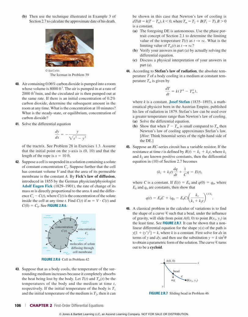
(b) Then use the technique illustrated in Example 3 of Section 2.7 to calculate the approximate date of his death.
© dpa/Corbis
The Iceman in Problem 39
40. Air containing 0.06% carbon dioxide is pumped into a room whose volume is 8000 ft 3. The air is pumped in at a rate of 2000 ft 3/min, and the circulated air is then pumped out at the same rate. If there is an initial concentration of 0.2% carbon dioxide, determine the subsequent amount in the room at any time. What is the concentration at 10 minutes? What is the steady-state, or equilibrium, concentration of carbon dioxide?
41. Solve the differential equation
dy
dx5 2
y
"s 2 2 y
2
of the tractrix. See Problem 28 in Exercises 1.3. Assume that the initial point on the y-axis is (0, 10) and that the length of the rope is x 5 10 ft.
42. Suppose a cell is suspended in a solution containing a solute of constant concentration Cs. Suppose further that the cell has constant volume V and that the area of its permeable membrane is the constant A. By Fick’s law of diffusion, introduced in 1855 by the German physician/physiologist Adolf Eugen Fick (1829–1901), the rate of change of its mass m is directly proportional to the area A and the differ-ence Cs 2 C(t), where C(t) is the concentration of the solute inside the cell at any time t. Find C(t) if m 5 V ? C(t) and C(0) 5 C0. See FIGURE 2.R.6.
FIGURE 2.R.6 Cell in Problem 42
concentrationCs
concentrationC (t)
molecules of solutediffusing through
cell membrane
43. Suppose that as a body cools, the temperature of the sur-rounding medium increases because it completely absorbs the heat being lost by the body. Let T(t) and Tm(t) be the temperatures of the body and the medium at time t, respectively. If the initial temperature of the body is T1 and the initial temperature of the medium is T2, then it can
be shown in this case that Newton’s law of cooling is d T/dt 5 k(T 2 Tm), k 0, where Tm 5 T2 1 B(T1 2 T), B 0 is a constant.(a) The foregoing DE is autonomous. Use the phase por-
trait concept of Section 2.1 to determine the limiting value of the temperature T(t) as t S q . What is the limiting value of Tm(t) as t S q?
(b) Verify your answers in part (a) by actually solving the differential equation.
(c) Discuss a physical interpretation of your answers in part (a).
44. According to Stefan’s law of radiation, the absolute tem-perature T of a body cooling in a medium at constant tem-perature Tm is given by
dT
dt5 k(T
4 2 T
4m) ,
where k is a constant. Josef Stefan (1835–1893), a math-ematical physicist born in the Austrian Empire, published his law of radiation in 1879. Stefan’s law can be used over a greater temperature range than Newton’s law of cooling.(a) Solve the differential equation.(b) Show that when T 2 Tm is small compared to Tm then
Newton’s law of cooling approximates Stefan’s law. [Hint: Think binomial series of the right-hand side of the DE.]
45. Suppose an RC-series circuit has a variable resistor. If the resistance at time t is defined by R(t) 5 k1 1 k2t, where k1 and k2 are known positive constants, then the differential equation in (10) of Section 2.7 becomes
(k1 1 k2t)
dq
dt1
1
C q 5 E(t),
where C is a constant. If E(t) 5 E0 and q(0) 5 q0, where E0 and q0 are constants, then show that
q(t) 5 E0C 1 (q0 2 E0C)a k1
k1 1 k2tb
1>Ck2
.
46. A classical problem in the calculus of variations is to find the shape of a curve such that a bead, under the influence of gravity, will slide from point A(0, 0) to point B(x1, y1) in the least time. See FIGURE 2.R.7. It can be shown that a non-linear differential equation for the shape y(x) of the path is y[1 1 (y9) 2] 5 k, where k is a constant. First solve for dx in terms of y and dy, and then use the substitution y 5 k sin2u to obtain a parametric form of the solution. The curve turns out to be a cycloid.
FIGURE 2.R.7 Sliding bead in Problem 46
bead
mg
y
x
B(x1, y1)
A(0, 0)
106 | CHAPTER 2 First-Order Differential Equations
© Jones & Bartlett Learning LLC, an Ascend Learning Company. NOT FOR SALE OR DISTRIBUTION.
© Jones & Bartlett Learning, LLCNOT FOR SALE OR DISTRIBUTION
© Jones & Bartlett Learning, LLCNOT FOR SALE OR DISTRIBUTION
© Jones & Bartlett Learning, LLCNOT FOR SALE OR DISTRIBUTION
© Jones & Bartlett Learning, LLCNOT FOR SALE OR DISTRIBUTION
© Jones & Bartlett Learning, LLCNOT FOR SALE OR DISTRIBUTION
© Jones & Bartlett Learning, LLCNOT FOR SALE OR DISTRIBUTION
© Jones & Bartlett Learning, LLCNOT FOR SALE OR DISTRIBUTION
© Jones & Bartlett Learning, LLCNOT FOR SALE OR DISTRIBUTION
© Jones & Bartlett Learning, LLCNOT FOR SALE OR DISTRIBUTION
© Jones & Bartlett Learning, LLCNOT FOR SALE OR DISTRIBUTION
© Jones & Bartlett Learning, LLCNOT FOR SALE OR DISTRIBUTION
© Jones & Bartlett Learning, LLCNOT FOR SALE OR DISTRIBUTION
© Jones & Bartlett Learning, LLCNOT FOR SALE OR DISTRIBUTION
© Jones & Bartlett Learning, LLCNOT FOR SALE OR DISTRIBUTION
© Jones & Bartlett Learning, LLCNOT FOR SALE OR DISTRIBUTION
© Jones & Bartlett Learning, LLCNOT FOR SALE OR DISTRIBUTION
© Jones & Bartlett Learning, LLCNOT FOR SALE OR DISTRIBUTION
© Jones & Bartlett Learning, LLCNOT FOR SALE OR DISTRIBUTION
© Jones & Bartlett Learning, LLCNOT FOR SALE OR DISTRIBUTION
© Jones & Bartlett Learning, LLCNOT FOR SALE OR DISTRIBUTION
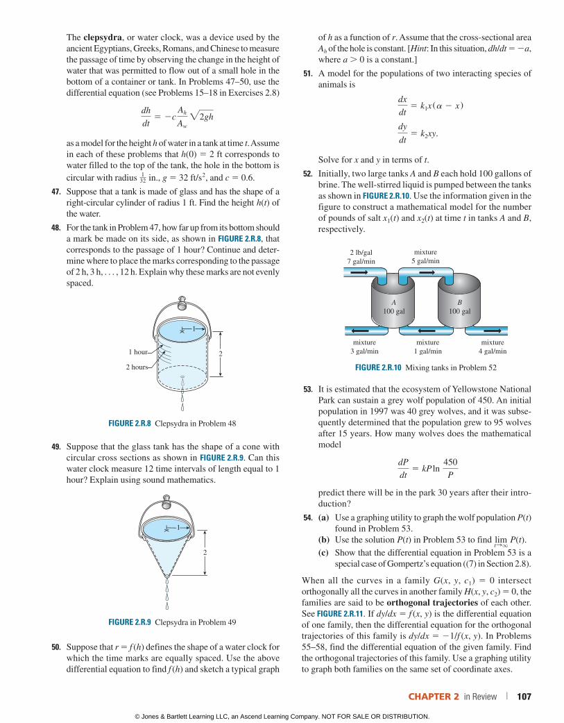
The clepsydra, or water clock, was a device used by the ancient Egyptians, Greeks, Romans, and Chinese to measure the passage of time by observing the change in the height of water that was permitted to flow out of a small hole in the bottom of a container or tank. In Problems 47–50, use the differential equation (see Problems 15–18 in Exercises 2.8)
dh
dt5 2c
Ah
Aw
"2gh
as a model for the height h of water in a tank at time t. Assume in each of these problems that h(0) 5 2 ft corresponds to water filled to the top of the tank, the hole in the bottom is circular with radius 1
32 in., g 5 32 ft/s 2, and c 5 0.6.
47. Suppose that a tank is made of glass and has the shape of a right-circular cylinder of radius 1 ft. Find the height h(t) of the water.
48. For the tank in Problem 47, how far up from its bottom should a mark be made on its side, as shown in FIGURE 2.R.8, that corresponds to the passage of 1 hour? Continue and deter-mine where to place the marks corresponding to the passage of 2 h, 3 h, . . . , 12 h. Explain why these marks are not evenly spaced.
FIGURE 2.R.8 Clepsydra in Problem 48
1 hour
2 hours
2
1
49. Suppose that the glass tank has the shape of a cone with circular cross sections as shown in FIGURE 2.R.9. Can this water clock measure 12 time intervals of length equal to 1 hour? Explain using sound mathematics.
2
1
FIGURE 2.R.9 Clepsydra in Problem 49
50. Suppose that r 5 f (h) defines the shape of a water clock for which the time marks are equally spaced. Use the above differential equation to find f (h) and sketch a typical graph
of h as a function of r. Assume that the cross-sectional area Ah of the hole is constant. [Hint: In this situation, dh/dt 5 2a, where a 0 is a constant.]
51. A model for the populations of two interacting species of animals is
dx
dt5 k1x(a 2 x)
dy
dt5 k2xy.
Solve for x and y in terms of t.
52. Initially, two large tanks A and B each hold 100 gallons of brine. The well-stirred liquid is pumped between the tanks as shown in FIGURE 2.R.10. Use the information given in the figure to construct a mathematical model for the number of pounds of salt x1(t) and x2(t) at time t in tanks A and B, respectively.
FIGURE 2.R.10 Mixing tanks in Problem 52
A100 gal
B100 gal
2 lb/gal7 gal/min
mixture5 gal/min
mixture1 gal/min
mixture3 gal/min
mixture4 gal/min
53. It is estimated that the ecosystem of Yellowstone National Park can sustain a grey wolf population of 450. An initial population in 1997 was 40 grey wolves, and it was subse-quently determined that the population grew to 95 wolves after 15 years. How many wolves does the mathematical model
dP
dt5 kP ln
450
P
predict there will be in the park 30 years after their intro-duction?
54. (a) Use a graphing utility to graph the wolf population P(t) found in Problem 53.
(b) Use the solution P(t) in Problem 53 to find limtSq
P(t).
(c) Show that the differential equation in Problem 53 is a special case of Gompertz’s equation ((7) in Section 2.8).
When all the curves in a family G(x, y, c1) 5 0 intersect orthogonally all the curves in another family H(x, y, c2) 5 0, the families are said to be orthogonal trajectories of each other. See FIGURE 2.R.11. If dy/dx 5 f (x, y) is the differential equation of one family, then the differential equation for the orthogonal trajectories of this family is dy/dx 5 21/f (x, y). In Problems 55–58, find the differential equation of the given family. Find the orthogonal trajectories of this family. Use a graphing utility to graph both families on the same set of coordinate axes.
CHAPTER 2 in Review | 107
© Jones & Bartlett Learning LLC, an Ascend Learning Company. NOT FOR SALE OR DISTRIBUTION.
© Jones & Bartlett Learning, LLCNOT FOR SALE OR DISTRIBUTION
© Jones & Bartlett Learning, LLCNOT FOR SALE OR DISTRIBUTION
© Jones & Bartlett Learning, LLCNOT FOR SALE OR DISTRIBUTION
© Jones & Bartlett Learning, LLCNOT FOR SALE OR DISTRIBUTION
© Jones & Bartlett Learning, LLCNOT FOR SALE OR DISTRIBUTION
© Jones & Bartlett Learning, LLCNOT FOR SALE OR DISTRIBUTION
© Jones & Bartlett Learning, LLCNOT FOR SALE OR DISTRIBUTION
© Jones & Bartlett Learning, LLCNOT FOR SALE OR DISTRIBUTION
© Jones & Bartlett Learning, LLCNOT FOR SALE OR DISTRIBUTION
© Jones & Bartlett Learning, LLCNOT FOR SALE OR DISTRIBUTION
© Jones & Bartlett Learning, LLCNOT FOR SALE OR DISTRIBUTION
© Jones & Bartlett Learning, LLCNOT FOR SALE OR DISTRIBUTION
© Jones & Bartlett Learning, LLCNOT FOR SALE OR DISTRIBUTION
© Jones & Bartlett Learning, LLCNOT FOR SALE OR DISTRIBUTION
© Jones & Bartlett Learning, LLCNOT FOR SALE OR DISTRIBUTION
© Jones & Bartlett Learning, LLCNOT FOR SALE OR DISTRIBUTION
© Jones & Bartlett Learning, LLCNOT FOR SALE OR DISTRIBUTION
© Jones & Bartlett Learning, LLCNOT FOR SALE OR DISTRIBUTION
© Jones & Bartlett Learning, LLCNOT FOR SALE OR DISTRIBUTION
© Jones & Bartlett Learning, LLCNOT FOR SALE OR DISTRIBUTION
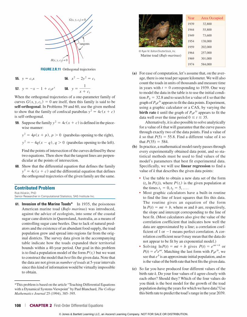
FIGURE 2.R.11 Orthogonal trajectories
tangents
G(x, y, c1) = 0
H(x, y, c2) = 0
55. y 5 c1x 56. x 2 2 2y
2 5 c1
57. y 5 2x 2 1 1 c1e x 58. y 5
1
x 1 c1
When the orthogonal trajectories of a one-parameter family of curves G (x, y, c1 ) 5 0 are itself, then this family is said to be self-orthogonal. In Problems 59 and 60, use the given method to show that the family of confocal parabolas y
2 5 4c(x 1 c) is self-orthogonal.
59. Suppose the family y 2 5 4c(x 1 c) is defined in the piece-
wise manner:
y 2 5 4p(x 1 p) , p . 0 (parabolas opening to the right),
y 2 52 4q(x 2 q) , q . 0 (parabolas opening to the left).
Find the points of intersection of the curves defined by these two equations. Then show that the tangent lines are perpen-dicular at the points of intersection.
60. Show that the differential equation that defines the family y
2 5 4c(x 1 c) and the differential equation that defines the orthogonal trajectories of the given family are the same.
Contributed ProblemRick Wicklin, PhD Senior Researcher in Computational Statistics, SAS Institute Inc.
61. Invasion of the Marine Toads* In 1935, the poisonous American marine toad (Bufo marinus) was introduced, against the advice of ecologists, into some of the coastal sugar cane districts in Queensland, Australia, as a means of controlling sugar cane beetles. Due to lack of natural pred-ators and the existence of an abundant food supply, the toad population grew and spread into regions far from the orig-inal districts. The survey data given in the accompanying table indicate how the toads expanded their territorial bounds within a 40-year period. Our goal in this problem is to find a population model of the form P( ti) but we want to construct the model that best fits the given data. Note that the data are not given as number of toads at 5-year intervals since this kind of information would be virtually impossible to obtain.
Year Area Occupied
1939 32,800
1944 55,800
1949 73,600
1954 138,000
1959 202,000
1964 257,000
1969 301,000
1974 584,000
© Ryan M. Bolton/ShutterStock, Inc.
Marine toad (Bufo marinus)
(a) For ease of computation, let’s assume that, on the aver-age, there is one toad per square kilometer. We will also count the toads in units of thousands and measure time in years with t 5 0 corresponding to 1939. One way to model the data in the table is to use the initial condi-tion P0 5 32.8 and to search for a value of k so that the graph of P0e
kt appears to fit the data points. Experiment, using a graphic calculator or a CAS, by varying the birth rate k until the graph of P0e
kt appears to fit the data well over the time period 0 # t # 35.
Alternatively, it is also possible to solve analytically for a value of k that will guarantee that the curve passes through exactly two of the data points. Find a value of k so that P(5) 5 55.8. Find a different value of k so that P(35) 5 584.
(b) In practice, a mathematical model rarely passes through every experimentally obtained data point, and so sta-tistical methods must be used to find values of the model’s parameters that best fit experimental data. Specifically, we will use linear regression to find a value of k that describes the given data points:
• Use the table to obtain a new data set of the form (ti, ln P(ti)), where P( ti) is the given population at the times t1 5 0, t2 5 5, . . . .
• Most graphic calculators have a built-in routine to find the line of least squares that fits this data. The routine gives an equation of the form ln P(t) 5 mt 1 b, where m and b are, respectively, the slope and intercept corresponding to the line of best fit. (Most calculators also give the value of the correlation coefficient that indicates how well the data are approximated by a line; a correlation coef-ficient of 1 or 21 means perfect correlation. A cor-relation coefficient near 0 may mean that the data do not appear to be fit by an exponential model.)
• Solving ln P(t) 5 mt 1 b gives P(t) 5 e mt1b or
P(t) 5 ebemt. Matching the last form with P0e kt, we
see that e b is an approximate initial population, and m
is the value of the birth rate that best fits the given data.
(c) So far you have produced four different values of the birth rate k. Do your four values of k agree closely with each other? Should they? Which of the four values do you think is the best model for the growth of the toad population during the years for which we have data? Use this birth rate to predict the toad’s range in the year 2039.
*This problem is based on the article “Teaching Differential Equations with a Dynamical Systems Viewpoint” by Paul Blanchard, The College Mathematics Journal 25 (1994), 385–395.
108 | CHAPTER 2 First-Order Differential Equations
© Jones & Bartlett Learning LLC, an Ascend Learning Company. NOT FOR SALE OR DISTRIBUTION.
© Jones & Bartlett Learning, LLCNOT FOR SALE OR DISTRIBUTION
© Jones & Bartlett Learning, LLCNOT FOR SALE OR DISTRIBUTION
© Jones & Bartlett Learning, LLCNOT FOR SALE OR DISTRIBUTION
© Jones & Bartlett Learning, LLCNOT FOR SALE OR DISTRIBUTION
© Jones & Bartlett Learning, LLCNOT FOR SALE OR DISTRIBUTION
© Jones & Bartlett Learning, LLCNOT FOR SALE OR DISTRIBUTION
© Jones & Bartlett Learning, LLCNOT FOR SALE OR DISTRIBUTION
© Jones & Bartlett Learning, LLCNOT FOR SALE OR DISTRIBUTION
© Jones & Bartlett Learning, LLCNOT FOR SALE OR DISTRIBUTION
© Jones & Bartlett Learning, LLCNOT FOR SALE OR DISTRIBUTION
© Jones & Bartlett Learning, LLCNOT FOR SALE OR DISTRIBUTION
© Jones & Bartlett Learning, LLCNOT FOR SALE OR DISTRIBUTION
© Jones & Bartlett Learning, LLCNOT FOR SALE OR DISTRIBUTION
© Jones & Bartlett Learning, LLCNOT FOR SALE OR DISTRIBUTION
© Jones & Bartlett Learning, LLCNOT FOR SALE OR DISTRIBUTION
© Jones & Bartlett Learning, LLCNOT FOR SALE OR DISTRIBUTION
© Jones & Bartlett Learning, LLCNOT FOR SALE OR DISTRIBUTION
© Jones & Bartlett Learning, LLCNOT FOR SALE OR DISTRIBUTION
© Jones & Bartlett Learning, LLCNOT FOR SALE OR DISTRIBUTION
© Jones & Bartlett Learning, LLCNOT FOR SALE OR DISTRIBUTION

Given that the area of Australia is 7,619,000 km 2, how confident are you of this prediction? Explain your reasoning.
62. Invasion of the Marine Toads—Continued In part (a) of Problem 61, we made the assumption that there was an av-erage of one toad per square kilometer. But suppose we are wrong and there were actually an average of two toads per
square kilometer. As before, solve analytically for a value of k that will guarantee that the curve passes through exactly two of the data points. In particular, if we now assume that P(0) 5 65.6, find a value of k so that P(5) 5 111.6, and a different value of k so that P(35) 5 1168. How do these values of k compare with the values you found previously? What does this tell us? Discuss the importance of knowing the exact average density of the toad population.
Chapter Opener: © Songquan Deng/Shutterstock
CHAPTER 2 in Review | 109
© Jones & Bartlett Learning LLC, an Ascend Learning Company. NOT FOR SALE OR DISTRIBUTION.
© Jones & Bartlett Learning, LLCNOT FOR SALE OR DISTRIBUTION
© Jones & Bartlett Learning, LLCNOT FOR SALE OR DISTRIBUTION
© Jones & Bartlett Learning, LLCNOT FOR SALE OR DISTRIBUTION
© Jones & Bartlett Learning, LLCNOT FOR SALE OR DISTRIBUTION
© Jones & Bartlett Learning, LLCNOT FOR SALE OR DISTRIBUTION
© Jones & Bartlett Learning, LLCNOT FOR SALE OR DISTRIBUTION
© Jones & Bartlett Learning, LLCNOT FOR SALE OR DISTRIBUTION
© Jones & Bartlett Learning, LLCNOT FOR SALE OR DISTRIBUTION
© Jones & Bartlett Learning, LLCNOT FOR SALE OR DISTRIBUTION
© Jones & Bartlett Learning, LLCNOT FOR SALE OR DISTRIBUTION
© Jones & Bartlett Learning, LLCNOT FOR SALE OR DISTRIBUTION
© Jones & Bartlett Learning, LLCNOT FOR SALE OR DISTRIBUTION
© Jones & Bartlett Learning, LLCNOT FOR SALE OR DISTRIBUTION
© Jones & Bartlett Learning, LLCNOT FOR SALE OR DISTRIBUTION
© Jones & Bartlett Learning, LLCNOT FOR SALE OR DISTRIBUTION
© Jones & Bartlett Learning, LLCNOT FOR SALE OR DISTRIBUTION
© Jones & Bartlett Learning, LLCNOT FOR SALE OR DISTRIBUTION
© Jones & Bartlett Learning, LLCNOT FOR SALE OR DISTRIBUTION
© Jones & Bartlett Learning, LLCNOT FOR SALE OR DISTRIBUTION
© Jones & Bartlett Learning, LLCNOT FOR SALE OR DISTRIBUTION
Related Documents