First measurements of radiative B decays in LHCb Memòria per a optar al títol de doctor en Física per Albert Puig Navarro Febrer de 2012 Dir. Ricardo Graciani Díaz Programa de Doctorat de Física de l’EEES

Welcome message from author
This document is posted to help you gain knowledge. Please leave a comment to let me know what you think about it! Share it to your friends and learn new things together.
Transcript
First measurements of radiative Bdecays in LHCb
Memòria per a optar al títol de doctor en Física
per
Albert Puig Navarro
Febrer de 2012
Dir. Ricardo Graciani Díaz
Programa de Doctorat de Física de l’EEES

Contents
Resum v
Summary xvii
Introduction 1
1. Radiative decays of B mesons 31.1. The Standard Model . . . . . . . . . . . . . . . . . . . . . . . . . . . . . 31.2. Radiative B Decays in the Standard Model . . . . . . . . . . . . . . . . 141.3. Current theoretical and experimental status . . . . . . . . . . . . . . . . 20
2. CERN and the LHC 232.1. The European Organization for Nuclear Research (CERN) . . . . . . . . 232.2. The Large Hadron Collider . . . . . . . . . . . . . . . . . . . . . . . . . 262.3. The experiments at the LHC . . . . . . . . . . . . . . . . . . . . . . . . 292.4. Computing resources for the LHC . . . . . . . . . . . . . . . . . . . . . . 31
3. The LHCb experiment 333.1. LHCb 2011 running conditions . . . . . . . . . . . . . . . . . . . . . . . 353.2. Detector layout . . . . . . . . . . . . . . . . . . . . . . . . . . . . . . . . 363.3. The Tracking System . . . . . . . . . . . . . . . . . . . . . . . . . . . . . 403.4. The Particle Identification System . . . . . . . . . . . . . . . . . . . . . 503.5. The Trigger System . . . . . . . . . . . . . . . . . . . . . . . . . . . . . 643.6. The Online System . . . . . . . . . . . . . . . . . . . . . . . . . . . . . . 683.7. Computing and resources . . . . . . . . . . . . . . . . . . . . . . . . . . 69
4. Trigger strategies for radiative B decays at LHCb 754.1. Data samples . . . . . . . . . . . . . . . . . . . . . . . . . . . . . . . . . 754.2. Methods for determining trigger efficiencies . . . . . . . . . . . . . . . . 764.3. L0 channels . . . . . . . . . . . . . . . . . . . . . . . . . . . . . . . . . . 784.4. HLT1 lines . . . . . . . . . . . . . . . . . . . . . . . . . . . . . . . . . . 794.5. HLT2 lines . . . . . . . . . . . . . . . . . . . . . . . . . . . . . . . . . . 814.6. Exclusive strategy . . . . . . . . . . . . . . . . . . . . . . . . . . . . . . 924.7. Inclusive strategy . . . . . . . . . . . . . . . . . . . . . . . . . . . . . . . 944.8. Performance in 2011 . . . . . . . . . . . . . . . . . . . . . . . . . . . . . 954.9. Prospects for 2012 . . . . . . . . . . . . . . . . . . . . . . . . . . . . . . 100
iii
Contents
5. Measurement of the ratio B(B0→K∗0γ)/B(B0s →ϕγ) 107
5.1. Data samples and software versions . . . . . . . . . . . . . . . . . . . . . 1085.2. Event selection . . . . . . . . . . . . . . . . . . . . . . . . . . . . . . . . 1105.3. Signal shape . . . . . . . . . . . . . . . . . . . . . . . . . . . . . . . . . . 1155.4. Background composition . . . . . . . . . . . . . . . . . . . . . . . . . . . 1215.5. Fit . . . . . . . . . . . . . . . . . . . . . . . . . . . . . . . . . . . . . . . 1345.6. Extraction of the ratio of branching fractions . . . . . . . . . . . . . . . 1415.7. Result . . . . . . . . . . . . . . . . . . . . . . . . . . . . . . . . . . . . . 155
6. Conclusions 159
A. Helicity formalism and angular distributions 161A.1. The helicity formalism . . . . . . . . . . . . . . . . . . . . . . . . . . . . 161A.2. Angular distributions in two-body decays . . . . . . . . . . . . . . . . . 164
B. Isospin-conserving decay of the K∗0 vector meson 169
iv
Resum
El Model Estàndard (ME) és la descripció més fonamental de la matèria i les sevesinteraccions, i la seva consistència ha estat validada per un gran nombre d’experiments.Malgrat el seu èxit, el ME no incorpora elements com la gravetat, l’energia fosca, lamatèria fosca o les (ja observades) oscil · lacions de neutrins.
Els hadrons B constitueixen un excel · lent banc de proves per a mesurar paràmetresdel ME tals com els elements de la matriu CKM or la violació de simetria CP . A més,els corrents neutres amb canvi de sabor (CNCS), que no són possibles a nivell arbrei, per tant, són molt sensibles a noves partícules massives, poden ser utilitzats com aproves per a la recerca de física més enllà del Model Estàndard. Les desintegracionsradiatives d’hadrons B són un bon exemple d’aquest tipus de corrent. L’experimentLHCb, un dels sis experiments del Gran Col · lidor d’Hadrons, està dedicat a l’estudide la violació de CP i de les desintegracions rares dels hadrons B.
Per tal d’estudiar desintegracions radiatives d’hadrons B a LHCb, és necessaridistingir-les i salvar-les d’entre la gran quantitat d’esdeveniments de fons produïtsa l’LHC, la majoria del quals són rebutjats pel sistema de trigger de l’experiment in-stants després que s’hagin produït. Aquest document descriu el procés de redissenyi optimització dels algoritmes de trigger ja existents per a aquest tipus de desinte-gracions, i la introducció de nous per tal d’ampliar el programa de desintegracionsradiatives d’LHCb a canals no previstos inicialment.
A més, aquest document descriu la mesura de la raó entre les fraccionsd’embrancament B de B0→K∗0γ i B0
s →ϕγ a partir d’1.0 fb−1 de dades recollides el2011. El resultat obtingut és compatible amb la predicció teòrica i amb les mesuresanteriors, i s’ha fet servir, juntament amb la mitjana mundial de B(B0→K∗0γ), per aobtenir la mesura més precisa de B(B0
s →ϕγ).
Desintegracions radiatives de mesons B
En el Model Estàndard, els CNCS del tipus b→ sγ són únicament possibles a travésde transicions electromagnètiques a un loop, dominades per un quark top virtual ques’aparella amb un bosó W . Extensions del ME prediuen partícules addicionals que,circulant en el loop, poden introduir efectes mesurables a la dinàmica de la transició.
Els processos a nivell de quarks tals com b→ sγ no es poden observar directamentperquè la interacció forta fa que es formin hadrons a partir dels quarks. Aquest procésd’hadronització es majoritàriament no pertorbatiu, i per tant provoca incerteses sig-nificants en el càlcul de les fraccions d’embrancament exclusives.
Les prediccions teòriques es realitzen separant les parts pertorbativa i no pertorbativadels elements de matriu hadrònics mitjançant SCET (Soft Collinear Effective Theory).
v
Les contribucions pertorbatives són conegudes parcialment fins a NNLO (Next-to-Next-Leading Order), i el càlcul de les contribucions no pertorbatives s’efectua mitjançantregles de suma de QCD (Quantum Chromodynamics) sobre el con de llum. La prediccióper a les B de B0 →K∗0γ i B0
s → ϕγ és (4.3 ± 1.4) × 10−5, i el càlcul de la seva raódóna 1.0± 0.2 a causa de la cancel · lació d’algunes incerteses.
Les desintegracions radiatives del mesó B0 van ser observades per primer cop perla col · laboració CLEO, l’any 1993, a través del mode B0 → K∗0γ. El 2007, lacol · laboració Belle va anunciar la primera observació de la desintegració anàloga delmesó B0
s , B0s → ϕγ. Els valors measurats per a B(B0 → K∗0γ) i B(B0
s → ϕγ) són(4.33±0.15) ×10−5 i (5.7+2.1
−1.8) ×10−5, respectivament. Aquest valors són compatiblesamb les prediccions teòriques obtingues de càlculs a NNLO. El valor experimental dela raó de B(B0 → K∗0γ) entre B(B0
s → ϕγ) és 0.7 ± 0.3, també compatible amb lapredicció del ME.
El CERN i l’LHC
L’Organitació Europea per a la Recerca Nuclear, coneguda com a CERN, és el labora-tori de física de partícules més gran del món, i està situat a la frontera franco-suïssa,prop de Ginebra. Actualment compta amb 20 Estats Membres, però molts països noEuropeus es troben involucrats de maneres diverses. En total, uns 10,000 científics de608 instituts i universitats de 113 països, la meitat dels físics de partícules del món,utilitzen les seves instal · lacions.
Al CERN s’hi han fet un gran nombre de descobriments, com per exemple els bosonsW± i Z. Al llarg de la seva història, diversos científics que treballaven allà han estatguardonats amb premis Nobel de física. A més, el laboratori ha estat la seu de diversoscol · lidors de particules, incloent el primer col · lidor protó-protó, el primer col · lidorprotó-antiprotó i, actualment, el col · lidor més potent del món, el Gran Col · lidord’Hadrons (Large Hadron Collider, LHC).
L’LHC és un col · lidor protó-protó dissenyat per a funcionar amb una energia alcentre de masses de 14TeV i està instal · lat al túnel circular de 27 km de perímetreque antigament havia contingut l’accelerador LEP.
Al voltant de quatre punts d’interacció de l’anell de l’LHC es troben situats quatregrans detectors i dos petits experiments, que són:
ALICE, dedicat a l’estudi de la física derivada de la col · lisió de nuclis pesants(Pb-Pb).
ATLAS, un experiment de propòsit general construït amb l’objectiu de posar aprova el ME a l’escala del TeV i de buscar el bosó de Higgs i física més enllà delModel Estàndard.
CMS, un altre experiment de propòsit general destinat a l’estudi del mecanismede la ruptura de simetria electrofeble, de la qual es considera responsable elmecanisme de Higgs, i a l’estudi del ME a energies per sobre d’1TeV.
LHCb, dedicat a l’estudi de la violació de CP i de les desintegracions rares departícules amb contingut de quark b.
LHCf, un petit experiment dissenyat per a mesurar la secció eficaç de pionsneutres i neutrons a angles molt petits.
vi
Resum
TOTEM, que intenta mesurar la secció eficaç pp amb un mètode independent dela lluminositat, basat en el Teorema Òptic.
L’experiment LHCb
L’experiment LHCb està dedicat a l’estudi de la física dels quarks massius a l’LHC. Elseu principal objectiu és la mesura de la violació de CP i de les desintegracions raresd’hadrons b i . Està situat al Punt d’Interacció 8 de l’LHC, antigament utilitzat perl’experiment DELPHI de LEP.
Disseny del detector
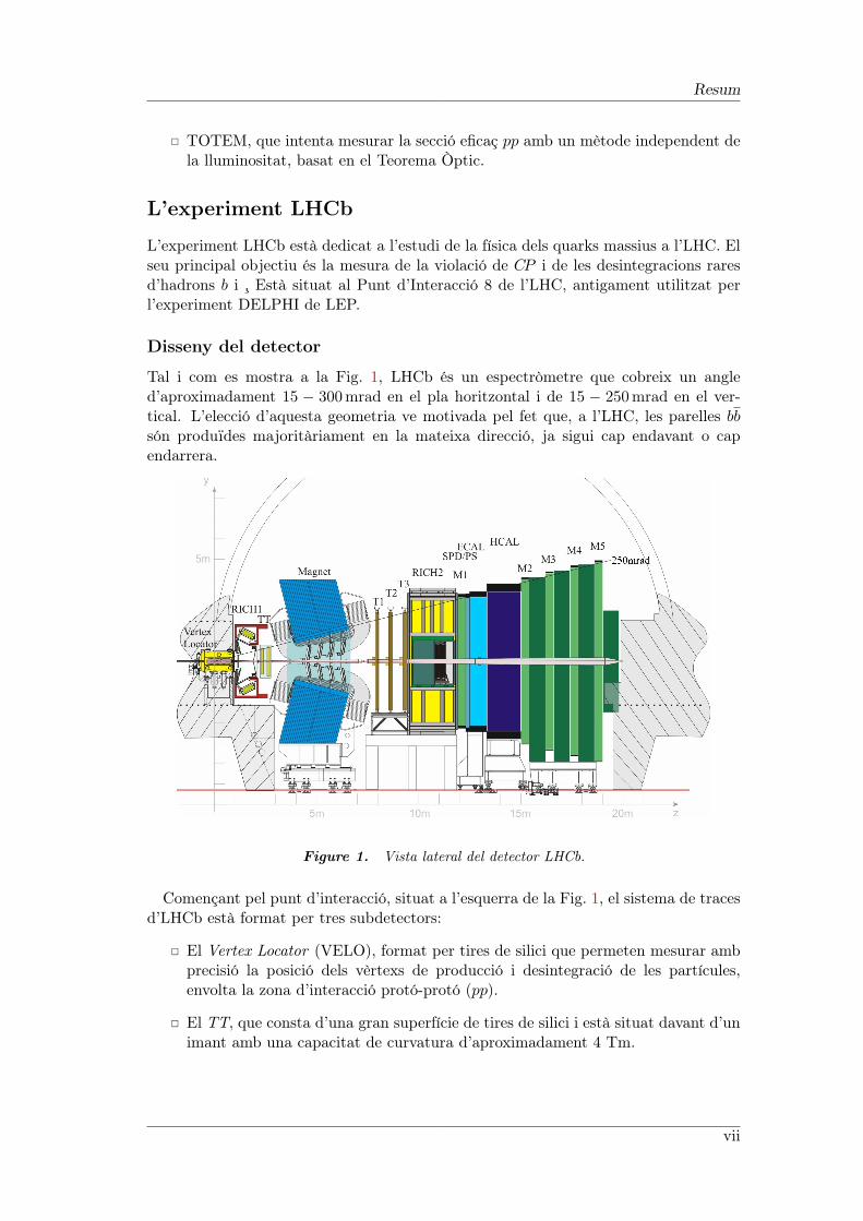
Tal i com es mostra a la Fig. 1, LHCb és un espectròmetre que cobreix un angled’aproximadament 15 − 300mrad en el pla horitzontal i de 15 − 250mrad en el ver-tical. L’elecció d’aquesta geometria ve motivada pel fet que, a l’LHC, les parelles bbsón produïdes majoritàriament en la mateixa direcció, ja sigui cap endavant o capendarrera.
Figure 1. Vista lateral del detector LHCb.
Començant pel punt d’interacció, situat a l’esquerra de la Fig. 1, el sistema de tracesd’LHCb està format per tres subdetectors:
El Vertex Locator (VELO), format per tires de silici que permeten mesurar ambprecisió la posició dels vèrtexs de producció i desintegració de les partícules,envolta la zona d’interacció protó-protó (pp).
El TT, que consta d’una gran superfície de tires de silici i està situat davant d’unimant amb una capacitat de curvatura d’aproximadament 4 Tm.
vii
Les estacions de mesura de trajectòries (Inner Tracker (IT) i Outer Tracker(OT)), són una combinació de detectors de tires de silici i de tubs de derivasituats al darrera de l’imant.
El sistema de traces complet té una resolució en moments δp/p que va del 0.3% al 0.5%en el rang de moments 5− 100GeV/c.
Dos detectors d’anells Cherenkov, Ring Imaging Cherenkov (RICH), equipats ambdiversos tipus de materials radiadors, són responsables de la identificació d’hadronscarregats en el rang de moments 2− 100GeV/c.
El sistema de calorimetria és l’encarregat de la detecció de partícules neutres i dela identificació d’electrons i fotons. Està format per un calorímetre electromagnètic,l’ECAL, i un d’hadrònic, l’HCAL. A més, dos plans de material centellejador, separatsper un absorbent de plom i situats abans de l’ECAL, són utilitzats per a millorar laidentificació de partícules, especialment al primer nivell de trigger. El primer d’aquestsplans està destinat a la separació fotons i electrons, mentre que el segon s’utilitza per ala identificació de cascades electromagnètiques. La correcta calibració de l’ECAL és unrequisit clau per a la mesura de desintegracions radiatives, ja que la seva característicadistintiva a nivell experimental és un fotó d’alta energia.
Finalment, els muons són identificats i mesurats a les cambres de muons, formadesper cinc capes de cambres proporcionals multifils separades per absorbent de ferro.
Sistema de trigger
El sistema de trigger d’LHCb redueix el ritme d’esdeveniments dels 10MHz produïtsper les col · lisions de l’LHC fins als 3 kHz permesos per els recursos d’emmagatzematge.Està dividit en dues fases: la primera fase, el L0, està implementada mitjançantplaques electròniques dissenyades especialment per a aquesta tasca, i redueix el ritmed’esdeveniments fins a 1MHz fent servir la informació proporcionada pels sistemes decalorimetria i de muons; la segona fase, el High Level Trigger (HLT), consisteix en unconjunt d’algoritmes que s’executen en una gran granja d’ordinadors i que efectuen demanera selectiva la reconstrucció completa dels esdeveniments.
Sistema Online
El sistema Online és l’encarregat d’assegurar que la transferència de dades des del’electrònica del detector fins als sistemes d’emmagatzematge s’efectua d’una maneraconsistent i controlada. Està dividit en tres sub-sistemes:
El sistema d’adquisició de dades (DAQ) transporta les dades acceptades pel L0fins al sistema d’emmagatzematge.
El sistema de Timing and Fast Control (TFC) controla el flux de dades entre eldetector i la granja d’ordinadors.
El sistema de control de l’experiment (ECS) permet controlar i monitoritzar eldetector i els sistemes de trigger, DAQ i TFC.
Aplicacions informàtiques
El programari d’LHCb està basat en l’arquitectura Gaudi, que proporciona un marccomú per a totes les aplicacions usades a l’experiment i que té la flexibilitat per a
viii
Resum
permetre executar el flux de dades d’LHCb per a simulacions Monte Carlo (MC) iper a dades reals fent servir les mateixes eines. Les dades es guarden en disc en unformat basat en Root, un conjunt de paquets de programari dissenyat per a manejari analitzar grans volums de dades.
La simulació de col · lisions pp i la interacció dels seus productes amb el detectorés realitzada per l’aplicació Gauss; llavors, l’aplicació Boole simula la digitalitzacióde les deposicions energètiques en el detector i en el L0. Arribats a aquest punt, lesdades, reals o simulades, passen a través de l’aplicació Moore, que executa l’HLT idecideix si els esdeveniments són acceptats o descartats; en el cas de les dades reals, elsesdeveniments acceptats són transferits al sistema d’emmagatzematge per a ser proces-sades i arxivades posteriorment. Aquestes dades (reals o simulades), encara pendentsde processar, s’analitzen amb l’aplicació Brunel, que s’encarrega de reconstruir lespartícules. A continuació, l’aplicació DaVinci classifica filtra aquestes partícules enun procés anomenat Stripping, i acaba produint al final un arxiu en format Root,anomenat Summary Data Tape (DST). Aquests arxius DST poden ser analitzats méstard mitjançant DaVinci per tal de produir NTuples de Root, adequades per a larealització d’anàlisi.
Les dades reals són reprocessades diversos cops a l’any per tal d’afegir millores enles aplicacions, algoritmes i constants de calibració de la reconstrucció, l’aliniament il’Stripping.
Condicions de presa de dades de 2010 i 2011
El 2010, l’LHC va proporcionar a LHCb 37 pb−1 de dades i va aconseguir arribar al80% de la lluminositat de disseny. Malgrat això, aquesta lluminositat es va assolirmitjançant l’ús de paràmetres de l’accelerador diferents dels previstos, i com a conse-qüència es va produir un augment del nombre d’interaccions visibles, µ. L’augment deµ implica un nombre major d’interaccions (i, per tant, de vèrtex) per xoc, un augmenten les taxes de lectura del detector i un augment en de la mida dels esdevenimentsi del temps necessari per a processar-los. Tot i el gran efecte que una µ alta té so-bre les condicions de treball del trigger, el sistema de trigger d’LHCb ha sigut capaçd’adaptar-se perfectament.
El 2011, l’LHC ha proporcionat a LHCb ∼ 1.2 fb−1 de dades, les quals han estatdesades amb una eficiència del 91%. El nombre mitjà de col · lisions pp inelàstiques haestat també per sobre del valor de disseny, però ha estat considerablement inferior alde 2010.
Estratègies de trigger per desintegracions radiativesd’hadrons B a LHCb
Un trigger eficient és essencial per a l’estudi de desintegracions radiatives d’hadronsB, ja que la seva raó d’embrancament és petita, de l’ordre de 10−5 o inferior, i pertant la seva producció es troba limitada a un màxim d’uns pocs milions per fb−1, quea més es troben diluïts entre un gran nombre d’esdeveniments de fons.
ix
Estratègies de trigger
En el L0, els canals L0Electron i L0Photon seleccionen aquells esdeveniments que tenenuna deposició energètica a l’ECAL amb una energia transversa respecte a la direcciódels feixos de protons, ET, superior a un cert llindar, col · locat a 2.5GeV durant el2011. A més, un subgrup dels esdeveniments que són acceptats per aquests canalstambé passen els canals L0ElectronHi i L0PhotonHi, de característiques similars peròamb un llindar superior, 4.2GeV. El requisit per a desintegracions radiatives és queel fotó de senyal hagi estat la causa de disparar el L0, això és, que o L0Electron oL0Photon siguin TOS (Trigger On Signal).
En l’HLT1, les línies rellevants per a desintegracions radiatives són les línies d’unatraça, Hlt1TrackAllL0 and Hlt1TrackPhoton, que seleccionen els esdevenimentsbasant-se en el moment transvers, pT, i el paràmetre d’impacte, IP, d’una de les tracesde l’esdeveniment. Per un costat, Hlt1TrackAllL0 accepta esdeveniments amb fo-tons de baixa ET mitjançant un tall més dur en el pT de la traça. Per l’altre costat,Hlt1TrackPhotonL0 permet relaxar el tall en pT de les traces requerint una ET mésalta al fotó. Per a desintegracions radiatives, el requisit aplicat en l’HLT1 és que oHlt1TrackAllL0 o Hlt1TrackPhotonL0 siguin TOS.
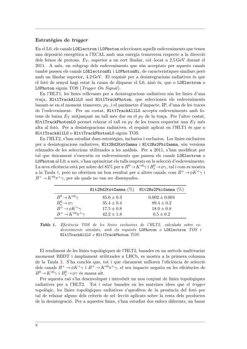
En l’HLT2, s’han estudiat dues estratègies, inclusiva i exclusiva. Les línies exclusivesper a desintegracions radiatives, Hlt2Bd2KstGamma i Hlt2Bs2PhiGamma, són versionsrelaxades de les seleccions utilitzades a les anàlisis. Per a 2011, s’han modificat pertal que únicament s’executin en esdeveniments que passen els canals L0Electron oL0Photon al L0; a més, s’han optimitzat els talls emprats en la selecció d’esdeveniments.La seva eficiència està per sobre del 85% per a B0→K∗0γ i B0
s →ϕγ, tal i com es mostraa la Taula 1, però no ofereixen un bon resultat per a altres canals, com B+→ϕK+γ iB+→K∗0π+γ, per als quals no van ser dissenyades.
Hlt2Bd2KstGamma (%) Hlt2Bs2PhiGamma (%)
B0→K∗0γ 85.6± 0.3 0.002± 0.004B0
s →ϕγ 35.4± 0.4 89.4± 0.2B+→ϕK+γ 17.5± 0.8 18.0± 0.8B+→K∗0π+γ 42.2± 1.8 0.5± 0.2
Table 1. Eficiència TOS de les línies exclusives de l’HLT2, calculada sobre es-deveniments simulats, amb els requisits L0Photon o L0Electron TOS iHlt1TrackAllL0 o Hlt1TrackPhoton TOS.
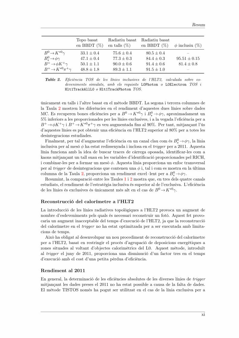
El rendiment de les línies topològiques de l’HLT2, basades en un mètode multivariatanomenat BBDT i àmpliament utilitzades a LHCb, es mostra a la primera columnade la Taula 2. S’ha conclòs que, tot i que clarament milloren l’eficiència de selecciódels canals B+ →ϕK+γ i B+ →K∗0π+γ, el seu impacte negatiu en les eficiències deB0→K∗0γ i B0
s →ϕγ és massa alt.Per aquesta raó s’ha desenvolupat i introduït un nou conjunt de línies topològiques
radiatives per a l’HLT2. Tot i estar basades en les mateixes idees que el triggertopològic, les línies topològiques radiatives s’aprofiten de la presència del fotó pertal de relaxar alguns dels criteris de sel · lecció aplicats sobre la resta dels productesde la desintegració. Per a aquestes línies, s’han estudiat dos enfocs diferents, un basat
x
Resum
Topo basat Radiatiu basat Radiatiu basaten BBDT (%) en talls (%) en BBDT (%) ϕ inclusiu (%)
B0→K∗0γ 33.1± 0.4 75.6± 0.4 80.5± 0.4 –B0
s →ϕγ 47.1± 0.4 77.3± 0.3 84.4± 0.3 95.51± 0.15B+→ϕK+γ 50.1± 1.1 90.0± 0.6 91.4± 0.6 81.4± 0.8B+→K∗0π+γ 48.8± 1.8 89.3± 1.1 91.5± 1.0 –
Table 2. Eficiència TOS de les línies inclusives de l’HLT2, calculada sobre es-deveniments simulats, amb els requisits L0Photon o L0Electron TOS iHlt1TrackAllL0 o Hlt1TrackPhoton TOS.
únicament en talls i l’altre basat en el mètode BBDT. La segona i tercera columnes dela Taula 2 mostren les diferències en el rendiment d’aquestes dues línies sobre dadesMC. Es recuperen bones eficiències per a B0→K∗0γ i B0
s →ϕγ, aproximadament un5% inferiors a les proporcionades per les línies exclusives, i a la vegada l’eficiència per aB+→ϕK+γ i B+→K∗0π+γ es veu augmentada fins al 90%. Per tant, mitjançant l’úsd’aquestes línies es pot obtenir una eficiència en l’HLT2 superior al 80% per a totes lesdesintegracions estudiades.
Finalment, per tal d’augmentar l’eficiència en un canal clau com és B0s →ϕγ, la línia
inclusiva per al mesó ϕ ha estat redissenyada i inclosa en el trigger per a 2011. Aquestalínia funciona amb la idea de buscar traces de càrrega oposada, identificar-les com akaons mitjançant un tall suau en les variables d’identificació proporcionades pel RICH,i combinar-les per a formar un mesó ϕ. Aquesta línia proporciona un enfoc transversalper al trigger de desintegracions que contenen una ϕ i, tal i com es mostra en la últimacolumna de la Taula 2, proporciona un rendiment excel · lent per a B0
s →ϕγ.Resumint, la comparació entre les Taules 1 i 2 mostra que, en tres dels quatre canals
estudiats, el rendiment de l’estratègia inclusiva és superior al de l’exclusiva. L’eficiènciade les línies és exclusives és únicament més alt en el cas de B0→K∗0γ.
Reconstrucció del calorímetre a l’HLT2
La introducció de les línies radiatives topològiques a l’HLT2 provoca un augment denombre d’esdeveniments pels quals és necessari reconstruir un fotó. Aquest fet provo-caria un augment inacceptable del temps d’execució de l’HLT2, ja que la reconstrucciódel calorímetre en el trigger no ha estat optimitzada per a ser executada amb limita-cions de temps.
Això ha obligat al desenvolupar un nou procediment de reconstrucció del calorímetreper a l’HLT2, basat en restringir el procés d’agrupació de deposicions energètiques azones situades al voltant d’objectes calorimètrics del L0. Aquest mètode, introduïtal trigger el juny de 2011, proporciona una disminució d’un factor tres en el tempsd’execució amb el cost d’una petita pèrdua d’eficiència.
Rendiment al 2011
En general, la determinació de les eficiències absolutes de les diverses línies de triggermitjançant les dades preses el 2011 no ha estat possible a causa de la falta de dades.El mètode TISTOS només ha pogut ser utilitzat en el cas de la línia exclusiva per a
xi
B0→K∗0γ, i s’ha trobat una eficiència de (84±3)%, en acord amb el valor determinatamb el MC, (85.6± 0.3)%
Tot i així, ha estat possible realizar una comparativa quantitativa del rendiment deles diverses línies de trigger, basada en l’estudi de les distribucions de massa invariantde B0→K∗0γ i B0
s →ϕγ. S’ha conclòs que, tot i que les línies exclusives proporcionenuna quantitat més alta d’esdeveniments, les línies inclusives tenen més capacitat per arebutjar esdeveniments de fons, i per tant proporcionen una millor raó S/B amb el costd’una petita disminució d’eficiència. A més, el trigger inclusiu de mesons ϕ ha tingutun rendiment extraordinari per a B0
s →ϕγ, tant en termes de nombre d’esdevenimentsde senyal com en termes de rebuig d’esdeveniments de fons.
Plans per a 2012
El gran rendiment de les línies radiatives topològiques de l’HLT2 a finals de 2011permet afirmar que, el 2012, l’estratègia de trigger per a desintegracions radiativesserà inclusiva.
Aquest canvi serà molt beneficiós, tant per a diverses anàlisis ja iniciades, coml’estudi de la asimetria CP en B+→ϕK+γ i B+→K∗0π+γ o l’estudi de les desinte-gracions radiatives dels barions Λb, com per a obrir camí a noves anàlisis com l’estudide la asimetria d’isospin de B0 →K∗0γ o la asimetria CP de les transicions b→ dγ,representades per B→ργ.
Les línies exclusives es mantindran com a control de les línies inclusives, però hanestat modificades per tal de disminuir el màxim possible el seu impacte en el nombred’esdeveniments acceptats per l’HLT2. Aquesta reducció s’ha aconseguit mitjançantl’aplicació de talls molt més durs, convertint-les de manera efectiva en quasi-seleccionsoffline.
Mesura de la raó B(B0→K∗0γ)/B(B0s→ϕγ)
El principal objectiu d’aquesta anàlisi és l’extracció de la raó de les fraccionsd’embrancament de B0 → K∗0γ, amb K∗0 → K±π∓, i B0
s → ϕγ, amb ϕ→ K+K−,i els seus complexos conjugats. A partir d’aquesta mesura, el valor de B(B0→K∗0γ)pot ser utilitzat per a obtenir B(B0
s →ϕγ).
Selecció d’esdeveniments
La selecció de les dues desintegracions B s’ha dissenyat per tal d’obtenir la màximacancel · lació d’incerteses sistemàtiques al calcular la raó de les seves eficiències. Enaquest sentit, tant el procés de reconstrucció dels candidates com els requisits que s’hiapliquen es mantenen el més similars possible: els mesons B0 (B0
s ) són reconstruïtsa partir de la combinació d’un fotó i un mesó vector K∗0 (ϕ), construït a partir deparelles kaó-pió (pió-pió) de càrrega oposada.
Les dues traces carregades amb les quals es construeix el mesó vector (V ) han de tenirpT > 500MeV/c i no poden apuntar cap a un vèrtex d’interacció pp, condició garantidapel requisit IPχ2 > 25. La identificació de les traces com a kaó o pió es realitzamitjançant l’aplicació de talls en la identificació de partícules (PID) proporcionadapel RICH. El PID està basat en la comparació entre dues hipòtesis d’identificacióde partícula, i es representa amb la diferència entre els logaritmes de les funcions de
xii
Resum
versemblança (DLL) entre les dues hipòtesis. Els kaons ham de tenir DLLKπ > 5 iDLLKp > 2, mentre que els pions han de complir DLLπK > 0. Amb aquests talls, elskaons (pions) que formen part dels canals estudiats són identificats correctament ambuna eficiència del ∼ 70 (83)%, amb un ∼ 3 (2)% de contaminació de pions (kaons).
Les combinacions de dues traces són acceptades com a candidats a K∗0 (ϕ) si formenun vèrtex amb χ2 < 9, si el pT d’una de les dues traces està per sobre de 1.2GeV/c, isi la seva massa invariant es troba dins d’una finestra de massa de 50 (10)MeV/c2 alvoltant de la massa nominal del K∗0 (ϕ).
El candidat a V resultant és combinat amb un fotó amb ET > 2.6GeV. Els clusterselectromagnètics a l’ECAL són separats entre neutres i carregats basant-se en la sevacompatibilitat amb traces extrapolades al calorímetre, mentre que els dipòsits neutrede fotons i π0 són identificats en base a la forma de les cascades electromagnètiques al’ECAL.
Els candidats a B han de tenir la massa invariant dins d’una finestra de massesd’1GeV/c2 al voltant de la massa nominal del mesó corresponent, pT > 3GeV/c, hand’haver volat des del punt d’interacció un mínim de 100 unitats en χ2, i han d’apuntara un vèrtex d’interacció pp, IPχ2 < 9. L’angle d’helicitat θH , definit com l’angle entreel moment de qualsevol de les filles de V i el moment del candidat a B en el sistema dereferència en què V està en repòs, es distribueix com sin2 θH per B→V γ i com a cos2 θHper els fons de tipus B→V π0. Per tant, l’estructura d’helicitat imposada per la senyalpot ser explotada per a eliminar fons del tipus B→V π0, en els quals el pió neutre s’haidentificat incorrectament com un fotó, requerint que | cos θH | < 0.8. El fons provinentde desintegracions parcialment reconstruïdes d’hadrons B es rebutja mitjançant un tallen l’aïllament del vèrtex: el χ2 del vèrtex del candidat ha d’augmentar en més de duesunitats quan se li afegeix qualsevol altra traça de l’esdeveniment.
Extracció de la raó de fraccions d’embrancament
La raó de fraccions d’embrancament es calcula a partir del nombre de candidates desenyal en els canals B0→K∗0γ i B0
s →ϕγ,
B(B0→K∗0γ)
B(B0s →ϕγ)
=NB0→K∗0γ
NB0s→ϕγ
B(ϕ→ K+K−)
B(K∗ → K+π−)
fsfd
ϵB0s→ϕγ
ϵB0→K∗0γ, (1)
on N correspon al nombre de candidats de senyal observats, B(ϕ→ K+K−) i B(K∗0 →K+π−) són les fraccions d’embrancament visible del mesons vector, fs/fd és la raó deles fraccions d’hadronització dels mesons B0 i B0
s en col · lisions pp a√s = 7TeV i
ϵB0s→ϕγ/ϵB0→K∗0γ és la raó de les eficiències dels dos canals. Aquest últim terme es
pot dividir en les contribucions provinents de l’acceptància (rAcc), la la reconstrucció iselecció (rReco&SelNoPID), els requisits de PID (rSelPID), i la selecció de trigger (rTrigger) :
ϵB0s→ϕγ
ϵB0→K∗0γ= rTrigger × rAcc × rReco&SelNoPID × rSelPID. (2)
La raó d’eficiències de PID, rPID = 0.839 ± 0.005 (stat), s’ha calculat a partir deles dades mitjançant un procediment de calibració realitzat sobre mostres pures dekaons i pions procedents de desintegracions D∗± → D0(K+π−)π±, seleccionadesúnicament amb criteris cinemàtics. La resta de raons d’eficiència s’han extret apartir d’esdeveniments simulats. La raó d’eficiències d’acceptància i reconstrucció,rAcc = 1.099 ± 0.004 (stat), és més gran que la unitat a causa de la correlació en
xiii
l’acceptància dels kaons provocada per les limitacions en l’espai de fases en la desinte-gració ϕ→K+K−. Aquests limitacions en l’espai de fases també provoquen una pitjorresolució espacial del vèrtex de la ϕ, i afecten l’eficiència de selecció de B0
s → ϕγa través dels talls en IP χ2, distancia de vol i aïllament del vèrtex. Per contra,els talls en el pT de les traces són menys eficients a l’actuar sobre el pió del K∗0,amb un espectre molt més suau. La raó d’eficiències de reconstrucció i selecció valrReco&SelNoPID = 0.881 ± 0.005 (stat) i s’observa la cancel · lació majoritària de les in-certeses sistemàtiques gràcies a que les seleccions cinemàtiques són quasi iguals pelsdos canals. La raó d’eficiències de trigger, rTrigger = 1.080± 0.009 (stat), s’ha calculattenint en compte les contribucions de les diverses configuracions del trigger durant elperíode de presa de dades.
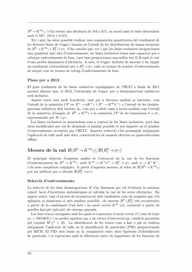
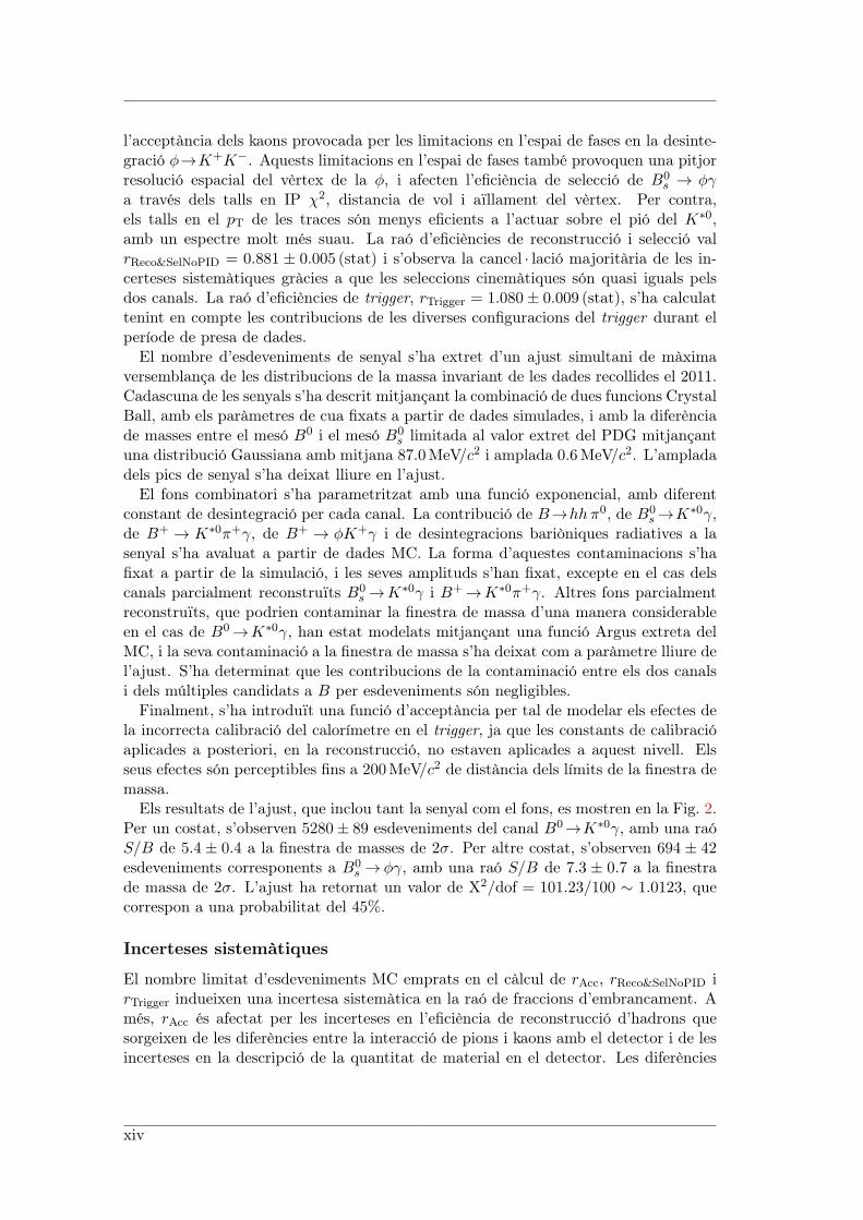
El nombre d’esdeveniments de senyal s’ha extret d’un ajust simultani de màximaversemblança de les distribucions de la massa invariant de les dades recollides el 2011.Cadascuna de les senyals s’ha descrit mitjançant la combinació de dues funcions CrystalBall, amb els paràmetres de cua fixats a partir de dades simulades, i amb la diferènciade masses entre el mesó B0 i el mesó B0
s limitada al valor extret del PDG mitjançantuna distribució Gaussiana amb mitjana 87.0MeV/c2 i amplada 0.6MeV/c2. L’ampladadels pics de senyal s’ha deixat lliure en l’ajust.
El fons combinatori s’ha parametritzat amb una funció exponencial, amb diferentconstant de desintegració per cada canal. La contribució de B→hhπ0, de B0
s →K∗0γ,de B+ → K∗0π+γ, de B+ → ϕK+γ i de desintegracions bariòniques radiatives a lasenyal s’ha avaluat a partir de dades MC. La forma d’aquestes contaminacions s’hafixat a partir de la simulació, i les seves amplituds s’han fixat, excepte en el cas delscanals parcialment reconstruïts B0
s →K∗0γ i B+→K∗0π+γ. Altres fons parcialmentreconstruïts, que podrien contaminar la finestra de massa d’una manera considerableen el cas de B0→K∗0γ, han estat modelats mitjançant una funció Argus extreta delMC, i la seva contaminació a la finestra de massa s’ha deixat com a paràmetre lliure del’ajust. S’ha determinat que les contribucions de la contaminació entre els dos canalsi dels múltiples candidats a B per esdeveniments són negligibles.
Finalment, s’ha introduït una funció d’acceptància per tal de modelar els efectes dela incorrecta calibració del calorímetre en el trigger, ja que les constants de calibracióaplicades a posteriori, en la reconstrucció, no estaven aplicades a aquest nivell. Elsseus efectes són perceptibles fins a 200MeV/c2 de distància dels límits de la finestra demassa.
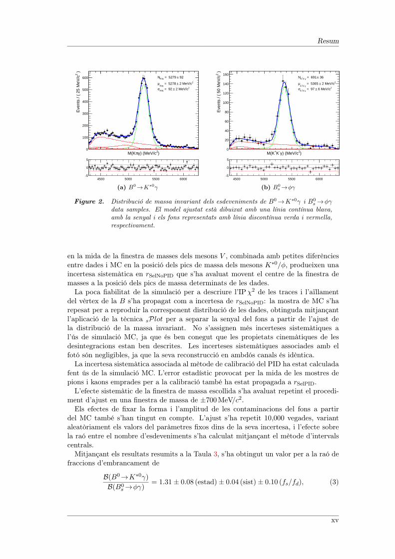
Els resultats de l’ajust, que inclou tant la senyal com el fons, es mostren en la Fig. 2.Per un costat, s’observen 5280± 89 esdeveniments del canal B0→K∗0γ, amb una raóS/B de 5.4 ± 0.4 a la finestra de masses de 2σ. Per altre costat, s’observen 694 ± 42esdeveniments corresponents a B0
s → ϕγ, amb una raó S/B de 7.3 ± 0.7 a la finestrade massa de 2σ. L’ajust ha retornat un valor de X2/dof = 101.23/100 ∼ 1.0123, quecorrespon a una probabilitat del 45%.
Incerteses sistemàtiques
El nombre limitat d’esdeveniments MC emprats en el càlcul de rAcc, rReco&SelNoPID irTrigger indueixen una incertesa sistemàtica en la raó de fraccions d’embrancament. Amés, rAcc és afectat per les incerteses en l’eficiència de reconstrucció d’hadrons quesorgeixen de les diferències entre la interacció de pions i kaons amb el detector i de lesincerteses en la descripció de la quantitat de material en el detector. Les diferències
xiv
Resum
)2) (MeV/cγπM(K
)2E
vent
s / (
25
MeV
/c
0
100
200
300
400
500
600 92± = 5279 γπKN2 2 MeV/c± = 5278
γπKµ
2 2 MeV/c± = 92 γπKσ
4500 5000 5500 6000-5
0
5
(a) B0→K∗0γ
)2) (MeV/cγ-K+M(K
)2E
vent
s / (
50
MeV
/c
0
20
40
60
80
100
120
140
160 36± = 691 γ-K+KN
2 2 MeV/c± = 5365 γ-K+K
µ2 6 MeV/c± = 97 γ-K+K
σ
4500 5000 5500 6000-5
0
5
(b) B0s →ϕγ
Figure 2. Distribució de massa invariant dels esdeveniments de B0→K∗0γ i B0s →ϕγ
data samples. El model ajustat està dibuixat amb una línia contínua blava,amb la senyal i els fons representats amb línia discontínua verda i vermella,respectivament.
en la mida de la finestra de masses dels mesons V , combinada amb petites diferènciesentre dades i MC en la posició dels pics de massa dels mesons K∗0/ϕ, produeixen unaincertesa sistemàtica en rSelNoPID que s’ha avaluat movent el centre de la finestra demasses a la posició dels pics de massa determinats de les dades.
La poca fiabilitat de la simulació per a descriure l’IPχ2 de les traces i l’aïllamentdel vèrtex de la B s’ha propagat com a incertesa de rSelNoPID: la mostra de MC s’harepesat per a reproduir la corresponent distribució de les dades, obtinguda mitjançantl’aplicació de la tècnica sPlot per a separar la senyal del fons a partir de l’ajust dela distribució de la massa invariant. No s’assignen més incerteses sistemàtiques al’ús de simulació MC, ja que és ben conegut que les propietats cinemàtiques de lesdesintegracions estan ben descrites. Les incerteses sistemàtiques associades amb elfotó són negligibles, ja que la seva reconstrucció en ambdós canals és idèntica.
La incertesa sistemàtica associada al mètode de calibració del PID ha estat calculadafent ús de la simulació MC. L’error estadístic provocat per la mida de les mostres depions i kaons emprades per a la calibració també ha estat propagada a rSelPID.
L’efecte sistemàtic de la finestra de massa escollida s’ha avaluat repetint el procedi-ment d’ajust en una finestra de massa de ±700MeV/c2.
Els efectes de fixar la forma i l’amplitud de les contaminacions del fons a partirdel MC també s’han tingut en compte. L’ajust s’ha repetit 10,000 vegades, variantaleatòriament els valors del paràmetres fixos dins de la seva incertesa, i l’efecte sobrela raó entre el nombre d’esdeveniments s’ha calculat mitjançant el mètode d’intervalscentrals.
Mitjançant els resultats resumits a la Taula 3, s’ha obtingut un valor per a la raó defraccions d’embrancament de
B(B0→K∗0γ)
B(B0s →ϕγ)
= 1.31± 0.08 (estad)± 0.04 (sist)± 0.10 (fs/fd), (3)
xv
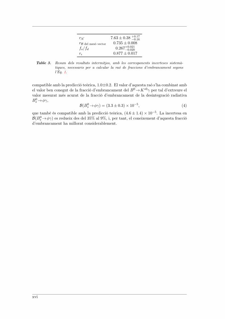
rN 7.63± 0.38 +0.17−0.16
rB del mesó vector 0.735± 0.008
fs/fd 0.267+0.021−0.020
rϵ 0.877± 0.017
Table 3. Resum dels resultats intermitjos, amb les corresponents incerteses sistemà-tiques, necessaris per a calcular la raó de fraccions d’embrancament segonsl’Eq. 1.
compatible amb la predicció teòrica, 1.0±0.2. El valor d’aquesta raó s’ha combinat ambel valor ben conegut de la fracció d’embrancament del B0→K∗0γ per tal d’extreure elvalor mesurat més acurat de la fracció d’embrancament de la desintegració radiativaB0
s →ϕγ,B(B0
s →ϕγ) = (3.3± 0.3)× 10−5, (4)
que també és compatible amb la predicció teòrica, (4.6± 1.4)× 10−5. La incertesa enB(B0
s →ϕγ) es redueix des del 35% al 9%, i, per tant, el coneixement d’aquesta fracciód’embrancament ha millorat considerablement.
xvi
Summary
The Standard Model (SM) is currently the most fundamental description of elemen-tary particles and their interactions, and its consistency has been validated by a largenumber of experiments. Despite its success, the SM fails to incorporate elements suchas gravity, dark energy, dark matter, and the already observed neutrino oscillations.B hadrons constitute an excellent benchmark for measuring SM parameters such
as the CKM matrix elements or CP violation. Furthermore, flavor-changing neutralcurrents (FCNC), which are only possible through loop processes and thus are verysensitive to new heavy particles circulating in the loop, can be used as probes ofphysics beyond the Standard Model. Radiative B hadron decays constitute excellentan example of this type of currents. The LHCb experiment, one of the six experimentsof the Large Hadron Collider (LHC), is dedicated to the study of CP violation andrare decays in the B sector.
In order to study radiative B decays at LHCb, it is necessary to distinguish and savesuch events from the copious amount of background produced at the LHC, most ofwhich is rejected by the experiment trigger system. Existing trigger algorithms havebeen redesigned and optimized, and new ones have been introduced in order to increasethe efficiency and extend the LHCb radiative decays program to channels which werenot initially foreseen.
Using 1.0 fb−1 of data recorded by LHCb in 2011, the ratio between the branchingfractions of the B0 → K∗0γ and B0
s → ϕγ has been measured. The value obtainedis compatible with the theoretical prediction and with previous measurements, and ithas been used, together with the well-known value of B(B0 →K∗0γ), to obtain theworld-best measurement of B(B0
s →ϕγ).
Radiative decays of B mesons
In the Standard Model the FCNC b→ sγ proceeds through one-loop electromagneticpenguin transitions, dominated by a virtual intermediate top quark coupling to a Wboson. Extensions of the SM predict additional one-loop contributions that can intro-duce sizeable effects on the dynamics of the transition.
Quark-level FCNC processes such as b→ sγ cannot be directly observed becausethe strong interaction forms hadrons from the underlying quarks. The hadronizationprocess is largely non-perturbative, and therefore introduces significant uncertaintiesin the calculation of exclusive branching fractions. Theoretical predictions are made byseparating the perturbative and non-perturbative parts of the hadronic matrix elementswith the help of Soft Collinear Effective Theory (SCET). Perturbative contributionsare partially known up to NNLO, while non-perturbative calculations are performed
xvii

by making use of light cone QCD sum rules. The current prediction for the branchingfractions of both B0→K∗0γ and B0
s →ϕγ is (4.3± 1.4)× 10−5, with their ratio beingcalculated to be 1.0± 0.2 due to the cancellation of some uncertainties.
Radiative decays of the B0 meson were first observed by the CLEO collaborationin 1993 through the B0 →K∗0γ mode. In 2007 the Belle collaboration reported thefirst observation of the analogous decay in the B0
s sector, B0s →ϕγ. The current world
averages of the branching fractions of B0→K∗0γ and B0s →ϕγ are (4.33±0.15) ×10−5
and (5.7+2.1−1.8) × 10−5, respectively. These results are in agreement with the theoretical
predictions from NNLO calculations. The ratio of experimental branching fractions ismeasured to be 0.7± 0.3, also in agreement with the SM prediction.
CERN and the LHC
The European Organization for Nuclear Research, known as CERN, is the world’slargest particle physics laboratory, and is situated on the Franco-Swiss border, nearGeneva. It is currently run by 20 European Member States, but many non-Europeancountries are also involved in different ways. Overall, a total of 10,000 visiting scientistsfrom 608 institutes and universities from 113 countries around the world —half of theworld’s particle physicists— use its facilities.
Many discoveries have been made at CERN, such as the W± and Z bosons, and, dur-ing its history, several Novel Prizes have been awarded to scientists working there. Inaddition, the laboratory has hosted many particle colliders, including the first proton-proton collider, the first proton-antiproton collider, and, currently, the largest colliderin the world, the Large Hadron Collider.
The LHC is a proton-proton collider installed in the 27 km tunnel built to host theLEP machine, designed to run at a center-of-mass energy of 14TeV. Four big detectorsand two smaller experiments are located around the four interaction points of the LHCring. These experiments are:
ALICE, dedicated to the study of the physics of strongly interacting matter andquark-gluon plasma in heavy nuclei (Pb-Pb) collisions.
ATLAS, a general purpose experiment with the objective to test the SM at theTeVscale, and to search for the Higgs boson and physics beyond the StandardModel.
CMS, another general purpose experiment with the aim of studying the mecha-nism of electroweak symmetry breaking, for which the Higgs mechanism is pre-sumed to be responsible, and testing the SM at energies above 1TeV.
LHCb, dedicated to the study of CP violation and rare decays in the b quarksector.
LHCf, a small experiment designed to measure the very forward production crosssections and energy spectra of neutral pions and neutrons.
TOTEM, which intends to measure the total pp cross section with a luminosity-independent method based on the Optical Theorem.
xviii
Summary
The LHCb experiment
The LHCb experiment is dedicated to the study of heavy flavor physics at the LHC.Its main aim is to make precise measurements of CP violation and rare decays ofbeauty and charm hadrons. It is located at Interaction Point 8 of the LHC accelerator,previously used by the DELPHI experiment from LEP.
Detector layout
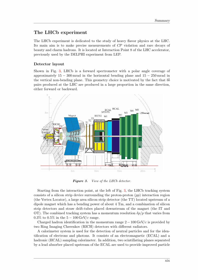
Shown in Fig. 3, LHCb is a forward spectrometer with a polar angle coverage ofapproximately 15 − 300mrad in the horizontal bending plane and 15 − 250mrad inthe vertical non-bending plane. This geometry choice is motivated by the fact that bbpairs produced at the LHC are produced in a large proportion in the same direction,either forward or backward.
Figure 3. View of the LHCb detector.
Starting from the interaction point, at the left of Fig. 3, the LHCb tracking systemconsists of a silicon strip device surrounding the proton-proton (pp) interaction region(the Vertex Locator), a large area silicon strip detector (the TT) located upstream of adipole magnet which has a bending power of about 4 Tm, and a combination of siliconstrip detectors and straw drift-tubes placed downstream of the magnet (the IT andOT). The combined tracking system has a momentum resolution δp/p that varies from0.3% to 0.5% in the 5− 100GeV/c range.
Charged hadron identification in the momentum range 2− 100GeV/c is provided bytwo Ring Imaging Cherenkov (RICH) detectors with different radiators.
A calorimeter system is used for the detection of neutral particles and for the iden-tification of electrons and photons. It consists of an electromagnetic (ECAL) and ahadronic (HCAL) sampling calorimeter. In addition, two scintillating planes separatedby a lead absorber placed upstream of the ECAL are used to provide improved particle
xix
identification, especially for the first level of trigger. The first of these planes providesseparation between electrons and photons, while the second one is used for tagging elec-tromagnetic showers. The correct calibration of the ECAL is a key requisite for thestudy of radiative decays, since their distinct experimental signature is a high energyphoton.
Finally, muons are identified and measured by means of the muon chambers, whichconsist of five layers of multiwire proportional chambers separated by iron absorbers.
Trigger system
The LHCb trigger system reduces the event rate from the 10MHz produced by theLHC collisions down to the 3 kHz allowed by the storage resources. It is divided in twostages: the first stage, the L0, is implemented using custom front-end electronics andreduces the event rate down to 1MHz by making use of the information provided bythe calorimeter and muon systems; the second stage, the High Level Trigger (HLT),consists in a set of software algorithms running on a large farm of commercial processorswhich applies a selective full event reconstruction.
Online system
The Online system is in charge of ensuring the transfer of data from the front-end elec-tronics of the LHCb detector to permanent storage in a known and controlled fashion.It is divided in three subsystems: the Data Acquisition (DAQ) system, in charge oftransporting the L0-accepted data from the front-end electronics to permanent storage,the Timing and Fast Control (TFC) system, in control of the data flow between thefront-end electronics and the Event Filter Farm, and the Experiment Control System(ECS), which allows to control and monitor the LHCb detector, the trigger, DAQ andTFC systems.
Computing
The LHCb software is based on the Gaudi architecture, which provides a commonframework for all the applications used within the experiment, and has the flexibilityto allow running the LHCb data flow for Monte Carlo simulation and real data withthe same tools. Data persistency is based on the Root software, a set of frameworksdesigned to handle and analyze large amounts of data.
In MC simulation, pp collisions and the interaction of their products with the detectorare handled by the Gauss application; then, the Boole application simulates thedigitization of the energy depositions in the detector and in the L0 trigger. At thispoint, real and simulated data go through the Moore application, which runs the HLTand decides whether an event is to be kept or not; in the case of real data, acceptedevents are transferred to permanent storage for further processing and archiving. Theseunprocessed data, real or simulated, are used by the Brunel application to reconstructthe physical particles, which are then further filtered using the DaVinci application,in a process called Stripping, the final result of which is a Data Summary Tape (DSTfile); in the case of real data, only stripped data are available for physics analysis. DSTfiles can be further analyzed with DaVinci in order to produce Root-based NTuplessuitable for analysis.
xx
Summary
Real data are reprocessed several times a year to incorporate improvements in thereconstruction, alignment and stripping software, algorithms and calibration constants.
2010 and 2011 running conditions
In 2010, the LHC delivered 37 pb−1 to LHCb and managed to achieve 80% of thedesign luminosity. However, this luminosity was achieved with different acceleratorparameters than the nominal ones, leading to an increase of the number of visibleinteractions, µ ∼ 2.5. An increase in µ means more interactions —and thus, vertices—per bunch crossing, an increase in the readout rate per bunch crossing, and an increaseof the event size and processing time. Even though a high µ affects greatly the triggerworking conditions, the LHCb trigger has managed to adapt perfectly.
In 2011, the LHC has delivered ∼ 1.2 fb−1 to LHCb, which have been recorded withan efficiency of 91%. The average number of inelastic pp collisions, µ ∼ 1.5, has alsobeen above the design value, but they have been substantially lower than in 2010.
Trigger strategies for radiative B decays at LHCb
An efficient trigger is an essential prerequisite for radiative B decays, since their branch-ing ratio is small, of O(10−5) or lower, and therefore their production is limited at mostto few millions per fb−1, diluted in a large amount background events.
Trigger strategies
In L0, L0Electron and L0Photon select those events with an electromagnetic deposi-tion in the ECAL with a transverse energy with respect to the beam direction, ET,greater than a given threshold, placed at 2.5GeV during 2011. Additionally, a subsetof the events that pass these two lines also pass the L0ElectronHi and L0PhotonHi
lines, which require a higher ET value of 4.2GeV. The L0 requirement for radiative Bdecays is that the signal photon has been responsible for firing the L0, i.e., either theL0Electron or L0Photon is TOS (Trigger On Signal).
In the HLT1, the relevant lines for radiative B decays are Hlt1TrackAllL0 andHlt1TrackPhoton single track lines. They select events based on the transverse mo-mentum (pT) of the tracks with respect to the beam direction and their impact pa-rameter (IP). On one side, Hlt1TrackAllL0 selects low-ET photons with a harder cutin the required track; on the other side, Hlt1TrackPhotonL0 allows to lower the pTrequirement for the track at the cost of a harder ET cut on the photon. For radiativedecays it is required that Hlt1TrackAllL0 or Hlt1TrackPhotonL0 are TOS.
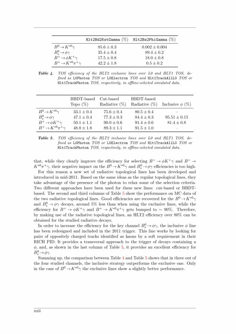
In HLT2, two strategies, exclusive and inclusive, have been studied. The exclusiveradiative lines, Hlt2Bd2KstGamma and Hlt2Bs2PhiGamma, which are loose versions ofthe respective offline selections, have been redesigned to run on events that pass theL0Electron and L0Photon lines and their cuts have been optimized. Their efficiencyis above 85% for B0→K∗0γ and B0
s →ϕγ, as shown in Table 4, but they offer a poorperformance for other channels, such as B+ → ϕK+γ and B+ →K∗0π+γ, for whichthey were not designed.
The performance of the widely used multivariate BBDT-based HLT2 topologicallines, shown in the first column of Table 5, has been assessed and it has been concluded
xxi
Hlt2Bd2KstGamma (%) Hlt2Bs2PhiGamma (%)
B0→K∗0γ 85.6± 0.3 0.002± 0.004B0
s →ϕγ 35.4± 0.4 89.4± 0.2B+→ϕK+γ 17.5± 0.8 18.0± 0.8B+→K∗0π+γ 42.2± 1.8 0.5± 0.2
Table 4. TOS efficiency of the HLT2 exclusive lines over L0 and HLT1 TOS, de-fined as L0Photon TOS or L0Electron TOS and Hlt1TrackAllL0 TOS orHlt1TrackPhoton TOS, respectively, in offline-selected simulated data.
BBDT-based Cut-based BBDT-basedTopo (%) Radiative (%) Radiative (%) Inclusive ϕ (%)
B0→K∗0γ 33.1± 0.4 75.6± 0.4 80.5± 0.4 –B0
s →ϕγ 47.1± 0.4 77.3± 0.3 84.4± 0.3 95.51± 0.15B+→ϕK+γ 50.1± 1.1 90.0± 0.6 91.4± 0.6 81.4± 0.8B+→K∗0π+γ 48.8± 1.8 89.3± 1.1 91.5± 1.0 –
Table 5. TOS efficiency of the HLT2 inclusive lines over L0 and HLT1 TOS, de-fined as L0Photon TOS or L0Electron TOS and Hlt1TrackAllL0 TOS orHlt1TrackPhoton TOS, respectively, in offline-selected simulated data.
that, while they clearly improve the efficiency for selecting B+ → ϕK+γ and B+ →K∗0π+γ, their negative impact on the B0→K∗0γ and B0
s →ϕγ efficiencies is too high.For this reason a new set of radiative topological lines has been developed and
introduced in mid-2011. Based on the same ideas as the regular topological lines, theytake advantage of the presence of the photon to relax some of the selection criteria.Two different approaches have been used for these new lines: cut-based or BBDT-based. The second and third columns of Table 5 show the performance on MC data ofthe two radiative topological lines. Good efficiencies are recovered for the B0→K∗0γand B0
s → ϕγ decays, around 5% less than when using the exclusive lines, while theefficiency for B+ → ϕK+γ and B+ → K∗0π+γ gets bumped to ∼ 90%. Therefore,by making use of the radiative topological lines, an HLT2 efficiency over 80% can beobtained for the studied radiative decays.
In order to increase the efficiency for the key channel B0s →ϕγ, the inclusive ϕ line
has been redesigned and included in the 2011 trigger. This line works by looking forpairs of oppositely charged tracks identified as kaons by a soft requirement in theirRICH PID. It provides a transversal approach to the trigger of decays containing aϕ, and, as shown in the last column of Table 5, it provides an excellent efficiency forB0
s →ϕγ.Summing up, the comparison between Table 4 and Table 5 shows that in three out of
the four studied channels, the inclusive strategy outperforms the exclusive one. Onlyin the case of B0→K∗0γ the exclusive lines show a slightly better performance.
xxii
Summary
Calorimeter reconstruction in HLT2
The introduction of the HLT2 radiative topological lines has the effect of increasingthe number of events for which the photon reconstruction is needed. Given the factthat the HLT2 calorimeter reconstruction was not optimized for running with timingconstraints, the addition of the inclusive lines implies an unacceptable increase of theHLT2 timing budget.
For this reason a new reconstruction procedure for the calorimeter in the trigger hasbeen developed. Based on reducing the calorimeter clusterization to regions of interestaround L0 calorimeter objects, it provides a three-fold decrease in the timing at thecost of a small efficiency loss. This new procedure was introduced in the trigger inJune 2011.
Performance in 2011
The determination of the absolute efficiencies of the various radiative trigger linesduring the 2011 data taking has not been possible due to the lack of statistics. Onlyin the case of the exclusive line for B0→K∗0γ it has been possible to use the TISTOSmethod, and the HLT2 efficiency has been found to be (84± 3)%, in good agreementwith the value calculated from MC, (85.6± 0.3)%
A quantitative performance comparison between the exclusive and inclusive triggershas been performed by studying the invariant mass distributions of the B0→K∗0γ andB0
s →ϕγ. It has been concluded that, while the exclusive lines provide a higher yieldthan the individual inclusive lines, the latter offer an improved background rejection,resulting in an enhanced S/B ratio for a moderate loss in efficiency for B0→K∗0γ. Inaddition, the inclusive ϕ trigger has shown an outstanding performance for B0
s →ϕγ,both in terms of yield and S/B.
Prospects for 2012
Given the excellent performance provided by the HLT2 radiative topological trigger atthe end of 2011, the radiative decays trigger strategy for 2012 will be inclusive.
Several new analyses, such as the CP -asymmetry studies for B+→ϕK+γ and B+→K∗0π+γ, or the study of radiative decays of Λb baryons, which were not included in theexclusive lines, will benefit from this change. Further studies with other channels, suchas the B0→K∗0γ isospin-asymmetry, or the CP asymmetry of b→dγ transitions suchas B→ ργ, will also be possible in the future because these events will have alreadybeen triggered with significant efficiency.
The exclusive lines will also be kept for cross checks of the inclusive lines, but theyhave been modified in order to lower their rate to a negligible rate. This rate reductionhas been achieved by tightening the cuts in the lines, effectively turning them intoquasi-offline selections.
Measurement of the ratio B(B0→K∗0γ)/B(B0s→ϕγ)
The main aim of this analysis is to extract the ratio of branching fractions of B0→K∗0γwith K∗0 →K±π∓ and B0
s → ϕγ with ϕ→K+K− (and complex conjugates). From
xxiii
this measurement, and using the well-known value of B(B0→K∗0γ), B(B0s →ϕγ) has
been extracted.
Event selection
The selection of both B decays is tuned to maximize the cancellation of systematicuncertainties in the ratio of their efficiencies. The procedure and requirements are keptas similar as possible: the B0 (B0
s ) mesons are reconstructed from a selected K∗0 (ϕ),built from oppositely charged kaon-pion (kaon-kaon) pairs, combined with a photon.
The two charged tracks used to build the vector meson are both required to havepT > 500MeV/c and to point away from all pp interaction vertex by requiring IPχ2 >25. The identification of the kaon and pion tracks is made by applying cuts to theparticle identification (PID) provided by the RICH system. The PID is based on thecomparison between two particle hypotheses, and it is represented by the difference inlogarithms of the likelihoods (DLL) between the two hypotheses. Kaons are requiredto have DLLKπ > 5 and DLLKp > 2, while pions are required to have DLLπK > 0.With these cuts, kaons (pions) coming from the studied channels are identified with a∼ 70 (83)% efficiency for a ∼ 3 (2)% pion (kaon) contamination.
Two-track combinations are accepted as K∗0 (ϕ) candidates if they form a vertexwith χ2 < 9, the highest pT of the two tracks is above 1.2GeV/c, and their invariantmass lies within 50 (10)MeV/c2 of the nominal K∗0 (ϕ) mass. The resulting vectormeson candidate is combined with a photon of ET > 2.6GeV. Neutral and chargedelectromagnetic clusters in the ECAL are separated based on their compatibility withextrapolated tracks while photon and π0 deposits are identified on the basis of theshapes of the electromagnetic shower in the ECAL.B candidates are required to have an invariant mass within 1GeV/c2 of the corre-
sponding B hadron mass, to have pT > 3GeV/c, to have a flight distance χ2 above100 units, and to point to a pp interaction vertex by applying a cut at IPχ2 < 9. Thedistribution of the helicity angle θH , defined as the angle between the momentum ofany of the daughters of the vector meson V and the momentum of the B candidate inthe rest frame of the vector meson, is expected to follow a sin2 θH function for B→V γ,and a cos2 θH for the B→V π0 background. Therefore, the helicity structure imposedby the signal decays is exploited to remove B→V π0 background, in which the neutralpion is misidentified as a photon, by requiring that | cos θH | < 0.8. Background comingfrom partially reconstructed b-hadron decays is rejected by requiring vertex isolation:the χ2 of the B vertex must increase by more than 2 units when adding any othertrack in the event.
Extraction of the ratio of branching fractions
The ratio of the branching fractions is calculated from the number of signal candidatesin the B0→K∗0γ and B0
s →ϕγ channels,
B(B0→K∗0γ)
B(B0s →ϕγ)
=NB0→K∗0γ
NB0s→ϕγ
B(ϕ→ K+K−)
B(K∗ → K+π−)
fsfd
ϵB0s→ϕγ
ϵB0→K∗0γ, (5)
where N corresponds to the observed number of signal candidates (yield), B(ϕ →K+K−) and B(K∗0 → K+π−) are the visible branching fractions of the vector mesons,fs/fd is the ratio of the B0 and B0
s hadronization fractions in pp collisions at√s =
xxiv
Summary
7TeV, and ϵB0s→ϕγ/ϵB0→K∗0γ is the ratio of efficiencies of the two decays. This latter
ratio is split into contributions coming from the acceptance (rAcc), the reconstructionand selection requirements (rReco&SelNoPID), the PID requirements (rSelPID), and thetrigger requirements (rTrigger) :
ϵB0s→ϕγ
ϵB0→K∗0γ= rTrigger × rAcc × rReco&SelNoPID × rSelPID. (6)
The PID efficiency ratio is measured from data to be rPID = 0.839 ± 0.005 (stat),by means of a calibration procedure using pure samples of kaons and pions fromD∗± → D0(K+π−)π± decays selected utilizing purely kinematic criteria. The otherefficiency ratios have been extracted using simulated events. The acceptance efficiencyratio, rAcc = 1.099±0.004 (stat), exceeds unity because of the correlated acceptance ofthe kaons due to the limited phase-space in the ϕ→K+K− decay. These phase-spaceconstraints also cause the ϕ vertex to have a worse spatial resolution than the K∗0 ver-tex. This affects the B0
s →ϕγ selection efficiency through the IP χ2, FD χ2, and vertexisolation cuts. Conversely, the pT track cuts are less efficient on the softer pion from theK∗0 decay. Both effects almost compensate and the selection efficiency ratio is foundto be rReco&SelNoPID = 0.881± 0.005 (stat), where the main systematic uncertainties inthe numerator and denominator cancel out since the kinematical selections are mostlyidentical for both decays. The trigger efficiency ratio rTrigger = 1.080 ± 0.009 (stat)has been computed taking into account the contributions from the different triggerconfigurations during the data taking period.
The yields of the two channels are extracted from a simultaneous unbinned maximumlikelihood fit to the invariant mass distributions of the data. Each of the signals isdescribed using two Crystal Ball functions, with their tail parameters fixed to theirvalue extracted from MC simulations and the mass difference between the B0 andB0
s signals constrained to the PDG value with a Gaussian distribution with mean87.0MeV/c2 and width 0.6MeV/c2. The width of the signal peak is left as a freeparameter.
Combinatorial background is parametrized by an exponential function with a differ-ent decay constant for each channel. The contribution of the B→hhπ0, B0
s →K∗0γ,B+→K∗0π+γ, B+→ϕK+γ, and baryonic radiative decays to the signal has been as-sessed from MC data. The shape of these contributions has been fixed from simulation,and their amplitudes have been fixed, except in the case of the partially reconstructedB0
s →K∗0γ and B+→K∗0π+γ. Other partially reconstructed backgrounds, which canhave a potentially large contribution, specially in B0→K∗0γ, have been parametrizedwith an Argus function from MC simulation, and their contamination in the mass win-dow has been left free. The contribution from cross feed between signal channels andmultiple candidates per event has been found to be negligible.
Finally, an acceptance function is introduced to model the effects of calorimetermiscalibration in the trigger, where the calibration coefficients applied at the recon-struction level were not applied. Its effects are noticeable up to 200MeV/c2 from theborder.
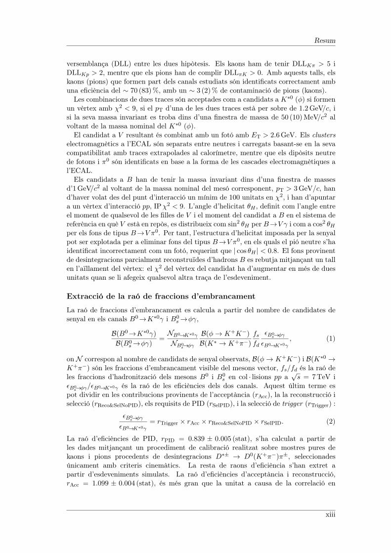
The results of the fit, including both the signal and the backgrounds, are shown inFig. 4. On one side, B0→K∗0γ is observed with a yield of 5280±89 events and a S/Bratio of 5.4± 0.4 in the 2σ mass window. On the other side, 694± 42 B0
s →ϕγ eventshave been observed with a S/B of 7.3 ± 0.7 in the 2σ mass window, constituting the
xxv
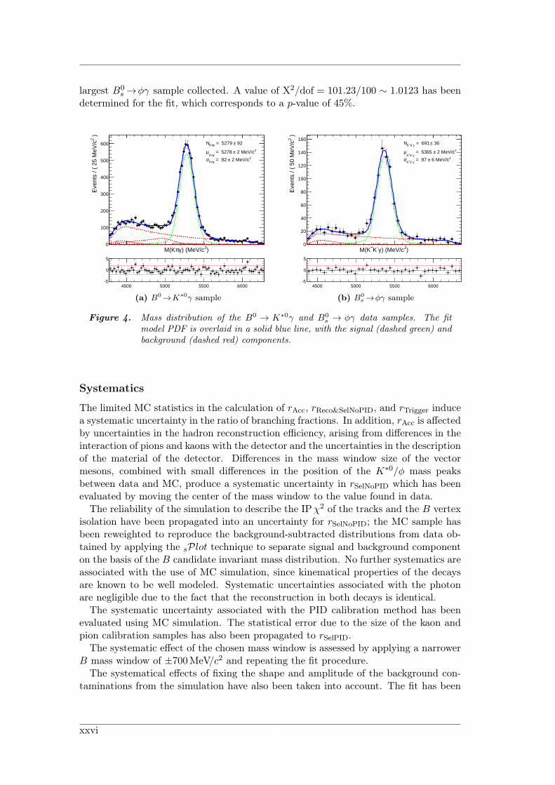
largest B0s →ϕγ sample collected. A value of X2/dof = 101.23/100 ∼ 1.0123 has been
determined for the fit, which corresponds to a p-value of 45%.
)2) (MeV/cγπM(K
)2E
vent
s / (
25
MeV
/c
0
100
200
300
400
500
600 92± = 5279 γπKN2 2 MeV/c± = 5278
γπKµ
2 2 MeV/c± = 92 γπKσ
4500 5000 5500 6000-5
0
5
(a) B0→K∗0γ sample
)2) (MeV/cγ-K+M(K
)2E
vent
s / (
50
MeV
/c
0
20
40
60
80
100
120
140
160 36± = 691 γ-K+KN
2 2 MeV/c± = 5365 γ-K+K
µ2 6 MeV/c± = 97 γ-K+K
σ
4500 5000 5500 6000-5
0
5
(b) B0s →ϕγ sample
Figure 4. Mass distribution of the B0 → K∗0γ and B0s → ϕγ data samples. The fit
model PDF is overlaid in a solid blue line, with the signal (dashed green) andbackground (dashed red) components.
Systematics
The limited MC statistics in the calculation of rAcc, rReco&SelNoPID, and rTrigger inducea systematic uncertainty in the ratio of branching fractions. In addition, rAcc is affectedby uncertainties in the hadron reconstruction efficiency, arising from differences in theinteraction of pions and kaons with the detector and the uncertainties in the descriptionof the material of the detector. Differences in the mass window size of the vectormesons, combined with small differences in the position of the K∗0/ϕ mass peaksbetween data and MC, produce a systematic uncertainty in rSelNoPID which has beenevaluated by moving the center of the mass window to the value found in data.
The reliability of the simulation to describe the IPχ2 of the tracks and the B vertexisolation have been propagated into an uncertainty for rSelNoPID; the MC sample hasbeen reweighted to reproduce the background-subtracted distributions from data ob-tained by applying the sPlot technique to separate signal and background componenton the basis of the B candidate invariant mass distribution. No further systematics areassociated with the use of MC simulation, since kinematical properties of the decaysare known to be well modeled. Systematic uncertainties associated with the photonare negligible due to the fact that the reconstruction in both decays is identical.
The systematic uncertainty associated with the PID calibration method has beenevaluated using MC simulation. The statistical error due to the size of the kaon andpion calibration samples has also been propagated to rSelPID.
The systematic effect of the chosen mass window is assessed by applying a narrowerB mass window of ±700MeV/c2 and repeating the fit procedure.
The systematical effects of fixing the shape and amplitude of the background con-taminations from the simulation have also been taken into account. The fit has been
xxvi

Summary
rN 7.63± 0.38 +0.17−0.16
rvector meson B 0.735± 0.008
fs/fd 0.267+0.021−0.020
rϵ 0.877± 0.017
Table 6. Summary of the intermediate results, with their corresponding systematic er-rors, needed for the calculation of the ratio of branching fractions, as definedin Eq. 5.
repeated 10,000 times, randomly varying the values of the fixed parameters withintheir uncertainties, and the effect on the ratio of yields has been determined using thecentral intervals method at 95% confidence level.
Results and conclusions
By making use of the intermediate results summarized in Table 6, the ratio of branchingfractions has been measured as
B(B0→K∗0γ)
B(B0s →ϕγ)
= 1.31± 0.08 (stat)± 0.04 (syst)± 0.10 (fs/fd), (7)
and thus has been found to be compatible with the theory prediction of 1.0± 0.2. Thevalue of the ratio has been combined with the well-measured value of the B0→K∗0γbranching fraction to extract the world-best measurement of the branching fraction ofthe radiative B0
s →ϕγ decay,
B(B0s →ϕγ) = (3.3± 0.3)× 10−5, (8)
which is also in agreement with the theoretical prediction of (4.6 ± 1.4) × 10−5. Theuncertainty in B(B0
s →ϕγ) is reduced from 35% down to 9%, and thus the knowledgeof this branching fraction is largely improved.
xxvii


Introduction
The Standard Model of particle physics is a set of theories, developed during the secondhalf of the 20th century, which aim to explain the electromagnetic, weak and stronginteractions of subatomic particles. While its theoretical formulation was finalized inthe 1970’s, experimental confirmation of some of its predictions, like the top quark andthe tau neutrino, had to wait until the end of the century. The last key piece of theStandard Model, the Higgs boson, still remains to be experimentally confirmed.
Despite its success, the Standard Model fails to incorporate gravity, as described bygeneral relativity, dark energy, dark matter, as it doesn’t contain any viable candidatefor dark matter, and neutrino oscillations, already observed by several experiments. Italso contains several unnatural features that give rise to the strong CP and hierarchyproblems.
Particles containing a beauty quark, called B hadrons, constitute an excellent bench-mark for measuring Standard Model aspects, such as the mixing between quark familiesand CP violation, controlled by the CKM matrix, and indirect effects caused by someof its extensions. The LHCb experiment, one of the experiments of the Large HadronCollider, is dedicated to the study of CP violation and rare decays in the B sector.
One topic of interest is flavor-changing neutral currents, which are only possiblethrough loop processes and thus are very sensitive to new heavy particles circulatingin the loop. Radiative B hadron decays, i.e., B hadron decays with a photon in thefinal state, constitute an excellent example of this type of decays.
With branching fractions of O(10−5) or lower, the production of rare B decays inLHCb, specially those in the B0
s sector, is small and found diluted in a large amountbackground events. Therefore, in order to avoid limiting the analysis potential of theexperiment, it is critical to develop efficient trigger strategies to pick these events apartat the data taking stage. In the case of radiative B decays, the presence of a neutralparticle, the photon, makes this selection even more challenging.
The first measurement of radiative B decays in the LHCb experiment, as well as thedevelopment of the trigger strategies that allow this and future measurements, are thesubject of this work.
Chapter 1 describes the Standard Model and provides the key elements to under-stand how to formulate predictions for radiative B decays within its framework. Whileinclusive calculations have good predicting power for branching fractions, exclusivepredictions, more accessible experimentally, suffer from big uncertainties. These uncer-tainties lead to a situation where the experimental results, also summarized in Chapter1, are more precise than their theoretical counterparts.
Chapter 2 briefly introduces the European Organization for Nuclear Research, knownas CERN, and its history. It also describes the world’s largest particle accelerator, the
1

Large Hadron Collider, including its six experiments.The LHCb experiment is described in Chapter 3. The running conditions during the
data taking periods of 2010 and 2011 are analyzed, and the LHCb detector systemsand subsystems are presented in detail.
Two trigger strategies for radiative B decays are studied in Chapter 4, an exclusiveand an inclusive approach. New or redesigned trigger lines are described, and theirefficiencies on simulated data are presented. The performance of the 2011 strategy isanalyzed, and the strategy adopted for the 2012 data taking is outlined.
Chapter 5 presents the measure of the ratio of branching fractions of the B0→K∗0γand B0
s → ϕγ decays on the full 2011 dataset. The procedure for extracting thisratio, including event selection, signal yield extraction and systematical uncertaintiesdetermination, is discussed. From the measured result, the value of B(B0
s → ϕγ) isextracted.
The conclusions of this work, as well as its impact on future radiative measurementsto be carried out in LHCb, are discussed in Chapter 6.
2
1Radiative decays of B mesons
Radiative b→ sγ decays are an example of effective flavor-changing neutral currentinteractions, which arise from the Standard Model through loop processes such as pen-guin or box diagrams. Such processes allow to probe physics at high energies throughthe virtual particles circulating in the loop. This feature makes them a good testingground in searches for Physics beyond the Standard Model, which may introduce newheavy flavor-changing particles to which radiative decays could be sensitive to.
Theoretical predictions for exclusive radiative decays, more accessible experimentallythan inclusive ones, are more difficult to calculate; quark-level processes cannot be ac-cessed directly in the experiment, and thus predictions have to be made at the hadroniclevel, where there are sizeable non-perturbative —and thus hard to calculate— contri-butions. Predictions are based on QCD factorization theorems derived from effectivefield theories, but suffer from large uncertainties due to non-perturbative QCD con-tributions. Some observables, such as CP or isospin asymmetries, benefit from can-cellations of some these uncertainties, making them better targets for experimentalstudy.
1.1. The Standard Model
The Standard Model (SM) is the theory that describes our current knowledge of theelementary constituents of matter and their interactions. It was formulated in the1960’s and 1970’s and it has been very successful so far. Many of its predictions havebeen confirmed experimentally with a high level of precision, except for the neutrinomasses [1–4] and the yet unobserved Higgs boson [5–7].
The SM is built upon the foundation of relativistic quantum field theory, which em-beds the dynamical framework of quantum field theory within the space-time structureof special relativity [8].
Symmetries are imposed to the theory through the principle of local gauge invariance[9–11], which postulates that the theory is invariant under transformations of the fieldsfollowing the form
ψ(xµ) → eiαa(xµ)Taψ(xµ), (1.1)
where Ta are the generators of a Lie group and αa(xµ) are a set of arbitrary real
3
1. Radiative decays of B mesons
functions of the space-time coordinate xµ, one for each generator. In order to preservethe invariance of the kinetic term of the lagrangian, it is necessary to replace the partialderivatives ∂µ by covariant derivatives Dµ build with gauge fields Aa
µ:
∂µ ⇒ Dµ ≡ ∂µ + igT aAaµ, (1.2)
where the gauge fields transform as:
Aaµ → Aa
µ − 1
g∂µαa(xµ). (1.3)
This construction allows the transformations of the gauge field to cancel terms arisingfrom the derivative of the gauge-transformed field ψ(xµ). Local gauge and Lorentzinvariance dictate that the Aa
µ particles are spin-1 Lorentz vectors transforming underthe adjoint representation of the Lie group. The coupling constant g is universal for agiven gauge group, and determines the strength of the interaction.
The Standard Model is a collection of gauge theories in which the constituents ofmatter —the fermions— interact through the exchange of force carrier gauge bosonsarising from the symmetry group
SU(3)C × SU(2)L ×U(1)Y . (1.4)
The electroweak interaction corresponds to the SU(2)L ×U(1)Y [12–14], and is me-diated by the massless photon and the massive W± and Z0 bosons, while the stronginteraction, described by Quantum ChromoDynamics (QCD), derives from SU(3)C [15]and is carried by the massless gluons.
The representation of the Ta generators within the covariant derivative for thefermions determines their group transformation and gauge interaction properties. Thefermions couple with the gauge bosons through the covariant derivative if the Ta gener-ators are a non-trivial representation of the group. Otherwise, they are singlets underthe gauge group and are transparent to the considered interaction.
As a final step, the mechanism of spontaneous symmetry breaking [16–20] is requiredto give mass to the particles within the SM through the introduction of a new field,the Higgs field. Electroweak gauge bosons —and the Higgs boson itself— and fermionsacquire mass through quadratic terms and Yukawa mass terms, respectively.
In summary, the Standard Model Lagrangian can be written as
L = LQCD + LEW + LHiggs + LYukawa. (1.5)
In the SM, elementary particles are divided into bosons and fermions according totheir spin. Each particle has a corresponding antiparticle which carries the oppositequantum numbers. In some cases, such as the photon or the Z0, the particle is its ownantiparticle.
1.1.1. Elementary Particles
Fermions are the constituents of matter and are indivisible. They have spin 1/2 andobey Fermi-Dirac statistics. Taking into account the group representation of the SMsymmetries, fermions are divided into two categories:
Six quarks, which transform under the fundamental representation of SU(3)C ,and thus participate in QCD.
4
1.1. The Standard Model
Six leptons, which are SU(3)C singlets, and therefore are not affected by QCD.
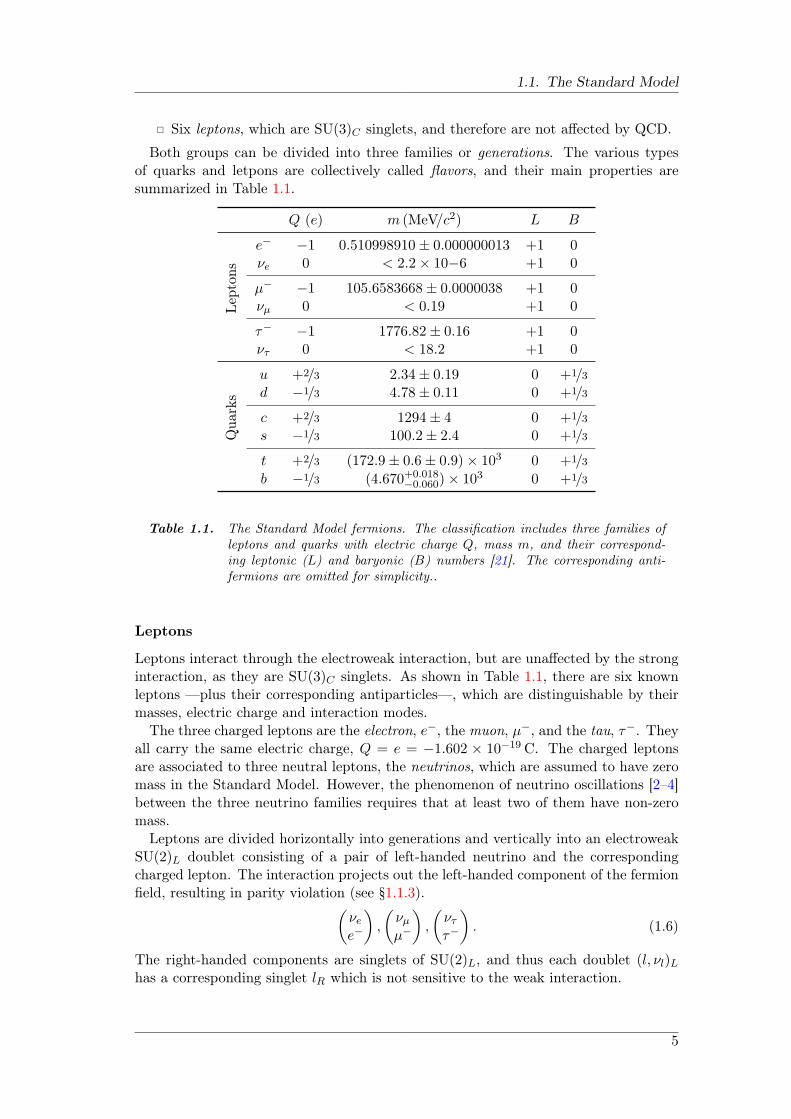
Both groups can be divided into three families or generations. The various typesof quarks and letpons are collectively called flavors, and their main properties aresummarized in Table 1.1.
Q (e) m (MeV/c2) L BLe
pton
se− −1 0.510998910± 0.000000013 +1 0νe 0 < 2.2× 10⁻⁶ +1 0
µ− −1 105.6583668± 0.0000038 +1 0νµ 0 < 0.19 +1 0
τ− −1 1776.82± 0.16 +1 0ντ 0 < 18.2 +1 0
Qua
rks
u +2/3 2.34± 0.19 0 +1/3d −1/3 4.78± 0.11 0 +1/3
c +2/3 1294± 4 0 +1/3s −1/3 100.2± 2.4 0 +1/3
t +2/3 (172.9± 0.6± 0.9)× 103 0 +1/3
b −1/3 (4.670+0.018−0.060)× 103 0 +1/3
Table 1.1. The Standard Model fermions. The classification includes three families ofleptons and quarks with electric charge Q, mass m, and their correspond-ing leptonic (L) and baryonic (B) numbers [21]. The corresponding anti-fermions are omitted for simplicity..
Leptons
Leptons interact through the electroweak interaction, but are unaffected by the stronginteraction, as they are SU(3)C singlets. As shown in Table 1.1, there are six knownleptons —plus their corresponding antiparticles—, which are distinguishable by theirmasses, electric charge and interaction modes.
The three charged leptons are the electron, e−, the muon, µ−, and the tau, τ−. Theyall carry the same electric charge, Q = e = −1.602 × 10⁻¹⁹ C. The charged leptonsare associated to three neutral leptons, the neutrinos, which are assumed to have zeromass in the Standard Model. However, the phenomenon of neutrino oscillations [2–4]between the three neutrino families requires that at least two of them have non-zeromass.
Leptons are divided horizontally into generations and vertically into an electroweakSU(2)L doublet consisting of a pair of left-handed neutrino and the correspondingcharged lepton. The interaction projects out the left-handed component of the fermionfield, resulting in parity violation (see §1.1.3).(
νee−
),
(νµµ−
),
(νττ−
). (1.6)
The right-handed components are singlets of SU(2)L, and thus each doublet (l, νl)Lhas a corresponding singlet lR which is not sensitive to the weak interaction.
5
1. Radiative decays of B mesons
Quarks
Quarks transform under the fundamental representation of chromodynamic SU(3)Cand therefore carry an extra quantum number, the chromodynamic charge, calledcolor. The six quarks are classified into up-type quarks, with electric charge +2/3, anddown-type quarks, with electric charge −1/3, as shown in Table 1.1.
Similarly to the leptons, quarks are horizontally divided into generations and verti-cally grouped in pairs of up- and down-type left-handed quarks as SU(2)L doublets.The first family is composed by the lightest quarks, the up (u) and down (d), which arethe most abundant in Nature as they constitute the basic components of the protonand the neutron; the second quark family is composed by the heavier charm (c) andstrange (s) quarks; the heaviest quarks, the top (t) and the bottom or beauty (b) makeup the third family. (
ud
),
(cs
),
(tb
). (1.7)
Due to the confinement property of QCD (see §1.1.2), colored objects can onlyappear in colorless combinations; thus, quarks are always found grouped in colorlessparticles, called hadrons. There are two types of hadrons: mesons, composed by aquark-antiquark pair (qq), and baryons, antisymmetric color triplets of different color(qqq, qqq).
1.1.2. Fundamental Interactions
In the SM, particles interact through the exchange of the gauge bosons that arisefrom imposing local gauge invariance with respect to the symmetry groups in Eq. 1.4.Gravitation is not included in the Standard Model, so the three interactions to considerare:
Electromagnetic interaction. It affects all particles with electric charge. It is de-scribed by Quantum ElectroDynamics (QED) [22–29], a quantum field theorywith the photon as the force mediator.
Strong interaction. Interaction which confines the quarks into hadrons. It is de-scribed by the theory of Quantum ChromoDynamics (QCD). The eight masslessgauge bosons arising from the adjoint representation of SU(3)C are called gluons,and are said to carry the color charge. QCD has two distinct properties:
Confinement. Unlike all other forces, the strength of the strong force doesnot diminish with increasing distance. This phenomenon is called colorconfinement, and it implies that only hadrons, and not individual free quarksor gluons, can be observed. In simple terms, the energy needed to pull twoquarks apart is so high that a new pair of quark-antiquark, which will pairup with the original ones, can be produced. Although analytically unproven,confinement is believed to be true due to the consistent failure of free quarksearches.
Asymptotic freedom. At very high-energy reactions, quarks and gluons in-teract very weakly. This analytical prediction of QCD was discovered inthe 1970’s by Politzer, Wilczek and Gross [30, 31], which were awarded theNobel Prize in Physics.
6
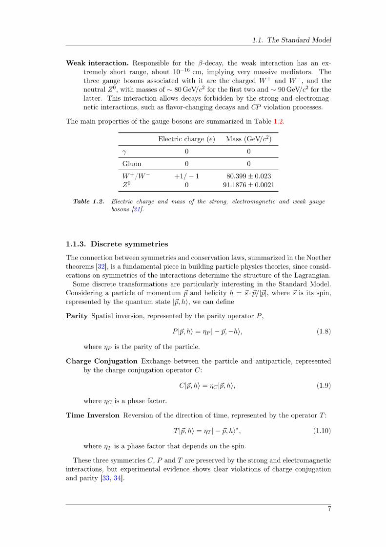
1.1. The Standard Model
Weak interaction. Responsible for the β-decay, the weak interaction has an ex-tremely short range, about 10−16 cm, implying very massive mediators. Thethree gauge bosons associated with it are the charged W+ and W−, and theneutral Z0, with masses of ∼ 80GeV/c2 for the first two and ∼ 90GeV/c2 for thelatter. This interaction allows decays forbidden by the strong and electromag-netic interactions, such as flavor-changing decays and CP violation processes.
The main properties of the gauge bosons are summarized in Table 1.2.
Electric charge (e) Mass (GeV/c2)
γ 0 0
Gluon 0 0
W+/W− +1/− 1 80.399± 0.023Z0 0 91.1876± 0.0021
Table 1.2. Electric charge and mass of the strong, electromagnetic and weak gaugebosons [21].
1.1.3. Discrete symmetries
The connection between symmetries and conservation laws, summarized in the Noethertheorems [32], is a fundamental piece in building particle physics theories, since consid-erations on symmetries of the interactions determine the structure of the Lagrangian.
Some discrete transformations are particularly interesting in the Standard Model.Considering a particle of momentum p and helicity h = s · p/|p|, where s is its spin,represented by the quantum state |p, h⟩, we can define
Parity Spatial inversion, represented by the parity operator P ,
P |p, h⟩ = ηP | − p,−h⟩, (1.8)
where ηP is the parity of the particle.
Charge Conjugation Exchange between the particle and antiparticle, representedby the charge conjugation operator C:
C|p, h⟩ = ηC |p, h⟩, (1.9)
where ηC is a phase factor.
Time Inversion Reversion of the direction of time, represented by the operator T :
T |p, h⟩ = ηT | − p, h⟩∗, (1.10)
where ηT is a phase factor that depends on the spin.
These three symmetries C, P and T are preserved by the strong and electromagneticinteractions, but experimental evidence shows clear violations of charge conjugationand parity [33, 34].
7
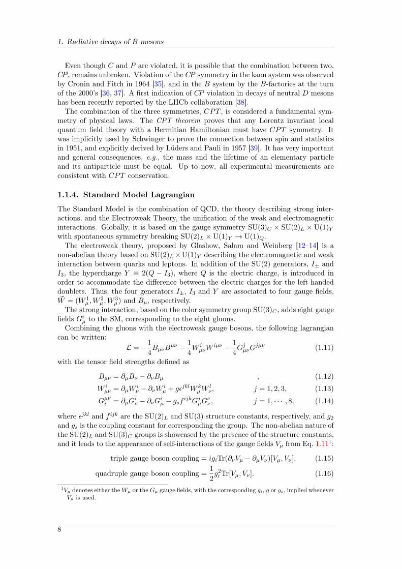
1. Radiative decays of B mesons
Even though C and P are violated, it is possible that the combination between two,CP , remains unbroken. Violation of the CP symmetry in the kaon system was observedby Cronin and Fitch in 1964 [35], and in the B system by the B-factories at the turnof the 2000’s [36, 37]. A first indication of CP violation in decays of neutral D mesonshas been recently reported by the LHCb collaboration [38].
The combination of the three symmetries, CPT , is considered a fundamental sym-metry of physical laws. The CPT theorem proves that any Lorentz invariant localquantum field theory with a Hermitian Hamiltonian must have CPT symmetry. Itwas implicitly used by Schwinger to prove the connection between spin and statisticsin 1951, and explicitly derived by Lüders and Pauli in 1957 [39]. It has very importantand general consequences, e.g., the mass and the lifetime of an elementary particleand its antiparticle must be equal. Up to now, all experimental measurements areconsistent with CPT conservation.
1.1.4. Standard Model Lagrangian
The Standard Model is the combination of QCD, the theory describing strong inter-actions, and the Electroweak Theory, the unification of the weak and electromagneticinteractions. Globally, it is based on the gauge symmetry SU(3)C × SU(2)L × U(1)Ywith spontaneous symmetry breaking SU(2)L ×U(1)Y → U(1)Q.
The electroweak theory, proposed by Glashow, Salam and Weinberg [12–14] is anon-abelian theory based on SU(2)L×U(1)Y describing the electromagnetic and weakinteraction between quarks and leptons. In addition of the SU(2) generators, I± andI3, the hypercharge Y ≡ 2(Q − I3), where Q is the electric charge, is introduced inorder to accommodate the difference between the electric charges for the left-handeddoublets. Thus, the four generators I±, I3 and Y are associated to four gauge fields,W = (W 1
µ ,W2µ ,W
3µ) and Bµ, respectively.
The strong interaction, based on the color symmetry group SU(3)C , adds eight gaugefields Gi
µ to the SM, corresponding to the eight gluons.Combining the gluons with the electroweak gauge bosons, the following lagrangian
can be written:L = −1
4BµνB
µν − 1
4W i
µνWiµν − 1
4Gj
µνGjµν (1.11)
with the tensor field strengths defined as
Bµν = ∂µBν − ∂νBµ , (1.12)
W iµν = ∂µW
iν − ∂νW
iµ + gϵjklW k
µWlν , j = 1, 2, 3, (1.13)
Gµνi = ∂µG
iν − ∂νG
iµ − gsf
ijkGjµG
cν , j = 1, · · · , 8, (1.14)
where ϵjkl and f ijk are the SU(2)L and SU(3) structure constants, respectively, and g2and gs is the coupling constant for corresponding the group. The non-abelian nature ofthe SU(2)L and SU(3)C groups is showcased by the presence of the structure constants,and it leads to the appearance of self-interactions of the gauge fields Vµ from Eq. 1.111:
triple gauge boson coupling = igiTr(∂νVµ − ∂µVν)[Vµ, Vν ], (1.15)
quadruple gauge boson coupling =1
2g2i Tr[Vµ, Vν ]. (1.16)
1Vµ denotes either the Wµ or the Gµ gauge fields, with the corresponding gi, g or gs, implied wheneverVµ is used.
8

1.1. The Standard Model
Following Eq. 1.2 we need to introduce the covariant derivatives to preserve theinvariance of the kinetic terms of the lagrangian. A suitable representation of thegenerators T a of the SM symmetry groups is chosen: the hypercharge generator Yq forU(1)Y ; the 2×2 Pauli matrices τi, with i = 1, 2, 3 for SU(2)L; and the 3×3 Gell-Mannmatrices λi, with i = 1, · · · , 8, for SU(3)C [40]. Thus, the partial derivatives in the SMhave to be replaced by the following covariant derivative:
Dµψ =(∂µ − i
gs2λiG
iµ︸ ︷︷ ︸
QCD
− ig
2τjW
jµ − i
g′
2YqBµ︸ ︷︷ ︸
EWT
)ψ. (1.17)
This covariant derivative leads to fermion-gauge boson couplings of the type−giψVµγµψ. In addition, when coupling left- and right-handed fermion fields to agauge field, ψL and ψR are assigned to different representations of the gauge group,and thus the covariant derivative affects them differently. Therefore,
Left-handed fermions
ELi =
(νee−
)L
QLj =
(ud
)L
, (1.18)
where i runs through the 3 lepton families (e, µ, τ) and j through the three quarkgenerations, are grouped in weak isodoublets with I3 = ±1/2, and Y = −1/2 andY = +1/6, respectively. Right-handed fermions, eRi , uRj and dRj form weakisosinglets with I3 = 0, and therefore Y = +2/3 for uR and Y = −1 for eR.
Leptons are not affected by the strong interaction and therefore are singlets inSU(3)C .
Mass terms of the form −me(eLeR + eReL) are forbidden because the fields eLand eR belong to different SU(2) representations and have different U(1) charges.
Ignoring fermion masses, the fermion kinetic energy terms can be written as
L = ELi(i /D)ELi + eRi(i /D)eRi + QLj (i /D)QLj + uRj (i /D)uRj + dRj (i /D)dRj , (1.19)
where the covariant derivative is given by Eq. 1.17; only the particular representation towhich each of the fermion field belongs is considered, i.e., leptons are SU(3)C singlets,and therefore the λiGi
µ term gives zero coupling.
Spontaneous Symmetry Breaking
At this point of the discussion, the electroweak theory is formulated as a SU(2)L×U(1)Ygauge theory with massless bosons and fermions. Its explicit lagrangian can be writtenas
LEW = −1
4BµνB
µν − 1
4W i
µνWiµν+
+ ELiγµ
(∂µ − i
g
2τiW
iµ − i
g′
2YqBµ
)ELi + eRiγ
µ
(∂µ − i
g′
2YqBµ
)eRi+
+ QLjγµ
(∂µ − i
g
2τiW
iµ − i
g′
2YqBµ
)QLj + uRjγ
µ
(∂µ − i
g′
2YqBµ
)uRj+
+ dRjγµ
(∂µ − i
g′
2YqBµ
)dRj (1.20)
9

1. Radiative decays of B mesons
The Higgs-Brout-Englert-Guralnik-Hagen-Kibble mechanism of spontaneous symme-try breaking [41–43], known as the Higgs Mechanism, allows the creation of massivegauge bosons without the the violation of the gauge symmetry which would otherwiseresult if explicit mass terms for the W± and Z0 bosons were inserted into the SMlagrangian. It can also be used to generate mass for the leptons and quarks.
The fundamental idea is to introduce an extra scalar field, the Higgs field, whichdoes not vanish into the vacuum (defined at the state in which all the fields have theirlowest possible energy). This field is a complex SU(2)L doublet ϕ,
Φ =
(ϕ+
ϕ0
)YΦ = +1, (1.21)
which is assumed to carry no color.In order to respect the gauge invariance, the kinetic term of the Higgs field must
also enter the lagrangian via the gauge covariant derivative:
LHiggs =
∣∣∣∣(∂µ − ig
2τiW
iµ − i
g′
2YqBµ
)Φ
∣∣∣∣2 − V (Φ), (1.22)
where the Higgs potential V (ϕ) is such that its minima are at non-zero values of theHiggs field.
V (Φ) = µ2(Φ†Φ) + λ(Φ†Φ)2, (1.23)
with µ2 < 0. The Higgs field acquires then a non-zero vacuum expectation value (vev)
v =
√−µ2λ
, (1.24)
and the electroweak gauge fields acquire mass from terms quadratic in the Higgs field.Since QED must stay an exact symmetry in order to keep the photon massless, thevev cannot be in the charged direction:
⟨0|Φ|0⟩ =(⟨0|ϕ+|0⟩⟨0|ϕ0|0⟩
)=
(0v√2
). (1.25)
Then, the Φ field can be parametrized by writing
Φ = U(x)1√2
(0
v +H(x)
), (1.26)
where U(x) is an arbitrary SU(2) gauge transformation that allows to produce themost general complex-valued spinor field, and H(x) is a fluctuating real field with⟨H(x)⟩ = 0. U(x) can be eliminated from the lagrangian with a gauge transformation,and therefore the ϕ field is reduced to a field with one physical degree of freedom.
Expanding the covariant derivative of Eq. 1.22 in terms of the Higgs doublet, onecan identify the new electroweak boson fields W±
µ , Zµ and Aµ, as the mass eigenstates:
W±µ =
1√2(W 1
µ ∓W 2µ) mW =
1
2vg, (1.27)
Zµ =gW 3
µ − g′Bµ√g2 + g′2
mZ =1
2v
√g2 + g′2, (1.28)
Aµ =gW 3
µ + g′Bµ√g2 + g′2
mA = 0. (1.29)
10

1.1. The Standard Model
The Higgs mechanism breaks the SU(2)L×U(1)Y symmetry and decouples the weakand electromagnetic interaction, giving rise to the massless photon, Aµ, and the threemassive weak bosons, W± and Z0.
The Higgs boson
The terms related to the Higgs potential in Eq. 1.23 give rise to
LV = −λv2H2 − λvH3 − 1
4λH4, (1.30)
and therefore the field H(x) is a scalar particle with mass m2H = 2λv2 = −2µ2. This
particle is known as the Higgs boson, and remains the only undiscovered piece of theStandard Model.
Fermion masses
It is not possible to put ordinary mass terms for the fermions into the Lagrangian, be-cause left- and right-handed components of the fermionic fields have different quantumnumbers and so simple mass terms violate gauge invariance.
Fermions acquire their masses through the spontaneous symmetry breaking mecha-nism. Using the Higgs field it is possible to write a gauge-invariant coupling linkingEL, eR and Φ:
Le = − 1√2λeELΦeR + h.c., (1.31)
where the SU(2) indices of the doublets EL and Φ are contracted, and λe is a newdimensionless coupling constant. Introducing the parametrization of Eq. 1.26 andchoosing the unitary gauge, the previous equation becomes
Le = − 1√2λeveLΦeR + h.c. + · · · . (1.32)
This is a mass term for the electron, with
me =λev√2. (1.33)
The Standard Model makes no predictions for the λe: it is an input parameter ofthe theory that has to be determined from experiment.
The mass terms for the quark fields can be written in the same way:
Lq = − 1√2λdvdLdR − 1√
2λuvuLuR + h.c. + · · · , (1.34)
withmd =
λdv√2, mu =
λuv√2. (1.35)
11
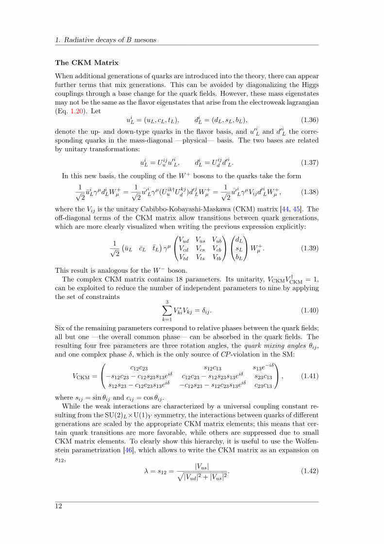
1. Radiative decays of B mesons
The CKM Matrix
When additional generations of quarks are introduced into the theory, there can appearfurther terms that mix generations. This can be avoided by diagonalizing the Higgscouplings through a base change for the quark fields. However, these mass eigenstatesmay not be the same as the flavor eigenstates that arise from the electroweak lagrangian(Eq. 1.20). Let
uiL = (uL, cL, tL), diL = (dL, sL, bL), (1.36)
denote the up- and down-type quarks in the flavor basis, and u′iL and d′iL the corre-sponding quarks in the mass-diagonal —physical— basis. The two bases are relatedby unitary transformations:
uiL = U iju u
′iL, diL = U ij
d d′iL. (1.37)
In this new basis, the coupling of the W+ bosons to the quarks take the form
1√2uiLγ
µdiLW+µ =
1√2u′
iLγ
µ(U ik†u Ukj
d )d′jLW
+µ =
1√2u′
iLγ
µVijd′iLW
+µ , (1.38)
where the Vij is the unitary Cabibbo-Kobayashi-Maskawa (CKM) matrix [44, 45]. Theoff-diagonal terms of the CKM matrix allow transitions between quark generations,which are more clearly visualized when writing the previous expression explicitly:
1√2
(uL cL tL
)γµ
Vud Vus VubVcd Vcs VcbVtd Vts Vtb
dLsLbL
W+µ . (1.39)
This result is analogous for the W− boson.The complex CKM matrix contains 18 parameters. Its unitarity, VCKMV
†CKM = 1,
can be exploited to reduce the number of independent parameters to nine by applyingthe set of constraints
3∑k=1
V ∗kiVkj = δij . (1.40)
Six of the remaining parameters correspond to relative phases between the quark fields;all but one —the overall common phase— can be absorbed in the quark fields. Theresulting four free parameters are three rotation angles, the quark mixing angles θij ,and one complex phase δ, which is the only source of CP -violation in the SM:
VCKM =
c12c23 s12c13 s13e−iδ
−s12c23 − c12s23s13eiδ c12c23 − s12s23s13e
iδ s23c13s12s23 − c12c23s13e
iδ −c12s23 − s12c23s13eiδ c23c13
, (1.41)
where sij = sin θij and cij = cos θij .While the weak interactions are characterized by a universal coupling constant re-
sulting from the SU(2)L×U(1)Y symmetry, the interactions between quarks of differentgenerations are scaled by the appropriate CKM matrix elements; this means that cer-tain quark transitions are more favorable, while others are suppressed due to smallCKM matrix elements. To clearly show this hierarchy, it is useful to use the Wolfen-stein parametrization [46], which allows to write the CKM matrix as an expansion ons12,
λ = s12 =|Vus|√
|Vud|2 + |Vus|2. (1.42)
12

1.1. The Standard Model
For CP violation studies it is necessary to expand the CKM matrix up to terms ofO(λ5) because VtdVts is of this order:
VCKM =
1− λ2
2 λ Aλ3(ρ− iη + iη λ2
2
)−λ 1− λ2
2 − iηA2λ4 Aλ2(1 + iηλ2)Aλ3 (1− ρ− iη) −Aλ2 1
+O(λ5),
(1.43)with the A, ρ and η defined as
s23 = Aλ2 = λ|Vcb|V us
, s13eiδ = Aλ3(ρ+ iη) = V ∗
ub, (1.44)
and with the following experimental values [21]:
λ = 0.2253±0.0007, A = 0.808+0.022−0.015, ρ = 0.132+0.022
−0.014, η = 0.341±0.013. (1.45)
The SM makes no predictions for the Vij matrix elements aside from unitarity, sothey need to be determined from experiment. Interestingly, the individual elements ofthe CKM matrix can be measured independently without making use of the theoreticalunitarity requirement; thus, unitarity can be used to over-constrain the CKM matrixand test the weak sector of the SM.
The unitarity of the CKM matrix can be conveniently summarized in unitarity tri-angles by picturing each of the unitarity relations in Eq. 1.40 as a triangle in a complexplane. For example, the first and third columns of the CKM matrix, i.e., the b and dsectors, can be used to build an unitarity relation,
V ∗udVub + V ∗
cdVcb + V ∗tdVtb = 0, (1.46)
which can be represented as a triangle, as shown in Fig. 1.1, with its sides normalizedand rotated by dividing by V ∗
cdVcb. The angles α, β and γ are defined as
α = arg(−V ∗tdVtbV ∗cdVcb
), β = arg
(−V ∗cdVcbV ∗tdVtb
), γ = arg
(−V ∗udVubV ∗cdVcb
), (1.47)
with the (ρ, η) vertex given by
ρ+ iη = −V ∗udVubV ∗cdVcb
. (1.48)
The sides of the triangle, which correspond to magnitudes of CKM elements, can bemeasured by analyzing the decay rates of processes involving these elements, while theangles, which correspond to the relative phases between the elements, can be accessedexperimentally through CP -violating asymmetries. The current experimental situationof this unitarity triangle is shown in Fig. 1.2 [47].
GIM Mechanism
Spontaneous symmetry breaking, which gives quarks different masses, is responsible forthe GIM suppression —from Glashow, Iliopoulos and Maiani [48]— in loop processesby interfering with the balance imposed by the unitarity of the CKM matrix, whichwould otherwise forbid effective flavor-changing neutral current processes.
13
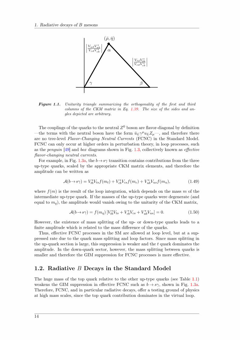
1. Radiative decays of B mesons
Figure 1.1. Unitarity triangle summarizing the orthogonality of the first and thirdcolumns of the CKM matrix in Eq. 1.39. The size of the sides and an-gles depicted are arbitrary.
The couplings of the quarks to the neutral Z0 boson are flavor-diagonal by definition—the terms with the neutral boson have the form uLγ
µuLZµ—, and therefore thereare no tree-level Flavor-Changing Neutral Currents (FCNC) in the Standard Model.FCNC can only occur at higher orders in perturbation theory, in loop processes, suchas the penguin [49] and box diagrams shown in Fig. 1.3, collectively known as effectiveflavor-changing neutral currents.
For example, in Fig. 1.3a, the b→sγ transition contains contributions from the threeup-type quarks, scaled by the appropriate CKM matrix elements, and therefore theamplitude can be written as
A(b→sγ) = V ∗tbVtsf(mt) + V ∗
cbVcsf(mc) + V ∗ubVusf(mu), (1.49)
where f(m) is the result of the loop integration, which depends on the mass m of theintermediate up-type quark. If the masses of the up-type quarks were degenerate (andequal to mq), the amplitude would vanish owing to the unitarity of the CKM matrix,
A(b→sγ) = f(mq) [V∗tbVts + V ∗
cbVcs + V ∗ubVus] = 0. (1.50)
However, the existence of mass splitting of the up- or down-type quarks leads to afinite amplitude which is related to the mass difference of the quarks.
Thus, effective FCNC processes in the SM are allowed at loop level, but at a sup-pressed rate due to the quark mass splitting and loop factors. Since mass splitting inthe up-quark section is large, this suppression is weaker and the t quark dominates theamplitude. In the down-quark sector, however, the mass splitting between quarks issmaller and therefore the GIM suppression for FCNC processes is more effective.
1.2. Radiative B Decays in the Standard Model
The huge mass of the top quark relative to the other up-type quarks (see Table 1.1)weakens the GIM suppression in effective FCNC such as b→ sγ, shown in Fig. 1.3a.Therefore, FCNC, and in particular radiative decays, offer a testing ground of physicsat high mass scales, since the top quark contribution dominates in the virtual loop.
14
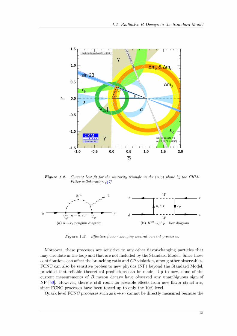
1.2. Radiative B Decays in the Standard Model
γ
γ
αα
dm∆Kε
Kε
sm∆ & dm∆
ubV
βsin 2
(excl. at CL > 0.95) < 0βsol. w/ cos 2
excluded at CL > 0.95
α
βγ
ρ-1.0 -0.5 0.0 0.5 1.0 1.5 2.0
η
-1.5
-1.0
-0.5
0.0
0.5
1.0
1.5excluded area has CL > 0.95
Summer 11
CKMf i t t e r
Figure 1.2. Current best fit for the unitarity triangle in the (ρ, η) plane by the CKM-Fitter collaboration [47].
(a) b→sγ penguin diagram (b) K∗0→µ+µ− box diagram
Figure 1.3. Effective flavor-changing neutral current processes.
Moreover, these processes are sensitive to any other flavor-changing particles thatmay circulate in the loop and that are not included by the Standard Model. Since thesecontributions can affect the branching ratio and CP violation, among other observables,FCNC can also be sensitive probes to new physics (NP) beyond the Standard Model,provided that reliable theoretical predictions can be made. Up to now, none of thecurrent measurements of B meson decays have observed any unambiguous sign ofNP [50]. However, there is still room for sizeable effects from new flavor structures,since FCNC processes have been tested up to only the 10% level.
Quark level FCNC processes such as b→sγ cannot be directly measured because the
15
1. Radiative decays of B mesons
strong interaction forms hadrons from the underlying quarks, which cannot be detecteddirectly due to the confinement property of QCD. Therefore, in order to establish aconnection between experimental observations and the CKM parameters, one needs tounfold the effects of confinement.
Inclusive B→Xsγ decays, which include all hadron combinations that arise fromthe b→sγ transition, are theoretically clean because they are dominated by partonic,perturbatively calculable, contributions, with small (∼ 5%) non-perturbative correc-tions [51]. Experimentally, inclusive quantities are difficult to define due to the factthat it is not feasible to measure all possible final states; the poor knowledge of therelative branching fractions of those that are measured makes it difficult to extractreliable inclusive values. Exclusive final states with one or a few specific hadrons in thefinal state, e.g., B0→K∗0γ, have less predictive power due to larger non-perturbativeQCD corrections. However, measurements are easier and better defined than inclusiveones, and many other useful observables beyond branching fractions can be obtained,such as CP , forward-backward, isospin, and polarization asymmetries.
To tackle the mixture of regimes of QCD behavior —perturbative and non-perturbative—, calculations are divided into two parts by making use of factorizationtheorems, which can be found using various techniques, such as effective field theories.Factorization allows to separate the contributions of perturbative QCD, occurring atscales well above the B meson mass, from the contributions from lower mass, longdistance, scales, where perturbative calculations are no longer possible. Long distancecontributions are calculated using non-perturbative techniques such as QCD sum rulesor lattice calculations. QCD Factorization (QCDF) [52–54] can be used to obtain afactorization theorem which allows to put together these long distance contributionsand the perturbative calculations, while the use of Soft Collinear Effective Theory(SCET) [55–58] allows to reach a deeper understanding of this factorization.
1.2.1. Effective Field Theories
Effective field theories [59, 60] are used to express a full, complete theory as an effectiveHamiltonian constructed from a set of local operators Oi in which the high energydegrees of freedom, defined with respect to a mass scale Λ, have been integrated out.The amplitude for a given weak process i→f is expressed as a sum of matrix elementsof the local operators:
⟨f |Heff|i⟩ =GF√2
∑i
ViCi(µ)⟨f |Oi(µ)|i⟩, (1.51)
where GF is the Fermi constant characterizing the strength of the underlying weakprocesses, Vi are the suitable CKM matrix elements for the quark transitions, Ci arethe Wilson coefficients and Oi are the local operators forming a complete set for a giventransition. The Wilson coefficients Ci are the numerical coefficients associated withthese effective transitions expressed with the local operators Oi. Therefore, the ampli-tude of the effective Hamiltonian is expressed as a sum of local operator amplitudesscaled by their Wilson coefficients.
The Wilson coefficients include the effects of interactions at scales higher than µ,and the operators absorb all the effects below. While the choice of µ is arbitrary, itis usually chosen to be O(mb) for the study of B decays; this is well above the ΛQCDscale where perturbative QCD starts to break down.
16
1.2. Radiative B Decays in the Standard Model
Wilson coefficients are calculated by matching the prediction of the effective theorywith the full theory (with all degrees of freedom) at a high mass scale, typically mW ;at this scale the relevant diagrams and their QCD corrections can be calculated per-turbatively and evolved down to the relevant energy scale —the previously mentionedmb in our case—by making use of the renormalization group equations. After renor-malization, the local operators Oi can be identified within the full calculation and theircorresponding Wilson coefficients extracted.
In general, there are several operators of the same dimension which mix under renor-malization.
⟨Oi⟩B =∑i
Zij(ϵ, µ)⟨Oj⟩R, (1.52)
where the subscript B (R) denotes the bare (renormalized) operator. This operatormixing can affect the decay rate: in b→ sγ, this can result in a three-fold enhance-ment [61, 62].
Effective Weak Hamiltonian for B→V γ Transitions
Following the convention by Becher, Hill and Neubert [63], in the Standard Model, theeffective weak Hamiltonian mediating FCNC b→s processes has the form
Hweak =GF√2
∑p=u,c
V ∗psVpb
[C1O
p1 + C2O
p2 +
8∑i=3
CiOi
], (1.53)
with the operators
Op1 = sγµ(1− γ5)ppγµ(1− γ5)b Op
2 = siγµ(1− γ5)pj pjγµ(1− γ5)b
i
O3 = sγµ(1− γ5)b∑q
qγµ(1− γ5)q O4 = siγµ(1− γ5)bj∑q
qjγµ(1− γ5)qi
O5 = sγµ(1 + γ5)b∑q
qγµ(1 + γ5)q O6 = siγµ(1 + γ5)bj∑q
qjγµ(1 + γ5)qi
O7 = − e
8π2mbsσ
µν(1 + γ5)bFµν O8 = − g
8π2mbsσ
µν(1 + γ5)TabGa
µν ,
(1.54)
where i, j are color indices. The effective weak Hamiltonian for b→ d transitions isobtained by replacing s with d in the above expressions.
The most relevant operators are the four-quark operator Op1, the electromagnetic
penguin operator Q7, and the chromomagnetic penguin operator O8, specially for CPstudies. The matrix elements of the QCD penguin operators Op
2, . . . , O6 contributes atO(αs) and are multiplied by small Wilson coefficients, while the contribution from Op
2
starts at O(αs).At one-loop order, the decay is mediated entirely by the O7 electromagnetic penguin
without mixing with the four-quark operators, which occurs at higher orders. The rateof the inclusive B→Xsγ transition can be written [64] at one-loop as
Γ(B→Xsγ) =αG2
Fm5b
128π4
∣∣∣∣∣ ∑p=u,c
V ∗psVpbC7(mb)
∣∣∣∣∣2
. (1.55)
17
1. Radiative decays of B mesons
1.2.2. Exclusive Radiative Decays
The Wilson coefficients of the effective weak Hamiltonian in Eq. 1.51 are process-independent and therefore can be used directly in the description of exclusive modes.The theoretical precision is thus limited by the difficulty of computing the hadronicmatrix elements between meson states, ⟨f |Oj |i⟩.
In the case of radiative decays, Heavy Quark Effective Theory (HQET) [65, 66]has been extensively used, specially in the prediction of inclusive B decays. HQETwas constructed as a general framework in which to explore heavy quark physics byperforming an expansion in ΛQCD/m, where m is the mass of the heavy quark. In it,all light degrees of freedom must have momenta of the order ΛQCD, i.e., the momentumpheavy of the heavy quark inside a heavy meson moving with velocity v = pmeson/Mmesonis decomposed as pheavy = mv+k and all components of the residual momentum k areassumed to be of O(ΛQCD).
However, in a decay of a heavy quark into a light quark one may have a kinematicalsituation in which the light degrees of freedom carry a large energy in the rest frame ofthe heavy quark, and therefore vplight ∼ m. For example, one may consider a radiativedecay in the corner of phase space where the energy Eγ of the photon is close to ismaximal value Eγ,max ∼MB/2, if we ignore the mass of the final state. In this case, thehadronic final state corresponds to a collimated “jet” of hadrons with small invariantmass but large energy in the rest frame of the decaying B meson.
At this point, one is faced with a multi-scale problem, which can be tackled bymaking use of SCET [55]. The three relevant energy scales are:
The soft scale of O(few×ΛQCD), set by the typical energies and momenta of thelight degrees of freedom in the hadronic bound states.
The hard scale of O(mb), set by the b quark mass and the energy of the outgoinghadron in the B meson rest frame.
The hard-collinear scale, µ =√mbΛ, appearing through interactions between
soft and energetic modes in the initial and final states.
The dynamics of hard and hard-collinear modes can be described perturbatively in theheavy quark limit, mb → ∞. SCET then describes B decays to light hadrons withenergies much larger than their masses, assuming that their constituents have momentacollinear to the hadron momentum.
Hadronic Matrix Elements for B→V γ
The QCDF formula for the matrix element of a given operator of the effective weakHamiltonian can be written in the form [67]
⟨V γ|Oi|B⟩ = FB→V⊥T Ii +
∫dωduϕB+(ω)ϕ
V⊥(u)T
IIi (ω, u), (1.56)
which is expected to be valid up to corrections of O(ΛQCD/m).The non-perturbative effects are contained in FB→V⊥ , a form factor evaluated at
q2 = 0, and in ϕB+ and ϕV⊥, the light-cone distribution amplitudes (LCDAs) for theB and V mesons, respectively. The hard-scattering kernels T I
i , related to virtualcorrections to the inclusive decay rate, and T II
i , related to parton exchange with the
18
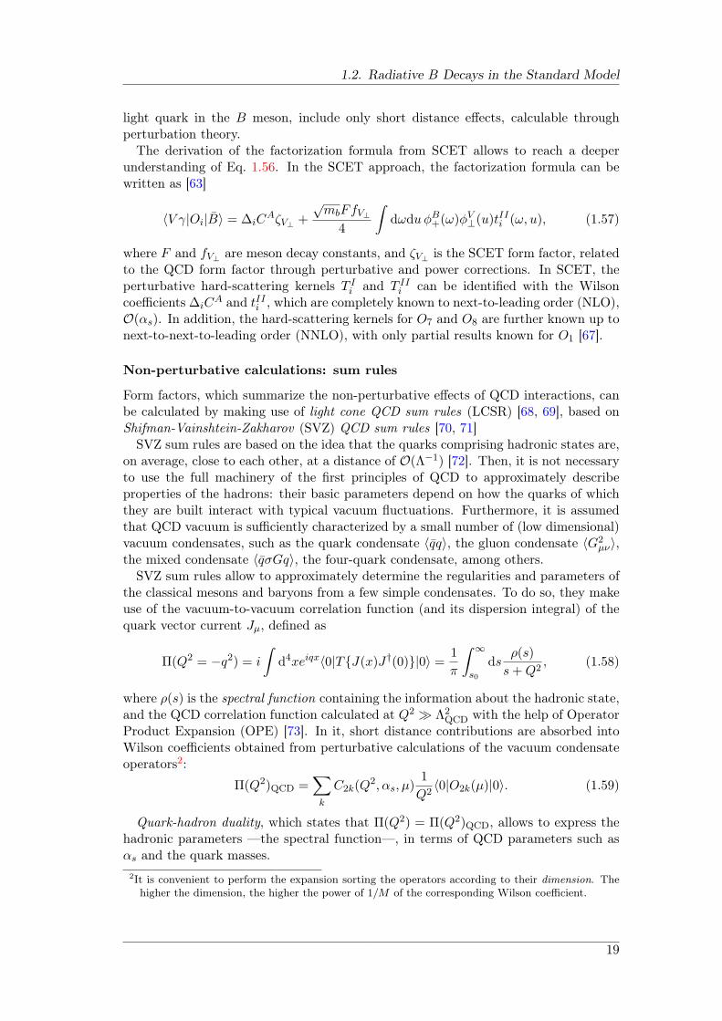
1.2. Radiative B Decays in the Standard Model
light quark in the B meson, include only short distance effects, calculable throughperturbation theory.
The derivation of the factorization formula from SCET allows to reach a deeperunderstanding of Eq. 1.56. In the SCET approach, the factorization formula can bewritten as [63]
⟨V γ|Oi|B⟩ = ∆iCAζV⊥ +
√mbFfV⊥
4
∫dωduϕB+(ω)ϕ
V⊥(u)t
IIi (ω, u), (1.57)
where F and fV⊥ are meson decay constants, and ζV⊥ is the SCET form factor, relatedto the QCD form factor through perturbative and power corrections. In SCET, theperturbative hard-scattering kernels T I
i and T IIi can be identified with the Wilson
coefficients ∆iCA and tIIi , which are completely known to next-to-leading order (NLO),
O(αs). In addition, the hard-scattering kernels for O7 and O8 are further known up tonext-to-next-to-leading order (NNLO), with only partial results known for O1 [67].
Non-perturbative calculations: sum rules
Form factors, which summarize the non-perturbative effects of QCD interactions, canbe calculated by making use of light cone QCD sum rules (LCSR) [68, 69], based onShifman-Vainshtein-Zakharov (SVZ) QCD sum rules [70, 71]
SVZ sum rules are based on the idea that the quarks comprising hadronic states are,on average, close to each other, at a distance of O(Λ−1) [72]. Then, it is not necessaryto use the full machinery of the first principles of QCD to approximately describeproperties of the hadrons: their basic parameters depend on how the quarks of whichthey are built interact with typical vacuum fluctuations. Furthermore, it is assumedthat QCD vacuum is sufficiently characterized by a small number of (low dimensional)vacuum condensates, such as the quark condensate ⟨qq⟩, the gluon condensate ⟨G2
µν⟩,the mixed condensate ⟨qσGq⟩, the four-quark condensate, among others.
SVZ sum rules allow to approximately determine the regularities and parameters ofthe classical mesons and baryons from a few simple condensates. To do so, they makeuse of the vacuum-to-vacuum correlation function (and its dispersion integral) of thequark vector current Jµ, defined as
Π(Q2 = −q2) = i
∫d4xeiqx⟨0|TJ(x)J†(0)|0⟩ = 1
π
∫ ∞
s0
dsρ(s)
s+Q2, (1.58)
where ρ(s) is the spectral function containing the information about the hadronic state,and the QCD correlation function calculated at Q2 ≫ Λ2
QCD with the help of OperatorProduct Expansion (OPE) [73]. In it, short distance contributions are absorbed intoWilson coefficients obtained from perturbative calculations of the vacuum condensateoperators2:
Π(Q2)QCD =∑k
C2k(Q2, αs, µ)
1
Q2⟨0|O2k(µ)|0⟩. (1.59)
Quark-hadron duality, which states that Π(Q2) = Π(Q2)QCD, allows to express thehadronic parameters —the spectral function—, in terms of QCD parameters such asαs and the quark masses.
2It is convenient to perform the expansion sorting the operators according to their dimension. Thehigher the dimension, the higher the power of 1/M of the corresponding Wilson coefficient.
19
1. Radiative decays of B mesons
The LCSR approach is a variant of the SVZ sum rules designed to overcome diffi-culties of the latter in three-point functions, e.g., in the case of A→B C. In them, thestandard condensate expansion contains a series of operators with derivatives whichgive rise to the expansion parameter of type pC(pA + pB)/p
2A,B ∼ 1. Therefore, all
terms in this subseries must be summed over.This partial summation is carried out automatically if one considers the correlation
function of the currents jA and jB sandwiched between the vacuum and state |C⟩,instead of the three-point function ⟨jA, jB, jC⟩. The vacuum expectation values ofthe condensates (operators) in the SVZ sum rules are substituted by the light-conewave functions ϕ. The OPE is then performed with the light-cone wave functionssorted in increasing twist, defined as the difference of the dimension and the spin ofthe condensate operator. In order words, using LCSR allows the partial summationwith the tradeoff that large distance dynamics are no longer parametrized by numbers,as in SVZ sum rules, but by functions —the leading twist, the next-to-leading twist,and so on. Quark-hadron duality then relates the twist expansion to the desired formfactor.
1.3. Current theoretical and experimental status
While exclusive radiative decays offer a larger variety of experimentally accessible ob-servables than the inclusive ones, the non-perturbative uncertainties in theoreticalpredictions are in general sizable.
Branching ratios
Large hadronic uncertainties arising from the non-perturbative input in Eq. 1.57 do notallow precise theoretical predictions of the branching fractions of exclusive radiativedecays. The SCET soft function ζV⊥ is the main theoretical uncertainty, which can bereduced by improved QCD non-perturbative QCD calculations.
NNLO calculations [67], which make use of form factor calculations in LCSR from[74] are compared to the latest experimental results in Table 1.3. It can be seen that themeasurements in the B0 sector, coming from CLEO [75], BaBar [76] and Belle [77],are more precise than the theoretical calculations; measurements in the B0
s sector,performed in Belle through the Υ(5S) resonance [78], suffer from great uncertaintiesdue to the low collected statistics.
The measure of the ratio of the branching fractions of B0 → K∗0γ and B0s → ϕγ
is rather interesting, since in this case only uncertainties in the quantities which aredifferent between the two decays add significant error. Ali, Pecjak and Greub find [67]
B(B0→K∗0γ)
B(B0s →ϕγ)
= 1.0± 0.2, (1.60)
to be compared with the experimental ratio 0.7± 0.3.
Isospin Asymmetry
The isospin asymmetry ratio, given by
Λ0±(B0→K∗0γ) =
Γ(B0→K∗0γ)− Γ(B±→K0±γ)
Γ(B0→K∗0γ) + Γ(B±→K0±γ), (1.61)
20
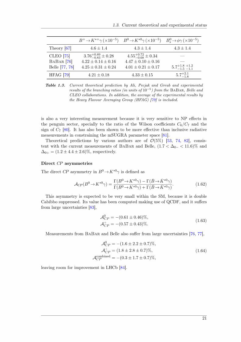
1.3. Current theoretical and experimental status
B+→K∗+γ (×10−5) B0→K∗0γ (×10−5) B0s →ϕγ (×10−5)
Theory [67] 4.6± 1.4 4.3± 1.4 4.3± 1.4
CLEO [75] 3.76+0.89−0.83 ± 0.28 4.55+0.72
−0.68 ± 0.34 —BaBar [76] 4.22± 0.14± 0.16 4.47± 0.10± 0.16 —Belle [77, 78] 4.25± 0.31± 0.24 4.01± 0.21± 0.17 5.7+1.8
−1.5+1.2−1.1
HFAG [79] 4.21± 0.18 4.33± 0.15 5.7+2.1−1.8
Table 1.3. Current theoretical prediction by Ali, Pecjak and Greub and experimentalresults of the branching ratios (in units of 10−5) from the BaBar, Belle andCLEO collaborations. In addition, the average of the experimental results bythe Heavy Flavour Averaging Group (HFAG) [79] is included.
is also a very interesting measurement because it is very sensitive to NP effects inthe penguin sector, specially to the ratio of the Wilson coefficients C6/C7 and thesign of C7 [80]. It has also been shown to be more effective than inclusive radiativemeasurements in constraining the mSUGRA parameter space [81].
Theoretical predictions by various authors are of O(5%) [53, 74, 82], consis-tent with the current measurements of BaBar and Belle, (1.7 < ∆0− < 11.6)% and∆0+ = (1.2± 4.4± 2.6)%, respectively.
Direct CP asymmetries
The direct CP asymmetry in B0→K∗0γ is defined as
ACP (B0→K∗0γ) =
Γ(B0→K∗0γ)− Γ(B→K∗0γ)
Γ(B0→K∗0γ) + Γ(B→K∗0γ). (1.62)
This asymmetry is expected to be very small within the SM, because it is doubleCabibbo suppressed. Its value has been computed making use of QCDF, and it suffersfrom large uncertainties [83],
A0CP = −(0.61± 0.46)%,
A+CP = −(0.57± 0.43)%.
(1.63)
Measurements from BaBar and Belle also suffer from large uncertainties [76, 77],
A0CP = −(1.6± 2.2± 0.7)%,
A+CP = (1.8± 2.8± 0.7)%,
AcombinedCP = −(0.3± 1.7± 0.7)%,
(1.64)
leaving room for improvement in LHCb [84].
21

2CERN and the LHC
The European Organization for Nuclear Research, known as CERN, is the world’slargest particle physics laboratory, and is situated on the Franco-Swiss border, nearGeneva. In its 50 years of existence, many high-energy physics experiments have beenbuilt within its facilities, usually by large international collaborations. It currentlyhosts the largest particle accelerator in the world, the LHC, and its six experiments:ALICE, ATLAS, CMS, LHCb, LHCf and TOTEM.
2.1. The European Organization for Nuclear Research(CERN)
CERN is the European Organization for Nuclear Research. The CERN acronym comesfrom the French Conseil Européen pour la Recherche Nucléaire, European Council forNuclear Research. At the time of the foundation of the Organization, in the mid-1950’s, the frontier for pure physics research was the inside of the atom, and hencethe use of the nuclear in the name. This becomes also clear in the phrasing of theConvention that established CERN in 1954, which lays down the main missions for theOrganization:
The Organization shall provide for collaboration among European Statesin nuclear research of a pure scientific and fundamental character (...). TheOrganization shall have no concern with work for military requirementsand the results of its experimental and theoretical work shall be publishedor otherwise made generally available.
Although our current understanding of matter goes deeper than the nucleus, CERN’smain mission remains the same.
CERN is run by 20 European Member States, but many non-European countriesare also involved in different ways. The current Member States are: Austria, Belgium,Bulgaria, the Czech Republic, Denmark, Finland, France, Germany, Greece, Hungary,Italy, the Netherlands, Norway, Poland, Portugal, the Slovak Republic, Spain, Sweden,Switzerland, and the United Kingdom, while Romania is nowadays a candidate to
23
2. CERN and the LHC
become a Member State of CERN. Some states (or international organizations) forwhich membership is either not possible or not yet feasible are Observers.
Overall, a total of 10000 visiting scientists from 608 institutes and universities from113 countries around the world use CERN’s facilities, amounting to half of the world’sparticle physicists. Moreover, CERN employs around 2400 people between scientificand technical staff.
History highlights
French physicist Louis de Broglie was the first to put forward an official proposal forthe creation of a European laboratory at the European Cultural Conference in Lau-sanne in December 1949. At the end of 1951 the first resolution for the creation ofan European Council For Nuclear Research was adopted, and a few months later 11countries signed an agreement establishing the provisional Council —CERN. At theend of 1952 Geneva was chosen as the site of the future laboratory. On September29th, 1954 the 12 founding Member States ratified the CERN Convention and the Eu-ropean Organization for Nuclear Research was created, keeping the provisional CERNacronym. CERN’s history highlights are presented in a schematic way in Fig. 2.1, andwill be summarized below.
The maximum expression of CERN’s achievements is the construction of severalgreat colliders, from the first 600 MeV Synchrocyclotron (SC), built in 1957 and closeddown in 1990, to the 7 TeV Large Hadron Collider (LHC), which started up in 2008and is currently the world’s biggest collider. In between, the first proton-proton col-lider —the Intersecting Storage Rings (ISR)— commissioned in 1971, the first proton-antiproton collider —the Super Proton Synchrotron (SPS)—, that led to the discoveryof the W± and Z0 bosons, and the Large Electron Positron (LEP) collider, commis-sioned in 1989, which provided a detailed study of the electroweak interaction. Thesecolliders have been at the core of CERN’s research and have provided great discoveriessuch as the existence of neutral currents.
During the history of CERN several Nobel Prizes in Physics have been awarded toscientists working at its facilities, which can be seen marked as yellow stars ( .. ) inFig. 2.1. In 1976, the afterwards LEP experiment L3 spokesman Sam Ting, alongwith Burt Richter, received the Nobel prize “for their pioneering work in the discoveryof a heavy elementary particle of a new kind ”. The J/ψ had been discovered twoyears before, but not at CERN. In 1984, just one year after the discovery of the W±
and Z0 bosons, Carlo Rubbia and Simon Van der Meer were awarded the Prize for“their decisive contributions to the large project which led to the discovery of the fieldparticles W and Z, communicators of the weak interaction”. The experimental resultsconfirmed the unification of weak and electromagnetic forces, the electroweak theoryof the Standard Model. Less than a decade later, Georges Charpak, a CERN physicistsince 1959, received the 1992 physics Nobel Prize for “his invention and developmentof particle detectors, in particular the multi-wire proportional chamber, a breakthroughin the technique for exploring the innermost parts of matter ”. Charpak’s multi-wireproportional chamber, invented in 1968, and his subsequent developments launched theera of fully electronic particle detection. In 1988, Jack Steinberger, a CERN physicistsince the late 1960s and head of the LEP ALEPH experiment at the time, was awardedthe Nobel Prize, together with Leon Lederman and Mel Schwartz, “for the neutrinobeam method and the demonstration of the doublet structure of the leptons through the
24
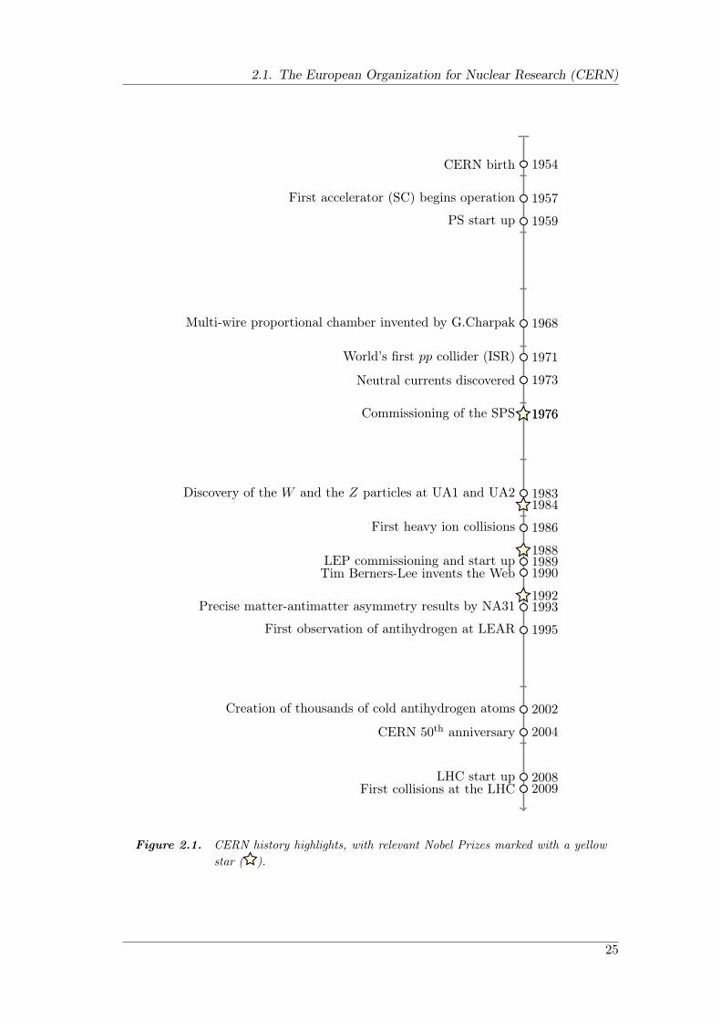
2.1. The European Organization for Nuclear Research (CERN)
...
1954
.
CERN birth
..
1957
.
First accelerator (SC) begins operation
..
1959
.
PS start up
..
1968
.
Multi-wire proportional chamber invented by G.Charpak
..
1971
.
World’s first pp collider (ISR)
..
1973
.
Neutral currents discovered
..
1976
.
Commissioning of the SPS
..
1983
.
Discovery of the W and the Z particles at UA1 and UA2
..
1986
.
First heavy ion collisions
..
1989
.
LEP commissioning and start up
..
1990
.
Tim Berners-Lee invents the Web
..
1993
.
Precise matter-antimatter asymmetry results by NA31
..
1995
.
First observation of antihydrogen at LEAR
..
2002
.
Creation of thousands of cold antihydrogen atoms
..
2004
.
CERN 50th anniversary
..
2008
.
LHC start up
..
2009
.
First collisions at the LHC
..
1984
..
1992
..
1976
..
1988
Figure 2.1. CERN history highlights, with relevant Nobel Prizes marked with a yellowstar ( .. ).
25
2. CERN and the LHC
discovery of the muon neutrino”. The discovery, made in 1962 at the US BrookhavenNational Laboratory, showed that there was more than one type of neutrino.
Finally, one must not forget to mention Tim Berners-Lee, a scientist at CERN whodefined the World Wide Web’s basic concepts —the URL, http and HTML— and wrotethe first browser and server software in 1990. The World Wide Web was conceived anddeveloped to meet the demand for information sharing between scientists around theworld, and has changed the way we live nowadays.
2.2. The Large Hadron Collider
The Large Hadron Collider (LHC) at CERN is the most powerful tool for particlephysics in the world [85]. It is a two-ring superconducting hadron accelerator andcollider installed in the existing 26.7 km tunnel built between 1984 and 1989 to housethe LEP machine. The tunnel has eight straight sections and eight arcs and liesbetween 45m and 170m below the surface on a plane inclined 1.4% towards the Lémanlake. There are two transfer tunnels of about 2.5 km that link the LHC to the CERNaccelerator complex, which acts as injector.
The LHC project was approved by the CERN council in December 1994. At thattime, the plan was to build the machine in two stages, starting with a center-of-massenergy of 10TeV, which would be upgraded to 14TeV at a later stage. In the end, in1996 the CERN council approved the construction of the 14TeV machine in one stage.
The aim of the LHC and its experiments is to test or reveal the physics beyond theStandard Model. The number of events of a given type generated each second in theLHC is given by:
Nevent = Lσevent, (2.1)
where σevent is the cross section for the event under study and L the machine luminosity.The machine luminosity solely depends on the beam parameters and can be writtenas [86, 87]:
L =N2
b nbfrevγr4πϵnβ∗
F, [ cm−2 s−1] (2.2)
where Nb is the number of particles per bunch, nb the number of colliding bunches,frev the revolution frequency, γr the relativistic gamma factor, ϵn the normalized trans-verse beam emittance, β∗ the beta function at the collision point and F the geometricluminosity reduction factor. This latter factor is has its origin in the crossing angle ofthe beams at the interaction point (IP), and can be expressed as
F =
[1 +
(θcσz2σ∗
)2]− 1
2
, (2.3)
being θc the full crossing angle at the IP, σz the RMS bunch length, and σ∗ thetransverse RMS bunch size at the IP. Therefore, we can see that the exploration ofrare events in the LHC collisions, characterized by very low cross sections, requires ahigh luminosity, achieved through both high beam energies and high beam intensities.
The ATLAS and CMS experiments, detailed in §2.3, are designed to run with a peakluminosity of L = 1034 cm−2 s−1 for proton operation. Furthermore, there are two lowluminosity experiments, also introduced in §2.3: LHCb, aiming at L = 1032 cm−2 s−1,and TOTEM, aiming at a peak luminosity L = 2 × 1029 cm−2 s−1 with 156 colliding
26

2.2. The Large Hadron Collider
bunches. The LHC has also one dedicated heavy ion experiment, ALICE, aiming at apeak luminosity of L = 1027 cm−2 s−1 for nominal lead-lead ion operation.
The high beam intensity required for the nominal luminosity L = 1034 cm−2 s−1
excludes a proton-antiproton (pp) collider. Therefore, the LHC was designed as aproton-proton (pp) collider. Furthermore, since colliding two counter-rotating protonbeams requires opposite magnetic dipole fields in both rings, the collider configurationwith common vacuum and magnet systems for both circulating rings was excluded. Theadopted configuration was thus a pp collider with separate magnetic fields and vacuumchambers in the main portion of the rings (see Fig. 2.2), with common sections onlyat the 4 insertion regions where the experimental detectors are located. Since there isnot enough room for two separate rings of magnets in the LEP tunnel, the LHC usestwin bore magnets that consist of two sets of coils and beam channels within the samemechanical structure and cryostat. The peak beam energy depends on the integrateddipole field around the storage ring, which bends the trajectory of the proton beams.For a beam energy of 7TeV in the LHC machine, a peak dipole field of 8.33T isneeded. These high field strengths are achieved through the use of superconductingelectromagnets cooled down to a temperature of 1.9K.
Figure 2.2. Cross-section of a LHC superconducting cryodipole [85].
The high peak luminosity of L = 1034 cm−2 s−1 is reached through a high numberof bunches per beam, nb = 2808, a high revolution rate, frev = 11245Hz, and a largenumber of protons per bunch, Nb = 1.1× 10¹¹. This gives a minimal distance of ∼ 7mbetween bunches, and a time of 25 ns between two bunch crossings, amounting to abunch crossing frequency of 40MHz.
27
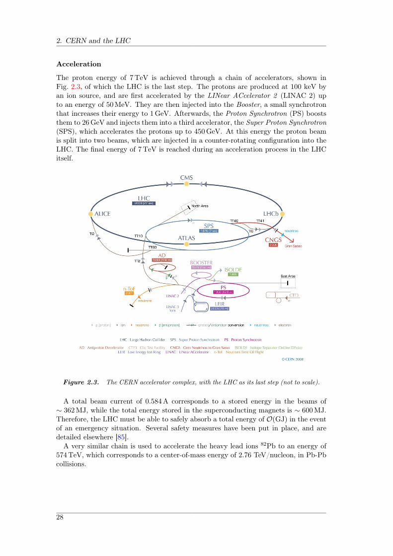
2. CERN and the LHC
Acceleration
The proton energy of 7TeV is achieved through a chain of accelerators, shown inFig. 2.3, of which the LHC is the last step. The protons are produced at 100 keV byan ion source, and are first accelerated by the LINear ACcelerator 2 (LINAC 2) upto an energy of 50MeV. They are then injected into the Booster, a small synchrotronthat increases their energy to 1GeV. Afterwards, the Proton Synchrotron (PS) booststhem to 26GeV and injects them into a third accelerator, the Super Proton Synchrotron(SPS), which accelerates the protons up to 450GeV. At this energy the proton beamis split into two beams, which are injected in a counter-rotating configuration into theLHC. The final energy of 7TeV is reached during an acceleration process in the LHCitself.
Figure 2.3. The CERN accelerator complex, with the LHC as its last step (not to scale).
A total beam current of 0.584A corresponds to a stored energy in the beams of∼ 362MJ, while the total energy stored in the superconducting magnets is ∼ 600MJ.Therefore, the LHC must be able to safely absorb a total energy of O(GJ) in the eventof an emergency situation. Several safety measures have been put in place, and aredetailed elsewhere [85].
A very similar chain is used to accelerate the heavy lead ions 82Pb to an energy of574TeV, which corresponds to a center-of-mass energy of 2.76 TeV/nucleon, in Pb-Pbcollisions.
28
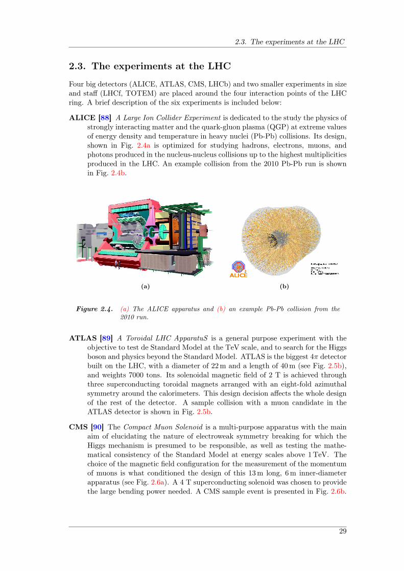
2.3. The experiments at the LHC
2.3. The experiments at the LHC
Four big detectors (ALICE, ATLAS, CMS, LHCb) and two smaller experiments in sizeand staff (LHCf, TOTEM) are placed around the four interaction points of the LHCring. A brief description of the six experiments is included below:
ALICE [88] A Large Ion Collider Experiment is dedicated to the study the physics ofstrongly interacting matter and the quark-gluon plasma (QGP) at extreme valuesof energy density and temperature in heavy nuclei (Pb-Pb) collisions. Its design,shown in Fig. 2.4a is optimized for studying hadrons, electrons, muons, andphotons produced in the nucleus-nucleus collisions up to the highest multiplicitiesproduced in the LHC. An example collision from the 2010 Pb-Pb run is shownin Fig. 2.4b.
(a) (b)
Figure 2.4. (a) The ALICE apparatus and (b) an example Pb-Pb collision from the2010 run.
ATLAS [89] A Toroidal LHC ApparatuS is a general purpose experiment with theobjective to test de Standard Model at the TeV scale, and to search for the Higgsboson and physics beyond the Standard Model. ATLAS is the biggest 4π detectorbuilt on the LHC, with a diameter of 22m and a length of 40m (see Fig. 2.5b),and weights 7000 tons. Its solenoidal magnetic field of 2 T is achieved throughthree superconducting toroidal magnets arranged with an eight-fold azimuthalsymmetry around the calorimeters. This design decision affects the whole designof the rest of the detector. A sample collision with a muon candidate in theATLAS detector is shown in Fig. 2.5b.
CMS [90] The Compact Muon Solenoid is a multi-purpose apparatus with the mainaim of elucidating the nature of electroweak symmetry breaking for which theHiggs mechanism is presumed to be responsible, as well as testing the mathe-matical consistency of the Standard Model at energy scales above 1TeV. Thechoice of the magnetic field configuration for the measurement of the momentumof muons is what conditioned the design of this 13m long, 6m inner-diameterapparatus (see Fig. 2.6a). A 4 T superconducting solenoid was chosen to providethe large bending power needed. A CMS sample event is presented in Fig. 2.6b.
29
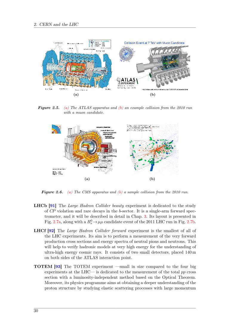
2. CERN and the LHC
(a) (b)
Figure 2.5. (a) The ATLAS apparatus and (b) an example collision from the 2010 runwith a muon candidate.
(a) (b)
Figure 2.6. (a) The CMS apparatus and (b) a sample collision from the 2010 run.
LHCb [91] The Large Hadron Collider beauty experiment is dedicated to the studyof CP violation and rare decays in the b-sector. It is a single-arm forward spec-trometer, and it will be described in detail in Chap. 3. Its layout is presented inFig. 2.7a, along with a B0
s →µµ candidate event of the 2011 LHC run in Fig. 2.7b.
LHCf [92] The Large Hadron Collider forward experiment is the smallest of all ofthe LHC experiments. Its aim is to perform a measurement of the very forwardproduction cross sections and energy spectra of neutral pions and neutrons. Thiswill help to verify hadronic models at very high energy for the understanding ofultra-high energy cosmic rays. It consists of two small detectors, placed 140mon both sides of the ATLAS interaction point.
TOTEM [93] The TOTEM experiment —small in size compared to the four bigexperiments at the LHC— is dedicated to the measurement of the total pp crosssection with a luminosity-independent method based on the Optical Theorem.Moreover, its physics programme aims at obtaining a deeper understanding of theproton structure by studying elastic scattering processes with large momentum
30
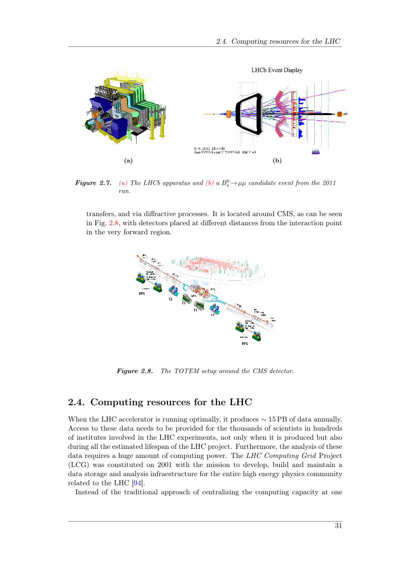
2.4. Computing resources for the LHC
(a) (b)
Figure 2.7. (a) The LHCb apparatus and (b) a B0s →µµ candidate event from the 2011
run.
transfers, and via diffractive processes. It is located around CMS, as can be seenin Fig. 2.8, with detectors placed at different distances from the interaction pointin the very forward region.
Figure 2.8. The TOTEM setup around the CMS detector.
2.4. Computing resources for the LHC
When the LHC accelerator is running optimally, it produces ∼ 15PB of data annually.Access to these data needs to be provided for the thousands of scientists in hundredsof institutes involved in the LHC experiments, not only when it is produced but alsoduring all the estimated lifespan of the LHC project. Furthermore, the analysis of thesedata requires a huge amount of computing power. The LHC Computing Grid Project(LCG) was constituted on 2001 with the mission to develop, build and maintain adata storage and analysis infraestructure for the entire high energy physics communityrelated to the LHC [94].
Instead of the traditional approach of centralizing the computing capacity at one
31

2. CERN and the LHC
location near the experiments, a novel globally distributed model —a computing Grid—was chosen for the LHC. This model allows, on one side, to share the maintenance andupgrade costs of the computing resources by distributing them in smaller computingcenters run by the individual institutes. On the other side, a distributed model has nosingle points of failure as long as multiple copies of data and automatic reassigning ofcomputational tasks to available resources is provided.
The Worldwide LHC Computing Grid (WLCG) is now the world’s largest computinggrid. It is based on the two main global grids currently in operation —the EuropeanGrid Infraestructure (EGI) and the USA Open Science Grid (OSG)—, as well as manyassociated regional and national grids across the world, such as the Taiwan Grid andthe EU-IndiaGrid.
Figure 2.9. Overview of the WLCG connections.
32
3The LHCb experiment
The LHCb experiment is dedicated to the study of heavy flavor physics at the LHC [91,95, 96]. Its main aim is to make precise measurements of CP violation and rare decays ofbeauty and charm hadrons. It is located at Interaction Point 8 of the LHC accelerator,previously used by the DELPHI experiment from LEP.
The LHC is the most extensive source of b-hadrons in the world, including B0s , B0
and Bc mesons, and b-baryons such as Λb. The LHCb detector must be able to exploitthis large number of b-hadrons in a high track multiplicity hadronic environment, i.e.,it must be able to trigger, reconstruct and correctly identify the b-hadrons coming frombb pairs generated by pp interactions. Events with multiple pp interactions are moredifficult to analyze since secondary vertices coming from the b-hadron decay are harderto distinguish from primary vertices coming from different pp interactions.
As Fig. 3.1 shows, the probability for multiple interactions increases with the lumi-nosity. In order to simplify B decay identification, the LHCb design target luminosityis lower than the LHC peak luminosity LLHC = 1034 cm−2 s−1, effectively reducingthe mean number of pp interactions per event. With the 2011 target luminosity ofLLHCb = 3.5 × 1032 cm−2 s−1, and a measured bb cross section at
√s = 7TeV of
σ(pp→bbX) = (284 ± 20 ± 49) µb [97] (see Fig. 3.2 for predictions at different LHCluminosities), the number of produced bb pairs in a nominal year is expected to be∼ 1012. They hadronize into b-hadrons —charged Bu, neutral B0, neutral B0
s andb-baryons— with proportions depending on the kinematics of the event [98]:
fB0s
fB0 + fBu
= 0.134± 0.004+0.011−0.010
fΛb
fB0 + fBu
= (0.404± 0.110)× [1− (0.031± 0.005)× pT (GeV)]
fB0s
fB0
= 0.267+0.021−0.020
(3.1)
Roughly speaking, at pT = 10GeV, Bu and B0 are produced ∼ 35% of the times, whileB0
s and Λb are produced ∼ 10% and ∼ 20% of the times, respectively.The physics requirements for LHCb, combined with the LHC running conditions,
give rise to a specific set of detector requirements:
33
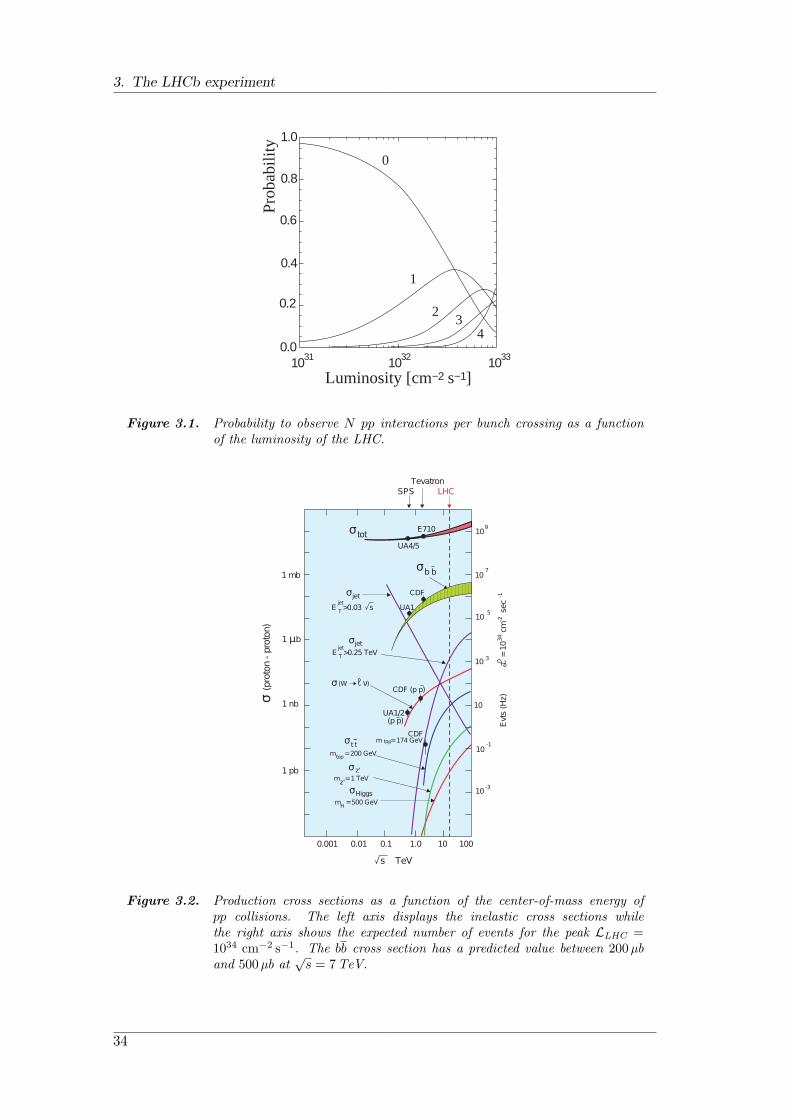
3. The LHCb experiment
1
23
4
0
Luminosity [cm−2 s−1]1031 1032 1033
0.2
0.4
0.6
0.8
1.0
0.0
Prob
abili
ty
Figure 3.1. Probability to observe N pp interactions per bunch crossing as a functionof the luminosity of the LHC.
Figure 3.2. Production cross sections as a function of the center-of-mass energy ofpp collisions. The left axis displays the inelastic cross sections whilethe right axis shows the expected number of events for the peak LLHC =1034 cm−2 s−1. The bb cross section has a predicted value between 200 µband 500 µb at
√s = 7TeV.
34
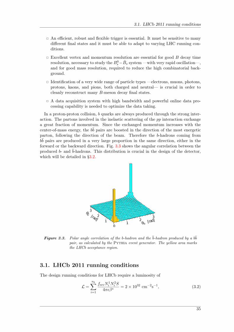
3.1. LHCb 2011 running conditions
An efficient, robust and flexible trigger is essential. It must be sensitive to manydifferent final states and it must be able to adapt to varying LHC running con-ditions.
Excellent vertex and momentum resolution are essential for good B decay timeresolution, necessary to study the B0
s−Bs system —with very rapid oscillation—,and for good mass resolution, required to reduce the high combinatorial back-ground.
Identification of a very wide range of particle types —electrons, muons, photons,protons, kaons, and pions, both charged and neutral— is crucial in order tocleanly reconstruct many B-meson decay final states.
A data acquisition system with high bandwidth and powerful online data pro-cessing capability is needed to optimize the data taking.
In a proton-proton collision, b quarks are always produced through the strong inter-action. The partons involved in the inelastic scattering of the pp interaction exchangea great fraction of momentum. Since the exchanged momentum increases with thecenter-of-mass energy, the bb pairs are boosted in the direction of the most energeticparton, following the direction of the beam. Therefore the b-hadrons coming frombb pairs are produced in a very large proportion in the same direction, either in theforward or the backward direction. Fig. 3.3 shows the angular correlation between theproduced b- and b-hadrons. This distribution is crucial in the design of the detector,which will be detailed in §3.2.
01
23
1
2
3
θb [rad]
θb [rad]
Figure 3.3. Polar angle correlation of the b-hadron and the b-hadron produced by a bbpair, as calculated by the Pythia event generator. The yellow area marksthe LHCb acceptance region.
3.1. LHCb 2011 running conditions
The design running conditions for LHCb require a luminosity of
L =
nb∑i=1
frevN1i N
2i S
4πϵβ∗= 2× 1032 cm−2s−1, (3.2)
35
3. The LHCb experiment
where
nb = 2622 is the number of colliding bunches per beam,
frev = 11254 kHz is the bunch revolution frequency around the LHC,
N1,2i ∼ 1011 is the number of protons per bunch,
S ∼ 673mrad is the beam crossing angle at LHCb,
ϵ = 3.75 µm is the normalized emittance for Ebeam = 7TeV, and
β∗ = 10m is the beta function [99].
With these nominal values, the expected average number of visible pp interactions perbunch crossing in the LHCb acceptance is µ ∼ 0.4, and therefore the collected datawould be dominated by single-interaction events.
In 2010, the LHC delivered 37 pb−1 to LHCb and managed to achieve 80% of thedesign luminosity. However, this luminosity was achieved with ∼ 10% of the nominalnumber of colliding bunches per beam (nb ∼ 344) and 1/3 of the nominal value ofβ∗, β∗ = 3.5m, leading to an increase of the number of visible interactions. Fig. 3.4compares the design value for µ and its behavior from July 2010 to the end of the 2010data taking period.
An increase in µ means more interactions —and thus, vertices— per bunch crossing,an increase in the readout rate per bunch crossing, and an increase of the event sizeand processing time. A high µ also affects greatly the trigger working conditions, butthe LHCb trigger has shown a great flexibility to adapt to LHC running conditionsduring 2010 and 2011 (see §3.5 for more details).
In 2011, the LHC has delivered ∼ 1.2 fb−1 to LHCb, of which ∼ 1.1 fb−1 have beenrecorded, as shown in Fig. 3.5. This corresponds to an efficiency of 91%.
Except for the ramp up period during the month of April, the 2011 data takingconditions have been very stable at LHCb. Data have been collected with nb in therange 1000 − 1300 (nb = 1296 in the July-October period in which most of the datawere recorded) and a target luminosity of 3.5×1032 cm−2 s−1. That means that LHCbhas been running at O(150%) of the design luminosity with O(35%) of the bunches perbeam. As a consequence, the average number of inelastic pp collisions has been abovethe design value, as can be seen in Fig. 3.6, but substantially lower than the valuesfrom 2010.
The trigger configuration during the 2011 data taking period has been more stablethan during the 2010 data taking, in which 18 different TCKs were used. Only a handfulof Trigger Configuration Keys (TCKs, see §3.7.1) have contributed significantly to thebulk of the recorded luminosity, as summarized in Table 3.1.
3.2. Detector layout
LHCb is a single-arm spectrometer with a forward coverage from approximately10mrad to 300 (250)mrad in the horizontal bending (non-bending) plane. In terms ofpseudorapidity,
η = − ln tan
(θ
2
), (3.3)
36
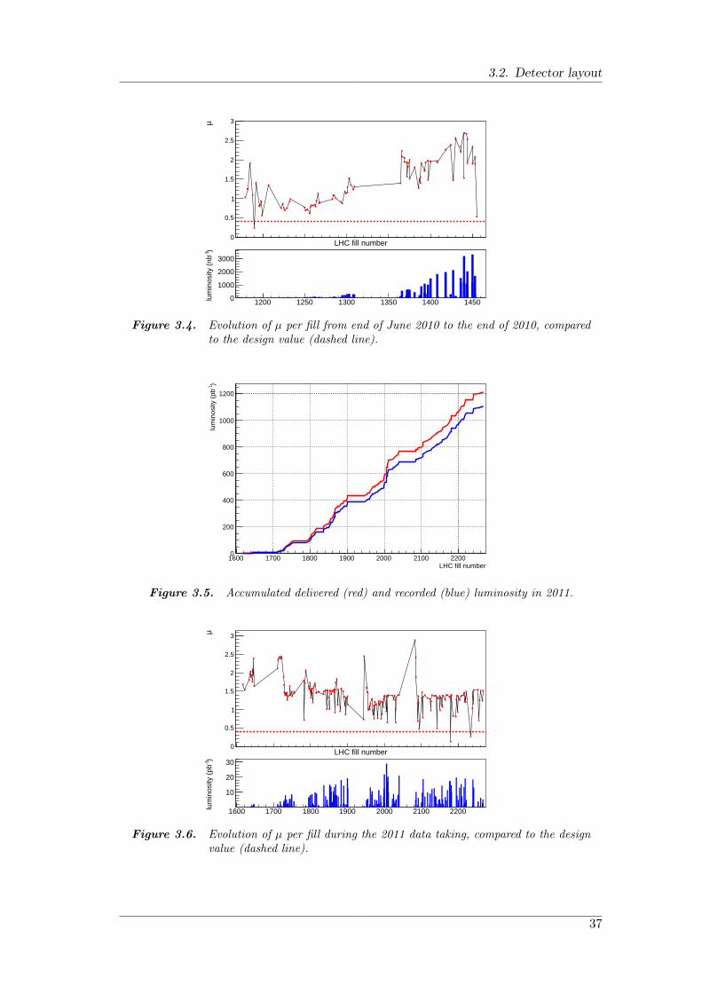
3.2. Detector layout
LHC fill number
µ
0
0.5
1
1.5
2
2.5
3
1200 1250 1300 1350 1400 1450
)-1
lum
inos
ity (
nb
0
1000
2000
3000
Figure 3.4. Evolution of µ per fill from end of June 2010 to the end of 2010, comparedto the design value (dashed line).
LHC fill number1600 1700 1800 1900 2000 2100 2200
)-1
lum
inos
ity (
pb
0
200
400
600
800
1000
1200
Figure 3.5. Accumulated delivered (red) and recorded (blue) luminosity in 2011.
LHC fill number
µ
0
0.5
1
1.5
2
2.5
3
1600 1700 1800 1900 2000 2100 2200
)-1
lum
inos
ity (
pb
10
20
30
Figure 3.6. Evolution of µ per fill during the 2011 data taking, compared to the designvalue (dashed line).
37
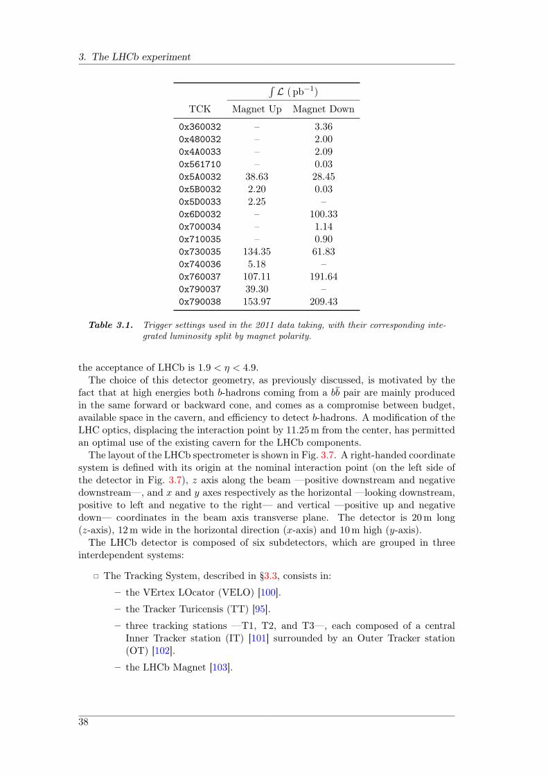
3. The LHCb experiment
∫L ( pb−1)
TCK Magnet Up Magnet Down
0x360032 – 3.360x480032 – 2.000x4A0033 – 2.090x561710 – 0.030x5A0032 38.63 28.450x5B0032 2.20 0.030x5D0033 2.25 –0x6D0032 – 100.330x700034 – 1.140x710035 – 0.900x730035 134.35 61.830x740036 5.18 –0x760037 107.11 191.640x790037 39.30 –0x790038 153.97 209.43
Table 3.1. Trigger settings used in the 2011 data taking, with their corresponding inte-grated luminosity split by magnet polarity.
the acceptance of LHCb is 1.9 < η < 4.9.The choice of this detector geometry, as previously discussed, is motivated by the
fact that at high energies both b-hadrons coming from a bb pair are mainly producedin the same forward or backward cone, and comes as a compromise between budget,available space in the cavern, and efficiency to detect b-hadrons. A modification of theLHC optics, displacing the interaction point by 11.25m from the center, has permittedan optimal use of the existing cavern for the LHCb components.
The layout of the LHCb spectrometer is shown in Fig. 3.7. A right-handed coordinatesystem is defined with its origin at the nominal interaction point (on the left side ofthe detector in Fig. 3.7), z axis along the beam —positive downstream and negativedownstream—, and x and y axes respectively as the horizontal —looking downstream,positive to left and negative to the right— and vertical —positive up and negativedown— coordinates in the beam axis transverse plane. The detector is 20m long(z-axis), 12m wide in the horizontal direction (x-axis) and 10m high (y-axis).
The LHCb detector is composed of six subdetectors, which are grouped in threeinterdependent systems:
The Tracking System, described in §3.3, consists in:
– the VErtex LOcator (VELO) [100].
– the Tracker Turicensis (TT) [95].
– three tracking stations —T1, T2, and T3—, each composed of a centralInner Tracker station (IT) [101] surrounded by an Outer Tracker station(OT) [102].
– the LHCb Magnet [103].
38
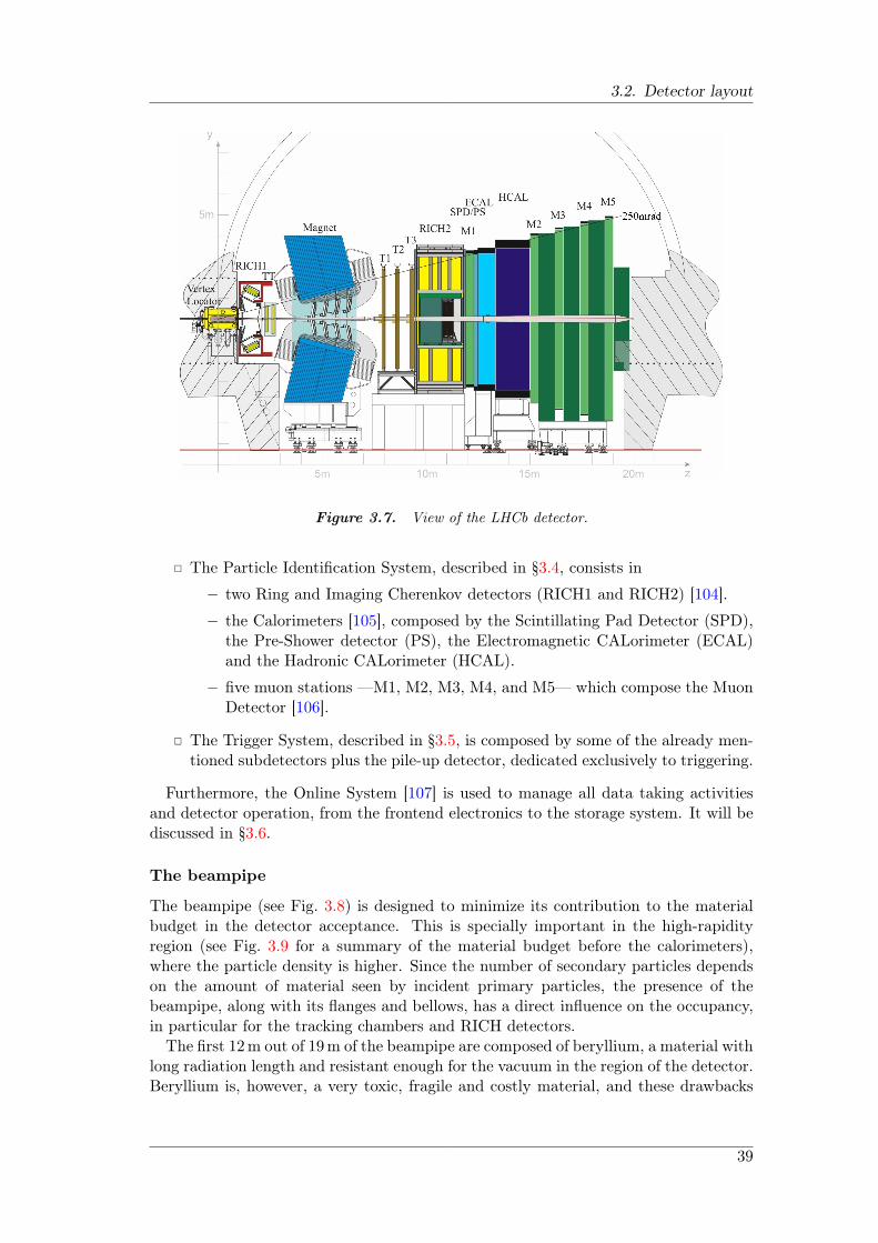
3.2. Detector layout
Figure 3.7. View of the LHCb detector.
The Particle Identification System, described in §3.4, consists in
– two Ring and Imaging Cherenkov detectors (RICH1 and RICH2) [104].
– the Calorimeters [105], composed by the Scintillating Pad Detector (SPD),the Pre-Shower detector (PS), the Electromagnetic CALorimeter (ECAL)and the Hadronic CALorimeter (HCAL).
– five muon stations —M1, M2, M3, M4, and M5— which compose the MuonDetector [106].
The Trigger System, described in §3.5, is composed by some of the already men-tioned subdetectors plus the pile-up detector, dedicated exclusively to triggering.
Furthermore, the Online System [107] is used to manage all data taking activitiesand detector operation, from the frontend electronics to the storage system. It will bediscussed in §3.6.
The beampipe
The beampipe (see Fig. 3.8) is designed to minimize its contribution to the materialbudget in the detector acceptance. This is specially important in the high-rapidityregion (see Fig. 3.9 for a summary of the material budget before the calorimeters),where the particle density is higher. Since the number of secondary particles dependson the amount of material seen by incident primary particles, the presence of thebeampipe, along with its flanges and bellows, has a direct influence on the occupancy,in particular for the tracking chambers and RICH detectors.
The first 12m out of 19m of the beampipe are composed of beryllium, a material withlong radiation length and resistant enough for the vacuum in the region of the detector.Beryllium is, however, a very toxic, fragile and costly material, and these drawbacks
39
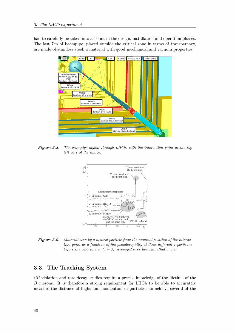
3. The LHCb experiment
had to carefully be taken into account in the design, installation and operation phases.The last 7m of beampipe, placed outside the critical zone in terms of transparency,are made of stainless steel, a material with good mechanical and vacuum properties.
Figure 3.8. The beampipe layout through LHCb, with the interaction point at the topleft part of the image.
10−1
1
2.5 3 3.5 4 4.5 η
25 mrad section of the beam pipe
10 mrad section of the beam pipe
Interface section betweenthe VELO vacuum tank
and the beam pipe VELO rf-shield
X /
X0
1) in front of Magnet
2) in front of RICH2
3) in front of Calo
Calorimeter acceptance
Figure 3.9. Material seen by a neutral particle from the nominal position of the interac-tion point as a function of the pseudorapidity at three different z positionsbefore the calorimeter (1− 3), averaged over the azimuthal angle.
3.3. The Tracking System
CP violation and rare decay studies require a precise knowledge of the lifetime of theB mesons. It is therefore a strong requirement for LHCb to be able to accuratelymeasure the distance of flight and momentum of particles: to achieve several of the
40
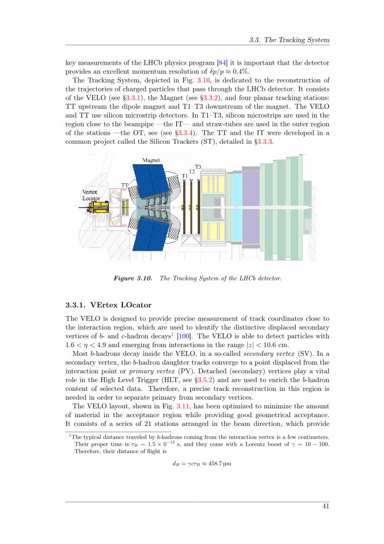
3.3. The Tracking System
key measurements of the LHCb physics program [84] it is important that the detectorprovides an excellent momentum resolution of δp/p ≈ 0.4%.
The Tracking System, depicted in Fig. 3.10, is dedicated to the reconstruction ofthe trajectories of charged particles that pass through the LHCb detector. It consistsof the VELO (see §3.3.1), the Magnet (see §3.3.2), and four planar tracking stations:TT upstream the dipole magnet and T1–T3 downstream of the magnet. The VELOand TT use silicon microstrip detectors. In T1–T3, silicon microstrips are used in theregion close to the beampipe —the IT— and straw-tubes are used in the outer regionof the stations —the OT, see (see §3.3.4). The TT and the IT were developed in acommon project called the Silicon Trackers (ST), detailed in §3.3.3.
Figure 3.10. The Tracking System of the LHCb detector.
3.3.1. VErtex LOcator
The VELO is designed to provide precise measurement of track coordinates close tothe interaction region, which are used to identify the distinctive displaced secondaryvertices of b- and c-hadron decays1 [100]. The VELO is able to detect particles with1.6 < η < 4.9 and emerging from interactions in the range |z| < 10.6 cm.
Most b-hadrons decay inside the VELO, in a so-called secondary vertex (SV). In asecondary vertex, the b-hadron daughter tracks converge to a point displaced from theinteraction point or primary vertex (PV). Detached (secondary) vertices play a vitalrole in the High Level Trigger (HLT, see §3.5.2) and are used to enrich the b-hadroncontent of selected data. Therefore, a precise track reconstruction in this region isneeded in order to separate primary from secondary vertices.
The VELO layout, shown in Fig. 3.11, has been optimized to minimize the amountof material in the acceptance region while providing good geometrical acceptance.It consists of a series of 21 stations arranged in the beam direction, which provide
1The typical distance traveled by b-hadrons coming from the interaction vertex is a few centimeters.Their proper time is τB ∼ 1.5 × 0−12 s, and they come with a Lorentz boost of γ ∼ 10 − 100.Therefore, their distance of flight is
dB = γcτB ≈ 458.7µm
41
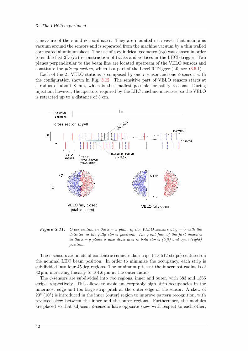
3. The LHCb experiment
a measure of the r and ϕ coordinates. They are mounted in a vessel that maintainsvacuum around the sensors and is separated from the machine vacuum by a thin walledcorrugated aluminum sheet. The use of a cylindrical geometry (rϕ) was chosen in orderto enable fast 2D (rz) reconstruction of tracks and vertices in the LHCb trigger. Twoplanes perpendicular to the beam line are located upstream of the VELO sensors andconstitute the pile-up system, which is a part of the Level-0 Trigger (L0, see §3.5.1).
Each of the 21 VELO stations is composed by one r-sensor and one ϕ-sensor, withthe configuration shown in Fig. 3.12. The sensitive part of VELO sensors starts ata radius of about 8 mm, which is the smallest possible for safety reasons. Duringinjection, however, the aperture required by the LHC machine increases, so the VELOis retracted up to a distance of 3 cm.
Figure 3.11. Cross section in the x − z plane of the VELO sensors at y = 0 with thedetector in the fully closed position. The front face of the first modulesin the x− y plane is also illustrated in both closed (left) and open (right)position.
The r-sensors are made of concentric semicircular strips (4× 512 strips) centered onthe nominal LHC beam position. In order to minimize the occupancy, each strip issubdivided into four 45 deg regions. The minimum pitch at the innermost radius is of32 µm, increasing linearly to 101.6 µm at the outer radius.
The ϕ-sensors are subdivided into two regions, inner and outer, with 683 and 1365strips, respectively. This allows to avoid unacceptably high strip occupancies in theinnermost edge and too large strip pitch at the outer edge of the sensor. A skew of20 (10) is introduced in the inner (outer) region to improve pattern recognition, withreversed skew between the inner and the outer regions. Furthermore, the modulesare placed so that adjacent ϕ-sensors have opposite skew with respect to each other,
42
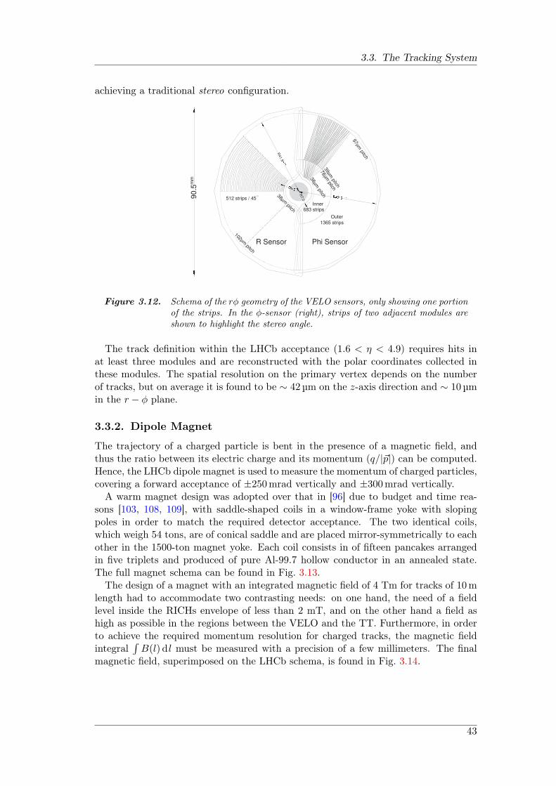
3.3. The Tracking System
achieving a traditional stereo configuration.
Figure 3.12. Schema of the rϕ geometry of the VELO sensors, only showing one portionof the strips. In the ϕ-sensor (right), strips of two adjacent modules areshown to highlight the stereo angle.
The track definition within the LHCb acceptance (1.6 < η < 4.9) requires hits inat least three modules and are reconstructed with the polar coordinates collected inthese modules. The spatial resolution on the primary vertex depends on the numberof tracks, but on average it is found to be ∼ 42 µm on the z-axis direction and ∼ 10 µmin the r − ϕ plane.
3.3.2. Dipole Magnet
The trajectory of a charged particle is bent in the presence of a magnetic field, andthus the ratio between its electric charge and its momentum (q/|p|) can be computed.Hence, the LHCb dipole magnet is used to measure the momentum of charged particles,covering a forward acceptance of ±250mrad vertically and ±300mrad vertically.
A warm magnet design was adopted over that in [96] due to budget and time rea-sons [103, 108, 109], with saddle-shaped coils in a window-frame yoke with slopingpoles in order to match the required detector acceptance. The two identical coils,which weigh 54 tons, are of conical saddle and are placed mirror-symmetrically to eachother in the 1500-ton magnet yoke. Each coil consists in of fifteen pancakes arrangedin five triplets and produced of pure Al-99.7 hollow conductor in an annealed state.The full magnet schema can be found in Fig. 3.13.
The design of a magnet with an integrated magnetic field of 4 Tm for tracks of 10mlength had to accommodate two contrasting needs: on one hand, the need of a fieldlevel inside the RICHs envelope of less than 2 mT, and on the other hand a field ashigh as possible in the regions between the VELO and the TT. Furthermore, in orderto achieve the required momentum resolution for charged tracks, the magnetic fieldintegral
∫B(l) dl must be measured with a precision of a few millimeters. The final
magnetic field, superimposed on the LHCb schema, is found in Fig. 3.14.
43
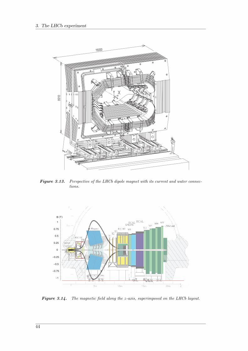
3. The LHCb experiment
Figure 3.13. Perspective of the LHCb dipole magnet with its current and water connec-tions.
1
0.75
0.5
0.25
0
-0.25
-0.5
-0.75
-1
B (T)
Figure 3.14. The magnetic field along the z-axis, superimposed on the LHCb layout.
44
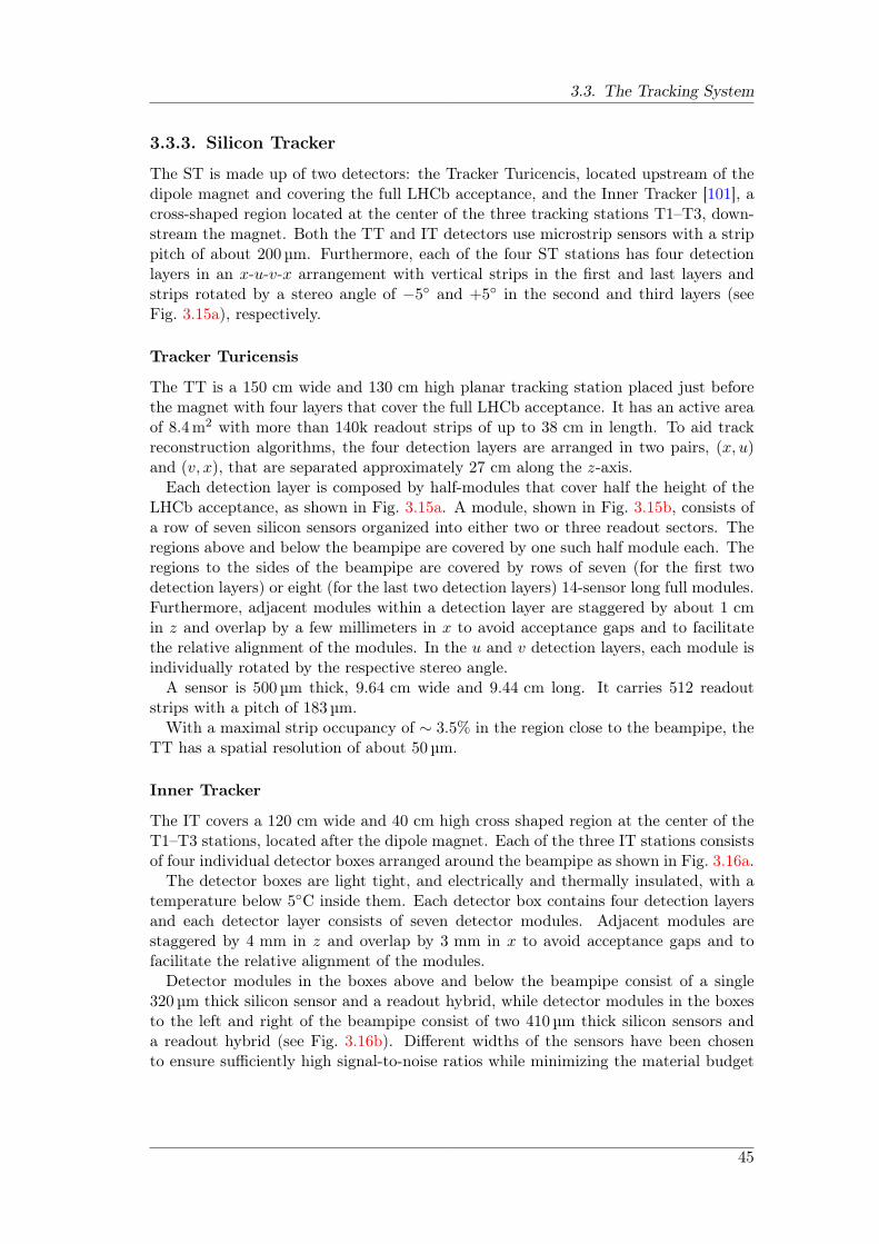
3.3. The Tracking System
3.3.3. Silicon Tracker
The ST is made up of two detectors: the Tracker Turicencis, located upstream of thedipole magnet and covering the full LHCb acceptance, and the Inner Tracker [101], across-shaped region located at the center of the three tracking stations T1–T3, down-stream the magnet. Both the TT and IT detectors use microstrip sensors with a strippitch of about 200µm. Furthermore, each of the four ST stations has four detectionlayers in an x-u-v-x arrangement with vertical strips in the first and last layers andstrips rotated by a stereo angle of −5 and +5 in the second and third layers (seeFig. 3.15a), respectively.
Tracker Turicensis
The TT is a 150 cm wide and 130 cm high planar tracking station placed just beforethe magnet with four layers that cover the full LHCb acceptance. It has an active areaof 8.4m2 with more than 140k readout strips of up to 38 cm in length. To aid trackreconstruction algorithms, the four detection layers are arranged in two pairs, (x, u)and (v, x), that are separated approximately 27 cm along the z-axis.
Each detection layer is composed by half-modules that cover half the height of theLHCb acceptance, as shown in Fig. 3.15a. A module, shown in Fig. 3.15b, consists ofa row of seven silicon sensors organized into either two or three readout sectors. Theregions above and below the beampipe are covered by one such half module each. Theregions to the sides of the beampipe are covered by rows of seven (for the first twodetection layers) or eight (for the last two detection layers) 14-sensor long full modules.Furthermore, adjacent modules within a detection layer are staggered by about 1 cmin z and overlap by a few millimeters in x to avoid acceptance gaps and to facilitatethe relative alignment of the modules. In the u and v detection layers, each module isindividually rotated by the respective stereo angle.
A sensor is 500µm thick, 9.64 cm wide and 9.44 cm long. It carries 512 readoutstrips with a pitch of 183µm.
With a maximal strip occupancy of ∼ 3.5% in the region close to the beampipe, theTT has a spatial resolution of about 50µm.
Inner Tracker
The IT covers a 120 cm wide and 40 cm high cross shaped region at the center of theT1–T3 stations, located after the dipole magnet. Each of the three IT stations consistsof four individual detector boxes arranged around the beampipe as shown in Fig. 3.16a.
The detector boxes are light tight, and electrically and thermally insulated, with atemperature below 5C inside them. Each detector box contains four detection layersand each detector layer consists of seven detector modules. Adjacent modules arestaggered by 4 mm in z and overlap by 3 mm in x to avoid acceptance gaps and tofacilitate the relative alignment of the modules.
Detector modules in the boxes above and below the beampipe consist of a single320µm thick silicon sensor and a readout hybrid, while detector modules in the boxesto the left and right of the beampipe consist of two 410µm thick silicon sensors anda readout hybrid (see Fig. 3.16b). Different widths of the sensors have been chosento ensure sufficiently high signal-to-noise ratios while minimizing the material budget
45

3. The LHCb experiment
(a) Layout of the third TT layer.
(b) View of a TT module.
Figure 3.15. Views of the Tracker Turicensis detector.
of the detector. The sensors are 11 cm long and 7.6 cm wide, and contain 384 siliconstrips with a pitch of 198µm.
(a) Layout of the second IT station. (b) View of a two-sensor ITmodule.
Figure 3.16. Views of the Inner Tracker detector.
The Inner Tracker has a spatial resolution of about 57 µm.
3.3.4. Outer Tracker
The OT is a drift-time detector [102] for the tracking of charged particles and themeasurement of their momentum over a large acceptance area in the outer region ofthe LHCb detector. Each module contains two staggered monolayers of drift-tubeswith inner diameters of 4.9 mm, shown in Fig. 3.17b. A mixture of Argon (70%) and
46
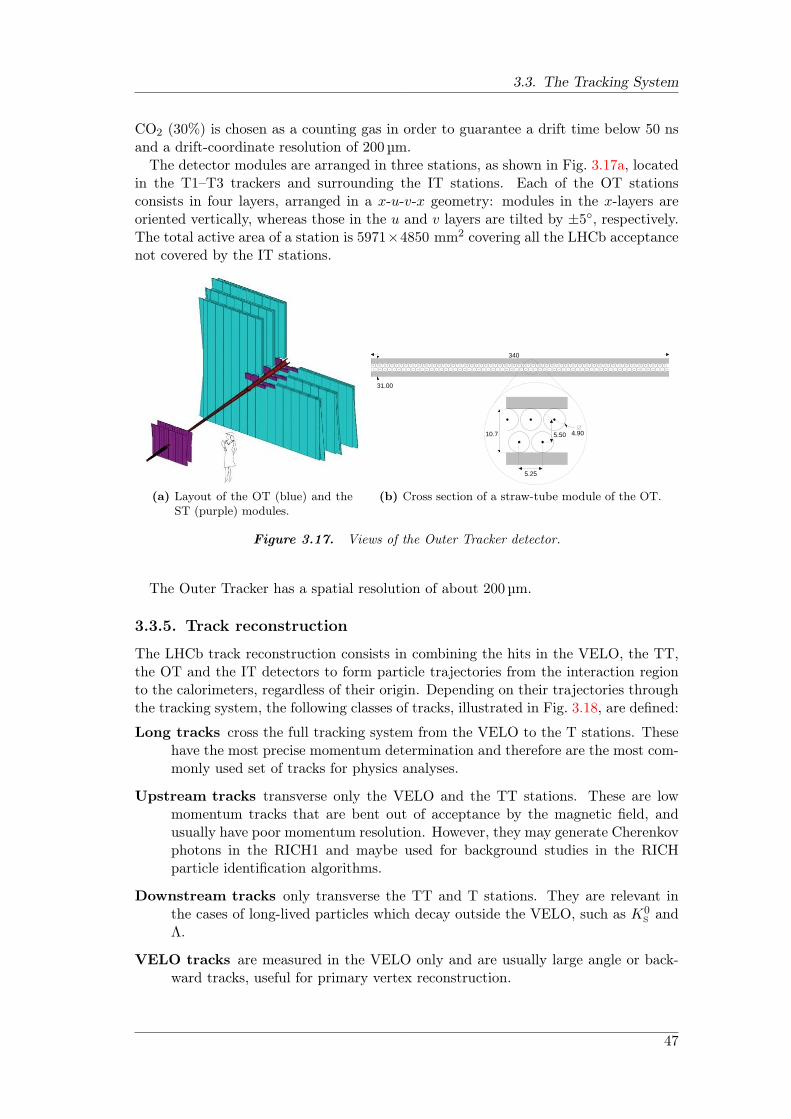
3.3. The Tracking System
CO2 (30%) is chosen as a counting gas in order to guarantee a drift time below 50 nsand a drift-coordinate resolution of 200µm.
The detector modules are arranged in three stations, as shown in Fig. 3.17a, locatedin the T1–T3 trackers and surrounding the IT stations. Each of the OT stationsconsists in four layers, arranged in a x-u-v-x geometry: modules in the x-layers areoriented vertically, whereas those in the u and v layers are tilted by ±5, respectively.The total active area of a station is 5971×4850 mm2 covering all the LHCb acceptancenot covered by the IT stations.
(a) Layout of the OT (blue) and theST (purple) modules.
10.7
340
31.00
5.25
5.50 4.90
(b) Cross section of a straw-tube module of the OT.
Figure 3.17. Views of the Outer Tracker detector.
The Outer Tracker has a spatial resolution of about 200µm.
3.3.5. Track reconstruction
The LHCb track reconstruction consists in combining the hits in the VELO, the TT,the OT and the IT detectors to form particle trajectories from the interaction regionto the calorimeters, regardless of their origin. Depending on their trajectories throughthe tracking system, the following classes of tracks, illustrated in Fig. 3.18, are defined:
Long tracks cross the full tracking system from the VELO to the T stations. Thesehave the most precise momentum determination and therefore are the most com-monly used set of tracks for physics analyses.
Upstream tracks transverse only the VELO and the TT stations. These are lowmomentum tracks that are bent out of acceptance by the magnetic field, andusually have poor momentum resolution. However, they may generate Cherenkovphotons in the RICH1 and maybe used for background studies in the RICHparticle identification algorithms.
Downstream tracks only transverse the TT and T stations. They are relevant inthe cases of long-lived particles which decay outside the VELO, such as K0
S andΛ.
VELO tracks are measured in the VELO only and are usually large angle or back-ward tracks, useful for primary vertex reconstruction.
47

3. The LHCb experiment
T-tracks are only measured in the T stations, and are typically produced in secondaryinteractions. They are useful for global pattern recognition in RICH2.
Upstream track
TT
VELO
T1 T2 T3
T track
VELO track
Long track
Downstream track
0
0
-0.2
-0.4
-0.6
-0.8
-1.0
-1.22 4 6 8 z (m)
By (
T)
Figure 3.18. Schematic illustration of the various types of tracks: long, upstream, down-stream, VELO and T tracks. The By magnetic field component responsiblefor their bending is plotted for reference.
The track reconstruction starts with a search for track seeds, the initial track can-didates, in the VELO and the T stations where the magnetic field is low. These trackseeds, the so-called VELO track seeds and T track seeds, should be almost aligned.After tracks have been found, their trajectories are refitted with a Kalman filter inorder to account for multiple scattering and correct for dE/dx energy loss. This al-gorithm then tries to associate hits in the other parts of the tracking system to formtrack candidates. The quality of the reconstructed tracks is monitored by the χ2 ofthe fit and the pull distribution of the track parameters.
The performance of the tracking algorithm has been evaluated on a Monte Carlo(MC) sample of B0→J/ψK0
S events in terms of two quantities [91]:
Reconstruction efficiency is defined as the fraction of the possible reconstructibletracks that have been actually reconstructed. To be considered as reconstructed,a track must have at least 70% of its associated hits coming from the same singleMC particle.
Ghost rate is the fraction of the tracks reconstructed with hits that do not correspondto a single particle.
The efficiency to reconstruct a long track from a particle with a momentum largerthan 10GeV/c is on average ∼ 94%. The corresponding average ghost fraction is ∼ 9%,but most ghost tracks have a low reconstructed pT.
48
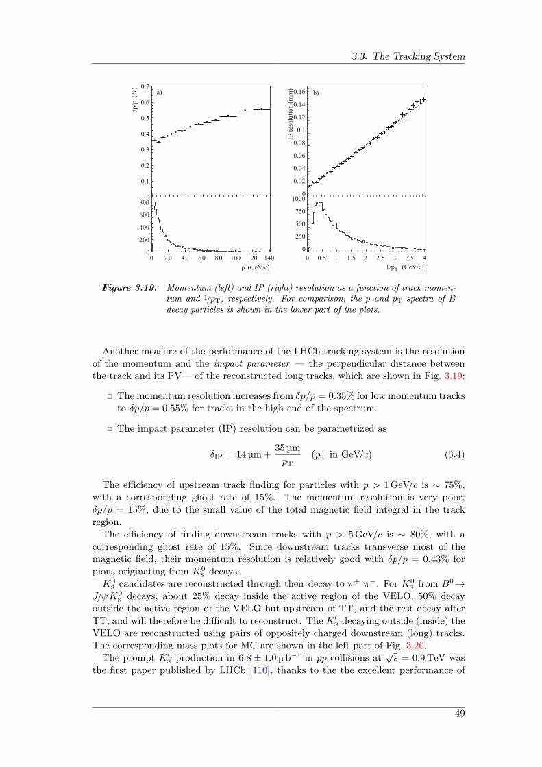
3.3. The Tracking System
0
0.1
0.2
0.3
0.4
0.5
0.6
0.7
dp
/p
(%)
0
200
400
600
800
a)
0 20 40 60 80 100 120 140
0
0.02
0.04
0.06
0.08
0.1
0.12
0.14
0.16
IP r
eso
luti
on
(m
m)
1/p t (GeV/c) -1
0
250
500
750
1000
0 0.5 1 1.5 2 2.5 3 3.5 4
b)
p (GeV/c)
Figure 3.19. Momentum (left) and IP (right) resolution as a function of track momen-tum and 1/pT, respectively. For comparison, the p and pT spectra of Bdecay particles is shown in the lower part of the plots.
Another measure of the performance of the LHCb tracking system is the resolutionof the momentum and the impact parameter — the perpendicular distance betweenthe track and its PV— of the reconstructed long tracks, which are shown in Fig. 3.19:
The momentum resolution increases from δp/p = 0.35% for low momentum tracksto δp/p = 0.55% for tracks in the high end of the spectrum.
The impact parameter (IP) resolution can be parametrized as
δIP = 14 µm +35 µmpT
(pT in GeV/c) (3.4)
The efficiency of upstream track finding for particles with p > 1GeV/c is ∼ 75%,with a corresponding ghost rate of 15%. The momentum resolution is very poor,δp/p = 15%, due to the small value of the total magnetic field integral in the trackregion.
The efficiency of finding downstream tracks with p > 5GeV/c is ∼ 80%, with acorresponding ghost rate of 15%. Since downstream tracks transverse most of themagnetic field, their momentum resolution is relatively good with δp/p = 0.43% forpions originating from K0
S decays.K0
S candidates are reconstructed through their decay to π+ π−. For K0S from B0→
J/ψK0S decays, about 25% decay inside the active region of the VELO, 50% decay
outside the active region of the VELO but upstream of TT, and the rest decay afterTT, and will therefore be difficult to reconstruct. The K0
S decaying outside (inside) theVELO are reconstructed using pairs of oppositely charged downstream (long) tracks.The corresponding mass plots for MC are shown in the left part of Fig. 3.20.
The prompt K0S production in 6.8 ± 1.0µ b−1 in pp collisions at
√s = 0.9TeV was
the first paper published by LHCb [110], thanks to the the excellent performance of
49
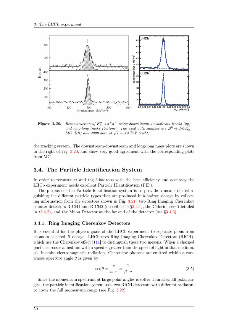
3. The LHCb experiment
Invariant mass (MeV/c2)
200
100
400
300
200
100
400 450 500 550 600
En
trie
s
2c
an
did
ate
s p
er
2 M
eV
/c
100
200
300
400
500LHCb
]2 [GeV/c-π+πm0.4 0.42 0.44 0.46 0.48 0.5 0.52 0.54 0.56 0.58 0.60
50
100
150
200
250
LHCb
Figure 3.20. Reconstruction of K0S →π+π− using downstream-downstream tracks (up)
and long-long tracks (bottom). The used data samples are B0 → J/ψK0S
MC (left) and 2009 data at√s = 0.9TeV (right)
the tracking system. The downstream-downstream and long-long mass plots are shownin the right of Fig. 3.20, and show very good agreement with the corresponding plotsfrom MC.
3.4. The Particle Identification System
In order to reconstruct and tag b-hadrons with the best efficiency and accuracy theLHCb experiment needs excellent Particle IDentification (PID).
The purpose of the Particle Identification system is to provide a means of distin-guishing the different particle types that are produced in b-hadron decays by collect-ing information from the detectors shown in Fig. 3.21: two Ring Imaging Cherenkovcounter detectors RICH1 and RICH2 (described in §3.4.1), the Calorimeters (detailedin §3.4.2), and the Muon Detector at the far end of the detector (see §3.4.3).
3.4.1. Ring Imaging Cherenkov Detectors
It is essential for the physics goals of the LHCb experiment to separate pions fromkaons in selected B decays. LHCb uses Ring Imaging Cherenkov Detectors (RICH),which use the Cherenkov effect [111] to distinguish these two mesons. When a chargedparticle crosses a medium with a speed v greater than the speed of light in that medium,c/n, it emits electromagnetic radiation. Cherenkov photons are emitted within a conewhose aperture angle θ is given by
cos θ =c
n · v=
1
β ·n(3.5)
Since the momentum spectrum at large polar angles is softer than at small polar an-gles, the particle identification system uses two RICH detectors with different radiatorsto cover the full momentum range (see Fig. 3.22).
50
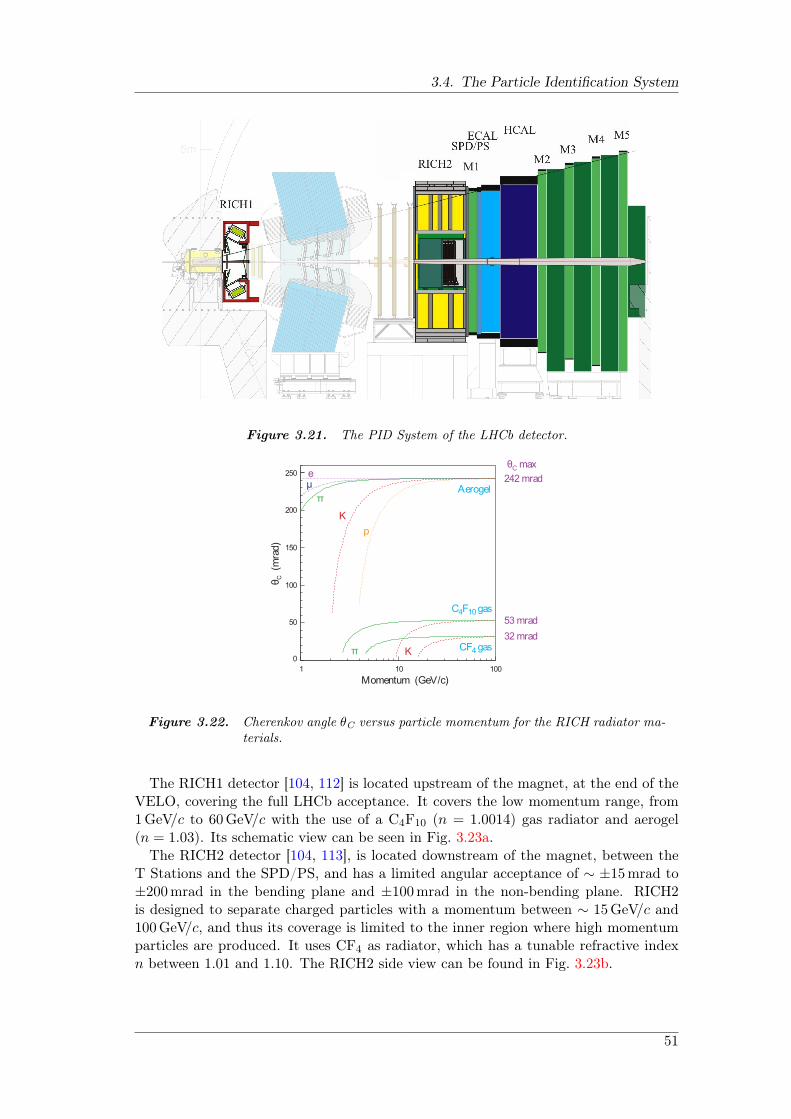
3.4. The Particle Identification System
Figure 3.21. The PID System of the LHCb detector.
θC
(mra
d)
250
200
150
100
50
0
1 10 100
Momentum (GeV/c)
Aerogel
C4F10 gas
CF4 gas
eµ
p
K
π
242 mrad
53 mrad
32 mrad
θC max
Kπ
Figure 3.22. Cherenkov angle θC versus particle momentum for the RICH radiator ma-terials.
The RICH1 detector [104, 112] is located upstream of the magnet, at the end of theVELO, covering the full LHCb acceptance. It covers the low momentum range, from1GeV/c to 60GeV/c with the use of a C4F10 (n = 1.0014) gas radiator and aerogel(n = 1.03). Its schematic view can be seen in Fig. 3.23a.
The RICH2 detector [104, 113], is located downstream of the magnet, between theT Stations and the SPD/PS, and has a limited angular acceptance of ∼ ±15mrad to±200mrad in the bending plane and ±100mrad in the non-bending plane. RICH2is designed to separate charged particles with a momentum between ∼ 15GeV/c and100GeV/c, and thus its coverage is limited to the inner region where high momentumparticles are produced. It uses CF4 as radiator, which has a tunable refractive indexn between 1.01 and 1.10. The RICH2 side view can be found in Fig. 3.23b.
51
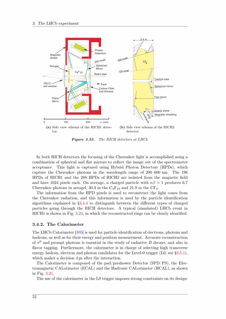
3. The LHCb experiment
250 mrad
Track
Beam pipe
Photon
Detectors
Aerogel
VELOexit window
Spherical
Mirror
Plane
Mirror
C4F10
0 100 200 z (cm)
Magnetic
Shield
Carbon Fiber
Exit Window
(a) Side view schema of the RICH1 detec-tor.
120mrad
Flat mirror
Spherical mirror
Central tube
Quartz plane
Magnetic shieldingHPD
enclosure
2.4 m
300mrad
CF4
(b) Side view schema of the RICH2detector.
Figure 3.23. The RICH detectors at LHCb.
In both RICH detectors the focusing of the Cherenkov light is accomplished using acombination of spherical and flat mirrors to reflect the image out of the spectrometeracceptance. This light is captured using Hybrid Photon Detectors (HPDs), whichcapture the Cherenkov photons in the wavelength range of 200–600 nm. The 196HPDs of RICH1 and the 288 HPDs of RICH2 are isolated from the magnetic fieldand have 1024 pixels each. On average, a charged particle with nβ > 1 produces 6.7Cherenkov photons in aerogel, 30.3 in the C4F10 and 21.9 in the CF4.
The information from the HPD pixels is used to reconstruct the light cones fromthe Cherenkov radiation, and this information is used by the particle identificationalgorithms explained in §3.4.4 to distinguish between the different types of chargedparticles going through the RICH detectors. A typical (simulated) LHCb event inRICH1 is shown in Fig. 3.24, in which the reconstructed rings can be clearly identified.
3.4.2. The Calorimeter
The LHCb Calorimeter [105] is used for particle identification of electrons, photons andhadrons, as well as for their energy and position measurement. Accurate reconstructionof π0 and prompt photons is essential in the study of radiative B decays, and also inflavor tagging. Furthermore, the calorimeter is in charge of selecting high transverseenergy hadron, electron and photon candidates for the Level-0 trigger (L0, see §3.5.1),which makes a decision 4µs after the interaction.
The Calorimeter is composed of the pad/preshower Detector (SPD/PS), the Elec-tromagnetic CALorimeter (ECAL) and the Hadronic CALorimeter (HCAL), as shownin Fig. 3.21.
The use of the calorimeter in the L0 trigger imposes strong constraints on its design:
52
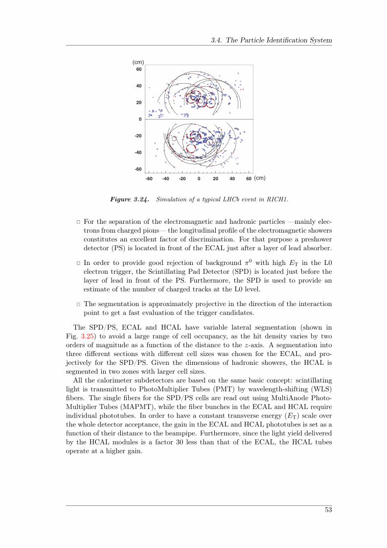
3.4. The Particle Identification System
(cm)
(cm)
Figure 3.24. Simulation of a typical LHCb event in RICH1.
For the separation of the electromagnetic and hadronic particles —mainly elec-trons from charged pions— the longitudinal profile of the electromagnetic showersconstitutes an excellent factor of discrimination. For that purpose a preshowerdetector (PS) is located in front of the ECAL just after a layer of lead absorber.
In order to provide good rejection of background π0 with high ET in the L0electron trigger, the Scintillating Pad Detector (SPD) is located just before thelayer of lead in front of the PS. Furthermore, the SPD is used to provide anestimate of the number of charged tracks at the L0 level.
The segmentation is approximately projective in the direction of the interactionpoint to get a fast evaluation of the trigger candidates.
The SPD/PS, ECAL and HCAL have variable lateral segmentation (shown inFig. 3.25) to avoid a large range of cell occupancy, as the hit density varies by twoorders of magnitude as a function of the distance to the z-axis. A segmentation intothree different sections with different cell sizes was chosen for the ECAL, and pro-jectively for the SPD/PS. Given the dimensions of hadronic showers, the HCAL issegmented in two zones with larger cell sizes.
All the calorimeter subdetectors are based on the same basic concept: scintillatinglight is transmitted to PhotoMultiplier Tubes (PMT) by wavelength-shifting (WLS)fibers. The single fibers for the SPD/PS cells are read out using MultiAnode Photo-Multiplier Tubes (MAPMT), while the fiber bunches in the ECAL and HCAL requireindividual phototubes. In order to have a constant transverse energy (ET) scale overthe whole detector acceptance, the gain in the ECAL and HCAL phototubes is set as afunction of their distance to the beampipe. Furthermore, since the light yield deliveredby the HCAL modules is a factor 30 less than that of the ECAL, the HCAL tubesoperate at a higher gain.
53
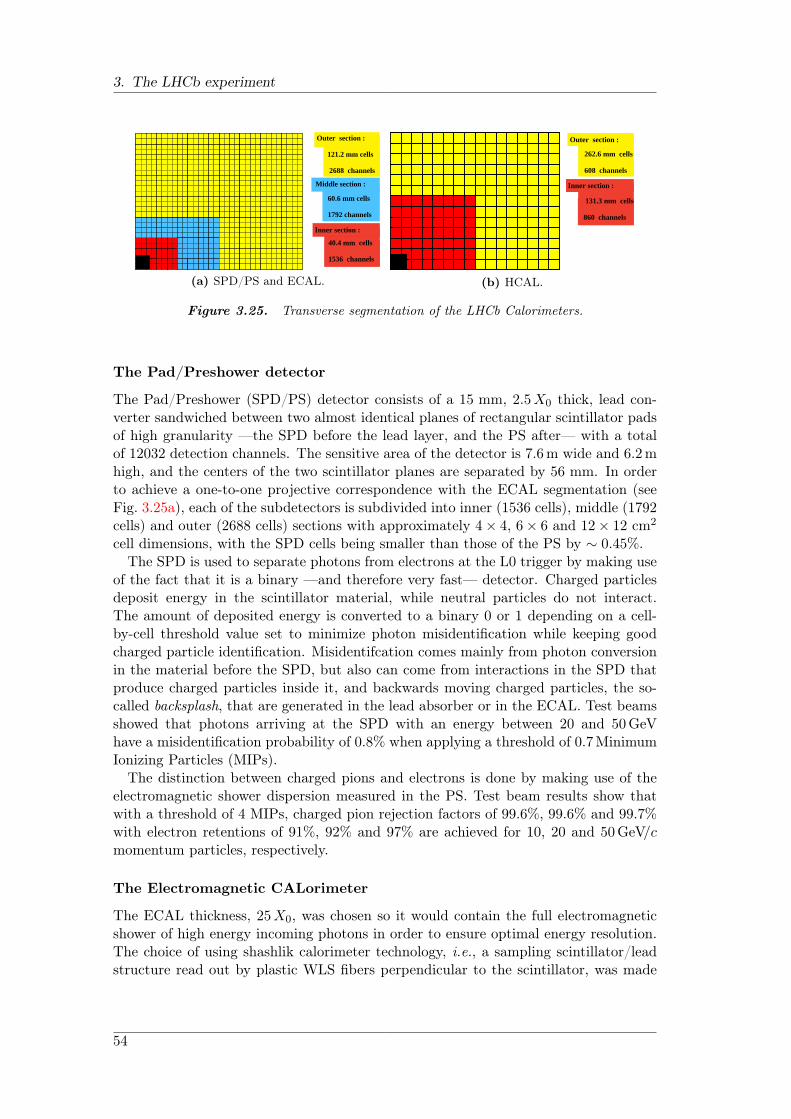
3. The LHCb experiment
Outer section :
Inner section :
121.2 mm cells
2688 channels
40.4 mm cells
1536 channels
Middle section :
60.6 mm cells
1792 channels
(a) SPD/PS and ECAL.
Outer section :
Inner section :
262.6 mm cells
608 channels
131.3 mm cells
860 channels
(b) HCAL.
Figure 3.25. Transverse segmentation of the LHCb Calorimeters.
The Pad/Preshower detector
The Pad/Preshower (SPD/PS) detector consists of a 15 mm, 2.5X0 thick, lead con-verter sandwiched between two almost identical planes of rectangular scintillator padsof high granularity —the SPD before the lead layer, and the PS after— with a totalof 12032 detection channels. The sensitive area of the detector is 7.6m wide and 6.2mhigh, and the centers of the two scintillator planes are separated by 56 mm. In orderto achieve a one-to-one projective correspondence with the ECAL segmentation (seeFig. 3.25a), each of the subdetectors is subdivided into inner (1536 cells), middle (1792cells) and outer (2688 cells) sections with approximately 4× 4, 6× 6 and 12× 12 cm2
cell dimensions, with the SPD cells being smaller than those of the PS by ∼ 0.45%.The SPD is used to separate photons from electrons at the L0 trigger by making use
of the fact that it is a binary —and therefore very fast— detector. Charged particlesdeposit energy in the scintillator material, while neutral particles do not interact.The amount of deposited energy is converted to a binary 0 or 1 depending on a cell-by-cell threshold value set to minimize photon misidentification while keeping goodcharged particle identification. Misidentifcation comes mainly from photon conversionin the material before the SPD, but also can come from interactions in the SPD thatproduce charged particles inside it, and backwards moving charged particles, the so-called backsplash, that are generated in the lead absorber or in the ECAL. Test beamsshowed that photons arriving at the SPD with an energy between 20 and 50GeVhave a misidentification probability of 0.8% when applying a threshold of 0.7MinimumIonizing Particles (MIPs).
The distinction between charged pions and electrons is done by making use of theelectromagnetic shower dispersion measured in the PS. Test beam results show thatwith a threshold of 4 MIPs, charged pion rejection factors of 99.6%, 99.6% and 99.7%with electron retentions of 91%, 92% and 97% are achieved for 10, 20 and 50GeV/cmomentum particles, respectively.
The Electromagnetic CALorimeter
The ECAL thickness, 25X0, was chosen so it would contain the full electromagneticshower of high energy incoming photons in order to ensure optimal energy resolution.The choice of using shashlik calorimeter technology, i.e., a sampling scintillator/leadstructure read out by plastic WLS fibers perpendicular to the scintillator, was made
54
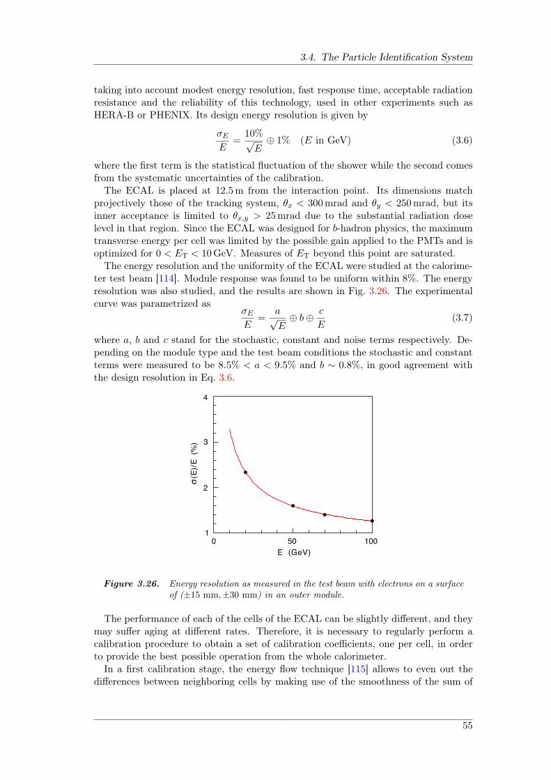
3.4. The Particle Identification System
taking into account modest energy resolution, fast response time, acceptable radiationresistance and the reliability of this technology, used in other experiments such asHERA-B or PHENIX. Its design energy resolution is given by
σEE
=10%√E
⊕ 1% (E in GeV) (3.6)
where the first term is the statistical fluctuation of the shower while the second comesfrom the systematic uncertainties of the calibration.
The ECAL is placed at 12.5m from the interaction point. Its dimensions matchprojectively those of the tracking system, θx < 300mrad and θy < 250mrad, but itsinner acceptance is limited to θx,y > 25mrad due to the substantial radiation doselevel in that region. Since the ECAL was designed for b-hadron physics, the maximumtransverse energy per cell was limited by the possible gain applied to the PMTs and isoptimized for 0 < ET < 10GeV. Measures of ET beyond this point are saturated.
The energy resolution and the uniformity of the ECAL were studied at the calorime-ter test beam [114]. Module response was found to be uniform within 8%. The energyresolution was also studied, and the results are shown in Fig. 3.26. The experimentalcurve was parametrized as
σEE
=a√E
⊕ b⊕ c
E(3.7)
where a, b and c stand for the stochastic, constant and noise terms respectively. De-pending on the module type and the test beam conditions the stochastic and constantterms were measured to be 8.5% < a < 9.5% and b ∼ 0.8%, in good agreement withthe design resolution in Eq. 3.6.
2
4
50 100
3
10
σ(E
)/E
(%
)
E (GeV)
Figure 3.26. Energy resolution as measured in the test beam with electrons on a surfaceof (±15 mm,±30 mm) in an outer module.
The performance of each of the cells of the ECAL can be slightly different, and theymay suffer aging at different rates. Therefore, it is necessary to regularly perform acalibration procedure to obtain a set of calibration coefficients, one per cell, in orderto provide the best possible operation from the whole calorimeter.
In a first calibration stage, the energy flow technique [115] allows to even out thedifferences between neighboring cells by making use of the smoothness of the sum of
55
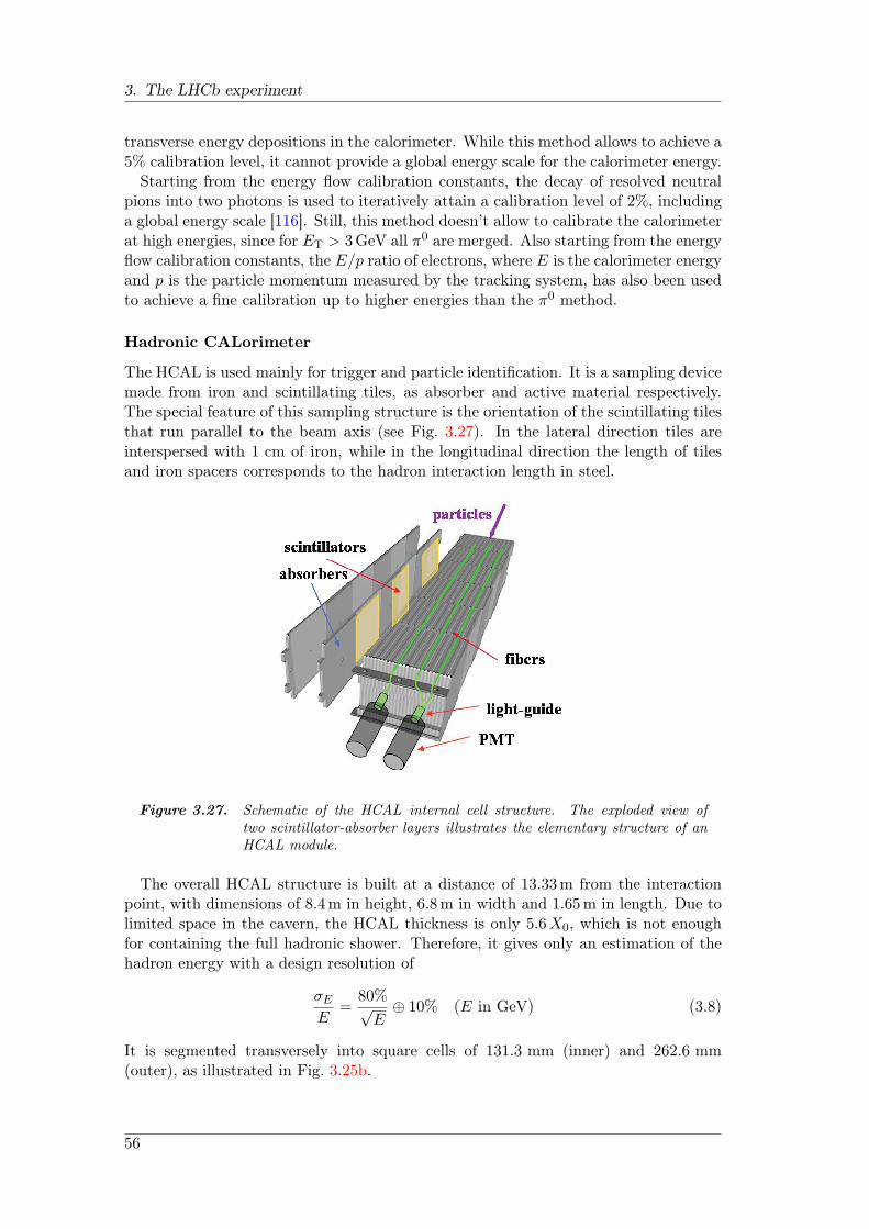
3. The LHCb experiment
transverse energy depositions in the calorimeter. While this method allows to achieve a5% calibration level, it cannot provide a global energy scale for the calorimeter energy.
Starting from the energy flow calibration constants, the decay of resolved neutralpions into two photons is used to iteratively attain a calibration level of 2%, includinga global energy scale [116]. Still, this method doesn’t allow to calibrate the calorimeterat high energies, since for ET > 3GeV all π0 are merged. Also starting from the energyflow calibration constants, the E/p ratio of electrons, where E is the calorimeter energyand p is the particle momentum measured by the tracking system, has also been usedto achieve a fine calibration up to higher energies than the π0 method.
Hadronic CALorimeter
The HCAL is used mainly for trigger and particle identification. It is a sampling devicemade from iron and scintillating tiles, as absorber and active material respectively.The special feature of this sampling structure is the orientation of the scintillating tilesthat run parallel to the beam axis (see Fig. 3.27). In the lateral direction tiles areinterspersed with 1 cm of iron, while in the longitudinal direction the length of tilesand iron spacers corresponds to the hadron interaction length in steel.
Figure 3.27. Schematic of the HCAL internal cell structure. The exploded view oftwo scintillator-absorber layers illustrates the elementary structure of anHCAL module.
The overall HCAL structure is built at a distance of 13.33m from the interactionpoint, with dimensions of 8.4m in height, 6.8m in width and 1.65m in length. Due tolimited space in the cavern, the HCAL thickness is only 5.6X0, which is not enoughfor containing the full hadronic shower. Therefore, it gives only an estimation of thehadron energy with a design resolution of
σEE
=80%√E
⊕ 10% (E in GeV) (3.8)
It is segmented transversely into square cells of 131.3 mm (inner) and 262.6 mm(outer), as illustrated in Fig. 3.25b.
56
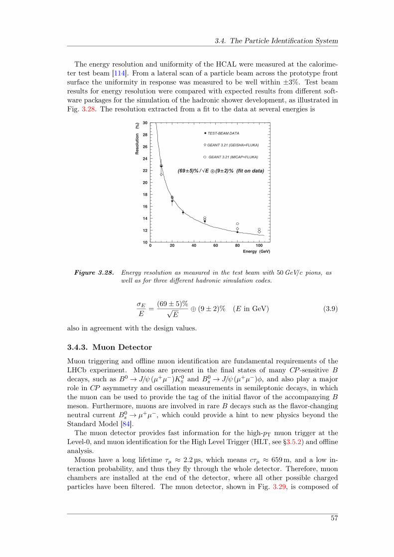
3.4. The Particle Identification System
The energy resolution and uniformity of the HCAL were measured at the calorime-ter test beam [114]. From a lateral scan of a particle beam across the prototype frontsurface the uniformity in response was measured to be well within ±3%. Test beamresults for energy resolution were compared with expected results from different soft-ware packages for the simulation of the hadronic shower development, as illustrated inFig. 3.28. The resolution extracted from a fit to the data at several energies is
10
12
14
16
18
20
22
24
26
28
30
0 20 40 60 80 100
Energy (GeV)
Re
so
luti
on
()
TEST-BEAM DATA
GEANT 3.21 (GEISHA+FLUKA)
GEANT 3.21 (MICAP+FLUKA)
(69 5)% / √E + (9±2) % (fit on data)±
%
Figure 3.28. Energy resolution as measured in the test beam with 50GeV/c pions, aswell as for three different hadronic simulation codes.
σEE
=(69± 5)%√
E⊕ (9± 2)% (E in GeV) (3.9)
also in agreement with the design values.
3.4.3. Muon Detector
Muon triggering and offline muon identification are fundamental requirements of theLHCb experiment. Muons are present in the final states of many CP -sensitive Bdecays, such as B0 → J/ψ (µ+µ−)K0
S and B0s → J/ψ (µ+µ−)ϕ, and also play a major
role in CP asymmetry and oscillation measurements in semileptonic decays, in whichthe muon can be used to provide the tag of the initial flavor of the accompanying Bmeson. Furthermore, muons are involved in rare B decays such as the flavor-changingneutral current B0
s → µ+µ−, which could provide a hint to new physics beyond theStandard Model [84].
The muon detector provides fast information for the high-pT muon trigger at theLevel-0, and muon identification for the High Level Trigger (HLT, see §3.5.2) and offlineanalysis.
Muons have a long lifetime τµ ≈ 2.2µs, which means cτµ ≈ 659m, and a low in-teraction probability, and thus they fly through the whole detector. Therefore, muonchambers are installed at the end of the detector, where all other possible chargedparticles have been filtered. The muon detector, shown in Fig. 3.29, is composed of
57
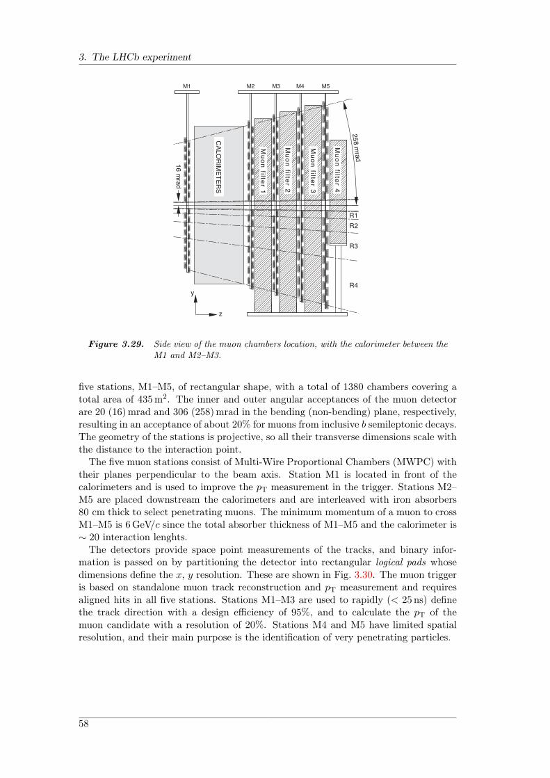
3. The LHCb experiment
16 m
rad
258 m
rad
Mu
on
filter 1
R2
R3
R4
R1
y
z
Mu
on
filter 4
Mu
on
filter 3
Mu
on
filter 2
CA
LO
RIM
ET
ER
S
M1 M2 M3 M4 M5
Figure 3.29. Side view of the muon chambers location, with the calorimeter between theM1 and M2–M3.
five stations, M1–M5, of rectangular shape, with a total of 1380 chambers covering atotal area of 435m2. The inner and outer angular acceptances of the muon detectorare 20 (16)mrad and 306 (258)mrad in the bending (non-bending) plane, respectively,resulting in an acceptance of about 20% for muons from inclusive b semileptonic decays.The geometry of the stations is projective, so all their transverse dimensions scale withthe distance to the interaction point.
The five muon stations consist of Multi-Wire Proportional Chambers (MWPC) withtheir planes perpendicular to the beam axis. Station M1 is located in front of thecalorimeters and is used to improve the pT measurement in the trigger. Stations M2–M5 are placed downstream the calorimeters and are interleaved with iron absorbers80 cm thick to select penetrating muons. The minimum momentum of a muon to crossM1–M5 is 6GeV/c since the total absorber thickness of M1–M5 and the calorimeter is∼ 20 interaction lenghts.
The detectors provide space point measurements of the tracks, and binary infor-mation is passed on by partitioning the detector into rectangular logical pads whosedimensions define the x, y resolution. These are shown in Fig. 3.30. The muon triggeris based on standalone muon track reconstruction and pT measurement and requiresaligned hits in all five stations. Stations M1–M3 are used to rapidly (< 25ns) definethe track direction with a design efficiency of 95%, and to calculate the pT of themuon candidate with a resolution of 20%. Stations M4 and M5 have limited spatialresolution, and their main purpose is the identification of very penetrating particles.
58
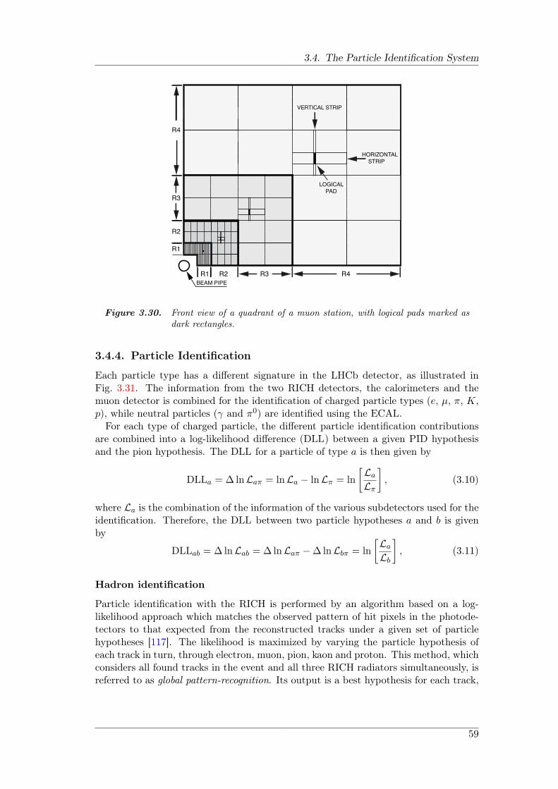
3.4. The Particle Identification System
R1
R2
R3
R4
R1 R2 R3 R4
VERTICAL STRIP
HORIZONTAL
STRIP
LOGICAL
PAD
BEAM PIPE
Figure 3.30. Front view of a quadrant of a muon station, with logical pads marked asdark rectangles.
3.4.4. Particle Identification
Each particle type has a different signature in the LHCb detector, as illustrated inFig. 3.31. The information from the two RICH detectors, the calorimeters and themuon detector is combined for the identification of charged particle types (e, µ, π, K,p), while neutral particles (γ and π0) are identified using the ECAL.
For each type of charged particle, the different particle identification contributionsare combined into a log-likelihood difference (DLL) between a given PID hypothesisand the pion hypothesis. The DLL for a particle of type a is then given by
DLLa = ∆ lnLaπ = lnLa − lnLπ = ln
[La
Lπ
], (3.10)
where La is the combination of the information of the various subdetectors used for theidentification. Therefore, the DLL between two particle hypotheses a and b is givenby
DLLab = ∆ lnLab = ∆ lnLaπ −∆lnLbπ = ln
[La
Lb
], (3.11)
Hadron identification
Particle identification with the RICH is performed by an algorithm based on a log-likelihood approach which matches the observed pattern of hit pixels in the photode-tectors to that expected from the reconstructed tracks under a given set of particlehypotheses [117]. The likelihood is maximized by varying the particle hypothesis ofeach track in turn, through electron, muon, pion, kaon and proton. This method, whichconsiders all found tracks in the event and all three RICH radiators simultaneously, isreferred to as global pattern-recognition. Its output is a best hypothesis for each track,
59
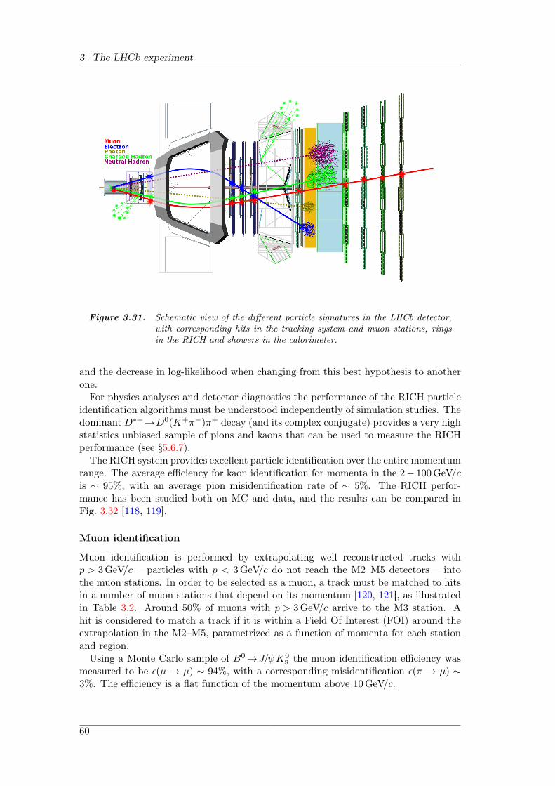
3. The LHCb experiment
Figure 3.31. Schematic view of the different particle signatures in the LHCb detector,with corresponding hits in the tracking system and muon stations, ringsin the RICH and showers in the calorimeter.
and the decrease in log-likelihood when changing from this best hypothesis to anotherone.
For physics analyses and detector diagnostics the performance of the RICH particleidentification algorithms must be understood independently of simulation studies. Thedominant D∗+→D0(K+π−)π+ decay (and its complex conjugate) provides a very highstatistics unbiased sample of pions and kaons that can be used to measure the RICHperformance (see §5.6.7).
The RICH system provides excellent particle identification over the entire momentumrange. The average efficiency for kaon identification for momenta in the 2− 100GeV/cis ∼ 95%, with an average pion misidentification rate of ∼ 5%. The RICH perfor-mance has been studied both on MC and data, and the results can be compared inFig. 3.32 [118, 119].
Muon identification
Muon identification is performed by extrapolating well reconstructed tracks withp > 3GeV/c —particles with p < 3GeV/c do not reach the M2–M5 detectors— intothe muon stations. In order to be selected as a muon, a track must be matched to hitsin a number of muon stations that depend on its momentum [120, 121], as illustratedin Table 3.2. Around 50% of muons with p > 3GeV/c arrive to the M3 station. Ahit is considered to match a track if it is within a Field Of Interest (FOI) around theextrapolation in the M2–M5, parametrized as a function of momenta for each stationand region.
Using a Monte Carlo sample of B0→J/ψK0S the muon identification efficiency was
measured to be ϵ(µ → µ) ∼ 94%, with a corresponding misidentification ϵ(π → µ) ∼3%. The efficiency is a flat function of the momentum above 10GeV/c.
60

3.4. The Particle Identification System
Momentum (MeV/c)20 40 60 80 100
310×
Effi
cien
cy
0
0.2
0.4
0.6
0.8
1
1.2
1.4) > 0π LL(K - ∆
) > 5π LL(K - ∆
K→K
K→ π
= 7 TeV Monte CarlosLHCb
(a) Monte Carlo MC10 sample.
Momentum (MeV/c)20 40 60 80 100
310×
Effi
cien
cy
0
0.2
0.4
0.6
0.8
1
1.2
1.4) > 0π LL(K - ∆
) > 5π LL(K - ∆
K→K
K→ π
= 7 TeV DatasLHCb
(b) Data Stripping13b, L < 100 pb−1.
Figure 3.32. Kaon/pion separation as a function of the particle momentum.
Track momentum (GeV/c) Required stations
3 < p < 6 M2+M36 < p < 10 M2+M3+(M4 or M5)p > 10 M2+M3+M4+M5
Table 3.2. Stations required to have a hit within FOI for tracks at different momentumranges.
For each track, two likelihoods, one for the muon and one for the non-muon hy-pothesis, are built using information from the tracking system and the muon stations.These likelihoods are built from the comparison of slopes in the muon detector and thetracking, and from the average track-hit distance of all hits in FOI associated to thetrack. Then the log-likelihood difference DLLµπ is determined, and summed with thevalues from the RICH and calorimeter systems (if available). By doing this the pionmisidentification rate can be reduced to ∼1%, while maintaining a muon efficiency of∼ 93% for muons above 3GeV/c.
The high purity that can be achieved with such cuts is illustrated in one of theearly results of the LHCb collaboration [122]. In the early stages of the experiment,with an integrated luminosity of L = 5.2 pb−1, the J/ψ cross section was measuredby building J/ψ→µ−µ+ taking oppositely charged pairs of tracks that pass the muonidentification requirements. The J/ψ mass peak is reconstructed with a resolution of12.3± 0.1MeV/c, as shown in Fig. 3.33.
Electron Identification
Electron identification [123] is performed using a combination of ∆lnLcaloe/non-e based on
the information of different subdetectors:
ECAL. All reconstructed tracks in the event are extrapolated to the ECAL planeand an all-to-all matching with the reconstructed clusters is performed. A χ2
γ isconstructed based on the distance of the extrapolated tracks and the clusters, andit is used to discriminate between charged and neutral clusters. A χ2
e estimatoris build and minimized using the matching between the corrected barycenter
61
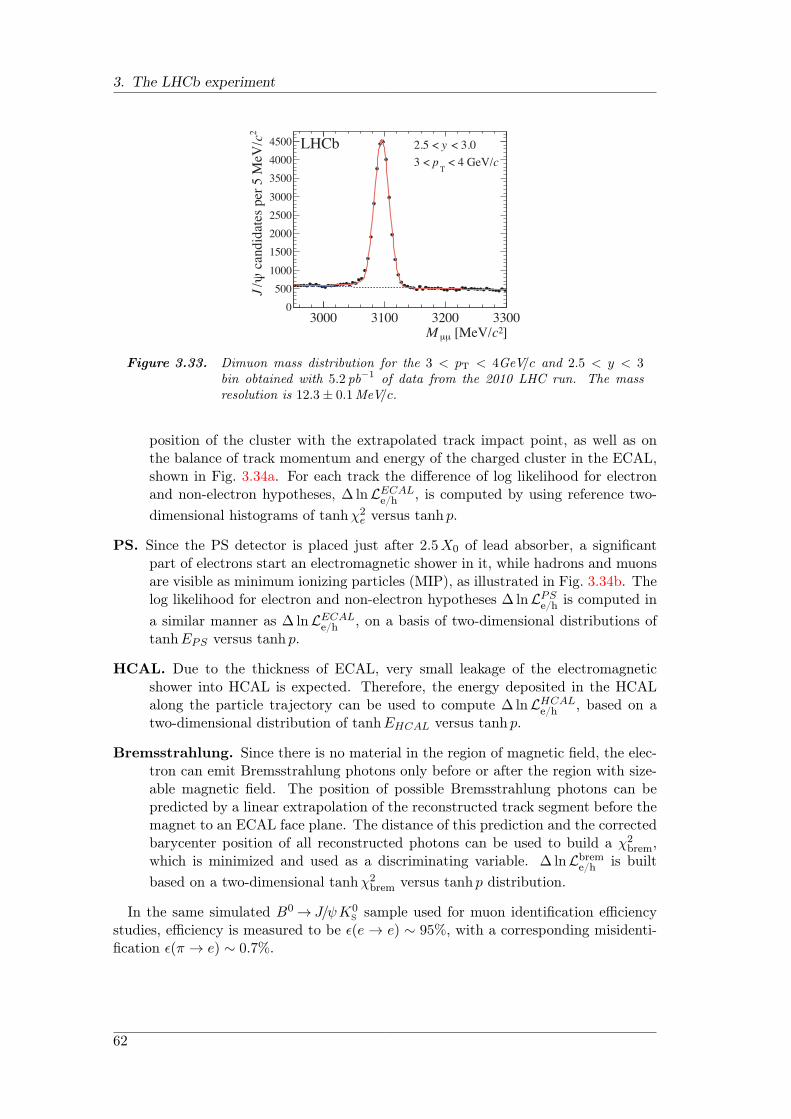
3. The LHCb experiment
]2c [MeV/μμM3000 3100 3200 3300
2c
can
did
ates
per
5 M
eV/
ψ/J
0
500
1000
1500
2000
2500
3000
3500
4000
4500 LHCb < 3.0y2.5 <
c < 4 GeV/T
p3 <
Figure 3.33. Dimuon mass distribution for the 3 < pT < 4GeV/c and 2.5 < y < 3bin obtained with 5.2 pb−1 of data from the 2010 LHC run. The massresolution is 12.3± 0.1MeV/c.
position of the cluster with the extrapolated track impact point, as well as onthe balance of track momentum and energy of the charged cluster in the ECAL,shown in Fig. 3.34a. For each track the difference of log likelihood for electronand non-electron hypotheses, ∆lnLECAL
e/h , is computed by using reference two-dimensional histograms of tanhχ2
e versus tanh p.
PS. Since the PS detector is placed just after 2.5X0 of lead absorber, a significantpart of electrons start an electromagnetic shower in it, while hadrons and muonsare visible as minimum ionizing particles (MIP), as illustrated in Fig. 3.34b. Thelog likelihood for electron and non-electron hypotheses ∆lnLPS
e/h is computed ina similar manner as ∆lnLECAL
e/h , on a basis of two-dimensional distributions oftanhEPS versus tanh p.
HCAL. Due to the thickness of ECAL, very small leakage of the electromagneticshower into HCAL is expected. Therefore, the energy deposited in the HCALalong the particle trajectory can be used to compute ∆lnLHCAL
e/h , based on atwo-dimensional distribution of tanhEHCAL versus tanh p.
Bremsstrahlung. Since there is no material in the region of magnetic field, the elec-tron can emit Bremsstrahlung photons only before or after the region with size-able magnetic field. The position of possible Bremsstrahlung photons can bepredicted by a linear extrapolation of the reconstructed track segment before themagnet to an ECAL face plane. The distance of this prediction and the correctedbarycenter position of all reconstructed photons can be used to build a χ2
brem,which is minimized and used as a discriminating variable. ∆ lnLbrem
e/h is builtbased on a two-dimensional tanhχ2
brem versus tanh p distribution.
In the same simulated B0 → J/ψK0S sample used for muon identification efficiency
studies, efficiency is measured to be ϵ(e → e) ∼ 95%, with a corresponding misidenti-fication ϵ(π → e) ∼ 0.7%.
62
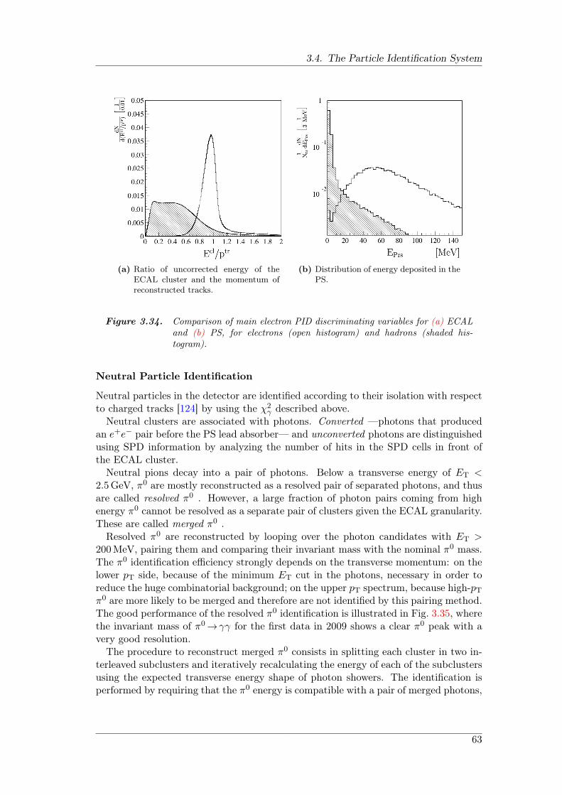
3.4. The Particle Identification System
(a) Ratio of uncorrected energy of theECAL cluster and the momentum ofreconstructed tracks.
(b) Distribution of energy deposited in thePS.
Figure 3.34. Comparison of main electron PID discriminating variables for (a) ECALand (b) PS, for electrons (open histogram) and hadrons (shaded his-togram).
Neutral Particle Identification
Neutral particles in the detector are identified according to their isolation with respectto charged tracks [124] by using the χ2
γ described above.Neutral clusters are associated with photons. Converted —photons that produced
an e+e− pair before the PS lead absorber— and unconverted photons are distinguishedusing SPD information by analyzing the number of hits in the SPD cells in front ofthe ECAL cluster.
Neutral pions decay into a pair of photons. Below a transverse energy of ET <2.5GeV, π0 are mostly reconstructed as a resolved pair of separated photons, and thusare called resolved π0 . However, a large fraction of photon pairs coming from highenergy π0 cannot be resolved as a separate pair of clusters given the ECAL granularity.These are called merged π0 .
Resolved π0 are reconstructed by looping over the photon candidates with ET >200MeV, pairing them and comparing their invariant mass with the nominal π0 mass.The π0 identification efficiency strongly depends on the transverse momentum: on thelower pT side, because of the minimum ET cut in the photons, necessary in order toreduce the huge combinatorial background; on the upper pT spectrum, because high-pTπ0 are more likely to be merged and therefore are not identified by this pairing method.The good performance of the resolved π0 identification is illustrated in Fig. 3.35, wherethe invariant mass of π0→γγ for the first data in 2009 shows a clear π0 peak with avery good resolution.
The procedure to reconstruct merged π0 consists in splitting each cluster in two in-terleaved subclusters and iteratively recalculating the energy of each of the subclustersusing the expected transverse energy shape of photon showers. The identification isperformed by requiring that the π0 energy is compatible with a pair of merged photons,
63
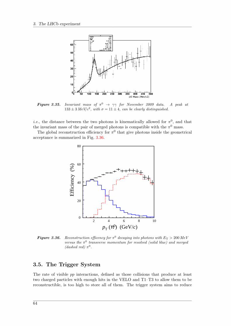
3. The LHCb experiment
Figure 3.35. Invariant mass of π0 → γγ for November 2009 data. A peak at133± 3MeV/c2, with σ = 11± 4, can be clearly distinguished.
i.e., the distance between the two photons is kinematically allowed for π0, and thatthe invariant mass of the pair of merged photons is compatible with the π0 mass.
The global reconstruction efficiency for π0 that give photons inside the geometricalacceptance is summarized in Fig. 3.36.
0
20
40
60
80
2 4 6 8 10
Eff
icie
ncy
(%
)
pT (π0) (GeV/c)
Figure 3.36. Reconstruction efficency for π0 decaying into photons with ET > 200MeVversus the π0 transverse momentum for resolved (solid blue) and merged(dashed red) π0.
3.5. The Trigger System
The rate of visible pp interactions, defined as those collisions that produce at leasttwo charged particles with enough hits in the VELO and T1–T3 to allow them to bereconstructible, is too high to store all of them. The trigger system aims to reduce
64
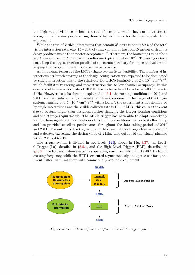
3.5. The Trigger System
this high rate of visible collisions to a rate of events at which they can be written tostorage for offline analysis, selecting those of higher interest for the physics goals of theexperiment.
While the rate of visible interactions that contain bb pairs is about 1/200 of the totalvisible interaction rate, only 15−20% of them contain at least one B meson with all itsdecay products inside the detector acceptance. Furthermore, the branching ratios of thekey B decays used in CP violation studies are typically below 10−3. Triggering criteriamust keep the largest fraction possible of the events necessary for offline analysis, whilekeeping the background event rate as low as possible.
An important feature of the LHCb trigger system is its flexibility. The number of in-teractions per bunch crossing at the design configuration was expected to be dominatedby single interaction due to the relatively low LHCb luminosity of 2 × 1032 cm−2s−1,which facilitates triggering and reconstruction due to low channel occupancy. In thiscase, a visible interaction rate of 10MHz has to be reduced by a factor 5000, down to2 kHz. However, as it has been in explained in §3.1, the running conditions in 2010 and2011 have been substantially different than those considered in the design of the triggersystem: running at 3.5×1032 cm−2 s−1 with a low β∗, the experiment is not dominatedby single interactions and the visible collision rate is 12−15MHz; this causes the eventsize to become larger than designed, further changing the trigger working conditionsand the storage requirements. The LHCb trigger has been able to adapt remarkablywell to these significant modifications of its running conditions thanks to its flexibility,and has provided excellent performance throughout the data taking periods of 2010and 2011. The output of the trigger in 2011 has been 3 kHz of very clean samples of band c decays, exceeding the design value of 2 kHz. The output of the trigger plannedfor 2012 is ∼ 4.5 kHz.
The trigger system is divided in two levels [125], shown in Fig. 3.37: the Level-0 Trigger (L0), detailed in §3.5.1, and the High Level Trigger (HLT), described in§3.5.2. The L0 uses custom electronics operating synchronously with the 40MHz bunchcrossing frequency, while the HLT is executed asynchronously on a processor farm, theEvent Filter Farm, made up with commercially available equipment.
40 MHz
1 MHz
3 kHz
HLT
Pile-up systemCalorimetersMuon system
Full detector
information
Level-0:
pT of
µ, e, h, Custom Electronics
Event Filter Farm
Figure 3.37. Schema of the event flow in the LHCb trigger system.
65
3. The LHCb experiment
3.5.1. Level-0 Trigger
The first level of trigger (Level-0) is designed to reduce the visible event rate to the1MHz at which the whole detector can be read out. It is implemented using custommade hardware, running synchronously with the LHC clock. Since B meson decayproducts are usually particles with a large transverse momentum and transverse energy,high pT and ET objects constitute a very clear signature to trigger on. Therefore, theLevel-0 trigger focuses on the reconstruction of:
The highest ET hadron, electron and photon clusters in the calorimeters.
The two highest pT muons in the muon chambers.
Furthermore, events with high particle multiplicity are rejected in order to reduce theprocessing time in the HLT.
The Level-0 Trigger is subdivided in three components: the L0 calorimeter trigger,the L0 muon trigger and the pile-up system. Each component is connected to onedetector and to the Level-0 Decision Unit (L0 DU), which collects the informationprovided by the three L0 components to produce a final decision as a logical OR of itsinputs.
The L0 DU has to release its decision 4µs after each collision, which correspondsto the buffer length implemented in the front-end read-out chips. Furthermore, thetime-of-flight of the particles, plus the cable delays, plus the front-end electronics delayleave only 2µs for processing the data in the L0 DU and delivering a decision.
The L0 Calorimeter Trigger looks for high ET electron, photon, neutral pion orhadron candidates. It forms clusters by summing the ET of 2 × 2 cells and selectsthose which have the highest ET. Then the information from the SPD/PS, ECAL andHCAL is combined to tag the clusters as electron, photon or hadron. In addition, thetotal ET in the HCAL is used to reject crossings without any visible interaction andto reject events triggered by halo muons.
The total number of cells of the SPD which have a hit is used to evaluate the chargedtrack multiplicity and to reject high occupancy events. In 2010, events with more than900 hits in the SPD were rejected in order to keep the OT occupancy at ∼ 20% andallow a good performance. In 2011, the running conditions allowed to lower the SPDmultiplicity cut 600 hits, as a balance between the calorimeter occupation, the muonictriggers and the output rate.
The L0 Muon Trigger uses a fast stand-alone reconstruction of muon tracks with aσpT ∼ 20%. A track is found if hits in the five muon chambers can form a straightline pointing to the interaction region. The two highest-pT muon candidates of eachquadrant of the muon chambers are selected for the decision.
The Pile-Up System was designed to distinguish between single interactions frommultiple ones. Four r-sensors, similar to the ones used in the VELO, are locatedbefore the interaction region to measure the radial position of the backward tracks.Since the average number of interactions in 2010 and 2011 is higher than one, andtherefore the collected events are not dominated by single interactions, this system iscurrently only used to trigger beam-gas interactions.
66
3.5. The Trigger System
3.5.2. High Level Trigger
The High Level Trigger (HLT) filters events using a software application. It uses theOnline Event Filter Farm (EFF), which contains up to 20,000 CPU cores, to processand reduce the rate at which events are kept down to ∼ 3 kHz.
The high rate of incoming events from the Level-0 Trigger and the computing powerlimitation of the EFF do not allow the up-front use of the full event data informationin the decision-making process. Thus, the HLT is divided in two stages: the first stage(HLT1) uses only a partial reconstruction to reduce the rate by a factor of ∼ 20 sothat the second stage (HLT2) is able to perform full event reconstruction to furtherdiscriminate signal events.
HLT1
The HLT1 is designed to minimize the impact of varying running conditions on itsperformance. It is based around a single track trigger [126], which searches for a sin-gle track with high momentum, a large impact parameter with respect to all primaryvertices in the event, and a good track quality. In addition to this, lifetime unbiasedmuon [127] and electron triggers are used for analyses which are sensitive to the pres-ence of lifetime biases. These latter triggers are based around the confirmation of theL0 trigger decision by matching tracks reconstructed in the HLT to the objects usedin the L0 decision, i.e., muon segments or calorimeter clusters.
HLT1 takes ∼ 15ms to process a L0-accepted minimum bias event, and accepts∼ 5% of such events with an efficiency of more than 80% on signal events for most ofLHCb’s benchmark B decay modes [126, 127]. The ∼ 50 kHz selected by HLT1 arepassed to HLT2.
HLT2
The HLT2 input rate is sufficiently low to perform an almost-full-offline reconstruc-tion, the main difference being that in the HLT2 only tracks with pT > 500MeV/cand p > 5000MeV/c are reconstructed. Having fully reconstructed events allows theHLT2 trigger lines to use event selection criteria more in line with those used in of-fline analyses. Furthermore, Global Event Cuts (GEC), such as the reconstructed trackmultiplicity, are used to reject complex events which require a big amount of processingtime.
The HLT2 trigger is made up of a mixture of inclusive, which search for generic Bdecay features such as displaced vertices or dilepton pairs, and exclusive trigger lines,which select specific decays using similar selections to those used offline. In 2011 [128],∼ 1/3 of the bandwidth was taken by the inclusive topological trigger [129], which allowsto obtain a high efficiency and low background retention on almost all n-body B decays.Muon triggers, which select high-pT single or dimuons, used up about another third ofthe bandwidth. Charm decays accounted for ∼ 1/3 of the HLT2 bandwidth, while therest was used by several exclusive lines, such as the radiative lines [130], and inclusivelines such as the ϕ trigger [131].
67
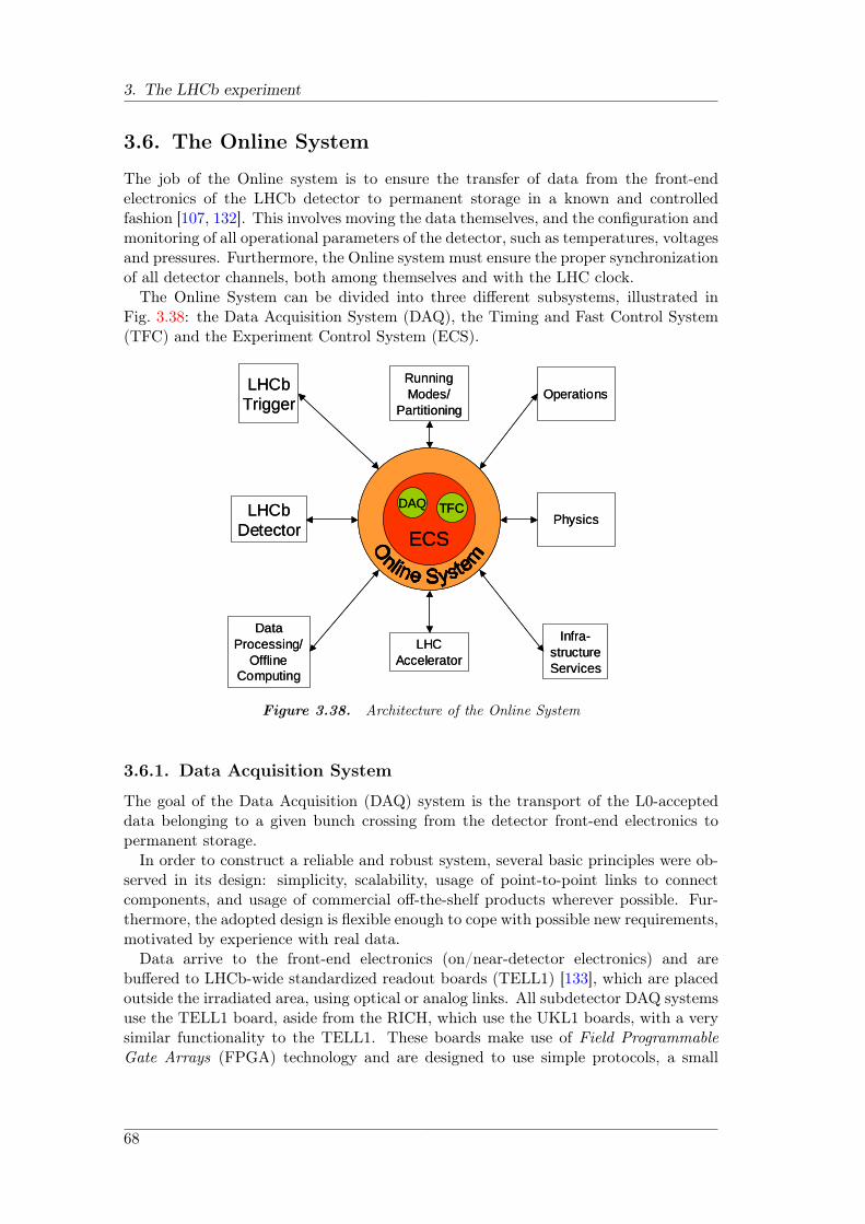
3. The LHCb experiment
3.6. The Online System
The job of the Online system is to ensure the transfer of data from the front-endelectronics of the LHCb detector to permanent storage in a known and controlledfashion [107, 132]. This involves moving the data themselves, and the configuration andmonitoring of all operational parameters of the detector, such as temperatures, voltagesand pressures. Furthermore, the Online system must ensure the proper synchronizationof all detector channels, both among themselves and with the LHC clock.
The Online System can be divided into three different subsystems, illustrated inFig. 3.38: the Data Acquisition System (DAQ), the Timing and Fast Control System(TFC) and the Experiment Control System (ECS).
ECS
DAQ TFC
Data
Processing/
Offline
Computing
LHC
Accelerator
Infra-
structure
Services
Operations
Running
Modes/
Partitioning
LHCb
Trigger
LHCb
DetectorPhysics
ECS
DAQ TFC
ECS
DAQ TFC
Data
Processing/
Offline
Computing
LHC
Accelerator
Infra-
structure
Services
Operations
Running
Modes/
Partitioning
LHCb
Trigger
LHCb
DetectorPhysics
Figure 3.38. Architecture of the Online System
3.6.1. Data Acquisition System
The goal of the Data Acquisition (DAQ) system is the transport of the L0-accepteddata belonging to a given bunch crossing from the detector front-end electronics topermanent storage.
In order to construct a reliable and robust system, several basic principles were ob-served in its design: simplicity, scalability, usage of point-to-point links to connectcomponents, and usage of commercial off-the-shelf products wherever possible. Fur-thermore, the adopted design is flexible enough to cope with possible new requirements,motivated by experience with real data.
Data arrive to the front-end electronics (on/near-detector electronics) and arebuffered to LHCb-wide standardized readout boards (TELL1) [133], which are placedoutside the irradiated area, using optical or analog links. All subdetector DAQ systemsuse the TELL1 board, aside from the RICH, which use the UKL1 boards, with a verysimilar functionality to the TELL1. These boards make use of Field ProgrammableGate Arrays (FPGA) technology and are designed to use simple protocols, a small
68
3.7. Computing and resources
number of components, and are able to react to changing system parameters. Thedata are zero-suppressed, compressed, packed, buffered and sent via Gigabit-Ethernetlinks to the Event Builder, which collects the data coming from all the subdetectorsfor a single event. These data are sent forward to the HLT, that selects which events—corresponding to physically interesting interactions— are sent to permanent storage.The storage system has a capacity of ∼ 40TB, which offer enough buffer space to copewith possible interruptions of the transfer of the data to permanent storage at CERN.Gigabit-Ethernet is used throughout the Online system as link technology.
3.6.2. Timing and Fast Control System
The TFC system is in charge of driving all stages of the data readout of the LHCbdetector between the front-end electronics and the Event Filter Farm by distributingthe beam-synchronous clock, the L0 trigger, synchronous resets and fast control com-mands. The system is a combination of electronics components common to all LHCexperiments and LHCb custom electronics. It is formed by three main parts: the TFCdistribution network transmits the beam synchronous clock, featuring a low-latencytrigger channel and a second channel used to encode control commands; the opticalthrottle network is used to transmit a trigger inhibit from the asynchronous parts ofthe readout system to the Readout Supervisor in case of congestion of the data path;the Readout Supervisor (ODIN), the most important part of the system, implementsthe interface between the LHCb trigger and the readout chain, synchronizing trig-ger decisions and beam-synchronous commands to the LHC clock. Furthermore, theReadout Supervisor is able to perform load balancing among the nodes in the EFF bydynamically selecting the destination node for the incoming events, and to provide awide variety of auto-triggers for calibration and test purposes.
3.6.3. Experiment Control System
The Experiment Control System (ECS) ensures the control and monitoring of the en-tire LHCb detector, including traditional detector control domains, such as voltages,temperatures, gas flows, or pressures, and the trigger, TFC and DAQ systems. TheLHCb ECS is based on the PVSS II [134, 135], a commercial SCADA (Supervisory Con-trol and Data Acquisition) system, also used in other LHC experiments, that providesfeatures such as the management of databases, the communication between distributedcomponents, graphical libraries and an alarm system.
The LHCb ECS is a hierarchical and distributed system which allows the controlof the whole detector from the top level, but also a finer control of any given sub-tree, which can be released from the top control and operated in standalone mode.Commands are propagated down the hierarchy, while states and alarms go upwards.This command and state/error flow is managed using a Finite State Machine packagebased on SMI++ [136, 137], which allows the creation of the complex logic needed, forexample, in the implementation of elaborate sequencing or automated error recovery.
3.7. Computing and resources
The LHCb computing model allows to perform an efficient processing of the collecteddata, an accurate alignment and calibration of the subdetectors and an efficient selec-
69

3. The LHCb experiment
tion of events of interest, and also provides facilities for extracting physics results fromthe selected data samples. Each physics working group relies heavily on a full centralprocessing chain from the raw data to the pre-selected reconstructed data sample usedfor physics analyses: individual analyses generally only deal with small samples whilethe manipulation of larger datasets is handled centrally by the LHCb production team.
Similar algorithms need to be executed in very different contexts, from the OnlineEvent Filter Farm to a physicist’s laptop, and therefore a high level of standardizationof the software is needed. Furthermore, the large amounts of data and of computingpower needs imply that data processing must be performed in a distributed manner,taking best advantage of all resources available in computing facilities around theworld. These resources (CPU and storage) are accessible through a standard set ofservices provided to all LHC experiments —and also to the larger HEP communityand beyond— by the WLCG project [94].
3.7.1. LHCb software
The LHCb software is based on the Gaudi [138, 139] architecture, which provides anObject Oriented framework for all the applications used within the experiment [140]. Ithas the flexibility needed for running the LHCb chain from the Monte Carlo generationto the real data analysis using the same tools. Data persistency is based on the Rootsoftware [141, 142], a set of object-oriented frameworks designed to handle and analyzelarge amounts of data.
The main software applications used in LHCb are:
Gauss. The validation of physics analyses or reconstruction schemes need to be per-formed using Monte Carlo simulation. The simulation of the physical aspects ofpp collisions in the LHCb detector is handled by the Gauss software [143, 144].In a first step, the Pythia software [145] is used to simulate the proton colli-sions, the generated particles and their corresponding momentum four-vectors.The decays of the produced particles are handled either with Pythia or throughan LHCb-tuned EvtGen package [146] in the case of B hadrons, with the finalstate radiation handled by Photos [147, 148]. The particle-detector interactionis handled by the Geant package [149], which is used to transport the particlesthrough the detector. Detector geometry and materials are stored in a database.
Boole. The Boole software package [150] simulates the digitization of the energydepositions in the LHCb detector and the L0 trigger. This digitization takes intoaccount the interference from previous pp events —the spillover. After a Boolepass, the simulated and the real data can be reconstructed and analyzed usingthe same software.
Moore. The Moore package [151] is used to run the HLT in the Online System,processing real data from the LHCb DAQ system, or offline starting from realdata or from the output of Boole. The trigger is configured via a unique key,called a Trigger Configuration Key (TCK), which defines the sequence of algo-rithms and their cuts. It is represented by a 32-bit number, with the lower 16 bitsreserved for the L0 configuration2 and the higher 16 bits for the HLT. Each of
2For simplicity purposes, when dealing with TCKs for 2010 and 2011, the first 6 bits of the L0configuration will be omitted because they are 0, i.e., TCK 0x00360032 will be referred to as0x360032.
70
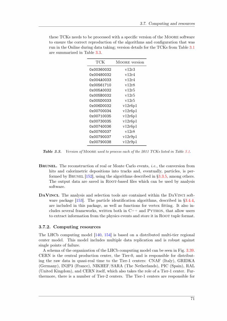
3.7. Computing and resources
these TCKs needs to be processed with a specific version of the Moore softwareto ensure the correct reproduction of the algorithms and configuration that wasrun in the Online during data taking; version details for the TCKs from Table 3.1are summarized in Table 3.3.
TCK Moore version
0x00360032 v12r30x00480032 v12r40x004A0033 v12r40x00561710 v12r80x005A0032 v12r50x005B0032 v12r50x005D0033 v12r50x006D0032 v12r6p10x00700034 v12r6p10x00710035 v12r6p10x00730035 v12r6p10x00740036 v12r6p10x00760037 v12r80x00790037 v12r9p10x00790038 v12r9p1
Table 3.3. Version of Moore used to process each of the 2011 TCKs listed in Table 3.1.
Brunel. The reconstruction of real or Monte Carlo events, i.e., the conversion fromhits and calorimetric depositions into tracks and, eventually, particles, is per-formed by Brunel [152], using the algorithms described in §3.3.5, among others.The output data are saved in Root-based files which can be used by analysissoftware.
DaVinci. The analysis and selection tools are contained within the DaVinci soft-ware package [153]. The particle identification algorithms, described in §3.4.4,are included in this package, as well as functions for vertex fitting. It also in-cludes several frameworks, written both in C++ and Python, that allow usersto extract information from the physics events and store it in Root tuple format.
3.7.2. Computing resources
The LHCb computing model [140, 154] is based on a distributed multi-tier regionalcenter model. This model includes multiple data replication and is robust againstsingle points of failure.
A schema of the organization of the LHCb computing model can be seen in Fig. 3.39.CERN is the central production center, the Tier-0, and is responsible for distribut-ing the raw data in quasi-real time to the Tier-1 centers: CNAF (Italy), GRIDKA(Germany), IN2P3 (France), NIKHEF/SARA (The Netherlands), PIC (Spain), RAL(United Kingdom), and CERN itself, which also takes the role of a Tier-1 center. Fur-thermore, there is a number of Tier-2 centers. The Tier-1 centers are responsible for
71
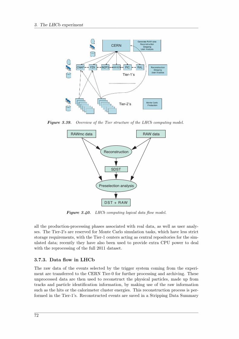
3. The LHCb experiment
Figure 3.39. Overview of the Tier structure of the LHCb computing model.
Figure 3.40. LHCb computing logical data flow model.
all the production-processing phases associated with real data, as well as user analy-ses. The Tier-2’s are reserved for Monte Carlo simulation tasks, which have less strictstorage requirements, with the Tier-1 centers acting as central repositories for the sim-ulated data; recently they have also been used to provide extra CPU power to dealwith the reprocessing of the full 2011 dataset.
3.7.3. Data flow in LHCb
The raw data of the events selected by the trigger system coming from the experi-ment are transferred to the CERN Tier-0 for further processing and archiving. Theseunprocessed data are then used to reconstruct the physical particles, made up fromtracks and particle identification information, by making use of the raw informationsuch as the hits or the calorimeter cluster energies. This reconstruction process is per-formed in the Tier-1’s. Reconstructed events are saved in a Stripping Data Summary
72

3.7. Computing and resources
Tape (SDST) file, which contains the necessary information for further event filteringwithout including the raw data.
The SDST files are analyzed in order to further filter events for physical analysesby making use of the full reconstructed information and with looser timing constraintsthan in the HLT. This sequence is known as Stripping, and finally produces a DataSummary Tape (DST) file, to which the raw data event information is attached. DSTsare the files accessible to scientists for physics analyses.
A summary of the data flow within the LHCb computing model is given in Fig. 3.40.The data are reprocessed several times a year with the improvement of the reconstruc-tion, alignment and stripping software and algorithms.
73

4Trigger strategies for radiative B
decays at LHCb
During 2010 and 2011, the HLT2 trigger for radiative decays has been based on looseexclusive selections for the B0→K∗0γ and B0
s →ϕγ decays, which provide a high effi-ciency for signal candidates passing the selection requirements of the analyses, referredto as offline-selected signal. This approach fails to provide good efficiencies for otherradiative decays, such as B+→ϕK+γ or B+→K∗0π+γ, and thus limits the ability toperform measurements outside the two main radiative channels.
Inclusive HLT2 triggers, mainly the topological trigger, took more than 1/3 of theLHCb trigger bandwidth in 2011 and are used in a wide variety of analyses. Whilethese generic triggers provide a uniform selection efficiency for many radiative channels,they only make use of tracks as generic B signatures, and this leads to compromises inorder to keep the rate within acceptable boundaries. In the case of radiative B decays,the presence of the photon in the final state provides an extra signature that can beused in inclusive lines to relax some of the adopted requirements for the tracks, leadingto a better trigger efficiency.
The adoption of an inclusive strategy would allow to expand the radiative decaysprogram to many radiative channels besides B0→K∗0γ and B0
s →ϕγ and would openthe possibility of exploring a wide range of analysis options in the future, provided thatgood signal efficiencies can be achieved at an acceptable rate.
4.1. Data samples
For the trigger studies in this chapter, data from the full 2011 LHCb dataset have beenused. These data include a mixture of the TCKs detailed in Table 3.1.
The signal Monte Carlo samples for the B0 → K∗0γ, B0s → ϕγ, B+ → ϕK+γ and
B+ →K∗0π+γ channels have been generated simulating the 2011 running conditions(see §5.1 for details). Unless specifically stated, the 0x790038 TCK, corresponding to∼ 30% of the 2011 data set, has been applied to these datasets.
Data, both real and simulated, have been offline selected with the criteria specifiedin Table 4.1. Details of the individual cuts and their meaning can be found in §5.2. It
75
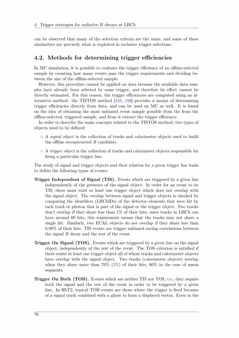
4. Trigger strategies for radiative B decays at LHCb
can be observed that many of the selection criteria are the same, and some of thesesimilarities are precisely what is exploited in inclusive trigger selections.
4.2. Methods for determining trigger efficiencies
In MC simulation, it is possible to evaluate the trigger efficiency of an offline-selectedsample by counting how many events pass the trigger requirements and dividing be-tween the size of the offline-selected sample.
However, this procedure cannot be applied on data because the available data sam-ples have already been selected by some trigger, and therefore its effect cannot bedirectly estimated. For this reason, the trigger efficiencies are computed using an al-ternative method: the TISTOS method [155, 156] provides a means of determiningtrigger efficiencies directly from data, and can be used on MC as well. It is basedon the idea of obtaining the most unbiased event sample possible from the from theoffline-selected, triggered sample, and from it extract the trigger efficiency.
In order to describe the main concepts related to the TISTOS method, two types ofobjects need to be defined:
A signal object is the collection of tracks and calorimeter objects used to buildthe offline reconstructed B candidate.
A trigger object is the collection of tracks and calorimeter objects responsible forfiring a particular trigger line.
The study of signal and trigger objects and their relation for a given trigger line leadsto define the following types of events:
Trigger Independent of Signal (TIS). Events which are triggered by a given lineindependently of the presence of the signal object. In order for an event to beTIS, there must exist at least one trigger object which does not overlap withthe signal object. The overlap between signal and trigger objects is checked bycomparing the identifiers (LHCbIDs) of the detector elements that were hit byeach track or photon that is part of the signal or the trigger object. Two tracksdon’t overlap if they share less than 1% of their hits; since tracks in LHCb canhave around 60 hits, this requirement means that the tracks may not share asingle hit. Similarly, two ECAL objects do not overlap if they share less than0.99% of their hits. TIS events are trigger unbiased saving correlations betweenthe signal B decay and the rest of the event.
Trigger On Signal (TOS). Events which are triggered by a given line on the signalobject, independently of the rest of the event. The TOS criterion is satisfied ifthere exists at least one trigger object all of whose tracks and calorimeter objectshave overlap with the signal object. Two tracks (calorimeter objects) overlapwhen they share more than 70% (1%) of their hits, 60% in the case of muonsegments.
Trigger On Both (TOB). Events which are neither TIS nor TOS, i.e., they requireboth the signal and the rest of the event in order to be triggered by a givenline. In HLT2, typical TOB events are those where the trigger is fired becauseof a signal track combined with a ghost to form a displaced vertex. Even in the
76
4.2. Methods for determining trigger efficiencies
B0→K
∗0γ
B0 s→ϕγ
B+→ϕK
+γ
B+→K
∗0π+γ
Tra
ckχ2
<5
<5
<5
<5
Tra
ckIP
χ2
>25
>25
>25
>25
Tra
ckpT
(MeV/c)
>500
>500
>500
>500
Max
trac
kpT
(MeV/c
)>
1200
>1200
>1000
>1000
Kao
nD
LLKπ
>5
>5
>5
>5
Kao
nD
LLKp
>2
>2
>2
>2
Pio
nD
LLKπ
<0
––
<0
Vec
tor
mes
onve
rtex
∆χ2
<9
<9
<9
<9
Vec
tor
mes
on∆M
PD
G(M
eV/c
2)
<50
<9
<9
<50
Pho
tonE
T(M
eV)
>2600
>2600
>2600
>2600
Pho
ton
CL
>0.25
>0.25
>0.25
>0.25
π0/γ
sepa
rati
on>
0.5
>0.5
>0.5
>0.5
Can
dida
tepT
(MeV/c)
>3000
>3000
>3000
>3000
Can
dida
teIP
χ2
<9
<9
<9
<9
Can
dida
teD
IRA
(mrad)
<20
<20
<20
<20
Can
dida
teFDχ2
>100
>100
>100
>100
Can
dida
te∆M
PD
G(M
eV/c
2)
<700
<700
<700
<700
Can
dida
te|cosθ H
|<
0.8
<0.8
––
Can
dida
teis
olat
ion∆χ2
>2
>2
>2
>2
Tab
le4.
1.Se
lect
ion
criter
iafo
rth
era
diat
ive
chan
nels
used
for
trig
ger
anal
ysis
.
77

4. Trigger strategies for radiative B decays at LHCb
case of the HLT1 single track trigger, it is also possible to have a TOB event,e.g., the VELO segment of the signal track is combined with a T-station ghost.TOB events are problematic because their efficiency cannot be defined withoutconstructing a model for the trigger efficiency on background events. Hence,TOB events are of limited use to any analysis which needs to know the triggerefficiency or acceptance.
With these definitions, the TOS efficiency can be calculated as
ϵTOS =NTIS&TOS
NTIS, (4.1)
and, likewise for the TIS efficiency:
ϵTIS =NTOS&TIS
NTOS. (4.2)
All trigger efficiencies quoted in this chapter are TOS efficiencies, unless specificallystated. In the case of MC samples, the TOS efficiency can also be obtained directly bycounting events that pass the given TOS requirement and dividing between the size ofthe offline-selected sample.
The TISTOS method allows to estimate the TOS efficiency of a signal by normalizingthe number of TOS events with the TIS requirement. The precision of the efficienciesobtained with this procedure is limited by the statistics of TIS events available, sincethese constitute a small fraction of the total offline-selected signal. Furthermore, sincethere may exist a correlation between the signal B and the other B in the event,efficiencies computed using the TISTOS method have to be determined as a functionof variables of interest, such as the B momentum, the B transverse momentum andthe B meson lifetime.
4.3. L0 channels
The relevant L0 channels for radiative decays are those included in the L0 CalorimeterTrigger [125]. The idea behind this set of L0 channels is to search for high ET objectsand identify them as electrons, photons, π0 or hadrons. Since showers are relativelynarrow, their corresponding ET is computed in a 2×2 cells zone, which is wide enoughto contain most of the energy and small enough to reduce significantly the probabilityof overlap between different particles. Furthermore, at each stage of the process onlythe candidate with the highest ET is kept, thus reducing the number of candidates toprocess. The selection of these L0 candidates is performed as following:
1. High ET deposits are selected by the Front-End (FE) cards, which handle ECALand HCAL information. Each of these handles 32 cells, and the highest ET overthe 32 sums of 2 × 2 cells is selected. To calculate these sums it is essential tohave access to neighboring cells in other cards.
2. Information from the SPD and PS is added in the Validation Cards in order toidentify the type of electromagnetic candidate. L0 candidates are distinguished aselectromagnetic by making use of the PS information of the cells in front of them:a certain energy deposit is required in order to ascertain that the electromagnetic
78
4.4. HLT1 lines
shower has begun in the lead absorber. The SPD information (hit/no hit) isthen used to distinguish between electron (L0Electron) and photon (L0Photon)candidates. Only one candidate per card and per type is selected and forwardedto the Selection Crate. The types are not exclusive, i.e., the same 2 × 2 clustercan be selected by different L0 calorimeter triggers. Finally, the ECAL transverseenergy is added to the relevant HCAL 2 × 2 clusters for hadron (L0Hadron)candidates.
3. The candidate with the highest ET for each type is selected in the SelectionCrate. In addition, the total ET in the HCAL and the total SPD multiplicity arecomputed as a measure of the activity in the event.
While the L0Photon and L0Electron thresholds were high and not completely stableduring 2010, 3.2GeV and 4.4GeV for the bulk of the data, in 2011 they have beenvery stable and almost all data have been collected with a lower threshold of 2.5GeV.In the case of the L0Hadron, during 2010 the threshold was placed at 3.6GeV almostfor all the data taking, while in 2011 the cut was lowered to 3.5GeV throughout mostof the year.
L0 trigger on the photon
It has been shown on simulation that using only L0Photon candidates is an ineffectiveway to trigger photons for radiative decays [157]. On one side, the requirement ofPS energy to identify electromagnetic energy depositions rejects 20% of the photonclusters. On the other side, the SPD only identifies as photon ∼ 60% of these elec-tromagnetic clusters due to the fact that 40% of the photons convert before the SPD,mostly in the M1 (∼ 0.265X0).
Therefore, incorporating the L0Electron to the definition of photon at the L0 levelhelps recovering part of those photons lost due to conversion, as can be seen in Fig. 4.1,at the cost of an increased rate. This rate can be controlled by tightening the ET cut forboth L0Photon and L0Electron, and doing so results in better efficiency (at a givenrate) than keeping a looser ET cut and using only L0Photon. For this reason, twofurther L0 channels have been added to the L0, L0PhotonHi and L0ElectronHi, whichcorrespond to L0Photon and L0Electron but with a tightened ET cut, ET > 4.2GeV.These high ET channels can be used in the HLT1 to provide a performance boost fordecays with photons.
L0 trigger on hadrons
In order to add robustness to the L0 trigger strategy, the L0Hadron requirement, whichrelies on the HCAL estimation of the transverse energy of the hadrons, can be addedin order to trigger, for example, on the daughter tracks of the K∗0 or the ϕ. This opensthe possibility of loosening the photon ET cut in the offline selections, since events nottriggered by the photon could be recovered if they were selected due to the hadrons.
4.4. HLT1 lines
Commissioning of the HLT1 in 2010 showed that hadronic triggers suffered from con-tamination by ghost tracks (reconstructed tracks with no real counterpart, produced by
79
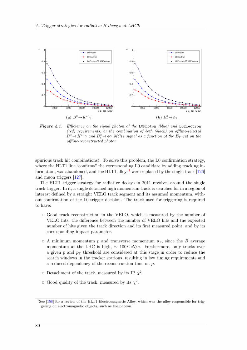
4. Trigger strategies for radiative B decays at LHCb
cut (MeV)T
Eγ4000 6000 8000 10000 12000
ε
0
0.2
0.4
0.6
0.8
1L0Photon
L0Electron
L0Photon OR L0Electron
(a) B0→K∗0γ.
cut (MeV)T
Eγ4000 6000 8000 10000 12000
ε
0
0.2
0.4
0.6
0.8
1L0Photon
L0Electron
L0Photon OR L0Electron
(b) B0s →ϕγ.
Figure 4.1. Efficiency on the signal photon of the L0Photon (blue) and L0Electron
(red) requirements, or the combination of both (black) on offline-selectedB0→K∗0γ and B0
s →ϕγ MC11 signal as a function of the ET cut on theoffline-reconstructed photon.
spurious track hit combinations). To solve this problem, the L0 confirmation strategy,where the HLT1 line “confirms” the corresponding L0 candidate by adding tracking in-formation, was abandoned, and the HLT1 alleys1 were replaced by the single track [126]and muon triggers [127].
The HLT1 trigger strategy for radiative decays in 2011 revolves around the singletrack trigger. In it, a single detached high momentum track is searched for in a region ofinterest defined by a straight VELO track segment and its assumed momentum, with-out confirmation of the L0 trigger decision. The track used for triggering is requiredto have:
Good track reconstruction in the VELO, which is measured by the number ofVELO hits, the difference between the number of VELO hits and the expectednumber of hits given the track direction and its first measured point, and by itscorresponding impact parameter.
A minimum momentum p and transverse momentum pT, since the B averagemomentum at the LHC is high, ∼ 100GeV/c. Furthermore, only tracks overa given p and pT threshold are considered at this stage in order to reduce thesearch windows in the tracker stations, resulting in low timing requirements anda reduced dependency of the reconstruction time on µ.
Detachment of the track, measured by its IP χ2.
Good quality of the track, measured by its χ2.
1See [158] for a review of the HLT1 Electromagnetic Alley, which was the alley responsible for trig-gering on electromagnetic objects, such as the photon.
80
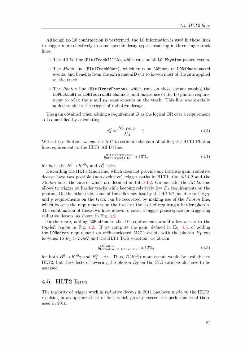
4.5. HLT2 lines
Although no L0 confirmation is performed, the L0 information is used in these linesto trigger more effectively in some specific decay types, resulting in three single tracklines:
The All L0 line (Hlt1TrackAllL0), which runs on all L0 Physics-passed events.
The Muon line (Hlt1TrackMuon), which runs on L0Muon- or L0DiMuon-passedevents, and benefits from the extra muonID cut to loosen most of the cuts appliedon the track.
The Photon line (Hlt1TrackPhoton), which runs on those events passing theL0PhotonHi or L0ElectronHi channels, and makes use of the L0 photon require-ment to relax the p and pT requirements on the track. This line was speciallyadded to aid in the trigger of radiative decays.
The gain obtained when adding a requirement B as the logical OR over a requirementA is quantified by calculating
gBA =NA OR B
NA− 1. (4.3)
With this definition, we can use MC to estimate the gain of adding the HLT1 Photonline requirement to the HLT1 All L0 line,
gHlt1TrackPhotonHlt1TrackAllL0 ≈ 13%, (4.4)
for both the B0→K∗0γ and B0s →ϕγ.
Discarding the HLT1 Muon line, which does not provide any intrinsic gain, radiativedecays have two possible (non-exclusive) trigger paths in HLT1, the All L0 and thePhoton lines, the cuts of which are detailed in Table 4.2. On one side, the All L0 lineallows to trigger on harder tracks while keeping relatively low ET requirements on thephoton. On the other side, some of the efficiency lost by the All L0 line due to the pTand p requirements on the track can be recovered by making use of the Photon line,which loosens the requirements on the track at the cost of requiring a harder photon.The combination of these two lines allows to cover a bigger phase space for triggeringradiative decays, as shown in Fig. 4.2.
Furthermore, adding L0Hadron to the L0 requirements would allow access to thetop-left region in Fig. 4.2. If we compute the gain, defined in Eq. 4.3, of addingthe L0Hadron requirement on offline-selected MC11 events with the photon ET cutloosened to ET > 2GeV and the HLT1 TOS selection, we obtain
gL0HadronL0Photon OR L0Electron ≈ 12%, (4.5)
for both B0 →K∗0γ and B0s →ϕγ. Thus, O(10%) more events would be available to
HLT2, but the effects of lowering the photon ET on the S/B ratio would have to beassessed.
4.5. HLT2 lines
The majority of trigger work in radiative decays in 2011 has been made on the HLT2,resulting in an optimized set of lines which greatly exceed the performance of thoseused in 2010.
81

4. Trigger strategies for radiative B decays at LHCb
All L0 line Photon line
L0 channel L0 physics L0PhotonHi or L0ElectronHiImplicit photon ET (GeV) > 2.5 > 4.2
VELO track IP (µm) > 100 > 100VELO track hits > 9 > 9Missed VELO hits < 3 < 4Track p (GeV/c) > 10.0 > 6.0Track pT (GeV/c) > 1.7 > 1.2Track χ2 < 2 < 2Track IP χ2 > 16 > 16
Table 4.2. Cut values for the HLT1 single track lines relevant to radiative decays for2011. The implicit photon ET cut corresponds to the photon cut in the L0channels on which the given HLT1 line runs.
210
310
(GeV)T
Eγ2.5 3 3.5 4 4.5 5 5.5 6
) (G
eV/c
)T
max
(tra
ck p
1
1.5
2
2.5
3
3.5
4
4.5
5
5.5
All L0 Line
Photon Line
(a) B0→K∗0γ.
210
(GeV)T
Eγ2.5 3 3.5 4 4.5 5 5.5 6
) (G
eV/c
)T
max
(tra
ck p
1
1.5
2
2.5
3
3.5
4
4.5
5
5.5
All L0 Line
Photon Line
(b) B0s →ϕγ.
Figure 4.2. Distribution of the maximum pT of the vector meson daughter versus thephoton ET on MC11 offline-selected events (the track pT and photon ET
cuts have not been included) for B0→K∗0γ (left) and B0s →ϕγ (right). Su-
perimposed, the pT-ET cuts of the HLT1 All L0 single track line (solid line)and the Photon single track line (dotted line), combined with the implicitL0 photon cuts.
On one side, the HLT2 exclusive lines used in 2010 were optimized from their originalversion in order to improve their signal selection efficiency. On the other side, aninclusive approach has been tested by studying a set of already existing lines, the HLT2Topological trigger, by introducing a new set of lines, the HLT2 Radiative Topologicaltrigger, and by improving the useful inclusive ϕ line. Furthermore, a new procedure forreconstruction of the calorimeter in the HLT2 has been developed in order to diminishthe timing problems of those lines that make use of photons.
82
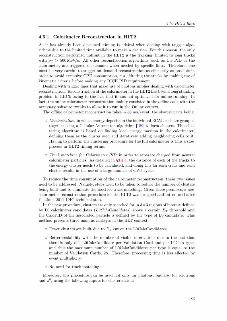
4.5. HLT2 lines
4.5.1. Calorimeter Reconstruction in HLT2
As it has already been discussed, timing is critical when dealing with trigger algo-rithms due to the limited time available to make a decision. For this reason, the onlyreconstruction performed upfront in the HLT2 is the tracking, limited to long trackswith pT > 500MeV/c. All other reconstruction algorithms, such as the PID or thecalorimeter, are triggered on demand when needed by specific lines. Therefore, onemust be very careful to trigger on-demand reconstruction as efficiently as possible inorder to avoid excessive CPU consumption, e.g., filtering the tracks by making use ofkinematic criteria before making any RICH PID requirement.
Dealing with trigger lines that make use of photons implies dealing with calorimeterreconstruction. Reconstruction of the calorimeter in the HLT2 has been a long standingproblem in LHCb owing to the fact that it was not optimized for online running. Infact, the online calorimeter reconstruction mainly consisted in the offline code with thenecessary software tweaks to allow it to run in the Online context.
The offline calorimeter reconstruction takes ∼ 56 ms/event, the slowest parts being:
Clusterization, in which energy deposits in the individual ECAL cells are groupedtogether using a Cellular Automaton algorithm [159] to form clusters. This clus-tering algorithm is based on finding local energy maxima in the calorimeter,defining them as the cluster seed and iteratively adding neighboring cells to it.Having to perform the clustering procedure for the full calorimeter is thus a slowprocess in HLT2 timing terms.
Track matching for Calorimeter PID, in order to separate charged from neutralcalorimeter particles. As detailed in §3.4.4, the distance of each of the tracks tothe energy cluster needs to be calculated, and doing this for each track and eachcluster results in the use of a large number of CPU cycles.
To reduce the time consumption of the calorimeter reconstruction, these two issuesneed to be addressed. Namely, steps need to be taken to reduce the number of clustersbeing built and to eliminate the need for track matching. Given these premises, a newcalorimeter reconstruction procedure for the HLT2 was designed and introduced afterthe June 2011 LHC technical stop.
In the new procedure, clusters are only searched for in 3×3 regions of interest definedby L0 calorimeter candidates (L0CaloCandidates) above a certain ET threshold andthe CaloPID of the associated particle is defined by the type of L0 candidate. Thismethod presents three main advantages in the HLT context:
Fewer clusters are built due to ET cut on the L0CaloCandidates.
Better scalability with the number of visible interactions due to the fact thatthere is only one L0CaloCandidate per Validation Card and per L0Calo type,and thus the maximum number of L0CaloCandidates per type is equal to thenumber of Validation Cards, 28. Therefore, processing time is less affected byevent multiplicity.
No need for track matching.
Moreover, this procedure can be used not only for photons, but also for electronsand π0, using the following inputs for clusterization:
83
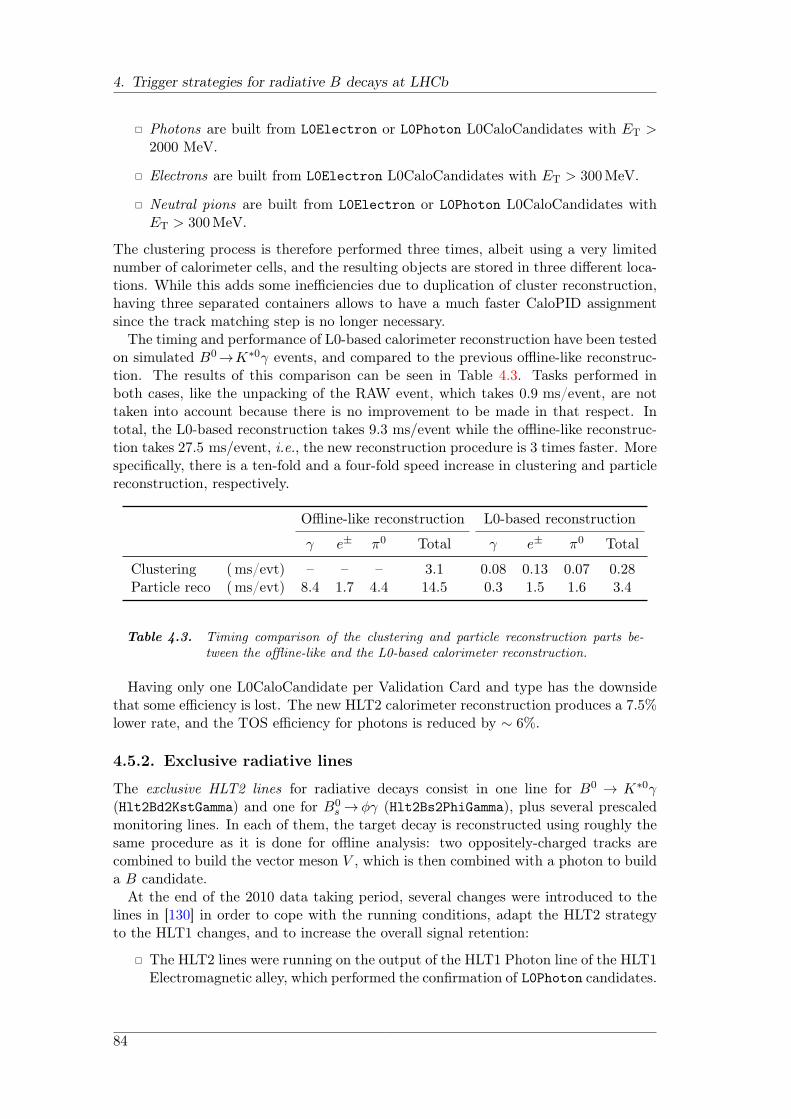
4. Trigger strategies for radiative B decays at LHCb
Photons are built from L0Electron or L0Photon L0CaloCandidates with ET >2000 MeV.
Electrons are built from L0Electron L0CaloCandidates with ET > 300MeV.
Neutral pions are built from L0Electron or L0Photon L0CaloCandidates withET > 300MeV.
The clustering process is therefore performed three times, albeit using a very limitednumber of calorimeter cells, and the resulting objects are stored in three different loca-tions. While this adds some inefficiencies due to duplication of cluster reconstruction,having three separated containers allows to have a much faster CaloPID assignmentsince the track matching step is no longer necessary.
The timing and performance of L0-based calorimeter reconstruction have been testedon simulated B0→K∗0γ events, and compared to the previous offline-like reconstruc-tion. The results of this comparison can be seen in Table 4.3. Tasks performed inboth cases, like the unpacking of the RAW event, which takes 0.9 ms/event, are nottaken into account because there is no improvement to be made in that respect. Intotal, the L0-based reconstruction takes 9.3 ms/event while the offline-like reconstruc-tion takes 27.5 ms/event, i.e., the new reconstruction procedure is 3 times faster. Morespecifically, there is a ten-fold and a four-fold speed increase in clustering and particlereconstruction, respectively.
Offline-like reconstruction L0-based reconstruction
γ e± π0 Total γ e± π0 Total
Clustering (ms/evt) – – – 3.1 0.08 0.13 0.07 0.28Particle reco (ms/evt) 8.4 1.7 4.4 14.5 0.3 1.5 1.6 3.4
Table 4.3. Timing comparison of the clustering and particle reconstruction parts be-tween the offline-like and the L0-based calorimeter reconstruction.
Having only one L0CaloCandidate per Validation Card and type has the downsidethat some efficiency is lost. The new HLT2 calorimeter reconstruction produces a 7.5%lower rate, and the TOS efficiency for photons is reduced by ∼ 6%.
4.5.2. Exclusive radiative lines
The exclusive HLT2 lines for radiative decays consist in one line for B0 → K∗0γ(Hlt2Bd2KstGamma) and one for B0
s → ϕγ (Hlt2Bs2PhiGamma), plus several prescaledmonitoring lines. In each of them, the target decay is reconstructed using roughly thesame procedure as it is done for offline analysis: two oppositely-charged tracks arecombined to build the vector meson V , which is then combined with a photon to builda B candidate.
At the end of the 2010 data taking period, several changes were introduced to thelines in [130] in order to cope with the running conditions, adapt the HLT2 strategyto the HLT1 changes, and to increase the overall signal retention:
The HLT2 lines were running on the output of the HLT1 Photon line of the HLT1Electromagnetic alley, which performed the confirmation of L0Photon candidates.
84

4.5. HLT2 lines
Therefore, following the ideas discussed in §4.3, to increase the global triggerefficiency of radiative decays events coming from the L0Electron channel werebeen included in the trigger path. Thus, events entering the HLT2 radiativeexclusive lines are required to have fired either L0Photon or L0Electron.
The replacement of the HLT1 alleys, including the Electromagnetic alley, bythe single track lines, triggered the removal of the explicit dependence on anyHLT1 lines, leaving only a requirement that events should have been triggerby any HLT1 physics line. As can be seen in Fig. 4.2, explicitly requiring thesingle track trigger removes a sizeable amount of events that would otherwise beselected offline. Therefore, removing the HLT1 single track requirement from theHLT2 lines allows to select more signal events, even if they are TIS; this helps inthose analyses that don’t require any knowledge of the trigger efficiency, such asthe CP asymmetry for B0→K∗0γ.
The HLT2 lines were completely rewritten before the 2011 run, adding a cut inthe quality of both charged tracks and improving their speed by applying thecuts in the correct order —fastest, more discriminant, first. The value of the Bcandidate IP χ2, K∗0 mass window and V vertex χ2 cuts were relaxed, adaptingto the experience with 2010 data. The final cuts used to filter the candidates,looser than their offline counterparts, are summarized in Table 4.4.
The use of the new calorimeter reconstruction was adopted after the June tech-nical stop, greatly improving the timing budget of these lines.
The changes in the L0 and HLT1 dependency, combined with the optimized code,result in half the execution time, approximately one third of the rate and double theefficiency with respect to 2010.
In addition, the monitoring lines for B0→K∗0γ and B0s →ϕγ were optimized in order
to help in the estimation of possible biases produced by the trigger cuts, prescaled to1/20 and 1/10, respectively:
Wide B and B0s invariant mass window lines, Hlt2Bd2KstGammaWideBMass and
Hlt2Bs2PhiGammaWideBMass, which can be used for checking for the appearanceof structures in the background mass distribution.
A wide K∗0 invariant mass window line, Hlt2Bd2KstGammaWideKMass, to see thefull line shape of the resonance, since the mass window cut in the non-prescaledline must be kept tight, at twice the natural width of the K∗0, to keep the rateunder control. The analogous line for the ϕ is not necessary, because its narrowwidth allows to have a wide cut of 5σ while keeping a reasonable rate.
The efficiency of these improved exclusive lines on simulated data is shown in Ta-ble 4.5. The table showcases that the exclusive lines are very effective in selecting thoseevents for which they were designed, particularly when taking into account that theseefficiencies include a 6% loss of efficiency due to the new HLT2 calorimeter reconstruc-tion. Furthermore, it can be seen that the B+ → ϕK+γ and B+ →K∗0π+γ decayshave a fairly high TOS efficiency with the exclusive line that contains the same vectormeson, mainly due to the loose IP and DIRA cuts on the B candidate.
85
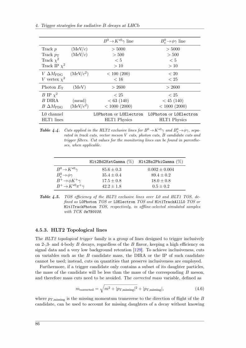
4. Trigger strategies for radiative B decays at LHCb
B0→K∗0γ line B0s →ϕγ line
Track p (MeV/c) > 5000 > 5000Track pT (MeV/c) > 500 > 500Track χ2 < 5 < 5Track IP χ2 > 10 > 10
V ∆MPDG (MeV/c2) < 100 (200) < 20V vertex χ2 < 16 < 25
Photon ET (MeV) > 2600 > 2600
B IP χ2 < 25 < 25B DIRA (mrad) < 63 (140) < 45 (140)B ∆MPDG (MeV/c2) < 1000 (2000) < 1000 (2000)
L0 channel L0Photon or L0Electron L0Photon or L0ElectronHLT1 lines HLT1 Physics HLT1 Physics
Table 4.4. Cuts applied in the HLT2 exclusive lines for B0→K∗0γ and B0s →ϕγ, sepa-
rated in track cuts, vector meson V cuts, photon cuts, B candidate cuts andtrigger filters. Cut values for the monitoring lines can be found in parenthe-ses, when applicable.
Hlt2Bd2KstGamma (%) Hlt2Bs2PhiGamma (%)
B0→K∗0γ 85.6± 0.3 0.002± 0.004B0
s →ϕγ 35.4± 0.4 89.4± 0.2B+→ϕK+γ 17.5± 0.8 18.0± 0.8B+→K∗0π+γ 42.2± 1.8 0.5± 0.2
Table 4.5. TOS efficiency of the HLT2 exclusive lines over L0 and HLT1 TOS, de-fined as L0Photon TOS or L0Electron TOS and Hlt1TrackAllL0 TOS orHlt1TrackPhoton TOS, respectively, in offline-selected simulated sampleswith TCK 0x790038.
4.5.3. HLT2 Topological lines
The HLT2 topological trigger family is a group of lines designed to trigger inclusivelyon 2-,3- and 4-body B decays, regardless of the B flavor, keeping a high efficiency onsignal data and a very low background retention [129]. To achieve inclusiveness, cutson variables such as the B candidate mass, the DIRA or the IP of such candidatecannot be used; instead, cuts on quantities that preserve inclusiveness are employed.
Furthermore, if a trigger candidate only contains a subset of its daughter particles,the mass of the candidate will be less than the mass of the corresponding B meson,and therefore mass cuts need to be avoided. The corrected mass variable, defined as
mcorrected =√m2 + |pT,missing|2 + |pT,missing|, (4.6)
where pT,missing is the missing momentum transverse to the direction of flight of the Bcandidate, can be used to account for missing daughters of a decay without knowing
86
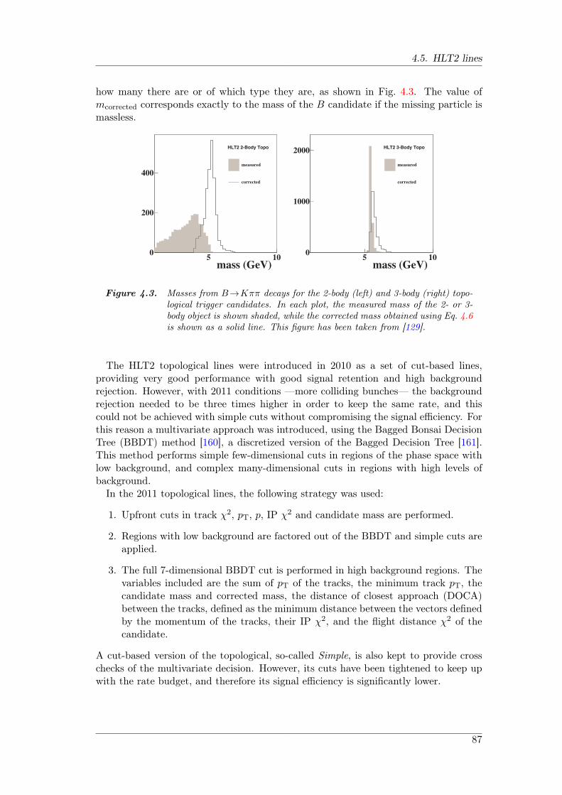
4.5. HLT2 lines
how many there are or of which type they are, as shown in Fig. 4.3. The value ofmcorrected corresponds exactly to the mass of the B candidate if the missing particle ismassless.
mass (GeV) 5 10
0
200
400
HLT2 2-Body Topo
measured
corrected
mass (GeV) 5 10
0
1000
2000HLT2 3-Body Topo
measured
corrected
Figure 4.3. Masses from B→Kππ decays for the 2-body (left) and 3-body (right) topo-logical trigger candidates. In each plot, the measured mass of the 2- or 3-body object is shown shaded, while the corrected mass obtained using Eq. 4.6is shown as a solid line. This figure has been taken from [129].
The HLT2 topological lines were introduced in 2010 as a set of cut-based lines,providing very good performance with good signal retention and high backgroundrejection. However, with 2011 conditions —more colliding bunches— the backgroundrejection needed to be three times higher in order to keep the same rate, and thiscould not be achieved with simple cuts without compromising the signal efficiency. Forthis reason a multivariate approach was introduced, using the Bagged Bonsai DecisionTree (BBDT) method [160], a discretized version of the Bagged Decision Tree [161].This method performs simple few-dimensional cuts in regions of the phase space withlow background, and complex many-dimensional cuts in regions with high levels ofbackground.
In the 2011 topological lines, the following strategy was used:
1. Upfront cuts in track χ2, pT, p, IP χ2 and candidate mass are performed.
2. Regions with low background are factored out of the BBDT and simple cuts areapplied.
3. The full 7-dimensional BBDT cut is performed in high background regions. Thevariables included are the sum of pT of the tracks, the minimum track pT, thecandidate mass and corrected mass, the distance of closest approach (DOCA)between the tracks, defined as the minimum distance between the vectors definedby the momentum of the tracks, their IP χ2, and the flight distance χ2 of thecandidate.
A cut-based version of the topological, so-called Simple, is also kept to provide crosschecks of the multivariate decision. However, its cuts have been tightened to keep upwith the rate budget, and therefore its signal efficiency is significantly lower.
87
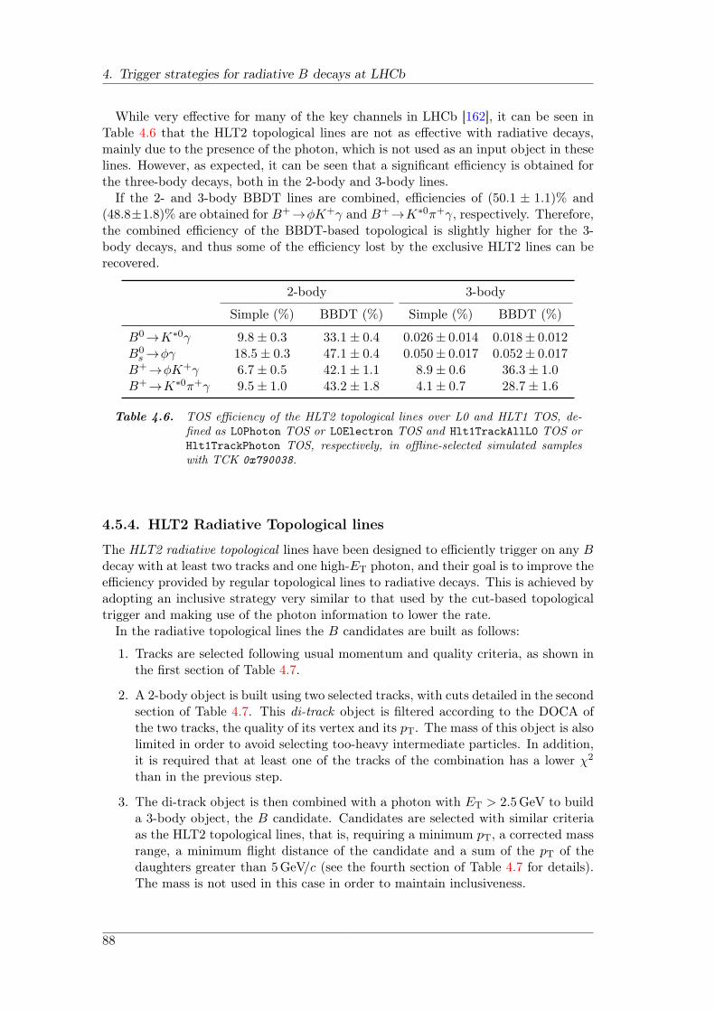
4. Trigger strategies for radiative B decays at LHCb
While very effective for many of the key channels in LHCb [162], it can be seen inTable 4.6 that the HLT2 topological lines are not as effective with radiative decays,mainly due to the presence of the photon, which is not used as an input object in theselines. However, as expected, it can be seen that a significant efficiency is obtained forthe three-body decays, both in the 2-body and 3-body lines.
If the 2- and 3-body BBDT lines are combined, efficiencies of (50.1 ± 1.1)% and(48.8±1.8)% are obtained for B+→ϕK+γ and B+→K∗0π+γ, respectively. Therefore,the combined efficiency of the BBDT-based topological is slightly higher for the 3-body decays, and thus some of the efficiency lost by the exclusive HLT2 lines can berecovered.
2-body 3-body
Simple (%) BBDT (%) Simple (%) BBDT (%)
B0→K∗0γ 9.8± 0.3 33.1± 0.4 0.026± 0.014 0.018± 0.012B0
s →ϕγ 18.5± 0.3 47.1± 0.4 0.050± 0.017 0.052± 0.017B+→ϕK+γ 6.7± 0.5 42.1± 1.1 8.9± 0.6 36.3± 1.0B+→K∗0π+γ 9.5± 1.0 43.2± 1.8 4.1± 0.7 28.7± 1.6
Table 4.6. TOS efficiency of the HLT2 topological lines over L0 and HLT1 TOS, de-fined as L0Photon TOS or L0Electron TOS and Hlt1TrackAllL0 TOS orHlt1TrackPhoton TOS, respectively, in offline-selected simulated sampleswith TCK 0x790038.
4.5.4. HLT2 Radiative Topological lines
The HLT2 radiative topological lines have been designed to efficiently trigger on any Bdecay with at least two tracks and one high-ET photon, and their goal is to improve theefficiency provided by regular topological lines to radiative decays. This is achieved byadopting an inclusive strategy very similar to that used by the cut-based topologicaltrigger and making use of the photon information to lower the rate.
In the radiative topological lines the B candidates are built as follows:
1. Tracks are selected following usual momentum and quality criteria, as shown inthe first section of Table 4.7.
2. A 2-body object is built using two selected tracks, with cuts detailed in the secondsection of Table 4.7. This di-track object is filtered according to the DOCA ofthe two tracks, the quality of its vertex and its pT. The mass of this object is alsolimited in order to avoid selecting too-heavy intermediate particles. In addition,it is required that at least one of the tracks of the combination has a lower χ2
than in the previous step.
3. The di-track object is then combined with a photon with ET > 2.5GeV to builda 3-body object, the B candidate. Candidates are selected with similar criteriaas the HLT2 topological lines, that is, requiring a minimum pT, a corrected massrange, a minimum flight distance of the candidate and a sum of the pT of thedaughters greater than 5GeV/c (see the fourth section of Table 4.7 for details).The mass is not used in this case in order to maintain inclusiveness.
88

4.5. HLT2 lines
Track p (MeV/c) > 5000Track pT (MeV/c) > 700Track χ2 < 5Track IP χ2 > 10
Min track χ2 < 3Di-track DOCA (mm) < 0.15Di-track vertex χ2 < 10Di-track mass (MeV/c2) < 2000Di-track pT (MeV/c) > 1500
Photon ET (MeV) > 2500
Candidate pT (MeV/c) > 1000Candidate mcorrected (MeV/c2) > 4000, < 7000Candidate FD χ2 > 64Daughters Σ pT (MeV/c) > 5000
# of forward tracks with pT > 500MeV/c < 120
Table 4.7. Selection criteria for the HLT2 radiative topological lines, divided in sections.The first section details the cuts on input tracks, the second the di-track com-bination cuts, the third the photon cuts, the fourth cuts on the B candidateand the last one is the GEC.
In addition, a Global Event Cut (GEC) on the track multiplicity is applied in order toreject events with a high level of background.
Furthermore, in order to achieve robustness under possible changes of the L0 trigger,two different radiative topological lines, with different L0 and HLT1 requirements, havebeen introduced:
L0 photon line (Hlt2RadiativeTopoPhotonL0): this line runs on those eventsthat have passed either the L0Photon or the L0Electron lines, and any HLT1physics line. The requirements are similar in this case to the exclusive lines, butthe efficiency of the line is highly dependent on the L0Photon and L0Electron
threshold, i.e., a higher cut on the ET would imply a sizeble loss of efficiency.
HLT1 Track TOS line (Hlt2RadiativeTopoTrackTOS): this line requires theevent to pass one of the HLT1 Track lines and requires that one of the usedtracks was actually responsible for firing the HLT1 track trigger —this is the so-called TOS track filter. Thus, this line allows to recover those events that haven’tbeen triggered on the photon by triggering on one of the daughter particles of the2-body object. It is thought of as backup of the L0 photon line in the event thatthe L0 thresholds were to be increased, but it will also be useful in the scenariowhere the photon ET requirement of the radiative selections is lowered and theL0Hadron is added to the current TOS selection.
To assess the effect of the HLT1 Track TOS line, trigger efficiencies with SPD multi-plicity < 600 and thresholds of L0Photon and L0Electron set at 4.2GeV —a possiblescenario for a high luminosity TCK— have been considered. The effect of increasing
89

4. Trigger strategies for radiative B decays at LHCb
the threshold of L0Photon and L0Electron is a ∼ 30% efficiency drop in the exclusivelines —and similarly in the radiative L0 Photon TOS line. In this case, the HLT1Track TOS line only loses ∼ 10% of its efficiency thanks to the L0Hadron channel.
As explained previously, the HLT2 topological lines used in the 2011 data takingperiod include a multivariate-based selection (BBDT) that allows to achieve a veryhigh efficiency on signal while rejecting most of the background. At the end of the2011 data taking period, two extra lines for radiative decays have been incorporatedto the topological trigger to benefit from this multivariate technique:
A 2-body BBDT line (Hlt2TopoRad2BodyBBDT) which runs on the output ofL0Photon and L0Electron. This line builds the 2-body object from a track anda photon, and therefore cuts need to be very tight in order to reject combinatorics.
A 3-body BBDT line (Hlt2TopoRad2plus1BodyBBDT) in which one of the bodiesis forced to be a photon; it is therefore a 2 track plus one photon line. This linebenefits from the presence of the photon, which allows to loosen the BBDT cutwhile keeping a reasonable rate.
Both lines apply a TOS track filter.The efficiency of the HLT2 radiative topological lines has been assessed on MC
simulation and documented in Table 4.8. In it we can see that, in general, the BBDT-based lines outperform the cut-based lines, specially in the case of B0 → K∗0γ andB0
s → ϕγ. When comparing to other HLT2 lines, the radiative topological providesefficiencies only slightly lower than the exclusive lines for B0→K∗0γ and B0
s →ϕγ, butthe improvement with respect to the regular topological lines ranges is approximatelytwo-fold.
Cut-based (%) BBDT-based (%)
B0→K∗0γ 75.6± 0.4 80.5± 0.4B0
s →ϕγ 77.3± 0.3 84.4± 0.3B+→ϕK+γ 90.0± 0.6 91.4± 0.6B+→K∗0π+γ 89.3± 1.1 91.5± 1.0
Table 4.8. TOS efficiency of the cut- and BBDT-based HLT2 radiative topological linesover L0 and HLT1 TOS, defined as L0Photon TOS or L0Electron TOS andHlt1TrackAllL0 TOS or Hlt1TrackPhoton TOS, respectively, in offline-selected simulated samples.
A detail on the individual performance of the BBDT-based lines is shown in Ta-ble 4.9. The 2-body radiative line, which uses one track and one photon as input, doesnot add any significant efficiency, and thus its removal should be considered.
4.5.5. Inclusive ϕ line
The inclusive ϕ trigger provides a robust and transversal trigger for radiative decaysinvolving ϕ vector mesons, such as B0
s →ϕγ and B+→ϕK+γ. It looks for detached ϕmesons built from pairs of oppositely charged tracks identified as kaons by making useof RICH information.
90
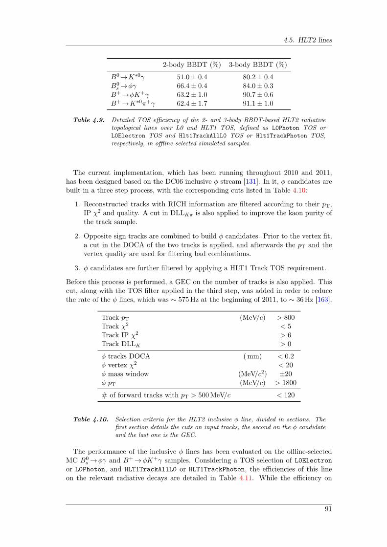
4.5. HLT2 lines
2-body BBDT (%) 3-body BBDT (%)
B0→K∗0γ 51.0± 0.4 80.2± 0.4B0
s →ϕγ 66.4± 0.4 84.0± 0.3B+→ϕK+γ 63.2± 1.0 90.7± 0.6B+→K∗0π+γ 62.4± 1.7 91.1± 1.0
Table 4.9. Detailed TOS efficiency of the 2- and 3-body BBDT-based HLT2 radiativetopological lines over L0 and HLT1 TOS, defined as L0Photon TOS orL0Electron TOS and Hlt1TrackAllL0 TOS or Hlt1TrackPhoton TOS,respectively, in offline-selected simulated samples.
The current implementation, which has been running throughout 2010 and 2011,has been designed based on the DC06 inclusive ϕ stream [131]. In it, ϕ candidates arebuilt in a three step process, with the corresponding cuts listed in Table 4.10:
1. Reconstructed tracks with RICH information are filtered according to their pT,IP χ2 and quality. A cut in DLLKπ is also applied to improve the kaon purity ofthe track sample.
2. Opposite sign tracks are combined to build ϕ candidates. Prior to the vertex fit,a cut in the DOCA of the two tracks is applied, and afterwards the pT and thevertex quality are used for filtering bad combinations.
3. ϕ candidates are further filtered by applying a HLT1 Track TOS requirement.
Before this process is performed, a GEC on the number of tracks is also applied. Thiscut, along with the TOS filter applied in the third step, was added in order to reducethe rate of the ϕ lines, which was ∼ 575Hz at the beginning of 2011, to ∼ 36Hz [163].
Track pT (MeV/c) > 800Track χ2 < 5Track IP χ2 > 6Track DLLK > 0
ϕ tracks DOCA (mm) < 0.2ϕ vertex χ2 < 20ϕ mass window (MeV/c2) ±20ϕ pT (MeV/c) > 1800
# of forward tracks with pT > 500MeV/c < 120
Table 4.10. Selection criteria for the HLT2 inclusive ϕ line, divided in sections. Thefirst section details the cuts on input tracks, the second on the ϕ candidateand the last one is the GEC.
The performance of the inclusive ϕ lines has been evaluated on the offline-selectedMC B0
s →ϕγ and B+→ϕK+γ samples. Considering a TOS selection of L0Electron
or L0Photon, and HLT1TrackAllL0 or HLT1TrackPhoton, the efficiencies of this lineon the relevant radiative decays are detailed in Table 4.11. While the efficiency on
91
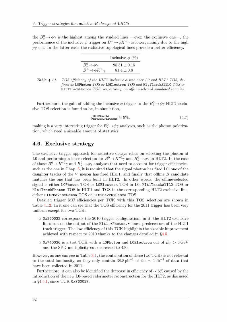
4. Trigger strategies for radiative B decays at LHCb
the B0s → ϕγ is the highest among the studied lines —even the exclusive one—, the
performance of the inclusive ϕ trigger on B+→ϕK+γ is lower, mainly due to the highpT cut. In the latter case, the radiative topological lines provide a better efficiency.
Inclusive ϕ (%)
B0s →ϕγ 95.51± 0.15
B+→ϕK+γ 81.4± 0.8
Table 4.11. TOS efficiency of the HLT2 inclusive ϕ line over L0 and HLT1 TOS, de-fined as L0Photon TOS or L0Electron TOS and Hlt1TrackAllL0 TOS orHlt1TrackPhoton TOS, respectively, on offline-selected simulated samples.
Furthermore, the gain of adding the inclusive ϕ trigger to the B0s →ϕγ HLT2 exclu-
sive TOS selection is found to be, in simulation,
gHlt2IncPhiHlt2Bs2PhiGamma ≈ 9%, (4.7)
making it a very interesting trigger for B0s →ϕγ analyses, such as the photon polariza-
tion, which need a sizeable amount of statistics.
4.6. Exclusive strategy
The exclusive trigger approach for radiative decays relies on selecting the photon atL0 and performing a loose selection for B0→K∗0γ and B0
s →ϕγ in HLT2. In the caseof those B0→K∗0γ and B0
s →ϕγ analyses that need to account for trigger efficiencies,such as the one in Chap. 5, it is required that the signal photon has fired L0, one of thedaughter tracks of the V meson has fired HLT1, and finally that offline B candidatematches the one that has been built in HLT2. In other words, the offline-selectedsignal is either L0Photon TOS or L0Electron TOS in L0, Hlt1TrackAllL0 TOS orHlt1TrackPhoton TOS in HLT1 and TOS in the corresponding HLT2 exclusive line,either Hlt2Bd2KstGamma TOS or Hlt2Bs2PhiGamma TOS.
Detailed trigger MC efficiencies per TCK with this TOS selection are shown inTable 4.12. In it one can see that the TOS efficiency for the 2011 trigger has been veryuniform except for two TCKs:
0x360032 corresponds the 2010 trigger configuration: in it, the HLT2 exclusivelines run on the output of the Hlt1.*Photon.* lines, predecessors of the HLT1track trigger. The low efficiency of this TCK highlights the sizeable improvementachieved with respect to 2010 thanks to the changes detailed in §4.5.
0x740036 is a test TCK with a L0Photon and L0Electron cut of ET > 3GeVand the SPD multiplicity cut decreased to 450.
However, as one can see in Table 3.1, the contribution of these two TCKs is not relevantto the total luminosity, as they only contain 38.8pb−1 of the ∼ 1 fb−1 of data thathave been collected in 2011.
Furthermore, it can also be identified the decrease in efficiency of ∼ 6% caused by theintroduction of the new L0-based calorimeter reconstruction for the HLT2, as discussedin §4.5.1, since TCK 0x760037.
92
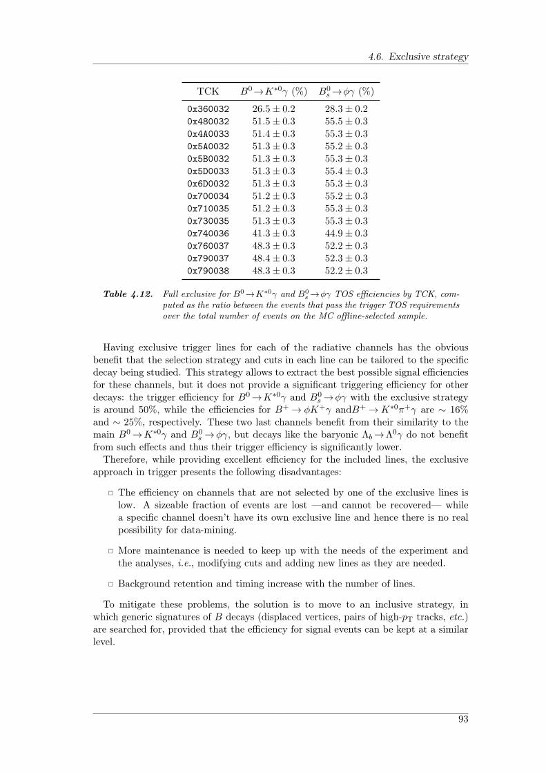
4.6. Exclusive strategy
TCK B0→K∗0γ (%) B0s →ϕγ (%)
0x360032 26.5± 0.2 28.3± 0.20x480032 51.5± 0.3 55.5± 0.30x4A0033 51.4± 0.3 55.3± 0.30x5A0032 51.3± 0.3 55.2± 0.30x5B0032 51.3± 0.3 55.3± 0.30x5D0033 51.3± 0.3 55.4± 0.30x6D0032 51.3± 0.3 55.3± 0.30x700034 51.2± 0.3 55.2± 0.30x710035 51.2± 0.3 55.3± 0.30x730035 51.3± 0.3 55.3± 0.30x740036 41.3± 0.3 44.9± 0.30x760037 48.3± 0.3 52.2± 0.30x790037 48.4± 0.3 52.3± 0.30x790038 48.3± 0.3 52.2± 0.3
Table 4.12. Full exclusive for B0→K∗0γ and B0s →ϕγ TOS efficiencies by TCK, com-
puted as the ratio between the events that pass the trigger TOS requirementsover the total number of events on the MC offline-selected sample.
Having exclusive trigger lines for each of the radiative channels has the obviousbenefit that the selection strategy and cuts in each line can be tailored to the specificdecay being studied. This strategy allows to extract the best possible signal efficienciesfor these channels, but it does not provide a significant triggering efficiency for otherdecays: the trigger efficiency for B0→K∗0γ and B0
s →ϕγ with the exclusive strategyis around 50%, while the efficiencies for B+ → ϕK+γ andB+ →K∗0π+γ are ∼ 16%and ∼ 25%, respectively. These two last channels benefit from their similarity to themain B0→K∗0γ and B0
s →ϕγ, but decays like the baryonic Λb→Λ0γ do not benefitfrom such effects and thus their trigger efficiency is significantly lower.
Therefore, while providing excellent efficiency for the included lines, the exclusiveapproach in trigger presents the following disadvantages:
The efficiency on channels that are not selected by one of the exclusive lines islow. A sizeable fraction of events are lost —and cannot be recovered— whilea specific channel doesn’t have its own exclusive line and hence there is no realpossibility for data-mining.
More maintenance is needed to keep up with the needs of the experiment andthe analyses, i.e., modifying cuts and adding new lines as they are needed.
Background retention and timing increase with the number of lines.
To mitigate these problems, the solution is to move to an inclusive strategy, inwhich generic signatures of B decays (displaced vertices, pairs of high-pT tracks, etc.)are searched for, provided that the efficiency for signal events can be kept at a similarlevel.
93
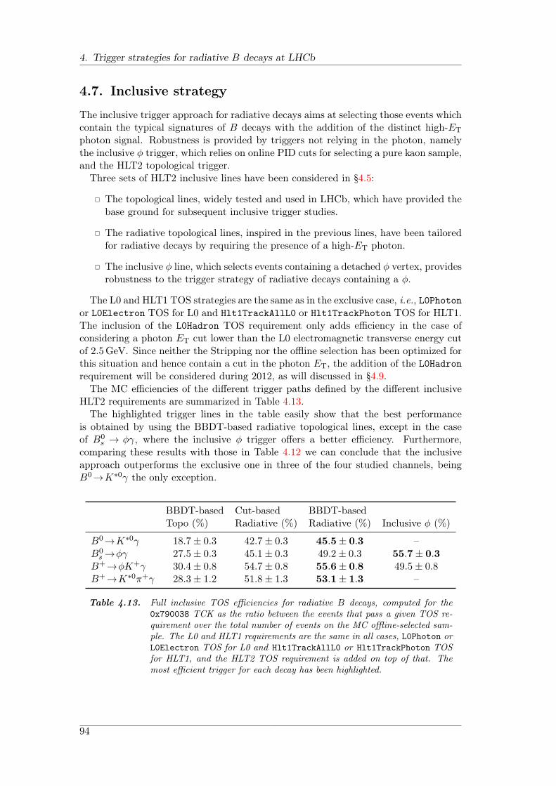
4. Trigger strategies for radiative B decays at LHCb
4.7. Inclusive strategy
The inclusive trigger approach for radiative decays aims at selecting those events whichcontain the typical signatures of B decays with the addition of the distinct high-ET
photon signal. Robustness is provided by triggers not relying in the photon, namelythe inclusive ϕ trigger, which relies on online PID cuts for selecting a pure kaon sample,and the HLT2 topological trigger.
Three sets of HLT2 inclusive lines have been considered in §4.5:
The topological lines, widely tested and used in LHCb, which have provided thebase ground for subsequent inclusive trigger studies.
The radiative topological lines, inspired in the previous lines, have been tailoredfor radiative decays by requiring the presence of a high-ET photon.
The inclusive ϕ line, which selects events containing a detached ϕ vertex, providesrobustness to the trigger strategy of radiative decays containing a ϕ.
The L0 and HLT1 TOS strategies are the same as in the exclusive case, i.e., L0Photonor L0Electron TOS for L0 and Hlt1TrackAllL0 or Hlt1TrackPhoton TOS for HLT1.The inclusion of the L0Hadron TOS requirement only adds efficiency in the case ofconsidering a photon ET cut lower than the L0 electromagnetic transverse energy cutof 2.5GeV. Since neither the Stripping nor the offline selection has been optimized forthis situation and hence contain a cut in the photon ET, the addition of the L0Hadron
requirement will be considered during 2012, as will discussed in §4.9.The MC efficiencies of the different trigger paths defined by the different inclusive
HLT2 requirements are summarized in Table 4.13.The highlighted trigger lines in the table easily show that the best performance
is obtained by using the BBDT-based radiative topological lines, except in the caseof B0
s → ϕγ, where the inclusive ϕ trigger offers a better efficiency. Furthermore,comparing these results with those in Table 4.12 we can conclude that the inclusiveapproach outperforms the exclusive one in three of the four studied channels, beingB0→K∗0γ the only exception.
BBDT-based Cut-based BBDT-basedTopo (%) Radiative (%) Radiative (%) Inclusive ϕ (%)
B0→K∗0γ 18.7± 0.3 42.7± 0.3 45.5± 0.3 –B0
s →ϕγ 27.5± 0.3 45.1± 0.3 49.2± 0.3 55.7± 0.3B+→ϕK+γ 30.4± 0.8 54.7± 0.8 55.6± 0.8 49.5± 0.8B+→K∗0π+γ 28.3± 1.2 51.8± 1.3 53.1± 1.3 –
Table 4.13. Full inclusive TOS efficiencies for radiative B decays, computed for the0x790038 TCK as the ratio between the events that pass a given TOS re-quirement over the total number of events on the MC offline-selected sam-ple. The L0 and HLT1 requirements are the same in all cases, L0Photon orL0Electron TOS for L0 and Hlt1TrackAllL0 or Hlt1TrackPhoton TOSfor HLT1, and the HLT2 TOS requirement is added on top of that. Themost efficient trigger for each decay has been highlighted.
94
4.8. Performance in 2011
However, the comparison between exclusive and inclusive approaches is still missingthe study of the background rejection for each line, i.e., the signal-over-backgroundratio, S/B. This last piece will be studied directly on data in the next section.
4.8. Performance in 2011
The performance of the trigger strategies defined in the previous sections has beenevaluated on Monte Carlo and using the 2011 data. Two aspects of the performance ofthe lines have been studied: the efficiency on offline-selected signal has been evaluatedon both data and Monte Carlo, and the event retention (rate) has been determined fromreal data, both running offline and by making use of the instantaneous rate monitorsin the Online System.
Performance for channels not included in the exclusive set of lines, such as B+ →ϕK+γ and B+→K∗0π+γ, will not be shown due to the lack of suitable Stripping linesin the Stripping17 configuration. At the time of writing, this deficiency has beensolved and they have been added to the Stripping17b configuration, but data havestill not been processed with it.
4.8.1. Efficiency
The TISTOS method detailed in §4.2 can be used to evaluate the TOS efficienciesof the different HLT2 lines on 2011 data. However, the real data sample contains amixture of signal and background events, which needs to be disentangled in order tocorrectly evaluate the signal TOS efficiency. The sPlot technique [164], a statisticaltool which can be used to unfold the different contributions of different sources to thedistribution of a data sample in a given variable, can be used to separate the signalfrom the background contribution.
However, applying the TIS criteria on the offline selected sample produces a sizeablereduction of the available statistics. Given the available statistics, the adopted TIScriteria are the most general possible, L0Global, Hlt1Global and Hlt2Global, mean-ing that an event will be considered TIS if there is at least one TIS decision in L0, onein HLT1 and one in HLT2.
In the case of B0 → K∗0γ, the size of the signal sample obtained with the sPlottechnique is reduced from 6106 events to 160 TIS events for the full 1.0 fb−1 of datarecorded in 2011; for B0
s → ϕγ, the number of TIS events is 20, from a 781 eventsample. The low number of TIS events available for B0→K∗0γ and B0
s →ϕγ, 160 and20 events, respectively, greatly limits the possibilities of applying the TISTOS methodto extract the trigger efficiencies from data.
Exclusive lines
The global TOS efficiency for the B0→K∗0γ exclusive lines, calculated on TIS events,is found to be
ϵB0→K∗0γ
TOS = (57± 4)%, (4.8)
which is higher than the value found in simulation, shown in Table 4.12. The calculationof the TOS efficiency of the HLT2 B0→K∗0γ exclusive line on events passing the TIS
95
4. Trigger strategies for radiative B decays at LHCb
requirement and the L0 and HLT1 TOS requirement is found to be
ϵB0→K∗0γ
HLT2TOS = (84± 3)%, (4.9)
compatible with the value computed from MC, (85.6 ± 0.3)%, as shown in Table 4.5.The reason for the inconsistency in the global TOS efficiency can be traced to the L0TOS efficiency. In particular, of the L0 TOS efficiencies,
ϵB0→K∗0γ
L0PhotonTOS = (50± 4)% and ϵB0→K∗0γ
L0ElectronTOS = (42± 4)%, (4.10)
the L0Electron channel shows a higher efficiency than anticipated from MC (seeFig. 4.1a).
Further insight can be gained without using the TISTOS method. The invariantmass distributions for offline-selected B0→K∗0γ and B0
s →ϕγ can be directly studiedand their respective yields extracted through unbinned maximum likelihood fits. Whilethis procedure doesn’t allow to calculate any absolute efficiency, it allows to assessthe relative efficiencies between the different trigger requirements by comparing theiryields and to determine their background rejection performance by comparing theirS/B ratios; this is precisely the type of information that is needed to shape the triggerstrategies for the future data taking. The invariant mass distributions will be describedby a Crystal Ball function for the signal (see §5.3 for a motivation and details for thisdistribution) and an exponential for the background.
Regarding the exclusive trigger strategy detailed in §4.6, one might wonder how muchis lost by applying the TOS requirement. For analyses that don’t need to account fortrigger efficiencies, dropping the L0 and HLT1 requirements may help to recover eventswith low-ET photons or low-pT tracks which have been triggered by the other B in theevent. However, this comes with a cost in terms of the background level. In the caseof offline-selected B0 →K∗0γ data, removing the TOS requirement produces a gainin signal yield of ∼ 15%, as can be seen in Fig. 4.4, but the S/B ratio is reduced by30%. In the case of B0
s →ϕγ, the presence of the inclusive ϕ trigger, with has a highefficiency, slightly accentuates the difference between no trigger requirement and theexclusive TOS requirement, which is ∼ 20% as shown in Fig. 4.5. However, removingthe exclusive TOS selection induces a 40% decrease in the S/B ratio.
Inclusive ϕ line
It is also worth it to compare the yield for B0s → ϕγ events with an exclusive TOS
requirement, in Fig. 4.5b, with what is obtained replacing the HLT2 requirement fora TOS requirement in the inclusive ϕ line, as shown in Fig. 4.6a. This comparisonshowcases the importance of a line like the inclusive ϕ, which is able to provide greatefficiency with a completely different —and somewhat transversal— triggering strategy,adding robustness to the B0
s → ϕγ selection. Even further, the inclusive ϕ triggerbenefits from adding the L0Hadron in the L0 TOS requirement, as shown in Fig. 4.6b,and would allow to lower the ET cut on the photon in the selection to recover someevents with high-pT ϕ daughters2.
2Unfortunately, the current Stripping for radiative decays contains a 2.5GeV cut in the photontransverse energy, and therefore it is not possible to study these kind of events.
96
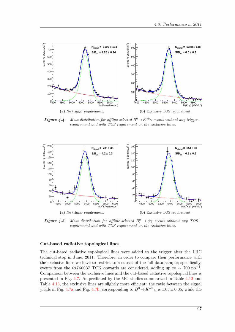
4.8. Performance in 2011
)2) (MeV/cγπM(K4600 4800 5000 5200 5400 5600 5800
)2E
vent
s / (
25
MeV
/c
0
100
200
300
400
500
600
700 0.14± = 4.26 σ2S/B
133± = 6106 signalN
(a) No trigger requirement.
)2) (MeV/cγπM(K4600 4800 5000 5200 5400 5600 5800
)2E
vent
s / (
25
MeV
/c
0
100
200
300
400
500
600
0.3± = 6.0 σ2S/B
138± = 5378 signalN
(b) Exclusive TOS requirement.
Figure 4.4. Mass distribution for offline-selected B0→K∗0γ events without any triggerrequirement and with TOS requirement on the exclusive lines.
)2) (MeV/cγ-K+M(K4800 5000 5200 5400 5600 5800 6000
)2E
vent
s / (
50
MeV
/c
0
20
40
60
80
100
120
140
160
180
200
0.3± = 4.2 σ2S/B
35± = 781 signalN
(a) No trigger requirement.
)2) (MeV/cγ-K+M(K4800 5000 5200 5400 5600 5800 6000
)2E
vent
s / (
50
MeV
/c
0
20
40
60
80
100
120
140
160
0.6± = 6.8 σ2S/B
30± = 651 signalN
(b) Exclusive TOS requirement.
Figure 4.5. Mass distribution for offline-selected B0s → ϕγ events without any TOS
requirement and with TOS requirement on the exclusive lines.
Cut-based radiative topological lines
The cut-based radiative topological lines were added to the trigger after the LHCtechnical stop in June, 2011. Therefore, in order to compare their performance withthe exclusive lines we have to restrict to a subset of the full data sample; specifically,events from the 0x760037 TCK onwards are considered, adding up to ∼ 700 pb−1.Comparison between the exclusive lines and the cut-based radiative topological lines ispresented in Fig. 4.7. As predicted by the MC studies summarized in Table 4.12 andTable 4.13, the exclusive lines are slightly more efficient: the ratio between the signalyields in Fig. 4.7a and Fig. 4.7b, corresponding to B0→K∗0γ, is 1.05± 0.05, while the
97
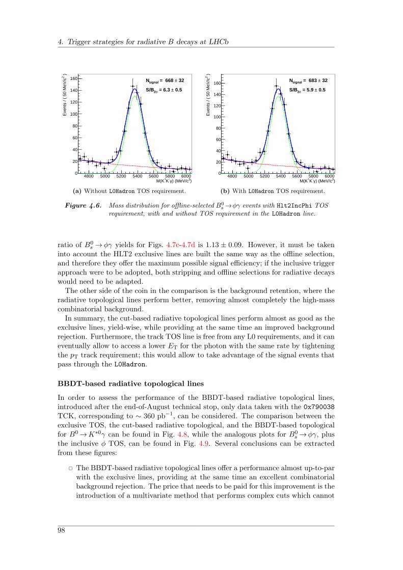
4. Trigger strategies for radiative B decays at LHCb
)2) (MeV/cγ-K+M(K4800 5000 5200 5400 5600 5800 6000
)2E
vent
s / (
50
MeV
/c
0
20
40
60
80
100
120
140
160
0.5± = 6.3 σ2S/B
32± = 668 signalN
(a) Without L0Hadron TOS requirement.
)2) (MeV/cγ-K+M(K4800 5000 5200 5400 5600 5800 6000
)2E
vent
s / (
50
MeV
/c
0
20
40
60
80
100
120
140
160
0.5± = 5.9 σ2S/B
32± = 683 signalN
(b) With L0Hadron TOS requirement.
Figure 4.6. Mass distribution for offline-selected B0s →ϕγ events with Hlt2IncPhi TOS
requirement, with and without TOS requirement in the L0Hadron line.
ratio of B0s → ϕγ yields for Figs. 4.7c-4.7d is 1.13 ± 0.09. However, it must be taken
into account the HLT2 exclusive lines are built the same way as the offline selection,and therefore they offer the maximum possible signal efficiency; if the inclusive triggerapproach were to be adopted, both stripping and offline selections for radiative decayswould need to be adapted.
The other side of the coin in the comparison is the background retention, where theradiative topological lines perform better, removing almost completely the high-masscombinatorial background.
In summary, the cut-based radiative topological lines perform almost as good as theexclusive lines, yield-wise, while providing at the same time an improved backgroundrejection. Furthermore, the track TOS line is free from any L0 requirements, and it caneventually allow to access a lower ET for the photon with the same rate by tighteningthe pT track requirement; this would allow to take advantage of the signal events thatpass through the L0Hadron.
BBDT-based radiative topological lines
In order to assess the performance of the BBDT-based radiative topological lines,introduced after the end-of-August technical stop, only data taken with the 0x790038
TCK, corresponding to ∼ 360 pb−1, can be considered. The comparison between theexclusive TOS, the cut-based radiative topological, and the BBDT-based topologicalfor B0 →K∗0γ can be found in Fig. 4.8, while the analogous plots for B0
s →ϕγ, plusthe inclusive ϕ TOS, can be found in Fig. 4.9. Several conclusions can be extractedfrom these figures:
The BBDT-based radiative topological lines offer a performance almost up-to-parwith the exclusive lines, providing at the same time an excellent combinatorialbackground rejection. The price that needs to be paid for this improvement is theintroduction of a multivariate method that performs complex cuts which cannot
98
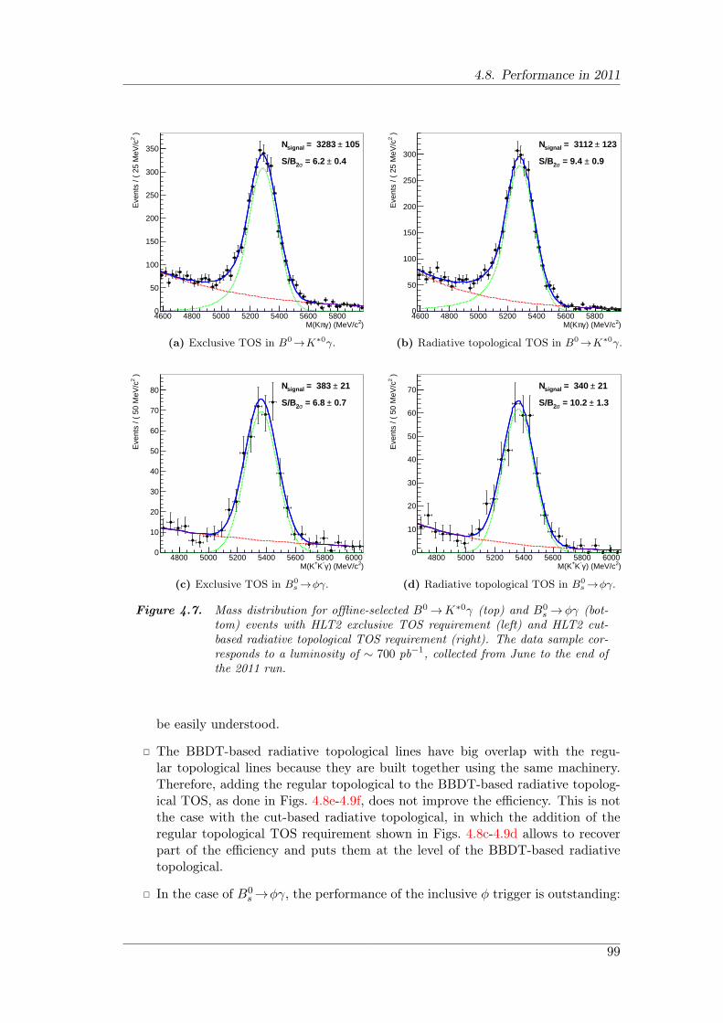
4.8. Performance in 2011
)2) (MeV/cγπM(K4600 4800 5000 5200 5400 5600 5800
)2E
vent
s / (
25
MeV
/c
0
50
100
150
200
250
300
350
0.4± = 6.2 σ2S/B
105± = 3283 signalN
(a) Exclusive TOS in B0→K∗0γ.
)2) (MeV/cγπM(K4600 4800 5000 5200 5400 5600 5800
)2E
vent
s / (
25
MeV
/c
0
50
100
150
200
250
300 0.9± = 9.4 σ2S/B
123± = 3112 signalN
(b) Radiative topological TOS in B0→K∗0γ.
)2) (MeV/cγ-K+M(K4800 5000 5200 5400 5600 5800 6000
)2E
vent
s / (
50
MeV
/c
0
10
20
30
40
50
60
70
80
0.7± = 6.8 σ2S/B
21± = 383 signalN
(c) Exclusive TOS in B0s →ϕγ.
)2) (MeV/cγ-K+M(K4800 5000 5200 5400 5600 5800 6000
)2E
vent
s / (
50
MeV
/c
0
10
20
30
40
50
60
70
1.3± = 10.2 σ2S/B
21± = 340 signalN
(d) Radiative topological TOS in B0s →ϕγ.
Figure 4.7. Mass distribution for offline-selected B0 →K∗0γ (top) and B0s → ϕγ (bot-
tom) events with HLT2 exclusive TOS requirement (left) and HLT2 cut-based radiative topological TOS requirement (right). The data sample cor-responds to a luminosity of ∼ 700 pb−1, collected from June to the end ofthe 2011 run.
be easily understood.
The BBDT-based radiative topological lines have big overlap with the regu-lar topological lines because they are built together using the same machinery.Therefore, adding the regular topological to the BBDT-based radiative topolog-ical TOS, as done in Figs. 4.8e-4.9f, does not improve the efficiency. This is notthe case with the cut-based radiative topological, in which the addition of theregular topological TOS requirement shown in Figs. 4.8c-4.9d allows to recoverpart of the efficiency and puts them at the level of the BBDT-based radiativetopological.
In the case of B0s →ϕγ, the performance of the inclusive ϕ trigger is outstanding:
99
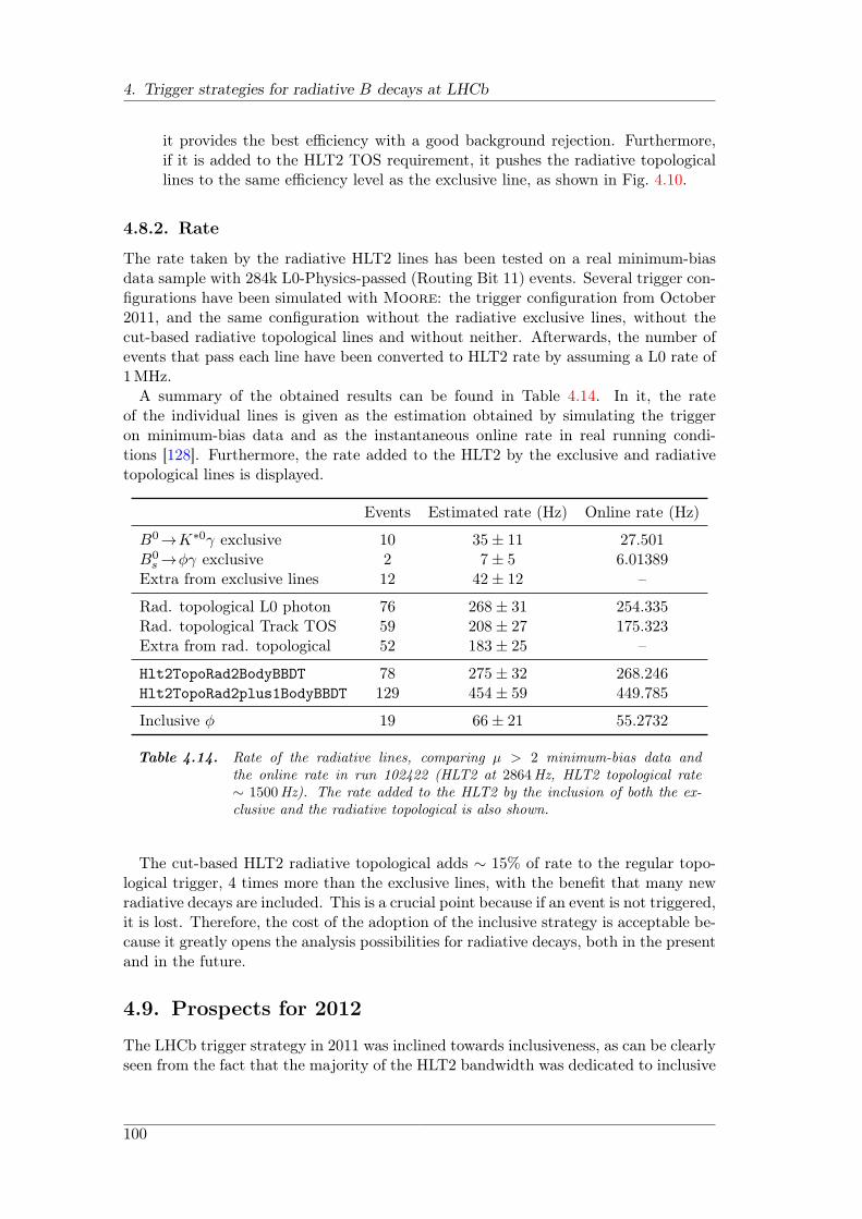
4. Trigger strategies for radiative B decays at LHCb
it provides the best efficiency with a good background rejection. Furthermore,if it is added to the HLT2 TOS requirement, it pushes the radiative topologicallines to the same efficiency level as the exclusive line, as shown in Fig. 4.10.
4.8.2. Rate
The rate taken by the radiative HLT2 lines has been tested on a real minimum-biasdata sample with 284k L0-Physics-passed (Routing Bit 11) events. Several trigger con-figurations have been simulated with Moore: the trigger configuration from October2011, and the same configuration without the radiative exclusive lines, without thecut-based radiative topological lines and without neither. Afterwards, the number ofevents that pass each line have been converted to HLT2 rate by assuming a L0 rate of1MHz.
A summary of the obtained results can be found in Table 4.14. In it, the rateof the individual lines is given as the estimation obtained by simulating the triggeron minimum-bias data and as the instantaneous online rate in real running condi-tions [128]. Furthermore, the rate added to the HLT2 by the exclusive and radiativetopological lines is displayed.
Events Estimated rate (Hz) Online rate (Hz)
B0→K∗0γ exclusive 10 35± 11 27.501B0
s →ϕγ exclusive 2 7± 5 6.01389Extra from exclusive lines 12 42± 12 –
Rad. topological L0 photon 76 268± 31 254.335Rad. topological Track TOS 59 208± 27 175.323Extra from rad. topological 52 183± 25 –
Hlt2TopoRad2BodyBBDT 78 275± 32 268.246Hlt2TopoRad2plus1BodyBBDT 129 454± 59 449.785
Inclusive ϕ 19 66± 21 55.2732
Table 4.14. Rate of the radiative lines, comparing µ > 2 minimum-bias data andthe online rate in run 102422 (HLT2 at 2864Hz, HLT2 topological rate∼ 1500Hz). The rate added to the HLT2 by the inclusion of both the ex-clusive and the radiative topological is also shown.
The cut-based HLT2 radiative topological adds ∼ 15% of rate to the regular topo-logical trigger, 4 times more than the exclusive lines, with the benefit that many newradiative decays are included. This is a crucial point because if an event is not triggered,it is lost. Therefore, the cost of the adoption of the inclusive strategy is acceptable be-cause it greatly opens the analysis possibilities for radiative decays, both in the presentand in the future.
4.9. Prospects for 2012
The LHCb trigger strategy in 2011 was inclined towards inclusiveness, as can be clearlyseen from the fact that the majority of the HLT2 bandwidth was dedicated to inclusive
100
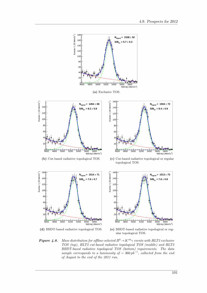
4.9. Prospects for 2012
)2) (MeV/cγπM(K4600 4800 5000 5200 5400 5600 5800
)2E
vent
s / (
25
MeV
/c
0
20
40
60
80
100
120
140
160
180
0.3± = 5.7 σ2S/B
52± = 1538 signalN
(a) Exclusive TOS.
)2) (MeV/cγπM(K4600 4800 5000 5200 5400 5600 5800
)2E
vent
s / (
25
MeV
/c
0
20
40
60
80
100
120
140 0.8± = 8.2 σ2S/B
68± = 1454 signalN
(b) Cut-based radiative topological TOS.
)2) (MeV/cγπM(K4600 4800 5000 5200 5400 5600 5800
)2E
vent
s / (
25
MeV
/c
0
20
40
60
80
100
120
140
160
0.9± = 8.4 σ2S/B
72± = 1504 signalN
(c) Cut-based radiative topological or regulartopological TOS.
)2) (MeV/cγπM(K4600 4800 5000 5200 5400 5600 5800
)2E
vent
s / (
25
MeV
/c
0
20
40
60
80
100
120
140
160
0.7± = 7.6 σ2S/B
71± = 1514 signalN
(d) BBDT-based radiative topological TOS.
)2) (MeV/cγπM(K4600 4800 5000 5200 5400 5600 5800
)2E
vent
s / (
25
MeV
/c
0
20
40
60
80
100
120
140
160
0.8± = 7.6 σ2S/B
73± = 1513 signalN
(e) BBDT-based radiative topological or reg-ular topological TOS.
Figure 4.8. Mass distribution for offline-selected B0→K∗0γ events with HLT2 exclusiveTOS (top), HLT2 cut-based radiative topological TOS (middle) and HLT2BBDT-based radiative topological TOS (bottom) requirements. The datasample corresponds to a luminosity of ∼ 360 pb−1, collected from the endof August to the end of the 2011 run.
101
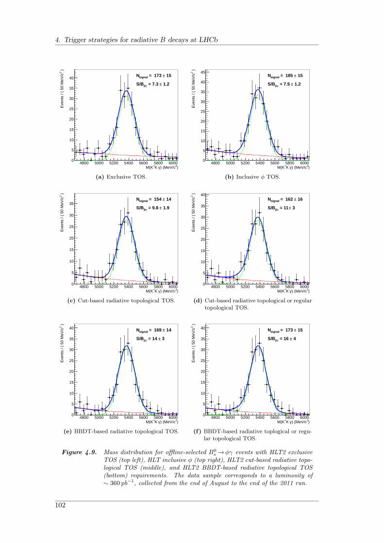
4. Trigger strategies for radiative B decays at LHCb
)2) (MeV/cγ-K+M(K4800 5000 5200 5400 5600 5800 6000
)2E
vent
s / (
50
MeV
/c
0
5
10
15
20
25
30
35
40
1.2± = 7.3 σ2S/B
15± = 173 signalN
(a) Exclusive TOS.
)2) (MeV/cγ-K+M(K4800 5000 5200 5400 5600 5800 6000
)2E
vent
s / (
50
MeV
/c
0
5
10
15
20
25
30
35
40
45
1.2± = 7.5 σ2S/B
15± = 185 signalN
(b) Inclusive ϕ TOS.
)2) (MeV/cγ-K+M(K4800 5000 5200 5400 5600 5800 6000
)2E
vent
s / (
50
MeV
/c
0
5
10
15
20
25
30
35 1.9± = 9.8 σ2S/B
14± = 154 signalN
(c) Cut-based radiative topological TOS.
)2) (MeV/cγ-K+M(K4800 5000 5200 5400 5600 5800 6000
)2E
vent
s / (
50
MeV
/c
0
5
10
15
20
25
30
35
40
3± = 11 σ2S/B
16± = 162 signalN
(d) Cut-based radiative topological or regulartopological TOS.
)2) (MeV/cγ-K+M(K4800 5000 5200 5400 5600 5800 6000
)2E
vent
s / (
50
MeV
/c
0
5
10
15
20
25
30
35
40
3± = 14 σ2S/B
14± = 169 signalN
(e) BBDT-based radiative topological TOS.
)2) (MeV/cγ-K+M(K4800 5000 5200 5400 5600 5800 6000
)2E
vent
s / (
50
MeV
/c
0
5
10
15
20
25
30
35
40
4± = 16 σ2S/B
15± = 173 signalN
(f) BBDT-based radiative toplogical or regu-lar topological TOS.
Figure 4.9. Mass distribution for offline-selected B0s →ϕγ events with HLT2 exclusive
TOS (top left), HLT inclusive ϕ (top right), HLT2 cut-based radiative topo-logical TOS (middle), and HLT2 BBDT-based radiative topological TOS(bottom) requirements. The data sample corresponds to a luminosity of∼ 360 pb−1, collected from the end of August to the end of the 2011 run.
102
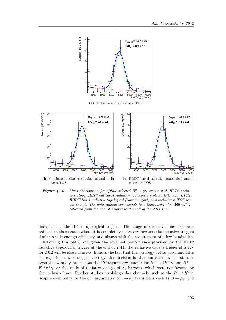
4.9. Prospects for 2012
)2) (MeV/cγ-K+M(K4800 5000 5200 5400 5600 5800 6000
)2E
vent
s / (
50
MeV
/c
0
10
20
30
40
50
1.1± = 6.9 σ2S/B
16± = 197 signalN
(a) Exclusive and inclusive ϕ TOS.
)2) (MeV/cγ-K+M(K4800 5000 5200 5400 5600 5800 6000
)2E
vent
s / (
50
MeV
/c
0
10
20
30
40
50
1.1± = 7.0 σ2S/B
16± = 195 signalN
(b) Cut-based radiative topological and inclu-sive ϕ TOS.
)2) (MeV/cγ-K+M(K4800 5000 5200 5400 5600 5800 6000
)2E
vent
s / (
50
MeV
/c
0
10
20
30
40
50
1.2± = 7.4 σ2S/B
16± = 198 signalN
(c) BBDT-based radiative topological and in-clusive ϕ TOS.
Figure 4.10. Mass distribution for offline-selected B0s → ϕγ events with HLT2 exclu-
sive (top), HLT2 cut-based radiative topological (bottom left), and HLT2BBDT-based radiative topological (bottom right), plus inclusive ϕ TOS re-quirement. The data sample corresponds to a luminosity of ∼ 360 pb−1,collected from the end of August to the end of the 2011 run.
lines such as the HLT2 topological trigger. The usage of exclusive lines has beenreduced to those cases where it is completely necessary because the inclusive triggersdon’t provide enough efficiency, and always with the requirement of a low bandwidth.
Following this path, and given the excellent performance provided by the HLT2radiative topological trigger at the end of 2011, the radiative decays trigger strategyfor 2012 will be also inclusive. Besides the fact that this strategy better accommodatesthe experiment-wise trigger strategy, this decision is also motivated by the start ofseveral new analyses, such as the CP -asymmetry studies for B+ → ϕK+γ and B+ →K∗0π+γ, or the study of radiative decays of Λb baryons, which were not favored bythe exclusive lines. Further studies involving other channels, such as the B0 →K∗0γisospin-asymmetry, or the CP asymmetry of b→ dγ transitions such as B→ ργ, will
103
4. Trigger strategies for radiative B decays at LHCb
also be possible in the future because these decays will have already been triggeredwith significant efficiency.
Based on the 2011 performance studies described in the previous section, the HLT2cut-based radiative topological lines have been modified to decouple the L0 Photonand the Track TOS lines. The idea behind the changes is to use the L0 Photon line toselect radiative events based on the distinct photon signature and use the Track TOSline to recover radiative events with low ET photons. To achieve this goal, the ET
cut in the photon has to be lowered, and a cut in the maximum pT of the two usedtracks needs to be introduced to keep a reasonable rate. Exact values of these cuts arestill to be determined during the 2012 HLT commissioning period, but working valuesare ET > 2GeV for the photon and max(pT) > 3.5GeV/c for the tracks, followingthe transverse energy cut in L0Hadron channel, which would imply a ∼ 10% gain inefficiency with a similar rate. If this improvement was indeed possible, stripping andoffline selection changes would need to follow this change.
The decision of which inclusive lines to use in 2012 will depend on the running con-ditions and the necessary background rejection. Since cuts in the radiative topologicallines are currently placed at the limit of the phase space where no substantial effi-ciency is lost, a need for further background rejection could imply a sizeable loss inperformance. In this scenario, the BBDT-based lines have the potential to provide abetter performance than cut-based ones, as it has already been shown in LHCb [160].If no further reduction is necessary, and the modifications of the cut-based radiativetopological lines provide a similar performance as the BBDT-based ones, it would beadvisable to keep the cut-based lines because they are easier to interpret. In the case ofB0
s →ϕγ and B+→ϕK+γ, the inclusive ϕ line provides robustness and extra efficiency.In addition, it is interesting to keep the exclusive trigger lines as a way to cross
check the results obtained by making use of the radiative topological lines, specially deBBDT-based ones, which may be hard to interpret. However, to do that their impacton the overall HLT2 rate needs to be negligible. Therefore, the exclusive lines forB0 →K∗0γ and B0
s → ϕγ have been be modified to lower their rate to an acceptablelevel of O(1Hz). This rate reduction has been achieved by tightening the cuts in thelines, effectively turning them into quasi-offline selections performed in the trigger, asshown in Table 4.15.
The new, tighter exclusive lines have been tested with two minimum bias testingsamples, one with a higher µ and the other with a low µ, with 85,417 and 81,635L0-Physics events, respectively; in addition, the tracking conditions in the HLT2 havebeen modified to add downstream tracking and pT > 300MeV/c and p > 3000MeV/cas the requirements for a track to be reconstructed3 It has been found that no eventspass the exclusive radiative triggers in the high µ sample, while one event passes theHlt2Bd2KstGamma line in the case of the low µ sample; this is equivalent to a rate of5Hz with almost a 100% uncertainty.
Given the big uncertainty on their rate, these new lines will be checked during theHLT commissioning work at the beginning of the 2012 run in order to determine withmore precision their rate and to make the proper adjustments. Possible modificationsto lower the rate include the addition of a track TOS filter or a GEC on the numberof tracks.
Summing up, an inclusive trigger strategy for radiative decays has been prepared for
3At the time of writing, these were the working conditions for the HLT2 trigger optimization for 2012.
104

4.9. Prospects for 2012
B0→K∗0γ line B0s →ϕγ line
Track p (MeV/c) > 3000 > 3000Track pT (MeV/c) > 300 > 300Track χ2 < 5 < 5Track IP χ2 > 20 > 20
V ∆MPDG (MeV/c2) < 100 < 20V vertex χ2 < 16 < 25
Photon ET (MeV) > 2600 > 2600
B pT (MeV/c) > 3000 > 3000B IP χ2 < 12 < 12B DIRA (mrad) < 63 < 45B ∆MPDG (MeV/c2) < 1000 < 1000
L0 channel L0Photon or L0Electron L0Photon or L0ElectronHLT1 lines HLT1 Physics HLT1 Physics
Table 4.15. Cuts applied in the 2012 HLT2 exclusive lines for B0→K∗0γ and B0s →ϕγ,
separated in track cuts, vector meson (V ) cuts, photon cuts, B candidatecuts and trigger filters.
the 2012 LHC run, replacing the exclusive strategy used so far. Furthermore, all newlines have been tested and checked at the end of the 2011 run, and have shown goodperformance. However, it will be necessary to perform a thorough commissioning ofboth the inclusive and the exclusive lines in order to adjust to possible changes in thetracking conditions in HLT2, which could largely affect the retention rates.
105

5Measurement of the ratioB(B0→K∗0γ)/B(B0
s→ϕγ)
The main aim of this analysis is to extract the ratio of branching fractions of B0→K∗0γwithK∗0→K±π∓ and B0
s →ϕγ with ϕ→K+K−, and their complex conjugates1. Fromthis result, and using the well-measured value of B(B0→K∗0γ), the branching fractionof B0
s →ϕγ can be extracted. This is the first analysis of radiative B decays performedat LHCb, and as such it requires a detailed study of elements, such as signal shapesand associated backgrounds, which will extremely helpful in future analyses.
The heart of the measurement is the extraction of the signal yields for each channel.To do that, the line shape of the mass distributions of the selected B0 and B0
s can-didates has to be determined, including a detailed account of all possible backgroundcontributions. These yields need to be corrected for the efficiency of the selection andthe relative abundance of both B species in LHC collisions.
In this analysis, the B0 and B0s candidates are built by combining a vector meson
candidate, either a K∗0 or a ϕ, and a photon. The vector meson candidates are builtfrom pairs of oppositely charged tracks, a kaon and a pion in the case of the K∗0
and two kaons in the case of the ϕ. Those track pairs with an invariant mass locatedwithin the defined mass window for each of vector mesons are combined with a photonto calculate the invariant mass of the B candidates.
In order to obtain the best possible measurement, the selection is carried out follow-ing the same procedure for both channels. In this way, most systematical effects cancelout in the calculation of the ratio of efficiencies, resulting in a reduced uncertainty. Fora complete cancellation, both decays should have:
The same photon efficiency.
The same kinematics.
The same topology.
However, this is not completely true in our case due to the different nature of the
1Throughout this chapter, whenever a mode is given, the charge conjugate is also implied.
107
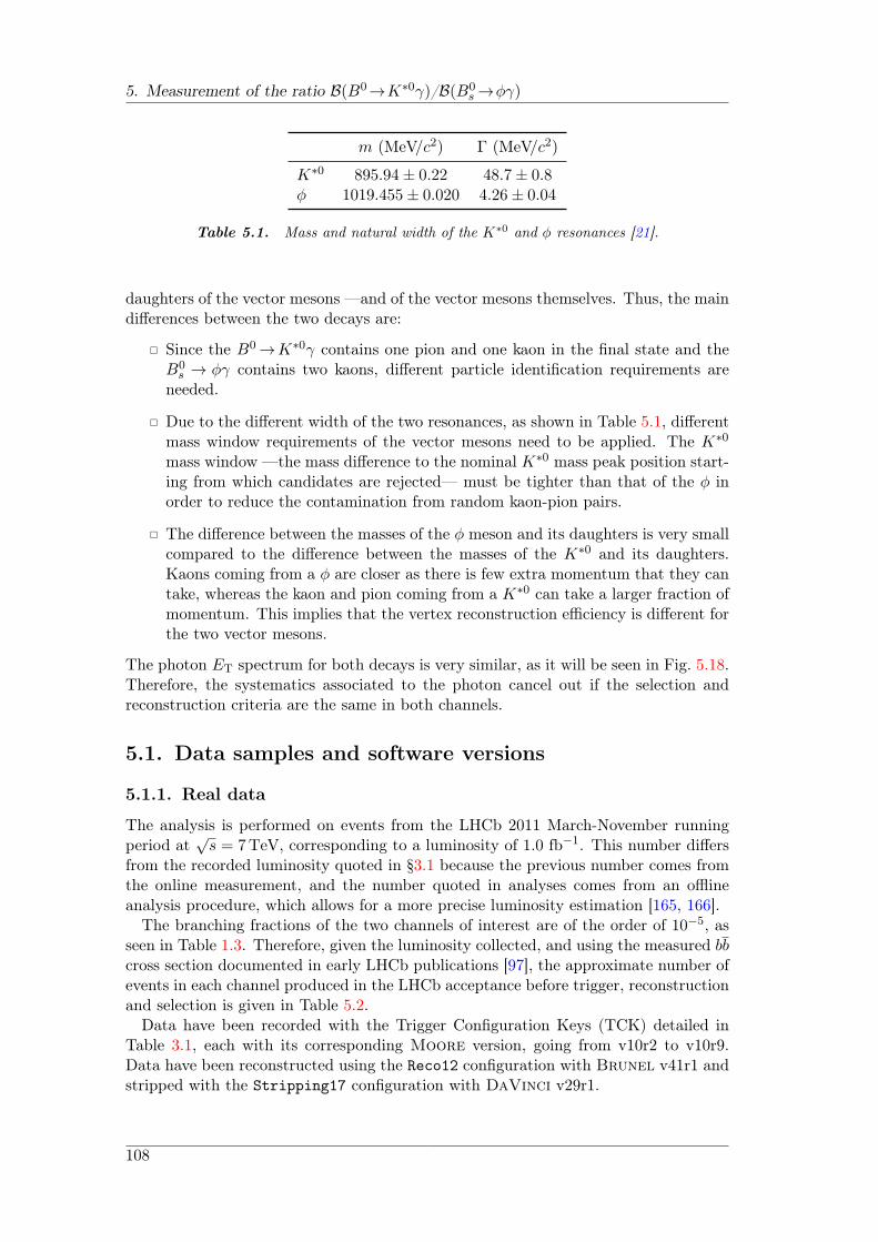
5. Measurement of the ratio B(B0→K∗0γ)/B(B0s →ϕγ)
m (MeV/c2) Γ (MeV/c2)
K∗0 895.94± 0.22 48.7± 0.8ϕ 1019.455± 0.020 4.26± 0.04
Table 5.1. Mass and natural width of the K∗0 and ϕ resonances [21].
daughters of the vector mesons —and of the vector mesons themselves. Thus, the maindifferences between the two decays are:
Since the B0→K∗0γ contains one pion and one kaon in the final state and theB0
s → ϕγ contains two kaons, different particle identification requirements areneeded.
Due to the different width of the two resonances, as shown in Table 5.1, differentmass window requirements of the vector mesons need to be applied. The K∗0
mass window —the mass difference to the nominal K∗0 mass peak position start-ing from which candidates are rejected— must be tighter than that of the ϕ inorder to reduce the contamination from random kaon-pion pairs.
The difference between the masses of the ϕ meson and its daughters is very smallcompared to the difference between the masses of the K∗0 and its daughters.Kaons coming from a ϕ are closer as there is few extra momentum that they cantake, whereas the kaon and pion coming from a K∗0 can take a larger fraction ofmomentum. This implies that the vertex reconstruction efficiency is different forthe two vector mesons.
The photon ET spectrum for both decays is very similar, as it will be seen in Fig. 5.18.Therefore, the systematics associated to the photon cancel out if the selection andreconstruction criteria are the same in both channels.
5.1. Data samples and software versions
5.1.1. Real data
The analysis is performed on events from the LHCb 2011 March-November runningperiod at
√s = 7TeV, corresponding to a luminosity of 1.0 fb−1. This number differs
from the recorded luminosity quoted in §3.1 because the previous number comes fromthe online measurement, and the number quoted in analyses comes from an offlineanalysis procedure, which allows for a more precise luminosity estimation [165, 166].
The branching fractions of the two channels of interest are of the order of 10−5, asseen in Table 1.3. Therefore, given the luminosity collected, and using the measured bbcross section documented in early LHCb publications [97], the approximate number ofevents in each channel produced in the LHCb acceptance before trigger, reconstructionand selection is given in Table 5.2.
Data have been recorded with the Trigger Configuration Keys (TCK) detailed inTable 3.1, each with its corresponding Moore version, going from v10r2 to v10r9.Data have been reconstructed using the Reco12 configuration with Brunel v41r1 andstripped with the Stripping17 configuration with DaVinci v29r1.
108
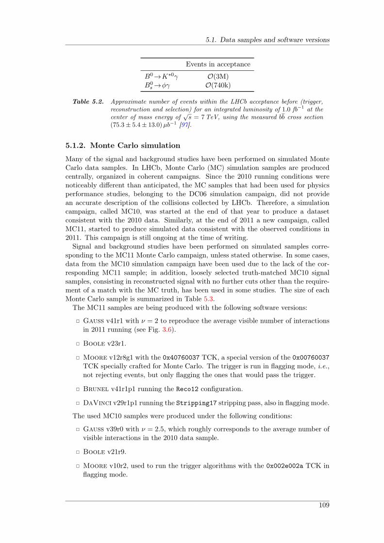
5.1. Data samples and software versions
Events in acceptance
B0→K∗0γ O(3M)B0
s →ϕγ O(740k)
Table 5.2. Approximate number of events within the LHCb acceptance before (trigger,reconstruction and selection) for an integrated luminosity of 1.0 fb−1 at thecenter of mass energy of
√s = 7TeV, using the measured bb cross section
(75.3± 5.4± 13.0)µb−1 [97].
5.1.2. Monte Carlo simulation
Many of the signal and background studies have been performed on simulated MonteCarlo data samples. In LHCb, Monte Carlo (MC) simulation samples are producedcentrally, organized in coherent campaigns. Since the 2010 running conditions werenoticeably different than anticipated, the MC samples that had been used for physicsperformance studies, belonging to the DC06 simulation campaign, did not providean accurate description of the collisions collected by LHCb. Therefore, a simulationcampaign, called MC10, was started at the end of that year to produce a datasetconsistent with the 2010 data. Similarly, at the end of 2011 a new campaign, calledMC11, started to produce simulated data consistent with the observed conditions in2011. This campaign is still ongoing at the time of writing.
Signal and background studies have been performed on simulated samples corre-sponding to the MC11 Monte Carlo campaign, unless stated otherwise. In some cases,data from the MC10 simulation campaign have been used due to the lack of the cor-responding MC11 sample; in addition, loosely selected truth-matched MC10 signalsamples, consisting in reconstructed signal with no further cuts other than the require-ment of a match with the MC truth, has been used in some studies. The size of eachMonte Carlo sample is summarized in Table 5.3.
The MC11 samples are being produced with the following software versions:
Gauss v41r1 with ν = 2 to reproduce the average visible number of interactionsin 2011 running (see Fig. 3.6).
Boole v23r1.
Moore v12r8g1 with the 0x40760037 TCK, a special version of the 0x00760037TCK specially crafted for Monte Carlo. The trigger is run in flagging mode, i.e.,not rejecting events, but only flagging the ones that would pass the trigger.
Brunel v41r1p1 running the Reco12 configuration.
DaVinci v29r1p1 running the Stripping17 stripping pass, also in flagging mode.
The used MC10 samples were produced under the following conditions:
Gauss v39r0 with ν = 2.5, which roughly corresponds to the average number ofvisible interactions in the 2010 data sample.
Boole v21r9.
Moore v10r2, used to run the trigger algorithms with the 0x002e002a TCK inflagging mode.
109

5. Measurement of the ratio B(B0→K∗0γ)/B(B0s →ϕγ)
MC10 (Mevts) MC11 (Mevts)
B0→K∗0γ 10.18 6.99B0
s →ϕγ 4.05 3.98
B+→K∗0π+γ — 2.01B+→ϕK+γ 0.10 2.01B0→K+π−π0 2.01 0.22B0
s →K+π−π0 2.01 —B0→π+π−π0 — 1.01B0→K∗0e+e− 1.03 3.98B0→D−ρ+ — 0.22B0→D∗
s(πππ0)π 1.00 —
B0→D0(Kππ0)K∗0 2.52 —B+→K∗+(K+π0)K+K− 0.10 —B+→K∗+(K+π0)π+π− 1.10 —B+→D0(Kππ0)π+ 0.10 —B+→J/ψ (ρ0π0)K+ 0.10 —B0
s →ρ+(π+π0)K− 0.06 —Λb→Λ0γ — 0.50Λb→Λ(1520)γ — 1.00Λb→Λ(1670)γ — 1.16
Table 5.3. Statistics of the MC10 and MC11 datasets used in this study, with radiativesignal in the top section and background in the bottom one. Each of thesamples is split in two halves of approximately the same size, correspondingto the two polarities of the magnetic field.
Brunel v37r8p5, with the Reco08 configuration.
DaVinci v28r2p2 running the Stripping12 stripping pass, also in flagging mode.
When producing the Root NTuples for analysis from the MC10 DSTs, an extra recon-struction pass was applied with DaVinci v29r1 to reproduce the Reco12 calorimeterconfiguration from 2011.
5.2. Event selection
As already mentioned, the main point in the analysis strategy is try to benefit fromthe cancellations of most uncertainties in the ratio of efficiencies. In particular, thecancellations are maximized by adopting the same selection strategy for both channels.B meson candidates are constructed through the following process:
1. Vector meson candidates are built from pairs of oppositely charged tracks.
2. Photon candidates are built from the clusters in the ECAL.
3. Vector meson and photon candidates are combined to build the B candidate.
Common cuts for the tracks and the photon are used to minimize the impact ofsystematic effects. However, some inevitable differences appear in the selection of the
110

5.2. Event selection
vector meson candidate, especially in the particle identification of its decay productsand in its mass window cut.
As explained in §3.7.3, events used in analysis have been selected through the fol-lowing steps:
1. Trigger. Data taken by LHCb are filtered by the L0 and HLT trigger stages, andonly those events that are selected by the trigger are kept.
2. Stripping. Stored raw data are reconstructed and selected to produced reduceddata samples for physics analyses. In the case of this analysis, the RadiativeStripping stream is used.
3. Offline selection. B candidates are built from stripped events and are selectedusing tight cuts in order to achieve the best possible signal significance; these arethe candidates used in the physics analyses.
Details on these three steps follow, with an explanation of the most relevant triggersin §5.2.1, the Radiative Stripping stream in §5.2.2 and the offline selection used for theB0→K∗0γ and B0
s →ϕγ decays in §5.2.3.
5.2.1. Trigger
The exclusive trigger strategy, defined in Chap. 4, has been chosen for this analysis,and therefore the required trigger lines are the following:
In L0, L0Electron and L0Photon select those events with an electromagneticdeposition in the ECAL with a transverse energy with respect to the beam di-rection, ET, greater than the thresholds detailed in Table 5.4. Additionally, asubset of the events that pass these two lines also pass the L0ElectronHi andL0PhotonHi lines, which require a higher ET cut.
In the HLT1, the relevant lines are Hlt1TrackAllL0 and Hlt1TrackPhoton
single track lines. They select events based on the transverse momentumand impact parameter of the tracks with respect to the beam direction.Hlt1TrackAllL0 selects low-ET photons with a harder cut in the required track,while Hlt1TrackPhotonL0 allows to lower the pT requirement for the track atthe cost of a harder ET cut on the photon, as illustrated in Table 5.4.
In HLT2, the exclusive radiative lines, Hlt2Bd2KstGamma and Hlt2Bs2PhiGamma,which only run on events that pass the L0Electron and L0Photon lines. Eventsare selected by building the vector meson, combining it with a high-ET pho-ton and applying loose cuts in the same direction as the stripping and offlineselections. Details of the ET and pT cuts can be found in Table 5.4.
In order to extract the ratio of branching fractions the exclusive TOS requirement ismade, i.e., it is required that the signal tracks and photon are responsible of firing thecorresponding trigger lines. This requirement is essential for a better understandingof the trigger efficiencies and for enforcing the similarity of the trigger path of theB0→K∗0γ and B0
s →ϕγ, which will ensure the cancellation of the systematic effectsinduced by the trigger. With that consideration in mind, the trigger TOS selectionsfor each channel are those given in §4.6:
111
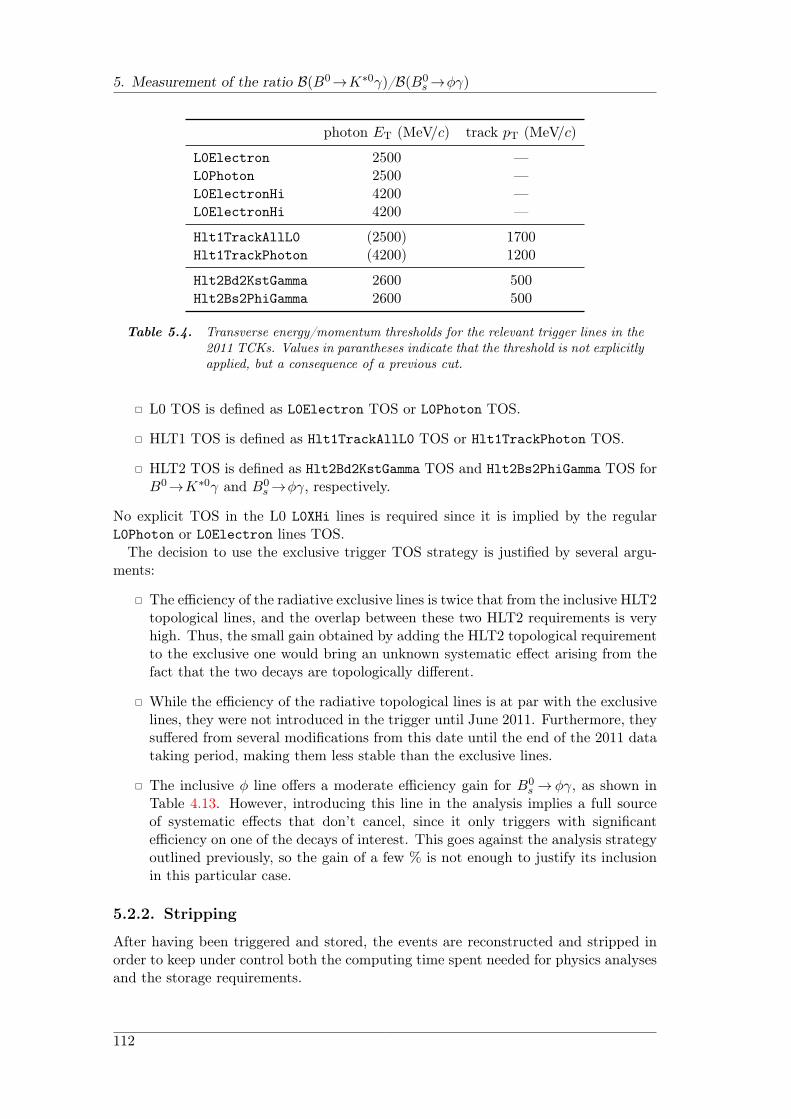
5. Measurement of the ratio B(B0→K∗0γ)/B(B0s →ϕγ)
photon ET (MeV/c) track pT (MeV/c)
L0Electron 2500 —L0Photon 2500 —L0ElectronHi 4200 —L0ElectronHi 4200 —
Hlt1TrackAllL0 (2500) 1700Hlt1TrackPhoton (4200) 1200
Hlt2Bd2KstGamma 2600 500Hlt2Bs2PhiGamma 2600 500
Table 5.4. Transverse energy/momentum thresholds for the relevant trigger lines in the2011 TCKs. Values in parantheses indicate that the threshold is not explicitlyapplied, but a consequence of a previous cut.
L0 TOS is defined as L0Electron TOS or L0Photon TOS.
HLT1 TOS is defined as Hlt1TrackAllL0 TOS or Hlt1TrackPhoton TOS.
HLT2 TOS is defined as Hlt2Bd2KstGamma TOS and Hlt2Bs2PhiGamma TOS forB0→K∗0γ and B0
s →ϕγ, respectively.
No explicit TOS in the L0 L0XHi lines is required since it is implied by the regularL0Photon or L0Electron lines TOS.
The decision to use the exclusive trigger TOS strategy is justified by several argu-ments:
The efficiency of the radiative exclusive lines is twice that from the inclusive HLT2topological lines, and the overlap between these two HLT2 requirements is veryhigh. Thus, the small gain obtained by adding the HLT2 topological requirementto the exclusive one would bring an unknown systematic effect arising from thefact that the two decays are topologically different.
While the efficiency of the radiative topological lines is at par with the exclusivelines, they were not introduced in the trigger until June 2011. Furthermore, theysuffered from several modifications from this date until the end of the 2011 datataking period, making them less stable than the exclusive lines.
The inclusive ϕ line offers a moderate efficiency gain for B0s → ϕγ, as shown in
Table 4.13. However, introducing this line in the analysis implies a full sourceof systematic effects that don’t cancel, since it only triggers with significantefficiency on one of the decays of interest. This goes against the analysis strategyoutlined previously, so the gain of a few % is not enough to justify its inclusionin this particular case.
5.2.2. Stripping
After having been triggered and stored, the events are reconstructed and stripped inorder to keep under control both the computing time spent needed for physics analysesand the storage requirements.
112
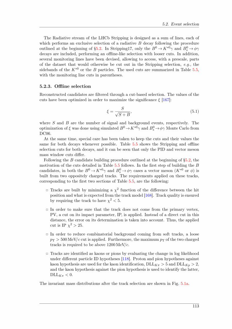
5.2. Event selection
The Radiative stream of the LHCb Stripping is designed as a sum of lines, each ofwhich performs an exclusive selection of a radiative B decay following the procedureoutlined at the beginning of §5.2. In Stripping17, only the B0 →K∗0γ and B0
s → ϕγdecays are included, performing an offline-like selection with looser cuts. In addition,several monitoring lines have been devised, allowing to access, with a prescale, partsof the dataset that would otherwise be cut out in the Stripping selection, e.g., thesidebands of the K∗0 or the B particles. The used cuts are summarized in Table 5.5,with the monitoring line cuts in parentheses.
5.2.3. Offline selection
Reconstructed candidates are filtered through a cut-based selection. The values of thecuts have been optimized in order to maximize the significance ξ [167]:
ξ =S√S +B
, (5.1)
where S and B are the number of signal and background events, respectively. Theoptimization of ξ was done using simulated B0→K∗0γ and B0
s →ϕγ Monte Carlo fromDC06.
At the same time, special care has been taken to keep the cuts and their values thesame for both decays whenever possible. Table 5.5 shows the Stripping and offlineselection cuts for both decays, and it can be seen that only the PID and vector mesonmass window cuts differ.
Following the B candidate building procedure outlined at the beginning of §5.2, themotivation of the cuts detailed in Table 5.5 follows. In the first step of building the Bcandidates, in both the B0 →K∗0γ and B0
s → ϕγ cases a vector meson (K∗0 or ϕ) isbuilt from two oppositely charged tracks. The requirements applied on these tracks,corresponding to the first two sections of Table 5.5, are the following:
Tracks are built by minimizing a χ2 function of the difference between the hitposition and what is expected from the track model [168]. Track quality is ensuredby requiring the track to have χ2 < 5.
In order to make sure that the track does not come from the primary vertex,PV, a cut on its impact parameter, IP, is applied. Instead of a direct cut in thisdistance, the error on its determination is taken into account. Thus, the appliedcut is IP χ2 > 25.
In order to reduce combinatorial background coming from soft tracks, a loosepT > 500MeV/c cut is applied. Furthermore, the maximum pT of the two chargedtracks is required to be above 1200MeV/c.
Tracks are identified as kaons or pions by evaluating the change in log likelihoodunder different particle ID hypotheses [118]. Proton and pion hypotheses againstkaon hypothesis are used for the kaon identification, DLLKπ > 5 and DLLKp > 2,and the kaon hypothesis against the pion hypothesis is used to identify the latter,DLLKπ < 0.
The invariant mass distributions after the track selection are shown in Fig. 5.1a.
113
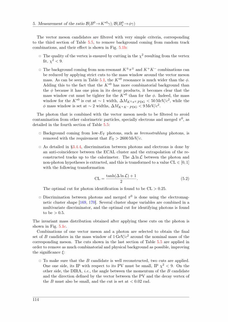
5. Measurement of the ratio B(B0→K∗0γ)/B(B0s →ϕγ)
The vector meson candidates are filtered with very simple criteria, correspondingto the third section of Table 5.5, to remove background coming from random trackcombinations, and their effect is shown in Fig. 5.1b:
The quality of the vertex is ensured by cutting in the χ2 resulting from the vertexfit, χ2 < 9.
The background coming from non-resonant K±π∓ and K+K− combinations canbe reduced by applying strict cuts to the mass window around the vector mesonmass. As can be seen in Table 5.1, the K∗0 resonance is much wider than the ϕ.Adding this to the fact that the K∗0 has more combinatorial background thanthe ϕ because it has one pion in its decay products, it becomes clear that themass window cut must be tighter for the K∗0 than for the ϕ. Indeed, the masswindow for the K∗0 is cut at ∼ 1 width, ∆MK±π∓,PDG < 50MeV/c2, while theϕ mass window is set at ∼ 2 widths, ∆MK+K−,PDG < 9MeV/c2.
The photon that is combined with the vector meson needs to be filtered to avoidcontamination from other calorimetric particles, specially electrons and merged π0, asdetailed in the fourth section of Table 5.5:
Background coming from low-ET photons, such as bremsstrahlung photons, isremoved with the requirement that ET > 2600MeV/c.
As detailed in §3.4.4, discrimination between photons and electrons is done byan anti-coincidence between the ECAL cluster and the extrapolation of the re-constructed tracks up to the calorimeter. The ∆lnL between the photon andnon-photon hypotheses is extracted, and this is transformed to a value CL ∈ [0, 1]with the following transformation
CL =tanh(∆ lnL) + 1
2. (5.2)
The optimal cut for photon identification is found to be CL > 0.25.
Discrimination between photons and merged π0 is done using the electromag-netic cluster shape [169, 170]. Several cluster shape variables are combined in amultivariate discriminator, and the optimal cut for identifying photons is foundto be > 0.5.
The invariant mass distribution obtained after applying these cuts on the photon isshown in Fig. 5.1c.
Combinations of one vector meson and a photon are selected to obtain the finalset of B candidates in the mass window of 1GeV/c2 around the nominal mass of thecorresponding meson. The cuts shown in the last section of Table 5.5 are applied inorder to remove as much combinatorial and physical background as possible, improvingthe significance ξ:
To make sure that the B candidate is well reconstructed, two cuts are applied.One one side, its IP with respect to its PV must be small, IP χ2 < 9. On theother side, the DIRA, i.e., the angle between the momentum of the B candidateand the direction defined by the vector between the PV and the decay vertex ofthe B must also be small, and the cut is set at < 0.02 rad.
114
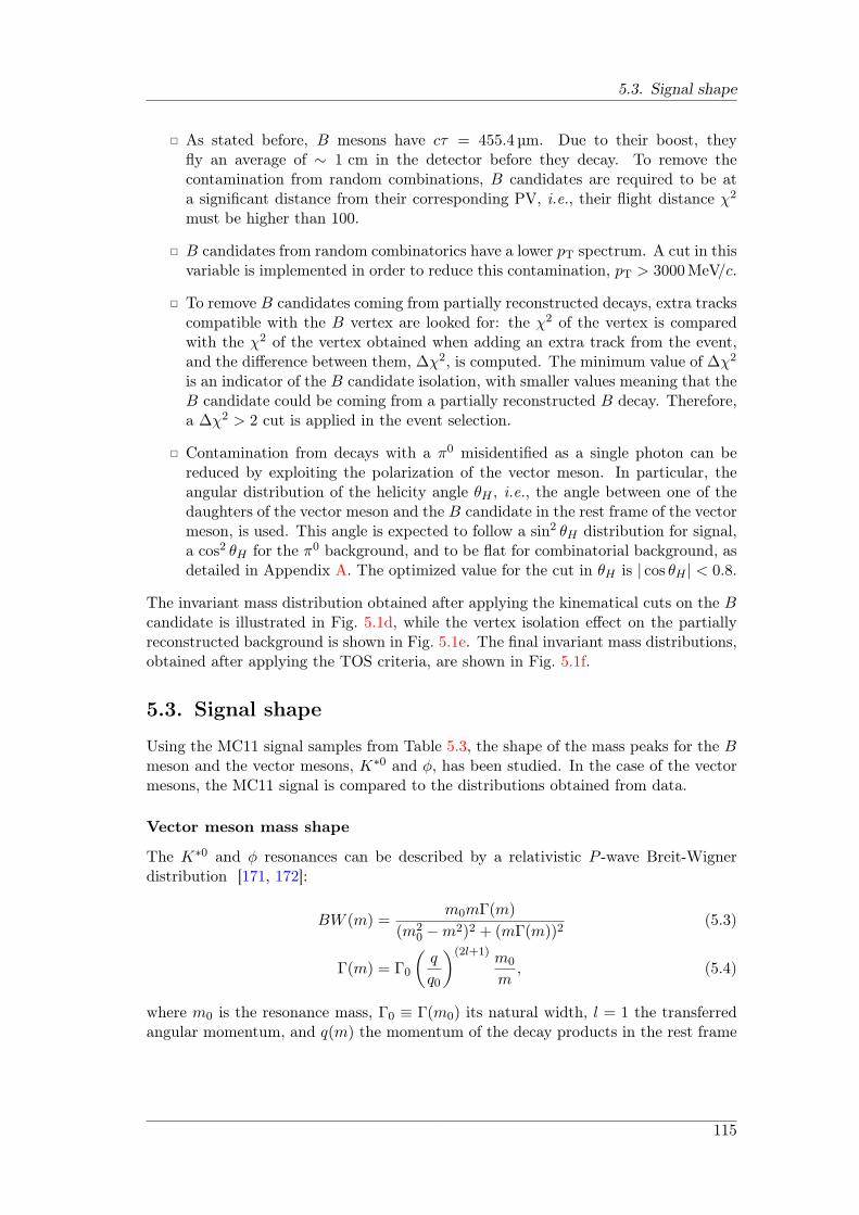
5.3. Signal shape
As stated before, B mesons have cτ = 455.4µm. Due to their boost, theyfly an average of ∼ 1 cm in the detector before they decay. To remove thecontamination from random combinations, B candidates are required to be ata significant distance from their corresponding PV, i.e., their flight distance χ2
must be higher than 100.
B candidates from random combinatorics have a lower pT spectrum. A cut in thisvariable is implemented in order to reduce this contamination, pT > 3000MeV/c.
To remove B candidates coming from partially reconstructed decays, extra trackscompatible with the B vertex are looked for: the χ2 of the vertex is comparedwith the χ2 of the vertex obtained when adding an extra track from the event,and the difference between them, ∆χ2, is computed. The minimum value of ∆χ2
is an indicator of the B candidate isolation, with smaller values meaning that theB candidate could be coming from a partially reconstructed B decay. Therefore,a ∆χ2 > 2 cut is applied in the event selection.
Contamination from decays with a π0 misidentified as a single photon can bereduced by exploiting the polarization of the vector meson. In particular, theangular distribution of the helicity angle θH , i.e., the angle between one of thedaughters of the vector meson and the B candidate in the rest frame of the vectormeson, is used. This angle is expected to follow a sin2 θH distribution for signal,a cos2 θH for the π0 background, and to be flat for combinatorial background, asdetailed in Appendix A. The optimized value for the cut in θH is | cos θH | < 0.8.
The invariant mass distribution obtained after applying the kinematical cuts on the Bcandidate is illustrated in Fig. 5.1d, while the vertex isolation effect on the partiallyreconstructed background is shown in Fig. 5.1e. The final invariant mass distributions,obtained after applying the TOS criteria, are shown in Fig. 5.1f.
5.3. Signal shape
Using the MC11 signal samples from Table 5.3, the shape of the mass peaks for the Bmeson and the vector mesons, K∗0 and ϕ, has been studied. In the case of the vectormesons, the MC11 signal is compared to the distributions obtained from data.
Vector meson mass shape
The K∗0 and ϕ resonances can be described by a relativistic P -wave Breit-Wignerdistribution [171, 172]:
BW (m) =m0mΓ(m)
(m20 −m2)2 + (mΓ(m))2
(5.3)
Γ(m) = Γ0
(q
q0
)(2l+1) m0
m, (5.4)
where m0 is the resonance mass, Γ0 ≡ Γ(m0) its natural width, l = 1 the transferredangular momentum, and q(m) the momentum of the decay products in the rest frame
115

5. Measurement of the ratio B(B0→K∗0γ)/B(B0s →ϕγ)
B0→
K∗0γ
B0s →
ϕγ
StrippingO
ffline
StrippingO
ffline
Track
χ2
<5
–<
5–
Track
IPχ2
>10
>25
>10
>25
Track
pT
(MeV/c)
–>
500
–>
500
Max
trackpT
(MeV/c)
–>
1200
–>
1200
Kaon
DLL
Kπ
>−5
>5
>−5
>5
Kaon
DLL
Kp
–>
2–
>2
Pion
DLL
Kπ
–<
0–
–
Vm
esonvertex
∆χ2
<15
<9
<15
<9
Vm
eson∆M
PD
G(M
eV/c
2)<
100(150)
<50
<15
<9
Photon
ET
(MeV
)>
2600
>2600
>2600
>2600
Photon
CL
–>
0.25
–>
0.25π0/γ
separation–
>0.5
–>
0.5
Bcandidate
pT
(MeV/c)
–>
3000
–>
3000B
candidateIP
χ2
<15
<9
<15
<9
Bcandidate
DIR
A(m
rad)<
20(60)
<20
<20
(60)<
20B
candidateFDχ2
–>
100
–>
100B
candidate∆M
PD
G(M
eV/c
2)<
1000(2000)
<1000
<1000
(2000)<
1000B
candidate|cos
θH|
–<
0.8–
<0.8
Bcandidate
isolation∆χ2
–>
2–
>2
Table
5.5.Selection
cutsfor
theB
0→K
∗0γ
andB
0s →ϕγ
decays.For
eachcut,
thestripping
(with
them
onitoringline
valuein
parentheses,if
different)and
offline
valuesare
shown.
The
cutsare
separatedin
sections,which
are,in
order,track
cuts,PID
cuts,vector
meson
cuts,photon
cuts,and
Bcandidate
cuts.
116
5.3. Signal shape
)2) (MeV/cγπM(K4400 4600 4800 5000 5200 5400 5600 5800 6000 6200
)2E
vent
s / (
25
MeV
/c
0
500
1000
1500
2000
2500
3000
)2) (MeV/cγ-K+M(K4400460048005000520054005600580060006200
)2E
vent
s / (
50
MeV
/c
0
100
200
300
400
500
600
700
800
(a) B0→K∗0γ and B0s →ϕγ after applying the track requirements.
)2) (MeV/cγπM(K4400 4600 4800 5000 5200 5400 5600 5800 6000 6200
)2E
vent
s / (
25
MeV
/c
0
200
400
600
800
1000
1200
1400
1600
1800
2000
2200
)2) (MeV/cγ-K+M(K4400460048005000520054005600580060006200
)2E
vent
s / (
50
MeV
/c
0
100
200
300
400
500
600
700
(b) B0→K∗0γ and B0s →ϕγ after applying the vector meson requirements.
)2) (MeV/cγπM(K4400 4600 4800 5000 5200 5400 5600 5800 6000 6200
)2E
vent
s / (
25
MeV
/c
0
200
400
600
800
1000
1200
)2) (MeV/cγ-K+M(K4400460048005000520054005600580060006200
)2E
vent
s / (
50
MeV
/c
0
50
100
150
200
250
300
350
(c) B0→K∗0γ and B0s →ϕγ after applying the photon requirements.
117
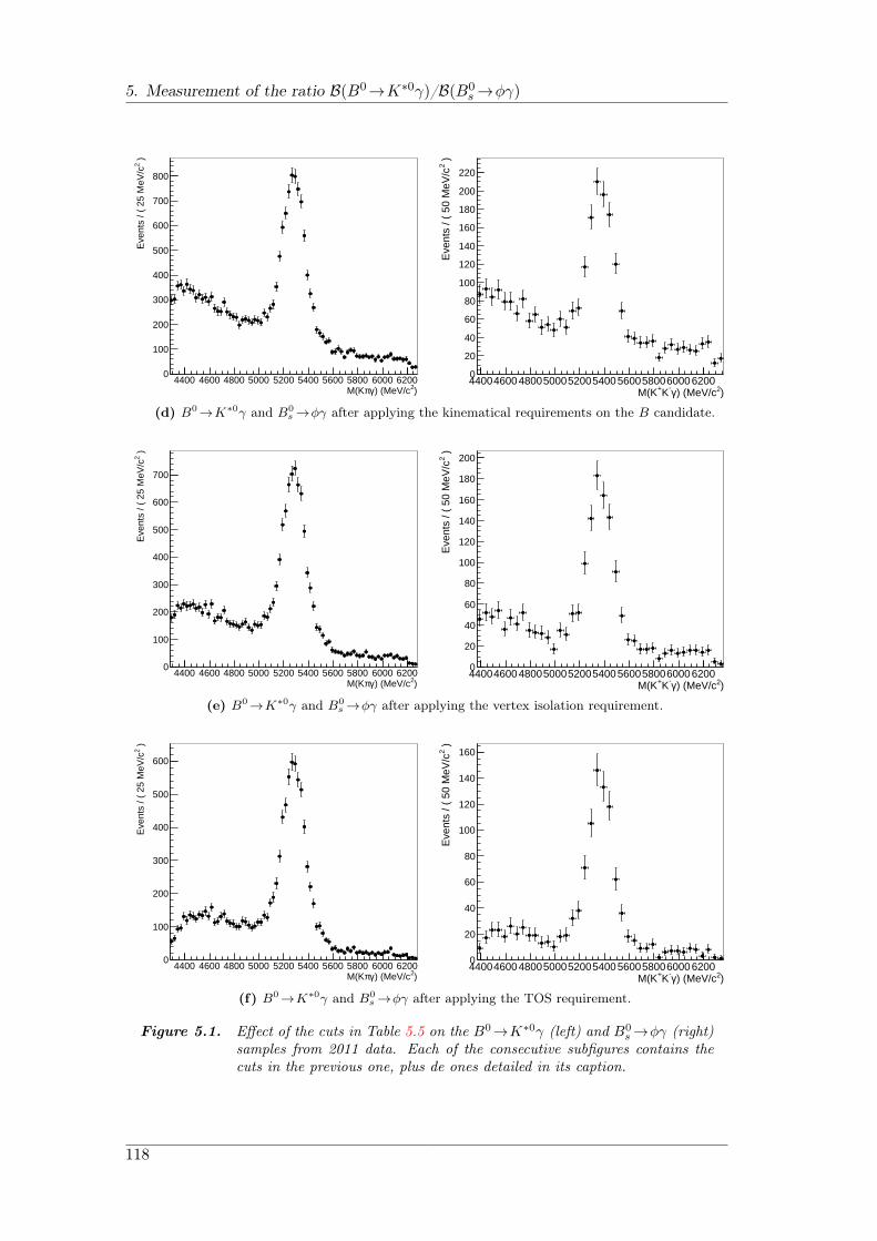
5. Measurement of the ratio B(B0→K∗0γ)/B(B0s →ϕγ)
)2) (MeV/cγπM(K4400 4600 4800 5000 5200 5400 5600 5800 6000 6200
)2E
vent
s / (
25
MeV
/c
0
100
200
300
400
500
600
700
800
)2) (MeV/cγ-K+M(K4400460048005000520054005600580060006200
)2E
vent
s / (
50
MeV
/c
0
20
40
60
80
100
120
140
160
180
200
220
(d) B0→K∗0γ and B0s →ϕγ after applying the kinematical requirements on the B candidate.
)2) (MeV/cγπM(K4400 4600 4800 5000 5200 5400 5600 5800 6000 6200
)2E
vent
s / (
25
MeV
/c
0
100
200
300
400
500
600
700
)2) (MeV/cγ-K+M(K4400460048005000520054005600580060006200
)2E
vent
s / (
50
MeV
/c
0
20
40
60
80
100
120
140
160
180
200
(e) B0→K∗0γ and B0s →ϕγ after applying the vertex isolation requirement.
)2) (MeV/cγπM(K4400 4600 4800 5000 5200 5400 5600 5800 6000 6200
)2E
vent
s / (
25
MeV
/c
0
100
200
300
400
500
600
)2) (MeV/cγ-K+M(K4400460048005000520054005600580060006200
)2E
vent
s / (
50
MeV
/c
0
20
40
60
80
100
120
140
160
(f) B0→K∗0γ and B0s →ϕγ after applying the TOS requirement.
Figure 5.1. Effect of the cuts in Table 5.5 on the B0→K∗0γ (left) and B0s →ϕγ (right)
samples from 2011 data. Each of the consecutive subfigures contains thecuts in the previous one, plus de ones detailed in its caption.
118
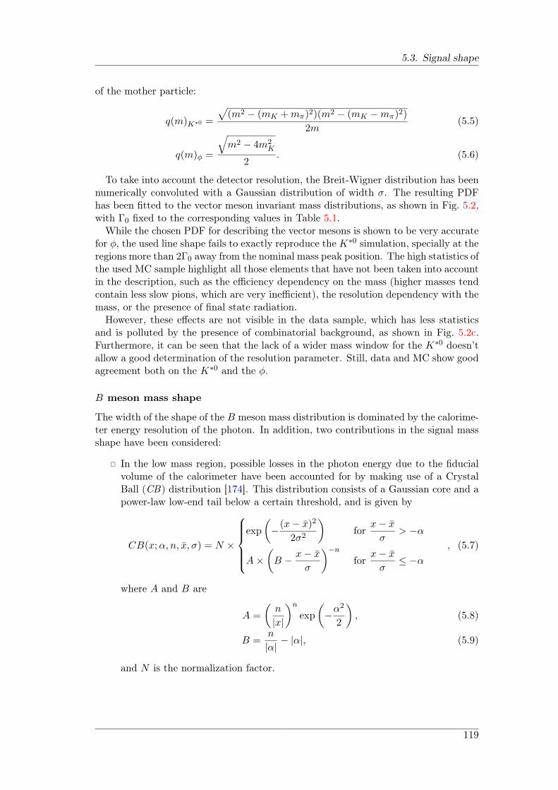
5.3. Signal shape
of the mother particle:
q(m)K∗0 =
√(m2 − (mK +mπ)2)(m2 − (mK −mπ)2)
2m(5.5)
q(m)ϕ =
√m2 − 4m2
K
2. (5.6)
To take into account the detector resolution, the Breit-Wigner distribution has beennumerically convoluted with a Gaussian distribution of width σ. The resulting PDFhas been fitted to the vector meson invariant mass distributions, as shown in Fig. 5.2,with Γ0 fixed to the corresponding values in Table 5.1.
While the chosen PDF for describing the vector mesons is shown to be very accuratefor ϕ, the used line shape fails to exactly reproduce the K∗0 simulation, specially at theregions more than 2Γ0 away from the nominal mass peak position. The high statistics ofthe used MC sample highlight all those elements that have not been taken into accountin the description, such as the efficiency dependency on the mass (higher masses tendcontain less slow pions, which are very inefficient), the resolution dependency with themass, or the presence of final state radiation.
However, these effects are not visible in the data sample, which has less statisticsand is polluted by the presence of combinatorial background, as shown in Fig. 5.2c.Furthermore, it can be seen that the lack of a wider mass window for the K∗0 doesn’tallow a good determination of the resolution parameter. Still, data and MC show goodagreement both on the K∗0 and the ϕ.
B meson mass shape
The width of the shape of the B meson mass distribution is dominated by the calorime-ter energy resolution of the photon. In addition, two contributions in the signal massshape have been considered:
In the low mass region, possible losses in the photon energy due to the fiducialvolume of the calorimeter have been accounted for by making use of a CrystalBall (CB) distribution [174]. This distribution consists of a Gaussian core and apower-law low-end tail below a certain threshold, and is given by
CB(x;α, n, x, σ) = N ×
exp
(−(x− x)2
2σ2
)for
x− x
σ> −α
A×(B − x− x
σ
)−n
forx− x
σ≤ −α
, (5.7)
where A and B are
A =
(n
|x|
)n
exp
(−α
2
2
), (5.8)
B =n
|α|− |α|, (5.9)
and N is the normalization factor.
119
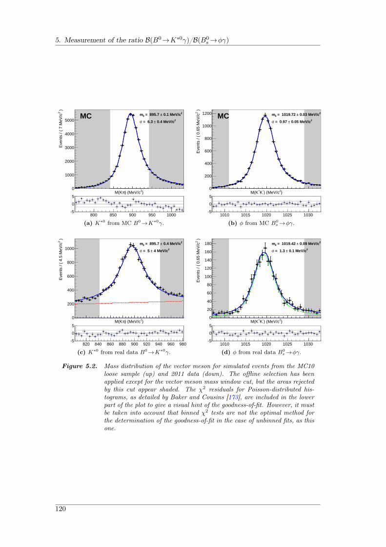
5. Measurement of the ratio B(B0→K∗0γ)/B(B0s →ϕγ)
)2) (MeV/cπM(K
)2E
vent
s / (
7 M
eV/c
0
1000
2000
3000
4000
5000
2 0.1 MeV/c± = 895.7 0m2 0.4 MeV/c± = 6.3 σ
MC
800 850 900 950 1000-5
0
5
(a) K∗0 from MC B0→K∗0γ.
)2) (MeV/c-K+M(K )2
Eve
nts
/ ( 0
.65
MeV
/c
0
200
400
600
800
1000
1200 2 0.03 MeV/c± = 1019.72 0m2 0.05 MeV/c± = 0.97 σ
MC
1010 1015 1020 1025 1030-5
0
5
(b) ϕ from MC B0s →ϕγ.
)2) (MeV/cπM(K
)2E
vent
s / (
4.5
MeV
/c
0
200
400
600
800
1000
2 0.4 MeV/c± = 895.7 0m2 4 MeV/c± = 5 σ
820 840 860 880 900 920 940 960 980-5
0
5
(c) K∗0 from real data B0→K∗0γ.
)2) (MeV/c-K+M(K
)2E
vent
s / (
0.6
5 M
eV/c
0
20
40
60
80
100
120
140
160
180 2 0.09 MeV/c± = 1019.42 0m2 0.1 MeV/c± = 1.3 σ
1010 1015 1020 1025 1030-5
0
5
(d) ϕ from real data B0s →ϕγ.
Figure 5.2. Mass distribution of the vector meson for simulated events from the MC10loose sample (up) and 2011 data (down). The offline selection has beenapplied except for the vector meson mass window cut, but the areas rejectedby this cut appear shaded. The χ2 residuals for Poisson-distributed his-tograms, as detailed by Baker and Cousins [173], are included in the lowerpart of the plot to give a visual hint of the goodness-of-fit. However, it mustbe taken into account that binned χ2 tests are not the optimal method forthe determination of the goodness-of-fit in the case of unbinned fits, as thisone.
120
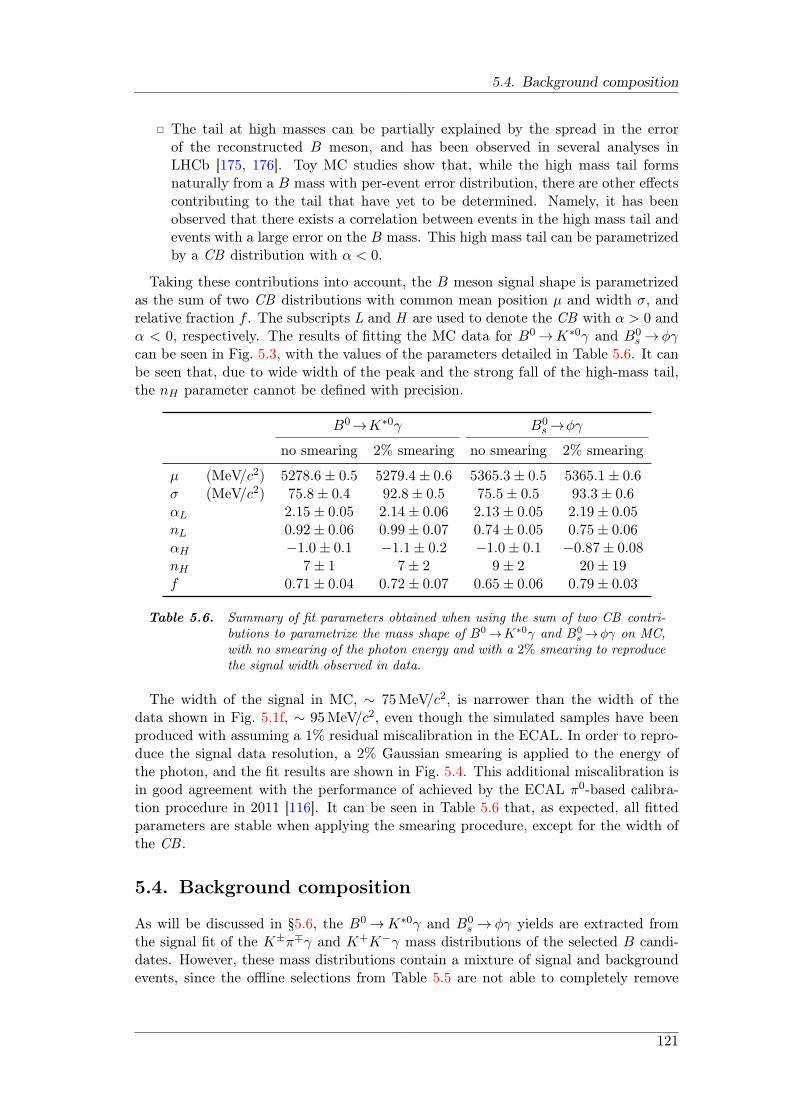
5.4. Background composition
The tail at high masses can be partially explained by the spread in the errorof the reconstructed B meson, and has been observed in several analyses inLHCb [175, 176]. Toy MC studies show that, while the high mass tail formsnaturally from a B mass with per-event error distribution, there are other effectscontributing to the tail that have yet to be determined. Namely, it has beenobserved that there exists a correlation between events in the high mass tail andevents with a large error on the B mass. This high mass tail can be parametrizedby a CB distribution with α < 0.
Taking these contributions into account, the B meson signal shape is parametrizedas the sum of two CB distributions with common mean position µ and width σ, andrelative fraction f . The subscripts L and H are used to denote the CB with α > 0 andα < 0, respectively. The results of fitting the MC data for B0 →K∗0γ and B0
s → ϕγcan be seen in Fig. 5.3, with the values of the parameters detailed in Table 5.6. It canbe seen that, due to wide width of the peak and the strong fall of the high-mass tail,the nH parameter cannot be defined with precision.
B0→K∗0γ B0s →ϕγ
no smearing 2% smearing no smearing 2% smearing
µ (MeV/c2) 5278.6± 0.5 5279.4± 0.6 5365.3± 0.5 5365.1± 0.6σ (MeV/c2) 75.8± 0.4 92.8± 0.5 75.5± 0.5 93.3± 0.6αL 2.15± 0.05 2.14± 0.06 2.13± 0.05 2.19± 0.05nL 0.92± 0.06 0.99± 0.07 0.74± 0.05 0.75± 0.06αH −1.0± 0.1 −1.1± 0.2 −1.0± 0.1 −0.87± 0.08nH 7± 1 7± 2 9± 2 20± 19f 0.71± 0.04 0.72± 0.07 0.65± 0.06 0.79± 0.03
Table 5.6. Summary of fit parameters obtained when using the sum of two CB contri-butions to parametrize the mass shape of B0→K∗0γ and B0
s →ϕγ on MC,with no smearing of the photon energy and with a 2% smearing to reproducethe signal width observed in data.
The width of the signal in MC, ∼ 75MeV/c2, is narrower than the width of thedata shown in Fig. 5.1f, ∼ 95MeV/c2, even though the simulated samples have beenproduced with assuming a 1% residual miscalibration in the ECAL. In order to repro-duce the signal data resolution, a 2% Gaussian smearing is applied to the energy ofthe photon, and the fit results are shown in Fig. 5.4. This additional miscalibration isin good agreement with the performance of achieved by the ECAL π0-based calibra-tion procedure in 2011 [116]. It can be seen in Table 5.6 that, as expected, all fittedparameters are stable when applying the smearing procedure, except for the width ofthe CB .
5.4. Background composition
As will be discussed in §5.6, the B0 →K∗0γ and B0s → ϕγ yields are extracted from
the signal fit of the K±π∓γ and K+K−γ mass distributions of the selected B candi-dates. However, these mass distributions contain a mixture of signal and backgroundevents, since the offline selections from Table 5.5 are not able to completely remove
121
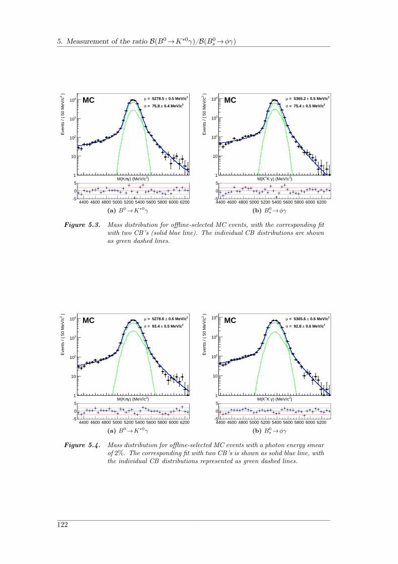
5. Measurement of the ratio B(B0→K∗0γ)/B(B0s →ϕγ)
)2) (MeV/cγπM(K
)2E
vent
s / (
50
MeV
/c
1
10
210
310
4102 0.5 MeV/c± = 5278.5 µ
2 0.4 MeV/c± = 75.8 σMC
4400 4600 4800 5000 5200 5400 5600 5800 6000 6200-5
0
5
(a) B0→K∗0γ
)2) (MeV/cγ-K+M(K
)2E
vent
s / (
50
MeV
/c
1
10
210
310
4102 0.5 MeV/c± = 5365.2 µ
2 0.5 MeV/c± = 75.4 σMC
4400 4600 4800 5000 5200 5400 5600 5800 6000 6200-5
0
5
(b) B0s →ϕγ
Figure 5.3. Mass distribution for offline-selected MC events, with the corresponding fitwith two CB ’s (solid blue line). The individual CB distributions are shownas green dashed lines.
)2) (MeV/cγπM(K
)2E
vent
s / (
50
MeV
/c
1
10
210
310
410 2 0.6 MeV/c± = 5278.6 µ2 0.5 MeV/c± = 93.4 σ
MC
4400 4600 4800 5000 5200 5400 5600 5800 6000 6200-5
0
5
(a) B0→K∗0γ
)2) (MeV/cγ-K+M(K
)2E
vent
s / (
50
MeV
/c
1
10
210
310
410 2 0.6 MeV/c± = 5365.6 µ2 0.6 MeV/c± = 92.8 σ
MC
4400 4600 4800 5000 5200 5400 5600 5800 6000 6200-5
0
5
(b) B0s →ϕγ
Figure 5.4. Mass distribution for offline-selected MC events with a photon energy smearof 2%. The corresponding fit with two CB ’s is shown as solid blue line, withthe individual CB distributions represented as green dashed lines.
122
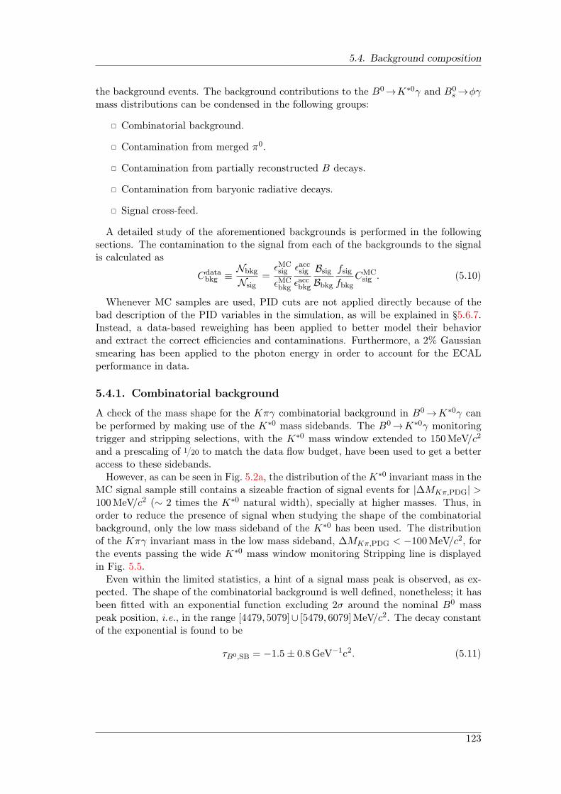
5.4. Background composition
the background events. The background contributions to the B0→K∗0γ and B0s →ϕγ
mass distributions can be condensed in the following groups:
Combinatorial background.
Contamination from merged π0.
Contamination from partially reconstructed B decays.
Contamination from baryonic radiative decays.
Signal cross-feed.
A detailed study of the aforementioned backgrounds is performed in the followingsections. The contamination to the signal from each of the backgrounds to the signalis calculated as
Cdatabkg ≡
Nbkg
Nsig=ϵMCsig
ϵMCbkg
ϵaccsig
ϵaccbkg
Bsig
Bbkg
fsig
fbkgCMC
sig . (5.10)
Whenever MC samples are used, PID cuts are not applied directly because of thebad description of the PID variables in the simulation, as will be explained in §5.6.7.Instead, a data-based reweighing has been applied to better model their behaviorand extract the correct efficiencies and contaminations. Furthermore, a 2% Gaussiansmearing has been applied to the photon energy in order to account for the ECALperformance in data.
5.4.1. Combinatorial background
A check of the mass shape for the Kπγ combinatorial background in B0→K∗0γ canbe performed by making use of the K∗0 mass sidebands. The B0→K∗0γ monitoringtrigger and stripping selections, with the K∗0 mass window extended to 150MeV/c2
and a prescaling of 1/20 to match the data flow budget, have been used to get a betteraccess to these sidebands.
However, as can be seen in Fig. 5.2a, the distribution of the K∗0 invariant mass in theMC signal sample still contains a sizeable fraction of signal events for |∆MKπ,PDG| >100MeV/c2 (∼ 2 times the K∗0 natural width), specially at higher masses. Thus, inorder to reduce the presence of signal when studying the shape of the combinatorialbackground, only the low mass sideband of the K∗0 has been used. The distributionof the Kπγ invariant mass in the low mass sideband, ∆MKπ,PDG < −100MeV/c2, forthe events passing the wide K∗0 mass window monitoring Stripping line is displayedin Fig. 5.5.
Even within the limited statistics, a hint of a signal mass peak is observed, as ex-pected. The shape of the combinatorial background is well defined, nonetheless; it hasbeen fitted with an exponential function excluding 2σ around the nominal B0 masspeak position, i.e., in the range [4479, 5079]∪ [5479, 6079]MeV/c2. The decay constantof the exponential is found to be
τB0,SB = −1.5± 0.8GeV−1c2. (5.11)
123
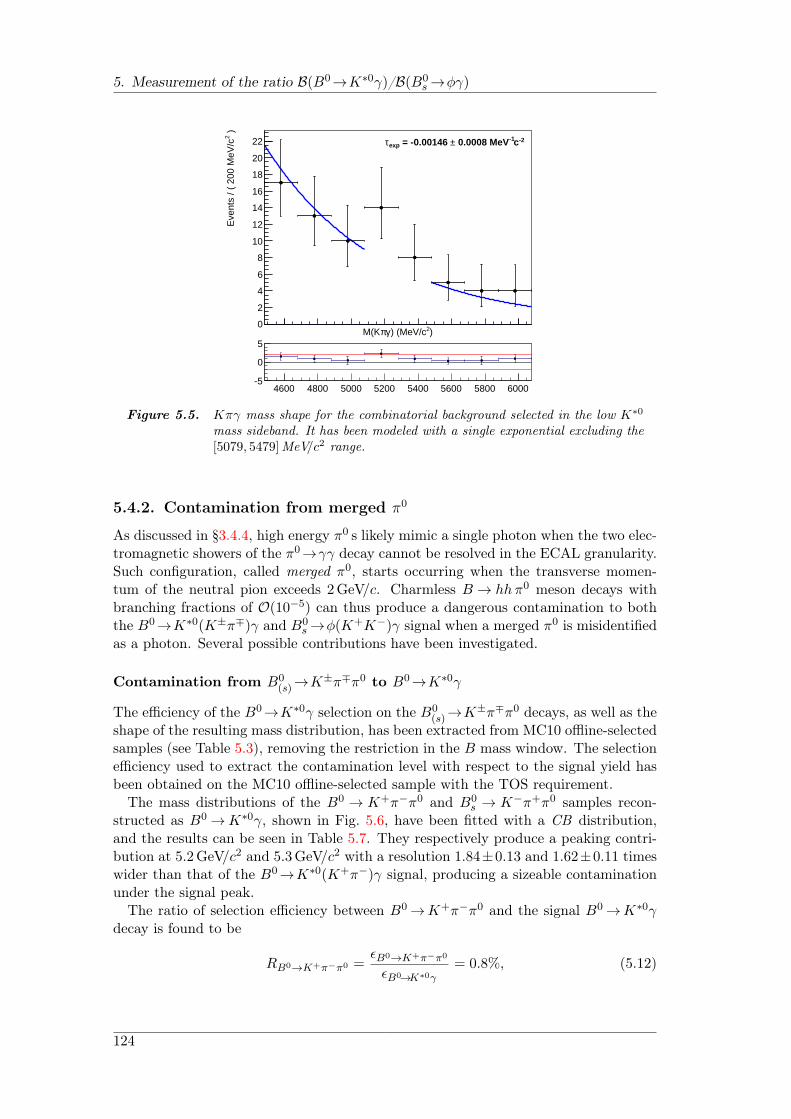
5. Measurement of the ratio B(B0→K∗0γ)/B(B0s →ϕγ)
)2) (MeV/cγπM(K
)2E
vent
s / (
200
MeV
/c
0
2
4
6
8
10
12
14
16
18
20
22 -2c-1 0.0008 MeV± = -0.00146 expτ
4600 4800 5000 5200 5400 5600 5800 6000-5
0
5
Figure 5.5. Kπγ mass shape for the combinatorial background selected in the low K∗0
mass sideband. It has been modeled with a single exponential excluding the[5079, 5479]MeV/c2 range.
5.4.2. Contamination from merged π0
As discussed in §3.4.4, high energy π0 s likely mimic a single photon when the two elec-tromagnetic showers of the π0→γγ decay cannot be resolved in the ECAL granularity.Such configuration, called merged π0, starts occurring when the transverse momen-tum of the neutral pion exceeds 2GeV/c. Charmless B → hhπ0 meson decays withbranching fractions of O(10−5) can thus produce a dangerous contamination to boththe B0→K∗0(K±π∓)γ and B0
s →ϕ(K+K−)γ signal when a merged π0 is misidentifiedas a photon. Several possible contributions have been investigated.
Contamination from B0(s)→K±π∓π0 to B0→K∗0γ
The efficiency of the B0→K∗0γ selection on the B0(s)→K±π∓π0 decays, as well as the
shape of the resulting mass distribution, has been extracted from MC10 offline-selectedsamples (see Table 5.3), removing the restriction in the B mass window. The selectionefficiency used to extract the contamination level with respect to the signal yield hasbeen obtained on the MC10 offline-selected sample with the TOS requirement.
The mass distributions of the B0 → K+π−π0 and B0s → K−π+π0 samples recon-
structed as B0 →K∗0γ, shown in Fig. 5.6, have been fitted with a CB distribution,and the results can be seen in Table 5.7. They respectively produce a peaking contri-bution at 5.2GeV/c2 and 5.3GeV/c2 with a resolution 1.84±0.13 and 1.62±0.11 timeswider than that of the B0→K∗0(K+π−)γ signal, producing a sizeable contaminationunder the signal peak.
The ratio of selection efficiency between B0 →K+π−π0 and the signal B0 →K∗0γdecay is found to be
RB0→K+π−π0 =ϵB0→K+π−π0
ϵB0→K∗0γ= 0.8%, (5.12)
124
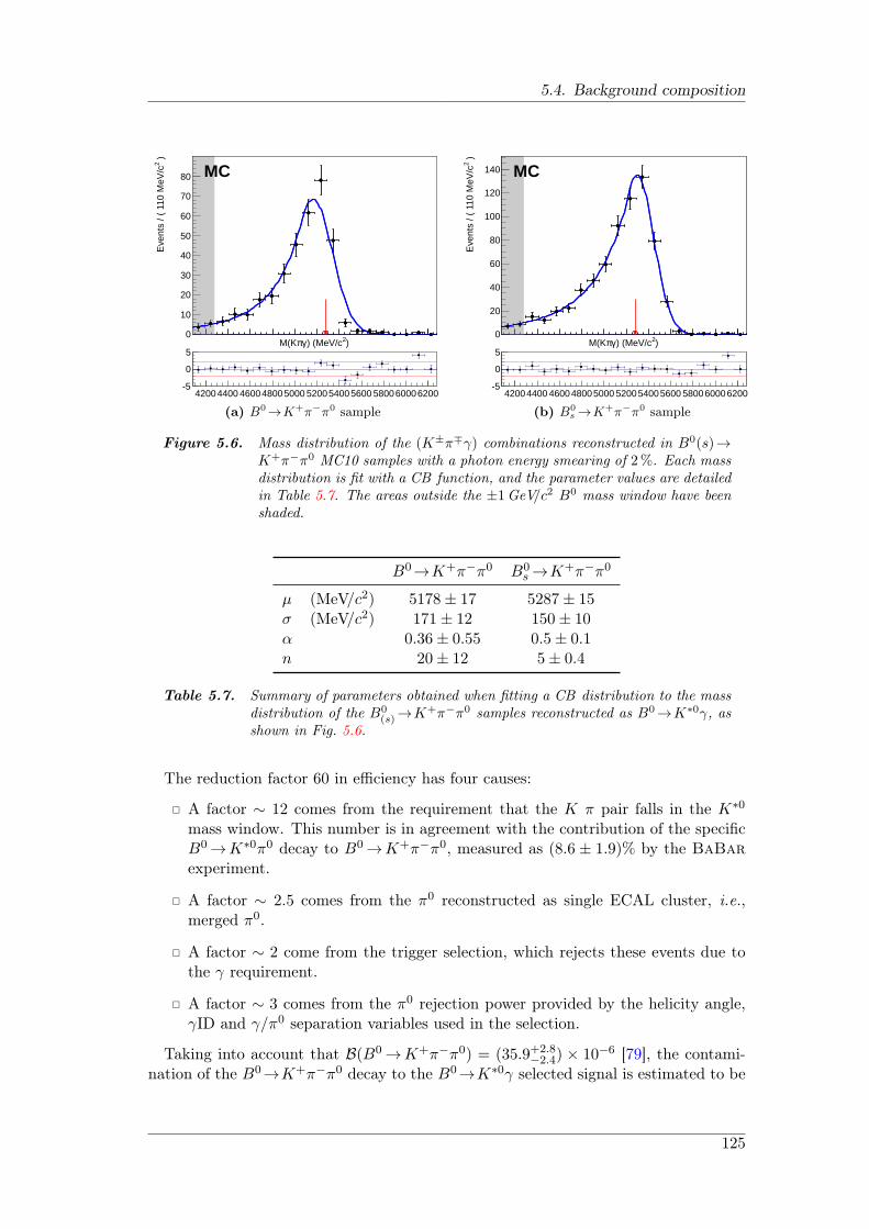
5.4. Background composition
)2) (MeV/cγπM(K
)2E
vent
s / (
110
MeV
/c
0
10
20
30
40
50
60
70
80 MC
42004400 460048005000 520054005600 580060006200-5
0
5
(a) B0→K+π−π0 sample
)2) (MeV/cγπM(K
)2E
vent
s / (
110
MeV
/c
0
20
40
60
80
100
120
140 MC
42004400 460048005000 520054005600 580060006200-5
0
5
(b) B0s →K+π−π0 sample
Figure 5.6. Mass distribution of the (K±π∓γ) combinations reconstructed in B0(s)→K+π−π0 MC10 samples with a photon energy smearing of 2%. Each massdistribution is fit with a CB function, and the parameter values are detailedin Table 5.7. The areas outside the ±1GeV/c2 B0 mass window have beenshaded.
B0→K+π−π0 B0s →K+π−π0
µ (MeV/c2) 5178± 17 5287± 15σ (MeV/c2) 171± 12 150± 10α 0.36± 0.55 0.5± 0.1n 20± 12 5± 0.4
Table 5.7. Summary of parameters obtained when fitting a CB distribution to the massdistribution of the B0
(s)→K+π−π0 samples reconstructed as B0→K∗0γ, asshown in Fig. 5.6.
The reduction factor 60 in efficiency has four causes:
A factor ∼ 12 comes from the requirement that the K π pair falls in the K∗0
mass window. This number is in agreement with the contribution of the specificB0→K∗0π0 decay to B0→K+π−π0, measured as (8.6 ± 1.9)% by the BaBarexperiment.
A factor ∼ 2.5 comes from the π0 reconstructed as single ECAL cluster, i.e.,merged π0.
A factor ∼ 2 come from the trigger selection, which rejects these events due tothe γ requirement.
A factor ∼ 3 comes from the π0 rejection power provided by the helicity angle,γID and γ/π0 separation variables used in the selection.
Taking into account that B(B0 →K+π−π0) = (35.9+2.8−2.4) × 10−6 [79], the contami-
nation of the B0→K+π−π0 decay to the B0→K∗0γ selected signal is estimated to be
125

5. Measurement of the ratio B(B0→K∗0γ)/B(B0s →ϕγ)
CB0→K+π−π0 =N sel
B0→K+π−π0
N selB0→K∗0γ
= (0.5± 0.1)%, (5.13)
where the dominating uncertainty comes from the error on the measured branchingfractions.
The B0s →K−π+π0 decay, not yet observed so far, proceeds via a Cabibbo-suppressed
penguin diagram. Conservatively assuming the same branching ratio as for the cor-responding B0 decay and the same K∗0π0 fraction, the contamination to B0→K∗0γoffline-selected signal is predicted to be
CB0s→K−π+π0 =
N selB0
s→K−π+π0
N selB0→K∗0γ
= (0.2± 0.2)%, (5.14)
which is reduced with respect to the analogous B0 decay due to the relative hadroniza-tion factor, fs/fd. A conservative uncertainty has been taken due to the lack of preciseknowledge of the corresponding branching fraction.
Contamination from B0s →K±K∓π0 to B0
s →ϕγ
In a similar way, the not yet observed B0s →K±K∓π0 decay can pollute the B0
s →ϕγsignal. Like the B0 → K∗0γ contribution to the B0 → K+π−π0 decay discussed in[177], the dangerous B0
s → ϕπ0 contribution to the B0s → K+K−π0 decay proceeds
via color-suppressed b → s penguin and b → u transitions. However, these diagramsinterfere with the B0
s →K∗∓(K+π0)K± tree and penguin transitions, which may havea significantly larger amplitude than the SU(2)-related mode, B0→K∗+(K+π0)π−.
A contamination of 0.6±0.6% is assumed, corresponding to the contamination of theB0→K+π−π0 decay to B0→K∗0γ signal. The large uncertainty is assigned to handlethe unknown level of this contamination, allowing it to be a factor 2 larger than in theSU(2)-related mode. The line shape is also assumed to be the same as B0→K+π−π0
reconstructed as B0 →K∗0γ, shifting the µ position by the mass difference betweenthe B0 and B0
s mesons.
Other contaminations from charmless decays with π0
Contamination from B0→π+π−π0, shown in Fig. 5.7, and B0s →K+K−π0 to the B0→
K∗0γ invariant mass window requires a π/K misidentification and is further suppressed.The relative contribution of these two decays has found to be of O(10−4), and thereforethey can be neglected. Likewise for the contamination from B0
(s)→K+(−)π−(+)π0 toB0
s →ϕγ.
5.4.3. Contamination from partially reconstructed B decays
The partial reconstruction of a decay fragment from both charmless and charmedB → V (γ/π0)X decays, where V denotes either K∗0 or ϕ, may provide a sizeablecontamination in the low mass side of the signal region.
As detailed in §5.2, several variables used in the signal selection are designed to fightagainst these partially reconstructed n-body B decays; in particular, the angle of the Bcandidate momentum with respect to its flight direction provided by the primary and
126
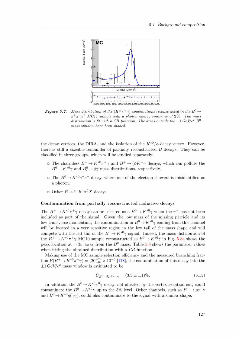
5.4. Background composition
)2) (MeV/cγπM(K
)2E
vent
s / (
110
MeV
/c0
1
2
3
4
5MC
42004400 460048005000 520054005600 580060006200-5
0
5
Figure 5.7. Mass distribution of the (K±π∓γ) combinations reconstructed in the B0→π+π−π0 MC11 sample with a photon energy smearing of 2%. The massdistribution is fit with a CB function. The areas outside the ±1GeV/c2 B0
mass window have been shaded.
the decay vertices, the DIRA, and the isolation of the K∗0/ϕ decay vertex. However,there is still a sizeable remainder of partially reconstructed B decays. They can beclassified in three groups, which will be studied separately:
The charmless B+ →K∗0π+γ and B+ → (ϕK+γ decays, which can pollute theB0→K∗0γ and B0
s →ϕγ mass distributions, respectively.
The B0→K∗0e+e− decay, where one of the electron showers is misidentified asa photon.
Other B→h+h−π0X decays.
Contamination from partially reconstructed radiative decays
The B+→K∗0π+γ decay can be selected as a B0→K∗0γ when the π+ has not beenincluded as part of the signal. Given the low mass of the missing particle and itslow transverse momentum, the contamination in B0→K∗0γ coming from this channelwill be located in a very sensitive region in the low tail of the mass shape and willcompete with the left tail of the B0 →K∗0γ signal. Indeed, the mass distribution ofthe B+ →K∗0π+γ MC10 sample reconstructed as B0 →K∗0γ in Fig. 5.8a shows thepeak location at ∼ 3σ away from the B0 mass. Table 5.8 shows the parameter valueswhen fitting the obtained distribution with a CB function.
Making use of the MC sample selection efficiency and the measured branching frac-tion B(B+→K∗0π+γ) = (20+7
−6)× 10−6 [178], the contamination of this decay into the±1GeV/c2 mass window is estimated to be
CB+→K∗0π+γ = (3.3± 1.1)%. (5.15)
In addition, the B0→K∗0π0γ decay, not affected by the vertex isolation cut, couldcontaminate the B0→K∗0γ up to the 5% level. Other channels, such as B+→ ρe+νand B0→K∗0η(γγ), could also contaminate to the signal with a similar shape.
127
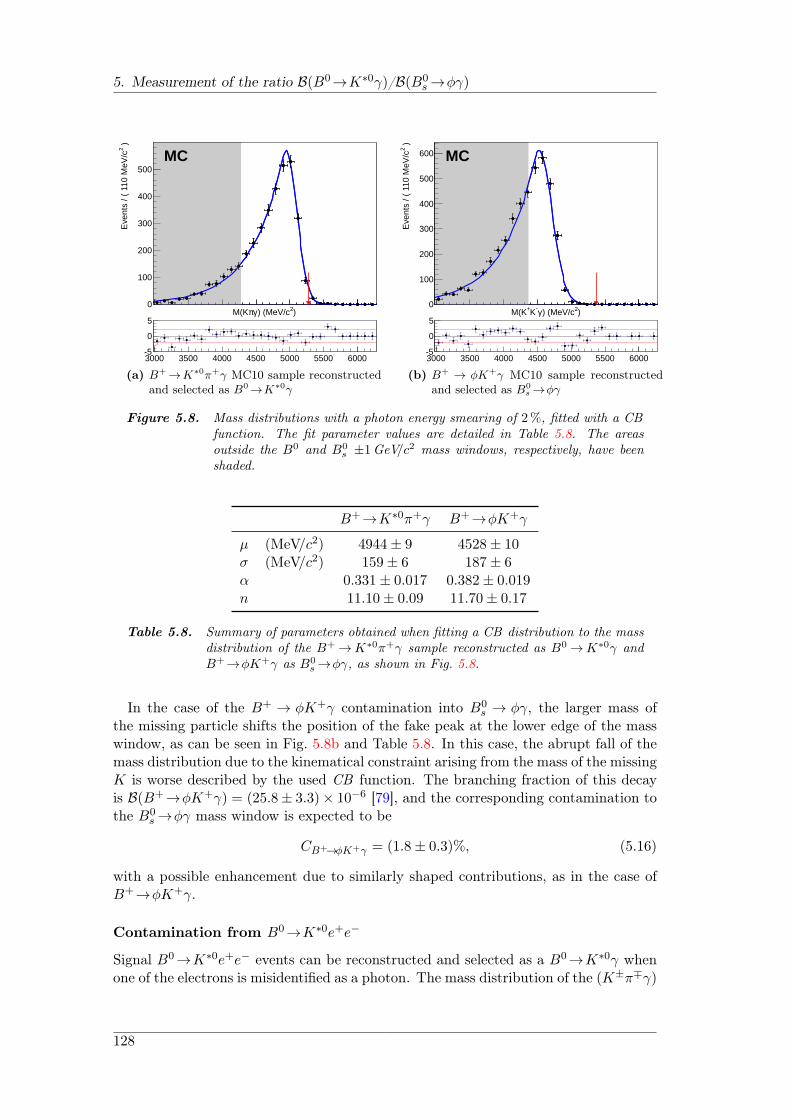
5. Measurement of the ratio B(B0→K∗0γ)/B(B0s →ϕγ)
)2) (MeV/cγπM(K
)2E
vent
s / (
110
MeV
/c
0
100
200
300
400
500MC
3000 3500 4000 4500 5000 5500 6000-5
0
5
(a) B+→K∗0π+γ MC10 sample reconstructedand selected as B0→K∗0γ
)2) (MeV/cγ-K+M(K
)2E
vent
s / (
110
MeV
/c
0
100
200
300
400
500
600 MC
3000 3500 4000 4500 5000 5500 6000-5
0
5
(b) B+ → ϕK+γ MC10 sample reconstructedand selected as B0
s →ϕγ
Figure 5.8. Mass distributions with a photon energy smearing of 2%, fitted with a CBfunction. The fit parameter values are detailed in Table 5.8. The areasoutside the B0 and B0
s ±1GeV/c2 mass windows, respectively, have beenshaded.
B+→K∗0π+γ B+→ϕK+γ
µ (MeV/c2) 4944± 9 4528± 10σ (MeV/c2) 159± 6 187± 6α 0.331± 0.017 0.382± 0.019n 11.10± 0.09 11.70± 0.17
Table 5.8. Summary of parameters obtained when fitting a CB distribution to the massdistribution of the B+ →K∗0π+γ sample reconstructed as B0 →K∗0γ andB+→ϕK+γ as B0
s →ϕγ, as shown in Fig. 5.8.
In the case of the B+ → ϕK+γ contamination into B0s → ϕγ, the larger mass of
the missing particle shifts the position of the fake peak at the lower edge of the masswindow, as can be seen in Fig. 5.8b and Table 5.8. In this case, the abrupt fall of themass distribution due to the kinematical constraint arising from the mass of the missingK is worse described by the used CB function. The branching fraction of this decayis B(B+→ϕK+γ) = (25.8± 3.3)× 10−6 [79], and the corresponding contamination tothe B0
s →ϕγ mass window is expected to be
CB+→ϕK+γ = (1.8± 0.3)%, (5.16)
with a possible enhancement due to similarly shaped contributions, as in the case ofB+→ϕK+γ.
Contamination from B0→K∗0e+e−
Signal B0→K∗0e+e− events can be reconstructed and selected as a B0→K∗0γ whenone of the electrons is misidentified as a photon. The mass distribution of the (K±π∓γ)
128
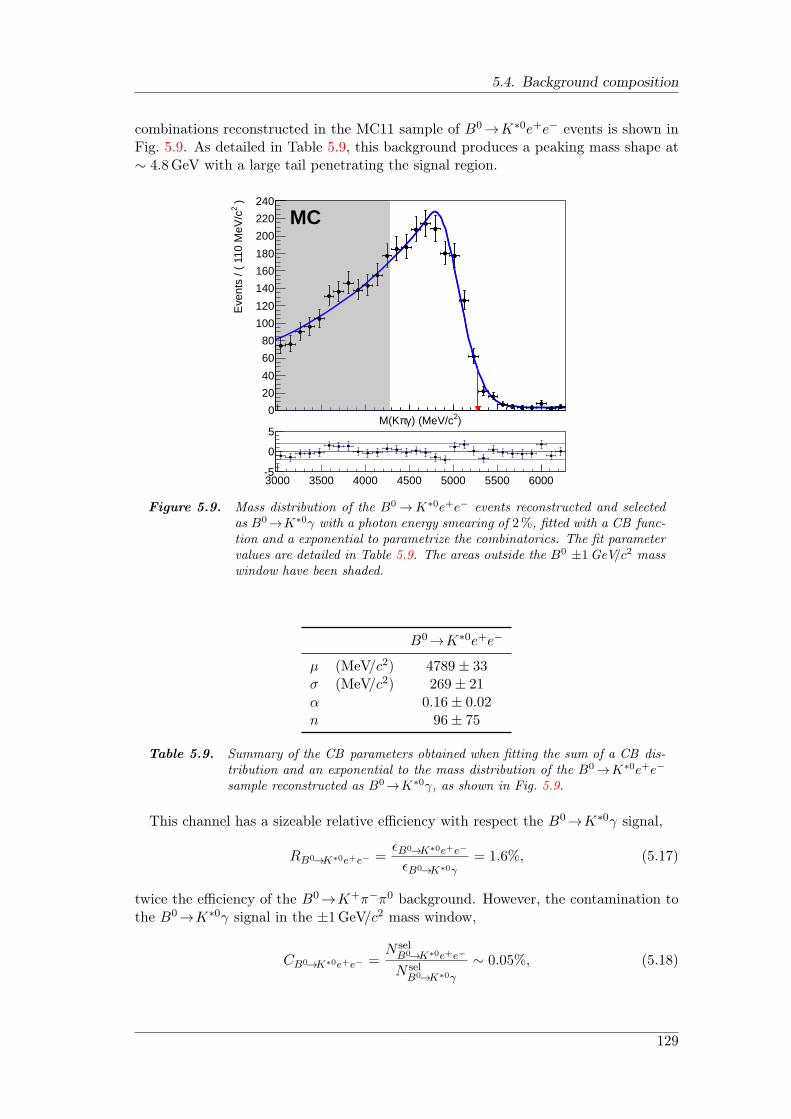
5.4. Background composition
combinations reconstructed in the MC11 sample of B0→K∗0e+e− events is shown inFig. 5.9. As detailed in Table 5.9, this background produces a peaking mass shape at∼ 4.8GeV with a large tail penetrating the signal region.
)2) (MeV/cγπM(K
)2E
vent
s / (
110
MeV
/c
0
20
40
60
80
100
120
140
160
180
200
220
240
MC
3000 3500 4000 4500 5000 5500 6000-5
0
5
Figure 5.9. Mass distribution of the B0 →K∗0e+e− events reconstructed and selectedas B0→K∗0γ with a photon energy smearing of 2%, fitted with a CB func-tion and a exponential to parametrize the combinatorics. The fit parametervalues are detailed in Table 5.9. The areas outside the B0 ±1GeV/c2 masswindow have been shaded.
B0→K∗0e+e−
µ (MeV/c2) 4789± 33σ (MeV/c2) 269± 21α 0.16± 0.02n 96± 75
Table 5.9. Summary of the CB parameters obtained when fitting the sum of a CB dis-tribution and an exponential to the mass distribution of the B0→K∗0e+e−
sample reconstructed as B0→K∗0γ, as shown in Fig. 5.9.
This channel has a sizeable relative efficiency with respect the B0→K∗0γ signal,
RB0→K∗0e+e− =ϵB0→K∗0e+e−
ϵB0→K∗0γ= 1.6%, (5.17)
twice the efficiency of the B0→K+π−π0 background. However, the contamination tothe B0→K∗0γ signal in the ±1GeV/c2 mass window,
CB0→K∗0e+e− =N sel
B0→K∗0e+e−
N selB0→K∗0γ
∼ 0.05%, (5.18)
129
5. Measurement of the ratio B(B0→K∗0γ)/B(B0s →ϕγ)
is negligible due to the O(102) reduction factor of its branching fraction with respectto B0→K∗0γ [179], giving B(B0→K∗0e+e−) = (1.03+0.19
−0.17)× 10−6.
Contamination from other B→h+h−π0X decays
Many meson decays —other than the ones previously discussed— can exhibit a finalstate topology close to the B0 →K∗0γ and B0
s → ϕγ signals when one of their decayproducts is not included. The K∗0/ϕ production from B0/B+ is of O(10%) and there-fore the branching fraction of the partially reconstructed background is potentially fourorders of magnitude above the B0 →K∗0γ and B0
s →ϕγ signals. Given the fact thatthe rejection of the partially reconstructed background by the offline selections is ofO(106), the remaining contamination may be significant.
These potentially dangerous decays involving high energy neutral pions have beenscrutinized at the simulation level by making use of a cocktail of MC10 B→h+h−π0Xdecays, where X stands for a single particle or a multi-body object, including:
B+→K∗+(K+π0)π+π−.
B+→J/Ψ(π+π−π0)K+.
B0→D0(Kππ0)K∗0(K+π−).
B+→K+K−K+π0.
B0→D−(K + π−π−)ρ+(π+π0).
The reconstructed K±π∓γ mass in this cocktail of partially reconstructed back-grounds is shown in Fig. 5.10.
Following the ideas in [180], the shape of this background has been parametrized bya generalized Argus function [181], given by
A(m;m0, c, p) =2−pc2(p+1)
Γ(p+ 1)− Γ(p+ 1, 12c
2)
m
m20
(1− m2
m20
)p
e− 1
2c2(1−m2
m20
), (5.19)
where Γ( · ) is the gamma function and Γ( · ; · ) is the upper incomplete gamma function.The parameters m0, c and p represent the cutoff, curvature and power, respectively,with 0 ≤ m ≤ m0.
B→h+h−(γ/π0)X
m0 (MeV/c2) 5089± 96c 20± 4p 7.1± 1.7
Table 5.10. Summary of the parameters obtained when fitting the Argus distribution(with an exponential for the combinatorics) to the K±π∓γ mass distributionof the B→h+h−(γ/π0)X cocktail sample reconstructed as B0→K∗0γ, asshown in Fig. 5.10.
Unfortunately, the lack of a sizeable amount of statistics of the suitable MC samplesdoesn’t allow to perform the same study with B→h+h−π0X events reconstructed asB0
s →ϕγ, since the narrow mass window for the ϕ rejects most of the events.
130
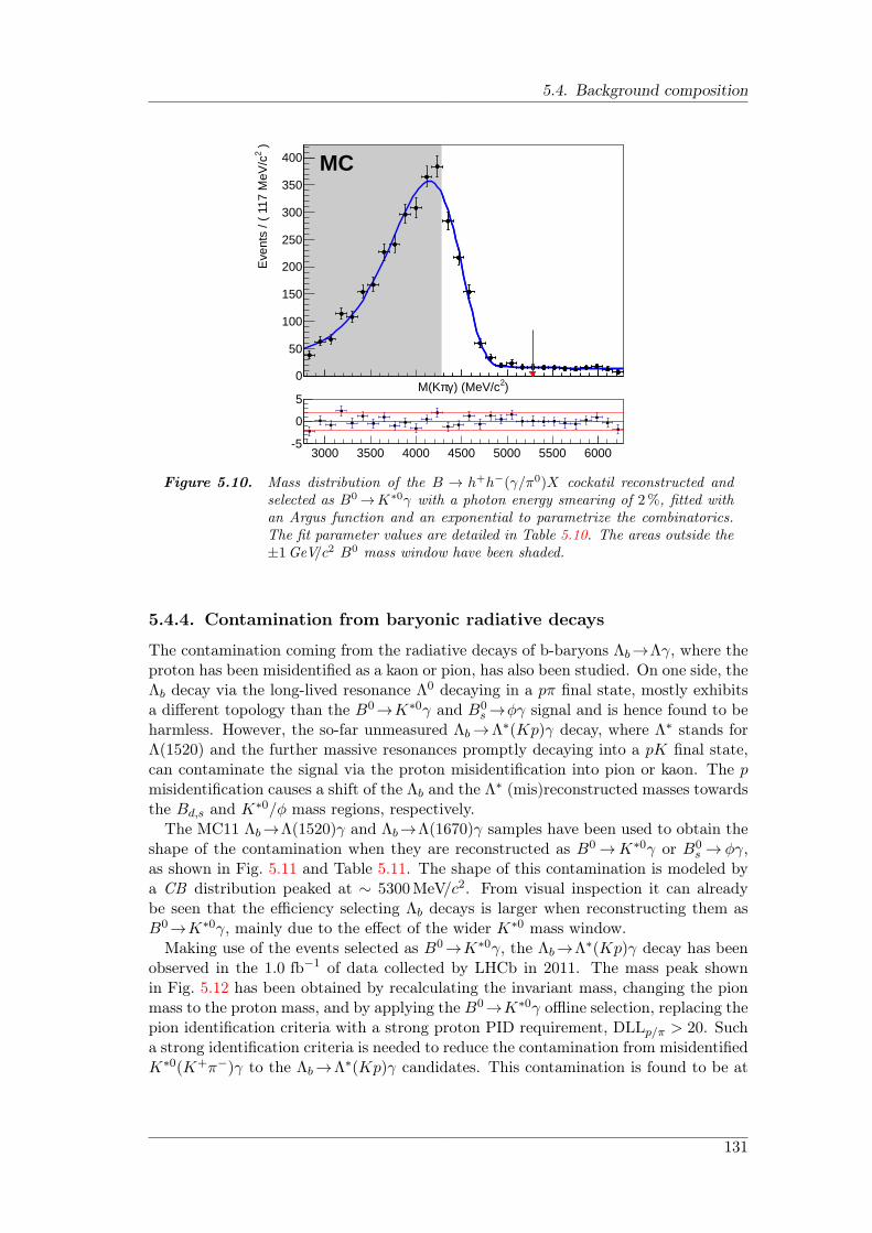
5.4. Background composition
)2) (MeV/cγπM(K
)2E
vent
s / (
117
MeV
/c
0
50
100
150
200
250
300
350
400 MC
3000 3500 4000 4500 5000 5500 6000-5
0
5
Figure 5.10. Mass distribution of the B → h+h−(γ/π0)X cockatil reconstructed andselected as B0 →K∗0γ with a photon energy smearing of 2%, fitted withan Argus function and an exponential to parametrize the combinatorics.The fit parameter values are detailed in Table 5.10. The areas outside the±1GeV/c2 B0 mass window have been shaded.
5.4.4. Contamination from baryonic radiative decays
The contamination coming from the radiative decays of b-baryons Λb→Λγ, where theproton has been misidentified as a kaon or pion, has also been studied. On one side, theΛb decay via the long-lived resonance Λ0 decaying in a pπ final state, mostly exhibitsa different topology than the B0→K∗0γ and B0
s →ϕγ signal and is hence found to beharmless. However, the so-far unmeasured Λb→Λ∗(Kp)γ decay, where Λ∗ stands forΛ(1520) and the further massive resonances promptly decaying into a pK final state,can contaminate the signal via the proton misidentification into pion or kaon. The pmisidentification causes a shift of the Λb and the Λ∗ (mis)reconstructed masses towardsthe Bd,s and K∗0/ϕ mass regions, respectively.
The MC11 Λb→Λ(1520)γ and Λb→Λ(1670)γ samples have been used to obtain theshape of the contamination when they are reconstructed as B0 →K∗0γ or B0
s → ϕγ,as shown in Fig. 5.11 and Table 5.11. The shape of this contamination is modeled bya CB distribution peaked at ∼ 5300MeV/c2. From visual inspection it can alreadybe seen that the efficiency selecting Λb decays is larger when reconstructing them asB0→K∗0γ, mainly due to the effect of the wider K∗0 mass window.
Making use of the events selected as B0→K∗0γ, the Λb→Λ∗(Kp)γ decay has beenobserved in the 1.0 fb−1 of data collected by LHCb in 2011. The mass peak shownin Fig. 5.12 has been obtained by recalculating the invariant mass, changing the pionmass to the proton mass, and by applying the B0→K∗0γ offline selection, replacing thepion identification criteria with a strong proton PID requirement, DLLp/π > 20. Sucha strong identification criteria is needed to reduce the contamination from misidentifiedK∗0(K+π−)γ to the Λb→Λ∗(Kp)γ candidates. This contamination is found to be at
131

5. Measurement of the ratio B(B0→K∗0γ)/B(B0s →ϕγ)
)2) (MeV/cγπM(K
)2E
vent
s / (
70
MeV
/c
0
200
400
600
800
1000 MC
4200 4400 4600 4800 5000 5200 5400 5600 5800 6000 6200-5
0
5
(a) B0→K∗0γ selection.
)2) (MeV/cγ-K+M(K
)2E
vent
s / (
140
MeV
/c
0
20
40
60
80
100MC
4400 4600 4800 5000 5200 5400 5600 5800 6000 6200-5
0
5
(b) B0s →ϕγ selection.
Figure 5.11. Mass distribution of the Λb→Λ(1520)γ and Λb→Λ(1670)γ MC11 samplesreconstructed and offline-selected as B0 → K∗0γ and B0
s → ϕγ, with aphoton energy smearing of 2%. Each mass distribution is fit with a CBfunction, the parameter values of which are detailed in Table 5.11. Theareas outside the B0 and B0
s ±1GeV/c2 mass windows, respectively, havebeen shaded.
B0→K∗0γ selection B0s →ϕγ selection
µ (MeV/c2) 5316± 4 5367± 12σ (MeV/c2) 141± 4 147± 10α 0.77± 0.06 1.0± 0.2n 5.0± 1.7 4± 4
Table 5.11. Summary of parameters obtained when fitting a CB distribution to the massdistribution of the Λb → Λ(1520)γ and Λb → Λ(1670)γ MC11 samples re-constructed and offline-selected as B0 →K∗0γ and B0
s → ϕγ, as shown inFig. 5.11.
the level of (3.2± 0.5)%, and needs to be subtracted to the number of fitted events inFig. 5.12, 263 ± 26. After the correction, the number of Λb → Λ∗γ events is found tobe
NB0→K∗0γ(Λb→Λ∗γ) = 255± 25, (5.20)
where the superscript in N indicates that the yield has been obtained on a sampleselected as B0→K∗0γ.
As the visible branching fraction of Λb→Λ∗(Kp)γ has not been measured so far, thecontamination from such decays to B0→K∗0γ,
CΛb→Λ∗γ ≡ NB0→K∗0γ(Λb → Λ∗γ)
NB0→K∗0γ(B0→K∗0γ)
=ϵB
0→K∗0γ(Λb→Λ∗γ)
ϵB0→K∗0γ(B0→K∗0γ)
B(Λb→Λ∗γ)
B(B0→K∗0γ)
fΛfd, (5.21)
132
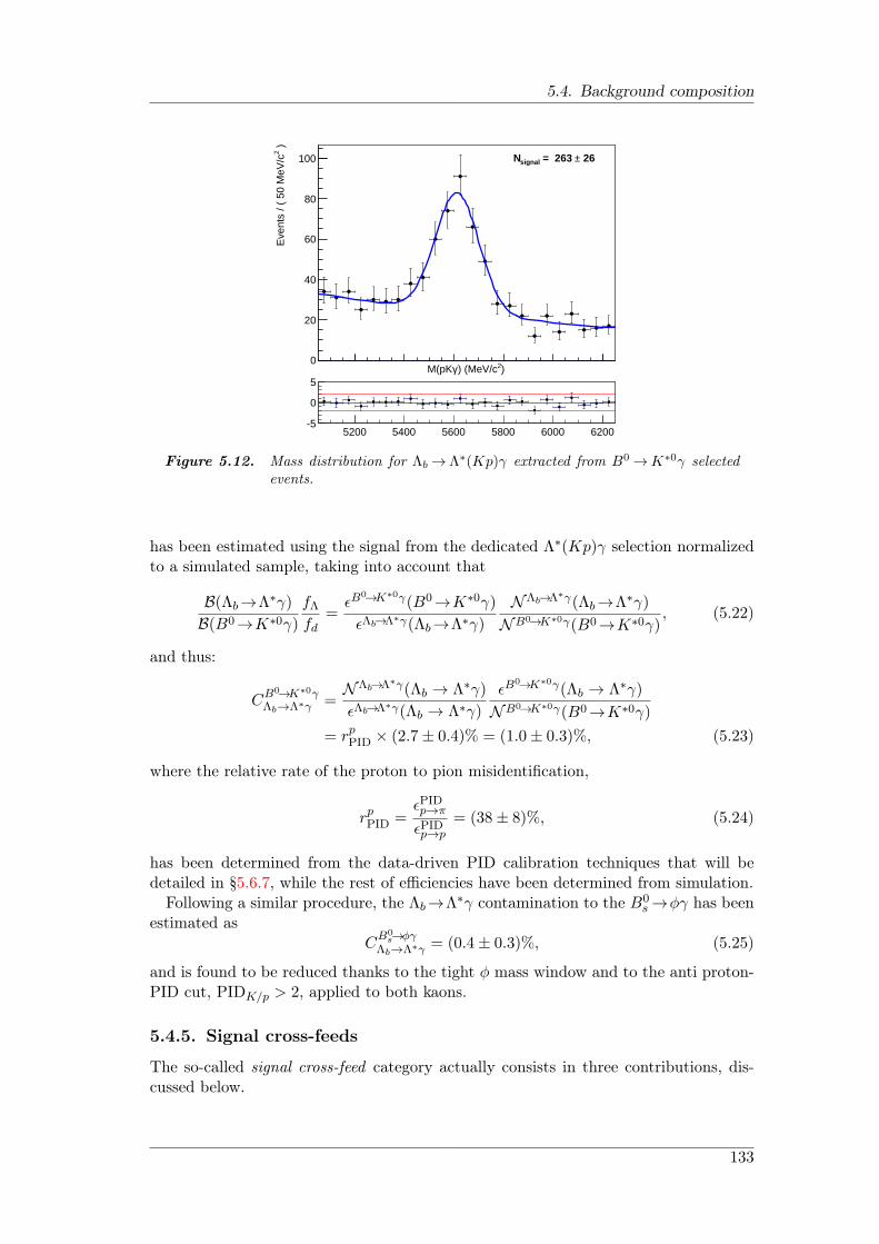
5.4. Background composition
)2) (MeV/cγM(pK
)2E
vent
s / (
50
MeV
/c
0
20
40
60
80
100 26± = 263 signalN
5200 5400 5600 5800 6000 6200-5
0
5
Figure 5.12. Mass distribution for Λb → Λ∗(Kp)γ extracted from B0 →K∗0γ selectedevents.
has been estimated using the signal from the dedicated Λ∗(Kp)γ selection normalizedto a simulated sample, taking into account that
B(Λb→Λ∗γ)
B(B0→K∗0γ)
fΛfd
=ϵB
0→K∗0γ(B0→K∗0γ)
ϵΛb→Λ∗γ(Λb→Λ∗γ)
NΛb→Λ∗γ(Λb→Λ∗γ)
NB0→K∗0γ(B0→K∗0γ), (5.22)
and thus:
CB0→K∗0γΛb→Λ∗γ =
NΛb→Λ∗γ(Λb → Λ∗γ)
ϵΛb→Λ∗γ(Λb → Λ∗γ)
ϵB0→K∗0γ(Λb → Λ∗γ)
NB0→K∗0γ(B0→K∗0γ)
= rpPID × (2.7± 0.4)% = (1.0± 0.3)%, (5.23)
where the relative rate of the proton to pion misidentification,
rpPID =ϵPIDp→π
ϵPIDp→p
= (38± 8)%, (5.24)
has been determined from the data-driven PID calibration techniques that will bedetailed in §5.6.7, while the rest of efficiencies have been determined from simulation.
Following a similar procedure, the Λb→Λ∗γ contamination to the B0s →ϕγ has been
estimated asC
B0s→ϕγ
Λb→Λ∗γ = (0.4± 0.3)%, (5.25)
and is found to be reduced thanks to the tight ϕ mass window and to the anti proton-PID cut, PIDK/p > 2, applied to both kaons.
5.4.5. Signal cross-feeds
The so-called signal cross-feed category actually consists in three contributions, dis-cussed below.
133
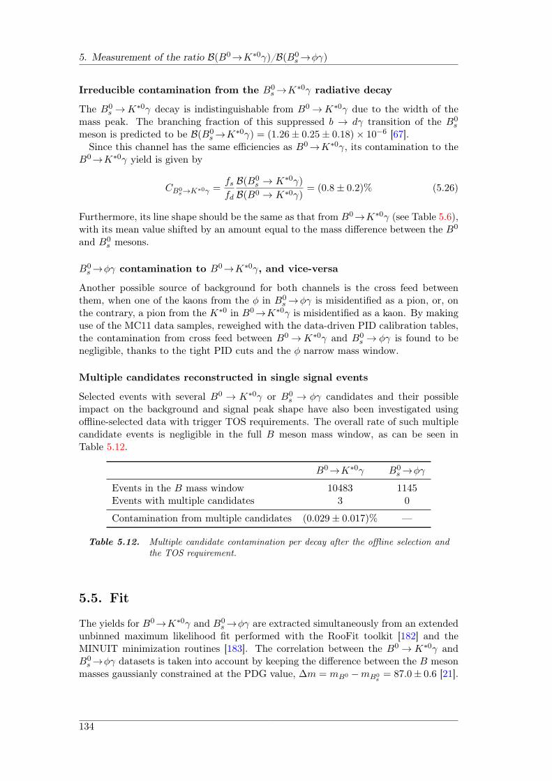
5. Measurement of the ratio B(B0→K∗0γ)/B(B0s →ϕγ)
Irreducible contamination from the B0s →K∗0γ radiative decay
The B0s →K∗0γ decay is indistinguishable from B0 →K∗0γ due to the width of the
mass peak. The branching fraction of this suppressed b → dγ transition of the B0s
meson is predicted to be B(B0s →K∗0γ) = (1.26± 0.25± 0.18)× 10−6 [67].
Since this channel has the same efficiencies as B0→K∗0γ, its contamination to theB0→K∗0γ yield is given by
CB0s→K∗0γ =
fsfd
B(B0s → K∗0γ)
B(B0 → K∗0γ)= (0.8± 0.2)% (5.26)
Furthermore, its line shape should be the same as that from B0→K∗0γ (see Table 5.6),with its mean value shifted by an amount equal to the mass difference between the B0
and B0s mesons.
B0s →ϕγ contamination to B0→K∗0γ, and vice-versa
Another possible source of background for both channels is the cross feed betweenthem, when one of the kaons from the ϕ in B0
s →ϕγ is misidentified as a pion, or, onthe contrary, a pion from the K∗0 in B0→K∗0γ is misidentified as a kaon. By makinguse of the MC11 data samples, reweighed with the data-driven PID calibration tables,the contamination from cross feed between B0 →K∗0γ and B0
s → ϕγ is found to benegligible, thanks to the tight PID cuts and the ϕ narrow mass window.
Multiple candidates reconstructed in single signal events
Selected events with several B0 → K∗0γ or B0s → ϕγ candidates and their possible
impact on the background and signal peak shape have also been investigated usingoffline-selected data with trigger TOS requirements. The overall rate of such multiplecandidate events is negligible in the full B meson mass window, as can be seen inTable 5.12.
B0→K∗0γ B0s →ϕγ
Events in the B mass window 10483 1145Events with multiple candidates 3 0
Contamination from multiple candidates (0.029± 0.017)% —
Table 5.12. Multiple candidate contamination per decay after the offline selection andthe TOS requirement.
5.5. Fit
The yields for B0→K∗0γ and B0s →ϕγ are extracted simultaneously from an extended
unbinned maximum likelihood fit performed with the RooFit toolkit [182] and theMINUIT minimization routines [183]. The correlation between the B0 → K∗0γ andB0
s →ϕγ datasets is taken into account by keeping the difference between the B mesonmasses gaussianly constrained at the PDG value, ∆m = mB0 −mB0
s= 87.0± 0.6 [21].
134
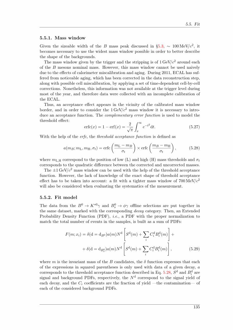
5.5. Fit
5.5.1. Mass window
Given the sizeable width of the B mass peak discussed in §5.3, ∼ 100MeV/c2, itbecomes necessary to use the widest mass window possible in order to better describethe shape of the backgrounds.
The mass window given by the trigger and the stripping is of 1GeV/c2 around eachof the B mesons nominal mass. However, this mass window cannot be used naivelydue to the effects of calorimeter miscalibration and aging. During 2011, ECAL has suf-fered from noticeable aging, which has been corrected in the data reconstruction step,along with possible cell miscalibration, by applying a set of time-dependent cell-by-cellcorrections. Nonetheless, this information was not available at the trigger level duringmost of the year, and therefore data were collected with an incomplete calibration ofthe ECAL.
Thus, an acceptance effect appears in the vicinity of the calibrated mass windowborder, and in order to consider the 1GeV/c2 mass window it is necessary to intro-duce an acceptance function. The complementary error function is used to model thethreshold effect:
erfc(x) = 1− erf(x) =2√π
∫ ∞
xe−t2dt. (5.27)
With the help of the erfc, the threshold acceptance function is defined as
a(mB;mL,mH, σt) = erfc
(mL −mB
σt
)× erfc
(mB −mH
σt
), (5.28)
where mL,H correspond to the position of low (L) and high (H) mass thresholds and σtcorresponds to the quadratic difference between the corrected and uncorrected masses.
The ±1GeV/c2 mass window can be used with the help of the threshold acceptancefunction. However, the lack of knowledge of the exact shape of threshold acceptanceeffect has to be taken into account: a fit with a tighter mass window of 700MeV/c2
will also be considered when evaluating the systematics of the measurement.
5.5.2. Fit model
The data from the B0 → K∗0γ and B0s → ϕγ offline selections are put together in
the same dataset, marked with the corresponding decay category. Then, an ExtendedProbability Density Function (PDF), i.e., a PDF with the proper normalization tomatch the total number of events in the samples, is built as a sum of PDFs:
F (m;xi) = δ(d = dB0)a(m)Nd
[Sd(m) +
∑i
Cdi B
di (m)
]+
+ δ(d = dB0s)a(m)Nd
[Sd(m) +
∑i
Cdi B
di (m)
], (5.29)
where m is the invariant mass of the B candidates, the δ function expresses that eachof the expressions in squared parentheses is only used with data of a given decay, acorresponds to the threshold acceptance function described in Eq. 5.28, Sd and Bd
i aresignal and background PDFs, respectively, the Nd correspond to the signal yield ofeach decay, and the Ci coefficients are the fraction of yield —the contamination— ofeach of the considered background PDFs.
135
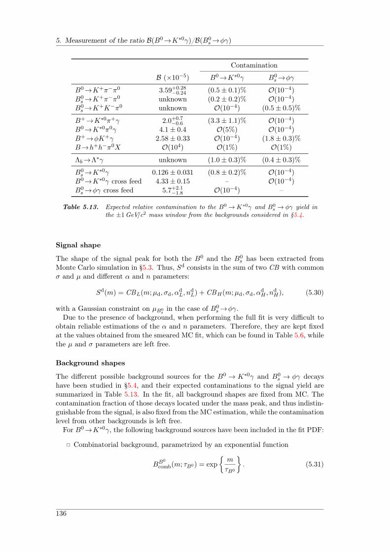
5. Measurement of the ratio B(B0→K∗0γ)/B(B0s →ϕγ)
Contamination
B (×10−5) B0→K∗0γ B0s →ϕγ
B0→K+π−π0 3.59+0.28−0.24 (0.5± 0.1)% O(10−4)
B0s →K+π−π0 unknown (0.2± 0.2)% O(10−4)
B0s →K+K−π0 unknown O(10−4) (0.5± 0.5)%
B+→K∗0π+γ 2.0+0.7−0.6 (3.3± 1.1)% O(10−4)
B0→K∗0π0γ 4.1± 0.4 O(5%) O(10−4)B+→ϕK+γ 2.58± 0.33 O(10−4) (1.8± 0.3)%B→h+h−π0X O(104) O(1%) O(1%)
Λb→Λ∗γ unknown (1.0± 0.3)% (0.4± 0.3)%
B0s →K∗0γ 0.126± 0.031 (0.8± 0.2)% O(10−4)
B0→K∗0γ cross feed 4.33± 0.15 – O(10−4)
B0s →ϕγ cross feed 5.7+2.1
−1.8 O(10−4) –
Table 5.13. Expected relative contamination to the B0 →K∗0γ and B0s → ϕγ yield in
the ±1GeV/c2 mass window from the backgrounds considered in §5.4.
Signal shape
The shape of the signal peak for both the B0 and the B0s has been extracted from
Monte Carlo simulation in §5.3. Thus, Sd consists in the sum of two CB with commonσ and µ and different α and n parameters:
Sd(m) = CBL(m;µd, σd, αdL, n
dL) + CBH(m;µd, σd, α
dH , n
dH), (5.30)
with a Gaussian constraint on µB0s
in the case of B0s →ϕγ.
Due to the presence of background, when performing the full fit is very difficult toobtain reliable estimations of the α and n parameters. Therefore, they are kept fixedat the values obtained from the smeared MC fit, which can be found in Table 5.6, whilethe µ and σ parameters are left free.
Background shapes
The different possible background sources for the B0 → K∗0γ and B0s → ϕγ decays
have been studied in §5.4, and their expected contaminations to the signal yield aresummarized in Table 5.13. In the fit, all background shapes are fixed from MC. Thecontamination fraction of those decays located under the mass peak, and thus indistin-guishable from the signal, is also fixed from the MC estimation, while the contaminationlevel from other backgrounds is left free.
For B0→K∗0γ, the following background sources have been included in the fit PDF:
Combinatorial background, parametrized by an exponential function
BB0
comb(m; τB0) = exp
m
τB0
. (5.31)
136

5.5. Fit
The irreducible B0s →K∗0γ contamination is parametrized by the same shape as
the B0→K∗0γ with the CB mean value shifted by ∆µ = 87MeV/c2,
BB0s→K∗0γ(m) = SB0→K∗0γ(m;µB0 +∆µ, σB0 .αB0
L , nB0
L , αB0
H , nB0
H ), (5.32)
Since this contribution is placed well under the mass peak, the contaminationfraction CB0
s→K∗0γ has been fixed from MC.
The Bd(s) →K±π∓π0 decays reconstructed as B0 →K∗0γ also contribute wellunder the B0 →K∗0γ mass peak. Their shape is fixed to a CB function withparameters fixed to the values detailed in Table 5.7:
BB0→K±π∓π0(m) = CB(m;µB0 , σB0 , αB0 , nB0), (5.33)BB0
s→K±π∓π0(m) = CB(m;µB0s, σB0
s, αB0
s, nB0
s). (5.34)
Their contamination fraction has been fixed in the fit.
The partially reconstructed B+→K∗0π+γ contribution is parametrized by a CB ,where the µ, σ, α, n parameters are fixed from Table 5.8:
BB+→K∗0π+γ(m) = CB(m;µK∗0π+γ , σK∗0π+γ , αK∗0π+γ , nK∗0π+γ), (5.35)
The contamination fraction CB+→K∗0π+γ , is left free in the fit because otherdecays can produce a sizeable contribution with a similar shape.
The baryonic Λb→Λ∗(Kp)γ decays are also taken into account as a CB -shapedcontribution,
BΛb→Λ∗γ(m) = CB(m;µΛb, σΛb
, αΛb, nΛb
), (5.36)
where the parameters have been fixed from Table 5.11 and the contaminationfraction from Eq. 5.23.
The partially reconstructed B→ h+h−π0X decays, referred to from now on aspartially reconstructed background, are modeled by making use of an Argus func-tion with its parameters fixed to the values obtained from MC (see Table 5.10):
BB0
partial(m) = A(m;m0, cB0 , pB0). (5.37)
The contamination from this source, which cannot be reliably extracted fromMC, is left as a free parameter in the fit.
The B0s →ϕγ fit PDF includes the following background sources:
Combinatorial background, parametrized by an exponential function in the sameway as for the B0→K∗0γ combinatorics:
BB0
scomb(m; τB0
s) = exp
m
τB0s
. (5.38)
The π0-related decay to B0s →ϕγ, B0
s →K+K−π0, is parametrized with the sameshape as B0→K+π−π0 with the µ parameter shifted by ∆M = 87.0MeV/c2:
BB0s→K+K−π0(m) = BB0→K±π∓π0(m;µB0 +∆M,σB0 , αB0 , nB0) (5.39)
Its contamination fraction is fixed to CB0s→K+K−π0 = CB0→K±π∓π0 = 0.5%.
137
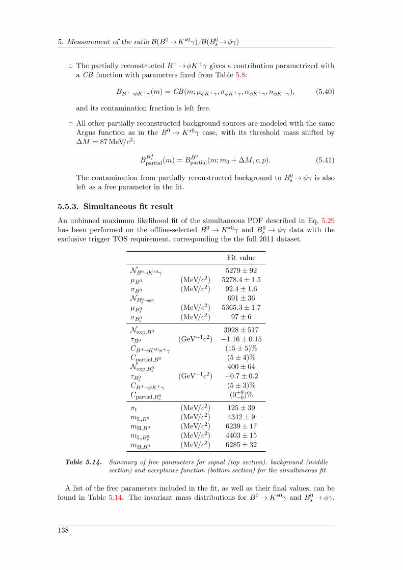
5. Measurement of the ratio B(B0→K∗0γ)/B(B0s →ϕγ)
The partially reconstructed B+→ϕK+γ gives a contribution parametrized witha CB function with parameters fixed from Table 5.8:
BB+→ϕK+γ(m) = CB(m;µϕK+γ , σϕK+γ , αϕK+γ , nϕK+γ), (5.40)
and its contamination fraction is left free.
All other partially reconstructed background sources are modeled with the sameArgus function as in the B0 → K∗0γ case, with its threshold mass shifted by∆M = 87MeV/c2:
BB0
spartial(m) = BB0
partial(m;m0 +∆M, c, p). (5.41)
The contamination from partially reconstructed background to B0s →ϕγ is also
left as a free parameter in the fit.
5.5.3. Simultaneous fit result
An unbinned maximum likelihood fit of the simultaneous PDF described in Eq. 5.29has been performed on the offline-selected B0 → K∗0γ and B0
s → ϕγ data with theexclusive trigger TOS requirement, corresponding the the full 2011 dataset.
Fit value
NB0→K∗0γ 5279± 92µB0 (MeV/c2) 5278.4± 1.5σB0 (MeV/c2) 92.4± 1.6NB0
s→ϕγ 691± 36
µB0s
(MeV/c2) 5365.3± 1.7
σB0s
(MeV/c2) 97± 6
Nexp,B0 3928± 517τB0 (GeV−1c2) −1.16± 0.15CB+→K∗0π+γ (15± 5)%Cpartial,B0 (5± 4)%Nexp,B0
s400± 64
τB0s
(GeV−1c2) −0.7± 0.2
CB+→ϕK+γ (5± 3)%
Cpartial,B0s
(0+9−0)%
σt (MeV/c2) 125± 39mL,B0 (MeV/c2) 4342± 9mH,B0 (MeV/c2) 6239± 17mL,B0
s(MeV/c2) 4403± 15
mH,B0s
(MeV/c2) 6285± 32
Table 5.14. Summary of free parameters for signal (top section), background (middlesection) and acceptance function (bottom section) for the simultaneous fit.
A list of the free parameters included in the fit, as well as their final values, can befound in Table 5.14. The invariant mass distributions for B0 →K∗0γ and B0
s → ϕγ,
138
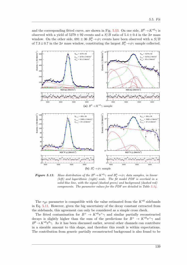
5.5. Fit
and the corresponding fitted curve, are shown in Fig. 5.13. On one side, B0→K∗0γ isobserved with a yield of 5279± 92 events and a S/B ratio of 5.4± 0.4 in the 2σ masswindow. On the other side, 691± 36 B0
s →ϕγ events have been observed with a S/Bof 7.3± 0.7 in the 2σ mass window, constituting the largest B0
s →ϕγ sample collected.
)2) (MeV/cγπM(K
)2E
vent
s / (
25
MeV
/c
0
100
200
300
400
500
600 92± = 5279 γπKN2 2 MeV/c± = 5278
γπKµ
2 2 MeV/c± = 92 γπKσ
4500 5000 5500 6000-5
0
5
)2) (MeV/cγπM(K
)2E
vent
s / (
25
MeV
/c
1
10
210
310 92± = 5279 γπKN
2 2 MeV/c± = 5278 γπK
µ2 2 MeV/c± = 92 γπKσ
4500 5000 5500 6000-5
0
5
(a) B0→K∗0γ sample
)2) (MeV/cγ-K+M(K
)2E
vent
s / (
50
MeV
/c
0
20
40
60
80
100
120
140
160 36± = 691 γ-K+KN
2 2 MeV/c± = 5365 γ-K+K
µ2 6 MeV/c± = 97 γ-K+K
σ
4500 5000 5500 6000-5
0
5
)2) (MeV/cγ-K+M(K
)2E
vent
s / (
50
MeV
/c
-110
1
10
210
36± = 691 γ-K+KN2 2 MeV/c± = 5365
γ-K+Kµ
2 6 MeV/c± = 97 γ-K+Kσ
4500 5000 5500 6000-5
0
5
(b) B0s →ϕγ sample
Figure 5.13. Mass distribution of the B0→K∗0γ and B0s →ϕγ data samples, in linear
(left) and logarithmic (right) scale. The fit model PDF is overlaid in asolid blue line, with the signal (dashed green) and background (dashed red)components. The parameter values for the PDF are detailed in Table 5.14.
The τB0 parameter is compatible with the value estimated from the K∗0 sidebandsin Eq. 5.11. However, given the big uncertainty of the decay constant extracted fromthe sidebands, this agreement can only be considered as a simple cross check.
The fitted contamination for B+ → K∗0π+γ and similar partially reconstructeddecays is slightly higher than the sum of the predictions for B+ → K∗0π+γ andB0→K∗0π0γ. As it has been discussed earlier, several other channels can contributein a sizeable amount to this shape, and therefore this result is within expectations.The contribution from generic partially reconstructed background is also found to be
139
5. Measurement of the ratio B(B0→K∗0γ)/B(B0s →ϕγ)
within expectations.
5.5.4. Fit quality
In order to assess the quality of the fit, its goodness-of-fit has been evaluated withthe χ2 method, while its stability has been assessed with toy Monte Carlo samplesgenerated following the shape of the fitted PDF.
Goodness-of-fit
Determination of the goodness-of-fit in the case of unbinned maximum likelihood fitsis not as straightforward as it is with binned fits [184]. For example, it has been shownthat the naive method of comparing the value of the likelihood at the maximum withthe distribution of the maximum likelihood of MC-generated toy models is a flawed andshould not be used [185, 186]. Thus, a usual approach to the goodness-of-fit problemconsists in binning the fitted dataset and applying the χ2 test.
The χ2 residuals [173] located at the bottom of the invariant mass plots in Fig. 5.13give already a visual hint about the suitability of the used PDF, since almost all ofthem lie within the ±2σ band. To obtain a numerical value for the goodness-of-fit, thechi-square test statistic, defined as
X2 =
n∑i
(datai − pdfi)datai
, (5.42)
can be used to calculate a p-value by comparing the X2 value obtained from the fitto a χ2 distribution of the appropriate degrees of freedom. The number of degrees offreedom is equal to the number of bins n, minus the reduction in degrees of freedom,calculated as the number of parameters, minus one, to account for the fact that, oncethe number of events in n − 1 bins is known, the number of events in the last bin isknown from the total number of events.
In the simultaneous fit case, however, it is difficult to define the individual number ofdegrees of freedom for each plot, since some of the parameters are related. A commonX2 has been extracted, X2 = 101.23, and the corresponding degrees of freedom havebeen calculated as
dof = 120 bins − (19 parameters)− 1− 1 = 99. (5.43)
Therefore, a value of X2/dof = 101.23/99 ∼ 1.0225 is determined, which correspondsto a p-value of 42%. This result confirms the good agreement between the data andthe fitted PDF.
Stability of the fit
The pull distribution Px of a given fit parameter x,
Px =xFit − xToy
σx, (5.44)
extracted from a set of toy MC experiments, can be used to assess the stability of thefit. If the fit is well behaved, the distribution of Px is a Gaussian with µ = 0 and
140

5.6. Extraction of the ratio of branching fractions
σ = 1. If the mean value diverges from 0, it means that the determination of theparameter is biased, while a divergence in the width of the pull indicates that errorsare not correctly estimated.
A set of 20,000 toy MC samples have been generated following the PDF from Eq. 5.29with the values of the parameters extracted from the fit to the data. Each of thegenerated samples has then been fitted with the same PDF. The pull distributions forthe six free signal parameters in the fit, fitted with a gaussian function, are shown inFig. 5.14. It can be seen that these parameters are unbiased and their errors havebeen correctly estimated, since the means and the widths obtained from the gaussianfit are compatible with zero and one, respectively. Thus, it can be concluded that thefit is stable under variations of the input data and that the signal parameters and theiruncertainties have been correctly extracted within the chosen model.
5.6. Extraction of the ratio of branching fractions
The expected yield for a given B decay is given by
N = L × σbb × f × B × ϵ, (5.45)
where L is the luminosity, σbb the bb production cross section, f is the B mesonhadronization fraction, B is the visible branching fraction of the studied decay, and ϵthe acceptance, trigger, reconstruction and selection efficiencies.
Thus, the expected yield for the studied decays is
NB0→K∗0γ = L × σbb × fd × B(B0→K∗0γ)× B(K∗0 → K+π−)× ϵB0→K∗0γ ,
NB0s→ϕγ = L × σbb × fs × B(B0
s →ϕγ)× B(ϕ→ K+K−)× ϵB0s→ϕγ ,
(5.46)
and the ratio of branching fractions is calculated as the product of the ratio of fittedevents, the inverse ratio of visible vector meson branching fractions, the ratio fs/fd,and the inverse ratio of selection efficiencies ϵ:
B(B0→K∗0γ)
B(B0s →ϕγ)
=NB0→K∗0γ
NB0s→ϕγ
B(ϕ→ K+K−)
B(K∗ → K+π−)
fsfd
ϵB0s→ϕγ
ϵB0→K∗0γ. (5.47)
The efficiency for each channel is split into trigger, acceptance, reconstruction andselection without PID requirements, and PID selection. The reason for separating thecalculation of the selection efficiency from the PID efficiency is that the PID distribu-tions are not accurately described by the simulation, and therefore cannot be extracteddirectly from MC. With this splitting in mind, the ratio of efficiencies between the twochannels can be written as:
rϵ ≡ϵB
0s→ϕγ
ϵB0→K∗0γ=
ϵB0
s→ϕγTrigger
ϵB0→K∗0γ
Trigger
×ϵB0
s→ϕγAcceptance
ϵB0→K∗0γ
Acceptance
×ϵB0
s→ϕγReco&SelNoPID
ϵB0→K∗0γ
Reco&SelNoPID
×ϵB0
s→ϕγPID
ϵB0→K∗0γ
PID
. (5.48)
The ratio of efficiencies for trigger, acceptance, and reconstruction and selection with-out PID have been extracted from MC11 simulation. The ratio of efficiencies of PIDcuts has been extracted by making use of a data-driven reweighing method on theMonte Carlo simulation.
141

5. Measurement of the ratio B(B0→K∗0γ)/B(B0s →ϕγ)
)0B
µP(-3 -2 -1 0 1 2 3
Eve
nts
/ ( 0
.04
)
0
50
100
150
200
250
300
350
400 0.007± = -0.0027 µ 0.005± = 1.002 σ
(a) Pull distribution for µB0 .
)sB
µP(-3 -2 -1 0 1 2 3
Eve
nts
/ ( 0
.04
)
0
50
100
150
200
250
300
350
400 0.007± = -0.0038 µ 0.005± = 1.002 σ
(b) Pull distribution for µB0s.
)0BσP(
-3 -2 -1 0 1 2 3
Eve
nts
/ ( 0
.04
)
0
50
100
150
200
250
300
350
400
450 0.007± = -0.0022 µ
0.005± = 0.998 σ
(c) Pull distribution for σB0 .)
sBσP(-3 -2 -1 0 1 2 3
Eve
nts
/ ( 0
.04
)
0
50
100
150
200
250
300
350
400
450 0.007± = 0.007 µ 0.005± = 0.998 σ
(d) Pull distribution for σB0s.
)0B
P(N-3 -2 -1 0 1 2 3
Eve
nts
/ ( 0
.04
)
0
50
100
150
200
250
300
350
400 0.007± = -0.0026 µ
0.005± = 0.994 σ
(e) Pull distribution for NB0 .
)sB
P(N-3 -2 -1 0 1 2 3
Eve
nts
/ ( 0
.04
)
0
50
100
150
200
250
300
350
400 0.007± = 0.026 µ 0.005± = 1.006 σ
(f) Pull distribution for NB0s.
Figure 5.14. Pull distributions of the free signal parameters, obtained from fitting20,000 toy MC samples generated with the model PDF. The fit of thepull distributions to a gaussian is shown in a blue solid line, with its pa-rameters on the top right corner of each plot.
142
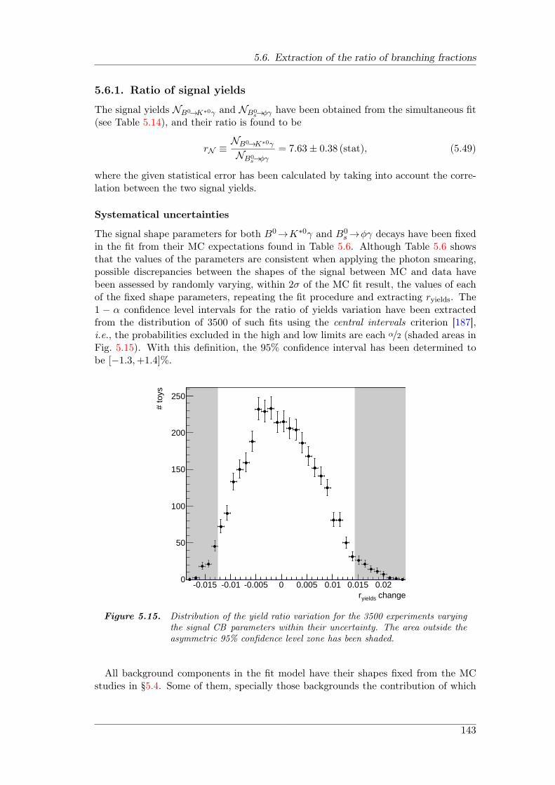
5.6. Extraction of the ratio of branching fractions
5.6.1. Ratio of signal yields
The signal yields NB0→K∗0γ and NB0s→ϕγ have been obtained from the simultaneous fit
(see Table 5.14), and their ratio is found to be
rN ≡NB0→K∗0γ
NB0s→ϕγ
= 7.63± 0.38 (stat), (5.49)
where the given statistical error has been calculated by taking into account the corre-lation between the two signal yields.
Systematical uncertainties
The signal shape parameters for both B0→K∗0γ and B0s →ϕγ decays have been fixed
in the fit from their MC expectations found in Table 5.6. Although Table 5.6 showsthat the values of the parameters are consistent when applying the photon smearing,possible discrepancies between the shapes of the signal between MC and data havebeen assessed by randomly varying, within 2σ of the MC fit result, the values of eachof the fixed shape parameters, repeating the fit procedure and extracting ryields. The1 − α confidence level intervals for the ratio of yields variation have been extractedfrom the distribution of 3500 of such fits using the central intervals criterion [187],i.e., the probabilities excluded in the high and low limits are each α/2 (shaded areas inFig. 5.15). With this definition, the 95% confidence interval has been determined tobe [−1.3,+1.4]%.
changeyieldsr-0.015 -0.01 -0.005 0 0.005 0.01 0.015 0.02
# to
ys
0
50
100
150
200
250
Figure 5.15. Distribution of the yield ratio variation for the 3500 experiments varyingthe signal CB parameters within their uncertainty. The area outside theasymmetric 95% confidence level zone has been shaded.
All background components in the fit model have their shapes fixed from the MCstudies in §5.4. Some of them, specially those backgrounds the contribution of which
143
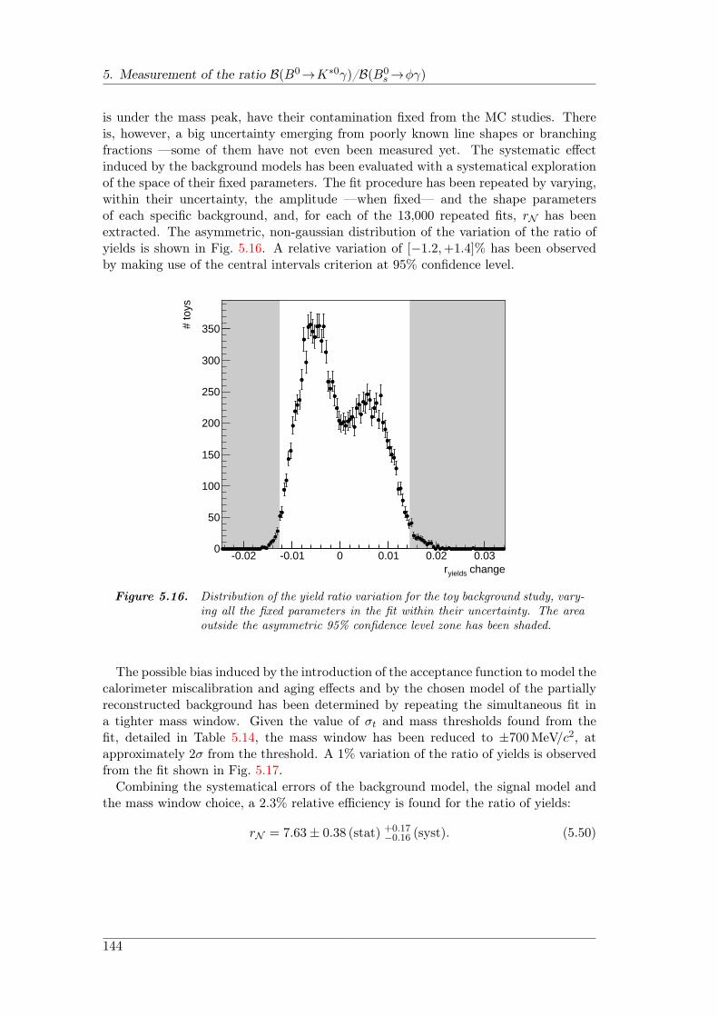
5. Measurement of the ratio B(B0→K∗0γ)/B(B0s →ϕγ)
is under the mass peak, have their contamination fixed from the MC studies. Thereis, however, a big uncertainty emerging from poorly known line shapes or branchingfractions —some of them have not even been measured yet. The systematic effectinduced by the background models has been evaluated with a systematical explorationof the space of their fixed parameters. The fit procedure has been repeated by varying,within their uncertainty, the amplitude —when fixed— and the shape parametersof each specific background, and, for each of the 13,000 repeated fits, rN has beenextracted. The asymmetric, non-gaussian distribution of the variation of the ratio ofyields is shown in Fig. 5.16. A relative variation of [−1.2,+1.4]% has been observedby making use of the central intervals criterion at 95% confidence level.
changeyieldsr-0.02 -0.01 0 0.01 0.02 0.03
# to
ys
0
50
100
150
200
250
300
350
Figure 5.16. Distribution of the yield ratio variation for the toy background study, vary-ing all the fixed parameters in the fit within their uncertainty. The areaoutside the asymmetric 95% confidence level zone has been shaded.
The possible bias induced by the introduction of the acceptance function to model thecalorimeter miscalibration and aging effects and by the chosen model of the partiallyreconstructed background has been determined by repeating the simultaneous fit ina tighter mass window. Given the value of σt and mass thresholds found from thefit, detailed in Table 5.14, the mass window has been reduced to ±700MeV/c2, atapproximately 2σ from the threshold. A 1% variation of the ratio of yields is observedfrom the fit shown in Fig. 5.17.
Combining the systematical errors of the background model, the signal model andthe mass window choice, a 2.3% relative efficiency is found for the ratio of yields:
rN = 7.63± 0.38 (stat) +0.17−0.16 (syst). (5.50)
144
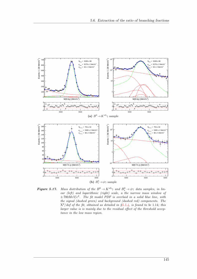
5.6. Extraction of the ratio of branching fractions
)2) (MeV/cγπM(K
)2E
vent
s / (
28
MeV
/c
0
100
200
300
400
500
600
700 88± = 5268 γπKN
2 2 MeV/c± = 5278 γπK
µ2 2 MeV/c± = 93 γπKσ
5000 5500-5
0
5
)2) (MeV/cγπM(K
)2E
vent
s / (
28
MeV
/c
1
10
210
310 88± = 5268 γπKN
2 2 MeV/c± = 5278 γπK
µ2 2 MeV/c± = 93 γπKσ
5000 5500-5
0
5
(a) B0→K∗0γ sample
)2) (MeV/cγ-K+M(K
)2E
vent
s / (
56
MeV
/c
0
20
40
60
80
100
120
140
160
180 34± = 701 γ-K+KN2 2 MeV/c± = 5365
γ-K+Kµ
2 5 MeV/c± = 98 γ-K+Kσ
5000 5500 6000-5
0
5
)2) (MeV/cγ-K+M(K
)2E
vent
s / (
56
MeV
/c
-110
1
10
210
34± = 701 γ-K+KN2 2 MeV/c± = 5365
γ-K+Kµ
2 5 MeV/c± = 98 γ-K+Kσ
5000 5500 6000-5
0
5
(b) B0s →ϕγ sample
Figure 5.17. Mass distribution of the B0 →K∗0γ and B0s → ϕγ data samples, in lin-
ear (left) and logarithmic (right) scale, a the narrow mass window of± 700MeV/c2. The fit model PDF is overlaid in a solid blue line, withthe signal (dashed green) and background (dashed red) components. TheX2/dof of the fit, obtained as detailed in §5.5.4, is found to be 1.14; thislarger value is is mainly due to the residual effect of the threshold accep-tance in the low mass region.
145

5. Measurement of the ratio B(B0→K∗0γ)/B(B0s →ϕγ)
5.6.2. Ratio of visible vector meson branching fractions
Since not all possible decay modes of the vector meson have been used on this theanalysis, to obtain the visible cross section one needs to add the partial branchingfractions of the observed modes K∗0→K±π∓ and ϕ→K+K−. In particular, the K∗0
decay is almost a 100% isospin-conserving string decay and therefore one expects a 2/3partial branching fraction for the charged decays (see Appendix B for more details).
The branching fractions of the vector mesons to the observed charged modes can befound in [21]:
B(K∗0→K±π∓) = (66.507± 0.014)× 10−2,
B(ϕ→K+K−) = (48.9± 0.5)× 10−2.(5.51)
Thus, the ratio of the visible vector meson branching fractions is
rvector meson B ≡ B(ϕ→ K+K−)
B(K∗ → K+π−)= 0.735± 0.008. (5.52)
5.6.3. Ratio of hadronization fractions
The LHCb experiment has measured the ratio [fs/(fu + fd)] using semileptonic decaysof b-hadrons [188], as well as the ratio fs/fd using the relative abundance of B0
s →D−s π
+
to B0→D−K+, and B0→D−π+ [189].The ratio fs/fd is taken from the combined LHCb measurement, which has a 7.5%
uncertainty [98]:fsfd
= 0.267+0.021−0.020. (5.53)
The contribution of fs/fd constitutes the main source of systematical uncertainty inthe measurement.
5.6.4. Ratio of trigger efficiencies
The trigger efficiencies —including the TOS requirements detailed in §5.2.1— havebeen evaluated from the offline selected signal Monte Carlo sample by applying thefollowing procedure:
1. Run the Moore software with the studied trigger configuration on the offline-selected MC sample without trigger requirements.
2. Apply the TISTOSing algorithm with respect to the signal decay.
3. Calculate the efficiency of the TOS selection.
To obtain the trigger efficiency for data with several TCKs run one must average theindividual efficiencies of each TCK, weighted by the luminosity taken with them.
For the data considered, a total number of 15 different TCKs have been used, theluminosities of which can be found in Table 3.1. Detailed TOS efficiencies per TCKare shown in Table 4.12, as well as the averaged TOS efficiency. This table can be used
146
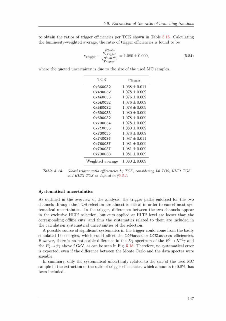
5.6. Extraction of the ratio of branching fractions
to obtain the ratios of trigger efficiencies per TCK shown in Table 5.15. Calculatingthe luminosity-weighted average, the ratio of trigger efficiencies is found to be
rTrigger ≡ϵB0
s→ϕγTrigger
ϵB0→K∗0γ
Trigger
= 1.080± 0.009, (5.54)
where the quoted uncertainty is due to the size of the used MC samples.
TCK rTrigger
0x360032 1.068± 0.0110x480032 1.078± 0.0090x4A0033 1.076± 0.0090x5A0032 1.076± 0.0090x5B0032 1.078± 0.0090x5D0033 1.080± 0.0090x6D0032 1.078± 0.0090x700034 1.078± 0.0090x710035 1.080± 0.0090x730035 1.078± 0.0090x740036 1.087± 0.0110x760037 1.081± 0.0090x790037 1.081± 0.0090x790038 1.081± 0.009
Weighted average 1.080± 0.009
Table 5.15. Global trigger ratio efficiencies by TCK, considering L0 TOS, HLT1 TOSand HLT2 TOS as defined in §5.2.1.
Systematical uncertainties
As outlined in the overview of the analysis, the trigger paths enforced for the twochannels through the TOS selection are almost identical in order to cancel most sys-tematical uncertainties. In the trigger, differences between the two channels appearin the exclusive HLT2 selection, but cuts applied at HLT2 level are looser than thecorresponding offline cuts, and thus the systematics related to them are included inthe calculation systematical uncertainties of the selection.
A possible source of significant systematics in the trigger could come from the badlysimulated L0 energies, which could affect the L0Photon or L0Electron efficiencies.However, there is no noticeable difference in the ET spectrum of the B0→K∗0γ andthe B0
s →ϕγ above 2GeV, as can be seen in Fig. 5.18. Therefore, no systematical erroris expected, even if the difference between the Monte Carlo and the data spectra weresizeable.
In summary, only the systematical uncertainty related to the size of the used MCsample in the extraction of the ratio of trigger efficiencies, which amounts to 0.8%, hasbeen included.
147
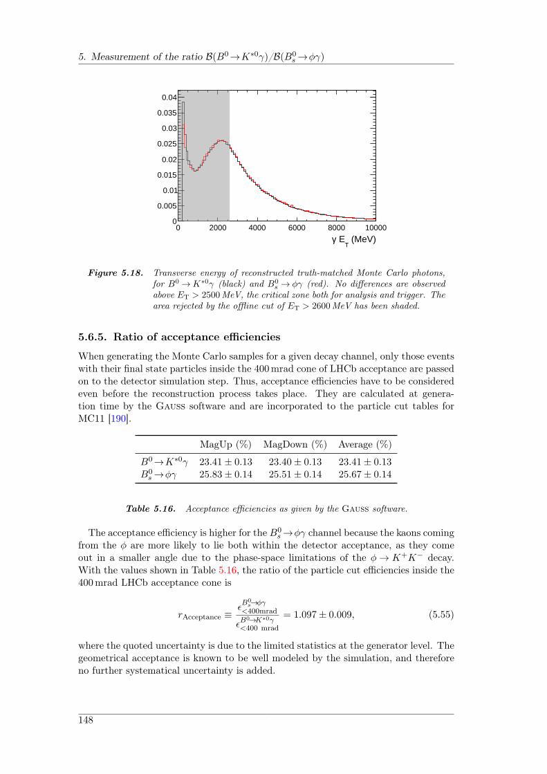
5. Measurement of the ratio B(B0→K∗0γ)/B(B0s →ϕγ)
(MeV)T
Eγ0 2000 4000 6000 8000 10000
0
0.005
0.01
0.015
0.02
0.025
0.03
0.035
0.04
Figure 5.18. Transverse energy of reconstructed truth-matched Monte Carlo photons,for B0 →K∗0γ (black) and B0
s → ϕγ (red). No differences are observedabove ET > 2500MeV, the critical zone both for analysis and trigger. Thearea rejected by the offline cut of ET > 2600MeV has been shaded.
5.6.5. Ratio of acceptance efficiencies
When generating the Monte Carlo samples for a given decay channel, only those eventswith their final state particles inside the 400mrad cone of LHCb acceptance are passedon to the detector simulation step. Thus, acceptance efficiencies have to be consideredeven before the reconstruction process takes place. They are calculated at genera-tion time by the Gauss software and are incorporated to the particle cut tables forMC11 [190].
MagUp (%) MagDown (%) Average (%)
B0→K∗0γ 23.41± 0.13 23.40± 0.13 23.41± 0.13B0
s →ϕγ 25.83± 0.14 25.51± 0.14 25.67± 0.14
Table 5.16. Acceptance efficiencies as given by the Gauss software.
The acceptance efficiency is higher for the B0s →ϕγ channel because the kaons coming
from the ϕ are more likely to lie both within the detector acceptance, as they comeout in a smaller angle due to the phase-space limitations of the ϕ→ K+K− decay.With the values shown in Table 5.16, the ratio of the particle cut efficiencies inside the400mrad LHCb acceptance cone is
rAcceptance ≡ϵB0
s→ϕγ<400mrad
ϵB0→K∗0γ
<400 mrad
= 1.097± 0.009, (5.55)
where the quoted uncertainty is due to the limited statistics at the generator level. Thegeometrical acceptance is known to be well modeled by the simulation, and thereforeno further systematical uncertainty is added.
148
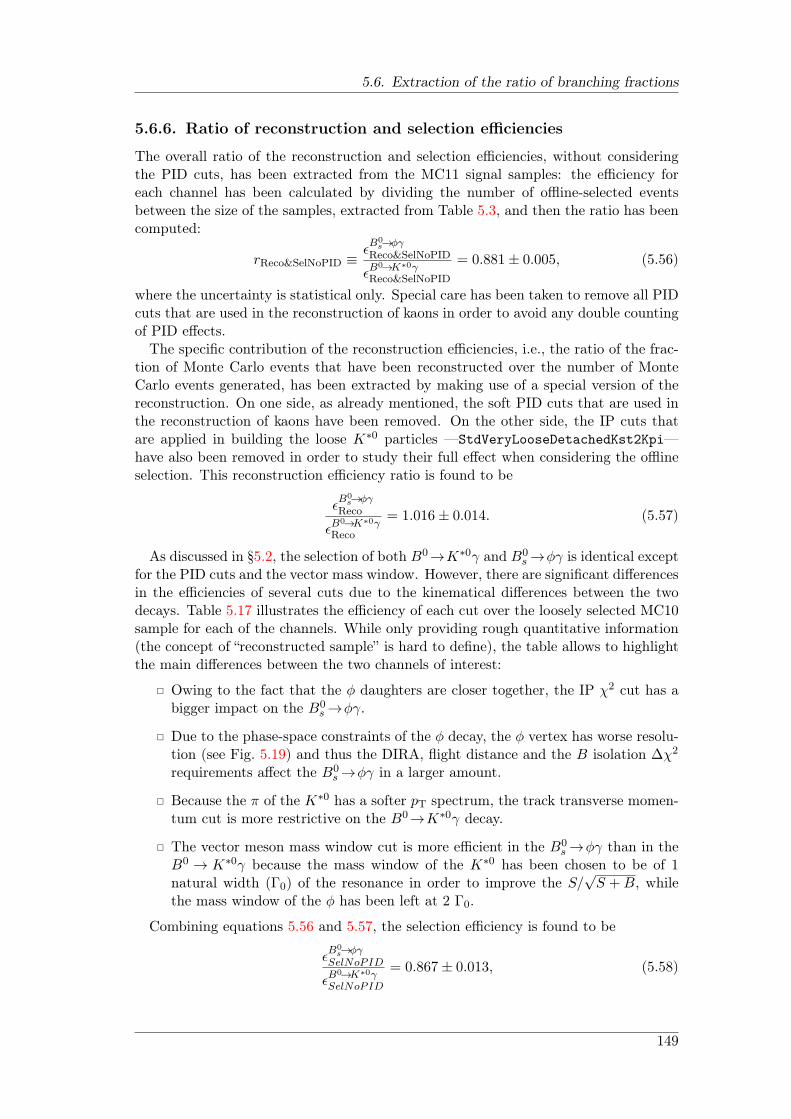
5.6. Extraction of the ratio of branching fractions
5.6.6. Ratio of reconstruction and selection efficiencies
The overall ratio of the reconstruction and selection efficiencies, without consideringthe PID cuts, has been extracted from the MC11 signal samples: the efficiency foreach channel has been calculated by dividing the number of offline-selected eventsbetween the size of the samples, extracted from Table 5.3, and then the ratio has beencomputed:
rReco&SelNoPID ≡ϵB0
s→ϕγReco&SelNoPID
ϵB0→K∗0γ
Reco&SelNoPID
= 0.881± 0.005, (5.56)
where the uncertainty is statistical only. Special care has been taken to remove all PIDcuts that are used in the reconstruction of kaons in order to avoid any double countingof PID effects.
The specific contribution of the reconstruction efficiencies, i.e., the ratio of the frac-tion of Monte Carlo events that have been reconstructed over the number of MonteCarlo events generated, has been extracted by making use of a special version of thereconstruction. On one side, as already mentioned, the soft PID cuts that are used inthe reconstruction of kaons have been removed. On the other side, the IP cuts thatare applied in building the loose K∗0 particles —StdVeryLooseDetachedKst2Kpi—have also been removed in order to study their full effect when considering the offlineselection. This reconstruction efficiency ratio is found to be
ϵB0
s→ϕγReco
ϵB0→K∗0γ
Reco
= 1.016± 0.014. (5.57)
As discussed in §5.2, the selection of both B0→K∗0γ and B0s →ϕγ is identical except
for the PID cuts and the vector mass window. However, there are significant differencesin the efficiencies of several cuts due to the kinematical differences between the twodecays. Table 5.17 illustrates the efficiency of each cut over the loosely selected MC10sample for each of the channels. While only providing rough quantitative information(the concept of “reconstructed sample” is hard to define), the table allows to highlightthe main differences between the two channels of interest:
Owing to the fact that the ϕ daughters are closer together, the IP χ2 cut has abigger impact on the B0
s →ϕγ.
Due to the phase-space constraints of the ϕ decay, the ϕ vertex has worse resolu-tion (see Fig. 5.19) and thus the DIRA, flight distance and the B isolation ∆χ2
requirements affect the B0s →ϕγ in a larger amount.
Because the π of the K∗0 has a softer pT spectrum, the track transverse momen-tum cut is more restrictive on the B0→K∗0γ decay.
The vector meson mass window cut is more efficient in the B0s →ϕγ than in the
B0 → K∗0γ because the mass window of the K∗0 has been chosen to be of 1natural width (Γ0) of the resonance in order to improve the S/
√S +B, while
the mass window of the ϕ has been left at 2 Γ0.
Combining equations 5.56 and 5.57, the selection efficiency is found to be
ϵB0
s→ϕγSelNoPID
ϵB0→K∗0γ
SelNoPID
= 0.867± 0.013, (5.58)
149
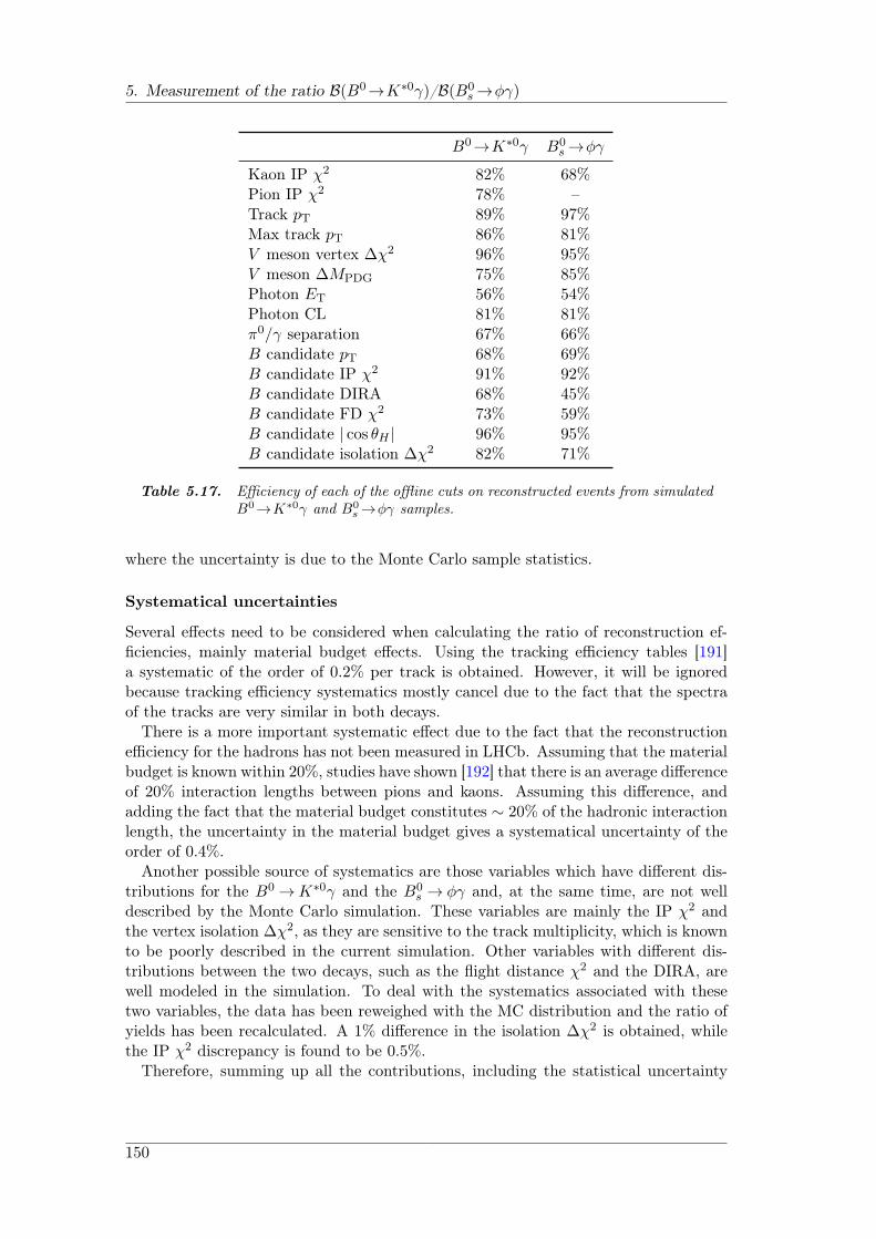
5. Measurement of the ratio B(B0→K∗0γ)/B(B0s →ϕγ)
B0→K∗0γ B0s →ϕγ
Kaon IP χ2 82% 68%Pion IP χ2 78% –Track pT 89% 97%Max track pT 86% 81%V meson vertex ∆χ2 96% 95%V meson ∆MPDG 75% 85%Photon ET 56% 54%Photon CL 81% 81%π0/γ separation 67% 66%B candidate pT 68% 69%B candidate IP χ2 91% 92%B candidate DIRA 68% 45%B candidate FD χ2 73% 59%B candidate | cos θH | 96% 95%B candidate isolation ∆χ2 82% 71%
Table 5.17. Efficiency of each of the offline cuts on reconstructed events from simulatedB0→K∗0γ and B0
s →ϕγ samples.
where the uncertainty is due to the Monte Carlo sample statistics.
Systematical uncertainties
Several effects need to be considered when calculating the ratio of reconstruction ef-ficiencies, mainly material budget effects. Using the tracking efficiency tables [191]a systematic of the order of 0.2% per track is obtained. However, it will be ignoredbecause tracking efficiency systematics mostly cancel due to the fact that the spectraof the tracks are very similar in both decays.
There is a more important systematic effect due to the fact that the reconstructionefficiency for the hadrons has not been measured in LHCb. Assuming that the materialbudget is known within 20%, studies have shown [192] that there is an average differenceof 20% interaction lengths between pions and kaons. Assuming this difference, andadding the fact that the material budget constitutes ∼ 20% of the hadronic interactionlength, the uncertainty in the material budget gives a systematical uncertainty of theorder of 0.4%.
Another possible source of systematics are those variables which have different dis-tributions for the B0 →K∗0γ and the B0
s → ϕγ and, at the same time, are not welldescribed by the Monte Carlo simulation. These variables are mainly the IP χ2 andthe vertex isolation ∆χ2, as they are sensitive to the track multiplicity, which is knownto be poorly described in the current simulation. Other variables with different dis-tributions between the two decays, such as the flight distance χ2 and the DIRA, arewell modeled in the simulation. To deal with the systematics associated with thesetwo variables, the data has been reweighed with the MC distribution and the ratio ofyields has been recalculated. A 1% difference in the isolation ∆χ2 is obtained, whilethe IP χ2 discrepancy is found to be 0.5%.
Therefore, summing up all the contributions, including the statistical uncertainty
150
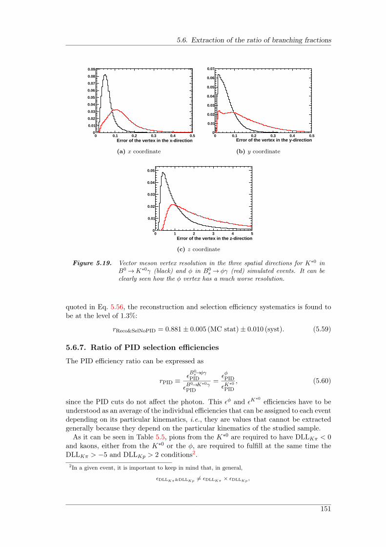
5.6. Extraction of the ratio of branching fractions
Error of the vertex in the x-direction0 0.1 0.2 0.3 0.4 0.5
0
0.01
0.02
0.03
0.04
0.05
0.06
0.07
0.08
0.09
(a) x coordinate
Error of the vertex in the y-direction0 0.1 0.2 0.3 0.4 0.5
0
0.01
0.02
0.03
0.04
0.05
0.06
0.07
(b) y coordinate
Error of the vertex in the z-direction0 1 2 3 4 5
0
0.01
0.02
0.03
0.04
0.05
(c) z coordinate
Figure 5.19. Vector meson vertex resolution in the three spatial directions for K∗0 inB0 →K∗0γ (black) and ϕ in B0
s → ϕγ (red) simulated events. It can beclearly seen how the ϕ vertex has a much worse resolution.
quoted in Eq. 5.56, the reconstruction and selection efficiency systematics is found tobe at the level of 1.3%:
rReco&SelNoPID = 0.881± 0.005 (MC stat)± 0.010 (syst). (5.59)
5.6.7. Ratio of PID selection efficiencies
The PID efficiency ratio can be expressed as
rPID ≡ϵB0
s→ϕγPID
ϵB0→K∗0γ
PID
=ϵϕPID
ϵK∗0
PID, (5.60)
since the PID cuts do not affect the photon. This ϵϕ and ϵK∗0 efficiencies have to be
understood as an average of the individual efficiencies that can be assigned to each eventdepending on its particular kinematics, i.e., they are values that cannot be extractedgenerally because they depend on the particular kinematics of the studied sample.
As it can be seen in Table 5.5, pions from the K∗0 are required to have DLLKπ < 0and kaons, either from the K∗0 or the ϕ, are required to fulfill at the same time theDLLKπ > −5 and DLLKp > 2 conditions2.
2In a given event, it is important to keep in mind that, in general,
ϵDLLKπ&DLLKp = ϵDLLKπ × ϵDLLKp ,
151
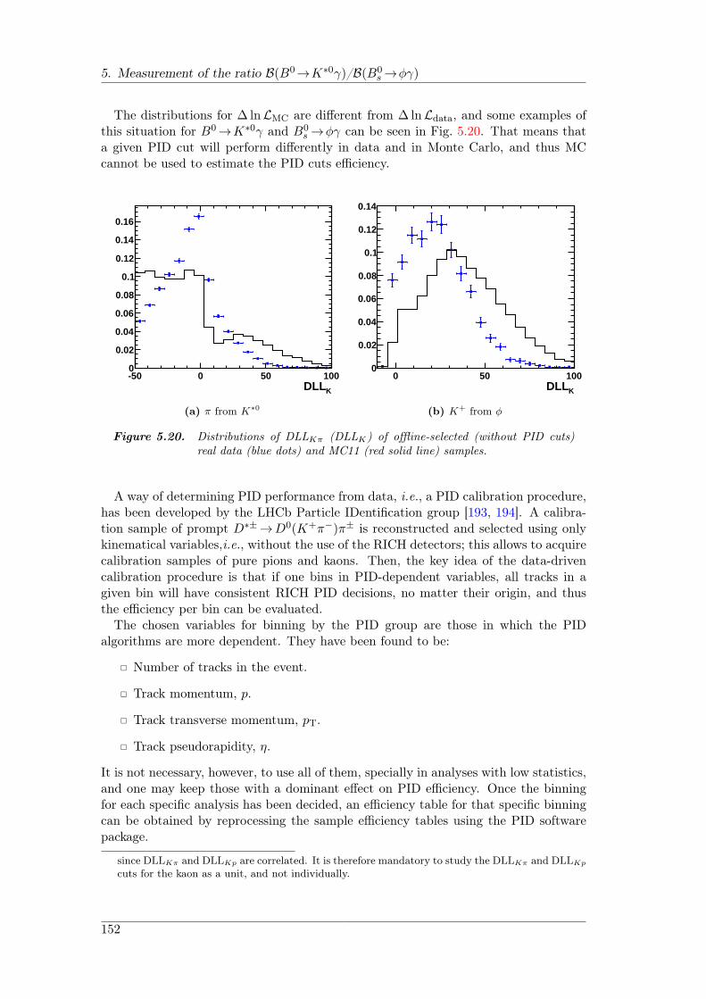
5. Measurement of the ratio B(B0→K∗0γ)/B(B0s →ϕγ)
The distributions for ∆lnLMC are different from ∆lnLdata, and some examples ofthis situation for B0→K∗0γ and B0
s →ϕγ can be seen in Fig. 5.20. That means thata given PID cut will perform differently in data and in Monte Carlo, and thus MCcannot be used to estimate the PID cuts efficiency.
KDLL-50 0 50 1000
0.02
0.04
0.06
0.08
0.1
0.12
0.14
0.16
(a) π from K∗0
KDLL0 50 100
0
0.02
0.04
0.06
0.08
0.1
0.12
0.14
(b) K+ from ϕ
Figure 5.20. Distributions of DLLKπ (DLLK) of offline-selected (without PID cuts)real data (blue dots) and MC11 (red solid line) samples.
A way of determining PID performance from data, i.e., a PID calibration procedure,has been developed by the LHCb Particle IDentification group [193, 194]. A calibra-tion sample of prompt D∗±→D0(K+π−)π± is reconstructed and selected using onlykinematical variables,i.e., without the use of the RICH detectors; this allows to acquirecalibration samples of pure pions and kaons. Then, the key idea of the data-drivencalibration procedure is that if one bins in PID-dependent variables, all tracks in agiven bin will have consistent RICH PID decisions, no matter their origin, and thusthe efficiency per bin can be evaluated.
The chosen variables for binning by the PID group are those in which the PIDalgorithms are more dependent. They have been found to be:
Number of tracks in the event.
Track momentum, p.
Track transverse momentum, pT.
Track pseudorapidity, η.
It is not necessary, however, to use all of them, specially in analyses with low statistics,and one may keep those with a dominant effect on PID efficiency. Once the binningfor each specific analysis has been decided, an efficiency table for that specific binningcan be obtained by reprocessing the sample efficiency tables using the PID softwarepackage.
since DLLKπ and DLLKp are correlated. It is therefore mandatory to study the DLLKπ and DLLKp
cuts for the kaon as a unit, and not individually.
152

5.6. Extraction of the ratio of branching fractions
Magnet Up Magnet Down Average
B0→K∗0γϵK
±PID (70.0± 0.3)% (72.2± 0.4)% (71.1± 0.2)%
ϵπ∓
PID (90.0± 0.3)% (92.0± 0.3)% (91.0± 0.2)%
ϵK∗0
PID (63.5± 0.4)% (66.9± 0.3)% (65.2± 0.2)%
B0s →ϕγ
ϵK+
PID (69.4± 0.3)% (72.2± 0.4)% (70.8± 0.2)%
ϵK−
PID (69.6± 0.3)% (72.2± 0.4)% (70.8± 0.2)%
ϵϕPID (52.8± 0.3)% (56.5± 0.4)% (54.7± 0.2)%
rPID 0.831± 0.007 0.844± 0.007 0.839± 0.005
Table 5.18. PID selection efficiencies, split in magnet polarity, obtained by reweighingthe (p, η) spectrum of the kaons and pions of the B0→K∗0γ and B0
s →ϕγdecays with the PID calibration tables. The last line gives the ratio ofthe PID selection efficiencies. The quoted errors are due to the statisticalerrors of each bin of the PID tables, which arise from the limited size ofthe calibration sample.
In this analysis, and given the statistics of the studied decays, seven bins in p andfive in η have been used. The efficiency map for pions with DLLKπ < 0, extracted withthe PID software package, is given in Fig. 5.21a; the corresponding efficiency map forkaons with DLLKπ > 5 and DLLKp > 2 is shown in Fig. 5.21b.
Since the ratio of branching fractions measurement is fully inclusive —not binned inany variable—, a global efficiency is obtained by integrating the full selected sample.However, as stated before, the PID efficiency for a given event is the product of theefficiencies of the daughters of the K∗0 or ϕ, depending on which channel is beingstudied. Thus, one cannot consider the p and η distributions of the individual daughtersof the candidate vector meson and sum over the efficiency of each bin. Instead, onemust consider the PID efficiency —calculated as the product of efficiencies for eachKπ and KK pair— as a per-event weight, and with that information calculate theintegrated efficiency.
To do that, the momentum, transverse momentum and pseudorapidity of the signaltracks must be known in order to assign the correct weight to each event. However,in the data samples signal is mixed with background, and thus they cannot be useddirectly because the kaon and pion distribution shapes between signal and backgroundmay be different.
The sPlot technique could be used to extract the required distributions of the signaltracks from real data. However, the low signal statistics in the data sample would giverise to big uncertainties when determining the PID efficiencies from the PID tables.A better precision is achieved by taking advantage of the fact that the simulationdescribes well kinematical variables such as p, pT and η. Thus, MC signal tracks canbe used as inputs for the data-driven PID calibration procedure.
Moreover, the PID performance is different depending on the magnet polarity, andthus PID calibration tables for the up and down configurations need to be used. Asummary of the PID efficiencies determined for each polarity, as well as their average,can be found in Table 5.18.
153
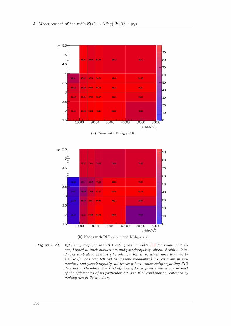
5. Measurement of the ratio B(B0→K∗0γ)/B(B0s →ϕγ)
89.36 94.00 98.15 99.11 95.35 80.11
89.18 94.35 97.90 98.57 96.17 90.01
85.82 91.20 96.94 98.40 98.11 96.77
72.04 88.07 92.70 96.61 96.42 93.75
96.56 88.49 91.44 88.73 88.41
)2p (MeV/c
10000 20000 30000 40000 50000 60000
η
1.5
2
2.5
3
3.5
4
4.5
5
5.5
0
10
20
30
40
50
60
70
80
90
(a) Pions with DLLKπ < 0
22.15 72.11 86.95 93.72 89.45 44.79
20.48 67.83 83.97 90.56 90.77 80.30
24.67 57.20 76.46 87.97 93.64 93.06
12.39 60.64 66.79 78.68 89.12 88.59
79.07 79.83 76.02 75.66 78.55
)2p (MeV/c
10000 20000 30000 40000 50000 60000
η
1.5
2
2.5
3
3.5
4
4.5
5
5.5
0
10
20
30
40
50
60
70
80
90
(b) Kaons with DLLKπ > 5 and DLLKp > 2
Figure 5.21. Efficiency map for the PID cuts given in Table 5.5 for kaons and pi-ons, binned in track momentum and pseudorapidity, obtained with a data-driven calibration method (the leftmost bin in p, which goes from 60 to400GeV/c, has been left out to improve readability). Given a bin in mo-mentum and pseudorapidity, all tracks behave consistently regarding PIDdecisions. Therefore, the PID efficiency for a given event is the productof the efficiencies of its particular Kπ and KK combination, obtained bymaking use of these tables.
154
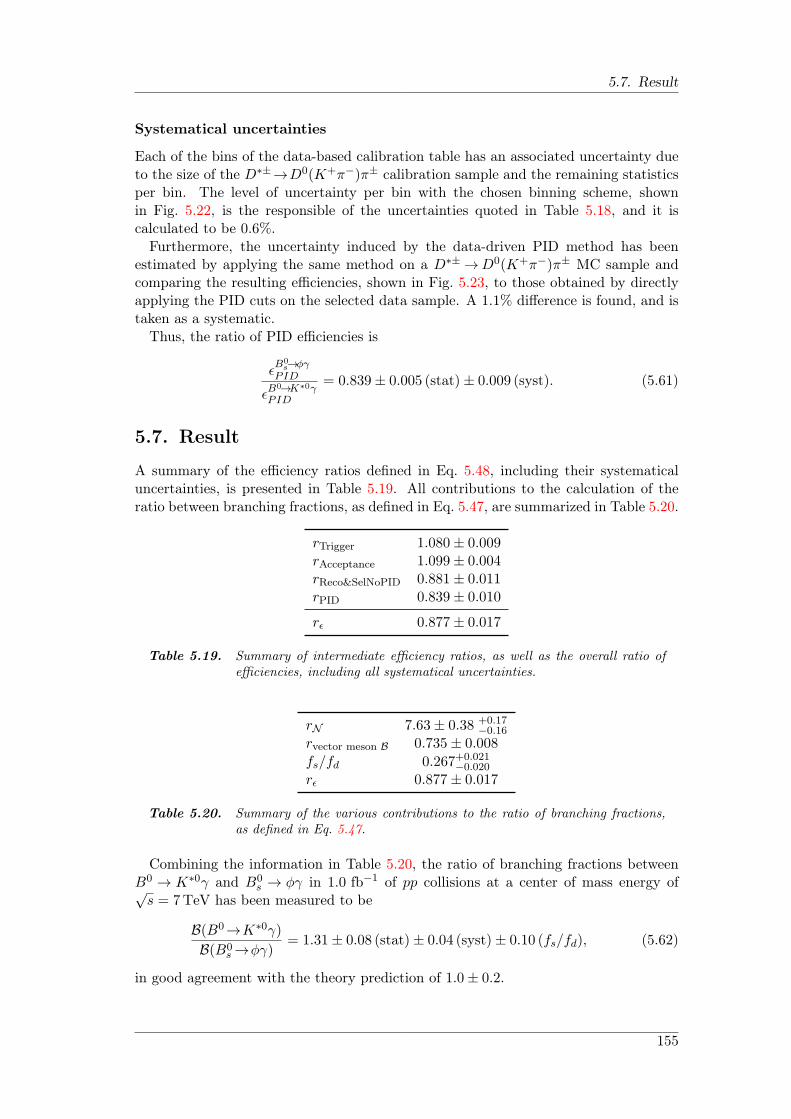
5.7. Result
Systematical uncertainties
Each of the bins of the data-based calibration table has an associated uncertainty dueto the size of the D∗±→D0(K+π−)π± calibration sample and the remaining statisticsper bin. The level of uncertainty per bin with the chosen binning scheme, shownin Fig. 5.22, is the responsible of the uncertainties quoted in Table 5.18, and it iscalculated to be 0.6%.
Furthermore, the uncertainty induced by the data-driven PID method has beenestimated by applying the same method on a D∗± →D0(K+π−)π± MC sample andcomparing the resulting efficiencies, shown in Fig. 5.23, to those obtained by directlyapplying the PID cuts on the selected data sample. A 1.1% difference is found, and istaken as a systematic.
Thus, the ratio of PID efficiencies is
ϵB0
s→ϕγPID
ϵB0→K∗0γ
PID
= 0.839± 0.005 (stat)± 0.009 (syst). (5.61)
5.7. Result
A summary of the efficiency ratios defined in Eq. 5.48, including their systematicaluncertainties, is presented in Table 5.19. All contributions to the calculation of theratio between branching fractions, as defined in Eq. 5.47, are summarized in Table 5.20.
rTrigger 1.080± 0.009rAcceptance 1.099± 0.004rReco&SelNoPID 0.881± 0.011rPID 0.839± 0.010
rϵ 0.877± 0.017
Table 5.19. Summary of intermediate efficiency ratios, as well as the overall ratio ofefficiencies, including all systematical uncertainties.
rN 7.63± 0.38 +0.17−0.16
rvector meson B 0.735± 0.008
fs/fd 0.267+0.021−0.020
rϵ 0.877± 0.017
Table 5.20. Summary of the various contributions to the ratio of branching fractions,as defined in Eq. 5.47.
Combining the information in Table 5.20, the ratio of branching fractions betweenB0 → K∗0γ and B0
s → ϕγ in 1.0 fb−1 of pp collisions at a center of mass energy of√s = 7TeV has been measured to be
B(B0→K∗0γ)
B(B0s →ϕγ)
= 1.31± 0.08 (stat)± 0.04 (syst)± 0.10 (fs/fd), (5.62)
in good agreement with the theory prediction of 1.0± 0.2.
155
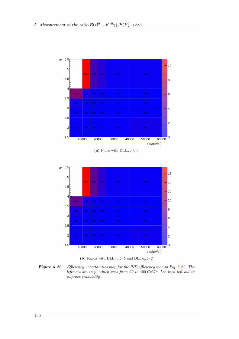
5. Measurement of the ratio B(B0→K∗0γ)/B(B0s →ϕγ)
0.36 0.25 0.19 0.17 0.26 0.80
0.34 0.19 0.12 0.13 0.14 0.28
0.89 0.30 0.17 0.12 0.10 0.14
5.73 1.16 0.41 0.27 0.16 0.19
10.89 2.70 1.57 0.49 0.42
)2p (MeV/c
10000 20000 30000 40000 50000 60000
η
1.5
2
2.5
3
3.5
4
4.5
5
5.5
0
2
4
6
8
10
(a) Pions with DLLKπ < 0
0.71 0.52 0.43 0.36 0.33 0.92
0.56 0.42 0.30 0.28 0.19 0.34
1.36 0.60 0.44 0.31 0.15 0.18
7.00 2.05 0.85 0.61 0.25 0.22
17.45 6.34 2.64 0.71 0.51
)2p (MeV/c
10000 20000 30000 40000 50000 60000
η
1.5
2
2.5
3
3.5
4
4.5
5
5.5
0
2
4
6
8
10
12
14
16
(b) Kaons with DLLKπ > 5 and DLLKp > 2
Figure 5.22. Efficiency uncertainties map for the PID efficiency map in Fig. 5.21. Theleftmost bin in p, which goes from 60 to 400GeV/c, has been left out toimprove readability
156
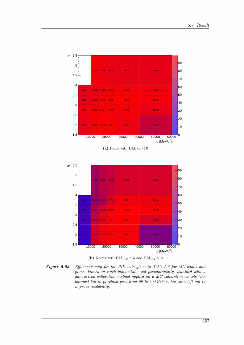
5.7. Result
90.81 96.42 98.79 99.14 93.14 77.34
94.48 96.27 97.84 98.68 96.26 90.41
89.80 93.35 97.39 98.26 98.14 95.77
90.37 90.58 94.65 97.89 96.95 94.58
95.83 92.60 92.70 90.35 89.63
)2p (MeV/c
10000 20000 30000 40000 50000 60000
η
1.5
2
2.5
3
3.5
4
4.5
5
5.5
0
10
20
30
40
50
60
70
80
90
(a) Pions with DLLKπ < 0
22.79 80.37 89.74 95.24 92.28 48.54
25.65 75.25 87.45 94.24 94.21 83.03
27.29 69.05 82.32 92.05 96.22 93.40
22.83 56.70 64.77 83.73 91.74 91.05
60.87 70.16 75.40 80.56 80.92
)2p (MeV/c
10000 20000 30000 40000 50000 60000
η
1.5
2
2.5
3
3.5
4
4.5
5
5.5
0
10
20
30
40
50
60
70
80
90
(b) Kaons with DLLKπ > 5 and DLLKp > 2
Figure 5.23. Efficiency map for the PID cuts given in Table 5.5 for MC kaons andpions, binned in track momentum and pseudorapidity, obtained with adata-driven calibration method applied on a MC calibration sample (theleftmost bin in p, which goes from 60 to 400GeV/c, has been left out toimprove readability).
157

5. Measurement of the ratio B(B0→K∗0γ)/B(B0s →ϕγ)
This ratio of branching fractions can be combined with the well-known value forB(B0→K∗0γ), included in Table 1.3, to extract a new value for B(B0
s →ϕγ),
B(B0s →ϕγ) = (3.3± 0.3)× 10−5, (5.63)
which agrees with the previous experimental measurement, as well as with the theo-retical prediction of B(B0
s →ϕγ) = (4.3± 1.4)× 10−5.
158
6Conclusions
This document has presented my contribution to the first steps of the radiative Bdecays program at LHCb.
Radiative B decays are an example of flavor-changing neutral currents, and as suchthey only appear in the Standard Model as loop-level processes. This feature makesthem sensitive to the heavy degrees of freedom circulating in the loop, turning them intovery sensitive probes for New Physics searches. While exclusive branching fractions ofradiative B decays are not well predicted theoretically, other observables such as CPand isospin asymmetries, and the photon polarization provide a good handle to testmodels beyond the Standard Model, such as mSUGRA or the Left Right SymmetricModel.
An essential requirement for these studies is a good trigger efficiency, so a sizeableamount of events can be kept from the background-dominated pp collisions at LHC.The optimizations introduced to the trigger lines for B0→K∗0γ and B0
s →ϕγ have beendetailed, and their performance has been assessed both on simulated and real data, withimpressive results. This exclusive trigger strategy, in which only the B0 →K∗0γ andB0
s →ϕγ decay channels are included, has been used successfully for radiative decaysstudies during 2011. However, this strategy does not scale well with the number ofchannels and completely discards the possibility of data mining.
An inclusive trigger strategy has been developed in order to overcome this problemand to open the possibility of new analyses involving channels for which no exclusivetrigger line existed. However, in order to broaden the scope of radiative decays triggerlines, which involve in all cases the reconstruction of the photon, it has been necessaryto rethink and redesign how the calorimeter reconstruction works in the HLT2. Re-ducing the timing of the calorimeter reconstruction was mandatory before larger eventsamples could make use of photons in the HLT.
A new reconstruction procedure for the calorimeter in the HLT2 environment, basedon L0 objects, has been devised, providing a three-fold reduction in executing time atthe cost of a small efficiency loss.
A new set of HLT2 inclusive radiative lines, in which only certain common aspectsamong radiative decays are exploited when making a trigger decision, and a redesignedinclusive ϕ line, have been introduced. Their performance on simulated data hasbeen remarkable, and in three out of the four analyzed radiative channels they have
159

6. Conclusions
outperformed the exclusive approach. A direct comparison with the exclusive approachhas also been presented for B0→K∗0(K±π∓)γ and B0
s →ϕ(K+K−)γ data from 2011.In addition, the experience of the 2011 data taking has led to new ideas on how toimprove the inclusive lines in order to access the lower part of the transverse energyspectrum of the photon.
LHCb has decided that inclusive radiative lines will form the base of the triggerstrategy for radiative decays in 2012, opening the way for several new analyses ofradiative B decays, such as the CP asymmetry studies in B+ → ϕK+γ and B0 →ργ. This decision has also caused a shift of the radiative stripping strategy towardsinclusiveness, and will open the way for new studies on the optimization of the offlineselection.
Data collected by the LHCb experiment during 2011 have been used to extract theratio of branching fractions of the B0 →K∗0γ and B0
s → ϕγ decays. The theoreticalprediction for this ratio has an uncertainty of 20%, while the error of the currentexperimental value is ∼ 40%, mainly due to the poor knowledge of the B0
s → ϕγbranching fraction.
By extracting the ratio of branching fractions directly, applying common selectionand trigger criteria for both decays, the cancellation of systematics has been maxi-mized and the total uncertainty has been reduced. The yield of each decay has beenextracted from a simultaneous fit to the K±π∓γ and K+K−γ invariant mass distri-butions. Possible background sources have been studied in detail and they have beenadded to the invariant mass fit. Special care has also been taken to account for alldiscrepancies between data and its MC description.
The ratio of branching fractions has been measured to be
B(B0→K∗0γ)
B(B0s →ϕγ)
= 1.31± 0.08 (stat)± 0.04 (syst)± 0.10 (fs/fd), (6.1)
and has been found to be compatible with the theory prediction of 1.0±0.2. This resulthas been combined with the well-measured value of the B0→K∗0γ branching fractionto extract the world-best measurement of the branching fraction of the radiative B0
s →ϕγ decay,
B(B0s →ϕγ) = (3.3± 0.3)× 10−5, (6.2)
which is also in agreement with the theoretical prediction of (4.6 ± 1.4) × 10−5. Thisresult largely improves the previous knowledge of B(B0
s →ϕγ), reducing its uncertaintyfrom 35% down to 9%.
160
AHelicity formalism and angular
distributions
A.1. The helicity formalism
The helicity formalism is the preferred method for obtaining angular distributions inrelativistic scattering and decay processes [195]. This formalism aims to solve the prob-lem that in the spin-orbit formalism —developed in non-relativistic quantum mechan-ics [196]— the orbital and spin angular momentum operators are defined in referenceframes that are not at rest with respect to one another. The helicity operator h = S · pallows to construct relativistic basis vectors that are either eigenstates of total angularmomentum and helicity (or of linear momentum and helicity) thanks to the fact thath is invariant under both rotations and boosts along p.
A.1.1. Rotation operators and Wigner D-Matrix
An arbitrary rotation R(αβγ) from one initial xyz coordinate system to a final XY Zcoordinate system can be constructed from three successive rotations performed in aspecific sequence [197]. The Euler angles (α, β, γ) are defined as the three successiveangles of rotation:
1. The xyz axes are rotated counterclockwise about the z-axis by an angle α. Theresulting coordinate system is labeled tuz.
2. The intermediate tuz axes are rotated counterclockwise about the u-axis by anangle β to produce a second intermediate set of axes, the t′uZ.
3. The t′uZ axes are rotated counterclockwise by an angle γ about the Z-axis toproduce the desired XY Z system of axes.
Since a rotation around a given axis n is generated by the angular momentum operatorJ · n, the complete rotation can be written as
R(αβγ) = RZ(γ)Ru(β)Rz(α) = e−iJZγe−iJuβe−iJzα. (A.1)
161
A. Helicity formalism and angular distributions
The previous expression is not very useful because it is not expressed in terms ofthe original axes xyz. Applying the invariance under rotation of observables of somephysical system, and exploiting the unitarity of the rotation operators, an arbitraryrotation specified by the Euler angles (α, βγ) can be expressed in terms of rotations ofthe fixed axes xyz:
R(αβγ) = Rz(γ)Ry(β)Rz(α) = e−iJzγe−iJyβe−iJzα. (A.2)
Angular momentum eigenstates |jm⟩ transform irreducibly under rotations because[R, J2] = 0. The action of R(αβγ) on the basis state |jm⟩ can be written as
R(αβγ)|jm⟩ =j∑
m′=−j
Djm′m(αβγ)|jm′⟩. (A.3)
The Wigner D-matrix [198] is defined as a 2j + 1-dimensional square matrix withelements
Djm′m(αβγ) ≡ ⟨jm′|R(αβγ)|jm⟩. (A.4)
Making use of Eq. A.2, the D-matrix can be expressed as
Djm′m(αβγ) = ⟨jm′|e−iJzγe−iJyβe−iJzα|jm⟩ = e−im′αdjm′m(β)e−imγ , (A.5)
in which the elementsdjm′m = ⟨jm′|e−iJyβ|jm⟩ (A.6)
define Wigner’s d-matrix. These matrix elements are given by the complex Wignerformula, which can be found elsewhere [199]. They have, however, many simple prop-erties, the most useful of which are:
djm′m(−β) = (−1)m′−mdjm′m(β)
djm′m(−β) = djmm′(β)
Djm′m(α, β, γ) = Dj
mm′(γ,−β, α) (A.7)
djm′m(π) = (−1)j−mδm′m(β)
djm′m(2π) = (−1)2jδm′m(β).
A.1.2. Plane-Wave helicity states
The states of a free particle of arbitrary spin s, momentum p, and mass m correspondto plane-wave solutions of the relativistic wave equation. For each p there are 2s + 1linearly independent states of definite helicity (λ = −s, s + 1, . . . , s) if the particle ismassive, and only two if the particle is massless (λ = ±1). If a rotation R(αβγ) ofthe system of axes is applied to one of these states, the direction of p changes, butλ remains constant. Similarly, when a Lorentz boost (L(p)) along p is applied to thesystem, p changes magnitude and λ remains unchanged as long as the direction of p isnot reversed.
Therefore, to obtain a state |p, s, λ⟩ |0, s, λ⟩ is rotated so that its quantization axispoints along p and afterwards apply a Lorentz boost along p (the reversed operationis completely equivalent):
|p, s, λ⟩ = L(p)R(α = φ, β = θ, γ = −φ)|0, s, λ⟩. (A.8)
162

A.1. The helicity formalism
The choice of γ = −φ is conventional and has no physical meaning [199].The next step is construct states of two free particles with masses m1 and m2, and
spins s1 and s2. These states are constructed as direct products of the previouslystudied one-particle plane-wave states,
|p1, λ1; p2, λ2⟩ ≡ |p1, s1, λ1⟩ ⊗ |p2, s2, λ2⟩. (A.9)
The spins s1 and s2 are fixed and therefore suppressed from the notation.Moving to the CM frame, in which the particles are back to back (p1 = −p2 = p),
the same two-particle state can be fully specified in terms of the magnitude of p andits direction. Defining p = |p1| = |p2| and (θ, φ) as the angles of p1, the state can bewritten as |p, θ, φ, λ1, λ2⟩. Furthermore, since the two-particle CM plane-wave statesare eigenstates of the total four-momentum Pα, the eigenstate |Pα⟩ can be factoredout and, with suitable normalization,
|p, θ, φ, λ1, λ2⟩ = (2π)3
√4√s
p|θ, φ, λ1, λ2⟩|Pα⟩. (A.10)
However, in order to apply conservation of angular momentum to the transitionmatrix element one needs to use eigenstates of total angular momentum as the ba-sis for the two-particle CM states, i.e., one needs to move from a basis of states ofdefinite direction (plane-wave states) to a basis of states of definite angular momen-tum (spherical-wave states). For that purpose one can use p, J , the total angularmomentum, M , the eigenvalue of Jz, and λ1 and λ2 to identify states in a new basis,|p, J,M, λ1, λ2⟩. With that, the transformation between the two bases can be writtenas
|p, θ, φ, λ1, λ2⟩ =∑J,M
cJM (p, θ, φ, λ1, λ2)|p, J,M, λ1, λ2⟩. (A.11)
The cJM (p, θ, φ, λ1, λ2) coefficients can easily be evaluated for θ = φ = 0. Afterapplying the rotation operator and normalization conditions, one obtains the finalexpression of the transformation between the bases:
|p, θ, φ, λ1, λ2⟩ =∑J,M
√2J + 1
4πDJ
Mλ(Ω)|p, J,M, λ1, λ2⟩, (A.12)
with the definitions λ ≡ λ1 − λ2 and Ω ≡ (φ, θ,−φ).Again, the states |p, J,M, λ1, λ2⟩ have total momentum P = 0 and, since they are
expressed in the CM frame, they are eigenstates of the total 4-momentum Pα. Thatallows to factor out the |Pα⟩ part of the state, similarly to Eq. A.10,
|p, J,M, λ1, λ2⟩ = (2π)3
√4√s
p|J,M, λ1, λ2⟩|Pα⟩, (A.13)
and thus, taking into account that |Pα⟩ is invariant under rotations, Eq. A.12 becomes
|θ, φ, λ1, λ2⟩ =∑J,M
√2J + 1
4πDJ
Mλ(Ω)|J,M, λ1, λ2⟩. (A.14)
163

A. Helicity formalism and angular distributions
A.2. Angular distributions in two-body decays
Now the process 1→2 3, in which the decaying particle 1 has spin s1 and spin projectionm1 along an arbitrarily chosen z-axis, is considered. The final state particles 2,3 havehelicities λ2, λ3 and momenta p2 = pf , p3 = −pf in the CM frame (rest frame ofparticle 1). The final state can be expressed by making use of Eqs. A.13-A.14:
|f⟩ = (2π)3
√4√s
pf|θf , φf , λ1, λ2⟩|Pα
f ⟩, (A.15)
where θf , φf are the angles of pf . Therefore, the amplitude for 1 to decay into thefinal state |f⟩ is
A(1→2 3) = (2π)3
√4√s
pfδ(Pα
f − Pαi )⟨θf , φf , λ1, λ2|U |s1,m1⟩, (A.16)
where conservation of momentum has been applied. The constants in Eq. A.16 don’thave any effect in the angular distributions, so they can be absorbed into U for easiernotation
A(1→2 3) ≡ ⟨θf , φf , λ2, λ3|U |s1,m1⟩. (A.17)
Inserting the two-particle helicity basis states |sf ,mf , λ2, λ3⟩ and making use ofEq. A.14, the amplitude can be expressed as
A(1→2 3) =⟨θf , φf , λ2, λ3|U |s1,m1⟩
=∑sf ,mf
⟨θf , φf , λ2, λ3|sf ,mf , λ2, λ3⟩⟨sf ,mf , λ2, λ3|U |s1,m1⟩
=∑sf ,mf
√2s1 + 1
4πDs1∗
m1λ(Ω)λsf ,s1λmf ,m1⟨λ2, λ3|U |m1⟩, (A.18)
and since ⟨λ2, λ3|U |m1⟩ must be rotationally invariant, the m1 dependence can beremoved and the braket can be rewritten as Aλ2λ3 :
A(1→2 3) =
√2s1 + 1
4πDs1∗
m1λ(Ω)Aλ2λ3 . (A.19)
From this equation, one would expect (2s2+1)(2s3+1) helicity amplitudes. However,conservation of angular momentum requires
|λ2 − λ3| ≤ s1, (A.20)
and also it can be shown that, if parity is conserved in the decay,
A−λ2−λ3 = η1η2η3(−1)s2+s3−s1Aλ2λ3 . (A.21)
The angular distribution is found by squaring the amplitude in Eq. A.19,
dΓ
dΩm1λ2λ3
(θf , φf ) =2s1 + 1
4π
∣∣DJ∗Mλ(Ω)Aλ2λ3
∣∣2 = 2s1 + 1
4π|dJMλ(θ)|2|Aλ2λ3 |2. (A.22)
164
A.2. Angular distributions in two-body decays
If the experiment does not measure the final state helicities λ2, λ3 they must be summedover.
The total decay rate is obtained by applying the sum and integrating over Ω. It doesnot depend on m1 because the decay rate of a free particle should not depend on whichway its spin vector is pointing. With that in mind, the notation can be simplified bydenoting the angular distribution as
I(Ω,m1) =1
Γ
dΓ
dΩm1
. (A.23)
A.2.1. Spin density matrix
Until this point the considered initial state has always been prepared with a definitevalue of m1 and no distinction has been made between m1 and λ1. Under experimentalconditions, it is usually not possible to obtain a measurement for λ1 on an event-by-event basis. Therefore, the amplitude in these cases must contain a coherent sum overλ1, and also, in the general case, a dependence in the lab direction of particle 1, aswell as other variables related to the process which generates particle 1.
Considering the parity-conserving process a b→ 1 (→ 2 3) X, and recalling [196]that a mixture of states |ψi⟩ with fractional populations ωi can be characterized by thedensity operator
ρ =∑
ωi|ψi⟩⟨ψi|, (A.24)
and denoting T as the transition operator corresponding to the interaction, the finalstate density operator can be expressed as
ρ ∝∑λa,λb
T |p1, λa, λb⟩⟨p1, λa, λb|T †, (A.25)
and be used to construct the density matrix ρλ1,λ′1
corresponding to particle 1 by takingthe trace over all final state variables. Thus, the angular distribution becomes
I(Ω) =1
Γ
∑λ1,λ′
1,λ2,λ3
A∗(Ω;λ1, λ2, λ3)ρλ1λ′1A(Ω;λ′1, λ2, λ3)
=1
Γ
2s1 + 1
4π
∑λ1,λ′
1,λ2,λ3
Ds1λ1,λ
(Ω)A∗λ2λ3
ρλ1λ′1Ds1∗
λ′1,λ
(Ω)A∗λ2λ3
. (A.26)
A.2.2. Sequential two-body decays
When considering the decay 1 → 2 (→ 4 5) 3, the first thing that must be done isconstruct a new coordinate system (x′y′z′) in the rest frame of particle 2. First theoriginal axes by are rotated R(φ, θ,−φ), which effectively aligns the z′-axis onto theflight direction of particle 2 in the rest frame of particle 1. With that choice of axes,if particle 2 has helicity λ2 in the rest frame of 1, it will have a spin component in itsown rest frame of m2 = λ2 along the z′-axis.
The angles Ω ≡ (φ′, θ′,−φ′) are defined in the direction of particle 4 in the x′y′z′
coordinate system, so θ′ is defined with respect to the spin quantization axis of particle2. The amplitude for the sequential decay is given by
A(1→2 (→ 4 5) 3) =∑λ2
⟨Ω′λ4λ5|U(2)|s2, λ2⟩⟨Ω|U(1)|s1λ1⟩. (A.27)
165

A. Helicity formalism and angular distributions
Following a similar derivation as Eq. A.19, the helicity formalism can be used toobtain the final expression for the amplitude
A(Ω,Ω′;λ1, λ3, λ4, λ5) =√2s1 + 1
4π
√2s2 + 1
4π
∑λ2
Ds1∗λ1,λ2−λ3
(Ω)Aλ2λ3Ds2∗λ2,λ4−λ5
(Ω′)Bλ4λ5 , (A.28)
where Bλ4λ5 are the helciity amplitudes for the 2→4 5 decay. Note the coherent sumover λ2. From this expression, the angular distribution is again obtained squaring theamplitude and summing over spins taking into account the spin density matrix:
I(Ω,Ω′) =1
Γ1
1
Γ2
2s1 + 1
4π
2s2 + 1
4π
∑λ1λ′
1λ2λ′2λ3λ4λ5
ρλ1λ′1× (A.29)
×Ds1∗
λ′1,λ
′2−λ3
(Ω)Ds1λ1,λ2−λ3
(Ω)A∗λ′2λ3Aλ2λ3D
s2∗λ2,λ4−λ5
(Ω′)Ds2λ′2,λ4−λ5
(Ω′)B∗λ4λ5
Aλ4λ5
.
Expanding the term in braces in Eq. A.29 using Eq. A.5 the angular dependence is
ei(λ1−λ′1)φei(λ2−λ′
2)(φ′−φ) (A.30)
times a product of d-functions that depend on θ and θ′.Since usually the interest lies in the angular distributions of particles 4 and 5, the
number of observables in Eq. A.29 can be reduced by performing a change of variablesχ ≡ (φ′ − φ) —so the amplitude depends on (θ, θ′, φ, χ)— and
Integrating over φ, yielding δλ1λ′1.
Integrating over χ, yielding δλ2λ′2.
Using the ortogonality relation of the D-matrix.∫Dj∗
mn(αβγ)Dj′
m′n′ dα d cosβ d γ =8π2
2j + 1δjj′δmm′δnn′ . (A.31)
Making use of the fact that the trace of the spin density matrix is 1, the angulardistribution in Ω′ can be expressed as
I(Ω′) =1
Γ1Γ2
2s2 + 1
4π
∑λ1λ2λ3λ4λ5
ρλ1λ1 |Ds2λ2,λ4−λ5
(Ω′)|2|Aλ2λ3 |2|Bλ4λ5 |2
=1
Γ1Γ2
2s2 + 1
4π
∑λ1
ρλ1λ1
︸ ︷︷ ︸
Tr(ρ)=1
∑λ2λ3λ4λ5
|ds2λ2,λ4−λ5(θ′)|2|Aλ2λ3 |2|Bλ4λ5 |2
=1
Γ1Γ2
2s2 + 1
4π
∑λ2λ3λ4λ5
|ds2λ2,λ4−λ5(θ′)|2|Aλ2λ3 |2|Bλ4λ5 |2, (A.32)
Thus the angular distribution does not depend on φ′.
166

A.2. Angular distributions in two-body decays
B decay K∗0 decay
λK∗0 = 0,±1 λK = 0λγ = ±1 λπ = 0
(a) B→K∗0(Kπ)γ
B decay K∗0 decay
λK∗0 = 0,±1 λK = 0λ0π = 0 λπ = 0
(b) B→K∗0(Kπ)π0
Table A.1. Possible helicities for the different particles involved in B→K∗0(Kπ)γ/π0.The table is analogous in the case of the B0
s → ϕ(K+K−)γ/π0 decays, re-placing π → K.
A.2.3. Angular distribution of B→K∗0(Kπ)γ
Using Eq. A.32 and the selection rule Eq. A.20 it is easy to determine the angulardistribution of the B →K∗0(Kπ)γ decay and the analogous B0
s → ϕ(K+K−)γ. Ta-ble A.1a shows all possible helicity values given the spins of the particles involved inthe decay.
However, the selection rule Eq. A.20 only allows λK∗0 = λγ , so only the A−1−1 andA11 amplitudes are allowed. Therefore, the angular distribution is
I(θ′) ∝|d1−10(θ
′)|2|A−1−1|2 + |d110(θ′)|2|A11|2. (A.33)
Making use of the d-function properties, it can be seen that
d11,0(θ) = d10,−1(θ) = (−1)d1−1,0(θ), (A.34)
and since the −1 is irrelevant when squared,
I(θ′) ∝ |d11,0(θ)|2. (A.35)
The value of d11,0(θ) can be extracted from [21],
d11,0(θ) = −sin θ√2, (A.36)
which, when squared, gives the angular dependence for the daughters of the vectormeson in B→K∗0(Kπ)γ and B0
s →ϕ(K+K−)γ:
I(θ′) ∝ sin2 θ′. (A.37)
A.2.4. Angular distribution of B→K∗0(Kπ)π0
Analogously to §A.2.3, Table A.1b shows all possibilities for the helicity values of theparticles involved in the B→K∗0(Kπ)π0 and B0
s →ϕ(K+K−)π0 decays.In this case, the selection rule Eq. A.20 only allows λK∗0 = λπ0 = 0, so only the A00
amplitude is allowed. This makes matters simpler, and the angular distribution for thedaughter particles of the vector mesons in the B→K∗0(Kπ)π0 and B0
s →ϕ(K+K−)π0
decays is found to beI(θ′) ∝ |d100|2 ∝ cos2 θ′. (A.38)
167

BIsospin-conserving decay of the
K∗0 vector meson
The K∗0 decay is almost a 100% isospin-conserving strong decay. If the particlesinvolved in the K∗0 decay are characterized, taking into account the fact that K∗0 andK have the same quark content, all the states involved in the K∗0 decay can be built:
|K0⟩ = |K∗0⟩ = ds = |12 − 12⟩ |K0⟩ = |K∗0⟩ = ds = |12
12⟩
|K+⟩ = |K∗+⟩ = us = |1212⟩ |K−⟩ = |K∗−⟩ = us = |12 − 1
2⟩
|π0⟩ = uu+dd√2
= |1 0⟩
|π+⟩ = ud = |1 1⟩ |π−⟩ = us = |1 − 1⟩
The Clebsch-Gordan coefficients [21] can then be used to construct the possible finalstates for the strong decay:
|K0π0⟩ =√
23 |32 − 1
2⟩+√
13 |12 − 1
2⟩ |K0π0⟩ =√
23 |32 − 1
2⟩ −√
13 |12 − 1
2⟩
|K−π+⟩ =√
13 |32
12⟩+
√23 |12
12⟩ |K+π−⟩ =
√13 |32 − 1
2⟩ −√
23 |12 − 1
2⟩
|K+π0⟩ =√
23 |32
12⟩ −
√13 |12
12⟩ |K−π0⟩ =
√23 |32 − 1
2⟩+√
13 |12 − 1
2⟩
|K0π+⟩ =√
13 |32
12⟩+
√23 |12
12⟩ |K0π−⟩ = |32 − 3
2⟩
|K0π+⟩ = |3232⟩ |K0π−⟩ =
√13 |32 − 1
2⟩ −√
23 |12 − 1
2⟩
Finally, the fractions of each decay mode can be calculated:
|⟨K0π0|K∗0⟩|2 = 13 |⟨K+π−|K∗0⟩|2 = 2
3
|⟨K0π0|K∗0⟩|2 = 13 |⟨K−π+|K∗0⟩|2 = 2
3
|⟨K+π0|K∗+⟩|2 = 13 |⟨K0π+|K∗+⟩|2 = 2
3
|⟨K−π0|K∗−⟩|2 = 13 |⟨K0π−|K∗−⟩|2 = 2
3
169

Bibliography
[1] B. Pontecorvo, Neutrino experiments and the question of leptonic-charge conser-vation, Sov. Phys. JETP 26 (1968) 984.
[2] Super-Kamiokande Collaboration, Y. Ashie et al., Evidence for an oscillatorysignature in atmospheric neutrino oscillation, Phys. Rev. Lett. 93 (2004) 101801,arXiv:hep-ex/0404034.
[3] SNO Collaboration, B. Aharmim et al., Electron energy spectra, fluxes, and day-night asymmetries of 8B solar neutrinos from measurements with NaCl dissolvedin the heavy-water detector at the Sudbury Neutrino Observatory, Phys. Rev.C72 (2005) 055502.
[4] MINOS Collaboration, P. Adamson et al., Measurement of Neutrino Oscillationswith the MINOS Detectors in the NuMI Beam, Phys. Rev. Lett. 101 (2008)131802, arXiv:0806.2237.
[5] LEP Working Group for Higgs boson searches, R. Barate et al., Search for thestandard model Higgs boson at LEP, Phys. Lett. B565 (2003) 61, arXiv:hep-ex/0306033.
[6] ATLAS Collaboration, A. Nisati, Standard Model Higgs boson searches with theATLAS detector at the Large Hadron Collider, arXiv:1111.7132.
[7] CMS Collaboration, K. Sung, A Search for Higgs Boson in H → W+W−,arXiv:1109.2457.
[8] A. Einstein, Zur Elektrodynamik bewegt Körper, Annalen der Physik 17 (1905)891.
[9] V. Fock, Über die invariante Form der Wellen- und der Bewegungsgleichungenfür einen geladenen Massenpunkt, Zeitschrift für Physik A Hadrons and Nuclei39 (1926) 226.
[10] H. Weyl, Elektron und Gravitation. I, Zeitschrift für Physik A Hadrons and Nuclei56 (1929) 330.
[11] C.-N. Yang and R. L. Mills, Conservation of isotopic spin and isotopic gaugeinvariance, Phys. Rev. 96 (1954) 191.
[12] S. L. Glashow, Partial Symmetries of Weak Interactions, Nucl. Phys. 22 (1961)579.
171

Bibliography
[13] S. Weinberg, A Model of Leptons, Phys. Rev. Lett. 19 (1967) 1264.
[14] A. Salam, Weak and Electromagnetic Interactions, in Svartholm: ElementaryParticle Theory, Proceedings Of The Nobel Symposium Held 1968 At Lerum,Sweden, pp. 367–377, 1968.
[15] M. Y. Han and Y. Nambu, Three-triplet model with double SU(3) symmetry,Phys. Rev. 139 (1965) B1006.
[16] Y. Nambu, Axial vector current conservation in weak interactions, Phys. Rev.Lett. 4 (1960) 380.
[17] J. Goldstone, Field Theories with Superconductor Solutions, Nuovo Cim. 19(1961) 154.
[18] J. Goldstone, A. Salam, and S. Weinberg, Broken Symmetries, Phys. Rev. 127(1962) 965.
[19] P. W. Higgs, Broken symmetries, massless particles and gauge fields, Phys. Lett.12 (1964) 132.
[20] P. W. Higgs, Spontaneous Symmetry Breakdown without Massless Bosons, Phys.Rev. 145 (1966) 1156.
[21] Particle Data Group, K. Nakamura et al., Review of particle physics, J. Phys.G37 (2010) 075021.
[22] S. Tomonaga, On a Relativistically Invariant Formulation of the Quantum The-ory of Wave Fields, Progress of Theoretical Physics 1 (1946), no. 2 27.
[23] J. Schwinger, On Quantum-Electrodynamics and the Magnetic Moment of theElectron, Phys. Rev. 73 (1948) 416.
[24] J. Schwinger, Quantum Electrodynamics. I. A Covariant Formulation, Phys. Rev.74 (1948) 1439.
[25] F. J. Dyson, The S Matrix in Quantum Electrodynamics, Phys. Rev. 75 (1949)1736.
[26] R. P. Feynman, The Theory of Positrons, Phys. Rev. 76 (1949) 749.
[27] F. J. Dyson, The Radiation Theories of Tomonaga, Schwinger, and Feynman,Phys. Rev. 75 (1949) 486.
[28] R. P. Feynman, Space-Time Approach to Quantum Electrodynamics, Phys. Rev.76 (1949) 769.
[29] R. P. Feynman, Mathematical Formulation of the Quantum Theory of Electro-magnetic Interaction, Phys. Rev. 80 (1950) 440.
[30] D. J. Gross and F. Wilczek, Ultraviolet Behavior of Non-Abelian Gauge Theories,Phys. Rev. Lett. 30 (1973) 1343.
[31] H. D. Politzer, Reliable Perturbative Results for Strong Interactions?, Phys. Rev.Lett. 30 (1973) 1346.
172
Bibliography
[32] E. Noether, Invariante Variationsprobleme, Nachr. d. König. Gesellsch. d. Wiss.zu Göttingen, Math-phys. Klasse (1918) 235. Translation by M.A.Tavel in Trans-port Theory and Statistical Physics, 1 (3), 183–207 (1971).
[33] C. S. Wu, E. Ambler, R. W. Hayward, D. D. Hoppes, and R. P. Hudson, Ex-perimental Test of Parity Conservation in Beta Decay, Phys. Rev. 105 (1957)1413.
[34] R. L. Garwin, L. M. Lederman, and M. Weinrich, Observations of the Failure ofConservation of Parity and Charge Conjugation in Meson Decays: the MagneticMoment of the Free Muon, Phys. Rev. 105 (1957) 1415.
[35] J. Christenson, J. Cronin, V. Fitch, and R. Turlay, Evidence for the 2π Decay ofthe K0
2 Meson, Phys. Rev. Lett. 13 (1964) 138.
[36] Belle Collaboration, K. Abe et al., Observation of large CP violation and evidencefor direct CP violation in B0 → π+π− decays, Phys. Rev. Lett. 93 (2004) 021601,arXiv:hep-ex/0401029.
[37] BaBar Collaboration, B. Aubert et al., Observation of direct CP violation inB0 → K+π− decays, Phys. Rev. Lett. 93 (2004) 131801, arXiv:hep-ex/0407057.
[38] LHCb Collaboration, R. Aaij et al., Evidence for CP violation in time-integratedD0 → h−h+ decay rates, arXiv:1112.0938.
[39] G. Lüders, Proof of the TCP theorem, Ann. Phys. 2 (1957), no. 1 1 .
[40] H. Georgi, Lie Algebras in Particle Physics. From Isospin to Unified Theories,Front. Phys. 54 (1982) 1.
[41] P. W. Higgs, Broken Symmetries and the Masses of Gauge Bosons, Phys. Rev.Lett. 13 (1964) 508.
[42] F. Englert and R. Brout, Broken Symmetry and the Mass of Gauge VectorMesons, Phys. Rev. Lett. 13 (1964) 321.
[43] G. Guralnik, C. Hagen, and T. Kibble, Global Conservation Laws and MasslessParticles, Phys. Rev. Lett. 13 (1964) 585.
[44] N. Cabibbo, Unitary Symmetry and Leptonic Decays, Phys. Rev. Lett. 10 (1963)531.
[45] M. Kobayashi and T. Maskawa, CP -Violation in the Renormalizable Theory ofWeak Interaction, Progress of Theoretical Physics 49 (1973), no. 2 652.
[46] L. Wolfenstein, Parametrization of the Kobayashi-Maskawa Matrix, Phys. Rev.Lett. 51 (1983) 1945.
[47] CKMfitter Group, J. Charles et al., CP violation and the CKM matrix: Assessingthe impact of the asymmetric B factories, Eur. Phys. J. C41 (2005) 1, arXiv:hep-ph/0406184. Updated results and plots available at: http://ckmfitter.in2p3.fr.
173
Bibliography
[48] S. L. Glashow, J. Iliopoulos, and L. Maiani, Weak Interactions with Lepton-Hadron Symmetry, Phys. Rev. D2 (1970) 1285.
[49] J. R. Ellis, M. Gaillard, D. V. Nanopoulos, and S. Rudaz, The Phenomenologyof the Next Left-Handed Quarks, Nucl. Phys. B131 (1977) 285.
[50] M. Antonelli et al., Flavor Physics in the Quark Sector, Phys. Rept. 494 (2010)197, arXiv:0907.5386.
[51] M. Misiak et al., Estimate of B(B → Xsγ) at O(α2s), Phys. Rev. Lett. 98 (2007)
022002, arXiv:hep-ph/0609232.
[52] M. Beneke, T. Feldmann, and D. Seidel, Systematic approach to exclusive B →V l+l−, V γ decays, Nucl. Phys. B612 (2001) 25, arXiv:hep-ph/0106067.
[53] A. L. Kagan and M. Neubert, Isospin breaking in B → K∗γ decays, Phys. Lett.B539 (2002) 227, arXiv:hep-ph/0110078.
[54] S. W. Bosch and G. Buchalla, The Radiative decays B → V γ at next-to-leadingorder in QCD, Nucl. Phys. B621 (2002) 459, arXiv:hep-ph/0106081.
[55] C. W. Bauer, S. Fleming, and M. E. Luke, Summing Sudakov logarithms inB → Xsγ in effective field theory, Phys. Rev. D63 (2000) 014006, arXiv:hep-ph/0005275.
[56] C. W. Bauer, S. Fleming, D. Pirjol, and I. W. Stewart, An effective field theory forcollinear and soft gluons: Heavy to light decays, Phys. Rev. D63 (2001) 114020,arXiv:hep-ph/0011336.
[57] C. W. Bauer and I. W. Stewart, Invariant operators in collinear effective theory,Phys. Lett. B516 (2001) 134, arXiv:hep-ph/0107001.
[58] C. W. Bauer, D. Pirjol, and I. W. Stewart, Soft-Collinear Factorization in Ef-fective Field Theory, Phys. Rev. D65 (2002) 054022, arXiv:hep-ph/0109045.
[59] S. Weinberg, The quantum theory of fields. Vol. 2: Modern applications. Cam-bridge University Press, 1996.
[60] A. Pich, Effective field theory: Course, arXiv:hep-ph/9806303.
[61] S. Bertolini, F. Borzumati, and A. Masiero, QCD Enhancement of Radiative bDecays, Phys. Rev. Lett. 59 (1987) 180.
[62] N. G. Deshpande, P. Lo, J. Trampetic, G. Eilam, and P. Singer, Prediction ofB → K∗γ as a Test of the Standard Model, Phys. Rev. Lett. 59 (1987) 183.
[63] T. Becher, R. J. Hill, and M. Neubert, Factorization in B → V γ decays, Phys.Rev. D72 (2005) 094017, arXiv:hep-ph/0503263.
[64] T. Hurth and M. Nakao, Radiative and Electroweak Penguin Decays of B Mesons,Ann. Rev. Nucl. Part. Sci. 60 (2010) 645, arXiv:1005.1224.
[65] E. Eichten and B. R. Hill, An Effective Field Theory for the Calculation of MatrixElements Involving Heavy Quarks, Phys. Lett. B234 (1990) 511.
174
Bibliography
[66] H. Georgi, An Effective Field Theory For Heavy Quarks At Low-Energies, Phys.Lett. B240 (1990) 447.
[67] A. Ali, B. D. Pecjak, and C. Greub, B → V γ Decays at NNLO in SCET, Eur.Phys. J. C55 (2008) 577, arXiv:0709.4422.
[68] I. Balitsky, V. M. Braun, and A. Kolesnichenko, Power corrections 1/Q2 to partonsum rules for deep inelastic scattering from polarized targets, Phys. Lett. B242(1990) 245, arXiv:hep-ph/9310316.
[69] V. Chernyak and I. Zhitnitsky, B meson exclusive decays into baryons, Nucl.Phys. B345 (1990) 137.
[70] M. A. Shifman, A. Vainshtein, and V. I. Zakharov, QCD and Resonance Physics:Sum Rules, Nucl. Phys. B147 (1979) 385.
[71] M. A. Shifman, A. Vainshtein, and V. I. Zakharov, QCD and Resonance Physics:Applications, Nucl. Phys. B147 (1979) 448.
[72] M. A. Shifman, Snapshots of hadrons or the story of how the vacuum mediumdetermines the properties of the classical mesons which are produced, live anddie in the QCD vacuum, Prog. Theor. Phys. Suppl. 131 (1998) 1, arXiv:hep-ph/9802214. Review.
[73] K. G. Wilson, Nonlagrangian models of current algebra, Phys. Rev. 179 (1969)1499.
[74] P. Ball, G. W. Jones, and R. Zwicky, B → V γ beyond QCD factorisation, Phys.Rev. D75 (2007) 054004, arXiv:hep-ph/0612081.
[75] CLEO Collaboration, T. E. Coan et al., Study of Exclusive Radiative B MesonDecays, Phys. Rev. Lett. 84 (2000), no. 23 5283.
[76] BaBar Collaboration, B. Aubert et al., Measurement of Branching Fractions andCP and Isospin Asymmetries in B → K∗(892)γ Decays, Phys. Rev. Lett. 103(2009) 211802, arXiv:0906.2177.
[77] Belle Collaboration, M. Nakao et al., Measurement of the B → K∗γ branchingfractions and asymmetries, Phys. Rev. D69 (2004), no. 11 112001.
[78] Belle Collaboration, J. Wicht et al., Observation of B0s → ϕγ and Search for
B0s → γγ Decays at Belle, Phys. Rev. Lett. 100 (2008) 121801, arXiv:0712.2659.
[79] Heavy Flavor Averaging Group, D. Asner et al., Averages of b-hadron, c-hadron,and τ -lepton Properties, arXiv:1010.1589.
[80] S. Descotes-Genon, D. Ghosh, J. Matias, and M. Ramon, Exploring New Physicsin the C7-C7’ plane, JHEP 1106 (2011) 099, arXiv:1104.3342.
[81] F. Mahmoudi and M. R. Ahmady, Constraints on mSUGRA from isospin asym-metry in B → K∗γ, AIP Conf. Proc. 903 (2007) 283, arXiv:hep-ph/0610144.
175
Bibliography
[82] M. Beneke, T. Feldmann, and D. Seidel, Exclusive radiative and electroweak b→d and b → s penguin decays at NLO, Eur. Phys. J. C41 (2005) 173, arXiv:hep-ph/0412400.
[83] Y. Y. Keum, M. Matsumori, and A. I. Sanda, CP asymmetry, branching ratiosand isospin breaking effects of B → K∗γ with perturbative QCD approach, Phys.Rev. D72 (2005) 014013, arXiv:hep-ph/0406055.
[84] LHCb Collaboration, Roadmap for selected key measurements of LHCb,arXiv:0912.4179.
[85] L. Evans and P. Bryant, LHC Machine, JINST 3 (2008) S08001.
[86] R. Fernow, Introduction to experimental particle physics. Cambridge UniversityPress, 1989. doi: 10.2277/0521379407.
[87] W. Herr and B. Muratori, Concept of luminosity, in CAS (CERN AcceleratorSchool): Intermediate Course on Accelerator Physics, pp. 361–378, Sep, 2006.
[88] ALICE Collaboration, K. Aamodt et al., The ALICE experiment at the CERNLHC, JINST 3 (2008) S08002.
[89] ATLAS Collaboration, G. Aad et al., The ATLAS Experiment at the CERNLarge Hadron Collider, JINST 3 (2008) S08003.
[90] CMS Collaboration, R. Adolphi et al., The CMS experiment at the CERN LHC,JINST 3 (2008) S08004.
[91] LHCb Collaboration, A. Augusto Alves Jr et al., The LHCb Detector at the LHC,JINST 3 (2008) S08005.
[92] LHCf Collaboration, O. Adriani et al., The LHCf detector at the CERN LargeHadron Collider, JINST 3 (2008) S08006.
[93] TOTEM Collaboration, G. Anelli et al., The TOTEM experiment at the CERNLarge Hadron Collider, JINST 3 (2008) S08007.
[94] LCG, C. Eck et al., LHC computing Grid: Technical Design Report, CERN-LHCC-2005-024.
[95] LHCb Collaboration, R. Antunes-Nobrega et al., LHCb reoptimized detector de-sign and performance: Technical Design Report, CERN-LHCC-2003-030.
[96] LHCb Collaboration, S. Amato et al., LHCb: Technical Proposal, CERN-LHCC-98-004.
[97] LHCb Collaboration, R. Aaij et al., Measurement of σ(pp→ bbX) at√s=7 TeV
in the forward region, Phys. Lett. B694 (2010) 209, arXiv:1009.2731.
[98] LHCb collaboration, R. Aaij et al., Measurement of b hadron production fractionsin 7 TeV pp collisions, Phys. Rev. D85 (2012) , arXiv:1111.2357.
[99] G. Lopez, Notes About the Beta Function, SSC-N-783, SSCL, 1991.
176
Bibliography
[100] LHCb Collaboration, P. R. Barbosa-Marinho et al., LHCb VELO (VErtex LO-cator): Technical Design Report, CERN-LHCC-2001-0011.
[101] LHCb Collaboration, P. R. Barbosa-Marinho et al., LHCb inner tracker: Tech-nical Design Report, CERN-LHCC-2002-029.
[102] LHCb Collaboration, P. R. Barbosa-Marinho et al., LHCb outer tracker: Tech-nical Design Report, CERN-LHCC-2001-024.
[103] LHCb Collaboration, S. Amato et al., LHCb magnet: Technical Design Report,CERN-LHCC-2000-007.
[104] LHCb Collaboration, S. Amato et al., LHCb RICH: Technical Design Report,CERN-LHCC-2000-037.
[105] LHCb Collaboration, S. Amato et al., LHCb Calorimeters, CERN-LHCC-2000-0036.
[106] LHCb Collaboration, P. R. Barbosa-Marinho et al., LHCb muon system: Tech-nical Design Report, CERN-LHCC-2001-010.
[107] LHCb Collaboration, P. R. Barbosa-Marinho et al., LHCb online system, dataacquisition and experiment control: Technical Design Report, CERN-LHCC-2001-040.
[108] J. Andre et al., Status of the LHCb magnet system, IEEE Transactions on AppliedSuperconductivity 12 (2002) 366 .
[109] J. Andre, W. Flegel, P. Giudici, O. Jamet, and M. Losasso, Status of the LHCbdipole magnet, IEEE Transactions on Applied Superconductivity 14 (2004) 509.
[110] LHCb Collaboration, R. Aaij et al., Prompt production in pp collisions at√s =
0.9 TeV, Phys. Lett. B693 (2010) 69, arXiv:1008.3105.
[111] P. A. Cherenkov, Visible emission of clean liquids by action of γ radiation, Dok-lady Akademii Nauk SSSR 2 (1934) 451.
[112] N. Brook et al., LHCb RICH1 Engineering Design Review Report, LHCb-2004-121.
[113] M. Adinolfi et al., LHCb RICH 2 engineering design review report, LHCb-2002-009.
[114] A. Arefev et al., Beam Test Results of the LHCb Electromagnetic Calorimeter,LHCb-2007-149.
[115] J. Lefrançois, F. Machefert, and A. Martens, Calibration of the LHCb calorime-ters with energy flow, LHCb-INT-2010-021.
[116] I. Belyaev, V. Egorychev, and D. Savrina, ECAL calibration within Kali frame-work: Mass distribution fit method calibration with the real data, LHCb-INT-2011-049.
177

Bibliography
[117] R. W. Forty and O. Schneider, RICH pattern recognition, LHCb-98-040.
[118] LHCb RICH Collaboration, A. Powell, Reconstruction and PID performance ofthe LHCb RICH detectors, Nucl. Instrum. Meth. A639 (2011) 260.
[119] RICH Performance Plots, https://lbtwiki.cern.ch/bin/view/RICH/
RichPIDPerformancePlots.
[120] M. Gandelman and E. Polycarpo, The Performance of the LHCb Muon Identifi-cation Procedure, LHCb-2007-145.
[121] J. R. T. De Mello-Neto and M. Gandelman, Muon ID performance with thereoptimized LHCb detector, LHCb-2003-089.
[122] R. Aaij et al., Measurement of J/ψ production in pp collisions at√s = 7 TeV,
Eur. Phys. J. C71 (2011) 1645, arXiv:1103.0423.
[123] H. Terrier and I. Belyaev, Particle identification with LHCb Calorimeters, LHCb-2003-092.
[124] O. Deschamps, F. Machefert, M.-H. Schune, G. Pakhlova, and I. Belyaev, Photonand Neutral Pion reconstruction, LHCb-2003-091.
[125] LHCb Collaboration, R. Antunes-Nobrega et al., LHCb Trigger System TechnicalDesign Report, CERN-LHCC-2003-031.
[126] V. V. Gligorov, A single track HLT1 trigger, LHCb-PUB-2011-003.
[127] R. Aaij and J. Albrecht, Muon triggers in the High Level Trigger of LHCb,CERN-LHCb-PUB-2011-017.
[128] E. V. Herwijnen, HLT2 Rates, https://twiki.cern.ch/twiki/bin/view/
LHCb/Hlt2Rates.
[129] M. Williams et al., The HLT2 Topological Lines, LHCb-PUB-2011-002.
[130] F. Soomro and I. Belyaev, HLT2 exclusive selections for Bs → ϕγ and Bd →K∗γ, LHCb-PUB-2010-007.
[131] M. Lieng, An Inclusive ϕ Stream for the LHCb High Level Trigger, DC06 Anal-ysis, CERN-LHCb-2009-010.
[132] LHCb Collaboration, N. Tatsuya, E. Aslanides, A. Smith, and W. Witzeling,Addendum to the LHCb Online System Technical Design Report, CERN-LHCC-2001-040-ADD-1. CERN-LHCC-2005-039.
[133] G. Haefeli et al., The LHCb DAQ interface board TELL1, Nucl. Instrum. Meth.A560 (2006) 494.
[134] W. Salter, The LHC experiments’ joint controls project (JCOP), Conf. Proc.C0109031 (2001) 2.
[135] CERN PVSS Service, http://j2eeps.cern.ch/wikis/display/EN/PVSS+
Service.
178

Bibliography
[136] B. Franek and C. Gaspar, SMI++ object oriented framework used for automa-tion and error recovery in the LHC experiments, J. Phys. Conf. Ser. 219 (2010)022031.
[137] SMI++ - State Management Interface, http://smi.web.cern.ch/smi/.
[138] P. Mato, GAUDI — Architecture design document, LHCb-98-064.
[139] G. Barrand et al., GAUDI — A software architecture and framework for buildingHEP data processing applications, Comput. Phys. Commun. 140 (2001) 45. Seealso: http://proj-gaudi.web.cern.ch/proj-gaudi/.
[140] LHCb Collaboration, R. Antunes-Nobrega et al., LHCb computing: TechnicalDesign Report, CERN-LHCC-2005-019.
[141] R. Brun and F. Rademakers, ROOT: An object oriented data analysis framework,Nucl. Instrum. Meth. A389 (1997) 81.
[142] The ROOT Project, http://root.cern.ch/.
[143] I. Belyaev et al., Simulation application for the LHCb experiment,arXiv:physics/0306035. See also: http://lhcb-release-area.web.cern.ch/
LHCb-release-area/DOC/gauss/.
[144] I. Belyaev et al., Handling of the generation of primary events in Gauss, theLHCb simulation framework, LHCb-PROC-2010-056. To appear in the proceed-ings of NSS 2010, the 2010 Nuclear Science Symposium, October 30-November6, 2010, Knoxville, USA.
[145] T. Sjostrand, S. Mrenna, and P. Z. Skands, PYTHIA 6.4 Physics and Manual,JHEP 0605 (2006) 026, arXiv:hep-ph/0603175.
[146] D. J. Lange, The EvtGen particle decay simulation package, Nucl. Instrum. Meth.A462 (2001), no. 1-2 123.
[147] E. Barberio, B. van Eijk, and Z. Was, PHOTOS: A Universal Monte Carlo forQED radiative corrections in decays, Comput. Phys. Commun. 66 (1991) 115.
[148] E. Barberio and Z. Was, PHOTOS: A Universal Monte Carlo for QED radiativecorrections. Version 2.0, Comput. Phys. Commun. 79 (1994) 291.
[149] S. Agostinelli et al., GEANT4—a simulation toolkit, Nucl. Instrum. Meth. A506(2003), no. 3 250.
[150] LHCb Collaboration, The Boole Project, http://lhcb-release-area.web.
cern.ch/LHCb-release-area/DOC/boole/.
[151] LHCb Collaboration, The Moore Project, http://lhcb-release-area.web.
cern.ch/LHCb-release-area/DOC/moore/.
[152] LHCb Collaboration, The Brunel Project, http://lhcb-release-area.web.
cern.ch/LHCb-release-area/DOC/brunel/.
179
Bibliography
[153] LHCb Collaboration, The DaVinci Project, http://lhcb-release-area.web.
cern.ch/LHCb-release-area/DOC/davinci/.
[154] R. Graciani, LHCb Computing Resources: 2011 re-assessment, 2012 request and2013 forecast, LHCb-PUB-2011-009.
[155] B. Souza de Paula, Studies on Systematic Effects of the Trigger on Flavour Tag-ging at the Generator Level, LHCb-PUB-2009-014.
[156] J. A. Hernando Morata, E. Lopez Asamar, D. Martinez Santos, H. Ruiz-Pérez,and F. Teubert, Measurement of trigger efficiencies and biases, LHCb-2008-073.
[157] M. Calvo and H. Ruiz, Photon/Electron trigger at high luminosity, LHCbCalorimeter Upgrade Meeting, 5th Oct, 2010.
[158] K. Senderowska, M. Witek, and A. Zuranski, HLT1 Electromagnetic Alley,LHCb-PUB-2009-001.
[159] V. Breton, N. Brun, and P. Perret, A clustering algorithm for the LHCb electro-magnetic calorimeter using a cellular automaton, LHCb-2001-123.
[160] M. Williams, HLT2 Topological Lines for 2011, LHCb Software & AnalysisWeek, CERN, Geneva, Feb, 2011.
[161] I. Narski, StatPatternRecognition: A C++ Package for Statistical Analysis ofHigh Energy Physics Data, arXiv:physics/0507143.
[162] V. Gligorov, C. Thomas, and M. Williams, The HLT inclusive B triggers, LHCb-PUB-2011-016.
[163] A. Puig, Inclusive ϕ trigger, Talk at the PPMTS Meeting on May 30th, 2011.
[164] M. Pivk and F. R. Le Diberder, sPlot: A statistical tool to unfold data distribu-tions, Nucl. Instrum. Meth. A555 (2005) 356, arXiv:physics/0402083.
[165] Y. Amhis et al., Absolute Luminosity Measurements at√s = 7 TeV, LHCb-
INT-2011-018.
[166] LHCb Collaboration, LHCb Luminosity Project, https://twiki.cern.ch/
twiki/bin/viewauth/LHCbPhysics/LuminosityMeasurements, Jan, 2012.
[167] L. Shchutska, A. Golutvin, and I. Belyaev, Study of radiative penguin decaysB → K∗0γ and Bs → ϕγ at LHCb, LHCb-2007-030.
[168] O. Callot and M. Schiller, PatSeeding: A Standalone Track Reconstruction Al-gorithm, LHCb-2008-042.
[169] M. Calvo, π0/γ separation tool, Talk at the Radiative Decays Meeting on Nov17th, 2011.
[170] M. Calvo, π0/γ separation status, Talk at the Calorimeter Objects Meeting onFeb 10th, 2011.
[171] J. Jackson, Remarks on the Phenomenological Analysis of Resonances, Il NuovoCimento 34 (1964) 1644.
180

Bibliography
[172] HERA-B Collaboration, I. Abt et al., K∗0 and ϕ meson production in proton-nucleus interactions at
√s = 41.6 GeV, Eur. Phys. J. C50 (2007) 315, arXiv:hep-
ex/0606049.
[173] S. Baker and R. D. Cousins, Clarification of the use of chi-square and likelihoodfunctions in fits to histograms, Nucl. Instrum. Meth. 221 (1984) 437.
[174] T. Skwarnicki, A study of the radiative cascade transitions between the Upsilon-prime and Upsilon resonances. PhD thesis. Cracow Institute of Nuclear Physics,1986. DESY-F31-86-02.
[175] P. David et al., Measurement of the relative yields of the decay modes B0 →D±π∓, B0 → D±K∓, B0
s → D±s π
∓ and determination of fs/fd for 7 TeV ppcollisions, LHCb-ANA-2010-010.
[176] K. D. Bruyn and P. Koppenburg, Understanding the High Mass Tail of the Re-constructed B Mass distribution, Talk at the PPMTS Meeting on Sep 12th,2011.
[177] BaBar Collaboration, B. Aubert et al., Dalitz Plot Analysis of the DecayB0(B0) → K±π∓π0, Phys. Rev. D78 (2008) 052005, arXiv:0711.4417.
[178] Belle Collaboration, S. Nishida et al., Radiative B meson decays into K pi gammaand K pi pi gamma final states, Phys. Rev. Lett. 89 (2002) 231801, arXiv:hep-ex/0205025.
[179] Y. Grossman and D. Pirjol, Extracting and using photon polarization informationin radiative B decays, JHEP 0006 (2000) 029, arXiv:hep-ph/0005069.
[180] A. Carbone et al., Measurement of direct CP violation in charmless charged two-body B decays at LHCb using 2010 data, LHCb-CONF-2011-011.
[181] ARGUS Collaboration, H. Albrecht et al., Search for Hadronic b → u Decays,Phys. Lett. B241 (1990) 278.
[182] W. Verkerke and D. P. Kirkby, The RooFit toolkit for data modeling,arXiv:physics/0306116.
[183] F. James and M. Roos, Minuit: A System for Function Minimization and Anal-ysis of the Parameter Errors and Correlations, Comput. Phys. Commun. 10(1975) 343.
[184] M. Williams, How good are your fits? Unbinned multivariate goodness-of-fit testsin high energy physics, JINST 5 (2010) P09004, arXiv:1006.3019.
[185] Belle Collaboration, K. Kinoshita, Evaluating quality of fit in unbinned maximumlikelihood fitting, in Proceedings of the Conference on Advanced Techniques inParticle Physics (M. Whaley and L. Lyons, eds.), pp. 176–181, 2002. www.ippp.dur.ac.uk/Workshops/02/statistics/proceedings/kinoshita.ps.
[186] J. Heinrich, Pitfalls of Goodness-of-Fit from Likelihood, eConf C030908 (2003)MOCT001, arXiv:physics/0310167.
181

Bibliography
[187] G. Cowan, Statistical data analysis. Clarendon Press (Oxford), 1998.
[188] LHCb Collaboration, R. Aaij et al., Measurement of b-hadron production frac-tions in 7 TeV centre-of-mass energy pp collisions, LHCb-CONF-2011-028.
[189] LHCb Collaboration, R. Aaij et al., Determination of fs/fd for 7 TeV pp colli-sions and a measurement of the branching fraction of the decay Bd → D−K+,arXiv:1106.4435.
[190] LHCb MC11 generator and simulation statistics, http://lhcb-release-area.
web.cern.ch/LHCb-release-area/DOC/STATISTICS/MC11STAT/index.shtml.
[191] J. V. Tilburg, LHCb Tracking Efficiencies status/results, https://twiki.cern.
ch/twiki/bin/view/LHCb/TrackingEffStatusUpdated.
[192] S. Miglioranzi and G. Corti, Material interaction cross section studies, LHCb-INT-2011-002.
[193] A. Powell, PID Performance Package, Internal talk at University of Oxford,Mar, 2011.
[194] A. Powell, Latest News on PIDCalib Package and PID Performance, RICHMeeting, CERN, Aug, 2011.
[195] J. D. Richman, An Experimenter’s Guide to the Helicity Formalism, DOE Re-search and Development Report CALT-68-1148, California Institute of Technol-ogy, June, 1984.
[196] J. J. Sakurai, Modern Quantum Mechanics. Addison-Wesley Publishing Com-pany, Reading, MA, Revised ed., 1994.
[197] H. Goldstein, Classical Mechanics. Addison-Wesley, 2nd ed., 1980.
[198] E. P. Wigner, Group Theory and Its Application to the Quantum Mechanics ofAtomic Spectra. Academic Press, 1959.
[199] M. Jacob and G. C. Wick, On the General Theory of Collisions for Particleswith Spin, Ann. Phys. 7 (1959) 404.
182
Related Documents