Firm-Product Linkages and the Evolution of Product Scopemjf2143/Flagge_JMPNov2014.pdf · 2 1 Introduction How does a firm’s product mix evolve? Consider the example of ITC Ltd.,

1

Firm-Product Linkages and the Evolution of Product Scope*

Matthew Flagge1 and Ritam Chaurey2

1Columbia University 2SUNY Binghamton

November 2014

JOB MARKET PAPER

What are the factors that shape the evolution of a firm’s product mix? New products added by firms

often share similarities with their existing products or those of nearby firms. This paper provides a

methodology for estimating the role of various measures of “distance” in firms’ product choice

decisions. We model additions of new products by firms using a dynamic model in which firms must pay

a one-time startup cost for adding new products to their production line. We allow this cost to be

reduced if the firm already produces similar products, or shares some characteristics with other firms

already producing the product. We consider three measurable characteristics along which firms may be

considered “close” to a particular product: input similarity, physical distance to existing locations of

production, and upstream-downstream connectedness. The set of potential product combinations is

prohibitively large for standard estimation methods. Instead, we apply the method of moment

inequalities developed by Pakes et al. (forthcoming) and Morales et al (2014). Results are

heterogeneous across sectors, though physical distance seems to be of greatest importance. The third

measure (upstream-downstream connectedness) seems to matter little after controlling for the other

two. Counterfactuals in which we negate the benefits from certain proximity channels show that even

in sectors where input similarity is important, physical proximity has a greater impact on the number of

profitable products available to a firm.

* We would like to thank Eric Verhoogen, Amit Khandelwal, Eduardo Morales, David Weinstein, Kate Ho, Jon Vogel,

Don Davis, Peter Schott, Peter Neary, Jonathan Dingle, and Chris Conlon for helpful comments.

2

1 Introduction How does a firm’s product mix evolve? Consider the example of ITC Ltd., a large conglomerate with

over $8 billion in revenue. This company started in 1910, producing tobacco, and entered the packing

and printing business in 1925 as a form of backward integration. It began producing paperboard in

1979. In 1990 it began the exportation of agricultural commodities, which it describes as a leveraging of

their agri-sourcing competency (ostensibly based on their existing ability to source wood and tobacco).

They started producing notebooks in 2002, and later expanded to books, pens, pencils, and other

stationary over the course of 2007-2009. They entered the food business with ready-to-eat meals in

2001, which their company website describes as “successfully blending multiple internal

competencies.”1 They then progressed into confectionary and wheat flour (2002), biscuits (2003), and

instant noodles (2010).

The nature of what a country’s firms produce is not merely a subject of idle curiosity. There is

theoretical literature that suggests that a country’s products can matter for welfare. For instance, there

can be learning, or spillovers across products (Matsuyama [1992], Harrison and Rodriguez-Clare [2010]).

On the empirical side, Bernard, Jensen, and Schott (2006) find that the capital intensity of an industry’s

products can affect employment growth and the probability of plant death in the presence of

international trade. Furthermore, Hidalgo et al. (2007) find the pairwise export correlations predict the

development of future comparative advantage, which implies that countries whose exports are

correlated with many products are more likely to develop comparative advantage in a broader range of

products. These authors all suggest that both the type and diversity of the products produced by a

country can have welfare effects for that country. Thus, a better understanding of the sequence in

which products are added by firms can in turn give us a better understanding of the development path

of a country, in terms of both product scope and welfare.

The question of what factors shape the evolution of a firm’s product mix also relates to the active recent

literature on multi-product firms in an international context. The existing literature offers two leading

explanations for what might drive the sequence in which firms add products. Bernard, Redding, and

Schott (2010) models the adding and dropping of products as the result of stochastic shocks to demand

and firm-product productivity. Eckel and Neary (2010) employ a model in which firms have a core

competency (lowest production cost) product, and firms add products in order of how similar they are

to the core product. But the former model fails to account for the high frequency at which certain pairs

of products are produced together, and the latter model is agnostic about what characteristics cause a

product to be “near” or “far” from a firm’s core competency.

Our paper develops a methodology that allows us to estimate the costs that firms face in transitioning to

new products, and calculate how those costs vary based on certain measures of “distance” between

firms and products. We consider three such measures within this paper: 1) Overlapping inputs, 2)

Physical proximity of the factory to other locations where the product is produced, 3)

upstream/downstream connectedness via input-output linkages.

1 http://www.itcportal.com/about-itc/profile/history-and-evolution.aspx (retrieved 9/16/2014)

http://www.itcportal.com/about-itc/profile/history-and-evolution.aspx

3

Determining the topology of the product landscape is a non-trivial undertaking. Modelling a decision as

complex as product choice would be difficult in a discrete-choice setting. The size of the choice set is

very large, and the problem would be computationally infeasible even if firms’ information sets were

known. We circumvent these difficulties by using a novel econometric technique called moment

inequalities, developed by Pakes, Porter, Ho, and Ishii (forthcoming) [henceforth, PPHI]. The method

relies on a “revealed preferences” assumption. Rather than trying to explicitly model firms’ choices, we

observe their actions and assume they are at least weakly more profitable (on average) than their other

possible choices. 2 This allows us to derive an inequality condition where on one side are the expected

profits for engaging in the chosen action, and on the other are profits from a potential counterfactual

choice. Each of these profit terms is a function of parameters defined in a theoretical model, and these

inequalities allow us to find upper and lower bounds on the parameters (i.e. the highest and lowest

values of the parameters that are consistent with the inequalities derived from the firm choices).

The theoretical and empirical framework for our analysis closely follows Morales, Sheu, and Zahler

(2014) [henceforth, MSZ], a structural gravity model with a dynamic component to capture how firms’

costs of entry into a new market might depend on their prior entry choices. MSZ studies firm entry into

country markets, which are distanced from the firm in physical space. We adapt their model to study

firm entry into product markets, where each new product has a distance from the firm within a

“characteristic space.” This model is able to capture the dynamic component of firm choice,

incorporating the connections that potential new markets have to firms’ existing abilities. In the model,

firms choose whether to add new products, and which products to add, out of a universe of possible

products. Each firm-product pair has a stream of projected revenue that it can offer the firm, but entry

is deterred by startup costs the firm must incur to begin production of a particular product. These

startup costs depend on whether the firm is “close” to the new product, along the three dimensions

enumerated earlier.

The data we use come from India’s Annual Survey of Industries, a factory-level dataset that includes

inputs, outputs, and physical location, among many other characteristics. The data are an unbalanced

panel with yearly observations, chosen because it allows us to observe adding of products by firms in an

emerging markets setting.

Our results are bounds on the costs of transitioning into new products. We estimate these costs

separately by sector, and results are heterogeneous across sectors. In general, the physical proximity

measure seemed to perform the best out of the three, across all sectors. Counterfactual exercises in

which we calculate the number of profitable products that would be available to firms if we nullified the

effects from one of the distance measures support this. Removing the cost benefits received from

physical proximity has the greatest impact on the number of potentially profitable products firms’ have

available.

2 The full assumptions we make on firm behavior are made explicit in Section 4.3 of the paper. For the time being,

it’s worth noting that the assumptions we need are consistent with, but substantially weaker than, perfect rationality.

4

The paper will proceed as follows. Section 2 discusses the dataset. Section 3 offers some preliminary

evidence from our data. Section 4 describes the model. Section 5 outlines the procedure by which the

model is estimated. Section 6 provides the results. Section 7 performs some supplementary analyses,

such as simulation of product entry by firms and counterfactuals. Section 8 concludes.

2 Data The primary dataset we use is the panel portion of the Annual Survey of Industries (ASI) from India. This

is an unbalanced panel spanning the years 1999-2008. The data are a representative sample of all

factories with 20 or more employees without power, and 10 or more employees if the factories have

power.

The standard panel dataset for the ASI includes (among other items), land, buildings, physical plant,

workers (male, female, child, managerial, and contractors), wages, material inputs and their costs, fuel

and electricity usage, and outputs and their associated revenues.

The data also have an associated cross-sectional version, which lacks unique identifiers for factories. We

merged the cross-section with the panel in order to observe plant location at the district level, as well as

the number of plants per firm.

In selecting firms for inclusion in our study, we dropped all factories that3:

1. Do not appear in at least two consecutive years, or

2. Did not fill out one of the blocks of the survey required for our analysis (inputs, outputs,

employment, expenses), or

3. Provided only aggregate output data, or

4. Classified all outputs as “miscellaneous.”

Table 1 presents some summary statistics for the data. As we can see, almost all factories in the data

belong to single-factory firms. Thus, in this paper, we will use the terms factory and firm synonymously.

The large proportion of single-factory firms is a useful feature of our data, because it implies our

estimates will be informative for understanding firm strategy, as opposed to being based on incomplete

information about products being transferred from one factory to another within the same firm. As a

note, single-factory firms tend to be smaller than multi-factory firms, and within our data they represent

a less than proportional share of output, but they nevertheless represent a non-trivial portion of the

economic output counted by our dataset (84% of all revenues).

We can also see that products were added in 37% of the firm-years in the data. Having such a large

number of observations in which products are added will be helpful for our estimation procedure, which

relies on analyzing firm behavior, such as adding products.

3 We also performed a robustness check in which we excluded all factories that were part of a collection of

factories belonging to the same owner. This did not have any qualitative impact on our results.

5

Other observations from the table are that the firms in the dataset use a rich set of inputs, which will be

helpful in analyzing how their input mix affects product choice. The average revenue per product line is

included in the table to give readers a perspective on the magnitude of our coefficients when we

provide our estimates later in the paper.

Table 1 - Summary Statistics

Mean

(Std. Dev)

Observations

(firm-years)

Number of products 2.16

(1.85) 192345

% that added products* 0.37 179972

Number of products added** 1.54

(1.00) 66464

Revenue per product line*** 443378.1

(3605142) 192345

% Single-factory firms

0.94 209857

% of revenue from single-factory firms 0.84 192586

Number of inputs (indigenous) 4.81

(3.15) 191085

Number of inputs (imported) 10.75

(3.28) 197166

* Among single-factory firms it is 36%

** Conditional on adding a product

*** Expressed in 1982 rupees

3 Preliminary Evidence Here we will present some reduced form evidence to show that the cluster correlations we are looking

for exist within our dataset, and will try to convince the readers that the explanations offered by the

standard models do not adequately explain these clusters.

Table 2 displays the conditional probabilities that a firm whose primary product (defined as the product

generating the most revenue for that firm) is in the row sector in period t will start producing a product

6

in the column sector in period t+1.4 The colors in the table merely highlight the relative magnitude of

the matrix elements and are not meant to convey any additional information beyond what is already

contained within the elements of the table.

As can be seen from the table, firms have a tendency to add products to their basket from within their

own sector. However, there are also a sizeable number of firms that add products from other sectors. It

is worth noting that the zeros in the table are “rounded zeros.” That is, those elements in the table are

very small, but not identically zero. We can deduce from this that path of a firm through the product

space is potentially very complicated, and it would be difficult to feasibly model this decision and the

choice set in a discrete-choice framework, thus necessitating the use of moment inequalities.

Table 2

Conditional probability of adding product in a sector

Main sector in previous year 1 2 3 4 5 6 7 8 9

1 Animal, vegetable, forestry 0.9 0.02 0.06 0 0 0.01 0.01 0 0

2 Ores, minerals, gas electricity 0.01 0.81 0.06 0.01 0 0 0.06 0 0.05

3 Chemicals 0.06 0.05 0.8 0.03 0.01 0.01 0.03 0 0.02

4 Rubber, plastic, leather 0.01 0 0.04 0.69 0.02 0.08 0.1 0.03 0.02

5 Wood, cork, paper 0.01 0 0.02 0.03 0.84 0.01 0.05 0 0.03

6 Textiles 0.02 0 0.01 0.04 0.01 0.92 0.01 0 0

7 Metals and machinery 0 0.02 0.02 0.04 0.01 0.01 0.83 0.05 0.03

8 Railways, ships, other transport 0 0 0 0.07 0.01 0 0.48 0.42 0.02

9 Other manuf. articles and services 0 0.07 0.02 0.04 0.03 0.02 0.19 0.01 0.62

The pattern observed in Table 2 persists even if we move to a greater level of disaggregation and

observe a single sector. Firms continue to add products predominantly along the diagonal, indicating a

tendency towards new products that are similar to ones they already produce.

Table 3 shows a similar conditional probability matrix for three-digit product categories within sector 77

(electrical machinery). As we indicated, firms tend to add new products along the diagonal. However,

there are also substantial product additions in “close” categories. For instance, those firms

manufacturing domestic and office equipment (777) are likely to add electrical machinery (771). Those

firms making switchgear and control panels (773) add measuring and controlling instruments (775).

Table 3 – Electrical and Electronic Machinery or Equipment

Conditional probability of adding product in a sector


4 Rows in the table do not add to 1 due to the presence of some firms adding multiple products in the same period.

7

771 Electrical Machinery 0.20 0.03 0.01 0.02 0.03 0.01 0.04 0.03 0.03

772 Motors, generators, transformers 0.04 0.22 0.05 0.02 0.05 0.01 0.00 0.03 0.05

773 Switchgear, control panels 0.02 0.06 0.27 0.05 0.09 0.00 0.00 0.02 0.07

774 Lamps, filaments, electrodes 0.01 0.01 0.03 0.37 0.02 0.00 0.01 0.01 0.05

775 Measuring/controlling instruments 0.02 0.06 0.08 0.02 0.24 0.01 0.00 0.01 0.07

776 Batteries and cells 0.03 0.04 0.00 0.03 0.03 0.51 0.00 0.00 0.02

777 Domestic and office equipment 0.10 0.02 0.02 0.04 0.00 0.00 0.17 0.04 0.04

778 Electromagnetic equipment 0.03 0.03 0.04 0.04 0.02 0.00 0.00 0.25 0.06

779 Electrical equipment, n.e.c. 0.02 0.05 0.07 0.08 0.07 0.00 0.02 0.02 0.12

4 Theoretical Framework This section outlines the theoretical framework we use for our estimation. In a study of the connections

between products, one might imagine that product linkages can exist on both the supply and demand

sides of the market. For this exercise, we exclude the possibility of demand-side linkages, and focus only

on supply-side features of products.5

The model we use is a modification of the model found in MSZ, but adapted to model the entry of firms

into product markets rather than into locational markets. While the use of this type of model to study

this type of problem may be unprecedented, the basic intuition underlying it applies to our situation as

well as it applies to the problem of international trade. In their model, exporters select destination

markets, favoring larger markets, and disfavoring markets that are further away. In our adaptation, the

process is the same, except the destination markets are product lines rather than physical locations, and

the “distance” between the firm and the destination is a startup cost for that product line, rather than

the trade costs associated with physical distance.

4.1 Demand Demand is modeled in the style of Dixit and Stiglitz (1977). There is a representative consumer with CES

utility over varieties 𝑖 in a given product category 𝑗. The consumer has separable utilities over product

categories, with the utility in any period 𝑡 from category 𝑗 given by:

𝑄𝑗𝑡 = [∫ 𝑞𝑖𝑗𝑡

𝜂𝑗−1

𝜂𝑗

𝑖∈𝐴𝑗𝑡

𝑑𝑖]

𝜂𝑗𝜂𝑗−1

𝜂𝑗 > 1 (1)

Where 𝐴𝑗𝑡 is the set of available varieties, 𝜂𝑗 is the elasticity of substitution for products of type 𝑗, and

𝑞𝑖𝑗𝑡 is the consumption of variety 𝑖 in time 𝑡.

The demand for varieties that emerge out of this utility function is: 5 We admit this is a strong assumption. However, it is made primarily due to data constraints, as opposed to prior

beliefs by the authors regarding the drivers of firm product choice. We are not currently aware of a dataset that allows us to observe demand side linkages and connect them to our current list of firms and products. Existing data that we are aware of uses different product classifications than those found in the ASI, and we have not found a concordance to match the two. It may be possible to relax this assumption in future versions of the paper.

8

𝑞𝑖𝑗𝑡 =

𝑝𝑖𝑗𝑡

−𝜂𝑗

𝑃𝑗𝑡

1−𝜂𝑗𝐶𝑗𝑡 (2)

Where 𝑃𝑗𝑡 is a price index given by:

𝑃𝑗𝑡 = [∫ 𝑝𝑖𝑗𝑡

1−𝜂𝑗𝑑𝑖

𝑖∈𝐴𝑗𝑡

]

11−𝜂𝑗

(3)

In the above index, 𝑝𝑖𝑗𝑡 is the price of a given variety and 𝐶𝑗𝑡 is the total consumption of all products of

type 𝑗.

4.2 Supply Firms in the model must choose whether they will produce a variety in a given product category 𝑗. Firms

that choose to produce will face three types of costs:

1. Marginal costs: 𝑚𝑐𝑓𝑗𝑡

2. Fixed costs: 𝑓𝑐𝐽

3. Product startup costs: 𝑠𝑐𝑓𝑗𝑡(𝑏𝑡−1)

We will explain each of these elements in turn.

4.2.1 Marginal Costs

Similar to Goldberg, Khandelwal, Pavcnik, and Topalova (2010), we give firms a Cobb-Douglas

production function:

𝑞𝑖𝑗𝑡 = (𝛽𝑓𝑡𝑚𝑐)

−1𝐿𝑓𝑗𝑡𝛽𝐿𝑚𝑐

𝐼𝐶𝑓𝑗𝑡𝛽𝐼𝐶𝑚𝑐

(4)

Where 𝐿𝑓𝑗𝑡 is the labor assigned by firm f to product j in period t, and 𝐼𝐶𝑓𝑗𝑡 is the basket of intermediate

inputs used in product j, and 𝛽𝐿𝑚𝑐 + 𝛽𝐼𝐶

𝑚𝑐 = 1.

This yields a log-linear form for marginal costs, as follows:

ln(𝑚𝑐𝑓𝑗𝑡) = 𝛽𝑓𝑡𝑚𝑐 + 𝛽𝐿

𝑚𝑐 ln(𝑃𝐿𝑗) + 𝛽𝐼𝐶𝑚𝑐 ln(𝑃𝐼𝐶𝑓𝑗𝑡) + 𝜖𝑓𝑗𝑡

𝑚𝑐 (5)

Where 𝑃𝐿𝑗 and 𝑃𝐼𝐶𝑓𝑗𝑡 are the price of labor and the price of the intermediate input basket respectively,

and 𝜖𝑓𝑗𝑡𝑚𝑐 is an error term. Please see the appendix, section 1, for details on the calculation of each of

these terms.

9

4.2.2 Fixed Costs

Fixed costs reflect costs the firm incurs every year it produces product j, regardless of the quantity

produced. We set fixed costs to be static for every product, but allow them to vary across industries.6

We denote the industry for product j as 𝐽, where by industry we mean the 1-digit product classification

associated with product j.

𝑓𝑐𝑓𝑗𝑡 = 𝜇𝐽𝑓𝑐+ 𝜖𝑓𝑗𝑡

𝑓𝑐 (6)

4.2.3 Product Startup Costs

These are analogous to the sunk costs in MSZ, and are paid by firms that are producing j in a given

period, but did not produce it in the previous period. They reflect the initial costs of setting up a new

production line, and can be diminished if a product is “closer” to a firm along a certain distance

measure. For instance, if a new product shares inputs with one or more of the firm’s existing products,

this diminishes or eliminates the search cost for the firm to find a supplier of these inputs, and

potentially eliminates a learning cost associated with discerning how to use those inputs effectively.

The startup costs in period 𝑡 are defined to be a function of the firm’s “basket” in the previous period,

which we denote as 𝑏𝑡−1. The basket is the collection of characteristics of the firm in any given period.

It is, most notably, the whole range of products produced by the firm in that period, but can also include

less tangible characteristics (such as proximity of the firm to production locations of other products). By

defining the startup costs as being a function of 𝑏𝑡−1 (as opposed to 𝑏𝑡), we are restricting the costs the

firm has to pay to begin production of a new product to be determined by characteristics of the firm

prior to making the decision to produce.

The startup costs are modeled as follows:

𝑠𝑐𝑓𝑗𝑏𝑡−1𝑡 = 𝜇𝐽𝑠𝑐 − 𝑒𝑗

𝑠𝑐(𝑏𝑡−1) + 𝜖𝑓𝑗𝑡𝑠𝑐

𝑒𝑗𝑆𝐶(𝑏𝑡−1) = 𝜁1

𝑆𝐶𝜙𝑗1(𝑏𝑡−1) + 𝜁2

𝑆𝐶𝜙𝑗2(𝑏𝑡−1) + 𝜁3

𝑆𝐶𝜙𝑗3(𝑏𝑡−1)

(7)

In the above equations, the 𝜙𝑗 are proximity measures, ranging from 0 to 1, where 1 indicates a

destination product j is considered “close” to a firm along a certain measure of distance. We have three

such distance measures we are considering in this paper, which we will explain in turn.

6 Previous versions of our estimation included more parameters, including labor, capital, or labor intensity.

However, these were found not to have a significant effect. In MSZ, they include many of the terms from the startup costs in the fixed cost equation as well. However, they are able to do this because there exists static versions of the startup costs in their framework. Specifically, they can look at the “distance” between Chile and another country (which is static), as opposed to the distance between a firm and another country (which is dynamic). However, in our framework, all of the distance measures are inherently dynamic. There are no static country-level versions to incorporate. Thus, in order to stay true to the nature of their model, in which the dynamics only appear in the startup costs, we avoid including the distance terms in our fixed cost.

10

4.2.3.1 Distance Measure 1: Similarity of Input Cost Shares

This distance measure corresponds to the variable 𝜙𝑗1(𝑏𝑡−1) in the equation for product startup costs.

We use Kugler and Verhoogen’s (2012) modified Gollop and Monahan (1991) measure of horizontal

differentiation. We use it to capture whether a firm f, seeking to produce product j uses similar inputs

to other firms already producing j. The index ranges from 0 to 1, where 0 represents completely

identical inputs (measured in terms of cost share), and 1 represents completely dissimilar inputs. The

index is calculated as follows, for any two firms f and f’:

𝜎𝑓𝑓′ = (∑|𝑤𝑓𝑚 − 𝑤𝑓′𝑚|

2𝑚

)

12

(8)

Where 𝑤ℎ𝑚 is the cost share of input m into firm h.

Having calculated 𝜎𝑓𝑓′ for every pair of firms, we define the distance from a firm to a product to be the

minimum of the distances to the firms already producing the desired product. After computing this

distance index, we convert this distance to a proximity, 𝜙1, which in this case merely requires reversing

the distance. More precisely:

𝜙𝑓𝑗1 (𝑏𝑡−1) = |( min

𝑓′∈ℱ𝑗,𝑡−1𝜎𝑓𝑓′) − 1| (9)

Where ℱ𝑗,𝑡−1 is the set of all firms already producing j in t-1.7 If 𝐹𝑗,𝑡−1 is the empty set, then we say 𝜙1 is

undefined. The |. | is the absolute value operator.

By including this measure in our estimation, we hope to capture some of the costs that firms must incur

in order to add new inputs to their production lines. These could include costs such as finding suppliers,

learning about new inputs, purchasing machines to process these inputs, training employees to use the

new inputs, etc.

4.2.3.2 Distance Measure 2: Physical Distance

Our second distance measure gives the physical distance between a selected firm f and the nearest firm

already producing its destination product j. We do not have the exact location of firms in the data, but

we do know a firm’s district, out of 619 districts in India that were indexed by the Ministry of Statistics

and Programme Implementation (MOSPI). See Appendix section 2 for a discussion of how districts were

mapped to firms, as well as further details on the distance calculation.

7 It is worth noting that although we only use 44,022 firms to find observations for the moments (see the Data

section of the paper for a discussion of this), we use all available firms in the dataset (over 100,000) to compute the modified Gollop and Monahan distance measure. This was to avoid the possibility that a firm producing j and having very similar inputs to a firm f would be excluded from the calculation because it did not satisfy the criteria needed in order to be used for the moment inequality estimation.

11

4.2.3.3 Distance Measure 3: Upstream/Downstream Connectedness

Our third type of distance measures how connected products are via upstream or downstream linkages,

as determined by our input-output table. This is distinct from Measure 1 (input similarity). For two

products, 𝑖 and 𝑗, Measure 1 tells us whether 𝑖 and 𝑗 share similar inputs, whereas Measure 3 tells us

whether 𝑖 is used as an input in 𝑗 (or vice versa). The formula we use to represent this is as follows:

𝜙𝑓𝑗3 (𝑏𝑡−1) = max

𝑖∈𝑏𝑡−1(max{𝑤𝑖𝑗 , 𝑤𝑗𝑖}) (10)

where 𝑤𝑖𝑗 is the cost share of input 𝑖 into product 𝑗.

Because this is a measure of distance, we want it to be symmetric. Thus, we view the use of 𝑖 in 𝑗 and

the use of 𝑗 in 𝑖 equivalently. max{𝑤𝑖𝑗, 𝑤𝑗𝑖} gives us the defined proximity between two products, and

after computing this for every product pair, the proximity of the firm to the given product 𝑗 is simply the

distance of the closest product to 𝑗 found within the firm’s basket in the previous period, 𝑏𝑡−1.

This measure of proximity varies between 0 and 1, with 𝜙3 = 0 if none of the firm’s products use

product 𝑗 as an input, nor are used in the production of 𝑗. On the other hand, 𝜙3 = 1 if the firm

possesses at least one product whose only input is product 𝑗 (or alternatively, if any of the firm’s

products are the only input in product 𝑗).

4.3 Firms’ Optimal Behavior The above theoretical framework yields the following profit function for firms:

𝜋𝑓𝑡(𝑏𝑡|𝑏𝑡−1) = ∑ 𝜋𝑓𝑗𝑡(𝑏𝑡−1)

𝑗∈𝑏𝑡

𝜋𝑓𝑗𝑡(𝑏𝑡−1) = 𝜈𝑓𝑗𝑡 − 𝑓𝑐𝑓𝑗𝑡 − 𝕀{𝑗 ∉ 𝑏𝑡−1}𝑠𝑐𝑓𝑗𝑡(𝑏𝑡−1)

(11)

Intuitively, a firm’s total profit is equal to the sum of the profits from its individual product lines. 𝕀{. } is

an indicator function, and 𝜈𝑓𝑗𝑡 is the gross value of producing j to firm f in period t, as calculated from

the demand function. The marginal costs are incorporated into the calculation of 𝜈𝑓𝑗𝑡, thus they do not

appear separately in the profit function. We will explain the estimation of 𝜈𝑓𝑗𝑡 in the section on the first

stage estimation, to follow shortly.

As in MSZ, firms in this model solve a two-stage problem to determine which product lines to enter. The

first stage is static, in which the firm looks at the universe of all products, and calculates the expected

12

gross profits from entering into each of those products8. The second stage is dynamic, in which the firm

chooses which products to produce, factoring in the fixed costs and startup costs.

There are a number of assumptions that need to be made about firm behavior in order to estimate this

model. We borrow these assumptions from MSZ, and modify them only to fit the notation found in this

paper.

Assumption 1: Let us denote by 𝑏1𝑇 = {𝑏1, 𝑏2, … , 𝑏𝑇} the observed sequence of baskets chosen by any

given firm f between periods 1 and T. Given a sequence of information sets for firm f at different time

periods, {ℐ𝑓𝑡, ℐ𝑓𝑡+1, … }, a sequence of choice sets from which firm f picks its preferred basket,

{ℬ𝑓𝑡 , ℬ𝑓𝑡+1, … }, and a particular conditional expectation function 𝔼[. ] capturing its subjective

expectations, we assume:

𝑏𝑡 = argmax𝑜𝑡∈ℬ𝑓𝑡

𝔼[Π𝑓𝑡(𝑜𝑡|𝑏𝑡−1)|ℐ𝑓𝑡] ∀𝑡 = 1, 2, … , 𝑇

Where

Π𝑓𝑡(𝑜𝑡|𝑏𝑡−1) = 𝜋𝑓𝑡(𝑜𝑡|𝑏𝑡−1) + 𝛿𝜋𝑓𝑡+1(𝑜𝑡+1|𝑜𝑡) + 𝜔𝑓𝑜𝑡+1𝑡+2

(12)

The term 𝜔𝑓𝑜𝑡+1𝑡+2 is any arbitrary function that satisfies:

(𝜔𝑓𝑜𝑡+1𝑡+2 ⊥ 𝑜𝑡)|𝑜𝑡+1

(13)

And the basket 𝑜𝑡+1 is defined as the optimal basket that would be chosen at period 𝑡 + 1 if the basket

𝑜𝑡 was chosen at period 𝑡:

𝑜𝑡+1 = argmaxℴ𝑡+1∈ℬ𝑓𝑡+1

𝔼[Π𝑓𝑡+1(ℴ𝑡+1|𝑜𝑡)|ℐ𝑓𝑡+1]

(14)

Assumption 1 imposes that the basket actually chosen by the firm must be the one that maximizes its

value function (Π𝑓𝑡) in expectation, where the expectations of the firm are based on ℐ𝑓𝑡, the information

set of the firm in the period in which it is making the decision. It also imposes that the firm takes into

account the effect of its decisions on future profits at least one period ahead. Note, this is still

consistent with firms that are perfectly forward looking (for instance, if 𝜔𝑓𝑜𝑡+1𝑡+2 is the discounted

stream of all future profits).

Equation (13) imposes that the basket choice in period 𝑡 does not affect firm profits beyond period 𝑡 +

1, except through its effect on the basket choice the firm makes at 𝑡 + 1. This is because the startup

costs the firm must pay in period 𝑡 only depend on the basket in period 𝑡 − 1, and not in any prior

periods. Furthermore, the firm internalizes that its choice in period 𝑡 + 1 is going to be the result of an

analogous optimization problem to the one it solved in period 𝑡 (see equation (14)).

8 We define “gross” here to mean profits before subtracting fixed costs and startup costs. Gross profits do take

into account marginal costs.

13

Assumption 1 does not impose any constraints on the expectation functions of the firms, the firms’

information sets, nor on the choice sets9, all of which may differ by firm, and the latter two of which

may differ by period.

Assumption 1 implies the following:

Corollary 1:10 If Assumption 1 holds, and 𝑏𝑡′ ∈ ℬ𝑓𝑡, then:

𝔼[𝜋𝑓𝑡(𝑏𝑡|𝑏𝑡−1) + 𝛿𝜋𝑓𝑡+1(𝑜𝑡+1|𝑏𝑡)|ℐ𝑓𝑡] ≥ 𝔼[𝜋𝑓𝑡(𝑏𝑡′|𝑏𝑡−1) + 𝛿𝜋𝑓𝑡+1(𝑜𝑡+1|𝑏𝑡

′)|ℐ𝑓𝑡] (15)

Where

𝑜𝑡+1 = argmaxℴ𝑡+1∈ℬ𝑓𝑡+1

𝔼[Π𝑓𝑡+1(ℴ𝑡+1|𝑜𝑡)|ℐ𝑓𝑡+1]

This corollary is used to derive observations for the moment inequalities, based on Assumption 1. It

states that the observed basket choice by the firm must be at least weakly more profitable (in

expectation) than any other basket that was in the firm’s choice set.

Assumption 1 and its associated corollary allow us to apply an analogue of Euler’s perturbation method

with one-period deviations to the analysis of single-agent dynamic discrete choice problems, like the

one we are analyzing.11 This lets us obtain our estimates without the need to compute the fixed point

for the value function, which would be infeasible in a problem of this size.

Each of the 𝜋 functions expressed in equation (15) is a function of the parameters we are seeking to

estimate. The estimation method then consists of solving a linear programming problem to find the

values of those parameters that are consistent with a set of inequalities of a form analogous to equation

(15). As one might surmise, inequalities with fewer terms lead to less ambiguity about the acceptable

values of the parameters.12 It is thus desirable to generate simpler inequalities when possible. This end

is aided by the use of one-period deviations. Equation (13) allows us to ignore the terms of the profit

function beyond period 𝑡 + 1 whenever we use a one-period deviation in period 𝑡 to generate an

9 In finding observations for the estimation of the moment inequalities, we do assume a certain minimum size for

the choice sets in order to generate our perturbations. The types of one-period deviations we consider are: 1) Beginning production of a product one period earlier than was actually chosen; 2) Delaying production of a product for one period; 3) Choosing production of some alternate product in lieu of a product the firm actually chose; 4) Choosing production of a product in lieu of non-production; and 5) Choosing non-production of a product in lieu of production. Thus, we require the choice set to include the firms’ actual choices, as well as a small space of perturbations around those choices. This is nowhere near the size of the space of all possible firm choices, although our framework does not exclude the possibility that firms are using that space. 10

This corollary to Assumption 1 is equivalent to “Proposition 1” in MSZ, and is proved in the appendix of their paper. 11

See Pakes, Porter, Ho, and Ishii (2011) for further details. 12

As an example of this, consider the following two sets of inequalities:

{2 ≤ 𝑥 ≤ 41 ≤ 𝑦 ≤ 2

} {3 ≤ 𝑥 + 𝑦 ≤ 61 ≤ 𝑦 ≤ 2

}

The first set generates a smaller range of acceptable values for 𝑥: [2,4] vs [1,5]. Because 𝑥 appears with 𝑦 in the second set’s inequality, any ambiguity in the true value of 𝑦 propagates into 𝑥.

14

inequality. Since (13) guarantees the profit beyond 𝑡 + 1 is the same in both the actual and

counterfactual scenarios, the profit terms past 𝑡 + 1 simply cancel out, leading to inequalities of the sort

found in equation (15).

Our procedure also requires some assumptions about the firms’ choice sets and information sets. The

constraints that we impose on the choice sets are laid out in Assumption 2:

Assumption 2: Let us denote by ℬ𝑓𝑡 the choice set of 𝑓 at 𝑡, and by 𝑏𝑡 its optimal basket. Then:

(𝑏𝑡 , {𝑏𝑗𝑡; ∀𝑗}, {𝑏𝑗𝑗′𝑡; ∀𝑗, 𝑗′}) ∈ ℬ𝑓𝑡

where 𝑏𝑗𝑡 is the basket that results from modifying the value corresponding to 𝑗 in 𝑏𝑡, and 𝑏𝑗𝑗′𝑡 is the

basket that results from exchanging elements 𝑗 and 𝑗′ in 𝑏𝑡

This assumption requires the choice set of any given firm to include, at the very least, the actual

observed choice of the firm (𝑏𝑡), and a small number of perturbations around it. Requiring 𝑏𝑗𝑡 to be in

the choice set means that a firm could have chosen to produce either one more, or one less product

than it actually chose to produce. Requiring 𝑏𝑗𝑗′𝑡 to be in the choice set means the firm could have

produced some other product, instead of one of the products it actually chose to produce.

Note that Assumption 2 is consistent with a firm’s choice set including the whole universe of possible

product combinations, but it does not require the choice set to be so large. Rather, it only imposes

certain minimum requirements on the choice set.

We further have Assumption 3, imposing the minimum necessary contents of the firms’ information

sets:

Assumption 3: Let us denote by ℐ𝑓𝑡 the information set of 𝑓 at 𝑡. Then,

𝑍𝑓𝑡 ∈ ℐ𝑓𝑡

where 𝑍𝑓𝑡 = {𝑍𝑓𝑗𝑡; ∀𝑗 ∈ ℬ𝑓𝑡}, and 𝑍𝑓𝑗𝑡 includes 𝑏𝑡−1, 𝜇𝐽𝑓𝑐

, 𝜇𝐽𝑠𝑐 , and all of the covariates determining 𝑟𝑓𝑗𝑡

and 𝑒𝑗𝑆𝐶.

So at the time in which the firm must choose its basket for the current period, Assumption 3 requires

the firm to know its basket in the previous period (𝑏𝑡−1), the determinants of the expected gross

revenue it would receive (𝑟𝑓𝑗𝑡),13 and the determinants of the fixed and startup costs (𝜇𝐽

𝑓𝑐, 𝜇𝐽

𝑠𝑐 , 𝑒𝑗𝑠𝑐) that

it would face if it were to produce any given product under consideration (less any 𝜖 error terms

included in the equations for those costs).

13

We have not introduced this term yet, but we will be discussing it shortly, at the beginning of section 5.

15

5 Estimation Estimation proceeds in two stages, mirroring the two-stage optimization problem of the firm. In the first

stage, we compute the expected gross profits for each firm of entering each product market. In the

second stage, we employ moment inequalities using the firms’ observed choices to estimate the

parameters of interest (𝜇 and 𝜁). This two-stage estimation allows us to generate moment inequalities

that are linear in the parameters of interest14, thus avoiding the added computational difficulty of

estimating with non-linear moments.

5.1 First Stage We use the first stage to find point estimates for the parameter vector 𝛽 found in equation (5). The

subsequent estimates of the 𝜇 and 𝜁 parameters in the model15 will depend on this 𝛽. A difficulty arises

because (5) is an equation for marginal costs, which are typically unobserved. However, from the Dixit-

Stiglitz demand system in our model, we can calculate the gross revenue a firm could expect from

producing j in period t:

𝑟𝑓𝑗𝑡 = (

𝜂𝑗

𝜂𝑗 − 1

𝑚𝑐𝑓𝑗𝑡(𝛽)

𝑃𝑗𝑡)

1−𝜂𝑗

𝐶𝑗𝑡 (16)

This equation is log-linear, so we can take the log of (16), collect all the observable variables into a

vector that we shall call 𝑧𝑓𝑗𝑡, and estimate the 𝛽’s with the following regression:

ln(𝑟𝑓𝑗𝑡) = 𝛽𝑧𝑓𝑗𝑡 + (1 − 𝜂𝑗)𝜖𝑓𝑗𝑡𝑚𝑐 (17)

Where 𝑧𝑓𝑗𝑡 includes all observable variables in equation (5), 𝜂𝑗 is taken as given, and 𝜖𝑓𝑗𝑡𝑚𝑐 is assumed to

be independent of all variables included in 𝑧𝑓𝑗𝑡. We use a power function of the market size (total sales

of product j) to proxy for the 𝑃𝑗𝑡

𝜂𝑗−1𝐶𝑗𝑡 in equation (16), and include firm-year fixed effects.

We then take the predicted values from this regression and convert them to levels—exp(�̂�𝑧𝑓𝑗𝑡)—to get

preliminary predictions for the revenue. However, as pointed out by Santos Silva and Tenreyro (2006),

estimating log-linear models with OLS can be biased due to Jensen’s Inequality. As an ad hoc way of

addressing this potential bias, we take the observed revenues and regress them on the predictions, with

no constant:

𝑟𝑓𝑗𝑡 = 𝛼 exp(�̂�𝑧𝑓𝑗𝑡) + 𝜖𝑓𝑗𝑡𝑟 (18)

The predicted �̂� from this regression is then used to generate our final predictions for the revenue, as

follows:

�̂�𝑓𝑗𝑡 = 𝜈𝑓𝑗𝑡(�̂�) =

1

𝜂𝑗 �̂�𝑓𝑗𝑡 =

1

𝜂𝑗 �̂� exp(�̂�𝑧𝑓𝑗𝑡) (19)

14

As will be shown, the moments are linear in all parameters except 𝛽, in which they are log-linear. 15

See equations (6) and (7) for 𝜇 and 𝜁.

16

Because the elasticities of substitution 𝜂𝑗 are not identified in this framework, we use the values

calculated by Broda, Greenfeld, and Weinstein (2006)16. Denote the error in our estimate of �̂�𝑓𝑗𝑡 as 𝜖𝑓𝑗𝑡𝑣 .

As a robustness check for our predictions, we also performed the first stage regression in levels (as

opposed to performing it in logs, and converting to levels). This was done by running a nonlinear least

squares regression based on the orthogonality condition 𝔼[𝑟𝑖𝑗𝑡 − exp(𝛽𝑧𝑓𝑗𝑡)] = 0. This NLS regression

would not be subject to the same Jensen’s Inequality bias as a standard log-linear OLS. We then did a

within-sample comparison of the predicted revenues from the NLS and found they performed

substantially worse than the two-step OLS. As a result, the values we report for the remainder of the

paper will be those coinciding with the two-step OLS described in this section.

5.2 Second Stage Using the predicted values of potential revenue from the first stage regression, �̂�𝑓𝑗𝑡, we estimate the

second stage using the system of moment inequalities laid out in PPHI. The estimation is founded upon

a “revealed preferences” assumption. That is, whatever profits a firm receives from its actions must be

at least as large as the profits it could have earned from some counterfactual course of action in its

original choice set. (This notion is formalized in Corollary 1).

This estimation method does not allow us to obtain point estimates on the variables of interest;

however it does allow us to establish upper and lower bounds on those variables, by determining which

values of the variables are consistent with the observed firm behavior, or in the absence of any such

values, what values minimize the deviation from the moment inequalities.

The estimation proceeds in several phases. In the first phase, we select observations from the data that

will help us identify particular coefficients in 𝜃, the set of variables to be estimated. In the second

phase, we aggregate those observations into moments, which take the form of a set of linear

inequalities. Estimation of the identified set then becomes equivalent to solving a linear programming

problem using these moment inequalities as constraints.

5.2.1 Selecting Observations for Moments

As explained in section 4.3, we search for one-period deviations to derive inequalities based on the

theoretical model described in the paper. Each of these inequalities becomes one “observation.” We

then aggregate these observations into moments by averaging them, and it is these final aggregated

moments that are used for the estimation of the parameter vector.

16

We use the values they calculate for the country India. Note that Broda, Greenfeld, and Weinstein provide their elasticities for 3-digit harmonized system codes, whereas our data are 5-digit ASICC codes. We accounted for this by building a concordance from 3-digit ASICC codes to 3-digit Harmonized System codes. In cases where there was an imperfect matching (such as when several different HS codes corresponding to one ASICC code) we averaged the associated elasticities. There were a few cases in which certain elasticities were “substantially” different from other elasticities within their HS category (that is, differing by half an order of magnitude or more). In these cases, we matched 5-digit ASICC codes to 3-digit HS codes, to ensure that these particular values were not misapplied to the wrong products within the data.

17

Equation (15) in Corollary 1 gives the expression for a single such observation. We can rewrite this

equation as 𝔼[𝜋𝑓𝑑𝑡|ℐ𝑓𝑡] ≥ 0, where the 𝑑 denotes a deviation at period 𝑡 from 𝑏𝑡 to 𝑏𝑡′. Using

Assumption 3, we can express this conditional inequality as an unconditional moment inequality:

𝕄𝑘 = 𝔼[𝑔𝑘(𝑍𝑓𝑡)𝜋𝑓𝑑𝑡] ≥ 0 (20)

where 𝑔𝑘(. ) is a positive-valued weighting function, and 𝑍𝑓𝑡 is the set of values we require to be in the

firm’s information set in Assumption 3. 𝑘 is an index for the particular moment inequality we are

considering, 𝑘 = 1,… , 𝐾.

Selecting observations for the moments is therefore equivalent to choosing the weight functions 𝑔𝑘 to

isolate one-period deviations that can be used to identify the parameters of interest. These 𝑔𝑘 are

allowed to depend on any information present in the firm’s information set in period 𝑡.

The process of observation selection involves searching for patterns of firm behavior that would be

informative for identifying one of the variables in our model. All of the variables we are estimating in

the second stage relate to costs the firm has to pay (or an abatement of those costs). Thus, we will

identify a variable by finding cases where the firm paid the costs associated with a variable, and then

compare them to counterfactuals in the firm’s choice set in which it could have avoided payment of the

cost (in all or in part).

Consider the following example for the distance term, 𝜁1𝑆𝐶, which appears in equation (7). This term

represents the abatement of startup costs the firm receives for sharing common inputs with its

destination product. The following table represents a hypothetical firm’s choice of whether to produce

a particular product j in periods 1 and 2. The “actual” row represents the observed production decision

of the firm. The “counterfactual” row represents a possible alternative decision that was in the firm’s

choice set in period 2. (Because we are doing one-period deviations, period 2 is the only period in which

the counterfactual behavior deviates from the actual behavior of the firm). A “1” in the table below

signifies production of the given product, while a 0 signifies non-production.

t = 1 2 3

Actual j 0 1 0

j' 0 0 0

Counterfactual j 0 0 0

j' 0 1 0

In the table above, the actual, observed behavior of the firm is production of product j in period 2, and

non-production of j’ in periods 1, 2, and 3. We consider the counterfactual where, in period 2, the firm

chooses to produce j’ instead of j.17 In this example, the firm produces neither j nor j’ in period 3.

17

Note there are many other potential counterfactuals that could be considered in this setting, each of which would give rise to different inequalities. We focus on this one merely to give an example of the method.

18

By Corollary 1, the expected profits the firm receives from its actual behavior must be at least weakly

greater than the profits from the counterfactual. This allows us to write the following inequality:

𝔼[𝜈𝑓𝑗2 − 𝜇0𝑓𝑐− 𝜖𝑗

𝑓𝑐− 𝜇0

𝑠𝑐 + 𝜁1𝑆𝐶𝜙𝑗𝑏1

1 + 𝜁2𝑆𝐶𝜙𝑗𝑏1

2 + 𝜁3𝑆𝐶𝜙𝑗𝑏1

3 − 𝜖𝑓𝑗2𝑠𝑐 |ℐ𝑓2]

≥ 𝔼 [𝜈𝑓𝑗′2 − 𝜇0𝑓𝑐− 𝜖

𝑗′𝑓𝑐− 𝜇0

𝑠𝑐 + 𝜁1𝑆𝐶𝜙𝑗′𝑏1

1 + 𝜁2𝑆𝐶𝜙𝑗′𝑏1

2 + 𝜁3𝑆𝐶𝜙𝑗′𝑏1

3 − 𝜖𝑓𝑗′2𝑠𝑐 |ℐ𝑓2]

(21)

Which reduces to:

𝔼 [(𝜈𝑓𝑗2 − 𝜈𝑓𝑗′2) + 𝜁1𝑆𝐶 (𝜙𝑗𝑏1

1 − 𝜙𝑗′𝑏11 ) + 𝜁2

𝑆𝐶 (𝜙𝑗𝑏12 − 𝜙𝑗′𝑏1

2 ) + 𝜁3𝑆𝐶 (𝜙𝑗𝑏1

3 − 𝜙𝑗′𝑏13 )

− (𝜖𝑗𝑓𝑐− 𝜖

𝑗′𝑓𝑐) − (𝜖𝑓𝑗2

𝑠𝑐 − 𝜖𝑓𝑗′2𝑠𝑐 )| ℐ𝑓2] ≥ 0

(22)

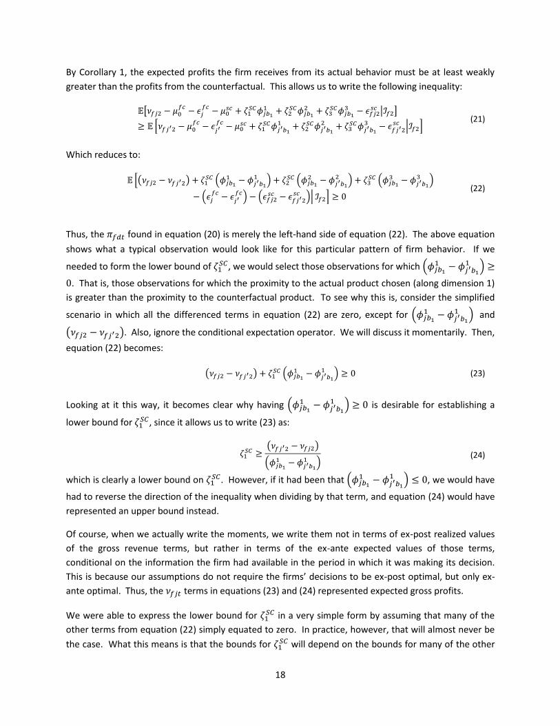
Thus, the 𝜋𝑓𝑑𝑡 found in equation (20) is merely the left-hand side of equation (22). The above equation

shows what a typical observation would look like for this particular pattern of firm behavior. If we

needed to form the lower bound of 𝜁1𝑆𝐶, we would select those observations for which (𝜙𝑗𝑏1

1 − 𝜙𝑗′𝑏11 ) ≥

0. That is, those observations for which the proximity to the actual product chosen (along dimension 1)

is greater than the proximity to the counterfactual product. To see why this is, consider the simplified

scenario in which all the differenced terms in equation (22) are zero, except for (𝜙𝑗𝑏11 − 𝜙𝑗′𝑏1

1 ) and

(𝜈𝑓𝑗2 − 𝜈𝑓𝑗′2). Also, ignore the conditional expectation operator. We will discuss it momentarily. Then,

equation (22) becomes:

(𝜈𝑓𝑗2 − 𝜈𝑓𝑗′2) + 𝜁1𝑆𝐶 (𝜙𝑗𝑏1

1 − 𝜙𝑗′𝑏11 ) ≥ 0 (23)

Looking at it this way, it becomes clear why having (𝜙𝑗𝑏11 − 𝜙𝑗′𝑏1

1 ) ≥ 0 is desirable for establishing a

lower bound for 𝜁1𝑆𝐶, since it allows us to write (23) as:

𝜁1𝑆𝐶 ≥

(𝜈𝑓𝑗′2 − 𝜈𝑓𝑗2)

(𝜙𝑗𝑏11 − 𝜙𝑗′𝑏1

1 ) (24)

which is clearly a lower bound on 𝜁1𝑆𝐶. However, if it had been that (𝜙𝑗𝑏1

1 − 𝜙𝑗′𝑏11 ) ≤ 0, we would have

had to reverse the direction of the inequality when dividing by that term, and equation (24) would have

represented an upper bound instead.

Of course, when we actually write the moments, we write them not in terms of ex-post realized values

of the gross revenue terms, but rather in terms of the ex-ante expected values of those terms,

conditional on the information the firm had available in the period in which it was making its decision.

This is because our assumptions do not require the firms’ decisions to be ex-post optimal, but only ex-

ante optimal. Thus, the 𝜈𝑓𝑗𝑡 terms in equations (23) and (24) represented expected gross profits.

We were able to express the lower bound for 𝜁1𝑆𝐶 in a very simple form by assuming that many of the

other terms from equation (22) simply equated to zero. In practice, however, that will almost never be

the case. What this means is that the bounds for 𝜁1𝑆𝐶 will depend on the bounds for many of the other

19

variables in the model, and vice versa. This is not necessarily a crippling obstacle for our estimation,

since in the moment inequalities method, all of the bounds are simultaneously determined. However,

what this does mean for our estimation is that wider bounds for one variable will translate into wider

bounds for the other variables that depend on it.

The pattern of firm behavior we used as a demonstration above is useful for finding a bound on 𝜁1𝑆𝐶, but

is less informative about other terms within the firms’ profit functions. For instance, both 𝜇0𝑆𝐶 and 𝜇0

𝐹𝐶

cancel out in equation (21). This is useful for estimating 𝜁1𝑆𝐶, since it allows us to attain simpler bounds

on that coefficient and thus estimate it with less ambiguity. However, this means that particular pattern

of behavior is useless for estimating 𝜇0𝑆𝐶 and 𝜇0

𝐹𝐶 . We instead use different patterns for isolating these

other variables.

Choosing such patterns for use in the moment inequalities framework is a bit of an art form, the goal

being to generate observations in such a way as to get unneeded terms to cancel out in order to best

isolate the coefficient of interest. Due to the similarity of our model to MSZ, many of the patterns we

use mirror the ones found in their paper.

Table 4 shows explicitly which patterns were used to bound each coefficient. In selection of our

patterns, we always conditioned on two periods: the period for which we are considering the

counterfactual deviation, and one period prior. Those periods are indexed in the table by t=0 and t=-1

respectively. A “1” in the table represents production of the given product, while a “0” represents non-

production. As explained earlier in the paper, firms are excluded if they are unobserved in any of the

periods on which we are conditioning, or in the period following the counterfactual deviation.18

Table 4

Coefficient Bound Product Actual Counterfactual Description of Counterfactual

t = -1 t = 0 t = -1 t = 0

𝜇0𝑓𝑐

lower j 1 0 1 1 Halt production of j

upper j 1 1 1 0 Produce j for one additional period

𝜇0𝑠𝑐

lower j 0 0 0 1 Produce j

upper j 0 1 0 0 Do not produce j

𝜁𝑠𝑐 (all)

lower j 0 1 0 0

Produce j' instead of j j' 0 0 0 1

upper j 0 1 0 0

Same as lower bound j' 0 0 0 1

As the reader might have guessed from the earlier discussion, although the patterns used for estimating

the upper and lower bounds of the 𝜁𝑆𝐶 terms are identical, we can identify which bound we are

18

We also perform a version of the estimation on large firms, since they are sampled with probability 1 in the ASI, thus eliminating ambiguity that may arise from firms entering and exiting the sample. The results are found in the appendix.

20

estimating by further conditioning on the sign of (𝜙𝑗 − 𝜙𝑗′) along the given proximity dimension under

consideration.

There is one further complication to consider. As we have already stated, we can only condition our

selection of observations on data in the firm’s information set during the period in which the

counterfactual deviation is occurring. This means we can condition on any number of periods into the

past, but not on any periods that occur after the deviation, since those were not observable to the firm

at the time. This means there are actually four patterns of firm behavior that we must consider when

estimating the bounds on the 𝜁’s19:

t = 1 2 3

1 2 3

1 2 3

1 2 3

Actual j 0 1 0

0 1 1

0 1 0

0 1 1

j' 0 0 0

0 0 0

0 0 1

0 0 1

Counterfactual j 0 0 0

0 0 1

0 0 0

0 0 1

j' 0 1 0

0 1 0

0 1 1

0 1 1

Each of the observations for those patterns would give rise to a separate type of inequality. For

instance, in the second pattern above, the firm would have to pay the static portion of the startup cost,

𝜇0𝑆𝐶 twice in the counterfactual case, once for product j’ in period 2, and then again for product j in

period 3, whereas in the actual case, the firm only has to pay it once. This means that in addition to the

other variables above, 𝜇0𝑆𝐶 will also appear in the bounds for the 𝜁’s, since it cannot be differenced out

in the second and third firm behavior possibilities above.20

Note that these potential effects on firm profits in period 3 are not meant to imply that we use two-

period deviations in our estimation. In each of the examples given above, the only difference in firm

behavior between the actual and counterfactual cases occurs in period 2. Rather, we are saying that

because firm profits are at least partially dependent on the state of the firm in previous periods, actions

taken in period 2 can cause profits in period 3 to be different in the actual vs counterfactual cases, even

if the period 3 actions of the firm are identical in both of those scenarios.

5.2.2 Aggregating Observations into Moments

After selecting observations in the manner described in the previous section, it remains to aggregate

those observations into moments to be used in the estimation.21 The theoretical moment inequalities

19

We are fleshing out this explanation for the bounding of the 𝜁’s, but the principle we are describing (i.e. that we cannot condition on future periods) applies to the selection of observations for each of our coefficients. 20

We do impose one restriction on the future in selecting our observations, and that is that the firm must actually be observed in all three periods of the search pattern. Because we need to know the firm behavior following the counterfactual period in order to fully compute the desired bound, if the firm does not appear in the dataset in the third period of our pattern, we drop that observation for being incomplete. 21

A reader might wonder why we do this at all. If we have two observations, one saying 𝑥 > 4 and another saying 𝑥 > 10, why not just say 𝑥 > 10 and be done with it? Econometrically, such a procedure would have undesirable

21

are of the form given in equation (20). Thus, the sample moment inequalities are obtained by averaging

all of the observations associated with a particular moment inequality, as follows:

𝕞𝑘(𝜃) =1

𝐷𝑘∑∑∑𝑔𝑘(𝑍𝑓𝑡)�̂�𝑓𝑑𝑡(θ, β̂)

𝐷𝑖𝑡

𝑑=1

𝑇

𝑡=1

𝐹

𝑓=1

(25)

Thus, for each moment inequality, (indexed by 𝑘), we are summing over all firms (F), all periods (T), and

all possible deviations consistent with the assumptions in our paper (𝐷𝑖𝑡). �̂�𝑓𝑑𝑡(θ, β̂) is the predicted

difference in profits between the actual and counterfactual firm actions, which depends on predicted

values from the first stage regression (a function of �̂�) and the parameter vector being estimated in the

second stage, 𝜃. 22 𝐷𝑘 is the total number of observations used to compute the sample moment 𝕞𝑘.

Note that since the weighting function 𝑔𝑘(𝑍𝑓𝑡) can be zero for some values of 𝑍𝑓𝑡, 𝕞𝑘 is computed with

only a subset of the possible deviations.

5.2.3 Estimating the Bounds

After aggregating the observations, the estimation procedure involves solving a simple linear

programming problem with the sample moment inequalities as constraints, as well as some “common

sense” restrictions we place on our estimation. These additional restrictions are 1) Since each of the

parameters we estimate is a cost, we require the acceptable values to be weakly positive, and 2) the

value of the abatement of the startup cost due to proximity cannot exceed the startup cost itself (i.e.

𝜁1𝑠𝑐 + 𝜁2

𝑠𝑐 + 𝜁3𝑠𝑐 ≤ 𝜇0

𝑠𝑐).

More formally, let Θ be the parameter space for 𝜃, and let Θ𝕞 be the set of all values of 𝜃 that satisfy

the moment inequalities (as well as our additional restrictions, listed above). Thus, Θ𝕞 = {𝜃 ∈

Θ:𝕞(𝜃) ≥ 0}, where 𝕞(𝜃) represents the set of all K of the moment inequalities 𝕞𝑘(𝜃).

Then, the maximum value along the first dimension of 𝜃 is given by:

𝜃1 = {𝜃 ∈ Θ𝕞: 𝜃1 = arg max

�̃�∈Θ𝕞

�̃�1} (26)

The definitions for the minimum and maximum values along other dimensions of the parameter vector

are analogous.

5.2.4 Properties of the Error Terms

One of the advantages of the PPHI moment inequalities framework is that it does not require us to

assume a specific functional form for the error terms. There are, however, some restrictions that must

properties (such as being vulnerable to measurement error), and might be compared to a linear regression performed on a single observation. 22

Note that although we do not index it, 𝜃 = (𝜇0𝑓𝑐, 𝜇0𝑠𝑐 , 𝜁1

𝑠𝑐 , 𝜁2𝑠𝑐 , 𝜁3

𝑠𝑐) is allowed to vary across sectors (that is,

across 1-digit ASICC categories).

22

be applied to ensure that our estimated set contains the true value of 𝜃. These restrictions are

encompassed by the following assumption:

Assumption 4:23 The error terms are such that

𝔼[𝑔𝑘(𝑍𝑓𝑡)(𝜖𝑓𝑑𝑡𝑣 + 𝜖𝑓𝑑𝑡

𝑓𝑐+ 𝜖𝑓𝑑𝑡

𝑠𝑐 )] ≤ 0 (27)

Recall that 𝜖𝑓𝑗𝑡𝑣 is the approximation error of our gross profit prediction, �̂�𝑓𝑗𝑡 from the first stage

regression, and 𝜖𝑓𝑗𝑡𝑓𝑐

and 𝜖𝑓𝑗𝑡𝑠𝑐 are the error terms from the fixed and sunk costs, equations (6) and (7),

respectively. The 𝑑 subscript (as opposed to 𝑗) on these error terms found in equation (27) merely

shows that Assumption 4 imposes restrictions on the differences in the 𝜖’s between the actual and

counterfactual cases, and not on the 𝜖𝑓𝑗𝑡’s themselves.

However, following MSZ, we can impose conditions on the 𝜖𝑓𝑗𝑡’s that are sufficient for the satisfaction

of Assumption 4: 1) The first stage estimation procedure yields a consistent prediction for the expected

gross revenues, and 2) 𝔼[𝜖𝑓𝑗𝑡𝑓𝑐, 𝜖𝑓𝑗𝑡

𝑠𝑐 |ℐ𝑓𝑡] = 0. The latter restriction imposes that the firm does not have

information on the fixed or sunk costs that is unknown to the econometrician.

5.2.5 Confidence Intervals

Confidence intervals for our parameter estimates follow the procedure outlined in PPHI, with the

adjustment made in Holmes (2011) to account for correlation between observations arising from the

same firm. We refer the reader to the cited papers for details on how these are computed.

6 Results The main results are presented here, in Table 5. Using the moment inequalities method in PPHI, we do

not get point estimates for any of our coefficients. Rather, we get upper and lower bounds on the

potential values that those coefficients can take. As an example, of how to interpret this, observe that

the static portion of fixed costs, 𝜇0𝑓𝑐

, takes a maximum value of $29,910 per product in industry 1

(Animals, vegetables, and forestry), and a minimum value of $31,120 per product in industry 8 (railways,

ships, and other transportation equipment), indicating that fixed costs are much greater in industry 8, as

one might expect.

The values on the 𝜁 coefficients are telling for the importance of the different distance measures in each

industry. To interpret the 𝜁’s, remember that the proximity measures were all projected onto a 0 to 1

space, with a proximity of 0 representing products that are as far away as possible from the given firm

along the chosen distance measure, and a proximity of 1 representing products that are “immediately

adjacent” to the firm along the given dimension of distance. Therefore, products with a proximity of 1

23

Note that Assumption 4 is analogous to Assumption 3 in PPHI. The additional requirement in PPHI’s assumption

is trivially satisfied in our model by the fact that weight function for firm f, 𝑔𝑘(𝑍𝑓𝑡) does not depend on the choices

of firms other than f.

23

to a firm along the first distance measure (input similarity) will receive the full benefit of the startup cost

abatement for that measure. Products with a proximity of 0 will not receive any such abatement

(though it is possible that such products are close to the firm along another measure, receiving startup

cost abatement from that alternate source).

Table 5 – Baseline Estimation

Lower Upper

Lower Upper

Lower Upper

Lower Upper

Industry: Animal, Vegetable,

Forestry

Ores, minerals, gas, electricity

Chemicals

Rubber, plastic, leather

𝜇0𝑓𝑐

4.04 29.91

27.82 171.17

22.93 170.60

8.37 35.94

𝜇0𝑠𝑐 5.70 109.21

26.41 598.02

56.45 670.82

28.35 164.29

𝜁1𝑠𝑐 0.00 66.52

0.00 318.94

0.00 273.82

0.00 62.26

𝜁2𝑠𝑐 0.00 109.21

0.00 598.02

0.00 670.82

0.00 164.29

𝜁3𝑠𝑐 0.00 36.18

0.00 190.08

0.00 203.24

0.00 43.75

Industry: Wood, cork, paper

Textiles

Metals,

Machinery Railways, ships,

transport

𝜇0𝑓𝑐

4.88 25.14

6.68 41.58

12.15 58.38

31.12 154.14

𝜇0𝑠𝑐 9.49 99.01

6.46 191.79

36.51 260.71

104.23 700.00

𝜁1𝑠𝑐 0.00 50.41

0.00 77.76

0.00 87.36

0.00 234.34

𝜁2𝑠𝑐 0.00 99.01

0.00 191.79

0.00 260.71

0.00 700.00

𝜁3𝑠𝑐 0.00 30.41

0.00 49.02

0.00 64.79

0.00 170.27

Notes: Values expressed in thousands of 1982 dollars. An exchange rate of 9 rupees per dollar was used for the conversion from

rupees.

For example, consider animals, vegetables and forestry. The coefficient on 𝜁1𝑠𝑐 has a maximum possible

value of $66,520. This means that if a potential destination product j had an inputs-similarity proximity

of 1 to a firm in that industry (meaning, the cost share of the inputs for j exactly mirrored the existing

cost shares of the firm in the period prior to introducing j), that firm would receive a maximum of

$66,520 reduction in the startup costs associated with beginning production of that product. If none of

the firms products shared any inputs with product j (and j was similarly far from the firm along the other

two dimensions of distance), then the firm would have to pay the full startup cost to begin production of

j, which our estimates show to be between $5700 and $109,210.

Adding a product with a proximity of 0 to your firm would provide no abatement of the startup costs

along the given distance measure. In our model, for proximities between 0 and 1, the benefit decreases

linearly. So in animals, vegetables, and forestry, the maximum benefit of adding a product with a

proximity of 0.5 along distance measure 1 would be $66,520/2 = $33,260.

It may appear from looking at the zeros in the table that it is possible that the distance measures do not

matter at all. It should be noted, however, that the estimated set is not the Cartesian product of the

upper and lower bounds presented in the table. Thus, just because the 𝜁 parameters all have 0 as their

24

lower bound in the table, it does not follow that (𝜁1𝑠𝑐 , 𝜁2

𝑠𝑐 , 𝜁3𝑠𝑐) = (0,0,0) is a point within the estimated

set. Each one of the distance parameters might individually be zero, given certain choices for the other

coefficients, but that does not imply they are jointly zero.

This is not easy to intuit just from looking at the table. The estimated set is a five-dimensional manifold,

whose true shape is computationally difficult to determine, and even more difficult to represent in a

two-dimensional picture. However, we can show a cross-section of the set, to illustrate to the reader

that the bounds are not jointly zero. One such cross-section is presented in Figure 1.

Figure 1 examines a cross-section of the estimated set for the Animals, Vegetables, and Forestry sector.

We chose the median values of 𝜇0𝑠𝑐 and 𝜇0

𝑓𝑐, and 𝜁3

𝑠𝑐 = 0 to determine the location of the cross-section.

We can observe from the picture that 𝜁2𝑠𝑐 is bounded away 0 for all values of 𝜁1

𝑠𝑐, and 𝜁1𝑠𝑐 is only 0 for

particularly large values of 𝜁2𝑠𝑐.

The readers are referred to the appendix if they wish to see the linear inequalities that define the entire

estimated set. Using these inequalities, it is possible to create cross-sections such as these for any

choice of the other parameters in the estimation.

Figure 1 – Cross-Section of the Estimated Set for

Animals, Vegetables, and Forestry

Notes: Values along the axes are thousands of 1982 dollars. Values of

𝜇0𝑓𝑐= $16,975, 𝜇0

𝑠𝑐 = $57,455, and 𝜁3𝑠𝑐 = 0 were used to determine the

position of the cross-section in the dimensions not shown in the picture.

By examining the 𝜁’s, we can receive some indication of which distance measures matter in which

industries. In every industry, the ranking of relative importance for the three distance measures seems

25

to be the same. Merely looking at the maximum values, physical distance (𝜁2) seems to be the greatest

contributor to product additions, followed by input similarity (𝜁1). The upstream/downstream

connectedness measure (𝜁3) seems to fair the worst out of the three, consistently.

This is not to say that inputs and vertical connections are meaningless for product additions. Rather,

that even at their maximum possible effectiveness, they tend to explain less of the variations in product

additions than the physical distance component. On the other hand, there is a point in the estimated

set for every industry in which the entire startup cost for new products in that industry can be abated by

immediate physical proximity to the location of production.

Unfortunately, due to data limitations, it is not possible at this time for us to know precisely which

portion of the production process is being helped by physical proximity. Many potential explanations

come to mind, among them, knowledge sharing, access to natural resources, or local labor markets

where workers have specialized skills. Distinguishing between these competing explanations is beyond

the scope of the present paper, but we feel our results are a useful first pass, to indicate which areas of

firm-product relatedness would be fruitful to investigate in the future.

Ninety-five percent single-sided confidence intervals for the baseline estimation and the restricted

found in Table 6. While the estimated set specified by the confidence interval is obviously wider than

that found in the estimation, the results are not dramatically different (with the exception of the

chemical industry), ostensibly due to the large number of observations included in the estimation.

Table 6 – Confidence Intervals for Baseline Estimation

Lower Upper

Lower Upper

Lower Upper

Lower Upper


Forestry


Chemicals


𝜇0𝑓𝑐

4.04 35.53

27.82 207.50

22.93 221.16

8.37 42.00

𝜇0𝑠𝑐 5.70 120.79

26.41 679.02

56.45 1,983.00

28.35 176.84

𝜁1𝑠𝑐 0.00 70.22

0.00 372.46

0.00 2,133.67

0.00 88.27

𝜁2𝑠𝑐 0.00 146.51

0.00 841.23

0.00 1,887.56

0.00 196.97

𝜁3𝑠𝑐 0.00 48.44

0.00 274.88

0.00 552.33

0.00 65.88


Textiles

Metals,

Machinery Railways, ships,

transport

𝜇0𝑓𝑐

4.88 32.49

6.68 49.68

12.15 68.60

31.12 184.60

𝜇0𝑠𝑐 9.49 123.59

6.46 213.73

36.51 281.51

104.23 872.74

𝜁1𝑠𝑐 0.00 64.93

0.00 88.40

0.00 127.21

0.00 592.46

𝜁2𝑠𝑐 0.00 149.72

0.00 244.77

0.00 311.22

0.00 885.64

𝜁3𝑠𝑐 0.00 48.52

0.00 57.82

0.00 87.50

0.00 852.07


rupees. The left parameter in every column represents the single-sided 95% confidence interval on the lower bound, and the right

parameter is the single-sided 95% confidence interval on the upper bound. Values account for correlation across observations, and

were computed using 500 subsamples.

26

7 Supplementary Analyses To help us understand how the different channels affect firm behavior, we performed some calculations

of potential firm product transitions using the model, and data from the estimation. Firms within this

calculation determine profits in the way we have described in the theoretical model, with two notable

exceptions: the degree to which firms are forward looking, and the calculation of the error terms.

In the model, we were not required to specify the degree to which firms are forward looking, because

the moment inequality framework is consistent with a broad array of firm expectations and behaviors

(see section 4.3). However, for the purposes of performing these calculations, this unbounded set of

behaviors needs to be made finite and concrete. Our assumptions require that firms take into account

the effects of their current choice on static profit at least one period ahead. We therefore take this

minimum required capacity for looking forward as the baseline for our calculation.

Secondly, within the PPHI moment inequalities framework, there are also relatively relaxed assumptions

on the error terms (see section 5.2.4). However, for the purposes of our simulation, we draw the error

terms from normal distributions with mean 0, which is consistent with the assumptions of the model.

For the error terms associated with firm-product profits (𝜖𝑓𝑗𝑡𝑣 , see section 5.1), the standard deviation

for the distribution is taken to be the actual standard deviation of a given firm’s profits within its

industry and year. For the other error terms (𝜖𝑓𝑗𝑡𝑓𝑐

and 𝜖𝑓𝑗𝑡𝑠𝑐 , mentioned in 4.2.2 and 4.2.3, respectively),

the standard deviation is taken to be 1

4 of the parameter estimate for the associated cost being used in

the simulation.

The expected gross profits for each firm in the calculation are exactly the gross profit estimates we

computed during our first-stage regression for the estimation. However, in order to mitigate the effects

of some large outliers in the data, we dropped the top ten percent of the predicted profits. Firm

locations are also identical to the actual locations found within the data.

We set the base year for the calculation to be 2000, and examined which products would be considered

profitable by firms. For the second stage costs, we used the median values of the estimates from our

baseline specification (those reported in Table 5). We excluded the upstream/downstream distance

measure from the calculation due to its poor performance in the estimation.

This calculation, in addition to showing us the strength or weakness of our estimates also allows us to

run counterfactuals, such as examining the results if we shut off or enhance one or both of the potential

distance channels, or seeing the effect of the density of the firm-product connections on the number of

profitable products.

7.1 Number of Profitable Products For our first exercise, we examine the impact of negating the effect of each distance measure. Due to

the amount of data produced by a calculation of this manner, we will only report one column of the

output, in order to give the reader the basic intuition of how to interpret our results. Other rows within

the output matrices follow the same general pattern.

27

The results of this exercise are reported in Table 7. Numbers in the table represent a count of the total

products that have positive expected profits for firms whose main product is in ASICC category 21 (Salts,

Sulpher, Lime, Cement). Stated another way, it is the sum of all the profitable firm-product relationships

for firms in category 21. For example, imagine there are only two firms in category 21, A and B. Firm A

has 3 potentially profitable products in Ores, and Firm B has 6 potentially profitable products in Ores. In

that case, the entry in the table for Ores would be 3+6 = 9. Thus, the table represents the number of

possible expansion paths available to firms within that industry.

The first column of the table represents the result of these calculations for the baseline results. The

second and third columns consider the counterfactual cases in which 𝜁1𝑠𝑐 = 0 and 𝜁2

𝑠𝑐 = 0, respectively.

Setting 𝜁1𝑠𝑐 = 0 effectively removes any benefit the firm might receive from sharing inputs with

potential products. Similarly, 𝜁2𝑠𝑐 = 0 removes any benefits it would receive from having production of

a potential product located nearby.

Table 7 – Profitable Products Available to Firms in Salts, Sulpher, Lime, and Cement

Baseline 𝜁1 = 0 𝜁2 = 0

Salts, sulpher, lime, cement 1750 1744 1146

Ores 110 110 70

Mineral fuels 391 391 264

Gas (fuel) 108 108 80

Electrical energy 154 154 107

Of note from the table is that negating the effect of the shared inputs does not substantially affect the

number of profitable products at all, whereas negating the effects of local production affects it

significantly.

Readers might be tempted to believe that this is an indictment against the shared inputs measure of

similarity. However, it is necessary to interpret results within the context of the population distributions

for the distances. In particular, observe the distribution for the input similarity measure. Most products

are stacked up at 1. Products with a measure of 1 for this distance share no inputs with the firms’

existing products, and thus receive no benefit from the cost abatement provided by 𝜁1𝑠𝑐. Thus, setting

𝜁1𝑠𝑐 = 0 does not affect the profitability for many products at all.

Alternatively, the distribution for the physical distances shows many products being produced in close

proximity to the firm. These products will receive a substantial reduction in their startup costs from the

physical proximity channel. Therefore, setting 𝜁2𝑠𝑐 = 0 makes a big difference for a large number of

products.

Therefore, the lesson to be learned from this exercise is that when interpreting the estimates, it is not

enough to look only at the magnitude of the coefficients, but to consider also how those cost measures

are interacting with the set of products in the firms’ potential choice sets, and along which dimensions

those products are “distanced” from the firm.

28

7.2 Firms’ Product Choices The previous exercise looked at all the profitable products available to the firm. In this exercise, we try

to predict which products firms will move into, by allowing them to choose one product to add each

period. For this simulation, we use the data for 2001-2002, since the earlier years of the sample were a

little more sparse.

We’ll motivate this exercise by showing the actual matrix of firm-product additions. The entries in the

matrix show the number of firms that added a product in the column sector, conditional on having their

main product in the row sector in the previous year.

Table 8 – Actual Product Additions (Base Metals and Machinery)

Count of firms adding products in given sector


71 Iron, steel, & articles 283 11 35 47 28 19 13 5 9

72 Copper, nickel, zinc, & articles 2 21 7 6 0 1 1 0 0

73 Aluminum, tin, etc., & articles 14 4 47 13 3 3 8 0 1

74 Misc. manuf. Articles 58 10 14 35 39 23 17 5 7

75 General purpose mach. (non-elec) 57 3 7 26 155 69 56 7 9

76 Industry-specific mach. (non-elec) 34 2 4 16 67 158 31 6 15

77 Electrical machinery 43 17 30 26 63 35 259 51 16

78 Electronics equipment 6 2 2 3 7 5 34 82 1

79 Special purpose machines 12 5 3 6 13 12 15 2 21

Next, we will show the results from our simulation.

Table 9 – Simulated Product Additions (Base Metals and Machinery)

Count of firms adding products in given sector


71 Iron, steel, & articles 87 1 14 61 237 156 274 36 26

72 Copper, nickel, zinc, & articles 9 0 3 4 19 12 23 4 2

73 Aluminum, tin, etc., & articles 18 0 3 19 39 24 61 3 7

74 Misc. manuf. Articles 34 1 7 16 73 65 125 17 14

75 General purpose mach. (non-elec) 51 0 5 39 143 83 163 19 18

76 Industry-specific mach. (non-elec) 37 1 17 25 89 73 117 19 7

77 Electrical machinery 82 4 11 44 199 124 279 38 19

78 Electronics equipment 19 0 4 16 42 34 67 7 5

79 Special purpose machines 8 0 1 6 22 18 34 1 6

29

Observing the tables, it is worth noting that although the simulation does not make perfect predictions,

it performs better than one might expect for a model of its simplicity. It certainly appears to perform

better than a fully random model, or an overly simplistic model in which firms only produce what they

produced in the previous period (which would generate a matrix of zeros).

In some categories, the predictions of the simulation are actually very close to what we observe in the

data. It predicts 279 electrical machinery firms will add products in their own sector, compared with

259 in the data. Its prediction of 143 general purpose machinery firms adding products within their

sector is also close to the observed 155. Many other categories also closely match the data. In broad

terms, it captures that there are few products being added in sectors 72, 73, and 74, and few products

being by firms specializing in those sectors.

However, the simulation also highlights some weaknesses of the model. The most notable difference

from the data seems to be the model’s over-prediction of the number of products being added in the

machinery sectors (75, 76, and 77), except in a few cases. This disparity seems most pronounced when

examining firms in sector 71 (Iron, steel, and articles thereof).

That said, given the simplicity of the model, and the small number of parameters we estimated, one

would not expect the model to perform perfectly. We used a very simple regression to determine

potential revenues, coupled with a cost structure with only four parameters (recall we excluded the

vertical connectedness measure, 𝜁3𝑠𝑐, from the simulation). Furthermore, we applied a sweeping

estimation technique generally to all firms in all industries.

With a process as complex and varied as the evolution of product scope, we cannot hope to fully

capture all of the nuances of firms’ decisions with one procedure. There are certainly many other

factors that could be affecting their choices, and it seems natural to believe that our model would not

be a good fit for every sector in every industry. Nevertheless, for some sectors, the model seems to

perform fairly well, producing predictions that are qualitatively and quantitatively similar to what we

observe in the data.

7.3 Network Density Regression As we mentioned in the introduction, one of the key results found by Hidalgo et al. (2007) was that the

network of connections linking products together in terms of their relatedness is not evenly distributed.

Rather, it dense (meaning, with many close connections) in some areas, and very sparse in others.

Therefore, countries (or in our context, firms) positioned in the dense part of the network are in a

position to take advantage of many more cost abatement opportunities than those in the sparse part of

the network.

In the work by Hidalgo et al. (2007), they presented a visual representation of the areas of these areas of

density by providing a picture of their network linking products together. Our network is substantially

more complicated to represent, because the connections we analyze are between firms and products,

30

not between the products themselves. Therefore, we proxy for this density by measuring exactly how

much abatement each firm receives from its position within the network for its sector.

Specifically, we compute for each firm and year, the normalized distance of the firm to each product

within its sector along each of the dimensions in our study, and multiply this by the median of the 𝜁𝑠𝑐

abatement parameter associated with that distance. Summing these figures together for all products

gives the total number of dollars of potential startup cost abatement that the firm receives for that year.

We call this number the “Network Density.”

We then regress the number of profitable products the firm has each year on: the network density just

described, the firm-year fixed effect from the first stage regression (representing the firm’s idiosyncratic

productivity shock for that year), and the size of the firm’s product basket in the given year. The results

are given in Table 10.

Table 10 – Network Density Regression

Regressor Number of Profitable

Products

Network Density 0.0052***

(0.00005)

Firm-Year Productivity 23.14***

(0.091)

Basket Size 2.264***

(0.134)

Constant 50.87***

(0.345)

Observations 136608

R2 0.405 Notes: Heteroskedasticity-robust standard errors reported in

parentheses. “Network Density” is measured in terms of ₹100,000s of

startup-cost abatement within the firm’s own sector only.

*** Significant at the 1% level

Even controlling for the number of current products and the firm productivity, the network density is

still highly significant (the t-statistic for that coefficient is 107). The seemingly small value of the

coefficient should be interpreted in the light of the very large values of the network density measure.24

It should come as no surprise that the amount of cost abatement a firm receives is positively correlated

with the number of potentially profitable products it has available. Rather, the purpose of this exercise

was merely to highlight, in rather unsophisticated way, that different firms receive different benefits

24

The average firm received ₹585,000,000 of abatement, and even the least-benefited firm had over ₹2,400,000.

31

from their connections due to the density or sparsity of the network around them. This is to reiterate

and expand upon the lesson of section 7.1, that the value and meaning of the coefficients found in this

paper must be viewed within the context of the network of firm-product connections they interact with.

8 Conclusion We approached the question of how firm’s product mixes evolve with the hypothesis that connections

between firms and potential products were driving their decisions about which products to produce.

We proposed several potential channels by which these connections might manifest, and tested their

relative significance by observing the actual behavior of firms as they added new products and

measuring the degree to which those products were connected to the firm along each of these

dimensions. The model was estimated using moment inequalities, a novel econometric technique that

allowed us to approach a large-scale choice problem of this nature in a computationally feasible

manner.

The results speak strongly in favor of our hypothesis—that product connections matter, and are part of

the driving force behind the observed co-production correlations between products. The success of the

estimation also shows that history matters for firms’ product choice, since each of the distance

measures looked at connections between firms and products in the year prior to actual production.

Finally, we were able to gain some insight into the nature of which connections matter most in which

sectors—physical distance seems to matter the most, followed by input similarity. Vertical

connectedness ranks as the least important measure of relatedness, in every industry.

There were, however, several drawbacks to our estimation. The first is that our estimates, based

primarily on firms adding products within their own industries, are not easily generalizable to firms

moving across industries. The second is that, due to data limitations and the constraints of our

estimation method, we were unable to account for a lot of richness that is obviously a factor in firms’

production decisions (such as the presence of specialized capital, credit constraints, or demand

complementarities). Our model and estimation method also do not account for potential effects from

cannibalism or credit constraints, which could be relevant in a developing country setting.

Nevertheless, the results we found should be an important first step in unraveling a very rich problem,

and should prove useful to those seeking to understand how firms (and potentially by extension,

countries) expand their product scope and migrate from one industry to another during their process of

development. Our paper also makes a methodological contribution, demonstrating how a traditional

trade model coupled with a relatively new econometric technique can be used to analyze a problem of

potential interest to both economists and policymakers.

32

References

Almon, Clopper (2000). “Product-to-Product Tables via Product-Technology with No Negative Flows.”

Economic Systems Research. Vol. 12, Issue 1.

Arthur, W. Brian (2000). Increasing Returns and Path Dependence in the Economy. The University of

Michigan Press.

Arthur, W. Brian (1989). “Competing Technologies, Increasing Returns, and Lock-in by Historical

Events.” The Economic Journal. 99, 116-131.

Bernard, Andrew, J. Bradford Jensen, and Peter Schott (2006). “Survival of the best fit: Exposure to low-

wage countries and the (uneven) growth of U.S. manufacturing plants.” Journal of International

Economics. 68, 219-237.

Bernard, Andrew, Stephen Redding, and Peter Schott (2010). “Multiple-Product Firms and Product

Switching.” American Economic Review. 100:1, 70-97.

Bohlin, Lars and Lars M. Widell (2006). “Estimation of commodity-by-commodity input-output

matrices.” Economic Systems Research. Vol 18, Issue 2.

Broda, Christian, Joshua Greenfield, and David Weinstein (2006). “From Groundnuts to Globalization: A

Structural Estimate of Trade and Growth.” NBER Working Paper No. 12512.

David, Paul (1985). “Clio and the Economics of QWERTY.” American Economic Review. Vol. 75, No. 2.

De Loecker, Jan (2011). “Product Differentiation, Multiproduct Firms, and Estimating the Impact of

Trade Liberalization on Productivity.” Econometrica. Vol 79, No. 5, 1407-1451.

Dixit, Avinash and Joseph Stiglitz (1977). “Monopolistic Competition and Optimum Product Diversity.”

American Economic Review. Vol. 67, No. 3.

Eckel, Carsten and J. Peter Neary (2010). “Multi-product firms and flexible manufacturing in the global

economy.” The Review of Economic Studies. Vol. 77, No. 1.

Foster, Lucia, John Haltiwanter, and Chad Syverson (2008). “Reallocation, Firm Turnover, and Efficiency:

Selection on Productivity or Profitability?” American Economic Review. Vol. 98, No. 1, pp. 394-425.

Gollop, Frank and James Monahan (1991). “A Generalized Index of Diversification: Trends in U.S.

Manufacturing.” The Review of Economics and Statistics. Vol. 73, No. 2, 318-330.

Goldberg, Pinelopi, Amit Khandelwal, Nina Pavcnik, and Petia Topalova (2010). “Imported Intermediate

Inputs and Domestic Product Growth: Evidence from India.” Quarterly Journal of Economics. 125 (4),

1727-1767.

Hall, Bronwyn, Adam Jaffe, and Manuel Trajtenberg (2001). “The NBER Patent Citations Data File:

Lessons, Insights, and Methodological Tools.” NBER Working Paper No. 8498.

33

Harrison, Ann and Andres Rodriguez-Clare (2010). “Trade, Foreign Investment, and Industrial Policy for

Developing Countries.” Handbook of Development Economics. Vol. 5. Elsevier B.V.

Harrison, Ann, Leslie Martin, and Shanthi Nataraj (2013). “Learning versus Stealing: How important are

market-share reallocations to India’s Productivity Growth?” World Bank Economic Review. Vol. 27,

Issue 2.

Hausmann, Ricardo (2014, July 26). “The Real Raw Material of Wealth.” Project Syndicate.

Hidalgo, Klinger, Barabasi, and Hausmann (2007). “The Product Space Conditions the Development of

Nations.” Science. 317, 482.

Hidalgo, Cesar and Ricardo Hausmann (2009). “The building blocks of economic complexity.”

Proceedings of the National Academy of Sciences, Vol. 106, No. 26.

Holmes, Thomas J. (2011). “The Diffusion of Wal-Mart and Economies of Density.” Econometrica. Vol.

79, No. 1, 253-302.

Kugler, Maurice and Eric Verhoogen (2012). “Prices, Plant Size, and Product Quality.” Review of

Economic Studies. 79, 307-339.

Leamer, Edward (1987). “Paths of Development in the Three-Factor, n-Good General Equilibrium

Model.” Journal of Political Economy. Vol. 95, No. 5.

Lederman, Daniel and William F. Maloney. (2012). Does What you Export Matter? In search of

empirical guidance for industrial policies. The World Bank.

Marshall, Alfred (1920). Principles of Economics. 8th Edition. London: MacMillan and Co., Ltd.

Matsuyama, Kiminori (1992). “Agricultural Productivity, Comparative Advantage, and Economic

Growth.” Journal of Economic Theory. 58, 317-334.

Morales, Eduardo, Gloria Sheu, and Andrés Zahler (2014). “Extended Gravity.” Mimeo.

Mowery, David, Joanne Oxley, and Brian Silverman (1998). “Technological overlap and interfirm

cooperation: implications for the resource-based view of the firm.” Research Policy. Vol. 27, Issue 5,

507-523.

Nelson, Richard and Sidney Winter (1982). An Evolutionary Theory of Economic Change. Cambridge,

Massachusetts: Harvard University Press.

Pakes, Ariel, Jack Porter, Kate Ho, and Joy Ishii (Forthcoming). “Moment Inequalities and Their

Application.” Econometrica.

Penrose, Edith (1959). The Theory of the Growth of the Firm. Oxford: Basil Blackwell.

34

Redding, Stephen (1999). “Dynamic Comparative Advantage and the Welfare Effects of Trade.” Oxford

Economic Papers. 51, 15-39.

Redding, Stephen (2002). “Path Dependence, Endogenous Innovation, and Growth.” International

Economic Review. Vol. 43, No. 4.

Rodrik, Dani (2006). “What’s So Special about China’s Exports?” China & World Economy. Vol. 14, No.

5.

Sandberg, Lars (1969). “American Rings and English Mules: The Role of Economic Rationality.”

Quarterly Journal of Economics. Vol. 83, No. 1.

Santos Silva, J.M.C. and Silvana Tenreyro (2006), The Review of Economics and Statistics, 88(4): 641-658.

Schott, Peter K. (2008). “The Relative Sophistication of Chinese Exports.” Economic Policy. Vol. 23, No.

53.

Sutton, John (1991). Sunk Costs and Market Structure. Cambridge, Massachusetts: The MIT Press.

Wang, Zhi and Shang-Jin Wei (2010). “What Accounts for the Rising Sophistication of China’s Exports?”

China’s Growing Role in World Trade. University of Chicago Press.

35

Appendix

The appendix will include details on how we performed some of the calculations in the paper, as well as

providing the results from alternative ways of estimating the model. Section A.1 will review how certain

terms in the first stage regression were calculated, as well as providing the regression results. Section

A.2 discusses our method for calculating the physical distance between firms and products. Section A.3

presents the results for some alternative specifications. Section A.4 presents the moments used in the

preferred specification. Section A.5 gives the results from the Kolmogorov-Smirnov tests comparing the

firm-choice and population distributions for firm-product distances discussed in section 6 of the paper.

A.1. Marginal Cost Regression

A.1.1. 𝑷𝑳𝒋

𝑃𝐿𝑗 is the price of a unit of labor in production of product j. Computation of this variable requires

computing the labor costs for each firm, and using that to impute the labor costs of each product.

We began by calculating the labor inputs (in rupees) for every firm-year. Because we are interested in

workers actually involved in the production process, we only included workers in the following

categories in Block E of the ASI data:

1. Male workers employed directly

2. Female workers employed directly

3. Child workers employed directly

4. Workers employed through contractors

5. Supervisory and Managerial Staff

6. Other employees

These categories excludes unpaid family members/proprietor/coop. members. The total wage bill was

calculated as the sum of the wages/salaries paid to employees in the included categories, excluding

bonuses, contributions to Provident and other funds, and workman and staff welfare expenses.

To calculate the labor cost for a product, we need to make an assumption regarding how labor costs are

assigned to given products within multi-product firms. We assumed that firms allocate labor expenses

to products proportional to that product’s share of the firm’s total revenue from all products. So the

labor costs allocated by firm f to product j in period t are:

𝐿𝑎𝑏𝑜𝑟 𝐶𝑜𝑠𝑡𝑠𝑓𝑗𝑡 = 𝐿𝑎𝑏𝑜𝑟 𝐶𝑜𝑠𝑡𝑠𝑓𝑡 ∗

𝑅𝑒𝑣𝑒𝑛𝑢𝑒𝑓𝑗𝑡∑ 𝑅𝑒𝑣𝑒𝑛𝑢𝑒𝑓𝑗𝑡𝑗

(28)

We need to define what we will call a “unit” of labor for the purposes of our production function, so we

can calculate the cost of such a unit. We use man-days as our unit of choice, and we use an analogous

36

relationship to the one given in equation (28) to assign man-days to products within multi-product firms

(that is, we assume man-days are proportional to revenue).

We then computed values for the price of labor (defined as labor costs divided by man-days) of each

product on the firm-year level. The median of these firm-year specific labor intensities was then taken

as the ultimate value for the product-level labor intensity:

𝑃𝐿𝑗 = median𝑓𝑡

{𝑃𝐿𝑓𝑗𝑡} (1)

A.1.2. 𝑷𝑰𝑪𝒇𝒋𝒕 (Intermediate Input Costs)

The calculation of the intermediate input costs for each firm-product-year combination requires several

steps, which we will go through in turn. We first need to compute an input-output table for products at

the 5-digit ASICC level25, we then use this table to assign inputs to outputs at the firm level. Finally,

having the quantity of the given inputs assigned to each output, we find the cost of these inputs by

multiplying the unit value of the input provided in the data.

A.1.2.1. Input-Output Table

There is a vast literature on the computation of input-output tables. As described in Bohlin and Widell

(2006), an assumption needs to be made about technology in order for an input-output table to be

identified. The two most common assumptions in the literature are the Product-Technology

Assumption (PTA) and the Industry-Technology Assumption (ITA). The PTA assumes that production of a

particular product requires the same inputs, regardless of which industry it is made in. The ITA assumes

that, within an industry, the same input mix is used for every product produced by the industry.

Almon (2000) provides a discussion about the merits and weaknesses of both of these assumptions, as

well as a demonstration of the types of input-output tables that would be produced as a result of each

of them. As one might expect, the ITA fares very poorly, and Almon describes the tables produced by

such an assumption to be “massive nonsense.”

We use the PTA for our input-output table, and generate it using the linear constraints in the technique

developed in Bohlin and Widell (2006). This method was chosen because it allows the use of the PTA

while avoiding the problem of negative flows (i.e. negative inputs being used in some outputs), as well

as allowing generalization to the use of rectangular “Make” and “Use” tables26.

25

This is a greater level of disaggregation than is available from the Indian government. 26

The Make table is the mapping from producers to outputs. In our case, it is an 𝐹 × 𝐽 matrix, where F is the total number of firms, and J is the total number of products. The element 𝑀𝑓𝑗 in the matrix gives the quantity of

product j that was made by firm f in the given year (we have one Make table for each year). The Use table is analogous, but for inputs rather than outputs.

37

We make use of the constraints in their minimization problem to harvest the usage coefficients that can

be exactly identified from the data. So computing the input-output table comes down to solving the

following set of linear constraints:

𝑈𝑢𝑓 = ∑ 𝛼𝑢𝑚𝑓𝑀𝑚𝑓𝑚∈ℳ

𝛼𝑢𝑚𝑓 ≥ 0

𝛼𝑢𝑚 = mean𝑓(𝛼𝑢𝑚𝑓)

(2)

In the above equations, 𝑈𝑢𝑓 is the quantity of input u that is used by firm f. 𝑀𝑚𝑓 is the quantity of

output m that is made by firm f. 𝛼𝑢𝑚𝑓 is the usage coefficient, which is the number of units of the input

good u needed to make one unit of the output good m. 𝛼𝑢𝑚𝑓 is firm-specific. The average of those

coefficients is 𝛼𝑢𝑚, which becomes an element of the input-output table. The set ℳ is all of the

products that the firm actually makes (in other words, we only apply the constraints for 𝑀𝑚𝑓 > 0).

Intuitively, the outputs of a firm 𝑀𝑚𝑓, times the quantity of input u that is needed to produce that

output 𝛼𝑢𝑚𝑓, must equal the total amount of u that is used by the firm.

In the above equation, both 𝑈𝑢𝑓 and 𝑀𝑚𝑓 are known from the data, and we must determine 𝛼𝑢𝑚𝑓. We

do this only for those 𝛼𝑢𝑚𝑓’s that are exactly identified from the constraints above. This happens in two

cases.

In the first case, ℳ is a singleton, so the firm only makes one product. Thus, 𝛼𝑢𝑚𝑓 is defined for every u

for that firm and product (with 𝛼𝑢𝑚𝑓 = 0 for those products the firm does not use).

In the second case, 𝑈𝑢𝑓 = 0 for some u and f. In that case, even if ℳ is not a singleton, we can

determine that 𝛼𝑢𝑚𝑓 = 0 for that (u,f) because 𝛼𝑢𝑚𝑓 ≥ 0 and 𝑀𝑚𝑓 > 0.

Intuitively, this method is roughly equivalent to using single-product firms to identify the elements of

our input-output table, although the current methodology allows us to identify more elements of the

table than merely using single-product firms.27

27

The above methodology allowed us to create a complete input profile for 3919 of our 5367 products, and a partial input profile for an additional 1099 of those products, leaving only 349 products for which no input data could be determined. Since many of our 5367 products only appear as inputs in the data (never outputs), this means we were able to calculate input data for almost all outputs in the dataset. With respect to the accuracy of this methodology, it is worth noting two points: 1) When computing the Gollop and Monahan (1991) distance measure between products, the distances looked qualitatively indistinguishable whether they were calculated using the input-output table above, or whether they were computed using firm input mixes (as in Kugler and Verhoogen [2012]), which incorporate multi-product firms and bypass the use of the input-output table (the formula for which is described in the “Theoretical Framework” section of the paper); and 2) The first-stage regression, which used intermediate inputs from the input-output table to predict marginal costs showed the coefficient on those inputs to be large and highly significant. Both of these facts lead us to conclude that this

38

An input-output table was calculated using the above method for every year in the data. The final input-

output table was then the median of the yearly tables.

A.1.2.2. Assigning Inputs to Outputs at the firm level

Our estimation is performed on single- as well as multi-product firms, so we need a method to map a

firm’s inputs to its outputs in order to determine the input costs for a particular output.

Previous authors, such as Foster, Haltiwanger, and Syverson (2008) and DeLoecker (2011) address the

problem of assigning inputs to outputs in multiproduct firms by assigning them in proportion to the

number of products produced. We perform a similar operation, but unlike the aforementioned authors,

we have the advantage of an input-output table which we can use to inform our assignment of inputs.

We therefore modify their approach and weight the assignment of inputs according to the values found

in the input-output table.

To do this, we assume there is a scaling factor 𝛾, that relates firm-specific 𝛼’s to the general economy-

wide 𝛼’s found in the input-output table, and that this scaling factor is constant for every product the

firm uses. Consider the following illustration:

The 𝛼 table is the economy-wide input-output table, in which we have only filled in two of the elements

for this example, because we are only considering how to assign the input U1 to the firm’s outputs. The

Use table shows the quantity of each input used by our example firm, and the Make table shows the

quantities of its outputs.

An average firm would need the following quantities of U1 to make the products of this example firm:

5⏟𝑀1

× 0.5⏟𝛼11

= 2.5 = amount of 𝑈1 needed to make 5 units of 𝑀1

10⏟𝑀2

× 1⏟𝛼12

= 10 = amount of 𝑈1 needed to make 10 units of 𝑀2

method, while not perfectly accurate, as at least a very good approximation to the “true” input-output matrix for these products.

39

This firm would therefore need 12.5 units of U1 to make its existing set of outputs, but it only uses 10.

We therefore apply our scaling factor:

𝛾 (𝑀1𝛼11 +𝑀2𝛼12)⏟ 12.5

= 𝑈1⏟10

In this example, 𝛾 = 0.8, so for the purposes of calculating the input costs for this firm, we would

assume 2 units of U1 were used for M1, and 8 units of U1 were used for M2. When applying this method

to the dataset, 𝛾 is allowed to vary by firm and use-product.

We use the above method to define a price for the total aggregated input basket used in production of

each product at the firm-year level. Since most products in the data do not have units given in terms of

quantity of items sold, we define a unit of output as being one rupee. We therefore divide the

aggregated input costs for each product by the ex-factory value of output to determine the unit price for

the input basket.

A.1.3 Regression Results

ln (𝑟𝑓𝑗𝑡)

𝛽𝐿𝑚𝑐 -0.779***

(0.039)

𝛽𝐼𝐶𝑚𝑐 -0.130***

(.003)

𝑓𝑖𝑟𝑚 × 𝑦𝑒𝑎𝑟 𝐹𝐸 Yes

N 296677

𝑅2 0.75 *** denotes 1% significance.

Robust standard errors are in

parentheses.

Above are the results from the regression in equation (17), the first stage in our estimation procedure.

A.2. Physical Distance Calculation

A.2.1. Mapping firms to districts

There are two difficulties to be overcome in determining the location of the firms at the district level.

The first is that the ASI panel data, which contains unique identifiers for firms, only gives firm location

down to the state level, which is far less precise. Districts are available in the cross-section data, but

there is no direct mapping from the cross-section to the panel. The second difficulty is that MOSPI

40

changed their state and district codes in 2001. This required us to make two mappings: The first from

the panel data to the cross-section, the second from pre-2001 district codes to post-2001 district codes.

To create the first mapping, from panel data to cross-section, we followed the technique used in

Harrison et al. (2013), and matched the closing net value of fixed assets found in the panel and the

cross-section, dropping any values of 0 or 1, and any duplicates, which could potentially lead to

ambiguous matches.

To create the second mapping, we made the assumption that firms (factories in the data), do not change

their location from year to year. Thus, by observing the location codes of individual firms prior to and

post-2001, we were able to create a concordance linking the two sets of codes.

A.2.2. Calculating the Distance

For each of the districts, longitude and latitude coordinates were obtained from Wikipedia’s GeoHack

tool. In the instances when coordinates were not available for a district, or when the available

coordinates were obviously false, the coordinates for the district capital were used instead.

The coordinates were linked to the post-2001 district codes, because we did not have a list linking pre-

2001 codes to district names. There were a few instances in which several pre-2001 codes were merged

into one post-2001 code. In such cases, all of the pre-2001 codes were assigned the same coordinates.

Distances between the districts were calculated using the haversine formula for great circle distance,

with the radius of the earth set to be 6372.8 km. Distances between firms were then defined to be the

distance between the firms’ associated districts, measured in kilometers, with a distance of 0 if the firms

were located in the same district.

The distance between a firm and a product is then defined as the distance to the closest firm producing

that product:

𝐷𝑓𝑗𝑏𝑡−1 = min𝑓′∈ℱ𝑗,𝑡−1

𝑑𝑓𝑓′ (3)

Where 𝑑𝑓𝑓′ is the physical distance between firms 𝑓 and 𝑓′, 𝐷𝑓𝑗𝑏𝑡−12 is the physical distance between

firm f and product j at period t-1, and ℱ𝑗,𝑡−1 is the set of all firms producing j at t-1.

We then construct our measure of proximity by dividing by the maximum distance between any two

points in India (to get the measure between 0 and 1), and flipping it, so that nearby products have a

proximity measure of 1 instead of 0.

𝜙𝑓𝑗𝑏𝑡−12 = |

𝐷𝑓𝑗𝑏𝑡−1max𝑓,𝑓′

𝑑𝑓𝑓′− 1| (4)

Where |. | is the absolute value operator.

41

A.3. Alternative Specifications

A.3.1 Large Firms Only

Table A.3.1.1: Estimates

Lower Upper

Lower Upper

Lower Upper

Lower Upper


Forestry


Chemicals


𝜇0𝑓𝑐

5.47 49.62

86.24 548.88

37.29 309.56

13.18 68.88

𝜇0𝑠𝑐 7.12 173.50

74.73 1,857.67

74.05 1,200.11

40.81 304.72

𝜁1𝑠𝑐 0.00 111.06

0.00 862.52

0.00 489.51

0.00 115.00

𝜁2𝑠𝑐 0.00 173.50

0.00 1,857.67

0.00 1,200.11

0.00 304.72

𝜁3𝑠𝑐 0.00 62.86

0.00 602.68

0.00 362.92

0.00 79.11


Textiles

Metals, Machinery

Railways, ships,

transport

𝜇0𝑓𝑐

13.60 85.32

8.99 58.60

21.55 118.90

55.45 307.21

𝜇0𝑠𝑐 25.96 323.99

8.33 267.61

61.39 525.62

184.97 1,324.89

𝜁1𝑠𝑐 0.00 167.76

0.00 112.29

0.00 176.23

0.00 452.14

𝜁2𝑠𝑐 0.00 323.99

0.00 267.61

0.00 525.62

0.00 1,324.89

𝜁3𝑠𝑐 0.00 104.35

0.00 71.34

0.00 133.60

0.00 328.64


rupees.

These are the results of our estimation performed only on the set of firms with 200 or more employees.

According to the sampling procedure for the ASI, these firms are sampled with probability 1 in every

year of the data.

Many of the broad trends identified in the baseline estimation persist. The physical distance parameter

(𝜁2𝑠𝑐) continues to have the largest upper bounds, followed by input similarity (𝜁1

𝑠𝑐), then vertical

connectedness (𝜁3𝑠𝑐). However, in this version of the estimation, both the lower bounds on the costs

(𝜇0𝑓𝑐

and 𝜇0𝑠𝑐)and the upper bounds on all parameters are substantially higher than in the baseline. This

might be attributed to the larger scale operations happening at these firms, resulting in higher costs (but

also potentially higher profits).

42

Table A.3.1.2: Confidence Intervals

Lower Upper

Lower Upper

Lower Upper

Lower Upper


Forestry


Chemicals


𝜇0𝑓𝑐

5.47 62.72

86.24 673.19

37.29 417.22

13.18 81.70

𝜇0𝑠𝑐 7.12 209.57

74.73 2,054.56

74.05 5,228.11

40.81 329.44

𝜁1𝑠𝑐 0.00 120.63

0.00 1,034.43

0.00 5,867.89

0.00 165.61

𝜁2𝑠𝑐 0.00 262.14

-0.03 2,602.22

0.00 4,802.56

0.00 373.71

𝜁3𝑠𝑐 0.00 87.86

0.00 1,019.66

0.00 1,884.56

0.00 119.79


Textiles

Metals, Machinery

Railways, ships,

transport

𝜇0𝑓𝑐

13.60 117.18

8.99 70.99

21.55 142.27

55.45 372.90

𝜇0𝑠𝑐 25.96 471.04

8.33 303.40

61.39 591.89

184.97 1,797.89

𝜁1𝑠𝑐 0.00 296.18

0.00 130.11

0.00 303.02

0.00 1,414.11

𝜁2𝑠𝑐 0.00 560.47

0.00 349.90

0.00 650.08

0.00 1,770.89

𝜁3𝑠𝑐 0.00 192.61

0.00 82.98

0.00 179.22

0.00 1,495.00


rupees. The left parameter in every column represents the single-sided 95% confidence interval on the lower bound, and the right

parameter is the single-sided 95% confidence interval on the upper bound. Values account for correlation across observations, and

were computed using 500 subsamples.

The above table represents the confidence intervals for the specification including only firms with 200 or

more employees. While for some sectors they are similar to the estimates themselves, in others

(chemicals, ores, and transportation, for instance) they are much wider. This is likely attributed to fewer

observations available in those sectors.

43

A.4.1 Moments for Baseline specification

Table A.4.1

Industry 1

Bound Δ𝜇0𝑓𝑐

Δ𝜇0𝑠𝑐 Δ𝜁1

𝑠𝑐 Δ𝜁2𝑠𝑐 Δ𝜁3

𝑠𝑐 Δ𝜈 Obs.

𝜇0𝑓𝑐

upper 1.00 -0.65 0.12 0.00 0.04 403,710 25,472

lower -1.00 0.21 -0.05 -0.01 -0.02 -28,299 8,363

𝜇0𝑠𝑐

upper 1.00 0.66 -0.39 -0.60 -0.05 65,075 8,069

lower -1.00 -1.00 0.99 0.21 0.00 -20,657 40,598,000

𝜁1𝑠𝑐

upper 0.00 -0.28 -0.44 0.14 -0.05 -25,975 3,872,500

lower 0.00 -0.17 0.20 0.20 -0.04 266,660 732,260

𝜁2𝑠𝑐

upper 0.00 -0.28 -0.42 0.09 -0.04 -20,092 3,369,100

lower 0.00 -0.23 -0.12 0.34 -0.10 354,010 4,012,400

𝜁3𝑠𝑐

upper 0.00 -0.29 -0.31 0.19 -0.29 -30,693 700,130

lower 0.00 -0.33 -0.10 0.29 0.21 322,360 123,730

Industry 2





𝜇0𝑓𝑐

upper 1.00 -0.58 0.13 0.00 0.09 1,648,400 4,058

lower -1.00 0.19 -0.06 -0.01 -0.01 -218,380 2,017

𝜇0𝑠𝑐

upper 1.00 0.66 -0.31 -0.59 -0.02 396,180 2,118

lower -1.00 -1.00 0.99 0.24 0.00 -47,464 12,068,000

𝜁1𝑠𝑐

upper 0.00 -0.28 -0.22 0.17 -0.04 -117,620 499,900

lower 0.00 -0.18 0.20 0.21 -0.03 5,214,300 380,730

𝜁2𝑠𝑐

upper 0.00 -0.27 -0.16 0.09 -0.03 -95,104 467,680

lower 0.00 -0.23 -0.05 0.37 -0.06 4,964,800 1,054,600

𝜁3𝑠𝑐

upper 0.00 -0.27 -0.13 0.24 -0.40 -95,989 62,616

lower 0.00 -0.32 -0.12 0.23 0.13 2,181,400 23,879

44

Industry 3





𝜇0𝑓𝑐

upper 1.00 -0.59 0.38 0.00 0.05 1,336,600 9,150

lower -1.00 0.19 -0.14 -0.01 -0.01 -162,720 3,706

𝜇0𝑠𝑐

upper 1.00 0.73 -0.12 -0.64 -0.02 677,930 4,138

lower -1.00 -1.00 0.99 0.18 0.00 -80,319 17,261,000

𝜁1𝑠𝑐

upper 0.00 -0.27 0.09 0.21 -0.04 -154,710 1,417,700

lower 0.00 -0.17 0.20 0.23 -0.02 960,350 998,920

𝜁2𝑠𝑐

upper 0.00 -0.25 0.11 0.11 -0.04 -128,230 1,138,300

lower 0.00 -0.21 0.11 0.34 -0.04 1,706,500 3,653,900

𝜁3𝑠𝑐

upper 0.00 -0.28 0.11 0.21 -0.16 -164,500 400,830

lower 0.00 -0.21 0.13 0.20 0.12 1,144,000 107,310

Industry 4





𝜇0𝑓𝑐

upper 1.00 -0.54 0.33 0.00 0.04 594,480 4,491

lower -1.00 0.16 -0.10 -0.01 -0.01 -60,811 3,177

𝜇0𝑠𝑐

upper 1.00 0.73 -0.18 -0.65 -0.02 246,970 3,291

lower -1.00 -1.00 0.99 0.16 0.00 -48,614 11,735,000

𝜁1𝑠𝑐

upper 0.00 -0.25 -0.03 0.18 -0.02 -70,731 1,059,100

lower 0.00 -0.16 0.22 0.19 -0.01 324,880 648,950

𝜁2𝑠𝑐

upper 0.00 -0.23 0.00 0.09 -0.02 -57,363 869,600

lower 0.00 -0.20 0.05 0.32 -0.02 467,740 2,042,400

𝜁3𝑠𝑐

upper 0.00 -0.28 -0.04 0.20 -0.16 -59,121 170,360

lower 0.00 -0.23 0.12 0.22 0.16 409,280 43,694

45

Industry 5





𝜇0𝑓𝑐

upper 1.00 -0.61 0.25 0.00 0.02 283,990 4,860

lower -1.00 0.18 -0.09 -0.01 -0.01 -36,280 2,204

𝜇0𝑠𝑐

upper 1.00 0.68 -0.28 -0.60 -0.03 79,402 2,452

lower -1.00 -1.00 0.99 0.19 0.00 -29,549 11,500,000

𝜁1𝑠𝑐

upper 0.00 -0.31 -0.13 0.23 -0.04 -37,488 979,580

lower 0.00 -0.16 0.20 0.21 -0.03 313,400 323,980

𝜁2𝑠𝑐

upper 0.00 -0.31 -0.09 0.15 -0.04 -29,973 757,730

lower 0.00 -0.21 -0.09 0.33 -0.03 288,130 1,457,400

𝜁3𝑠𝑐

upper 0.00 -0.30 -0.12 0.23 -0.21 -27,443 198,710

lower 0.00 -0.28 0.02 0.24 0.23 431,800 32,707

Industry 6





𝜇0𝑓𝑐

upper 1.00 -0.52 0.18 0.00 0.06 429,470 10,946

lower -1.00 0.15 -0.06 0.00 -0.03 -54,524 8,661

𝜇0𝑠𝑐

upper 1.00 0.73 -0.34 -0.69 -0.11 86,646 6,916

lower -1.00 -1.00 0.99 0.17 0.00 -23,197 29,306,000

𝜁1𝑠𝑐

upper 0.00 -0.26 -0.23 0.16 -0.16 -28,815 1,830,200

lower 0.00 -0.15 0.20 0.18 -0.03 421,220 796,440

𝜁2𝑠𝑐

upper 0.00 -0.26 -0.19 0.11 -0.15 -24,490 1,642,900

lower 0.00 -0.18 -0.08 0.29 -0.05 444,300 2,856,100

𝜁3𝑠𝑐

upper 0.00 -0.32 -0.30 0.21 -0.56 -14,972 509,780

lower 0.00 -0.24 -0.07 0.19 0.19 432,050 143,780

46

Industry 7





𝜇0𝑓𝑐

upper 1.00 -0.54 0.35 0.00 0.04 911,670 19,401

lower -1.00 0.15 -0.11 -0.01 -0.01 -91,434 15,278

𝜇0𝑠𝑐

upper 1.00 0.75 -0.15 -0.68 -0.02 334,670 15,969

lower -1.00 -1.00 0.98 0.17 0.00 -54,246 48,288,000

𝜁1𝑠𝑐

upper 0.00 -0.24 0.02 0.15 -0.02 -85,650 4,957,200

lower 0.00 -0.16 0.23 0.18 -0.01 649,930 3,291,400

𝜁2𝑠𝑐

upper 0.00 -0.23 0.04 0.08 -0.02 -74,199 4,245,200

lower 0.00 -0.18 0.08 0.31 -0.02 674,990 9,073,800

𝜁3𝑠𝑐

upper 0.00 -0.22 -0.04 0.13 -0.14 -87,244 938,590

lower 0.00 -0.22 0.10 0.21 0.15 740,030 439,510

Industry 8





𝜇0𝑓𝑐

upper 1.00 -0.55 0.36 0.00 0.01 3,619,500 2,334

lower -1.00 0.15 -0.11 -0.01 0.00 -223,200 1,536

𝜇0𝑠𝑐

upper 1.00 0.77 -0.15 -0.69 0.00 920,590 1,746

lower -1.00 -1.00 0.98 0.17 0.00 -151,860 5,819,300

𝜁1𝑠𝑐

upper 0.00 -0.26 0.04 0.18 -0.01 -248,480 452,100

lower 0.00 -0.15 0.23 0.20 0.00 1,583,900 403,300

𝜁2𝑠𝑐

upper 0.00 -0.26 0.08 0.11 0.00 -229,150 403,350

lower 0.00 -0.18 0.10 0.33 0.00 3,942,400 1,025,100

𝜁3𝑠𝑐

upper 0.00 -0.37 0.13 0.26 -0.05 -155,790 60,322

lower 0.00 -0.22 0.09 0.22 0.07 2,137,500 67,471

Notes: Differences in profits are expressed in 1982 rupees. Besides the restrictions imposed above, we also impose the restrictions

that the sum of the startup-cost-abatement parameters (𝜁) cannot be larger than the total startup cost 𝜇0𝑠𝑐, and that no costs in the

estimation can be negative.

Firm-Product Linkages and the Evolution of Product Scopemjf2143/Flagge_JMPNov2014.pdf · 2 1 Introduction How does a firm’s product mix evolve? Consider the example of ITC Ltd.,

Documents