FINlTE-ELEMENT MODELLING OF THE FLUID …audilab.bme.mcgill.ca/~funnell/AudiLab/theses/day_1990_thesis.pdf · FINlTE-ELEMENT MODELLING OF THE FLUID-STRUCTURE INTERACTION BETWEEN THE

FINlTE-ELEMENT MODELLING

OF THE FLUID-STRUCTURE INTERACTION

BETWEEN THE EAR CANAL AND EARDRUM

Jennifer L. Day

A thesis submitted to the Faculty of Graduate Studies and Research in partial fulfillment of the requirements

for the degree of Master of Engineering

Department of Electrical Engineering McGill University Montréal, Canada

October 1990

o Jennifer L. Day, 1990

•

l

ln this work mathematical modelling methods are formulated in order to examine

how sound pressures in the ear canal interact with diaplacements on the eardrum. Existing finite­

element code is aJtered and new code developed to deaJ with the acoustics of the ear canal and

the mathematics of the fluid-structure interaction problem. A finite-elemf t model of the human

ear canal and eardrum using simplified geometry is developed as an initial approach to the

coupled problem. The preliminary finite-element model coDSists of li cylindrical tube attached

to a circular plate, witb appropriate material properties assigned to each part. The coupled car

canal/eardrum problem is analyzed al several frequencies. Output is discussed in view of results

obtained for eigenvalue analyses of both ear canal and eardrum as separate problems.

1

J

ii

Dans cette étude, des méthodes de modélisation mathématique sont employées afin

d'examiner l'interaction entre la pression sonore dans le canal auditif et les déplaœmcnl~ du

tympan. Un logiciel d'éléments finis est modifié et de nouveaux algorithmes développés de façon

à traiter l'acoustique du canal auditif et le problème de l'action réciproque fluide-solide. Un

modèle d'éléments finis du canal auditif et du tympan humains employant une géométrie

simplifiée est développé comme approche initiale au problème couplé. Le modèle préliminaire

est constitué d'un tube cylindrique rattaché à une plaque circulaire auxquels sont assignés des

propriétés des matériaux appropriées. Le problème couplé canal ':îUditif/tympan c~t aralysé à

plusieurs fréquences. Les résultats de cette analyse sont éclairés par les solutions ohtcnucs en

traitant le canal auditif et le tympan en tant que problèmes séparés. La méthode des valeurs

propres est utiJ isée à cet effet.

Hi

1 ACKNOWLEDGMENTS

1 would like to thanle my research director, Dr. W.RJ. Funnell, for a1l the supervision

and guidance provided throughout the course ofthis thesis. His patience was greatly appreciated,

in light of my interest in the courses offered by the Arts Department al McGill, as weIl as my

elJdless questions pertaining to this work.

1 also greatly appreciate the help and encouragement 1 have received from the students

and staff of the Biomedical Engineering Department. fhese people and the special working

environment make il difficult to imagine a better place to undertake graduate studies.

1 am indebted to all my friends, who have shared discussions with me on film, literature

and music, who have made things seem easier, and who have made me understand that we can

and must change our lives.

Fina/ly, 1 thank my parents and my aunt, for their constant care and support.

This research was supported by s/;holarships from NSERC and FCAR, and an operating

grant from MRC.

1

ABSTRACT

RÉSuMÉ

ACKNOWLEDGMENTS

TABLE OF CONTENTS

LIST OF FIGURES

LIST OF TABLES

PRINCIPAL NOTATION

TABLE OF CONTENTS

CHAPTER 1 INTRODUCTION

CHAPTER 2 PHYSIOLOOY OF THE EXTERNAL AND MIDDLE EAR

2.1 Introduction to the Hearing System

2.2 The External Ear 2.2.1 The piMa 2.2.2 The ear canal

2.3 The Eardrum

2.4 The Middle Ear

CHAPTER 3 EXPERIMENTAL OBSERVATIONS AND MODELLING OF THE EXTERNAL AND MIDDLE EAR

3. 1 Introduction

3.2 The Ear Canal 3.2.1 Sound-pressure experiments in the external ear 3.2.2 Energy reflectance studies 3.2.3 Network modelling of the ear canal 3.2.4 Studies focusing on ear-canal geometry

iv

ii

iii

iv

vii

viii

ix

3

5 7

9

Il

15

15 19 21 22

1 3.3 The Ear~rum 3.3.1 Experimental observation of eardrum vibrations 3.3.2 Theories and modela of eardrum behaviour

3.4 The Middle Ear 3.4.1 Experiments concernine vibration of the middle-w- ossicles 3.4.2 Middle~ modela

3.S Modelline the Ear CanallEardrum Coupling

CHAPTER 4 FINITE-ELEMENT MODELLING

4.1 Introduction

4.2 The Finite-Element Method 4.2.1 The variationaJ formulation and the functional 4.2.2 Finite~ement equilibrium equations 4.2.3 Element formulations

4.3 An Acoustic Analogy

4.4 Fluid-Structure Interaction 4.4. 1 Introduction 4.4.2 Approaches to the interaction problem 4.4.3 Solution of the tluid-structure problem

usine existing finite-element code 4.4.4 Implementing the f1uid-structure coupling using SAP 4.4.5 Viewing the coupled results 4.4.6 Code val idation

CHAPTER 5 FINITE-ELEMENT TESTS AND RESULTS

5.1 Introduction

5.2 The Finite-Element Model of the Ear Canal and Eardrum 5.2. 1 Eardrum shape and properties 5.2.2 Ear canal shape and properties 5.2.3 Finite-element meshes for the eardrum and ear canal

5.3 Eigenvalue Analysis of the Uncoupled Problem 5.3.1 The eardrum 5.3.2 The ear canal

v

24 27

30 31

34

39

40 42 43 47

54

58 59

60 67 69 70

71

72 72 73

7S 79

5.4 Results for the coupled problem 5.4.1 Introduction 5.4.2 Results at individual frequencies

CHAPTER 6 CONCLUSION

6.1 Summary of Contributions 6.2 Future Work 6.3 Applications

REFERENCES

vi

82 82

91 91 93

95

vii

(.IST OF nGURES

Fig. 2.1 The human ear 4

Fig. 2.2 View of the external ear 6

FIg. 2.3 The human eardrum (a) Sketch of the eardrum 10 (b) Schematic outline of the eardrum 10

Fig. 24 The middle-ear ossicles, their ligaments and muscles 13

Fig. 3.1 Average transformation of 30und pressure from free field to human eardrum as a function of frcquency al eight values of angle of incident sound 17

Fig. 3.2 Average acoustic pressure gain for various ear components 18

Fig. 3.3 Standing-wave ratios derived from various investigations 20

Fig. 3.4 Holographie image of cal eardrum vibration 26

Fig. 3.5 Eardrum vibration patterns determined by the finite-element method for the tirst six natural frequencies 29

Fig. 3.6 Schematic block: diagram of the human middle ear 32

Fig. 3.7 Circuit diagram of the human middle ear 33

Fig. 3.8 Ratio of plane-wave radiation coefficient to the sum of radiation coefficients for ail higher modes and percentage of acoustic coupling of model cat eardru.m attributable to nonplanar modes 37

Fig. 3.9 Standing pressure waves in the ear canal (a) Ampli:Ude of modes a! 1 kHz 38 (b) Amplitude of modes at 15 kHz 38

Fig. 4.1 Sorne typical element types 41

Ffg.4.2 Natural coordinates for the quadrilateral 48

Fig. 4.3 Quadrilateral area determinatioD 63

Fig. 5.1 Finite-element meshes for the eardrum and ear canal 74

viii

J Fig. S.2 Eigenvafue anaJysis of the eardrum (circular plate): Ficst six modes 76

Fig. 5.3 Eigenvafue analysis of the ear canal (cyHndrica1 tube): Ficst six modes 80

Fig. 5.4 Results for the coupled problem al 100 Hz (a) Eardrum: reaf comp<ment 85 (b) Eardrum: imaginary comp<ment 85 (c) Ear canal: reaf component 86 (d) Ear canal: imaginary '~mponent 86

Fig. 5.5 Results for the coupled problem al 3.5 kHz (a) Eardrum: reaf component 87 (b) Eardrum: imaginary component 87 (c) Ear canal: reaf component 88 (d) Ear canal: imaginary component 88

Fig. 5.6 Results for the coupled problem al 7.1 kHz (a) Eardrum: reaf component 89 (b) Eardrum: imaginary component 89 (c) Ear canal: reaf component 90 (d) Ear canal: imaginary component 90

LIST OF TABLES

Table 1.1 Human ear-canal variation 8

Table 5.1 Finite-element and theoretical frequencies for the first six modes of the eardrum 77

Table 5.2 Finite-element and theoretical frequencies for the first five longitudinal modes of the ear canal 79

Table 5.3 Finite-element and theoretica1 frequency for the first transverse mode of the ear canal 81

• ix

PRINCIPAL NOTATION

A area of two-ilimensional region

B strain-ilisplacement matrix

C constitutive or elasticity matrix

D damping matrix

E modulus of elasticity

f frequency

F force vector

G modulus of rigidity

H vector of shape functions

J Jacobian operator

K stiffness matrix

M mass matrix

p acoustic pressure

U displacement vector

U strain energy

V potential energy

ô variational operator

l' shear strain vector

f normal strain vector

u Poisson's ratio .,

II functional of the problem

nonnal stress vector

mass density

shear stress vector

angular frequency

x

t CHAPTER 1

INTRODUCTION

ln this study, mathematical modelling methods are developed for examining the

interaction between the acoustical behaviour of the ear canal and the mechanical behaviour of the

eardrum in humans. A greater knowJedge of how ::ound-pressure distributions in the ear canal

interact with the eardrum is essential in order to have a better quantitative understanding of how

sound energy is ta ansmitted to the middle ear. In an experimental context, the kind of

understanding acquired from such a study would allow the proper interpretation of various

physiological acoustic experiments. In a c1inical context, the rre .... er understa.1ding would allow

the extraction of more information from non-invasive diagnostic tests. Ultimately, knowledge

ohtained from examining ear canal and eardrum interactions is relevant to the design of hearing­

aids and earphones.

Modelling the coupled system of the ear canal and the eardrum is not a simple matter.

Because the pressures at th(! end of the ear canal influence the mechanical motion of the eardrum

and vice versa, modelJing should involve some sort of feedback technique. Ear canaJ/eardrum

modelling is an example of a prohlem involving fluid-structure interaction. AnalyticaJ solutions

to these fluirj-structure problellls are usually limited to simple geometries. NUlllericai methods

such as finite-element analysis must be used when the system becomes more complex. In recent

years there has heen considerable interest in applying finite-element computer programs to the

solution of tluid-structure interaction prohlems. Finite-element analysis involving fluid-structure

interaction has been applied to diverse systems including nuclear reactor components, naval and

aerospace structures, dam/reservoir systems, and vehicle passenger compartments, as weil as

hiologkaJ systems (Akkas et al., 1979).

1

l

OuJpter 1: IntroductlOlt 2

The work presented bere deals with an initial attempt Il modelling ear canal and eardrum

interaction usin, the finite-element metbod. To be,in, an overview of the anatomy and

physiology of hearina is presented in Chapter 2. Chaptec 3 presents a review of relevant research

in the study of the acoustical behaviour of the ear canal, and the mechanical behaviour of the

eardrum and middle ear. Various approaches ID modellinl the ear canal, eardrum and Middle

ear are a1so overviewed, as weil as wort which bas actually examined the problem of

ear canal/eardrum interaction. An introduction to the concepts of tinite-element modelling is

given in Chapter 4, as weil as explanations on how the finite-element code is altered to deal with,

tirst, the acoustic modelling in the ear canal, and second, the actual implementation of the

interaction problem. The actual models used for the ear canal and eardrum, and results obtained

for both the uncoupled and coupled problems, are presented in Chapter 5. As there remains a

good deal of work ID be done before the complete aims of this project are realized, Chapter 6

discusses the future directions which this work will take, as weil as other conclusions.

1

1

3

CHAPfER l

PHYSrOLOGY OF TIlE EXTERNAL AND MIDDLE EAR

1.1 INTRODUCTION TO THE HEARING SYSTEM

The human ear (Fig. 2. J) is a complex and sensitive organ which is divided into three

main parts: the outer, middle and ioner ear. The ear canal collects sound and leads it inward

to the tympanic membrane which separates the outer ear from the middle-ear cavity. The air­

tillcd middle-car cavity contains three bones or ossicles : the malleus (hammer), the incus (anviJ)

and the stapes (stirrup), together with supponing ligaments and muscles. Sound is transmitted

from the tympanic membrane to the malleus, from the malleus to the incus, and from the incus

to the stapes, which covers the oval window, and thus to the liquid-tilled inner ear. The middle

ear acts as an impedance-mat ching device: il transforms acoustic sound pressure in front of the

tympanic membrane into fluid pressure within the inner ear. The ossicular chain amplifies the

sound pressure it conveys: first, by a mechanicallever action; and second, by pressure amplifica­

tion due to the faet thal the area of the ovaJ window is about seventeen limes smaller than that

of the tympanic membrane. Therefore the total pressure gain in the middle ear insures effective

sound transfer to the fluid-filled inner ear. The ioner ear contains the cochlea, a tube

approximately circular in cross-section and wound in the shape of a spiral shell. It is here that

the meehanical energy is converted to neural activity in the production of frequency-coded

signals. The tinal step in hearing occurs wh en these coded signais from the cochlea are

interpreted in the auditory centres of the brain.

1

l 1

Chapter 2: Physiology olthe E:cIernaJ and Middle Eor

ear cana

malleus stares

rncus (in oval wlndowl

Fig. 2.1

auditory (eustachlanl tube

The human ear. From Vander et al. (1985, p. 659).

4

cochlea

----------------------------------------------------------------~

1

Oulpt~, 2: Physiology olthL Ext~rnaJ and Middle FAr s

1.Z 11IE EXTERNAL EAR

2.2.1 THE PINNA

The outer ear is composed of two components: the pinoa or auricle of the externaJ ear,

which is the "visible flap" of the eM; and the ear canal, or extemal auditory meatus. The pinoa

consists of a thin plate of cartilaae covered witb sm. It may be subdivided into the concha, the

cavity which surrounds the entrance to the ear canal; the helix, which is the rim of the pinna; and

the lobule, the soft lower end of the piona. A diagram of the pinoa and its associated features

can be found in Fig. 2.2. According to Shaw (1980), certain individual structures are of special

interest at high frequencies: the fossa, which is acoustically connected to the cymba, and the crus

helias, which separates the cymba from the cavum. Other structures including the helix, the

antihelix and the piMa extension or lobule apparently function together as a simple flange (Shaw,

1975).

The human pinna tlange is small relative to head size and is tllerefore not a very efficient

sound collector. The piMa tlange's primary functioD seems to be in sound locaJizatioD. Roftler

and Butler (1968) and Gardner and Gardner (1973) have respectively shown that ifhuman pinna

activity is impeded, or if the pinna is progressively occluded, localization of sound is hindered.

Average measurements for the human concha indicate a depth of 13 mm, a volume of

4500 mm3 and a radius of 8.9 mm (Wever and Lawrence, 1954). The concha aets as a eavity

resonator producing a pressure increase of about 10 dB al approximately S kHz (Teranishi and

Shaw, 1968).

l

Chapter 2: Physiology of the Exlernal and Middle Ear

\~ __ - 8 -­

Helix (pf)-_--.:.~ ........ Fossa of Hel ix

Antihelix (pf) ~~---.

Cymba (concha) ..J-.t---"""~ '-"'-_

A------------------\

Covum (concho)

Antitragus

Fig. 2.2

\

-r \ , L

6

Crus helias

1 A' \

"---t Trag us \ , .i.

View of the external ear. From Shaw (1974, p. 456).

, Chapler 2: Physiology of the ExternaJ and Middle Ear 7

The pinna varies greatl)" amongst differenl species. For example, cal and guinea-pig

pinnae differ in shape from mose of tJte human and are much larger in proportion to tJte size of

the head. Also, il is nol cJear whether cal and guinea-pig pinnae have subdivisions of concha,

helix and lobule corresponding to those in the human ear. Furthermore, cats, unlike humans, are

allie to turn their pinnae towards a sound source without moving the head.

2.2.2 THE EAR CANAL

Refer again to Fig. 2. J for an illustration of the human ear canal. lnteresting aspects of

the geometry inc1ude a sharp bend upward and to the rear Dear the entrance of the canal and a

downward curve by the eardrum. Wever and Lawrence (1954) and Johansen (1975) determined

that the human ear canal has a mean length of about 25 mm. Weyer and Lawrence give the ear

canal a mean diamcter of about 7mm and a volume of approximately 1000 mm). More recently,

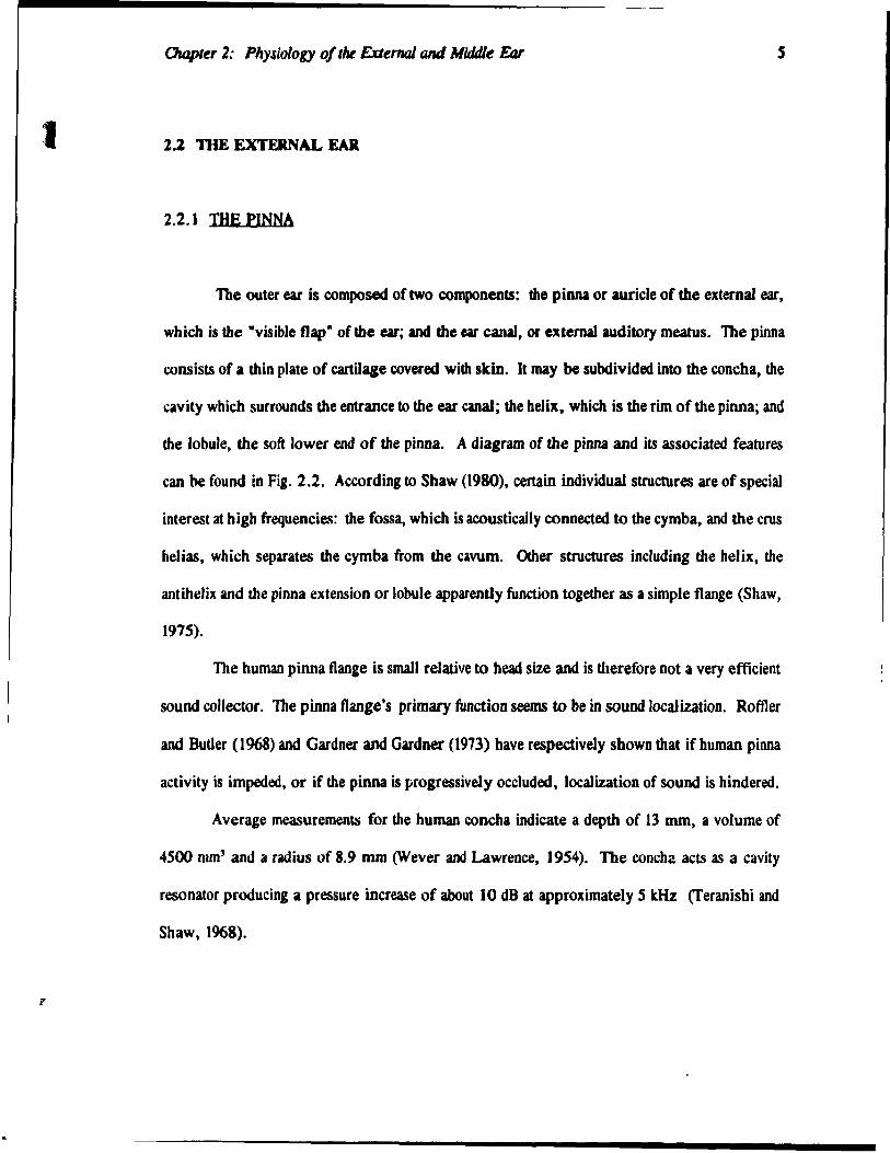
Stinson and Lawton (1989) studied human ear-canal geometry giving an idea of the range of

variation among humans. Results obtained for range and mean value of ear-canallength, volume

and cross-sectionaJ area from fifteen cadaver moulds are given in Table 1.1. The angle between

the hase of the eardrum co ne and a section normal to the ear canal close to the eardrum has been

found to be about 7er (Johansen, J975).

1

1

1

Chapter 2: Physiology of the Euernal and Midd/~ Ear 8

Length Volume Awrage Arta

(mm) (mmJ) ("un:)

Range 27-37 910-1725 30.0-54.9

Mean 30.8 1271.3 41.9

Table 1.1 Human ear-canal variation (calculated from Stinson and Lawton data, 1989).

The ear canal is greatly variable among different species. The cat car canal is quite

different from that of the human. A cylindrical portion extends out from the eardrum for about

15 mm. The ear canal then bends sharply at a right angle and the cross-sectional area bccomes

narro\\er and dumbbell-shaped and leads to the pinna (Wiener et aL, 1965). The cat ear canal

has a !ength of about 20 mm. The guinea-pig ear canal is shaped like a tube ahout 10 mm in

length and 2.5 mm in diameter, although at the end of the canal it expands sharply tu

approximately 8 mm, the diameter of the eardrum (Sinyor, 1971; Sinyor and Laszlo,1973).

Mechanical Properties of the Ear Canal

The ear canal is Iined with an epidermal layer. In the human car, the cpidermal layer

is backed by bone near the eardrum and cartilage in the rcst of the canal. Bascd on eMimat\.!s of

elastic moduli for epidermis, cartilage and bone from Fung (1981), the ear canal has a dilatationaJ

1

Chapler 2: Physiology of the E.xrernaJ an.f Middle Ear 9

impedance that is 104 limes larger than that of air (Rabbitt and Holmes, 1988). Thus the ear­

canal wall cao be treated as rigid.

2.3 THE EARDRUM

A diagram and schematic outline of the human eardrum are given in Fig. 2.3. The

eardrum is conical in shape with its apex pointing medially. The sides of the cone are convex

outward. Referring to me schematic out/ine of the eardrum, there are three distinguishable areas:

the pars tensa, the pars tlaccida and the manubrium. The bony process of the malleus, known

as the manubrium, attaches to the eardrum near the umbo, the point of deepest concavity of the

eardrum. The pars tensa forms the main surface of the eardrum and is composed of three layers

of tissue: an outer epidermallayer; the lamina propria, consisting of two connective tissue layers

and a fibrous layer; and an inner mucosal layer. The fibrous layer of the lamina propria forms

the main structural component of the eardrum. It is composed of fibres that are circularly and

radiallyarranged. The pars tensa is anchored to the bone around most of its circumference by

the annular ligament. The pars tlaccida is superior to the manubrium. Il is the more elastic part

of the eardrum and is separated from the pars tensa by the annular ligament. The major diame,er

of the human eardrum ranges from 9 to 10.2 mm and the minor diameter ranges from 8.5 to

9.0 mm (Rahhitt, 1985). The eardrum varies in thickness from 30 to 90 l'm (Lim, 1970).

ln terms of inter-species variation, the size of the eardrum tends to vary less among

species than overall body size. Khanna and Tonndorf (1969) found among seven different

•

1

1

Chapler 2: Physiology of lM ExternaJ and Middle Ear

Shrapnell's Membrane Pars Flaccida

10

Head of !'falleu3

--__ ShOrt Proces5 of the Malleus

!'finor Diameter

Umbo Pars Tensa

Annll1ar Ring

Oepth

MaJor Diamecer

(a)

pars flaccida

manubrium

pars tensa

(b)

Fig. 2.3

The human eardrum.

(a) Sketch of the eardrum. From Rabbitt (1985, p.25). (b) Schematic outline of the eardrum. After Kojo (1954).

1

Oulpttr 2: Physlology 01 lM ExttrMl and Middlt &r 11

mammaJs that the area of the tympanic membrane is approximateJy proportionaJ to a linear

dimension of the whole body, such as the cube root of weight.

MechanicaJ Propertjes of the Eardrum

Békésy (1949) measured the bending stiffness ofbuman cadaver eardrums and determined

it to he 2 X 101 N/m2• Kirkae (1960) determined values two or three times stiffer than Békésy.

Decraemer (1980) obtained results in good agreement with Békésy.

There are no data ilvailable conceming the Poisson's ratio of the eardrum. ft appears that

the value has little effect (FuMell, 1975). Funnell and Laszlo (1982) point out that for a material

composed of parallel fibres with no lateral interaction among fibres, the Poisson's ratio would

be zero for stress applied in the direction of the fibres. Common materials have a Poisson's ratio

ranging from 0.3 to 0.5. Funnell and Laszlo (1978) use a value of 0.3 for their eardrum model.

The eardrum presumably has a volume density somewhere between that of water

(1000 kg/ml) and that of undehydrated collagen (1200 kg/ml) (Harkness, 1961).

2.4 nIE MIDDLE EAR

The human middle ear contains several interconnected air-filled chambers: the main

chamber or tympanic cavity which lies behind the eardrum; a smaller cavity, the epitympanum

which lies above and extends backward and laterally; and small cavities called pneumatic cells,

wh ich 1 ine the upper pan of the middle ear. The malleus, the incus and the stapes are suspended

within the middle-ear cavities by a set of ligaments and by the tensor tympani and stapedius

•

1

Chapler 2: Physiolog)' of the E:cternaJ and Middle Ear 12

muscles (Fig. 2.4). The malleus is supported by anterior, lateral and superior ligaments. The

incus is supported by a posterior ligament. At low frequencies, the middle-e.u a"ls of rotatIOn

lies approximately bt'tw~n the line joining the posterior incudal ligament and the anterior

malleolar ligament. The annular ligament (not to be confusoo Wlth the annula .. ligament of the

eardrum) connects the footplate of the stapes to the oval window. Finally, a hg.tlllent .llso c"iMS

between tht' malleus and the drum membrane. The tensor tympam muscle is att.tched to the

malleus and when it contracts it pulls tht! malleus and therefore the eardrum further lOto the

middle ear. The stapedius muscle is connected to the stapes and pulls It Sldcw.lys during

contraction.

The cat and guinea-pig middle ears are similar in ove rail anatomkal ~tru~ture and

function to that of man, aIthough there are various differences in Jetail (Funncll, 1975).

Mechanical Properties of the Middle Ear

Ligaments and muscles are composed of connective tissue made up of tihrc~ wh I\:h

contain collagen, elastin and other proteins. The problem in modelling thl! musde~ and lig,uncnt~

is more than a non-linear elastic problem, because the response of tls.sue~ I~ loadlOg-path and rate

dependent. Sorne prel iminary finite-element modell ing of cat middle-car 1 igament~ hy

Funnell (1989), has assumt!d material and geometric line3f1ty, as weil a.., I\otwpil.: and

homogeneous materials. ft is possihle, however, to use the tinlte-eh:ment mdhod to "\llve

problems characterizoo by nonlinearities, inhomogeneiues and anisotropy

Chapler 2: Physiology of lM Exlernal and Middle Ear

AUDITQRY OSSICLES - Ligaments and Muscles

5UPERIOR MALLEAL L1G. to head of maileui

LATERAL ~ MALLEAL LlG.

to neck of malleus

to onterior procass of malleus

TENSOR 1 TYMPAN! M.

to manubrium of mal/ AHachment of tymponic membrane to manubrium

SUPERIOR INCUDAL L1G. /dYOfincu.

POSTERIOR INCUDAL L1G. to short process of incus

ANNULAR LIGAMENT to morgin of vestibular fenestra

Fig. 2.4

The middle-ear ossicles, their ligaments and muscles. From Anson and DonaJdson (1973, p. 245).

• 13

OIapter 2: Physlology o/the Enernal and Middl~ Ear 14

The middle-ear ossicles are generally modelled as rigid. However. Decraemer et al.

(1989) found sorne of evidence of bending of the manubrium. The matter may therefore need

further consideration.

1

3.1 INTRODUCTION

CIIAPfER 3

EXPERIMENTAL OBSERVATIONS AND MODELUNGOF

THE EXTERNAL AND MIDDLE !AR

15

This chapter presents a historiçaJ review of literature conceming experimental

observations on the ear canal, eardrum and Middle car, Various approaches to modelling the

outer and middle ear are also discussed, Pirst, a summary of ear canal work is presented;

followed by a coverage of eardrum and middle-ear studies; concluding with a discussion of the

initial atternpts made to deal with the coupled problem,

3.2 mE EAI( CANAL

3.2,1 SOUND-PRESSURE EXPERIMENIS IN THE EXTERNAL EAR

Sorne of the earliest research that examined pressure distributions in the ear canal includes

the well-known work ofWeiner and Ross (1946), Weiner and Ross inserted a microphone along

the auditory canal of human subjects. A plane progressive wave from a loudspealcer served as

a free sound field for the subject. A sound pressure increase of 12 dB was found al the eardrum

with a peak around 3 kHz. If one considers the ear canal as a cylindrical cavity open at one end

and c10sed at the other, this peak is effectively due to the fundamental longitudinal resonance of

., ,

1

Oulpler J: ExptrlmenlaJ ObservatlolU fJIId Modtl/ln, of the ÜltnuJl and Middle Elu

16

the eu canal. Besides this first resonance Il ~4, other modes Il 3).1" and 5).1" intetact with

concha modes at hiaher frequencies to increase the number of resonances. Weiner and Ross used

incident angles of 0, "5 and 90 degrees for the incident ways.

Other early extemal ear studies iDclude the work of Shaw and Teranishi. Shaw and

Teranishi (1968) performed experiments on real eus and rubber replicas. The rubber model

replicated the dimensions of the human pinna, concha and ear canal. A point source at various

angles of incidence from 1 to 15 kHz wu used. Sound pressure was measured with a probe tube

microphone al certain positions with the ear canal open and blocked. The replica data were in

agreement with real ear data for frequencies up to 7 kHz. In conjunction with this work,

Teranishi and Shaw (1968) constructed physical models with simple geometry. A cylindrical

cavity was set in an intinite plane to rcpresent the concha. The pinna was modelled by a

rectangular flange attached to the inclined concha and the cylindrical canal was completed with

a 2-element network representing the eardrum impedance. The simple model was in good

agreement with real ear data for frequencies up to 7 kHz.

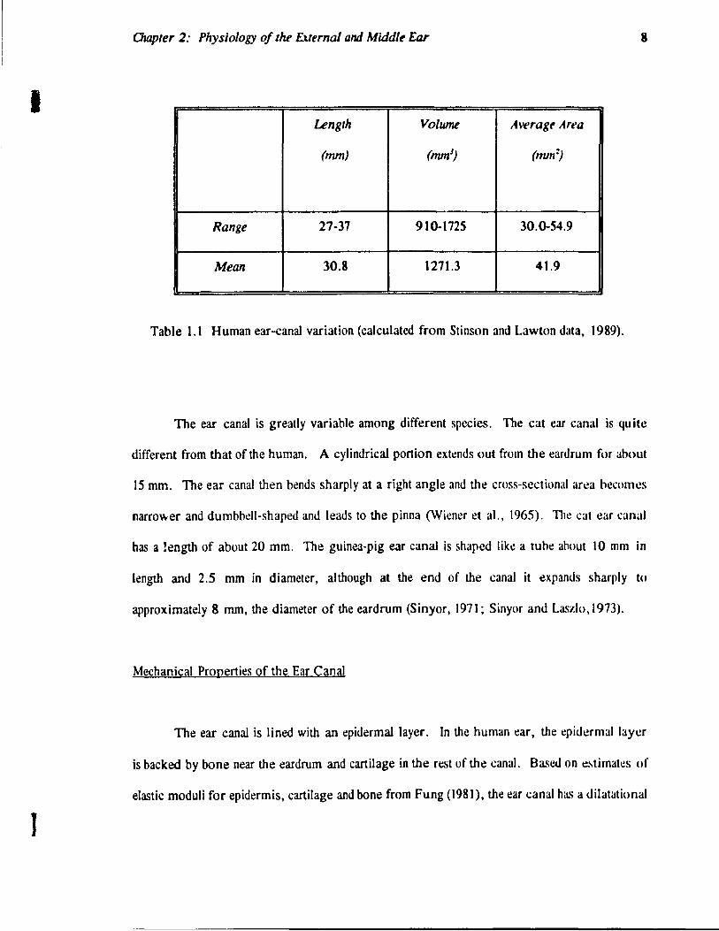
Many cesearchers have undtl1ak:en basic ear-canal pressure studies. Shaw (1974)

synthesized data from 10 studies and 5 different countries for various angles of incidence. The

synthesized data are displayed in Fig. 3.1, from Shaw (1974), indicating the average sound-

pressure transformation from free field to eardrum for frequencies from 0.2 to 12 kHz.

Shaw (1974) a1so summarized the various contributions of the components of the external ear as

weil as the head, neck and torso to the acoustic pressure gain (see Fig. 3.2). At frequencies less

than 350 Hz, the head has no effect. It adds about 5 dB when the frequency is raised to 10kHz.

The torso can have different effects depending on the frequency range considered. Il has an

amplifying effect at low frequencies, an attenuating effect around 1.5 kHz, and no eff~1 al hiaher

frequencies. The pinna flange pcoduces a 3 dB increase around 4 kHz.

--------------------------~~

Chapler 3: Experlmtnlal Observations and Modelling of Iht ExteT7UJl and Middle Elu

~+--'f~- ·110'

-135"

Fig. 3.1

17

Average transformation of sound pressure from free field to human eardrum as a function of frequency al eight values of angle of incident sound. From Shaw (1974).

CID

" 1 lit -c • c 0 ~ E 0 u c '0 C> u ,--lit ~ 0 u <

Chapter 3: Experimenlal Observations and Modelllng of the External and Middle Ear

18

T 1 2 3 4 5

Total: 450

Spherical head Torso and neck, etc, Concha Pinna flange Earcanal and eardrum 5

,," 3 . , / \ "-,

" , / \ / . / ~ " \,/.: .... J ...... \ ........... . ., ······7'······ ............. :::.;,'" .. : .................. ~ _._ . .:, \ 1

----------.,-"'........-' ~_ .... ' 't... 4 \. 1 •••.•••••••••• • :...'.......... • _._ . .,~ l, "'" ..... _._. l " ........ -~ . .:.._._._ .... _._._._._._._.-. ~ "-'.'" .

1 1 0.5 1.0 2

Frequency - kHz

Fig. 3.2

5

\ \ \./

10

Average acoustic pressure gain for various ear components. (Incident sound at an angle of 45u.)

From Shaw (1974, p. 468).

l

l

Oulpler J: ExperimemaJ Observations and Modelling of lM ExterNll and Middle Ear

3.2.2 ENERGY REFLECTANCE STUPrES

19

Sorne research in recent years has focused on the deterrnination of the coefficient of

reflection of acoustic energy at the eardrum. Energy reflectance is relatively insensitive to

anatomical geometry at higher frequencies, as opposed to the method of eardrum impedance

which becornes an unreliable rnethod to deterrnine input to the middle ear at such frequencies due

to difficulties in differentiating between eardrurn impedance and the effects of ear-canal

geometry.

Stinson, Shaw, and Lawton (1982) studied standing wave ratios in the ear canal. A

significant portion of the acoustic energy entering the ear canal is reflected back along the canal

from the eardrum. Standing waves result because (lf the interference between incident and

retlected waves. Standing wave ratios were determined for a range of 5 to 10 kHz by examining

the sound field set up in occluded human ear canals. The standard impedance tube method was

employed; that is, assuming a uniform duct terminated by an acoustic load. the sound pressure

is measured as a function of position, and pressure ma>. ima and minim:i are used to calcuJate the

energy reflection coefficients. Over the 5 10 10 kHz range, energy retlectance values of 60-78%

were obtained; these values were considerably higher than those determined from previous

studies. Fig. 3.3 compares experimental values of standing wave ratios determined in various

studies. Lawton and Stinson (1986) also used standing wave patterns to estimate acoustic energy

retlectance. Standing wave patterns were measured in unoccluded ear canals of human subjects

for pure tones ranging from 3 to 13 kHz. The region where probe measurements were made was

assumed 10 be a duet of constant cross-section. The energy coefficient was found to rise from

0.3 at 4 kHz up to 0.8 at 8 kHz, staying at this value up to 13 kHz. These data agreed weil with

those of Stinson et al. (1982).

ï

1 :

Chapter 3: ExperimemaJ Observations and Modelling of the ExternaJ and Middle Ear

25

-Cl ..... ." . . .. - 20 . . . . • . . . • • . 0 • . . • . . . . . .... • . 0

• 0 . ct • .... a: 15 . •

0 00

LIJ •••• • > "'J ct ~ 10 C) • .. z • 0 z 5 ct .... U')

0 Z 3 4 5 6 e 10 15

FREQUENCY ( kHz)

Fig. 3.3

20

O.B ... z lU

0.7 u ~ ~

0.6 lU 0

0.5 u Z

04 0 ... 0.3 u

lU ..J

02 ~ lU

01 a: >-C) c: w Z

20 w

Standing wave ratios derived from various investigations. On the right, the vertl\.:al aXI~ ~h(JWS the corresponding energy reflection coefficient. The symbols, dotted Iinc and solid curve indicatc the different authors of the investigations. From Stinson et al. (1982, P 768).

Chapter 3; Experimental Observations and Modelling olIM ExternaJ and Middle Ear

21

Stinson (t985a) determined acoustic retlection coefficients at a duct termination by

measuring the maximum rate change of phase with position. The method produced results similar

to the usual impedance tube method where amplitude components are considered. The advantage

of this phase method is that only a smalt amount of space is required to make the measurements;

this avoids potential in jury associated with increasing the penetration of the probe. The met.iod

is valid for ducts with uniform cross-section as weil as for ducts with conical area functions, but

otherwise it is still restricted.

Rabbitt (1988) used a high-frequency asymptotic theory (refer to Rabbitt and

Holmes, 1988, in Section 3.4) combined with multiple sound-pressure measurements in the ear

canal to determine energy flow and pl anar standing wave equations. The theory agrees weil with

experimental measurements in replicas of human ear canals from Stinson (1985b), but is limited

to high frequencies and is not valid at the terminating end of the canal. (Multidimensional effects

are not induded; only the plane wave component of the !)ressure field is deaJt with.)

3.2.3 NETWORK MODELLING OF THE EAR CANAL

External ear modelling has sometimes involved the network representation of the ear

canal. Zwislocki, whose influential work in middle-ear acoustics (1962) involved the

development of electrical analogs (refer to Section 3.4.2), also used electrical networks to

calculate theoreticaJ sound pressure in the ear canal (1965). Inductance and capacitance are made

analogous to acoustic mass and compliance. To form a network model, inductive and capacitive

Tee sections are connected in series, with the number of sections depending on the high

frequency limit (Bauer, 1965). Zwislocki's model agreed weil with data obtained by Weiner and

CluJpter Jo' ExperlmtnlQ] Obstl'WJlloflS œtd MCdtlllll' 01 lM ExteTMI and Middle Elu

22

Ross (1946). Furtber wort in this acea wu undertakeo by Gardner' and Hawley (1972). The ear

canal wu represented by • to-section anaIoe network of uniform and tapered desip. Two-

branch and four-branch networb for the representation of the eardrum and adjacent structures

were found effective. Usine values from Zwislocki (1970) of canallength equal to 22.5 mm and

canal radius equal ID 3.74 mm, values of induCWlCe and capacitance were calculated from

standard uniform tube formulas.

3.2.4 STUDIES FOCUSING ON EAR-CANAL GEOMETRY

Although there has been sorne interest in network modelling, the uniform tube has been

the most popular model approximation to the real ear canal. At low frequencies, wavelengths

are much larger than ear-canal dimensions, 50 that the cylindricaJ tube model is a reasonable

approximation for the geometry of the ear canal. However, at high frequencies where variations

over small distances are signiftcant, this approximation 00 longer holds. Therefore, certain recent

research bas focused on the importance of the actual shape of the ear canal in determining

acoustic input ID the middle ear, and thus the timited validity of the cylindricaJ ear-canaJ model.

Stinson and Shaw (1982), using experimental cavities of different shapes and a simulated

eardrum, determined that the geometry of the eardrum and adjoining section of ear canal affect

the flow of energy ID the middle ear. Hudde (1983) measured sound pressure at three locations

ID determine the area function of the human ear canal. The area function is the variation of the

cross-section along the middle axis of the duct. As areas were obtained for cross-sections al righl

angles to a straight axis, curvature was ROt taken into account. Stinson and Shaw (1983)

determined the importance of geometry at frequencies &reater than 10 kHz. The sound-pressure

distribution was measured in a scaled replica of the ear canal, and a theory was developed to

................ .n ___ . __________________________________________ _

awpltr J: ExptrilMnlGI Obs~1'WIIOlll tlIId Modellln, 01 tM Exlel7ll1l and Middle Elu

23

express the ear canal in terms of cross-sectional Heu defined lIonl a curved uis using an

extension of Webster's onHimensionai born equatiOD. The first papet to present the

mathematics of this theory wu mat of Khanna and Stinson (1985). The modified born equation

is applied ID three-dimensional, rigid-walled tubes that bave variable cross-section and curvature

along their length. The equation is expressed as:

d( dp CS» ds A(,,);" + t2A(s)p.(s) - 0 (3.1)

where s represents the curved axis, A(s) are the area funetions, perpendicular to the s axis, k is

the wave number, and Po is the pressure along the axis. The total solution p(s) can be considered

as the sum of two Iinearly independent solutions, propagating in the +s and -s directions.

Numerical techniques are used to determine the s axis, and A(s) is determined from silastic casts

of the ear canal. Khanna and Stinson also measured sound pressure between 100 Hz and 33 kHz

at 14 different locations in the ear canal of a cal. Large variations of sound pressure were

observed along the ear canal and over the surface of the eardrum above 10 kHz. The shapes of

the standing wave patterns agreed weil with results obtained from using the theoretical horn

equation approach for frequencies above 12 kHz. However, the analysis assumed rigid walls,

so that if high-frequency absorption should occur, modifications in theory would need to be

made. This modification was undertaken by Stinson (l98Sb). Stinson measured sound pressure

distributions in scaled replicas ofbuman ear canals. Using the horn extension theory, absorption

of acoustic energy at the eardrum was accommodated by incorporating an effective eardrum

impedance acting al a single point. Theory agreed weil with measurements, and al frequencies

greater than 6 kHz it was clear that the theory was an improvement over that of the uniform tube.

Owpter J: Experl1MlIIaI Obs~rwulo1lS and MOtkllln, of the ExlenuM and Middle Elu

24

Rabbitt (1988) determined ear-anal cross-sectioNi area funetions usina the asymptotic

theory in conjunction with pressure measurements. Because only two frequencies were used, the

calculated area functions do DOt tUe full advantaae of the theory. Future appliœions of the

theory over 1 broader frequency ~pectrum are expected ta improve results.

Stinson and Lawton (1989) studied the .eomeuy of IS ear canals by makinl rubber

moulds, and by usina 1 mechanical probe system ta record 1000 coordinate points over the

surface of the mould. Ear canals were described with respect ta a curved axis. Area functions

were then derived, which were in agreement with work done by Johansen (1975) and

Hudde (1983). Large inter-subject variations were found. Area functions were used in

conjunction with the one-dimensional born equation ta predict sound-pressure distributions in

human ear canals up to 19 kHz. Variations in ear-canalleometry produced the greatest sound

pressure transformation from the canal entrance to the innermost region for frequencies greater

than 10 kHz. Therefore, the accu rate specification of ear-canal geometry is important in the

proper prediction of sound-pressure distribution.

3.3 THE EARDRUM

3.3.1 EXPERIMENTAL OBSERVATION OF EARPRUM ViBRATIONS

There has been a great deal of research undertaken involving experimentaJ observations

of eardrum function as weil as theoretical modelling of eardrum behaviour. For a historical

review the reader is referred to Funnell " Laszlo (1982). Most observations of eardrum

vibrations bave been al low frequencies - from 1 ID 2 kHz. Kessel (1874) performed some of

l

(JrQpter J: ExperltMnlai Observallons and Modelllng olthe F.xterMI and Middle Eor

25

the earliest researcb on eardrum vibrations. Displacements of human cadaver eardrums due to

stalie pressures were observed usine 1 magnifyine lens. Kesse! aJso used a stroboscope to

observe vibrations al 2.56 and 512 Hz. The ,reatest displaeements were seen in the po~terior

section of the eardrum. Mader (1900) employed 1 mechano-electrica1 probe to study human

eada" er eardrum vibrations using 240 Hz and 600 Hz tones. The greatest amplitudes oeeurred

in the posterior/inferior quadrant of the drum. Dabmann (1929, 1930) used mirrors to observe

the displacements on human cadaver eardrums. Using a statie pressure change of 170 dB SPL,

il was determined that the middle parts of the drum undergo larger displaeements than the

manubrium. In this study onJy one illustration was pubUshed - a sketch of the eardrum with

marks superimposed representing the loci of retlected beams of Hgbt from the mirrors.

Capacitive probe measurements on human eadavers were made by Békésy in 1941. Again, onJy

one illustration was publisbed. Sound pressures and displacements were not presented. Békésy

concluded that the eardrum (except for the extreme periphery) and the manubrium vibrate as a

sliff surface. Stroboscopie methods were used by Kobrak (1941) for cadavers and living subjects,

but no results were presented in the discussion. Perl man (1945) also used stroboscopie methods

and reported that the amplitude of vibration on the anterior and posterior regions was about the

same in cadaver eardrums. The first high-resolution work using holographie methods was

undertaken by Khanna (1970). In a frequency range covering 400 Hz to 6 kHz, complete iso-

amplitude contour maps were produeed. Holographie methods were used on live cats (Khanna

and Tonndorf, 1972) and on human cadavers (Tonndorf and Khanna, 1972). The displaeements

on the manubrium were smaller than those of the surrounding membrane, and the largest

displaeements were found in the posterior segment. An example of eardrum output from Khanna

and Tonndorf (1972) is given in Fig. 3.4.

1

1

Chapter 3; Experimental Observations and Modelling of tlle External and Middle Ear

AXIS OF ROTATION

l;f 1 MALLE US 1

1

----62

4.9

1 .) ~~O \ 1 \

1

Fig. 3.4

26

Holographie image of eat eardrum vibrations at 969 Hz. The vibration amplitude (x /0.7 m) is marked for eaeh isoamplitude contour. From Khanna and Tonndorf (1972, p. 1914).

1

r

Owpler 3: Experimental Observai ions and Modelling O/Ihe Exlerna/ and Middle Ear

27

At low frequencies the general conclusion made by most of these experiments was that

the displacements of the manubrium are less than those of the surrounding membrane. The main

conflicting view cornes from Békésy who eoncluded that the eardrum vibrated as a stiff plate, but

subsequent work has effectively invalidated this notion.

High frequency response of the eardrum has been examined by a few researchers. In

their holographie study, Khanna and Tonndorf (1972) observed cat eardrum vibrations up to 6

kHz. The low-frequency pattern was present at 2.5 kHz but broke up as the frequency increased.

Similar results were found for human ears ([onndorf and Khanna, 1972). More recently,

Dccraemer, Khanna, and Funnell (1989) examined the amplitude and phase of ear::Jrum and

malleus vihrations up ta approximately 20 kHz in anaesthetized cats. Up to 10 kHz, results

ohtained were similar to those of Khanna and Tonndorf (1972), including a low-frequency plateau

up to about 3 kHz and minima around 4 kHz. Above 5 kHz, resonances were present. Between

10 and 20 kHz, the vibration amplitude was found to oscillate around a value about 20 dB lower

than the low-frequeney plateau level. Different points on the eardrum were found to vibrate in

phase at ffequencies below 1 kHz. At higher frequencies, points vibrated out of phase.

3.3.2 THEORIES AND MODELS OF EARDRUM BEHAVIOUR

Lumpoo-parameter models of the eardrum are popular, especially in connection with

lumped-parameter middle-ear modelling in general (refer to Section 3.4.2). In a lumped-

parameter model, certain characteristics of a system are lumped into distinct circuit e1ements, thus

produdng an equivalent circuit (whi.:h could be electrical, mechanical or acouslicaJ). Gt!nerally

the parameters are not dosdy tied to actual physical or anatomical data, but these models are

appealing due to their simplicity. Shaw (1977) and Shaw and Stinson (1981) used a 2-piston

Ottlpter 3: Experl1MlIIaI ObservtJlions twl Motûllln, of lM ExltrnDI and Middle Eor

28

lumped-parameter mode! for the eardrum, where one piston or zone represented the vibratina

portion of the eardrum, and the other represented the eardrumlmalleus couplina. In 1986, Shaw

and Stinson extended work to a three-zone model where the free vibrating zone was divided into

anterior and postt:rior zones.

Early attempts to account for shape in eardrum models, for example, the ·curved

membrane" hypothesis of Helmholtz (1869) and the subsequent work of Esser in 1947, were

seriously Iimited. It is difticult to develop a quantitative theory for the eardrum because of the

mathematical complexity. In recent years, however, numerical techniques have been used by

Funnell (1975) and Funnell and Laszlo (1978) to model the cat eardrum. Through their finite-

element modelling they determined that eardrum curvature, conical shape, anisotropy, stiffness

and thickness were important model parameters. Funnell (1983) examined the undamped natural

frequencies and mode shapes for a cat eardrum, again using the finite-element method. The

vibration patterns obtained for the first six natural frequencies are given in Fig. 3.5. The

eardrum vibration patterns were found to break up into complex patterns al high frequencies.

Results agreed weil with Khanna and Tonndorf (1972). Findings suggest that ossicular

parameters have little effect on the natural frequencies and mode shapes. Also, the conical shape

and possibly the curvature May serve to extend the urdrum frequency range. Funnell,

Decraemer, and Khanna (1987) included the effects of damping in the model. Increasing the

degree of damping smoothed the frequency response both on the manubrium and on the eardrum

away from the manubrium, but the overall level of the displacement amplitude was oot

significantly decreased. Therefore, it seems that damping results in little loss of the energy

being delivered to the middle ear. Instead of using finite-element methods, Rabbitt and

Hùlmes (1986) developed a fibrous dynamic continuum model of the tympanic membrane using

asymptotic methods, where the model specifically includes the fibrous ultrastru"ture of the

Chapter 3: Experimental Observalions and Modelling of the External and Middle Ear

Fig. 3.5

29

Eardrum vibration patterns determined by the finite-element method for the tirst six natural frequencies. The contours represent lines of constant vibration amplitude. The soUd contours represent positive displacements, the long dashed ones represent negative displacements, and the short dashed lines indicate zero amplitude. (a) 1.761 kHz, (b) 2.312 kHz, (c) 2.590 kHz, (d) 2.622 kHz, (e) 2.926 kHz, (f) 3.194 kHz. From Funnell (1983, p. 1659).

1

,

CJuJpler J: Experimental Observations and Modelling OliM ExternaJ and Middle Ear

30

eardrum. The coupling of the ossieular chain and coehlea were includoo in the modd. The

asymptotic method involves the development of equations deseribing the structural damping,

transverse inertia and membrane restoring forces which are used in order to incorporate

differences in bending, shear. and extensional stiffness across the eardrum. In order to solve the

equations. small parameter assumptions must be made. As for any model, accurate geometric

and material 3S:iumptions are essential for the creation of a successful representation.

3.4 mE MIDDLE EAR

3.4.1 EXPERIMENTS CONCERNING VIBRATION OF THE MIDDLE-EAR OSSrCLES

Middle-ear experiments which are of special interest here include those that deaJ with

ossicular vibration. As the manubrium of the malleus is couplcd to the eardrum, osskular

loading will a1so affect the coupled car canal/eardrum problem. A brief review of sorne of the

more relevant middle-ear experiments foJlows.

Moller (1963) determined the amplitude and phase angle of the vihrations of the malleus,

incus and round window of anaesthetized cats using a capacitive probe. The impeJance at the

eardrum from 200 to 8000 Hz was also measured. The middle ear was then modelled as a

second~rder low-pass function, which was valid up to 4 kHz. (It was detcrmined that the

eardrum could be modelled as a rigid piston in this region.)

Guinan and Peake (1967) measured osskular motion of anae:.thctized catI; u:.ing

stroboscopie illumination. The stapes was observed to have a lincar di~placcment up to 130 dB

SPL. Below 3 kHz, the ossicles moved as one rigid body. At higher frequendcs, the ~lapcs and

C7uJpttr J: ExptrlmenJaI Obstrvatlons t.UId Modtllln, olthe Exltmlll and Mlddlt Elu

31

incus laued behind the malleus. Ouinan and Peake a1so developed 1 circuit model to represent

the uansfer characteriatic of the middle ear.

Buunen and Vlamin, (1981) measured malleus vibratioDS in anaesthetized cats usina_

laser-Dopplu velocity mder. Resulta IIreed witb tbose of other studies. Decraemer

et al. (1989), who made interferometric measurements of eardrum vibrations in anaesthetized

cats, also examined malleus vibratioDS. It wu found that the mode of malleus vibration c:hanged

with frequency. Decraemer et al. (1990), usin,_ diffaent interferometric technique, were able

to clearly discriminate changes of the maJleus vibration response with time.

3.4.2 MIDDLE-BAR MOpELS

Lumped-parameter models, wbich have already been mentioned witb respect to the

modelling of the ear canal aDd eardrum, have been frequently applied to the modelling of the

middle ear. Onchi (1961), Moller (1961), Zwislocki (1962), and Lynch (1981) among others,

bave developed circuit models of the middle ear. As an example, the Zwislocki (1962) model

will be presented. Zwislocki's anaIog is based on the functional anatomy of the middle ear.

Values of elements were derived from impedance measurements on nonnal and pathological ears

and from anatomical data. The model is valid from 100 Hz to 2 kHz. A schematic block

diagram of the middle ear is presented in Fig. 3.6. Block 1 represents the middle-ear cavities.

Block 2 simulates the part of the eardrum DOt coupled to the ossicles. Block 3 represents the

coupling between eardrum and ossicles. Block 4 indicates that not ail acoustic energy is

transmitted across the incudo-stapedial joint. Block S inuoduces the input impedance of the inner

ear. The corresponding circuit model is given in fig. 3.7.

•

Oulpter Jo' ExptrlmentaJ Observations and Modelllng 01 the ExternaJ and Middle Elu

M'OOl.E-[Ait_ - [A" O"UM

CAvlllES IMLLlUS INCUS

[Ait. U.cuoo-DRU"

2 STA'(D~"" 4 .101'"

Fig. 3.6

S'A~U

coc .. "" ItOu'-O .... OOw

Schematic block diagram of the human middle ear with five functional units. From Zwislocki (1962, p. 1515).

32

Chaprl'f 3: Experimental Observations and Modelling of the Externat and Middle Ear

La Ra Cp

Co la

Ct Cd.

Cd2

RdZT Ld

Rd.

Fig. 3.7

33

Ro

Cs Cc

R, Le

R e

Circuit diagram of the human middle ear. Elements denoted by subscripts a, p, m. and t belong to the middle-ear cavities; those with the subscript d 10 a ponion of the eardrum; tho!ie with the subscript 0 to the malleolar complex; those with the subscript s to the incudo-stapedial joint; and tinally those with the subscript c to the cochlear complex. From Zwislocki (1962, p.15.l0).

•

1

Oulpt~r Jo' Experimental Obstrvations and Modtlllng OlIM Ext~rM1 and Middle &r

3.4 MODELLING 11IE EAR CANAUEARDRUM COUPLING

34

Recent research has considered the importance of coupling between ear canal and

eardrl,lm:

Khanna and Stinson (1986) examined energy reflection coefficients in cats. Two cats

yielded quite different energy reflection patterns. For one animal, the retlection coefficient rose

from 0.22 al Il kHz to a value of 0.92 al 31 kHz. For the other cal, the reflection coefficient

increased to a value of 0.28 at 18.5 kHz and then decreased to a value of 0.05 al 29 kHz.

Beyond 30 kHz the reflection coefficient rose steadily to a value of 0.7 al 33 kHz. The faet that

in this cat absorption coefficients of 90% were measured at frequencies :>bove 25 kHz emphasizes

that the tympanic membrane cannot be treated as rigid. Therefore, in 1989, Stinson and Khanna

made further modifications to their theoreticaJ model (modified horn equation including cur,ature)

of 1985. Because of the effects of absorption. the point impedance method of Stinsun (1985h)

is only useful at frequencies that are not too bigh. A bener representation of the load is

nect:.",sary to properly predict the sound-pressure distribution in the eardrum vicinity. Stinson and

Khanna modified the horn equation by including the motion of the tympanic membrane in the

form of a driving term, F(s). The modified horn equation becomes:

d ( dp (s» ds A(s>T + k,lA(s)p,,(s) = F(s) (3.2)

The behaviour of the eardrum was simulated u.iÏng either a mechanically-driven piston ur a

distributed locally reacting impedance. The thoory was tested using model ear canals of uniform

cross-section. Thus this testing only took into account the new features of the thoory, that is, the

CluJpter 3: Experimental ObStrvatiof1J and Modelling o/the ExIernaJ and Middle Ear

35

load modelling. Comparison of theory and experimental work indicates thal the theory is useful

up to 25 kHz in cats and 15 kHz in humans. Sound pressure is assumed ta be constant througb

each cross-section, thus the one~imensional aspect of the sound field still holds.

Rabbitt and Holmes (1988) studied three~imensional acoustic waves in the ear canal and

their interaction with the tympanic membrane. Although lower acoustic modes travel along the

length of the ear canal, higher modes are trapped neac the ends of the ear canal, that is, near the

concha and near the eardrum. The mod~ ulUle piMa result in the complex pressure distribution

at the enlrance, whereas the complex vibrational shape of the eardrum is responsible for the

intricate pressure situation at thal end of the canal. Because of the intluence of the eardrum, the

one~imensionaJ model of the ear canal is only valid al low frequencies. Thus for validity al high

frequencies, a three-dimensional approach is taken. Asymptotic expansions are used ta solve the

coupled system. The soluti0n is represented by two parts: an outer solution (WKB expansion)

valid over most of the length of the canal; and a transition layer, valid near critical resonant

cross-sections. As an example, the analysis was applied to a geometry resembling the ear canal

and eardrum of a cal. The ear canal, modelled as an axisymmetric tube, was coupled to a flat

tympanic membrane, perpendicular to the canal. It was found thal al low frequencies, only the

plane-wave component mode propagates (refer to Fig. 3.9a). As the WKB expansion is not valid

for plane waves at low frequencies, the one-dimensional theory approach was taken ta model the

(0,0) mode. nle new three-dimensional theory introduced rapidly decaying higher modes.

However, because of the rapid decay of these modes, the one-dimensional approacia remains a

reasonahle approximation al low frequencies for the given geometry. Also. al 1 kHz, the higher

modes only account for a small fraction of the acoustic coupling at the eardrum. This fact is

iIIustrated in Fig. 3.8, where the right-hand axis represents the percent of the total acoustic

coupling attributable to the nonplanar modes. The solid curve in the figure, which corresponds

1

..

Otopter 3: E.xperlmentm Observations œtd Model/lnl olIM Exte11llll œtd Middle Elu

36

to the model cal eardrum, indicates very Iittle eft'ect Il 1 k.Hz. Nonplanar modes become more

important al higber frequencies. For example, IIIS kHz, il can be seen in Fi,. 3.9b (comparin,

to the 1 kHz case in Fig. 3.9a) that trapped modes affect an increasing re,ion of the canal.

Hiaher modes also influence eardrum behaviour. Referrina llaÎn to Fia. 3.8, the 50lid curve in

the figure indicates that higher modes represent more !han SO~ of total acoustic couplina above

I~ kHz. In summary, multidimensional modes were found to have Iittle effect on the sound

pressure in the ear canal for frequencies less than 10 kHz, but were important al higher

frequencies. Results indicated that mass loading induced by trapped modes might exceed the

magnitude of plane-wave radiation at high frequencies; mus the response of the eardrum May he

considerably influenced by nonplanar modes at these frequencies.

Rabbitt (1990) provides a hierarchy of examples illustrating the acoustic coupling of the

eardrum. The examples range from a piston coupled to a semi-infinite acoustic duel, to a flexible

partition coupled to a semi-infinite variable duel, and to a closed cavity. Results indicate mat the

acoustics in the ear canal, the eardrum and the secondary middle-ear chambers contribute

importandy to the acoustic coupling, limiting passive energy absorption and transmission

properties. The work affirms that lumped-parameter models are not suitable al high frequencieJ.

1

Chapler 3: ExptrilMnlal Obs~rvalions and Mod~lIing of the Externa! and Middle &u

0 Q , . , 0") , , , , , ,

1

0 /

H 1 , 1- / a: o , o:~ 1

(J:) 1 I

Z 1

a 1

H 1 , 1- , a: H Cl a: o 0:0 .,.

(") .,.

.... .;

0 0

0 0.00 10.00 20.00 FREOUENCY (kHz)

Fig. 3.8

37

0 C»&f

~ ..J ~ ;:) 0 U

0 u .... -l-en ;:) 0

0 u ~ -<

a: 0 -< III Z

-< ..J ~

1

Z 0 Z

0

Ratio of plane-wave radiation coefficient to the sum of radiation coefficients for ail higher modes (on left vertical axis) and percentage of acoustic coupling of mode) cat eardrum attributable ta nonplanar modes (on right vertical axis). The solid curve corresponds to the model cat eardrum. The top curve corresponds to the same eardrum scaled up to the size of an adult human. The bottom curve corresponds to the eardrum scaled down to that representative of a rabbit. From Rabbitt and Holmes (1988, p. 1072)

Oaapter J: ExperilMnJal Observa/ions and Modelling of the ExterTUJ/ and Middle EIJr

~ -

(01) (021

CI

~~===----------O.QO 0.40 0.90 1.20 1.60 POSITION (CMl

(a)

~~ ~ 1

~ CLa

ID Sa N M -l CI'a

~~ ~021 i a

\ '., g ,~ ...... ~.,. }~11 a

0.00 0 .• 0 0.80 1.20 POSITION (CMl

(b)

Fig. 3.9

1.60

Standing pressure waves in the ear canal. From Rabbitt and Holmes (1988, p. 1075).

(a) Amplitude of modes at 1 kHz.

38

The plane-wave mode (0,0) is the top curve. Dnly ~i·..: plane-wave mode propagates at 1 kHz. The remaining modes are trapped in close vicinit, lO the eardrum and decay rapidly as the distance from the tympanic membrane is increased. Note that th: amplitudes of the nonplanar modes are the WKB solution and the plane-wave result is a numerical solution.

(b) Amplitude of modes at 15 kHz. The length of the trapped mode zone is extended over about one-th ird of the length of

the ear canal at this frequency. The plane-wave mode is the only propagating wave. Ali modal amplitudes are the WKB solution.

The WKB solution in (a) and (b) applies to the case of an eardrum coated with a 2 l'm thick layer of bronze powder. The coating was found to have little effect at these frequencies.

39

CHAPTER.

FlNITE-ELEMENT MODELLING

4.1 INTRODUCTION

Problems involving physical systems are often solved by finding a solution that satisfies

a differentiaJ equation throughout a region. AnaJytic methods such as separation of variables

work weil for simple goometries; however, as problems become more complex, different methods

must be employed such as the semi-analytic method of conformai mapping or numerical methods.

Numerical methods are particularly well-suited to the solution of problems involving more

difficult shapes and inhomogeneities. NumericaJ methods include the finite-difference method,

the finite-element method, and the boundary-element method. In the finite-difference method

(e.g. Hildebrand, 1968), the derivatives in the partiaJ differential equations are represented by

finite-difference approximations. A grid is placed over the structure of interest, and solutions are

determined at intersection points. The finite-element method (e.g. Bathe, 1982; Grandin,1986)

involves the division of a region into many simply-shaped subregions so that the solution for each

suhregion can he represented by a function much simpler than that required for the entire region.

The more recently developed boundary-element method (e.g. Brebbia and Dominguez, 1989)

involves the discretization of only the surface of the region, whether it is two-dimensional or

three-dimensional. as opposed to the finite-element method where in three-dimensional problems

the entire volume is discretized.

This chapter is divided into three main sections. The first section presents a basic

introduction to the finite-e1ement method, overviewing the mathematical basis and the

development of the system matrix equations. The second section explains how standard structural

•

1

Chapter 4: Finite-Elemelll Modelling 40

anaJysis finite-element code can be altered in order to solve acoustic prohlems. The third section

deals with the concepts involved in fluid-structure interaction, such as the couplcd ear

canal/eardrum problem, and how the solution is actuaJty implemented using finite-element code,

as weil as how the output is displayed and, finally, code validation.

4.2 THE FINITE-ELEMENT METHOD

In the finite-element method a system is divided into discrete two- or threc-dirnensional

elements. For example, a plane region may be divided inta triangular or quadrilateral elements.

A three-dimensional region may be divided into three-dimensional elements such as bricks or

tetrahedra. Fig 4.1 ilIustrates these typical element types. Elements are joined togcther at pOint"

called nodes, and conditions are usually enforced so that each deml!nt houndary is corn pat ihle

with each of its neighbouring elements. The mechanical behaviour of each element is analYLed.

This element analysis leads to the formation of a matrix equation relating the hchaviour of the

element to applied forces. The actual components of each element matrix arc dcpcndent upon

the shape and material properties of that element. Ali element equations are then intcgrated into

one complete system matrix equation. lne actual nodal responses are detcrmined hy solving the

system matrix equation using appropriate numerical techniques.

ln the following pages, the mathematics which lie behind the ahove stcps arc prc~cnted.

inc1uding the determination of the functional, and the subsequent developrnent of the governing

finite-element equil ibrium equations.

1

1

Chapter 4: Finlte-Elemenl Modelllng 41

-------..L 7

/

Fig. 4.1

Some typical element types. The triangle and quadrilateral are examples of two-dimensional elements. The tetrahedron and brick are exarnples of three-dimensional elements.

Owpttr 4: Finltt-Eltment Modelling 42

4.2.1 IHE.. VARIATIONAL FORMULATION AND THE FUNCJ10NAL

Finite-element approximations are commonly formulated using the principle of minimum

potential energy. The variational principle is expressed as follows: given a functional which

represents the potential energy of the system, then the function which minimizes that functional

is the solution of the system. For example, the following integral has an integrand involving the

variable x, a function u(x) and a derivative of u(x) with respect to x:

lr:I

n - f !(x, u(x), u'(x» dx (4. J)

Jra

The function u(x) (which must satisfy certain boundary conditions) that causes the functional, n.

to be a minimum is the solution.

The variational principle can also be stated as follows: the vanishing of the variation of

the functional,

(4.2)

is a nec\:Ssary condition for the existence of the extreme value of the functional.

A Variational Formulation For Elasticity Problems

Determining functionals can be a very difficult procedure. However, a simple example

will be presented here. The principle of virtual work is used as the basis to construct a

functional, II, for equilibrium elasticity problems. Virtual work is defined as work done by a

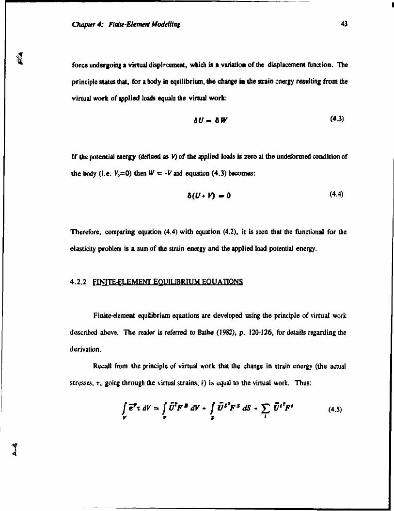
• Oaopttr 4: Flnltt-Ele~nt Motkllln, 43

force underaoinal virtual displ?cement. which is • variation of the displacement function. The

principle states that, for a body in equilibrium, the chanee in the strain '-"nec&)' resulting from the

virtuaJ work of applied Joads equaJs the virtual work:

au- aw (4.3)

If the potentiaJ energy (defined as V) of the applied loads is zero at the undeformed condition of

the body (i.e. Vo=O) then W = -V and equation (4.3) becomes:

a(u + JI) - 0 (4.4)

Therefore, comparing equation (4.4) with equation (4.2), it is seen that the functiJnal for the

elasticity problem is a sum of the strain energy and the applied load potentiaJ energy.

4.2.2 FINITE-ELEMENI EQUILIBRIUM EQUATIONS

Finite-element equilibrium equations are de\'eloped using the principle of virtual work

described above. The reader is referred to Bathe (1982), p. 120-126, for detaiJs regarding the

derivation.

RecaU from the principle of virtuaJ work that the change in strain energy (the actuaJ

stresses, Tt going through the \ irtuaJ strains, Ë) i~ e41uaJ to the virtual work. Thus:

fiTt; dV = f Ü'p· dV + f ijs'F s dS + E U"F' (4.5) y y S i

1

Chapter 4: Finite-Elemelll Modelling 44

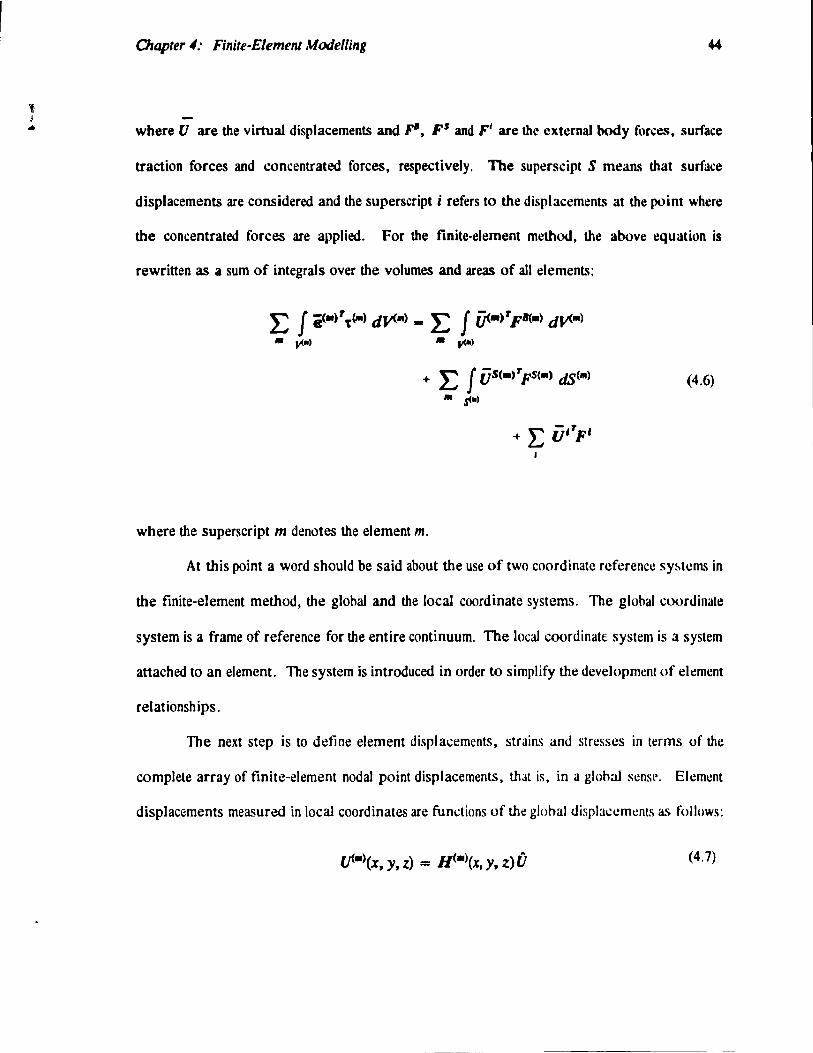
where U are the virtual displacements and F', F$ and FI are the external body forces, surface

traction forces and concentrated forces, respectively. The superscipt S means that surface

displacements are considered and the superscript i refers to the displacements at the point where

the concentrated forces are applied. For the finite-element method, the above equation is

rewritten as a sum of integrals over the volumes and areas of ail elements:

E f i C.)''t(III) dY<") - E f jj<_)'pl(a) dJÂIII) • .,<.) • .,<.)

+ E f ÜSC.) r FS(IfI) cIS(lII)

III sC.)

where the superscript m denotes the element m.

(4.6)

At this point a word should be sa id about the use of two coordinate referencc syMems in

the finite-element method, the global and the local coordinate systems. The global coordinate

system is a frame of reference for the entire continuum. The local coordinate system is a system

attached to an element. The system is introduced in order to simplify the developmenl of clement

relationships.

The next step is to define element displacements, strains and stresses in terms of the

complete array of finite-element nodal point displacements, that is, in a glohal scnsl'. Element

displacements measured in local coordinates are functions of the glohal displaccrncnts as follows:

(4.7)

l

OIaptl!r 4: Finlte-EltfM'" Modtllln, 4S

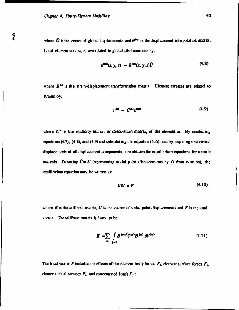
where (j is the vector of global displaeements and lf"'J is the displaeement interpolation matrix.

Local element straios, f, are related to alobal displaeeanents by:

(4.8)

where r) is the strain-displaeement transformation matrix. Element stresses are related to

strains by:

(4.9)

where 0"') is the elasticity matrix, or stress-strain matrix, of the element m. Dy combining

equations (4.7), (4.8), and (4.9) and substituting into equation (4.6), and by imposing unit virtual

displacements at ail displacement components, one obtains the equilibrium equations for a statie

analysis. Denoting Ù. U (representing nodal point displacements by U from now on), the

equilibrium equation May be written as:

KU-F (4.10)

where K is the stiffness matrix, U is the vector of nodaJ point displaeements and F is the load

vector. The stiffness matrix is found to be:

K L J B(a)'C(a)B(a) dV<a) . ~) (4.11)

The load vector F includes the effects of the element body forces F •• element surface forces F s.

element initial stresses F" and concentrated loads Fe :

..

Chapter 4: Finite-Element Modelling

and

FB

= L f W,,)'FB(.) dV<m) Il ~.)

F s = L f HS(II)' pS(.) dS(m)

.. s<.)

FI = L f B(III)' ~(,.) dV<m) .. .,<-)

46

(4.12)

(4.13)

(4.14)

(4.15)

where H is the volume-displacement interpolation matrix, FI is a vel.!tor of hody forcc!l, F S is

a vector of surface tractions, H S is the surface-displacement interpolation matrix, and 1 is the

stress vector, and B is once again the strain-displacement matrix. Note that Fe IS the vector of

externally applied forces where the ith component of Fe is the ~onCt!ntrated force at the ith node.

If one wishes to inc1ude the effects of inertia and solve a dynamic prohlcm, clement

inertia forces are included as part of the body forces Fil using d'Alcmhen's princlple. The

element equilibrium equation becomes:

MU + KU = F (4. ) 6)

Owpter 4: Finite-Elemerat Modellin,

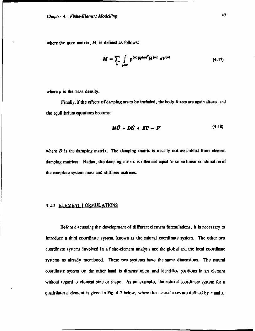
where the mass matri", M, is defined as follows:

where p is the mass density.

M -= E f p (.) H(a) r H""~ dV<·) • ,ca)

.7

(4.17)

finally, if the effects of damping are to be incJuded, the body forces are again altered and

the equilibrium equations become:

MÜ+DÛ+KU-F (4.18)

where D is the damping matrix. The damping matrix is usually not assembled from element

damping matrices. Rather, the damping matrix is often set equal to some Iinear combination of

the complete system mass and stiffness matrices.

4.2.3 ELEMENT FORMULATIONS

Before discussing the development of different element fonnulations, il is necessary to

introduce a third coordinate system, known as the natural coordinale system. The other two

coordinate systems involved in a finite-element analysis are the global and the local coordinate

systems as already mentioned. These two systems have the same dimensions. The natural

coordinate system on the other hand is dimensionless and identifies positions in an element

without regard to element size or shape. As an example. the natural coordinate system for a

quadrilaleral element is given in Fig. 4.2 below. where the natural axes are defined by rand s.

f (

...

Chapter 4: Finlte-Elemelll Modelllng

s

(-1,1) __ ---~---_ (1,1)

(-1,-1) (1,-1)

Fig. 4.2

Natural coordinates for the quadrilateral.

48

r

1

OIapt~r 4: Finit~-Elemenl Modelling 49

There are many differenl types of elements, both two- and three-dimensionaJ. This

chapter describes the formulation of matrices for a general three~imensionaJ isoparametric

element. (Jsoparamelric elements are elements that use the same basis functions for the spatial

coordinate and displacement interpolation formulas.) The problem can easily he reduced to the

one~imensionaJ or two~imensional case by including only the appropriate coordinate axes.

Special mention is made, however, of expressions necessary to implement the quadrilateral

element as weil as the 8-node brick element - the two element types which are uSed in this work

to model the eardrum and car canal. Again the reader is referred to Bathe, Chapter 5, for more

detaiJed explanations and derivations.

The first slep in developing the element sliffness and mass matrix equations and force

vectors is to set coordinate interpolation functions:

f % = ~ h%. ~ ,.

i-l f ,= E h,', f

Z = ~ h z· ~ 1 1

(4.19)

where x, y, and z are coordinates at any point of the element; x" YI and Z, are coordinates of the

q element nodes and the h" or shape functions, are defined in the naturaJ coordinate system of

the element: for three-dimensional elements the h, will have variables r, s, and t that vary from

-1 to t; for two-dimensional elements there is no z component, and therefore the DaturaJ

coordinate system will only include the r and s variables (refer to the quadrilateraJ element

example given in Fig. 4.2). The h, are unit y at node i and zero al ail other nodes.

The shape functions for a 2-D quadrilateraJ element are given by:

1 ". - !(l + r)(1 + .1)

4

la - ! (1 - r)(1 + .1)

II, - ! (1 - r)( 1 - .1)

la. - ! (1 + r)(1 -.1)

The shape functions for an 8-node 3-D brick element are given by:

", == i(1 -~)(1 - t)(1 + r)

~ ==!(1 + 3)(1 - t)(1 + r) 8

"3 _!(I + 3)(1 + t)(1 + r) 8

"4 - i(l -$)(1 + t)(l + r)

", ==!(1 - $)(1 - t)(l - r) 8

la, ==!(1 + $)(1 - t)(1 - r) 8 1 la, - S(1 + $)(1 + 1)(1 - r)

.... _!(1 - ,f)(1 + t)(1 - r) 8

50

(4.:20)

(4.21)

As these are isoparametric elements, the same basis fum:tions that were used for the

spatial coordinates are also used for the displacement interpolalion formula...,. The element

displacements are then defined as follows:

l

Oulpltr 4: Fillitt-E1emtlll Modelllll'

9

.. - E ",", '-1 9

Y - E ",V, 1-1 9

W - E",W, '-1

SI

(4.22)

where u, v, and w are the local element displacements at any point on the element and Ms, VI' and

W j are the corresponding element displacements al the nodes. Recall that the element stiffness

matrix depends on the strain-displacement transformation matrix, B. Strains must be determined

in tenns of derivatives of nodal displacements with rf' .. pect to local coordinates. To determine

the displacement derivatives, one must evaluate:

a ar iJy5 - -àr ar iJr ar a ax ôy clz - = œ cS œ œ a ax ôy &: -éJr 01 Or at

The above equation cao be expressed more concisely as:

a a --J­ar ch'

a -ar a -ay a -cl:

where J is the Jacobean operator. Now, solving for spatial derivatives, one obtains:

(4.23)

(4.24)

OIopttT 4: FllIlIt-Elemtlll Modeilln, 52

(4.25)

Usina equation (4.22) (the displacement interpolation formulas), and equation (4.25), one

evaluates the partial derivatives of Il, v, and w with respect to x, y, and z ID obtain the strain-

displacement transformation matrix, B. Thus we have the elements of the B matril which are

funetions of T, s, and t, the natural coordinates. Recaii equation (4.6) for the system stiffness

matril. The stiffness matrix for one element is therefore given as:

(4.26)

In order to solve for the stiffness matrix as given in equation (4.26), a change of variable must

be performed from x, y, z to r, s, t to obtain

dY - det} dr ds dt (4.21)

The determination of the stiffness matrix is also dependent upon the constitutive matrix or stress-

strain matrix, C. For a plane strain element, such as the quadrilateral element, the stress-strain

matrix is defined as follows:

1 v 0 --I-v

c- E(1- v) v 1 0 (1 + \1)(1 - 2,,) (1 - ,,)

(4.28)

0 0 1- 2v

2(1 - v)

• OIapter 4: Flnlle-Eltmelll Modtllln, 53

where " is Poisson'. ratio and E is the modulus of e1asticity or Young's modulus.

For 1 three~imensional e1ement:

1 " v 0 0 0 -1-" 1-"

" 1 v 0 0 0 -- --

1-" 1-"

" v 1 0 0 0 -- --c _ E(l- v) I-v J-v

(1 + vXI -1,,) 0 0 0 I-lv 0 0

2(1 - v)

0 0 0 0 1-1" 0 2(1- v)

0 0 0 0 0 1 - 2v

1(1 - v)

(4.29)

Finally, numerical integration is used to determine the integral of equalion (4.26). For

example, using two-point integralion for a liai ~-dimensional problem, one obtains:

(4.30)

where W'jl are the weighting factors, F- sTes det}, and Fiji is the matrix Fevaluated al points

The element load vewJrs and mass matrix ofequations (4.13), (4.14), (4.1S), and (4.17)

are easily determined, as the vector of interpolation funetions, H, is simply formed of the h, for

the appropriate element type, and other relevant matrices and variables have been determined.

1

OIapter 4: Finlte-E1ttnelll ModtIIÛl'

In the final step of the tinite-element analysis, element stiffness and mass mauices U'e

inserted into system stiffness and mass matrices, by traD.\ferring local element entries 10 the

appropriate global matrix entries.

4.3 AN ACOUSTIC ANALOGY

In order to use existing structural analysis code for an acoustic finite-element analysis,

acoustic pressures must he equated in some manner to structural response. The two basic

analogies are the displacement-pressure analogy and the stress-pressure anaJogy as discussed in

Lamancusa (1988). For the stress-pressure analogy, the aC(Justic pressure is equated to the

structural stress. The displacement-pressure analogy involv~ equating the acoustic pressure to

the structural displacement. In three dimensions, the stress-pressure formulation results in three

degrees of freedom per finite-element mesh point, whereas the displacement-pressure analogy

results in one degree of freedom per node. Therefore the displacement approach has the

advantage of having fewer unknowns. Also, in the displacement approach, results are directly

produced in the form of pressure fields which would be desirable in certain situations. On the

other band, the stress-pressure analogy has the advantage that the predicted structural

displacements are equal to the actual acoustical displacements, thus avoiding potential difficulties

involved in solving the tluid-structure interaction probJem (refer tu Section 4.4). However, the

stress-pressure analogy suffers from the presence of spurious resonances (Harndi and

Ousset, 1978). These spurious modes can occur with very small frequencies as weil as

frequencies far from zero, and it is therefore not possible to separate the real modes from the

spurious ones. Enforcing irrotationaJity wiJI cause these unwanted modes to vanish. Hamdi and

•

'( 1

Chapler 4: Finite-Element Modelling ss

Ousset use a penalty method to en force irrotationality which involves modifying the variational

principle for the prohlem. Lamancusa deals with the spurious mode problem by enforcing

irrotational elements. Thus no transverse wave propagation is allowed, and onJy two-dimensional

plane-wave prohlems can be solved. Considering all of the above factors, it was determined that

the displacement-pressure method was the analogy of choice to solve the three-dimensionaJ ear-

canal prohlem. A brief outline of the analogy follows, based on Lamancusa (1988).

The stress-equilibrium equation in one fixed direction (that is x) is described as:

(4.31)

where a" is the normal stress component in L'le x direction, 1'x, and T~ are the shear stress

components, p is the material mass density, and Uz is the structural d isplacement in the x

direction.

The Iinearized acoustic wave equation for no losses and no mean flow is:

a2P &p 1 a2P +-+-=--

ay2 èz2 c2 êJtl (4.32)

where P is the acoustic pressure and c is the velocity of sound in the fluid.

The essence of the displacement-pressure analogy is to force the structural equation to

take on the form of the wave equation. To begin, the disp/acement in the x direction is set equaJ

10 the acoustic pressure, while the displacements in the y and z directions are set to zero:

J

Orapter 4: Flnlte-Element Modelll,.,

u -p • (4.33)

U, -0 (4.34)

Now, the three-dimensional isotropie stress-strain relations for a solid are once again considered.

Using Lamancusa's notation, equation (4.9) can he written as:

", 1 + 2" 1 1 0 0 0 l,

", l + 2" À 0 0 0 l,

", 1 + 2" 0 0 0 l, (4.35) -".., G 0 0 Y..,

"JI G 0 y'/C

t. G

Y.

where E", Ey, E, are the normal strain components, 'Yry' 'Y,,:' 'Yz: are the shear strain components,

and Gis the modulus of rigidity. The). and 14 are lamé coefficients, defined as follows:

vE 1-------(1 + v)(l - 2v)

E I.L----

2(1 + v)

(4.36)

(4.37)

where E is the modulus of elasticity, and Il is Poisson's ratio. The next step involved in the

analogy is to set the Poisson's ratio, v, to zero and to set the modulus of rigidity, G, equaJ to the

1

OuJpler 4: Flnlle-EJemelll Mrxklllnl 57

elastic modulus, E. Dy substitutinl these values into equation (4.35), and recalling that U, and

Uc have been set to zero, the followinl equations are obtained:

au. fi -Ee -E-

l 1 clI

au. ~ -Ey -E-., ., ay

au. ~ -Ey -E-• .. az

Now, using U. = P, and substituting equations (4.38), (4.39), and (4.40) into (4.31):

Finally, equation (4.41) above is identical to equation (4.32) if:

(4.38)

(4.39)

(4.40)

(4.41)

(4.42)

ln summary then, in order to trick a structural finite-'!lement code 10 solve an acoustic

problem, one must set structural displacements equal to zero in ail but one direction, set 1.1 = 0

and G = E, and set E = pc? (where p will be the desired density of air). Finally, appropriate

boundary conditions must he set. On free surfaces, pressure in the selected degree of freedom

is set to zero. On rigid walls, no boundary condition is needed. If pressure is known at a certain

1

Chapler 4: Finile-Elemenl Model/ing 58

node, that node is given a forced displacement equal to the pressure. If the normal com(l\ment

of displacement is known at a cenain node, an external force equal to pG,Ü(t) ShllUld he applioo

al this node (where A is the area surrounding the node. Note that this force term is derived and

explained in Section 4.4).

4.4 FLUlD-STRUCTURE INTERACTION

4.4.1 INTRODUCTION

Most finite-element code availahle cannot be directly appl ied to the solution of l1uid­

structure interaction problems. Sorne finite-elernent paàagt!s, for example, ANSYS,

(Kohnke, 1977), include a tluid elernent in the possihle selection of e1emcntl> and can handle

tluid-solid interaction. However, in most cases, various techniques mu!>.t he IInplcmcntc(!,

involving moditications to input data files and alterations to the finite-dernent code. The

development of pre-processing and post-processing prograrns is also often ncœssary.

Modifications of this kind were necessary for the work undenaken hère.

This section introduces the tluid-structure interaction prohlem. To hegin, various

methods of dealing with the interaction prohlem are discu~seJ, followeJ by the rnathcrnatics

behind the rnethod chosen, and the actual finite-e1ement implementation. G. aphl(al vicwing of

the coupled results and code validation are also covered.

Chapler 4: Finile-Elemenl Modelling S9

4.4.2 APPRQACHES TO THE INTERACTION HtOBLEM

Fluid-structure interaction problems are typicaJly solved using one of the two approaches

mentioned in the previous section (4.3). Either the pressure is used as unknown in the tluid and

displacement as unknown in the solid (displacement-pressure analogy), or displacements are used

as nodal variables in both the tluid and the structure (stress-pressure analogy). As mentioned in

Section 4.3, having displacements as variables in both tluid and structure simplifies the solving

of the interaction problem. The other anal ogy creates difficulties in interaction problems: when

the displacement-pressure analogy is employed, special terms must be introduced to couple the

pressurts of the tluid and the displacement output of the structure. These coupling terms lead

to the formation of asymmetric matrices. In the stress-pressure analogy, these terms are not

necessary, thus simplifying analysis as weil as maintaining matrix symmetry. Papers by

Zienkiewicz and Bettess (1978) and Belytschko (1980) review these two methods and their

mathematical ba.o;is. Oison and Bathe (1985) give a listing of various researchers who have used

either one of these approaches. OIson and Bathe themselves presented a formulation for tluid­

structure interaction problems based on the tluid velocity potential. Previous work employing

a velocity-potential approach had been undertaken by Everstine et al. (1984). ln Oison and

Bathe's work, veJocity potentials are used as nodal variables in the tluid and a hydrostatic

pressure variahle is introduced and measured at only one node in each tluid region. Displace­

mcnts are onœ again the nodal variable in the solid. The resulting matrix equations are banded

and symmetric, which makes the velocity-potential approach an interesting alternative to solving

the tluid-structure prohlem, especially fOf large models.

The displacement-pressure analogy selected in Section 4.3 for the acoustic problem is

also a satisfactory approach for the coupled problem, and in comparison with the velocity-

0Iapt~,. 4: Flnltt-Eltmelll Motüllllll 60

potential approach, bas the Idvantaae of beinl ea5ier ta implement with the finit~lement code

available. The modifications and code development necessary to undertake the interaction

problem are DOW discussed, based on the work of Kalinowski and Nebelunl (1982).

4.4.3 SOLUTION OF THE FLUID-STRUCTURE PROBLEM

USING EXlSTlNG FINITE-ELEMENI COPE

Kalinowski and Nebelung have developed a method for the solution of f1uid-structure

interaction problems with the NASTRAN finite-element code. The same approach is, however,

applicable to SAP (Bathe, 1974), the structural analysis finite-element package being used in this

work. Kalinowski and Nebelung's paper covers the solution of an axisymmetric problem using

cylindrical coordinates. Necessary modifications are made in order to solve a generaJ problem

in Cartesian coordinates. Initially. finite-element equations are formed for both the acoustic

portion and structural portion of the problem:

FlMid Equation: M'Ü' + D'U' + K'U' _ F' (4.43)

(where the superscript p refers to pressure)

S~ral Equation: MÜ + DÛ + KU - F (4.44)

The f1uid and structural portions of the problem are merged together to form a complete matrix

equation:

OuJpltr 4: Ftl'lÛt-EJe~nI MOtÜllln, 61

(4045)

where the upper parts of the matrices correspond ID the acoustic part of the problem and the

lower parts correspond to the structural part. However, equation (4.45) is DOt the complete

equation for the interaction problem. The essence of tluid-structure interaction is that the

pressures on the acoustic side of the problem influence the displacements on the structural side

of the problem and vice versa, leading ID the develupment of coupling terms. Solving the

coupled problem iovolves the insertion of special coupling terms ioto equation (4.45).

To begin, the structural part of the problem is built with elements in the usual finite-

elemeot fashion with appropriate materiaJ propenies and constraiots. The acoustic pan of the

problem is modelled with elemen~s with appropriate material propenies and constraints as

determined from the acoustic anaJogy (refer to Section 4.3). A double set of node numbers must

be generated at the fluid-structure interface, where nodes on both sides of the interface have the

same spatial coordinates. After normal mass, stjffness and damping matrices have been

produced, coupling terms are calculated and insened into the mass and stiffness matrices 50 that

equation (4.45) takes on a new form, where the blocks represent the introduction of the coupling

terms:

(4.46)

.1

62

The derivation of these tenns and an elplicit description of how they are inserted are aiven

below.

StifJness Matri' CoypliOI Teons

The stiffness mattix coupling terms bave 1 value of A, representing the surface arel

surrounding the node. They are due to the pressures at the acoustic interface of the problem

acting on the structural interface.

The derivation for the coupling terms for the stiffness matrix is intuitively uooerstood.

For the ear canal/eardrum modelling, element surfaces are in the form of four-node quadrilat-

erals. The pressures exected by the tluid on the structural part of the problem must he translated

to a set of forces normal to the surface:

~pA, F-pA- LJ -

4 (4.41)

where Fis the force vector applied to a given node, p is the pressure, At is the area of the ith

element surrounding a given node, and the summation is over all clements auached to that node.

The insertion of the coupling terIns into the stiffness matrix is effectively equivaJent to carrying

out equation (4.47).

Stiffness tenns are introduced into the stiffness matri", as follows: off-diagonal coupling

terms baving a value of A" are insected in the column corresponding to the interface DOde pressure

variable and the row corresponding to the .x translationaJ comp<ment of the interface structural

1

Chapler 4: Finile-Elemenr Mode/ling 63

node. Similarly, in the column corresponding to the interface node pressure variable and the

rows corresponding to the y and z translationaJ components of the interface structural node,

coupling ter ms with the value If, and A, are insened. In the coupling terms, A", If, and A, are

the three components whid. make up the area vector A. which represents the surface area

surrounding the node.

The area surrounding anode is calculated in tenns of the areas of ail elements

surrounding that node. Each surrounding element bas a specifie area, and a quarter of this area

is distrihuted to each of the four nodes of that element. Therefore, the node in question will

rcceive appropriate area contributions from ail elements surrounding it. This procedure is easily

implemented in a program by using a DO loop, and by calculating and distributing areas on an

element-by-element basis for the entire structure_ The area of a quadrilateral element is

determined by dividing it into two triangular elements (as in Fig. 4.3) wberex], X2• XJ• and x4 are

Fig. 4.3

Quadrilateral area determination.

J

Oaapter 4: Finite-Eltrnent Modelling 64

the coordinate vectors of the four nodes of the quadrilateral element and the diagonal arhitrarily

runs from XI to XJ' The vector, A, which is normal to the element with a IImgth !hat is

proportionaJ to the element area, is determined using vector cross products:

Mass Matrix Coupline Terms

Area1 = (.12 - x.) )( (.x, - .1.)(2

Area1 = (.14 - xJ )( (.x. - .1))(2 (4.48)

The mass matrix coupling terms have a value of -ApG, where A represents the surface

area surrounding the node, p is the tluid density and G is the tluid hulk modulus The mass

matrix coupling terms are due to the mechanical displacements at the structural intt!rfJœ acting

on the acoustic interface.

The derivation of the mass matrix coupling terms given below is based on that round in

Everstine et al. (1975). To hegin, pressure must satisfy the following boumlary conJition at the

fluid-solid interface:

ap = -pü,. an

(4.49)

Chapler 4: Finite-Element Mode/ling 6S

l where n is the unit outward normal from the solid al the interface, and p is the fluid mass

density. Now using the directional derivalive of p in the direction of the unit outward normal

v from the fluid at a surface point Cv = -n) and substituting the structural anaJog II. for p yields:

(4.50)

Now, from the acoustic anaJogy using equations (4.38), (4.39), (4.40), and (4.42), and

substituting into equation (4.50):

(4.51)

The expression 10 the parenthesis is equal to the.t component of the surface traction vector, T

(Cook and Young, 1985). Therefore,

(4.52)

If the surface is discretized into a finite number of nodes, the surface traction can be replaced by

its lumped equivalent:

(4.53)

whcre FI is the x component of the force applied to a certain node which has an associated area

A. Now combining equations (4.52) and (4.53), one obtains:

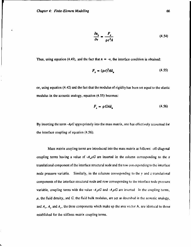
Chapur 4: Finile-Ele~lIl Modelling 66

èu. F. ---- (4.54) av pe2A

Thus, using equation (4.49), and the fact that n = -v, the interface condition is obtained:

(4.55)

or, using equation (4.42) and the fact that the modulus of rigidity has been set equal to the elastic

modulus in the acoustic analogy, equation (4.55) becomes:

F. = pGAü. (4.56)

By insening the terrn -ApG appropriately into the rnass matrix, one has effectivc/y accountcd for

the interface coupling of equation (4.56).

Mass matrix coupling ter ms are introduced into the mass matrix a..'1 follows: off-diagonal

coupling terms having a value of -A;rpG are inserted in the colurnn corresponding to the x

translational component of the interface structural node and the row cora I!spond ing to the interface

node pressure variable. Sirnilarly, in the colurnns corresponding to the y and z tran~lational

components of the interface structural node and row corresponding to the interface node prc~c;ure

variable, coupling terms with the value -AjpG and -AIPC arc in<;ertcJ ln the coupling tcrrns,

P. the tluid density, and G, the tluid bulk moduJus, are set as descnht!{) in the ac()u~tic analogy.

and Az, Ay and Az' the three components which rnake up the area ve..:tor A, are idcnllcaJ to tho!le

established for the stiffness rnatrix coupling terrns.

l

r

OIapIer 4: Flnûe-EletMIII Modellm, 67

Now that the stiffness and mua matrix couplina terms bave been determined, the matrix

schematic aiven in equation (4.046) cao be completed:

(4.S7)

4.4.4 IMPLEMENTING THE FLUID-STRUcruRE COUPLING USING SAP

KaJinowski and Nebelung describe bow coupling terms can be directly inserted into the

mass and stiffness matrices by altering the NASTRAN input file using -DMIG- cards, allowing

the coupled problem to be solved entirely within NASTRAN. Lflfortunately, this was not

possible using SAP, as SAP has nothina similar to NASTRAN's direct matrix insertion

capabilities. Therefore, the calculation of the coupling tenns, and their insertion into the mass

and stiffness matrices, were uodenaken in a separate program. First it was necessary to generale

mass and stiffness matrices for the uncoupled problem. The ear canal and eardrum parts of the

problem were run separately through SAP, thus generating mass and stiffness matrices in the

form of equation (4.45). In the speciaJly written code, called LUK, coupling terms are inserted

into the matrices. These coupling terms bave been calculated by a separate program and output

to two files: one for mass coupling terms and one for stiffness coupling terms. The main LUK

code aso the user if coupling terros are present. In response to a positive reply, the code reads

in the two files wbich contain coupling terms, as weil as equation column and row Dumbers for

each coupled term, and inserts the coupling terms ~nto the matrices appiOpriately. The user is

also questioned as to whether damping should be introduced in the problem. A positive reply

Chapler 4: Finile-Element Modelling 68

J resuJts in the formation of a damping matrix which will have non-zero tenns along the diagonal

corresponding to nodes for the structural part of the probJem. These terms have been calculatoo

by muJtiplying the mass matrix for the structural part of the probJem by sorne appropriate value.

Funne)) et al. (1987) have found this mass-proportional damping to produce results must similar

to experimentally observed responses. However, stiffness proportional damping or a comhinalilln

of the two can also be used. For this work, a mass-proportionaJ damping coefficient uf 1000 was

employed.

At this point, the LUK code has produced mass, sliffness and damping matrices for the

coupJed probJem. The user is then prompted for a frequency at whkh 10 perform an analysis.

The actual coupled system of equations, as presented in equation (4 57), is then solved. Recall

that differentiation of U yields:

Ü=j~U Ü = U~)2U - -w2U

(4.58)

Substituting equation (4.58) into (4.57), and assuming that damping is not indudcd in the

analysis, it can be seen that the problem will reduce to a system of real linear equations:

(4.59)

On the other hand, if damping is included, a system of complex linear equations is formet!:

(4.60)

,J

Olapltr 4: Flnlle-Elentent Modtlllng 69

Therefore, in order ID deal with either of these cases, a routine that will solve a system of

complex linear equations is employed. A routine from the NAG library (F04ADF) wu chosen,

which employs the method of Crout factorization to solve the problem (NAG, Mark13, 1988).

4.4.S YIEWING THE COUPLED RESULTS

An important aspect of finite-element analysis is the post-processing necessacy ID view

results, involving some sort of graphies program. In our laboratory, a graphies program known

as CON has been developed by Funnell ID view results from a SAP analysis. This program reads

in necessary data from the SAP results file to produce contour plots for acoustical or mechanical

problems. Obviously the output produeed by NAG within the LUK code will not be in a format

immediately ready for graphies viewing. For example, coupled output is ~n the form of real and

imaginary parts and different element types are involved. The modifications necessary in order

to view this output by CON are explained here. Similar sorts of manual manipulations would

be necessary for any graphies package which uses SAP output files to view results.

As stated, the output produced by NAG consists of real and imaginary nodal output for

the entire problem (note that il is also possible. by slightJy altering code, to output phase and

amplitude components instead). To begin, in the main LUK code, the acoustic nodal output is

separated from the structural nodal output. The real and imaginary components for both parts

of the problem are then output separately to two files, producing four files in ail. In order to

view these four files, they have to he in proper file format ID he read by the graphies program.

For example, in order 10 view the real part of the acousties output, it is necessary to insert the

real acoustic nodal output file into the displacement section of a normally structured SAP output

file, which has been produeed by running ooly the acoustic part of the problem through SAP.

Oulpttr 4: Finitt-E1tmtnl Modtlllng 70

Similarly, to view either the rea1 or imaginary structura! output, the appropriate file is inserted

into normally structured SAP output files obtained by running only the structural problem through

SAP. These new files then contain ail important nodal and element definitions necessary for the

ploning of structures as weil as correct output obtained from ruMing the coupled problem. Most

imponantly, these files are structured in a way that the graphies program CON will accept them.

4.4.6 CODE VALIDATION

Unfortunately, we have not found an appropriate three-dimensional coupled problem with

an analytical solution in order to check fully the validity of the coupling concepts as presented

in the theory section and the finite-element implementation. Nevertheless, various checks were

performed on the code to ensure its correctness. Preliminary checking of the coupled program

code, LUK, included ruMing the exarnple presented in the Kalinowski paper. Results obtained

were in good agreement with those of the paper. Following this, various internai checks were

performed on the code using the ear canal/eardrum problem. To begin, NAG output was

compared with SAP output for the static case. The acoustic pressure output al the ear

canal/eardrum interface determined by ruMing the coupled problem through LUK wa'i used as

force input to the eardrum problem alone - which was then run through SAP. Displacements

obtained on the eardrum were the same as those obtained by NAG for the coupled problem.

Similarly, the displacement data from the eardrum part of the coupled output were converted to

force input for the end of the ear canal, and the ear canal problem was run separately through

SAP. Output ear canal pressures were the same as those obtained by NAG for the coupled

problem. Similar internai checking was successfully performed when inertial and damping effects

were included.

71

CHAPTER 5

FlNJTE-ELEMENT MODEL ~'TS AND RESVLTS

5.1 INTRODUCTION

This chapter presents the results of the initial attempts made al modelling the coupled car

canal/eardrum problem using the finite-element method. To begin, geometric simplifications

which were employed to model both eardrum and ear canal are presented, as weil as mesh size

and associated material propenies. The preliminary model does not represent the exact geometric

characteristics of the coupled system. Its purpose is 10 test the implementation of the fluid-

structure theory, using a system which resembles that of the coupled eardrum/ear canal, but that

does not require the more complicated computerized three-dimensional reconstruction and

meshing techniques that would be necessary in the ideal modelling case. To begin analysis, the

eardrum/ear canal system is uncoupled. An eigenvalue analysis is perforrned on both the ear

canal and eardrum, treating them as separate problems. Results for these analyses are presented,

and as there are theoretical solutions for the individual models due to their regular geornetric

shape, results are compared to theory. The coupled problem is then dealt with. Output obtained

for a forced response analysis pelformed at several frequencies is presented, followed by a

discussion of these results.

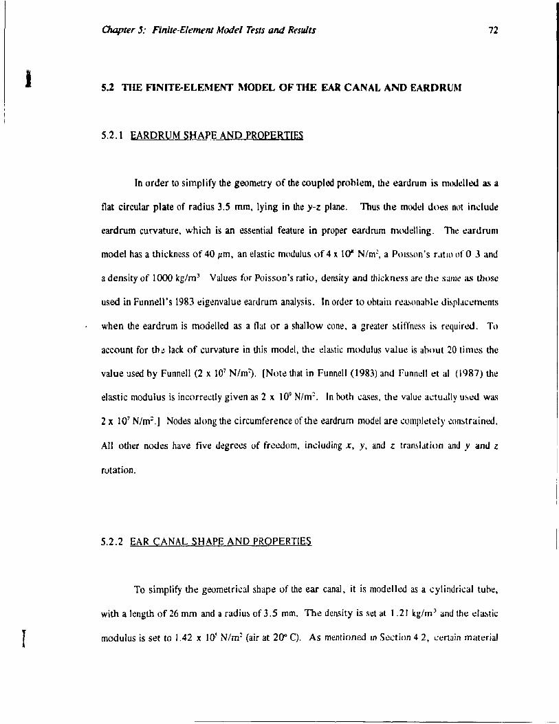
1

r

Chapter J: Finlte-EleftU>fII Model Tests and Results 72

S.l THE FlNITE-ELEl\fENT MODEL OF THE EAR CANAL AND EARDRUM

5.2.1 EARORUM SHAPE AND PROPERTIES

ln order to simplify the geometry of the coupled problem, the eardrum is modelltXl as a

flat circular plate of radius 3.5 mm, lying in the y-z plane. Thus the modd docs not indudc

eardrum curvature, which is an essential feature in proper eardrum modelling. The cardrum

model has a thickness of 40 ILm, an elastic modulus of 4 x 10" N/m2, a PlHS~()n's r..ltlO of 0 3 and

a density of 1000 kg/m) Values for Poisson's ratio, density and thickncss are the saille: as thosc

use<! in Funnell's 1983 eigenvalue eardrum analysis. In onler to ohtain rea.\onahlc di~plJCèmCnlS

when the eardrum is modelled as a flat or a shallow cone, a greater ~tiffness is requircd. To

account for th.! lack of curvature in this model, fue eJa.\tic modulus value is ahoul 20 limes fue

vaJue used by Funnell (2 x 107 N/mz:J. [Note that in Funnell (1983) and Funncll cl al (1987) the

eJastic moduJus is incorrcctly given as 2 x 109 N/m". In hoth ca.o;es, the value aClu..llly u~c.d was

2 x 107 N/m=.] Nodes aIong the circumference of the eardrum model are cumpletely c()n~lraincd.

Ail otIter nodes have five degrees of fre~om, induding x, y, and z lran!.l.ltion and y and z

rotation.

5.2.2 EAR CANAL SHAPE AND PROPERTIES

To simplify the geometricaJ shape of the ear canal, it is modelled as a cylindrical tuhe,

with a length of 26 mm and a radiu!l of 3.5 mm. The density is set al 1.21 kg/ml amI the cla.~tic

modulus is set to 1.42 x 1ft N/m~ (air at 20" C). As mentioned ln Section 42, œrt:.tin materiaJ

1

"

Owpter 5: Finite-EIl'mel2l Model Tests and ResuJts 73

properties in the finite-element file must be set appropriately to apply the acoustic anaJogy.

Therefore, Poisson's ratio is set to 0.0 and the bulk moduJus is set equal to the elastic modulus

al 1.42 x 10' N/m2• Nodes on the surface at the open end of the canal are completely

conslrained. Ali other nodes have one degree of freedom corresponding to x translation.

5.2.3 FINITE-ELEMENT MESHES FOR THE EARDRUM AND EAR CANAL

The tinite-e/ement mesh for the flat circulac eardrum consists of 49 quadrilateraJ

cJcmtmt'i. The mcsh for the eardrum is formed by mapping a uniform 7-element by 7-element

lIquare onto a circle. The mesh for the cylindricaJ ear canal consists of 343 8-node brick

clements. The cross-section of this mesh is identicaJ to that of the eardrum, and the mesh has

a longitudinal depth of seven elements.

Fig. 5.1 presents the finite-element meshes for the initial models of eardrum and ear

canal. Obviously the m~h of the end face of the ear canal is identical to the eardrurr mesh. The

nodes on the two surfaces share the same coordinates in space, thus establishing the double-node

interface which is necessary in order to solve the coupled problem as described in Chapter Four.

1

1

Chapter 5: Fin/te-ElemenJ Model Tests and Results

Fig. 5.1

Finite-element meshes for the eardrum (represented by a flat plate) and the car canal (representoo by a cylindricaJ tube).

74

•

.,

Owpler 5: Flnitt-EielMnI Model Tesls QIII/ Results 75

5.3 EIGENV ALUE ANAL YSIS OF mE lTNCOVPLFJ) PROBLEM

An eigenvaJue analysis was performed on each part of the uncoupled system in order ID

determine undamped Datural frequencies and mode shapes. This involves the solution of the

followin, equation:

(5.1)

where w is the frequency.

5.3.1 THE EARDRUM

The first six modes of vibration obtained for the finite-element analysis of the eardrum

(circular plate) are shown in Fig. 5.2. This figure and ail subsequent figures in this chapter were

generated using CON. For the eardrum problem, CON produces contour Hnes of equal

displacement amplitude by Iinearly interpolating between calculated nodal displacements. The

thin black: lines correspond ID positive displacement contours; the thin grey Hnes correspond to

negative displacement contours; and the thick: black: lines to zero displacement.

In Fig. 5.2, the first mode occurs al around 1 kHz, which is simitar to that determined

by FunneJl (1983) for his eardrum modeJ. (As stated previously, this wu accomplished by

adjusting the elastic modulus, E.)

" \

L

Chapler 5: Finile-Eleme1Jl Model Tests and Resu/Is 76

Fig. 5.2

Eigenvalue analysis of the eardrum (circular plate). The first six modes have th\! follow mg frequencies: 1) 1.02 kHz, 2) 2.197 kHz, 3) 2.197 kHz, 4) 3.527 kHz, 5) 3.833 kHl, and 6) 4.017 kHz.

.,

Oaopler 5: Finlle-Element Model Tesls and R~sults 77

The formula to determine the theoretical eiaenvalues of a unifonn circular plate is given

by:

(5.2)

where the subscript mn refers to the (m,n)lh mode and the 11.,11 are:

POl = 1.015, POl = 2.007, ~03 = 3.000

Pu = 1.468, P11 = 2.483, ~13 = 3.490 (5.3)

P21 - 1.879, Pu - 2.992, PD - 4.000

etc.

and E is the modulus of elasticity, " is the Poisson's ratio, p is the density, h is the half-thickness

of the plate, and a is radius of the plate (Morse and Ingard, 1968, p.215-216). The finite-

element output values can be compared with theoretical values in the table below.

m,n

t--0,1

1,1

1,1

2,1

2,1

0,2

Fin;Ie-element 1heoretical frequency frequency

(kHt,) (kHz)

LOO 1.016

2.197 2.114

2.197 2.114

3.527 3.469

3.833 3.469

4.017 3.955

Table 5.1 Finite-element and theoretical frequencies for the tirst six modes of the eardrum.

% Error

0.39

3.93

3.93

1.67

10.49

1.57

OuJpler 5: Flnlle-EltlMlIl Model Tests and RendIS 11

Note the presence of delenerate modes in Table ~.1. As deeenerale modes, mode. (1,1)

and (2, 1) have two eiaenvecton for eadl frequency. In Fia. ~. 2, the finite-element method reault

for mode (1,1) is presented in Cue 2 and Case 3. Case 2 and Case 3 have the ume frequency,

that is, 2.197 kHz. Note lb. there il a rotation of 9Q- between the two patterns. They ar~ the

same because the finite-element mesh used ta model the circular eardrum exhibits 90' symmetry.

On the other hand, Case .. and Case S whicb correspond to mode (2,1) do DOt have identical

frequencies (Case 4: 3.S27 kHz, Case S: 3.833 kHz). Note that there is a rotation of 45·

between the two patterns. As the finite-element mesh does not exhibit 45° symmetry, it splits this

mode.

By examining Table 5.1, it cao he seen that the percent age error between finite-element

and theoretical frequency differs for different modes. This is because the mesh has greater

difficulty in accurately determining the modes which are more complex. An important factor thal

must be considered in finite-element modelling is the resolution or fineness of the mesh. A finer

mesh generally produces more accurate results than a eoarse one, but there are other

considerations as weil. For example, a mesh of a given resolution may only allow a eeruain

number of modes to be resolved in an eigenvalue analysis. In fact, using the 49-element mesh

developed here, it was ooly possible to resolve the first six modes as presented in Table S.I and

Fig. 5.2. To experiment, a finer mesh of the eardrum was generated (using a 9-eJemenl

diameter). With this mesh it was possible to resolve many higher modes, a.c; weil as incn".a.·;e

accuracy. However, one must also consider the faet that computer storage requirements and run

time increase with increasing mesh resolution. In this work, the 49-element mesh produced

results of sufficient accuracy for our purposes, and was therefore employed.

OuJpter 5: Ftnllt-EltmLnI Model Tests and RtndlS 79

S.3.2 THE EAR CANAL

The tirst six modes obtained for an eiienvaJue analysis of the ear canal (cylindrical tube)

are shown in Fig. S.3. Here the thin black Iines correspond to positive pressure contours; the

thin grey lines correspond to negative pressure contours; and the thick black lines correspond to

zero pressure contours. The first tive modes are longitudinal modes, that is, pressure variations

exist ooly along the longitudinal axis. The sixth mode, wbicb occurs at about 27 kHz, is the tirst

transverse mode, that is, where variations occur in the plane perpendicular to the longitudinal

axis.

The Û1eoretical natura) frequencies for the longitudinal modes of a cylindrical tube closed

at one end are given by:

2n-l c J.---

4 L Il .. 1,2,3 ... (5.4)

where c is the speed of sound, and L is the length of the tube (Morse and Ingard, 1968, p. 474).

The longitudinal mode results determined from the tinite-element acoustic analogy are compared

to theoret;r:t! values in Û1e table below:

n

1

2

3

4

5

Finile-Element 1heorelical ~ Frequency Frequency Errar

(kHz) (kHz)

3.287 3.298 0.33

9.696 9.894 2.00

15.62 16.49 5.28

20.76 23.09 10.09

24.86 29.68 16.24

Table 5.2 Finite-eJement and theoretical fr~uencies for the first five longitudinal modes of the ear canal.

Chapter 5: Fin/te-Element Model Tests and Rt'sults 80

1 2 3

4 5 6

Fig. 5.3

Eigenvalue analysis of the ear canal (cyJindrical tube). The tirst six modes ha"'e the following frequencies: 1) 3.287 kHz, 2) 9.696 kHz, 3) 15.62 kHz, 4) 20.76 kHz, 5) 24.86 kHz, and 6) 28.53 kHz. Note that in Case 1, because the distribution is uniform across the eal canal, ail the surface nodes on the near end are joined together by the contour line.

Oaapt~r 5: Flnûe-Elemelll Model TesIS and Rendts 81

The theoretical natural frequencies for the transverse modes of a circularly cylindricaJ

tube are liven by:

where a ..... for the (m,n)th mode are:

CliO = 0.5861, ClOl = 1.2197,

~tc.

Cl20 = 0.9722 Cl n = 1.6970

and b is the radius of the cireular tube (Morse and Ingard, 1968, p.Sll).

(5.5)

(5.6)

The tirst transverse mode result determined from the tinite-eJernent acoustic anaJogy

compares weil to the tbeoretical value:

m,n

1,0

Finite-Elemelll Frequency

(kllz)

28.53

1heoretical Frequency

(kHz)

28.72

Table 5.3 Finite-element and theoretical frequency for the tirst transverse mode of the car canal.

% E"or

0.66

Note the increasing percentage error with inereasing frequency in the longitudinal modes.

However, the result for the tirst transverse mode, whicb occurs at about 28 kHz, is very

accu rate. Although the frequency is quite high, the tirst transverse mode is not cornplex, and the

49-element mesh is sufficiently fine to resolve it.

OIDpter 5: FInlte-fltlMlII Model Tests QN/ ResuIts 82

5 •• RESULTS FOR TIIE COVPLED PROBLEM

5 .... 1 INTROPUCDQN

ln this section results obtained for the coupled eardrumlear canal problem are presented.

Using SAP in conjunction with the special code deve10ped as described in Chapter Four,

harmonie forced response analyses were performed al several frequencies. Note that runDing the

coupled problem (on a V AXstation 3520) at a single frequency and displaying results took from

30 to 45 minutes.

Due to the form of the output, which is four plots per run (real and imaginary parts for

both plate and tube sections), il is not feasible to give a complete description of the coupled

problem behaviour over the entire frequency range of interest. The problem was solved for

approximately twenty different frequencies, with a constant pressure field of 2.828 N!m2 acting

over the surface nodes al the entrance to the canal. (This is the zero-lo-peak pressure variation

equivalent to 100 dB SPL.) 'The results for three frequencies will be presented in this section:

100Hz, 3.5 kHz, and 7.1 kHz. These frequencies were chosen with the 3im of presenting some

interesting aspects of the coupled problem by comparing coupled output with eigenvaJue output

obtained from the uncoupJed problem.

5.4.2 RESUL TS AT INDIVIDUAL FREOUENCIES

A. 100 Hz

Coupled results for 100 Hz are presented in Fig. 5.4. At very low frequencies a simple

low-Qrder vibration pattern appears on the eardrum. This is to be expected considering the

Chapter 5: Finite-ElemenJ Model Tesls and Results 83

uncoupled results for both the ear canal and eardrum. The first uncoup/ed eardrum mc,de does

not appear until approximately 1 kHz, and the first mode of the ear canaI appears at about 3 kHz.

Note the very small size of the imaginary component relative to the real component for the ear

canal and eardrum. The imaginary comp<ment of the e.ardrum displacement is smaller than the

reaJ component by a factor of more than t()l (Fig. 5.4b and a). These small imaginary

components are expected at such a low frequency where damping will have little effect on the

problem. In the ear canal as the pressure travels down the tube, the real component is effectively

constant, increasing from 2.828 to 2.843 N/m2 (Fig. S.4c).

B. 3.5 kHz

Resu/ts obtained for the coupled problem at 3.5 kHz are presented in Fig. 5.5. This

more complex, circular mode appears at about 4 kHz in the uncoup/ed drum problem. In

examining the real and imaginary parts of the eardrum in Fig. 5.5a and b, one notices the

increasing effects of damping: for the point of maximum positive disp/acement, the imaginary

componcnt is now approximately 47% of the real component. Damping effects are also present

in the car canal: al the eardrum end, the imaginary ear-canal pressure component has become

quite large, reaching ahout 55 % of the rea1 ear-canal pressure component (Fig. 5.5d and c). In

Fig. 5.5c, the real pressure changes from 2.828 at the ear-canaI end to -24.83 N/m2 al the

canlrum end, whcre the zero pressure contour is just inside the opening. This is similar to the

tirst longitudinal mode for the uncoupled tuhe which contains a quarter wavelength. Note that

the negalive real components of the eardrum displacements and of the ear-canal sound pressures

rl!tlect in~reasing inertial effe~ts.

•

1

CIulpter 5: Finite-ElemenJ Model Tests and Results 84

C. 7.1 kHz

An interesting higher-order mode appears for the coupled prohlem al 7. 1 kHz (refer 10

Fig. 5.6). As mentioned previously, il was nol possible to resolve any more than the first six

modes for the uncoupled drum problem with the mesh resolution heing used. However, this

mode appears to be a combination of theoretically predicted modes (4,1) and (4.2). U',llIg

Equation 5.2, mode (4,1) would in theory have a frequency of about 6.9 kHz. Note that for the

uneoupled canal problem, the first transverse mode does nol appear until ahout 27 kHz. The real

pressure component of the tube contains a half wavelength from 2.828 to -2.827 N/mz. This is

similar to the haJf-wavelength mode for an uncoupled tube c10sed al hotil ends, which would

oceur at about 6 kHz (half-way between the 3 and 9 kHz of the first two modes of the uncoupled

tube open al one end). Once again the imaginary component in plate and tuhe (Fig 5.6h and d)

reflects the influence of damping. The imaginary part of the tuhe output whil:h ranges from

-0.0294 to 0.0259 N/m2 (see Fig. 5.6d) is very i.nteresting. The higher-order mode is secn to

be trapped at the end. Therefore, Fig. 5.6d provides an example of a non-propagaling higher

order mode as discussed in Rabbitt and Holmes (1988).

Chapter 5: Finite-Element Mode/ Tests and Results

(a)

fi~. 5.4

Results for the coupled problem at 100Hz.

(a) Eardrum: real component. Range: 0.0 m to 2.702 l'm. Centour lines are spaced at intervals of 0.300 l'm.

(h) Imaginary comp<ment for the eardrum. Range: 43.33 nm to 0.0 m. Contour Iines are spaced al intervals of 4.814 om.

85

(h)

Note that in these and the following eardrum figures, the black upward pointing triangle corresponds to the contour of Most positive displacement, and the downward pointing triangle corresponds to the contour of Most negative displacement.

Chapter 5: Finite-Element Model Tests and Results

(c)

Fig. 5.4 (Continue<l)

Results for the coupled problem at 100Hz.

(c) Ear canal: rea1 component. Range: 2.828 N/m2 to 2.843 N/m2•

Contour lines are spaced at intervals of 2.843 x 10 .. 3 N/m2•

(d)

(d) Ear canal: imaginary component. Range: -186.6 x lQ-6 N/m2 to -9.728 x 1(}t2 N/m2•

Contour lines are spaced at intervals of 9.821 x l~ N/m2•

86

..

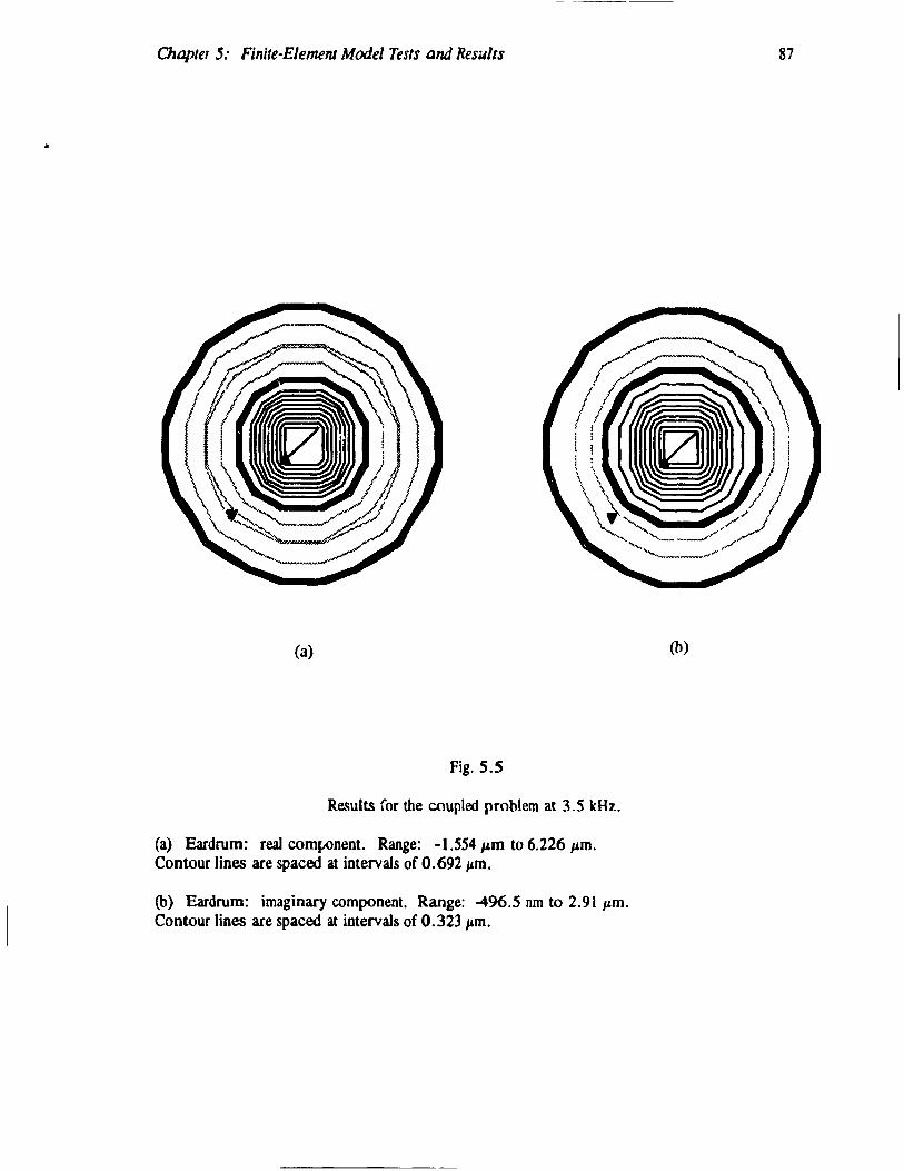
Chaple1 5: Fin/le-Element Model Tests and Results

(a)

Fig. 5.5

Results for the coupled problem at 3.5 kHz.

(a) Eardrum: real comJ1Qnent. Range: -1.554 JLm to 6.226 l'm. Contour \ines are spaced al intervals of 0.692 l'm.

(b) Eardrum: imaginary component. Range: -496.5 nm to 2.91 ILm. Contour \ines are spaced at intervals of 0.323 l'm.

87

(b)

1

Chapter 5: Finite-Elemenl Model Tests and Results

/

(c)

Fig. 5.5 (Continued)

Results for the coupled probJem at 3.5 kHz.

(c) Ear canal: real comp<ment. Range: -24.83 N/m2 to 2.828 N/m2•

Contour lines are spaced al intervals of 1.307 N/m2•

(d)

(d) Ear canal: imaginary component. Range: -14.01 N/m2 to -1.259 x 10-9 N/m2•

Contour Iines are spaced al intervals of 0.737 N/m l•

88

1 A

Chapter 5: Finite-Eleme1Jl Model Tests and Results

(a)

Fig. 5.6

Results for the coupled problem at 7.1 kHz.

(a) Eardrum: real component. Range: -29.87 nrn to 102.3 nm. Contour lines are spaced at intervals of 11.367 nm.

(b) Eardrum: imaginary comp<>nent. Range: -22.09 nm to 25.23 nm. Contour Iines are spaced at intervals of 2.803 nm.

89

(b)

1

Chapter 5: ."inite-EJement Model Tests and Results

(c)

Fig. 5.6 CContinue(J)

Results for the coupled problem at 7,1 kHz.

(c) Ear canal: real component. Range: -2.87 N/m2 to 2.828 N/m2•

Contour lines are spaced al intervals of 0.151 N/m2•

Cd)

(d) Ear canal: imaginary component. Range: -29.44 x W-3 N/m2 to 25.87 x 10.3 N/m2 •

Contour lines are spaced al intervals of 3.271 x 10-3 N/m2•

90

CHAPTER'

CONCWSIONS

6.1 SUMMARY OF CONTRIBunONS

91

A method bas been presented ID dea1 wi!.h the problems involved in coupl ing the

acoustical behaviour of the ear canal with the mecbanical behaviour of the eardrum. The method

involves the use of the SAP finite-element package, the use of an acoustic-structural analogy in

order ID use this code ID perform an acoustic analysis, and finaJly the development of special code

to deaJ with the actuaJ coupling. The combined ear canal/eardrum model developed here is a

preliminary model, where the simplified geometry permitted an uncomplicated initial examination

of the effects of coupling. Results obtained for the ear canal as cylindrical tube coupled ID the

eardrum as flat plate are promising and indicate the future usefulness of the method, especially

when more realistic geometry is included in the modelling.

6.2 1<"1JTURE WORK

The next step in modelling is to include proper geometricaI representation for both the

eardrum and ear canal. The curved cone-Iike shape of the eardrum is important and must be

included in the model. The eardrum's various sections, including the pars tensa, the pars tlaccida

and the manubrium sbould aIso be distinguished, with appropriate material propt!rties assigned

to each section. The ear canal's actuaI geometry must a1so be included. The importance of the

1

Chapur 6: Conclusions 92

middle ear must a1so be considered, including the behaviouf of the ligaments and ossicles as weil

as the loading effects of the middle-ear air cavities.

To begin, future worlc will talce two differen~ directions. In one case, work will be

continued on modelling the human eardrum and ear canal, stressing a better geometrical

representation of the system. However, as finite-element modelling of the cat eardrum has

already been undertaken (Funnell, 1983), future worlc will a1so deal with modelling the coupled

system of ear canal and eardrum for a cat. The methods that will be applied to reconstruct the

three-dimensional geometry of the ear canal have already been developed. Cat ear-canal Jata will

be generated using a series of histological slices. Each prepared slide will be projected onto a

surface and contours defining the shape of the ear canal will be digitized and stored on the

computer. After aligning the digitized slices, the three-dimensional geometry of the ear canal will

be reconstructed. This method of three-dimensional reconstruction has been used to reconstruct

the middle-ear ligaments and ossicles as described in Funnell (1989). The three-dimensÏ0nal ear

canal must then be meshed into elements, and this cou Id be a complicated process. It will be

undertaken using a three-dim~nsional meshing program for irregular shapes developed by

Bouhez (1985), which automatically generates a mesh of tetrahedral elements for a three­

dimensional ohject using seriaI sections. This program has been successfully applied to th~

meshing of a cat middle-ear ligament (Funnell, 1989).

Modelling the coupled system for both cat and human can be approached using methods

other than pl:re finite-e1ement analysis. For example, the ear canal can be modelled using the

boundary-elt!ment method, where the structure of the ear canal would be definoo only by its

boundary. Boundary ell!ments are now fre'lliently used in oonjunwùn with tinite dements; for

examplc, in tluid-stru~ture interaction problems, the tluid can be repr~ented using two­

dimensional surfact' bt1und.lry elements which match on the boundary of the timte-element mesh

1

Chapter 6: Conclusions 93

of the structure (Walker, 1980; Everstine and Henderson, (990). The advantJge..'i of moddlmg

using these hybrid methods indude simpler me..l1,h gen~~ration and d~~reast.>J wmputatilln time fnr

some problems. High-quality commercial code which comhines linite-\!Iement and houndary

element methods bas recently starte~ to appear (Coyette, 1990).

6.3 APPLICATIONS

After including more accurate anatomical repre..~entations in the cnupled prohlem, il will

be possible to undertake comparisons with actual expcrimcntal ùata Furthermore. it will be

possible to examine how various pJrameters affect the hchaviour of the mode!. For cxample, ear­

canal length, sue and shape could he altered to dcterminc the effect on car-c.tn.lI ",ound prc!>~ures.

Results obtained from su ch an analysis mlght then he compareJ with tho!-e of Goultc ct al.

(1977), who found that moddicJtions of c-w;ternal-ear andtomy followmg tympJnomJ.~toll.J surgcry

can have sigmtïcant effects on the external car sound-pres ... ure gam and thcreforc humdn hcaring

response.

Obviously, the couplcd system will have different features for dllferent specics. For

example, as discussed ln Chapter Two, the human, cat, Jnd guineJ-plg car candl~ each hdVC

distinctive features. Other features which will differ across spt!cles, mcludlllg the \hape of the

concha and the orientation of the eardrum. Will be Important in the coupll!d prohlcm (R..Ihhitt ,md

Holmes, 1988). Therdllre, mndelllllg th,~ ~ouplcd system for dIffèrent anlmdl" ... hould rcveal

interesting information regardmg the role of specltir car componenl<; dnd gcometry in the

interaction problem.

Dlapter 6: Conclusions 94

The initial finite-element modelling which has been undertaken for the cat middle-ear

ligaments and ossicles (Funnell, 1989) has aJready been mentioned. However, to complete

middle-ear modelling, the air cavities must be included, and this will involve the use of the tluid­

structure coupling method developed here. Combining the resulting middle-ear model with

existing eardrum mooels, and the ear canal/eardrum work undertaken in this thesis, it should

eventuaJly be possiLle to have a complete tinite-element model of the middle and outer ear with

appropriate structures of interest modelled as desired. Sucn a mode! would be of considerable

use in understanding the transmission of sound through the eardrum and lead to a greater

knowledge of the hearing process in general.

1

95

REFERENCES

Akkas, N., Akay, H.U., and Yilmaz, C. (1979). • Applicability of generaJ-purpose tinite element programs in solid-fluid interaction problems, " Comput. Struct., ~O, 773-783.

Anson, B.J. and DonaJdson, J .A. (1973). Sur~içal Anatomy of the Temporal Bone and Ear. (W.B. Saunders, Philadelphia).

Bathe, K.J. (1974 revised). SAP IY - A Structura! AnaJysis PrQ~ram for Static and Dynamlç ~nse of Linear S:yste~. Report no. EERC 73-11, Col1ege of Engineering, University of California, (Berkeley, California).

Bathe, K.J. (1982). finite Element procedures in Eni;;neerin~ Analysis. (prentiœ-Hall, New Jersey).

Bauer, B B. (1965). "Equivalent circuit of a tube or spring," 1. Aeoust Soc. Am , 38, 882.

Békésv. G.v. (1941). "On the measurement of the amplitude of vibration of the osslcle..1'1 with a capacitive probe,· Akust. Zeltschr , 6, 1-16. 1 ln German)

Békésy, G.v. (1949). "The structure of the middle ear and the hearlng of one's own vOlee hy bone conduction," J. Acoust. Soc Am, 21,217-232.

Belyts..:hko, T. (1980). "Fluid-structure ir.teraetion,· Comput Struet, 12, 459-469.

Boubez, T.I. (1986). Three-Djmensio' aJ Finite-Element Mesh Generation Usm~ Senal Seçtjons (M. Eng. Thesis, McG~lI UniverSity, Montreal).

Brebbia, C.A., and Dominguez, J. (1989). Boundary Elements: An Introductory Course. (McGraw-Hill, NY).

Buunen, T.J.F., and Vlaming, M.S.M.G. (1981). "Laser-Doppler veloclty mctcr applicd tu tympanic membrane vibratiOns in cat," J. Acoust. Soc Am., 69(3),744-750

Cook, R.D, and Young, W.C. (1985). Advanced Mechanics of Matenals (Mal:mlllan Publishing COIDi1any, New York).

Coyetce, J .P. (lm). "Finite element and boundary element technique.'; to solve acouMÎc problems," Cano Acoust., 18(3), 75

Dahmann, H. (1929). "On the physiology of heanng. expenmental studll!-.<' on the mechanH;!o. of the ossicular chain, as weil as on the behaviours of tones and air pres~urc l," Zeitschr. f. Hals. Nas. Ohrenhlk., 24, 462-498. (in German).

1

96

Dahmann, H. (1930). -00 the physiology of bearine: experimentaJ studies 00 the mechanics of the ossicular chain, as weil as on the behaviours of tones and air pressure II-IV," Zeitschr. f. Hals. Nas. Ohrenhlk., 17, 329-368, discussion 398-402. {in German].

Decraemer, W.F. (1980). Personal communication to W.RJ. Funnell.

Decraemer, W.F., Khanna, S.M., aM Funnell, W.RJ. (1989). "Interferometric measurement of the amplitude and phasl! of tympanic membrane vibrations in cat," Hear. Res., 38(1), 1-18.

Decraemer. W.F., Khanna, S.M., and Funnell, W.R.J. (1990). "Heterodyne interferometer measurements of the frequeocy resonse of the manubrium tip io cat," Hear. Res., 47(3), 205-211.

Esser, M.H.M. (1947). -The mechanisrr. of the middle ear: II. The drum," Bull. Math. Biophys., 9, 75-91.

Everstine, G.C., and Henderson, (lm). ·Coupled finite ~Iementlboundary element approach for fluid-structure interaction," J. Acoust. Soc. Am., 87(5), 1938-1947.

Everstine, G.C., Henderson, F.M., and Lipman, R.R. (1984). "Finite element prediction of acoustic scattering and radiation from submerged elastic structures," Proceedings of Twelfth NASTRAN User's ColloQuium, NASA Conference Publication 2328, 192-209.

Evers:ine,G.C., Schroeder, E.A., and Marcus, M.S. (1975). "The dynamic analysis of submerged structures," PrQceedings of the Fourth NASTRAN User's CollQquium, NASA TM X-3278, 419-429.

Fung, Y.C. (1981). Biomechanics - Me,;hanicaJ Properties of Livin2 Tissues. (Springer, New York).

Funnell, S. (1989). An Approach to Finite-Element Mod;;!1ing of the Middle Ear. (Master's Thesis, McGill University, Montréal).

Funnell, W.RJ. (1972). The AcousticaJ Impedance of the Guinea-PilX Middle Ear and the Effects of the Middle-Ear M~. (Master's Thesis, McGill Universit). Montréal).

Funnell, W. RJ. (1975) A Theoretical Study of Eardrum Vibrations Using the Finite-Element Method. (phD Thesis, McGill University, Montréal).

Funnell. W.RJ. (1983). ·On the und.unped natural frequencies and mode shapes of a finite­elemenl model of the cat eardrum," J. Acoust. Soc. Am., 73(5), 1657-1661.

Funnell, W.RJ., Decraemer, W.F., and Khanna, S.M. (1987). "On the damped frequency response of a finite-element model of the cat eardrum,· J. Acoust. Soc. Am., 81. 1851-1859.

r !

97

Funnell, W.R.J., and Laszlo, C.A. (1978). "Modelling of the cat eardrum as a thin shell using the finite-element method," 1. Acoust. Soc. Am., 63, 1461-1467.

Funnell, W.RJ., and Laszlo, C.A. (1982). "A critical review of exrerimental ohservatillns on eardrum structure and function: ORL, 44(4), 181-205.

Gardner, M.B., and Hawley, M.S. (1972). "Network representation of the ex,lernal ear," 1. Acoust. Soc. Am., 52(6), 1620-1628.

Gardner, M.B., and Gardner, R.S. (1973) "Problemoflocalizatlon in the medianplane' effeet of pinnae cavity occlusion," J. Acoust. Soc. Am., 53(2), 400-408.

Goode, R.L., Friedrichs, R., and Falk, S. (1977). "Effeet on hearing thresholds of surgical modification of the external ear," Ann. Otol Rhinol. Laryngol., 86(4),441-451.

Grandin, H. (1986). Fundamentals of the Finite Flement Methnd. (Macmillan, New Yllrk).

Guinan, J.J., and Peake, W. T. (1967). "Mlddle-ear characterbtlcs of aneMhetizoo cats," J. Acoust. Soc. Am., 41(5),1237-1261.

Hamdi, M.A., and Ousset. Y. (1978). "A displacement method for th!! analysis of vlhrations of coupled fluid-structure systems," Int. J. Num. Meth. in Engrg., 13, 139-150.

Harkness, R.D. (1961). "Biological functions of collagen," Diol. Rev. Camhridge Phil. Soc., 36, 399-463.

Helmholtz, H.L.F. (1869). "The mechanism of the middle-car ossiclc", and of the eardrum," PtUgers Arch. f. PhysioI. (Bonn), 1(1-60). [in Germanl.

Hildebrand, F.B. (1968). Finite Difference Equations and SimulatIOns (Prentiœ-Hall, NJ.).

Hudde, H. (1983). "Estimation of the area function of human ear canals by sound pressure measurement," 1. Acoust. Soc. Am , 73(1), 24-31.

Johansen, P.A. (1975). "Me:}Surement of the human car canal," Acustlca, 33(5), 349-351.

Kalinowski, AJ , and Nebelung, C.W. (1982) ·Solution ofaxi!->ymmetflc fluuJ ~lructurc

interaction problems witl! NASTRAN," Proceeding~ of Tenth NASTRAN Uscr's Colloguium, NASA Conference Publication 2249. 87-111

Kessel, J. (1874). ·On the int1ucnce of the midJh:-ear mu~cle!-> on the Ji~plaœments and vibrations of the eardrum in '.he cadaver ear," AfI.:h. Ohr!!nhlk ,8, 80-92 lin Gl.!rmanl

Khanna, S.M. (1970). A Holographïc Study ofTympanic Mt>mhrane Vlhration<, in Cat~ (PhD Thesis, City University of New York, NYC).

98

Khanna, S.M., and Stioson, M.R. (1985). ·Specification of the acoustical input to the ear at hiah frequencies," J. Acoust. Soc. Am., 77(2), S77-S89.

Khanna. S.M., and StiOSOb, M.R. (1986). ·Sound pressure distribution in the ear canals of cats,· in Proceedin~s of the 12th InternatioQaI COQUess on Acoustics, Toronto, Canada, paper 86-4.

Khanna, S.M., and Tonndorf, J. (1969). ·Middle ear power tansfer,· ArCh. klin. exp. Ohr. Nas. Kehlk. Heilk., 193, 78-88.

Khanna, S.M., and Tonndorf, J. (1972). "Tympanic membrane vibrations in cats studied by time-averaged holo&raphy," J. Acoust. Soc. Am., 51, 1904-1920.

Kirilcae, 1. (1960). The Structure apdFunction of the Middle Ear. (University of Tokyo Press, Tokyo).

Kobrak, H.G. (1941). "A cinematographic sudy of the conduction of sound in the human ear," J. Acoust. Soc. Am., 13, 179-181.

Kohnke, P.C. (1977). ANSYS En&ineerin& Analysjs System Theoretical Manual (Swanson Analysis Systems, Houston, PA).

Kojo, Y. (1954). "MorphologicaJ studies of the human tympanic membrane," J. O.-R.-L. Soc. Japan, 57, 115-126. [in Japanese).

Lamancusa, J .S. (1988). "Acoustic finite element modeling using commercial structural analysis programs," J. Noise Cont. Eng., 30(2), 65-71.

Lawton, B.W., and Stinson, M.R. (1986). "Standing wave patterns in the human ear canal used for estimation of acoustic energy reflectance at the eardrum," J. Acoust. Soc. Am., 79(4), 1003-1009.

Lim, D.J. (1970). "Human tympanic membrane," Acta Otolaryngol., 70, 176-186.

Lynch, T.J. (1981). Simal Processin& By the Cat Middle Ear: Adm~e and Transmission. Measurements and Models. (PhD Thesis, Massachusetts Institute of Technology, Cambridge, Mass.)

Mader, L. (1900). "Microphonic studies of the sound-conducting apparatus of the buman ear, " SitzBer. Math.-Naturw. CI. Kaiser. Abd. Wiss. (Wien) 3, 109, 37-75. [in german).

Meller, A.R. (1963). "Transfer function of the middle ear," J. Acoust. Soc. Am., 35(10), 1526-1534.

Meller, A.R. (1961). "Network model of the micidle ear," J. Acoust. Soc. Am., 33(6), 794-805.

..

99

Morse, P.M., and Ingard, K.U. (1968). Theoretjcai Acoustics. (McGraw-HiIJ, NY).

Numerical AJgorithms Group (1988). NAG Fortran Library Manual - Mark 13. (NAG Inc., Downers Grove, 111.).

OIson, L.G., and Bathe, K.J. (1985). "Analysi~ of tluid-structure interactions. A direct symmetric coupled formulation based on the tluid velocity potentital," Comput. Struct., 21,21-32.

Onchi, Y. (1961). "Mechanism of the middle ear," J. Ac'1ust. Soc. Am., 33(6), 794-805.

Perlman, H.B. (1945). "Stroboscopie examination of the ear," Ann. O.R.L., 54, 483-494.

Rabbitt, R.D. (1985). "A dynamic fiber c.omposite continuum model of the tympanic membrane. Part 1: Model Formulation," Math. Report No. 151. (Rensselaer Polytechnic Institute, Troy, NY).

Rabbitt, R.D. (1988). "High-frequcncy plane waves in the ear canal: Application of a simple asymptotic ilieory," J. Acoust. Soc. Am., 84(6), 2070-2080.

Rabbitt, R.D. (1990). "A hierarchy of examples illustrating the acoustic coupling of the eardrum: J. Acoust. Soc. Am., 87(6), 2566-2582.

Rabbitt, R.D., and Holmes, M.H. (1986). "A fibrous dynamk continuum modcl of the tympanic membrane," J. Acoust. Soc. Am., 80(6), 1716-1728.

Rabbitt, R.D., and Holmes, M.H. (1988). "Three-dimensional acoustic waves in the ear canal and their interaction with the tympanic membrane," J. Acoust. Soc. Am., 83(3), 1064-1080.

Roffler, S.K., and Butler, R.A. (1968). "Factors that influence the localization of sound JO the vertical plane," J. Acoust. Soc. Am., 43(6), 1255-1259.

Shaw, E.A.G. (1974). "The external ear: in Handbook of ~ensory Physiology, editcd by W.D. Keidel and W.D. Neff(Springer-Verlag, Berlin),Vol. v/l, Chap. 14, pp. 455-490.

Shaw, E.A.G. (1975). "The external ear: new knowledge," in EarrnQulds and Associatcd Problems (proc. Seventh Danavox Symposium, GL. Avernaes, Denmark), Scand. Audio. Suppl. 5, pp. 24-50.

Shaw, E.A.G. (1977). "Eardrum repr~entation in mlJdle-ear acoustical networks," J. Acoust. Soc. Am. Suppl. 1, 62, S12.

Shaw, E.A.G. (1980). "The acoustics of the external ear," in Acoustical Fact:lrs Affecting Hearing Aid Performance, edited by G.A. Studebaker and 1. Hochberg (University Park, Baltimore), pp. 109-125 .

100

Shaw, E.A.G., and Stinson, M.R. (1981). "Network concepts and enerey flow in the human middle-ear: J. Acoust. Soc. Am. Suppl. l, ", S43.

Shaw, E.A.G., and Stinson, M.R. (198'). "Eardrum dynamics, middle ear transmission and the buman hearing threshold curve," Proceedings of the 12th International Congress on Acoustics, Toronto, paper b6-6.

Shaw, E.A.G., and Teranisbi, R. (1968). ·Sound pressure generated in an external-ear replica and real buman ws by a nearby point source," 1. Acoust. Soc. Am., "(1),240-249.

Sinyor, A. (1971). A.1beoretjcaJ and Experimentallpyestieationofthe AcoustjcTransmissjon Properties of the ExternaJ Eac. (Master's Thesis, McGiII University, Montréal).

Sinyor, A., and Laszlo, C.A. (1973). "Acoustic behaviour of the outer ear of the guinea pig and the influence of the middle ear," J. Acoust. Soc. Am., 54(4),916-921.

Stinson, M.R. (1985a). "Spatial variation of phase in ducts and measurement of acoustic energy reflection coefficients," J. Acoust. Soc. Am., 77(2), 386-393.

Stinson, M.R. (1 985b). "The spatial distribution of sound pressure within scaled replicas of the buman ear canal," J. Acoust. Soc. Am., 78(5), 1596-1602.

Stinson, M.R., and Khanna, S.M. (1989). "Sound propagation in the ear canal and coupling to the eardrum, with measurements on model systems," J. Acoust. Soc. Am., 85(6), 2481-2491.

Stinson, M.R., and Lawton, B.W. (1989). "Specification of the geometry of the human ear canal for the prediction of sound-pressure level distribution, " 1. Acoust. Soc. Am., 85(6), 2492-2503.

Stinson, M.R., and Shaw, E.A.G. (1981). "Wave effects and pressure distribution in the human ear canal," 1. Acoust. Soc. Am. Suppl. 1, 71, S88.

Stinson, M.R., and Shaw, E.A.G. (1983). "Sound pressure: distribution in the human ear canal," J. Acoust. Soc. Am. Suppl. 1,73, S59-{i().

Stinson, M.R., Shaw, E.A.G., and Lawton, B.W. (1981). "Estimation of acoustical energy refl~"'tance at the eardrum from measurements of pressure distribution in the human ear canal," J. Acoust. Soc. Am., 72(3), 766-713.

Teranishi, R., and Shaw, E.A.G. (1968). "External-ear acoustic models with simple geometry," J. Acoust. Soc. Am., 44(1), 257-263.

Tonndorf, J., and Khanna, S.M. (1972). -Tympanic-membrane vibrations in human cadaver ears studied by time-averaged holography: J. Acoust. Soc. Am., 52, 1221-1233.

1

101

Vander, A.J., Sherman, J.H., and Luciano, O.S. (1985). Human Physiolo&y - The Mechanjsms of Body FunctioD. (McGraw-HUI, NY).

Walker, S. (1980). ·Boundary elements in tluid-structure interaction problems,· A!,pl. Math. Modemng, 4, 345-350.

Weiner, F.M., Pfeiffer, R.R., and Backus, A.S. (1965). ·On the sound pressure transformation by the head and auditory meatus of the cal: Acta. Otolaryngol., 61, 255-269.

Weiner, F.M. and Ross, D.A. (1946). "The pressure distribution in the auditory canal in a progressive sound field,· J. Acoust. Soc. Am., 18(2), 401-408.

Weyer, E.G. and Lawrence, M. (1954). Physiolo&ica) Acoustics. (princeton University Pre..~s, New Jersey).

Zienkiewicz, O.C., and Bettess, P. (1978). "Fluid-structure dynamic interaction and wave forces. An introduction to numerical trealment," Int. J. Num. Melh. Engng., 13, 1-16.

Zwislocki, J. (1962). "Analysis of the middle-ear function. Part 1: Inpl.Jt impedance: J. Acou.st. Soc. Am., 34(9), 1514-1523.

Zwislocki, J. (1965). "Analysis of Some Auditory Characteristics," in Handbook of Mathematical Psycholol:Y, edited by R.D. Luce, R.R. Bush, and E. Galanler, (V/iley, NY).

Zwislocki, J. (1970). "An Ear-like coupler for earphone calibration," LSC-S-9 Grant NGR-33-022-091, Nat. Aeron. Space Admin., Washington D.C. 20546. (From the Lahoratory of Sensory Communication, Syracuse University, N.Y. 13210.) [as cited by Gardner and Hawley, 19721.