Finite Element Structural Analysis on an Excel Spreadsheet Course No: S04-003 Credit: 4 PDH Richard Campbell, P.E., S.E. Continuing Education and Development, Inc. 9 Greyridge Farm Court Stony Point, NY 10980 P: (877) 322-5800 F: (877) 322-4774 [email protected]

Welcome message from author
This document is posted to help you gain knowledge. Please leave a comment to let me know what you think about it! Share it to your friends and learn new things together.
Transcript

Finite Element Structural Analysis on an Excel Spreadsheet Course No: S04-003
Credit: 4 PDH
Richard Campbell, P.E., S.E.
Continuing Education and Development, Inc. 9 Greyridge Farm Court Stony Point, NY 10980 P: (877) 322-5800 F: (877) 322-4774 [email protected]

FINITE ELEMENT STRUCTURAL ANALYSIS ON AN EXCEL
SPREADSHEET
COURSE DESCRIPTION:
Conventional thinking is that Finite Element (FE) analysis is complex and requires
expensive commercial software. This course shows that this is not necessarily true; FE
theory can be understood in a few hours and is simple enough to put on an Excel
spreadsheet. Finite Element software is an essential tool for structural engineers but it
need not be complex or expensive. This course will present finite element in a simplified
spreadsheet form, combining the power of FE method with the versatility of a
spreadsheet format.
The user is provided with a Microsoft Excel spreadsheet that solves FE two dimensional
(2D) frame-type structural engineering problems. This spreadsheet is simplistic in
comparison to commercial software and much more limited in capabilities, but is
completely adequate for many structural building frame-type problems. I have used the
FE spreadsheet for years and it has been invaluable. It is easy to learn if the user is
already familiar with spreadsheets and it is much less expensive than commercial FE
software.
Conventional FE thinking Spreadsheet-based FE thinking
Huge amounts of data & equations Data, equations, results on one spreadsheet
Complex “black box” algorithms Formulas are all on one spreadsheet
Complex theory, beyond average user Calculation steps and intermediate
calculation results all on one spreadsheet
Commercial software is best for handling
complex algorithms and complex theory
Spreadsheets are best for handling huge
amounts of data and equations
Commercial software is expensive but
needed.
The FE spreadsheet is free and most
engineers already have the software
necessary for spreadsheets.
This course is divided into a number of sections, covering:
• Introduction to FE
• Definitions and terminology
• Finite Element examples / applications
• Finite element theory
• Capabilities and limitations of the FE spreadsheet
• Summary

COURSE OUTLINE:
The course introduction provides a description of finite element analysis, as well as some
of the typical assumptions underlying structural finite element analysis.
The first portion of the course provides definitions and terminology as they apply to this
course. Finite element analysis has broad application and in different contexts terms may
have different meanings, so this section defines terms as used in this course.
The second portion of the course provides a number of FE analysis examples /
applications for structural engineers. It is important to see applications and results before
delving into theory so the purpose of the analysis is clear, much as it is easier to bake
cookies if you are allowed to sample a few before delving into the recipe.
The third portion of the course presents some methods to check results. The complexity
of many FE problems makes checking a formidable task. Too often, engineers are
enamored by the precision of computer generated results and they forget that accuracy is
far more important. Checking is about verifying accuracy, not precision.
FE method is by nature an approximate solution technique. The fourth portion of the
course presents the capabilities and limitations of the FE spreadsheet provided with the
course. All FE methods will have their strengths and weaknesses, their capabilities and
limitations. This section illustrates that point with respect to the provided FE spreadsheet,
with the idea that the engineer needs to be aware of similar boundaries for whatever
method / software they are using.
LEARNING OBJECTIVES. After taking this course, the student will:
1. know the difference between truss, beam and frame-type members
2. be able to differentiate node data from member data
3. know the difference between local coordinates & global coordinates
4. know some methods to check calculated computer results
5. understand continuous versus discretized systems
6. know the basic assumptions underlying FE theory
7. know some methods to simplify complex FE problems
8. have a basic understanding of the theory used to solve a FE problem
9. understand the transformation of local stiffness values to global stiffness values
10. be able to provide sufficient boundary conditions (supports) for stability
11. understand Microsoft Excel matrix size limitations, and the corresponding FE
spreadsheet problem-size limitations.
12. know the benefits, uses and limitations of the provided FE spreadsheet
INTENDED AUDIENCE AND ASSUMED KNOWLEDGE
A typical user would be a structural design engineer working with a beam, truss, frame or
elastic foundation problems. The user should:
• have Excel 5.0 or higher software.
• have a working understanding of spreadsheet formulas (Visual Basic [VBA]
programming and macro skills are not necessary).

• be able to create a structural 2D frame model with nodes and members.
• be aware of matrix mathematics (addition, multiplication and inversion of
matrices), although detailed knowledge of matrices is not needed.
BENEFIT TO THE AUDIENCE
This course presents Finite Element in an easy to learn format via a FE spreadsheet for
Microsoft Excel. All of the intermediate steps and intermediate calculated values in
example FE problems are easily viewable on the spreadsheet. Understanding FE theory
allows the user to in many cases forego commercial software and use more basic
software, such as the FE spreadsheet. In addition to providing FE theory, this course
provides a functional FE spreadsheet that is versatile, easy to use and easy to understand.
It can be used on any computer that has Microsoft Excel; no license or password or
hardware key is required. The spreadsheet can easily be customized by the user. It can be
expanded or modified for specialized problems. It can be adapted from the structural
discipline to other disciplines. It can be shared with others at no cost.
INTRODUCTION
Finite Element (FE) software is an essential tool for most structural design engineers, and
at the cost of most commercial FE software, it had better be essential. The commercial
FE software used by many engineering firms will provide you with more computer-
output than you could read in a month and more than you can understand in a year.
Commercial programs are great for impressing clients, and great for performing extensive
analysis when really needed. But in design of frame-type structures, rarely is all that
power and output really needed.
In 25 years of engineering, I have never seen a design that was flawed because the
designer failed to generate enough computer output. I have never seen a structure that
was inadequate because the designer didn’t use enough nodes in his analysis model. I
have never seen an analysis that was erroneous because there weren’t enough digits to the
right of the decimal point. For most frame-type structure problems, use of commercial
FE software results in too much output, too many nodes, and too many insignificant
digits.
In 10 years of private practice, I have relied almost exclusively on a FE spreadsheet for
analyzing frame-type structures. I am presenting that spreadsheet in this course as a
practical and effective design tool. Even if you need commercial FE software size and
power for some problems, you will probably find the FE spreadsheet to be superior for
problems within its range. It is limited to 2-dimensional frames of about 50 nodes, but if
your problem is within that range you will find it is easier to use, easier to understand,
easier to port, easier to check and much less expensive than commercial programs.
FE method is a numerical solution technique used to analyze continuous systems, in
which the system is discretized into a finite number of elements. Continuity of the
system is modeled by compatibility equations between adjacent elements. This course
will focus on frame-type structures in which the elements are the framing members and
the compatibility is of force and deflection.

If we limit our scope to members in which
• stress is linearly proportional to strain, and
• elements are isotropic, homogeneous members,
it follows that member force (f) is linearly proportional to member deflection (d). Force
and deflection for each member can be related by the equation f = k * d where k is
defined as a stiffness matrix and is determined based on the properties of the member.
f = k*d is to structural engineers what E=mc^2 is too physicists. It is the fundamental
equation for FE analysis, and once solved can be the key to reams and reams of computer
output (unless you choose to keep things simple).
In this course, you will learn how to formulate f = k*d for each member, and F = K*D
for a system of members. You will learn how to solve for unknowns f, d and D. And you
will be able to see the benefits of keeping problems simple.
It should be emphasized that this course focuses on FE analysis of 2D structural frames
subject to static loading, with all elements being linear members with nodes at each end.
This is a very specific segment of a huge field of FE applications. FE analysis for this
specific segment of problems is really an application of matrix mathematics to solve a
series of simultaneous compatibility equations. Some would argue that this is not a true
FE analysis since the system itself is discretized (a finite number of members connected at
a finite number of joints, with closed form solution shape functions).
In the broader realm of FE analysis, the system is generally continuous and the model is
discretized. Examples would be bending in a flat plate or fluid flow around an
obstruction. In these examples, the system is continuous, the model is discretized, and
the precision of the solution varies with the refinement of the model. A very fine mesh
with a number of small elements will more accurately capture the system behavior than a
course mesh.
In a FE frame analysis, dividing members into increasingly small elements by adding
intermediate nodes does not increase solution accuracy, rather it has no effect on the
solution. This is because member behavior between joint nodes is already solved in
closed-form solution (for the assumption that only bending and axial strains are relevant).
Integral calculus is beyond the scope of this course, but for background information the
closed-form integral equations for flexure derive from d2y/dx
2 = M/EI.
Since a building frame is essentially a discretized system of beams and columns, a
complete solution can be calculated with enough nodes and members. In reality,
completely detailing each node and member is impractical and the number is typically
pared down to simplify the problem. Examples of some typical frame model
simplifications are:
• Modeling a 3D structure in two dimensions.

• Idealizing boundary conditions (modeling “rigid” or “pinned” when neither is a
reality).
• Parsing a model because of symmetry
• Parsing a model for component analysis
• Eliminating / ignoring minor members (ignoring wallboard that is nailed to studs).
These assumptions are often appropriate, but a sensitivity analysis may be warranted in a
design process for confirmation.
Section 1: Description of the Finite Element Spreadsheet:
Two spreadsheet workbooks in Microsoft Excel format are provided for download as a
part of this course. They are both FE spreadsheets; one is a training sheet with just 5
nodes and 5 members, the other is a sheet for practical use with 16 nodes and 37
members. Each workbook consists of three sheets:
1. a documentation sheet,
2. a FE analysis sheet,
3. a plot sheet.
1. The documentation sheet gives an overview of the structure of the FE spreadsheet and
a list of the basic underlying assumptions.
2. The FE analysis sheet provides all the formulas and calculations to solve frame-type
2D static problem. Required inputs are:
• node coordinates,
• member node-to-node connectivity,
• member properties,
• support conditions,
• loadings.
Calculated output (on the same sheet) is:
• support reactions,
• node displacements,
• member end forces,
• all intermediate calculations.
3. The plot sheet that shows node and member geometry to assist in verifying model
input.
Section 2: Definitions ~ Element Properties:
(these definitions are in the context of the FE spreadsheet provided with this course, and
may have other or broader meaning in other contexts)
• A frame member has both axial and flexural stiffness properties.
• A beam-type member is a frame member with axial stiffness approaching zero.
• A truss-type member is a frame member with flexural stiffness approaching zero.
• In the FE spreadsheet provided with this course, frame members (including
special beam-type and truss-type) are the only elements allowed. (Plate-type
elements and shear-strain elements are not allowed).

• A frame is a structure composed of any number of frame-type members, joined at
nodes, with axial and flexural stiffness continuity at the nodes.
• “Axx” is member cross-sectional area perpendicular to the local x-axis.
• “Izz” is member moment-of-inertia about the local z-axis.
• “E_mod” is material modulus of elasticity.
Section 3: Definitions ~ Local and Global Coordinates:
• The FE spreadsheet is for 2D members in the x-y plane.
• Local coordinates are relative to the member; global coordinates are consistent for
all members. There are as many local coordinate systems as there are members,
but there is only one global coordinate system.
• Local x-axis is along the member axis, with positive being from the “i”-end
toward the “j”-end.
• Right hand rule applies such that if the x-axis points east and the y-axis north, the
z-axis points up. Similarly, if the x-axis points east and the y-axis points up, then
the z-axis points south.)
• Typically, lower case letters represent local coordinates, capital letters represent
global coordinates. In matrix notation, lower case letters indicate local member
properties, with respect to local axis and upper case represent global properties.
Section 4: Use of Spreadsheet for Simple Beam Example
Figures 1A & 1B show a simple beam problem, including a sketch of the model, the input
loads and the resulting forces and deflections. To mirror the results:
• download the spreadsheet FE 5N 5M.xls (for Finite Element 5 Node 5 Member)
• save the original
• save a working copy as FE_Sec4.xls
• change the input cells (colored yellow) to match Figure 1A
• verify that calculated results match Figure 1A
The structure model and input are annotated in Figure 1A. On this spreadsheet, the
number of nodes is set at 5 and the number of members is set at 5. All nodes must be
connected and all members must be used. If a problem requires more nodes or more
members a larger version of the spreadsheet is required. If a problem requires fewer than
5 nodes or members this spreadsheet may be used, with the extraneous nodes and
members inactivated. This is in contrast to typical commercial FE programs, in which
the user selects the number of nodes and members.
To inactivate a member, set properties Axx and Izz to near zero. In some cases the
values can be set to zero, but in most cases setting properties to zero will result in a
spreadsheet “!NUM” error message. To inactivate a node, connect to it only with
inactivated members. The Figure 1 problem requires 5 nodes but only requires 4
members so member 5 is inactivated by setting its properties to near zero.
Calculated results are annotated in Figure 1B. Be careful of sign convention with respect
to output. Coordinate axes are per right hand rule (per the Definitions section previously

and as shown in Fig 1B.), and results follow accordingly. Note also that consistent units
must be used.
The Figure 1 Example has input of node-point loads of 2.0, 3.0 and 4.0 at nodes 2, 3 & 4
respectively. The resulting maximum moment is 60 at member 3, end “i”, maximum y-
direction deflection “Dy” is 0.95 at node 3.


Section 5: Truss Example ~ Figure 2.
Figure 2 Example is a triangular truss, with a vertical 3.0 load and a horizontal 2.0 load,
both at node 3.
A truss is essentially a frame with no flexural resistance. Therefore, to analyze a truss the
member moment of inertia needs to be set near zero (it cannot be set to zero or an Excel
error message “#NUM!” will result). To mirror Figure 2 results, copy the input from Fig.
2 to your spreadsheet. Verify that your output matches Fig 2.
Note that each node is at the end of at least one member (no nodes are unconnected). To
see the effect of having an unconnected node, change member 5 i-node from “5” to “3”
(by changing cell B21 from “5” to “3”) such that node 5 is not connected to any
members. Output values all change to “!NUM” error message.
Note that nodes 1, 4 & 5 can have the same coordinates (0,0), but that you can’t connect a
member between two identical nodes because the member will have zero length. To see
the effect of a zero length member, change node 4 ordinates from (0,0) to (10,0) such that
it has the same coordinates as node 2. Output values all change to “#DIV/0!” error
message.
The result summary for the Figure 2 truss example is that node 3 has calculated
deflections of 0.003 vertical and 0.002 horizontal. The maximum member axial force is
3.54 in member 3.


Section 6: Beam on Elastic Foundation with Uniform Member Load ~ Figure 3
The Figure 3 example is a beam on spring supports. Each support node has a k_y spring
value of 80. The beam has varying uniform member loads per Figure 3. To mirror
results, copy the input data to your working spreadsheet. Verify that your output matches
Fig. 3. Note that Member Data, “Uni_Load” input cells (G17-G21) are for inputting a
uniform load perpendicular to the local x-axis of the member (in the local y-direction).
The input/output sections of the FE spreadsheet are divided into two categories: “Node
Data” and “Member Data”. Nodes can have supports, applied forces, and deflections.
Members have properties, end forces, and can have distributed load. Member end forces
are at node locations and are not necessarily maximum values for that member.
Resulting deflections for this example vary from –1.0 to –1.8 and maximum moment is
324 at member 2, end “j”. Note that maximums may be greater between nodes. If more
detail is required, use more nodes or further analyze critical members as a component
problem.


Section 7: 16-Node 37-Member Spreadsheet with Member End Release ~ Fig 4 & 5
Previous examples have been limited to a few nodes and a few members to demonstrate
the functionality of the spreadsheet. Most design problems require more nodes and
members. Figures 4 & 5 show a 16-node, 37-member spreadsheet, which is a functional
size for a number of structural design problems. The particular problem shown is a
building frame with two 1000 horizontal loads and some –50 uniform member loads.
Maximum deflections are –1.7 in the y-direction and 9.9 in the x-direction. Reactions at
node 1 are FY = –1500 & FX = -637.2. Reactions are FY = 4500 & FX = -1362.8 at
node 14.
Member end release of member-15 at node-15 is modeled by inserting a very short
member-14 with a very low Izz value. Member-14 is essentially a pin of 0.001 diameter
and very low friction in this example.

FIGURE 4 3-STORY BUILDING EXAMPLE 16 NODE, 37 MEMBER SPREADSHEET
This spreadsheet is provided for illustrative teaching purpose only, and is not intended for use in any specific project." Anyone making use Rev:of the information contained in this spreadsheet does so at his/her own risk and assumes any and all resulting liability arising therefrom. 1/25/12
[rad]
NODE DATA: Support Springs Input Forces Support Reactions Output Deflections
Node x y k_rot k_y k_x Mom FY FX Mom FY FX Rot [radians] Dy Dx
1 0 0 999999 999999 0 -1500 -637.2 -0.22 0.0 0.0
2 0 15 0 0 0.0 -0.21 0.2 3.2
3 0 30 1000 0 0 0.0 -0.17 0.4 6.1
4 0 40 0 0 0.0 -0.14 0.4 7.6
5 0 50 0 0 0.0 -0.11 0.5 8.9
6 0 60 1000 0 0 0.0 -0.09 0.5 9.9
7 10 60 0 0 0.0 -0.07 -0.2 9.8
8 20 60 0 0 0.0 -0.07 -0.9 9.7
9 30 60 0 0 0.0 -0.09 -1.7 9.6
10 30 50 0 0 0.0 -0.12 -1.5 8.5
11 30 40 0 0 0.0 -0.13 -1.3 7.2
12 30 30 0 0 0.0 -0.13 -1.1 5.9
13 30 15 0 0 0.0 -0.20 -0.6 3.3
14 30 0 999999 999999 0 4500 -1362.8 -0.23 0.0 0.0
15 0.001 30 0 0 0.0 -0.02 0.4 6.1
16 20 30 0 0 0.0 -0.06 -0.2 5.9
1 2 3 4 5 6
MEMBER DATA: Output Member Forces
Mem I_node j_node Axx Izz E_mod Uni_Load Len Mi Vi Axi Mj Vj Axj
1 1 2 0.200 10 596571 15 0 637 -1500 9557 -637 1500
2 2 3 0.200 10 596571 15 -9557 637 -1500 19115 -637 1500
3 3 4 0.200 10 596571 10 -19113 -152 -546 17596 152 546
4 4 5 0.200 10 596571 10 -17596 -152 -546 16079 152 546
5 5 6 0.200 10 596571 10 -16079 -152 -546 14562 152 546
6 6 7 0.200 10 596571 -50 10 -14562 -546 1152 6602 1046 -1152
7 7 8 0.200 10 596571 -50 10 -6602 -1046 1152 -6357 1546 -1152
8 8 9 0.200 10 596571 -50 10 6357 -1546 1152 -24317 2046 -1152
9 9 10 0.200 10 596571 10 24317 1152 2046 -12800 -1152 -2046
10 10 11 0.200 10 596571 10 12800 1152 2046 -1282 -1152 -2046
11 11 12 0.200 10 596571 10 1282 1152 2046 10235 -1152 -2046
12 12 13 0.200 10 596571 15 40885 1363 4500 -20443 -1363 -4500
13 13 14 0.200 10 596571 15 20443 1363 4500 0 -1363 -4500
14 3 15 0.050 1.0E-08 596571 [Pin] 0.001 -1 -954 211 0 954 -211
15 15 16 0.050 10 596571 -50 20 0 -954 211 -29080 1954 -211
16 16 12 0.050 10 596571 -50 10 29080 -1954 211 -51120 2454 -211
17 1 2 0.000 0.000 0.000 [Inactive] 15 0 0 0 0 0 0
18 2 3 0.000 0.000 0.000 15 0 0 0 0 0 0
19 3 4 0.000 0.000 0.000 10 0 0 0 0 0 0
20 4 5 0.000 0.000 0.000 10 0 0 0 0 0 0
21 5 6 0.000 0.000 0.000 10 0 0 0 0 0 0
22 6 7 0.000 0.000 0.000 10 0 0 0 0 0 0
23 7 8 0.000 0.000 0.000 10 0 0 0 0 0 0
24 8 9 0.000 0.000 0.000 10 0 0 0 0 0 0
25 9 10 0.000 0.000 0.000 10 0 0 0 0 0 0
26 10 11 0.000 0.000 0.000 10 0 0 0 0 0 0
27 11 12 0.000 0.000 0.000 10 0 0 0 0 0 0
28 12 13 0.000 0.000 0.000 15 0 0 0 0 0 0
29 13 14 0.000 0.000 0.000 15 0 0 0 0 0 0
30 3 15 0.000 0.000 0.000 0 0 0 0 0 0 0
31 15 16 0.000 0.000 0.000 20 0 0 0 0 0 0
32 16 12 0.000 0.000 0.000 10 0 0 0 0 0 0
33 1 2 0.000 0.000 0.000 15 0 0 0 0 0 0
34 2 3 0.000 0.000 0.000 15 0 0 0 0 0 0
35 3 4 0.000 0.000 0.000 10 0 0 0 0 0 0
36 4 5 0.000 0.000 0.000 10 0 0 0 0 0 0
37 1 2 0.000 0.000 0.000 [Inactive] 15 0 0 0 0 0 0


Section 8: Matrix Size Limitations
Microsoft Excel does impose size limitations on matrix operations. The largest matrix
that could be inverted with Excel 2000 was 51x51. More recent versions of Excel have
expanded that capability, probably by orders of magnitude, but by way of example, a
51x51 stiffness matrix limits a problem 51 Degrees-Of-Freedom (DOF). The FE
spreadsheet allows 3 DOF per node (deflection in x & y, rotation in z), thus would be
limited to 17 nodes by the 51 DOF constraint in Excel 2000.
The stiffness matrix is square with size equal to the number of DOF. The number of
nodes determines the number of DOF and thus the stiffness matrix size. The number of
members is not a factor.
Section 9: Checking Results
It is a good idea to perform some basic checks on results.
• applied forces = calculated reactions
• values are of the expected order of magnitude
• obvious known values (example: a symmetric problem should have symmetric
results, a pinned end should have no moment)
• inactive members have no significant force
• deflection of fixed supports approaches zero
It is also a good idea to check critical results.
• The sum of member end forces at a node equals applied node load.
• The sum of member resulting forces equals applied uniform load, and sum of
member moments equals zero.
The member force check is particularly useful to verify the sign of reaction forces. It is
easy to get mixed up on which direction a member end shear force is acting.
Be wary of thinking that a small number of nodes are just not enough for your problems.
I have never seen a design that was flawed because the designer used too few nodes.
Conversely, I have seen numerous designs that were flawed because the computer model
was too large, too complex, and too difficult to visualize and check.
This FE spreadsheet can be an effective tool for analysis, but is can be equally effective
in checking output from large complex problems, either by condensing the problem into a
small approximation that the spreadsheet can handle, or be analyzing parts from within
the large problem.
Section 10: Basic FE Theory
This chapter gives a basic description of the solution method used in the FE spreadsheet
without going into the details of the underlying theory. More detailed theory can be
found from a multitude of sources should the user be so inclined to pursue.

Finite element method involves generating a series of compatibility equations relating
structure deflections and forces. The equations are handled in matrix form for simplicity
and easy of manipulation.
The FE spreadsheet performs the following steps using Excel functions (without macros
or VBA programming):
• Calculates member local stiffnesses
• transforms local stiffness to global stiffness components,
• sums global stiffness components to formulate the global stiffness matrix
• inverts the global stiffness matrix
• multiplies the inverted stiffness matrix * node forces to calculate node deflections
• calculates member end forces from node deflections
The basic equation relating local member end-forces with end-deflections is:
(6.1) f = k * d (a Bold letter indicates a matrix)
In expanded form:
ivx
ivy
imz
_
_
_
LAE
LEILEI
LEILEI
/00
03^/122^/6
02^/6/4
LAE
LEILEI
LEILEI
/00
03^/122^/6
02^/6/2
−
−
−
idx
idy
idz
_
_
_
jvx
jvy
jmz
_
_
_
LAE
LEILEI
LEILEI
/00
03^/122^/6
02^/6/2
−
−
−
LAE
LEILEI
LEILEI
/00
03^/122^/6
02^/6/4
jdx
jdy
jdz
_
_
_
Lower case matrix letters indicate local coordinates & UPPER CASE letters indicate
global coordinates.
• The force vector f consists of mz, vy, and vx for ends “i” and “j”.
• The stiffness matrix k is the 6x6 matrix with variables E, I, L and A.
• The deflection vector d consists of dz, dy, and dx for ends “i” and “j”.
Note that these are “local” matrices, with the x-axis being aligned with the axis of the
member.
In global coordinates, the stiffness equations become:
(6.2) F = K*D, where:
n = degrees-of-freedom (3*num-of-nodes for the FE Spreadsheet)
F is a force vector,
D is the resulting deflection vector,
F & D are vectors with “n” number of elements
K is a square stiffness matrix, of size n*n
In a typical structure problem, the known values are:
• member properties (local)
• structure geometry (both local and global), and
• applied forces (global).

Knowing local member properties and geometry we can calculate the local stiffness
matrix k for each member per Equation 6.1 above.
Knowing the geometric relationship between local and global coordinates for each
member allows use to transform each stiffness matrix from local to global coordinates.
In the FE Spreadsheet, the local member axis defines the local x-axis, while the global
horizontal axis is the X-axis. If the local x-axis is aligned identically with the global X-
axis, then local stiffness = global stiffness. For all other cases, where the local member
axis is not aligned with the global X-axis, local stiffness does not equal global stiffness.
A coordinate transformation is required to calculate the relationship between local and
global properties, with that transformation being a function of the angle between the “x”
and “X” axes.
In mathematical terms, first define a coordinate transformation matrix, t such that:
(6.3) d = t*D
Member end forces can be similarly transformed by t such that:
(6.4) f = t*F
Recalling (6.1), f = k * d,
Then substituting (6.3) and (6.4) into (6.1)
t*F = k*t*D
Then, pre-multiply each side by t-inverse, or t-1
.
t-1
*t*F = t-1
*k*t *D
Simplifying with t-1
*t = unity matrix and defining k_T = t-1
*k*t:
(6.6) F = k_T * D where:
(6.7) k_T = t-1
*k*t = a member stiffness matrix transformed to global coordinates.
Once all member stiffness matrices are transformed to a global reference (ie: k_T is
calculated for each member), global stiffness at each node can be calculated by summing
the global stiffness of each member that is connected to that node. For example, if
members 3, 4 & 5 connect at joint 10, and their X-force stiffnesses are 1, 2 & 3 kips/ft
respectively, the global stiffness factor for joint 10 would be the sum of the stiffnesses, or
6 kips/ft. The stiffness of each node is calculated by summing the contributing stiffness
elements from each k_T matrix, then all the node stiffness values are assembled to form
the global stiffness matrix, K.
Note that if a node is a support point, there is an external or global support stiffness that
must be added to the k_T sum for that node. In the FE spreadsheet, all supports must be
entered as support “springs”. As in real structures, there is no infinitely rigid support, but
absolute fixity can be approached by inserting very high support spring values.
The known applied global forces are assembled into the force vector, F.
Recalling equation (6.2), F = K * D; we have now calculated F & K so D is the only
unknown. To solve for D pre-multiply by K-1
, where K-1
= the inverse of K.
K-1
* F = K-1
*K * D, but since K-1
*K is the identify matrix, this simplifies to
(6.2) K-1
* F = D, where K-1
is calculated by an Excel matrix inversion function.

Inherent in the formulation of the stiffness equations is linear elastic theory, with all its
assumptions, particularly that stress and strain are related in a linear fashion, deflections
are small and materials are isotropic and homogeneous. Also note that the elements or
members in this spreadsheet are limited to axial and flexural strains, shear strains are
assumed to be negligible and are not calculated.
Section 11: Spreadsheet Layout / Design
Figure 6 shows local stiffness and transformation matrices (k & t) for each member of
the 5-member Example 2.
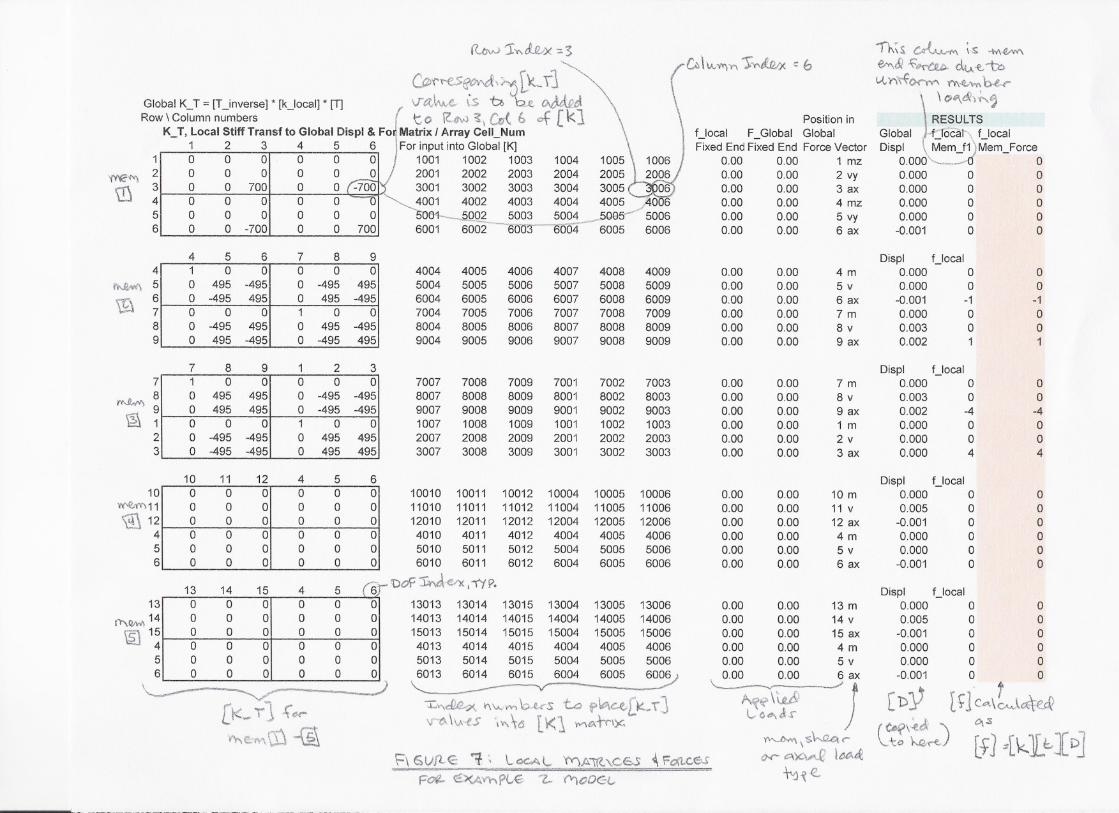
Figure 7 shows:
• Equation (6.7) result, k_T, for each member.
• Index numbers to position k_T elements into global stiffness matrix K.
• Applied load vectors
• Calculated displacements
• Calculated local member forces by substituting (6.3) into (6.5) f = k*t*D
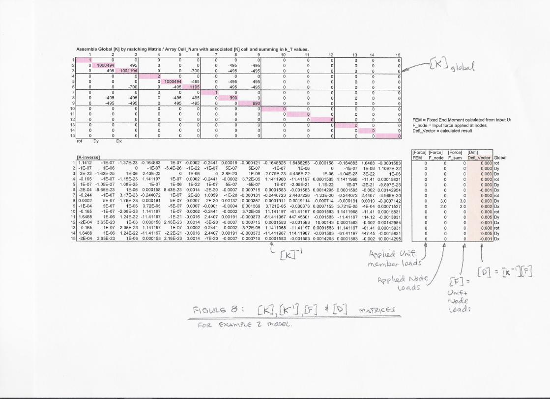
Figure 8 shows:
• K, global stiffness matrix
• K^-1, inverse of K
• F, global applied load vector
• D, calculated node displacement vector


Section 12: Linking spreadsheets for progressive analysis
One of the powerful features of spreadsheet FE analysis is the ability to link spreadsheets
to represent a series of consecutive loadings. A few examples of this application:
• A steel frame structure that has composite concrete – one spreadsheet could
analyze the steel-only loads, a second spreadsheet could analyze loads on the
composite section, a third spreadsheet could be a summation of the first two.
• Calculating deflections during a sequential construction of a cantilever
constructed bridge
• Analyzing a jacking sequence where the structure is modified in each step, say by
adding or removing a member or by jacking at varying points.
A variation on linking is using Excel tables to quantify “what if” scenarios.
Section 13: Capabilities and Limitations of the FE Spreadsheet:
Ease of Use and Minimal Learning Curve:
Most engineers are familiar with, if not adept with spreadsheet software. For those who
are regular spreadsheet users, the FE spreadsheet has a minimal learning curve. It only
makes sense to incorporate Finite Element analysis into an environment in which so
many engineers are already comfortable.
Availability of Spreadsheet and Finite Element Software:
Spreadsheet software is readily available on nearly all engineering computers and can be
purchased for a modest (or zero) cost. In contrast, commercial FE software is limited in
distribution and high in cost.
With the FE spreadsheet, analysis can be performed on any machine with corresponding
spreadsheet software. The spreadsheet is all-inclusive using formulas and Excel
functions. There are no macros and no VBA programming, no password protection, no
hardware locks, and no license restrictions. In contrast, commercial FE analysis can only
be performed on machines with the FE software, and that software nearly always has
hardware lock, password or licensing restrictions.
Integration of Data:
Design data for a project is often voluminous and could typically include items such as
material properties, structure geometry, loading tabulation, quantity summaries, cost
estimates and more. That data is often kept on a series of spreadsheets. As an exception,
the actual analysis data from a commercial FE program is typically not kept on a
spreadsheet. It is common that input-data and output-results from commercial FE
analysis are ported to or from spreadsheets, but the actual analysis and results resides in
the FE software.
With the FE spreadsheet, all data, including analysis and results, can all be integrated into
one spreadsheet workbook. Consider for example, design of a 3-story building. The
designer could have the project design details on a series of spreadsheets (a workbook),
such as:
1. Structural framing properties (member properties, material properties, etc)

2. Loads (Structure dead load, live loads, equipment loads, etc)
3. Cost Estimate
4. Finite Element Analysis (member forces, stresses, etc)
The data can all be linked to assure continuity of design in the event of a design change.
For example, change the loading of floor-2 from 50 psf to 150 psf on the loading sheet,
the FE sheet shows you need to upsize beam weight by 30 plf, the DL weight is increased
on that sheet and the cost estimate interactively reflects the new weights.
This is in contrast to using commercial structural analysis software that is not seamlessly
integrated into the Excel workbook for the project. Changes need to be updated manually
across different programs.
Depth of Data on Spreadsheets:
The FE spreadsheet has all of the input data, output results, intermediate calculations and
supporting formulas on one sheet. Each detail can be scrutinized and checked if
necessary. This is in contrast to commercial programs that typically do not produce all
intermediate steps, nor all underlying formulas.
Ease of Processing Data with Spreadsheets:
Post-processing capability of the FE spreadsheet is superb, with all of Excel’s capabilities
readily available. In contrast, output from commercial programs is often ported to Excel
for the purpose of displaying, formatting, or further using results. With the input,
calculations and output all on the same Excel spreadsheet, you can easily format output
with colored cells, bold or italic font, you can add arrows or notes, etcetera.
Ease of Modifying Spreadsheet:
An adept and frequent user of the FE spreadsheet may want to customize it for a special
need. The FE spreadsheet for structural analysis can easily be linked to other
spreadsheets, sequenced with other FE spreadsheets, modified for use in other
engineering disciplines, etc.
Ease of Checking:
The FE spreadsheet is all-inclusive with respect to input, equations, intermediate
calculation steps and final output. Each step and calculation can be checked in minute
detail. In contrast, commercial software is a black-box. You see the input and output,
but little of what is in between.
Uses as presented in this course:
• Frame, truss and beam-on-elastic foundation problems.
• Checking large program output, or parts of large program output.
Uses beyond what was presented in this course on enhanced spreadsheets:
• p*y soil-structure interaction
• p*delta analyses
• Excel tables to analyze varying data input

• Seismic response spectrum analysis.
Limitations
• Limited graphics / plotting.
• Limited to 2D frame-type elements (no 3D, no plates).
• Limited to relatively small problems (problems over 100 nodes become
cumbersome).
• Expansion of the spreadsheet to vary number of nodes or members requires user
manipulation.
• Member end release is not an input variable and must be achieve by manipulation
of member local stiffness matrix or inclusion of a short member with small Izz.
Section 14: Summary:
Finite Element method is a powerful analysis tool used by almost all structural design
engineers. Many if not most frame-type structural design problems can be solved with
the provided Excel spreadsheet. The software is free, easy to use, easy to port between
machines, easy to pre- and post-process. In contrast, commercial FE software can be
cumbersome to use, difficult to check, difficult to port between machines, and expensive.
More advanced analyses, such as seismic response spectrum problems or soil-structure
p*y problems, can also be solved by enhanced versions of the spreadsheet, subject to the
size limitations above. Those problems are beyond the scope of this course, but may
become available in subsequent courses.
The Excel Spreadsheets provided with this course are believed to be accurate, but use
thereof shall be at the user’s risk. Results of the software should be independently
checked (as when making any calculations or using any software). The user is cautioned
that the spreadsheet original shall be saved and only copies used for calculations. The
formulas in the spreadsheet have minimal protection, so it would be easy to inadvertently
(or intentionally) revise the formulas.
Related Documents