www.ijecs.in International Journal Of Engineering And Computer Science ISSN: 2319-7242 Volume 5 Issues 8 Aug 2016, Page No. 17397-17481 H.T. Rathod a , IJECS Volume 05 Issue 08 Aug 2016 Page No.17397-17473 Page 17397 Finite Element Solution of Poisson Equation over Polygonal Domains using an Explicit Integration Scheme and a novel Auto Mesh Generation Technique H.T. Rathod a* , K. Sugantha Devi b a Department of Mathematics, Central College Campus, Bangalore University, Bangalore- 560001 E-mail: [email protected] f Department of Mathematics, Dr. T. Thimmaiah Institute of Technology, Oorgam Post, Kolar Gold Field, Kolar District, Karnataka state, Pin- 563120, India. Email: [email protected] Abstract : This paper presents an explicit finite element integration scheme to compute the stiffness matrices for linear convex quadrilaterals. Finite element formulationals express stiffness matrices as double integrals of the products of global derivatives. These integrals can be shown to depend on triple products of the geometric properties matrix and the matrix of integrals containing the rational functions with polynomial numerators and linear denominator in bivariates as integrands over a 2-square. These integrals are computed explicitely by using symbolic mathematics capabilities of MATLAB. The proposed explicit finite element integration scheme can be applied solve boundary value problems in continuum mechanics over convex polygonal domains.We have also developed an automatic all quadrilateral mesh generation technique for convex polygonal domain which provides the nodal coordinates and element connectivity. We have used the explicit integration scheme and the novel mesh generation technique to solve the Poisson equation with given Dirichlet boundary conditions over convex polygonal domains. Key words: Explicit Integration, Finite Element Method, Matlab Symbolic Mathematics, All Quadrilateral Mesh Generation Technique,Poisson Equation,Dirichlet Boundary Conditions ,Polygonal Domain 1. Introduction : In recent years, the finite element method (FEM) has emerged as a powerful tool for the approximate solution of differential equations governing diverse physical phenomena. Today, finite element analysis is an integral and major component in many fields of engineering design and manufacturing. Its use in industry and research is extensive, and indeed without it many practical problem in science, engineering and emerging technologies such as nanotechnology, biotechnology, aerospace, chemical. etc would be incapable of solution [1,2,3]. In FEM, various integrals are to be determined numerically in the evaluation of stiffness matrix, mass matrix, body force vector, etc. The algebraic integration needed to derive explicit finite element relations for second order continuum mechanics problems generally defies our analytic skill and in most cases, it appears to be a prohibitive task. Hence, from a practical point of view, numerical integration scheme is not only necessary but very important as well. Among various numerical integration schemes, Gaussian quadrature, which can evaluate exactly the (2n-1) th order polynomial with n Gaussian integration points, is mostly used in view of the accuracy and efficiency of calculation. However, the integrands of global derivative products in stiffness matrix computations of practical applications are not always simple polynomials but rational expressions which the Gaussian quadrature cannot evaluate exactly

Welcome message from author
This document is posted to help you gain knowledge. Please leave a comment to let me know what you think about it! Share it to your friends and learn new things together.
Transcript

www.ijecs.in International Journal Of Engineering And Computer Science ISSN: 2319-7242 Volume 5 Issues 8 Aug 2016, Page No. 17397-17481
H.T. Rathoda, IJECS Volume 05 Issue 08 Aug 2016 Page No.17397-17473 Page 17397
Finite Element Solution of Poisson Equation over Polygonal Domains using
an Explicit Integration Scheme and a novel Auto Mesh Generation
Technique H.T. Rathod
a*, K. Sugantha Devi
b
a
Department of Mathematics, Central College Campus,
Bangalore University, Bangalore- 560001
E-mail: [email protected] f
Department of Mathematics, Dr. T. Thimmaiah Institute of Technology, Oorgam Post,
Kolar Gold Field, Kolar District, Karnataka state, Pin- 563120, India.
Email: [email protected]
Abstract : This paper presents an explicit finite element integration scheme to compute the stiffness matrices for linear convex quadrilaterals. Finite element formulationals express stiffness matrices as double integrals of the products of global derivatives. These integrals can be shown to depend on triple products of the geometric properties matrix and the matrix of integrals containing the rational functions with polynomial numerators and linear denominator in bivariates as integrands over a 2-square. These integrals are computed explicitely by using symbolic mathematics capabilities of MATLAB. The proposed explicit finite element integration scheme can be applied solve boundary value problems in continuum mechanics over convex polygonal domains.We have also developed an automatic all quadrilateral mesh generation technique for convex polygonal domain which provides the nodal coordinates and element connectivity. We have used the explicit integration scheme and the novel mesh generation technique to solve the Poisson equation with given Dirichlet boundary conditions over convex polygonal domains. Key words: Explicit Integration, Finite Element Method, Matlab Symbolic Mathematics, All Quadrilateral Mesh Generation Technique,Poisson Equation,Dirichlet Boundary Conditions ,Polygonal Domain 1. Introduction : In recent years, the finite element method (FEM) has emerged as a powerful tool for the approximate solution of differential equations governing diverse physical phenomena. Today, finite element analysis is an integral and major component in many fields of engineering design and manufacturing. Its use in industry and research is extensive, and indeed without it many practical problem in science, engineering and emerging technologies such as nanotechnology, biotechnology, aerospace, chemical. etc would be incapable of solution [1,2,3]. In FEM, various integrals are to be determined numerically in the evaluation of stiffness matrix, mass matrix, body force vector, etc. The algebraic integration needed to derive explicit finite element relations for second order continuum mechanics problems generally defies our analytic skill and in most cases, it appears to be a prohibitive task. Hence, from a practical point of view, numerical integration scheme is not only necessary but very important as well. Among various numerical integration schemes, Gaussian quadrature, which can evaluate exactly the (2n-1)th order polynomial with n Gaussian integration points, is mostly used in view of the accuracy and efficiency of calculation. However, the integrands of global derivative products in stiffness matrix computations of practical applications are not always simple polynomials but rational expressions which the Gaussian quadrature cannot evaluate exactly

DOI: 10.18535/ijecs/v5i8.08
H.T. Rathoda, IJECS Volume 05 Issue 08 Aug 2016 Page No.17397-17481 Page 17398
[7-15]. The integration points have to be increased in order improve the integration accuracy but it is also desirable to make these evaluations by using as few Gaussian points as possible, from the point of view of the computational efficiency. Thus it is an important task to strike a proper balance between accuracy and economy in computation. Therefore analytical integration is essential to generate a smaller error as well as to save the computational costs of Gaussian quadrature commonly applied for science, engineering and technical problems. In explicit integration of stiffness matrix, complications arise from two main sources, firstly the large number of integrations that need to be performed and secondly, in methods which use isoparametric elements, the presence of determinant of the Jacobian matrix ( we refer this as Jacobian here after ) in the denominator of the element matrix integrands. This problem is considered in the recent work [16] for the linear convex quadrilateral proposes a new discretisation method and use of pre computed universal numeric arrays which do not depend on element size and shape. In this method a linear polygon is discretized into a set of linear triangles and then each of these triangles is further discretised into three linear convex quadrilateral elements by joining the centroid to the mid-point of sides. These quadrilateral elements are then mapped into 2-squares (-1 ) in the natural space ( ) to obtain the same expression of the Jacobian, namely c(4+ ) where c is some appropriate constant which depends on the geometric data for the triangle. Many important problems in engineering,science and applied mathematics are formulated by appropriate differential equations with some boundary conditions imposed on the desired unknown function or the set of functions. There exists a large literature which demonstrates numerical accuracy of the finite element method to deal with such issues [1]. Clough seems to be the first who introduced the fnite elements to standard computational procedures [2]. A further historical development and present{day concepts of fnite element analysis are widely described in references [1, 3]. In this paper the well-known Laplace and Poisson equations will be examined by means of the finite element method applied to an appropriate 'mesh'. The class of physical situations in which wemeet these equations is really broad. Let's recall such problems like heat conduction, seepage through porous media, irrotational flow of ideal fluids, distribution of electrical or magnetic potential, torsion of prismatic shafts, lubrication of pad bearings and others [4]. Therefore, in physics and engineering arises a need of some computational methods that allow to solve accurately such a large variety of physical situations.The considered method completes the above-mentioned task. Particularly, it refers to a standard discrete pattern allowing to find an approximate solution to continuum problem. At the beginning, the continuum domain is discretized by dividing it into a finite number of elements which properties must be determined from an analysis of the physical problem (e. g. as a result of experiments). These studies on particular problem allow to construct so{called the stiffness matrix for each element that, for instance, in elasticity comprising material properties like stress strain relationships [2, 5]. Then the corresponding nodal loads associated with elements must be found. The construction of accurate elements constitutes the subject of a mesh generation recipe proposed by the author within the presented article. In many realistic situations, mesh generation is a time{consuming and error prone process because of various levels of geometrical complexity. Over the years, there were developed both semi automatic and fully automatic mesh generators obtained, respectively, by using the mapping methods or, on the contrary, algorithms based on the Delaunay triangulation method [6], the advancing front method [7] and tree methods [8]. It is worth mentioning that the first attempt to create fully automatic mesh generator capable to produce valid finite element meshes over arbitrary domains has been made by Zienkiewicz and Phillips [9].
In the present paper, we propose a similar discretisation method for linear polygon in Cartesian two space (x,y). This discrtisation is carried in two steps, We first discretise the linear polygon into a set of linear triangles in the Cartesian space (x,y) and these linear triangles are then mapped into a standard triangle in a local space (u,v). We further discretise the standard triangles into three linear quadrilaterals by joining the centroid to the midpoints of triangles in (u,v) space which are finally mapped into 2-square in the local

DOI: 10.18535/ijecs/v5i8.08
H.T. Rathoda, IJECS Volume 05 Issue 08 Aug 2016 Page No.17397-17481 Page 17399
( ) space. We then establish a derivative product relation between the linear convex quadrilaterals in the Cartesian space, (x,y) which are interior to an arbitrary triangle and the linear quadrilaterals in the local space (u,v) interior to the standard triangle. In this procedure, all computations in the local space (u,v) for product of global derivative integrals are free from geometric properties and hence they are pure numbers. We then propose a numerical scheme to integrate the products of global derivatives. We have shown that the matrix product of global derivative integrals is expressible as matrix triple product comprising of geometric properties matrices and the product of local derivative integrals matrix. We have obtained explicit integration of the product of local derivatives which is now possible by use of symbolic integration commands available in leading mathematical softwares MATLAB, MAPLE, MATHEMATIKA etc. In this paper, we have used the MATLAB symbolic mathematics to compute the integrals of the products of local derivatives in (u, v) space .The proposed explicit integration scheme is shown as a useful technique in the formation of element stiffness matrices for second order boundary problems governed by partial differential equations. 2. POISSON EQUATION 2.1 Statement of the Problem The Poisson equation u .............................................(1) is the simplest and most famous elliptic partial differential equations.The source (or load) function is given on some two or three dimensional domain or . A solution u satisfying (1.1) will also satisfy boundary conditions on the boundary for example
=g on
............................................(2) where ⁄ denotes directional derivative in the direction normal to the boundary (conveniently pointing outwards) and and are constants, although variable coefficients are also possible.The combination of (1.1) and (1.2) together is referred to as boundary value problem. If the constant in (1.2) is zero,then the boundary condition is known as the Dirichlet type, and the boundary value problem is referred as the Dirichlet problem for the Poisson equation. Alternatively, if the constant in (1.2) is zero,then we correspondingly have a Neumann boundary value problem. A third possibility is that Dirichlet conditions hold on part of the boundary and Neumann conditions(or indeed mixed conditions where and are both nonzero) hold on remainder . The case in (1.2) demands special attention.First, since u=constant satisfies the homogeneous problem with ,it is clear that a solution to a Neumann problem can only be unique up to an additive constant.Second,integrating (1.1) over using Gauss’s theorem gives
∫
∫
=∫
.....................................................(3) thus a necessary condition for the existence of a solution to the Neumann problem is that the source and boundary data satisfy the compatibility condition:
∫
+∫
--------------------------------
------------------(4) 2.2 Weak Formulation of the Poisson Boundary Value Problem A sufficiently smooth function u satisfying both eqns(1) and (2) is known as classical solution to the Poisson boundary value problem. For a Dirichlet problem, u is a classical solution only if it has continuousecond derivatives in (i.e. u is and is continuous up to the boundary i.e.u is in ). In case of nonsmooth domains or discontinuous source functions,the function u satisfying eqns(1) and (2) may not be smooth (or regular) enough to be regarded as classical solution. For problems which arise from , perfectly reasonable mathematical models an alternative description of the boundary value

DOI: 10.18535/ijecs/v5i8.08
H.T. Rathoda, IJECS Volume 05 Issue 08 Aug 2016 Page No.17397-17481 Page 17400
problem is required. Since this alternative description is less restrictive in terms of admissible data it is called weak formulation. To derive a weak formulation of a Poisson problem,we require that for an appropriate set of test functions ,
∫
.
...............................................(5) This formulation exists provided that the integrals are well defined. If u is a classical solution then it must also satisfy eqn (5). If is sufficiently smooth however,then the smoothness required of can be reduced by using the derivative of a product rule and the divergence theorem
∫
∫
-∫
=∫
-∫
,
so that
∫
∫
∫
.........................................(6a) The point here is that the problem posed byeqn(6) may have a solution called a weak solution,that is not smooth enough to be a classical solution. If a classical solution does exist then eqn(6)is equivalent to eqns (1) and (2) and the weak solution is classical. The case of Neumann problem ( in eqn(2) is particularly straight forward. Substituting from eqn(2) into eqn(6)gives us the following formulation: find defined on such that
∫
∫
∫
........................................(6b) for all suitable test functions . 2.3 Finite Elements for Poisson’s Equation with Dirichlet conditions: Implementation and Review Of Theory 2.3.1 Weak Form Given Poisson Equation: = ) for all x ............................(7a) ) on ...............................(7b) We have already obtained in eqn(6) with ( the weak form of the equation by multiplying both sides by a test function (i.e a function which is infinitely differentiable and has compact support,integrating over the domain and performing integration by parts or by application of Divergence(GREEN) theorem. The result is
∫
∫
..............................(7c) ) on ...............................(7d) For all test functions . 2.3.2 Finite Elements

DOI: 10.18535/ijecs/v5i8.08
H.T. Rathoda, IJECS Volume 05 Issue 08 Aug 2016 Page No.17397-17481 Page 17401
To find an approximation to the solution , we choose a finite dimensional space and ask that eqn(7a-b) is satisfied only for rather than for all test functions . Then we look for a function which satisfies
∫
∫
for all
................................(8) is called the finite element solution and functions in are called finite elements. Note that it is also common for the triangles or quadrilaterals in the mesh to be called elements.
If a basis for is { }
then we can write ∑
. Substituting this in eqn(8) and choosing
to be a basis function gives the following set of equations
∑ ∫
∫ ,i=1,2,3,...., N
..................(9) This is really a linear system of the form = ..................(10) Where, = and
∫
.....................(11a)
∫
.......................(11b) and is called stiffness matrix because the linear system looks like Hookes law if represents forces and represents displacemewnts.
In general, ∑ , where is the number of elements discritised in the domain . In two
dimensions the mesh elements are triangles or quadrilaterals.The choice of finite element spaces are usually piecewise polynomials. 2.3.3 Overview on the implementation of Finite Element Method Once we have choosen the finite element space (and the element type),then we can implement the finite element method.The implementation is divided into three steps: 1. Mesh Generation:how does one perform a triangulation or quadrangulation of the domain ? 2. Assembling the Stiffness Matrix:how does one compute the entries in the stiffness matrix in an efficient way? 3. Solving the linear System:What kind of methodse suited for solving the linear system? In this paper,we present new approach to mesh generation [ ] and explicit computations for the entries in the stiffness matrix [ ] which is vital in Assembling the Stiffness Matrix,since we believe that the methods of solving linear system are well researched and standardised. We shall first take up the derivations regarding the topic on Assembling the Stiffness Matrix. The Mesh Generation topic will be discussed immediately there after. 2.3.4 Assembling the Stiffness Matrix In order to assemble the stiffness matrix,we need to compute integrals of the form(see eqn(11) in section 2.3.2)
∫
.............................................(11a)

DOI: 10.18535/ijecs/v5i8.08
H.T. Rathoda, IJECS Volume 05 Issue 08 Aug 2016 Page No.17397-17481 Page 17402
The most obvious way to assemble the stiffness matrix is to compute the integrals for the nodal
pairs i and j ; this is a node oriented computation and we need to know the common support of basis functions .This means we need to know which elements contain both i and j.The mesh
generator provides us with the information regarding the nodes on a particular element so we would need to do some extra processing to find the elements that contain a particular node.This is an issue which is very complicated.Hence,in practice assembling is focussed on elements rather than on nodes.We note that on a particular element,the basis functions have a simple expression and the elements themselves are very simple domains like triangles and quadrilaterals. It is very easy to make a change of variables for integrals over triangles and quadrilaterals to standard triangles and squares. In the element oriented computation,we rewrite or interpret the integral in eqn(11) as
∑
............................................(12a) where
=∫
...................................(12b)
and is the set of (mesh) elements in contributing to and ∑
, is an element
contained in the set .This says us that we can compute by computing the integrals over each
element and then summing up over all elements .
Notice that the integrals
∫ look like the entries ∫
∑ ∫
except the domain of integration is an element . So,we only need to save all entries of =[ ]
which corresponds to nodes on . Then if has d nodes , we can think of as a dxd matrix. In view of the above,the procedure for computing the stiffness maerix is done on an element by element basis. We must also compute the integrals
∫ ∑
.........................................................................................(12c) where
= ∫
.........................................................................................(12d)
Now further assume that on an element , ∑
From eqn(9) and eqns(12a-d) it follows that = is equivalent to
∑ ∑
.......................................................(12e) Where = (
,
............. , = (
,
.............
.........................................................(12f) d referes to number of nodes per element, referes to the total number of elements in the domain 2.3.5 Computing the Integrals
and

DOI: 10.18535/ijecs/v5i8.08
H.T. Rathoda, IJECS Volume 05 Issue 08 Aug 2016 Page No.17397-17481 Page 17403
In order to compute the local/element stiffness matrices,we need to compute the integrals
∫ .These integrals are computed by making a change of variables to a reference
element. We now outline a brief procedure for element oriented computation (1)For each element , compute it’s local stiffness matrix . This requires computing the integrals
∫ which we compute by transforming to a reference element. In two dimensions
is an arbitrary linear triangle and each triangle will be further discritised three convex quadrilaterals Each triangle will be transformed to the corresponding reference elements:the standard triangle(a right isosceles triangle) and further Each triangle will be transformed to the corresponding reference elements:the standard triangle(a right isosceles triangle) and further Each triangle will be transformed to the corresponding reference elements:the standard triangle(a right isosceles triangle) and further each quadrilateral will be transformed into a standard square(1-square or a
2-square).Since in two dimensional space x= (x,y) the explicit form of ∫ is given by
∫
=∫
∑ ∑ ∫
=∑ ∑
.......................(12g)
Where ∫
and E=3e+n-2,e=1,2,... andn=0,1,2
and hence we must be careful about the derivatives when we perform the change of variables. These bring extra factors involving the affine transformations (when is an arbitrary linear triangle) and bilinear transformations(when is an arbitrary linear convex quadrilateral)
= ∫ can be computed in a straight forward manner if is a simple function otherwise we
have to apply numerical integration (2) For each element , first compute the local stiffness matrices
and then add
contribution of + to the global stiffness matrix K. We repeat this procedure for all elements i.e for e=1,2,......, ; where is the number of elements are discritised in the
domain ,in fact we have ∑ =∑ ∑
, E=3e+n-2
2.3.6 Linear Convex Quadrilateral Elements :
Let us first consider an arbitrary four noded linear convex quadrilateral in the global
(Cartesian) coordinate system (u, v) as in Fig 1a, which mapped into a 2-square in the
local(natural) parametric coordinate ( ) as in Fig 1b.

DOI: 10.18535/ijecs/v5i8.08
H.T. Rathoda, IJECS Volume 05 Issue 08 Aug 2016 Page No.17397-17481 Page 17404
( ) ∑ (
)
--
---------------------- (13)
Where , (k=1,2,3,4 ) are the vertices of the original arbitrary linear convex quadrilateral in
(u, v) plane and denote the well known bilinear basis functions [1-3] in the local parametric
space ( ) and they are given by
---
-------------------- (14a)
Where { ( = {(-1,-1),(1,-1),(1,1),(-1,1)} ---
-------------------- (14b)
describe two transformations over a linear convex quadrilateral element from the original global
space into the local parametric space.
2.3.7 Isoparametric Transformation :
For the isoparametric coordinate transformation over the linear convex quadrilateral element as
shown in Fig 1, we select the field variables, say , etc governing the physical problem as
( ) ∑ (
)
----
-------------------- (15)

DOI: 10.18535/ijecs/v5i8.08
H.T. Rathoda, IJECS Volume 05 Issue 08 Aug 2016 Page No.17397-17481 Page 17405
Where refer to unknowns at node k and the shape functions and are defined
as in Eqn.(2a-b)
2.3.8 Subparmetric Transformation :
For the subparametric transformation over the nde – noded element we define the field variables
(say) governing the physical problem as
( ) ∑ (
)
-----
------------------- (16)
Where refer to unknowns at node k and nde 4
In our recent paper[ ], the explicit finite element integration scheme is presented by using the
isoparametric transformation over the 4 node linear convex quadrilateral element which is applied
to torison of square shaft,on considering symmetry mesh generation for 1/8 of the cross section
which is a triangle was discritised into an all quadrilateral mesh.In this paper we consider
applications to polygonal domains.
2.3.9 Explicit Form of the Jacobian and Global Derivatives :
Jacobian
Let us consider an arbitrary linear convex quadrilateral in the global Cartesian space (u, v) as in
Fig 1a , c which is mapped into a 8- node 2- square in the local parametric space as in Fig
1b, d
From the Eq.(13) and Eq.(14), we have
∑
)
------------ (17a)
∑
)
------------ (17b)
)
------------ (17c)
)
------------ (17d)
Hence the Jacobian, can be expressed as [1, 2, 3]
=
-------------- (18a)

DOI: 10.18535/ijecs/v5i8.08
H.T. Rathoda, IJECS Volume 05 Issue 08 Aug 2016 Page No.17397-17481 Page 17406
Where
) ]
) ]
) ]
---------------- (18b)
Global Derivatives:
If denotes the basis functions of node of any order of the element , then the chain rule of
differentiation from Eq.(1) we can write the global derivative as in [1, 2, 3]
(
+
*
+ *
+ ---
------------------------ (19)
Where
and
are defined as in Eqs.(17a)–(17d) while is defined in Eq.(18a-b) , (
nde) , nde = the number of nodes per element.
2.3.10 Discretisation of an Arbitrary Triangle :
A linear convex polygon in the physical plane (x, y) can be always discretised into a finite
number of linear triangles. However, we would like to study a particular discretization of these
triangles further into linear convex quadrilaterals. This is stated in the following Lemma [ 6 ].
Lemma 1. Let ∆ PQR be an arbitrary triangle with the vertices P(xp, yp) , Q(xq, yq) and R(xr, yr) and S, T, U be the midpoints of sides PQ, QR and RP respectively and let Z be its centroid. We can obtain three linear convex quadrilaterals ZTRU, ZUPS and ZSQT from triangle ∆ PQR as shown in Fig2. If we map each of these quadrilaterals into 2-squares in which the nodes are oriented in counter clockwise from Z then Jacobian for each element is given by
=
--------------- (20) Where is the area of the triangle
2 |
| [ ( )( ) ( )( ) ]
------------ (21)

DOI: 10.18535/ijecs/v5i8.08
H.T. Rathoda, IJECS Volume 05 Issue 08 Aug 2016 Page No.17397-17481 Page 17407
Proof : Proof is straight forward and it can be elaborated on the lines of proof given in [17].
Lemma 2. Let be an arbitrary triangle with the vertices P(xp, yp) , Q(xq, yq) and R(xr, yr) , let S, T, U be the midpoints of sides PQ, QR, and RP and let Z be the centroid of , Then we obtain three quadrilaterals Q1, Q2, Q3 spanning the vertices <ZUPS> , <ZSQT> and <ZTRU> . these quadrilaterals can be mapped into the quadrilateral spanning vertices GECF with G(1/3, 1/3), E(0, ½) , C(0, 0) and F(1/2, 0) of the right isosceles triangle with spanning vertices A(1, 0), B(0, 1) and C(0, 0) in the (u, v) space as shown in Fig 3a and Fig 3b

DOI: 10.18535/ijecs/v5i8.08
H.T. Rathoda, IJECS Volume 05 Issue 08 Aug 2016 Page No.17397-17481 Page 17408
Proof : The sum of the quadrilaterals Q1+ Q2+ Q3 = as shown in Fig 2a & Fig 3a. The linear transformations
(
) (
) (
) (
)
--------------------------- (22a)
(
) (
) (
) (
)
-------------------------- (22b)
(
) (
) (
) (
)
------------------------ (22c) with ------------------------ (22d) map the arbitrary triangle into a right isosceles triangle A(1, 0) , B(0, 1) and C(0, 0) in the uv–plane
We can now verify that quadrilateral Q1 spanned by vertices Z(
,
, U(
) ,
P( ,S(
) in xy- plane is mapped into the quadrilateral spanning the vertices G( 1/3, 1/3) ,
E(0, ½), C(0, 0) and F(1/2, 0) by use of the transformation given in Eq.(22a), Similarly, we see that the quadrilateral Q2 spanned by vertices Z,S,Q,T is mapped into the quadrilateral spanned by vertices G(1/3, 1/3), E(0, ½), C(0, 0) and F(½, 0) by use of the transformation of Eq.(22b), Finally the quadrilateral Q3 in the xy- plane is mapped into the quadrilateral GECF in uv- plane by use of the linear transformation of Eq.(22c), This completes the proof We have shown in the present section that an arbitrary triangle can be discretised into three linear convex
quadrilaterals. Further, each of these quadrilaterals can be mapped into a unique quadrilateral in uv-plane
spanned by vertices (1/3, 1/3), (0, ½), (0, 0) and (½, 0) .
3.0 Computing the Integrals :
3.1 Global Derivative Integrals: ∫

DOI: 10.18535/ijecs/v5i8.08
H.T. Rathoda, IJECS Volume 05 Issue 08 Aug 2016 Page No.17397-17481 Page 17409
If
denotes the basis function for node of element e , then by chain rule of partial differentiation
(
+ *
+ [
]
-------------------------- (23)
We note that to transform of in Cartesian space (x,y) into , the quadrilateral spanned by vertices (1/3,1/3), (0,½), (0,0) and (1/2,0) in uv-plane we must use the earlier transformations.
(
) (
) (
* (
) for in
--------------------------- (24a)
(
) (
) (
) (
) for in
-------------------------- (24b)
(
) (
) (
) (
) for in
------------------------ (24c) and the above transformations viz Eqs.(24a)-(24c) are of the form
(
) (
) (
) (
)
------------------------ (24d) which can map an arbitrary triangle , A( xa ,ya) ,B(xb ,yb) , C(xc , yc) in xy – plane into a right isosceles triangle in the uv – plane Hence, we have
( ) (
)
(
)
-------------------------- (25) This gives u = ( v = ( ------------------------ (26) (xbyc– xcyb ) , (xcya– xayc ) , (yb– yc ) , (yc– ya ) , (xc– xb ) , (xa– xc ) ,
|
| area of the triangle
= ( ------------------- (27) Hence from Eq.(23) and Eq.(22), we obtain
(
+ (
) (
+
= (
* (
+
----------------------------- (28)
where
,
--------------------------- (29) Letting,

DOI: 10.18535/ijecs/v5i8.08
H.T. Rathoda, IJECS Volume 05 Issue 08 Aug 2016 Page No.17397-17481 Page 17410
= (
+ , P = (
* , = (
+
---------------------------- (30) We obtain from Eq.(24),
= P
----------------------------- (31) So that from Eq.(30) and Eq.(31) , we obtain
= (
+ (
) = (
= (
, -
---------------------------- (32a)
= (
+ (
) = (
= (
) -
---------------------------- (32b) We have now from Eq.(27) and Eq.(28)
= ( (
)
= P
--------------------------- (33) We now define the submatrices of global derivative integrals in (x,y) and (u,v) space associated with the nodes i and j as ;
∬
, (e=1,2,3)
--------------------------- (34)
∬
--------------------------- (35)
where, we have already defined the quadrilaterals (e=1,2,3) in (x,y) space and in (u,v) space in Fig
3a-b. From Eqs.(28)-(33) , we obtain the following relations connecting the submatrices and
We now obtain the submatrices and in an explicit form from Eqs.(32a)- (32b) as
∬
= (
∬
∬
∬
∬
,
(
) (say)
------------------(36) and in similar manner
∬
= (
∬
∬
∬
∬
)

DOI: 10.18535/ijecs/v5i8.08
H.T. Rathoda, IJECS Volume 05 Issue 08 Aug 2016 Page No.17397-17481 Page 17411
(
) (say)
------------------(37) We now obtain from the above Eq.(23)-(33)
∬
= ∬
= ∬
= ∬
= -----------------------(38) We can thus obtain the global derivative integrals in the physical space or Cartesian space (x,y) by using the matrix triple product established in eqn.(33).
From Eq.(35) and noting the fact that is the quadrilateral in (u, v) space spanned by the vertices (1/3, 1/3), (0, 1/2), (0, 0)and (1/2, 0) we obtain
∬
∫ ∫
------------------------(39) We now refer to section 5 of this paper, in this section we have derived the necessary relations to integrate the integrals of Eq.(39), As in Eq.(22a-d) , we use the transformation
u( =
v( =
-----------------------(40)
to map the quadrilateral to the 2-square -1≤ Using Eq.(40) in Eq.(39), we obtain
∬
----------------------- (41) The submatrices for the quadrilateral Qe is expressed from Eq.(38) as
---------------------- (42) In eqn.(38) , x area of the triangle spanning vertices A( xa ,ya) ,B(xb ,yb) , C(xc , yc) which is scalar.
The matrices P, PT depend purely on the nodel coordinates ( xa ,ya) ,(xb ,yb) , (xc , yc) the matrix can be
explicity computed by the relations obtained in section 2 and 3 . We find that is a (2X2) matrix of integrals whose integrands are rational functions with polynomial numerator and the linear denominator ( Hence these integrals can be explicity computed. The explicit values of these integrals are expressible in terms of logarithmic constants. We have used symbolic mathematics software of MATLAB to compute the explicit values and their conversion to any number of digits can be obtained by using variable precision arithmetic (vpa) command. The matrix Ke as noted in Eq.(33) is of order (2xnde) x (2xnde) . We have computed Ke for the four noded isoparametric quadrilateral element. This is listed in Table 1,1 and Table 1.2 , We may note that In order to compute the local/element stiffness matrices for the Poisson Boundary
Value problem, we need to compute the integrals Eqns(12a-b)
∫
=∫
,
,,,,,,,,,,,,,,,,,,,,,,,,,,,,,,,,,,,,(43a)

DOI: 10.18535/ijecs/v5i8.08
H.T. Rathoda, IJECS Volume 05 Issue 08 Aug 2016 Page No.17397-17481 Page 17412
from the above derivations, we can rewrite in the notations of this sections by taking
and so that
∫
=∫
=
....................................(43b )
3.2 Computation of
The explicit integration scheme explained above compute four derivative product integrals as given in eqn(36) and they are necessary to compute the stiffness matrix entries of plane stress/plane strain problems in elasticity and sevral other applications in continuum mechanics.But this computation requires matrix triple product as given in eqn (42).Since,we only need the sum of two of these integrals viz :
.We now present an efficient method to compute this sum by using matrix product.
Let
=
,
∫
, then we have from eqns(36-37) :
∬
= (
∬
∬
∬
∬
,
(
) (say)
=(
+
.................................................................(44a)
∬
= (
∬
∬
∬
∬
)
(
) (say)
= (
+
......................................................(44b)
Let P=(
* , =(
*
......................................................(45)
From eqns( 44a-b ) and (45)
∬
= ∬

DOI: 10.18535/ijecs/v5i8.08
H.T. Rathoda, IJECS Volume 05 Issue 08 Aug 2016 Page No.17397-17481 Page 17413
= (
* (
+ (
*
=
( (
) (
) (
) (
)
(
) (
) (
) (
) +
............................................................................................................................................(46)
From eqn(43b) ,eqn( 44a) and eqn(46) , we find
trace ( )= trace(∬
)=(
)=
∫
=∫
=(
+( + (
) =(
..........(47)
W e can obtain the above integraql ∫
by use of matrix operations which
doesnot need the computation matrix triple product.This procedure is presented below
From eqn (44b) and eqn(45),let us do the following:
( (
+ =*
+ ...................................(48)
We observe from eqn(48) that sum of all the entries gives us the value of the integral i.e
∫
( (
+ +
............................(49)
Where,sum is aq Matlab function.We note that S=sum(X) gives the sum of the elements of vector X. If X
is a matrix then S is a row vector with the sum over each column.It is clear that sum(sum(X)) gives the
sum of all the entries in a matrix X .
3.2 Computing of Force Vector Integrals ∫
We shall now propose numerical integration for the complicated integrands in the force vector integrals over the domain which is an arbitrary linear triangle and .We also refer to the section 2 for the theory necessary to derive the composite numerical integration formla We shall now establish a composite integration formula for an arbitrary linear triangular region shown in Fig 2a or Fig 3a. We have for an arbitrary smooth function (x, y)
II ∆PQR = ∬ ∑ ∬
--------------------- (50)

DOI: 10.18535/ijecs/v5i8.08
H.T. Rathoda, IJECS Volume 05 Issue 08 Aug 2016 Page No.17397-17481 Page 17414
= ∬ ∑
( )
= (2 ∬ ∑
-------------------- (51)
Where ( are the transformations of Eqs.(8)–(10) and is the
quadrilateral in uv- plane spanned by vertices G(1/3 ,1/3) , E(0, ½) , C(0, 0) and F(1/2,0) , and is the area of triangle , Now using the transformations defined in Eqs.(1)–(2) we obtain
II ∆PQR = (2 ∬ ∑
--------------- (52) In Eq.(14) we have used the transformation
u( =
v( =
---------------------- (53)
to map the quadrilateral into a 2 – square in – plane. We can now obtain from Eqs.(14)–(15)
II ∆PQR = (2 ∫ ∫ ∑ (
)
------------- (54) We can evaluate Eq.(16) either analytically or numerically depending on the form of the integrand. Using Numerical Integration ;
II∆PQR=2 ∑ ∑ (
) ∑
( (
) (
)
----------------------- (55) Where,
= (
and
= v(
---------------------- (56)
and (
, (
are the weight coefficients and sampling points of Nth order Gauss
Legendre Quadrature rules. The above composite rule is applied to numerical Integration over polygonal domains using convex quadrangulation and Gauss Legendre Quadrature Rules[27].
The above method will help in integrating ∫ ,when the intgrand is complicated
4.0 A NEW APPROACH TO MESH GENERATION The first step in implimenting finite element method isto generate a mesh.In a recent work the author and his co-workers have proposed a new approach to mesh generation which can discretise a convex polygon into an all quadrilateral mesh.This will be presented next.This new approach to mesh generation meets the necessary requirements of regularity on the shape of elements.There are two types of them which usually suffice in finite element computations.The first is called shape regularity. It says that the ratio of the diameter of the element to the radius of the inner circle must be less than some constant. For triangles,the diameter of the triangle is related to the smallest circle which contain the triangle.The inner circle refers to the largest circle which fits inside the triangle. Shape regularity focuses on the shape of individual triangles and doesnot refer to how the shapes of different elements relate to each other. So some elements can be large wshile others might be very small. There is a second type of requirement on the shape of elements.This requirement says that ratio of the maximum diameter of elements to the radius of the inner circle of an element must be less than some constant .If a mesh satisfies this

DOI: 10.18535/ijecs/v5i8.08
H.T. Rathoda, IJECS Volume 05 Issue 08 Aug 2016 Page No.17397-17481 Page 17415
requirement,it is called quasiuniform.This requirement is more important when we perform refinements.We must note that a mesh generation gives us the nodes on a particular element as well as the coordinates of the nodes.We now give an account of this novel mesh generation technique with an aim to use it further in the solution of Poisson problem. Stated in eqn(7a-b). In our recent paper[ ], the explicit finite element integration scheme is presented by using the
isoparametric transformation over the 4 node linear convex quadrilateral element which is applied
to torison of square shaft, on considering symmetry of the problem domain, mesh generation for
1/8 of the cross section which is a triangle was discritised into an all quadrilateral mesh. In this
paper we consider applications to polygonal domains.
4.1 An automatic indirect quadrilateral mesh generator
A wide range of problems in applied science and engineering can be simulated by partial derivative equations(PDE).In the last few decade,one of the most relevant techniques to solve is the Finite Element Method(FEM).It is well known that a good quality mesh is required in order to obtain an accurate solution.Hence the construction of a mesh is on e of the most important steps. In the next few sections , we present a novel mesh generation scheme of all quadrilateral elements for
convex polygonal domains. This scheme converts the elements in background triangular mesh into
quadrilaterals through the operation of splitting. We first decompose the convex polygon into simple
subregions in the shape of triangles. These simple subregions are then triangulated to generate a fine mesh
of triangles. We propose then an automatic triangular to quadrilateral conversion scheme in which each
isolated triangle is split into three quadrilaterals according to the usual scheme, adding three vertices in the
middle of edges and a vertex at the barrycentre of the triangular element. Further, to preserve the mesh
conformity a similar procedure is also applied to every triangle of the domain and this fully discretizes the
given convex polygonal domain into all quadrilaterals, thus propogating uniform refinement. In section 4.2,
we present a scheme to discretize the arbitrary and standard triangles into a fine mesh of six node triangular
elements. In section 4.3, we explain the procedure to split these triangles into quadrilaterals. In section
4.4,we have presented a method of piecing together of all triangular subregions and eventually creating a all
quadrilateral mesh for the given convex polygonal domain. In section 4.5,we present several examples to
illustrate the simplicity and efficiency of the proposed mesh generation method for standard and arbitrary
triangles,rectangles and convex polygonal domains.
4.2 Division of an Arbitrary Triangle
We can map an arbitrary triangle with vertices into a right isosceles triangle in the
space as shown in Fig. 4a, b. The necessary transformation is given by the equations.
(57)
The mapping of eqn.(1) describes a unique relation between the coordinate systems. This is illustrated by
using the area coordinates and division of each side into three equal parts in Fig. 5a Fig. 5b. It is clear that
all the coordinates of this division can be determined by knowing the coordinates of
the vertices for the arbitrary triangle. In general , it is well known that by making ‘n’ equal divisions on all
sides and the concept of area coordinates, we can divide an arbitrary triangle into smaller triangles having
the same area which equals ∆/ where ∆ is the area of a linear arbitrary triangle with vertices
in the Cartesian space.

DOI: 10.18535/ijecs/v5i8.08
H.T. Rathoda, IJECS Volume 05 Issue 08 Aug 2016 Page No.17397-17481 Page 17416
4.a 4 b
Fig. 4a An Arbitrary Linear Triangle in the (x, y) space Fig. 4b A Right Isosceles Triangle
in the (u, v) space

DOI: 10.18535/ijecs/v5i8.08
H.T. Rathoda, IJECS Volume 05 Issue 08 Aug 2016 Page No.17397-17481 Page 17417
We have shown the division of an arbitrary triangle in Fig. 6a , Fig. 6b, We divided each side of the triangles
(either in Cartesian space or natural space) into n equal parts and draw lines parallel to the sides of the
triangles. This creates (n+1) (n+2) nodes. These nodes are numbered from triangle base line ( letting
as the line joining the vertex and ) along the line and upwards up to the line .
The nodes 1, 2, 3 are numbered anticlockwise and then nodes 4, 5, ------, (n+2) are along line and the
nodes (n+3), (n+4), ------, 2n, (2n+1) are numbered along the line i.e. and then the node
(2n+2), (2n+3), -------, 3n are numbered along the line . Then the interior nodes are numbered in
increasing order from left to right along the line
bounded on the right by the line
. Thus the entire triangle is covered by (n+1) (n+2)/2 nodes. This is shown in the matrix of size
, only nonzero entries of this matrix refer to the nodes of the triangles
=
[
]
...................................................(58)

DOI: 10.18535/ijecs/v5i8.08
H.T. Rathoda, IJECS Volume 05 Issue 08 Aug 2016 Page No.17397-17481 Page 17418
4.3. Quadrangulation of an Arbitrary Triangle
We now consider the quadrangulation of an arbitrary triangle. We first divide the arbitrary triangle
into a number of equal size six node triangles. Let us define as the line joining the points and
in the Cartesian space . Then the arbitrary triangle with vertices at is
bounded by three lines and . By dividing the sides into divisions ( m, an
integer ) creates six node triangular divisions. Then by joining the centroid of these six node triangles to
the midpoints of their sides, we obtain three quadrilaterals for each of these triangle. We have illustrated this
process for the two and four divisions of and sides of the arbitrary and standard triangles in
Figs. 4 and 5
Two Divisions of Each side of an Arbitrary Triangle
7(a) 7(b)
Fig 7(a). Division of an arbitrary triangle into three quadrilaterals
Fig 7(b). Division of a standard triangle into three quadrilaterals
Four Divisions of Each side of an Arbitrary Triangle

DOI: 10.18535/ijecs/v5i8.08
H.T. Rathoda, IJECS Volume 05 Issue 08 Aug 2016 Page No.17397-17481 Page 17419
8a 8b
Fig 8a. Division of an arbitrary triangle into 4 six node triangles
Fig 8b. Division of a standard triangle into 4 right isosceles triangle
In general, we note that to divide an arbitrary triangle into equal size six node triangle, we must divide each
side of the triangle into an even number of divisions and locate points in the interior of triangle at equal
spacing. We also do similar divisions and locations of interior points for the standard triangle. Thus n (even )
divisions creates ( n/2)2 six node triangles in both the spaces. If the entries of the sub matrix
are nonzero then two six node triangles can be formed. If
then one six node triangle can be formed. If the sub matrices is a
zero matrix , we cannot form the six node triangles. We now explain the creation of the six node
triangles using the matrix of eqn.( ). We can form six node triangles by using node points of three
consecutive rows and columns of matrix. This procedure is depicted in Fig. 9 for three consecutive rows
and three consecutive columns of the sub matrix
Formation of six node triangle using sub matrix
Fig. 9 Six node triangle formation for non zero sub matrix
If the sub matrix ( ( ( is nonzero, then we can construct two
six node triangles. The element nodal connectivity is then given by
(e1) < ( ( , ( , ( , ( >
(e2) < ( ( , ( , ( , >
...............................(59)
If the elements of sub matrix ( ( ( are nonzero, then as
standard earlier, we can construct two six node triangles. We can create three quadrilaterals in each of these
six node triangles. The nodal connectivity for the 3 quadrilaterals created in (e1) are given as

DOI: 10.18535/ijecs/v5i8.08
H.T. Rathoda, IJECS Volume 05 Issue 08 Aug 2016 Page No.17397-17481 Page 17420
< c1 , ( , ( >
< c1 , ( , ( >
< c1 , ( , ( >
.......................................(60)
and the nodal connectivity for the 3 quadrilaterals created in (e2) are given as
< c2 , ( , ( >
< c2 , ( , ( >
< c2 , ( , ( >
-------------------- (61)
4.4 Quadrangulation of the Polygonal Domain
We can generate polygonal meshes by piecing together triangular with straight sides. Subsection (called
LOOPs). The user specifies the shape of these LooPs by designating six coordinates of each LOOP
As an example, consider the geometry shown in Fig. 8(a). This is a a square region which is simply
chosen for illustration. We divide this region into four LOOPs as shown in Fig.8(d). These LOOPs 1,2,3 and
4 are triangles each with three sides. After the LOOPs are defined, the number of elements for each LOOP is
selected to produce the mesh shown in Fig. 8(c).The complete mesh is shown in Fig.8(b)
10a 10b
(i)Fig.10a: Region R to be analyzed (ii) Fig.10b: Example of completed mesh
R

DOI: 10.18535/ijecs/v5i8.08
H.T. Rathoda, IJECS Volume 05 Issue 08 Aug 2016 Page No.17397-17481 Page 17421
10c 10d
(iii)Fig.10c:Exploded view showing four loops (iv)Fig.10d:Example of a loop and side numbering scheme
How to define the LOOP geometry, specify the number of elements and piece together the LOOPs will now
be explained
Joining LOOPs : A complete mesh is formed by piecing together LOOPs. This piecing is done sequentially
thus, the first LOOP formed is the foundation LOOP, with subsequent LOOPs joined either to it or to other
LOOPs that have already been defined. As each LOOP is defined, the user must specify for each of the three
sides of the current LOOP.
In the present mesh generation code, we aim to create a convex polygon. This requires a simple procedure.
We join side 3 0f LOOP 1 to side 1 of LOOP 2, side 3 of LOOP 2 will joined to side 1 of LOOP 3, side 3 of
LOOP 3 will be joined to side 1 of LOOP 4. Finally side 3 of LOOP 4 will be joined to side 1 of LOOP 1.
When joining two LOOPs, it is essential that the two sides to be joined have the same number of divisions.
Thus the number of divisions remains the same for all the LOOPs. We note that the sides of LOOP ( ) and
side of LOOP ( ) share the same node numbers. But we have to reverse the sequencing of node numbers
of side 3 and assign them as node numbers for side 1 of LOOP ( . This will be required for allowing
the anticlockwise numbering for element connectivity
4.5. Application Programs
4.5.1 Mesh Generation Over an Arbitrary Triangle
In applications to boundary value problems due to symmetry considerations, we may have to discretize
an arbitrary triangle. Our purpose is to have a code which automatically generates convex quadrangulations
of the domain by assuming the input as coordinates of the vertices. We use the theory and procedure
developed in section 2 and section 3 of this paper for this purpose. The following MATLAB codes are
written for this purpose.

DOI: 10.18535/ijecs/v5i8.08
H.T. Rathoda, IJECS Volume 05 Issue 08 Aug 2016 Page No.17397-17481 Page 17422
(1) polygonal_domain_coordinates. m
(2) nodaladdresses_special_convex_quadrilaterals. m
(3) generate_area_coordinate_over_standard_triangle. m
(4) quadrilateral_mesh4arbitrarytriangle_q4. m
4.5.2 Mesh Generation over a Convex Polygonal Domain
In several physical applications in science and engineering, the boundary value problem require meshes
generated over convex polygons. Again our aim is to have a code which automatically generates a mesh of
convex quadrilaterals for the complex domains such as those in [21,22]. We use the theory and procedure
developed in sections 2, 3 and 4 for this purpose. The following MATLAB codes are written for this
purpose.
(1) quadrilateral_mesh4MOINEX_q4. m
(2) nodaladdresses_special_convex_quadrilaterals_trial. m
(3) polygonal_domain_coordinates. m
(4) generate_area_coordinate_over_standard_triangle. m
(5) quadrilateral_mesh4convexpolygonsixside_q4. m
5.0 Application Examples Let us use the explicit integration scheme and the auto mesh generation techniques which are developed in the previous sections to solve the Poisson Equation with Dirichlet boundary value problem: - .................................................................................................(1) .................................................................................................(2) Where is a polygonal domain and is the standard standard Laplace operator 5.1 POISSON EQUATION OVER A TRIANGULAR DOMAIN In a recent paper[26] a new approach to automatic generation of all quadrilateral mesh for finite analysis is proposed and it was applied to discretise the 1/8-th of the square cross section a triangular region into an all quadrilateral mesh. We have demonstrated the proposed explicit integration scheme to solve the St. Venant Torsion problem for a square cross section. Monotonic convergence from below is observed with known analytical solutions for the Prandtl stress function and the torisonal constant which are expessed in terms of infinite series The following MATLAB PROGRAMS were used for this purpose: (1) D2LaplaceEquationQ4Ex3automeshgen.m (2)coordinate_rtisoscelestriangle00_h0_hh.m (3)nodaladdresses4special_convex_quadrilaterals.m (4)quadrilateralmesh_square_cross_section_q4.m We are not listing these programs since they are already presented in [28]
5.2 POISSON EQUATION OVER A LINEAR CONVEX POLYGONAL DOMAIN
Example 1
,

DOI: 10.18535/ijecs/v5i8.08
H.T. Rathoda, IJECS Volume 05 Issue 08 Aug 2016 Page No.17397-17481 Page 17423
,
,
, on the line x= 1 - 0.5t ,y=0..5+ 0.5t ,0
.......................................(62)
Where and is a pentagonal domain joining the vertices
{(0,0),(1,0),(1,0.5),(0.5,1),(0,1)}
The exact solution of the above boundary value problem is .
Example 2
,
u =0 , on the boundary
............................................(63)
Where and is a square domain .
We have written the following codes to solve the Poisson Equations with Dirichlet
Boundary Conditions over linear convex polygonal domains
(1)D2LaplaceEquationQ4MoinExautomeshgen.m
(2) polygonal_domain_coordinates.m (3) nodaladdresses_special_convex_quadrilaterals_trial (4) quadrilateral_mesh4MOINEX_q4.m (5) D2PoissonEquationQ4Ex01_02_MeshgridContour Conclusions: This paper proposes the explicit integration scheme for a unique linear convex quadrilateral which can be obtained from an arbitrary linear triangle by joining the centroid to the midpoints of sides of the triangle. The explicit integration scheme proposed for these unique linear convex quadrilaterals is derived by using the standard transformations in two steps. We first map an arbitrary triangle into a standard right isosceles triangle by using a affine linear transformation from global (x, y) space into a local space (u, v). We discritise this standard right isosceles triangle in (u, v) space into three unique linear convex quadrilaterals. We have shown that any unique linear convex quadrilateral in (x, y) space can be mapped into one of the unique quadrilaterals in (u, v) space. We can always map these linear convex quadrilaterals into a 2-aquare in space by an approximate transformation. Using these two mapping, we have established an integral derivative product relation between the linear convex quadrilaterals in the (x, y) space interior to the arbitrary triangle and the linear convex quadrilaterals of the local space (u, v) interior to the standard
right isosceles triangle. Further , we have shown that the product of global derivative integrals in (x, y)
space can be expressed as a matrix triple product P ( X (2 * area of the arbitrary triangle in (x, y)
space ) in which P is a geometric properties matrix and is the product of global derivative integrals in (u, v) space.We have shown that the explicit integration of the product of local derivative integrals in (u, v) space over the unique quadrilateral spanning vertices (1/3 ,1/3), (0, ½), (0, 0) , (1/2, 0) is now possible by use of symbolic processing capabilities in MATLAB which are based on Maple – V software package. The proposed explicit integration scheme is a useful technique for boundary value problems governed by either

DOI: 10.18535/ijecs/v5i8.08
H.T. Rathoda, IJECS Volume 05 Issue 08 Aug 2016 Page No.17397-17481 Page 17424
a single equation or a system of second order partial differential equations. The physical applications of such problems are numerous in science, and engineering, the examples of single equations are the well known Laplace and Poisson equations with suitable boundary conditions and the examples of the system of equations are plane stress, plane stress and axisymmetric stress analysis etc in linear elasticity. We have demonstrated the proposed explicit integration scheme to solve the Poisson Boundary Value Problem for a pentagonal and square domains. Monotonic convergence from below is observed with known analytical solutions for the governing unknown function of Poisson Boundary Value Problem.We have shown the solutions in Tables which list both the FEM and exact solutions.The graphical solutions of contour level curves are also displayed. We conclude that efficient scheme on explicit integration of stiffness matrix and a novel automesh generation technique developed in this paper will be useful for the solution of many physical problems governed by second order partial differential equations. REFERENCES: [1] Zienkiewicz O.C, Taylor R.L and J.Z Zhu, Finite Element Method, its basis and fundamentals, Elservier, (2005) [2] Bathe K.J, Finite Element Procedures, Prentice Hall, Englewood Cliffs, N J (1996) [3] Reddy J.N, Finite Element Method, Third Edition, Tata Mc Graw-Hill (2005) [4] Burden R.L and J.D Faires, Numerical Analysis, 9th Edition, Brooks/Cole, Cengage Learning (2011) [5] Stroud A.H and D.Secrest, Gaussian quadrature formulas, Prentice Hall,Englewood Cliffs, N J, (1966) [6] Stoer J and R. Bulirsch, Introduction to Numerical Analysis, Springer-Verlag, New York (1980) [7] Chung T.J, Finite Element Analysis in Fluid Dynamics, pp.191-199, Mc Graw Hill, Scarborough, C A , (1978) [8] Rathod H.T, Some analytical integration formulae for four node isoparametric element, Computer and structures 30(5), pp.1101-1109, (1988) [9] Babu D.K and G.F Pinder, Analytical integration formulae for linear isoparametric finite elements, Int. J. Numer. Methods Eng 20, pp.1153-1166 [10] Mizukami A, Some integration formulas for four node isoparametric element, Computer Methods in Applied Mechanics and Engineering. 59 pp. 111-121(1986) [11] Okabe M, Analytical integration formulas related to convex quadrilateral finite elements, Computer methods in Applied mechanics and Engineering. 29, pp.201-218 (1981) [12] Griffiths D.V, Stiffness matrix of the four node quadrilateral element in closed form, International Journal for Numerical Methods in Engineering. 28, pp.687- 703(1996) [13] Rathod H.T and Md. Shafiqul Islam, Integration of rational functions of bivariate polynomial numerators with linear denominators over a (-1,1) square in a local parametric two dimensional space, Computer Methods in Applied Mechanics and Engineering. 161 pp.195-213 (1998) [14] Rathod H.T and Md. Sajedul Karim, An explicit integration scheme based on recursion and matrix multiplication for the linear convex quadrilateral elements, International Journal of Computational Engineering Science. 2(1) pp. 95- 135(2001) [15] Yagawa G, Ye G.W and S. Yoshimura, A numerical integration scheme for finite element method based on symbolic manipulation, International Journal for Numerical Methods in Engineering. 29, pp.1539-1549 (1990) [16] Rathod H.T and Md. Shafiqul Islam , Some pre-computed numeric arrays for linear convex quadrilateral finite elements, Finite Elements in Analysis and Design 38, pp. 113-136 (2001) [17] Hanselman D and B. Littlefield, Mastering MATLAB 7 , Prentice Hall, Happer Saddle River, N J . (2005) [18] Hunt B.H, Lipsman R.L and J.M Rosenberg , A Guide to MATLAB for beginners and experienced users, Cambridge University Press (2005) [19] Char B, Geddes K, Gonnet G, Leong B, Monagan M and S.Watt , First Leaves; A tutorial Introduction to Maple , New York : Springer–Verlag (1992) [20] Eugene D, Mathematica , Schaums Outlines Theory and Problems, Tata Mc Graw Hill (2001)

DOI: 10.18535/ijecs/v5i8.08
H.T. Rathoda, IJECS Volume 05 Issue 08 Aug 2016 Page No.17397-17481 Page 17425
[21] Ruskeepaa H, Mathematica Navigator, Academic Press (2009) [22] Timoshenko S.P and J.N Goodier , Theory of Elasticity, 3rd Edition, Tata Mc Graw Hill Edition (2010) [23] Budynas R.G, Applied Strength and Applied Stress Analysis, Second Edition, Tata Mc Graw Hill Edition (2011) [24] Roark R.J, Formulas for stress and strain, Mc Graw Hill, New York (1965) [25] Nguyen S.H, An accurate finite element formulation for linear elastic torsion calculations, Computers and Structures. 42, pp.707-711 (1992) [26]Rathod H.T,Rathod .Bharath,Shivaram.K.T,Sugantha Devi.K, A new approach to automatic generation of all quadrilateral mesh for finite analysis, International Journal of Engineering and Computer Science, Vol. 2,issue 12,pp3488-3530(2013) [27] Rathod H.T, Venkatesh.B, Shivaram. K.T,Mamatha.T.M, Numerical Integration over polygonal domains using convex quadrangulation and Gauss Legendre Quadrature Rules, International Journal of Engineering and Computer Science, Vol. 2,issue 8,pp2576-2610(2013) [28] H.T. Rathod, Bharath Rathod, Shivaram K.T , H. Y. Shrivalli , Tara Rathod ,K. Sugantha Devi , An
explicit finite element integration scheme usingautomatic mesh generation technique for linearconvex
quadrilaterals over plane regions
International Journal Of Engineering And Computer Science ISSN:2319-7242 Volume 3 Issue 4 April, 2014 Page No. 5400-5435
TABLES Table-1.1 Values of integrals of the product of global derivatives over the quadrilateral {(xk,yk),k=1,2,3,4}={(1/3,1/3),(0,1/2),(0,0),(1/2,0)}, in the interior of the standard triangle (see eqn (37)) IntJdnidnjuvrs=[ Ke (2*i-1,2*j-1) Ke (2*i-1,2*j) Ke (2*i,2*j-1) Ke (2*i,2*j)] where, (i,j=1,2,3,4,5,6,7,8) ANALYTICAL VALUES ___ ___ ___ ___ ___ ___ ___ ___ ___ ___ ___ ___ ___ ___ ___ ___ ___ ___ ___ ___ ___ IntJdn1dn1uvrs = [ -11/2-34*log (2)+27*log (3), -1/2-20*log (2)+27/2*log (3);... -1/2-20*log (2)+27/2*log (3), -11/2-34*log (2)+27*log (3) ] ___ ___ ___ ___ ___ ___ ___ ___ ___ ___ ___ ___ ___ ___ ___ ___ ___ ___ ___ ___ ___ IntJdn1dn2uvrs = [11/3+68/3*log (2)-18*log (3), 5/6+40/3*log (2)-9*log (3);... 1/3+40/3*log (2)-9*log (3), 25/6+68/3*log (2)-18*log (3) ] ___ ___ ___ ___ ___ ___ ___ ___ ___ ___ ___ ___ ___ ___ ___ ___ ___ ___ ___ ___ ___ IntJdn1dn3uvrs = [ -7/3-34/3*log (2)+9*log (3), -2/3-20/3*log (2)+9/2*log (3);... -2/3-20/3*log (2)+9/2*log (3), -7/3-34/3*log (2)+9*log (3)] ___ ___ ___ ___ ___ ___ ___ ___ ___ ___ ___ ___ ___ ___ ___ ___ ___ ___ ___ ___ ___ IntJdn1dn4uvrs = [ 25/6+68/3*log (2)-18*log (3), 1/3+40/3*log (2)-9*log (3);... 5/6+40/3*log (2)-9*log (3), 11/3+68/3*log (2)-18*log (3)] ___ ___ ___ ___ ___ ___ ___ ___ ___ ___ ___ ___ ___ ___ ___ ___ ___ ___ ___ ___ ___ IntJdn2dn1uvrs = [ 11/3+68/3*log (2)-18*log (3), 1/3+40/3*log (2)-9*log (3);... 5/6+40/3*log (2)-9*log (3), 25/6+68/3*log (2)-18*log (3)] ___ ___ ___ ___ ___ ___ ___ ___ ___ ___ ___ ___ ___ ___ ___ ___ ___ ___ ___ ___ ___ IntJdn2dn2uvrs = [ -22/9-136/9*log (2)+12*log (3), -5/9-80/9*log (2)+6*log (3);... -5/9-80/9*log (2)+6*log (3), -22/9-136/9*log (2)+12*log (3) ] ___ ___ ___ ___ ___ ___ ___ ___ ___ ___ ___ ___ ___ ___ ___ ___ ___ ___ ___ ___ ___ IntJdn2dn3uvrs =[ 14/9+68/9*log (2)-6*log (3), 4/9+40/9*log (2)-3*log (3);...

DOI: 10.18535/ijecs/v5i8.08
H.T. Rathoda, IJECS Volume 05 Issue 08 Aug 2016 Page No.17397-17481 Page 17426
-1/18+40/9*log (2)-3*log (3), 19/18+68/9*log (2)-6*log (3)] ___ ___ ___ ___ ___ ___ ___ ___ ___ ___ ___ ___ ___ ___ ___ ___ ___ ___ ___ ___ ___ IntJdn2dn4uvrs = [ -25/9-136/9*log (2)+12*log (3), -2/9-80/9*log (2)+6*log (3);... -2/9-80/9*log (2)+6*log (3), -25/9-136/9*log (2)+12*log (3)] ___ ___ ___ ___ ___ ___ ___ ___ ___ ___ ___ ___ ___ ___ ___ ___ ___ ___ ___ ___ ___ IntJdn3dn1uvrs = [ -7/3-34/3*log (2)+9*log (3), -2/3-20/3*log (2)+9/2*log (3);... -2/3-20/3*log (2)+9/2*log (3), -7/3-34/3*log (2)+9*log (3) ] ___ ___ ___ ___ ___ ___ ___ ___ ___ ___ ___ ___ ___ ___ ___ ___ ___ ___ ___ ___ ___ IntJdn3dn2uvrs = [ 14/9+68/9*log (2)-6*log (3), -1/18+40/9*log (2)-3*log (3);... 4/9+40/9*log (2)-3*log (3), 19/18+68/9*log (2)-6*log (3)] ___ ___ ___ ___ ___ ___ ___ ___ ___ ___ ___ ___ ___ ___ ___ ___ ___ ___ ___ ___ ___ IntJdn3dn3uvrs =[ -5/18-34/9*log (2)+3*log (3), 5/18-20/9*log (2)+3/2*log (3);... 5/18-20/9*log (2)+3/2*log (3), -5/18-34/9*log (2)+3*log (3) ] ___ ___ ___ ___ ___ ___ ___ ___ ___ ___ ___ ___ ___ ___ ___ ___ ___ ___ ___ ___ ___ IntJdn3dn4uvrs = [ 19/18+68/9*log (2)-6*log (3), 4/9+40/9*log (2)-3*log (3);... -1/18+40/9*log (2)-3*log (3), 14/9+68/9*log (2)-6*log (3)] ___ ___ ___ ___ ___ ___ ___ ___ ___ ___ ___ ___ ___ ___ ___ ___ ___ ___ ___ ___ ___ IntJdn4dn1uvrs = [25/6+68/3*log (2)-18*log (3), 5/6+40/3*log (2)-9*log (3);... 1/3+40/3*log (2)-9*log (3), 11/3+68/3*log (2)-18*log (3)] ___ ___ ___ ___ ___ ___ ___ ___ ___ ___ ___ ___ ___ ___ ___ ___ ___ ___ ___ ___ ___ IntJdn4dn2uvrs = -25/9-136/9*log (2)+12*log (3), -2/9-80/9*log (2)+6*log (3);... -2/9-80/9*log (2)+6*log (3), -25/9-136/9*log (2)+12*log (3) ___ ___ ___ ___ ___ ___ ___ ___ ___ ___ ___ ___ ___ ___ ___ ___ ___ ___ ___ ___ ___ IntJdn4dn3uvrs = [ 19/18+68/9*log (2)-6*log (3), -1/18+40/9*log (2)-3*log (3);... 4/9+40/9*log (2)-3*log (3), 14/9+68/9*log (2)-6*log (3)] ___ ___ ___ ___ ___ ___ ___ ___ ___ ___ ___ ___ ___ ___ ___ ___ ___ ___ ___ ___ ___ IntJdn4dn4uvrs = [ -22/9-136/9*log (2)+12*log (3), -5/9-80/9*log (2)+6*log (3);... -5/9-80/9*log (2)+6*log (3), -22/9-136/9*log (2)+12*log (3)] ___ ___ ___ ___ ___ ___ ___ ___ ___ ___ ___ ___ ___ ___ ___ ___ ___ ___ ___ ___ ___ Table-1.2 Values of integrals of the product of global derivatives over the quadrilateral {(xk,yk),k=1,2,3,4}={(1/3,1/3),(0,1/2),(0,0),(1/2,0)}, in the interior of the standard triangle (see eqn ()). IntJdnidnjuvrs=[ K_e (2*i-1,2*j-1) K_e (2*i-1,2*j) K_e (2*i,2*j-1) K_e (2*i,2*j) where, (i,j=1,2,3,4,5,6,7,8) NUMERICAL VALUES IN VARIABLE PRECISION ARITHMETIC ___ ___ ___ ___ ___ ___ ___ ___ ___ ___ ___ ___ ___ ___ ___ ___ ___ ___ ___ ___ ___ ___ ___ ___ ___ ___ ___ ___ ___ ___ intJdn1dn1uvrs = vpa (sym (' .595527655000821147485729267330')), vpa (sym ('.468322285820574645491168269290'));... vpa (sym (' .46832228582057464549116826929')), vpa (sym ('.595527655000821147485729267330')) ;

DOI: 10.18535/ijecs/v5i8.08
H.T. Rathoda, IJECS Volume 05 Issue 08 Aug 2016 Page No.17397-17481 Page 17427
intJdn1dn2uvrs = vpa (sym (' -.397018436667214098323819511552')), vpa (sym ('.1877851427862835696725544871395'));... vpa (sym (' -.3122148572137164303274455128604')), vpa (sym ('.102981563332785901676180488448')) ; intJdn1dn3uvrs = vpa (sym (' -.3014907816663929508380902442235')),vpa (sym (' -.3438925713931417848362772435700'));... vpa (sym (' -.3438925713931417848362772435700')), vpa (sym ('-.3014907816663929508380902442235')) ; intJdn1dn4uvrs = vpa (sym (' .102981563332785901676180488448')), vpa (sym ('-.3122148572137164303274455128604'));... vpa (sym (' .1877851427862835696725544871395')), vpa (sym ('-.397018436667214098323819511552')) ; ___ ___ ___ ___ ___ ___ ___ ___ ___ ___ ___ ___ ___ ___ ___ ___ ___ ___ ___ ___ ___ ___ ___ ___ ___ ___ ___ ___ ___ ___ ___ intJdn2dn1uvrs = vpa (sym (' -.397018436667214098323819511552')), vpa (sym ('-.3122148572137164303274455128604'));... vpa (sym (' .1877851427862835696725544871395')), vpa (sym (' .102981563332785901676180488448')) ; intJdn2dn2uvrs = vpa (sym (' .264678957778142732215879674369')), vpa (sym ('-.1251900951908557131150363247600'));... vpa (sym (' -.1251900951908557131150363247600')), vpa (sym (' .264678957778142732215879674369')) ; intJdn2dn3uvrs = vpa (sym (' .2009938544442619672253934961491')), vpa (sym ('.2292617142620945232241848290466'));... vpa (sym (' -.2707382857379054767758151709534')), vpa (sym ('-.2990061455557380327746065038509')) ; intJdn2dn4uvrs = vpa (sym (' -.68654375555190601117453658965e-1')), vpa (sym ('.2081432381424776202182970085734'));... vpa (sym (' .2081432381424776202182970085734')), vpa (sym ('-.68654375555190601117453658965e-1')) ; ___ ___ ___ ___ ___ ___ ___ ___ ___ ___ ___ ___ ___ ___ ___ ___ ___ ___ ___ ___ ___ ___ ___ ___ ___ ___ ___ ___ ___ ___ ___ intJdn3dn1uvrs = vpa (sym (' -.3014907816663929508380902442235')), vpa (sym ('-.3438925713931417848362772435700'));... vpa (sym (' -.3438925713931417848362772435700')),vpa (sym (' -.3014907816663929508380902442235')) ; intJdn3dn2uvrs = vpa (sym (' .2009938544442619672253934961491')), vpa (sym ('-.2707382857379054767758151709534'));... vpa (sym (' .2292617142620945232241848290466')), vpa (sym ('-.2990061455557380327746065038509')) ; intJdn3dn3uvrs = vpa (sym (' .3995030727778690163873032519254')), vpa (sym ('.3853691428689527383879075854768'));... vpa (sym (' .3853691428689527383879075854768')), vpa (sym ('.3995030727778690163873032519254')) ; intJdn3dn4uvrs = vpa (sym (' -.2990061455557380327746065038509')), vpa (sym (' .2292617142620945232241848290466'));... vpa (sym (' -.2707382857379054767758151709534')), vpa (sym ('.2009938544442619672253934961491')) ;

DOI: 10.18535/ijecs/v5i8.08
H.T. Rathoda, IJECS Volume 05 Issue 08 Aug 2016 Page No.17397-17481 Page 17428
___ ___ ___ ___ ___ ___ ___ ___ ___ ___ ___ ___ ___ ___ ___ ___ ___ ___ ___ ___ ___ ___ ___ ___ ___ ___ ___ ___ ___ ___ intJdn4dn1uvrs = vpa (sym (' .102981563332785901676180488448')), vpa (sym ('.1877851427862835696725544871395'));... vpa (sym (' -.3122148572137164303274455128604')), vpa (sym (' -.397018436667214098323819511552')) ; intJdn4dn2uvrs = vpa (sym (' -.68654375555190601117453658965e-1')), vpa (sym (' .2081432381424776202182970085734'));... vpa (sym (' .2081432381424776202182970085734')), vpa (sym ('-.68654375555190601117453658965e-1')) ; intJdn4dn3uvrs = vpa (sym (' -.2990061455557380327746065038509')), vpa (sym ('-.2707382857379054767758151709534'));... vpa (sym (' .2292617142620945232241848290466')), vpa (sym ('.2009938544442619672253934961491')) ; intJdn4dn4uvrs = vpa (sym (' .264678957778142732215879674369')), vpa (sym ('-.1251900951908557131150363247600'));... vpa (sym (' -.1251900951908557131150363247600')), vpa (sym (' .264678957778142732215879674369')) ; ___ ___ ___ ___ ___ ___ ___ ___ ___ ___ ___ ___ ___ ___ ___ ___ ___ ___ ___ ___ ___ ___ ___ ___ ___ ___ ___ ___ ___ ___ ___ Table 2.1 MESH-1 POISS0N BOUNDARY VALUE PROBLEM(EXAMPLE-1 FOR PENTAGONAL DOMAIN) FEM MODEL:NODES=561,FOUR NODE QUADRILATERAL ELEMENTS=525 SOLUTION AT ELEMENT CENTROIDS __________________________________________________________________ NODE NUMBER FEM computed values anlytical(theoretical)-values ------------------------------------------------------------------------------------------------------------- 72 0.956342038675229 0.972789205831714 73 0.845359429347379 0.861281226008774 74 0.652090747638962 0.665465038884934 75 0.395488719079333 0.404508497187474 76 0.10137243109474 0.10395584540888 77 0.877999178111196 0.893582297554377 78 0.713344881963615 0.726905328038456 79 0.479270076623328 0.489073800366903 80 0.198918190409272 0.2033683215379 81 0.777943989024293 0.791153573830373 82 0.600715455836758 0.611281226008774 83 0.36496600816973 0.371572412738697 84 0.0936803517666488 0.0954915028125263 85 0.632991881150565 0.643582297554377 86 0.42576939486992 0.433012701892219 87 0.176949249337238 0.180056805991955 88 0.489712369140768 0.497260947684137 89 0.297770601494129 0.302264231633827 90 0.0764195999964257 0.0776797865924606 91 0.32979341875372 0.334565303179429

DOI: 10.18535/ijecs/v5i8.08
H.T. Rathoda, IJECS Volume 05 Issue 08 Aug 2016 Page No.17397-17481 Page 17429
92 0.137109461997713 0.139120075745983 93 0.200797202034953 0.2033683215379 94 0.051472150671726 0.0522642316338267 95 0.0834695926100803 0.0845653031794291 96 0.0211681475304891 0.0217326895365599 151 0.957095948127395 0.972789205831713 152 0.77848546830983 0.791153573830373 153 0.489964234227698 0.497260947684137 154 0.200852141918208 0.2033683215379 155 0.0211556498393284 0.0217326895365599 156 0.879325082183277 0.893582297554377 157 0.633772253149379 0.643582297554377 158 0.330054818688145 0.334565303179429 159 0.0834824164438746 0.0845653031794291 160 0.848079326227668 0.861281226008774 161 0.602280861089591 0.611281226008774 162 0.298262585170787 0.302264231633827 163 0.0514833998552369 0.0522642316338269 164 0.716081327799552 0.726905328038456 165 0.426953546226785 0.433012701892219 166 0.137297150304503 0.139120075745983 167 0.656026449725016 0.665465038884933 168 0.366525035220783 0.371572412738697 169 0.0765669376010333 0.0776797865924607 170 0.482355040428158 0.489073800366903 171 0.177617097590093 0.180056805991955 172 0.399334528727753 0.404508497187474 173 0.0941635770206533 0.0954915028125265 174 0.200744159277264 0.2033683215379 175 0.102713486598107 0.10395584540888 230 0.973700800497692 0.989073800366903 231 0.894840879010582 0.908540960039796 232 0.728787664059357 0.739073800366903 233 0.491277621416967 0.497260947684137 234 0.20498984636605 0.2067727288213 235 0.942159832614301 0.956772728821301 236 0.834968017375505 0.847100670886274 237 0.646233818736246 0.654508497187474 238 0.394142083170019 0.397848471555116 239 0.8948373376725 0.908540960039796 240 0.822950457455464 0.834565303179429 241 0.670887810071097 0.678896579685477 242 0.453239511003202 0.4567727288213 243 0.834964654998739 0.847100670886274 244 0.740556048518765 0.75 245 0.574301670036781 0.579484103556456 246 0.728787208636643 0.739073800366903 247 0.670888136428741 0.678896579685477

DOI: 10.18535/ijecs/v5i8.08
H.T. Rathoda, IJECS Volume 05 Issue 08 Aug 2016 Page No.17397-17481 Page 17430
248 0.548067032358607 0.552264231633827 249 0.646230956976273 0.654508497187474 250 0.574300467568855 0.579484103556456 251 0.4912804840465 0.497260947684137 252 0.453241238683383 0.4567727288213 253 0.394139967368799 0.397848471555116 254 0.204993904379209 0.2067727288213 309 0.957079301954746 0.972789205831713 310 0.848070107485286 0.861281226008774 311 0.656022072196632 0.665465038884933 312 0.399334598711217 0.404508497187474 313 0.102716847623164 0.10395584540888 314 0.879315377666895 0.893582297554377 315 0.716079638452058 0.726905328038456 316 0.482360203173582 0.489073800366903 317 0.200755109571035 0.2033683215379 318 0.778472067681015 0.791153573830373 319 0.602275496981583 0.611281226008774 320 0.366528811355639 0.371572412738697 321 0.094177651088305 0.0954915028125265 322 0.633769505637659 0.643582297554377 323 0.4269607448309 0.433012701892219 324 0.177636329503656 0.180056805991955 325 0.489956982035174 0.497260947684137 326 0.298268295408819 0.302264231633827 327 0.0765901145211773 0.0776797865924607 328 0.330060431566015 0.334565303179429 329 0.137321072311919 0.139120075745983 330 0.200852697720788 0.2033683215379 331 0.0515105604322022 0.0522642316338269 332 0.0835012965779403 0.0845653031794291 333 0.0211695074800534 0.0217326895365599 388 0.956319689209778 0.972789205831714 389 0.777932082629173 0.791153573830373 390 0.489706975750355 0.497260947684137 391 0.200792186361779 0.2033683215379 392 0.0211538529789274 0.0217326895365599 393 0.877976074528338 0.893582297554377 394 0.632976404366267 0.643582297554377 395 0.329779975672512 0.334565303179429 396 0.0834489379635179 0.0845653031794291 397 0.845337749394084 0.861281226008774 398 0.6007034220094 0.611281226008774 399 0.297757780172745 0.302264231633827 400 0.0514438839369268 0.0522642316338267 401 0.713323037635475 0.726905328038456 402 0.425751100573011 0.433012701892219 403 0.137082447494272 0.139120075745983 404 0.652074163807158 0.665465038884934

DOI: 10.18535/ijecs/v5i8.08
H.T. Rathoda, IJECS Volume 05 Issue 08 Aug 2016 Page No.17397-17481 Page 17431
405 0.364952707344858 0.371572412738697 406 0.076394671616776 0.0776797865924606 407 0.479251185459368 0.489073800366903 408 0.176925740322997 0.180056805991955 409 0.395477919147725 0.404508497187474 410 0.0936639904444136 0.0954915028125263 411 0.198902634989885 0.2033683215379 412 0.101366735055029 0.10395584540888 467 0.955778706883997 0.972789205831713 468 0.845027463179336 0.861281226008774 469 0.651909382898348 0.665465038884934 470 0.3954024792368 0.404508497187474 471 0.101351933786852 0.10395584540888 472 0.877217721137085 0.893582297554377 473 0.71290933095817 0.726905328038456 474 0.479050374708885 0.489073800366903 475 0.198840514207396 0.2033683215379 476 0.776734963640895 0.791153573830373 477 0.600066342184399 0.611281226008774 478 0.36466122186493 0.371572412738697 479 0.0936108760292304 0.0954915028125263 480 0.63203978602147 0.643582297554376 481 0.425296682415595 0.433012701892219 482 0.176784238326969 0.180056805991955 483 0.488806658418007 0.497260947684137 484 0.297352826783137 0.302264231633827 485 0.0763253729667889 0.0776797865924605 486 0.329233007149343 0.334565303179429 487 0.136916347822103 0.139120075745983 488 0.200422266262704 0.2033683215379 489 0.0513885370060442 0.0522642316338267 490 0.0833225628720519 0.0845653031794291 491 0.0211288108859121 0.0217326895365599 537 0.955775381841167 0.972789205831713 538 0.776735262405017 0.791153573830373 539 0.488807456213092 0.497260947684137 540 0.200419456501963 0.2033683215379 541 0.0211147341590103 0.0217326895365599 542 0.877209593047908 0.893582297554377 543 0.632032908218026 0.643582297554376 544 0.329223357317644 0.334565303179429 545 0.0833027823700829 0.0845653031794291 546 0.845019169165609 0.861281226008774 547 0.600062074950928 0.611281226008774 548 0.297343349266752 0.302264231633827 549 0.0513608078751592 0.0522642316338267 550 0.712897321665431 0.726905328038456 551 0.425283390367404 0.433012701892219 552 0.136890797076387 0.139120075745983

DOI: 10.18535/ijecs/v5i8.08
H.T. Rathoda, IJECS Volume 05 Issue 08 Aug 2016 Page No.17397-17481 Page 17432
553 0.651901321267705 0.665465038884934 554 0.364652091868112 0.371572412738697 555 0.076301257720936 0.0776797865924605 556 0.479037191042077 0.489073800366903 557 0.176762652224923 0.180056805991955 558 0.395396250660319 0.404508497187474 559 0.0935955275526634 0.0954915028125263 560 0.19882715001752 0.2033683215379 561 0.101347347819409 0.10395584540888
Table 2.2 MESH-2 POISS0N BOUNDARY VALUE PROBLEM(EXAMPLE-1 FOR PENTAGONAL DOMAIN) FEM MODEL:NODES=2171 , FOUR NODE QUADRILATERAL ELEMENTS=2400 SOLUTION AT ELEMENT CENTROIDS __________________________________________________________________ NODE NUMBER FEM computed values anlytical(theoretical)-values ------------------------------------------------------------------------------------------------------------- 237 0.989071978987411 0.993158937674856 238 0.960362622219687 0.96460205851448 239 0.90808192844253 0.912293475342785 240 0.833476136985861 0.837521199079693 241 0.738373338403803 0.742126371321759 242 0.625115541777433 0.628457929325666 243 0.496498468830464 0.499314767377287 244 0.355705208959811 0.357876818725374 245 0.206237640370143 0.207626755071376 246 0.0518773349737633 0.0522642316338267 247 0.968639760774418 0.972789205831714 248 0.924310799544386 0.928466175238718 249 0.85725935804802 0.861281226008774 250 0.769126822588465 0.772888674565986 251 0.662081590914475 0.665465038884934 252 0.53876364385553 0.541655445394692 253 0.402220704026274 0.404508497187474 254 0.255838102969519 0.257401207292766 255 0.103267318142764 0.10395584540888 256 0.940813487711602 0.944818029471471 257 0.889651556601135 0.893582297554377 258 0.816609962282716 0.820343603841875 259 0.723485606836393 0.726905328038456 260 0.612571939633487 0.615568230598259 261 0.486604177136443 0.489073800366903 262 0.348693215969287 0.350536750027629 263 0.202249719503307 0.2033683215379 264 0.0508902319092544 0.0511922900311449

DOI: 10.18535/ijecs/v5i8.08
H.T. Rathoda, IJECS Volume 05 Issue 08 Aug 2016 Page No.17397-17481 Page 17433
265 0.897901952943134 0.90176944487161 266 0.832813597159249 0.836516303737808 267 0.74724247116605 0.750665354967537 268 0.64329543667892 0.646330533842485 269 0.523533912229346 0.526080909926171 270 0.390911848882088 0.392877428045034 271 0.248702736695724 0.25 272 0.100413989764671 0.100966742252535 273 0.849275746165037 0.852868157970561 274 0.779589709017032 0.782966426513139 275 0.690728758060215 0.693785463118374 276 0.584880473373356 0.587521199079693 277 0.464651307139934 0.466790213248601 278 0.333002341265291 0.334565303179429 279 0.193173772529779 0.194102284987398 280 0.0486036812663231 0.0488598243504264 281 0.787820610016442 0.791153573830373 282 0.70691013947738 0.709958163014307 283 0.608612496369594 0.611281226008774 284 0.495346785518136 0.497552516492827 285 0.36990053102777 0.371572412738697 286 0.235359296339763 0.236442963004803 287 0.0950279611967388 0.0954915028125263 288 0.723332792360579 0.72631001724706 289 0.640915737821986 0.643582297554377 290 0.542732465230097 0.545007445768716 291 0.431196616690832 0.433012701892219 292 0.309048918929775 0.31035574820837 293 0.179287751049827 0.180056805991955 294 0.0451031905215681 0.0453242676377401 295 0.649126770386328 0.65176944487161 296 0.558892750555525 0.56118014566465 297 0.454907204095813 0.4567727288213 298 0.339724210022336 0.341118051452597 299 0.216170417965923 0.217063915551223 300 0.0872758450180442 0.0876649456551453 301 0.575276561599788 0.577531999897402 302 0.487171969509519 0.489073800366903 303 0.387074827490653 0.388572980728485 304 0.277440146772026 0.278504204704746 305 0.160954321890377 0.161577730858712 306 0.0404828379708958 0.0406726770331925 307 0.495364857860055 0.497260947684137 308 0.403218822995754 0.404745680624419 309 0.301138460563558 0.302264231633827 310 0.191624346698157 0.192340034102939 311 0.0773588558290928 0.0776797865924606 312 0.419570528390531 0.421097534857171 313 0.333378501373647 0.334565303179429

DOI: 10.18535/ijecs/v5i8.08
H.T. Rathoda, IJECS Volume 05 Issue 08 Aug 2016 Page No.17397-17481 Page 17434
314 0.238962881912389 0.239794963378827 315 0.138633143043895 0.139120075745983 316 0.0348590650860893 0.0350195901352117 317 0.341558156391989 0.342752450496663 318 0.255099178057986 0.255967663274761 319 0.16233182943102 0.162880102675064 320 0.0655247417628147 0.0657818933794382 321 0.271431178986264 0.272319517507514 322 0.194566841337604 0.195181174220666 323 0.112875982035243 0.113236822655327 324 0.0283710049494732 0.0285042047047456 325 0.202740339270173 0.2033683215379 326 0.129014817328174 0.12940952255126 327 0.0520652750137041 0.0522642316338267 328 0.145342320823199 0.145761376784013 329 0.0843147453141511 0.0845653031794291 330 0.0211776311300555 0.0212869511544169 331 0.0924894500141357 0.092752450496663 332 0.0373093941169535 0.0374596510503502 333 0.0536449353360819 0.0538115052831031 334 0.0134524856057618 0.013545542219326 335 0.0216125961456229 0.0217326895365599 336 0.00535971699375773 0.00547059707971809 546 0.989168513491059 0.993158937674856 547 0.940903714854474 0.944818029471471 548 0.849352565935386 0.852868157970561 549 0.723392154262675 0.72631001724706 550 0.575317371235676 0.577531999897402 551 0.419594779839078 0.421097534857172 552 0.27144304466582 0.272319517507513 553 0.145346563304387 0.145761376784013 554 0.0536454902684243 0.053811505283103 555 0.00535879860193477 0.00547059707971812 556 0.968828829558917 0.972789205831713 557 0.898070149434932 0.90176944487161 558 0.787957226205733 0.791153573830373 559 0.649226533640733 0.65176944487161 560 0.495428788097215 0.497260947684137 561 0.341592798498049 0.342752450496663 562 0.202755068033581 0.2033683215379 563 0.0924932706115278 0.092752450496663 564 0.0216118227124735 0.0217326895365599 565 0.960744191463744 0.96460205851448 566 0.889989505055692 0.893582297554377 567 0.779863854833083 0.782966426513139 568 0.641115407080801 0.643582297554377 569 0.487299266762048 0.489073800366903 570 0.333446848386558 0.334565303179429 571 0.194595383182974 0.195181174220666

DOI: 10.18535/ijecs/v5i8.08
H.T. Rathoda, IJECS Volume 05 Issue 08 Aug 2016 Page No.17397-17481 Page 17435
572 0.0843217585683347 0.0845653031794291 573 0.0134510583220761 0.0135455422193261 574 0.924764890250526 0.928466175238718 575 0.833199357513632 0.836516303737808 576 0.707206982059819 0.709958163014308 577 0.559095165425583 0.561180145664649 578 0.403337314935977 0.404745680624419 579 0.255155515880115 0.255967663274761 580 0.129033597562986 0.12940952255126 581 0.0373107958648573 0.0374596510503503 582 0.908724525495235 0.912293475342785 583 0.817153607410241 0.820343603841875 584 0.691145450570353 0.693785463118375 585 0.543014328816039 0.545007445768716 586 0.387237337785808 0.388572980728485 587 0.239037927301339 0.239794963378828 588 0.112899176663778 0.113236822655327 589 0.0211780682242638 0.0212869511544171 590 0.857944675750211 0.861281226008774 591 0.747795347110956 0.750665354967537 592 0.609010561990531 0.611281226008774 593 0.455155314185785 0.456772728821301 594 0.301266130478194 0.302264231633827 595 0.162380450421002 0.162880102675064 596 0.0520734171283086 0.0522642316338269 597 0.834344222346749 0.837521199079693 598 0.724181742796426 0.726905328038456 599 0.585377237245962 0.587521199079693 600 0.431500639124576 0.433012701892219 601 0.277591095234343 0.278504204704746 602 0.138685929606064 0.139120075745983 603 0.0283758852605683 0.0285042047047458 604 0.769996827606085 0.772888674565986 605 0.643954264813862 0.646330533842485 606 0.495781056656018 0.497552516492828 607 0.339962063222099 0.341118051452596 608 0.19172300264612 0.192340034102939 609 0.0655458352140635 0.0657818933794384 610 0.739417013995797 0.742126371321759 611 0.61335441554072 0.615568230598259 612 0.465157457162821 0.466790213248601 613 0.309315317229022 0.31035574820837 614 0.161055064375459 0.161577730858712 615 0.0348718789288993 0.035019590135212 616 0.663074724368381 0.665465038884933 617 0.524225100027525 0.526080909926171 618 0.370300810203354 0.371572412738697 619 0.216346945511906 0.217063915551224 620 0.077401448523751 0.0776797865924607

DOI: 10.18535/ijecs/v5i8.08
H.T. Rathoda, IJECS Volume 05 Issue 08 Aug 2016 Page No.17397-17481 Page 17436
621 0.62626755754782 0.628457929325666 622 0.487391262743002 0.489073800366903 623 0.333439837978658 0.334565303179429 624 0.179462547559523 0.180056805991955 625 0.0405084165397245 0.0406726770331929 626 0.53979977865085 0.541655445394692 627 0.3915475389022 0.392877428045034 628 0.235654298106104 0.236442963004804 629 0.0873521051275679 0.0876649456551455 630 0.497669492004695 0.499314767377287 631 0.349384233564127 0.350536750027629 632 0.193462813794467 0.194102284987398 633 0.0451485779269482 0.0453242676377405 634 0.403195346659082 0.404508497187474 635 0.249180805419627 0.25 636 0.0951567019777165 0.0954915028125265 637 0.356775454508344 0.357876818725374 638 0.202722933245784 0.2033683215379 639 0.0486803024276766 0.0488598243504268 640 0.256611858982057 0.257401207292766 641 0.100628925216211 0.100966742252535 642 0.207038060788549 0.207626755071376 643 0.0510204280436817 0.0511922900311454 644 0.103646894068313 0.10395584540888 645 0.0521215395701683 0.0522642316338272 855 0.993386367943437 0.997260947684137 856 0.972960531578743 0.976807083442103 857 0.928689473666576 0.932300986968877 858 0.86158268415691 0.864838546066896 859 0.773269718335622 0.776080909926171 860 0.665910897886715 0.668213586118192 861 0.542136321727311 0.543892626146237 862 0.404978416624184 0.406179224642423 863 0.257795871416631 0.258464342596354 864 0.104179999010112 0.104385210641588 865 0.985192111097925 0.989073800366903 866 0.956899773222374 0.96063438354617 867 0.905089180313217 0.908540960039796 868 0.831014152242658 0.834076242822669 869 0.736483052796474 0.739073800366903 870 0.623810359686408 0.625872908100787 871 0.495756282275672 0.497260947684137 872 0.355456214764886 0.356404772421034 873 0.206349993566172 0.2067727288213 874 0.972960132845576 0.976807083442103 875 0.953082905836338 0.956772728821301 876 0.909744270343944 0.913179454270281 877 0.844026297111487 0.847100670886274 878 0.757539756122328 0.760163457619103

DOI: 10.18535/ijecs/v5i8.08
H.T. Rathoda, IJECS Volume 05 Issue 08 Aug 2016 Page No.17397-17481 Page 17437
879 0.652403402633683 0.654508497187474 880 0.531192703141431 0.532737365365924 881 0.396876311463867 0.397848471555116 882 0.252725344177156 0.253163227991246 883 0.956899482893147 0.96063438354617 884 0.929474565092452 0.933012701892219 885 0.879176846094529 0.882417151026054 886 0.807250404195257 0.810093561327006 887 0.71546001927026 0.717822779601698 888 0.606055364865995 0.607876818725374 889 0.48171538581046 0.482962913144534 890 0.345497014547649 0.346156857780064 891 0.928689113213019 0.932300986968877 892 0.909744144703313 0.913179454270281 893 0.868410095495528 0.871572412738697 894 0.805714805693361 0.808504365822488 895 0.723201554075878 0.725528258147577 896 0.622894970053053 0.624687236866834 897 0.507254211528693 0.508464342596354 898 0.379087883987651 0.379721368714746 899 0.9050888628107 0.908540960039796 900 0.879176728355692 0.882417151026054 901 0.831636764203677 0.834565303179429 902 0.763644976983998 0.766163687805082 903 0.676873447232183 0.678896579685477 904 0.573449844043997 0.574912784645444 905 0.455926533549453 0.4567727288213 906 0.861582422508033 0.864838546066896 907 0.844026169598884 0.847100670886274 908 0.805714766090407 0.808504365822488 909 0.747597584902235 0.75 910 0.671106602234271 0.673028145070219 911 0.578122069212497 0.579484103556456 912 0.470896076315735 0.471671240215656 913 0.831013878796477 0.834076242822669 914 0.807250258521815 0.810093561327006 915 0.763644922222067 0.766163687805082 916 0.701276098373329 0.7033683215379 917 0.621678085074288 0.623253692848829 918 0.526827092956106 0.527792489781403 919 0.773269571240199 0.776080909926171 920 0.757539677087922 0.760163457619103 921 0.723201524495232 0.725528258147577 922 0.671106598329204 0.673028145070219 923 0.602541645552638 0.60395584540888 924 0.519162621738687 0.520012148419041 925 0.736482847719668 0.739073800366903 926 0.715459887326437 0.717822779601698 927 0.67687337574893 0.678896579685477

DOI: 10.18535/ijecs/v5i8.08
H.T. Rathoda, IJECS Volume 05 Issue 08 Aug 2016 Page No.17397-17481 Page 17438
928 0.621678057487678 0.623253692848829 929 0.551257829267231 0.552264231633827 930 0.665910867564529 0.668213586118192 931 0.65240339019201 0.654508497187474 932 0.622894973966787 0.624687236866834 933 0.578122082792992 0.579484103556456 934 0.519162634792305 0.520012148419041 935 0.623810229361775 0.625872908100787 936 0.606055262579374 0.607876818725374 937 0.573449774559061 0.574912784645444 938 0.526827055044508 0.527792489781403 939 0.542136400368925 0.543892626146237 940 0.531192756091589 0.532737365365924 941 0.507254253752498 0.508464342596354 942 0.470896116276625 0.471671240215656 943 0.495756219620295 0.497260947684137 944 0.481715311157422 0.482962913144534 945 0.455926469598944 0.4567727288213 946 0.404978582659867 0.406179224642423 947 0.396876410586192 0.397848471555116 948 0.37908795300837 0.379721368714746 949 0.355456195266028 0.356404772421034 950 0.345496947395311 0.346156857780064 951 0.257796079836311 0.258464342596354 952 0.252725446930971 0.253163227991246 953 0.206349963496184 0.2067727288213 954 0.104180157046049 0.104385210641588 1164 0.989167371266231 0.993158937674856 1165 0.960743426976563 0.96460205851448 1166 0.908723953682405 0.912293475342785 1167 0.834343802230892 0.837521199079693 1168 0.739416732697577 0.742126371321759 1169 0.62626740903346 0.628457929325666 1170 0.497669468081148 0.499314767377287 1171 0.356775536631722 0.357876818725374 1172 0.207038209347555 0.207626755071376 1173 0.0521216843668531 0.0522642316338272 1174 0.96882786080935 0.972789205831713 1175 0.924764252409035 0.928466175238718 1176 0.857944264977237 0.861281226008774 1177 0.769996607705775 0.772888674565986 1178 0.663074679957371 0.665465038884933 1179 0.539799899246584 0.541655445394692 1180 0.403195617211082 0.404508497187474 1181 0.256612250538441 0.257401207292766 1182 0.103647340750603 0.10395584540888 1183 0.940902588965589 0.944818029471471 1184 0.889988712230255 0.893582297554377 1185 0.817153053959429 0.820343603841875

DOI: 10.18535/ijecs/v5i8.08
H.T. Rathoda, IJECS Volume 05 Issue 08 Aug 2016 Page No.17397-17481 Page 17439
1186 0.724181393462063 0.726905328038456 1187 0.613354259690698 0.615568230598259 1188 0.48739129874319 0.489073800366903 1189 0.349384459007324 0.350536750027629 1190 0.202723337040571 0.2033683215379 1191 0.0510209610623039 0.0511922900311454 1192 0.898069314998935 0.90176944487161 1193 0.8331988254434 0.836516303737808 1194 0.747795064275458 0.750665354967537 1195 0.643954211501698 0.646330533842485 1196 0.524225271928999 0.526080909926171 1197 0.391547936338437 0.392877428045034 1198 0.249181425622479 0.25 1199 0.100629741268595 0.100966742252535 1200 0.849351636792266 0.852868157970561 1201 0.779863202047722 0.782966426513139 1202 0.691145045498516 0.693785463118375 1203 0.585377078497575 0.587521199079693 1204 0.465157558879522 0.466790213248601 1205 0.333440221049794 0.334565303179429 1206 0.193463497732768 0.194102284987398 1207 0.048681229633339 0.0488598243504268 1208 0.787956617362747 0.791153573830373 1209 0.707206649463457 0.709958163014308 1210 0.609010498160936 0.611281226008774 1211 0.495781273759216 0.497552516492828 1212 0.370301331460919 0.371572412738697 1213 0.235655150199541 0.236442963004804 1214 0.0951578862296332 0.0954915028125265 1215 0.723391432127149 0.72631001724706 1216 0.641114950120376 0.643582297554377 1217 0.543014156225058 0.545007445768716 1218 0.431500789349612 0.433012701892219 1219 0.309315840632925 0.31035574820837 1220 0.17946349535722 0.180056805991955 1221 0.0451498780609468 0.0453242676377405 1222 0.649226152826943 0.65176944487161 1223 0.559095072964509 0.561180145664649 1224 0.455155547345832 0.456772728821301 1225 0.339962675380856 0.341118051452596 1226 0.216347997293846 0.217063915551224 1227 0.0873536254035847 0.0876649456551455 1228 0.575316846765725 0.577531999897402 1229 0.487299045470468 0.489073800366903 1230 0.387237489594895 0.388572980728485 1231 0.277591707852948 0.278504204704746 1232 0.161056227818322 0.161577730858712 1233 0.0405100510256647 0.0406726770331929 1234 0.495428624007366 0.497260947684137
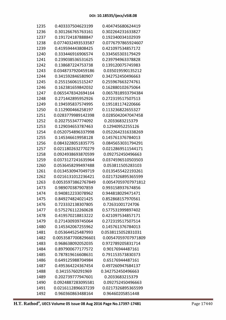
DOI: 10.18535/ijecs/v5i8.08
H.T. Rathoda, IJECS Volume 05 Issue 08 Aug 2016 Page No.17397-17481 Page 17440
1235 0.403337504623199 0.404745680624419 1236 0.301266765763161 0.302264231633827 1237 0.191724187888847 0.192340034102939 1238 0.0774032493533587 0.0776797865924607 1239 0.419594443808425 0.421097534857172 1240 0.333446916906574 0.334565303179429 1241 0.239038536531625 0.239794963378828 1242 0.138687224753738 0.139120075745983 1243 0.0348737920459186 0.035019590135212 1244 0.341592846580907 0.342752450496663 1245 0.255156061515247 0.255967663274761 1246 0.162381659842032 0.162880102675064 1247 0.0655478342694164 0.0657818933794384 1248 0.271442895952926 0.272319517507513 1249 0.194595837574995 0.195181174220666 1250 0.112900466258197 0.113236822655327 1251 0.0283779989142398 0.0285042047047458 1252 0.202755347774092 0.2033683215379 1253 0.129034653787463 0.12940952255126 1254 0.0520754896337998 0.0522642316338269 1255 0.145346619958128 0.145761376784013 1256 0.0843228051835775 0.0845653031794291 1257 0.0211802632770279 0.0212869511544171 1258 0.0924938693870599 0.092752450496663 1259 0.0373127241635964 0.0374596510503503 1260 0.0536458299497488 0.053811505283103 1261 0.0134530947049719 0.0135455422193261 1262 0.0216131012236421 0.0217326895365599 1263 0.00535973862767849 0.00547059707971812 1473 0.989070387907859 0.993158937674856 1474 0.940812233078962 0.944818029471471 1475 0.849274824021425 0.852868157970561 1476 0.723332138307805 0.72631001724706 1477 0.575276112260628 0.577531999897402 1478 0.419570218813222 0.421097534857171 1479 0.271430939745064 0.272319517507514 1480 0.145342067255962 0.145761376784013 1481 0.053644525487993 0.0538115052831031 1482 0.00535877008296601 0.00547059707971809 1483 0.968638092052035 0.972789205831714 1484 0.897900677177572 0.90176944487161 1485 0.787819616608631 0.791153573830373 1486 0.649125988704984 0.65176944487161 1487 0.495364224367454 0.497260947684137 1488 0.34155760291969 0.342752450496663 1489 0.202739777947601 0.2033683215379 1490 0.0924887283095581 0.092752450496663 1491 0.0216112896637239 0.0217326895365599 1492 0.960360863488164 0.96460205851448

DOI: 10.18535/ijecs/v5i8.08
H.T. Rathoda, IJECS Volume 05 Issue 08 Aug 2016 Page No.17397-17481 Page 17441
1493 0.889650250069332 0.893582297554377 1494 0.779588771327282 0.782966426513139 1495 0.640915044878229 0.643582297554377 1496 0.48717140536418 0.489073800366903 1497 0.333377938839285 0.334565303179429 1498 0.19456611619421 0.195181174220666 1499 0.0843135863682769 0.0845653031794291 1500 0.0134504317614859 0.013545542219326 1501 0.924309082001121 0.928466175238718 1502 0.832812299085105 0.836516303737808 1503 0.706909120676642 0.709958163014307 1504 0.558891894133852 0.56118014566465 1505 0.403218011209601 0.404745680624419 1506 0.255098266590039 0.255967663274761 1507 0.129013585554868 0.12940952255126 1508 0.0373074167668466 0.0374596510503502 1509 0.90808027113552 0.912293475342785 1510 0.816608709960335 0.820343603841875 1511 0.690727837052859 0.693785463118374 1512 0.542731714051637 0.545007445768716 1513 0.387074077072161 0.388572980728485 1514 0.238961928881232 0.239794963378827 1515 0.112874538190221 0.113236822655327 1516 0.0211754080876743 0.0212869511544169 1517 0.857257723006268 0.861281226008774 1518 0.747241212134868 0.750665354967537 1519 0.608611461314503 0.611281226008774 1520 0.454906234220432 0.4567727288213 1521 0.301137376624789 0.302264231633827 1522 0.162330392413547 0.162880102675064 1523 0.052063132481843 0.0522642316338267 1524 0.833474642756425 0.837521199079693 1525 0.723484454318834 0.726905328038456 1526 0.584879572344913 0.587521199079693 1527 0.431195766431653 0.433012701892219 1528 0.277439119308826 0.278504204704746 1529 0.1386316524432 0.139120075745983 1530 0.0283688528593958 0.0285042047047456 1531 0.769125323250457 0.772888674565986 1532 0.643294242437702 0.646330533842485 1533 0.495345720889111 0.497552516492827 1534 0.339723069556265 0.341118051452597 1535 0.191622883257325 0.192340034102939 1536 0.0655226520130923 0.0657818933794382 1537 0.73837203633059 0.742126371321759 1538 0.612570904063755 0.615568230598259 1539 0.464650409543193 0.466790213248601 1540 0.309047913811053 0.31035574820837 1541 0.160952923454352 0.161577730858712

DOI: 10.18535/ijecs/v5i8.08
H.T. Rathoda, IJECS Volume 05 Issue 08 Aug 2016 Page No.17397-17481 Page 17442
1542 0.034857103299005 0.0350195901352117 1543 0.662080255509987 0.665465038884934 1544 0.523532788046609 0.526080909926171 1545 0.369899407895789 0.371572412738697 1546 0.216169040508229 0.217063915551223 1547 0.0773569443656873 0.0776797865924606 1548 0.625114449793743 0.628457929325666 1549 0.486603259627316 0.489073800366903 1550 0.3330014177198 0.334565303179429 1551 0.179286532262985 0.180056805991955 1552 0.0404811450662988 0.0406726770331925 1553 0.538762488712235 0.541655445394692 1554 0.390910787223658 0.392877428045034 1555 0.235358077566375 0.236442963004803 1556 0.0872741957599868 0.0876649456551453 1557 0.496497598461704 0.499314767377287 1558 0.348692407506837 0.350536750027629 1559 0.193172789204743 0.194102284987398 1560 0.0451018232761581 0.0453242676377401 1561 0.402219737842934 0.404508497187474 1562 0.248701722626115 0.25 1563 0.0950266331280811 0.0954915028125263 1564 0.355704566676816 0.357876818725374 1565 0.20224900569785 0.2033683215379 1566 0.0486026806470247 0.0488598243504264 1567 0.255837328968869 0.257401207292766 1568 0.100413023829473 0.100966742252535 1569 0.206237227281556 0.207626755071376 1570 0.0508896252472168 0.0511922900311449 1571 0.103266749344947 0.10395584540888 1572 0.051877134699036 0.0522642316338267 1782 0.98898902382404 0.993158937674856 1783 0.96029703693913 0.96460205851448 1784 0.908031588857293 0.912293475342785 1785 0.833438153179454 0.837521199079693 1786 0.738345177923647 0.742126371321759 1787 0.625095142846711 0.628457929325666 1788 0.496484233995617 0.499314767377287 1789 0.355695968178555 0.357876818725374 1790 0.206232606959439 0.207626755071376 1791 0.0518760523077303 0.0522642316338267 1792 0.968498007484748 0.972789205831713 1793 0.92420151509718 0.928466175238718 1794 0.857176526090506 0.861281226008774 1795 0.769065081531992 0.772888674565986 1796 0.66203651030674 0.665465038884934 1797 0.538731739200388 0.541655445394692 1798 0.402199372533962 0.404508497187474 1799 0.255825536612913 0.257401207292766

DOI: 10.18535/ijecs/v5i8.08
H.T. Rathoda, IJECS Volume 05 Issue 08 Aug 2016 Page No.17397-17481 Page 17443
1800 0.10326242250201 0.10395584540888 1801 0.940556599923704 0.944818029471471 1802 0.889455302166683 0.893582297554377 1803 0.816462324014038 0.820343603841875 1804 0.723376429181326 0.726905328038456 1805 0.61249303097005 0.615568230598259 1806 0.486549224604159 0.489073800366903 1807 0.348657615384354 0.350536750027629 1808 0.202230392357491 0.2033683215379 1809 0.0508854902705989 0.0511922900311449 1810 0.897635872628218 0.90176944487161 1811 0.832612682512498 0.836516303737808 1812 0.747093166809217 0.750665354967537 1813 0.643186695733752 0.646330533842485 1814 0.523457114687276 0.526080909926171 1815 0.390860594046809 0.392877428045034 1816 0.248672601064751 0.25 1817 0.100402316082291 0.100966742252535 1818 0.848945701170776 0.852868157970561 1819 0.779342620903002 0.782966426513139 1820 0.690546766798188 0.693785463118374 1821 0.584749361354688 0.587521199079693 1822 0.464560228967578 0.466790213248601 1823 0.332943450484206 0.334565303179429 1824 0.193141855072173 0.194102284987398 1825 0.0485958768011992 0.0488598243504264 1826 0.787515197566643 0.791153573830373 1827 0.706684309629738 0.709958163014307 1828 0.608448684867514 0.611281226008774 1829 0.495231459697171 0.497552516492827 1830 0.36982374477135 0.371572412738697 1831 0.235314229608207 0.236442963004803 1832 0.0950105374028706 0.0954915028125263 1833 0.723004106767646 0.72631001724706 1834 0.640675104459839 0.643582297554376 1835 0.542559933359385 0.545007445768716 1836 0.431077199471634 0.433012701892219 1837 0.308971905534634 0.31035574820837 1838 0.179246087315555 0.180056805991955 1839 0.0450930216803871 0.0453242676377401 1840 0.648841928765112 0.65176944487161 1841 0.558687326473152 0.56118014566465 1842 0.454763220337894 0.4567727288213 1843 0.339628650060411 0.341118051452596 1844 0.216114456106162 0.217063915551223 1845 0.0872542445889102 0.0876649456551453 1846 0.574997135046075 0.577531999897402 1847 0.486972890754194 0.489073800366903 1848 0.386937681061452 0.388572980728485

DOI: 10.18535/ijecs/v5i8.08
H.T. Rathoda, IJECS Volume 05 Issue 08 Aug 2016 Page No.17397-17481 Page 17444
1849 0.277351989839604 0.278504204704746 1850 0.160906731782573 0.161577730858712 1851 0.040471241756322 0.0406726770331925 1852 0.495135660948874 0.497260947684137 1853 0.403059072217266 0.404745680624419 1854 0.30103285540682 0.302264231633827 1855 0.191562664313124 0.192340034102939 1856 0.0773350885054873 0.0776797865924605 1857 0.419363128642851 0.421097534857172 1858 0.333236414905229 0.334565303179429 1859 0.238871896030343 0.239794963378828 1860 0.138584144070389 0.139120075745983 1861 0.034847145439552 0.0350195901352117 1862 0.341397748341267 0.342752450496663 1863 0.254993612812118 0.255967663274761 1864 0.162270349290303 0.162880102675064 1865 0.0655010958776946 0.0657818933794383 1866 0.271298151004723 0.272319517507513 1867 0.194481998591943 0.195181174220666 1868 0.112830406285622 0.113236822655327 1869 0.0283599374814171 0.0285042047047456 1870 0.202645394188443 0.2033683215379 1871 0.128959685341104 0.12940952255126 1872 0.0520441109830907 0.0522642316338267 1873 0.145272373446405 0.145761376784013 1874 0.0842772617839007 0.0845653031794291 1875 0.0211685464133473 0.0212869511544169 1876 0.0924463966481637 0.0927524504966629 1877 0.0372928992585609 0.0374596510503502 1878 0.0536195176004406 0.053811505283103 1879 0.0134463417241656 0.013545542219326 1880 0.0216025273434743 0.0217326895365599 1881 0.00535718754836614 0.00547059707971807 2072 0.988988802185878 0.993158937674856 2073 0.940556506315261 0.944818029471471 2074 0.848945685919081 0.852868157970561 2075 0.723004129994988 0.72631001724706 2076 0.574997166827329 0.577531999897402 2077 0.419363139022064 0.421097534857172 2078 0.271298104495139 0.272319517507513 2079 0.145272217900555 0.145761376784013 2080 0.0536191427452417 0.053811505283103 2081 0.00535624407766375 0.00547059707971807 2082 0.968497587700828 0.972789205831713 2083 0.89763560384042 0.90176944487161 2084 0.787514976532452 0.791153573830373 2085 0.648841712362943 0.65176944487161 2086 0.495135418038085 0.497260947684137 2087 0.341397443726033 0.342752450496663

DOI: 10.18535/ijecs/v5i8.08
H.T. Rathoda, IJECS Volume 05 Issue 08 Aug 2016 Page No.17397-17481 Page 17445
2088 0.202644972125798 0.2033683215379 2089 0.0924457359697444 0.0927524504966629 2090 0.0216012347965218 0.0217326895365599 2091 0.960296460126589 0.96460205851448 2092 0.889454951567644 0.893582297554377 2093 0.779342421817886 0.782966426513139 2094 0.640674955159213 0.643582297554376 2095 0.486972703325695 0.489073800366903 2096 0.333236091952731 0.334565303179429 2097 0.1944814059084 0.195181174220666 2098 0.0842761582127039 0.0845653031794291 2099 0.0134442965506163 0.013545542219326 2100 0.924200835966129 0.928466175238718 2101 0.832612207780462 0.836516303737808 2102 0.706683913934786 0.709958163014307 2103 0.558686916618442 0.56118014566465 2104 0.403058557900146 0.404745680624419 2105 0.254992878418721 0.255967663274761 2106 0.128958539392859 0.12940952255126 2107 0.0372909461090412 0.0374596510503502 2108 0.908030908771528 0.912293475342785 2109 0.816461850431181 0.820343603841875 2110 0.690546437584101 0.693785463118374 2111 0.542559606704973 0.545007445768716 2112 0.386937211964412 0.388572980728485 2113 0.238871107319029 0.239794963378828 2114 0.112829037191969 0.113236822655327 2115 0.0211663371102261 0.0212869511544169 2116 0.857175741593294 0.861281226008774 2117 0.747092571502396 0.750665354967537 2118 0.608448141049197 0.611281226008774 2119 0.454762589726171 0.4567727288213 2120 0.301031982668911 0.302264231633827 2121 0.162269021247312 0.162880102675064 2122 0.0520420024815229 0.0522642316338267 2123 0.833437455867595 0.837521199079693 2124 0.723375900332822 0.726905328038456 2125 0.584748921741657 0.587521199079693 2126 0.431076665620638 0.433012701892219 2127 0.277351154987251 0.278504204704746 2128 0.138582746098223 0.139120075745983 2129 0.0283578039433155 0.0285042047047456 2130 0.769064268017946 0.772888674565986 2131 0.64318602427363 0.646330533842485 2132 0.495230767674702 0.497552516492827 2133 0.339627750062283 0.341118051452596 2134 0.1915613306799 0.192340034102939 2135 0.0654990493187459 0.0657818933794383 2136 0.738344514152188 0.742126371321759

DOI: 10.18535/ijecs/v5i8.08
H.T. Rathoda, IJECS Volume 05 Issue 08 Aug 2016 Page No.17397-17481 Page 17446
2137 0.612492481351269 0.615568230598259 2138 0.464559674860588 0.466790213248601 2139 0.308971116766148 0.31035574820837 2140 0.160905441817087 0.161577730858712 2141 0.0348452066404085 0.0350195901352117 2142 0.662035714968029 0.665465038884934 2143 0.52345638670232 0.526080909926171 2144 0.369822885437373 0.371572412738697 2145 0.21611322629087 0.217063915551223 2146 0.07733322846582 0.0776797865924605 2147 0.625094548132663 0.628457929325666 2148 0.48654866862622 0.489073800366903 2149 0.332942761604251 0.334565303179429 2150 0.179244990276529 0.180056805991955 2151 0.0404695757681872 0.0406726770331925 2152 0.53873099321708 0.541655445394692 2153 0.390859812700939 0.392877428045034 2154 0.235313172683076 0.236442963004803 2155 0.0872526537970532 0.0876649456551453 2156 0.496483733497188 0.499314767377287 2157 0.348657053794858 0.350536750027629 2158 0.193141003734482 0.194102284987398 2159 0.0450916846434457 0.0453242676377401 2160 0.402198695746848 0.404508497187474 2161 0.24867175889953 0.25 2162 0.0950092734087884 0.0954915028125263 2163 0.355695578416438 0.357876818725374 2164 0.20222981736586 0.2033683215379 2165 0.0485949089302559 0.0488598243504264 2166 0.255824940051354 0.257401207292766 2167 0.100401418193516 0.100966742252535 2168 0.206232335846344 0.207626755071376 2169 0.0508849180524333 0.0511922900311449 2170 0.103261923939942 0.10395584540888 2171 0.0518758872654712 0.0522642316338267 _____________________________________________________________________________________ Table 3.1 POISS0N BOUNDARY VALUE PROBLEM(EXAMPLE-2 FOR A SQUARE DOMAIN) FEM MODEL:NODES=643,FOUR NODE QUADRILATERAL ELEMENTS=600 SOLUTION AT ELEMENT CENTROIDS __________________________________________________________________ NODE NUMBER FEM computed values anlytical(theoretical)-values ------------------------------------------------------------------------------------------------------------- 73 0.953482135754673 0.972789205831714 74 0.843161171273121 0.861281226008774

DOI: 10.18535/ijecs/v5i8.08
H.T. Rathoda, IJECS Volume 05 Issue 08 Aug 2016 Page No.17397-17481 Page 17447
75 0.650620087326386 0.665465038884934 76 0.394681801654656 0.404508497187474 77 0.101174463950614 0.10395584540888 78 0.875332012150061 0.893582297554377 79 0.711534774014504 0.726905328038456 80 0.478204029068659 0.489073800366903 81 0.1985066028557 0.2033683215379 82 0.775284911091137 0.791153573830373 83 0.599053315481233 0.611281226008774 84 0.364086776887519 0.371572412738697 85 0.0934682695292481 0.0954915028125263 86 0.63098601484579 0.643582297554377 87 0.424641288869316 0.433012701892219 88 0.176523669210805 0.180056805991955 89 0.488070174157289 0.497260947684137 90 0.296933348853692 0.302264231633827 91 0.0762209811250351 0.0776797865924606 92 0.328773598753415 0.334565303179429 93 0.136733242558403 0.139120075745983 94 0.200160059597621 0.2033683215379 95 0.0513233141659784 0.0522642316338267 96 0.0832180603536406 0.0845653031794291 97 0.021103084633879 0.0217326895365599 152 0.953475580166896 0.972789205831713 153 0.775284490266195 0.791153573830373 154 0.488070769846778 0.497260947684137 155 0.200157210243284 0.2033683215379 156 0.0210890068506871 0.0217326895365599 157 0.875321066900196 0.893582297554377 158 0.630978369734502 0.643582297554377 159 0.328763753767147 0.334565303179429 160 0.0831982579441417 0.0845653031794291 161 0.843148056993177 0.861281226008774 162 0.599047646706308 0.611281226008774 163 0.296923524544665 0.302264231633827 164 0.0512955590513467 0.0522642316338269 165 0.711519768408377 0.726905328038456 166 0.42462713138835 0.433012701892219 167 0.136707551662263 0.139120075745983 168 0.65060852875044 0.665465038884933 169 0.364076636397866 0.371572412738697 170 0.0761967569793705 0.0776797865924607 171 0.47818882371802 0.489073800366903 172 0.176501674085163 0.180056805991955 173 0.394673605078406 0.404508497187474 174 0.093452651964265 0.0954915028125265 175 0.198492418230007 0.2033683215379 176 0.101169394800268 0.10395584540888 231 0.953482135754673 0.972789205831714

DOI: 10.18535/ijecs/v5i8.08
H.T. Rathoda, IJECS Volume 05 Issue 08 Aug 2016 Page No.17397-17481 Page 17448
232 0.843161171273121 0.861281226008774 233 0.650620087326386 0.665465038884934 234 0.394681801654654 0.404508497187474 235 0.101174463950613 0.10395584540888 236 0.875332012150061 0.893582297554377 237 0.711534774014504 0.726905328038456 238 0.478204029068657 0.489073800366903 239 0.198506602855699 0.2033683215379 240 0.775284911091137 0.791153573830373 241 0.599053315481232 0.611281226008774 242 0.364086776887518 0.371572412738697 243 0.0934682695292477 0.0954915028125265 244 0.63098601484579 0.643582297554377 245 0.424641288869315 0.433012701892219 246 0.176523669210804 0.180056805991955 247 0.488070174157289 0.497260947684137 248 0.296933348853691 0.302264231633827 249 0.076220981125035 0.0776797865924608 250 0.328773598753414 0.334565303179429 251 0.136733242558403 0.139120075745983 252 0.200160059597621 0.2033683215379 253 0.0513233141659783 0.0522642316338269 254 0.0832180603536405 0.0845653031794291 255 0.021103084633879 0.0217326895365599 310 0.953475580166895 0.972789205831714 311 0.775284490266194 0.791153573830373 312 0.488070769846778 0.497260947684137 313 0.200157210243284 0.2033683215379 314 0.021089006850687 0.0217326895365599 315 0.875321066900196 0.893582297554377 316 0.630978369734502 0.643582297554377 317 0.328763753767147 0.334565303179429 318 0.0831982579441415 0.0845653031794291 319 0.843148056993177 0.861281226008774 320 0.599047646706308 0.611281226008774 321 0.296923524544665 0.302264231633827 322 0.0512955590513466 0.0522642316338269 323 0.711519768408376 0.726905328038456 324 0.424627131388349 0.433012701892219 325 0.136707551662263 0.139120075745983 326 0.650608528750439 0.665465038884934 327 0.364076636397866 0.371572412738697 328 0.0761967569793705 0.0776797865924608 329 0.47818882371802 0.489073800366903 330 0.176501674085163 0.180056805991955 331 0.394673605078406 0.404508497187474 332 0.0934526519642648 0.0954915028125265 333 0.198492418230007 0.2033683215379 334 0.101169394800268 0.10395584540888

DOI: 10.18535/ijecs/v5i8.08
H.T. Rathoda, IJECS Volume 05 Issue 08 Aug 2016 Page No.17397-17481 Page 17449
389 0.953482135754673 0.972789205831713 390 0.843161171273121 0.861281226008774 391 0.650620087326387 0.665465038884933 392 0.394681801654654 0.404508497187474 393 0.101174463950613 0.10395584540888 394 0.875332012150061 0.893582297554377 395 0.711534774014505 0.726905328038456 396 0.478204029068657 0.489073800366903 397 0.198506602855699 0.2033683215379 398 0.775284911091138 0.791153573830373 399 0.599053315481233 0.611281226008774 400 0.364086776887517 0.371572412738697 401 0.0934682695292476 0.0954915028125265 402 0.63098601484579 0.643582297554377 403 0.424641288869315 0.433012701892219 404 0.176523669210804 0.180056805991955 405 0.488070174157289 0.497260947684137 406 0.296933348853691 0.302264231633827 407 0.0762209811250349 0.0776797865924607 408 0.328773598753414 0.334565303179429 409 0.136733242558403 0.139120075745983 410 0.200160059597621 0.2033683215379 411 0.0513233141659784 0.0522642316338269 412 0.0832180603536406 0.0845653031794291 413 0.021103084633879 0.0217326895365599 468 0.953475580166897 0.972789205831714 469 0.775284490266195 0.791153573830373 470 0.488070769846778 0.497260947684137 471 0.200157210243284 0.2033683215379 472 0.0210890068506871 0.0217326895365599 473 0.875321066900198 0.893582297554377 474 0.630978369734501 0.643582297554377 475 0.328763753767147 0.334565303179429 476 0.0831982579441417 0.0845653031794291 477 0.843148056993178 0.861281226008774 478 0.599047646706307 0.611281226008774 479 0.296923524544666 0.302264231633827 480 0.0512955590513467 0.0522642316338267 481 0.711519768408378 0.726905328038456 482 0.42462713138835 0.433012701892219 483 0.136707551662263 0.139120075745983 484 0.650608528750441 0.665465038884934 485 0.364076636397867 0.371572412738697 486 0.0761967569793706 0.0776797865924606 487 0.478188823718021 0.489073800366903 488 0.176501674085163 0.180056805991955 489 0.394673605078407 0.404508497187474 490 0.0934526519642651 0.0954915028125263 491 0.198492418230008 0.2033683215379

DOI: 10.18535/ijecs/v5i8.08
H.T. Rathoda, IJECS Volume 05 Issue 08 Aug 2016 Page No.17397-17481 Page 17450
492 0.101169394800269 0.10395584540888 547 0.953482135754673 0.972789205831713 548 0.843161171273121 0.861281226008774 549 0.650620087326387 0.665465038884934 550 0.394681801654656 0.404508497187474 551 0.101174463950613 0.10395584540888 552 0.875332012150061 0.893582297554377 553 0.711534774014506 0.726905328038456 554 0.478204029068659 0.489073800366903 555 0.1985066028557 0.2033683215379 556 0.775284911091137 0.791153573830373 557 0.599053315481233 0.611281226008774 558 0.364086776887519 0.371572412738697 559 0.093468269529248 0.0954915028125263 560 0.63098601484579 0.643582297554376 561 0.424641288869316 0.433012701892219 562 0.176523669210805 0.180056805991955 563 0.488070174157289 0.497260947684137 564 0.296933348853692 0.302264231633827 565 0.0762209811250352 0.0776797865924605 566 0.328773598753414 0.334565303179429 567 0.136733242558403 0.139120075745983 568 0.200160059597621 0.2033683215379 569 0.0513233141659784 0.0522642316338267 570 0.0832180603536405 0.0845653031794291 571 0.021103084633879 0.0217326895365599 617 0.953475580166896 0.972789205831713 618 0.775284490266194 0.791153573830373 619 0.488070769846778 0.497260947684137 620 0.200157210243284 0.2033683215379 621 0.021089006850687 0.0217326895365599 622 0.875321066900197 0.893582297554377 623 0.630978369734502 0.643582297554376 624 0.328763753767147 0.334565303179429 625 0.0831982579441414 0.0845653031794291 626 0.843148056993177 0.861281226008774 627 0.599047646706307 0.611281226008774 628 0.296923524544665 0.302264231633827 629 0.0512955590513465 0.0522642316338267 630 0.711519768408377 0.726905328038456 631 0.424627131388349 0.433012701892219 632 0.136707551662263 0.139120075745983 633 0.65060852875044 0.665465038884934 634 0.364076636397866 0.371572412738697 635 0.0761967569793706 0.0776797865924605 636 0.47818882371802 0.489073800366903 637 0.176501674085163 0.180056805991955 638 0.394673605078407 0.404508497187474 639 0.093452651964265 0.0954915028125263

DOI: 10.18535/ijecs/v5i8.08
H.T. Rathoda, IJECS Volume 05 Issue 08 Aug 2016 Page No.17397-17481 Page 17451
640 0.198492418230008 0.2033683215379 641 0.101169394800269 0.10395584540888 _____________________________________________________________________________________ Table 3.2 POISS0N BOUNDARY VALUE PROBLEM(EXAMPLE-2 FOR A SQUARE DOMAIN) FEM MODEL:NODES=2481,FOUR NODE QUADRILATERAL ELEMENTS=2400 SOLUTION AT ELEMENT CENTROIDS __________________________________________________________________ NODE NUMBER FEM computed values anlytical(theoretical)-values ------------------------------------------------------------------------------------------------------------- 238 0.988417102735794 0.993158937674856 239 0.959717112262044 0.96460205851448 240 0.907504096874246 0.912293475342785 241 0.83298056560894 0.837521199079693 242 0.737962689174309 0.742126371321759 243 0.624788084447998 0.628457929325666 244 0.496251014002483 0.499314767377287 245 0.355534498291853 0.357876818725374 246 0.206141060159078 0.207626755071376 247 0.0518532769561828 0.0522642316338267 248 0.967931080289033 0.972789205831714 249 0.923676783123244 0.928466175238718 250 0.856714061402572 0.861281226008774 251 0.768672563342312 0.772888674565986 252 0.661715907202288 0.665465038884934 253 0.538482463011842 0.541655445394692 254 0.402019886275129 0.404508497187474 255 0.255714234905616 0.257401207292766 256 0.103218122035525 0.10395584540888 257 0.940039092112261 0.944818029471471 258 0.888990021590203 0.893582297554377 259 0.816057094614254 0.820343603841875 260 0.723035365233011 0.726905328038456 261 0.612217381393755 0.615568230598259 262 0.486338676438818 0.489073800366903 263 0.34851122205529 0.350536750027629 264 0.202147166698121 0.2033683215379 265 0.0508647496796162 0.0511922900311449 266 0.897170725410378 0.90176944487161 267 0.832204079146261 0.836516303737808 268 0.746745025871177 0.750665354967537 269 0.642900797495705 0.646330533842485 270 0.523233680006328 0.526080909926171 271 0.390699043294539 0.392877428045034 272 0.248572127727066 0.25 273 0.10036226097908 0.100966742252535

DOI: 10.18535/ijecs/v5i8.08
H.T. Rathoda, IJECS Volume 05 Issue 08 Aug 2016 Page No.17397-17481 Page 17452
274 0.848534395528583 0.852868157970561 275 0.778985859067914 0.782966426513139 276 0.690246081472839 0.693785463118374 277 0.584505568553036 0.587521199079693 278 0.464373382546206 0.466790213248601 279 0.332813168009446 0.334565303179429 280 0.193067644985375 0.194102284987398 281 0.0485773679258657 0.0488598243504264 282 0.787156432500507 0.791153573830373 283 0.706378893094704 0.709958163014307 284 0.608197394824003 0.611281226008774 285 0.495034535526922 0.497552516492827 286 0.369680993497343 0.371572412738697 287 0.235225274318541 0.236442963004803 288 0.0949750365793498 0.0954915028125263 289 0.722694092687376 0.72631001724706 290 0.640414000613426 0.643582297554377 291 0.542348002805854 0.545007445768716 292 0.43091449114091 0.433012701892219 293 0.308858263244099 0.31035574820837 294 0.179181276779572 0.180056805991955 295 0.0450768499873504 0.0453242676377401 296 0.648578401596787 0.65176944487161 297 0.558470433448355 0.56118014566465 298 0.454593042991271 0.4567727288213 299 0.339505111389888 0.341118051452597 300 0.216037382352943 0.217063915551223 301 0.0872234663946664 0.0876649456551453 302 0.574775302431038 0.577531999897402 303 0.486792781269151 0.489073800366903 304 0.386799290085722 0.388572980728485 305 0.277255243287368 0.278504204704746 306 0.160851518462883 0.161577730858712 307 0.0404574624706277 0.0406726770331925 308 0.494953071684126 0.497260947684137 309 0.402915731798129 0.404745680624419 310 0.300928720902451 0.302264231633827 311 0.191497653764516 0.192340034102939 312 0.0773091197163312 0.0776797865924606 313 0.419214837492182 0.421097534857171 314 0.33312242234375 0.334565303179429 315 0.238792166370687 0.239794963378827 316 0.138538625551592 0.139120075745983 317 0.0348357862826007 0.0350195901352117 318 0.341281289335076 0.342752450496663 319 0.254908971814031 0.255967663274761 320 0.162217489793882 0.162880102675064 321 0.0654799793879199 0.0657818933794382 322 0.271208594361582 0.272319517507514

DOI: 10.18535/ijecs/v5i8.08
H.T. Rathoda, IJECS Volume 05 Issue 08 Aug 2016 Page No.17397-17481 Page 17453
323 0.194419341863302 0.195181174220666 324 0.112794628927132 0.113236822655327 325 0.0283510117997932 0.0285042047047456 326 0.202580286335157 0.2033683215379 327 0.128919017486617 0.12940952255126 328 0.0520278670515734 0.0522642316338267 329 0.145226812288235 0.145761376784013 330 0.0842512460022017 0.0845653031794291 331 0.021162060266308 0.0212869511544169 332 0.0924179370308632 0.092752450496663 333 0.0372815367832284 0.0374596510503502 334 0.0536032710262482 0.0538115052831031 335 0.0134422979227653 0.013545542219326 336 0.0215960502353594 0.0217326895365599 337 0.00535559321134433 0.00547059707971809 547 0.988416638768864 0.993158937674856 548 0.940038925856626 0.944818029471471 549 0.848534347235084 0.852868157970561 550 0.722694098795867 0.72631001724706 551 0.574775325112241 0.577531999897402 552 0.419214843237481 0.421097534857172 553 0.271208545754388 0.272319517507513 554 0.145226655994887 0.145761376784013 555 0.0536028960146885 0.053811505283103 556 0.00535464973643106 0.00547059707971812 557 0.967930418538892 0.972789205831713 558 0.897170361314643 0.90176944487161 559 0.787156164311979 0.791153573830373 560 0.6485781602077 0.65176944487161 561 0.49495281566464 0.497260947684137 562 0.341280978356805 0.342752450496663 563 0.20257986166334 0.2033683215379 564 0.0924172755964508 0.092752450496663 565 0.0215947576012202 0.0217326895365599 566 0.959716104399742 0.96460205851448 567 0.888989489384571 0.893582297554377 568 0.778985568459127 0.782966426513139 569 0.640413802512979 0.643582297554377 570 0.486792568228329 0.489073800366903 571 0.333122087025405 0.334565303179429 572 0.194418744193771 0.195181174220666 573 0.0842501410653084 0.0845653031794291 574 0.0134402526454918 0.0135455422193261 575 0.923675780853794 0.928466175238718 576 0.832203448906093 0.836516303737808 577 0.706378415365746 0.709958163014308 578 0.558469979762594 0.561180145664649 579 0.402915195240418 0.404745680624419 580 0.254908227513152 0.255967663274761

DOI: 10.18535/ijecs/v5i8.08
H.T. Rathoda, IJECS Volume 05 Issue 08 Aug 2016 Page No.17397-17481 Page 17454
581 0.128917868176791 0.12940952255126 582 0.0372795830710437 0.0374596510503503 583 0.907503011739698 0.912293475342785 584 0.816056416755252 0.820343603841875 585 0.690245642650839 0.693785463118375 586 0.542347617318759 0.545007445768716 587 0.386798791286274 0.388572980728485 588 0.238791364697046 0.239794963378828 589 0.112793255720789 0.113236822655327 590 0.0211598505203014 0.0212869511544171 591 0.856712967113923 0.861281226008774 592 0.746744265479098 0.750665354967537 593 0.608196761245313 0.611281226008774 594 0.454592365271099 0.456772728821301 595 0.300927825913565 0.302264231633827 596 0.162216153393314 0.162880102675064 597 0.0520257568419518 0.0522642316338269 598 0.832979519952825 0.837521199079693 599 0.723034644858218 0.726905328038456 600 0.584505023605272 0.587521199079693 601 0.430913902134175 0.433012701892219 602 0.277254382922407 0.278504204704746 603 0.138537218656194 0.139120075745983 604 0.0283488770996573 0.0285042047047458 605 0.768671479863861 0.772888674565986 606 0.642899975255592 0.646330533842485 607 0.495033761831376 0.497552516492828 608 0.339504170978071 0.341118051452596 609 0.191496303797552 0.192340034102939 610 0.0654779290391075 0.0657818933794384 611 0.737961738218371 0.742126371321759 612 0.612216668286359 0.615568230598259 613 0.464372739705348 0.466790213248601 614 0.308857431403524 0.31035574820837 615 0.160850212298559 0.161577730858712 616 0.0348338450960422 0.035019590135212 617 0.661714889429731 0.665465038884933 618 0.523232827095317 0.526080909926171 619 0.36968006968248 0.371572412738697 620 0.216036124903195 0.217063915551224 621 0.0773072526534658 0.0776797865924607 622 0.624787262007606 0.628457929325666 623 0.486337991734603 0.489073800366903 624 0.332812413770859 0.334565303179429 625 0.179180153646868 0.180056805991955 626 0.0404557922710227 0.0406726770331929 627 0.538481543641445 0.541655445394692 628 0.390698168513625 0.392877428045034 629 0.235224175222532 0.236442963004804

DOI: 10.18535/ijecs/v5i8.08
H.T. Rathoda, IJECS Volume 05 Issue 08 Aug 2016 Page No.17397-17481 Page 17455
630 0.0872218640840389 0.0876649456551455 631 0.496250342180063 0.499314767377287 632 0.348510569391932 0.350536750027629 633 0.193066755281027 0.194102284987398 634 0.0450755062868499 0.0453242676377405 635 0.402019084598442 0.404508497187474 636 0.248571226326356 0.25 637 0.0949737553694593 0.0954915028125265 638 0.355533990709867 0.357876818725374 639 0.20214653944413 0.2033683215379 640 0.0485763903784784 0.0488598243504268 641 0.25571356092414 0.257401207292766 642 0.100361339269195 0.100966742252535 643 0.206140722531811 0.207626755071376 644 0.0508641644011484 0.0511922900311454 645 0.103217592685841 0.10395584540888 646 0.0518530954249093 0.0522642316338272 856 0.988417102735795 0.993158937674856 857 0.959717112262043 0.96460205851448 858 0.907504096874244 0.912293475342785 859 0.832980565608938 0.837521199079693 860 0.737962689174308 0.742126371321759 861 0.624788084447997 0.628457929325666 862 0.496251014002481 0.499314767377287 863 0.355534498291852 0.357876818725374 864 0.206141060159078 0.207626755071376 865 0.0518532769561827 0.0522642316338272 866 0.967931080289033 0.972789205831714 867 0.923676783123241 0.928466175238718 868 0.856714061402569 0.861281226008774 869 0.76867256334231 0.772888674565986 870 0.661715907202286 0.665465038884934 871 0.53848246301184 0.541655445394692 872 0.402019886275128 0.404508497187474 873 0.255714234905615 0.257401207292766 874 0.103218122035524 0.10395584540888 875 0.940039092112261 0.944818029471471 876 0.888990021590202 0.893582297554377 877 0.816057094614252 0.820343603841875 878 0.723035365233009 0.726905328038456 879 0.612217381393752 0.615568230598259 880 0.486338676438816 0.489073800366903 881 0.348511222055288 0.350536750027629 882 0.20214716669812 0.2033683215379 883 0.050864749679616 0.0511922900311454 884 0.897170725410378 0.90176944487161 885 0.832204079146259 0.836516303737808 886 0.746745025871175 0.750665354967537 887 0.642900797495703 0.646330533842485

DOI: 10.18535/ijecs/v5i8.08
H.T. Rathoda, IJECS Volume 05 Issue 08 Aug 2016 Page No.17397-17481 Page 17456
888 0.523233680006326 0.526080909926171 889 0.390699043294536 0.392877428045034 890 0.248572127727064 0.25 891 0.10036226097908 0.100966742252535 892 0.848534395528583 0.852868157970561 893 0.778985859067913 0.782966426513139 894 0.690246081472837 0.693785463118375 895 0.584505568553035 0.587521199079693 896 0.464373382546203 0.466790213248601 897 0.332813168009443 0.334565303179429 898 0.193067644985373 0.194102284987398 899 0.0485773679258654 0.0488598243504268 900 0.787156432500507 0.791153573830373 901 0.706378893094702 0.709958163014308 902 0.608197394824002 0.611281226008774 903 0.49503453552692 0.497552516492828 904 0.36968099349734 0.371572412738697 905 0.235225274318539 0.236442963004804 906 0.0949750365793492 0.0954915028125265 907 0.722694092687375 0.72631001724706 908 0.640414000613424 0.643582297554377 909 0.542348002805852 0.545007445768716 910 0.430914491140907 0.433012701892219 911 0.308858263244097 0.31035574820837 912 0.179181276779571 0.180056805991955 913 0.0450768499873501 0.0453242676377405 914 0.648578401596785 0.65176944487161 915 0.558470433448354 0.561180145664649 916 0.45459304299127 0.456772728821301 917 0.339505111389887 0.341118051452596 918 0.216037382352942 0.217063915551224 919 0.0872234663946658 0.0876649456551456 920 0.574775302431037 0.577531999897403 921 0.486792781269149 0.489073800366903 922 0.38679929008572 0.388572980728485 923 0.277255243287366 0.278504204704746 924 0.160851518462882 0.161577730858712 925 0.0404574624706275 0.0406726770331929 926 0.494953071684125 0.497260947684137 927 0.402915731798127 0.404745680624419 928 0.300928720902449 0.302264231633827 929 0.191497653764515 0.192340034102939 930 0.0773091197163306 0.0776797865924608 931 0.419214837492181 0.421097534857171 932 0.333122422343748 0.334565303179429 933 0.238792166370685 0.239794963378828 934 0.138538625551591 0.139120075745983 935 0.0348357862826004 0.0350195901352119 936 0.341281289335075 0.342752450496663

DOI: 10.18535/ijecs/v5i8.08
H.T. Rathoda, IJECS Volume 05 Issue 08 Aug 2016 Page No.17397-17481 Page 17457
937 0.254908971814029 0.255967663274761 938 0.162217489793881 0.162880102675064 939 0.0654799793879194 0.0657818933794384 940 0.27120859436158 0.272319517507514 941 0.194419341863301 0.195181174220667 942 0.112794628927131 0.113236822655327 943 0.028351011799793 0.0285042047047459 944 0.202580286335156 0.2033683215379 945 0.128919017486616 0.12940952255126 946 0.0520278670515729 0.0522642316338269 947 0.145226812288233 0.145761376784013 948 0.084251246002201 0.0845653031794291 949 0.0211620602663079 0.0212869511544171 950 0.0924179370308623 0.0927524504966631 951 0.0372815367832281 0.0374596510503503 952 0.0536032710262477 0.0538115052831031 953 0.0134422979227652 0.0135455422193262 954 0.0215960502353592 0.0217326895365599 955 0.00535559321134428 0.00547059707971813 1165 0.988416638768866 0.993158937674856 1166 0.940038925856628 0.944818029471471 1167 0.848534347235085 0.852868157970561 1168 0.722694098795866 0.72631001724706 1169 0.57477532511224 0.577531999897403 1170 0.419214843237479 0.421097534857171 1171 0.271208545754387 0.272319517507514 1172 0.145226655994886 0.145761376784013 1173 0.053602896014688 0.0538115052831031 1174 0.00535464973643101 0.00547059707971813 1175 0.967930418538894 0.972789205831714 1176 0.897170361314644 0.90176944487161 1177 0.787156164311979 0.791153573830373 1178 0.648578160207699 0.65176944487161 1179 0.494952815664639 0.497260947684137 1180 0.341280978356804 0.342752450496663 1181 0.202579861663338 0.2033683215379 1182 0.09241727559645 0.0927524504966631 1183 0.02159475760122 0.0217326895365599 1184 0.959716104399745 0.96460205851448 1185 0.888989489384574 0.893582297554377 1186 0.778985568459128 0.782966426513139 1187 0.640413802512978 0.643582297554377 1188 0.486792568228328 0.489073800366903 1189 0.333122087025404 0.334565303179429 1190 0.194418744193769 0.195181174220667 1191 0.0842501410653075 0.0845653031794291 1192 0.0134402526454916 0.0135455422193262 1193 0.923675780853799 0.928466175238718 1194 0.832203448906094 0.836516303737808
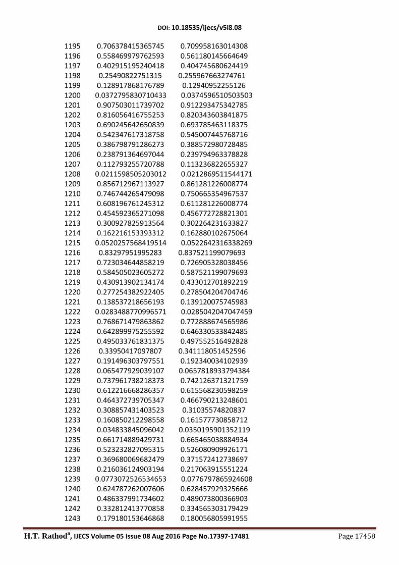
DOI: 10.18535/ijecs/v5i8.08
H.T. Rathoda, IJECS Volume 05 Issue 08 Aug 2016 Page No.17397-17481 Page 17458
1195 0.706378415365745 0.709958163014308 1196 0.558469979762593 0.561180145664649 1197 0.402915195240418 0.404745680624419 1198 0.25490822751315 0.255967663274761 1199 0.128917868176789 0.12940952255126 1200 0.0372795830710433 0.0374596510503503 1201 0.907503011739702 0.912293475342785 1202 0.816056416755253 0.820343603841875 1203 0.690245642650839 0.693785463118375 1204 0.542347617318758 0.545007445768716 1205 0.386798791286273 0.388572980728485 1206 0.238791364697044 0.239794963378828 1207 0.112793255720788 0.113236822655327 1208 0.0211598505203012 0.0212869511544171 1209 0.856712967113927 0.861281226008774 1210 0.746744265479098 0.750665354967537 1211 0.608196761245312 0.611281226008774 1212 0.454592365271098 0.456772728821301 1213 0.300927825913564 0.302264231633827 1214 0.162216153393312 0.162880102675064 1215 0.0520257568419514 0.0522642316338269 1216 0.83297951995283 0.837521199079693 1217 0.723034644858219 0.726905328038456 1218 0.584505023605272 0.587521199079693 1219 0.430913902134174 0.433012701892219 1220 0.277254382922405 0.278504204704746 1221 0.138537218656193 0.139120075745983 1222 0.0283488770996571 0.0285042047047459 1223 0.768671479863862 0.772888674565986 1224 0.642899975255592 0.646330533842485 1225 0.495033761831375 0.497552516492828 1226 0.33950417097807 0.341118051452596 1227 0.191496303797551 0.192340034102939 1228 0.065477929039107 0.0657818933794384 1229 0.737961738218373 0.742126371321759 1230 0.612216668286357 0.615568230598259 1231 0.464372739705347 0.466790213248601 1232 0.308857431403523 0.31035574820837 1233 0.160850212298558 0.161577730858712 1234 0.034833845096042 0.0350195901352119 1235 0.661714889429731 0.665465038884934 1236 0.523232827095315 0.526080909926171 1237 0.369680069682479 0.371572412738697 1238 0.216036124903194 0.217063915551224 1239 0.0773072526534653 0.0776797865924608 1240 0.624787262007606 0.628457929325666 1241 0.486337991734602 0.489073800366903 1242 0.332812413770858 0.334565303179429 1243 0.179180153646868 0.180056805991955

DOI: 10.18535/ijecs/v5i8.08
H.T. Rathoda, IJECS Volume 05 Issue 08 Aug 2016 Page No.17397-17481 Page 17459
1244 0.0404557922710225 0.0406726770331929 1245 0.538481543641444 0.541655445394692 1246 0.390698168513624 0.392877428045034 1247 0.235224175222531 0.236442963004804 1248 0.0872218640840384 0.0876649456551456 1249 0.496250342180062 0.499314767377287 1250 0.348510569391931 0.350536750027629 1251 0.193066755281026 0.194102284987398 1252 0.0450755062868497 0.0453242676377405 1253 0.402019084598441 0.404508497187474 1254 0.248571226326356 0.25 1255 0.0949737553694587 0.0954915028125265 1256 0.355533990709866 0.357876818725374 1257 0.202146539444129 0.2033683215379 1258 0.0485763903784781 0.0488598243504268 1259 0.255713560924139 0.257401207292766 1260 0.100361339269194 0.100966742252535 1261 0.20614072253181 0.207626755071376 1262 0.0508641644011482 0.0511922900311454 1263 0.10321759268584 0.10395584540888 1264 0.0518530954249092 0.0522642316338272 1474 0.988417102735796 0.993158937674856 1475 0.959717112262046 0.96460205851448 1476 0.907504096874249 0.912293475342785 1477 0.832980565608942 0.837521199079693 1478 0.737962689174311 0.742126371321759 1479 0.624788084447997 0.628457929325666 1480 0.496251014002481 0.499314767377287 1481 0.355534498291853 0.357876818725374 1482 0.206141060159078 0.207626755071376 1483 0.0518532769561828 0.0522642316338272 1484 0.967931080289036 0.972789205831713 1485 0.923676783123247 0.928466175238718 1486 0.856714061402574 0.861281226008774 1487 0.768672563342314 0.772888674565986 1488 0.661715907202288 0.665465038884933 1489 0.538482463011841 0.541655445394692 1490 0.402019886275129 0.404508497187474 1491 0.255714234905615 0.257401207292766 1492 0.103218122035525 0.10395584540888 1493 0.940039092112264 0.944818029471471 1494 0.888990021590207 0.893582297554377 1495 0.816057094614256 0.820343603841875 1496 0.723035365233012 0.726905328038456 1497 0.612217381393756 0.615568230598259 1498 0.486338676438818 0.489073800366903 1499 0.34851122205529 0.350536750027629 1500 0.202147166698121 0.2033683215379 1501 0.0508647496796162 0.0511922900311454

DOI: 10.18535/ijecs/v5i8.08
H.T. Rathoda, IJECS Volume 05 Issue 08 Aug 2016 Page No.17397-17481 Page 17460
1502 0.897170725410382 0.90176944487161 1503 0.832204079146264 0.836516303737808 1504 0.746745025871179 0.750665354967537 1505 0.642900797495706 0.646330533842485 1506 0.523233680006329 0.526080909926171 1507 0.390699043294538 0.392877428045034 1508 0.248572127727066 0.25 1509 0.10036226097908 0.100966742252535 1510 0.848534395528586 0.852868157970561 1511 0.778985859067917 0.782966426513139 1512 0.690246081472841 0.693785463118375 1513 0.584505568553037 0.587521199079693 1514 0.464373382546206 0.466790213248601 1515 0.332813168009446 0.334565303179429 1516 0.193067644985375 0.194102284987398 1517 0.0485773679258657 0.0488598243504268 1518 0.78715643250051 0.791153573830373 1519 0.706378893094706 0.709958163014308 1520 0.608197394824005 0.611281226008774 1521 0.495034535526923 0.497552516492828 1522 0.369680993497343 0.371572412738697 1523 0.235225274318541 0.236442963004804 1524 0.09497503657935 0.0954915028125265 1525 0.722694092687379 0.72631001724706 1526 0.640414000613427 0.643582297554377 1527 0.542348002805855 0.545007445768716 1528 0.43091449114091 0.433012701892219 1529 0.3088582632441 0.31035574820837 1530 0.179181276779572 0.180056805991955 1531 0.0450768499873505 0.0453242676377405 1532 0.648578401596789 0.65176944487161 1533 0.558470433448356 0.561180145664649 1534 0.454593042991272 0.456772728821301 1535 0.339505111389889 0.341118051452596 1536 0.216037382352944 0.217063915551224 1537 0.0872234663946665 0.0876649456551455 1538 0.574775302431039 0.577531999897402 1539 0.486792781269151 0.489073800366903 1540 0.386799290085722 0.388572980728485 1541 0.277255243287368 0.278504204704746 1542 0.160851518462884 0.161577730858712 1543 0.0404574624706278 0.0406726770331929 1544 0.494953071684128 0.497260947684137 1545 0.40291573179813 0.404745680624419 1546 0.300928720902451 0.302264231633827 1547 0.191497653764516 0.192340034102939 1548 0.0773091197163313 0.0776797865924607 1549 0.419214837492184 0.421097534857172 1550 0.333122422343751 0.334565303179429

DOI: 10.18535/ijecs/v5i8.08
H.T. Rathoda, IJECS Volume 05 Issue 08 Aug 2016 Page No.17397-17481 Page 17461
1551 0.238792166370687 0.239794963378828 1552 0.138538625551593 0.139120075745983 1553 0.0348357862826008 0.035019590135212 1554 0.341281289335077 0.342752450496663 1555 0.254908971814032 0.255967663274761 1556 0.162217489793883 0.162880102675064 1557 0.0654799793879201 0.0657818933794384 1558 0.271208594361583 0.272319517507513 1559 0.194419341863303 0.195181174220666 1560 0.112794628927132 0.113236822655327 1561 0.0283510117997934 0.0285042047047458 1562 0.202580286335158 0.2033683215379 1563 0.128919017486618 0.12940952255126 1564 0.0520278670515736 0.0522642316338269 1565 0.145226812288235 0.145761376784013 1566 0.084251246002202 0.0845653031794291 1567 0.0211620602663081 0.0212869511544171 1568 0.0924179370308634 0.092752450496663 1569 0.0372815367832286 0.0374596510503503 1570 0.0536032710262483 0.053811505283103 1571 0.0134422979227653 0.0135455422193261 1572 0.0215960502353594 0.0217326895365599 1573 0.00535559321134433 0.00547059707971812 1783 0.988416638768866 0.993158937674856 1784 0.94003892585663 0.944818029471471 1785 0.848534347235088 0.852868157970561 1786 0.72269409879587 0.72631001724706 1787 0.574775325112243 0.577531999897402 1788 0.419214843237483 0.421097534857171 1789 0.271208545754389 0.272319517507514 1790 0.145226655994887 0.145761376784013 1791 0.0536028960146886 0.0538115052831031 1792 0.00535464973643106 0.00547059707971809 1793 0.967930418538895 0.972789205831714 1794 0.897170361314647 0.90176944487161 1795 0.787156164311982 0.791153573830373 1796 0.648578160207703 0.65176944487161 1797 0.494952815664642 0.497260947684137 1798 0.341280978356807 0.342752450496663 1799 0.20257986166334 0.2033683215379 1800 0.0924172755964509 0.092752450496663 1801 0.0215947576012202 0.0217326895365599 1802 0.959716104399745 0.96460205851448 1803 0.888989489384576 0.893582297554377 1804 0.778985568459131 0.782966426513139 1805 0.640413802512981 0.643582297554377 1806 0.486792568228332 0.489073800366903 1807 0.333122087025407 0.334565303179429 1808 0.194418744193771 0.195181174220666

DOI: 10.18535/ijecs/v5i8.08
H.T. Rathoda, IJECS Volume 05 Issue 08 Aug 2016 Page No.17397-17481 Page 17462
1809 0.0842501410653083 0.0845653031794291 1810 0.0134402526454918 0.013545542219326 1811 0.923675780853799 0.928466175238718 1812 0.832203448906097 0.836516303737808 1813 0.706378415365749 0.709958163014307 1814 0.558469979762597 0.56118014566465 1815 0.402915195240421 0.404745680624419 1816 0.254908227513152 0.255967663274761 1817 0.128917868176791 0.12940952255126 1818 0.0372795830710437 0.0374596510503502 1819 0.907503011739702 0.912293475342785 1820 0.816056416755256 0.820343603841875 1821 0.690245642650843 0.693785463118374 1822 0.542347617318762 0.545007445768716 1823 0.386798791286276 0.388572980728485 1824 0.238791364697046 0.239794963378827 1825 0.112793255720789 0.113236822655327 1826 0.0211598505203014 0.0212869511544169 1827 0.856712967113927 0.861281226008774 1828 0.746744265479101 0.750665354967537 1829 0.608196761245316 0.611281226008774 1830 0.454592365271101 0.4567727288213 1831 0.300927825913566 0.302264231633827 1832 0.162216153393314 0.162880102675064 1833 0.0520257568419518 0.0522642316338267 1834 0.83297951995283 0.837521199079693 1835 0.723034644858222 0.726905328038456 1836 0.584505023605276 0.587521199079693 1837 0.430913902134177 0.433012701892219 1838 0.277254382922407 0.278504204704746 1839 0.138537218656194 0.139120075745983 1840 0.0283488770996573 0.0285042047047456 1841 0.768671479863864 0.772888674565986 1842 0.642899975255595 0.646330533842485 1843 0.495033761831378 0.497552516492827 1844 0.339504170978073 0.341118051452597 1845 0.191496303797552 0.192340034102939 1846 0.0654779290391075 0.0657818933794382 1847 0.737961738218374 0.742126371321759 1848 0.61221666828636 0.615568230598259 1849 0.46437273970535 0.466790213248601 1850 0.308857431403526 0.31035574820837 1851 0.16085021229856 0.161577730858712 1852 0.0348338450960423 0.0350195901352117 1853 0.661714889429734 0.665465038884934 1854 0.523232827095319 0.526080909926171 1855 0.369680069682482 0.371572412738697 1856 0.216036124903196 0.217063915551223 1857 0.0773072526534659 0.0776797865924606

DOI: 10.18535/ijecs/v5i8.08
H.T. Rathoda, IJECS Volume 05 Issue 08 Aug 2016 Page No.17397-17481 Page 17463
1858 0.624787262007608 0.628457929325666 1859 0.486337991734604 0.489073800366903 1860 0.33281241377086 0.334565303179429 1861 0.179180153646869 0.180056805991955 1862 0.0404557922710228 0.0406726770331925 1863 0.538481543641446 0.541655445394692 1864 0.390698168513626 0.392877428045034 1865 0.235224175222533 0.236442963004803 1866 0.0872218640840389 0.0876649456551453 1867 0.496250342180064 0.499314767377287 1868 0.348510569391933 0.350536750027629 1869 0.193066755281027 0.194102284987398 1870 0.04507550628685 0.0453242676377401 1871 0.402019084598443 0.404508497187474 1872 0.248571226326358 0.25 1873 0.0949737553694593 0.0954915028125263 1874 0.355533990709868 0.357876818725374 1875 0.20214653944413 0.2033683215379 1876 0.0485763903784784 0.0488598243504264 1877 0.255713560924141 0.257401207292766 1878 0.100361339269195 0.100966742252535 1879 0.206140722531811 0.207626755071376 1880 0.0508641644011485 0.0511922900311449 1881 0.103217592685841 0.10395584540888 1882 0.0518530954249094 0.0522642316338267 2092 0.988417102735794 0.993158937674856 2093 0.959717112262045 0.96460205851448 2094 0.907504096874247 0.912293475342785 2095 0.832980565608941 0.837521199079693 2096 0.73796268917431 0.742126371321759 2097 0.624788084447998 0.628457929325666 2098 0.496251014002482 0.499314767377287 2099 0.355534498291854 0.357876818725374 2100 0.206141060159079 0.207626755071376 2101 0.051853276956183 0.0522642316338267 2102 0.967931080289034 0.972789205831713 2103 0.923676783123244 0.928466175238718 2104 0.856714061402572 0.861281226008774 2105 0.768672563342312 0.772888674565986 2106 0.661715907202287 0.665465038884934 2107 0.538482463011841 0.541655445394692 2108 0.402019886275129 0.404508497187474 2109 0.255714234905616 0.257401207292766 2110 0.103218122035525 0.10395584540888 2111 0.940039092112263 0.944818029471471 2112 0.888990021590206 0.893582297554377 2113 0.816057094614255 0.820343603841875 2114 0.723035365233012 0.726905328038456 2115 0.612217381393755 0.615568230598259
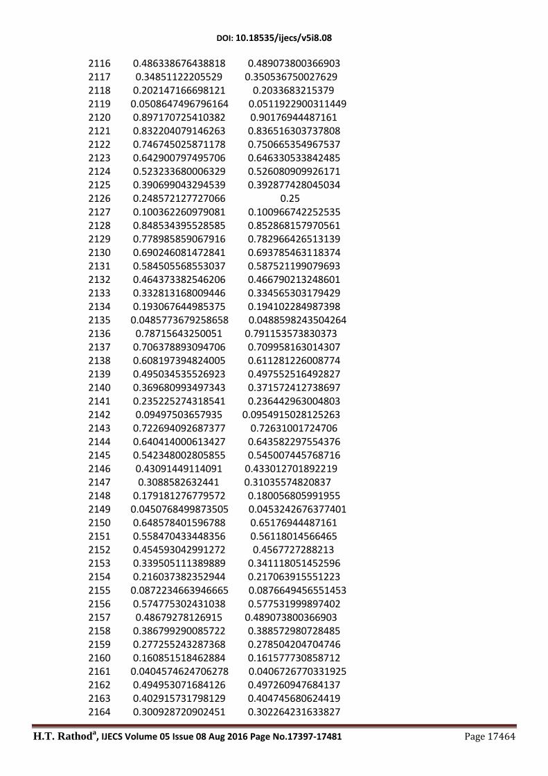
DOI: 10.18535/ijecs/v5i8.08
H.T. Rathoda, IJECS Volume 05 Issue 08 Aug 2016 Page No.17397-17481 Page 17464
2116 0.486338676438818 0.489073800366903 2117 0.34851122205529 0.350536750027629 2118 0.202147166698121 0.2033683215379 2119 0.0508647496796164 0.0511922900311449 2120 0.897170725410382 0.90176944487161 2121 0.832204079146263 0.836516303737808 2122 0.746745025871178 0.750665354967537 2123 0.642900797495706 0.646330533842485 2124 0.523233680006329 0.526080909926171 2125 0.390699043294539 0.392877428045034 2126 0.248572127727066 0.25 2127 0.100362260979081 0.100966742252535 2128 0.848534395528585 0.852868157970561 2129 0.778985859067916 0.782966426513139 2130 0.690246081472841 0.693785463118374 2131 0.584505568553037 0.587521199079693 2132 0.464373382546206 0.466790213248601 2133 0.332813168009446 0.334565303179429 2134 0.193067644985375 0.194102284987398 2135 0.0485773679258658 0.0488598243504264 2136 0.78715643250051 0.791153573830373 2137 0.706378893094706 0.709958163014307 2138 0.608197394824005 0.611281226008774 2139 0.495034535526923 0.497552516492827 2140 0.369680993497343 0.371572412738697 2141 0.235225274318541 0.236442963004803 2142 0.09497503657935 0.0954915028125263 2143 0.722694092687377 0.72631001724706 2144 0.640414000613427 0.643582297554376 2145 0.542348002805855 0.545007445768716 2146 0.43091449114091 0.433012701892219 2147 0.3088582632441 0.31035574820837 2148 0.179181276779572 0.180056805991955 2149 0.0450768499873505 0.0453242676377401 2150 0.648578401596788 0.65176944487161 2151 0.558470433448356 0.56118014566465 2152 0.454593042991272 0.4567727288213 2153 0.339505111389889 0.341118051452596 2154 0.216037382352944 0.217063915551223 2155 0.0872234663946665 0.0876649456551453 2156 0.574775302431038 0.577531999897402 2157 0.48679278126915 0.489073800366903 2158 0.386799290085722 0.388572980728485 2159 0.277255243287368 0.278504204704746 2160 0.160851518462884 0.161577730858712 2161 0.0404574624706278 0.0406726770331925 2162 0.494953071684126 0.497260947684137 2163 0.402915731798129 0.404745680624419 2164 0.300928720902451 0.302264231633827

DOI: 10.18535/ijecs/v5i8.08
H.T. Rathoda, IJECS Volume 05 Issue 08 Aug 2016 Page No.17397-17481 Page 17465
2165 0.191497653764516 0.192340034102939 2166 0.0773091197163313 0.0776797865924605 2167 0.419214837492183 0.421097534857172 2168 0.33312242234375 0.334565303179429 2169 0.238792166370687 0.239794963378828 2170 0.138538625551593 0.139120075745983 2171 0.0348357862826008 0.0350195901352117 2172 0.341281289335076 0.342752450496663 2173 0.254908971814031 0.255967663274761 2174 0.162217489793883 0.162880102675064 2175 0.06547997938792 0.0657818933794383 2176 0.271208594361582 0.272319517507513 2177 0.194419341863302 0.195181174220666 2178 0.112794628927132 0.113236822655327 2179 0.0283510117997933 0.0285042047047456 2180 0.202580286335157 0.2033683215379 2181 0.128919017486617 0.12940952255126 2182 0.0520278670515734 0.0522642316338267 2183 0.145226812288235 0.145761376784013 2184 0.0842512460022019 0.0845653031794291 2185 0.0211620602663081 0.0212869511544169 2186 0.0924179370308633 0.0927524504966629 2187 0.0372815367832285 0.0374596510503502 2188 0.0536032710262482 0.053811505283103 2189 0.0134422979227653 0.013545542219326 2190 0.0215960502353594 0.0217326895365599 2191 0.00535559321134433 0.00547059707971807 2382 0.988416638768864 0.993158937674856 2383 0.940038925856629 0.944818029471471 2384 0.848534347235087 0.852868157970561 2385 0.722694098795869 0.72631001724706 2386 0.574775325112242 0.577531999897402 2387 0.419214843237481 0.421097534857172 2388 0.271208545754388 0.272319517507513 2389 0.145226655994887 0.145761376784013 2390 0.0536028960146886 0.053811505283103 2391 0.00535464973643106 0.00547059707971807 2392 0.967930418538894 0.972789205831713 2393 0.897170361314646 0.90176944487161 2394 0.787156164311982 0.791153573830373 2395 0.648578160207701 0.65176944487161 2396 0.49495281566464 0.497260947684137 2397 0.341280978356806 0.342752450496663 2398 0.20257986166334 0.2033683215379 2399 0.0924172755964509 0.0927524504966629 2400 0.0215947576012202 0.0217326895365599 2401 0.959716104399744 0.96460205851448 2402 0.888989489384576 0.893582297554377 2403 0.778985568459131 0.782966426513139

DOI: 10.18535/ijecs/v5i8.08
H.T. Rathoda, IJECS Volume 05 Issue 08 Aug 2016 Page No.17397-17481 Page 17466
2404 0.64041380251298 0.643582297554376 2405 0.48679256822833 0.489073800366903 2406 0.333122087025405 0.334565303179429 2407 0.194418744193771 0.195181174220666 2408 0.0842501410653084 0.0845653031794291 2409 0.0134402526454918 0.013545542219326 2410 0.9236757808538 0.928466175238718 2411 0.832203448906096 0.836516303737808 2412 0.706378415365749 0.709958163014307 2413 0.558469979762595 0.56118014566465 2414 0.402915195240419 0.404745680624419 2415 0.254908227513151 0.255967663274761 2416 0.128917868176791 0.12940952255126 2417 0.0372795830710437 0.0374596510503502 2418 0.907503011739702 0.912293475342785 2419 0.816056416755254 0.820343603841875 2420 0.690245642650841 0.693785463118374 2421 0.54234761731876 0.545007445768716 2422 0.386798791286275 0.388572980728485 2423 0.238791364697046 0.239794963378828 2424 0.112793255720789 0.113236822655327 2425 0.0211598505203015 0.0212869511544169 2426 0.856712967113928 0.861281226008774 2427 0.746744265479099 0.750665354967537 2428 0.608196761245315 0.611281226008774 2429 0.4545923652711 0.4567727288213 2430 0.300927825913565 0.302264231633827 2431 0.162216153393314 0.162880102675064 2432 0.0520257568419519 0.0522642316338267 2433 0.832979519952829 0.837521199079693 2434 0.72303464485822 0.726905328038456 2435 0.584505023605274 0.587521199079693 2436 0.430913902134176 0.433012701892219 2437 0.277254382922407 0.278504204704746 2438 0.138537218656194 0.139120075745983 2439 0.0283488770996573 0.0285042047047456 2440 0.768671479863862 0.772888674565986 2441 0.642899975255594 0.646330533842485 2442 0.495033761831377 0.497552516492827 2443 0.339504170978071 0.341118051452596 2444 0.191496303797552 0.192340034102939 2445 0.0654779290391076 0.0657818933794383 2446 0.737961738218373 0.742126371321759 2447 0.612216668286359 0.615568230598259 2448 0.464372739705349 0.466790213248601 2449 0.308857431403525 0.31035574820837 2450 0.16085021229856 0.161577730858712 2451 0.0348338450960423 0.0350195901352117 2452 0.661714889429733 0.665465038884934

DOI: 10.18535/ijecs/v5i8.08
H.T. Rathoda, IJECS Volume 05 Issue 08 Aug 2016 Page No.17397-17481 Page 17467
2453 0.523232827095318 0.526080909926171 2454 0.369680069682481 0.371572412738697 2455 0.216036124903196 0.217063915551223 2456 0.0773072526534659 0.0776797865924605 2457 0.624787262007607 0.628457929325666 2458 0.486337991734604 0.489073800366903 2459 0.33281241377086 0.334565303179429 2460 0.179180153646869 0.180056805991955 2461 0.0404557922710228 0.0406726770331925 2462 0.538481543641446 0.541655445394692 2463 0.390698168513626 0.392877428045034 2464 0.235224175222533 0.236442963004803 2465 0.087221864084039 0.0876649456551453 2466 0.496250342180064 0.499314767377287 2467 0.348510569391932 0.350536750027629 2468 0.193066755281027 0.194102284987398 2469 0.04507550628685 0.0453242676377401 2470 0.402019084598442 0.404508497187474 2471 0.248571226326357 0.25 2472 0.0949737553694593 0.0954915028125263 2473 0.355533990709868 0.357876818725374 2474 0.20214653944413 0.2033683215379 2475 0.0485763903784784 0.0488598243504264 2476 0.25571356092414 0.257401207292766 2477 0.100361339269195 0.100966742252535 2478 0.206140722531811 0.207626755071376 2479 0.0508641644011485 0.0511922900311449 2480 0.103217592685841 0.10395584540888 2481 0.0518530954249094 0.0522642316338267 ________________________________________________________________

DOI: 10.18535/ijecs/v5i8.08
H.T. Rathoda, IJECS Volume 05 Issue 08 Aug 2016 Page No.17397-17481 Page 17468
FIGURES(Example-1:A PENTAGONAL DOMAIN)

DOI: 10.18535/ijecs/v5i8.08
H.T. Rathoda, IJECS Volume 05 Issue 08 Aug 2016 Page No.17397-17481 Page 17469
f

DOI: 10.18535/ijecs/v5i8.08
H.T. Rathoda, IJECS Volume 05 Issue 08 Aug 2016 Page No.17397-17481 Page 17470
MESH-2

DOI: 10.18535/ijecs/v5i8.08
H.T. Rathoda, IJECS Volume 05 Issue 08 Aug 2016 Page No.17397-17481 Page 17471

DOI: 10.18535/ijecs/v5i8.08
H.T. Rathoda, IJECS Volume 05 Issue 08 Aug 2016 Page No.17397-17481 Page 17472
FIGURES(Example-2: A SQUARE DOMAIN) MESH-1

DOI: 10.18535/ijecs/v5i8.08
H.T. Rathoda, IJECS Volume 05 Issue 08 Aug 2016 Page No.17397-17481 Page 17473

DOI: 10.18535/ijecs/v5i8.08
H.T. Rathoda, IJECS Volume 05 Issue 08 Aug 2016 Page No.17397-17481 Page 17474

DOI: 10.18535/ijecs/v5i8.08
H.T. Rathoda, IJECS Volume 05 Issue 08 Aug 2016 Page No.17397-17481 Page 17475
MESH-2

DOI: 10.18535/ijecs/v5i8.08
H.T. Rathoda, IJECS Volume 05 Issue 08 Aug 2016 Page No.17397-17481 Page 17476

DOI: 10.18535/ijecs/v5i8.08
H.T. Rathoda, IJECS Volume 05 Issue 08 Aug 2016 Page No.17397-17481 Page 17477
FEM MESHES USED IN THE ABOVE PRESENTATIONS (1)MESH GENERATION:PENTAGONAL DOMAIN

DOI: 10.18535/ijecs/v5i8.08
H.T. Rathoda, IJECS Volume 05 Issue 08 Aug 2016 Page No.17397-17481 Page 17478

DOI: 10.18535/ijecs/v5i8.08
H.T. Rathoda, IJECS Volume 05 Issue 08 Aug 2016 Page No.17397-17481 Page 17479
(2)MESH GENERATION:SQUARE DOMAIN

DOI: 10.18535/ijecs/v5i8.08
H.T. Rathoda, IJECS Volume 05 Issue 08 Aug 2016 Page No.17397-17481 Page 17480
Related Documents