Finite Element Simulation of Residual Stresses from Welding and High Frequency Hammer Peening submitted in fulfilment of the requirements for the degree of Doctor of Engineering (Dr.Eng.) to the Department of Civil Engineering, Geo- and Environmental Sciences of Karlsruhe Institute of Technology (KIT) approved Doctoral Dissertation of Dipl.Eng. Stefanos Gkatzogiannis from Veria, Greece Date of oral examination: 10 June 2020 First reviewer: Prof. Dr.-Ing. Thomas Ummenhofer Second reviewer: Prof. Dr. Andreas Taras

Welcome message from author
This document is posted to help you gain knowledge. Please leave a comment to let me know what you think about it! Share it to your friends and learn new things together.
Transcript
Finite Element Simulation of Residual Stresses from Welding and
High Frequency Hammer Peening
submitted in fulfilment of the requirements for the degree of
Doctor of Engineering (Dr.Eng.)
to the Department of Civil Engineering, Geo- and Environmental Sciences
of Karlsruhe Institute of Technology (KIT)
approved
Doctoral Dissertation
of
Dipl.Eng. Stefanos Gkatzogiannis
from Veria, Greece
Date of oral examination: 10 June 2020
First reviewer: Prof. Dr.-Ing. Thomas Ummenhofer
Second reviewer: Prof. Dr. Andreas Taras
Finite Element Simulation of Residual Stresses from Welding and
High Frequency Hammer Peening
zur Erlangung des akademischen Grades eines
Doktors der Ingenieurwissenschaften (Dr.-Ing.)
von der KIT-Fakultät für Bauingenieur-, Geo- und Umweltwissenschaften
des Karlsruher Instituts für Technologie (KIT)
genehmigte
Dissertation
von
Dipl.-Ing. Stefanos Gkatzogiannis
aus Veria, Griechenland
Tag der mündlichen Prüfung: 10. Juni 2020
Referent: Prof. Dr.-Ing. Thomas Ummenhofer
Korreferent: Prof. Dr. Andreas Taras
i
Summary
The present doctoral dissertation focuses on the simulation of the residual stress
state (RS) in steel weldments after their post-weld treatment with High Fre-
quency Mechanical Impact (HFMI). Main goal is the establishment of an efficient
engineering approach, which will include straightforward simulation models
without compromising the accuracy, in order to estimate the RS field and enable
a future evaluation of its influence on the fatigue life of the simulated compo-
nents. The established approach should be applicable for both research and prac-
tical purposes. The Finite Element method is applied overall in the framework of
the present study for the fulfilment of the research goal.
Prior to the application of HFMI, significant welding residual stresses (WRS),
which cannot be neglected, are present in the as-welded state. Although research
on welding simulation with the FE method is ongoing since decades, the method-
ology for practical applications remains vague. Based on existing knowledge, the
present study establishes a straightforward engineering approach that considers
all significant aspects for the accurate estimation of the WRS, which is proven
applicable for several materials. Subsequently, the influence of several practical
and special aspects of welding simulation on the simulated RS such as the applied
values for thermal expansion coefficient, welding sequence, modelling of bound-
ary conditions, phase changes, size of the modelled heat source etc. is investi-
gated with this model. Validation of the simulations is based on direct comparison
of the simulated temperature and RS profiles with respective experimental meas-
urements found either in literature or in a completed research project. Conclu-
sions, which can act as a modelling guide for the engineering practice, are pre-
sented. The commercial general-purpose FE software ANSYS has been applied for
all welding simulations.
A similar approach is followed in the second part of the present research study,
where modelling of HFMI is investigated. Once again, practical and special aspects
of the HFMI simulation are considered. Amongst others, modelling of boundary
conditions, density of HFMI treatment, scaling of components, applied values for
the friction coefficient, material modelling and the influence of WRS are consid-
ered. Calibration of applied material models is carried out based on material test-
ing from a completed research project and data from literature. Additionally, a
Summary
ii
series of drop tests for estimating the dynamic yielding behaviour of the investi-
gated materials under the deformation mode present during HFMI treatment, are
implemented for the first time. The present series of numerical investigations re-
garding HFMI either confirm or reject initial assumptions and conclusions from
previous experimental and numerical studies. Additionally, new conclusions re-
garding the necessary aspects, which have to be considered or neglected, in order
to achieve the desired accuracy, are proposed. The commercial general-purpose
FE software LS Dyna has been applied for all HFMI simulations.
Finally, recommendations for future work are presented regarding both the
above-mentioned main parts of the present study and the numerical investiga-
tions regarding fatigue in general.
iii
Kurzfassung
Die vorliegende Dissertation befasst sich mit der numerischen Simulation der Ei-
genspannungen von Schweißverbindungen nach ihrer Behandlung mit dem hö-
herfrequenten Hämmerverfahren (HFH). Hauptziel ist die Entwicklung eines effi-
zienten Inngenieurkonzeptes, das praxisorientierte Modelle einschließt, ohne die
Genauigkeit der Ergebnisse zu beeinträchtigen. Es soll die Bestimmung des Ein-
flusses der Eigenspannungen auf die Ermüdungsfestigkeit der simulierten Bau-
teile ermöglichen. Der entwickelte Ansatz sollte sowohl für Forschungszwecke als
auch für praktische Zwecke anwendbar sein. In Rahmen der vorliegenden Studie
wird die Finite-Elemente-Methode für die Erfüllung des aktuellen Forschungszie-
les angewendet.
Die Schweißverbindungen im wie-geschweißten Zustand haben schon vor der
Nachbehandlung signifikante Schweißeigenspannungen. Obwohl die Forschung
zum Thema Schweißsimulation schon seit Jahrzehnten betrieben wird, bleibt die
Methodik für ihre praktische Anwendung unklar. Basierend auf dem vorhande-
nen Wissen wird in der vorliegenden Studie ein technischer Ansatz für die genaue
Simulation des Lichtbogenschweißens entwickelt, der alle wichtigen Aspekte für
die genaue Schätzung der Schweißeigenspannungen berücksichtigt und erwiese-
nermaßen für mehrere Materialien anwendbar ist. Mithilfe dieses Modells wurde
der Einfluss einiger praktischer oder spezieller Aspekte der Schweißsimulation,
wie z.B. die verwendeten Werte des Wärmeausdehnungskoeffizienten, die
Schweißreihenfolge, die Modellierung der Randbedingungen, die Phasenum-
wandlungen, die Abmessungen der Wärmequelle usw. auf die gerechneten Ei-
genspannungen untersucht. Die Validierung der Simulationen basiert auf einem
direkten Vergleich der simulierten Temperaturprofile und Eigenspannungen mit
entsprechenden experimentellen Messungen, die entweder in der Literatur oder
in einem abgeschlossenen Forschungsprojekt gefunden wurden. Es werden
Schlussfolgerungen präsentiert, die als Modellierungsleitfaden für die Ingenieur-
praxis dienen können. Die kommerzielle FE-Software ANSYS wurde für alle
Schweißsimulationen angewendet.
Ein ähnlicher Ansatz wird im zweiten Teil der vorliegenden Doktorarbeit verfolgt,
in der die FE-Modellierung des höherfrequenten Hämmerns HFH untersucht wird.
Kurzfassung
iv
Auch hier werden praktische und spezielle Aspekte der HFH-Simulation betrach-
tet. Unter anderen werden berücksichtigt: die Modellierung der Randbedingun-
gen, die Überlappung von HFH-Schlägen, die Skalierung von Bauteilen in der Si-
mulation, die angewendeten Werte für den Reibungskoeffizienten, die
Werkstoffgesetze und der Einfluss der Schweißeigenspannungen. Die Kalibrie-
rung der verwendeten Werkstoffgesetze erfolgt mithilfe von der Werkstoffcha-
rakterisierung aus einem abgeschlossenen Projekt und von Daten aus der Litera-
tur. Darüber hinaus wurde eine Reihe von Fallversuchen für die Bestimmung der
dynamischen Streckgrenze von den untersuchten Werkstoffen durchgeführt. Die
aktuelle Serie von numerischen Untersuchungen des HFH bestätigt entweder o-
der widerlegt Anfangsannahmen und Schlussfolgerungen aus früheren experi-
mentellen und numerischen Untersuchungen. Zusätzlich werden neue Schlussfol-
gerungen bezüglich der notwendigen Aspekte vorgeschlagen, die zu
berücksichtigen sind, um die gewünschte Genauigkeit zu erreichen. Die kommer-
zielle FE-Software LS Dyna wird für alle HFH-Simulationen angewendet.
Abschließend werden Empfehlungen für zukünftige Untersuchungen zu den oben
genannten Hauptthemen der vorliegenden Doktorarbeit sowie zum Gebiet Ermü-
dung und FE-Simulationen im Allgemeinen gegeben.

…«Κι ἂν πτωχικὴ τὴν βρῇς, ἡ Ἰθάκη δὲν σὲ γέλασε. Ἔτσι σοφὸς ποὺ ἔγινες, μὲ τόση πείρα,
ἤδη θὰ τὸ κατάλαβες ᾑ Ἰθάκες τί σημαίνουν.»
…”And if you find her poor, Ithaka won’t have fooled you.
Wise as you will have become, so full of experience,
you’ll have understood by then what these Ithakas mean.”
Ἰθάκη (Ithaka)
by C. P. Cavafy,
translated by Edmund Keeley
metallurgy
From French métallurgie, from Ancient Greek μεταλλουργός (metallourgós, “worker in metal”), from μέταλλον (métallon, “metal”) +
ἔργον (érgon, “work”).


To my parents Genovefa and Stylianos for
unveiling to me the fathomless beauty
of knowledge, for their love and support.


ix
Preface
During my undergraduate studies at the School of Civil Engineering, at the Aristo-
tle University of Thessaloniki, I was fascinated by two subjects of structural engi-
neering, which would shape my academic future: steel structures and computa-
tional mechanics. The possibilities of the accurate design enabled by the
mechanical properties of steel, its application on more complicated structures
and the fact that during design of such structures, the challenge of combining
complex scientific knowledge with practical engineering solutions arises, have
been the reasons for concentrating on the first subject. Regarding the latter one,
the computational mechanics, it has been from the beginning pure fascination in
front of the capabilities, which are enabled by introduction of computers in mod-
ern engineering. Therefore, when I decided to pursue the doctoral title of engi-
neering it was the natural course of events to land on the field of simulation of
steel structures.
When I first met Professor Thomas Ummenhofer in June 2012 and made my in-
tentions of having a doctoral dissertation regarding numerical analysis in the field
of steel structures known to him, he proposed the present subject. Back then, my
knowledge on welding was restricted to design of weldments against static loads
and the terms “post-weld treatment” and “residual stresses” were unknown to
me. I agreed to begin my postgraduate research in Karlsruhe Institute of Technol-
ogy on this subject without imagining the very interesting journey, which was
about to begin. Over the years, I investigated several aspects, which were not
strictly attached to the main subject, they were not dots of a straight path, but
small sidesteps I had to take. I strongly believe now that they helped me signifi-
cantly to better comprehend the subjects of plasticity, residual stress, metallurgy
and fatigue amongst others. The completion of the present study broadened my
scientific knowledge but more significantly, it reshaped my personality by increas-
ing my work ethics on a level I could not foresee.
I would sincerely like to thank my supervisor Professor Thomas Ummenhofer for
giving me the opportunity to work in such a challenging environment, like the KIT
Steel and Lightweight Structures Institute - Research Centre for Steel, Wood and
Masonry. Without his trust in me and my previous education, this dissertation
Preface
x
would not have been realized. His scientific vigour was and will always be an in-
spiration for me. His ability to lead the younger researchers with such insightful-
ness on so many different subjects of our field will always be for me a source of
admiration, something to look up to.
Furthermore, I would like to thank my colleagues, scientific and laboratory asso-
ciates of the KIT Steel and Lightweight Structures Institute, for the smooth coop-
eration over the years. Especially I have to mention Philipp Ladendorf for the in-
teresting scientific discussions and his input regarding material testing over the
years, my research assistant Ioannis Savvanidis for his contribution in designing
and setting up the drop tests of the present study and Dr. Tim Zinke for his valu-
able advice regarding the process of writing and publishing my doctoral disserta-
tion. Special thanks to Dr. Majid Farajian and Mr. Jan Schubnell for the fruitful
collaboration in the framework of the project HFH-Simulation. Without their in-
put, the present study could not have been finalized. For their financial support
to the same research project, which provided significant input for the present
dissertation, I should acknowledge as well the DVS – Deutscher Verband für
Schweißen und verwandte Verfahren and the Arbeitsgemeinschaft industrieller
Forschungsvereinigungen "Otto von Guericke" e.V. (AiF).
I would like to thank Professor Andreas Taras for being the second reviewer of
the present dissertation, the time he invested for this task, his valuable remarks
and overall for his positive feedback. I thank him as well along with Professor Pe-
ter Betsch and Professor Joachim Blaß for being members of the examining com-
mittee and for acknowledging the hard effort for completing this dissertation and
the quality of my work.
At this point, I would like to state explicitly my gratitude to my mentor Professor
Peter Knoedel, a great scientist and a wonderful person, for his patience, for all
the things he taught me and for all the memorable moments. He never stopped
motivating me take up new challenges. He has been rigorous but just, he kindly
pinpointed my mistakes and cheerfully congratulated my successes, always re-
specting my personality. For me he is much more than a tutor, a director or a
colleague, he has become a heartwarming, dearest friend. For all these, Peter,
thank you.
I should not forget to mention my friends Alexandros, Andreas, Georgios, Ioannis,
Michalis, Orestes and Vasilis, with whom I lived over the last years many memo-
rable moments, which helped me going. Many special thanks to my companion
Preface
xi
Aikaterini, for her support and for the nice moments we had in Karlsruhe. Her
sweet, vivid and kind personality has been a shelter in difficult moments. The
healthy competition with her wit and scientific duality have pushed me to im-
prove myself significantly. Additionally, I would like to thank her for contributing
to the syntax of the MATLAB code for the present study. Finally yet importantly,
I would like to thank my parents Genovefa and Stylianos to whom I devote this
dissertation. Without their love and support, this doctoral dissertation would not
have been completed. I am grateful to them for showing me the joy of knowledge,
for teaching me to choose always the hard path of virtue and for making me un-
derstand in their very own words, what the Ithacas of this world mean.
Stefanos Gkatzogiannis
Karlsruhe, September 2020


xiii
Table of Contents
Summary ...................................................................................................... ii
Kurzfassung .................................................................................................. iii
Preface ......................................................................................................... ix
Table of Contents ........................................................................................ xiii
List of Publications ........................................................................................ 1
Publications Carried Out in the Framework of the Present Dissertation ..... 1
Publications in Regard to Fatigue and HFMI................................................. 3
List of Figures ................................................................................................ 5
1 Introduction ........................................................................................... 15
1.1 Problem Statement ............................................................................ 15
1.2 Research Methodology....................................................................... 18
1.3 High Performance Computing ............................................................ 20
1.4 Outline of the Present Dissertation .................................................... 20
2 Theoretical Background .......................................................................... 23
2.1 Numerical Investigations .................................................................... 23
2.1.1 FE Simulation of Fusion Welding Residual Stresses ................... 23
2.1.2 FE Simulation of HFMI ................................................................ 48
2.2 Analytical Investigations for the Calculation of the Dynamic Yield
Strength during a Spherical Impact ............................................................ 62
2.3 RS Profiles Introduced by the Impact of a Metallic Sphere ................ 65
3 FE Simulation of Welding ........................................................................ 69
3.1 Methodology ...................................................................................... 69
3.1.1 Thermal Transient Analysis ........................................................ 70
3.1.2 Microstructural Modelling ......................................................... 71
Table of Contents
xiv
3.1.3 Static Structural Analysis ............................................................ 71
3.2 Single-pass Butt Welds ....................................................................... 73
3.2.1 Investigated Components ........................................................... 73
3.2.2 Material Modelling ..................................................................... 75
3.2.3 Investigated Aspects ................................................................... 78
3.2.4 Analyses and Results .................................................................. 79
3.2.5 Conclusions ............................................................................... 102
3.3 Further Applications of the Proposed Approach .............................. 104
3.4 Fillet welds ........................................................................................ 105
3.4.1 Investigated Components ......................................................... 105
3.4.2 WRS Measurements ................................................................. 109
3.4.3 Material Modelling ................................................................... 111
3.4.4 Analyses and Results ................................................................ 118
3.4.5 Conclusions ............................................................................... 142
4 Drop Tests for the Calibration of HFMI Simulation .................................. 145
4.1 Work Hypothesis............................................................................... 145
4.2 Methodology .................................................................................... 145
4.3 Investigations .................................................................................... 146
4.3.1 Experimental Setup .................................................................. 146
4.3.2 Estimation of Impact Velocity ................................................... 149
4.3.3 Strain Rate Calculation through FE Analysis ............................. 149
4.3.4 Measurement of crater and restitution coefficient ................. 151
4.3.5 Analytical Estimation of the Dynamic Yield Limit ..................... 153
4.4 Summary and Open Questions ......................................................... 158
5 FE Simulation of HFMI ........................................................................... 161
5.1 Methodology .................................................................................... 161
Table of Contents
xv
5.2 Convergence Analysis ....................................................................... 163
5.3 Component of Parent material ......................................................... 164
5.4 Fillet Welds ....................................................................................... 184
5.4.1 Investigated Component .......................................................... 184
5.4.2 Discretization ............................................................................ 185
5.4.3 Modelling of Material Behaviour ............................................. 188
5.4.4 HFMI Treatment Setup and Boundary Conditions ................... 189
5.4.5 Preliminary Investigations for the Simulation of Fillet Welds .. 192
5.4.6 Analyses and Results ................................................................ 195
5.4.7 Discussion and Conclusions ...................................................... 222
5.5 Summary and Open Questions Regarding HFMI Simulation ............ 226
6 Overall Discussion ................................................................................. 229
7 Future Work on Numerical Investigations and Fatigue ............................ 231
List of Abbreviations ................................................................................... 233
List of Notations ......................................................................................... 235
References ................................................................................................. 241
Appendix A – Investigated Materials ........................................................... 259
Appendix B – FE Background ....................................................................... 275
Appendix C – Statistics ............................................................................... 277

1
List of Publications
Publications Carried Out in the Framework of the Present Dissertation
The following studies were published in the framework of the present doctoral
dissertation and acted as milestones during its realization. They are presented
categorized and in chronological order:
Publications in peer reviewed academic and technical journals
Gkatzogiannis S., Knoedel P., Ummenhofer T.; Calibration of HFMI Simulation based on Drop Tests, Journal of Material Engineering and Performance, published online on 04 May 2020.
Gkatzogiannis S., Knoedel P., Ummenhofer T.; Strain Rate Dependency of Simu-lated Welding Residual Stresses, Journal of Material Engineering and Perfor-mance 27 (10), pp. 5079-5085, 2018.
Knoedel P., Gkatzogiannis, S., Ummenhofer T.; Practical Aspects of Welding Re-sidual Stress Simulation, Journal of Constructional Steel Research 132, pp. 83-96, 2017.
Publications in peer reviewed conference proceedings Gkatzogiannis S., Knoedel P., Ummenhofer T.; FE Simulation of High Frequency Mechanical Impact (HFMI) Treatment – First Results, Proceeding of NORDIC STEEL 2019, The 14th Nordic Steel Construction Conference, Copenhagen 18–20 Septem-ber 2019, ce/papers 3 (3-4), pp. 797-802, Ernst & Sohn, 2019.
Gkatzogiannis S., Knoedel P., Ummenhofer T.; A Pseudothermal Approach for Simulating the Residual Stress Field Caused by Shot Blasting, Proceedings of the VIII International Conference on Computational Methods for Coupled Problems in Science and Engineering, Sitges 3-6 June 2019, pp. 777-788, 2019.
Gkatzogiannis S., Knoedel P., Ummenhofer T.; Simulation of Welding Residual Stresses – From Theory to Practice, Selected Peer Reviewed Papers from the 12th International Seminar Numerical Analysis of Weldability, Graz – Schloss Seggau 23-26 September 2018, published in Sommitsch C., Enzinger N., Mayr P.; Mathe-matical Modelling of Weld Phenomena 12, pp. 383-400, 2019.
List of Publications
2
Gkatzogiannis S., Knoedel P., Ummenhofer T.; Reviewing the Influence of Welding Setup on FE-simulated Welding Residual Stresses, Proceedings of the 10th Euro-pean Conference on Residual Stresses - ECRS10, Leuven 11-14 September 2018, published in Materials Research Proceedings 6, pp. 197-202, 2018.
Gkatzogiannis S., Knoedel P., Ummenhofer T.; FE Welding Residual Stress Simula-tion – Influence of Boundary Conditions and Material Models, Proceedings of EU-ROSTEEL 2017, Copenhagen 13–15 September 2017, ce/papers 1, Ernst & Sohn, 2017.
Gkatzogiannis S., Knoedel P., Ummenhofer T.; Influence of Welding Parameters on the Welding Residual Stresses, Proceedings of the VII International Conference on Coupled Problems in Science and Engineering, Rhodes 12–14 June 2017, pp. 767–778, 2017.
Knoedel P., Gkatzogiannis S., Ummenhofer T.; FE Simulation of Residual Welding Stresses: Aluminum and Steel Structural Components, selected peer reviewed pa-pers from the 13th International Aluminium Conference INALCO 2016, Naples 21–23 September 2016, published in Key Engineering Materials 710, pp. 268-274, 2016.
Conference presentations Gkatzogiannis S., Knoedel P., Ummenhofer T.; FE Simulation of the HFMI Treat-ment - Previous and Upcoming Results, Symposium Mechanische Oberflächen-behandlung 2019 – 8th Workshop Machine Hammer Peening, Karlsruhe 22-23 Oc-tober 2019.
Gkatzogiannis S., Knoedel P., Ummenhofer T.; Calibration of HFMI Simulation based on Drop Tests, EUROMAT 19, Stockholm 1-5 September 2019.
Schubnell J., Carl E., Farajian M., Gkatzogiannis S., Knödel P., Ummenhofer T., Wimpory R., Eslami H.; Residual Stress Relaxation in HFMI-Treated Fillet Welds After Single Overload Peaks, IIW Commission XIII, Fatigue of Welded Components and Structures XIII-2829-19, 2019.
Gkatzogiannis S., Knoedel P., Ummenhofer T.; Strain Rate Dependency of Weld Simulation, EUROMAT 17, Thessaloniki 17-22 September 2017.
Knoedel P., Gkatzogiannis S., Ummenhofer T.; Creep-behaviour of Welded Struc-tures, Simulationsforum 2016 – Schweißen und Wärmebehandlung, Weimar 8-10 November 2016, pp. 209–219, 2016.
List of Publications
3
Research projects: Schubnell J., Gkatzogiannis S., Farajian M., Knoedel P., Luke T., Ummenhofer T.; Rechnergestütztes Bewertungstool zum Nachweis der Lebensdauerverlängerung von mit dem Hochfrequenz-Hämmerverfahren (HFMI) behandelten Schweißver-bindungen aus hochfesten Stählen, Abschlussbericht DVS 09069 – IGF 19227 N, Fraunhofer Institut für Werkstoffmechanik, Freiburg und KIT Stahl- und Leicht-bau, Versuchsanstalt für Stahl, Holz und Steine, Karlsruhe, 2019.
Publications in Regard to Fatigue and HFMI
The following studies were published parallel to the present doctoral dissertation.
They are mentioned at this point, categorized and in chronological order, as they
are relevant to the general subject of HFMI and fatigue:
Publications in peer reviewed academic and technical journals
Schubnell J., Carl E., Farajian M., Gkatzogiannis S., Knödel P., Ummenhofer T., Wimpory R., Eslami H.; Residual Stress Relaxation in HFMI-Treated Fillet Welds after Single Overload Peaks, Welding in the World 64, pp. 1107–1117, 2020.
Gkatzogiannis S., Weinert J., Engelhardt I., Knoedel P., Ummenhofer T.; Correla-tion of Laboratory and Real Marine Corrosion for the Investigation of Corrosion Fatigue Behaviour of Steel Components, International Journal of Fatigue 126, pp. 90-102, 2019.
Weinert, J., Gkatzogiannis, S., Engelhardt, I., Knödel, P., Ummenhofer, T.; Erhö-hung der Ermüdungsfestigkeit von geschweißten Konstruktionsdetails in korrosi-ver Umgebung durch Anwendung höherfrequenter Hämmerverfahren, Schwei-ßen und Schneiden 70 (11), pp. 782–789, 2018.
Publications in peer reviewed conference proceedings: Ummenhofer, T., Gkatzogiannis, S., Weidner, P.; Einfluss der Korrosion auf die Er-müdungsfestigkeit von Konstruktionen des Stahlwasserbaus, Tagungsband BAW Kolloquium - Korrosionsschutz und Tragfähigkeit bestehender Stahlwasserbauver-schlüsse, Karlsruhe 8-9 Februar 2017, pp. 80-86, 2017.
Conference presentations: Schubnell J., Carl E., Farajian M., Gkatzogiannis S., Knödel P., Ummenhofer T., Wimpory R., Eslami H.; Residual Stress Relaxation in HFMI-Treated Fillet Welds After Single Overload Peaks, Symposium Mechanische Oberflächenbehandlung 2019 – 8th Workshop Machine Hammer Peening, Karlsruhe 22-23 October 2019.
List of Publications
4
Weinert J, Gkatzogiannis S., Engelhardt I., Knoedel P., Ummenhofer T.; Applica-tion of High Frequency Mechanical Impact Treatment to Improve the Fatigue Strength of Welded Joints in Corrosive Environment, IIW Commission XIII, Fatigue of Welded Components and Structures XIII-2781-19, 2019.
Weinert J, Gkatzogiannis S., Engelhardt I., Knoedel P., Ummenhofer T.; Potential der Schweißnahtnachbehandlung mithilfe von höherfrequenten Hämmernver-fahren für den Einsatz an Offshore Gründungsstrukturen, 19. Tagung Schweißen in der Maritimen Technik und im Ingenieurbau, Hamburg 24-25 April 2019, pp. 92-105, 2019.
Gkatzogiannis S., Weinert J., Engelhardt I., Knoedel P., Ummenhofer T.; Corrosion Fatigue Behaviour of HFMI-Treated Welded Joints of Steel S355 – Correlation of Testing Methods, EUROMAT 17, Thessaloniki 17-22 September 2017.
Weinert J., Löschner D., Gkatzogiannis S., Engelhardt I., Knödel P., Ummenhofer T.; Influence of Seawater Corrosion on The Fatigue Strength of High Frequency Hammerpeened (HFH-Treated) Welded Joints, Joint European Corrosion Congress 2017, EUROCORR 2017 and 20th International Corrosion Congress and Process Safety Congress 2017; Prague 3-7 September 2017.
Research projects: Ummenhofer T., Engelhardt I., Knoedel P., Gkatzogiannis S., Weinert J., Loeschner D.; Erhöhung der Ermüdungsfestigkeit von Offshore-Windenergieanlagen durch Schweißnahtnachbehandlung unter Berücksichtigung des Korrosionseinflusses, Schlussbericht, DVS 09069 – IGF 18457 N, KIT Stahl- und Leichtbau, Versuchsan-stalt für Stahl, Holz und Steine, Karlsruhe und Hochschule für angewandte Wis-senschaften München, Labor für Stahl- und Leichtmetallbau, 2018.
5
List of Figures
Figure 1: HFMI devices manufactured in Germany: a) HiFIT (courtesy of HiFIT GmbH); (b) PITec (courtesy of PITec GmbH) ....................................................... 16
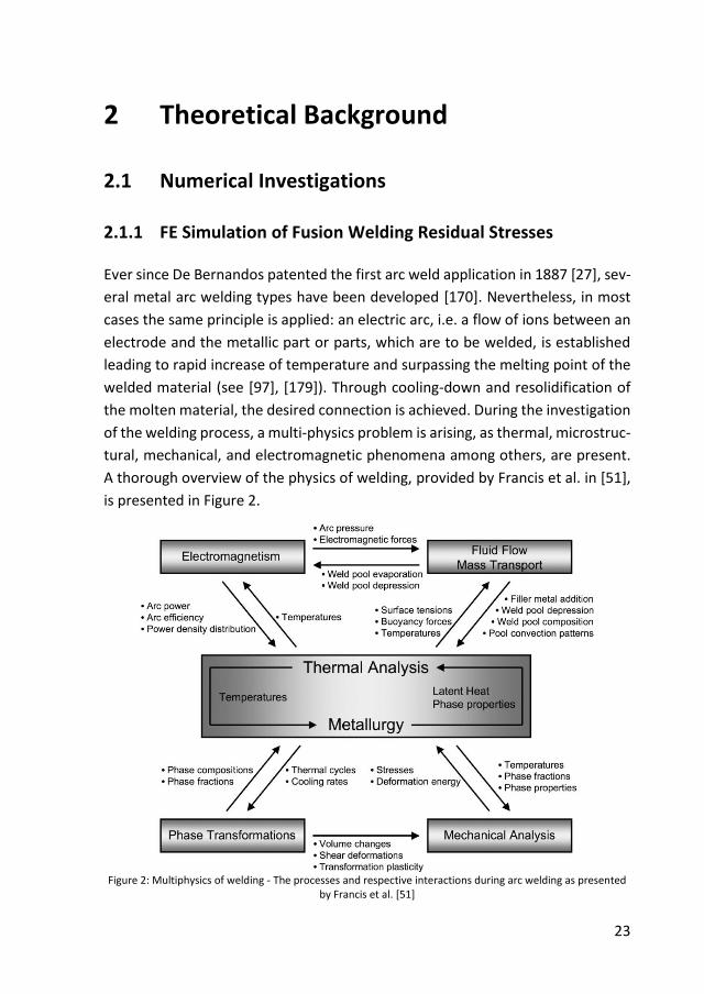
Figure 2: Multiphysics of welding - The processes and respective interactions during arc welding as presented by Francis et al. [51] ........................................ 23
Figure 3: Theoretical profiles of WRS found in [96]: a) Longitudinal WRS; (b) Transverse WRS, “with external constraint” stands for the case of clamped longitudinal sides ................................................................................................. 24
Figure 4: Investigated fields and respective interactions in an engineering approach for arc welding simulation – Arrows with broken and continuous contour are symbolizing the existing and the considered interactions respectively ............................................................................................................................. 26
Figure 5: The Goldak’s heat source model, figure found in [186] ....................... 28
Figure 6: Sensitivity analysis for the heat source parameters (N to T are different sets of heat source parameters a, c, fr and ff) and real temperature measurements of a thermal cycle in the HAZ during welding for HT- 36 steel – Published in [92], measurements and welding parameters were found in [3] .. 30
Figure 7: Carbon steel weld: a) HAZ; b) Phase diagram (found in [96], γ stands for austenite and α for ferrite).................................................................................. 31
Figure 8: CCT diagram of steel S355, found elsewhere [69] ............................... 34
Figure 9: Modelling principle of heating and cooling in the Gkatzogiannis-Knoedel-Ummenhofer engineering approach, A1 and A3 are symbolized as AC1 and AC3 respectively, figure found in [69] ........................................................................ 36
Figure 10: Application example of the proposed method: the areas of the component, with different material models during cooling-down: CMM4 was assigned to blue areas; CMM3 was assigned to red areas; CMM2 was assigned to purple areas; rest of the plate is preserving CMM1 (parent material) ............... 37
Figure 11: The arbitrary reduction of yield strength in the respective temperature range proposed by Karlsson for the consideration of TRIP during welding simulation, based on a diagram from [87] .......................................................... 38
Figure 12: Dilatometric curves found in [39]....................................................... 40
Figure 13: Modelling of restrained-free component by using springs with low stiffness, previously presented in [92] ................................................................ 45
List of Figures
6
Figure 14: Investigated setups of linear spring elements for modelling the clamping mechanisms [53] .................................................................................. 46
Figure 15: Introduced RS from various treatments on the surface of a mechanical component of steel [149] .................................................................................... 47
Figure 16: WRS profiles of welded plates with thickness of 8 mm, at as welded, after milling and after cutting states [26]............................................................ 48
Figure 17: Simulated RS profiles in depth direction for different yield strength values of the investigated material, found in [103] – Component with thickness of 12 mm .................................................................................................................. 50
Figure 18: Correlation of static and dynamic yield stress based in experimental data from various studies carried out by Symonds [157], found in [86] ............. 51
Figure 19: Comparison between dynamic yield strength in tension and in compression, based on a diagram found in [20] ................................................. 52
Figure 20: SRS of UFG and CG Al 99.5, m corresponds to mSRS of Equation (25), n = 1/m [117] .......................................................................................................... 54
Figure 21: Shot-peening simulation with elastic (EDS), rigid (RS) and plastic (PDS) shots compared with measured RS, found elsewhere [90] ................................ 58
Figure 22: Measurement of the HFMI groove with the LIMESS measurement system; a) Measurement of a fillet weld; b) 3D depiction of the measured surface and the measurement lines ................................................................................. 58
Figure 23: Measuring the contact force of the PITec device and its correlation to working frequency, found in [44] ....................................................................... 59
Figure 24: Relationship between mean pressure pm and yield stress (marked as Y) and non-dimensional strain found in [82] ....................................................... 64
Figure 25: Contour of hoop stresses predicted by a FE model by Boyce et al. [16] for the impact of a rigid sphere with 200 m/s (a) and 300 m/s (b) on a plate of Ti-6Al-4V alloy – Stresses and distance from crater’s centre are normalized to the static yield strength and the crater diameter respectively – W is the diameter of the crater ............................................................................................................. 67
Figure 26: Measured RS introduced by shot peening for 1 to 4 impacts of 0.5 mm diameter shots and velocity of 100 m/s, a crater diameter of 0.1 mm is calculated based on figures found in the literature source, found in [63] ........................... 67
Figure 27: Transverse residual stress through-depth profiles in UIT-treated fields for variating treatment intensity and for a pin diameter of 4.8 mm in the base material S690, crater swallower than 0.5 mm, based on a diagram found in [130] ............................................................................................................................. 68
List of Figures
7
Figure 28: Component A previously investigated in [3], dimensions are given in mm – Four clampers were applied on each side, the applied symmetry condition is presented as well ............................................................................................. 73
Figure 29: Cross section of component A, dimensions are given in mm – The applied symmetry condition is presented as well ............................................... 74
Figure 30: Component B previously investigated in [21], dimensions are given in mm – No restraints during welding, the applied symmetry condition is presented as well .................................................................................................................. 74
Figure 31: Cross section of component B, dimensions are given in mm – The applied symmetry condition is presented as well ............................................... 74
Figure 32: CCT diagram of steel HT36, from [3] .................................................. 76
Figure 33: Pattern of applied mesh - CC1 mesh on the cross section of component A........................................................................................................................... 80
Figure 34: Results of the convergence study ...................................................... 81
Figure 35: Location of the thermocouples A, B and C, dimensions are given in mm ............................................................................................................................. 82
Figure 36: Dimensioning heat source – Simulated and measured temperature history at point A ................................................................................................. 83
Figure 37: Dimensioning heat source – Simulated and measured temperature history at point B ................................................................................................. 83
Figure 38: Dimensioning heat source – Simulated and measured temperature history at point C ................................................................................................. 84
Figure 39: Modelling of thermal losses – Simulated and measured temperature history at point A ................................................................................................. 85
Figure 40: Modelling of thermal losses – Simulated and measured temperature history at point B ................................................................................................. 86
Figure 41: Modelling of thermal losses – Simulated and measured temperature history at point C ................................................................................................. 86
Figure 42: Contour plot of longitudinal WRS – Top side of component A – Stresses are given in Pa – Initially published in [92] ......................................................... 87
Figure 43: Contour plot of transverse WRS – Top side of component A – Stresses are given in Pa – Initially published in [92] ......................................................... 88
Figure 44: Validation of longitudinal WRS at the centre of the top side of component A adjacent to weld line – Measurements found in [3] – The cross
List of Figures
8
section of the component at its centre transverse to the weld line along with the assigned CMMs and the symmetry condition are illustrated at the bottom ...... 89
Figure 45: Validation of transverse WRS at the centre of the top side of component A adjacent to weld line – (Gkatzogiannis, 2017) refers to [92] – Measurements found in [3] ................................................................................. 91
Figure 46: Longitudinal WRS at the centre of the top side of component A adjacent to weld line – (Gkatzogiannis, 2017) refers to [92] – Influence of boundary conditions ............................................................................................................ 93
Figure 47: Transverse WRS at the centre of the top side of component A adjacent to weld line – (Gkatzogiannis, 2017) refers to [92] – Influence of boundary conditions ............................................................................................................ 94
Figure 48: Longitudinal WRS at the centre of the top side of component B adjacent to weld line – Measurements found in [21] – Simulation of restraint-free conditions ............................................................................................................ 95
Figure 49: Transverse WRS at the centre of the top side of component B adjacent to weld line – Measurements found in [21] – Simulation of restraint-free conditions ............................................................................................................ 96
Figure 50: Longitudinal WRS at the centre of the top side of component A adjacent to weld line – Measurements found in [21] – Influence of hardening behaviour ............................................................................................................................. 97
Figure 51: Longitudinal WRS at the centre of the top side of component B adjacent to weld line – Measurements found in [21] – Influence of Tref ......................... 98
Figure 52: Transverse WRS at the centre of the top side of component B adjacent to weld line – Measurements found in [21] – Influence of Tref ......................... 99
Figure 53: Fitting of the Perzyna model to the experimental data found in [46], [47], [48], [49] and [91] with MATLAB: a) At 20 °C; b) At 400 °C; c) At 550 °C; d) At 700 °C ................................................................................................................. 100
Figure 54: Longitudinal WRS at the centre of the top side of component B adjacent to weld line – Measurements found in [21] – Strain rate dependency of simulated WRS.................................................................................................................... 101
Figure 55: Transverse WRS at the centre of the top side of component B adjacent to weld line – Measurements found in [21] – Strain rate dependency of simulated WRS.................................................................................................................... 101
Figure 56: Fillet welds of the project HFH-Simulation, two clampers were applied on the left side during welding – Dimensions are given in mm (setup FWBC1) 106
List of Figures
9
Figure 57: Component of the project HFH-Simulation, two clampers were applied on the left side during welding – Dimensions are given in mm (setup FWBC1) 106
Figure 58: Mesh applied for the simulations of fillet welds: a) Top view; b) Isometric view ................................................................................................... 107
Figure 59: The real component of the project HFH-Simulation made of steel S355 after completion of the welding procedure – The clamping mechanisms are seen on the left side................................................................................................... 108
Figure 60: Welded plates of S690 from the project HFH-Simulation ................ 108
Figure 61: WRS measurements from the project HFH-Simulation ................... 110
Figure 62: CCT diagram for steel S355, based on a diagram found in [147] ..... 112
Figure 63: CCT diagram for steel S690 found in [12] ......................................... 115
Figure 64: Vickers Hardness measurements (HV) carried out on FW960 by IWM in the framework of [146] ..................................................................................... 118
Figure 65: Macrosections of the investigated fillet welds taken by IWM [146] – Measurement of the weld pool size .................................................................. 120
Figure 66: Macrosections of the investigated fillet welds taken by IWM [146] – Measurement of the weld pool size .................................................................. 121
Figure 67: Quantitative temperature contours in the weld zone – Temperatures in oC ................................................................................................................... 122
Figure 68: Comparison of the thermal analysis and thermocouples measurements of FW355 ........................................................................................................... 123
Figure 69: Comparison of the thermal analysis and thermocouples measurements of FW960 ........................................................................................................... 123
Figure 70: Longitudinal WRS at the centre of component FW355 – Influence of Tref .................................................................................................................... 125
Figure 71: Transverse WRS at the centre of component FW355 – Influence of Tref ........................................................................................................................... 126
Figure 72: Longitudinal WRS at the centre of component FW355 – measured WRS from the 1st pass are mirrored on the right side .............................................. 128
Figure 73: Longitudinal WRS at the centre of component FW690 ................... 128
Figure 74: Longitudinal WRS at the centre of component FW960 ................... 129
Figure 75: CMM assignment for S355 (CMM 5 identical with CMM 4 but with Tref (melted material), Material 1 is PM): a) 1st pass; b) 4th pass .......................... 130
List of Figures
10
Figure 76: Transverse WRS at the centre of component FW355 ...................... 131
Figure 77: Transverse WRS at the centre of component FW690 ...................... 132
Figure 78: Transverse WRS at the centre of component FW960 ...................... 133
Figure 79: Longitudinal WRS at the centre of component FW960 – Influence of symmetric welding ............................................................................................ 134
Figure 80: Transverse WRS at the centre of component FW960 – Influence of symmetric welding ............................................................................................ 134
Figure 81: Longitudinal WRS at the centre of component FW960 – Influence of clamping setup .................................................................................................. 136
Figure 82: Transverse WRS at the centre of component FW960 – Influence of clamping setup .................................................................................................. 136
Figure 83: Influence of introducing shot blasting pseudothermal modelling in the present weld simulation .................................................................................... 138
Figure 84: Transverse WRS of the whole plate FW355 – Contour of the single specimen is marked with black line – Stresses are given in Pa ......................... 140
Figure 85: Transverse WRS of the cut specimen from FW355 – Area of deactivated elements are presented in grey – Stresses are given in Pa ............................... 140
Figure 86: Stress relaxation of longitudinal WRS due to cut of specimen from component FW960 transverse to the weld line at the centre of the component ........................................................................................................................... 141
Figure 87: Stress relaxation of transverse WRS due to cut of specimen from component FW960 transverse to the weld line at the centre of the component ........................................................................................................................... 141
Figure 88: Stress relaxation of WRS due to cut of specimen from component FW960 along the weld toe of the 4th weld pass ............................................... 142
Figure 89: Flowchart for the calibration of the strain rate dependent material behaviour through the implementation of the drop tests ................................ 146
Figure 90: Experimental setup for the implementation of drop tests .............. 148
Figure 91: Upper surface of investigated specimen of S355 and the craters for the 4 impacts ........................................................................................................... 148
Figure 92: Introduction of the plastic strain spherical zone underneath the impact surface: a) Maximum von Mises strain rate; (b) Maximum shear strain rate .. 151
Figure 93: Average plastic shear strain rate as a function of impact velocity for the drop tests on S355 ............................................................................................. 151
List of Figures
11
Figure 94: Crater on specimen of S960 under stereomicroscope, impact speed of 3.9 m/s ............................................................................................................... 152
Figure 95: Selected frames from impact 3A: a) Impact complex still not in the frame; b) Impact assembly enters the frame and reaches for the target; c) Rebound peak; d) Initiation of secondary free fall ............................................ 153
Figure 96: The dynamic yield strength of S355 as a function of the strain rate, results from present drop tests and previous studies by Foehrenbach et al. [44], Cadoni et al. [20] and Forni et al. [47] ............................................................... 158
Figure 97: Convergence study for the numerical investigation of HFMI treatment – RS after 0.01 s of simulation with global damping Ds = 0.5 (Ds and mesh size are marked as D and ms rspectively)....................................................................... 164
Figure 98: Investigated specimen of parent material with dimensions 20 mm x 20 mm x 10 mm with a symmetry plane at the middle – A HFMI pin with diameter of 4 mm is considered ........................................................................................... 165
Figure 99: Mesh applied on the specimen of parent material .......................... 166
Figure 100: Diagram of σ-ε (real) and the applied bilinear material models for the investigated material – Hollow symbols mark extrapolated values – BM stands for bilinear model ................................................................................................... 167
Figure 101: Diagram of vertical and longitudinal displacement of the pin, for 3 consecutive passes during a displacement-based simulation .......................... 169
Figure 102: Diagram of accelerating force and longitudinal displacement of the pin over time, for 3 consecutive passes during a velocity-based simulation .... 171
Figure 103: Diagram of vertical velocity of HFMI Pin for the first 0.04 s of the simulation .......................................................................................................... 171
Figure 104: WRS simulated with the displacement-based method, compared with previous numerical results [54] and WRS measurements found in [44] and [145] ........................................................................................................................... 173
Figure 105: Simulated and measured transverse RS - Component of parent material S355 – (Schubnell, 2019) measurements were found in [44] and [145] ........................................................................................................................... 177
Figure 106: Simulated and measured longitudinal RS - Component of parent material S355 – (Schubnell, 2019) measurements were found in [44] and [145] ........................................................................................................................... 177
Figure 107: Simulated and measured transverse RS - Component of parent material S690 – (Schubnell, 2019) measurements were found in [145]........... 179

List of Figures
12
Figure 108: Simulated and measured longitudinal RS - Component of parent material S690 – (Schubnell, 2019) measurements were found in [145] ........... 179
Figure 109: Simulated and measured transverse RS - component of parent material S960 – (Schubnell, 2019) measurements were found in [145] ........... 180
Figure 110: Simulated and measured longitudinal RS - Component of parent material S960 – (Schubnell, 2019) measurements were found in [145] ........... 180
Figure 111: Stress contour plots of the specimen of parent material after the end of the treatment for the strain rate dependent case, calibrated based on compressive material testing – Stresses are given in MPa: a) Longitudinal (Y); b) Transverse (X) .................................................................................................... 182
Figure 112: Modelled geometry and the assigned mesh inside and near the treatment area, for the investigation of the HFMI treatment on fillet welds of S355 ................................................................................................................... 186
Figure 113: Modelled geometry and assigned mesh for the investigation of the HFMI treatment on fillet welds of S960 ............................................................ 187
Figure 114: Initial position of the pin: a) Lateral view; b) Isometric view and the local and global coordinate systems ................................................................. 191
Figure 115: Results of the convergence study for the simulation of fillet welds ........................................................................................................................... 194
Figure 116: Final mesh for the simulation of FW960 ........................................ 195
Figure 117: Initial geometry of the weld toe and the introduced HFMI groove after the 1st pass of the treatment: a) Without fillet; b) 0.1 mm; fillet; c) 0.2 mm fillet; d) 0.5 mm fillet .................................................................................................. 197
Figure 118: Transverse RS in the HFMI crater at the middle of the component perpendicular to the treatment ........................................................................ 198
Figure 119: Displacement orthogonal to the upper plate surface inside the modelled HFMI groove perpendicular to the treatment line............................ 199
Figure 120: Contour plot of transverse WRS at the beginning of the HFMI simulation – Stresses are given in MPa ............................................................. 201
Figure 121: Transverse RS profiles at the middle of the component on the side of the HFMI simulated weld toe ............................................................................ 202
Figure 122: Simulated and measured transverse RS profiles on the surface of the S355 specimen treated with a pin of 3 mm diameter, perpendicular to the HFMI groove – Measurements from [146] ................................................................. 204
List of Figures
13
Figure 123: Simulated and measured transverse RS profiles in depth direction at the weld toe of the S355 specimen treated with a pin of 3 mm diameter, at the middle of the specimen – Measurements from [146] ...................................... 206
Figure 124: Simulated and measured longitudinal RS profiles in depth direction at the weld toe of the S355 specimen treated with a pin of 3 mm diameter, at the middle of the specimen – Measurements from [146] ...................................... 206
Figure 125: The applied mesh and RS contours of the model A3 inside and near the HFMI groove – Section at the middle of the investigated component – Stresses are given in MPa: a) Transverse; b) Longitudinal .............................................. 208
Figure 126: Simulated and measured transverse RS profiles on the surface of the S355 specimen treated with a pin of 4 mm diameter, perpendicular to the HFMI groove – Measurements from [146] ................................................................. 210
Figure 127: Simulated and measured transverse RS profiles in depth direction at the weld toe of the S355 specimen treated with a pin of 4 mm diameter, at the middle of the specimen – Measurements from [146] ...................................... 211
Figure 128: Simulated and measured longitudinal RS profiles in depth direction at the weld toe of the S355 specimen treated with a pin of 4 mm diameter, at the middle of the specimen – Measurements from [146] ...................................... 212
Figure 129: RS contours of the model B2 inside and near the HFMI groove– Section at the middle of the investigated component – Stresses are given in MPa: a) Transverse; b) Longitudinal ........................................................................... 213
Figure 130: Simulated and measured transverse RS profiles on the surface of the S960 specimen, perpendicular to the HFMI groove – Measurements from [146] ........................................................................................................................... 215
Figure 131: Simulated and measured transverse RS profiles in depth direction at the weld toe of the S960 specimen treated with a pin of 3 mm diameter, at the middle of the specimen – Measurements from [146] ...................................... 216
Figure 132: Simulated and measured longitudinal RS profiles in depth direction at the weld toe of the S960 specimen treated with a pin of 3 mm diameter, at the middle of the specimen – Measurements from [146] ...................................... 217
Figure 133: RS contours of the model C2 inside and near the HFMI groove – Section at the middle of the investigated component – Stresses are given in MPa: a) Transverse; b) Longitudinal ........................................................................... 218
Figure 134: Simulated and measured transverse RS profiles on the surface of the S960 specimen treated with a pin of 4 mm diameter, perpendicular to the HFMI groove – Measurements from [146] ................................................................. 220

List of Figures
14
Figure 135: Simulated and measured transverse RS profiles in depth direction at the weld toe of the S960 specimen treated with a pin of 4 mm diameter, at the middle of the specimen – Measurements from [146] ...................................... 221
Figure 136: Simulated and measured longitudinal RS profiles in depth direction at the weld toe of the S355 specimen treated with a pin of 4 mm diameter, at the middle of the specimen – Measurements from [146] ...................................... 221
15
1 Introduction
1.1 Problem Statement
It was more than 50 years past the first patented application of welding in Russia
at the end of the 19th century [27], when engineers started to realize the phe-
nomenon of fatigue fracture in weldments. Events like the collapses of the Point
Pleasant Bridge in the US and the Alexander Kielland offshore platform in Norway,
which were caused due to fatigue cracking of welded connections and led to
losses of human lives [66], increased the awareness regarding fatigue design and
exhibited the vulnerability of welded joints against cyclic loading1. Ever since,
methods and recommendations regarding fatigue design ([35], [76] e.g.), steel
quality ([29] e.g.), welding quality ([79] e.g.) and non-destructive testing ([80]
e.g.) have been developed and activated respectively. Therewith, the fatigue life
of steel structures can be predicted with safety, the ductile performance of the
parent material and the welded joint are assured and joining defects can be
avoided or detected.
Nonetheless, welded joints remain the Achilles heel of steel structures, when
they are subjected to fatigue loading. The fatigue strength of welds lies signifi-
cantly lower than that of parent material due to the notch effect and the respec-
tive concentration factor, the tensile welding residual stresses (WRS)2, the una-
voidable welding defects and the reduced ductility of the heat-affected zone
(HAZ). Hence, extending fatigue life of welded joints leads to significant increase
of a construction’s life cycle.
Several methods have been developed in the last decades with the purpose of
increasing fatigue life of welds, with High Frequency Mechanical Impact treat-
ment3 (HFMI) [118] being one of the most straightforward and effective (see
[167]). It can be applied through the use of a device by the craftsman or by a robot
both during manufacturing process and on existing and new structures in the
1 the problem of fatigue regarding parent (unwelded) metallic materials was already known from the 19th cen-tury, worth mentioning are the Versailles rail accident and the work of Julius Albert and August Wöhler
2 a list of abbreviations is given at the end of the present dissertation at page 242
3 or Hochfrequetes Hämmerverfahren (HFH) in German
1 Introduction
16
field. Therewith, a significant increase of fatigue strength of even more than
100 % in some cases is possible (see [118]). The first HFMI application was de-
signed in the 70’s in the Soviet Union under the name Ultrasonic Impact Treat-
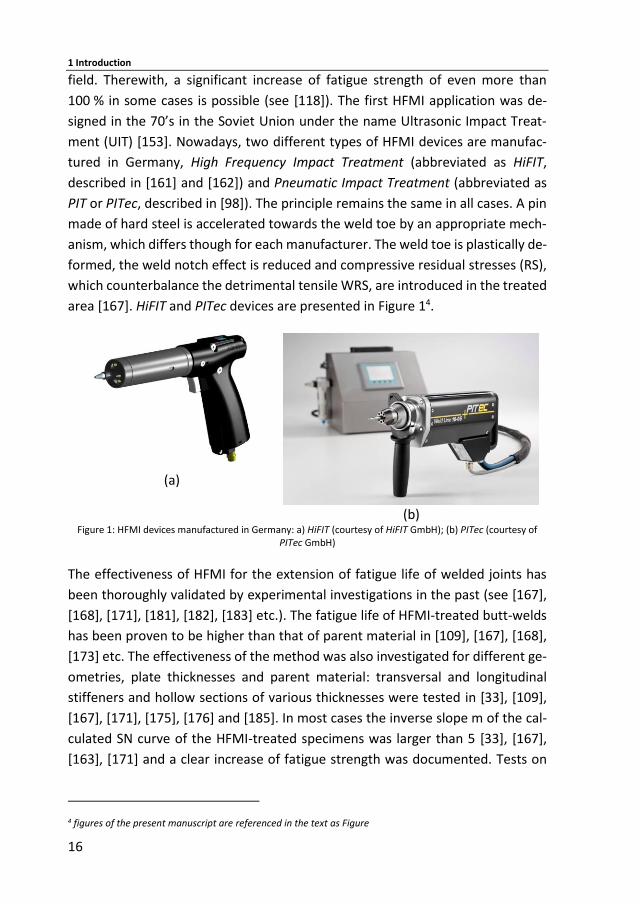
ment (UIT) [153]. Nowadays, two different types of HFMI devices are manufac-
tured in Germany, High Frequency Impact Treatment (abbreviated as HiFIT,
described in [161] and [162]) and Pneumatic Impact Treatment (abbreviated as
PIT or PITec, described in [98]). The principle remains the same in all cases. A pin
made of hard steel is accelerated towards the weld toe by an appropriate mech-
anism, which differs though for each manufacturer. The weld toe is plastically de-
formed, the weld notch effect is reduced and compressive residual stresses (RS),
which counterbalance the detrimental tensile WRS, are introduced in the treated
area [167]. HiFIT and PITec devices are presented in Figure 14.
(a)
(b) Figure 1: HFMI devices manufactured in Germany: a) HiFIT (courtesy of HiFIT GmbH); (b) PITec (courtesy of
PITec GmbH)
The effectiveness of HFMI for the extension of fatigue life of welded joints has
been thoroughly validated by experimental investigations in the past (see [167],
[168], [171], [181], [182], [183] etc.). The fatigue life of HFMI-treated butt-welds
has been proven to be higher than that of parent material in [109], [167], [168],
[173] etc. The effectiveness of the method was also investigated for different ge-
ometries, plate thicknesses and parent material: transversal and longitudinal
stiffeners and hollow sections of various thicknesses were tested in [33], [109],
[167], [171], [175], [176] and [185]. In most cases the inverse slope m of the cal-
culated SN curve of the HFMI-treated specimens was larger than 5 [33], [167],
[163], [171] and a clear increase of fatigue strength was documented. Tests on
4 figures of the present manuscript are referenced in the text as Figure
1.1 Problem Statement
17
specimens made of S355, S690, S910, S1100 and S1300 ([33], [167], [168], [169],
[171], [174], [176] etc.) have displayed a dependency of the HFMI effectiveness
on the yield strength of the investigated material, with high strength steels dis-
playing more potential. The higher introduced compressive RS are to be ac-
counted for this increase in effectiveness. It is clear from the above, that the HFMI
enhancement of fatigue strength depends on many parameters and respective
factors for the consideration during the design of the increased fatigue life have
been proposed in [119], [172].
Extensive research on HFMI during the last two decades enabled the regulation
of the method by the International Institute of Welding (IIW) according to [118]
by analogy to existing recommendations for as-welded specimens (see [35], [76]).
Influence of material nominal yield strength and fatigue loading stress ratio was
as well taken into consideration. Nevertheless, the approach of SN curves and the
respective proposed FAT classes in both cases are quite conservative: the 95 %
confidence interval is proposed as the characteristic fatigue strength of each in-
vestigated notch detail. Moreover, the proposed FAT classes are calculated based
on several test series carried out by different research groups on welded speci-
mens, which are nominally identical, but in reality can qualitatively differ signifi-
cantly from each other. This problem is thoroughly described in [38]. Although
this approach is reasonable enough, when fatigue design recommendations for
the practitioner have to be compiled, extracted FAT classes can be too conserva-
tive for weldments of high quality.
Numerical modelling of HFMI could be a valuable alternative to costly fatigue
tests. Coupled with weld simulation it could enable a safe prediction of the RS
field, taking into consideration the various unique parameters of each investi-
gated case, such as welding parameters, notch effect, complex geometries, ma-
terial etc. The calculated WRS field should be input for an accurate calculation of
fatigue life through simulation of RS from HFMI. Computational welding mechan-
ics (see [60], [111]) have evolved rapidly in the last decades and results with sat-
isfying precision regarding WRS and respective deformation can be extracted
[57]. Some numerical investigations of HFMI have been carried out during the
last years as well, neglecting however in most cases significant effects of the pro-
cess (see, [1], [44], [68], [98], [99], [103], [142], [150], [167], [187], etc.). For ex-
ample, precise modelling of material behaviour, as a high-speed impact event is
simulated, movement of the HFMI pin, boundary conditions as well as WRS is re-
quired. These aspects were taken into consideration only in very recent studies,
1 Introduction
18
which were published parallel and shortly prior to the conclusion of the present
dissertation [36], [108].
Objective of the present study is the establishment of a validated engineering ap-
proach for the simulation of HFMI, taking into consideration all the significant as-
pects of the process, in order to provide a robust prediction of the introduced RS.
The developed approach should serve a dual role. It should be applicable both for
research purpose, whereby it could be used as a tool for sensitivity analyses and
in extension further investigation and improvement of the method, and in prac-
tice, in order achieve less conservative design. During the development of the
presented method, all predominant factors that affect RS should be considered.
The application of the method should be straightforward, meaning that special
knowledge of physical metallurgy apart from the basic knowledge of material sci-
ence taught to undergraduate level of engineering would not be required, with-
out compromising though the preciseness of the results.
1.2 Research Methodology
The subject of the present study can be divided into two major fields, the weld
process and the HFMI simulation. Although the main subject of the presented
study is numerical, analytical calculations as part of the method were deployed,
when it was considered necessary. Moreover, experimental results, which were
extracted in the framework of the present or others studies ([3], [21], [146]) were
used as input for the developed approach or for validation of the results.
Several investigations regarding the first field have been presented in a series of
previous publications by the author, which were carried out in the framework of
the present doctoral dissertation. A straightforward, appropriate for practical ap-
plications approach for modelling the WRS was developed [92] and validated
based on measurements found elsewhere [1], [21]. The method was extended in
[20], [55] and [56] for simulating various materials and used for sensitivity anal-
yses regarding parameters of material modelling [53], welding parameters [56]
and boundary conditions [55], [57]. The model was adapted and revalidated for
the presently investigated materials, based on measurements from the research
project HFH-Simulation [146]. Whenever possible, values from literature were ap-
plied for common material properties. As the above-mentioned publications
were carried out in the framework of the present doctoral dissertation, the main
1.2 Research Methodology
19
aspects of the method are thoroughly presented in this study as well, when nec-
essary. Commercial FE software ANSYS was applied for all numerical investiga-
tions of weld processes [4].
Material data, which was used as input for the HFMI simulation, was extracted
from drop tests. The results of the drop tests were evaluated based on appropri-
ate analytical and numerical calculations and were compared with respective ex-
perimental results for the same batches of the investigated materials from HFH-
Simulation [146]. In this case as well, values from literature were applied for com-
mon material properties, when it was considered that the preciseness would not
be compromised. Results from a previous study, wherein the HFMI treatment of
an unnotched plate was investigated, were used for a first step validation of the
developed HFMI modelling approach [44]. After the HFMI simulation model was
validated, it was coupled with the welding simulation model and the results were
once again validated based on the measurements from the research project HFH-
Simulation [146]. During the development and validation of the present ap-
proach, significant conclusions regarding practical aspects of the HFMI simulation
were drawn. Material modelling, definition of boundary conditions, simulation of
real scale fatigue tests and modelling techniques regarding the motion of HFMI
pin were investigated amongst others. The commercial FE software LS-Dyna was
applied for all numerical investigations of the HFMI treatment [114].
As it was mentioned above, the developed approach should be appropriate for
both research and practical applications. Therefore, an appropriate balance be-
tween preciseness and computational effort should be held at all times. Ultimate
objective of the present study was to enable a safe prediction of the RS in the
areas of the components, which are susceptible to fatigue cracking i.e. the near-
surface region of the heat-affected zone, in order to allow for a safe estimation
of fatigue life. An empirical thumb rule of a deviation equal to ± 10 % of the in-
vestigated material’s yield stress or smaller between simulated and measured RS
at these areas of the components was considered sufficient and feasible for the
targeted engineering application and was fulfilled in most of the investigated
cases.
1 Introduction
20
1.3 High Performance Computing
The high performance research computer ForHLR I of the Steinbuch Centre for
Computing at the Karlsruhe Institute of Technology was applied for carrying out
the numerical investigations of the present doctoral dissertation. In the case of
the welding simulations in ANSYS [4], a fat node was used for Parallel Processing
with 16 processors. Initial memory request was set to 500 GB in each case. To
give an example, the duration of simulating a 1000 mm x 370 mm x 10 mm, 4-
pass fillet weld, meshed with 175827 nodes and 160296 elements using these
computing resources was in real time 97 hours 45 min and 34 seconds. In the case
of the HFMI simulation, 16 nodes with 16 processors each were applied with Mas-
sive Parallel Processing (MPP). For simulating the 3-pass treatment of a compo-
nent with dimensions of 20 mm x 20 mm x 10 mm, meshed with 195640 nodes
and 208022 elements, 7 hours 21 minutes and 52 seconds elapsed. Deployment
of up to 512 processors in total was the upper limit regarding HFMI simulations,
due to the available number of LS Dyna licenses [113].
1.4 Outline of the Present Dissertation
The present dissertation is organised in 7 chapters, the present introductory one
and seven more. In the 2nd chapter, a thorough review of the theoretical back-
ground for the present analytical and numerical investigations is made. The ana-
lytical investigations were carried out in order to evaluate the above-described
drop tests. The theoretical background of all numerical investigations, which are
necessary for the calculation of RS from welding and HFMI is presented as well.
The highlights of previous work by other authors and the author of the present
dissertation are exhibited, so that a comprehensive overview of the state of the
art regarding the present subject becomes available to the reader.
In the 3rd chapter the numerical investigations regarding residual stresses from
welding, which were carried out in the framework of the present study, are pre-
sented. Mesh and modelling restrictions are discussed. After a detailed analysis
of the applied methodology, results regarding three different weldments are pre-
sented. A series of investigations, regarding the influence of various practical and
special aspects of weld simulation, like boundary conditions, material modelling
1.4 Outline of the Present Dissertation
21
and welding parameters etc. on the modelled WRS is presented. Conclusions re-
garding the welding simulation and recommendations regarding future work are
summarized at the end of the chapter.
The 4th chapter reports on the experimental investigations, which were carried
out in the framework of the present study, along with the analytical and numeri-
cal models, which were applied for the evaluation of the test results. The test set
up is described thoroughly and restrictions and errors that arise are reported. The
inevitable assumptions for the simplifications of the analytical model are high-
lighted. The test results and the extracted material properties are presented and
compared with respective results from other sources.
In the 5th chapter, the numerical study on HFMI and the introduced RS is de-
scribed. The methodology and the results of some preliminary investigations are
outlined. The numerical study of the HFMI treatment for two different geome-
tries is reported. Therewith, the influence of various aspects of the simulation
process on the modelled RS are investigated, analogously to the case of WRS in
the previous chapter. Both numerical approaches and practical aspects are dis-
cussed. Based on the present results, a review of the recommendations from pre-
vious studies is made as well. Explicit conclusions for the case of HFMI modelling
and recommendations regarding future work are highlighted at the end of this
chapter.
Finally, as specific conclusions and recommendations regarding future work over
welding and HFMI simulation are presented in the previous respective chapters,
a general discussion regarding the present dissertation and a proposal regarding
the implementation of the present method in a holistic numerical approach re-
garding fatigue of metals are presented in chapters 6 and 7.

23
2 Theoretical Background
2.1 Numerical Investigations
2.1.1 FE Simulation of Fusion Welding Residual Stresses
Ever since De Bernandos patented the first arc weld application in 1887 [27], sev-
eral metal arc welding types have been developed [170]. Nevertheless, in most
cases the same principle is applied: an electric arc, i.e. a flow of ions between an
electrode and the metallic part or parts, which are to be welded, is established
leading to rapid increase of temperature and surpassing the melting point of the
welded material (see [97], [179]). Through cooling-down and resolidification of
the molten material, the desired connection is achieved. During the investigation
of the welding process, a multi-physics problem is arising, as thermal, microstruc-
tural, mechanical, and electromagnetic phenomena among others, are present.
A thorough overview of the physics of welding, provided by Francis et al. in [51],
is presented in Figure 2.
Figure 2: Multiphysics of welding - The processes and respective interactions during arc welding as presented
by Francis et al. [51]
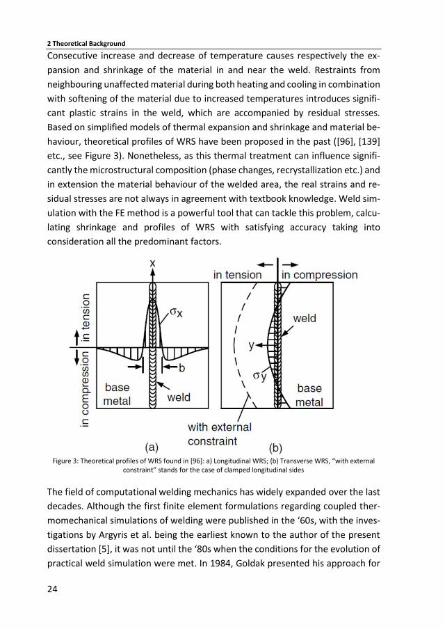
2 Theoretical Background
24
Consecutive increase and decrease of temperature causes respectively the ex-
pansion and shrinkage of the material in and near the weld. Restraints from
neighbouring unaffected material during both heating and cooling in combination
with softening of the material due to increased temperatures introduces signifi-
cant plastic strains in the weld, which are accompanied by residual stresses.
Based on simplified models of thermal expansion and shrinkage and material be-
haviour, theoretical profiles of WRS have been proposed in the past ([96], [139]
etc., see Figure 3). Nonetheless, as this thermal treatment can influence signifi-
cantly the microstructural composition (phase changes, recrystallization etc.) and
in extension the material behaviour of the welded area, the real strains and re-
sidual stresses are not always in agreement with textbook knowledge. Weld sim-
ulation with the FE method is a powerful tool that can tackle this problem, calcu-
lating shrinkage and profiles of WRS with satisfying accuracy taking into
consideration all the predominant factors.
Figure 3: Theoretical profiles of WRS found in [96]: a) Longitudinal WRS; (b) Transverse WRS, “with external
constraint” stands for the case of clamped longitudinal sides
The field of computational welding mechanics has widely expanded over the last
decades. Although the first finite element formulations regarding coupled ther-
momechanical simulations of welding were published in the ‘60s, with the inves-
tigations by Argyris et al. being the earliest known to the author of the present
dissertation [5], it was not until the ‘80s when the conditions for the evolution of
practical weld simulation were met. In 1984, Goldak presented his approach for
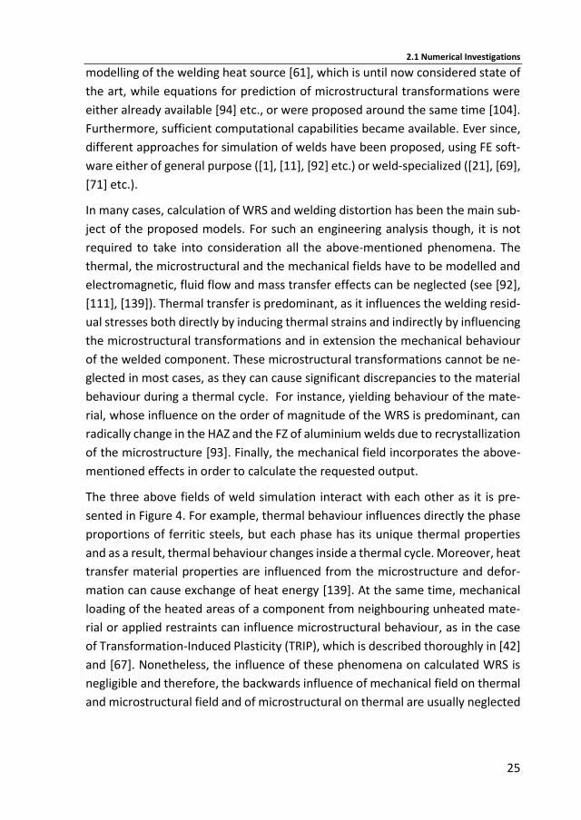
2.1 Numerical Investigations
25
modelling of the welding heat source [61], which is until now considered state of
the art, while equations for prediction of microstructural transformations were
either already available [94] etc., or were proposed around the same time [104].
Furthermore, sufficient computational capabilities became available. Ever since,
different approaches for simulation of welds have been proposed, using FE soft-
ware either of general purpose ([1], [11], [92] etc.) or weld-specialized ([21], [69],
[71] etc.).
In many cases, calculation of WRS and welding distortion has been the main sub-
ject of the proposed models. For such an engineering analysis though, it is not
required to take into consideration all the above-mentioned phenomena. The
thermal, the microstructural and the mechanical fields have to be modelled and
electromagnetic, fluid flow and mass transfer effects can be neglected (see [92],
[111], [139]). Thermal transfer is predominant, as it influences the welding resid-
ual stresses both directly by inducing thermal strains and indirectly by influencing
the microstructural transformations and in extension the mechanical behaviour
of the welded component. These microstructural transformations cannot be ne-
glected in most cases, as they can cause significant discrepancies to the material
behaviour during a thermal cycle. For instance, yielding behaviour of the mate-
rial, whose influence on the order of magnitude of the WRS is predominant, can
radically change in the HAZ and the FZ of aluminium welds due to recrystallization
of the microstructure [93]. Finally, the mechanical field incorporates the above-
mentioned effects in order to calculate the requested output.
The three above fields of weld simulation interact with each other as it is pre-
sented in Figure 4. For example, thermal behaviour influences directly the phase
proportions of ferritic steels, but each phase has its unique thermal properties
and as a result, thermal behaviour changes inside a thermal cycle. Moreover, heat
transfer material properties are influenced from the microstructure and defor-
mation can cause exchange of heat energy [139]. At the same time, mechanical
loading of the heated areas of a component from neighbouring unheated mate-
rial or applied restraints can influence microstructural behaviour, as in the case
of Transformation-Induced Plasticity (TRIP), which is described thoroughly in [42]
and [67]. Nonetheless, the influence of these phenomena on calculated WRS is
negligible and therefore, the backwards influence of mechanical field on thermal
and microstructural field and of microstructural on thermal are usually neglected

2 Theoretical Background
26
(see for instance [92], [111] and [139]). Sole exception is the TRIP, whose influ-
ence on the WRS is non-negligible and consequently has to be taken into consid-
eration [87], [92].
Figure 4: Investigated fields and respective interactions in an engineering approach for arc welding simula-tion – Arrows with broken and continuous contour are symbolizing the existing and the considered inter-
actions respectively
2.1.1.1 Modelling of Thermal Field
As already mentioned, modelling of the thermal field includes the solution of the
heat-transfer problem. Ensuring sufficient preciseness during the calculation of
the WRS requires accurate modelling of the heat transfer inside the component
and use of temperature-dependent material properties. As mentioned above, the
influence of microstructure on thermal material behaviour is neglected and ther-
mal properties of parent material are usually applied for the whole investigated
thermal cycle [3], [21], [92]. Loading and boundary conditions of the problem are
the heat input from the weld heat source to the weld pool and heat losses from
the component to the environment respectively.
Welding Heat Source
The double ellipsoidal model of Figure 5, which was proposed by Goldak et al. in
1984 [61] is still considered state of the art for modelling the heat input into the
weld pool during simulations of metal arc welds (see [28], [71], [92] etc.). It can
be properly modified for different types of welds as well, such as in [128] for laser
welding. The model describes the power density distribution of each point around
the centre of a moving heat source as a function of time, and position of the point
about the centre, by using quadrants from two different ellipsoidal sources. The
two quadrants have common width and depth but different length in order to
properly model the elongation of the power heat distribution rear to the centre,
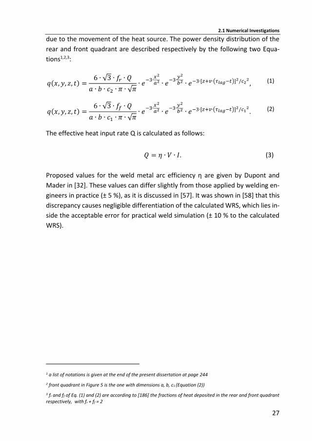
2.1 Numerical Investigations
27
due to the movement of the heat source. The power density distribution of the
rear and front quadrant are described respectively by the following two Equa-
tions1,2,3:
𝑞(𝑥, 𝑦, 𝑧, 𝑡) =6 ∙ √3 ∙ 𝑓𝑟 ∙ 𝑄
𝑎 ∙ 𝑏 ∙ 𝑐2 ∙ 𝜋 ∙ √𝜋∙ 𝑒
−3∙𝑥2
𝑎2 ∙ 𝑒−3∙
𝑦2
𝑏2 ∙ 𝑒−3∙[𝑧+𝑣∙(𝜏𝑙𝑎𝑔−𝑡)]2/𝑐22, (1)
𝑞(𝑥, 𝑦, 𝑧, 𝑡) =6 ∙ √3 ∙ 𝑓𝑓 ∙ 𝑄
𝑎 ∙ 𝑏 ∙ 𝑐1 ∙ 𝜋 ∙ √𝜋∙ 𝑒
−3∙𝑥2
𝑎2 ∙ 𝑒−3∙
𝑦2
𝑏2 ∙ 𝑒−3∙[𝑧+𝑣∙(𝜏𝑙𝑎𝑔−𝑡)]2/𝑐12. (2)
The effective heat input rate Q is calculated as follows:
𝑄 = 𝜂 ∙ 𝑉 ∙ 𝐼. (3)
Proposed values for the weld metal arc efficiency η are given by Dupont and
Mader in [32]. These values can differ slightly from those applied by welding en-
gineers in practice (± 5 %), as it is discussed in [57]. It was shown in [58] that this
discrepancy causes negligible differentiation of the calculated WRS, which lies in-
side the acceptable error for practical weld simulation (± 10 % to the calculated
WRS).
1 a list of notations is given at the end of the present dissertation at page 244
2 front quadrant in Figure 5 is the one with dimensions a, b, c1 (Equation (2))
3 fr and ff of Eq. (1) and (2) are according to [186] the fractions of heat deposited in the rear and front quadrant respectively, with fr + ff = 2
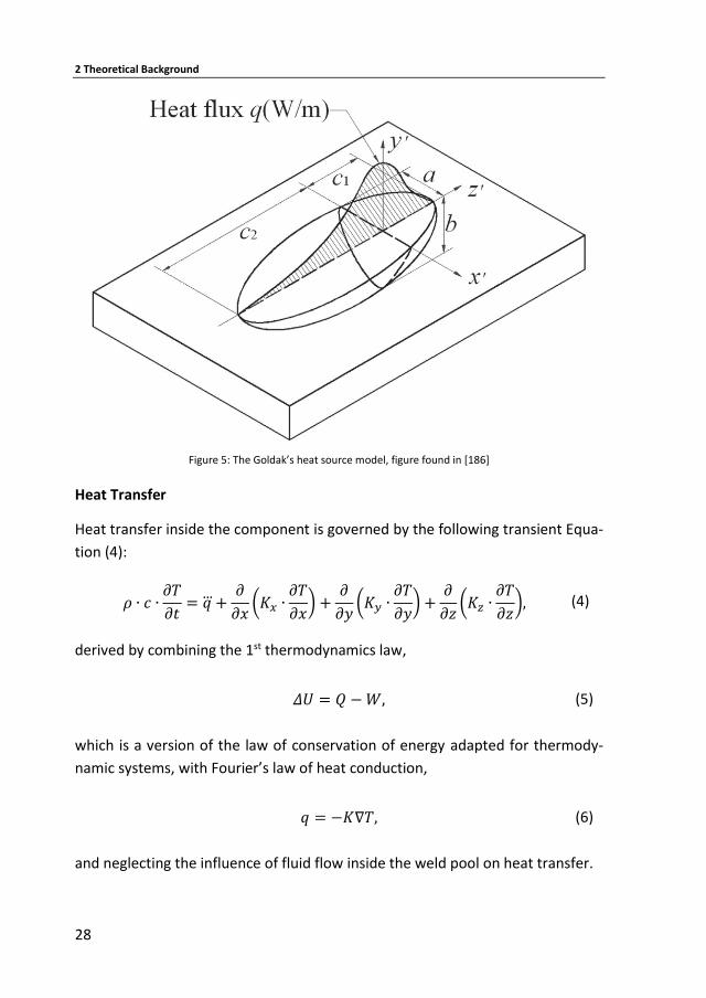
2 Theoretical Background
28
Figure 5: The Goldak’s heat source model, figure found in [186]
Heat Transfer
Heat transfer inside the component is governed by the following transient Equa-
tion (4):
𝜌 ∙ 𝑐 ∙𝜕𝑇
𝜕𝑡= 𝑞 +
𝜕
𝜕𝑥(𝐾𝑥 ∙
𝜕𝑇
𝜕𝑥) +
𝜕
𝜕𝑦(𝐾𝑦 ∙
𝜕𝑇
𝜕𝑦) +
𝜕
𝜕𝑧(𝐾𝑧 ∙
𝜕𝑇
𝜕𝑧), (4)
derived by combining the 1st thermodynamics law,
𝛥𝑈 = 𝑄 − 𝑊, (5)
which is a version of the law of conservation of energy adapted for thermody-
namic systems, with Fourier’s law of heat conduction,
𝑞 = −𝐾∇𝑇, (6)
and neglecting the influence of fluid flow inside the weld pool on heat transfer.
2.1 Numerical Investigations
29
Heat Losses
Heat losses from the component to the environment through convection and ra-
diation constitute the boundary conditions of the thermal problem. Heat loss due
to convection and radiation are described by Newton’s law of cooling,
q
A= hc ∙ (Ts − Tb) (7)
and Stefan-Boltzmann’s law,
q
A= hr ∙ (Ts − Tb)4, (8)
respectively. During the first weld-modelling applications, a temperature inde-
pendent value for the coefficient of heat losses was applied [3], [5]. In the latter
case, a more delicate approach was followed by applying a coefficient for the ma-
terial in the FZ, accounting for radiation effects as well. In any case, the influence
of radiation on heat losses at room temperature is negligible, but cannot be ne-
glected as it is becoming predominant at high temperatures. Therefore, its mod-
elling is necessary for precise thermal results inside and near the weld pool. New-
ton’s law of cooling, albeit is not anymore physically valid when radiation
becomes predominant, was applied with a modified coefficient for heat losses, in
order to account for the radiation effects as well in [5]. This approach has ever
since provided sufficient results ([1], [44], [140], [92] e.g.). Proposed values for
the total coefficient of heat losses hT applied instead of hC, were calculated in [1]
based on data found in [18].
2.1.1.2 Modelling of Microstructural Effects
Some microstructural properties of the metallic alloys influence their macro-
scopic mechanical behaviour. Their differentiation due to rapid heating and cool-
ing inside a welding thermal cycle has to be taken into consideration during weld-
ing simulation, in order to ensure that WRS are calculated with required
preciseness.
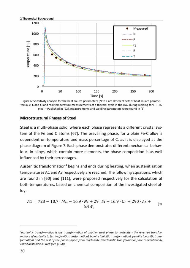
2 Theoretical Background
30
Figure 6: Sensitivity analysis for the heat source parameters (N to T are different sets of heat source parame-
ters a, c, fr and ff) and real temperature measurements of a thermal cycle in the HAZ during welding for HT- 36 steel – Published in [92], measurements and welding parameters were found in [3]
Microstructural Phases of Steel
Steel is a multi-phase solid, where each phase represents a different crystal sys-
tem of the Fe and C atoms [67]. The prevailing phase, for a plain Fe-C alloy is
dependent on temperature and mass percentage of C, as it is displayed at the
phase diagram of Figure 7. Each phase demonstrates different mechanical behav-
iour. In alloys, which contain more elements, the phase composition is as well
influenced by their percentages.
Austenitic transformation4 begins and ends during heating, when austenitization
temperatures A1 and A3 respectively are reached. The following Equations, which
are found in [60] and [111], were proposed respectively for the calculation of
both temperatures, based on chemical composition of the investigated steel al-
loy:
𝐴1 = 723 − 10.7 ∙ 𝑀𝑛 − 16.9 ∙ 𝑁𝑖 + 29 ∙ 𝑆𝑖 + 16.9 ∙ 𝐶𝑟 + 290 ∙ 𝐴𝑠 +6.4𝑊,
(9)
4austenitic transformation is the transformation of another steel phase to austenite - the reversed transfor-mations of austenite to ferrite (ferritic transformation), bainite (bainitic transformation), pearlite (pearlitic trans-formation) and the rest of the phases apart from martensite (martensitic transformation) are conventionally called austenitic as well (see [104])
0
200
400
600
800
1000
1200
0 50 100 150 200 250 300
Tem
per
atu
re [
°C]
Time [s]
Measured
N
P
Q
R
T
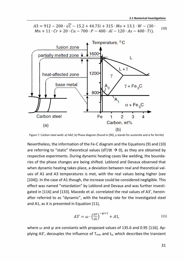
2.1 Numerical Investigations
31
𝐴3 = 912 − 200 ∙ √𝐶 − 15.2 + 44.7𝑆𝑖 + 315 ∙ 𝑀𝑜 + 13.1 ∙ 𝑊 − (30 ∙𝑀𝑛 + 11 ∙ 𝐶𝑟 + 20 ∙ 𝐶𝑢 − 700 ∙ 𝑃 − 400 ∙ 𝐴𝑙 − 120 ∙ 𝐴𝑠 − 400 ∙ 𝑇𝑖).
(10)
Figure 7: Carbon steel weld: a) HAZ; b) Phase diagram (found in [96], γ stands for austenite and α for ferrite)
Nevertheless, the information of the Fe-C diagram and the Equations (9) and (10)
are referring to “static” theoretical values (dT/dt 0), as they are obtained by
respective experiments. During dynamic heating cases like welding, the bounda-
ries of the phase changes are being shifted. Leblond and Devaux observed that
when dynamic heating takes place, a deviation between real and theoretical val-
ues of A1 and A3 temperatures is met, with the real values being higher (see
[104]). In the case of A1 though, the increase could be considered negligible. This
effect was named “retardation” by Leblond and Devaux and was further investi-
gated in [116] and [133]. Macedo et al. correlated the real values of A3’, herein-
after referred to as “dynamic”, with the heating rate for the investigated steel
and A1, as it is presented in Equation (11),
𝐴3′ = 𝜔 ∙ (
𝑑𝑇
𝑑𝑡)
−𝜑+1+ 𝐴1, (11)
where 𝜔 and 𝜑 are constants with proposed values of 135.6 and 0.95 [116]. Ap-
plying A3’, decouples the influence of Tmax and ta, which describes the transient
2 Theoretical Background
32
nature of austenitic transformation. The dynamic effect is incorporated in the cal-
culation of A3’. Hence, the influence of ta for single-pass welds (single thermal
cycle) can be neglected.
The Fe-C phase diagram, although being inadequate to describe precisely the dy-
namic nature of microstructural transformations during welding, can act qualita-
tively and advisory. At an initial stage of a weld analysis, it can offer a first rough
evaluation of the predominant microstructural transformations in the different
parts of the weld, based on the locally reached maximum temperature (Tmax) dur-
ing heating. A thorough overview of the zones with different microstructure in
and near the weld pool based on the phase diagram of FE-C is given in Figure 7.
In the fusion zone (FZ), when the temperature exceeds the melting point (Tmelt),
full austenitization at first and full melting later take place. Material in the HAZ
transforms partially to austenite, away from the FZ, or even completely, closest
the boundaries with the FZ, without exceeding the fusion temperature. Between
the FZ and the HAZ, lies the thin zone of material, where partial melting takes
place. The microstructure of the “parent” or “base” material (PM of BM) outside
the HAZ, remains uninfluenced by the heat treatment.
During cooling, the proportion of the austenitized material transforms again.
However, the resulting microstructure deviates from the respective one in the
phase diagram of the parent material as rapid cooling takes place after welding.
Final microstructure after cooling can differ significantly depending on the cooling
rate. Conventionally, the cooling time from 800 oC to 500 oC (t85) is used as index
for the cooling rate. Rapid cooling rates (t85 < 10 s) lead to the creation of mar-
tensitic microstructure (martensitic transformation). Nevertheless, due to the
rapid change, full transformation may not be achieved and remaining austenite
can be met in the final microstructure. If lower cooling rates take place and cool-
ing time is in the order of magnitude of 50 s, austenite transforms to pearlite
instead (pearlitic transformation). For slow cooling rates (t85 ≈ 100 s), austenite
transforms to bainite or ferrite (bainitic of ferritic transformation). For each alloy
the exact boundaries between the various possible transformations may deviate
from the above rough description due to the above-mentioned dependence of
phase transformations on chemical composition. Continuous cooling transfor-
mation (CCT) diagrams (see [147], [148], [188]) as the one presented in Figure 8,
illustrate the influence of cooling rate on the microstructural transformations, de-
pending on the chemical composition of the parent material.
2.1 Numerical Investigations
33
State of the Art Models for the Simulation of Phase Changes
Austenitic transformation, whose influence on WRS is discussed in [177], takes
place through diffusion [67], while martensitic transformation is a non-diffusional
thermal-driven process and takes place through rearrangement of all the atoms
of the crystal lattice [67], [111]. The different nature of each of the two transfor-
mations dictates the use of different prediction models. The models proposed by
Leblond and Devaux in [8] and Koistinen and Marburger in [9] were widely applied
in the last decades (see [74], [112], [184] etc.) for modelling austenitic and mar-
tensitic transformations respectively. The semi-empirical JMAK model developed
by Johnson-Mehl [85], Avrami [7] and Kolmogorov [95] and the Kirkaldy model,
which is described in [60], have been as well applied as an alternative to the Le-
blond model, for considering the several phase transformations of various metals
(see for instance [8], [9] and [154]).
The Leblond-Devaux model was formatted initially for two existing phases and a
unique transformation and was then generalized for the case of n phases and
several possible transformations, for both heating and cooling. The evolution of
microstructure n is governed by Equation (12)
�̇�𝑖 =𝑛𝑖
𝑒𝑞(𝑇) − 𝑛𝑖
𝜃(𝑇). (12)
The model is based on the existence of an equivalent volume fraction of the trans-
formed phase neq, which is different at each temperature level. The model is
based on a rational assumption: if enough time is provided, the microstructural
transformations will end when this equivalent fraction is reached. In the case of
austenitic transformation during heating, neq for the austenitic phase is equal to
0 and 1 at A1 and A3 temperature respectively. Yet, calibration for each investi-
gated material is required, as θ(T) is dependent on chemical composition as well
[104].
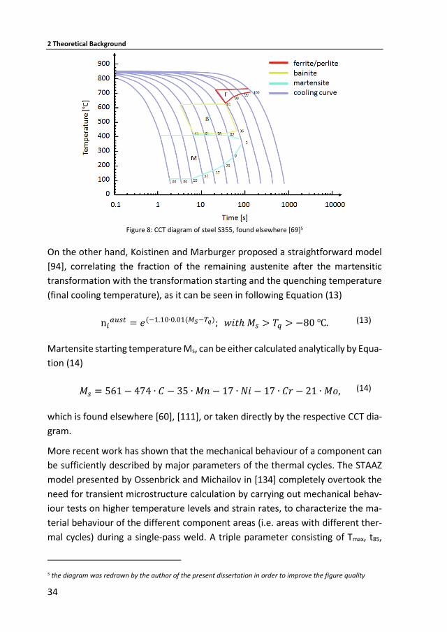
2 Theoretical Background
34
Figure 8: CCT diagram of steel S355, found elsewhere [69]5
On the other hand, Koistinen and Marburger proposed a straightforward model
[94], correlating the fraction of the remaining austenite after the martensitic
transformation with the transformation starting and the quenching temperature
(final cooling temperature), as it can be seen in following Equation (13)
n𝑖𝑎𝑢𝑠𝑡 = 𝑒(−1.10∙0.01(𝑀𝑆−𝑇𝑞); 𝑤𝑖𝑡ℎ 𝑀𝑠 > 𝑇𝑞 > −80 ℃. (13)
Martensite starting temperature Ms, can be either calculated analytically by Equa-
tion (14)
𝑀𝑠 = 561 − 474 ∙ 𝐶 − 35 ∙ 𝑀𝑛 − 17 ∙ 𝑁𝑖 − 17 ∙ 𝐶𝑟 − 21 ∙ 𝑀𝑜, (14)
which is found elsewhere [60], [111], or taken directly by the respective CCT dia-
gram.
More recent work has shown that the mechanical behaviour of a component can
be sufficiently described by major parameters of the thermal cycles. The STAAZ
model presented by Ossenbrick and Michailov in [134] completely overtook the
need for transient microstructure calculation by carrying out mechanical behav-
iour tests on higher temperature levels and strain rates, to characterize the ma-
terial behaviour of the different component areas (i.e. areas with different ther-
mal cycles) during a single-pass weld. A triple parameter consisting of Tmax, t85,
5 the diagram was redrawn by the author of the present dissertation in order to improve the figure quality

2.1 Numerical Investigations
35
and ta was proven to be sufficient to describe the material behaviour inside a
thermal cycle. This statement is becoming easily understood, based on the above-
described influence of these three parameters. Mechanical material behaviour of
the investigated material inside a thermal cycle for different values of this triple
parameter were experimentally acquired. A finite element analysis was subse-
quently carried out, wherein each investigated component was divided to differ-
ent areas, as in the present approach. During simulation, each area should then
be assigned with a respective, experimentally acquired material behaviour de-
pending on its triple parameter values. In this way, the material behaviour during
welding could be adequately modelled. Experimental results from later work
have shown that the method could be extendable to multi-pass welds [19] as
well. In order to apply the STAAZ model though, there is a need to repeat the
delicate calibration tests for every newly investigated material.
The Gkatzogiannis – Knoedel – Ummenhofer Engineering Approach
Alternatively to the above-mentioned methods, an engineering approach was
proposed for the simulation of WRS in a study, which was carried out in the
framework of the present doctoral dissertation [92]. The proposed method is in
its original form predictive, calculating the WRS based on existing CCT diagrams.
Theoretical A1 and A3 temperatures were calculated based on Equations (9) and
(10) respectively. The dynamic A3’ temperature taking into consideration the re-
tardation effect was calculated based on Equation (11). During heating, the whole
component was simulated with parent material behaviour. When Tmax was be-
tween A1 and A3’ a linear interpolation between no and complete austenitization
was carried out, in order to calculate the percentage of austenitized fraction (see
Figure 9). During cooling, the austenitized behaviour was assumed to behave ac-
cording to the respective CCT diagram. Several material models6 for different lev-
els of austenitization during heating and cooling paths were simulated. Each ma-
terial model was characterized by its Tmax and t85. Applying A3’ decouples the
influence of Tmax and ta, which describes the transient nature of austenitic trans-
formation. The dynamic effect is incorporated in the calculation of A3’. Hence,
the influence of ta for single-pass welds (single thermal cycle) can be neglected
and only a double parameter consisting of Tmax and t85 is applied. Each FE-element
6 hereinafter called Cooling Material Model (CMM)
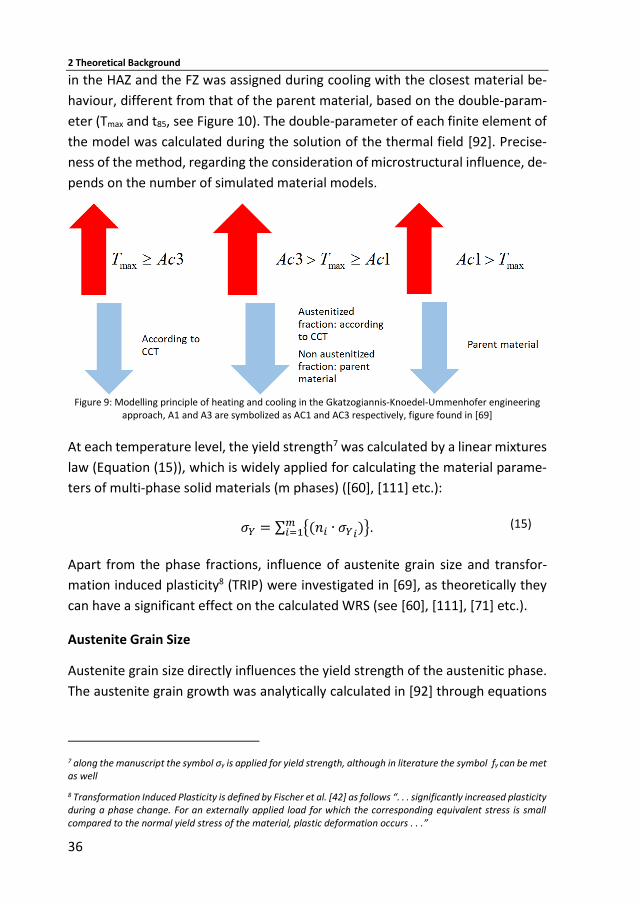
2 Theoretical Background
36
in the HAZ and the FZ was assigned during cooling with the closest material be-
haviour, different from that of the parent material, based on the double-param-
eter (Tmax and t85, see Figure 10). The double-parameter of each finite element of
the model was calculated during the solution of the thermal field [92]. Precise-
ness of the method, regarding the consideration of microstructural influence, de-
pends on the number of simulated material models.
Figure 9: Modelling principle of heating and cooling in the Gkatzogiannis-Knoedel-Ummenhofer engineering
approach, A1 and A3 are symbolized as AC1 and AC3 respectively, figure found in [69]
At each temperature level, the yield strength7 was calculated by a linear mixtures
law (Equation (15)), which is widely applied for calculating the material parame-
ters of multi-phase solid materials (m phases) ([60], [111] etc.):
𝜎𝑌 = ∑ {(𝑛𝑖 ∙ 𝜎𝑌𝑖)}𝑚𝑖=1 . (15)
Apart from the phase fractions, influence of austenite grain size and transfor-
mation induced plasticity8 (TRIP) were investigated in [69], as theoretically they
can have a significant effect on the calculated WRS (see [60], [111], [71] etc.).
Austenite Grain Size
Austenite grain size directly influences the yield strength of the austenitic phase.
The austenite grain growth was analytically calculated in [92] through equations
7 along the manuscript the symbol σy is applied for yield strength, although in literature the symbol fy can be met as well
8 Transformation Induced Plasticity is defined by Fischer et al. [42] as follows “. . . significantly increased plasticity during a phase change. For an externally applied load for which the corresponding equivalent stress is small compared to the normal yield stress of the material, plastic deformation occurs . . .”
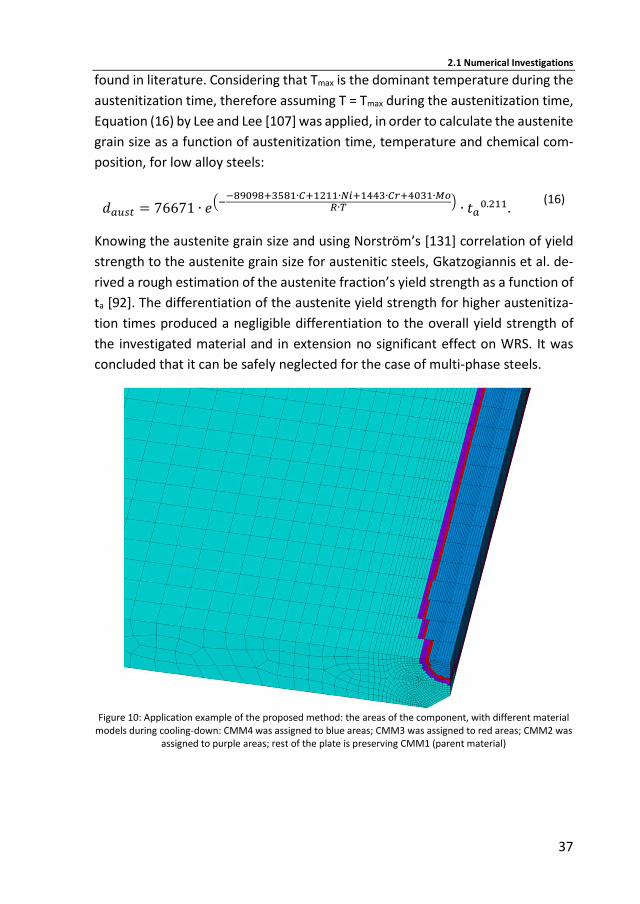
2.1 Numerical Investigations
37
found in literature. Considering that Tmax is the dominant temperature during the
austenitization time, therefore assuming T = Tmax during the austenitization time,
Equation (16) by Lee and Lee [107] was applied, in order to calculate the austenite
grain size as a function of austenitization time, temperature and chemical com-
position, for low alloy steels:
𝑑𝑎𝑢𝑠𝑡 = 76671 ∙ 𝑒(−
−89098+3581∙𝐶+1211∙𝑁𝑖+1443∙𝐶𝑟+4031∙𝑀𝑜𝑅∙𝑇
)∙ 𝑡𝑎
0.211. (16)
Knowing the austenite grain size and using Norström’s [131] correlation of yield
strength to the austenite grain size for austenitic steels, Gkatzogiannis et al. de-
rived a rough estimation of the austenite fraction’s yield strength as a function of
ta [92]. The differentiation of the austenite yield strength for higher austenitiza-
tion times produced a negligible differentiation to the overall yield strength of
the investigated material and in extension no significant effect on WRS. It was
concluded that it can be safely neglected for the case of multi-phase steels.
Figure 10: Application example of the proposed method: the areas of the component, with different material
models during cooling-down: CMM4 was assigned to blue areas; CMM3 was assigned to red areas; CMM2 was assigned to purple areas; rest of the plate is preserving CMM1 (parent material)

2 Theoretical Background
38
TRIP: Transformation Induced Plasticity
Greenwood and Johnson were the first to investigate TRIP in 1965 [62]. Later on,
TRIP was included in mathematical formulations of computational welding me-
chanics by Rammerstorfer [138], Argyris et al. [5] and Leblond [105]. The signifi-
cance of considering TRIP influence during simulation of WRS was highlighted by
Oddy et al. in 1989 (see [132]). Around the same time, Karlsson proposed a more
straightforward approach for taking into consideration the TRIP effect [87], which
is applicable even to cases, when classical plasticity theory is applied and no com-
plicated mathematical formulations of material behaviour are required. Karls-
son’s proposal was the arbitrary lowering of the yield stress in the respective re-
gions of the HAZ during cooling. This approach was adopted as well by
Gkatzogiannis et al. in [92], when martensitic transformation took place.
Figure 11: The arbitrary reduction of yield strength in the respective temperature range proposed by Karlsson
for the consideration of TRIP during welding simulation, based on a diagram from [87]
2.1.1.3 Modelling of Mechanical Behaviour
Analysis Type
Inertia effects during welding are negligible but plastic strains are introduced;
hence, a quasi-static analysis for non-linear material is carried out for modelling
0
0.2
0.4
0.6
0.8
1
1.2
200 250 300 350 400
No
rmal
ized
Yie
ld s
tren
gth
[-]
Temperature [oC]
Without TRIP
TRIP
2.1 Numerical Investigations
39
the component’s structural behaviour. The quasi-static analysis for a system of
finite elements is governed by the following Equation9, 10:
𝐟𝑠(𝐮) = 𝐩(𝑡). (17)
In the case of structural analysis during welding simulation, the thermal strains
caused by the welding thermal cycle constitute the imposed loading. They can be
calculated with the following Equation:
휀𝑡ℎ = 𝑎𝑠𝑒(𝑇) ∙ (𝑇 − 𝑇𝑟𝑒𝑓), (18)
based on the FE nodal thermal history, which is previously calculated during the
thermal transient analysis, and they are applied as structural nodal loads (see
[92]).
Dilatometry
The coefficient of thermal expansion α (secant or instantaneous) is strongly de-
pendent on microstructure. According to common engineering knowledge, fer-
ritic and austenitic steels have a coefficient of thermal expansion equal to
12·10-6 and 16·10-6 respectively at room temperature, both variating slightly de-
pending on the specific microstructure of each investigated alloy and the temper-
ature. All phases of steel apart from austenite are usually assumed to have the
same dilatation behaviour as ferrite. When the microstructure is multiphase (m
phases), α can be calculated by applying once again a linear mixtures law:
𝑎𝑡𝑜𝑡(𝑇) = ∑{𝑛𝑖(𝑇) ∙ 𝛼𝑛𝑖(𝑇)}
𝑚
𝑖=1
, (19)
Such an approach was adopted elsewhere (see [39], [92]). The dilatometric dia-
grams, such the one given by Ferro and Bonolo [39] (see Figure 12), provide a
thorough overview over the microstructural and temperature dependency of the
dilatation behaviour. The instantaneous coefficient of thermal expansion, which
9 use of bold letters states tensor notation
10 due to the inelastic behaviour of the material the force-displacement relation is path-dependent, thus the resisting force vector is an implicit function of displacement 𝒇𝑠 = 𝒇𝑠(𝒖) and no more equal to 𝒌𝒖, where 𝒌 is the stiffness matrix, as in the case of elastic material behaviour
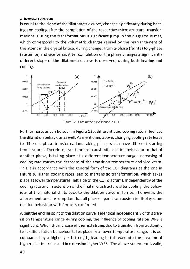
2 Theoretical Background
40
is equal to the slope of the dilatometric curve, changes significantly during heat-
ing and cooling after the completion of the respective microstructural transfor-
mations. During the transformations a significant jump in the diagrams is met,
which corresponds to the volumetric changes caused by the rearrangement of
the atoms in the crystal lattice, during changes from α-phase (ferrite) to γ-phase
(austenite) and vice versa. After completion of the phase changes a significantly
different slope of the dilatometric curve is observed, during both heating and
cooling.
Figure 12: Dilatometric curves found in [39]
Furthermore, as can be seen in Figure 12b, differentiated cooling rate influences
the dilatation behaviour as well. As mentioned above, changing cooling rate leads
to different phase-transformations taking place, which have different starting
temperatures. Therefore, transition from austenitic dilation behaviour to that of
another phase, is taking place at a different temperature range. Increasing of
cooling rate causes the decrease of the transition temperature and vice versa.
This is in accordance with the general form of the CCT diagrams as the one in
Figure 8. Higher cooling rates lead to martensitic transformation, which takes
place at lower temperatures (left side of the CCT diagram). Independently of the
cooling rate and in extension of the final microstructure after cooling, the behav-
iour of the material shifts back to the dilation curve of ferrite. Therewith, the
above-mentioned assumption that all phases apart from austenite display same
dilation behaviour with ferrite is confirmed.
Albeit the ending point of the dilation curve is identical independently of this tran-
sition temperature range during cooling, the influence of cooling rate on WRS is
significant. When the increase of thermal strains due to transition from austenitic
to ferritic dilation behaviour takes place in a lower temperature range, it is ac-
companied by a higher yield strength, leading in this way into the creation of
higher plastic strains and in extension higher WRS. The above-statement is valid,
2.1 Numerical Investigations
41
only when the influence of microstructure on yield strength is negligible. Never-
theless, as the yield limit is for many alloys not only temperature-dependent but
microstructure-dependent also, as it was described above, the interpretation of
the influence of cooling and dilation is becoming even more complex. Under-
standing this complexity, further confirms the necessity of FE modelling of weld-
ing shrinkage and WRS. A direct modelling of the dilation behaviour of the inves-
tigated material for heating or a specific cooling rate through direct input of
thermal strains is more straightforward than the use of the coefficient of thermal
expansion based on Equation (19). Gkatzogiannis et al. applied Equation (19) in
[92], in order to predict the dilation curves of their CMMs, based on the predicted
microstructural transformations. Thermal strains as a function of temperature
were then applied as input for the simulation.
Rate-Independent Nonlinear Material Behaviour
In order to calculate the plastic strains and the WRS caused by the external load-
ing, plasticity of the investigated material must be considered. The non-linear ma-
terial behaviour of steel can be simulated as bilinear, multi-linear, with Ramberg-
Osgood model [137] etc. However, as the maximal plastic strains during welding
are usually lower than 2 % [92], a bilinear model with a tangent modulus H (slope
of the second branch), which is selected based on the stress for this introduced
plastic strain, can be considered sufficient for welding simulation [55]. The von-
Mises yield criterion,
𝑓(𝜎) = 𝐽2 − 𝜏2, (20)
which is widely applied for simulating the yield behaviour for metallic compo-
nents, is applied as well during simulation of welding. Temperature-dependent
material parameters are usually taken into consideration (see [3], [21], [28], [92]
etc.).
Zhu and Chao have nonetheless proven in 0 that an engineering approach,
whereby only the predominant yield strength is considered to be temperature-
dependent, can offer results with sufficient preciseness. Moreover, even in cases
where more material properties were temperature-dependent, usually a thresh-
old temperature was defined, above which either stiffness was set to zero [164]
or effects of thermal treatment were neglected [165], [52]. This threshold tem-
perature was named “cut-off” by Lindgren (Tcut). It varies from 500 °C up to 900
2 Theoretical Background
42
°C in [52], [164] and [165]. Preciseness was not compromised in these cases. The
influence of defining and variating Tcut, from up to Tmelt down to 600 °C, was in-
vestigated by Tekriwal and Mazumber in [160]. It was concluded that at lowest
Tcut a maximal overestimation of 15 % of the WRS took place. The principal of Tcut
is thoroughly described by Goldak and Akhlaghi in [60] and Lindgren in [111]. In
any case, it has to be considered that attaining material properties at higher tem-
peratures (>1000 °C) is subject to significant testing restrictions.
Rate-Dependent Nonlinear Material Behaviour
Lindgren [111] proposed that during welding simulation, when very high accuracy
is required, strain rate dependent plasticity should be considered, without provid-
ing though any information regarding the order of magnitude of the influence on
calculated WRS. Strain rate was introduced quite early into the formulation of
finite element equations for modelling the thermomechanical welding process.
Argyris et al. proposed in 1984 a viscoplastic material model, wherewith the strain
rate dependency of the yield behaviour11 is taken into account [5]. However, prior
to an investigation from Gkatzogiannis et al. [59], no quantified influence of strain
rate dependency on simulated WRS was known to the author of the present
study. In this study that was carried out in the framework of the present doctoral
dissertation, the effect of strain rate dependency on WRS was investigated and
quantified. Preliminary analyses showed that in the heat affected zone (HAZ) and
the fusion zone (FZ) of a 3-pass butt-weld, strain rates of up to 0.122 s-1 are pre-
sent. Although this value lies clearly lower than the classical dynamic cases such
as modelling of ballistic tests (휀̇ ≈ 106 𝑠−1) or car crash simulation (휀̇ ≈
100 𝑠−1), still clearly deviates from the static case (휀̇ → 0 𝑠−1 ). The authors ap-
plied the material model presented by Perzyna in 1966 in [136]:
휀⏞.
𝑝𝑙 = 𝛼 ∙ (𝜎𝑦′
𝜎𝑦− 1)
1𝛽
, (21)
which enables the consideration of strain rate dependency during implicit quasi-
static FE simulations. It is analogous to the Cowper-Symonds model [25], as it was
presented by Jones in [86]:
11 hereinafter called simply strain rate dependency
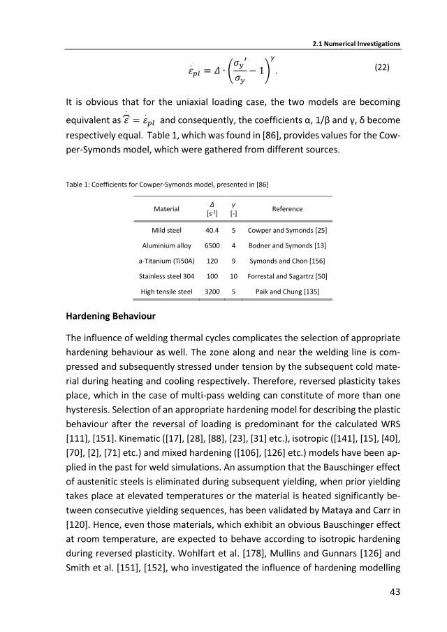
2.1 Numerical Investigations
43
휀.
𝑝𝑙 = 𝛥 ∙ (𝜎𝑦′
𝜎𝑦− 1)
𝛾
. (22)
It is obvious that for the uniaxial loading case, the two models are becoming
equivalent as 휀⏞.
= 휀.
𝑝𝑙 and consequently, the coefficients α, 1/β and γ, δ become
respectively equal. Table 1, which was found in [86], provides values for the Cow-
per-Symonds model, which were gathered from different sources.
Table 1: Coefficients for Cowper-Symonds model, presented in [86]
Material Δ [s-1]
γ [-] Reference
Mild steel 40.4 5 Cowper and Symonds [25]
Aluminium alloy 6500 4 Bodner and Symonds [13]
a-Titanium (Ti50A) 120 9 Symonds and Chon [156]
Stainless steel 304 100 10 Forrestal and Sagartrz [50]
High tensile steel 3200 5 Paik and Chung [135]
Hardening Behaviour
The influence of welding thermal cycles complicates the selection of appropriate
hardening behaviour as well. Τhe zone along and near the welding line is com-
pressed and subsequently stressed under tension by the subsequent cold mate-
rial during heating and cooling respectively. Therefore, reversed plasticity takes
place, which in the case of multi-pass welding can constitute of more than one
hysteresis. Selection of an appropriate hardening model for describing the plastic
behaviour after the reversal of loading is predominant for the calculated WRS
[111], [151]. Kinematic ([17], [28], [88], [23], [31] etc.), isotropic ([141], [15], [40],
[70], [2], [71] etc.) and mixed hardening ([106], [126] etc.) models have been ap-
plied in the past for weld simulations. An assumption that the Bauschinger effect
of austenitic steels is eliminated during subsequent yielding, when prior yielding
takes place at elevated temperatures or the material is heated significantly be-
tween consecutive yielding sequences, has been validated by Mataya and Carr in
[120]. Hence, even those materials, which exhibit an obvious Bauschinger effect
at room temperature, are expected to behave according to isotropic hardening
during reversed plasticity. Wohlfart et al. [178], Mullins and Gunnars [126] and
Smith et al. [151], [152], who investigated the influence of hardening modelling
2 Theoretical Background
44
on WRS simulation of austenitic steels, came to the conclusion that isotropic
hardening provides better agreement than kinematic. The latter two proposed as
well to use of a mixed hardening behaviour, which was even more accurate. On
the contrary, investigations by Gkatzogiannis et al. for ferritic multiphase [55] and
austenitic steels [56] have shown a reversed effect, with kinetic hardening provid-
ing better agreement than isotropic. Still, the difference between isotropic and
kinematic hardening in these investigations was inside the uncertainty bounda-
ries of the applied weld modelling approach. In all above-mentioned comparative
investigations though, kinematic hardening under-predicted the WRS in the weld
area in comparison with isotropic.
Boundary Conditions
During the structural analysis, appropriate boundary conditions have to be ap-
plied, in order to simulate the mechanical restraints of the real component in re-
ality. Components for scientific measurements are usually welded in the labora-
tory either restraint free or clamped down. Wherever possible, symmetry
conditions can be applied as well in order to reduce the computational time.
According to common practice, modelling of clamping mechanisms is usually
done by fixing the displacements of the respective nodes in all directions. None-
theless, this modelling approach may deviate from reality, whereby clamping
mechanisms allow small in-plane displacements to take place. On the other hand,
carrying out a restraint free implicit analysis leads to numerical instabilities (un-
derdetermined static system). These two modelling challenges were discussed by
Gkatzogiannis et al. in [55], who proposed the use of linear spring elements for
modelling both cases and investigated the effect of boundary conditions on the
calculated WRS. Different setups, using either “soft” or “hard” linear spring ele-
ments for modelling of restraint free and clamped components respectively, were
applied. A similar approach for modelling a free plate was applied earlier by Caron
et al. in [21] and Gkatzogiannis et al. in [92]. The terms “soft” and “hard” exhibit
the empirical nature of the method. In any case, stiffness should be respectively
low in the former case in order to allow an almost free movement and high
enough in the latter case, so that only very small displacements are possible.
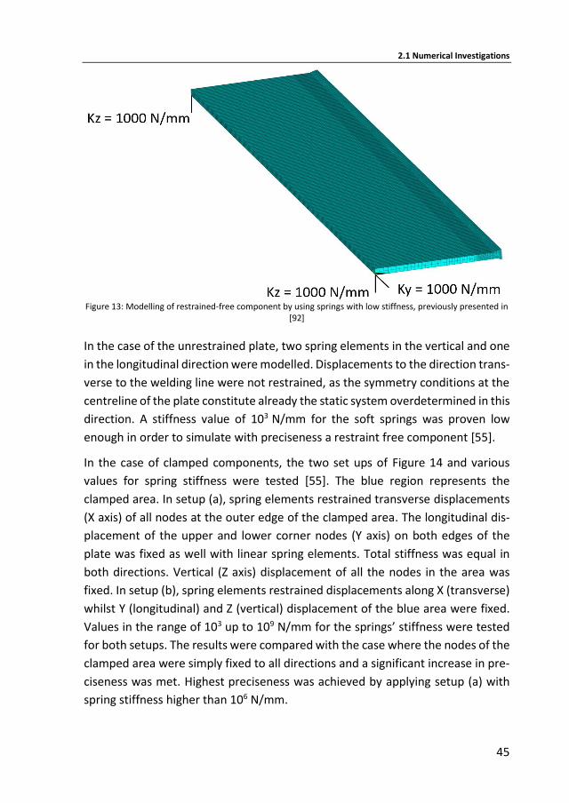
2.1 Numerical Investigations
45
Figure 13: Modelling of restrained-free component by using springs with low stiffness, previously presented in
[92]
In the case of the unrestrained plate, two spring elements in the vertical and one
in the longitudinal direction were modelled. Displacements to the direction trans-
verse to the welding line were not restrained, as the symmetry conditions at the
centreline of the plate constitute already the static system overdetermined in this
direction. A stiffness value of 103 N/mm for the soft springs was proven low
enough in order to simulate with preciseness a restraint free component [55].
In the case of clamped components, the two set ups of Figure 14 and various
values for spring stiffness were tested [55]. The blue region represents the
clamped area. In setup (a), spring elements restrained transverse displacements
(X axis) of all nodes at the outer edge of the clamped area. The longitudinal dis-
placement of the upper and lower corner nodes (Y axis) on both edges of the
plate was fixed as well with linear spring elements. Total stiffness was equal in
both directions. Vertical (Z axis) displacement of all the nodes in the area was
fixed. In setup (b), spring elements restrained displacements along X (transverse)
whilst Y (longitudinal) and Z (vertical) displacement of the blue area were fixed.
Values in the range of 103 up to 109 N/mm for the springs’ stiffness were tested
for both setups. The results were compared with the case where the nodes of the
clamped area were simply fixed to all directions and a significant increase in pre-
ciseness was met. Highest preciseness was achieved by applying setup (a) with
spring stiffness higher than 106 N/mm.
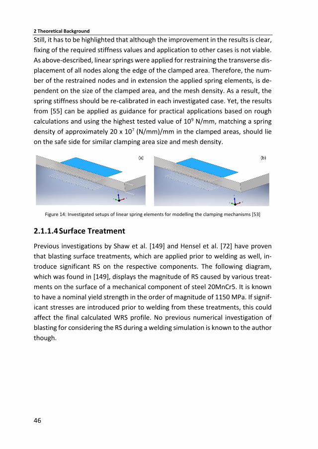
2 Theoretical Background
46
Still, it has to be highlighted that although the improvement in the results is clear,
fixing of the required stiffness values and application to other cases is not viable.
As above-described, linear springs were applied for restraining the transverse dis-
placement of all nodes along the edge of the clamped area. Therefore, the num-
ber of the restrained nodes and in extension the applied spring elements, is de-
pendent on the size of the clamped area, and the mesh density. As a result, the
spring stiffness should be re-calibrated in each investigated case. Yet, the results
from [55] can be applied as guidance for practical applications based on rough
calculations and using the highest tested value of 109 N/mm, matching a spring
density of approximately 20 x 107 (N/mm)/mm in the clamped areas, should lie
on the safe side for similar clamping area size and mesh density.
Figure 14: Investigated setups of linear spring elements for modelling the clamping mechanisms [53]
2.1.1.4 Surface Treatment
Previous investigations by Shaw et al. [149] and Hensel et al. [72] have proven
that blasting surface treatments, which are applied prior to welding as well, in-
troduce significant RS on the respective components. The following diagram,
which was found in [149], displays the magnitude of RS caused by various treat-
ments on the surface of a mechanical component of steel 20MnCr5. It is known
to have a nominal yield strength in the order of magnitude of 1150 MPa. If signif-
icant stresses are introduced prior to welding from these treatments, this could
affect the final calculated WRS profile. No previous numerical investigation of
blasting for considering the RS during a welding simulation is known to the author
though.
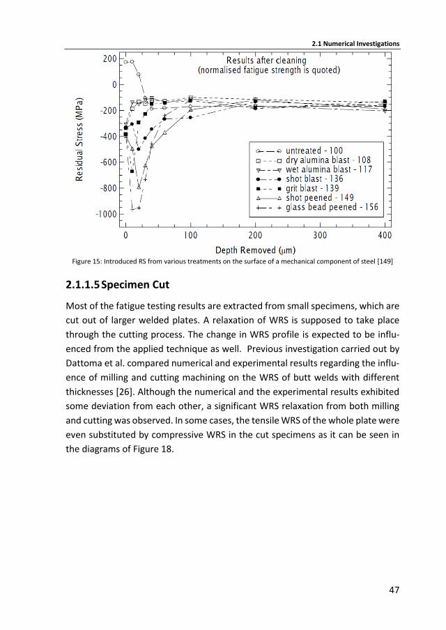
2.1 Numerical Investigations
47
Figure 15: Introduced RS from various treatments on the surface of a mechanical component of steel [149]
2.1.1.5 Specimen Cut
Most of the fatigue testing results are extracted from small specimens, which are
cut out of larger welded plates. A relaxation of WRS is supposed to take place
through the cutting process. The change in WRS profile is expected to be influ-
enced from the applied technique as well. Previous investigation carried out by
Dattoma et al. compared numerical and experimental results regarding the influ-
ence of milling and cutting machining on the WRS of butt welds with different
thicknesses [26]. Although the numerical and the experimental results exhibited
some deviation from each other, a significant WRS relaxation from both milling
and cutting was observed. In some cases, the tensile WRS of the whole plate were
even substituted by compressive WRS in the cut specimens as it can be seen in
the diagrams of Figure 18.
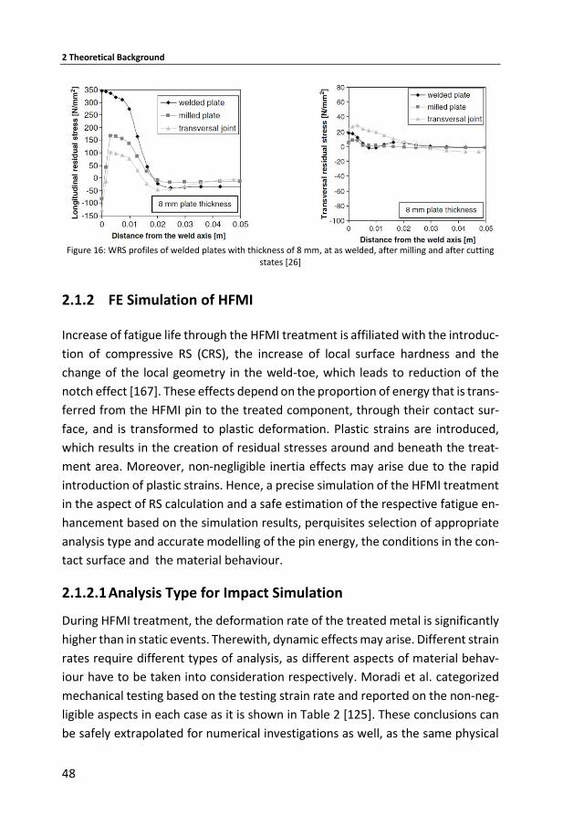
2 Theoretical Background
48
Figure 16: WRS profiles of welded plates with thickness of 8 mm, at as welded, after milling and after cutting
states [26]
2.1.2 FE Simulation of HFMI
Increase of fatigue life through the HFMI treatment is affiliated with the introduc-
tion of compressive RS (CRS), the increase of local surface hardness and the
change of the local geometry in the weld-toe, which leads to reduction of the
notch effect [167]. These effects depend on the proportion of energy that is trans-
ferred from the HFMI pin to the treated component, through their contact sur-
face, and is transformed to plastic deformation. Plastic strains are introduced,
which results in the creation of residual stresses around and beneath the treat-
ment area. Moreover, non-negligible inertia effects may arise due to the rapid
introduction of plastic strains. Hence, a precise simulation of the HFMI treatment
in the aspect of RS calculation and a safe estimation of the respective fatigue en-
hancement based on the simulation results, perquisites selection of appropriate
analysis type and accurate modelling of the pin energy, the conditions in the con-
tact surface and the material behaviour.
2.1.2.1 Analysis Type for Impact Simulation
During HFMI treatment, the deformation rate of the treated metal is significantly
higher than in static events. Therewith, dynamic effects may arise. Different strain
rates require different types of analysis, as different aspects of material behav-
iour have to be taken into consideration respectively. Moradi et al. categorized
mechanical testing based on the testing strain rate and reported on the non-neg-
ligible aspects in each case as it is shown in Table 2 [125]. These conclusions can
be safely extrapolated for numerical investigations as well, as the same physical
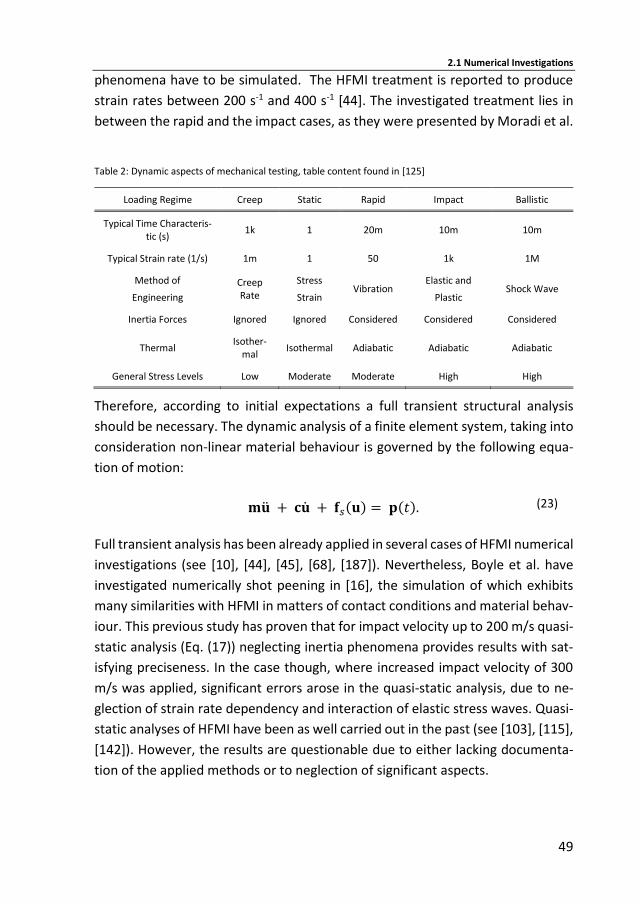
2.1 Numerical Investigations
49
phenomena have to be simulated. The HFMI treatment is reported to produce
strain rates between 200 s-1 and 400 s-1 [44]. The investigated treatment lies in
between the rapid and the impact cases, as they were presented by Moradi et al.
Table 2: Dynamic aspects of mechanical testing, table content found in [125]
Loading Regime Creep Static Rapid Impact Ballistic Typical Time Characteris-
tic (s) 1k 1 20m 10m 10m
Typical Strain rate (1/s) 1m 1 50 1k 1M Method of
Engineering Creep Rate
Stress Strain Vibration Elastic and
Plastic Shock Wave
Inertia Forces Ignored Ignored Considered Considered Considered
Thermal Isother-mal Isothermal Adiabatic Adiabatic Adiabatic
General Stress Levels Low Moderate Moderate High High
Therefore, according to initial expectations a full transient structural analysis
should be necessary. The dynamic analysis of a finite element system, taking into
consideration non-linear material behaviour is governed by the following equa-
tion of motion:
𝐦�̈� + 𝐜�̇� + 𝐟𝑠(𝐮) = 𝐩(𝑡). (23)
Full transient analysis has been already applied in several cases of HFMI numerical
investigations (see [10], [44], [45], [68], [187]). Nevertheless, Boyle et al. have
investigated numerically shot peening in [16], the simulation of which exhibits
many similarities with HFMI in matters of contact conditions and material behav-
iour. This previous study has proven that for impact velocity up to 200 m/s quasi-
static analysis (Eq. (17)) neglecting inertia phenomena provides results with sat-
isfying preciseness. In the case though, where increased impact velocity of 300
m/s was applied, significant errors arose in the quasi-static analysis, due to ne-
glection of strain rate dependency and interaction of elastic stress waves. Quasi-
static analyses of HFMI have been as well carried out in the past (see [103], [115],
[142]). However, the results are questionable due to either lacking documenta-
tion of the applied methods or to neglection of significant aspects.
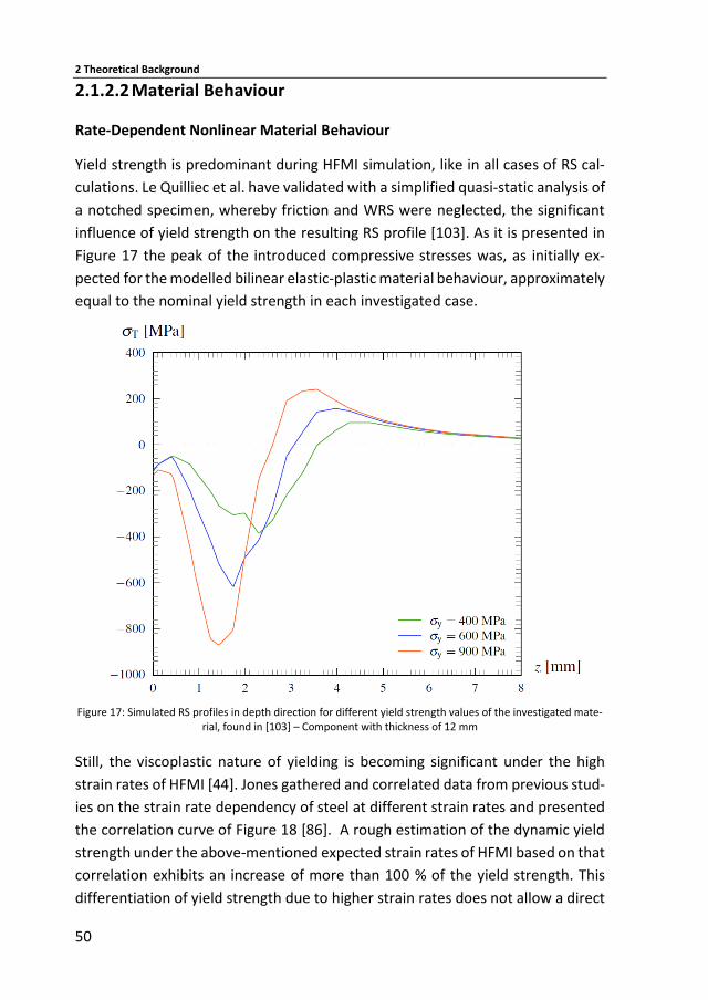
2 Theoretical Background
50
2.1.2.2 Material Behaviour
Rate-Dependent Nonlinear Material Behaviour
Yield strength is predominant during HFMI simulation, like in all cases of RS cal-
culations. Le Quilliec et al. have validated with a simplified quasi-static analysis of
a notched specimen, whereby friction and WRS were neglected, the significant
influence of yield strength on the resulting RS profile [103]. As it is presented in
Figure 17 the peak of the introduced compressive stresses was, as initially ex-
pected for the modelled bilinear elastic-plastic material behaviour, approximately
equal to the nominal yield strength in each investigated case.
Figure 17: Simulated RS profiles in depth direction for different yield strength values of the investigated mate-
rial, found in [103] – Component with thickness of 12 mm
Still, the viscoplastic nature of yielding is becoming significant under the high
strain rates of HFMI [44]. Jones gathered and correlated data from previous stud-
ies on the strain rate dependency of steel at different strain rates and presented
the correlation curve of Figure 18 [86]. A rough estimation of the dynamic yield
strength under the above-mentioned expected strain rates of HFMI based on that
correlation exhibits an increase of more than 100 % of the yield strength. This
differentiation of yield strength due to higher strain rates does not allow a direct
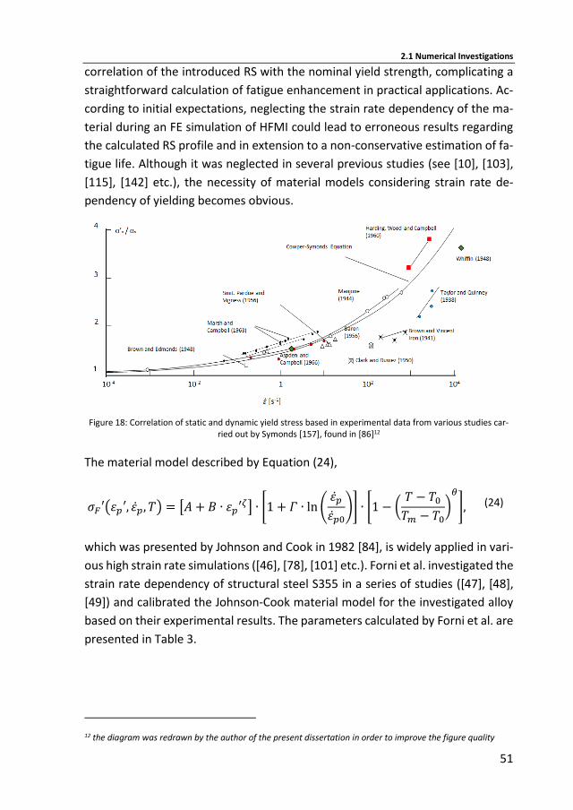
2.1 Numerical Investigations
51
correlation of the introduced RS with the nominal yield strength, complicating a
straightforward calculation of fatigue enhancement in practical applications. Ac-
cording to initial expectations, neglecting the strain rate dependency of the ma-
terial during an FE simulation of HFMI could lead to erroneous results regarding
the calculated RS profile and in extension to a non-conservative estimation of fa-
tigue life. Although it was neglected in several previous studies (see [10], [103],
[115], [142] etc.), the necessity of material models considering strain rate de-
pendency of yielding becomes obvious.
Figure 18: Correlation of static and dynamic yield stress based in experimental data from various studies car-
ried out by Symonds [157], found in [86]12
The material model described by Equation (24),
𝜎𝐹′(휀𝑝′, 휀�̇�, 𝛵) = [𝐴 + 𝐵 ∙ 휀𝑝′𝜁] ∙ [1 + 𝛤 ∙ ln (휀�̇�
휀�̇�0)] ∙ [1 − (
𝑇 − 𝑇0
𝑇𝑚 − 𝑇0)
𝜃
], (24)
which was presented by Johnson and Cook in 1982 [84], is widely applied in vari-
ous high strain rate simulations ([46], [78], [101] etc.). Forni et al. investigated the
strain rate dependency of structural steel S355 in a series of studies ([47], [48],
[49]) and calibrated the Johnson-Cook material model for the investigated alloy
based on their experimental results. The parameters calculated by Forni et al. are
presented in Table 3.
12 the diagram was redrawn by the author of the present dissertation in order to improve the figure quality
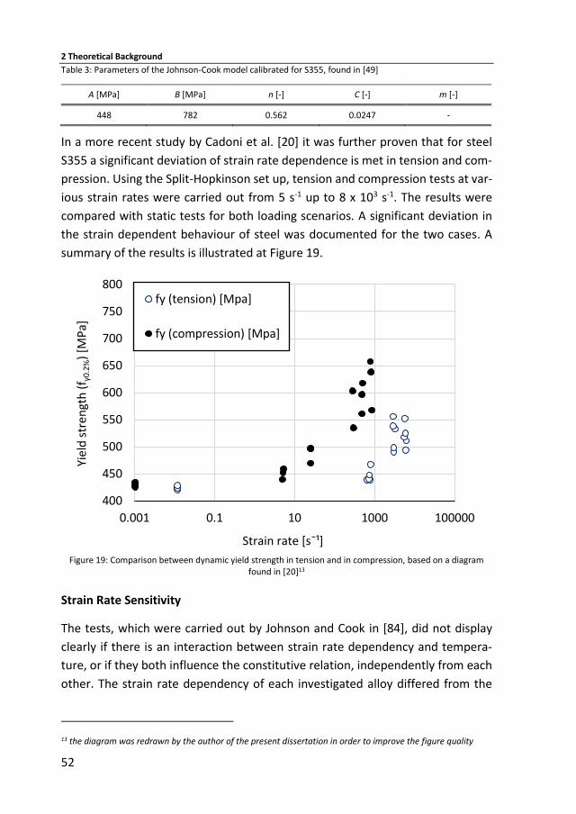
2 Theoretical Background
52
Table 3: Parameters of the Johnson-Cook model calibrated for S355, found in [49]
A [MPa] B [MPa] n [-] C [-] m [-]
448 782 0.562 0.0247 -
In a more recent study by Cadoni et al. [20] it was further proven that for steel
S355 a significant deviation of strain rate dependence is met in tension and com-
pression. Using the Split-Hopkinson set up, tension and compression tests at var-
ious strain rates were carried out from 5 s-1 up to 8 x 10³ s-1. The results were
compared with static tests for both loading scenarios. A significant deviation in
the strain dependent behaviour of steel was documented for the two cases. A
summary of the results is illustrated at Figure 19.
Figure 19: Comparison between dynamic yield strength in tension and in compression, based on a diagram
found in [20]13
Strain Rate Sensitivity
The tests, which were carried out by Johnson and Cook in [84], did not display
clearly if there is an interaction between strain rate dependency and tempera-
ture, or if they both influence the constitutive relation, independently from each
other. The strain rate dependency of each investigated alloy differed from the
13 the diagram was redrawn by the author of the present dissertation in order to improve the figure quality
400
450
500
550
600
650
700
750
800
0.001 0.1 10 1000 100000
Yiel
d s
tre
ngt
h (
f y0
.2%
) [M
Pa]
Strain rate [sˉ¹]
fy (tension) [Mpa]
fy (compression) [Mpa]
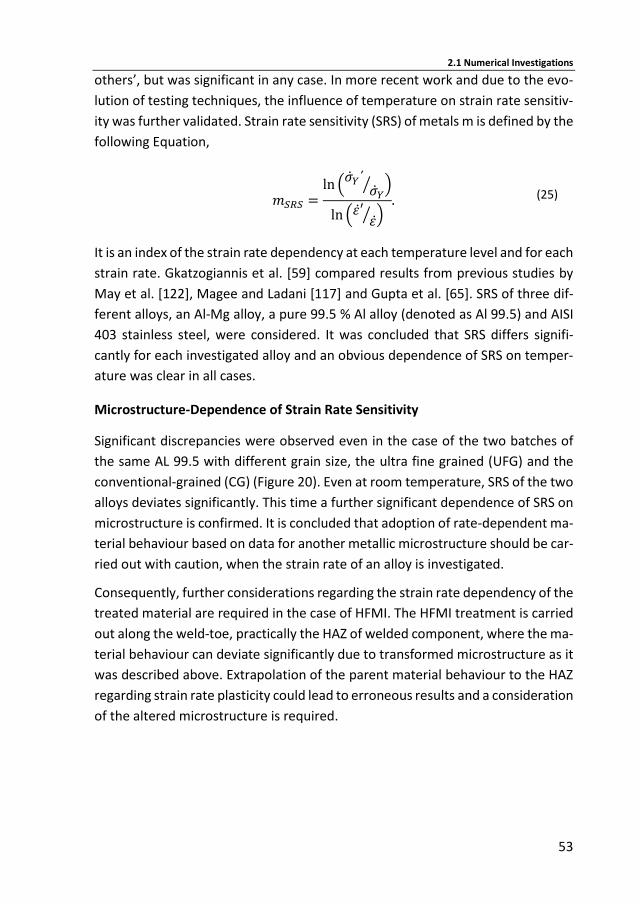
2.1 Numerical Investigations
53
others’, but was significant in any case. In more recent work and due to the evo-
lution of testing techniques, the influence of temperature on strain rate sensitiv-
ity was further validated. Strain rate sensitivity (SRS) of metals m is defined by the
following Equation,
𝑚𝑆𝑅𝑆 =ln (
�̇�𝑌΄�̇�𝑌
⁄ )
ln (휀̇′휀̇⁄ )
. (25)
It is an index of the strain rate dependency at each temperature level and for each
strain rate. Gkatzogiannis et al. [59] compared results from previous studies by
May et al. [122], Magee and Ladani [117] and Gupta et al. [65]. SRS of three dif-
ferent alloys, an Al-Mg alloy, a pure 99.5 % Al alloy (denoted as Al 99.5) and AISI
403 stainless steel, were considered. It was concluded that SRS differs signifi-
cantly for each investigated alloy and an obvious dependence of SRS on temper-
ature was clear in all cases.
Microstructure-Dependence of Strain Rate Sensitivity
Significant discrepancies were observed even in the case of the two batches of
the same AL 99.5 with different grain size, the ultra fine grained (UFG) and the
conventional-grained (CG) (Figure 20). Even at room temperature, SRS of the two
alloys deviates significantly. This time a further significant dependence of SRS on
microstructure is confirmed. It is concluded that adoption of rate-dependent ma-
terial behaviour based on data for another metallic microstructure should be car-
ried out with caution, when the strain rate of an alloy is investigated.
Consequently, further considerations regarding the strain rate dependency of the
treated material are required in the case of HFMI. The HFMI treatment is carried
out along the weld-toe, practically the HAZ of welded component, where the ma-
terial behaviour can deviate significantly due to transformed microstructure as it
was described above. Extrapolation of the parent material behaviour to the HAZ
regarding strain rate plasticity could lead to erroneous results and a consideration
of the altered microstructure is required.
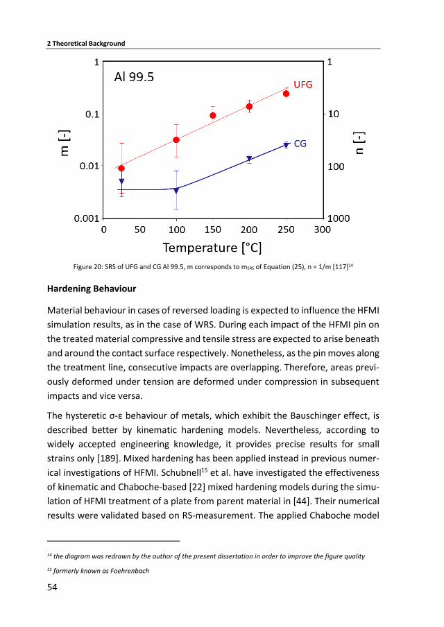
2 Theoretical Background
54
Figure 20: SRS of UFG and CG Al 99.5, m corresponds to mSRS of Equation (25), n = 1/m [117]14
Hardening Behaviour
Material behaviour in cases of reversed loading is expected to influence the HFMI
simulation results, as in the case of WRS. During each impact of the HFMI pin on
the treated material compressive and tensile stress are expected to arise beneath
and around the contact surface respectively. Nonetheless, as the pin moves along
the treatment line, consecutive impacts are overlapping. Therefore, areas previ-
ously deformed under tension are deformed under compression in subsequent
impacts and vice versa.
The hysteretic σ-ε behaviour of metals, which exhibit the Bauschinger effect, is
described better by kinematic hardening models. Nevertheless, according to
widely accepted engineering knowledge, it provides precise results for small
strains only [189]. Mixed hardening has been applied instead in previous numer-
ical investigations of HFMI. Schubnell15 et al. have investigated the effectiveness
of kinematic and Chaboche-based [22] mixed hardening models during the simu-
lation of HFMI treatment of a plate from parent material in [44]. Their numerical
results were validated based on RS-measurement. The applied Chaboche model
14 the diagram was redrawn by the author of the present dissertation in order to improve the figure quality
15 formerly known as Foehrenbach
2.1 Numerical Investigations
55
provided better results near the treatment surface. Hardenacke et al. have as well
previously discussed the influence of hardening behaviour [68]. Isotropic, com-
bined and rate-dependent hardening models produced qualitatively similar re-
sults in depth direction, but as in the case of the WRS, significant deviation to the
magnitude of the peak residual stresses was met. Zheng et al. [189], Le Quillec et
al. [103] and Baptista [10] applied combined, isotropic and kinematic and
Chaboche hardening models respectively, while Yuan et al. used usual linear kin-
ematic hardening [187].
Damping
Apart from the deformation behaviour and constitutive law of the investigated
material, its damping behaviour should be taken into consideration as well. Pre-
cise calculation of RS during nonlinear impact simulations, as in the case of HFMI,
perquisites sufficient modelling of the damping behaviour of the investigated ma-
terial as well, as a portion of the kinetic energy of the pin that is transferred into
the component is consumed by the damping mechanisms.
Damping is somewhat an abstract concept. Microscopic mechanisms exist in
structures, such as friction between metallic components or opening and closing
of microcracks etc., which are responsible for the lack of perfect oscillations in
nature. Albeit these mechanisms constitute a property of the structure, which
depends on geometry and material, and their influence is evident even for large
structures, a direct calculation of their magnitude based on physical characteris-
tics of the structure is not possible. Sophisticated measurements for direct esti-
mation of damping behaviour of existing components/structures are possible.
Nevertheless, results from measurements are transferable to analysis of similar
structures. Moreover, differentiation of damping behaviour for different levels of
external excitation does not allow extrapolation of the damping behaviour from
measurements of low excitation to analysis of larger excitation. On the other
hand, measurements of energy dissipation, in the case of large excitation, which
leads to non-linear deformation, include the plastic deformation energy and com-
plicate even more the evaluation of damping. Hence, predictive modelling of
damping, when appropriate measurements are not available, requires an appro-
priate idealization, which produces reasonable results.
It has been observed that the damping behaviour of a structural system or a com-
ponent is sufficiently simulated, when it is correlated both with its mass and stiff-
ness [24]. In this sense, Rayleigh’s damping model (described thoroughly in [24]),
2 Theoretical Background
56
which is a widely applied in numerical analysis and accounts for both mass and
stiffness influence was proposed. It is defined as follows:
𝑐 = 𝑎𝑅 ∙ 𝑚 + 𝛽𝑅 ∙ 𝑘. (26)
It was applied during a previous numerical investigation of shot peening, carried
out by Meguid et al. [124]. After a trial and error procedure, αR and βR were set
equal to 0.5 and 2 x 10⁻⁹ respectively. The following viscous damping model,
𝑐 = 2 ∙ 𝑓0 ∙ 𝜉 ∙ 𝑚 = Ds ∙ 𝑚, (27)
was applied instead by Kim et al. for 2D and 3D simulation of shot peening in more
recent studies [89], [90]. Different values for ξ between 0 and 0.5 were tested.
The resulted RS profiles were almost identical in all cases, arising questions about
the negligibility of damping in the investigated type of simulations. A value of 0.5
was proposed for ξ due to numerical efficiency reasons, as it led to the lowest
computational time [89]. Such a consideration of damping, based on the model
of Equation (27) and applying the same damping factor ξ = 0.5, was made as well
by Yuan et al. during numerical analysis of HFMI in [187]. This has been the sole
reference to damping in previous modelling efforts of HFMI, known to the author
of the present study.
An even more straightforward approach is the application of a global damping
factor, i.e. an arbitrary definition of damping matrix C16 (Eq. (23)), which is applied
to the response of all nodes or elements of the investigated component during a
FE simulation [113], [114]. Such an approach is usually applied during dynamic
simulations, where damping is not predominant for the results, but complete ne-
glection leads to numerical problems.
2.1.2.3 Modelling of the HFMI Pin
Material Behaviour of the HFMI Pin
HFMI pin is manufactured by hardened high strength metallic material17. There-
fore, linear elastic deformation of the pin is expected. Nonetheless, in comparison
16 by giving an arbitrary value to the product 𝐷𝑠 = 2 ∙ 𝑓0 ∙ 𝜉
17 exact information about the pin material is not provided by the manufacturers of the HFMI device due to confidentiality reasons
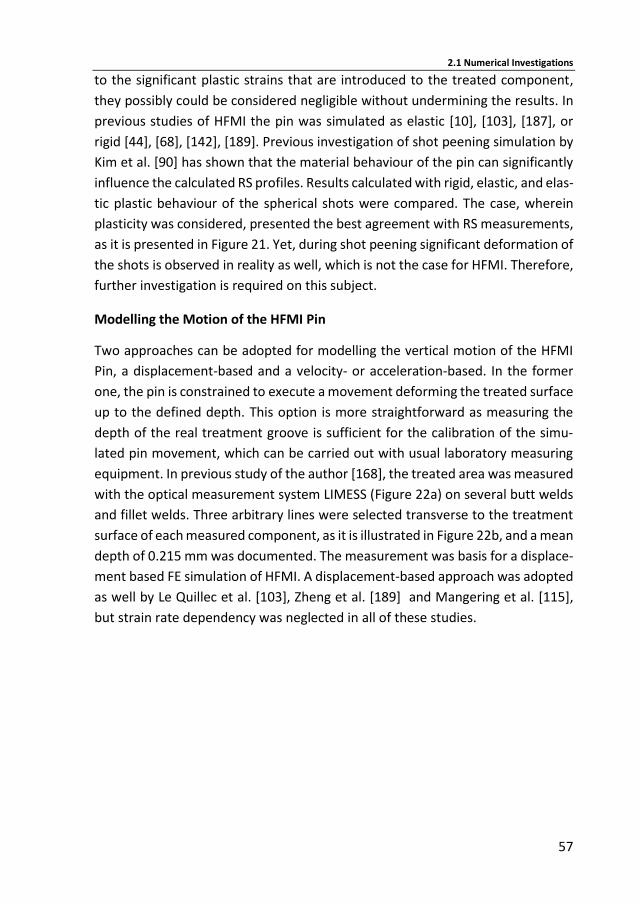
2.1 Numerical Investigations
57
to the significant plastic strains that are introduced to the treated component,
they possibly could be considered negligible without undermining the results. In
previous studies of HFMI the pin was simulated as elastic [10], [103], [187], or
rigid [44], [68], [142], [189]. Previous investigation of shot peening simulation by
Kim et al. [90] has shown that the material behaviour of the pin can significantly
influence the calculated RS profiles. Results calculated with rigid, elastic, and elas-
tic plastic behaviour of the spherical shots were compared. The case, wherein
plasticity was considered, presented the best agreement with RS measurements,
as it is presented in Figure 21. Yet, during shot peening significant deformation of
the shots is observed in reality as well, which is not the case for HFMI. Therefore,
further investigation is required on this subject.
Modelling the Motion of the HFMI Pin
Two approaches can be adopted for modelling the vertical motion of the HFMI
Pin, a displacement-based and a velocity- or acceleration-based. In the former
one, the pin is constrained to execute a movement deforming the treated surface
up to the defined depth. This option is more straightforward as measuring the
depth of the real treatment groove is sufficient for the calibration of the simu-
lated pin movement, which can be carried out with usual laboratory measuring
equipment. In previous study of the author [168], the treated area was measured
with the optical measurement system LIMESS (Figure 22a) on several butt welds
and fillet welds. Three arbitrary lines were selected transverse to the treatment
surface of each measured component, as it is illustrated in Figure 22b, and a mean
depth of 0.215 mm was documented. The measurement was basis for a displace-
ment based FE simulation of HFMI. A displacement-based approach was adopted
as well by Le Quillec et al. [103], Zheng et al. [189] and Mangering et al. [115],
but strain rate dependency was neglected in all of these studies.
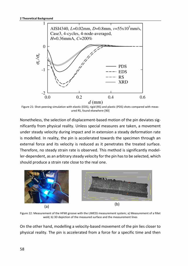
2 Theoretical Background
58
Figure 21: Shot-peening simulation with elastic (EDS), rigid (RS) and plastic (PDS) shots compared with meas-
ured RS, found elsewhere [90]
Nonetheless, the selection of displacement-based motion of the pin deviates sig-
nificantly from physical reality. Unless special measures are taken, a movement
under steady velocity during impact and in extension a steady deformation rate
is modelled. In reality, the pin is accelerated towards the specimen through an
external force and its velocity is reduced as it penetrates the treated surface.
Therefore, no steady strain rate is observed. This method is significantly model-
ler-dependent, as an arbitrary steady velocity for the pin has to be selected, which
should produce a strain rate close to the real one.
(a)
(b)
Figure 22: Measurement of the HFMI groove with the LIMESS measurement system; a) Measurement of a fillet weld; b) 3D depiction of the measured surface and the measurement lines
On the other hand, modelling a velocity-based movement of the pin lies closer to
physical reality. The pin is accelerated from a force for a specific time and then
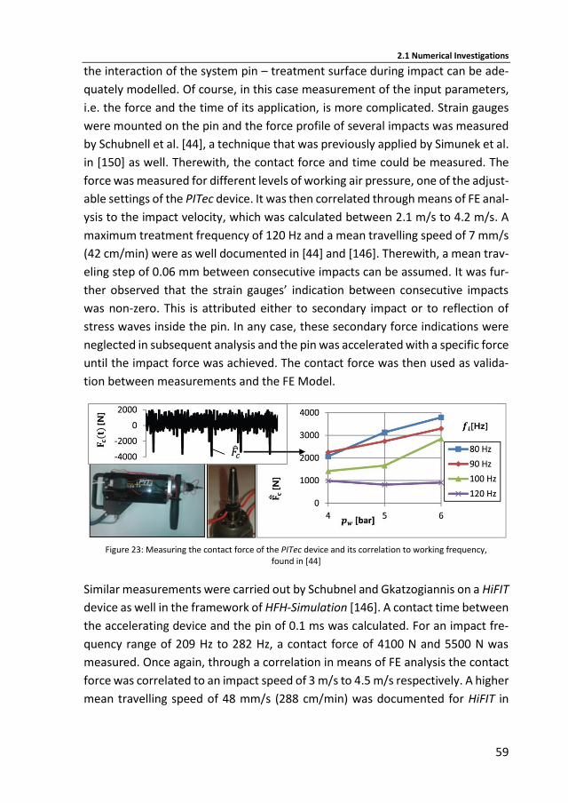
2.1 Numerical Investigations
59
the interaction of the system pin – treatment surface during impact can be ade-
quately modelled. Of course, in this case measurement of the input parameters,
i.e. the force and the time of its application, is more complicated. Strain gauges
were mounted on the pin and the force profile of several impacts was measured
by Schubnell et al. [44], a technique that was previously applied by Simunek et al.
in [150] as well. Therewith, the contact force and time could be measured. The
force was measured for different levels of working air pressure, one of the adjust-
able settings of the PITec device. It was then correlated through means of FE anal-
ysis to the impact velocity, which was calculated between 2.1 m/s to 4.2 m/s. A
maximum treatment frequency of 120 Hz and a mean travelling speed of 7 mm/s
(42 cm/min) were as well documented in [44] and [146]. Therewith, a mean trav-
eling step of 0.06 mm between consecutive impacts can be assumed. It was fur-
ther observed that the strain gauges’ indication between consecutive impacts
was non-zero. This is attributed either to secondary impact or to reflection of
stress waves inside the pin. In any case, these secondary force indications were
neglected in subsequent analysis and the pin was accelerated with a specific force
until the impact force was achieved. The contact force was then used as valida-
tion between measurements and the FE Model.
Figure 23: Measuring the contact force of the PITec device and its correlation to working frequency,
found in [44]
Similar measurements were carried out by Schubnel and Gkatzogiannis on a HiFIT
device as well in the framework of HFH-Simulation [146]. A contact time between
the accelerating device and the pin of 0.1 ms was calculated. For an impact fre-
quency range of 209 Hz to 282 Hz, a contact force of 4100 N and 5500 N was
measured. Once again, through a correlation in means of FE analysis the contact
force was correlated to an impact speed of 3 m/s to 4.5 m/s respectively. A higher
mean travelling speed of 48 mm/s (288 cm/min) was documented for HiFIT in
2 Theoretical Background
60
comparison to the 7 mm/s (42 cm/min) of PITec. The mean travelling step be-
tween consecutive impacts is nonetheless significantly higher and equal to 0.22
mm due to the increased frequency in this case.
A velocity-based approach was adopted by Yan et al. [187], while the two meth-
ods were compared by Schubnell et al. [44] and Hardenacke et al. [68]. Actually,
it was concluded by the former one that the displacement-based approach pro-
duced results showing better agreement with measured RS. The authors recom-
mend though that the displacement-based model should be applied with strain
rate dependent material behaviour, but the applied displacement-rate of the pin,
which would affect the rate dependent material behaviour, is not reported.
Finally, regarding the moving velocity of the pin, a step of 0.4 mm and 0.3 mm
was proposed in [44], [68], and [150] and [187] respectively. Both values are
larger than the real overlap between consecutive impacts but it was mentioned
in the above studies that this deviation had a negligible effect on the results. In a
more recent study [145] though, the influence of coverage has been investigated
thoroughly. It was suggested based on RS measurements that an increased over-
lap up to a threshold value leads to a higher magnitude of transverse RS. Above
this threshold point though, no significant change on the RS field was observed.
Modelling of Contact Conditions
Appropriate definition of contact conditions between the HFMI Pin and the
treated surface is required in order to ensure a close to physical-reality simulation
of contact problems. Contact dissipates part of the pin’s kinetic energy, prior to
its transfer in the component in the form of stress waves. Coulomb’s friction
model (Eq. (28), see [114]), which is described by Equation (48)
𝐹𝑓 = 𝜇 ∙ 𝐹𝑁 , (28)
is widely applied for metallic materials and has been applied for the simulation of
HFMI and shot peening in the past. The coefficient μ takes various values depend-
ing on the nature of the surfaces, which slide under friction. It is usually charac-
terized as static or dynamic, when it describes the state at the beginning or during
sliding respectively. Generic values for different surface qualities and for both
cases, the static and the dynamic, are proposed in [6]. A selection from the pro-
posed values is presented in Table 4.
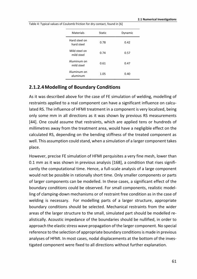
2.1 Numerical Investigations
61
Table 4: Typical values of Coulomb friction for dry contact, found in [6]
Materials Static Dynamic
Hard steel on hard steel
0.78 0.42
Mild steel on mild steel
0.74 0.57
Aluminum on mild steel
0.61 0.47
Aluminum on aluminum
1.05 0.40
2.1.2.4 Modelling of Boundary Conditions
As it was described above for the case of FE simulation of welding, modelling of
restraints applied to a real component can have a significant influence on calcu-
lated RS. The influence of HFMI treatment in a component is very localized, being
only some mm in all directions as it was shown by previous RS measurements
[44]. One could assume that restraints, which are applied tens or hundreds of
millimetres away from the treatment area, would have a negligible effect on the
calculated RS, depending on the bending stiffness of the treated component as
well. This assumption could stand, when a simulation of a larger component takes
place.
However, precise FE simulation of HFMI perquisites a very fine mesh, lower than
0.1 mm as it was shown in previous analysis [168], a condition that rises signifi-
cantly the computational time. Hence, a full-scale analysis of a large component
would not be possible in rationally short time. Only smaller components or parts
of larger components can be modelled. In these cases, a significant effect of the
boundary conditions could be observed. For small components, realistic model-
ling of clamping-down mechanisms or of restraint free condition as in the case of
welding is necessary. For modelling parts of a larger structure, appropriate
boundary conditions should be selected. Mechanical restraints from the wider
areas of the larger structure to the small, simulated part should be modelled re-
alistically. Acoustic impedance of the boundaries should be nullified, in order to
approach the elastic stress wave propagation of the larger component. No special
reference to the selection of appropriate boundary conditions is made in previous
analyses of HFMI. In most cases, nodal displacements at the bottom of the inves-
tigated component were fixed to all directions without further explanation.
2 Theoretical Background
62
2.2 Analytical Investigations for the Calculation of the Dynamic Yield Strength during a Spherical Impact
Hertzian theory of elastic contact has been the basis for analytical solutions of
impacts since its evolution more than 130 years ago [73]. In 1998, Lim and Stronge
proposed such an analytical solution for the calculation of a rigid cylinder’s impact
on an elastoplastic-half space [110]. In their study, this impact was analysed in
three consecutive phases, the elastic, whereby Hertzian theory is applied, the
elastic-plastic, whereby elastic and plastic behaviour coexist in the area beneath
the contact and finally, the fully plastic phase. Their solution beyond yielding was
based on the cavity model, which was initially proposed by Hill [75] and later sim-
plified by Johnson [83]. This model assumes the symmetrical expansion of a
spherical cavity in an elastic-plastic material so that compatibility between the
volume of displaced material and the accommodated radial elastic expansion is
ensured during the contact.
Classical Hertzian theory [73] refers to elastic bodies. In the present case, the im-
pacting sphere is regarded rigid (E ∞). Therefore, the physical quantity defined
by Hertz as E* and given by Equation (29),
1
𝐸∗=
1 − 𝜈𝑠𝑝ℎ𝑒𝑟𝑒2
𝐸𝑠𝑝ℎ𝑒𝑟𝑒+
1 − 𝜈𝑝𝑙𝑎𝑡𝑒2
𝐸𝑝𝑙𝑎𝑡𝑒, (29)
will hereinafter be given by the following equation
1
𝐸∗=
1 − 𝜈𝑝𝑙𝑎𝑡𝑒2
𝐸𝑝𝑙𝑎𝑡𝑒. (30)
According to Hertzian theory ([73], [110]) the indentation depth of a rigid sphere
in an elastic half space and in the elastic regime is calculated as follows:
𝛿 = [9 ∙ 𝐹2 ∙ (1 − 𝜈2)
16 ∙ 𝑅 ∙ 𝐸]
1/3
. (31)
Under the assumptions of infinitesimal strains in the elastic regime and continu-
ous contact between the indenter and the half-space, the contact area between
the sphere and the plate is circular and the contact force is correlated to the mean
pressure according to the following Equation (32),
2.2 Analytical Investigations for the Calculation of the Dynamic Yield Strength during a Spherical Impact
63
𝐹 = 𝜋 ∙ 𝑎2 ∙ 𝑝𝑚. (32)
The contact half width α in the elastic regime and therefore during yielding as
well, is given by Equation (33):
𝑎3 = 3 ∙ 𝐹 ∙ 𝑅 ∙ (1 − 𝜈2)
4 ∙ 𝐸. (33)
When Lim and Stronge investigated the elastic-plastic impact of the rigid cylinder
on a half-space [110], they noticed that after the end of the indentation and un-
loading and as long as full plastification has taken place, the crater’s half width αc
after full plastification is correlated with the contact half width at yielding accord-
ing to Equation (34),
𝑎𝑐2 (
1
𝑅−
1
𝑅′) =
𝑎𝑦2
𝑅, (34)
where R and R’ is the radius of curvature of the contact area prior and after un-
loading. Prior to unloading R is equal to the radius of the indenter, as full contact
is assumed at all times. This latter equation was extracted assuming that the con-
tact width at maximum compression ac is equal to the width of the residual in-
dentation i.e. the elastic spring back is negligible, the residual indentation has a
final curvature R’, which is slightly larger than R due to elastic recovery and finally,
no piling up or sinking in takes place during the indentation of the plate.
Johnson, analysing the indentation of an elastic - perfect plastic and incompress-
ible material by a rigid sphere, proposed in [83] that the average pressures pmY
and pmp at initiation of yielding and at full plastification are respectively correlated
with the material yield stress according to the following equations:
𝑝𝑚𝑌 = 1.1 ∙ 𝜎𝑌, (35)
𝑝𝑚𝑃 = 3.072 ∙ 𝜎𝑌. (36)
These empirical equations were subsequently validated for steel by numerical
and experimental investigations (see for instance [159]). Yet, the diagram of Fig-
ure 24, found in [82], reveals that these relationships between average pressure
and yield strength, which mark the transition from the elastic to the elastic plastic
and from the latter one to the perfect plastic regime, are dependent on the yield
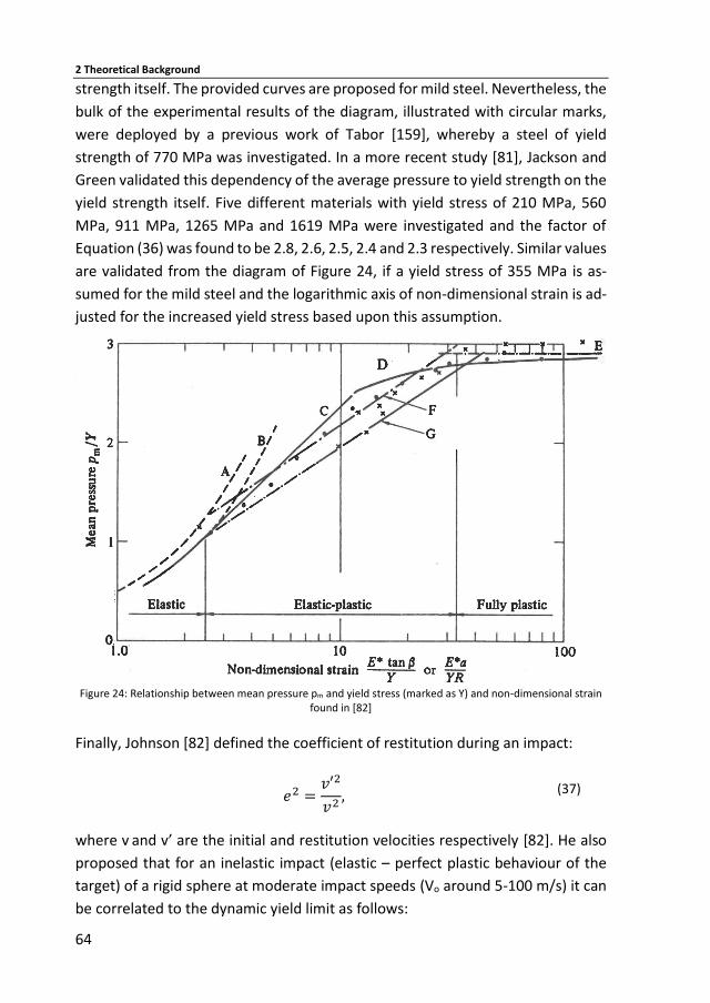
2 Theoretical Background
64
strength itself. The provided curves are proposed for mild steel. Nevertheless, the
bulk of the experimental results of the diagram, illustrated with circular marks,
were deployed by a previous work of Tabor [159], whereby a steel of yield
strength of 770 MPa was investigated. In a more recent study [81], Jackson and
Green validated this dependency of the average pressure to yield strength on the
yield strength itself. Five different materials with yield stress of 210 MPa, 560
MPa, 911 MPa, 1265 MPa and 1619 MPa were investigated and the factor of
Equation (36) was found to be 2.8, 2.6, 2.5, 2.4 and 2.3 respectively. Similar values
are validated from the diagram of Figure 24, if a yield stress of 355 MPa is as-
sumed for the mild steel and the logarithmic axis of non-dimensional strain is ad-
justed for the increased yield stress based upon this assumption.
Figure 24: Relationship between mean pressure pm and yield stress (marked as Y) and non-dimensional strain
found in [82]
Finally, Johnson [82] defined the coefficient of restitution during an impact:
𝑒2 =𝑣′2
𝑣2, (37)
where v and v’ are the initial and restitution velocities respectively [82]. He also
proposed that for an inelastic impact (elastic – perfect plastic behaviour of the
target) of a rigid sphere at moderate impact speeds (Vo around 5-100 m/s) it can
be correlated to the dynamic yield limit as follows:
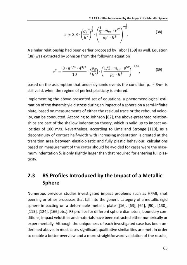
2.3 RS Profiles Introduced by the Impact of a Metallic Sphere
65
𝑒 ≈ 3.8 ∙ (𝜎𝑌
′
𝐸∗ )
12
∙ (
12
∙ 𝑚𝑠𝑝 ∙ 𝑣′2
𝜎𝑌′ ∙ 𝑅3
)
−18
. (38)
A similar relationship had been earlier proposed by Tabor [159] as well. Equation
(38) was extracted by Johnson from the following equation
𝑒2 =3 ∙ 𝜋5/4 ∙ 43/4
10∙ (
𝑝𝑑
𝐸∗) ∙ (
1/2 ∙ 𝑚𝑠𝑝 ∙ 𝑣′2
𝑝𝑑 ∙ 𝑅3 )
−1/4
, (39)
based on the assumption that under dynamic events the condition pm ≈ 3·σY’ is
still valid, when the regime of perfect plasticity is entered.
Implementing the above-presented set of equations, a phenomenological esti-
mation of the dynamic yield stress during an impact of a sphere on a semi-infinite
plate, based on measurements of either the residual trace or the rebound veloc-
ity, can be conducted. According to Johnson [82], the above-presented relation-
ships are part of the shallow indentation theory, which is valid up to impact ve-
locities of 100 m/s. Nevertheless, according to Lime and Stronge [110], as a
discontinuity of contact half-width with increasing indentation is created at the
transition area between elastic-plastic and fully plastic behaviour, calculations
based on measurement of the crater should be avoided for cases were the maxi-
mum indentation δc is only slightly larger than that required for entering full plas-
ticity.
2.3 RS Profiles Introduced by the Impact of a Metallic Sphere
Numerous previous studies investigated impact problems such as HFMI, shot
peening or other processes that fall into the generic category of a metallic rigid
sphere impacting on a deformable metallic plate ([16], [63], [64], [90], [130],
[115], [124], [166] etc.). RS profiles for different sphere diameters, boundary con-
ditions, impact velocities and materials have been extracted either numerically or
experimentally. Although the uniqueness of each investigated case has been un-
derlined above, in most cases significant qualitative similarities are met. In order
to enable a better overview and a more straightforward validation of the results,
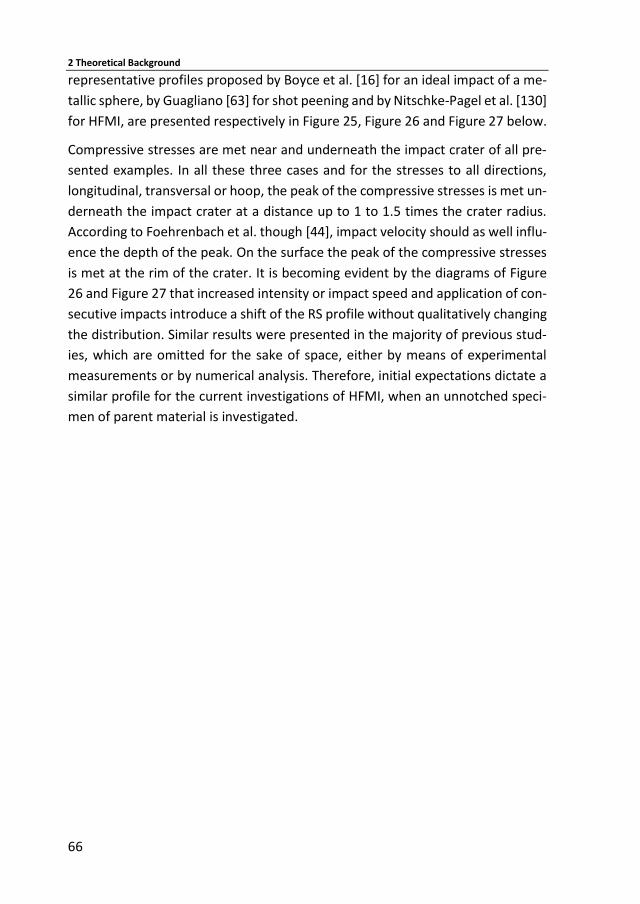
2 Theoretical Background
66
representative profiles proposed by Boyce et al. [16] for an ideal impact of a me-
tallic sphere, by Guagliano [63] for shot peening and by Nitschke-Pagel et al. [130]
for HFMI, are presented respectively in Figure 25, Figure 26 and Figure 27 below.
Compressive stresses are met near and underneath the impact crater of all pre-
sented examples. In all these three cases and for the stresses to all directions,
longitudinal, transversal or hoop, the peak of the compressive stresses is met un-
derneath the impact crater at a distance up to 1 to 1.5 times the crater radius.
According to Foehrenbach et al. though [44], impact velocity should as well influ-
ence the depth of the peak. On the surface the peak of the compressive stresses
is met at the rim of the crater. It is becoming evident by the diagrams of Figure
26 and Figure 27 that increased intensity or impact speed and application of con-
secutive impacts introduce a shift of the RS profile without qualitatively changing
the distribution. Similar results were presented in the majority of previous stud-
ies, which are omitted for the sake of space, either by means of experimental
measurements or by numerical analysis. Therefore, initial expectations dictate a
similar profile for the current investigations of HFMI, when an unnotched speci-
men of parent material is investigated.
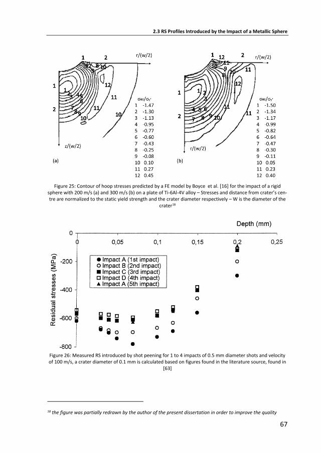
2.3 RS Profiles Introduced by the Impact of a Metallic Sphere
67
Figure 25: Contour of hoop stresses predicted by a FE model by Boyce et al. [16] for the impact of a rigid
sphere with 200 m/s (a) and 300 m/s (b) on a plate of Ti-6Al-4V alloy – Stresses and distance from crater’s cen-tre are normalized to the static yield strength and the crater diameter respectively – W is the diameter of the
crater18
Figure 26: Measured RS introduced by shot peening for 1 to 4 impacts of 0.5 mm diameter shots and velocity of 100 m/s, a crater diameter of 0.1 mm is calculated based on figures found in the literature source, found in
[63]
18 the figure was partially redrawn by the author of the present dissertation in order to improve the quality
2 Theoretical Background
68
Figure 27: Transverse residual stress through-depth profiles in UIT-treated fields for variating treatment inten-sity and for a pin diameter of 4.8 mm in the base material S690, crater swallower than 0.5 mm, based on a dia-
gram found in [130]
-800
-600
-400
-200
0
200
400
0 1 2 3 4 5 6 7 8
Tran
sver
se R
S [M
Pa]
Distance from surface [mm]
Intensity = s3
Intensity = s4
Intensity = s5
Intensity = s5, ND
69
3 FE Simulation of Welding
3.1 Methodology
Simulations of welding, which were carried out in the framework of the present
dissertation, were based on the above-presented theoretical background. Each
investigated case acted as a milestone towards the completion of the present
task, the FE simulation of welding, fulfilling the conditions that were set at the
beginning of the present research study regarding straightforwardness and pre-
ciseness.
Single-pass butt welds were simulated as a first step towards the development of
the present approach due to their simple geometry and the reduced required
modelling, as the influence of a single thermal cycle has to be considered. Valida-
tion was initially based on measurements, which were found in literature. The
classical example presented by Anderson back in 1978 - component A - along with
a newer study from Caron et al. - component B - were used as reference ([3] and
[21] respectively). These two cases were selected, due to the full documentation
of the welding procedure along with WRS measurements provided by the au-
thors. The components were remodelled with the current approach, applying
identical welding parameters and geometry. Some of the results were presented
in earlier work of the author in [53], [59] and [92].
The results regarding component A were compared with other efforts of simulat-
ing the same component by Anderson himself [3] and Lindgren in [111] as well.
Results from the simulation of component B were compared with the respective
simulation carried out by Caron et al., using the specialized FE software SYSWELD
[158]. Valuable conclusions regarding several practical aspects of weld modelling
were drawn and applied in subsequent simulations.
Next step was the extension of the present approach for the case of multi-pass
welding of austenitic steels [56] and the simulation of aluminium alloys [93]. Nev-
ertheless, these investigations although relative to the filed, are only outlined and
a detailed presentation is excluded from this dissertation, as they do not directly
contribute to the present research goal.
3 FE Simulation of Welding
70
The presented approach was finally applied, in order to simulate plates with
transversal stiffeners (fillet welds) welded on both sides from the research project
HFH-Simulation [146], wherein RS measurements were carried out in as-welded
and HFMI-treated state (see [146]). Goal was the calculation of the WRS field so
that it could be applied as input for the subsequent HFMI simulation.
Although modifications based on the available information and improvements in
modelling were carried out after each investigation, the backbone of the ap-
proach remained unaltered, as it was initially presented in [92]. The physics fields
and the predominant interactions that are presented in Figure 4 were taken into
consideration. FE commercial software ANSYS was applied for all weld simula-
tions.
3.1.1 Thermal Transient Analysis
A transient thermal analysis was initially carried out in order to calculate the ther-
mal history of each node, based on Equation (4). ANSYS 8-node solid finite ele-
ments SOLID70, which allow the simulation of heat conductivity and heat gener-
ation, were applied [4]. The element temperature is calculated at each time step
based on its shape functions, from the temperatures of its nodes (see Appendix
B).
Goldak’s heat source was applied, using an algorithm, which was provided by the
company CADFEM. It was applied in such a way, that the centre of the source was
moving at each solution step along the welding line, for a distance equal to the
welding speed multiplied by the time between the consecutive solution steps.
Power of the heat source is calculated according to Equation (3). Values for the
coefficient of heat source η proposed by Dupont et al. were applied based on the
investigated weld type (see [32]), unless otherwise stated below. Heat losses
were simulated according to Equation (7), using a common coefficient for heat
losses hT, as described above. Values for the coefficient were found in [140] and
they are presented in Table 5. Thermal material properties were assumed inde-
pendent of the microstructural transformations in all cases. Therefore, thermal
properties of the parent material were applied in the thermal transient analysis.
Ambient temperature was assumed equal to 20 °C in all cases. In each solution
step, information regarding elements whose temperature was exceeding the
melting point was documented. After completion of the transient solution the

3.1 Methodology
71
double parameter (Tmax, t85) of each element in the HAZ and FZ was calculated
based on the temperature history of its nodes.
Table 5: Applied values for the total coefficient of heat losses, found in [140]
Temperature [oC] 20 100 450 850 1550 2350 3000 10000
hT [W/(m2 ∙ K)] 4.7 22.8 48.2 117.9 396.9 1082.3 2032.9 58214.0
3.1.2 Microstructural Modelling
Microstructural modelling was carried out based on the approach presented in
[92] and described in the theoretical background. A bilinear elastic – plastic ma-
terial behaviour was assumed in most cases, unless otherwise referred. Parent
material properties for the butt welds were taken from literature, while for the
transversal stiffeners respective measurements were carried out in the frame-
work of the project HFH-Simulation [146]. A1 and A3’ were calculated using Equa-
tions (9) and (10), (11) based on the chemical composition of each investigated
alloy. Bilinear elastic – plastic CMMs were built for different levels of Tmax and for
different cooling rates t85. The former influenced the austenitization percentage
and the later the final transformed microstructure, which unless otherwise
stated, was calculated from appropriate CCT diagrams found in literature. The
dilation behaviour and yield strength of the CMMs was calculated by applying
linear mixtures law, with Equations (15) and (19) respectively. Yield strength of
the individual phases was found in [74]. Unless otherwise mentioned, coefficient
of thermal expansion of austenite and the rest of the phases was assumed equal
to 16 x 10-6 and 12 x 10-6 respectively and tangent modulus H was assumed same
for all phases. Whenever necessary, TRIP was taken into consideration according
to Karlsson’s approach, as it was described earlier.
3.1.3 Static Structural Analysis
A quasi-static structural analysis (see Equation (17)) was carried out based on the
thermal history of the nodes, which was calculated during the transient thermal
analysis. ANSYS 8-node solid finite elements SOLID185, which have stiffness and
allow simulation of stress and thermal loading, were applied for this analysis. The
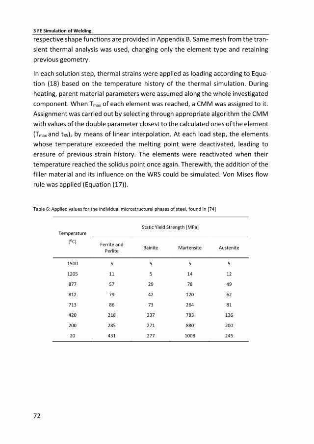
3 FE Simulation of Welding
72
respective shape functions are provided in Appendix B. Same mesh from the tran-
sient thermal analysis was used, changing only the element type and retaining
previous geometry.
In each solution step, thermal strains were applied as loading according to Equa-
tion (18) based on the temperature history of the thermal simulation. During
heating, parent material parameters were assumed along the whole investigated
component. When Tmax of each element was reached, a CMM was assigned to it.
Assignment was carried out by selecting through appropriate algorithm the CMM
with values of the double parameter closest to the calculated ones of the element
(Tmax and t85), by means of linear interpolation. At each load step, the elements
whose temperature exceeded the melting point were deactivated, leading to
erasure of previous strain history. The elements were reactivated when their
temperature reached the solidus point once again. Therewith, the addition of the
filler material and its influence on the WRS could be simulated. Von Mises flow
rule was applied (Equation (17)).
Table 6: Applied values for the individual microstructural phases of steel, found in [74]
Temperature
[⁰C]
Static Yield Strength [MPa]
Ferrite and Perlite
Bainite Martensite Austenite
1500 5 5 5 5
1205 11 5 14 12
877 57 29 78 49
812 79 42 120 62
713 86 73 264 81
420 218 237 783 136
200 285 271 880 200
20 431 277 1008 245
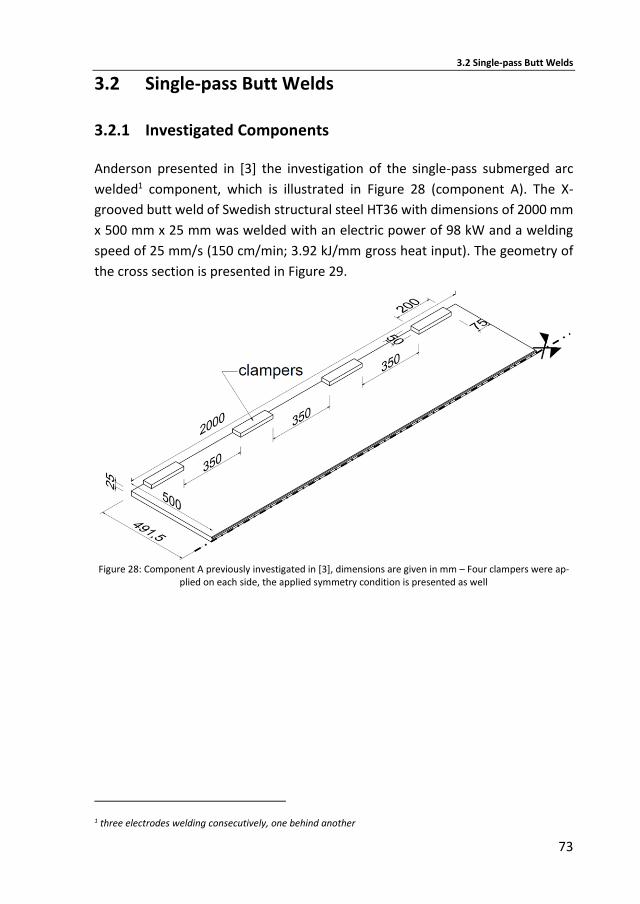
3.2 Single-pass Butt Welds
73
3.2 Single-pass Butt Welds
3.2.1 Investigated Components
Anderson presented in [3] the investigation of the single-pass submerged arc
welded1 component, which is illustrated in Figure 28 (component A). The X-
grooved butt weld of Swedish structural steel HT36 with dimensions of 2000 mm
x 500 mm x 25 mm was welded with an electric power of 98 kW and a welding
speed of 25 mm/s (150 cm/min; 3.92 kJ/mm gross heat input). The geometry of
the cross section is presented in Figure 29.
Figure 28: Component A previously investigated in [3], dimensions are given in mm – Four clampers were ap-
plied on each side, the applied symmetry condition is presented as well
1 three electrodes welding consecutively, one behind another

3 FE Simulation of Welding
74
Figure 29: Cross section of component A, dimensions are given in mm – The applied symmetry condition is
presented as well2
Caron et al. investigated in [21] a single-pass V-grooved butt weld of steel S355
[29], which is presented in Figure 30 (component B). The component with dimen-
sions of 500 mm x 200 mm x 5 mm was welded with an electric power of 7.934
kW and a welding speed of 6.7 mm/s (40 cm/min; 1.18 kJ/mm gross heat input).
Figure 30: Component B previously investigated in [21], dimensions are given in mm – No restraints during
welding, the applied symmetry condition is presented as well
Figure 31: Cross section of component B, dimensions are given in mm – The applied symmetry condition is
presented as well
2 the component was X-grooved as it would be welded with 3 passes of a single electrode – with the applied submerged arc welding technique with 3 electrodes welding consecutively, one behind another, it was possible to weld with a single-pass the middle and upper seam, the final geometry of the weld section area is illustrated better bellow (see Figure 35), more information is provided in [3]
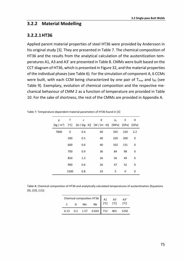
3.2 Single-pass Butt Welds
75
3.2.2 Material Modelling
3.2.2.1 HT36
Applied parent material properties of steel HT36 were provided by Andersson in
his original study [3]. They are presented in Table 7. The chemical composition of
HT36 and the results from the analytical calculation of the austenitization tem-
peratures A1, A3 and A3’ are presented in Table 8. CMMs were built based on the
CCT diagram of HT36, which is presented in Figure 32, and the material properties
of the individual phases (see Table 6). For the simulation of component A, 6 CCMs
were built, with each CCM being characterized by one pair of Tmax and t85 (see
Table 9). Exemplary, evolution of chemical composition and the respective me-
chanical behaviour of CMM 2 as a function of temperature are provided in Table
10. For the sake of shortness, the rest of the CMMs are provided in Appendix A.
Table 7: Temperature-dependent material parameters of HT36 found in [3]
ρ
[kg / m3]
T
[oC]
c
[kJ / (kg ∙ K)]
K
[W / (m ∙ K)]
σy
[MPa]
E
[GPa]
H
[GPa]
7800 0 0.4 40 355 220 2.2
200 0.5 40 320 200 0
600 0.6 40 102 131 0
700 0.9 36 84 98 0
850 1.3 26 56 49 0
900 0.6 26 47 32 0
1500 0.8 33 5 0 0
Table 8: Chemical composition of HT36 and analytically calculated temperatures of austenitization (Equations
(9), (10), (11))
Chemical composition HT36 A1 [oC]
A3 [oC]
A3’ [oC] C Si Mn Nb
0.13 0.2 1.57 0.024 712 801 1250
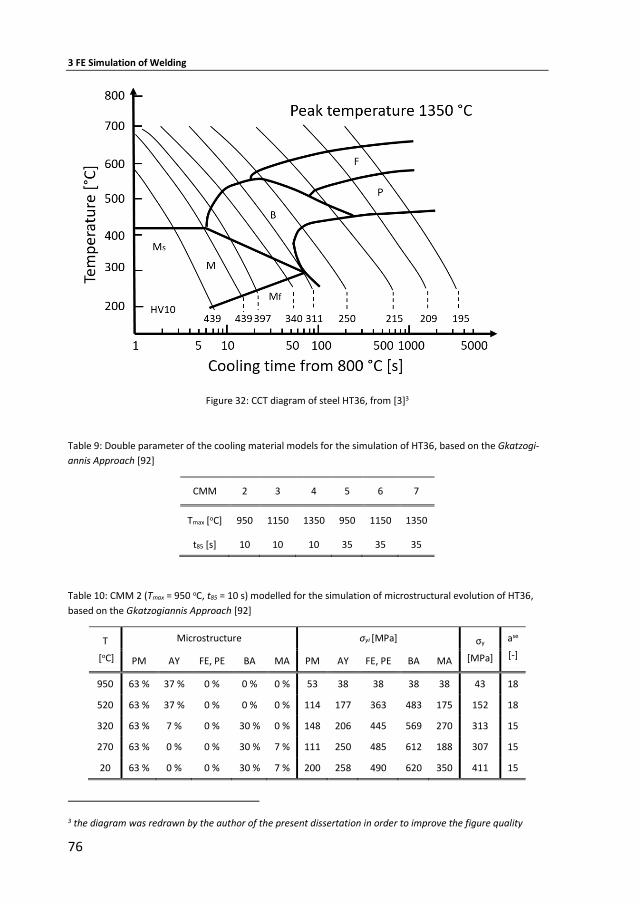
3 FE Simulation of Welding
76
Figure 32: CCT diagram of steel HT36, from [3]3
Table 9: Double parameter of the cooling material models for the simulation of HT36, based on the Gkatzogi-
annis Approach [92]
CMM 2 3 4 5 6 7
Tmax [oC] 950 1150 1350 950 1150 1350
t85 [s] 10 10 10 35 35 35
Table 10: CMM 2 (Tmax = 950 oC, t85 = 10 s) modelled for the simulation of microstructural evolution of HT36,
based on the Gkatzogiannis Approach [92]
T
[oC]
Microstructure σyi [MPa] σy
[MPa]
ase
[-] PM AY FE, PE BA MA PM AY FE, PE BA MA
950 63 % 37 % 0 % 0 % 0 % 53 38 38 38 38 43 18
520 63 % 37 % 0 % 0 % 0 % 114 177 363 483 175 152 18
320 63 % 7 % 0 % 30 % 0 % 148 206 445 569 270 313 15
270 63 % 0 % 0 % 30 % 7 % 111 250 485 612 188 307 15
20 63 % 0 % 0 % 30 % 7 % 200 258 490 620 350 411 15
3 the diagram was redrawn by the author of the present dissertation in order to improve the figure quality
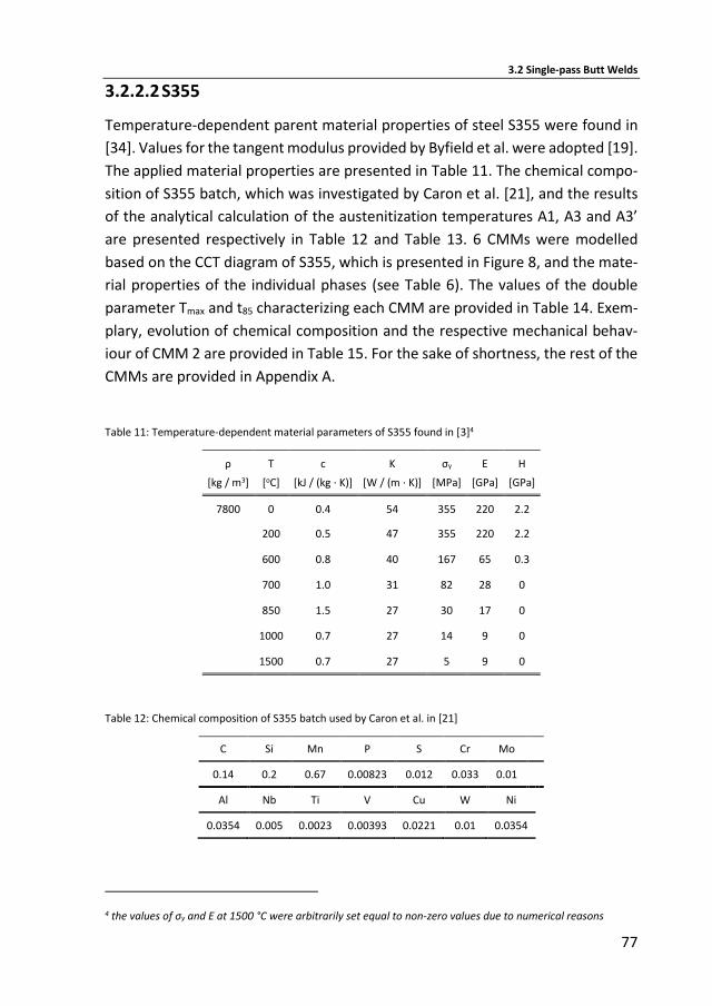
3.2 Single-pass Butt Welds
77
3.2.2.2 S355
Temperature-dependent parent material properties of steel S355 were found in
[34]. Values for the tangent modulus provided by Byfield et al. were adopted [19].
The applied material properties are presented in Table 11. The chemical compo-
sition of S355 batch, which was investigated by Caron et al. [21], and the results
of the analytical calculation of the austenitization temperatures A1, A3 and A3’
are presented respectively in Table 12 and Table 13. 6 CMMs were modelled
based on the CCT diagram of S355, which is presented in Figure 8, and the mate-
rial properties of the individual phases (see Table 6). The values of the double
parameter Tmax and t85 characterizing each CMM are provided in Table 14. Exem-
plary, evolution of chemical composition and the respective mechanical behav-
iour of CMM 2 are provided in Table 15. For the sake of shortness, the rest of the
CMMs are provided in Appendix A.
Table 11: Temperature-dependent material parameters of S355 found in [3]4
ρ
[kg / m3]
T
[oC]
c
[kJ / (kg ∙ K)]
K
[W / (m ∙ K)]
σy
[MPa]
E
[GPa]
H
[GPa]
7800 0 0.4 54 355 220 2.2
200 0.5 47 355 220 2.2
600 0.8 40 167 65 0.3
700 1.0 31 82 28 0
850 1.5 27 30 17 0
1000 0.7 27 14 9 0
1500 0.7 27 5 9 0
Table 12: Chemical composition of S355 batch used by Caron et al. in [21]
C Si Mn P S Cr Mo
0.14 0.2 0.67 0.00823 0.012 0.033 0.01
Al Nb Ti V Cu W Ni
0.0354 0.005 0.0023 0.00393 0.0221 0.01 0.0354
4 the values of σy and E at 1500 °C were arbitrarily set equal to non-zero values due to numerical reasons
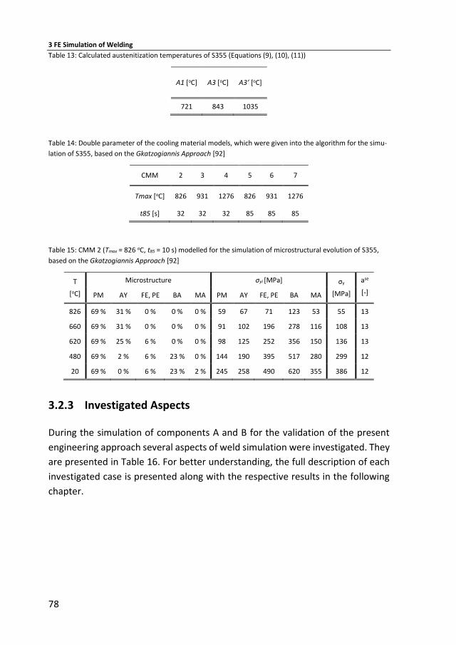
3 FE Simulation of Welding
78
Table 13: Calculated austenitization temperatures of S355 (Equations (9), (10), (11))
A1 [oC] A3 [oC] A3’ [oC]
721 843 1035
Table 14: Double parameter of the cooling material models, which were given into the algorithm for the simu-
lation of S355, based on the Gkatzogiannis Approach [92]
CMM 2 3 4 5 6 7
Tmax [oC] 826 931 1276 826 931 1276
t85 [s] 32 32 32 85 85 85
Table 15: CMM 2 (Tmax = 826 oC, t85 = 10 s) modelled for the simulation of microstructural evolution of S355,
based on the Gkatzogiannis Approach [92]
T
[oC]
Microstructure σyi [MPa] σy
[MPa]
ase
[-] PM AY FE, PE BA MA PM AY FE, PE BA MA
826 69 % 31 % 0 % 0 % 0 % 59 67 71 123 53 55 13
660 69 % 31 % 0 % 0 % 0 % 91 102 196 278 116 108 13
620 69 % 25 % 6 % 0 % 0 % 98 125 252 356 150 136 13
480 69 % 2 % 6 % 23 % 0 % 144 190 395 517 280 299 12
20 69 % 0 % 6 % 23 % 2 % 245 258 490 620 355 386 12
3.2.3 Investigated Aspects
During the simulation of components A and B for the validation of the present
engineering approach several aspects of weld simulation were investigated. They
are presented in Table 16. For better understanding, the full description of each
investigated case is presented along with the respective results in the following
chapter.
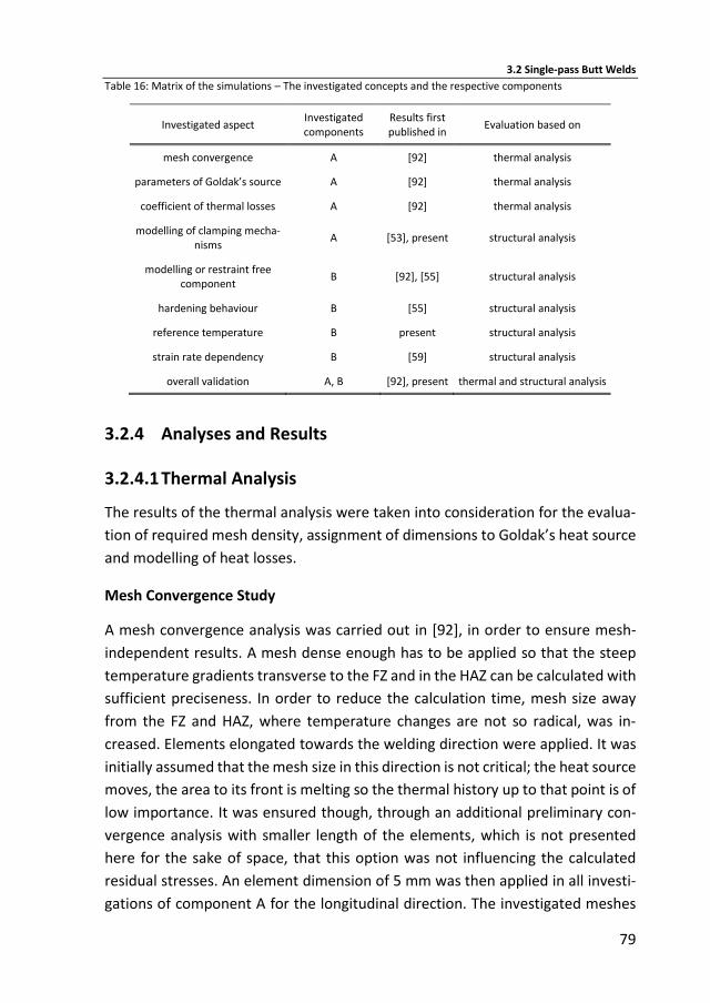
3.2 Single-pass Butt Welds
79
Table 16: Matrix of the simulations – The investigated concepts and the respective components
Investigated aspect Investigated components
Results first published in
Evaluation based on
mesh convergence A [92] thermal analysis
parameters of Goldak’s source A [92] thermal analysis
coefficient of thermal losses A [92] thermal analysis
modelling of clamping mecha-nisms
A [53], present structural analysis
modelling or restraint free component
B [92], [55] structural analysis
hardening behaviour B [55] structural analysis
reference temperature B present structural analysis
strain rate dependency B [59] structural analysis
overall validation A, B [92], present thermal and structural analysis
3.2.4 Analyses and Results
3.2.4.1 Thermal Analysis
The results of the thermal analysis were taken into consideration for the evalua-
tion of required mesh density, assignment of dimensions to Goldak’s heat source
and modelling of heat losses.
Mesh Convergence Study
A mesh convergence analysis was carried out in [92], in order to ensure mesh-
independent results. A mesh dense enough has to be applied so that the steep
temperature gradients transverse to the FZ and in the HAZ can be calculated with
sufficient preciseness. In order to reduce the calculation time, mesh size away
from the FZ and HAZ, where temperature changes are not so radical, was in-
creased. Elements elongated towards the welding direction were applied. It was
initially assumed that the mesh size in this direction is not critical; the heat source
moves, the area to its front is melting so the thermal history up to that point is of
low importance. It was ensured though, through an additional preliminary con-
vergence analysis with smaller length of the elements, which is not presented
here for the sake of space, that this option was not influencing the calculated
residual stresses. An element dimension of 5 mm was then applied in all investi-
gations of component A for the longitudinal direction. The investigated meshes
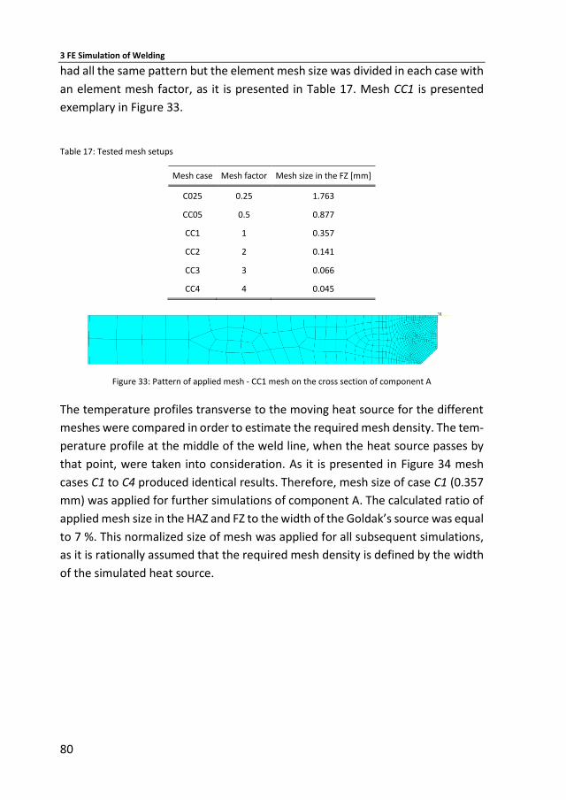
3 FE Simulation of Welding
80
had all the same pattern but the element mesh size was divided in each case with
an element mesh factor, as it is presented in Table 17. Mesh CC1 is presented
exemplary in Figure 33.
Table 17: Tested mesh setups
Mesh case Mesh factor Mesh size in the FZ [mm]
C025 0.25 1.763
CC05 0.5 0.877
CC1 1 0.357
CC2 2 0.141
CC3 3 0.066
CC4 4 0.045
Figure 33: Pattern of applied mesh - CC1 mesh on the cross section of component A
The temperature profiles transverse to the moving heat source for the different
meshes were compared in order to estimate the required mesh density. The tem-
perature profile at the middle of the weld line, when the heat source passes by
that point, were taken into consideration. As it is presented in Figure 34 mesh
cases C1 to C4 produced identical results. Therefore, mesh size of case C1 (0.357
mm) was applied for further simulations of component A. The calculated ratio of
applied mesh size in the HAZ and FZ to the width of the Goldak’s source was equal
to 7 %. This normalized size of mesh was applied for all subsequent simulations,
as it is rationally assumed that the required mesh density is defined by the width
of the simulated heat source.

3.2 Single-pass Butt Welds
81
Figure 34: Results of the convergence study
Parameters of Goldak’s Source
A problem that arises during the first steps of welding simulation is the assign-
ment of proper dimensions to Goldak’s heat source. The depth and width of the
weld pool in an existing present weld can be measured on macrosections. Never-
theless, in cases where the simulation has to reproduce an older not fully docu-
mented result, or act predictively about a future welding process an uncertainty
rises. Moreover, measuring of the front and rear length of the weld source should
be possible only during welding and this could be challenging. Goldak proposed
in [61] that the a and b are equal to the width and depth of the weld pool respec-
tively. He further proposed that, in absence of experimental data, the front half-
length of his source should be assumed equal to one half of the width (cf = a) and
the rear half-length equal to twice the width (cr = 4a). A set of arbitrary values for
the dimensions of Goldak’s source, all selected though in the same order of mag-
nitude with the theoretical size of the weld pool, was tested on component A.
The investigated cases along with the respective values for the parameters of
Goldak’s source, which were considered in [92], are presented in Table 18.
800
1000
1200
1400
1600
1800
2000
0 5 10 15
Tem
per
atu
re [
°C]
Distance from weld centerline [mm]
C2
C3
C4
C1
C05
C025

3 FE Simulation of Welding
82
Table 18: Arbitrary selected and tested parameters for the Goldak’s source in [92]
Cases cf
[mm]
cr
[mm]
a
[mm]
b
[mm]
N 7.5 15 7.5 5
P 7.5 15 7.5 7.5
Q 10 20 10 10
R 5 10 5 3
T 5 20 5 7
The results were compared with thermocouple measurements, which were car-
ried out by Andersson (found in [3]). The location of the three thermocouples, as
it was found in [3], is presented on the sketch of Figure 35. The temperature pro-
files at points A, B and C are presented in Figure 36, Figure 37 and Figure 38 re-
spectively.
Figure 35: Location of the thermocouples A, B and C5, dimensions are given in mm
5 the thermocouples were placed at a depth of 10 mm by drilling holes to the component, see [3]
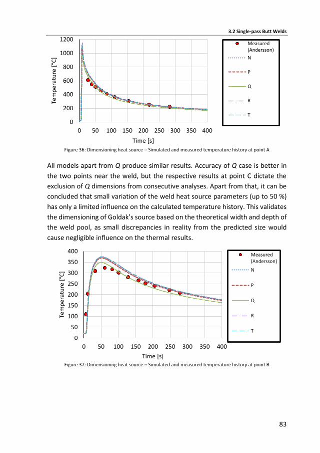
3.2 Single-pass Butt Welds
83
Figure 36: Dimensioning heat source – Simulated and measured temperature history at point A
All models apart from Q produce similar results. Accuracy of Q case is better in
the two points near the weld, but the respective results at point C dictate the
exclusion of Q dimensions from consecutive analyses. Apart from that, it can be
concluded that small variation of the weld heat source parameters (up to 50 %)
has only a limited influence on the calculated temperature history. This validates
the dimensioning of Goldak’s source based on the theoretical width and depth of
the weld pool, as small discrepancies in reality from the predicted size would
cause negligible influence on the thermal results.
Figure 37: Dimensioning heat source – Simulated and measured temperature history at point B
0
200
400
600
800
1000
1200
0 50 100 150 200 250 300 350 400
Tem
per
atu
re [
°C]
Time [s]
Measured(Andersson)
N
P
Q
R
T
0
50
100
150
200
250
300
350
400
0 50 100 150 200 250 300 350 400
Tem
per
atu
re [
°C]
Time [s]
Measured(Andersson)
N
P
Q
R
T
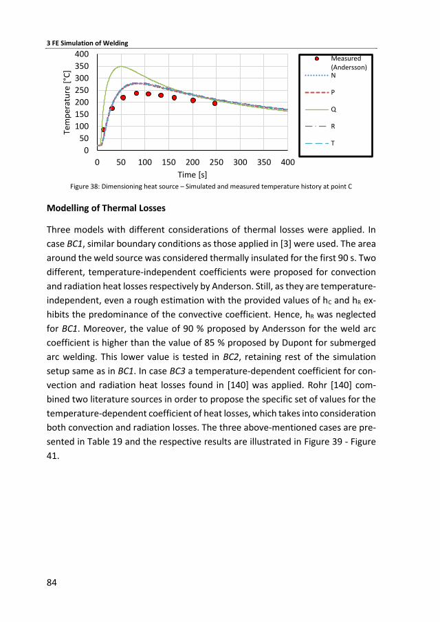
3 FE Simulation of Welding
84
Figure 38: Dimensioning heat source – Simulated and measured temperature history at point C
Modelling of Thermal Losses
Three models with different considerations of thermal losses were applied. In
case BC1, similar boundary conditions as those applied in [3] were used. The area
around the weld source was considered thermally insulated for the first 90 s. Two
different, temperature-independent coefficients were proposed for convection
and radiation heat losses respectively by Anderson. Still, as they are temperature-
independent, even a rough estimation with the provided values of hC and hR ex-
hibits the predominance of the convective coefficient. Hence, hR was neglected
for BC1. Moreover, the value of 90 % proposed by Andersson for the weld arc
coefficient is higher than the value of 85 % proposed by Dupont for submerged
arc welding. This lower value is tested in BC2, retaining rest of the simulation
setup same as in BC1. In case BC3 a temperature-dependent coefficient for con-
vection and radiation heat losses found in [140] was applied. Rohr [140] com-
bined two literature sources in order to propose the specific set of values for the
temperature-dependent coefficient of heat losses, which takes into consideration
both convection and radiation losses. The three above-mentioned cases are pre-
sented in Table 19 and the respective results are illustrated in Figure 39 - Figure
41.
0
50
100
150
200
250
300
350
400
0 50 100 150 200 250 300 350 400
Tem
per
atu
re [
°C]
Time [s]
Measured(Andersson)N
P
Q
R
T
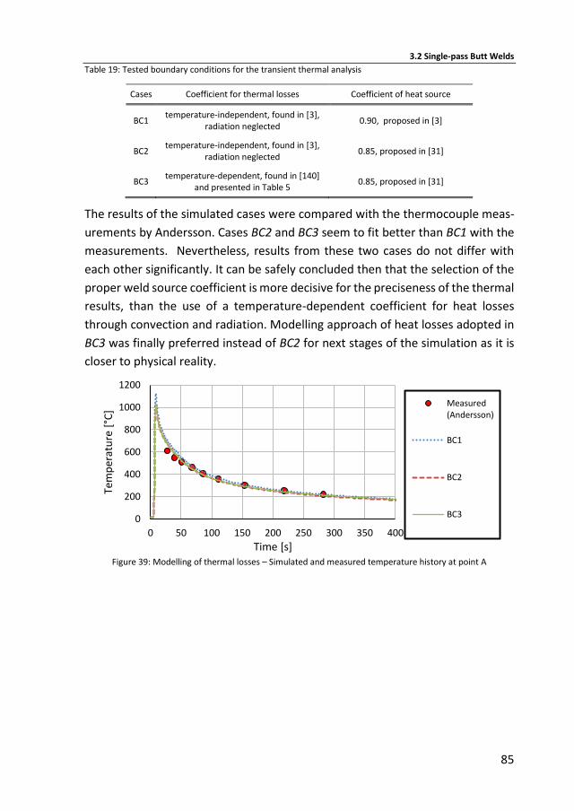
3.2 Single-pass Butt Welds
85
Table 19: Tested boundary conditions for the transient thermal analysis
Cases Coefficient for thermal losses Coefficient of heat source
BC1 temperature-independent, found in [3],
radiation neglected 0.90, proposed in [3]
BC2 temperature-independent, found in [3],
radiation neglected 0.85, proposed in [31]
BC3 temperature-dependent, found in [140]
and presented in Table 5 0.85, proposed in [31]
The results of the simulated cases were compared with the thermocouple meas-
urements by Andersson. Cases BC2 and BC3 seem to fit better than BC1 with the
measurements. Nevertheless, results from these two cases do not differ with
each other significantly. It can be safely concluded then that the selection of the
proper weld source coefficient is more decisive for the preciseness of the thermal
results, than the use of a temperature-dependent coefficient for heat losses
through convection and radiation. Modelling approach of heat losses adopted in
BC3 was finally preferred instead of BC2 for next stages of the simulation as it is
closer to physical reality.
Figure 39: Modelling of thermal losses – Simulated and measured temperature history at point A
0
200
400
600
800
1000
1200
0 50 100 150 200 250 300 350 400
Tem
per
atu
re [
°C]
Time [s]
Measured(Andersson)
BC1
BC2
BC3

3 FE Simulation of Welding
86
Figure 40: Modelling of thermal losses – Simulated and measured temperature history at point B
Figure 41: Modelling of thermal losses – Simulated and measured temperature history at point C
3.2.4.2 Structural Analysis
Results of the structural analysis were applied for the validation of the method
regarding the calculation of WRS. Therewith, various aspects of weld simulation
and their influence on the calculated WRS were investigated.
Overall Validation of the Simulated Welding Residual Stresses
Contour plots of the calculated longitudinal and transverse WRS on the top of
component A, as they were published in [92], are illustrated in Figure 42 and Fig-
ure 43 respectively. Both profiles confirm the theoretical expected distribution of
WRS. In the longitudinal case, tensile stresses near and inside the FZ and HAZ are
met, which are at the same order of magnitude as the local yield strength. Away
from the weld, counterbalancing compressive WRS are met as expected.
0
50
100
150
200
250
300
350
400
0 50 100 150 200 250 300 350 400
Tem
per
atu
re [
°C]
Time [s]
Measured(Andersson)
BC1
BC2
BC3
0
50
100
150
200
250
300
0 50 100 150 200 250 300 350 400
Tem
per
atu
re [
°C]
Time [s]
Measured(Andersson)
BC1
BC2
BC3
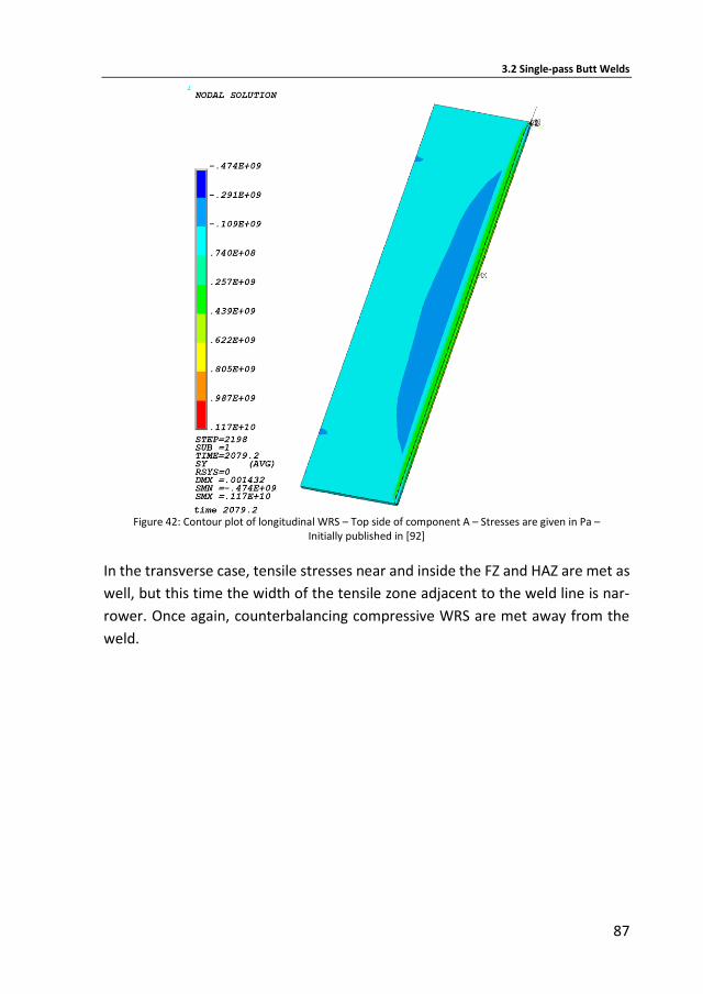
3.2 Single-pass Butt Welds
87
Figure 42: Contour plot of longitudinal WRS – Top side of component A – Stresses are given in Pa –
Initially published in [92]
In the transverse case, tensile stresses near and inside the FZ and HAZ are met as
well, but this time the width of the tensile zone adjacent to the weld line is nar-
rower. Once again, counterbalancing compressive WRS are met away from the
weld.
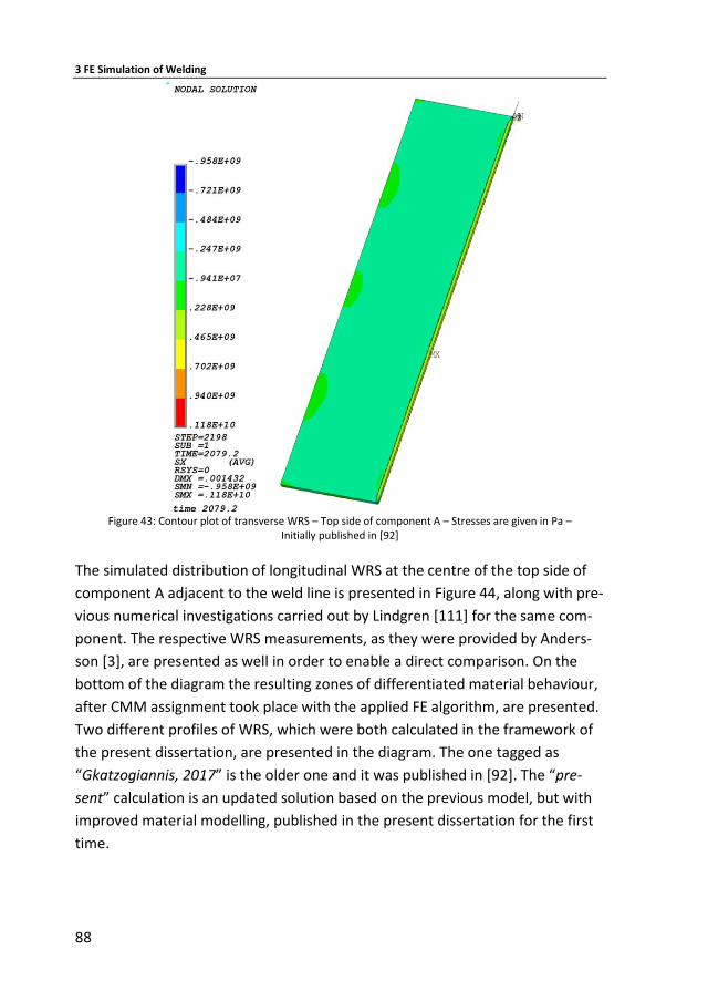
3 FE Simulation of Welding
88
Figure 43: Contour plot of transverse WRS – Top side of component A – Stresses are given in Pa –
Initially published in [92]
The simulated distribution of longitudinal WRS at the centre of the top side of
component A adjacent to the weld line is presented in Figure 44, along with pre-
vious numerical investigations carried out by Lindgren [111] for the same com-
ponent. The respective WRS measurements, as they were provided by Anders-
son [3], are presented as well in order to enable a direct comparison. On the
bottom of the diagram the resulting zones of differentiated material behaviour,
after CMM assignment took place with the applied FE algorithm, are presented.
Two different profiles of WRS, which were both calculated in the framework of
the present dissertation, are presented in the diagram. The one tagged as
“Gkatzogiannis, 2017” is the older one and it was published in [92]. The “pre-
sent” calculation is an updated solution based on the previous model, but with
improved material modelling, published in the present dissertation for the first
time.
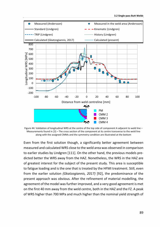
3.2 Single-pass Butt Welds
89
Figure 44: Validation of longitudinal WRS at the centre of the top side of component A adjacent to weld line –
Measurements found in [3] – The cross section of the component at its centre transverse to the weld line along with the assigned CMMs and the symmetry condition are illustrated at the bottom
Even from the first solution though, a significantly better agreement between
measured and calculated WRS close to the weld area was observed in comparison
to earlier studies by Lindgren [111]. On the other hand, the previous models pre-
dicted better the WRS away from the HAZ. Nonetheless, the WRS in the HAZ are
of greatest interest for the subject of the present study. This area is susceptible
to fatigue loading and is the one that is treated by the HFMI treatment. Still, even
from the earlier solution (Gkatzogiannis, 2017) [92], the predominance of the
present approach was obvious. After the refinement of material modelling, the
agreement of the model was further improved, and a very good agreement is met
on the first 40 mm away from the weld centre, both in the HAZ and the FZ. A peak
of WRS higher than 700 MPa and much higher than the nominal yield strength of
-200
-100
0
100
200
300
400
500
600
700
800
-100 -80 -60 -40 -20 0 20 40 60 80 100
Lon
gitu
din
al W
RS
[MP
a]
Distance from weld centreline [mm]
Measured (Andersson) Measured in the weld area (Andersson)
Standard (Lindgren) Kinematic (Lindgren)
TRIP (Lindgren) History (Lindgren)
Calculated (Gkatzogiannis, 2017) Calculated (present)
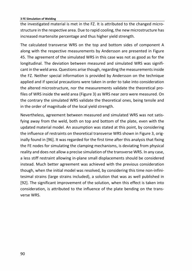
3 FE Simulation of Welding
90
the investigated material is met in the FZ. It is attributed to the changed micro-
structure in the respective area. Due to rapid cooling, the new microstructure has
increased martensite percentage and thus higher yield strength.
The calculated transverse WRS on the top and bottom sides of component A
along with the respective measurements by Andersson are presented in Figure
45. The agreement of the simulated WRS in this case was not as good as for the
longitudinal. The deviation between measured and simulated WRS was signifi-
cant in the weld area. Questions arise though, regarding the measurements inside
the FZ. Neither special information is provided by Andersson on the technique
applied and if special precautions were taken in order to take into consideration
the altered microstructure, nor the measurements validate the theoretical pro-
files of WRS inside the weld area (Figure 3) as WRS near zero were measured. On
the contrary the simulated WRS validate the theoretical ones, being tensile and
in the order of magnitude of the local yield strength.
Nevertheless, agreement between measured and simulated WRS was not satis-
fying away from the weld, both on top and bottom of the plate, even with the
updated material model. An assumption was stated at this point, by considering
the influence of restraints on theoretical transverse WRS shown in Figure 3, orig-
inally found in [96]. It was regarded for the first time after this analysis that fixing
the FE nodes for simulating the clamping mechanisms, is deviating from physical
reality and does not allow a precise simulation of the transverse WRS. In any case,
a less stiff restraint allowing in-plane small displacements should be considered
instead. Much better agreement was achieved with the previous consideration
though, when the initial model was resolved, by considering this time non-infini-
tesimal strains (large strains included), a solution that was as well published in
[92]. The significant improvement of the solution, when this effect is taken into
consideration, is attributed to the influence of the plate bending on the trans-
verse WRS.
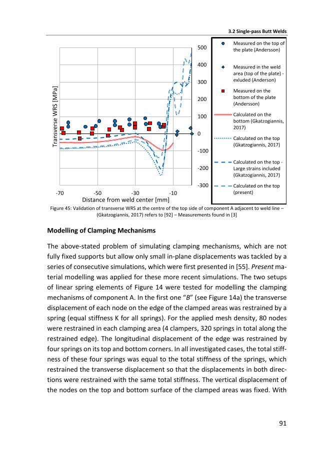
3.2 Single-pass Butt Welds
91
Figure 45: Validation of transverse WRS at the centre of the top side of component A adjacent to weld line –
(Gkatzogiannis, 2017) refers to [92] – Measurements found in [3]
Modelling of Clamping Mechanisms
The above-stated problem of simulating clamping mechanisms, which are not
fully fixed supports but allow only small in-plane displacements was tackled by a
series of consecutive simulations, which were first presented in [55]. Present ma-
terial modelling was applied for these more recent simulations. The two setups
of linear spring elements of Figure 14 were tested for modelling the clamping
mechanisms of component A. In the first one “B” (see Figure 14a) the transverse
displacement of each node on the edge of the clamped areas was restrained by a
spring (equal stiffness K for all springs). For the applied mesh density, 80 nodes
were restrained in each clamping area (4 clampers, 320 springs in total along the
restrained edge). The longitudinal displacement of the edge was restrained by
four springs on its top and bottom corners. In all investigated cases, the total stiff-
ness of these four springs was equal to the total stiffness of the springs, which
restrained the transverse displacement so that the displacements in both direc-
tions were restrained with the same total stiffness. The vertical displacement of
the nodes on the top and bottom surface of the clamped areas was fixed. With
-300
-200
-100
0
100
200
300
400
500
-70 -50 -30 -10
Tran
sver
se W
RS
[MP
a]
Distance from weld center [mm]
Measured on the top ofthe plate (Andersson)
Measured in the weldarea (top of the plate) -exluded (Anderson)
Measured on thebottom of the plate(Andersson)
Calculated on thebottom (Gkatzogiannis,2017)
Calculated on the top(Gkatzogiannis, 2017)
Calculated on the top -Large strains included(Gkatzogiannis, 2017)
Calculated on the top(present)

3 FE Simulation of Welding
92
this setup of boundary conditions, small in-plane displacement of the plate in the
clamped areas are possible, depending on the stiffness of the springs.
In the second proposed approach “B2”, only transverse displacement of the edge
was restrained by springs. This simplification was based on the above-mentioned
negligible influence of modelling the clamping mechanisms on the calculated lon-
gitudinal WRS. This time, both the vertical and longitudinal displacement of the
nodes on the upper and bottom surface of the clamped areas was fixed (see Fig-
ure 14b). Different values of stiffness were tested for both setups. They are pre-
sented in Table 20. A more recent analysis “Gkatzogiannis, 2019”, identical to the
previously investigated case B21 with large strains being taken into consideration
though, is presented for the first time in the present dissertation.
Table 20: Investigated cases of stiff springs in [53]
Cases K
[N/mm] Spring setup
B1 103 B
B2 106 B
B3 109 B
B21 103 B2
B22 106 B2
The results of this series of simulations are presented in Figure 46 and Figure 47.
As expected the influence on the longitudinal WRS is negligible. Cases B2 and B3
along with the case, where the nodes in the clamped areas were fixed, provided
slightly better agreement with the measured residual stresses, with this differ-
ence though, lying inside the confidence boundaries of the present approach.
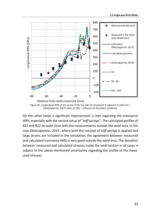
3.2 Single-pass Butt Welds
93
Figure 46: Longitudinal WRS at the centre of the top side of component A adjacent to weld line –
(Gkatzogiannis, 2017) refers to [92] – Influence of boundary conditions
On the other hand, a significant improvement is met regarding the transverse
WRS, especially with the second setup of “stiff springs”. The calculated profiles of
B21 and B22 lie quite close with the measurements outside the weld area. In the
case Gkatzogiannis, 2019 , where both the concept of stiff springs is applied and
large strains are included in the simulation, the agreement between measured
and calculated transverse WRS is very good outside the weld area. The deviation
between measured and calculated stresses inside the weld section in all cases is
subject to the above-mentioned uncertainty regarding the profile of the meas-
ured stresses.
-200
-100
0
100
200
300
400
500
600
700
800
-80 -60 -40 -20 0
Lon
gitu
din
al W
RS
[MP
a]
Distance from weld centerline [mm]
Measured (Andersson)
Measured in the weldarea (Andersson)
Calculated(Gkatzogiannis, 2017)
Calculated (present)
(Gkatzogiannis, 2019)
B1
B2 - B3
B21 - B22
3 FE Simulation of Welding
94
Figure 47: Transverse WRS at the centre of the top side of component A adjacent to weld line –
(Gkatzogiannis, 2017) refers to [92] – Influence of boundary conditions
Modelling of a Restraint Free Component
Simulation of the freely welded component B was achieved with the use of “soft
springs”, meaning linear spring elements subject to Hooke’s law with relatively
low stiffness, in comparison to the stiffness of the investigated component. The
use of such boundary conditions was necessary, as the simulation of a restraint-
free component would lead to numerical problems. At the same time, the applied
conditions should allow the plate to deform similarly to the real component. Two
different values of stiffness were tested in [53] and they are presented in Table
18. The applied set up of springs is illustrated in Figure 13.
Table 21: Applied values of stiffness K for the simulation of soft springs in [53]
Cases K
[N/mm]
A1 103
A2 100
-400
-300
-200
-100
0
100
200
300
400
500
600
-80 -60 -40 -20 0
Tran
sver
se W
RS
[MP
a]
Distance from weld centerline [mm]
Measured (Andersson)
Measured in the weld(Andersson)
Calculated on the top(Gkatzogiannis, 2017)
Calculated on the top - Largestrains included(Gkatzogiannis, 2017)Calculated on the top(present)
(Gkatzogiannis, 2019)
B1
B2 - B3
B21 - B22
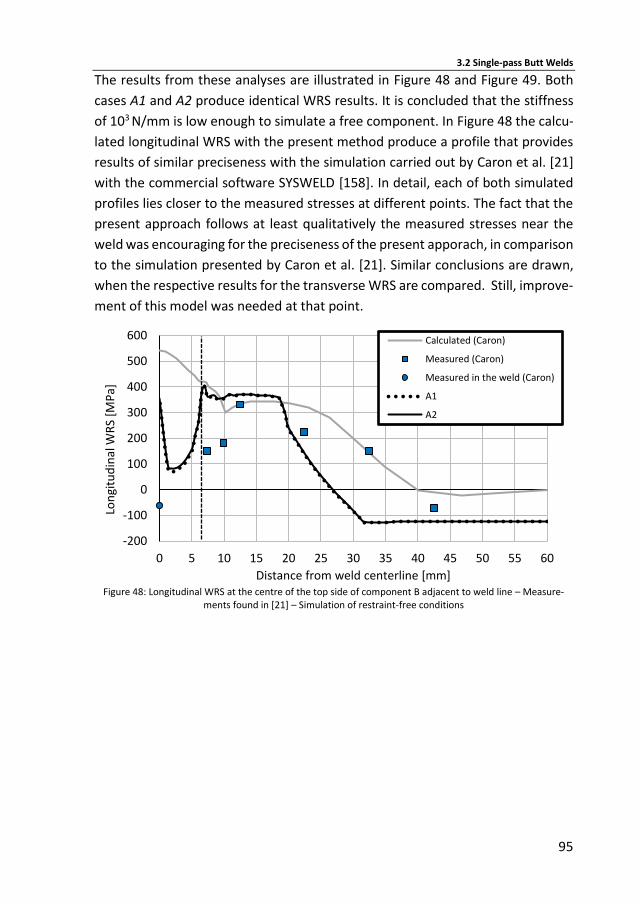
3.2 Single-pass Butt Welds
95
The results from these analyses are illustrated in Figure 48 and Figure 49. Both
cases A1 and A2 produce identical WRS results. It is concluded that the stiffness
of 103 N/mm is low enough to simulate a free component. In Figure 48 the calcu-
lated longitudinal WRS with the present method produce a profile that provides
results of similar preciseness with the simulation carried out by Caron et al. [21]
with the commercial software SYSWELD [158]. In detail, each of both simulated
profiles lies closer to the measured stresses at different points. The fact that the
present approach follows at least qualitatively the measured stresses near the
weld was encouraging for the preciseness of the present apporach, in comparison
to the simulation presented by Caron et al. [21]. Similar conclusions are drawn,
when the respective results for the transverse WRS are compared. Still, improve-
ment of this model was needed at that point.
Figure 48: Longitudinal WRS at the centre of the top side of component B adjacent to weld line – Measure-
ments found in [21] – Simulation of restraint-free conditions
-200
-100
0
100
200
300
400
500
600
0 5 10 15 20 25 30 35 40 45 50 55 60
Lon
gitu
din
al W
RS
[MP
a]
Distance from weld centerline [mm]
Calculated (Caron)
Measured (Caron)
Measured in the weld (Caron)
A1
A2
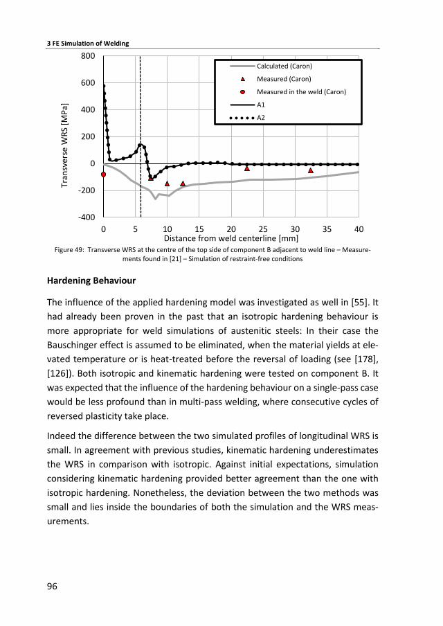
3 FE Simulation of Welding
96
Figure 49: Transverse WRS at the centre of the top side of component B adjacent to weld line – Measure-
ments found in [21] – Simulation of restraint-free conditions
Hardening Behaviour
The influence of the applied hardening model was investigated as well in [55]. It
had already been proven in the past that an isotropic hardening behaviour is
more appropriate for weld simulations of austenitic steels: In their case the
Bauschinger effect is assumed to be eliminated, when the material yields at ele-
vated temperature or is heat-treated before the reversal of loading (see [178],
[126]). Both isotropic and kinematic hardening were tested on component B. It
was expected that the influence of the hardening behaviour on a single-pass case
would be less profound than in multi-pass welding, where consecutive cycles of
reversed plasticity take place.
Indeed the difference between the two simulated profiles of longitudinal WRS is
small. In agreement with previous studies, kinematic hardening underestimates
the WRS in comparison with isotropic. Against initial expectations, simulation
considering kinematic hardening provided better agreement than the one with
isotropic hardening. Nonetheless, the deviation between the two methods was
small and lies inside the boundaries of both the simulation and the WRS meas-
urements.
-400
-200
0
200
400
600
800
0 5 10 15 20 25 30 35 40
Tran
sver
se W
RS
[MP
a]
Distance from weld centerline [mm]
Calculated (Caron)
Measured (Caron)
Measured in the weld (Caron)
A1
A2
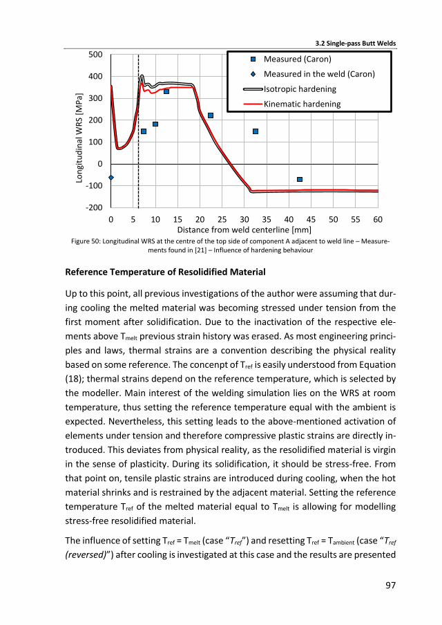
3.2 Single-pass Butt Welds
97
Figure 50: Longitudinal WRS at the centre of the top side of component A adjacent to weld line – Measure-
ments found in [21] – Influence of hardening behaviour
Reference Temperature of Resolidified Material
Up to this point, all previous investigations of the author were assuming that dur-
ing cooling the melted material was becoming stressed under tension from the
first moment after solidification. Due to the inactivation of the respective ele-
ments above Tmelt previous strain history was erased. As most engineering princi-
ples and laws, thermal strains are a convention describing the physical reality
based on some reference. The concenpt of Tref is easily understood from Equation
(18); thermal strains depend on the reference temperature, which is selected by
the modeller. Main interest of the welding simulation lies on the WRS at room
temperature, thus setting the reference temperature equal with the ambient is
expected. Nevertheless, this setting leads to the above-mentioned activation of
elements under tension and therefore compressive plastic strains are directly in-
troduced. This deviates from physical reality, as the resolidified material is virgin
in the sense of plasticity. During its solidification, it should be stress-free. From
that point on, tensile plastic strains are introduced during cooling, when the hot
material shrinks and is restrained by the adjacent material. Setting the reference
temperature Tref of the melted material equal to Tmelt is allowing for modelling
stress-free resolidified material.
The influence of setting Tref = Tmelt (case “Tref”) and resetting Tref = Tambient (case “Tref
(reversed)”) after cooling is investigated at this case and the results are presented
-200
-100
0
100
200
300
400
500
0 5 10 15 20 25 30 35 40 45 50 55 60
Lon
gitu
din
al W
RS
[MP
a]
Distance from weld centerline [mm]
Measured (Caron)
Measured in the weld (Caron)
Isotropic hardening
Kinematic hardening
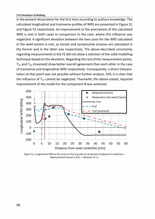
3 FE Simulation of Welding
98
in the present dissertation for the first time according to authors knowledge. The
calculated longitudinal and transverse profiles of WRS are presented in Figure 51
and Figure 52 respectively. An improvement to the preciseness of the calculated
WRS is met in both cases in comparison to the case, where this influence was
neglected. A significant deviation between the two cases for the WRS calculated
in the weld section is met, as tensile and compressive stresses are calculated in
the former and in the latter one respectively. The above-described uncertainty
regarding measurements in the FZ did not allow a selection of the valid modelling
technique based on this deviation. Regarding the rest of the measurement points,
Tref and Tref (reversed) show better overall agreement than each other in the case
of transverse and longitudinal WRS respectively. Consequently, a direct interpre-
tation at that point was not possible without further analysis. Still, it is clear that
the influence of Tref cannot be neglected. Therewith, the above-stated, required
improvement of the model for the component B was achieved.
Figure 51: Longitudinal WRS at the centre of the top side of component B adjacent to weld line –
Measurements found in [21] – Influence of Tref
-200
-100
0
100
200
300
400
500
600
0 5 10 15 20 25 30 35 40 45 50 55 60
Longitudin
al W
RS
[M
Pa]
Distance from weld centerline [mm]
Measured (Caron)
Measured in the weld (Caron)
No Tref
Tref
Tref (reversed)
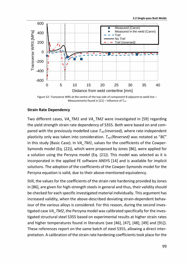
3.2 Single-pass Butt Welds
99
Figure 52: Transverse WRS at the centre of the top side of component B adjacent to weld line –
Measurements found in [21] – Influence of Tref
Strain Rate Dependency
Two different cases, VA_TM1 and VA_TM2 were investigated in [59] regarding
the yield strength strain rate dependency of S355. Both were based on and com-
pared with the previously modelled case Tref (reversed), where rate-independent
plasticity only was taken into consideration. Tref (Reversed) was notated as “BC”
in this study (Basic Case). In VA_TM1, values for the coefficients of the Cowper-
Symonds model (Eq. (22)), which were proposed by Jones [86], were applied for
a solution using the Perzyna model (Eq. (21)). This model was selected as it is
incorporated in the applied FE software ANSYS [14] and is available for implicit
solutions. The adoption of the coefficients of the Cowper-Symonds model for the
Perzyna equation is valid, due to their above-mentioned equivalency.
Still, the values for the coefficients of the strain rate hardening provided by Jones
in [86], are given for high-strength steels in general and thus, their validity should
be checked for each specific investigated material individually. This argument has
increased validity, when the above-described deviating strain-dependent behav-
iour of the various alloys is considered. For this reason, during the second inves-
tigated case VA_TM2, the Perzyna model was calibrated specifically for the inves-
tigated structural steel S355 based on experimental results at higher strain rates
and higher temperatures found in literature (see [46], [47], [48], [49] and [91]).
These references report on the same batch of steel S355, allowing a direct inter-
pretation. A calibration of the strain rate hardening coefficients took place for the
-600
-400
-200
0
200
400
600
0 5 10 15 20 25 30 35 40
Tra
nsvers
e W
RS
[M
Pa]
Distance from weld centerline [mm]
Measured (Caron)Measured in the weld (Caron)TrefNo TrefTref (reversed)
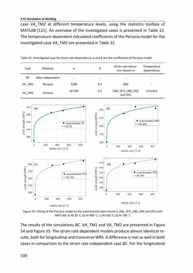
3 FE Simulation of Welding
100
case VA_TM2 at different temperature levels, using the statistics toolbox of
MATLAB [121]. An overview of the investigated cases is presented in Table 22.
The temperature-dependent calculated coefficients of the Perzyna model for the
investigated case VA_TM2 are presented in Table 22.
Table 22: Investigated case for strain rate dependency, α and β are the coefficients of Perzyna model
Case Plasticity α β Strain rate behav-
iour based on Temperature dependency
BC Rate independent - - - -
VA_TM1 Perzyna 3200 0.2 [86] -
VA_TM2 Perzyna 18.540 0.2 [46], [47], [48], [49]
and [91] included
Figure 53: Fitting of the Perzyna model to the experimental data found in [46], [47], [48], [49] and [91] with
MATLAB: a) At 20 °C; b) At 400 °C; c) At 550 °C; d) At 700 °C
The results of the simulations BC, VA_TM1 and VA_TM2 are presented in Figure
54 and Figure 55. The strain rate dependent models produce almost identical re-
sults, both for longitudinal and transverse WRS. A difference is met as well in both
cases in comparison to the strain rate independent case BC. For the longitudinal

3.2 Single-pass Butt Welds
101
stresses, both strain rate independent and dependent deviate equally from the
measured WRS. In the case of the transverse stresses however, the strain rate
independent case shows better agreement with the measurements. The fact that
the case Tref (Reversed) was considered as BC for the present analysis, while up to
that point it was not clear if this would be the most suitable consideration of Tref
for subsequent analyses, can be accounted for this incompatibility. Nonetheless,
the non-negligible difference of the results, when strain rate dependency is taken
into account, has to be highlighted at this point. Although, in the current case
slightly worse agreement is met, the non-negligible deviation of results shows
that when high accuracy is required, strain rate dependency must be considered
as it was proposed by Lindgren [111].
Figure 54: Longitudinal WRS at the centre of the top side of component B adjacent to weld line –
Measurements found in [21] – Strain rate dependency of simulated WRS
Figure 55: Transverse WRS at the centre of the top side of component B adjacent to weld line –
Measurements found in [21] – Strain rate dependency of simulated WRS
-500
-300
-100
100
300
500
0 5 10 15 20 25 30 35 40 45 50 55 60
Longitudin
al W
RS
[M
Pa]
Distance from weld centerline [mm]
Measured (Caron)Measured in the weld (Caron)ΒCVA_TM1VA_TM2VA_TM3
-800
-600
-400
-200
0
200
400
0 5 10 15 20 25 30 35 40
Tra
nsvers
e W
RS
[M
Pa]
Distance from weld centerline [mm]
Measured (Caron)Measured in the weld (Caron)
ΒCVA_TM1VA_TM2VA_TM3
3 FE Simulation of Welding
102
3.2.5 Conclusions
A series of analyses was carried out regarding single-pass butt welds. This weld-
ment was selected, due to its simplicity for a first-step overall validation of the
presented engineering approach and for the investigation of several practical as-
pects of weld simulation by excluding the influence of more complex geometry
or multiple weld passes.
The following conclusions were drawn regarding the overall evaluation of the pre-
sented approach:
The current approach, additionally to its straightforwardness, provides re-
sults with preciseness within the required boundaries that were set at the
beginning of the present study. Moreover, it shows better agreement with
respective WRS measurements in the FZ and HAZ, which are critical for the
fatigue behaviour of the component, when compared with other numerical
simulations found in literature.
The approach is straightforward. Sophisticated aspects of material science
like phase transformations or TRIP, are taken into consideration, based on
practical simplifications, without changing the FE formulations. The phase
changes are predicted based on existing CCT diagrams and no numerical
solution is required. Its straightforwardness constitutes the approach re-
producible in practice by a structural engineer with only basic knowledge of
material science. The approach enables the calculation of WRS and in ex-
tension the estimation of the fatigue behaviour of a component, allowing
for an adjustment in each investigated case of the preciseness and compu-
tational effort by increasing or decreasing the number of CMMs, which are
modelled.
Although the approach was originally developed to act predictively, it can
also be applied for existing weldments, based on destructive testing. Hard-
ness measurements on a macro-section can provide enough information
about the yield limit of each area of the weld. Therefore, alternatively to
the CCT diagrams the hardness measurements can provide information nec-
essary for modelling the mechanical behaviour during cooling.
The practical nature of the method allows its application on other materials
as well, as it was shown for aluminium in [43], whereby different micro-
structural effects must be modelled. Appropriate assumptions also allow
extension of the model to multi-pass welding, as it is discussed below.
3.2 Single-pass Butt Welds
103
The present method allows for flexibility. The level of preciseness depends
on the number of cooling-down material models and can be selected by the
modeller. Depending upon the case, further, more sophisticated modelling
of mechanical behaviour can be deployed, like mixed-hardening constitu-
tive laws or strain rate dependent plasticity. The computational effort in-
creases at the same time.
The following conclusions were drawn regarding specific aspects of the simula-
tion:
In order to provide mesh independent results, a mesh dimension in the HAZ
and FZ transverse to the weld line equal or smaller than 7 % of the Goldak’s
source half width is required, when first order hexahedral finite elements
are applied.
When no relevant information is available, setting the width a and depth b
of Goldak’s source equal to the theoretical width and depth of the weld
seam provides sufficient results. In this case, forward and rear lengths are
set as cf = 4·a and cr = a.
Regarding the preciseness of thermal analysis, the selection of a proper
value for the weld source coefficient is more decisive than the use of a tem-
perature-dependent coefficient for heat losses through convection and ra-
diation. Still, both effects should be considered for safer results, as model-
ling with a temperature-dependent coefficient lies closer to physical reality.
Accurate modelling of material behaviour is predominant for the improve-
ment of the preciseness, especially when the longitudinal WRS are consid-
ered.
Considering large strains is predominant for the precise calculation of trans-
verse WRS.
When a clamped-component is simulated, modelling of boundary condi-
tions with stiff springs instead of zero displacement restraints improves sig-
nificantly the preciseness of transverse WRS. This deviation validates the
influence of external restraint on the transverse WRS as it is presented in
Figure 3. When this modelling technique is combined with consideration of
large strains very precise calculation of transverse WRS can be achieved.
B2 Setup of the stiff springs provided the best improvement in simulations
results. Application of the springs is mesh dependent and the individual
stiffness of the springs has to be adjusted depending on their number. A
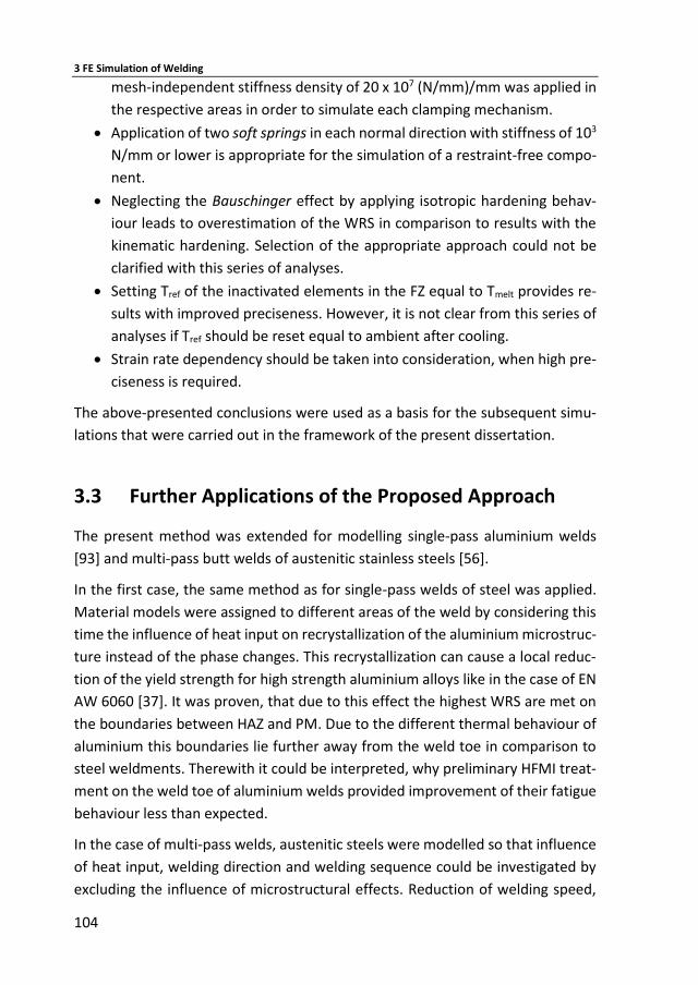
3 FE Simulation of Welding
104
mesh-independent stiffness density of 20 x 107 (N/mm)/mm was applied in
the respective areas in order to simulate each clamping mechanism.
Application of two soft springs in each normal direction with stiffness of 103
N/mm or lower is appropriate for the simulation of a restraint-free compo-
nent.
Neglecting the Bauschinger effect by applying isotropic hardening behav-
iour leads to overestimation of the WRS in comparison to results with the
kinematic hardening. Selection of the appropriate approach could not be
clarified with this series of analyses.
Setting Tref of the inactivated elements in the FZ equal to Tmelt provides re-
sults with improved preciseness. However, it is not clear from this series of
analyses if Tref should be reset equal to ambient after cooling.
Strain rate dependency should be taken into consideration, when high pre-
ciseness is required.
The above-presented conclusions were used as a basis for the subsequent simu-
lations that were carried out in the framework of the present dissertation.
3.3 Further Applications of the Proposed Approach
The present method was extended for modelling single-pass aluminium welds
[93] and multi-pass butt welds of austenitic stainless steels [56].
In the first case, the same method as for single-pass welds of steel was applied.
Material models were assigned to different areas of the weld by considering this
time the influence of heat input on recrystallization of the aluminium microstruc-
ture instead of the phase changes. This recrystallization can cause a local reduc-
tion of the yield strength for high strength aluminium alloys like in the case of EN
AW 6060 [37]. It was proven, that due to this effect the highest WRS are met on
the boundaries between HAZ and PM. Due to the different thermal behaviour of
aluminium this boundaries lie further away from the weld toe in comparison to
steel weldments. Therewith it could be interpreted, why preliminary HFMI treat-
ment on the weld toe of aluminium welds provided improvement of their fatigue
behaviour less than expected.
In the case of multi-pass welds, austenitic steels were modelled so that influence
of heat input, welding direction and welding sequence could be investigated by
excluding the influence of microstructural effects. Reduction of welding speed,
3.4 Fillet welds
105
avoidance of intermediate cooling, and antisymmetric welding sequence were
proven, according to initial expectations, beneficial for the reduction of WRS and
in extension for the prolongation of the fatigue life of the investigated weld-
ments. These conclusions could be very useful for the optimization of welding
process for austenitic steels. Nevertheless, they cannot be directly adopted for
the case multi-phase steels, where microstructural changes can influence pro-
foundly the calculated WRS. The theoretical background and modelling aspects
for extending the present approach in the case of multi-pass welds on multi-
phase steels was discussed in [57].
Detailed description of these investigations is excluded from the present disser-
tation as they, although being relevant to the general subject, are not directly
contributing to the fulfilment of the present research goal, i.e. the simulation of
RS from welding and HFMI. Further details regarding these investigations can be
found in the respective, given publications.
3.4 Fillet welds
A series of numerical investigations was carried out in the framework of the pre-
sent dissertation, in order to calculate the WRS of the fillet welds from the re-
search project HFH-Simulation. Some of the results were carried out as part of
the project as well, while other are published in the present dissertation for the
first time. Goal was the precise calculation of the WRS field, which would be ap-
plied as input to the subsequent HFMI analysis. The above-mentioned conclu-
sions drawn from the former investigations on single-pass butt welds constituted
the base for this latter simulation. Measurements of WRS, which were carried out
in the framework of the project HFH-Simulation, are used for validation of the
present numerical analyses. Previously unsolved issues regarding practical as-
pects of modelling were as well investigated in this series of analyses.
3.4.1 Investigated Components
The investigated components of the project HFH-Simulation were fillet welds of
three different materials, namely S355 [29], S690 and S960 [30]. They consisted
of a plate with dimensions 1000 mm x 370 mm x 10 mm and transversal stiffeners
with dimensions 1000 mm x 50 mm x 10 mm welded on both sides. In the case of
the S355 component, length was in reality 1350 mm. Nonetheless, a length of

3 FE Simulation of Welding
106
1000 mm was assumed in the numerical models for this case as well, in order to
reduce the computational time. No influence on the calculated WRS is expected,
as the length remains significantly larger than the width of the plate. The geome-
try of the investigated component and the weld section are illustrated in Figure
56 and Figure 57 respectively. The real component of steel S355 is presented in
Figure 59. It was restrained with two clampers during welding, on the side of the
1st and 4th pass (setup of clamping mechanisms FWBC1). Applied welding se-
quence A-B-C-D is as well presented in Figure 57 . Coarse mesh was applied away
from the weld, while finer mesh dimensions, with dimensions of 0.37 mm and 1
mm transverse to and along the weld direction respectively, were selected for
the FZ and the HAZ based on previous investigations.
Figure 56: Fillet welds of the project HFH-Simulation, two clampers were applied on the left side during weld-
ing – Dimensions are given in mm (setup FWBC1)
Figure 57: Component of the project HFH-Simulation, two clampers were applied on the left side during weld-
ing – Dimensions are given in mm (setup FWBC1)
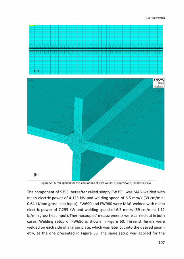
3.4 Fillet welds
107
Figure 58: Mesh applied for the simulations of fillet welds: a) Top view; b) Isometric view
The component of S355, hereafter called simply FW355, was MAG-welded with
mean electric power of 4.125 kW and welding speed of 6.5 mm/s (39 cm/min;
0.64 kJ/mm gross heat input). FW690 and FW960 were MAG-welded with mean
electric power of 7.293 kW and welding speed of 6.5 mm/s (39 cm/min; 1.12
kJ/mm gross heat input). Thermocouples’ measurements were carried out in both
cases. Welding setup of FW690 is shown in Figure 60. Three stiffeners were
welded on each side of a larger plate, which was later cut into the desired geom-
etry, as the one presented in Figure 56. The same setup was applied for the
(a)
(b)

3 FE Simulation of Welding
108
FW960. Both materials were welded with automated procedure by a robot-
welder, which welded simultaneously the two upper and consecutively the two
bottom passes. Therefore, a second FE model was built, identical with the one
presented in Figure 54 but with symmetry conditions on the middle plane of the
stiffeners. Nevertheless, sequential welding sequence identical to that of FW355
was as well modelled, so that the most unfavourable case, i.e. the weld toe with
the highest tensile WRS, could be taken into consideration to the subsequent sim-
ulation of HMFI as well. As it was not documented, on which plate the WRS meas-
urements of the Project HFH-Simulation were carried out, the setup FWBC1 was
assumed for FW690 and FW960 as well. It was decided that if no satisfying agree-
ment was achieved, further actions would be taken. WPS for all materials are pre-
sented in Appendix A. In all cases, the stiffeners were initially tack-welded on the
plates, with full welding taking place afterwards. During the simulation, both the
tack welding procedure and the discontinuity between the stiffener and the base
plate were neglected, as they were rationally believed to have negligible influ-
ence on the final WRS.
Figure 59: The real component of the project HFH-Simulation made of steel S355 after completion of the weld-
ing procedure – The clamping mechanisms are seen on the left side
Figure 60: Welded plates of S690 from the project HFH-Simulation
3.4 Fillet welds
109
3.4.2 WRS Measurements
Measurements of the WRS took place in the framework of the project HFH-Sim-
ulation. The measurements were carried out by the Fraunhofer Institute for Me-
chanics of Materials (IWM)6 with an X-Ray diffractometer7 on the 1st welding pass
of each fillet weld at the middle of the plate and transverse to the welding line.
In the case of S355 three measurement lines, parallel to each other at a distance
of some mm from each other (≈ 10 mm), were measured. Further details regard-
ing the measuring method can be found in [146], but they are excluded from the
present dissertation as they exceed the boundaries of the present subject.
The measured WRS for all three investigated materials are presented in Figure 61
along with their confidence boundaries and the mean line for the measurements
of S355. Despite the fact that all measurements were carried out on the 1st weld-
ing pass, they are presented schematically in such a way that the transverse WRS
can be found on the left hand side of the diagram and the longitudinal on the
right hand side. Against initial expectations, the transverse WRS range in all cases
in the compressive zone and they exhibit a very strong fluctuation. A significant
deviation of even up to 250 MPa is met between the parallel measurements of
S355. Such a conclusion cannot be drawn for the other two steel grades due to
the single measurements but a very irregular WRS-pattern with steep peaks and
valleys is met especially in the case of S960. On the other hand, longitudinal meas-
urements exhibit no significant fluctuation and the deviation for the measure-
ments of S355 is significantly smaller. Moreover, the longitudinal profiles are
closer to initial expectations, as tensile WRS are met near the weld toe that move
to the compressive area away from it. Nevertheless, it seems that the whole pro-
file is shifted downwards as the tensile and the compressive WRS have lower and
higher magnitude than expected respectively and the width of the tensile area is
quite narrow.
6 IWM stands for „Institut für Werkstoffmechanik“, German for “Institute for Mechanics of Materials”
7 a Stresstech G3 Diffractometer was used

3 FE Simulation of Welding
110
Figure 61: WRS measurements from the project HFH-Simulation
It was assumed that the rolling process of the parent plates or the shot blasting
of the surface prior to welding should be accounted for these discrepancies of
measured WRS. For instance, shot blasting can introduce significant compressive
WRS (Figure 15), but also its localized mechanical effect can lead to significant
differentiation of the RS, which could explain the present significant deviations
and fluctuations. A similar effect, i.e. presence of compressive stresses of the
magnitude of 200 MPa prior to welding was attributed to hot rolling of the inves-
tigated steel plates, in a previous numerical study of HFMI [150]. In any case, the
longitudinal measurements are considered more valid due to the absence of sig-
nificant fluctuations and the small deviation of the measurements for S355.
-600
-400
-200
0
200
400
600
-600
-400
-200
0
200
400
600
-40 -30 -20 -10 0 10 20 30 40
Logn
itu
din
al W
RS
[MP
a]
Tran
sver
se W
RS
[MP
a]
Distance from the stiffener centreline [mm]
S355 Transverse - 1st Measurement S355 Transverse - 2nd Measurement
S355 Transverse - 3d Measurement S355 Transverse - Mean
S690 Transverse S960 Transverse
S355 Longitudinal - 1st Measurement S355 Lognitudinal - 2nd Measurement
S355 Lognitudinal - 3d Measurement S355 Lognitudinal - Mean
S690 Longitudinal S960 Longitudinal
transversal stiffener
weld toe
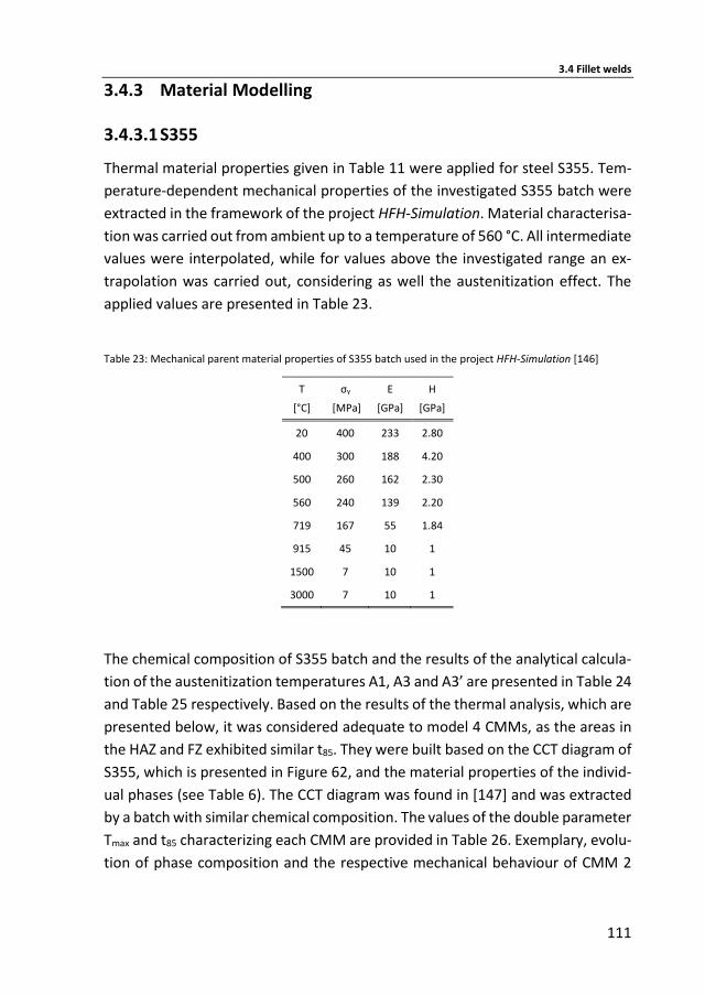
3.4 Fillet welds
111
3.4.3 Material Modelling
3.4.3.1 S355
Thermal material properties given in Table 11 were applied for steel S355. Tem-
perature-dependent mechanical properties of the investigated S355 batch were
extracted in the framework of the project HFH-Simulation. Material characterisa-
tion was carried out from ambient up to a temperature of 560 °C. All intermediate
values were interpolated, while for values above the investigated range an ex-
trapolation was carried out, considering as well the austenitization effect. The
applied values are presented in Table 23.
Table 23: Mechanical parent material properties of S355 batch used in the project HFH-Simulation [146]
T
[°C]
σy
[MPa]
E
[GPa]
H
[GPa]
20 400 233 2.80
400 300 188 4.20
500 260 162 2.30
560 240 139 2.20
719 167 55 1.84
915 45 10 1
1500 7 10 1
3000 7 10 1
The chemical composition of S355 batch and the results of the analytical calcula-
tion of the austenitization temperatures A1, A3 and A3’ are presented in Table 24
and Table 25 respectively. Based on the results of the thermal analysis, which are
presented below, it was considered adequate to model 4 CMMs, as the areas in
the HAZ and FZ exhibited similar t85. They were built based on the CCT diagram of
S355, which is presented in Figure 62, and the material properties of the individ-
ual phases (see Table 6). The CCT diagram was found in [147] and was extracted
by a batch with similar chemical composition. The values of the double parameter
Tmax and t85 characterizing each CMM are provided in Table 26. Exemplary, evolu-
tion of phase composition and the respective mechanical behaviour of CMM 2
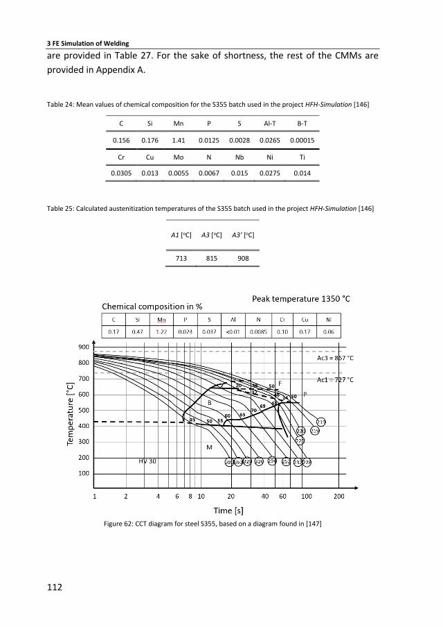
3 FE Simulation of Welding
112
are provided in Table 27. For the sake of shortness, the rest of the CMMs are
provided in Appendix A.
Table 24: Mean values of chemical composition for the S355 batch used in the project HFH-Simulation [146]
C Si Mn P S Al-T B-T
0.156 0.176 1.41 0.0125 0.0028 0.0265 0.00015
Cr Cu Mo N Nb Ni Ti
0.0305 0.013 0.0055 0.0067 0.015 0.0275 0.014
Table 25: Calculated austenitization temperatures of the S355 batch used in the project HFH-Simulation [146]
A1 [oC] A3 [oC] A3’ [oC]
713 815 908
Figure 62: CCT diagram for steel S355, based on a diagram found in [147]
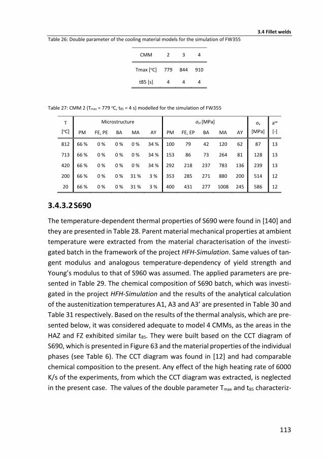
3.4 Fillet welds
113
Table 26: Double parameter of the cooling material models for the simulation of FW355
CMM 2 3 4
Tmax [oC] 779 844 910
t85 [s] 4 4 4
Table 27: CMM 2 (Tmax = 779 oC, t85 = 4 s) modelled for the simulation of FW355
T
[oC]
Microstructure σyi [MPa] σy
[MPa]
ase
[-] PM FE, PE BA MA AY PM FE, EP BA MA AY
812 66 % 0 % 0 % 0 % 34 % 100 79 42 120 62 87 13
713 66 % 0 % 0 % 0 % 34 % 153 86 73 264 81 128 13
420 66 % 0 % 0 % 0 % 34 % 292 218 237 783 136 239 13
200 66 % 0 % 0 % 31 % 3 % 353 285 271 880 200 514 12
20 66 % 0 % 0 % 31 % 3 % 400 431 277 1008 245 586 12
3.4.3.2 S690
The temperature-dependent thermal properties of S690 were found in [140] and
they are presented in Table 28. Parent material mechanical properties at ambient
temperature were extracted from the material characterisation of the investi-
gated batch in the framework of the project HFH-Simulation. Same values of tan-
gent modulus and analogous temperature-dependency of yield strength and
Young’s modulus to that of S960 was assumed. The applied parameters are pre-
sented in Table 29. The chemical composition of S690 batch, which was investi-
gated in the project HFH-Simulation and the results of the analytical calculation
of the austenitization temperatures A1, A3 and A3’ are presented in Table 30 and
Table 31 respectively. Based on the results of the thermal analysis, which are pre-
sented below, it was considered adequate to model 4 CMMs, as the areas in the
HAZ and FZ exhibited similar t85. They were built based on the CCT diagram of
S690, which is presented in Figure 63 and the material properties of the individual
phases (see Table 6). The CCT diagram was found in [12] and had comparable
chemical composition to the present. Any effect of the high heating rate of 6000
K/s of the experiments, from which the CCT diagram was extracted, is neglected
in the present case. The values of the double parameter Tmax and t85 characteriz-
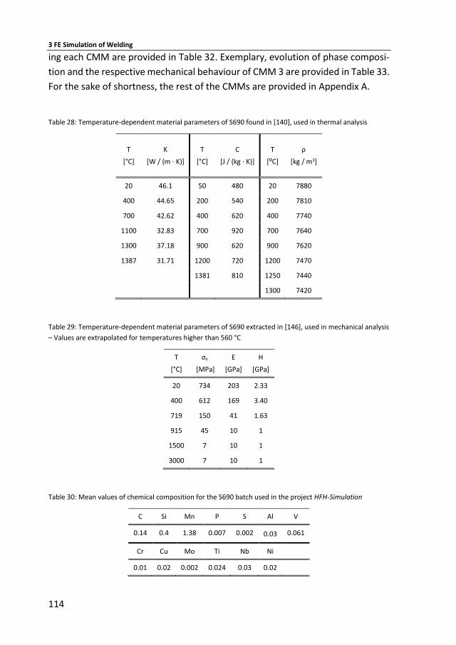
3 FE Simulation of Welding
114
ing each CMM are provided in Table 32. Exemplary, evolution of phase composi-
tion and the respective mechanical behaviour of CMM 3 are provided in Table 33.
For the sake of shortness, the rest of the CMMs are provided in Appendix A.
Table 28: Temperature-dependent material parameters of S690 found in [140], used in thermal analysis
T
[°C]
K
[W / (m · K)]
T
[°C]
C
[J / (kg · K)]
T
[⁰C]
ρ
[kg / m3]
20 46.1 50 480 20 7880
400 44.65 200 540 200 7810
700 42.62 400 620 400 7740
1100 32.83 700 920 700 7640
1300 37.18 900 620 900 7620
1387 31.71 1200 720 1200 7470
1381 810 1250 7440
1300 7420
Table 29: Temperature-dependent material parameters of S690 extracted in [146], used in mechanical analysis
– Values are extrapolated for temperatures higher than 560 °C
T
[°C]
σy
[MPa]
E
[GPa]
H
[GPa]
20 734 203 2.33
400 612 169 3.40
719 150 41 1.63
915 45 10 1
1500 7 10 1
3000 7 10 1
Table 30: Mean values of chemical composition for the S690 batch used in the project HFH-Simulation
C Si Mn P S Al V
0.14 0.4 1.38 0.007 0.002 0.03 0.061
Cr Cu Mo Ti Nb Ni
0.01 0.02 0.002 0.024 0.03 0.02

3.4 Fillet welds
115
Table 31: Calculated austenitization temperatures for the simulation of FW690
A1 [oC] A3 [oC] A3’ [oC]
720 835 935
Figure 63: CCT diagram for steel S690 found in [12]8
Table 32: Double parameter of the cooling material models for the simulation of FW690
CMM 2 3 4
Tmax [oC] 817 882 1208
t85 [s] 4 4 4
8 the diagram was partially redrawn by the author of the present dissertation in order to improve the figure quality
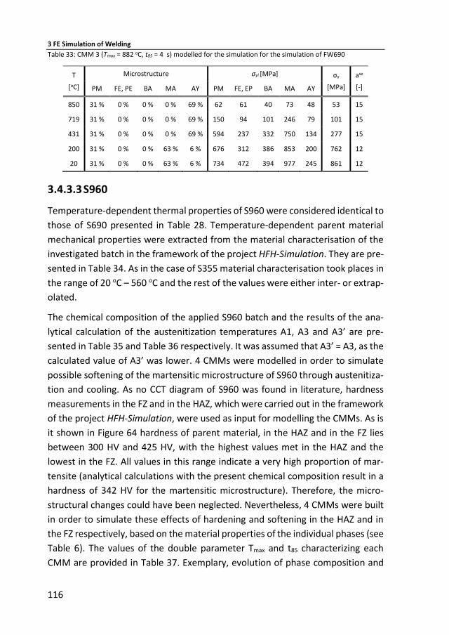
3 FE Simulation of Welding
116
Table 33: CMM 3 (Tmax = 882 oC, t85 = 4 s) modelled for the simulation for the simulation of FW690
T
[oC]
Microstructure σyi [MPa] σy
[MPa]
ase
[-] PM FE, PE BA MA AY PM FE, EP BA MA AY
850 31 % 0 % 0 % 0 % 69 % 62 61 40 73 48 53 15
719 31 % 0 % 0 % 0 % 69 % 150 94 101 246 79 101 15
431 31 % 0 % 0 % 0 % 69 % 594 237 332 750 134 277 15
200 31 % 0 % 0 % 63 % 6 % 676 312 386 853 200 762 12
20 31 % 0 % 0 % 63 % 6 % 734 472 394 977 245 861 12
3.4.3.3 S960
Temperature-dependent thermal properties of S960 were considered identical to
those of S690 presented in Table 28. Temperature-dependent parent material
mechanical properties were extracted from the material characterisation of the
investigated batch in the framework of the project HFH-Simulation. They are pre-
sented in Table 34. As in the case of S355 material characterisation took places in
the range of 20 oC – 560 oC and the rest of the values were either inter- or extrap-
olated.
The chemical composition of the applied S960 batch and the results of the ana-
lytical calculation of the austenitization temperatures A1, A3 and A3’ are pre-
sented in Table 35 and Table 36 respectively. It was assumed that A3’ = A3, as the
calculated value of A3’ was lower. 4 CMMs were modelled in order to simulate
possible softening of the martensitic microstructure of S960 through austenitiza-
tion and cooling. As no CCT diagram of S960 was found in literature, hardness
measurements in the FZ and in the HAZ, which were carried out in the framework
of the project HFH-Simulation, were used as input for modelling the CMMs. As is
it shown in Figure 64 hardness of parent material, in the HAZ and in the FZ lies
between 300 HV and 425 HV, with the highest values met in the HAZ and the
lowest in the FZ. All values in this range indicate a very high proportion of mar-
tensite (analytical calculations with the present chemical composition result in a
hardness of 342 HV for the martensitic microstructure). Therefore, the micro-
structural changes could have been neglected. Nevertheless, 4 CMMs were built
in order to simulate these effects of hardening and softening in the HAZ and in
the FZ respectively, based on the material properties of the individual phases (see
Table 6). The values of the double parameter Tmax and t85 characterizing each
CMM are provided in Table 37. Exemplary, evolution of phase composition and
3.4 Fillet welds
117
the respective mechanical behaviour of CMM 4 are provided in Table 38. For the
sake of shortness, the rest of the CMMs are provided in Appendix A.
Table 34: Temperature-dependent material parameters of S690 extracted in [146], used in mechanical analysis
– Values are extrapolated for temperatures higher than 915 °C
T
[°C]
σy
[MPa]
E
[GPa]
H
[GPa]
20 1021 203 2.33
400 851 169 3.40
719 208 41 1.63
915 45 10 1
1500 7 10 1
3000 7 10 1
Table 35: Mean values of chemical composition for the S960 batch used in the project HFH-Simulation
C Si Mn P S Al V
0.22 1.25 0.008 0.001 0.22 0.052 0.043
Cr Cu Mo Ti Nb Ni
0.2 0.01 0.603 0.003 0.016 0.05
Table 36: Calculated austenitization temperatures for the simulation of FW960
A1 [oC] A3 [oC] A3’ [oC]
719 1013 1013
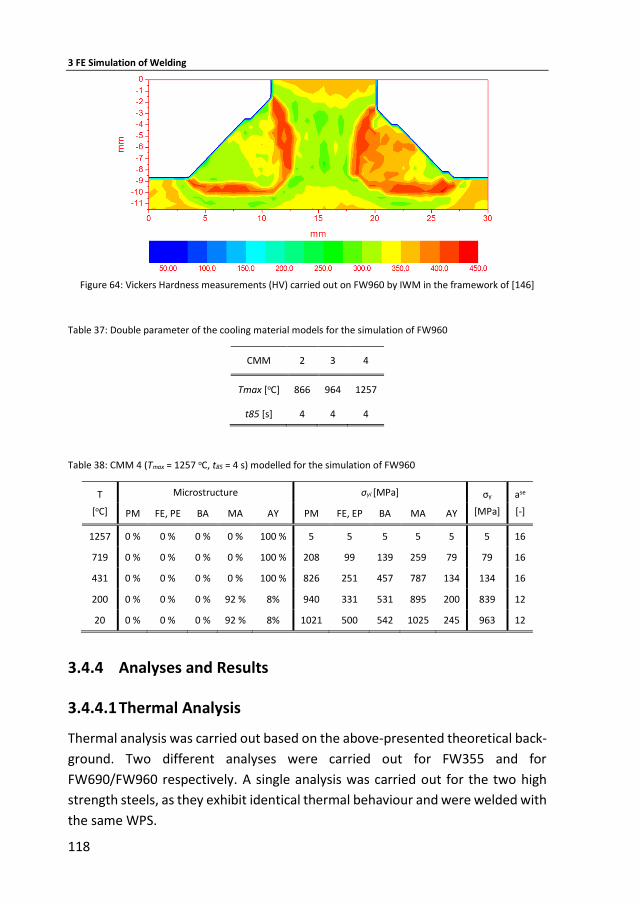
3 FE Simulation of Welding
118
Figure 64: Vickers Hardness measurements (HV) carried out on FW960 by IWM in the framework of [146]
Table 37: Double parameter of the cooling material models for the simulation of FW960
CMM 2 3 4
Tmax [oC] 866 964 1257
t85 [s] 4 4 4
Table 38: CMM 4 (Tmax = 1257 oC, t85 = 4 s) modelled for the simulation of FW960
T
[oC]
Microstructure σyi [MPa] σy
[MPa]
ase
[-] PM FE, PE BA MA AY PM FE, EP BA MA AY
1257 0 % 0 % 0 % 0 % 100 % 5 5 5 5 5 5 16
719 0 % 0 % 0 % 0 % 100 % 208 99 139 259 79 79 16
431 0 % 0 % 0 % 0 % 100 % 826 251 457 787 134 134 16
200 0 % 0 % 0 % 92 % 8% 940 331 531 895 200 839 12
20 0 % 0 % 0 % 92 % 8% 1021 500 542 1025 245 963 12
3.4.4 Analyses and Results
3.4.4.1 Thermal Analysis
Thermal analysis was carried out based on the above-presented theoretical back-
ground. Two different analyses were carried out for FW355 and for
FW690/FW960 respectively. A single analysis was carried out for the two high
strength steels, as they exhibit identical thermal behaviour and were welded with
the same WPS.
3.4 Fillet welds
119
The heat source was calibrated for both analyses based on macrosections of the
investigated fillet welds, which were taken by IWM during HFH-Simulation [146].
Initially, the width and depth of Goldak’s source were adapted directly to the
measured weld pool size. The length of the forward and rear quadrant were once
again set equal to 1 and 4 times the half width of the weld pool respectively. The
macrosections along with the measured dimensions are displayed in Figure 65.
The applied welding parameters are presented in Table 39. Values for the weld
metal arc coefficient proposed by Dupont [32] were used once again. Still, initial
thermal results have shown that this setup leads to a smaller weld pool size in the
simulation, i.e. temperature of some elements inside and near the boundaries of
the FZ did not reach Tmelt. Consequently, the parameters of the heat source had
to be recalibrated.
Through a trial and error procedure the parameters of the Goldak’s source were
reset so that the FZ in the simulation would match the real one and the agree-
ment of the calculated thermal profiles with the respective thermocouples’ meas-
urements, which were carried out in the framework of HFH-Simulation [146],
would be sufficient. Finally, a common width of the weld source of 6 mm, an equal
depth and a retained ration of 4:1:1 for the forward and rear length to the half
width were selected. The final parameters of the heat source are presented as
well in Table 39. The calculated FZ and the temperature distribution in the fusion
zone at the middle of the heat source were compared with the real macrosection
after recalibration. This comparison is illustrated in Figure 66. On the left side of
the figure, the macrosections are presented for both materials with the bounda-
ries of the FZ being highlighted with a black line. At the middle, qualitative con-
tours of the temperature distribution are presented. Exemplary, the quantitative
contour for the component FW355 (mirrored) is presented in Figure 67.
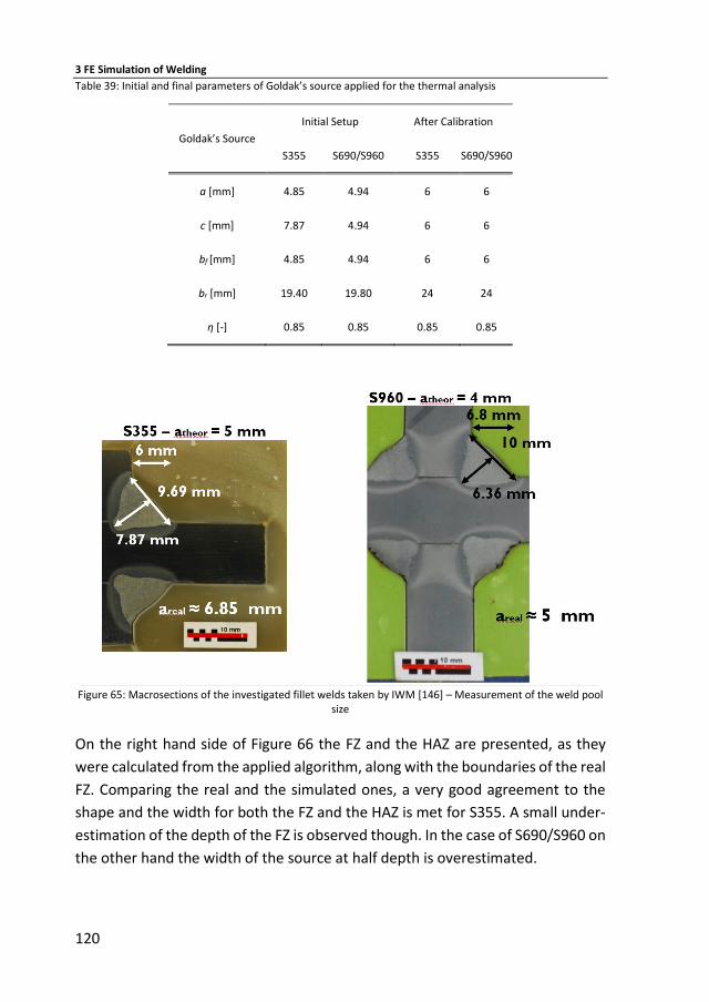
3 FE Simulation of Welding
120
Table 39: Initial and final parameters of Goldak’s source applied for the thermal analysis
Goldak’s Source
Initial Setup After Calibration
S355 S690/S960 S355 S690/S960
a [mm] 4.85 4.94 6 6
c [mm] 7.87 4.94 6 6
bf [mm] 4.85 4.94 6 6
br [mm] 19.40 19.80 24 24
η [-] 0.85 0.85 0.85 0.85
Figure 65: Macrosections of the investigated fillet welds taken by IWM [146] – Measurement of the weld pool
size
On the right hand side of Figure 66 the FZ and the HAZ are presented, as they
were calculated from the applied algorithm, along with the boundaries of the real
FZ. Comparing the real and the simulated ones, a very good agreement to the
shape and the width for both the FZ and the HAZ is met for S355. A small under-
estimation of the depth of the FZ is observed though. In the case of S690/S960 on
the other hand the width of the source at half depth is overestimated.
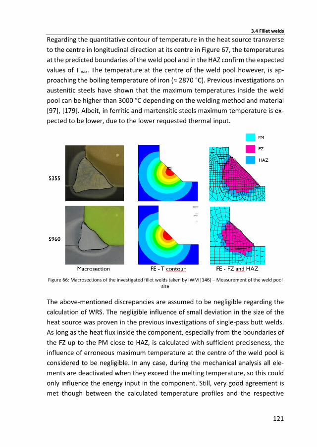
3.4 Fillet welds
121
Regarding the quantitative contour of temperature in the heat source transverse
to the centre in longitudinal direction at its centre in Figure 67, the temperatures
at the predicted boundaries of the weld pool and in the HAZ confirm the expected
values of Tmax. The temperature at the centre of the weld pool however, is ap-
proaching the boiling temperature of iron (≈ 2870 °C). Previous investigations on
austenitic steels have shown that the maximum temperatures inside the weld
pool can be higher than 3000 °C depending on the welding method and material
[97], [179]. Albeit, in ferritic and martensitic steels maximum temperature is ex-
pected to be lower, due to the lower requested thermal input.
Figure 66: Macrosections of the investigated fillet welds taken by IWM [146] – Measurement of the weld pool
size
The above-mentioned discrepancies are assumed to be negligible regarding the
calculation of WRS. The negligible influence of small deviation in the size of the
heat source was proven in the previous investigations of single-pass butt welds.
As long as the heat flux inside the component, especially from the boundaries of
the FZ up to the PM close to HAZ, is calculated with sufficient preciseness, the
influence of erroneous maximum temperature at the centre of the weld pool is
considered to be negligible. In any case, during the mechanical analysis all ele-
ments are deactivated when they exceed the melting temperature, so this could
only influence the energy input in the component. Still, very good agreement is
met though between the calculated temperature profiles and the respective
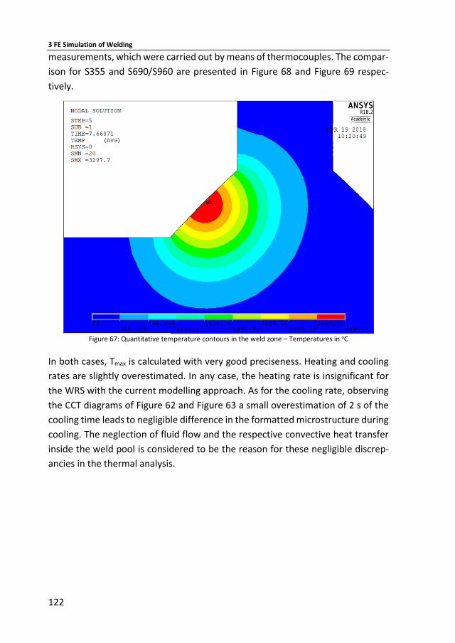
3 FE Simulation of Welding
122
measurements, which were carried out by means of thermocouples. The compar-
ison for S355 and S690/S960 are presented in Figure 68 and Figure 69 respec-
tively.
Figure 67: Quantitative temperature contours in the weld zone – Temperatures in oC
In both cases, Tmax is calculated with very good preciseness. Heating and cooling
rates are slightly overestimated. In any case, the heating rate is insignificant for
the WRS with the current modelling approach. As for the cooling rate, observing
the CCT diagrams of Figure 62 and Figure 63 a small overestimation of 2 s of the
cooling time leads to negligible difference in the formatted microstructure during
cooling. The neglection of fluid flow and the respective convective heat transfer
inside the weld pool is considered to be the reason for these negligible discrep-
ancies in the thermal analysis.
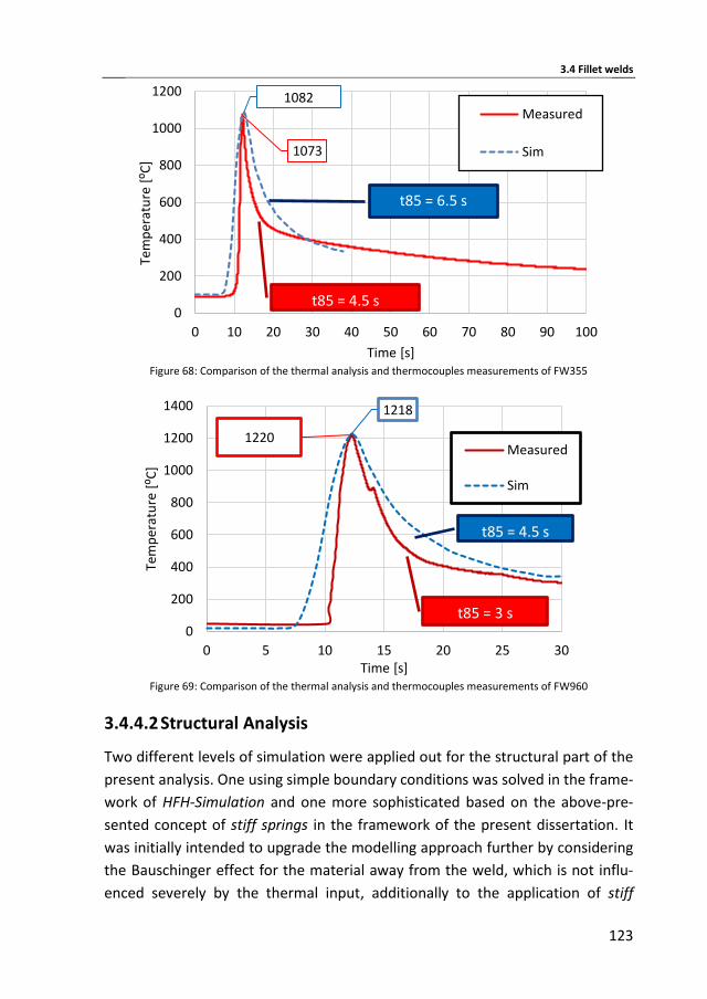
3.4 Fillet welds
123
Figure 68: Comparison of the thermal analysis and thermocouples measurements of FW355
Figure 69: Comparison of the thermal analysis and thermocouples measurements of FW960
3.4.4.2 Structural Analysis
Two different levels of simulation were applied out for the structural part of the
present analysis. One using simple boundary conditions was solved in the frame-
work of HFH-Simulation and one more sophisticated based on the above-pre-
sented concept of stiff springs in the framework of the present dissertation. It
was initially intended to upgrade the modelling approach further by considering
the Bauschinger effect for the material away from the weld, which is not influ-
enced severely by the thermal input, additionally to the application of stiff
1073
1082
0
200
400
600
800
1000
1200
0 10 20 30 40 50 60 70 80 90 100
Tem
per
atu
re [
⁰C]
Time [s]
Measured
Sim
t85 = 6.5 s
t85 = 4.5 s
1218
1220
0
200
400
600
800
1000
1200
1400
0 5 10 15 20 25 30
Tem
per
atu
re [
⁰C]
Time [s]
Measured
Sim
t85 = 4.5 s
t85 = 3 s
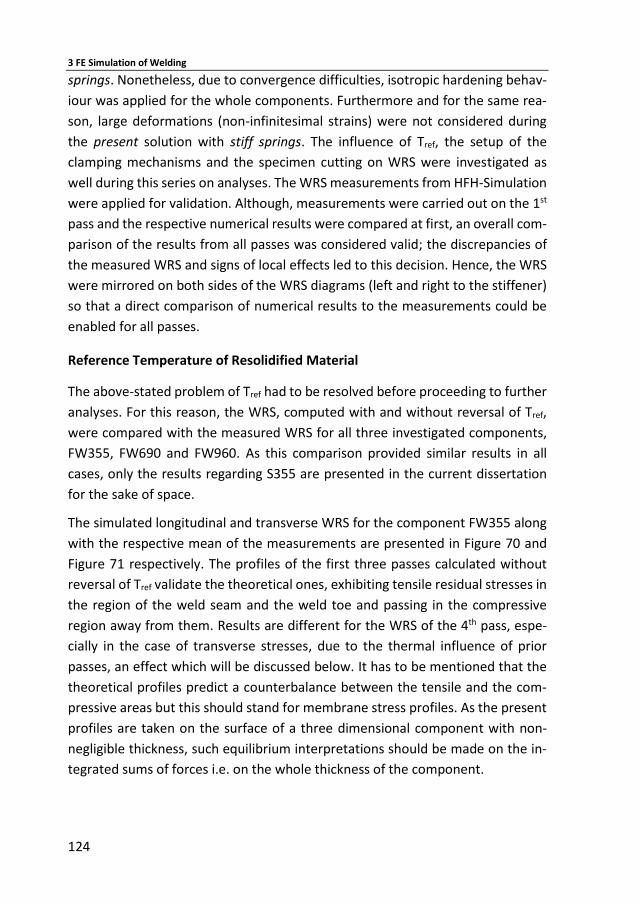
3 FE Simulation of Welding
124
springs. Nonetheless, due to convergence difficulties, isotropic hardening behav-
iour was applied for the whole components. Furthermore and for the same rea-
son, large deformations (non-infinitesimal strains) were not considered during
the present solution with stiff springs. The influence of Tref, the setup of the
clamping mechanisms and the specimen cutting on WRS were investigated as
well during this series on analyses. The WRS measurements from HFH-Simulation
were applied for validation. Although, measurements were carried out on the 1st
pass and the respective numerical results were compared at first, an overall com-
parison of the results from all passes was considered valid; the discrepancies of
the measured WRS and signs of local effects led to this decision. Hence, the WRS
were mirrored on both sides of the WRS diagrams (left and right to the stiffener)
so that a direct comparison of numerical results to the measurements could be
enabled for all passes.
Reference Temperature of Resolidified Material
The above-stated problem of Tref had to be resolved before proceeding to further
analyses. For this reason, the WRS, computed with and without reversal of Tref,
were compared with the measured WRS for all three investigated components,
FW355, FW690 and FW960. As this comparison provided similar results in all
cases, only the results regarding S355 are presented in the current dissertation
for the sake of space.
The simulated longitudinal and transverse WRS for the component FW355 along
with the respective mean of the measurements are presented in Figure 70 and
Figure 71 respectively. The profiles of the first three passes calculated without
reversal of Tref validate the theoretical ones, exhibiting tensile residual stresses in
the region of the weld seam and the weld toe and passing in the compressive
region away from them. Results are different for the WRS of the 4th pass, espe-
cially in the case of transverse stresses, due to the thermal influence of prior
passes, an effect which will be discussed below. It has to be mentioned that the
theoretical profiles predict a counterbalance between the tensile and the com-
pressive areas but this should stand for membrane stress profiles. As the present
profiles are taken on the surface of a three dimensional component with non-
negligible thickness, such equilibrium interpretations should be made on the in-
tegrated sums of forces i.e. on the whole thickness of the component.
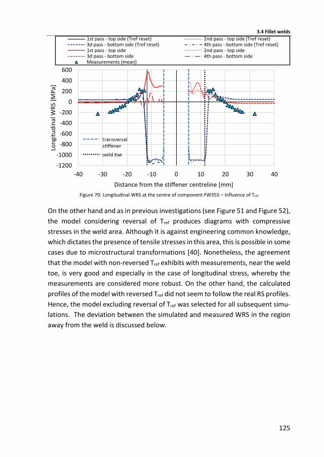
3.4 Fillet welds
125
Figure 70: Longitudinal WRS at the centre of component FW355 – Influence of Tref
On the other hand and as in previous investigations (see Figure 51 and Figure 52),
the model considering reversal of Tref produces diagrams with compressive
stresses in the weld area. Although it is against engineering common knowledge,
which dictates the presence of tensile stresses in this area, this is possible in some
cases due to microstructural transformations [40]. Nonetheless, the agreement
that the model with non-reversed Tref exhibits with measurements, near the weld
toe, is very good and especially in the case of longitudinal stress, whereby the
measurements are considered more robust. On the other hand, the calculated
profiles of the model with reversed Tref did not seem to follow the real RS profiles.
Hence, the model excluding reversal of Tref was selected for all subsequent simu-
lations. The deviation between the simulated and measured WRS in the region
away from the weld is discussed below.
-1200
-1000
-800
-600
-400
-200
0
200
400
600
-40 -30 -20 -10 0 10 20 30 40
Lon
gitu
din
al W
RS
[MP
a]
Distance from the stiffener centreline [mm]
1st pass - top side (Tref reset) 2nd pass - top side (Tref reset)3d pass - bottom side (Tref reset) 4th pass - bottom side (Tref reset)1st pass - top side 2nd pass - top side3d pass - bottom side 4th pass - bottom sideMeasurements (mean)
3 FE Simulation of Welding
126
Figure 71: Transverse WRS at the centre of component FW355 – Influence of Tref
Overall Validation
The longitudinal WRS for all three investigated components, calculated with the
modelling approach of HFH-Simulation (tagged “HFH Sim” - fixing of the clamped
nodes) and the current one (tagged as “present” – using stiff springs and im-
proved material modelling) are presented in Figure 72, Figure 73 and Figure 74
along with the respective measurements. Similar results are met for all materials
and for both modelling approaches. The highest and the lowest WRS are met on
the 1st and the 4th passes respectively. In the case of FW355, tensile stresses
around 630 MPa clearly higher than the nominal yield strength are met on the
weld toe of the 1st pass. They match though the order of magnitude of the higher
yield strength in the HAZ, which is increased due to microstructural transfor-
mations.
The large deviation to the tensile WRS of the 1st to the rest of the passes can be
attributed to the effects caused by the thermal influence of prior to consequent
weld passes. No specifications were given regarding the intermediate tempera-
ture in the WPS, so probably all passes were welded consecutively. Therefore, a
-600
-500
-400
-300
-200
-100
0
100
200
300
400
500
-40 -30 -20 -10 0 10 20 30 40
Tran
sver
se W
RS
[MP
a]
Distance from the stiffener centreline [mm]
1st pass - top side (Tref reset) 2nd pass - top side (Tref reset)
3d pass - bottom side (Tref reset) 4th pass - bottom side (Tref reset)
1st pass - top side 2nd pass - top side
3d pass - bottom side 4th pass - bottom side
Measurements (Mean)
3.4 Fillet welds
127
cooling time between passes of 120 s was assumed9. At this time, temperature in
the weld region is approximately 200 °C (see Figure 69 for example). Thus, heat
input from the prior weld passes acts as preheating for the former ones, reducing
in this way the introduced WRS. As no preheating is applied prior to welding, the
first pass is cold-welded and exhibits significantly higher WRS than the rest of the
passes as expected.
Furthermore, as cooling time was similar for all passes, Tmax was predominant for
the rest of them. Heat input from passes 1 and 2 acted as preheating for the
passes 4 and 3 respectively and higher Tmax was reached. This led to assignment
of different microstructural models to the first two and later passes. CMM 4 and
2 were assigned to the HAZ of the 1st and 2nd passes exhibiting respectively yield
stresses of 947 MPa and 586 MPa. CMM 3 with yield strength of 766 MPa was
assigned to the other two instead of CMM 2. Therewith, a broader zone of high
strength is created allowing for no sudden peak of strength on the weld toe that
could be secondary accounted for the highest peak of WRS on the first pass. Ex-
emplary, the CCM assignment for the 1st and 4th pass of S355 is presented in Fig-
ure 75. This effect was limited for the case of the two high strength steels due to
the homogeneity when yield strength is considered. Small changes in yield stress
due to microstructural transformation took place.
The influence of modelling approach for the boundary conditions on the tensile
WRS, as expected, is limited for all three components. Application of stiff springs
produces slightly higher WRS on the weld toe and, due to equilibrium, slightly
lower away from it.
9 no documentation available, 120 s were assumed rational for practical reasons i.e. for the welder to change position.
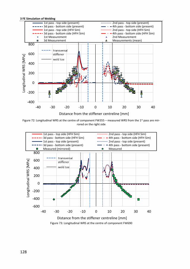
3 FE Simulation of Welding
128
Figure 72: Longitudinal WRS at the centre of component FW355 – measured WRS from the 1st pass are mir-
rored on the right side
Figure 73: Longitudinal WRS at the centre of component FW690
-400
-200
0
200
400
600
800
-40 -30 -20 -10 0 10 20 30 40
Lon
gitu
din
al W
RS
[MP
a]
Distance from the stiffener centreline [mm]
1st pass - top side (present) 2nd pass - top side (present)3d pass - bottom side (present) 4th pass - bottom side (present)1st pass - top side (HFH Sim) 2nd pass - top side (HFH Sim)3d pass - bottom side (HFH Sim) 4th pass - bottom side (HFH Sim)1st Measurement 2nd Measurement3d Measurement Measurements (mean)
-600
-400
-200
0
200
400
600
800
-40 -30 -20 -10 0 10 20 30 40
Lon
gitu
din
al W
RS
[MP
a]
Distance from the stiffener centreline [mm]
Diagrammtitel1st pass - top side (HFH Sim) 2nd pass - top side (HFH Sim)3d pass - bottom side (HFH Sim) 4th pass - bottom side (HFH Sim)1st pass - top side (present) 2nd pass - top side (present)3d pass - bottom side (present) 4th pass - bottom side (present)Measured (mirrored) Measured
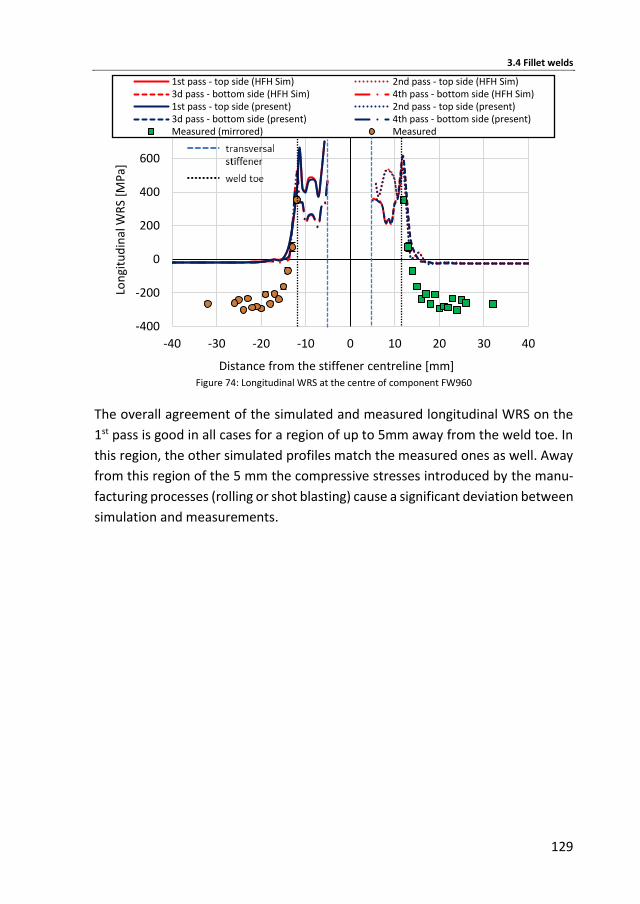
3.4 Fillet welds
129
Figure 74: Longitudinal WRS at the centre of component FW960
The overall agreement of the simulated and measured longitudinal WRS on the
1st pass is good in all cases for a region of up to 5mm away from the weld toe. In
this region, the other simulated profiles match the measured ones as well. Away
from this region of the 5 mm the compressive stresses introduced by the manu-
facturing processes (rolling or shot blasting) cause a significant deviation between
simulation and measurements.
-400
-200
0
200
400
600
800
-40 -30 -20 -10 0 10 20 30 40
Lon
gitu
din
al W
RS
[MP
a]
Distance from the stiffener centreline [mm]
Diagrammtitel1st pass - top side (HFH Sim) 2nd pass - top side (HFH Sim)3d pass - bottom side (HFH Sim) 4th pass - bottom side (HFH Sim)1st pass - top side (present) 2nd pass - top side (present)3d pass - bottom side (present) 4th pass - bottom side (present)Measured (mirrored) Measured
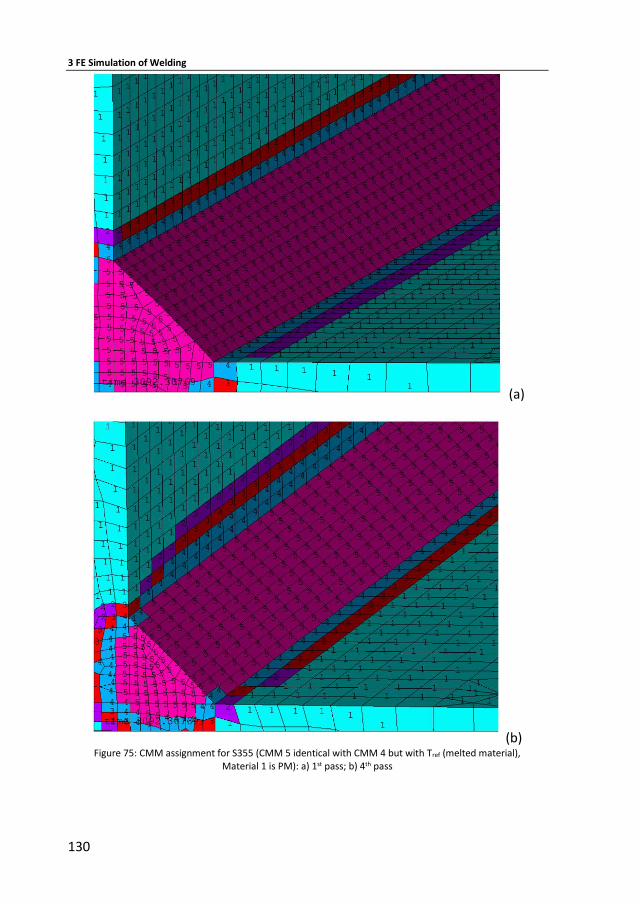
3 FE Simulation of Welding
130
(a)
(b) Figure 75: CMM assignment for S355 (CMM 5 identical with CMM 4 but with Tref (melted material),
Material 1 is PM): a) 1st pass; b) 4th pass
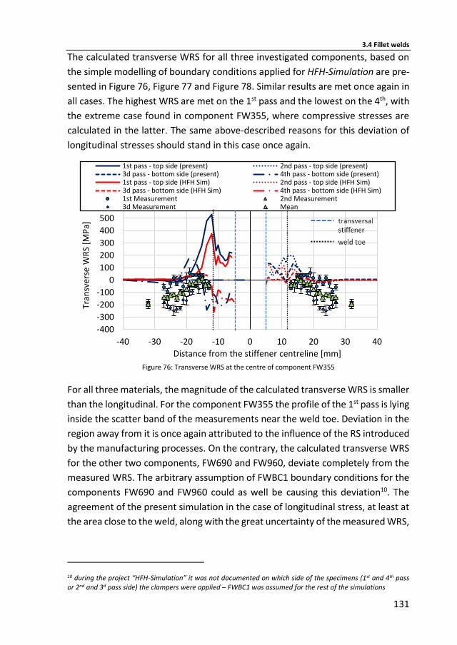
3.4 Fillet welds
131
The calculated transverse WRS for all three investigated components, based on
the simple modelling of boundary conditions applied for HFH-Simulation are pre-
sented in Figure 76, Figure 77 and Figure 78. Similar results are met once again in
all cases. The highest WRS are met on the 1st pass and the lowest on the 4th, with
the extreme case found in component FW355, where compressive stresses are
calculated in the latter. The same above-described reasons for this deviation of
longitudinal stresses should stand in this case once again.
Figure 76: Transverse WRS at the centre of component FW355
For all three materials, the magnitude of the calculated transverse WRS is smaller
than the longitudinal. For the component FW355 the profile of the 1st pass is lying
inside the scatter band of the measurements near the weld toe. Deviation in the
region away from it is once again attributed to the influence of the RS introduced
by the manufacturing processes. On the contrary, the calculated transverse WRS
for the other two components, FW690 and FW960, deviate completely from the
measured WRS. The arbitrary assumption of FWBC1 boundary conditions for the
components FW690 and FW960 could as well be causing this deviation10. The
agreement of the present simulation in the case of longitudinal stress, at least at
the area close to the weld, along with the great uncertainty of the measured WRS,
10 during the project “HFH-Simulation” it was not documented on which side of the specimens (1st and 4th pass or 2nd and 3d pass side) the clampers were applied – FWBC1 was assumed for the rest of the simulations
-400
-300
-200
-100
0
100
200
300
400
500
600
-40 -30 -20 -10 0 10 20 30 40
Tran
sver
se W
RS
[MP
a]
Distance from the stiffener centreline [mm]
Diagrammtitel1st pass - top side (present) 2nd pass - top side (present)3d pass - bottom side (present) 4th pass - bottom side (present)1st pass - top side (HFH Sim) 2nd pass - top side (HFH Sim)3d pass - bottom side (HFH Sim) 4th pass - bottom side (HFH Sim)1st Measurement 2nd Measurement3d Measurement Mean

3 FE Simulation of Welding
132
as it is exposed from the multiple measurements on S355, could as well arise
questions regarding the validity of the measured transverse WRS.
In the case of S355, the influence of modelling approach on the transverse WRS,
as expected, is more significant than for the longitudinal. Application of stiff
springs produces WRS of significantly larger magnitude near the weld toe, as in
the case of the previously investigated butt welds. For the other two materials
negligible difference is observed. The unavoidable neglection of geometrical non-
linearities (large strains were neglected), which was previously proven predomi-
nant for the transverse WRS due to convergence problems, could be accounted
for this. The broad scatter band of the WRS measurements for S355 and negligible
difference between the HFH-Simulation and the present approach though, do not
allow for exclusion of one of the two methods.
Figure 77: Transverse WRS at the centre of component FW690
-600
-400
-200
0
200
400
600
800
-40 -30 -20 -10 0 10 20 30 40
Tran
sver
se W
RS
[MP
a]
Distance from the stiffener centreline [mm]
Diagrammtitel1st pass - top side (HFH Sim) 2nd pass - top side (HFH Sim)
3d pass - bottom side (HFH Sim) 4th pass - bottom side (HFH Sim)
1st pass - top side (present) 2nd pass - top side (present)
3d pass - bottom side (present) 4th pass - bottom side (present)
Measured Measured (mirrored)
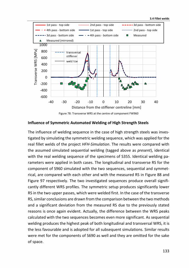
3.4 Fillet welds
133
Figure 78: Transverse WRS at the centre of component FW960
Influence of Symmetric Automated Welding of High Strength Steels
The influence of welding sequence in the case of high strength steels was inves-
tigated by simulating the symmetric welding sequence, which was applied for the
real fillet welds of the project HFH-Simulation. The results were compared with
the assumed simulated sequential welding (tagged above as present), identical
with the real welding sequence of the specimens of S355. Identical welding pa-
rameters were applied in both cases. The longitudinal and transverse RS for the
component of S960 simulated with the two sequences, sequential and symmet-
rical, are compared with each other and with the measured RS in Figure 88 and
Figure 97 respectively. The two investigated sequences produce overall signifi-
cantly different WRS profiles. The symmetric setup produces significantly lower
RS in the two upper passes, which were welded first. In the case of the transverse
RS, similar conclusions are drawn from the comparison between the two methods
and a significant deviation from the measured RS due to the previously stated
reasons is once again evident. Actually, the difference between the WRS peaks
calculated with the two sequences becomes even more significant. As sequential
welding produces the highest peak of both longitudinal and transversal WRS, it is
the less favourable and is adopted for all subsequent simulations. Similar results
were met for the components of S690 as well and they are omitted for the sake
of space.
-600
-400
-200
0
200
400
600
800
1000
-40 -30 -20 -10 0 10 20 30 40
Tran
sver
se W
RS
[MP
a]
Distance from the stiffener centreline [mm]
Diagrammtitel1st pass - top side 2nd pass - top side 3d pass - bottom side
4th pass - bottom side 1st pass - top side 2nd pass - top side
3d pass - bottom side 4th pass - bottom side Measured
Measured (mirrored)
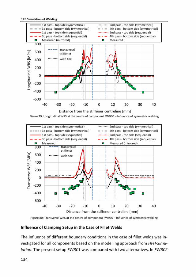
3 FE Simulation of Welding
134
Figure 79: Longitudinal WRS at the centre of component FW960 – Influence of symmetric welding
Figure 80: Transverse WRS at the centre of component FW960 – Influence of symmetric welding
Influence of Clamping Setup in the Case of Fillet Welds
The influence of different boundary conditions in the case of fillet welds was in-
vestigated for all components based on the modelling approach from HFH-Simu-
lation. The present setup FWBC1 was compared with two alternatives. In FWBC2
-600
-400
-200
0
200
400
600
800
-40 -30 -20 -10 0 10 20 30 40
Lon
gitu
din
al W
RS
[MP
a]
Distance from the stiffener centreline [mm]
Diagrammtitel1st pass - top side (symmetrical) 2nd pass - top side (symmetrical)3d pass - bottom side (symmetrical) 4th pass - bottom side (symmetrical)1st pass - top side (sequential) 2nd pass - top side (sequential)3d pass - bottom side (sequential) 4th pass - bottom side (sequential)Measured (mirrored) Measured
-600
-400
-200
0
200
400
600
800
1000
-40 -30 -20 -10 0 10 20 30 40
Tran
sver
se W
RS
[MP
a]
Distance from the stiffener centreline [mm]
Diagrammtitel1st pass - top side (symmetrical) 2nd pass - top side (symmetrical)
3d pass - bottom side (symmetrical) 4th pass - bottom side (symmetrical)
1st pass - top side (sequential) 2nd pass - top side (sequential)
3d pass - bottom side (sequential) 4th pass - bottom side (sequential)
Measured Measured (mirrored)
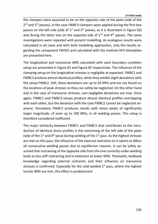
3.4 Fillet welds
135
the clampers were assumed to be on the opposite side of the plate (side of the
2nd and 3rd passes). In the case FWBC3 clampers were applied during the first two
passes on the left side (side of 1st and 3rd passes, as it is illustrated in Figure 56)
and during the latter two on the opposite side of 2nd and 4th passes. The same
investigations were repeated with present modelling. As analogous results were
calculated in all cases and with both modelling approaches, only the results re-
garding the component FW355 and calculated with the method HFH-Simulation
are presented here.
The longitudinal and transverse WRS calculated with each boundary condition
setup are presented in Figure 81 and Figure 82 respectively. The influence of the
clamping setup on the longitudinal stresses is negligible as expected. FWBC1 and
FWBC3 produce almost identical profiles, while they exhibit slight deviations with
the setup FWBC2. Still, these deviations are up to 50 MPa and are not found on
the locations of peak stresses so they can safely be neglected. On the other hand
and in the case of transverse stresses, non-negligible deviations are met. Once
again, FWBC1 and FWBC3 setups produce almost identical profiles overlapping
with each other, but the deviation with the case FWBC2 cannot be neglected an-
ymore. Simulation FWBC2 produces results with stress peaks of significantly
larger magnitude, of even up to 100 MPa, in all welding passes. This setup is
therefore considered inefficient.
The major similarity between FWBC1 and FWBC3 that contributes to the intro-
duction of identical stress profiles is the restraining of the left side of the plate
(side of the 1st and 4th pass) during welding of the 1st pass. As the highest stresses
are met on this pass, the influence of the external restraints on it seems to affect
all consecutive welding passes due to equilibrium reasons. It can be safely as-
sumed that restraining of the opposite side from the one currently under welding
leads to less stiff restraining and in extension to lower WRS. Therewith, textbook
knowledge regarding external restraints and their influence on transverse
stresses is confirmed. Especially for the cold welded 1st pass, where the highest
tensile WRS are met, this effect is predominant
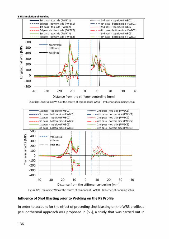
3 FE Simulation of Welding
136
Figure 81: Longitudinal WRS at the centre of component FW960 – Influence of clamping setup
Figure 82: Transverse WRS at the centre of component FW960 – Influence of clamping setup
Influence of Shot Blasting prior to Welding on the RS Profile
In order to account for the effect of preceding shot blasting on the WRS profile, a
pseudothermal approach was proposed in [53], a study that was carried out in
-200
-100
0
100
200
300
400
500
600
700
-40 -30 -20 -10 0 10 20 30 40
Lon
gitu
din
al W
RS
[MP
a]
Distance from the stiffener centreline [mm]
1st pass - top side (FWBC1) 2nd pass - top side (FWBC1)3d pass - bottom side (FWBC1) 4th pass - bottom side (FWBC1)1st pass - top side (FWBC2) 2nd pass - top side (FWBC2)3d pass - bottom side (FWBC2) 4th pass - bottom side (FWBC2)1st pass - top side (FWBC3) 2nd pass - top side (FWBC3)3d pass - bottom side (FWBC3) 4th pass - bottom side (FWBC3)
-400
-300
-200
-100
0
100
200
300
400
500
-40 -30 -20 -10 0 10 20 30 40
Tran
sver
se W
RS
[MP
a]
Distance from the stiffener centreline [mm]
Diagrammtitel1st pass - top side (FWBC1) 2nd pass - top side (FWBC1)3d pass - bottom side (FWBC1) 4th pass - bottom side (FWBC1)1st pass - top side (FWBC2) 2nd pass - top side (FWBC2)3d pass - bottom side (FWBC2) 4th pass - bottom side (FWBC2)1st pass - top side (FWBC3) 2nd pass - top side (FWBC3)3d pass - bottom side (FWBC3) 4th pass - bottom side (FWBC3)
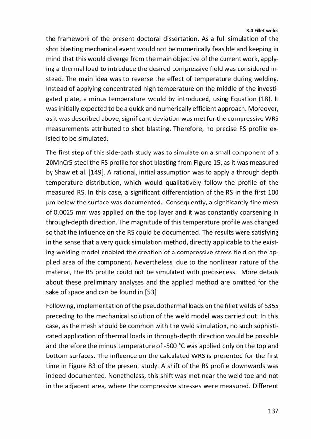
3.4 Fillet welds
137
the framework of the present doctoral dissertation. As a full simulation of the
shot blasting mechanical event would not be numerically feasible and keeping in
mind that this would diverge from the main objective of the current work, apply-
ing a thermal load to introduce the desired compressive field was considered in-
stead. The main idea was to reverse the effect of temperature during welding.
Instead of applying concentrated high temperature on the middle of the investi-
gated plate, a minus temperature would by introduced, using Equation (18). It
was initially expected to be a quick and numerically efficient approach. Moreover,
as it was described above, significant deviation was met for the compressive WRS
measurements attributed to shot blasting. Therefore, no precise RS profile ex-
isted to be simulated.
The first step of this side-path study was to simulate on a small component of a
20MnCr5 steel the RS profile for shot blasting from Figure 15, as it was measured
by Shaw et al. [149]. A rational, initial assumption was to apply a through depth
temperature distribution, which would qualitatively follow the profile of the
measured RS. In this case, a significant differentiation of the RS in the first 100
μm below the surface was documented. Consequently, a significantly fine mesh
of 0.0025 mm was applied on the top layer and it was constantly coarsening in
through-depth direction. The magnitude of this temperature profile was changed
so that the influence on the RS could be documented. The results were satisfying
in the sense that a very quick simulation method, directly applicable to the exist-
ing welding model enabled the creation of a compressive stress field on the ap-
plied area of the component. Nevertheless, due to the nonlinear nature of the
material, the RS profile could not be simulated with preciseness. More details
about these preliminary analyses and the applied method are omitted for the
sake of space and can be found in [53]
Following, implementation of the pseudothermal loads on the fillet welds of S355
preceding to the mechanical solution of the weld model was carried out. In this
case, as the mesh should be common with the weld simulation, no such sophisti-
cated application of thermal loads in through-depth direction would be possible
and therefore the minus temperature of -500 °C was applied only on the top and
bottom surfaces. The influence on the calculated WRS is presented for the first
time in Figure 83 of the present study. A shift of the RS profile downwards was
indeed documented. Nonetheless, this shift was met near the weld toe and not
in the adjacent area, where the compressive stresses were measured. Different
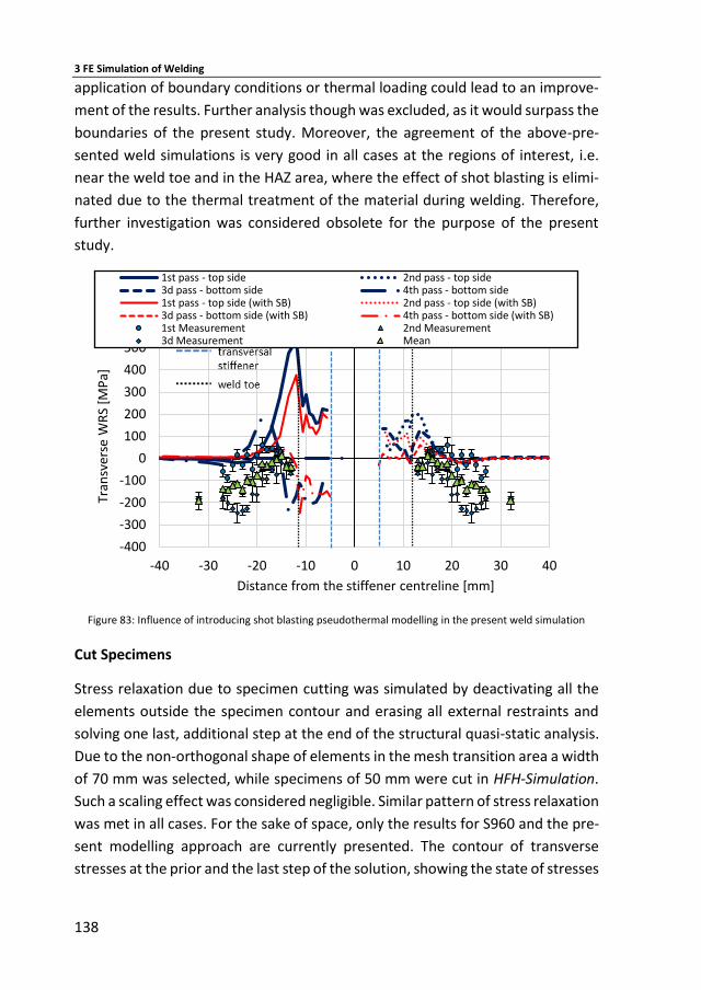
3 FE Simulation of Welding
138
application of boundary conditions or thermal loading could lead to an improve-
ment of the results. Further analysis though was excluded, as it would surpass the
boundaries of the present study. Moreover, the agreement of the above-pre-
sented weld simulations is very good in all cases at the regions of interest, i.e.
near the weld toe and in the HAZ area, where the effect of shot blasting is elimi-
nated due to the thermal treatment of the material during welding. Therefore,
further investigation was considered obsolete for the purpose of the present
study.
Figure 83: Influence of introducing shot blasting pseudothermal modelling in the present weld simulation
Cut Specimens
Stress relaxation due to specimen cutting was simulated by deactivating all the
elements outside the specimen contour and erasing all external restraints and
solving one last, additional step at the end of the structural quasi-static analysis.
Due to the non-orthogonal shape of elements in the mesh transition area a width
of 70 mm was selected, while specimens of 50 mm were cut in HFH-Simulation.
Such a scaling effect was considered negligible. Similar pattern of stress relaxation
was met in all cases. For the sake of space, only the results for S960 and the pre-
sent modelling approach are currently presented. The contour of transverse
stresses at the prior and the last step of the solution, showing the state of stresses
-400
-300
-200
-100
0
100
200
300
400
500
600
-40 -30 -20 -10 0 10 20 30 40
Tran
sver
se W
RS
[MP
a]
Distance from the stiffener centreline [mm]
Diagrammtitel1st pass - top side 2nd pass - top side3d pass - bottom side 4th pass - bottom side1st pass - top side (with SB) 2nd pass - top side (with SB)3d pass - bottom side (with SB) 4th pass - bottom side (with SB)1st Measurement 2nd Measurement3d Measurement Mean
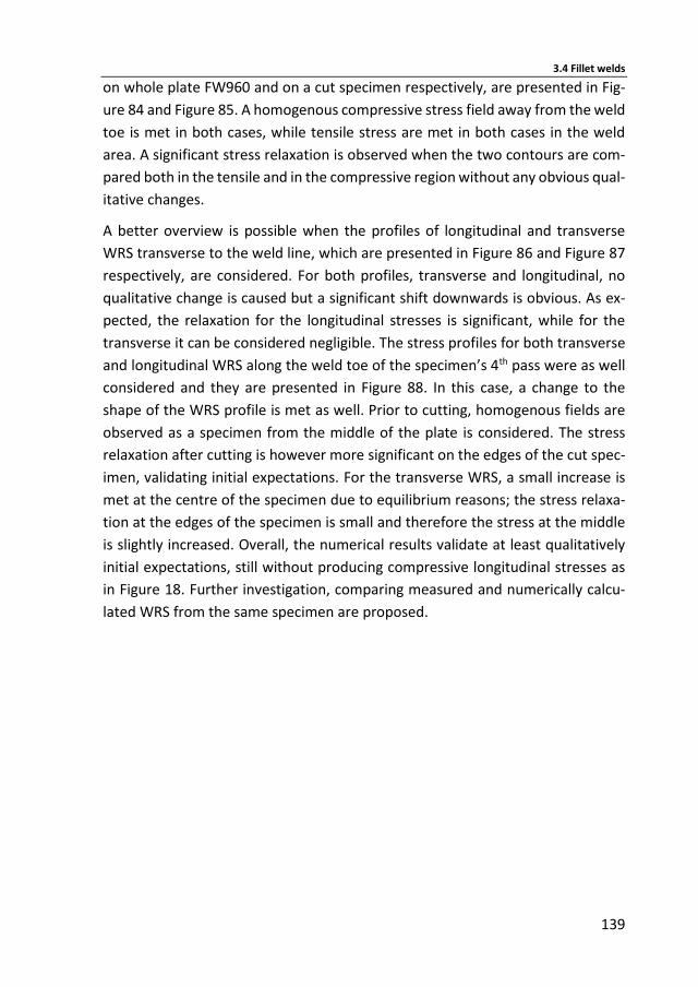
3.4 Fillet welds
139
on whole plate FW960 and on a cut specimen respectively, are presented in Fig-
ure 84 and Figure 85. A homogenous compressive stress field away from the weld
toe is met in both cases, while tensile stress are met in both cases in the weld
area. A significant stress relaxation is observed when the two contours are com-
pared both in the tensile and in the compressive region without any obvious qual-
itative changes.
A better overview is possible when the profiles of longitudinal and transverse
WRS transverse to the weld line, which are presented in Figure 86 and Figure 87
respectively, are considered. For both profiles, transverse and longitudinal, no
qualitative change is caused but a significant shift downwards is obvious. As ex-
pected, the relaxation for the longitudinal stresses is significant, while for the
transverse it can be considered negligible. The stress profiles for both transverse
and longitudinal WRS along the weld toe of the specimen’s 4th pass were as well
considered and they are presented in Figure 88. In this case, a change to the
shape of the WRS profile is met as well. Prior to cutting, homogenous fields are
observed as a specimen from the middle of the plate is considered. The stress
relaxation after cutting is however more significant on the edges of the cut spec-
imen, validating initial expectations. For the transverse WRS, a small increase is
met at the centre of the specimen due to equilibrium reasons; the stress relaxa-
tion at the edges of the specimen is small and therefore the stress at the middle
is slightly increased. Overall, the numerical results validate at least qualitatively
initial expectations, still without producing compressive longitudinal stresses as
in Figure 18. Further investigation, comparing measured and numerically calcu-
lated WRS from the same specimen are proposed.
3 FE Simulation of Welding
140
Figure 84: Transverse WRS of the whole plate FW355 –
Contour of the single specimen is marked with black line – Stresses are given in Pa
Figure 85: Transverse WRS of the cut specimen from FW355 –
Area of deactivated elements are presented in grey – Stresses are given in Pa

3.4 Fillet welds
141
Figure 86: Stress relaxation of longitudinal WRS due to cut of specimen from component FW960 transverse to
the weld line at the centre of the component
Figure 87: Stress relaxation of transverse WRS due to cut of specimen from component FW960 transverse to
the weld line at the centre of the component
-200
0
200
400
600
800
-40 -30 -20 -10 0 10 20 30 40
Lon
gitu
din
al W
RS
[MP
a]
Distance from the stiffener centreline [mm]
Diagrammtitel1st pass - top side (after cut) 2nd pass - top side (after cut)
3d pass - bottom side (after cut) 4th pass - bottom side (after cut)
1st pass - top side 2nd pass - top side
3d pass - bottom side 4th pass - bottom side
-200
-100
0
100
200
300
400
500
600
700
-40 -30 -20 -10 0 10 20 30 40
Tran
sver
se W
RS
[MP
a]
Distance from the stiffener centreline [mm]
Diagrammtitel1st pass - top side (after cut) 2nd pass - top side (after cut)
3d pass - bottom side (after cut) 4th pass - bottom side (after cut)
1st pass - top side 2nd pass - top side
3d pass - bottom side 4th pass - bottom side
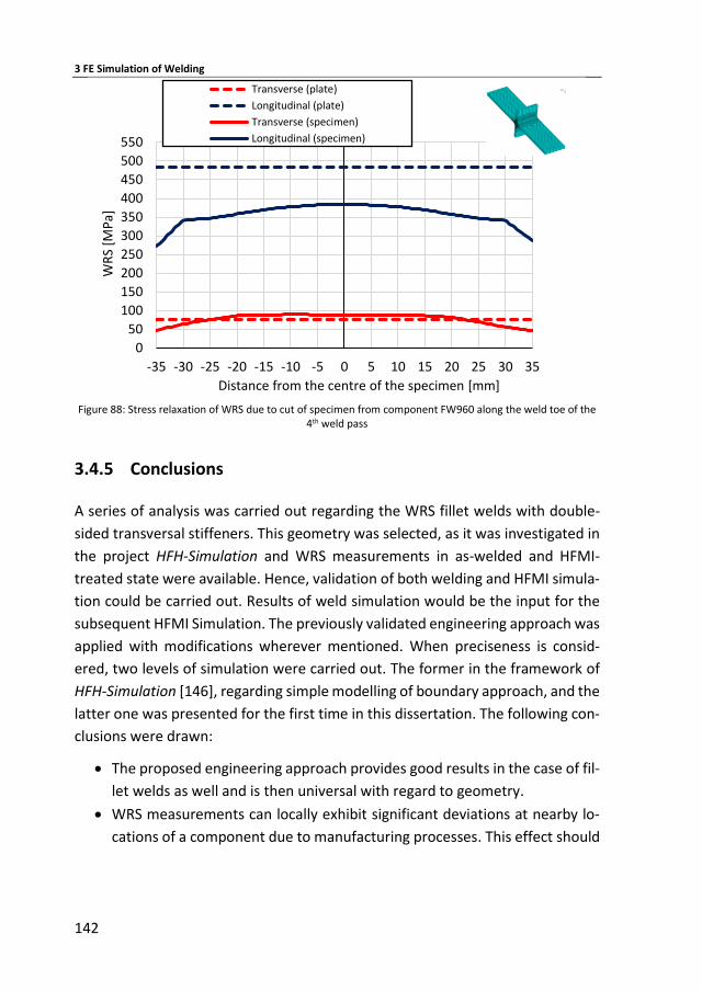
3 FE Simulation of Welding
142
Figure 88: Stress relaxation of WRS due to cut of specimen from component FW960 along the weld toe of the
4th weld pass
3.4.5 Conclusions
A series of analysis was carried out regarding the WRS fillet welds with double-
sided transversal stiffeners. This geometry was selected, as it was investigated in
the project HFH-Simulation and WRS measurements in as-welded and HFMI-
treated state were available. Hence, validation of both welding and HFMI simula-
tion could be carried out. Results of weld simulation would be the input for the
subsequent HFMI Simulation. The previously validated engineering approach was
applied with modifications wherever mentioned. When preciseness is consid-
ered, two levels of simulation were carried out. The former in the framework of
HFH-Simulation [146], regarding simple modelling of boundary approach, and the
latter one was presented for the first time in this dissertation. The following con-
clusions were drawn:
The proposed engineering approach provides good results in the case of fil-
let welds as well and is then universal with regard to geometry.
WRS measurements can locally exhibit significant deviations at nearby lo-
cations of a component due to manufacturing processes. This effect should
0
50
100
150
200
250
300
350
400
450
500
550
-35 -30 -25 -20 -15 -10 -5 0 5 10 15 20 25 30 35
WR
S [M
Pa]
Distance from the centre of the specimen [mm]
Transverse (plate)
Longitudinal (plate)
Transverse (specimen)
Longitudinal (specimen)

3.4 Fillet welds
143
always be considered, when these measurements are applied for the vali-
dation of numerical results, which may not be able to depict these devia-
tions.
The rolling and/or the shot blasting process, which is usually applied for
cleaning of metallic surfaces prior to welding, introduced significant com-
pressive residual stresses. These influences cannot be ignored when WRS
are simulated overall. Nevertheless, in cases where only the WRS in and
near the weld are of great importance, this could be neglected. The effect
of thermal treatment of welding seems to erase this effect near the weld as
very good agreement is met for the measurements closest to the weld toe.
Moreover, in the latter case the significantly localized effect of shot blasts
around the area of impact should be accounted for the fact that the pre-
ciseness is not influenced by the remaining compressive stresses away from
the weld. In the present study, where the WRS on the HFMI treatment area
i.e. the weld toe are needed, this influence can be neglected.
Tref of the elements in the FZ should be equal to the melting temperature of
the investigated material applied and should remain so after cooling.
Modelling approach of boundary conditions is not as predominant for the
transverse WRS, as in the case of butt welds. This was at some point ex-
pected, as the heat input and the shrinkage of the plate takes place on the
bottom and top of the plate outside the plate plane. Thus, the effect would
be more mediocre than in the case of butt welds were both the restrains
and the heat input causing the dilatation are coplanar. The effect on the
longitudinal WRS was in any case negligible.
In order to minimize WRS and increase fatigue strength of a fillet weld with
transversal stiffeners, the opposite side from the currently welded pass
should be clamped down. For practical reasons, the side opposite to the
cold-welded 1st pass should be restrained during welding, as in this case the
effect is predominant. If preheating is applied, this approach is expected to
have limited effect.
The present engineering approach provides sufficient results for high
strength steels as well.
The proposed values for the weld metal arc efficiency found in literature
were insufficient for the present analysis. Significant arbitrary increase of
thermal heat input was necessary in order to calibrate the thermal analysis
3 FE Simulation of Welding
144
and match the respective measurement results. This could be attributed to
the variety of the investigated materials.
Symmetrical welding, i.e. simultaneous welding of the top two welding
passes and subsequent simultaneous welding of the bottom two passes or
vice versa, can significantly decrease the peak WRS at all weld toes and lead
to an improved fatigue behaviour of the weldments.
An approach in order to simulate shot blasting by applying thermal loading
instead of modelling the real mechanical effect was proposed. Although the
results of preliminary analyses were satisfying, when the proposed ap-
proach was incorporated to the present weld simulation model, no signifi-
cant improvement was observed. The proposed method though, seems
promising as it is numerically efficient and worked well for the smaller com-
ponents. A further investigation of the method was excluded as it was con-
sidered to lie outside the boundaries of the present study.
Influence of cutting single fatigue test specimens was investigated, validat-
ing the common engineering knowledge that stress relaxation of the longi-
tudinal WRS takes place. The results were qualitatively identical with earlier
investigations on other specimens, but as quantitative deviation was ob-
served, further investigations are proposed for this subject.
To summarize, sufficient results were met in most cases regarding the welding
simulation of the fillet welds based on the precision requirements set at the be-
ginning of the present study. The calculated WRS were considered suitable to be
applied as input for the subsequent HFMI simulation.
145
4 Drop Tests for the Calibration of HFMI Simulation
4.1 Work Hypothesis
A series of drop tests was implemented in the framework of the present doctoral
dissertation in order to allow the reproduction of a HFMI impact under monitored
conditions in the laboratory and therewith, enable the characterization of the in-
vestigated material’s mechanical behaviour by considering explicitly possible ir-
regularities concerning the present deformation modus. During the initial defini-
tion of the objectives, it was considered that the applied experimental procedure
should be straightforward, reproducible and therefore would not require com-
plex experimental equipment. Main goal was the determination of the investi-
gated material’s dynamic yield strength for various strain rates inside the spec-
trum of interest, so that a calibration of the applied material model for the
subsequent HFMI simulation could be enabled.
4.2 Methodology
During the drop tests, the HFMI pin should carry out a free fall and impact on a
specimen of the investigated material with a known velocity, carrying a known
mass. Impact velocity would be both analytically calculated and measured during
the experiment. Analytical calculations based on Equations (31) to (38) would al-
low the calculation of the dynamic yield strength based on measurements of ei-
ther the impact crater or the restitution coefficient e respectively. During a FE
analysis of the impact using as input the known mass and impact velocity, the
plastic strain rate would be defined. The obtained dynamic yield stress for the
given strain rate would be initially validated through comparison with respective
results from material testing under high strain rates, which was carried out in the
framework of previous studies, found in literature (see [46], [47], [48], [86] etc.).
The strain rate dependent material model calibrated with the results of the drop
tests would be introduced to the simulation of HFMI. Comparison of this late FE
model with measured profiles of residual stresses would act as a final validation
step. The calibration of the material model and the upon-based FE simulation are
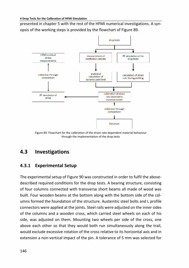
4 Drop Tests for the Calibration of HFMI Simulation
146
presented in chapter 5 with the rest of the HFMI numerical investigations. A syn-
opsis of the working steps is provided by the flowchart of Figure 89.
Figure 89: Flowchart for the calibration of the strain rate dependent material behaviour
through the implementation of the drop tests
4.3 Investigations
4.3.1 Experimental Setup
The experimental setup of Figure 90 was constructed in order to fulfil the above-
described required conditions for the drop tests. A bearing structure, consisting
of four columns connected with transverse short beams all made of wood was
built. Four wooden beams at the bottom along with the bottom side of the col-
umns formed the foundation of the structure. Austenitic steel bolts and L profile
connectors were applied at the joints. Steel rails were adjusted on the inner sides
of the columns and a wooden cross, which carried steel wheels on each of his
side, was adjusted on them. Mounting two wheels per side of the cross, one
above each other so that they would both run simultaneously along the trail,
would exclude excessive rotation of the cross relative to its horizontal axis and in
extension a non-vertical impact of the pin. A tolerance of 5 mm was selected for
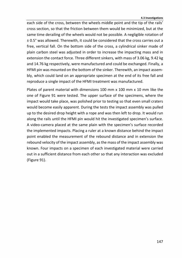
4.3 Investigations
147
each side of the cross, between the wheels middle point and the tip of the rails’
cross section, so that the friction between them would be minimized, but at the
same time derailing of the wheels would not be possible. A negligible rotation of
± 0.5° was allowed. Therewith, it could be considered that the cross carries out a
free, vertical fall. On the bottom side of the cross, a cylindrical sinker made of
plain carbon steel was adjusted in order to increase the impacting mass and in
extension the contact force. Three different sinkers, with mass of 3.06 kg, 9.42 kg
and 14.76 kg respectively, were manufactured and could be exchanged. Finally, a
HFMI pin was mounted on the bottom of the sinker. Therewith, an impact assem-
bly, which could land on an appropriate specimen at the end of its free fall and
reproduce a single impact of the HFMI treatment was manufactured.
Plates of parent material with dimensions 100 mm x 100 mm x 10 mm like the
one of Figure 91 were tested. The upper surface of the specimens, where the
impact would take place, was polished prior to testing so that even small craters
would become easily apparent. During the tests the impact assembly was pulled
up to the desired drop height with a rope and was then left to drop. It would run
along the rails until the HFMI pin would hit the investigated specimen’s surface.
A video-camera placed at the same plain with the specimen’s surface recorded
the implemented impacts. Placing a ruler at a known distance behind the impact
point enabled the measurement of the rebound distance and in extension the
rebound velocity of the impact assembly, as the mass of the impact assembly was
known. Four impacts on a specimen of each investigated material were carried
out in a sufficient distance from each other so that any interaction was excluded
(Figure 91).
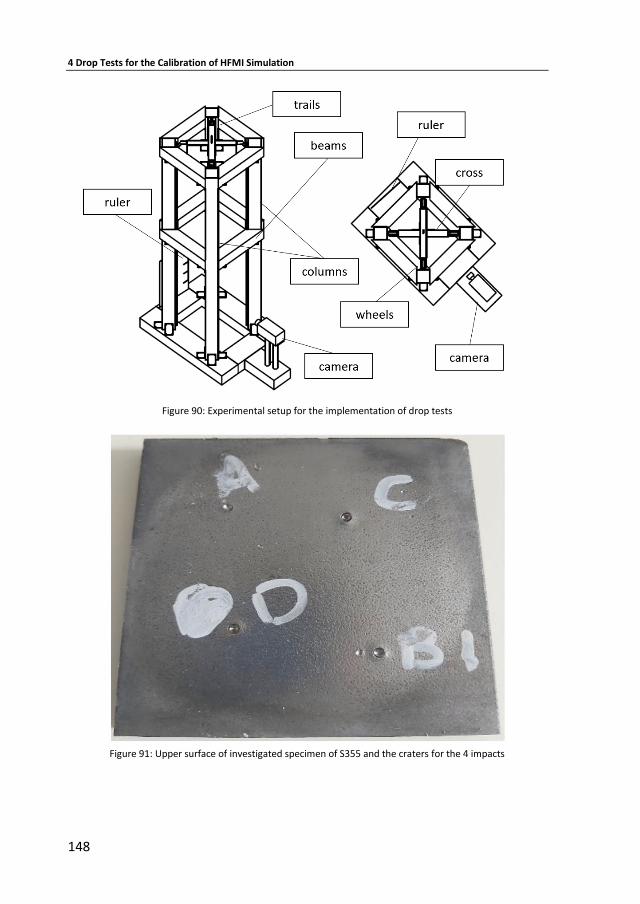
4 Drop Tests for the Calibration of HFMI Simulation
148
Figure 90: Experimental setup for the implementation of drop tests
Figure 91: Upper surface of investigated specimen of S355 and the craters for the 4 impacts
4.3 Investigations
149
4.3.2 Estimation of Impact Velocity
Impact velocity was calculated analytically based on trivial physics and was ini-
tially expected to be measured as well from the recorded video. During the ana-
lytical calculation, a comparison of the results by taking into consideration or ne-
glecting the air drag shown that this influence was negligible (0.001 m/s). A drag
coefficient for a perfect cylinder (sinker) ignoring the influence of the rest of the
impact assembly was considered. This negligibility during the drop meant of
course that the drag was negligible during the rebound too, as the rebound ve-
locity is always lower. Drag was therefore neglected in the calculation of the res-
titution coefficient. In most cases, a validation of the impact velocity during the
drop based on the video frames was against initial expectations not possible, as
it was too high to be caught by the present video recording rate.
4.3.3 Strain Rate Calculation through FE Analysis
A finite element analysis of the drop tests was carried out in order to calculate
the plastic strain rate. A strain rate independent non-linear material behaviour
was applied. Considering the strain rate dependency of the yield strength and the
hardening behaviour would be naturally closer to physical reality, but this would
create an infinite loop to the flowchart of Figure 89. Overrunning this obstacle
through an optimization process could be possible, but this would exceed the lim-
its of the present study and it was therefore excluded. The FE analysis was carried
out based on the previously presented theoretical background and the velocity-
based modelling technique applied for HFMI, described thoroughly in the follow-
ing chapter 5. For this reason, no further information is given on the FE model at
this point. Sole difference between the simulations of the drop tests and the HFMI
treatment, apart from the singularity of the impact and the strain rate independ-
ent material modelling, is the additional mass of the impact assembly. The addi-
tional mass was considered to be concentrated at the centroid of the pin, a valid
assumption for a vertical impact with negligible rotations. Additionally, the singu-
larity of the impact in these cases allowed the use of double symmetry at the
impact point at the intersection of two orthogonal planes, whose intersecting line
is parallel to the normal of the impact (see Figure 92).
During the initiation of contact, unexpectedly high equivalent von Mises and
shear strain rates (휀̇εq > 105 s-1) were evident on the contact surface for a very
4 Drop Tests for the Calibration of HFMI Simulation
150
short time (dt < 10-4 s). This effect was present in the case of the subsequently
presented HFMI analysis and is attributed to numerical singularities, which arise
due to the applied contact model. No significant influence from these singularities
on the numerical results was evident, as it is described later in chapter 5. Still, the
plastic strain rate was not evaluated directly after yielding, but at the point that
a plastic spherical zone was created underneath the contact surface, as it is pre-
sented in Figure 92. At this point, the average of the maximum shear strain rate
along the vertical line at the intersection of the two symmetry points in depth
direction (line AB in Figure 92 b) was extracted and was the applied strain rate
for subsequent material model calibration. Exemplary, a correlation of the impact
velocities and the respective calculated strain rate for S355 is illustrated in Figure
93.
Unfortunately, there is no previous respective correlation of a spherical in-
denter’s impact speed with the plastic strain rate known to the author, which
could act as reference for the present results. Still, in the above-mentioned study
by Cadoni et al. [20], during Split-Hopkinson bar tests impact velocities of 9 m/s
to 27 m/s were correlated with strain rates of 900 sˉ¹ to 7000 sˉ¹. Yet, contact
between wider circular normal surfaces (diameter of 5 mm) takes place in the
former case. On the contrary, in the case of the spherical indenter the contact
initiates from a point and then is applied only on a significantly smaller circular
area (< 0.5 mm for the present case). Therefore, higher strain rates can be ex-
pected in the latter one due to higher stress concentration. The present calcu-
lated strain rates, which are in the same order of magnitude with those of Cadoni
et al. [20] but slightly higher and for lower impact values, are thus considered
valid.
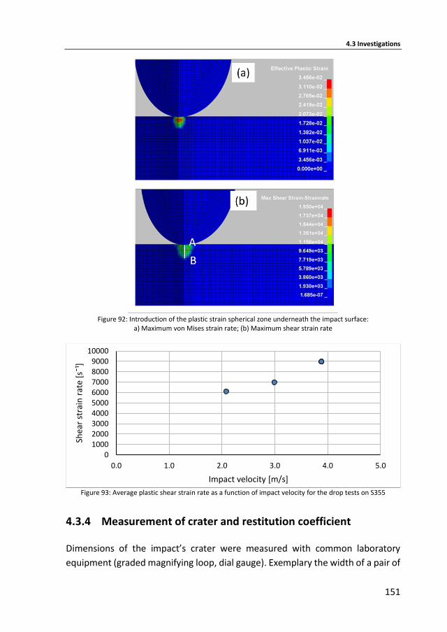
4.3 Investigations
151
Figure 92: Introduction of the plastic strain spherical zone underneath the impact surface:
a) Maximum von Mises strain rate; (b) Maximum shear strain rate
Figure 93: Average plastic shear strain rate as a function of impact velocity for the drop tests on S355
4.3.4 Measurement of crater and restitution coefficient
Dimensions of the impact’s crater were measured with common laboratory
equipment (graded magnifying loop, dial gauge). Exemplary the width of a pair of
0100020003000400050006000700080009000
10000
0.0 1.0 2.0 3.0 4.0 5.0
Shea
r st
rain
rat
e [s
ˉ¹]
Impact velocity [m/s]
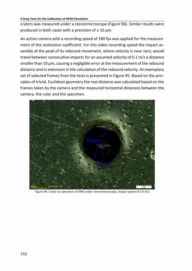
4 Drop Tests for the Calibration of HFMI Simulation
152
craters was measured under a stereomicroscope (Figure 96). Similar results were
produced in both cases with a precision of ± 10 μm.
An action camera with a recording speed of 180 fps was applied for the measure-
ment of the restitution coefficient. For this video recording speed the impact as-
sembly at the peak of its rebound movement, where velocity is near zero, would
travel between consecutive impacts for an assumed velocity of 0.1 m/s a distance
smaller than 10 μm, causing a negligible error at the measurement of the rebound
distance and in extension in the calculation of the rebound velocity. An exemplary
set of selected frames from the tests is presented in Figure 95. Based on the prin-
ciples of trivial, Euclidean geometry the real distance was calculated based on the
frames taken by the camera and the measured horizontal distances between the
camera, the ruler and the specimen.
Figure 94: Crater on specimen of S960 under stereomicroscope, impact speed of 3.9 m/s
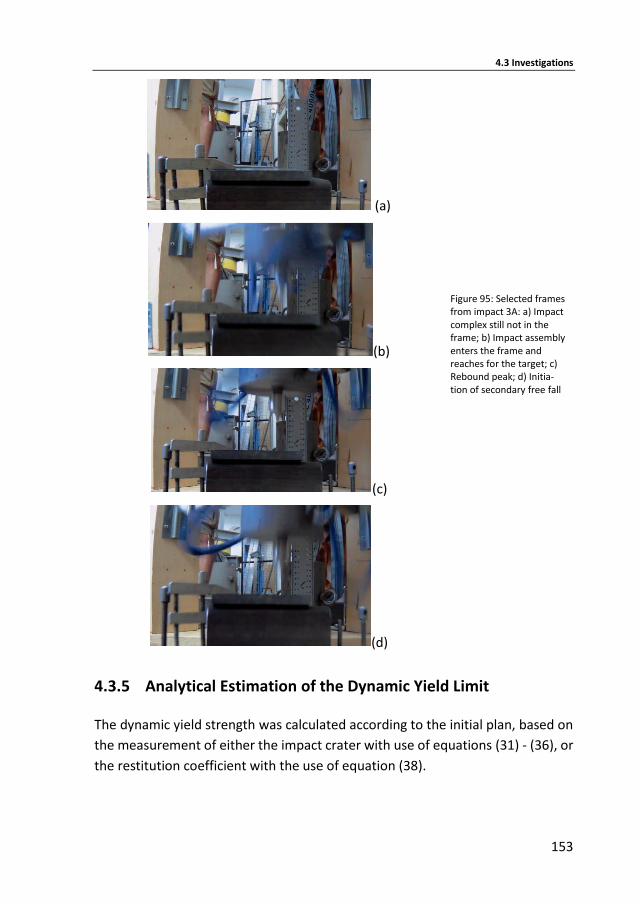
4.3 Investigations
153
(a)
Figure 95: Selected frames from impact 3A: a) Impact complex still not in the frame; b) Impact assembly enters the frame and reaches for the target; c) Rebound peak; d) Initia-tion of secondary free fall
(b)
(c)
(d)
4.3.5 Analytical Estimation of the Dynamic Yield Limit
The dynamic yield strength was calculated according to the initial plan, based on
the measurement of either the impact crater with use of equations (31) - (36), or
the restitution coefficient with the use of equation (38).
4 Drop Tests for the Calibration of HFMI Simulation
154
Analytical Estimation based on the Dimensions of the Crater
Calculating the dynamic yield stress by measuring the crater’s size is based on the
above presented equations and the reasoning path that Lim and Stronge followed
for the solution of a rigid cylinder impacting on an elastic-plastic half space [110].
Analogously to Equation (34), in the case of a spherical indenter contact-half
width at yielding is correlated with the half width of the crater according to the
following equation
𝑎𝑐3 (
1
𝑅−
1
𝑅′) =
𝑎𝑦3
𝑅. (40)
Contact force at yielding is calculated based on Equations (32), (33) as follows
𝐹𝑌 = 4 ∙ 𝐸 ∙ 𝑎𝑦
3
3 ∙ 𝑅 ∙ (1 − 𝑣2), (41)
while stress at yielding is correlated with the contact force based on the assump-
tion of Equation (35) as follows
𝜎𝑌 = 0.351 ∙ (𝐸
𝑅 ∙ (1 − 𝑣2))
23
∙ 𝐹𝑌
13. (42)
Nonetheless, this reasoning course is based on the assumptions that were stated
by Lime and Stronge [110] for the cylindrical indenter. In the present case though,
significant pile-up could be observed at the periphery of the crater. This led to the
introduction of a residual crater with curvature R’ which in most cases was smaller
than the initial curvature prior to unloading. Therewith, the requirements for the
application of a solution analogous to that of Lime and Stronge [110] were no
more valid. As expected, the present method yielded no rational results and
therefore, the respective calculated dynamic yield strengths are not presented.
Exemplary, the results of the measurement of the crater and the calculation of
the half contact width at yielding for S355 are given in Table 40.
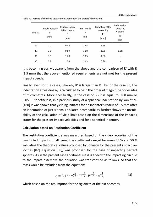
4.3 Investigations
155
Table 40: Results of the drop tests – measurement of the craters’ dimensions
Impact
Impact velocity
u
[m/s]
Residual inden-tation depth
δ
[mm]
Half width
α
[mm]
Curvature after unloading
R’
[mm]
Indentation depth at yielding
αY
[mm]
3A 2.1 0.82 1.45 1.28 -
3B 3.0 0.69 1.60 1.86 0.08
3C 3.9 1.28 1.65 1.06 -
3D 3.9 1.34 1.63 0.96 -
It is becoming easily apparent from the above and the comparison of R’ with R
(1.5 mm) that the above-mentioned requirements are not met for the present
impact speeds.
Finally, even for the cases, whereby R’ is larger than R, like for the case 3B, the
indentation at yielding δY is calculated to be in the order of magnitude of decades
of micrometres. More specifically, in the case of 3B it is equal to 0.08 mm or
0.05·R. Nonetheless, in a previous study of a spherical indentation by Yan et al.
[180] it was shown that yielding initiates for an indenter’s radius of 0.5 mm after
an indentation of just 49 nm. This later incompatibility further shows the unsuit-
ability of the calculation of yield limit based on the dimensions of the impact’s
crater for the present impact velocities and for a spherical indenter.
Calculation based on Restitution Coefficient
The restitution coefficient e was measured based on the video recording of the
conducted impacts. In all cases, the coefficient ranged between 35 % and 50 %
validating the theoretical values proposed by Johnson for the present impact ve-
locities [82]. Equation (38), was proposed for the case of impacting perfect
spheres. As in the present case additional mass is added to the impacting pin due
to the impact assembly, the equation was transformed as follows, so that the
mass would be excluded from the equation:
𝑒 = 3.46 ∙ 𝜎𝛶′
58 ∙ 𝐸∗−
12 ∙ 𝑉′−
14 ∙ 𝜌−
18, (43)
which based on the assumption for the rigidness of the pin becomes
4 Drop Tests for the Calibration of HFMI Simulation
156
𝑒 = 3.46 ∙ 𝜎𝛶′
58 ∙ (
1 − 𝑣2
𝐸)
12
∙ 𝑉′−14 ∙ 𝜌−
18, (44)
which in turn, for v = 0.3 and ρ = 7850 kg / m3, becomes
𝜎𝛶′ = 0.90 ∙ 𝑒 ∙ 𝐸
12 ∙ 𝑉′
14. (45)
As already mentioned above, Equation (38) was proposed by Johnson based on
the premise that the average pressure during full plastification is equal to 3 times
the yield stress (pmp ≈ 3 · σY’). The sensitivity of this assumption on the yield
strength has as well already been described and thus, a modification taking into
consideration the changed yield stress in the case of the two high strength steels
had to be adopted. Interpolating the values from Jackson and Green [81], Equa-
tion (45) becomes for S690
𝜎𝛶′ = 1.06 ∙ 𝑒 ∙ 𝐸
12 ∙ 𝑉′
14, (46)
and for S960
𝜎𝛶′ = 1.10 ∙ 𝑒 ∙ 𝐸
12 ∙ 𝑉′
14, (47)
respectively. Evaluation of the dynamic yield stress based on these equations was
carried out for the three investigated materials. In all cases, the measured coeffi-
cient of restitution was increased by 10 %, which are the losses due to elastic
wave propagation during a spherical indentation, according to [110].
Equation 44 yielded reasonable results for S355. Nonetheless, in the case of the
two high strength steels, apart from one case, a dynamic yield lower than the
static one was calculated. Therefore, the above-mentioned reasoning course can-
not describe phenomena, which correlate with the dynamic behaviour of these
high strength steels in a deformation case like the present one. Consequently the
results regarding the two high strength steels are excluded from the rest of this
evaluation. The calculated yield stresses for S355 are presented in Table 41, along
with the analytically calculated impact speed and the respective strain rate, re-
ceived by the FE analysis of the drop tests.
The calculated dynamic limit is compared with the results of the previous studies
for the same material in the diagram of Figure 96. The results of the drop tests lie
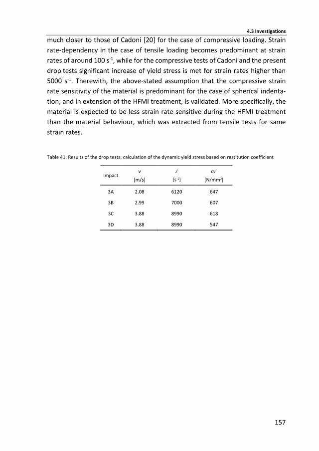
4.3 Investigations
157
much closer to those of Cadoni [20] for the case of compressive loading. Strain
rate-dependency in the case of tensile loading becomes predominant at strain
rates of around 100 s-1, while for the compressive tests of Cadoni and the present
drop tests significant increase of yield stress is met for strain rates higher than
5000 s-1. Therewith, the above-stated assumption that the compressive strain
rate sensitivity of the material is predominant for the case of spherical indenta-
tion, and in extension of the HFMI treatment, is validated. More specifically, the
material is expected to be less strain rate sensitive during the HFMI treatment
than the material behaviour, which was extracted from tensile tests for same
strain rates.
Table 41: Results of the drop tests: calculation of the dynamic yield stress based on restitution coefficient
Impact v
[m/s]
휀̇
[s-1]
σΥ’
[N/mm2]
3A 2.08 6120 647
3B 2.99 7000 607
3C 3.88 8990 618
3D 3.88 8990 547
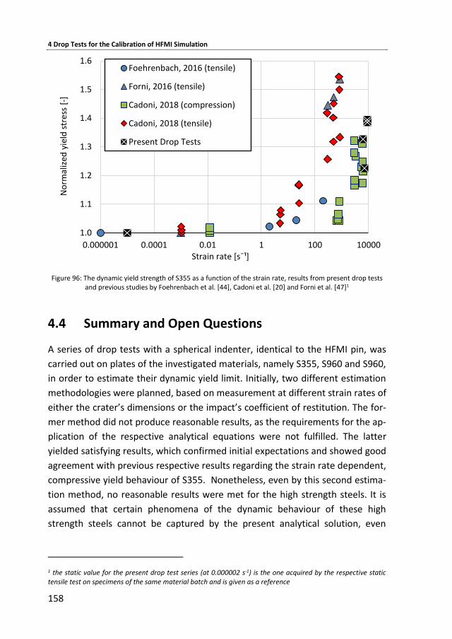
4 Drop Tests for the Calibration of HFMI Simulation
158
Figure 96: The dynamic yield strength of S355 as a function of the strain rate, results from present drop tests and previous studies by Foehrenbach et al. [44], Cadoni et al. [20] and Forni et al. [47]1
4.4 Summary and Open Questions
A series of drop tests with a spherical indenter, identical to the HFMI pin, was
carried out on plates of the investigated materials, namely S355, S960 and S960,
in order to estimate their dynamic yield limit. Initially, two different estimation
methodologies were planned, based on measurement at different strain rates of
either the crater’s dimensions or the impact’s coefficient of restitution. The for-
mer method did not produce reasonable results, as the requirements for the ap-
plication of the respective analytical equations were not fulfilled. The latter
yielded satisfying results, which confirmed initial expectations and showed good
agreement with previous respective results regarding the strain rate dependent,
compressive yield behaviour of S355. Nonetheless, even by this second estima-
tion method, no reasonable results were met for the high strength steels. It is
assumed that certain phenomena of the dynamic behaviour of these high
strength steels cannot be captured by the present analytical solution, even
1 the static value for the present drop test series (at 0.000002 s-1) is the one acquired by the respective static tensile test on specimens of the same material batch and is given as a reference
1.0
1.1
1.2
1.3
1.4
1.5
1.6
0.000001 0.0001 0.01 1 100 10000
No
rmal
ized
yie
ld s
tres
s [-
]
Strain rate [sˉ¹]
Foehrenbach, 2016 (tensile)
Forni, 2016 (tensile)
Cadoni, 2018 (compression)
Cadoni, 2018 (tensile)
Present Drop Tests
4.4 Summary and Open Questions
159
though an adjustment was proposed based on data from previous studies. In all
cases, the strain rate was calculated by means of FE analyses for strain rate inde-
pendent yielding. As a last-step-validation of the calculated material behaviour, a
strain rate dependent material model was calibrated and introduced to a FE
model for the HFMI treatment of a specimen of parent material. This analysis is
presented in the next chapter of this dissertation along with the rest of the nu-
merical investigations regarding HFMI. The applied approach shows potential for
calibrating the material behaviour of steel for the simulation of HFMI taking into
consideration the irregularities of material behaviour during spherical indenta-
tion. Still, many difficulties arise regarding different aspects of the present solu-
tion, which lead to discrepancies, especially for the high strength steels.
In order to eliminate the above-mentioned difficulties and to further develop the
present approach, the implementation of the following steps in future work, as
they exceed the limits of the present study, is encouraged:
More tests and for a wider variety of impact speeds could offer a better
overview regarding the distinctiveness of the steels with higher yield point.
Exclusion of outliers and a better adjustment of the analytical equations
could be enabled by a larger sample population.
Further validation is possible through the measurement of the residual
stresses introduced during the drop tests on the investigated plates by X-
ray or another measurement method. The simulation of the RS field by a FE
analysis of the drop tests, this time by considering the calibrated strain rate
dependent material model, could enable a more robust validation.
The influence of the specimens’ thickness could as well be investigated. All
the implemented analytical calculations were based on the premise that the
deformed plate is behaving like an infinite half-space. Although in the pre-
sent case the thickness of the specimen was considered sufficiently larger
than that of the crater’s depth (larger than 6.5 times in all cases) some ef-
fect could still be evident. Investigation of thicker and thinner plates is en-
couraged.
Finally, it has to be underlined that the material model, which was calibrated
by the present drop test, was subsequently introduced to a simulation of spec-
imen of parent material. In order to calibrate a model for the simulation of
HFMI-treated weldments, specimens whose microstructure is similar to that
of the weldments’ HAZ should be tested. This could be enabled through an

4 Drop Tests for the Calibration of HFMI Simulation
160
appropriate thermal pre-treatment of the specimens, for instance with a Glee-
ble® thermo-mechanical simulator instrument.
161
5 FE Simulation of HFMI
5.1 Methodology
A bottom up approach was adopted for the validation of the HFMI modelling
methodology, as in the former case of welding simulation. Initially a simpler, un-
notched component of parent material was simulated. The results of this prelim-
inary model were compared with previous numerical studies and RS measure-
ments, which were found in literature [44], [145]. The validated model was then
applied for evaluating the influence of different aspects of modelling and the
treatment on the calculated RS. Conclusions regarding the scaling effect, bound-
ary conditions and modelling of material behaviour were drawn. These conclu-
sions were valuable for the subsequent series of simulation, wherein the fillet
welds from the research project HFH-Simulation [146] were investigated, in order
to fulfil the goal of the present study. RS measurements from HFH-Simulation
were used for a further and final validation of the established approach. The in-
fluence of WRS from the preceding weld simulation was considered as well. After
validation of this model, further aspects of the treatment were investigated.
Commercial FE software LS-DYNA [113] was applied in all HFMI simulations of the
present study. Explicit dynamic FE analysis was carried out and respective mesh
of 8-node solid elements, hexaedra, was applied on the simulated components.
More details regarding the FE theoretical background is given in Appendix B. As
described above, proper modelling of the HFMI pin movement and material be-
haviour is decisive for an accurate simulation. In all investigations of the present
study the HFMI pin was simulated as a rigid body due to its negligible deformation
and significantly higher hardness in comparison to that of the treated surface.
Two different diameters were considered, 3 mm and 4 mm, corresponding to the
pin size of the HiFIT and PITec devices.
Two different approaches were taken into consideration for simulating the move-
ment of the HFMI pin. When a displacement-based approach is considered, mass
and inertia of the pin can be selected arbitrary, as they have no effect on the
calculated RS; a rigid volume is pressed upon the treatment surface with a pre-
scribed motion similarly to a punching process. On the contrary, when a force- or
5 FE Simulation of HFMI
162
velocity-based1 approach is adopted, the mass and the inertia of the real pin has
to be considered; an arbitrary accelerating force is applied on the pin, calibrated
on measurements on the real device, and the resulting impact velocity is depend-
ent on these properties. When the pin hits the treatment surface, it has initial
velocity and no further restrain on its vertical axis movement. The horizontal
movement of the pin, along the treatment line, was modelled stepwise (displace-
ment-based) for all simulations as this has no influence on the impact and in ex-
tension to the modelled RS.
Coulomb’s frictional contact (Eq. (28)) between the HFMI pin and the treated sur-
face is taken into consideration in all cases. Friction coefficient μ is calculated au-
tomatically by the applied Software LS-Dyna through interpolation between a
static (μs) and a dynamic value (μd) according to the following Equation (48):
𝜇 = 𝜇𝑑 + (𝜇𝑠 − 𝜇𝑑) ∙ 𝑒−𝑐|𝑣𝑠𝑙𝑖𝑑𝑖𝑛𝑔|. (48)
The values of 0.78 and 0.42, which were initially applied respectively for the two
coefficients, were found in [6]. Several values can be found in literature for these
coefficients. Although no significant influence on the introduced RS due to their
variation was expected according to initial expectations, further lower values
were tested, as it is described below. A damping model according to Equation (27)
with a factor ξ initially set equal to 0.5 was applied as in previous numerical in-
vestigations of impacts ([89], [90] etc.). Flanagan-Belytschko hourglass control is
applied in all cases for the elements inside and near the treatment area [43]. Two
different types of this hourglass control, the classical and the exact volume inte-
gration for solid elements (see [114]), were compared with no significant devia-
tion, with the latter one though being the most stable numerically. It was there-
fore adopted for all subsequent analyses.
Suitable modelling of material behaviour is predominant for the precise simula-
tion of HFMI, a prerequisite that becomes clear even from a preliminary literature
review. According to initial expectations, strain rate dependency had to be taken
into consideration otherwise erroneous results might arise. The Cowper-Symonds
1 the velocity-based term is preferred in the present case as the pin is accelerated through the application of an arbitrary force until it reaches the required impact velocity, the method though is physically equivalent to a force-based, or an acceleration-based approach
5.2 Convergence Analysis
163
model of Equation (12) combined with a bilinear σ-ε material behaviour with kin-
ematic hardening is applied in all subsequent investigations of the present study
for the consideration of viscous material behaviour.
It should be highlighted at this point that during the displacement-based simula-
tions, questions regarding the application of a viscous material behaviour arise.
Although a displacement-based simulation has been carried out in previous stud-
ies combined with strain rate dependent material behaviour ([44], [108] etc.) this
approach should be applied cautiously. Defining an arbitrary vertical, over time
displacement-based motion of the pin is straightforward from the modeller’s per-
spective but directly influences the strain rate, under which the treated surface is
deformed. Hence, yielding and the introduced RS depend on this arbitrary de-
fined displacement. Unless measurements of this displacement over time during
a real treatment are made, which would require a very elaborate experimental
investigation, this modelling approach is invalid. If the contact duration is known,
the assumption of a sinusoidal displacement of the pin inside this contact time
could be valid. Nevertheless, if the contact force and in extension the impact ve-
locity are known, applying a velocity-based approach for simulations considering
a viscous material behaviour should be preferred instead as such an approach is
more valid and closer to physical reality.
5.2 Convergence Analysis
Preliminary investigations considering a single impact of a HFMI pin with a diam-
eter of 3 mm on a component of parent material made of S355 were carried out
in order to define the maximum mesh dimensions at the contact area, which
would produce mesh-independent results and enable at the same time a compu-
tational efficient simulation. A displacement-based vertical movement of the
HFMI pin of 0.5 mm was considered, as in this case comparing the influence of
different mesh sizes was the goal and not the precise simulation of the RS. The
modelled HFMI groove was on purpose significantly higher than the real one, so
that the selection of mesh size would be conservative. Strain rate dependent be-
haviour was taken into consideration as well, as variated yielding behaviour could
require different mesh size. Due to consideration of a single impact in this case,
adoption of double symmetry was enabled.

5 FE Simulation of HFMI
164
Four different discretization setups with element dimensions of 0.2 mm, 0.1 mm,
0.075 mm and 0.05 mm to all directions were applied. The longitudinal RS on the
surface from the centre of the impact and transverse to the impact crater were
selected as an index of convergence. The results of this convergence analysis are
given in Figure 97. It is becoming evident that the results diverge for the two first
applied mesh sizes but converge for the latter two. Therewith, a required element
length to pin diameter ratio of 1/40, which was proposed for the simulation of
shot peening in [77] and [90], is validated in this case as well. More information
on these investigations and the range of variations are not significant but can be
found in [168].
Figure 97: Convergence study for the numerical investigation of HFMI treatment – RS after 0.01 s of simulation
with global damping Ds = 0.5 (Ds and mesh size are marked as D and ms rspectively)
5.3 Component of Parent material
5.3.1.1 Investigated Component
The specimen of parent material with dimensions 20 mm x 20 mm x 10 mm, which
is presented in Figure 98, treated with a 4 mm diameter HFMI pin, was considered
in a first-step validation of the applied modelling approach. An adaptive mesh
approach was selected in this case. At the contact area and near the surface, dis-
cretization with element size of 0.125 mm or even smaller was applied, gradually
coarsening in depth direction. Transverse to the treatment line and 4 mm away
from it, transition mesh was adjusted, so that coarsening in this direction could
-500
-400
-300
-200
-100
0
100
0 2 4 6 8 10
Lon
gtid
un
al W
RS
[MP
a]
Distance from impact centre [mm]
t = 0.01 s - ms = 0.2 mm - D = 0.5
t = 0.01 s - ms = 0.1 mm - D = 0.5
t = 0.01 s - ms = 0.075 mm - D = 0.5
t = 0.01 s - ms = 0.05 mm - D = 0.5
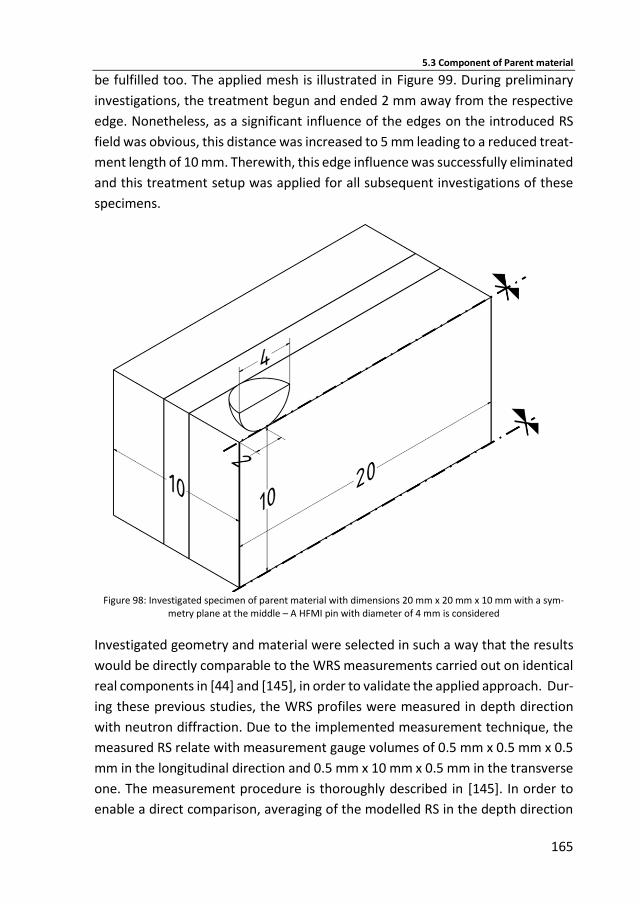
5.3 Component of Parent material
165
be fulfilled too. The applied mesh is illustrated in Figure 99. During preliminary
investigations, the treatment begun and ended 2 mm away from the respective
edge. Nonetheless, as a significant influence of the edges on the introduced RS
field was obvious, this distance was increased to 5 mm leading to a reduced treat-
ment length of 10 mm. Therewith, this edge influence was successfully eliminated
and this treatment setup was applied for all subsequent investigations of these
specimens.
Figure 98: Investigated specimen of parent material with dimensions 20 mm x 20 mm x 10 mm with a sym-
metry plane at the middle – A HFMI pin with diameter of 4 mm is considered
Investigated geometry and material were selected in such a way that the results
would be directly comparable to the WRS measurements carried out on identical
real components in [44] and [145], in order to validate the applied approach. Dur-
ing these previous studies, the WRS profiles were measured in depth direction
with neutron diffraction. Due to the implemented measurement technique, the
measured RS relate with measurement gauge volumes of 0.5 mm x 0.5 mm x 0.5
mm in the longitudinal direction and 0.5 mm x 10 mm x 0.5 mm in the transverse
one. The measurement procedure is thoroughly described in [145]. In order to
enable a direct comparison, averaging of the modelled RS in the depth direction
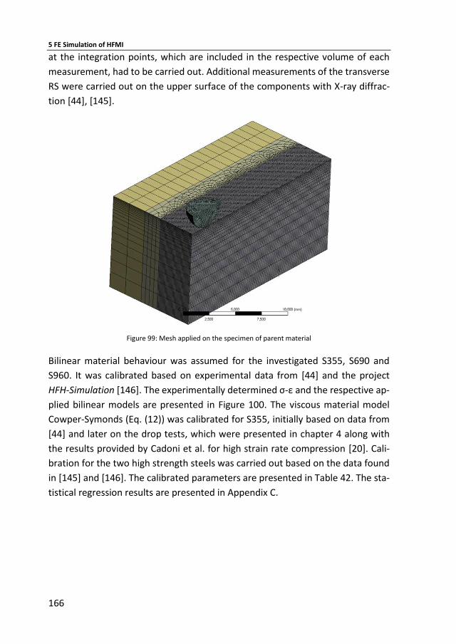
5 FE Simulation of HFMI
166
at the integration points, which are included in the respective volume of each
measurement, had to be carried out. Additional measurements of the transverse
RS were carried out on the upper surface of the components with X-ray diffrac-
tion [44], [145].
Figure 99: Mesh applied on the specimen of parent material
Bilinear material behaviour was assumed for the investigated S355, S690 and
S960. It was calibrated based on experimental data from [44] and the project
HFH-Simulation [146]. The experimentally determined σ-ε and the respective ap-
plied bilinear models are presented in Figure 100. The viscous material model
Cowper-Symonds (Eq. (12)) was calibrated for S355, initially based on data from
[44] and later on the drop tests, which were presented in chapter 4 along with
the results provided by Cadoni et al. for high strain rate compression [20]. Cali-
bration for the two high strength steels was carried out based on the data found
in [145] and [146]. The calibrated parameters are presented in Table 42. The sta-
tistical regression results are presented in Appendix C.
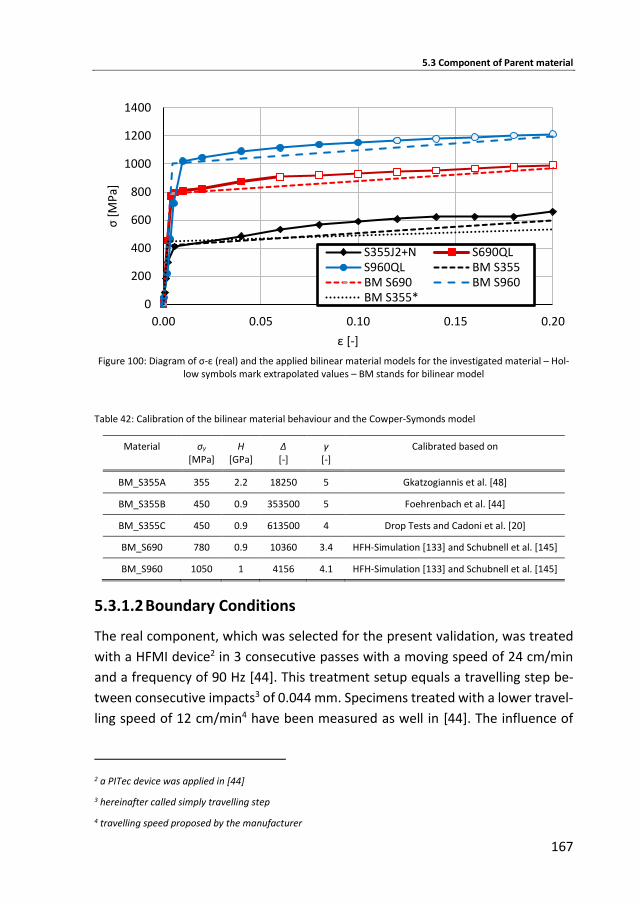
5.3 Component of Parent material
167
Figure 100: Diagram of σ-ε (real) and the applied bilinear material models for the investigated material – Hol-
low symbols mark extrapolated values – BM stands for bilinear model
Table 42: Calibration of the bilinear material behaviour and the Cowper-Symonds model
Material σy
[MPa] H
[GPa] Δ [-]
γ [-]
Calibrated based on
BM_S355A 355 2.2 18250 5 Gkatzogiannis et al. [48]
BM_S355B 450 0.9 353500 5 Foehrenbach et al. [44]
BM_S355C 450 0.9 613500 4 Drop Tests and Cadoni et al. [20]
BM_S690 780 0.9 10360 3.4 HFH-Simulation [133] and Schubnell et al. [145]
BM_S960 1050 1 4156 4.1 HFH-Simulation [133] and Schubnell et al. [145]
5.3.1.2 Boundary Conditions
The real component, which was selected for the present validation, was treated
with a HFMI device2 in 3 consecutive passes with a moving speed of 24 cm/min
and a frequency of 90 Hz [44]. This treatment setup equals a travelling step be-
tween consecutive impacts3 of 0.044 mm. Specimens treated with a lower travel-
ling speed of 12 cm/min4 have been measured as well in [44]. The influence of
2 a PITec device was applied in [44]
3 hereinafter called simply travelling step
4 travelling speed proposed by the manufacturer
0
200
400
600
800
1000
1200
1400
0.00 0.05 0.10 0.15 0.20
σ [
MP
a]
ε [-]
S355J2+N S690QLS960QL BM S355BM S690 BM S960BM S355*
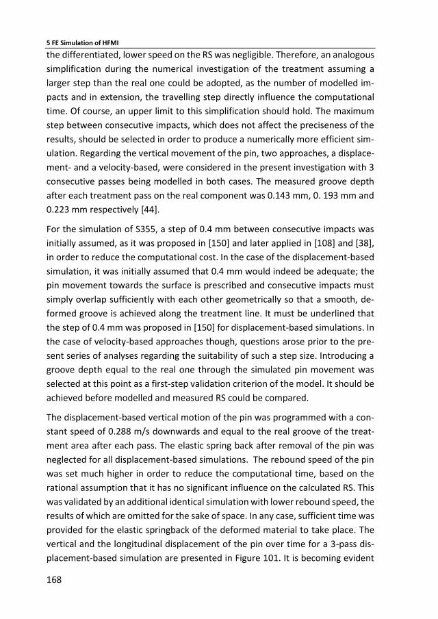
5 FE Simulation of HFMI
168
the differentiated, lower speed on the RS was negligible. Therefore, an analogous
simplification during the numerical investigation of the treatment assuming a
larger step than the real one could be adopted, as the number of modelled im-
pacts and in extension, the travelling step directly influence the computational
time. Of course, an upper limit to this simplification should hold. The maximum
step between consecutive impacts, which does not affect the preciseness of the
results, should be selected in order to produce a numerically more efficient sim-
ulation. Regarding the vertical movement of the pin, two approaches, a displace-
ment- and a velocity-based, were considered in the present investigation with 3
consecutive passes being modelled in both cases. The measured groove depth
after each treatment pass on the real component was 0.143 mm, 0. 193 mm and
0.223 mm respectively [44].
For the simulation of S355, a step of 0.4 mm between consecutive impacts was
initially assumed, as it was proposed in [150] and later applied in [108] and [38],
in order to reduce the computational cost. In the case of the displacement-based
simulation, it was initially assumed that 0.4 mm would indeed be adequate; the
pin movement towards the surface is prescribed and consecutive impacts must
simply overlap sufficiently with each other geometrically so that a smooth, de-
formed groove is achieved along the treatment line. It must be underlined that
the step of 0.4 mm was proposed in [150] for displacement-based simulations. In
the case of velocity-based approaches though, questions arose prior to the pre-
sent series of analyses regarding the suitability of such a step size. Introducing a
groove depth equal to the real one through the simulated pin movement was
selected at this point as a first-step validation criterion of the model. It should be
achieved before modelled and measured RS could be compared.
The displacement-based vertical motion of the pin was programmed with a con-
stant speed of 0.288 m/s downwards and equal to the real groove of the treat-
ment area after each pass. The elastic spring back after removal of the pin was
neglected for all displacement-based simulations. The rebound speed of the pin
was set much higher in order to reduce the computational time, based on the
rational assumption that it has no significant influence on the calculated RS. This
was validated by an additional identical simulation with lower rebound speed, the
results of which are omitted for the sake of space. In any case, sufficient time was
provided for the elastic springback of the deformed material to take place. The
vertical and the longitudinal displacement of the pin over time for a 3-pass dis-
placement-based simulation are presented in Figure 101. It is becoming evident
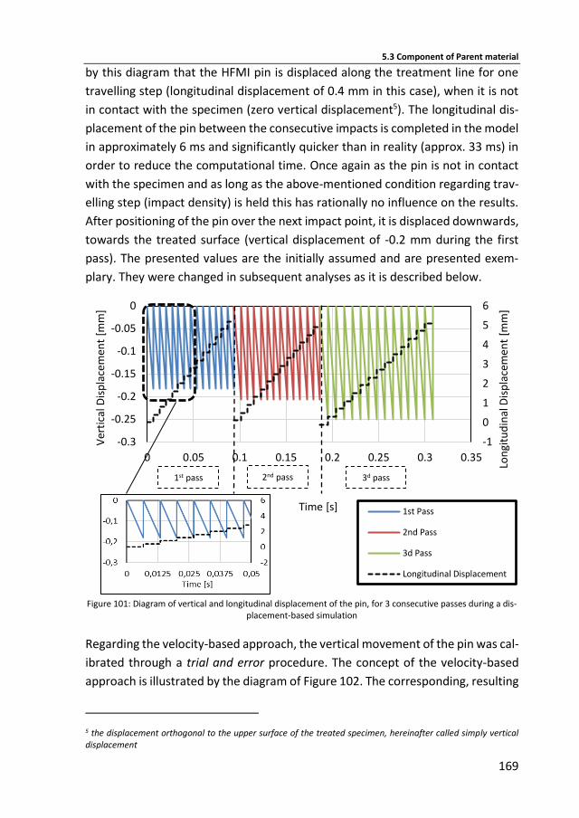
5.3 Component of Parent material
169
by this diagram that the HFMI pin is displaced along the treatment line for one
travelling step (longitudinal displacement of 0.4 mm in this case), when it is not
in contact with the specimen (zero vertical displacement5). The longitudinal dis-
placement of the pin between the consecutive impacts is completed in the model
in approximately 6 ms and significantly quicker than in reality (approx. 33 ms) in
order to reduce the computational time. Once again as the pin is not in contact
with the specimen and as long as the above-mentioned condition regarding trav-
elling step (impact density) is held this has rationally no influence on the results.
After positioning of the pin over the next impact point, it is displaced downwards,
towards the treated surface (vertical displacement of -0.2 mm during the first
pass). The presented values are the initially assumed and are presented exem-
plary. They were changed in subsequent analyses as it is described below.
Figure 101: Diagram of vertical and longitudinal displacement of the pin, for 3 consecutive passes during a dis-
placement-based simulation
Regarding the velocity-based approach, the vertical movement of the pin was cal-
ibrated through a trial and error procedure. The concept of the velocity-based
approach is illustrated by the diagram of Figure 102. The corresponding, resulting
5 the displacement orthogonal to the upper surface of the treated specimen, hereinafter called simply vertical displacement
-1
0
1
2
3
4
5
6
-0.3
-0.25
-0.2
-0.15
-0.1
-0.05
0
0 0.05 0.1 0.15 0.2 0.25 0.3 0.35
Lon
gitu
din
al D
isp
lace
men
t [m
m]
Ver
tica
l Dis
pla
cem
ent
[mm
]
Time [s] 1st Pass
2nd Pass
3d Pass
Longitudinal Displacement
2nd pass 3d pass1st pass
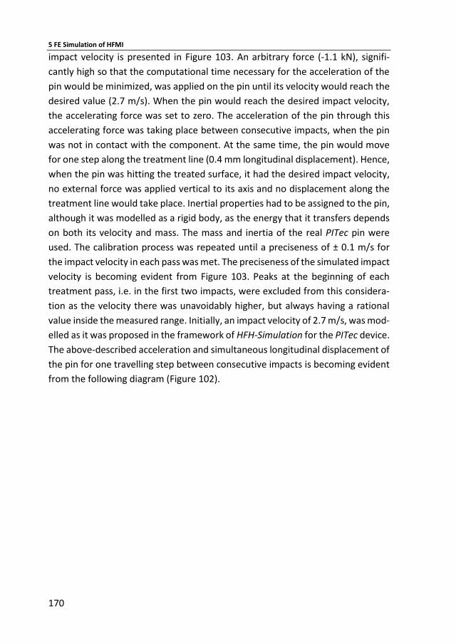
5 FE Simulation of HFMI
170
impact velocity is presented in Figure 103. An arbitrary force (-1.1 kN), signifi-
cantly high so that the computational time necessary for the acceleration of the
pin would be minimized, was applied on the pin until its velocity would reach the
desired value (2.7 m/s). When the pin would reach the desired impact velocity,
the accelerating force was set to zero. The acceleration of the pin through this
accelerating force was taking place between consecutive impacts, when the pin
was not in contact with the component. At the same time, the pin would move
for one step along the treatment line (0.4 mm longitudinal displacement). Hence,
when the pin was hitting the treated surface, it had the desired impact velocity,
no external force was applied vertical to its axis and no displacement along the
treatment line would take place. Inertial properties had to be assigned to the pin,
although it was modelled as a rigid body, as the energy that it transfers depends
on both its velocity and mass. The mass and inertia of the real PITec pin were
used. The calibration process was repeated until a preciseness of ± 0.1 m/s for
the impact velocity in each pass was met. The preciseness of the simulated impact
velocity is becoming evident from Figure 103. Peaks at the beginning of each
treatment pass, i.e. in the first two impacts, were excluded from this considera-
tion as the velocity there was unavoidably higher, but always having a rational
value inside the measured range. Initially, an impact velocity of 2.7 m/s, was mod-
elled as it was proposed in the framework of HFH-Simulation for the PITec device.
The above-described acceleration and simultaneous longitudinal displacement of
the pin for one travelling step between consecutive impacts is becoming evident
from the following diagram (Figure 102).
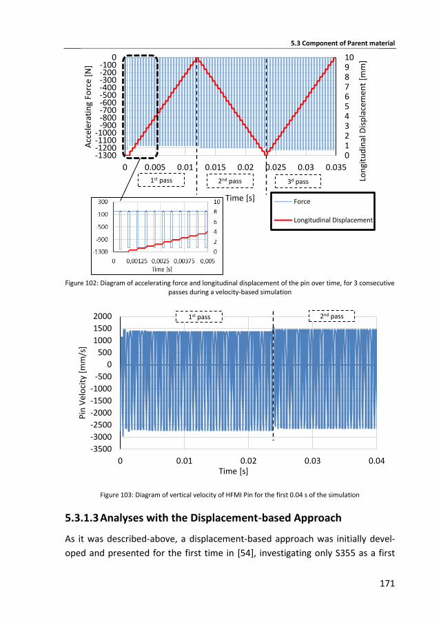
5.3 Component of Parent material
171
Figure 102: Diagram of accelerating force and longitudinal displacement of the pin over time, for 3 consecutive
passes during a velocity-based simulation
Figure 103: Diagram of vertical velocity of HFMI Pin for the first 0.04 s of the simulation
5.3.1.3 Analyses with the Displacement-based Approach
As it was described-above, a displacement-based approach was initially devel-
oped and presented for the first time in [54], investigating only S355 as a first
012345678910
-1300-1200-1100-1000
-900-800-700-600-500-400-300-200-100
0
0 0.005 0.01 0.015 0.02 0.025 0.03 0.035
Lon
gitu
din
al D
isp
lace
men
t [m
m]
Acc
eler
atin
g Fo
rce
[N]
Time [s] Force
Longitudinal Displacement
2nd pass 3d pass1st pass
-3500
-3000
-2500
-2000
-1500
-1000
-500
0
500
1000
1500
2000
0 0.01 0.02 0.03 0.04
Pin
Vel
oci
ty [
mm
/s]
Time [s]
2nd pass1st pass
5 FE Simulation of HFMI
172
step. The vertical movement of the pin was calibrated based on the groove, which
was measured on the real specimens in [168]. Material model BM_S355A was
applied in two different simulations the 355_DB_RD and 355_DB_RI, including
and excluding6 strain rate dependency respectively. As it was mentioned above,
the introduction of a viscous material behaviour in a displacement-based ap-
proach is invalid without further data and it should be carried out with caution.
Nonetheless, it was applied in the present case in order to enable a first evalua-
tion of the influence of viscosity at least qualitatively. The vertical displacement
of the pin was carried out with a velocity of 2.7 m/s prior and during the contact
and up to the targeted depth, so that the strain rate would be at least at same
order of magnitude with the real one. When the results of this approach were
published for the first time in [54], the above-mentioned averaging procedure of
the modelled RS was not implemented. Instead, the results on the integration
points underneath the weld toe were directly compared to the measurements. A
significant deviation between measured and modelled RS was met. The averaged
results of the displacement-based models are presented in Figure 104 along with
the unaveraged ones, as they were published in [54], and the measured RS.
Both dipslacement-based approaches, 355_DB_RI and 355_DB_RD,
underestimated the longitudinal RS near the surface, while a better agreement
was met in the case of the transverse RS at the same region. The overall
disagreement, even qualitatively, of the rate-indendent approach 355_DB_RI
dictated the introduction of strain rate dependency to the subsequent analysis
355_DB_RD. The rate-dependent model, which still underestimates the
longitudinal RS and shows no good agremment in the first two mm below the
surface, exhibits due to an overall shift of both RS profiles a significantly improved
qualitative agreement with the measured RS. Therewith, the initially assumed
significance of strain rate dependency for the HFMI simulation seems to be
validated but further investigations were necessary at this point. Averaging of the
numerical results did not improve their agreement with the measurements. A
further improvement of the displacement-based approach, by assuming a
sinuisoidal movement of the pin or considering the elastic springback of the
treated material during calibration of the pin’s movement, was not adopted at
6 setting coefficients D and q equal to 0
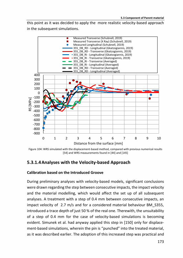
5.3 Component of Parent material
173
this point as it was decided to apply the more realistic velocity-based approach
in the subsequent simulations.
Figure 104: WRS simulated with the displacement-based method, compared with previous numerical results
[54] and WRS measurements found in [44] and [145]
5.3.1.4 Analyses with the Velocity-based Approach
Calibration based on the Introduced Groove
During preliminary analyses with velocity-based models, significant conclusions
were drawn regarding the step between consecutive impacts, the impact velocity
and the material modelling, which would affect the set up of all subsequent
analyses. A treatment with a step of 0.4 mm between consecutive impacts, an
impact velocity of 2.7 m/s and for a considered material behaviour BM_S355,
introduced a trace depth of just 50 % of the real one. Therewith, the unsuitability
of a step of 0.4 mm for the case of velocity-based simulations is becoming
evident. Simunek et al. had anyway applied this step in [150] only for displace-
ment-based simulations, wherein the pin is “punched” into the treated material,
as it was described earlier. The adoption of this increased step was practical and
-900-800-700-600-500-400-300-200-100
0100200300400
0 1 2 3 4 5 6 7 8 9 10
RS
[MP
a]
Distance from the surface [mm]
Measured Transverse (Schubnell, 2019)Measured Transverse (X Ray) (Schubnell, 2019)Measured Longitudinal (Schubnell, 2019)355_DB_RD - Longitudinal (Gkatzogiannis, 2019)355_DB_RD - Transverse (Gkatzogiannis, 2019)355_DB_RI - Longitudinal (Gkatzogiannis, 2019)355_DB_RI - Transverse (Gkatzogiannis, 2019)355_DB_RI - Transverse (Averaged)355_DB_RI - Longitudinal (Averaged)355_DB_RD - Transverse (Averaged)355_DB_RD - Longitudinal (Averaged)
5 FE Simulation of HFMI
174
it was implemented in other previous studies as well [44], [68], [187], with no
further investigation on its suitability though. Of course, in the present case a low
impact speed could be attributed for the shallow groove as well. Given that the
present value of 2.7 m/s lies in the boundaries of the real, measured impact speed
and the step of 0.4 is 5 times larger than the real one, a decrease of the step to
0.2 mm was decided for subsequent analyses. This led to the introduction of a
deeper trace by the model, but still lower than the real one. Groove depths equal
to 79 % and 74 % of the real one were documented for the 1st and 2nd pass re-
spectively7.
At this point, a further decrease of the applied step was avoided as it would in-
crease significantly the computational time. Instead, an increase of the impact
velocity to 3.79 m/s, a value that as well lies inside the measured spectrum and
closer to the mean of the measured real impact velocities, was preferred. More-
over, new lower values for the friction coefficients μs and μd of Equation (48),
equal to 0.3 and 0.15 respectively, were selected according to common engineer-
ing knowledge. The adopted changes led to a simulated groove depth, which lies
much closer to the real one for all three passes of the treatment, as it can be seen
in Table 44, where the results of these preliminary analyses are summarized. An
acceptable deviation smaller than ± 5 % in all cases was documented. As the con-
sidered material behaviour as well influences the introduced trace, the travelling
step of 0.2 mm and the new lower values for the friction coefficients were
adopted for all subsequent analyses. Prior to any evaluation of RS results, the
impact velocity would be adjusted for each material taking values from inside the
measured spectrum, until an acceptable agreement with the real groove would
be met. If this would not be sufficient, then the travelling step would be further
reduced.
7 during the 3d pass numerical problems were met and therefore the respective results are excluded from the present evaluation
5.3 Component of Parent material
175
Table 43: Measured and simulated groove depth of the HFMI treatment – Travelling step in mm and impact
velocity in m/s
Case Groove depth [mm]
1st Pass 2nd Pass 3d Pass
measured in [44] 0.143 0.193 0.223
simulated with 0.4 mm - 2.72 m/s
0.072 0.093 0.106
simulated with 0.2 mm - 2.72 m/s
0.113 0.143 -
simulated with 0.2 mm – 3.68 m/s
0.148 0.184 0.217
Influence of Simulated Material Behaviour
Simulation of the present component for all three investigated materials S355,
S690 and S960 based on material models BM_355, BM_690 and BM_960 were
carried out by both considering and neglecting in all cases the strain rate depend-
ency. In the former case of S355, an elastic - perfect plastic model behaviour was
tested as well8. The through-depth, averaged longitudinal and transverse RS for
S355 at the centre of the HFMI groove at the middle of the component are given
in Figure 105 and Figure 106. Figure 107 and Figure 108 show the respective re-
sults for S690. Finally, Figure 109 and Figure 110 illustrate the respective trans-
verse and longitudinal profiles regarding S960. In all cases, the respective meas-
urements found in [145] are presented along the present simulation results. Small
fluctuations, which are met in some simulated profiles, are attributed to the av-
eraging process of the results, without this having a significant macroscopic influ-
ence either qualitatively or on the magnitude.
Regarding the RS of S355, all three investigated models provided qualitatively
similar profiles. Both longitudinal and transverse RS profiles are compressive near
the surface with a transition to the tensile area in a depth of approximately 1.5
mm to 2 mm. Regarding the transverse RS, very good agreement with the meas-
ured profile is met on most of the measurement points in all cases apart from the
compressive strain rate dependent model. For all models, the largest deviation
from the measured RS is met at a depth of approximately 0.75 mm, where the
peak of both the measured and simulated compressive stresses is located. This
8 setting H = 0 for the BM_355
5 FE Simulation of HFMI
176
deviation is slightly higher for the strain rate dependent simulation, although the
difference can be considered negligible. On the contrary, longitudinal simulated
RS profiles present a significant quantitative deviation with each other. The ten-
sile strain rate dependent model estimated with very good agreement the meas-
ured RS on and near the surface, but underestimated them on a depth larger than
1 mm. On the other hand, both strain rate independent material models under-
estimated the RS near the surface. The compressive strain rate dependent model
produces a similar profile with the tensile one, overestimating though overall the
RS.
The significantly better agreement of the tensile strain rate dependent material
model for the RS near the surface, where fatigue cracks initiate, reveals the pre-
dominance of the strain rate dependency for the present simulation, verifying in
this first-step analysis the respective initial assumption regarding its importance.
When the material exhibits significant viscosity, the layers near the surface where
the high strain rates are met during the impact, yield at higher stresses absorbing
more kinetic energy and therefore, the peak of the WRS is shifted nearer to the
surface. Therefore, the introduction of viscosity becomes necessary even for a
qualitatively precise simulation.
On the contrary, the higher preciseness of the tensile versus the compressive
strain rate dependent material model, does not overthrow the assumption re-
garding the predominance of the compressive behaviour in the case of HFMI yet.
The better agreement of the tensile model can be attributed to the fact that it
was calibrated based on the same batch of the investigated material, applied in
[44] as well. On the other hand, during the calibration of the compressive strain
rate dependent material model, data from [20] for the same material but another
batch was considered along with the results of the drop tests in order to increase
the statistical sample. As it was discussed in [59] though, the strain rate sensitivity
of the metallic alloys can differ significantly from a batch of a material to another.
Therefore, no assumption regarding the predominance of the compressive be-
haviour could be made, unless more measured and simulated results from the
same batch could be compared.
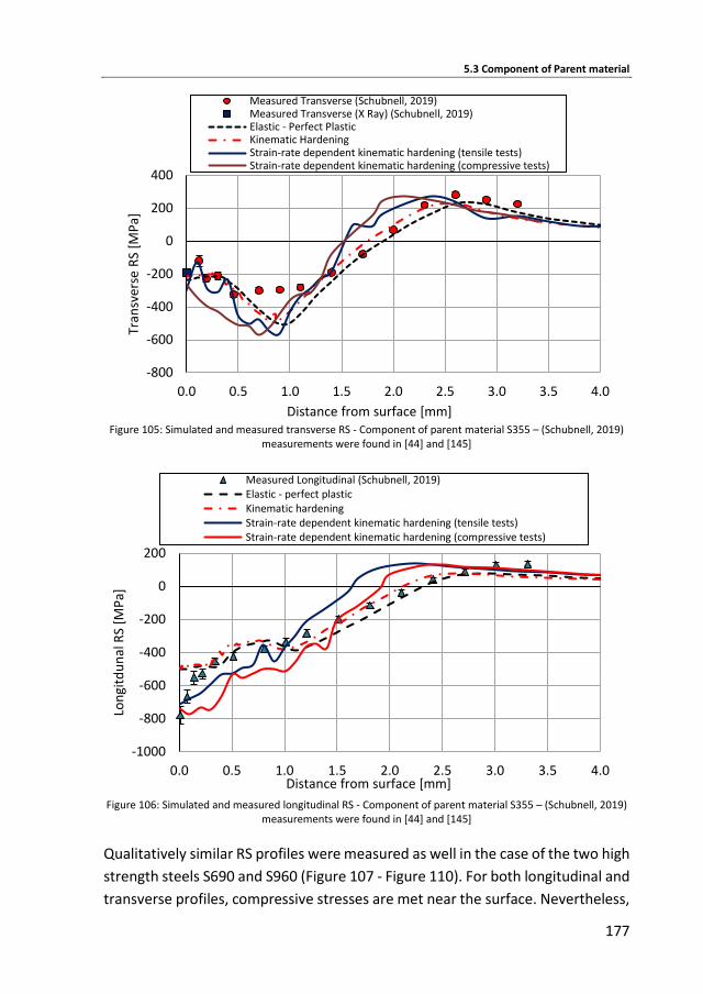
5.3 Component of Parent material
177
Figure 105: Simulated and measured transverse RS - Component of parent material S355 – (Schubnell, 2019)
measurements were found in [44] and [145]
Figure 106: Simulated and measured longitudinal RS - Component of parent material S355 – (Schubnell, 2019)
measurements were found in [44] and [145]
Qualitatively similar RS profiles were measured as well in the case of the two high
strength steels S690 and S960 (Figure 107 - Figure 110). For both longitudinal and
transverse profiles, compressive stresses are met near the surface. Nevertheless,
-800
-600
-400
-200
0
200
400
0.0 0.5 1.0 1.5 2.0 2.5 3.0 3.5 4.0
Tran
sver
se R
S [M
Pa]
Distance from surface [mm]
Measured Transverse (Schubnell, 2019)Measured Transverse (X Ray) (Schubnell, 2019)Elastic - Perfect PlasticKinematic HardeningStrain-rate dependent kinematic hardening (tensile tests)Strain-rate dependent kinematic hardening (compressive tests)
-1000
-800
-600
-400
-200
0
200
0.0 0.5 1.0 1.5 2.0 2.5 3.0 3.5 4.0
Lon
gitd
un
al R
S [M
Pa]
Distance from surface [mm]
Measured Longitudinal (Schubnell, 2019)Elastic - perfect plasticKinematic hardeningStrain-rate dependent kinematic hardening (tensile tests)Strain-rate dependent kinematic hardening (compressive tests)
5 FE Simulation of HFMI
178
the transition point from the compressive to the tensile zone is shifted in this case
closer to the surface and to a depth of 1 mm for both high strength steels and for
both longitudinal and transverse RS. This is attributed to the shallower HFMI
groove introduced in the case of the two high strength steels in comparison to
S355.
It is becoming evident from Figure 107 to Figure 110 that analyses with non-vis-
cous material modelling for both high strength steels exhibit very good agree-
ment with the measured profiles, while those considering viscosity tend to over-
estimate the RS contrariwise to the case of S355. The non-viscous models of S690
predict overall the transverse RS with a deviation of 70 MPa or smaller. Only near
the surface, a significant deviation of 200 MPa is met. In regard to the longitudinal
profiles, very good agreement is met near the surface and up to a depth of 1.5
mm. Overestimation of the RS is evident for a depth between 1.25 mm and 1.75
mm. In the case of S960 similar or better agreement is met, especially for the case
of longitudinal RS. On the contrary, the models considering strain rate depend-
ency exhibit overall a significant deviation with the measured profiles of even
higher than 100 % of the yield stress.
This incompatibility contradicts the above statement regarding the predomi-
nance of strain rate dependency during HFMI simulation. Nonetheless, tensile
only material data was used for the calibration of the present model. The earlier-
described influence of the deformation mode on the viscosity of steel and not a
negligibility of the strain rate sensitivity could be accounted for this incompatibil-
ity. It is possible that for the high strength steels, the deviation between the ten-
sile and the compressive strain rate dependency is much more significant, with
the later one being significantly less viscous, almost strain rate independent.
Therewith, the non-viscous model predicts RS much closer to the measured ones.
In other words, when the static yield strength increases the strain rate depend-
ency in compression is significantly reduced. This assumption is supported by the
significantly better agreement of the models neglecting viscosity for both high
strength steels and for both longitudinal and transverse RS. More experimental
and numerical investigations in the future, which would confirm the above-stated
assumption, are encouraged. It is as well possible that present material modelling
is unsuitable for the current analyses and a more elaborate approach considering
viscosity could lead to similar or better accuracy than that of the current analyses
with non-viscous material behaviour.
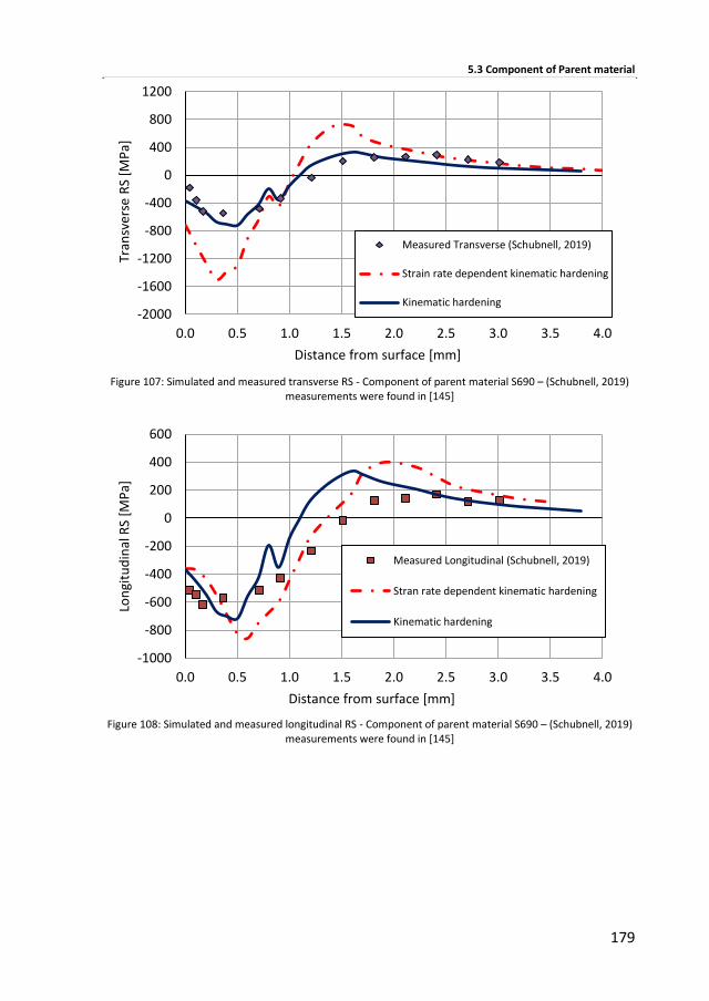
5.3 Component of Parent material
179
Figure 107: Simulated and measured transverse RS - Component of parent material S690 – (Schubnell, 2019)
measurements were found in [145]
Figure 108: Simulated and measured longitudinal RS - Component of parent material S690 – (Schubnell, 2019)
measurements were found in [145]
-2000
-1600
-1200
-800
-400
0
400
800
1200
0.0 0.5 1.0 1.5 2.0 2.5 3.0 3.5 4.0
Tran
sver
se R
S [M
Pa]
Distance from surface [mm]
Measured Transverse (Schubnell, 2019)
Strain rate dependent kinematic hardening
Kinematic hardening
-1000
-800
-600
-400
-200
0
200
400
600
0.0 0.5 1.0 1.5 2.0 2.5 3.0 3.5 4.0
Lon
gitu
din
al R
S [M
Pa]
Distance from surface [mm]
Measured Longitudinal (Schubnell, 2019)
Stran rate dependent kinematic hardening
Kinematic hardening
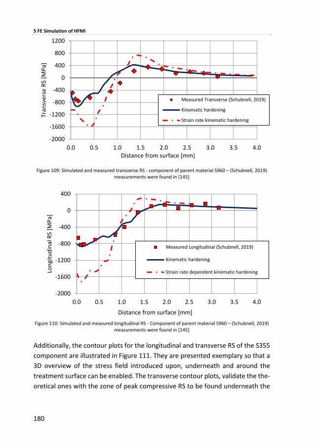
5 FE Simulation of HFMI
180
Figure 109: Simulated and measured transverse RS - component of parent material S960 – (Schubnell, 2019)
measurements were found in [145]
Figure 110: Simulated and measured longitudinal RS - Component of parent material S960 – (Schubnell, 2019)
measurements were found in [145]
Additionally, the contour plots for the longitudinal and transverse RS of the S355
component are illustrated in Figure 111. They are presented exemplary so that a
3D overview of the stress field introduced upon, underneath and around the
treatment surface can be enabled. The transverse contour plots, validate the the-
oretical ones with the zone of peak compressive RS to be found underneath the
-2000
-1600
-1200
-800
-400
0
400
800
1200
0.0 0.5 1.0 1.5 2.0 2.5 3.0 3.5 4.0
Tran
sver
se R
S [M
Pa]
Distance from surface [mm]
Measured Transverse (Schubnell, 2019)
Kinematic hardening
Strain rate kinematic hardening
-2000
-1600
-1200
-800
-400
0
400
0.0 0.5 1.0 1.5 2.0 2.5 3.0 3.5 4.0
Lon
gitu
din
al R
S [M
Pa]
Distance from surface [mm]
Measured Longitudinal (Schubnell, 2019)
Kinematic hardening
Strain rate dependent kinematic hardening
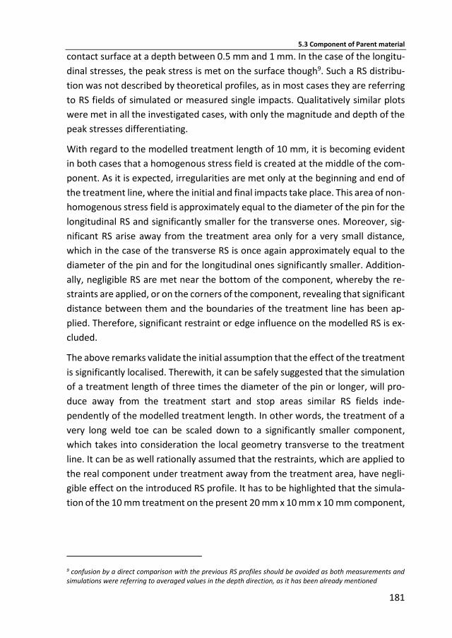
5.3 Component of Parent material
181
contact surface at a depth between 0.5 mm and 1 mm. In the case of the longitu-
dinal stresses, the peak stress is met on the surface though9. Such a RS distribu-
tion was not described by theoretical profiles, as in most cases they are referring
to RS fields of simulated or measured single impacts. Qualitatively similar plots
were met in all the investigated cases, with only the magnitude and depth of the
peak stresses differentiating.
With regard to the modelled treatment length of 10 mm, it is becoming evident
in both cases that a homogenous stress field is created at the middle of the com-
ponent. As it is expected, irregularities are met only at the beginning and end of
the treatment line, where the initial and final impacts take place. This area of non-
homogenous stress field is approximately equal to the diameter of the pin for the
longitudinal RS and significantly smaller for the transverse ones. Moreover, sig-
nificant RS arise away from the treatment area only for a very small distance,
which in the case of the transverse RS is once again approximately equal to the
diameter of the pin and for the longitudinal ones significantly smaller. Addition-
ally, negligible RS are met near the bottom of the component, whereby the re-
straints are applied, or on the corners of the component, revealing that significant
distance between them and the boundaries of the treatment line has been ap-
plied. Therefore, significant restraint or edge influence on the modelled RS is ex-
cluded.
The above remarks validate the initial assumption that the effect of the treatment
is significantly localised. Therewith, it can be safely suggested that the simulation
of a treatment length of three times the diameter of the pin or longer, will pro-
duce away from the treatment start and stop areas similar RS fields inde-
pendently of the modelled treatment length. In other words, the treatment of a
very long weld toe can be scaled down to a significantly smaller component,
which takes into consideration the local geometry transverse to the treatment
line. It can be as well rationally assumed that the restraints, which are applied to
the real component under treatment away from the treatment area, have negli-
gible effect on the introduced RS profile. It has to be highlighted that the simula-
tion of the 10 mm treatment on the present 20 mm x 10 mm x 10 mm component,
9 confusion by a direct comparison with the previous RS profiles should be avoided as both measurements and simulations were referring to averaged values in the depth direction, as it has been already mentioned
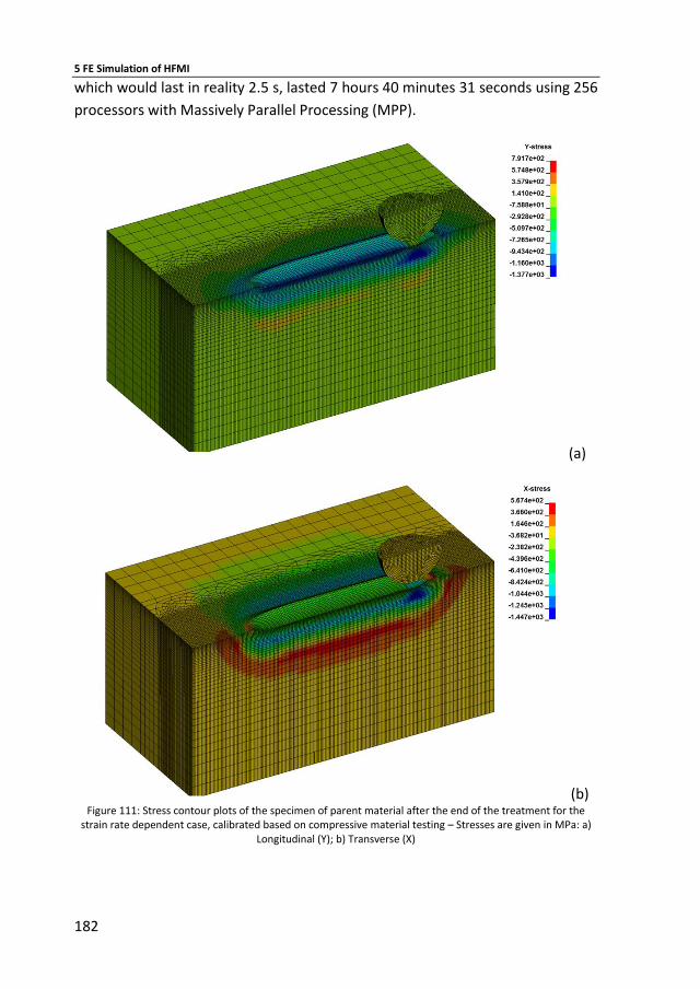
5 FE Simulation of HFMI
182
which would last in reality 2.5 s, lasted 7 hours 40 minutes 31 seconds using 256
processors with Massively Parallel Processing (MPP).
(a)
(b) Figure 111: Stress contour plots of the specimen of parent material after the end of the treatment for the
strain rate dependent case, calibrated based on compressive material testing – Stresses are given in MPa: a) Longitudinal (Y); b) Transverse (X)
5.3 Component of Parent material
183
The significance of the above-stated conclusion regarding the scaling effect and
the following assumption for the influence of the boundary conditions is of ut-
most significance, if it is considered that for real scale components treatment
lengths of more than 1 m in total can be met10. As a full-scale modelling of such a
component’s treatment would not be possible, simulation of the treatment on
the expected location of the first fatigue crack of the HFMI-treated component
instead, could offer a sufficient estimation of the increased fatigue life, provided
that the above assumptions are indeed valid. Further investigation on this scaling
effect in future work is therefore encouraged11.
5.3.1.5 Conclusions
The conclusions, which were drawn from the simulation of the specimens of par-
ent material, are summarized as follows:
During the simulation of HFMI, a mesh size of 1/40 of the pin’s diameter or
smaller is needed in order to provide mesh independent results for the cur-
rent mesh type (linear brick solid elements).
A displacement-based approach for the simulation of the pin’s movement
is proven unsuitable for high preciseness simulations of HFMI under the
present conditions. Coupling of this approach with a strain rate dependent
material model could provide better results, if it would be based on elabo-
rate measurements and based on the assumption of a sinusoidal movement
of the pin.
A velocity-based approach for the simulation of the pin’s movement is
proven suitable for high preciseness simulations of HFMI. Measuring of the
HFMI pin’s contact force is straightforward and the calibration of the nu-
merical model is not complicated. Moreover, such an approach is closer to
reality than the displacement-based one.
The present numerical results show satisfying agreement with the meas-
ured RS profiles. Compressive stresses are met near the surface constantly
reducing away from it until they pass to the tensile region in a depth of ap-
proximately 1.5 mm to 2 mm. In the case of the transverse residual stresses,
10 if for example, all the weld toes of a welded structural beam are hammered
11 efforts for analogously scaling-down the welding simulation of large components by releasing the accuracy requirements have been made parallel to the present study in another research project of the KIT Steel and Lightweight Structures Institute [102]
5 FE Simulation of HFMI
184
a peak is met in the compressive zone below the surface at a depth of ap-
prox. 1 mm.
The present simulated and measured RS profiles validate the theoretical
ones provided for spherical indentation and those of previous analyses of
HFMI and shot peening. The peak stress though, is met significantly deeper
in comparison to the other methods, like shot peening. This shift is at-
tributed to the repetitive treatment of the surface and the significantly
deeper groove achieved by HFMI.
According to initial expectations, the strain rate dependent material mod-
elling enables a much more accurate simulation of the RS profiles for S355.
On the contrary, the strain rate independent material models for the two
high strength steels provided much better agreement, with the strain rate
dependent ones overestimating the RS in all cases. It is possible that the
significantly deviating strain rate dependence of these steels in tension and
compression and the fact that the applied material model was calibrated
based on tensile experimental data are causing this unexpected result. Fur-
ther investigations are proposed to validate this assumption. Of course, it
cannot be excluded that considering a more elaborate viscous material
model could provide better agreement. Still, the agreement of the non-vis-
cous models for the present first-step validation is satisfying in most cases.
It has been shown that modelling a treatment length of more than 2.5 times
the pin diameter, can create a homogenous stress field without singularities
at distance larger than one pin diameter away from the treatment start and
stop locations. Negligible influence from the external restraints was ob-
served as well. The above observations support the assumption of the lo-
calized effect of the HFMI treatment and in extension the proposal that scal-
ing down during a simulation of a long treatment can offer precise results
for a larger component.
5.4 Fillet Welds
5.4.1 Investigated Component
Final step for the validation of the present modelling approach was the simulation
of the fillet welds, which were investigated in the research project HFH-Simula-
tion [146]. In the framework of this project, RS measurements were carried out
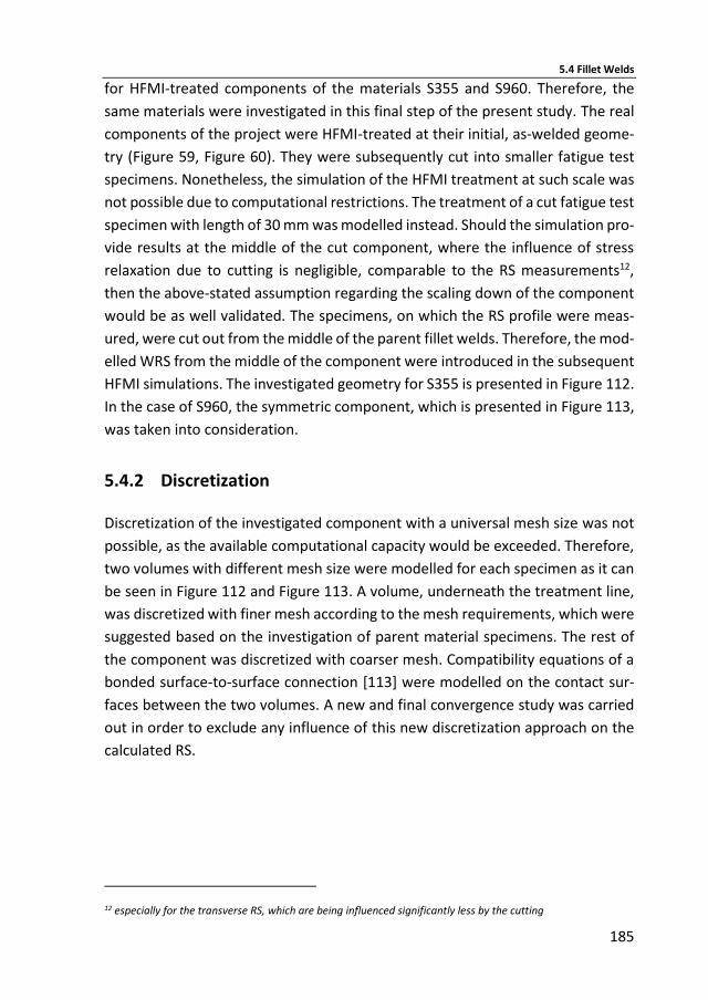
5.4 Fillet Welds
185
for HFMI-treated components of the materials S355 and S960. Therefore, the
same materials were investigated in this final step of the present study. The real
components of the project were HFMI-treated at their initial, as-welded geome-
try (Figure 59, Figure 60). They were subsequently cut into smaller fatigue test
specimens. Nonetheless, the simulation of the HFMI treatment at such scale was
not possible due to computational restrictions. The treatment of a cut fatigue test
specimen with length of 30 mm was modelled instead. Should the simulation pro-
vide results at the middle of the cut component, where the influence of stress
relaxation due to cutting is negligible, comparable to the RS measurements12,
then the above-stated assumption regarding the scaling down of the component
would be as well validated. The specimens, on which the RS profile were meas-
ured, were cut out from the middle of the parent fillet welds. Therefore, the mod-
elled WRS from the middle of the component were introduced in the subsequent
HFMI simulations. The investigated geometry for S355 is presented in Figure 112.
In the case of S960, the symmetric component, which is presented in Figure 113,
was taken into consideration.
5.4.2 Discretization
Discretization of the investigated component with a universal mesh size was not
possible, as the available computational capacity would be exceeded. Therefore,
two volumes with different mesh size were modelled for each specimen as it can
be seen in Figure 112 and Figure 113. A volume, underneath the treatment line,
was discretized with finer mesh according to the mesh requirements, which were
suggested based on the investigation of parent material specimens. The rest of
the component was discretized with coarser mesh. Compatibility equations of a
bonded surface-to-surface connection [113] were modelled on the contact sur-
faces between the two volumes. A new and final convergence study was carried
out in order to exclude any influence of this new discretization approach on the
calculated RS.
12 especially for the transverse RS, which are being influenced significantly less by the cutting

5 FE Simulation of HFMI
186
Figure 112: Modelled geometry and the assigned mesh inside and near the treatment area, for the investiga-
tion of the HFMI treatment on fillet welds of S355
5.4 Fillet Welds
187
Figure 113: Modelled geometry and assigned mesh for the investigation of the HFMI treatment on fillet welds
of S960
5 FE Simulation of HFMI
188
5.4.3 Modelling of Material Behaviour
Bilinear material behaviour with kinematic hardening and the Cowper-Symonds
model (Eq. (12)) were once again taken into consideration for simulating respec-
tively the elastic-plastic behaviour and the strain rate dependency of the investi-
gated steels. Furthermore and in order to enable a more precise simulation, the
differentiated microstructure of the HAZ and the FZ and their respective yield
stress, as they were estimated during welding simulation, were introduced in the
HFMI simulation model. The yield stress of the FZ was predicted earlier during the
welding simulation and it was validated through the hardness measurements in
[146]. PM yield stress was selected in all cases based on the above-presented re-
spective material parameters. The yield stress of the HAZ and its strain rate de-
pendency were explicitly calibrated through tensile tests under various strain
rates of micro-specimens cut out from the HAZ [146]. The results of this material
characterisation of the HAZ are presented in Table 44. The good agreement be-
tween the experimentally determined yield stress of the HAZ [146] and the re-
spective values predicted through the present FE welding simulation, which are
as well presented in Table 4413, further supports the validity of the welding simu-
lation approach, as it was presented in chapter 4. Moreover, the fact that satisfy-
ing agreement is met for all three investigated materials reveals once again the
robustness and versatility of the approach. The calibrated parameters of the Cow-
per-Symonds model (Eq. (12)) for the HAZ were adopted for the rest of the mate-
rial zones for all three materials with negligible expected influence on the results,
as no significant strain rate is met in the PM and the microstructure in the FZ
deviates slightly than that in the HAZ. H is assumed to be for all material zones
equal to that of the parent material. The applied material parameters for the bi-
linear elastic-plastic behaviour and the Cowper-Symonds model and for all inves-
tigated materials are presented in Table 45.
13 although as mentioned above, only S355 and S960 were simulated, the material parameters for S690 are presented as well
5.4 Fillet Welds
189
Table 44: Experimental results from [133] for the dynamic yield stress of the HAZ for various strain rates and
predicted values of the static yield stress with the FE weld modelling approach
휀�̇�
[s-1]
𝜎𝑌′ [MPa]
S355 S690 S690
FE
(static) 786 861 981
0.001 713 861 952
1 856 961 1031
50 913 1003 1247
50 943 996 1198
500 1165 1126 1518
500 1200 1226 1457
5.4.4 HFMI Treatment Setup and Boundary Conditions
Setup of the HFMI treatment in the present simulation was based on the results
of the investigations for the specimens of parent material, the recommendations
of the manufacturers and the monitoring of the treatment on real specimens in
[146]. The vertical axis of the pin was set at a 20° and 90° angle to the global
vertical and longitudinal14 axis. The centreline normal to the pin’s upper circular
face and coming through its centre was intersecting the weld toe at all times.
Treatment was initially set to begin and end 5 mm away from the edges of the
component. A local coordinate system was defined on the top circular face of the
pin for implementing the respective boundary conditions. Initial position of the
pin, its local coordinate system and the global one are presented in Figure 10.
14 axis parallel to the treatment line

5 FE Simulation of HFMI
190
Table 45: Calibration of the Cowper-Symonds model based on the Data from Table 44
Material Material Zone σy [MPa] H [GPa] Δ [-] γ [-]
S355
PM 450
0.9 5993 5 HAZ 713
FZ 918
S690
PM 734
0.9 11740 5 HAZ 861
FZ 918
S960
PM 1050
1.0 12830 5 HAZ 952
FZ 963
A velocity-based approach, as it was presented earlier for parent material speci-
mens, was applied for simulating the movement of the pin vertical to its axis. The
accelerating force is applied this time on the Z direction of the local coordinate
system. The impact velocity, as it was determined for each material during the
earlier investigations of PM, was initially adopted. Nonetheless, a change in the
introduced impact velocity or a denser overlap of consecutive impacts was ex-
pected due to the altered hardness in the HAZ or the different local geometry at
the weld toe, so that the real groove depth could be simulated. The trace depth
was compared with real specimens for a second-step validation in a new trial and
error calibration round. Finally, simulation of the treatment on all four weld toes
was not possible with the present computational capacity. It was then decided to
model the HFMI treatment only on the weld toe, where the RS were measured in
[146]. Otherwise, when the simulation would be carried out predictively the
treatment on the most unfavourable weld toe in terms of fatigue strength should
be considered. As an ideal geometry is modelled in purpose, so that the influence
of local weld geometric irregularities and other flaws is neglected, this would be
the one with the highest tensile WRS.
Two pin diameters of 3 mm and 4 mm were considered in order to simulate the
different RS profiles introduced by HiFIT and PITec [146]. Apart from the different
pin diameter, the above-mentioned variations in frequency and contact force
were as well taken into consideration. PITec treatment with a real average trav-
elling step of 0.08 mm between consecutive impacts, was simulated in a 3-pass
analysis, based on the results of the specimens of PM and previous studies ([44],

5.4 Fillet Welds
191
[45], [54] etc.). The measured average step of 0.22 mm of the HiFIT treatment
between consecutive impacts dictated the simulation of a single-pass treatment.
(a)
(b) Figure 114: Initial position of the pin: a) Lateral view; b) Isometric view and the local and global coordinate sys-
tems
According to initial expectations, the introduction of the real groove depth with
a single treatment pass would be attributed to the higher impact velocity of the
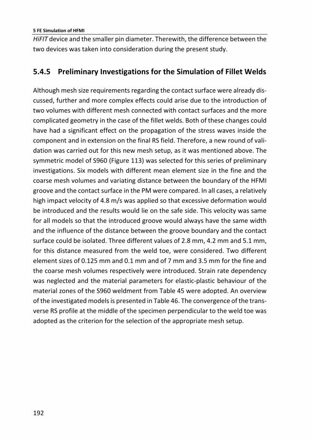
5 FE Simulation of HFMI
192
HiFIT device and the smaller pin diameter. Therewith, the difference between the
two devices was taken into consideration during the present study.
5.4.5 Preliminary Investigations for the Simulation of Fillet Welds
Although mesh size requirements regarding the contact surface were already dis-
cussed, further and more complex effects could arise due to the introduction of
two volumes with different mesh connected with contact surfaces and the more
complicated geometry in the case of the fillet welds. Both of these changes could
have had a significant effect on the propagation of the stress waves inside the
component and in extension on the final RS field. Therefore, a new round of vali-
dation was carried out for this new mesh setup, as it was mentioned above. The
symmetric model of S960 (Figure 113) was selected for this series of preliminary
investigations. Six models with different mean element size in the fine and the
coarse mesh volumes and variating distance between the boundary of the HFMI
groove and the contact surface in the PM were compared. In all cases, a relatively
high impact velocity of 4.8 m/s was applied so that excessive deformation would
be introduced and the results would lie on the safe side. This velocity was same
for all models so that the introduced groove would always have the same width
and the influence of the distance between the groove boundary and the contact
surface could be isolated. Three different values of 2.8 mm, 4.2 mm and 5.1 mm,
for this distance measured from the weld toe, were considered. Two different
element sizes of 0.125 mm and 0.1 mm and of 7 mm and 3.5 mm for the fine and
the coarse mesh volumes respectively were introduced. Strain rate dependency
was neglected and the material parameters for elastic-plastic behaviour of the
material zones of the S960 weldment from Table 45 were adopted. An overview
of the investigated models is presented in Table 46. The convergence of the trans-
verse RS profile at the middle of the specimen perpendicular to the weld toe was
adopted as the criterion for the selection of the appropriate mesh setup.
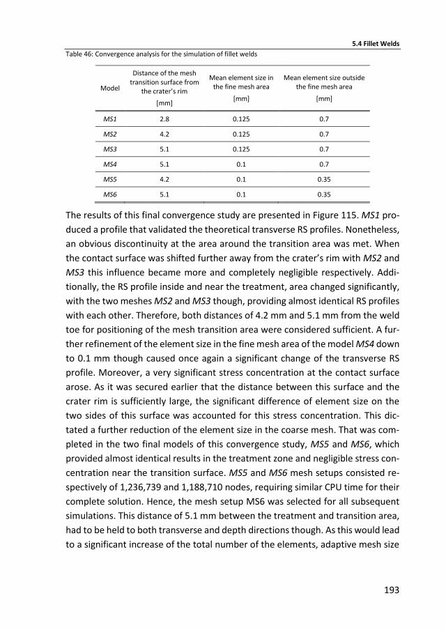
5.4 Fillet Welds
193
Table 46: Convergence analysis for the simulation of fillet welds
Model
Distance of the mesh transition surface from
the crater’s rim
[mm]
Mean element size in the fine mesh area
[mm]
Mean element size outside the fine mesh area
[mm]
MS1 2.8 0.125 0.7
MS2 4.2 0.125 0.7
MS3 5.1 0.125 0.7
MS4 5.1 0.1 0.7
MS5 4.2 0.1 0.35
MS6 5.1 0.1 0.35
The results of this final convergence study are presented in Figure 115. MS1 pro-
duced a profile that validated the theoretical transverse RS profiles. Nonetheless,
an obvious discontinuity at the area around the transition area was met. When
the contact surface was shifted further away from the crater’s rim with MS2 and
MS3 this influence became more and completely negligible respectively. Addi-
tionally, the RS profile inside and near the treatment, area changed significantly,
with the two meshes MS2 and MS3 though, providing almost identical RS profiles
with each other. Therefore, both distances of 4.2 mm and 5.1 mm from the weld
toe for positioning of the mesh transition area were considered sufficient. A fur-
ther refinement of the element size in the fine mesh area of the model MS4 down
to 0.1 mm though caused once again a significant change of the transverse RS
profile. Moreover, a very significant stress concentration at the contact surface
arose. As it was secured earlier that the distance between this surface and the
crater rim is sufficiently large, the significant difference of element size on the
two sides of this surface was accounted for this stress concentration. This dic-
tated a further reduction of the element size in the coarse mesh. That was com-
pleted in the two final models of this convergence study, MS5 and MS6, which
provided almost identical results in the treatment zone and negligible stress con-
centration near the transition surface. MS5 and MS6 mesh setups consisted re-
spectively of 1,236,739 and 1,188,710 nodes, requiring similar CPU time for their
complete solution. Hence, the mesh setup MS6 was selected for all subsequent
simulations. This distance of 5.1 mm between the treatment and transition area,
had to be held to both transverse and depth directions though. As this would lead
to a significant increase of the total number of the elements, adaptive mesh size

5 FE Simulation of HFMI
194
inside the fine mesh volume was applied. Exemplary the final mesh for the simu-
lation of the FW960 fillet weld is illustrated in Figure 116.
The above, proposed models were still marginally possible to be solved under the
provided computational capacity. Nevertheless, increase of computational time
due to the addition of strain rate dependency, further local mesh refinement due
to later observations or consideration of WRS would exceed these limits. Ergo, it
was decided to reduce the simulated component length from 30 mm down to 20
mm. The HFMI pin would start and stop its movement 5 mm away from the re-
spective edges leading to a treatment length of 10 mm. Despite this reduction,
the previously mentioned perquisites for scaling down, i.e. a minimum treatment
length of 2.5 times the pin diameter and a distance of the treatment from edges
of the components of 1 pin diameter, were met. With this length reduction and
the above-mentioned finalized discretization setup the simulated model came up
to a number of 1,255,205 elements for the case of FW960.
Figure 115: Results of the convergence study for the simulation of fillet welds
-1600
-1400
-1200
-1000
-800
-600
-400
-200
0
200
400
0 1 2 3 4 5 6 7 8 9 10
Tran
sver
se R
S [M
Pa]
Distance from weld toe [mm]
MS1 MS2
MS3 MS4
MS5 MS6
crat
er r
im
mes
h t
ran
siti
on
1
mes
h t
ran
siti
on
3
mes
h t
ran
siti
on
2
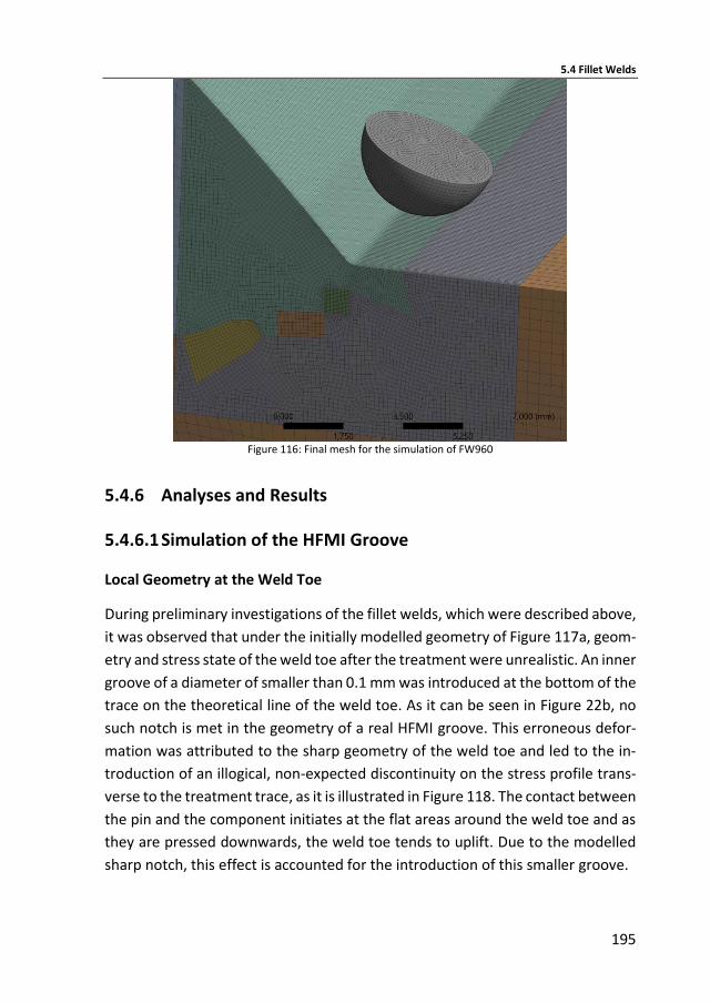
5.4 Fillet Welds
195
Figure 116: Final mesh for the simulation of FW960
5.4.6 Analyses and Results
5.4.6.1 Simulation of the HFMI Groove
Local Geometry at the Weld Toe
During preliminary investigations of the fillet welds, which were described above,
it was observed that under the initially modelled geometry of Figure 117a, geom-
etry and stress state of the weld toe after the treatment were unrealistic. An inner
groove of a diameter of smaller than 0.1 mm was introduced at the bottom of the
trace on the theoretical line of the weld toe. As it can be seen in Figure 22b, no
such notch is met in the geometry of a real HFMI groove. This erroneous defor-
mation was attributed to the sharp geometry of the weld toe and led to the in-
troduction of an illogical, non-expected discontinuity on the stress profile trans-
verse to the treatment trace, as it is illustrated in Figure 118. The contact between
the pin and the component initiates at the flat areas around the weld toe and as
they are pressed downwards, the weld toe tends to uplift. Due to the modelled
sharp notch, this effect is accounted for the introduction of this smaller groove.

5 FE Simulation of HFMI
196
Therefore, it was decided to alter locally the geometry by adding a small fillet
radius of 0.1 mm and refine the mesh so that at least 3 elements are assigned
along this fillet (Figure 117b)15. Such a local, significantly smaller than the HFMI
groove, change of the geometry can rationally be expected to have a negligible
influence on final RS. The implemented change led to a significant improvement
but not a complete elimination of the described phenomena, as it can be seen in
Figure 117b. Therefore, a further increase of the filleting radius up to 0.2 mm and
0.5 mm was tested sequentially (Figure 117b and Figure 117c). After the latter
change, the effect was completely eliminated. Additionally, the introduction of
the fillets lead to a constant “normalization” of the RS profiles inside the treat-
ment trace with the calculated RS profiles gradually converge to each other, at
least qualitatively (Figure 118). It has to be underlined that during the present
calibration, a single-pass treatment with a pin of 3 mm diameter was modelled.
Such an impact speed was assigned to the pin that it would just reach contact
with the weld toe. Calibration with the above setup lies on the safe side, as an
increase of treatment passes or of the pin’s penetration would cause a deeper
groove and would possibly eliminate the above effect, even for the initial unfa-
vourable geometry. Ergo, a filleting radius of 0.5 mm was adopted for all subse-
quent simulations.
15 the reader should recall the fictitious 1 mm radius added to the weld toe during fracture mechanics simulations with the notch stress concept, a state of the art method [155]
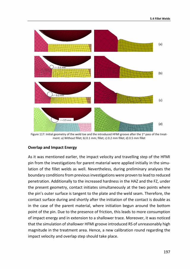
5.4 Fillet Welds
197
Figure 117: Initial geometry of the weld toe and the introduced HFMI groove after the 1st pass of the treat-
ment: a) Without fillet; b) 0.1 mm; fillet; c) 0.2 mm fillet; d) 0.5 mm fillet
Overlap and Impact Energy
As it was mentioned earlier, the impact velocity and travelling step of the HFMI
pin from the investigations for parent material were applied initially in the simu-
lation of the fillet welds as well. Nevertheless, during preliminary analyses the
boundary conditions from previous investigations were proven to lead to reduced
penetration. Additionally to the increased hardness in the HAZ and the FZ, under
the present geometry, contact initiates simultaneously at the two points where
the pin’s outer surface is tangent to the plate and the weld seam. Therefore, the
contact surface during and shortly after the initiation of the contact is double as
in the case of the parent material, where initiation begun around the bottom
point of the pin. Due to the presence of friction, this leads to more consumption
of impact energy and in extension to a shallower trace. Moreover, it was noticed
that the simulation of shallower HFMI groove introduced RS of unreasonably high
magnitude in the treatment area. Hence, a new calibration round regarding the
impact velocity and overlap step should take place.
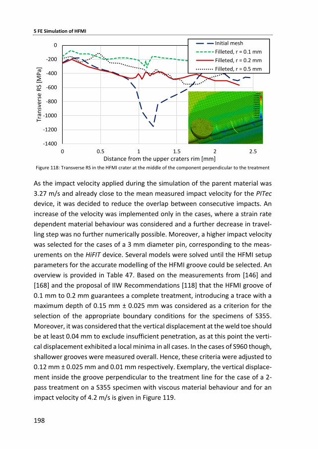
5 FE Simulation of HFMI
198
Figure 118: Transverse RS in the HFMI crater at the middle of the component perpendicular to the treatment
As the impact velocity applied during the simulation of the parent material was
3.27 m/s and already close to the mean measured impact velocity for the PITec
device, it was decided to reduce the overlap between consecutive impacts. An
increase of the velocity was implemented only in the cases, where a strain rate
dependent material behaviour was considered and a further decrease in travel-
ling step was no further numerically possible. Moreover, a higher impact velocity
was selected for the cases of a 3 mm diameter pin, corresponding to the meas-
urements on the HiFIT device. Several models were solved until the HFMI setup
parameters for the accurate modelling of the HFMI groove could be selected. An
overview is provided in Table 47. Based on the measurements from [146] and
[168] and the proposal of IIW Recommendations [118] that the HFMI groove of
0.1 mm to 0.2 mm guarantees a complete treatment, introducing a trace with a
maximum depth of 0.15 mm ± 0.025 mm was considered as a criterion for the
selection of the appropriate boundary conditions for the specimens of S355.
Moreover, it was considered that the vertical displacement at the weld toe should
be at least 0.04 mm to exclude insufficient penetration, as at this point the verti-
cal displacement exhibited a local minima in all cases. In the cases of S960 though,
shallower grooves were measured overall. Hence, these criteria were adjusted to
0.12 mm ± 0.025 mm and 0.01 mm respectively. Exemplary, the vertical displace-
ment inside the groove perpendicular to the treatment line for the case of a 2-
pass treatment on a S355 specimen with viscous material behaviour and for an
impact velocity of 4.2 m/s is given in Figure 119.
-1400
-1200
-1000
-800
-600
-400
-200
0
0 0.5 1 1.5 2 2.5
Tran
sver
se R
S [M
Pa]
Distance from the upper craters rim [mm]
Initial mesh
Filleted, r = 0.1 mm
Filleted, r = 0.2 mm
Filleted, r = 0.5 mm
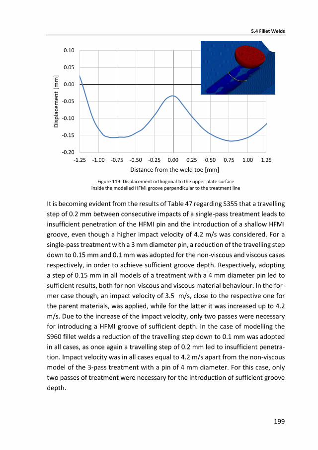
5.4 Fillet Welds
199
Figure 119: Displacement orthogonal to the upper plate surface
inside the modelled HFMI groove perpendicular to the treatment line
It is becoming evident from the results of Table 47 regarding S355 that a travelling
step of 0.2 mm between consecutive impacts of a single-pass treatment leads to
insufficient penetration of the HFMI pin and the introduction of a shallow HFMI
groove, even though a higher impact velocity of 4.2 m/s was considered. For a
single-pass treatment with a 3 mm diameter pin, a reduction of the travelling step
down to 0.15 mm and 0.1 mm was adopted for the non-viscous and viscous cases
respectively, in order to achieve sufficient groove depth. Respectively, adopting
a step of 0.15 mm in all models of a treatment with a 4 mm diameter pin led to
sufficient results, both for non-viscous and viscous material behaviour. In the for-
mer case though, an impact velocity of 3.5 m/s, close to the respective one for
the parent materials, was applied, while for the latter it was increased up to 4.2
m/s. Due to the increase of the impact velocity, only two passes were necessary
for introducing a HFMI groove of sufficient depth. In the case of modelling the
S960 fillet welds a reduction of the travelling step down to 0.1 mm was adopted
in all cases, as once again a travelling step of 0.2 mm led to insufficient penetra-
tion. Impact velocity was in all cases equal to 4.2 m/s apart from the non-viscous
model of the 3-pass treatment with a pin of 4 mm diameter. For this case, only
two passes of treatment were necessary for the introduction of sufficient groove
depth.
-0.20
-0.15
-0.10
-0.05
0.00
0.05
0.10
-1.25 -1.00 -0.75 -0.50 -0.25 0.00 0.25 0.50 0.75 1.00 1.25
Dis
pla
cem
ent
[mm
]
Distance from the weld toe [mm]
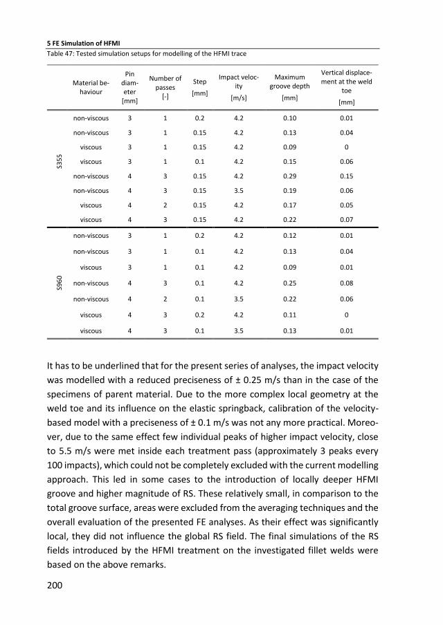
5 FE Simulation of HFMI
200
Table 47: Tested simulation setups for modelling of the HFMI trace
Material be-
haviour
Pin diam-eter
[mm]
Number of passes
[-]
Step
[mm]
Impact veloc-ity
[m/s]
Maximum groove depth
[mm]
Vertical displace-ment at the weld
toe
[mm]
S35
5
non-viscous 3 1 0.2 4.2 0.10 0.01
non-viscous 3 1 0.15 4.2 0.13 0.04
viscous 3 1 0.15 4.2 0.09 0
viscous 3 1 0.1 4.2 0.15 0.06
non-viscous 4 3 0.15 4.2 0.29 0.15
non-viscous 4 3 0.15 3.5 0.19 0.06
viscous 4 2 0.15 4.2 0.17 0.05
viscous 4 3 0.15 4.2 0.22 0.07
S96
0
non-viscous 3 1 0.2 4.2 0.12 0.01
non-viscous 3 1 0.1 4.2 0.13 0.04
viscous 3 1 0.1 4.2 0.09 0.01
non-viscous 4 3 0.1 4.2 0.25 0.08
non-viscous 4 2 0.1 3.5 0.22 0.06
viscous 4 3 0.2 4.2 0.11 0
viscous 4 3 0.1 3.5 0.13 0.01
It has to be underlined that for the present series of analyses, the impact velocity
was modelled with a reduced preciseness of ± 0.25 m/s than in the case of the
specimens of parent material. Due to the more complex local geometry at the
weld toe and its influence on the elastic springback, calibration of the velocity-
based model with a preciseness of ± 0.1 m/s was not any more practical. Moreo-
ver, due to the same effect few individual peaks of higher impact velocity, close
to 5.5 m/s were met inside each treatment pass (approximately 3 peaks every
100 impacts), which could not be completely excluded with the current modelling
approach. This led in some cases to the introduction of locally deeper HFMI
groove and higher magnitude of RS. These relatively small, in comparison to the
total groove surface, areas were excluded from the averaging techniques and the
overall evaluation of the presented FE analyses. As their effect was significantly
local, they did not influence the global RS field. The final simulations of the RS
fields introduced by the HFMI treatment on the investigated fillet welds were
based on the above remarks.
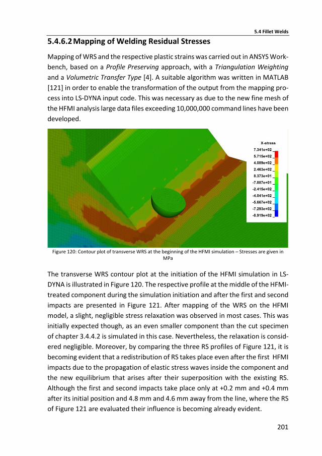
5.4 Fillet Welds
201
5.4.6.2 Mapping of Welding Residual Stresses
Mapping of WRS and the respective plastic strains was carried out in ANSYS Work-
bench, based on a Profile Preserving approach, with a Triangulation Weighting
and a Volumetric Transfer Type [4]. A suitable algorithm was written in MATLAB
[121] in order to enable the transformation of the output from the mapping pro-
cess into LS-DYNA input code. This was necessary as due to the new fine mesh of
the HFMI analysis large data files exceeding 10,000,000 command lines have been
developed.
Figure 120: Contour plot of transverse WRS at the beginning of the HFMI simulation – Stresses are given in
MPa
The transverse WRS contour plot at the initiation of the HFMI simulation in LS-
DYNA is illustrated in Figure 120. The respective profile at the middle of the HFMI-
treated component during the simulation initiation and after the first and second
impacts are presented in Figure 121. After mapping of the WRS on the HFMI
model, a slight, negligible stress relaxation was observed in most cases. This was
initially expected though, as an even smaller component than the cut specimen
of chapter 3.4.4.2 is simulated in this case. Nevertheless, the relaxation is consid-
ered negligible. Moreover, by comparing the three RS profiles of Figure 121, it is
becoming evident that a redistribution of RS takes place even after the first HFMI
impacts due to the propagation of elastic stress waves inside the component and
the new equilibrium that arises after their superposition with the existing RS.
Although the first and second impacts take place only at +0.2 mm and +0.4 mm
after its initial position and 4.8 mm and 4.6 mm away from the line, where the RS
of Figure 121 are evaluated their influence is becoming already evident.
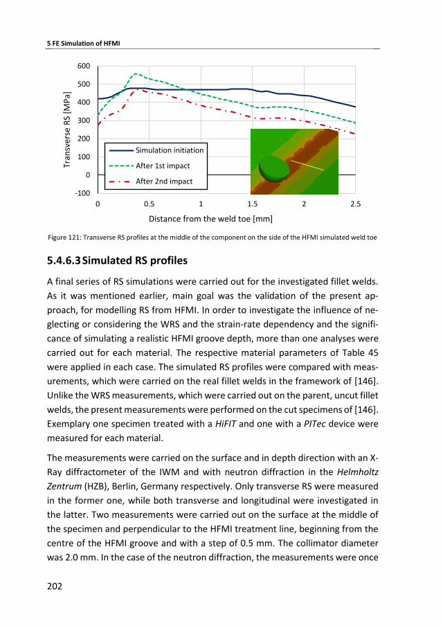
5 FE Simulation of HFMI
202
Figure 121: Transverse RS profiles at the middle of the component on the side of the HFMI simulated weld toe
5.4.6.3 Simulated RS profiles
A final series of RS simulations were carried out for the investigated fillet welds.
As it was mentioned earlier, main goal was the validation of the present ap-
proach, for modelling RS from HFMI. In order to investigate the influence of ne-
glecting or considering the WRS and the strain-rate dependency and the signifi-
cance of simulating a realistic HFMI groove depth, more than one analyses were
carried out for each material. The respective material parameters of Table 45
were applied in each case. The simulated RS profiles were compared with meas-
urements, which were carried on the real fillet welds in the framework of [146].
Unlike the WRS measurements, which were carried out on the parent, uncut fillet
welds, the present measurements were performed on the cut specimens of [146].
Exemplary one specimen treated with a HiFIT and one with a PITec device were
measured for each material.
The measurements were carried on the surface and in depth direction with an X-
Ray diffractometer of the IWM and with neutron diffraction in the Helmholtz
Zentrum (HZB), Berlin, Germany respectively. Only transverse RS were measured
in the former one, while both transverse and longitudinal were investigated in
the latter. Two measurements were carried out on the surface at the middle of
the specimen and perpendicular to the HFMI treatment line, beginning from the
centre of the HFMI groove and with a step of 0.5 mm. The collimator diameter
was 2.0 mm. In the case of the neutron diffraction, the measurements were once
-100
0
100
200
300
400
500
600
0 0.5 1 1.5 2 2.5
Tran
sver
se R
S [M
Pa]
Distance from the weld toe [mm]
Simulation initiation
After 1st impact
After 2nd impact
5.4 Fillet Welds
203
again carried out at the middle of the component and underneath the weld toe,
which coincided with the middle of the HFMI groove. Gauge volumes of 2 mm x
2 mm x 2 mm and 5 mm x 2 mm x 2 mm were investigated for the longitudinal
and transverse direction respectively. Measurements were carried out every 0.5
mm in depth direction. The applied gauge volumes were significantly larger than
those, which were measured earlier in [44] and [145] for the specimens of parent
material. Once again, averaging of the results from the integration points on the
measured surface or inside the measured gauge volumes was necessary in order
to enable a direct comparison of simulation and measurements. More details re-
garding the present RS measurements can be found in [144] and [146].
S355 Specimens Treated with a Pin of 3 mm Diameter
An overview of the numerical investigations regarding the single-pass treatments
of the S355 fillet welds with a 3 mm diameter HFMI pin is given in Table 48. Three
analyses, A1, A2 and A3, adopting a non-viscous material behaviour were carried
out, with the first one neglecting and the other two considering the WRS. Due to
a larger travelling step of 0.2 mm between consecutive impacts, A2 introduced a
HFMI groove shallower than the above-mentioned criterion of acceptance. Simi-
larly, the model A4 considering strain-rate dependency and a step of 0.15 mm led
to the introduction of a shallow trace. An adoption of a smaller step of 0.1 mm in
A5 produced an acceptable HFMI groove. All simulations were carried out with
an impact velocity of 4.2 m/s. The HFMI groove in the present case had an aver-
age half width of 0.8 mm.
The simulated transverse RS profiles on the surface of the fillet welds and per-
pendicular to the HFMI groove are presented along with the respective measure-
ments in Figure 122. A non-negligible deviation is met between the two measure-
ment series only at a distance of 3 mm from the weld toe. The agreement on the
rest of the measurement points is very good. They both produce qualitatively
similar results; compressive RS are met along total measurement length and the
peak stress is met outside the rim of the HFMI groove at a proximity of approxi-
mately 2 mm and 2.5 mm respectively. Peak stress of approximately -300 MPa is
measured in both cases. Inside the HFMI groove though, significantly lower
stresses are documented approaching zero at its middle.
Nonetheless, all simulated RS profiles, which are qualitatively similar to each
other, show a peak stress at the middle of the HFMI groove. Models A1, A2, A4
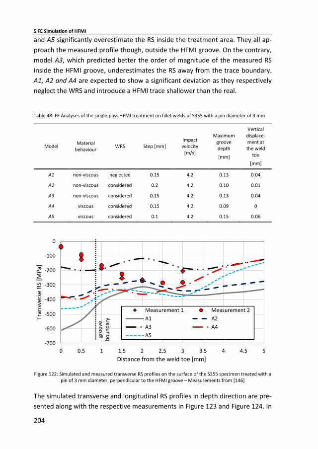
5 FE Simulation of HFMI
204
and A5 significantly overestimate the RS inside the treatment area. They all ap-
proach the measured profile though, outside the HFMI groove. On the contrary,
model A3, which predicted better the order of magnitude of the measured RS
inside the HFMI groove, underestimates the RS away from the trace boundary.
A1, A2 and A4 are expected to show a significant deviation as they respectively
neglect the WRS and introduce a HFMI trace shallower than the real.
Table 48: FE Analyses of the single-pass HFMI treatment on fillet welds of S355 with a pin diameter of 3 mm
Model Material
behaviour WRS Step [mm]
Impact velocity
[m/s]
Maximum groove depth
[mm]
Vertical displace-ment at the weld
toe
[mm]
A1 non-viscous neglected 0.15 4.2 0.13 0.04
A2 non-viscous considered 0.2 4.2 0.10 0.01
A3 non-viscous considered 0.15 4.2 0.13 0.04
A4 viscous considered 0.15 4.2 0.09 0
A5 viscous considered 0.1 4.2 0.15 0.06
Figure 122: Simulated and measured transverse RS profiles on the surface of the S355 specimen treated with a
pin of 3 mm diameter, perpendicular to the HFMI groove – Measurements from [146]
The simulated transverse and longitudinal RS profiles in depth direction are pre-
sented along with the respective measurements in Figure 123 and Figure 124. In
-700
-600
-500
-400
-300
-200
-100
0
0 0.5 1 1.5 2 2.5 3 3.5 4 4.5 5
Tran
sver
se R
S [M
Pa]
Distance from the weld toe [mm]
Measurement 1 Measurement 2
A1 A2
A3 A4
A5gro
ove
bo
un
dar
y
5.4 Fillet Welds
205
the case of the transverse RS, analyses considering a non-viscous material model
match qualitatively the measured profiles, being in the compressive regime near
the surface and passing to the tensile one after a significant depth of approxi-
mately 3 mm or larger. The models considering strain-rate dependency produced
different profiles even qualitatively. Once again, the introduced RS near the sur-
face are compressive but the transition to the tensile zone takes place at much
smaller depth of around 1 mm to 1.5 mm. The compressive stresses near the sur-
face though have a higher magnitude, than those simulated with non-viscous ma-
terial modelling. This change due to the introduction of strain rate dependency is
expected as the elements on the top layers, underneath the contact surface, yield
at a higher stress. Due to the higher magnitude of compressive residual stress and
as the energy of the system is equal with the non-viscous case, the zone of the
compressive stresses has to become thinner so that equilibrium of the RS can be
achieved. Therewith, the transition points shifts up. Regarding the quantitative
agreement of numerical and experimental results, model A3, which neglects
strain-rate dependency but considered the WRS, shows overall a very good agree-
ment with the measured RS. The highest deviation of 60 MPa, which is lower than
10 % of the material’s yield stress, is met near the surface. Models A1, A2 and A4
are expected to show a significant deviation due to the above-stated reasons. The
profile of A5 though, despite considering the WRS and introducing a realistic
HFMI groove, still deviates significantly from the measured one.
In the case of the longitudinal RS (Figure 124), all numerical models produce pro-
files qualitatively similar with each other and with the measured ones. In all cases,
only compressive stresses are introduced in the first 4 mm underneath the con-
tact surface. Model A3 once again exhibits the best agreement with the measure-
ments especially near the surface. A significant deviation of 100 MPa is met only
at a depth between 1 mm and 1.5 mm. Otherwise the deviation is considered
overall acceptable. The rest of the profiles although less accurate than A3 deviate
slightly from it, with each other and with the measured RS. This fact may reveal a
smaller sensitivity of the longitudinal RS to the investigated effects in comparison
to the transverse, especially regarding the depth of the introduced HFMI groove.
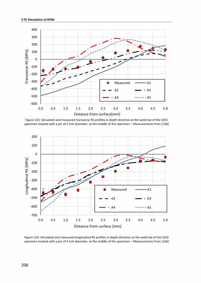
5 FE Simulation of HFMI
206
Figure 123: Simulated and measured transverse RS profiles in depth direction at the weld toe of the S355
specimen treated with a pin of 3 mm diameter, at the middle of the specimen – Measurements from [146]
Figure 124: Simulated and measured longitudinal RS profiles in depth direction at the weld toe of the S355 specimen treated with a pin of 3 mm diameter, at the middle of the specimen – Measurements from [146]
-600
-500
-400
-300
-200
-100
0
100
200
300
400
0.0 0.5 1.0 1.5 2.0 2.5 3.0 3.5 4.0 4.5 5.0
Tran
sver
se R
S [M
Pa]
Distance from surface[mm]
Measured A1
A2 A3
A4 A5
-700
-600
-500
-400
-300
-200
-100
0
100
200
0.0 0.5 1.0 1.5 2.0 2.5 3.0 3.5 4.0 4.5 5.0
Lon
gitu
din
al R
S [M
Pa]
Distance from surface [mm]
Measured A1
A2 A3
A4 A5

5.4 Fillet Welds
207
Exemplarily, the applied mesh and the longitudinal and transverse RS contours of
the model A3 below the contact surface at a section at the middle of the investi-
gated component and perpendicular to the introduced HFMI groove are pre-
sented in Figure 125. In the case of the transverse RS the compressive zone un-
derneath and around the contact surface is becoming evident, without exhibiting
though at any point significantly higher stresses than the rest. Overall, the com-
pressive stresses do not exceed the yield stress of the material in the treatment
area. On the contrary, longitudinal stresses significantly higher than the yield
strength, even higher than 1400 MPa, are met on the top layer elements under-
neath the contact surface. Nevertheless, the RS in the rest of the compressive
zone are as well approximately equal to the real yield stress of the material in the
HAZ. Significantly higher stresses met exclusively at the top layer of elements
could be as well the result of the numerical modelling of contact. Away from the
treatment zone, significant tensile stress of even up to 500 MPa are met. This
field of tensile stresses, which is attributed to the initial WRS field, is interrupted
by the compressive stresses introduced with HFMI. The redistribution of RS
through the HFMI deformation in the area of the weld toe is becoming evident.
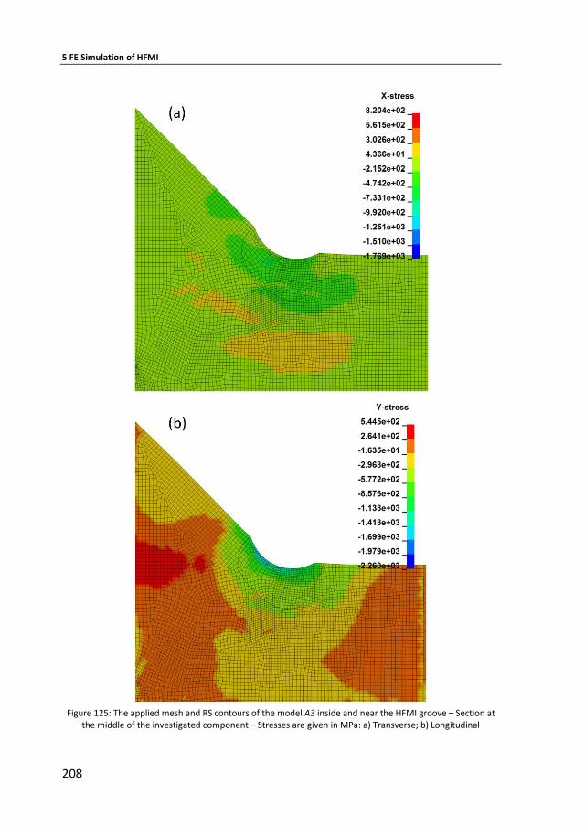
5 FE Simulation of HFMI
208
Figure 125: The applied mesh and RS contours of the model A3 inside and near the HFMI groove – Section at
the middle of the investigated component – Stresses are given in MPa: a) Transverse; b) Longitudinal
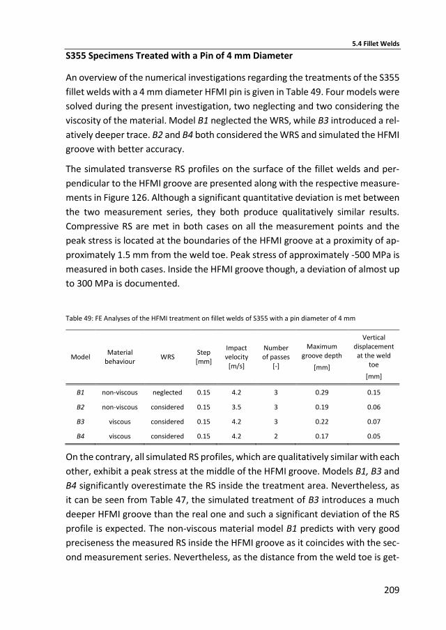
5.4 Fillet Welds
209
S355 Specimens Treated with a Pin of 4 mm Diameter
An overview of the numerical investigations regarding the treatments of the S355
fillet welds with a 4 mm diameter HFMI pin is given in Table 49. Four models were
solved during the present investigation, two neglecting and two considering the
viscosity of the material. Model B1 neglected the WRS, while B3 introduced a rel-
atively deeper trace. B2 and B4 both considered the WRS and simulated the HFMI
groove with better accuracy.
The simulated transverse RS profiles on the surface of the fillet welds and per-
pendicular to the HFMI groove are presented along with the respective measure-
ments in Figure 126. Although a significant quantitative deviation is met between
the two measurement series, they both produce qualitatively similar results.
Compressive RS are met in both cases on all the measurement points and the
peak stress is located at the boundaries of the HFMI groove at a proximity of ap-
proximately 1.5 mm from the weld toe. Peak stress of approximately -500 MPa is
measured in both cases. Inside the HFMI groove though, a deviation of almost up
to 300 MPa is documented.
Table 49: FE Analyses of the HFMI treatment on fillet welds of S355 with a pin diameter of 4 mm
Model Material
behaviour WRS
Step [mm]
Impact velocity
[m/s]
Number of passes
[-]
Maximum groove depth
[mm]
Vertical displacement at the weld
toe
[mm]
B1 non-viscous neglected 0.15 4.2 3 0.29 0.15
B2 non-viscous considered 0.15 3.5 3 0.19 0.06
B3 viscous considered 0.15 4.2 3 0.22 0.07
B4 viscous considered 0.15 4.2 2 0.17 0.05
On the contrary, all simulated RS profiles, which are qualitatively similar with each
other, exhibit a peak stress at the middle of the HFMI groove. Models B1, B3 and
B4 significantly overestimate the RS inside the treatment area. Nevertheless, as
it can be seen from Table 47, the simulated treatment of B3 introduces a much
deeper HFMI groove than the real one and such a significant deviation of the RS
profile is expected. The non-viscous material model B1 predicts with very good
preciseness the measured RS inside the HFMI groove as it coincides with the sec-
ond measurement series. Nevertheless, as the distance from the weld toe is get-
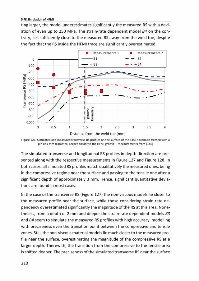
5 FE Simulation of HFMI
210
ting larger, the model underestimates significantly the measured RS with a devi-
ation of even up to 250 MPa. The strain-rate dependent model B4 on the con-
trary, lies sufficiently close to the measured RS away from the weld toe, despite
the fact that the RS inside the HFMI trace are significantly overestimated.
Figure 126: Simulated and measured transverse RS profiles on the surface of the S355 specimen treated with a
pin of 4 mm diameter, perpendicular to the HFMI groove – Measurements from [146]
The simulated transverse and longitudinal RS profiles in depth direction are pre-
sented along with the respective measurements in Figure 127 and Figure 128. In
both cases, all simulated RS profiles match qualitatively the measured ones, being
in the compressive regime near the surface and passing to the tensile one after a
significant depth of approximately 3 mm. Hence, significant quantitative devia-
tions are found in most cases.
In the case of the transverse RS (Figure 127) the non-viscous models lie closer to
the measured profile near the surface, while those considering strain rate de-
pendency overestimated significantly the magnitude of the RS at this area. None-
theless, from a depth of 2 mm and deeper the strain-rate dependent models B3
and B4 seem to simulate the measured RS profiles with high accuracy, modelling
with preciseness even the transition point between the compressive and tensile
zones. Still, the non-viscous material models lie much closer to the measured pro-
file near the surface, overestimating the magnitude of the compressive RS at a
larger depth. Therewith, the transition from the compressive to the tensile area
is shifted deeper. The preciseness of the simulated transverse RS near the surface
-1000
-900
-800
-700
-600
-500
-400
-300
-200
-100
0
0 0.5 1 1.5 2 2.5 3 3.5 4
Tran
sver
se R
S [M
Pa]
Distance from the weld toe [mm]
Measurements 1 Measurements 2
B1 B2
B3 B4
gro
ove
bo
un
dar
y
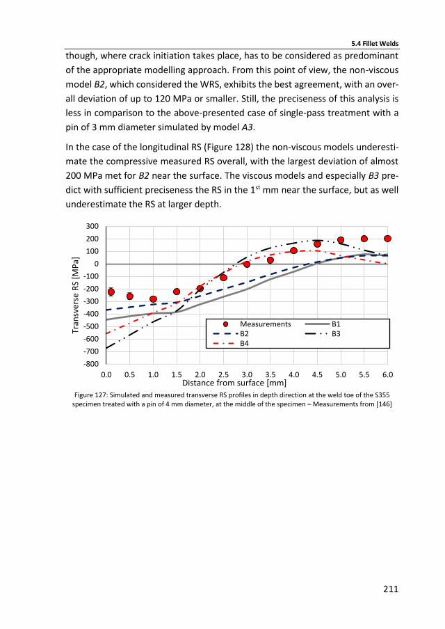
5.4 Fillet Welds
211
though, where crack initiation takes place, has to be considered as predominant
of the appropriate modelling approach. From this point of view, the non-viscous
model B2, which considered the WRS, exhibits the best agreement, with an over-
all deviation of up to 120 MPa or smaller. Still, the preciseness of this analysis is
less in comparison to the above-presented case of single-pass treatment with a
pin of 3 mm diameter simulated by model A3.
In the case of the longitudinal RS (Figure 128) the non-viscous models underesti-
mate the compressive measured RS overall, with the largest deviation of almost
200 MPa met for B2 near the surface. The viscous models and especially B3 pre-
dict with sufficient preciseness the RS in the 1st mm near the surface, but as well
underestimate the RS at larger depth.
Figure 127: Simulated and measured transverse RS profiles in depth direction at the weld toe of the S355
specimen treated with a pin of 4 mm diameter, at the middle of the specimen – Measurements from [146]
-800
-700
-600
-500
-400
-300
-200
-100
0
100
200
300
0.0 0.5 1.0 1.5 2.0 2.5 3.0 3.5 4.0 4.5 5.0 5.5 6.0
Tran
sver
se R
S [M
Pa]
Distance from surface [mm]
Measurements B1B2 B3B4
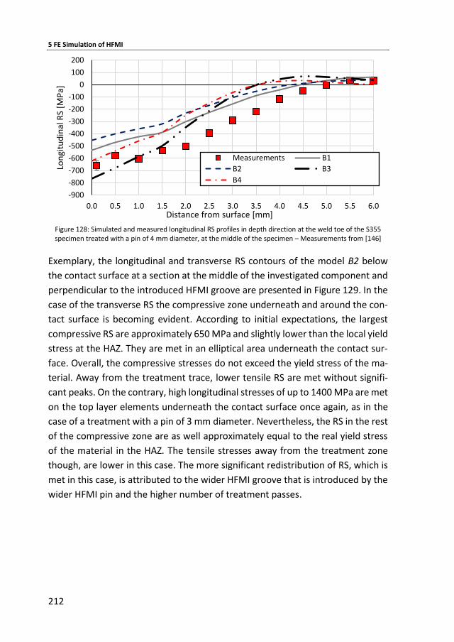
5 FE Simulation of HFMI
212
Figure 128: Simulated and measured longitudinal RS profiles in depth direction at the weld toe of the S355 specimen treated with a pin of 4 mm diameter, at the middle of the specimen – Measurements from [146]
Exemplary, the longitudinal and transverse RS contours of the model B2 below
the contact surface at a section at the middle of the investigated component and
perpendicular to the introduced HFMI groove are presented in Figure 129. In the
case of the transverse RS the compressive zone underneath and around the con-
tact surface is becoming evident. According to initial expectations, the largest
compressive RS are approximately 650 MPa and slightly lower than the local yield
stress at the HAZ. They are met in an elliptical area underneath the contact sur-
face. Overall, the compressive stresses do not exceed the yield stress of the ma-
terial. Away from the treatment trace, lower tensile RS are met without signifi-
cant peaks. On the contrary, high longitudinal stresses of up to 1400 MPa are met
on the top layer elements underneath the contact surface once again, as in the
case of a treatment with a pin of 3 mm diameter. Nevertheless, the RS in the rest
of the compressive zone are as well approximately equal to the real yield stress
of the material in the HAZ. The tensile stresses away from the treatment zone
though, are lower in this case. The more significant redistribution of RS, which is
met in this case, is attributed to the wider HFMI groove that is introduced by the
wider HFMI pin and the higher number of treatment passes.
-900
-800
-700
-600
-500
-400
-300
-200
-100
0
100
200
0.0 0.5 1.0 1.5 2.0 2.5 3.0 3.5 4.0 4.5 5.0 5.5 6.0
Lon
gitu
din
al R
S [M
Pa]
Distance from surface [mm]
Measurements B1
B2 B3
B4
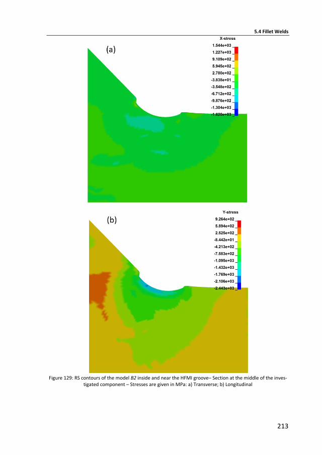
5.4 Fillet Welds
213
Figure 129: RS contours of the model B2 inside and near the HFMI groove– Section at the middle of the inves-
tigated component – Stresses are given in MPa: a) Transverse; b) Longitudinal
5 FE Simulation of HFMI
214
S960 Specimens Treated with a Pin of 3 mm Diameter
An overview of the numerical investigations regarding the single-pass treatments
of the S960 fillet welds with a 3 mm diameter HFMI pin is given in Table 50. Four
different models were considered in the present investigation, three neglecting
and one considering the material’s viscosity. Model C2 due to the larger assumed
step of 0.2 mm between consecutive impacts, introduced an unrealistically shal-
low HFMI groove, while C1 neglected WRS. Therefore, these two models were
expected to exhibit significant deviation from the measured RS. The HFMI groove
in the present case had an average half width of 1 mm.
The simulated transverse RS profiles on the surface of the fillet welds and per-
pendicular to the HFMI groove are presented along with the respective measure-
ments in Figure 130. A deviation of 100 MPa or less was met between the two
measurement series for the whole measurement length, as they produce similar
results both qualitatively and quantitatively. Compressive RS are met in both
cases on all measurement points and the peak stress is met outside the boundary
of the HFMI groove at a proximity of 2 mm and 3 mm from the weld toe. Peak
stress of approximately -300 MPa is measured in both cases. Inside the HFMI
groove though, lower stresses are documented lying close to zero at its middle.
Simulated RS profiles C1 - C3 produce results qualitatively similar to each other
and with the measured profiles. They all exhibited lower stress inside the HFMI
groove and a peak stress at approximately 2.5 mm away from the weld toe.
Model C3 approached the measured RS profile as well with high preciseness,
showing a deviation of less than 100 MPa from the second measurement all along
the measurement length. Models C1 and C2 as expected exhibited less accuracy
than the model C3. Regarding the 4th carried out analysis C4, once again the in-
troduction of strain-rate dependency in the considered material model led to a
larger deviation between measurements and simulation results and even quali-
tative discrepancies.
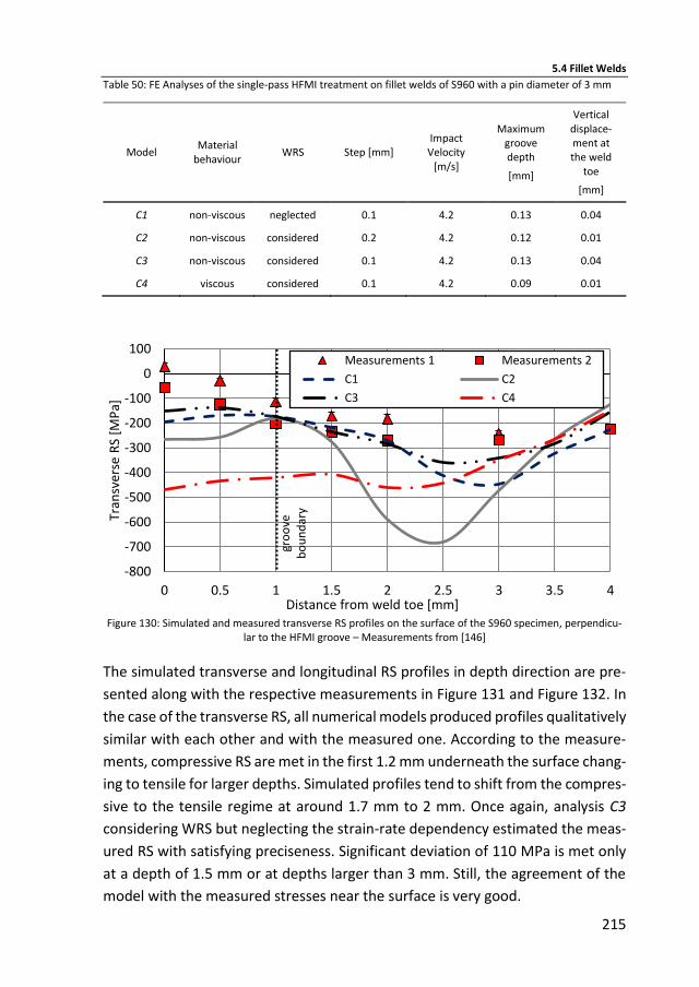
5.4 Fillet Welds
215
Table 50: FE Analyses of the single-pass HFMI treatment on fillet welds of S960 with a pin diameter of 3 mm
Model Material
behaviour WRS Step [mm]
Impact Velocity
[m/s]
Maximum groove depth
[mm]
Vertical displace-ment at the weld
toe
[mm]
C1 non-viscous neglected 0.1 4.2 0.13 0.04
C2 non-viscous considered 0.2 4.2 0.12 0.01
C3 non-viscous considered 0.1 4.2 0.13 0.04
C4 viscous considered 0.1 4.2 0.09 0.01
Figure 130: Simulated and measured transverse RS profiles on the surface of the S960 specimen, perpendicu-
lar to the HFMI groove – Measurements from [146]
The simulated transverse and longitudinal RS profiles in depth direction are pre-
sented along with the respective measurements in Figure 131 and Figure 132. In
the case of the transverse RS, all numerical models produced profiles qualitatively
similar with each other and with the measured one. According to the measure-
ments, compressive RS are met in the first 1.2 mm underneath the surface chang-
ing to tensile for larger depths. Simulated profiles tend to shift from the compres-
sive to the tensile regime at around 1.7 mm to 2 mm. Once again, analysis C3
considering WRS but neglecting the strain-rate dependency estimated the meas-
ured RS with satisfying preciseness. Significant deviation of 110 MPa is met only
at a depth of 1.5 mm or at depths larger than 3 mm. Still, the agreement of the
model with the measured stresses near the surface is very good.
-800
-700
-600
-500
-400
-300
-200
-100
0
100
0 0.5 1 1.5 2 2.5 3 3.5 4
Tran
sver
se R
S [M
Pa]
Distance from weld toe [mm]
Measurements 1 Measurements 2
C1 C2
C3 C4
gro
ove
bo
un
dar
y
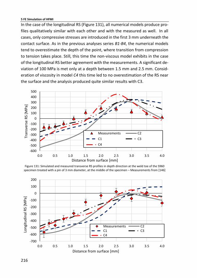
5 FE Simulation of HFMI
216
In the case of the longitudinal RS (Figure 131), all numerical models produce pro-
files qualitatively similar with each other and with the measured as well. In all
cases, only compressive stresses are introduced in the first 3 mm underneath the
contact surface. As in the previous analyses series B1-B4, the numerical models
tend to overestimate the depth of the point, where transition from compression
to tension takes place. Still, this time the non-viscous model exhibits in the case
of the longitudinal RS better agreement with the measurements. A significant de-
viation of 100 MPa is met only at a depth between 1.5 mm and 2.5 mm. Consid-
eration of viscosity in model C4 this time led to no overestimation of the RS near
the surface and the analysis produced quite similar results with C3.
Figure 131: Simulated and measured transverse RS profiles in depth direction at the weld toe of the S960
specimen treated with a pin of 3 mm diameter, at the middle of the specimen – Measurements from [146]
-600
-500
-400
-300
-200
-100
0
100
200
300
400
500
0.0 0.5 1.0 1.5 2.0 2.5 3.0 3.5 4.0
Tran
sver
se R
S [M
Pa]
Distance from surface [mm]
Measurements C2
C1 C3
C4
-700
-600
-500
-400
-300
-200
-100
0
100
200
0.0 0.5 1.0 1.5 2.0 2.5 3.0 3.5 4.0
Lon
gitu
din
al R
S [M
Pa]
Distance from surface [mm]
Measurements C2C1 C3C4
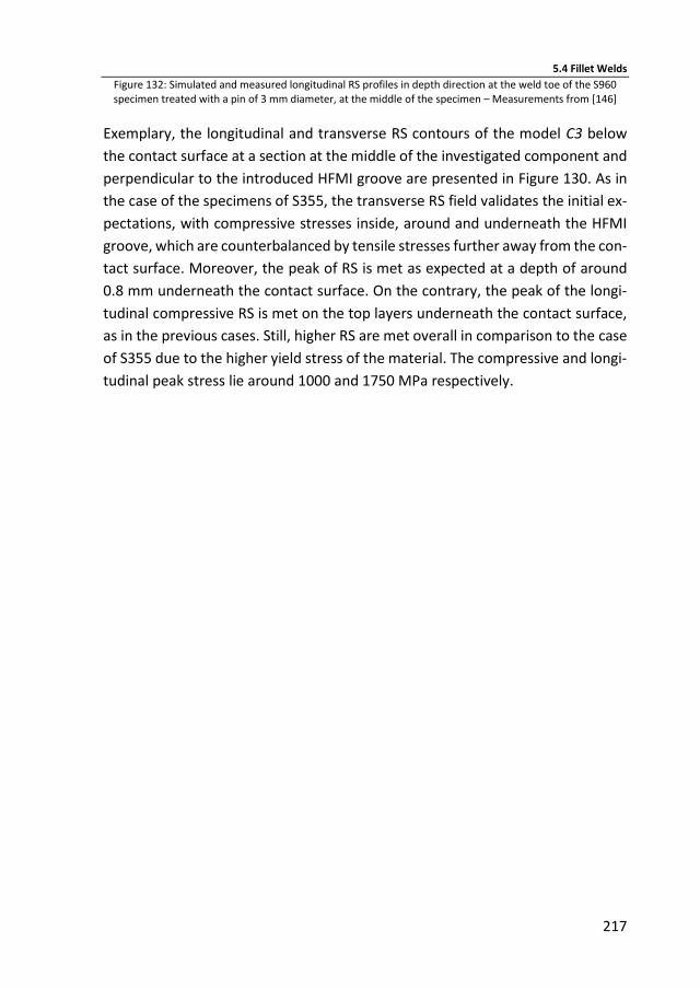
5.4 Fillet Welds
217
Figure 132: Simulated and measured longitudinal RS profiles in depth direction at the weld toe of the S960 specimen treated with a pin of 3 mm diameter, at the middle of the specimen – Measurements from [146]
Exemplary, the longitudinal and transverse RS contours of the model C3 below
the contact surface at a section at the middle of the investigated component and
perpendicular to the introduced HFMI groove are presented in Figure 130. As in
the case of the specimens of S355, the transverse RS field validates the initial ex-
pectations, with compressive stresses inside, around and underneath the HFMI
groove, which are counterbalanced by tensile stresses further away from the con-
tact surface. Moreover, the peak of RS is met as expected at a depth of around
0.8 mm underneath the contact surface. On the contrary, the peak of the longi-
tudinal compressive RS is met on the top layers underneath the contact surface,
as in the previous cases. Still, higher RS are met overall in comparison to the case
of S355 due to the higher yield stress of the material. The compressive and longi-
tudinal peak stress lie around 1000 and 1750 MPa respectively.
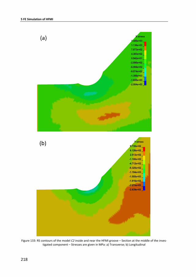
5 FE Simulation of HFMI
218
Figure 133: RS contours of the model C2 inside and near the HFMI groove – Section at the middle of the inves-
tigated component – Stresses are given in MPa: a) Transverse; b) Longitudinal
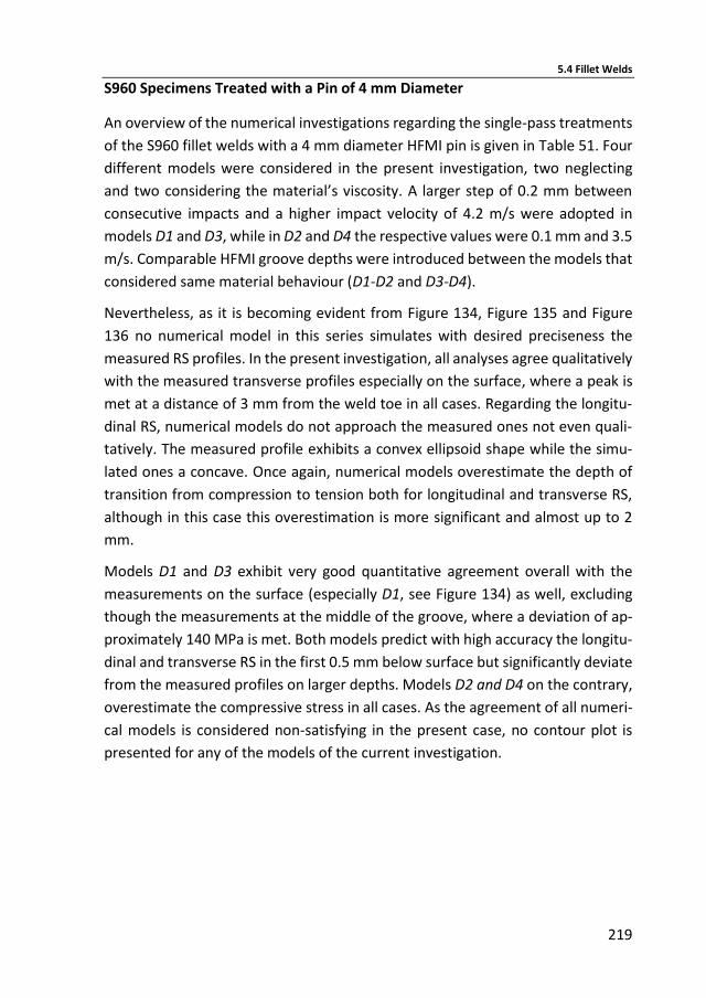
5.4 Fillet Welds
219
S960 Specimens Treated with a Pin of 4 mm Diameter
An overview of the numerical investigations regarding the single-pass treatments
of the S960 fillet welds with a 4 mm diameter HFMI pin is given in Table 51. Four
different models were considered in the present investigation, two neglecting
and two considering the material’s viscosity. A larger step of 0.2 mm between
consecutive impacts and a higher impact velocity of 4.2 m/s were adopted in
models D1 and D3, while in D2 and D4 the respective values were 0.1 mm and 3.5
m/s. Comparable HFMI groove depths were introduced between the models that
considered same material behaviour (D1-D2 and D3-D4).
Nevertheless, as it is becoming evident from Figure 134, Figure 135 and Figure
136 no numerical model in this series simulates with desired preciseness the
measured RS profiles. In the present investigation, all analyses agree qualitatively
with the measured transverse profiles especially on the surface, where a peak is
met at a distance of 3 mm from the weld toe in all cases. Regarding the longitu-
dinal RS, numerical models do not approach the measured ones not even quali-
tatively. The measured profile exhibits a convex ellipsoid shape while the simu-
lated ones a concave. Once again, numerical models overestimate the depth of
transition from compression to tension both for longitudinal and transverse RS,
although in this case this overestimation is more significant and almost up to 2
mm.
Models D1 and D3 exhibit very good quantitative agreement overall with the
measurements on the surface (especially D1, see Figure 134) as well, excluding
though the measurements at the middle of the groove, where a deviation of ap-
proximately 140 MPa is met. Both models predict with high accuracy the longitu-
dinal and transverse RS in the first 0.5 mm below surface but significantly deviate
from the measured profiles on larger depths. Models D2 and D4 on the contrary,
overestimate the compressive stress in all cases. As the agreement of all numeri-
cal models is considered non-satisfying in the present case, no contour plot is
presented for any of the models of the current investigation.
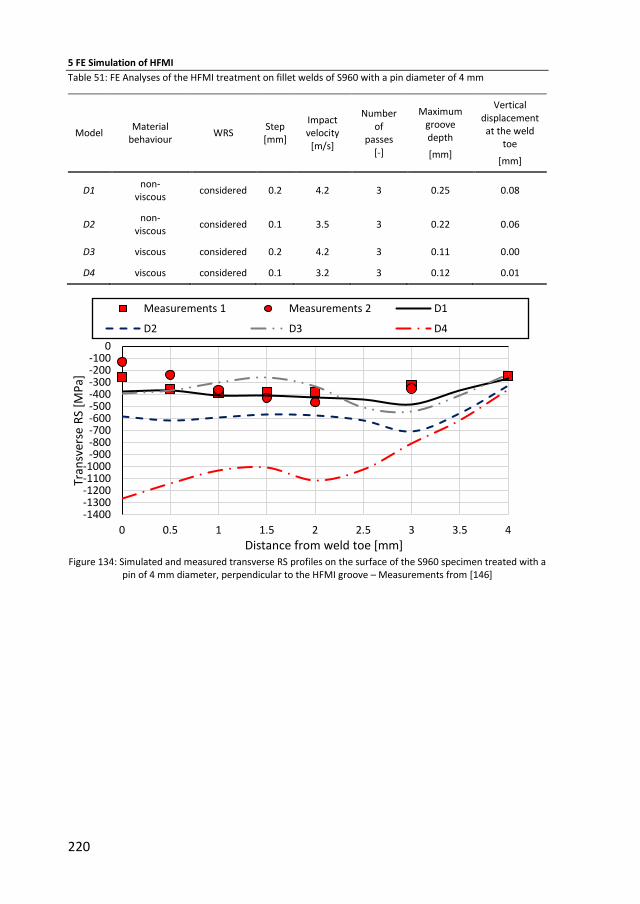
5 FE Simulation of HFMI
220
Table 51: FE Analyses of the HFMI treatment on fillet welds of S960 with a pin diameter of 4 mm
Model Material
behaviour WRS
Step [mm]
Impact velocity
[m/s]
Number of
passes [-]
Maximum groove depth
[mm]
Vertical displacement at the weld
toe
[mm]
D1 non-
viscous considered 0.2 4.2 3 0.25 0.08
D2 non-
viscous considered 0.1 3.5 3 0.22 0.06
D3 viscous considered 0.2 4.2 3 0.11 0.00
D4 viscous considered 0.1 3.2 3 0.12 0.01
Figure 134: Simulated and measured transverse RS profiles on the surface of the S960 specimen treated with a
pin of 4 mm diameter, perpendicular to the HFMI groove – Measurements from [146]
-1400-1300-1200-1100-1000
-900-800-700-600-500-400-300-200-100
0
0 0.5 1 1.5 2 2.5 3 3.5 4
Tran
sver
se R
S [M
Pa]
Distance from weld toe [mm]
Measurements 1 Measurements 2 D1
D2 D3 D4
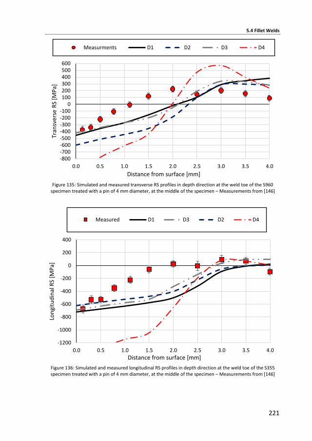
5.4 Fillet Welds
221
Figure 135: Simulated and measured transverse RS profiles in depth direction at the weld toe of the S960
specimen treated with a pin of 4 mm diameter, at the middle of the specimen – Measurements from [146]
Figure 136: Simulated and measured longitudinal RS profiles in depth direction at the weld toe of the S355 specimen treated with a pin of 4 mm diameter, at the middle of the specimen – Measurements from [146]
-800-700-600-500-400-300-200-100
0100200300400500600
0.0 0.5 1.0 1.5 2.0 2.5 3.0 3.5 4.0
Tran
sver
se R
S [M
Pa]
Distance from surface [mm]
Measurments D1 D2 D3 D4
-1200
-1000
-800
-600
-400
-200
0
200
400
0.0 0.5 1.0 1.5 2.0 2.5 3.0 3.5 4.0
Lon
gitu
din
al R
S [M
Pa]
Distance from surface [mm]
Measured D1 D3 D2 D4
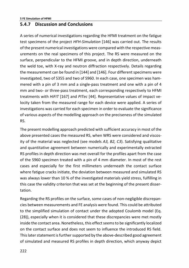
5 FE Simulation of HFMI
222
5.4.7 Discussion and Conclusions
A series of numerical investigations regarding the HFMI treatment on the fatigue
test specimens of the project HFH-Simulation [146] was carried out. The results
of the present numerical investigations were compared with the respective meas-
urements on the real specimens of this project. The RS were measured on the
surface, perpendicular to the HFMI groove, and in depth direction, underneath
the weld toe, with X-ray and neutron diffraction respectively. Details regarding
the measurement can be found in [144] and [146]. Four different specimens were
investigated, two of S355 and two of S960. In each case, one specimen was ham-
mered with a pin of 3 mm and a single-pass treatment and one with a pin of 4
mm and two- or three-pass treatment, each corresponding respectively to HFMI
treatments with HiFIT [167] and PITec [44]. Representative values of impact ve-
locity taken from the measured range for each device were applied. A series of
investigations was carried for each specimen in order to evaluate the significance
of various aspects of the modelling approach on the preciseness of the simulated
RS.
The present modelling approach predicted with sufficient accuracy in most of the
above presented cases the measured RS, when WRS were considered and viscos-
ity of the material was neglected (see models A3, B2, C3). Satisfying qualitative
and quantitative agreement between numerically and experimentally extracted
RS profiles in depth direction was met overall for the profiles apart from the case
of the S960 specimen treated with a pin of 4 mm diameter. In most of the rest
cases and especially for the first millimeters underneath the contact surface
where fatigue cracks initiate, the deviation between measured and simulated RS
was always lower than 10 % of the investigated materials yield stress, fulfilling in
this case the validity criterion that was set at the beginning of the present disser-
tation.
Regarding the RS profiles on the surface, some cases of non-negligible discrepan-
cies between measurements and FE analysis were found. This could be attributed
to the simplified simulation of contact under the adopted Coulomb model (Eq.
(28)), especially when it is considered that these discrepancies were met mostly
inside the contact area. Nonetheless, this effect seems to be significantly localized
on the contact surface and does not seem to influence the introduced RS field.
This later statement is further supported by the above-described good agreement
of simulated and measured RS profiles in depth direction, which anyway depict
5.4 Fillet Welds
223
better the three dimensional stress state of the RS. The measured and simulated
RS are averaged in this case inside the three-dimensional measured gauge vol-
ume, while for surface stresses a two-dimensional averaging area is applied.
Based on the evaluation of the above-presented investigations regarding the fillet
welds the following conclusions can be drawn:
A discretization with mesh finer than 1/40 of the pin’s diameter for the pre-
sent element type and for a distance of at least 1.3 x Dpin away from the
weld toe to all directions is necessary for the precise simulation of HFMI. If
contact surfaces for a transition to a volume with coarser are mesh dictated
as in the present case, the outer coarse mesh should not be larger than 3.5
times the element size of the fine mesh. It has to be mentioned at this point,
that small separation or penetration of the nodes on the contact surface
between the volumes of fine and coarse mesh was observed in a few, indi-
vidual cases without having any obvious effect on the simulated RS. No
stress concentration or discontinuity was observed when the above-men-
tioned requirements were met. A further refinement was anyway not pos-
sible in any case due to computational restrictions.
Modelling a travelling step of 0.2 mm between consecutive impacts, has
been proven insufficient in the present case of a velocity-based simulation.
Denser overlap of 0.15 mm to 0.1 mm had to be adopted depending on the
materials parameters and the number of passes so that a realistic depth of
the HFMI groove could be modelled under the present impact velocities.
The reason for this discrepancy in comparison to the previously investigated
case of parent material specimens was the local geometry of the fillet welds
at the weld toe. The increased friction force in the current analyses due to
the larger contact surface during the penetration of the HFMI pin to the
treated material has to be accounted for the necessity of denser impacts.
For identical material modelling different pairs of impact velocity and trav-
elling step may have introduced grooves of approximately similar depths
but the simulated transverse RS profiles deviate with each other signifi-
cantly (see for example models D1 and D2). Therefore, the density of the
impacts exhibits a significant influence on the modelled transverse RS as it
was proposed earlier in [145]. Hence, a limitation to the assumption of a
step larger than the real for the reduction of the computational time, a sim-
plification that was initially based on the experimental results from [44], is
met as expected.
5 FE Simulation of HFMI
224
Comparing analyses, which assumed identical non-viscous material proper-
ties and overlap of impacts (B1 with B2 or B3 with B4 etc.), the significance
of modelling with preciseness the depth and in extension the geometry of
the HFMI groove, is becoming evident. When no further information is
available, modelling a HFMI groove of 0.15 mm for S355, i.e. the mean value
of the range (0.10 mm - 0.20 mm) proposed by IIW Recommendations for
the quality assurance of the HFMI treatment [118], and a groove of 0.125
mm for S960 in order to compensate for the harder material is recom-
mended for practical applications.
The significant deviation of the simulated RS in cases between pairs of iden-
tical models, which either neglected or considered the WRS (A1 and A3 etc.)
and the significantly better results of the latter exhibit the significance of
considering WRS during a HFMI simulation. Ergo, any assumption that WRS
and the respective plastic strains are negligible in comparison to those in-
troduced by HFMI and they should not be considered during its modelling
is not valid.
Similarly to the case of modelling the HFMI treatment of parent material
specimens of S690 and S960, the consideration of the material’s viscosity in
the present investigations led to overestimation of the compressive RS and
a significant deviation between modelled and measured RS profiles. The
previously stated assumption that for the high strength materials the strain
rate dependency can be lower under the present deformation mode than
that extracted by tensile tests at high strain rates is emphasized again at
this point. It has to be underlined that even for the present S355 specimens,
the higher yield stress of the HAZ was considered which is at the same order
of magnitude with that of the parent material S690 (713 MPa and 734 MPa).
Nonetheless, this incompatibility could be attributed to the simplicity of the
applied Cowper-Symonds model (Eq. (12)), which only scales the yield stress
based on the plastic strain rate and not the hardening behaviour as well. It
is possible, that with a more elaborate material model (Chaboche model
[22], see [143] for instance) an accurate simulation of RS with consideration
of the materials viscocity could be possible. Still, the good agreement of the
current analyses considering a non-viscous model, when the impact density
and velocity and the WRS are modelled accurately, constitutes the respec-
tive models valid and allows for the neglection of strain rate dependency,
5.4 Fillet Welds
225
at least for the currently investigated materials and especially for practical
applications.
Based on the evaluation of the above-presented investigations, which satis-
fied the accuracy criteria of the present study and are considered valid, i.e. the
non-viscous material models with consideration of WRS and accurate simula-
tion of the HFMI groove the following conclusions were drawn:
The RS contours bellow the HFMI groove validate the theoretical distribu-
tions. The stresses around and near the HFMI trace are compressive and
they are counterbalanced by outer tensile stresses. The peak compressive
transverse stresses are met in an elliptical area less than a millimetre
deeper underneath the treatment surface and they are approximately
equal to the yield stress of the material under treatment, i.e. the yield stress
of the HAZ. On the contrary, peak longitudinal RS are met on the top layer
elements underneath the treatment surface and they are significantly
higher than the HAZ yield stress (80 % to 100 % higher). These peaks could
not be depicted by the measurements in the depth direction due to the
large gauge volumes, which were applied during measurements (2 mm x 2
mm x 2 mm and 5 mm x 2 mm x 2 mm for longitudinal and transverse direc-
tion respectively). As the average of the RS inside these volumes is extracted
at each measurement point, the finer fluctuations of the RS profiles that can
be seen on the RS contour plots could not be measured.
The above-stated assumption regarding the scaling-down of the compo-
nent during FE simulation of the HFMI treatment and the proposed require-
ments regarding the modelled HFMI treatment length and the distance
from the edges of the component are validated. The initial assumption that
the local nature of the HFMI treatment allows for the precise simulation of
the RS field of a large HFMI-treated component on a small numerical model
stands and is proposed for practical applications.
The current valid models show better agreement in the case of a single-pass
treatment than in the case of multiple treatment passes (A3, C3 vs B2), alt-
hough sufficient accuracy was met in all cases for the purpose of the present
study. The influence of cyclic plasticity is accounted for the reduced precise-
ness in the latter case. As it was proposed above for the consideration of
viscosity, further improvement could be achieved by adoption of more elab-
orate material modelling such as multilinear σ-ε constitutive relation and
5 FE Simulation of HFMI
226
mixed hardening behaviour. The last one has already been proven to pro-
vide more accurate results than kinematic hardening in previous studies
(see [45], [127]).
Finally, the deviation in some cases between the two series of measurements,
which were carried out on the surface of the specimens, reveals the complexity
of the subject of RS. These measurements, which were carried out parallel to each
other at the centre of the specimens and only some mm away from each other
on macroscopically identical locations, should be theoretically under the same
stress state. Still, they exhibit deviations of up to 10 % of the materials yield limit.
This observation on the one side validates the suitability of the thumb rule of 10 %
agreement between measurements and FE analyses of RS as a criterion for the
validity of the latter one. On the other side, it is becoming evident that local ef-
fects which cannot be easily included in a FE analysis, such as stress concentration
due to local geometrical anomalies or localized changes of hardness, can have a
small effect of this order of magnitude on the RS state.
5.5 Summary and Open Questions Regarding HFMI Simulation
A series of FE analyses regarding the HFMI treatment of parent material and
welded specimens were carried out in the framework of the present disserta-
tion’s last chapter. In the case of parent material specimens, steels S355, S690
and S960 were investigated. In the case of the fillet welds, only the first and the
last ones were investigated. In both cases, measurements of RS were applied for
the validation of the results based on the thumb rule of 10 %, as it was set at the
beginning of the current study. Two different approaches for modelling the
boundary conditions regarding the movement of the HFMI pin were investigated,
a displacement- and a velocity-based. A new, more precise evaluation of a previ-
ous displacement-based study of the author have shown that this method as well
can provide sufficient results. Nonetheless, the velocity-based approach was pre-
ferred in most cases, as it lies closer to physical reality.
During the validation of the present modelling approach, significant conclusions
were drawn regarding the predominant aspects of the HFMI modelling. In most
cases, neglecting the strain-rate dependency of the material in the FE analyses
5.5 Summary and Open Questions Regarding HFMI Simulation
227
led to a very good agreement between modelled and measured RS profiles. In-
troducing viscosity led to increased accuracy only in the simulation of the parent
material S355, the only case where the treated material would not be classified
as high strength steel. On the contrary, it has been shown that during modelling
of HFMI treatment on welded components, WRS should be considered as input
parameter. Otherwise, significant overestimation of the compressive RS field af-
ter completion of the treatment can take place and therefore, contribute to a
non-conservative estimation of the investigated components fatigue life.
Further investigations on an even more elaborate material modelling, which
could provide an even better agreement between measured and simulated RS, is
strongly recommended in future work [143]. Finally, the present validated mod-
elling approach should be applied as a base for a sensitivity analysis regarding the
setup parameters of the HFMI treatment such as HFMI groove depth, impact ve-
locity, travelling velocity, pin diameter, angle of application etc. in an effort to
maximize the magnitude of the introduced compressive RS and in extension the
positive effect of the HFMI treatment on the fatigue life of the welded compo-
nents.

229
6 Overall Discussion
Goal of the present doctoral dissertation was the investigation of the possibilities
regarding the estimation of RS introduced by welding and the HFMI treatment by
means of FE analysis. Initial intention was the establishment of a validated ap-
proach, which would estimate with sufficient preciseness the RS field, taking into
consideration all the predominant aspects that would have a significant influence.
Nevertheless, it was considered fundamental that the established approach could
be reproduced in practice by a structural engineer with only basic knowledge of
material science if possible. In order to fulfil this latter condition, it was required
by the author to investigate in depth not only practical but special aspects of the
simulation, such as elaborate material modelling or boundary conditions model-
ling influence of numerical effects, behaviour of various materials etc. Moreover,
during the realization of the present dissertation, various relevant aspects regard-
ing the investigated subject came up, which were not included in the initial work-
ing plan and were necessary for the fulfilment of the research goal. It was be-
lieved though that their investigation would widen the current knowledge on the
field of RS simulation.
A straightforward engineering modelling approach was developed and proposed
for the consideration of microstructural transformations during welding. Sophis-
ticated aspects of material science like phase transformations or TRIP were taken
into consideration, based on new or existing practical solutions, without changing
the FE formulations. The level of the method’s preciseness can be adjusted de-
pending on the accuracy desired by the modeller in each investigated case. Under
its current form the approach provided significantly better agreement with meas-
ured RS profiles than previous models, fulfilling the set goal of the present disser-
tation. The established method can act either as a validation base for existing
measured welds or predictively for new ones and is applicable for other materials
as well.
Similarly and based on the same principles regarding the applied methodology of
the complex investigated subjects and the straightforwardness of the final estab-
lished model, an approach for the simulation of HFMI was developed as well. A
good agreement between measured and simulated RS profiles with the present
approach was met once again. The influence of several simulation’s aspects on
6 Overall Discussion
230
the modelled RS profiles was investigated and conclusions, which can act as a
guide for practical approach, were drawn.
For the calibration of the material models, which were applied in the numerical
investigations, a series of drop tests was conceived and implemented for the es-
timation of the material’s behaviour under the deformation mode introduced by
HFMI. Useful conclusions were drawn and the method seems promising, although
difficulties regarding the evaluation of the results were encountered.
Future work on the individual parts of the present study has been proposed in
the respective chapters. In the next, final chapter of the current manuscript, pos-
sibilities regarding the future application of the present approach in the frame-
work of a holistic estimation of a HFMI-treated weldment’s fatigue life are dis-
cussed.
231
7 Future Work on Numerical Investigations and Fatigue
If fatigue of steel and metallic components in general could be investigated in a
holistic approach it would constitute a multidisciplinary subject. Of course, fa-
tigue tests accommodated by appropriate, modern measurements and monitor-
ing enable not only a clear overview of the total fatigue life but precise infor-
mation about the regimes of crack initiation and growth. Other than in material
science, in civil engineering the describing models remain in most cases phenom-
enological and are calibrated based on that data. On the contrary, validated nu-
merical analyses can enable a detailed description of the physical phenomena
themselves. Numerical investigations regarding the prediction of fatigue life can
be tracked in studies from different subjects of modern science though. Suitable
FE analyses can predict the crack initiation at metallic crystalline grain level and
they are already applied in the field of material science (see [14] for instance). In
the state-of-the-art investigations of mechanical components, a damage tolerant
approach is adopted and an estimation of the propagation of existing fatigue
cracks is carried out based on fracture mechanics (see for instance [123] or [129]).
Such investigations are common in modern mechanical engineering. Auxiliary to
this fracture mechanics models, the evolution of the WRS simulation methods in
the last years allows for consideration of the stress fields on the investigated
crack’s tip, which can increase significantly their preciseness. Similarly, the pre-
sent study shows that a simulation of the RS field introduced by HFMI is possible.
Until today though, the restricted computational capacity has been the main rea-
son for breaking down the phenomena of fatigue into different regimes. Still, the
increase in computational power will possibly allow in the upcoming years the
synergy of the above-mentioned numerical investigations, up to the composition
of a holistic simulation approach. Such an approach could predict the full fatigue
life of a real scale component from the crack initiation at the grain level up to
fracture. The use of sub-modelling techniques could further accelerate this com-
position. Therewith, an optimal design for each unique mechanical component
against fatigue would be enabled leading to a significant upgrade of engineering
efficiency.

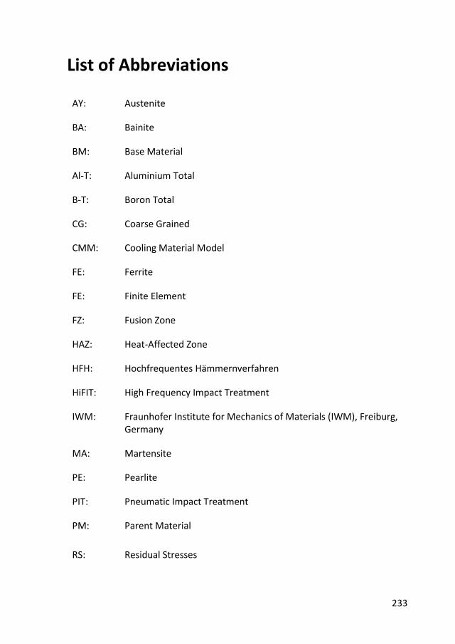
233
List of Abbreviations
AY: Austenite
BA: Bainite
BM: Base Material
Al-T: Aluminium Total
B-T: Boron Total
CG: Coarse Grained
CMM: Cooling Material Model
FE: Ferrite
FE: Finite Element
FZ: Fusion Zone
HAZ: Heat-Affected Zone
HFH: Hochfrequentes Hämmernverfahren
HiFIT: High Frequency Impact Treatment
IWM: Fraunhofer Institute for Mechanics of Materials (IWM), Freiburg, Germany
MA: Martensite
PE: Pearlite
PIT: Pneumatic Impact Treatment
PM: Parent Material
RS: Residual Stresses

List of Abbreviations
234
STAAZ: Spitzentemperatur, Austenitisierungs- und Abkühlungszeit
TRIP: Transformation Induced Plasticity
UFG: Ultra Fine Grained
WPS Welding Procedure Specifications
WRS: Welding Residual Stresses
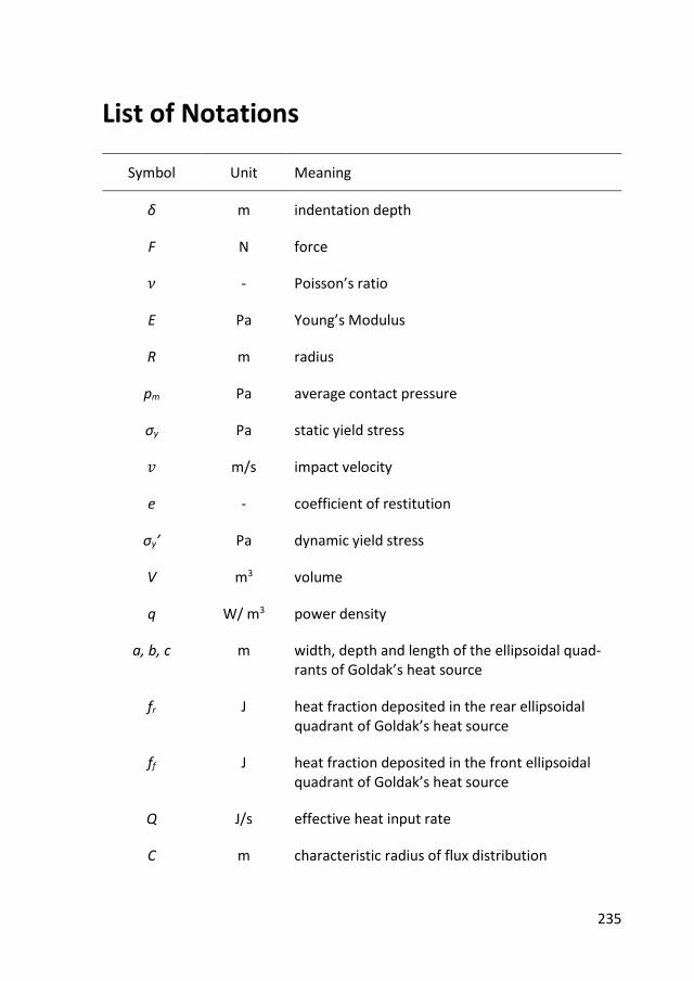
235
List of Notations
Symbol Unit Meaning
δ m indentation depth
F N force
𝜈 - Poisson’s ratio
Ε Pa Young’s Modulus
R m radius
pm Pa average contact pressure
σy Pa static yield stress
𝑣 m/s impact velocity
e - coefficient of restitution
σy’ Pa dynamic yield stress
V m3 volume
q W/ m3 power density
a, b, c m width, depth and length of the ellipsoidal quad-rants of Goldak’s heat source
fr J heat fraction deposited in the rear ellipsoidal quadrant of Goldak’s heat source
ff J heat fraction deposited in the front ellipsoidal quadrant of Goldak’s heat source
Q J/s effective heat input rate
C m characteristic radius of flux distribution
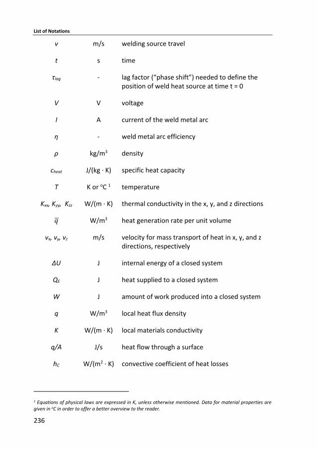
List of Notations
236
v m/s welding source travel
t s time
τlag - lag factor (“phase shift”) needed to define the position of weld heat source at time t = 0
V V voltage
I A current of the weld metal arc
η - weld metal arc efficiency
ρ kg/m3 density
cheat J/(kg ∙ K) specific heat capacity
T K or oC 1 temperature
Kxx, Kyy, Kzz W/(m ∙ K) thermal conductivity in the x, y, and z directions
𝑞 W/m3 heat generation rate per unit volume
vx, vy, vz m/s velocity for mass transport of heat in x, y, and z directions, respectively
ΔU J internal energy of a closed system
QE J heat supplied to a closed system
W J amount of work produced into a closed system
q W/m3 local heat flux density
K W/(m ∙ K) local materials conductivity
q/A J/s heat flow through a surface
hC W/(m2 ∙ K) convective coefficient of heat losses
1 Equations of physical laws are expressed in K, unless otherwise mentioned. Data for material properties are given in oC in order to offer a better overview to the reader.
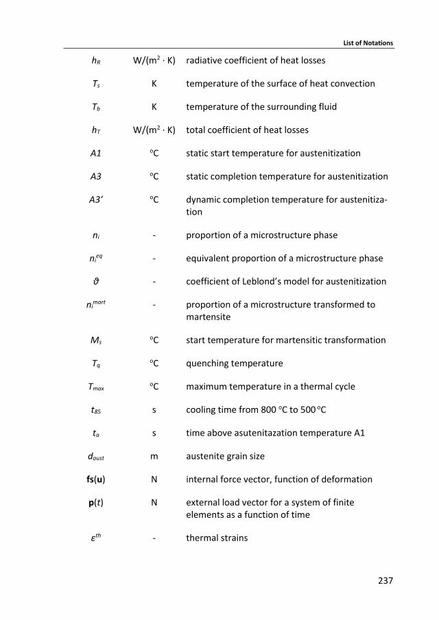
List of Notations
237
hR W/(m2 ∙ K) radiative coefficient of heat losses
Ts K temperature of the surface of heat convection
Tb K temperature of the surrounding fluid
hT W/(m2 ∙ K) total coefficient of heat losses
Α1 oC static start temperature for austenitization
Α3 oC static completion temperature for austenitization
Α3’ oC dynamic completion temperature for austenitiza-tion
ni - proportion of a microstructure phase
nieq - equivalent proportion of a microstructure phase
θ - coefficient of Leblond’s model for austenitization
nimart - proportion of a microstructure transformed to
martensite
Ms oC start temperature for martensitic transformation
Tq oC quenching temperature
Tmax oC maximum temperature in a thermal cycle
t85 s cooling time from 800 oC to 500 oC
ta s time above asutenitazation temperature A1
daust m austenite grain size
fs(u) N internal force vector, function of deformation
p(t) N external load vector for a system of finite elements as a function of time
εth - thermal strains
List of Notations
238
ase - secant coefficient of thermal expansion
H Pa tangent modulus
f(σ) - yield function
J1, J2, J3 N2/mm4 1st, 2nd and 3d invariant of stresses
τ N/mm2 yield stress in shear
s-1 equivalent plastic strain rate
α, β, γ and δ - coefficients with no direct physical meaning char-acterizing the strain rate hardening behaviour
𝒎 kg mass matrix
𝒄 (N ∙ s)/m damping matrix
𝒖, �̇�, �̈� m displacement, velocity and acceleration vector
𝜎𝐹′ Pa von Mises flow stress
휀𝑝′ - equivalent plastic strain
Α Pa coefficient of the Johnson-Cook model
Β Pa coefficient of the Johnson-Cook model
Γ - coefficient of the Johnson-Cook model
ζ - coefficient of the Johnson-Cook model
θ - coefficient of the Johnson-Cook model
휀̇ - reference strain rate
휀̇’ - investigated strain rate
To oC reference temperature level
Tm oC investigated temperature level
pl
List of Notations
239
mSRS - strain rate sensitivity
αR 1/kg coefficient of the Rayleigh model
βR 1/Pa coefficient of the Rayleigh model
f Hz frequency
ξ - damping ratio
Ds - damping factor
Ff N friction force
μ - friction coefficient
FN N normal force exerted by each surface on the other, perpendicular to the contact sufrace
vsliding m/s relative sliding velocity between two surfaces
D m diameter

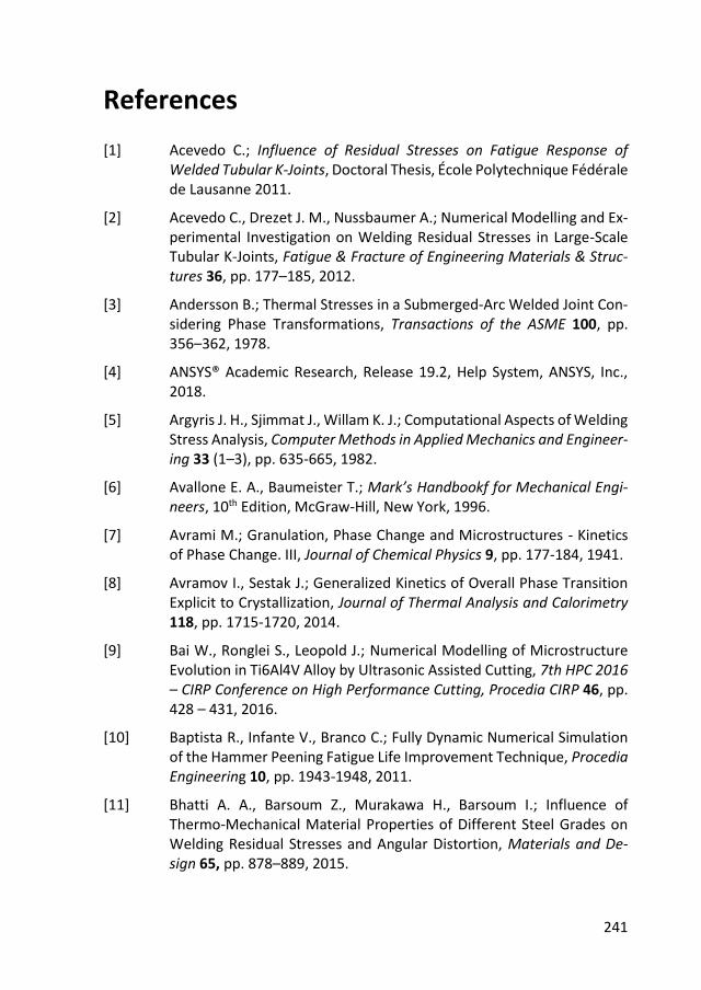
241
References
[1] Acevedo C.; Influence of Residual Stresses on Fatigue Response of Welded Tubular K-Joints, Doctoral Thesis, École Polytechnique Fédérale de Lausanne 2011.
[2] Acevedo C., Drezet J. M., Nussbaumer A.; Numerical Modelling and Ex-perimental Investigation on Welding Residual Stresses in Large-Scale Tubular K-Joints, Fatigue & Fracture of Engineering Materials & Struc-tures 36, pp. 177–185, 2012.
[3] Andersson B.; Thermal Stresses in a Submerged-Arc Welded Joint Con-sidering Phase Transformations, Transactions of the ASME 100, pp. 356–362, 1978.
[4] ANSYS® Academic Research, Release 19.2, Help System, ANSYS, Inc., 2018.
[5] Argyris J. H., Sjimmat J., Willam K. J.; Computational Aspects of Welding Stress Analysis, Computer Methods in Applied Mechanics and Engineer-ing 33 (1–3), pp. 635-665, 1982.
[6] Avallone E. A., Baumeister T.; Mark’s Handbookf for Mechanical Engi-neers, 10th Edition, McGraw-Hill, New York, 1996.
[7] Avrami M.; Granulation, Phase Change and Microstructures - Kinetics of Phase Change. III, Journal of Chemical Physics 9, pp. 177-184, 1941.
[8] Avramov I., Sestak J.; Generalized Kinetics of Overall Phase Transition Explicit to Crystallization, Journal of Thermal Analysis and Calorimetry 118, pp. 1715-1720, 2014.
[9] Bai W., Ronglei S., Leopold J.; Numerical Modelling of Microstructure Evolution in Ti6Al4V Alloy by Ultrasonic Assisted Cutting, 7th HPC 2016 – CIRP Conference on High Performance Cutting, Procedia CIRP 46, pp. 428 – 431, 2016.
[10] Baptista R., Infante V., Branco C.; Fully Dynamic Numerical Simulation of the Hammer Peening Fatigue Life Improvement Technique, Procedia Engineering 10, pp. 1943-1948, 2011.
[11] Bhatti A. A., Barsoum Z., Murakawa H., Barsoum I.; Influence of Thermo-Mechanical Material Properties of Different Steel Grades on Welding Residual Stresses and Angular Distortion, Materials and De-sign 65, pp. 878–889, 2015.
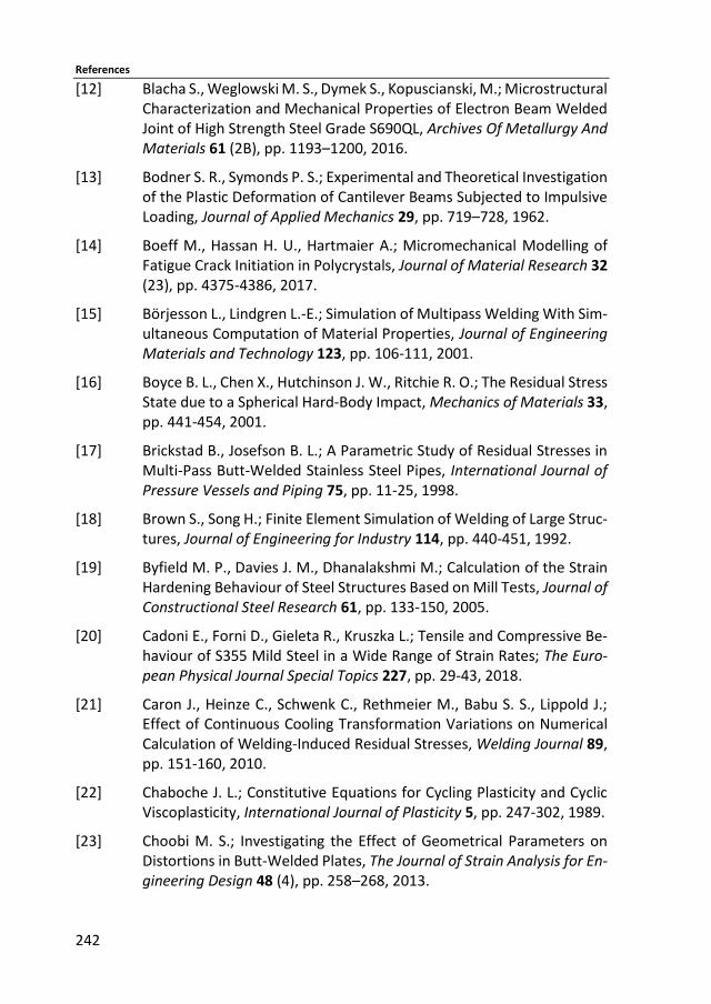
References
242
[12] Blacha S., Weglowski M. S., Dymek S., Kopuscianski, M.; Microstructural Characterization and Mechanical Properties of Electron Beam Welded Joint of High Strength Steel Grade S690QL, Archives Of Metallurgy And Materials 61 (2B), pp. 1193–1200, 2016.
[13] Bodner S. R., Symonds P. S.; Experimental and Theoretical Investigation of the Plastic Deformation of Cantilever Beams Subjected to Impulsive Loading, Journal of Applied Mechanics 29, pp. 719–728, 1962.
[14] Boeff M., Hassan H. U., Hartmaier A.; Micromechanical Modelling of Fatigue Crack Initiation in Polycrystals, Journal of Material Research 32 (23), pp. 4375-4386, 2017.
[15] Börjesson L., Lindgren L.-E.; Simulation of Multipass Welding With Sim-ultaneous Computation of Material Properties, Journal of Engineering Materials and Technology 123, pp. 106-111, 2001.
[16] Boyce B. L., Chen X., Hutchinson J. W., Ritchie R. O.; The Residual Stress State due to a Spherical Hard-Body Impact, Mechanics of Materials 33, pp. 441-454, 2001.
[17] Brickstad B., Josefson B. L.; A Parametric Study of Residual Stresses in Multi-Pass Butt-Welded Stainless Steel Pipes, International Journal of Pressure Vessels and Piping 75, pp. 11-25, 1998.
[18] Brown S., Song H.; Finite Element Simulation of Welding of Large Struc-tures, Journal of Engineering for Industry 114, pp. 440-451, 1992.
[19] Byfield M. P., Davies J. M., Dhanalakshmi M.; Calculation of the Strain Hardening Behaviour of Steel Structures Based on Mill Tests, Journal of Constructional Steel Research 61, pp. 133-150, 2005.
[20] Cadoni E., Forni D., Gieleta R., Kruszka L.; Tensile and Compressive Be-haviour of S355 Mild Steel in a Wide Range of Strain Rates; The Euro-pean Physical Journal Special Topics 227, pp. 29-43, 2018.
[21] Caron J., Heinze C., Schwenk C., Rethmeier M., Babu S. S., Lippold J.; Effect of Continuous Cooling Transformation Variations on Numerical Calculation of Welding-Induced Residual Stresses, Welding Journal 89, pp. 151-160, 2010.
[22] Chaboche J. L.; Constitutive Equations for Cycling Plasticity and Cyclic Viscoplasticity, International Journal of Plasticity 5, pp. 247-302, 1989.
[23] Choobi M. S.; Investigating the Effect of Geometrical Parameters on Distortions in Butt-Welded Plates, The Journal of Strain Analysis for En-gineering Design 48 (4), pp. 258–268, 2013.
References
243
[24] Chopra A. K.; Dynamics of Structures – Theory and Application to Earth-quake Engineering, 4th Edition, Pearson Prentice Hall, New Jersey 2012.
[25] Cowper G. R., Symonds P. S.; Strain Hardening and Strain rate Effects in the Impact Loading of Cantilever Beams, Report No. 28, Brown Univer-sity Division of Applied Mathematics, September 1957.
[26] Dattoma V., De Giorgi M., Nobile R.; On the Evolution of Welding Re-sidual Stress after Milling and Cutting Machining, Computers and Struc-tures 84, pp. 1965–1976, 2006.
[27] De Benardos N., Olszewski S; Process of AMD Apparatus for Working Metals by the Direct Application of the Electric Current, No. 363, 320, 1887.
[28] Deng D., Murakawa H.; Numerical Simulation of Temperature Field and Residual Stress in Multi-Pass Welds in Stainless Steel Pipe and Compar-ison with Experimental Measurements, Computational Materials Sci-ence 37, pp. 269–277, 2006.
[29] DIN EN 10025-2:2005-04; Hot Rolled Products of Structural Steels - Part 2: Technical Delivery Conditions for Non-Alloy Structural Steels, 2004.
[30] DIN EN 10025-6:2018-07; Hot Rolled Products of Structural Steels - Part 6: Technical Delivery Conditions for Flat Products of High Yield Strength Structural Steels in the Quenched and Tempered Conditions, 2018.
[31] Dong P.; Residual Stress Analyses of a Multi-Pass Girth Weld: 3-D Spe-cial Shell versus Axisymmetric Models, Journal of Pressure Vessel Tech-nology 123, pp. 207-213, 2001.
[32] Dupont J. N., Marder A. R.; Thermal Efficiency of Arc Welding Pro-cesses, Welding Journal 74, pp. 406–416, 1995.
[33] Dürr, A.; Zur Ermüdungsfestigkeit von Schweißkonstruktionen aus hö-herfesten Baustählen bei Anwendung von UIT-Nachbehandlung, Disser-tation, Fakultät Bau- und Umweltingenieurwissenschaften, Universität Stuttgart 2006.
[34] EN 1993-1-9; Eurocode 3: Design of Steel Structures - Part 1-2: General Rules - Structural Fire Design, 2009.
[35] EN 1993-1-9; Eurocode 3 - Design of Steel Structures - Part 1-9: Fatigue, 2009.
[36] Ernould C., Schubnell J., Farajian M., Maciolek A., Simunek D., Leitner M., Stotschka M.; Applications of Different Simulation Approaches to Numerically Optimize High-Frequency Mechanical Impact (HFMI) Post-Treatment Process, Welding in the World 63 (3), pp. 725–738, 2019.
References
244
[37] DIN EN 573-3:2018-12; Aluminium and Aluminium Aalloys - Chemical Composition and Form of Wrought Products - Part 3: Chemical Compo-sition and Form of Products, 2018
[38] Feldmann M., Bartsch H., Ummenhofer T., Seyfried B., Kuhlmann U., Drebenstedt K.; Neubewertung und Erweiterung des Kerbfallkataloges nach Eurocode 3 für eine zukunftsfähige Auslegung hochbeanspruchter Stahlkonstruktionen, Schlussbericht (in Bearbeitung), Im Auftrag von Deutscher Ausschuss für Stahlbau (DASt) in Kooperation mit For-schungsvereinigung Stahlanwendung e.V. FOSTA, IGF 19178 N, 2019.
[39] Ferro P., Bonollo F.; Modelling of the Carburizing and Quenching Pro-cess Applied to Caterpillar Track Bushings, Modelling and Simulation in Materials Science and Engineering 22 (2), 2014.
[40] Ferro P., Porzner H., Tiziani A., Bonollo F.; The Influence of Phase Trans-formations on Residual Stresses Induced by the Welding Process—3D and 2D Numerical Models, Modelling and Simulation in Materials Sci-ence and Engineering 14, pp. 117–136, 2006.
[41] Fischer-Cripps A. C.; Introduction to Contact Mechanics, 2nd Edition, Springer, Boston, 2007.
[42] Fischer F. D., Sun Q.-P., Tanaka K.; Transformation-Induced Plasticity (TRIP), ASME Appied Mechanics Reviews 49 (6), pp. 317-364, 1996.
[43] Flanagan D. P., Belytcshko T.; A Uniform Strain Hexaedron and Quadri-lateral with Orthogonal Hourglass Control, International Journal for Nu-merical Methods in Engineering 17, pp. 679-706, 1981.
[44] Foehrenbach J., Hardenacke V., Farajian M.; High Frequency Mechani-cal Impact Treatment (HFMI) for the Fatigue Improvement: Numerical and Experimental Investigations to describe the Condition in the Sur-face Layer, Welding in the World 60 (4), pp. 749–755, 2016.
[45] Foehrenbach J., Hardenacke V., Farajian M., Luke M.; Fatigue Life Cal-culation of High Frequency Mechanical Impact (HFMI) Treated Welded Joints by means of Numerical Process Simulation and Critical Plane Ap-proaches, IIW Commission XIII, Doc. XIII-2637-16, 2016.
[46] Forni D., Chiaia B., Cadoni E.; Blast Effects on Steel Columns under Fire Conditions, Journal of Constructional Steel Research 136, pp. 1-10, 2017.
[47] Forni D., Chiaia B., Cadoni E.; High Strain Rate Response of S355 at High Temperatures, Materials and Design 94, pp. 467-478, 2016.
References
245
[48] Forni D., Chiaia B., Cadoni E.; Mechanical Properties of S355 under Ex-treme Coupled Effect of High Temperatures and High Strain Rates, EC-COMAS Congress 2016 VII European Congress on Computational Meth-ods in Applied Sciences and Engineering M. Papadrakakis, V. Papadopoulos, G. Stefanou, V. Plevris (eds.), Crete Island 5-10 June 2016.
[49] Forni D., Chiaia B., Cadoni E.; Strain Rate Behaviour in Tension of S355 Steel: Base for Progressive Collapse Analysis, Engineering Structures 119, pp. 167-173, 2016.
[50] Forrestal M. J., Sagartz M. J.; Elastic–Plastic Response of 304 Stainless Steel Beams to Impulse Loads, Journal of Applied Mechanics 45, pp. 685–687, 1978.
[51] Francis J. A., Bhadeshia H. K. D. H., Withers P. J.; Welding Residual Stresses in Ferritic Power Plant Steels, Material Science and Technology 23, pp. 1009-1020, 2007.
[52] Fujita Y., Takesshi Y., Kitamura M., Nomoto T.; Welding Stresses with Special Reference to Cracking, IIW Doc X-655-72, 1972.
[53] Gkatzogiannis S., Knoedel P., Ummenhofer T.; A Pseudothermal Ap-proach for Simulating the Residual Stress Field Caused by Shot Blasting, Proceedings of the VIII International Conference on Computational Methods for Coupled Problems in Science and Engineering, Sitges 3-6 June 2019, pp. 777-788, 2019.
[54] Gkatzogiannis S., Knoedel P., Ummenhofer T.; FE Simulation of High Frequency Mechanical Impact (HFMI) Treatment – First Results, Pro-ceeding of NORDIC STEEL 2019, The 14th Nordic Steel Construction Con-ference, Copenhagen 18–20 September 2019, ce/papers 3 (3-4), pp. 797-802, Ernst & Sohn, 2019.
[55] Gkatzogiannis S., Knoedel P., Ummenhofer T.; FE Welding Residual Stress Simulation – Influence of Boundary Conditions and Material Models, Proceedings of EUROSTEEL 2017, Copenhagen 13–15 Septem-ber 2017, ce/papers 1, Ernst & Sohn, 2017.
[56] Gkatzogiannis S., Knoedel P., Ummenhofer T.; Influence of Welding Pa-rameters on the Welding Residual Stresses, Proceedings of the VII In-ternational Conference on Coupled Problems in Science and Engineer-ing, Rhodes 12–14 June 2017, pp. 767–778, 2017.
[57] Gkatzogiannis S., Knoedel P., Ummenhofer T.; Reviewing the Influence of Welding Setup on FE-simulated Welding Residual Stresses, Proceed-ings of the 10th European Conference on Residual Stresses - ECRS10,
References
246
Leuven 11-14 September 2018, published in Materials Research Pro-ceedings 6, pp. 197-202, 2018.
[58] Gkatzogiannis S., Knoedel P., Ummenhofer T.; Simulation of Welding Residual Stresses – From Theory to Practice, Selected Peer Reviewed Papers from the 12th International Seminar Numerical Analysis of Weldability, Graz – Schloss Seggau 23-26 September, published in Som-mitsch C., Enzinger N., Mayr P.; Mathematical Modelling of Weld Phe-nomena 12, pp. 383-400, 2019.
[59] Gkatzogiannis S., Knoedel P., Ummenhofer T.; Strain Rate Dependency of Simulated Welding Residual Stresses, Journal of Material Engineer-ing and Performance 27 (10), pp. 5079-5085, 2017.
[60] Goldak J. A., Akhlaghi M.; Computational Welding Mechanics, 1st Edi-tion, Springer US, New York, 2005.
[61] Goldak J. A., Chakravarti A., Bibby M.; A New Finite Element Model for Welding Heat Sources, Metallurgical Transactions B 15, pp. 299–305, 1984.
[62] Greenwood G. W., Johnson R. H.; The Deformation of Metals Under Small Stresses During Phase Transformation, Proceedings of the Royal Society A 283, pp. 403-422, 1965.
[63] Guagliano M.; Relating Almen Intensity to Residual Stresses Induced by Shot Peening: a Numerical Approach, Journal of Materials Processing Technology 110, pp. 277-286, 2001.
[64] Guo C., Zhijiang W., Dongpo W., Shengsun H.; Numerical Analysis of the Residual Stress in Ultrasonic Impact Treatment Process with Single-Im-pact and Two-Impact Mode, Applied Surface Science 347, pp. 596-601, 2015.
[65] Gupta C., Chakravartty J. K., Wadekar S. L., Dubey J. S.; Effect of Ser-rated Flow on Deformation Behaviour of AISI 403 Stainless Steel, Ma-terials Science and Engineering A 292, pp. 49-55, 2000.
[66] Ηaidemenopoulos G.; Εισαγωγή στις Συγκολλήσεις [Introduction to Welding], 1st Edition, Tziolas Publications, Thessaloniki 2010.
[67] Ηaidemenopoulos G.; Φυσική Μετταλουργία [Physical Metallurgy], 1st Edition, Tziolas Publications, Thessaloniki 2007.
[68] Hardenacke V., Farajian M., Siegele D.; Modelling and Simulation of the High Frequency Mechanical Impact (HFMI) Treatment of Welded Joints, IIW Commission XIII, Doc. XIII-2533-14, 2014.
References
247
[69] Heinze C., Schwenk C., Rethmeier M., Caron J.; Numerical Sensitivity Analysis of Welding-Induced Residual Stress Depending on Variations in Continuous Cooling Transformation Behavior, Frontiers of Material Science 5 (2), pp. 168–178, 2011.
[70] Heinze C., Schwenk C., Rethmeier M.; Numerical Calculation of Residual Stress Development of Multi-Pass Gas Metal Arc Welding, Journal of Constructional Steel Research 72, pp. 12-19, 2012.
[71] Hensel J., Nitschke-Pagel T., Dilger K.; On The Effects of Austenite Phase Transformation on Welding Residual Stresses in Non-Load Carrying Longitudinal Welds, Welding in the World 59, pp. 179–190, 2015.
[72] Hensel J., Nitschke-Pagel T., Eslami H., Dilger K.; Fatigue Strength En-hancement of Butt Welds by Means of Shot Peening and Clean Blasting, IIW Document XIII-2733-18, 2018.
[73] Hertz H.; Über die Berührung fester elastischer Körper, J. Reine und An-gewandte Mathematik 92, pp. 156-171, 1881.
[74] Hildebrand J.; Numerische Schweißsimulation: Bestimmung von Tem-peratur, Gefüge und Eigenspannung an Schweißverbindungen aus Stahl- und Glaswerkstoffen, Dissertation, Fakultät Bauingenieurwesen, Bauhaus-Universität Weimar 2008.
[75] Hill R.; The Mathematical Theory of Plasticity, 1st Edition, Oxford Uni-versity Press, New York, 1950.
[76] Hobbacher A.; Recommendations for Fatigue Design of Welded Joints and Components, IIW Commission XIII, Doc. XIII-2151r4-07/XV-1254r4-07, 2008.
[77] Hong T., Ooi J. Y., Shaw B.; A Numerical Simulation to Relate the Shot peening parameters to the Induced Residual Stresses, Engineering Fail-ure Analysis 15, pp. 1097–1110, 2008.
[78] Huh H., Lim J. H., Song J. H., Lee K.-S., Lee Y.-W., Han S. S.; Crashwor-thiness Assessment of Side Impact of an Auto-Body with 60trip Steel for Side Members, International Journal of Automotive Technology 4 (3), pp. 146-156, 2003.
[79] ISO 5817:2014; Welding - Fusion-Welded Joints in Steel, Nickel, Tita-nium and Their Alloys (Beam Welding Excluded) - Quality Levels for Im-perfections, 3rd Edition.
[80] ISO 19675:2017; Non-destructive testing — Ultrasonic testing — Speci-fication for a calibration block for phased array testing (PAUT), 2017.
References
248
[81] Jackson R, Green I.; A Finite Element Study of Elasto-plastic Hemispher-ical Contact, Proceedings of 2003 STLE/ASME Joint International Tribol-ogy Conference, Ponte Vedra Beach 26-29 October 2003, .
[82] Johnson K. L.; Contact Mechanics, 1st Edition, Cambridge University Press, Cambridge (UK), 1985.
[83] Johnson K. L.; The Correlation of Indentation Experiments, Journal of the Mechanics and Physics of Solids 18, pp. 115-126, 1970.
[84] Johnson G. R., Cook W. H.; A Constitutive Model and Data for Metals subjected to Larger Strains, High Strain Rates and High Temperatures, Proceedings of the 7th International Symposium on Ballistics, the Hague 19-21 April 1983, pp. 541–547, 1983.
[85] Johnson W., Mehl R.; Reaction Kinetics in Processes of Nucleation and Growth, Transactions of American Institute of Mining and Metallurgical Engineers 135, pp. 416-458, 1939.
[86] Jones, N.; Structural Impact, 2nd Edition, Cambridge University Press, New York, 2012.
[87] Karlsson C. T.; Finite Element Analysis of Temperatures and Stresses in a Single-Pass Butt-Welded Pipe — Influence Of Mesh Density And Ma-terial Modelling, Engineering with Computers 6, pp. 133–141, 1989.
[88] Katsareas D. E., Ohms C., Youtsos A. G.; Finite Element Simulation of Welding in Pipes: A Sensitivity Analysis, Proceedings of a Special Sym-posium held within the 16th European Conference of Fracture – ECF16, Alexandroupolis, 3-7 July 2006, pp. 15-26, 2006.
[89] Kim T., Lee H., Hyun H. C., Jung S.; A Simple but Effective FE Model with Plastic Shot for Evaluation of Peening Residual Stress and its Experi-mental Validation, Science and Engineering A 528, pp. 5945–5954, 2011.
[90] Kim T., Lee H., Jung S., Lee J. H.; A 3D FE Model with Plastic Shot for Evaluation of Equi-Biaxial Peening Residual Stress due to Multi-Im-pacts, Surface & Coatings Technology 206, pp. 3125–3136, 2012.
[91] Knobloch M., Pauli J., Fontana M.; Influence of the Strain Rate on the Mechanical Properties of Mild Carbon Steel at Elevated Temperatures, Materials & Design 49, pp. 553-565, 2013.
[92] Knoedel P., Gkatzogiannis, S., Ummenhofer T.; Practical Aspects of Welding Residual Stress Simulation, Journal of Constructional Steel Re-search 132, pp. 83-96, 2017.
References
249
[93] Knoedel P., Gkatzogiannis S., Ummenhofer T.; FE Simulation of Residual Welding Stresses: Aluminum and Steel Structural Components, Key En-gineering Materials 710, pp. 268-274, 2016.
[94] Koistinen D. P., Marburger R. E.; A General Equation Prescribing the Ex-tent of the Austenite-Martensite Transformation in Pure Iron-Carbon Alloys and Plain Carbon Steels, Acta Metall. 7, pp. 59–61, 1959.
[95] Kolmogorov A.; Statistical Theory of Crystallization of Metals (in Rus-sian), Izvestia Akameia Nauk SSSR Ser. Mathematica 1(1), pp. 355-359, 1937 (cited after [111]).
[96] Kou S.; Welding Metallurgy, 2nd Edition, John Wiley & Sons, Hoboken New Jersey, 2003.
[97] Kraus H. G.; Experimental Measurement of Thin Plate 304 Stainless Steel GTA Weld Pool Surface Temperatures, Welding Research Supple-ment, pp. 353-359, 1987.
[98] Kuhlmann U.; Experimentelle Untersuchungen zur ermüdungssteigern-den Wirkung des PIT-Verfahrens, Versuchsbericht, Fakultät Bau- und Umweltingenieurwissenschaften, Universität Stuttgart 2009.
[99] Kuilin Y., Sumi Y.; Simulation of Residual Stress and Fatigue Strength of Welded Joints Under the Effects of Ultrasonic Impact Treatment (UIT), International Journal of Fatigue 92, pp. 321-332, 2016.
[100] Kuilin Y., Sumi Y.; Modelling of Ultrasonic Impact Treatment (UIT) of Welded Joints and its Effect on Fatigue Strength, Frattura ed Integrità Strutturale 34, pp. 476-486, 2015.
[101] Kurtara H., Buyuk M., Eskandarian A.; Ballistic Impact Simulation of GT Model Vehicle Door Using Finite Element Method, Theoretical and Ap-plied Fracture Mechanics 40, pp. 113-121, 2003.
[102] Ladendorf P., Schubnell J., Knoedel P., Farajian M., Ummenhofer T., Luke T.; Entwicklung einer verifizierten Prozedur für die zuverlässige schweißtechnische Instandsetzung von Großbauteilen: Ausführung, Be-messung und Lebensdauerbewertung, Abschlussbericht DVS 12021 – IGF 18988, KIT Stahl- und Leichtbau, Versuchsanstalt für Stahl, Holz und Steine, Karlsruhe und Fraunhofer Institut für Werkstoffmechanik, Frei-burg, 2019.
[103] Le Quilliec G., Lieurade H.-P., Bousseau M., Drissi-Habti M., Inglebert G., Macquet P., Jubin L.; Fatigue Behaviour of Welded Joints Treated by High Frequency Hammer Peening: Part II, Numerical Study, IIW Com-mission XIII, Doc. XIII -2395-11, 2011.
References
250
[104] Leblond J. B., Devaux J.; A New Kinetic Model for Anisothermal Metal-lurgical Transformations in Steels Including Effect of Austenite Grain Size, Acta Metallurgica 32, pp. 137–146, 1984.
[105] Leblond J. B., Devaux J.; Mathematical Modelling of Transformation Plasticity in Steels I: Case of Ideal-Plastic Phases, International Journal of Plasticity 5, pp. 551-572, 1989.
[106] Lee C. K., Chiew S. P., Jiang J.; 3D Residual Stress Modelling of Welded High Strength Steel Plate-to-Plate Joints, Journal of Constructional Steel Research 84, pp. 94–104, 2013.
[107] Lee S. J., Lee Y. K.; Prediction of Austenite Grain Growth during Austen-itization of Low Alloy Steels, Materials & Design 29, pp. 1840–1844, 2008.
[108] Leitner M., Simunek D., Shah S. F., Stoschka M.; Numerical Fatigue As-sessment of Welded and HFMI-Treated Joints by Notch Stress/Strain and Fracture Mechanical Approaches, Advances in Engineering Soft-ware 120, pp. 96-106, 2018.
[109] Leitner M., Stoschka M., Eichlseder W.; Fatigue Enhancement of Thin-Walled, High-Strength Steel Joints by High-Frequency Mechanical Im-pact Treatment, Welding in the World 58 (1), pp. 29-39, 2013.
[110] Lim C. T., Stronge W. J.; Normal Elastic-Plastic Impact in Plane Strain, Mathematical and Computer Modelling 28 (4-8), pp. 323-340, 1998.
[111] Lindgren L.-E.; Computational Welding Mechanics - Thermomechanical and Microstructural Simulations, 1st Edition, Woodhead Publishing in Materials, Cambridge (UK), 2007.
[112] Loose T.; Einfluß des transienten Schweißvorganges auf Verzug, Eigen-spannungen und Stabilitätsverhalten axial gedrückter Kreiszylinder-schalen aus Stahl, Fakultät für Bauingenieur-, Geo- und Umweltwisse-schaften, Universität Friedericiana zu Karlsruhe (TH) 2007.
[113] LS-DYNA, Keyword User’s Manual, Livermore Software Technology Cor-poration (LSTC), Livermore California, 2016.
[114] LS-DYNA, Theory Manual, Livermore Software Technology Corporation (LSTC), Livermore California, 2016.
[115] Mangering I., Kroyer R., Koller M.; Experimental and Numerical Analysis of the Effectiveness of High-Frequency Peening Processes, Steel Con-struction 10 (1), pp. 54-66, 2017.
References
251
[116] Macedo M. Q., Cota A. B., Araújo F. G. d. S.; The Kinetics of Austenite Formation at High Heating Rates, Rem Revista Escola de Minas 64 (2), pp. 163–167, 2011.
[117] Magee A. C., Ladani L.; Temperature Dependency of Mechanical Behav-ior and Strain Rate Sensitivity of an Al-Mg Alloy with Bimodal Grain Size, Materials Science and Engineering A 582, pp. 276-283, 2013.
[118] Marquis G. B., Barsoum Z.; IIW Recommendations for the HFMI Treat-ment – For Improving the Fatigue Strength of Welded Joints, 1st Edition, Springer Singapore (IIW Collection), Singapore, 2016.
[119] Marquis G. B., Mikkola E., Yildirim H. C.; Fatigue Strength Improvement of Steel Structures by High-Frequency Mechanical Impact: Proposed Fatigue Assessment Guidelines, Welding in the World 57, pp. 803–822, 2013.
[120] Mataya M. C., Carr M. J.; The Bauschinger Effect in a Nitrogen-Strength-ened Austenitic Stainless Steel, Materials Science and Engineering 57, pp. 205-222, 1983.
[121] MATLAB and Statistics Toolbox Release R2015a, The MathWorks, Na-tick, Massachusetts, USA, 2015.
[122] May J., Höppel H. W., Göken M.; Strain Rate Sensitivity of Ultrafine-Grained Aluminium Processed by Severe Plastic Deformation, Scripta Materialia 53, pp. 189-194, 2005.
[123] Mc Clung R. C., Sehitoglu H.; On the Finite Element Analysis of Fatigue Crack Closure – 1. Basic Modeling Issues, Engineering Fracture Mechan-ics 33 (2), pp. 237-252, 1989.
[124] Meguid S. A., Yang F., Zhuo C., Guagliano M.; 3D FE Analysis of Shot Peening of Strain rate Sensitive Material Account for Multiple and Re-peated Impingement, 13th International Conference on Fracture, Bei-jing 16-21 June 2013.
[125] Moradi R., McCoy M. L., Lankarani M.; Impact Analysis of Mechanical Systems Using Stress Wave Propagation Methodology, published in Wave Propagation, 1st Edition, Academy Publishing, pp. 209-247, 2014.
[126] Mullins J., Gunnars J.; Influence of Hardening Model on Weld Residual Stress Distribution, Research Report 2009:16, Inspecta Technology AB, Stockholm 2009.
[127] Nagel S., Knoedel P., Ummenhofer T.; Testing of Ultra-Low Cycle Fa-tigue at Complex Loading Scenarios, presented in the 2nd International
References
252
Conference on Structural Integrity, Madeira 4-7 September 2017, pub-lished in Structural Integrity Procedia 5, pp. 1377-1384, 2017.
[128] Nart E., Celik Y.; A Practical Approach for Simulating Submerged Arc Welding Process Using FE Method, Journal of Constructional Steel Re-search 84, pp. 62–71, 2013.
[129] Ngoula D. T., Beier H. T., Vormwald M.; Fatigue of Welded Joints De-scribed by Elastic-Plastic Fracture Mechanics, Stahlbau 87 (5), pp. 491-496, 2018.
[130] Nitschke-Pagel T., Dilger K., Eslami H., Ummenhofer T.; Residual Stresses and Near Surface Material Condition of Welded High Strength Steels after Different Mechanical Post-Weld Treatments, The Twenti-eth International Offshore and Polar Engineering Conference, Beijing 20-25 June 2010.
[131] Norström L. Å.; The Influence of Nitrogen and Grain Size On Yield Strength in Type AISI 316L Austenitic Stainless Steel, Metal Science 11 (6), pp. 208-212, 1977.
[132] Oddy A., Goldak J., Mc Dill M.; Transformation Effects in the 3D Finite Element Analysis of Welds, 2nd International Conference in Welding Re-search, Gatlinburg, 1989.
[133] Oliveira F. L. G., Andrade M. S., Cota A. B.; Kinetics of Austenite For-mation During Continuous Heating in a Low Carbon Steel, Materials Characterization 58, pp. 256–261, 2007.
[134] Ossenbrink R., Michailov V.; Thermomechanical Numerical Simulation with the Maximum Temperature Austenisation Cooling Time Model (STAAZ), Mathematical Modelling of Weld Phenoma 8, pp. 357–372, 2007.
[135] Paik J. K.; Cutting of a Longitudinally Stiffened Plate by a Wedge, Journal of Ship Research 38 (4), pp. 340–348, 1994.
[136] Perzyna P.; Fundamental Problems in Viscoplasticity, Advances in Ap-plied Mechanics 9, pp. 243-377, 1966.
[137] Ramberg W., Osgood W. R.; Description of Stress-Strain Curves by three Parameters, Technical Note No. 902, National Advisory Committee for Aeronautics, Washington DC, 1943.
[138] Rammerstorfer F. G., Fischer D. F., Mitter W., Bathe K. J., Snyder M. D.; On Thermo-Elastic-Plastic Analysis of Heat-Treatment Processes In-cluding Creep and Phase Changes, Computers and Structures 13, pp. 771-77, 1981.
References
253
[139] Radaj D.; Heat Effects of Welding – Temperature Field, Residual Stress, Distortion, 1st Edition, Springer Verlag, Berlin 1992.
[140] Rohr K.; Evaluation of Weld-induced Residual Stresses in S690 Steel, Di-ploma Thesis, KIT Faculty of Civil Engineering, Geo- and Environmental Sciences, Karlsruhe 2013.
[141] Sarkani S., Tritchkov V., Michaelov G.; An Efficient Approach for Com-puting Residual Stresses in Welded Joints, Finite Elements in Analysis and Design 35, pp. 247-268, 2000.
[142] Schaumann P., Keindorf C.; Numerische Schweißsimulation gekoppelt mit einem anschließenden Hämmerprozess und integrierten lokalen Ermüdungsberechnungen, Stahlbau 79 (1), pp. 34-45, 2010.
[143] Schubnell J.; Doctoral Dissertation, KIT Faculty of Mechanical Engineer-ing, Karlsruhe, to be submitted in 2020.
[144] Schubnell J., Carl E., Farajian M., Gkatzogiannis S., Knödel P., Ummen-hofer T., Wimpory R., Eslami H.; Residual Stress Relaxation in HFMI-Treated Fillet Welds After Single Overload Peaks, IIW Commission XIII, Fatigue of Welded Components and Structures XIII-2829-19, 2019.
[145] Schubnell J., Eichheimer C., Ernould C., Maciolek A., Rebelo-Kornmeier J., Farajian M.; The Influence of Coverage for High Frequency Mechan-ical Impact Treatment of Different Steel Grades, Journal of Materials Processing Technology 277, 116437, 2020.
[146] Schubnell J., Gkatzogiannis S., Farajian M., Knoedel P., Luke T., Ummen-hofer T.; Rechnergestütztes Bewertungstool zum Nachweis der Lebens-dauerverlängerung von mit dem Hochfrequenz-Hämmerverfahren (HFMI) behandelten Schweißverbindungen aus hochfesten Stählen, Ab-schlussbericht DVS 09069 – IGF 19227 N, Fraunhofer Institut für Werk-stoffmechanik, Freiburg und KIT Stahl- und Leichtbau, Versuchsanstalt für Stahl, Holz und Steine, Karlsruhe, 2020.
[147] Seyffarth P.; Atlas SchweiB-ZTU-Schaubilder, VEB Verlag Technik and DVS-Verlag, Berlin und Düsseldorf, 1982.
[148] Seyffarth P, Meyer B., Scharff A.; Großer Atlas Schweiß-ZTU-Schaubil-der, DVS-Verlag, Düsseldorf, 1992.
[149] Shaw B. A., Korsunsky A. M., Evans J. T.; Surface Treatment and Resid-ual Stress Effects on the Fatigue Strength of Carburised Gears, Pre-sented at the 12th European Conference on Fracture (ECF-12), Sheffield 14–18 September 1998.
References
254
[150] Simunek D., Leitner M., Stoschka M.; Numerical Simulation Loop to In-vestigate the Local Fatigue Behaviour of Welded and HFMI-Treated Joints, IIW Document XIII-WG2-136-13.
[151] Smith M. C., Bouchard P. J., Turski M., Edwards L., Dennis R. J.; Accurate Prediction of Residual Stress in Stainless Steel Welds, Computational Materials Science 54, pp. 312–328, 2012.
[152] Smith M. C., Smith A. C., Wimpory R., Ohms C.; A Review of the NeT Task Group 1 Residual Stress Measurement and Analysis Round Robin on a Single Weld Bead-on-Plate Specimen, International Journal of Pressure Vessels and Piping 120-121, pp. 93-140, 2014.
[153] Statnikov E., Zhuravlev L. V., Alekseev A. F.; Ultrasonic Head for Strain Hardening and Relaxation Treatment (in Russian), USSR Inventor’s Cer-tificate No. 472782, Bull Izobret 21, 1975.
[154] Stefani N., Bylya O., Reshetov A., Blackwell P.; On the Applicability of JMAK-Type Models in Predicting IN718 Microstructural Evolution, Com-puter Methods in Materials Science 17 (1), 59-68, 2017.
[155] Suresh S.; Fatigue of Materials, 2nd Edition, Cambridge University Press, Cambridge (UK), 2004.
[156] Symonds P. S., Chon C. T.; Approximation Techniques for Impulsive Loading of Structures of Time-Dependent Plastic Behaviour with Finite-Deflections, Mechanical Properties of Materials at High Strain Rates, Institute of Physics Conference Series 21, pp. 299–316, 1974.
[157] Symonds P. S.; Survey of Methods of Analysis for Plastic Deformation of Structures under Dynamic Loading, Department of the Navy Office of Naval Research Contract Nonr 3248(01)(X), Naval Ship Research and Development Centre, 1967.
[158] SYSWELD, SYSWELD Reference Manual, ESI Group, 2005.
[159] Tabor D.; The Hardness of Metals, Monographs on the Physics and Chemistry of Materials, Clarendon Press, Oxford, 1951.
[160] Tekriwal P., Mazumder J.; Transient and Residual Thermal Strain-Stress Analysis of GMAW, Journal of Engineering Materials and Technology 113 (3), pp. 336-343, 1991.
[161] Telljohann G., Dannemeyer S.; HiFIT – Hämmerverfahren zur Nachbe-handlung geschweißter Stahlkonstruktionen, Stahlbau 77, pp. 761-763, 2010.
[162] Telljohann G., Dannemeyer S.; HiFIT – Technische Entwicklung und An-wendung, Stahlbau 78 (9), pp. 622-626, 2009.
References
255
[163] Ting W., Dongpo W., Lixing H., Yufeng Z.; Discussion on Fatigue Design of Welded Joints Enhanced by Ultrasonic Peening Treatment (UPT), In-ternational Journal of Fatigue 31, pp. 644-650, 2009.
[164] Ueda Y., Kim Y. C., Chen C., Tang Y. M.; Mathematical Treatment of Phase Transformation and Analytical Calculation Method of Restrain Stress-Strain, Transactions of Japan Welding Institute 14 (1), pp. 153-162, 1985.
[165] Ueda Y., Yamakawa T.; Thermal Stress Analysis of Metals with Temper-ature Dependent Mechanical Properties, Transactions of the Japan Welding Research Institute 2 (2), pp. 90-100, 1971.
[166] Ullah H., Ullah B., Muhammad R.; Explicit Dynamics Simulation of Shot Peening Process Induced by Various Types of Shot Impacts, Journal of the Brazilian Society of Mechanical Sciences and Engineering 40 (110), 2018.
[167] Ummenhofer T.; REFRESH: Lebensdauerverlängerung bestehender und neuer geschweißter Stahlkonstruktionen, Abschlussbericht D 761, KIT Stahl- und Leichtbau, Versuchsanstalt für Stahl, Holz und Steine, Karls-ruhe, 2009.
[168] Ummenhofer T., Engelhardt I., Knoedel P., Gkatzogiannis S., Weinert J., Loeschner D.; Erhöhung der Ermüdungsfestigkeit von Offshore-Wind-energieanlagen durch Schweißnahtnachbehandlung unter Berücksich-tigung des Korrosionseinflusses, Schlussbericht, DVS 09069 – IGF 18457 N, KIT Stahl- und Leichtbau, Versuchsanstalt für Stahl, Holz und Steine, Karlsruhe und Hochschule für angewandte Wissenschaften München, Labor für Stahl- und Leichtmetallbau, 2018.
[169] Ummenhofer T., Herion S., Puthli R., Weidner P.; Effects of Post Weld Treatment and Loading Condition on the Fatigue Life of Ultra High Strength Steels, 21st International Offshore and Polar Engineering Con-ference, Maui Hawaii 19-24 June 2011.
[170] Ummenhofer T., Knödel P., Rohr K.; Stahlwerkstoffe, Schweißtechnik und Ermüdung Teilmodul Schweißtechnik, Skript, Lehrstuhl für Stahl und Leichtmetallbau, Karlsruhe 2017.
[171] Ummenhofer T., Weich I., Nitschke-Pagel T.; Lebens- und Restlebens-dauerverlängerung geschweißter Windenergieanlagentürme und an-derer Stahlkonstruktionen durch Schweißnahtnachbehandlung, Stahl-bau 74 (6), pp. 412-422, 2005.
References
256
[172] Ummenhofer T., Weidner P.; Improvement Factors for the Design of Welded Joints subjected to High Frequency Mechanical Impact Treat-ment, Steel Construction 6 (3), pp. 191-199, 2013.
[173] Ummenhofer T., Weidner P., Zinke T.; New and Existing Bridge Con-strictions – Increase of Fatigue Strength of Welded Joints by High Fre-quency Mechanical Impact Treatment, International Scientific Confer-ence Road Research and Administration, “CAR 2013”, Bucharest 4-5 July 2013.
[174] Weich I., Ummenhofer T., Nitschke-Pagel T., Dilger K., Eslami H.; Fa-tigue Behaviour of Welded High-Strength Steels after High Frequency Mechanical Post-Weld Treatments, Welding in the World 53 (11-12), pp. 322-332, 2009.
[175] Weidner P., Herion S., Puthli R., Ummenhofer T.; Lebensdauerverlän-gerung von geschweißten Verbindungen aus Rundhohlprofilen. Stahlbau 80 (7), pp. 502-512, 2011.
[176] Weidner P., Mehdianpour M., Ummenhofer T.; Ermüdungsfestigkeit einseitig geschweißter Stumpfnähte von Kreishohlprofilen, Stahlbau 85 (9), pp. 620-629, 2016.
[177] Wohlfahrt H.; Die Bedeutung der Austenitumwandlung für die Eigen-spannungsentstehung beim Schweißen, Härterei - technische Mittei-lungen 41 (5), pp. 248-257, 1986.
[178] Wohlfahrt H., Nitschke-Pagel T., Dilger K., Siegele D., Brand M., Sakkiet-tibutra J., Loose T.; Residual Stress Calculations and Measurements – Review and Assessment of the IIW Round Robin Results, IIW Document 2224:120-140, 2012.
[179] Yamazaki K., Yamamoto E., Suzuki K., Koshiishi F., Tashiro S., Tanaka M., Nakata K.; Measurement of Surface Temperature of Weld Pools by In-frared Two Colour Pyrometry, Science and Technology of Welding and Joining 15, pp. 40-47, 2010.
[180] Yan W., Sun Q., Hodgson P. D.; Determination of Plastic Yield Stress from Spherical Indentation Slope Curve, Materials Letters 62, pp. 2260 – 2262, 2008.
[181] Yildirim H. C., Marquis G. B.; A Round Robin Study of High-Frequency Mechanical Impact (HFMI) - Treated Welded Joints subjected to Varia-ble Amplitude Loading, Welding in the World 57, pp. 437–447, 2013.
[182] Yildirim H. C., Marquis G. B.; Fatigue Strength Improvement Factors For High Strength Steel Welded Joints Treated By High Frequency Mechan-ical Impact, International Journal of Fatigue 44, pp. 168-176, 2012.
References
257
[183] Yildirim H. C., Marquis G. B.; Overview of Fatigue Data for High Fre-quency Mechanical Impact Treated Welded Joints, Weld World 56 (7-8), pp. 82-96, 2013.
[184] Wilson E. A., Medina S. F.; Application of Koistinen and Marburger’s Athermal Equation for Volume Fraction of Martensite to Diffusional Transformations Obtained on Continuous Cooling 0.13 %C High Strength Low Alloy Steel, Materials Science and Technology 16 (6), pp. 630-633, 2013.
[185] Yildirim H. C., Marquis G. B., Barsoum Z.; Fatigue Assessment of High Frequency Mechanical Impact (HFMI) – Improved Fillet Welds by Local Approaches, International Journal of Fatigue 52, pp. 57-67, 2013.
[186] Yuan K. L., Sumi Y.; Welding Residual Stress and its Effect on Fatigue Crack Propagation after Overloading, published in Guedes Soares C., Romanoff J.; Analysis and Design of Marine Structures, 1st Edition, Tay-lor & Francis Group, London, 2013.
[187] Yuan K. L., Sumi Y.; Modelling of Ultrasonic Impact Treatment (UIT) of Welded Joints and its Effect on Fatigue Strength, Frattura ed Integrità Strutturale 34, pp. 476–486, 2015.
[188] Zhang Z., Farrar R.; An Atlas of Continuous Cooling Transformation (CCT) Diagrams Applicable to Low Carbon Low Alloy Weld Metals, 1st Edition, Bourne Press Ltd, Bournemouth 1995.
[189] Zheng J., Ince A., Tang L.; Modelling and Simulation of Weld Residual Stresses and Ultrasonic Impact Treatment of Welded Joints, 7th Inter-national Conference on Fatigue Design, Senlis 29-30 November 2017, Procedia Engineering 213, pp. 36–47, 2018.
Zhu X. K., Chao Y. J.; Effects of Temperature-Dependent Material Prop-erties on Welding Simulation, Computers and Structures 80, pp. 967-976, 2002.

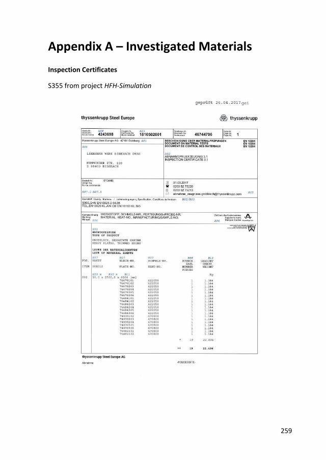
259
Appendix A – Investigated Materials
Inspection Certificates
S355 from project HFH-Simulation
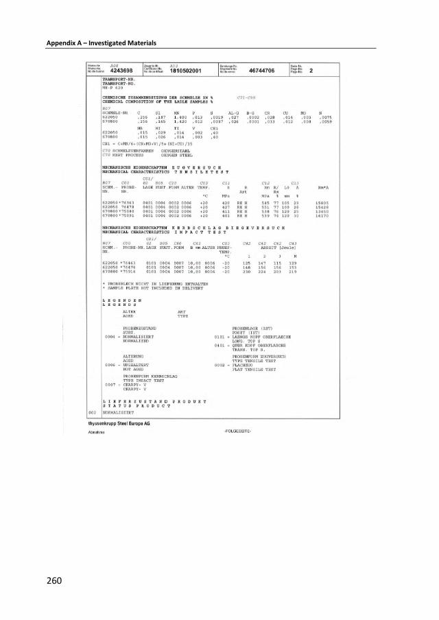
Appendix A – Investigated Materials
260
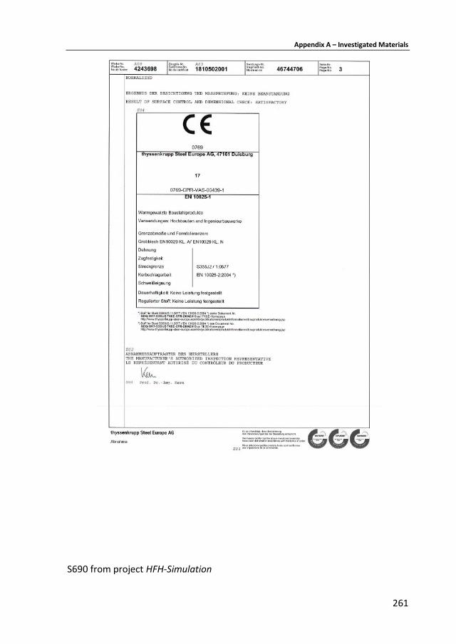
Appendix A – Investigated Materials
261
S690 from project HFH-Simulation
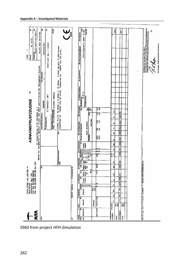
Appendix A – Investigated Materials
262
S960 from project HFH-Simulation
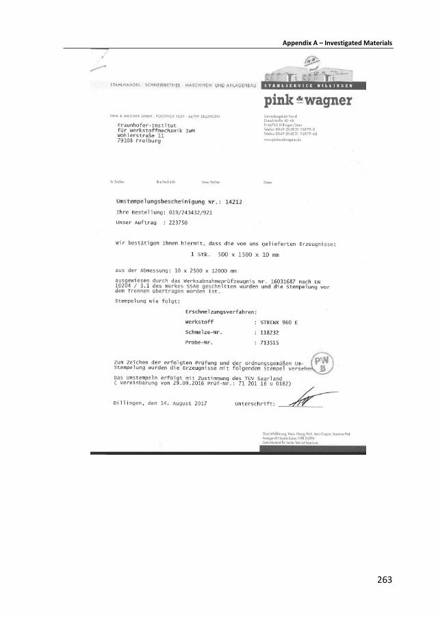
Appendix A – Investigated Materials
263
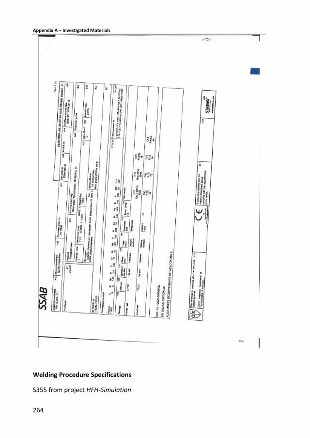
Appendix A – Investigated Materials
264
Welding Procedure Specifications
S355 from project HFH-Simulation
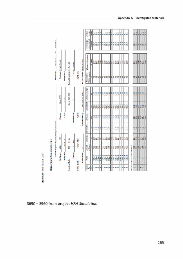
Appendix A – Investigated Materials
265
S690 – S960 from project HFH-Simulation
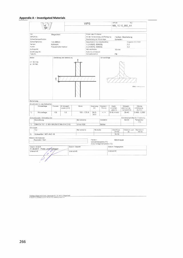
Appendix A – Investigated Materials
266
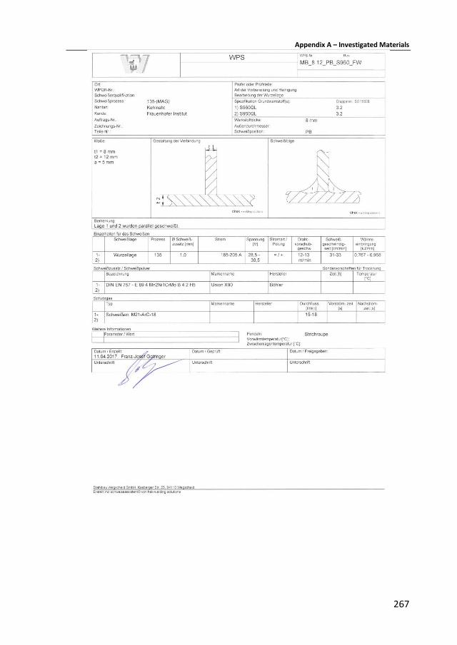
Appendix A – Investigated Materials
267
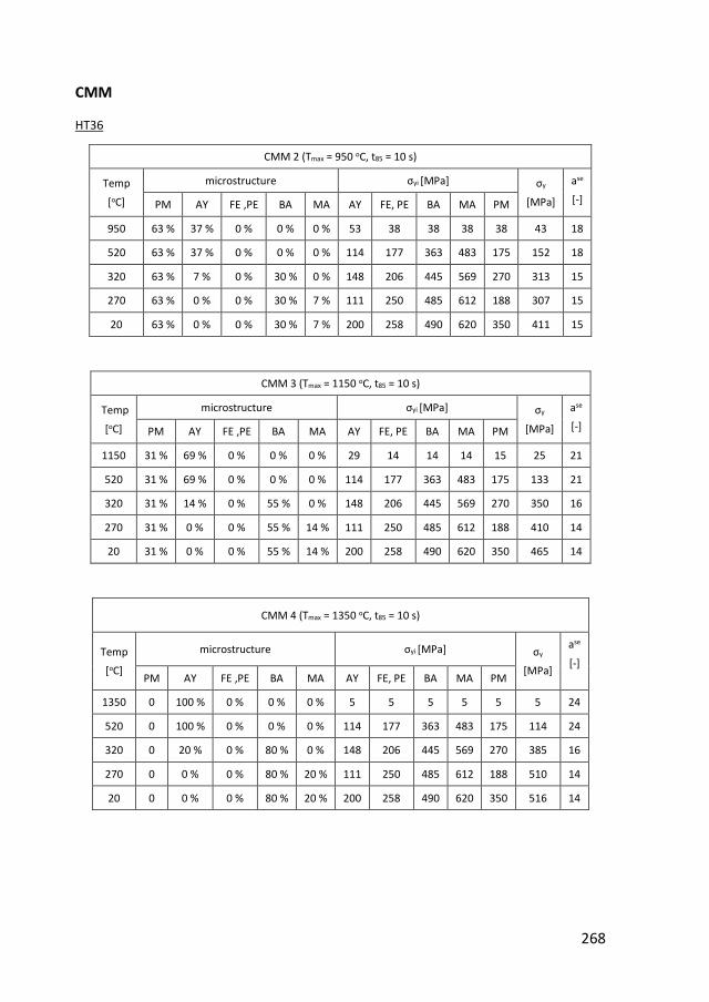
268
CMM
HT36
CMM 2 (Tmax = 950 oC, t85 = 10 s)
Temp
[oC]
microstructure σyi [MPa] σy
[MPa]
ase
[-] PM AY FE ,PE BA MA AY FE, PE BA MA PM
950 63 % 37 % 0 % 0 % 0 % 53 38 38 38 38 43 18
520 63 % 37 % 0 % 0 % 0 % 114 177 363 483 175 152 18
320 63 % 7 % 0 % 30 % 0 % 148 206 445 569 270 313 15
270 63 % 0 % 0 % 30 % 7 % 111 250 485 612 188 307 15
20 63 % 0 % 0 % 30 % 7 % 200 258 490 620 350 411 15
CMM 3 (Tmax = 1150 oC, t85 = 10 s)
Temp
[oC]
microstructure σyi [MPa] σy
[MPa]
ase
[-] PM AY FE ,PE BA MA AY FE, PE BA MA PM
1150 31 % 69 % 0 % 0 % 0 % 29 14 14 14 15 25 21
520 31 % 69 % 0 % 0 % 0 % 114 177 363 483 175 133 21
320 31 % 14 % 0 % 55 % 0 % 148 206 445 569 270 350 16
270 31 % 0 % 0 % 55 % 14 % 111 250 485 612 188 410 14
20 31 % 0 % 0 % 55 % 14 % 200 258 490 620 350 465 14
CMM 4 (Tmax = 1350 oC, t85 = 10 s)
Temp
[oC]
microstructure σyi [MPa] σy
[MPa]
ase
[-]
PM AY FE ,PE BA MA AY FE, PE BA MA PM
1350 0 100 % 0 % 0 % 0 % 5 5 5 5 5 5 24
520 0 100 % 0 % 0 % 0 % 114 177 363 483 175 114 24
320 0 20 % 0 % 80 % 0 % 148 206 445 569 270 385 16
270 0 0 % 0 % 80 % 20 % 111 250 485 612 188 510 14
20 0 0 % 0 % 80 % 20 % 200 258 490 620 350 516 14
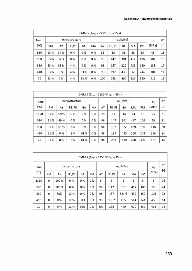
Appendix A – Investigated Materials
269
CMM 5 (Tmax = 950 oC, t85 = 35 s)
Temp
[oC]
microstructure σyi [MPa] σy
[MPa]
ase
[-] PM AY FE ,PE BA MA AY FE, PE BA MA PM
950 63 % 37 % 0 % 0 % 0 % 53 38 38 38 38 43 18
580 63 % 37 % 0 % 0 % 0 % 96 147 301 417 106 102 18
560 63 % 33 % 4 % 0 % 0 % 96 157 322 439 150 133 17
410 63 % 0 % 4 % 33 % 0 % 98 197 435 560 244 304 14
20 63 % 0 % 4 % 33 % 0 % 200 258 490 620 350 411 15
CMM 6 (Tmax = 1150 oC, t85 = 35 s)
Temp
[oC]
microstructure σyi [MPa] σy
[MPa]
ase
[-] PM AY FE ,PE BA MA AY FE, PE BA MA PM
1150 31 % 69 % 0 % 0 % 0 % 29 14 14 14 15 25 21
580 31 % 69 % 0 % 0 % 0 % 96 147 301 417 106 99 21
560 31 % 61 % 8% 0 % 0 % 96 157 322 439 150 118 20
410 31 % 0 % 8% 61 % 0 % 98 197 435 560 244 356 14
20 31 % 0 % 8% 61 % 0 % 200 258 490 620 350 427 14
CMM 7 (Tmax = 1350 oC, t85 = 35 s)
Temp
[oC]
microstructure σyi [MPa] σy
[MPa]
ase
[-]
PM AY FE ,PE BA MA AY FE, PE BA MA PM
1350 0 100 % 0 % 0 % 0 % 5 5 5 5 5 5 24
580 0 100 % 0 % 0 % 0 % 96 147 301 417 106 96 24
560 0 88% 12 % 0 % 0 % 96 157 321,6 439 150 103 23
410 0 0 % 12 % 88% 0 % 98 1967 435 561 244 406 14
20 0 0 % 12 % 88% 0 % 200 258 490 620 350 462 14
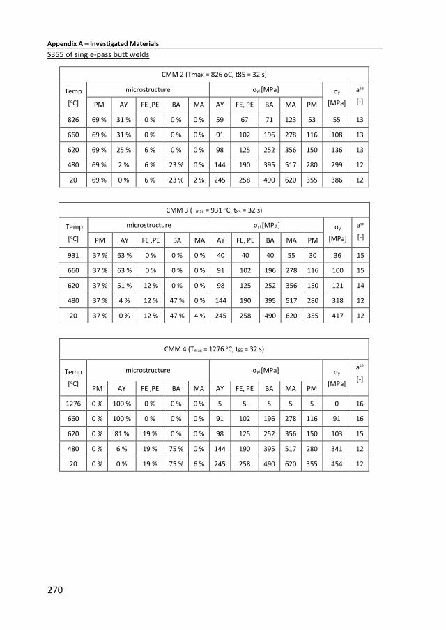
Appendix A – Investigated Materials
270
S355 of single-pass butt welds
CMM 2 (Tmax = 826 oC, t85 = 32 s)
Temp
[oC]
microstructure σyi [MPa] σy
[MPa]
ase
[-] PM AY FE ,PE BA MA AY FE, PE BA MA PM
826 69 % 31 % 0 % 0 % 0 % 59 67 71 123 53 55 13
660 69 % 31 % 0 % 0 % 0 % 91 102 196 278 116 108 13
620 69 % 25 % 6 % 0 % 0 % 98 125 252 356 150 136 13
480 69 % 2 % 6 % 23 % 0 % 144 190 395 517 280 299 12
20 69 % 0 % 6 % 23 % 2 % 245 258 490 620 355 386 12
CMM 3 (Tmax = 931 oC, t85 = 32 s)
Temp
[oC]
microstructure σyi [MPa] σy
[MPa]
ase
[-] PM AY FE ,PE BA MA AY FE, PE BA MA PM
931 37 % 63 % 0 % 0 % 0 % 40 40 40 55 30 36 15
660 37 % 63 % 0 % 0 % 0 % 91 102 196 278 116 100 15
620 37 % 51 % 12 % 0 % 0 % 98 125 252 356 150 121 14
480 37 % 4 % 12 % 47 % 0 % 144 190 395 517 280 318 12
20 37 % 0 % 12 % 47 % 4 % 245 258 490 620 355 417 12
CMM 4 (Tmax = 1276 oC, t85 = 32 s)
Temp
[oC]
microstructure σyi [MPa] σy
[MPa]
ase
[-]
PM AY FE ,PE BA MA AY FE, PE BA MA PM
1276 0 % 100 % 0 % 0 % 0 % 5 5 5 5 5 0 16
660 0 % 100 % 0 % 0 % 0 % 91 102 196 278 116 91 16
620 0 % 81 % 19 % 0 % 0 % 98 125 252 356 150 103 15
480 0 % 6 % 19 % 75 % 0 % 144 190 395 517 280 341 12
20 0 % 0 % 19 % 75 % 6 % 245 258 490 620 355 454 12
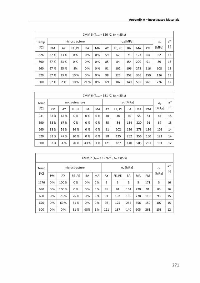
Appendix A – Investigated Materials
271
CMM 5 (Tmax = 826 oC, t85 = 85 s)
Temp
[oC]
microstructure σyi [MPa] σy
[MPa]
ase
[-] PM AY FE ,PE BA MA AY FE, PE BA MA PM
826 67 % 33 % 0 % 0 % 0 % 59 67 71 123 64 62 13
690 67 % 33 % 0 % 0 % 0 % 85 84 154 220 91 89 13
660 67 % 25 % 8% 0 % 0 % 91 102 196 278 116 108 13
620 67 % 23 % 10 % 0 % 0 % 98 125 252 356 150 136 13
500 67 % 2 % 10 % 21 % 0 % 121 187 140 505 261 226 12
CMM 6 (Tmax = 931 oC, t85 = 85 s)
Temp
[oC]
microstructure σyi [MPa] σy
[MPa]
ase
[-] PM AY FE ,PE BA MA AY FE, PE BA MA PM
931 33 % 67 % 0 % 0 % 0 % 40 40 40 55 51 44 15
690 33 % 67 % 0 % 0 % 0 % 85 84 154 220 91 87 15
660 33 % 51 % 16 % 0 % 0 % 91 102 196 278 116 101 14
620 33 % 47 % 20 % 0 % 0 % 98 125 252 356 150 121 14
500 33 % 4 % 20 % 43 % 1 % 121 187 140 505 261 191 12
CMM 7 (Tmax = 1276 oC, t85 = 85 s)
Temp
[oC]
microstructure σyi [MPa] σy
[MPa]
ase
[-]
PM AY FE ,PE BA MA AY FE, PE BA MA PM
1276 0 % 100 % 0 % 0 % 0 % 5 5 5 5 171 5 16
690 0 % 100 % 0 % 0 % 0 % 85 84 154 220 91 85 16
660 0 % 75 % 25 % 0 % 0 % 91 102 196 278 116 93 15
620 0 % 69 % 31 % 0 % 0 % 98 125 252 356 150 107 15
500 0 % 0 % 31 % 68% 1 % 121 187 140 505 261 158 12
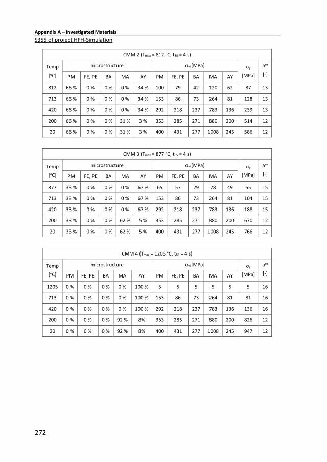
Appendix A – Investigated Materials
272
S355 of project HFH-Simulation
CMM 2 (Tmax = 812 °C, t85 = 4 s)
Temp
[oC]
microstructure σyi [MPa] σy
[MPa]
ase
[-] PM FE, PE BA MA AY PM FE, PE BA MA AY
812 66 % 0 % 0 % 0 % 34 % 100 79 42 120 62 87 13
713 66 % 0 % 0 % 0 % 34 % 153 86 73 264 81 128 13
420 66 % 0 % 0 % 0 % 34 % 292 218 237 783 136 239 13
200 66 % 0 % 0 % 31 % 3 % 353 285 271 880 200 514 12
20 66 % 0 % 0 % 31 % 3 % 400 431 277 1008 245 586 12
CMM 3 (Tmax = 877 °C, t85 = 4 s)
Temp
[oC]
microstructure σyi [MPa] σy
[MPa]
ase
[-] PM FE, PE BA MA AY PM FE, PE BA MA AY
877 33 % 0 % 0 % 0 % 67 % 65 57 29 78 49 55 15
713 33 % 0 % 0 % 0 % 67 % 153 86 73 264 81 104 15
420 33 % 0 % 0 % 0 % 67 % 292 218 237 783 136 188 15
200 33 % 0 % 0 % 62 % 5 % 353 285 271 880 200 670 12
20 33 % 0 % 0 % 62 % 5 % 400 431 277 1008 245 766 12
CMM 4 (Tmax = 1205 °C, t85 = 4 s)
Temp
[oC]
microstructure σyi [MPa] σy
[MPa]
ase
[-] PM FE, PE BA MA AY PM FE, PE BA MA AY
1205 0 % 0 % 0 % 0 % 100 % 5 5 5 5 5 5 16
713 0 % 0 % 0 % 0 % 100 % 153 86 73 264 81 81 16
420 0 % 0 % 0 % 0 % 100 % 292 218 237 783 136 136 16
200 0 % 0 % 0 % 92 % 8% 353 285 271 880 200 826 12
20 0 % 0 % 0 % 92 % 8% 400 431 277 1008 245 947 12
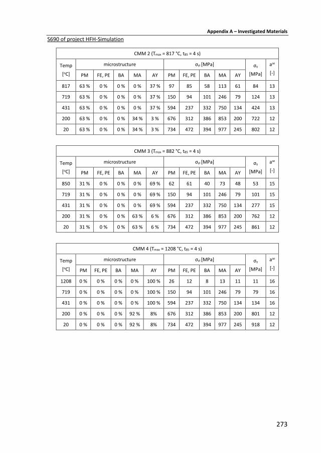
Appendix A – Investigated Materials
273
S690 of project HFH-Simulation
CMM 2 (Tmax = 817 °C, t85 = 4 s)
Temp
[oC]
microstructure σyi [MPa] σy
[MPa]
ase
[-] PM FE, PE BA MA AY PM FE, PE BA MA AY
817 63 % 0 % 0 % 0 % 37 % 97 85 58 113 61 84 13
719 63 % 0 % 0 % 0 % 37 % 150 94 101 246 79 124 13
431 63 % 0 % 0 % 0 % 37 % 594 237 332 750 134 424 13
200 63 % 0 % 0 % 34 % 3 % 676 312 386 853 200 722 12
20 63 % 0 % 0 % 34 % 3 % 734 472 394 977 245 802 12
CMM 3 (Tmax = 882 °C, t85 = 4 s)
Temp
[oC]
microstructure σyi [MPa] σy
[MPa]
ase
[-] PM FE, PE BA MA AY PM FE, PE BA MA AY
850 31 % 0 % 0 % 0 % 69 % 62 61 40 73 48 53 15
719 31 % 0 % 0 % 0 % 69 % 150 94 101 246 79 101 15
431 31 % 0 % 0 % 0 % 69 % 594 237 332 750 134 277 15
200 31 % 0 % 0 % 63 % 6 % 676 312 386 853 200 762 12
20 31 % 0 % 0 % 63 % 6 % 734 472 394 977 245 861 12
CMM 4 (Tmax = 1208 °C, t85 = 4 s)
Temp
[oC]
microstructure σyi [MPa] σy
[MPa]
ase
[-] PM FE, PE BA MA AY PM FE, PE BA MA AY
1208 0 % 0 % 0 % 0 % 100 % 26 12 8 13 11 11 16
719 0 % 0 % 0 % 0 % 100 % 150 94 101 246 79 79 16
431 0 % 0 % 0 % 0 % 100 % 594 237 332 750 134 134 16
200 0 % 0 % 0 % 92 % 8% 676 312 386 853 200 801 12
20 0 % 0 % 0 % 92 % 8% 734 472 394 977 245 918 12

Appendix A – Investigated Materials
274
S960 of project HFH-Simulation
CMM 2 (Tmax = 866 °C, t85 = 4 s)
Temp
[oC]
microstructure σyi [MPa] σy
[MPa]
ase
[-] PM FE, PE BA MA AY PM FE, PE BA MA AY
866 63 % 0 % 0 % 0 % 37 % 86 71 62 87 51 73 13
719 63 % 0 % 0 % 0 % 37 % 208 99 139 259 79 161 13
431 63 % 0 % 0 % 0 % 37 % 826 251 457 787 134 570 13
200 63 % 0 % 0 % 34 % 3 % 940 331 531 895 200 903 12
20 63 % 0 % 0 % 34 % 3 % 1021 500 542 1025 245 999 12
CMM 3 (Tmax = 964 °C, t85 = 4 s)
Temp
[oC]
microstructure σyi [MPa] σy
[MPa]
ase
[-] PM FE, PE BA MA AY PM FE, PE BA MA AY
915 31 % 0 % 0 % 0 % 69 % 42 33 24 23 33 36 15
719 31 % 0 % 0 % 0 % 69 % 208 99 139 259 79 119 15
431 31 % 0 % 0 % 0 % 69 % 826 251 457 787 134 349 15
200 31 % 0 % 0 % 63 % 6 % 940 331 531 895 200 871 12
20 31 % 0 % 0 % 63 % 6 % 1021 500 542 1025 245 981 12
CMM 4 (Tmax = 1257 °C, t85 = 4 s)
Temp
[oC]
microstructure σyi [MPa] σy
[MPa]
ase
[-] PM FE, PE BA MA AY PM FE, PE BA MA AY
1257 0 % 0 % 0 % 0 % 100 % 5 5 5 5 5 5 16
719 0 % 0 % 0 % 0 % 100 % 208 99 139 259 79 79 16
431 0 % 0 % 0 % 0 % 100 % 826 251 457 787 134 134 16
200 0 % 0 % 0 % 92 % 8% 940 331 531 895 200 839 12
20 0 % 0 % 0 % 92 % 8% 1021 500 542 1025 245 963 12
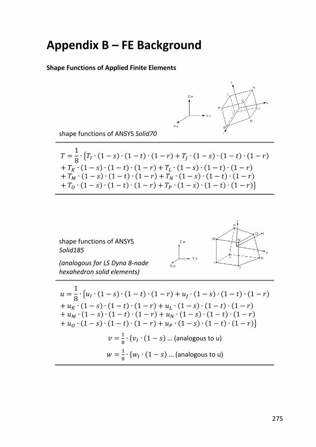
275
Appendix B – FE Background
Shape Functions of Applied Finite Elements
shape functions of ANSYS Solid70
𝑇 =1
8∙ {𝑇𝐼 ∙ (1 − 𝑠) ∙ (1 − 𝑡) ∙ (1 − 𝑟) + 𝑇𝐽 ∙ (1 − 𝑠) ∙ (1 − 𝑡) ∙ (1 − 𝑟)
+ 𝑇𝐾 ∙ (1 − 𝑠) ∙ (1 − 𝑡) ∙ (1 − 𝑟) + 𝑇𝐿 ∙ (1 − 𝑠) ∙ (1 − 𝑡) ∙ (1 − 𝑟)+ 𝑇𝑀 ∙ (1 − 𝑠) ∙ (1 − 𝑡) ∙ (1 − 𝑟) + 𝑇𝑁 ∙ (1 − 𝑠) ∙ (1 − 𝑡) ∙ (1 − 𝑟)
+ 𝑇𝑂 ∙ (1 − 𝑠) ∙ (1 − 𝑡) ∙ (1 − 𝑟) + 𝑇𝑃 ∙ (1 − 𝑠) ∙ (1 − 𝑡) ∙ (1 − 𝑟)}
shape functions of ANSYS Solid185
(analogous for LS Dyna 8-node hexahedron solid elements)
𝑢 =1
8∙ {𝑢𝐼 ∙ (1 − 𝑠) ∙ (1 − 𝑡) ∙ (1 − 𝑟) + 𝑢𝐽 ∙ (1 − 𝑠) ∙ (1 − 𝑡) ∙ (1 − 𝑟)
+ 𝑢𝐾 ∙ (1 − 𝑠) ∙ (1 − 𝑡) ∙ (1 − 𝑟) + 𝑢𝐿 ∙ (1 − 𝑠) ∙ (1 − 𝑡) ∙ (1 − 𝑟)+ 𝑢𝑀 ∙ (1 − 𝑠) ∙ (1 − 𝑡) ∙ (1 − 𝑟) + 𝑢𝑁 ∙ (1 − 𝑠) ∙ (1 − 𝑡) ∙ (1 − 𝑟)
+ 𝑢𝑂 ∙ (1 − 𝑠) ∙ (1 − 𝑡) ∙ (1 − 𝑟) + 𝑢𝑃 ∙ (1 − 𝑠) ∙ (1 − 𝑡) ∙ (1 − 𝑟)}
𝑣 =1
8∙ {𝑣𝐼 ∙ (1 − 𝑠) … (analogous to u)
𝑤 =1
8∙ {𝑤𝐼 ∙ (1 − 𝑠) … (analogous to u)

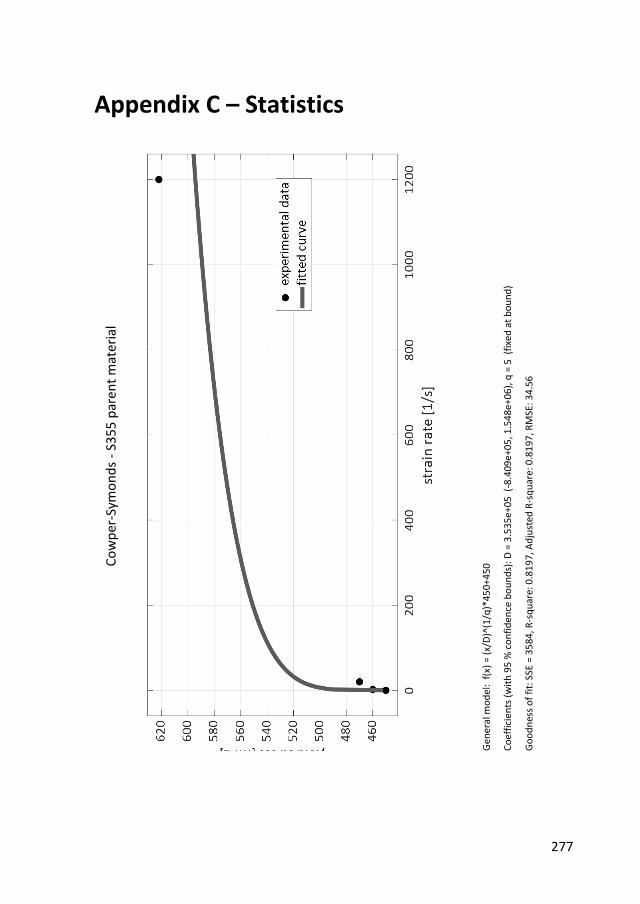
277
Appendix C – Statistics C
ow
per
-Sym
on
ds
- S3
55
par
ent
mat
eri
al
Gen
eral
mo
del
: f(
x) =
(x/
D)^
(1/q
)*4
50
+45
0
Co
effi
cien
ts (
wit
h 9
5 %
co
nfi
den
ce b
ou
nd
s): D
= 3
.53
5e+
05
(-8
.409
e+0
5, 1
.54
8e+
06
), q
= 5
(fi
xed
at
bo
un
d)
Go
od
nes
s o
f fi
t: S
SE =
35
84
, R-s
qu
are:
0.8
19
7, A
dju
sted
R-s
qu
are:
0.8
197
, RM
SE: 3
4.5
6
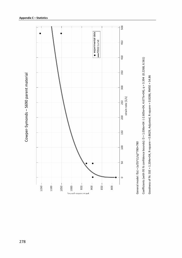
Appendix C – Statistics
278
Co
wp
er-S
ymo
nd
s –
S69
0 p
aren
t m
ate
rial
Gen
eral
mo
del
: f(x
) =
(x/D
)^(1
/q)*
78
0+7
80
Co
effi
cien
ts (
wit
h 9
5 %
co
nfi
den
ce b
ou
nd
s): D
= 1
.03
6e+
04
(-2
.605
e+0
4, 4
.67
7e+
04
), q
= 3
.39
4 (
0.2
26
8, 6
.561
)
Go
od
nes
s o
f fi
t: S
SE =
1.2
04
e+0
4, R
-sq
uar
e =
0.8
62
9, A
dju
sted
, R-s
qu
are
= 0
.82
86,
RM
SE =
54
.86
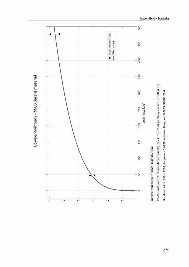
Appendix C – Statistics
279
Co
wp
er-S
ymo
nd
s –
S96
0 p
aren
t m
ate
rial
G
ener
al m
od
el: f
(x)
= (x
/D)^
(1/q
)*9
52
+95
2
Co
effi
cien
ts (
wit
h 9
5 %
co
nfi
den
ce b
ou
nd
s): D
= 4
15
6 (
15
56
, 675
6),
q =
4.1
25
(3
.33
8, 4
.91
2)
Go
od
nes
s o
f fi
t: S
SE =
32
26
, R-s
qu
are
= 0
.98
88
, Ad
just
ed R
-sq
uar
e: 0
.98
65
, RM
SE: 2
5.4

Appendix C – Statistics
280
Co
wp
er-S
ymo
nd
s –
S35
5 H
eat
Aff
ecte
d Z
on
e
Gen
eral
mo
del
: f(x
) =
(x/D
)^(1
/q)*
71
3+7
13
Co
effi
cien
ts (
wit
h 9
5 %
co
nfi
den
ce b
ou
nd
s): D
= 5
99
3 (
91
2.5
, 1.1
07
e+0
4),
q =
5 (
fixe
d a
t b
ou
nd
)
Go
od
nes
s o
f fi
t: S
SE =
1.1
81
e+0
4, R
-sq
uar
e =
0.9
32
, Ad
just
ed R
-sq
uar
e: 0
.93
2, R
MSE
: 48
.6
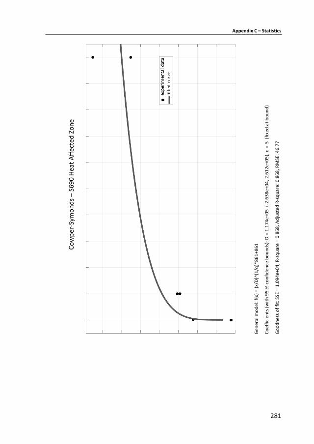
Appendix C – Statistics
281
Co
wp
er-S
ymo
nd
s –
S69
0 H
eat
Aff
ecte
d Z
on
e
Gen
eral
mo
del
: f(x
) =
(x/D
)^(1
/q)*
86
1+8
61
Co
effi
cien
ts (
wit
h 9
5 %
co
nfi
den
ce b
ou
nd
s): D
= 1
.17
4e+
05
(-2
.638
e+0
4, 2
.61
2e+
05
), q
= 5
(fi
xed
at
bo
un
d)
Go
od
nes
s o
f fi
t: S
SE =
1.0
94
e+0
4, R
-sq
uar
e =
0.8
68
, Ad
just
ed R
-sq
uar
e: 0
.86
8, R
MSE
: 46
.77
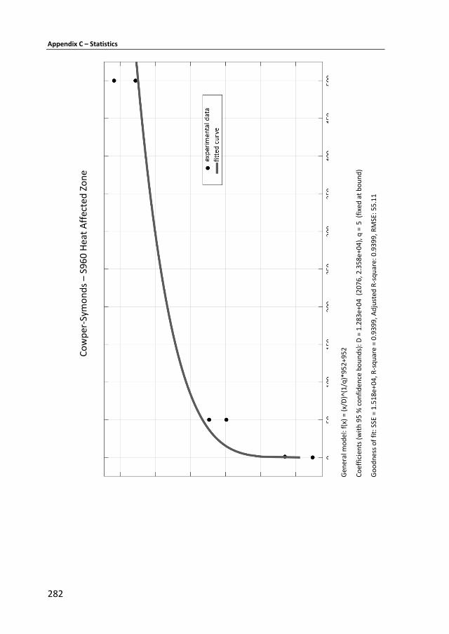
Appendix C – Statistics
282
Co
wp
er-S
ymo
nd
s –
S96
0 H
eat
Aff
ecte
d Z
on
e
G
ener
al m
od
el: f
(x)
= (x
/D)^
(1/q
)*9
52
+95
2
Co
effi
cien
ts (
wit
h 9
5 %
co
nfi
den
ce b
ou
nd
s): D
= 1
.28
3e+
04
(2
07
6, 2
.35
8e+
04
), q
= 5
(fi
xed
at
bo
un
d)
Go
od
nes
s o
f fi
t: S
SE =
1.5
18
e+0
4, R
-sq
uar
e =
0.9
39
9, A
dju
sted
R-s
qu
are:
0.9
39
9, R
MSE
: 55
.11
Related Documents


