Ž . JOURNAL OF MATHEMATICAL ANALYSIS AND APPLICATIONS 205, 107]132 1997 ARTICLE NO. AY965148 Finite Dimensional Global Attractor for Dissipative Schrodinger ] Boussinesq Equations ¨ Li Yongsheng and Chen Qingyi Department of Mathematics, Huazhong Uni ¤ ersity of Science and Technology, Wuhan, 430074, China Submitted by Colin Rogers Received April 19, 1995 In this paper the authors consider the initial boundary value problems of dissipative Schrodinger ]Boussinesq equations and prove the existence of global ¨ attractors and the finiteness of the Hausdorff and the fractal dimensions of the attractors. Q 1997 Academic Press 1. INTRODUCTION In the laser and plasma physics under interaction of a nonlinear com- plex Schrodinger field and a real Boussinesq field, the dynamics is de- ¨ Ž . scribed by the equations SBq , i c q D c s fc , 1.1 Ž . t 2 < < 2 f y D f q g D f y D F f s D c , 1.2 Ž . Ž . tt where c represents the complex Schrodinger field and f represents the ¨ Ž w x. real Boussinesq field see 15 ] 17, 19 . The existence and the uniqueness Ž .Ž . w x w x of a global solution of 1.1 , 1.2 have been studied in 8, 9, 11, 12 . In 10 Ž . the authors considered the one-dimensional dissipative SBq which in- volves a three-order nonlinear term in the Schrodinger equation and ¨ proved the existence of the global attractor and the finiteness of dimension of the attractor. In this paper, we consider the dissipative SBq equations i c q D c q i ac y fc s f , 1.3 Ž . t 2 < < 2 f y D f q g D f y b D f y D F f y D c s g , 1.4 Ž . Ž . tt t 107 0022-247Xr97 $25.00 Copyright Q 1997 by Academic Press All rights of reproduction in any form reserved.

Welcome message from author
This document is posted to help you gain knowledge. Please leave a comment to let me know what you think about it! Share it to your friends and learn new things together.
Transcript
Ž .JOURNAL OF MATHEMATICAL ANALYSIS AND APPLICATIONS 205, 107]132 1997ARTICLE NO. AY965148
Finite Dimensional Global Attractor for DissipativeSchrodinger]Boussinesq Equations¨
Li Yongsheng and Chen Qingyi
Department of Mathematics, Huazhong Uni ersity of Science and Technology, Wuhan,430074, China
Submitted by Colin Rogers
Received April 19, 1995
In this paper the authors consider the initial boundary value problems ofdissipative Schrodinger]Boussinesq equations and prove the existence of global¨attractors and the finiteness of the Hausdorff and the fractal dimensions of theattractors. Q 1997 Academic Press
1. INTRODUCTION
In the laser and plasma physics under interaction of a nonlinear com-plex Schrodinger field and a real Boussinesq field, the dynamics is de-¨
Ž .scribed by the equations SBq ,
ic q Dc s fc , 1.1Ž .t
2 < < 2f y Df q g Df y D F f s D c , 1.2Ž . Ž .t t
where c represents the complex Schrodinger field and f represents the¨Ž w x.real Boussinesq field see 15]17, 19 . The existence and the uniquenessŽ . Ž . w x w xof a global solution of 1.1 , 1.2 have been studied in 8, 9, 11, 12 . In 10
Ž .the authors considered the one-dimensional dissipative SBq which in-volves a three-order nonlinear term in the Schrodinger equation and¨proved the existence of the global attractor and the finiteness of dimensionof the attractor. In this paper, we consider the dissipative SBq equations
ic q Dc q iac y fc s f , 1.3Ž .t
2 < < 2f y Df q g Df y b Df y D F f y D c s g , 1.4Ž . Ž .t t t
107
0022-247Xr97 $25.00Copyright Q 1997 by Academic Press
All rights of reproduction in any form reserved.
LI AND CHEN108
c 0, x s c x , f 0, x s f x , f 0, x s f x , x g V ,Ž . Ž . Ž . Ž . Ž . Ž .0 0 t 1
1.5Ž .
c t , x s 0, f t , x s 0, Df t , x s 0, t g R, x g V , 1.6Ž . Ž . Ž . Ž .
where a , b , and g are positive constants, F is a sufficiently smooth realŽ . n Ž .function with F 0 s 0, and V ; R n F 3 is a bounded domain with a
smooth boundary V.We arrange this paper as follows. First we establish time-uniform a
priori estimates which imply the existence of solutions and boundedabsorbing sets. Then we construct the global attractor of the system as the
Ž w x.v-limit of one of those bounded absorbing sets see 18 . Finally, we showthat the global attractor has finite Hausdorff and fractal dimensions.
We introduce the following standard notations. We denote the spaces ofcomplex-valued and the real-valued functions by the same symbols.
m , pŽ . m , pŽ . mŽ . m , 2Ž .W V and W V are the usual Sobolev spaces. H V s W V ,0mŽ . m , 2Ž . 5 5 pŽ .H V s W V . We denote by ? the norm in L V , especiallyp0 0
5 5 5 5 Ž . 2Ž . ² :? s ? . We denote by ?, ? the inner product in L V , by ? , ? the2y1Ž . 1Ž . 5 5 m , pŽ .dual product of H V and H V , and by ? the norm of W V .m , p0
Ž .C I; E denotes the space of continuous and bounded functions on I ; RbŽ q . `Ž q .with values in the Banach space E. For u g C R ; E , or u g L R ; E ,b
A A A A A A 2 A Au denotes its norm, especially u s u , u sE L m , pA A m , pu . C is a generic constant and may assume different values inW
different formulae.Ž w x.We shall frequently use the Gargliardo]Nirenberg inequality see 4 :
5 j 5 5 51yl 5 m 5 l q m , rD u F C u D u , u g L l W V ,Ž .p q r
where
1 j 1 m 1 y ls q l y q ,ž /p n r n q
1 F q, r F `, j is an integer, 0 F j F m, and jrm F l F 1. If m y j y nrris a nonnegative integer, then the inequality holds for jrm F l - 1. We
5 5 1Ž .also use the short norm =u of u in H V and the equivalent norm05 5 2 1Ž .Du of u in H l H V .0
2. THE TIME-UNIFORM A PRIORI ESTIMATES
It is convenient to introduce a transformation u s f q df, where d istŽ . Ž .a positive constant to be chosen later. The problems 1.3 ] 1.6 are
FINITE DIMENSIONAL GLOBAL ATTRACTOR 109
equivalent to
ic q Dc q iac y fc s f , 2.1Ž .t
f q df s u , t g R, x g V , 2.2Ž .t
u y du y b Du q d 2f y 1 y db Df q g D2fŽ .t
< < 2yD F f y D c s g , 2.3Ž . Ž .c , f , u 0, x s c , f , u x , x g V , 2.4Ž . Ž . Ž . Ž . Ž .0 0 0
c s 0, f s Df s 0, u s 0, t g R, x g V , 2.5Ž .
where u s df q f . We set0 0 1
E s H 1 = H 1 = Hy1 V ,Ž .0 0 0
E s H 2 l H 1 = H 2 l H 1 = L2 V .Ž .1 0 0
E s H 3 l H 1 = H 3 l H 1 = H 1 V .Ž .2 0 0 0
Then E ¨ E ¨ E with compact imbedding.2 1 0In this section we are going to establish time-uniform a priori estimates
Ž .of solutions c , f, u in E and then in E .0 1
2.1. The Time-Uniform Estimates in E0
`Ž q 2Ž .. `Ž q 2Ž ..LEMMA 2.1. Suppose that f g L R ; L V . Then c g L R ; L Vsatisfies
A A 2f2 25 5 5 5c t F c exp ya t q 1 y exp ya t . 2.6Ž . Ž . Ž . Ž .Ž .0 2a
Ž .Proof. Taking the inner product of 2.1 with c , then taking imaginaryparts we obtain
5 5 21 d a f2 2 25 5 5 5 5 5 5 5 5 5c q a c s Im f , c F f c F c q .Ž .2 dt 2 2a
By Gronwall inequality we have the lemma.
LI AND CHEN110
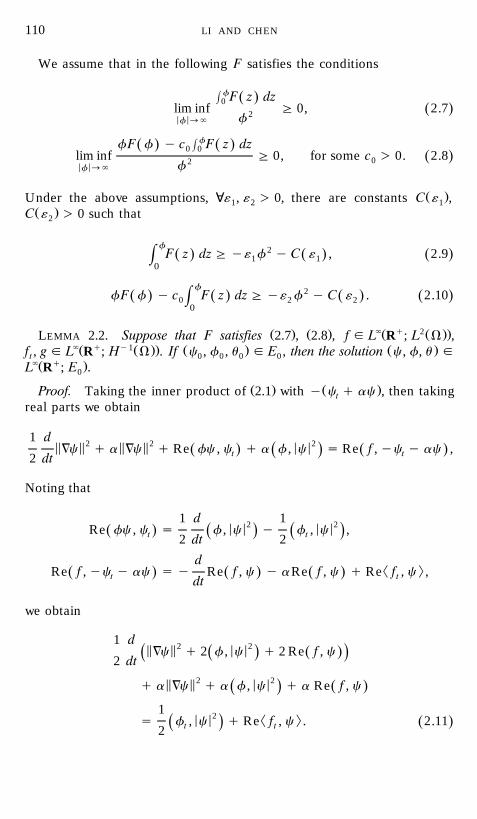
We assume that in the following F satisfies the conditions
HfF z dzŽ .0lim inf G 0, 2.7Ž .2f< <f ª`
fF f y c HfF z dzŽ . Ž .0 0lim inf G 0, for some c ) 0. 2.8Ž .02f< <f ª`
Ž .Under the above assumptions, ;« , « ) 0, there are constants C « ,1 2 1Ž .C « ) 0 such that2
f 2F z dz G y« f y C « , 2.9Ž . Ž . Ž .H 1 10
f 2fF f y c F z dz G y« f y C « . 2.10Ž . Ž . Ž . Ž .H0 2 20
Ž . Ž . `Ž q 2Ž ..LEMMA 2.2. Suppose that F satisfies 2.7 , 2.8 , f g L R ; L V ,`Ž q y1Ž .. Ž . Ž .f , g g L R ; H V . If c , f , u g E , then the solution c , f, u gt 0 0 0 0
`Ž q .L R ; E .0
Ž . Ž .Proof. Taking the inner product of 2.1 with y c q ac , then takingtreal parts we obtain
1 d 2 2 25 5 5 5 < <=c q a =c q Re fc , c q a f , c s Re f , yc y ac ,Ž . Ž .Ž .t t2 dt
Noting that
1 d 12 2< < < <Re fc , c s f , c y f , c ,Ž . Ž . Ž .t t2 dt 2
d² :Re f , yc y ac s y Re f , c y a Re f , c q Re f , c ,Ž . Ž . Ž .t tdt
we obtain
1 d 2 25 5 < <=c q 2 f , c q 2 Re f , cŽ .Ž .Ž .2 dt
5 5 2 < < 2q a =c q a f , c q a Re f , cŽ .Ž .1 2< < ² :s f , c q Re f , c . 2.11Ž .Ž .t t2
FINITE DIMENSIONAL GLOBAL ATTRACTOR 111
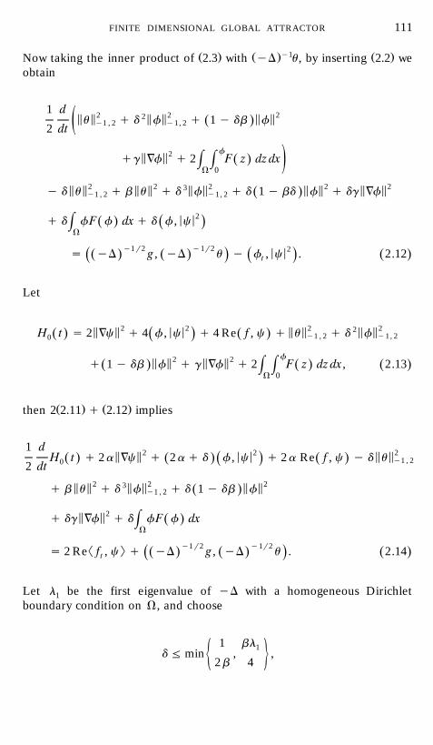
Ž . Ž .y1 Ž .Now taking the inner product of 2.3 with yD u , by inserting 2.2 weobtain
1 d 2 2 225 5 5 5 5 5u q d f q 1 y db fŽ .y1 , 2 y1, 2ž2 dt
f25 5qg =f q 2 F z dz dxŽ .H H /V 0
5 5 2 5 5 2 3 5 5 2 5 5 2 5 5 2y d u q b u q d f q d 1 y bd f q dg =fŽ .y1 , 2 y1, 2
< < 2q d fF f dx q d f , cŽ . Ž .HV
y1r2 y1r2 2< <s yD g , yD u y f , c . 2.12Ž . Ž . Ž .Ž . Ž .t
Let
5 5 2 < < 2 5 5 2 2 5 5 2H t s 2 =c q 4 f , c q 4 Re f , c q u q d fŽ . Ž .Ž . y1 , 2 y1, 20
f2 25 5 5 5q 1 y db f q g =f q 2 F z dz dx , 2.13Ž . Ž . Ž .H HV 0
Ž . Ž .then 2 2.11 q 2.12 implies
1 d 2 2 25 5 < < 5 5H t q 2a =c q 2a q d f , c q 2a Re f , c y d uŽ . Ž . Ž .Ž . y1 , 202 dt
5 5 2 3 5 5 2 5 5 2q b u q d f q d 1 y db fŽ .y1 , 2
5 5 2q dg =f q d fF f dxŽ .HV
y1r2 y1r2² :s 2 Re f , c q yD g , yD u . 2.14Ž . Ž . Ž .Ž .t
Let l be the first eigenvalue of yD with a homogeneous Dirichlet1boundary condition on V, and choose
1 bl1d F min , ,½ 52b 4
LI AND CHEN112
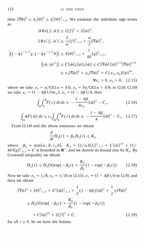
5 5 2 5 5 2 2 5 5 2then =u G l u G l u . We estimate the indefinite sign termsy1, 21 1as
< < 5 5 2 5 5 24 Re f , c F 2 f q 2 c ,Ž .2 a2 2² : < 5 5 5 52 Re f , c F f q =c ,y1 , 2t a 2
1y1r2 y1r2 2 25 5 5 5yD g , yD u F d u q g ,Ž . Ž .Ž . y1 , 2 y1, 24d
2 5r4 3r4< < 5 5 5 5 5 5 5 5 5 5 5 5f , c F C f c c F C =f c =cŽ . 4 4
5 5 2 5 5 2 5 510F « =c q « =f q C « , « c ,Ž .3 4 3 4
;« ) 0, « ) 0, 2.15Ž .3 4
Ž Ž .. Ž Ž .. Ž . Ž .where we take « s ar 2 2a q d , « s dgr 2 2a q d ; in 2.9 , 2.103 4Ž . Ž . Ž .we take « s 1 y db r 4c , « s 1 y db r4, then1 0 2
1 y dbf 25 5F z dz dx G y f y C , 2.16Ž . Ž .H H 14cV 0 0
1 y dbf 25 5fF f dx G c F z dz dx G y f y C . 2.17Ž . Ž . Ž .H H H0 24V V 0
Ž .From 2.14 and the above estimates we obtain
dH t q b H t F KŽ . Ž .0 0 0 0dt
� 4 Ž .5 5 2 5 510 Žwhere b s min a , d , c d , K s 2ra f q C c q 1ry1, 20 0 0 t.5 5 2 q4d g q C is bounded in R , and we denote its bound also by K . Byy1, 2 0
Gronwall inequality we obtain
K0H t F H 0 exp yb t q 1 y exp yb t . 2.18Ž . Ž . Ž . Ž . Ž .Ž .0 0 0 0b0
Ž . Ž . Ž .Now we take « s 1r8, « s 1r16 in 2.15 , « s 1 y db r4 in 2.9 , and3 4 1then we obtain
1 12 2 2 2 225 5 5 5 5 5 5 5 5 5=c q u q d f q 1 y db f q g =fŽ .y1 , 2 y1, 2 2 2
K0F H 0 exp yb t q 1 y exp yb tŽ . Ž . Ž .Ž .0 0 0b0
5 510 5 5 2q C c q 2 f q C , 2.19Ž .for all t G 0. So we have the lemma.
FINITE DIMENSIONAL GLOBAL ATTRACTOR 113
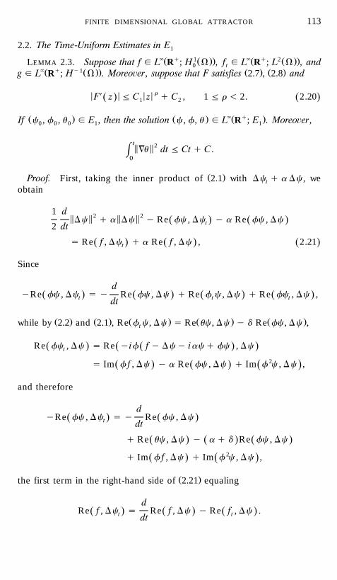
2.2. The Time-Uniform Estimates in E1
`Ž q 1Ž .. `Ž q 2Ž ..LEMMA 2.3. Suppose that f g L R ; H V , f g L R ; L V , and0 t`Ž q y1Ž .. Ž . Ž .g g L R ; H V . Moreo¨er, suppose that F satisfies 2.7 , 2.8 and
< X < < < rF z F C z q C , 1 F r - 2. 2.20Ž . Ž .1 2
Ž . Ž . `Ž q .If c , f , u g E , then the solution c , f, u g L R ; E . Moreo¨er,0 0 0 1 1
t 25 5=u dt F Ct q C.H0
Ž .Proof. First, taking the inner product of 2.1 with Dc q a Dc , wetobtain
1 d 2 25 5 5 5Dc q a Dc y Re fc , Dc y a Re fc , DcŽ . Ž .t2 dt
s Re f , Dc q a Re f , Dc , 2.21Ž . Ž . Ž .t
Since
dyRe fc , Dc s y Re fc , Dc q Re f c , Dc q Re fc , Dc ,Ž . Ž . Ž . Ž .t t tdt
Ž . Ž . Ž . Ž . Ž .while by 2.2 and 2.1 , Re f c , Dc s Re uc , Dc y d Re fc , Dc ,t
Re fc , Dc s Re yif f y Dc y iac q fc , DcŽ . Ž .Ž .t
s Im f f , Dc y a Re fc , Dc q Im f 2c , Dc ,Ž . Ž . Ž .
and therefore
dyRe fc , Dc s y Re fc , DcŽ . Ž .t dt
q Re uc , Dc y a q d Re fc , DcŽ . Ž . Ž .q Im f f , Dc q Im f 2c , Dc ,Ž . Ž .
Ž .the first term in the right-hand side of 2.21 equaling
dRe f , Dc s Re f , Dc y Re f , Dc .Ž . Ž . Ž .t tdt
LI AND CHEN114
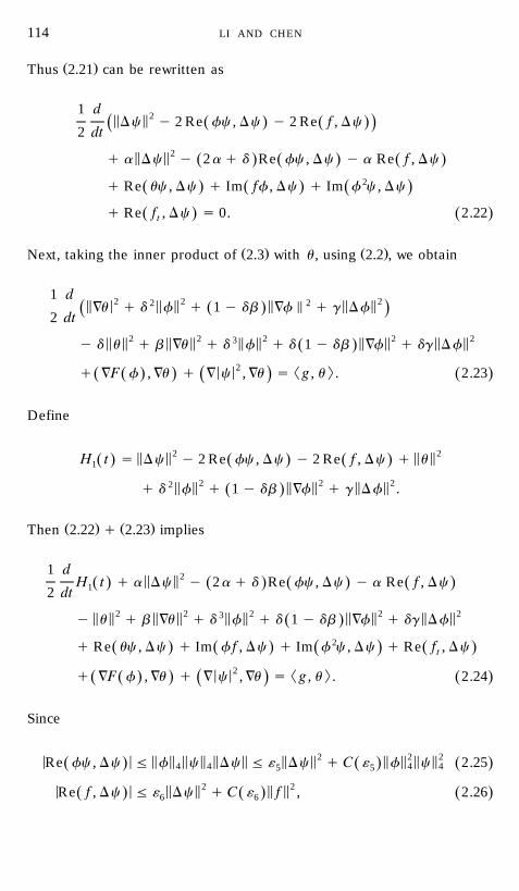
Ž .Thus 2.21 can be rewritten as
1 d 25 5Dc y 2 Re fc , Dc y 2 Re f , DcŽ . Ž .Ž .2 dt
5 5 2q a Dc y 2a q d Re fc , Dc y a Re f , DcŽ . Ž . Ž .q Re uc , Dc q Im ff , Dc q Im f 2c , DcŽ . Ž . Ž .q Re f , Dc s 0. 2.22Ž . Ž .t
Ž . Ž .Next, taking the inner product of 2.3 with u , using 2.2 , we obtain
1 d 2 2 22 25 < 5 5 5 5 5=u q d f q 1 y db =f I q g DfŽ .Ž .2 dt
5 5 2 5 5 2 3 5 5 2 5 5 2 5 5 2y d u q b =u q d f q d 1 y db =f q dg DfŽ .< < 2 ² :q =F f , =u q = c , =u s g , u . 2.23Ž . Ž .Ž . Ž .
Define
5 5 2 5 5 2H t s Dc y 2 Re fc , Dc y 2 Re f , Dc q uŽ . Ž . Ž .1
2 5 5 2 5 5 2 5 5 2q d f q 1 y db =f q g Df .Ž .
Ž . Ž .Then 2.22 q 2.23 implies
1 d 25 5H t q a Dc y 2a q d Re fc , Dc y a Re f , DcŽ . Ž . Ž . Ž .12 dt
5 5 2 5 5 2 3 5 5 2 5 5 2 5 5 2y u q b =u q d f q d 1 y db =f q dg DfŽ .q Re uc , Dc q Im f f , Dc q Im f 2c , Dc q Re f , DcŽ . Ž . Ž .Ž . t
< < 2 ² :q =F f , =u q = c , =u s g , u . 2.24Ž . Ž .Ž . Ž .
Since
< < 5 5 5 5 5 5 5 5 2 5 5 2 5 5 2Re fc , Dc F f c Dc F « Dc q C « f c 2.25Ž . Ž . Ž .4 4 4 45 5
< < 5 5 2 5 5 2Re f , Dc F « Dc q C « f , 2.26Ž . Ž . Ž .6 6
FINITE DIMENSIONAL GLOBAL ATTRACTOR 115
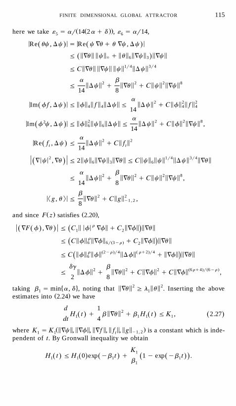
Ž Ž ..here we take « s ar 14 2a q d , « s ar14,5 6
< < < <Re uc , Dc s Re c =u q u =c , DcŽ . Ž .5 5 5 5 5 5 5 5 5 5F =u c q u =c =cŽ .` 6 3
5 5 5 5 5 51r4 5 5 3r4F C =u =c c Dc
a b2 2 2 85 5 5 5 5 5 5 5F Dc q =u q C c =c14 8
a 2 2 2< < 5 5 5 5 5 5 5 5 5 5 5 5Im f f , Dc F f f Dc F Dc q C f fŽ . 4 4 4 414a2 2 2 82< < 5 5 5 5 5 5 5 5 5 5 5 5Im f c , Dc F f c Dc F Dc q C f =c ,Ž . 6 6 14
a 2 2< 5 5 5 5Re f , Dc F Dc q C fŽ .t t142 1r4 3r4< < 5 5 5 5 5 5 5 5 5 5 5 5 5 5= c , =u F 2 c =c =u F C c c Dc =uŽ . 6 3 6
a b2 2 2 85 5 5 5 5 5 5 5F Dc q =u q C c =c ,14 8
b 2 2<² : < 5 5 5 5g , u F =u q C g ,y1 , 28
Ž . Ž .and since F z satisfies 2.20 ,r5 < < 5 5 5 5 5=F f , =u F C f =f q C =f =uŽ .Ž . Ž .1 2
5 5 r 5 5 5 5 5 5F C f =f q C =f =uŽ .6 6rŽ3yr . 2
5 5 r 5 5 Ž2yr .r4 5 5 Ž rq2.r4 5 5 5 5F C f f Df q =f =uŽ .6
dg b2 2 2 Ž6 rq4.rŽ6yr .5 5 5 5 5 5 5 5F Df q =u q C =f q C =f ,2 8
� 4 5 5 2 5 5 2taking b s min a , d , noting that =u G l u . Inserting the above1 1Ž .estimates into 2.24 we have
d 1 25 5H t q b =u q b H t F K , 2.27Ž . Ž . Ž .1 1 1 1dt 4
Ž5 5 5 5 5 5 5 5 5 5 .where K s K =c , =f , =f , f , g is a constant which is inde-y1, 21 1 tpendent of t. By Gronwall inequality we obtain
K1H t F H 0 exp yb t q 1 y exp yb t .Ž . Ž . Ž . Ž .Ž .1 1 1 1b1
LI AND CHEN116
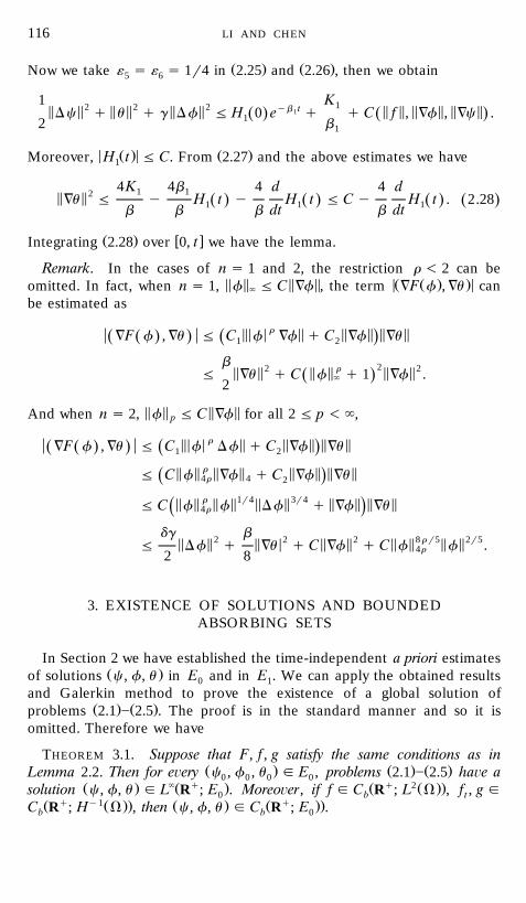
Ž . Ž .Now we take « s « s 1r4 in 2.25 and 2.26 , then we obtain5 6
1 K12 2 2 yb t15 5 5 5 5 5 5 5 5 5 5 5Dc q u q g Df F H 0 e q q C f , =f , =c .Ž . Ž .12 b1
< Ž . < Ž .Moreover, H t F C. From 2.27 and the above estimates we have1
4K 4b 4 d 4 d1 125 5=u F y H t y H t F C y H t . 2.28Ž . Ž . Ž . Ž .1 1 1b b b dt b dt
Ž . w xIntegrating 2.28 over 0, t we have the lemma.
Remark. In the cases of n s 1 and 2, the restriction r - 2 can be5 5 5 5 <Ž Ž . . <omitted. In fact, when n s 1, f F C =f , the term =F f , =u can`
be estimated as
r5 < < 5 5 5 5 5=F f , =u F C f =f q C =f =uŽ .Ž . Ž .1 2
b 22 r 25 5 5 5 5 5F =u q C f q 1 =f .Ž .`2
5 5 5 5And when n s 2, f F C =f for all 2 F p - `,p
r5 < < 5 5 5 5 5=F f , =u F C f Df q C =f =uŽ .Ž . Ž .1 2
5 5 r 5 5 5 5 5 5F C f =f q C =f =uŽ .4r 4 2
5 5 r 5 51r4 5 5 3r4 5 5 5 5F C f f Df q =f =uŽ .4r
dg b2 2 2 8 r r5 2r55 5 5 < 5 5 5 5 5 5F Df q =u q C =f q C f f .4r2 8
3. EXISTENCE OF SOLUTIONS AND BOUNDEDABSORBING SETS
In Section 2 we have established the time-independent a priori estimatesŽ .of solutions c , f, u in E and in E . We can apply the obtained results0 1
and Galerkin method to prove the existence of a global solution ofŽ . Ž .problems 2.1 ] 2.5 . The proof is in the standard manner and so it is
omitted. Therefore we have
THEOREM 3.1. Suppose that F, f , g satisfy the same conditions as inŽ . Ž . Ž .Lemma 2.2. Then for e¨ery c , f , u g E , problems 2.1 ] 2.5 ha¨e a0 0 0 0
Ž . `Ž q . Ž q 2Ž ..solution c , f, u g L R ; E . Moreo¨er, if f g C R ; L V , f , g g0 b tŽ q y1Ž .. Ž . Ž q ..C R ; H V , then c , f, u g C R ; E .b b 0
FINITE DIMENSIONAL GLOBAL ATTRACTOR 117
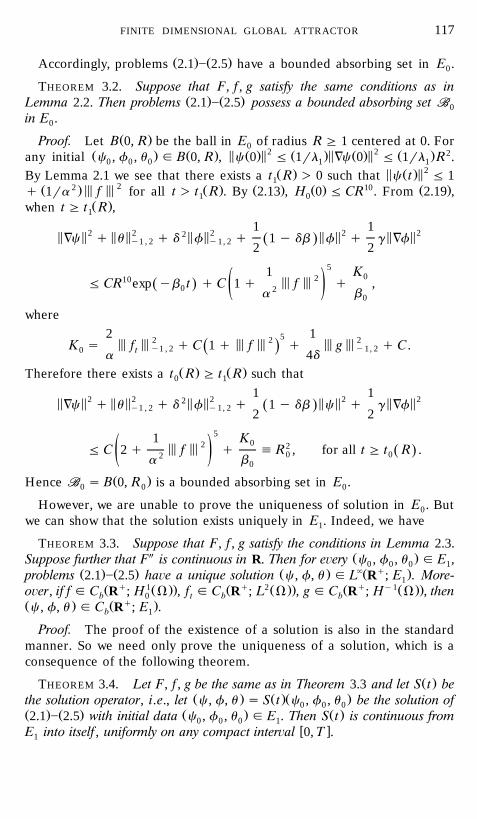
Ž . Ž .Accordingly, problems 2.1 ] 2.5 have a bounded absorbing set in E .0
THEOREM 3.2. Suppose that F, f , g satisfy the same conditions as inŽ . Ž .Lemma 2.2. Then problems 2.1 ] 2.5 possess a bounded absorbing set BB0
in E .0
Ž .Proof. Let B 0, R be the ball in E of radius R G 1 centered at 0. For0Ž . Ž . 5 Ž .5 2 Ž .5 Ž .5 2 Ž . 2any initial c , f , u g B 0, R , c 0 F 1rl =c 0 F 1rl R .0 0 0 1 1
Ž . 5 Ž .5 2By Lemma 2.1 we see that there exists a t R ) 0 such that c t F 11Ž 2 .A A 2 Ž . Ž . Ž . 10 Ž .q 1ra f for all t ) t R . By 2.13 , H 0 F CR . From 2.19 ,1 0
Ž .when t G t R ,1
1 12 2 2 2 225 5 5 5 5 5 5 5 5 5=c q u q d f q 1 y db f q g =fŽ .y1 , 2 y1, 2 2 251 K0210 A AF CR exp yb t q C 1 q f q ,Ž .0 2ž / ba 0
where2 152 2 2A A A A A AK s f q C 1 q f q g q C.Ž .y1 , 2 y1, 20 ta 4d
Ž . Ž .Therefore there exists a t R G t R such that0 1
1 12 2 2 2 225 5 5 5 5 5 5 5 5 5=c q u q d f q 1 y db c q g =fŽ .y1 , 2 y1, 2 2 251 K02 2A AF C 2 q f q ' R , for all t G t R .Ž .0 02ž / ba 0
Ž .Hence BB s B 0, R is a bounded absorbing set in E .0 0 0
However, we are unable to prove the uniqueness of solution in E . But0we can show that the solution exists uniquely in E . Indeed, we have1
THEOREM 3.3. Suppose that F, f , g satisfy the conditions in Lemma 2.3.Y Ž .Suppose further that F is continuous in R. Then for e¨ery c , f , u g E ,0 0 0 1
Ž . Ž . Ž . `Ž q .problems 2.1 ] 2.5 ha¨e a unique solution c , f, u g L R ; E . More-1Ž q 1Ž .. Ž q 2Ž .. Ž q y1Ž ..o¨er, if f g C R ; H V , f g C R ; L V , g g C R ; H V , thenb 0 t b b
Ž . Ž q .c , f, u g C R ; E .b 1
Proof. The proof of the existence of a solution is also in the standardmanner. So we need only prove the uniqueness of a solution, which is aconsequence of the following theorem.
Ž .THEOREM 3.4. Let F, f , g be the same as in Theorem 3.3 and let S t beŽ . Ž .Ž .the solution operator, i.e., let c , f, u s S t c , f , u be the solution of0 0 0
Ž . Ž . Ž . Ž .2.1 ] 2.5 with initial data c , f , u g E . Then S t is continuous from0 0 0 1w xE into itself, uniformly on any compact inter al 0, T .1
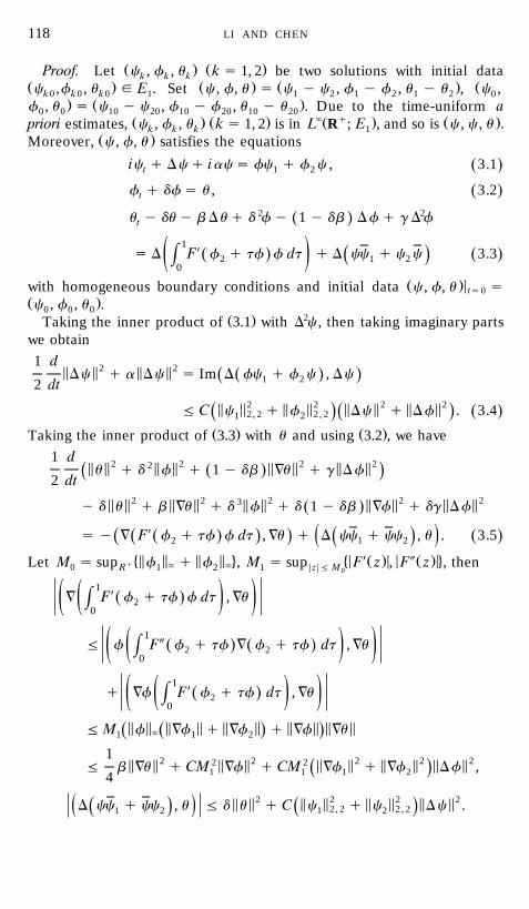
LI AND CHEN118
Ž . Ž .Proof. Let c , f , u k s 1, 2 be two solutions with initial datak k kŽ . Ž . Ž . Žc ,f , u g E . Set c , f, u s c y c , f y f , u y u , c ,k 0 k 0 k 0 1 1 2 1 2 1 2 0
. Ž .f , u s c y c , f y f , u y u . Due to the time-uniform a0 0 10 20 10 20 10 20Ž . Ž . `Ž q . Ž .priori estimates, c , f , u k s 1, 2 is in L R ; E , and so is c , c , u .k k k 1
Ž .Moreover, c , f, u satisfies the equations
ic q Dc q iac s fc q f c , 3.1Ž .t 1 2
f q df s u , 3.2Ž .t
u y du y b Du q d 2f y 1 y db Df q g D2fŽ .t
1 Xs D F f q tf f dt q D cc q c c 3.3Ž . Ž .Ž .H 2 1 2ž /0
Ž . <with homogeneous boundary conditions and initial data c , f, u sts0Ž .c , f , u .0 0 0
Ž . 2Taking the inner product of 3.1 with D c , then taking imaginary partswe obtain1 d 2 25 5 5 5Dc q a Dc s Im D fc q f c , DcŽ .Ž .1 22 dt
5 5 2 5 5 2 5 5 2 5 5 2F C c q f Dc q Df . 3.4Ž .Ž .Ž .2, 2 2, 21 2
Ž . Ž .Taking the inner product of 3.3 with u and using 3.2 , we have1 d 2 2 2 225 5 5 5 5 5 5 5u q d f q 1 y db =u q g DfŽ .Ž .2 dt
5 5 2 5 5 2 3 5 5 2 5 5 2 5 5 2y d u q b =u q d f q d 1 y db =f q dg DfŽ .Xs y = F f q tf f dt , =u q D cc q cc , u . 3.5Ž . Ž .Ž .Ž . Ž .ž /2 1 2
�5 5 5 5 4 � < XŽ . < < YŽ . <4qLet M s sup f q f , M s sup F z , F z , then` `0 R 1 2 1 < z < F M0
1 X= F f q tf f dt , =uŽ .H 2ž /ž /0
1 YF f F f q tf = f q tf dt , =uŽ . Ž .H 2 2ž /ž /0
1 Xq =f F f q tf dt , =uŽ .H 2ž /ž /0
5 5 5 5 5 5 5 5 5 5F M f =f q =f q =f =uŽ .Ž .`1 1 2
1 2 2 2 2 22 25 5 5 5 5 5 5 5 5 5F b =u q CM =f q CM =f q =f Df ,Ž .1 1 1 242 2 2 25 5 5 5 5 5 5 5D cc q cc , u F d u q C c q c Dc .Ž .Ž . 2, 2 2, 2ž /1 2 1 2
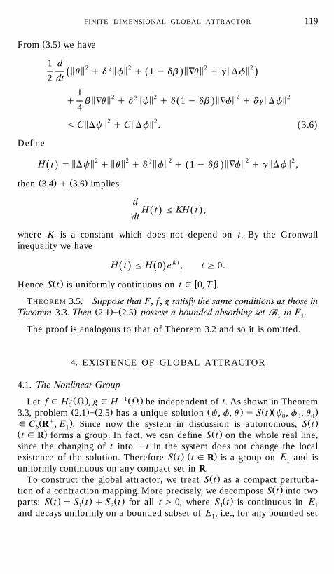
FINITE DIMENSIONAL GLOBAL ATTRACTOR 119
Ž .From 3.5 we have
1 d 2 2 2 225 5 5 5 5 5 5 5u q d f q 1 y db =u q g DfŽ .Ž .2 dt
1 2 2 2 235 5 5 5 5 5 5 5q b =u q d f q d 1 y db =f q dg DfŽ .4
5 5 2 5 5 2F C Dc q C Df . 3.6Ž .
Define
5 5 2 5 5 2 2 5 5 2 5 5 2 5 5 2H t s Dc q u q d f q 1 y db =f q g Df ,Ž . Ž .
Ž . Ž .then 3.4 q 3.6 implies
dH t F KH t ,Ž . Ž .
dt
where K is a constant which does not depend on t. By the Gronwallinequality we have
H t F H 0 e K t , t G 0.Ž . Ž .
Ž . w xHence S t is uniformly continuous on t g 0, T .
THEOREM 3.5. Suppose that F, f , g satisfy the same conditions as those inŽ . Ž .Theorem 3.3. Then 2.1 ] 2.5 possess a bounded absorbing set BB in E .1 1
The proof is analogous to that of Theorem 3.2 and so it is omitted.
4. EXISTENCE OF GLOBAL ATTRACTOR
4.1. The Nonlinear Group1Ž . y1Ž .Let f g H V , g g H V be independent of t. As shown in Theorem0Ž . Ž . Ž . Ž .Ž .3.3, problem 2.1 ] 2.5 has a unique solution c , f, u s S t c , f , u0 0 0
Ž q . Ž .g C R , E . Since now the system in discussion is autonomous, S tb 1Ž . Ž .t g R forms a group. In fact, we can define S t on the whole real line,since the changing of t into yt in the system does not change the local
Ž . Ž .existence of the solution. Therefore S t t g R is a group on E and is1uniformly continuous on any compact set in R.
Ž .To construct the global attractor, we treat S t as a compact perturba-Ž .tion of a contraction mapping. More precisely, we decompose S t into two
Ž . Ž . Ž . Ž .parts: S t s S t q S t for all t G 0, where S t is continuous in E1 2 1 1and decays uniformly on a bounded subset of E , i.e., for any bounded set1
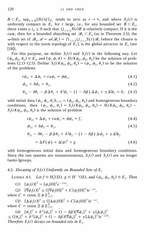
LI AND CHEN120
5 Ž . 5 Ž .B ; E , sup S t j tends to zero as t ª `, and where S t isE1 j g B 21
uniformly compact in E for t large, i.e., for any bounded set B ; E ,1 1Ž .there exists a t G 0 such that D S t B is relatively compact. If it is the0 t G t0
Ž .case, then for a bounded absorbing set BB ; E as in Theorem 3.5 , the1 1
Ž . Žv-limit set of BB , AA s v BB s F D S t BB where the closure isŽ .1 1 sG 0 t G s 1. Žwith respect to the norm topology of E , is the global attractor in E see1 1
w x.18 .Ž . Ž .For this purpose, we define S t and S t in the following way. Let1 2
Ž . Ž . Ž .Ž .c ,f , u g E , and c , f, u s S t c , f , u be the solution of prob-0 0 0 1 0 0 0Ž . Ž . Ž .Ž . Ž .lems 2.1 ] 2.5 . Define S t c , f , u s c , f , u to be the solution1 0 0 0 1 1 1
of the problems
ic q Dc q iac s fc , 4.1Ž .1 t 1 1 1
f q df s u , 4.2Ž .1 t 1 1
u y du y b Du q d 2f y 1 y db Df q g D2f s 0, 4.3Ž . Ž .1 t 1 1 1 1 1
Ž . < Ž .with initial data c , f , u s c , f , u and homogeneous boundaryts01 1 1 0 0 0Ž . Ž .Ž . Ž .Ž .conditions, then c , f , u s S t c , f , u s S t c , f , u y2 2 2 2 0 0 0 0 0 0
Ž .Ž .S t c , f , u is the solution of problem1 0 0 0
ic q Dc q iac s fc q f , 4.4Ž .2 t 2 2 2
f q df s u , 4.5Ž .2 t 2 2
u y du y b Du q d 2f y 1 y db Df q g D2fŽ .2 t 2 2 2 2 2
< < 2s D F f q D c q g 4.6Ž . Ž .
with homogeneous initial data and homogeneous boundary conditions.Ž . Ž .Since the two systems are nonautonomous, S t and S t are no longer1 2
Ž .semi- groups.
Ž .4.2. Decaying of S t Uniformly on Bounded Sets of E1 1
1Ž . y1Ž . Ž .LEMMA 4.1. Let f g H V , g g H V , and c , f , u g E . Then0 0 0 0 1
Ž . 5 Ž .5 2 5 Ž .5 2 y2 a t1 c t s c 0 e ,1 1
Ž . 5 Ž .5 2 Ž5 Ž .5 2 5 Ž .5 2 . ya t2 =c t F =c 0 q C c 0 e ,1 1 1A A8where C s const. f .2.2
Ž . 5 Ž .5 2 Ž5 Ž .5 2 5 Ž .5 2 . ya t3 Dc t F Dc 0 q C c 0 e ,1 1 1A A8where C s const. f .2.2
Ž . 5 5 2 2 5 5 2 Ž .5 5 2 5 5 24 u q d f q 1 y db =f q g Df1 1 1 1Ž5 5 2 2 5 5 2 Ž .5 5 2 5 5 2 . y2 d tF u q d f q 1 y db =f q g Df e .0 0 0 1
Ž .Therefore S t decays on bounded sets in E .1 1
FINITE DIMENSIONAL GLOBAL ATTRACTOR 121
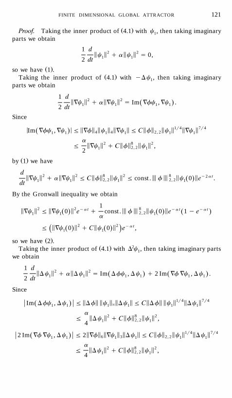
Ž .Proof. Taking the inner product of 4.1 with c , then taking imaginary1parts we obtain
1 d 2 25 5 5 5c q a c s 0,1 12 dtŽ .so we have 1 .
Ž .Taking the inner product of 4.1 with yDc , then taking imaginary1parts we obtain
1 d 2 25 5 5 5=c q a =c s Im =fc , =c .Ž .1 1 1 12 dt
Since
< < 5 5 5 5 5 5 5 5 5 51r4 5 5 7r4Im =fc , =c F =f c =c F C f c =cŽ . 4 4 2, 21 1 1 1 1 1
a 2 8 25 5 5 5 5 5F =c q C f c ,2, 21 12
Ž .by 1 we have
d 2 2 8 2 8 y2 a t5 5 5 5 5 5 5 5 A A 5 5=c q a =c F C f c F const. f c 0 e .Ž .2, 2 2, 21 1 1 1dt
By the Gronwall inequality we obtain
12 2 8ya t ya t ya t5 5 5 5 A A 5 5=c F =c 0 e q const. f c 0 e 1 y eŽ . Ž . Ž .2, 21 1 1a
5 5 2 5 5 2 ya tF =c 0 q C c 0 e ,Ž . Ž .Ž .1 1
Ž .so we have 2 .Ž . 2Taking the inner product of 4.1 with D c , then taking imaginary parts1
we obtain
1 d 2 25 5 5 5Dc q a Dc s Im Dfc , Dc q 2 Im =f =c , Dc .Ž . Ž .1 1 1 1 1 12 dt
Since
1r4 7r45 5 5 5 5 5 5 5 5 5 5 5Im Dfc , Dc F Df c Dc F C Df c DcŽ . `1 1 1 1 1 1
a 2 8 25 5 5 5 5 5F Dc q C f c ,2, 21 141r4 7r45 5 5 5 5 5 5 5 5 5 5 52 Im =f =c , Dc F 2 =f =c Dc F C f c DcŽ . 6 3 2, 21 1 1 1 1 1
a 2 8 25 5 5 5 5 5F Dc q C f c ,2, 21 14
LI AND CHEN122
we obtain
d 2 2 8 2 8 y2 a t5 5 5 5 5 5 5 5 A A 5 5Dc q a Dc F C f c F const. f c 0 e .Ž .2, 2 2, 21 1 1 1dt
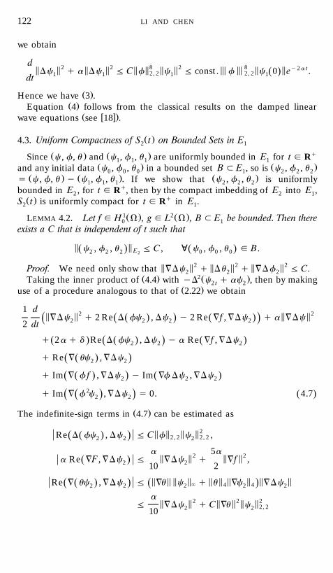
Ž .Hence we have 3 .Ž .Equation 4 follows from the classical results on the damped linear
Ž w x.wave equations see 18 .
Ž .4.3. Uniform Compactness of S t on Bounded Sets in E2 1
Ž . Ž . qSince c , f, u and c , f , u are uniformly bounded in E for t g R1 1 1 1Ž . Ž .and any initial data c , f , u in a bounded set B ; E , so is c , f , u0 0 0 1 2 2 2
Ž . Ž . Ž .s c , f, u y c , f , u . If we show that c , f , u is uniformly1 1 1 2 2 2bounded in E , for t g Rq, then by the compact imbedding of E into E ,2 2 1Ž . qS t is uniformly compact for t g R in E .2 1
1Ž . 2Ž .LEMMA 4.2. Let f g H V , g g L V , B ; E be bounded. Then there0 1exists a C that is independent of t such that
5 5c , f , u F C , ; c , f , u g B.Ž . Ž .E2 2 2 0 0 02
5 5 2 5 5 2 5 5 2Proof. We need only show that =Dc q Du q =Df F C.2 2 2Ž . 2Ž .Taking the inner product of 4.4 with yD c q ac , then by making2 t 2
Ž .use of a procedure analogous to that of 2.22 we obtain
1 d 2 25 5 5 5=Dc q 2 Re D fc , Dc y 2 Re =f , =Dc q a =DcŽ . Ž .Ž .Ž .2 2 2 22 dt
q 2a q d Re D fc , Dc y a Re =f , =DcŽ . Ž . Ž .Ž .2 2 2
q Re = uc , =DcŽ .Ž .2 2
q Im = f f , =Dc y Im =f Dc , =DcŽ . Ž .Ž .2 2 2
q Im = f 2c , =Dc s 0. 4.7Ž .Ž .Ž .2 2
Ž .The indefinite-sign terms in 4.7 can be estimated as
25 5 5 5Re D fc , Dc F C f c ,Ž .Ž . 2, 2 2, 22 2 2
a 5a2 25 5 5 5a Re =F , =Dc F =Dc q =f ,Ž .2 210 2
5 5 5 5 5 5 5 5 5 5Re = uc , =Dc F =u c q u =c =DcŽ . Ž .Ž . ` 4 42 2 2 2 2
a 2 2 25 5 5 5 5 5F =Dc q C =u c 2, 22 210
FINITE DIMENSIONAL GLOBAL ATTRACTOR 123
5 5 5 5 5 5 5 5 5 5Im = f f , =Dc F f f q f =f =DcŽ . Ž .Ž . 4 4 `2 2
a 25 5 5 5 5 5F =Dc q C f f ,2, 2 1, 2210
5 5 5 5 5 5Im =f Dc , =Dc F =f Dc =DcŽ . 4 42 2 2 2
5 5 5 51r4 5 5 7r4F C f c =Dc2, 2 2, 22 2
a 2 8 25 5 5 5 5 5F =Dc q C f c ,2, 2 2, 22 21022 5 5 5 5 5 5Im = f c , =Dc F C f c =DcŽ .Ž . 2, 2 2, 22 2 2 2
a 2 4 25 5 5 5 5 5F =Dc q C f c .2, 2 2, 22 210Let
5 5 2H t s =Dc q 2 Re D fc , Dc y 2 Re =f , =Dc .Ž . Ž . Ž .Ž .2 2 2 2 2
Ž .Then from 4.7 and the above estimates we get
d 2 25 5 5 5H t q aH t F K q C c =u ,Ž . Ž . 2, 22 2 2 2dt
5 5 5 5 5 5where K is a polynomial of c , f , and f . We note that K2, 2 2, 2 1, 22 2 2is bounded in Rq and denote its bound also by K . However, we have been2
5 5 2 `Ž q. Ž .unable to show that =u g L R , but we have 2.28 instead. SinceŽ . Ž .H 0 s 0, by using the Gronwall inequality, inserting 2.28 , and noting2
Ž .that H t is bounded we obtain1
K t2 2ya t ya Ž tys.5 5H t F 1 y e q C =u e dsŽ . Ž . H2 a 0
K 4t2 Xya t ya Ž tys.F 1 y e q C C y H s e dsŽ . Ž .H 1ž /a b0
K q C 4C 42 ya t ya ts q 1 y e q H 0 e y H t ,Ž . Ž . Ž .Ž .1 1ž /a b b
and therefore we obtain
2 K q 2C 8C22 ya t5 5=Dc F q 1 y eŽ .2 ž /a b
82 2 ya t5 5 5 5q C f c q H 0 e y H t .Ž . Ž .Ž .2, 2 2, 22 1 1b
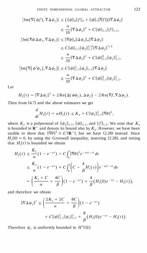
3Ž .Therefore c is uniformly bounded in H V .2
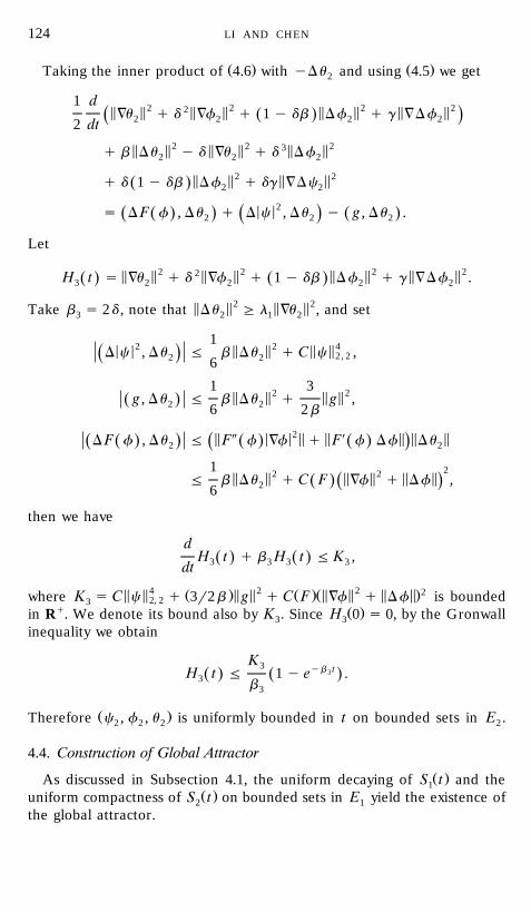
LI AND CHEN124
Ž . Ž .Taking the inner product of 4.6 with yDu and using 4.5 we get2
1 d 2 2 2 225 5 5 5 5 5 5 5=u q d =f q 1 y db Df q g =DfŽ .Ž .2 2 2 22 dt
5 5 2 5 5 2 3 5 5 2q b Du y d =u q d Df2 2 2
5 5 2 5 5 2q d 1 y db Df q dg =DcŽ . 2 2
< < 2s D F f , Du q D c , Du y g , Du .Ž . Ž .Ž . Ž .2 2 2
Let
5 5 2 2 5 5 2 5 5 2 5 5 2H t s =u q d =f q 1 y db Df q g =Df .Ž . Ž .3 2 2 2 2
5 5 2 5 5 2Take b s 2d , note that Du G l =u , and set3 2 1 2
12 2 4< < 5 5 5 5D c , Du F b Du q C c ,Ž . 2, 22 26
1 32 25 5 5 5g , Du F b Du q g ,Ž .2 26 2b
2Y X5 < < 5 5 5 5 5D F f , Du F F f =f q F f Df DuŽ . Ž . Ž .Ž . Ž .2 2
1 22 25 5 5 5 5 5F b Du q C F =f q Df ,Ž . Ž .26
then we have
dH t q b H t F K ,Ž . Ž .3 3 3 3dt
5 5 4 Ž .5 5 2 Ž .Ž5 5 2 5 5.2where K s C c q 3r2b g q C F =f q Df is bounded2, 23q Ž .in R . We denote its bound also by K . Since H 0 s 0, by the Gronwall3 3
inequality we obtain
K3 yb t3H t F 1 y e .Ž . Ž .3 b3
Ž .Therefore c , f , u is uniformly bounded in t on bounded sets in E .2 2 2 2
4.4. Construction of Global Attractor
Ž .As discussed in Subsection 4.1, the uniform decaying of S t and the1Ž .uniform compactness of S t on bounded sets in E yield the existence of2 1
the global attractor.
FINITE DIMENSIONAL GLOBAL ATTRACTOR 125
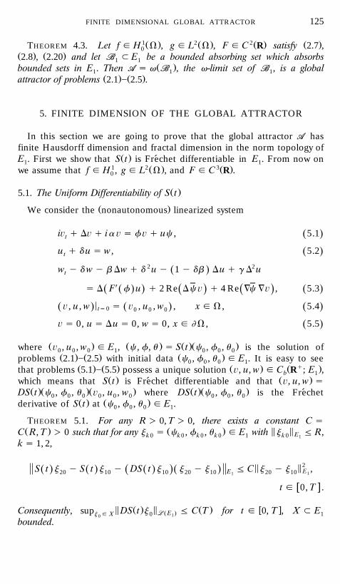
1Ž . 2Ž . 2Ž . Ž .THEOREM 4.3. Let f g H V , g g L V , F g C R satisfy 2.7 ,0Ž . Ž .2.8 , 2.20 and let BB ; E be a bounded absorbing set which absorbs1 1
Ž .bounded sets in E . Then AA s v BB , the v-limit set of BB , is a global1 1 1Ž . Ž .attractor of problems 2.1 ] 2.5 .
5. FINITE DIMENSION OF THE GLOBAL ATTRACTOR
In this section we are going to prove that the global attractor AA hasfinite Hausdorff dimension and fractal dimension in the norm topology of
Ž .E . First we show that S t is Frechet differentiable in E . From now on´1 11 2Ž . 3Ž .we assume that f g H , g g L V , and F g C R .0
Ž .5.1. The Uniform Differentiability of S t
Ž .We consider the nonautonomous linearized system
i q D¨ q ia ¨ s f¨ q uc , 5.1Ž .t
u q d u s w , 5.2Ž .t
w y d w y b Dw q d 2 u y 1 y db Du q g D2 uŽ .t
Xs D F f u q 2 Re Dc ¨ q 4 Re =c =¨ , 5.3Ž . Ž .Ž . Ž . Ž .<¨ , u , w s ¨ , u , w , x g V , 5.4Ž . Ž . Ž .ts0 0 0 0
¨ s 0, u s Du s 0, w s 0, x g V , 5.5Ž .
Ž . Ž . Ž .Ž .where ¨ , u , w g E , c , f, u s S t c , f , u is the solution of0 0 0 1 0 0 0Ž . Ž . Ž .problems 2.1 ] 2.5 with initial data c , f , u g E . It is easy to see0 0 0 1
Ž . Ž . Ž . Ž q .that problems 5.1 ] 5.5 possess a unique solution ¨ , u, w g C R ; E ,b 1Ž . Ž .which means that S t is Frechet differentiable and that ¨ , u, w s´
Ž .Ž .Ž . Ž .Ž .DS t c , f , u ¨ , u , w where DS t c , f , u is the Frechet´0 0 0 0 0 0 0 0 0Ž . Ž .derivative of S t at c , f , u g E .0 0 0 1
THEOREM 5.1. For any R ) 0, T ) 0, there exists a constant C sŽ . Ž . 5 5C R, T ) 0 such that for any j s c , f , u g E with j F R,Ek 0 k 0 k 0 k 0 1 k 0 1
k s 1, 2,
25 5S t j y S t j y DS t j j y j F C j y j ,Ž . Ž . Ž . Ž .Ž . EE20 10 10 20 10 20 10 11
w xt g 0, T .
5 Ž . 5 Ž . w xConsequently, sup DS t j F C T for t g 0, T , X ; ELL ŽE .j g X 0 110
bounded.
LI AND CHEN126
Ž .The proof is similar to that of the continuity of S t on E , so it is1omitted.
Ž .5.2. Transformation of m-Dimensional Volume by DS t
Ž .Let X be invariant set of S t in E , j g X. For any m linearly1 0Ž . Ž Ž . . Žindependent vectors j , . . . , j in E , we set U t s DS t j j 1 F k1 m 1 k 0 k
. 5 Ž . Ž .5 mF m . We are going to show that U t n ??? n U t , the m!-timesH E1 m 1
Ž . Ž .of the volume of a polyhedron with vertices 0, U t , . . . , U t , decays1 mexponentially as t ª q`, if m is sufficiently large.
Ž . Ž .Since the solution of 5.1 ] 5.5 is expected to be exponentially damped,Ž . s tŽ .it is suitable to put q, p, r s e ¨ , u, w , where s is a positive constant
Ž .to be determined later. It is easy to see that q, p, r satisfies the equations
iq q Dq q i a y s q s qf q c p 5.6Ž . Ž .t
p q d y s p s r , 5.7Ž . Ž .t
r y d q s r y b D r q d 2 p y 1 y db D p q g D2 pŽ . Ž .t
Xs D F f p q 2 Re Dc q q 4 Re =c =q , 5.8Ž . Ž .Ž . Ž . Ž .
Ž . Ž .Ž . Ž . Ž .where c , f, u s S t c , f , u , c , f , u g X. Note that c , f, u0 0 0 0 0 0Ž q .g C R ; E .b 1
5 Ž . Ž .5 m2 Ž Ž . Ž ..Since U t n ??? n U t s det U t , U t , we may construct aH E1 m j k1
Ž . Ž .bounded coercive quadratic form associated to 5.6 ] 5.8 and use it to5 Ž . Ž .5 m
2study the development of U t n ??? n U t .H E1 m 1
Ž .Taking the inner product of 5.6 with q, then taking imaginary parts weobtain
1 d 2 25 5 5 5q q a y s q s Im c p , q . 5.9Ž . Ž . Ž .2 dt
Ž . Ž .Taking the inner product of 5.6 with Dq q a y s Dq, making use of atŽ .procedure analogous to that of 2.22 , we can obtain
1 d 2 25 5 5 5Dq y 2 Re f q q c p , Dq q a y s DqŽ . Ž .Ž .2 dt
s 2a y 2s q d Re f q , Dq q a y 2s q d Re c p , DqŽ . Ž . Ž . Ž .q Im f 2q , Dq q Im fc p , Dq y Re u q , DqŽ . Ž .Ž .
qRe c r , Dq y Re c p , Dq s 0. 5.10Ž . Ž . Ž .t
FINITE DIMENSIONAL GLOBAL ATTRACTOR 127
Ž . Ž .Taking the inner product of 5.8 with r, using 5.7 we get
1 d 2 2 2 2 225 5 5 5 5 5 5 5 5 5r q d p q 1 y db =p q g D p y d q s rŽ . Ž .Ž .2 dt
5 5 2 2 5 5 2 5 5 2q b =r q d d y s p q d y s 1 y db =pŽ . Ž . Ž .5 5 2q d y s g D pŽ .
Xs y =F f p , =r q 2 Re Dc q , r q 4 Re =c =q , r . 5.11Ž . Ž . Ž . Ž .Ž .
Ž .Let m, n be large constants to be chosen . Define some quadratic formsŽ .on E : for any h s q, p, r g E ,1 1
5 5 2 5 5 2G t , h s m q q Dq y 2 Re f q , Dq y 2 Re c p , DqŽ . Ž . Ž .5 5 2 2 5 5 2 5 5 2 5 5 2q n r q nd p q n 1 y db =p q ng D p , 5.12Ž . Ž .
5 5 2 5 5 2 5 5 2 5 5 2G h s m a y s q q a y s Dq y n d q s r q nb =rŽ . Ž . Ž . Ž .1
2 5 5 2 5 5 2q nd d y s p q n d y s 1 y db =pŽ . Ž . Ž .5 5 2q n d y s g D p , 5.13Ž . Ž .
G t , h s m Im c p , q q 2a y 2s q d Re f q , DqŽ . Ž . Ž . Ž .2
q a y 2s q d Re c p , DqŽ . Ž .
q Im f 2 , Dq y Im fc p , Dq y Re u q , DqŽ . Ž .Ž .q
y Re c r , Dq y Re c p , Dq q n = FX f p , =rŽ . Ž . Ž .Ž .Ž .t
q 2n Re Dc q , r q 4n Re =c =q , r . 5.14Ž . Ž . Ž .
Ž . Ž . Ž .Then m 5.9 q 5.10 q n 5.11 implies
1 dG t , h q G h s G t , h . 5.15Ž . Ž . Ž . Ž .1 22 dt
2 2 12A A Ž .A A � 4Choose m G 8 f , n G 8rd c , and s F min d , a . Then0, ` 0, ` 2
1 2 1 2< < 5 5 5 5 5 5 5 5 5 52 Re f q , Dq F 2 f q Dq F m q q Dq ,Ž . ` 2 4
1 2 1 22< < 5 5 5 5 5 5 5 5 5 52 Re c p , Dq F 2 c p Dq F nd p q Dq ,Ž . ` 2 4
LI AND CHEN128
Ž . qtherefore G t, h is a bounded quadratic form on E , uniformly in t g R ,1i.e.,
< < 5 5 2G t , h F C h , for h s q , p , r g E , 5.16Ž . Ž . Ž .E 11
and coercive, uniformly in t g Rq:
1 2 1 2 2 1 225 5 5 5 5 5 5 5G t , h G m q q Dq q n r q nd pŽ . 2 2 2
5 5 2 5 5 2q n 1 y db =p q ng D pŽ .5 5 2G C h . 5.17Ž .E1
Ž .Obviously G h is also bounded and coercive quadratic form on E .1 15 5 5 5 5 5 5 5 `Ž q.Noting that c , f , u , c are all in L R , by estimating2, 2 2, 2 t
Ž .G t, h term by term we have2
1 2 2 2< < 5 5 5 5 5 5G t , h F G h q C q q p q r . 5.18Ž . Ž . Ž .Ž .y1 , 22 12
Ž . Ž . Ž .Let J t, h s G t, h y G h , then from the above analysis there exists2 1an « ) 0 such that
1 d 2 2 25 5 5 5 5 5G t , h s J t , h F y« G t , h q C q q p q r .Ž . Ž . Ž . Ž .y1 , 22 dt5.19Ž .
ŽŽ .y1 Ž .y1 Ž .y1 . Ž .Define Kh s yD q, yD p, yD r for any h s p, q, r g E .1Then K is a linear, self-adjoint, positive, and compact operator on E . So1
Ž .it possesses a sequence of eigenvalues k l s 1, 2, . . . , which is decreasinglin l and tends to zero as l ª `. Moreover,
5 5 2 5 5 2 5 5 2Kh , h s =q q =p q r . 5.20Ž . Ž .E y1, 21
Therefore there exists a constant C ) 0 such that
J t , h F C Kh , h . 5.21Ž . Ž . Ž .E1
˜ ˜Ž . Ž . Ž .Let G t, ? , ? and J t, ? , ? be the polar forms associated to G t, ? and˜Ž . Ž .J t, ? respectively. Then G t, ? , ? is bounded and coercive, uniformly in
q ˜ ˜Ž . Ž .t g R . Moreover, J t, ? , ? is dominated by G t, ? , ? in the sense ofŽ .5.21 .
Ž . Ž . Ž .Now let j , j 1 F k F m and U t 1 F k F m be the same as at the0 k kŽ . s t Ž .beginning of this subsection. Then h t ' e U t is the solution ofk k
Ž . Ž . 5 Ž . Ž .5 m25.6 ] 5.8 corresponding to initial data j , and U t n ??? n U t H Ek 1 m 1
FINITE DIMENSIONAL GLOBAL ATTRACTOR 129
y2 ms t 5 Ž . Ž .5 m2s e h t n ??? n h t . By the boundedness and coercivity ofH E1 m 1
G, there are two constants C , C ) 0 such that1 2
m ˜C det h t , h t F det G t , h t , h tŽ . Ž . Ž . Ž .Ž . Ž .1 j k j kE1
F C mdet h t , h t 5.22Ž . Ž . Ž .Ž .2 j k E1
˜ ˜Ž w x. Ž . Ž Ž . Ž .. Ž Ž . Ž ..see 5 . Since drdt G t, h t , h t s J t, h t , h t , differentiatingj k j k˜Ž Ž . Ž ..det G t, h t , h t column by column we obtainj k
d ˜det G t , h t , h tŽ . Ž .Ž .j kdtm
˜ ˜s det 1 y d G t , h t , h t q d J t , h t , h t ,Ž . Ž . Ž . Ž . Ž .Ž . Ž .Ý ž /k l j k k l j kls1
5.23Ž .
Ž w x.where d is the Kronecker deltas. By a linear algebraic lemma see 5 ,jk
m˜ ˜det 1 y d G t , h t , h t q d J t , h t , h tŽ . Ž . Ž . Ž . Ž .Ž . Ž .Ý ž /k l j k k l j k
ls1
m˜s v det G t , h t , h t , 5.24Ž . Ž . Ž .Ž .Ý l j kž /
ls1
where
J t ,Ým x h tŽ .Ž .js1 j jv s max min .l mm xgF t ,Ý x h tF;R Ž .Ž .js1 j jx/0dim Fsl
Ž .Using 5.21 and coercivity of G,
KÝm x h t ,Ým x h tŽ . Ž .Ž .js1 j j js1 j j E1v F C max minl 2mm 5 5xgFF;R Ý x h tŽ . Ejs1 j j 1x/0dim Fsl
Kh , hŽ . E1F C max min 25 5F;E hgF h1 E1h/0dim Fsl
F Ck .l
LI AND CHEN130
Ž . Ž .Therefore 5.23 , 5.24 yield
m˜ ˜det G t , h t , h t F det G 0, j , j exp C k t .Ž . Ž . Ž .Ž . Ýj k j k lž /
ls1
Ž .Hence, by 5.22 ,
5 5 mh t n ??? n h t s det h t , h tŽ . Ž . Ž . Ž .Ž .H E1 m j k1 E1
m mC2 2m5 5F j n ??? n j exp C k t .ÝH E1 m l1 ž /ž /C1 ls1
5.25Ž .
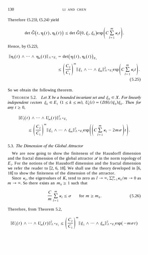
So we obtain the following theorem.
THEOREM 5.2. Let X be a bounded in¨ariant set and j g X. For linearly0Ž . Ž . Ž Ž . .independent ¨ectors j g E 1 F k F m , U t s DS t j j . Then fork 1 k 0 k
any t G 0,
5 5 m2U t n ??? n U tŽ . Ž . H E1 m 1
m mC2 2m5 5F j n ??? n j exp C k y 2ms t .ÝH E1 m l1 ž /ž / ž /C1 ls1
5.3. The Dimension of the Global Attractor
We are now going to show the finiteness of the Hausdorff dimensionand the fractal dimension of the global attractor AA in the norm topology ofE . For the notions of the Hausdorff dimension and the fractal dimension1
w x wwe refer the reader to 2, 6, 18 . We shall use the theory developed in 6,x18 to show the finiteness of the dimension of the attractor.Since k , the eigenvalues of K, tend to zero as l ª `, Ým k rm ª 0 asl ls1 l
m ª `. So there exists an m G 1 such that0
mCk F s for m G m . 5.26Ž .Ý l 0m ls1
Therefore, from Theorem 5.2,
mC22 2
m m5 5 5 5U t n ??? n U t F j n ??? n j exp yms tŽ . Ž . Ž .H E H E1 m 1 m1 1ž /C1
FINITE DIMENSIONAL GLOBAL ATTRACTOR 131
for t G 0, m G m . From this inequality we see that there exists a t G 00 0w x Žsuch that the conditions of Theorem V.3.1 and V.3.2 in 18 or of
w x.Theorem 4.1 in 6 hold. Therefore we have the following theorem.
Ž .THEOREM 5.3. Let m be the same as in 5.26 . Then0
Ž .1 the Hausdorff dimension of the global attractor AA is less than orequal to m ;0
Ž .2 the fractal dimension of the global attractor AA is less than or equalto 2m .0
REFERENCES
1. R. A. Adams, ‘‘Sobolev Spaces,’’ Academic Press, New York, 1975.2. P. Constantin, C. Foias, and R. Temam, Attractors representing turbulent flows, Memoirs
Ž .Amer. Math. Soc. 53, No. 314 1985 .Ž .3. I. Flahaut, Attractors for the dissipative Zakharov system, Nonlinear Anal. 16 1991 ,
599]633.4. A. Friedman, ‘‘Partial Differential Equations,’’ Holt, Reinhart, and Winston, 1969.5. J. M. Ghidaglia, Weakly damped forced KdV equation behave as a finite dimensional
Ž .dynamical system in the long time, J. Differential Equations 74 1988 , 369]390.6. J. M. Ghidaglia and R. Temam, Attractors for damped nonlinear hyperbolic equations,
Ž .J. Math. Pures Appl. 66 1987 , 273]319.7. J. M. Ghidaglia, Finite dimensional behavior for weakly damped Schrodinger equations,¨
Ž .Ann. Inst. H. Poincare Anal. 5 1988 , 365]405.´8. B. Guo, Global solutions of Schrodinger equation interacting with Bq-type self-consistent¨
Ž .field, Acta Math. Sinica 26, No. 3 1983 , 295]306.9. B. Guo, Initial boundary value problems for one class of system of multidimensional
nonlinear Schrodinger]Boussinesq type equations, J. Math. Res. Exposition 8, No. 1¨Ž .1988 , 61]71.
10. B. Guo and F. Chen, Finite dimensional behavior of global attractors for weakly dampedŽ .nonlinear Schrodinger]Boussinesq equation, Phys. D 93 1996 , 101]118.¨
11. B. Guo and L. Shen, The global solution for the initial boundary value problem of thesystem of Schrodinger]Boussinesq type equations in three dimensions, Acta Math. Appl.¨
Ž .Sinica 6, No. 1 1990 ; see also Symposium of DD7 Tianjin, China, 1986, 26]27.12. Y. Li, On the initial boundary value problems for two dimensional systems of Zakharov
equations and of complex-Schrodinger-real-Boussinesq equations, J. Partial Differential¨Ž .Equations 5, No. 2 1992 , 81]93.
13. Y. Li, Finite dimension of global attractor of dissipative Klein]Gordon]Schrodinger¨Ž .equations, Appl. Math. 8 1995 , 174]179.
14. J. L. Lions and E. Magenes, ‘‘Nonhomogeneous Boundary value Problem and Applica-tions,’’ Vol. 1, Springer-Verlag, BerlinrHeidelbergrNew York, 1972; transl. from Frenchby P. Kenneth.
15. V. G. Makhankov, On stationary solutions of Schrodinger equations with a self-consistent¨Ž .potential satisfying Boussinesq equations, Phys. Lett. A 50 1974 , 42]44.
LI AND CHEN132
Ž .16. V. G. Makhankov, Dynamics of classical solitons in Nonintegrable systems , Phys. Rep.,Ž .Phys. Lett. C 35, No. 1 1978 .
17. K. Nishikawa, H. Hijo, K. Mima, and H. Ikezi, Coupled nonlinear electron-plasma andŽ .ion-acoustic waves, Phys. Lett. 33 1974 , 148]150.
18. R. Temam, ‘‘Infinite Dimensional Dynamical Systems in Mechanics and Physics,’’Springer-Verlag, Berlin, 1988.
19. V. E. Zakharov and A. B. Shabat, Integrable system of nonlinear equations in mathemati-Ž .cal physics, Funct. Anal. Appl. 83 1974 , 43]53.
Related Documents