FINITE DIFFERENCE MODELLING OF LATERALLY LOADED PILES GEEN501 – Advanced Geotechnics Coursework (Group 13) Abstract This report aims to provide a design analysis for the client for a concrete pile that is subject to an active load of 45kN and a passive load generated by an embankment. In order to carry out the design analysis, a finite difference method was used in conjunction with a number of logical assumptions to generate a matrix and from a series of iterations, the deflection of the pile under passive and active loading was obtained. The lateral deflection of the concrete pile was found to be 0.0258m which generated a bending moment of 182.3426kNm. The deflection was deemed to be too great for the assumed usage of the pile and so suitable remedies to this problem were suggested. A suitable pile design was determined from this moment to be 0.6m, reducing the lateral deflection by 0.016m. Daniel Wilkinson – Student ID: 10342869 Lawrence Taylor – Student ID: 10395608

Welcome message from author
This document is posted to help you gain knowledge. Please leave a comment to let me know what you think about it! Share it to your friends and learn new things together.
Transcript

FINITE DIFFERENCE
MODELLING OF LATERALLY
LOADED PILES GEEN501 – Advanced Geotechnics Coursework
(Group 13)
Abstract This report aims to provide a design analysis for the client for a concrete pile that is subject to an active load of 45kN and a passive load generated by an embankment. In order to carry out the design analysis, a finite difference method was used in conjunction with a number of logical assumptions to generate a matrix and from a series of iterations, the deflection of the pile under passive and active loading was obtained. The lateral deflection of the concrete pile was found to be 0.0258m which generated a bending moment of 182.3426kNm. The deflection was deemed to be too great for the assumed usage of the pile and so suitable remedies to this problem were suggested. A suitable pile design was determined from this moment to be 0.6m, reducing the lateral deflection by 0.016m.
Daniel Wilkinson – Student ID: 10342869 Lawrence Taylor – Student ID: 10395608
1
Contents 1.0 Introduction ...................................................................................................................................... 2
1.1 Statement of the Problem ............................................................................................................ 2
1.2 Soil and Loading Conditions .......................................................................................................... 2
2.0 Method ............................................................................................................................................. 3
2.1 Determination of Boundary Conditions ........................................................................................ 3
2.2 Determination of Pile Deflection .................................................................................................. 3
2.3 Determining of Slope, Bending Moment, Shear Force and Soil Reaction .................................... 4
03.0 Results ............................................................................................................................................. 5
4.0 Calculations (Design of Concrete Pile) .............................................................................................. 7
5.0 Discussion .......................................................................................................................................... 8
6.0 Conclusion ....................................................................................................................................... 13
References ............................................................................................................................................ 14
Appendices ............................................................................................................................................ 15

2
1.0 Introduction
1.1 Statement of the Problem A pile is required near an embankment to support a lateral load. The head of the pile is to
be fixed so as not to provide any rotation to the attached structure. Either the embankment
will not be built until the pile has been embedded or the ground conditions relating to the
passive displacement of the earth has not been collected. Therefore, the conditions of the
embankment must be estimated using graphs to produce the lateral displacement of the
soil. It is unknown what the pile will be supporting but possible structures include a bridge
abutment, supporting an inclined column or supporting a retaining structure etc. (The
Institution of Structural Engineers, 2013, p. 142).
A report must be compiled which not
only analyses the conditions that the
pile will be subjected to using Finite
Difference Modelling, but also
produce a critical analysis of the
results and produce a conclusion to
determine whether the pile solution is
appropriate.
The report is structured as follows:
Section 2 outlines the method
employed to model the pile and the boundary conditions used. Section 3 provides the initial
results of the pile solution. Section 4 critically analyses and discusses the results providing
an alternative solution to the problem & Section 5 presents the conclusions of the report. All
calculations relating to the report can be found in Appendices A & B.
1.2 Soil and Loading Conditions Loading conditions:
The head of the pile is to be subjected to an active (Design) load of 45kN at the head of the
pile. The pile will also be subjected to passive lateral loading via an adjacent embankment of
which the loading will only affect the portion of the pile embedded in the top soil. The
maximum passive soil displacement due to the embankment is assumed to be
approximately 20mm.
Pile attributes:
The diameter of the pile is 0.52m. The head of the pile is to be fixed (to allow for horizontal
translation but no rotation) and the tip of the pile is to be modelled as rigidly embedded, as
it is embedded in a hard stratum by 1.5m. The elastic modulus of the concrete is, E =
2.2x10⁷kN/m².
Soil conditions:
Depth of top soil is 6.7m. The Kh value of the top soil is to 5700yz0.72kN/m³ and the Kh value
of the hard stratum is to 3300yzkN/m³ (subgrade reaction moduli).
Figure 1: Diagram showing type of problem to be
solved.

3
2.0 Method
2.1 Determination of Boundary Conditions The boundary conditions of the numerical model must conform to those of the pile being
modelled. As the pile has a fixed head, it can be assumed that there is no rotation at node 1,
so that the pile will only deflect through translation. This means the first fixed head
boundary condition is (Azizi, 2013, p. 290):
𝑦−1 = 𝑦2
As the pile head is fixed, a moment will be generated at the head of the pile when it is
subjected to a lateral force. The equation for the free head pile is modified to include a
moment and through rearrangement it can be seen that the second boundary condition for
the fixed head pile is as follows (Azizi, 2013, p. 290):
𝑦−2 = 𝑦3 −2𝐻𝑜(∆𝑧)³
𝐸𝑝𝐼𝑝
For this problem, the pile is to be embedded into a hard stratum. For this reason, it was
assumed that the pile would be rigidly embedded. Although the depth of embedment is not
a design parameter, it is assumed that for the use of a numerical model that the pile is
flexible (Azizi, 2013, p. 281).
In order to implement a computational molecule in correspondence with these boundary
conditions, it is necessary to have two imaginary nodes above the fixed head pile. These
imaginary nodes form part of the boundary conditions by using the assumptions that the
pile head is fixed and the pile tip is rigidly embedded in the hard stratum.
As the pile is rigidly embedded, it can be assumed that there is neither deflection nor
rotation at the tip and according to Azizi (2013, 2013, p. 290) this creates only one imaginary
node at the base of the pile. These conditions conform to the boundary conditions below:
𝑦𝑛 = 0
𝑦𝑛+1 = 𝑦𝑛−1
2.2 Determination of Pile Deflection To allow for a full analysis of the pile, the deflection must be determined by using the
second derivative of the beam equation. This involves the use of a computational molecule
in conjunction with a suitably sized finite difference mesh. A mesh with a value of ∆𝑧 = 0.05
is used as too finer a mesh would introduce truncation errors (Azizi, 2013, p. 300). In total,
this gives 165 nodes which is deemed an appropriate number of nodes for the solution.
As the problem involves two layers of soil, there is a need for two separate molecules, one
for each soil layer. In addition to this, a third computational molecule is used for node 𝑦165
to incorporate the additional imaginary node placed at the tip of the pile. In total three
computational molecules are used in the realisation of the problem based on the finite
difference formulas (Azizi, 2013, p. 285):
(1)
(2)
(4)
(3)

4
𝑦𝑖−2 − 4𝑦𝑖−1 + (6 +𝐾ℎ𝑑
𝐸𝑝𝐼𝑝(∆𝑧)4) 𝑦𝑖 − 4𝑦𝑖+1 + 𝑦𝑖+2 =
𝐾ℎ𝑑
𝐸𝑝𝐼𝑝(∆𝑧)4𝑔(𝑧)
𝑦𝑖−2 − 4𝑦𝑖−1 + 6𝑦𝑖+1 (𝐾ℎ𝑑
𝐸𝑝𝐼𝑝
(∆𝑧)4 − 4) 𝑦𝑖 + 𝑦𝑖+2 =𝐾ℎ𝑑
𝐸𝑝𝐼𝑝
(∆𝑧)4𝑔(𝑧)
Computational molecules are then devised for each soil layer and one for the rigidly
embedded boundary condition at the pile tip.
These computational nodes are placed systematically on each node along the pile shaft and
a separate nodal equation is used for each of the 165 nodes. The first molecule is used to a
depth of 6.7m of top soil and the second is used in the hard stratum for the remaining 1.5m.
The third modified molecule is used to enforce the boundary conditions at the rigidly
embedded tip of the pile.
The first iteration uses an assumed value for y, the deflection. A value of 𝑦 = 0.05𝑚 is used
for an initial deflection assumption. Subsequent interactions use the deflections from the
previous matrix iteration. Iterations are then performed until the difference between each
iteration was less than or equal to 1 × 10⁻⁴𝑚.
2.3 Determining of Slope, Bending Moment, Shear Force and Soil Reaction From the deflection values determined from matrix iterations, the slope, bending moment,
shear force and soil reaction can then be determined (equations 7, 8, 9 & 10).
𝑆𝑙𝑜𝑝𝑒 =𝑦𝑖+1−𝑦𝑖−1
2(∆𝑧)
𝐵𝑒𝑛𝑑𝑖𝑛𝑔 𝑀𝑜𝑚𝑒𝑛𝑡 =𝐸𝑝𝐼𝑝
(∆𝑧)2(𝑦𝑖−1 − 2𝑦𝑖 + 𝑦𝑖+1)
1
1
-4
-4
6 + 0.000000234613yz0.72
1
1
-4
-4
6 + 0.000000135829yz
1
1
-4
0.000000135829yz - 4
6
(5)
(6)
(7)
(8)
Figure 2: Computational molecules.
5
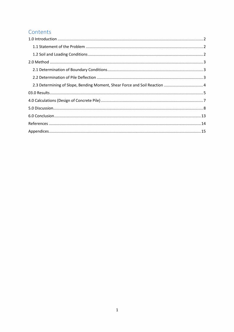
𝑆ℎ𝑒𝑎𝑟 𝐹𝑜𝑟𝑐𝑒 =𝑀𝑖+1−𝑀𝑖−1
2(∆𝑧)
𝑆𝑜𝑖𝑙 𝑅𝑒𝑎𝑐𝑡𝑖𝑜𝑛 = −𝐾ℎ𝑑. 𝑦
These values are plotted to obtain the graphs shown in the results section below.
03.0 Results
Figure 3: Graph showing lateral deflection of pile with and
without passive loading.
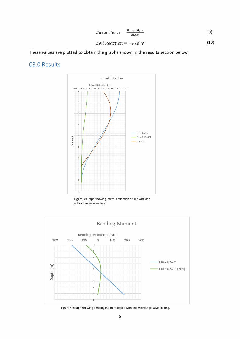
Figure 4: Graph showing bending moment of pile with and without passive loading.
(9)
(10)

6
Figure 5: Graph showing shear force of pile with and without passive loading.
Figure 6: Graph showing Soil Reaction of pile with and
without passive loading.

7
Table 1: Table showing maximum values for 0.52m diameter pile actively and passively loaded and
only actively loaded.
4.0 Calculations (Design of Concrete Pile) The pile has been modelled as a beam. To convert the rectangular beam to a circular
concrete pile the Charles Whitney method (McCormac and Brown, 2015) has been used
(Figure 7). Ag is the cross-sectional area of the
column. BM has been multiplied by 1.5 as the
Charles Whitney method is an approximation.
The diameter of the links is assumed to be
10mm and DS = 0.4m.
The minimum cover required (over the rebar)
is 50mm, as d ≤ 0.6m (ref).
Depth of beam = 416mm & beam width = 510mm.
𝑘 = 𝑀𝐸𝑑
𝑏𝑑2𝑓𝑐𝑘=
1.5 ∗ 183𝑥106
510 ∗ 3432 ∗ 30= 0.152
𝑘 ≤ 𝑘′(0.168) ∴ 𝑁𝑜 𝑐𝑜𝑚𝑝𝑟𝑒𝑠𝑠𝑖𝑜𝑛 𝑟𝑒𝑖𝑛𝑓𝑜𝑟𝑐𝑒𝑚𝑒𝑛𝑡 𝑟𝑒𝑞𝑢𝑖𝑟𝑒𝑑.
𝑧 = 𝑑
2[1 + √1 − 3.53𝑘] ≤ 0.95𝑑
𝑧 = 343
2[1 + √1 − 3.53 ∗ 0.152] ≤ 0.95𝑑 (0.95𝑑 = 326)
288 ≤ 326 ∴ 𝑧 = 288
𝐴𝑠 = 𝑀
𝑓𝑦𝑑𝑧=
1.5 ∗ 183 ∗ 106
435 ∗ 288= 2191𝑚𝑚2
According to The British Standards Institution (2015, p. 28) As ≥ 0.5%Ac, therefore As,min,req’d =
0.00105m2.
𝐴𝑠,𝑚𝑎𝑥 = 0.04𝐴𝑐 = 0.04 ∗ [(510 ∗ 416) − (2454 + 2454)] = 8486𝑚𝑚2
ADOPT 5 No. H25’s TOP STEEL (Tension in both sides)
ADOPT 5 No. H25’s BOTTOM STEEL
Figure 7: Charles Whitney method.
0.0258 0.0041
-182.3426 -79.7625
-2.3614 -13.6285
45 45Max. Shear Force (kN)
Active + Passive Loading Active Loading Only
Max. Lateral Deflection (m)
Max. Bending Moment (kNm)
Max. Soil Reaction (kN/m)

8
Therefore 10 No. H25’s for longitudinal rebar
VEd = 45kN
𝜈𝐸𝑑 = 𝑉𝐸𝑑
𝑏𝑤𝑧=
45 ∗ 103
510 ∗ 288= 0.306𝑁/𝑚𝑚2
For fck = 30N/mm²: VRd,maxcotθ=2.5 = 3.64; VRd,maxcotθ=1.0 = 5.28.
𝜈𝑅𝑑,𝑚𝑎𝑥𝑐𝑜𝑡𝜃=2.5 = 3.64𝑁/𝑚𝑚2 > 𝑣𝐸𝑑 ∴ 𝑃𝑟𝑜𝑣𝑖𝑑𝑒 𝑚𝑖𝑛𝑖𝑚𝑢𝑚 𝑠ℎ𝑒𝑎𝑟 𝑟𝑒𝑖𝑛𝑓𝑜𝑟𝑐𝑒𝑚𝑒𝑛𝑡
𝑠𝑙,𝑚𝑎𝑥 = 0.75𝑑 = 0.75 ∗ 343 = 257𝑚𝑚
𝐴𝑠𝑤 = 𝜈𝐸𝑑𝑏𝑤𝑠𝑙
𝑓𝑦𝑤𝑑𝑐𝑜𝑡𝜃=
0.306 ∗ 510 ∗ 257
435 ∗ 2.5= 37𝑚𝑚2
According to The British Standards Institution (2015, p. 29) the minimum transverse links
required: 6mm or ¼ max diameter of the longitudinal bars.
ADOPT H10 SHEAR LINKS
Deflection has not been checked as this is a serviceability requirement and therefore not
appropriate to be considered for the pile solution.
5.0 Discussion The purpose of this report was to determine if the pile used to resist the lateral active and
passive loads was over or under designed. Within engineering there is the need to find an
appropriate balance between safety, cost, build ability and serviceability. With tools such as
finite difference modelling and finite element analysis, it is relatively simple to be able to
analyse these factors and determine the most effective solution to an engineering problem.
According to Azizi (2013), using a pile with a diameter less than or equal to 600mm allows
the pile to be driven into the ground. If the piles diameter were to be greater than 600mm,
then the preferred option would be to bore a hole into the ground and then embed the pile
to allow easier construction. The pile that a solution must be provided for is 520mm in
diameter meaning that it is close to not being practical to embed it into the soil by driving, it
is also not known if the hard stratum is suitable for driven piles. Therefore, it is deemed
appropriate to design the pile for boring into the ground. Indeed, Section 4 above uses the
British Standards document for bored piles in the calculations for information such as the
appropriate amount of cover for the rebar (British Standards Institution, 2015). Another
reason for boring a hole for the pile is to ensure that the tip of the pile is not subjected to
undue pressure which may crack/weaken the overall pile structure when driven into the
hard stratum.
Although enough about the initial conditions is known to carry out the finite difference
modelling, there are many unknowns associated with this problem that require the use of
assumptions and engineering judgement. The finite difference analysis determined that the
maximum displacement of the concrete pile is 0.026m (Table 1). It is reasonable (and safe)
to assume that the pile is supporting a superstructure of some kind that is built before the
9
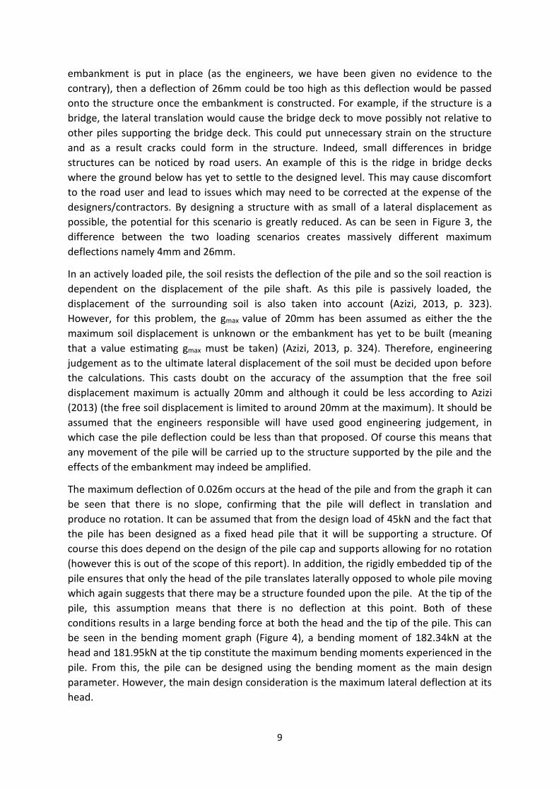
embankment is put in place (as the engineers, we have been given no evidence to the
contrary), then a deflection of 26mm could be too high as this deflection would be passed
onto the structure once the embankment is constructed. For example, if the structure is a
bridge, the lateral translation would cause the bridge deck to move possibly not relative to
other piles supporting the bridge deck. This could put unnecessary strain on the structure
and as a result cracks could form in the structure. Indeed, small differences in bridge
structures can be noticed by road users. An example of this is the ridge in bridge decks
where the ground below has yet to settle to the designed level. This may cause discomfort
to the road user and lead to issues which may need to be corrected at the expense of the
designers/contractors. By designing a structure with as small of a lateral displacement as
possible, the potential for this scenario is greatly reduced. As can be seen in Figure 3, the
difference between the two loading scenarios creates massively different maximum
deflections namely 4mm and 26mm.
In an actively loaded pile, the soil resists the deflection of the pile and so the soil reaction is
dependent on the displacement of the pile shaft. As this pile is passively loaded, the
displacement of the surrounding soil is also taken into account (Azizi, 2013, p. 323).
However, for this problem, the gmax value of 20mm has been assumed as either the the
maximum soil displacement is unknown or the embankment has yet to be built (meaning
that a value estimating gmax must be taken) (Azizi, 2013, p. 324). Therefore, engineering
judgement as to the ultimate lateral displacement of the soil must be decided upon before
the calculations. This casts doubt on the accuracy of the assumption that the free soil
displacement maximum is actually 20mm and although it could be less according to Azizi
(2013) (the free soil displacement is limited to around 20mm at the maximum). It should be
assumed that the engineers responsible will have used good engineering judgement, in
which case the pile deflection could be less than that proposed. Of course this means that
any movement of the pile will be carried up to the structure supported by the pile and the
effects of the embankment may indeed be amplified.
The maximum deflection of 0.026m occurs at the head of the pile and from the graph it can
be seen that there is no slope, confirming that the pile will deflect in translation and
produce no rotation. It can be assumed that from the design load of 45kN and the fact that
the pile has been designed as a fixed head pile that it will be supporting a structure. Of
course this does depend on the design of the pile cap and supports allowing for no rotation
(however this is out of the scope of this report). In addition, the rigidly embedded tip of the
pile ensures that only the head of the pile translates laterally opposed to whole pile moving
which again suggests that there may be a structure founded upon the pile. At the tip of the
pile, this assumption means that there is no deflection at this point. Both of these
conditions results in a large bending force at both the head and the tip of the pile. This can
be seen in the bending moment graph (Figure 4), a bending moment of 182.34kN at the
head and 181.95kN at the tip constitute the maximum bending moments experienced in the
pile. From this, the pile can be designed using the bending moment as the main design
parameter. However, the main design consideration is the maximum lateral deflection at its
head.

10
It is stated in geotechnical design codes that a deflection of up to 100mm is permitted on
piles that are under 600mm in diameter (British Standards Institution, 2015). From the
information in the technical document, it is assumed that cracking of the concrete will not
occur which will undermine the protection of the rebar. However, it could be assumed that
if the pile was part of a number of piles supporting a building or a bridge, then movement in
a single pile could become more problematic. For example, in a building, a movement of
0.026m could exceed the serviceability limit of the design and as a result of this, cracking
and damage to finishes may occur. This could lead to lawsuits and costly steps to correct the
issue by either replacing the pile or inserting more piles. So although a deflection of 0.026m
could be interpreted as acceptable according to the codes and by judgement, if the
embankment (which exerts the passive load) is built after the superstructure (or temporarily
placed there after the structure is built) then depending on the original design brief of the
pile, it may not be acceptable as far as the design of the structure above it. Additionally, it
could be suggested that if the structure above the pile is a bridge, the effect of the lateral
movement of the pile could be mitigated by the use of flexible links on the bridge deck. In
this instance, the movement is perhaps less of an issue, however as the use of the pile is
unstated so this can only be speculated. One way of interpreting the results is that the
embankment shown next to the pile may in fact be a temporary structure and could be
removed after the construction phase is complete. To ensure that this causes little issue,
this should be done before the pile is subjected to its supporting load, if not, when the
embankment load is removed the deflection would return to 0.004m from 0.025m (Table 1
and Figure 3). Obviously, this would create the same situation as above and could result in
damage to finishes or structural stresses.
To reduce the lateral deflection in the pile to produce a smaller displacement (if the
embankment were to be removed after the structure is built etc.) then one way to increase
the lateral resistance of the pile would be to replace the existing pile with a steel hollow
section or a steel H section pile (by increasing the Young’s Modulus of the section).
However, the use of steel hollow piles is more normally used in the marine environment
(Azizi, 2013, p.192) and the information given in the brief for this problem does not suggest
that this pile will be situated in such an environment. In addition to this, as the deflection in
the pile is derived from both the stiffness of the pile in question and the stiffness of the soil
around it, the lateral deflection of the pile can be reduced by increasing the second moment
of area of the pile and/or the stiffness of the surrounding soil. Techniques to improve the
lateral resistance of the top soil could be used in order to make savings on costs compared
to the removal and installation of a new pile. These techniques can include the removal and
replacement of the top soil, adjustments to the density of the top soil, grouting, or soil
mixing (using a binder such as cement or a more granular material) (Transportation
Research Board, 2011). Although there may be limitations on doing this such as site access
or water tables or other site variables, with the information given it may be a plausible
method for increasing the lateral resistance of the soil without having to remove or alter the
pile itself.
Indeed, the idea that strengthening the soil around the pile could become more important if
the pile is in a position where it is extremely difficult to remove or alter. For example, as

11
assumed, the pile is supporting a bridge deck or perhaps a building, to get to the pile
remove it the bridge or building must also be altered at great expense. Furthermore, from a
practical build ability point of view, it may be more beneficial to a project to pursue this line
of action to limit disruption to the structure and potentially save time in correcting the
matter. This option would be expensive to correct any issues. It is therefore far better to use
a well-designed pile in the first instance.
The preferred solution to decrease the lateral deflection of the pile is to increase its
diameter. As the brief has suggested the use of a concrete pile already the model only
requires adjustment of the matrices involved with designing the 0.52m diameter pile
solution saving time and money for the client. Figure 7 below shows a set of differing
diameter piles and what the effect of diameter size has on the overall deflected shape.
From Figure 8 it can be shown that as the diameter increases the lateral deflection
decreases. It is interesting to note that as the piles diameter increases, the change in
deflection decreases. In order to keep the cost down for the client it is proposed that the
diameter of the pile should be increased to a diameter of 0.6m as this decreases the
deflection by approximately 16mm.
When the deflection of the 0.6m diameter pile is compared to that of the 0.52m pile under
active + passive loading and active loading only it can be seen that the deflection of the
actively loaded pile barely changes. This results in a difference in deflection of the two pile
types of 1mm as shown in Figure 9.
Figure 8: Graph showing change in deflection vs. change in
diameter of concrete pile.

12
Figure 9 therefore suggests that if the embankment is to be placed after the pile has been
actively loaded then the 0.6m diameter pile would deflect by only 12mm whereas the 0.52m
diameter pile would deflect by 22mm which has a higher chance of causing problems as
written above. Therefore, a diameter of 0.6m is suggested as the preferred option for the
client.
To provide a full solution to the problem to the client, the 0.52m diameter pile has been
designed in Section 4. Attached as Appendix A is the design of the 0.6m diameter pile for
the suggested alternative. Therefore, both of the solutions works with bending moment and
rebar etc. and the deflection is kept to a more reasonable and appropriate standard in the
0.6m diameter pile.
In order to produce the models presented above it has been necessary to use finite
difference modelling. A second order error formulation has been used throughout all of the
models as this produces a relatively accurate solution to the problem. It should be noted
however that the models could be more accurate if using a fourth order error formulation
for the matrices. This has not been used, as shown by Azizi (2013, p. 303) it will only
produce very small adjustments in the actual answer. The increase in accuracy produced by
using a fourth order error analysis may not be of any relevance anyway in the real world as
workmanship on site and differences between the behaviour of the soil compared to that
Figure 9: Graph showing change in deflection of actively and
passively loaded piles vs. only actively loaded piles.

13
tested will result in differences between the model and the pile and soil conditions
produced on site (The Institution of Structural Engineers, 2013).
6.0 Conclusion To conclude, it has been found that the deflection of the pile with a diameter of 0.52m is too high.
The circumstances under which the pile will be operating are unknown. If the pile has an
embankment built next to it after a superstructure has been connected to it, then the resulting
deflection could be very damaging to the superstructure. This may only result in finishes being
damaged or could potentially result in building structural damage resulting in high cost restorative
procedures. If the pile is deemed to be at fault (under designed) then, there is little that can be
done to rectify the problem unless major structural works are carried out, either to replace
the pile with something more suitable (a larger diameter pile) or to strengthen and
therefore increase the resistance of the soil using methods such as grouting or soil mixing.
This report therefore suggests an alternative pile design based on the assumption that the
lateral displacement is too large. When designed as a 0.52m diameter pile, the pile will
deflect to approximately 26mm from equilibrium at its head. However, when the pile is
designed to a diameter of 0.6m, the pile will deflect by only 15mm under the full design
load. It is the opinion of this report that this is a much more reasonable deformation in the
pile structure to avoid any potential problems to the structure attached to it.
14
References Azizi, F. (2013) Engineering Design In Geotechnics. 2nd edn. Cornwall: T J International Ltd.
British Standards Institute (2015) BS EN 1536:2012+A1:2015: Execution of special
geotechnical works – Bored piles. Construction Information Service [Online]. Available at:
http://www.ihsti.com.plymouth.idm.oclc.org/cis/default.aspx?x&authcode=D57A88
(Accessed: 25 November 2015).
McCormac, J. and Brown, R. (2015) Design of Reinforced Concrete. America: Courier
Kendallville. Google Books [Online]. Available at: https://books.google.co.uk/books
(Accessed: 27 November 2015).
The Institution of Structural Engineers (2013) Manual for the geotechnical design of
structures to Eurocode 7. Construction Information Service [Online]. Available at:
http://www.ihsti.com.plymouth.idm.oclc.org/cis/default.aspx?x&authcode=D57A88
(Accessed: 25 November 2015).
Transportation Research Board (2011) Design Guidelines for Increasing the Lateral
Resistance of Highway-Bridge Pile Foundations by Improving Weak Soils, Washington D.C.:
Transportation Research Board [Online]. Available at: http://onlinepubs.trb.org/onlinepubs/nchrp/nchrp_rpt_697.pdf (Accessed: 30 November 2015).

15
Appendices
Appendix A
The pile has been modelled as a beam. To convert the rectangular beam to a circular
concrete pile the Charles Whitney method (McCormac and Brown, 2015) has been used. Ag is
the cross-sectional area of the column. BM has been multiplied by 1.5 as the Charles
Whitney method is an approximation.
The diameter of the links is assumed to be 8mm and DS = 0.484m.
The minimum cover required (over the rebar) is 50mm, as d ≤ 0.6m (ref).
Depth of beam = 480mm & beam width = 589mm.
𝑘 = 𝑀𝐸𝑑
𝑏𝑑2𝑓𝑐𝑘=
1.5 ∗ 192𝑥106
589 ∗ 4022 ∗ 30= 0.101
𝑘 ≤ 𝑘′(0.168) ∴ 𝑁𝑜 𝑐𝑜𝑚𝑝𝑟𝑒𝑠𝑠𝑖𝑜𝑛 𝑟𝑒𝑖𝑛𝑓𝑜𝑟𝑐𝑒𝑚𝑒𝑛𝑡 𝑟𝑒𝑞𝑢𝑖𝑟𝑒𝑑.
𝑧 = 𝑑
2[1 + √1 − 3.53𝑘] ≤ 0.95𝑑
𝑧 = 402
2[1 + √1 − 3.53 ∗ 0.101] ≤ 0.95𝑑 (0.95𝑑 = 382)
362 ≤ 382 ∴ 𝑧 = 362
𝐴𝑠 = 𝑀
𝑓𝑦𝑑𝑧=
1.5 ∗ 192 ∗ 106
435 ∗ 362= 1829𝑚𝑚2
According to The British Standards Institution (2015, p. 28) As ≥ 0.5%Ac, therefore As,min,req’d =
0.00141m2.
𝐴𝑠,𝑚𝑎𝑥 = 0.04𝐴𝑐 = 0.04 ∗ [(589 ∗ 480) − (1829 + 1829)] = 11162𝑚𝑚2
ADOPT 4 No. H25’s TOP STEEL (Tension in both sides)
ADOPT 4 No. H25’s BOTTOM STEEL
Therefore 8 No. H25’s for longitudinal rebar
VEd = 45kN
𝜈𝐸𝑑 = 𝑉𝐸𝑑
𝑏𝑤𝑧=
45 ∗ 103
589 ∗ 362= 0.211𝑁/𝑚𝑚2
For fck = 30N/mm²: VRd,maxcotθ=2.5 = 3.64; VRd,maxcotθ=1.0 = 5.28.
𝜈𝑅𝑑,𝑚𝑎𝑥𝑐𝑜𝑡𝜃=2.5 = 3.64𝑁/𝑚𝑚2 > 𝑣𝐸𝑑 ∴ 𝑃𝑟𝑜𝑣𝑖𝑑𝑒 𝑚𝑖𝑛𝑖𝑚𝑢𝑚 𝑠ℎ𝑒𝑎𝑟 𝑟𝑒𝑖𝑛𝑓𝑜𝑟𝑐𝑒𝑚𝑒𝑛𝑡
𝑠𝑙,𝑚𝑎𝑥 = 0.75𝑑 = 0.75 ∗ 402 = 302𝑚𝑚
𝐴𝑠𝑤 = 𝜈𝐸𝑑𝑏𝑤𝑠𝑙
𝑓𝑦𝑤𝑑𝑐𝑜𝑡𝜃=
0.211 ∗ 589 ∗ 302
435 ∗ 2.5= 35𝑚𝑚2

16
According to The British Standards Institution (2015, p. 29) the minimum transverse links
required: 6mm or ¼ max diameter of the longitudinal bars.
ADOPT H8 SHEAR LINKS
Deflection has not been checked as this is a serviceability requirement and therefore not
appropriate to be considered for the pile solution.
Related Documents