Finite difference methods for viscous incompressible global stability analysis

This article appeared in a journal published by Elsevier. The attachedcopy is furnished to the author for internal non-commercial researchand education use, including for instruction at the authors institution

and sharing with colleagues.

Other uses, including reproduction and distribution, or selling orlicensing copies, or posting to personal, institutional or third party

websites are prohibited.

In most cases authors are permitted to post their version of thearticle (e.g. in Word or Tex form) to their personal website orinstitutional repository. Authors requiring further information

regarding Elsevier’s archiving and manuscript policies areencouraged to visit:

http://www.elsevier.com/copyright

Author's personal copy

Review

Finite difference methods for viscous incompressible global stability analysis

Xavier Merle *, Frédéric Alizard, Jean-Christophe RobinetDynFluid Laboratory – Arts et Métiers – ParisTech – 151, boulevard de l’Hôpital, 75013 Paris, France

a r t i c l e i n f o

Article history:Received 24 June 2008Received in revised form 1 December 2009Accepted 4 December 2009Available online 4 January 2010

Keywords:Global instabilityFinite-difference schemeCompact schemeDRP schemeLid-driven cavitySeparated boundary-layer flow

a b s t r a c t

In the present article some high-order finite-difference schemes and in particularly dispersion-relation-preserving (DRP) family schemes, initially developed by Tam and Webb [Dispersion-relation-preservingfinite difference schemes for computational acoustics, J. Comput. Phys. 107 (1993) 262–281.] for compu-tational aeroacoustic problems, are used for global stability issue. (The term global is not used in weakly-non-parallel framework but rather for fully non-parallel flows. Some authors like Theofilis [Advances inglobal linear instability analysis of non-parallel and three-dimensional flows, Progress in Aerospace Sci-ences 39 (2003) 249–315] refer to this approach as ‘‘BiGlobal”.) These DRP schemes are compared withdifferent classical schemes as second and fourth-order finite-difference schemes, seven-order compactschemes and spectral collocation scheme which is usually employed in such stability problems. Adetailed comparative study of these schemes for incompressible flows over two academic configurations(square lid-driven cavity and separated boundary layer at different Reynolds numbers) is presented, andwe intend to show that these schemes are sufficiently accurate to perform global stability analyses.

� 2010 Elsevier Ltd. All rights reserved.

Contents

1. Introduction . . . . . . . . . . . . . . . . . . . . . . . . . . . . . . . . . . . . . . . . . . . . . . . . . . . . . . . . . . . . . . . . . . . . . . . . . . . . . . . . . . . . . . . . . . . . . . . . . . . . . . . . . 9122. Global stability theory . . . . . . . . . . . . . . . . . . . . . . . . . . . . . . . . . . . . . . . . . . . . . . . . . . . . . . . . . . . . . . . . . . . . . . . . . . . . . . . . . . . . . . . . . . . . . . . . . 9123. Eigenproblem resolution . . . . . . . . . . . . . . . . . . . . . . . . . . . . . . . . . . . . . . . . . . . . . . . . . . . . . . . . . . . . . . . . . . . . . . . . . . . . . . . . . . . . . . . . . . . . . . . 9124. Spatial discretization . . . . . . . . . . . . . . . . . . . . . . . . . . . . . . . . . . . . . . . . . . . . . . . . . . . . . . . . . . . . . . . . . . . . . . . . . . . . . . . . . . . . . . . . . . . . . . . . . . 913

4.1. DRP schemes . . . . . . . . . . . . . . . . . . . . . . . . . . . . . . . . . . . . . . . . . . . . . . . . . . . . . . . . . . . . . . . . . . . . . . . . . . . . . . . . . . . . . . . . . . . . . . . . . . . 9134.2. Others schemes: spectral collocation, compact and non-compact centered schemes . . . . . . . . . . . . . . . . . . . . . . . . . . . . . . . . . . . . . . . . . 913

4.2.1. Collocation spectral scheme. . . . . . . . . . . . . . . . . . . . . . . . . . . . . . . . . . . . . . . . . . . . . . . . . . . . . . . . . . . . . . . . . . . . . . . . . . . . . . . . 9134.2.2. Compact schemes . . . . . . . . . . . . . . . . . . . . . . . . . . . . . . . . . . . . . . . . . . . . . . . . . . . . . . . . . . . . . . . . . . . . . . . . . . . . . . . . . . . . . . . . 913

4.3. Intrinsic comparison of the different schemes . . . . . . . . . . . . . . . . . . . . . . . . . . . . . . . . . . . . . . . . . . . . . . . . . . . . . . . . . . . . . . . . . . . . . . . . 9145. Base flows. . . . . . . . . . . . . . . . . . . . . . . . . . . . . . . . . . . . . . . . . . . . . . . . . . . . . . . . . . . . . . . . . . . . . . . . . . . . . . . . . . . . . . . . . . . . . . . . . . . . . . . . . . . 914

5.1. Square lid-driven cavity . . . . . . . . . . . . . . . . . . . . . . . . . . . . . . . . . . . . . . . . . . . . . . . . . . . . . . . . . . . . . . . . . . . . . . . . . . . . . . . . . . . . . . . . . . 9145.2. Separated boundary-layer flow . . . . . . . . . . . . . . . . . . . . . . . . . . . . . . . . . . . . . . . . . . . . . . . . . . . . . . . . . . . . . . . . . . . . . . . . . . . . . . . . . . . . 914

6. Results. . . . . . . . . . . . . . . . . . . . . . . . . . . . . . . . . . . . . . . . . . . . . . . . . . . . . . . . . . . . . . . . . . . . . . . . . . . . . . . . . . . . . . . . . . . . . . . . . . . . . . . . . . . . . . 9146.1. Lid-driven cavity at Re = 1000 . . . . . . . . . . . . . . . . . . . . . . . . . . . . . . . . . . . . . . . . . . . . . . . . . . . . . . . . . . . . . . . . . . . . . . . . . . . . . . . . . . . . . 9146.2. Lid-driven cavity at Re = 8000 . . . . . . . . . . . . . . . . . . . . . . . . . . . . . . . . . . . . . . . . . . . . . . . . . . . . . . . . . . . . . . . . . . . . . . . . . . . . . . . . . . . . . 9166.3. Separated boundary layer on flat plate at Re� ¼ 200. . . . . . . . . . . . . . . . . . . . . . . . . . . . . . . . . . . . . . . . . . . . . . . . . . . . . . . . . . . . . . . . . . . . 919

6.3.1. Two-dimensional perturbation . . . . . . . . . . . . . . . . . . . . . . . . . . . . . . . . . . . . . . . . . . . . . . . . . . . . . . . . . . . . . . . . . . . . . . . . . . . . . 9206.3.2. Three-dimensional perturbation . . . . . . . . . . . . . . . . . . . . . . . . . . . . . . . . . . . . . . . . . . . . . . . . . . . . . . . . . . . . . . . . . . . . . . . . . . . . 921

7. Conclusion and prospects . . . . . . . . . . . . . . . . . . . . . . . . . . . . . . . . . . . . . . . . . . . . . . . . . . . . . . . . . . . . . . . . . . . . . . . . . . . . . . . . . . . . . . . . . . . . . . 922Acknowledgments . . . . . . . . . . . . . . . . . . . . . . . . . . . . . . . . . . . . . . . . . . . . . . . . . . . . . . . . . . . . . . . . . . . . . . . . . . . . . . . . . . . . . . . . . . . . . . . . . . . . 924Appendix A. Coefficients details . . . . . . . . . . . . . . . . . . . . . . . . . . . . . . . . . . . . . . . . . . . . . . . . . . . . . . . . . . . . . . . . . . . . . . . . . . . . . . . . . . . . . . . 924Appendix B. Bauer and Fike theorem [78] . . . . . . . . . . . . . . . . . . . . . . . . . . . . . . . . . . . . . . . . . . . . . . . . . . . . . . . . . . . . . . . . . . . . . . . . . . . . . . . 924References . . . . . . . . . . . . . . . . . . . . . . . . . . . . . . . . . . . . . . . . . . . . . . . . . . . . . . . . . . . . . . . . . . . . . . . . . . . . . . . . . . . . . . . . . . . . . . . . . . . . . . . . . . 924

0045-7930/$ - see front matter � 2010 Elsevier Ltd. All rights reserved.doi:10.1016/j.compfluid.2009.12.002

* Corresponding author.E-mail addresses: [email protected] (X. Merle), Frederic.Alizard@

paris.ensam.fr (F. Alizard), [email protected] (J.-C. Robinet).

Computers & Fluids 39 (2010) 911–925

Contents lists available at ScienceDirect

Computers & Fluids

journal homepage: www.elsevier .com/ locate /compfluid

Author's personal copy

1. Introduction

Past few years, the studies on the global stability of stronglynon-parallel flows have attracted a great deal of attention. In suchproblems in which the local stability analysis is inefficient, it isnecessary to use a more general approach. Thanks to technicalimprovements, many physical configurations have become acces-sible and start to be studied in detail as separated flows [3–5],lid-driven cavity [6–12], open cavity [13–16], rectangular channelflow [2,17–20], attachment-line boundary layers [21–25], profile(for subsonic regime [26–28], for transonic regime [29,30]), cylin-der [31,32], sphere [33] and rocket motors [34].

Many of these global stability analyses rely on the eigenvaluesof the linearized stability operator. The spectral methods, as spec-tral collocation, spectral elements [35,26,36–39] or spectral multi-domain methods [40], are still largely used because of their effec-tiveness in terms of the accuracy versus grid-size. Another methodwhich has been considered for the solutions of such problems isthe finite element method. However, although being inexpensive,this method is generally limited to low-order of accuracy [41–43]and requires very fine grids for the resolution of the eigenproblem.

Despite the increasing of computer resources and the develop-ment of powerful algorithms based on Krylov subspace, the mem-ory demand due to the size of the linearized operator associatedwith inhomogeneous base flows in two spatial directions stillposes a computational challenge. Moreover, in order to develop re-duced models based on global modes which are able to approxi-mate the transient and asymptotic dynamics of the perturbation,we need to determine a large number of eigenmodes [44–46].For instance, a Shift/Invert Arnoldi strategy requires several resolu-tions of large linear systems in order to built the Krylov subspace,which leads to strong computational effort.

In order to overcome those difficulties, different strategies arecurrently employed. For that purpose, the Madrid group headedby Theofilis investigates a massively parallel solution to deal withlarge global eigenvalue problems discretized by spectral colloca-tion scheme [47,28]. Another way is to use a matrix-free method,where the storage of the operators is avoided. A ‘‘time-stepper” ap-proach in which a Navier–Stokes code is used to provide the globalmodes or the largest transient growth, is for instance employed by[48,32,49,50]. Nonetheless, concerning these last two methods, thebenefits in memory are often counter-balanced by a longer compu-tational time.

It is therefore still essential to develop highly accurate numeri-cal methods requiring less storage demands and easy to implementin order to deal with geometrically curvilinear flows.

Consequently, in this paper we propose to use the finite-differ-ence (DRP) schemes developed by Tam and Webb [1] in order tosolve global stability problems. We decided to use DRP schemes in-stead of classical finite-difference schemes because, for a samestencil, the DRP schemes are more accurate [1]. The resultsachieved by these schemes are compared to those obtained by sev-eral low- and high-order finite-difference schemes as compactschemes [51], classical centered finite-difference schemes andthe Chebyshev spectral collocation scheme.

These comparisons are performed for a few academic test casessuch as the square lid-driven cavity [9] and the adverse pressuregradient boundary layer on a flat plate [52,45].

The aim of this paper is to show that finite-difference schemes,in particular the DRP schemes, represent a good compromise interms of accuracy and consuming cost for solving global stabilityproblems provided that the scheme has a sufficiently high preci-sion to ensure a good accuracy in the determination of eigenvalues.The band structure of the corresponding matrices reduces the timeand memory consuming of the eigenproblem. Moreover, theseschemes are relatively simple to implement and can be easily used

for curvilinear geometries by means of a coordinate-transformsystem.

2. Global stability theory

The analysis of flow stability is based on the incompressibledimensionless Navier–Stokes equations. The instantaneous flowis written as the superimposition of a basic flow and of a small per-turbation. All physical quantities q (velocities and pressure) arethus decomposed into an unperturbed value and a fluctuating one:

qðx; y; z; tÞ ¼ Q ðx; yÞ þ eq0ðx; y; z; tÞ; ð1Þ

with Q ¼ ðU;V ;W; PÞT and q0 ¼ ðu0;v 0;w0; p0ÞT representing the basicflow and the unsteady three-dimensional infinitesimal perturba-tion, respectively. In the following, the base flow is supposed tobe two-dimensional, steady and solution of the equations ofmotion.

According to the base flow properties, the perturbation can besought as

q0ðx; y; z; tÞ ¼ qðx; yÞ exp½iðbz�xtÞ� þ conjugate complex; ð2Þ

with q ¼ ðu; v; w; pÞT representing the vector of two-dimensionalcomplex amplitude functions of the infinitesimal three-dimensionalperturbations. In the present temporal framework, b is taken to be areal wavenumber parameter in the z-direction, while x is the com-plex circular frequency.

The linear disturbance equations of global stability analysis areobtained at OðeÞ by substituting the decomposition (1) into theequations of motion, subtracting out the Oð1Þ basic flow termsand neglecting terms at Oðe2Þ, leading to the equations:

K� @U@x

� �u� @U

@yv � @p

@x¼ �ixu;

� @V@x

uþ K� @V@y

� �v � @p

@y¼ �ixv ;

Kw� ibp ¼ �ixw;

@u@xþ @v@yþ ibw ¼ 0; ð3Þ

where K ¼ ð@2=@x2 þ @2=@y2 � b2Þ=Re� ðU@=@xþ V@=@yÞ. This sys-tem can then be rewritten as a complex non-symmetric generalizedeigenvalue problem as follows:

½L1ðRe;bÞ �xL2ðRe;bÞ�qðx; yÞ ¼ 0; ð4Þ

where x is the complex eigenvalue and q is the associated eigen-function. The real part of the eigenvalue, RðxÞ, is related to the fre-quency of the global eigenmode while the imaginary partrepresents its growth/damping rate: a positive value of IðxÞ indi-cates an exponential growth of the instability mode whileIðxÞ < 0 denotes a decay of q0 in time.

3. Eigenproblem resolution

The incompressible global linear eigenvalue problem (4) istransformed into a discrete matrix eigenvalue problem by a dis-cretization method:

½AðRe; bÞ �xBðRe; bÞ�Z ¼ 0; ð5Þ

where Z ¼ fqijg. A restarted implicit Arnoldi method [53], availablein the ARPACK library, is used to compute the eigenvalues and theeigenfunctions. In its algorithm, ARPACK uses the LAPACK libraryto construct the Ritz vector basis, and particularly the routines tocompute LU factorizations and to solve linear problems. In our code,the routines for banded matrices have been used, which are conse-quently well adapted to the banded nature of A involved by the

912 X. Merle et al. / Computers & Fluids 39 (2010) 911–925

Author's personal copy

finite-difference methods here considered. Moreover, it is worth tonotice that the B matrix is never explicitly written.

4. Spatial discretization

As stated in the introduction, the objective of this paper is toshow that high-order finite-difference methods as the DRPschemes of Tam and Webb [1] are capable to combine flexibility,precision and moderate cost, as well as allowing to deal with geo-metrically non trivial flows.

4.1. DRP schemes

DRP schemes [1] are finite-difference schemes the coefficientsof which are optimized in the Fourier space over a selected rangeof wave numbers (k 6 p=2 in our case corresponding to a discret-ized wavelength of four Dx). Consider the first derivative in x direc-tion of qðx; yÞ. Let the approximation of this derivative be:

@q@xðx; yÞ ’ 1

Dx

XM

j¼�M

ajqðxþ jDx; yÞ: ð6Þ

Instead of developing this last expression in Taylor series, con-sider its spatial Fourier transform:

~qða; yÞ ¼ 12p

Z 1

�1qðx; yÞe�iaxdx; qðx; yÞ ¼

Z 1

�1

~qða; yÞeiaxda: ð7Þ

Replacing it in the above expression (6) provides the followingrelation:

ia~q ’ 1Dx

XM

j¼�M

ajeiajDx

!~q: ð8Þ

Assuming n ¼ aDx the exact reduced wave number, we get:

in� ¼XM

j¼�M

ajeijn; ð9Þ

where n� is the modified wave number of the approximation.Imposing aj ¼ �a�j and a0 ¼ 0 to have a zero dissipation error, themodified wave number can be written as follows:

n� ¼ 2XM

j¼1

aj sinðjnÞ: ð10Þ

To ensure the Fourier transform of the scheme to be a valuableapproximation of the exact partial derivative over the selectedwave number range, we minimize the error E defined belowthrough the aj coefficients as follows:

E ¼Z p=2

�p=2jn� n�j2dn ¼

Z p=2

�p=2n� 2

XM

j¼1

aj sinðjnÞ�����

�����2

dn;

@E@aj¼ 0; j ¼ 1; . . . ;M:

8>>>><>>>>: ð11Þ

Thus the aj coefficients are found by resolving the system of Mequations provided by the minimization.

It is also possible to consider just a limited number of theseequations in addition with constrains provided by a Taylor seriesexpansion until reaching a wished order of accuracy. In this workwe insure a fourth order scheme in Taylor sense and only one Fou-rier constraint, resulting in a seven point centered fourth-orderscheme. For what concerns the second derivative, the same meth-od is used, except for the conditions imposed on the aj coefficients,being in this last case aj ¼ a�j.

The short stencil used in the DRP scheme permits to numeri-cally handle the A and B matrices as banded ones of dimensions

2kL þ kU þ 1 by dimðqÞ � ðnx þ 1Þ � ðny þ 1Þ, where kL and kU repre-sent the number of sub- and super-diagonals within the band of A

and are equal to kL ¼ EntðM=2Þ � ðnx þ 1Þ � dimðqÞ and kU ¼EntðM=2Þ � ðnx þ 1Þ � dimðqÞ þ dimðqÞ � 1 respectively. EntðM=2Þis the entire part of the half number of points of the stencil.

4.2. Others schemes: spectral collocation, compact and non-compactcentered schemes

To evaluate the efficiency of the DRP schemes for stability anal-ysis problems, a number of finite-difference schemes as compactscheme [51], second and fourth-order centered finite-differenceschemes and a collocation spectral scheme [54,55] are used forcomparison. The partial differential stability equations (4) are dis-cretized by the numerical methods below.

4.2.1. Collocation spectral schemeThis scheme uses an algorithm based on the collocation method

by nx and ny order Chebyshev polynomials respectively. Tnx ; Tny aredefined on the interval ðfi; njÞ 2 ½�1;1�2, where the collocationpoints fi and nj are the Gauss–Lobatto points. In order to applythe spectral collocation method, an interpolant polynomial is con-structed for the dependent variables in terms of their values at thecollocation points.

qðf; nÞ ¼Xnx

k¼0

Xny

l¼0

hkðfÞhlðnÞqðfk; nlÞ; ð12Þ

where hkðfÞ (resp. hlðnÞ) is the classical interpolant for the Cheby-shev scheme. The first and second derivatives of qðf; nÞ for exampleversus f may be written

@q@fðfi; njÞ ¼

Xnx

k¼0

DðxÞik qðfk; njÞ and@2q@f2 ðfi; njÞ ¼

Xnx

k¼0

Dð2xÞik qðfk; njÞ;

ð13Þ

where Dð2xÞik ¼ DðxÞim DðxÞmk and DðxÞik are the elements of the derivative

matrices. With this type of numerical schemes the matrix A is fulland square with a dimension equal to dimðqÞ � ðnx þ 1Þ � ðny þ 1Þ.For details of the method, see [54,55]. This method was initially ap-plied to a laminar flow in a rectangular duct by Tatsumi andYoshimura [18].

4.2.2. Compact schemesIn fluid dynamics, these spatially implicit schemes or so-called

compact difference schemes became popular through the work ofLele [51]. The general structure of these schemes is the following:

bf 0i�2 þ af 0i�1 þ f 0i þ af 0iþ1 þ bf 0iþ2 ¼ cfiþ3 � fi�3

6hþ b

fiþ2 � fi�2

4hþ a

fiþ1 � fi�1

2h;

bf 00i�2 þ af 00i�1 þ f 00i þ af 00iþ1 þ bf 00iþ2

¼ cfiþ3 � 2f i þ fi�3

9h2 þ bfiþ2 � 2f i þ fi�2

4h2 þ afiþ1 � 2f i þ fi�1

h2 :

8>>>>><>>>>>:ð14Þ

Developing the right hand side of the above equations in Taylorseries extension until a suitable order and equating them with theleft hand side provides relations between the ða; bÞ and the ða; b; cÞcoefficients. The solutions of these relations can then be employedto determine numerically the first and second derivatives of a func-tion at every grid points. These formulae are used to compute thefirst and second derivatives in the x and y directions in the sameway as for the DRP schemes. The resulting structure of the A

and B matrices is found to be different to the banded one of theDRP case, due to the implicit formulation of the compact schemes.

X. Merle et al. / Computers & Fluids 39 (2010) 911–925 913

Author's personal copy

As a consequence, the use of such schemes for the discretization ofthe stability equations does not improve memory storage or CPUtime with respect to spectral methods.

Classical numerical methods in stability computations are usu-ally employed on simple geometries often associated with struc-tured Cartesian or cylindrical meshes. For complex geometries,meshes are curvilinear and these methods become useless. To cir-cumvent this problem and solve the generalized eigenvalue equa-tions, a curvilinear coordinate transformation system is used. Formore details on this method, see [56]. One example of this methodhas been recently applied by Kitsios et al. [28] for a global stabilitystudy of a flow around an airfoil.

4.3. Intrinsic comparison of the different schemes

In this work we intend to perform stability analyses using fourdifferent schemes: the classical collocation spectral method, a se-ven point centered fourth-order (in Taylor sense) optimized DRPscheme, an eleven point centered fourth-order one, and a sevenpoint centered pentadiagonal tenth order compact scheme. Intrin-sic comparisons of these schemes can be found in [1,51]. Concern-ing the boundary points we use as long as possible centeredstencils of decreasing size and consequently decreasing order.Non-centered schemes are used for the points of the extremities(i; j ¼ 0 and i; j ¼ nx;y). Nevertheless, whatever the concernedscheme we conserve a lowest second order for the boundary pointsensuring a ‘‘high” order resolution for all the grid points of themesh.

Details of all the coefficients are provided in Appendix A.

5. Base flows

In the following, different test cases are considered in order tocompare the performances of the various schemes. An exampleof confined flow, which is well-known in the literature, such asthe square lid-driven cavity is investigated at different Reynoldsnumbers [9,10,37]. An example of open flow, such as a separatedboundary-layer flow [52], is also considered. For both cases, a non-linear state of the stationary Navier–Stokes system is computed atdifferent Reynolds numbers. In order to get reliable instability re-sults it is necessary to compute an accurate base flow because alow convergence of the base flow can act as a forcing term in thestability equations, leading to erroneous prediction of the develop-ment of instabilities. In laminar flows, current hardware capabili-ties allow to determine a basic state using 2D DNS at arbitrarilyhigh resolution. For the configurations presented in this paper,when the flow is subcritical, we have performed base flow compu-tations employing an unsteady finite-difference DNS algorithm un-til reaching a machine round-off of 10�15. When the flow issupercritical, the two-dimensional equilibrium steady state of theNavier–Stokes equations can be determined using a nonlinear con-tinuation procedure (for example by Newton approach) or using afully implicit Navier–Stokes solver.

5.1. Square lid-driven cavity

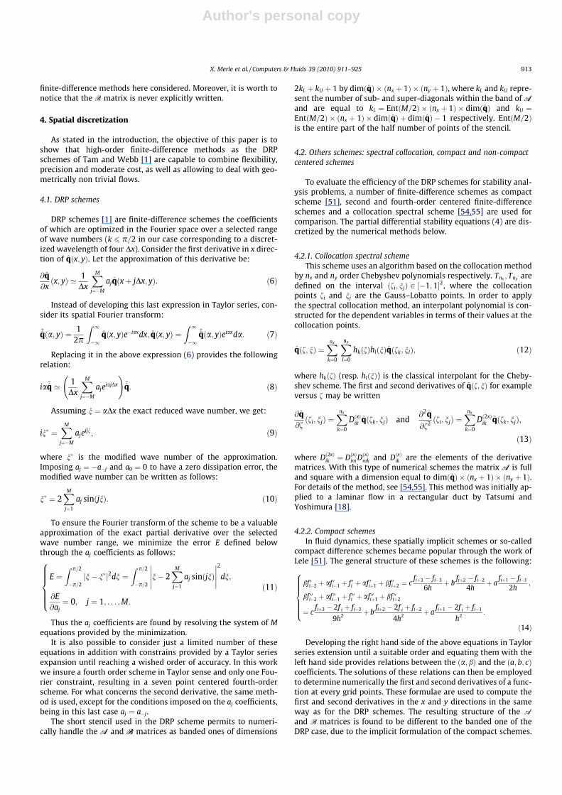
The first test case is a square lid-driven cavity flow, where thenormalized flow domain is ½0; þ1� � ½0; þ1�. A fully implicit thirdorder Navier–Stokes solver is used with a fine grid ð301� 301Þ tocorrectly converge the solution. The steady solution for a largerange of Reynolds numbers has already been computed by manyauthors: Ghia et al. [57], Botella and Peyret [58], Erturk [59], Erturket al. [60], Erturk and Gokcol [61]. In this paper two Reynolds num-bers are computed: Re ¼ 1000 and 8000. Fig. 1 shows the base flowcorresponding to a Reynolds number of 8000. These results are in

very good agreements with those of the literature [58] for bothRe ¼ 1000 and [61] Re ¼ 8000. A detailed comparison of these re-sults with those resulting from the literature can be found in [62]for a Reynolds number range Re 2 ½100; 10;000�.

5.2. Separated boundary-layer flow

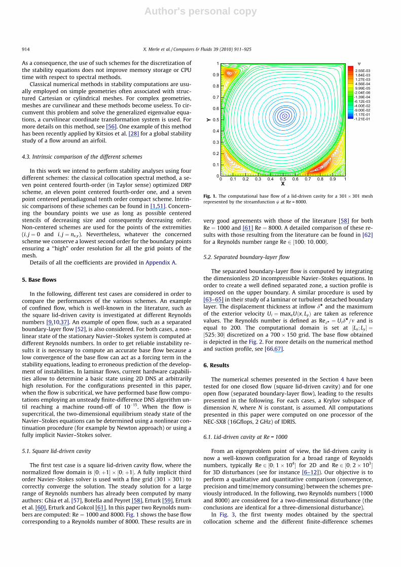
The separated boundary-layer flow is computed by integratingthe dimensionless 2D incompressible Navier–Stokes equations. Inorder to create a well defined separated zone, a suction profile isimposed on the upper boundary. A similar procedure is used by[63–65] in their study of a laminar or turbulent detached boundarylayer. The displacement thickness at inflow dH and the maximumof the exterior velocity Ui ¼maxxUðx; LyÞ are taken as referencevalues. The Reynolds number is defined as RedH ¼ Uid

H=m and isequal to 200. The computational domain is set at ½Lx; Ly� ¼½525; 30� discretized on a 700� 150 grid. The base flow obtainedis depicted in the Fig. 2. For more details on the numerical methodand suction profile, see [66,67].

6. Results

The numerical schemes presented in the Section 4 have beentested for one closed flow (square lid-driven cavity) and for oneopen flow (separated boundary-layer flow), leading to the resultspresented in the following. For each cases, a Krylov subspace ofdimension N, where N is constant, is assumed. All computationspresented in this paper were computed on one processor of theNEC-SX8 (16Gflops, 2 GHz) of IDRIS.

6.1. Lid-driven cavity at Re = 1000

From an eigenproblem point of view, the lid-driven cavity isnow a well-known configuration for a broad range of Reynoldsnumbers, typically Re 2 ½0; 1� 104� for 2D and Re 2 ½0; 2� 103�for 3D disturbances (see for instance [6–12]). Our objective is toperform a qualitative and quantitative comparison (convergence,precision and time/memory consuming) between the schemes pre-viously introduced. In the following, two Reynolds numbers (1000and 8000) are considered for a two-dimensional disturbance (theconclusions are identical for a three-dimensional disturbance).

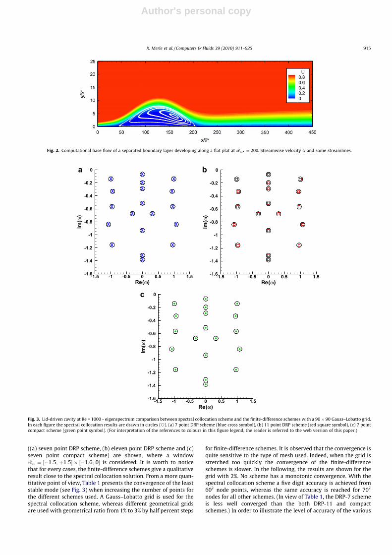
In Fig. 3, the first twenty modes obtained by the spectralcollocation scheme and the different finite-difference schemes

X

Y

0 0.1 0.2 0.3 0.4 0.5 0.6 0.7 0.8 0.9 10

0.1

0.2

0.3

0.4

0.5

0.6

0.7

0.8

0.9

12.55E-031.84E-031.27E-034.56E-049.99E-05-2.04E-06-1.39E-04-6.12E-03-4.00E-02-9.00E-02-1.17E-01-1.21E-01

ψ

Fig. 1. The computational base flow of a lid-driven cavity for a 301� 301 meshrepresented by the streamfunction w at Re = 8000.

914 X. Merle et al. / Computers & Fluids 39 (2010) 911–925

Author's personal copy

((a) seven point DRP scheme, (b) eleven point DRP scheme and (c)seven point compact scheme) are shown, where a windowDx ¼ ½�1:5; þ1:5� � ½�1:6; 0� is considered. It is worth to noticethat for every cases, the finite-difference schemes give a qualitativeresult close to the spectral collocation solution. From a more quan-titative point of view, Table 1 presents the convergence of the leaststable mode (see Fig. 3) when increasing the number of points forthe different schemes used. A Gauss–Lobatto grid is used for thespectral collocation scheme, whereas different geometrical gridsare used with geometrical ratio from 1% to 3% by half percent steps

for finite-difference schemes. It is observed that the convergence isquite sensitive to the type of mesh used. Indeed, when the grid isstretched too quickly the convergence of the finite-differenceschemes is slower. In the following, the results are shown for thegrid with 2%. No scheme has a monotonic convergence. With thespectral collocation scheme a five digit accuracy is achieved from602 node points, whereas the same accuracy is reached for 702

nodes for all other schemes. (In view of Table 1, the DRP-7 schemeis less well converged than the both DRP-11 and compactschemes.) In order to illustrate the level of accuracy of the various

Fig. 2. Computational base flow of a separated boundary layer developing along a flat plat at RedH ¼ 200. Streamwise velocity U and some streamlines.

XXX

X

XX

X

X

X

X

X

XX

XX

XX

XX

Re(ω)

Im(ω)

-1.5 -1 -0.5 0 0.5 1 1.5-1.6

-1.4

-1.2

-1

-0.8

-0.6

-0.4

-0.2

0

Re(ω)

Im(ω

)

-1.5 -1 -0.5 0 0.5 1 1.5-1.6

-1.4

-1.2

-1

-0.8

-0.6

-0.4

-0.2

0

Re(ω)

Im(ω)

-1.5 -1 -0.5 0 0.5 1 1.5-1.6

-1.4

-1.2

-1

-0.8

-0.6

-0.4

-0.2

0

a b

c

Fig. 3. Lid-driven cavity at Re = 1000 - eigenspectrum comparison between spectral collocation scheme and the finite-difference schemes with a 90� 90 Gauss–Lobatto grid.In each figure the spectral collocation results are drawn in circles (s). (a) 7 point DRP scheme (blue cross symbol), (b) 11 point DRP scheme (red square symbol), (c) 7 pointcompact scheme (green point symbol). (For interpretation of the references to colours in this figure legend, the reader is referred to the web version of this paper.)

X. Merle et al. / Computers & Fluids 39 (2010) 911–925 915

Author's personal copy

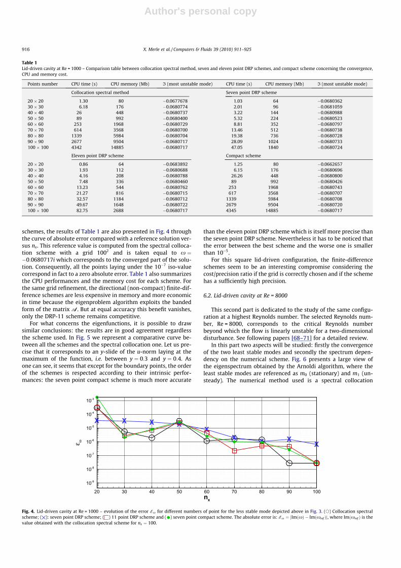
schemes, the results of Table 1 are also presented in Fig. 4 throughthe curve of absolute error compared with a reference solution ver-sus nx. This reference value is computed from the spectral colloca-tion scheme with a grid 1002 and is taken equal to x ¼�0:0680717i which corresponds to the converged part of the solu-tion. Consequently, all the points laying under the 10�7 iso-valuecorrespond in fact to a zero absolute error. Table 1 also summarizesthe CPU performances and the memory cost for each scheme. Forthe same grid refinement, the directional (non-compact) finite-dif-ference schemes are less expensive in memory and more economicin time because the eigenproblem algorithm exploits the bandedform of the matrix A. But at equal accuracy this benefit vanishes,only the DRP-11 scheme remains competitive.

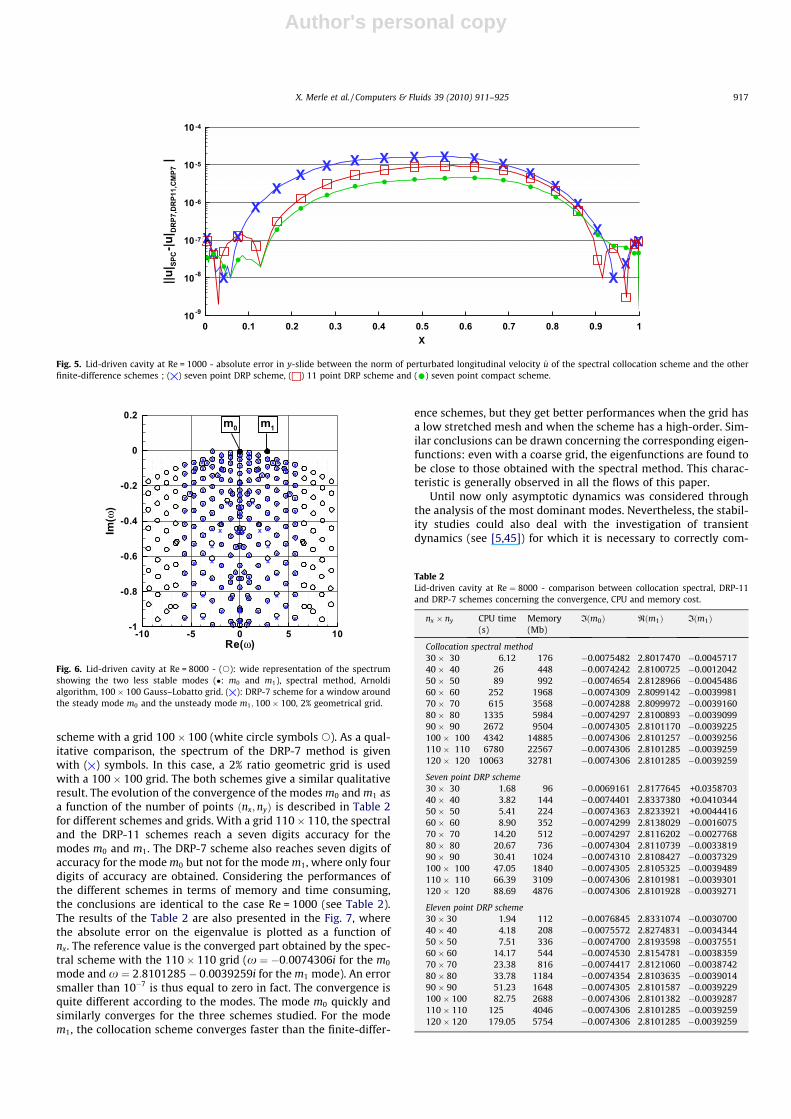
For what concerns the eigenfunctions, it is possible to drawsimilar conclusions: the results are in good agreement regardlessthe scheme used. In Fig. 5 we represent a comparative curve be-tween all the schemes and the spectral collocation one. Let us pre-cise that it corresponds to an y-slide of the u-norm laying at themaximum of the function, i.e. between y ¼ 0:3 and y ¼ 0:4. Asone can see, it seems that except for the boundary points, the orderof the schemes is respected according to their intrinsic perfor-mances: the seven point compact scheme is much more accurate

than the eleven point DRP scheme which is itself more precise thanthe seven point DRP scheme. Nevertheless it has to be noticed thatthe error between the best scheme and the worse one is smallerthan 10�5.

For this square lid-driven configuration, the finite-differenceschemes seem to be an interesting compromise considering thecost/precision ratio if the grid is correctly chosen and if the schemehas a sufficiently high precision.

6.2. Lid-driven cavity at Re = 8000

This second part is dedicated to the study of the same configu-ration at a highest Reynolds number. The selected Reynolds num-ber, Re = 8000, corresponds to the critical Reynolds numberbeyond which the flow is linearly unstable for a two-dimensionaldisturbance. See following papers [68–71] for a detailed review.

In this part two aspects will be studied: firstly the convergenceof the two least stable modes and secondly the spectrum depen-dency on the numerical scheme. Fig. 6 presents a large view ofthe eigenspectrum obtained by the Arnoldi algorithm, where theleast stable modes are referenced as m0 (stationary) and m1 (un-steady). The numerical method used is a spectral collocation

Table 1Lid-driven cavity at Re = 1000 – Comparison table between collocation spectral method, seven and eleven point DRP schemes, and compact scheme concerning the convergence,CPU and memory cost.

Points number CPU time (s) CPU memory (Mb) I (most unstable mode) CPU time (s) CPU memory (Mb) I (most unstable mode)

Collocation spectral method Seven point DRP scheme

20 � 20 1.30 80 �0.0677678 1.03 64 �0.068036230 � 30 6.18 176 �0.0680774 2.01 96 �0.068105940 � 40 26 448 �0.0680737 3.22 144 �0.068098850 � 50 89 992 �0.0680400 5.32 224 �0.068052360 � 60 253 1968 �0.0680729 8.81 352 �0.068079770 � 70 614 3568 �0.0680700 13.46 512 �0.068073880 � 80 1339 5984 �0.0680704 19.38 736 �0.068072890 � 90 2677 9504 �0.0680717 28.09 1024 �0.0680733100 � 100 4342 14885 �0.0680717 47.05 1840 �0.0680724

Eleven point DRP scheme Compact scheme

20 � 20 0.86 64 �0.0683892 1.25 80 �0.066265730 � 30 1.93 112 �0.0680688 6.15 176 �0.068069640 � 40 4.16 208 �0.0680788 26.26 448 �0.068080050 � 50 7.48 336 �0.0680460 89 992 �0.068042660 � 60 13.23 544 �0.0680762 253 1968 �0.068074370 � 70 21.27 816 �0.0680715 617 3568 �0.068070780 � 80 32.57 1184 �0.0680712 1339 5984 �0.068070890 � 90 49.67 1648 �0.0680722 2679 9504 �0.0680720100 � 100 82.75 2688 �0.0680717 4345 14885 �0.0680717

X X X XX

X X XX

nx

ε ω

20 30 40 50 60 70 80 90 100

10-9

10-8

10-7

10-6

10-5

10-4

10-3

Fig. 4. Lid-driven cavity at Re = 1000 – evolution of the error Ex for different numbers of point for the less stable mode depicted above in Fig. 3. (s) Collocation spectralscheme; ( ): seven point DRP scheme; ( ) 11 point DRP scheme and ( ) seven point compact scheme. The absolute error is: Ex ¼ jImðxÞ � Imðxref Þj, where Imðxref Þ is thevalue obtained with the collocation spectral scheme for nx ¼ 100.

916 X. Merle et al. / Computers & Fluids 39 (2010) 911–925

Author's personal copy

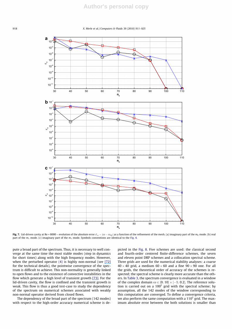
scheme with a grid 100� 100 (white circle symbols s). As a qual-itative comparison, the spectrum of the DRP-7 method is givenwith ( ) symbols. In this case, a 2% ratio geometric grid is usedwith a 100� 100 grid. The both schemes give a similar qualitativeresult. The evolution of the convergence of the modes m0 and m1 asa function of the number of points ðnx;nyÞ is described in Table 2for different schemes and grids. With a grid 110� 110, the spectraland the DRP-11 schemes reach a seven digits accuracy for themodes m0 and m1. The DRP-7 scheme also reaches seven digits ofaccuracy for the mode m0 but not for the mode m1, where only fourdigits of accuracy are obtained. Considering the performances ofthe different schemes in terms of memory and time consuming,the conclusions are identical to the case Re = 1000 (see Table 2).The results of the Table 2 are also presented in the Fig. 7, wherethe absolute error on the eigenvalue is plotted as a function ofnx. The reference value is the converged part obtained by the spec-tral scheme with the 110� 110 grid (x ¼ �0:0074306i for the m0

mode and x ¼ 2:8101285� 0:0039259i for the m1 mode). An errorsmaller than 10�7 is thus equal to zero in fact. The convergence isquite different according to the modes. The mode m0 quickly andsimilarly converges for the three schemes studied. For the modem1, the collocation scheme converges faster than the finite-differ-

ence schemes, but they get better performances when the grid hasa low stretched mesh and when the scheme has a high-order. Sim-ilar conclusions can be drawn concerning the corresponding eigen-functions: even with a coarse grid, the eigenfunctions are found tobe close to those obtained with the spectral method. This charac-teristic is generally observed in all the flows of this paper.

Until now only asymptotic dynamics was considered throughthe analysis of the most dominant modes. Nevertheless, the stabil-ity studies could also deal with the investigation of transientdynamics (see [5,45]) for which it is necessary to correctly com-

Im(ω)

-1

-0.8

-0.6

-0.4

-0.2

0

0.2

Re(ω)-10 -5 0 5 10

Fig. 6. Lid-driven cavity at Re = 8000 - (s): wide representation of the spectrumshowing the two less stable modes (�: m0 and m1), spectral method, Arnoldialgorithm, 100� 100 Gauss–Lobatto grid. ( ): DRP-7 scheme for a window aroundthe steady mode m0 and the unsteady mode m1;100� 100, 2% geometrical grid.

Table 2Lid-driven cavity at Re ¼ 8000 - comparison between collocation spectral, DRP-11and DRP-7 schemes concerning the convergence, CPU and memory cost.

nx � ny CPU time(s)

Memory(Mb)

Iðm0Þ Rðm1Þ Iðm1Þ

Collocation spectral method30 � 30 6.12 176 �0.0075482 2.8017470 �0.004571740 � 40 26 448 �0.0074242 2.8100725 �0.001204250 � 50 89 992 �0.0074654 2.8128966 �0.004548660 � 60 252 1968 �0.0074309 2.8099142 �0.003998170 � 70 615 3568 �0.0074288 2.8099972 �0.003916080 � 80 1335 5984 �0.0074297 2.8100893 �0.003909990 � 90 2672 9504 �0.0074305 2.8101170 �0.0039225100 � 100 4342 14885 �0.0074306 2.8101257 �0.0039256110 � 110 6780 22567 �0.0074306 2.8101285 �0.0039259120 � 120 10063 32781 �0.0074306 2.8101285 �0.0039259

Seven point DRP scheme30 � 30 1.68 96 �0.0069161 2.8177645 +0.035870340 � 40 3.82 144 �0.0074401 2.8337380 +0.041034450 � 50 5.41 224 �0.0074363 2.8233921 +0.004441660 � 60 8.90 352 �0.0074299 2.8138029 �0.001607570 � 70 14.20 512 �0.0074297 2.8116202 �0.002776880 � 80 20.67 736 �0.0074304 2.8110739 �0.003381990 � 90 30.41 1024 �0.0074310 2.8108427 �0.0037329100 � 100 47.05 1840 �0.0074305 2.8105325 �0.0039489110 � 110 66.39 3109 �0.0074306 2.8101981 �0.0039301120 � 120 88.69 4876 �0.0074306 2.8101928 �0.0039271

Eleven point DRP scheme30 � 30 1.94 112 �0.0076845 2.8331074 �0.003070040 � 40 4.18 208 �0.0075572 2.8274831 �0.003434450 � 50 7.51 336 �0.0074700 2.8193598 �0.003755160 � 60 14.17 544 �0.0074530 2.8154781 �0.003835970 � 70 23.38 816 �0.0074417 2.8121060 �0.003874280 � 80 33.78 1184 �0.0074354 2.8103635 �0.003901490 � 90 51.23 1648 �0.0074305 2.8101587 �0.0039229100 � 100 82.75 2688 �0.0074306 2.8101382 �0.0039287110 � 110 125 4046 �0.0074306 2.8101285 �0.0039259120 � 120 179.05 5754 �0.0074306 2.8101285 �0.0039259

XXX

X

XX

X X X X X X X X XX

XX

XXXX

X

||u| SP

C-|u| DRP7,DRP11,CMP7|

0 0.1 0.2 0.3 0.4 0.5 0.6 0.7 0.8 0.9 110-9

10 -8

10 -7

10 -6

10 -5

10 -4

Fig. 5. Lid-driven cavity at Re = 1000 - absolute error in y-slide between the norm of perturbated longitudinal velocity u of the spectral collocation scheme and the otherfinite-difference schemes ; ( ) seven point DRP scheme, ( ) 11 point DRP scheme and ( ) seven point compact scheme.

X. Merle et al. / Computers & Fluids 39 (2010) 911–925 917

Author's personal copy

pute a broad part of the spectrum. Thus, it is necessary to well con-verge at the same time the most stable modes (step in dynamicsfor short times) along with the high frequency modes. However,when the perturbed operator (4) is highly non-normal (see [72]for the technical details), the pointwise convergence of the spec-trum is difficult to achieve. This non-normality is generally linkedto open flows and to the existence of convective instabilities in theflow which generate a high level of transient growth [73]. For thelid-driven cavity, the flow is confined and the transient growth isweak. This flow is thus a good test-case to study the dependencyof the spectrum on numerical schemes associated with weaklynon-normal operator derived from closed flows.

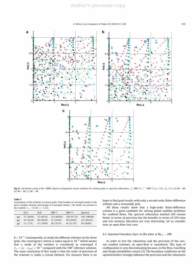
The dependency of the broad part of the spectrum (142 modes)with respect to the high-order accuracy numerical scheme is de-

picted in the Fig. 8. Five schemes are used: the classical secondand fourth-order centered finite-difference schemes, the sevenand eleven point DRP schemes and a collocation spectral scheme.Three grids are used for the numerical stability analyses: a coarse40� 40 grid, a medium 60� 60 and a fine 90� 90 one. For allthe grids, the theoretical order of accuracy of the schemes is re-spected; the spectral scheme is clearly more accurate than the oth-ers. In Table 3, the spectrum convergence is evaluated in a windowof the complex domain x 2 ½0; 10� � ½�1; 0:2�. The reference solu-tion is carried out on a 1002 grid with the spectral scheme; byassumption, all the 142 modes of the window corresponding tothis computation are converged. To define a convergence criteria,we also perform the same computation with a 1102 grid. The max-imum absolute error between the both solutions is smaller than

x

x xx x

x xx

xnx

nx

nx

ε ω

30 40 50 60 70 80 90 100 110

10-11

10-10

10-9

10-8

10-7

10-6

10-5

10-4

xx x

x x x x xx

ε ω

30 40 50 60 70 80 90 100 110

10-9

10-8

10-7

10-6

10-5

10-4

10-3

10-2

10-1

x xx

x x xx

xx

ε ω

30 40 50 60 70 80 90 100 110

10-1010-910-810-710-610-510-410-310-210-1

a

b

c

Fig. 7. Lid-driven cavity at Re = 8000 – evolution of the absolute error Ex ¼ jx�xref j as a function of the refinement of the mesh. (a) imaginary part of the m0 mode. (b) realpart of the m1 mode. (c) imaginary part of the m1 mode. Symbols conventions are identical to the Fig. 4.

918 X. Merle et al. / Computers & Fluids 39 (2010) 911–925

Author's personal copy

8� 10�5. Consequently, to study the different schemes on the threegrids, the convergence criteria is taken equal to 10�4 which meansthat a mode of the window is considered as converged ifEx ¼ jx�xref j 6 10�4 compared with the 1002 reference solution.The main conclusion of this study is that the order of precision ofthe schemes is really a crucial element. For instance there is no

hope to find good results with only a second order finite-differencescheme and a reasonable grid.

All those results show that a high-order finite-differencescheme is a good candidate for solving global stability problemsfor confined flows. The spectral collocation method still remainbetter in terms of precision but the benefits in terms of CPU timeand size memory allocation are very interesting. Let us considernow an open-flow test-case.

6.3. Separated boundary layer on flat plate at RedH ¼ 200

In order to test the robustness and the precision of the vari-ous studied schemes, an open-flow is considered. This type ofconfiguration is very discriminating because, in this flow, travellingand steady instabilities coexist [3]. The boundary conditions on theopened borders strongly influence the precision and the robustness

Re(ω)

Im(ω)

0 1 2 3-2

-1.5

-1

-0.5

0

Re(ω)Im(ω)

0 1 2 3-2

-1.5

-1

-0.5

0

Re(ω)

Im(ω)

0 1 2 3-2

-1.5

-1

-0.5

0

a b

c

Fig. 8. Lid-driven cavity at Re = 8000. Spectra comparison versus schemes for various grids. �: spectral collocation; : DRP-11; : DRP-7; : Oð4Þ; : Oð2Þ. (a) 40 � 40,(b) 60 � 60, (c) 90 � 90.

Table 3Convergence of the schemes in various grids. Total number of converged modes in thegiven complex domain (percentage of converged modes). 142 modes are present inthe window Dx ¼ ½0; 10� � ½�1; 0:2�.

O(2) O(4) DRP-7 DRP-11 Spectral

902 37 (26.0%) 72 (50.7%) 123 (86.6%) 128 (97.1%) 142 (100.0%)

602 23 (16.2%) 40 (28.2%) 51 (35.9%) 78 (54.9%) 121 (85.2%)

402 11 (7.7%) 21 (14.8%) 28 (19.7%) 45 (31.7%) 54 (38.0%)

X. Merle et al. / Computers & Fluids 39 (2010) 911–925 919

Author's personal copy

of the eigenproblem solutions and particularly the computation ofthe convective waves [45]. Moreover, large transient growth isgenerally observed in open flows due to the strongly non-normal-ity of the evolution operator in the streamwise direction [73]. Thisnon-normality involves a strong sensitivity of the modes of con-vective nature to numerical parameters. The aim of the two lastsections is to evaluate the performances of the finite-differenceschemes in a global stability computation for an open flow. Twofamilies of modes are studied. The first family is reminiscent toclassical convective waves spatially amplified along the flat plate(Section 6.3.1) and the second one relates to non-propagativethree-dimensional modes mainly located in the separated zone(Section 6.3.2). The first family of modes corresponds to a selectivenoise amplifier, whereas the second one behaves like an intrinsicoscillator. We will show that these two families of modes are char-acterized by a very different numerical behaviour.

Two sets of boundary conditions are used:

BC—1 :u ¼ 0 at y=d� ¼ 0; y=d� ¼ Ly and x=d� ¼ 0@u@x ¼ 0 at x=d� ¼ Lx;

(ð15aÞ

BC—2 :

u ¼ 0 at y=d� ¼ 0; y=d� ¼ Ly

@u@x þ i x0�x

c0�Rða0Þ

� �u ¼ 0 at x=d� ¼ 0 and

x=d� ¼ Lx;

8>><>>: ð15bÞ

where ðx0;a0Þ verify the local dispersion relationDðx0;a0;RedH Þ ¼ 0 at inflow and outflow. c0 ¼ @x=@aðx0Þ is the lo-cal group velocity. The boundary condition BC–2 is a Robin condi-tion based on a Gaster’s transformation [44,45]. Furthermore, thedivergence free on all boundaries of the computational box and aparticular treatment of the corners will complete the system (5).BC–1 implies that there is no disturbance at upstream and BC–2 as-sumes that the flow is weakly non-parallel at inflow and outflow,the local dispersion relation enables to impose rightly the spatialcharacteristic of convective modes.

Thereafter, the eigenvalue spectrum is computed with a Cheby-chev collocation scheme on different grids. The flow domain istransformed into ½0; Lx� � ½0; Ly� using the following algebraic map-ping [74] in the wall-normal direction, in order to take into accountthe boundary layer structure

yðnÞ ¼ a1þ nb� n

with a ¼ yiLy

Ly � 2yi; yi ¼ 1:5d and b ¼ 1þ 2a

Ly:

ð16Þ

For the streamwise direction, a classical mapping xðfÞ ¼Lxð1� fÞ=2 is used.

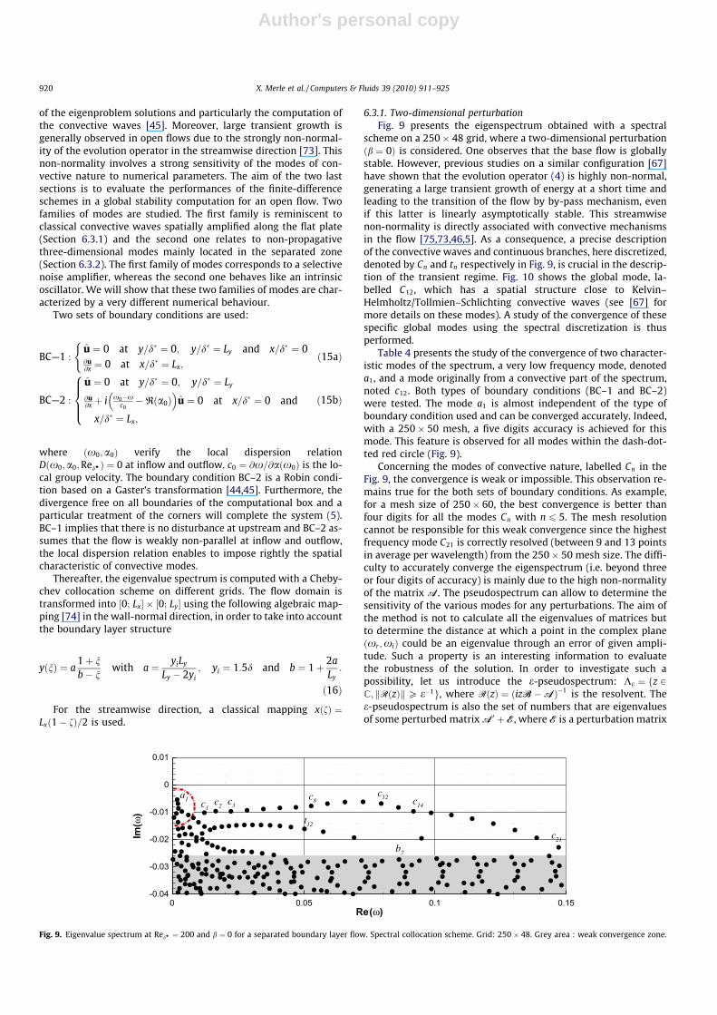
6.3.1. Two-dimensional perturbationFig. 9 presents the eigenspectrum obtained with a spectral

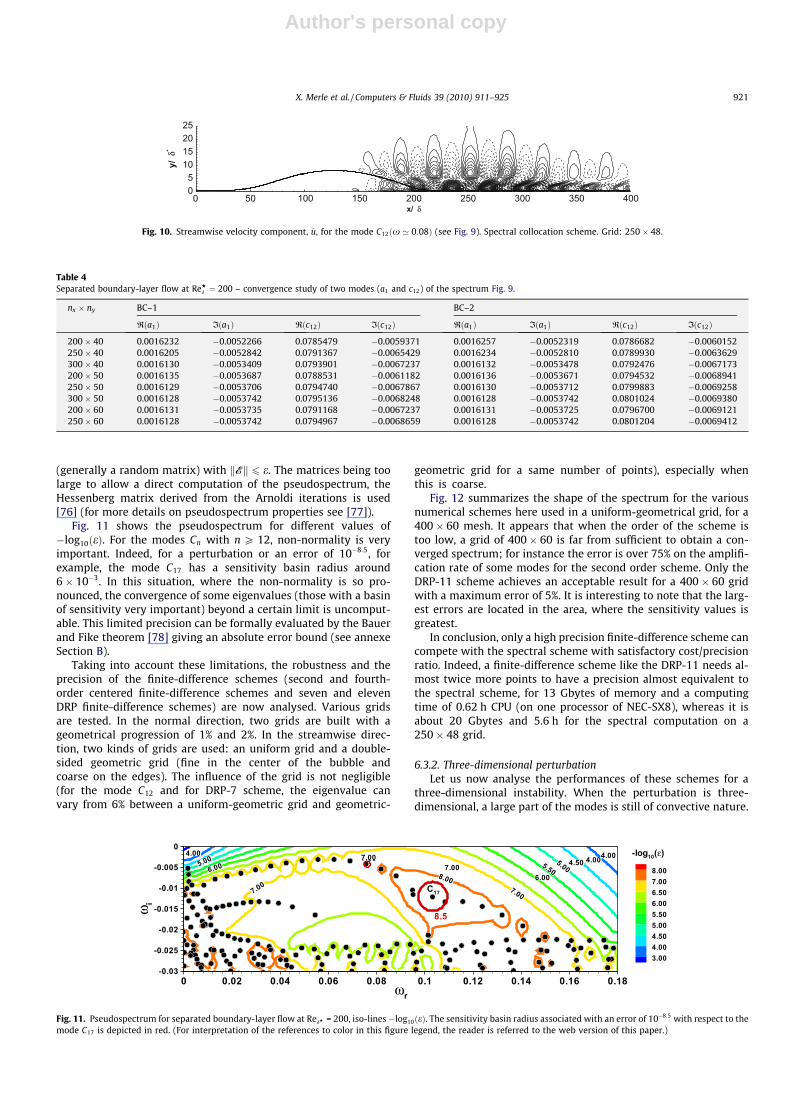
scheme on a 250� 48 grid, where a two-dimensional perturbationðb ¼ 0Þ is considered. One observes that the base flow is globallystable. However, previous studies on a similar configuration [67]have shown that the evolution operator (4) is highly non-normal,generating a large transient growth of energy at a short time andleading to the transition of the flow by by-pass mechanism, evenif this latter is linearly asymptotically stable. This streamwisenon-normality is directly associated with convective mechanismsin the flow [75,73,46,5]. As a consequence, a precise descriptionof the convective waves and continuous branches, here discretized,denoted by Cn and tn respectively in Fig. 9, is crucial in the descrip-tion of the transient regime. Fig. 10 shows the global mode, la-belled C12, which has a spatial structure close to Kelvin–Helmholtz/Tollmien–Schlichting convective waves (see [67] formore details on these modes). A study of the convergence of thesespecific global modes using the spectral discretization is thusperformed.

Table 4 presents the study of the convergence of two character-istic modes of the spectrum, a very low frequency mode, denoteda1, and a mode originally from a convective part of the spectrum,noted c12. Both types of boundary conditions (BC–1 and BC–2)were tested. The mode a1 is almost independent of the type ofboundary condition used and can be converged accurately. Indeed,with a 250� 50 mesh, a five digits accuracy is achieved for thismode. This feature is observed for all modes within the dash-dot-ted red circle (Fig. 9).

Concerning the modes of convective nature, labelled Cn in theFig. 9, the convergence is weak or impossible. This observation re-mains true for the both sets of boundary conditions. As example,for a mesh size of 250� 60, the best convergence is better thanfour digits for all the modes Cn with n 6 5. The mesh resolutioncannot be responsible for this weak convergence since the highestfrequency mode C21 is correctly resolved (between 9 and 13 pointsin average per wavelength) from the 250� 50 mesh size. The diffi-culty to accurately converge the eigenspectrum (i.e. beyond threeor four digits of accuracy) is mainly due to the high non-normalityof the matrix A. The pseudospectrum can allow to determine thesensitivity of the various modes for any perturbations. The aim ofthe method is not to calculate all the eigenvalues of matrices butto determine the distance at which a point in the complex planeðxr ;xiÞ could be an eigenvalue through an error of given ampli-tude. Such a property is an interesting information to evaluatethe robustness of the solution. In order to investigate such apossibility, let us introduce the e-pseudospectrum: Ke ¼ fz 2C; kRðzÞkP e�1g, where RðzÞ ¼ ðizB�AÞ�1 is the resolvent. Thee-pseudospectrum is also the set of numbers that are eigenvaluesof some perturbed matrix A0 þ E, where E is a perturbation matrix

Re(ω)

Im(ω)

0 0.05 0.1 0.15-0.04

-0.03

-0.02

-0.01

0

0.01

c1

c21

c2c3

c8

b7

c12 c14

t12

a1

Fig. 9. Eigenvalue spectrum at RedH ¼ 200 and b ¼ 0 for a separated boundary layer flow. Spectral collocation scheme. Grid: 250� 48. Grey area : weak convergence zone.

920 X. Merle et al. / Computers & Fluids 39 (2010) 911–925

Author's personal copy

(generally a random matrix) with kEk 6 e. The matrices being toolarge to allow a direct computation of the pseudospectrum, theHessenberg matrix derived from the Arnoldi iterations is used[76] (for more details on pseudospectrum properties see [77]).

Fig. 11 shows the pseudospectrum for different values of�log10ðeÞ. For the modes Cn with n P 12, non-normality is veryimportant. Indeed, for a perturbation or an error of 10�8:5, forexample, the mode C17 has a sensitivity basin radius around6� 10�3. In this situation, where the non-normality is so pro-nounced, the convergence of some eigenvalues (those with a basinof sensitivity very important) beyond a certain limit is uncomput-able. This limited precision can be formally evaluated by the Bauerand Fike theorem [78] giving an absolute error bound (see annexeSection B).

Taking into account these limitations, the robustness and theprecision of the finite-difference schemes (second and fourth-order centered finite-difference schemes and seven and elevenDRP finite-difference schemes) are now analysed. Various gridsare tested. In the normal direction, two grids are built with ageometrical progression of 1% and 2%. In the streamwise direc-tion, two kinds of grids are used: an uniform grid and a double-sided geometric grid (fine in the center of the bubble andcoarse on the edges). The influence of the grid is not negligible(for the mode C12 and for DRP-7 scheme, the eigenvalue canvary from 6% between a uniform-geometric grid and geometric-

geometric grid for a same number of points), especially whenthis is coarse.

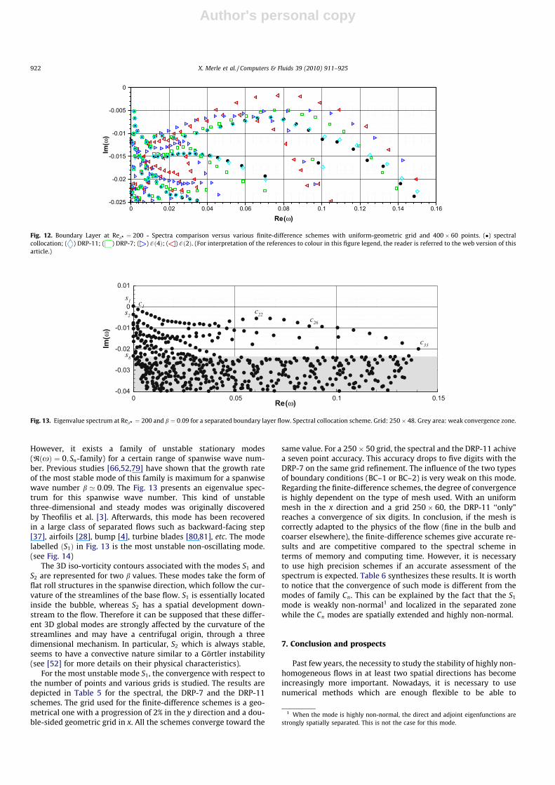
Fig. 12 summarizes the shape of the spectrum for the variousnumerical schemes here used in a uniform-geometrical grid, for a400� 60 mesh. It appears that when the order of the scheme istoo low, a grid of 400� 60 is far from sufficient to obtain a con-verged spectrum; for instance the error is over 75% on the amplifi-cation rate of some modes for the second order scheme. Only theDRP-11 scheme achieves an acceptable result for a 400� 60 gridwith a maximum error of 5%. It is interesting to note that the larg-est errors are located in the area, where the sensitivity values isgreatest.

In conclusion, only a high precision finite-difference scheme cancompete with the spectral scheme with satisfactory cost/precisionratio. Indeed, a finite-difference scheme like the DRP-11 needs al-most twice more points to have a precision almost equivalent tothe spectral scheme, for 13 Gbytes of memory and a computingtime of 0.62 h CPU (on one processor of NEC-SX8), whereas it isabout 20 Gbytes and 5.6 h for the spectral computation on a250� 48 grid.

6.3.2. Three-dimensional perturbationLet us now analyse the performances of these schemes for a

three-dimensional instability. When the perturbation is three-dimensional, a large part of the modes is still of convective nature.

7.00

7.008.00 6.00

5.505.00

4.50 4.004.004.00

6.005.00

7.00

7.007.00

ωr

ωi

0 0.02 0.04 0.06 0.08 0.1 0.12 0.14 0.16 0.18-0.03

-0.025

-0.02

-0.015

-0.01

-0.005

0

8.007.006.506.005.505.004.504.003.00

-log10(ε)

8.5

C17

Fig. 11. Pseudospectrum for separated boundary-layer flow at RedH = 200, iso-lines �log10ðeÞ. The sensitivity basin radius associated with an error of 10�8:5 with respect to themode C17 is depicted in red. (For interpretation of the references to color in this figure legend, the reader is referred to the web version of this paper.)

Table 4Separated boundary-layer flow at ReH

d ¼ 200 – convergence study of two modes (a1 and c12) of the spectrum Fig. 9.

nx � ny BC–1 BC–2

Rða1Þ Iða1Þ Rðc12Þ Iðc12Þ Rða1Þ Iða1Þ Rðc12Þ Iðc12Þ

200� 40 0.0016232 �0.0052266 0.0785479 �0.0059371 0.0016257 �0.0052319 0.0786682 �0.0060152250� 40 0.0016205 �0.0052842 0.0791367 �0.0065429 0.0016234 �0.0052810 0.0789930 �0.0063629300� 40 0.0016130 �0.0053409 0.0793901 �0.0067237 0.0016132 �0.0053478 0.0792476 �0.0067173200� 50 0.0016135 �0.0053687 0.0788531 �0.0061182 0.0016136 �0.0053671 0.0794532 �0.0068941250� 50 0.0016129 �0.0053706 0.0794740 �0.0067867 0.0016130 �0.0053712 0.0799883 �0.0069258300� 50 0.0016128 �0.0053742 0.0795136 �0.0068248 0.0016128 �0.0053742 0.0801024 �0.0069380200� 60 0.0016131 �0.0053735 0.0791168 �0.0067237 0.0016131 �0.0053725 0.0796700 �0.0069121250� 60 0.0016128 �0.0053742 0.0794967 �0.0068659 0.0016128 �0.0053742 0.0801204 �0.0069412

x/ δ*

y/δ*

0 50 100 150 200 250 300 350 4000510152025

Fig. 10. Streamwise velocity component, u, for the mode C12ðx ’ 0:08Þ (see Fig. 9). Spectral collocation scheme. Grid: 250� 48.

X. Merle et al. / Computers & Fluids 39 (2010) 911–925 921

Author's personal copy

However, it exists a family of unstable stationary modes(RðxÞ ¼ 0; Sn-family) for a certain range of spanwise wave num-ber. Previous studies [66,52,79] have shown that the growth rateof the most stable mode of this family is maximum for a spanwisewave number b ’ 0:09. The Fig. 13 presents an eigenvalue spec-trum for this spanwise wave number. This kind of unstablethree-dimensional and steady modes was originally discoveredby Theofilis et al. [3]. Afterwards, this mode has been recoveredin a large class of separated flows such as backward-facing step[37], airfoils [28], bump [4], turbine blades [80,81], etc. The modelabelled ðS1Þ in Fig. 13 is the most unstable non-oscillating mode.(see Fig. 14)

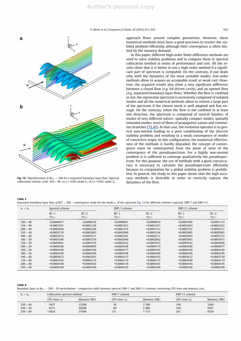
The 3D iso-vorticity contours associated with the modes S1 andS2 are represented for two b values. These modes take the form offlat roll structures in the spanwise direction, which follow the cur-vature of the streamlines of the base flow. S1 is essentially locatedinside the bubble, whereas S2 has a spatial development down-stream to the flow. Therefore it can be supposed that these differ-ent 3D global modes are strongly affected by the curvature of thestreamlines and may have a centrifugal origin, through a threedimensional mechanism. In particular, S2 which is always stable,seems to have a convective nature similar to a Görtler instability(see [52] for more details on their physical characteristics).

For the most unstable mode S1, the convergence with respect tothe number of points and various grids is studied. The results aredepicted in Table 5 for the spectral, the DRP-7 and the DRP-11schemes. The grid used for the finite-difference schemes is a geo-metrical one with a progression of 2% in the y direction and a dou-ble-sided geometric grid in x. All the schemes converge toward the

same value. For a 250� 50 grid, the spectral and the DRP-11 achivea seven point accuracy. This accuracy drops to five digits with theDRP-7 on the same grid refinement. The influence of the two typesof boundary conditions (BC–1 or BC–2) is very weak on this mode.Regarding the finite-difference schemes, the degree of convergenceis highly dependent on the type of mesh used. With an uniformmesh in the x direction and a grid 250� 60, the DRP-11 ‘‘only”reaches a convergence of six digits. In conclusion, if the mesh iscorrectly adapted to the physics of the flow (fine in the bulb andcoarser elsewhere), the finite-difference schemes give accurate re-sults and are competitive compared to the spectral scheme interms of memory and computing time. However, it is necessaryto use high precision schemes if an accurate assessment of thespectrum is expected. Table 6 synthesizes these results. It is worthto notice that the convergence of such mode is different from themodes of family Cn. This can be explained by the fact that the S1

mode is weakly non-normal1 and localized in the separated zonewhile the Cn modes are spatially extended and highly non-normal.

7. Conclusion and prospects

Past few years, the necessity to study the stability of highly non-homogeneous flows in at least two spatial directions has becomeincreasingly more important. Nowadays, it is necessary to usenumerical methods which are enough flexible to be able to

Re(ω)

Im(ω)

0 0.02 0.04 0.06 0.08 0.1 0.12 0.14 0.16-0.025

-0.02

-0.015

-0.01

-0.005

0

Fig. 12. Boundary Layer at RedH ¼ 200 - Spectra comparison versus various finite-difference schemes with uniform-geometric grid and 400� 60 points. (�) spectralcollocation; ( ) DRP-11; ( ) DRP-7; ( ) Oð4Þ; ( ) Oð2Þ. (For interpretation of the references to colour in this figure legend, the reader is referred to the web version of thisarticle.)

Re(ω)

Im(ω)

0 0.05 0.1 0.15-0.04

-0.03

-0.02

-0.01

0

0.01

c1

c33

c22c26

s8

s1

s2

Fig. 13. Eigenvalue spectrum at RedH ¼ 200 and b ¼ 0:09 for a separated boundary layer flow. Spectral collocation scheme. Grid: 250� 48. Grey area: weak convergence zone.

1 When the mode is highly non-normal, the direct and adjoint eigenfunctions arestrongly spatially separated. This is not the case for this mode.

922 X. Merle et al. / Computers & Fluids 39 (2010) 911–925

Author's personal copy

approach flows around complex geometries. However, thesenumerical methods must have a good precision to resolve the sta-bility problem efficiently although their convergence is often lim-ited by the memory demand.

In this paper, different high-order finite-difference methods areused to solve stability problems and to compare them to spectralcollocation method in terms of performance and cost. All the re-sults show that it is better to use a high-order method if a signifi-cant part of spectrum is computed. On the contrary, if one dealsonly with the dynamics of the most unstable modes, low-ordermethods allow to acquire an acceptable result at weak cost. How-ever, the acquired results also show a very significant differencebetween a closed flow (e.g. lid-driven cavity) and an opened flow(e.g. separated boundary-layer flow). Whether the flow is confinedor not, the eigenvalue spectrum is exclusively composed of isolatedmodes and all the numerical methods allow to restore a large partof the spectrum if the chosen mesh is well adapted and fine en-ough. On the contrary, when the flow is not confined in at leastone direction, the spectrum is composed of several families ofmodes of very different nature: spatially compact modes, spatiallyextended modes, most of them of propagative nature and continu-ous branches [72,45]. In that case, the evolution operator is in gen-eral non-normal leading to a poor conditioning of the discretestability problem and resulting in a weak convergence of modesof convective origin. In this configuration, the numerical effective-ness of the methods is hardly degraded, the concept of conver-gence must be reinterpreted from the point of view of theconvergence of the pseudospectrum. For a highly non-normalproblem it is sufficient to converge qualitatively the pseudospec-trum. For this purpose, the use of methods with a good cost/accu-racy is necessary to calculate the pseudospectrum efficientlybecause its computation for a global stability problem is prohibi-tive. In general, the study in this paper shows that the high accu-racy methods is desirable in order to correctly capture thedynamics of the flow.

Fig. 14. Eigenfunctions at RedH ¼ 200 for a separated boundary-layer flow. Spectralcollocation scheme. Grid: 250� 48. (a) b = 0.09, mode S1, (b) b = 0.04, mode S2.

Table 5Separated boundary-layer flow at ReH

d ¼ 200 – convergence study for the mode s1 of the spectrum Fig. 13 for different schemes (spectral, DRP-7 and DRP-11).

nx � ny Spectral scheme DRP-7 scheme DRP-11 scheme

BC–1 BC–2 BC–1 BC–2 BC–1 BC–2Iðs1Þ Iðs1Þ Iðs1Þ Iðs1Þ Iðs1Þ Iðs1Þ

100� 40 +0.0000817 �0.0000216 +0.0000051 +0.0000010 +0.0001059 +0.0001123150� 40 +0.0001931 +0.0001528 +0.0001021 +0.0001027 +0.0001854 +0.0001632200� 40 +0.0002844 +0.0002266 +0.0001574 +0.0001512 +0.0002732 +0.0002311250� 40 +0.0003170 +0.0002863 +0.0002009 +0.0002104 +0.0003005 +0.0002965300� 40 +0.0003912 +0.0003511 +0.0002501 +0.0002511 +0.0003895 +0.0003721100� 50 +0.0003346 +0.0003130 +0.0002840 +0.0002842 +0.0003043 +0.0003011150� 50 +0.0003961 +0.0003729 +0.0003552 +0.0003553 +0.0003932 +0.0003698200� 50 +0.0004186 +0.0004095 +0.0004168 +0.0004174 +0.0004180 +0.0004077250� 50 +0.0004199 +0.0004199 +0.0004177 +0.0004181 +0.0004199 +0.0004199300� 50 +0.0004199 +0.0004199 +0.0004198 +0.0004199 +0.0004199 +0.0004199100� 60 +0.0003872 +0.0003501 +0.0004157 +0.0004163 +0.0003612 +0.0003754150� 60 +0.0004183 +0.0004179 +0.0004170 +0.0004175 +0.0004180 +0.0004179200� 60 +0.0004194 +0.0004192 +0.0004178 +0.0004181 +0.0004194 +0.0004195250� 60 +0.0004199 +0.0004199 +0.0004193 +0.0004190 +0.0004199 +0.0004199

Table 6Boundary layer at RedH ¼ 200 – 3D perturbation – comparison table between spectral, DRP-7 and DRP-11 schemes concerning CPU time and memory cost.

nx � ny Collocation spectral method DRP-7 scheme DRP-11 scheme

CPU time (s) Memory (Mb) CPU time (s) Memory (Mb) CPU time (s) Memory (Mb)

250� 40 5427 15200 59 2 300 104 3360250� 50 8375 20208 84 3 886 156 5057250� 60 13824 37840 131 7 573 261 8520

X. Merle et al. / Computers & Fluids 39 (2010) 911–925 923

Author's personal copy

Acknowledgments

Computing time was provided by ‘‘Institut du Développementet des Ressources en Informatique Scientifique (IDRIS)-CNRS”.The authors thank the French Centre National d’Études Spatiales(CNES) for their financial support of the present work and StefaniaCherubini for her precious remarks.

Appendix A. Coefficients details

a33ð�3Þ ¼ �0:02651995a33ð�2Þ ¼ 0:18941314a33ð�1Þ ¼ �0:79926643a33ð0Þ ¼ 0a33ð1Þ ¼ �a33ð�1Þa33ð2Þ ¼ �a33ð�2Þa33ð3Þ ¼ �a33ð�3Þ

8>>>>>>>>>>><>>>>>>>>>>>:

a22ð�2Þ ¼ 0:08333333a22ð�1Þ ¼ �0:66666667a22ð0Þ ¼ 0a22ð1Þ ¼ �a22ð�1Þa22ð2Þ ¼ �a22ð�2Þ

8>>>>>><>>>>>>:

�a11ð�1Þ ¼ �0:5a11ð0Þ ¼ 0a11ð1Þ ¼ �a11ð�1Þ

8><>:a02ð0Þ ¼ �1:5a02ð1Þ ¼ 2:0a02ð2Þ ¼ �0:5

8><>:a20ð�2Þ ¼ 0:5a20ð�1Þ ¼ �2:0a20ð0Þ ¼ 1:5

8><>: ðA:1Þ

b33ð�3Þ ¼ 0:0157364441b33ð�2Þ ¼ �0:177751998b33ð�1Þ ¼ 1:56937999b33ð0Þ ¼ 0b33ð1Þ ¼ b33ð�1Þb33ð2Þ ¼ b33ð�2Þb33ð3Þ ¼ b33ð�3Þ

8>>>>>>>>>>><>>>>>>>>>>>:

b22ð�2Þ ¼ �0:08333333b22ð�1Þ ¼ 1:33333333b22ð0Þ ¼ �2:5b22ð1Þ ¼ b22ð�1Þb22ð2Þ ¼ b22ð�2Þ

8>>>>>><>>>>>>:

�b11ð�1Þ ¼ �1:0b11ð0Þ ¼ 2:0b11ð1Þ ¼ b11ð�1Þ

8><>:b03ð0Þ ¼ 2:0b03ð1Þ ¼ �5:0b03ð2Þ ¼ 4:0b03ð3Þ ¼ �1:0

8>>><>>>:b30ð�3Þ ¼ �1:0b30ð�2Þ ¼ 4:0b30ð�1Þ ¼ �5:0b30ð0Þ ¼ 2:0

8>>><>>>: ðA:2Þ

Appendix B. Bauer and Fike theorem [78]

Let an eigenproblem ðA�xIÞZ ¼ 0 and let ~x and eZ arerespectively an approximation of an eigenvalue and of an eigenvec-tor of the matrix A. Assume A is diagonalizable and A ¼XDX�1

with D diagonal matrix and X is a matrix of eigenvectors of A.Then, the matrix A has an eigenvalue x which satisfies the follow-ing inequality:

jx� ~xj 6 jpðXÞkrkp;

where jpðXÞ ¼ kXkpkX�1kp is the usual condition number in p-norm and r ¼ ðA� ~xIÞeZ is the residual.

For a normal matrix jpðXÞ ¼ 1 but for a non-normal matrixjpðXÞ is generally very high. In our case j2ðXÞ � 1010.

References

[1] Tam C, Webb J. Dispersion-relation-preserving finite difference schemes forcomputational acoustics. J Comput Phys 1993;107:262–81.

[2] Theofilis V. Advances in global linear instability analysis of nonparallel andthree-dimensional flows. Prog Aerosp Sci 2003;39:249–315.

[3] Theofilis V, Hein S, Dallmann U. On the origin of unsteadiness and three-dimensionality in a laminar separation bubble. Philos Trans R Lond A2000;358:3229–46.

[4] Gallaire F, Marquillie M, Ehrenstein U. Three-dimensional transverseinstabilities in detached boundary layers. J Fluid Mech 2007;571:221–33.

[5] Åkervik E, Hœpffner J, Ehrenstein U, Henningson D. Optimal growth, modelreduction and control in a separating boundary-layer flow using globaleigenmodes. J Fluid Mech 2007;579:305–14.

[6] Ding Y, Kawahara M. Linear stability of incompressible fluid flow in a cavityusing finite element method. Int J Numer Method Fluids 1998;27:139–57.

[7] Theofilis V. Globally unstable basic flows in open cavities. AIAA Paper 2000-1965 (2000).

[8] Albensoeder S, Kuhlmann HC, Rath HJ. Three-dimensional centrifugal-flowinstabilities in the lid-driven cavity problem. Phys Fluids 2001;13:121–35.

[9] Theofilis V, Duck PW, Owen J. Viscous linear stability analysis of rectangularduct and cavity flows. J Fluid Mech 2004;105:249–86.

[10] Robinet J-C, Gloerfelt X, Corre C. Dynamics of two-dimensional square lid-driven cavity at high Reynolds number. In: 3rd Global flow instability andcontrol symposium, Hersonissos, Crete, GR; 2005.

[11] Albensoeder S, Kuhlmann HC. Accurate three-dimensional lid-driven cavityflow. J Comput Phys 2005;206:536.

[12] Chicheportiche J, Merle X, Gloerfelt X, Robinet J-C. Direct numerical simulationand global stability analysis of three-dimensional instabilities in a lid-drivencavity. C.R. Méc 2008;336(7):586–91.

[13] Bres G, Colonius T. Three-dimensional linear stability analysis of cavity flows.AIAA Paper 2007–1126, 2007.

[14] Sipp D, Lebedev A. Global stability of base and mean flows: a general approachand its applications to cylinder and open cavity flows. J Fluid Mech2007;593:333–58.

[15] Bres G, Colonius T. Three-dimensional instabilities in compressible flow overopen cavities. J Fluid Mech 2008;599:309–39.

[16] Barbagallo A, Sipp D, Jacquin L, Schmid PJ. Control of an incompressible cavityflow using a reduced model based on global modes. In: 5th AIAA theoreticalfluid mechanics conference, 23–26 June 2008, Seattle, Washington - AIAA;2008. p. 2008–3904.

[17] Theofilis V. Linear instability analysis in two spatial dimensions,ECCOMAS98. John Wiley and Sons, Ltd.; 1998.

[18] Tatsumi T, Yoshimura T. Stability of the laminar flow in a rectangular duct. JFluid Mech 1990;212:437–49.

[19] Robinet J-C, Pfauwadel C. Two-dimensional local instability: completeeigenvalue spectrum. In: IUTAM symposium on laminar-turbulent transition,Bangalore, India, 13–17 December 2004.

[20] Uhlmann M, Nagata M. Linear stability of flow in an internally heatedrectangular duct. J Fluid Mech 2006;551:387–404.

[21] Lin R, Malik M. On the stability of attachment-line boundary layers. Part 1. Theincompressible swept hiemenz flow. J Fluid Mech 1996;311:239–55.

[22] Theofilis A, Fedorov V, Obrist D, Dallmann U. The extended Görtler–Hammerlin model for linear instability of three-dimensional incompressibleswept attachment-line boundary layer flow. J Fluid Mech 2003;487:271–313.

[23] Obrist D, Schmid P. On the linear stability of swept attachment-line boundarylayer flow. Part 1. Spectrum and asymptotic behaviour. J Fluid Mech2003;493:1–29.

[24] Obrist D, Schmid P. On the linear stability of swept attachment-line boundarylayer flow. Part 2. Non-modal effects and receptivity. J. Fluid Mech.2003;493:31–58.

[25] Theofilis V, Fedorov A, Collis CD, Prandtl’s Vision SS, Perspectives F. Leading-edge boundary layer flow. In: IUTAM symposium on one hundred years ofboundary layer research proceedings of the IUTAM symposium held at DLR-Göttingen, Germany, August 12–14, 2004.

[26] Theofilis V, Sherwin S. Global instabilities in trailing-edge laminarseparated flow on a naca 0012 aerofoil. In: Proceeding ISABE, Bangalore,India; 2001.

[27] Tezuka A. Global stability analysis of attached or separated flows over anaca0012 airfoil, AIAA Paper (2006) No. 2006-1300. In: 44th Aerospacesciences meeting and exhibit, Reno, Nevada, January 9–12, 2006.

[28] Kitsios V, Rodríguez D, Theofilis V, Ooi A, Soria J. Biglobal stability analysis incurvilinear coordinates of massively separated lifting bodies. J Comput Phys2009;228:7181–96.

[29] Crouch J, Garbaruk A, Magidov D. Predicting the onset of flow unsteadinessbased on global instability. J Comput Phys 2007;224(2):924–40.

[30] Crouch J, Garbaruk A, Magidov D, Travin A. Origin of transonic buffet onaerofoils. J Fluid Mech 2009;628:357–69.

[31] Barkley D, Henderson R. Three-dimensional Floquet stability analysis of thewake of a circular cylinder. J Fluid Mech 1996;322:215–41.

[32] Barkley D. Linear analysis of the cylinder wake mean flow. Europhys Lett2006;75:750–6.

[33] Tezuka A, Suzuki K. Three-dimensional global linear stability analysis of flowaround a spheroid. AIAA J 2006;44(8).

[34] Chedevergne F, Casalis G, Feraille T. Biglobal linear stability analysis of the flowinduced by wall injection. Phys Fluids 2006;18:014103.

[35] Karniadakis G, Sherwin S, editors. Spectral/hp element methods in CFD. New-York: Oxford University Press; 1999.

[36] Theofilis D, Barkley V, Sherwin S. Spectral/hp technology for global flowinstability. Aeronaut J 2002;106:619–25.

[37] Barkley G, Gomes D, Henderson R. Three-dimensional instability in flow over abackward-facing step. J Fluid Mech 2002;473:167–90.

[38] Blackburn HM, Sherwin SJ. Formulation of a galerkin spectral element-fouriermethod for three-dimensional incompressible flows in cylindrical geometries.J Comput Phys 2004;97(2):759–78.

[39] Blackburn HM, Sherwin SJ. Instability modes and transition of pulsatilestenotic flow: pulse-period dependence. J Fluid Mech 2007;573:57–88.

[40] Vicente J, Valero E, González L, Theofilis V. Spectral multi-domain methods forBiGlobal instability analysis of complex flows over open cavity configuration.AIAA Paper 2006-2877.

924 X. Merle et al. / Computers & Fluids 39 (2010) 911–925

Author's personal copy

[41] Marquet O, Sipp D, Jacquin L. Global optimal perturbations in a separated flowover a backward-rounded-step. In: 36th AIAA fluid dynamics conference, AIAA2006-2879, exhibit, San Francisco, California; 2006.

[42] Gonzalez L, Theofilis V. Finite element methods for viscous incompressiblebiglobal instability analysis on unstructured meshes. AIAA J 2007;45(4):840–54.

[43] Brion V, Sipp D, Jacquin L. Optimal amplification of the crow instability. PhysFluids 2007;19:111703.

[44] Ehrenstein U, Gallaire F. On two dimensional temporal modes in spatiallyevolving open flows: the flat-plate boundary layer. J Fluid Mech2005;78:4387–90.

[45] Alizard F, Robinet J-C. Spatially convective global modes in a boundary layer.Phys Fluids 2007;19:114105.

[46] Åkervik E, Ehrenstein U, Gallaire F, Henningson D. Global two-dimensionalstability measures of the flat plate boundary-layer flow. Eur J Mech B/Fluids2008.

[47] Rodríguez D, Theofilis V. Massively parallel solution of the biglobal eigenvalueproblem using dense linear algebra. AIAA J 2009;47(10).

[48] Tuckerman L, Barkley D. Bifurcation analysis for timesteppers. In: Doedel E,editor. Numerical methods for bifurcation problems and large-scale dynamicalsystems; 2008.

[49] Blackburn H, Barkley D, Sherwin S. Convective instability and transient growthin flow over a backward-facing step. J Fluid Mech 2008;603:271–304.

[50] Barkley D, Blackburn HM, Sherwin SJ. Direct optimal growth analysis fortimesteppers. Int J Numer Method Fluids 2008;57:1435–58.

[51] Lele S. Compact finite difference schemes with spectral-like resolution. JComput Phys 1992;103:16–42.

[52] Alizard F, Robinet J-C. Influence of 3d perturbations on separated flows. In:IUTAM symposium on unsteady separated flows and their control; 2007.

[53] Lehoucq RB, Sorensen DC, Yang C. Arpack user’s guide: solution of large scaleeigenvalue problems with implicitly restarted arnoldi methods. Technicalnote, 1997.

[54] Canuto C, Hussaini MY, Quarteroni A, Zang TA. Spectral methods in fluiddynamics. Springer-Verlag; 1987.

[55] Deville M, Fischer P, Mund E. High-order methods for incompressible fluidflow. Cambridge monographs on applied and computational mathematics;2002.

[56] Vinokur M. Conservation equations of gas dynamics in curvilinear coordinatesystems. J Comput Phys 1974;14:105–25.

[57] Ghia U, Ghia K, Shin C. High-re solutions for incompressible flow using theNavier–Stokes equation and a multigrid method. J Comput Phys1982;48:387–411.

[58] Botella O, Peyret R. Benchmark spectral results on the lid-driven cavity flow.Comput Fluids 1998;27:421–33.

[59] Erturk E. Discussions on driven cavity flow. Int J Numer Method Fluids2009;60(3):275–94.

[60] Erturk E, Corke T, Gokcol C. Numerical solutions of 2-D steady incompressibledriven cavity flow at high reynolds numbers. Int J Numer Method Fluids2005;48:747–74.

[61] Erturk E, Gokcol C. Fourth order compact formulation of Navier–Stokesequations and driven cavity flow at high reynolds numbers. Int J NumerMethod Fluids 2006;50:421–36.

[62] Chicheportiche J. Simulation numérique directe d’une cavité entraınée carrée.Master’s thesis, Ecole Nationale Supérieure des Arts et Métiers de Paris,France; 2007.

[63] Pauley L, Moin P, Reynolds W. The structure of two dimensional separation. JFluid Mech 1990;220:397–411.

[64] Rist U, Maucher U. Direct numerical simulation of 2-d and 3-d instabilitywaves in a laminar separation bubble. AGARD-CP 1994;551:361–7.

[65] Na Y, Moin P. The structure of wall-pressure fluctuations in turbulentboundary layers with adverse pressure gradient and separation. J FLuidMech 1998;377:347–73.

[66] Alizard F. Analyse de la stabilité globale et de la croissance transitoire d’unecouche limite décollée. Ph.D thesis, École Nationale Supérieure d’Arts etMétiers; 2007.

[67] Alizard F, Cherubini S, Robinet J-C. Sensitivity and optimal forcing response inseparated boundary layer flows. Phys Fluids 2009;21:064108.

[68] Fortin A, Jardak M, Gervais J, Pierre R. Localization of hopf bifurcations in fluidflow problems. Int J Numer Method Fluids 1997;24:1185–210.

[69] Auteri F, Parolini N, Quartapelle L. Numerical investigation on the stability ofsingular driven cavity flow. J Comput Phys 2002;183:1–25.

[70] Sahin M, Owens R. A novel fully-implicit finite volume method appliedto the lid driven cavity problem. Int J Numer Method Fluids 2003;42:79–88.

[71] Bruneau C, Saad M. The 2D lid driven cavity problem revisited. Comput Fluids2006;35(3):326–48.

[72] Schmid P, Henningson D. Stability and transition in shear flows. Appliedmathematical sciences, vol. 142. Springer; 2001.

[73] Chomaz J-M. Global instabilities in spatially developing flows: non-normalityand non-linearity. Ann Rev Fluid Mech 2005;37:357–92.

[74] Malik M. Numerical methods for hypersonic boundary layer stability. J ComputPhys 1990;86:376–413.

[75] Cossu C, Chomaz J-M. Global measures of local convective instability. Phys RevLett 1997;78:4387–90.

[76] Wright TG, Trefethen LN. Large-scale computation of pseudospectra usingarpack and eigs. SIAM J Sci Comput 2001;23:591–605.

[77] Trefethen LN, Embree M. Spectra and pseudospectra: the behavior ofnonnormal matrices and operators. Princeton University Press; 2005.

[78] Bauer FL, Fike C. Norms ad exclusion theorems. Numer Method1960;4:137–41.

[79] Alizard F, Robinet J-C. Convective and global instabilities in separated flows.In: 6th international congress on industrial and applied mathematics, Zurich,Switzerland, 16–20 July, 2007.

[80] Abdessemed N, Sherwin S, Theofilis V. On unstable 2d basic states in lowpressure turbine flows at moderate reynolds numbers. AIAA Paper 2004-2541;2004.

[81] Abdessemed N, Sherwin S, Theofilis V. Linear stability of the flow past a lowpressure turbine blade. In: 36th AIAA fluid dynamics conference and exhibit -AIAA Paper 2006-3530; 2006.

X. Merle et al. / Computers & Fluids 39 (2010) 911–925 925