Fine arts in Solow model: a clarification

Fine arts in Solow model: a clarification

Jason (Jen-Shan) Kao Yeung-Nan ShiehTaiwan Institute of Economic Research Department of Economics, San Jose State University

Abstract

This paper shows that the Saito version of Solow growth model contains an error. It correctsthis error. It further applies some built-in functions of Mathematica to the correct version ofSolow economic growth model and derives some interesting graphs from the Solowconvergent paths.

We thank M. Wen and especially an anonymous referee for valuable discussions and comments. Any errors are soleresponsibility of the authors.Citation: Kao, Jason (Jen-Shan) and Yeung-Nan Shieh, (2008) "Fine arts in Solow model: a clarification." EconomicsBulletin, Vol. 1, No. 2 pp. 1-20Submitted: January 11, 2008. Accepted: February 22, 2008.URL: http://economicsbulletin.vanderbilt.edu/2008/volume1/EB-08A00002A.pdf

1. Introduction Recently, in Economics Bulletin, Saito (2007) applies some built-in functions of Mathematica to derive some interesting and important graphical illustrations of the famous Solow full employment equilibrium growth model. Saito’s graphical illustrations are based on the following differential equation:

= (1 – s)f(k) – (n + δ)k (6) •

k where k = K/L, n = labor force growth rate, δ = depreciation rate, s = saving rate, and the dot indicates the rate of change over time. To utilize the algorithm for computing, Saito assumes that f(k) = kα for α є (0, 1) and evaluates whether |k* - k| is larger than ε or not. If |k* - k| > ε turns to “TRUE”, Saito proceeds to the next stage with capital accumulation according to

kj+1 = kj +•

k j= kj + (1 – s)f(kj) – (n + δ)kj (10) where k* (capital stock per labor at steady state) = [(1- s)/(n + δ)][1/(1-α)], kj = the capital stock per labor at j-th stage of computing for j = 0, 1, 2, …., where k0 is the positive initial capital stock per labor. Once |k* - k| > ε turns to “FALSE”, then the computing stops. However, equations (6) and (10) contain an error. They are different from the basic differential equation of Solow growth model. Since the purpose of Saito (2007) is to offer alternative analyzing tools in teaching economic growth theory, it is necessary to provide a correct version of Solow growth model. The purpose of this paper is to correct the error in equations (6) and (10). Using the correct version of Solow’s differential equation, this paper further applies Saito’s numerical examples to obtain some different graphical illustrations based on Solow’s convergent paths.

2. Solow growth model The Solow full employment equilibrium growth model considers an economy that produces a single consumption-investment good. This economy can be described by the following system of five equations, in which the government sector is ignored for the sake of simplicity. Y = C + I (1) Y = F(L, K) (2)

•

K = I + δK (3)

/L = n (4) •

L C = cY = (1 – s)Y (5) where Y = output, C = consumption, I = investment, F = production function, L = labor force, K = capital, δ = depreciation rate, n = labor force growth rate, c = consumption rate (or marginal propensity to consume), s = saving rate (or marginal propensity to save), and c + s = 1. Note that Saito incorrectly specifies C = sY.

1

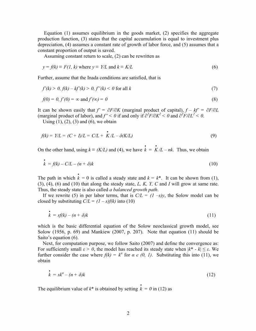
Equation (1) assumes equilibrium in the goods market, (2) specifies the aggregate production function, (3) states that the capital accumulation is equal to investment plus depreciation, (4) assumes a constant rate of growth of labor force, and (5) assumes that a constant proportion of output is saved. Assuming constant return to scale, (2) can be rewritten as

y = f(k) ≡ F(1, k) where y ≡ Y/L and k ≡ K/L (6)

Further, assume that the Inada conditions are satisfied, that is

f’(k) > 0, f(k) – kf’(k) > 0, f”(k) < 0 for all k (7)

f(0) = 0, f’(0) = ∞ and f’(∞) = 0 (8)

It can be shown easily that f’ = ∂F/∂K (marginal product of capital), f – kf’ = ∂F/∂L (marginal product of labor), and f” < 0 if and only if ∂2F/∂K2 < 0 and ∂2F/∂L2 < 0. Using (1), (2), (3) and (6), we obtain

f(k) = Y/L = (C + I)/L = C/L + •

K /L – δ(K/L) (9)

On the other hand, using k ≡ (K/L) and (4), we have = •

k•

K /L – nk. Thus, we obtain

= f(k) – C/L – (n + δ)k (10) •

k

The path in which = 0 is called a steady state and k = k*. It can be shown from (1), (3), (4), (6) and (10) that along the steady state, L, K, Y, C and I will grow at same rate. Thus, the steady state is also called a balanced growth path.

•

k

If we rewrite (5) in per labor terms, that is C/L = (1 –s)y, the Solow model can be closed by substituting C/L = (1 – s)f(k) into (10)

= sf(k) – (n + δ)k (11) •

k

which is the basic differential equation of the Solow neoclassical growth model, see Solow (1956, p. 69) and Mankiew (2007, p. 207). Note that equation (11) should be Saito’s equation (6). Next, for computation purpose, we follow Saito (2007) and define the convergence as: For sufficiently small ε > 0, the model has reached its steady state when |k* - k| ≤ ε. We further consider the case where f(k) = kα for α є (0, 1). Substituting this into (11), we obtain

= sk•

k α – (n + δ)k (12)

The equilibrium value of k* is obtained by setting = 0 in (12) as •

k

2

k* = [s/(n + δ)][1/(1-α)] (13)

Let kj be the capital stock at j-th stage of computing for j = 0, 1, 2, …, where k0 > 0 is the given initial capital stock. Starting from k0, we evaluate whether |k* - k| is larger than ε or not. If |k* - k| > ε turns to “TRUE”, we proceed to the next stage with capital accumulation according to

kj+1 = kj + •

k j = kj + skjα – (n + δ)kj (14)

Once |k* - k| > ε turns to “FALSE”, then stop computing to return the total number of steps. It is clear that equation (14) would be the correct version of Saito’s equation (10).

3. Programming code

In Saito’s programming code, he writes (* Definition of each variable *) (* s : saving rate, n : population growth rate, d : capital depreciation rate, k0 : initial per – capita capital stock, a : parameter on production function, e : epsilon to determine convergence, max : maximum number of iterations *) Solow [s_ , n_ , d_ , k0_ , e_ , max_ ] : = ( (* Initializing parameters *) j = 0; (* Steps to the steady state *) k = k0; (* Initial capital stock *) b = 1/(1 – a); (* Just for convergence *) z = ((1 – s)/(n + d))^b; (* Steady state capital stock *)

(* Loop while convergence *) While [ Abs [z – k] > e && j < max , (* Evaluate whether close enough *) k = k + (1 – s)*k^a – (n + d)*k; (* Accumulate capital stock *) j++ (* Count each step *) ]; (* Return total steps as the result *) Return [j]; )

3

According to the correct version of Solow growth model, we make the following changes, z = ((1 – s)/(n + d))^b; (* Steady state capital stock *) has been rewritten as z = (s/(n + d))^b; (* Steady state capital stock *) and k = k + (1 – s)*k^a – (n + d)*k; (* Accumulate capital stock *) has been rewritten as k = k + s*k^a – (n + d)*k; (* Accumulate capital stock *) Using this revised programming code with (s, n, d, k0, a, e, max) = (0.4, 0.1, 0.01, 1 or 10, 0.3, 0.00001, 5000) for Figure 1 to Figure 8, and (s, n, d, k0, a, e, max) = (0.4, 0.1, 0.1, 1 or 10, 0.3, 0.001, 1000) for Figure 9 to Figure 13, we derive thirteen figures.1 It is easy to see the graphical illustrations are different from Saito’s.2

Finally, it is worth mentioning that Saito’s specification of the horizontal axis (x) and the vertical axis (y) contains some errors. Taking Figure 1 as an example, the programming code is (* Drawing initial capital vs depreciation rate *) DensityPlot [ Solow [0.4, x, 0.01, y, 0.3, 0.00001, 5000], {x, 0, 1}, {y, 0.001, 25}, PlotPoints -> {800, 800}, Mesh -> False, ColorFunction -> Hue ] Obviously, x = n and y = k0. Thus, (* Drawing initial capital vs depreciation rate *) should be changed to (* Drawing initial capital vs population growth rate *). We correct some Saito’s errors in his programming code. For the revised version, please see Appendix.

4. Concluding remarks We have derived the basic differential equation of the neoclassical growth model from the well-known Solow’s 1956 paper and shown that Saito incorrectly specified the consumption function as: C = sY where s = saving rate. The correct specification of consumption function should be C = (1 – s)Y. Based on the correct basic differential equation, we follow Saito (2007) and apply some built-in functions of Mathematica to derive some graphical illustrations from Solow’s

1 . Equation (12) can also be specified as: = (1 - c)k

•

k α – (n + δ)k where c = 1 – s. Applying this formulation into the programming code, as a referee points out, the computation will take a longer computing time because of an additional “subtraction” step. 2 . The referee also points out that in the graphical presentation s and 1- s = c are point symmetric to each other on horizontal or vertical axes against s = 0.5. The referee further points out that when graphics do not involve saving rate (s), experiments in the original paper, s = 1 – c = 1 – 0.4 = 0.6 means s = 0.4 in the corrected version and two papers provide complement experiments.

4

convergent paths. While corrected Saito’s misspecification, our graphs show that Solow model displays convergent growth paths.

References Mankiw, N. Gregory (2007) Macroeconomics, 6/e. Worth Publishers. New York Saito, Tetsuya (2007) ‘Fine arts in Solow model’ Economics Bulletin, 1, 3, 1-20. Solow, Robert (1956) ‘A contribution to the theory of economic growth’ The Quarterly

Journal of Economics, 70(1), 65-94. Solow, Robert (1957) ‘Technical change and the aggregate production’ The Review of

Economics and Statistics, 39(3), 312-320. Wilfram, Stephan (2003) The Mathematica Book, 5/e. Wilfram Media Inc. Champaign,

IL.

5

Appendix A Programming Code In this source code, we correct some errors in Satio’s programming code especially the specification of the x axis and the y axis. Based on this revised version, we will be able to present the correct figure legend. (* Definition of each variable *) (* s : saving rate ,

n : population growth rate , d : capital depreciation rate , k0 : initial per - capita capital stock , a : parameter on production function , e : epsilon to determine convergence , max : maximum number of iterations *)

Solow [s_ , n_ , d_ , k0_ , a_ , e_ , max_ ] :=

((* Initializing parameters *) j = 0; (* Steps to the steady state *) k = k0; (* Initial capital stock *) b = 1/(1 - a); (* Just for convenience *) z = (s/(n + d))^b; (* Steady state capital stock *) (* Loop while convergence *) While [Abs [z - k] > e && j < max , (* Evaluate whether close enough *) k = k + s*k^a – (n + d)*k; (* Accumulate capital stock *) j++ (* Count each step *)]; (* Return total steps as the result *) Return [j];)

SolowLegend [T_] := (max = Max [T]; DensityPlot [x/max , {x, 0, max }, {y, 0, 1},

PlotPoints -> {100 , 100} , Axes -> {True , False }, Ticks -> Automatic , Mesh -> False , ColorFunction -> Hue , Frame -> False , AspectRatio -> 0.05 , TextStyle -> { FontSize -> 8}])

(* Draw pictures *) (* Figure 1: Drawing initial capital vs population growth rate *) DensityPlot [Solow [0.4 , x, 0.01 , y, 0.3 , 0.00001 , 5000] , {x, 0, 1}, {y, 0.001 , 25} ,

PlotPoints -> {800 , 800}, Mesh -> False, ColorFunction -> Hue]

(*Generate legend *) (*This process generates legend as follows ;

(1) Apply Solow function to get maximum steps ; (2) Principally minimum is always zero -- consider the case k0 = k*; (3) Then draw legend applying DensityPlot and Hue functions *)

T = Table [Solow [0.4 , x, 0.01 , y, 0.3 , 0.00001,5000],{x,0,1,0.1},{y, 0.001,25,0.1}]; T = Flatten [T];

6

SolowLegend [T]; (* Figure 2: Drawing 2D for initial capital vs population growth rate *) ListPlot [Table [Solow [0.4 , x, 0.01 , 5, 0.3 , 0.00001 , 5000] , {x, 0, 1, 0.0001}]] (* Figure 3.1: Drawing 3D for initial capital vs population growth rate *) Plot3D [Solow [0.4 , x, 0.01 , y, 0.3 , 0.00001 , 5000] , {x, 0, 1}, {y, 0.001 , 25} ,

PlotPoints -> {300 , 300} , Mesh -> False] (* Figure 3.2: Drawing 3D for initial capital vs population growth rate *) Show [graph , ViewPoint -> {-1, -0.5 , -0.5} , PlotRange -> {0, 300}] (* Change viewpoint *) (* Figure 4: Drawing initial capital vs saving rate *) DensityPlot [Solow [x, 0.1 , 0.01 , y, 0.3 , 0.00001 , 5000] , {x, 0, 1}, {y, 0.001 , 25} ,

PlotPoints -> {800 , 800} , Mesh -> False , ColorFunction -> Hue] (* Generate legend *) T = Flatten [T]; SolowLegend [T];

(* Figure 5: Drawing 3D for initial capital vs saving rate *) Plot3D [Solow [x, 0.1 , 0.01 , y, 0.3 , 0.00001 , 5000] , {x, 0, 1}, {y, 0.001 , 25} ,

PlotPoints -> {300 , 300} , Mesh -> False]

(* Figure 6: Drawing population growth rate vs saving rate for k0 =10 *) DensityPlot [Solow [x, y, 0.01 , 10, 0.3 , 0.00001 , 5000] , {x, 0, 1}, {y, 0, 1},

PlotPoints -> {800 , 800} , Mesh -> False , ColorFunction -> Hue] (* Generate legend *) T = Table [Solow [x, y, 0.01 , 10, 0.3 , 0.00001 , 5000] , {x, 0, 1, 0.1} , {y, 0, 1, 0.1}]; T = Flatten [T]; SolowLegend [T];

(* Figure 7: Drawing population growth rate vs saving rate for k0 =1 *) DensityPlot [Solow [x, y, 0.01 , 1, 0.3 , 0.00001 , 5000] , {x, 0, 1}, {y, 0, 1},

PlotPoints -> {800 , 800} , Mesh -> False , ColorFunction -> Hue] (* Generate legend *) T = Table [Solow [x, y, 0.01 , 1, 0.3 , 0.00001 , 5000] , {x, 0, 1, 0.1} , {y, 0, 1, 0.1}]; T = Flatten [T]; SolowLegend [T];

(* Figure 8: Drawing depreciation rate vs population growth *) DensityPlot [Solow [0.4 , x, y, 1, 0.3 , 0.00001 , 5000] , {x, 0, 1}, {y, 0, 1},

PlotPoints -> {800 , 800} , Mesh -> False , ColorFunction -> Hue] (* Generate legend *) T = Table [Solow [0.4 , x, y, 1, 0.3 , 0.00001 , 5000] , {x, 0, 1, 0.1} , {y, 0, 1, 0.1}]; T = Flatten [T]; SolowLegend [T];

(* Figure 9: Drawing share of capital input vs saving rate for k0 =1 *) (*d and n are redefined as 0.1 for computational reason .By the same reason , e = 0.001 and max = 1000 are also redefined.*) (* NOTE : Ignore some errors caused by dividing 0 *) DensityPlot [Solow [x, 0.1 , 0.1 , 1, y, 0.001 , 1000] , {x, 0, 1}, {y, 0, 1},

PlotPoints -> {800 , 800} , Mesh -> False , ColorFunction -> Hue] (* Generate legend *) T = Table [Solow [x, 0.1 , 0.1 , 1, y, 0.001 , 1000] , {x, 0, 1, 0.1} , {y, 0, 1, 0.1}];

7

T = Flatten [T]; SolowLegend [T];

(* Figure 10: Drawing share of capital input vs saving rate for k0 =10 *) (* NOTE : Ignore some errors caused by dividing 0 *) DensityPlot [Solow [x, 0.1 , 0.1 , 10, y, 0.001 , 1000] , {x, 0, 1}, {y, 0, 1},

PlotPoints -> {800 , 800} , Mesh -> False , ColorFunction -> Hue] (* Generate legend *) T = Table [Solow [x, 0.1 , 0.1 , 10, y, 0.001 , 1000] , {x, 0, 1, 0.1} , {y, 0, 1, 0.1}]; T = Flatten [T]; SolowLegend [T];

(* Figure 11: Drawing share of capital input vs population growth rate for k0 =1 *) (* NOTE : Ignore some errors caused by dividing 0 *) DensityPlot [Solow [0.4 , x, 0.1 , 1, y, 0.001 , 1000] , {x, 0, 1}, {y, 0, 1},

PlotPoints -> {800 , 800} , Mesh -> False , ColorFunction -> Hue] (* Generate legend *) T = Table [Solow [0.4 , x, 0.1 , 1, y, 0.001 , 1000] , {x, 0, 1, 0.1} , {y, 0, 1, 0.1}]; T = Flatten [T]; SolowLegend [T];

(* Figure 12: Drawing share of capital input vs population growth rate for k0 =10 *) (* NOTE : Ignore some errors caused by dividing 0 *) DensityPlot [Solow [0.4 , x, 0.1 , 10, y, 0.001 , 1000] , {x, 0, 1}, {y, 0, 1},

PlotPoints -> {800 , 800} , Mesh -> False , ColorFunction -> Hue] (* Generate legend *) T = Table [Solow [0.4 , x, 0.1 , 10, y, 0.001 , 1000] , {x, 0, 1, 0.1} , {y, 0, 1, 0.1}]; T = Flatten [T]; SolowLegend [T];

(*Figure 13: Drawing share of capital input vs initial capital *) (* NOTE : Ignore some errors caused by dividing 0 *) DensityPlot [Solow [0.4 , 0.1 , 0.1 , x, y, 0.001 , 1000] , {x, 0, 200} , {y, 0, 1},

PlotPoints -> {800 , 800} , Mesh -> False , ColorFunction -> Hue] (* Generate legend *) T = Table [Solow [0.4 , 0.1 , 0.1 , x, y, 0.001 , 1000] , {x, 0, 1, 0.1} , {y, 0, 1, 0.1}]; T = Flatten [T]; SolowLegend [T];

8

k0

n Legend: Number of steps to the steady state

Figure 1: Initial capital stock vs population growth rate

9

Figure 2: Initial capital stock vs population growth

k*

k0

n Figure 3.1: Initial capital stock v.s. population growth rate

10

k*

k0

n Figure 3.2: Initial capital stock v.s. population growth rate (Note: Figure 3.1 and 3.2 are the same plot. They are just presented in different view angle)

11

k0

s Legend: Number of steps to the steady state

Figure 4: Initial capital stock vs saving rate

12

k* k0

Figure 5: Initial capital stock vs saving rate s

13

n

s Legend: Number of steps to the steady state

Figure 6: Population growth rate vs saving rate (k0 = 10)

14

n

s Legend: Number of steps to the steady state

Figure 7: Population growth rate vs saving rate (k0 = 1)

15

δ

n Legend: Number of steps to the steady state

Figure 8: Depreciation rate vs population growth

16

α

s Legend: Number of steps to the steady state

Figure 9: Share of capital input vs saving rate (k0 = 1)

17

α

s Legend: Number of steps to the steady state

Figure 10: Share of capital input vs saving rate (k0 = 10)

18

α

n Legend: Number of steps to the steady state

Figure 11: Share of capital input vs population growth rate (k0 = 1)

19

α

n Legend: Number of steps to the steady state

Figure 12: Share of capital input vs population growth rate (k0 = 10)

20

α

k0 Legend: Number of steps to the steady state

Figure 13: Share of capital input vs initial capital stock

21