Finding The Best Statistical Model To Predict Customer ...

Finding The Best Statistical ModelTo Predict Customer Defection InTelecommunication Retail Setting

Nkululeko Ngcongo

February 11, 2014

University of Witwatersrand

Supervisor: Prof. David Lubinsky

Student Number: 576639

A Research Report submitted to the Faculty of Science,University of the Witwatersrand, Johannesburg, in partial

fulfilment of the requirements for the degree of Master of Sciencein Mathematical Statistics

brought to you by COREView metadata, citation and similar papers at core.ac.uk

provided by Wits Institutional Repository on DSPACE

Candidate’s Declaration

I, Nkululeko Ngcongo, declare that this Theses is my own, unaided work.It is being submitted for the Degree of Masters of Science at the Universityof the Witwatersrand, Johannesburg. It has not been submitted before forany degree or examination at any other University.

Nkululeko Ngcongo11 February 2014

i

Abstract

In this study we examine the question of which statistical mod-els work well in predicting customer defection in the retail mobiletelecommunication industry. For each of the two data sets that wereused (mobile call pattern and billing, and time taken to churn data),four statistical models were fitted and compared namely; artificialneural networks, decision trees, logistic regression and support vectormachines. The artificial neural network model proved to be supe-rior than the other three models when fitted on both data sets. Thismodel gave the best area under the receiver operating characteristiccurve (0.93 for call pattern data and 0.88 for billing and time taken tochurn data), highest lift at 10 per cent of the population (7.01 for callpattern data and 2.12 for billing and time taken to churn data) andlowest misclassification rate (0.04 for call pattern data and 0.19 forbilling and time taken to churn data). The logistic regression modelunder performed the other models when fitted to call pattern data andcame out as third when fitted to billing and time taken to churn datawhereby they outperformed the decision tree model. Support vectormachine came out as the second best model for billing and time takento churn data and third when fitted to call pattern data. Decisiontree model performed well when fitted to call pattern data and worstwhen fitted to billing and time taken to churn data The study showedthat in the retail mobile telecommunication industry, companies canincrease revenue streams and competitive advantage by using datamining techniques to predict customers that are likely to churn. Thenext step for the business is to embark on retention programs to usethese methods to reduce churners.

ii

Dedication

This thesis is dedicated to my family, friends and all the under privilegedchildren trying to strive in the ghetto.

iii

Acknowledgments

I would like to thank my supervisor Professor David Lubinsky for dedicatinghis time and guiding me with my work. I would like to send my sincerethanks to my family for being supportive and understanding all the time.Another great thanks goes to all my friends especially Njabulo Ngcongo,Sivuyile Mgobhozi, John Mukombewrana and Nompumelelo Zama for theirsupport and assistance. A great thanks also goes to the University of Cali-fornia and Data Mining Inc. for their data sets.

Lastly, I would like to thank GOD for making this possible.

iv

Contents

1 Introduction 11.1 Background . . . . . . . . . . . . . . . . . . . . . . . . . . . 11.2 Statistical problem: finding the best model . . . . . . . 2

2 Statistical Theory 32.1 Models to be used . . . . . . . . . . . . . . . . . . . . . . . 3

2.1.1 Decision Trees . . . . . . . . . . . . . . . . . . . . . 32.1.2 Logistic Regression . . . . . . . . . . . . . . . . . . 52.1.3 Support Vector Machines . . . . . . . . . . . . . . 62.1.4 Artificial Neural Networks . . . . . . . . . . . . . . 9

2.2 Model evaluation . . . . . . . . . . . . . . . . . . . . . . . . 122.2.1 Bayes and Akaike Information Criterion . . . . . 122.2.2 Receiver Operating Characteristic Curve . . . . 132.2.3 Lift Charts . . . . . . . . . . . . . . . . . . . . . . . . 14

3 Literature Review 163.1 Credit Card Churn Forecasting . . . . . . . . . . . . . . . 163.2 Data Mining Techniques for the Evaluation of Wire-

less Churn . . . . . . . . . . . . . . . . . . . . . . . . . . . . 173.3 Customer Relationship Management at Pay TV . . . . 193.4 Partial Defection of Loyal Clients . . . . . . . . . . . . . 203.5 Customer Headroom Model . . . . . . . . . . . . . . . . . 213.6 Churn Prediction Model . . . . . . . . . . . . . . . . . . . 223.7 Churn Prediction in the Mobile Telecommunication

Industry . . . . . . . . . . . . . . . . . . . . . . . . . . . . . 233.8 Analysis of Clustering Technique for Customer Rela-

tion Management . . . . . . . . . . . . . . . . . . . . . . . 253.9 Churn Prediction in Telecommunications . . . . . . . . 253.10 Turning Telecommunication Call Details to Churn Pre-

diction . . . . . . . . . . . . . . . . . . . . . . . . . . . . . . 273.11 Churn Prediction Using Complaints Data . . . . . . . . 283.12 Churn Models for Prepaid Customers . . . . . . . . . . . 303.13 Mobile Telecommunication Handling in India . . . . . . 313.14 Knowledge Discovery on Customer Churn . . . . . . . . 323.15 Under-Sampling Approaches for Improving Predictions 333.16 Examining Churn and Loyalty Using Support Vector

Machine . . . . . . . . . . . . . . . . . . . . . . . . . . . . . 353.17 Literature Summary . . . . . . . . . . . . . . . . . . . . . . 36

v

4 Methodology 374.1 Analysis Process . . . . . . . . . . . . . . . . . . . . . . . . 374.2 Understanding the data sets . . . . . . . . . . . . . . . . . 38

4.2.1 Data Cleaning . . . . . . . . . . . . . . . . . . . . . 384.2.2 Data Exploration . . . . . . . . . . . . . . . . . . . . 39

4.3 Sampling . . . . . . . . . . . . . . . . . . . . . . . . . . . . . 444.3.1 Stratifying the data . . . . . . . . . . . . . . . . . . 444.3.2 Splitting the data . . . . . . . . . . . . . . . . . . . 44

5 Analysis and results 465.1 Data Set 1 Results . . . . . . . . . . . . . . . . . . . . . . . 46

5.1.1 Artificial Neural Networks . . . . . . . . . . . . . . 465.1.2 Decision Trees . . . . . . . . . . . . . . . . . . . . . 525.1.3 Support Vector Machines . . . . . . . . . . . . . . 555.1.4 Logistic Regression . . . . . . . . . . . . . . . . . . 59

5.2 Data Set 2 Results . . . . . . . . . . . . . . . . . . . . . . . 615.2.1 Artificial Neural Networks . . . . . . . . . . . . . . 615.2.2 Decision Trees . . . . . . . . . . . . . . . . . . . . . 655.2.3 Support Vector Machines . . . . . . . . . . . . . . 675.2.4 Logistic Regression . . . . . . . . . . . . . . . . . . 69

6 Comparison of Models 72

7 Conclusion and recommendations 74

8 Summary and Future Research 75

References 76

Appendix 81

vi

List of Figures

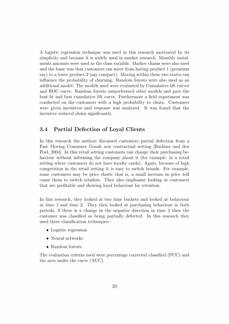
1 Plane separating the data points . . . . . . . . . . . . . . . . . 72 A typical artificial neural network . . . . . . . . . . . . . . . . 103 Logistic and hyperbolic tangent sigmoid functions . . . . . . . 114 A feed forward neural network with two hidden layers . . . . . 125 ROC Curve . . . . . . . . . . . . . . . . . . . . . . . . . . . . 146 Distribution of service calls and number of voice mails . . . . 407 Correlation table for data set two . . . . . . . . . . . . . . . . 428 Bi-variate logistic plot for data set 2 . . . . . . . . . . . . . . 449 Lift curves for the six neural networks before data transformation 4810 Lift curves for the six neural networks after data transformation 4811 ROC and lift curves for ANN model data number A . . . . . . 5012 ROC and lift curves for ANN model data number F . . . . . . 5113 Number of Decision Tree Splits . . . . . . . . . . . . . . . . . 5314 Decision trees variable importance data set 1 . . . . . . . . . . 5415 Support vector constant effect 1: RBF kernel function . . . . . 5516 Support vector constant effect 2: RBF kernel function . . . . . 5617 Support vector machines ROC curve fit for data set 1 . . . . . 5718 Probability cut off for data set 1 SVM model . . . . . . . . . . 5819 Probability cut off for logistic regression data set 1 . . . . . . 6020 ROC and lift curve for logistic regression data set 1 . . . . . . 6121 AUC for ANN models . . . . . . . . . . . . . . . . . . . . . . 6322 R-Square for a change in the number of hidden units in ANN

model . . . . . . . . . . . . . . . . . . . . . . . . . . . . . . . 6423 Sensitivity for a change in the number of hidden units in ANN

model . . . . . . . . . . . . . . . . . . . . . . . . . . . . . . . 6424 Misclassification rates for a change in the number of hidden

units in ANN model . . . . . . . . . . . . . . . . . . . . . . . 6425 Decision trees R-Square value per split for data set 2 . . . . . 6626 Decision trees lift curves for data set 2 . . . . . . . . . . . . . 6727 ROC fit for kernel SVM models data set 2 . . . . . . . . . . . 6828 Probability cut off for data set 2 SVM model . . . . . . . . . . 6929 Probability cut off for logistic regression on data set 2 . . . . . 7130 ROC and lift curve for logistic regression on data set 2 . . . . 71A1 Data set 1 distribution A . . . . . . . . . . . . . . . . . . . . . 83A2 Data set 1 distribution B . . . . . . . . . . . . . . . . . . . . . 83A3 Data set 1 distribution C . . . . . . . . . . . . . . . . . . . . . 84A4 Data set 1 bi-variate logistic fit . . . . . . . . . . . . . . . . . 84A5 Data set 2 distributions A . . . . . . . . . . . . . . . . . . . . 85A6 Data set 2 distributions B . . . . . . . . . . . . . . . . . . . . 85

vii

A7 Data set 1 kernel SVM fit . . . . . . . . . . . . . . . . . . . . 86A8 Data set 2 kernels SVM fit . . . . . . . . . . . . . . . . . . . . 86A9 Correlation table for data set 1 . . . . . . . . . . . . . . . . . 87

viii

List of Tables

1 Model Comparison . . . . . . . . . . . . . . . . . . . . . . . . 32 Training sample results for standardised and un-standardised

data . . . . . . . . . . . . . . . . . . . . . . . . . . . . . . . . 463 Test sample results for standardised and unstandardised data . 464 Neural networks results before transforming the data . . . . . 475 Neural networks results after transforming the data . . . . . . 476 Sample Test and Train Ratios . . . . . . . . . . . . . . . . . . 497 Train data model performance for data set 1 . . . . . . . . . . 498 Test data model performance for data set 1 . . . . . . . . . . . 499 Train data model performance for data set 2 . . . . . . . . . . 6110 Test data model performance for data set 2 . . . . . . . . . . . 6211 Data set 1 model comparisons . . . . . . . . . . . . . . . . . . 7312 Data set 2 model comparisons . . . . . . . . . . . . . . . . . . 73A1 Data set 1 variables . . . . . . . . . . . . . . . . . . . . . . . . 81A2 Data set 2 variables . . . . . . . . . . . . . . . . . . . . . . . . 82

ix

Abbreviations

ANN = Artificial Neural Networks

SVM = Support Vector Machines

Data set 1 = Call pattern churn data

Data set 2 = Billing and time taken to default data

RBF = Radial basis function

SMOTE = Synthetic minority over sampling technique

ROC = Receiver operating characteristic

AUC = Area under the curve

AIC = Akaike information criteria

BIC = Bayes information criteria

SBC = Schwarz Bayesian criteria

x

1 Introduction

1.1 Background

Statistical data mining is the process of extracting data from different datasources and manipulating the data in order to produce meaningful informa-tion that can be used by management to make decisions. Data mining isan ’emerging’ field in statistics since technology has allowed us to store largeamounts of data to be analysed so that companies, governments and other or-ganizations can make informed decisions. Statistical data mining techniquescan be applied to many social science fields [Chow, 2002, Kvam and Sokol,2004, Crang, 2002, Philip et al., 2011, Mazzocchi, 2007, Juahiainen, 2012].In this research, we concentrate on using statistical data mining techniquesin the marketing field. Marketing departments around the world have hugedatabases with customer’s demographic and behavioural details. They nolonger need to rely on gut feel, rather they can use statistics in order tomake informed decisions. In the case where the industry has reached satu-ration the market becomes a churn market and it is difficult and expensiveto recruit new customers [Friedman, 1997]. In order for a business to survivefierce competition where churn rates are high, it must rely on statistical datamining techniques to predict churners. Statistical data mining has played animportant role in market research in recent years [Imhoff, 2001].

In the retail mobile telecommunication setting, customer relationship man-agement is a very important aspect of the business. Customers have a fixedcontract with a known expiry date or termination date. Not all customers willbe satisfied with the service they receive and this will lead to customers notrenewing their contracts or terminating them earlier than expected. Thereare various factors that will lead to this, for example:

• Bad service

• Better offers by competitors

• Network inefficiencies

There are also some exogenous factors that one cannot account for that canlead to customer defection, for example:

• Deceased or emigrated customers

• Financial situation where by a customer loses employment and decidesto terminate the contract

1

• Fraudulent contracts that need to be terminated

• Natural disasters

Because retention efforts are expensive, it makes sense to look at retentioninitiatives for only high value customers. A high value customer may bedetermined based on the following factors:

• Their ’age on book’ is at least more than the initial contract period(excluding new customers)

• They have never missed any of their monthly instalments

• They have participated in a customer satisfaction survey or other study

• They have at least one of the top of the range products

• They must have at least renewed their contract once

• They have not opted out of marketing initiatives

1.2 Statistical problem: finding the best model

The main research question that we address is which statistical techniquepredicts with accuracy the ’high value’ customers that are likely to defect inthe retail mobile telecommunication setting. In this problem of predictingcustomer defection, we are not highly concerned about time taken to defectbut mainly concerned about detecting a type of customer profile that is likelyto defect. The aim is to predict defection or termination of the service bycustomers and to also understand the type of statistical techniques that aremost successful in predicting customer defection in this setting. This willenable us to classify with a certain probability whether customers are likelyto defect or not, based on their historical data.

The retail mobile telecommunication setting is highly competitive therefore,it is easy for a customer not to renew his or her contract. If no new highvalue customers are recruited as the old ones that churned, then there willbe a significant decrease in profit margins. This will lead to business insol-vency.

2

2 Statistical Theory

2.1 Models to be used

The following standard data mining classification models were used in thisresearch to predict churn:

• Artificial neural networks

• Decision trees

• Linear support vector machines

• Logistic regression

The motivation behind using these models is their simplicity and it is fairlyeasy to interpret the results. We want to find out which model is the mostsuitable for dealing with retail mobile telecommunication data. Table 1 showsthe basics of the four models. Yang and Chiu argued that artificial neuralnetwork models are a black box and that the weights of the neurons are un-interpretable. This is a big disadvantage compared to the other three models[WSE, 2006].

Table 1: Model Comparison

Model Decision trees Logistic regression Support vector machines Artificial neural networksLoss Function Confusion Matrix Log Loss Hinge Loss LogHigh Dimen-sional Feature

Linear Kernel Gaussian Kernel Polynomial Hyperbolic Tangent

Works WellWith

Continuous and Binary Binary Continuous Continuous and Binary

Over fitting Pruning Cross Validation L2 Norm Early Stopping

In the remainder of this section we will introduced each modelling tech-nique.

2.1.1 Decision Trees

The basic idea of decision tree models is that for a given training sampled ⊂ D, where D is the entire data set containing Xi, ∀i = 1, 2, · · · , n in-dividuals with k attributes and n >> k, you want to divide d based on thekth attribute and the class j, ∀j = 1, · · · , f you wish to predict such thatyou have unique trees with unique individuals [Kamber and Han, 2006]. The

3

class j is the response variable which can be binary or has multiple states.Suppose that the class variable that you wish to predict is the likelihood thata customer will terminate his/her cell phone contract with a certain serviceprovider (good = not terminate, bad = terminate). The training sample dwill be used to build the tree and the model derived from d will be used toclassify the Xi in the test sample T = D− d. Using the test sample you canalso check the model accuracy by checking how many individuals you havecorrectly classified. The model will enable you to classify new data pointsentering the system as to whether they will terminate or not.

The decision tree technique is widely used in the data mining industry andis well known for its simplicity. To decide which variable to split on, manyfunctions have been suggested. The most common are GINI index, entropyand information. When a node p is split into l partitions, the quality of thesplit is given by

GINIsplit =l∑

j=1

P (kj)GINI(p/k) (2.1)

where k is the attribute used to split into class j and GINI index at node pis

GINI(p) = 1−f∑j=1

(Prob(j/k))2

where Prob(j/k) is the probability of class j at node p. A pure node isreached if GINI(p/k) = 0 and a best split is the variable with the lowestGINI index [Linoff and Berry, 2004].

The entropy of a random variable Xi, i = 1, 2, · · · , n is

entropy(a1, a2, · · · , aj) = −a1 log a1 − a2 log a2 − · · · ,−aj log aj

which is= −

∑ajlog(aj),∀j = 1, · · · , n

where aj is the probability that Xi belongs to a class j.

Let d be the training data set, j be the class that you want to predict (cus-tomer terminates contract or not) and k the data attributes and entropyfunction g(x) then the information gain is:

Info(d, k) = g(x)−∑i

|Yi/kattribute||d|

g(Yiεd/k)

4

The information gain has a huge disadvantage when it comes to splittingdata with distinct or unique values as these carry the highest informationin the data set (This means that the data will be split first by this variablethus showing it as the most significant variable). The k attribute with thehighest information gain will be used to split the data [Kamber and Han,2006]. Proust suggested that one can also split on the G squared statisticswhich works out to be twice the size of entropy, that is G2 = 2 ∗ entropy[Proust, 2012].

2.1.2 Logistic Regression

The second classification technique that was considered was logistic regres-sion. The basic idea is that you have a data set of n distinct individuals withXi,∀i = 1, 2, · · · , n and you want to predict each individual belonging to acertain class j (terminate phone contract = bad or not terminate = good,say) with a certain probability. Let j = class where j = 1 if good and 0 ifbad and let X = X1, · · · , Xn be the observed data set variables then

P (j = Class|X = Xi) =exp(β0 + β1X1 + · · ·+ βnXn)

1 + exp(β0 + β1X1 + · · ·+ βnXn)(2.2)

is the probability of belonging to a certain class [Friedman et al., 2008]. Itmust be noted that the exponent part is the normal multivariate linear equa-tion where you can have dummy variables, indicators or interaction terms.Not all attributes for Xi points will be significant in predicting the member-ship of a class j, you can therefore select the attributes that are significantin predicting class j. This may be done by a forward or backward selectionmethod. After fitting the logistic model the contribution or significance ofeach selected attribute to the model can be determined by likelihood ratiotest or the Wald statistic and other methods [Cios et al., 2007].

The odds ratio is used to measure the association between response andpredictor variables, that is, the probability of occurring versus not occurring.The odds ratio is widely used in Bio-statistics for evaluating association andrelative risk of a certain factor for the groups being studied [Raygoza, 2009].Suppose two groups are being studied (control and treatment group) andlet T̄ be the probability of an event in the treatment group and C be theprobability of an event in the control group then the odd ratio is:

OR =T̄

1−T̄C

1−C(2.3)

5

If OR = 1 then the odds of the event being studied are equally likely to occurin both groups that is the probability of each event occurring is half. Thislead to the following equation

P (j = Class|X = Xi) =OR

1 +OR

which means that

OR =P (j = Class|Y = Yi)

1− P (j = Class|X = Xi)

The odds ratio can be studied for each variable in the logistic regressionand this measures the contribution of that variable to the regression equa-tion.

2.1.3 Support Vector Machines

The third technique considered was the support vector machines (SVM).The basic idea is that you have a training sample d and data points Xi, i =1, 2, · · · , n and you want to divide the data set into j regions (j may be theclass variable). The data will be divided by a set of hyper planes into jregions [Mirowski et al., 2008]. The support vectors are the data points thatare closest to the plane that divides the data into j sub regions. You mayhave quite a large number of the hyper planes that divide the data into j subregion but what you really want is a hyper plane (line) that maximizes theregion between the support vectors [Friedman et al., 2008]. This is becausemaximising the region between the support vectors decreases the likelihoodof misclassifying new data points.

6

Figure 1: Plane separating the data points

Figure 1 shows three planes that can separate the positive and negative datapoints with zero misclassification rate [Mirowski et al., 2008]. From this fig-ure, the black plane is the best separator because it gives a bigger marginbetween the two groups of points. A bigger margin is best because there is ahigher chance that if a new data point is imputed it will be classified correctly.Finding the best plane (line) that separates these points is an optimisationproblem which can be solved using Lagrangian methods. Sometimes thesedata points may not be linearly separable.

To define this in a mathematical way, suppose you have a training dataset

D = [(x1, y1), (x2, y2), · · · , (xl, yl)],∀xεRn, yε[−1, 1]

where xl,∀i = 1, 2, · · · , l is the vector of individual and attributes, and yl areregions of belonging for each individual Xn. These points can be separatedinto −1 or 1 by a hyper plane < w, x > +b = 0 where b is the distance fromthe point to the plane, w the weights vector and < w, x > is the dot product.The separating hyper plane must satisfy

yi[< w, xi > +b] >= 1,∀i = 1, 2, · · · , l (2.4.1)

and the distance of x to the hyper plane which is

7

d(w, b;x) =| < w, xi > +b|

||w||(2.4.2)

The optimal hyper plane is the one that minimises φ(w) = 12||w||2 and com-

bining this with 2.4.1 and forming a Lagrangian equation with parameteralpha it leads to finding a solution of

φ(w, b, α) =1

2||w||2 −

l∑i=1

αi(yi[< w, xi > +b]− 1) (2.4.3)

which satisfies the Karush Kuhn Tucker condition which is first order condi-tion for an optimal value. From 2.4.3 one must find the first partial derivativewith respect to b and w and equate to zero for an optimal solution. The so-lution to the problem is then given by

α‘ = argminα1

2

l∑i=1

j∑i=1

αiαjyiyj < xi, xj > −l∑

k=1

αk (2.4.4)

constrained by αi > 0 and∑j

i=1 αjyi = 0

Assume now that the data is not linearly separable by a hyper plane andsuppose now that there is an error ψi,∀i = 1, 2, · · · , l then the constraintequation 2.4.1 will be modified to

yi[< w, xi > +b] >= 1− ψi,∀i = 1, 2, · · · , l (2.4.5)

and the optimal plane is found by w that minimises

φ(w, α) =1

2||w||2 − C

l∑i=1

ψi (2.4.6)

where C is given subject to constrains. The Lagrangian equation now be-comes

φ(w, b, α, ψ) =1

2||w||2 + C

l∑i=1

ψi −l∑

i=1

αi(yi[wTxi + b]− 1 + ψi)−

l∑j=1

βiψi

(2.4.7)where β and α are Lagrangian multipliers. The equation 2.4.7 is solved insimilar fashion to 2.4.3 and the solution is given by

α‘ = argminα1

2

l∑i=1

j∑i=1

αiαjyiyj < xi, xj > −l∑

k=1

αk (2.4.8)

8

constrained by 0 <= αi <= C and∑j

i=1 αjyi = 0 [Gunn, 1998]

Now that the optimisation problem is solved one needs to know the typeof hyper plane to be fitted. When fitting a SVM model one can use kernelfunctions to map the data into high dimension with the aim of making thedata more separable. There are quite a number of kernel functions that areavailable but we will look at the following kernels:

• Radial Basis Function: k(x, x‘) = exp(−σ||x− x‘||2)

• Polynomial: k(x, x‘) = (scale < x, x‘ > +K)N

• Hyperbolic Tangent: k(x, x‘) = tanh(< x, x‘ > +K)

• Laplace: k(x, x‘) = exp(−σ||x− x‘||)

and the choice of the kernel really depends on the data set. The parameterchoices of K, N (degree) and σ also depends on the data set. Furthermore,in R (A statistical analysis software) if these parameters are not given, theprogram will select the best ”parameter” values for you [Karatzoglou et al.,2006].

2.1.4 Artificial Neural Networks

The final model that was used in this research was artificial neural networks(ANN). The reason behind using this approach was that it can fit the datawell where linear and other models have proved inadequate. The drawbacksare that this model tends to over fit the data and the fact that it is complex toexecute and interpret at times. This data mining classification technique wasinspired by biological nervous system architect [Nemati, 2000]. In biology,millions of neurons are interconnected by synapses which carry ”information”from one neuron to another. This information is then sent to other neurons asoutput and the end results are just sensory information (for example: jump).

Data mining construction of a neural network uses almost similar ideologyto biology in the sense that you have the following:

• An output vector that passes information

• A ”neuron” that processes this information

• A weight for every piece of information entering the neuron

9

Figure 2: A typical artificial neural network

Figure 2 shows a typical ANN where the xi for i = 1, 2, · · · , j are the inputvectors, the wi for i = 1, 2, · · · , j are input vector weights and

Σ =

j∑i=1

wixi

is the sum of each weight times the input vector [Cheng and Titterington,2000]. Let yi =

∑ji=1wixi be the net input of a neuron then there exists an

activation function that gives an output, that is

f(yi) = h(

j∑i=1

wixi) (2.5)

where f(yi) is the output from h a sigmoid or linear activation function. Thesigmoidal function can be of the form of a hyperbolic tangent, logistic, radialbasis function etc. A sigmoidal function is an S shaped curve.

10

Figure 3: Logistic and hyperbolic tangent sigmoid functions

Figure 3 shows logistic (in blue f(xi)log) and hyperbolic tangent (in redf(xi)tanh) sigmoidal functions [Turhan, 1995]. The logistic sigmoid is asymp-totic to the lines f(xi) = 0 and f(xi) = 1 while the hyperbolic tangentsigmoid is asymptotic to the lines f(xi) = 1 and f(xi) = −1. The twosigmoid functions are continuous and differentiable on xiε[−∞,∞] interval[Turhan, 1995]. Furthermore,

f(xi)tanh = 2f(xi)log − 1 (1)

=2

1 + exp(−xi)− 1 (2)

=1− exp(−xi)1 + exp(−xi)

(3)

In this research, we looked at a feed forward artificial neural network andused the hyperbolic tangent as a sigmoidal function. A feed forward neuralnetwork has a hidden neural network structure such that the message getspassed from the first neuron to next one but the message is not returnedback.

11

Figure 4: A feed forward neural network with two hidden layers

Figure 4 shows a typical feed forward neural network architecture where thew’s are the weights of each neuron, Y is the output and the x’s are the inputvector. When fitting an artificial network model we try to find the unknownweights wj by minimising the error of the output from the estimated weights.Optimisation techniques such as Back-Propagation, Newton-Raphson andother techniques are used to estimate the wj. Two problems that may arisefrom fitting ANN is getting the starting values of the weights to be estimatedand over fitting the neural network model. A zero value can be used asa starting point of estimating weights and the early stopping rule in theoptimisation technique can be used to avoid over fitting.

2.2 Model evaluation

We evaluate the models using; Bayes Information Criterion (BIC), ReceiverOperating Characteristic Curve (ROC), Akaike Information Criteria (AIC),misclassification rates and the lift charts because these are the commonlyused evaluation criteria methods.

2.2.1 Bayes and Akaike Information Criterion

The AIC and BIC measure the performance of a statistical model for a dataset being analysed. These models depend mostly on the likelihood functionand will penalise models with higher numbers of parameters. The main ideais to see which models are over fitting the data amongst the ones that arebeing compared. These measures are calculated as below:

12

AIC = −2 log(l) + 2k (2.6)

and

BIC = −2 log(l) + k log(n) (2.7)

where l is the likelihood value, k is the number of parameters and n is thetotal number of observations. As the model becomes more complicated, knumber of parameters used to estimate the model will increase, the AIC andBIC values will increase and the model will be over fitting the data.

2.2.2 Receiver Operating Characteristic Curve

The ROC curve measures how well the model fits by plotting the false positiveand negative fraction and evaluating the area under the fitted curve. Giventhat we have a class that we want to predict (that is, customer defectingor not) and a given set of data divided into training and test sample. Themodel is built on the training sample and evaluated on the test sample. Forthe ROC curve we will be looking at the following:-

• True Positive and Negative Fraction: Predicted to defect in the trainingsample and actually defected and predicted not to defect and actuallynot defecting

• False Positive and Negative Fraction: Predicted to defect but does notdefect and predicted not to defect but defect.

A best fitting model is the one with the lowest error rate, that is, withlow false positive fraction. As a retail mobile telecommunication companyyou would want to reduce these errors. The ROC curve is then a plot ofsensitivity (true positive rate) versus 1−specificity (true negative rates/falsepositive rates). Figure 5 shows a typical ROC curve.

13

Figure 5: ROC Curve

The 45 degree line (y = x which is labelled D) signifies a worthless model,curve C show that the model is performing better, curve B is better fittingtest and curve A is the perfect model [Zou et al., 2007]. The higher the areaunder the ROC curve the better is the performance of the model. The AUC(area under the ROC curve) is an element of the set [0, 1] [Gatsonis, 2008]

2.2.3 Lift Charts

The idea of the lift chart is that as a marketing firm you do not want toemail or SMS all your customers for a promotional offer. Imagine doing thisfor a base of 1 million customers at a cost of 20 cents and only 500 customersrespond to the offer of R10. The cost of sending these SMS’s will not berecovered in this case, thus the business will lose a lot of money. The liftchart assists the business in identifying and selecting only the top customersthat are likely to respond to the marketing offer rather than using randomselection. Measuring a statistical model using the lift curve is done by rank-ing customers with the highest probability of responding and evaluating thenumber of the correct predicted customers that actually respond to the cam-paign at a certain population proportion.

14

To define this in detail, let Sc be the percentage of customers with highestranked probability of churning when selected and P0 be the proportion ofcustomer selected from the whole population of churners and non-churnersthen

Lift(P0, Sc) = P0/Sc

As the proportion of the population selected increases, the lift value tends to1 and in fact

Lift(100, Sc) = 1

and the maximum lift attainable is 1/Sc [Kno, 1999]. A lift of a randommodel is 1 for all P0 values.

15

3 Literature Review

The research involved looking at relevant literature and detailed review ofsixteen papers by the researcher that focused on churning of customers inindustries such as banking, telecommunication and other retail sectors. Oneof the paper reviewed concentrated on sampling techniques when a class ofinterest is rare. We have applauded and questioned some of the literaturebased on their approach toward solving the churn problem.

3.1 Credit Card Churn Forecasting

In this research two data mining techniques were used to build a churn pre-diction model using credit card data from a Chinese Bank [Nie et al., 2011].The authors defined data mining as discovering knowledge and patterns froma large data set. They argued that it costs a lot to acquire new customers soit is important to retain existing high value or profitable customers. In thepaper they argued that a bank can increase profits by up to 85 per cent byan improvement of 5 per cent in the retention rate. As the economy developsin China, a large number of credit cards have been issued however most ofthese credit cards were inactive. With an increased competition in the bank-ing sector, it is easier for a customer to exercise their right of switching theproduct if the current service is not satisfactory.

In this study churn was considered from a customer’s initiation point of view,for example

• More favourable competitor pricing

• False information given to customers from acquisition

• Customer expectation not met etc.

and not by customers that churn because of the bank’s initiation (for examplebad debt). A sample of customers was taken from the database and dividedinto two time frames. A churner was then defined as a customer with notransaction at a chosen time period t (after) and the customer did make atransaction at a previous time t− 1 (before). In this paper they used logisticregression and decision trees to predict churn. They also emphasized thatthese two methods work well in classification problems. The models werevalidated using percentage of correctly classified, GINI coefficient and ROCcurve. They considered two types of errors:-

16

• Type 1 error: customer did not churn but is classified as a churner

• Type 2 error: customer churned but were classified as a non-churner

The model selection was also based on which model costs the most whenselected, that is, the actual currency cost of marketing to the customersthat were classified as churners but did not churn. A random sample wasselected from a database of 60 million customers from January 2005 to April2008. The data contained customer’s demographic information, transactioninformation, abnormal card usage and other transactional activities withthe bank. The time period was divided into observation period (where thenumber of total transactions was counted) and the evaluation period (wherethey check if the customers that were transacting before are still transacting).Out of 135 variables, only 95 variables were included in the final model.This is because some of the variables were found to be correlated (multi-co-linearity) and this would have affected the model performance if they wereincluded. Logistic regression and decision tree models were compared; theyboth showed that the demographic variables were not significant in predictingthe churn rate. The activity level variables contributed more to significancein the models than the demographic variables and hence the model with thesevariables performed better than the model without them (for both models).Logistic regression model performed better than the decision trees and gaveless cost on error (decision tree cost = 85283 and logistic regression cost =80377).

3.2 Data Mining Techniques for the Evaluation of Wire-less Churn

The authors of this article start by explaining the fact that the wireless mo-bile telecommunication industry is very competitive [Ferreira et al., 2004].As wireless companies grow in numbers customers are faced with wider op-tions to choose from which best satisfy their needs. They explain that thereis a battle of advertisement within wireless companies in order to lure cus-tomers to change their mind and switch to utilise their services. Churn wasdefined as abandoning your service provider as a customer and moving toa competitor. Churn is recognised as a crucial issue in consumer businessand economics. The author emphasises that predicting churn beforehand canhelp in retaining high value customers by giving them counter offers and thussaving the business money.

17

Their dataset came from a wireless carrier in Brazil with a sample of onehundred thousand customers and for a time period of nine months. A churnerwas defined based on termination of service before the ninth month and thiswas used as a target variable. From the dataset 1.25 per cent was a monthlychurn rate which is very small when trying to model customer churn. Theauthors overcame this problem of very low churn rate by oversampling. Thishad an implication on the data and the accuracy of the churn model. Theauthors used the below variables for predicting churn:

• Billing data (roaming cost, revenue, etc.)

• Customer demographic data (gender, marital, region, etc.)

• Customer relationship data (rate plan, handset age etc.)

• Market data (competitor rates etc.)

• Usage data (airtime, data bundles etc.)

In total there were 37 data attributes (behavioural and demographic vari-ables). These variables were transformed and standardised for modellingpurposes. The authors then divided the data into two:

• Simple dataset where no modification was done

• Enhanced dataset where the features were reduced using Least SquareEstimation and other methods

Using the feature selection methods, it was found that variables related tothe airtime consumption by customers were decisive in defining churn. Thetwo data sets were then standardised. The enhanced data representation had10 variables while the simple data representation had 20 variables. The datawas divided into 70 per cent training set, 20 per cent validation set and 10per cent test set.

Four models were then run on the data set namely neural networks, decisiontrees, hierarchical neuro-fuzzy system and genetic algorithm rule evolver.The neural network model had optimal number of hidden layers determinedempirically and was trained by back-propagation. The cost of each model wasevaluated based on the assumption that 50 per cent of the churners that areoffered incentive will be retained, the cost of incentive is 25 dollars, averagemonthly subscription is 80 dollars and only 20 per cent of those predictedas churners are contactable. Based on a total of two million subscribers forthis company, results showed that using a neural network model on enhanceddata representation can save the company a large sum of money (44.2 dollars

18

per client that is likely to churn). The models performed on the enhanceddata representation set yielded better results than using a simple data setfor all model. Neural network model with fifteen hidden units outperformedthe other models.

3.3 Customer Relationship Management at Pay TV

Pay TV is a European company that offers premium channel viewing tosubscribers [Burez and den Poel, 2005]. It offers entertainment, news andeducational channels to its viewers. Pay TV has a huge database of activecustomers but in recent years the number of active customers started todecline. It was speculated that the churn was caused by higher fixed cost tocustomers because it was expensive to maintain Pay TV infrastructure. Inthis research, they mentioned the following marketing initiatives to try andreduce customer churn

• Give customers free services

• Organising special events to pamper customers

• Survey study on customer satisfaction

In this research, they mention two ways of reducing customer churn. Thefirst of which was an untargeted approach, which is mass marketing to everycustomer. The second was a targeted marketing approach to customers witha higher probability of churning and provide them with lucrative offers.

Similar to DSTV, if you subscribe to Pay TV you only pay a monthly sub-scription fee. There are no other charges except for pay per view which wasnot discussed in this research. The subscription is a twelve months contractby which cancellation before the end of twelve months is not allowed. Cus-tomers need to inform Pay TV if they will terminate the contract after twelvemonths; if this is not done then the contract is automatically renewed. Thedata was divided into two time buckets that is estimation period (from startof Pay TV to sampling date) and follow up period (a year after the samplingperiod). Variables that were extracted from the database were:-

• Previous and current subscription

• Demographic (e.g. Age, gender etc.)

• Number of payment reminder notifications to customers

19

A logistic regression technique was used in this research motivated by itssimplicity and because it is widely used in market research. Monthly instal-ments amounts were used as the class variable. Markov chains were also usedand the basic was that customers can move from having product 1 (premiumsay) to a lower product 2 (say compact). Moving within these two states caninfluence the probability of churning. Random forests were also used as anadditional model. The models used were evaluated by Cumulative lift curvesand ROC curve. Random forests outperformed other models and gave thebest fit and best cumulative lift curve. Furthermore a field experiment wasconducted on the customers with a high probability to churn. Customerswere given incentives and response was analysed. It was found that theincentive reduced churn significantly.

3.4 Partial Defection of Loyal Clients

In this research the authors discussed customers partial defection from aFast Moving Consumer Goods non contractual setting [Buckinx and denPoel, 2004]. In this retail setting customers can change their purchasing be-haviour without informing the company about it (for example, in a retailsetting where customers do not have loyalty cards). Again, because of highcompetition in the retail setting it is easy to switch brands. For example,some customers may be price elastic that is, a small increase in price willcause them to switch retailers. They also emphasize looking at customersthat are profitable and showing loyal behaviour for retention.

In this research, they looked at two time buckets and looked at behaviourat time 1 and time 2. They then looked at purchasing behaviour in bothperiods, if there is a change in the negative direction in time 2 then thecustomer was classified as being partially defected. In this research theyused three classification techniques:-

• Logistic regression

• Neural networks

• Random forests

The evaluation criteria used were percentage corrected classified (PCC) andthe area under the curve (AUC).

20

In this study they selected only the behavioural loyal customers for analysissatisfying the following conditions:-

• The frequency of shopping is above average

• Ratio of the standard deviation σt of the inter-purchase time to themean µt inter-purchase time is below average

The data chosen for this study contained customer behavioural and demo-graphic attributes. One may argue that most variables that were used inthis study were correlated which may have caused bias in the predictions.Random forest outclassed neural networks and logistic regression techniques.The content of this paper is very powerful in the sense that it looks at par-tial changes in customer behaviour so that corrective initiative can be appliedearly enough before a customer totally defects.

3.5 Customer Headroom Model

This paper talks about basket analysis in a retail setting in which some bas-kets were believed to have a missing spend [Shashanka and Giering, 2009].For example, if a customer usually buys only bread in a store yet it is knownfrom previous experience that bread is associated with butter or milk (say)then there is a possibility that the customer is buying these products fromanother retailer or the customer does not consume these products at all. Ifa customer has this property then they can make an initiative to try andcross sell products that are highly associated with the ones that are in thecustomer’s basket.

Customer’s transactional data was extracted for all customers who shoppedin the sampled time period using their loyalty cards. Log normal distributionof customers total spend and spend in each item was assumed because thedata was skewed. Cross shoppers and customers that buy for large commu-nities were excluded from the analysis as they were outliers and will distortthe results. Customers spend, frequency, items bought, number of distinctitems bought and demographics variables were used to cluster customers intosub-regions. Each sub-region or segment was modelled on its own for an in-crease in accuracy of the prediction. Singular Value Decomposition was thenused to predict customer’s potential spend in each subgroup

21

3.6 Churn Prediction Model

The authors explain how costly it is to recruit new customers in mobiletelecommunication retail settings where the service providers are faced withhigh churn rates. Churn is a highly debatable research area not only in mobiletelecommunication but also in other industries [Shaaban et al., 2012]. Datamining techniques have helped service providers to reduce customer churn.The authors defined churners as voluntary and involuntary where by volun-tary churn is incidental (unplanned churn) and deliberate (price elasticity,better service and offers). Service providers are concerned with deliberatechurn and thus creating a predictive model for this is important. The authormentioned the most frequently used data mining classification techniqueswith their advantages and disadvantages. These techniques are:

• Decision trees

• Regression analysis

• Neural networks

• Fuzzy logic

The authors sampled 5000 records from a database which was not mentionedand divided it into 80 per cent training and 20 per cent test data set and bothtrain and test data set had a churn rate of 0.2. The data mining and analysisprogram used by the authors was WEKA. There was a total of 23 variablesselect from the database and they included demographic, calls and billingdata. The authors used decision trees, neural networks and support vectormachine for modelling churn and found that neural networks and supportvector machine performed better (both 84 per cent model accuracy) thandecision tress (78 per cent model accuracy). The authors selected supportvector machine as the best model because although the model accuracy rate isthe same as neural network model, the support vector machine model is ableto pick up more customers that are predicted to churn and they do churn (421true positives for support vector machines and 403 true positive for neuralnetwork model). The authors created three cluster groups of customers (low,medium and high value) based on the 23 variables. We agree with the authorsof this paper because:

• It can be clear from the retention program which cluster performs best(more customers are retained)

• Cost can be saved by targeting a cluster that is likely to respond ratherthat clusters that do not respond

22

• High value customers can be targeted since they are loyal and profitableto the organisation

3.7 Churn Prediction in the Mobile Telecommunica-tion Industry

In this research Alberts started by explaining why was there a need for pre-dicting customer churn [Alberts, 2006]. In the Netherlands there has beena rapid change in the mobile telecommunication industry, from a growingmarket to saturation and highly competitive market. Therefore most com-panies are no longer investing in acquiring new customers they rather investin retaining the existing ones. It is easier for a customer to switch from oneservice provider to another because of high competition. The study was car-ried out for Netherlands Vodafone.

The author used two data mining techniques for predicting churn namely:The Cox survival model and decision trees. These techniques predicted aclass of belonging (churner or non-churner) by a certain probability value. Inthis research the author does not focus on contract customers but only post-paid (prepaid) customers. It is also much easier to predict churn for contractcustomers because the expiry date of the contract is known. In the researchchurn was defined as stopping to use the company’s services by:

• Voluntary: when the customers switch by choice (say to competitors)

• Involuntary: customers churn because of missed payments or fraud(say)

The proposed research question was the feasibility of modelling churn ofprepaid customers using survival and decision tree model. The shortcomingwas on how one measures the churn of prepaid customers since there is nospecified end date as in a contractual setting. Do survival models have anadded value compared to decision tree predictive model? The author definedfour states that a prepaid customer can be in:

• Normal use: normal active customers with credit on the prepaid ac-count (1)

• No credit: zero credit in the prepaid account (2)

• Recharge only (3)

23

• Deactivation: ’churn state’ (4)

A customer can move from state 2 and 3 to the normal state after recharg-ing. In general, it takes longer for a prepaid customer to be disconnected ina network. So in many instances prepaid customers churn before they havebeen disconnected. The paper looked at prepaid customers that have beencompletely disconnected.

The data was taken from a Vodafone database and was aggregated monthlyfor each customer. Twenty thousand customers who joined between Apriland July 2005 were sampled and analysed. In addition the data containeddemographic and activity level with Vodafone variables. Some of the selectedvariables were:

• Number of months since last recharge

• Number of months since last voice mail

• Ratio of incoming call to outgoing calls

The data was manipulated and it was represented as survival data and thenCox Model was fitted. Some customers churned in the sampled period otherswere censored. Since survival models are not mostly used for classificationor prediction, the author used a specific procedure to do this [Ripley andRipley, 1998]. A hazard function and instantaneous probability was usedfor this. A predetermined threshold was used and if the hazard functionwas above this then these customers were churners [Poel and Larivire, 2003].On using decision trees the data was divided into test and train sample forvalidating the model. The splitting criteria or variable importance selectionthat was used was the GINI co-efficient. The problem of over fitting wasavoided by pruning the trees that hold the low information. The decisiontrees outperformed the Cox survival model but the survival model had anadvantage over decision trees in that the survival model takes the time aspectinto consideration by means of using a baseline. So the author does not onlyknow which customer will defect but also what is the expected time until thecustomer defect is.

24

3.8 Analysis of Clustering Technique for Customer Re-lation Management

This paper reviews different types of clustering techniques used in CustomerRelationship Management [Manu, 2012]. Manu defines clustering as creatinga group of objects based on their features or attributes in a way that theobjects belonging to the same groups are similar and those in different groupsare dissimilar. He also mentions that clustering plays a significant role inpattern recognition, text mining, web analytics and customer relationshipmanagement. Data mining adds a complexity in the sense that you can havea huge data set with many attributes. The way they defined the componentsof the clustering task was by using the following steps:

• Pattern Proximity: a distance measure on pairs of patterns (there arevarious distance measures functions)

• Data Abstraction: extracting a data set

• Cluster Validity Analysis: cluster analysis and validating clusters

In the paper they represented a feature vector of a single data point as

X = (X1, X2, · · · , Xp)

with p being the dimensions of the space, X is the pattern or vector andthe X ′s are the attributes. The attributes of this feature vector can bequalitative (nominal) or quantitative (continuous or discrete). In the pa-per they focused on the data with continuous attribute and use Euclidean

distance as a measure of similarity (√∑d

k=1(Xi,k −Xj,k)2). Other texts sug-

gest ways of dealing with qualitative data when performing cluster analy-sis [Linoff and Berry, 2004, Friedman et al., 2008]. The author mentionedthe disadvantages of having linearly correlated data when clustering whichcan distort the distance measure. In such instances one can transformthe data using whitening transformation or using the Mahalanobis distancedm(xi, xj) = (xi − xj)

∑−1(xi, xj)′

where xi, xj are row vectors and∑−1 is

the inverse of the covariance matrix of the x′s. The author went on to definemany clustering techniques with their advantages and disadvantages.

3.9 Churn Prediction in Telecommunications

In this paper which is relevant directly relevant to our story, the authorsstarted by explaining why it is important to maintain customers in a Telecom-

25

munication retail setting [Idrisa et al., 2012]. If high value customers are lostthen the company’s revenue will decline significantly. This creates a need todevelop a churn probability model that will predict customers that are likelyto churn. The authors mentioned that in this setting the dataset has highdimensionality and an imbalanced class distribution. High dimensionalityarises from a data set having many behavioural and demographic variableswhile the imbalance arises from the fact that in general, there are many morenon-churners than churners. The imbalance may cause high misclassificationrates in the model.

The authors processed the dataset to check for missing values and transform-ing the nominal values. Below is how the data was processed before applyingthe classification methods:

• Dataset with useful fields was extracted from the database

• Useless features are removed and the data was reduced in size usingprincipal component analysis.

• Nominal features (70) were transformed to numerical values by group-ing into three categories

• Data was further processed by applying Random Under Sampling (RUS)and Particle Swarm Optimisation because churn class rate was low (7.3per cent)

• Principal Component Analysis, Fisher’s Ratio, F-score and minimumredundancy maximum relevance methods were applied for selecting thefeatures to be used in the model.

K nearest neighbour and Random Forest were applied to the datasets in orderto predict customers that are likely to churn. These classification techniqueswere firstly applied to original dataset without any feature selection methodapplied and then applied to the data set with feature selection methods(four methods). The model performance was evaluated using Area under theCurve (AUC). Random Forest and K Nearest Neighbour performed betterwhen features were selected using minimum redundancy maximum relevancewere employed rather than using Principal Component Analysis, Fisher’sRatio and the F-score. The author concluded by stating that using minimumredundancy maximum relevance feature selection and Random Forest modelwas efficient for predicting churn in the Telecommunication retail settingwhere the data set is large and high computational costs are involved. Theauthors complained about the imbalanced class and did enhance the data by

26

using under or over sampling techniques. These techniques did improve themodel performance.

3.10 Turning Telecommunication Call Details to ChurnPrediction

A rapid increase in mobile telecommunication service providers has led tohigh competition [Wei and Chiu, 2002]. In order to survive in such a com-petitive environment businesses nowadays rely on data mining techniques inorder to gain advantage over their competitors. The authors of this articlemention that churn management and customer retention is the key in busi-ness success in the telecommunication industry. Data mining (informationdiscovery) can be classified into classification, clustering, dependency anal-ysis, data visualisation and text mining as per authors view. In this paperthey argued that the use of demographic variables when predicting churnmay be misleading because:

• Churn is at customer level rather than contract level as it is commonfor a customer to have more than one contract

• Often customer databases in mobile telecommunication industry usu-ally don’t have substantial demographic information

They analysed churn data for contract customers by using their call patternchanges. They also argued that using call pattern changes (for example,diminishing incoming or outgoing calls) can be used as a signal for churn. Thedata was taken from a Taiwanese mobile telecommunication provider whichhas a monthly churn rate of between 1.5 to 2 per cent. The class variablefor this analysis was derived from contract end date. The data contained114,000 customer call records made between October 2000 and January 2001.This data set excluded customers whose contract was terminated based ondelinquency. The authors had prior information about the variable thatmostly influence churn from the company managements. These variableswere:

• Length of subscriber’s services

• Payment type (debit order or over the counter)

• Contract type (there are different rates for different contracts)

The call patterns were described based on the three variables:

27

• Number of minutes for outgoing calls

• Number of outgoing calls made

• Number of distinct people contacted

In the sample data set, a T period was divided into k ”sub-regions” in or-der to evaluate the change in customer patterns. In the data set there arebetween 1.5 to 2 per cent instances of churn, so the author decided to usemulti-classifier class combiner approach. This approach is similar to over-sampling approach in the sense that the small class sample was replicatedacross different train-test sets while the bigger class was selected at random.A prediction period P was chosen at random from T where churners wheredefined as having a disconnected status at this period and if the status wasactive at the end of P then the customers were defined as a non-churner.They also mentioned that there was a retention period R after T and Pwhich allowed the company to offer incentives to keep their customers. Theymentioned that data mining techniques are widely used for predicting churnand they used two models (which were not mentioned) on 10 fold cross vali-dation data set. They were mostly concerned about finding the sub-periodswhere call patterns change and in which prediction period do the models havehigh accuracy. The model evaluation criteria used were the cumulative liftcurves and false alarm rates. The best model gave a lift of 4.68. They alsobuilt a model with demographic variables and found that it had a lift of 3.9which was lower than the lift when no demographic variables are used. It wasshown in this research that using behavioural variables for predicting churnis vital and it outperforms the model with demographic variables.

3.11 Churn Prediction Using Complaints Data

In this study the authors explain how valuable it is to maintain existing cus-tomers for the business [Hadden et al., 2006]. They also highlight that itis very costly to acquire new customers and with the rise in competition inthe telecommunication industry, customers are likely to move to competi-tors. The authors explained that from past research it has been shown thatpredicting churn using demographic data is very unstable (Wei and Chiu,2002). They argued that churn is dependent on customer and not on thecontract and so they proposed using call pattern changes. In this paper theytook a different approach to this as they predict churn using complaints andrepairs data. They used three groups of variables to create the data setnamely:

28

• Provision data: estimations that are made by the company with regardsto resolving a complaint or repair

• Complaint data: information about customer complaints

• Repairs data: fault and repair data

We question the authors because they used only 202 customers to train themodel with 50 per cent churners and 50 per cent non-churners whilst the testset contained 700 customers with 70 per cent non churners and 30 per centchurners. This data set was very small for training a model and the classratios were not the same for both train and test sample. The results mightbe biased and misleading because the model was built on less churners andtested on data with more churners.

The authors used linear regression, regression trees and neural networks totrain the data of 202 customers using Matlab and SPSS. The neural networkmodel was performed by back propagation method with different activationfunctions and in addition a Bayesian neural network was used. The feedforward back propagated neural network using logistic sigmoid gave the bestresults when a probability threshold of 70 per cent was used for churners.The authors analysed the weights from the 24 variables that were used todevelop the model and found that only seven variables were significant. It wasnot clear on how this variable significance process was done as the authorsdid not mention full details. The variables that held the most informationwere:

• Number of engineers arrived on site

• Customer years on book

• Length of repair

• Number of appointments for repair

• Time to resolve a customer query

• If an order has been placed

• Number of times that a specific repair has been done

The authors then used regression trees in order to assess risk of churningwhich provided an overall accuracy level of 82 per cent. The regressionmethod performed in SPSS gave an overall accuracy of 81 per cent. Bayesian

29

neural network outperformed the other models for predicting churners andthe best performing technology was the regression tree technology.

3.12 Churn Models for Prepaid Customers

The author of this article start by highlighting the importance of CustomerRelation Management Department in customer retention [Owczarczuk, 2010].In retention, the company tries to lure back customers that are likely to de-fect and in doing so there are cost associated with the process (marketingmaterial) and bonus if the customer is retained. He argued that the reten-tion projects must not target loyal customers as they will continue using theservices of the company. We disagree with the author of this paper becauseneglecting loyal customers will lead to dissatisfaction and thus loyal cus-tomers will churn. In instances where the loyal customer base is very smalland most profit is generated on the ”non-loyal” customers then the authorof this paper is correct.

The author worked on predicting churn for prepaid customers rather thancontract customer. He argued that it was much simpler to predict churn forcontract customers as they have all demographic information about the cus-tomers and the exact expiry date of the contract. The author did not wantto define churn in a standard terms used in Poland (SIM expiration). Thiswas mainly because if a prepaid customer makes a recharge in month one ofsim card purchase then it takes 365 days of non-use for the card to expire.If the customer recharges a month later then the days to expiry (churn) arere-set to 365 days. The author felt like the period was too long and definedchurn as having no incoming or outgoing calls in the last six weeks.

The data set was taken from a Polish mobile provider. It contained two years’worth of data (2007 to 2008) and it had 1318 variables (behavioural and de-mographics). The author used four models for predicting churn namely:

• Logistic regression

• Linear regression

• Fisher linear discriminant analysis

• Decision trees

The idea behind using these models was because of their simplicity and the

30

ease of interpretation. They mentioned that random forest and support vec-tor machines as the black-box models which are unsuitable for predictingchurn. We criticised the author by saying this because he did not had a validreason as to why these are black-box models. Again we disagree with theauthor of this paper because these models may be suitable for a different ormuch more complex data sets than the one used in the study. The authorwas very cautious when extracting the data from the database because ofattribute data type mix and the fact that on a relational database you donot want to accidentally use primary key field in your model. The authorsampled 167,595 records and divided it into 51 per cent train, 22 per centvalidation and 27 per cent test set.

The author argued that using regression and Fisher discriminant model ina high dimensional vector may lead to wrong conclusions because multi-co-linearity may arise. Also, there may be computational power probleminvolved. On each variable the t-test was performed and the variables wereranked according to t-score. The top 50 significant variables were used to fitthe models. The model performance was obtained from plotting lift curvesof each model in the same axis. Logistic regression performed slightly betterthan the other models. Decision trees were fitted to full data set (1381 vari-ables) and enhanced data set (50 variables) and it gave similar results.

3.13 Mobile Telecommunication Handling in India

India has the second largest telecommunication industry in the world withmore than 650 million active customers [Jamwal, 2011]. The author ex-plains that in earlier years (1990’s) there were fewer telecommunication ser-vice providers and in recent years there are about 17 service providers. Thishas created a lot of competition and the management in the telecommuni-cation industry are mostly concerned and focused on maintaining existingcustomers. Our opinion differ with the author of this paper and the man-agement because there is natural churn from death, migration and other sorecruiting new customers should also be a priority even if the market is sat-urated.

The author was motivated to predict churn because the market has a churnrate of 27 per cent per year. This is very high (more than a quarter of cus-tomers are lost every year), knowing that it is costly to recruit new customers.The main problem is that it is difficult to predict which customer will churn

31

and the reasons behind it. Data mining techniques can help us predict churnfrom the database thus promoting competitive advantage. The author men-tions that most organisations lack skills and expertise of data mining andanalysis. We agree with the author totally because there is a gap betweenmanagement and analysts. This gap is because management finds it hardto believe or understand analysts and they may base their decisions on gutfeel rather than numbers. The main concern of the author in this research iswhy do customer churn and who is likely to churn. The author used Chor-diant Predictive Analytics Director software to prepare the data and logisticregression and decision trees for modelling churn. The collected data set se-lected at random had demographic, call details and billing variables of eachcustomer. A total of 15000 customers with a churn rate of 8 per cent weresampled.

From data exploration stage it was found that there was a higher probabil-ity of churn for age group of 45 to 48 than the average churn rate and forthe customers whose contract are between 25 to 30 months. The customersthat paid low monthly fee are more likely to churn and those that are billedless than 190NT in 6 months. Also customers that have less outgoing callsminutes had a higher probability of churning. From these results the authorcreated KPI’s (key performance indicators) flags on the database to signalcustomers that are likely to churn. We criticise the author for not mentioningthe model that performed the best. Also the sampled data was too small forchurn prediction considering the fact the Indian telecommunication compa-nies have huge databases and an average of 27 per cent churn per year andthis may create bias in the models used results.

3.14 Knowledge Discovery on Customer Churn

In this paper they reviewed churn in the retail mobile telecommunicationspace and used the same data set as in this research (data set 1: call patterndata). The author starts by explaining the importance of customer churnin business nowadays [WSE, 2006]. The business need to focus on gettingmore knowledgeable about its customers in order to maintain a quality ser-vice focus. The study focused on modelling customer churn in a Taiwanesecompany for prepaid customers who churned voluntary. On the other hand,involuntary churn, that is, customers that churn because of fraud and delin-quency were not included in the analysis. Unavoidable churn customers,that is, customers that churn because of death and migration were included

32

in building the model. This is because the mobile service provider cannotdifferentiate this with voluntary churn.

The authors used a field test to monitor customers after they had been mod-elled as churners. This was different to most churn papers cited in thisresearch. Most of them used historic data to predict churn but do not thenmonitor the customers that have a higher probability to churn in the nexttime frame. Below are the steps taken in this research:

• Data extraction in the database

• Data transformation and selection of desired variable

• Sampling for modelling

• Modelling and scoring the whole customer database (on SQL)

For model performance the author used hit rate and lift curves. Decision treesand logistic regression were used as classification techniques because of theirsimplicity and ease of interpretation. The author criticise using the neuralnetworks for predicting churn heavily saying that the one cannot interpret theweights and calling this model a ”black box”. From the database there were170 variables selected (containing demographics, billing, usage, call detailsdata etc.) and explored using graphics and chi square. Based on a probabilityvalue of 25 per cent (univariate study), variables were reduced to 99. Thechurn rate in the data set was 0.5 per cent which was very low (but very bigwhen taking into account a database size of more than 1 million records).Due to the low class ratio, the author decided to create bias in train andtest data varying the churn rate from 1 to 10 per cent. The best decisiontree model was obtained on a churn rate of 2 per cent and a sample sizeof 375,000. From the list of 5000 customers where a field experiment wasconducted a 56 per cent hit rate was obtained. Decision trees outperformedthe logistic regression methods. This paper showed that data mining methodare applicable even in low churn rates.

3.15 Under-Sampling Approaches for Improving Pre-dictions

The authors explain that the most important thing in classification problemis to improve accuracy in the training data [Yen and Lee, 2009]. It is normalfor a data set to have an imbalanced class and when training a model the

33

majority class will be predicted more accurately than the minority class.A classification technique performs well when the class variable is evenlydistributed. The author emphasises that given any data set with a classvariable, data mining techniques can be used to train the data and predictthe class in the test data set. The authors explained that the process ofclassification involves the following steps:

• Sample Collection

• Selecting features for training

• Training the data

• Predicting or forecasting the class of the new data set

We felt that the authors of this paper was missing a step of exploratory dataanalysis because it was not clear in the paper whether this step was includedin step two (selecting features for training) or not.

Some authors have suggested techniques like over and under sampling andsynthetic minority over sampling technique (SMOTE) to approach the prob-lem of unbalanced class [Chawla et al., 2002]. In over sampling, the instancesof the minority class are increased in order to reduce the imbalance. SMOTEregenerates the minority class instances from a sample using the nearestneighbour and create a new sample with more minority instances. The au-thors explain that generating more of minority class instances without takinginto account the majority class can lead over generalisation. Under samplingapproach can also be used to reduce the majority class in the data set. In thispaper the authors used under sampling based on clustering method in orderto overcome the imbalanced class. This was done by clustering the train datainto some clusters, say k. In theory the cluster should be dissimilar and sothe author evaluated the ratio of the majority class and the minority classin each sample. Based on the authors discretion a cluster with the desiredratio can be used to training the data but with the majority class selectedrandom from each k.

The authors applied the method of under sampling using cluster methodto a data set using IBM Intelligence Miner for Data (application) using aneural network classification technique. This under sampling technique wascompared to other under sampling technique proposed by other authors onthe same data set using neural network model. The data set comes from a1994/95 United States of America census which contains income data. The

34

class variable to be predicted was the level of income (binary). There were30,162 records in the data and the minority class was about 25 per cent.The author used 8 per cent to train the data and 24 per cent to evaluatethe performance precision, recall and F-measures. We felt that this wasnot a very unbalanced data set as one of the cited paper in this researchcontained about 2 per cent of the minority class which was less than the 25per cent churn class in this paper [Wei and Chiu, 2002]. In evaluating theperformance the under sampling based on clustering method produced goodresult when compared to the other seven imbalanced class approaches. Thismethod also proved to have a better stability and less run time that the othermethods.

3.16 Examining Churn and Loyalty Using Support Vec-tor Machine

The authors start by explaining that the telecommunication industry isamongst the fastest growing industries in the world [Dehghan and Trafalis,2012]. Companies are offering a wide range of products and because it is hardand expensive to obtain new customers, they rely mainly on maintaining theexisting customers. A highly loyal customer is less likely to churn. Thesetypes of customers are satisfied with the company’s current services and theywould like to keep the relationship with the company for longer. The authorexplained churn and causes of churn for example competitor offering lowerprices. From the authors opinion, customer loyalty comes from actively us-ing the service of the same company from a certain period so the decision ofwhether to churn or not depends on the account length. The authors gavea brief discussion of support vector machines and the uses but we disagreewith the authors when they say that support vectors can only separate thedata into two classes as they can also be used for multi class problems.

The data comes for this research came from University of California datarepository. It contained call details variables and few demographic variables.The authors had to transform some of the variables into integer type as therewere many categorical variables in the data. The author used Matlab for theanalysis. Firstly, principal component analysis (PCA) was used in order todetermine the most significant variables and eight variables accounted for themost variation in the data set, that is, 98 per cent. The authors removed 50data entries from the training sample and put them into the test data andobserved the model performance changes when he did this a 100 times. The

35

author used support vector machines to model the data. The accuracy plotfor the class defect true and false shows that the optimal median accuracywas reached at 57.16 and 57.18 per cent. The optimal value of C was ob-tained by fine tuning.

We are concerned with the authors approach based on the following rea-sons:

• The choice of sigma was not mentioned in the study

• Only one model was performed and compared to itself. We think thiswas not competitive and sound

3.17 Literature Summary

In this section we summarise all the papers that were reviewed in the previoussections. Decision tree technique was the most common technique used. Theauthors emphasise that the main reason behind using this model was becauseof its simplicity. Random forests were used in three of the cited paper andthey outperformed the other models in all of them. Support vector machineswere used in two papers and came as the best model once. Neural networkmodels were used in three papers and came out as the best model twice. Themain issues that the authors came across were:

• How to define churners in a non-contractual setting

• How to deal with a rare class when modelling the data

36

4 Methodology

4.1 Analysis Process

In this chapter we explain the processes, procedures and techniques thatwere involved in analysing the data. Two data sets from different sourceswere used in this research, Data set 1 (Call pattern churn data) containedmostly information about calls and plan types variables while Data set 2(Billing and time taken to churn) contained information about billing, credittype and contract date variables [Berry and Linoff, 2009b, Blake and Merz,1998]. Data set 1 comes from University of California data repository andwas collected over 51 regional states in United States of America for long dis-tance customers. The sampling date for this data set was not specified in thewebsite. Data set 2 comes from a mobile service provider also in the UnitedStates of America. The data contained eight years history of customers in thedatabase sample from a period of May 2000 to August 2008. Both data setscontained few customer demographic variables. The data sets were small interms of variables (20 for data set 1 and 23 for data set 2) and data set 1 had3333 records while data set 2 had over 476223 records. Data set 1 contained14 per cent of customers that churned over the sampled period and data set 2contained 45 per cent of customer that churned on the sampled period. Thedata sets were from contractual telecommunication retail settings. Tables A1and A2 in the appendix show the variables used and a brief description.

The report is structured as follows:

1. Understanding the data sets:Getting to understand the data is often the most difficult part in datamining. The data might be polluted, have missing values and containwrong data types (for example a customer age might be a character fieldinstead of an integer field), so getting it into correct format is vital formodelling. We also explored the relationship between variables in thisstep.

2. SamplingIn this stage we split the data into training and test sample by takingrandom samples from the data set.

3. Analysis and Results, which involves the actual architecture and ex-tensive modelling of the data sets.

37

4. Model comparison, in this stage we compared model performance andhow they differ for the two data sets used in this research.

5. Conclusion and recommendations about the results

6. Summary and future research

4.2 Understanding the data sets

4.2.1 Data Cleaning

• Data set 1

The initial data set contained 20 variables and had no missing val-ues so there was no need to use missing values techniques. The classvariable ”defect” was a binary variable (0 and 1) and converted to anominal binary variable (true and false). Figures A1, A2 and A3 inthe appendix show the distribution of the standardised variables. Statewas not used in model building because there were 51 states whereeach customer dwells. Number of voice mail which showed an unde-sired distribution (about 70 per cent of customers concentrated to thesame point) was later transformed into a binary variable.

• Data set 2

This data set was polluted and we had to clean it. The manipulationsand cleaning of the data was firstly done in Excel for 476233 recordsand 26 variables (including 3 derived variables). There were recordsthat had missing customer’s date of birth. These records were less than0.1 per cent of the sampled data, so we decided to delete them fromthe data set. The initial monthly fee field also contained some missingvalue however we decided not to impute mean or median for missingvalues in this field. The main reason behind this was that the distri-bution of this variable which was not normal and did not allow thistransformation. The distribution of this field is discussed in the dataexploration section.

38

The age variable, in years, was derived using date of birth and thesampling date of the data. The resulting age’s were analysed and itwas found that some values did not make sense. For example, somecustomers had a negative age, some with age more than 110 and othersless than 16 years. This meant that there was a possible mistake thatwas made either during the data capturing or data storing phase. Wedecided to remove these records and we were left with approximately4700 records. Time to defect was derived from the data set using con-tract start date and defect date. Class variable, churn, was derivedusing defect date and account status. Account age was also derived byusing sampling date and the contract start date. After all these manip-ulation the data was uploaded to SAS JMP for exploration. FiguresA5, A6 and A7 show the distribution of the variables in this data set.

4.2.2 Data Exploration

This process is critical in data mining before doing data modelling. It helpsto understand the data set and the relationship between the variables at ahigh level. This process involves knowing the distribution of the dataset sothat proper transformations can be done. Data exploration involves mainlydescriptive statistics thus summarising the data using box plots, histogramsetc.

• Data set 1

We explored the distribution of each variable in the data and decidedto transform some of the variables because they were not normally dis-tributed. The number of service calls variable was not in a desireddistribution and contained a lot of outliers and some values were con-centrated at the same point. The number of service calls ranged from 0to 9 (more points were concentrated at 0 and less points concentrated at9). We then decided to transform this variable into an ordinal variablewhereby 0, 1, 2, 3 and (4, · · · 9) service calls were coded as 0, 1, 2, 3 and4. The number of voice mail messages variable was not normally dis-tributed since most of the customers had no voice messages and somepoints were scattered across. There were outliers (range between themean and the maximum value was large and the standard deviation13.8 was higher than the mean 8) and this variable ranged from 0 to51. The mean was not the centre point of the data and the standard

39

deviation was large. This led us to transform this variable into a binaryvariable. Zero represented customers that had no voice messages andone for customer that had one or more voice messages. Figure 6 showsthe distribution of service calls and number of voice mails before (vmailmessage, custserv calls) and after (vmail messages 2, service calls 2 )the transformation. The median was far away from the mean for bothvariables before transformation and they had a large standard devia-tion.

Figure 6: Distribution of service calls and number of voice mails

We then went on to standardise these variables (excluding ordinal andnominal variables) to force them to follow a standard normal distribu-tion thus putting them in the same scale for modelling purposes. Wewant variables to have an equal contribution in modelling phase in or-der to arrive at correct conclusions. It was noted that all continuousvariables distributions were almost following normal distribution. Wethen explored the correlation and correlation plots between the vari-ables because, when fitting a model using variables that are correlated,the results and the estimates thereafter are biased and may be mislead-ing. Below are the variables that were found to be perfectly correlated(correlation = 1):

40

– Day call charge: This variable was correlated with the number ofday calls and the number of day minutes.

– Evening call charge: This variable was correlated with the numberof evening calls and evening minutes.

– Night call charge: This variable was correlated with the numberof night calls and the number of night minutes.

This led us to remove correlated variables (Day call charge, Eveningcall charge and Night call charge) in the model fitting stage because ofredundancy (see Figure A9 in the appendix section for the correlationtable). We then went on to find a relationship between each of theremaining variables and the class variable. Below are the variableswhose relationship with the class variable stands out more than theother variables (see Figure A4 in the appendix section).

– A logistic bi-variate fit between the class variable and the numberof service call variable. It was found that there was a strongrelationship between the two variables and in fact as number ofservice call variable increased the number of defected customersincreased (R-square of 0.1). The Chi-square value of this fit was204.10 and was significance at 1 percent.

– A logistic bi-variate fit between the class variable and the numberof day minutes showed that customers with few day minutes aremore likely to defect than customers with more day minutes (R-square of 0.1). The Chi-square value of this fit was 221.11 andwas significance at 1 percent.

– A logistic bi-variate fit between the class variable and total in-ternational calls showed that as the number of international callsincreases the likelihood of defecting decrease. The relationshipwas not as strong as with the other variable because the R-squarevalue was 0.002 and the Chi-square value was 11.52 and but thefit was significant at 1 per cent.

• Data set 2

The distribution of each variable was explored before transformingthe data set. Account age and customer age were transformed by a logfunction because their distributions were skewed and not normal. Aftertransforming these variables they were then standardise into a normal

41

scale. Some variables were derived using date variables in the dataset as discussed earlier. Deposit was converted to a binary variable,that is, all those who paid deposit were represented by one and thosewho did not pay deposit by zero. Channel variable was converted intoa binary variable with all the customers that were acquired throughindirect marketing represented by zero and those who were acquiredthrough direct marketing by one. Market variable was transformedinto an ordinal variable with customers belonging to New York marketas 1, Chicago market as 2 and Seattle market as 3. The marker colourwas also transformed into an ordinal variable with unknown colour as0, red as 1, orange as 2, blue as 3, yellow as 4 and green as 5. Auto paywas already in a binary form. We then analysed the correlation of allvariables and it was discovered that:

– Time to defect had a strong correlation with account age (ρ =0.588), however this variable was not used to model the data be-cause of it high correlation level with the class variable, that is, acustomer had a time to defect value greater than zero if they hadchurned

– There was also a weaker negative correlation between account ageand handset maker (−0.4562)

– Other variables had partial or no correlation with each other.

Figure 7 shows the correlation values for some variables in the data set

Figure 7: Correlation table for data set two

We explored the relationship of each variable individually with the classvariable by doing a bi-variate study. We found that the relationshipof these variables with the class variable stand out the most from theother variables. These variables were account age, initial monthly fee

42

and customer age. Please see Figure 8 for as logistic fit with the classvariable.

– Account Age

In the logistic plot (Figure 8) between the account age andchurn variable (class), it is clear from the chart that as the accountage increases the likelihood of the customer churning was verylow. In business terms, this means that loyal clients (long onbook) are less likely to switch to other service providers. Thegeneralised R-Square value was telling us that approximately 0.25of the variation in this data set was being explained by accountage. This variable also had a large Chi-square (998.05) and the fitwas significant at 1 per cent.

– Initial Monthly Fee

In the logistic plot (Figure 8) between initial monthly fee andchurn variable (class), it is evident that as the customer pay moreof initial monthly fee the likelihood of defecting increases signifi-cantly. The generalised R-Square value shows us that the initialmonthly fee variable explains about 0.16 of the variation in thedata. In business terms this means customers that pay high ini-tialisation fee are more likely to churn.

– Customer Age

In the logistic plot (Figure 8) between customer age and churnvariable (class), it is very clear that there was little or no change inlikelihood of churning as customer age increase or decrease. Thismeant that customer age was not a good predictor of customerchurning however it was important to note that customer age doesnot play any role in defection. Furthermore, this variable had aChi-square value of 4.84 which was not significant at 1 per centbased on it p-value.

43

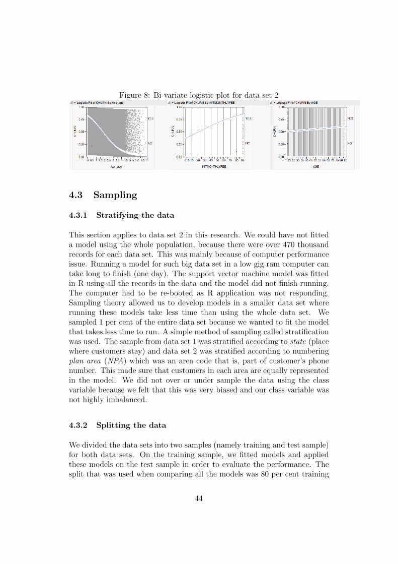
Figure 8: Bi-variate logistic plot for data set 2

4.3 Sampling

4.3.1 Stratifying the data

This section applies to data set 2 in this research. We could have not fitteda model using the whole population, because there were over 470 thousandrecords for each data set. This was mainly because of computer performanceissue. Running a model for such big data set in a low gig ram computer cantake long to finish (one day). The support vector machine model was fittedin R using all the records in the data and the model did not finish running.The computer had to be re-booted as R application was not responding.Sampling theory allowed us to develop models in a smaller data set whererunning these models take less time than using the whole data set. Wesampled 1 per cent of the entire data set because we wanted to fit the modelthat takes less time to run. A simple method of sampling called stratificationwas used. The sample from data set 1 was stratified according to state (placewhere customers stay) and data set 2 was stratified according to numberingplan area (NPA) which was an area code that is, part of customer’s phonenumber. This made sure that customers in each area are equally representedin the model. We did not over or under sample the data using the classvariable because we felt that this was very biased and our class variable wasnot highly imbalanced.

4.3.2 Splitting the data

We divided the data sets into two samples (namely training and test sample)for both data sets. On the training sample, we fitted models and appliedthese models on the test sample in order to evaluate the performance. Thesplit that was used when comparing all the models was 80 per cent training

44

and 20 per cent test sample. Kohavi suggested that one can use a validationsample and bootstrap methods to enhance the performance of the model fromthe training sample [Kohavi, 1995]. One can also use k-fold cross validationsample(s) to evaluate model performance and stability.

45

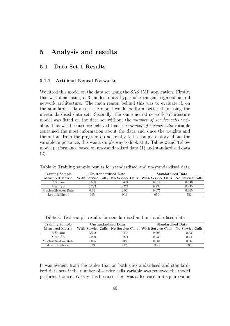
5 Analysis and results

5.1 Data Set 1 Results

5.1.1 Artificial Neural Networks

We fitted this model on the data set using the SAS JMP application. Firstly,this was done using a 3 hidden units hyperbolic tangent sigmoid neuralnetwork architecture. The main reason behind this was to evaluate if, onthe standardise data set, the model would perform better than using theun-standardised data set. Secondly, the same neural network architecturemodel was fitted on the data set without the number of service calls vari-able. This was because we believed that the number of service calls variablecontained the most information about the data and since the weights andthe output from the program do not really tell a complete story about thevariable importance, this was a simple way to look at it. Tables 2 and 3 showmodel performance based on un-standardised data (1) and standardised data(2).

Table 2: Training sample results for standardised and un-standardised data

Training Sample Un-standardised Data Standardised DataMeasured Metric With Service Calls No Service Calls With Service Calls No Service Calls

R Square 0.588 0.424 0.614 0.546Mean SE 0.233 0.274 0.232 0.245

Misclassification Rate 0.06 0.06 0.075 0.065-Log Likelihood 695 908 659 752

Table 3: Test sample results for standardised and unstandardised data

Training Sample Unstandardised Data Standardised DataMeasured Metric With Service Calls No Service Calls With Service Calls No Service Calls

R Square 0.542 0.435 0.603 0.53Mean SE 0.239 0.271 0.235 0.24

Misclassification Rate 0.065 0.083 0.081 0.06-Log Likelihood 379 447 338 384

It was evident from the tables that on both un-standardised and standard-ised data sets if the number of service calls variable was removed the modelperformed worse. We say this because there was a decrease in R square value

46

accompanied with an increase in the negative log likelihood and a slight in-crease in mean square error. Standardising the data helped us because therewas an increase in R square value and a decrease in the negative log likeli-hood (meaning the model on the un-standardised data was over generalisingcompared to the un-standardised). It was not clear as to why the misclassifi-cation rate for the un-standardised data was better than that of standardiseddata. We examined this further by running six neural network models on thedata set using six different random samples for each model. Each samplewas divided into 80 per cent training and 20 per cent test sample. Theneural network architecture was a multi-layer perceptron with three hiddenunits.

Table 4: Neural networks results before transforming the data

Before Average Square Error Schwarz Bayesian Criteria Train Misclassification Test Misclassification)Model 1 0.179 1 570.962 0.0353 0.0353Model 2 0.218 1 527.640 0.0552 0.0659Model 3 0.182 1 226.232 0.0384 0.0422Model 4 0.172 1 152.413 0.0314 0.0452Model 5 0.217 1 449.130 0.0657 0.0703Model 6 0.178 1 210.819 0.0355 0.0422

Table 5: Neural networks results after transforming the data

After Average Square Error Schwarz Bayesian Criteria Train Misclassification Test Misclassification)Model 1 0.176 1 629.439 0.0329 0.0329Model 2 0.203 1 468.321 0.0470 0.0444Model 3 0.188 1 361.707 0.0406 0.0496Model 4 0.198 1 441.521 0.0435 0.0577Model 5 0.211 1 585.728 0.0470 0.0563Model 6 0.200 1 486.565 0.0460 0.0592

Each result was very different and this meant that the model was unstable.This highlighted to us that there was more data exploration required. Thenumber of voice mail variable was transformed to a binary variable and alsothe number of service calls was transformed to ordinal variable (discussedearlier). The resulting models were more stable than the previous models.Tables 4 and 5 shows the models result before and after the transformationswere done. Although after the data transformation the models had a slightlyhigher Schwarz Bayesian Criteria (penalty value similar to BIC), the mis-classification rates in both training and test data were more stable and theaverage mean square error did not vary much as with the previous models.

47

Furthermore, Figures 9 and 10 shows the lift curves for the models beforeand after transformation. It is evident from the two charts that there wasa dispersion in the lift value at 10 per cent of the population before datatransformation. After transforming the data this dispersion disappeared andthe models seem to have almost the same lift value for all population per-centiles.

Figure 9: Lift curves for the six neural networks before data transformation

Figure 10: Lift curves for the six neural networks after data transformation

48

We had a hypothesis that changing the training and test sample ratios wouldimpact the neural network results. This was because we believed that amodel with more training instances would outperform the one with fewerinstances. In order to test this hypothesis we divided the data into six unevenproportioned data sets as shown in Table 6 with a belief that data set A wouldperform better than data set F because data set A had more data points totrain the model than data set F.

Table 6: Sample Test and Train Ratios

Data Set Training Sample (per cent) Test Sample (per cent)A 90 10B 80 20C 70 30D 60 40E 50 50F 40 60

Tables 7 and 8 show the overview results from the models fitted

Table 7: Train data model performance for data set 1

Train Data R Square Misclassification Rate -2Log Likelihood Mean SE True Positive RatioA 0.756 0.035 603 0.179 0.77B 0.757 0.037 532 0.179 0.78C 0.712 0.061 540 0.205 0.57D 0.766 0.036 387 0.177 0.78E 0.723 0.051 374 0.195 0.64F 0.721 0.041 299 0.191 0.72

Table 8: Test data model performance for data set 1

Test Data R Square Misclassification Rate -2Log Likelihood Mean SE True Positive RatioA 0.72 0.044 74 0.191 0.72B 0.71 0.048 156 0.198 0.73C 0.65 0.059 272 0.216 0.61D 0.73 0.041 290 0.189 0.76E 0.6 0.0634 510 0.218 0.57F 0.71 0.042 458 0.188 0.73

The R-square values for all the models did not vary significantly also therewere no big variation in the misclassification rate. Data set C had the lowest

49

true positives for the training data and second lowest from the test data. Theresults showed that when we decrease the training sample size the negativelog-likelihood decreases significantly which meant that the model with lesstraining data had lower AIC and BIC value. Data set A produced similarresults as data set F, this meant that neural networks had learned the datausing less instances or data points. Thus the hypothesis we had was untrue,that is, in this case training a neural network model with less data yieldsimilar results to the one trained with more data. Furthermore, we went onto confirm this by evaluating the model performance of data set A and F.This was done using ROC and the lift curves. Bearing in mind that an areaunder the ROC curve greater than 75 per cent meant that the model wasperforming very well and that the maximum lift we could have had was 7.14.This was because the data set had 14 per cent of customers that actuallychurned in the sampled period and the maximum lift at 10 per cent of thepopulation was 1/0.14 ≈ 7.14. Figures 11 and 12 show the results obtainedfor the two data sets:

Figure 11: ROC and lift curves for ANN model data number A

50

Figure 12: ROC and lift curves for ANN model data number F

The four charts from Figure 11 are results from data set A and the fourcharts in Figure 12 (two lift and ROC curves) are results from data set F.The area under the curve for the class defect true for data set A was 0.93 forthe training and 0.92 for the test sample while it was 0.91 and 0.907 respec-tively for data set F. Also the lift value at 10 per cent of the population forthe four lift curves was approximately 7. This meant that for the two datasets (A and F), we had similarly good results (based on AUC and lift) andthey were similar implying that neural networks do not need a lot of traininginstances to accurately predict new data points.

The weights of the neural network were studied and we realised that theywere not telling us anything about variable importance. This is because theresults from the model give you weights estimates to each connection of layerwithin the neural network. These weights when analysed do not give youa clear view of which variables are important although Olden and Jacksonhave proposed ways of extracting the important variables [Olden and Jack-son, 2002]. We then removed all the variables that we thought were significantfrom the model and evaluated the R-Square, misclassification rate, and thetrue positive value expecting that the model performance would drop. Thesevariables were selected by looking at a logistic bi-variate plot between theclass and explanatory variables and therefore do not take into account themultivariate interdependent to the class variable. Variables that showed a

51

strong relationship were selected and removed from the model. We removedinternational plan, number of service calls and total day minutes and themodel was as good as random. The R-square value decreased from 0.8 to0.06, the misclassification rate increased from 0.04 to 0.14 (which is whatwe would have if no model was used) and the area under the ROC curvefor dropped from 0.93 to 0.65. We observed that in this data set these werenot the only important variables but there was a higher proportion of thepopulation that when sampled the class variable depends mostly on thesethree removed variables. This was also the reason why the area under theROC curve was not 0.5 as in a case of a random model.

Sharma and Panigrahi worked on predicting customer churn using the samedata set as in this research [Sharma and Panigrahi, 2011]. They used artificialneural networks techniques to fit the data on a sample of 2427 customers. Theauthors did not mention the data exploration phase in their analysis and theyfit their model in SPSS using all variables but excluding state and customerphone number. We criticised the authors by doing this as we had foundcorrelated variables in our data exploration phase. Our model performedbetter than their model (comparing it to data number 2 results). They hadan accuracy rate of 0.924 and true positive ratio of 0.663 while our accuracyrate was 0.952 and true positive ratio of 0.73 (using the test data set). Itwas interesting to see that our models gave the same top three variables asthe most important ones (namely service calls, international plan and totalday minutes).

5.1.2 Decision Trees

We then used a decision tree models on the standardised and un-standardiseddata. This was done because we wanted to check whether standardising thedata would have a significant impact in the model results. Firstly the modelwas fitted on the un-standardised data set split into 80 per cent training and20 per cent test set. The number of splits was chosen to be ten for bothmodels by evaluating if there was a significant incremental increase in theR-Square value. The AIC for this model was 5152 and the R-Square for thetraining sample was 0.501 and 0.436 for the test sample. The decision treemodel was then applied again to an 80 per cent training and 20 per centtest sample of standardised data set. The optimal number of splits chosenagain was ten and the R-Square value for the train and test sample was 0.551and 0.455 and the AIC value was 4952. This was an improvement from the

52

previous results based on the R-square value which explained 55.1 per centof the variation in the data compared to previous R-square of 0.501. We alsoobserved a significant decrease in the model penalty value (AIC, from 5152to 4952) meaning that the second model was fitting better. The decision treemodel performed better on a standardised data set than the un-standardiseddata set.

We then ran a decision tree model on a newly generated training and testsamples (80 and 20 per cent respectively). There were no rules for the min-imum or maximum number of splits in the model. The optimal numberof split was chosen based on an incremental R-square value after each split.This was done by evaluating if there was a significant increase in the R-squarevalue at each split. The chart in Figure 13 shows the incremental R-Squarevalue from each split.

Figure 13: Number of Decision Tree Splits

It is evident from the chart in Figure 13 that after 14 splits the increment inthe R-Square value was small and the optimal value was found to be 0.576for the training sample and 0.604 for the test sample. We also checked if themodel was not over-fitting the data before exploring the results even further.This is because results from an over-fitted model can be misleading and wemay make incorrect conclusions about the data. Fivefold cross-validationsamples were used and the model was found to be stable with an overallR-Square value of 0.580 and -2log likelihood of 938 which did not vary fromthe initial model results.

The model misclassification rates for the training and test data sets were0.054 and 0.048 respectively. These are very good rates because if no model

53

was used and we classified the data with the majority class (the majorityclass was 86 per cent) then we would have had a misclassification rate of0.14. We then evaluated the model confusion matrix and learned that therewere about 69.2 per cent of the true positives in the training sample and 73.1per cent in the test sample. The area under the ROC curve for class defecttrue was 0.92 and 0.93 for both training and test samples respectively whichproved that this model was performing well (A better performing modelhas an area under the ROC curve more or equal to 0.75). Furthermore,the lift curves were plotted and at 10 per cent of the population with thehighest probability of churning, a lift value of 6.5 and 6.7 was obtained forthe train and test samples respectively (for class defect true). These two liftvalues were reasonable high considering the fact that they were close to themaximum attainable lift of 7.14. We investigated variable importance in themodel using G-Square statistics which is the same as twice the natural log ofentropy. The total day minutes gave the highest number of splits (four) andthe highest G-square statistic value. Figure 14 shows the number of splitsby each variable, the G-Square statistics value and the G-Square plot (bars).The number of splits shows how many nodes were split by that variable, G2

is the G-Square statistics that measures variable importance and the barsmeasure the magnitude of the G-Square value. It was evident from the chartthat account length, number of evening calls, night calls, night minutes andvoice mail messages were not significant in the model as there were no splitsbased on these variables.

Figure 14: Decision trees variable importance data set 1

From the decision tree model there were only four pure nodes where theentropy or the G-Square statistics was zero. The minimum number of cus-tomers obtained in a final leaf was 20 and they were obtained from the purenode. We then fitted a decision tree model with all the significant variables inthe model with a minimum final node size set to 50 customers. The R-Square

54

values were similar to the previous decision tree model with all variables in-cluded for both train and test sample. There was a slight decrease in theAIC value which meant that this model was a better fit than the one withall the variables.

5.1.3 Support Vector Machines

Support vector machines models were applied using R software with KSVMand ROCR packages (used for creating the model and evaluating performancerespectively). These models were fitted using three kernel functions namelyradial basis, Laplace and polynomial in order to classify the data into twoclasses (churners and non-churners). The data was divided into 80 per centtraining and 20 per cent test sample. We firstly fitted an SVM radial basiskernel model by trying a series of constant values in order to find out whichone optimises the model accuracy and minimises the misclassification error.It is important to note that the radial basis and Laplace kernel functiondepends on sigma and constant values in their construction. Choosing theright sigma (σ) and the right constant (C) for the model will yield goodresults. At the initial stage, the effect of a constant was crucial and the sigmavalue was chosen using a built in function in R that automatically finds thebest sigma given a constant C. If R did not have this function, we wouldhave chosen sigma using similar method as finding the best constant. Figure15 shows the objective function value and the number of support vectors forconstant values ranging from one to a hundred for a RBF kernel.

Figure 15: Support vector constant effect 1: RBF kernel function

The following phenomenon must be noted from this chart:

55

• The number of support vectors initially decreases at lower constantvalues and then stabilises after C >= 60 to one hundred

• As the constant increase, the objective function declines significantly.

The chart in Figure 16 plots the error on the training sample (secondaryaxis) and the cross validation sample (primary axis). The following werenoted from the chart:

• As the constant increases, the error on the training sample decreases

• For every increase in the constant, the cross validation sample errorslightly increases.

• It can be shown that there is not much change in accuracy of the RBFmodel with an increase in constant (except for K < 0)

Figure 16: Support vector constant effect 2: RBF kernel function

The change in the constant affects mostly the objective function and thetraining error. In fact, it can be proven that as the constant tends to infinityfor the RBF model:-

• the objective function tends to negative infinity

• the training error tends to zero or the neighbourhood of zero

• the cross validation error becomes the same as having no model [Al-paydın, 2004]

On evaluating the three fitted models it was found that Laplace kernel SVMoutperformed the polynomial kernel of degree 3 and the radial basis kernel(with best sigma and the constant equalling to 0.05 and 10 respectively).Some of the results are shown in the appendix Figure A8 and Figure 17 shows

56

the ROC and lift curve. Laplace kernel SVM gave the best training and crossvalidation error (1.46 and 7.99 per cent respectively), test misclassificationrate (8.4 per cent), area under the ROC curve (0.86) and the number of truepositive (64 customers).

Figure 17: Support vector machines ROC curve fit for data set 1

We noted the disadvantages of the Laplace kernel SVM and the polynomialmodel. These two models were over-fitting the data because the variation orthe range in the training error compared to the cross validation error (threefolds cross validation sample) was large. The range between the two errors(train and cross validation sample) was 0.144 for polynomial kernel of de-gree three, 0.062 for a Laplace kernel and 0.058 for radial Basis kernel. TheRBF SVM seemed to produce more stable results than when the other kernelfunctions were used. This was then chosen as the best model out of the three.

We then went on to test the strength of the RBF kernel by evaluating theperformance of the model when different probability thresholds were usedin the test set. The minimum cut off probability threshold was 0.4 and themaximum was 0.95. We noted the following from the results as the cut offprobabilities increases:

• The true positive ratio increases and at a cut off equalling 0.95 it wasequal to 1. These results were disappointing as the number of the

57

actual true positive was very low, that is, only 31 customers out of a667 in the test set.

• The model accuracy decreased from 0.93 to 0.89 which we thought wasa fairly good level.

• The true negative class increased as the model was classifying mostcustomers to the majority class.

The chart in Figure 18 shows the results from the different probability cut offin details. The red bar is the accuracy rate, the blue bar is the true positiveratio and the line on the secondary axis is the predicted true positive dividedby the total sample.

Figure 18: Probability cut off for data set 1 SVM model

Brandusoiu and Toderean used SVM model to predict churn on the samedata set [Brandusoiu and Toderean, 2013]. On their data exploration phase,they concluded that the data was ”complete” and they were no missing val-ues. They discovered that four charge variables were correlated with minutesvariables and this was similar to our findings. They argued that SVM workswell if the class ratio is balanced. They decided to boost the data set bycloning the number of churn class equal yes to be the same as no. Theyfound that a polynomial kernel SVM (of degree 3) outperformed the otherthree used kernels (sigmoid, RBF and linear) and it gave an accuracy rateof 0.887. In our analysis, polynomial kernel SVM was the worst performingmodel and it gave the same accuracy rate (0.884) as the latter. Our bestperforming SVM models (Laplace and RBF) had an accuracy rate of 0.919and 0.904 respectively thus better than the author’s results.

58

5.1.4 Logistic Regression

The final model that was explored for data set 1 was the logistic regression.This was done using R statistical software. This regression method was per-formed using a backward selection technique whereby all variables are enteredinto a model and the non-significant variables are removed one by one. Theoptimisation method used was the Fisher scoring and the selection criterionwas the AIC with a 0.05 level of significance. The model started by putting inall variables and the AIC value was 2538.12 for thirteen variables. After themodel had removed four insignificant variables the AIC value had decreasedslightly to 2532. We assessed the p-value and the z value and concludedat 5 and 10 per cent level of significance that account length, total numberof day calls, total evening calls and number of night calls were not significant.

We analysed the coefficient and the z score of each significant variable andfound that international plan factor yes was the most significant variable(with a z score of 14.88) followed by total day minutes (with a z score of13.01) and the number of service calls (with a z score of 12.303). The oddsfor international plan factor yes was 7.188 implying that there was a highassociation between defecting and having an international plan. This reasonwhy this was the case was because 0.42 customers that had international plandefected. The logistic regression equation for the reduced model was

f(defect)

= 1/(1 + exp{

2.97− 0.71x1 − 0.34x2 − 0.22x3 − 0.25x4

+0.17x5 − 0.5x6 + 1.0x7 − 1.9x8

})

where x1 is total day minutes, x2 is the total evening minutes, x3 is the totalnight minutes, x4is the total international minutes, x5 is the total number ofinternational calls, x6 is the total number of service calls, x7 is voice mailplan and x8 the international plan.

We went on to evaluate the model performance in the test data set. Themodel had an accuracy value of 0.87 at 0.5 probability value which wasexactly the same as for the training sample. The performance was also

59

evaluated at different probability thresholds and the following were observedas the probability cut off increased:

• The model accuracy level was stable

• The ratio between the true positive and the actual true positive de-creased, in fact at probability threshold greater or equal to 0.9 therewe no true positives

• The model misclassified the data and put all instances to the majorityclass at 95 per cent probability threshold.

The chart in Figure 19 shows the model performance at different probabilitythreshold values chosen at certain intervals. The red bar is the accuracy rate,the blue bar is the true positive ratio and the line on the secondary axis isthe predicted true positive divided by the total sample.

Figure 19: Probability cut off for logistic regression data set 1

A further analysis of the model using ROC and the lift curve showed thatthe model was not performing well. The area under the ROC curve was0.81 and the lift value at 10 per cent of the population was 3.6, which wasvery low considering the fact that a maximum lift attainable was 7.14. Aperson looking at the results bluntly would say that an average of 87 percent accuracy on this model (in fact any model) is good, forgetting that if allinstances are classified into the same class an accuracy value of 86 per centwould be attained thus this was not a good model. The charts in Figure 20show the ROC and the lift curves of this model at probability threshold of0.5.

60

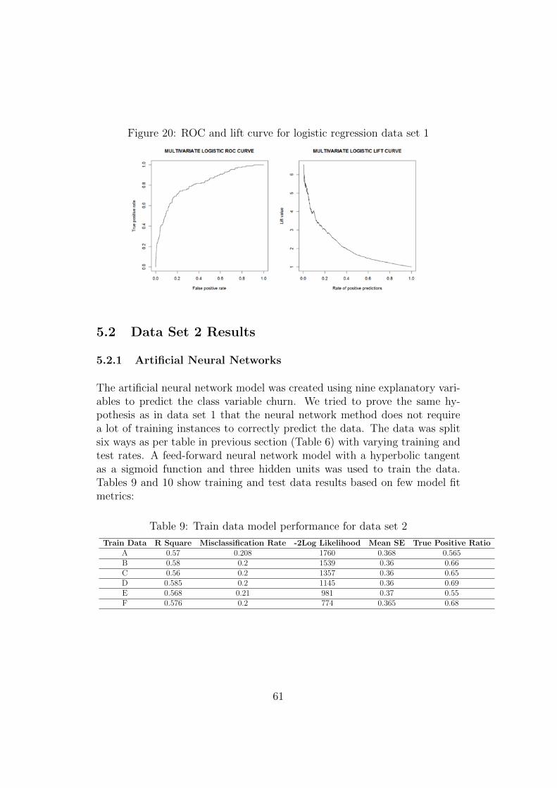
Figure 20: ROC and lift curve for logistic regression data set 1

5.2 Data Set 2 Results

5.2.1 Artificial Neural Networks

The artificial neural network model was created using nine explanatory vari-ables to predict the class variable churn. We tried to prove the same hy-pothesis as in data set 1 that the neural network method does not requirea lot of training instances to correctly predict the data. The data was splitsix ways as per table in previous section (Table 6) with varying training andtest rates. A feed-forward neural network model with a hyperbolic tangentas a sigmoid function and three hidden units was used to train the data.Tables 9 and 10 show training and test data results based on few model fitmetrics:

Table 9: Train data model performance for data set 2

Train Data R Square Misclassification Rate -2Log Likelihood Mean SE True Positive RatioA 0.57 0.208 1760 0.368 0.565B 0.58 0.2 1539 0.36 0.66C 0.56 0.2 1357 0.36 0.65D 0.585 0.2 1145 0.36 0.69E 0.568 0.21 981 0.37 0.55F 0.576 0.2 774 0.365 0.68

61

Table 10: Test data model performance for data set 2

Test Data R Square Misclassification Rate -2Log Likelihood Mean SE True Positive RatioA 0.467 0.251 226 0.398 0.469B 0.531 0.221 415 0.387 0.6C 0.545 0.206 609 0.374 0.63D 0.548 0.22 808 0.376 0.67E 0.561 0.21 991 0.37 0.55F 0.55 0.21 1207 0.374 0.67

The AIC and BIC value increases as sample size increases, that is, the modelwas penalised for using more observations to fit (based on -2log likelihood).Results from data set D were slightly better than the other data set resultsbecause:

• The R-Square value was fairly large for both training and test set (0.59and 0.55 respectively)

• The model had the highest true positives ratio (0.69 and 0.67 for thetraining and test set respectively)

Again, these results showed that the neural network model does not needmuch training information in order to build a good model. The differencesin the results in Tables 9 and 10 are minimal for both train and test data.We then went on to evaluate model performance using the receiver operatingcharacteristic curve and the lift curve. The lift curves for all six data sets(for class defect = yes) at ten per cent of the population fluctuated around2.2 which was a maximum lift that can be obtained (maxlift = 1

0.45≈

2.22). This meant that the model in all data sets performed very well (withan exception of data set A). Figure 21 shows the area under the receiveroperating characteristic curve for training and test sample.

62

Figure 21: AUC for ANN models

It is important to note that the scale of the chart in Figure 21 starts at 0.8.There was a slight incremental increase in the AUC value for test data fromdata set A to data set D which stabilises afterwards. The AUC value fortrain data stabilises at data set B then drops at data set E and return to“equilibrium” at data set F. This sudden deviation at data set E for the trainAUC value was inexplicable unless there were data point(s) that when notsampled in the data set the model performance deteriorates in accuracy.

We then explored what happens when the number of hidden units was in-creased. Does the neural network model reach a point of stability in accu-racy? If so, how many hidden units were needed? Is there any informationgain by increasing the number of hidden units? The line chart in Figure 22shows R-Squared, misclassification and true positive ratio for seven varia-tions of hidden units (from 3 to 21 hidden units) using 80 per cent trainingand 20 per cent test data.

63

Figure 22: R-Square for a change in the number of hidden units in ANNmodel

Figure 23: Sensitivity for a change in the number of hidden units in ANNmodel

Figure 24: Misclassification rates for a change in the number of hidden unitsin ANN model

The numbers of hidden units were varied by multiples of three up to twentyone hidden units. The feed-forward hyperbolic tangent neural network model

64

with six hidden units slightly outperforms the other models based on R-Square, Misclassification and True positive rate. The R-Square value dropsafter eighteen hidden units for the training data set and the true positive ratetends to stabilise after six hidden units. The model with three hidden unitswas the “worst” performer amongst the seven models based on the threecharts (Figures 22, 23 and 24). This model also had the highest AIC andBIC value for the training data set when compared to other models (basedon -2log likelihood of 1539).

We then tried to evaluate which variables were important by removing thevariables that we thought could be significant using prior information fromthe data exploration step. Using the six hidden units neural network modelwe removed customer account age and initial monthly fee. The misclassifica-tion rate increased from 0.19 to 0.22, the R-Square value decrease from 0.6to 0.45 and the true positive ratio dropped from 0.68 to 0.58. The variablemaker (hand set colour) was also removed and the R-Square value decreasedsignificantly to 0.1, misclassification rate to 0.39 and the area under the curvefor both train and test sample was 0.65.

5.2.2 Decision Trees

A decision tree model was applied to the second data set using a similarstrategy as the one used for data set 1 (with the data set split 80 per cent trainand 20 per cent test sample). We stopped splitting the tree by evaluatingif there was no significant incremental increase in the R-square value of themodel. The results showed that after six splits there was no incrementalvalue on the R-Square, however we made twelve splits and had to prune tosix splits as the model was over-fitting. The five folds cross validation sampleshowed that the overall R-Square was 0.41 and minus twice log likelihood was3080 which was almost as the same as the model with six splits. The AICvalue for the model at six splits was 10169 and the R-square for the trainingsample was 0.4 and 0.35 for the test sample. The chart in Figure 25 showsthe total number of splits for the decision tree model.

65

Figure 25: Decision trees R-Square value per split for data set 2

The confusion matrix showed 99 per cent of the true negative fraction and54 per cent of the true positive fraction for the training sample and 98 percent of true negative fraction and 52 per cent of the true positive instance inthe test sample. These were good ratios considering that in the total samplethere were 45 per cent instances belonging to the defect class true and 55 percent belonging to defect class false. The total misclassification rate of thetraining sample was 20.9 per cent and 22 per cent for the test sample. Themodel performance was evaluated using the area under the ROC curve whichwas evaluated to be at 0.85 and 0.83 for training and test sample respectively(for class defect equals true). We then computed the lift curve and foundthat there was no lift value at ten per cent of the population and that thelift value for the class defect equal true was obtained at 25 per cent of thepopulation which was 2.20 and 2.1 for training and test sample respectively.The reason why there was no lift at lower population proportion of the datawas that no customer had a probability of defecting more than 0.75. Figure26 shows the lift curve for the training sample on the left and the test sampleon the right.

66

Figure 26: Decision trees lift curves for data set 2

We went on to evaluate which variables were important in the model andlearned that only three variables were important namely maker, account typeand account age. It was noted that credit class, auto pay and market variablesbecome significant if the number of splits were increased. We were surprisedas to why the maker (colour of the hand set) was the most significant variable.This may be caused by the fact that a certain hand set colour may be

• associated with a certain contract offer

• associated with a high take up of new customers which are in naturehaving a high probability of defecting

• associated with a certain area where the probability of defecting is high

5.2.3 Support Vector Machines

The SVM model was applied using the same strategy as the one used fordata set 1. We observed similar results as in data set 1 when looking for aneffect of an increase in cost parameter C. The best σ was 0.109 and the bestcost parameter was 10 for radial basis and Laplace kernel function. Threekernel SVM models were fitted and compared. The polynomial kernel SVMwas of degree three and for all models three folds cross validation sampleswere used. The model accuracy and results are shown in the appendix FigureA8. The results showed that:

67

• Polynomial Kernel SVM was the worst performing model with the low-est area under the ROC curve. The lift value (at 10 per cent) for thismodel was lower than for the three models.

• The Laplace SVM kernel gave the best training error at 0.11 but itmisclassification rate (23 per cent) on the test sample was the worst

• The radial basis kernel gave the best results and the model proved tobe more stable than the other two model as the range of training (17.8per cent) and cross validation sample error (20.9 per cent) rate wasminimal (range equals 3.1) and less number of support vectors used.

The charts in Figure 27 show the ROC curve and the lift curve for the threesupport vector machine kernel models

Figure 27: ROC fit for kernel SVM models data set 2

The radial basis kernel SVM was taken to be the best model out of the three.We evaluated the performance for this model at different probability thresh-old cut off points. We observed the following as the probability thresholdincreased:

• The accuracy increased until for a threshold greater than 0.8 it de-creased sharply

• The true positive ratio increased but the model was classifying moreinstances into the majority class.

68

• The true positive total decreased rapidly.

The chart in Figure 28 shows the performance of the model when differentprobability thresholds are used. The red bar is the accuracy rate, the blue baris the true positive ratio and the line on the secondary axis is the predictedtrue positive divided by the total sample.

Figure 28: Probability cut off for data set 2 SVM model

5.2.4 Logistic Regression

We performed the logistic regression on data set 2 in a similar fashion asin data set 1. The Fisher scoring optimisation model stopped after 5 itera-tions and gave an AIC value of 3719.3. The full model showed that all ninevariables that were used in the model were significant but the credit classfactor B was not significant. It was noted that credit class factor D, acqui-sition channel and customer age were not significant at one per cent levelof significant based on their p-value (0.013, 0.014 and 0.011 respectively).Market was found not to be significant when an ANOVA Chi squared testwas performed. We ran the variable importance and saw that account age,maker and initial monthly fee were the most significant variables based ontheir Chi square values.

The odds ratio for account age was equal to 4.177 suggesting that a oneunit change in account age results in 4.177 increase in chances of churning.This also meant that there was a high association between defecting andaccount age. Conversely, auto pay had the lowest odds ratio equalling 0.353which meant that there was a high association between not defecting and this

69

variable, that is, the chances of defecting per one unit increase as auto paydecreases by 0.353. The logistic regression equation for this data was

f(defect)

= 1/(1 + exp{− 0.73− 0.63x1 − 0.42x2 − 0.45x3 + 1.04x4

+0.4x5 − 0.3x6 + 0.37x7 − 1.4x8 + 0.17x9 + 0.11age}

)

where x1 and x2 refer to credit class factors C and D, x3 is account type, x4

is auto pay, x5 is the market x6 is channel, x7 is the maker,x8 is account ageand x9 is initial monthly fee.

We then evaluated the model performance on the test set at different proba-bility threshold. These probability thresholds were chosen to be the same asin the case of SVM model. The following were observed as the probabilitythreshold was increased:

• The true positive ratio decreased exponentially and at 0.95 probabilitythreshold the model had 1 true positive out of 954 customers.

• The model accuracy increases from 0.75 to 0.78 and then drops to 0.54(after probability of 0.8)

• The model classifies most instances to the majority class

The chart in Figure 29 shows the model performance at different thresh-olds.The red bar is the accuracy rate, the blue bar is the true positive ratioand the line on the secondary axis is the predicted true positive divided bythe total sample.

70

Figure 29: Probability cut off for logistic regression on data set 2

Also, for the model performance at 0.5 probability value, an ROC and liftcurves were computed. The area under the ROC curve was found to be0.85 and the lift value at 10 per cent of the population was 2.01, which wasslightly less than the maximum lift attainable at 10 per cent (2.22). Themodel performance at 0.5 probability value was fairly good. The two chartsin Figure 30 show the ROC and the lift curve for the logistic model at 0.5probability cut off. The training sample model accuracy at 0.5 probabilitycut off was 0.755.

Figure 30: ROC and lift curve for logistic regression on data set 2

71

6 Comparison of Models

In this section we compare the four models based on the area under the ROCcurve, lift value, misclassification rate and the true positive rates. Althoughother measures could have been used to compare these models, we wanted touse only measures that are common in the four models. We could not haveused AIC or BIC value as support vector machines model construction doesnot give log likelihood and probabilities. This was a major drawback for thismodel. The probability for SVM model was computed using Platt’s poste-rior probability as suggested and improved by Lin and Wang [Lin and Wang,1999]. The neural network models had probability outputs as a hyperbolicsigmoid function was employed. If we had used a radial basis sigmoid func-tion then the probability would have been computed in similar fashion as inSVM. We found SVM and ANN models to be complex and they both tooklong to run (10 and 15 minutes respectively). Also, the choice of a constant inSVM model was non-trivial because we had to make sure that the number ofsupport vectors was minimised and also take into account the accuracy of themodel. It was much easier to perform decision trees and logistic regressionmodel as they required less computer run time (2-3 minutes for both models).

Rank and score variables were created in order to evaluate which model wasthe best. This was done because we wanted a robust measure of performanceusing the four metrics. The score was created by equally weighting all fourvariables and summing their Z scores and in the case of misclassificationvalue a reciprocal was used as low values were preferred for this variable(other ways could have been used, for example, 1-misclassification rate). Thehigher the score value the better is the model performance. Rank was createdby ranking the models based on each metric that was measured (from 1 to 4).We then took the average rank for the four models with the lowest being thebest performing model. Tables 11 and 12 show the model performance forthe two data sets. It is evident that the artificial neural network model hadoutperformed the three other models by a margin for both data sets. Thismodel had the highest score value and the lowest average rank (lower rankpreferred than higher rank). The score range of the next best model wasalmost half the size of the ANN score. The logistic regression was the worstperforming model of the four (using data set 1). This model had a negativescore (-1.3) and a highest average rank (4, for data set 1). Decision treesoutperformed SVM model and was ranked second with a score of 0.52. Fordata set 2, artificial neural networks outperformed the other three modelsand had a score value of 0.9 while support vector machine with a radial basis

72

kernel function came second (score of 0.31 and an average rank equal to 2).The decision tree model was the worst performer with a score value of -0.99and an average rank of 3.75 (for data set 2).

Table 11: Data set 1 model comparisons

Models for data set 1 AUC Lift Misclassification rate True positive Score Average RankARTIFICIAL NEURAL NETWORKS (3 Hidden Units) 0.930 7.010 0.040 0.73 0.810 1.5

DECISION TREES 0.920 6.300 0.048 0.731 0.52 2SUPPORT VECTOR MACHINES 0.869 5.800 0.093 0.847 -0.020 2.25

LOGISTIC REGRESSION 0.810 3.600 0.130 0.12 -1.310 4

Table 12: Data set 2 model comparisons

Models for data set 2 AUC Lift Misclassification rate True positive Score Average RankARTIFICIAL NEURAL NETWORKS (6 Hidden Units) 0.880 2.120 0.190 0.710 0.900 1.5

SUPPORT VECTOR MACHINES 0.838 2.100 0.212 0.859 0.310 2LOGISTIC REGRESSION 0.850 2.010 0.230 0.740 -0.220 2.75

DECISION TREES 0.830 1.890 0.220 0.540 -0.990 3.75

73

7 Conclusion and recommendations

The data sets that were used had few demographics variables (2 for data set1 and 4 for data set 2). They also contained a small numbers of variables(13 for data set 1 and 9 for data set 2) from which models were fitted. Dataset 2 was much polluted and it required a lot of cleaning and derivation ofnew variables. Data set 2 had many variables concerning billing informa-tion while data set 1 had more behavioural information. We showed thatstandardising the data helped as there was an improvement in the R-squarevalue for neural networks and decision tree models on data set 1. All modelsfitted using data set 2 showed that customer account age was a significantindicator of churning while in data set 1 this was not the case. This couldmean that in some retail mobile telecommunication settings loyalty is not abig factor that can prevent customers from churning. The customers thatchurn the most when looking at account age for data set 2 were the newcustomers. Data set 2 is also suited for survival analysis where we can focuson the expected time until a customer churns rather that finding a type ofcustomer that will churn as in data set 1 [Berry and Linoff, 2009a]. It wasmuch easier to run the models in data set 1 than data set 2 as most variablesin data set 1 were binary variables and we had to make sure that there wasno problem of linearity.

We recommend artificial neural networks over the three other techniques asthey outperformed all of them. This must not be interpreted bluntly, asin some data sets other data mining techniques might be more suited forpredicting customer churn because different models can work better whenfitting different data sets. This paper has also showed that logistic regressiondoes not work well in instances where the data set has few variables as thisrequires a more complex statistical model. Furthermore, for industry practiceif an artificial neural network model is fitted, we suggest that this model isfitted in conjunction with decision trees model as they were able to extractvaluable information from the data concerning variable importance. This canbe used to confirm variable importance. It is also up to us to decide whichsigmoid function to use, we preferred using a hyperbolic tangent and logisticsigmoid as both these function have a probability output.

74

8 Summary and Future Research

In the retail mobile telecommunication industry which is very competitive,the likelihood of churning is very high. Using statistical models can help abusiness retain some of it customers by predicting the ones that are likely tochurn and incentivising them. In this research, deployment of artificial neuralnetworks for predicting customer defection in the retail mobile telecommu-nication industry proved to be helpful. We saw that the artificial neuralnetwork technique showed good results but it had some limitation when itcomes to variable importance and interpreting the weights. The two datasets had fewer explanatory variables than we would have liked. A data setwith more demographic and behavioural variables would have been preferredfor this research. It would also be interesting to see how these models willperform in the real world. Furthermore, developing different churn mod-els for high, medium and low value customers might be what is needed forthe business as they can minimise cost and maximise profit margins if moreretention projects are channelled towards high value customers. A multivari-ate response model can be built in order to evaluate response rate for all thecustomers that were incentivised. This is to make sure that the retentionprojects are working because it does not make economic sense to continuewith the retention projects if the response is too low, that is, if the costsof implementing such a projects are not covered by keeping customers thatwould have defected [Cohen et al., 2006].

75

References

L.J.S.M Alberts. Churn prediction in mobile telecommunication. September2006. Online; June 2012.

E. Alpaydın. The Elements of Statistical Learning Data Mining, Inferenceand Prediction. The MIT Press, London, England, second edition, October2004.

M.J.A. Berry and G.S. Linoff. Customer centric forecasting us-ing survival analysis. http://www.data-miners.com/companion/sas/

forecastingWP_001.pdf, 2009a. Online; accessed March 2012.

M.J.A. Berry and G.S. Linoff. Customer centric forecasting using survivalanalysis. 2009b. Online; March 2012.

C. L. Blake and C. J. Merz. Churn Data Set, UCI Repository of MachineLearning Databases. University of California, Department of Informationand Computer Science, Irvine, 1998. Online; March 2011.

I. Brandusoiu and G. Toderean. Churn prediction in the telecommunicationssector using support vector machines. May 2013. Online; June 2013.

W. Buckinx and D. Van den Poel. Customer base analysis: partial defec-tion of behaviourally loyal clients in a non-contractual fmcg retail setting.European Journal of Operational Research, 164:1–32, 2004.

J. Burez and D. Van den Poel. Using analytical models to reduce customerattrition by targeted marketing for subscription services. Expert Systemswith Applications Journal, 32:277–288, 2005.

N.V. Chawla, K.W. Bowyer, L.O. Hall, and W.P. Kegelmeyer. Sytheticminority over sampling technique. International Journal of Artificial In-telligence Research, 16:321–357, 2002. Online; June 2013.

B. Cheng and D.M. Titterington. Neural networks: A review from a statis-tical perspective. Statistical Sciences, 9:2–54, Jan 2000.

S.L. Chow. Statistics and it role in psychological research. http://

cogprints.org/2782/1/eolss.pdf, 2002. Online; accessed March 2012.

K.J. Cios, W. Pedrycz, R.W. Swiniarski, and L.A. Kurgan. Data Mining,A Knowledge Discovery Approach. Springer, New York, USA, February2007.

76

D. Cohen, C. Gan, H.H.A. Yong, and E. Choong. Customer satisfaction: Astudy of a bank customer retention in New Zeland. http://www.lincoln.ac.nz/Documents/, March 2006. Online; November 2012.

M. Crang. Quantitative methods: The new orthodoxy. http://dx.doi.

org/10.1191/0309132502ph392pr, 2002. Online; January 2013.

A. Dehghan and T.B. Trafalis. Examining churn and loyalty using supportvector machine. Business and Management Research, 1:153–161, December2012. Online; June 2013.

J.B. Ferreira, M. Vellasco, M.A. Pacheco, and C.H. Barbosa. Data miningtechniques on the evaluation of wireless churn. In European Symposium onArtificial Neural Networks, pages 483–488, Bruges, Belgium, 28-30 April2004. Online; March 2013.

J. Friedman, T. Hastie, and R. Tibshirani. The Elements of Statistical Learn-ing Data Mining, Inference and Prediction. Springer, Stanford, CarlifoniaUSA, second edition, September 2008.

J.H. Friedman. Data mining and statistics: What is the connection? http:

//www.salfordsystems.com/doc/dmstat.pdf, November 1997. Online;May 2012.

C. Gatsonis. Statistical methods for meta-analysis of diagnostic testaccuracy. http://legacy.samsi.info/200809/meta/presentations/

diag-test-metan-bib-june08.pdf, June 2008. Online; March 2012.

S.R. Gunn. Support vector machines for classification and regression. http://www.users.ecs.soton.ac.uk/srg/publications, May 1998. Online;April 2013.

J. Hadden, A. Tiwari, R. Roy, and D. Ruta. Churn prediction using complainsdata. World Academy of Science Engineering and Technology, 19:1–6,2006. Online; May 2013.

A. Idrisa, M. Rizwan, and A. Khan. Churn prediction in telecom usingrandom forest and pso based data balancing in combination with variousfeature selection strategies. Computers and Electrical Engineering, 38:1808–1819, September 2012.

C. Imhoff. Bouygues telecom. http://www.teradata.com/casestudies/

BouyguesTelecomtheIntelligentTelecommunicationsCompany/,March 2001. Online; March 2012.

77

S. Jamwal. An approach to mobile telecom churn halding in india. Inter-national Journal of Computer Information Systems, 2:54–58, April 2011.Online; June 2013.

A. Juahiainen. Experimental design. http://pingpong.ki.se/puplic/pp/,2012. Online; January 2013.

M. Kamber and J. Han. Data Mining: Concepts and Techniques, chapter 7,pages 383–464. Diane Cerra, San Francisco, USA, second edition, 2006.

A. Karatzoglou, D. Meyer, and K. Hornik. Support vector machines in R.Journal of Statistical Software, 15:1–27, April 2006. Online; April 2013.

Estimating campaign benefits and modeling lift, San Diego, Carlifonia, USA,1999. Knowledge Stream Partners and GTE Laboratories. Online; May2013.

R. Kohavi. A study of cross validation and bootstrap for accuracy estimationand model selection. Proccedings of the 14th international joint conferenceon Artificial Intelligence, 2:1137–1143, 1995. Online; June 2013.

P.H. Kvam and J. Sokol. Teaching statistics with sports example. http:

//www2.isye.gatech.edu/statistics/papers/, 2004. Online; January2013.

C.F. Lin and S.D. Wang. Fuzzy support vector machines. EEE Transactionson NeuralNetworks, 13:464–471, 1999. Online; June 2013.

G.S. Linoff and M.J.A. Berry. Data Mining Techniques For Marketing, Sales,and Customer Relationship Management. Wiley Publishing, Indianapolis,Indiana USA, second edition, April 2004.

C. Manu. Analysis of clustering technique for crm. International Journal ofEngineering and Management Science, 3:402–408, July 2012.

M. Mazzocchi. Statistics for marketing and consumer research. http:

//consumer.stat.unibo.it/Private/Chap14.ppt, December 2007. On-line; January 2013.

P. Mirowski, S. Chopra, F.J. Huang, and M Mohri. Support vector ma-chines. http://www.cs.nyu.edu/~yann/2010f-G22-2565-001/diglib/

lecture03a-svm-2010.pdf, June 2008. Online; November 2012.

Dr. H. Nemati. Introduction to data mining using artificial neural networks.www.uncg.edu/ism/ism611/neuralnet.pdf, 2000. Online; April 2013.

78

G. Nie, W. Rowe, L. Zhang, Y. Tian, and Y. Shi. Credit card churn fore-casting. Expert System with Applications Journal, 38:15273–15285, 2011.

J.D. Olden and D.A. Jackson. Illuminating the ””black box”: A randomisedapproach for understanding variable contribution in artificial neural net-works. Ecological Modeling, 154:135–150, 2002. Online; August 2013.

M. Owczarczuk. Churn models for prepaid customers in the cellular telecom-munication industry using large data mart. Expert Systems with Applica-tions, 37:4710–4712, 2010. Online; May 2013.

A.A. Philip, A.A Taofiki, and A.A Bidemi. Artificial neural network modelfor forecasting foreign exchange rates. World of Computer Science andInformation Technology, 1(3):110–118, 2011.

D. Van Den Poel and B. Larivire. Customer attrition analysis for financialservices using proportional hazard models. European Journal of Opera-tional Research, 157:196–217, 2003.

M. Proust. Modeling and Multivariate Methods. SAS Institute Inc, SASCampus Drive, Cary, North Carolina 27513, tenth edition, March 2012.

N.P. Raygoza. Effect measures in 2 by 2 tables. http://www.piit.edu/

~super4/34011-35001/, 2009. Online; January 2013.

B. Ripley and R. Ripley. Neural networks as statistical methods in sur-vival analysis. http://www.stats.ox.ac.uk/pub/bdr/NNSM.pdf, 1998.Online; September 2012.

E. Shaaban, Y. Helmy, A. Kherd, and M. Nars. A proposed churn predictionmodel. International Journal of Engineering Research and Application, 2:693–697, July 2012. Online; June 2013.

A. Sharma and P.K. Panigrahi. A neural network approach for predictingcustomer churn in cellular network services. International Journal of Com-puter Applications, 27:26–31, August 2011. Online; June 2013.

M. Shashanka and M. Giering. Mining retail data for targeting customerswith headroom. Artificial Intelligence Applications and Inovations IIIJournal, 296:347–355, 2009.

Dr. M. Turhan. Neural networks and their supervised training.rocksolidimages.com/pdf/neural_network.pdf, 1995. Online; April2013.

79

C.P. Wei and I.T. Chiu. Turning telecomunication call details to churn pre-diction. Expert Systems with Applications, 23:103–112, 2002. Online; May2013.

Knowledge Discovery on Customer Churn, volume 10, Dallas, Texas, USA,November 2006. WSEAS. Online; May 2013.

S.J. Yen and Y.S. Lee. Cluster based under sampling approach for imbalancedata. Expert Systems with Applications, 36:5718–5727, 2009. Online; June2013.

K.H. Zou, A. O’Malley, and L. Mauri. Receiver operating characteristicanalysis for evaluating diagnostic tests and predictive models. http://

circ.ahajournals.org/content/115/5/654, 2007. Online; March 2012.

80

Appendix

Table A1: Data set 1 variables

Variable A brief descriptionState Categorical variable, for the 50 states and the dis-

trict of ColumbiaAccount length Continuous variable for how long account has been

activeArea code Categorical variable, for area of the customerPhone number Customer phone number, primary key in the

databaseInternational Plan Binary variable, yes or noVoice Mail Plan Binary variable, yes or noNumber of voice mail messages Integer-valued variableTotal day minutes Continuous variable for number of minutes cus-

tomer has used the service during the dayTotal day calls Continuous variableTotal day charge Continuous variable based on foregoing day calls

and minutesTotal evening minutes Continuous variable for minutes customer has used

the service during the eveningTotal evening calls Continuous variableTotal evening charge Continuous variable based on previous two vari-

ablesTotal night minutes Continuous variable for storing minutes the cus-

tomer has used the service during the nightTotal night calls Continuous variableTotal night charge Continuous variable based on foregoing night calls

and minutesTotal international minutes Continuous variable for minutes customer has used

service to make international callsTotal international calls Continuous variableTotal international charge Continuous variable based on foregoing two vari-

ablesNumber of service call Continuous variable

81

Table A2: Data set 2 variables

Variable A brief descriptionCustomer ID Integer, unique client identifierNpa Integer, area code oneNxx Integer, area code twoAccount type Nominal, account type, standard or premiumCredit class Ordinal, customer credit class, four classesDeposit Continuous, depositAuto pay Binary, auto pay, yes or noMarket Three market places, LocationChannel Two acquisition channels, direct or indirectDealer code Categorical, acquisition dealer codeDealer group Nominal, acquisition dealer groupMaker Phone colour, converted from one to sixStart date Date, start of contractStop date Date, stop of contractTime to default Continuous, derived time taken to defaultIs active Binary, account active status, yes or noAccount status Nominal, account statusAccount status dtl Nominal, account deferred tax statusEffective date Date, effective contract dateAccount Age Continuous, derived age on bookInitial monthly fee Continuous, initial monthly fee paidContract end date DateBirthday Date, customer date of birthAge Continuous, derived customer ageSafety flag Binary, one or zeroCut-off date Date, sample cut-off date

82

Figure A1: Data set 1 distribution A

The above chart shows data set 1 variables distribution with descriptive statistics

Figure A2: Data set 1 distribution B

The above chart shows data set 1 variables distribution with descriptive statistics

83

Figure A3: Data set 1 distribution C

The above chart shows data set 1 variables distribution with descriptive statistics

Figure A4: Data set 1 bi-variate logistic fit

The chart above shows a bi-variate logistic fit between the class variable churnand 3 exploratory variables (number of service calls, total day minutes and total

international calls)

84

Figure A5: Data set 2 distributions A

Data set 2 variables distributions with channel and market transformed to anordinal variable channel and marker1 respectively.

Figure A6: Data set 2 distributions B

Data set 2 variables distributions with deposit transformed to a binary variabledeposit1

85

Figure A7: Data set 1 kernel SVM fit

SVM fit results for data set 1 (polynomial of degree 3, Laplace and radial basiskernels)

Figure A8: Data set 2 kernels SVM fit

SVM fit results for data set 2 (polynomial of degree 3, Laplace and radial basiskernels)

86

Figure A9: Correlation table for data set 1

The above table shows the correlation between data set 1 variables. Coloursrange from dark green (strong positive correlation to dark red (negative

correlation). These are the variables that have a positive correlation with eachother (ρ = 1): Day charge and day minutes,evening charge and evening minutes,

night charge and night minutes and international charge and internationalminutes

87