Finding Structure in Dynamic Networks 1 Arnaud Casteigts LaBRI, University of Bordeaux [email protected] June 4, 2018 1 This document is the first part of the author’s habilitation thesis (HDR) [37], defended on June 4, 2018 at the University of Bordeaux. Given the nature of this document, the contributions that involve the author have been emphasized; however, these four chapters were specifically written for distribution to a larger audience. We hope they can serve as a broad introduction to the domain of highly dynamic networks, with a focus on temporal graph concepts and their interaction with distributed computing. arXiv:1807.07801v1 [cs.DC] 20 Jul 2018

Welcome message from author
This document is posted to help you gain knowledge. Please leave a comment to let me know what you think about it! Share it to your friends and learn new things together.
Transcript

Finding Structure in Dynamic Networks1
Arnaud CasteigtsLaBRI, University of [email protected]
June 4, 2018
1This document is the first part of the author’s habilitation thesis (HDR) [37], defendedon June 4, 2018 at the University of Bordeaux. Given the nature of this document, thecontributions that involve the author have been emphasized; however, these four chapterswere specifically written for distribution to a larger audience. We hope they can serve as abroad introduction to the domain of highly dynamic networks, with a focus on temporal graphconcepts and their interaction with distributed computing.
arX
iv:1
807.
0780
1v1
[cs
.DC
] 2
0 Ju
l 201
8


Contents
1 Dynamic networks? 3
1.1 A variety of contexts . . . . . . . . . . . . . . . . . . . . . . . . . . . . . 3
1.2 Graph representations . . . . . . . . . . . . . . . . . . . . . . . . . . . . 4
1.3 Some temporal concepts . . . . . . . . . . . . . . . . . . . . . . . . . . . 8
1.4 Redefinition of problems . . . . . . . . . . . . . . . . . . . . . . . . . . . 11
2 Feasibility of distributed problems 15
2.1 Basic conditions . . . . . . . . . . . . . . . . . . . . . . . . . . . . . . . . 15
2.2 Shortest, fastest, and foremost broadcast . . . . . . . . . . . . . . . . . . 19
2.3 Bounding the temporal diameter . . . . . . . . . . . . . . . . . . . . . . 22
2.4 Minimal structure and robustness . . . . . . . . . . . . . . . . . . . . . . 25
3 Around classes of dynamic networks 29
3.1 List of classes . . . . . . . . . . . . . . . . . . . . . . . . . . . . . . . . . 29
3.2 Relations between classes . . . . . . . . . . . . . . . . . . . . . . . . . . . 36
3.3 Testing properties automatically . . . . . . . . . . . . . . . . . . . . . . . 39
3.4 From classes to movements (and back) . . . . . . . . . . . . . . . . . . . 45
4 Beyond structure 49
4.1 Spanning forest without assumptions . . . . . . . . . . . . . . . . . . . . 49
4.2 Measuring temporal distances distributedly . . . . . . . . . . . . . . . . . 52
4.3 The power of waiting . . . . . . . . . . . . . . . . . . . . . . . . . . . . . 55
4.4 Collection of curiosities . . . . . . . . . . . . . . . . . . . . . . . . . . . . 58
1

2 CONTENTS

Chapter 1
Dynamic networks?
Behind the terms “dynamic networks” lies a rich diversity of contexts ranging fromnear-static networks with occasional changes, to networks where changes occur continu-ously and unpredictably. In the past two decades, these highly-dynamic networks gaverise to a profusion of research activities, resulting (among others) in new concepts andrepresentations based on graph theory. This chapter reviews some of these emergingnotions, with a focus on our own contributions. The content also serves as a defini-tional resource for the rest of the document, restricting ourselves mostly to the notionseffectively used in the subsequent chapters.
1.1 A variety of contexts
A network is traditionally defined as a set of entities together with their mutual relations.It is dynamic if these relations change over time. There is a great variety of contexts inwhich this is the case. Here, we mention two broad categories, communication networksand complex systems, which despite an important overlap, usually capture different(and complementary) motivations.
(Dynamic) communication networks. These networks are typically made of wireless-enabled entities ranging from smartphones to laptops, to drones, robots, sensors, ve-hicles, satellites, etc. As the entities move, the set of communication links evolve, ata rate that goes from occasional (e.g., laptops in a managed Wi-Fi network) to nearlyunrestricted (e.g., drones and robots). Networks with communication faults also fall inthis category, albeit with different concerns (on which we shall return later).
(Dynamic) complex networks. This category comprises networks from a larger range ofcontexts such as social sciences, brain science, biology, transportation, and communica-tion networks (as a particular case). An extensive amount of real-world data is becomingavailable in all these areas, making it possible to characterize various phenomena.
While the distinction between both categories may appear somewhat artificial, itshed some light to the typically different motivations underlying these areas. In partic-ular, research in communication networks is mainly concerned with what can be donefrom within the network through distributed interactions among the entities, while re-search in complex networks is mainly concerned with defining mathematical models
3

4 CHAPTER 1. DYNAMIC NETWORKS?
that capture, reproduce, or predict phenomena observed in reality, based mostly on theanalysis of available data in which centralized algorithms play the key role.
Interactions between both are strong and diverse. However, it seems that for a sig-nificant period of time, both communities (and sub-communities) remained essentiallyunaware of their respective effort to develop a conceptual framework to capture thenetwork dynamics using graph theoretical concepts. In way of illustration, let us men-tion the diversity of terminologies used for even the most basic concepts in dynamicnetworks, e.g., that of journey [32], also called schedule-conforming path [24], time-respecting path [101], and temporal path [61, 136]; and that of temporal distance [32],also called reachability time [94], information latency [103], propagation speed [98] andtemporal proximity [104].
In the rest of this chapter, we review some of these efforts in a chronological order.Next, we present some of the main temporal concepts identified in the literature, with afocus on the ones used in this document. The early identification of these concepts, ina unifying attempt, was one of the components of our most influencial paper so far [53].Finally, we present a general discussion as to some of the ways these new conceptsimpact the definition of combinatorial (or distributed) problems classically studied instatic networks, some of which are covered in more depth in subsequent chapters.
1.2 Graph representations
Figure 1.1: A graph depict-ing communication links ina wireless network.
Standard graphs. The structure of a network is clas-sically given by a graph, which is a set of vertices (ornodes) V and a set of edges (links) E ⊆ V × V , i.e.,pairs of nodes. The edges, and by extension the graph it-self, may be directed or undirected, depending on whetherthe relations are unidirectional or bidirectional (symmet-rical). Figure 1.1 shows an example of undirected graph.Graph theory is a central topic in discrete mathematics.We refer the reader to standard books for a general intro-duction (e.g., [137]), and we assume some acquaintance ofthe reader with basic concepts like paths, distance, con-nectivity, trees, cycles, cliques, etc.
1.2.1 Graph models for dynamic networks
Dynamic networks can be modeled in a variety of ways using graphs and related notions.Certainly the first approach that comes to mind is to represent a dynamic network asa sequence of standard (static) graphs as depicted in Figure 1.2. Each graph of thesequence (snapshot, in this document) represents the relations among vertices at a givendiscrete time. This idea is natural, making it difficult to trace back its first occurrencein the literature. Sequences of graphs were studied (at least) back in the 1980s (see,e.g., [135, 86, 129, 74]) and simply called dynamic graphs. However, in a subtle way,the graph properties considered in these studies still refer to individual snapshots, andtypical problems consist of updating standard information about the current snapshot,

1.2. GRAPH REPRESENTATIONS 5
like connectivity [129].
G0 G1 G2 G3
time
Figure 1.2: A dynamic network seen as a sequence of graphs
A conceptual shift occurred when researchers started to consider the whole sequenceas being the graph. Then, properties of interest became related to temporal features ofthe network rather than to its punctual structure. In the distributed computing commu-nity, one of the first work in this direction was that of Awerbuch and Even in 1984 [11],who considered the broadcasting problem in a network that satisfies a temporal versionof connectivity. On the modeling side, one of the first work considering explicitly agraph sequence as being the graph seem to be due to Harary and Gupta [93]. Then, anumber of graph models were introduced to describe dynamic networks, reviewed herein chronological order.
In 2000, Kempe, Kleinberg, and Kumar [101] defined a model called temporal net-work, where the network is represented by a graph G (the footprint, in this document)together with a labeling function λ : E → R that associates to every edge a number in-dicating when the two corresponding endpoints communicate. The model is quite basic:the communication is punctual and a single time exist for every edge. Both limitationscan be circumvented by considering multiple edges and artificial intermediate verticesslowing down communication.
Independently, Ferreira and Viennot [80] represented a dynamic network by a graphG together with a matrix that describes the presence schedule of edges (the same holdsfor vertices). The matrix is indexed in one dimension by the edges and in the other byintegers that represent time. The authors offer an alternative point of view as a sequenceof graphs where each graph Gi(Vi, Ei) correspond to the 1-entries of the matrix, thissequence being called an evolving graph, and eventually renamed as untimed evolvinggraph in subsequent work (see below).
Discussion 1 (Varying the set of vertices). Some graph models consider a varyingset of vertices in addition to a varying set of edges, some do not. From a formal pointof view, all models can easily be adapted to fit in one or the other category. In thepresent document, we are mostly interested in edge dynamics, thus we will ignore thisdistinction most of the time (unless it matters in the context). Also note that an absentnode could sometimes be simulated by an isolated node using only edge dynamics.
A similar statement as that of Discussion 1 could be made for directed edges versusundirected edges. We call on the reader’s flexibility to ignore non essential details inthe graph models when these details are not important. We state them explicitly whenthey are.
Ferreira and his co-authors [79, 32, 78] further generalize evolving graphs by con-sidering a sequence of graph Gi = G1, G2, ... where each Gi may span a non unitaryperiod of time. The duration of each Gi is encoded in an auxiliary table of times t1, t2, ...

6 CHAPTER 1. DYNAMIC NETWORKS?
such that every Gi spans the period [ti, ti+1).1 A consequence is that the times can nowbe taken from the real domain, with mild restrictions pertaining to theoretical limita-tions (e.g., countability or accumulation points). In order to disambiguate both versionsof evolving graphs, the earlier version from [80] is qualified as untimed evolving graphs.Another contribution of [32] is to incorporate the latency (i.e., time it takes to cross agiven edge at a given time) through a function ζ called traversal time in [32].
In 2009, Kostakos [104] describes a model called temporal graphs, in which the wholedynamic graph is encoding into a single static (directed) graph, built as follows. Everyentity (vertex) is duplicated as many times as there are time steps, then directed edgesare added between consecutive copies of the same node. One advantage of this represen-tation is that some temporal features become immediately available on the graph, e.g.,directed paths correspond to non-strict journeys (defined further down). Recently, theterm “temporal graph” has also been used to refer to the temporal networks of [101],with some adaptations (see e.g., [4]). This latter usage of the term seems to becomemore common than the one from [104].
In the complex network community, where researchers are concerned with the effec-tive manipulation of data, different models of dynamic networks have emerged whosepurpose is essentially to be used as a data structure (as opposed to being used only as adescriptive language, see Discussion 2 below). In this case, the network history is typi-cally recorded as a sequence of timed links (e.g., time-stamped e-mail headers in [103])also called link streams. The reader is referred to [73, 103, 140, 95] for examples of useof these models, and to [110] for a recent survey.
As part of a unifying effort with Flocchini, Quattrociocchi, and Santoro from 2009to 2012, we reviewed a vast body of research in dynamic networks [53], harmonizingconcepts and attempting to bridge the gap between the two (until then) mostly dis-joint communities of complex systems and networking (distributed computing). Tak-ing inspiration from several of the above models, we defined a formalism called TVG(for time-varying graphs) whose purpose was to favor expressivity and elegance over allpractical aspects such as implementability, data structures, and efficiency. The resultingformalism is free from intrinsic limitation.
Let V be a set of entities (vertices, nodes) and E a set of relations (edges, links)between them. These relations take place over an interval T called the lifetime of thenetwork, being a subset of N (discrete) or R+ (continuous), and more generally sometime domain T. In its basic version, a time-varying graph is a tuple G = (V,E, T , ρ, ζ)such that
• ρ : E × T → 0, 1, called presence function, indicates if a given edge is availableat a given time.
• ζ : E×T → T, called latency function, indicates the time it takes to cross a givenedge at a given start time (the latency of an edge could itself vary in time).
The latency function is optional and other functions could equally be added, suchas a node presence function ψ : V ×T → 0, 1, a node latency function ϕ : V ×T → T(accounting e.g., for local processing times), etc.
1For French readers: [a, b) is an equivalent notation to [a, b[.

1.2. GRAPH REPRESENTATIONS 7
Discussion 2 (Model, formalism, language). TVGs are often referred to as a formalism,to stress the fact that using it does not imply restrictions on the environment, as opposedto the usual meaning of the word model. However, the notion of formalism has adedicated meaning in mathematics related to formal logic systems. With hindsight, wesee TVGs essentially as a descriptive language. In this document, the three terms areused interchangeably.
The purely descriptive nature of TVGs makes them quite general and allows tem-poral properties to be easily expressible. In particular, the presence and latency func-tions are not a priori constrained and authorize theoretical constructs like accumulationpoints or uncountable 0/1 transitions. While often not needed in complex systems andoffline analysis, this generality is relevant in distributed computing, e.g., to character-ize the power of an adversary controlling the environment (see [45] and Section 4.3 fordetails).
Visual representation. Dynamic networks can be depicted in different ways. Oneof them is the sequence-based representation shown above in Figure 1.2. Another is alabeled graph like the one in Figure 1.3, where labels indicate when an edge is present(either as intervals or as discrete times). Other representations include chronologicaldiagrams of contacts (see e.g., [95, 88, 110]).
a
b
c
d
et ∈
R: btc
prim
e
[0, 1] ∪ [2, 5]
[1, π
]
[5, 7]
[99999,∞
) [0,∞)
[i, i+ 2] :
i mod3 = 0
Figure 1.3: A dynamic network represented by a labeled graph. The labels indicateswhen the corresponding edges are present.
1.2.2 Moving the focus away from models (a plea for unity)
Up to specific considerations, the vast majority of temporal concepts transcend theirformulation in a given graph model (or stream model), and the same holds for manyalgorithmic ideas. Of course, some models are more relevant than others depending onthe uses. In particular, is the model being used as a data structure or as a descriptivelanguage? Is time discrete or continuous? Is the point of view local or global? Is timesynchronous or asynchronous? Do links have duration? Having several models at ourdisposal is a good thing. On the other hand, the diversity of terminology makes it harderfor several sub-communities to track the progress made by one another. We hope thatthe diversity of models does not prevent us from acknowledging each others conceptualworks accross communities.

8 CHAPTER 1. DYNAMIC NETWORKS?
In this document, most of the temporal concepts and algorithmic ideas being re-viewed are independent from the model. Specific models are used to formulate theseconcepts, but once formulated, they can often be considered at a more general level.To stress independence from the models, we tend to refer to a graph representing adynamic network as just a graph (or a network), using calligraphic letters like G or Hto indicate their dynamic nature. In contrast, when referring to static graphs in a waynot clear from the context, we add the adjective static or standard explicitly and useregular letters like G and H.
1.3 Some temporal concepts
Main articles: ADHOCNOW’11 [52] (long version IJPEDS’12 [53]).
This section presents a number of basic concepts related to dynamic networks. Manyof them were independently identified in various communities using different names.We limit ourselves to the most central ones, alternating between time-varying graphsand untimed evolving graphs (i.e., basic sequences of graphs) for their formulation(depending on which one is the most intuitive). Most of the terminology is in line withthe one of our 2012 article [53], in which a particular effort was made to identify thefirst use of each concept in the literature and to give proper credit accordingly. Most ofthese concepts are now becoming folklore, and we believe this is a good thing.
Subgraphs
There are several ways to restrict a dynamic network G = (V,E, T , ρ, ζ). Classically,one may consider a subgraph resulting from taking only a subset of V and E, whilemaintaining the behavior of the presence and latency functions, specialized to their newdomains. Perhaps more specifically, one may restrict the lifetime to a given sub-interval[ta, tb] ⊆ T , specializing again the functions to this new domain without otherwisechanging their behavior. In this case, we write G[ta,tb] for the resulting graph and call ita temporal subgraph of G.
Footprints and Snapshots
Given a graph G = (V,E, T , ρ, ζ), the footprint of G is the standard graph consisting ofthe vertices and edges which are present at least once over T . This notion is sometimesidentified with the underlying graph G = (V,E), that is, the domain of possible verticesand edges, although in general an element of the domain may not appear in a consideredinterval, making the distinction between both notions useful. We denote the footprintof a graph G by footprint(G) or simply ∪(G). The snapshot of G at time t is the standardgraph Gt = (V, e : ρ(e, t) = 1). The footprint can also be defined as the union ofall snapshots. Conversely, we denote by ∩(G) the intersection of all snapshots of G,which may be called intersection graph or denominator of G. Observe that, so defined,both concepts make sense as well in discrete time as in continuous time. In a context ofinfinite lifetime, Dubois et al. [30] defined the eventual footprint of G as the graph (V,E ′)whose edges reappear infinitely often; in other words, the limsup of the snapshots.

1.3. SOME TEMPORAL CONCEPTS 9
In the literature, snapshots have been variously called layers, graphlets, or instan-taneous graphs; footprints have also been called underlying graphs, union graphs, orinduced graphs.
Journeys and temporal connectivity
The concept of journey is central in highly dynamic networks. Journeys are the analogueof paths in standard graphs. In its simplest form, a journey in G = (V,E, T , ρ, ζ) is asequence of ordered pairs J = (e1, t1), (e2, t2) . . . , (ek, tk), such that e1, e2, ..., ek isa walk in (V,E), ρ(ei, ti) = 1, and ti+1 ≥ ti. An intuitive representation is shown onFigure 1.4. The set of all journeys from u to v when the context of G is clear is denotedby J ∗(u,v).
a
b
c
d
e
G0
a
b
c
d
e
G1
a
b
c
d
e
G2
a
b
c
d
e
G3
Figure 1.4: Intuitive representation of a journey (from a to e) in a dynamic network.
Several versions can be formulated, for example taking into account the latency byrequiring that ti+1 ≥ ti + ζ(ei, ti). In a communication network, it is often also requiredthat ρ(ei, t) = 1 for all t ∈ [ti, ti + ζ(ei, ti)), i.e., the edge remains present during thecommunication period. When time is discrete, a more abstract way to incorporatelatency is to distinguish between strict and non-strict journeys [101], strictness referringhere to requiring that ti+1 > ti in the journey times. In other words, non-strict journeyscorrespond to neglecting latency.
Somewhat orthogonally, a journey is direct if every next hop occurs without delayat the intermediate nodes (i.e., ti+1 = ti + ζ(ei, ti)); it is indirect if it makes a pauseat least at one intermediate node. We showed that this distinction plays a key rolefor computing temporal distances among the nodes in continuous time (see [48, 50],reviewed in Section 4.2). We also showed, using this concept, that the ability of thenodes to buffer a message before retransmission decreases dramatically the expressivepower of an adversary controlling the topology (see [44, 46, 45], reviewed in Section 4.3).
Finally, departure(J ) and arrival(J ) denote respectively the starting time t1 andthe last time tk (or tk+ζ(ek, tk) if latency is considered) of journey J . When the contextof G is clear, we denote the possibility of a journey from u to v by u v, which doesnot imply v u even if the links are undirected, because time induces its own level ofdirection (e.g., a e but e 6 a in Figure 1.4). If forall u and v, it holds that u v,then G is temporally connected (Class T C in Chapter 3). Interestingly, a graph maybe temporally connected even if none of its snapshots are connected, as illustrated inFigure 1.5 (the footprint must be connected, though).
The example on Figure 1.5 suggests a natural extension of the concept of connectedcomponents for dynamic networks, which we discuss in a dedicated paragraph in Sec-tion 4.4.

10 CHAPTER 1. DYNAMIC NETWORKS?
a b
c
d
a b
c
d
a b
c
d
−−−−−−−−−−−−−−−−−→time
Figure 1.5: Connectivity over time and space. (Dashed arrows denote movements.)
Temporal distance and related metrics
As observed in 2003 by Bui-Xuan et al. [32], journeys have both a topological length(number of hops) and a temporal length (duration), which gives rise to several conceptsof distance and at least three types of optimal journeys (shortest, fastest, and foremost,covered in Section 2.2 and 4.2). Unfolding the concept of temporal distance leads tothat of temporal diameter and temporal eccentricity [32]. Precisely, the temporal eccen-tricity of a node u at time t is the earliest time that u can reach all other nodes througha journey starting after t. The temporal diameter at time t is the maximum among allnodes eccentricities (at time t). Another characterization of the temporal diameter (attime t) is the smallest d such that G[t,t+d] is temporally connected. These concepts arecentral in some of our contributions (e.g., [48, 50], further discussed in Section 4.2). In-terestingly, all these parameters refer to time quantities, and these quantities themselvesvary over time, making their study (and computation) more challenging.
1.3.1 Further concepts
The number of definitions built on top of temporal concepts could grow large. Let usmention just a few additional concepts which we had compiled in [53, 133] and [38].Most of these emerged in the area of complex systems, but are of general applicability.
Small-world. A temporal analogue of the small-world effect is defined in [136] basedon the duration of journeys (as opposed to hop distance in the original definition instatic graphs [139]). Perhaps without surprise, this property is observed in a number ofmore theoretical works considering stochastic dynamic networks (see e.g., [61, 69]). Ananalogue of expansion for dynamic networks is defined in [69].
Network backbones. A temporal analogue of the concept of backbone was definedin [103] as the “subgraph consisting of edges on which information has the potential toflow the quickest.” In fact, we observe in [50] that an edge belongs to the backbonerelative to time t iff it is used by a foremost journey starting at time t. As a result,the backbone consists exactly of the union of all foremost broadcast trees relative toinitiation time t (the computation of such structure is reviewed in Section 4.2).
Centrality. The structure (i.e., footprint) of a dynamic network may not reflecthow well interactions are balanced within. In [53], we defined a metric of fairness asthe standard deviation among temporal eccentricities. In the caricatural example ofFigure 1.6 (depicting weekly interaction among entities), node c or d are structurallymore central, but node a is actually the most central in terms of temporal eccentricity:

1.4. REDEFINITION OF PROBLEMS 11
a b c d e fMonday Tuesday Wednesday Thursday Friday
Figure 1.6: Weekly interactions between six people (from [53]).
it can reach all other nodes within 5 to 11 days, compared to nearly three weeks for dand more than a month for f .
Together with a sociologist, Louise Bouchard, in 2010 [38], we proposed to applythese measures (together with a stochastic version of network backbones) to the studyof health networks in Canada. (The project was not retained and we started collabo-rating on another topic.) This kind of concepts, including also temporal betweenness orcloseness (which we expressed in the TVG formalism in [133]), received a lot of attentionlately (see e.g., [125, 130]).
Other temporal or dynamic extensions of traditional concepts, not covered here,include treewidth [116], temporal flows [3], and characteristic temporal distance [136].Several surveys reviewed the conceptual shift induced by time in dynamic networks,including (for the distributed computing community) Kuhn and Oshman [108], Michailand Spirakis [119], and our own 2012 survey with Flocchini, Quattrociocchi, and San-toro [53].
1.4 Redefinition of problems
Main articles: arXiv’11 [58], DRDC reports’13 [42, 43], IJFCS [51].
The fact that a network is dynamic has a deep impact on the kind of tasks onecan perform within. This impact ranges from making a problem harder, to making itimpossible, to redefining the metrics of interest, or even change the whole definition ofthe problem. In fact, many standard problems must be redefined in highly dynamicnetworks. For example, what is a spanning tree in a partitioned (yet temporally con-nected) network? What is a maximal independent set, and a dominating set? Decidingwhich definition to adopt depends on the target application. We review here a few ofthese aspects through a handful of problems like broadcast, election, spanning trees, andclassic symmetry-breaking tasks (independent sets, dominating sets, vertex cover), onwhich we have been involved.
1.4.1 New optimality metrics in broadcasting
As explained in Section 1.3, the length of a journey can be measured both in terms of thenumber of hops or in terms of duration, giving rise to two distinct notions of distanceamong nodes: the topological distance (minimum number of hop) and the temporaldistance (earliest reachability), both being relative to a source u, a destination v, andan initiation time t.
Bui-Xuan, Ferreira, and Jarry [32] define three optimality metrics based on thesenotions: shortest journeys minimize the number of hops, foremost journeys minimize

12 CHAPTER 1. DYNAMIC NETWORKS?
reachability time, and fastest journeys minimize the duration of the journey (possiblydelaying its departure). See Figure 1.7 for an illustration.
a
bc
d
e
f g
[1, 2]
[3, 4]
[5, 6]
[4, 5] [9, 10]
[6, 8]
[6, 8]
[6, 8]
Optimal journeys from a to d (starting at time 0):
- the shortest: a-e-d (only two hops)
- the foremost: a-b-c-d (arriving at 5 + ζ)
- the fastest: a-f-g-d (no intermediate waiting)
Figure 1.7: Different meanings for length and distance (assuming latency ζ 1).
The centralized problem of computing the three types of journeys given full knowl-edge of the graph G is introduced (and algorithms are proposed) in [32]. We investigateda distributed analogue of this problem; namely, the ability for the nodes to broadcastaccording to these metrics without knowing the underlying networks, but with variousassumptions about its dynamics [47, 51] (reviewed in Section 2.2).
1.4.2 Election and spanning trees
While the definition of problems like broadcast or routing remains intuitive in highlydynamic networks, other problems are definitionally ambiguous. Consider leader elec-tion and spanning trees. In a static network, leader election consists of distinguishinga single node, the leader, for playing subsequently a distinct role. The spanning treeproblem consists of selecting a cycle-free set of edges that interconnects all the nodes.Both problems are central and widely studied. How should these problems be definedin a highly dynamic network which (among other features) is possibly partitioned mostof the time?
At least two (somewhat generic) versions emerge. Starting with election, is theobjective still to distinguish a unique leader? This option makes sense if the leader caninfluence other nodes reasonably often. However, if the temporal connectivity withinthe network takes a long time to be achieved, then it may be more relevant to electa leader in each component, and maintain a leader per component when componentsmerge and split. Both options are depicted on Figure 1.8.
(a) A single global leader (b) One leader per connected component
Figure 1.8: Two possible definitions of the leader election problem.

1.4. REDEFINITION OF PROBLEMS 13
The same declination holds for spanning trees, the options being (1) to build a uniquetree whose edges are intermittent, or (2) to build a different tree in each component, tobe updated when the components split and merge. Together with Flocchini, Mans, andSantoro, we considered the first option in [47, 51] (reviewed in Section 2.2), building(distributedly) a fixed but intermittent broadcast tree in a network whose edges are allrecurrent (Class ER). In a different line of work (with a longer list of co-authors) [35,124, 40, 18], we proposed and studied a “best effort” principle for maintaining a setof spanning trees of the second type, while guaranteeing that some properties holdwhatever the dynamics (reviewed in Section 4.1). A by-product of this algorithm is tomaintain a single leader per tree (the root).
1.4.3 Covering problems
With Mans and Mathieson in 2011 [58], we explored three canonical ways of redefiningcombinatorial problems in highly-dynamic networks, with a focus on covering problemslike dominating set. A dominating set in a (standard) graph G = (V,E) is a subset ofnodes S ⊆ V such that each node in the network either is in S or has a neighbor inS. The goal is usually to minimize the size (or cost) of S. Given a dynamic networkG = G1, G2, . . . , the problem admits three natural declinations:
• Temporal version: domination is achieved over time – every node outside the setmust share an edge at least once with a node in the set, as illustrated below.
G1 G2 G3
Temporaldominating set
• Evolving version: domination is achieved in every snapshot, but the set can varybetween them. This version is commonly referred to as “dynamic graph algo-rithms” in the algorithmic literature (also called “reoptimization”).
G1 G2 G3
Evolvingdominating set
• Permanent version: domination is achieved in every snapshot, with a fixed set.
G1 G2 G3
Permanentdominating set

14 CHAPTER 1. DYNAMIC NETWORKS?
The three versions are related. Observe, in particular, that the temporal versionconsists of computing a dominating set in ∪G (the footprint), and the permanent versionone in ∩G. Solutions to the permanent version are valid (but possibly sub-optimal) forthe evolving version, and those for the evolving version are valid (but possibly sub-optimal) for the temporal version [58]. In fact, the solutions to the permanent andthe temporal versions actually form upper and lower bounds for the evolving version.Note that the permanence criterion may force the addition of some elements to thesolution, which explains why some problems like spanning tree and election do notadmit a permanent version.
Open question 1. Make a more systematic study of the connexions between the tempo-ral, the evolving, and the permanent versions. Characterize the role these versions playwith respect to each other both in terms of lower bound and upper bound, and designalgorithms exploiting this triality (“threefold duality”).
In a distributed (or online) setting, the permanent and the temporal versions are notdirectly applicable because the future of the network is not known a priori. Nonetheless,if the network satisfies other forms of regularity, like periodicity [83, 81, 100] (Class EP)or recurrence of edges [47] (Class ER), then such solutions can be built despite lack ofinformation about the future. In this perspective, Dubois et al. [72] define a variant ofthe temporal version in infinite lifetime networks, requiring that the covering relationholds infinitely often (e.g., for dominating sets, every node not in the set must be dom-inated infinitely often by a node in the set). We review in Section 2.4 a joint work withDubois, Petit, and Robson [41], where we define a new hereditary property in graphscalled robustness that captures the ability for a solution to have such features in a largeclass of highly-dynamic networks (Class T CR, all classes are reviewed in Chapter 3).The robustness of maximal independent sets (MIS) is investigated in particular and thelocality of finding a solution in various cases is characterized.
This type of problems have recently gained interest in the algorithmic and distributedcomputing communities. For example, Mandal et al. [115] study approximation algo-rithms for the permanent version of dominating sets. Akrida et al. [5] (2018) define avariant of the temporal version in the case of vertex cover, in which a solution is notjust a set of nodes (as it was in [58]) but a set of pairs (nodes, times), allowing differentnodes to cover the edges at different times (and within a sliding time window). Bam-berger et al. [15] (2018) also define a temporal variant of two covering problems (vertexcoloring and MIS) relative to a sliding time window.
Concluding remark
Given the reporting nature of this document, we reviewed here the definition of conceptsand problems in which we have been effectively involved (through contributions). Assuch, the content does not aim at comprehensiveness and many concepts and problemswere not covered. In particular, the network exploration problem received a lot ofattention recently in the context of dynamic networks, for which we refer the reader toa number of dedicated works [84, 82, 96, 27, 114].

Chapter 2
Feasibility of distributed problems
A common approach to analyzing distributed algorithms is the characterization of nec-essary and sufficient conditions to their success. These conditions commonly refer tothe communication model, synchronicity, or structural properties of the network (e.g.,is the topology a tree, a grid, a ring, etc.) In a dynamic network, the topology changesduring the computation, and this has a dramatic effect on computations. In order tounderstand this effect, the engineering community has developed a number of mobilitymodels, which govern how the nodes move and make it possible to compare results ona relatively fair basis and enable their reproducibility (the most famous, yet unrealisticmodel is random waypoint).
In the same way as mobility models enable the experimental investigations of al-gorithms and protocols in highly dynamic networks, logical properties on the networkdynamics, i.e.,classes of dynamic graphs, have the potential to guide a more formalexploration of their qualities and limitations. This chapter reviews our contributions inthis area, which has acted as a general driving force through most of our works in dy-namic networks. The resulting classes of dynamic graphs are then revisited, compiled,and independently discussed in Chapter 3.
2.1 Basic conditions
Main article: SIROCCO’09 [39]
In way of introduction, consider the broadcasting of a piece of information in thedynamic network depicted on Figure 2.1. The ability to complete this task depends onwhich node is the initial emitter: a and b may succeed, while c is guaranteed to fail.The obvious reason is that no journey (thus no chain of causality) exists from c to a.
a b c a b c a b c
beginning movement end
Figure 2.1: A basic mobility scenario.
Together with Chaumette and Ferreira in 2009 [39], we identified a number of such
15

16 CHAPTER 2. FEASIBILITY OF DISTRIBUTED PROBLEMS
requirements relative to a few basic tasks, namely broadcasting, counting, and election.For the sake of abstraction, the algorithms were described in a high-level model calledgraph relabelings systems [112], in which interactions consist of atomic changes in thestate of neighboring nodes. Different scopes of action were defined in the literature forsuch models, ranging from a single edge to a closed star where the state of all verticeschanges atomically [62, 63]. The expression of algorithms in the edge-based versionis close to that of population protocols [10], but the context of execution is different(especially in our case), and perhaps more importantly, the type of questions which areinvestigated are different.
In its simplest form, the broadcasting principle is captured by a single rule, repre-
sented as I N I I and meaning that if an informed node “interacts” (in a sensethat will become clear) with a non-informed node, then the latter becomes informed.This node can in turn propagate information through the same rule. Graph relabelingsystems1 typically take place over a fixed graph, which unlike the interaction graphof population protocols, is thought of as a static network. In fact, the main purposeof graph relabeling systems is to abstract communications, while that of populationprotocols is to abstract dynamism (through scheduling). In our case, dynamism is notabstracted by the scheduling; relabeling operations take place over a support graph thatitself changes, which is fundamentally different and makes it possible to inject propertiesof the network dynamics into the analysis.
The model. Given a dynamic network G = G1, G2, ..., the model we proposedin [39]2 considers relabeling operation taking place on top of the sequence. Precisely,every Gi may support a number of interactions (relabelings), then at some point, thegraph transitions from Gi to Gi+1. The adversary (scheduler, or daemon) controls boththe selection of edges on which interactions occur, and the moment when the systemtransitions from Gi to Gi+1, subject to the constraint that every edge of every Gi isselected at least once before transitioning to Gi+1. This form of fairness is reasonable,as otherwise some edges may be present or absent without incidence on the computation.The power of the adversary mainly resides in the order in which the edges are selectedand the number of times they are selected in each Gi. The adversary does not controlthe sequence of graph itself (contrary to common models of message adversaries).
2.1.1 Necessary or sufficient conditions in terms of dynamics
The above model allows us to define formally the concept of necessary and sufficientconditions for a given algorithm, in terms of network dynamics. For a given algorithmA and network G, X is the set of all possible executions and X ∈ X one of themcorresponding to the adversary choices.
Definition 1 (Necessary condition). A property P (on a graph sequence) is necessary(in the context of A) if its non-satisfaction on G implies that no sequence of relabelingscan transform the initial states to desired final states. (¬P (G) =⇒ ∀X ∈ X ,A fails.)
1This model is sometimes referred to as “local computations”, but with a different meaning to thatof Naor and Stockmeyer [120], therefore we do not use this term.
2In [39], we relied on the general (i.e., timed) version of evolving graphs. With hindsight, untimedevolving graphs, i.e., basic sequences of graphs, are sufficient and make the description simpler.

2.1. BASIC CONDITIONS 17
Definition 2 (Sufficient condition). A property P (on graph sequences) is sufficientif its satisfaction on G implies that all possible sequences of relabelings take the initialstates into desired final states. (P (G) =⇒ ∀X ∈ X ,A succeeds.)
In other words, if a necessary condition is not satisfied by G, then the executionwill fail whatever the choices of the adversary; if a sufficient condition is satisfied, theexecution will succeed whatever the choices of the adversary. In between lies the actualpower of the adversary. In the case of the afore-mentioned broadcast algorithm, thisspace is not empty: it is necessary that a journey exist from the emitter to all othernodes, and it is sufficient that a strict journey exist from the emitter to all other nodes.
Discussion 3 (Sensitivity to the model). By nature, sufficient conditions are dependenton additional constraints imposed to the adversary, namely here, of selecting every edgeat least once. No property on the sequence of graph could, alone, guarantee that thenodes will effectively interact, thus sufficient conditions are intrinsically model-sensitive.On the other hand, necessary conditions on the graph evolution do not depend on theparticular model, which is one of the advantages of considering high-level computationalmodel without abstracting dynamism.
We considered three other algorithms in [39] which are similar to some protocolsin [10], albeit considered here in a different model and with different questions in mind.The first is a counting algorithm in which a designated counter node increments its
count when it interacts with a node for the first time ( k N k+1 F ). An obviousnecessary condition to count all nodes is the existence of a direct edge between thecounter and every other node (possibly at the same time or at different times). Infact, this condition is also sufficient in the considered model, leaving no power at all tothe adversary: either the condition holds and success is guaranteed, or it does not andfailure is certain.
The second counting algorithm has uniform initialization: every node has a variableinitially set to 1. When two nodes interact, one of them cumulates the count of the
other, which is eliminated ( i j i+j 0 ). Here, a necessary condition to completethe process is that at least one node can be reached by all others through a journey. Asufficient condition due to Marchand de Kerchove and Guinand [117] is that all pairsof nodes interact at least once over the execution (i.e., the footprint of G is complete).The third counting algorithm adds a circulation rule to help surviving counters to meet,with same necessary condition as before.
Open question 2. Find a sufficient condition for this version of the algorithm in termsof network dynamics.
2.1.2 Tightness of the conditions
Given a condition (necessary or sufficient), an important question is whether it is tight forthe considered algorithm. Marchand de Kerchove and Guinand [117] defined a tightnesscriterion as follows. Recall that a necessary condition is one whose non-satisfactionimplies failure; it is tight if, in addition, its satisfaction does make success possible (i.e.,a nice adversary could make it succeed). Symmetrically, a sufficient condition is tight if
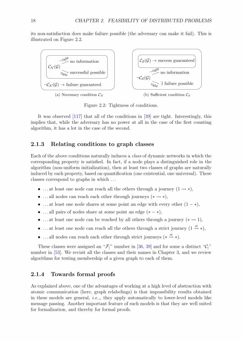
18 CHAPTER 2. FEASIBILITY OF DISTRIBUTED PROBLEMS
its non-satisfaction does make failure possible (the adversary can make it fail). This isillustrated on Figure 2.2.
¬CN (G) → failure guaranteed
CN (G)no information
successful possible
¬ tight
tight
(a) Necessary condition CN
CS(G) → success guaranteed
¬CS(G)no information
∃ failure possible
¬ tight
tight
(b) Sufficient condition CS
Figure 2.2: Tightness of conditions.
It was observed [117] that all of the conditions in [39] are tight. Interestingly, thisimplies that, while the adversary has no power at all in the case of the first countingalgorithm, it has a lot in the case of the second.
2.1.3 Relating conditions to graph classes
Each of the above conditions naturally induces a class of dynamic networks in which thecorresponding property is satisfied. In fact, if a node plays a distinguished role in thealgorithm (non-uniform initialization), then at least two classes of graphs are naturallyinduced by each property, based on quantification (one existential, one universal). Theseclasses correspond to graphs in which . . .
• . . . at least one node can reach all the others through a journey (1 ∗),• . . . all nodes can reach each other through journeys (∗ ∗),• . . . at least one node shares at some point an edge with every other (1− ∗),• . . . all pairs of nodes share at some point an edge (∗ − ∗),• . . . at least one node can be reached by all others through a journey (∗ 1),
• . . . at least one node can reach all the others through a strict journey (1st ∗),
• . . . all nodes can reach each other through strict journeys (∗ st ∗).
These classes were assigned an “F〉” number in [36, 39] and for some a distinct “C〉”number in [53]. We revisit all the classes and their names in Chapter 3, and we reviewalgorithms for testing membership of a given graph to each of them.
2.1.4 Towards formal proofs
As explained above, one of the advantages of working at a high level of abstraction withatomic communication (here, graph relabelings) is that impossibility results obtainedin these models are general, i.e.,, they apply automatically to lower-level models likemessage passing. Another important feature of such models is that they are well suitedfor formalization, and thereby for formal proofs.

2.2. SHORTEST, FASTEST, AND FOREMOST BROADCAST 19
From 2009 to 2012 [59, 60], Casteran et al. developed an early set of tools andmethodologies for formalizing graph relabeling systems within the framework of theCoq proof assistant, materializing as the Loco library. More recently, Corbineau etal. developed the Padec library [7], which allows one to build certified proofs (againwith Coq) in a computational model called locally shared memory model with compositeatomicity, much related to graph relabeling systems. This library is being developedintensively and may in the mid term incorporate other models and features. Besidesthe Coq realm, recent efforts were made by Fakhfakh et al. to prove the correctnessof algorithms in dynamic networks based on the Event-B framework [75, 76]. Thesealgorithms are formalized using graph relabeling systems (in particular, one of them isour spanning forest algorithm presented in Section 4.1). Another work pertaining tocertifying distributed algorithms for mobile robots in the Coq framework, perhaps lessdirectly relevant here, is that of Balabonski et al. [14].
Research avenue 3. Building on top of these plural (and related) efforts, formalizein the framework of Coq or Event-B the main objects involved in this section, namelysequences of graphs, relabeling algorithms, and the fairness condition for edge selec-tion. Use them to prove formally that a given assumption on the network dynamics isnecessary or sufficient to a given algorithm.
2.2 Shortest, fastest, and foremost broadcast
Main articles: IFIP-TCS’10 [47] and IJFCS’15 [51]
We reviewed in Section 1.4 different ways in which the time dimension impacts theformulation of distributed and combinatorial problems. One of them is the declinationof optimal journeys into three metrics: shortest, fastest, and foremost defined in [32] ina context of centralized offline problems. In a series of work with Flocchini, Mans, andSantoro [47, 51], we studied a distributed version of these problems, namely shortest,fastest, and foremost broadcast with termination detection at the emitter, in which theevolution of the network is not known to the nodes, but must obey various forms ofregularities (i.e., be in various classes of dynamic networks). Some of the findings weresurprising, for example the fact that the three variants of the problems require a gradualset of assumptions, each of which is strictly included in the previous one.
2.2.1 Broadcast with termination detection (TDB)
The problem consists of broadcasting a piece of information from a given source (emitter)to all other nodes, with termination detection at the source (TDB, for short). Only thebroadcasting phase is required to be optimal, not the termination phase. The metricswere adapted as follows:
• TDB[foremost]: every node is informed at the earliest possible time,
• TDB[shortest]: the number of hops relative to every node is minimized,
• TDB[fastest]: the time between first emission and last reception is globally min-imized.

20 CHAPTER 2. FEASIBILITY OF DISTRIBUTED PROBLEMS
These requirements hold relative to a given initiation time t, which is triggeredexternally at the initial emitter. Since the schedule of the network is not known inadvance, we examine what minimal regularity in the network make TDB feasible, andso for each metric. Three cases are considered:
• Class ER (recurrent edges): graphs whose footprint is connected (not necessarilycomplete) and every edge in it re-appears infinitely often. In other words, if anedge is available once, then it will be available recurrently.
• Class EB ⊂ ER (bounded-recurrent edges): graphs in which every edge of thefootprint cannot be absent for more than ∆ time, for a fixed ∆.
• Class EP ⊂ EB (periodic edges) where every edge of the footprint obeys a periodicschedule, for some period p. (If every edge has its own period, then p is their leastcommon multiple.)
As far as inclusion is concerned, it holds that EP ⊂ EB ⊂ ER and the containmentis strict. However, we show that being in either class only helps if additional knowledgeis available. The argument appears in different forms in [47, 51] and proves quiteubiquitous – let us call it a “late edge” argument.
Late edge argument. If an algorithm is able to decide termination of the broadcastin a network G by time t, then one can design a second network G ′ indistinguishablefrom G up to time t, with an edge appearing for the first time after time t. Dependingon the needs of the proof, this edge may (1) reach new nodes, (2) create shortcuts, or(3) make some journeys faster.
In particular, this argument makes it clear that the nodes cannot decide when thebroadcast is complete, unless additional knowledge is available. We consider variouscombinations of knowledge among the following: number of nodes n, a bound ∆ on thereappearance time (in EB), and the period p (in EP), the resulting settings are referredto as ERn, EB∆, etc.
The model. A message passing model in continuous time is considered, where thelatency ζ is fixed and known to the nodes. When a link appears, it lasts sufficientlylong for transmitting at least one message. If a message is sent less than ζ time beforethe edge disappears, it is lost. Nodes are notified immediately when an incident linkappears (onEdgeAppearance()) or disappears (onEdgeDisappearance()), which we calla presence oracle in the present document. Together with ζ and the fact that links arebidirectional, the immediacy of the oracle implies that a node transmitting a messagecan detect if it was indeed successfully received (if the corresponding edge is still presentζ time after the emission). Based on this observation, we introduced in [47] a specialprimitive sendRetry() that re-sends a message upon the next appearance of an edgeif the transmission fails (or if the edge is absent when called), which simplifies theexpression of algorithms w.l.o.g. Finally, a node can identify an edge over multipleappearances, and we do not worry about interferences.
In a subsequent work with Gomez-Calzado, Lafuente, and Larrea [91] (reviewed inSection 2.3), we explored various ways of relaxing these assumptions, in particular thepresence oracle. Raynal et al. [128] also explored different variants of this model.

2.2. SHORTEST, FASTEST, AND FOREMOST BROADCAST 21
2.2.2 Main results
We review here only the most significant results from [47, 51], referring the reader tothese articles for missing details. The first problem, TDB[foremost], can be solvedalready in ERn by a basic flooding technique: every time a new edge appears locallyto an informed node, information is sent onto it. Knowledge of n is not required forthe broadcast itself, but for termination detection due to a late edge argument. Usingthe parent-child relations resulting from the broadcasting phase, termination detectionproceeds by sending acknowledgments up the tree back to the emitter every time anew node is informed, which is feasible thanks to the recurrence of edges. The emitterdetects termination after n− 1 acknowledgments have been received.
TDB[shortest] and TDB[fastest] are not feasible in ERn because of a late edgeargument (in its version 2 and 3, respectively). Moving to the more restricted class EB,observe first that being in this class without knowing ∆ is indistinguishable from being inER. Knowing ∆ makes it possible for a node to learn its incident edges in the footprint,because these edges must appear at least once within any window of duration ∆. Themain consequence is that the nodes can perform a breadth-first search (BFS) relative tothe footprint, which guarantees the shortest nature of journeys. It also makes it possiblefor a parent to know its definitive list of children, which enables recursive terminationusing a linear number of messages (against O(n2) in the termination described above).Knowing both n and ∆ further improves the termination process, which now becomesimplicit after ∆n time units.
Remark 1. EB∆ is strictly stronger than EBn in the considered model, because n canbe inferred from ∆, the reverse being untrue [51]. In fact, the whole footprint can belearned in EB∆ with potential consequences on many problems.
TDB[fastest] remains unsolvable in EB. In fact, one may design a network in EBwhere fastest journeys do not exist because the journeys keep improving infinitely manytimes, despite ∆, exploiting here the continuous nature of time. (We give such a con-struct in [51].) Being in EPp prevents such constructs and makes the problem solvable.In fact, the whole schedule becomes learnable in EPp with great consequences. In par-ticular, the source can learn the exact time (modulo p) when it has minimum temporaleccentricity (i.e., when it takes the smallest time to reach all nodes), and initiate aforemost broadcast at that particular time (modulo p), which will be fastest. Temporaleccentricities can be computed using T-Clocks [49, 50], reviewed in Section 4.2.
Remark 2. A potential risk in continuous time (identified by E. Godard in a privatecommunication) is that the existence of accumulation points in the presence functionmight prevent fastest journeys to exist at all even in EP . Here, we are on the safe sidethanks to the fact that every edge appears at least for ζ time units, which is constant isthe considered model.
Missing results are summarized through Tables 2.1 and 2.2. Besides feasibility, wecharacterized the time and message complexity of all algorithms, distinguishing betweeninformation messages and other (typically smaller) control messages. We also consideredthe reusability of structures from one broadcast to the next, e.g., the underlying pathsin the footprint. Interestingly, while some versions of the problem are harder to solve,they offer a better reusability. Some of these facts are discussed further in Section 3.2.

22 CHAPTER 2. FEASIBILITY OF DISTRIBUTED PROBLEMS
Metric Class Knowledge Feasibility Reusability Result from
Foremost
ER ∅ no – \
ER n yes no [47] (long [51])EB ∆ yes no /EP p yes yes [48] (long [50])
ShortestER ∅ no – \
ER n no – [47] (long [51])EB ∆ yes yes /
Fastest
ER ∅ no – \
ER n no – [47] (long [51])EB ∆ yes no /EP p yes yes [49] (long [50])
Table 2.1: Feasibility and reusability of TDB in different classes of dynamic networks(with associated knowledge).
Metric Class Knowl. Time Info. msgs Control msgs Info. msgs Control msgs(1st run) (1st run) (next runs) (next runs)
Foremost ER n unbounded O(m) O(n2) O(m) O(n)EB n O(n∆) O(m) O(n2) O(m) O(n)
∆ O(n∆) O(m) O(n) O(m) 0n&∆ O(n∆) O(m) 0 O(m) 0
Shortest EB ∆ O(n∆) O(m) 2n− 2 O(n) 0
either of n&∆ O(n∆) O(m) n− 1 O(n) 0n&∆ O(n∆) O(m) 0 O(m) 0
Table 2.2: Complexity of TDB in ER and EB with related knowledge (Table from [51]).Control messages are typically much smaller than information messages, and thuscounted separately.
Open question 4. While ER is more general (weaker) than EB and EP , it still repre-sents a strong form of regularity. The recent characterization of Class T CR in terms ofeventual footprint [30] (see Section 2.4 in the present chapter) makes the inner struc-ture of this class more apparent. It seems plausible to us (but without certainty) thatsufficient structure may be found in T CR to solve TDB[foremost] with knowledge n,which represents a significant improvement over ER.
2.3 Bounding the temporal diameter
Main article: EUROPAR’15 [91]
Being able to bound communication delays in a network is instrumental in solvinga number of distributed tasks. It makes it possible, for instance, to distinguish betweena crashed node and a slow node, or to create a form of synchronicity in the network. Inhighly-dynamic networks, the communication delay between two (remote) nodes maybe arbitrary long, and so, even if the communication delay between every two neighborsare bounded. This is due to the disconnected nature of the network, which de-correlates

2.3. BOUNDING THE TEMPORAL DIAMETER 23
the global delay (temporal diameter) from local delays (edges latencies).
In a joint work with Gomez, Lafuente, and Larrea [91], we explored different waysof bounding the temporal diameter of the network and of exploiting such a bound.This work was first motivated by a problem familiar to my co-authors, namely theagreement problem, for which it is known that a subset of sufficient size (typically amajority of the nodes) must be able to communicate timely. For this reason, the workin [91] considers properties that apply among subsets of nodes (components). Here, wegive a simplified account of this work, focusing on the case that these properties applyto the whole network. One reason is to make it easier to relate these contributions tothe other works presented in this document, while avoiding many details. The readerinterested more specifically in the agreement problem, or to finer (component-based)versions of the properties discussed here is referred to [91]. The agreement problem inhighly-dynamic networks has also been studied in a number of recent works, includingfor example [92, 64].
The model. The model is close to the one of Section 2.2, with some relaxations.Namely, time is continuous and the nodes communicate using message passing. Here,the latency ζ is not a constant, which induces a partial asynchrony, but it remainsbounded by some ζMAX . Different options are considered regarding the awareness thatnodes have of their incident links, starting with the use of a presence oracle as before(nodes are immediately notified when an incident link appears or disappears). Then,we explore possible replacements for such an oracle, which are described gradually. Asbefore, a node can identify a same edge over multiple appearances, and we do not worryabout interferences.
2.3.1 Temporal diameter
Let us recall that the temporal diameter of the network, at time t, is the smallestduration d such that G[t,t+d] is temporally connected (i.e., G[t,t+d] ∈ T C). The objectiveis to guarantee the existence of a bound ∆ such that G[t,t+∆] ∈ T C for all t, which werefer to as having a bounded temporal diameter. The actual definitions in [91] rely onthe concept of ∆-journeys, which are journeys whose duration is bounded by ∆. Basedon these journeys, a concept of ∆-component is defined as a set of nodes able to reacheach other within every time window of duration ∆.
Networks satisfying a bounded temporal diameter are said to be in class T C(∆)in [91]. For consistency with other class names in this document, we rename this classas T CB, mentioning the ∆ parameter only if need be. (A more general distinctionbetween parametrized and non-parametrized classes, inspired from [91], is discussed inChapter 3.) At an abstract level, being in T CB with a known ∆ makes it possible for thenodes to make decisions that depend on (potentially) the whole network following a waitof ∆ time units. However, if no additional assumptions are made, then one must ensurethat no single opportunity of journey is missed by the nodes. Indeed, membership toT CB may rely on specific journeys whose availability are transient. In discrete time, afeasible (but costly) way to circumvent this problem is to send a message in each timestep, but this makes no sense in continuous time.

24 CHAPTER 2. FEASIBILITY OF DISTRIBUTED PROBLEMS
This impossibility motivates us to write a first version of our algorithms in [91] usingthe presence oracles from [47, 51]; i.e., primitives of the type onEdgeAppearance()
and onEdgeDisappearance(). However, we observe that these oracles have no realisticimplementations and thus we explore various ways of avoiding them, possibly at the costof stronger assumptions on the network dynamics (more restricted classes of graphs).
2.3.2 Link stability
Instead of detecting edges, we study how T CB could be specialized for enabling a similartrick to the one in discrete time, namely that if the nodes send messages at regularinterval, at least some of the possible ∆-journeys will be effectively used. The precisecondition quite specific and designed to this sole objective. Precisely, we require theexistence of particular kinds of ∆-journeys (called β-journeys in [91]) in which everynext hop can be performed with some flexibility as to the exact transmission time,exploiting a stability parameter β on the duration of edge presences. The name β wasinspired from a similar stability parameter used by Fernandez-Anta et al. [77] for adifferent purpose.
The graphs satisfying this requirement (for some β and ∆) form a strict subsetof T CB for the same ∆. The resulting class was denoted by T C ′(β) in [91], and calledoracle-free. We now believe this class is quite specific, and may preferably be formulatedin terms of communication model within the more general class T CB. This matter raisesan interesting question as to whether and when a set of assumptions should be stated asa class of graphs and when it should not. No such ambiguity arises in static networks,where computational aspects and synchronism are not captured by the graph modelitself, whereas it becomes partially so with graph theoretical models like TVGs, throughthe latency function. These aspects are discussed again in Section 3.1.3.
2.3.3 Steady progress
While making the presence oracle unnecessary, the stability assumption still requires thenodes to send the message regularly over potentially long periods of time. Fernandez-Anta et al. consider another parameter called α in [77], in a discrete time setting. Theparameter is formulated in terms of partitions within the network, as the largest numberof consecutive steps, for every partition (S, S) of V , without an edge between S and S.This idea is quite general and extends naturally to continuous time. Reformulated interms of journeys, parameter α is a bound on the time it takes for every next hop ofsome journeys to appear, “some” being here at least one between every two nodes (andin our case, within every ∆-window).
One of the consequences of this parameter is that a node can stop retransmitting amessage α time units after it received it, adding to the global communication bound asecond local one of practical interest. In [91], we considered α only in conjunction withβ, resulting in a new class based on (α, β)-journeys and called T C ′′(α, β) ⊂ T C ′(β) ⊂T CB (of which the networks in [77] can essentially be seen as discrete versions). Withhindsight, the α parameter deserves to be considered independently. In particular, aconcept of α-journey where the time of every next hop is bounded by some duration is

2.4. MINIMAL STRUCTURE AND ROBUSTNESS 25
of great independent interest, and it is perhaps of a more structural nature than β. Asa result, we do consider an α-T CB class in Chapter 3 while omitting classes based on β.
Impact on message complexity. Intuitively, the α parameter makes it possible toreduce drastically the number of messages. However, its precise effects in an adversarialcontext remain to be understood. In particular, a node has no mean to decide which ofseveral journeys prefixes will eventually lead to an α-journey. As a result, even thougha node can stop re-transmitting a message after α time units, it will have to retransmitthe same message again if it receives it again in the future (e.g., possibly through adifferent route).
Open question 5. Understand the real effect of α-journeys in case of an adversarial(i.e., worst-case) edge scheduling ρ. In particular, does it significantly reduces the numberof messages?
In conclusion, the properties presented above helped us propose in [91] differentversions of a same algorithm (here, a primitive called terminating reliable broadcast inrelation to the agreement problem). Each version lied at different level of abstraction andwith a gradual set of assumptions, offering a tradeoff between realism and assumptionson the network dynamics.
2.4 Minimal structure and robustness
Main article: arXiv’17 [41] (submitted)
As we have seen along this chapter, highly dynamic networks may possess varioustypes of internal structure that an algorithm can exploit. Because there is a naturalinterplay between generality and structure, an important question is whether generaltypes of dynamic networks possess sufficient structure to solve interesting problems.Arguably, one of the weakest assumptions in dynamic networks is that every pair ofnodes is able to communicate recurrently (infinitely often) through journeys. Thisproperty was identified more than three decades ago by Awerbuch and Even [11]. Thecorresponding class of dynamic networks (Class 5 in [53] – hereby referred to as T CR) isindeed the most general among all classes of infinite-lifetime networks discussed in thisdocument. This means that, if a structure is present in T CR, then it can be found invirtually any network, including always-connected networks (C∗), networks whose edgesare recurrent or periodic (ER, EB, EP), and networks in which all pairs of nodes areinfinitely often neighbors (KR). (All classes are reviewed in Chapter 3.) Therefore, webelieve that the question is important. We review here a joint work with Dubois, Petit,and Robson [41], in which we exploit the structure of T CR to built stable intermittentstructures.
2.4.1 Preamble
In Section 1.4.3, we presented three ways of interpreting standard combinatorial prob-lems in highly-dynamic networks [58], namely a temporal, an evolving, and a permanentversion. The temporal interpretation requires that the considered property (e.g., in case

26 CHAPTER 2. FEASIBILITY OF DISTRIBUTED PROBLEMS
of dominating sets, being either in the set, or adjacent to a node in it) is realized atleast once over the execution.
Motivated by a distributed setting, Dubois et al. [72] define an extension of thetemporal version, in which the property must hold not only once, but infinitely often –in the case of dominating sets, this means being either in the set or recurrently neighborto a node in the set. Aiming for generality, they focus on T CR and exploit the fact thatthis class also corresponds to networks whose eventual footprint is connected [30]. Inother words, if a network is in T CR, then its footprint contains a connected spanningsubset of edges which are recurrent, and vice versa.
This observation is perhaps simple, but has profound implications. While some ofthe edges incident to a node may disappear forever, some others must reappear infinitelyoften. Since a distributed algorithm has no mean to distinguish between both types ofedges, Dubois et al. [72] call a solution strong if it remains valid relative to the actualset of recurrent edges, whatever they be.
2.4.2 Robustness and the case of the MIS
In a joint work with Dubois, Petit, and Robson [41], we revisited these notions, em-ploying the terminology of “robustness” (suggested by Y. Metivier), and defining a newform of heredity in standard graphs, motivated by these considerations about dynamicnetworks.
Definition 3 (Robustness). A solution (or property) is said to be robust in a graph Giff it is valid in all connected spanning subgraphs of G (including G itself).
This notion indeed captures the uncertainty of not knowing which of the edges arerecurrent and which are not in the footprint of a network in T CR. Then we realizedthat it also has a very natural motivation in terms of static networks, namely that someedges of a given network may crash definitely and the network is used so long as it isconnected. This duality makes the notion quite general and its study compelling. Italso makes it simpler to think about the property.
In [41], we focus on maximal independent sets (MIS), which is a maximal set ofnon-neighbor nodes. Interestingly, robust MISs may or may not exist depending on theconsidered graph. For example, if the graph is a triangle (Figure 2.3(a)), then only
(a) (b) (c) (d)
Figure 2.3: Four examples of MISs in various graphs (or footprints).
one MIS exists up to isomorphism, consisting of a single node. However, this set is nolonger maximal in one of the possible connected spanning subgraphs: the triangle graphadmits no robust MIS. Some graphs do admit a robust MIS, but not all of the MISs arerobust. Figures 2.3(b) and 2.3(c) show two MISs in the bull graph, only one of which

2.5. CONCLUSION AND PERSPECTIVES 27
is robust. Finally, some graphs are such that all MISs are robust (e.g., the square onFigure 2.3(d)).
We characterize exactly the set of graphs in which all MISs are robust [41], denotedRMIS∀, and prove that it consists exactly of the union of complete bipartite graphsand a new class of graphs called sputniks, which contains among others things all thetrees (for which any property is trivially robust). Graphs not inRMIS∀ may still admita robust MIS, i.e., be in RMIS∃, such as the bull graph on Figure 2.3. However, thecharacterization of RMIS∃ proved quite complex, and instead of a closed characteriza-tion, we presented in [41] an algorithm that finds a robust MIS if one exists, and rejectsotherwise. Interestingly, our algorithm has low polynomial complexity despite the factthat exponentially many MISs and exponentially many connected spanning subgraphsmay exist.
We also turn to the distributed version of the problem, and prove that finding arobust MIS in RMIS∀ is a local problem, namely a node can decide whether or not itbelongs to the MIS by considering only information available within logn
log logn= o(log n)
hops in the graph (resp. in the footprint in case of dynamic networks). On the otherhand, we show that finding a robust MIS in RMIS∃ (or deciding if one exists in generalgraphs) is not local, as it may require information up to Ω(n) hops away, which impliesa separation between the MIS problem and the robust MIS problem in general graphs,since the former is solvable within 2O(
√logn) rounds in the LOCAL model [123].
Some remarks
Whether a closer characterization of RMIS∃ exists in terms of natural graph prop-erties remains open. (It might be that it does not.) It would be interesting, at least,to understand how large this existential class is compared to its universal counterpartRMIS∀. Another general question is whether large universal classes exist for othercombinatorial problems than MIS, or if the notion is somewhat too restrictive for theuniversal versions of these classes. Of particular interests are other symmetry break-ing problems like MDS or k-coloring, which play an important role in communicationnetworks.
2.5 Conclusion and perspectives
Identifying necessary or sufficient conditions for distributed problems has been a recur-rent theme in our research. It has acted as a driving force and sparked off many of ourinvestigations. Interestingly, the structure revealed through them often turn out to bequite general and of a broader applicability. The next chapter reviews all the classesof graphs found through these investigations, together with classes inferred from otherassumptions found in the literature.
We take the opportunity of this conclusion to discuss a matter which we believe isimportant and perhaps insufficiently considered by the distributed computing commu-nity: that of structures available a finite number of times. Some distributed problemsmay require a certain number k of occurrences of a structural property, like an edge

28 CHAPTER 2. FEASIBILITY OF DISTRIBUTED PROBLEMS
appearance of a journey. If an algorithm requires k1 such occurrences and another algo-rithm requires k2 such occurrences, an instinctive reaction is to discard the significanceof their difference, especially if k1 and k2 are of the same order, on the basis that con-stant factors among various complexity measures is not of utmost importance. Themissed point here is that, in a dynamic network, such difference may not only relate tocomplexity, but also to feasibility! A dynamic network G may typically enable only afinite number of occurrences of some desired structure, e.g., three round-trip journeysbetween all the nodes. If an algorithm requires only three such journeys and anotherrequires four, then the difference between both is highly significant.
For this reason, we call for the definition of structural metrics in dynamic networkswhich may be used to characterize fine-grained requirements of an algorithm. Early ef-forts in this direction, motivated mainly by complexity aspects (but with similar effects),include Bramas and Tixeuil [29], Bramas et al. [28], and Dubois et al. [72].
Research avenue 6. Systematize the definition of complexity measures based on tempo-ral features which may be available on a non-recurrent basis. Start comparing algorithmsbased on the number of occurrences they require of these structures.

Chapter 3
Around classes of dynamic networks
In the same way as standard graph theory identifies a large number of special classes ofgraphs (trees, planar graphs, grids, complete graphs, etc.), we review here a collectionof classes of dynamic graphs introduced in various works. Many of these classes werecompiled in the context of a joint work with Flocchini, Quattrociocchi, and Santoro in2012 [53], some others defined in a joint work with Chaumette and Ferreira in 2009 [39],with Gomez-Calzado, Lafuente, and Larrea 2015 [91], and with Flocchini, Mans, andSantoro [47, 51]; finally, some are original generalizations of existing classes. We resistthe temptation of defining a myriad of classes by limiting ourselves to properties usedeffectively in the literature (often in the form of necessary or sufficient conditions fordistributed algorithms, see Chapter 2).
Here, we get some distance from distributed computing and consider the intrinsicfeatures of the classes and their inter-relations from a set-theoretic point of views. Somediscussions are adapted from the above papers, some are new; the existing ones arerevisited with (perhaps) more hindsight. In a second part, we review our efforts relatedto testing automatically properties related to these classes, given a trace of a dynamicnetwork. Finally, we discuss the connection between classes of graphs and real-worldmobility, with an opening on the emerging topic of movement synthesis.
3.1 List of classes
Main articles: SIROCCO’09 [39], IJPEDS’12 [53], IJFCS’15 [51],EUROPAR’15 [91].
The classes listed below are described mostly in the language of time-varying graphs(see definitions in Section 1.2.1). However, the corresponding properties are conceptu-ally general and may be expressed in other models as well. For generality, we formulatethem in a continuous time setting (nonetheless giving credit to the works introducingtheir discrete analogues). Common restrictions apply in the whole section. In partic-ular, we consider networks with a fixed number of nodes n. We consider only edgeappearances which lasts sufficiently long for the edge to be used (typically in relationto the latency); for example, when we say that an edge “appears at least once”, wemean implicitly for a sufficient duration to be used. The exact meaning of being used isvague to accomodate various notions of interaction (e.g., atomic operations or message
29

30 CHAPTER 3. AROUND CLASSES OF DYNAMIC NETWORKS
exchanges). Finally, we limit ourselves to undirected edges, which impacts inclusionrelations among classes.
Classes names. Opportunity is taken to give new names to the classes. Some classeswere assigned a Cx name in some of our previous works and some others a Fx name(sometimes for the same class). We hope the new names convey mnemonic informationwhich will prove more convenient. In particular, the base letter indicates the subjectof the property applies: journeys (J ), edges (E), paths (P), connectivity (C), temporalconnectivity (T C). The superscript provides information about the property itself:recurrent (R), bounded recurrent (B), periodic (P), round-trip (), one to all (1∀), allto one (∀1), and so on. Note that the letter P is used twice in this convention, but itsposition (base or superscript) makes it non-ambiguous.
3.1.1 Classes based on finite properties
We say that a graph property Prop is finite if Prop(G[0,t]) =⇒ Prop(G) for some t. Inother words, if by some time the property has been satisfied, then the subsequent evolu-tion of the graph with respect to this property is irrelevant. Among other consequences,this makes the properties satisfiable by graphs whose lifetime is finite (with advantagesfor offline analysis). Below are a number of classes based on finite properties. Thecontexts of their introduction in briefly reminded in Section 3.1.5.
Class J 1∀ (Temporal source). ∃u ∈ V, ∀v ∈ V, u v. At least one node can reachall the others through a journey.
Class J ∀1 (Temporal sink). ∃v ∈ V, ∀u ∈ V, u v. At least one node can be reachedby all others through a journey.
Class T C (Temporal connectivity). ∀u, v ∈ V, u v. Every node can reach all theothers through a journey.
Class T C (Round-trip temporal connectivity). ∀u, v ∈ V, ∃J1 ∈ J ∗(u,v),∃J2 ∈J ∗(v,u), arrival(J1) ≤ departure(J2). Every node can reach every other node and bereached from that node afterwards.
Class E1∀ (Temporal star). ∃u ∈ V, ∀v ∈ V, ∃t ∈ T , (u, v) ∈ Gt. At least one nodewill share an edge at least once with every other node (possibly at different times).
Class K (Temporal clique). ∀u, v ∈ V, ∃t ∈ T , (u, v) ∈ Gt. Every pair of nodes willshare an edge at least once (possibly at different times).
Subclasses of K (Counsils). Three subclasses of K are defined by Laplace [109],called FOC (open counsil), FPCC (punctually-closed counsil), and FCC (closed counsil)corresponding to gradual structural constraints in K. For instance, FOC correspondsto network in which the nodes gather incrementally as a clique that eventually forms acomplete graph, each node joining the clique at a distinct time.
Discussion 4 (On the relevance of strict journeys). Some of the classes presented herewere sometimes separated into a strict and a non-strict version, depending on which

3.1. LIST OF CLASSES 31
kind of journey is guaranteed to exist. However, the very notion of a strict journey ismore relevant in discrete time, where a clear notion of time step exists. In constrast,an explicit latency is commonly considered in continous time and unifies both versionselegantly (non-strict journeys simply correspond to assuming a latency of 0).
In some of our works (e.g., [39]), we considered strict versions of some classes. Wemaintain the distinction between both versions in some of the content below, due to(1) the reporting nature of this document, and (2) the fact that many works targetdiscrete time. In particular, we suggest to denote strict versions of the classes using asuperscript “>” applied to the class name, such as in J 1∀>, T C>, and T C>. Later inthe section, we will ignore the disctinction between both, in particular in the updatedhierarchy given in Figure 3.2.
3.1.2 Classes based on recurrent properties
When the lifetime is infinite, temporal connectivity is often taken for granted and moreelaborate properties are considered. We review below a number of such classes, mostof which were compiled in [53]. For readability, most domains of the variables are notrepeated in each definition. By convention, variable t always denotes a time in thelifetime of the network (i.e., t ∈ T ), variables ∆ and p denote durations (in T), variablee denotes an edge (in E) and variables u and v denote vertices (in V ), all relative to anetwork G = (V,E, T , ρ, ζ).
Class T CR (Recurrent temporal connectivity). For all t, G[t,+∞) ∈ T C. At anypoint in time, the network will again be temporally connected in the future.
Class T CB (Bounded temporal diameter). ∃∆,∀t, G[t,t+∆) ∈ T C. At any point intime, the network is temporally connected within the next ∆ units of time.
Class ER (Recurrent edges). The footprint (V,E) is connected and ∀e ∈ E,∀t,∃t′ >t, ρ(e, t′) = 1. If an edge appears once, it appears infinitely often (or remains present).
Class EB (Bounded edge recurrence). The footprint (V,E) is connected and thereis a ∆ such that ∀e ∈ E,∀t, ∃t′ ∈ [t, t + ∆), ρ(e, t′) = 1. If an edge appears once, thenit always re-appears within bounded time (or remains present).
Class EP (Periodic edges). The footprint (V,E) is connected and ∀e ∈ E,∀t, ρ(e, t) =ρ(e, t + kp), for some p and all integer k. The schedule of every edge repeats modulosome period. (If every edge has its own period, then p is the least common multiple.)
Class PR (Recurrent paths). ∀u, v,∀t,∃t′ > t, a path from u to v exists in Gt′. Aclassical path will exist infinitely many times between every two vertices.
Class CR (Recurrently-connected snapshots). ∀t,∃t′ > t,Gt′ is connected. At anypoint in time, there will be a connected snapshot in the future.
Class C∗ (Always-connected snapshots). ∀t, Gt is connected. At any point in time,the snapshot is connected.
Class C∩ (T-interval connectivity). For a given T ∈ T, ∀t, ∩G[t,t+T ) is connected.For all period of length T , there is a spanning connected subgraph which is stable.

32 CHAPTER 3. AROUND CLASSES OF DYNAMIC NETWORKS
Class KR (Complete graph of interaction). The footprint G = (V,E) is complete,and ∀e, ∀t,∃t′ > t : ρ(e, t′)=1. Every pair of vertices share an edge infinitely often. (Inother words, the eventual footprint is complete.)
Class α-T CB (Steady progress). There is a duration α such that for all starting timet and vertices u and v, at least one (elementary) journey from u to v is such that everynext hop occurs within α time units.
The next two classes are given for completeness. We argued in Section 3.1.3 thatthey may preferably not be stated as independent classes, due to their high-degree ofspecialization, and rather stated as extra stability constraints within T CB or α-T CB.
Class β-T CB (Bounded temporal diameter with stable links). There is a max-imal latency ζMAX , durations β ≥ 2ζMAX and ∆ such that for all starting time t andvertices u and v, at least one journey from u to v within [t, t + ∆) is such that itsedges are crossed in disjoint periods of length β, each edge remaining present in thecorresponding period.
Class (α, β)-T CB. α-T CB ∩ β-T CB.
3.1.3 Dimensionality of the assumptions
The complexity of the above description of β-T CB raises a question as to the prerogativesof a class. In static graphs, the separation between structural properties (i.e., thenetwork topology) and computational and communicational aspects (e.g., synchronicity)are well delineated. The situation is more complex in dynamic networks, and especiallyin continuous time, due to the injection of time itself into the graph model. For example,in time-varying graphs, the latency function encodes assumptions about synchronicitydirectly within the graph, making the distinction between structure and communicationmore ambiguous.
The down side of this expressivity is a temptation to turn any combination of as-sumptions into a dedicated class. We do not think this is a reasonable approach, neitherdo we have a definite opinion on this matter. Some types of assumptions remain non-ambiguously orthogonal to graph models (e.g., size of messages, knowledge availableto the nodes, unique identifiers), but it is no longer true that dynamic graph modelscapture only structural information. A discussion on related topics can also be foundin Santoro [131].
Research avenue 7. Clarify the prerogatives of (dynamic) graph models with respectto the multi-dimensionality of assumptions in distributed computing.
3.1.4 Parametrized classes
With Gomez-Calzado, Lafuente, and Larrea, we distinguish in [91] between two versionsof some classes which admit parameters. Let us extend the discussion to parametrizedclasses in general, including for example T CB, EB, and C∩, which are all parametrized bya duration. Given such a class, one should distinguish between the instantiated version

3.1. LIST OF CLASSES 33
(i.e., for a given value of the parameter) and the universal version (union of instantiatedversions over all finite parameter values). Taking class EB as an example, three notationscan be defined: EB is the instantiated version with an implicit parameter (as used above);EB(x) is the instantiated version with an explicit parameter; and ∪EB is the universalversion. Some inclusions relations among classes, discussed next, are sensitive to thisaspect, for example the fact that C∩ ⊆ C∗ ⊆ ∪C∩ brought some confusion in previousversions of the hierarchy (where this distinction was absent).
3.1.5 Background in distributed computing
We review here some of the contexts in which the above classes were introduced. Wemainly focus on recurrent properties, the case of finite properties being already coveredin Section 2.1.
T CR is perhaps the most general class among the ones having infinite lifetime. Thisproperty corresponds to class C5 in our 2012 article [53]. It seems to have been firstconsidered by Awerbuch and Even in the 80s [11]. Being in this class is often implicitlyassumed in mobile ad hoc networks, as it captures the ability for the nodes to influenceeach other recurrently. We describe in Section 2.4 a joint work with Dubois, Petit, andRobson [41], in which the structure of T CR is explored.
T CB corresponds to the subset of T CR in which the communication time is boundedby some value ∆. This class corresponds in essence to classical assumptions madein static distributed computing, when the communication is asynchronous, but inter-preted here as a bounded temporal diameter of a highly-dynamic network. Together withGomez-Calzado, Lafuente, and Larrea, we explored in [91] (reviewed in Section 2.3)gradual restrictions of this class that make it possible to exploit the communicationbound in realistic and efficient ways. One of the restriction corresponds to Class α-T CB, where α stands for a parameter introduced by Fernandez-Anta et al. in [77],which we re-interpret in terms of the existence of journeys whose wait at every inter-mediate nodes is bounded (steady progress). Interestingly, this property also manifestswith high probability in a wide range of edge-markovian dynamic graphs [22], makingit possible to stop re-transmission after some time (parsimonious broadcast).
Classes ER, EB, and EP were introduced in a joint work with Flocchini, Mans, andSantoro [47] (journal version [51]). These classes were shown to have a tight relation withthe problems of foremost, shortest, and fastest broadcasts (with termination detection).The reader is referred to Section 2.2 for details. These three classes were later consideredby Aaron et al. in [1], who show that the dynamic map visitation problem admitdifferent complexities depending on the class, namely severe inapproximability in ER,limited approximability in EB, and tractability in EP . A number of works on networkexploration [83, 96, 81] and [102, 113] also considered periodical networks.
Classes PR and CR were introduced by Ramanathan et. al in [126]; these classescapture, among other things, the ability to wait, for any two given nodes, that a snapshotof the network occurs where these nodes are connected by a standard path (Class PR);or to wait for a snapshot where all the nodes are connected (Class CR). The originalpaper does not mention that these features must hold infinitely often (only “one ormore” times).

34 CHAPTER 3. AROUND CLASSES OF DYNAMIC NETWORKS
KR are graphs from ER whose footprint is a complete graph. In other words, everytwo nodes in the network are infinitely often neighbors. The network resulting from therandom scheduler from [10] almost surely belongs to this class and inspired its definition.However, we take the opportunity to correct here a statement from [53], in which wemisattributed the results from [10] to KR. The results from [10] apply when a fairnesscriterion is satisfied, namely that every global state (configuration) that is infinitely oftenreachable is infinitely often reached. The random scheduler in [10] is only a possible wayof satisfying this constraint, as it is one of the possible ways of generating graphs in KR.As for the relation between KR and fair executions of population protocols, both are infact incomparable.
The characteristic property of C∗ (every snapshot is connected) was consideredin [122] in the context of information dissemination. For exemple, this property impliesthat at any point in time, at least one non-informed node has an informed neighbor(unless dissemination is complete), which bounds the propagation time by n− 1 roundsin synchronous systems.
Class C∩ corresponds to a variant of Class C∗ with an additional stability parameter.It was introduced by Kuhn et al. in [107] to study problems such as counting, tokendissemination, and computation of functions whose input is spread over all the nodes(with adversarial edge scheduling). The running time of some algorithms for theseproblems in class C∩(T ) is sped up by a factor of T . In other words, the algorithmsprofit from stability. Godard and Mazauric [90] consider the particular case that aconnected spanning subgraph is always present (i.e., C∩(∞)), which they refer to as astatically-connected dynamic network (see also Section 4.4.1.)
Message adversaries. A significant line of work in distributed computing has con-sidered dynamic transmission faults occurring on top of an (otherwise) static network.These systems are typically synchronous, and an execution is modeled by sequence ofgraphs, each element of which represents successful transmissions in the correspondinground. The main difficuly is to deal with uncertainty as to what faults will occur inwhat round, and a typical way of restricting uncertainty is to restrict the set of possiblegraphs, while having little or no control over the order in which these graphs will occur.The reader is referred to Santoro and Widmayer [132] for one of the seminal works inthis area and to [127] for a more recent survey. In the past decade, there has been in-teresting convergences between these models and the kind of highly-dynamic networksdiscussed here (e.g., [66, 64]). In particular, while the common approach was mainlyto restrict the set of possible graphs, some works (like the heard-of [66] model) haveconsidered constraints in the form of predicates that apply to the sequence as a whole,which is what some of the above classes of dynamic networks essentially are.
Research avenue 8. Establish a methodical comparison between predicates “a la heard-of” and classes of dynamic networks discussed above. The usual restrictions on the set ofallowed graphs (e.g., standard connectivity) have been relaxed in recent works (e.g., [65]),taking the assumptions down to pure temporal reachability achieved on top of possiblydisconnected graphs (close in spirit to the above classes). Explicit efforts to unify bothareas have also been made by Coulouma et al. [71] and Godard [89].

3.1. LIST OF CLASSES 35
3.1.6 Synthetic view of the classes
The classes are summarized in Table 3.1. Besides being dichotomized into finite orrecurrent, some are based on the concept of journeys, others on standard paths (withinsnapshots), and others on the individual behavior of edges. Some are uniform, meaningthat every node plays the same role in the definition; some are not. The distinctionbetween strict and non-strict journeys is preserved in this table (it will be droppedsubsequently based on Discussion 4 on page 30).
Proposed In [53] In [39] Other Journey- Path- Edge- Finite Uniform Visualname names based based based
J 1∀ C1 F1 - X – – X – 1 ∗J 1∀> - F3 - X – – X – 1
st ∗J ∀1 C2 F7 - X – – X – ∗ 1
J ∀1> - - - X – – X – ∗ st 1T C C3 F2 T C [4] X – – X X ∗ ∗T C> - F4 T C [4] X – – X X ∗ st ∗T C C4 - - X – – X X ∗ ∗E1∀ - F5 - – – X X – 1–∗K - F6 - – – X X X ∗–∗
Counsils - - FOC/[P ]CC [109] – – X X – –
T CR C5 - ETDN[126], COT [30] X – – – X ∗R ∗T CB - - T C(∆) [91] X – – – X ∗ B ∗α-T CB - - - X – – – X –
ER C6 - F9 [36], R[51] – – X – X R–
EB C7 - B[51] – – X – X B–
EP C8 - P[51] – – X – X P–
KR C13 - F8 [36] – – X – X ∗R–∗PR C12 - ERDN [126] – X – – X R
––
CR C11 - ECDN [126] – X – – X ∗ R––∗C∗ C9 - - – X – – X ∗ ∗––∗C∩ C10 - - – X – – X T-∗ ∗––∗
Table 3.1: Summary of key properties of the classes.
Research avenue 9. Revisit the expression of the classes using temporal logic. Manyof the definitions make extensive use of temporal adjectifs and quantifiers (e.g., “even-tually”, “over time”, “at least once” etc.) making temporal logic a natural choice.
Subclasses of dynamic networks induced by footprints Dubois et al. [72] definean notion of induced subclass in which one restricts a class of dynamic network to the oneswhose footprints fall into a given class of (static) graphs F . For example, T CR|F is thesubset of T CR whose footprint is in F . Fluschnik et al. [85] also suggest a classificationof dynamic networks based mostly on properties of the footprint (underlying graph)that impact the computational complexity of computing separators [101, 142].

36 CHAPTER 3. AROUND CLASSES OF DYNAMIC NETWORKS
Typesetting the classes in LATEX
To all intents and purposes, here are some typeset commands:
\newcommand\ER\ensuremath\cal E^R\xspace
\newcommand\EB\ensuremath\cal E^B\xspace
\newcommand\EP\ensuremath\cal E^P\xspace
\newcommand\JOA\ensuremath\cal J^1\forall\xspace
\newcommand\JAO\ensuremath\cal J^\forall 1\xspace
\newcommand\RT\ensuremath\cal TC^\circlearrowleft\xspace
\newcommand\TC\ensuremath\cal TC\xspace
\newcommand\TCR\ensuremath\cal TC^R\xspace
\newcommand\TCB\ensuremath\cal TC^B\xspace
\newcommand\AC\ensuremath\cal C^*\xspace
\newcommand\TINT\ensuremath\cal C^\cap\xspace
\newcommand\PR\ensuremath\cal P^R\xspace
\newcommand\CR\ensuremath\cal C^R\xspace
\newcommand\KG\ensuremath\cal K\xspace
\newcommand\EOA\ensuremath\cal E^1\forall\xspace
\newcommand\KR\ensuremath\cal K^R\xspace
3.2 Relations between classes
Main articles: SIROCCO’09 [39], IJPEDS’12 [53], IJFCS’15 [51],EUROPAR’15 [91].
Formally, each class is a set of graphs, and these sets are related to each other throughinclusion relations. We review here a number of such relations among the known classes.Most of the relations concerning finite properties are from [36, 39] and most of the onesconcerning recurrent properties are from [53]. Here, we give a unified account includingalso new classes and relations. Then, we discuss relations of a more computationalnature which we characterized with Flocchini, Mans, and Santoro in [51]. Finally, somepossible uses of such hierarchy are reviewed.
3.2.1 Inclusion relations among classes
Due to the reporting nature of this document, the hiearchies from [39] and [53] arereproduced unchanged (up to the names) on Figure 3.1. We briefly recall the argumentsbehind these inclusions and present the new relations.
K T C>
E1∀
T C
J 1∀>
J ∀1
J 1∀
T C T C
J ∀1
J 1∀
T CRERKR
EBEP
PRCRC∗C∩
Figure 3.1: Hierarchies from [39] (left) and [53] (right), unified in Figure 3.2.

3.2. RELATIONS BETWEEN CLASSES 37
Finite properties. Unless n = 0, it holds that something true for all nodes is alsotrue for at least one node, therefore T C ⊆ J 1∀, T C ⊆ J ∀1, and K ⊆ E1∀. Becauseevery edge induces a valid (one-hop) journey, it holds that E1∀ ⊆ J 1∀ and K ⊆ T C,and (somewhat reversely) E1∀ ⊆ J ∀1. It also holds that T CR ⊆ T C ⊆ T C. Theseinclusions are actually strict, and so are most of the subsequent ones.
Recurrent properties. As expected, T CR is the largest class among those basedon recurrent properties. In particular, it contains ER, which itself contains EB, whichin turn contains EP . Indeed, periodicity of edges is a special case of bounded recur-rence of edges, which is a special case of recurrence of edges. The containment of ERinto T CR holds because ER additionally requires that the footprint is connected, thusreappearance of edges transitively create recurrent journeys between all pairs of nodes.The inclusion is strict, because some graphs in T CR may contain non-recurrent edges.In fact, T CR is the set of graphs in which a connected spanning subset of edges is re-current [30] (see also Section 2.4). A special case within ER is when the footprint iscomplete, yielding class KR = K ∩ ER.
The repetition of available paths within snapshots eventually creates journeys be-tween nodes, so PR ⊆ T CR. Since connected snapshots offer paths between all pairsof nodes, it follows that CR ⊆ PR. Next, what is true in each step must also be trueinfinitely often, thus C∗ ⊆ CR. The case of C∩ is more subtle because the universalversion of this class (see Section 3.1.4) equals C∗, while instantiated versions of it maybe strictly smaller than C∗. The relations represented on Figures 3.1 and 3.2 are for theinstantiated versions of C∩.
Having a bounded temporal diameter at all times implies that all nodes can recur-rently reach each other through journeys, thus T CB ⊆ T CR. The inclusion is actuallystrict, as one could design a graph in T CR whose temporal diameter keeps growingunboundedly with time.
Under mild assumption (including discrete settings and bounded latency continuoussettings), it holds that C∗ ⊆ T CB. Finally, the existence of α-journeys imply boundson the temporal diameter (by α(n − 1) time units, plus latencies), implying that α-T CB ⊆ T CB (and justifying the B superscript in the name). All these relations aredepicted in the updated version of the hierarchy on Figure 3.2.
T C T C J 1∀
J ∀1
T CR
ER
KR
EBEP
T CBα-T CB
PRCRC∗C∩
K E1∀
recurrent finite
Figure 3.2: Updated hierarchy of the main classes of dynamic networks.

38 CHAPTER 3. AROUND CLASSES OF DYNAMIC NETWORKS
Research avenue 10. Investigate the relations between directed analogues of theseclasses, i.e., when directed (non-symmetrical) edges can exist. The impact is significant.For example, with undirected edges, the repetition of journeys from a node u to a node veventually creates backward journeys from v to u, which explains why no recurrent ver-sion of J 1∀ was defined (J 1∀R would amount to T CR itself). This type of “reversibility”argument does not apply to directed networks.
3.2.2 Computational Relations
Besides set-theoretical relations (i.e., inclusions) among classes of graphs, e.g., EP ⊂EB ⊂ ER, we considered with Flocchini, Mans, and Santoro [51] (partially reviewedin Section 2.2), the computational relations induced by various combinations of theseclasses with given knowledge, namely the number n of nodes in the network, a bound∆ on the recurrence time, and the period p. In particular, we considered the relationsbetween P(ERn), P(EB∆), and P(EPp), where P(Ck) is the set of problems one cansolve in class C with knowledge k. We showed that, in the considered model, it holdsthat
P(ERn) ⊂P(EB∆) ⊂P(EPp) (3.1)
In other words, the computational relations between these three contexts form astrict hierarchy. The fact that P(ERn) ⊆ P(EB∆) comes from EB ⊆ ER togetherwith the fact that n is learnable in EB∆. In fact, the entire footprint can be learnedin EB∆, making it a rather powerful setting. For example, EB∆ can emulate algorithmsfor synchronous static networks, by confining every round within a ∆ window whereall neighbors communicate. The strictness of inclusions in Equation 3.1 comes fromthe existence of at least one problem in each setting which is not solvable in the other,using again the example of foremost, shortest, and fastest broadcast with termination(covered in Section 2.2).
3.2.3 Stochastic Comparison
Some of the classes are incomparable from a set-theoretic (and a fortiori computational)perspective. For example, none of ER, T CB, or CR could be declared more general thanthe others, and the same holds for E1∀ and T C. While incomparable using set theory,one may look at different ordering relations, in particular stochastic ones.
Research avenue 11. Compare the generality of (otherwise incomparable) classes ofdynamic networks by measuring how long it takes for a random network (e.g., edge-markovian dynamic graph) to satify the corresponding property. For recurrent proper-ties, one may look instead at how frequently the property is satisfied.
3.2.4 Conclusion
Several open questions related to the relations between classes have been discussed inthis section. In way of conclusion, we will simply mention some of the uses one couldmake of such a hierarchy. First, we believe that these relations have the potential

3.3. TESTING PROPERTIES AUTOMATICALLY 39
to guide an algorithm designer. Clearly, one should seek properties that offer sufficientstructure to be exploited, while remaining as general as possible. Second, such hierarchyallows one to compare the requirements of several candidate solutions on a rigorous basis.For example, we reviewed in Section 2.1 two counting algorithms, one of which requiresthe graph to be in K, while the other requires it to be in J ∀1. Precisely, both algorithmswere guaranteed to succeed in K and to fail outside of J ∀1; in between, i.e., in J ∀1 \K,the first algorithm must fail, while the second could succeed, implying that the secondis more general. Third, knowing which class a network belongs to provides immediateinformation as to what problem can be solved within. Giving again an example based onthe model in Section 2.1, if a network is (say) in T C ∩J 1∀>, then we have immediatelythat (1) broadcast has some chances of success whatever the emitter (depending on theadversary) and (2) it is guaranteed to succeed for at least one emitter.
This back and forth movement between classes and problems also manifests in moreelaborate contexts, as seen above with Equation 3.1, which together with the gradualfeasibility of foremost, shortest, and fastest broadcast in these contexts, implies a hi-erarchy of difficulty among these problems (in terms of topological requirements). Webelieve hierarchies of this type have the potential to lead more equivalence results andformal comparison between problems, and between algorithms.
3.3 Testing properties automatically
Main articles: SIROCCO’09 [39], ALGOTEL’14 [21, 20], CIAC’15 [54],SIROCCO’17 [55] (long version in Theory of Computing Systems [56]),
SNAMAS’11 [133], PhD Y. Neggaz [121].
This section is concerned with the a posteriori analysis of connectivity traces usingcentralized algorithm. While we have not carried ourselves such studies on real data,we have designed a number of algorithms in this perspective. We first discuss method-ological aspects, then describe some of our contributions in this area. In particular, wereview various basic reductions of temporal properties in dynamic graphs to standardgraph properties introduced in [39], then focus on the particular case of computing tran-sitive closures of journeys [21, 20]. Next, we present a general framework for computingparameters of sequence-based dynamic graphs. The framework was introduced in [54]and generalized in [55] (both being combined in [56]). It can be instantiated with spe-cific operations to address the computation of various parameters without changing thehigh-level logic. Finally, we review some suggestions made in [133] concerning the anal-ysis of two-fold dynamic phenomena, namely the (long-term) evolution of (short-term)temporal metrics.
3.3.1 A methodological framework
While not a central topic in [39], one of the perspectives discussed therein suggest ageneral approach to connect efforts in the analysis of distributed algorithms with prac-tical considerations (usability of the algorithms). The workflow, depicted in Figure 3.3,considers temporal properties resulting from the analysis of distributed algorithms, onthe one hand, and dynamic graphs resulting from either real-world measures (traces) or

40 CHAPTER 3. AROUND CLASSES OF DYNAMIC NETWORKS
artificial generation through mobility models. The main motivation is to assist the al-gorithm designer in making realistic assumptions and the algorithm deployer in chosingthe appropriate algorithm for the target mobility context.
Algorithm
Mobility Model
Real Network
Temporal properties
Dynamic graphs
Conditions
Network Traces
Network Traces
Analysis
Generation
Collection
Property Testing
Yes No
Figure 3.3: Suitability of a distributed algorithm in given mobility contexts.
This architecture has been the guiding principle (motivation) behind most of thework reported in this section.
3.3.2 Around transitive closures of journeys (and paths)
In [26], Bhadra and Ferreira define the concept of transitive closure of journeys as thestatic directed graphH = (V,AH), whereAH = (vi, vj) : vi vj) (see Figure 3.4). We
a
b
c
d
e1
2
3,4
1
22, 3
3, 4
a
b
c
d
e
Figure 3.4: Transitive closure of journeys (here in discrete time).
considered in [39] two versions of this notion, whether the arcs in the closure representstrict or non-strict journeys (see Section 1.3 for definitions). Testing membership of agiven graph to a number of basic classes listed above (based on finite properties) canbe done using static derivated structures like this one. Precisely, given a graph G, itsfootprint G, its transitive closure H, and strict transitive closure Hstrict, membership tothe seven classes discussed in Section 2.1 can be reduced to the following.
• G ∈ J 1∀ ⇐⇒ H contains an out-dominating set of size 1.
• G ∈ T C ⇐⇒ H is a complete graph.
• G ∈ J 1∀> ⇐⇒ Hstrict contains an out-dominating set of size 1.
• G ∈ T C> ⇐⇒ Hstrict is a complete graph.
• G ∈ E1∀ ⇐⇒ G contains a dominating set of size 1.
• G ∈ K ⇐⇒ G is a complete graph.
• G ∈ J ∀1 ⇐⇒ H contains an in-dominating set of size 1.

3.3. TESTING PROPERTIES AUTOMATICALLY 41
Computing the transitive closure
The problem of computing the transitive closure of a dynamic network varies slightlydepending on whether strict or non-strict journeys are considered. We first focus on thecase that all journeys must be strict (at most one hop at a time), then we show howto adapt the same solution to non-strict journeys based on a pre-processing trick of theinput graph.
Let us first observe that existing algorithms for other problems could be adaptedto compute the transitive closure. In particular, one may compute a tree of foremostjourneys using the centralized algorithm in Bhadra et al. [32], doing so from every nodeand adding arc (u, v) iff v was reached when computing foremost journeys from u. Usingthe data structure from [32] (described further down), this amounts to O(n(m log k +n log n)) time steps, where k is the number of characteristic dates in the network (timesof appearance or disappearance of edges).
In Barjon et al. [20] (French version [21]), we proposed an alternative algorithmfor computing the transitive closure when the input graph is given as a sequence G =G1, G2, ..., Gk, with Gi = (V,Ei). The main feature of our algorithm is that it unifiesstrict and non-strict through a preprocessing step (described later). The algorithm isbasic and consists of scanning the graphs in a chronological order, updating for each edgethe union of predecessors on both endpoints nodes (to enforce strictness, the union isbased on a copy of the predecessors obtained at the end of the previous time). The finalset of predecessors is the transitive closure. Complexity parameters include the numberof times k, the maximum instant density µ = max(|Ei|), and the cumulative densitym = | ∪ Ei|, yielding an overall cost of O(kµn) operations. Depending on the values ofthe parameters, our algorithm achieves a better or worse complexity than the solutionbased on foremost trees. In particular, it performs better in sparse scenario where theinstant density and the number of times are low (since we pay a linear dependency onk). A comparative table is given in [20] for all combination of parameters.
In the case of non-strict journeys no previous algorithm existed. Our algorithm isbased on a double transitive closure: a standard transitive closure (i.e., of paths) appliedto each Gi, after which the resulting graph can be processed by the algorithm for strictclosure (see Figure 3.5). Interestingly, the pre-processing remains contained withinO(kµn) operations, resulting in the same running time complexity (up to a constantfactor).
More general objects. A generalization of the concept of transitive closure wasproposed in Whitbeck et al. [140], which captures the reachability relative to all possibleinitiation times and durations. Once computed, the resulting structure makes it possibleto quickly answer queries of the type “can node u reach node b after time t and withind time units?”. The complexity of their algorithm (based on an algebra of matrices) isstrictly larger than ours (see [20]), but the object is more general.
Discussion 5 (Efficiency of data structures). The algorithms in [32], [140], and [20]all use different data structures to represent the input network. In [32], the input is alist of temporal adjacencies, which is similar to an adjacency list augmented with nestedlists of presence intervals (one for each edge, see Page 101 of [99] for details). In [140],

42 CHAPTER 3. AROUND CLASSES OF DYNAMIC NETWORKS
transitiveclosureof paths
a
b
c
d
e
G1
a
b
c
d
e
G2
a
b
c
d
e
G3
a
b
c
d
e
G4
a
b
c
d
e
G∗1
a
b
c
d
e
G∗2
a
b
c
d
e
G∗3
a
b
c
d
e
G∗4
a
b
c
d
e
Result
transitive closure of journeys
Figure 3.5: Computing the transitive closure of both strict and non-strict journeys.
the input is a time-indexed sequence of events of the type (u, v,UP), (v, w,DOWN ).Finally, in [20], the data structure is essentially a sequence of sets of edges Ei. Thelatter is admittedly a poor choice in terms of performance because it does not exploitstability, the status of an edge being duplicated even when it does not change. Similarly,any change in the network induces a new graph in the sequence. This has tremendousimpact on the running time complexity of the above algorithms. Data structures basedon sequences of links (link streams) like [140] or [110] often prove more efficient.
Despite Discussion 5, models based on sequences of graphs may be choices for high-level thinking and algorithmic design, as exemplified by the above pre-processing trickfor non-strict journeys that may not be easily expressed in other models. Anotherillustration is the high-level strategies discussed next, which exploit the specificities ofgraph sequences.
Open question 12. If both strict and non-strict journeys are considered, then somegraphs cannot be obtained as transitive closure. For example, the graph G = (u, v, w,(u, v), (v, u), (v, w), (w, v)) (two-hop undirected path) cannot be a transitive closure,because it should include either (u,w) or (w, u) additionally (or both). Characterize theset of graphs which can be obtained as transitive closures.
3.3.3 Computing parameters of sequence-based dynamic graphs
With Klasing, Neggaz, and Peters, we presented in [54] a high-level algorithm for find-ing the largest T such that a given sequence of graphs G is T -interval connected (seeSection 3.1.2 for definitions) and the related decision version for given T . The approachis high-level, i.e., the graphs in the sequence are considered as atomic elements that thealgorithm manipulates through two abstract operations: intersection (of two graphs),and connectivity testing (of one graph). We showed that both the maximization anddecision versions of the problem can be solved using only a number of such operationswhich is linear in the length δ of the sequence. The technique is based on a walk

3.3. TESTING PROPERTIES AUTOMATICALLY 43
through a lattice-like meta-graph which we call intersection hierarchy, the elements ofwhich represent intersections of various sub-sequences of G (see Figure 3.6(a)). Then,the largest T for which the network is T-interval connected corresponds to the row inwhich the walk terminates (3 in both examples).
G1
G2
G3
G4
G(1,1) G(2,2) G(3,3) G(4,4) G(5,5) G(6,6) G(7,7) G(8,8)
G(1,2) G(2,3) G(3,4) G(4,5) G(5,6) G(6,7) G(7,8)
G(1,3) G(2,4) G(3,5) G(4,6) G(5,7) G(6,8)
G(1,4) G(2,5) G(3,6) G(4,7) G(5,8)
(a) Intersection Hierarchy
× ×× ××
(b) Maximization walk
Figure 3.6: (a) Example of an intersection hierarchy (the first row is the input sequenceitself). (b) Example of execution of the maximization algorithm. The elements in grayand red are the only ones that need to be effectively computed; the gray ones are referredto as ladders.
Then, with the same co-authors in [55], we generalized this framework for computingother parameters than T-interval connectivity. At a general level, the two operations arereferred to as a composition operation and a test operation. The framework allows us tocompute various parameters of dynamic graphs by simply changing the two operations,while using a high-level strategy for the construction and for the walk that are problem-insensitive (up to having one for maximization, one for minimization). The frameworkis illustrated in [55] through three other problems (in addition to T -interval connectiv-ity, which are bounded realization of the footprint, temporal diameter, and round triptemporal diameter.
Realization of the Footprint. This property is motivated by Class EB. Given afootprint G (whose vertex set is identified with that of G), the problem is to find thesmallest duration b such that in any window of length b in G, all edges of G appearat least once. Here, the composition operation is the union of two graphs and the testoperation is the equality to G. The row in which the walk terminates is the answer b.
Temporal Diameter. This property is motivated by Classes T C and T CB. Theproblem is to find the smallest duration d such that every pair of node can communicate

44 CHAPTER 3. AROUND CLASSES OF DYNAMIC NETWORKS
through a journey in any window of length d. The hierarchy built here is one of transitiveclosures of journeys. More precisely, the composition operation is the concatenation oftwo transitive closures, and the test operation is equality to the complete graph. Therow in which the walk terminates is the answer d.
Round-trip Temporal Diameter. This property is motivated by Class T C. Theproblem is to find the smallest duration d such that a back-and-forth journey existsbetween every two nodes. This problem is more complicated than searching two con-tiguous temporally connected subsequences: we must allow that the arrival of someforth journeys occur after the departure of other back journeys, making the problemmore intricate. To solve the problem, we introduce the notion of round-trip transitiveclosure, in which every present arc (u, v) is additionally labelled with two extra timesthat indicate the earliest arrival and latest departure of journeys from u to v. Thehierarchy built for this problem is one of round-trip transitive closures, using a specialtype of concatenation for composition, and equality to a complete graph for test, withthe additional constraint that for the earliest arrival of every edge must be smaller thanits latest departure.
Concluding remarks. These algorithms consider strict journeys by default, but theycan be adapted to non-strict journeys by using the same pre-processing trick as above(illustrated on Figure 3.5). Other results from [55] include showing that the algorithmscan work online with amortized Θ(1) composition and test operations for each graphof the sequence and proving constructively that some of the problems are in NC (NCis Nick’s class, containing all problems solvable in polylogarithmic time on parallelmachines with polynomially many processors).
3.3.4 Fine-grain dynamics vs. Coarse-grain dynamics
Social network analysis is traditionally concerned with measuring parameters relatedto the network as well as the evolution of these parameters over time. The problem ofcapturing the evolution of structural parameters (such as paths, connectivity, distances,and clustering coefficients) proceeds usually through aggregation windows. One consid-ers a sequence of graphs G1, G2, ... such that each Gi corresponds to the aggregationof interactions (often seen as a union of edges) taking place over some interval [ti, t
′i].
In other words, every Gi is the footprint of some G[ti,t′i]and then the main object of
study becomes the sequence of these footprints. (Other terminologies in complex sys-tems include aggregated graphs or induced graphs.) Note that choosing the appropriateduration for time windows in this type of investigation is a typically difficult problem(see e.g., [106, 34, 111]), which we have not considered per se.
The case of temporal parameters like journeys or temporal distances is more complexbecause two different time scales are involved in their studies: (1) their very definitionrelies on time and does not survive aggregation, and (2) their average features maybe themselves subject to long-term evolution. For example, questions like how doesthe temporal distance evolve between nodes over large time scales? embed two differentreferences to time. Same for questions like how does a network self-organize, optimize,

3.4. FROM CLASSES TO MOVEMENTS (AND BACK) 45
or deteriorate over time in terms of temporal efficiency? We introduced in [133] a dis-tinction between fine-grain and coarse-grain dynamics to capture this distinction. Thecoarse-grain evolution of fine-grain dynamics is studied through considering a sequenceof non-aggregated graphs G1,G2, ..., each one corresponding to G[a,b] for some interval[a, b] (see Section 1.3 for definitions). Then temporal metrics can be mesured on eachGi and their long term evolution examined classically over the sequence.
Concluding remarks. This section reviewed some of our contributions around thequestion of testing properties of dynamic networks, given a trace of the communicationlinks over some period of time. These contributions are of a centralized nature. However,the recognition of properties from a distributed point of view is a relevant question. Inparticular, if the nodes of a distributed network are able to learn properties about theunderlying dynamic network, then this might help solve further problems. Some ofour works reviewed in Section 2.2 relate to this topic, for example we explain that thenodes can learn the footprint of the network if the edges reappear within bounded time.From that, they can infer the number of nodes, which helps reduce in turn the messagecomplexity of some problems. We also present in Section 4.2.3 a distributed algorithmfor learning temporal distances among the nodes of a periodic network.
Research avenue 13. Investigate further distributed problems pertaining to the learn-ing of properties of the dynamic network (self-awareness), with the aim to exploit thecorresponding structure and gained knowledge in the solving of other problems.
3.4 From classes to movements (and back)
This section is more prospective; it discusses several links between real-world mobilityand properties of dynamic networks. Fragments of these discussions appeared in a jointreport with Flocchini in 2013 [42]; other fragments are recurrent in our own talks; how-ever, most of the ideas were not yet systematically explored (whence the “prospective”adjective). In particular, the second part about movement synthesis prefigure a longer-term research program for us, some aspects of which are the object of a starting PhDby Jason Schoeters (since Nov. 2017).
3.4.1 Real-world mobility contexts
Real-world mobility contexts are varied, including for instance sensors, pedestrians,robots, drones, vehicles, or satellites. Each of these networks is of course dynamic,but in its own peculiar way. An interesting question is to understand what propertiescould be found in each type of network, making it possible to design better distributedalgorithms that exploit this structure in more specific ways.
A number of such connections are illustrated in Figure 3.7, using the visual repre-sentation of the classes (see Table 3.1 on page 35). For instance, it is generally admittedthat satellites have periodic movements (Class EP), while sensor networks remain ingeneral connected at any instant (Class C∗). Interaction between smartphones may rep-resent interactions between people in a given context, such as in a small company with

46 CHAPTER 3. AROUND CLASSES OF DYNAMIC NETWORKS
∗ R ∗R–
B–
P–
∗R–∗R––∗ R––∗∗ ∗––∗T-∗ ∗––∗
? ? ?
Figure 3.7: Properties of real-world mobility contexts.
bounded recurrence of edges, typically within a week (Class EB), or in a communitywith unbounded, yet recurrent interactions (Class ER). Vehicular networks exhibit animportant range of densities and connectivity patterns, but they still offer recurrentconnectivity over time and space (Class T CR). Vehicles also share some traits withpedestrian through having their movements constrained by the environment (roads andpathways).
Through linking mobility contexts to graph properties, we expect to understandbetter what are the possibilities and limitations of each context, as well as enabling amore systematic transfer of results among the different contexts. It also help understandhow networks of different natures could inter-operate.
Research avenue 14. Conduct a more systematic study of what property (structure)could be expected in what context, using real mobility traces datasets like the ones fromthe CRAWDAD initiative [134].
On a related note, studies measuring specific temporal metrics in such traces havebeen carried out recently, e.g., reachability [140] and density of interaction [87].
3.4.2 Inducing structure through movements
Some types of mobility contexts like drones or robots have the convenient feature thatthe entities control their movements; that is, mobility is active rather than passive. Ofcourse, the entities have a primary mission which determines to a large extent theirpatterns of movements. However, it is possible to influence their movements in orderto force the satisfaction of certain properties. This general approach is often consid-ered with respect to classical properties, e.g., swarms of mobile entities moving whileremaining connected all the time.
Going further, one may typically relax the connectivity constraint, making it pos-sible for the network to operate in a disconnected mode with temporal connectivityconstraints. Such properties would make movements less constrained while preserving

3.4. FROM CLASSES TO MOVEMENTS (AND BACK) 47
the ability to communicate within the group. Several temporal properties may actuallybe considered. Of particular interest are movements preserving a bounded temporal di-ameter (Class T CB), because this makes it possible for the nodes to distinguish betweena temporary isolated node and a crashed node (if the group does not hear from it forsome time).
Research avenue 15. Design collective mobility patterns whose resulting graph/net-work satisfies a number of temporal properties, possibly inspired from the classes reviewedin this chapter.
This topic raises in turn a number of fundamental questions about movements, inparticular about the way they should be approached in theoretical computer science.A lot of effort has been devoted to movements synthesis in control theory, with ap-proaches ranging from analytical (here, we use “analytical” in the mathematical senseof analytic functions) to heuristics based on potential fields. We refer here in partic-ular to movements satisfying kinodynamic constraints (acceleration, deceleration, andmore generally inertia). It seems that little research was conducted in this directionso far from a discrete and combinatorial setting, which is however at the core of ouralgorithmic culture. (We do not include here a large body of literature about mobilerobots in the distributed computing community, where the motivations and constraintsare typically different, e.g., forming fixed patterns, breaking symmetry, or gathering ata same point.)
Research avenue 16. Explore discrete combinatorial models for movement synthesiswhich satisfy acceleration constraints and yet are simple enough to serve as a basis fortheoretical investigation. Consider trajectory problems typically based on heuristics andsimulations (e.g., path planning, obstacle avoidance), trying to tackle them with a morealgorithmic approach (e.g., exact algorithms, reductions, approximations).
In a recent work with M. Raffinot and J. Schoeters, we revisited the TSP problemsubject to acceleration constraints modelled by a “Vector Racer”-like model. In such amodel, the mobile entities can move by discrete amount (integral vector coordinates),and every next vector cannot diverge by much from the previous one. This approachmade it possible for us to design reductions from and to the TSP with inertia constraintsto other versions of TSP. The years to come will likely see the emergence of an algorith-mic science of movements based on similar discrete approaches, motivated by the factthat mobile entities with controlled movements are becoming commonplace. On a morepersonal note, we find the topic quite exciting and forsee many interesting connectionsto temporal properties being possibly induced by movements in the resulting network.(Another recent work considering such model for an s-t trajectory optimization is [23].)

48 CHAPTER 3. AROUND CLASSES OF DYNAMIC NETWORKS

Chapter 4
Beyond structure
This chapter reviews several contributions not directly related to the presence of struc-ture in dynamic networks, which are however fully integrated within the same lines ofwork. In fact, some sections relate explicitly to the absence of structure. We first re-view a series of contributions around the topic of maintaining a distributed spanningforest in a highly-dynamic network when no assumption is made on the underlying dy-namics. This topic is a recurrent source of interest to us since the introduction of theabstract scheme in [35]; it has since then generated many developments with variousco-authors (listed below) [19, 124, 40]), covering different aspects of the problem. Next,we present an algorithm called T-Clocks, elaborated with Flocchini, Mans, and San-toro through [48] and [50], which makes it possible to measure temporal distances ina distributed (and continuous-time) setting. While the algorithm requires no partic-ular structure on the underlying dynamics, it has interesting applications when morestructure is available (e.g., if the network is periodic). Then, we present a theoreticalinvestigation about the expressivity of time-varying graphs in terms of automata andlanguages, carried out with Flocchini, Godard, Santoro, and Yamashita in [44, 46, 45],focusing on the impact of being able to buffer information at intermediate nodes (alongjourneys). We conclude with a small collection of interesting facts which we have col-lected over the years, in which the dynamic feature seems to have an impact on the verynature of things.
4.1 Spanning forest without assumptions
Main articles: ICAS’06 [35], ALGOTEL’10 [124], ADHOCNOW’13 [40],OPODIS’14 [18] (long version in The Computer Journal [19]), PhD Y. Neggaz [121],
PhD M. Barjon [17]
We reviewed in Section 1.4 several ways to reformulate the spanning tree problemin highly-dynamic networks. Among the possible ways, one is as the maintenance ofa set of trees, containing only edges that exist at the considered time (see Figure 4.1for an illustration). The formulation of spanning trees as a maintenance problem isquite standard in the area of “dynamic graph algorithms”. In constrast, here, thesetting is distributed and the network is typically disconnected, meaning that the bestconfiguration is a single tree per component. Furthermore, the nodes may not be given
49

50 CHAPTER 4. BEYOND STRUCTURE
enough time between the changes to converge to a single tree per component. In fact, it
Figure 4.1: A spanning forest in a disconnected graph.
may even be the case that convergence never occurs. This section reviews our attemptsat understanding what can still be done in such a context, with a focus on solutionswhere all decisions are taken immediately, without consulting the rest of the component.
4.1.1 Background
We introduced in 2006 [35] a high level (abstract) algorithm for this problem, whose ini-tial purpose was to illustrate the automatic generation of code based on relabeling rules(a somewhat unrelated topic). Several versions of this scheme were subsequently stud-ied; Guinand and Pigne realized some experimentations on random and deterministicvariants, with or without backtracking, leading to a short joint account of experimentalresults in [124] (in French). Then, we established the correctness of the algorithm inthe abstract model three years later in [40]. More recently, together with Johnen andNeggaz, we showed in [18] (long version [19]) that this algorithm can be adapted inthe synchronous message-passing model, at the cost of substantial sophistications anda new technique for dealing with non-atomicity. The article includes simulation resultsobtained together with Barjon and Chaumette, showing that the algorithm is relevantin a practical scenario (based on real mobility datasets).
A number of other works in the literature considered spanning trees in dynamicnetworks, with various limitations on the dynamics [33, 105, 2, 13, 25, 12], with aspecial mention to [12], in which the restrictions are very mild (and the computed treesare minimum). We refer the reader to [19] for a more detailed description of these worksand how they relate to our solution.
4.1.2 The algorithm
The algorithm in [35] was specified at a high-level of abstraction, based on a coarsegrain interaction model inspired from graph relabeling systems [112], where interactionoccurs among two neighbors in an atomic way (the model is different from populationprotocols in that the scheduler does not abstract dynamism, but only communication,see Section 2.1 for a discussion on these two models). The general principle is as follows.Initially every node has a token, meaning that it is the root of a tree (initially, its owntree). The first rule (merging rule on Figure 4.2) specifies that if two neighbors having

4.1. SPANNING FOREST WITHOUT ASSUMPTIONS 51
a token interact, then their trees are merged and one of the node becomes the parentof the other (which also loses its token). In absence of merging opportunity, the tokensexecute a walk (typically random, but not necessarily) within the tree in the search forother merging opportunities (circulation rule). The circulation of the token flips thedirection of relations in the tree, so that the node having the token is always the rootof its tree, and the tree is correctly rooted (all relations point towards the root). Thefact that the walk uses only edges in the tree is crucial, because it makes it possible toregenerate a token immediately when an edge of the tree disappears (regeneration rule,on the child side). Indeed, the child side of a disappeared edge knows that its subtreeis token free; it can regenerate a token without concertation and in a seemless way forthe rest of its subtree. As a result, both mergings and regenerations are purely localizedand immediate decisions.
(a) Merging rule (b) Circulation rule
×(c) Regeneration rule
Figure 4.2: Spanning forest principle (high-level representation). Black nodes are thosehaving a token. Black directed edges denote child-to-parent relationships. Gray verticalarrows represent transitions.
Properties. We proved in [40] that the above scheme guarantees that, at any time,the network remains covered by a set of trees such that 1) no cycle exists, 2) every nodebelongs to a tree, and 3) exactly one node has a token in every tree and all the edges ofthe tree are properly directed towards it. These properties hold whatever the chaos oftopological changes. One might object here that an algorithm doing basically nothingalso satisfies these requirements, which is correct. The above scheme also guaranteesthat (with slight care given to the implementation), the process eventually convergestowards a single tree per connected component if the network stops changing at somepoint. In some sense, it is a best effort algorithm. Correctness was much more difficultto establish in the case of the message-passing version; it occupied us for months andwas eventually done successfully [19].
Speed of convergence. Little is known about the speed of convergence of (any ver-sion of) this algorithm. As already discussed, it may so happen that the rate of changeis too fast for the algorithm to converge. Furthermore, the network may be partitionedat all time steps. We suggested in [124] that an appropriate metric in such cases is thenumber of trees per connected component, considered for example in a stationary regime(in case of probabilistic investigation) or over a real-world mobility trace (in case ofsimulations, which is exactly what we did in [19]).
Open question 17. Understand the theoretical complexity of this process. Based ondiscussions with knowledgeable colleagues in related areas (in particular T. Radzik, D.Sohier, and J.-F. Marckert), even a static analogue of this process based only on themerging and circulation operations has not been considered in standard graphs. Theseoperations thus define a new form of coalescing process whose study remains to be done.

52 CHAPTER 4. BEYOND STRUCTURE
We made preliminary observations in this direction in [40], however the problemremains mostly open. Because the algorithmic principle is high-level, an ambiguity arisesas to the exact behavior of the process: is it continuous or discrete? is it synchronousor asynchronous? what priority rules apply in case of ties? etc. These parameters havean impact on the analysis. However, we believe that the choice among them shouldbe precisely driven by simplicity. In the longer term, the objective is to understandthe dynamic version (with edge dynamics and regeneration rule) in a stochastic modelof dynamic network like edge-markovian dynamic graphs [68], characterizing e.g., thenumber of trees per connected components in a stationary regime, as a function of birthand death rates for edges. We refer the reader to [16, 97, 6, 70, 31] for references oncoalescing processes in general.
4.2 Measuring temporal distances distributedly
Main articles: IPDPS’11 [48], arXiv’12 [49], IEEE Trans. Computers’14 [50]
We mentioned in Chapter 1 a number of temporal concepts, among which that oftemporal distance that accounts for the time it takes for entities of a dynamic network toreach each others. We present here a joint work with Flocchini, Mans, and Santoro [48]in which we design distributed algorithms for the nodes to learn temporal distancesto each other in a unstructured dynamic network. The time setting is continuous;contacts may have arbitrary durations; and the latency of individual contacts is non-zero, altogether making the problem more complex. Our solution relies on the definitionof an abstraction called T-Clocks, which enables to solve other problems in periodically-varying networks.
4.2.1 Overview
The problem of measuring temporal distances in dynamic networks was addressed in anumber of works from the field of social network analysis [94, 104, 103]. In particular,Kossinets, Kleinberg, and Watts [103] flip the point of view, asking how ”out-of-date”an entity (node) v is with respect to every other node at a time t. They define aconcept of view as the answer table to this question, the indices being the nodes andthe values indicating, for every other node u, the latest time at which u could send apiece of information arriving at v before t (i.e., latest time of influence). The settingis centralized and contacts among entities are punctual, which implies that the viewsonly changes punctually by discrete amounts. Finally, the speed of propagation alonga contact (edge latency) is neglecte as well.
In [48], we considered the distributed version of this problem in a continuous timesetting where contacts can have arbitrary durations. We also relaxed the assumptionthat latency is instantaneous, by considering an arbitrary (but fixed) latency. We con-struct an abstraction called T-Clocks, which every node can use to know, at any pointin time, how out-of-date it is with respect to every other node. The main difficultystems from considering continuous time together with non punctual contacts, the com-bination of which induces continuums of direct journeys (direct journeys are journeysrealized without pauses at intermediate nodes) which induces continuous evolution of

4.2. MEASURING TEMPORAL DISTANCES DISTRIBUTEDLY 53
the view (more below). The edge latencies also complicates things by making it possiblefor an direct journey to be actually slower than an indirect one (indirect journeys aresuch that a pause is made at least at one intermediate node).
The use of T-Clocks is illustrated through solving two problems in periodicallyvarying networks (class EP), namely building reusable foremost broadcast trees (samearticle [48]), and building fastest broadcast trees (in [49]), both being combined in a longversion [50]. The latter reduces to the problems of (i) finding minimum time of temporaleccentricity (i.e., when the duration needed to reach all other nodes is the smallest),then (ii) building a foremost broadcast tree for this particular time (modulo the periodp). Next, we briefly discuss some of the key technical aspects.
4.2.2 Temporal views
In [48, 50] we refer to the concept of view as temporal views to avoid conflicts withthe (unrelated) views of Yamashita and Kameda [141]. As explained, considering nonpunctual contacts implies the possible co-existence of indirect journeys, and continuumsof direct journeys on the other hand. While both can be dealt with in the same wayin discrete time, their combination in continuous time produces complex patterns oftemporal distances among nodes, as illustrated on Figure 4.3 (from [50]).
a b c[0, 4] [1, 3] ∪ [5, 6]
(a) A dynamic network
0
2ζ
1+ζ1+2ζ
2+3ζ3
1−ζ 3−2ζ 4−ζ
da,t(c)
t
(b) Temporal distance from ato c (seen from a)
0
1−ζ
3−2ζ
4−ζ
1+ζ 3 5 + ζ
φc,t(a)
t
(c) Temporal view that c has ofa (i.e., flipped point of view)
Figure 4.3: Temporal distance and temporal views as a function of time (with ζ 1).
Temporal distance and temporal view actually refer to the same quantity seen fromdifferent perspectives: the first is a duration seen from the emitter, while the second isa time seen from the receiver.
4.2.3 The T-Clocks abstraction
Direct journeys are often faster than indirect ones, but this is not always true. As aresult, the temporal view φ that a node has (of another node) could result from eithertypes of journey. The algorithm we introduced tracks the evolution of both types ofviews separately. While indirect views need only be updated punctually (in a similarway as in [103]), direct views evolve continuously, and are thus inferred, on demand,from the knowledge of the (currently best) number of hops in contemporaneous journeysfrom a considered node (say u) to the local node v. We call this hop distance the levelof v with respect to u. The T-Clocks algorithm consists of maintaining up-to-date

54 CHAPTER 4. BEYOND STRUCTURE
information at each node v relative to its level (for direct views), and latest date ofinfluence (for indirect views) relative to every other node u. This work assumed thesame computational model as in [51] (described in Section 2.2); in particular, it relieson presence oracle to detect the appearance and disappearance of incident edges. Theresulting abstraction is illustrated on Figure 4.4.
Network
T-Clocks
Higher-Level Algorithm
levelChanged() dateImproved()
onEdgeAppearance() onEdgeDisappearance()
Figure 4.4: T-Clocks as an abstraction to track temporal views. Picture from [50].
4.2.4 Using T-Clocks in periodically-varying networks
Using T-Clocks, it becomes easier to build foremost or fastest broadcast trees inperiodically-varying networks (EP), thereby completing the results presented in Sec-tion 2.2. We briefly review how T-Clocks were used to build foremost broadcast treesin [48] and fastest broadcast trees in [49] (both being combined in [50]).
Foremost broadcast trees in EP . These trees indicate what structural path(routing choice) a message initiated at a given emitter (here node a) should follow toarrive at every other node (here, b and c) at the earliest possible time. Examples of suchtrees are shown on Figure 4.5, where the intervals correspond to when the message isinitiated at the emitter (rather than when the routing is made). Some edges may not beavailable directly, in which case the message should be sent upon their next appearance.Solving this problem with T-Clocks boils down to monitoring at each node (here, band c) the evolution of the temporal view with respect to the considered emitter (here,node a). Whether due to direct and indirect journeys, T-Clocks make it possible totrack which local neighbors are responsible for providing the best view of the emitterover a complete period p, these neighbors being then selected as foremost parent for thecorresponding times (modulo p).
Fastest broadcast trees in EP . Fastest journeys minimize the span between firstemission and last reception (possibly at the cost of delaying the first emission). Unlikethe foremost quality, it is not always possible to find a tree in which every journeyis fastest; this kind of “optimal substructure” feature applied to the foremost metric,making the definition of a tree more natural. We thus define a fastest broadcast treeas one (among the possibly many) which minimizes time between first emission at theemitter and last reception everywhere.
So defined, an interesting observation is that at least one of the foremost broadcasttrees must also be fastest. In fact, the considered problem reduces to (i) finding the time

4.3. THE POWER OF WAITING 55
a
cb
[0, 30] [20, 60]
[10, 40] ∪ [70, 80]
(a) A periodic graph withperiod 100.
[0, 19) [19, 29) [29, 59) [59, 100)a
b
c
a
b c
a
c
b
a
b
c
(b) Foremost broadcast trees from node a, depending on theinitiation time (modulo 100), assuming edge latency ζ = 1.
Figure 4.5: Example of foremost broadcast trees from a given node, as a function ofthe initiation times at the emitter (adapted from [50]).
of minimum temporal eccentricity of the emitter (modulo the period p), and (ii) builda foremost broadcast tree for this initiation time. Since the construction of foremostbroadcast tree is already solved by the algorithm presented above, we focus on theproblem of determining the time of minimum temporal eccentricity using T-Clocks.Note that this problem is interesting in its own right, and may be used as a buildingblock for other tasks than broadcasting (e.g., electing a leader based on its ability toreach other nodes quickly).
The algorithm consists of monitoring the evolution of temporal views at each nodeover a complete period (relative to the given emitter). The resulting information isconverted back to temporal distance information, which are then aggreated back tothe emitter, which eventually knows its eccentricity over a complete period. Finally,the emitter choses any time of minimum eccentricity to initiate the construction of aforemost (and thus here fastest) broadcast tree.
4.3 The power of waiting
Main articles: PODC’12 [44], FCT’13 [46], TCS’15 [45]
Together with Flocchini, Godard, Santoro, and Yamashita in [45] (brief anounce-ment [44] and conference version [46]), we explored the connections between dynamicnetworks and computability in terms of formal languages. Focusing on the particu-lar case of time-varying graphs (see Section 1.2.1 for definitions), we showed how themanipulation of a time-varying graph as an automata makes it possible to study thepower of buffering in dynamic networks (that is, the ability for a node to store and carryinformation before retransmitting it). In summary, we show that the set of languagesthat can be generated if only direct journeys are allowed (no waiting/buffering) containsall computable languages, whereas the set of languages if waiting is allowed (indirectjourneys are possible) it is just the family of regular languages. In other words, whenwaiting is allowed, the expressivity of the environment drops drastically from being aspowerful as a Turing machine, to becoming that of a Finite-State machine, which givesa (admittedly abstract) idea of the importance of buffering in dynamic networks.

56 CHAPTER 4. BEYOND STRUCTURE
4.3.1 Automata based on time-varying graphs
Given a dynamic network modeled as a time-varying graph G, a journey in G can beviewed as a word in the alphabet of the edge labels. In this light, the class of feasiblejourneys defines the language Lf (G) expressed by G, where f ∈ wait, nowait indicateswhether or not indirect journeys are considered feasible by the environment. Hence, aTVG G whose edges are labelled over Σ, can be viewed as a TVG-automaton A(G) =(Σ, S, I, E , F ) where Σ is the input alphabet; S = V is the set of states; I ⊆ S is the set ofinitial states; F ⊆ S is the set of accepting states; and E ⊆ S×T ×Σ×S×T is the set oftransitions such that (s, t, a, s′, t′) ∈ E iff ∃e = (s, s′, a) ∈ E : ρ(e, t) = 1, ζ(e, t) = t′ − t.
Figure 4.6 shows an example of a deterministic TVG-automaton A(G) that recog-nizes the context-free language anbn for n ≥ 1 (using only direct journeys). The presenceand latency of the edges of G are specified in Table 4.1, where p and q are two distinctprime numbers greater than 1, v0 is the initial state, v2 is the accepting state, andreading starts at time t = 1.
v0start v1
v2
e0
a
e1
b
e2
b
e4b
e3b
Figure 4.6: A TVG-automaton A(G) such that Lnowait(G) = anbn : n ≥ 1. [45]
e Presence ρ(e, t) = 1 iff Latency ζ(e, t) =
e0 always true (p− 1)te1 t > p (q − 1)te2 t 6= piqi−1,i > 1 (q − 1)te3 t = p anye4 t = piqi−1, i > 1 any
Table 4.1: Presence and latency functions for the edges of G.
The reader may have noticed the basic principle employed here, which consists ofusing latencies as a mean to encode words into time, and presences as a means to selectthem through opening the appropriate edges at the appropriate time.
4.3.2 Summary of the results
We characterize the two sets of languages Lnowait = Lnowait(G) : G ∈ U and Lwait =Lwait(G) : G ∈ U, where U is the set of all time-varying graphs; that is, the languagesexpressed when waiting is or is not allowed. For each of these two sets, the complexityof recognizing any language in the set (that is, the computational power needed by theaccepting automaton) defines the level of difficulty of the environment. We first study

4.3. THE POWER OF WAITING 57
the expressivity of time-varying graphs when waiting is not allowed—that is, the onlyfeasible journeys are direct ones—and prove that the set Lnowait contains all computablelanguages. The proof is constructive and shows how any given Turing machine can besimulated by a time-varying graph.
Corollary 3.3 in [45]. For any computable language L, there exists a time-varyinggraph G such that L = Lnowait(G).
We next examined the expressivity of time-varying graphs if indirect journeys areallowed; that is, entities have the choice to wait for future opportunities of interactionrather than seizing only those that are directly available. In striking contrast with thenon-waiting case, the languages Lwait recognized by TVG-automata are precisely theset of regular languages. In other words, when waiting is no longer forbidden, the powerof the accepting automaton (i.e., the difficulty of the environment, the power of theadversary), drops drastically from being at least as powerful as a Turing machine, tobecoming that of a finite state machine. This gap is a measure of the computationalpower of waiting. (This result may appear counterintuitive, but the fact that the powerof the environment/adversary drops is in fact a good news for the algorithm, which isa more intuitive way to think of this result.)
Theorem 4.13 in [45]. Lwait is the set of regular languages.
To better understand the power of waiting, we then turn our attention to boundedwaiting—that is, when indirect journeys are considered feasible if the pause betweenconsecutive edges in the journeys have a bounded duration d > 0. In other words, ateach step of the journey, waiting is allowed only for at most d time units. We examinethe set Lwait[d] of the languages expressed by TVG in this case and prove the negativeresult that the complexity of the environment is not affected by allowing waiting for alimited amount of time, that is, for any fixed d ≥ 0, Lwait[d] = Lnowait. As a result, thepower of the adversary is decreased only if it has no control over the length of waiting,i.e., if the waiting is unpredictable.
Theorem 5.1 in [45]. For any fixed d ≥ 0, Lwait[d] = Lnowait.
The basic idea of the proof is to reuse the same technique as for the nowait case, butwith a dilatation of time, i.e., given the bound d, the edge schedule is time-expanded bya factor d (and thus no new choice of transition is created compared to the no-waitingcase). As a result, the power of the adversary is decreased only if it has no control overthe length of waiting, i.e., if the waiting is unpredictable.
Open question 18. Understand the significance of this technical result. Dependingon the point of view, say (1) network designer or (2) edge presence adversary, theinterpretation of the result is fundamentally different. In (1) it is a good news, since itgives more expressivity to design interactions in the network, but in (2) it implies thata distributed algorithm may be forced to act in a way imposed by the environment. Theoverall implications are not yet well understood.
Open question 19. Do these results have analogues in the area of timed automata,which are automata where transitions are subject to time constraints. (See e.g., [8]).

58 CHAPTER 4. BEYOND STRUCTURE
4.4 Collection of curiosities
We conclude this part of the document with a small collection of observations regardingconcepts whose dynamic version (temporal version) seem different in essence to theirstatic analogues, or whose implications are perhaps not yet well understood. Some ofthese observations are well-known or direct, others less obvious and some raise interest-ing questions.
4.4.1 Relation between paths and journeys
A first and simple fact is that having a connected footprint does not implies that thenetwork is temporally connected, as exemplified by the graph on Figure 4.7 (from [53]).
ab c
d0 1 0
Figure 4.7: A graph whose footprint is connected, but which is not temporally con-nected.
Clementi and Pasquale ask the reader in [69] whether one can define a graph whosetemporal diameter is large despite the fact that every snapshot has small diameter.This is indeed feasible. Using a broadcasting analogy in discrete time, one can designevery snapshot as two cliques linked by a single edge, one of which represents informednodes and the other non-informed nodes. In each step, the construction is updatedbased on the same rule (see Figure 4.8). Then, every snapshot has diameter 3, whilethe temporal diameter is n−1. Observe that the temporal diameter cannot exceed n−1
Informed nodes Non-informed nodes
Figure 4.8: Small diameter vs. large temporal diameter.
in this setting, because at least one new node is informed in each time step. The latterargument applies more generally when all the snapshots are connected. In fact, it is thereason why C∗ ⊆ T CB in Section 3.2.
Hardness of computing the temporal diameter. Godard and Mazauric [90] con-sider the problem of computing the temporal diameter of dynamic networks in an offline,but uncertain setting. More precisely, the network is described by an unknown sequenceof graphs, each snapshot of which belongs to a known set of possible graphs. Every nextgraph in the sequence is independent from the previous (time-homogeneity). In thiscontext, they show that computing the worst-case temporal diameter of the network

4.4. COLLECTION OF CURIOSITIES 59
is hard. In fact, it is inapproximable in general, and becomes approximable (but stillNP-Hard) if all the possible graphs contain a common connected spanning subgraph. Incontrast, computing the standard diameter of a standard graph has a low-polynomialcomplexity.
4.4.2 Connected components
There are several ways to consider the temporal analogue of a component in terms ofjourneys. If the lifetime is infinite, it seems reasonable to define them as maximal setsof nodes, each of which can reach the others infinitely often through a journey, eitherwithin bounded or unbounded time windows (this is the point of view we adopted in [91],reviewed in Section 2.3). If the lifetime is finite, one may rather define components asmaximal sets of nodes, each of which can reach the others at least once.
The latter point of view is the one adopted by Bhadra and Ferreira in [26], whichseems to be the first significant study on the subject (2003). Bhadra and Ferreira furtherdistinguish between open and closed components, depending on whether the journeyscan travel through nodes outside the component. The existence of open componentsmay seem strange, but it follows naturally from the fact that transitivity does not applyto journeys. Bhadra and Ferreira also observe that maximal components may overlap,which we illustrate using a minimal example on Figure 4.9 where a, b, c and b, c, dare two maximal components (a and d cannot reach each other). Again, this contrasts
a b c d
2 1,3 2
Figure 4.9: Two overlapping maximal components
with static graphs, in which maximal components partition the network (i.e., they defineequivalence classes among the nodes).
Exponential number?
In a static network (directed or undirected alike), the number of component cannotexceed O(n) because components partition the nodes. The overlapping nature of com-ponents in dynamic graphs (see e.g., Figure 4.9) raises the question of their number. Inparticular, can there be exponentially many maximal components?
Let us first examine the case that only strict journeys are allowed (i.e.,, latency ispositive). Take a footprint that contains exponentially many maximal cliques, such asa Moon and Moser graph (Figure 4.10(a)), and make all of its edges appear at the sametime for a single time unit of time (or ζ time). Then, only one-hop journeys may exist,implying that every maximal clique in the footprint induces a maximal component in thedynamic network. (This idea is inspired from a similar construct in [101] used to showthat every edge of the footprint might be necessary to achieve temporal connectivity.)
This argument for exponentially many connected components does not hold if non-strict journeys are possible (latency is neglected). With Klasing, Neggaz, Peters, and

60 CHAPTER 4. BEYOND STRUCTURE
Renault [57], we designed a slightly more complex gadget that generalizes this argumentto all types of journeys. Take again a Moon and Moser graph and replace every edge(u, v) with four edges (u, u′), (u′, v), (v, v′), (v′, u), where u′ and v′ are new nodes (seeFigure 4.10). Give these edges presence times 1, 2, 1, 2, respectively. (We call this asemaphore gadget.) Then, the arrival at u from v (resp. at v from u) is now too late forcrossing another edge, turning original cliques into maximum components again. Moonand Moser graphs can have up to 3n/3 = 2Θ(n) maximal cliques. Our solution inducesa quadratic blow up in the number of vertices (two extra vertices per edge), leading to2Θ(√n) maximal components.
(a) Moon and Moser graph
−→
u
v
u
v
u′v′1
21
2
(b) Semaphore gadget to re-place every edge
Figure 4.10: Dynamic networks can have super-polynomially many maximal compo-nents. The argument holds for strict and non-strict journeys alike.
Computational complexity
Bhadra and Ferreira prove in [26] that finding a maximum size component in a dynamicnetwork is NP-hard, based on a reduction from the clique problem. The reductiongadgets are different from our constructs above and no counting argument is invocated.Note that, while finding the largest component is hard, testing if a given set of nodesare temporally connected is clearly not and can be inferred directly from the transitiveclosure of journeys (itself efficiently computable, see Section 3.3.2).
On a related note, Viard et al. [138] look at the enumeration of temporal cliques,which in that case refer to cliques in the footprint of all G[t,t+∆] for some ∆ (slidingwindow), which are also exponentially many. This is however less surprisingly, sincecliques can already be in exponential number in static graphs (unlike components).
How about recurrent components?
Interestingly, if we consider the above recurrent version of connected components, whichrequires that journeys exist infinitely often among the nodes, then transitivity comesback in the picture and every two overlapping components collapse into one. Connectedcomponents in this case amount to (standard) components in the eventual footprint.Recurrent components are in this sense much closer to their classical analogue thannon-recurrent ones.
Research avenue 20. Make a more systematic study of these questions.

4.4. COLLECTION OF CURIOSITIES 61
4.4.3 Menger’s theorem
In the context of static networks, Menger’s theorem [118] states that the maximumnumber of node-disjoint paths between any two nodes s and t is equal to the mini-mum number of nodes needed to separate them. For example, in the static networkdepicted on Figure 4.11(a), two disjoint paths exist between s and t, namely (s, v1, t)and (s, v2, v3, t), and indeed at least two nodes must be removed to disconnect s and t(e.g., v1 and v2). In [24], Berman observe that the natural analogue of Menger’s the-orem does not hold in dynamic networks. We reproduce here an example from [101](Figure 4.11(b)), showing a dynamic network in which the theorem fails: any two jour-neys must share a node, and yet two nodes are needed to separate s and t. Intuitively,
s t
v1
v2 v3
(a) A static networks
s t
v1
v2 v3
5
1
3
2 6
47
(b) A dynamic networks
Figure 4.11: Illustration of Menger’s theorem in both a static and a dynamic network(adapted from [101])
the times are used to force a journey to use certain edges, which prevents journeyswhose underlying paths are the same as above. Note that some footprints (charac-terized in [101]) have the nice property that the resulting network remains Mengerianwhatever the presence schedule of the edges.
4.4.4 Degrees and density
Bramas and Tixeuil [29] study the problem of data aggregation in a dynamic wirelesssensor network where collisions may occur. The goal is to find a collision-free schedulethat aggregates data from all the nodes to a single designated node in minimum time.This problem is known to be NP-complete in static networks, and so, even when thedegree is restricted to 4 [67] (improved to 3 in [29]). Interestingly, Bramas and Tixeuilprove in the same paper that although the problem is trivial in static networks withdegree at most 2, it is NP-hard in dynamic networks whose degree is never more than2 at a single time. This result again tells us something about essential differencesbetween static and dynamic contexts. In this case, however, it must be pointed outthat the footprint of the graph used in their reduction does have degree more than 2.
Open question 21. See if a different reduction exists that limits the degree to 2 evenin the footprint, making an even more essential separation between static and dynamicnetworks.
Cumulated vs. instant degrees. On a related note, with Barjon et al., we char-acterized in [20] the complexity of an algorithm for dynamic networks based on two

62 CHAPTER 4. BEYOND STRUCTURE
types of densities: the maximum instant density (largest amount of edges existing at asame time) and the cumulative density (number of edges in the footprint), both beingpossibly much different. The same distinction applies between both types of degrees,and in some sense, the above question (Open question 21) embodies this distinction.
4.4.5 Optimality of journeys prefixes
Bhadra et al. observed in [32] that foremost journeys have the convenient feature thatall prefixes of a foremost journey are themselves foremost journeys. This feature allowsus to define a distributed version of the problems in [32] in terms of foremost broadcasttrees, all parts of which are themselves foremost (reviewed in Sections 2.2 and 4.2).Unfortunately (and interestingly), this feature does not apply to the fastest metric,pushing us to define fastest broadcast trees in a different way (minimizing the overallspan between first emission and last reception). We give in Figure 4.12 a concreteexample where the fastest quality is not prefix-stable, which adapts a continuous-timeexample we gave in [50] into the discrete time setting (for simplicity). To see this,
a b c d1, 3 2, 5 6
Figure 4.12: A graph in which prefixes of fastest journeys are not themselves fastest.
consider the fastest journey from node a to node d, namely (ab, 3), (bc, 5), (cd, 6).One of the prefixes of this journey, namely (ab, 3), (bc, 5) is not itself a fastest journey,since (ab, 1), (bc, 2) is faster. (Note that using the latter as an alternative prefixtowards d would lead to a non-fastest journey.)

Bibliography
[1] Eric Aaron, Danny Krizanc, and Elliot Meyerson. Dmvp: foremost waypointcoverage of time-varying graphs. In International Workshop on Graph-TheoreticConcepts in Computer Science, pages 29–41. Springer, 2014.
[2] Sheila Abbas, Mohamed Mosbah, and Akka Zemmari. Distributed computationof a spanning tree in a dynamic graph by mobile agents. In Proc. of IEEE Int.Conference on Engineering of Intelligent Systems (ICEIS), pages 1–6, 2006.
[3] Eleni C Akrida, Jurek Czyzowicz, Leszek Gasieniec, Lukasz Kuszner, and Paul GSpirakis. Temporal flows in temporal networks. In International Conference onAlgorithms and Complexity, pages 43–54. Springer, 2017.
[4] Eleni C Akrida, Leszek Gasieniec, George B Mertzios, and Paul G Spirakis. Ontemporally connected graphs of small cost. In International Workshop on Approx-imation and Online Algorithms (WAOA), pages 84–96. Springer, 2015.
[5] Eleni C. Akrida, George B. Mertzios, Paul G. Spirakis, and Viktor Zamaraev.Temporal vertex cover with a sliding time window. CoRR, abs/1802.07103, 2018.
[6] David Aldous and Jim Fill. Reversible markov chains and random walks on graphs,2002.
[7] Karine Altisen, Pierre Corbineau, and Stephane Devismes. A framework for cer-tified self-stabilization. Logical Methods in Computer Science, 13(4), 2017.
[8] Rajeev Alur and David L Dill. A theory of timed automata. Theoretical computerscience, 126(2):183–235, 1994.
[9] Frederic Amblard, Arnaud Casteigts, Paola Flocchini, Walter Quattrociocchi, andNicolas Santoro. On the Temporal Analysis of Scientific Network Evolution. InInternational Conference on Computational Aspects of Social Networks (CASoN),pages 169–174, 2011.
[10] D. Angluin, J. Aspnes, Z. Diamadi, M. Fischer, and R. Peralta. Computa-tion in networks of passively mobile finite-state sensors. Distributed Computing,18(4):235–253, 2006.
[11] B. Awerbuch and S. Even. Efficient and reliable broadcast is achievable in aneventually connected network. In Proceedings of the 3rd ACM symposium onPrinciples of distributed computing (PODC), pages 278–281, Vancouver, Canada,1984. ACM.
63

64 BIBLIOGRAPHY
[12] Baruch Awerbuch, Israel Cidon, and Shay Kutten. Optimal maintenance of aspanning tree. J. ACM, 55(4):18:1–18:45, September 2008.
[13] Hichem Baala, Olivier Flauzac, Jaafar Gaber, Marc Bui, and Tarek El-Ghazawi.A self-stabilizing distributed algorithm for spanning tree construction in wirelessad hoc networks. Journal of Parallel and Distributed Computing, 63:97–104, 2003.
[14] Thibaut Balabonski, Pierre Courtieu, Lionel Rieg, Sebastien Tixeuil, and XavierUrbain. Certified gathering of oblivious mobile robots: Survey of recent resultsand open problems. In joint 22nd Int. Workshop on Formal Methods for IndustrialCritical Systems - and - 17th Int. Workshop on Automated Verification of CriticalSystems (FMICS-AVoCS), pages 165–181, 2017.
[15] Philipp Bamberger, Fabian Kuhn, and Yannic Maus. Local distributed algorithmsin highly dynamic networks. arXiv preprint arXiv:1802.10199, 2018.
[16] Judit Bar-Ilan and Dror Zernik. Random leaders and random spanning trees. InWorkshop on Distributed Algorithms (WDAG), volume 392 of Lecture Notes inComputer Science, pages 1–12. Springer Berlin Heidelberg, 1989.
[17] Matthieu Barjon. Autour des groupes tolerants aux delais dans les flottes mobilescommunicantes. (On Delay-Tolerant Groups in Communicating Mobile Fleets).PhD thesis, University of Bordeaux, France, 2016.
[18] Matthieu Barjon, Arnaud Casteigts, Serge Chaumette, Colette Johnen, andY. Neggaz. Maintaining a spanning forest in highly dynamic networks: Thesynchronous case. In 18th Int. Conference on Principles of Distributed Systems(OPODIS), volume 8878 of LNCS, pages 277–292, 2014.
[19] Matthieu Barjon, Arnaud Casteigts, Serge Chaumette, Colette Johnen, andY. Neggaz. Maintaining a distributed spanning forest in highly dynamic networks.The Computer Journal, 2018.
[20] Matthieu Barjon, Arnaud Casteigts, Serge Chaumette, Colette Johnen, andYessin M. Neggaz. Testing temporal connectivity in sparse dynamic graphs.CoRR, abs/1404.7634, 2014.
[21] Matthieu Barjon, Arnaud Casteigts, Serge Chaumette, Colette Johnen, andYessin M. Neggaz. Un algorithme de test pour la connexite temporelle dans lesgraphes dynamiques de faible densite. In 16e Rencontres Francophones sur lesAspects Algorithmiques de Telecommunications (ALGOTEL), 2014.
[22] H. Baumann, P. Crescenzi, and P. Fraigniaud. Parsimonious flooding in dynamicgraphs. In Proceedings of the 28th ACM Symposium on Principles of DistributedComputing (PODC), pages 260–269, Calgary, Canada, 2009. ACM.
[23] Michael A Bekos, Till Bruckdorfer, Henry Forster, Michael Kaufmann, SimonPoschenrieder, and Thomas Stuber. Algorithms and insights for racetrack. InProc. of 8th Int. Conf. on FUN with algorithms, LIPIcs-Leibniz, volume 49.Schloss Dagstuhl-Leibniz-Zentrum fuer Informatik, 2016.

BIBLIOGRAPHY 65
[24] K.A. Berman. Vulnerability of scheduled networks and a generalization ofMenger’s Theorem. Networks, 28(3):125–134, 1996.
[25] Thibault Bernard, Alain Bui, and Devan Sohier. Universal adaptive self-stabilizingtraversal scheme: Random walk and reloading wave. J. Parallel Distrib. Comput.,73(2):137–149, 2013.
[26] S. Bhadra and A. Ferreira. Complexity of connected components in evolvinggraphs and the computation of multicast trees in dynamic networks. In Proceedingsof the 2nd International Conference on Ad Hoc, Mobile and Wireless Networks(AdHoc-Now), pages 259–270, Montreal, Canada, 2003. Springer.
[27] Marjorie Bournat, Swan Dubois, and Franck Petit. Computability of perpetualexploration in highly dynamic rings. In Distributed Computing Systems (ICDCS),2017 IEEE 37th International Conference on, pages 794–804. IEEE, 2017.
[28] Quentin Bramas, Toshimitsu Masuzawa, and Sebastien Tixeuil. Distributed On-line Data Aggregation in Dynamic Graphs. Research report, Sorbonne Univer-sites, UPMC Univ Paris 06, CNRS, LIP6 UMR 7606, 4 place Jussieu 75005 Paris.; Osaka University, Japan, January 2016.
[29] Quentin Bramas and Sebastien Tixeuil. The complexity of data aggregation instatic and dynamic wireless sensor networks. Information and Computation, 2016.
[30] Nicolas Braud-Santoni, Swan Dubois, Mohamed-Hamza Kaaouachi, and FranckPetit. The next 700 impossibility results in time-varying graphs. InternationalJournal of Networking and Computing, 6(1):27–41, 2016.
[31] Nicolas Broutin and Jean-Francois Marckert. A new encoding of coalescent pro-cesses: applications to the additive and multiplicative cases. Probability Theoryand Related Fields, 166(1-2):515–552, 2016.
[32] B. Bui-Xuan, A. Ferreira, and A. Jarry. Computing shortest, fastest, and foremostjourneys in dynamic networks. International Journal of Foundations of ComputerScience, 14(2):267–285, April 2003.
[33] Janna Burman and Shay Kutten. Time optimal asynchronous self-stabilizingspanning tree. In Andrzej Pelc, editor, Distributed Computing, volume 4731 ofLecture Notes in Computer Science, pages 92–107. Springer Berlin Heidelberg,2007.
[34] Rajmonda Sulo Caceres and Tanya Berger-Wolf. Temporal scale of dynamic net-works. In Temporal Networks, pages 65–94. Springer, 2013.
[35] Arnaud Casteigts. Model driven capabilities of the DA-GRS model. In Proc. of 1stIntl. Conference on Autonomic and Autonomous Systems (ICAS), pages 24–32.IEEE, 2006.
[36] Arnaud Casteigts. Contribution a l’Algorithmique Distribuee dans les ReseauxMobiles Ad Hoc - Calculs Locaux et Reetiquetages de Graphes Dynamiques. PhDthesis, University of Bordeaux, 2007.

66 BIBLIOGRAPHY
[37] Arnaud Casteigts. A Journey Through Dynamic Networks (with Excursions).Habilitation a diriger des recherches, University of Bordeaux, June 2018.
[38] Arnaud Casteigts and Louise Bouchard. Integration de la dimension temporelledans l’analyse des reseaux de sante en francais. Technical report, Institut de Santedes Populations d’Ottawa, 2010.
[39] Arnaud Casteigts, Serge Chaumette, and Afonso Ferreira. Characterizing topo-logical assumptions of distributed algorithms in dynamic networks. In Proc. of16th Intl. Conference on Structural Information and Communication Complexity(SIROCCO), volume 5869 of LNCS, pages 126–140. Springer, 2009.
[40] Arnaud Casteigts, Serge Chaumette, Frederic Guinand, and Yoann Pigne. Dis-tributed maintenance of anytime available spanning trees in dynamic networks.In Proc. of 12th conf. on Adhoc, Mobile, and Wireless Networks (ADHOC-NOW),LNCS, pages 99–110, 2013.
[41] Arnaud Casteigts, Swan Dubois, Franck Petit, and John Michael Robson. Ro-bustness in highly dynamic networks. CoRR, abs/1703.03190, 2017.
[42] Arnaud Casteigts and Paola Flocchini. Deterministic algorithms in dynamic net-works: Formal models and metrics. Technical report, Commissioned by DefenseResearch and Development Canada (DRDC), 2013.
[43] Arnaud Casteigts and Paola Flocchini. Deterministic algorithms in dynamic net-works: Problems, analysis, and algorithmic tools. Technical report, Commissionedby Defense Research and Development Canada (DRDC), 2013.
[44] Arnaud Casteigts, Paola Flocchini, E. Godard, Nicolas Santoro, and MasafumiYamashita. Brief announcement: Waiting in dynamic networks. In Proceedingsof the 31th ACM Symposium on Principles of Distributed Computing (PODC),2012.
[45] Arnaud Casteigts, Paola Flocchini, E. Godard, Nicolas Santoro, and MasafumiYamashita. On the expressivity of time-varying graphs. Theoretical ComputerScience, 590:27–37, 2015.
[46] Arnaud Casteigts, Paola Flocchini, Emmanuel Godard, Nicolas Santoro, andMasafumi Yamashita. Expressivity of time-varying graphs. In 19th InternationalSymposium on Fundamentals of Computation Theory (FCT), 2013.
[47] Arnaud Casteigts, Paola Flocchini, Bernard Mans, and Nicolas Santoro. Deter-ministic computations in time-varying graphs: Broadcasting under unstructuredmobility. In 6th IFIP International Conference on Theoretical Computer Science(TCS), pages 111–124, 2010.
[48] Arnaud Casteigts, Paola Flocchini, Bernard Mans, and Nicolas Santoro. Mea-suring temporal lags in delay-tolerant networks. In 25th IEEE Intl. Parallel &Distributed Processing Symposium (IPDPS), pages 209–218, 2011.
[49] Arnaud Casteigts, Paola Flocchini, Bernard Mans, and Nicolas Santoro. Buildingfastest broadcast trees in periodically-varying graphs. CoRR, abs/1204.3058, 2012.

BIBLIOGRAPHY 67
[50] Arnaud Casteigts, Paola Flocchini, Bernard Mans, and Nicolas Santoro. Measur-ing temporal lags in delay-tolerant networks. IEEE Transactions on Computers,63(2), 2014.
[51] Arnaud Casteigts, Paola Flocchini, Bernard Mans, and Nicolas Santoro. Shortest,fastest, and foremost broadcast in dynamic networks. Int. Journal of Foundationsof Computer Science, 26(4):499–522, 2015.
[52] Arnaud Casteigts, Paola Flocchini, Walter Quattrociocchi, and Nicolas Santoro.Time-varying graphs and dynamic networks. In 10th International Conference onAd Hoc Networks and Wireless (ADHOC-NOW), pages 346–359, 2011.
[53] Arnaud Casteigts, Paola Flocchini, Walter Quattrociocchi, and Nicolas Santoro.Time-varying graphs and dynamic networks. International Journal of Parallel,Emergent and Distributed Systems, 27(5):387–408, 2012.
[54] Arnaud Casteigts, R. Klasing, Yessin Neggaz, and J. Peters. Efficiently testingT-Interval connectivity in dynamic graphs. In 9th Int. Conference on Algorithmsand Complexity (CIAC), volume 9079 of LNCS, pages 89–100, 2015.
[55] Arnaud Casteigts, Ralf Klasing, Yessin Neggaz, and Joseph Peters. A genericframework for computing parameters of sequence-based dynamic graphs. In Proc.of 24th Intl. Conference on Structural Information and Communication Complex-ity (SIROCCO), 2017.
[56] Arnaud Casteigts, Ralf Klasing, Yessin Neggaz, and Joseph Peters. Computingparameters of sequence-based dynamic graphs. Theory of Computing Systems,2018.
[57] Arnaud Casteigts, Ralf Klasing, Yessin Neggaz, Joseph Peters, and David Renault.Private communication, 2016.
[58] Arnaud Casteigts, Bernard Mans, and Luke Mathieson. On the feasibility ofmaintenance algorithms in dynamic graphs. CoRR, abs/1107.2722, 2011.
[59] P. Casteran, V. Filou, and M. Mosbah. Certifying distributed algorithms byembedding local computation systems in the coq proof assistant. In Proc. ofSymbolic Computation in Software Science (SCSS’09), 2009.
[60] Pierre Casteran and Vincent Filou. Tasks, types and tactics for local computationsystems. Stud. Inform. Univ., 9(1):39–86, 2011.
[61] A. Chaintreau, A. Mtibaa, L. Massoulie, and C. Diot. The diameter of opportunis-tic mobile networks. Communications Surveys & Tutorials, 10(3):74–88, 2008.
[62] Jeremie Chalopin. Algorithmique distribuee, calculs locaux et homomorphismes degraphes. PhD thesis, Bordeaux 1, 2006.
[63] Jeremie Chalopin and Daniel Paulusma. Graph labelings derived from mod-els in distributed computing: A complete complexity classification. Networks,58(3):207–231, 2011.

68 BIBLIOGRAPHY
[64] Bernadette Charron-Bost, Matthias Fugger, and Thomas Nowak. Approximateconsensus in highly dynamic networks: The role of averaging algorithms. InInternational Colloquium on Automata, Languages, and Programming, pages 528–539. Springer, 2015.
[65] Bernadette Charron-Bost and Shlomo Moran. The firing squad problem revisited.In LIPIcs-Leibniz International Proceedings in Informatics, volume 96. SchlossDagstuhl-Leibniz-Zentrum fuer Informatik, 2018.
[66] Bernadette Charron-Bost and Andre Schiper. The heard-of model: computing indistributed systems with benign faults. Distributed Computing, 22(1):49–71, 2009.
[67] Xujin Chen, Xiaodong Hu, and Jianming Zhu. Minimum data aggregation timeproblem in wireless sensor networks. In International conference on mobile ad-hocand sensor networks, pages 133–142. Springer, 2005.
[68] A. Clementi, C. Macci, A. Monti, F. Pasquale, and R. Silvestri. Flooding timein edge-markovian dynamic graphs. In Proceedings of the 27th ACM Symposiumon Principles of distributed computing (PODC), pages 213–222, Toronto, Canada,2008. ACM.
[69] A. Clementi and F. Pasquale. Information spreading in dynamic networks: Ananalytical approach. In S. Nikoletseas and J.D.P. Rolim, editors, TheoreticalAspects of Distributed Computing in Sensor Networks, chapter 19, pages 591–619.Springer, 2011.
[70] Colin Cooper, Robert Elsasser, Hirotaka Ono, and Tomasz Radzik. Coalescingrandom walks and voting on graphs. In Proceedings of the 31st ACM symposiumon Principles of distributed computing (PODC), pages 47–56. ACM, 2012.
[71] Etienne Coulouma, Emmanuel Godard, and Joseph G. Peters. A characterizationof oblivious message adversaries for which consensus is solvable. Theor. Comput.Sci., 584:80–90, 2015.
[72] Swan Dubois, Mohamed-Hamza Kaaouachi, and Franck Petit. Enabling minimaldominating set in highly dynamic distributed systems. In 17th International Sym-posium on Stabilization, Safety, and Security of Distributed Systems (SSS), pages51–66, 2015.
[73] A. Dutot, F. Guinand, D. Olivier, and Y. Pigne. Graphstream: A tool for bridgingthe gap between complex systems and dynamic graphs. EPNACS: EmergentProperties in Natural and Artificial Complex Systems, 2007.
[74] David Eppstein, Giuseppe F. Italiano, Roberto Tamassia, Robert E. Tarjan, Jef-fery R. Westbrook, and Moti Yung. Maintenance of a minimum spanning forestin a dynamic planar graph. In Proc. 1st Symp. Discrete Algorithms, pages 1–11.ACM and SIAM, January 1990.
[75] Faten Fakhfakh, Mohamed Tounsi, Ahmed Hadj Kacem, and Mohamed Mosbah.Towards a formal model for dynamic networks through refinement and evolvinggraphs. In Software Engineering, Artificial Intelligence, Networking and Paral-lel/Distributed Computing 2015, pages 227–243. Springer, 2016.

BIBLIOGRAPHY 69
[76] Faten Fakhfakh, Mohamed Tounsi, Mohamed Mosbah, Ahmed Hadj Kacem, andDominique Mery. A formal approach for maintaining forest topologies in dynamicnetworks. In 16th IEEE/ACIS International Conference on Computer and Infor-mation Science (ICIS 2017), 2017.
[77] Antonio Fernandez Anta, Alessia Milani, Miguel A. Mosteiro, and Shmuel Zaks.Opportunistic information dissemination in mobile ad-hoc networks: the profit ofglobal synchrony. Distributed Computing, 25(4):279–296, 2012.
[78] A. Ferreira. Building a reference combinatorial model for MANETs. IEEE Net-work, 18(5):24–29, 2004.
[79] Afonso Ferreira. On models and algorithms for dynamic communication networks:The case for evolving graphs. In In Proc. ALGOTEL, 2002.
[80] Afonso Ferreira and Laurent Viennot. A note on models, algorithms, and datastructures for dynamic communication networks. Technical Report 4403, INRIA,2002.
[81] P. Flocchini, M. Kellett, P. Mason, and N. Santoro. Searching for black holes insubways. Theory of Computing Systems, 50(1):158–184, 2012.
[82] P. Flocchini, M. Kellett, P.C. Mason, and N. Santoro. Searching for black holesin subways. Theory of Computing Systems, 50(1):158–184, 2012.
[83] P. Flocchini, B. Mans, and N. Santoro. Exploration of periodically varying graphs.In Proceedings of 20th International Symposium on Algorithms and Computation(ISAAC), pages 534–543, 2009.
[84] Paola Flocchini, Bernard Mans, and Nicola Santoro. On the exploration of time-varying networks. Theoretical Computer Science, 469:53–68, 2013.
[85] Till Fluschnik, Hendrik Molter, Rolf Niedermeier, and Philipp Zschoche. Tem-poral graph classes: A view through temporal separators. arXiv preprintarXiv:1803.00882, 2018.
[86] Greg N Frederickson. Data structures for on-line updating of minimum spanningtrees, with applications. SIAM Journal on Computing, 14(4):781–798, 1985.
[87] Noe Gaumont, Clemence Magnien, and Matthieu Latapy. Finding remarkablydense sequences of contacts in link streams. Social Network Analysis and Mining,6(1):87, 2016.
[88] Noe Gaumont, Tiphaine Viard, Raphael Fournier-S’Niehotta, Qinna Wang, andMatthieu Latapy. Analysis of the temporal and structural features of threads ina mailing-list. In Complex Networks VII, pages 107–118. Springer, 2016.
[89] Emmanuel Godard. Distributed Computability in Communication Networks. Ha-bilitation a diriger des recherches en mathematiques et en informatique, UniversiteAix-Marseille, 2015.

70 BIBLIOGRAPHY
[90] Emmanuel Godard and Dorian Mazauric. Computing the dynamic diameter ofnon-deterministic dynamic networks is hard. In Algorithms for Sensor Systems- 10th International Symposium on Algorithms and Experiments for Sensor Sys-tems, Wireless Networks and Distributed Robotics, ALGOSENSORS 2014, Wro-claw, Poland, September 12, 2014, Revised Selected Papers, pages 88–102, 2014.
[91] Carlos Gomez-Calzado, Arnaud Casteigts, Mikel Larrea, and Alberto Lafuente.A connectivity model for agreement in dynamic systems. In 21st Int. Conferenceon Parallel Processing (EUROPAR), volume 9233 of LNCS, pages 333–345, 2015.
[92] F. Greve, L. Arantes, and P. Sens. What model and what conditions to imple-ment unreliable failure detectors in dynamic networks? In Proceedings of the 3rdInternational Workshop on Theoretical Aspects of Dynamic Distributed Systems,pages 13–17, Rome, Italy, 2011. Springer.
[93] F. Harary and G. Gupta. Dynamic graph models. Mathematical and ComputerModelling, 25(7):79–88, 1997.
[94] P. Holme. Network reachability of real-world contact sequences. Physical ReviewE, 71(4):46119, 2005.
[95] Petter Holme and Jari Saramaki. Temporal networks. Physics reports, 519(3):97–125, 2012.
[96] D. Ilcinkas and A. Wade. On the power of waiting when exploring public trans-portation systems. Proceedings of the 15th International Conference on Principlesof Distributed Systems (OPODIS), pages 451–464, 2011.
[97] Amos Israeli and Marc Jalfon. Token management schemes and random walksyield self-stabilizing mutual exclusion. In Proceedings of the ninth annual ACMsymposium on Principles of distributed computing, pages 119–131. ACM, 1990.
[98] P. Jacquet, B. Mans, and G. Rodolakis. Information propagation speed in mo-bile and delay tolerant networks. IEEE Transactions on Information Theory,56(1):5001–5015, 2010.
[99] Aubin Jarry. Connexite dans les reseaux de telecommunications. (Connectivity intelecommunication networks). PhD thesis, University of Nice Sophia Antipolis,France, 2005.
[100] M. Kellett. Black hole search in the network and subway models. PhD thesis,University of Ottawa, 2012.
[101] D. Kempe, J. Kleinberg, and A. Kumar. Connectivity and inference problemsfor temporal networks. In Proceedings of 32nd ACM Symposium on Theory ofComputing, pages 504–513, Portland, USA, 2000. ACM.
[102] A. Keranen and J. Ott. DTN over aerial carriers. In Proceedings of 4th ACMWorkshop on Challenged Networks, pages 67–76, Beijing, China, 2009. ACM.

BIBLIOGRAPHY 71
[103] G. Kossinets, J. Kleinberg, and D. Watts. The structure of information pathwaysin a social communication network. In Proceedings of 14th International Con-ference on Knowledge Discovery and Data Mining (KDD), pages 435–443, LasVegas, USA, 2008. ACM.
[104] V. Kostakos. Temporal graphs. Physica A, 388(6):1007–1023, 2009.
[105] Alex Kravchik and Shay Kutten. Time optimal synchronous self stabilizing span-ning tree. In Yehuda Afek, editor, Distributed Computing, volume 8205 of LectureNotes in Computer Science, pages 91–105. Springer Berlin Heidelberg, 2013.
[106] Gautier Krings, Marton Karsai, Sebastian Bernhardsson, Vincent D Blondel, andJari Saramaki. Effects of time window size and placement on the structure of anaggregated communication network. EPJ Data Science, 1(1):4, 2012.
[107] Fabian Kuhn, Nancy Lynch, and Rotem Oshman. Distributed computation indynamic networks. In Proceedings of the 42nd ACM symposium on Theory ofcomputing (STOC), pages 513–522. ACM, 2010.
[108] Fabian Kuhn and Rotem Oshman. Dynamic networks: models and algorithms.ACM SIGACT News, 42(1):82–96, 2011.
[109] Remi Laplace. Applications et services DTN pour flotte collaborative de drones.PhD thesis, Universite de Bordeaux, 2012.
[110] Matthieu Latapy, Tiphaine Viard, and Clemence Magnien. Stream graphs andlink streams for the modeling of interactions over time. CoRR, abs/1710.04073,2017.
[111] Yannick Leo, Christophe Crespelle, and Eric Fleury. Non-Altering Time Scalesfor Aggregation of Dynamic Networks into Series of Graphs. In 11th InternationalConference on emerging Networking EXperiments and Technologies – CoNEXT2015, 11th International Conference on emerging Networking EXperiments andTechnologies – CoNEXT 2015, Heidelberg, Germany, 2015.
[112] I. Litovsky, Y. Metivier, and E. Sopena. Graph Relabelling Systems and DistributedAlgorithms. H. Ehrig, H.J. Kreowski, U. Montanari and G. Rozenberg (Eds.),Handbook of Graph Grammars and Computing by Graph Transformation, pages1–53, 1999.
[113] C. Liu and J. Wu. Scalable routing in cyclic mobile networks. IEEE Transactionson Parallel and Distributed Systems, 20(9):1325–1338, 2009.
[114] Giuseppe Antonio Di Luna, Stefan Dobrev, Paola Flocchini, and Nicola Santoro.Live exploration of dynamic rings. In 36th IEEE International Conference onDistributed Computing Systems, ICDCS 2016, Nara, Japan, June 27-30, 2016,pages 570–579, 2016.
[115] Subhrangsu Mandal and Arobinda Gupta. Approximation algorithms for perma-nent dominating set problem on dynamic networks. In International Conferenceon Distributed Computing and Internet Technology, pages 265–279. Springer, 2018.

72 BIBLIOGRAPHY
[116] Bernard Mans and Luke Mathieson. On the treewidth of dynamic graphs. Theo-retical Computer Science, 554:217–228, 2014.
[117] F. Marchand de Kerchove and F. Guinand. Strengthening topological condi-tions for relabeling algorithms in evolving graphs. Technical report, Universite duHavre, 2012.
[118] Karl Menger. Zur allgemeinen kurventheorie. Fundamenta Mathematicae,10(1):96–115, 1927.
[119] Othon Michail and Paul G Spirakis. Elements of the theory of dynamic networks.Communications of the ACM, 61(2):72–72, 2018.
[120] M. Naor and L. Stockmeyer. What can be computed locally? In Proceedings ofthe 25th annual ACM symposium on Theory of computing, pages 184–193. ACM,1993.
[121] Yessin M. Neggaz. Automatic Classification of Dynamic Graphs. PhD thesis,University of Bordeaux, 2016.
[122] R. O’Dell and R. Wattenhofer. Information dissemination in highly dynamicgraphs. In Proceedings of the Joint Workshop on Foundations of Mobile Comput-ing (DIALM-POMC), pages 104–110, Cologne, Germany, 2005. ACM.
[123] Alessandro Panconesi and Aravind Srinivasan. On the complexity of distributednetwork decomposition. Journal of Algorithms, 20(2):356–374, 1996.
[124] Yoann Pigne, Arnaud Casteigts, Frederic Guinand, and Serge Chaumette. Con-struction et maintien d’une foret couvrante dans un reseau dynamique. In 12eRencontres Francophones sur les Aspects Algorithmiques de Telecommunications(ALGOTEL), 2010.
[125] Yvonne Anne Pignolet, Matthieu Roy, Stefan Schmid, and Gilles Tredan. Themany faces of graph dynamics. Journal of Statistical Mechanics: Theory andExperiment, 2017(6):063401, 2017.
[126] R. Ramanathan, P. Basu, and R. Krishnan. Towards a formalism for routingin challenged networks. In Proceedings of 2nd ACM Workshop on ChallengedNetworks (CHANTS), pages 3–10, 2007.
[127] Michel Raynal. Message adversaries. Encyclopedia of Algorithms, pages 1–6, 2014.
[128] Michel Raynal, Julien Stainer, Jiannong Cao, and Weigang Wu. A simple broad-cast algorithm for recurrent dynamic systems. In 28th IEEE International Con-ference on Advanced Information Networking and Applications, AINA 2014, Vic-toria, BC, Canada, May 13-16, 2014, pages 933–939, 2014.
[129] John H Reif. A topological approach to dynamic graph connectivity. InformationProcessing Letters, 25(1):65–70, 1987.
[130] G. Rossetti and R. Cazabet. Community Discovery in Dynamic Networks: aSurvey. ArXiv e-prints, July 2017.

BIBLIOGRAPHY 73
[131] Nicola Santoro. Time to change: On distributed computing in dynamic networks(keynote). In LIPIcs-Leibniz International Proceedings in Informatics, volume 46.Schloss Dagstuhl-Leibniz-Zentrum fuer Informatik, 2016.
[132] Nicola Santoro and Peter Widmayer. Time is not a healer. In Annual Symposiumon Theoretical Aspects of Computer Science, pages 304–313. Springer, 1989.
[133] Nicolas Santoro, Walter Quattrociocchi, Paola Flocchini, Arnaud Casteigts, andFrederic Amblard. Time-varying graphs and social network analysis: Temporalindicators and metrics. In 3rd AISB Social Networks and Multiagent SystemsSymposium (SNAMAS), pages 32–38, 2011.
[134] James Scott, Richard Gass, Jon Crowcroft, Pan Hui, Christophe Diot, and Au-gustin Chaintreau. Crawdad dataset cambridge/haggle (v. 2009-05-29). CRAW-DAD wireless network data archive, 2009.
[135] Yossi Shiloach and Shimon Even. An on-line edge-deletion problem. Journal ofthe ACM (JACM), 28(1):1–4, 1981.
[136] J. Tang, S. Scellato, M. Musolesi, C. Mascolo, and V. Latora. Small-world behaviorin time-varying graphs. Phys. Rev. E, 81(5), 2010.
[137] Richard J Trudeau. Introduction to graph theory. Courier Corporation, 2013.
[138] Tiphaine Viard, Clemence Magnien, and Matthieu Latapy. Enumerating maximalcliques in link streams with durations. arXiv preprint arXiv:1712.06970, 2017.
[139] Duncan J Watts and Steven H Strogatz. Collective dynamics of small-world net-works. nature, 393(6684):440–442, 1998.
[140] John Whitbeck, Marcelo Dias de Amorim, Vania Conan, and Jean-Loup Guil-laume. Temporal reachability graphs. In Proc. of MOBICOM, pages 377–388.ACM, 2012.
[141] Masafumi Yamashita and Tiko Kameda. Computing on anonymous networks:Part I and II. IEEE Trans. on Par. and Distributed Systems, 7(1):69 – 96, 1996.
[142] Philipp Zschoche, Till Fluschnik, Hendrik Molter, and Rolf Niedermeier. Thecomputational complexity of finding separators in temporal graphs. arXiv preprintarXiv:1711.00963, 2017.
Related Documents


![arXiv:1402.6942v1 [cs.DC] 27 Feb 2014 · arXiv:1402.6942v1 [cs.DC] 27 Feb 2014 Exact algorithms incorporating, among others, dynamic programming, branch- and-bound algorithms and](https://static.cupdf.com/doc/110x72/5b90933109d3f21c788c3fbb/arxiv14026942v1-csdc-27-feb-2014-arxiv14026942v1-csdc-27-feb-2014.jpg)