Finding genes in Mendelian disorders using sequence data: methods and applications Iuliana Ionita-Laza 1 , Vlad Makarov 2 , Seungtai Yoon 2 , Benjamin Raby 3 , Joseph Buxbaum 2 , Dan L. Nicolae 4 , Xihong Lin 5 1 Department of Biostatistics, Columbia University, New York, NY 10032 2 Department of Psychiatry, Mount Sinai School of Medicine, New York, NY 10029 3 Channing Laboratory, Brigham and Women’s Hospital, Harvard Medical School, Boston MA 02115 4 Departments of Medicine and Statistics, University of Chicago, Chicago 5 Department of Biostatistics, Harvard University, Boston, MA 02115 Corresponding author: Iuliana Ionita-Laza 722 W 168th St 6th Floor New York, NY, 10025 E-mail: [email protected] Phone: 212-304-5551 1

Welcome message from author
This document is posted to help you gain knowledge. Please leave a comment to let me know what you think about it! Share it to your friends and learn new things together.
Transcript

Finding genes in Mendelian disorders using sequence
data: methods and applications
Iuliana Ionita-Laza1, Vlad Makarov2, Seungtai Yoon2, Benjamin Raby3,
Joseph Buxbaum2, Dan L. Nicolae4, Xihong Lin5
1 Department of Biostatistics, Columbia University, New York, NY 10032
2 Department of Psychiatry, Mount Sinai School of Medicine, New York, NY 10029
3 Channing Laboratory, Brigham and Women’s Hospital, Harvard Medical School, Boston MA 02115
4 Departments of Medicine and Statistics, University of Chicago, Chicago
5 Department of Biostatistics, Harvard University, Boston, MA 02115
Corresponding author:
Iuliana Ionita-Laza
722 W 168th St 6th Floor
New York, NY, 10025
E-mail: [email protected]
Phone: 212-304-5551
1

Abstract Many sequencing studies are now underway to identify the genetic causes for
both Mendelian and complex traits. Using exome-sequencing, genes for several Mendelian
traits including Miller Syndrome, Freeman-Sheldon Syndrome and Kabuki Syndrome have al-
ready been identified. The underlying methodology in these studies is a multi-step algorithm
based on filtering variants identified in a small number of affected individuals depending on
whether they are novel (not yet seen in public resources such as dbSNP, and 1000 Genomes
Project), shared among affected (possibly related) individuals, and other external functional
information available on the variants.
While intuitive, these filter-based methods are non-optimal and do not provide any mea-
sure of statistical uncertainty. We describe here a formal statistical approach that has several
distinct advantages: (1) provides fast computation of approximate P-values for individual
genes, (2) adjusts for the background variation in each gene so that large genes do not rise
to the top based on their sheer size alone, (3) allows for natural incorporation of functional
or linkage-based information, and (4) accommodates designs based on both affected rela-
tive pairs and unrelated affected individuals. We show via simulations that the proposed
approach can be used in conjunction with the existing filter-based methods to achieve a sub-
stantially better ranking of a disease gene when compared with currently used filter-based
approaches, especially so in the presence of disease locus heterogeneity.
We revisit recent studies on three Mendelian diseases that used filter-based approaches
to identify the corresponding disease genes and show how the proposed approach can be
applied in such cases, resulting in the disease gene being ranked first in all three studies, and
2
approximate P-values of 10−6 for the gene for the Miller Syndrome, 1.0 · 10−4 for the gene
for the Freeman-Sheldon Syndrome, and 3.5 · 10−5 for the gene for the Kabuki Syndrome.
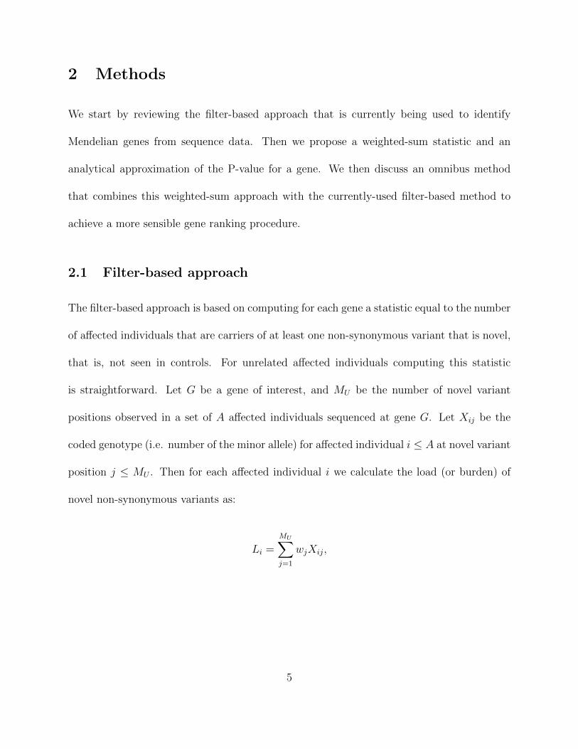
1 Introduction
Spurred by recent advances in high-throughput sequencing technologies, sequencing studies
for varied Mendelian and complex traits are currently underway. Such studies will provide
an unprecedented view of the genetic variation, rare and common, that influences risk to
these diseases. Genes for several Mendelian diseases have already been identified1, 2, 3, using
exome-sequencing of a small number of affected individuals and additional information from
public resources such as dbSNP and the 1000 Genomes Project.
The large number of genetic variants in the human genome, and the low population
frequency of the majority of these variants create challenges for the computational and sta-
tistical analysis of these data. In particular, traditional testing strategies based on individual
variant testing can have low power, and new statistical methods that aggregate information
across multiple variants in a genetic region have been proposed4, 5, 6, 7, 8, 9, 10, 11, 12, 13.
For Mendelian diseases, traditional methods for gene identification range from candidate
gene studies (where candidates were selected based, for example, on functional similarity to
already established genes, and in many situations their exons were sequenced in a small num-
ber of subjects) to positional cloning strategies (where small regions discovered using linkage
analysis were followed-up with denser genotyping that led to identification of haplotypes
thought to harbor causal mutations). Recently, several studies have been published on using
3

whole-exome sequencing data on a small number of (mostly unrelated) affected individuals to
identify the genes for several Mendelian traits1, 2, 3. Unlike traditional linkage methods, the
underlying gene could be identified directly, and by using unrelated subjects. More precisely,
in each case the causal gene was identified using a filter-based methodology, where variants
identified in cases were checked for novelty (not identified before), functionality (e.g. non-
synonymous variants), and sharing among affected (possibly related) individuals. Such an
approach is intuitive and reasonable; however, from an inferential perspective it has several
disadvantages including: (1) it does not produce any measure of statistical uncertainty (e.g.
gene level P-values), making it unfeasible to assess consistency with the null hypothesis (2)
it does not adjust for background variation in each gene, therefore allowing large genes to
rank high based on their size alone, and (3) it does not properly account for the different
levels of variant sharing expected among relatives of different types, which can affect the
rank of the disease gene. Although the filter-based approach can take into account external
information such as functional predictions or linkage scores, such information needs to be
provided in a dichotomized fashion (e.g. linkage or no linkage) rather than original scores
(or transformations thereof).
In what follows, we discuss a formal statistical framework that aims to address the
aforementioned limitations of the filter-based approach, and show applications to simulated
data and recent studies for three Mendelian traits. For these previously published Mendelian
studies, we show that the proposed approach ranks the true disease gene first in all three
studies, and assigns significant P-values to the respective disease genes.
4
2 Methods
We start by reviewing the filter-based approach that is currently being used to identify
Mendelian genes from sequence data. Then we propose a weighted-sum statistic and an
analytical approximation of the P-value for a gene. We then discuss an omnibus method
that combines this weighted-sum approach with the currently-used filter-based method to
achieve a more sensible gene ranking procedure.
2.1 Filter-based approach
The filter-based approach is based on computing for each gene a statistic equal to the number
of affected individuals that are carriers of at least one non-synonymous variant that is novel,
that is, not seen in controls. For unrelated affected individuals computing this statistic
is straightforward. Let G be a gene of interest, and MU be the number of novel variant
positions observed in a set of A affected individuals sequenced at gene G. Let Xij be the
coded genotype (i.e. number of the minor allele) for affected individual i ≤ A at novel variant
position j ≤ MU . Then for each affected individual i we calculate the load (or burden) of
novel non-synonymous variants as:
Li =
MU∑j=1
wjXij,
5

where wj is 1 for non-synonymous variant, and 0 otherwise. Then the filter-based method
is based on the following statistic:
Sfilter =A∑i=1
I{Li>0}, (1)
where I(·) is an indicator function.
For affected relative pairs and Mendelian diseases, it is reasonable to assume that both
affected individuals in a pair share the disease variant. If each pair of affected relatives is
treated as a unit, the score for each unit (i.e. the equivalent of I{Li>0} above) is taken to
be 1 if there is at least one novel, non-synonymous variant in gene G shared between both
relatives, and 0 otherwise. However, this definition fails to account for the different levels of
expected sharing among relatives of different types. Ideally, one would like to assign a higher
score if two cousins share a variant vs. two siblings. Later on we discuss such an alternative
scoring scheme.
As the number of sequenced controls increases, restricting attention to only the novel
variants runs the risk of disregarding rare disease mutations that are in fact present in
control individuals as well (possibly due to reduced penetrance and/or recessive mode of
inheritance). A simple extension of the filter-based approach is to also consider variants that
have a frequency in controls less than some threshold, say 0.01, rather than only the novel
ones. We refer to this approach Filter-R (all rare variants are included), and the existing
filter-based approach based on novel variants only is referred to as Filter-N.
6

2.2 Weighted-sum statistic for Mendelian traits
We describe here a weighted-sum statistic that resembles statistics that have been proposed
before for case-control designs6. However, unlike existing weighted-sum statistics, for the
proposed statistic (1) an approximate analytical P-value can be calculated for each gene, and
(2) both affected relative pairs and unrelated affected individuals can be accommodated.
Let G be a gene of interest, and M be the number of rare variant positions observed
in a set of individuals (both affected and unaffected) sequenced at gene G. We assume for
now that all individuals are unrelated. A rare variant is defined as a variant with popula-
tion frequency less than some pre-specified threshold, e.g. 0.01. The optimal threshold is
not known and necessarily depends on the underlying frequency spectrum for disease muta-
tions in Mendelian diseases. However, extensive data available on the frequency spectrum
for Mendelian mutations suggests that the total mutation frequency is << 1% for most
Mendelian diseases14. For each rare variant position j, with j ≤ M , let T (j) be the total
number of variants in affected individuals (note that this corresponds to an additive model).
One simple statistic we can define is:
S =M∑j=1
T (j).
Moreover, incorporation of external weights such as those from Polyphen15 or SIFT16 can be
done easily. For example,
Sw =M∑j=1
wjT (j),
7

where wj is the weight for variant j which can be any real positive number (derived indepen-
dently of the data). For example, if only non-synonymous variants are to be included then
wj = 1 for such variants and 0 otherwise. A similar weighting scheme works if only variants
that are not in dbSNP are to be considered.
Let Na be the total number of chromosomes in affected individuals, and Nu be the
corresponding number for controls. For variant j let fj be the estimated frequency based on
controls. If we assume that the underlying frequency distribution of the variants in a region
can be approximated by Beta(α, β), then we estimate fj by:
fj =xj + α
Nu + α + β,
where xj is the observed number of occurrences of the minor allele in controls at variant
position j (The parameters α and β can be estimated from data available on controls using
standard maximum likelihood estimation 19. We also note that results are robust to the
choice of α and β especially as Nu becomes large.). If we assume for now that the rare
variants under consideration are in linkage equilibrium then we show in the Supplemental
Materials S1.1 and S1.2 that:
E(Sw) =M∑j=1
wjNafj and
Var(Sw) =M∑j=1
w2jNa
[Na − 1
Nu
+ 1
]fj(1− fj).
In the general case when variants are allowed to be correlated, a suitable variance estimator
8

has also been derived (Supplemental Material S1.2).
We use the following gamma-based approximation for the probability density function
of the weighted-sum statistic of Poisson-like random variables (Supplemental Table S5; see
also Fay and Feuer17):
Pnull(a) = P (Sw ≥ a) = 1−Q
(a
wequiv
,E(Sw)
wequiv
), (2)
where wequiv = Var(Sw)
E(Sw)and Q is the incomplete gamma function: Q(a, x) = 1
Γ(a)
∫∞xe−tta−1dt.
This approximation becomes very accurate as the observed number of variants M in a
region increases. It can however be conservative when M is small (Supplemental Table S5).
2.2.1 Only novel variants in cases are considered.
Previous studies on several Mendelian traits1, 2, 3 have used public resources such as dbSNP
and 1000 Genomes Project data, as well as sequence data on a small number of controls
to filter out variants that are common and only keep those that are novel (do not appear
in these existing databases). This is indeed a reasonable approach if disease mutations are
assumed to be very rare and highly penetrant. We can modify our weighted-sum statistic
above as follows:
Snovelw =
MU∑j=1
wjT (j),
where MU is the number of novel variants in affected individuals. Note that MU is a subset
of M , and that E(Snovelw ) ≤ E(Sw) and Var(Snovel
w ) ≤ Var(Sw). In order to calculate E(Snovelw )
9

and Var(Snovelw ) one would need to estimate the number of novel variants in cases based on
the observed variants in controls, and both parametric and non-parametric methods can
be applied to obtain such estimates18, 19. However, it can be difficult to obtain accurate
estimates on the number of novel variants in a gene if only a small number of variants is
observed in controls, as would be the case for many genes of small to moderate length.
Therefore we use the same gamma-based approximation as in eq. (2) to obtain an upper
bound on the P-value for this scenario.
In what follows we refer to the weighted-sum approach with all rare variants as WS-R,
and to the above approach with only the novel variants as WS-N.
2.2.2 Affected-relative pairs
For Mendelian diseases data on affected relatives, e.g. affected siblings or affected cousins,
may be available. It would be desirable to extend both the filter-based approach and the
weighted-sum approach discussed above to be able to handle relative pairs. A simple solution
adopted in the current filter-based approach is to score each pair of affected relatives as 1
if they share at least one novel and non-synonymous variant, and 0 otherwise. A potential
weakness of such a scoring scheme is that it fails to account for the different levels of expected
sharing among relatives of different types. In particular, we would like to assign a higher
score when such sharing happens between more distant relatives, e.g. cousins, compared
with siblings.
In Ionita-Laza and Ottman20 we have developed such a scoring scheme. Namely, for a
10
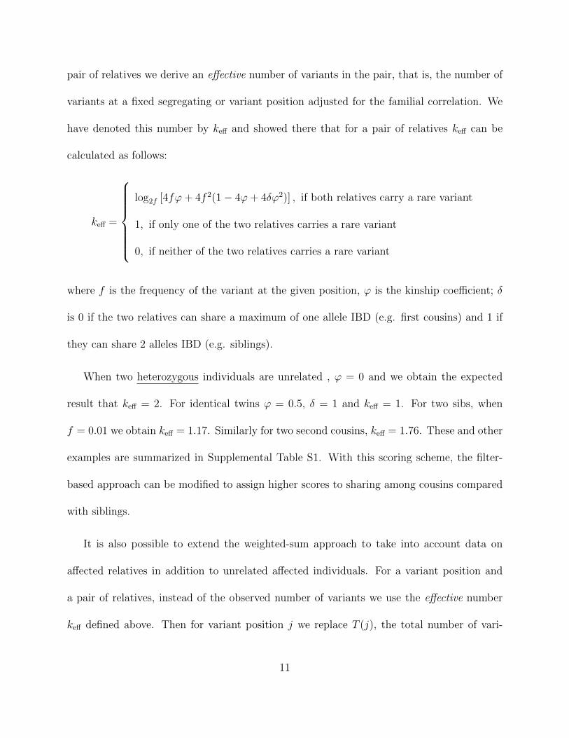
pair of relatives we derive an effective number of variants in the pair, that is, the number of
variants at a fixed segregating or variant position adjusted for the familial correlation. We
have denoted this number by keff and showed there that for a pair of relatives keff can be
calculated as follows:
keff =
log2f [4fϕ+ 4f 2(1− 4ϕ+ 4δϕ2)] , if both relatives carry a rare variant
1, if only one of the two relatives carries a rare variant
0, if neither of the two relatives carries a rare variant
where f is the frequency of the variant at the given position, ϕ is the kinship coefficient; δ
is 0 if the two relatives can share a maximum of one allele IBD (e.g. first cousins) and 1 if
they can share 2 alleles IBD (e.g. siblings).
When two heterozygous individuals are unrelated , ϕ = 0 and we obtain the expected
result that keff = 2. For identical twins ϕ = 0.5, δ = 1 and keff = 1. For two sibs, when
f = 0.01 we obtain keff = 1.17. Similarly for two second cousins, keff = 1.76. These and other
examples are summarized in Supplemental Table S1. With this scoring scheme, the filter-
based approach can be modified to assign higher scores to sharing among cousins compared
with siblings.
It is also possible to extend the weighted-sum approach to take into account data on
affected relatives in addition to unrelated affected individuals. For a variant position and
a pair of relatives, instead of the observed number of variants we use the effective number
keff defined above. Then for variant position j we replace T (j), the total number of vari-
11

ants at position j in the affected individuals, with Teff(j) and the weighted-sum statistic is
correspondingly defined as:
Sw =M∑j=1
wjTeff(j).
As for the scenarios with only unrelated individuals, we derive a gamma-based approximation
for the distribution of Sw (Supplemental Material S2).
For Mendelian diseases, it is reasonable to assume that affected relatives within the
same family are likely to share the disease mutation. The approach discussed above can
be modified easily to reflect this assumption, by setting keff to be zero unless both relatives
share a variant (that can be non-synonymous and novel). This is the default setting in our
handling of affected relatives, and the one illustrated in the examples that follow.
2.3 Joint-Rank approach
We describe here how the weighted-sum approach above can be combined with the currently-
used filter-based method to produce an overall better ranking for the true disease gene(s) in a
study. Both approaches discussed in the previous sections attempt to quantify the increase in
rare variant burden in affected individuals, although in slightly different ways. The weighted-
sum approach aggregates information across all affected individuals and adjusts for the
underlying variation in controls, but does not always distinguish whether the variants that
enter the calculation of Sw occur in many or just a few of the individuals. On the contrary, the
existing filter-based approach essentially exploits the information on the number of affected
individuals that carry at least one novel variant, but fails to distinguish whether variants
12

occur recurrently at the same position, or different positions, and does not take into account
the number of novel variants an individual carries, unlike the weighted-sum approach.
For the purpose of ranking genes, we propose to combine the two approaches to calculate
for each gene a combined rank, henceforth called the Joint-Rank, that represents the average
of the ranks from the weighted-sum and filter-based approaches. For a true disease gene both
ranks should be high, and the Joint-Rank approach may lead to an overall better ranking
of the true disease gene. The filter-based rank is not adjusted for the background variation,
and hence the Joint-Rank can be viewed as adjusting the filter-based rank for the length of
the gene, and the background variation in each gene.
The various approaches discussed in this section are summarized in Table 1.
3 Applications
Next, we investigate via simulations the properties of the proposed approaches. We also
use real high-coverage sequence data on 310 control individuals randomly selected from the
large collection of unaffected individuals that have been sequenced as part of the ARRA
Autism Project (see Supplemental Material S4 for more details on these data) to illustrate
applications to three Mendelian disease examples recently reported in the literature: Miller
Syndrome2, Freeman-Sheldon Syndrome1, and Kabuki Syndrome3.
13

3.1 Simulated data
We first use simulations to investigate the underlying properties of the proposed approaches.
We simulated 10 independent genomic regions each of length 1 Mb under a coalescent model
using the software package COSI21. The model used in the simulation was the calibrated
model for the European population, and was an option available in the COSI package. A
total of 10, 000 haplotypes were generated for each region. We then randomly sample small
subregions of the size of individual genes. The size of each gene is sampled from the length
distribution of real exonic regions (as available from the refGene table).
Type-1 Error
We evaluated the Type-1 error of the proposed approaches for several different scenarios,
including two different designs: (1) case-control, and (2) affected sib-pairs and unrelated
controls. The results for the case-control design are shown in Table 2. We show there that
the proposed gamma-based approximation is valid and leads to a good control of the Type-1
error.
When only novel variants (i.e. not seen in a set of independent controls) are considered,
the approximation can be very conservative. Despite this conservativeness, since the mag-
nitude of the effect at the disease gene is expected to be large for Mendelian diseases, the
approximation is expected to be powerful for such effects.
Similar results hold for datasets containing affected relative pairs (Supplemental Table
S2).
14
Disease Gene Ranking
We investigate here the performance of the various approaches as measured by the overall
ranking of the disease gene in a genome-scan with 20, 000 genes. A genome-scan is simulated
by sampling 20, 000 regions with region length selected from the gene (exonic) length distri-
bution in refGene table. The genes are sampled independently from the ten 1 Mb regions
we have simulated. We assume 10 affected individuals and a number of controls between
100 and 500. One gene at random is selected to be the disease gene and a small number
of affected individuals (between 2 and 6) are assumed to each carry a different novel dis-
ease mutation. We simulate 1000 such genome-scans, and calculate the median rank for the
disease gene across the 1000 simulations.
We show in Figure 1 that the Joint-Rank-N approach outperforms both the WS-N and the
Filter-N methods in terms of the rank assigned to the disease gene. The performance of the
filter-based approach decreases as the genetic heterogeneity at the disease gene increases, and
it is in these situations that a formal approach such as the weighted-sum method discussed
in this paper becomes particularly necessary. The extension of the filter-based approach to
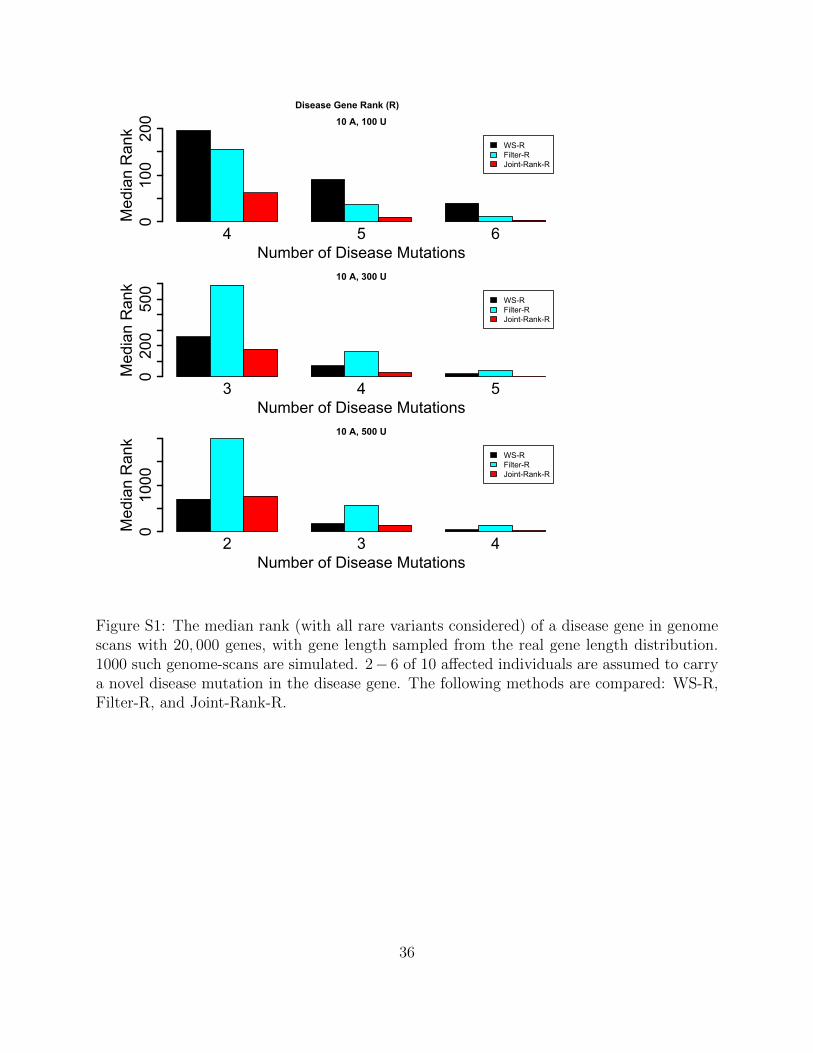
include rare variants rather than only novel variants (i.e. Filter-R) does not perform very
well, especially as the number of affected individuals that carry a disease mutation at a
disease locus decreases (Supplemental Figure S1). In such situations the proposed weighted-
sum approach alone is expected to perform better.
Results for affected sib-pairs are shown in Supplemental Figure S2, and are similar to
those for the case-control design.
15

3.2 Applications to three Mendelian diseases
For these applications, we use high-coverage sequence data with spiked-in mutations to re-
semble the original disease studies as closely as possible. In particular, we assume that
the same number of affected individuals as in the original studies are carriers of novel non-
synonymous disease mutations, and these mutations are artificially added to the correspond-
ing disease gene, above and beyond the existing variation in our real data. We also disregard
variants with a known rs number by simply setting their weights to 0. The next set of results
are based on these spike-in datasets.
Miller Syndrome
In Ng et al.2 the authors performed exome-sequencing of four affected individuals with
Miller Syndrome, two siblings and two unrelated affected individuals. All four affected
individuals were compound heterozygotes for novel and non-synonymous mutations in one
gene, DHODH, and the two siblings shared the disease mutations. Since the sequence data
available to us contains only unrelated individuals, we emulated the original study by using
data on only 3 unrelated individuals as cases, and 300 unrelated individuals as controls; all
individuals are part of the same exome-sequencing study (Supplemental Material S4). For
the disease gene DHODH we make the additional assumption that each of the three affected
individuals is compound heterozygote for unique mutations in this gene.
In Figure 2 we plot the P-values (WS-N) for all genes, as well as the value of the filter-
based statistic (i.e. the number of affected individuals carriers of novel non-synonymous
16
variants). With only three affected individuals, we identify gene DHODH as the leading
gene, with an approximate P-value of 10−6 (analytic gamma-approximation).
Freeman-Sheldon Syndrome
For the Freeman-Sheldon syndrome example, Ng et al.1 performed exome-sequencing of four
unrelated affected individuals. Two different novel and non-synonymous variant positions
in the same gene, MYH3, were detected in all four individuals. Three individuals had a
mutation at the first variant position, while the fourth individual had a mutation at the
second variant position. Based on our spike-in dataset, the resulting approximate P-value
(WS-N) in this case is 1.0 · 10−4. This was the highest ranked gene in the study (Figure 2).
Kabuki Syndrome
For the Kabuki Syndrome example, exome-sequencing was performed in ten unrelated af-
fected individuals (Ng et al.3). Nine different novel and non-synonymous mutations in gene
MLL2 were identified in the 10 affected individuals. Based on our spike-in dataset, the re-
sulting approximate P-value is 3.5 · 10−5, and again this is the highest ranked gene (Figure
2).
Results for these three Mendelian diseases are summarized in Table 3.
17

4 Discussion
Recent studies have shown how genes for Mendelian diseases can be identified using whole-
exome sequence data for a small number of affected individuals. The underlying approach
is based on filtering variants based on novelty, functionality, and sharing among multiple
affected individuals. Such filter-based approaches are intuitive and powerful for Mendelian
diseases, but suffer from several shortcomings. Notable among them are: (1) the lack of sta-
tistical uncertainty assessment (e.g. in the form of P-values), (2) the lack of adjustment for
the background variation in each gene, so that large genes can rank high based on their size
alone, and (3) genetic distance between biological relatives is not modeled properly. We have
shown here that such a filter-based approach can be complemented by a formal statistical
procedure that has several distinct advantages: (1) evaluates statistical significance by calcu-
lating approximate P-values, (2) can handle both related and unrelated affected individuals,
(3) can incorporate external weights about the functionality of variants or linkage-based
scores, and (4) importantly, adjusts for background variation so that more variable regions
do not rise to the top based on noise alone. The resulting procedure leads to an overall
better ranking of the disease gene, and allows for untieing genes that otherwise have the
same number of affected individuals that carry a novel mutation in the gene.
We have investigated two distinct scenarios: one that considers all rare variants in the
population, regardless of whether they have been seen before or not (WS-R); and a second
scenario where only novel variants in cases are included (WS-N). We have derived a gamma-
based approximation for the null distribution of the weighted-sum statistic WS-R and have
18

shown that this approximation is good. Also, we have shown that the same approximation
can be used for WS-N to derive an upper bound on the P-value. Via applications to both
simulated and real data, we have shown that a combination of the weighted-sum approach
and the filter-based approach, a procedure we call Joint-Rank, provides a more robust way
to rank genes in Mendelian diseases compared with filter-based approaches alone. In partic-
ular, the Joint-Rank approach adjusts for the background variation in each gene (as does the
weighted-sum approach) and at the same time favors genes with larger number of affected
individuals that are carriers of novel variants (as does the filter-based approach). Through-
out our examples we have assumed that causal variants are novel and hence not present
in unaffected individuals. Under such a scenario, the optimal approach is indeed to only
consider novel variants. However, if causal variants could be present in unaffected individu-
als (for example, for a recessive mode of inheritance, or reduced penetrance scenarios), the
weighted-sum approach WS-R should also be considered.
We revisited recent exome-sequencing studies on several Mendelian diseases and showed
how the approach works concretely in these examples. The proposed approach produced
significant P-values for each of the disease genes in the three Mendelian traits, while properly
adjusting for the background variation in each gene, as estimated from exome-sequencing
data available to us for 300 controls. Due to the lack of even modest-sized sequence datasets
in the past, the filter-based approach used a variety of variant databases to filter out already
discovered variants, including dbSNP and 1000 Genomes Project data. With the proposed
approach, it is still possible to use these databases to filter out variants by simply setting the
19

weights for variants in the databases to 0, and this is especially useful when the number of
controls available is rather small. For our own examples, we have presented results based on
a relatively small number of controls (i.e. 300); however, increasing the number of controls
will naturally lead to smaller P-values and improved overall ranking for the true disease gene.
As with any association study, good experimental design is essential. The validity of the
P-values obtained from the weighted-sum approach, and of the Joint-Rank procedure overall
is contingent on having a control dataset that is well matched to the affected individuals, for
both ethnic background, as well as sensitivity and specificity for variant detection. Other
potential issues such as hidden relatedness among individuals can lead to inflated Type-1
error. Principal component analysis or mixed-model methods can be used to adjust for
relatedness of subjects by extending the current method to a regression-framework.
One strength of the proposed weighted-sum approach is that the P-values can be obtained
in an analytical fashion. This fact makes the proposed approach to be computationally very
fast compared to a permutation-based procedure, and also allows inclusion of affected relative
pairs, situations where resampling-based procedures are non-trivial.
The proposed methods implicitly assume an additive model for the effect of mutations at
a position. This model is optimal for additive, dominant, and compound heterozygous modes
of inheritance (as true for the three Mendelian disease examples we considered). Even for a
recessive model with two mutations required at the same position, the proposed approach is
expected to be very powerful.
For Mendelian diseases, results from previous linkage-based scans may be available. In
20

that case, Roeder et al.24 proposed an exponential weighting scheme, whereby linkage scores
are translated into weights that can be used to weight the gene level P-values calculated
with the proposed approach, as in a weighted-hypothesis testing procedure25.
In summary, we have discussed an analytic framework to identify disease genes for
Mendelian diseases, and have shown that it performs well in simulations and applications to
previous exome-sequencing studies for three Mendelian traits.
Software Software implementing the proposed approaches is available freely on our website
at: http://www.columbia.edu/∼ii2135/.
Acknowledgments The research was partially supported by NSF grant DMS-1100279
and NIH grant 1R03HG005908 (to II-L), and R37-CA076404 and P01-CA134294 from the
National Cancer Institute (to XL).
Control exomes were sequenced as part of an ongoing ARRA-funded autism exome-
sequencing grant (MH089025, Mark Daly, communicating PI, Joseph Buxbaum, Bernie De-
vlin, Richard Gibbs, Gerard Schellenberg, James Sutcliffe, collaborating PI’s).
Web Resources
PolyPhen http://genetics.bwh.harvard.edu/pph2/
SIFT http://sift.jcvi.org/
dbSNP http://www.ncbi.nlm.nih.gov/projects/SNP/
1000 Genomes Project http://www.1000genomes.org/
refGene http://genome.ucsc.edu/cgi-bin/hgTables/
21
Supplemental Material
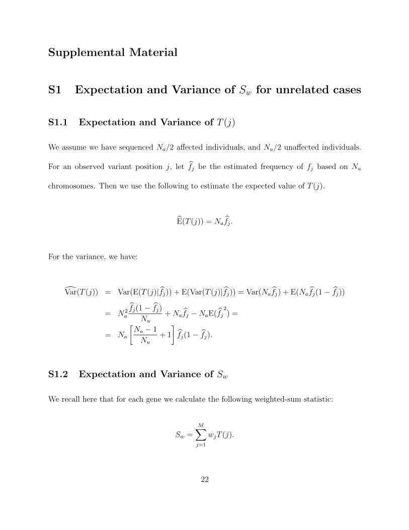
S1 Expectation and Variance of Sw for unrelated cases
S1.1 Expectation and Variance of T (j)
We assume we have sequenced Na/2 affected individuals, and Nu/2 unaffected individuals.
For an observed variant position j, let fj be the estimated frequency of fj based on Nu
chromosomes. Then we use the following to estimate the expected value of T (j).
E(T (j)) = Nafj.
For the variance, we have:
Var(T (j)) = Var(E(T (j)|fj)) + E(Var(T (j)|fj)) = Var(Nafj) + E(Nafj(1− fj))
= N2a
fj(1− fj)Nu
+Nafj −NaE(fj2) =
= Na
[Na − 1
Nu
+ 1
]fj(1− fj).
S1.2 Expectation and Variance of Sw
We recall here that for each gene we calculate the following weighted-sum statistic:
Sw =M∑j=1
wjT (j).
22

Then E(Sw) =∑M
j=1 wjE(T (j)). For the variance of Sw we have:
Var(Sw) =M∑j=1
w2j Var(T (j)) +
∑1≤j 6=j′≤M
wjwj′Cov(T (j), T (j′)).
The covariance can be estimated as follows27. Let Ve be the M ×M empirical variance esti-
mator with vjj′ = AN
∑Ni=1(Xij−E(Xij))(Xij′−E(Xij′)), where N = A+U is the total num-
ber of individuals (affected and unaffected). Let D be the M×M diagonal matrix with djj =
Var(T (j)). Also we define an adjusted variance matrix: VA = D1/2[Diag(Ve)−1/2VeDiag(Ve)
−1/2]D1/2.
Then an estimate for Var(Sw) is∑
j,j′ VA[j, j′].
S2 Expectation and Variance of Sw when affected in-
dividuals are related
S2.1 Expectation and Variance for T (j)
We show here how to derive the expected value and variance of Teff at a variant position
when affected relatives are considered. Let A be the total number of affected relative pairs
(of same type). If f is estimated based on Nu chromosomes, then we can get for
E[Teff] = A[keff|24fϕ+ 4f(1− 2ϕ)
].
Var[Teff] = A2(keff|24ϕ+ 4(1− 2ϕ)
)2 f(1− f)
Nu
+ A ·(keff|24fϕ+ 4f(1− 2ϕ)
).
To assess the covariance between Teff at two different positions, we need to know the
23

joint distribution of genotypes at two positions in two relatives. Lange28 has derived the
relative-to-relative transition probabilities for two linked genes, and we make use of these
transition probabilities and the observed genotype distribution at two positions in unrelated
controls to derive the joint distribution in relatives that we need. We then use a gamma-based
approximation for the weighted-sum of Poisson random variables.
We claim here that the distribution of Teff under the null hypothesis of no associa-
tion with disease can be approximated by an overdispersed Poisson distribution with mean∑Ai=1E[keff(i)], and an index of dispersion very close to 1. It is easy to verify this claim by
simple simulation experiments. We have simulated datasets of affected sib-pairs and controls
at one single variant position of frequency 0.001 ≤ f ≤ 0.01. For each dataset we calculate
Teff assuming (1) the true value of f , and (2) the estimated value of f from controls. We
report the mean and variance for Teff(f) and Teff(f) based on 10000 random simulations,
as well as the correlation between Teff(f) and Teff(f). Results are shown in Supplemental
Table S3. For more distant relatives, such as first and second cousins, we only report the
theoretical mean and variance for Teff(f) (Supplemental Table S4). As shown, the theoretical
and empirical results match very well. There is a slight inflation in the variance over the
mean for sib-pairs and when f = 0.01 (dispersion index < 1.06), although this inflation dis-
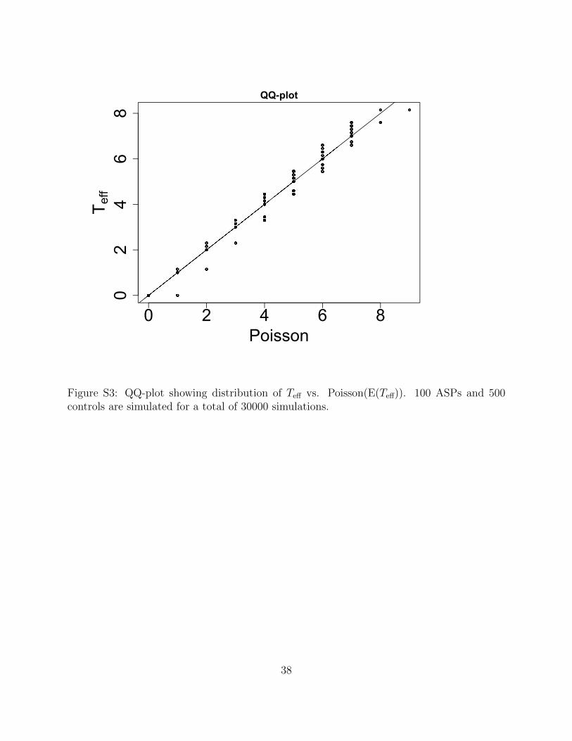
appears for more distant relatives. In Figure S3 we also show the distribution of Teff against
a Poisson with the same mean for a scenario with 100 affected sib-pairs and 500 controls and
f = 0.005.
24

S3 Gamma-based approximation for a sum of weighted-
Poisson random variables
We have done some simple calculations in R to assess the accuracy of the gamma-based
approximation for the weighted-sum of Poisson random variables. We assume M Poisson
random variables are included, and for each a weight wi is chosen from U(0, 1). The results
for different values for M are shown in Table S5.
S4 Sequence Data
To illustrate applications to real sequence data, we used exome-level data on 310 control
individuals randomly selected from the large collection of unaffected individuals that have
been sequenced as part of the ARRA Autism Project (AAP). The AAP involves whole-
exome sequencing of 1000 autism cases and 1000 controls, and several hundred trios. Whole-
exome sequencing of controls was carried out at the Broad Institute and at Baylor College
of Medicine using standard approaches. Following QC, variants were called using several
approaches (including the Genome Analysis Toolkit26), and variant call files with all variants
and relevant QC metrics were made available to us. For our applications we considered data
on 310 randomly chosen control individuals.
25
References
[1] Ng SB, Turner EH, Robertson PD, Flygare SD, Bigham AW, Lee C, Shaffer T, Wong
M, Bhattacharjee A, Eichler EE et al. (2009) Targeted capture and massively parallel
sequencing of 12 human exomes. Nature 461: 272–276.
[2] Ng SB, Buckingham KJ, Lee C, Bigham AW, Tabor HK, Dent KM, Huff CD, Shannon
PT, Jabs EW, Nickerson DA et al. (2010a) Exome sequencing identifies the cause of a
mendelian disorder. Nat Genet 42: 30–35.
[3] Ng SB, Bigham AW, Buckingham KJ, Hannibal MC, McMillin MJ, Gildersleeve HI, Beck
AE, Tabor HK, Cooper GM, Mefford HC et al. (2010b) Exome sequencing identifies MLL2
mutations as a cause of Kabuki syndrome. Nat Genet 42: 790–793.
[4] Li B, Leal SM (2008) Methods for detecting associations with rare variants for common
diseases: application to analysis of sequence data. Am J Hum Genet 83: 311–321.
[5] Madsen BE, Browning SR (2009) A groupwise association test for rare mutations using
a weighted sum statistic. PLoS Genet 5: e1000384.
[6] Price AL, Kryukov GV, de Bakker PI, Purcell SM, Staples J, Wei LJ, Sunyaev SR (2010)
Pooled association tests for rare variants in exon-resequencing studies. Am J Hum Genet
86: 832–838.
26

[7] Liu DJ, Leal SM (2010) A novel adaptive method for the analysis of next-generation
sequencing data to detect complex trait associations with rare variants due to gene main
effects and interactions. PLoS Genet 6: e1001156.
[8] King CR, Rathouz PJ, Nicolae DL (2010) An evolutionary framework for association
testing in resequencing studies. PLoS Genet 6: e1001202.
[9] Bhatia G, Bansal V, Harismendy O, Schork NJ, Topol EJ, Frazer K, Bafna V (2010)
A covering method for detecting genetic associations between rare variants and common
phenotypes. PLoS Comput Biol 6: e1000954.
[10] Han F, Pan W (2010) A data-adaptive sum test for disease association with multiple
common or rare variants. Hum Hered 70: 42–54.
[11] Ionita-Laza I, Buxbaum J, Laird NM, Lange C (2011) A new testing strategy to identify
rare variants with either risk or protective effect on disease. Plos Genet, 7: e1001289.
[12] Neale BM, Rivas MA, Voight BF, Altshuler D, Devlin B, Orho-Melander M, Kathiresan
S, Purcell SM, Roeder K, Daly MJ (2011) Testing for an unusual distribution of rare
variants. PLoS Genet 7: e1001322.
[13] Wu M, Lee S, Cai T, Li Y, Boehnke M, Lin X (2011) Rare Variant Association Testing
for Sequencing Data Using the Sequence Kernel Association Test (SKAT) Am J Hum
Genet, in press.
[14] Pritchard JK, Cox NJ (2002) The allelic architecture of human disease genes: common
disease-common variant...or not? Hum Mol Genet 11: 2417–2423.
27
[15] Adzhubei IA, Schmidt S, Peshkin L, Ramensky VE, Gerasimova A, Bork P, Kondrashov
AS, Sunyaev SR (2010) A method and server for predicting damaging missense mutations.
Nat Methods 7: 248–249.
[16] Kumar P, Henikoff S, Ng PC (2009) Predicting the effects of coding non-synonymous
variants on protein function using the SIFT algorithm. Nature Protocols 4: 1073–1081.
[17] Fay MP, Feuer EJ (1997) Confidence intervals for directly standardized rates: a method
based on the gamma distribution, Stat Med, 16: 791–801.
[18] Efron B, Thisted R (1976) Estimating the number of unknown species: How many
words did Shakespeare know? Biometrika 63: 435–437
[19] Ionita-Laza I, Lange C, Laird NM (2009) Estimating the number of unseen variants in
the human genome. Proc Natl Acad Sci USA 106: 5008–5013.
[20] Ionita-Laza I, Ottman R (2011) On study designs for identification of rare disease vari-
ants in complex diseases. Genetics. In press.
[21] Schaffner SF, Foo C, Gabriel S, Reich D, Daly MJ, Altshuler D (2005) Calibrating a
coalescent simulation of human genome sequence variation. Genome Res 15: 1576–1583.
[22] Lemire M (2011) Defining rare variants by their frequencies in controls may increase
type I error. Nat Genet 43: 391–392.
[23] Pearson RD (2011) Bias due to selection of rare variants using frequency in controls.
Nat Genet 43: 392–393.
28

[24] Roeder K, Bacanu SA, Wasserman L, Devlin B (2006) Using linkage genome scans to
improve power of association in genome scans. Am J Hum Genet 78: 243–252.
[25] Ionita-Laza I, McQueen MB, Laird NM, Lange C (2007) Genomewide weighted hypoth-
esis testing in family-based association studies, with an application to a 100K scan. Am J
Hum Genet 81: 607–614.
[26] McKenna A, Hanna M, Banks E, Sivachenko A, Cibulskis K, Kernytsky A, Garimella K,
Altshuler D, Gabriel S, Daly M et al. (2010) The Genome Analysis Toolkit: a MapReduce
framework for analyzing next-generation DNA sequencing data. Genome Res 20: 1297–
1303.
[27] Rakovski CS, Xu X, Lazarus R, Blacker D, Laird NM (2007) A new multimarker test
for family-based association studies. Genet Epidemiol 31: 9–17.
[28] Lange K (1974) Relative-to-relative transition probabilities for two linked genes. Theo-
retical Population Biology 6: 92–107.
29

Figure Legends
Figure 1: The median rank (novel-variants only) of a disease gene in genome scans with
20, 000 genes, with gene length sampled from the real gene length distribution. 1000
such genome-scans are simulated. 2−6 of 10 affected individuals are assumed to carry
a novel disease mutation in the disease gene (with fewer mutations for larger number of
controls). The following methods are compared: WS-N, Filter-N, and Joint-Rank-N.
Figure 2: Applications to three Mendelian diseases: Miller Syndrome, Freeman-Sheldon
Syndrome and Kabuki Syndrome. On the left we show the P-values (WS-N) for 19, 811
genes surveyed (manhattan plot). On the right we show for each gene the number of
affected individuals that are carriers of novel disease variants, and the gene P-value.
30
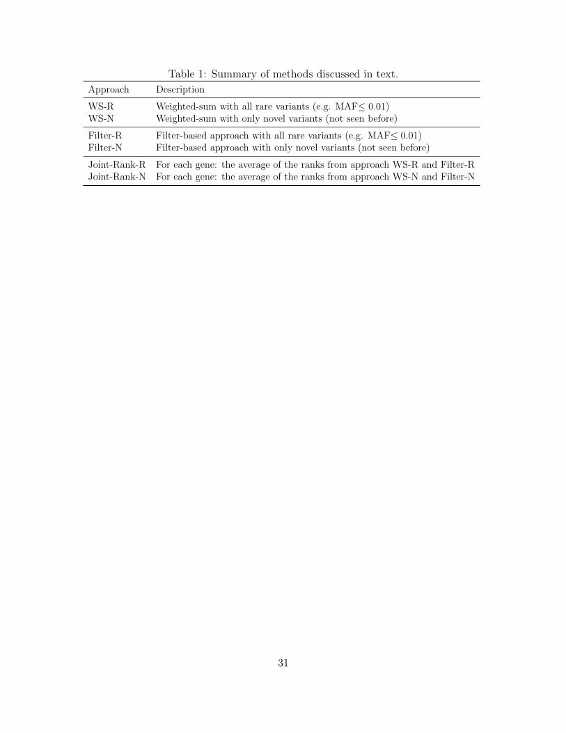
Table 1: Summary of methods discussed in text.
Approach Description
WS-R Weighted-sum with all rare variants (e.g. MAF≤ 0.01)WS-N Weighted-sum with only novel variants (not seen before)
Filter-R Filter-based approach with all rare variants (e.g. MAF≤ 0.01)Filter-N Filter-based approach with only novel variants (not seen before)
Joint-Rank-R For each gene: the average of the ranks from approach WS-R and Filter-RJoint-Rank-N For each gene: the average of the ranks from approach WS-N and Filter-N
31

Table 2: Type-1 error for the Case-Control Design.
Approach Aa Ub α10−4 10−3 10−2 5 · 10−2
WS-R 5 100 1.5 · 10−4 6.0 · 10−4 4.0 · 10−3 1.7 · 10−2
500 1.3 · 10−4 7.0 · 10−4 5.0 · 10−3 2.1 · 10−2
1000 1.1 · 10−4 5.7 · 10−4 5.0 · 10−3 2.1 · 10−2
10 100 1.0 · 10−4 4.0 · 10−4 3.0 · 10−3 1.6 · 10−2
500 1.2 · 10−4 7.1 · 10−4 4.8 · 10−3 2.3 · 10−2
1000 1.1 · 10−4 8.0 · 10−4 5.0 · 10−3 2.3 · 10−2
20 100 1.7 · 10−5 1.4 · 10−4 1.4 · 10−3 1.0 · 10−2
500 1.1 · 10−4 6.4 · 10−4 5.0 · 10−3 2.5 · 10−2
1000 1.1 · 10−4 6.5 · 10−4 5.0 · 10−3 2.6 · 10−2
WS-N 5 100 7.8 · 10−5 3.0 · 10−4 1.5 · 10−3 6.7 · 10−3
500 2.6 · 10−5 7.4 · 10−5 4.3 · 10−4 3.0 · 10−3
1000 2.1 · 10−5 1.2 · 10−4 2.9 · 10−4 1.1 · 10−3
10 100 3.3 · 10−5 1.4 · 10−4 1.1 · 10−3 6.1 · 10−2
500 7.0 · 10−6 5.2 · 10−5 2.5 · 10−4 2.0 · 10−3
1000 1.3 · 10−5 3.0 · 10−5 1.1 · 10−4 8.6 · 10−4
20 100 8.0 · 10−6 4.2 · 10−5 3.0 · 10−4 2.7 · 10−3
500 3.0 · 10−6 2.1 · 10−5 1.7 · 10−4 1.7 · 10−3
1000 2.3 · 10−6 2.3 · 10−5 8.7 · 10−5 7.8 · 10−4
a#unrelated affected individualsb#unrelated unaffected individuals
32

Table 3: Summary results for the applications to three Mendelian traits.
Syndrome Gene Length (kb) Dataset MOIa P-valueb
Ac Ud (WS-N)
Miller 16.0 3 300 CH 1.0E-06Freeman-Sheldon 28.7 4 300 D 1.0E-04Kabuki 36.3 10 300 D 3.5E-05
aMode of Inheritance: compound heterozygote (CH) or dominant (D)bAnalytical P-valuec#unrelated affected individualsd# unaffected individuals
33

4 5 6
WS-NFilter-NJoint-Rank-N
10 A, 100 U
Number of Disease Mutations
Med
ian
Ran
k0
4080
3 4 5
WS-NFilter-NJoint-Rank-N
10 A, 300 U
Number of Disease Mutations
Med
ian
Ran
k0
4080
2 3 4
WS-NFilter-NJoint-Rank-N
10 A, 500 U
Number of Disease Mutations
Med
ian
Ran
k0
100
250
Disease Gene Rank (N)
Figure 1:
34

01
23
45
6
-log10(P)
Chromosome
DHODH0
12
34
56
MS - Gene P-values
# Carriers
-log10(P)
01
23
45
6
0 1 2 3
DHODH
MS - P vs. # Carriers
01
23
45
-log10(P)
Chromosome
MYH3
01
23
45
FSS - Gene P-values
# Carriers-log10(P)
01
23
45
0 1 2 3 4
MYH3
FSS - P vs. # Carriers
01
23
45
6
-log10(P)
Chromosome
MLL2
01
23
45
6
KS - Gene P-values
# Carriers
-log10(P)
01
23
45
6
0 2 4 6 8 10
MLL2
KS - P vs. # Carriers
Applications to three Mendelian Diseases
Figure 2:
35
4 5 6
WS-RFilter-RJoint-Rank-R
10 A, 100 U
Number of Disease Mutations
Med
ian
Ran
k0
100
200
3 4 5
WS-RFilter-RJoint-Rank-R
10 A, 300 U
Number of Disease Mutations
Med
ian
Ran
k0200
500
2 3 4
WS-RFilter-RJoint-Rank-R
10 A, 500 U
Number of Disease Mutations
Med
ian
Ran
k0
1000
Disease Gene Rank (R)
Figure S1: The median rank (with all rare variants considered) of a disease gene in genomescans with 20, 000 genes, with gene length sampled from the real gene length distribution.1000 such genome-scans are simulated. 2− 6 of 10 affected individuals are assumed to carrya novel disease mutation in the disease gene. The following methods are compared: WS-R,Filter-R, and Joint-Rank-R.
36

2 3 4
WS-NFilter-NJoint-Rank-N
5 ASP, 100 U
Number of Disease Mutations
Med
ian
Ran
k0
4080
2 3 4
WS-NFilter-NJoint-Rank-N
5 ASP, 300 U
Number of Disease Mutations
Med
ian
Ran
k0
1020
2 3 4
WS-NFilter-NJoint-Rank-N
5 ASP, 500 U
Number of Disease Mutations
Med
ian
Ran
k0
612
ASP - Disease Gene Rank (N)
Figure S2: The median rank of a disease gene in genome scans with 20, 000 genes, withgene length sampled from the real gene length distribution. 1000 such genome-scans aresimulated. 2− 4 of 5 affected sib-pairs (ASP) are assumed to share a novel disease mutationin the disease gene. The following methods are compared: WS-N, Filter-N, and Joint-Rank-N.
37
0 2 4 6 8
02
46
8
Poisson
T eff
QQ-plot
Figure S3: QQ-plot showing distribution of Teff vs. Poisson(E(Teff)). 100 ASPs and 500controls are simulated for a total of 30000 simulations.
38

Table S1: The effective number of variants at a rare variant position in two relatedheterozygous individuals, as defined in text; ϕ is the kinship coefficient. Results for f = 0.01are shown.
Relationship ϕ keff
Identical twins 1/2 1.00Parent-child 1/4 1.17Sibs 1/4 1.17Half-sibs 1/8 1.34Uncle-nephew 1/8 1.34First Cousins 1/16 1.50First Cousins-1 (once removed) 1/32 1.64Second Cousins 1/64 1.76Unrelateds 0 2.00
39

Table S2: Type-1 error for the Sib-Pair Design.
Approach Aa Ub α10−4 10−3 10−2 5 · 10−2
WS-R 5 100 1.7 · 10−4 8.0 · 10−4 4.7 · 10−3 2.0 · 10−2
500 1.0 · 10−4 7.4 · 10−4 5.5 · 10−3 2.6 · 10−2
1000 1.4 · 10−4 7.0 · 10−4 4.9 · 10−3 2.5 · 10−2
10 100 1.0 · 10−4 5.0 · 10−4 3.8 · 10−3 1.8 · 10−2
500 1.1 · 10−4 9.8 · 10−4 6.0 · 10−3 2.7 · 10−2
1000 1.5 · 10−4 9.9 · 10−4 5.9 · 10−3 2.7 · 10−2
WS-N 5 100 1.0 · 10−4 4.5 · 10−4 2.2 · 10−3 8.0 · 10−3
500 2.7 · 10−5 2.7 · 10−4 4.9·10−4 2.4 · 10−3
1000 2.4 · 10−5 5 · 10−5 3.0 · 10−4 1.5 · 10−3
10 100 4.9 · 10−5 2.5 · 10−4 1.4 · 10−3 6.7 · 10−3
500 2.0 · 10−5 1.0 · 10−4 3.8 · 10−4 1.7 · 10−3
1000 4.9 · 10−5 1.0 · 10−4 2.9 · 10−4 1.4 · 10−3
a#affected sib-pairsb#unrelated unaffected individuals
40

Table S3: Simulation results for Teff.
f Nsibs Ncontrols f f Cora Theoreticalµ var µ var µ var
0.01 5 100 0.152 0.163 0.152 0.163 0.999915 0.156 0.161500 0.153 0.151 0.153 0.151 0.999968 0.156 0.1611000 0.162 0.168 0.162 0.168 0.999986 0.156 0.161
0.001 5 100 0.017 0.018 0.017 0.018 0.999864 0.016 0.016500 0.014 0.015 0.014 0.015 0.999984 0.016 0.0161000 0.016 0.017 0.016 0.017 0.999985 0.016 0.016
aCorrelation between Teff(f) and Teff(f)
41
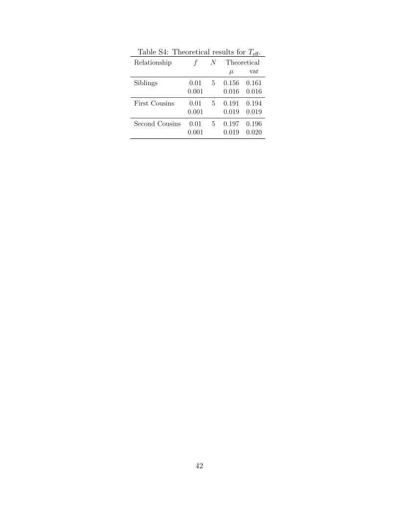
Table S4: Theoretical results for Teff.
Relationship f N Theoreticalµ var
Siblings 0.01 5 0.156 0.1610.001 0.016 0.016
First Cousins 0.01 5 0.191 0.1940.001 0.019 0.019
Second Cousins 0.01 5 0.197 0.1960.001 0.019 0.020
42

Table S5: Gamma-based approximation of weighted-sum of M Poisson RVs.
M α10−5 10−4 10−3 10−2 0.05
3 4.7 · 10−6 5.3 · 10−5 4.3 · 10−4 6.3 · 10−3 2.8 · 10−2
5 1.0 · 10−5 9.3 · 10−5 8.3 · 10−4 7.0 · 10−3 3.3 · 10−2
20 1.0 · 10−5 9.3 · 10−5 8.4 · 10−4 8.0 · 10−3 3.9 · 10−2
40 1.0 · 10−5 9.7 · 10−5 8.8 · 10−4 8.4 · 10−3 4.1 · 10−2
43
Related Documents