Zurich Open Repository and Archive University of Zurich University Library Strickhofstrasse 39 CH-8057 Zurich www.zora.uzh.ch Year: 2020 Financing the energy transition: the impact of a changing power sector on investors Hörnlein, Lena Posted at the Zurich Open Repository and Archive, University of Zurich ZORA URL: https://doi.org/10.5167/uzh-188697 Dissertation Published Version Originally published at: Hörnlein, Lena. Financing the energy transition: the impact of a changing power sector on investors. 2020, University of Zurich, Faculty of Economics.

Welcome message from author
This document is posted to help you gain knowledge. Please leave a comment to let me know what you think about it! Share it to your friends and learn new things together.
Transcript

Zurich Open Repository andArchiveUniversity of ZurichUniversity LibraryStrickhofstrasse 39CH-8057 Zurichwww.zora.uzh.ch
Year: 2020
Financing the energy transition: the impact of a changing power sector oninvestors
Hörnlein, Lena
Posted at the Zurich Open Repository and Archive, University of ZurichZORA URL: https://doi.org/10.5167/uzh-188697DissertationPublished Version
Originally published at:Hörnlein, Lena. Financing the energy transition: the impact of a changing power sector on investors.2020, University of Zurich, Faculty of Economics.
FINANCING THE ENERGY TRANSITION
The impact of a changing power sector
on investors
Dissertation
submitted to the
Faculty of Business, Economics and Informatics
of the University of Zurich
to obtain the degree of
Doktorin der Wirtschaftswissenschaften, Dr. oec.
(corresponds to Doctor of Philosophy, PhD)
presented by
Lena Hörnlein
from Germany
approved in April 2020 at the request of
Prof. Dr. Marc Chesney
Prof. Dr. Stefano Battiston
Prof. Dr. Rolf Wüstenhagen

The Faculty of Business, Economics and Informatics of the University of Zurich hereby authorizes
the printing of this dissertation, without indicating an opinion of the views expressed in the work.
Zurich, 1 April, 2020
Chairman of the Doctoral Board: Prof. Dr. Steven Ongena

Contents
Acknowledgements 7
1 Introduction 8
1.1 The energy transition . . . . . . . . . . . . . . . . . . . . . . . . . . . . . . . . . . . . . . . 8
1.2 Motivation of this thesis . . . . . . . . . . . . . . . . . . . . . . . . . . . . . . . . . . . . . 10
1.3 Contribution to the literature . . . . . . . . . . . . . . . . . . . . . . . . . . . . . . . . . . 11
1.4 Background:
Germany’s power market investor landscape is changing . . . . . . . . . . . . . . . . . 11
1.4.1 Traditional utilities retreat . . . . . . . . . . . . . . . . . . . . . . . . . . . . . . . . 11
1.4.2 New investors come in . . . . . . . . . . . . . . . . . . . . . . . . . . . . . . . . . . 14
1.5 Summary of research methods, results and contribution . . . . . . . . . . . . . . . . . . 16
1.5.1 The value of gas-fired power plants in markets with high shares of renewable
energy - A real options application . . . . . . . . . . . . . . . . . . . . . . . . . . . 16
1.5.2 Utility divestitures in Germany - A case study of corporate financial strategies
and energy transition risk . . . . . . . . . . . . . . . . . . . . . . . . . . . . . . . . 17
1.5.3 The impact of production and macroeconomic risk on wind power equity re-
turns - An analysis from a financial investor’s perspective . . . . . . . . . . . . . 18
1.6 Summary and research outlook . . . . . . . . . . . . . . . . . . . . . . . . . . . . . . . . . 19
1.7 Bibliography . . . . . . . . . . . . . . . . . . . . . . . . . . . . . . . . . . . . . . . . . . . . 21
2 The value of gas-fired power plants in markets with high shares of renewable energy 24
2.1 Introduction . . . . . . . . . . . . . . . . . . . . . . . . . . . . . . . . . . . . . . . . . . . . 25
2.2 Literature and contribution . . . . . . . . . . . . . . . . . . . . . . . . . . . . . . . . . . . 27
2.2.1 From net present value to real option . . . . . . . . . . . . . . . . . . . . . . . . . 27
2.2.2 Option to operate in the literature . . . . . . . . . . . . . . . . . . . . . . . . . . . 28
2.3 Electricity and gas price model . . . . . . . . . . . . . . . . . . . . . . . . . . . . . . . . . 30
2.3.1 Model length, number of time steps and time step size . . . . . . . . . . . . . . . 31
2.3.2 Price data . . . . . . . . . . . . . . . . . . . . . . . . . . . . . . . . . . . . . . . . . 33
3
CONTENTS
2.3.3 Removing seasonalities . . . . . . . . . . . . . . . . . . . . . . . . . . . . . . . . . 33
2.3.4 Parameter estimation of stochastic price parts . . . . . . . . . . . . . . . . . . . . 34
2.3.5 Building the quadrinomial lattice . . . . . . . . . . . . . . . . . . . . . . . . . . . 34
2.4 Power plant model . . . . . . . . . . . . . . . . . . . . . . . . . . . . . . . . . . . . . . . . 36
2.4.1 Operating profit . . . . . . . . . . . . . . . . . . . . . . . . . . . . . . . . . . . . . . 38
2.4.2 Operating value . . . . . . . . . . . . . . . . . . . . . . . . . . . . . . . . . . . . . . 38
2.4.3 Construction value . . . . . . . . . . . . . . . . . . . . . . . . . . . . . . . . . . . . 40
2.4.4 Capacity factor . . . . . . . . . . . . . . . . . . . . . . . . . . . . . . . . . . . . . . 40
2.5 Results . . . . . . . . . . . . . . . . . . . . . . . . . . . . . . . . . . . . . . . . . . . . . . . 41
2.5.1 Capacity factor . . . . . . . . . . . . . . . . . . . . . . . . . . . . . . . . . . . . . . 41
2.5.2 Operating value . . . . . . . . . . . . . . . . . . . . . . . . . . . . . . . . . . . . . . 42
2.5.3 Construction value . . . . . . . . . . . . . . . . . . . . . . . . . . . . . . . . . . . . 44
2.5.4 Comparison of daily and hourly model over the whole modelling horizon . . . 45
2.5.5 Sensitivity analysis of interest rates . . . . . . . . . . . . . . . . . . . . . . . . . . 47
2.6 Conclusion . . . . . . . . . . . . . . . . . . . . . . . . . . . . . . . . . . . . . . . . . . . . . 49
2.7 Further research and outlook . . . . . . . . . . . . . . . . . . . . . . . . . . . . . . . . . . 50
2.8 Bibliography . . . . . . . . . . . . . . . . . . . . . . . . . . . . . . . . . . . . . . . . . . . . 52
2.9 Appendix . . . . . . . . . . . . . . . . . . . . . . . . . . . . . . . . . . . . . . . . . . . . . . 56
2.9.1 Estimating the seasonalities . . . . . . . . . . . . . . . . . . . . . . . . . . . . . . . 56
2.9.2 Ornstein-Uhlenbeck parameters and goodness of fit of daily price model . . . . 57
2.9.3 Goodness of fit of hourly price model . . . . . . . . . . . . . . . . . . . . . . . . . 57
2.9.4 Power plant models . . . . . . . . . . . . . . . . . . . . . . . . . . . . . . . . . . . 66
2.9.5 Cost inputs for power plant model . . . . . . . . . . . . . . . . . . . . . . . . . . . 67
3 Utility divestitures in Germany 69
3.1 Introduction . . . . . . . . . . . . . . . . . . . . . . . . . . . . . . . . . . . . . . . . . . . . 70
3.2 Goal, contribution and case selection . . . . . . . . . . . . . . . . . . . . . . . . . . . . . 71
3.2.1 Goal and relevance . . . . . . . . . . . . . . . . . . . . . . . . . . . . . . . . . . . . 71
3.2.2 Contribution to the literature . . . . . . . . . . . . . . . . . . . . . . . . . . . . . . 72
3.2.3 Case selection . . . . . . . . . . . . . . . . . . . . . . . . . . . . . . . . . . . . . . . 72
3.3 The divestiture literature . . . . . . . . . . . . . . . . . . . . . . . . . . . . . . . . . . . . . 73
3.3.1 Divestiture outcomes . . . . . . . . . . . . . . . . . . . . . . . . . . . . . . . . . . 73
3.3.2 Divestiture drivers . . . . . . . . . . . . . . . . . . . . . . . . . . . . . . . . . . . . 74
3.4 Methodology . . . . . . . . . . . . . . . . . . . . . . . . . . . . . . . . . . . . . . . . . . . . 78
3.5 Indicators and summary of results . . . . . . . . . . . . . . . . . . . . . . . . . . . . . . . 79
3.5.1 Indicators and interview results . . . . . . . . . . . . . . . . . . . . . . . . . . . . 79
4

CONTENTS
3.5.2 Summary of results . . . . . . . . . . . . . . . . . . . . . . . . . . . . . . . . . . . . 82
3.6 Drivers related to operations and management . . . . . . . . . . . . . . . . . . . . . . . 82
3.6.1 Poor performance before and better after divestiture . . . . . . . . . . . . . . . . 82
3.6.2 Inefficient diversification, change in synergies, better fit with new managers’
skills or management focus? . . . . . . . . . . . . . . . . . . . . . . . . . . . . . . 82
3.7 Drivers related to investing . . . . . . . . . . . . . . . . . . . . . . . . . . . . . . . . . . . 84
3.7.1 Over-investment due to asset substitution or managerial discretion . . . . . . . 84
3.7.2 Distorted investment due to rent-seeking or a biased capital allocation method 85
3.8 Drivers related to financing . . . . . . . . . . . . . . . . . . . . . . . . . . . . . . . . . . . 87
3.8.1 Debt overhang . . . . . . . . . . . . . . . . . . . . . . . . . . . . . . . . . . . . . . . 87
3.8.2 Appropriate gearing . . . . . . . . . . . . . . . . . . . . . . . . . . . . . . . . . . . 89
3.8.3 Asymmetric information . . . . . . . . . . . . . . . . . . . . . . . . . . . . . . . . 90
3.8.4 Risk contamination . . . . . . . . . . . . . . . . . . . . . . . . . . . . . . . . . . . . 91
3.9 Drivers related to investor preferences . . . . . . . . . . . . . . . . . . . . . . . . . . . . 103
3.9.1 Trading and share price returns on the ex date . . . . . . . . . . . . . . . . . . . . 103
3.9.2 Sin stocks, search for yield or falling profits? . . . . . . . . . . . . . . . . . . . . . 104
3.9.3 Interview results . . . . . . . . . . . . . . . . . . . . . . . . . . . . . . . . . . . . . 105
3.10 Conclusion . . . . . . . . . . . . . . . . . . . . . . . . . . . . . . . . . . . . . . . . . . . . . 106
3.11 Policy implications and outlook . . . . . . . . . . . . . . . . . . . . . . . . . . . . . . . . 107
3.12 Bibliography . . . . . . . . . . . . . . . . . . . . . . . . . . . . . . . . . . . . . . . . . . . . 109
3.13 Appendix . . . . . . . . . . . . . . . . . . . . . . . . . . . . . . . . . . . . . . . . . . . . . . 120
3.13.1 EON’s and RWE’s generation portfolios and geographical origin of revenues . . 120
3.13.2 The Stoxx Europe 600 Utilities control groups . . . . . . . . . . . . . . . . . . . . 120
3.13.3 Capital expenditure indicators . . . . . . . . . . . . . . . . . . . . . . . . . . . . . 122
3.13.4 EBIT(DA) and free cash flow of main segments . . . . . . . . . . . . . . . . . . . 122
3.13.5 Leverage and liquidity indicators . . . . . . . . . . . . . . . . . . . . . . . . . . . . 122
3.13.6 Calculation of market capitalisation of parents and subsidiaries pre- and post
divestiture . . . . . . . . . . . . . . . . . . . . . . . . . . . . . . . . . . . . . . . . . 124
3.13.7 Enterprise value over EBITDA . . . . . . . . . . . . . . . . . . . . . . . . . . . . . 126
3.13.8 Event studies . . . . . . . . . . . . . . . . . . . . . . . . . . . . . . . . . . . . . . . 126
4 The impact of production and macroeconomic risk on wind power equity returns 148
4.1 Introduction . . . . . . . . . . . . . . . . . . . . . . . . . . . . . . . . . . . . . . . . . . . . 149
4.2 Contribution to the literature . . . . . . . . . . . . . . . . . . . . . . . . . . . . . . . . . . 151
4.3 Research question and hypotheses . . . . . . . . . . . . . . . . . . . . . . . . . . . . . . . 152
4.4 Model . . . . . . . . . . . . . . . . . . . . . . . . . . . . . . . . . . . . . . . . . . . . . . . . 153
5

CONTENTS
4.5 Model inputs . . . . . . . . . . . . . . . . . . . . . . . . . . . . . . . . . . . . . . . . . . . . 156
4.5.1 Scenarios . . . . . . . . . . . . . . . . . . . . . . . . . . . . . . . . . . . . . . . . . . 156
4.5.2 Hurdle rate . . . . . . . . . . . . . . . . . . . . . . . . . . . . . . . . . . . . . . . . . 162
4.5.3 Wind park specific data . . . . . . . . . . . . . . . . . . . . . . . . . . . . . . . . . 163
4.6 Results . . . . . . . . . . . . . . . . . . . . . . . . . . . . . . . . . . . . . . . . . . . . . . . 167
4.6.1 Production . . . . . . . . . . . . . . . . . . . . . . . . . . . . . . . . . . . . . . . . . 168
4.6.2 Power prices and wind market values . . . . . . . . . . . . . . . . . . . . . . . . . 170
4.6.3 Inflation . . . . . . . . . . . . . . . . . . . . . . . . . . . . . . . . . . . . . . . . . . 172
4.6.4 Interest . . . . . . . . . . . . . . . . . . . . . . . . . . . . . . . . . . . . . . . . . . . 174
4.7 Discussion . . . . . . . . . . . . . . . . . . . . . . . . . . . . . . . . . . . . . . . . . . . . . 175
4.8 Conclusion and policy implications . . . . . . . . . . . . . . . . . . . . . . . . . . . . . . 176
4.9 Bibliography . . . . . . . . . . . . . . . . . . . . . . . . . . . . . . . . . . . . . . . . . . . . 178
4.10 Appendix . . . . . . . . . . . . . . . . . . . . . . . . . . . . . . . . . . . . . . . . . . . . . . 182
4.10.1 Wind park specific data . . . . . . . . . . . . . . . . . . . . . . . . . . . . . . . . . 182
Curriculum Vitae 184
6

Acknowledgements
For chapter 2, the author gratefully acknowledges funding by the University of Zurich’s Department
of Banking and Finance and oikos Stiftung für Ökologie und Ökonomie via a joint research grant.
The model was implemented with infrastructure provided by S3IT, the Service and Support for
Science IT team at the University of Zurich. Special thanks goes to Darren Reed for his helpful
IT support. The author would also like to thank Marc Chesney, Shije Deng, Adrian Etter, Karl
Frauendorfer, Felix Güthe, Gido Haarbrücker, Dogan Keles and Adriano Tosi for comments and
ideas during the research phase.
For chapter 3, the author gratefully acknowledges funding by the German Federal Ministry for
Education and Research and the Heinrich Boell Foundation via a research grant. The author
thanks the anonymous interviewees who took the time to contribute to this research, as well as
Stefano Battiston, Marc Chesney, Jonathan Krakow, Tobias S. Schmidt, Alexander Wagner, Rolf
Wüstenhagen and Alexandre Ziegler for comments on earlier drafts of this paper.
For chapter 4, the author would like to thank Marc Chesney and Henning Prigge for ideas and
comments during all phases of completing this paper, Roman Briskine for ideas on coding and an
anonymous asset manager for data provision and comments.
7
Chapter 1
Introduction
1.1 The energy transition
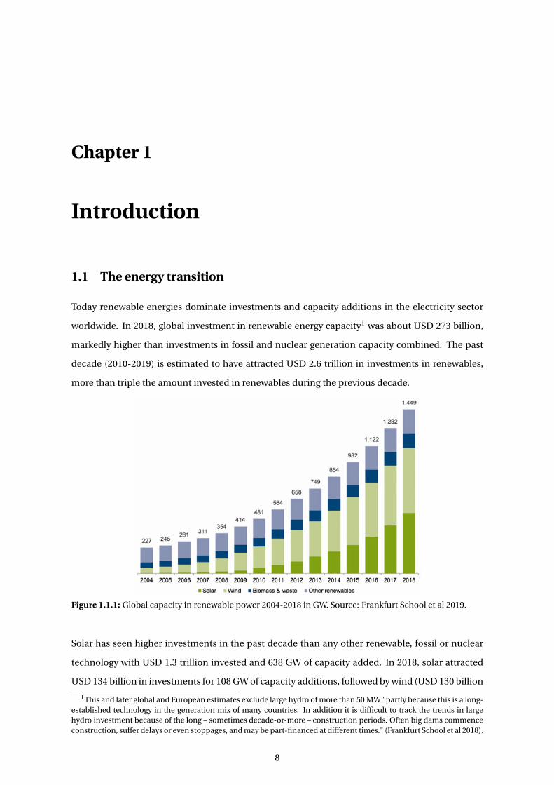
Today renewable energies dominate investments and capacity additions in the electricity sector
worldwide. In 2018, global investment in renewable energy capacity1 was about USD 273 billion,
markedly higher than investments in fossil and nuclear generation capacity combined. The past
decade (2010-2019) is estimated to have attracted USD 2.6 trillion in investments in renewables,
more than triple the amount invested in renewables during the previous decade.
Figure 1.1.1: Global capacity in renewable power 2004-2018 in GW. Source: Frankfurt School et al 2019.
Solar has seen higher investments in the past decade than any other renewable, fossil or nuclear
technology with USD 1.3 trillion invested and 638 GW of capacity added. In 2018, solar attracted
USD 134 billion in investments for 108 GW of capacity additions, followed by wind (USD 130 billion
1This and later global and European estimates exclude large hydro of more than 50 MW "partly because this is a long-established technology in the generation mix of many countries. In addition it is difficult to track the trends in largehydro investment because of the long – sometimes decade-or-more – construction periods. Often big dams commenceconstruction, suffer delays or even stoppages, and may be part-financed at different times." (Frankfurt School et al 2018).
8

CHAPTER 1. INTRODUCTION
for 50 GW) and gas-fired generation (USD 49 billion for 42 GW). This has led to a steep upwards
curve in capacity provided by renewable power (figure 1.1.1).
In 2010 only 6.1% of global power generation and 10.2% of global power capacity was provided
by renewables, figures that both more than doubled during the past decade (Frankfurt School et
al 2019, IEA 2019). Cost reductions played an important role in this transition: levelized cost of
electricity from solar photovoltaics came down by 81%, from onshore wind by 46% and from off-
shore wind by 44%, making renewable technologies today the cheapest option for new generation
in many locations (Frankfurt School et al 2019).
This thesis focuses on Germany, as the country has long been at the forefront of the power sector’s
transition to renewables globally. The German government adopted grid priority and 20-year fixed
tariffs differentiated by renewable energy technology as early as 2000. As a result, renewable elec-
tricity capacity was at 49.4% and generation at 32.5% in 2018,2 up from 2% generation in 20003 and
more than double the global average numbers of 21.0% and 12.9% (figure 1.1.2).
Figure 1.1.2: Gross electricty production from different technologies in Germany. Source: Own illustrationbased on BDEW 2019.
At the same time, Germany embarked on an exit from nuclear energy, a technology that is largely
emissions-free but was regarded as risky by large parts of the German population and turned out
to be difficult to value in terms of decommissioning and storage costs. Germany’s reduction in
electricity generation from nuclear and hard coal was balanced out by the increase in renewables.
2German estimates are conservative as they do not include any small- or large-scale hydro, while global numbers onlyexclude large-scale hydro.
3The share of renewable power capacity in Germany is not available before 2008.
9

CHAPTER 1. INTRODUCTION
However, lignite generation - the most climate-damaging technology - remained largely stable,
while gas-fired generation showed a long-term increasing, although at times volatile, trend leading
to only slowly decreasing greenhouse gas emissions (figure 1.1.2).
The revolution in the electricity sector in Germany was accompanied by heavy impacts on incum-
bent electric utilities and a radical change in the investor landscape. This change is described in
more detail in section 1.4.
1.2 Motivation of this thesis
Germany’s power sector investor landscape has fundamentally changed in the past years, as will
be described in more detail in section 1.4. The goal of this PhD thesis is to better understand the
impact of the energy transition on different types of investors in the power sector.
Why do we care to know what the impacts of a changing power sector are on investors?
Gas-fired power generation capacity is widely praised as a relatively low-carbon transition tech-
nology, because it could, due to its ramping flexibility, also deal with a rising share of weather-
fluctuating wind and solar in the grid. Yet, in Germany the increase of renewables came with a
ramp-down of gas-fired power plants due to investors’ reaction to depressed power prices - partly
a result of the energy transition.
The big four German incumbent utilities were taken by surprise by the energy transition, lost mar-
ket share and in 2015 faced the risk of bankruptcy. Being still responsible for a third of German
power generation capacity, policy makers feared that a default of a big utility posed a systemic risk
to the energy sector with major implications for the German economy as a whole.
Financial and institutional investors, on the other hand, have increasingly invested in the operating
phase of renewable energy assets. With the market getting more competitive and governments
wanting to phase out policy support, it is now crucial for both investors and policy makers to better
understand the key risk factors of investing in energy assets. Only if financial investors’ needs are
thoroughly understood and taken into account when devising new policies, can this major new
source of low-cost capital be tapped in order to reach ambitious renewable energy deployment
and climate goals.
For these reasons, this thesis seeks to understand the behaviour and needs of private investors in
the energy sector and to explore lessons learned in Germany that are applicable to other countries
on a similar path away from nuclear and fossils to more renewable electricity sources.
10

CHAPTER 1. INTRODUCTION
1.3 Contribution to the literature
This thesis is part of the energy finance literature analysing investments in the electricity sector.
A growing number of research articles are dedicated to the impact of the energy transition on in-
vestment and investor behaviour. However, most research to date is grounded in techno-economic
modelling (e.g. Santos et al 2017; Hirth 2018), management science (e.g. Frei et al 2018; Ossenbrink
et al 2019), innovation theory (e.g. Egli et al 2018; Mazzucato and Semienuk 2018) or sociology (e.g.
Kungl and Geels 2018). Only a modest but growing body of literature analyses power sector invest-
ment relying on finance theory (e.g. Sen and Schickfus 2017; Steffen 2018), methodologies (e.g.
Kitzing et al 2017; Vargas and Chesney 2018) or addressing core finance questions (e.g. Salm and
Wüstenhagen 2018; Schmidt et al 2019).
The thesis contributes to this body of literature by building on various theories and methodologies
from finance research. Chapter 2 uses the real options modelling approach from finance to inves-
tigate the impact of low power prices on operators of gas-fired power plants. Chapter 3 investigates
the corporate restructurings by two main German utilities drawing on the divestiture literature and
also makes a modest conceptual contribution to this field of corporate finance. Chapter 4 employs
the well-known discounted cash-flow model from corporate finance to analyse the impacts of dif-
ferent risk factors on a financial investor’s wind park portfolio.
1.4 Background:
Germany’s power market investor landscape is changing
Two main developments can be observed in the German power sector investor landscape in the
past years. The first concerns the retreat of traditional utilities (section 1.4.1) and the second the
advent of new investor types (section 1.4.2).
1.4.1 Traditional utilities retreat
The four main German utilities - EON, RWE, EnBW and Vattenfall - had dominated the power sector
since the liberalisation of electricity markets in the late 1990s.
They came late, however, to the renewables boom. Between 2009 and 2015,4 they more than dou-
bled the share of renewables in their overall portfolio, from 3.0% to 6.8% on average. But in Ger-
many overall, renewables’ share of total power generation capacity had almost doubled from an
already much higher base in the same time frame: from 27.1% to 45.0%. Utilities’ investments did
not catch up with the overall German trend towards renewables already under way. The four utili-
4In 2016, Vattenfall sold its German lignite operations and EON and RWE underwent large restructurings, which areanalysed in chapter 3. Therefore, market shares from 2016 are no longer comparable to previous years.
11
CHAPTER 1. INTRODUCTION
ties’ share of total German renewable capacity stayed roughly stable at around 5.0% between 2009
and 2015 (figure 1.4.1a).
Since electricity production from fossil fuels and nuclear energy starkly decreased and renewables
were the only growth sector (figure 1.1.2), the big four utilities lost market share overall. Between
2009 and 2015, their contribution to total German power generation capacity fell from 57% to 34%
(figure 1.4.1b).
Why did utilities not invest in renewable energies more pro-actively and thereby secured their mar-
ket share in a transforming power sector?
The reasons for this are manifold, some of which are examined in this thesis. First, utilities’ expe-
rience in fossil fuel and nuclear assets was not directly applicable to renewables. Wind and solar
assets are much smaller and more decentralised. Second, in the early 2000s, high power prices
meant that conventional power plants offered higher returns compared to the governmental feed-
in tariffs for renewables. This topic is discussed in chapter 3.5
In the late 2000s, low electricity prices in Europe - and particularly in Germany - led to low profits
for conventional power plant operators. Utilities had to ramp down and in some cases mothball the
power plants with highest marginal costs in order to limit their losses. In the case of Germany, these
were mainly the relatively climate-friendly gas-fired assets, a development which is illustrated in
chapter 2. Losses at utilities’ conventional generation segments meant less capital expenditure
available for renewables. On top of this, German utilities also suffered from the nuclear exit. This
is examined in chapter 3.
Both chapters 2 and 3 shed light on the fate of existing power plant operators during the German
energy transition. Lessons learned could be applied more broadly beyond Germany, as utilities all
over Europe to a certain extent face these same problems (Annex and Typoltova 2018).
5For retail investors, the opposite was the case: small assets suited their small amounts of capital available to invest; atthe same time, feed-in tariffs offered attractive returns compared to alternative investments available to retail investors.
12

CHAPTER 1. INTRODUCTION
(a) Overall and big four utilities’ share of renewable generation capacity in Germany.
(b) Big four utilities’ share of German generation capacity.
Figure 1.4.1: Big four utilities’ role in German power generation capacity. Source: Own illustration based onannual reports of EON, RWE, EnBW, Vattenfall 2005-2019; BMWi 2018; Bundesnetzagentur 2019.
13

CHAPTER 1. INTRODUCTION
1.4.2 New investors come in
Who took the utilities’ place as dominant power plant investors and asset owners in the growing
renewables market? In Germany, these were mainly retail investors (31.5% of renewable generation
assets in 2016), project developers (14.4%), financial investors like banks and funds, and industrials
(each 13.4%) (see figure 1.4.2).
Figure 1.4.2: Owners of renewable energy assets in MW in Germany in 2016. Source: trend:research 2017.
Whereas project developers specialise in building renewable power plants and often sell them on
to other investors after construction (Hostert 2016), the other investor types usually hold the assets
longer-term, sometimes over their entire operational life of more than 20 years. Distressed utilities
also discovered the build-sell-operate model as a way to recycle funds and generate profits by sell-
ing early-stage renewable assets to institutional investors (McCrone 2017). This explains the high
share of financial investors in Germany, who usually do not develop projects themselves but enter
after construction.
Looking at Europe, institutional investors like pension funds and insurance companies committed
a growing amount to renewable energy projects in the past years. Their investments hit a record in
20176 of USD 9.9 billion, up 42% on 2016. Growth can especially be noted in direct investments,
project bonds and private equity funds (figure 1.4.3).7
In summary, one can observe a growing interest by institutional investors in European renew-
able energy private equity assets. Chapter 4 focuses on an institutional investor’s point of view
by analysing risk factors during a wind power plant acquisition.
62018 numbers are not available.7The data excludes the sale of equity by companies that not only invest in renewables, e.g. utilities. However, as
the previous section showed, at least in Germany the big utilities were slow at investing in renewables. And becausenon-utilities often finance renewable assets not on balance sheet but via special purpose vehicles (Steffen 2018), thegraph might indicate a general trend towards private equity and project bonds in order to gain exposure to the growingrenewables market.
14

CHAPTER 1. INTRODUCTION
Figure 1.4.3: Institutional investor commitments to European renewable energy projects in USD billion.Source: Frankfurt School et al 2018.
What are the reasons for institutional investment in the growing renewables sector? First, renew-
able energy assets have some inherent qualities that make them attractive to institutional investors.
They have comparatively low operational risk: solar and wind power plants, unlike nuclear or fossil
fuel ones, carry no fuel price risk. Once built the main risk factors are weather variability and power
prices (Awerbuch 2000).
Second, many European countries decided to cancel out power price risk altogether by providing
up to 20 years fixed remuneration for each kilowatt-hour produced, the so-called feed-in tariffs
(FiT). These suited institutional investors’ preference for low-risk assets that have stable long-term
cash-flows and a low correlation with the market (Ernst & Young 2014; Allianz 2017).
Third, high levels of liquidity in financial markets since the 2008 crisis pushed international inter-
est rates and bond yields to record lows. This forced institutional investors to look at alternative
investments, among those renewables (Gatzert and Kosub 2016; Annex and Typoltova 2018). A
major European utility’s CEO recently said that low interest rates were a major reason why utilities
could sell renewable assets to institutional investors at a profit (Collins and McCrone 2018).
A fourth reason for institutional investors’ interest in renewables might also be the recent public
pressure to increase their portfolio’s sustainability scores (McCrone 2017, also examined in chapter
3).
Overall, renewable energies developed into an attractive market for institutional investors. In re-
cent years, however, competition increased as the market professionalized and governments be-
gun to introduce renewable capacity auctions in order to cap capacity built and slowly expose re-
newables to more price risk. As a result, equity return expectations have fallen across Europe (Met-
calfe 2019). Institutional investors therefore have to model their risk exposure in renewable energy
assets more thoroughly, a topic explored in chapter 4.
15
CHAPTER 1. INTRODUCTION
1.5 Summary of research methods, results and contribution
This section summarizes research methods, results, contribution to the academic literature and
policy discussions of the three papers that constitute the main chapters (2-4) of this thesis.
1.5.1 The value of gas-fired power plants in markets with high shares of renewable en-
ergy - A real options application
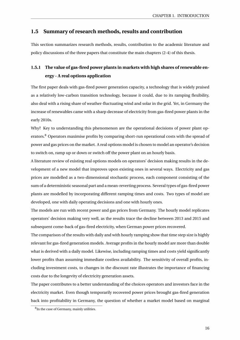
The first paper deals with gas-fired power generation capacity, a technology that is widely praised
as a relatively low-carbon transition technology, because it could, due to its ramping flexibility,
also deal with a rising share of weather-fluctuating wind and solar in the grid. Yet, in Germany the
increase of renewables came with a sharp decrease of electricity from gas-fired power plants in the
early 2010s.
Why? Key to understanding this phenomenon are the operational decisions of power plant op-
erators.8 Operators maximise profits by comparing short-run operational costs with the spread of
power and gas prices on the market. A real options model is chosen to model an operator’s decision
to switch on, ramp up or down or switch off the power plant on an hourly basis.
A literature review of existing real options models on operators’ decision making results in the de-
velopment of a new model that improves upon existing ones in several ways. Electricity and gas
prices are modelled as a two-dimensional stochastic process, each component consisting of the
sum of a deterministic seasonal part and a mean-reverting process. Several types of gas-fired power
plants are modelled by incorporating different ramping times and costs. Two types of model are
developed, one with daily operating decisions and one with hourly ones.
The models are run with recent power and gas prices from Germany. The hourly model replicates
operators’ decision making very well, as the results trace the decline between 2013 and 2015 and
subsequent come-back of gas-fired electricity, when German power prices recovered.
The comparison of the results with daily and with hourly ramping show that time step size is highly
relevant for gas-fired generation models. Average profits in the hourly model are more than double
what is derived with a daily model. Likewise, including ramping times and costs yield significantly
lower profits than assuming immediate costless availability. The sensitivity of overall profits, in-
cluding investment costs, to changes in the discount rate illustrates the importance of financing
costs due to the longevity of electricity generation assets.
The paper contributes to a better understanding of the choices operators and investors face in the
electricity market. Even though temporarily recovered power prices brought gas-fired generation
back into profitability in Germany, the question of whether a market model based on marginal
8In the case of Germany, mainly utilities.
16

CHAPTER 1. INTRODUCTION
costs sufficiently incentivises low-carbon power generation, is still highly relevant to the energy
transition across Europe.
1.5.2 Utility divestitures in Germany - A case study of corporate financial strategies
and energy transition risk
In recent years, the two biggest German electric utilities, EON and RWE, had the most difficult
times of their history. From 2011 to 2015 they each wrote off more than 13% of their book asset
value and lost between 70% (EON) and 80% (RWE) of their market capitalisation. EON and RWE,
until then integrated firms spanning the whole energy value chain, responded with two of the most
dramatic restructuring moves in recent German corporate history and in the history of privately-
run European utilities as a whole. EON spun off its fossil fuel and trading segments, while RWE
carved out its renewable energy, retail and grid business.
Why did EON and RWE divest? While the firms themselves argued that the restructurings would
bring about a large array of benefits, encompassing all possible advantages ever discussed in the
context of divestitures, this second paper critically assesses different hypotheses from the corpo-
rate finance literature and establishes the main reasons responsible for the decisions.
A literature review first identifies four possible types of drivers for divestitures: operations and
management, investing, financing and investor preferences. These drivers are then tested in the
empirical case of the EON and RWE divestitures of 2016. A mixed methods approach is used: com-
parative descriptive statistics using a control group of European listed utilities; interviews with
EON and RWE staff and management, analysts, journalists and academics; gray literature like an-
nual reports, investor presentations and newspaper articles; and several event studies examining
the effect of news items on EON’s and RWE’s share price and stocks traded.
The combination of methods converges in rejecting drivers related to operations, management and
investing. The drivers related to investor preferences cannot sufficiently be distinguished from risk
contamination.
The analysis supports debt overhang as a driver, since EON and RWE accumulated higher liabil-
ities than their peers due to provisions for nuclear dismantling and storage. There is also strong
evidence for risk contamination based on the firms’ and subsidiaries’ valuations pre- and post-
divestiture, a share price event study and interviews. Likely sources of risk contamination are ex-
pected losses by fossil fuel-fired power plants and the acute risk of unmanageably high nuclear
dismantling and especially storage costs linked to the German nuclear exit.
Utilities appear to have restructured to avoid further risk contamination of their healthy assets
(renewables and grid infrastructure) by the conventional power generation business (fossil fuel
and nuclear plants). Already weakened from record losses in their fossil fuel powered generation
17

CHAPTER 1. INTRODUCTION
fleet due to low electricity prices, after 2011 the nuclear exit emerged as an additional challenge to
the utilities. Investors doubted the adequacy of utilities provisions for decommissioning nuclear
power plants and storing toxic waste, and feared major cost increases for which the utilities would
be unlimitedly liable.
The paper uses existing research on divestitures in an empirical case that has implications for the
evolution of European power markets. The results suggest that exiting conventional technologies
as part of the transition to a more renewable energy mix can have substantial costs. If these are not
clarified and allocated ex ante, policy makers find themselves forced to either burden tax payers or
endanger utilities that are of systemic relevance to the energy sector.
1.5.3 The impact of production and macroeconomic risk on wind power equity re-
turns - An analysis from a financial investor’s perspective
Financial investors play an increasing role in the operational phase of renewable energy assets. In
recent years, with substantial experience gained in construction, management and financing of
renewable energy, the sector matured and competition between investors increased. Moreover,
in Germany the first wind farms are approaching the end of their guaranteed feed-in tariff (FiT)
period of 20 years, exposing operators to market price risk.
As a result, project evaluation techniques are maturing as well. In a competitive environment, asset
managers have to accurately model asset returns in order to be able to offer a competitive price to
project developers. On the other hand, they should not overpay for an asset and thereby impair
their shareholders’ returns. In this context, it is critical for industry investors to understand the
sensitivity of equity returns to variations in production and macroeconomic factors.
In this last paper, four sources of risk for a wind park operator are examined. First, realised produc-
tion in kilowatt-hours (kWh) is the biggest factor of uncertainty for any wind park. Second, for wind
parks in Germany, market power prices are important after the guaranteed FiT period of 20 years.
Third, inflation plays a role for power prices as well as operating costs, which are partly indexed.
Fourth, after the end of the fixed interest period of their long-term loans, wind parks are exposed
to interest rate risk. A discounted cash-flow model is used to examine how variations in these four
risk factors impact equity returns.
The results show that, among the four risk factors, uncertainty in energy production has the highest
impact on shareholder payouts, while power prices and the resulting market values of wind power
have the second highest impact. Greater production or power prices ceteris paribus lead to greater
revenues and thereby shareholder returns.
Inflation has a medium and generally positive impact on equity payout returns. A "bath tub curve"
with the lowest return somewhere near the median can be observed for wind parks that opt to stay
18
CHAPTER 1. INTRODUCTION
in the FiT for a long time. In this case there is no downside risk of inflation, as both lower and higher
than expected inflation yields higher than expected returns. For wind parks operating mainly on
the free market, on the other hand, low inflation yields a comparably low return as revenue losses
due to lower than expected inflation are higher than opex savings.
Interest rates have a negative but small impact on shareholder payouts due to the relatively long
fixation of interest rates for bank loans of 10 to 20 years. Interest rate risk is likely to rise, however,
as loan tenors might shorten with the future reduction or phase-out of FiTs.
This last paper contributes to the energy economics and finance literature by presenting a financial
investor perspective on production and macroeconomic risk in wind energy. Several strategies
to partly mitigate the identified risks are suggested. To policy makers, the results offer a deeper
understanding of equity investors’ needs in order to harvest their available capital for reaching
renewable energy targets. This understanding is crucial if policy makers want to reach climate
targets while at the same time phasing out renewable energy policy support.
1.6 Summary and research outlook
This thesis contributes to the energy finance literature by investigating what the energy transition
means for different investors in the German power sector.
It analyses the decision making of power plant operators and shows that low power prices - partly
caused by renewable energies - might unintentionally push out flexible low-carbon generation
first.
Using the case of the nuclear phase-out in Germany, the thesis demonstrated that the exit from
a conventional technology might burden tax payers or endanger systemically relevant utilities, if
conventional technology costs are not fully internalised early enough.
Finally, the thesis tests the sensitivity of an institutional investor’s equity returns to variations in
production and macroeconomic developments. It shows that in a market still largely shielded off
from market price risk by 20-year guaranteed tariffs, shareholder returns strongly depend on power
prices.
The thesis opens up many more research avenues. Concerning chapter 2, the question arises of
whether "energy-only" markets, where power generation capacity is built and deployed mainly
according to price setting mechanisms on the wholesale electricity exchange, lead to the right in-
vestment incentives in the long term.
Not only transition technologies like gas, with comparatively high marginal costs, might suffer.
As solar and wind plants have very low marginal costs, a higher share of renewables overall leads
to lower wholesale power prices. In addition, due to similar weather patterns across one region,
19
CHAPTER 1. INTRODUCTION
wind and solar generation is strongly auto-correlated. Renewables’ profitability might therefore
cannibalise itself over time by causing very low wholesale prices precisely when a lot of renewable
electricity is produced. Future research could devise an efficient power market design that ensures
sufficient investment in renewable generation, electricity storage and demand-side measures to
ensure a reliable and affordable electricity supply.
Regarding chapter 3, further research might look into how other sectors or sub-sectors can benefit
from experiences like the German nuclear exit. The findings might be applied to coal mining and
coal-fired power generation, a sector that the German government recently decided to phase-out
as well. Another interesting case is mobility and the transformation of the market for combustion
engines towards alternative engines and approaches to mobility.
Applied research in this field can devise realistic cost estimates for technology exit costs in each
case and evaluate who would efficiently incur those. One the one hand, the principle should be
"polluter pays". On the other hand, some regions or industries might be systemically relevant for
an economy and - while future incentives should be structured in a fair way - it might sometimes
be cost-effective to bail out certain regions or industries in order to make them ready for the chal-
lenges of a renewable future.
A related field of research could quantify the systemic risk present in the energy sector by devising
methodologies and measures to conduct stress tests. This has already been done in finance re-
search regarding the effect of interconnections among financial actors in the aftermath of the 2008
crisis and regarding the impact of climate risk on the financial system. A similar approach to the
energy sector, with a stress test measuring the consequences of different transition scenarios on
incumbent investors could be useful to derive low-cost policy recommendations.
As regards chapter 4, a question arising from the model is how both project developers and insti-
tutional investors will be able to earn their cost of capital in renewable energy markets with less or
no policy support. What is the impact of the renewables market’s transition from state-guaranteed
FiTs to privately negotiated power purchase agreements (PPAs) between producers and corporate
consumers? PPAs are long-term as well, but recent experience has shown that they are generally
entered into for only five to 15 years, offering therefore a shorter hedge with more exposure to price
risk. In addition, counter-party risk is higher than in the case of state-guaranteed tariffs.
Applied research can play an important role in examining the impact of PPAs on shareholder re-
turns via increased power price and counter-party risk and a change in interest rates and loan
tenures. Possible decreases in margins earned by manufacturers to power traders along the value
chain also have to be taken into account. If policy makers want to completely phase out policy
support to renewables while not losing institutional investors’ available capital in order to reach
ambitious renewable energy targets, further research in this field is crucial.
20

CHAPTER 1. INTRODUCTION
1.7 Bibliography
Allianz (2017): Renewable Energy – A real-asset alternative for institutions seeking growth, yield
and low correlation, Allianz Global Investors.
Annex M. and Typoltova J. (2018): Changing Business Models for European Renewable Energy.
Presentation at BNEF-Hawthorn Club Event.
Awerbuch S. (2000): Investing in photovoltaics: risk, accounting and the value of new technology.
Energy Policy 28, pp. 1023-1035.
BDEW (2019): BRD Stromerzeugung 1990-2018. Bundesverband der Energie- und Wasser-
wirtschaft.
BMWi (2018): Datenübersicht zum zweiten Monitoringbericht "Energie der Zukunft". Bundemi-
nisterium für Wirtschaft und Energie.
BNEF (2019): Clean Energy Investment Trends 2018. Bloomberg New Energy Finance.
Bundesnetzagentur (2019): Kraftwerksliste 2019(1), Bundesnetzagentur.
Collins B. and McCrone A. (2018): Low Interest Rates Key to Enel Renewables Investment Model:
BNEF. Bloomberg New Energy Finance Shorts.
Egli F., Steffen S. and Schmidt T. (2018): A dynamic analysis of financing conditions for renewable
energy technologies. Nature Energy (3), pp. 1084-1092.
EnBW (2005-2019): Annual reports.
EON (2005-2019): Annual reports.
Ernst & Young (2014): Renewable energy assets – An interesting investment proposition for
European insurers, Ernst and Young.
Frankfurt School, UNEP Centre, BNEF (2018): Global Trends in Renewable Energy Investment
2018.
21

CHAPTER 1. INTRODUCTION
Frankfurt School, UNEP Centre, BNEF (2019): Global Trends in Renewable Energy Investment
2019.
Frei F., Sinsel S., Hanafy A. and Hoppmann J. (2018): Leaders or laggards? The evolution of electric
utilities’ business portfolios during the energy transition, Energy Policy 120, 655-665.
Gatzert N. and Kosub T. (2016): Risks and risk management of renewable energy projects: The case
of onshore and offshore wind parks. Renewable and Sustainable Energy Reviews(60), pp. 982-998.
Hach D. and Spinler S. (2014): Capacity Payment Impact on Gas-Fired Generation Investments
under Rising Renewable Feed-In – A Real Options Analysis. Energy Economics (53), pp. 270-280.
Hirth L. (2018): What Caused the Drop in European Electricity Prices? A factor decomposition
analysis. The Energy Journal, International Association for Energy Economics (1).
Hostert D. (2016): Portfolio Hunters 2015-16: European Wind. Bloomberg New Energy Finance.
IEA (2019): World Energy Investment 2019. International Energy Agency.
Kitzing L., Juul N., Drud M. and Boomsma T.K. (2017): A real options approach to analyse wind
energy investments under different support schemes. Applied Energy (188), pp. 83-96.
Kungl G. and Geels F. W. (2018): Sequence and alignment of external pressures in industry desta-
bilisation: Understanding the downfall of incumbent utilities in the German energy transition
(1998–2015), Environmental Innovation and Societal Transitions 26, 78–100.
Mazzucato M. and Semienuk G. (2018): Financing renewable energy: Who is financing what and
why it matters. Technological Forecasting & Social Change (127), pp. 8-22.
McCrone A. (2017): Utilities discover joy of selling assets to institutional investors. Bloomberg New
Energy Finance EMEA Research Note.
Metcalfe O. (2019): Institutional Investors Seek Value In Europe’s Wind Energy: BNEF. Bloomberg
New Energy Finance Shorts.
22

CHAPTER 1. INTRODUCTION
Ossenbrink J., Hoppmann J. and Hoffmann V. (2019): Hybrid Ambidexterity: How the Environment
Shapes Incumbents’ Use of Structural and Contextual Approaches. Organization Science (30), pp.
1319–1348.
RWE (2005-2019): Annual reports.
Salm S. and Wüstenhagen R. (2018): Dream team or strange bedfellows? Complementarities
and differences between incumbent energy companies and institutional investors in Swiss
hydropower. Energy Policy (121, C), pp. 476-487.
Santos S.F., Fitiwi D.Z., Bizuayehu A.W., Shafie-khah M., Asensio M., Contreras J., Cabrita C. and
Catalao J. (2017): Impacts of Operational Variability and Uncertainty on Distributed Generation
Investment Planning: A Comprehensive Sensitivity Analysis. IEEE transactions on sustainable
energy (8.2), pp. 855-869.
Schmidt T.S., Steffen B., Egli F., Pahle M., Tietjen O. and Edenhofer O. (2019): Adverse effects of
rising interest rates on sustainable energy transitions. Nature Sustainability (2), pp. 879-885.
Sen S. and von Schickfus M.-T. (2017): Will Assets be Stranded or Bailed Out? Expectations of
Investors in the Face of Climate Policy, ifo working papers 238.
Steffen B. (2018): The importance of project finance for renewable energy projects. Energy
Economics(69), pp. 280-294.
trend:research (2017): Eigentümerstruktur: Erneuerbare Energien. Entwicklung der Ak-
teursvielfalt, Rolle der Energieversorger, Ausblick bis 2020. Kurzstudie.
Vargas C. and Chesney M. (2018): What are you waiting to invest? Long-term investment in
grid-connected residential solar energy in California. A real options analysis, working paper
available at SSRN: ❤tt♣✿✴✴❞①✳❞♦✐✳♦r❣✴✶✵✳✷✶✸✾✴ssr♥✳✸✷✸✶✾✽✹.
Vattenfall (2005-2019): Annual reports.
23

Chapter 2
The value of gas-fired power plants in
markets with high shares of renewable
energy
A real options application
A version of this chapter was published in the journal Energy Economics (81), pp. 1078-1098, in June 2019.
Abstract
Using a real options model, this paper quantifies a gas-fired power plant’s operating value
and the value of a new investment against the background of a market transition to renewable
electricity. The model is run with recent data for Germany’s power sector and for different types
of gas-fired power plants.
The result is twofold. First, the paper achieves a more realistic value by improving on ex-
isting models: it models electricity and gas prices as a two-dimensional stochastic process,
each component consisting of the sum of a seasonal pattern and a mean-reverting process; it
uses high granularity by modelling hourly time-steps; and it incorporates power plant ramping
times and costs. Second, it compares two types of power plant models, one with daily and one
with hourly operating decisions, and thereby quantifies the value of a plant’s intraday flexibil-
ity. The hourly model replicates operators’ and investors’ decision making accurately. This is
evidenced by the fact that the results trace current major developments like the recent decline
and come-back of gas-fired generation in Germany.
The paper contributes to a better understanding of the choices operators and investors face
in current electricity markets. In the absence of large scale storage solutions flexible supply of
electricity, as provided by gas, is important in the transition to renewable energies in Germany
and across Europe.
Key words— Real options; electricity; investment; gas-fired generation; energy transition.
24
CHAPTER 2. THE VALUE OF GAS-FIRED POWER PLANTS IN MARKETS WITH HIGH SHARES OFRENEWABLE ENERGY
2.1 Introduction
In Germany, the share of renewable energy in the power mix has increased rapidly in the past years:
from 6 % renewable electricity generated in 2000 to around a third in 2017. As renewables do not
have to pay for fuel, these energy sources produce power at very low marginal cost once power
plants have been built. The increasing share of renewables, together with a range of other factors
- low European emissions certificate and coal prices, the economic crisis - led to German power
prices falling from above 50 Euros per megawatt hour (EUR/MWh) in the mid-2000s to record lows
of below 30 EUR/MWh by 2016. While researchers disagree on the exact contribution of different
price drivers, there is general agreement that in markets with little storage and dominated by re-
newables, low power prices could create a difficult environment for power sources with relatively
high marginal cost, such as natural gas (Everts et al 2016; Bublitz et al 2017; Hirth 2018).
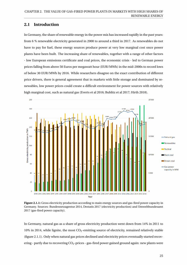
Figure 2.1.1: Gross electricity production according to main energy sources and gas-fired power capacity inGermany. Sources: Bundesnetzagentur 2014, Destatis 2017 (electricity production) and Umweltbundesamt2017 (gas-fired power capacity).
In Germany, natural gas as a share of gross electricity production went down from 14% in 2011 to
10% in 2014, while lignite, the most CO2-emitting source of electricity, remained relatively stable
(figure 2.1.1). Only when natural gas prices declined and electricity prices eventually started recov-
ering - partly due to recovering CO2-prices - gas-fired power gained ground again: new plants were
25

CHAPTER 2. THE VALUE OF GAS-FIRED POWER PLANTS IN MARKETS WITH HIGH SHARES OFRENEWABLE ENERGY
commissioned and production increased to 12% in 2016 (Bundesnetzagentur 2014; Destatis 2017).
Natural gas has two advantages as opposed to coal, Germany’s other main fossil source of electric-
ity: relatively low greenhouse gas emissions and high production flexibility. Gas-fired power plants
can balance fluctuating wind and solar in-feed in the absence of affordable storage technologies or
demand side management. Some experts hence call for keeping stable or even increasing gas-fired
generation as a part of the energy mix at least in the mid-term (Graichen and Redl 2014).
This paper shows that existing academic models fail to adequately model the competitiveness of
gas-fired power plants in markets with low power prices. By modelling only daily and not hourly
operating decisions and by neglecting ramping times and costs, these models on the one hand
under- and on the other hand over-estimate the value of gas-fired generation.
Using a real options model, this paper better quantifies a gas-fired power plant’s operating value
as well as the value of an investment in a new plant against the background of an energy market
in transition to renewable energies. The model is run with recent data for Germany’s power sector
and for different types of gas-fired power plants.
The goal of this paper is twofold. First, the paper achieves a more realistic value by improving on
existing option models in several ways: it models electricity and gas prices as a two-dimensional
stochastic process, each component consisting of the sum of a seasonal pattern and a mean-
reverting process; it uses higher granularity by modelling hourly time-steps; and it incorporates
power plant ramping times and costs. Second, it compares two types of power plant models, one
with daily and one with hourly operating decisions, and quantifies the value of a plant’s intraday
flexibility. The hourly model replicates operators’ and investors’ decision making accurately. This
is evidenced by the fact that the results trace current major developments like the recent decline
and come-back of gas-fired power in Germany.
The paper contributes to a better understanding of the choices operators and investors face in cur-
rent electricity markets. In the absence of large scale storage solutions flexible supply of electricity,
as provided by gas, is important in the transition to renewable energies in Germany and across
Europe.
The paper uniquely focuses on electricity spot markets and, for simplicity, abstracts away from
interactions with ancillary services. Ancillary services consist of a variety of operations beyond
generation and transmission that are required to maintain grid stability and security. In light of an
increase in intermittent renewable energy, this is an interesting area for further research outlined
in the last section.
The paper is structured as follows. Section 2.2 gives an overview of the literature and defines the
specific contribution of this paper. Section 2.3 lays out how electricity and gas prices are modelled.
Section 2.4 explains the power plant model. Section 2.5 presents and discusses the results. Section
26

CHAPTER 2. THE VALUE OF GAS-FIRED POWER PLANTS IN MARKETS WITH HIGH SHARES OFRENEWABLE ENERGY
2.6 draws conclusions and section 2.7 gives ideas for further research and an outlook into the future
of gas-fired generation in Germany.
2.2 Literature and contribution
2.2.1 From net present value to real option
Net present value (NPV) models are common in academia and practice to determine the prof-
itability of investment decisions. While their simplicity is attractive, simplifying assumptions lead
to problems: NPV models can only give yes-or-no investment advice, excluding the possibility to
react strategically when risk resolves over time, thereby seriously undervaluing investment oppor-
tunities (Mei et al 2012). When using NPV approaches for valuing operating assets such as power
plants, commodity prices have to be taken as deterministic and the operator has to fix an operat-
ing schedule beforehand without being able to react to changing prices. To counter this problem,
NPV models are often used with several different price scenarios. Even though undervaluation can
partly be alleviated in this way, the assignment of probabilities to different price paths remains
arbitrary (Hsu 1998; Frayer and Uludere 2001).
Real option models take a different approach. Stewart Myers first coined the term Real Option
in 1977 by applying option pricing theory to the valuation of non-financial growth opportunities
(Myers 1977). In the late 1990s, we find first articles on the valuation of flexible power plants, where
the operating decision of switching the plant on and off is depicted as a call option. The paper
builds on this research.
Real options models explicitly estimate price trend and volatility from the data and thereby address
arbitrariness. They give investors the possibility to alter their investment decision in light of evolv-
ing prices. In the case of operating assets such as power plants, operators are given the possibility
to adapt production at specific points in time, that is by exercising their real option to produce and
sell electricity. In this paper, the operator can decide – every day in the first model and every hour
in the second - if the plant should buy gas in order to produce and sell electricity. The value of
the power plant and thus its profitability is equal to the sum of call option values on the spread
between electricity and gas prices over the plant’s lifetime. To bring the model closer to reality,
technical restrictions are also modelled, such as time and money spent to start and ramp up the
plant.
While base load power plants, e.g. nuclear and coal, have to be operated pretty much throughout
the year to be profitable, flexibility in production is very important for gas-fired power plants: as
they ramp the fastest among all power plants and are often operated as peakers, that is only during
some hours of the day, a large part of their value stems from price fluctuation and the operator’s
27

CHAPTER 2. THE VALUE OF GAS-FIRED POWER PLANTS IN MARKETS WITH HIGH SHARES OFRENEWABLE ENERGY
flexibility (Hsu 1998; Frayer and Uludere 2001; Fraser 2003; Fleten and Näsäkkälä 2009).
2.2.2 Option to operate in the literature
Table 2.1 provides an overview of the different model features in the literature. Features that were
judged decisive for the choice of the modelling techniques used here are marked in green in the
table.
Table 2.1: Option models of operating assets in the literature (MR = Mean Reversion, GBM = GeometricBrownian Motion, SDP = Stochastic Dynamic Programming, BS = Black and Scholes, MC = Monte Carlo).
ReferenceExchange
option
Ramping
restrictionsModel Method Application
Hsu 1998 Yes No GBM Adjusted BS Gas plant in US
Gardner, Zhuang 2000 No Yes MR SDP Hypothetical power plant
Tseng, Barz 2000 Yes Yes MR MC, SDP Hypothetical gas-fired plant
Deng et al 2001 Yes No GBM Adjusted BS Four gas-fired plants in California
Frayer, Uludere 2001 Yes No GBM Adjusted BS Gas- and coal-fired plants in US
Deng, Oren 2003 Yes Yes MRQuadrinomial,
SDPHypothetical gas-fired plant
Denton et al 2003 No Yes MR Trinomial n/a
Hahn, Dyer 2007 Yes No MR Quadrinomial Hypothetical gas/oil switching option
Tseng, Lin 2007 Yes No MR Trinomial, SDP Hypothetical gas-fired plant
Fleten, Näsäkkälä 2009 Yes No MRAnalytical, nu-
mericalGas-fired plant in Scandinavia
Hach, Spinler 2014 Yes No GBM Quadrinomial Combined cycle gas-fired plant in Germany
This paper Yes Yes MRQuadrinomial,
SDPSeveral different German gas-fired plants
This paper innovates on the existing real options literature by combining the following features:
1. The option is modelled as an exchange option with two correlated underlyings as opposed
to one. If only electricity and not gas is modelled stochastically, the plant is likely to be over-
28

CHAPTER 2. THE VALUE OF GAS-FIRED POWER PLANTS IN MARKETS WITH HIGH SHARES OFRENEWABLE ENERGY
valued if one fixes the gas price too low, or undervalued if too high. Papers that used two
underlyings are marked green in table 2.1.
2. It is generally assumed that commodity prices are mean-reverting (MR) rather than follow-
ing a Geometric Brownian Motion. The logic behind this assumption is that if a commodity
increases in price, new suppliers are attracted to the market. They increase supply, which
will lower the price until it eventually equals its long-term mean again, the marginal cost of
production. Papers that used mean-reverting prices are marked green in table 2.1.
3. This paper marries option model research with another body of literature dedicated to the
estimation of commodity spot prices (e.g. Keles et al 2012; Paraschiv et al 2015). It depicts
electricity and gas prices as a two-dimensional stochastic process, each component con-
sisting of the sum of an Ornstein-Uhlenbeck mean-reverting process and a deterministic
seasonal pattern. The way prices are modelled is not listed in table 2.1: all authors use either
only hypothetical price parameters to test their model, or they estimate parameters from
historical prices in a simplistic way without accounting for seasonalities.
4. Ramping restrictions are modelled. Ramping times and costs, e.g. the time and costs it takes
to get a power plant from zero to full production, significantly lower the value of the option.
Even though gas-fired power plants are ramping fast and cheaply compared to others, the
results of this paper show how omitting ramping restrictions would nevertheless overvalue
the plant significantly. Papers that used ramping restrictions are marked green in table 2.1.
5. Hourly granularity is modelled as opposed to daily or annual granularity implying that the
operator can exercise the option every hour. As gas plant operators can maximise profits by
adapting production on at least an hourly basis 1, this paper is more realistic than previous
work. The granularity of the models is not listed in table 2.1: all papers either used daily
or annual operating decisions. As section 2.5.4 will show, by modelling hourly granularity,
profitability increases considerably as opposed to the daily model. It is therefore clearly nec-
essary to model hourly operating decisions when analysing gas-fired power plants.
The paper’s application is similar to Hach and Spinler (2014), who analyse a combined cycle gas-
fired power plant in the current German energy market. Hach and Spinler approximate the in-
vestor’s decision with two Geometric Brownian Motions for the prices, annual operating decisions
and no restrictions regarding the ramping of the power plant. Their focus is on the option to invest,
while this paper models the option to operate and derives the value of investing via the operating
1In addition to hourly contracts, in 2014 EPEX SPOT launched auctions for 15-minute contracts on the German intra-day market (EPEX 2017).
29

CHAPTER 2. THE VALUE OF GAS-FIRED POWER PLANTS IN MARKETS WITH HIGH SHARES OFRENEWABLE ENERGY
profits. It combines the empirical approach and relevance of Hach and Spinler with a more de-
tailed operating decision model relying on Hahn and Dyer (2007) and Deng and Oren (2003). Hahn
and Dyer build a quadrinomial lattice of two correlated mean-reverting prices, which is used in this
paper, and apply it to investments in gas and oil exploration. Deng and Oren derive an equivalent,
but slightly less intuitive, quadrinomial model. On top of that, they build a power plant model us-
ing stochastic dynamic programming, which is able to depict ramping restrictions, and test it on a
hypothetical plant. A similar power plant model depicting different existing German plants is used
in this paper.
An advantage of modelling the operating decision as an option as in Deng and Oren (2003) and
Hahn and Dyer (2007) is that capacity factors, i.e. how often the plant is run (see section 2.4.4), can
be derived endogenously. The model can thereby be used, for example, in markets with different
electricity price levels and varying shares of renewable energy. Capacity factors and profitability are
affected via the observed electricity prices, without having to assume exogenous capacity factors
driving the model, as in Hach and Spinler (2014).
2.3 Electricity and gas price model
Following the commodity price literature (e.g. Keles et al 2012; Paraschiv et al 2015), electricity and
gas prices (St ,Pt ), are modelled as a two-dimensional stochastic process as described in equations
2.3.1 to 2.3.3. In accordance with the literature, electricity and gas prices are modelled separately
as opposed to modelling only one single process (St −Pt ). This enables a more realistic depiction
of seasonalities, which follow different cycles for electricity and for gas.
St = X t + g t , d X t = κX (µX −X t )d t +σX ·dWt (2.3.1)
Pt = Yt +ht , dYt = κY (µY −Yt )d t +σY ·dBt (2.3.2)
dWt dBt = ρd t (2.3.3)
Each component is assumed to be the sum of a mean-reverting Ornstein-Uhlenbeck process
({X t ,Yt ; t Ê 0}) and a deterministic seasonal part (g t ,ht ). The seasonal parts are first estimated
and removed from historical prices in section 2.3.3, thereby obtaining stochastic residue prices.
Then, using these stochastic residues, the two-dimensional stochastic process is estimated in sec-
tion 2.3.4 and modelled via a quadrinomial lattice in section 2.3.5. The estimated seasonal parts are
then added back on to the modelled stochastic process in order to use these modelled electricity
30
CHAPTER 2. THE VALUE OF GAS-FIRED POWER PLANTS IN MARKETS WITH HIGH SHARES OFRENEWABLE ENERGY
and gas prices with their respective probabilities in the power plant model in section 2.4.
A log-normal specification of the model was also tested, but did not create a sufficient fit. This is
likely due to an increasing frequency of very low and even negative prices, which are allowed on the
power exchange since 2008. Low or negative prices increasingly occur with the rise of renewables,
since at times intermittent zero-marginal cost renewable sources like wind and sun produce at
high levels and there are few profitable large-scale storage options available yet (Paraschiv et al
2014; Hirth 2018).
To test the log-normal specification, prices at or below zero have been transformed to the lowest
positive value possible at the exchange, 0.01 e /MWh, in order to take the logarithm, following
Keles et al (2012). As a high number of low prices occurred in the past few years, however, the
distribution was unduly pulled to the left by the low values leading to bad fits. Hence this approach
was deemed not suitable for recent electricity prices and the normally distributed model was used
instead.
2.3.1 Model length, number of time steps and time step size
A quadrinomial lattice approach is used, based on Hahn and Dyer (2007). This lattice is essentially
a three-dimensional binomial tree, which approaches the analytical option value by tracing the
evolution of the two underlyings in discrete time. The model length2 T is given by T = n ·△t , with
n being the number of time steps and △t the time step size.
△t , T and n have to fulfil several conditions, as described in the following. First, we choose the
time step size △t . There are real world implications that influence our choice: to model a gas-
fired power plant as an option, at least hourly time steps are desirable, because of the plant’s high
flexibility. In reality, operators maximise profits by running the plant only during peak electricity
price hours. This feature has received little attention in previous work and mostly daily time steps
have been modelled, as described in section 2.2.2. However, when both electricity and gas prices
are modelled stochastically, one encounters the problem that, while for electricity even quarter-
hourly prices exist, intraday gas prices are generally not liquid and daily prices have to be used
instead. It therefore seems that only daily granularity is feasible, because there is no hourly gas
price to match the hourly electricity price. For the estimation of seasonalities, it is acceptable to
smooth the gas price over the day to create hourly prices; for the Ornstein-Uhlenbeck parameters
in the price model, however, this is not possible, as it would lead to false volatility estimates.
To overcome this challenge, the paper follows a dual approach: seasonalities of the daily prices
are estimated and removed (section 2.3.3), then the daily Ornstein-Uhlenbeck parameters are esti-
mated (2.3.4), the stochastic parts of the daily prices are simulated (2.3.5) and the results are used
2We do not call T the maturity, but the model length or time horizon for the analysis, because the operator has theright to exercise the option at each time step.
31

CHAPTER 2. THE VALUE OF GAS-FIRED POWER PLANTS IN MARKETS WITH HIGH SHARES OFRENEWABLE ENERGY
in section 2.4 to run the daily power plant model. The results of the daily model (section 2.4.1.1) are
not satisfactory, however, as they underestimate the value of gas-fired power as described earlier.
The Ornstein-Uhlenbeck parameters estimated from the daily prices are therefore used in a power
plant model with hourly granularity, too (2.4.1.2), whereas the seasonalities are estimated from
hourly electricity prices and from daily gas prices smoothed over the day to increase the goodness
of fit (2.3.3). As △t is expressed in terms of years (△td ai l y Model = 1365 , △thour l y Model = 1
8760 ), the
same parameters received from section 2.3.4 and 2.3.5 can be used in both the daily and the hourly
model.
Second, having set △t equal to one day and one hour for the daily and hourly models respectively,
we now have to choose the model horizon T and, implied by that, the number of time steps mod-
elled in one model run n. The goal of the analysis is to receive the operating margins (or later called
operating values) and profits considering capital cost (or later called construction values) of differ-
ent power plants over their whole lifetime. The lifetime of a power plant is estimated at 32 years
following Schröder et al (2013). However, this does not imply that T necessarily has to equal 32
years. An alternative is to set T equal to a shorter time frame and sum up the results of the model
runs in the end to receive the result over the whole lifetime.
In order to properly estimate the seasonal patterns of electricity and gas prices, however, T should
equal at least one week, as electricity prices have strong weekly patterns with lower prices during
the weekends.
Moreover, to be sure that the modelled option value approaches its analytical value and thereby
closely tracks the historical price curves, n - and thereby also T - should be sufficiently large. At
the same time, there is a trade-off of having a large n and T for two reasons: first, we want to keep
computing time and memory use in a reasonable range. If we run, for example, the model over the
whole life time of the plant, we would model n = T /△t = (32·8,760h)/1h = 280,320 time steps. In a
quadrinomial lattice, even if the time steps themselves are modelled in several sections, a tree with
at least n2 = 78 ·109 nodes for the branching of power and gas prices has to be built, which could
potentially slow down calculations quite a bit. Second, the more decisive disadvantage of a big T
is that one would assume constant mean and volatility parameters for electricity and gas prices
over 32 years, which is not realistic. The smaller T , the better the model depicts changes in price
behaviour partly due to, for example, increases in power from renewable energy.
After running several tests with artificially created price paths and ensuring accuracy, in the daily
model, one month was set for T , i.e. Thour l y Model = nhour l y Model ·△thour l y Model = 876012 · 1
8760 = 112
and nhour l y Model = 876012 = 730.
In the daily model, with one month n would equal to only around 36512 ≈ 30, which proved to be
insufficient to approximate the analytical value of the option. Half a year is therefore modelled at a
32
CHAPTER 2. THE VALUE OF GAS-FIRED POWER PLANTS IN MARKETS WITH HIGH SHARES OFRENEWABLE ENERGY
time, i.e. Td ai l y Model = nd ai l y Model ·△td ai l y Model = 3652 · 1
365 = 12 , and nd ai l y Model = 365
2 = 182.5, i.e.
either 182 or 183, for January 1 to June 30 and July 1 to December 31. This is sufficient to obtain a
correct option value and at the same time keep the time frame short enough to model changes in
the price parameters.
2.3.2 Price data
For electricity prices, we use the Phelix (Physical Electricity Index) day-ahead auction price, which
is based on a daily auction of electricity for delivery the following day in 24-hour intervals. In the
hourly model, the hourly base load price is used, i.e. the average auction price for each hour. In
the daily model, the Phelix Day Base is used, i.e. an average over the hourly base load prices (EPEX
2017). The Phelix is the most widely used electricity price in the German market area, determining
prices also on forward markets (Interview A 2016).
For gas prices, daily settlement prices of NetConnect Germany (NCG), which covers the biggest
German market area, are used. They are calculated by taking the average of the trades closed from
5:15 to 5:30 pm on the trading day preceding the delivery day (EEX 2014). This price is chosen
for two reasons. First, whereas hourly prices often rely on only few or no trades at all, trading of
daily settlement prices is more liquid and therefore often used by utilities in their gas purchasing
contracts (Interview B 2016). Second, the European Energy Exchange (EEX) started publishing
settlement prices in 2007, which makes for a relatively long history compared to, for example, daily
reference prices, which are only available from 2011 (EEX 2017).
2.3.3 Removing seasonalities
Seasonalities are removed in several steps, relying partly on Keles et al (2012) (see equations 2.3.4,
2.3.5, 2.3.6 and 2.3.7). The goal is to receive the stochastic residues by subtracting various seasonal
patterns. The seasonalities are estimated and removed in the order in which they appear below. Ap-
pendix 2.9.1 contains the equations for the estimations of all seasonalities. Building on the model
by Keles et al, different other specifications and orders of estimation were tested but they resulted
in lower fits.
Daily model
X t = St −TrendSt−MonthlyMeansSt
−WeeklyAndOtherCyclesDailySt(2.3.4)
Yt = Pt −TrendPt−MonthlyMeansPt
−WeeklyAndOtherCyclesDailySt(2.3.5)
33
CHAPTER 2. THE VALUE OF GAS-FIRED POWER PLANTS IN MARKETS WITH HIGH SHARES OFRENEWABLE ENERGY
Hourly model
X t = St −TrendSt−DailyMeansSt
−WeeklyAndOtherCyclesHourlySt(2.3.6)
Yt = Pt −TrendPt−DailyMeansPt
−WeeklyAndOtherCyclesHourlySt(2.3.7)
2.3.4 Parameter estimation of stochastic price parts
After having obtained X t and Yt by estimating and subtracting the seasonalities as described above,
the Ornstein-Uhlenbeck parameters µX ,µY ,σX ,σY ,κX ,κY and ρ can be estimated. They are ob-
tained by multivariate Maximum Likelihood:
ln(L) =−N · ln(2π)− ln(|Σ|)−1
2
N∑
i=1
(Xi −µ)TΣ−1(Xi −µ) (2.3.8)
whereas
N = nd ai l y Model , X =
X t
Yt
, µ=
µX
µY
, Σ=
ΣX X ΣX Y
ΣY X ΣY Y
(2.3.9)
The results of the parameter estimation and the goodness of fit measures are reported in appen-
dices 2.9.2 and 2.9.3. The results for κX and κY imply a half life of the two-dimensional stochastic
process of 15 hours on average. Apart from the greater profitability obtained as results of the power
plant model (see section 2.5.4), this is another indication that the hourly model is more suited than
the daily one. Figure 2.3.1 shows the historical and simulated daily prices.
2.3.5 Building the quadrinomial lattice
To model the stochastic part X t and Yt of the prices, a quadrinomial lattice approach is chosen,
following Hahn and Dyer (2007). X t and Yt are approximated by a quadrinomial sequence of n
periods of length △t , with T being the time horizon for the analysis, T = n ·△t , and
Xupt+1 = X t +uX , X down
t+1 = X t −uX (2.3.10)
Yup
t+1 = Yt +uY , Y downt+1 = Yt −uX (2.3.11)
The size of the increments of the price movements uX and uY and their probabilities for each
34

CHAPTER 2. THE VALUE OF GAS-FIRED POWER PLANTS IN MARKETS WITH HIGH SHARES OFRENEWABLE ENERGY
Jan08 Jan09 Jan10 Jan11 Jan12 Jan13 Jan14 Jan15 Jan16 Jan17
Delivery date
-500
-400
-300
-200
-100
0
100
200
300
400
500
EP
EX
Phe
lix D
ay B
ase
(mea
n ho
urly
day
-ahe
ad p
rice)
in E
UR
/MW
h
Data seriesQuadrinomial lattice simulation
(a) Historical daily electricity spot price and model simula-tion
Jan08 Jan09 Jan10 Jan11 Jan12 Jan13 Jan14 Jan15 Jan16 Jan17
Delivery date
5
10
15
20
25
30
35
40
EE
X G
as S
pot M
arke
t NC
G D
aily
Set
tlem
ent P
rice
in E
UR
/MW
h
Data seriesQuadrinomial lattice simulation
(b) Historical daily gas spot price and model simulation
Figure 2.3.1: Electricity and gas prices in Germany 2008-2017. Source: EPEX 2017 and EEX 2017.
branch are given by
uX =p△t ·σX , uY =
p△t ·σY (2.3.12)
p(Xup ,Yup ) =uX uY +uY κX (µX −X t )△t +uX κY (µY −Yt )△t +ρσX σY △t
4uX uY(2.3.13)
p(Xup ,Ydown) =uX uY +uY κX (µX −X t )△t −uX κY (µY −Yt )△t −ρσX σY △t
4uX uY(2.3.14)
p(Xdown ,Yup ) =uX uY −uY κX (µX −X t )△t +uX κY (µY −Yt )△t −ρσX σY △t
4uX uY(2.3.15)
p(Xdown ,Ydown) =uX uY −uY κX (µX −X t )△t −uX κY (µY −Yt )△t +ρσX σY △t
4uX uY(2.3.16)
If at any node, any of these four probabilities result in a value smaller than zero or greater than
one, they have to be censored to zero or one respectively. All four probabilities have to add up to
one at each node. However, one cannot simply define p(Xup ) and infer p(Xdown) = 1−p(Xup ) as
in the case in a binomial tree with just one stochastic process and two probabilities. To solve this
problem, conditional probabilities are calculated and used to infer the unconditional probabilities.
It holds from Bayes’ Rule that
p(Xup ,Yup ) = p(Yup |Xup ) ·p(Xup ) → p(Yup |Xup ) =p(Xup ,Yup )
p(Xup )(2.3.17)
35
CHAPTER 2. THE VALUE OF GAS-FIRED POWER PLANTS IN MARKETS WITH HIGH SHARES OFRENEWABLE ENERGY
The marginal probabilities of X t are given by
p(Xup ) =1
2+
1
2
κX (µX −X t )
uX, p(Xdown) =
1
2−
1
2
κX (µX −X t )
uX(2.3.18)
The conditional probabilities of Yt , of which only two exist per node, can therefore be calculated
and directly censored to one:
p(Yup |Xup ) = max[0,min(1,p(Xup ,Yup )
p(Xup ))] (2.3.19)
p(Ydown |Xup ) = 1−p(Yup |Xup ) (2.3.20)
p(Yup |Xdown) = max[0,min(1,p(Xdown ,Yup )
p(Xdown))] (2.3.21)
p(Ydown |Xdown) = 1−p(Yup |Xdown) (2.3.22)
The conditional probabilities are then used to calculate the correctly censored marginal probabili-
ties:
p(Xup ,Yup ) = p(Yup |Xup ) ·p(Xup ) (2.3.23)
p(Xup ,Ydown) = p(Ydown |Xup ) ·p(Xup ) (2.3.24)
p(Xdown ,Yup ) = p(Yup |Xdown) ·p(Xdown) (2.3.25)
p(Xdown ,Ydown) = p(Ydown |Xdown) ·p(Xdown) (2.3.26)
2.4 Power plant model
The power plant model is adapted from Deng and Oren (2003). One advantage of Deng and Oren’s
approach is that the operating capacity, i.e. how much electricity is produced by the power plant, is
not fixed exogenously as in Hach and Spinler (2014), but is determined endogenously as operating
profit is maximised.
Another advantage is that rather than assuming that ramping and switching off the plant occurs
immediately and at no cost, as in most research so far, start-up and ramping times as well as costs
36

CHAPTER 2. THE VALUE OF GAS-FIRED POWER PLANTS IN MARKETS WITH HIGH SHARES OFRENEWABLE ENERGY
are modelled. While the authors depict a hypothetical power plant to test their model, here differ-
ent power plant types that come close to the current German plants are modelled. Appendix 2.9.5
contains values, units and sources of the different cost items.
Seven different types of power plants are modelled in the daily, and eight in the hourly model: two
combustion (or gas) turbines (type 5, 6), two steam turbines (type 7, 8) - both are also called open
cycle gas turbines (OCGT) -, two combined cycle gas turbines (CCGT) (type 3, 4), a hypothetical
plant that does not incur any of the described costs and ramps like a CCGT plant (type 2, only in
the hourly model) and a hypothetical plant without costs and immediate ramping (type 1). Gas
turbines are more flexible than steam turbines. CCGTs combine both turbine types, steam and
combustion, in a sequential cycle, and thereby increase overall efficiency; the ramping time, how-
ever, is also longer than in a pure gas turbine (Schröder et al 2013). For each of the real existing
plant types an efficient and an inefficient plant are modelled. The heat rate values are taken from
a database of German power plants. For efficient plants the average efficiencies of gas-fired power
plants built after 2010 are used; for inefficient ones the average efficiency until 2010 (Open Power
Systems Data 2017). For the hypothetical plants one assumes the characteristics of an efficient
CCGT.
Start-up time restrictions result from the need to synchronize the generator to the grid frequency
and from the thermal stress through temperature and pressure differences. Start-up costs (cst ar t )
occur due to the start-up fuel needed. Ramping costs (cr amp ) imply fuel, capital and maintenance
cost. Fixed cost (c f i x ), variable cost (cvar ), CO2-cost (cCO2) and the efficiency of the plant (ex-
pressed as heat rate Hr , the multiplicative inverse of efficiency) are also considered.
The plant runs more efficiently - with a low heat rate Hrmi n - when it produces at maximum capac-
ity Qmax and less efficiently - with a high heat rate Hrmax - when it produces at minimum capacity
Qmi n . The minimum capacity is chosen as the minimum load level below which a stable operation
is not possible due to insufficient temperature or excessive emissions (Schröder et al 2013). The
model only uses these three levels of capacity - off, minimum and maximum - even though in re-
ality, an infinite number of different capacity levels are possible. The model has also been tested
for three different capacity levels - zero, minimum, medium and maximum. For the two gas tur-
bines (type 5, 6), the difference is negligible with an average difference of 4.7·10−5% in the monthly
operating value. The difference is defined as △OV = OV2l evel s−OV3level s
|OV2level s | .
For the other plant types (CCGT and steam - type 3, 4, 7, 8), due to the discreteness of the model,
more capacity levels would imply an unrealistically long ramping time of two hours. This leads to a
situation, where more modelled capacity levels would actually lead to lower operating values. The
average difference is 8.03%. This indicates that the model specification with zero, minimum and
maximum capacity is in our case both sufficient and more suited to modelling gas turbines as well
37
CHAPTER 2. THE VALUE OF GAS-FIRED POWER PLANTS IN MARKETS WITH HIGH SHARES OFRENEWABLE ENERGY
as CCGT and steam turbines.
As a discount rate, a single estimate of the energy sector’s cost of capital of 7.2% (KPMG 2014) has
been used for simplicity. A sensitivity analysis is performed in section 2.5.5.
2.4.1 Operating profit
Rt (at ,St ,Pt , w) depicts the operating profit of the power plant, with electricity and gas prices St ,Pt .
The states of the power plant are either off (wt = 1) or on (wt = 2). In each state, the power plant op-
erator can choose between the actions of switching off the power plant (at = aI ), go to low capacity
(at = aII), or to full capacity (at = aIII).
For the hypothetical plant with immediate ramping and no costs (type 1), a simpler model is used
where the states of the power plant are not distinguished and the operator can decide at each time
step to run the plant at zero (at = aI), low (at = aII) or full (at = aIII) capacity. Equations for all
power plant models can be found in appendix 2.9.4.
2.4.1.1 Daily model
In the daily model, one time step corresponds to one day. As gas-fired power plants can be ramped
to full capacity within few hours or even minutes, the power plant is modelled as being able to be
ramped to the low state (at = aI I , wt = 1) and the full state immediately (at = aI I I , wt = 1).
2.4.1.2 Hourly model
In the hourly version, one time step corresponds to one hour, which allows for more realistic mod-
elling. As gas turbines (type 5, 6) ramp within minutes, we again assume that they can reach low
(at = aI I I , wt = 3) and full capacity (at = aI I I , wt = 3) immediately.
The second hypothetical plant (type 2), CCGTs (type 3, 4) and steam turbines (type 7, 8), however,
reach full capacity only after around one hour (Schröder et al 2013). In these models, the states
of the power plant are either off (wt = 1), low (wt = 2) or full (wt = 3). In each state, the power
plant operator can choose between the actions of switching off the power plant (at = aI ), stay in
the current state (at = aII), or (try to) ramp up the power plant (at = aIII). If the plant already is in
full state (wt = 3), both actions at = aII and at = aIII imply staying in the current state.
2.4.2 Operating value
The operating value Vt , i.e. the value of the operating decisions not considering capital cost, is
modelled as the sum of the expected profit in each period when choosing the most profitable action
at . V0 is thus calculated using stochastic dynamic programming with backwards induction, based
38

CHAPTER 2. THE VALUE OF GAS-FIRED POWER PLANTS IN MARKETS WITH HIGH SHARES OFRENEWABLE ENERGY
on the model by Deng and Oren (2003).
Vt (St ,Pt ,1) = maxat
R(aI ,St ,Pt ,1)+e−r ·△t ·Et [Vt+1(St+1,Pt+1)] if at = aI
R(aI I ,St ,Pt ,1)+e−r ·△t ·Et [Vt+1(St+1,Pt+1)] if at = aI I
R(aI I I ,St ,Pt ,1)+e−r ·△t ·Et [Vt+1(St+1,Pt+1)] if at = aI I I
∀St ,Pt , wt = 1
(2.4.1)
Vt (St ,Pt ,2) = maxat
R(aI ,St ,Pt ,2)+e−r ·△t ·Et [Vt+1(St+1,Pt+1)] if at = aI
R(aI I ,St ,Pt ,2)+e−r ·△t ·Et [Vt+1(St+1,Pt+1)] if at = aI I
R(aI I I ,St ,Pt ,2)+e−r ·△t ·Et [Vt+1(St+1,Pt+1)] if at = aI I I
∀St ,Pt , wt = 2
(2.4.2)
Vt (St ,Pt ,3) = maxat
R(aI ,St ,Pt ,3)+e−r ·△t ·Et [Vt+1(SX t t+1,Pt+1)] if at = aI
R(aI I ,St ,Pt ,3)+e−r ·△t ·Et [Vt+1(St+1,Pt+1)] if at = aI I
R(aI I I ,St ,Pt ,3)+e−r ·△t ·Et [Vt+1(St+1,Pt+1)] if at = aI I I
∀St ,Pt , wt = 3
(2.4.3)
In order to make the operating profits at each time step in the daily and the ones in the hourly
model comparable, one can calculate the monthly discounted operating profit for the daily model
as follows:
Vmonthl y
0 =1
6·V semi annual
0 ·e5r ·△t (2.4.4)
with △t equal to one month expressed in years, i.e. 112 .
The operating value over the whole time frame, i.e. from January 2008 to end of June 2017, is cal-
culated by taking the present value of all profits over the whole modelling period:
Vd ai l y
2008−2017 =K∑
k=1
(e−r2 ·k ·V0,k ) (2.4.5)
Vhour l y
2008−2017 =K∑
k=1
(e−r12 ·k ·V0,k ) (2.4.6)
whereas k = 1 stands for the first half year modelled (daily model) or the first month (hourly model)
and K for the last. I.e. V0,1 is the operating value of the first half of 2008 (daily) or of January 2008
(hourly), discounted to the first day of 2008, V0,2 is the operating value of the second half of 2008
39
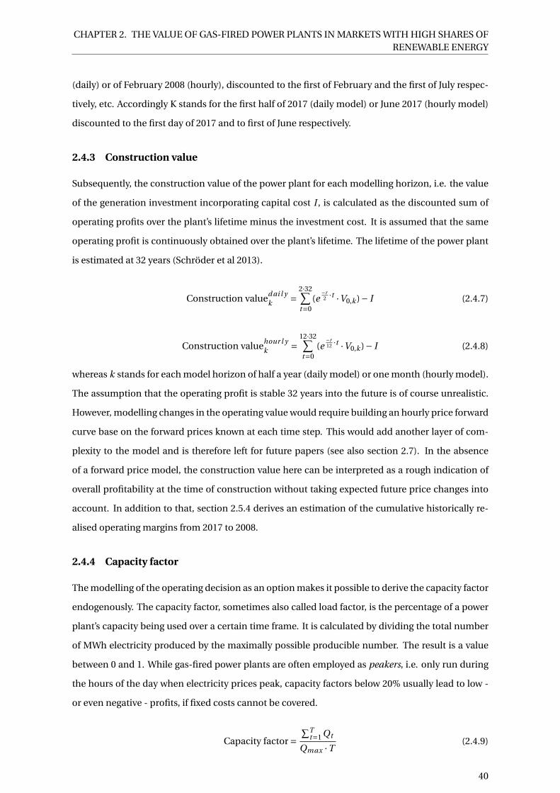
CHAPTER 2. THE VALUE OF GAS-FIRED POWER PLANTS IN MARKETS WITH HIGH SHARES OFRENEWABLE ENERGY
(daily) or of February 2008 (hourly), discounted to the first of February and the first of July respec-
tively, etc. Accordingly K stands for the first half of 2017 (daily model) or June 2017 (hourly model)
discounted to the first day of 2017 and to first of June respectively.
2.4.3 Construction value
Subsequently, the construction value of the power plant for each modelling horizon, i.e. the value
of the generation investment incorporating capital cost I , is calculated as the discounted sum of
operating profits over the plant’s lifetime minus the investment cost. It is assumed that the same
operating profit is continuously obtained over the plant’s lifetime. The lifetime of the power plant
is estimated at 32 years (Schröder et al 2013).
Construction valued ai l y
k=
2·32∑
t=0(e
−r2 ·t ·V0,k )− I (2.4.7)
Construction valuehour l y
k=
12·32∑
t=0(e
−r12 ·t ·V0,k )− I (2.4.8)
whereas k stands for each model horizon of half a year (daily model) or one month (hourly model).
The assumption that the operating profit is stable 32 years into the future is of course unrealistic.
However, modelling changes in the operating value would require building an hourly price forward
curve base on the forward prices known at each time step. This would add another layer of com-
plexity to the model and is therefore left for future papers (see also section 2.7). In the absence
of a forward price model, the construction value here can be interpreted as a rough indication of
overall profitability at the time of construction without taking expected future price changes into
account. In addition to that, section 2.5.4 derives an estimation of the cumulative historically re-
alised operating margins from 2017 to 2008.
2.4.4 Capacity factor
The modelling of the operating decision as an option makes it possible to derive the capacity factor
endogenously. The capacity factor, sometimes also called load factor, is the percentage of a power
plant’s capacity being used over a certain time frame. It is calculated by dividing the total number
of MWh electricity produced by the maximally possible producible number. The result is a value
between 0 and 1. While gas-fired power plants are often employed as peakers, i.e. only run during
the hours of the day when electricity prices peak, capacity factors below 20% usually lead to low -
or even negative - profits, if fixed costs cannot be covered.
Capacity factor =∑T
t=1 Qt
Qmax ·T(2.4.9)
40

CHAPTER 2. THE VALUE OF GAS-FIRED POWER PLANTS IN MARKETS WITH HIGH SHARES OFRENEWABLE ENERGY
with
Qt = argmaxVtQ∈[0,Qmi n ,Qmax ]
(2.4.10)
2.5 Results
2.5.1 Capacity factor
All models and power plant types show a decrease in usage of gas-fired power from mid-2012 at
the latest, a period of very low or even zero capacity factors and then an increase from mid-2015,
pointing at the decline of gas prices and the recovery of electricity prices as discussed in the intro-
duction.
Jan09 Jan10 Jan11 Jan12 Jan13 Jan14 Jan15 Jan16 Jan17
Delivery date
0.1
0.2
0.3
0.4
0.5
0.6
0.7
0.8
0.9
Cap
acity
fact
or
No ramping, no costs
(a) Daily model
Jan09 Jan10 Jan11 Jan12 Jan13 Jan14 Jan15 Jan16 Jan17
Delivery date
0.1
0.2
0.3
0.4
0.5
0.6
0.7
0.8
0.9
Cap
acity
fact
or
No ramping, no costsNo costs
(b) Hourly model
Jan09 Jan10 Jan11 Jan12 Jan13 Jan14 Jan15 Jan16 Jan17
Delivery date
0
0.1
0.2
0.3
0.4
0.5
0.6
0.7
0.8
0.9
Cap
acity
fact
or
New CCGTOld CCGTNew gas turbineOld gas turbineNew steam turbineOld steam turbine
(c) Daily model
Jan09 Jan10 Jan11 Jan12 Jan13 Jan14 Jan15 Jan16 Jan17
Delivery date
0
0.1
0.2
0.3
0.4
0.5
0.6
0.7
0.8
0.9
Cap
acity
fact
or
(d) Hourly model
Figure 2.5.1: Capacity factor for each period of simulation
For the hypothetical plants with no costs modelled except for gas, the capacity factors range be-
tween 9 and 95 % (figure 2.5.1a and 2.5.1b). In the hourly model, the power plant with one hour
41

CHAPTER 2. THE VALUE OF GAS-FIRED POWER PLANTS IN MARKETS WITH HIGH SHARES OFRENEWABLE ENERGY
ramping time displays considerably lower capacity factors as opposed to the plant with immediate
generation, at times by some 50 percentage points.
As to be expected, for the existing power plants, capacity factors are at all times lower than for
the respective plants without ramping and costs (figure 2.5.1c and 2.5.1d). In the daily model,
new and old CCGT plants display clearly higher capacity factors than all other plants. This picture
changes when looking at the hourly model: as CCGT plants ramp slower than gas turbines, which
can only be properly modelled with hourly time steps, the latter overtake CCGT plants in terms of
their capacity factor during some months between 2008 and 2010 and again in December 2016 and
January 2017. CCGT and steam plants show a smaller range of capacity factors than gas turbines:
as they loose time ramping up, they cannot exploit peaks in price spreads to the extent that gas
turbines can. In general, all plants tend to increase their load from mid-2015 when electricity prices
recover and gas prices decline.
It is noticeable that in the hourly model all power plants display very low capacity factors, mostly
smaller than 20% during the period from 2012 to 2015. While low capacity factors are common for
power plants used only during peak hours, as gas plants often are, numbers below 30% point at low
profitability (Hach and Spinler 2014). This low profitability becomes evident when analysing the
operating value in the next section.
2.5.2 Operating value
Operating values give an idea of the operating margins over a certain time frame without consid-
ering any capital costs for building the plant. Daily (figure 2.5.2a and 2.5.2c) and hourly (fig. 2.5.2b
and 2.5.2d) operating values have roughly similar shapes. But as operators profit more from higher
spreads by ramping up production only in peak hours, hourly results are generally higher and dis-
play higher peaks.
While operating values of the power plants without costs are always positive (figure 2.5.2a and
2.5.2b), real world power plants were facing tougher times. In the daily model (figure 2.5.2c), all
plants operate at a loss from 2013 to 2016. The flat lines indicate that power plants are operated
at (almost) zero capacity, which means that (negative) operating profits reflect the incurred fixed
costs. In the hourly model (figure 2.5.2d), CCGT plants are partly in the money during that time.
Profits tend to increase from mid-2015 and in December 2016 and January 2017, all power plants
show a positive peak in the hourly model due to a jump in hourly electricity prices to over 160
EUR/MW (figure 2.5.3). In the daily model, on the other hand, only CCGT plants operate at a -
lower - profit from mid-2016.
Interestingly, while ramping times played a major role for the capacity factors, when looking at
profitability, their importance vanishes. The hypothetical plant with one hour ramping and no
42

CHAPTER 2. THE VALUE OF GAS-FIRED POWER PLANTS IN MARKETS WITH HIGH SHARES OFRENEWABLE ENERGY
Jan09 Jan10 Jan11 Jan12 Jan13 Jan14 Jan15 Jan16 Jan17
Delivery date
0
0.5
1
1.5
2
2.5
3
Ope
ratin
g va
lue
over
1 m
onth
in E
UR
/100
MW
106
No ramping, no costs
(a) Daily model
Jan09 Jan10 Jan11 Jan12 Jan13 Jan14 Jan15 Jan16 Jan17
Delivery date
0
0.5
1
1.5
2
2.5
3
Ope
ratin
g va
lue
over
1 m
onth
in E
UR
/100
MW
106
No ramping, no costsNo costs
(b) Hourly model
Jan09 Jan10 Jan11 Jan12 Jan13 Jan14 Jan15 Jan16 Jan17
Delivery date
0
0.5
1
1.5
2
2.5
Ope
ratin
g va
lue
over
1 m
onth
in E
UR
/100
MW
106
New CCGTOld CCGTNew gas turbineOld gas turbineNew steam turbineOld steam turbine
(c) Daily model
Jan09 Jan10 Jan11 Jan12 Jan13 Jan14 Jan15 Jan16 Jan17
Delivery date
0
0.5
1
1.5
2
2.5O
pera
ting
valu
e ov
er 1
mon
th in
EU
R/1
00 M
W106
(d) Hourly model
Figure 2.5.2: Operating value over 1 month in EUR/100MW
costs generates almost as high profits as the one with immediate ramping and no costs (figure
2.5.2b). This is also evident in figure 2.5.2d: in spite of their slower ramping times, CCGT plants
are, thanks to their high efficiency, always more profitable than all other plants. The reason might
be that the additional hours during which a faster plant can be profitably operated contribute only
little to the overall profit because they exhibit low spreads between electricity and gas price.
For the whole modelling exercise this indicates that the granularity of the model is probably suffi-
cient to model profits and there is no need to model time steps of, say, quarters of an hour. More-
over, the very low capacity values that are observed in the hourly model (figure 2.5.2c) might be
an under-estimation. Smaller time steps are likely to lead to higher capacity factors, even if profits
would hardly change.
43
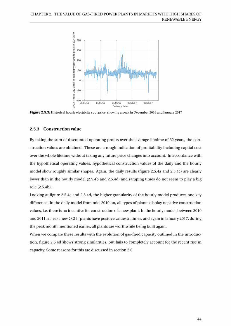
CHAPTER 2. THE VALUE OF GAS-FIRED POWER PLANTS IN MARKETS WITH HIGH SHARES OFRENEWABLE ENERGY
09/01/16 11/01/16 01/01/17 03/01/17 05/01/17
Delivery date
-100
-50
0
50
100
150
200
EP
EX
Phe
lix D
ay B
ase
(mea
n ho
urly
day
-ahe
ad p
rice)
in E
UR
/MW
h
Figure 2.5.3: Historical hourly electricity spot price, showing a peak in December 2016 and January 2017
2.5.3 Construction value
By taking the sum of discounted operating profits over the average lifetime of 32 years, the con-
struction values are obtained. These are a rough indication of profitability including capital cost
over the whole lifetime without taking any future price changes into account. In accordance with
the hypothetical operating values, hypothetical construction values of the daily and the hourly
model show roughly similar shapes. Again, the daily results (figure 2.5.4a and 2.5.4c) are clearly
lower than in the hourly model (2.5.4b and 2.5.4d) and ramping times do not seem to play a big
role (2.5.4b).
Looking at figure 2.5.4c and 2.5.4d, the higher granularity of the hourly model produces one key
difference: in the daily model from mid-2010 on, all types of plants display negative construction
values, i.e. there is no incentive for construction of a new plant. In the hourly model, between 2010
and 2011, at least new CCGT plants have positive values at times, and again in January 2017, during
the peak month mentioned earlier, all plants are worthwhile being built again.
When we compare these results with the evolution of gas-fired capacity outlined in the introduc-
tion, figure 2.5.4d shows strong similarities, but fails to completely account for the recent rise in
capacity. Some reasons for this are discussed in section 2.6.
44
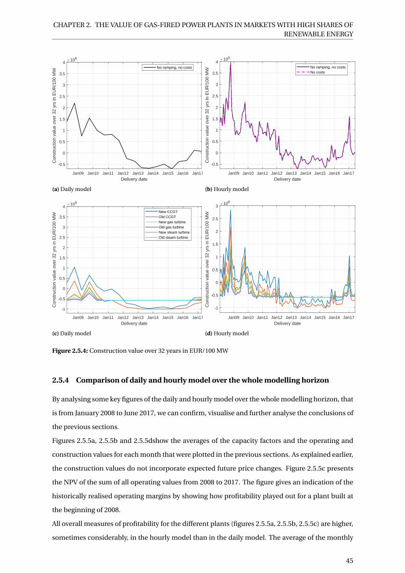
CHAPTER 2. THE VALUE OF GAS-FIRED POWER PLANTS IN MARKETS WITH HIGH SHARES OFRENEWABLE ENERGY
Jan09 Jan10 Jan11 Jan12 Jan13 Jan14 Jan15 Jan16 Jan17
Delivery date
-0.5
0
0.5
1
1.5
2
2.5
3
3.5
4
Con
stru
ctio
n va
lue
over
32
yrs
in E
UR
/100
MW
108
No ramping, no costs
(a) Daily model
Jan09 Jan10 Jan11 Jan12 Jan13 Jan14 Jan15 Jan16 Jan17
Delivery date
-0.5
0
0.5
1
1.5
2
2.5
3
3.5
4
Con
stru
ctio
n va
lue
over
32
yrs
in E
UR
/100
MW
108
No ramping, no costsNo costs
(b) Hourly model
Jan09 Jan10 Jan11 Jan12 Jan13 Jan14 Jan15 Jan16 Jan17
Delivery date
-1
-0.5
0
0.5
1
1.5
2
2.5
3
3.5
4
Con
stru
ctio
n va
lue
over
32
yrs
in E
UR
/100
MW
108
New CCGTOld CCGTNew gas turbineOld gas turbineNew steam turbineOld steam turbine
(c) Daily model
Jan09 Jan10 Jan11 Jan12 Jan13 Jan14 Jan15 Jan16 Jan17
Delivery date
-1
-0.5
0
0.5
1
1.5
2
2.5
3C
onst
ruct
ion
valu
e ov
er 3
2 yr
s in
EU
R/1
00 M
W108
(d) Hourly model
Figure 2.5.4: Construction value over 32 years in EUR/100 MW
2.5.4 Comparison of daily and hourly model over the whole modelling horizon
By analysing some key figures of the daily and hourly model over the whole modelling horizon, that
is from January 2008 to June 2017, we can confirm, visualise and further analyse the conclusions of
the previous sections.
Figures 2.5.5a, 2.5.5b and 2.5.5dshow the averages of the capacity factors and the operating and
construction values for each month that were plotted in the previous sections. As explained earlier,
the construction values do not incorporate expected future price changes. Figure 2.5.5c presents
the NPV of the sum of all operating values from 2008 to 2017. The figure gives an indication of the
historically realised operating margins by showing how profitability played out for a plant built at
the beginning of 2008.
All overall measures of profitability for the different plants (figures 2.5.5a, 2.5.5b, 2.5.5c) are higher,
sometimes considerably, in the hourly model than in the daily model. The average of the monthly
45
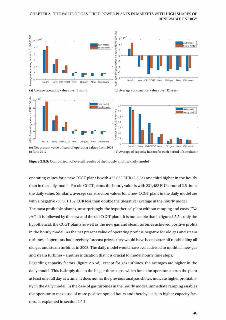
CHAPTER 2. THE VALUE OF GAS-FIRED POWER PLANTS IN MARKETS WITH HIGH SHARES OFRENEWABLE ENERGY
No r/c New, Old CCGT New, Old gas New, Old steam-2
0
2
4
6
8
10
Ave
rage
of o
pera
ting
valu
es in
EU
R/1
00 M
W
105
daily modelhourly model
(a) Average operating values over 1 month
No r/c New, Old CCGT New, Old gas New, Old steam-8
-6
-4
-2
0
2
4
6
Ave
rage
of c
onst
ruct
ion
valu
es in
EU
R/1
00 M
W
107
daily modelhourly model
(b) Average construction values over 32 years
No r/c New, Old CCGT New, Old gas New, Old steam-2
0
2
4
6
8
NP
V o
f ope
ratin
g va
lues
in E
UR
/100
MW
107
daily modelhourly model
(c) Net present value of sum of operating values from 2008to June 2017
No r/c New, Old CCGT New, Old gas New, Old steam0
0.1
0.2
0.3
0.4
0.5
0.6
0.7
Ave
rage
of c
apac
ity fa
ctor
s daily modelhourly model
(d) Average of capacity factors for each period of simulation
Figure 2.5.5: Comparison of overall results of the hourly and the daily model
operating values for a new CCGT plant is with 422,832 EUR (2.5.5a) one third higher in the hourly
than in the daily model. For old CCGT plants the hourly value is with 231,482 EUR around 2.5 times
the daily value. Similarly, average construction values for a new CCGT plant in the daily model are
with a negative -38,981,152 EUR less than double the (negative) average in the hourly model.
The most profitable plant is, unsurprisingly, the hypothetical plant without ramping and costs ("No
r/c"). It is followed by the new and the old CCGT plant. It is noticeable that in figure 2.5.5c, only the
hypothetical, the CCGT plants as well as the new gas and steam turbines achieved positive profits
in the hourly model. As the net present value of operating profit is negative for old gas and steam
turbines, if operators had precisely forecast prices, they would have been better off mothballing all
old gas and steam turbines in 2008. The daily model would have even advised to mothball new gas
and steam turbines - another indication that it is crucial to model hourly time steps.
Regarding capacity factors (figure 2.5.5d), except for gas turbines, the averages are higher in the
daily model. This is simply due to the bigger time steps, which force the operators to run the plant
at least one full day at a time. It does not, as the previous analysis shows, indicate higher profitabil-
ity in the daily model. In the case of gas turbines in the hourly model, immediate ramping enables
the operator to make use of more positive-spread hours and thereby leads to higher capacity fac-
tors, as explained in section 2.5.1.
46

CHAPTER 2. THE VALUE OF GAS-FIRED POWER PLANTS IN MARKETS WITH HIGH SHARES OFRENEWABLE ENERGY
2.5.5 Sensitivity analysis of interest rates
To keep the analysis simple, a discount rate of 7.2 % has been used throughout the paper as a
rough estimate of the firm’s cost of capital (KPMG 2012). In reality, the discount rate used has a
large impact especially on the construction values calculated over the lifetime of the plants. The
following sensitivity tests have been performed for the new CCGT plant parameters and the hourly
model.
0 0.036 0.072 0.108 0.144
Interest rate
0
0.5
1
1.5
2
2.5
Ope
ratin
g va
lues
of d
iffer
ent m
onth
s at
sam
e in
tere
st r
ate 106
(a) Operating value
0 0.036 0.072 0.108 0.144
Interest rate
-1
0
1
2
3
4
5
6
7
8
Con
stru
ctio
n va
lues
of d
iffer
ent m
onth
s at
sam
e in
tere
st r
ate
108
(b) Construction value
-0.5 0 0.5 1 1.5 2 2.5
Average operating values for each month simulated 106
-10
-8
-6
-4
-2
0
2
Inte
rest
rat
e co
effic
ient
for
each
mon
th s
imul
ated
104
(c) Operating value
-2 -1 0 1 2 3 4
Average of construction values for each month simulated 108
-5
-4
-3
-2
-1
0
1
Inte
rest
rat
e co
effic
ient
for
each
mon
th s
imul
ated
109
(d) Construction value
Figure 2.5.6: Relationship of profit measures and interest rates
Figure 2.5.6a and 2.5.6b show the box plots of the values simulated for different months at the
same interest rate. While the dispersion of operating values is similar for different interest rates,
the dispersion of construction values, calculated as the NPV of operating values over 32 years, dra-
matically shrinks for higher interest rates. The average difference between a monthly operating
value discounted at 0% and one discounted at 14.4% is 0.65%, whereas for the construction values
47

CHAPTER 2. THE VALUE OF GAS-FIRED POWER PLANTS IN MARKETS WITH HIGH SHARES OFRENEWABLE ENERGY
the average difference is 446%.3
Figures 2.5.6c and 2.5.6d show the simple ordinary least squares regression coefficient of the oper-
ating and construction values on the interest rate. The coefficient is generally negative: the higher
the interest rate, the lower the operating and construction values. However, for some values, the
coefficient becomes positive. Plotting the coefficient against the average values for each month
reveals that the coefficient decreases and thereby takes on larger negative values with increasing
averages for each month simulated. The interest rate coefficient only becomes positive for very
small and mostly negative average operating and construction values, indicating that in these cases
a higher interest rate led to "less negative" values. The values in the left hand scatter plot (figure
2.5.6c) are slightly less linear because operating values are received from a probabilistic model: the
impact of the interest rate depends on the relative probabilities and size of positive and negative
operating values. While positive values tend to result in a negative coefficient, negative values tend
to result in a positive one, and the overall coefficient depends on the overall likelihood of different
operating values realised with optimised ramping decisions.
The impact of the discount rate is decisive especially for the construction values as evidenced in
the impact on the boxplots and in the very low interest rate coefficients in figure 2.5.6. This is also
shown in figure 2.5.7: whereas for a 3.6% discount rate, a monthly operating value of EUR 400,000
is sufficient to make an investment in a new CCGT plant worthwhile, at a rate of 7.2% the operating
value should be more in the range of EUR 600,000 and above, and at a 10.8% discount rate, the
power plant operator already needs a monthly operating margin of around EUR 800,000. These
results illustrate the sensitivity of electricity generation profits to interest rates due to the longevity
of the assets. The interest rates reflect the cost of capital of the investor, which depends on macro-
economic factors and on the risk-return profile of each project, which in turn is affected by power
prices. Financing costs represent thus an additional indirect channel through which power prices
impact gas-fired generation’s profits.
3The difference is defined as △V = Vmax−Vmi n|Vmi n | .
48

CHAPTER 2. THE VALUE OF GAS-FIRED POWER PLANTS IN MARKETS WITH HIGH SHARES OFRENEWABLE ENERGY
0 0.036 0.072 0.108 0.144
Interest rate
-4
-3
-2
-1
0
1
2
3
Con
stru
ctio
n va
lues
dep
endi
ng o
n di
ffere
nt o
pera
ting
valu
es 108
10e58e56e54e52e50
-2e5-4e5-6e5-8e5-10e5zero-line
Operating values over one month
Figure 2.5.7: Relationship between monthly operating values and construction values at different interest rates
2.6 Conclusion
The goal of this paper was twofold. First, the relevant literature was analysed and a model was de-
veloped that improved upon existing ones in several ways: electricity and gas prices were modelled
as a two-dimensional stochastic process, each component consisting of the sum of a deterministic
seasonal part and a mean-reverting process. A power plant model for different types of gas-fired
power plants incorporated ramping times and costs and it was run in daily and hourly time steps.
Second, the results of two types of gas plant models were compared, one with daily and one with
hourly time steps. The results show that modelling ramping times and costs pay off: operating and
construction values of plants modelled without costs are at all times higher and average values are
significantly higher than when including the ramping and other costs. Modelling ramping times
is only relevant for capacity factors and not for the profit indicators. The reason might be that the
additional hours during which a faster plant can be profitably operated contribute only little to the
overall profit because they exhibit low spreads between electricity and gas prices.
When comparing daily and hourly models, the result is that, for gas-fired power plants, time step
size matters. Average operating and construction values in the hourly model are more than double
of what is derived with a daily model. The reason is that with hourly time steps, operators can
benefit from jumps in prices as occurred in January 2017. Due to these results and because in
reality gas-fired power plants are used as peakers with operation being optimised at least hourly,
the hourly model is clearly preferable to the daily one.
As quarter hourly electricity prices are traded on the EPEX exchange, it is conceivable to model
even smaller time steps of 30 or only 15 minutes. But while capacity factors are likely to increase if
granularity was further improved, profits would probably stay in a similar range, as similar profits
of the two hypothetical power plants - one fast and one slow, but otherwise comparable - indicate.
49
CHAPTER 2. THE VALUE OF GAS-FIRED POWER PLANTS IN MARKETS WITH HIGH SHARES OFRENEWABLE ENERGY
The hourly model replicates operators’ and investors’ decision making very well as the results trace
current major developments like the recent decline and come-back of gas-fired power in Germany.
From 2008 profits showed a decreasing tendency and from 2013 to 2016, all plants but CCGTs op-
erated at a loss and ran at very low, sometimes zero, capacity. The recent rise in profitability can
partly be seen in the model: capacity factors and operating profits displayed an increasing ten-
dency from mid-2015. Construction values from 2013, however, were only positive in December
2016 and January 2017, due to a surge in hourly electricity prices. The reason for operators nev-
ertheless building new plants in this period can be explained if we assume that they used future
rather than historical prices to evaluate their investment options and that future prices indicated
an increase in the electricity-gas-spread.
The sensitivity of construction values to changes in the discount rate illustrates the importance of
financing costs due to the longevity of electricity generation assets. Financing costs represent an
additional indirect channel through which power prices impact gas-fired generation’s profits.
2.7 Further research and outlook
Future research could extend this model in several ways. First, while this paper uses historical spot
prices and thereby models factual profitability of power plants during a certain time period in the
past, a possible extension would be to use future prices. Using futures, the results would get closer
to the decision making of operators, who have to take investment decisions that lock them in for
around 30 years into the future. A whole separate body of literature is concerned with building
the "hourly price forward curve" (HPFC) in order to receive hourly future prices that are consistent
with all future products traded on the market at a certain point in time (e.g. Paraschiv et al 2015).
By marrying this strand of literature with the model presented in this paper, one could get one step
closer to the real decision making process of operators.
Second, it might be worthwhile to incorporate price jumps rather than mean reversion only into
the price model (see for example Keles et al 2012). Especially for future electricity markets with
even higher shares of variable renewable electricity this step might be worthwhile.
Third, the results show that differences between the types of power plants are large. In order to
deduce results that hold for an entire sector and to test the behaviour of specific types of plants, a
larger number of models could be calibrated to more accurately reflect different technologies and
thereby explain the relative importance of different plant types.
A fourth extension to this model, and real options in general, could be in other areas of energy
economics that are currently intensively researched, such as (battery) storage: one could model
the option to sell stored electricity and consider the costs incurred while storing it.
50

CHAPTER 2. THE VALUE OF GAS-FIRED POWER PLANTS IN MARKETS WITH HIGH SHARES OFRENEWABLE ENERGY
The paper contributes to a better understanding of the choices operators and investors face in
the electricity market. This is currently all the more important as electricity markets are shaped
by market factors and new policies for the transition to renewable energies in Germany and across
Europe. In this context, four major developments might favour investments in new gas-fired power
plants in the coming years in Germany. Further research in this area is needed to determine exactly
how these changes might impact the financial attractiveness of gas-fired and other power plants.
First, there have been several suggestions for measures to incentivise investment into flexible ca-
pacity. Researchers have analysed capacity markets, which, unlike energy-only markets, remuner-
ate the capacity built and not the electricity generated. For the time being, legislators in Germany
decided against it but recently created the possibility for transmission grid operators to auction
off an additional capacity reserve, which is part of the ancillary services provided to stabilise the
grid. New gas-fired power plants in the south of Germany are likely benefactors (Energate 2017).
Ancillary services in general are of growing importance and an interesting area for research. Most
of the services intended to stabilise the grid are requested by transmission system operators on
an obligatory basis from power plant operators. Only the balancing power market is organised via
capacity auctions. In both cases, ancillary services require different modelling techniques than the
price-taker model employed in this paper (Bundesnetzagentur 2017).
Second, the so-called "back-loading initiative" by the European Commission has come into effect
in 2018 and contributed to a supply reduction and thereby price increase on the EU emissions
trading market favouring low-emitting electricity sources (Graichen et al 2018).
Third, the phase-out of nuclear power in Germany by 2022 is likely to have an increasing effect on
power prices and thereby making all remaining energy sources more profitable.
And fourth, if European countries want to reach their climate goals under the Paris agreement, ex-
perts have argued that a coal phase out might be necessary (Heinrichs et al 2017). The German
Federal "Special Commission on Growth, Structural Economic Change and Employment" is cur-
rently working on policy recommendations for the early closure of coal power plants - a step that
might push gas-fired power plants further into the money.
Modelling power plant capacity factors and profitability more realistically thus has increasing rel-
evance not just in academic research, but also for policy makers and investors.
51

CHAPTER 2. THE VALUE OF GAS-FIRED POWER PLANTS IN MARKETS WITH HIGH SHARES OFRENEWABLE ENERGY
2.8 Bibliography
Black F. and Scholes M. (1973): The Pricing of Options and Corporate Liabilities. Journal of Political
Economy (81), pp. 637–654.
Bloomberg (2017): EEX spot prices for European Emission Allowances. Bloomberg terminal.
Bublitz A., Keles D. and Fichtner W. (2017): An analysis of the decline of electricity spot prices in
Europe: Who is to blame? Energy Policy (107), pp. 323-336.
Clewlow L. and Strickland C. (1999): Valuing Energy Options in a One Factor Model Fitted to
Forward Prices. Last accessed online on January 10, 2019: ❤tt♣✿✴✴❞①✳❞♦✐✳♦r❣✴✶✵✳✷✶✸✾✴ssr♥✳
✶✻✵✻✵✽.
Deng S. and Oren S. (2003): Incorporating operational characteristics and start-up costs in option-
based valuation of power generation capacity. Probability in the Engineering and Informational
Sciences (17), pp. 155-181.
Deng S., Johnson B. and Sogomonian A. (2001): Exotic electricity options and the valuation of
electricity generation and transmission assets. Decision Support Systems (30), pp. 383–392.
Denton M., Palmer A., Masiello R. and Skantze P. (2003): Managing Market Risk in Energy. IEEE
(18), pp. 494-502.
Destatis (2017): Bruttostromerzeugung in Deutschland für 2014 bis 2016. Last accessed online on
January 10, 2019: ❤tt♣s✿✴✴✇✇✇✳❞❡st❛t✐s✳❞❡✴❉❊✴❩❛❤❧❡♥❋❛❦t❡♥✴❲✐rts❝❤❛❢ts❜❡r❡✐❝❤❡✴❊♥❡r
❣✐❡✴❊r③❡✉❣✉♥❣✴❚❛❜❡❧❧❡♥✴❇r✉tt♦str♦♠❡r③❡✉❣✉♥❣✳❤t♠❧.
EEX (2014): Product Brochure Natural Gas. Last accessed online on January 10, 2019:
❤tt♣✿✴✴❝❞♥✳❡❡①✳❝♦♠✴❞♦❝✉♠❡♥t✴✶✺✸✺✽✾✴✷✵✶✹✵✶✵✶✪✷✵❊❊❳✪✷✵Pr♦❞✉❝t✪✷✵❇r♦❝❤✉r❡✪✷✵◆❛
t✉r❛❧✪✷✵●❛s✳♣❞❢
EEX (2017): Gas Spot Market NCG Daily Settlement Price. EEX, Leipzig.
52

CHAPTER 2. THE VALUE OF GAS-FIRED POWER PLANTS IN MARKETS WITH HIGH SHARES OFRENEWABLE ENERGY
Energate (2017): Bayern drängt auf den Bau von Gaskraftwerken. Last accessed online on January
10, 2019: ❤tt♣✿✴✴✇✇✇✳❡♥❡r❣❛t❡✲♠❡ss❡♥❣❡r✳❞❡✴♥❡✇s✴✶✼✼✵✺✵✴❜❛②❡r♥✲❞r❛❡♥❣t✲❛✉❢✲❜❛✉✲✈
♦♥✲❣❛s❦r❛❢t✇❡r❦❡♥.
EPEX (2017): Phelix Day-Ahead Auction Price. EPEX, Paris.
Everts M., Huber C. and Blume-Werry E. (2016): Politics vs markets: how German power prices hit
the floor. Journal of World Energy Law and Business (0), pp. 1–8.
Bundesnetzagentur (2014): Datenübersicht Fortschrittsbericht. Last accessed online on January
10, 2019: ❤tt♣s✿✴✴✇✇✇✳❜♠✇✐✳❞❡✴❘❡❞❛❦t✐♦♥✴❉❊✴❇✐♥❛❡r✴❞❛t❡♥✉❡❜❡rs✐❝❤t✲❢♦rts❝❤r✐tts❜❡
r✐❝❤t✲✷✵✶✹✳①❧s❄❴❴❜❧♦❜❂♣✉❜❧✐❝❛t✐♦♥❋✐❧❡✫✈❂✸.
Bundesnetzagentur (2017): Monitoringbericht 2017. Bundesnetzagentur für Elektrizität, Gas,
Telekommunikation, Post und Eisenbahnen Bundeskartellamt. Bonn.
Fleten S. and Näsäkkälä E. (2009): Gas fired power plants: Investment timing, operating flexibility
and abandonment, MPRA Paper (217), University Library of Munich.
Frayer J. and Uludere N. (2001): What Is It Worth? Application of Real Options Theory to the
Valuation of Generation Assets. The Electricity Journal, pp. 40-51.
Fraser P. (2003): Power generation investment in electricity markets. OECD/IEA.
Gardner D. and Zhuang Y. (2000): Valuation of Power Generation Assets: A Real Options Approach.
Algo Research Quaterly (3), pp. 9-20.
Graichen, P. and Redl, C. (2014): Das deutsche Energiewende-Paradox: Ursachen und Heraus-
forderungen, Agora Energiewende.
Graichen, P., Litz, P., Matthes, F. and Herrmann, H. (2018): Vom Wasserbett zur Badewanne.
Die Auswrikungen der EU-Emissionshandelsreform 2018 auf CO2-Preis, Kohleausstieg und den
Ausbau der Erneuerbaren. Agora Energiewende und Öko-Institut.
Hach D. and Spinler S. (2014): Capacity Payment Impact on Gas-Fired Generation Investments
53
CHAPTER 2. THE VALUE OF GAS-FIRED POWER PLANTS IN MARKETS WITH HIGH SHARES OFRENEWABLE ENERGY
under Rising Renewable Feed-In – A Real Options Analysis. Energy Economics (53), pp. 270-280.
Hahn, W.J. and Dyer, J.S. (2008): Discrete time modeling of mean-reverting stochastic processes
for real option valuation. European Journal of Operational Research (184), pp. 534-548.
Heinrichs H., Schumann D., Vögele S., Biß K., Shamon H., Markewitz P., Többen J., Gillessen B.,
Gotzens F. and Ernst A. (2017): Integrated assessment of a phase-out of coal-fired power plants in
Germany. Energy (126), pp. 285-305.
Hirth L. (2018): What Caused the Drop in European Electricity Prices? A factor decomposition
analysis. The Energy Journal, International Association for Energy Economics (1).
Hsu M. (1998): Spark spread options are hot! The Electricity Journal (11), pp. 1-12.
IEA (2013): Power Generation in the New Policies and 450 Scenarios. Assumed investment costs,
operation and maintenance costs and efficiencies in the IEA World Energy Investment Outlook
2014. International Energy Agency.
Interview A (2016): Interview with an electricity market consultant, Switzerland.
Interview B (2016): Interview with a gas market consultant, Switzerland.
Keles D., Genoese M., Möst D. and Fichtner W. (2012): Comparison of extended mean-reversion
and time series models for electricity spot price simulation considering negative prices. Energy
Economics (34), pp. 1012-1032.
Kumar, N., Besuner, P.M., Lefton, S., Agan, D. and Hilleman, D.D. (2012): Power plant cycling costs.
Intertek APTECH prepared for National Renewable Energy Laboratory and Western Electricity Co-
ordinating Council. Last accessed on January 10, 2019: ❤tt♣s✿✴✴✇✇✇✳♥r❡❧✳❣♦✈✴❞♦❝s✴❢②✶✷♦st✐
✴✺✺✹✸✸✳♣❞❢.
KPMG (2014): Cost of capital study 2014. KPMG.
Margrabe W. (1978): The Value of an Option to Exchange One Asset for Another. The Journal of
Finance (33), pp. 177-186.
54
CHAPTER 2. THE VALUE OF GAS-FIRED POWER PLANTS IN MARKETS WITH HIGH SHARES OFRENEWABLE ENERGY
Mei W., Bernstein A. and Chesney M. (2012): An experimental study on real-options strategies.
Quantitative Finance (12), pp. 1753-1772.
Myers S. (1977): Determinants of Corporate Borrowing. Journal of Financial Economics (5), pp.
147-175.
Open Power System Data (2017): Data Package Conventional power plants. Version 2017-07-07.
Last accessed on January 10, 2019: ❤tt♣s✿✴✴❞❛t❛✳♦♣❡♥✲♣♦✇❡r✲s②st❡♠✲❞❛t❛✳♦r❣✴❝♦♥✈❡♥t✐♦♥
❛❧❴♣♦✇❡r❴♣❧❛♥ts✴✷✵✶✼✲✵✼✲✵✼✴.
Paraschiv F., Erni D. and Pietsch R. (2014): The impact of renewable energies on EEX day-ahead
electricity prices, Energy Policy (73), 2014, pp. 196-210.
Paraschiv F., Fleten S. and Schürle M. (2015): A spot-forward model for electricity prices with
regime shifts, Energy Economics (47), pp. 142-153.
Schröder A., Kunz F., Meiss J., Mendelevitch R. and von Hirschhausen C. (2013): Current and
Prospective Costs of Electricity Generation until 2050. Deutsches Institut für Wirtschafts-
forschung, Berlin.
Tseng C. and Lin K. (2007): Framework Using Two-Factor Price Lattices for Generation Asset
Valuation. Operations Research 55, pp. 234-251.
Tseng C. and Barz G. (2000): Short-term generation asset valuation. Operations Research (50), pp.
297–310.
Umweltbundesamt (2017): Datenbank Kraftwerke Deutschland ab 10 MW. Berlin.
55

CHAPTER 2. THE VALUE OF GAS-FIRED POWER PLANTS IN MARKETS WITH HIGH SHARES OFRENEWABLE ENERGY
2.9 Appendix
2.9.1 Estimating the seasonalities
2.9.1.1 Long-term trend
First, for both daily and hourly model, a long-term trends is estimated by ordinary least squares
regression and removed if the confidence interval is at least 90%.
Tr end St=α+β · t (2.9.1)
This and the following steps are done accordingly for the gas price Pt .
2.9.1.2 Monthly means (daily model)
In the daily model, the monthly means are then calculated and subtracted, whereas we differenti-
ate whether the day is a weekday or a weekend:
Monthl y MeansSt=
12∑
m=1{1(m′|m′ = m(t )) ·
T∑
t=1[St ·1(d ′|d ′ = d(t ))]} ∀d = {weekd ay, weekend}
(2.9.2)
2.9.1.3 Daily means (hourly model)
In the hourly model, as only one month is modelled at a time, the daily averages are instead sub-
tracted, whereas we again differentiate whether the day is a weekday or weekend:
Dai l y MeansSt=
T∑
t=1{1(d ′|d ′ = d(t )) ·
24∑
h=1
[SXh·1(h|h = t mod 24)]} ∀d = {weekd ay, weekend}
(2.9.3)
2.9.1.4 Weekly and other cycles (daily model)
Finally, cycles are estimated that follow the oscillation of sinus and cosinus curves with different
lengths. They are estimated by an ordinary least squares regression and removed if the confidence
interval is at least 90%. In the daily model, as T equals six months, a function with period lengths
that range from six months (for l = 1,m = 1) to less than one week (for n = 5,o = 5) is fitted:
W eekl y AndOtherC ycl esDai l ySt= γ+
5∑
l=1
(δl si nl ·π · t
T)+
5∑
m=1(ǫm si n
m ·π · t
T)
+5
∑
n=1(ζncos
n ·6 ·π · t
T)+
5∑
o=1(ηocos
o ·6 ·π · t
T)
(2.9.4)
56

CHAPTER 2. THE VALUE OF GAS-FIRED POWER PLANTS IN MARKETS WITH HIGH SHARES OFRENEWABLE ENERGY
2.9.1.5 Weekly and other cycles (hourly model)
In the hourly model, as T equals one month, a function with period lengths that range from one
month (for m = 1, o = 1) to less than one week (for m = 5, n = 5) is fitted:
W eekl y AndOtherC ycl esHour l ySt=
5∑
m=1(ǫm si n
m ·π · t
T)+
5∑
o=1(ηocos
o ·π · t
T) (2.9.5)
2.9.2 Ornstein-Uhlenbeck parameters and goodness of fit of daily price model
See table 2.2 and 2.3.
2.9.3 Goodness of fit of hourly price model
See table 2.4 and 2.5.
Table 2.4: Goodness of fit of hourly price model for electricity price St
YearPart of
year
Mean of
historic X t
Mean of
simulated X t
Mean of
historic St
Mean of
simulated St
SD of
historic St
SD of
simulated St
R2 of
simulated St
2008 1 0.00 0.74 56.00 56.74 20.42 18.22 78.98%
2008 2 0.00 0.28 59.47 59.75 16.57 15.67 85.68%
2008 3 0.00 1.43 53.30 54.73 19.29 16.57 72.34%
2008 4 0.00 0.89 67.46 68.35 25.33 23.85 84.46%
2008 5 0.00 1.10 56.24 57.34 23.15 21.17 79.16%
2008 6 0.00 -0.66 73.24 72.57 30.83 28.79 84.96%
2008 7 0.00 -0.84 69.94 69.11 25.81 23.55 83.21%
2008 8 0.00 0.15 61.76 61.91 22.80 20.78 83.85%
2008 9 0.00 -0.62 88.30 87.68 27.95 26.83 89.84%
2008 10 0.00 0.70 85.65 86.35 36.21 32.59 77.95%
2008 11 0.00 0.49 63.72 64.21 33.31 27.79 66.78%
2008 12 0.00 -1.14 54.55 53.41 27.80 24.15 74.60%
2009 1 0.00 1.42 57.12 58.54 21.83 20.19 73.76%
2009 2 0.00 0.47 47.79 48.26 16.08 14.33 76.39%
2009 3 0.00 0.20 37.15 37.35 13.06 10.42 62.54%
2009 4 0.00 0.43 33.05 33.48 12.08 10.90 77.91%
2009 5 0.00 0.52 30.93 31.45 15.94 12.67 61.15%
2009 6 0.00 0.07 33.21 33.29 12.07 10.72 80.69%
2009 7 0.00 -0.66 35.52 34.87 12.10 10.62 78.56%
2009 8 0.00 0.61 36.07 36.68 14.99 13.35 79.57%
2009 9 0.00 -0.39 39.58 39.19 15.76 14.89 88.18%
2009 10 0.00 0.06 44.57 44.63 29.66 20.31 45.83%
2009 11 0.00 -0.41 35.94 35.53 17.62 14.77 69.47%
57

CHAPTER 2. THE VALUE OF GAS-FIRED POWER PLANTS IN MARKETS WITH HIGH SHARES OFRENEWABLE ENERGY
Table 2.4: Goodness of fit of hourly price model for electricity price St
YearPart of
year
Mean of
historic X t
Mean of
simulated X t
Mean of
historic St
Mean of
simulated St
SD of
historic St
SD of
simulated St
R2 of
simulated St
2009 12 0.00 -0.48 35.69 35.22 25.02 19.56 58.35%
2010 1 0.00 0.26 42.21 42.46 12.88 11.07 69.84%
2010 2 0.00 0.17 41.73 41.90 12.81 12.18 88.64%
2010 3 0.00 -0.54 39.17 38.63 12.52 11.57 79.87%
2010 4 0.00 0.22 40.04 40.26 10.63 9.26 70.78%
2010 5 0.00 0.50 41.17 41.67 14.02 12.79 78.72%
2010 6 0.00 -0.01 43.34 43.34 13.83 13.15 85.18%
2010 7 0.00 -0.21 45.83 45.62 11.17 10.36 83.95%
2010 8 0.00 0.17 39.80 39.97 12.17 10.67 80.06%
2010 9 0.00 -0.17 45.86 45.69 11.66 10.90 86.60%
2010 10 0.00 0.02 50.31 50.33 11.93 10.80 82.22%
2010 11 0.00 0.55 48.53 49.08 14.05 13.10 83.85%
2010 12 0.00 -0.02 55.55 55.52 18.30 16.61 80.65%
2011 1 0.00 0.27 50.13 50.40 16.05 14.37 81.12%
2011 2 0.00 0.85 50.86 51.71 14.22 13.51 80.48%
2011 3 0.00 0.19 54.40 54.59 9.67 8.41 78.48%
2011 4 0.00 -0.25 51.58 51.33 11.73 10.23 70.48%
2011 5 0.00 -0.29 56.83 56.54 12.01 11.21 81.55%
2011 6 0.00 0.43 52.30 52.73 13.20 11.35 68.84%
2011 7 0.00 -0.02 46.40 46.38 12.45 11.52 80.76%
2011 8 0.00 0.64 48.57 49.21 11.47 10.66 82.36%
2011 9 0.00 0.44 52.64 53.08 13.19 12.17 85.28%
2011 10 0.00 0.45 51.68 52.13 13.27 12.22 84.10%
2011 11 0.00 0.25 55.36 55.61 15.01 14.20 88.04%
2011 12 0.00 0.19 42.90 43.09 13.82 12.67 80.06%
2012 1 0.00 0.54 39.89 40.43 15.99 12.84 66.58%
2012 2 0.00 -0.03 54.92 54.89 25.36 21.15 70.20%
2012 3 0.00 0.49 41.09 41.58 12.64 11.34 79.41%
2012 4 0.00 0.15 43.57 43.72 13.48 11.95 72.19%
2012 5 0.00 -0.53 38.85 38.32 11.96 9.64 64.91%
2012 6 0.00 0.39 38.81 39.19 13.40 13.29 85.27%
2012 7 0.00 -0.20 41.02 40.82 11.72 10.95 83.10%
2012 8 0.00 0.03 44.90 44.93 11.30 9.99 78.51%
2012 9 0.00 -0.14 44.67 44.53 13.13 12.20 80.52%
2012 10 0.00 -0.43 43.94 43.51 13.74 12.24 75.75%
2012 11 0.00 0.64 44.79 45.43 16.09 14.21 81.11%
58

CHAPTER 2. THE VALUE OF GAS-FIRED POWER PLANTS IN MARKETS WITH HIGH SHARES OFRENEWABLE ENERGY
Table 2.4: Goodness of fit of hourly price model for electricity price St
YearPart of
year
Mean of
historic X t
Mean of
simulated X t
Mean of
historic St
Mean of
simulated St
SD of
historic St
SD of
simulated St
R2 of
simulated St
2012 12 0.00 -0.59 35.51 34.92 38.72 30.23 62.87%
2013 1 0.00 0.69 43.31 44.00 16.21 14.85 87.33%
2013 2 0.00 -0.93 44.62 43.68 13.60 13.82 79.97%
2013 3 0.00 -0.13 39.06 38.93 17.18 15.69 75.59%
2013 4 0.00 0.30 37.92 38.22 16.63 14.79 75.65%
2013 5 0.00 1.22 32.06 33.29 13.30 10.95 71.23%
2013 6 0.00 0.91 27.82 28.73 14.64 12.01 67.09%
2013 7 0.00 -0.14 36.42 36.28 11.52 10.88 80.50%
2013 8 0.00 0.51 38.23 38.75 12.69 11.09 76.42%
2013 9 0.00 0.51 41.71 42.23 15.38 14.53 83.83%
2013 10 0.00 -0.04 37.72 37.67 16.22 14.38 75.20%
2013 11 0.00 0.90 39.22 40.11 17.15 15.03 79.10%
2013 12 0.00 -0.30 35.75 35.45 22.84 20.09 74.94%
2014 1 0.00 0.78 35.87 36.66 15.77 13.73 78.92%
2014 2 0.00 0.51 33.59 34.10 13.37 12.22 79.83%
2014 3 0.00 0.25 31.01 31.26 14.40 12.59 73.73%
2014 4 0.00 0.26 31.58 31.84 10.52 9.49 73.92%
2014 5 0.00 0.72 30.63 31.35 11.94 9.48 61.20%
2014 6 0.00 -0.24 31.52 31.28 9.27 8.88 76.02%
2014 7 0.00 0.08 31.88 31.96 6.31 5.70 82.05%
2014 8 0.00 0.12 27.93 28.05 11.52 10.26 73.94%
2014 9 0.00 -0.62 34.79 34.17 9.67 8.82 79.47%
2014 10 0.00 -0.01 35.25 35.24 12.28 11.00 76.94%
2014 11 0.00 0.52 36.37 36.89 13.64 12.56 83.88%
2014 12 0.00 -0.76 32.89 32.13 17.71 15.96 84.32%
2015 1 0.00 1.59 28.72 30.31 14.85 12.62 73.76%
2015 2 0.00 0.16 36.72 36.88 12.55 11.94 77.32%
2015 3 0.00 0.39 31.31 31.70 12.98 11.64 79.95%
2015 4 0.00 -0.30 29.72 29.42 13.22 10.98 62.50%
2015 5 0.00 0.38 25.36 25.73 9.95 8.32 66.17%
2015 6 0.00 -0.37 30.06 29.69 8.59 7.74 70.58%
2015 7 0.00 0.16 35.00 35.16 12.50 10.62 72.66%
2015 8 0.00 0.08 31.61 31.69 9.10 8.23 82.67%
2015 9 0.00 0.04 31.88 31.92 11.47 9.99 74.46%
2015 10 0.00 0.09 39.38 39.47 11.34 10.18 77.78%
2015 11 0.00 0.69 32.39 33.08 13.92 12.31 72.86%
59

CHAPTER 2. THE VALUE OF GAS-FIRED POWER PLANTS IN MARKETS WITH HIGH SHARES OFRENEWABLE ENERGY
Table 2.4: Goodness of fit of hourly price model for electricity price St
YearPart of
year
Mean of
historic X t
Mean of
simulated X t
Mean of
historic St
Mean of
simulated St
SD of
historic St
SD of
simulated St
R2 of
simulated St
2015 12 0.00 -0.61 27.78 27.18 13.19 11.44 78.30%
2016 1 0.00 0.70 29.04 29.74 13.30 11.90 78.36%
2016 2 0.00 0.51 21.99 22.50 9.47 8.55 78.34%
2016 3 0.00 -0.19 24.28 24.09 8.16 6.60 63.30%
2016 4 0.00 0.00 24.21 24.21 5.85 5.14 77.10%
2016 5 0.00 0.16 22.54 22.70 13.55 11.07 58.23%
2016 6 0.00 0.02 27.69 27.71 6.90 6.30 77.80%
2016 7 0.00 0.47 27.19 27.65 7.24 5.87 66.49%
2016 8 0.00 0.02 27.18 27.21 7.25 6.67 78.30%
2016 9 0.00 0.19 30.49 30.68 7.90 6.69 75.36%
2016 10 0.00 0.11 37.14 37.25 9.66 8.32 76.39%
2016 11 0.00 0.46 38.22 38.68 13.87 11.58 66.57%
2016 12 0.00 -0.35 37.48 37.12 21.06 19.34 79.98%
2017 1 0.00 0.00 52.37 52.37 25.82 23.31 76.95%
2017 2 0.00 0.49 39.70 40.19 16.05 14.70 79.05%
2017 3 0.00 0.41 31.70 32.11 9.69 8.17 67.93%
2017 4 0.00 0.18 28.87 29.05 13.49 10.55 57.93%
2017 5 0.00 -1.92 30.46 28.54 13.91 12.18 50.19%
2017 6 0.00 0.31 30.00 30.31 9.61 8.22 69.79%
60
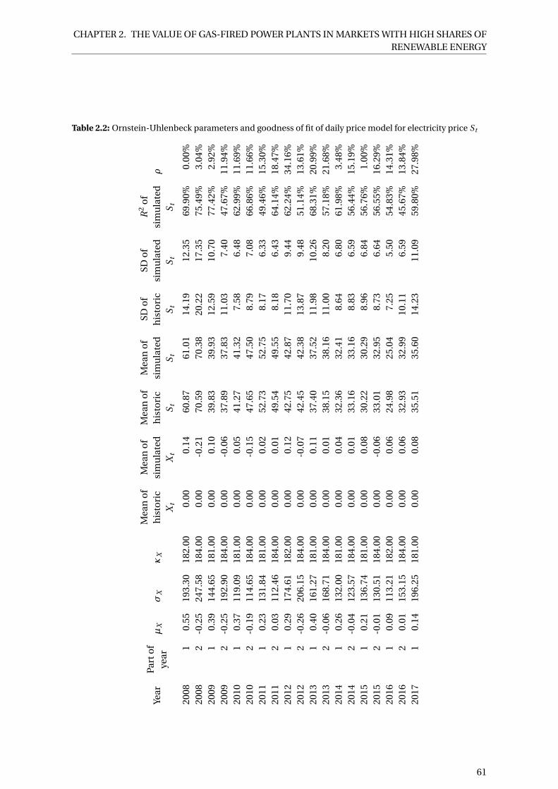
CHAPTER 2. THE VALUE OF GAS-FIRED POWER PLANTS IN MARKETS WITH HIGH SHARES OFRENEWABLE ENERGY
Table 2.2: Ornstein-Uhlenbeck parameters and goodness of fit of daily price model for electricity price St
Year
Par
to
fye
arµ
Xσ
Xκ
X
Mea
no
fh
isto
ric
Xt
Mea
no
fsi
mu
late
dX
t
Mea
no
fh
isto
ric
St
Mea
no
fsi
mu
late
dS
t
SDo
fh
isto
ric
St
SDo
fsi
mu
late
dS
t
R2
of
sim
ula
ted
St
ρ
2008
10.
5519
3.30
182.
000.
000.
1460
.87
61.0
114
.19
12.3
569
.90%
0.00
%20
082
-0.2
524
7.58
184.
000.
00-0
.21
70.5
970
.38
20.2
217
.35
75.4
9%3.
04%
2009
10.
3914
4.65
181.
000.
000.
1039
.83
39.9
312
.59
10.7
077
.42%
2.92
%20
092
-0.2
519
2.90
184.
000.
00-0
.06
37.8
937
.83
11.0
37.
4047
.67%
11.9
4%20
101
0.37
119.
0918
1.00
0.00
0.05
41.2
741
.32
7.58
6.48
62.9
9%11
.69%
2010
2-0
.19
114.
6518
4.00
0.00
-0.1
547
.65
47.5
08.
797.
0866
.86%
11.6
6%20
111
0.23
131.
8418
1.00
0.00
0.02
52.7
352
.75
8.17
6.33
49.4
6%15
.30%
2011
20.
0311
2.46
184.
000.
000.
0149
.54
49.5
58.
186.
4364
.14%
18.4
7%20
121
0.29
174.
6118
2.00
0.00
0.12
42.7
542
.87
11.7
09.
4462
.24%
34.1
6%20
122
-0.2
620
6.15
184.
000.
00-0
.07
42.4
542
.38
13.8
79.
4851
.14%
13.6
1%20
131
0.40
161.
2718
1.00
0.00
0.11
37.4
037
.52
11.9
810
.26
68.3
1%20
.99%
2013
2-0
.06
168.
7118
4.00
0.00
0.01
38.1
538
.16
11.0
08.
2057
.18%
21.6
8%20
141
0.26
132.
0018
1.00
0.00
0.04
32.3
632
.41
8.64
6.80
61.9
8%3.
48%
2014
2-0
.04
123.
5718
4.00
0.00
0.01
33.1
633
.16
8.83
6.59
56.4
4%15
.19%
2015
10.
2113
6.74
181.
000.
000.
0830
.22
30.2
98.
966.
8456
.76%
1.00
%20
152
-0.0
113
0.51
184.
000.
00-0
.06
33.0
132
.95
8.73
6.64
56.5
5%16
.29%
2016
10.
0911
3.21
182.
000.
000.
0624
.98
25.0
47.
255.
5054
.83%
14.3
1%20
162
0.01
153.
1518
4.00
0.00
0.06
32.9
332
.99
10.1
16.
5945
.67%
13.8
4%20
171
0.14
196.
2518
1.00
0.00
0.08
35.5
135
.60
14.2
311
.09
59.8
0%27
.98%
61

CHAPTER 2. THE VALUE OF GAS-FIRED POWER PLANTS IN MARKETS WITH HIGH SHARES OFRENEWABLE ENERGY
Table 2.3: Ornstein-Uhlenbeck parameters and goodness of fit of daily price model for gas price Pt
Year
Par
to
fye
arµ
Yσ
Yκ
YM
ean
of
his
tori
cY
t
Mea
no
fsi
mu
late
dY
t
Mea
no
fh
isto
ric
Pt
Mea
no
fsi
mu
late
dP
t
SDo
fh
isto
ric
Pt
SDo
fsi
mu
late
dP
t
R2
of
sim
ula
ted
Pt
2008
1-0
.01
9.79
173.
650.
00-0
.02
24.8
424
.82
1.60
1.52
89.5
5%20
082
0.01
24.7
018
4.00
0.00
0.00
26.0
626
.07
3.20
3.05
86.3
3%20
091
0.04
24.7
511
9.60
0.00
0.03
15.4
015
.43
5.71
5.62
92.3
8%20
092
0.00
12.4
715
1.00
0.00
0.01
10.0
510
.06
1.63
1.54
80.2
0%20
101
0.02
13.3
518
1.00
0.00
-0.0
214
.94
14.9
22.
452.
3892
.07%
2010
20.
0015
.21
184.
000.
000.
0219
.85
19.8
72.
362.
3190
.06%
2011
1-0
.04
10.3
715
2.46
0.00
-0.0
222
.78
22.7
60.
960.
8463
.33%
2011
2-0
.03
15.8
418
4.00
0.00
0.00
22.5
222
.51
1.81
1.66
81.2
1%20
121
0.03
23.6
818
2.00
0.00
0.06
24.1
324
.19
2.03
1.70
68.0
9%20
122
-0.0
26.
3918
4.00
0.00
0.00
25.8
325
.83
1.40
1.40
94.6
0%20
131
0.01
18.6
418
1.00
0.00
0.06
27.5
327
.59
2.08
1.95
82.1
1%20
132
-0.0
15.
9918
4.00
0.00
0.00
26.5
926
.59
0.82
0.79
89.5
1%20
141
0.01
8.05
181.
000.
000.
0021
.78
21.7
83.
183.
1398
.59%
2014
2-0
.03
10.8
918
4.00
0.00
0.00
20.1
720
.16
2.68
2.59
96.1
2%20
151
-0.0
17.
9318
1.00
0.00
-0.0
121
.31
21.3
01.
051.
0084
.78%
2015
20.
005.
7718
4.00
0.00
0.02
18.6
518
.67
1.78
1.77
98.1
0%20
161
0.01
8.38
182.
000.
000.
0113
.19
13.2
01.
071.
0083
.61%
2016
20.
029.
6912
4.41
0.00
0.01
15.0
715
.08
2.47
2.38
93.6
6%20
171
0.01
8.59
140.
520.
00-0
.01
17.4
017
.39
2.18
2.14
94.5
1%
62
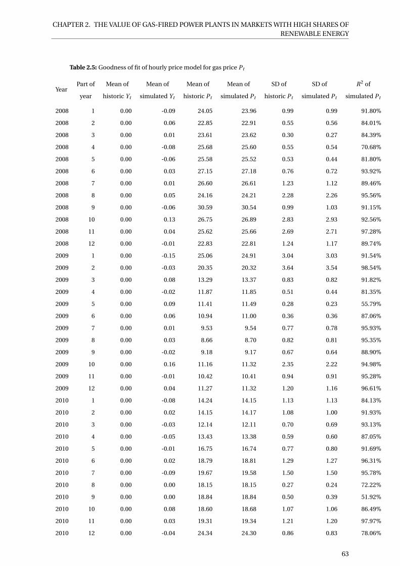
CHAPTER 2. THE VALUE OF GAS-FIRED POWER PLANTS IN MARKETS WITH HIGH SHARES OFRENEWABLE ENERGY
Table 2.5: Goodness of fit of hourly price model for gas price Pt
YearPart of
year
Mean of
historic Yt
Mean of
simulated Yt
Mean of
historic Pt
Mean of
simulated Pt
SD of
historic Pt
SD of
simulated Pt
R2 of
simulated Pt
2008 1 0.00 -0.09 24.05 23.96 0.99 0.99 91.80%
2008 2 0.00 0.06 22.85 22.91 0.55 0.56 84.01%
2008 3 0.00 0.01 23.61 23.62 0.30 0.27 84.39%
2008 4 0.00 -0.08 25.68 25.60 0.55 0.54 70.68%
2008 5 0.00 -0.06 25.58 25.52 0.53 0.44 81.80%
2008 6 0.00 0.03 27.15 27.18 0.76 0.72 93.92%
2008 7 0.00 0.01 26.60 26.61 1.23 1.12 89.46%
2008 8 0.00 0.05 24.16 24.21 2.28 2.26 95.56%
2008 9 0.00 -0.06 30.59 30.54 0.99 1.03 91.15%
2008 10 0.00 0.13 26.75 26.89 2.83 2.93 92.56%
2008 11 0.00 0.04 25.62 25.66 2.69 2.71 97.28%
2008 12 0.00 -0.01 22.83 22.81 1.24 1.17 89.74%
2009 1 0.00 -0.15 25.06 24.91 3.04 3.03 91.54%
2009 2 0.00 -0.03 20.35 20.32 3.64 3.54 98.54%
2009 3 0.00 0.08 13.29 13.37 0.83 0.82 91.82%
2009 4 0.00 -0.02 11.87 11.85 0.51 0.44 81.35%
2009 5 0.00 0.09 11.41 11.49 0.28 0.23 55.79%
2009 6 0.00 0.06 10.94 11.00 0.36 0.36 87.06%
2009 7 0.00 0.01 9.53 9.54 0.77 0.78 95.93%
2009 8 0.00 0.03 8.66 8.70 0.82 0.81 95.35%
2009 9 0.00 -0.02 9.18 9.17 0.67 0.64 88.90%
2009 10 0.00 0.16 11.16 11.32 2.35 2.22 94.98%
2009 11 0.00 -0.01 10.42 10.41 0.94 0.91 95.28%
2009 12 0.00 0.04 11.27 11.32 1.20 1.16 96.61%
2010 1 0.00 -0.08 14.24 14.15 1.13 1.13 84.13%
2010 2 0.00 0.02 14.15 14.17 1.08 1.00 91.93%
2010 3 0.00 -0.03 12.14 12.11 0.70 0.69 93.13%
2010 4 0.00 -0.05 13.43 13.38 0.59 0.60 87.05%
2010 5 0.00 -0.01 16.75 16.74 0.77 0.80 91.69%
2010 6 0.00 0.02 18.79 18.81 1.29 1.27 96.31%
2010 7 0.00 -0.09 19.67 19.58 1.50 1.50 95.78%
2010 8 0.00 0.00 18.15 18.15 0.27 0.24 72.22%
2010 9 0.00 0.00 18.84 18.84 0.50 0.39 51.92%
2010 10 0.00 0.08 18.60 18.68 1.07 1.06 86.49%
2010 11 0.00 0.03 19.31 19.34 1.21 1.20 97.97%
2010 12 0.00 -0.04 24.34 24.30 0.86 0.83 78.06%
63

CHAPTER 2. THE VALUE OF GAS-FIRED POWER PLANTS IN MARKETS WITH HIGH SHARES OFRENEWABLE ENERGY
Table 2.5: Goodness of fit of hourly price model for gas price Pt
YearPart of
year
Mean of
historic Yt
Mean of
simulated Yt
Mean of
historic Pt
Mean of
simulated Pt
SD of
historic Pt
SD of
simulated Pt
R2 of
simulated Pt
2011 1 0.00 0.00 22.94 22.94 1.07 1.10 95.34%
2011 2 0.00 -0.04 21.84 21.80 0.34 0.34 91.74%
2011 3 0.00 -0.04 23.73 23.69 0.85 0.83 92.19%
2011 4 0.00 -0.13 22.80 22.67 1.04 0.99 87.91%
2011 5 0.00 -0.01 22.76 22.75 0.49 0.49 90.32%
2011 6 0.00 -0.06 22.58 22.52 0.49 0.45 92.58%
2011 7 0.00 -0.01 21.68 21.68 0.31 0.27 67.99%
2011 8 0.00 -0.02 21.48 21.46 0.89 0.89 95.54%
2011 9 0.00 0.01 23.56 23.57 1.41 1.27 88.03%
2011 10 0.00 0.10 21.85 21.95 3.09 2.92 97.67%
2011 11 0.00 0.01 23.89 23.90 0.69 0.65 89.15%
2011 12 0.00 0.01 22.75 22.77 0.87 0.80 89.62%
2012 1 0.00 -0.03 21.74 21.71 0.67 0.69 88.99%
2012 2 0.00 -0.23 26.14 25.91 3.45 3.35 85.79%
2012 3 0.00 0.00 24.10 24.10 0.77 0.75 92.80%
2012 4 0.00 0.00 24.84 24.84 0.28 0.26 70.80%
2012 5 0.00 -0.04 24.31 24.27 0.83 0.79 91.79%
2012 6 0.00 0.02 23.72 23.75 0.48 0.45 78.50%
2012 7 0.00 -0.03 24.34 24.31 0.51 0.51 93.84%
2012 8 0.00 -0.01 24.03 24.02 0.59 0.58 86.48%
2012 9 0.00 -0.02 25.61 25.59 0.37 0.35 91.70%
2012 10 0.00 -0.02 26.57 26.56 0.68 0.69 97.56%
2012 11 0.00 0.01 27.19 27.21 0.22 0.21 79.06%
2012 12 0.00 -0.02 27.26 27.24 0.62 0.62 97.68%
2013 1 0.00 0.00 26.85 26.85 0.46 0.46 92.92%
2013 2 0.00 -0.01 26.34 26.33 0.30 0.31 88.76%
2013 3 0.00 0.14 29.96 30.09 3.22 3.11 94.08%
2013 4 0.00 -0.08 28.47 28.39 2.01 1.90 95.32%
2013 5 0.00 0.03 26.97 27.00 0.24 0.23 86.45%
2013 6 0.00 0.02 26.47 26.49 0.21 0.22 90.72%
2013 7 0.00 -0.02 26.27 26.26 0.16 0.15 78.86%
2013 8 0.00 0.00 25.75 25.76 0.23 0.21 86.56%
2013 9 0.00 0.00 26.58 26.58 0.38 0.37 97.44%
2013 10 0.00 -0.02 26.26 26.25 0.46 0.44 89.87%
2013 11 0.00 0.04 26.97 27.01 0.93 0.87 96.28%
2013 12 0.00 -0.03 27.69 27.67 0.59 0.59 95.01%
64

CHAPTER 2. THE VALUE OF GAS-FIRED POWER PLANTS IN MARKETS WITH HIGH SHARES OFRENEWABLE ENERGY
Table 2.5: Goodness of fit of hourly price model for gas price Pt
YearPart of
year
Mean of
historic Yt
Mean of
simulated Yt
Mean of
historic Pt
Mean of
simulated Pt
SD of
historic Pt
SD of
simulated Pt
R2 of
simulated Pt
2014 1 0.00 0.03 26.51 26.54 0.30 0.28 81.81%
2014 2 0.00 0.03 24.29 24.32 0.66 0.69 97.35%
2014 3 0.00 0.05 22.91 22.95 0.90 0.88 92.36%
2014 4 0.00 0.03 20.70 20.74 0.67 0.65 87.92%
2014 5 0.00 0.07 19.29 19.36 0.34 0.31 67.34%
2014 6 0.00 0.05 17.24 17.29 0.55 0.57 91.08%
2014 7 0.00 0.01 16.40 16.41 0.88 0.89 95.15%
2014 8 0.00 0.01 17.26 17.27 0.82 0.82 95.55%
2014 9 0.00 -0.05 20.48 20.44 0.98 0.96 90.39%
2014 10 0.00 0.01 21.36 21.36 0.70 0.69 88.02%
2014 11 0.00 0.07 22.67 22.74 1.25 1.06 91.61%
2014 12 0.00 -0.02 22.84 22.82 0.67 0.66 95.85%
2015 1 0.00 0.01 20.11 20.12 0.50 0.51 94.72%
2015 2 0.00 -0.03 22.51 22.49 1.03 1.02 95.44%
2015 3 0.00 -0.01 21.96 21.96 0.56 0.54 95.32%
2015 4 0.00 -0.05 22.05 22.00 0.49 0.47 90.01%
2015 5 0.00 0.03 20.66 20.69 0.22 0.21 62.52%
2015 6 0.00 0.00 20.69 20.69 0.16 0.14 78.99%
2015 7 0.00 -0.02 20.95 20.94 0.18 0.18 81.96%
2015 8 0.00 0.01 19.85 19.86 0.58 0.58 94.47%
2015 9 0.00 0.00 19.35 19.35 0.31 0.30 89.96%
2015 10 0.00 0.03 18.48 18.51 0.26 0.22 77.01%
2015 11 0.00 0.01 17.37 17.39 0.55 0.55 95.85%
2015 12 0.00 -0.04 16.01 15.96 1.31 1.28 96.74%
2016 1 0.00 0.01 14.37 14.38 0.64 0.60 80.55%
2016 2 0.00 0.03 12.74 12.77 0.35 0.35 82.63%
2016 3 0.00 -0.01 12.46 12.45 0.26 0.24 89.12%
2016 4 0.00 0.03 12.10 12.13 0.92 0.93 94.49%
2016 5 0.00 0.00 13.01 13.01 0.44 0.43 93.41%
2016 6 0.00 0.00 14.45 14.45 0.39 0.37 88.73%
2016 7 0.00 0.06 14.39 14.45 0.31 0.28 78.67%
2016 8 0.00 0.01 12.18 12.18 0.89 0.87 96.56%
2016 9 0.00 0.04 12.34 12.39 0.77 0.75 93.14%
2016 10 0.00 0.08 15.73 15.81 1.41 1.32 97.86%
2016 11 0.00 -0.10 17.93 17.83 0.41 0.34 52.68%
2016 12 0.00 0.01 17.74 17.76 0.66 0.65 95.08%
65
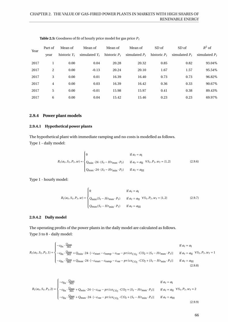
CHAPTER 2. THE VALUE OF GAS-FIRED POWER PLANTS IN MARKETS WITH HIGH SHARES OFRENEWABLE ENERGY
Table 2.5: Goodness of fit of hourly price model for gas price Pt
YearPart of
year
Mean of
historic Yt
Mean of
simulated Yt
Mean of
historic Pt
Mean of
simulated Pt
SD of
historic Pt
SD of
simulated Pt
R2 of
simulated Pt
2017 1 0.00 0.04 20.28 20.32 0.85 0.82 93.04%
2017 2 0.00 -0.13 20.24 20.10 1.67 1.57 95.54%
2017 3 0.00 0.01 16.39 16.40 0.73 0.73 96.82%
2017 4 0.00 0.03 16.39 16.42 0.36 0.33 90.67%
2017 5 0.00 -0.01 15.98 15.97 0.41 0.38 89.43%
2017 6 0.00 0.04 15.42 15.46 0.23 0.23 69.97%
2.9.4 Power plant models
2.9.4.1 Hypothetical power plants
The hypothetical plant with immediate ramping and no costs is modelled as follows.
Type 1 - daily model:
Rt (at ,St ,Pt , w) =
0 if at = aI
Qmin ·24 · (St −Hrmax ·Pt ) if at = aII
Qmax ·24 · (St −Hrmin ·Pt ) if at = aIII
∀St ,Pt , wt = {1,2} (2.9.6)
Type 1 - hourly model:
Rt (at ,St ,Pt , w) =
0 if at = aI
Qmin(St −Hrmax ·Pt ) if at = aII
Qmax(St −Hrmin ·Pt ) if at = aIII
∀St ,Pt , wt = {1,2} (2.9.7)
2.9.4.2 Daily model
The operating profits of the power plants in the daily model are calculated as follows.
Type 3 to 8 - daily model:
Rt (at ,St ,Pt ,1) =
−cfix ·Qmax365 if at = aI
−cfix ·Qmax365 +Qmin ·24 · [−cstart − cramp − cvar −pr i ceCO2
·CO2 + (St −Hrmax ·Pt )] if at = aII
−cfix ·Qmax365 +Qmax ·24 · [−cstart − cramp − cvar −pr i ceCO2
·CO2 + (St −Hrmin ·Pt )] if at = aIII
∀St ,Pt , wt = 1
(2.9.8)
Rt (at ,St ,Pt ,2) =
−cfix ·Qmax365 if at = aI
−cfix ·Qmax365 +Qmin ·24 · [−cvar −pr i ceCO2
·CO2 + (St −Hrmax ·Pt )] if at = aII
−cfix ·Qmax365 +Qmax ·24 · [−cvar −pr i ceCO2
·CO2 + (St −Hrmin ·Pt )] if at = aIII
∀St ,Pt , wt = 2
(2.9.9)
66

CHAPTER 2. THE VALUE OF GAS-FIRED POWER PLANTS IN MARKETS WITH HIGH SHARES OFRENEWABLE ENERGY
2.9.4.3 Hourly model
Type 5 and 6:
Rt (at ,St ,Pt ,1) =
−cfix ·Qmax8760 if at = aI
−cfix ·Qmax8760 +Qmin[−cstart − cramp − cvar −pr i ceCO2
·CO2 + (St −Hrmax ·Pt )] if at = aII
−cfix ·Qmax8760 +Qmax[−cstart − cramp − cvar −pr i ceCO2
·CO2 + (St −Hrmin ·Pt )] if at = aIII
∀St ,Pt , wt = 1
(2.9.10)
Rt (at ,St ,Pt ,2) =
−cfix ·Qmax8760 if at = aI
−cfix ·Qmax8760 +Qmin[−cvar −pr i ceCO2
·CO2 + (St −Hrmax ·Pt )] if at = aII
−cfix ·Qmax8760 +Qmax[−cvar −pr i ceCO2
·CO2 + (St −Hrmin ·Pt )] if at = aIII
∀St ,Pt , wt = 2
(2.9.11)
Type 2, 3, 4, 7 and 8:
Rt (at ,St ,Pt ,1) =
−cfix ·Qmax8760 if at = aI
−cfix ·Qmax8760 if at = aII
−cfix ·Qmax8760 +Qmin[−cramp − cstart − cvar −pr i ceCO2
·CO2 + (St −Hrmax ·Pt )] if at = aIII
∀St ,Pt , wt = 1
(2.9.12)
Rt (at ,St ,Pt ,2) =
−cfix ·Qmax8760 if at = aI
−cfix ·Qmax8760 +Qmin[−cvar −pr i ceCO2
·CO2 + (St −Hrmax ·Pt )] if at = aII
−cfix ·Qmax8760 − cramp(Qmax −Qmin)+Qmax[−cvar −pr i ceCO2
·CO2 + (St −Hrmin ·Pt )] if at = aIII
∀St ,Pt , wt = 2
(2.9.13)
Rt (at ,St ,Pt ,3) =
−cfix ·Qmax8760 if at = aI
−cfix ·Qmax8760 +Qmax[−cvar −pr i ceCO2
·CO2 + (St −Hrmin ·Pt )] if at = aII
−cfix ·Qmax8760 +Qmax[−cvar −pr i ceCO2
·CO2 + (St −Hrmin ·Pt )] if at = aIII
∀St ,Pt , wt = 3
(2.9.14)
2.9.5 Cost inputs for power plant model
See table 2.6.
67

CHAPTER 2. THE VALUE OF GAS-FIRED POWER PLANTS IN MARKETS WITH HIGH SHARES OFRENEWABLE ENERGY
Parameter
name
Value (new CCCGT; old CCGT;
new gas turbine; old gas turbine;
new steam; old steam) and unit
Details Source
cst ar t 21.05; 26.32; 16.54; 24.06; 18.80;27.07e/△ MW
Fuel-related start-up costs for hotstart. 25th percentile (for new plants)and median value (for old plants). Hotstart means the plant has been off-line for 8 hours or less, warm start formore than 8 hours and cold start formore than 50 hours. Cold start oc-curs rarely, mainly for maintenance,and the model cannot distinguish be-tween hot, warm and cold start.
Kumar et al(2012), p. 12.
cr amp 0.25; 0.25; 0.66; 0.66; 1.17; 1.17e/△ MW
Ramping cost. Kumar et al(2012), p. 16.
c f i x 17,000; 17,000; 15,000; 15,000;15,000; 15,000e/MW/year
Fixed O&M cost. Schröder et al(2013), p. 88.
cvar 2.1; 2.1; 2; 2; 2; 2e/MWh Variable O&M cost. Schröder et al(2013), p. 88.
co2 0.33; 0.36; 0.55; 0.55; 0.55; 0.55t/MWh
CO2 equivalent estimates in t/MWh. Schröder et al(2013), p. 42.
pr i ceco2 Between 4.48 and 22 e/t from2008 to 2016
CO2 prices as average of daily priceseach year ine/t.
Bloomberg(2017).
Qmax 100; 100; 100; 100; 100; 100 MW Maximum capacity of power plant cal-culated as average of net generationcapacity of operating German gas-fired power plants.
Open PowerSystem Data(2017).
Lmi n 40.33; 40.33; 33.13; 33.13; 40; 40% Minimum load as percentage of max-imum capacity, calculated as averagevalue. Below the minimum load a sta-ble operation is not possible due toinsufficient temperature or excessiveemissions.
Schröder et al(2013), p. 66.
Qmi n Lmi n ·Qmax Minimum capacity of power plant inMW.
Hrmi n 1.67; 1.93; 2.43; 2.89; 2.50; 2.71 Minimum heat rate. For one unit elec-tricity you need, if plant is running atmaximum capacity, Hrmi n units gas.Calculated via the average of efficien-cies of German power plants built un-til (old) and after 2010 (new).
Open PowerSystem Data(2017).
Hrmax 1.1 ·Hrmi n Maximum heat rate. For one unit elec-tricity you need, if plant is running atminimum capacity, Hrmax units gas.
IEA (2015).
di scount 7.20% Weighted average cost of capital(WACC) for energy sector in Germany,Austria and Switzerland.
KPMG (2014).
I 800,000; 800,000; 400,000;400,000; 400,000; 400,000e/MW
Capital cost defined as greenfield andovernight investment cost, compris-ing the construction of a power plantexcluding all interest effects.
Schröder et al(2013), p. 88.
l i f et i me 32 years Lifetime of power plant. Calculated asaverage value.
Schröder et al(2013), p. 72.
Table 2.6: Cost inputs for power plant model
68
Chapter 3
Utility divestitures in Germany
A case study of corporate financial strategies and energy
transition risk
A version of this chapter was published as an SSRN working paper on ❤t t♣ ✿ ✴✴ ❞① ✳❞ ♦✐ ✳♦ r❣ ✴✶ ✵✳ ✷✶ ✸✾
✴s sr ♥✳ ✸✸ ✼✾ ✺✹ ✺ in May 2019.
Abstract
Germany is in the midst of a radical transformation of its power sector, which in 2016 led
two of its main electric utilities, EON and RWE, to undertake dramatic restructurings. EON
spun off its fossil fuel and trading segments, while RWE carved out its renewable energy, retail
and grid business.
The paper examines the drivers of these divestitures. Building on corporate finance liter-
ature, the paper uses a mix of comparative descriptive statistics, interviews and event studies
to test four groups of hypotheses. The evidence rejects drivers related to operations and man-
agement, biased investment and investor preferences and instead points to financing-related
drivers. Among the financing-related drivers, debt overhang and risk contamination seemed
to have played the main role. Utilities restructured to save their healthy assets (renewables and
grid infrastructure) from losses at their conventional power generation business (fossil fuel and
nuclear plants).
The paper uses existing research on divestitures in an empirical case that has implications
for the evolution of European power markets. The results suggest that exiting conventional
technologies as part of the transition to a more renewable energy mix can cause substantial
costs. If these are not clarified and allocated ex ante, policy makers find themselves forced
to either burden tax payers or endanger utilities that are of systemic relevance to the energy
sector.
Key words— Electric utilities; event study; risk; energy transition; nuclear power; renewable energy.
69
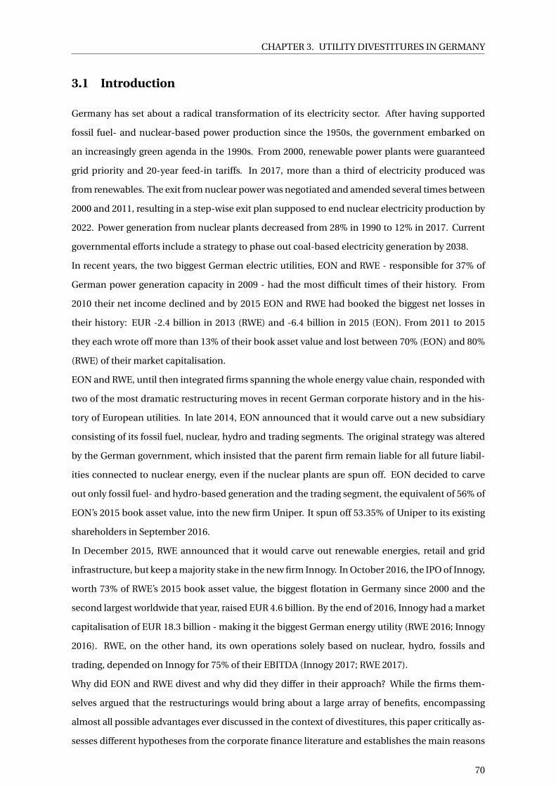
CHAPTER 3. UTILITY DIVESTITURES IN GERMANY
3.1 Introduction
Germany has set about a radical transformation of its electricity sector. After having supported
fossil fuel- and nuclear-based power production since the 1950s, the government embarked on
an increasingly green agenda in the 1990s. From 2000, renewable power plants were guaranteed
grid priority and 20-year feed-in tariffs. In 2017, more than a third of electricity produced was
from renewables. The exit from nuclear power was negotiated and amended several times between
2000 and 2011, resulting in a step-wise exit plan supposed to end nuclear electricity production by
2022. Power generation from nuclear plants decreased from 28% in 1990 to 12% in 2017. Current
governmental efforts include a strategy to phase out coal-based electricity generation by 2038.
In recent years, the two biggest German electric utilities, EON and RWE - responsible for 37% of
German power generation capacity in 2009 - had the most difficult times of their history. From
2010 their net income declined and by 2015 EON and RWE had booked the biggest net losses in
their history: EUR -2.4 billion in 2013 (RWE) and -6.4 billion in 2015 (EON). From 2011 to 2015
they each wrote off more than 13% of their book asset value and lost between 70% (EON) and 80%
(RWE) of their market capitalisation.
EON and RWE, until then integrated firms spanning the whole energy value chain, responded with
two of the most dramatic restructuring moves in recent German corporate history and in the his-
tory of European utilities. In late 2014, EON announced that it would carve out a new subsidiary
consisting of its fossil fuel, nuclear, hydro and trading segments. The original strategy was altered
by the German government, which insisted that the parent firm remain liable for all future liabil-
ities connected to nuclear energy, even if the nuclear plants are spun off. EON decided to carve
out only fossil fuel- and hydro-based generation and the trading segment, the equivalent of 56% of
EON’s 2015 book asset value, into the new firm Uniper. It spun off 53.35% of Uniper to its existing
shareholders in September 2016.
In December 2015, RWE announced that it would carve out renewable energies, retail and grid
infrastructure, but keep a majority stake in the new firm Innogy. In October 2016, the IPO of Innogy,
worth 73% of RWE’s 2015 book asset value, the biggest flotation in Germany since 2000 and the
second largest worldwide that year, raised EUR 4.6 billion. By the end of 2016, Innogy had a market
capitalisation of EUR 18.3 billion - making it the biggest German energy utility (RWE 2016; Innogy
2016). RWE, on the other hand, its own operations solely based on nuclear, hydro, fossils and
trading, depended on Innogy for 75% of their EBITDA (Innogy 2017; RWE 2017).
Why did EON and RWE divest and why did they differ in their approach? While the firms them-
selves argued that the restructurings would bring about a large array of benefits, encompassing
almost all possible advantages ever discussed in the context of divestitures, this paper critically as-
sesses different hypotheses from the corporate finance literature and establishes the main reasons
70

CHAPTER 3. UTILITY DIVESTITURES IN GERMANY
responsible for the decisions.
The paper distils hypotheses from the corporate finance literature on divestitures and tests them
in an empirical case that has implications for the evolution of European power markets. An inno-
vative mixed methods approach facilitates the testing of different hypotheses that would not have
been possible otherwise and strengthens confidence in the validity of the results. Qualitative re-
search, interviews, descriptive statistics and event studies converge in rejecting drivers related to
operations and management, biased investment and investor preferences and in confirming debt
overhang and risk contamination as the main drivers.
The paper is structured as follows. Section 3.2 lays out the goal and contribution of this paper.
Section 3.3 reviews the corporate finance literature and distils its main hypotheses and their rela-
tion to each other. Section 3.4 gives an overview of the methodology used. Section 3.5 summarizes
the main hypotheses and results. Section 3.6 to 3.9 are each dedicated to testing one group of di-
vestiture drivers: drivers related to operations and management, investing, financing and investor
preferences. Section 3.10 concludes and section 3.11 suggests policy implications as well as ideas
for further research.
3.2 Goal, contribution and case selection
3.2.1 Goal and relevance
The goal of this paper is to investigate why EON and RWE divested in 2016 and why their approach
was at the same time very similar (they separated their business segments in exactly the same way)
and very different (EON intended to keep renewables and grid infrastructure and spun off the rest,
while RWE kept the conventional generation and trading).
Why do we care what was driving the two utility divestitures in Germany? World wide, electricity
markets are transitioning from a fossil fuel- and nuclear-based power supply towards more renew-
ables. The transition has major consequences on incumbent utilities and thereby on the existing
electricity system as a whole. This is all the more important, as electricity is generally regarded as
a basic good that should be reliably available to all. Affordable and reliable access to electricity is
also a fundamental factor for private investment and thereby a country’s economic wealth. More-
over, electricity markets have strong monopoly tendencies and state policies play an important
role. For these reasons, researchers and policy makers should have a vital interest in understand-
ing the problems and strategies of utilities in order to apply lessons learned in Germany to other
countries on a similar path away from nuclear and fossils to more renewable electricity sources.
71
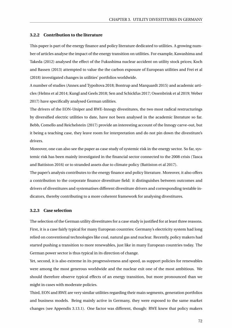
CHAPTER 3. UTILITY DIVESTITURES IN GERMANY
3.2.2 Contribution to the literature
This paper is part of the energy finance and policy literature dedicated to utilities. A growing num-
ber of articles analyse the impact of the energy transition on utilities. For example, Kawashima and
Takeda (2012) analysed the effect of the Fukushima nuclear accident on utility stock prices; Koch
and Bassen (2013) attempted to value the the carbon exposure of European utilities and Frei et al
(2018) investigated changes in utilities’ portfolios worldwide.
A number of studies (Annex and Typoltova 2018; Bontrup and Marquardt 2015) and academic arti-
cles (Helms et al 2014; Kungl and Geels 2018; Sen and Schickfus 2017; Ossenbrink et al 2019; Weber
2017) have specifically analysed German utilities.
The drivers of the EON-Uniper and RWE-Innogy divestitures, the two most radical restructurings
by diversified electric utilities to date, have not been analysed in the academic literature so far.
Bebb, Comello and Reichelstein (2017) provide an interesting account of the Innogy carve-out, but
it being a teaching case, they leave room for interpretation and do not pin down the divestiture’s
drivers.
Moreover, one can also see the paper as case study of systemic risk in the energy sector. So far, sys-
temic risk has been mainly investigated in the financial sector connected to the 2008 crisis (Tasca
and Battiston 2016) or to stranded assets due to climate policy (Battiston et al 2017).
The paper’s analysis contributes to the energy finance and policy literature. Moreover, it also offers
a contribution to the corporate finance divestiture field: it distinguishes between outcomes and
drivers of divestitures and systematises different divestiture drivers and corresponding testable in-
dicators, thereby contributing to a more coherent framework for analysing divestitures.
3.2.3 Case selection
The selection of the German utility divestitures for a case study is justified for at least three reasons.
First, it is a case fairly typical for many European countries: Germany’s electricity system had long
relied on conventional technologies like coal, natural gas and nuclear. Recently, policy makers had
started pushing a transition to more renewables, just like in many European countries today. The
German power sector is thus typical in its direction of change.
Yet, second, it is also extreme in its progressiveness and speed, as support policies for renewables
were among the most generous worldwide and the nuclear exit one of the most ambitious. We
should therefore observe typical effects of an energy transition, but more pronounced than we
might in cases with moderate policies.
Third, EON and RWE are very similar utilities regarding their main segments, generation portfolios
and business models. Being mainly active in Germany, they were exposed to the same market
changes (see Appendix 3.13.1). One factor was different, though: RWE knew that policy makers
72
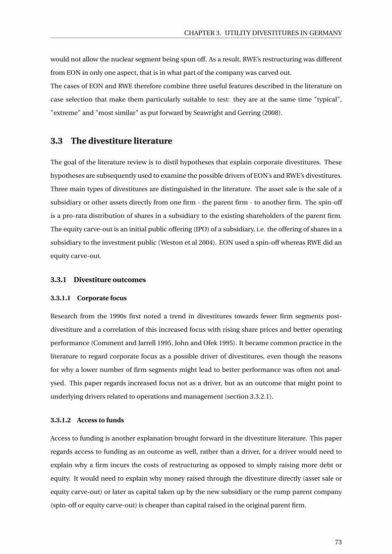
CHAPTER 3. UTILITY DIVESTITURES IN GERMANY
would not allow the nuclear segment being spun off. As a result, RWE’s restructuring was different
from EON in only one aspect, that is in what part of the company was carved out.
The cases of EON and RWE therefore combine three useful features described in the literature on
case selection that make them particularly suitable to test: they are at the same time "typical",
"extreme" and "most similar" as put forward by Seawright and Gerring (2008).
3.3 The divestiture literature
The goal of the literature review is to distil hypotheses that explain corporate divestitures. These
hypotheses are subsequently used to examine the possible drivers of EON’s and RWE’s divestitures.
Three main types of divestitures are distinguished in the literature. The asset sale is the sale of a
subsidiary or other assets directly from one firm - the parent firm - to another firm. The spin-off
is a pro-rata distribution of shares in a subsidiary to the existing shareholders of the parent firm.
The equity carve-out is an initial public offering (IPO) of a subsidiary, i.e. the offering of shares in a
subsidiary to the investment public (Weston et al 2004). EON used a spin-off whereas RWE did an
equity carve-out.
3.3.1 Divestiture outcomes
3.3.1.1 Corporate focus
Research from the 1990s first noted a trend in divestitures towards fewer firm segments post-
divestiture and a correlation of this increased focus with rising share prices and better operating
performance (Comment and Jarrell 1995, John and Ofek 1995). It became common practice in the
literature to regard corporate focus as a possible driver of divestitures, even though the reasons
for why a lower number of firm segments might lead to better performance was often not anal-
ysed. This paper regards increased focus not as a driver, but as an outcome that might point to
underlying drivers related to operations and management (section 3.3.2.1).
3.3.1.2 Access to funds
Access to funding is another explanation brought forward in the divestiture literature. This paper
regards access to funding as an outcome as well, rather than a driver, for a driver would need to
explain why a firm incurs the costs of restructuring as opposed to simply raising more debt or
equity. It would need to explain why money raised through the divestiture directly (asset sale or
equity carve-out) or later as capital taken up by the new subsidiary or the rump parent company
(spin-off or equity carve-out) is cheaper than capital raised in the original parent firm.
73

CHAPTER 3. UTILITY DIVESTITURES IN GERMANY
The access-to-funds topic has been distinguished in two ways in the literature. The first possibility
is that the divestiture decreases the firm’s higher-than-average debt either by using the proceeds
directly to retire debt and thereby reducing financial distress (Brown, James and Mooradian 1994;
Lang, Poulsen and Stulz 1995) or by transferring debt to their subsidiary (Desai and Jain 1999). This
outcome would hint at debt overhang being a main driver (section 3.3.2.3).
The second possibility is that the goal is to raise funds for growth in the subsidiary (Schipper and
Smith 1986; Daley, Mehrotra and Sivakumar 1997; Vijh 2002).1 This outcome could hint at a num-
ber of drivers, which would need to explain why growth opportunities cannot be funded in the
integrated firm, e.g. debt overhang, agency conflicts related to investing or risk contamination (see
also table 3.1).
3.3.2 Divestiture drivers
Drivers are divided into four groups: operations and management, investing, financing and in-
vestor preferences.
3.3.2.1 Drivers related to operations and management
The first group of drivers refers to the relationship of the firm’s operations to each other and to the
managers. Authors generally use poor performance pre- and better performance post-divestiture
to argue for these drivers.
Inefficient diversification. The inefficient diversification argument suggests that managers pre-
viously diversified inefficiently, driven by agency problems like empire building (Jensen 1986,
1988), hubris (Roll 1986), managerial entrenchment (Shleifer and Vishny 1989) or managerial dis-
cretion (Stulz 1990, see also section 3.3.2.2).
Change in synergies. Similarly, a change in synergies between business segments might also lead
to poor performance and drive firms to divest (Hanson and Song 2003). Reasons for changes in syn-
ergies might be changes in regulations or technical innovations (Shleifer and Vishny 1990; Kaplan
and Weisbach 1992).
Lack of fit with owner or better fit with buyer. Another driver of divestitures might be a better fit
with the buyer’s skill set (John and Ofek 1995; Daley, Mehrotra and Sivakumar 1997).
1This holds only for equity carve-outs, where funds are raised immediately, and for spin-offs, where funds can beraised later in the separate firm, but not for asset sales, where the subsidiary does not become a separate entity.
74

CHAPTER 3. UTILITY DIVESTITURES IN GERMANY
Management focus. Even if the skill sets of managers in subsidiary and rump parent firm are not
so different, one could argue that simply the reduction of the diversity of segments under manage-
ment increases the efficiency of the managers (Berger and Ofek 1995; Desai and Jain 1999).
3.3.2.2 Drivers related to investing
The second group of drivers is related to suboptimal investment decisions by the management in
the integrated pre-divestiture firm, be it at headquarters or in the divisions. Suboptimal invest-
ments are caused by some type of agency conflict between managers and shareholders. The result
is a ‘pecking order’ in the sense of Myers (1984), where proceeds from a divestiture or capital raised
in the post-divestiture firms are cheaper than new equity or debt in the integrated firm. Lang,
Poulsen and Stulz (1995) first referred to this in the context of divestitures.
Asset substitution. This driver refers to the danger of managers being pushed into high risk
projects by shareholders at the expense of debt holders, as shareholders have unlimited upside but
limited downside risk. The mechanism was first discussed by Jensen and Meckling (1976). Lang,
Poulsen and Stulz (1995) and Officer (2007) mention it as a potential driver for divestitures, albeit
without going into detail.
Managerial discretion. This is another agency problem causing less than optimal investments.
The argument was first developed by Jensen (1986). Due to personal benefits linked to invest-
ments, managers always claim that cash flow is too low to fund all positive net present value (NPV)
projects. Their claim is therefore not credible when cash flow is truly low. The result is a situation
of under-investment when cash flow is low and over-investment when it is high, as capital mar-
kets price in the agency conflict (Stulz 1990). Divestiture might therefore be a cheaper way to raise
funds directly than on the capital markets.
Rent-seeking by divisions. Another explanation for suboptimal investment in the integrated firm
is a failure to optimally allocate capital to different divisions. Meyer, Milgrom, and Roberts (1992),
Wulf (1997) and Scharfstein and Stein (2000) theoretically model how rent-seeking by the divisions
can induce corporate headquarters to allocate excessive capital to divisions with poor investment
opportunities. Empirically, Lamont (1997), Shin and Stulz (1998), Scharfstein (1998) and Rajan et
al (2000), among others, have shown that conglomerate divisions might receive cross-subsidies,
that is more funds than is justified by their own cash flows or by their growth opportunities. In
the empirical divestiture literature, Dittmar and Shivdasani (2001) find that after asset sales par-
ents’ investment allocation improves. Gertner, Power and Scharfstein (2002) find that spun-off
subsidiaries optimize their capital allocation.
75

CHAPTER 3. UTILITY DIVESTITURES IN GERMANY
Failure of capital allocation method. A recent stream in the literature relates to the failure of
companies to adequately reflect the risk-return profile of different projects in their capital allo-
cation method. Krüger et al (2015) argue that, controlling for growth opportunities, companies
are inclined to invest less in their low-risk divisions because they use one single cost of capital to
appraise projects across segments. Helms, Salm and Wüstenhagen (2014) have applied the same
argument to utilities’ investment behaviour.
3.3.2.3 Drivers related to financing
The last group of drivers analyses the effect of financing decisions in an integrated compared to a
separated firm. While most drivers assume an effect of financing on investment incentives, appro-
priate gearing and the risk contamination effect can be explained through purely financial effects
keeping investment constant.
Debt overhang. Debt overhang describes a situation where a positive NPV project cannot be
funded by either debt or equity, because the project returns would partly benefit existing credi-
tors (Myers 1977). This might explain why asset sales can be attractive: the proceeds might be
cheaper than new debt or equity. And the firm could use the funds to retire debt, thereby allevi-
ating debt overhang. The problem is mentioned by Lang, Poulsen and Stulz (1995) and Hanson
and Song (2003) in the divestiture context and high leverage is generally used as an indicator for
poor financing options of divesting firms (see section 3.3.1.2). For spin-offs, Desai and Jain (1999)
hypothesise that the firm could get rid of some debt by transferring it to the new subsidiary.
Appropriate gearing. Some authors argue that the debt overhang problem can be less severe for
separate as opposed to integrated firms. For example, Myers (1977) observes that depending on the
joint cash flows and existing debt, either separate or joint financing can lead to better investment
incentives. John (1993) models spin-offs and shows that when divisional cash flows are positively
correlated, spin-offs can lead to value increases: the "intuition is that for sufficiently high debt
levels on the parent firm, there is a lock-up effect such that the technologies are either exercised
together or neither is exercised. The flexibility afforded by optimally allocating the debt between
components improves investment incentives." (John 1993, p. 139)
Leland (2007) relies on purely financial effects to develop the appropriate gearing hypothesis, i.e.
investment stays constant. He assumes an optimal debt level in the trade-off theory sense: the
benefit of a debt-related tax shield is balanced against the increase in bankruptcy cost with higher
debt levels. Depending on whether a divestiture increases or decreases the overall tax shield in
the two henceforth separate firms taken together, there is thus a positive or negative effect from
appropriate gearing after divestiture (Leland 2007).
76

CHAPTER 3. UTILITY DIVESTITURES IN GERMANY
Risk contamination. The risk contamination argument constitutes the other half of Leland’s
model and it is an unambiguously positive financial effect of separation. It is essentially the down-
side of the co-insurance effect: divisions can co-insure each other, but they can also contaminate
each other. Specifically, if divisions’ cash flows can be negative, one division can eat into another
one’s cash flows or even assets (Scott 1977; Sarig 1985). In a separated structure, one division’s
losses are limited by the same division’s assets with no effects on other divisions. Leland (2007)
calls this the ‘limited liability (LL) effect’ of separation. His model predicts that the benefits of sep-
aration increase in segments’ cash flows correlation and with high or very different volatilities or
default costs. Banal-Estanol, Ottaviani and Winton (2013) extend the analysis to show that also
without the ‘appropriate gearing’ aspect, i.e. when holding total debt constant, the net of LL and
co-insurance effect can justify separation.
Asymmetric information. The asymmetric information hypothesis goes back to a paper by My-
ers and Majluf (1984) that inspired the development of the pecking order theory of capital structure.
Managers know the true value of the firm’s assets and growth opportunities whereas outside in-
vestors can only guess. Acting in the interest of existing shareholders, managers cannot issue new
stock for all positive NPV projects because equity issues signal the firm being overvalued by the
market. They thus prefer internal funds to debt and debt to equity. Nanda (1991) extends the
model and explains why equity carve-outs on average have a positive effect on the parent’s share
price, contrary to seasoned equity offerings. His model is, however, not applicable to EON or RWE.2
Another mechanism related to asymmetric information is simply the reduction of information
asymmetry by going public (Schipper and Smith 1986). Several researchers have examined this
by looking at analysts’ forecast dispersion or error or the increase in coverage by analysts post-
divestiture (Best, Best and Agapos 1998; Krishnaswami and Subramaniam 1999; Gilson et al 2001;
Chen and Guo 2005).
3.3.2.4 Drivers related to investor preferences
The last driver rests on the assumption that investors have heterogeneous preferences and that
spin-offs and equity carve-outs facilitate the trading in different stocks than pre-divestiture. Value
creation might thus stem from relaxing a trading constraint that existed previously.
Vijh (1994) finds increased trading volume and abnormal positive stock returns on the day that the
subsidiary starts trading separately. Were value gains related to the parent firm only, one would
expect share price improvements taking place on the announcement day of the splits and the ex
2Nanda’s model is only applicable to divestitures with immediate funds being raised, thus not to EON. The modelhinges on the assumption that the subsidiary is smaller than the parent so that the positive share price effect of theparent’s being undervalued dominates. Innogy, however, is more than 40% larger in terms of book asset value andmarket cap than its parent RWE ex Innogy.
77
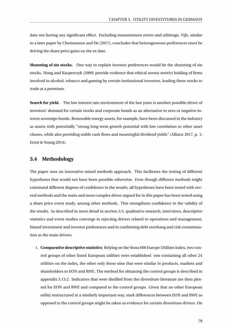
CHAPTER 3. UTILITY DIVESTITURES IN GERMANY
date not having any significant effect. Excluding measurement errors and arbitrage, Vijh, similar
to a later paper by Chemmanur and He (2017), concludes that heterogeneous preferences must be
driving the share price gains on the ex date.
Shunning of sin stocks. One way to explain investor preferences would be the shunning of sin
stocks. Hong and Kacperczyk (2009) provide evidence that ethical norms restrict holding of firms
involved in alcohol, tobacco and gaming by certain institutional investors, leading these stocks to
trade at a premium.
Search for yield. The low interest rate environment of the last years is another possible driver of
investors’ demand for certain stocks and corporate bonds as an alternative to zero or negative in-
terest sovereign bonds. Renewable energy assets, for example, have been discussed in the industry
as assets with potentially "strong long-term growth potential with low correlation to other asset
classes, while also providing stable cash flows and meaningful dividend yields" (Allianz 2017, p. 1;
Ernst & Young 2014).
3.4 Methodology
The paper uses an innovative mixed methods approach. This facilitates the testing of different
hypotheses that would not have been possible otherwise. Even though different methods might
command different degrees of confidence in the results, all hypotheses have been tested with sev-
eral methods and the main and most complex driver argued for in this paper has been tested using
a share price event study, among other methods. This strengthens confidence in the validity of
the results. As described in more detail in section 3.5, qualitative research, interviews, descriptive
statistics and event studies converge in rejecting drivers related to operations and management,
biased investment and investor preferences and in confirming debt overhang and risk contamina-
tion as the main drivers.
1. Comparative descriptive statistics: Relying on the Stoxx 600 Europe Utilities index, two con-
trol groups of other listed European utilities were established: one containing all other 24
utilities on the index, the other only those nine that were similar in products, markets and
shareholders to EON and RWE. The method for obtaining the control groups is described in
appendix 3.13.2. Indicators that were distilled from the divestiture literature are then plot-
ted for EON and RWE and compared to the control groups. Given that no other European
utility restructured in a similarly important way, stark differences between EON and RWE as
opposed to the control groups might be taken as evidence for certain divestiture drivers. On
78

CHAPTER 3. UTILITY DIVESTITURES IN GERMANY
the other hand, if EON and RWE were very similar to their control groups in certain indica-
tors, this might be evidence against these drivers.3
2. Interviews: in the course of 2018, 20 interviews were conducted to triangulate the other
methods. The interviewees were 10 people who worked at EON or RWE in 2016, of which
two and three were from management, and three and two from staff at EON and RWE re-
spectively. Ten were experts, of which three equity analysts, three financial news journalists,
two from management at two other European utilities and two academics. The clear focus
of the responses on a couple of drivers turned out to be in line with the rest of the analysis.
All interviews were done in a semi-structured way and started from the question: "What do
you think were the main drivers responsible for the splits of EON and RWE in 2016?" so as to
not bias the responses initially. In the course of the interview, all possible drivers identified
were then offered as potential alternative explanations.
3. Analysis of gray literature: EON and RWE annual reports (2005-2017), investor presenta-
tions, and more than 280 newspaper articles have been analysed in order to enrich and tri-
angulate the results of the other methods.
4. Share price event study: While comparative descriptive statistics, interviews and the analy-
sis of gray literature are used to test all hypotheses, the event studies are only used to inves-
tigate two hypotheses that were most referred to in the interviews: risk contamination and
investor preferences. Using regression analyses, the effect of different events on EON’s and
RWE’s share price and stocks traded is examined. The tests are used to examine whether cer-
tain types of new information were perceived as a risk for the utilities’ future growth options
in line with the risk contamination hypothesis developed earlier and whether the ex dates
had an effect on trading indicating evidence for heterogeneous investor preferences.
3.5 Indicators and summary of results
3.5.1 Indicators and interview results
Table 3.1 lists the possible drivers with empirical indicators identified from the literature as well as
the methods used to test them. The drivers related to operating and management are all summa-
rized into one column, as well as the drivers related to investing and investor preferences, whereas
the financial drivers are listed separately because their distinction will be important later on. The
3Vattenfall and EnBW, even though they own the third and fourth biggest generation portfolio in Germany, are notpart of the control group. They are dominated by public shareholders holding more than 95% and are thus not part ofthe Stoxx index.
79

CHAPTER 3. UTILITY DIVESTITURES IN GERMANY
cells are only filled if the corresponding hypothesis predicts the indicator to be confirmed. Indi-
cators that are confirmed are marked with yes and rejected with no. The last line states whether
sufficient evidence could be gathered for each driver. Only if all of the relevant indicators are con-
firmed, evidence is deemed sufficient to confirm a driver. Drivers are rejected if at least one indi-
cator is marked with no. Only debt overhang (III.1.) and risk contamination (III.4.) are confirmed;
all other drivers are rejected.
Table 3.2 shows the number of interview partners supporting each hypothesis. For anonymity rea-
sons the results cannot be distinguished any further, but there were no trends evident in responses
from different sub-groups. Interview results strongly concentrate on two drivers: risk contamina-
tion (III.4.) and investor preferences (IV., total support of 15 and 16).
80

CHAPTER 3. UTILITY DIVESTITURES IN GERMANY
Indicator Methodused
I.Operations
and man-
agement
II.Investing III.1.Financing:
debt over-
hang
III.2.Financing:
appropriate
gearing
III.3.Financing:
asymmetric
information
III.4.Financing:
risk con-
tamination
IV.Investor
preferences
Low performancepre-, better post-divestiture
Comparativedescriptivestatistics
Yes Yes Yes Yes
Increase in focus Gray lit-erature,interviews
Yes
Changes insynergies pre-divestiture
Interviews,gray litera-ture
No
New managerswith different skillsets
Interviews,gray litera-ture
No
Funds raised forgrowth
Comparativedescriptivestatistics,gray litera-ture
Yes Yes Yes
Funds raised forretirement of debt
Comparativedescriptivestatistics,gray litera-ture
Yes
High overallcapex/assets
Comparativedescriptivestatistics
No
High correlationcapex with cashflows
Comparativedescriptivestatistics
No
Low capex in re-newables vs. con-ventional
Capex num-bers fromannualreports
No
One cost of cap-ital used for allsegments
Interviews No
High leverage Comparativedescriptivestatistics
Only if incl.nuclear pro-visions
Higher tax shieldpost-divestiture
Tax shield No
Improved earn-ing estimatespost-divestiture
Analysts’ es-timates fromBloomberg
Only atRWE’sInnogy
Different valua-tions parent vs.subsidiary
Valuationsfrom Thom-son Reuters
Yes
Big past and riskof future losses inone part of firm
Comparativedescriptivestatistics,interviews,event stud-ies
Yes
Share price effecton ex date
Event stud-ies
Only onRWE-Innogyex date
Investor prefer-ence for renew-ables and gridsover conventionalgeneration
Interviews,gray litera-ture
Possibly butunclear ifloss avoid-ance
Divestments dueto political com-mitments
Interviews,gray litera-ture, data onsharehold-ings
No
Driver con-
firmed?
No No Yes No No Yes No
Table 3.1: Hypotheses with main indicators tested in this paper. Indicators that are confirmed are markedwith yes, undecided with unclear and rejected with no. Cells are empty for indicators not relevant for therespective hypotheses. The last line summarizes the overall result for each driver tested.
81
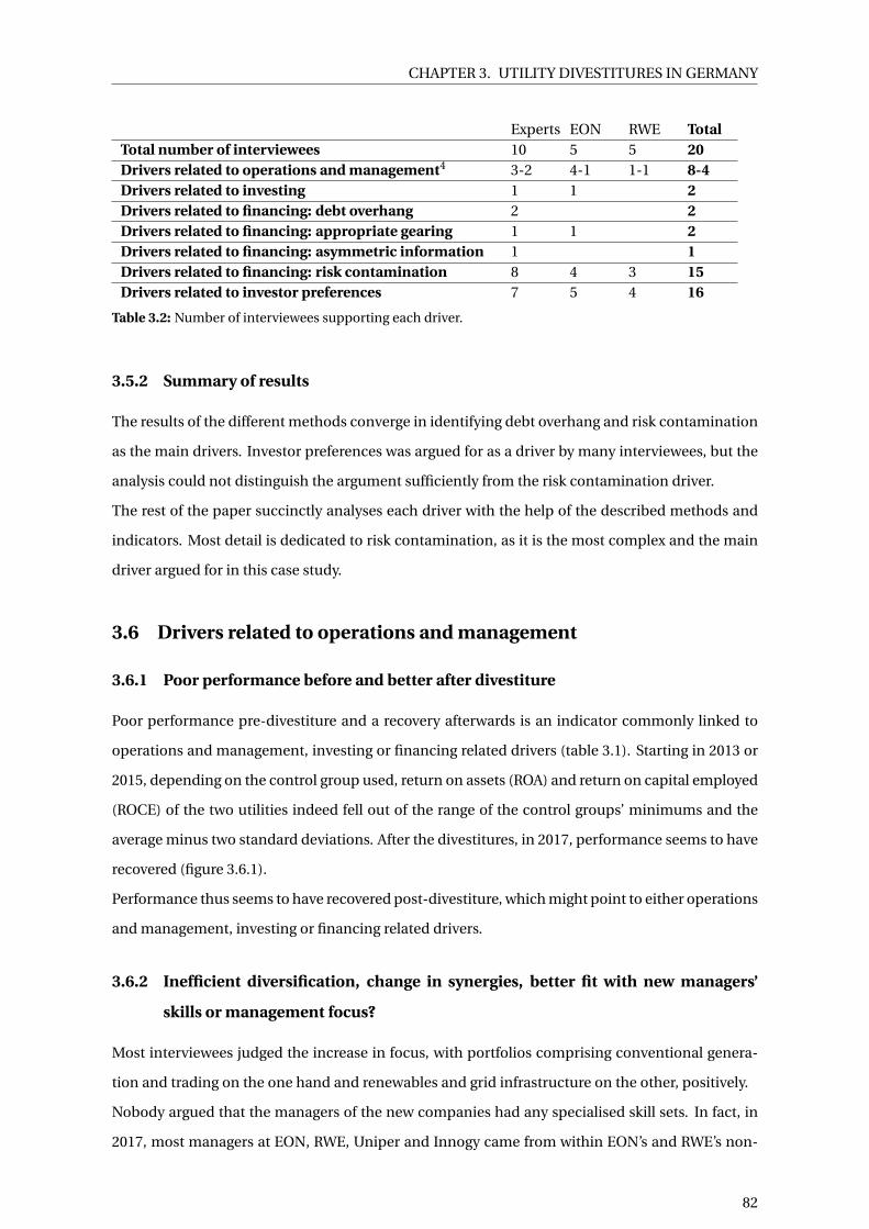
CHAPTER 3. UTILITY DIVESTITURES IN GERMANY
Experts EON RWE Total
Total number of interviewees 10 5 5 20
Drivers related to operations and management4 3-2 4-1 1-1 8-4
Drivers related to investing 1 1 2
Drivers related to financing: debt overhang 2 2
Drivers related to financing: appropriate gearing 1 1 2
Drivers related to financing: asymmetric information 1 1
Drivers related to financing: risk contamination 8 4 3 15
Drivers related to investor preferences 7 5 4 16
Table 3.2: Number of interviewees supporting each driver.
3.5.2 Summary of results
The results of the different methods converge in identifying debt overhang and risk contamination
as the main drivers. Investor preferences was argued for as a driver by many interviewees, but the
analysis could not distinguish the argument sufficiently from the risk contamination driver.
The rest of the paper succinctly analyses each driver with the help of the described methods and
indicators. Most detail is dedicated to risk contamination, as it is the most complex and the main
driver argued for in this case study.
3.6 Drivers related to operations and management
3.6.1 Poor performance before and better after divestiture
Poor performance pre-divestiture and a recovery afterwards is an indicator commonly linked to
operations and management, investing or financing related drivers (table 3.1). Starting in 2013 or
2015, depending on the control group used, return on assets (ROA) and return on capital employed
(ROCE) of the two utilities indeed fell out of the range of the control groups’ minimums and the
average minus two standard deviations. After the divestitures, in 2017, performance seems to have
recovered (figure 3.6.1).
Performance thus seems to have recovered post-divestiture, which might point to either operations
and management, investing or financing related drivers.
3.6.2 Inefficient diversification, change in synergies, better fit with new managers’
skills or management focus?
Most interviewees judged the increase in focus, with portfolios comprising conventional genera-
tion and trading on the one hand and renewables and grid infrastructure on the other, positively.
Nobody argued that the managers of the new companies had any specialised skill sets. In fact, in
2017, most managers at EON, RWE, Uniper and Innogy came from within EON’s and RWE’s non-
82
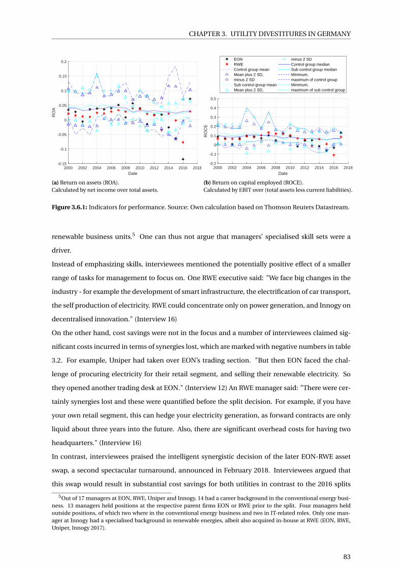
CHAPTER 3. UTILITY DIVESTITURES IN GERMANY
2000 2002 2004 2006 2008 2010 2012 2014 2016 2018
Date
-0.15
-0.1
-0.05
0
0.05
0.1
0.15
0.2
RO
A
(a) Return on assets (ROA).Calculated by net income over total assets.
2000 2002 2004 2006 2008 2010 2012 2014 2016 2018
Date
-0.2
-0.1
0
0.1
0.2
0.3
0.4
0.5
RO
CE
EONRWEControl group meanMean plus 2 SD,minus 2 SDSub control group meanMean plus 2 SD,
minus 2 SDControl group medianSub control group medianMinimum,maximum of control groupMinimum,maximum of sub control group
(b) Return on capital employed (ROCE).Calculated by EBIT over (total assets less current liabilities).
Figure 3.6.1: Indicators for performance. Source: Own calculation based on Thomson Reuters Datastream.
renewable business units.5 One can thus not argue that managers’ specialised skill sets were a
driver.
Instead of emphasizing skills, interviewees mentioned the potentially positive effect of a smaller
range of tasks for management to focus on. One RWE executive said: "We face big changes in the
industry - for example the development of smart infrastructure, the electrification of car transport,
the self production of electricity. RWE could concentrate only on power generation, and Innogy on
decentralised innovation." (Interview 16)
On the other hand, cost savings were not in the focus and a number of interviewees claimed sig-
nificant costs incurred in terms of synergies lost, which are marked with negative numbers in table
3.2. For example, Uniper had taken over EON’s trading section. "But then EON faced the chal-
lenge of procuring electricity for their retail segment, and selling their renewable electricity. So
they opened another trading desk at EON." (Interview 12) An RWE manager said: "There were cer-
tainly synergies lost and these were quantified before the split decision. For example, if you have
your own retail segment, this can hedge your electricity generation, as forward contracts are only
liquid about three years into the future. Also, there are significant overhead costs for having two
headquarters." (Interview 16)
In contrast, interviewees praised the intelligent synergistic decision of the later EON-RWE asset
swap, a second spectacular turnaround, announced in February 2018. Interviewees argued that
this swap would result in substantial cost savings for both utilities in contrast to the 2016 splits
5Out of 17 managers at EON, RWE, Uniper and Innogy, 14 had a career background in the conventional energy busi-ness. 13 managers held positions at the respective parent firms EON or RWE prior to the split. Four managers heldoutside positions, of which two where in the conventional energy business and two in IT-related roles. Only one man-ager at Innogy had a specialised background in renewable energies, albeit also acquired in-house at RWE (EON, RWE,Uniper, Innogy 2017).
83

CHAPTER 3. UTILITY DIVESTITURES IN GERMANY
(Interview 9, 11).
In summary, there might be a benefit of having a smaller range of tasks; however, none of the
other operational and management related indicators could be confirmed. In fact, for synergy
reasons, a different segment separation would have been more efficient and there even seem to be
substantial dis-synergies of the 2016 divestitures. This is why operational and management drivers
are rejected.
3.7 Drivers related to investing
3.7.1 Over-investment due to asset substitution or managerial discretion
To confirm distortions related to investing due to agency conflicts, the literature has commonly
used capital expenditure (capex) relative to assets or correlated with cash flows (e.g. Lamont 1997;
Andrade and Kaplan 1998; Scharfstein 1998; Shin and Stulz 1998; Gertner, Power and Scharfstein
2002; Eisdorfer 2008). We compare capex over total assets, over property, plant and equipment
(PPE) and correlated with cash flows for EON and RWE and our control groups. If managers over-
invested due to agency problems like asset substitution or managerial discretion, we would expect
higher than average capex and higher correlation of capex with cash flows.
2000 2002 2004 2006 2008 2010 2012 2014 2016 2018
Date
-0.4
-0.2
0
0.2
0.4
0.6
Cap
ex o
ver
asse
ts
EONRWEControl group meanMean plus 2 SD,minus 2 SDSub control group meanMean plus 2 SD,
minus 2 SDControl group medianSub control group medianMinimum,maximum of control groupMinimum,maximum of sub control group
(a) Capital expenditure over total assets.
2000 2002 2004 2006 2008 2010 2012 2014 2016 2018
Date
-0.4
-0.2
0
0.2
0.4
0.6
0.8
1
Cap
ex o
ver
PP
E
(b) Capital expenditure over property, plant and equipment.
Figure 3.7.1: Indicators for total capital expenditure. Source: Own calculation based on Thomson ReutersDatastream.
The figures reveal that investment was in line with both control groups except for capex on PPE
at RWE pre-2012. The correlation coefficient of capex with cash flows from 2000 to 2017 is only
moderate and even lower at EON and RWE than in the control groups: 0.46 for EON; 0.41 for RWE;
0.68 for all utilities. The result is robust to taking the more recent period from 2005 to 2014, which
is possibly more relevant for the divestitures, and to looking at operating cash flows only (see also
84
CHAPTER 3. UTILITY DIVESTITURES IN GERMANY
appendix 3.13.3).
The overall numbers thus do not provide sufficient evidence for higher than average agency con-
flicts at EON and RWE.
3.7.2 Distorted investment due to rent-seeking or a biased capital allocation method
Next, we test for cross-segment subsidization due to rent-seeking or a biased capital allocation
method. As renewables became a growth market and conventional generation was forced out of
the market, if there were no distortions, one would expect investment to shift from conventional
generation towards renewables at EON and RWE.
Most data for this section is taken from EON’s and RWE’s reporting only, because segment reporting
is not comparable across all Stoxx utilities.
Pre-2009/10, segment reporting on renewables is not available, but the existing literature (e.g.
Kungl 2018) and interviewees point at decisions not being taken optimally. An equity analyst: "Be-
tween 2000 and 2005 the utilities had a fat harvest. They ignored renewable energy. They found the
sector suspicious because it still needed subsidies. Coal was cheap, nuclear was profitable. So they
were blind to anything new. They entered the renewables business too late." (Interview 14)
Interviewees also emphasized that the capital allocation method at the time fostered a bias toward
the existing conventional segments. Both RWE and EON had allocated capital by adjusting dis-
count rates according to segment, technology and country risk (Interview 6, 16, 19). The claim by
Krüger et al (2015) that investment distortions occur simply due to the usage of one single cost
of capital in the entire firm does not hold in this case. Rather, the pressures from powerful divi-
sions might have biased assumptions and thereby indirectly affected discount rates. For example
at RWE, "it was a political bazaar. Everyone knew that the assets are very long-lived. So if you
wanted more funds for your segment, it could help if you pushed certain assumptions about the
long-term trend of power prices." (Interview 7). At EON, it was "every business segment for itself.
[...] Every segment said we need amount X. Then the negotiation ensued. Now, on the contrary,
strategy and management decide on an overall number for each segment and the segments only
decide on the allocation between projects." An EON manager thought that before the reform in
capital budgeting, "we might have given high risk projects to much money, because we did not
price the risks accordingly. Sometimes it was also the division managers that were screaming the
loudest, who got the most of the funds." (Interview 6) Interestingly, EON reformed the capital al-
location method towards a more top-down approach in 2017, that is after the Uniper spin-off. In
fact, none of the interviewees connected the splits in 2016 to problems in capital allocation.
Moreover, even though EON and RWE probably initially under-invested in renewables, other util-
ities that did not restructure under-invested on a similar scale: figure 3.7.2 shows that EON’s and
85

CHAPTER 3. UTILITY DIVESTITURES IN GERMANY
RWE’s renewables share is a little below the mean but in line with the median of the control groups.
2007 2008 2009 2010 2011 2012 2013 2014 2015 2016 2017
Date
-0.5
0
0.5
1
Ren
ewab
les/
tota
l cap
acity
in M
W
EONRWEControl group meanMean plus 2 SD,minus 2 SDSub control group meanMean plus 2 SD,
minus 2 SDControl group medianSub control group medianMinimum,maximum of control groupMinimum,maximum of sub control group
Figure 3.7.2: Renewables capacity in MW over total capacity.
Between 2010 and 2016 total capital expenditure at EON and RWE starkly decreased (see figure
3.7.3). Investments in the conventional sector took the largest cuts: EON’s investment in its ‘gen-
eration’ segment decreased by 78% between 2010 and 2015 and RWE’s ‘conventional power gen-
eration’ by 81% between 2012 and 2016. Investment in German electricity distribution grids and
sales did not show any consistent trend. Investment in renewables at EON showed a peak in 2012
and then declined. At RWE, renewables capex almost tripled between 2008 and 2013, but in 2015
collapsed to less than half, following the overall declining capex trend.
Figure 3.7.3: Capital expenditure on intangible assets, property, plant and equipment and investment prop-erty in EON’s and RWE’s main segments in EUR million. Source: Own illustration based on EON and RWEannual reports.
Appendix 3.13.3 shows segment capex over different measures of segment profitability and size.
What stands out are the high capex ratios in the renewables segments. Even though investment
86

CHAPTER 3. UTILITY DIVESTITURES IN GERMANY
in renewables did not increase or even decreased in absolute terms post-2010, measured by prof-
itability and segment size it still received a higher share of investments than the overall firm and
conventional generation. This means that utilities had acknowledged renewables as a growth mar-
ket. After being hit by declining profits, they mainly reduced investing in conventional generation,
but they eventually had to cut spending in renewables, too.
This is all the more understandable, since renewables were still free-cash-flow negative until
around 2014 for various reasons (EON and RWE 2005-2014),6 while parts of the conventional fleet,
such as the remaining nuclear power plants, were still profitable. Furthermore, returns in the con-
ventional segments were not continuous: "In conventional energy production, we had to under-
take some investments because of path dependencies" said one senior staff at RWE (Interview 7).
RWE’s CFO Bernhard Günther, when asked about why RWE would not close its conventional power
plants more pro-actively, said that "lignite is a complex system where you cannot close individual
plants so easily," hinting at the scale effects of operating German lignite power plants at full ca-
pacity close to the lignite mines (RWE 2016-03-08). Similarly, in a 2013 EON presentation to in-
vestors, management had justified investments in conventional and distribution assets by calling
them "maintenance capex" that are "necessary to maintain existing assets in operation", "neces-
sary to keep [the] license to operate" and "inflexible: to significantly reduce capex [we] would have
to exit [the] business altogether". EON management announced that "discretionary capex" would
by "2015 almost completely [be] allocated to priority growth areas: renewable energy, distributed
energy, outside Europe" (EON CMD 2013).
Thus from around 2010, there were path dependencies in investing, but no systematic bias disad-
vantaging renewable energies due to agency conflicts, rent-seeking or a biased allocation method,
which is why drivers related to investing are rejected. Thus the question is rather why the firms
could apparently not raise additional debt or equity to invest into more growth in renewables.
3.8 Drivers related to financing
3.8.1 Debt overhang
This section examines whether, in accordance with debt overhang, EON and RWE raised funds for
growth or the retirement of debt and whether they had higher leverage prior to the divestiture as
compared to their non-divesting peer group.
6See also appendix 3.13.4. The reason why the renewables segments were still losing money in 2013 and 2014 issubject to debate in the literature and among practitioners. Factors might have been long lead times of offshore windprojects (Interview 12), delays in grid access of offshore parks (Spiegel 2011), unforeseen cuts in renewable electricitytariffs in Spain and the Netherlands (EON 2013, RWE 2013) as well as the planned scaling down of subsidies in Germany(Interview 6). Some interviewees also blamed a lack of experience in renewable technologies paired with the pressure toinvest at any cost to make up for lost time at the utilities (e.g. Interview 16).
87

CHAPTER 3. UTILITY DIVESTITURES IN GERMANY
3.8.1.1 Funds raised for growth and retirement of debt
Raising funds through divestitures could hint at different drivers: biased investment, risk contam-
ination or debt overhang (see table 3.1).
EON did not raise funds when Uniper had its stock market listing in September 2016, but funding
was accessed later: in March 2017, the new EON raised EUR 1.35 billion through a capital increase.
This was used to partly fund the contribution to the public nuclear fund (see section 3.8.4). In June
2018, EON finalized the sale of its 46.65% stake in Uniper to its competitor Fortum for EUR 3.8
billion. EON stated that the proceeds would be used to fund growth in renewables and networks
(EON 2018).
In October 2016, RWE sold 73.4 million shares of its holding of its subsidiary Innogy and another
55.6 million were placed through a capital increase by Innogy at the same time. RWE’s stake in
Innogy dropped to 76.8% as a result. RWE also announced that it would use the EUR 2.6 billion
from the sale of Innogy shares to fund its share in the nuclear fund, while the 2 billion from Innogy’s
capital increase were intended for growth projects in renewables and networks (RWE 2016).
2000 2002 2004 2006 2008 2010 2012 2014 2016
Date
-0.02
0
0.02
0.04
0.06
Pro
ceed
s fr
om s
tock
s/to
tal a
sset
s
EONRWEControl group meanMean plus 2 SD,minus 2 SDSub control group meanMean plus 2 SD,
minus 2 SDControl group medianSub control group medianMinimum,maximum of control groupMinimum,maximum of sub control group
Figure 3.8.1: Proceeds from issuing stocks over total assets for different utilities. Source: Own calculationbased on Thomson Reuters Datastream.
Figure 3.8.1 shows proceeds from stocks raised by EON and RWE over assets compared to the con-
trol groups. It shows very low issuance until 2015 and a spike compared to the control group for
RWE in 2016 and for EON in 2017.7
RWE and EON thus had raised a considerable amount of funds directly and indirectly through the
divestitures. They stated that they would invest the funds in growth and also retire debt, insofar as
the nuclear funds contributions can be classified as debt.
7In the late 2000s, a few utilities had pursued a similar strategy to RWE, which leads to high standard deviations duringthat time. EDF floated its renewable subsidiary in 2006, which was followed by Iberdrola in 2007, EDP in 2008 and Enelin 2010. All intended to use the funds for growth and bought back the minority shares later.
88

CHAPTER 3. UTILITY DIVESTITURES IN GERMANY
3.8.1.2 High leverage
Concerning long-term bond ratings, European utilities suffered from a wave of downgrades. Be-
tween 2005 and 2017 their average rating deteriorated from A+ to between A- and BBB+. EON’s
and RWE’s ratings decreased in line with that. Debt and liquidity indicators were also in line with
control groups; EON and RWE net debt and long-term debt were even lower than average in the
recent years (see appendix 3.13.5).
When looking at total liabilities over assets, the picture is different, however (see figure 3.8.2): EON’s
liabilities increased noticeably and RWE’s increased slightly from a very high level between 2013
and 2015. The reason is that total liabilities include provisions for nuclear dismantling and storage,
whereas debt does not. Between 2007 and 2015 nuclear provisions increased by 40 and 16% in
absolute terms and by 69 and 22% relative to total assets at EON and RWE respectively.8
2000 2002 2004 2006 2008 2010 2012 2014 2016 2018
Date
0.2
0.3
0.4
0.5
0.6
0.7
0.8
0.9
1
1.1
Tot
al li
abili
ties
over
tota
l ass
ets
(a) Total liabilities over total assets. EON black, RWE red,control groups blue (for full legend see previous graph). (b) Nuclear provisions in EUR million and over total assets.
Figure 3.8.2: Nuclear provisions and overall liabilities. Source: Own calculation based on Thomson ReutersDatastream and EON and RWE annual reports.
There is thus strong evidence for the debt overhang hypothesis - but only if one counts nuclear
liabilities towards debt.
3.8.2 Appropriate gearing
The idea of appropriate gearing is that, by splitting up, the tax shield of debt increases due to the
possibility to adjust debt levels more appropriately to the two henceforth separate firms. This has
been argued for EON, for example, in J.P. Morgan’s equity analyst report (Casali 2015).
In 2017 interest over assets and interest times tax rate over assets at EON and RWE was very close
8For 2016 and 2017 ratios, total assets are calculated by still assuming the integrated company. As EON does notconsolidate its Uniper holding, EON cum Uniper assets = EON assets + Uniper assets. Since RWE fully consolidates itsInnogy holding, RWE cum Innogy assets = RWE assets + Innogy assets - RWE majority holding in Innogy assets of 76.8%.This is to avoid an exaggeration of the ratio due to the decreased asset base post-divestiture.
89

CHAPTER 3. UTILITY DIVESTITURES IN GERMANY
to or even lower than in 2015 (figure 3.8.3). This means that the overall tax shield did not increase
in response to the divestiture and the appropriate gearing hypothesis can be rejected.
Figure 3.8.3: Interest over assets and interest times tax rate over assets. Source: Own calculation based onEON and RWE annual reports.
3.8.3 Asymmetric information
2006 2007 2008 2009 2010 2011 2012 2013 2014 2015 2016 2017
Date
0
5
10
15
20
25
30
35
40
45
50
EO
N a
nd U
nipe
r
Number of analysts EONNumber of analysts UniperNumber of total analysesStandard error of estimates EONStandard error of estimates UniperStandardized forecast error EONStandardized forecast error Uniper
2006 2007 2008 2009 2010 2011 2012 2013 2014 2015 2016 2017
Date
0
5
10
15
20
25
30
35
40
RW
E a
nd In
nogy
Number of analysts RWENumber of analysts InnogyNumber of total analysesStandard error of estimates RWEStandard error of estimates InnogyStandardized forecast error RWEStandardized forecast error Innogy
Figure 3.8.4: Analysts’ coverage, standard errors and standardized forecast errors for EON, Uniper, RWEand Innogy. The standard error of estimates is calculated as the standard deviation of estimates/number ofanalysts and the standardized forecast error by the |mean EBITDA estimate - historical EBITDA|/standarddeviation of the estimates.
Authors have argued that going public reduces asymmetric information or that information asym-
metries are less relevant for one part of the firm leading to a better understanding and valuation of
the separate firms. We search for a possible decrease in analysts’ forecast dispersion or error or an
increase in coverage by analysts post-divestiture.
There was indeed an increase in total coverage by analysts of EON cum Uniper and RWE cum
90

CHAPTER 3. UTILITY DIVESTITURES IN GERMANY
Innogy (figure 3.8.4). This, however, did not translate into a better EBITDA estimate or less dis-
persion in 2016 and 2017 for EON and RWE: standard errors of estimates and standardized forecast
errors increased for both. Uniper’s estimate has a lower standard error but higher forecast error
than EON. Innogy has both lower standard error and standardized forecast error than RWE. Asym-
metric information might thus have been lower only for Innogy as compared to RWE.
Why could it have been easier for analysts to value Innogy? In the next section it will be argued that
RWE, EON and Uniper were to a certain extent risk-contaminated by the conventional generation
portfolio.
3.8.4 Risk contamination
The test of the risk contamination hypothesis consists of four parts. First, the origin of the profit
decline at EON and RWE is examined. If past losses are an indication of future expected losses,
then the risk contamination argument only makes sense if divestitures are structured such that the
risky segments are shielded off. Second, stock market valuations of the pre- and post divestiture
utilities are compared over time and to their peer group. If risk contamination was a driver, one
would expect large valuation differences between parents and subsidiaries and an overall valuation
increase post-divestiture. Third, a share price event study is conducted in order to find further
possible reasons for risk contamination. Fourth, interview results are used for triangulation.
3.8.4.1 Sources of profit decline
Net income at EON and RWE closely followed losses from impairments. Impairments over book
asset value increased from around 2011 to above average or median, but still below the control
groups’ maximums (see figure 3.8.5). EON wrote off EUR 20 billion between 2011 and 2015, or 13%
of 2011 book asset value. At RWE, EUR 17 billion, or 19% of their 2011 book asset value were written
off (EON, RWE 2011-2015).
In which segments did the impairments occur? Conventional generation segments were hit hardest
at both EON and RWE. Of EON’s 2011-2015 impairments, 74% were in the conventional generation
unit, 33% of which due to low power prices. The renewables segment was responsible for only
5%; other segments contributing were trading and gas exploration with about 4% and 9% (EON
2011-2015).
Of RWE’s 2012-2015 impairments, 82% occurred in the conventional generation segment, 59% of
which were due to low power prices and shut-downs in Germany and the Netherlands. The renew-
ables segment was responsible for around 9% of impairments, mainly due to regulatory changes in
the Netherlands, Spain and Poland and due to delays in network connections and increased invest-
ment costs at German offshore wind parks. About 5% was in the German supply and distribution
91
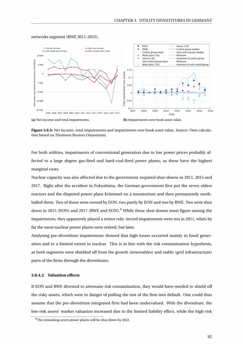
CHAPTER 3. UTILITY DIVESTITURES IN GERMANY
networks segment (RWE 2011-2015).
(a) Net income and total impairments.
2004 2006 2008 2010 2012 2014 2016 2018
Date
-0.1
-0.05
0
0.05
0.1
0.15
Tot
al im
pairm
ents
ove
r as
sets
EONRWEControl group meanMean plus 2 SD,minus 2 SDSub control group meanMean plus 2 SD,
minus 2 SDControl group medianSub control group medianMinimum,maximum of control groupMinimum,maximum of sub control group
(b) Impairments over book asset value.
Figure 3.8.5: Net income, total impairments and impairments over book asset value. Source: Own calcula-tion based on Thomson Reuters Datastream.
For both utilities, impairments of conventional generation due to low power prices probably af-
fected to a large degree gas-fired and hard-coal-fired power plants, as these have the highest
marginal costs.
Nuclear capacity was also affected due to the government-required shut-downs in 2011, 2015 and
2017. Right after the accident in Fukushima, the German government first put the seven oldest
reactors and the disputed power plant Krümmel on a moratorium and then permanently moth-
balled them. Two of those were owned by EON, two partly by EON and two by RWE. Two were shut
down in 2015 (EON) and 2017 (RWE and EON).9 While these shut-downs must figure among the
impairments, they apparently played a minor role: record impairments were not in 2011, when by
far the most nuclear power plants were retired, but later.
Analysing pre-divestiture impairments showed that high losses occurred mainly in fossil gener-
ation and to a limited extent in nuclear. This is in line with the risk contamination hypothesis,
as both segments were shielded off from the growth (renewables) and stable (grid infrastructure)
parts of the firms through the divestitures.
3.8.4.2 Valuation effects
If EON and RWE divested to attenuate risk contamination, they would have needed to shield off
the risky assets, which were in danger of pulling the rest of the firm into default. One could thus
assume that the pre-divestiture integrated firm had been undervalued. With the divestiture, the
low-risk assets’ market valuation increased due to the limited liability effect, while the high-risk
9The remaining seven power plants will be shut down by 2022.
92

CHAPTER 3. UTILITY DIVESTITURES IN GERMANY
assets’ valuation decreased due to the loss of co-insurance from the low-risk business. Overall, the
whole firm’s valuation improved, if the limited liability effect dominates the loss of the co-insurance
effect. Taken together this would be evidence for the risk contamination hypothesis.
A first step is to look at the annual market to book asset value of European utilities (figure 3.8.6).
RWE and especially EON had relatively low values in the early 2000s, average valuations from
around 2007, which then again deteriorated from around 2013/14. The 2015 valuations were below
average though still in the range of both control groups.
2000 2002 2004 2006 2008 2010 2012 2014 2016
Date
0.8
0.9
1
1.1
1.2
1.3
Mar
ket t
o bo
ok a
sset
rat
io
EON, from 2016: EON ex UniperRWE, from 2016: RWE cum InnogyEON cum Uniper
RWE ex InnogyUniperInnogy
Figure 3.8.6: Market to book asset ratio, calculated by (market price year end · common shares outstanding+ book value of total liabilities)/book value of total assets. Source: Own calculation based on ThomsonReuters Datastream.
To analyse the valuation effect of the divestitures, we can compare EON cum Uniper and RWE
cum Innogy 2015 values (denoted by circles 3.8.6) with 2016 and 2017 (black star for EON, red
circle for RWE).10 EON cum Uniper’s valuation improved from 1.01 to 1.06/1.13 (2015 black star
compared to 2016/2017 black circles), as did RWE cum Innogy’s, from 1.02 to 1.06/1.06 (2015 red
star compared to 2016/2017 red circles). The best valued firms are Innogy (1.21/1.20) and the new
EON (1.23/1.28), whereas Uniper (0.84/0.94) and RWE ex Innogy (0.83/0.77) have low market to
book values, clearly below the minimums of their control groups in 2016/17.11 This is first evidence
for the risk contamination hypothesis.
Comparing pre- and post divestiture valuation of the listed companies reveals that EON’s valuation
10Calculation of the ex and cum values is described in the appendix. EON cum Uniper is a benevolent estimate, as itincludes Uniper’s full market value. It assumes that shareholders anticipated the complete sale of EON’s Uniper stake,as announced in December 2014, even though EON still held a minority stake of 46.65% until June 2018, when it sold toFortum.
11In 2017, Innogy deteriorates compared to Uniper, which is likely related to low profits in their UK segment (Innogy2017), whereas Uniper values up, due to recovering electricity prices, pulling EON cum Uniper with it (Uniper 2017).
93

CHAPTER 3. UTILITY DIVESTITURES IN GERMANY
benefited more (1.23 and 1.28 in 2016/17 compared to 1.01 in 2015) than RWE’s (1.02 to 1.06). This
illustrates that EON’s split, being the first of the two divestitures, was strategically more intuitive
for the existing management: they got to be managers of a new firm with an improved valuation.
RWE’s CEO Peter Terium, on the other hand, had to make himself CEO of the subsidiary Innogy in
order to be still heading a firm with high growth potential.
Figure 3.8.7 plots the daily development of market capitalisation at the two utilities. Two effects are
striking. First, RWE ex Innogy’s implicit negative valuation: on the day of Innogy’s IPO on October
7, 2016, its market cap was at EUR -7.3 billion and at the beginning of 2018 still between -3 and
-4 billion. Second, the jump in market value of RWE cum Innogy of about 45%, while EON cum
Uniper only valued up by less than 9%.
01/14 07/14 01/15 07/15 01/16 07/16 01/17 07/17 01/18
Date
0
0.5
1
1.5
2
2.5
3
3.5
Mar
ket v
alue
EO
N
104
EONUniperEON ex UniperEON cum Uniper
(a) EON, Uniper and combined market value
01/14 07/14 01/15 07/15 01/16 07/16 01/17 07/17 01/18
Date
-1
-0.5
0
0.5
1
1.5
2
2.5M
arke
t val
ue R
WE
104
RWEInnogyRWE ex InnogyRWE cum Innogy
(b) RWE, Innogy and combined market value
Figure 3.8.7: Market value calculated by market price · number of common shares outstanding. Source:Own calculation based on Thomson Reuters Datastream.
This is also illustrated in graph 3.8.8 showing market capitalisation prior to and on the days of
Uniper and Innogy going public. The full calculation is described in appendix 3.13.6. The legend
entries in brackets rest on the arbitrary assumption that Uniper’s value halved and Innogy’s value
doubled by going public. This assumption would be in line with the risk contamination argument:
the Uniper segment was co-insured by the rest of EON; it risk-contaminated EON. By going public,
it lost the insurance. Innogy was co-insuring the rest of RWE; it was risk-contaminated by the
conventional business. By going public, it lost the risk contamination. The graph shows that such
an assumption would be consistent with the observed valuations.
The difference between Uniper’s positive and RWE ex Innogy’s implicit negative valuation might
be surprising at first glance, since the two have very similar business models. However, first, RWE
ex Innogy’s valuation is only hypothetical and the result of Innogy’s very high valuation. Uniper, in
contrast to RWE ex Innogy, being a real traded firm, must have a positive valuation.
94

CHAPTER 3. UTILITY DIVESTITURES IN GERMANY
Pre
-spl
it E
ON
Pos
t-sp
lit E
ON
cum
Uni
per
(Pre
-spl
it E
ON
ex
Uni
per)
Pos
t-sp
lit E
ON
ex
Uni
per
(Pre
-spl
it U
nipe
r)
Pos
t-sp
lit U
nipe
r
Pre
-spl
it R
WE
Pos
t-sp
lit R
WE
cum
Inno
gy
(Pre
-spl
it R
WE
ex
Inno
gy)
Pos
t-sp
lit R
WE
ex
Inno
gy
(Pre
-spl
it In
nogy
)
Pos
t-sp
lit In
nogy
-1
-0.5
0
0.5
1
1.5
2
2.5104 EON RWE
Figure 3.8.8: Market values on day -1 and 0 of Uniper’s and Innogy’s listing. Source: Own calculation basedon Thomson Reuters Datastream.
A second explanation is that at the time of the splits, Uniper was indeed more attractive than RWE
ex Innogy.12 Why might Uniper be more attractive? The most obvious difference: Uniper did not
operate any nuclear power plants. EON kept the nuclear segment and in turn EON cum Uniper
might have benefited less from the risk separation effect than RWE cum Innogy.
3.8.4.3 Event study on reasons for risk contamination
This section investigates the reasons for a possible risk contamination using a share price event
study. Events from January 2013 until November 2016 were collected.13 Google news, the search
functions of eight major German papers (Der Spiegel, Frankfurter Allgemeine Zeitung, Handels-
blatt, Manager Magazin, Tagesspiegel, Sueddeutsche, Welt, Zeit) and the international edition of
the Financial Times were used to identify events. Initial keywords were "EON" and "RWE", and
events were tracked with varying keywords thereafter.
Overall, 26 events were identified that could possibly have had an impact on EON’s and RWE’s
default risk. Four events had to be discarded because they coincided with earnings report publi-
cations, dividend payments or news about disposals. The two divestiture announcements and the
two divestitures themselves - the so-called ex dates - were also added to the events, giving a total of
26 events tested.
A negative share price reaction to an event does not prove an increase in default risk and risk con-
12J.P. Morgan’s valuation of enterprise value over EBITDA supports this: Uniper 2016/2017 estimates are higher thanthe implied values for RWE ex Innogy and also than EON’s German nuclear unit (see appendix 3.13.7).
13January 2013 is about two years prior to the EON-Uniper spinoff announcement. EON stated that the strategy hadbeen developed over one year. RWE had publicly rejected the possibility of a split until mid-2015. The last event includedis Innogy’s IPO.
95

CHAPTER 3. UTILITY DIVESTITURES IN GERMANY
tamination, but points more generally at investors seeing growth potential lost. To corroborate the
risk contamination argument, it therefore is interesting to also look at events that led to a reduction
in risk. If they cause positive share price reactions - regardless of or in contrast to their likely effect
on future returns - this might support the risk contamination argument. It means that utilities’ had
been exposed to a risk involving high possible costs and a decision eliminating uncertainty relieved
the share price of some of this downside risk priced in earlier.
The events can be classified into three categories:14
1. Four events related to the divestitures: the two utilities’ announcements to split (Novem-
ber 30, 2014 and December 1, 2015) and the two divestitures (September 12 and October 7,
2016). All hypotheses - not only risk contamination - would predict a positive effect of the
announcements on the parents’ share price. Assuming risk contamination, one would also
expect the parent to devalue on the divestiture day if it contains the ‘contaminated’ assets
and to value up otherwise.
2. Four events related to renewable energy policy reforms. In January 2013, the German min-
istry for the environment launched efforts to reduce the power price for consumers by en-
forcing limits to renewable energy construction (Handelsblatt 2013-01-28). In June 2014, the
Bundestag decided on a renewable energy law reform, among other things limiting feed-in
tariffs for renewable energy (BMWi 2014-06-27).
The risk contamination hypothesis predicts that changes in favour of renewable energies
would increase utilities’ risk due to their fossil- and nuclear-heavy portfolio and therefore
have a negative impact on their share price. Events reducing uncertainty might also have a
positive effect on share prices.
3. Five events related to climate policy. In November 2014, Energy and Economics Minister
Sigmar Gabriel presented first ideas for a CO2 levy on coal power plants in order to reach
Germany’s internationally agreed 2020 climate targets (Handelsblatt 2014-11-24). The ne-
gotiations with utilities and unions turned out to be difficult and finally also the heads of
lignite-rich states allied against Gabriel. In June 2015, the levy was replaced with an about
EUR 800 million annual premium in order to retire about 2.7 Gigawatt of lignite capacity
between 2017 and 2020 (Tagesschau 2015-06-24, Frankfurter Neue Presse 2015-06-27).
Events making the introduction of a CO2 levy likelier are expected to have a negative im-
pact on utilities’ share prices, especially on RWE, which has a higher share of lignite. Events
reducing uncertainty might also have a positive effect on share prices.
14Changes in commodity prices like electricity have a high impact on utilities, however, no news related to this couldbe identified. The previous section 3.8.4.1 therefore serves to cover the impact of depressed power prices on EON andRWE.
96

CHAPTER 3. UTILITY DIVESTITURES IN GERMANY
4. Eleven events related to nuclear energy policy changes and news. Due to the planned com-
plete exit from nuclear energy by 2022, the question arose of whether utilities would be able
to cover all costs for dismantling power plants and storage of nuclear waste. EON and RWE
had EUR 16.6 and 10.4 billion in provisions for nuclear dismantling and storage as liabilities
on their balance sheets. Together with the other three operators of nuclear power plants in
Germany (Vattenfall, EnBW, and a small share by the Munich municipal utility), provisions
added up to EUR 38.3 billion (Warth and Klein 2015).
Policy makers had three main concerns. First, since on the asset side the use of the nuclear
provisions was not ring-fenced, they could fall victim to impairments or bankruptcy. Against
the backdrop of utilities’ already shrunk balance sheets and market valuations, this suddenly
seemed possible (Irrek and Vorfeld 2015).
Second, even if the provisions were available, it was unclear how much of the cost they would
cover. World-wide no experience exists with dismantling and storing nuclear equipment in-
definitely into the future. In a study on different nuclear financing options, it was estimated
that even infrastructure projects with long track records regularly have cost over-runs of 35-
1,500% (Küchler et al 2014).
Another factor adding to the uncertainty in estimates were discount rates. Because the bulk
of the costs would arise far in the future, the real discount rate - interest earned minus in-
flation - had a high impact. While utilities used a discount rate of 4.58%, a report commis-
sioned by the Ministry for Economics and Energy tested different scenarios ranging from 2.03
to 4.53% and obtained estimates between EUR 32.4 and 77.4 billion, i.e. up to two times or
almost EUR 40 billion higher than the utilities’ provisions (Warth and Klein 2015).15
For these reasons cost estimates covered a wide range. The graph below gives an overview of
estimates by various sources.
Third, and in addition to these economic issues, utilities and government disagreed about
the legal aspects regarding the division of costs between industry and state. The four major
utilities published a joint report emphasizing the role of the state in ensuring legal security
and argued that cost increases due to changes in regulations should entirely be covered by
the state (Freshfields Bruckhaus Deringer 2015). The Ministry for Economics and Energy, on
the other hand, stated that all costs are borne entirely by utilities (BMWi 2014).
When EON announced the Uniper spin-off in late 2014, Minister Gabriel threatened to pass
"lex EON", or the "parents are liable for their children law". The law - indeed passed later
in October (DW 2015-10-14) - would make companies eternally liable for their nuclear op-
15Very low interest rates in recent years imply that these estimates at least partly under-estimated the real costs.
97
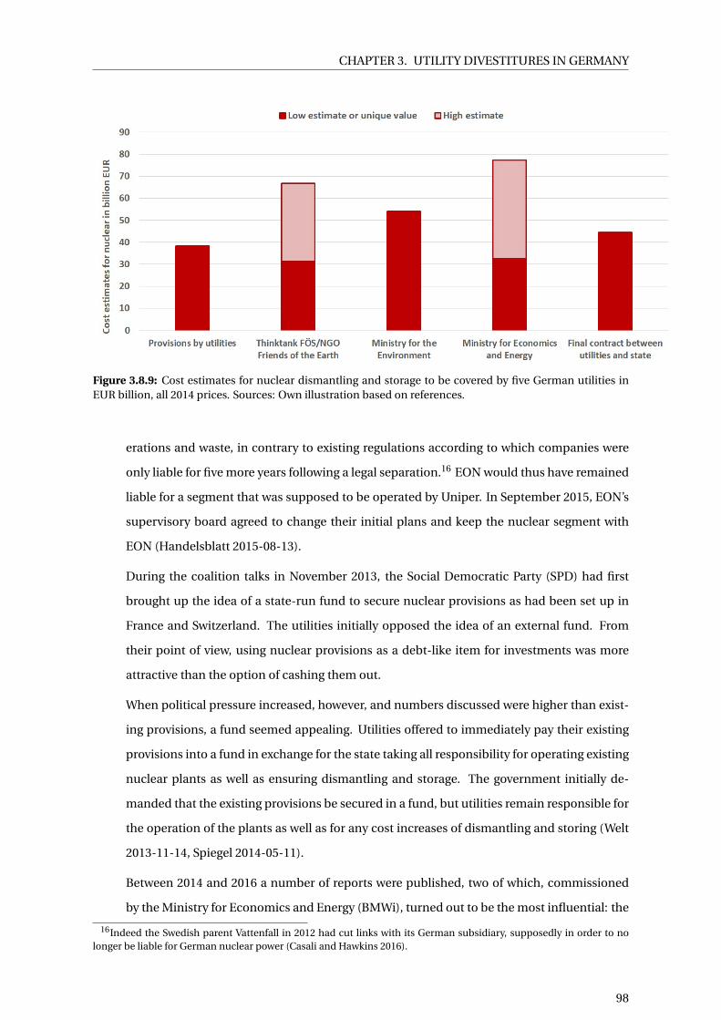
CHAPTER 3. UTILITY DIVESTITURES IN GERMANY
Figure 3.8.9: Cost estimates for nuclear dismantling and storage to be covered by five German utilities inEUR billion, all 2014 prices. Sources: Own illustration based on references.
erations and waste, in contrary to existing regulations according to which companies were
only liable for five more years following a legal separation.16 EON would thus have remained
liable for a segment that was supposed to be operated by Uniper. In September 2015, EON’s
supervisory board agreed to change their initial plans and keep the nuclear segment with
EON (Handelsblatt 2015-08-13).
During the coalition talks in November 2013, the Social Democratic Party (SPD) had first
brought up the idea of a state-run fund to secure nuclear provisions as had been set up in
France and Switzerland. The utilities initially opposed the idea of an external fund. From
their point of view, using nuclear provisions as a debt-like item for investments was more
attractive than the option of cashing them out.
When political pressure increased, however, and numbers discussed were higher than exist-
ing provisions, a fund seemed appealing. Utilities offered to immediately pay their existing
provisions into a fund in exchange for the state taking all responsibility for operating existing
nuclear plants as well as ensuring dismantling and storage. The government initially de-
manded that the existing provisions be secured in a fund, but utilities remain responsible for
the operation of the plants as well as for any cost increases of dismantling and storing (Welt
2013-11-14, Spiegel 2014-05-11).
Between 2014 and 2016 a number of reports were published, two of which, commissioned
by the Ministry for Economics and Energy (BMWi), turned out to be the most influential: the
16Indeed the Swedish parent Vattenfall in 2012 had cut links with its German subsidiary, supposedly in order to nolonger be liable for German nuclear power (Casali and Hawkins 2016).
98

CHAPTER 3. UTILITY DIVESTITURES IN GERMANY
legal opinion by Becker Büttner Held (2015) that nuclear provisions were not sufficiently safe
unless transferred to an external fund, and the report by Warth and Klein (2015) with cost
estimates ranging from 6 billion less to 40 billion more than utilities had provisioned.
In November 2015, the government set up an expert commission tasked with reviewing the
financing for the phase-out of nuclear energy. The final "law on the reorganization of respon-
sibility in nuclear waste management" reflected the recommendation by this commission,
which in turn reflected the two BMWi reports. It was a compromise: for storage, utilities paid
24 billion - 7 billion more than provisioned - into a state-run fund (10.3 billion by EON and
6.8 billion by RWE) in exchange for ridding themselves of any storage responsibilities and of
any liabilities for future cost increases. Dismantling of nuclear power plants remained the
utilities’ responsibility and on their balance sheets.
In the event study, negative share price reactions are expected for events that made utilities’
cashing out of nuclear provisions or their unlimited liability in case of cost increases likely.
Events reducing uncertainty might also have a positive effect on share prices.
Figure 3.8.10 plots EON’s and RWE’s share price with lines representing events in the different
colours. It shows a widening gap between the utilities and the Stoxx Europe 600 index compared
to their January 1, 2012 prices. Renewable energy related events are spread throughout 2013 and
2014; climate policy related events occur mainly in 2015. Nuclear related events started in late 2013
and intensified in the second half of 2015, coinciding with share prices plummeting.
Table 3.13.8.1 in the appendix (3.13.8.1) lists all events with their expected impact and the regres-
sion results. The estimation method is also described in the appendix, as well as the results of a
Brown Warner test with randomized event dates. Results were also tested and found mainly robust
for event and estimation windows of one to eleven days and 20 to 200 days respectively. The spec-
ification chosen was one day for the event period and 100 days for the normal period. The short
event period is justified to distinguish between events that follow each other closely like the ones
in late 2016.
The results of the event study are as follows:
1. Positive significant effect of divestiture announcements. As predicted by all hypotheses
(not only risk contamination), there is a significantly positive share price reaction on the
Uniper spin-off announcement day for EON of 4.1% abnormal returns compared to the Stoxx
600 Europe Index and of 16.5% on the Innogy carve-out announcement day for RWE. This
indicates that shareholders expected positive value creation from the divestitures and is in
line with all hypotheses discussed.
Regarding the ex-date effects, both EON’s and RWE’s reaction to the Uniper spin-off was
99

CHAPTER 3. UTILITY DIVESTITURES IN GERMANY
2013 2014 2015 2016 20170.2
0.4
0.6
0.8
1
1.2
1.4
1.6EONRWEStoxx Europe 600Renewable energy related eventClimate policy related eventNuclear related eventDivestiture (announcement or listing)
Figure 3.8.10: EON and RWE price of common stock and Stoxx Europe 600 normalized by their January 1,2013 value, and event types in different colors. Source: Own illustration based on Thomson Reuters Datas-tream.
negative but insignificant. They both reacted significantly, though, to the Innogy carve-out.
EON’s share price valued up by 3.7% compared to the index, whereas RWE devalued by 7.0%.
The reason for these effects might be that only the RWE-Innogy split offered perfect risk sep-
aration. The split drove investors away from the now fossil and nuclear heavy RWE stock
towards the clean Innogy and also to the relatively cleaner competitor EON (which still held
the nuclear segment).
2. No impact of renewable energy related reforms. The two utilities’ stock prices did not react
significantly to any of the renewable energy related events and often with reactions opposite
to the predicted effects.
3. Limited impact of climate policy in favour of RWE. Regarding climate policy, the govern-
ment’s first efforts in late 2014 and early 2015 did not seem to weigh on EON’s or RWE’s share
price. The final decision on June 24, 2015 not to implement any CO2 levy and instead reward
the retirement of lignite plants, however, gave a significant boost to RWE’s share price: ab-
normal returns compared to the index were 2.5%; when the full compromise was published
on July 2 the reaction was 5.8%. Given that RWE announced its divestiture almost half a year
after this favourable decision, immediate fears of climate policy should not have played any
100

CHAPTER 3. UTILITY DIVESTITURES IN GERMANY
role.
EON’s lack of a reaction makes sense: due to its lower relative share of lignite, it was less
threatened by a levy.17
4. High impact of nuclear-related events. From May 2014 until August 2015, nuclear related
events had no significant impact on share prices. This changed in September:
(a) Negative impact of EON keeping nuclear. On September 9/10, 2015, investors strongly
punished EON for the decision to keep its nuclear segment with significantly negative
abnormal returns of 2.4% and 5.8%.
(b) Negative impact of higher cost estimates. Four days later, Spiegel leaked the results of
the "stress test", the Warth and Klein report commissioned by the Ministry: allegedly an
up to 30 billion funding gap for overall nuclear provisions existed, as utilities were too
generous in their discount rate estimates (Spiegel 2015-09-15, Wirtschaftswoche 2015-
09-17). Abnormal returns compared to the Stoxx on that day were -6.6% (EON) and
-3.5% (RWE).
(c) Positive impact of lobbying efforts. EON’s and RWE’s share price suffered further losses
until on September 17 the government intervened. Minister Gabriel declared that he
did not to know about the EUR 30 billion funding gap, that the report was not yes fi-
nalized and that leaked results were "irresponsible speculations" (Spiegel 2015-09-19).
The share prices started recovering with significant positive abnormal returns of 8.2%
(EON) and 1.0% (RWE).
(d) Positive impact of resolution of nuclear risk. When the Warth and Klein study was
published on October 8, one could still read about a possible funding gap in the worst
case of even EUR 40 billion. Share prices did not react to it, though, and media painted
the results in a positive light. For example, a Reuters article at the time was titled, "Ger-
many says firms set aside enough nuclear decommissioning funds" (Reuters 2015-10-
10). Policy makers had successfully signalled that the utilities were too big to fail. And
indeed, when the nuclear commission published their recommendation on the division
of costs and liabilities on April 27, 2016, while EON and RWE complained that it "placed
too much of a strain [...] on their economic capacity" (FT 2016-04-27), their share prices
showed significant positive abnormal returns of 3.0% and 5.3%. This corroborates the
argument of risk contamination by the nuclear segment. Even though the amounts to
be paid into the fund by EON and RWE (10.3 and 6.8 billion) were each more than one
17For both utilities, of course, climate policy in general was of high relevance. In 2014, however, European CO2 priceswere on a record low. Only from late 2017 did the EU Commission take concrete steps to reduce emissions tradingcertificate amounts.
101
CHAPTER 3. UTILITY DIVESTITURES IN GERMANY
billion or 13% and 22% above their existing provisions for nuclear storage, they were
moderate enough that the market remunerated the liability cap on storage cost (EON,
RWE 2015, 2016).
The event study established strong evidence for risk contamination from the nuclear segment.
Supporting evidence is the high amount of uncovered nuclear costs discussed, the market’s nega-
tive reaction to the nuclear segment staying with EON and to the alleged funding gap, EON cum
Uniper’s absence of a valuation increase on the ex date, the policy makers’ hesitation between a
polluter-pays-all and a too-big-to-fail attitude and the market’s relief at the costly but risk-reducing
nuclear commission proposal.
3.8.4.4 Interview results
Fifteen out of 20 interviewees thought that the utilities’ decision to split was driven by some sort of
risk contamination.
Outsiders attributed a big role to the nuclear risks. As one equity analyst put it: "The utilities were
confronted with two main problems: the flooding with renewable energies resulting in a drop in
electricity prices and the issue of the nuclear exit. In 2014, they were going towards a valuation
of zero - the whole companies were worth less than their grid segments. So either the market’s
valuation was totally wrong or there were big risks due to insufficient nuclear provisions. To be
honest, the former was exactly the situation before the nuclear commission resolved the problem
in favour of the utilities." (Interview 3)
Among the utility insiders, some staff members were equally outspoken: "The spin-off announce-
ment was a shock for the whole staff at EON. We quickly understood that it was about nuclear
energy. They wanted to create a bad bank for the liabilities. That was quickly blocked with the
‘parents are liable for their children’ law. Otherwise, if it had been too expensive, you could have
let go of Uniper and after five years you’re off." (Interview 10) "RWE was worried that the nuclear
liabilities would drag down the whole shop. Then there was EON’s failed and naive move. So we
learned." (Interview 7)
The interviewed managers were much more cautious. Also publicly, EON never spoke about any
risk-related drivers, let alone nuclear liabilities (EON 2014-11-30). RWE, in contrast, even empha-
sised their continued responsibility for nuclear liabilities. During the investor phone call on the
divestiture announcement day, CEO Peter Terium argued that RWE would increase "visibility of the
downstream and renewables business that have been overshadowed by the conventional business"
and benefit from increased financial flexibility, as it could sell further Innogy shares if liquidity was
needed, while assuming "full responsibility for nuclear liabilities" (RWE 2015-12-01).
102
CHAPTER 3. UTILITY DIVESTITURES IN GERMANY
Interviewees judged RWE’s the more successful strategy, but only because EON’s move was altered
by policy makers: "EON wanted to bring nuclear into the spin-off deal - that would have been a
successful move. But RWE’s strategy was much better in the end: the good part was not burdened
by nuclear. And from the point of view of policy makers, RWE’s liability mass did not decrease. If
liquidity was needed, they could always sell Innogy for cash." (Interview 3) RWE killed two birds
with one stone: separating the risks and as a result being able to raise money for the nuclear cash-
out. But it came with the price of a business model that was unsustainable in the long-run and
therefore only a temporary solution: "RWE could not survive without Innogy. So they said: why
not swap with EON?" (Interview 19) With the asset swap announced in 2018, RWE will obtain both
EON’s and Innogy’s renewables assets in exchange for the grid- and customer-related part of its
own Innogy share.
In summary, there is strong support for risk contamination based on the firms’ and subsidiaries’
valuations pre- and post-divestiture, a share price event study and interviews. Likely sources of
risk contamination were further losses by fossil fuel-fired power plants and the acute risk of un-
manageably high nuclear dismantling and especially storage costs linked to the nuclear exit.
3.9 Drivers related to investor preferences
3.9.1 Trading and share price returns on the ex date
First evidence in line with investor preferences driving the splits would be if investors rebalanced
their portfolios on the divestiture day and if that had a significant impact on share price returns.
To see whether there is increased trading on the ex date, the change in trading volume as compared
to an index and a normal period of 100 days is calculated. The detailed model is laid out in the
appendix (3.13.8.2). It reveals significant abnormal trading of 374% for EON and 521% for RWE.
Trading increased in a comparable manner when the competitor’s subsidiary went public, i.e. at
EON on the Innogy ex date and at RWE on the Uniper ex date.18
Only the Innogy ex date triggered significantly positive abnormal returns for EON (4%) and nega-
tive ones for RWE (-7%). So there is evidence that both EON and RWE investors rebalanced their
portfolios on both the Uniper and Innogy ex dates. Rebalancing on the Innogy ex date seemed to
have been in favour of Innogy and EON and to the detriment of RWE.
This is in accordance with a financial driver such as risk contamination, though, as investor pref-
erences would predict only positive abnormal returns on the ex date. If investors wanted to hold
18Apart from that, only few events triggered a significant increase in trading, in accordance with the most significantimpact on returns described earlier: the decision against a CO2 levy for RWE, the divestiture announcements for EONand RWE respectively, EON’s decision to keep the nuclear segment, the leak of the Warth and Klein results for both.Appendix 3.13.8.2 contains methodology and detailed results.
103

CHAPTER 3. UTILITY DIVESTITURES IN GERMANY
only the uncontaminated part because of risk contamination, not because of their individual pref-
erences, they might wait and trade only on the ex date to avoid transaction costs. This could also
explain why there is no significant returns effect on the EON-Uniper ex date: risk separation was
not perfect since nuclear stayed with EON.
3.9.2 Sin stocks, search for yield or falling profits?
Another hint at investor preferences driving the splits would be if investors had expressed support
for the splits or interest in certain firm segments.
In December 2016 the number of investors committed to selling off fossil fuel assets had jumped
to USD 5.2 trillion in assets under management doubling in just over a year (Carrington 2016). One
example is the Norwegian USD 900 billion sovereign wealth fund, the world’s biggest after Japan’s.
In November 2014, the fund, which held 2.1% of EON’s stock and 2.2% of RWE’s stock, considered
a divestment from firms engaged in mining or burning of coal. In May 2015, the fund sent a letter
to RWE asking about their plans to exit coal and whether they would consider a split à la EON.
In June, Norway’s parliament formally endorsed the move to sell off coal investments (Manager
Magazin 2014-11-26, 2015-05-06). In 2017, the fund still held at least 2.3% of EON and 1.4% of RWE
stocks (Norges Bank 2018). What had happened?
As with many investors that committed to divestment policies, the policies left room for exceptions.
In the case of the Norwegian fund, their guidelines only recommended to divest from companies
with more than 30% revenues from coal. RWE does not reach that threshold.19 Even if a company
does but is the process of decreasing its coal activities, the fund does not need to divest (Wolff
2018).20 Probably other investors apply similar guidelines. Whereas at least 16 of EON’s and 14
of RWE’s investors committed to some sort of fossil fuel divestment since 2013, only one of these
actually divested from EON and two from RWE. The overall share of stocks held by these investors
actually increased since 2013, as figure 3.9.1 shows.
This does not mean that utilities were not under pressure from investors. In September 2016, the
city of Bochum, which held about 1.1% of RWE’s stock decided to divest completely. Essen, Düs-
seldorf, and Dortmund, which were part of the municipal shareholders making up around 23% of
RWE holdings, also temporarily considered divesting. This was, however, after RWE’s planned split
was already long public, so unlikely a driver. And financial reasons played the predominant role:
cities were hit hard by falling dividends, which in 2016 were zero at RWE for the first time (Grüne
2016-04-29, Handelsblatt 2017-08, WAZ 2016-09-15).
Many global investors that committed to divest from fossil fuels also mixed ethical and financial
19Even if excluding revenues from Innogy, lignite and nuclear revenues were responsible for less than 23% of revenuein 2016 and 2017 (RWE 2016, 2017).
20This policy was changed in April 2019 resulting in the divestiture from RWE.
104

CHAPTER 3. UTILITY DIVESTITURES IN GERMANY
Figure 3.9.1: Percentages and total shares held by investors committed to divesting from fossil fuels. Source:Own calculation based on Thomson Reuters Datastream, Bloomberg and Gofossilfree.org (2018)
arguments. For example, the parliamentary committee recommending Norway’s exit from coal
assets stated that "investing in coal companies poses both a climate risk and a future economic
risk" (Reuters 2015-05-28). This economic risk argument is more akin to the risk contamination
hypothesis: if conventional energy becomes unprofitable and excessively risky, a split can offer
investors the opportunity to invest in a profitable, uncontaminated business. This argument is
distinct, though, from investors’ heterogeneous demand for different risk-return profiles or their
exclusion of stocks on ethical grounds.
3.9.3 Interview results
Thirteen out of 20 interviewees thought that investors’ preferences played a role. A financial jour-
nalist thought that "pension funds and other institutionals had high pressure to invest. And grid in-
frastructure is a pearl in a low interest rate environment." Interviewees also acknowledged, though,
that in the energy case it is hard to distinguish a preference for low-risk assets, ethical preferences
and the fear of further losses due to risk contamination. "We wanted to get rid of everything with
commodity price risk", said one EON staff. "A lot of investors did not want any risk, like municipal-
ities. Mainly because they thought that our past investments had failed." (Interview 6). An equity
analyst thought that "there is a lot of interest now in ESG investments, like products with lower
CO2 emissions. Why? I think it is a mixture of risk preferences, return expectations and ethical
considerations." (Interview 9)
So while more and more investors wanted to exit fossil fuels and demand for low-risk renewable
energy and grid infrastructure assets was apparently high, this could not be traced to one specific
105

CHAPTER 3. UTILITY DIVESTITURES IN GERMANY
reason. It is in line with search for yield, ethical considerations as well as the avoidance of economic
loss. Further, since holdings from divestment committed funds did not seem to decrease, it is
unclear whether the divestment movement was a concrete factor in the utilities’ decisions to split.
3.10 Conclusion
This study investigated why the two biggest German utilities, EON and RWE, split up in 2016. Four
possible types of drivers for divestitures were identified from the divestiture literature: operations
and management, investing, financing and investor preferences. These drivers were tested in the
empirical case of the EON and RWE divestitures of 2016. The results of different methods - com-
parative descriptive statistics, interviews, gray literature and event studies - converged in rejecting
drivers related to operations, management and investing. Drivers related to investor preferences
could not sufficiently be distinguished from risk contamination.
The analysis supports debt overhang as one driver, as EON and RWE accumulated higher liabilities
than their peers due to provisions for nuclear dismantling and storage. There is also strong evi-
dence for risk contamination. This is tested by analysing EON’s and RWE’s previous losses and the
valuations pre- and post-divestiture and by conducting share price event studies and interviews.
Likely sources of risk contamination were further possible losses by fossil fuel-fired power plants
and the acute risk of unmanageably high nuclear dismantling and especially storage costs linked
to the nuclear exit.
In 2015 alone, the year when discussions about provisions for decommissioning nuclear power
plants and storing toxic waste intensified, EON’s market cap decreased by half and RWE’s by 75%.
Investors doubted the adequacy of utilities provisions for nuclear related costs, and feared major
cost increases while utilities being unlimitedly liable. Even though utilities’ nuclear provisions had
increased considerably, in 2015 a study estimated a funding gap of up to EUR 40 billion for Ger-
many’s nuclear capacity overall.
Utilities restructured to avoid further risk contamination of their healthy assets (renewables and
grid infrastructure) by the conventional power generation business (fossil fuel and nuclear plants).
There was one major difference between the two utilities’ strategies: EON announced to spin off
its risky conventional power generation and its trading segment to the new subsidiary Uniper. For
RWE, being the second mover, it was already clear that policy makers would not allow nuclear lia-
bilities being spun off. As a result, RWE carved out renewables and grid infrastructure into the new
Innogy, turning itself into a conventional generation and trading utility only financially invested in
the growth firm Innogy.
106

CHAPTER 3. UTILITY DIVESTITURES IN GERMANY
3.11 Policy implications and outlook
The example of German policy making shows that an ambitious energy transition - an increase
in renewables and the simultaneous exit from nuclear - can come at a cost to incumbent utilities.
One could argue that severe losses or bankruptcies of main electric utilities are necessary evils in
the transition away from a fossil fuel- and nuclear-based power market. However, under certain
circumstances there are problems with this approach:
1. In Germany, the utilities’ nuclear provisions were not ring-fenced. If utilities had faced fur-
ther impairments or bankruptcy, tax payers might have had to burdened all costs for disman-
tling plants and storing nuclear waste estimated at between EUR 32 and 77 billion (Warth and
Klein 2015).
2. Many authors argue that in the absence of affordable storage solutions, fossil fuel-based
power plants are still needed to balance out fluctuating renewable energy in the mid-term.
In Germany, about 60% of this capacity was operated by the big incumbent utilities - EON,
RWE, Vattenfall and EnBW (BMWi 2018; Bundesnetzagentur 2019). A default of one of these
big four might have thus affected security of supply in power generation.
3. In addition to power generation, the big German utilities also played a main role in electricity
trading, operation of distribution grids and provision of customer services. A bankruptcy
might have thus endangered not only security of supply in power generation but in the whole
energy value chain.
In this market environment, risking utilities’ bankruptcy might have destroyed more value than it
created. For this reason policy makers were caught in between a ‘polluter pays’ and a ‘too big to
fail’ attitude, leading to indecisive, contradictory and possibly too lenient policies. Three measures
might have altered the market environment ex-ante such as to avoid the problems described above:
1. The government should have set-up a well-endowed, ring-fenced and state-run fund for nu-
clear provisions much earlier, following the example of countries like France and Switzer-
land. German utilities had their golden times in the late 2000s. This would have been the
time to skim off some profits to secure appropriate funding for nuclear dismantling and stor-
age.
2. Even though heavily debated and possibly not necessary in Germany at the time, a well-
designed and transparent capacity market might have its merits depending on the existing
power plant fleet and structure of the electricity market. As Weber (2017) notes, "prices based
on volatile marginal costs and a long-term capital lock-up are not a good basis for substantial
107

CHAPTER 3. UTILITY DIVESTITURES IN GERMANY
investment. In most deregulated electricity markets in the US and Europe capacity mecha-
nisms exist, which together with energy trading ensure the security of supply."
3. A less oligopolistic power market structure helps against the moral hazard of ‘too big to fail’.
Germany’s oligopolistic market structure is partly the effect of natural monopoly tendencies
and partly caused by the governmentally-encouraged mergers in the 1990s. While oligopolies
especially in grid infrastructure cannot be avoided, moves towards further market concen-
tration like the recent EON-RWE asset swap should be viewed critical. The benefits of scale
stand against not only potential price increases for consumers but also the exposure of the
power market to concentration risk and the need for bail-outs by tax payers.
Further research might look into how other sectors or sub-sectors can benefit from past experi-
ences like the German case. An interesting case would be the coal exit, Germany’s next big step
in the energy transition. With the coal commission just having adopted its recommendations to
exit hard coal- and lignite-based power by 2038, parallels and differences to the nuclear exit will be
interesting to explore. Another interesting sector is mobility: applying these lessons to the transfor-
mation of the market for combustion engines could possibly save costs for tax payers and industry
alike.
This paper has identified risk contamination as a possible major concern in the transition of the
power sector towards renewables. Further research could quantify this potential systemic risk by
devising methodologies and measures to conduct stress tests on the energy sector. This has already
been done in finance research regarding the effect of interconnections among financial actors in
the aftermath of the 2008 crisis (e.g. Tasca and Battiston 2016) and regarding the impact of climate
risk on the financial system (e.g. Battiston et al 2017). A similar approach to the energy sector, with
a stress test measuring the consequences of different transition scenarios on incumbent investors
could be useful to derive low-cost policy recommendations.
108
CHAPTER 3. UTILITY DIVESTITURES IN GERMANY
3.12 Bibliography
Abarbanell J., Bushee B. and Raedy J. (2003): Institutional investor preferences and price pressure:
the case of corporate spin-offs, Journal of Business 76, 233–261.
Alchian A. (1969). Corporate management and property rights. In Henry Manne, ed.: Economic
policy and the regulation of corporate securities. Washington D.C.: American Enterprise Institute.
Allianz (2017): Renewable Energy – A real-asset alternative for institutions seeking growth, yield
and low correlation, NYC: Allianz Global Investors.
Andresen T. and Hyde C. (2016): Innogy closes at offer price after biggest IPO since 2011,
Bloomberg.
Annex M. and Typoltova J. (2018): Changing business models for European renewable energy,
Presentation at BNEF - Hawthorn Club event, Januar 16, 2018.
Battiston S., Mandel A., Monasterolo I., Schütze F. and Visentin G. (2017): A climate stress-test of
the financial system. Nature Climate Change (7), pp. 283–288.
Bayernkurier (2015): Abspaltung der Atommeiler ist vom Tisch, Bayernkurier.
Bebb D., Comello S. and Reichelstein S. (2017): Restructuring a utility: RWE’s carve-out of Innogy.
Graduate School of Stanford Business, case SM-278.
Becker Büttner Held (2015): Finanzielle Vorsorge im Kernenergiebereich - Etwaige Risiken des
Status quo und mögliche Reformoptionen. Study commissioned by the German Federal Ministry
of Energy and Economics.
Berger, P.G. and Ofek E. (1995): Diversification’s effect on firm value, Journal of Financial Eco-
nomics 37, 39–65.
Best R.W., Best R. J. and Agapos A. M. (1998): Earnings forecasts and the information contained in
spinoff announcements, Financial Review 33, 53–67.
Bloomberg (2018): Bloomberg financial data terminal. Last accessed on November 5, 2018.
109
CHAPTER 3. UTILITY DIVESTITURES IN GERMANY
BMWi (2014-06): Gesetz für den Ausbau erneuerbarer Enerigen (EEG 2014), nicht-amtliche
Lesefassung des EEG in der ab 1. August 2014 geltenden Fassung, Berlin: Bundestag.
BMWi (2014-07): Schriftliche Frage an die Bundesregierung im Monat Juli 2014, Frage Nr. 10. Last
accessed online on September 5, 2014: ❤tt♣✿✴✴❜♠✇✐✳❞❡✴❇▼❲✐✴❘❡❞❛❦t✐♦♥✴P❉❋✴P✲❘✴P❛r❧❛♠❡♥t
❛r✐s❝❤❡✲❆♥❢r❛❣❡♥✴✼✲✶✵,♣r♦♣❡rt②❂♣❞❢,❜❡r❡✐❝❤❂❜♠✇✐✷✵✶✷,s♣r❛❝❤❡❂❞❡,r✇❜❂tr✉❡✳♣❞❢.
BMWi (2017): Ein Stromnetz für die Energiewende. Last accessed online on January 21, 2019:
❤tt♣s✿✴✴✇✇✇✳❜♠✇✐✳❞❡✴❘❡❞❛❦t✐♦♥✴❉❊✴❉♦ss✐❡r✴♥❡t③❡✲✉♥❞✲♥❡t③❛✉s❜❛✉✳❤t♠❧.
BMWi (2018): Datenübersicht zum zweiten Monitoringbericht "Energie der Zukunft". Bundemi-
nisterium für Wirtschaft und Energie.
Bontrup H.-J. and Marquardt R-.M. (2015): Die Zukunft der grossen Energieversorger, study
commissioned by Greenpeace Germany, Hannover/Lüdinghausen.
Buck T. (2018-01): Eon sells Uniper stake to Finland’s Fortum for €3.78 billion, Financial Times.
Bundesnetzagentur (2019): Kraftwerksliste 2019(1), Bundesnetzagentur.
Casali N.F. (2015): E.ON’s atomic split is an elegant response to the Energiewende; but hard to
replicate for RWE, J.P. Morgan Cazenove, European Equity Research.
Casali N.F. and Hawkins C. (2016): German utilities - making sense of mayhem: upgrade RWE to
overweight, J.P. Morgan Cazenove, European Equity Research.
Chemmanur T.H. and He S. (2017): Institutional trading, information production, and corporate
spin-offs, Journal of Corporate Finance 38, 54-76.
Chen H.-L. and Guo R.-J. (2005): On Corporate divestiture, Review of Quantitative Finance and
Accounting 24, 399–421.
Comment R. and Jarrell G. (1995): Corporate focus and stock returns, Journal of Financial Eco-
nomics 37, 67–87.
110

CHAPTER 3. UTILITY DIVESTITURES IN GERMANY
Copley C. and Eckert V., 2015-10-10 - Germany says firms set aside enough nuclear decommis-
sioning funds, Reuters.
Daley L., Mehrotra V. and Sivakumar R. (1997): Corporate focus and value creation: evidence from
spin-offs, Journal of Financial Economics 45, 257–281.
Desai H. and Jain P. C. (1999): Firm performance and focus: long-run stock market performance
following spin-offs, Journal of Financial Economics 54, 75–101.
Dittmar A. and Shivdasani A. (2001): Divestitures and divisional investment policies, Indiana
University: working paper.
Dohmen F. (2015): Atomrückstellungen – Energiekonzernen fehlen 30 Milliarden Euro, Spiegel.
Dohmen F. and Hawranek D. (2014): Bad Banks for Nuclear Plants - Utilities look to German
taxpayers, Spiegel.
Dohmen F. and Schießl M. (2015): Energie-Riesen im freien Fall, Spiegel.
Drozdiak N. (2014): EON to split into two companies, Wall Street Journal.
EON (2005-2017): Various annual reports, EON.
EON CMD (2013): EON capital markets day presentation, EON.
EON (2014-11-30): New corporate strategy. Last accessed online on April 4, 2019:
❤tt♣s✿✴✴✇✇✇✳❡♦♥✳❝♦♠✴❡♥✴❛❜♦✉t✲✉s✴♠❡❞✐❛✴♣r❡ss✲r❡❧❡❛s❡✴✷✵✶✹✴♥❡✇✲❝♦r♣♦r❛t❡✲str❛t❡❣
②✲❡♦♥✲t♦✲❢♦❝✉s✲♦♥✲r❡♥❡✇❛❜❧❡s✲❞✐str✐❜✉t✐♦♥✲♥❡t✇♦r❦s✲❛♥❞✲❝✉st♦♠❡r✲s♦❧✉t✐♦♥s✲❛♥
❞✲t♦✲s♣✐♥✲♦❢❢✲t❤❡✲♠❛❥♦r✐t②✲♦❢✲❛✲♥❡✇✲♣✉❜❧✐❝❧②✲❧✐st❡❞✲❝♦♠♣❛♥②✲s♣❡❝✐❛❧✐③✐♥❣✲✐♥✲
♣♦✇❡r✲❣❡♥❡r❛t✐♦♥✲❣❧♦❜❛❧✲❡♥❡r❣②✲tr❛❞✐♥❣✲❛♥❞✲❡①♣❧♦r❛t✐♦♥✲❛♥❞✲♣r♦❞✉❝t✐♦♥✳❤t♠❧.
Ernst & Young (2014): Renewable energy assets – An interesting investment proposition for
European insurers, Ernst and Young.
111
CHAPTER 3. UTILITY DIVESTITURES IN GERMANY
Financial Times (2016): German utilities told to pay €23bn to nuclear clean-up, Financial Times.
Flauger J. (2015-09): Rückstellungen zu niedrig – Stresstests bringen Energiekonzerne in Not,
Handelsblatt.
Flauger, J. (2015-07): Probleme mit der Energiewende – Teurer Abschied, Handelsblatt.
Frei F., Sinsel S., Hanafy A. and Hoppmann J. (2018): Leaders or laggards? The evolution of electric
utilities’ business portfolios during the energy transition, Energy Policy 120, 655-665.
Frese A. (2015): Der Krampf um die Kohle, Tagesspiegel.
Freshfields Bruckhaus Deringer (2015): Stilllegung und Entsorgung Kernenergie. Rechtsgutachten
zur finanziellen Vorsorge für Stilllegung, Rückbau und Entsorgung in der Kernenergiewirtschaft.
Study commissioned by EnBW, EON, RWE and Vattenfall.
Gabriel S. (2014): Eckpunkte für die Reform des EEG, Berlin.
Gertner R. Scharfstein D. and Stein J. (1994): Internal versus external capital markets, Quarterly
Journal of Economics 109, 1211–1230.
Gilson S., Healy P., Noe C. and Palepu K. (2001): Analyst specialization and conglomerate stock
break-ups, Journal of Accounting Research 39, 565–582.
Gofossilfree.org (2018): Full list of divestment commitments. Last accessed online on February 27,
2019: ❤tt♣s✿✴✴❣♦❢♦ss✐❧❢r❡❡✳♦r❣✴❞✐✈❡st♠❡♥t✴❝♦♠♠✐t♠❡♥ts✴.
Handelsblatt (2013-01): Energiewende – Altmaier zieht die Strompreis-Bremse, Handelsblatt.
Handelsblatt (2013-11): Arbeitsgruppe Energie – Union und SPD beschließen radikalen EEG-
Umbau, Handelsblatt.
Handelsblatt (2014-11): Reduzierung von Kohlekraftwerken – Die „Kohle-Wende“ kommt, Han-
delsblatt.
112

CHAPTER 3. UTILITY DIVESTITURES IN GERMANY
Handelsblatt (2014-12): Für Rückbau der Werke – Atomkonzerne sollen Milliarden in Fonds
einzahlen, Handelsblatt.
Handelsblatt (2015): Gutachten über Rückstellungen – Konzerne sollen Milliarden für Atom-
ausstieg in Fonds zahlen, Handelsblatt.
Hanson R.C. and Song M.H. (2003): Long-term performance of divesting firms and the effect of
managerial ownership, Journal of Economics and Finance 27(3), 321-336.
Helms T., Salm S. and Wüstenhagen R. (2014): Investor-specific cost of capital and renewable
energy investment decisions, in: Donovan C.: Renewable energy finance, Imperial College Press.
Hite G. L. and Owers J.E. (1983): Security price reactions around corporate spin-off announce-
ments, Journal of Financial Economics 12, 409–436.
Holstenkamp L. and Degenhart, H. (2013): Definition und Marktanalyse von Bürgerenergie in
Deutschland, trend:research and Leuphana University Lüneburg, commissioned by initiative “Die
Wende – Energie in Bürgerhand” and Agency for Renewable Energies.
Hong H. and Kacperczyk M. (2009): The price of sin: The effects of social norms on markets,
Journal of Financial Economics 93, 15–36.
Innogy (2005-2017): Various annual reports, Innogy.
Interview 1: Financial journalist, 2018-06-04.
Interview 2: Academic, 2018-06-06.
Interview 3: Equity analyst, 2018-06-18.
Interview 4: Financial journalist, 2018-06-18.
Interview 5: RWE staff, 2018-06-18.
Interview 6: EON staff, 2018-06-21.
113

CHAPTER 3. UTILITY DIVESTITURES IN GERMANY
Interview 7: RWE staff, 2018-06-21.
Interview 8: EON staff, 2018-06-22.
Interview 9: Equity analyst, 2018-06-22.
Interview 10: EON staff, 2018-06-23.
Interview 11: Financial journalist, 2018-06-26.
Interview 12: Academic, 2018-06-28.
Interview 13: Financial journalist, 2018-06-28.
Interview 14: Equity analyst, 2018-07-06.
Interview 15: RWE management, 2018-07-06.
Interview 16: RWE management, 2018-09-27.
Interview 17: EON management, 2018-10-29.
Interview 18: Other European utility management, 2018-10-29.
Interview 19: EON management, 2018-11-08.
Interview 20: Other European utility management, 2018-11-08.
Jensen M.C. and Meckling W. (1976): Theory of the firm: managerial behaviour, agency costs and
ownership structure, Journal of Financial Economics 3, 305-360.
Jensen, M.C. (1986): The agency costs of free cash flow: corporate finance and takeovers. American
Economic Review 76, 323-329.
114
CHAPTER 3. UTILITY DIVESTITURES IN GERMANY
John T. A. (1993): Optimality of spin-offs and allocation of debt, Journal of financial and quantita-
tive analysis 28(1), 139-160.
John K. and Ofek E. (1995): Asset Sales and increase in focus, Journal of Financial Economics 37:
105-126.
Kallabis T., Pape C. and Weber C. (2016): The plunge in German electricity futures prices – Analysis
using a parsimonious fundamental model, Energy Policy 95, 280–290.
Kaplan S. and Weisbach M. (1992): The success of acquisitions, evidence from divestitures, Journal
of Finance 47: 107-139.
Kawashima S. and Takeda F. (2012): The effect of the Fukushima nuclear accident on stock prices
of electric power utilities in Japan, Energy Economics 34(6), 2029-2038.
Koch N. and Bassen A. (2013): Valuing the carbon exposure of European utilities. The role of fuel
mix, permit allocation and replacement investments, Energy Economics 36, 431-443.
Kothari S.P. and Warner J.B. (2007): Econometric of event studies, Eckbo B.E. (ed): Handbook of
Corporate Finance, Volume 1, North-Holland/Elsevier.
Krishnaswami S. and Subramanian V. (1999): Information asymmetry, valuation, and the corporate
spin-off decision, Journal of Financial Economics 53, 73–112.
Krueger P., Landier A. and Thesmar D. (2015): The WACC Fallacy: The Real Effects of Using a
Unique Discount Rate, Journal of Finance 70(3), 1253-1285.
Küchler S., Meyer B. and Wronski R. (2014): Atomrückstellungen für Stillegung, Rückbau und
Entsorgung. Kostenrisiken und Reformvorschläge für eine verursachergerechte Finanzierung,
Study commissioned by BUND.
Kungl G. and Geels F. W. (2018): Sequence and alignment of external pressures in industry desta-
bilisation: Understanding the downfall of incumbent utilities in the German energy transition
(1998–2015), Environmental Innovation and Societal Transitions 26, 78–100.
115

CHAPTER 3. UTILITY DIVESTITURES IN GERMANY
Lamont O. (1997): Cash flow and investment: evidence from internal capital markets, Journal of
Finance 52, 83–109.
Lang L. and Stulz R. (1994): Tobin’s Q, corporate diversification and firm performance, Journal of
Political Economy 102, 1248–1280.
Lang L., Poulsen A. and Stulz R. (1995): Asset sales, firm performance, and the agency costs of
managerial discretion, Journal of Financial Economics 37, 3-37.
Leland H.E. (2007): Financial synergies and the optimal scope of the firm: Implications for
mergers, spinoffs, and structured finance, Journal of Finance 62(2), 765-807.
MacKinlay A. C. (1997): Event studies in economics and finance, Journal of Economic Literature
35.1, 13-39.
Manager Magazin (2015): EON will Öl- und Gasfelder an Oligarchen Michail Friedmann verkaufen,
Manager Magazin.
Maug, E. (1998): Large shareholders as monitors: Is there a trade-off between liquidity and
control?, The Journal of Finance 53, 65-98.
Mayer-Rüth, O. (2015): Unionsabgeordnete wollen Kohleabgabe verhindern, Tagesschau.
Meyer M., Milgrom P. and Roberts J. (1992): Organizational prospects, influence costs, and
ownership changes, Journal of Economics Management and Strategy 1, 9–35.
Miles J., and Rosenfeld J. (1983): An empirical analysis of the effects of spin-off announcements on
shareholder wealth, Journal of Finance 38, 1597–1606.
Moodys (2017): Methodology for unregulated utilities and unregulated power companies, Moodys.
Myers S.C. (1977): Determinants of corporate borrowing, Journal of Financial Economics 5,
147-175.
Ossenbrink J., Hoppmann J. and Hoffmann V. (2019): Hybrid Ambidexterity: How the Environment
116

CHAPTER 3. UTILITY DIVESTITURES IN GERMANY
Shapes Incumbents’ Use of Structural and Contextual Approaches. Organization Science (30), pp.
1319–1348.
Powers E. (2001): Spin-offs, sell-offs, and equity carve-outs: An analysis of divestiture method
choice, University of South Carolina: working paper.
Rajan R., Servaes H. and Zingales L. (2000): The cost of diversity: The diversification discount and
inefficient investment, Journal of Finance 55, 35–80.
Roll, R. (1986): The hubris hypothesis of corporate takeovers, Journal of Business 59: 198-216.
RWE (2005-2017): Various annual reports, RWE.
RWE (2015-12-01): Investor phone call on 2015-12-01. Last accessed on April 2, 2019:
❤tt♣✿✴✴✇✇✇✳r✇❡✳❝♦♠✴✇❡❜✴❝♠s✴❞❡✴✷✾✸✶✼✹✽✴r✇❡✴✐♥✈❡st♦r✲r❡❧❛t✐♦♥s✴.
RWE (2016-03-08): Investor phone call on 2016-03-08. Last accessed on April 17, 2019:
❤tt♣s✿✴✴✇✇✇✳❣r♦✉♣✳r✇❡✴✲✴♠❡❞✐❛✴❘❲❊✴❞♦❝✉♠❡♥ts✴✵✺✲✐♥✈❡st♦r✲r❡❧❛t✐♦♥s✴✷✵✶✺✲◗✹✴
P♦❞❝❛st✲❞❡r✲■♥✈❡st♦r❡♥✲✉♥❞✲❆♥❛❧②st❡♥✲❬❤②♣❤❡♥s❪❚❡❧❡❢♦♥❦♦♥❢❡r❡♥③✲●❏✲✷✵✶✺✳♠♣✸.
Sarig O. (1985): On mergers, divestments, and options: A note, Journal of Financial and Quantita-
tive Analysis 20, 385–389.
Scharfstein D. and Stein J. (2000): The dark side of internal capital markets: divisional rent-seeking
and inefficient investment, Journal of Finance 55, 2537–2564.
Scharfstein, David (1998): Evidence on the dark side of internal capital markets, NBER Working
Paper No. 6352.
Schipper K. and Smith A. (1983): Effects of recontracting on shareholder wealth: The case of
voluntary spin-offs, Journal of Financial Economics 12, 437–467.
Schlingemann F., Stulz R., and Walkling R.A. (2001): Divestitures and the liquidity of the market for
corporate assets, Journal of Financial Economics 64, 117–144.
117

CHAPTER 3. UTILITY DIVESTITURES IN GERMANY
Scott J. (1977): On the theory of corporate mergers, Journal of Finance 32, 1235–1250.
Seawright J. and Gerring J. (2008): Case selection techniques in case study research, Political
Research Quarterly 61(2), 294-308.
Sen S. and von Schickfus M.-T. (2017): Will Assets be Stranded or Bailed Out? Expectations of
Investors in the Face of Climate Policy, ifo working papers 238.
Shin H.H. and Stulz R. (1998): Are internal capital markets efficient? Quarterly Journal of Eco-
nomics 113, 531–552.
Shleifer A. and Vishny R. (1989): Management entrenchment: The case of manager-specific
investments. Journal of Financial Economics 25, 123–140.
Slovin M. B., Sushka M.E. and Ferraro S.R. (1995): A comparison of the information conveyed by
equity carve-outs, spin-offs, and asset sell-offs, Journal of Financial Economics 37, 89–104.
Spiegel (2011): Energiewende – RWE warnt vor Scheitern wegen Netzanschlussproblemen, Spiegel.
Spiegel (2014): Energiekonzerne wollen Bad Bank für Atomkraftwerke, Spiegel.
Stein J.C. (1997): Internal capital markets and the competition for corporate resources, Journal of
Finance 52, 111–133.
Steitz C. (2016-09): RWE’s Innogy eyes largest German IPO since 2000, Reuters.
Steitz C. (2016-10): Split from RWE, Innogy struggles to make headway on market debut, Reuters.
Steitz C. and Schütze A. (2016): Uniper sets USD 4.5 billion listing date as spin-off from EON nears
end, Reuters.
Storbeck O. (2018): Eon deal with RWE set to transform German energy sector, Financial Times.
Stoxx (2019): Index methodology guide 2019, Stoxx.
118

CHAPTER 3. UTILITY DIVESTITURES IN GERMANY
Stratmann, K. (2014): Energiewende - Regierung nimmt sich Atom-Rückstellungen vor, Handels-
blatt.
Stulz, R. (1990): Managerial discretion and optimal financing policies, Journal of Financial
Economics 26, 3-27.
Süddeutsche Zeitung (2015): Atom-Rückstellungen von Eon und RWE in Gefahr, Süddeutsche
Zeitung.
Tagesschau (2015): Was der Kohle-Kompromiss bedeutet, Tagesschau.
Tasca P. and Battiston S. (2016): Market procyclicality and systemic risk. Quantitative Finance
16(8), pp. 1219-1235.
Terium P. and Günther P. (2015): Statements regarding the restructuring of the RWE AG, RWE.
Thomson Reuters Datastream (2018): Thomson Reuters Datastream fincancial data. Last accessed
on November 5, 2018.
Uniper (2005-2017): Various annual reports, Uniper.
Vasagar J. (2015): Eon scraps plans to spin off its nuclear business, Financial Times.
Vijh A. M. (1994): The Spinoff and merger ex-date effects, Journal of Finance, 49, 581–609.
Warth and Klein Grant Thornton (2015): Gutachtliche Stellungnahme zur Bewertung der Rückstel-
lungen im Kernenergiebereich. Study commissioned by the German Federal Ministry for Energy
and Economics.
Weber C. (2017): Investitionen und unternehmerische Risiken in der Energiewirtschaft, in Kaluza
B., Braun K.D., Beschorner H. and Rolfes B. (Hrsg.): Betriebswirtschaftliche Fragen zu Steuern,
Finanzierung, Banken und Management, FOM-Edition.
Welt (2015): NRW-Minister fordert Deckel für die Atomkosten der Konzerne, Die Welt.
119
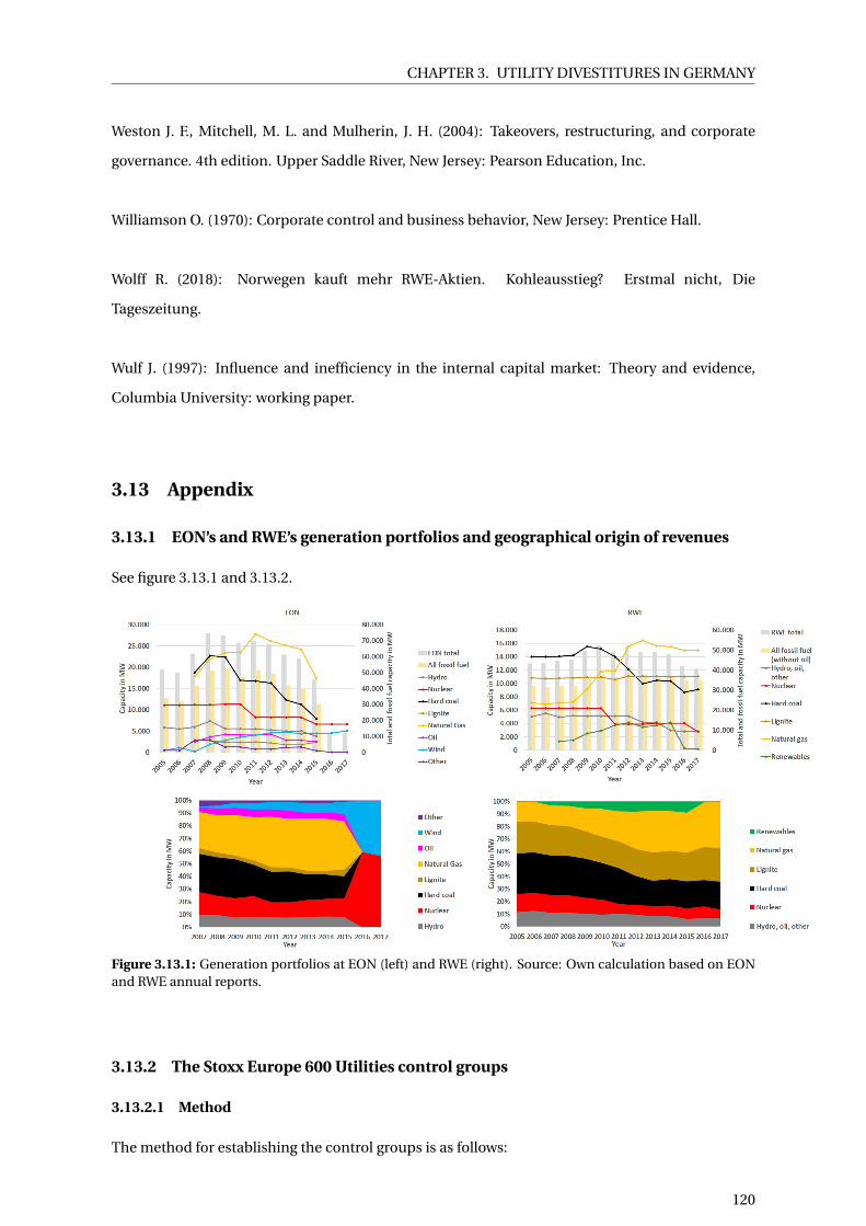
CHAPTER 3. UTILITY DIVESTITURES IN GERMANY
Weston J. F., Mitchell, M. L. and Mulherin, J. H. (2004): Takeovers, restructuring, and corporate
governance. 4th edition. Upper Saddle River, New Jersey: Pearson Education, Inc.
Williamson O. (1970): Corporate control and business behavior, New Jersey: Prentice Hall.
Wolff R. (2018): Norwegen kauft mehr RWE-Aktien. Kohleausstieg? Erstmal nicht, Die
Tageszeitung.
Wulf J. (1997): Influence and inefficiency in the internal capital market: Theory and evidence,
Columbia University: working paper.
3.13 Appendix
3.13.1 EON’s and RWE’s generation portfolios and geographical origin of revenues
See figure 3.13.1 and 3.13.2.
Figure 3.13.1: Generation portfolios at EON (left) and RWE (right). Source: Own calculation based on EONand RWE annual reports.
3.13.2 The Stoxx Europe 600 Utilities control groups
3.13.2.1 Method
The method for establishing the control groups is as follows:
120
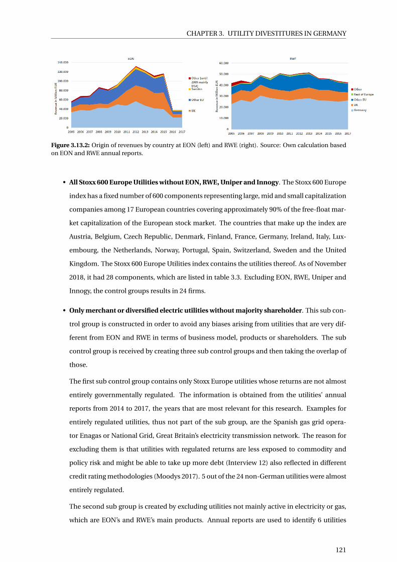
CHAPTER 3. UTILITY DIVESTITURES IN GERMANY
Figure 3.13.2: Origin of revenues by country at EON (left) and RWE (right). Source: Own calculation basedon EON and RWE annual reports.
• All Stoxx 600 Europe Utilities without EON, RWE, Uniper and Innogy. The Stoxx 600 Europe
index has a fixed number of 600 components representing large, mid and small capitalization
companies among 17 European countries covering approximately 90% of the free-float mar-
ket capitalization of the European stock market. The countries that make up the index are
Austria, Belgium, Czech Republic, Denmark, Finland, France, Germany, Ireland, Italy, Lux-
embourg, the Netherlands, Norway, Portugal, Spain, Switzerland, Sweden and the United
Kingdom. The Stoxx 600 Europe Utilities index contains the utilities thereof. As of November
2018, it had 28 components, which are listed in table 3.3. Excluding EON, RWE, Uniper and
Innogy, the control groups results in 24 firms.
• Only merchant or diversified electric utilities without majority shareholder. This sub con-
trol group is constructed in order to avoid any biases arising from utilities that are very dif-
ferent from EON and RWE in terms of business model, products or shareholders. The sub
control group is received by creating three sub control groups and then taking the overlap of
those.
The first sub control group contains only Stoxx Europe utilities whose returns are not almost
entirely governmentally regulated. The information is obtained from the utilities’ annual
reports from 2014 to 2017, the years that are most relevant for this research. Examples for
entirely regulated utilities, thus not part of the sub group, are the Spanish gas grid opera-
tor Enagas or National Grid, Great Britain’s electricity transmission network. The reason for
excluding them is that utilities with regulated returns are less exposed to commodity and
policy risk and might be able to take up more debt (Interview 12) also reflected in different
credit rating methodologies (Moodys 2017). 5 out of the 24 non-German utilities were almost
entirely regulated.
The second sub group is created by excluding utilities not mainly active in electricity or gas,
which are EON’s and RWE’s main products. Annual reports are used to identify 6 utilities
121
CHAPTER 3. UTILITY DIVESTITURES IN GERMANY
out of 24, which are mainly active in the waste and water sectors. These markets are likely
governed by different pressures than the ones our case study utilities operate in.
The third sub group excludes any utility that had an influential shareholder at some point
between 2014 and 2017. Influential shareholders are defined as those holding veto power
or own golden shares.21 Data for this is taken from Thomson Reuters Datastream. EDF or
Fortum are examples of utilities dominated by the French and Finnish state respectively. 6
utilities fell in that category. They might experience certain benefits or also pressures from
their dominant shareholder, differentiating them from utilities with diversified shareholder
bases (Maug 2002). The overlap of these three different sub groups creates a sub control
group that consists of only 9 utilities.
3.13.2.2 List of Stoxx Europe 600 Utilities components used for control group
See table 3.3.
3.13.3 Capital expenditure indicators
3.13.3.1 Capital expenditure correlations
See table 3.4.
3.13.3.2 Capital expenditure over operating cash flows
See table 3.5.
3.13.4 EBIT(DA) and free cash flow of main segments
See figure 3.13.3.
3.13.5 Leverage and liquidity indicators
See figure 3.13.4.
21A golden share gives its owner the right to outvote all other shares in certain specified circumstances.
122

CHAPTER 3. UTILITY DIVESTITURES IN GERMANY
Country Mainly regu-lated business
Products notmainly elec-tricity or gasrelated
Any majorityshareholder2014-2017
A2A SpA Italy
Centrica PLC Great Britain
EON Germany
EDF France X
EDP Portugal
Enagas Spain X
Endesa Spain X
Enel Italy
Engie/GDF Suez France X
Fortum Finland X
Iberdrola Spain
Innogy Germany
Italgas/Snam Italy X
National Grid Great Britain X
Naturgy Energy Group Spain
Orsted/Dong Denmark X
Pennon Group Great Britain X
Red Electrica Corporation Spain X
Rubis France X
RWE Germany
Scottish and Southern Energy Great Britain
Severn Trent Great Britain X
Suez Environnement France X
Terna Italy X
Uniper Germany
United Utilities Group Great Britain X X
Veolia Environnement France X
Table 3.3: List of Stoxx Europe 600 Utilities components. Source: https://www.stoxx.com/index-details?symbol=SX6p, accessed on November 10, 2018.
123
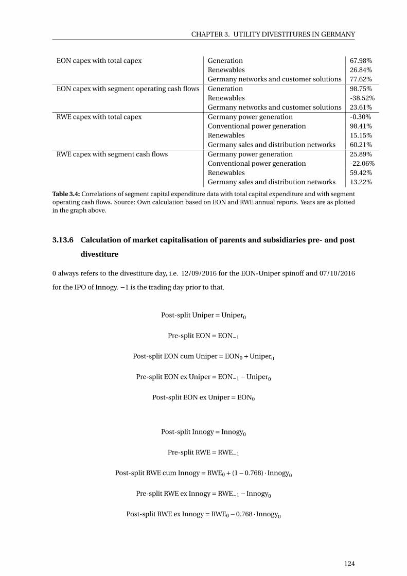
CHAPTER 3. UTILITY DIVESTITURES IN GERMANY
EON capex with total capex Generation 67.98%Renewables 26.84%Germany networks and customer solutions 77.62%
EON capex with segment operating cash flows Generation 98.75%Renewables -38.52%Germany networks and customer solutions 23.61%
RWE capex with total capex Germany power generation -0.30%Conventional power generation 98.41%Renewables 15.15%Germany sales and distribution networks 60.21%
RWE capex with segment cash flows Germany power generation 25.89%Conventional power generation -22.06%Renewables 59.42%Germany sales and distribution networks 13.22%
Table 3.4: Correlations of segment capital expenditure data with total capital expenditure and with segmentoperating cash flows. Source: Own calculation based on EON and RWE annual reports. Years are as plottedin the graph above.
3.13.6 Calculation of market capitalisation of parents and subsidiaries pre- and post
divestiture
0 always refers to the divestiture day, i.e. 12/09/2016 for the EON-Uniper spinoff and 07/10/2016
for the IPO of Innogy. −1 is the trading day prior to that.
Post-split Uniper = Uniper0
Pre-split EON = EON−1
Post-split EON cum Uniper = EON0 +Uniper0
Pre-split EON ex Uniper = EON−1 −Uniper0
Post-split EON ex Uniper = EON0
Post-split Innogy = Innogy0
Pre-split RWE = RWE−1
Post-split RWE cum Innogy = RWE0 + (1−0.768) · Innogy0
Pre-split RWE ex Innogy = RWE−1 − Innogy0
Post-split RWE ex Innogy = RWE0 −0.768 · Innogy0
124

CHAPTER 3. UTILITY DIVESTITURES IN GERMANY
2010
2011
2012
2013
2014
2015
2016
2017
Ave
rage
EO
Nca
pex
ove
rse
g-m
ent
op
er-
atin
gca
shfl
ow
s
E.O
NSE
Gro
up
78.0
7%83
.01%
68.6
7%99
.56%
56.3
6%59
.30%
79.7
4%-1
48.0
1%74
.16%
Gen
erat
ion
66.1
7%64
.71%
56.8
8%57
.54%
48.7
3%37
.53%
55.2
6%R
enew
able
s91
.97%
80.9
6%15
1.78
%67
.90%
105.
25%
87.6
7%97
.59%
Ger
man
yn
et-
wo
rks
and
cus-
tom
erso
luti
on
s
62.5
6%54
.43%
37.3
1%30
.27%
40.2
5%84
.21%
47.4
0%28
.07%
51.5
0%
RW
Eca
pex
ove
rse
g-m
ent
cash
flo
ws
RW
EG
rou
p11
5.98
%11
5.30
%11
5.61
%78
.09%
58.4
1%86
.79%
86.1
8%84
.72%
Ger
man
yp
ow
erge
ner
atio
n37
.29%
41.8
2%68
.37%
Co
nve
nti
on
alp
ow
erge
ner
atio
n13
1.47
%12
1.21
%47
.61%
37.8
6%24
.78%
84.5
4%
Ren
ewab
les
479.
69%
585.
11%
178.
70%
488.
51%
774.
07%
480.
43%
Ger
man
ysa
les
and
dis
trib
uti
on
net
wo
rks
83.3
9%12
1.94
%11
5.45
%53
.73%
48.2
6%65
.66%
70.7
8%
Table 3.5: Capital expenditure in EON’s and RWE’s main segments over operating cash flows in the samesegments. Average for EON 2010-2015, for RWE 2012-2015. Source: Own calculation based on EON andRWE annual reports.
125
CHAPTER 3. UTILITY DIVESTITURES IN GERMANY
3.13.7 Enterprise value over EBITDA
See figure 3.13.5.
3.13.8 Event studies
3.13.8.1 Share price event study
Estimation strategy Following MacKinlay (1997) and Kothari and Warner (2007), the market
model is defined as follows: Ri ,t =Pi ,t−Pi ,t−1
Pi ,t−1
Ri ,t =αi +βi Rm,t +ǫi ,t
E(ǫi ,t ) = 0
var(ǫi ,t ) =σ2ǫt
where Pi ,t are the period-t share prices and Ri ,t and Rm,t the period-t returns of firm i (EON or
RWE) and the market portfolio, respectively. ǫi , t is the the zero mean disturbance term. αi , βi and
σ2ǫt
are the parameters of the market model. Following the literature in using a broad based stock
index, the Stoxx Europe 600 index as of November 2018 is used for the market portfolio.
The predicted return for a firm for a day in the event period is thus given by the estimation of this
market model during a normal period defined as N = 100, i.e. day -101 to -1 prior to the event day:
Ri ,t = αi + βi Rm,t
Then the abnormal returns of each firm i = EON, RWE on the event day, t = 0, is calculated:
ri ,t = Ri ,t − Ri ,t
The relatively short normal and event periods are justified by the fast succession of events espe-
cially in 2015 and 2016, but results are largely robust to longer periods of up to 200 and 40 days for
the normal and event period respectively.
If returns are normally, identically and independently distributed, then
ri ,t
s(ri )
has a t-distribution, with s(ri ) = 1N−1
∑t=−1t=−N−1(ri ,t − ri )2 being the standard deviation of the residu-
als over the normal period prior to the event day.
Regression results See table 3.6.
126

CHAPTER 3. UTILITY DIVESTITURES IN GERMANY
(a) EON EBITDA contributions, free cash flow generation and earning prospects. Source: JP Morgan 2013from EON.
(b) RWE EBIT and free cash flows in the main segments in EUR million. In contrast to adjusted numbers thatexclude "non-operational effects", e.g. impairments, this is an estimation of the unadjusted EBIT = adjustedEBITDA - (operating depreciation + amortisation) - impairments. Source: Own calculation and illustration,data from RWE annual reports.
Figure 3.13.3: Illustrations of value creation and potential by segments at EON and RWE.
127

CHAPTER 3. UTILITY DIVESTITURES IN GERMANY
2006 2008 2010 2012 2014 2016
Date
14
15
16
17
18
19
20
21
22
23
Fitc
h lo
ng-t
erm
bon
d ra
ting
(a) Long-term bond rating as provided by Fitch. AAA = 24,DDD = 1.
2000 2002 2004 2006 2008 2010 2012 2014 2016 2018
Date
-0.4
-0.2
0
0.2
0.4
0.6
0.8
Net
deb
t ove
r to
tal a
sset
s
EONRWEControl group meanMean plus 2 SD,minus 2 SDSub control group meanMean plus 2 SD,
minus 2 SDControl group medianSub control group medianMinimum,maximum of control groupMinimum,maximum of sub control group
(b) Net debt over total assets. Net debt is total debt minuscash and short-term investments.
2000 2002 2004 2006 2008 2010 2012 2014 2016 2018
Date
-0.1
0
0.1
0.2
0.3
0.4
0.5
0.6
0.7
Long
-ter
m d
ebt o
ver
tota
l ass
ets
(c) Long-term debt over total assets.
2000 2002 2004 2006 2008 2010 2012 2014 2016
Date
-0.5
0
0.5
1
1.5
2
2.5
3
3.5
Cur
rent
ass
ets
over
cur
rent
liab
ilitie
s
(d) Liquidity ratio: current assets over current liabilities.
2000 2002 2004 2006 2008 2010 2012 2014 2016 2018
Date
0.2
0.3
0.4
0.5
0.6
0.7
0.8
0.9
1
1.1
Tot
al li
abili
ties
over
tota
l ass
ets
(e) Total liabilities over total assets.
2000 2002 2004 2006 2008 2010 2012 2014 2016 2018
Date
0.2
0.3
0.4
0.5
0.6
0.7
0.8
0.9
1
1.1
Tot
al li
abili
ties
over
tota
l ass
ets
(f ) Total liabilities and, for EON and RWE, total liabilities lessprovisions for nuclear dismantling and storage over total as-sets.
Figure 3.13.4: Leverage and liquidity indicators. Source: Own calculation and illustration, data by ThomsonReuters Datastream.
128

CHAPTER 3. UTILITY DIVESTITURES IN GERMANY
May15 Aug15 Dec15 Mar16 Jun16 Sep16 Jan17 Apr17 Jul17 Nov17 Feb18Date
0
2
4
6
8
10
Ent
erpr
ise
valu
es o
ver
EB
ITD
A
RWE ex InnogyInnogyEON ex UniperEON German nuclearUniper
Figure 3.13.5: JP Morgan’s estimates for enterprise value over EBITDA based on reports between May 2014and June 2017. Source: Own illustration based on J.P. Morgan Cazenove (2014-2017).
129

CH
AP
TE
R3.
UT
ILIT
YD
IVE
STIT
UR
ES
ING
ER
MA
NY
Table 3.6: Regression results for share price event study. Two-sided t-test, * p<0.10, ** p<0.05, *** p<0.01. Normal period is 100 days prior to event day, event period is the eventday. Type refers to the type of event: RE = renewable energy, N = nuclear policy, C = climate policy, D = divestiture related.
Event
date t
Description Source Type Exp.
ef-
fect
αEON βEON R2EON s(rEON) rEON,t αRWE βRWE R2
RWE s(rRWE) rRWE,t
28-
Jan-
2013
Minister for the Environ-
ment, Altmaier, publishes
proposal to cap renewable
energy subsidy cost.
Handelsblatt
(2013-01)
RE + -0.004 0.676 10.01% 0.013 -0.013 -0.003 0.770 18.65% 0.011 -0.004
9-
Nov-
2013
Agreement in CDU-SPD
coalition talks on measures
to cap renewable energy
support costs.
Handelsblatt
(2013-11)
RE + 0.000 0.676 10.39% 0.014 0 0.000 0.605 4.69% 0.019 -0.002
21-
Jan-
2014
Measures to cap renew-
able energy costs are fur-
ther specified by Ministry
of Economic Affairs and
Energy.
Gabriel
(2014)
RE + 0.001 0.798 10.45% 0.013 -0.003 0.002 0.793 5.81% 0.018 -0.001
5-
May-
2014
Handelsblatt reports on
speech draft by environ-
mental ministry executive
saying that nuclear pro-
visions will be examined
soon.
Stratmann
(2014)
N - -0.001 0.834 31.59% 0.009 -0.003 -0.000 0.835 18.41% 0.014 -0.004
130

CH
AP
TE
R3.
UT
ILIT
YD
IVE
STIT
UR
ES
ING
ER
MA
NY
Table 3.6: Regression results for share price event study. Two-sided t-test, * p<0.10, ** p<0.05, *** p<0.01. Normal period is 100 days prior to event day, event period is the eventday. Type refers to the type of event: RE = renewable energy, N = nuclear policy, C = climate policy, D = divestiture related.
Event
date t
Description Source Type Exp.
ef-
fect
αEON βEON R2EON s(rEON) rEON,t αRWE βRWE R2
RWE s(rRWE) rRWE,t
11-
May-
2014
Utilities suggest
government-run nuclear
fund that takes over all
operationial, dismantling
and storage related tasks
in exhange for dropping
various lawsuits against the
government worth around
EUR 15 billion.
Spiegel
(2014),
Dohmen and
Hawranek
(2014)
N + 0.000 0.882 32.02% 0.010 0 0.000 0.879 18.64% 0.014 -0.011
27-
Jun-
2014
Bundestag decides on re-
newable energy law reform
(EEG 2014) capping renew-
ables subsidy cost.
BMWi (2014-
06)
RE + 0.001 0.863 24.55% 0.010 0 0.001 0.874 16.04% 0.013 0.013
23-
Nov-
2014
Minister in charge of en-
ergy, Gabriel, presents
idea for CO2 reduction
contribution by coal power
plants.
Handelsblatt
(2014-11)
C - -0.001 1.223 57.72% 0.010 0.002 -0.001 1.341 52.35% 0.012 0.003
131

CH
AP
TE
R3.
UT
ILIT
YD
IVE
STIT
UR
ES
ING
ER
MA
NY
Table 3.6: Regression results for share price event study. Two-sided t-test, * p<0.10, ** p<0.05, *** p<0.01. Normal period is 100 days prior to event day, event period is the eventday. Type refers to the type of event: RE = renewable energy, N = nuclear policy, C = climate policy, D = divestiture related.
Event
date t
Description Source Type Exp.
ef-
fect
αEON βEON R2EON s(rEON) rEON,t αRWE βRWE R2
RWE s(rRWE) rRWE,t
30-
Nov-
2014
E.ON announces to split off
Uniper.
Drozdiak
(2014)
D + 0.000 1.237 54.68% 0.010 0.041*** -0.001 1.352 49.03% 0.012 0.014
17-
Dec-
2014
Süddeutsche Zeitung
learns that state-run fund
with 17 bn is planned
according to ministries.
Fund should solely se-
cure funds but not take
any operational or other
liabilities.
Handelsblatt
(2014-12)
N - 0.000 1.182 51.86% 0.011 0.012 -0.001 1.336 51.63% 0.013 0.013
20-
Mar-
2015
Report written by consul-
tancy Becker Büttner Held
for Ministry of Economic
Affairs concludes according
to Handelsblatt that provi-
sions are only safe if moved
into external fund.
Handelsblatt
(2015)
N - -0.001 0.989 36.62% 0.013 0.015 -0.003 1.030 29.98% 0.016 -0.002
132

CH
AP
TE
R3.
UT
ILIT
YD
IVE
STIT
UR
ES
ING
ER
MA
NY
Table 3.6: Regression results for share price event study. Two-sided t-test, * p<0.10, ** p<0.05, *** p<0.01. Normal period is 100 days prior to event day, event period is the eventday. Type refers to the type of event: RE = renewable energy, N = nuclear policy, C = climate policy, D = divestiture related.
Event
date t
Description Source Type Exp.
ef-
fect
αEON βEON R2EON s(rEON) rEON,t αRWE βRWE R2
RWE s(rRWE) rRWE,t
21-
Mar-
2015
Secretary of State for En-
ergy, Baake, publishes pa-
per on how coal power
plants should contribute to
climate policy via a pro-
posed CO2 levy.
Frese (2015) C - -0.001 0.980 35.47% 0.013 -0.005 -0.003 1.016 28.94% 0.016 -0.007
11-
Jun-
2015
Tagesschau reports on let-
ter by CDU against the
planned CO2 levy.
Mayer-Rüth
(2015)
C + -0.001 0.871 27.20% 0.012 -0.016 -0.002 0.992 27.52% 0.014 -0.011
24-
Jun-
2015
Tagesschau reports on the
failure of an agreement on
a CO2 levy and instead the
granting of compensation
payments to lignite power
plant operators.
Tagesschau
(2015)
C + -0.001 0.911 29.85% 0.012 -0.001 -0.003 1.053 34.55% 0.013 0.025***
2-Jul-
2015
Government publishes
compromise on CO2 levy.
Flauger
(2015-07)
C + -0.001 0.909 32.59% 0.012 0.018 -0.002 0.970 33.59% 0.013 0.058***
133
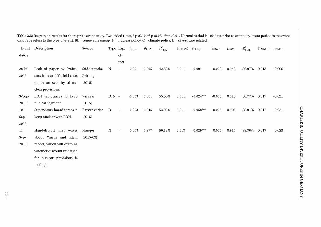
CH
AP
TE
R3.
UT
ILIT
YD
IVE
STIT
UR
ES
ING
ER
MA
NY
Table 3.6: Regression results for share price event study. Two-sided t-test, * p<0.10, ** p<0.05, *** p<0.01. Normal period is 100 days prior to event day, event period is the eventday. Type refers to the type of event: RE = renewable energy, N = nuclear policy, C = climate policy, D = divestiture related.
Event
date t
Description Source Type Exp.
ef-
fect
αEON βEON R2EON s(rEON) rEON,t αRWE βRWE R2
RWE s(rRWE) rRWE,t
28-Jul-
2015
Leak of paper by Profes-
sors Irrek and Vorfeld casts
doubt on security of nu-
clear provisions.
Süddeutsche
Zeitung
(2015)
N - -0.001 0.895 42.58% 0.011 -0.004 -0.002 0.948 36.07% 0.013 -0.006
9-Sep-
2015
EON announces to keep
nuclear segment.
Vasagar
(2015)
D/N - -0.003 0.861 55.56% 0.011 -0.024*** -0.005 0.919 38.77% 0.017 -0.021
10-
Sep-
2015
Supervisory board agrees to
keep nuclear with EON.
Bayernkurier
(2015)
D - -0.003 0.845 53.93% 0.011 -0.058*** -0.005 0.905 38.04% 0.017 -0.021
11-
Sep-
2015
Handelsblatt first writes
about Warth and Klein
report, which will examine
whether discount rate used
for nuclear provisions is
too high.
Flauger
(2015-09)
N - -0.003 0.877 50.12% 0.013 -0.029*** -0.005 0.915 38.36% 0.017 -0.023
134
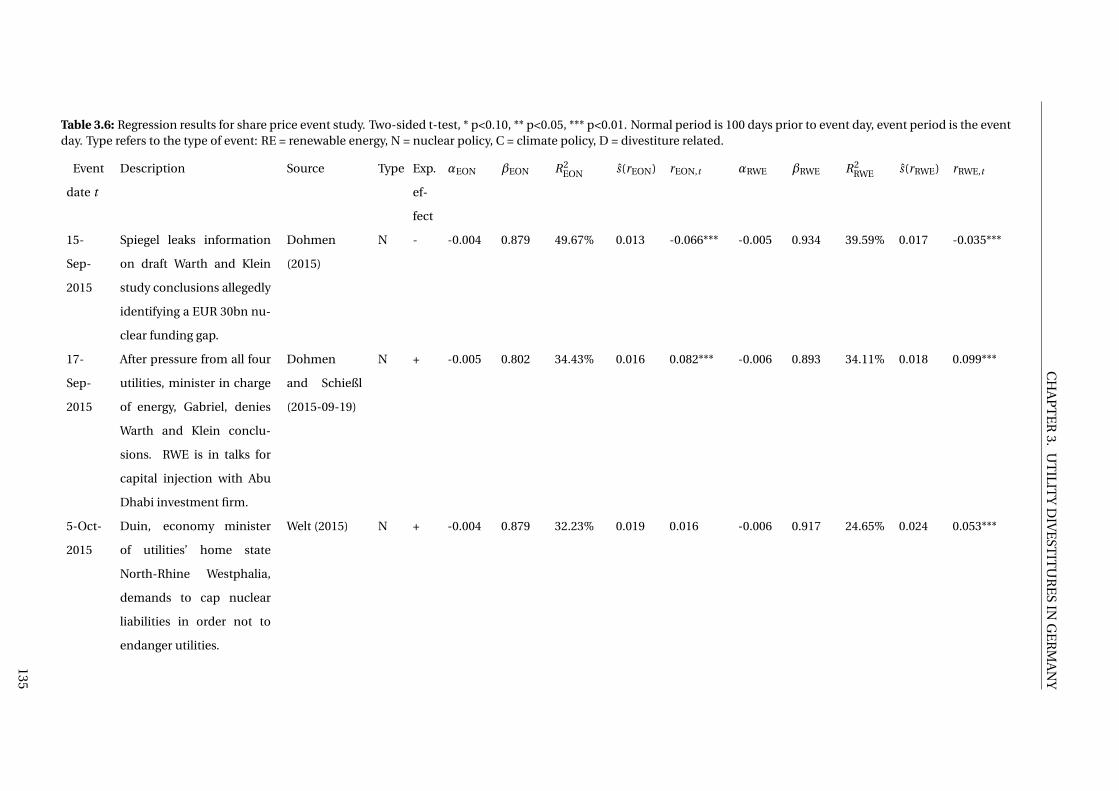
CH
AP
TE
R3.
UT
ILIT
YD
IVE
STIT
UR
ES
ING
ER
MA
NY
Table 3.6: Regression results for share price event study. Two-sided t-test, * p<0.10, ** p<0.05, *** p<0.01. Normal period is 100 days prior to event day, event period is the eventday. Type refers to the type of event: RE = renewable energy, N = nuclear policy, C = climate policy, D = divestiture related.
Event
date t
Description Source Type Exp.
ef-
fect
αEON βEON R2EON s(rEON) rEON,t αRWE βRWE R2
RWE s(rRWE) rRWE,t
15-
Sep-
2015
Spiegel leaks information
on draft Warth and Klein
study conclusions allegedly
identifying a EUR 30bn nu-
clear funding gap.
Dohmen
(2015)
N - -0.004 0.879 49.67% 0.013 -0.066*** -0.005 0.934 39.59% 0.017 -0.035***
17-
Sep-
2015
After pressure from all four
utilities, minister in charge
of energy, Gabriel, denies
Warth and Klein conclu-
sions. RWE is in talks for
capital injection with Abu
Dhabi investment firm.
Dohmen
and Schießl
(2015-09-19)
N + -0.005 0.802 34.43% 0.016 0.082*** -0.006 0.893 34.11% 0.018 0.099***
5-Oct-
2015
Duin, economy minister
of utilities’ home state
North-Rhine Westphalia,
demands to cap nuclear
liabilities in order not to
endanger utilities.
Welt (2015) N + -0.004 0.879 32.23% 0.019 0.016 -0.006 0.917 24.65% 0.024 0.053***
135

CH
AP
TE
R3.
UT
ILIT
YD
IVE
STIT
UR
ES
ING
ER
MA
NY
Table 3.6: Regression results for share price event study. Two-sided t-test, * p<0.10, ** p<0.05, *** p<0.01. Normal period is 100 days prior to event day, event period is the eventday. Type refers to the type of event: RE = renewable energy, N = nuclear policy, C = climate policy, D = divestiture related.
Event
date t
Description Source Type Exp.
ef-
fect
αEON βEON R2EON s(rEON) rEON,t αRWE βRWE R2
RWE s(rRWE) rRWE,t
8-Oct-
2015
Publication of stress test
(Warth and Klein) report
with main conclusion that
firms set aside enough
nuclear decommissioning
funds.
Copley and
Eckert (2015)
N + -0.003 0.904 32.83% 0.020 0.005 -0.005 0.980 25.87% 0.025 0.005
1-
Dec-
2015
RWE announces to split off
Innogy.
Terium and
Günther
(2015)
D + -0.003 0.938 27.53% 0.022 0.013 -0.005 1.134 21.38% 0.032 0.165***
27-
Apr-
2016
Commission unveils plans
for utilities to pay EUR
23.3bn towards the cost of
storing nuclear waste in ex-
change for a cap on stor-
age liabilities. It is expected
that the government fol-
lows the recommendation.
Financial
Times (2016)
N +/- 0.002 1.245 49.14% 0.018 0.031* 0.002 1.075 27.02% 0.026 0.053***
136
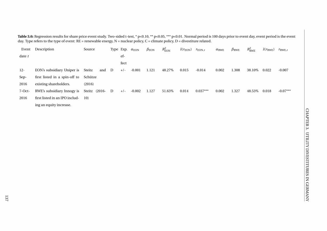
CH
AP
TE
R3.
UT
ILIT
YD
IVE
STIT
UR
ES
ING
ER
MA
NY
Table 3.6: Regression results for share price event study. Two-sided t-test, * p<0.10, ** p<0.05, *** p<0.01. Normal period is 100 days prior to event day, event period is the eventday. Type refers to the type of event: RE = renewable energy, N = nuclear policy, C = climate policy, D = divestiture related.
Event
date t
Description Source Type Exp.
ef-
fect
αEON βEON R2EON s(rEON) rEON,t αRWE βRWE R2
RWE s(rRWE) rRWE,t
12-
Sep-
2016
EON’s subsidiary Uniper is
first listed in a spin-off to
existing shareholders.
Steitz and
Schütze
(2016)
D +/- -0.001 1.121 48.27% 0.015 -0.014 0.002 1.308 38.10% 0.022 -0.007
7-Oct-
2016
RWE’s subsidiary Innogy is
first listed in an IPO includ-
ing an equity increase.
Steitz (2016-
10)
D +/- -0.002 1.127 51.63% 0.014 0.037*** 0.002 1.327 48.53% 0.018 -0.07***
137
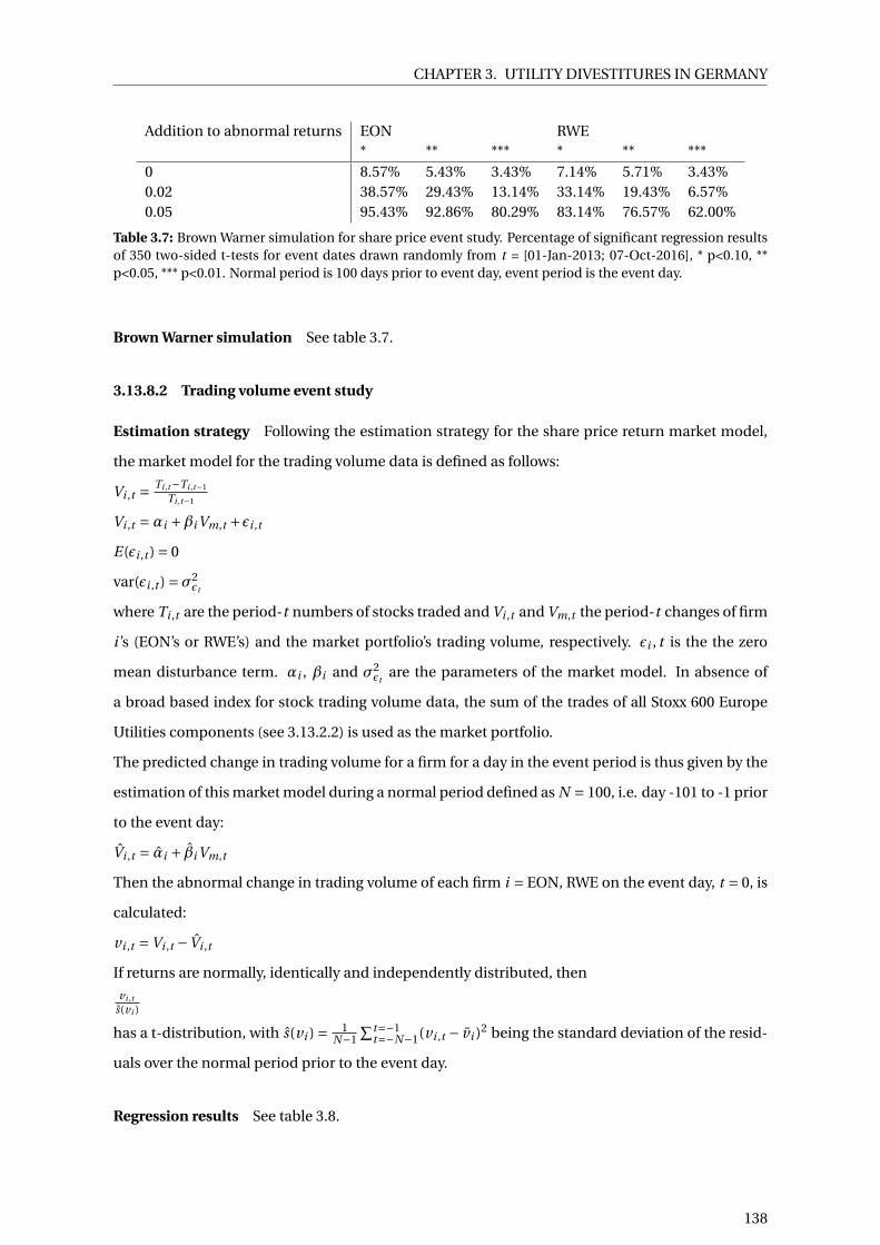
CHAPTER 3. UTILITY DIVESTITURES IN GERMANY
Addition to abnormal returns EON RWE* ** *** * ** ***
0 8.57% 5.43% 3.43% 7.14% 5.71% 3.43%0.02 38.57% 29.43% 13.14% 33.14% 19.43% 6.57%0.05 95.43% 92.86% 80.29% 83.14% 76.57% 62.00%
Table 3.7: Brown Warner simulation for share price event study. Percentage of significant regression resultsof 350 two-sided t-tests for event dates drawn randomly from t = [01-Jan-2013; 07-Oct-2016], * p<0.10, **p<0.05, *** p<0.01. Normal period is 100 days prior to event day, event period is the event day.
Brown Warner simulation See table 3.7.
3.13.8.2 Trading volume event study
Estimation strategy Following the estimation strategy for the share price return market model,
the market model for the trading volume data is defined as follows:
Vi ,t =Ti ,t−Ti ,t−1
Ti ,t−1
Vi ,t =αi +βi Vm,t +ǫi ,t
E(ǫi ,t ) = 0
var(ǫi ,t ) =σ2ǫt
where Ti ,t are the period-t numbers of stocks traded and Vi ,t and Vm,t the period-t changes of firm
i ’s (EON’s or RWE’s) and the market portfolio’s trading volume, respectively. ǫi , t is the the zero
mean disturbance term. αi , βi and σ2ǫt
are the parameters of the market model. In absence of
a broad based index for stock trading volume data, the sum of the trades of all Stoxx 600 Europe
Utilities components (see 3.13.2.2) is used as the market portfolio.
The predicted change in trading volume for a firm for a day in the event period is thus given by the
estimation of this market model during a normal period defined as N = 100, i.e. day -101 to -1 prior
to the event day:
Vi ,t = αi + βi Vm,t
Then the abnormal change in trading volume of each firm i = EON, RWE on the event day, t = 0, is
calculated:
vi ,t =Vi ,t − Vi ,t
If returns are normally, identically and independently distributed, then
vi ,t
s(vi )
has a t-distribution, with s(vi ) = 1N−1
∑t=−1t=−N−1(vi ,t − vi )2 being the standard deviation of the resid-
uals over the normal period prior to the event day.
Regression results See table 3.8.
138
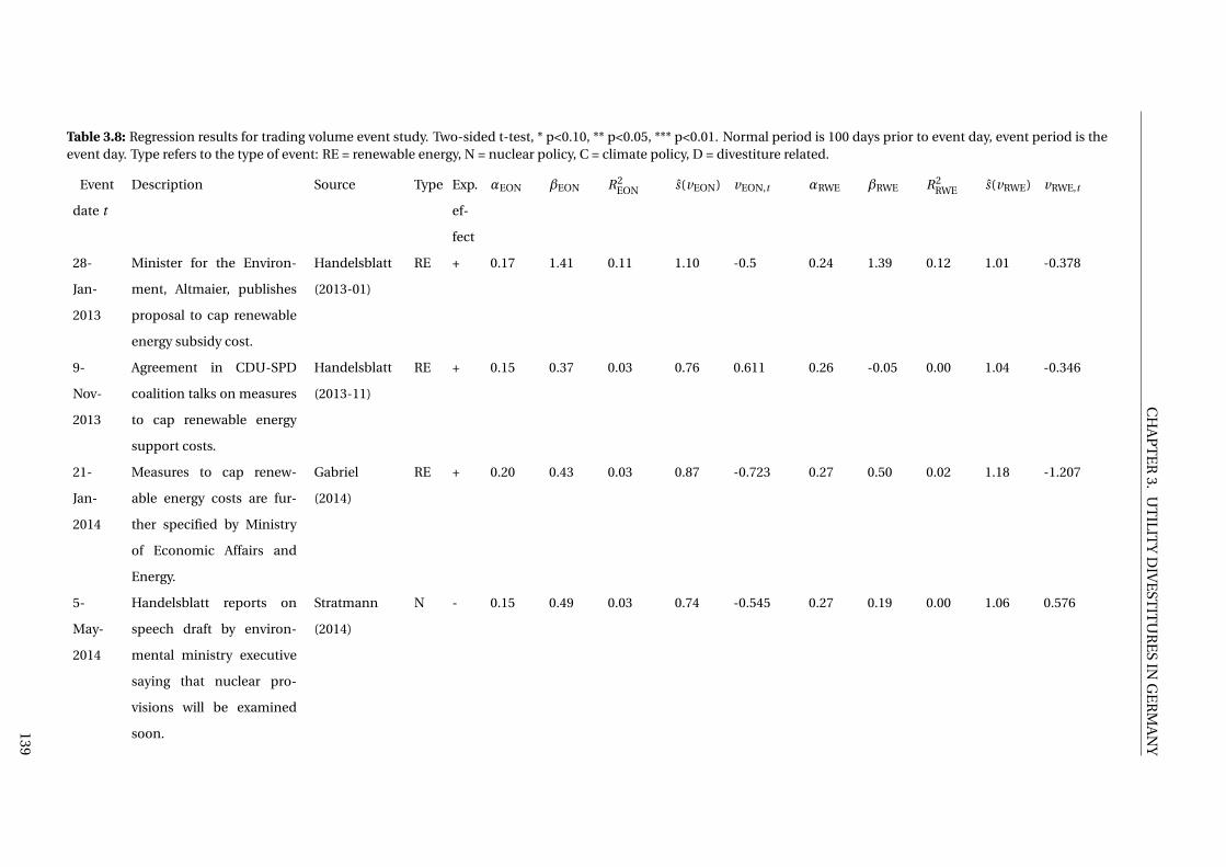
CH
AP
TE
R3.
UT
ILIT
YD
IVE
STIT
UR
ES
ING
ER
MA
NY
Table 3.8: Regression results for trading volume event study. Two-sided t-test, * p<0.10, ** p<0.05, *** p<0.01. Normal period is 100 days prior to event day, event period is theevent day. Type refers to the type of event: RE = renewable energy, N = nuclear policy, C = climate policy, D = divestiture related.
Event
date t
Description Source Type Exp.
ef-
fect
αEON βEON R2EON s(vEON) vEON,t αRWE βRWE R2
RWE s(vRWE) vRWE,t
28-
Jan-
2013
Minister for the Environ-
ment, Altmaier, publishes
proposal to cap renewable
energy subsidy cost.
Handelsblatt
(2013-01)
RE + 0.17 1.41 0.11 1.10 -0.5 0.24 1.39 0.12 1.01 -0.378
9-
Nov-
2013
Agreement in CDU-SPD
coalition talks on measures
to cap renewable energy
support costs.
Handelsblatt
(2013-11)
RE + 0.15 0.37 0.03 0.76 0.611 0.26 -0.05 0.00 1.04 -0.346
21-
Jan-
2014
Measures to cap renew-
able energy costs are fur-
ther specified by Ministry
of Economic Affairs and
Energy.
Gabriel
(2014)
RE + 0.20 0.43 0.03 0.87 -0.723 0.27 0.50 0.02 1.18 -1.207
5-
May-
2014
Handelsblatt reports on
speech draft by environ-
mental ministry executive
saying that nuclear pro-
visions will be examined
soon.
Stratmann
(2014)
N - 0.15 0.49 0.03 0.74 -0.545 0.27 0.19 0.00 1.06 0.576
139

CH
AP
TE
R3.
UT
ILIT
YD
IVE
STIT
UR
ES
ING
ER
MA
NY
Table 3.8: Regression results for trading volume event study. Two-sided t-test, * p<0.10, ** p<0.05, *** p<0.01. Normal period is 100 days prior to event day, event period is theevent day. Type refers to the type of event: RE = renewable energy, N = nuclear policy, C = climate policy, D = divestiture related.
Event
date t
Description Source Type Exp.
ef-
fect
αEON βEON R2EON s(vEON) vEON,t αRWE βRWE R2
RWE s(vRWE) vRWE,t
11-
May-
2014
Utilities suggest
government-run nuclear
fund that takes over all
operationial, dismantling
and storage related tasks
in exhange for dropping
various lawsuits against the
government worth around
EUR 15 billion.
Spiegel
(2014),
Dohmen and
Hawranek
(2014)
N + 0.14 0.50 0.03 0.75 0.435 0.30 0.12 0.00 1.07 -0.711
27-
Jun-
2014
Bundestag decides on re-
newable energy law reform
(EEG 2014) capping renew-
ables subsidy cost.
BMWi (2014-
06)
RE + 0.23 0.99 0.08 0.95 -0.669 0.33 0.92 0.04 1.22 0.003
23-
Nov-
2014
Minister in charge of en-
ergy, Gabriel, presents
idea for CO2 reduction
contribution by coal power
plants.
Handelsblatt
(2014-11)
C - 0.38 1.01 0.02 1.93 -0.345 0.57 1.89 0.06 2.19 -0.312
140

CH
AP
TE
R3.
UT
ILIT
YD
IVE
STIT
UR
ES
ING
ER
MA
NY
Table 3.8: Regression results for trading volume event study. Two-sided t-test, * p<0.10, ** p<0.05, *** p<0.01. Normal period is 100 days prior to event day, event period is theevent day. Type refers to the type of event: RE = renewable energy, N = nuclear policy, C = climate policy, D = divestiture related.
Event
date t
Description Source Type Exp.
ef-
fect
αEON βEON R2EON s(vEON) vEON,t αRWE βRWE R2
RWE s(vRWE) vRWE,t
30-
Nov-
2014
E.ON announces to split off
Uniper.
Drozdiak
(2014)
D + 0.38 1.22 0.03 1.93 12.353*** 0.61 2.04 0.07 2.21 -0.173
17-
Dec-
2014
Süddeutsche Zeitung
learns that state-run fund
with 17 bn is planned
according to ministries.
Fund should solely se-
cure funds but not take
any operational or other
liabilities.
Handelsblatt
(2014-12)
N - 0.49 0.82 0.01 2.30 0.018 0.62 1.81 0.05 2.24 -0.603
20-
Mar-
2015
Report written by consul-
tancy Becker Büttner Held
for Ministry of Economic
Affairs concludes according
to Handelsblatt that provi-
sions are only safe if moved
into external fund.
Handelsblatt
(2015)
N - 0.37 0.55 0.01 1.68 0.151 0.41 0.64 0.01 1.41 -0.5
141

CH
AP
TE
R3.
UT
ILIT
YD
IVE
STIT
UR
ES
ING
ER
MA
NY
Table 3.8: Regression results for trading volume event study. Two-sided t-test, * p<0.10, ** p<0.05, *** p<0.01. Normal period is 100 days prior to event day, event period is theevent day. Type refers to the type of event: RE = renewable energy, N = nuclear policy, C = climate policy, D = divestiture related.
Event
date t
Description Source Type Exp.
ef-
fect
αEON βEON R2EON s(vEON) vEON,t αRWE βRWE R2
RWE s(vRWE) vRWE,t
21-
Mar-
2015
Secretary of State for En-
ergy, Baake, publishes pa-
per on how coal power
plants should contribute to
climate policy via a pro-
posed CO2 levy.
Frese (2015) C - 0.38 0.54 0.01 1.68 -0.329 0.42 0.60 0.01 1.40 0.501
11-
Jun-
2015
Tagesschau reports on let-
ter by CDU against the
planned CO2 levy.
Mayer-Rüth
(2015)
C + 0.21 0.94 0.06 0.99 0.912 0.34 0.96 0.05 1.19 -0.878
24-
Jun-
2015
Tagesschau reports on the
failure of an agreement on
a CO2 levy and instead the
granting of compensation
payments to lignite power
plant operators.
Tagesschau
(2015)
C + 0.21 0.91 0.06 0.99 0.949 0.35 1.08 0.05 1.22 2.568***
2-Jul-
2015
Government publishes
compromise on CO2 levy.
Flauger
(2015-07)
C + 0.21 0.79 0.05 0.93 0.296 0.36 0.94 0.04 1.23 5.855***
142
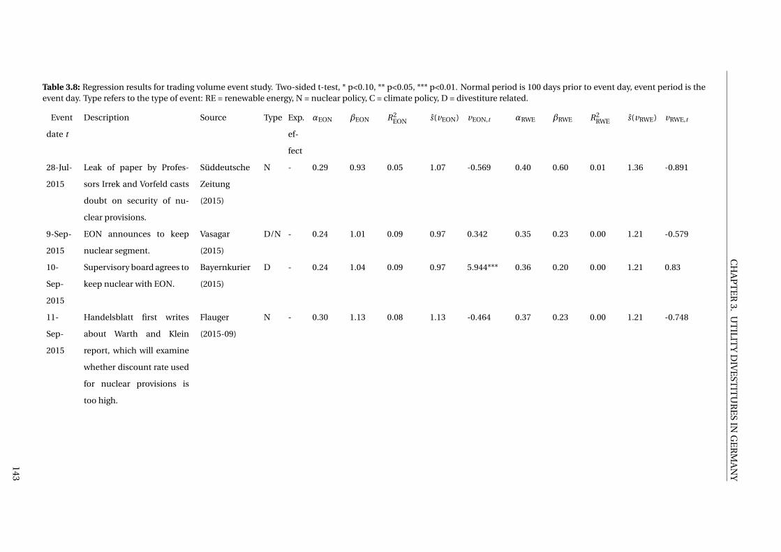
CH
AP
TE
R3.
UT
ILIT
YD
IVE
STIT
UR
ES
ING
ER
MA
NY
Table 3.8: Regression results for trading volume event study. Two-sided t-test, * p<0.10, ** p<0.05, *** p<0.01. Normal period is 100 days prior to event day, event period is theevent day. Type refers to the type of event: RE = renewable energy, N = nuclear policy, C = climate policy, D = divestiture related.
Event
date t
Description Source Type Exp.
ef-
fect
αEON βEON R2EON s(vEON) vEON,t αRWE βRWE R2
RWE s(vRWE) vRWE,t
28-Jul-
2015
Leak of paper by Profes-
sors Irrek and Vorfeld casts
doubt on security of nu-
clear provisions.
Süddeutsche
Zeitung
(2015)
N - 0.29 0.93 0.05 1.07 -0.569 0.40 0.60 0.01 1.36 -0.891
9-Sep-
2015
EON announces to keep
nuclear segment.
Vasagar
(2015)
D/N - 0.24 1.01 0.09 0.97 0.342 0.35 0.23 0.00 1.21 -0.579
10-
Sep-
2015
Supervisory board agrees to
keep nuclear with EON.
Bayernkurier
(2015)
D - 0.24 1.04 0.09 0.97 5.944*** 0.36 0.20 0.00 1.21 0.83
11-
Sep-
2015
Handelsblatt first writes
about Warth and Klein
report, which will examine
whether discount rate used
for nuclear provisions is
too high.
Flauger
(2015-09)
N - 0.30 1.13 0.08 1.13 -0.464 0.37 0.23 0.00 1.21 -0.748
143

CH
AP
TE
R3.
UT
ILIT
YD
IVE
STIT
UR
ES
ING
ER
MA
NY
Table 3.8: Regression results for trading volume event study. Two-sided t-test, * p<0.10, ** p<0.05, *** p<0.01. Normal period is 100 days prior to event day, event period is theevent day. Type refers to the type of event: RE = renewable energy, N = nuclear policy, C = climate policy, D = divestiture related.
Event
date t
Description Source Type Exp.
ef-
fect
αEON βEON R2EON s(vEON) vEON,t αRWE βRWE R2
RWE s(vRWE) vRWE,t
15-
Sep-
2015
Spiegel leaks information
on draft Warth and Klein
study conclusions allegedly
identifying a EUR 30bn nu-
clear funding gap.
Dohmen
(2015)
N - 0.29 1.16 0.08 1.13 0.969 0.37 0.25 0.00 1.21 2.811***
17-
Sep-
2015
After pressure from all four
utilities, minister in charge
of energy, Gabriel, denies
Warth and Klein conclu-
sions. RWE is in talks for
capital injection with Abu
Dhabi investment firm.
Dohmen
and Schießl
(2015-09-19)
N + 0.30 1.22 0.09 1.13 -0.486 0.37 0.37 0.01 1.23 -0.428
5-Oct-
2015
Duin, economy minister
of utilities’ home state
North-Rhine Westphalia,
demands to cap nuclear
liabilities in order not to
endanger utilities.
Welt (2015) N + 0.30 1.12 0.08 1.13 -0.495 0.32 0.33 0.01 1.13 -0.469
144
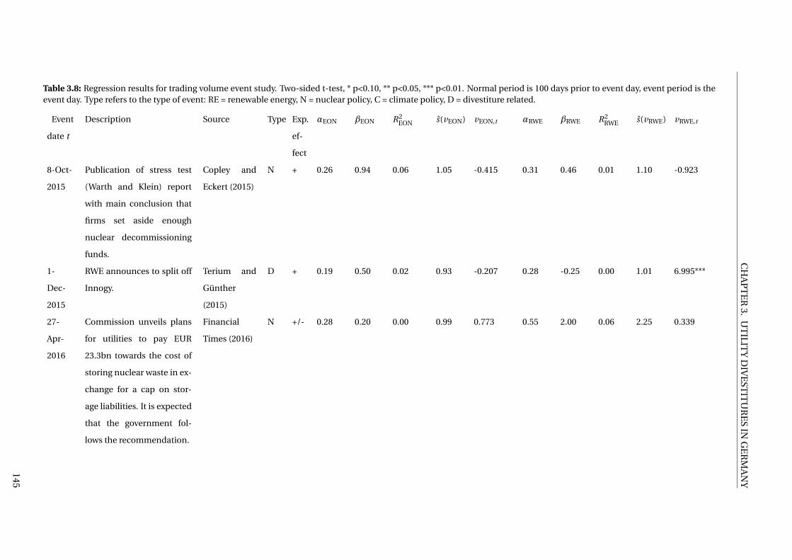
CH
AP
TE
R3.
UT
ILIT
YD
IVE
STIT
UR
ES
ING
ER
MA
NY
Table 3.8: Regression results for trading volume event study. Two-sided t-test, * p<0.10, ** p<0.05, *** p<0.01. Normal period is 100 days prior to event day, event period is theevent day. Type refers to the type of event: RE = renewable energy, N = nuclear policy, C = climate policy, D = divestiture related.
Event
date t
Description Source Type Exp.
ef-
fect
αEON βEON R2EON s(vEON) vEON,t αRWE βRWE R2
RWE s(vRWE) vRWE,t
8-Oct-
2015
Publication of stress test
(Warth and Klein) report
with main conclusion that
firms set aside enough
nuclear decommissioning
funds.
Copley and
Eckert (2015)
N + 0.26 0.94 0.06 1.05 -0.415 0.31 0.46 0.01 1.10 -0.923
1-
Dec-
2015
RWE announces to split off
Innogy.
Terium and
Günther
(2015)
D + 0.19 0.50 0.02 0.93 -0.207 0.28 -0.25 0.00 1.01 6.995***
27-
Apr-
2016
Commission unveils plans
for utilities to pay EUR
23.3bn towards the cost of
storing nuclear waste in ex-
change for a cap on stor-
age liabilities. It is expected
that the government fol-
lows the recommendation.
Financial
Times (2016)
N +/- 0.28 0.20 0.00 0.99 0.773 0.55 2.00 0.06 2.25 0.339
145

CH
AP
TE
R3.
UT
ILIT
YD
IVE
STIT
UR
ES
ING
ER
MA
NY
Table 3.8: Regression results for trading volume event study. Two-sided t-test, * p<0.10, ** p<0.05, *** p<0.01. Normal period is 100 days prior to event day, event period is theevent day. Type refers to the type of event: RE = renewable energy, N = nuclear policy, C = climate policy, D = divestiture related.
Event
date t
Description Source Type Exp.
ef-
fect
αEON βEON R2EON s(vEON) vEON,t αRWE βRWE R2
RWE s(vRWE) vRWE,t
12-
Sep-
2016
EON’s subsidiary Uniper is
first listed in a spin-off to
existing shareholders.
Steitz and
Schütze
(2016)
D +/- 0.30 0.22 0.01 1.31 3.738*** 0.63 0.12 0.00 2.58 5.534***
7-Oct-
2016
RWE’s subsidiary Innogy is
first listed in an IPO includ-
ing an equity increase.
Steitz (2016-
10)
D +/- 0.29 0.22 0.01 1.25 2.959*** 0.75 0.36 0.00 2.77 5.214*
146

CHAPTER 3. UTILITY DIVESTITURES IN GERMANY
Addition to abnormal change in volume EON RWE* ** *** * ** ***
0 6.29% 4.29% 3.43% 6.29% 3.43% 2.29%2 60.57% 48.29% 30.00% 32.86% 20.86% 11.43%5 100.00% 96.57% 89.71% 93.71% 87.14% 75.14%
Table 3.9: Brown Warner simulation for trading volume event study. Percentage of significant regressionresults of 350 two-sided t-tests for event dates drawn randomly from t = [01-Jan-2013; 07-Oct-2016], * p<0.10,** p<0.05, *** p<0.01. Normal period is 100 days prior to event day, event period is the event day.
Brown Warner simulation See table 3.9.
147

Chapter 4
The impact of production and
macroeconomic risk on wind power
equity returns
An analysis from a financial investor’s perspective
Abstract
Financial investors play an increasing role in the operational phase of renewable energy
assets. As policy support is reduced and the sector matures, investors have to rely on more
prudent modelling of their asset returns.
This paper analyses how German wind park equity returns react if production and macroe-
conomic factors are misestimated at acquisition. Specifically, four sources of risk are examined:
production, power prices, inflation and interest rates. A discounted cash flow model with de-
tailed cost and revenue data of existing German wind parks with feed-in tariff is used to test the
sensitivity of shareholder payouts to these risk factors.
The results underline the importance of energy production and power prices: shareholder
payout returns range from 2.8 to 10.1% and from 3.6 to 9.3% for a reasonable variation in pro-
duction and power prices respectively. Inflation has a medium and ambiguous impact de-
pending on the time frame that wind parks operate under the guaranteed feed-in tariff regime.
A possible increase in interest rates plays only a limited negative role for existing German wind
park equity returns. Several strategies are suggested to mitigate the identified risks, which will
substantially increase in the coming years as governmental support policies are phased out.
The paper contributes to the energy economics and finance literature by presenting a fi-
nancial investor perspective on production and macroeconomic risk in wind energy. To policy
makers, the results offer a deeper understanding of equity investor needs in order to harvest
their available capital for reaching renewable energy targets.
Key words— Renewable energy; wind; financial investors; DCF model; sensitivity analysis.
148

CHAPTER 4. THE IMPACT OF PRODUCTION AND MACROECONOMIC RISK ON WIND POWEREQUITY RETURNS
4.1 Introduction
Utilities have traditionally dominated investments in electricity assets in Europe. However, the
growing market of renewable energy generation attracted new classes of investors in recent years.
In Germany, almost one third of renewable generation assets were owned by retail investors and
around 14% each by project developers, financial investors like banks and funds and industrial
firms in 2016 (figure 4.1.1).
Figure 4.1.1: Owners of renewable energy assets in MW in Germany in 2016. Source: trend:research 2017.
Whereas project developers specialise in building renewable power plants and often sell them on
to other investors after construction (Hostert 2016), the other investor types usually hold the assets
longer-term, sometimes over their entire operational life of more than 20 years. Distressed utilities
also discovered the build-sell-operate model as a way to recycle funds and generate profits by sell-
ing early-stage renewable assets to institutional investors (McCrone 2017). This explains the high
share of financial investors in Germany, who usually do not develop projects themselves but enter
after construction.
Institutional investors like pension funds and insurance companies allocate a growing part of their
portfolios to renewable energies. In Europe, institutional investors’ investments hit a record in
20171 of USD 9.9 billion, up 42% on 2016 (figure 4.1.2).
The attraction of renewable energies for institutional investors can be explained by the decen-
tralised and relatively low-risk nature of renewable energy technologies compared to fossil fuels
and nuclear, the low interest rate environment of the recent years, renewable energies’ low corre-
lation with capital markets and their relatively high returns while also being shielded from power
price risk through governmental subsidy schemes (Ernst and Young 2014; Allianz 2017). Another
factor was the weakening of traditional utilities in the face of low power prices, which opened a
12018 numbers are not available.
149
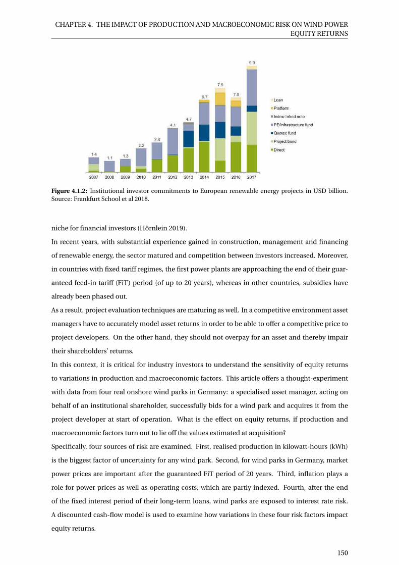
CHAPTER 4. THE IMPACT OF PRODUCTION AND MACROECONOMIC RISK ON WIND POWEREQUITY RETURNS
Figure 4.1.2: Institutional investor commitments to European renewable energy projects in USD billion.Source: Frankfurt School et al 2018.
niche for financial investors (Hörnlein 2019).
In recent years, with substantial experience gained in construction, management and financing
of renewable energy, the sector matured and competition between investors increased. Moreover,
in countries with fixed tariff regimes, the first power plants are approaching the end of their guar-
anteed feed-in tariff (FiT) period (of up to 20 years), whereas in other countries, subsidies have
already been phased out.
As a result, project evaluation techniques are maturing as well. In a competitive environment asset
managers have to accurately model asset returns in order to be able to offer a competitive price to
project developers. On the other hand, they should not overpay for an asset and thereby impair
their shareholders’ returns.
In this context, it is critical for industry investors to understand the sensitivity of equity returns
to variations in production and macroeconomic factors. This article offers a thought-experiment
with data from four real onshore wind parks in Germany: a specialised asset manager, acting on
behalf of an institutional shareholder, successfully bids for a wind park and acquires it from the
project developer at start of operation. What is the effect on equity returns, if production and
macroeconomic factors turn out to lie off the values estimated at acquisition?
Specifically, four sources of risk are examined. First, realised production in kilowatt-hours (kWh)
is the biggest factor of uncertainty for any wind park. Second, for wind parks in Germany, market
power prices are important after the guaranteed FiT period of 20 years. Third, inflation plays a
role for power prices as well as operating costs, which are partly indexed. Fourth, after the end
of the fixed interest period of their long-term loans, wind parks are exposed to interest rate risk.
A discounted cash-flow model is used to examine how variations in these four risk factors impact
equity returns.
150

CHAPTER 4. THE IMPACT OF PRODUCTION AND MACROECONOMIC RISK ON WIND POWEREQUITY RETURNS
The paper contributes to a better understanding of financial equity investors’ needs and chal-
lenges. This understanding is crucial if policy makers want to harvest financial investors’ available
capital in order to reach ambitious renewable energy targets.
The paper is structured as follows. Section 4.2 explains how the article contributes to the existing
academic literature. Section 4.3 lays out the research question and four related hypotheses. Sec-
tion 4.4 states the model and section 4.5 gives details on all the model’s inputs. Section 4.6 states
the results of the paper and section 4.7 discusses their implications in more detail. Section 4.8
concludes.
4.2 Contribution to the literature
The paper builds on and contributes to three strands of the energy finance and economics litera-
ture:
1. Literature on the relative importance and needs of different investor classes. In recent
years scholars have increasingly analysed the evolution of the energy sector in terms of dif-
ferent investor classes (e.g. Nelson and Pierpont 2013; Mazzucato and Semienuk 2018; Stef-
fen 2018) and their needs in terms of risks and returns (e.g. Bürer and Wüstenhagen 2009;
Gatzert and Kosub 2016; Salm and Wüstenhagen 2018). Researchers generally conclude that
financial investors have become more important in Europe’s renewable energy sector and
that they might be well suited for the long-term nature of energy investing but less willing to
take on construction or power price risk. The literature stays silent, though, on the specific
way financial investors evaluate private equity investments in renewable energies and on
the role that different cost and revenue items as well as macroeconomic expectations play.
This paper adds by presenting a discounted cash flow model typically used by institutional
investors to evaluate wind power plant acquisitions and by testing the sensitivity of equity
return to different assumptions.
2. Literature on the importance of the cost of capital for renewable energy investments. This
strand of literature looks at the role of financing costs for renewable energy investments. It is
generally agreed that compared to conventional energy investments, where fuel costs occur
over the lifetime of the projects, investment and therefore financing costs play a much larger
role for renewable energy (Bean et al 2017, Monnin 2015, Ondraczek et al 2015, Wiser and
Pickle 1998). In the past few years, both macroeconomic factors and experience contributed
to bringing financing costs down (Egli, Steffen and Schmidt 2018). The current literature
does not analyse the interplay of financial investors’ cost of capital and how future macroe-
conomic developments influence the projects’ economic viability, which will be this paper’s
151

CHAPTER 4. THE IMPACT OF PRODUCTION AND MACROECONOMIC RISK ON WIND POWEREQUITY RETURNS
contribution.2
3. Literature using investment models. The last strand of literature is concerned with build-
ing investment models to evaluate renewable energy projects, e.g. Afanasyeva et al (2016),
Diaz et al (2015), Kim et al (2017), Kitzing et al (2018), Levitt et al (2011), Santos et al (2017).
However, these models have two shortcomings. First, most models do not analyse the sensi-
tivity of the profitability to macroeconomic factors like inflation and interest rates. If they do,
like Kaldellis and Gavras (2000), typically they do not use real macroeconomic forecasts but
rather arbitrary values. Second, none of these models capture the reality of financial institu-
tional investors like pension funds and insurances. These investors, or the asset managers
acting on their behalf, have detailed knowledge of revenues and costs arising from contrac-
tual and other obligations, while academic research often captures these factors in a rather
general and inaccurate manner. This paper is using revenues and costs from four real turn-
key wind power projects. Another contribution of this paper is that it models the effects of
production and macroeconomic risk on equity returns from the point of view of the share-
holder instead of merely looking at overall project value or levelized cost of energy (LCOE),
as most aforementioned studies do.
4.3 Research question and hypotheses
The research question of this paper is: to what extent do production uncertainty, power prices,
inflation and interest rate dynamics affect a wind park shareholder’s payout? The goal is to quantify
the impact of these risks on equity returns of German wind assets acquired as turn-key projects
using a discounted cash flow model.
The following effects are expected.
1. Higher production in terms of kilowatt-hours (kWh) leads to higher revenues and therefore
ceteris paribus to a higher equity return. This is the case for the guaranteed feed-in tariff
remuneration as well as for revenues from the market. In the case of the feed-in tariff, policy
makers partly balance out low revenues due to unfavourable locations by a higher remuner-
ation per kWh. A higher overall production means a lower FiT, albeit not fully compensating
the quantity effect. Production is thus expected to have a positive impact on the equity re-
turn.
2. All four wind parks analysed receive a guaranteed remuneration in terms of EUR per kWh for
20 years. After that, higher wholesale power prices ceteris paribus lead to higher revenues, as
2One recent paper by Schmidt et al (2019) looks at the effect of interest rates on different renewable energy technolo-gies in a more general manner and will be referred to in the section on interest rate assumptions.
152

CHAPTER 4. THE IMPACT OF PRODUCTION AND MACROECONOMIC RISK ON WIND POWEREQUITY RETURNS
power purchase agreements (PPAs) are assumed to be indexed to power prices. As an addi-
tional effect, high power prices could lead to an early switch from the fixed FiT remuneration
to a PPA. Power prices are therefore expected to have a positive impact on equity returns.
3. Inflation3 affects equity returns through two levers: first, a portion of operating cost is in-
creasing with inflation due to indexed contracts. Second, revenues increase with inflation,
insofar as one assumes that operators negotiate PPAs that are inflation-indexed. Feed-in tar-
iffs, on the other hand, are not inflation-indexed.4 Which effect dominates depends on the
specific contractual arrangement of each wind park and on how long the wind park stays
in the FiT regime. Inflation is therefore expected to have an ambiguous impact on equity
returns.
4. Interest rates of the analysed wind parks are fixed for several years, after which they have to
be renegotiated. Higher interest rates after the fixed-interest period are expected to have a
negative impact on equity returns via higher interest payments.
4.4 Model
The goal of the analysis is to quantify the sensitivity of the payout return to different production
(Q), power price (P), inflation (I) and interest rate (D) scenarios. A deterministic discounted cash-
flow model is used, which is common practice in the renewable energy industry (Hürlimann 2018).
The model is appropriate, inter alia, because renewable energy assets have a finite lifetime and
because returns are determined by long-term trends for which stochastic estimates are generally
not available (see also section 4.5.1). The model is implemented in Matlab R2019a.
Buy-and-hold risk-averse investors, like pension funds and insurances, typically buy turnkey or
operational power plants to avoid construction risk. The model assumes such a long-term investor
and therefore sets the acquisition date equal to the month prior to beginning of operation.
Equation 4.4.1 gives all components of monthly cash-flow to equity, whereas the four factors for
which a sensitivity analysis will be performed are listed in brackets after each component that de-
pends on any of those factors. Each of the components of cash-flow to equity is described in more
3Deflation is not ruled out, however, forecast ranges result in positive inflation values year-on-year.4Indirectly, inflation also has an effect via its correlation with interest rates and power prices. Modelling this correla-
tion, however, goes beyond the scope of this paper.
153

CHAPTER 4. THE IMPACT OF PRODUCTION AND MACROECONOMIC RISK ON WIND POWEREQUITY RETURNS
0 50 100 150 200 250 300
Months
-2
-1.5
-1
-0.5
0
0.5
1
1.5
Ca
sh
-flo
ws in
EU
R/m
on
th
106
revenue
opex
tax payment
debt service
investment cost
payment to debt service reserve account
Figure 4.4.1: Revenue and cost components of cash-flow to equity in EUR/month for wind park 2. All valueshave been shrunk by factor 10 in the first month for illustration purposes.
detail in the next section.
CF to equitym = Revenue(Q, P)m −Opex(Q, P, I)m −Tax(Q, P, I, D)m − Investment cost(Q, P, I, D)m
−Net debt service(D)m −Reserve payments(Q, P, I, D)m
(4.4.1)
with operating months m = [0;300]. m = 0 is the acquisition date; m = 1 is the first and m = 300 the
last month of operation.
Revenue(Q, P) is the revenue from the feed-in tariff and the PPA depending on the production
of the wind farm Q in kWh and the power price P. Opex(Q, P, I) is operating cost depending on
production in kWh (Q), power price (P) and inflation (I). Tax(Q, P, I, D) is the trade tax paid. It is
calculated based on revenues less opex less depreciation less interest payment. Investment cost(Q,
P, I, D) consists mainly of the acquisition price and various other transaction costs. The acquisition
price is obtained endogenously by setting the required payout return to an exogenous hurdle rate.
Net debt service (D) adds up all cash flows related to debt: disbursements of loans, redemption
payments and interest cost, which depend on the redemption schedule, on the fixed rate and, after
the fixed rate period, on the negotiated subsequent rate. Reserve payments (Q, P, I, D) are payments
to the debt service reserve account. This account is required by the loan contracts and built up after
serving opex, tax, investment cost and debt.
154
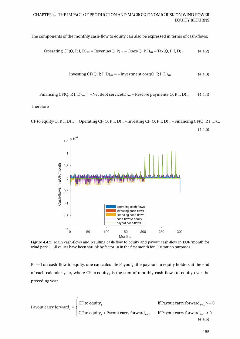
CHAPTER 4. THE IMPACT OF PRODUCTION AND MACROECONOMIC RISK ON WIND POWEREQUITY RETURNS
The components of the monthly cash-flow to equity can also be expressed in terms of cash-flows:
Operating CF(Q, P, I, D)m = Revenue(Q, P)m −Opex(Q, P, I)m −Tax(Q, P, I, D)m (4.4.2)
Investing CF(Q, P, I, D)m =−Investment cost(Q, P, I, D)m (4.4.3)
Financing CF(Q, P, I, D)m =−Net debt service(D)m −Reserve payments(Q, P, I, D)m (4.4.4)
Therefore
CF to equity(Q, P, I, D)m = Operating CF(Q, P, I, D)m+Investing CF(Q, P, I, D)m+Financing CF(Q, P, I, D)m
(4.4.5)
0 50 100 150 200 250 300
Months
-2
-1.5
-1
-0.5
0
0.5
1
1.5
Ca
sh
-flo
ws in
EU
R/m
on
th
106
operating cash-flows
investing cash-flows
financing cash-flows
cash-flow to equity
payout cash-flows
Figure 4.4.2: Main cash-flows and resulting cash-flow to equity and payout cash-flow in EUR/month forwind park 2. All values have been shrunk by factor 10 in the first month for illustration purposes.
Based on cash-flow to equity, one can calculate Payoutt , the payouts to equity holders at the end
of each calendar year, where CF to equityt is the sum of monthly cash-flows to equity over the
preceding year.
Payout carry forwardt =
CF to equityt if Payout carry forwardt+1 >= 0
CF to equityt +Payout carry forwardt+1 if Payout carry forwardt+1 < 0
(4.4.6)
155
CHAPTER 4. THE IMPACT OF PRODUCTION AND MACROECONOMIC RISK ON WIND POWEREQUITY RETURNS
Payoutt = max(0,Payout carry forwardt ) (4.4.7)
Equation 4.4.7 can be solved with backwards induction. The relationship between cash-flow to
equity and payout cash-flows is plotted in an illustrative way in figure 4.4.2.
The payouts are used in equation 4.4.8, which is solved for the acquisition price, a part of invest-
ment cost (see equation 4.4.1 on cash-flow to equity).
0 =T∑
t=1Payoutt · (1+ IRR)−t (4.4.8)
with operating years t = [1;T ];T = 25 where T is the lifetime of the plant fixed at 25 years and IRR
is a hurdle rate fixed exogenously as well.
Equation 4.4.8 is first solved with all risk factors (Q, P, I, D) fixed at their median scenario. Then, the
risk factors are varied each at a time, while the acquisition price calculated for the median scenario,
the other risk factors and all other inputs are kept constant. Using up to equation 4.4.7, this yields
a different payout time series for each scenario. Equation 4.4.8 is then solved again, but this time
for IRR, given these different payout series. This yields a range of results for IRR depending on the
scenario. The range of results is then used to evaluate the impact of the different risk factors on
shareholder payout returns.
The model implicitly assumes that the bidding process is perfectly competitive and the investors
offer the highest price possible still yielding their required equity payout return. This is done to
ensure comparability between the four wind parks.
4.5 Model inputs
4.5.1 Scenarios
The scenarios are not modelled endogenously but taken from existing historical data and forecasts
as long-term macroeconomic modelling lies beyond the scope of this paper.5
Since wind parks are long-lived, the model requires long-term forecasts of the four risk factors over
the next 25 years. This is a time frame for which probabilistic modelling estimates are not available.
Forecasts used therefore only contain expected values and no probabilistic estimates.
The following section describes the most pertinent forecasts for production, power prices and wind
market values, inflation and interest. For each parameter, a median scenario is selected. Based on
this, five scenarios are evaluated: first, the acquisition price is derived as described earlier for the
5For example, to endogenously derive future power prices one would require a fundamental model with detailedassumptions about governmental policies in terms of grid expansion, coal exit and renewables support as well as aboutprivate investment in and retirement of different types of power plants. To model future inflation and interest rates, onewould require a macroeconomic model depicting different economic sectors and monetary policy.
156

CHAPTER 4. THE IMPACT OF PRODUCTION AND MACROECONOMIC RISK ON WIND POWEREQUITY RETURNS
median scenario. For this scenario, the payout return is by definition equal to the set hurdle rate.
Then the sensitivity of the payout return is tested for the four remaining scenarios: maximum and
minimum as well as two intermediate scenarios.
4.5.1.1 Production
Figure 4.5.1: Illustration of P50, P75 and P90 values. Source: Solargis (2018).
Production uncertainty is a key source of risk for renewable energy assets. Unlike conventional
power plants based on fossil fuels or nuclear, wind and solar plants’ production is weather-
dependent. In order to forecast the energy production at each site, at least one detailed wind
assessment is part of every wind project development process. The assessments are also shared
with the equity investors during the due diligence process before an acquisition. The production
assumptions are directly taken from these wind assessments.
Wind assessments assume a normal distribution to describe production uncertainty and they re-
port the long-term median energy production in kWh, or P50 value, and further percentiles like P75
and P90. P50 is exceeded with 50% likelihood, whereas P75 is a lower, more conservative value and
exceeded with 75% likelihood, as illustrated in figure 4.5.1. For a risk-neutral investor one would
thus use the P50 value plus/minus some variation. However, in reality, often P75 and sometimes
even P90 is used. One reason is that as wind assessments are commissioned by project developers
who then go on to sell their assets, there is a motivation to overestimate future production (Inter-
view 2018, Interview 2019a). For this study, the minimum production scenario is therefore set at
P90 and the maximum at P50, which conservatively assumes a median between the two.
The annual production is assumed to be constant over the parks’ lifetime and to vary only between
the different scenarios.6 As the model works with monthly granularity, each month’s production
is calculated as a fixed percentage of the annual assumed production. This yields the well-known
bell-shaped annual revenue curve that can be observed in figure 4.4.1.
The P-values used here are net of expected shut-downs due to bats or other protected animals as
well as acoustic noise or shading. However, grid losses, technical unavailability and paragraph 51
6This is done for simplicity and comparability but of course in practice, production varies between years.
157

CHAPTER 4. THE IMPACT OF PRODUCTION AND MACROECONOMIC RISK ON WIND POWEREQUITY RETURNS
(EEG 2017)7 are not considered, which is why the production scenarios are reduced by another 3%.
This number is merely an educated guess but follows industry practice and has been confirmed
with practitioners as reasonable (Interview 2018, Interview 2019b).
4.5.1.2 Power prices and wind market values
For future power prices, the academic and practitioners’ literature of power wholesale price fore-
casts for Germany has been reviewed. Only forecasts published in 2016 or later were considered.
Eight scenarios were identified, which are plotted in figure 4.5.2a.
Using the wholesale power price as an estimate for wind market prices would overstate revenues.
This is due to the so-called cannibalisation effect, which is closely connected to the intermittent
nature of renewable energy production described in the previous section. Since wind power pro-
duction depends on the occurrence of wind, which is auto-correlated for different locations within
one region like Germany, there tend to be times of overall high and low power production depend-
ing on the availability of wind. In times of strong wind, wholesale power prices decrease and vice
versa. Since by definition wind parks produce more energy during high wind times, the average
price they obtain on the market is below the average power price. This is expressed as the "market
value" of wind, which is currently estimated at around 86% of average wholesale power prices in
Germany (Hirth 2019).
For future forecasts of market values, an average of Reeg (2019) and Böing and Regett (2019) is
used, which results in a market value of 83% of the wholesale price for 2019, declining to 66%
in 2042. All future power price scenarios from figure 4.5.2 are multiplied by these market values.
As a maximum and minimum scenario the median of all market value forecasts plus/minus two
standard deviations of the historical EEX Phelix baseload price between 2010 and 2018 is used.8
Thus a range of scenarios of wind market values is obtained. These are used in the calculation of
revenues as described in section 4.5.3.2.
7Paragraph 51 (EEG 2017) stipulates that if hourly spot prices are negative for at least six consecutive hours in theday-ahead auction, no remuneration is paid during this negative-price time period.
8The standard deviation is 7.76 EUR/MWh.
158

CHAPTER 4. THE IMPACT OF PRODUCTION AND MACROECONOMIC RISK ON WIND POWEREQUITY RETURNS
(a) Overview of all sources for power price forecasts and historical EEX Phelix Base for compari-son in EUR/MWh.
(b) Descriptive statistics of power price forecasts in EUR/MWh. (Historical EEX Phelix Base is notincluded in calculation of descriptive statistics.)
Figure 4.5.2: Power wholesale price forecasts for Germany in EUR/MWh.
159

CHAPTER 4. THE IMPACT OF PRODUCTION AND MACROECONOMIC RISK ON WIND POWEREQUITY RETURNS
4.5.1.3 Inflation
Inflation increases market revenues as well as operating costs. The operation and maintenance
(O&M) contract represents the largest amount explicitly indexed. The inflation indexes used in
the contracts are a combination of producer prices and labour costs, of which the most common
indexes used are plotted in figure 4.5.3.
Deflation is not ruled out. However, moderate forecasts are used in order to avoid results being
driven by wide ranging assumptions. The forecasts used here result in only positive inflation values
year-on-year.
(a) German producer price forecast and indexes in % year-on-year.
(b) German labour cost forecast and indexes in % year-on-year.
Figure 4.5.3: German inflation forecasts and indexes used in wind power service contracts in % year-on-year.
160

CHAPTER 4. THE IMPACT OF PRODUCTION AND MACROECONOMIC RISK ON WIND POWEREQUITY RETURNS
Figure 4.5.4: German inflation forecasts and indexes used for revenue and opex indexation in % year-on-year.
For producer prices, the Oxford Economics data9 lie in a reasonable range where historical values
track the actual indexes and forecast values are in line with past data (figure 4.5.3a). For labour cost,
the only long-term forecast found is a general indicator of labour cost in Germany, which does not
coincide with the historical data of the more sector specific industry labour cost. As a forecast, the
Destatis index is therefore extrapolated by taking the mean of 2010 to 2018 (figure 4.5.3b).
The two forecasts are combined in figure 4.5.4 in a way that mirrors the wind park service contracts.
Producer prices are weighted by 39% and labour cost by 61%, the average weighing in the four
contracts. The maximum/minimum scenarios of inflation are set at this median plus/minus two
times the average of the standard deviations of the historical weighted inflation rate from 2010 to
2018. This yields a long-term inflation range of 0.27 to 3.87% per year.
Power prices are a major driver of producer prices in the industrial sector (Destatis 2019). For
simplicity and since producer prices and labour costs in the industrial sector have very similar
forecasts, power prices are assumed to increase at the same rate as operating costs.
4.5.1.4 Interest
For interest rates, several historical time series from the European Central Bank were analysed (ECB
2019). The most pertinent ones, for corporate loans larger than EUR 1 million and with an initial
rate fixed for five to over 10 years, are plotted in figure 4.5.5.
The Oxford Economics long-term data are historically slightly above the ECB values, which is why
9According to information by the consultancy, their "macroeconomic forecasts are done in a fully integrated globaleconomic model, where individual country models are linked through assumptions about trade volume and prices,competitiveness, capital flows, interest and exchange rates and commodity prices. It is an eclectic model designedto capture the key relationships in the global economy so it is Keynesian in the short run and Monetarist in the longrun" (Oxford Economics 2019). To the author’s knowledge, whenever Oxford Economics data is used, no other publiclyavailable long-term forecast data exist.
161
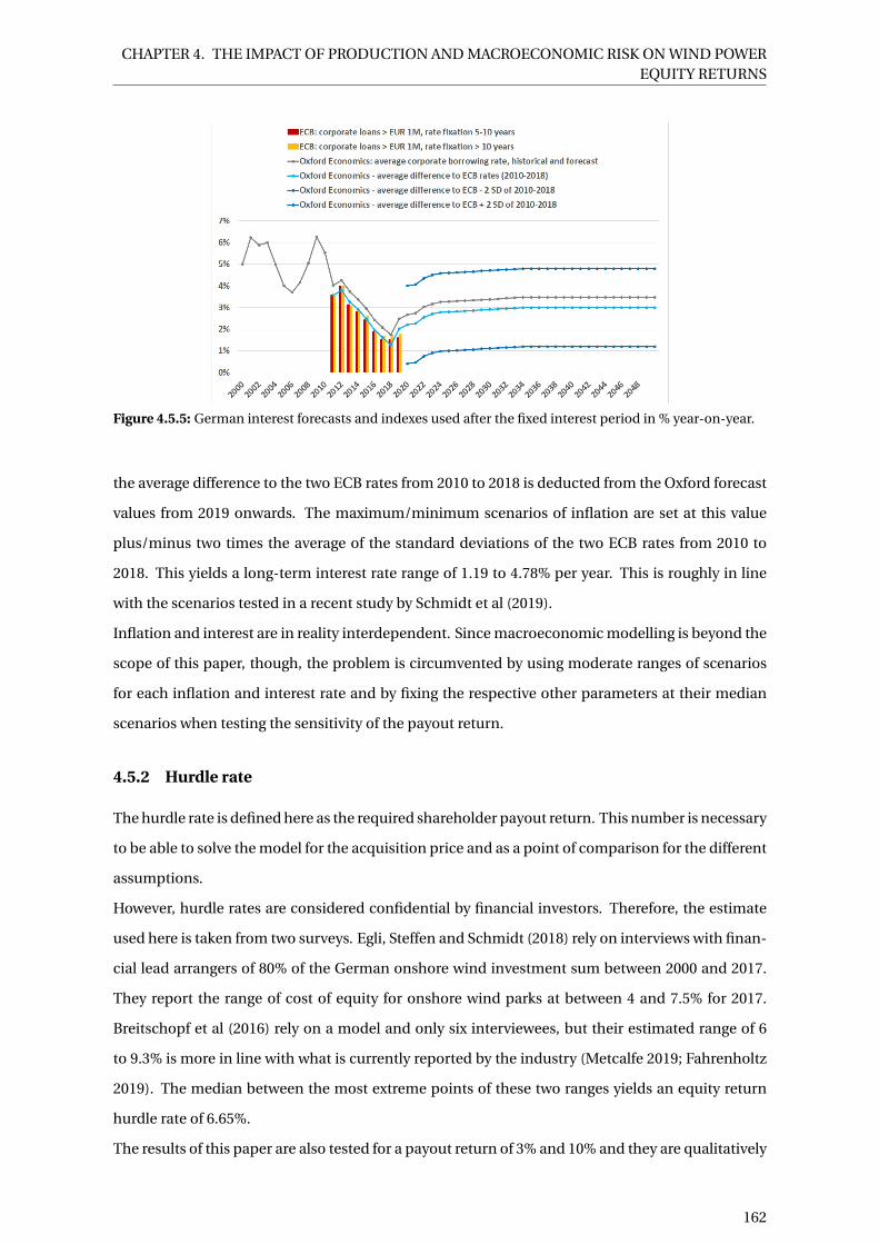
CHAPTER 4. THE IMPACT OF PRODUCTION AND MACROECONOMIC RISK ON WIND POWEREQUITY RETURNS
Figure 4.5.5: German interest forecasts and indexes used after the fixed interest period in % year-on-year.
the average difference to the two ECB rates from 2010 to 2018 is deducted from the Oxford forecast
values from 2019 onwards. The maximum/minimum scenarios of inflation are set at this value
plus/minus two times the average of the standard deviations of the two ECB rates from 2010 to
2018. This yields a long-term interest rate range of 1.19 to 4.78% per year. This is roughly in line
with the scenarios tested in a recent study by Schmidt et al (2019).
Inflation and interest are in reality interdependent. Since macroeconomic modelling is beyond the
scope of this paper, though, the problem is circumvented by using moderate ranges of scenarios
for each inflation and interest rate and by fixing the respective other parameters at their median
scenarios when testing the sensitivity of the payout return.
4.5.2 Hurdle rate
The hurdle rate is defined here as the required shareholder payout return. This number is necessary
to be able to solve the model for the acquisition price and as a point of comparison for the different
assumptions.
However, hurdle rates are considered confidential by financial investors. Therefore, the estimate
used here is taken from two surveys. Egli, Steffen and Schmidt (2018) rely on interviews with finan-
cial lead arrangers of 80% of the German onshore wind investment sum between 2000 and 2017.
They report the range of cost of equity for onshore wind parks at between 4 and 7.5% for 2017.
Breitschopf et al (2016) rely on a model and only six interviewees, but their estimated range of 6
to 9.3% is more in line with what is currently reported by the industry (Metcalfe 2019; Fahrenholtz
2019). The median between the most extreme points of these two ranges yields an equity return
hurdle rate of 6.65%.
The results of this paper are also tested for a payout return of 3% and 10% and they are qualitatively
162

CHAPTER 4. THE IMPACT OF PRODUCTION AND MACROECONOMIC RISK ON WIND POWEREQUITY RETURNS
the same.
4.5.3 Wind park specific data
For all cash-flow components, real data of four wind parks is used. The data is obtained from the
portfolio of an infrastructure fund focused on renewable energies. Individual wind park parame-
ters cannot be revealed due to confidentiality, but the following section gives general information
on all main parameters and the appendix (table 4.1) contains a list with means and standard devi-
ations of the main parameters.
4.5.3.1 Wind park characteristics
In order to avoid comparability issues due to different renewable energy policies or tax regimes,
the four wind power plants chosen are all located in Germany and built in 2017 and 2018. It is
assumed that all four wind parks start operation on December 31, 2018, which is also the date of
the acquisition by the financial investor. The lifetime is assumed to be 25 years, i.e. the wind parks
stop operating on December 30, 2043. The wind parks are comparatively small with a nameplate
capacity of between 4.7 and 9.9 MW each and 7.22 MW on average. Various turbine types and
manufacturers are represented (Enercon, General Electric, Vestas).
4.5.3.2 Revenue
The revenue is given by
Revenuem(Q, P) =
Qm ·max[FiTm(Q),Market valuem(P, I )] if m = [1;240]
Qm ·Market valuem(P, I ) if m = [241;300]
(4.5.1)
During the first 20 years, the operator always receives the maximum of the feed-in tariff (FiT) de-
pending on the quantity produced (Q) and the market value depending on power prices and infla-
tion (P, I). The FiT constitutes a lower bound on the operator’s revenue, as the operator receives the
revenue in two parts. The direct marketer pays the monthly average market value of wind energy
according to EEG Annex 1, 2.2.2. (EEG 2017). On top of that, if the guaranteed FiT is higher than
the market value, the grid operator pays a market premium of FiTm(Q)−Market valuem(P ).
As all four wind parks are assumed to start operation on December 31, 2018, they are all entitled
to the same feed-in tariff. The German renewable energy law stipulates that onshore wind parks
becoming operational between October and December 2018 receive 6.97 ct/kWh during the first
five years. If a wind park’s production (Q) in the first five years is below a certain defined reference
production for the specific location and turbine type, this period can be prolonged for several years
163

CHAPTER 4. THE IMPACT OF PRODUCTION AND MACROECONOMIC RISK ON WIND POWEREQUITY RETURNS
0 50 100 150 200 250 300 350
Months
0
0.5
1
1.5
2
2.5
Re
ve
nu
e in
EU
R/m
on
th
105
Revenue FiT
Revenue market
Figure 4.5.6: Possible revenues in EUR/month from FiT and from the market for wind park 2.
depending on the amount of the shortfall. After that, the remuneration is lowered to 3.87 ct/kWh
until the end of the 20th calendar year (EEG 2017, § 46.2, 46a).
From year 21 to 25, the wind park has to raise its revenues on the power market. It is widely
assumed that operators therefore negotiate long-term power purchase agreements (PPAs) with
traders, utilities or industrial firms. These contracts vary in their specifics and could contain fixed
as well as floating price structures. For simplicity and in order to illustrate the impact of power
prices, it is assumed that the PPA price is always equal to the conservatively estimated monthly
market value of wind power (see section 4.5.1.2).
For median power price assumptions, the high FiT of 8.38 ct/kWh is initially competitive for all
four wind parks. Wind parks 2, 3 and 4 produce relatively less than their reference production and
therefore benefit from a prolonged high FiT, as illustrated in figure 4.5.6. After year 17, though, the
assumed median PPA price overtakes even the high FiT of 8.38 ct/kWh and operators thus switch
to the PPA. For wind park 1, this is already earlier the case, namely when the FiT is lowered to 3.87
ct/kWh after year 13 (see also figure 4.6.1b).
Overall the revenues from the FiT account for 61% of the total revenue per MW on average and
PPAs for the remaining 39%.
4.5.3.3 Operating cost
Operating cost consists of the following main elements. An O&M contract ensures maintenance of
the wind park and is usually signed for 15 to 20 years. The overall cost per MW amounts to 28% of
164

CHAPTER 4. THE IMPACT OF PRODUCTION AND MACROECONOMIC RISK ON WIND POWEREQUITY RETURNS
total opex on average. The contract is explicitly linked to both production and inflation, and the
inflation indices used are incorporated in the inflation assumptions above.
After the end of the O&M contract, assumptions are made for the cost of maintenance to the end
of the park’s lifetime. Inflation indexation is assumed. The overall cost per MW of O&M cost after
the service contract is 14% of total opex on average.
Lease of land is another substantial part of opex, accounting for 22% on average. Lease contracts
are usually indexed on revenues and follow a fixed increasing schedule, which is why inflation
indexation is not assumed.
The wind parks analysed use an outsourcing model for technical supervision and accounting,
which is common for financial investors. Technical and commercial management on average ac-
count for 5 and 3% of total opex per MW respectively, and both parameters are indexed to inflation.
The cost of decommissioning the wind park after 25 years is estimated in the permission docu-
ments. It amounts to 5% of opex per MW on average. Inflation indexation is assumed.
The remaining 23% of total opex per MW are distributed between costs for technical assessments,
the commission on the bank guarantee for decommissioning, administrative costs of asset man-
agement, tax audit, insurance, power consumption and direct marketing.
4.5.3.4 Tax
All four wind parks are limited partnerships (KG) and therefore only liable to pay trade tax - and
not corporate tax - under German law. The quarterly tax is
Taxq (Q, P, I, D) = Collection rate ·Tax base ·Tax referenceq (4.5.2)
with q = [1;75].
The collection rate is a number between 2.9 and 4.55 depending on the location of the wind park
and the tax base is equal to 0.035. The tax reference is based on a figure derived from the quarterly
EBT, with
Tax reference = EBTq +Tax additionsq (4.5.3)
EBTq (Q, P, I, D) = Revenueq (Q, P, I)−Opexq (Q, P, I)−Depreciationq (Q, P, I, D)− Interestq (D)
(4.5.4)
Tax additions include half of the lease, the full interest payment and the loss carry over of negative
EBT from the previous period (Gewerbesteuergesetz 2009). Usually tax starts to become due after
all the investment cost is depreciated and the debt is paid off, as figure 4.5.7 illustrates.
165

CHAPTER 4. THE IMPACT OF PRODUCTION AND MACROECONOMIC RISK ON WIND POWEREQUITY RETURNS
0 50 100 150 200 250 300 350
Months
-3
-2.5
-2
-1.5
-1
-0.5
0
0.5
1
1.5
2
Incom
e s
tate
ment item
s in E
UR
/month
105
EBITDA
depreciation
interest payment
EBT
tax payment
Figure 4.5.7: EBITDA (calculated as revenue-opex), EBT and the resulting tax payment at wind park 2 inEUR/month.
4.5.3.5 Investment cost
The investment cost consists mainly of the acquisition price (97% of investment cost on average),
which is obtained endogenously for a fixed hurdle rate and median assumptions for production,
power price, inflation and interest. The remaining part of investment cost consists of various trans-
action costs.
4.5.3.6 Net debt service
The wind parks come with two to four long-term loans with an average amount of 3.09 mio EUR
each. The maturities of the loans are between 5 and 19 years with 14.5 years on average. Annual
interest is at 1.86% and the period of fixed interest is 11.5 years on average for each loan. The debt
schedule of each wind park is calculated according to the interest and redemption specifications
laid out in the loan contracts. Figure 4.5.8 shows the different cash-flows related to debt.
4.5.3.7 Reserve payments
The debt service reserve is a minimum liquidity stipulated by the loan contracts. It is expressed as
either an absolute amount or 50% of interest and redemption of the preceding year. It is built up
over time from the initial liquidity of the wind park and cash-flows as they arise after serving opex,
tax, investment cost and debt.
166

CHAPTER 4. THE IMPACT OF PRODUCTION AND MACROECONOMIC RISK ON WIND POWEREQUITY RETURNS
0 50 100 150 200 250 300
Months
-4
-2
0
2
4
6
8
10
12
14
Re
ve
nu
e in
EU
R/m
on
th
105
loan disbursement
redemption payment
interest payment
payment to debt service reserve account
Figure 4.5.8: Cash-flows related to debt at wind park 2 in EUR/month. The loan disbursement in the firstmonth has been shrunk by factor 10 for illustration purpose.
4.6 Results
In the following, the wind parks’ payout returns are calculated for a range of scenarios with the ac-
quisition price fixed as described in the model section. In order to understand the levers through
which the payout returns are impacted, the cash-flow components in a specific scenario are dis-
counted by the median hurdle rate and compared to those in the median scenario for each pro-
duction, power prices, inflation and interest. For any cash-flow component, such as revenues or
opex, a ratio is calculated as follows. The ratio for the median scenario is one by definition.
Cash-flow ratioScenarioi=
∑Tt=0 Cash-flow componentt ,Scenarioi
· (1+ IRR)−t
∑Tt=0 Cash-flow componentt ,Scenariomedian
· (1+ IRR)−t(4.6.1)
with operating years t = [1;T ];T = 25.
167
CHAPTER 4. THE IMPACT OF PRODUCTION AND MACROECONOMIC RISK ON WIND POWEREQUITY RETURNS
4.6.1 Production
Uncertainty in energy production has the highest impact on the shareholders’ payouts: the return
varies from 2.8 to 10.1% per year (figure 4.6.1a).
The mechanism is simple. Higher production means higher revenues, as apparent in the compari-
son values for different scenarios, due to a higher amount of kWh produced (figure 4.6.1c). In some
cases, there is also an additional indirect effect. Wind park 1 and 4 have an incentive to exit the FiT
earlier and access the power market for higher production, because the FiT itself is inversely cor-
related with the quantity produced, as explained in the section on revenues. Under the current
German renewable energy law, policy makers partly balance out low revenues due to unfavourable
locations by an increased FiT per kWh (EEG 2017). Higher production means a lower FiT, which
can make an earlier market entry attractive (figure 4.6.1b).
Operating costs (which are partly indexed to production and revenues), taxes and the payments
into the debt service reserve also increase with increasing production, but they do not offset the
increase in revenues (figures 4.6.1d to 4.6.1f). Investment cost and net debt service by definition do
not react to an increase in production.
168

CHAPTER 4. THE IMPACT OF PRODUCTION AND MACROECONOMIC RISK ON WIND POWEREQUITY RETURNS
1 2 3 4 5
Production scenarios
2
3
4
5
6
7
8
9
10
11
Payout re
turn
in %
Wind park1
Wind park2
Wind park3
Wind park4
(a)
1 2 3 4 5
Production scenarios
10
11
12
13
14
15
16
17
18
Num
ber
of years
in feed-in tariff
Wind park1
Wind park2
Wind park3
Wind park4
(b)
1 2 3 4 5
Production scenarios
0.9
0.92
0.94
0.96
0.98
1
1.02
1.04
1.06
1.08
1.1
Revenue r
atio
Wind park1
Wind park2
Wind park3
Wind park4
(c)
1 2 3 4 5
Production scenarios
0.98
0.985
0.99
0.995
1
1.005
1.01
1.015
1.02
1.025
Op
ex r
atio
Wind park1
Wind park2
Wind park3
Wind park4
(d)
1 2 3 4 5
Production scenarios
0.2
0.4
0.6
0.8
1
1.2
1.4
1.6
1.8
Tax p
aym
ent ra
tio
Wind park1
Wind park2
Wind park3
Wind park4
(e)
1 2 3 4 5
Production scenarios
0.992
0.994
0.996
0.998
1
1.002
1.004
1.006
Pa
ym
en
t to
re
se
rve
acco
un
t ra
tio
Wind park1
Wind park2
Wind park3
Wind park4
(f )
Figure 4.6.1: Payout return in %, number of years in the feed-in tariff and main cash-flow ratios for differentproduction scenarios.
169

CHAPTER 4. THE IMPACT OF PRODUCTION AND MACROECONOMIC RISK ON WIND POWEREQUITY RETURNS
4.6.2 Power prices and wind market values
Higher power prices and wind market values have a high and positive impact on shareholder pay-
outs: return varies between 3.6 and 9.3% per year (figure 4.6.2a).
Again, the increasing effect on payout returns works through revenues (figure 4.6.2c). The indirect
effect is at play for power prices, too. Ceteris paribus, all wind parks exit the FiT earlier when the
highest level of power prices is assumed. In the case of wind park 2 and 3, the effect is the most
pronounced. In the lowest power price scenario, the operator uses the FiT for the full possible 20
years, whereas in the highest power price scenario only for nine years (figure 4.6.2b).
Operating costs (which are partly indexed to revenues) and taxes also increase with increasing
power prices, but they do not offset the increase in revenues (figure 4.6.2d and 4.6.2e). Payments
into the debt service reserve are not affected, most likely due to the late and moderate effect of
power price (figure 4.6.2f). Investment cost and net debt service by definition do not react to an
increase in production.
The high impact of power price uncertainty on payout returns in spite of secure revenues from the
FiT for between nine and 20 years is notable. It means that once the FiT is phased out and plants
have to secure their revenues on the private market, as already the case for example in Spain and
the Nordic countries, hedging power price risk will be a major concern of wind power operators.
170
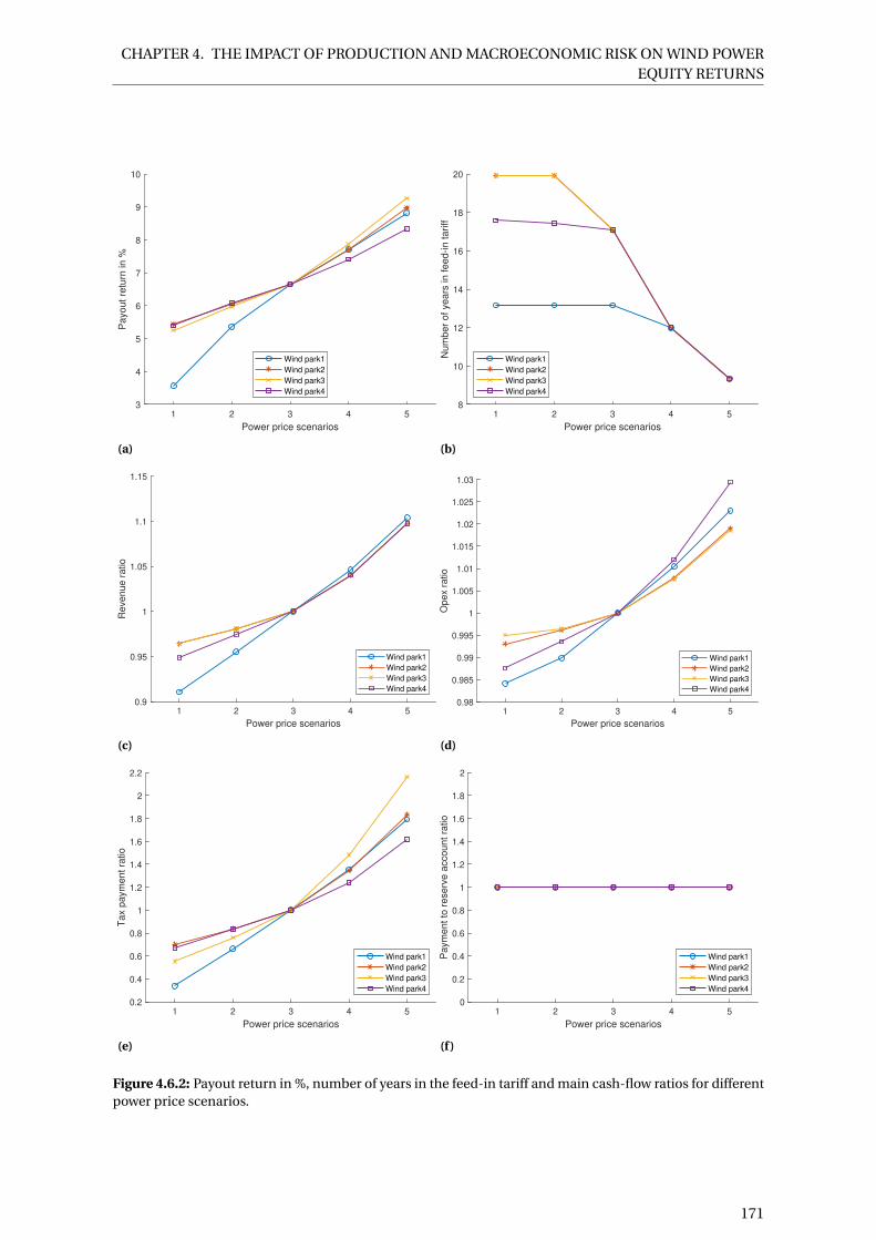
CHAPTER 4. THE IMPACT OF PRODUCTION AND MACROECONOMIC RISK ON WIND POWEREQUITY RETURNS
1 2 3 4 5
Power price scenarios
3
4
5
6
7
8
9
10
Payout re
turn
in %
Wind park1
Wind park2
Wind park3
Wind park4
(a)
1 2 3 4 5
Power price scenarios
8
10
12
14
16
18
20
Num
ber
of years
in feed-in tariff
Wind park1
Wind park2
Wind park3
Wind park4
(b)
1 2 3 4 5
Power price scenarios
0.9
0.95
1
1.05
1.1
1.15
Revenue r
atio
Wind park1
Wind park2
Wind park3
Wind park4
(c)
1 2 3 4 5
Power price scenarios
0.98
0.985
0.99
0.995
1
1.005
1.01
1.015
1.02
1.025
1.03
Op
ex r
atio
Wind park1
Wind park2
Wind park3
Wind park4
(d)
1 2 3 4 5
Power price scenarios
0.2
0.4
0.6
0.8
1
1.2
1.4
1.6
1.8
2
2.2
Tax p
aym
ent ra
tio
Wind park1
Wind park2
Wind park3
Wind park4
(e)
1 2 3 4 5
Power price scenarios
0
0.2
0.4
0.6
0.8
1
1.2
1.4
1.6
1.8
2
Paym
ent to
reserv
e a
ccount ra
tio
Wind park1
Wind park2
Wind park3
Wind park4
(f )
Figure 4.6.2: Payout return in %, number of years in the feed-in tariff and main cash-flow ratios for differentpower price scenarios.
171

CHAPTER 4. THE IMPACT OF PRODUCTION AND MACROECONOMIC RISK ON WIND POWEREQUITY RETURNS
4.6.3 Inflation
Inflation has a medium and generally positive impact on equity payout returns: it varies from 5.0
to 8.4% per year. A "bath tub curve" can be observed for wind park 2 and 3. The payout return
has its minimum at the median inflation scenario and slopes steeply upwards for higher inflation
(figure 4.6.3a). For higher hurdle rates, this effect becomes even more pronounced.
Inflation has a strictly positive impact on revenues. Similarly to power prices, the inflation effect
works on the one hand via an increase of post-FiT market values. Indirectly, this also causes an
earlier exit from FiT and access to power markets. This is because, as described in the hypothe-
ses section, market revenues are indexed to inflation, whereas the FiT is not (EEG 2017). Ceteris
paribus, higher inflation makes market prices more attractive relative to the fixed FiT. The effect is
especially pronounced for wind park 2 and 3: for the lowest two levels of inflation, the parks stay
in the FiT regime for the maximum period of 20 years, as opposed to only less than 12 years for the
highest level of inflation (figure 4.6.3b).
When wind parks are in the FiT regime for a long time, overall revenues are less impacted by in-
flation and the slope of revenue to inflation is therefore comparatively flatter for low inflation at
wind park 2 and 3 (figure 4.6.3c). Opex, on the other hand, is steeply increasing in inflation at wind
park 2 and 3 (figure 4.6.3d). In combination, the flat revenue curve and steep opex at wind parks
2 and 3 lead to a slightly negative relationship of payout return with lower than expected inflation
and a positive relationship for higher than expected inflation, as also reflected in the slope of tax
payment (figure 4.6.3e).
172
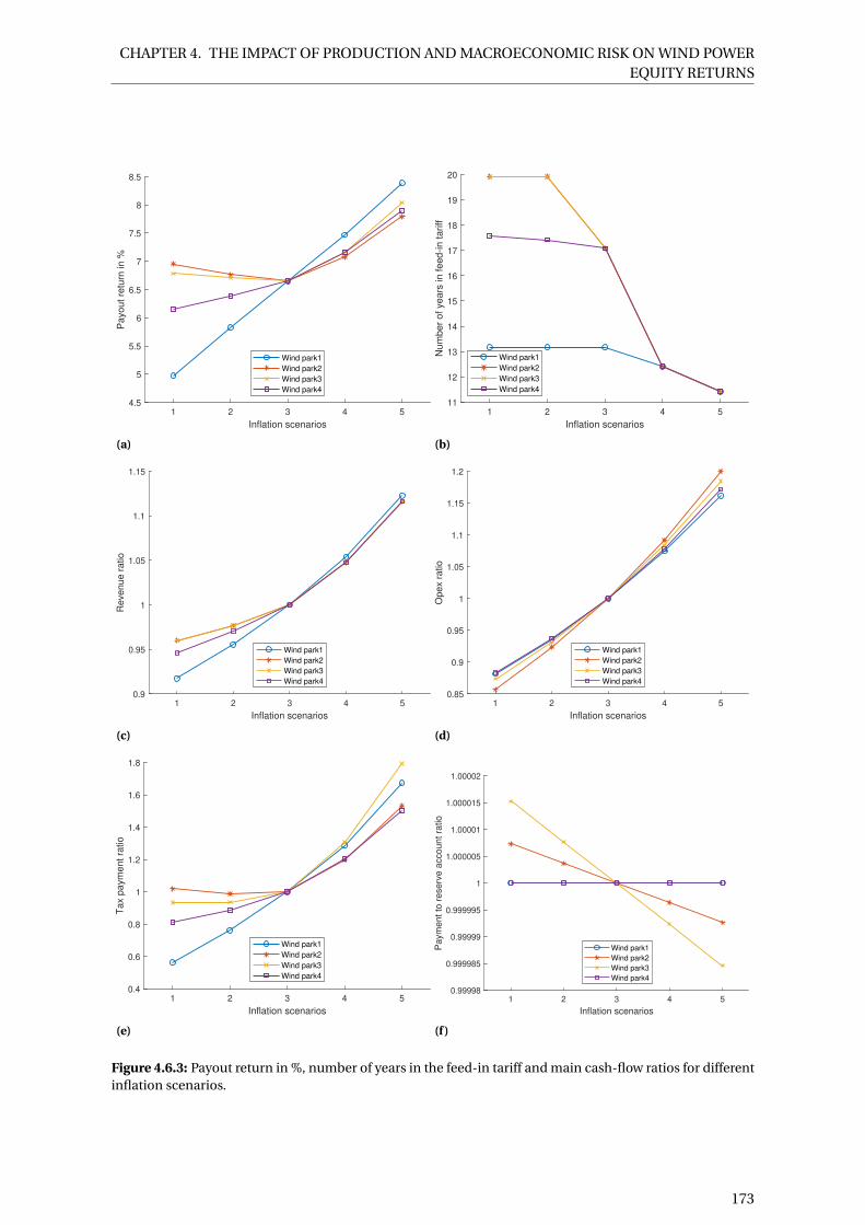
CHAPTER 4. THE IMPACT OF PRODUCTION AND MACROECONOMIC RISK ON WIND POWEREQUITY RETURNS
1 2 3 4 5
Inflation scenarios
4.5
5
5.5
6
6.5
7
7.5
8
8.5
Pa
yo
ut
retu
rn in
%
Wind park1
Wind park2
Wind park3
Wind park4
(a)
1 2 3 4 5
Inflation scenarios
11
12
13
14
15
16
17
18
19
20
Num
ber
of years
in feed-in tariff
Wind park1
Wind park2
Wind park3
Wind park4
(b)
1 2 3 4 5
Inflation scenarios
0.9
0.95
1
1.05
1.1
1.15
Revenue r
atio
Wind park1
Wind park2
Wind park3
Wind park4
(c)
1 2 3 4 5
Inflation scenarios
0.85
0.9
0.95
1
1.05
1.1
1.15
1.2
Opex r
atio
Wind park1
Wind park2
Wind park3
Wind park4
(d)
1 2 3 4 5
Inflation scenarios
0.4
0.6
0.8
1
1.2
1.4
1.6
1.8
Tax p
aym
ent ra
tio
Wind park1
Wind park2
Wind park3
Wind park4
(e)
1 2 3 4 5
Inflation scenarios
0.99998
0.999985
0.99999
0.999995
1
1.000005
1.00001
1.000015
1.00002
Paym
ent to
reserv
e a
ccount ra
tio
Wind park1
Wind park2
Wind park3
Wind park4
(f )
Figure 4.6.3: Payout return in %, number of years in the feed-in tariff and main cash-flow ratios for differentinflation scenarios.
173

CHAPTER 4. THE IMPACT OF PRODUCTION AND MACROECONOMIC RISK ON WIND POWEREQUITY RETURNS
4.6.4 Interest
Interest rate scenarios have a negative but small impact on shareholder payouts: the return only
varies between 7.0% per year for the lowest interest rate scenario and 6.2% for the highest one
(figure 4.6.4a).
Interest rate changes impact payout returns via only one channel. Higher interest rates mean
higher interest payments, with a negative effect on payouts. In the case of wind park 1, due to
the signing of an interest rate swap contract over the full duration of the loans, there is no inter-
est rate risk (figure 4.6.4a). Higher interest rates also mean lower tax payments, a positive effect
not fully compensating for the effect on interest payments (figure 4.6.4c). The debt service reserve
payment is not sensitive to interest rate scenarios due to the small overall effect (figure 4.6.4d).
1 2 3 4 5
Interest scenarios
6.2
6.3
6.4
6.5
6.6
6.7
6.8
6.9
7
Pa
yo
ut
retu
rn in
%
Wind park1
Wind park2
Wind park3
Wind park4
(a)
1 2 3 4 5
Interest scenarios
0.85
0.9
0.95
1
1.05
1.1
1.15In
tere
st paym
ent ra
tio
Wind park1
Wind park2
Wind park3
Wind park4
(b)
1 2 3 4 5
Interest scenarios
0.92
0.94
0.96
0.98
1
1.02
1.04
1.06
1.08
Tax p
aym
ent ra
tio
Wind park1
Wind park2
Wind park3
Wind park4
(c)
1 2 3 4 5
Interest scenarios
0
0.2
0.4
0.6
0.8
1
1.2
1.4
1.6
1.8
2
Paym
ent to
reserv
e a
ccount ra
tio
Wind park1
Wind park2
Wind park3
Wind park4
(d)
Figure 4.6.4: Payout return in % and main cash-flow ratios for different interest scenarios.
The results suggest that interest rate risk is no major concern for wind parks built under the current
German FiT regime. This could change, however, once the FiT is further lowered, shortened or
phased out and plants have to secure more of their revenues via PPAs. With PPAs of five to 10 years
174

CHAPTER 4. THE IMPACT OF PRODUCTION AND MACROECONOMIC RISK ON WIND POWEREQUITY RETURNS
instead of 20 years guaranteed FiT, loan tenures might shorten and interest rate risk might become
a higher priority for wind park operators (Interview 2018, Interview 2019).
4.7 Discussion
Uncertainty in energy production has the highest impact on the shareholders’ payouts: the re-
turn varies from 2.8 to 10.1% per year. On the one hand, production affects revenues directly via
a change of quantities remunerated. On the other hand, there is also an indirect effect. Higher
production pushes some wind parks to exit the FiT and access the power market, because the FiT
per kWh is inversely correlated with the total kWh produced.
The high sensitivity of wind park profits to production uncertainty is well known, even though its
impact on equity returns has not been analysed in the literature so far. Investors and asset man-
agers can respond to this in three ways. First, they could add a risk premium by using more con-
servative production estimates like the P90 value or deducting a percentage from P50 or P75. This,
however, might endanger their ability to win acquisition when bidding for a wind park, a balance
which might be difficult to strike. Second, financial asset managers could try to become more at-
tuned to the technical details of wind power projects. This could entail analysing the quality of
different wind assessments in depth prior to an acquisition, commissioning own independent as-
sessments or requesting from policy makers to enhance quality controls and independence of as-
sessments, thereby compressing the normal distribution of production to a narrower range. A third
possibility, already practised by many investors, is to combine different locations in one portfolio
or add further technologies like solar PV in order to reduce overall production risk.
Power prices and the resulting market values have a high and positive impact on shareholder pay-
outs: return varies between 3.6 and 9.3% per year. Again, the increasing effect on returns works
through revenues and indirectly through the FiT, as wind parks exit the FiT earlier for higher levels
of power prices.
The high impact of power price uncertainty on payout returns in spite of secure revenues from the
FiT for between nine and 20 years is notable. Once the German FiT is phased out and plants have to
secure their revenues fully on the private market, hedging power price risk will be a major concern
for wind power operators. Financial investors will likely pursue fixed price PPA contracts instead
of the floating PPA prices indexed to power prices, which were assumed here.
Inflation has a medium and generally positive impact on equity payout returns: it varies from 5.0
to 8.4% per year. A "bath tub curve", with the lowest return not at the lowest inflation rate but
somewhere in the middle, can be observed for wind parks that opt to stay in the FiT for a long
time. In this case there is hardly any downside risk to inflation, as both lower and higher than
175

CHAPTER 4. THE IMPACT OF PRODUCTION AND MACROECONOMIC RISK ON WIND POWEREQUITY RETURNS
expected inflation scenarios yield higher than expected returns. For wind parks operating on the
free market, on the other hand, low inflation yields a comparably low return as revenue losses due
to lower-than-expected inflation are higher than opex savings. A solution to hedge against inflation
risk might be to mirror the indexation of operating costs by fixing an equivalent indexation for
revenues in the PPA contract.
Interest rate scenarios have a negative but small impact on shareholder payouts: the return only
varies between 7.0% per year for the lowest interest rate scenario and 6.2% for the highest one.
Higher interest rates affect payout returns via higher interest payments, with a negative effect on
payouts.
The results suggest that interest rate risk is not a major concern for wind parks built under the
current German FiT regime. This could change, however, once the FiT is further lowered, shortened
or phased out and plants have to secure more of their revenues via PPAs. With PPAs of five to
15 years instead of a 20 years guaranteed FiT, fixed interest rate periods and loan tenures might
shorten and interest rate risk might become a higher priority for wind park operators.
4.8 Conclusion and policy implications
This paper has quantified the effect of production, power price, inflation and interest rate risk on
wind park equity returns. It contributes to the energy economics and finance literature by pre-
senting a financial investor perspective on production and macroeconomic risk in wind energy. To
policy makers the results offer a deeper understanding of equity investors’ needs in order to har-
vest their available capital for reaching renewable energy targets. This understanding is crucial if
policy makers want to reach climate targets while at the same time phasing out renewable energy
policy support.
The results underline the importance of energy production and power prices: shareholder payout
returns range from 2.8 to 10.1% and from 3.6 to 9.3% respectively for a reasonable variation in
production and power prices. Inflation has a medium and ambiguous impact depending on the
time frame that wind parks operate under the guaranteed feed-in tariff regime. A possible increase
in interest rates plays only a limited negative role for existing German wind park equity returns.
It is likely that power price, inflation and interest rate risks will increase if governmental support
policies are further reduced. Further research is needed in order to determine how exactly equity
payouts will react. It is concerning, though, that even for wind parks under the feed-in tariff for
nine years or more, equity returns react strongly to moderate variations in power prices.
In this context it is crucial that the nascent PPA market develops the hedging strategies in order to
avoid excessively risky equity returns and a possible retreat of financial investors from renewable
176

CHAPTER 4. THE IMPACT OF PRODUCTION AND MACROECONOMIC RISK ON WIND POWEREQUITY RETURNS
energy markets. Policy makers can play a role in facilitating appropriate risk allocation, by, for
example devising long-term reliable policies and supporting the standardisation of PPA contracts.
What cannot be concluded from this paper is whether expected returns are sufficient for institu-
tional investors or project developers to continue investing in German wind onshore. Per construc-
tion, the model assumes that equity investors can buy the wind park at their required expected re-
turn from project developers. It is left for future research to determine whether both project devel-
opers and financial investors will be able to earn their cost of capital in renewable energy markets
with less or no policy support.
177
CHAPTER 4. THE IMPACT OF PRODUCTION AND MACROECONOMIC RISK ON WIND POWEREQUITY RETURNS
4.9 Bibliography
Afanasyeva S., Saari J., Kalkofen M., Partanen J. and Pyrhönen O. (2016): Technical, economic and
uncertainty modelling of a wind farm project. Energy Conversion and Management (107), pp.
22–33.
Allianz (2017): Renewable Energy – A real-asset alternative for institutions seeking growth, yield
and low correlation, Allianz Global Investors.
Bean P., Balzquez J. and Nezamuddin N. (2017): Assessing the cost of renewable energy policy
options – A Spanish wind case study. Renewable Energy (103), pp. 180-186.
Breitschopf B., Noothout P., de Jager D., Tesniere L., van Rooijen S., Karypidis K., Bruckmann R.,
Jirou F., Angelopoulos D., Doukas H., Konstantinavi I. and Resch G.(2016): The impact of risks in
renewable energy investments and the role of smart policies. Final report.
BNEF (2017): Europe Asset Finance and Institutional Flows, Bloomberg New Energy Finance,
2017-07-24.
Böing F. and Regett A. (2019): Hourly CO2 Emission Factors and Marginal Costs of Energy Carriers
in Future Multi-Energy Systems. Energies (2260).
Bürer M. J. and Wüstenhagen R. (2009): Which renewable energy policy is a venture capitalist’s
best friend? Empirical evidence from a survey of international cleantech investors. Energy Policy
(37), pp. 4997–5006.
Christidis A., Mollenhauer E., Tsatsaronis G., Schuchardt G.K., Holler S., Böttger D. and Bruckner
T. (2017): EnEff-Wärme: Einsatz von Wärmespeichern und Power-to-Heat-Anlagen in der Fern-
wärmeerzeugung. Technische Universität Berlin, Institut für Energietechnik.
Danish Energy Agency (2018): Basisfremskrivninger. Last accessed online on 21 November, 2019:
❤tt♣s✿✴✴❡♥s✳❞❦✴s✐t❡s✴❡♥s✳❞❦✴❢✐❧❡s✴❆♥❛❧②s❡r✴❢✐❣✉r❡r❴♦❣❴t❛❜❡❧❧❡r✳①❧s①. Danish
Energy Agency.
Destatis (2019): Various data. Last accessed online on 21 November, 2019: ❤tt♣✿✴✴❞❡st❛t✐s✳❝♦♠.
178

CHAPTER 4. THE IMPACT OF PRODUCTION AND MACROECONOMIC RISK ON WIND POWEREQUITY RETURNS
Diaz G., Moreno B., Coto J. and Gomez-Aleixandre J. (2015): Valuation of wind power distributed
generation by using Longstaff–Schwartz option pricing method. Applied Energy (145), pp.
223–233.
ECB (2019): Various data. Last accessed online on 21 November, 2019: ❤tt♣✿✴✴s❞✇✳❡❝❜✳❡✉r♦♣❛
✳❡✉. European Central Bank.
EEG (2017): Erneuerbares Energien Gesetz. Last accessed online on 21 November, 2019:
❤tt♣s✿✴✴✇✇✇✳❣❡s❡t③❡✲✐♠✲✐♥t❡r♥❡t✳❞❡✴❡❡❣❴✷✵✶✹✴❇❏◆❘✶✵✻✻✶✵✵✶✹✳❤t♠❧. Bundestag.
EEX (2019): Historical Phelix Base for Germany. European Energy Exchange.
Egli F., Steffen S. and Schmidt T. (2018): A dynamic analysis of financing conditions for renewable
energy technologies. Nature Energy (3), pp. 1084-1092.
Energy Brainpool (2018): Update: Trends der Strompreisentwicklung – EU Energy Outlook 2050.
Last accessed online on 21 November, 2019: ❤tt♣s✿✴✴❜❧♦❣✳❡♥❡r❣②❜r❛✐♥♣♦♦❧✳❝♦♠✴✉♣❞❛t❡✲tr
❡♥❞s✲❞❡r✲str♦♠♣r❡✐s❡♥t✇✐❝❦❧✉♥❣✲❡✉✲❡♥❡r❣②✲♦✉t❧♦♦❦✲✷✵✺✵✴, Energy Brainpool.
Ernst and Young (2014): Renewable energy assets – An interesting investment proposition for
European insurers, Ernst and Young.
Eurostat (2019): Various data. Last accessed online on 21 November, 2019: ❤tt♣s✿
✴✴❡❝✳❡✉r♦♣❛✳❡✉✴❡✉r♦st❛t✴❞❛t❛✴❞❛t❛❜❛s❡. Eurostat.
Fahrenholtz F. (2019): First Private and re:cap global investors ag initiate further Renewable Energy
Fund. Press release.
Frankfurt School, UNEP Centre, BNEF (2018): Global Trends in Renewable Energy Investment
2018.
Gatzert N. and Kosub T. (2016): Risks and risk management of renewable energy projects: The case
of onshore and offshore wind parks. Renewable and Sustainable Energy Reviews (60), pp. 982–998.
Gewerbesteuergesetz (2009): Gewerbesteuergesetz, Abschnitt II, §§ 7 - 11. Last accessed online on
179

CHAPTER 4. THE IMPACT OF PRODUCTION AND MACROECONOMIC RISK ON WIND POWEREQUITY RETURNS
21 November, 2019: ❤tt♣s✿✴✴❞❡❥✉r❡✳♦r❣✴❣❡s❡t③❡✴●❡✇❙t●✴✽✳❤t♠❧, Bundestag.
Hirth L. (2013): The market value of variable renewables – The effect of solar wind power variability
on their relative price. Energy Economics (38), pp. 218-236.
Hirth L. (2019): updated graph based on Hirth (2013), personal communication with the author.
Hostert D. (2016): Portfolio Hunters 2015-16: European Wind. Bloomberg New Energy Finance.
Hörnlein L. (2019): Utility Divestitures in Germany: A Case Study of Corporate Finan-
cial Strategies and Energy Transition Risk. Last accessed online on 21 November, 2019:
❤tt♣✿✴✴❞①✳❞♦✐✳♦r❣✴✶✵✳✷✶✸✾✴ssr♥✳✸✸✼✾✺✹✺, SSRN working paper.
Hürlimann C. (2018): Valuation Methods in Renewable Energy Investments: An Explanatory
Mixed-Methods Study among German and Swiss Investment Professionals. PhD Thesis. Univer-
sity of Gloucestershire.
Interview (2018): Interview with a financial investor, November 21.
Interview (2019a): Interview with a power market consultant, August 29.
Interview (2019b): Interview with a financial investor, October 3.
Kaldellis J. K. and Gavras T. J. (2000): The economic viability of commercial wind plants in Greece
– A complete sensitivity analysis. Energy Policy (28), pp. 509-517.
Kim K., Park H. and Kim H. (2017): Real options analysis for renewable energy investment
decisions in developing countries. Renewable and Sustainable Energy Reviews (75), pp. 918-926.
Kitzing L., Juul N., Drud M. and Boomsma T.K. (2017): A real options approach to analyse wind
energy investments under different support schemes. Applied Energy (188), pp. 83-96.
Kopiske J., Spieker S. and Tsatsaronis G. (2017): Value of power plant flexibility in power systems
with high shares of variable renewables: A scenario outlook for Germany 2035. Energy (137), pp.
823-833.
180
CHAPTER 4. THE IMPACT OF PRODUCTION AND MACROECONOMIC RISK ON WIND POWEREQUITY RETURNS
Kringstad A., Bøhnsdalen E.T., Døskeland I.H., Lövebrant Västermark K., Holmefjord V. and
Aarstad J. (2016): Long-Term Market Analysis The Nordic Region and Europe 2016–2040. Stattnet.
Lenz K., Bomberg C., Grundmann R.A., Hönniger S., Brauns P., Feske L., Früh S., Schubert F.,
Trott T., and Zöll J. (2018): Strommarkt 2050 – Analyse möglicher Szenarien der Entwicklung des
deutschen und mitteleuropäischen Strommarktes bis zum Jahr 2050. Fachhochschule Erfurt,
Fachgebiet Energiewirtschaft.
Levitt A. C., Kempton W., Smith A.P., Musial W. and Firestone J. (2011): Pricing offshore wind power.
Energy Policy (39), pp. 6408-6421.
Mazzucato M. and Semienuk G. (2018): Financing renewable energy: Who is financing what and
why it matters. Technological Forecasting & Social Change (127), pp. 8-22.
McCrone A. (2017): Utilities discover joy of selling assets to institutional investors. Bloomberg New
Energy Finance EMEA Research Note.
Metcalfe O. (2019): Institutional Investors Seek Value In Europe’s Wind Energy. Bloomberg New
Energy Finance Shorts.
Monnin P. (2015): The Impact of Interest Rates on Electricity Production Costs. Discussion Note
2015/3. Council on Economic Policies (CEP).
Nelson D. and Pierpont B. (2013): The Challenge of Institutional Investment in Renewable Energy.
Climate Policy Initiative.
Ondraczek J., Komendantova N. and Patt A. (2015): WACC the dog: The effect of financing costs on
the levelized cost of solar PV power. Renewable Energy (75), pp. 888-898.
Oxford Economics (2019): Various data via Thomson Reuters Data Stream and supplementary
information via email.
Reeg M. (2019): Amiris – ein agentenbasiertes Simulationsmodell zur akteursspezifischen Analyse
techno-ökonomischer und soziotechnischer Effekte bei der Strommarktintegration und Refi-
181

CHAPTER 4. THE IMPACT OF PRODUCTION AND MACROECONOMIC RISK ON WIND POWEREQUITY RETURNS
nanzierung erneuerbarer Energien. PhD thesis. Institut für Energietechnik der Technischen
Universität Dresden.
Salm S. and Wüstenhagen R. (2018): Dream team or strange bedfellows? Complementarities
and differences between incumbent energy companies and institutional investors in Swiss
hydropower. Energy Policy (121), pp. 476-487.
Santos S.F., Fitiwi D.Z., Bizuayehu A.W., Shafie-khah M., Asensio M., Contreras J., Cabrita C. and
Catalao J. (2017): Impacts of Operational Variability and Uncertainty on Distributed Generation
Investment Planning: A Comprehensive Sensitivity Analysis. IEEE transactions on sustainable
energy (8.2), pp. 855-869.
Schmidt T.S., Steffen B., Egli F., Pahle M., Tietjen O. and Edenhofer O. (2019): Adverse effects of
rising interest rates on sustainable energy transitions. Nature Sustainability (2), pp. 879-885.
Steffen B. (2018): The importance of project finance for renewable energy projects. Energy
Economics(69), pp. 280-294.
Solargis (2018): How to calculate P90 (or other Pxx) PV energy yield estimates. Last accessed online
on 21 November, 2019: ❤tt♣s✿✴✴s♦❧❛r❣✐s✳❝♦♠✴❜❧♦❣✴❜❡st✲♣r❛❝t✐❝❡s✴❤♦✇✲t♦✲❝❛❧❝✉❧❛t❡✲
♣✾✵✲♦r✲♦t❤❡r✲♣①①✲♣✈✲❡♥❡r❣②✲②✐❡❧❞✲❡st✐♠❛t❡s.
trend:research (2017): Eigentümerstruktur: Erneuerbare Energien. Entwicklung der Ak-
teursvielfalt, Rolle der Energieversorger, Ausblick bis 2020. Kurzstudie.
Wiser R. and Pickle S. (1998): Financing investments in renewable energy – the impacts of policy
design. Renewable and Sustainable Energy Reviews (2), pp. 361-386.
4.10 Appendix
4.10.1 Wind park specific data
Table 4.1 contains the descriptive statistics of the most important wind park specific data for all
four wind parks. All values are given as a sum over the entire lifetime of 25 years.
182

CHAPTER 4. THE IMPACT OF PRODUCTION AND MACROECONOMIC RISK ON WIND POWEREQUITY RETURNS
Parameter Unit Mean Standard deviation
MW per wind park MW 7.22 2.17
Leverage at acquisition Percent 74.37 9.77
Number of years of FiT Years 16.10 1.96
Revenue per MW EUR 4’247’853.37 676’575.34
Revenue from FiT per MW EUR 2’579’814.34 325’227.82
Revenue from market per MW EUR 1’668’039.02 546’381.90
Opex per MW EUR 1’336’038.56 110’263.61
Years of O&M contract Years 17.50 1.73
O&M contract per MW EUR 368’799.70 12’861.77
O&M cost after contract per MW EUR 193’773.16 96’091.69
Lease per MW EUR 296’714.87 92’643.67
Technical management per MW EUR 66’977.45 19’344.40
Commercial management per MW EUR 39’792.10 9’960.83
Decommission cost per MW EUR 62’795.88 15’502.95
Tax payment per MW EUR 105’173.45 37’294.58
Investment cost per MW EUR 1’756’666.44 271’859.92
Number of loans per wind park Number 3.00 0.82
Loan amount per MW EUR 1’265’483.93 213’604.53
Loan period per wind park EUR 14.46 4.75
Fixed interest per loan Percent 1.86 0.38
Interest payment per MW EUR 236’558.21 45’647.66
Debt service reserve account per MW EUR 49’640.90 27’434.03
Initial cash per MW EUR 27’210.62 33’089.91
Table 4.1: Data for the four wind parks analysed.
183

Curriculum Vitae
Lena Hörnlein
Born: August 26, 1985 in Würzburg, Germany
Education
2014–2020 PhD Candidate
Department for Banking and Finance, University of Zurich, Switzerland
2011–2012 MSc Environmental Economics and Climate Change
London School of Economics and Political Science, UK
2006–2010 BA Philosophy and Economics
University of Bayreuth, Germany
184
Related Documents