University of Pretoria Department of Economics Working Paper Series Financial Tail Risks and the Shapes of the Extreme Value Distribution: A Comparison between Conventional and Sharia-Compliant Stock Indexes John W. Muteba Mwamba University of Johannesburg Shawkat Hammoudeh Drexel University Rangan Gupta University of Pretoria Working Paper: 2014-80 December 2014 __________________________________________________________ Department of Economics University of Pretoria 0002, Pretoria South Africa Tel: +27 12 420 2413

Welcome message from author
This document is posted to help you gain knowledge. Please leave a comment to let me know what you think about it! Share it to your friends and learn new things together.
Transcript
University of Pretoria
Department of Economics Working Paper Series
Financial Tail Risks and the Shapes of the Extreme Value Distribution: A
Comparison between Conventional and Sharia-Compliant Stock Indexes John W. Muteba Mwamba University of Johannesburg
Shawkat Hammoudeh Drexel University
Rangan Gupta University of Pretoria
Working Paper: 2014-80
December 2014
__________________________________________________________
Department of Economics
University of Pretoria
0002, Pretoria
South Africa
Tel: +27 12 420 2413
1
Financial Tail Risks and the Shapes of the Extreme Value Distribution: A
Comparison between Conventional and Sharia-Compliant Stock Indexes
John W. Muteba Mwamba*, Shawkat Hammoudeh
** and Rangan Gupta
***
Abstract
This paper makes use of two types of extreme value distributions, namely: the generalised
extreme value distribution often referred to as the block of maxima method (BMM), and the
peak-over-threshold method (POT) of the extreme value distributions, to model the financial
tail risks associated with the empirical daily log-return distributions of the sharia-compliant
stock index and three regional conventional stock markets from 01/01/1998 to 16/09/2014.
These include the Dow Jones Islamic market (DJIM), the U.S. S&P 500, the S&P Europe
(SPEU), and the Asian S&P (SPAS50) indexes. Using the maximum likelihood (ML) method
and the bootstrap simulations to estimate the parameters of these extreme value distributions,
we find a significant difference in the tail risk behaviour between the Islamic and the
conventional stock markets. We find that the Islamic market index exhibits fat tail behaviour
in its right tail with high likelihood of windfall profit during extreme market conditions
probably due to the ban on short selling strategies in Islamic finance. However, the
conventional stock markets are found to be more risky than the Islamic markets, and exhibit
fatter tail behaviour in both left and right tails. Our findings suggest that during extreme
market conditions, short selling strategies lead to larger financial losses in the right tail than
in the left tails.
JEL Classification: G1, G13, G14.
Keywords: Tail risks, extreme value distributions, expected shortfall, BMM and POT, value
at risk.
* Department of Economics and Econometrics, University of Johannesburg, Auckland Park, 2006, South Africa.
Email: [email protected]. ** Corresponding author. LeBow College of Business, Drexel University, Philadelphia, PA, USA. Email:
[email protected]. *** Department of Economics, University of Pretoria, Pretoria, 0002, South Africa. Email:
2
1. Introduction
Extreme episodes, better known as Black Swan events, have the worrying feature that when
they occur they have great or extreme effects despite their paucity. These rare events exist in
economics, finance, ecology, earth sciences and biometry, among others. However, in
economics and finance, these “worst-case” episodes have become more recurrent than before,
but they kept their overwhelming consequences. Examples of financial extreme events
include the Black Monday of the stock market crash that took place on October 19, 1987, the
turmoil in the bond market in February 1994, the 1997 Asian currency crisis, and the
2007/2008 global financial crisis. Such crises are a major concern for regulators, financial
institutions and investors because of their heavy and widespread consequences.
As a consequence, many economists and financial analysts have shown increasing interest
in examining the behavior of financial markets, testing financial stress and managing risks
during those events. Frank Graham (1930) indicates that drastic events such as the 1920-1923
hyperinflation in Germany offer a much better way to test competing theories than normal
events. The current research hopes to do so by taking into account the impact of the recent
financial crises such as the 2007/2008 global financial crisis on the risks in different financial
markets by applying the extreme value theory.
This paper examines the extraordinary behavior of certain random variables specifically
the seemingly different conventional and Islamic stock returns, using the recently developed
models known as the extreme value theory methods which quantify risks in left and right tail
distributions. During extreme financial crises, these variables are characterized by extreme
value changes and have very small probabilities of occurrence. The extreme value theory
relies on extreme observations to derive the tail distributions. The risk is measured more
efficiently using this model than by modeling the entire distributions of the random variables.
Then the link between the extreme value theory and risk management is that the EVT fits
extreme quantiles better than the conventional methods for tail-heavy data. In risk
management, two types of extreme value distributions are frequently used namely the
generalized extreme value distribution often referred to as the block of maxima method
(BMM), and the Pareto distribution referred to as the peak-over-threshold method (POT).
While these methods have been applied to conventional stock markets to model the tail
risks associated with the empirical return distributions, to our knowledge only Frad and
Zouari (2014) used only the POT method but not the BMM method and applied it to DJIM.
3
Moreover, these authors have not applied this method to compare the left (long position) and
right (short position) tail risks in Islamic and regional conventional stock markets which may
be ostensibly different markets. Specifically, this study models the tail risks associated with
the empirical return distributions of four global financial markets which include the U.S. S&P
500 index (SP500), the S&P Europe index (SPEU), the Asian S&P index (SPAS50) and the
Dow Jones Islamic market (DJIM).
Accordingly, our main objective of this study is to use both the BMM and the POT
methodologies in order to model the tail risk behaviour associated with the occurrence of
extreme events in the Islamic and conventional stock markets. We also consider the left and
the right tails of the empirical return distribution to estimate financial losses as a result of a
long or short position on these markets.
The comparison between the Islamic and conventional markets in the tail distributions is
relevant and useful because the Islamic stocks are arguably viewed as a viable financial
system that can endure financial crises better than the conventional system and can also be
used as a diversification vehicle to reduce the risk in conventional portfolios. In essence,
Islamic finance may offer products and instruments that are fortified by greater social
responsibility, ethical and moral values and sustainable finance.
The Islamic and conventional markets differ in several ways (Dridi and Hassan, 2010;
Chapra, 2008; Dewi and Ferdian, 2010). First, Islamic markets prefer growth and small cap
stocks, but conventional markets opt for value and mid cap stocks. Second, Islamic finance
restricts investments in certain sectors (e.g. alcohol, tobacco, rearms, gambling, nuclear
power and military-weapons activities, etc.). Third, unlike the conventional finance, Islamic
finance also restricts speculative financial transactions such as financial derivatives like
futures and options which have no underlying real transactions, government debt issues with
a fixed coupon rate, and hedging by forward sale, interest-rate swaps and any other
transactions involving items not physically in the ownership of the seller (e.g., short sales).
Therefore, the research contends that Islamic stock markets have low correlations and limited
long-run relationships with the conventional markets, whereby they can provide financial
stability and diversification. The more recent literature underlines the superiority of Islamic
stock investing in outperforming conventional investments, particularly under the recent
global financial crisis (Jawadi et al., 2013).
4
The novelty of this paper is that it makes use of two extreme value distributions, namely
the generalized Pareto distribution and the generalized extreme value distribution, to
simultaneously model both the left and right tails of the empirical return distribution. The
paper use the maximum likelihood and the bootstrap techniques to estimate the parameters of
these two distributions. In addition, unlike previous studies (e.g., Longin, 1996; McNeil and
Frey, 2000; Xubiao and Gong, 2009), this paper provides reliable confidence intervals within
which the tail risk measures are expected to be found. These confidence intervals are vital in
assessing the investor’s risk tolerance level. For example, a risk lover investor is likely to
have a risk measure that is close to the upper bound of the confidence interval, while a risk
averse investor is expected to be near the lower bound of the confidence interval.
The results show that the POT method generates more elaborate estimates of the shape
parameters than those suggested by the maximum likelihood (ML) and the bootstrap
simulation methods. They also provide evidence that the US SP500 and the Eurozone SPEU
exhibit fat tail behavior in their right tails, whereas the Islamic DJIM, the Asian SPAS50, and
the Eurozone SPEU exhibit fatter tail behaviour in their left tails. In addition, the paper
attempts to answer the question of whether Islamic market is different from conventional
market during extreme market conditions. Applying the single the analysis of variance
(ANOVA) technique to the tail distribution data, we find that the Islamic DJIM market is
significantly different from the conventional markets, which is likely to be due to its Sharia
rules.
The paper is organized as follows. After this introduction, Section 2 presents a review of
the literature on Islamic stock markets and the use of extreme value theory (EVT)
distributions in finance. Section 3 discusses the modeling of extreme events using the BMM
and the POT methods. Section 4 presents the empirical analysis while section 5 concludes the
paper
2. Literature review
Many studies have used the EVT to measure the downside risk for conventional markets
but to our knowledge this theory has not been applied to a comparison between conventional
and Islamic stock markets. The EVT is becoming popular for its ability to focus directly on
the tail of the empirical return distribution, and therefore it performs better than other
theoretical distributions in predicting extreme events (Dacorogna et al., 1995). To reflect the

5
volatility dynamics in the tail risk estimation, McNeil and Frey (2000) used a GARCH
process with EVT and find quite interesting results that favors the extreme value theory.
Other studies on EVT-based tail risk estimation include among others Gençay and Selçuk
(2004), who investigated the relative performance of market risk models for the daily stock
market returns of nine different emerging markets. They use the EVT to generate tail risk
estimates. Their results indicate that the EVT-based tail risk estimates are more accurate at
higher quantiles. Using U.S. stock market data, Longin (2005) shows how EVT can be useful
to know more precisely the characteristics of the distributions of asset returns, and finally
help to select a better model by focusing on the tails of the distribution. A survey of some
major applications of EVT to finance is provided by Rocco (2011).
The literature on Islamic finance can be divided into four categories. These include the
characteristics of Islamic finance, the relative performance of this financial system in
comparison to that of other socially responsible and faith-based investments, possible links
between Islamic banks and markets and their conventional counterparts, and the potential
performance between the two business systems during the global crisis and the shrinking gap
between them. Therefore, this review is conducted on the basis of these four themes.
The early literature deals with the unique characteristics of the Islamic financial system,
particularly the prohibitions against the payment and receipt of interest. It also deals with the
Islamic industry screens that restrict investment in businesses related to the sharia-forbidden
activities (Abd Rahman, 2010; Bashir, 1983; Robertson, 1990; Usmani, 2002; Iqbal and
Mirakhor, 2007 among others).
The more recent strand of the literature investigates the links between Islamic and
conventional financial markets in terms of relative returns and relative volatility. The
comparison also focuses on the relative performance during the recent global financial crisis
and relies on some characteristics of Islamic markets. The markets are represented by indexes
from different regions where some are a subset of the Dow Jones indexes, while others
belong to the FTSE indexes, among others. The available data series of the indexes related to
individual Muslim countries are not comprehensive and short in length. The literature also
uses different methodologies to achieve the stated goals, ranging from the traditional linear
autoregressive models to more sophisticated nonlinear models and tests (Ajmi et al., 2014;
Hakim and Rashidian, 2002; Dewandaru et al.,2013; Boubaker and Sghaier, 2014).
6
More recently, Dania and Malhotra (2013) find evidence of a positive and significant
return spillover from the conventional market indexes in North America, European Union,
Far East, and Pacific markets to their corresponding Islamic index returns. Sukmana and
Kholid (2012) examine the risk performance of the Jakarta Islamic stock index (JAKISL) and
its conventional counterpart Jakarta Composite Index (JCI) in Indonesia using GARCH
models. Their result shows that investing in the Islamic stock index is less risky than
investing in the conventional counterpart.
Girard and Kabir (2008) compare the differences in return performance between Islamic
and non-Islamic indexes. After controlling for the firm, market and global factors, the authors
do not find significant differences in terms of performance between these types of
investments. Hashim (2008) examines the effect of adopting Islamic screening rules on stock
index returns and risk, using monthly data from FTSE Global Islamic index. The results show
that the performance of the FTSE Global Islamic is superior to that of the well
diversified socially responsible index, the FTSE4Good.
The literature also explores the potential importance of Islamic finance, particularly
during the recent global financial crisis. Chapra (2008) indicates that excessive lending, high
leverage on the part of the conventional financial system and lack of an adequate market
discipline have created the background for the global crisis. This author contends that the
Islamic finance principles can help introduce better discipline into the markets and preclude
new crises from happening. Dridi and Hassan (2010) compare the performance of Islamic
banks and conventional banks during the recent global financial crisis in terms of the crisis
impact on their profitability, credit and asset growth and external ratings. Those authors find
that the two business models are impacted differently by the crisis. Dewi and Ferdian (2010)
also argue that Islamic finance can be a solution to the financial crisis because it prohibits the
practice of Riba. Ahmed (2009) claims that the global financial crisis has revealed the
misunderstanding and mismanagement of risks at institutional, organizational and product
levels. This author also suggests that if institutions, organizations and products had followed
the principles of Islamic finance, they would have prevented the current global crisis from
happening.1 More recently, Jawadi et al. (2014) measure financial performance for Islamic
1 There is also a growing literature on Islamic banks (see for example, Cihak and Hesse, 2010; Abd Rahman,
2010; Hesse et al., 2008). Sole (2007) also presents a “good” review of how Islamic banks have become
increasingly more integrated in the conventional banking system.
7
and conventional stock indexes for three regions (the U.S., Europe and the World) before and
after the subprime crisis and point to the attractiveness of performance of Islamic stock
returns, particularly after the subprime crisis. Arouri et al. (2011) pursue a different approach.
While comparing the impacts of the financial crisis on Islamic and conventional stock
markets in the same three global areas and finding less negative effects on the former than the
latter, these authors examine diversified portfolios in which the Islamic stock markets
outperform the conventional markets. They demonstrate that diversified portfolios of
conventional and Islamic investments lead to less systemic risks.
To our knowledge, only Frad and Zouari (2014) use the EVT -POT method and apply it
to DJIM to identify the extreme observations that exceed a given threshold for this index. Our
study uses both the BMM and POT methods to examine the tail risk for the Islamic and
regional conventional stock markets.
3. Methodology
The process of fitting log-returns series to the extreme value distributions is described
below. We will discuss both the BMM and POT methods.
3.1. The Block of Maxima
Let 1X ,
2X , …,
nX be a sequence of iid random variables representing negative
returns for the left tail (or positive returns for the right tail) of the distribution of a portfolio
with common density function F. In what follows, fluctuations of the sample maxima
(minima) are investigated. Let 11
XR = be the largest rate of return in the portfolio; and
1 2max( , ,..., )m n
R X X X= the maximal returns or maxima for the right tail of the same
portfolio. Corresponding results for the minima (left tail) can be easily obtained by changing
the sign of the maxima into negative:
1 2 1 2min( , ,..., ) max( , ,..., )n n
X X X X X X= − − − − (1)
Assuming that the maxima (minima) are independent and identically distributed, we
obtain the density function as follows:
1 2Pr ( ) Pr ( , ,..., ) ( ) ( ) ( ) ( )n
m nob R x ob X x X x X x F x F x F x F x≤ = ≤ ≤ ≤ = × × × =⋯ ; x R∀ ∈ ,
n N∈ (2)
8
where F(x) is cumulative distribution function of the random variable x.
Following Embrechts, Kluppelberg, and Mikosch (1997), extreme events happen in
the tail of the empirical distribution. Therefore, the asymptotic behavior of the extreme
returns/losses m
R must be related to the density function in its right-hand tail for positive
returns or in its left hand tail for maximum/largest losses. If the series of maximum/largest
losses of a portfolio during each quarterly or yearly block are centered with a mean n
d and
standard deviationn
c , then its density function can be expressed as:
m nm n n
n
R -dProb x =Prob(R u )=F(u )
c
≤ ≤
(3)
where ( )n n n n
u u x c x d= = + , ( )n
F u is the limit distribution of m
R , while n
d and n
c are the
location and scale parameters, respectively. Given some continuous density function H such
that m n
n
R -d
c converges in distribution in H, Embrechts et al. (1997) show that H belongs to
the type of one of the following three density functions:
Fréchet:
0, for 0
( ) 0
exp( ), for 0
x
x
x xα
ϕ α−
≤
= ∀ > − > (4)
Weibull:
exp( ( ) ), 0
( ) 0
1, 0
x x
x
x
α
φ α
− − ≤
= > > (5)
Gumbel: ( ) exp( ),xx e x Rψ −= − ∈ (6)
The density functions are called standard extreme value distributions.
3.1.1. Generalised extreme value distribution
Let X be a vector of extreme returns representing the maximum returns (positive or
negative) of each quarterly or yearly block period as depicted in Figure 1 below, and denote
by F, the density function of X . The limiting distribution of the normalised maximum
returns X is known to be the generalised extreme value distribution.
PLACE FIGURE 1 HERE

9
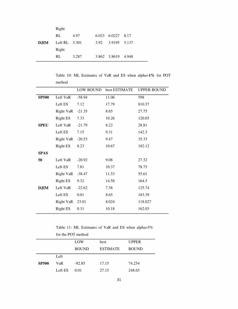
Figure 1 shows the hypothetical returns for a long position on the SP500 index during five
consecutive years. The maximum returns of each year block denoted by2X ,
5X , 7X ,
11X
and 13X have a limiting distribution known as the generalised extreme value distribution
expressed as:
1/
( , , )( ) exp 1
xH x
ξ
ξ µ σ
µξ
σ
− −
= − + (7)
ξ represents the shape parameter of the tail distribution, µ its location, and σ its scale
parameter. When 1 0ξ α −= > Equation (7) corresponds to the Fréchet distribution, when
1 0ξ α −= < Equation (7) corresponds to the Weibull distribution, and when 0ξ = Equation
(7) corresponds to the Gumbel distribution, as shown in Equations (4), (5) and (6),
respectively. Following Gilli and Kellezi (2006); we re-parameterise the generalised extreme
value distribution above in order to include a tail risk measure which is referred to as the
“return level”:
( ) ( )
( )1/
, ,
exp
1exp log 1 ; 0
11 ; =0
Kk
k
Rx R
x Rk
H x
k
ξξ
ξ σ
σ
ξξ
σ
ξ
−−
−−
− − + − ∀ ≠ = − ∀
(8)
where k
nR represents the return level that is the maximum loss expected in one out of k
periods of length n computed as:
1
, ,
11
k
nR Hk
ξ µ σ−
= −
(9)
The ML method is used to estimate the parameters of the re-parameterised generalised
extreme value distribution as well as their corresponding confidence intervals by maximising
its log-likelihood function:
( ) ( ),
max , ,k kL R L R
ξ σ
ξ σ= (10)

10
These confidence intervals satisfy the following condition:
( ) ( ) 2
1
1ˆ ˆˆ, ,2
k kL R L R αξ σ χ −− > − (11)
where 2
1 αχ − is the ( )1th
α− quantile of the Chi-square distribution with 1 degree of freedom.
3.2. The peak over the threshold approach
3.2.1. Generalised Pareto distribution
Let X be a vector of extreme returns larger than a specific threshold u as depicted in
Figure 2 below, and assume that the density function of X is given by F . The limiting
distribution of the extreme returns above a specific threshold is known as the generalised
Pareto distribution. The excess density function of X over the thresholdu is defined as;
( ) ( )( ) ( )
( )Pr ( ) / ; 0
1u
F x u F uF x ob X u x X u x
F u
+ −= − ≤ > = ≥
− (12)
This function is obtained via the generalised Pareto distribution in what is termed as the
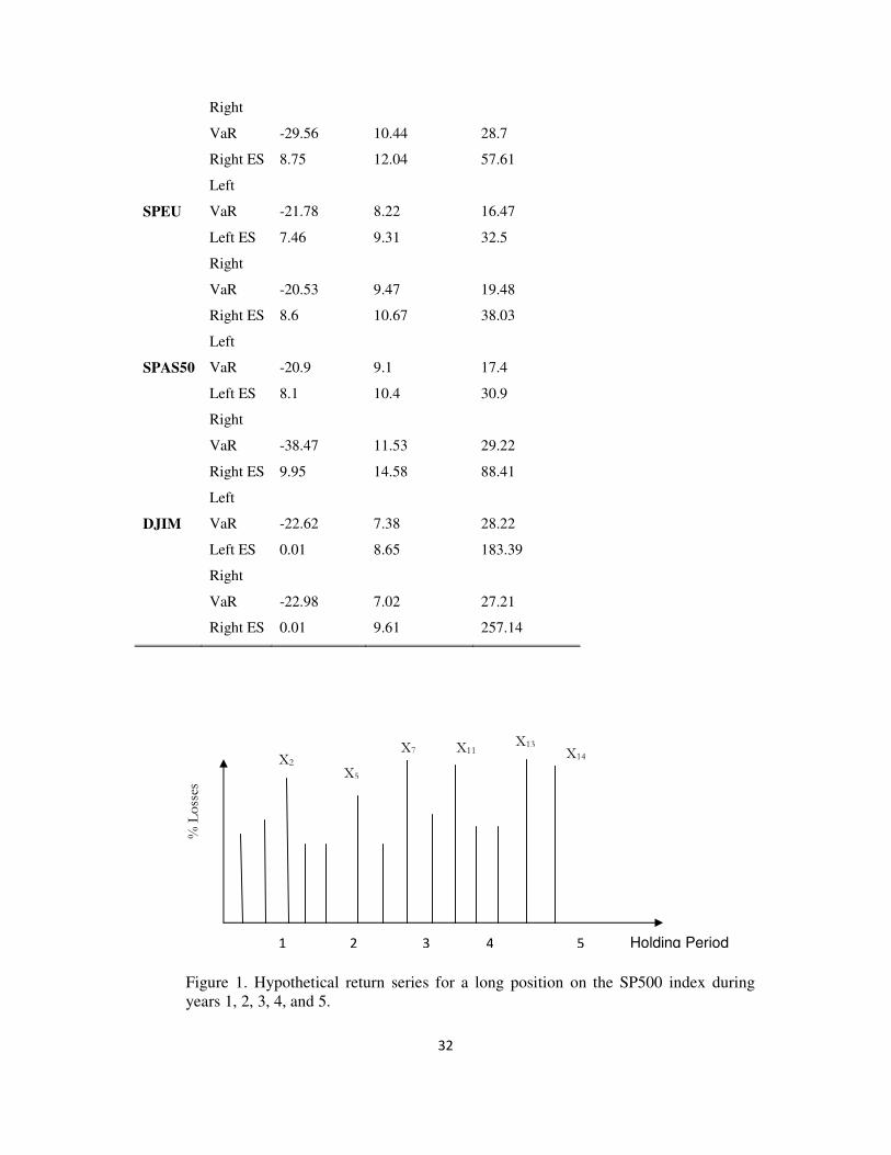
“peak-over-threshold method. Figure 2 illustrates how the generalised Pareto distribution fits
the extreme returns above a specific threshold value of 3u = .
PLACE FIGURE 2 HERE
This figure shows a hypothetical extreme return distribution marked as 1, 2, 3, 4, 5, 6,
and 7 observed during the first half of January, and the y-axis reports their magnitudes.
Assume that the return marked as 3 is our threshold. In this case the returns marked as 4, 5, 6
and 7 are considered here as extreme returns since they are larger than the threshold 3u = .
The limiting distribution of these extreme returns over the threshold 3u = is known as
generalised Pareto distribution (GPD) and is given by the following expression:
( )
1
, ( )
1 1 ; 0( )
( )
x1-exp - ; 0
u
u
x
uG x
ξ
ξ β
ξ ξβ
ξβ
− − + ≠ =
=
(13)
11
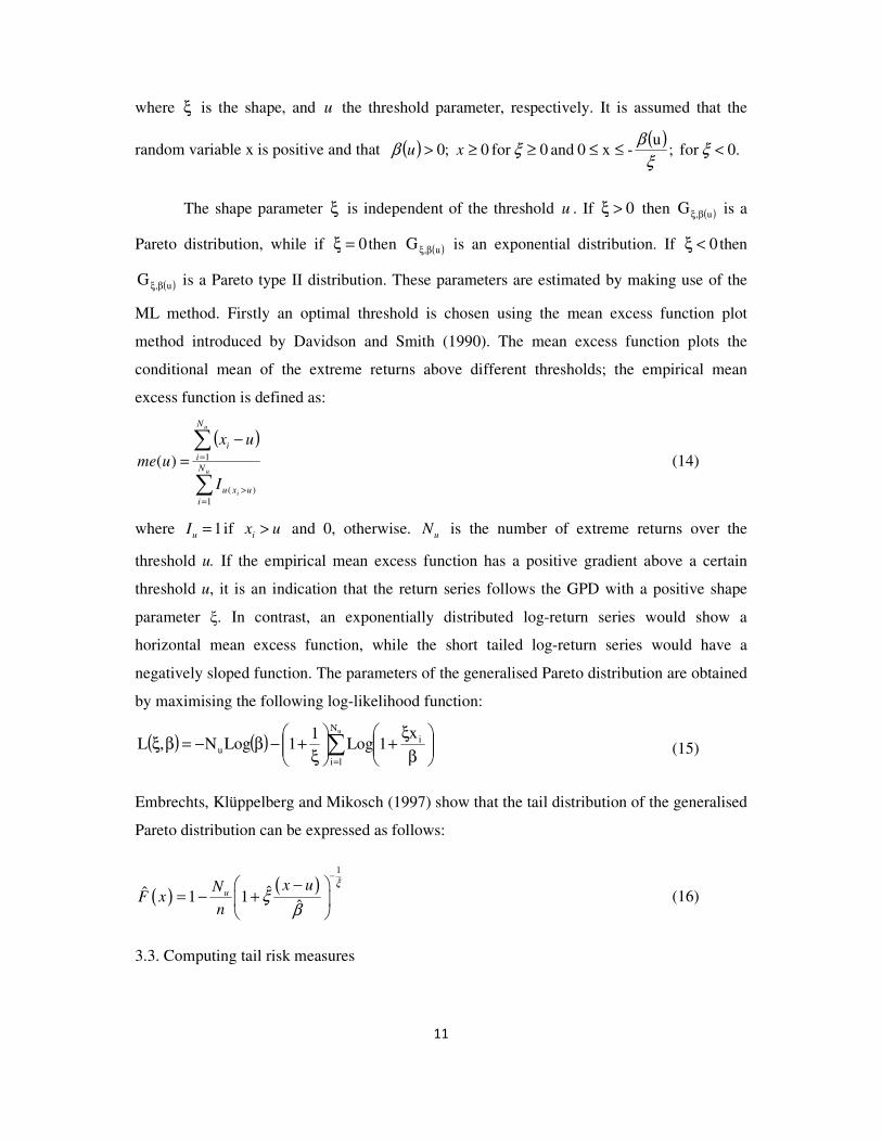
where ξ is the shape, and u the threshold parameter, respectively. It is assumed that the
random variable x is positive and that ( ) ( )0.for ;
u-x0 and 0for 0 ;0 <≤≤≥≥> ξ
ξ
βξβ xu
The shape parameter ξ is independent of the threshold u . If 0>ξ then ( )u,G βξ is a
Pareto distribution, while if 0=ξ then ( )u,G βξ is an exponential distribution. If 0<ξ then
( )u,G βξ is a Pareto type II distribution. These parameters are estimated by making use of the
ML method. Firstly an optimal threshold is chosen using the mean excess function plot
method introduced by Davidson and Smith (1990). The mean excess function plots the
conditional mean of the extreme returns above different thresholds; the empirical mean
excess function is defined as:
( )
∑
∑
=>
=
−
=u
i
u
N
i
uxu
N
i
i
I
ux
ume
1
)(
1)( (14)
where 1=uI if uxi > and 0, otherwise. uN is the number of extreme returns over the
threshold u. If the empirical mean excess function has a positive gradient above a certain
threshold u, it is an indication that the return series follows the GPD with a positive shape
parameter ξ. In contrast, an exponentially distributed log-return series would show a
horizontal mean excess function, while the short tailed log-return series would have a
negatively sloped function. The parameters of the generalised Pareto distribution are obtained
by maximising the following log-likelihood function:
( ) ( ) ∑=
β
ξ+
ξ+−β−=βξ
uN
1i
iu
x1Log
11LogN,L (15)
Embrechts, Klüppelberg and Mikosch (1997) show that the tail distribution of the generalised
Pareto distribution can be expressed as follows:
( )( )
1
ˆ
ˆˆ 1 1ˆ
ux uN
F xn
ξ
ξβ
− −
= − +
(16)
3.3. Computing tail risk measures

12
Although widely used to measure market risk, the value at risk (VaR) method is not a
coherent measure of risk because it doesn’t satisfy the sub-additivity condition. Assume that
we have a long position in two financial assets 1z and 2z , then sub-additivity means the total
risk of a portfolio of these two assets must be less than the sum of the individual asset risks.
Consequently, VaR doesn’t satisfy the diversification principle. A more coherent risk
measure is the Expected Shortfall (ES). The ES measures the expected loss of a portfolio,
given that the VaR is exceeded. In this paper, we compute the VaR as the alpha quantile of
the tail distribution in Equation (16), and obtain the ES by adding to the VaR the mean excess
function over the VaR (see Coles, 2001 for derivation):
( )ˆ
ˆ 11
ˆ /u
pVaR p u
N n
ξ
β
ξ
− − = + −
(17)
( ) ( )( ) ( ) ( ) ( )( )/ /ES p E Y Y VaR p VaR p E Y VaR p Y VaR p= > = + − > (18)
( )( ) ˆ ˆ
ˆ ˆ1 1
VaR p uES p
β ξ
ξ ξ
−= +
− − (19)
where p is the significance level at which the VaR is computed. For example, when
0.99p = Equations (17) and (18) produce the tail risk measures at the 99 significance level.
4. Empirical results
4.1. Data description
We make use of closing daily stock market indexes for the Sharia-compliant stocks in
the Dow Jones stock index universe and for stocks in three main regions: the United States,
Europe and Asia in the S&P universe (see, for example, Hammoudeh et al., 2014;
Hammoudeh et al., forthcoming). As indicated earlier, the four Islamic and regional
conventional market indexes under consideration are the US SP500, the Eurozone SPEU, the
Asian SPAS50 and the Islamic market DJIM. The time series for the four stock market
indexes are sourced from Bloomberg. The DJIM index represents the global universe of
investable equities that have been screened for Sharia compliance. The companies in this index
13
pass the industry and financial ratio screens. The regional allocation for DJIM is classified as
follows: 60.14% for the United States; 24.33% for Europe and South Africa; and 15.53% for
Asia. The S&P Euro (SPEU) is a sub-index of the S&P Europe 350 and includes all Eurozone
domiciled stocks from the parent index. This index is designed to be reflective of the
Eurozone market, yet efficient to replicate. The Asian SPAS50 is an index that represents the
most liquid 50 blue chip companies in four Asian countries: Hong Kong, Korea, Singapore,
and Taiwan.
The data spans from 01/01/1998 to 16/09/2014, making a total of 4358 observations
which include the recent global financial crisis period. Our aim is to model the tail
distribution of these financial markets which follow different business models and compute
the corresponding left and right risk measures. The left tail represents the losses for an
investor with a long position on the market indexes, whereas the right tail represents the
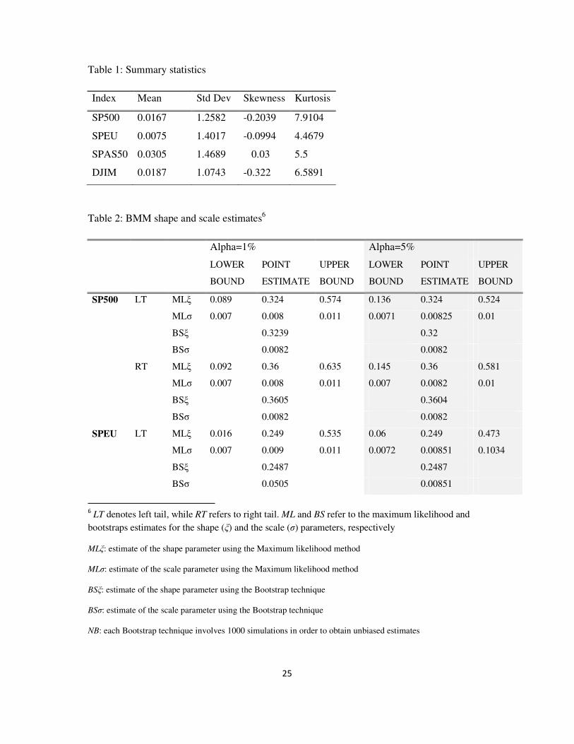
losses for an investor being short on the market indexes. Table 1 exhibits the basic statistics
of the log-returns. It shows that the Asian market SPAS50 has on average the highest
historical rate of return which is equal to 0.0305%, with a corresponding standard deviation
of 1.47%. The Islamic market (DJIM) has the lowest historical average rate of return, with
the corresponding lowest standard deviation of 1.0743%.
PLACE TABLE 1 HERE
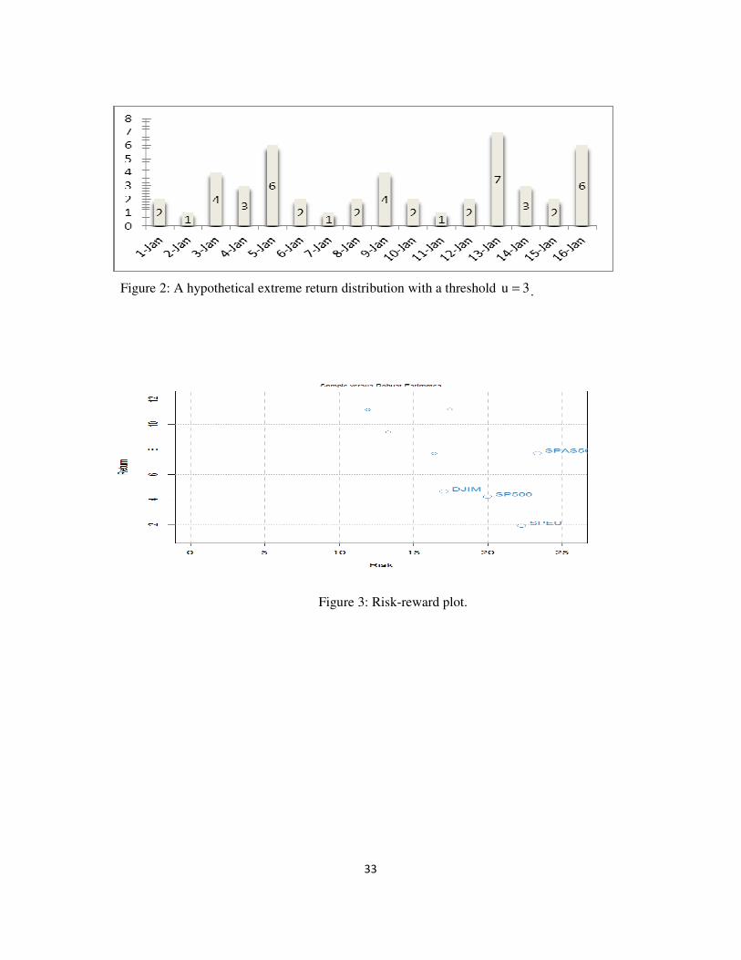
A risk-reward analysis exhibited in Figure 3 shows that the Islamic market
represented by the DJIM index has the lowest annualised risk of all the markets, and has an
annualised rate of return higher than that of the US and the Euro zone markets which are
represented by the SP500 and SPEU, respectively. However, the Asian market provides the
annualised rate of return with a corresponding relatively higher level of risk. Unlike the
Islamic markets, the Asian market is characterised by higher uncertainty and political
instability that requires higher premium.
PLACE FIGURE 3 HERE
4.2. Tail estimation results
Since we are interested in both the downside (left tail) and the upside (right tail) risk
measures, we collect all negative and positive log-returns, respectively, and fit them
separately to the generalised extreme value distribution using the BMM method and to the
14
Pareto distribution using the POT method. For the generalised extreme value distribution, we
first divide our sample period into quarterly blocks2 and collect the maximum positive return
(for the right tail) and the largest loss (for the left tail) of each quarterly block. The limiting
distribution of these maximums (minimums) is known as the generalised extreme value
distribution, whose re-parameterised version that is expressed in Equation (8) is used to
estimate the shape and scale parameters using the maximum likelihood (ML) method. Table 2
reports the ML estimates of these parameters as well as their confidence intervals. For the
purpose of robustness, we report the best estimate and its corresponding bootstrapped value.
PLACE TABLE 2 HERE
Table 2 reports the shape (ξ) and the scale (σ) parameters of the re-parameterised
GEV function shown in Equation (8), the point estimates and their corresponding confidence
intervals for the Islamic and conventional stock market at the 1% and 5% significance levels.
The maximum likelihood estimates are referred to as ML, whereas the bootstrapped estimates
are denoted by BS. Moreover, LT (RT) refers to the left tail (right tail) of the empirical return
distribution, representing the downside risk and upside risk, respectively. We find that the
BMM method generates only positive shape parameters for all of the four market indexes
used in our study. A positive shape parameter is an indication that these market indexes have
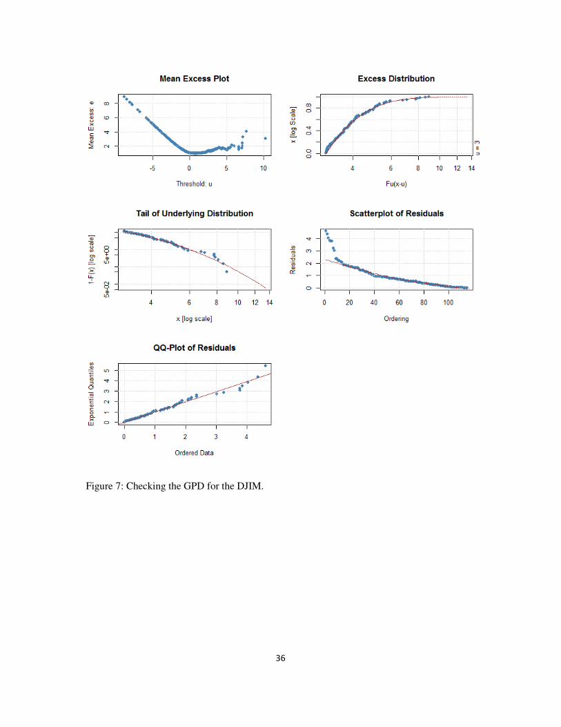
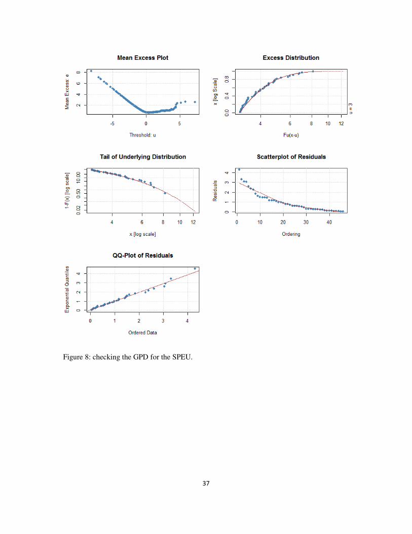
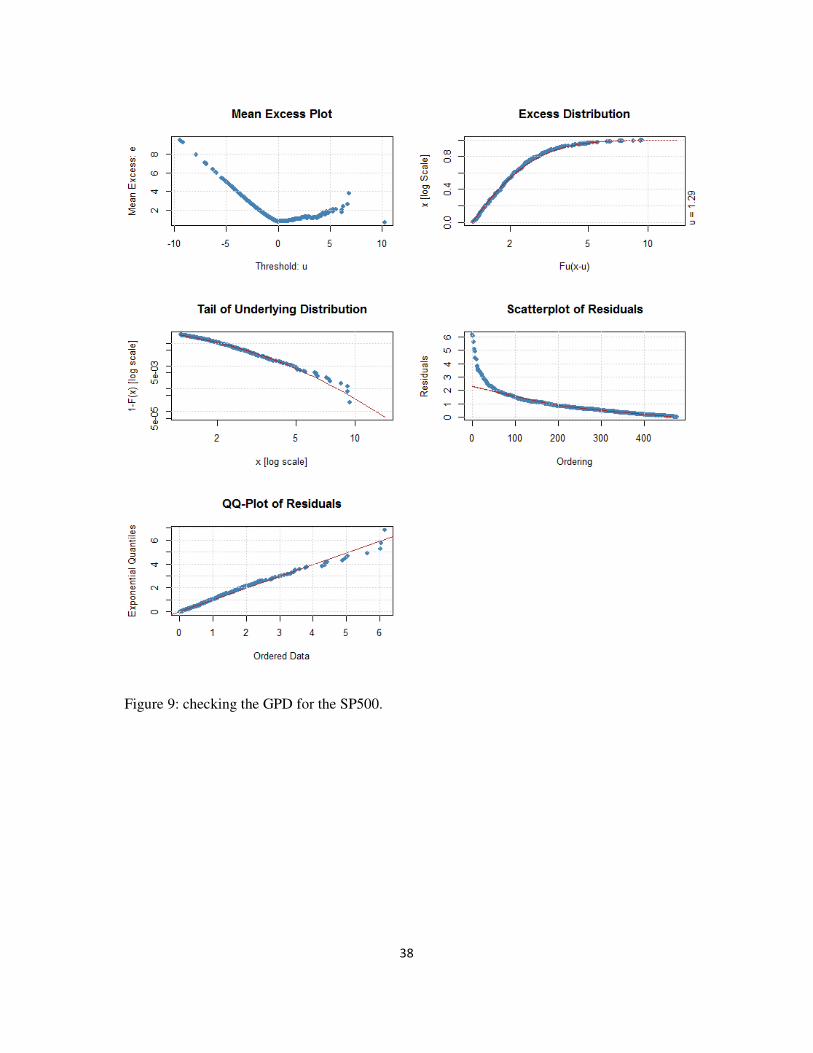
fatter tails than the normal distribution. The quantile-quantile plots shown Figures 6, 7, 8 and
9 confirm that the generalised extreme value distribution best fits the set of quarterly block
maximums (minimums) data.
Given the parameters of the re-parameterised generalized extreme value distribution,
we thereafter compute one tail risk measure associated with the generalised extreme value
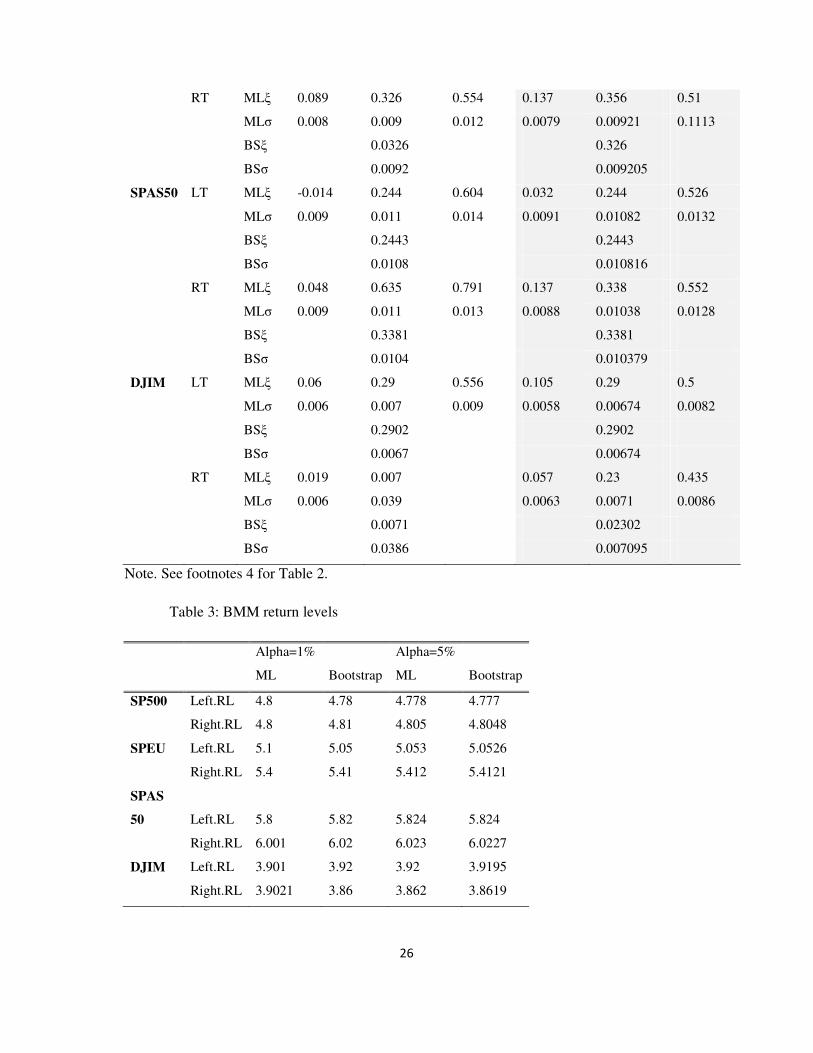
distribution, namely the return level (see Gilli and Kellezi, 2006). We denote by RL the
return level which represents the maximum loss expected in one out of ten quarters. Table 3
reports the RL for both the left and the right tails of the empirical distribution at the 1% and
5% significance levels as per the Basel II accord.3 Their confidence intervals are reported in
2 One of the criticisms of the BMM method is that there is not a standard way of grouping data in blocks of
maxima. Given the length of our daily sample period (i.e., 16 years), we believe that grouping the maximums
(minimums) in quarterly blocks would result in enough data points to generate unbiased estimates of the
generalised extreme value distribution.
3 The Basel II accords recommend that the VaR be estimated at higher quantile, i.e., the 1% significance level
for the next 10 trading days.
15
Tables 8 and 9. For the purpose of robustness, we also report the bootstrapped return level
after 1000 resamples.
PLACE TABLE 3 HERE
For example, using the US SP500 market index, one would say that at 1%
significance level the maximum loss observed during a period of one quarter exceeds 4.8% in
one out of ten quarters on average for an investor with a long position on the market index
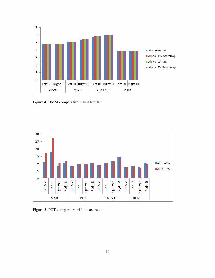
(left tail). Figure 4 below highlights the differences in the return level of each market index at
both the 1% and 5% significance levels. At these levels, we find that due to its Sharia laws,
the Islamic market is less risky than other three market indexes. Both the left and right ML
and bootstrapped maximum losses during one quarter are expected to exceed 3.8% on
average in one out of ten quarters for an investor with long and/or short positions in the
Islamic market. In contrast, the Asian market index SPAS50 is more risky than the rest of the
market indexes in our portfolio. Its maximum loss observed during one quarter exceeds 5.8%
in one out of ten quarters on average for an investor with a long position on the index (left
tail) and 6% for an investor with a short position on the index (right tail).
PLACE FIGURE 4 HERE
Based on the specific market regulations, we find that in the US market and the Sharia
- law compliant market which has 64% of it constiutents in the US maket, the portfolio risk
measure is indepedend of the investment strategy used, i.e., the long or the short position. The
maximum expected losses in these markets are almost the same for both the long position
(left tail) and short positions (right tail) on the market indexes. However, in the Eurozone and
Asian markets, we find that the short (selling) position generates higher risk than the long
only position. We argue that this has to do with the presence of market speculations and
short selling regulations, particualrly during the debt crisis.
Contrary to the BMM methodology, the POT methodology produces more reliable
and efficient shape parameters, and seems to be well suited for the modelling of the tails of
financial time series (see for example Coles, 2001; McNeil, Frey and Embrechts, 2005 for
more documentation of this result). The POT methodology proceeds as follows. Firstly, an
16
optimal threshold4 value is determined by using the mean excess function method which is
described above. We report in Figures 6, 7, 8, and 9 the plots of the mean excess function, the
excess distribution and the quantile-quantile distribution for the left tail of the empirical
distribution. A visual analysis suggests that the optimal threshold value for the four market
indexes varies between 3% and 5%. These values are located at the beginning of a portion of
the sample mean excess plot that is roughly linear. Given the large number of values the
thresholds can take in this interval of 3% to 5%, and the resulting subjectivity about the
correct threshold value, in this study we follow Mackay, Challenor, and Bahaj (2010),
Damon (2009); and Sigauke, Vester and Chikobvu (2012) who suggest the preferable use of
the 90th
quantile of the empirical return distribution5.
We follow the same procedure described above for the BMM method to separate the
data for the left and right tails, respectively. Using the LM estimation method, we obtain the
shape and scale parameters of the generalised Pareto distribution expressed in Equation (13).
We also make use the Bonferroni confidence interval to correct for the sample bias. Two
types of confidence intervals are reported: the ML confidence interval and the Bonferroni
confidence interval for the left and the right tail distributions at the 1% and 5% significance
levels, respectively. The ML and bootstrapped point estimates are reported in Table 4 in the
column labelled “best estimate”. For example, using the SP500 one would say that the 1%
level, ML and bootstrapped estimates of the left tail shape are 0.397% and 0.011%,
respectively. Their corresponding confidence intervals are -0.034 (-1.028), and 1.669 (3.99),
respectively. These numbers represent the smallest and the largest values these parameters
can take.
Unlike the BMM methodology which produced only positive shape parameters, the
POT methodology produces negative and positive shape parameters. The negative shape
parameter indicates that the tail of the empirical distribution (left and/or right) is thinner than
4 The mean excess analysis may be used to select an optimum threshold. An optimal threshold is crucial to
obtaining a reliable risk measures. Notice that a lower threshold is likely to reduce the variance of the estimates
of the Generalised Pareto Distribution and induce a bias in the data above the threshold. A higher threshold
reduces the bias but increases the volatility of the estimate of the GPD distribution. See for example Danielsson
and de Vries (1997) and Dupuis (1998) for more discussion on this issue. To avoid these issues, we use the 90th
quantile of the empirical log-return distribution as the threshold value. 5 For more discussion on the choice of the optimal threshold value, we refer the interested readers to the
following studies Damen (2009); Mackay et al. (2010); Sigauke at al. (2012).
17
the tail of the normal distribution. However a positive shape parameter is an indication that
the empirical distribution (left and/or right) has a fatter tail than that of the normal
distribution, which can lead to the occurrence of extreme losses. Table 4 shows that the US
SP500 and the Eurozone indexes have thinner right tail distributions, meaning that the
probability of the occurrence of extreme losses due to short (selling) positions is minimal.
However, on the downside, the Eurozone SPEU, the Asian SPAS50, and the Sharia-based
Islamic market indexes exhibit negative shape parameters, meaning that the probability of
extreme losses due to long position is minimal. These results highlight the importance of the
generalised Pareto distribution in fitting appropriately the tails of time series data
characterised by extreme events.
PLACE TABLE 4 HERE
Based on these estimates, we compute two types of risk measures: the VaR and the
ES. Theoretically, the ES is equal to the sum of VaR and the average of all losses exceeding
the VaR. Therefore, we expect in all cases the VaR estimates to be of less magnitude than the
ES estimates. Table 5 reports the risk measures for both the left and right tail distributions.
Their confidence intervals are reported in Tables 8, 9, 10, and 11 . We find almost the same
results with the BMM methodology, except for the US SP500 market index which results in
the two largest risk measures, i.e. 17.15% (VaR) and 27.15% (ES) at the 5% significant level.
We believe that this has to do with the recent 2008 – 2009 financial crisis.
PLACE TABLE 5 HERE
Figure 5 highlights the differences in the magnitude of the risk measures correponding
to each of the four market indexes. Although the Sharia-based Islamic market index (DJIM)
remains the least risky market, the POT methodology highlights the relatively high risk
associated with the short (selling) position in the right tail of the return distributions of
conventional markets. In general, the short positions lead to a higher likelihood of the
occurrence of maximum/extreme losses.
PLACE FIGURE 5 HERE
In addition, we attempt to answer the question of whether the Islamic market as
represented by the DJIM is different from the three conventional financial markets. We apply
18
the ANOVA technique to the tail distribution data, i.e. the quartely maximum and nimum
return series. Our aim in this section is to study the variability (dynamics) of each stock
market during extreme events. In other words, we attempt to see whether the variability of the
Islamic market during extreme market conditions is the same as that of conventional stock
markets. We therefore test the null hypothesis of equal variability for the four markets i.e.
H0: V1=V2=V3=V4 against H1: at least one stock market different from the others, where V1
is the variability in the SP500 market, V2 is the variability in the SPEU market, V3 is the
variability in the SPAS50 market and V4 is the variability in the Islamic DJIM market.
Two results can be obtained from this test. First, if we fail to reject the null hypothesis
H0, it means that there is no difference between the Islamic and the conventional markets
during extreme market events. Second, if we reject the null hypothesis it means that at least
one market is different from others. In this case, we need to further test two sets of the null
hypotheses:
i. The conventional stock markets are not different (they have equal variability during
extreme events) against the alternative that they are different. We refer to these
hypotheses as H01: V1=V2=V3, and H11: at least one conventional market is
different from the rest.
ii. The Islamic stock market is different from each one of the conventional market; in
this case the following hypotheses are formulated: H02: V4=V1 against H12: V4≠V1;
and H03: V4=V2 against H13: V4≠V2; and H04: V4=V3 against H14: V4≠V3. With
V1, V2, V3, and V4 defined as above.
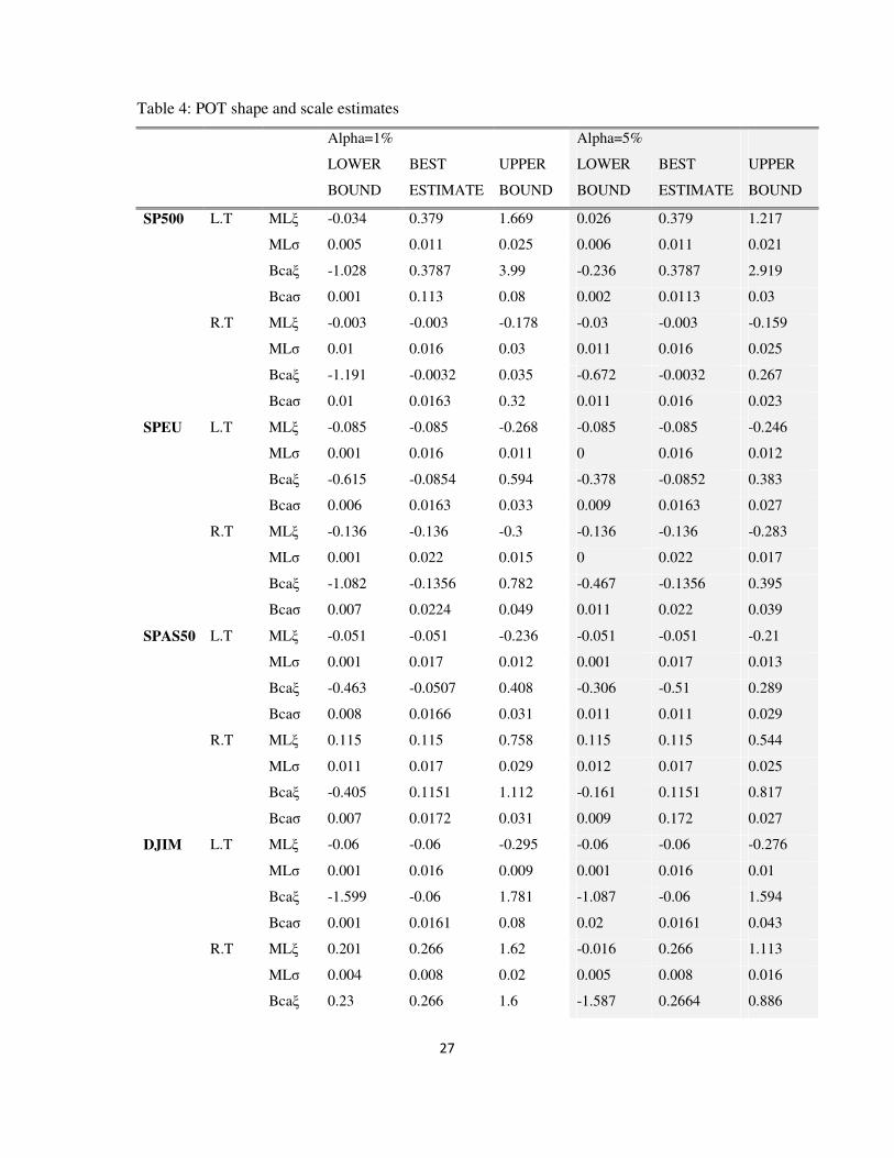
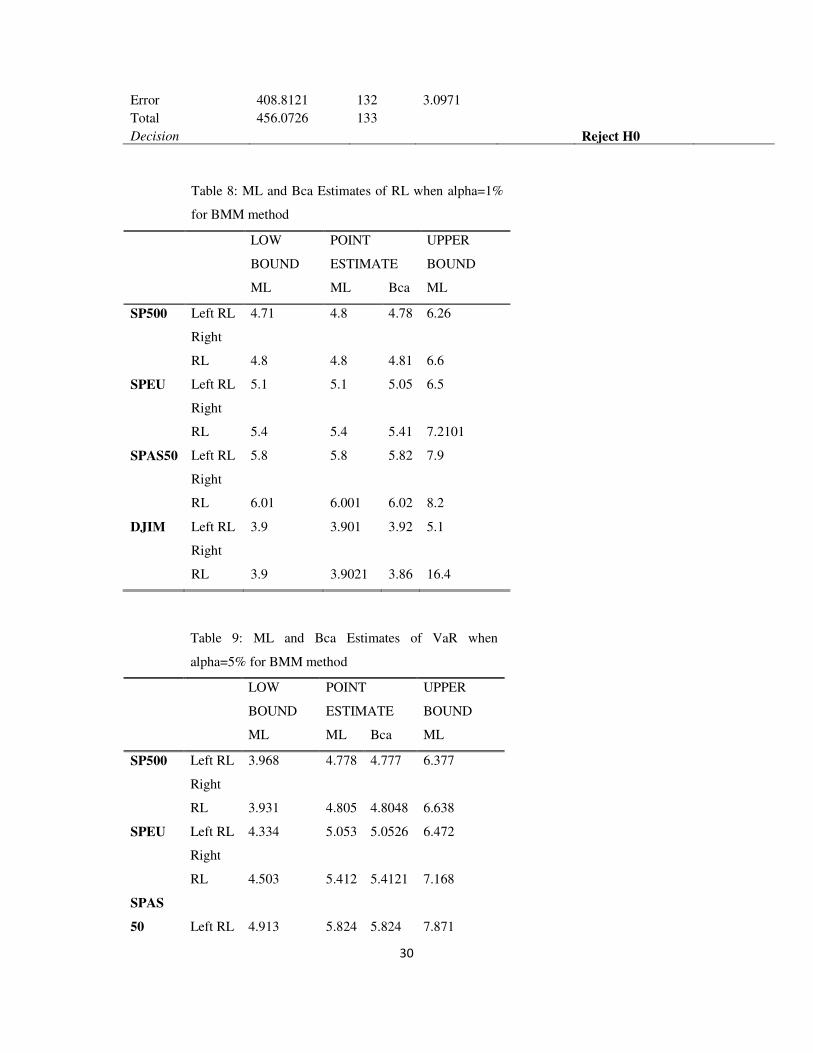
Tables 6 and 7 report the test statistic corresponding to each hypothesis test as well as
its p-values. We reject the null hypothesis H0 of equal variability in all stock markets and
conclude that at least one stock market is different from the others. To find out which one it
is, we first test the null hypothesis H01 of equal variability in all conventional stock markets.
We fail to reject this null hypothesis only at 10% significance level and conclude that the
variability in convnentional stock markets during extreme events are the same. Lastly, we test
the null hypothesis of equal variability between the Islamic market and each one of the
conventional stock markets; that is hypotheses H02, H03, and H04. We do reject these null
hypotheses at the 5% signifiance level for H03 and H04, and at the10% significance level for
19
H02; and conclude that the Islamic DJIM market is significantly different from the
convnentional stock markets.
5. Conclusion
This paper makes use of two techniques used in the extreme value theory, namely the
block of maxima method (BMM) based on the generalised extreme value dostribution and the
peak-over-the threshold method (POT) based on the generalised Pareto distribution, in order
to model the tails of the empirical distributions of three regional conventional imdxes and the
Islamic market indexes. They indexes are represenetd by the US SP500, the Eurozone SPEU,
the Asian SPAS50 and the Islamic DJIM. The main objective of the paper is to compute the
financial tail risk measures associated with the distributions of these markets which follow
different business models. To achieve this purpose, the study bigins by separating the log-
return data for the left and the right tail distributions.
For the BMM method, the paper groups the log-return data in 67 independent and
overlapping quarterly blocks and identified the minimum (maximum) of each block as the
adequate inputs to the BMM methodology. However, the inputs for the POT methodology
have been identified as the excesses over the threshold of the 90th
quantile of the empirical
log-return distribution.
Using the ML method and the 1000 bootstrap simulations, we estimate the parameters
of the re-parameterised generalised extreme value distribution. The estimation of the re-
parameterised distribution results in positive shape parameters for all four market indexes,
leading to the conclusion that the BMM method suggests that these market indexes exhibit
fatter tails than the tail of the normal distribution. However, when the POT methodology is
used, we find more elaborate estimates of the shape parameters. We find that the US SP500
and the Eurozone SPEU exhibit fatter tail behaviour in the right tail, whereas the Islamic
DJIM, the Asian SPAS50, and the Eurozone SPEU exhibit fatter tail behaviour in the left
tails. Stock markets with fatter left tails are prone to higher risk due to short selling positions.
However, based on the risk-reward analysis reported in Fgure 3, we find that the Islamic
market, although exhibiting a fatter left tail behaviour, is less risky than the conventional
stock markets. Since short selling and other excessive risk taking behaviours are not allowed
20
in Islamic markets, we argue that its left fat-tailedness behaviour is an indication of windfall
profits on long positions only that investors can reap during extreme events. We have applied
the ANOVA technique to the tail distribution data in order to determine whether the Islamic
market is different from the conventional markets. Using different statistical tests, we find
that the Islamic stock market is indeed significantly different from the conventional stock
markets during extreme market events. We therefore recommend the Islamic finance as a
solution to financial crises in order to curb excessive risk taking behaviour in conventional
stock markets
Based on the shape parameters, we find that the Asian SPAS50 market index is the
more risky market in its right tail than in its left tail. This is an indication that short (selling)
positions on this market index have a more negative impact on its performance. The Islamic
market index is the least risky market index most likely due to its restrictive Sharia laws that
discourage high risk taking behaviour. However, the developed markets (the US SP500, and
the Eurozone SPEU) are relatively riskier.
The results of this current study are really significant because they show clearly that
during major crises the Islamic stock index is not only less risky but also significantly
different from the conventional markets. Thus, the results come differently to those of the
recent studies which show that the former is no different from the counventional counterparts
in different regions. Both the left and right risk measures depend on whether the investor is
long or short on these market indexes. In general, we find that in most volatile and worst
market conditions, short (selling) positions on conventional stock market indexes have a
more negative impact on the respective portfolio performance than long position strategies.
Finally, Islamic market provides generous opportunities for windfall profits during periods of
financial crises.
References
Abd Rahman, Z., (2010). Contracts & The Products of Islamic Banking, Kuala Lumpur,
MY: CERT Publications.
Ahmed, H., (2009). Financial crisis risks and lessons for Islamic finance, International
Journal of Islam Finance 1, 7-32.

21
Arouri, M.H., Lihiani, A. and Nguyen, D. K. (2011). Return and volatility transmission
between world oil prices and stock markets of GCC. Economic Modelling 26, 1815-1825.
Ajmi, A. N., Hammoudeh, S., Nguyen, D. K., Sarafrazi, S., (2014). How strong are the
causal relationships between Islamic and conventional finance systems? Evidence from
linear and nonlinear tests. Journal of International Financial Markets, Institutions and
Money 28, 213-227.
Arouri, M. E., Ameur, H. B., Jawadi, N., F. Jawadi and Louhichi, W., (2013). Are Islamic
finance innovations enough for investors to escape from a financial downturn? Further
evidence from portfolio simulations, Applied Economics 45, 3412-3420.
Bashir, B. A., (1983). Portfolio management of Islamic banks, Certainty Model, Journal
of Banking and Finance 7, 339-354.
Boubaker, H., and Sghaier, N., (2014). Semiparametric generalized long memory
modelling of GCC stock market return: a wavelet approach. IPAG, Working Paper 066.
Available on the link: http://www.ipag.fr/wp-
content/uploads/recherche/WP/IPAG_WP_2014_066.pdf
Cihak, M., Hesse, H., (2010). Islamic Banks and Financial Stability: An Empirical
Analysis, Journal of Financial Services Research, Journal of Financial Services Research,
38(2), 95-113.
Coles, S. (2001). An Introduction to Statistical Modeling of Extreme Values,
Springer Series in Statistics. Springer, London
Dacorogna, M. M., Müller, U. A., Pictet, O. V., DeVries, C. G., (1995) The Distribution
of Extremal Foreign Exchange Rate Returns in Extremely Large Data Sets. Preprint, O&A
Research Group.
Damon, L (2009). Modelling tail behaviour with extreme value theory. Risk management,
17, 13- 18
22
Dania, A., Malhotra, D.K., (2013), An Empirical Examination of the Dynamic Linkages
of Faith-Based Socially Responsible Investing, The Journal of Wealth Management 16(1),
65-79.
Davison, A. C., and Smith, R. L., (1990). Models for exceedances over high
thresholds. Journal of Royal Statistical Society, 52(3), 393–442.
Danielsson, J., and DeVries, C. G., (1997). Tail index and quantile estimation with very
high frequency data. Journal of Empirical Finance, 4, 241 – 257,
Dewandaru, G., El Alaoui, A., Masih, A.M.A., and Alhabshi, S.O., (2013). Comovement
and resiliency of Islamic equity market: evidence from GCC Islamic equity index based on
wavelet analysis. MPRA working paper number 56980. Available on the link:
http://mpra.ub.uni-muenchen.de/56980
Dewi M., Ferdian. I. R., (2010). Islamic finance: A therapy for healing the global
financial crisis, http://ebookpdf. Net/islamic-finance-a-therapy-for-healing-the-global-
financial-crisis.html, accessed on 10/04/2012.
Dridi, J., Hassan, M., (2010). The effects of global crisis on Islamic and conventional
banks: A comparative study, International Monetary Fund Working Paper No, 10/201.
Dupuis, D.J. (1998). Exceedances over high thresholds: A guide to threshold selection.
Extremes, 1(3), 251–261.
Embrechts, P., Klüppelberg, C. and Mikosch, T. (1997). Modelling Extremal Events for
Insurance and Finance. Springer-Verlag, Berlin.
Frad, H., Zouari, E. (2014). Estimation of value-at-risk measures in the Islamic stock
market: Approach based on Extreme Value Theory (EVT). Journal of World Economic
Research, 3(2), 15-20. Published online July 10, (2014)
(http://www.sciencepublishinggroup.com/j/jwer) doi: 10.11648/j.jwer.20140302.11
Gençay, R., and Selçuk, F., (2004). Extreme Value Theory and Value-at-Risk: Relative
Performance in Emerging Markets. International Journal of Forecasting, 20, 287– 303
Gilli, M., and Kellezi, E. (2006). An application of extreme value theory to measuring
financial risk. Computational Economics, 27, 207 – 228.
23
Girard, E.C., Kabir, M., (2008). Is there a cost to faith-based investing: Evidence from
FTSE Islamic indices. Journal of Investing 17(4), 112-121.
Graham, F. D. (1930). Exchanges, Prices, and Production in Hyperinflation Countries:
Germany, 1920-1923. Princeton University Press, Princeton, NJ.
Hakim, S., Rashidian, M., (2002). Risk and return of Islamic stock market indexes. Paper
Presented at the 9th
Economic Research Forum Annual Conference in Sharjah, U.A.E. on
October 26-28, 2002.
Hammoudeh, S., W. Mensi, J. C. Reboredo and D. K. Nguyen (2014). Dynamic
dependence of Global Islamic stock index with global conventional indexes and risk factors.
Pacific Basin Financial Journal, 30, 189-206.
Hammoudeh, S., Kim. W.J. and S. Sarafrazi, S. (forthcoming). Sources of Fluctuations in
Islamic, U.S., EU and Asia Equity Markets: The Roles of Economic Uncertainty, Interest
Rates. Emerging Markets Finance and Trade.
Hashim, N., (2008). The FTSE global Islamic and the risk dilemma, AIUB Bus Econ
Working Paper Series, No 2008-08.
http://orp.aiub.edu/WorkingPaper/WorkingPaper.aspx?year=2008.
Hesse, H., Jobst, A. A., Sole, J., (2008). Trends and challenges in Islamic finance, World
Economics, 9(2), 175-193.
Iqbal, Z., Mirakhor, A., (2007). An introduction to Islamic finance: theory and practice,
John Wiley & Sons (Asia) Pte Ltd, Singapore.
Jawadi, F., Sousa, R. A., (2013). Structural breaks and nonlinearity in U.S. and UK public
debts. Applied Economics Letters 20(7), 653-657.
Jawadi, F., Jawadi, N. et Louhichi, W. (2014), Conventional and Islamic Stock Price
Performance: An Empirical Investigation, International Economics, 137, 73–87.
Longin, F. M. (1996). The Asymptotic Distribution of Extreme Stock
Market Returns,” Journal of Business, 69, 3, 383–408.
Longin, F. (2005). The choice of the distribution of asset returns: How extreme value
theory can help? Journal of Banking & Finance, Elsevier, 29(4), 1017-1035.

24
Mackay, E. B. L, Challenor, A. S., and Bahay A. S. (2010). On the use of discrete
seasonal and directional models for estimation of extreme wave conditions. Ocean
Engineering, 37, 425 – 442.
McNeil, A. J., and Frey, R. (2000). Estimation of Tail-related Risk Measures for
Heteroskedastic Financial Time Series: An Extreme Value Approach,” Journal of Empirical
Finance, 7, 271– 300.
McNeil, A., Frey, R. and Embrechts, P. (2005). Quantitative Risk Management: Concepts
Techniques and Tools. Princeton University Press, Princeton, NJ.
Robertson, J., (1990). Future wealth: A new economics for the 21st century. London:
Cassell Publications.
Rocco, M. (2011). Extreme value theory for finance: a survey. Bank of Canada.
https://ideas.repec.org/p/bdi/opques/qef_99_11.html
Sigauke, S. Verster A., and Chikobvu, E. (2012). Tail quantile estimation of the
heteroskedastic intraday increases in peak electricity demand. Open Journal of Statistics, 2,
435 - 442
Sole, J., (2007). Introducing Islamic banks into conventional banking systems, IMF
Working Paper, International Monetary Fund, Washington, D. C.
Sukmana, R., Kolid, M., (2012). Impact of global financial crisis on Islamic and
conventional stocks in emerging market: an application of ARCH and GARCH method,
Asian Academy of Management Journal of Accounting & Finance, to appear.
Usmani, M. T., (2002). An introduction to Islamic finance, The Netherlands:
Kluwer Law International.
Xubiao H., Gong, P. (2009). Measuring the Coupled Risks: A Copula-Based CVaR
Model. Journal of Computational and Applied Mathematics, 223, 2, 1066-1080.
25
Table 1: Summary statistics
Index Mean Std Dev Skewness Kurtosis
SP500 0.0167 1.2582 -0.2039 7.9104
SPEU 0.0075 1.4017 -0.0994 4.4679
SPAS50 0.0305 1.4689 0.03 5.5
DJIM 0.0187 1.0743 -0.322 6.5891
Table 2: BMM shape and scale estimates6
Alpha=1% Alpha=5%
LOWER
BOUND
POINT
ESTIMATE
UPPER
BOUND
LOWER
BOUND
POINT
ESTIMATE
UPPER
BOUND
SP500 LT MLξ 0.089 0.324 0.574 0.136 0.324 0.524
MLσ 0.007 0.008 0.011 0.0071 0.00825 0.01
BSξ 0.3239 0.32
BSσ 0.0082 0.0082
RT MLξ 0.092 0.36 0.635 0.145 0.36 0.581
MLσ 0.007 0.008 0.011 0.007 0.0082 0.01
BSξ 0.3605 0.3604
BSσ 0.0082 0.0082
SPEU LT MLξ 0.016 0.249 0.535 0.06 0.249 0.473
MLσ 0.007 0.009 0.011 0.0072 0.00851 0.1034
BSξ 0.2487 0.2487
BSσ 0.0505 0.00851
6 LT denotes left tail, while RT refers to right tail. ML and BS refer to the maximum likelihood and
bootstraps estimates for the shape (ξ) and the scale (σ) parameters, respectively
MLξ: estimate of the shape parameter using the Maximum likelihood method
MLσ: estimate of the scale parameter using the Maximum likelihood method
BSξ: estimate of the shape parameter using the Bootstrap technique
BSσ: estimate of the scale parameter using the Bootstrap technique
NB: each Bootstrap technique involves 1000 simulations in order to obtain unbiased estimates
26
RT MLξ 0.089 0.326 0.554 0.137 0.356 0.51
MLσ 0.008 0.009 0.012 0.0079 0.00921 0.1113
BSξ 0.0326 0.326
BSσ 0.0092 0.009205
SPAS50 LT MLξ -0.014 0.244 0.604 0.032 0.244 0.526
MLσ 0.009 0.011 0.014 0.0091 0.01082 0.0132
BSξ 0.2443 0.2443
BSσ 0.0108 0.010816
RT MLξ 0.048 0.635 0.791 0.137 0.338 0.552
MLσ 0.009 0.011 0.013 0.0088 0.01038 0.0128
BSξ 0.3381 0.3381
BSσ 0.0104 0.010379
DJIM LT MLξ 0.06 0.29 0.556 0.105 0.29 0.5
MLσ 0.006 0.007 0.009 0.0058 0.00674 0.0082
BSξ 0.2902 0.2902
BSσ 0.0067 0.00674
RT MLξ 0.019 0.007 0.057 0.23 0.435
MLσ 0.006 0.039 0.0063 0.0071 0.0086
BSξ 0.0071 0.02302
BSσ 0.0386 0.007095
Note. See footnotes 4 for Table 2.
Table 3: BMM return levels
Alpha=1% Alpha=5%
ML Bootstrap ML Bootstrap
SP500 Left.RL 4.8 4.78 4.778 4.777
Right.RL 4.8 4.81 4.805 4.8048
SPEU Left.RL 5.1 5.05 5.053 5.0526
Right.RL 5.4 5.41 5.412 5.4121
SPAS
50 Left.RL 5.8 5.82 5.824 5.824
Right.RL 6.001 6.02 6.023 6.0227
DJIM Left.RL 3.901 3.92 3.92 3.9195
Right.RL 3.9021 3.86 3.862 3.8619
27
Table 4: POT shape and scale estimates
Alpha=1% Alpha=5%
LOWER
BOUND
BEST
ESTIMATE
UPPER
BOUND
LOWER
BOUND
BEST
ESTIMATE
UPPER
BOUND
SP500 L.T MLξ -0.034 0.379 1.669 0.026 0.379 1.217
MLσ 0.005 0.011 0.025 0.006 0.011 0.021
Bcaξ -1.028 0.3787 3.99 -0.236 0.3787 2.919
Bcaσ 0.001 0.113 0.08 0.002 0.0113 0.03
R.T MLξ -0.003 -0.003 -0.178 -0.03 -0.003 -0.159
MLσ 0.01 0.016 0.03 0.011 0.016 0.025
Bcaξ -1.191 -0.0032 0.035 -0.672 -0.0032 0.267
Bcaσ 0.01 0.0163 0.32 0.011 0.016 0.023
SPEU L.T MLξ -0.085 -0.085 -0.268 -0.085 -0.085 -0.246
MLσ 0.001 0.016 0.011 0 0.016 0.012
Bcaξ -0.615 -0.0854 0.594 -0.378 -0.0852 0.383
Bcaσ 0.006 0.0163 0.033 0.009 0.0163 0.027
R.T MLξ -0.136 -0.136 -0.3 -0.136 -0.136 -0.283
MLσ 0.001 0.022 0.015 0 0.022 0.017
Bcaξ -1.082 -0.1356 0.782 -0.467 -0.1356 0.395
Bcaσ 0.007 0.0224 0.049 0.011 0.022 0.039
SPAS50 L.T MLξ -0.051 -0.051 -0.236 -0.051 -0.051 -0.21
MLσ 0.001 0.017 0.012 0.001 0.017 0.013
Bcaξ -0.463 -0.0507 0.408 -0.306 -0.51 0.289
Bcaσ 0.008 0.0166 0.031 0.011 0.011 0.029
R.T MLξ 0.115 0.115 0.758 0.115 0.115 0.544
MLσ 0.011 0.017 0.029 0.012 0.017 0.025
Bcaξ -0.405 0.1151 1.112 -0.161 0.1151 0.817
Bcaσ 0.007 0.0172 0.031 0.009 0.172 0.027
DJIM L.T MLξ -0.06 -0.06 -0.295 -0.06 -0.06 -0.276
MLσ 0.001 0.016 0.009 0.001 0.016 0.01
Bcaξ -1.599 -0.06 1.781 -1.087 -0.06 1.594
Bcaσ 0.001 0.0161 0.08 0.02 0.0161 0.043
R.T MLξ 0.201 0.266 1.62 -0.016 0.266 1.113
MLσ 0.004 0.008 0.02 0.005 0.008 0.016
Bcaξ 0.23 0.266 1.6 -1.587 0.2664 0.886

28
Bcaσ 0.0031 0.008 0.021 0.002 0.0083 0.017
Table 5: POT estimates of VaR and ES
Alpha=1% Alpha=5%
SP500 Left.VaR 11.06 17.15
Left.ES 17.79 27.15
Right.VaR 8.65 10.44
Right.ES 10.26 12.04
SPEU Left.VaR 8.22 8.22
Left.ES 9.31 9.31
Right.VaR 9.47 9.47
Right.ES 10.67 10.67
SPAS50 Left.VaR 9.08 9.1
Left.ES 10.37 10.4
Right.VaR 11.53 11.53
Right.ES 14.58 14.58
DJIM Left.VaR 7.38 7.38
Left.ES 8.65 8.65
Right.VaR 8.024 7.02
Right.ES 10.18 9.61
Table 6: Summary of ANOVA tests for lower tail
Source of Variation
Sum-of
Squared
Degree
of
Freedom
Mean
Square
F.
Calculated
P
value
F.
Theoretical
H0:V1=V2=V3=V4
Between Markets 43.6297 3 14.54323 5.8797 0.000672 2.6388
Error 652.9923 264 2.4725
Total 696.622 267
Decision Reject H0
H01: V1=V2=V3
Between Markets 12.7728 2 6.4864 2.3885 0.0944 3.0415
Error 537.7111 198 2.7157
Total 550.6839 200
Decision
Do not Reject
H0 @ 10%

29
H02: V4=V1
Between Markets 6.9886 1 6.9886 2.9873 0.086258 3.912875
Error 308.804 132 2.3394
Total 315.7926 133
Decision RejectOnlyat10%
H03: V4=V2
Between Markets 21.9468 1 21.9468 11.1996 0.001066 3.912875
Error 258.6684 132 1.9596
Total 280.6152 133
Decision Reject H0
H04: V4=V3
Between Markets 38.8648 1 38.8648 16.2305 0.000094 3.9129
Error 316.0822 132 2.3946
Total 354.947 133
Decision Reject H0
Table 7: Summary of NOVA tests for upper tail
Source of Variation
Sum-of
Squared
Degree
of
Freedom
Mean
Square
F
Calculated
P
value
F
Theoretical
H0:V1=V2=V3=V4
Between Markets 54.9709 3 18.3236 6.0139 0.00056 2.6388
Error 804.3742 264 3.0469
Total 859.3451 267
Decision Reject H0
H01: V1=V2=V3
Between Markets 20.1067 2 10.0534 2.8871 0.058087 3.041518
Error 689.4675 198 3.4822
Total 709.5742 200
Decision
Do not Reject
H0 @ 10%
H02: V4=V1
Between Markets 5.9004 1 5.9004 2.654607 0.1056 3.912875
Error 293.3947 132 2.2227
Total 299.295 133
Decision RejectOnlyat10%
H03: V4=V2
Between Markets 26.6209 1 26.6209 10.5848 0.00148 3.91288
Error 331.9807 132 2.515
Total 358.6016 133
Decision Reject H0
H04: V4=V3
Between Markets 47.2605 1 47.2605 15.2598 0.000149 3.912875
30
Error 408.8121 132 3.0971
Total 456.0726 133
Decision Reject H0
Table 8: ML and Bca Estimates of RL when alpha=1%
for BMM method
LOW
BOUND
POINT
ESTIMATE
UPPER
BOUND
ML ML Bca ML
SP500 Left RL 4.71 4.8 4.78 6.26
Right
RL 4.8 4.8 4.81 6.6
SPEU Left RL 5.1 5.1 5.05 6.5
Right
RL 5.4 5.4 5.41 7.2101
SPAS50 Left RL 5.8 5.8 5.82 7.9
Right
RL 6.01 6.001 6.02 8.2
DJIM Left RL 3.9 3.901 3.92 5.1
Right
RL 3.9 3.9021 3.86 16.4
Table 9: ML and Bca Estimates of VaR when
alpha=5% for BMM method
LOW
BOUND
POINT
ESTIMATE
UPPER
BOUND
ML ML Bca ML
SP500 Left RL 3.968 4.778 4.777 6.377
Right
RL 3.931 4.805 4.8048 6.638
SPEU Left RL 4.334 5.053 5.0526 6.472
Right
RL 4.503 5.412 5.4121 7.168
SPAS
50 Left RL 4.913 5.824 5.824 7.871
31
Right
RL 4.97 6.023 6.0227 8.17
DJIM Left RL 3.301 3.92 3.9195 5.137
Right
RL 3.287 3.862 3.8619 4.948
Table 10: ML Estimates of VaR and ES when alpha=1% for POT
method
LOW BOUND best ESTIMATE UPPER BOUND
SP500 Left VaR -58.94 11.06 598
Left ES 7.12 17.79 810.37
Right VaR -21.35 8.65 27.75
Right ES 7.33 10.26 120.05
SPEU Left VaR -21.79 8.22 28.81
Left ES 7.15 9.31 142.3
Right VaR -20.53 9.47 35.33
Right ES 8.23 10.67 182.12
SPAS
50 Left VaR -20.92 9.08 27.32
Left ES 7.81 10.37 78.75
Right VaR -38.47 11.53 55.61
Right ES 9.32 14.58 164.5
DJIM Left VaR -22.62 7.38 125.74
Left ES 0.01 8.65 183.39
Right VaR 23.01 8.024 118.027
Right ES 0.31 10.18 162.03
Table 11: ML Estimates of VaR and ES when alpha=5%
for the POT method
LOW
BOUND
best
ESTIMATE
UPPER
BOUND
SP500
Left
VaR -92.85 17.15 74.254
Left ES 0.01 27.15 248.65
32
Right
VaR -29.56 10.44 28.7
Right ES 8.75 12.04 57.61
SPEU
Left
VaR -21.78 8.22 16.47
Left ES 7.46 9.31 32.5
Right
VaR -20.53 9.47 19.48
Right ES 8.6 10.67 38.03
SPAS50
Left
VaR -20.9 9.1 17.4
Left ES 8.1 10.4 30.9
Right
VaR -38.47 11.53 29.22
Right ES 9.95 14.58 88.41
DJIM
Left
VaR -22.62 7.38 28.22
Left ES 0.01 8.65 183.39
Right
VaR -22.98 7.02 27.21
Right ES 0.01 9.61 257.14
Figure 1. Hypothetical return series for a long position on the SP500 index during
years 1, 2, 3, 4, and 5.
Holding Period
% Losses
1 2 3 4 5
X2 X5
X7 X11 X13
X14
33
Figure 2: A hypothetical extreme return distribution with a threshold 3u = .
Figure 3: Risk-reward plot.
34
Figure 4: BMM comparative return levels.
Figure 5: POT comparative risk measures.

35
Figure 6: Checking the GPD for the SPAS50.
36
Figure 7: Checking the GPD for the DJIM.
37
Figure 8: checking the GPD for the SPEU.
38
Figure 9: checking the GPD for the SP500.
Related Documents