Financial Stability Review May 2022

Welcome message from author
This document is posted to help you gain knowledge. Please leave a comment to let me know what you think about it! Share it to your friends and learn new things together.
Transcript

Financial Stability Review
May 2022
Financial Stability Review, May 2022 – Contents
1
Contents
Foreword 3
Overview 4
1 Macro-financial and credit environment 17
1.1 Euro area economic outlook weakens on the back of global cost
pressures and the war in Ukraine 17
1.2 Normalisation of fiscal positions is challenged by a slower
economic recovery and the impact of the war 21
1.3 Corporates face new headwinds as supply bottlenecks persist 24
Box 1 Identifying the corporates most vulnerable to price shocks
following the pandemic 28
1.4 Households face rising inflation and greater uncertainty 31
1.5 Vulnerabilities continue to build in euro area real estate markets 33
Box 2 Drivers of rising house prices and the risk of reversal 35
2 Financial markets 39
2.1 War exacerbates existing trends of higher energy prices and
higher inflation 39
2.2 Market sensitivity to pace of policy normalisation 42
2.3 Commodity price shocks may lead to a reassessment of risks in
the corporate sector 47
Box 3 Financial stability implications of higher than expected inflation 50
Box 4 The impact of Chinese macro risk shocks on global financial
markets 54
3 Euro area banking sector 57
3.1 Asset quality continues to improve, but higher energy prices
revive risks for some loans 57
3.2 Profitability above pre-pandemic levels, but outlook weaker 63
Box 5 Interest rate risk exposures and hedging of euro area banks’
banking books 67
3.3 Higher market funding costs and improved capital ratios 70
Financial Stability Review, May 2022 – Contents
2
Box 6 Assessing the resilience of the euro area banking sector in light
of the Russia-Ukraine war 74
4 Non-bank financial sector 77
4.1 Non-bank financial sector faces higher credit risk as duration risk
starts to materialise 77
4.2 Bond funds are vulnerable to rising yields and uncertain
second-round effects from the war 80
Box 7 Synthetic leverage and margining in non-bank financial
institutions 83
4.3 Insurers face near-term headwinds from inflation, while benefiting
from rising interest rates 86
5 Macroprudential policy issues 90
5.1 Setting the appropriate pace of policy action to address
medium-term vulnerabilities 90
Box 8 Transmission and effectiveness of capital-based
macroprudential policies 93
5.2 Addressing both liquidity mismatch and leverage in the non-bank
financial sector 96
5.3 Other ongoing policy initiatives that support euro area financial
stability 99
Special Features 101
Climate-related risks to financial stability 101
Decrypting financial stability risks in crypto-asset markets 113
Acknowledgements 124

Financial Stability Review, May 2022 – Foreword
3
Foreword
The May 2022 Financial Stability Review (FSR) has been prepared against the
backdrop of the devastating invasion of Ukraine. We do not yet know how the war will
be resolved. But we do know that the human suffering it has caused is enormous. We
hope for peace.
This war is also affecting the economy, in Europe and beyond. The invasion and the
associated uncertainty have prompted some repricing in global financial markets,
albeit with much less turmoil than seen in March 2020, and dampened the confidence
of businesses and consumers that are only just emerging from the tight restrictions
imposed during the coronavirus (COVID-19) pandemic. Higher energy and
commodity prices are pushing up inflation and slowing the economic recovery.
Elevated volatility has highlighted some liquidity risks, notably in some commodity
derivatives markets. However, the main threat to euro area financial stability comes
from the impact through macroeconomic channels. This implies additional challenges
for indebted businesses at a point in time when countries’ fiscal space is very limited
and support may need to be more targeted than the broad fiscal policy response to
the pandemic.
With these developments in mind, this FSR assesses financial stability vulnerabilities
and their implications for financial markets, debt sustainability, bank resilience, the
non-bank financial sector and macroprudential policies.
This issue of the FSR also includes two special features on topics that are
increasingly part of our routine financial stability assessment at the ECB. The first
focuses on recent advances in the monitoring of financial stability risks stemming
from climate change, building on previous special features on the topic. The second
special feature explores risks arising from crypto-assets – which have been
increasing over time, as this sector grows both in its size and in its integration with the
core financial system.
This issue of the FSR has been prepared with the involvement of the ESCB Financial
Stability Committee, which assists the decision-making bodies of the ECB in the
fulfilment of their tasks. The FSR exists to promote awareness of systemic risks
among policymakers, the financial industry and the public at large, with the ultimate
goal of promoting financial stability.
Luis de Guindos
Vice-President of the European Central Bank

Financial Stability Review, May 2022 – Overview
4
Overview
Financial stability conditions have deteriorated
Banks, which have remained strikingly resilient and able to support the economy, see
increased credit risk and a weaker profit outlook.
Energy and commodity price shocks, amplified by the Russian invasion of Ukraine, increase
risks to post-pandemic growth, inflation and financial conditions in the euro area and globally.
Euro area sovereigns, corporates and households face higher interest rates and cost
pressures that could test debt sustainability for the more highly indebted entities.
Higher financial market volatility, although largely orderly, underscores risks of sharp
corrections. Non-banks are most exposed to duration, credit and liquidity risks.
Markets vulnerable as rates adjust
to inflation and growth weakens
• Higher-for-longer energy prices
• Corporate spreads widen as risks grow
• Financial fragmentation could emerge
• Interest rate volatility increases
Rising inflation and lower growth put
pressure on vulnerable borrowers
• Inflation spikes as outlook deteriorates
• House prices face correction risk
• Rising input costs weigh on corporate margins
• Ukraine war may challenge fiscal positions
Non-banks face duration risk amid low
liquidity and uncertain credit risk outlook
• Valuation losses from rising rates
• Fund outflows may trigger forced sales
• Increase in illiquid holdings of insurers
• Exposures from synthetic leverage
Macroprudential authorities
should continue to address
building vulnerabilities,
adjusting the type of measure,
pace and timing for economic
conditions in order to avoid
procyclicality.
Having macroprudential space
and effective buffers using the
whole range of macroprudential
instruments would help support
medium-term resilience.
Risks arising from liquidity
mismatches, leverage and
margining practices in the non-
bank financial sector need to be
tackled comprehensively.
Renewed bank asset quality and
profitability concerns
• Re-emerging credit risks
• Possible tightening of credit standards
• Higher bond funding costs
• Rising cyber risks
Non-financial private
and sovereign debt-to-
GDP ratio
226%
237%
2011 2021
Analysts' 2022
ROE forecasts
7.6%7.0%
02/22 05/22
Holdings of NFC bonds
Cre
dit r
isk
Sector energy
intensity
39%
29%
32%
Euro area one-year
inflation swap rate
1.4
6.6
01/21 05/22
Invasio
n

Financial Stability Review, May 2022 – Overview
5
Higher prices, exacerbated by the Russia-Ukraine war,
weaken the recovery and increase global risks
Financial stability conditions have deteriorated, as the post-pandemic recovery
has been tested by higher inflation and Russia’s invasion of Ukraine. Since late
2021, rising inflationary pressures have threatened to slow the momentum of the
recovery in 2022. Upside risks to euro area inflation and downside risks to growth
rose sharply following the outbreak of the Russia-Ukraine war (Chart 1, panel a). In
particular, large rises in commodity and energy prices (Chart 1, panel b) and ongoing
global supply chain pressures are expected to prolong the period of elevated inflation.
The course and consequences of the Russia-Ukraine war are still hard to predict.
While peace could reverse some pressures, a protracted conflict could imply
sustained higher inflation and even lower growth outturns than currently expected.
Risks to inflation, growth and global financial conditions could also be triggered by
other global events, such as a broader resurgence of the coronavirus (COVID-19),
emerging market weakness or a sharper economic slowdown in China (Box 4).
Chart 1
Risks of higher inflation and lower growth outturns in the euro area amplified by an
intensified commodity and energy price shock
a) 2022 and 2023 real GDP growth and HICP inflation forecasts for the euro area
b) Oil and other commodity price developments
(2022-23, annual percentage changes) (1 Jan. 2008-17 May 2022, USD, index: 2020 = 100)
Sources: Consensus Economics Inc., Refinitiv, Hamburg Institute of International Economics and ECB calculations.
Note: Panel a: shaded areas display one and two standard deviations in Consensus expectations for euro area real GDP growth and
HICP inflation. HICP stands for Harmonised Index of Consumer Prices. Panel b: other commodities include food (cereals, oilseeds/oils
and tropical beverages/sugar) and industrial raw materials (agricultural raw materials, non-ferrous metals and iron-ore/scrap).
Higher inflation and lower growth could increase market volatility and
challenge debt servicing capacity as financing costs rise. The consequences of
the war and the shift to a lower-growth, higher-inflation environment affect virtually
every aspect of economic activity and financing conditions. In turn, these
developments might not only amplify, but could also trigger the materialisation of
pre-existing financial stability vulnerabilities identified in previous issues of the FSR.
These include heightened debt sustainability concerns in non-financial sectors or the
possibility of corrections in both financial and tangible asset markets (Box 3).
1
2
3
4
5
6
7
8
2022 2023 2022 2023
GDP HICP
1 standard deviation
2 standard deviations
May 2022
1 standard deviation
2 standard deviations
November 2021
0
25
50
75
100
125
150
175
200
2008 2011 2014 2017 2020
Oil (Brent)
Other commodities

Financial Stability Review, May 2022 – Overview
6
Initial risk-off reaction in markets largely orderly, but asset
price correction concerns remain
The Russian invasion of Ukraine triggered a large but, in most cases,
short-lived market reaction. In early 2022, markets, positioning for solid growth, a
temporary spike in inflation and relatively modest policy tightening, saw a repricing in
global equity and bond markets. The outbreak of the war, which increased the risk of
a higher-inflation, lower-growth scenario, saw market volatility increase, credit
spreads widen and equity indices decline (Chart 2, panels a and b). The market
response was substantial, but more modest than at the onset of the pandemic.
Movements in commodity markets were most pronounced, as Russia and Ukraine
are key suppliers. Euro area assets, given greater proximity and links to Russia and
Ukraine, experienced larger losses than US assets. By the end of March, euro area
markets had recovered most of the initial losses, but commodity prices remained
elevated. Over the course of April and May, concerns about the global growth outlook
and central banks’ response to higher inflation rates led to renewed weakness in risky
asset valuations.
Chart 2
The initial market correction to the war was largely orderly, but liquidity pressures
arose in some derivatives markets
a) Euro area and US high-yield corporate bond spreads
b) Development of global stock markets
c) Natural gas futures two-day absolute price changes and applied initial margin
(1 Jan. 2020-17 May 2022, basis points) (1 Jan. 2020-17 May 2022, indices: 1 Jan.
2020 = 100)
(6 Jul. 2021-17 May 2022, €/MWh)
Sources: Bloomberg Finance L.P., EPFR Global, ICE Clear Europe and ECB calculations.
Notes: Panel a: dashed lines represent the long-term average over the past two decades. Government option-adjusted spreads are
employed. Panel b: equity indices shown are the MSCI All Country World Index, the MSCI USA Index, the MSCI Euro Index and the
MSCI Emerging Markets Index. Panel c: data on margins are provided by ICE Clear Europe in accordance with the Terms of Use.
Applied initial margins are based on the scanning ranges published by ICE Clear Europe. Full initial margins should be computed with the
CCPs’ proprietary risk models, in this case those of ICE Clear Europe, taking into account all risk parameters and full exposures.
Further corrections in financial markets could be triggered by an escalation of
the war, even weaker global growth or if monetary policy needs to adjust faster
than expected. Despite recent asset price corrections, valuations remain stretched in
the light of the deterioration in macro-fundamentals, and further sharp corrections are
250
350
450
550
650
750
850
950
1,050
1,150
01/20 07/20 01/21 07/21 01/22
Euro area
United States
60
80
100
120
140
160
01/20 07/20 01/21 07/21 01/22
World
United States
Euro area
Emerging markets
Invasion
0
10
20
30
40
50
60
70
80
90
100
07/21 10/21 01/22 04/22
Two-day price change
Applied initial margin
Financial Stability Review, May 2022 – Overview
7
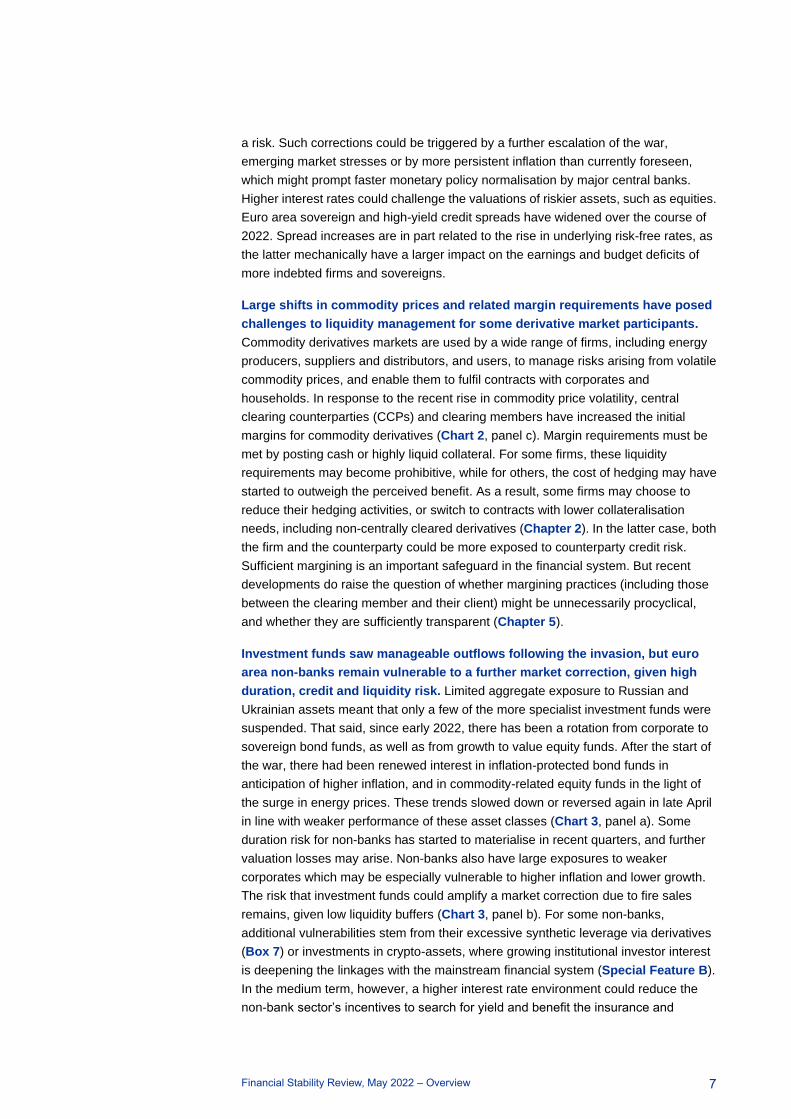
a risk. Such corrections could be triggered by a further escalation of the war,
emerging market stresses or by more persistent inflation than currently foreseen,
which might prompt faster monetary policy normalisation by major central banks.
Higher interest rates could challenge the valuations of riskier assets, such as equities.
Euro area sovereign and high-yield credit spreads have widened over the course of
2022. Spread increases are in part related to the rise in underlying risk-free rates, as
the latter mechanically have a larger impact on the earnings and budget deficits of
more indebted firms and sovereigns.
Large shifts in commodity prices and related margin requirements have posed
challenges to liquidity management for some derivative market participants.
Commodity derivatives markets are used by a wide range of firms, including energy
producers, suppliers and distributors, and users, to manage risks arising from volatile
commodity prices, and enable them to fulfil contracts with corporates and
households. In response to the recent rise in commodity price volatility, central
clearing counterparties (CCPs) and clearing members have increased the initial
margins for commodity derivatives (Chart 2, panel c). Margin requirements must be
met by posting cash or highly liquid collateral. For some firms, these liquidity
requirements may become prohibitive, while for others, the cost of hedging may have
started to outweigh the perceived benefit. As a result, some firms may choose to
reduce their hedging activities, or switch to contracts with lower collateralisation
needs, including non-centrally cleared derivatives (Chapter 2). In the latter case, both
the firm and the counterparty could be more exposed to counterparty credit risk.
Sufficient margining is an important safeguard in the financial system. But recent
developments do raise the question of whether margining practices (including those
between the clearing member and their client) might be unnecessarily procyclical,
and whether they are sufficiently transparent (Chapter 5).
Investment funds saw manageable outflows following the invasion, but euro
area non-banks remain vulnerable to a further market correction, given high
duration, credit and liquidity risk. Limited aggregate exposure to Russian and
Ukrainian assets meant that only a few of the more specialist investment funds were
suspended. That said, since early 2022, there has been a rotation from corporate to
sovereign bond funds, as well as from growth to value equity funds. After the start of
the war, there had been renewed interest in inflation-protected bond funds in
anticipation of higher inflation, and in commodity-related equity funds in the light of
the surge in energy prices. These trends slowed down or reversed again in late April
in line with weaker performance of these asset classes (Chart 3, panel a). Some
duration risk for non-banks has started to materialise in recent quarters, and further
valuation losses may arise. Non-banks also have large exposures to weaker
corporates which may be especially vulnerable to higher inflation and lower growth.
The risk that investment funds could amplify a market correction due to fire sales
remains, given low liquidity buffers (Chart 3, panel b). For some non-banks,
additional vulnerabilities stem from their excessive synthetic leverage via derivatives
(Box 7) or investments in crypto-assets, where growing institutional investor interest
is deepening the linkages with the mainstream financial system (Special Feature B).
In the medium term, however, a higher interest rate environment could reduce the
non-bank sector’s incentives to search for yield and benefit the insurance and

Financial Stability Review, May 2022 – Overview
8
pension fund sector because of its negative duration gap, thereby mitigating overall
financial stability risks (Chapter 4).
Chart 3
Non-banks proved largely resilient to the market impact of the invasion, but underlying
credit, duration and liquidity risks remain causes for concern
a) Euro area bond and equity fund flows b) Investment fund duration and liquidity risk
(1 Jan. 2022-17 May 2022, cumulative daily flows as a percentage of total net assets) (Q4 2013-Q4 2021, left-hand scale: years,
right-hand scale: percentages of total
assets)
Sources: EPFR Global, ECB (Investment Funds Balance Sheet Statistics and Securities Holding Statistics) and ECB calculations.
Note: Panel b: average residual maturity is a proxy for duration risk and is used here because of the longer available time series.
Input price increases and higher financing cost add strains
for more indebted firms and sovereigns
Euro area corporates face renewed headwinds as input prices have soared and
the economic outlook has become more clouded. A solid economic recovery
helped measures of aggregate corporate vulnerability to improve towards the end of
2021 (Chapter 1.3). Gross profits recovered to 7% above pre-pandemic levels, while
policy support measures have kept corporate insolvencies at historic lows. However,
a weaker economic growth outlook, coupled with growing margin pressure as a result
of soaring input prices, has led to some increase in expected corporate default rates
(Chart 4, panel a).
There is a sizeable cohort of more vulnerable and pandemic-strained firms,
some of which are also sensitive to commodity prices. The most vulnerable
corporates which are more indebted, less liquid and have lower sales levels might
face particular challenges in the event of a pronounced economic slowdown (Box 1).
Higher energy and commodity prices could hurt activity in economic sectors which
have not yet fully recovered from the pandemic, such as air transport,
-9
-6
-3
0
3
6
9
12
15
18
01/22 02/22 03/22 04/22 05/22
Euro area corporate
Euro area sovereign
Euro area inflation-protected
US corporate
US sovereign
US inflation-protected
Bond funds
Invasion
-9
-6
-3
0
3
6
9
12
15
18
01/22 02/22 03/22 04/22 05/22
Global equity blend
Global equity growth
Global equity value
Global commodities/materials
Global energy
Emerging Europe
Equity funds
Invasion
2.5
3.0
3.5
4.0
4.5
7
8
9
10
11
Q413
Q414
Q415
Q416
Q417
Q418
Q419
Q420
Q421
Average residual maturity
Cash holdings (right-hand scale)

Financial Stability Review, May 2022 – Overview
9
accommodation, and food and beverages (Chart 4, panel b), or which have low
pricing power to pass on higher costs (Chapter 2). These vulnerabilities are
compounded by the prospect of tighter financing conditions that would adversely
affect the debt servicing capacity of lower-rated firms in particular. This could also fuel
corporate downgrade risk, as the bulk of issuance activity in recent years has taken
place in the lowest investment grade bucket (BBB).
Chart 4
Signs of renewed risks for the corporate sector, with some pandemic-strained sectors
highly exposed to higher energy prices
a) European speculative-grade 12-month trailing default rates
b) Corporate turnover relative to pre-pandemic and energy use by industrial sector
(Sep. 2021-Feb. 2023E, percentages) (x-axis: 2018, percentages, y-axis: difference 2019/21,
index: 2019 = 100)
Sources: Moody’s Analytics, OECD Trade in Value Added (TiVA) database (2018), Eurostat and ECB calculations.
Notes: Panel a: European speculative-grade default rates forecast by Moody’s Analytics as at January 2022 (solid lines) and April 2022
(dotted lines). The baseline forecasts incorporate low refinancing risk and healthy corporate fundamentals. The optimistic scenario builds
on the favourable baseline, expecting markets to remain very supportive of speculative-grade issuers in 2022, while showing exceptional
demand for high-yield debt in the search for yield. By contrast, the pessimistic scenario acknowledges a particularly weak ratings mix
among European speculative-grade issuers. For more details on the different scenarios, see the Moody’s website. There is a structural
break in the time series of realised rates as of March 2022, as defaulting and non-defaulting Russian issuers whose ratings were recently
withdrawn have been excluded. Panel b: energy use includes direct and indirect use of: (i) electricity, gas, steam and air conditioning; (ii)
mining and quarrying; and (iii) coke and refined petroleum products as a share of total output. Energy inputs by industry are classified
according to the United Nations International Standard Industrial Classification for All Economic Activities (ISIC), Rev. 4, and are
attributed to each sector based on the four-digit SIC code. The red vertical line represents the median usage of energy inputs as share of
total output across all sectors of economic activity. Out of 42 NACE sectors, 24 are shown in the chart.
Euro area fiscal positions also face challenges as they now encounter a weaker
recovery and tighter financial conditions. In 2021, as the euro area economy
began recovering from the COVID-19 shock, governments gradually withdraw the
stimulus they provided during the pandemic. As a result, fiscal positions in 2022 are
expected to improve compared to 2021. However, the repercussions of the war in
Ukraine may create new draws on public finances. While immediate stress in euro
area sovereign bond markets remained low, short-term fiscal pressures have
increased in a number of countries (Chart 5, panel a). This is attributable to
measures aimed at cushioning the adverse impact of higher energy prices on
households and corporates, as well as the cost of managing the flow of refugees and
higher defence spending in some countries. Market participants estimate the
associated additional fiscal impact for the largest euro area countries at around 1.2
percentage points of GDP on average. Also, where coupled with lower economic
0
1
2
3
4
5
6
7
8
9
09/21 12/21 03/22 06/22 09/22 12/22
Realised
Forecast baseline
Forecast pessimistic
Forecast optimistic
January forecast
April forecast
Accommodation
Air transport
Base metalsChemical products
Food and beverages
Land transport
Mining
Motor vehicles
Non-metallic products
Paper products
Pharma-ceuticals
Textiles
Transport equipment
Warehousing
Wood products
-30
-20
-10
0
10
20
30
40
50
0 5 10 15 20 25
Dis
tan
ce
fro
m 2
01
9 t
urn
ove
r
Energy inputs as a share of total output
Pandemic and energy sensitive sectors
Financial Stability Review, May 2022 – Overview
10
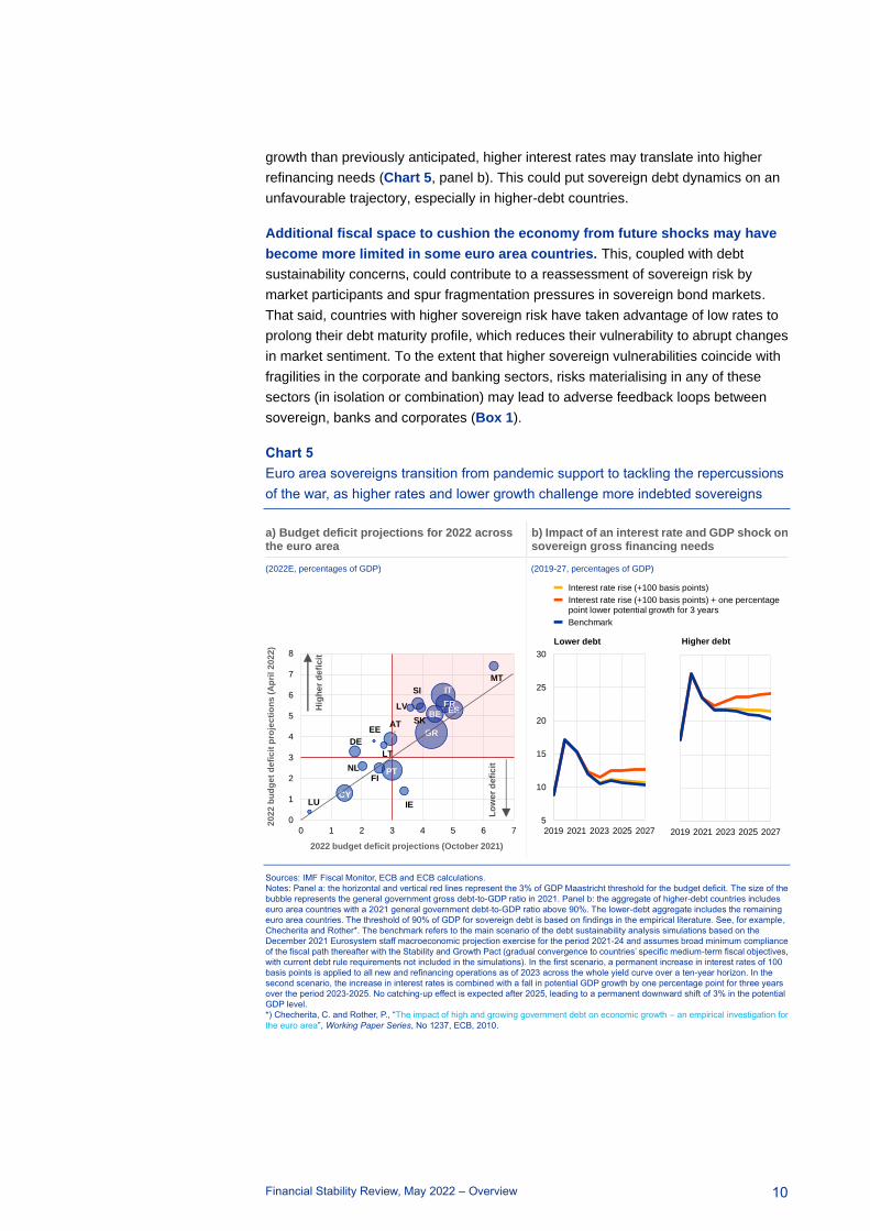
growth than previously anticipated, higher interest rates may translate into higher
refinancing needs (Chart 5, panel b). This could put sovereign debt dynamics on an
unfavourable trajectory, especially in higher-debt countries.
Additional fiscal space to cushion the economy from future shocks may have
become more limited in some euro area countries. This, coupled with debt
sustainability concerns, could contribute to a reassessment of sovereign risk by
market participants and spur fragmentation pressures in sovereign bond markets.
That said, countries with higher sovereign risk have taken advantage of low rates to
prolong their debt maturity profile, which reduces their vulnerability to abrupt changes
in market sentiment. To the extent that higher sovereign vulnerabilities coincide with
fragilities in the corporate and banking sectors, risks materialising in any of these
sectors (in isolation or combination) may lead to adverse feedback loops between
sovereign, banks and corporates (Box 1).
Chart 5
Euro area sovereigns transition from pandemic support to tackling the repercussions
of the war, as higher rates and lower growth challenge more indebted sovereigns
a) Budget deficit projections for 2022 across the euro area
b) Impact of an interest rate and GDP shock on sovereign gross financing needs
(2022E, percentages of GDP) (2019-27, percentages of GDP)
Sources: IMF Fiscal Monitor, ECB and ECB calculations.
Notes: Panel a: the horizontal and vertical red lines represent the 3% of GDP Maastricht threshold for the budget deficit. The size of the
bubble represents the general government gross debt-to-GDP ratio in 2021. Panel b: the aggregate of higher-debt countries includes
euro area countries with a 2021 general government debt-to-GDP ratio above 90%. The lower-debt aggregate includes the remaining
euro area countries. The threshold of 90% of GDP for sovereign debt is based on findings in the empirical literature. See, for example,
Checherita and Rother*. The benchmark refers to the main scenario of the debt sustainability analysis simulations based on the
December 2021 Eurosystem staff macroeconomic projection exercise for the period 2021-24 and assumes broad minimum compliance
of the fiscal path thereafter with the Stability and Growth Pact (gradual convergence to countries’ specific medium-term fiscal objectives,
with current debt rule requirements not included in the simulations). In the first scenario, a permanent increase in interest rates of 100
basis points is applied to all new and refinancing operations as of 2023 across the whole yield curve over a ten-year horizon. In the
second scenario, the increase in interest rates is combined with a fall in potential GDP growth by one percentage point for three years
over the period 2023-2025. No catching-up effect is expected after 2025, leading to a permanent downward shift of 3% in the potential
GDP level.
*) Checherita, C. and Rother, P., “The impact of high and growing government debt on economic growth – an empirical investigation for
the euro area”, Working Paper Series, No 1237, ECB, 2010.
ATBE
CY
EE
FI
FR
DEGR
IE
IT
LV
LT
LU
MT
NL PT
SK
SI
ES
0
1
2
3
4
5
6
7
8
0 1 2 3 4 5 6 7
2022 budget deficit projections (October 2021)
20
22
bu
dg
et
de
fic
it p
roje
cti
on
s (
Ap
ril
20
22
)
Hig
her
defi
cit
Lo
we
r d
efi
cit
5
10
15
20
25
30
2019 2021 2023 2025 2027
Interest rate rise (+100 basis points)
Interest rate rise (+100 basis points) + one percentage point lower potential growth for 3 years
Benchmark
Lower debt
2019 2021 2023 2025 2027
Higher debt

Financial Stability Review, May 2022 – Overview
11
Expansion continues in residential real estate markets,
increasing the vulnerability to corrections
Vulnerabilities in euro area residential real estate markets continued to build.
Euro area house prices increased at a rate of almost 10% in the final quarter of
2021 – the fastest pace observed in the last 20 years (Chart 6, panel a). The trend
was driven among other things by changes in housing preferences triggered by the
pandemic, low interest rates and supply-side constraints (Box 2). At the same time,
the buoyant growth of residential real estate prices is coupled with robust mortgage
lending (Section 1.5). The associated rise in vulnerabilities led to the European
Systemic Risk Board issuing new warnings and recommendations in December
2021, strengthening the case for macroprudential action in some countries
(Chapter 5). While house price pressures are buttressed in the near term by tight
supply conditions and continued demand amid household and investor preference for
housing, signs of overvaluation render some housing markets prone to price
corrections. In particular, an abrupt increase in real interest rates could induce house
price corrections (Box 2).
Chart 6
Euro area households could face the triple challenge of possible corrections in
residential real estate markets, higher interest rates and an income squeeze
a) House price and mortgage lending growth, and construction price expectations
b) Household debt-to-GDP and household debt service ratios
(Jan. 2001-Apr. 2022, left-hand scale: index, right-hand scale:
percentages)
(Q4 2021, percentages)
Sources: Eurostat, ECB and ECB calculations.
Notes: Panel a: construction price expectations refer to the three months ahead. RRE price growth is shown until the fourth quarter of
2021 and lending for house purchase until March 2022. Panel b: the red horizontal and vertical lines represent the euro area aggregate
values. The debt service ratio is calculated as debt service cost divided by income following Drehmann et al.* Compensation of
employees is used to measure the income of households.
*) Drehmann, M., Illes, A., Juselius, M. and Santos, M., “How much income is used for debt payments? A new database for debt service
ratios”, BIS Quarterly Review, September 2015.
Risks from mortgage indebtedness are amplified by the impact of higher costs
on the debt servicing capacity of euro area households. Despite rising
indebtedness since the start of the pandemic (Section 1.4), balance sheet
fundamentals of euro area households remained relatively solid overall. However,
higher inflation and energy price outturns may reduce households’ purchasing power,
-12
-9
-6
-3
0
3
6
9
12
15
18
-40
-30
-20
-10
0
10
20
30
40
50
60
2001 2004 2007 2010 2013 2016 2019 2022
House price growth (right-hand scale)
Lending for house purchase (right-hand scale)
Construction price expectations
AT
BE
CY
DE
EE
ES
FI
FR
GR
IE
IT
LT
LU
LV
MT
NL
PT
SI
SK
0
2
4
6
8
10
12
14
16
18
20
0 20 40 60 80 100 120
Ho
us
eh
old
de
bt
se
rvic
e r
ati
o
Household debt-to-GDP ratio
Financial Stability Review, May 2022 – Overview
12
unless wages catch up sufficiently without destabilising inflation expectations. The
associated squeeze may particularly affect lower-income households, which spend a
larger portion of their incomes on food and energy. At the same time, the currently
relatively favourable financial and employment situations of euro area households
could worsen, should prolonged economic weakness translate into a growing number
of corporate insolvencies and restructurings. In an environment of deteriorating
income positions and higher interest rates, households’ debt servicing capacity could
be challenged, particularly in countries with elevated debt levels and high debt
servicing needs (Chart 6, panel b). That said, the shift towards more fixed-rate
mortgage lending in recent years will shield many households from the immediate
impact of higher interest rates (Chart 7, panel c). Similarly, active use of
macroprudential policies in most euro area countries, notably through
borrower-based measures, are helping to improve the resilience of borrowers.
Euro area banks show resilience, but profitability
prospects worsen as asset quality concerns resurface
The positive market sentiment towards euro area banks in 2021 reversed
sharply following the Russian invasion of Ukraine. Marked corrections in bank
share prices (Chart 7, panel a) erased the gains made in 2021 amid improved
earnings and expectations of higher interest rates. After the initial shock, markets
reversed some of the losses as it became apparent that only a few banks had
material direct exposures to Russia and Ukraine. In addition, the majority of banks
signalled their commitment to previously announced dividend and share buyback
plans for 2022.
After a remarkable recovery in bank profitability in 2021, projections for 2022
have been revised down as credit risks have increased. Bank profitability
surpassed pre-pandemic levels in 2021, driven by higher operating income and lower
loan loss provisions, but profitability prospects have worsened in line with a weaker
macroeconomic backdrop. Profitability remained solid at the start of 2022 too, but
bank analysts revised down their 2022 return on equity (ROE) forecasts for euro area
banks to around 7% (Chart 7, panel a) – a level which is still low by international
standards. While banks showed resilience and credit risks associated with direct
exposures are limited, the banking sector could be indirectly affected by the
repercussions of the war. For example, it may be exposed to greater corporate and
household credit risks as a result of higher commodity prices and disrupted global
supply chains. In fact, a further major energy price shock could translate into higher
corporate probabilities of default (PDs), including in some sectors that were badly hit
by the pandemic, such as accommodation and food services (Chart 7, panel b).
However, a broader vulnerability exercise suggests that overall the banking sector is
resilient to the second-round effects arising from the Russia-Ukraine war (see Box 6).
A rise in interest rates may provide some support to bank margins in the short
run, but some banks might face challenges in the medium term. A higher interest
rate environment and steeper yield curve will mechanically support interest income
and, in turn, bank profitability, but funding low-yielding assets profitably may become

Financial Stability Review, May 2022 – Overview
13
challenging in the medium term. In particular, the large-scale shift over the last
decade from floating to fixed-rate lending, especially for households, may dampen
some of the benefits that banks enjoy from higher interest rates (Chart 7, panel c).
This may pose a risk to banks’ medium-term profitability prospects in cases where
such interest rate exposures are less well hedged (Box 5). As interest rates rise,
banks could also face higher credit risks, given growing exposures to vulnerabilities in
the non-financial sector in recent years.
Chart 7
Bank stock prices reflect an uncertain outlook amid resurfacing asset quality concerns
and rising interest rate risks for some banks
a) Euro area banks’ stock prices, dividend futures and 2022 profit expectations
b) Change in median firm PDs under two different scenarios of energy price rises by sector
c) Fixed-rate lending to euro area households and firms
(1 Jan. 2020-17 May 2022, indices: January
2020 = 100, percentages)
(percentages of PD levels) (2009, 2021, percentages of total new
lending)
Sources: Bloomberg Financial L.P., Urgentem, Moody's Analytics, Bureau van Dijk – Orbis database, ECB and ECB calculations.
Notes: Panel a: 2022 bank ROE expectations indicate the weighted average of a sample of 32 listed euro area banks. Panel b: adverse
scenario: +69% on gas price and +24% on oil price; severe scenario: +138% on gas and +48% on oil price. The energy price
assumptions are consistent with the scenario analysis conducted in the context of the March 2022 ECB staff macroeconomic projections.
NACE codes and corresponding economic activities: A – Agriculture, forestry and fishing, B – Mining and quarrying, C – Manufacturing,
D – Electricity, gas, steam and air conditioning supply, E – Water supply; sewerage, waste management and remediation activities, F –
Construction, G – Wholesale and retail trade; repair of motor vehicles and motorcycles, H – Transportation and storage, I –
Accommodation and food service activities, J – Information and communication, L – Real estate activities, M – Professional, scientific
and technical activities, N – Administrative and support service activities, O – Public administration and defence; compulsory social
security, P – Education, Q – Human health and social work activities, R – Arts, entertainment and recreation, S – Other service activities.
Panel c: NFCs stands for non-financial corporations.
Long-standing structural challenges, together with a greater need to manage
cyber risk, continue to weigh on the outlook for euro area banks. Longer-term
challenges associated with low cost-efficiency, limited revenue diversification and
overcapacity compound growing cyclical headwinds. In addition, euro area banks
urgently need to press ahead with their digital transformation, not least to be able to
manage the growing threat of cyber risks. However, having focused on cost-cutting in
recent years to boost profits, parts of the banking sector continue to lag behind global
peers in terms of IT infrastructure investment (Chapter 3). Heightened uncertainty
surrounding the outlook and lower profit expectations may now further delay the
transformation plans of euro area banks, which would have an adverse impact on
their competitiveness.
4.4
5.1
5.9
6.6
7.4
8.1
8.9
20
40
60
80
100
120
140
2020 2021 2022
EURO STOXX Banks
2022 bank ROE expectations (right-hand scale)
EURO STOXX Banks dividend futures (December 2022)
0
5
10
15
20
25
30
35
40
45
50
A B C D E F G H I J L M N
O-S
Adverse: gas
Adverse: oil
Severe: gas
Severe: oil
AT
BE
CY
DE
ES
FI
FR
GR
IE
IT
LT
LU
MT
NL
PT
SI
SK
EA
AT DE
EE
ES
FR
NL
EA
0
20
40
60
80
100
0 20 40 60 80 100
20
21
2009
Households
NFCs

Financial Stability Review, May 2022 – Overview
14
Financial institutions and markets need to accelerate the
transition to a low-carbon economy
Banks and non-banks alike need to step up their efforts to support the move
towards a net-zero economy. Metrics of financial institutions’ exposure to
climate-related risks show little evidence of a decline over the last few years. In fact,
while euro area NFCs have reduced actual emissions, loans to more polluting firms
still represent around two-thirds of banks’ credit exposures (Special Feature A).
Similarly, banks and non-banks have reduced their holdings of securities issued by
firms with higher emission levels only slightly over the last five years (Chart 8, panel
a). The Russian war in Ukraine has highlighted the risks that can arise from high
dependency on fossil fuels, whose price and supply can be volatile.
Chart 8
The carbon footprint of financial institutions’ portfolios has not decreased significantly,
and greenwashing risks remain high in financial markets
a) Euro area banks’ credit exposures to, and securities holdings of, high and low emitters
b) Disclosure of NFC greenhouse gas (GHG) emission data by type of emitter
(2018-21, 2016-20, percentages of total exposures and securities
holdings)
(2010-20, share of listed NFCs disclosing GHG emissions and
emission-reduction targets; share of audited disclosures)
Sources: ECB (AnaCredit and Securities Holding Statistics), Bureau van Dijk – Orbis database, Refinitiv, Urgentem and ECB
calculations.
Notes: Panel a: ICPFs stands for insurance corporations and pension funds; IFs stands for investment funds. High/low emitters are
defined as firms with reported emission intensity in the top/bottom 33% of the distribution across euro area banks’ borrowers as of
end-2020, i.e. firms with annual emission intensity registered in 2020 above 556 tCO2e/USD million and below 47 tCO2e/USD million.
ICPFs stands for insurance corporations and pension funds, IFs stands for investment funds. Panel b: combined market capitalisation
refers only to firms disclosing emission-reduction targets.
While green financial markets continue to deepen, there is a need to monitor
greenwashing risks. Sustainable financial markets continued to grow at a brisk pace
in 2021, amid growing investor interest in green finance. Firms are increasingly
disclosing their exposure to transition risk as well as their commitments to reduce
emissions (Chart 8, panel b), indicating increasing awareness of the need to
transition to a low-carbon economy. That said, greenwashing risks do remain in
capital markets. These need to be tackled using better, more consistent information
and enhanced standards for financial instruments, to ensure that green finance
effectively supports the transition to a low-carbon economy.
0
10
20
30
40
50
60
70
80
90
100
20
18
20
19
20
20
20
21
Bank loans
High emitters
Medium emitters
Low emitters
Securities holdings
0
10
20
30
40
50
60
70
80
90
100
20
16
20
17
20
18
20
19
20
20
Banks
20
16
20
17
20
18
20
19
20
20
ICPFs
20
16
20
17
20
18
20
19
20
20
IFs
0
10
20
30
40
50
60
70
80
90
100
2010 2015 2020
Firms disclosing emissions
Combined market capitalisation
Firms disclosing emission reduction targets
€1 tn
€5 tn
€27 tn
Financial Stability Review, May 2022 – Overview
15
Macroprudential policy needs to strengthen resilience to
handle future shocks
The euro area financial stability outlook has deteriorated as inflation has risen,
especially since the start of the Russia-Ukraine war. Upside risks to inflation,
especially from energy prices, and downside risks to growth are amplifying
pre-existing vulnerabilities identified in previous issues of the FSR, such as those
associated with mispricing in some financial and tangible asset markets, as well as
the legacy of higher debt levels in non-financial sectors. The vulnerabilities identified
could be exacerbated by shocks such as (i) a further escalation of the Russia-Ukraine
war or further economic sanctions imposed in response to the war; (ii) unexpected
changes in growth or inflation; or (iii) a resurgence in COVID-19 infections, with a
greater economic impact than currently expected. The potential for these
vulnerabilities to materialise simultaneously and possibly amplify each other further
increases the medium-term risks to financial stability.
As economic conditions allow, further building resilience in a timely manner
remains a sound policy strategy. Banks currently have ample capital headroom on
top of their regulatory requirements, and a vulnerability analysis specifically
assessing the adverse implications of the war in Ukraine indicates that the euro area
banking system remains resilient under the scenarios considered. Nevertheless,
macroprudential policy action would further enhance resilience against vulnerabilities
that have already accumulated, including those in residential real estate markets, and
mitigate the risk of bank de-leveraging if systemic risk materialises. As long as
economic conditions do not deteriorate significantly, existing bank capital generation
capacity and headroom should mitigate a detrimental impact on credit supply from
increasing capital buffers. In addition, there are also costs associated with delayed
action, especially if uncertainty persisted into the medium term and vulnerabilities
remained unaddressed or continued to build. Overall, if the economic costs of
activating additional capital buffers remain low and the financial cycle is expected to
remain on an upward trend, as was the case prior to the outbreak of the war, when
policy tightening commenced in some countries, authorities can continue to act
appropriately while taking into account the uncertainty related to the war to avoid
procyclical effects. Authorities should tailor their policy strategy to the national context
by using the whole range of macroprudential instruments that are at their disposal,
including borrower-based measures as already in place in several countries.
Creating additional macroprudential space while also enhancing the
effectiveness of the existing countercyclical capital buffer would support the
resilience of the financial system over the medium term. In its input to the
European Commission’s review of the macroprudential framework, the ECB has
called for more macroprudential space in the form of a higher amount of releasable
capital buffers that could further improve banks’ loss absorption capacity while
maintaining the provision of key services in a downturn. In addition, increasing the
flexibility in the existing countercyclical capital buffer (CCyB) framework could
facilitate timely policy action in both the activation and release phases. The ECB’s
response also included additional proposals to fill other gaps in the policy toolkit,
promote the implementation of instruments at the national level, streamline the
Financial Stability Review, May 2022 – Overview
16
activation and coordination procedures for macroprudential measures and address
global risks.
Regulatory initiatives to tackle risks from liquidity mismatches, leverage and
margining practices in the non-bank financial sector should continue to
progress. Developing a comprehensive macroprudential approach for non-banks
remains essential to address structural vulnerabilities and strengthen the sector’s
resilience. The focus of the international policy agenda has now shifted to structural
liquidity mismatches in the investment fund sector and should prioritise a better
alignment of asset liquidity with redemption terms. The use of leverage by non-banks
in a highly interconnected global financial system is a key concern for financial
stability and needs to be tackled using a range of measures across entities and
activities. In addition, recent events have underlined the need to make further
progress with international efforts to assess financial stability risks arising from
margining practices.
Financial Stability Review, May 2022 – Macro-financial and credit environment
17
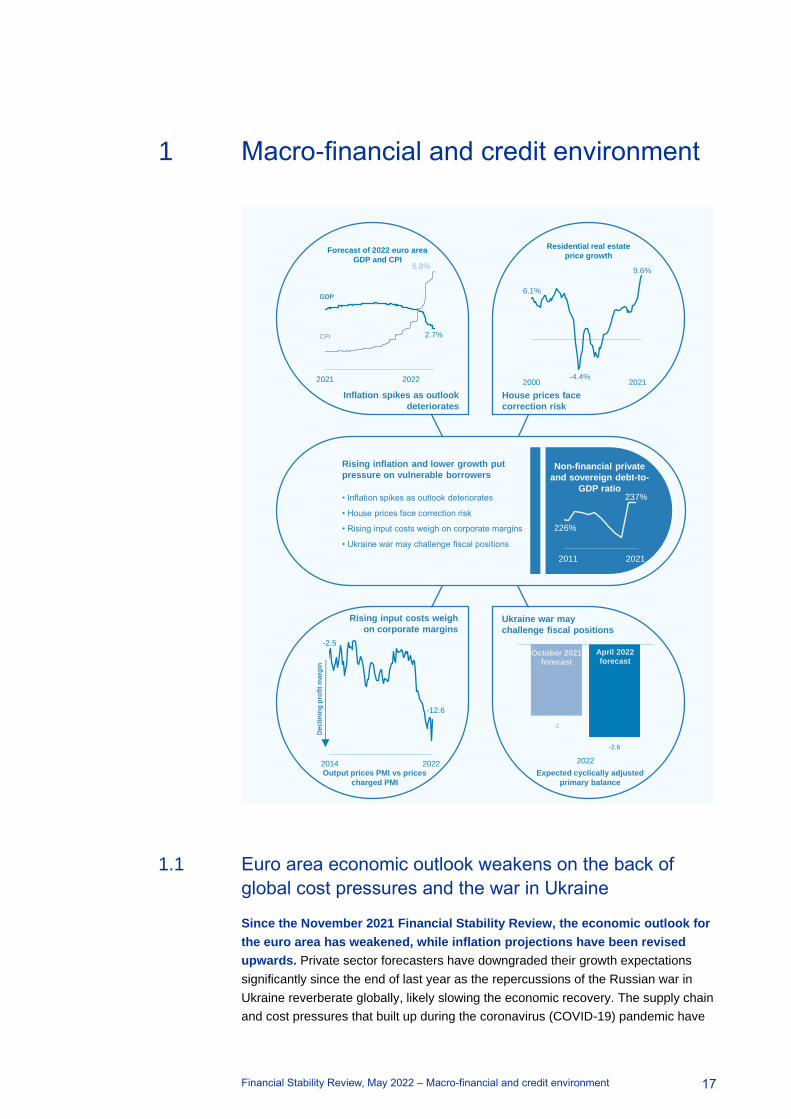
1 Macro-financial and credit environment
1.1 Euro area economic outlook weakens on the back of
global cost pressures and the war in Ukraine
Since the November 2021 Financial Stability Review, the economic outlook for
the euro area has weakened, while inflation projections have been revised
upwards. Private sector forecasters have downgraded their growth expectations
significantly since the end of last year as the repercussions of the Russian war in
Ukraine reverberate globally, likely slowing the economic recovery. The supply chain
and cost pressures that built up during the coronavirus (COVID-19) pandemic have
House prices face
correction risk
Inflation spikes as outlook
deteriorates
Ukraine war may
challenge fiscal positions
• Inflation spikes as outlook deteriorates
• House prices face correction risk
• Rising input costs weigh on corporate margins
• Ukraine war may challenge fiscal positions
Rising input costs weigh
on corporate margins
Output prices PMI vs prices
charged PMI
Rising inflation and lower growth put
pressure on vulnerable borrowers
Expected cyclically adjusted
primary balance
Forecast of 2022 euro area
GDP and CPI
Residential real estate
price growth
-2
-2.6
2022
October 2021 forecast
April 2022 forecast
2021 2022
CPI
GDP
6.8%
2.7%
-2.5
-12.6
2014 2022
Decli
nin
g p
rofi
t m
arg
in
2000 2021
9.6%
-4.4%
6.1%
Non-financial private
and sovereign debt-to-
GDP ratio
226%
237%
2011 2021
Financial Stability Review, May 2022 – Macro-financial and credit environment
18
been amplified by the war, which has prompted further increases in commodity
prices, affected supply chains and substantially weakened consumer confidence. As
a result, consensus expectations for real GDP growth in the euro area in 2022 have
been downgraded to 2.7% (down 1 percentage points since late February), while
inflation expectations have been revised upwards to 6.8% (up 2.6 percentage points
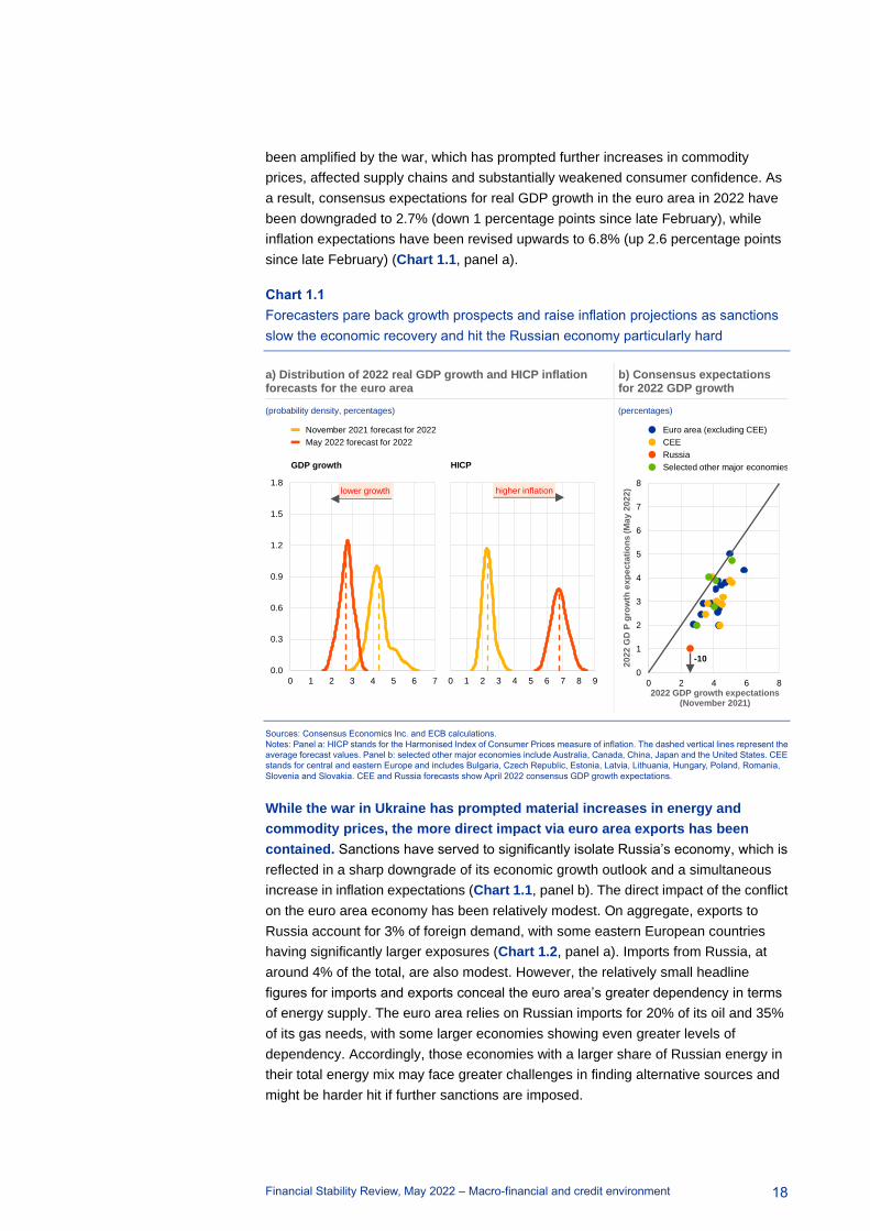
since late February) (Chart 1.1, panel a).
Chart 1.1
Forecasters pare back growth prospects and raise inflation projections as sanctions
slow the economic recovery and hit the Russian economy particularly hard
a) Distribution of 2022 real GDP growth and HICP inflation forecasts for the euro area
b) Consensus expectations for 2022 GDP growth
(probability density, percentages) (percentages)
Sources: Consensus Economics Inc. and ECB calculations.
Notes: Panel a: HICP stands for the Harmonised Index of Consumer Prices measure of inflation. The dashed vertical lines represent the
average forecast values. Panel b: selected other major economies include Australia, Canada, China, Japan and the United States. CEE
stands for central and eastern Europe and includes Bulgaria, Czech Republic, Estonia, Latvia, Lithuania, Hungary, Poland, Romania,
Slovenia and Slovakia. CEE and Russia forecasts show April 2022 consensus GDP growth expectations.
While the war in Ukraine has prompted material increases in energy and
commodity prices, the more direct impact via euro area exports has been
contained. Sanctions have served to significantly isolate Russia’s economy, which is
reflected in a sharp downgrade of its economic growth outlook and a simultaneous
increase in inflation expectations (Chart 1.1, panel b). The direct impact of the conflict
on the euro area economy has been relatively modest. On aggregate, exports to
Russia account for 3% of foreign demand, with some eastern European countries
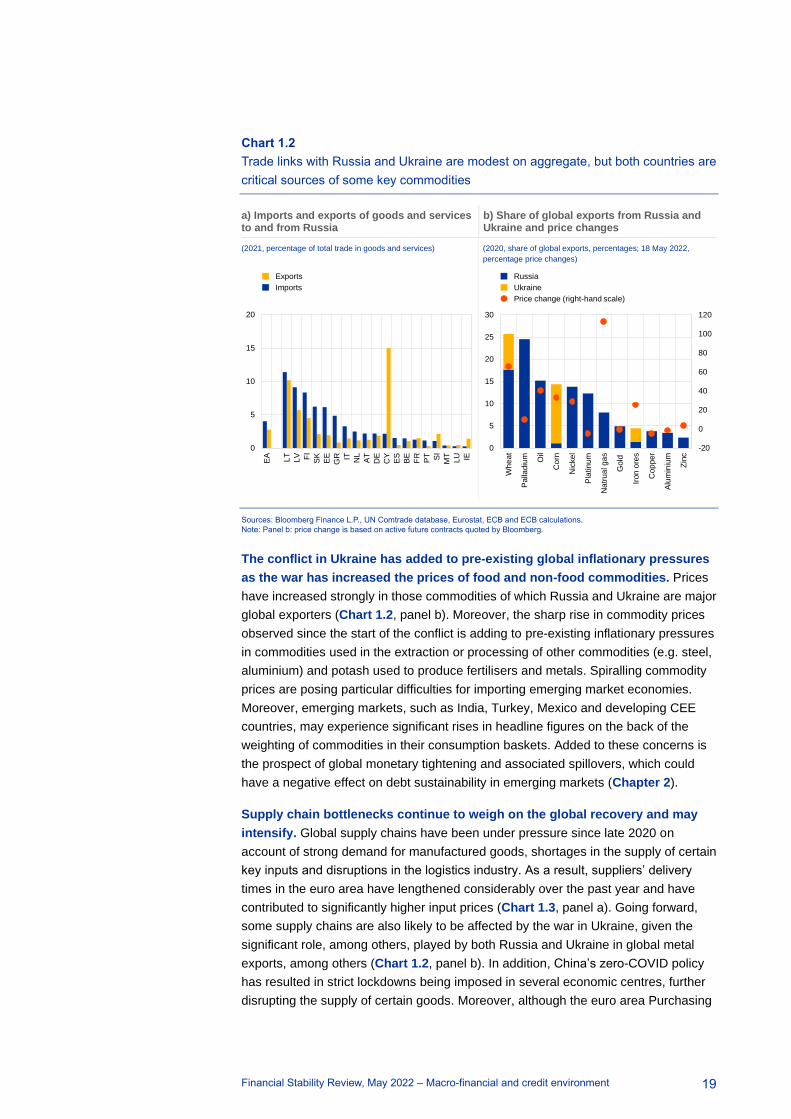
having significantly larger exposures (Chart 1.2, panel a). Imports from Russia, at
around 4% of the total, are also modest. However, the relatively small headline
figures for imports and exports conceal the euro area’s greater dependency in terms
of energy supply. The euro area relies on Russian imports for 20% of its oil and 35%
of its gas needs, with some larger economies showing even greater levels of
dependency. Accordingly, those economies with a larger share of Russian energy in
their total energy mix may face greater challenges in finding alternative sources and
might be harder hit if further sanctions are imposed.
0.0
0.3
0.6
0.9
1.2
1.5
1.8
0 1 2 3 4 5 6 7
lower growth
November 2021 forecast for 2022
May 2022 forecast for 2022
GDP growth
0 1 2 3 4 5 6 7 8 9
higher inflation
HICP
0
1
2
3
4
5
6
7
8
0 2 4 6 8
20
22
GD
P g
row
th e
xp
ec
tati
on
s (
Ma
y 2
02
2)
2022 GDP growth expectations (November 2021)
Euro area (excluding CEE)
CEE
Russia
Selected other major economies
-10
Financial Stability Review, May 2022 – Macro-financial and credit environment
19
Chart 1.2
Trade links with Russia and Ukraine are modest on aggregate, but both countries are
critical sources of some key commodities
a) Imports and exports of goods and services to and from Russia
b) Share of global exports from Russia and Ukraine and price changes
(2021, percentage of total trade in goods and services) (2020, share of global exports, percentages; 18 May 2022,
percentage price changes)
Sources: Bloomberg Finance L.P., UN Comtrade database, Eurostat, ECB and ECB calculations.
Note: Panel b: price change is based on active future contracts quoted by Bloomberg.
The conflict in Ukraine has added to pre-existing global inflationary pressures
as the war has increased the prices of food and non-food commodities. Prices
have increased strongly in those commodities of which Russia and Ukraine are major
global exporters (Chart 1.2, panel b). Moreover, the sharp rise in commodity prices
observed since the start of the conflict is adding to pre-existing inflationary pressures
in commodities used in the extraction or processing of other commodities (e.g. steel,
aluminium) and potash used to produce fertilisers and metals. Spiralling commodity
prices are posing particular difficulties for importing emerging market economies.
Moreover, emerging markets, such as India, Turkey, Mexico and developing CEE
countries, may experience significant rises in headline figures on the back of the
weighting of commodities in their consumption baskets. Added to these concerns is
the prospect of global monetary tightening and associated spillovers, which could
have a negative effect on debt sustainability in emerging markets (Chapter 2).
Supply chain bottlenecks continue to weigh on the global recovery and may
intensify. Global supply chains have been under pressure since late 2020 on
account of strong demand for manufactured goods, shortages in the supply of certain
key inputs and disruptions in the logistics industry. As a result, suppliers’ delivery
times in the euro area have lengthened considerably over the past year and have
contributed to significantly higher input prices (Chart 1.3, panel a). Going forward,
some supply chains are also likely to be affected by the war in Ukraine, given the
significant role, among others, played by both Russia and Ukraine in global metal
exports, among others (Chart 1.2, panel b). In addition, China’s zero-COVID policy
has resulted in strict lockdowns being imposed in several economic centres, further
disrupting the supply of certain goods. Moreover, although the euro area Purchasing
0
5
10
15
20
IELU
MTSI
PT
FR
BE
ES
CY
DE
AT
NLIT
GR
EE
SKFI
LV
LT
EA
Exports
Imports
-20
0
20
40
60
80
100
120
0
5
10
15
20
25
30
Wh
ea
t
Pa
llad
ium Oil
Co
rn
Nic
ke
l
Pla
tin
um
Na
tru
al g
as
Go
ld
Iron
ore
s
Co
pp
er
Alu
min
ium
Zin
c
Russia
Ukraine
Price change (right-hand scale)

Financial Stability Review, May 2022 – Macro-financial and credit environment
20
Managers’ Index (PMI) remains comfortably in expansionary territory (55.8 in April
2022), disruptions continue to weigh on the business cycle, delaying the (global)
recovery from the pandemic (Chart 1.3, panel b).
Chart 1.3
Supply chain disruptions increase input prices and depress the economic recovery
a) Euro area suppliers’ delivery times PMI versus input prices PMI
b) Euro area output PMI and supply and demand factors
(Jan. 2018-Apr. 2022, index) (Jan. 2008-Apr. 2022, deviation from long-run average)
Sources: IHS Markit, ECB and ECB calculations.
Notes: Panel a: suppliers’ delivery times shown on an inverted scale; a lower reading indicates longer supplier delivery times. First
lockdown refers to the period between March and May 2020. Panel b: historical decomposition of euro area output PMI, which was
obtained using a two-variable Bayesian VAR with output PMI and suppliers’ delivery times component of PMI, identified through sign
restrictions and estimated over the period from January 1999 to April 2022. See also the box entitled “Supply chain disruptions and the
effects on the global economy”, Economic Bulletin, Issue 8, ECB, 2021. The identification strategy was inspired by Bhushan and
Struyven*.
*) Bhushan, S. and Struyven, D., “Supply Chains, Global Growth, and Inflation”, Global Economics Analyst, Goldman Sachs Research,
20 September 2021.
The slowdown in the Chinese economy is adding to the vulnerabilities in
emerging markets and is increasing the downside risks to the global recovery.
The turmoil in China’s property development sector continued at the start of 2022,
with growth in residential real estate sales remaining negative and house prices
weakening further. In addition, strict pandemic containment policies are depressing
economic activity, which is forecast to grow at around 5% annually in the period
2022-24, significantly below the long-term average of 8%. A slowing Chinese
economy also poses additional challenges for emerging market economies with close
financial links to China. All in all, these developments add further downside risks for
global economic prospects, with a potentially significant spillover to the euro area
(Box 4).
The new economic challenges come at a time when some sectors and countries
are still recovering from the pandemic shock. Although high vaccination levels
and the less deadly Omicron variant have allowed euro area economies to largely
reopen since the start of the year, economic sectors continue to be affected
asymmetrically by the pandemic. For example, activity in the arts and entertainment
sector still lags pre-pandemic levels, while the technology sector has clearly benefited
0
10
20
30
40
50
60
70
40 50 60 70 80 90
PM
I: s
up
pli
ers
’ d
eli
ve
ry t
ime
s
PMI input prices
2018-20
2021
2022
First lockdown
-35
-30
-25
-20
-15
-10
-5
0
5
10
15
2008 2010 2012 2014 2016 2018 2020 2022
Total
Supply disruptions
Economic growth
Financial Stability Review, May 2022 – Macro-financial and credit environment
21
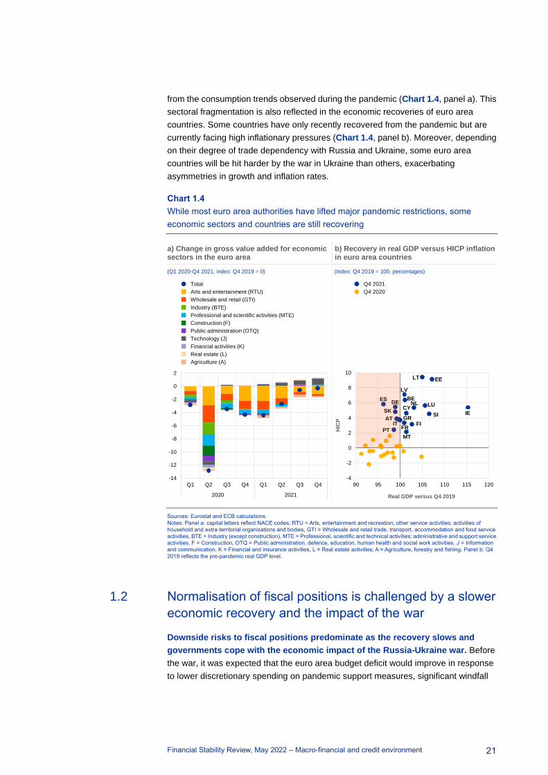
from the consumption trends observed during the pandemic (Chart 1.4, panel a). This
sectoral fragmentation is also reflected in the economic recoveries of euro area
countries. Some countries have only recently recovered from the pandemic but are
currently facing high inflationary pressures (Chart 1.4, panel b). Moreover, depending
on their degree of trade dependency with Russia and Ukraine, some euro area
countries will be hit harder by the war in Ukraine than others, exacerbating
asymmetries in growth and inflation rates.
Chart 1.4
While most euro area authorities have lifted major pandemic restrictions, some
economic sectors and countries are still recovering
a) Change in gross value added for economic sectors in the euro area
b) Recovery in real GDP versus HICP inflation in euro area countries
(Q1 2020-Q4 2021, index: Q4 2019 = 0) (index: Q4 2019 = 100, percentages)
Sources: Eurostat and ECB calculations.
Notes: Panel a: capital letters reflect NACE codes; RTU = Arts, entertainment and recreation; other service activities; activities of
household and extra-territorial organisations and bodies, GTI = Wholesale and retail trade, transport, accommodation and food service
activities, BTE = Industry (except construction), MTE = Professional, scientific and technical activities; administrative and support service
activities, F = Construction, OTQ = Public administration, defence, education, human health and social work activities, J = Information
and communication, K = Financial and insurance activities, L = Real estate activities, A = Agriculture, forestry and fishing. Panel b: Q4
2019 reflects the pre-pandemic real GDP level.
1.2 Normalisation of fiscal positions is challenged by a slower
economic recovery and the impact of the war
Downside risks to fiscal positions predominate as the recovery slows and
governments cope with the economic impact of the Russia-Ukraine war. Before
the war, it was expected that the euro area budget deficit would improve in response
to lower discretionary spending on pandemic support measures, significant windfall
-14
-12
-10
-8
-6
-4
-2
0
2
Q1 Q2 Q3 Q4 Q1 Q2 Q3 Q4
2020 2021
Total
Arts and entertainment (RTU)
Wholesale and retail (GTI)
Industry (BTE)
Professional and scientific activities (MTE)
Construction (F)
Public administration (OTQ)
Technology (J)
Financial activities (K)
Real estate (L)
Agriculture (A)
AT
BE
CYDE
EE
ES
FIFR
GRIE
IT
LT
LU
LV
MT
NL
PT
SISK
-4
-2
0
2
4
6
8
10
90 95 100 105 110 115 120
Real GDP versus Q4 2019
Q4 2021
Q4 2020
HIC
P
Financial Stability Review, May 2022 – Macro-financial and credit environment
22
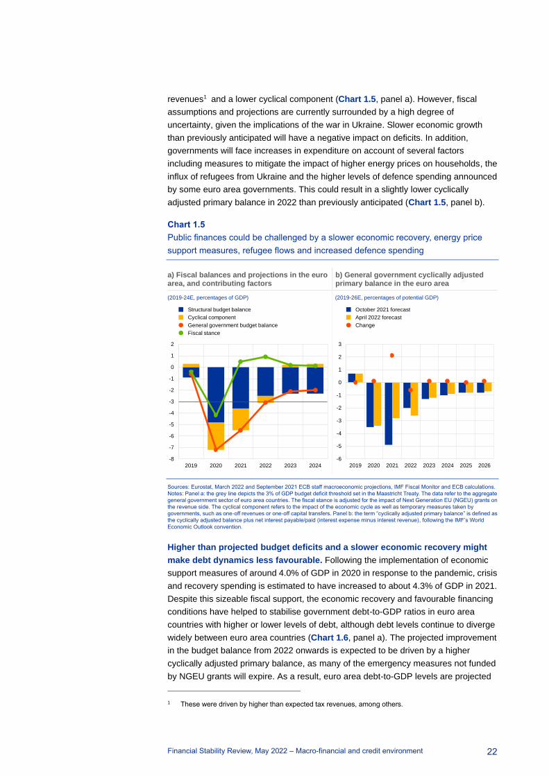
revenues1 and a lower cyclical component (Chart 1.5, panel a). However, fiscal
assumptions and projections are currently surrounded by a high degree of
uncertainty, given the implications of the war in Ukraine. Slower economic growth
than previously anticipated will have a negative impact on deficits. In addition,
governments will face increases in expenditure on account of several factors
including measures to mitigate the impact of higher energy prices on households, the
influx of refugees from Ukraine and the higher levels of defence spending announced
by some euro area governments. This could result in a slightly lower cyclically
adjusted primary balance in 2022 than previously anticipated (Chart 1.5, panel b).
Chart 1.5
Public finances could be challenged by a slower economic recovery, energy price
support measures, refugee flows and increased defence spending
a) Fiscal balances and projections in the euro area, and contributing factors
b) General government cyclically adjusted primary balance in the euro area
(2019-24E, percentages of GDP) (2019-26E, percentages of potential GDP)
Sources: Eurostat, March 2022 and September 2021 ECB staff macroeconomic projections, IMF Fiscal Monitor and ECB calculations.
Notes: Panel a: the grey line depicts the 3% of GDP budget deficit threshold set in the Maastricht Treaty. The data refer to the aggregate
general government sector of euro area countries. The fiscal stance is adjusted for the impact of Next Generation EU (NGEU) grants on
the revenue side. The cyclical component refers to the impact of the economic cycle as well as temporary measures taken by
governments, such as one-off revenues or one-off capital transfers. Panel b: the term “cyclically adjusted primary balance” is defined as
the cyclically adjusted balance plus net interest payable/paid (interest expense minus interest revenue), following the IMF’s World
Economic Outlook convention.
Higher than projected budget deficits and a slower economic recovery might
make debt dynamics less favourable. Following the implementation of economic
support measures of around 4.0% of GDP in 2020 in response to the pandemic, crisis
and recovery spending is estimated to have increased to about 4.3% of GDP in 2021.
Despite this sizeable fiscal support, the economic recovery and favourable financing
conditions have helped to stabilise government debt-to-GDP ratios in euro area
countries with higher or lower levels of debt, although debt levels continue to diverge
widely between euro area countries (Chart 1.6, panel a). The projected improvement
in the budget balance from 2022 onwards is expected to be driven by a higher
cyclically adjusted primary balance, as many of the emergency measures not funded
by NGEU grants will expire. As a result, euro area debt-to-GDP levels are projected
1 These were driven by higher than expected tax revenues, among others.
-8
-7
-6
-5
-4
-3
-2
-1
0
1
2
2019 2020 2021 2022 2023 2024
Structural budget balance
Cyclical component
General government budget balance
Fiscal stance
-6
-5
-4
-3
-2
-1
0
1
2
3
2019 2020 2021 2022 2023 2024 2025 2026
October 2021 forecast
April 2022 forecast
Change

Financial Stability Review, May 2022 – Macro-financial and credit environment
23
to decline from 95.6% of GDP in 2021 to 88.7% in 2024. Going forward, however,
risks to sovereign indebtedness are to the upside as governments face challenges
from higher than anticipated deficits and slowing economic activity. As such,
debt-to-GDP ratios might not follow the downward path currently envisaged under the
baseline scenario (Overview).
Chart 1.6
Debt ratios have declined under favourable growth dynamics as sovereign stress has
so far been contained
a) General government debt-to-GDP ratio and contributing factors for higher and lower indebted euro area countries
b) Sovereign CISS index versus general government debt-to-GDP ratio for selected euro area countries
(Q1 2020-Q4 2021, percentage points of GDP) (quantile rank, percentage points)
Sources: Eurostat, ECB and ECB calculations.
Notes: Panel a: the debt-deficit adjustment (DDA) captures the effects of the accumulation or sale of financial assets; see Kezbere and
Maurer*. The aggregate of higher-debt countries includes euro area countries with a 2019 debt-to-GDP ratio above 90%. The lower-debt
aggregate includes the remaining euro area countries. Figures are in nominal terms. Panel b: “sovereign debt crisis” refers to November
2011, “pandemic” refers to April 2020 and “Russia-Ukraine war” to April 2022. CISS stands for composite indicator of systemic stress.
The chart shows the euro area countries for which a sovereign CISS Index is available, i.e. Belgium, Germany, Ireland, Greece, Spain,
France, Italy, the Netherlands, Austria, Portugal and Finland.
*) Kezbere, L. and Maurer, H., “Deficit-debt adjustment (DDA) analysis: an analytical tool to assess the consistency of government
finance statistics”, Statistics Paper Series, No 29, ECB, November 2018.
Higher than expected inflation can contribute to debt servicing pressures,
especially in cases of high refinancing needs and relatively large shares of
inflation-indexed securities. Although debt ratios would benefit from a declining real
debt burden owing to first round effects (a favourable denominator effect), higher risk
premia and slower economic growth could still contribute to increasing debt ratios in
the medium term, particularly for high-debt countries.2 As such, additional fiscal
space to cushion the economy from future economic downturns might become more
limited in some euro area countries. Moreover, the level of recovery from the
pandemic and inflation rates diverge widely across euro area countries, contributing
to higher fragmentation risks (Section 1.1).
2 See the box entitled “Sensitivity of sovereign debt in the euro area to an interest rate-growth differential
shock”, Financial Stability Review, ECB, November 2021.
-15
-10
-5
0
5
10
15
20
25
Q1 Q2 Q3 Q4 Q1 Q2 Q3 Q4 Q1 Q2 Q3 Q4 Q1 Q2 Q3 Q4
2020 2021 2020 2021
High-debt Low-debt
Change in debt-to-GDP
Primary balance
Debt-deficit adjustment
Interest
Economic growth
0.0
0.2
0.4
0.6
0.8
1.0
1.2
40 90 140 190 240
So
ve
reig
n C
ISS
in
de
x
SovCISS Russia-Ukraine war
SovCISS pandemic
SovCISS sovereign debt crisis
Debt-to-GDP

Financial Stability Review, May 2022 – Macro-financial and credit environment
24
Financing conditions for euro area sovereigns have remained favourable
overall. Although government bond yields have increased of late, financing
conditions have remained relatively favourable in recent months, despite the
heightened uncertainty, increasing sovereign bond yields and deteriorating
macroeconomic backdrop. Moreover, although measures of sovereign stress are
rising, so far this has not affected higher-debt countries more than other euro area
countries (Chart 1.6, panel b). In addition, governments had extended the average
residual maturity to eight years by the end of March 2022, mostly by issuing
longer-term securities, increasing their resilience to rising interest rates. At the same
time, debt servicing needs remain elevated, with some euro area countries facing
refinancing and interest expenditure in excess of 40% of GDP over the next two
years. As such, a further deterioration in financial conditions could weigh on fiscal
positions going forward.
All in all, risks to sovereign debt sustainability appear to be manageable in the
short run, but sovereign risks could intensify in the event of a sustained rise in
credit risk premia or more subdued growth outturns. Although sovereign yields
have increased of late, the economic recovery at the end of 2021 and largely
favourable financing conditions have helped to stabilise debt levels in the euro area.
Going forward, fiscal policy will be affected by both exposure to the war and recovery
from the pandemic. Moreover, the fundamental role of economic growth dynamics in
determining fiscal sustainability underlines the need for fiscal policy to be
growth-friendly. The NGEU package could provide additional cushioning for the euro
area economy and trigger the kind of reforms required to boost long-term growth
potential. Adding to sovereign risks, some sovereigns with higher debt are also
exposed to weaker banks and exhibit a less robust, more fragmentated corporate
landscape, increasing risks relating to a sovereign-bank-corporate nexus (Box 1).
These adverse developments could trigger a reassessment of sovereign risk by
market participants and reignite pressures on more vulnerable sovereigns.
1.3 Corporates face new headwinds as supply bottlenecks
persist
Following the solid recovery seen in the second half of 2021, euro area
corporates are now facing increasing headwinds from rising producer prices
and supply chain pressures. Measures of aggregate corporate vulnerabilities
improved as the economy experienced a robust recovery in the second half of 2021,
with gross profits bouncing back to 7% above pre-pandemic levels. Moreover, the
economic recovery and pandemic support measures have helped to keep financing
conditions favourable, cushioning debt service needs and rollover risks. As a result,
the composite indicator for euro area corporate vulnerabilities has remained well
below its historical average (Chart 1.7, panel a). However, corporates now face new
headwinds stemming from a slowing economy, higher interest rates, worsening
supply chain bottlenecks and rising energy prices (Section 1.1).

Financial Stability Review, May 2022 – Macro-financial and credit environment
25
Chart 1.7
Euro area non-financial corporates have benefited from favourable financing
conditions and robust profits, but activity remains subdued
a) Composite indicator of corporate vulnerabilities and contributing factors
b) Ratio of sales and EBIT to total assets for euro area non-financial corporations
(Q1 2004-Q1 2024E, z-scores) (Q1 2000-Q4 2021, percentages)
Sources: Eurostat, ECB, IHS Markit and ECB calculations.
Notes: Panel a: positive values indicate higher vulnerability and negative values indicate lower vulnerability. The shaded area represents
a forecast. For the construction of the index in more detail, see the box entitled “Assessing corporate vulnerabilities in the euro area”,
Financial Stability Review, ECB, November 2020. Panel b: total assets are the sum of total financial and non-financial assets (liabilities)
of non-financial corporations. Sales and earnings before interest and taxes (EBIT) are approximated by the four-quarter moving average
of gross value added and mixed income respectively, as reported in the quarterly sector accounts. Series multiplied by 100.
The sharp increase in input prices may squeeze corporate profit margins.
Despite the robust recovery in corporate earnings, activity in the corporate sector
remained subdued towards the end of 2021 (Chart 1.7, panels a and b). Moreover,
corporate profitability partially recovered on account of higher profit margins,
offsetting the more persistent loss in output since the start of the pandemic (Chart
1.7, panel b). Going forward, it might become harder for some sectors to sustain high
profit margins as input prices soar in many sectors and the economy slows. Higher
input prices currently translate into expectations of increased selling prices going
forward, especially for sectors with high energy consumption and low inventories
(Chart 1.8, panel a). At the same time, some firms have started to indicate that input
prices are increasing faster than output prices, possibly resulting in margin
compression. This seems to be the case for the corporates that still face challenges
stemming from the pandemic and for corporates with high energy needs, such as
manufacturers of metals (Chart 1.8, panel b). Historically, higher input prices are
largely passed on to end users, particularly when the cost-push shock is global,
although given the fact that the economic outlook has softened considerably some
producers might have less pricing power going forward. Moreover, the magnitude of
current price volatility could be a concern for companies with (unhedged) fixed
contractual obligations, and which cannot easily adjust pricing, such as utilities and
construction firms (Chapter 2).
-1.0
-0.5
0.0
0.5
1.0
1.5
2.0
2004 2007 2010 2013 2016 2019 2022
Debt servicing capacity
Leverage/indebtedness
Financing/rollover
Profitability
Activity
Composite
Q2 2020
Q3 2020Q4 2020
Q1 2021
Q2 2021
Q3 2021
Q4 2021
19.0
19.5
20.0
20.5
21.0
21.5
22.0
22.5
7.5 8 8.5 9 9.5
Sa
les
/to
tala
ss
ets
EBIT/total assets
Q1 2000-Q1 2020
Q2-Q4 2020
Q1-Q4 2021

Financial Stability Review, May 2022 – Macro-financial and credit environment
26
Chart 1.8
Margins might come under pressure as input prices soar and the economy slows
a) Selling price expectations versus use of energy as input and inventory level
b) Euro area output prices PMI minus producer prices PMI
(Apr. 2022, index) (Apr. 2022, index)
Sources: OECD Trade in Value Added (TiVA) database (2018), European Commission, Eurostat, IHS Markit and ECB calculations.
Notes: Panel a: energy intensity measured is measured by the average share of input from mining and quarrying, energy producing
products, coke and refined petroleum product and the electricity, gas, steam and air-conditioning industries for each sector, classified
according to the United Nations International Standard Industrial Classification for All Economic Activities (ISIC), Rev. 4. Rev. 4. ISIC
codes are converted back to NACE codes and matched with survey data on selling price expectations. Selling price expectations reflect
seasonally adjusted selling price expectations for the services, retail and industry sectors. The data are extracted on subsector level from
the European Commission business and consumer surveys. Direct and indirect energy use reflect 2018 figures. Selling price
expectations reflect expectations from the April 2022 European Commission Business and consumer surveys. Panel b: shown as the
PMI output price index minus the producer prices PMI on sector level. A narrowing spread between output and producer prices PMIs can
be interpreted as margin compression.
External financing needs have risen in response to robust economic activity,
but the economic impact of the war in Ukraine might dampen credit growth
going forward. Bank lending to corporates continued to increase in the first months
of 2022, but moderated in March as credit standards tightened, and risk perceptions
increased as a result of the war in Ukraine. During the first months of the year the
demand for loans remained high on account of high working capital and fixed
investment requirements. The need for higher working capital mainly reflects
financing demands created by the pandemic situation, while the increase in fixed
investment is driven by the economic recovery. Amid a wide range across firms and
euro area countries, debt levels declined to 80% of GDP in the fourth quarter of 2021
but remained above the 75% of GDP recorded before the pandemic.3 The increase in
net debt has been much less pronounced, reflecting elevated working capital levels
and liquid holdings (Chart 1.9, panel a). Going forward, corporate financing
conditions might deteriorate when economic growth slows, inflation remains elevated
and both markets and banks reassess the risk surrounding corporate activity
(Chapter 2). Moreover, banks anticipate a stronger net tightening of credit standards
in the future, reflecting the uncertain economic impact of the war. This might be
3 This reflects consolidated debt securities and loans of non-financial corporations as a share of GDP.
Mineral products
Paper productsFood
products
Land transport and transport via pipelines
Chemicals
Basic metals
0
10
20
30
40
50
60
70
80
0 5 10 15 20 25
Below-average stock level
Above-average stock level
Direct and indirect energy use
Se
llin
g p
ric
e e
xp
ec
tati
on
s (
thre
e-m
on
ths
ah
ea
d)
-25 -20 -15 -10 -5 0 5
Accommodation
Motor vehicles
Warehousing
Consumer goods ex food
Basic materials
Consumer goods
Fabricated metal
Professional/scientific activities
Other professional/scientific activities
Financial services
Capital goods
Textiles
Consultancy
Transport and storage
Basic metals
Food and beverages
Computer/electronic products
Chemicals
Intermediate goods
Rubber and plastics
Manufacture of coke, refined petroleum
Machinery equipment
Wood and paper
Composite
Services
Manufacturing
Manufacturing
Services

Financial Stability Review, May 2022 – Macro-financial and credit environment
27
particularly concerning for firms that exited the pandemic with high debt levels,
subdued earnings and lower liquidity buffers (Chart 1.9, panel b, and Box 1).
Chart 1.9
The increase in debt levels has varied across firms and euro area countries as default
rates might rise
a) Changes in liquid assets, gross debt and debt service ratio for euro area non-financial corporations
b) Earnings per share, indebtedness and current ratio for EURO STOXX sectors
c) Euro area expected default frequency versus real GDP growth
(Q4 2019-Q4 2021, ratio) (Q1 2022, sub-index averages) (Q1 2006-Q1 2022, percentage changes,
percentages)
Sources: Bank for International Settlements, Bloomberg Finance L.P., Moody’s Analytics, ECB and Eurostat.
Notes: Panel a: “Liquid assets” comprises currency and deposits; “Gross debt” refers to consolidated debt securities and loans of
non-financial corporations; “Net debt” is the difference between gross debt and liquid assets. The debt service ratio (DSR) is defined as
the ratio of interest payments plus amortisations to income. As such, the DSR provides a flow-to-flow comparison – the flow of debt
service payments divided by the flow of income; see “How much income is used for debt payments? A new database for debt service
ratios”, BIS Quarterly Review, September 2015. Panel b: earnings per share reflect Bloomberg consensus estimates for the sector level
sub-indices of the STOXX EUROPE index. The total debt and current ratio are sub-index averages. The current ratio reflects the ratio of
current assets to current liabilities and measures a firm’s ability to settle short-term liabilities with its short-term assets.
Insolvencies, which would normally be expected to rise as economic growth
softens, have remained well below their pre-pandemic levels. Policy support
measures have successfully mitigated solvency risks which, together with robust
economic growth, kept insolvencies 20% below their pre-pandemic levels in the first
quarter of 2022. Moreover, forward-looking measures for defaults remain subdued
(Chart 1.9, panel c). At the same time, firms whose balance sheets weakened by the
pandemic now face fresh challenges from strong input price inflation, softening
economic growth and rising interest rates. Furthermore, results from the latest ECB
bank lending survey show banks indicating that they are concerned that supply chain
disruptions, high energy and other input prices, and corporate exposures to Russia,
Ukraine and Belarus might amplify firms’ credit risks. As such, insolvencies could rise
in the sectors most affected by supply chain disruptions and by an economic recovery
that has proved fragile since the pandemic.
Overall, firms weakened by the pandemic now face additional challenges from
intensifying cost pressures as the economic recovery slows. Some countries
and sectors have experienced an increase in net debt levels since the start of the
pandemic. Moreover, some corporates will also face significant debt servicing needs
0
10
20
30
40
50
60
70
-0.2
-0.1
0.0
0.1
0.2
DE FR ES IT BE PT NL
Liquid assets (-)
Gross debt
Net debt
DSR (right-hand scale)
Utilities
Travel
Media
Personal care
Real estate
15
20
25
30
35
40
45
0 20 40 60 80 100
To
tal d
eb
t/to
tal a
ss
ets
Earnings per share
Current ratio > 1.3
Current ratio 1-1.3
Current ratio <1
-20
-15
-10
-5
0
5
10
15
20
2006 2010 2014 2018 2022
Expected default frequency
GDP

Financial Stability Review, May 2022 – Macro-financial and credit environment
28
over the coming years (Chart 1.9, panel a). Although public guarantee schemes have
helped corporates to attract longer-term funding during the pandemic and corporates
have built significant cash buffers, a possible further rise in interest rates might impact
non-financial corporations that borrow at variable rates. In addition, some firms have
been less able to profit from the economic recovery over recent quarters as their
business models have continued to be affected by pandemic containment measures.
Some of these corporations also have higher debt, lower liquidity and lower sales
levels and might face challenges when the economy slows or if they cannot pass on
increases in input prices to end users in full (Box 1). Adding further to these
vulnerabilities, weaker corporates are also concentrated in countries with greater
sovereign and bank vulnerabilities.
Box 1
Identifying the corporates most vulnerable to price shocks following the pandemic
Prepared by Julian Metzler, Benjamin Mosk, Nander de Vette and Peter Welz
By the end of 2021, the aggregate profitability and debt positions of euro area non-financial
corporations (NFCs) had recovered to pre-pandemic levels. While overall gross debt relative to
gross value added remains elevated at around 160%, net debt has returned to its pre-pandemic level
of around 100% of gross value added, with firms having increased precautionary cash buffers amid
favourable financing conditions. However, these aggregate developments were mostly driven by
large firms, while the net debt positions of small firms increased as they used credit to offset those
cash flow losses that were not covered by government support measures. In addition, many
corporates now face broad-based increases in input prices on the back of energy price rises and
supply chain disruptions. Against this backdrop, this box uses firm-level balance sheet data for
around 91,000 euro area non-financial corporations to identify vulnerable firms based on the Altman
Z-score, a measure of insolvency risk that uses five balance sheet and income statement ratios and
their joint importance.4, 5, 6 It then matches bank and sovereign exposures to consider related risks
associated with the sovereign-bank-corporate nexus.
Although corporate revenues deteriorated sharply during the COVID-19 pandemic, policy
support measures helped to keep insolvencies remarkably subdued. The economic effects of
the pandemic have weakened firms’ balance sheets, particularly in the services sector. At the same
time, firms in technology and many consumer goods sectors also benefited (Chart A, panel a).
Declining revenues appear to have been the biggest driver of deteriorating financial health.
Firm-level data also suggest that more leveraged firms experienced a larger decline in financial
health (Chart A, panel b), and firms classified as weak had relatively higher debt, lower earnings and
lower revenues than firms classified as healthy. Compared with the broad-based revenue declines,
earnings and margins remained relatively resilient. This can be explained in part by government
support measures.7
An increase in liabilities, lower liquidity levels and subdued earnings continue to pose a risk
for a subset of companies. Translating Altman Z-scores into implied corporate credit ratings, the
4 For more details, see Casey, C.J., Bibeault, D. and Altman, E.I., “Corporate financial distress: A
Complete guide to Predicting, Avoiding, and Dealing with Bankruptcy”, Journal of Business Strategy
(pre-1986), Vol. 5, Issue 000001, 1984, p. 102f.
5 See also the article entitled “Assessing corporate vulnerabilities in the euro area”, Economic Bulletin,
Issue 2, ECB, 2022.
6 The results reported in this box pertain to the specific sample at hand, which is not fully representative for
the overall corporate sector as it contains relatively fewer micro firms.
7 See also the box entitled “The role of profit margins in the adjustment to the COVID-19 shock”, Economic
Bulletin, Issue 2, ECB, 2021.
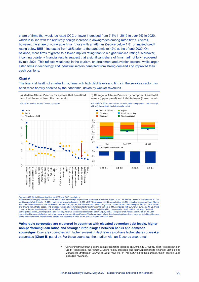
Financial Stability Review, May 2022 – Macro-financial and credit environment
29
share of firms that would be rated CCC or lower increased from 7.5% in 2019 to over 9% in 2020,
which is in line with the relatively benign increase in downgrades among rated firms. Overall,
however, the share of vulnerable firms (those with an Altman Z-score below 1.81 or implied credit
rating below BBB-) increased from 36% prior to the pandemic to 42% at the of end 2020. On
balance, more firms migrated to a lower implied rating than to a higher implied rating.8 Moreover,
incoming quarterly financial results suggest that a significant share of firms had not fully recovered
by mid-2021. This reflects weakness in the tourism, entertainment and aviation sectors, while larger
listed firms in technology and industrial sectors benefited from strong demand and improved their
cash positions.
Chart A
The financial health of smaller firms, firms with high debt levels and firms in the services sector has
been more heavily affected by the pandemic, driven by weaker revenues
Sources: S&P Global Market Intelligence, ECB and ECB calculations.
Notes: Panel a: the grey line reflects the weaker firm threshold (1.81) based on the Altman Z-score as at end-2020. The Altman Z-score is calculated as 0.717 x
working capital/total assets + 0.847 x retained earnings/total assets + 3.107 x EBIT/total assets + 0.420 x equity/debt + 0.998 sales/total assets. A higher Altman
Z-score is associated with lower default risk. Sample size (N) = 91,649. The sample contains roughly half of the total debt outstanding for NFCs in the euro area
and around 40% of total assets. The leverage ratio (total debt/total assets) for the firms in the sample is 34% compared with 30% for all euro area NFCs. Panel
b: sum of the median changes in the variables included in the Altman Z-score: working capital (working capital/total assets), retained earnings (retained
earnings/total assets), earnings (EBIT/total assets), revenue (sales/total assets) and equity (equity/debt). The upper chart reflects the impact on the 25th
percentile of firms most affected by the pandemic in terms of Altman Z-score. The lower panel reflects the change in Altman Z-score per bucket of indebtedness
measured by the firm’s total debt/total assets. The debt level is fixed on the end-2019 debt and asset level.
Vulnerable corporates are clustered in countries with elevated sovereign debt levels, higher
non-performing loan ratios and stronger interlinkages between banks and domestic
sovereigns. Euro area countries with higher sovereign debt levels also have higher shares of weaker
corporates (Chart B, panel a). For those countries, the median Altman Z-scores also remain
8 Converting the Altman Z-score into a credit rating is based on Altman, E.I., “A Fifty-Year Retrospective on
Credit Risk Models, the Altman Z-Score Family of Models and their Applications to Financial Markets and
Managerial Strategies”, Journal of Credit Risk, Vol. 14, No 4, 2018. For this purpose, the z’’-score is used
excluding revenues.
a) Median Altman Z-score for sectors that benefited and lost the most from the pandemic
b) Change in Altman Z-score by component and total assets (upper panel) and indebtedness (lower panel)
(2019-20, median Altman Z-score by sector) (Q4 2019-Q4 2020, upper chart: sum of median components, total assets (€
millions), lower chart: total debt/total assets)
0
1
2
3
4
5
6
He
alth
ca
re s
erv
ice
s
He
alth
ca
re d
istr
ibu
tors
Meta
l a
nd
gla
ss c
on
tain
ers
Foo
twe
ar
Ag
ricu
ltu
ral p
rod
ucts
Pa
pe
r p
acka
gin
g
Ho
use
ho
ld p
rod
ucts
Ho
me f
urn
ishin
gs
So
ft d
rin
ks
Tyre
s a
nd
ru
bb
er
{…}
Em
plo
ym
en
t se
rvic
es
Re
sta
ura
nts
Co
pp
er
Ca
sin
os a
nd
gam
ing
Film
s a
nd
en
tert
ain
me
nt
Inte
gra
ted
oil
and
ga
s
Air
po
rt s
erv
ice
s
Multi-
se
cto
r h
old
ings
Ho
tels
an
d r
eso
rts
Air
line
s
2020
2019
Threshold = 1.81
-0.8
-0.7
-0.6
-0.5
-0.4
-0.3
-0.2
-0.1
0.0
0.1
2-50 50-1,000 >1,000
Altman Z-score
Earnings
Revenue
Equity
Retained earnings
Working capital
-0.3
-0.2
-0.1
0.0
0.01-0.1 0.1-0.2 0.2-0.3 0.3-0.4
Change in Altman Z-score

Financial Stability Review, May 2022 – Macro-financial and credit environment
30
significantly below the pre-pandemic levels. In addition, spillover vulnerabilities exist in several
countries due to a tighter sovereign-corporate-bank nexus. These countries tend to have higher
shares of vulnerable corporates, and banks hold larger credit exposures to the domestic sovereign; at
the same time, the sovereign has provided sizeable loan guarantees, notably for loans to firms in
vulnerable sectors (Chart B, panel b).
Chart B
Corporate vulnerabilities are clustered in countries with elevated sovereign debt and weaker banks
Sources: OECD Trade in Value Added (TiVA) database (2018), S&P Global Market Intelligence and ECB calculations.
Notes: Panel a: a higher Altman Z-score is associated with lower default risk. The chart excludes Estonia, Cyprus, Latvia, Lithuania, Luxembourg, Malta,
Slovakia and Slovenia due to low firm count in the sample. The bubble size reflects the gross NPL ratio. Sample size (N) = 91,649. Panel b: PGS stands for public
guarantee scheme. Yellow circles represent low Altman Z-score countries, i.e. those with a Z-score<1.81. Panel c: converting the Altman Z-score into a credit
rating is based on Table 6 in Altman E.I., op. cit. To this end, the modified Altman Z’’-score is used, which exclude a revenue component. IG stands for investment
grade; HY stands for high-yield. Direct and indirect energy use is measured by the average share of input from mining and quarrying, energy producing products,
coke and refined petroleum product and the electricity, gas, steam and air-conditioning industries for each sector, classified according to the United Nations
International Standard Industrial Classification for All Economic Activities (ISIC), Rev. 4. This is attributed to each sector based on the 4-digit SIC code.
Weaker firms and firms with lower pricing power are more vulnerable to supply chain
disruptions and rising input prices. Indices measuring input prices for euro area producers
increased strongly over the course of 2021 and the first months of 2022, driven by higher energy
costs and supply bottlenecks. Moreover, some key input materials showed double-digit price rises.
The large increase in input prices and costs will likely put pressure on profit margins, notably for firms
that have weaker pricing power and cannot easily pass on price increases. This could create cash
flow challenges in the short run and undermine the debt sustainability and investment capacity in the
medium term. Vulnerabilities are concentrated in firms at the intersection of lower pricing power and
those with higher energy intensity of production and lower Altman Z-scores (Chart B, panel c).
All in all, corporate vulnerabilities remain and are correlated with exposures to the pandemic
and the fallout from the Russian war in Ukraine. The corporate sector on aggregate proved
resilient to the pandemic shock, as reflected in the recovery of profits. However, the euro area has a
sizeable cohort of vulnerable smaller firms that are still recovering from the pandemic and are now
facing additional cost pressures from the sharp rise in input prices observed over recent months. At
the current juncture, financing conditions remain in their favour, but they could deteriorate quickly if
the economy slows and lenders reassess the risks relating to certain business models. Moreover,
uncertainty will reduce investment and contribute to bleaker growth prospects going forward.
a) Altman Z-score by sovereign debt level and NPL ratio
b) Guaranteed lending and euro area banks’ sovereign exposure
c) Implied rating by industry and energy use
(Q4 2020, percentage of GDP, percentage of total
loans)
(Q4 2021, percentage of total loans, weighted
median Z-score)
(2020, percentage of total output in 2018)
AT
BEFI
FR
DE
GR
IE
IT
NL
PTES
0
50
100
150
200
250
0.2 0.4 0.6 0.8 1
So
ve
reig
n d
eb
t (p
erc
en
tag
e o
f G
DP
)
Share of vulnerable firms
NPL ratio
0
5
10
15
20
25
0 5 10
Do
me
sti
c s
ove
reig
n e
xp
os
ure
Share of PGS loans
Other countries
Vulnerable countries
Oil and gas storage and
transportation
Gas utilities
MarineAir freight
and logistics
Road freight
Airlines
Railways
Copper
0
5
10
15
20
25
2345678910
Dir
ec
t a
nd
in
dir
ec
t e
ne
rgy u
se
AAA AA A+ A BBB+ BB+ B CCC
Credit rating
IG rating
HY rating, <75th percentile energy input
HY rating, >75th percentile energy input
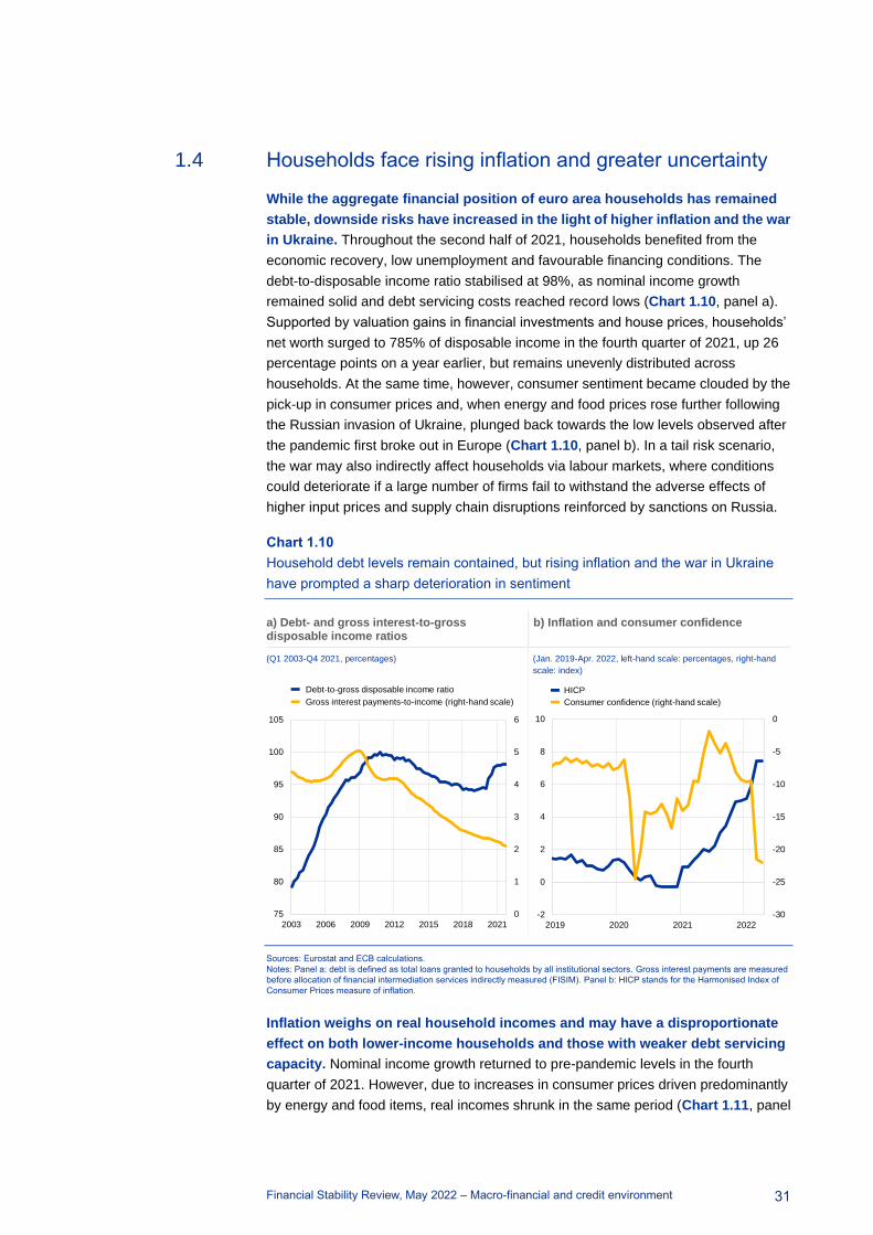
Financial Stability Review, May 2022 – Macro-financial and credit environment
31
1.4 Households face rising inflation and greater uncertainty
While the aggregate financial position of euro area households has remained
stable, downside risks have increased in the light of higher inflation and the war
in Ukraine. Throughout the second half of 2021, households benefited from the
economic recovery, low unemployment and favourable financing conditions. The
debt-to-disposable income ratio stabilised at 98%, as nominal income growth
remained solid and debt servicing costs reached record lows (Chart 1.10, panel a).
Supported by valuation gains in financial investments and house prices, households’
net worth surged to 785% of disposable income in the fourth quarter of 2021, up 26
percentage points on a year earlier, but remains unevenly distributed across
households. At the same time, however, consumer sentiment became clouded by the
pick-up in consumer prices and, when energy and food prices rose further following
the Russian invasion of Ukraine, plunged back towards the low levels observed after
the pandemic first broke out in Europe (Chart 1.10, panel b). In a tail risk scenario,
the war may also indirectly affect households via labour markets, where conditions
could deteriorate if a large number of firms fail to withstand the adverse effects of
higher input prices and supply chain disruptions reinforced by sanctions on Russia.
Chart 1.10
Household debt levels remain contained, but rising inflation and the war in Ukraine
have prompted a sharp deterioration in sentiment
a) Debt- and gross interest-to-gross disposable income ratios
b) Inflation and consumer confidence
(Q1 2003-Q4 2021, percentages) (Jan. 2019-Apr. 2022, left-hand scale: percentages, right-hand
scale: index)
Sources: Eurostat and ECB calculations.
Notes: Panel a: debt is defined as total loans granted to households by all institutional sectors. Gross interest payments are measured
before allocation of financial intermediation services indirectly measured (FISIM). Panel b: HICP stands for the Harmonised Index of
Consumer Prices measure of inflation.
Inflation weighs on real household incomes and may have a disproportionate
effect on both lower-income households and those with weaker debt servicing
capacity. Nominal income growth returned to pre-pandemic levels in the fourth
quarter of 2021. However, due to increases in consumer prices driven predominantly
by energy and food items, real incomes shrunk in the same period (Chart 1.11, panel
0
1
2
3
4
5
6
75
80
85
90
95
100
105
2003 2006 2009 2012 2015 2018 2021
Debt-to-gross disposable income ratio
Gross interest payments-to-income (right-hand scale)
-30
-25
-20
-15
-10
-5
0
-2
0
2
4
6
8
10
2019 2020 2021 2022
HICP
Consumer confidence (right-hand scale)

Financial Stability Review, May 2022 – Macro-financial and credit environment
32
a). Many households may be able to temporarily cushion the impact of higher prices
by scaling back saving or drawing on excess savings accumulated during the
pandemic. But these savings are likely concentrated in higher-income households,
whereas lower-income households are more exposed to the inflation shock as they
spend a relatively larger share of their income on energy and food-related items
(Chart 1.11, panel b). Accordingly, a share of households has to rely on fiscal relief
measures or cut down on non-essential consumption. In general, some households
may benefit from higher than expected inflation in the sense that it lowers the real
cost of pre-existing debt, but it is unlikely that these households are sufficiently
compensated for the rise in inflation through higher nominal income.
Chart 1.11
A decline in real incomes may disproportionately affect lower income households
a) Growth in nominal and real disposable income and savings ratio
b) Monthly income spent on energy and food
c) Impact of a 100 basis point interest rate increase on household debt-to-GDP and interest payment-to-GDP ratios
(Q1 2018-Q4 2021, percentages) (Q1 2022, left-hand scale: percentages,
right-hand scale: €)
(2021-24E, percentages)
Sources: Eurostat, ECB (Consumer Expectations Survey) and ECB calculations.
Notes: Panel b: data cover surveys from Belgium, Germany, Spain, France, Italy and the Netherlands. The share of income spent on
energy and food is calculated as the share of households’ reported spending on utilities, transport and food, beverages, groceries and
tobacco divided by monthly income, where income is inferred from income buckets. Data shown are averages over the full period for
which CES data are available, i.e. April 2020 to January 2022. Questions on spending are surveyed once per quarter. Accordingly, the
data should be interpreted with caution and mainly as an illustration of differences across different income classes. Panel c: shaded bars
show projections. The simulations capture the effects of a permanent one-off 100 basis point increase in short and long-term market
interest rates in July 2022 (with higher rates kept constant thereafter) on gross interest payments (based on a national accounts concept
before FISIM allocation) and consolidated gross indebtedness ½, 1½ and 2½ years after the shock. The results are based on models and
tools used in the context of the Eurosystem projection exercises. They take into account the dampening impact of higher market interest
rates on economic activity, prices and debt financing. The increase in the household debt-to-GDP ratio is mostly due to a denominator
effect as GDP is projected to decline more than debt levels.
Vulnerabilities among households have picked up, albeit from generally
moderate levels. With strong balance sheets thanks to excess savings, solid net
wealth and low debt servicing costs, households are well positioned to weather
economic headwinds. At the same time, rising inflation is having an adverse effect on
households’ purchasing power, which could slow the economy’s return to its
pre-pandemic growth path. Some households may have to limit consumption or
become dependent on government support. While the impact of rising interest rates
on aggregate household indebtedness and interest payments may be limited (Chart
0
4
8
12
16
20
24
28
-6
-4
-2
0
2
4
6
8
2018 2019 2020 2021
Nominal disposable income growth
Real disposable income growth
Savings ratio (right-hand scale)
450
500
550
600
650
700
0
10
20
30
40
50
1 2 3 4 5
Share of income
Euro amounts (right-hand scale)
Income quintile
1.0
1.1
1.2
1.3
1.4
1.5
1.6
57
58
59
60
61
62
63
2021 2022 2023 2024
Household debt-to-GDP ratio
Household gross interest payments-to-GDP ratio (right-hand scale)

Financial Stability Review, May 2022 – Macro-financial and credit environment
33
1.11, panel c), some households’ debt servicing capacity could suffer. Vulnerabilities
could build further over the medium term and concerns over household debt
sustainability may rise, especially in countries where residential properties are
overvalued, debt levels are elevated and a larger share of household debt has
variable interest rates.
1.5 Vulnerabilities continue to build in euro area real estate
markets
Prices in euro area residential real estate (RRE) markets rose at a record pace,
resulting in increasingly stretched valuations. Nominal house prices rose by 9.6%
year-on-year at the euro area level in the fourth quarter of 2021, the fastest rate
observed in the last 20 years (Chart 6, panel a, Overview). The key factors putting
upward pressure on prices are the low cost of borrowing coupled with stronger
demand for housing stemming from shifts in household preferences (e.g. demand for
home office space) and supply-side constraints. Shortages of both labour and
materials are raising expectations of increasing prices in the construction sector,
contributing to further upward pressure on house prices going forward. Such growing
supply-side constraints, together with flight-to-safety effects amid higher inflation,
may be exacerbated by the war in Ukraine. As house price dynamics exceed the
fundamentals, estimates of overvaluation are also growing (Chart 1.12, panel a).
Accelerating mortgage lending has increased household indebtedness, raising
concerns of further debt-fuelled house price rises. Lending for house purchase in
the euro area remains robust, with the pace of growth at 5.4% in March 2022,
contributing to the build-up of household debt. Patterns vary greatly from country to
country: in some euro area countries, upward movements in both house prices and
lending are pronounced, indicating that a price-loan spiral may have started
emerging. Overall, while most euro area countries have macroprudential measures in
place, a further build-up of medium-term vulnerabilities in some countries led the
ESRB to issue new warnings and recommendations in December 2021 (Chart 1.12,
panel b).9 This strengthens the case for considering further macroprudential policy
measures to build resilience, as economic conditions allow and taking into account
the uncertainty related to the war (Chapter 5).
9 See also the report “Vulnerabilities in the residential real estate sectors of the EEA countries”, ESRB,
February 2022 and the overview of macroprudential measures.

Financial Stability Review, May 2022 – Macro-financial and credit environment
34
Chart 1.12
Rising RRE prices result in increasingly stretched valuations, underpinned in some
countries by buoyant lending growth
a) Distribution of valuation estimates for RRE prices across euro area countries
b) RRE price and mortgage lending growth, and household indebtedness by country
(percentages) (percentages)
Sources: ECB, Eurostat, European Systemic Risk Board (ESRB) and ECB calculations.
Notes: Panel a: the average valuation estimate is the simple average of the price-to-income ratio and an estimated Bayesian vector
autoregression (BVAR) model. For details of the methodology, see Box 3 in the Financial Stability Review, ECB, June 2011, and Box 3 in
the Financial Stability Review, ECB, November 2015. Overall, estimates from the valuation models are subject to considerable
uncertainty and should be interpreted with caution. Alternative valuation measures can point to lower/higher estimates of overvaluation.
Whiskers denote minimum and maximum values. For Belgium, Ireland, Finland and Austria the last observation is from Q3 2021. Panel
b: latest available data are shown, RRE price growth and household debt-to-GDP ratio refer to Q4 2021 and mortgage lending growth
refers to Q1 2022. Horizontal and vertical red lines indicate the euro area aggregate. The bubble size indicates the size of the household
debt-to-GDP ratio.
Conditions in commercial real estate (CRE) markets appear to be stabilising,
and markets have initially not priced in a major impact from the war in Ukraine.
After suffering a tangible decline during the pandemic, price growth dynamics for
prime CRE are beginning to stabilise (Chart 1.13, panel a). However, prime
segments account for only a relatively small share of CRE markets. Conditions
remain challenging in non-prime markets due to environmental, social and
governance (ESG) concerns and changed patterns of behaviour in the wake of the
pandemic. Comparing initial REIT price reactions with those in wider equity markets
after the outbreak of the war in Ukraine suggests that investors see real estate as a
sector less affected by the war (Chart 1.13, panel b). Nevertheless, demand for CRE
assets would be affected by any economic downturn resulting from the war. A
pronounced correction in CRE markets could have an adverse effect on the wider
financial system and the real economy. This is because financial institutions may
suffer from direct losses, increased credit risk and declines in collateral values, which
could limit their ability to provide financing to non-financial corporations and may be
exacerbated through negative feedback loops.
-30
-20
-10
0
10
20
30
40
50
60
70
Q4 2015 Q4 2017 Q4 2019 Q4 2021
Euro area aggregate
Euro area median
Country interquartile range
BE
FI
LU
NL
ATDE
FR
SK
CY
EE
ES
GR
IE
IT
LT
LV
MT
PT
SI
-2
0
2
4
6
8
10
12
14
16
18
20
22
24
-10 -5 0 5 10 15
RR
E p
ric
es
-16
Mortgage lending
ESRB recommendation in 2019
ESRB recommendation in 2021
ESRB warning in 2019
ESRB warning in 2021
No ESRB recommendation or warning

Financial Stability Review, May 2022 – Macro-financial and credit environment
35
Chart 1.13
Conditions in commercial real estate markets appear to be stabilising as the initial
impact of the war in Ukraine appears limited
a) Nominal price growth in prime commercial real estate
b) Euro area REITs versus broader stock market
(Q1 2005-Q4 2021, percentages) (9 Feb.-17 May 2022, indices: 9 Feb. 2022 = 100)
Sources: Jones Lang LaSalle, Bloomberg Finance L.P. and ECB calculations.
Notes: Panel b: 9 February 2022 corresponds to the peak of the EURO STOXX index before the invasion of Ukraine. REITs stands for
real estate investment trusts. The FTSE EPRA Nareit Eurozone Index is shown here.
Uncertainty in real estate markets is rising as different factors put upward
pressure on prices simultaneously while also increasing the risk of a price
correction. RRE prices have continued to benefit from tight supply conditions and
stable household and investor demand for housing. Over the medium term, this
continued expansion and signs of overvaluation render some RRE markets prone to
a correction. At the same time, an abrupt increase in real interest rates could induce
house price corrections in the near term, with the current low level of interest rates
making substantial house price reversals more likely (Box 2). In CRE markets,
low-quality segments are under pressure from structural demand shifts. While
resilience is supported by macroprudential measures and relative household strength
(Section 1.4), the financial sector may be exposed to the risk of real estate market
corrections, especially in those countries where debt levels are elevated, exposures
are high and properties are overvalued.
Box 2
Drivers of rising house prices and the risk of reversal
Prepared by Paola Di Casola, Daniel Dieckelmann, Magdalena Grothe, Hannah Hempell, Barbara Jarmulska,
Jan Hannes Lang and Marek Rusnák
House prices increased substantially during the pandemic, fuelling concerns about possible
price reversals and their implications for financial stability. In many advanced economies, real
house price growth exceeded 4% during the pandemic (Chart A, panel a), reaching 4.3% in the euro
area in the fourth quarter of 202110 amid signs of exuberance in some countries.11 At the same time,
10 Nominal house price growth in the euro area amounted to 9.6% in the fourth quarter of 2021, the
second-highest rate since the first quarter of 2005, exceeded only by the growth rate of the third quarter
of 2021.
-30
-20
-10
0
10
20
30
2005 2008 2011 2014 2017 2020
Prime commercial real estate – retail
Prime commercial real estate – office
60
65
70
75
80
85
90
95
100
105
110
09/02 23/02 09/03 23/03 06/04 20/04 04/05
Invasion
Euro area REITs
EURO STOXX
EURO STOXX Banks

Financial Stability Review, May 2022 – Macro-financial and credit environment
36
real mortgage lending rates in the euro area have fallen further to reach historic lows in the current
low interest rate environment (Chart A, panel b).12 Against this backdrop, this box discusses the
main drivers of recent house price increases across advanced economies and in the euro area, and
the associated risks of possible price reversals and the potential implications for financial stability.
Chart A
Strong house price growth in advanced economies coincides with the period of low interest rates
Sources: Federal Reserve Bank of Dallas, ECB and ECB calculations.
Notes: Panel a: real house price growth across advanced economies is measured year on year and seasonally adjusted; the dataset is described in Mack and
Martínez-García*. The trends observed during the pandemic are compared with observations during the 20 years before the pandemic. Panel b: real mortgage
lending rates are computed as country-specific average nominal mortgage lending rates minus the ECB’s inflation target of 2%.
*) Mack, A. and Martínez-García, E., “A Cross-Country Quarterly Database of Real House Prices: A Methodological Note”, Working Paper Series, No 99,
Globalization and Monetary Policy Institute, Federal Reserve Bank of Dallas, 2011.
Shifts in housing preferences and low interest rates have been important drivers of recent
strong house price growth across advanced economies. Estimates based on country-specific
Bayesian vector autoregression (BVAR) models indicate that the house price increases across
advanced economies during 2020-21 were mainly driven by increased demand for housing. There is
a positive correlation between the magnitude of the estimated housing demand shock across
countries and the share of teleworkable jobs, signalling that the housing demand shocks are related
to a shift in housing preferences during the pandemic (Chart B, panel a), possibly reflecting a desire
for more space coupled with less need for commuting.13 Increased demand for housing could also be
related to search-for-yield behaviour in the low-yield environment. In addition, monetary policy shocks
11 See Box 2 entitled “Assessing the strength of the recent residential real estate expansion”, Financial
Stability Review, ECB, November 2021. For tests of house price exuberance across advanced
economies, see a modified unit root test of real house price growth in Pavlidis, E. et al., “Episodes of
Exuberance in Housing Markets: In Search of the Smoking Gun”, Journal of Real Estate Finance and
Economics, Vol. 53, Issue 4, November 2016, pp. 419-449, and the updated assessment based on this
test provided by the Federal Reserve Bank of Dallas.
12 Average nominal euro area mortgage lending rates reached historic lows in 2021, and increased slightly
at the start of 2022, back to levels observed in 2020.
13 These results are in line with the related assessments in recent policy analysis. See, for example, the
article entitled “The euro area housing market during the COVID-19 pandemic”, Economic Bulletin, Issue
7, ECB, 2021; the box entitled “Assessing the strength of the recent residential real estate expansion”,
Financial Stability Review, ECB, November 2021; European Systemic Risk Board, “Vulnerabilities in the
residential real estate sectors of the EEA countries”, February 2022; and Igan, D., Kohlscheen, E. and
Rungcharoenkitkul, P., “Housing market risks in the wake of the pandemic”, BIS Bulletin, No 50, Bank for
International Settlements, March 2022.
a) Real house price growth b) Euro area real house prices and real mortgage lending rates since 2013
(Q1 1999-Q4 2021, percentages) (Q1 2013-Q4 2021; y-axis: index; x-axis: percentages)
-2
0
2
4
6
8
10
12
14
16
Ne
w Z
ea
lan
d
Ca
na
da
Au
str
alia
Sw
ed
en
Ne
therl
an
ds
Ge
rma
ny
So
uth
Ko
rea
Un
ite
d S
tate
s
De
nm
ark
Isra
el
No
rwa
y
Fra
nce
Be
lgiu
m
Un
ite
d K
ingd
om
Sw
itze
rla
nd
Irela
nd
Ja
pan
Ita
ly
Fin
lan
d
Sp
ain
Pre-pandemic average (1999-2019)
Pandemic average (2020-21)
Q1 2013
Q4 2021
95
100
105
110
115
120
125
130
-1.0 -0.5 0.0 0.5 1.0 1.5Re
al e
sta
te p
ric
e in
de
x i
n r
ea
l te
rms
Real household cost of mortgage borrowing

Financial Stability Review, May 2022 – Macro-financial and credit environment
37
combined with mortgage supply shocks contributed to the recent house price increases across
advanced economies, including the euro area. Unlike housing demand shocks, monetary policy and
mortgage supply shocks move interest rates and house prices in opposite directions.
Chart B
A reversal in housing preferences or an abrupt increase in real interest rates could induce house price
corrections, with potential adverse implications for macro-financial stability
Sources: Federal Reserve Bank of Dallas, Dingel and Neiman*, Haver Analytics, ECB and ECB staff calculations.
Notes: Panel a: average standardised housing demand during the pandemic (Q1 2020-Q2 2021) and the share of teleworkable jobs from Dingel and Neiman*.
The authors classify the feasibility of working at home for all occupations and merge this classification with occupational employment counts, but no values are
provided for Australia, Canada, Israel, Japan, South Korea and New Zealand. The estimation results come from structural country-specific BVAR models in the
spirit of Calza et al.** and Nocara and Roma***, with the following structural shocks: monetary policy, housing demand, mortgage supply, aggregate demand and
aggregate supply, identified with a combination of sign and zero restrictions as well as a max share approach for the housing demand shock. The model includes
the following variables: household credit, consumer prices index, real GDP, real house price, interest rate/shadow rate and the real effective exchange rate. For
all the countries except the United States, the model includes cross-country average interest rate/shadow rate, CPI and GDP as block-exogenous. Estimation
sample starts later than Q1 1995 for a few countries due to data limitations. Panel b: house price responses from an asset-pricing model where real house prices
are explained with current real rents in the numerator and the expected long-term real interest rate plus the risk premium minus the expected future real rent
growth in the denominator. “Linear model” denotes a formulation in log-levels, “Non-linear model” in log-logs. The models use euro area country-level data from
Q1 2013 to Q4 2021 and account for country fixed effects.
*) Dingel, J.I. and Neiman, B., “How many jobs can be done at home?”, Journal of Public Economics, Vol. 189, 2020.
**) Calza, A., Monacelli, T. and Stracca, L., “Housing finance and monetary policy”, Journal of the European Economic Association, Vol. 11, pp. 101-122.
***) Nocera, A. and Roma, M., “House prices and monetary policy in the euro area: evidence from structural VARs”, Working Paper Series, No 2073, ECB, 2017.
In the current low interest rate environment, increased sensitivity of house price growth to
changes in real interest rates makes substantial house price reversals more likely. Evidence
for the euro area shows that a model with an interest rate-dependent sensitivity of real house prices to
real interest rates outperforms a model with a constant sensitivity. Such a non-linear model is
consistent with asset pricing theory and implies that the lower the level of the real interest rate, the
larger should be the response of house prices for a given change in that rate.14 Given the current low
level of interest rates, therefore, potential reversals in residential real estate prices could be larger
than several years ago, especially if interest rates increased sharply. In particular, the comparison
between estimated linear and non-linear models (Chart B, panel b) for the euro area shows that the
estimated house price response to a 0.1 percentage point increase in real mortgage rates from the
14 The net present value of a given income stream (e.g. rents) is more sensitive to changes in the discount
rate, when the discount rate is low.
a) Housing demand shock during the pandemic and the share of teleworkable jobs across countries
b) Estimated marginal impact on real house prices of a 10 basis points increase in the real mortgage rate
(Q1 1995-Q2 2021, y-axis: ratio; x-axis: percentages) (Q1 2013-Q4 2021: percentages)
BE
DK
FIFR
DE
IE
IT
NLNO
ES
SECH
GB
US
0.30
0.35
0.40
0.45
0.50
-0.5 0.0 0.5 1.0 1.5
Sh
are
of
tele
wo
rka
ble
jo
bs
Housing demand shocks in crisis
-0.83-0.89
-1.04
-1.17
-1.4
-1.2
-1.0
-0.8
-0.6
-0.4
-0.2
0.0
Non-linear model (2013 real mortgage rate level: 1.05%)
Linear model (independent of mortgage rate level)
Non-linear model (2017 real mortgage rate level: -0.17%)
Non-linear model (current real mortgage rate level: -0.69%)
Financial Stability Review, May 2022 – Macro-financial and credit environment
38
current very low level is around 28 basis points stronger when accounting for non-linear relationships
(Chart B, panel b).15
An abrupt repricing in the housing market – if the demand for housing were to go into
reverse, for example, or real interest rates were to rise significantly – could produce
spillovers to the wider financial system and economy. Such price reversals in housing markets
could reflect a return to pre-pandemic work modalities or a strong increase in real interest rates. Other
possible factors include a change in investor preferences for holding residential real estate assets, as
well as a more general deterioration in risk sentiment related to an exacerbation of geopolitical risks
or progressing climate change. The BVAR models described above indicate that a 1% drop in house
prices due to a shift in housing demand could, on average across countries, generate a peak drop in
real GDP of 0.2% after two years. However, the decline varies from country to country, with a fall of up
to 0.9% in some advanced economies and wide uncertainty bands around these estimates. To
cushion adverse financial stability implications of potential house price reversals, a tightening of
macroprudential measures seems warranted in some countries, especially where strong house price
growth has been accompanied by buoyant credit dynamics.16
15 Any further increase in real mortgage lending rates would imply a lower marginal house price response.
The estimated pattern is consistent with asset pricing theory, which implies that real house prices should
respond more than proportionally to changes in interest rates, with price sensitivities increasing as rates
decline. See also Liu, H., Lucca, D., Parker, D. and Rays-Wahba, G., “The Housing Boom and the
Decline in Mortgage Rates”, Liberty Street Economics, Federal Reserve Bank of New York, 7 September
2021; and Igan et al, op. cit..
16 See also the ESRB’s warnings and recommendations on medium-term residential real estate
vulnerabilities published in February 2022.
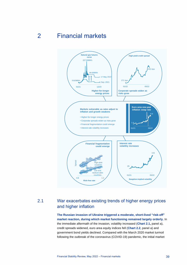
Financial Stability Review, May 2022 – Financial markets
39
2 Financial markets
2.1 War exacerbates existing trends of higher energy prices
and higher inflation
The Russian invasion of Ukraine triggered a moderate, short-lived “risk-off”
market reaction, during which market functioning remained largely orderly. In
the immediate aftermath of the invasion, volatility increased (Chart 2.1, panel a),
credit spreads widened, euro area equity indices fell (Chart 2.2, panel a) and
government bond yields declined. Compared with the March 2020 market turmoil
following the outbreak of the coronavirus (COVID-19) pandemic, the initial market
Interest rate
volatility increasesFinancial fragmentation
could emerge
Higher-for-longer
energy prices
Markets vulnerable as rates adjust to
inflation and growth weakens
• Higher-for-longer energy prices
• Corporate spreads widen as risks grow
• Financial fragmentation could emerge
• Interest rate volatility increases
Corporate spreads widen as
risks grow
Natural gas futures
curve
Risk-free rateSwaption implied volatility
High-yield credit spread
Sp
rea
d
19 €/MWh
227 €/MWh
116
01/21 05/22
29
Euro area one-year
inflation swap rate
1.4
6.6
01/21 05/22
Inva
sio
n
01/22 05/22
-0.8 1.2
High-debt
countries
Low and
medium-debt
countries
271 bps
421 bps
17 May 2022
94 €/MWh
1 Sep. 2021
01/21 12/23

Financial Stability Review, May 2022 – Financial markets
40
reaction to the invasion was relatively mild. Despite the profound medium and
long-term implications of the war, as discussed in detail below, this correction was
followed by a relatively fast rebound. A significant further escalation, in economic
and/or military terms, could still cause renewed market stress. However, regardless of
how the conflict evolves (e.g. a ceasefire agreement, prolonged entrenchment or
further escalation), several medium-term consequences have crystallised, as
discussed below. Notably, the war increases the risk of a higher-inflation,
lower-growth scenario resulting from higher energy prices and supply chain
disruptions (Chapter 1). The policy response to higher inflation and concerns about
the global growth outlook have contributed to renewed weakness in financial markets
during the second quarter of 2022.
Chart 2.1
The initial risk-off market reaction to the invasion was temporary and limited, but
energy prices are expected to be higher for longer and the upward trend in inflation
swap rates accelerated after the invasion
a) Equity volatility indices b) Natural gas futures curve c) Inflation swap rates
(1 Jan. 2020-17 May 2022, index points) (1 Jan. 2021-17 May 2022, €/MWh) (1 Jan. 2021-17 May 2022, percent)
Sources: Bloomberg Finance L.P., Refinitiv and ECB calculations.
Notes: Panel b: futures curves are based on futures contracts for different delivery dates. The active futures contract price refers to
the futures contract that matures in the next month. Futures contracts are traded on the Intercontinental Exchange (ICE) and linked to
Dutch TTF natural gas. Panel c: inflation swap rates refer to the fixed rate at which contracts are opened, whereby the floating leg, with
annual payments over the duration of the contract, is tied to an inflation index. Inflation swap rates do not purely reflect inflation
expectations, as they also include a risk premium.
Commodity futures prices suggest that energy prices will remain higher for
longer. Energy prices had already increased markedly before the start of the war in
Ukraine: tensions had already risen in the second half of 2021, with strong demand
for commodities as economies recovered from the pandemic. For example, the
average natural gas price in the fourth quarter of 2021 was 550% higher than in the
same quarter of 2020. As the conflict escalated, increases were not limited to spot
prices. The natural gas forward curve now points to elevated prices up to and
including the winter of 2023 (Chart 2.1, panel b).
The upward trend in inflation swap rates accelerated after the invasion was
launched. Inflation swap rates surged, driven in part by rising energy prices (Chart
0
10
20
30
40
50
60
70
80
90
01/20 09/20 05/21 01/22
Euro area (VSTOXX)
United States (VIX)
02/22 05/22
Inva
sio
n
0
50
100
150
200
250
01/21 09/21 05/22 01/23 09/23
Active futures contract price
Futures curve 1 Sep. 2021
Futures curve 31 Dec. 2021
Futures curve 17 May 2022
0
1
2
3
4
5
6
7
8
01/21 05/21 09/21 01/22 05/22
Invasion
Euro area one-year
Euro area five-year
United States one-year
United States five-year

Financial Stability Review, May 2022 – Financial markets
41
2.1, panel c). The euro area one-year inflation swap rate currently stands at around
6.6%,17 its highest level since the introduction of the euro, up from around 3.4% at
the end of 2021. The implications of higher than expected inflation are discussed from
a conceptual point of view in Box 3, while empirically observed consequences for
financial markets are discussed in this chapter.
Chart 2.2
A divergence between the United States and the more energy import-dependent euro
area emerged after the start of the invasion of Ukraine
a) Equity market indices and fund flows b) Relative equity market performance vs energy prices
(23 Feb.-17 May 2022, left-hand scale: percentage change,
right-hand scale: cumulative flows as a percentage of assets under
management)
(1 Jan.-17 May 2022, y-axis: euro area equity index
outperformance versus US in percentage points, x-axis: US
dollars)
Sources: Bloomberg Finance L.P., EPFR Global, Refinitiv and ECB calculations.
Notes: Panel a: percentage change since 23 February 2022, fund flows as a share of assets under management. Western Europe equity
refers to funds that invest in developed European markets, namely Austria, Belgium, Denmark, Finland, France, Germany, Greece, Italy,
Ireland, the Netherlands, Norway, Portugal, Spain, Sweden, Switzerland and the United Kingdom. Panel b: daily data on relative
performance in terms of the EURO STOXX price change versus the S&P 500 price change, as of 1 January 2022, mapped against the oil
price in US dollars. The result is not driven by differences in the shares of the oil and gas sector between the indices.
Euro area equity markets experienced a relatively weak recovery during the first
weeks after the invasion, as compared with US markets. While the EURO STOXX
index had just returned to pre-invasion levels by the end of March, the S&P 500 index
had already posted a 10% gain (Chart 2.2, panel a). Prior to the invasion, global fund
managers were positive on European equities,18 but this sentiment shifted with the
start of the war, as evidenced by the outflows from funds with a focus on western
European equities (Chart 2.2, panel a). The euro area’s high level of dependence on
energy imports may explain much of this divergence: energy prices are correlated
with performance differentials between US and euro area equities (Chart 2.2,
panel b). At the same time, other factors also impact this differential, especially in
April and May. Notably, more recent underperformance in US equity markets may be
17 As of 17 May 2022.
18 For example, Bank of America’s December Global Fund Manager Survey showed that a net 31% of fund
managers were “bullish” on euro area equities. US equities came in second with a net 18% of fund
managers.
-6
-4
-2
0
2
4
6
-15
-10
-5
0
5
10
15
23/02/22 22/03/22 18/04/22 15/05/22
EURO STOXX
Fund flows – western Europe equity (right-hand scale)
S&P 500
Fund flows – United States equity (right-hand scale)
-10
-8
-6
-4
-2
0
2
4
6
8
70 90 110 130
Eu
ro a
rea
ou
tpe
rfo
rms
Eu
ro a
rea
un
de
rpe
rfo
rms
Oil price
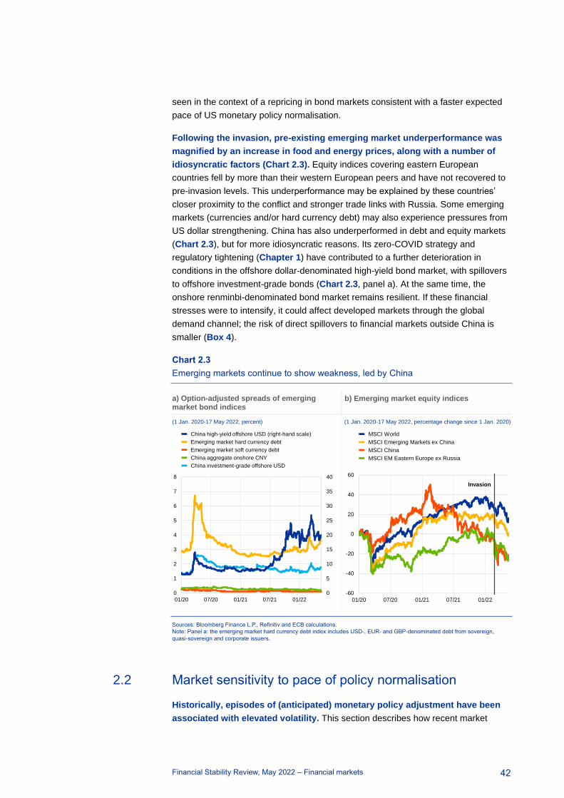
Financial Stability Review, May 2022 – Financial markets
42
seen in the context of a repricing in bond markets consistent with a faster expected
pace of US monetary policy normalisation.
Following the invasion, pre-existing emerging market underperformance was
magnified by an increase in food and energy prices, along with a number of
idiosyncratic factors (Chart 2.3). Equity indices covering eastern European
countries fell by more than their western European peers and have not recovered to
pre-invasion levels. This underperformance may be explained by these countries’
closer proximity to the conflict and stronger trade links with Russia. Some emerging
markets (currencies and/or hard currency debt) may also experience pressures from
US dollar strengthening. China has also underperformed in debt and equity markets
(Chart 2.3), but for more idiosyncratic reasons. Its zero-COVID strategy and
regulatory tightening (Chapter 1) have contributed to a further deterioration in
conditions in the offshore dollar-denominated high-yield bond market, with spillovers
to offshore investment-grade bonds (Chart 2.3, panel a). At the same time, the
onshore renminbi-denominated bond market remains resilient. If these financial
stresses were to intensify, it could affect developed markets through the global
demand channel; the risk of direct spillovers to financial markets outside China is
smaller (Box 4).
Chart 2.3
Emerging markets continue to show weakness, led by China
a) Option-adjusted spreads of emerging market bond indices
b) Emerging market equity indices
(1 Jan. 2020-17 May 2022, percent) (1 Jan. 2020-17 May 2022, percentage change since 1 Jan. 2020)
Sources: Bloomberg Finance L.P., Refinitiv and ECB calculations.
Note: Panel a: the emerging market hard currency debt index includes USD-, EUR- and GBP-denominated debt from sovereign,
quasi-sovereign and corporate issuers.
2.2 Market sensitivity to pace of policy normalisation
Historically, episodes of (anticipated) monetary policy adjustment have been
associated with elevated volatility. This section describes how recent market
0
5
10
15
20
25
30
35
40
0
1
2
3
4
5
6
7
8
01/20 07/20 01/21 07/21 01/22
China high-yield offshore USD (right-hand scale)
Emerging market hard currency debt
Emerging market soft currency debt
China aggregate onshore CNY
China investment-grade offshore USD
-60
-40
-20
0
20
40
60
01/20 07/20 01/21 07/21 01/22
Invasion
MSCI World
MSCI Emerging Markets ex China
MSCI China
MSCI EM Eastern Europe ex Russia

Financial Stability Review, May 2022 – Financial markets
43
repricing is consistent with changing expectations around the pace of monetary policy
normalisation. It also discusses the associated risks of financial fragmentation and a
disorderly correction in markets for risky assets.19
In recent months, central banks around the world have moved towards
reducing net asset purchases and signalled a tighter monetary policy stance
ahead. Notably, the Federal Reserve System ended its net asset purchases as of
March, while the ECB terminated its net purchases under the pandemic emergency
purchase programme (PEPP) at the same time. In addition, the ECB’s Governing
Council has stated that incoming data have reinforced its expectation for net asset
purchases under the asset purchase programme (APP) to be concluded in the third
quarter of 2022. This would mark an end to the rapid expansion of central bank
balance sheets in response to the COVID-19 crisis (Chart 2.4, panel a). During that
period, firms and governments benefited from favourable financing conditions
supported by central bank purchases (Chart 2.4, panel b).
Chart 2.4
Firms and sovereigns face changing market conditions as central bank purchases are
reduced
a) United States and euro area monthly net asset purchases by central banks
b) Net issuance and Eurosystem purchases of corporate and public sector bonds
(Jan. 2016-Jun. 2022, € billions) (Mar. 2020-Mar. 2022, € billions)
Sources: Bloomberg Finance L.P., ECB and Federal Reserve System.
Notes: Panel a: net asset purchases by the Federal Reserve shown include only those under System Open Market Account (SOMA)
treasury transactions and SOMA agency MBS transactions; net asset purchases under the Eurosystem include those under the APP and
PEPP. Net purchases are negative when monthly redemptions surpass gross purchases. Panel b: net issuance of debt securities by euro
area public sector and corporate entities. The general government category is as defined in the European System of Accounts (ESA
2010).
19 In the monthly Bank of America Global Fund Manager Surveys conducted between December 2021 and
February 2022, fund managers saw “Hawkish central bank rate hikes” as the biggest tail risk. In the
March 2022 survey, this position was overtaken by “The Russia-Ukraine conflict”. The April survey listed
“Global recession” as the largest risk (26%), closely followed by “Hawkish central banks” (25%). The
leading position was taken once again by “Hawkish central banks” (31%) in the May edition.
-100
100
300
500
700
900
1,100
1,300
2016 2018 2020 2022
Ma
y
20
22
Eurosystem
Federal Reserve
Announced Eurosystem net purchases
Announced Federal Reserve net purchases
0
500
1,000
1,500
2,000
2,500
Netpurchases
public sector
Net issuancepublic sector
Netpurchasescorporates
Net issuancecorporates
Pandemic emergency purchase programme
Asset purchase programme
General government
European Union
European Investment Bank
Non-financial corporations
Other non-monetary financial corporations

Financial Stability Review, May 2022 – Financial markets
44
Markets have repriced for a faster pace of policy normalisation in both the euro
area and the United States, compared with 2021. Pricing for interest rate
derivatives suggests that market participants now foresee more imminent policy rate
hikes than previously (Chart 2.5, panel a).20 Interest rates rebounded from a brief
decline immediately after the invasion and continued their climb in subsequent weeks
as market participants considered it increasingly likely that central banks would move
faster towards monetary policy normalisation in response to inflationary pressures
(Chart 2.5, panel b).
Differences in the pace of policy adjustment can lead to a spillover of risks from
the United States to the euro area. Higher US yields may affect global capital flows
and thereby indirectly affect euro area yields. In addition, elevated volatility in US
markets can spill over to euro area markets and lead to a deterioration in risk
sentiment.21
Chart 2.5
Markets are pricing in a faster pace of monetary policy tightening than previously
a) EURIBOR futures curve b) Longer-term German government real and nominal bond yields
(Jun. 2022-Mar. 2023, percent) (1 Jul. 2021-17 May 2022, percent)
Sources: Bloomberg Finance L.P. and ECB calculations.
Notes: Panel a: EURIBOR futures curves are based on contracts traded on the Intercontinental Exchange (ICE) based on the underlying
three-month EURIBOR. Panel b: real yields are shown as the nominal German government bond yield less the break-even inflation rate.
Volatility and uncertainty in interest rate and government bond markets, as well
as potential upward pressure on real rates, could challenge risky asset
valuations. Markets, already priced for faster increases in short-term rates (Chart
2.5, panel a), have become increasingly sensitive to information that could – as seen
20 In the ECB Survey of Monetary Analysts, the December 2021 results showed December 2023 as the
median expected timing of the next increase in the deposit facility rate. This median had shifted forward
by more than one year to September 2022 in the April survey results. In addition, the Bloomberg
Economist Survey conducted between 1 and 6 April 2022 found -0.25% to be the median expectation for
the deposit facility rate for December 2022 compared with a median expectation of -0.5% in the survey
conducted between 8 and 14 December 2021.
21 See the Box entitled “Risk of spillovers from US equity market corrections to euro area markets and
financial conditions”, Financial Stability Review, May 2021, ECB.
-0.6
-0.4
-0.2
0.0
0.2
0.4
0.6
0.8
1.0
1.2
06/22 09/22 12/22 03/23
17 May 2022
1 March 2022
30 December 2021
-6.0
-5.0
-4.0
-3.0
-2.0
-1.0
07/21 10/21 01/22 04/22
Two-year nominal yield
Ten-year nominal yield
Two-year real yield
Ten-year real yield
Invasion
-1.0
-0.5
0.0
0.5
1.0

Financial Stability Review, May 2022 – Financial markets
45
through the lens of market participants – affect the pace of policy normalisation. As
inflationary pressures built over the course of 2021, implied volatility in euro area
government bond markets increased, as did uncertainty22 with regard to future
short-term interest rates (Chart 2.6, panel a). In addition, there is now the potential for
real interest rate rises after years of declines (Chart 2.5, panel b). All else equal,
increases in both nominal and real rates are typically associated with investor
de-risking, and may lead to pressures on valuations of risky assets such as equities.
A theoretical exercise, with cyclically adjusted earnings and equity risk premia23 held
constant, shows that equity valuations could decline significantly for given, relatively
limited increases in longer-term, risk-free real interest rates (Chart 2.6, panel b).
Nevertheless, (euro area) real risk-free rates remain in negative territory. In addition,
equities are also considered to have some inflation hedging properties, which can
support valuations in the current inflation environment.
The first half of 2022 saw a sizeable market correction especially in
higher-duration equities and more speculative asset classes. As set out in the
November 2021 Financial Stability Review (FSR), equity markets have become
increasingly sensitive to interest rate increases in recent years. As rates increased
sharply since November 2021, higher duration equities, such as those in the
technology sector, underperformed.24 Market volatility also expanded into
crypto-asset markets. Bitcoin lost 50% of its value (versus the US dollar),25 and
stresses emerged in markets for stablecoins.26 While a number of stablecoins lost
their peg against the US dollar, broader financial stability risks remain limited. At the
same time, the implications of stresses on stablecoin Tether could be significant for
the crypto-asset ecosystem. A failure of Tether may pose a threat to the stability of
crypto-asset markets, as it provides a substantial amount of trading liquidity for
buying and selling of other crypto-assets.27 A run on Tether could disrupt trading and
price discovery in crypto-asset markets, which could turn disorderly. Contagion
effects for the broader financial system arising from a potential “crypto crash” still
seem limited (Special Feature B), although individual investors may suffer significant
losses.
22 As measured by the standard deviation of the option-implied probability density functions.
23 In this exercise, the excess cyclically adjusted price/earnings (CAPE) yield, which is sometimes
interpreted as the equity risk premium, is held constant. In addition, cyclically adjusted earnings – by
design a relatively stable variable based on a long-term inflation-adjusted average – are also held
constant. It would be possible to relax the assumption of a fixed equity risk premium, and in theory, there
could even be a relationship between the equity risk premium and the risk-free interest rate. Evidence
presented below (Chart 2.7) suggests that credit risk premia have shown a positive relationship with
risk-free rates more recently. There have been historical episodes with both positive and negative
relationships between the risk-free rate and the equity risk premium.
24 For example, between 17 November 2021 and 17 May 2022 the Nasdaq Composite declined by 25
percent. Sources: Bloomberg, ECB calculations.
25 Between 17 November 2021 and 17 May 2022 the Bitcoin lost 50 percent of its value versus the US
dollar. Sources: Bloomberg, ECB calculations.
26 See also “The expanding functions and uses of stablecoins”, Financial Stability Review, ECB, November
2021.
27 See the updated “Assessment of Risks to Financial Stability from Crypto-assets”, Financial Stability
Board, February 2022.

Financial Stability Review, May 2022 – Financial markets
46
Chart 2.6
Volatility and upward pressure on real rates could challenge valuations of risky assets
a) Standard deviation of option-implied distribution of three-month EURIBOR and rates market volatility index
b) Simulation of change in EURO STOXX price based on real risk-free rate, keeping the equity risk premium constant
(1 Jan. 2019-17 May 2022, left-hand scale: percent, right-hand
scale: index points)
(1 Jun. 2021-13 May 2022, x-axis: ten-year risk-free real rate in
percentage points, y-axis: percentage change of price index,
realised prices are weekly data with reference point of 1 Jan. 2022)
Sources: Bloomberg Finance L.P., Refinitiv and ECB calculations.
Notes: Panel a: the Swaption Merrill Option Volatility Estimate (SMOVE) is a yield curve-weighted index of the normalised implied
volatility on three-month swaptions. It is the weighted average of volatilities on 2-year, 5-year, 10-year and 30-year maturity swaps. Panel
b: equity price movements are projected for different levels of real risk-free rates. The excess cyclically adjusted price/earnings yield over
the risk-free rate (“equity risk premium”) is assumed to be constant and equal to its value as at 1 January 2022. Dots indicate historically
realised price changes in the EURO STOXX index compared with 1 January 2022.
Rising interest rates could present challenges to highly indebted firms and
governments. An increase in interest rates exposes borrowers to higher
(re)financing costs. For more indebted firms and sovereigns, the impact of higher
financing costs on earnings and budget deficits is mechanically larger. This implies
that, all else equal, the debt sustainability of more indebted firms and governments
may deteriorate relatively more rapidly than for less indebted firms and governments.
This in turn can lead to higher credit and sovereign spreads and increasing financial
fragmentation (Chart 2.7). At the same time, both firms and governments have
extended the maturity of their debt in recent years, which might shield them from the
higher marginal cost of funding to some extent.
Interest rate increases may entail risks, especially if underlying growth
dynamics are muted. All else equal, a tighter monetary policy stance generally leads
to increasing interest rates and an attenuation of (expected) growth. Consequently,
monetary policy tightening can drive a wedge between interest rates and growth, and
this can have consequences for debt sustainability (Box 3). At the same time,
increases in market rates (the marginal cost of funding) only feed through into
average interest rates paid slowly, as existing fixed-rate debt matures and new debt
is issued. Issuers with relatively higher outstanding amounts of variable-rate or
inflation-linked debt instruments are more directly exposed.
0
30
60
90
120
150
0.0
0.5
1.0
1.5
2.0
2.5
01/19 07/19 01/20 07/20 01/21 07/21 01/22
One-year
Two-year
Five-year
SMOVE index (right-hand scale)
-20
-15
-10
-5
0
5
10
15
20
-2.5 -2.0 -1.5 -1.0
Simulated price change
Realised price change

Financial Stability Review, May 2022 – Financial markets
47
Chart 2.7
Higher rates could challenge debt sustainability and drive spread-widening
a) Euro area corporate spreads vs. risk-free rates
b) Rate elasticity of sovereign spreads vs. debt-to-GDP ratio
(1 Jan. 2021-17 May 2022, y-axis: basis points, x-axis: percentage
points)
(1 Jan. 2021-17 May 2022, y-axis: basis point spread per basis
point of risk-free rate, x-axis: 2021 government debt/GDP,
percentages)
Sources: Bloomberg Finance L.P., ECB and ECB calculations.
Notes: Panel a: high-yield spreads refer to the five-year iTraxx Crossover CDS spreads; risk-free rate refers to the Germany five-year
government bond yield. Panel b: spreads and rates refer to ten-year government bond yields of euro area countries; risk-free rate refers
to German government ten-year yields. Error bars indicate a two standard deviation confidence interval around the parameter estimate.
There are not sufficient data for Cyprus and Malta.
2.3 Commodity price shocks may lead to a reassessment of
risks in the corporate sector
Corporate spreads increased in a challenging environment of higher
commodity prices, higher inflation, higher interest rates and a weaker growth
outlook. After a brief spike, spreads on high-yield corporate bonds returned to
pre-invasion levels, but remain elevated compared with 2021, reflecting the more
challenging macro-financial environment (Chart 2.8, panel a). Higher commodity
prices and inflation will probably translate into higher cost and input prices, which can,
in turn, erode earnings. Rising financing costs may further impair earnings as rates
increase, especially for firms with variable-rate loans (e.g. leveraged loans) or
floating-rate bonds, and for firms with significant near-term refinancing needs. Since
the invasion, issuance of high-yield corporate bonds has remained subdued. Rating
agencies have recently upgraded their predictions for speculative grade defaults and
also indicated that risks are seen to the upside (Chart 4, panel a, Overview).
Sector-level equity performance over the course of 2021 was closely related to
firms’ ability to maintain or increase margins (Chart 2.8, panel b). Pricing power
is a key factor determining firms’ ability to cope with higher inflation and higher
commodity prices (Chapter 1). In particular, a high energy intensity in production
does not automatically imply that earnings will be materially compressed by higher
energy prices. Firms might be able to pass on much of the cost increases to their
customers, depending on their pricing power. Indeed, equity sub-indices for several
0
50
100
150
200
250
300
350
400
450
500
-1 -0.5 0 0.5 1
High-yield
Investment-grade
EE
LU LV
LTNL
IE
SK
FI
SI
AT
BE
FR
ESPT
IT
GR
EA
-0.2
0.0
0.2
0.4
0.6
0.8
1.0
1.2
0 50 100 150 200
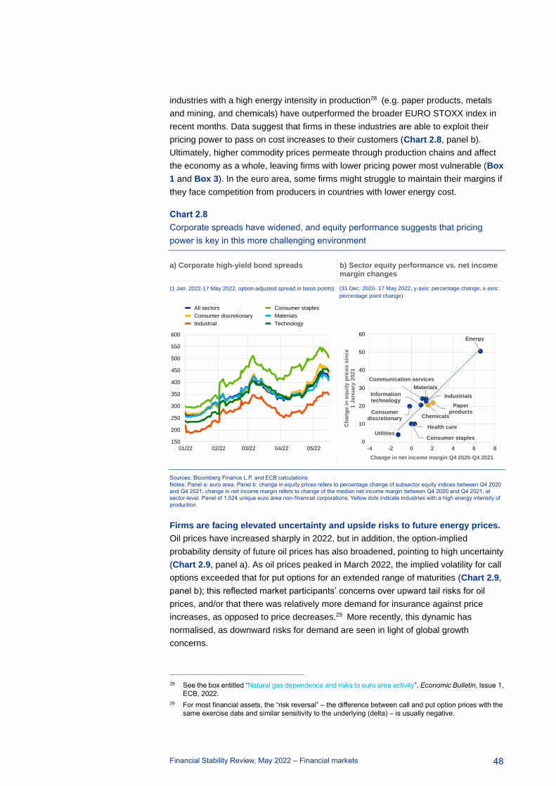
Financial Stability Review, May 2022 – Financial markets
48
industries with a high energy intensity in production28 (e.g. paper products, metals
and mining, and chemicals) have outperformed the broader EURO STOXX index in
recent months. Data suggest that firms in these industries are able to exploit their
pricing power to pass on cost increases to their customers (Chart 2.8, panel b).
Ultimately, higher commodity prices permeate through production chains and affect
the economy as a whole, leaving firms with lower pricing power most vulnerable (Box
1 and Box 3). In the euro area, some firms might struggle to maintain their margins if
they face competition from producers in countries with lower energy cost.
Chart 2.8
Corporate spreads have widened, and equity performance suggests that pricing
power is key in this more challenging environment
a) Corporate high-yield bond spreads b) Sector equity performance vs. net income margin changes
(1 Jan. 2022-17 May 2022, option-adjusted spread in basis points) (31 Dec. 2020- 17 May 2022, y-axis: percentage change, x-axis:
percentage point change)
Sources: Bloomberg Finance L.P. and ECB calculations
Notes: Panel a: euro area. Panel b: change in equity prices refers to percentage change of subsector equity indices between Q4 2020
and Q4 2021; change in net income margin refers to change of the median net income margin between Q4 2020 and Q4 2021, at
sector-level. Panel of 1,524 unique euro area non-financial corporations. Yellow dots indicate industries with a high energy intensity of
production.
Firms are facing elevated uncertainty and upside risks to future energy prices.
Oil prices have increased sharply in 2022, but in addition, the option-implied
probability density of future oil prices has also broadened, pointing to high uncertainty
(Chart 2.9, panel a). As oil prices peaked in March 2022, the implied volatility for call
options exceeded that for put options for an extended range of maturities (Chart 2.9,
panel b); this reflected market participants’ concerns over upward tail risks for oil
prices, and/or that there was relatively more demand for insurance against price
increases, as opposed to price decreases.29 More recently, this dynamic has
normalised, as downward risks for demand are seen in light of global growth
concerns.
28 See the box entitled “Natural gas dependence and risks to euro area activity”, Economic Bulletin, Issue 1,
ECB, 2022.
29 For most financial assets, the “risk reversal” – the difference between call and put option prices with the
same exercise date and similar sensitivity to the underlying (delta) – is usually negative.
150
200
250
300
350
400
450
500
550
600
01/22 02/22 03/22 04/22 05/22
All sectors
Consumer discretionary
Industrial
Consumer staples
Materials
Technology
Utilities
Consumer discretionary
Consumer staples
Health care
Information technology
Communication services
Materials
Industrials
Energy
Chemicals
Paper products
0
10
20
30
40
50
60
-4 -2 0 2 4 6 8
Ch
an
ge
in
eq
uit
y p
ric
es
sin
ce
1
Ja
nu
ary
20
21
Change in net income margin Q4 2020-Q4 2021
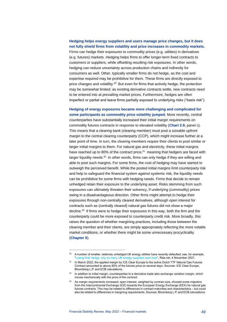
Financial Stability Review, May 2022 – Financial markets
49
Hedging helps energy suppliers and users manage price changes, but it does
not fully shield firms from volatility and price increases in commodity markets.
Firms can hedge their exposures to commodity prices (e.g. utilities) in derivatives
(e.g. futures) markets. Hedging helps firms to offer longer-term fixed contracts to
customers or suppliers, while offsetting resulting risk exposures. In other words,
hedging can reduce uncertainty across production chains and indirectly for
consumers as well. Other, typically smaller firms do not hedge, as the cost and
expertise required may be prohibitive for them. These firms are directly exposed to
price changes and volatility.30 But even for firms that actively hedge, the protection
may be somewhat limited: as existing derivative contracts settle, new contracts need
to be entered into at prevailing market prices. Furthermore, hedges are often
imperfect or partial and leave firms partially exposed to underlying risks (“basis risk”).
Hedging of energy exposures became more challenging and complicated for
some participants as commodity price volatility jumped. More recently, central
counterparties have substantially increased their initial margin requirements on
commodity futures contracts in response to elevated volatility (Chart 2.9, panel c).
This means that a clearing bank (clearing member) must post a sizeable upfront
margin to the central clearing counterparty (CCP), which might increase further at a
later point of time. In turn, the clearing members require their clients to post similar or
larger initial margins to them. For natural gas and electricity, these initial margins
have reached up to 80% of the contract price,31 meaning that hedgers are faced with
larger liquidity needs.32 In other words, firms can only hedge if they are willing and
able to post such margins. For some firms, the cost of hedging may have started to
outweigh the perceived benefit. While the posted initial margins limit counterparty risk
and help to safeguard the financial system against systemic risk, the liquidity needs
can be prohibitive for some firms with hedging needs. Firms that decide to remain
unhedged retain their exposure to the underlying asset. Risks stemming from such
exposures can ultimately threaten their solvency, if underlying (commodity) prices
swing in a disadvantageous direction. Other firms might attempt to hedge their
exposures through non-centrally cleared derivatives, although open interest for
contracts such as (centrally cleared) natural gas futures did not show a major
decline.33 If firms were to hedge their exposures in this way, both the firm and the
counterparty could be more exposed to counterparty credit risk. More broadly, this
raises the question of whether margining practices, including those between the
clearing member and their clients, are simply appropriately reflecting the more volatile
market conditions, or whether there might be some unnecessary procyclicality
(Chapter 5).
30 A number of smaller, relatively unhedged UK energy utilities have recently defaulted; see, for example,
“Losing their hedge: why so many UK energy suppliers went bust”, Risk.net, 4 November 2021.
31 In March 2022, the applied margin by ICE Clear Europe to the active Dutch TTF Natural Gas Futures
Contract amounted to above 80% of the futures price on several days. Sources: ICE Clear Europe,
Bloomberg L.P. and ECB calculations.
32 In addition to initial margin, counterparties to a derivative trade also exchange variation margin, which
moves mechanically with the price of the contract.
33 As margin requirements increased, open interest, weighted by contract size, showed some migration
from the Intercontinental Exchange (ICE) towards the European Energy Exchange (EEX) for natural gas
futures contracts. This may be related to differences in contract maturities and characteristics – but could
also be related to differences in margining requirements. Sources: Bloomberg L.P. and ECB calculations.
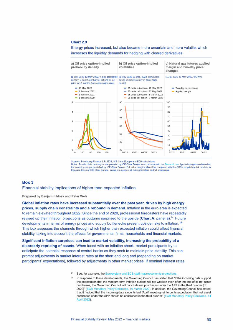
Financial Stability Review, May 2022 – Financial markets
50
Chart 2.9
Energy prices increased, but also became more uncertain and more volatile, which
increases the liquidity demands for hedging with cleared derivatives
a) Oil price option-implied probability density
b) Oil price option-implied volatilities
c) Natural gas futures applied margin and two-day price changes
(1 Jan. 2020-13 May 2022, y-axis: probability
density, x-axis: € per barrel, options on oil
price in 12 months from observation date)
(1 May 2022-31 Dec. 2023, annualised
option-implied volatility in percentage
points)
(1 Jul. 2021-17 May 2022, €/MWh)
Sources: Bloomberg Finance L.P., ECB, ICE Clear Europe and ECB calculations.
Notes: Panel c: data on margins are provided by ICE Clear Europe in accordance with the Terms of Use. Applied margins are based on
the scanning ranges published by ICE Clear Europe. Full initial margins should be computed with the CCPs’ proprietary risk models, in
this case those of ICE Clear Europe, taking into account all risk parameters and full exposures.
Box 3
Financial stability implications of higher than expected inflation
Prepared by Benjamin Mosk and Peter Welz
Global inflation rates have increased substantially over the past year, driven by high energy
prices, supply chain constraints and a rebound in demand. Inflation in the euro area is expected
to remain elevated throughout 2022. Since the end of 2020, professional forecasters have repeatedly
revised up their inflation projections as outturns surprised to the upside (Chart A, panel a).34 Future
developments in terms of energy prices and supply bottlenecks present upside risks to inflation.35
This box assesses the channels through which higher than expected inflation could affect financial
stability, taking into account the effects for governments, firms, households and financial markets.
Significant inflation surprises can lead to market volatility, increasing the probability of a
disorderly repricing of assets. When faced with an inflation shock, market participants try to
anticipate the potential response of central banks as they seek to maintain price stability. This can
prompt adjustments in market interest rates at the short and long end (depending on market
participants’ expectations), followed by adjustments in other market prices. If nominal interest rates
34 See, for example, the Eurosystem and ECB staff macroeconomic projections.
35 In response to these developments, the Governing Council has stated that “If the incoming data support
the expectation that the medium-term inflation outlook will not weaken even after the end of its net asset
purchases, the Governing Council will conclude net purchases under the APP in the third quarter [of
2022]” (ECB Monetary Policy Decisions, 10 March 2022). In addition, the Governing Council has stated
that it “judged that the incoming data since its last [April] meeting reinforce its expectation that net asset
purchases under the APP should be concluded in the third quarter” (ECB Monetary Policy Decisions, 14
April 2022).
0
1
2
3
4
5
0 40 80 120 160
13 May 2022
1 January 2022
1 January 2021
1 January 2020
30
40
50
60
70
80
90
05/22 10/22 03/23 08/23
25 delta put option - 17 May 2022
25 delta call option - 17 May 2022
25 delta put option - 3 March 2022
25 delta call option - 3 March 2022
0
10
20
30
40
50
60
70
80
90
100
07/21 10/21 01/22 04/22
Two-day price change
Applied margin
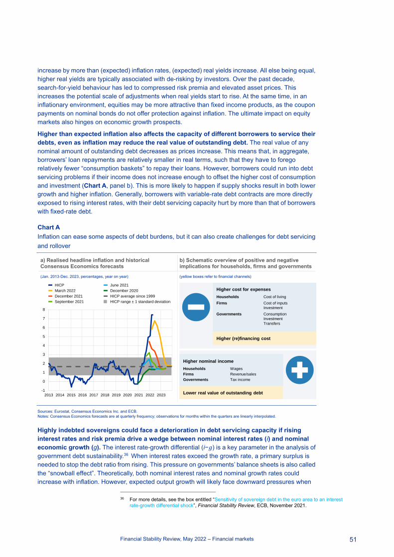
Financial Stability Review, May 2022 – Financial markets
51
increase by more than (expected) inflation rates, (expected) real yields increase. All else being equal,
higher real yields are typically associated with de-risking by investors. Over the past decade,
search-for-yield behaviour has led to compressed risk premia and elevated asset prices. This
increases the potential scale of adjustments when real yields start to rise. At the same time, in an
inflationary environment, equities may be more attractive than fixed income products, as the coupon
payments on nominal bonds do not offer protection against inflation. The ultimate impact on equity
markets also hinges on economic growth prospects.
Higher than expected inflation also affects the capacity of different borrowers to service their
debts, even as inflation may reduce the real value of outstanding debt. The real value of any
nominal amount of outstanding debt decreases as prices increase. This means that, in aggregate,
borrowers’ loan repayments are relatively smaller in real terms, such that they have to forego
relatively fewer “consumption baskets” to repay their loans. However, borrowers could run into debt
servicing problems if their income does not increase enough to offset the higher cost of consumption
and investment (Chart A, panel b). This is more likely to happen if supply shocks result in both lower
growth and higher inflation. Generally, borrowers with variable-rate debt contracts are more directly
exposed to rising interest rates, with their debt servicing capacity hurt by more than that of borrowers
with fixed-rate debt.
Chart A
Inflation can ease some aspects of debt burdens, but it can also create challenges for debt servicing
and rollover
Sources: Eurostat, Consensus Economics Inc. and ECB.
Notes: Consensus Economics forecasts are at quarterly frequency; observations for months within the quarters are linearly interpolated.
Highly indebted sovereigns could face a deterioration in debt servicing capacity if rising
interest rates and risk premia drive a wedge between nominal interest rates (i) and nominal
economic growth (g). The interest rate-growth differential (i−𝑔) is a key parameter in the analysis of
government debt sustainability.36 When interest rates exceed the growth rate, a primary surplus is
needed to stop the debt ratio from rising. This pressure on governments’ balance sheets is also called
the “snowball effect”. Theoretically, both nominal interest rates and nominal growth rates could
increase with inflation. However, expected output growth will likely face downward pressures when
36 For more details, see the box entitled “Sensitivity of sovereign debt in the euro area to an interest
rate-growth differential shock”, Financial Stability Review, ECB, November 2021.
a) Realised headline inflation and historical Consensus Economics forecasts
b) Schematic overview of positive and negative implications for households, firms and governments
(Jan. 2013-Dec. 2023, percentages, year on year) (yellow boxes refer to financial channels)
-1
0
1
2
3
4
5
6
7
8
2013 2014 2015 2016 2017 2018 2019 2020 2021 2022 2023
HICP
March 2022
December 2021
September 2021
June 2021
December 2020
HICP average since 1999
HICP range ± 1 standard deviation
Higher cost for expenses
Households Cost of living
Firms Cost of inputs
Investment
Governments Consumption
Investment
Transfers
Higher (re)financing cost
Higher nominal income
Households Wages
Firms Revenue/sales
Governments Tax income
Lower real value of outstanding debt
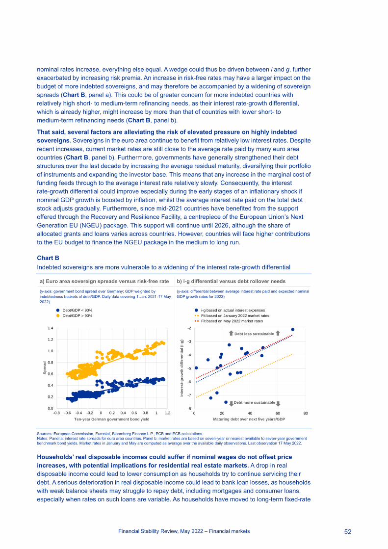
Financial Stability Review, May 2022 – Financial markets
52
nominal rates increase, everything else equal. A wedge could thus be driven between i and g, further
exacerbated by increasing risk premia. An increase in risk-free rates may have a larger impact on the
budget of more indebted sovereigns, and may therefore be accompanied by a widening of sovereign
spreads (Chart B, panel a). This could be of greater concern for more indebted countries with
relatively high short- to medium-term refinancing needs, as their interest rate-growth differential,
which is already higher, might increase by more than that of countries with lower short- to
medium-term refinancing needs (Chart B, panel b).
That said, several factors are alleviating the risk of elevated pressure on highly indebted
sovereigns. Sovereigns in the euro area continue to benefit from relatively low interest rates. Despite
recent increases, current market rates are still close to the average rate paid by many euro area
countries (Chart B, panel b). Furthermore, governments have generally strengthened their debt
structures over the last decade by increasing the average residual maturity, diversifying their portfolio
of instruments and expanding the investor base. This means that any increase in the marginal cost of
funding feeds through to the average interest rate relatively slowly. Consequently, the interest
rate-growth differential could improve especially during the early stages of an inflationary shock if
nominal GDP growth is boosted by inflation, whilst the average interest rate paid on the total debt
stock adjusts gradually. Furthermore, since mid-2021 countries have benefited from the support
offered through the Recovery and Resilience Facility, a centrepiece of the European Union’s Next
Generation EU (NGEU) package. This support will continue until 2026, although the share of
allocated grants and loans varies across countries. However, countries will face higher contributions
to the EU budget to finance the NGEU package in the medium to long run.
Chart B
Indebted sovereigns are more vulnerable to a widening of the interest rate-growth differential
Sources: European Commission, Eurostat, Bloomberg Finance L.P., ECB and ECB calculations.
Notes: Panel a: interest rate spreads for euro area countries. Panel b: market rates are based on seven-year or nearest available to seven-year government
benchmark bond yields. Market rates in January and May are computed as average over the available daily observations. Last observation 17 May 2022.
Households’ real disposable incomes could suffer if nominal wages do not offset price
increases, with potential implications for residential real estate markets. A drop in real
disposable income could lead to lower consumption as households try to continue servicing their
debt. A serious deterioration in real disposable income could lead to bank loan losses, as households
with weak balance sheets may struggle to repay debt, including mortgages and consumer loans,
especially when rates on such loans are variable. As households have moved to long-term fixed-rate
a) Euro area sovereign spreads versus risk-free rate b) i-g differential versus debt rollover needs
(y-axis: government bond spread over Germany; GDP weighted by
indebtedness buckets of debt/GDP. Daily data covering 1 Jan. 2021-17 May
2022)
(y-axis: differential between average interest rate paid and expected nominal
GDP growth rates for 2023)
0.0
0.2
0.4
0.6
0.8
1.0
1.2
1.4
-0.8 -0.6 -0.4 -0.2 0 0.2 0.4 0.6 0.8 1 1.2
Sp
rea
d
Ten-year German government bond yield
Debt/GDP < 90%
Debt/GDP > 90%
-8
-7
-6
-5
-4
-3
-2
0 20 40 60 80
Inte
res
t-g
row
th d
iffe
ren
tia
l (i
-g)
Maturing debt over next five years/GDP
i-g based on actual interest expenses
Fit based on January 2022 market rates
Fit based on May 2022 market rates
Debt more sustainable
Debt less sustainable

Financial Stability Review, May 2022 – Financial markets
53
contracts in many euro area countries, they might be shielded to some extent against this effect. In
addition, households’ borrowing capacity could deteriorate, potentially putting downward pressure on
valuations of residential real estate. In aggregate, households still benefit from the sizeable volumes
of liquid assets that they accumulated during the pandemic and that would, to some extent, relieve
the debt servicing burden, which on aggregate is also low relative to disposable income. However,
this masks the fact that liquid assets are unevenly distributed and that higher than expected inflation
can have negative distributional consequences that affect low-income households the most. Finally,
consumer confidence may erode in a high inflation environment, with potentially adverse
consequences for consumption.
Vulnerable corporates with lower pricing power and higher debt are more exposed to
pressure on debt sustainability from inflation shocks than other corporates. While some firms
can pass on cost increases to consumers, other firms with less pricing power may face cost increases
that outpace revenue growth. Smaller and more indebted firms might have lower pricing power,
according to data on net income margins (Chart C).37 Insolvency rates have been very low recently,
but vulnerabilities have built up in the sectors worst affected by the pandemic. If higher inflation rates
drive cost increases while revenue growth is subdued, insolvency cases may start to rise among
vulnerable and indebted firms, raising creditor losses.
Chart C
Smaller and more indebted firms have lower net income margins, pointing to lower pricing power
Sources: S&P Global Market Intelligence and ECB calculations.
Notes: Net income margins vary by sector. Sample of 1,183 unique euro area non-financial corporations.
If higher inflation is accompanied by subdued growth, the negative impact of inflation on
financial stability would be exacerbated amid limited scope for offsetting income increases.
Inflation exists in different forms, such as demand-pull, cost-push, imported or wage/price-spiral
inflation. When inflation is driven by more exogenous supply shocks or cost-push shocks generated
by higher energy prices, the scope for higher income is more limited, the balance of risks is tilted to
the downside and the i−𝑔 gap is more likely to widen.
37 Lower net income margins do not necessarily point to lower pricing power. For example, margins for
more indebted firms may simply be lower due to higher interest expenses. At the same time, this still
leaves these firms vulnerable, as the “buffer” in terms of positive margins is already smaller to begin with,
meaning that a compression of margins may result in realised losses more quickly.
a) Net income margins of non-financial corporations b) Net income margins of non-financial corporations
(median net income margin, percentages, 2021) (y-axis: median net income margin, percentages, by firm size measured by
total assets – buckets, € millions)
Debt/assets ratio
(0.0, 0.25] (0.25, 0.5] (0.5, 0.75] (0.75, 2.0]
Total
assets
(€
millions)
(2, 50] 1.0 1.5 -7.5 ND
(50, 250] 5.4 3.4 -1.8 -2.2
(250,
1,000] 6.7 4.9 1.5 -1.8
(1,000] 6.4 6.7 8.2 -0.2
-4
-2
0
2
4
6
8
Q1 Q2 Q3 Q4 Q1 Q2 Q3 Q4 Q1 Q2 Q3 Q4
2019 2020 2021
>2-50
>50-250
>250-1,000
>1,000-1,000,000
Financial Stability Review, May 2022 – Financial markets
54
While financial stability is a prerequisite for price stability, price stability also affects financial
stability. The ECB monetary policy strategy review conducted in 2021 recognises that price stability
depends on financial stability38 and states that the preparation of monetary policy decisions will be
enhanced with additional information on financial stability considerations. At the same time, the
considerations presented in this box illustrate that financial stability is also influenced by price
stability.
Box 4
The impact of Chinese macro risk shocks on global financial markets
Prepared by David Lodge, Ana-Simona Manu and Ine Van Robays
Since the middle of last year, global investors have stepped up their scrutiny of risks
emanating from China as it experiences rising defaults and a slowing economy.39 In the past,
spillovers from China to other financial markets were typically judged to be small,40 reflecting China’s
less developed financial markets, a largely closed capital account regime, a managed exchange rate
and a relatively small share of foreign investors in the domestic market. Yet China’s footprint in the
global economy has grown rapidly over recent years, while domestic financial markets have
deepened and integrated more with global capital markets.41 This box looks at how Chinese macro
risk shocks identified from movements in Chinese and US asset prices can affect global and
European financial markets.
This box takes a two-step approach to quantify the importance of China-specific shocks for
global financial markets. The first step involves applying a structural Bayesian vector
autoregression (BVAR) model using daily financial market data from 2017 to 2021 to disentangle the
drivers of movements in US and Chinese financial markets.42 The five structural shocks – Chinese
macro risk and monetary policy shocks, US macro risk and monetary policy shocks, and global risk
shocks – are identified using sign restrictions43 and relative magnitude restrictions in the spirit of the
recent literature.44 The second step entails assessing the effects of shocks originating in China on
38 See The ECB’s monetary policy strategy statement.
39 See Box 4 entitled “Downside Risks from Property Developer Stress”, Staff Report, International
Monetary Fund, January 2022.
40 See Arslanalp, S. et al., “China’s Growing Influence on Asian Financial Markets”, IMF Working Papers,
No 2016/173, International Monetary Fund, 2016, which documents how spillovers from China to Asian
equity markets have increased during the period since the global financial crisis, though they remain
lower than those from the United States.
41 However, the foreign ownership of the Chinese onshore bond market remains relatively low, accounting
for around 4% of the total market.
42 The sample starts in 2017 in order to focus the analysis on a period when China’s policy paradigm shifted
closer to a market system after interest rates were broadly liberalised by 2015. Since then, efforts have
been made to increase the flexibility of the renminbi.
43 The estimations are made using the BEAR toolbox – see Dieppe et al., “The BEAR toolbox”, Working
Paper Series, No 1934, ECB, 2016. For China and the United States, accommodative monetary policy
shocks are assumed to lower domestic yields and boost equities, while a favourable macro outlook is
assumed to boost both yields and equities. Chinese shocks are separated from US shocks based on
assumptions that shocks in both countries have a larger impact on domestic yields than foreign yields. In
addition, the safe-haven role of the US dollar is used to identify a global risk shock, similar to Brandt et al.,
“What drives euro area financial market developments? The role of US spillovers and global risk”,
Working Paper Series, No 2560, ECB, 2021.
44 See Brandt et al., op. cit.
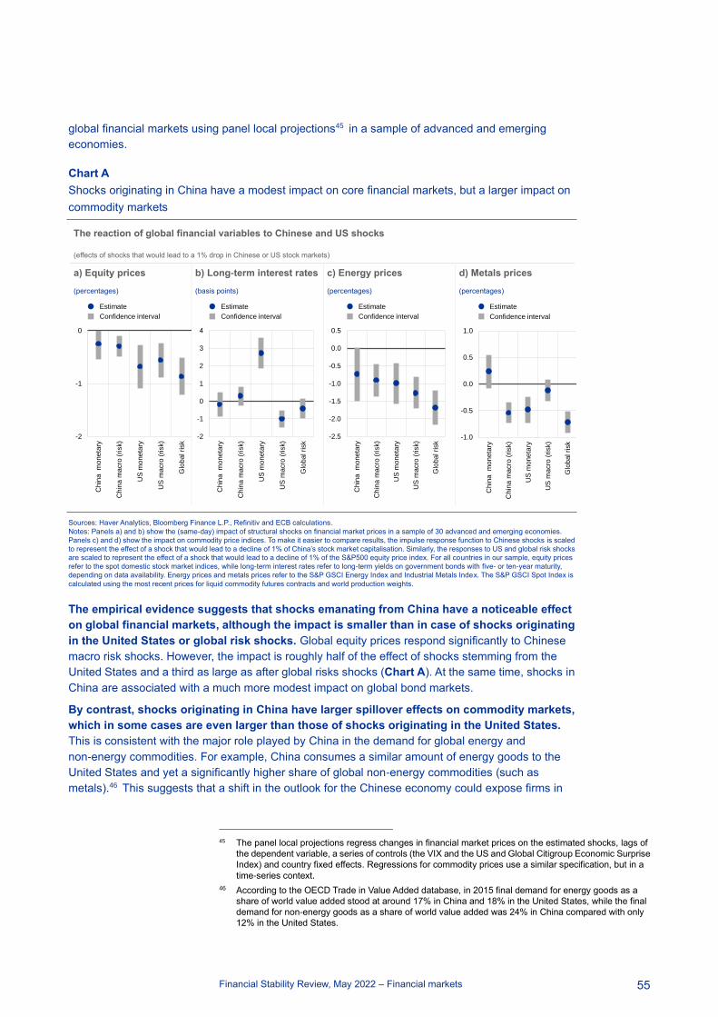
Financial Stability Review, May 2022 – Financial markets
55
global financial markets using panel local projections45 in a sample of advanced and emerging
economies.
Chart A
Shocks originating in China have a modest impact on core financial markets, but a larger impact on
commodity markets
Sources: Haver Analytics, Bloomberg Finance L.P., Refinitiv and ECB calculations.
Notes: Panels a) and b) show the (same-day) impact of structural shocks on financial market prices in a sample of 30 advanced and emerging economies.
Panels c) and d) show the impact on commodity price indices. To make it easier to compare results, the impulse response function to Chinese shocks is scaled
to represent the effect of a shock that would lead to a decline of 1% of China’s stock market capitalisation. Similarly, the responses to US and global risk shocks
are scaled to represent the effect of a shock that would lead to a decline of 1% of the S&P500 equity price index. For all countries in our sample, equity prices
refer to the spot domestic stock market indices, while long-term interest rates refer to long-term yields on government bonds with five- or ten-year maturity,
depending on data availability. Energy prices and metals prices refer to the S&P GSCI Energy Index and Industrial Metals Index. The S&P GSCI Spot Index is
calculated using the most recent prices for liquid commodity futures contracts and world production weights.
The empirical evidence suggests that shocks emanating from China have a noticeable effect
on global financial markets, although the impact is smaller than in case of shocks originating
in the United States or global risk shocks. Global equity prices respond significantly to Chinese
macro risk shocks. However, the impact is roughly half of the effect of shocks stemming from the
United States and a third as large as after global risks shocks (Chart A). At the same time, shocks in
China are associated with a much more modest impact on global bond markets.
By contrast, shocks originating in China have larger spillover effects on commodity markets,
which in some cases are even larger than those of shocks originating in the United States.
This is consistent with the major role played by China in the demand for global energy and
non-energy commodities. For example, China consumes a similar amount of energy goods to the
United States and yet a significantly higher share of global non-energy commodities (such as
metals).46 This suggests that a shift in the outlook for the Chinese economy could expose firms in
45 The panel local projections regress changes in financial market prices on the estimated shocks, lags of
the dependent variable, a series of controls (the VIX and the US and Global Citigroup Economic Surprise
Index) and country fixed effects. Regressions for commodity prices use a similar specification, but in a
time-series context.
46 According to the OECD Trade in Value Added database, in 2015 final demand for energy goods as a
share of world value added stood at around 17% in China and 18% in the United States, while the final
demand for non-energy goods as a share of world value added was 24% in China compared with only
12% in the United States.
The reaction of global financial variables to Chinese and US shocks
(effects of shocks that would lead to a 1% drop in Chinese or US stock markets)
a) Equity prices b) Long-term interest rates c) Energy prices d) Metals prices
(percentages) (basis points) (percentages) (percentages)
-2
-1
0
Chin
a m
on
eta
ry
Chin
a m
acro
(ri
sk)
US
mon
eta
ry
US
ma
cro
(ri
sk)
Glo
bal ri
sk
Estimate
Confidence interval
-2
-1
0
1
2
3
4
Chin
a m
on
eta
ry
Chin
a m
acro
(ri
sk)
US
mo
neta
ry
US
ma
cro
(ri
sk)
Glo
bal ri
sk
Estimate
Confidence interval
-2.5
-2.0
-1.5
-1.0
-0.5
0.0
0.5
Chin
a m
on
eta
ry
Chin
a m
acro
(ri
sk)
US
mo
neta
ry
US
macro
(ri
sk)
Glo
bal ri
sk
Estimate
Confidence interval
-1.0
-0.5
0.0
0.5
1.0
Chin
a m
on
eta
ry
Chin
a m
acro
(ri
sk)
US
mo
neta
ry
US
ma
cro
(ri
sk)
Glo
bal ri
sk
Estimate
Confidence interval

Financial Stability Review, May 2022 – Financial markets
56
commodity-related industries to increasing financing costs, making it harder for them to secure or roll
over debt.
Shocks from China also affect European bank valuations, with a greater impact when general
market conditions are more volatile. While, on average, the effects on European banks from
Chinese macro risk shocks appear modest (Chart B, panel a and panel b), the impact is more
pronounced during periods of high market stress. Moreover, there is some evidence to suggest that
banks with higher exposure to China are likely to see their equity prices react more heavily to negative
Chinese macro risk shocks (Chart B, panel c).
Chart B
Shocks from China also affect European bank valuations, with larger effects during periods of
heightened market volatility
Sources: Bloomberg Finance L.P., Refinitiv and ECB calculations.
Notes: Panels a) and b) show the (same-day) impact response of equity prices and five-year CDS spreads of EU banks to structural shocks from local
projections. The responses are scaled to represent the impact of Chinese (US and global shocks) shocks that would knock 1% off Chinese (US) equity prices.
The grey bars indicate the 95% confidence intervals based on corrected Driscoll-Kraay standard errors. Panel c) shows the individual response of a bank’s equity
price to a positive Chinese macro (risk) shock that would knock 1% off Chinese stock market capitalisation relative to the bank’s exposure to China as a share of
total assets.
All in all, the analysis suggests that macro risk shocks originating in China can have a
material impact on global financial markets in specific asset classes such as equities and
commodities. This is particularly true when such shocks hit in a time of heightened global volatility.
China’s policy paradigm has shifted from a tightly controlled system towards a more market-based
mechanism with ongoing efforts to allow market forces to play a greater role in the functioning of
credit and forex markets. Consequently, its impact on global financial markets will continue to catch
up with its role in the global economy47, increasing the country’s importance for euro area financial
stability. This calls for close monitoring of developments in China from the perspective of both
financial market liberalisation and economic growth.
47 In 2021 China accounted for 19% of global output, whereas the share of the renminbi in various
measures of international use remains low.
The reaction of European bank equity prices and CDS spreads
(effects of shocks that would lead to a 1% drop in Chinese or US stock markets)
a) Equity prices b) CDS spreads c) Equity price impact across banks and their financial exposure to China
(percentages) (basis points) (y-axis: percentages; x-axis: percentages of total loans)
-2.5
-2.0
-1.5
-1.0
-0.5
0.0
0.5
Ave
rage
Lo
w v
ola
tilit
y
Hig
h v
ola
tilit
y
Avera
ge
Lo
w v
ola
tilit
y
Hig
h v
ola
tilit
y
China macro(risk)
US macro(risk)
Estimate
Confidence interval
-0.4
0.0
0.4
0.8
1.2
1.6
2.0
Ave
rage
Lo
w v
ola
tilit
y
Hig
h v
ola
tilit
y
Ave
rage
Lo
w v
ola
tilit
y
Hig
h v
ola
tilit
y
China macro(risk)
US macro(risk)
Estimate
Confidence interval
-5
-4
-3
-2
-1
0
1
2
3
0.0 0.5 1.0 1.5 2.0 2.5
Eq
uit
y p
ric
e r
es
po
ns
e t
o a
ne
ga
tive
Ch
ina
ma
cro
(ri
sk
) s
ho
ck
Chinese assets

Financial Stability Review, May 2022 – Euro area banking sector
57
3 Euro area banking sector
3.1 Asset quality continues to improve, but higher energy
prices revive risks for some loans
The asset quality of euro area banks improved during 2021 as stocks of
non-performing loans (NPLs) continued to fall and inflows into riskier asset
stages decelerated. In the fourth quarter of 2021, the aggregate NPL ratio fell
further, to 2.1% of total loans, its lowest level since 2008. This was 58 basis points
lower than in the fourth quarter of 2020, and continued the downward trend that had
been sustained throughout the previous two years of the coronavirus (COVID-19)
Possible tightening
of credit standards
Re-emerging
credit risks
Higher bond
funding costs
Renewed bank asset quality and
profitability concerns
• Re-emerging credit risks
• Possible tightening of credit standards
• Higher bond funding costs
• Rising cyber risks
Rising
cyber risks
52
64
2019 2021
+23%
Yields of senior unsecured
bonds
Number of significant
cyber incidents globally
2019 2020 2021 2022
NFC credit standards
2
21
1.2%
0.2% 0.2%
NFCs Russia Energy
Vulnerable bank exposures
10/21 05/22
+200 bps
Analysts' 2022
ROE forecasts
7.6%7.0%
02/22 05/22

Financial Stability Review, May 2022 – Euro area banking sector
58
pandemic (Chart 3.1, panel a). At the same time, the ratio of loans classified as
“underperforming” stage 2 remained stable at elevated, end-2020 levels of around
9%, well above pre-pandemic levels. Loans subject to forbearance measures48, have
stabilised at around 1.5% of total loans since the second quarter of 2021. The
reduction in NPLs was driven by disposals and securitisations of loan portfolios
between late 2020 and early 2021 (Chart 3.1, panel b). Cure rates of loans brought
back to performing forborne status remain low, which underlines the importance of a
functioning, liquid secondary market for NPL sales and securitisations as the primary
measure for reducing larger NPL volumes.
Chart 3.1
Asset quality ratios continued to improve throughout 2021 on the back of sales and
securitisations
a) Asset quality and stage 2 ratios b) Quarterly NPL inflows and outflows
(Q1 2017-Q4 2021, percentages of total loans) (Q2 2020-Q4 2021, € billions)
Sources: ECB (Supervisory Banking Statistics) and ECB calculations.
Notes: Panel a: the adjusted NPL ratio displayed deducts central bank cash reserves from the total loan denominator. The category
“Performing forborne” excludes non-performing measures. Panel b: the “Restructuring” category consists of restructuring measures that
have led to the partial repayment of outstanding debt and the seizure of collateral. Disposals relate to the sale of NPL portfolios as well as
the securitisation of NPLs. “Other” captures flows that cannot be linked to any of the other, specified sources of flows. Among other
things, it includes changes in the gross carrying amount of non-performing exposures due to additional amounts disbursed during the
period, the capitalisation of past due amounts including capitalised fees and expenses, and changes in exchange rates related to
non-performing loans and advances that were classified as non-performing at the end of the preceding financial year and have been
continuously classified as such ever since.
Although the surge in “underperforming” stage 2 loans tapered off in 2021 on
aggregate, the volume remains above pre-pandemic levels and has continued
to increase in some sectors which are still affected by the pandemic. New flows
into stage 2 loan classification stabilised at between 1.3% and 1.4% per quarter,
based on four-quarter moving averages. This is still 70 basis points above
pre-pandemic levels. The recovery in loan quality since the start of the pandemic has
been widespread across most corporate sectors and for household (HH) loans (Chart
3.2, panel a). However, credit risk is still struggling to fall in some sectors that had
48 Forbearance measures are concessions towards an obligor that is experiencing or is likely to experience
difficulties in meeting its financial commitments. A modified contract is classified as performing if it has
been classified as performing before the modification or would not be classified as non-performing in the
absence of modification.
0
1
2
3
4
5
6
7
8
9
10
0
1
2
3
4
5
6
7
Q1
17
Q2 1
7
Q3 1
7
Q4
17
Q1
18
Q2
18
Q3
18
Q4
18
Q1
19
Q2
19
Q3
19
Q4
19
Q1
20
Q2
20
Q3
20
Q4
20
Q1 2
1
Q2 2
1
Q3
21
Q4
21
Adjusted NPL ratio
Stage 2 ratio (right-hand scale)
Performing forborne
Unlikely to pay
>90 days past due
-30
-25
-20
-15
-10
-5
0
5
10
15
20
Q22020
Q32020
Q42020
Q12021
Q22021
Q32021
Q42021
Bill
ions
Net inflows
From forborne
To forborne
Restructuring
Disposals
Write-offs
Other
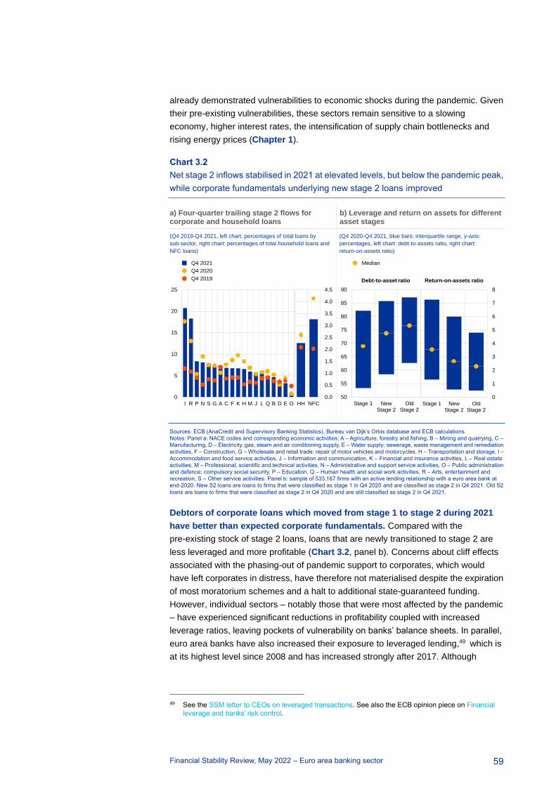
Financial Stability Review, May 2022 – Euro area banking sector
59
already demonstrated vulnerabilities to economic shocks during the pandemic. Given
their pre-existing vulnerabilities, these sectors remain sensitive to a slowing
economy, higher interest rates, the intensification of supply chain bottlenecks and
rising energy prices (Chapter 1).
Chart 3.2
Net stage 2 inflows stabilised in 2021 at elevated levels, but below the pandemic peak,
while corporate fundamentals underlying new stage 2 loans improved
a) Four-quarter trailing stage 2 flows for corporate and household loans
b) Leverage and return on assets for different asset stages
(Q4 2019-Q4 2021, left chart: percentages of total loans by
sub-sector, right chart: percentages of total household loans and
NFC loans)
(Q4 2020-Q4 2021, blue bars: interquartile range, y-axis:
percentages, left chart: debt-to-assets ratio, right chart:
return-on-assets ratio)
Sources: ECB (AnaCredit and Supervisory Banking Statistics), Bureau van Dijk’s Orbis database and ECB calculations.
Notes: Panel a: NACE codes and corresponding economic activities: A – Agriculture, forestry and fishing, B – Mining and quarrying, C –
Manufacturing, D – Electricity, gas, steam and air conditioning supply, E – Water supply; sewerage, waste management and remediation
activities, F – Construction, G – Wholesale and retail trade; repair of motor vehicles and motorcycles, H – Transportation and storage, I –
Accommodation and food service activities, J – Information and communication, K – Financial and insurance activities, L – Real estate
activities, M – Professional, scientific and technical activities, N – Administrative and support service activities, O – Public administration
and defence; compulsory social security, P – Education, Q – Human health and social work activities, R – Arts, entertainment and
recreation, S – Other service activities. Panel b: sample of 533,167 firms with an active lending relationship with a euro area bank at
end-2020. New S2 loans are loans to firms that were classified as stage 1 in Q4 2020 and are classified as stage 2 in Q4 2021. Old S2
loans are loans to firms that were classified as stage 2 in Q4 2020 and are still classified as stage 2 in Q4 2021.
Debtors of corporate loans which moved from stage 1 to stage 2 during 2021
have better than expected corporate fundamentals. Compared with the
pre-existing stock of stage 2 loans, loans that are newly transitioned to stage 2 are
less leveraged and more profitable (Chart 3.2, panel b). Concerns about cliff effects
associated with the phasing-out of pandemic support to corporates, which would
have left corporates in distress, have therefore not materialised despite the expiration
of most moratorium schemes and a halt to additional state-guaranteed funding.
However, individual sectors – notably those that were most affected by the pandemic
– have experienced significant reductions in profitability coupled with increased
leverage ratios, leaving pockets of vulnerability on banks’ balance sheets. In parallel,
euro area banks have also increased their exposure to leveraged lending,49 which is
at its highest level since 2008 and has increased strongly after 2017. Although
49 See the SSM letter to CEOs on leveraged transactions. See also the ECB opinion piece on Financial
leverage and banks’ risk control.
0
5
10
15
20
25
I R P N S G A C F K H M J L Q B D E O
Q4 2021
Q4 2020
Q4 2019
0.0
0.5
1.0
1.5
2.0
2.5
3.0
3.5
4.0
4.5
HH NFC
50
55
60
65
70
75
80
85
90
Stage 1 NewStage 2
OldStage 2
Debt-to-asset ratio
Median
0
1
2
3
4
5
6
7
8
Stage 1 NewStage 2
OldStage 2
Return-on-assets ratio
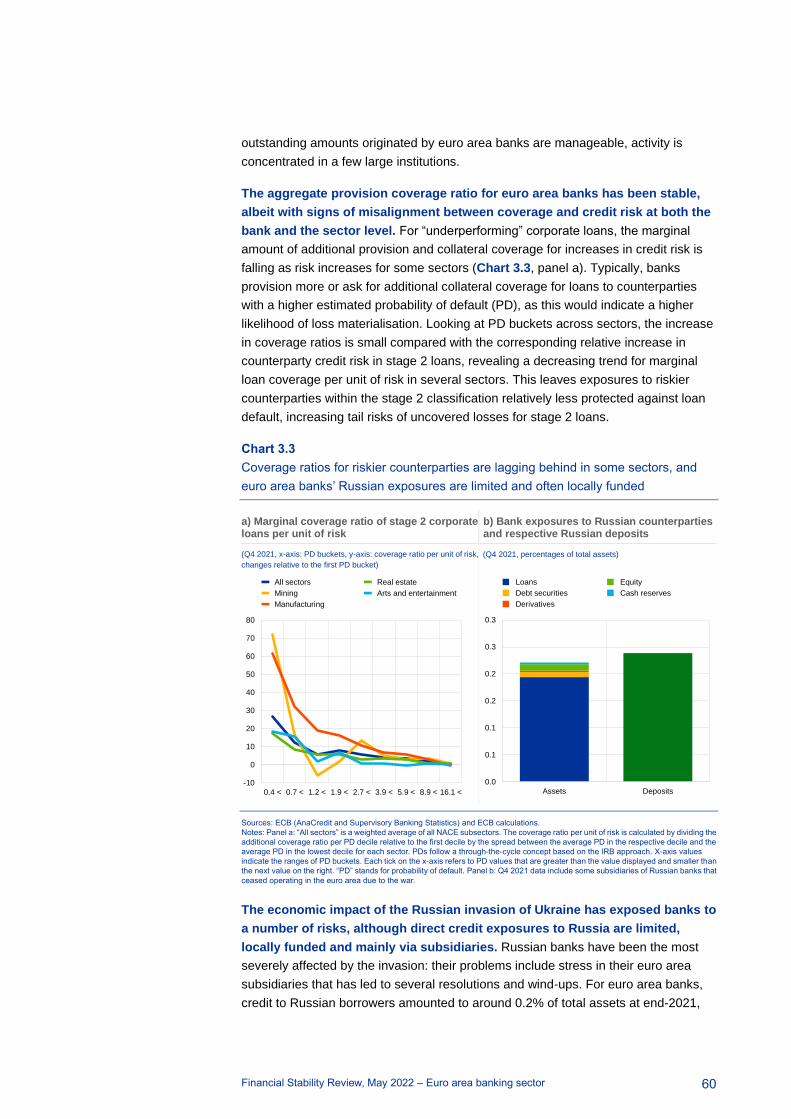
Financial Stability Review, May 2022 – Euro area banking sector
60
outstanding amounts originated by euro area banks are manageable, activity is
concentrated in a few large institutions.
The aggregate provision coverage ratio for euro area banks has been stable,
albeit with signs of misalignment between coverage and credit risk at both the
bank and the sector level. For “underperforming” corporate loans, the marginal
amount of additional provision and collateral coverage for increases in credit risk is
falling as risk increases for some sectors (Chart 3.3, panel a). Typically, banks
provision more or ask for additional collateral coverage for loans to counterparties
with a higher estimated probability of default (PD), as this would indicate a higher
likelihood of loss materialisation. Looking at PD buckets across sectors, the increase
in coverage ratios is small compared with the corresponding relative increase in
counterparty credit risk in stage 2 loans, revealing a decreasing trend for marginal
loan coverage per unit of risk in several sectors. This leaves exposures to riskier
counterparties within the stage 2 classification relatively less protected against loan
default, increasing tail risks of uncovered losses for stage 2 loans.
Chart 3.3
Coverage ratios for riskier counterparties are lagging behind in some sectors, and
euro area banks’ Russian exposures are limited and often locally funded
a) Marginal coverage ratio of stage 2 corporate loans per unit of risk
b) Bank exposures to Russian counterparties and respective Russian deposits
(Q4 2021, x-axis: PD buckets, y-axis: coverage ratio per unit of risk,
changes relative to the first PD bucket)
(Q4 2021, percentages of total assets)
Sources: ECB (AnaCredit and Supervisory Banking Statistics) and ECB calculations.
Notes: Panel a: “All sectors” is a weighted average of all NACE subsectors. The coverage ratio per unit of risk is calculated by dividing the
additional coverage ratio per PD decile relative to the first decile by the spread between the average PD in the respective decile and the
average PD in the lowest decile for each sector. PDs follow a through-the-cycle concept based on the IRB approach. X-axis values
indicate the ranges of PD buckets. Each tick on the x-axis refers to PD values that are greater than the value displayed and smaller than
the next value on the right. “PD” stands for probability of default. Panel b: Q4 2021 data include some subsidiaries of Russian banks that
ceased operating in the euro area due to the war.
The economic impact of the Russian invasion of Ukraine has exposed banks to
a number of risks, although direct credit exposures to Russia are limited,
locally funded and mainly via subsidiaries. Russian banks have been the most
severely affected by the invasion: their problems include stress in their euro area
subsidiaries that has led to several resolutions and wind-ups. For euro area banks,
credit to Russian borrowers amounted to around 0.2% of total assets at end-2021,
-10
0
10
20
30
40
50
60
70
80
0.4 < 0.7 < 1.2 < 1.9 < 2.7 < 3.9 < 5.9 < 8.9 < 16.1 <
All sectors
Mining
Manufacturing
Real estate
Arts and entertainment
0.0
0.1
0.1
0.2
0.2
0.3
0.3
Assets Deposits
Loans
Debt securities
Derivatives
Equity
Cash reserves

Financial Stability Review, May 2022 – Euro area banking sector
61
with a selection of banks from Italy, Cyprus, Latvia, Luxembourg and Austria having
relatively higher exposures in terms of total assets (Chart 3.3, panel b). Most credit
exposures were funded by Russian deposits, reducing the net exposure to Russia.50
Recently, large euro area banks with sizeable exposures to Russia reported
increases in their loan loss provisioning for Q1.
Chart 3.4
Euro area banks’ exposures to energy-intensive sectors and to direct risks from
energy prices are concentrated in certain sectors and the derivatives market
a) Euro area banks’ country exposures to high energy usage and vulnerable firms
b) Breakdown of euro area banks’ and corporates’ commodity derivatives holdings
(Q4 2021, percentages of total corporate loans) (12 May 2022, gross notional, € billions, inner ring: NFCs’
derivatives holdings, outer ring: euro area banks’ derivatives
holdings)
EA 0.0
3
0.0
1
0.0
7
0.2
5
0.1
4
0.4
5
0.5
1
0.4
7
0.5
9
0.8
9
0.2
1
0.1
5
AT
BE
DE
EE
FI
FR
GR
IT
LT
LU
NL
PT
ES
Fis
hin
g
Me
tal o
res
Oth
er
min
ing
Pa
pe
r
Pri
nting
an
d m
ed
ia
Che
mic
als
Rub
be
r a
nd
pla
stic
Gla
ss
Ba
sic
me
tals
La
nd
tra
nsp
ort
Wa
ter
tra
nsp
ort
Air
tra
nsp
ort
Sources: ECB (AnaCredit, Supervisory Banking Statistics and European Market Infrastructure Regulation), OECD Trade in Value Added
(TiVA) database (2018) and ECB calculations.
Notes: Panel a: colour scale from green to orange to red. Green indicates small exposures to vulnerable firms; cells become orange/red
if share of exposure increases. Vulnerable firms are entities with an Altman z-score below 1.81. The Altman z-score is calculated as
0.717 x working capital/total assets + 0.847 x retained earnings/total assets + 3.107 x EBIT/total assets + 0.420 x equity/debt + 0.998
sales/total assets. Sector average energy intensity is measured by the share of input from the energy-producing mining and quarrying
sector, coke and refined petroleum products as well as the electricity, gas, steam and air conditioning industries, classified according to
the United Nations International Standard Industrial Classification for All Economic Activities, Rev. 4., and is attributed to the sector
based on the four-digit Standard Industrial Classification code. Firms in sectors above the 75th percentile of the energy intensity ratio are
regarded as high-energy consumers. Panel b: the rings represent the gross notional outstanding (€ billions) in energy (blue), agricultural
(red) and metal (yellow) derivatives for which at least one of the two counterparties of the trade is a bank domiciled in the euro area (outer
ring) and for which at least one of the two counterparties of the trade is a non-financial firm.
Looking ahead, elevated and volatile energy and commodity prices have
increased credit risk, especially for more vulnerable corporates. The shift in the
outlook for euro area growth and inflation is, in general, likely to weigh on corporate
profitability and debt sustainability (Chapter 1). Credit granted by euro area banks to
50 Although linkages of euro area banks with Russia are limited to a few banks, exposures and deposits are
not always located in the same entity but often separated between subsidiary and parent company.
Electricity105
Natural gas102
Oil58
Preciousmetals
73
Electricity211
Natural gas173
Oil303
Grains77
Other95
Preciousmetals
144
Non-preciousmetals
104

Financial Stability Review, May 2022 – Euro area banking sector
62
firms with significant reliance on energy and specific forms of fossil fuel51, and weak
corporate fundamentals52 amounts to 3.8% of total corporate lending.53 Loans to the
transport and manufacturing sectors appear to be the most vulnerable, although total
exposure is limited at both the country and the euro area level (Chart 3.4, panel a).
Euro area banks also have some exposures stemming from their role in
intermediating derivatives markets, as they act as counterparties in over half of
euro area core commodity derivatives contracts. Commodity derivatives account
for less than 1% of the overall euro area derivatives market’s size in terms of gross
notional. However, the business is highly concentrated in a few large banks which
provide both client clearing services and ancillary financing services to commodity
traders and energy sector firms.54 Financial stability considerations might arise with
regard to substitutability, given that a limited number of large NFCs access the
commodity derivatives market via a few large banks. These banks offer liquidity
through market making in the bilateral market segment and act as clearing members
of the few central counterparties clearing commodity derivatives (Chart 3.4, panel b).
The prices of futures on commodities rose rapidly during March 2022, and this
was accompanied by corresponding increases in margin calls. The recent
volatility in energy prices has also seen liquidity pressures in some derivatives
markets (Chapter 2). The surge in commodity prices and volatility exerted liquidity
pressure on NFCs with hedging activities, especially for energy derivatives, given
their need to meet initial and variation margin calls. Initial margins posted by NFCs on
cleared commodity derivatives more than doubled between December 2021 and
March 2022. The high proportion of centrally cleared trades (68% in terms of gross
notional), especially for energy derivatives, decreases banks’ counterparty credit risk
towards their clients; this does, however, introduce some residual step-in liquidity risk
to cover the margins required by CCPs if some NFCs are unable to meet margin
calls. Banks’ exposures to NFCs in this market are limited, though, and should
therefore not add significant counterparty risk to banks’ balance sheets.
Overall, euro area banks’ asset quality has remained stable, albeit with material
risks to corporate loans persisting. Concerns about aftershocks from 2020 have
not materialised over the last year, although some sectors of NFCs remain vulnerable
to shocks. Overlaps between firms affected by weak debt sustainability and high
energy prices have led to pockets of default risks in the corporate sector. Looking
ahead, the combination of existing vulnerabilities and effects of inflation and the war
in Ukraine increases risks to asset quality.
51 For details on the identification and dependence of euro area firms on natural gas, see the box entitled
“Natural gas dependence and risks to euro area activity”, Economic Bulletin, Issue 1, ECB, 2022.
52 For more details, see Casey, C.J., Bibeault, D. and Altman, E.I., “Corporate financial distress: A
Complete guide to Predicting, Avoiding, and Dealing with Bankruptcy”, Journal of Business Strategy, Vol.
5, No 1, 1984, p. 102. See also the box entitled “Identifying the corporates most vulnerable to price
shocks following the pandemic shock” in this edition of the Financial Stability Review.
53 3.8% of total corporate loans refers to exposures to corporates reliant on a high share of energy input to
generate outputs as well as weak corporate fundamentals as measured by z-scores.
54 Universal and investment banks usually have the capacity to run proprietary trading, maintain a trading
desk and play an active role in the derivatives market.

Financial Stability Review, May 2022 – Euro area banking sector
63
3.2 Profitability above pre-pandemic levels, but outlook
weaker
The financial performance of euro area banks improved substantially during
2021 and exceeded pre-pandemic levels, amid lower loan loss provisions. On
aggregate, euro area significant institutions recorded a return on equity (ROE) of
6.6%, up from 1.7% a year earlier (Chart 3.5, panel a).55 Looking at a sample of
listed euro area banks, for which the data span a longer period, reveals that this was
their strongest performance in a decade. Weak profitability in the euro area banking
sector has been a concern as it affects financial stability by reducing banks’
intermediation capacity and resilience.56 While banks’ performance was adversely
affected by pandemic-related impairments during 2020, robust economic growth,
lower loan loss provisions and higher operating profits contributed to the marked
improvement in 2021. With net interest income (NII) remaining unchanged and
expenses rising, the improvement in operating profits was largely down to higher net
trading income (NTI) and, especially, net fee and commission income (NFCI). Results
for listed banks’ first quarter 2022 earnings suggest that profitability remained robust
in Q1, albeit slightly lower than in Q4, amid weaker other profit and loss items and
higher provisions, while operating income improved on the back of stronger NII.
Chart 3.5
Profitability in 2021 exceeded pre-pandemic levels on the back of lower loan loss
provisions and higher non-interest income components
a) ROE of euro area significant institutions b) Main factors contributing to annual changes in operating profits for banks of above/below-median size and profitability
(Q1 2019-Q4 2021, percentages) (Q4 2021, percentage changes and percentage point
contributions)
Sources: ECB (Supervisory Banking Statistics) and ECB calculations.
Notes: Based on a balanced sample of 89 significant institutions. Panel b: “Other” stands for other operating profits.
55 In the Financial Stability Review, the four-quarter average of stock variables is used, while flow variables
are annualised using trailing four-quarter sums. In addition, to avoid composition effects, a balanced
sample of banks is used, which might result in figures which are different from those in the published
supervisory banking statistics.
56 See the special feature entitled “Euro area bank profitability: where can consolidation help?”, Financial
Stability Review, ECB, November 2019.
-2
-1
0
1
2
3
4
5
6
7
8
Q1 Q2 Q3 Q4 Q1 Q2 Q3 Q4 Q1 Q2 Q3 Q4
2019 2020 2021
Annualised quarterly ROE
Four-quarter trailing ROE
-50
-40
-30
-20
-10
0
10
20
30
Belowmedian
Abovemedian
Belowmedian
Abovemedian
Size ROE
NFCI
NII
NTI
Expenses
Other
Operating profit

Financial Stability Review, May 2022 – Euro area banking sector
64
Net fee and commission income, driven by asset management activities,
strongly supported profitability in 2021, while net interest income remained flat.
In 2021, euro area banks saw their NFCI grow by almost 12%, by far the largest
increase observed over the past few years, thanks to the economic recovery and
strong growth in assets under management. The positive role played by NFCI in
supporting operating profits was more pronounced for larger banks and for those with
below-median ROE, as the latter faced a decline in their NII (Chart 3.5, panel b).
NFCI might, however, be vulnerable to stock market corrections. The decline in
operating profits for smaller banks was driven to a large extent by NPL sales of Greek
banks. On aggregate, NII remained broadly unchanged on the previous year and is
slowly climbing back towards pre-pandemic levels on the back of rising lending
volumes and a bottoming-out of margins. However, heterogeneity among banks
continues to be pronounced, with around 45% of banks still reporting lower NII than in
the previous year.
Chart 3.6
Downward revisions in 2022 ROE projections as a result of the war in Ukraine, with
higher impairments seen as the main driver
a) Q4 2021 ROE and revisions in ROE projections of listed euro area banks for 2022-24
b) Main factors contributing to the revisions in 2022 ROE projections
c) Revisions of expected 2022 ROE and exposures to Russia and Ukraine
(percentages) (percentages, percentage point
contributions)
(Q4 2021, percentages of CET1 capital;
18 Feb.-17 May 2022, percentage change)
Sources: Bloomberg Finance L.P., Refinitiv, ECB (Supervisory Banking Statistics) and ECB calculations.
Notes: Panels a) and b) are based on a sample of 32 listed euro area banks. Actual and projected ROEs are averages weighted by
banks’ total assets. Panel b: LLP stands for loan loss provisions; OPC stands for operating costs. Panel c) is based on a sample of 28
listed euro area banks. Raiffeisen Bank International has been excluded from the sample in the interests of better readability. EA
indicates the euro area average.
The Russia-Ukraine war casts uncertainty on the economic outlook and implies
a downward revision of bank profitability for this year. After strong profitability
results in 2021, the ROE of listed euro area banks is expected to be lower this year
before gradually improving over the next few years to 8.2% in 2024, although
analysts have lowered their bank profitability projections on account of the economic
fallout from the war (Chart 3.6, panel a). The downward revisions of ROE this year
are attributed to higher impairments and rising costs, coupled with lower NFCI while
NII is expected to be higher (Chart 3.6, panel b). Since the direct exposure of euro
5.0
5.5
6.0
6.5
7.0
7.5
8.0
8.5
9.0
Q4 2021 2022E 2023E 2024E
Actual Projections
Actual ROE - Q4 2021
Projected ROE - 18 Feb. 2022
Projected ROE - 17 May 2022
6.6
6.8
7.0
7.2
7.4
7.6
7.8
RO
E(1
8 F
eb
)
NII
NF
CI
LL
P
OP
C
Eq
uity
RO
E(1
7 M
ay)
Projected ROE 2022
Positive revisions
Negative revisions
EA
R² = 0.60
-3.0
-2.5
-2.0
-1.5
-1.0
-0.5
0.0
0.5
1.0
1.5
0 5 10 15 20 25 30 35
Re
vis
ion
in
20
22
E R
OE
sin
ce
18
Fe
bru
ary
Exposure to Russia and Ukraine
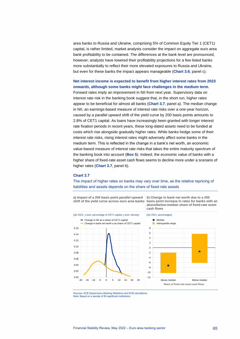
Financial Stability Review, May 2022 – Euro area banking sector
65
area banks to Russia and Ukraine, comprising 5% of Common Equity Tier 1 (CET1)
capital, is rather limited, market analysts consider the impact on aggregate euro area
bank profitability to be contained. The differences at the bank level are pronounced,
however; analysts have lowered their profitability projections for a few listed banks
more substantially to reflect their more elevated exposures to Russia and Ukraine,
but even for these banks the impact appears manageable (Chart 3.6, panel c).
Net interest income is expected to benefit from higher interest rates from 2023
onwards, although some banks might face challenges in the medium term.
Forward rates imply an improvement in NII from next year. Supervisory data on
interest rate risk in the banking book suggest that, in the short run, higher rates
appear to be beneficial for almost all banks (Chart 3.7, panel a). The median change
in NII, an earnings-based measure of interest rate risks over a one-year horizon,
caused by a parallel upward shift of the yield curve by 200 basis points amounts to
2.8% of CET1 capital. As loans have increasingly been granted with longer interest
rate fixation periods in recent years, these long-dated assets need to be funded at
costs which rise alongside gradually higher rates. While banks hedge some of their
interest rate risks, rising interest rates might adversely affect some banks in the
medium term. This is reflected in the change in a bank’s net worth, an economic
value-based measure of interest rate risks that takes the entire maturity spectrum of
the banking book into account (Box 5). Indeed, the economic value of banks with a
higher share of fixed-rate asset cash flows seems to decline more under a scenario of
higher rates (Chart 3.7, panel b).
Chart 3.7
The impact of higher rates on banks may vary over time, as the relative repricing of
liabilities and assets depends on the share of fixed-rate assets
a) Impact of a 200 basis point parallel upward shift of the yield curve across euro area banks
b) Change in bank net worth due to a 200 basis point increase in rates for banks with an above/below-median share of fixed-rate asset cash flows
(Q4 2021, x-axis: percentage of CET1 capital, y-axis: density) (Q4 2021, percentages)
Sources: ECB (Supervisory Banking Statistics) and ECB calculations.
Note: Based on a sample of 80 significant institutions.
0.00
0.02
0.04
0.06
0.08
0.10
0.12
0.14
0.16
-20 -15 -10 -5 0 5 10 15 20 25
Change in NII as a share of CET1 capital
Change in bank net worth a as share of CET1 capital
-12
-10
-8
-6
-4
-2
0
2
4
6
8
Above median Below median
Median
Interquartile range
Share of fixed-rate asset cash flows
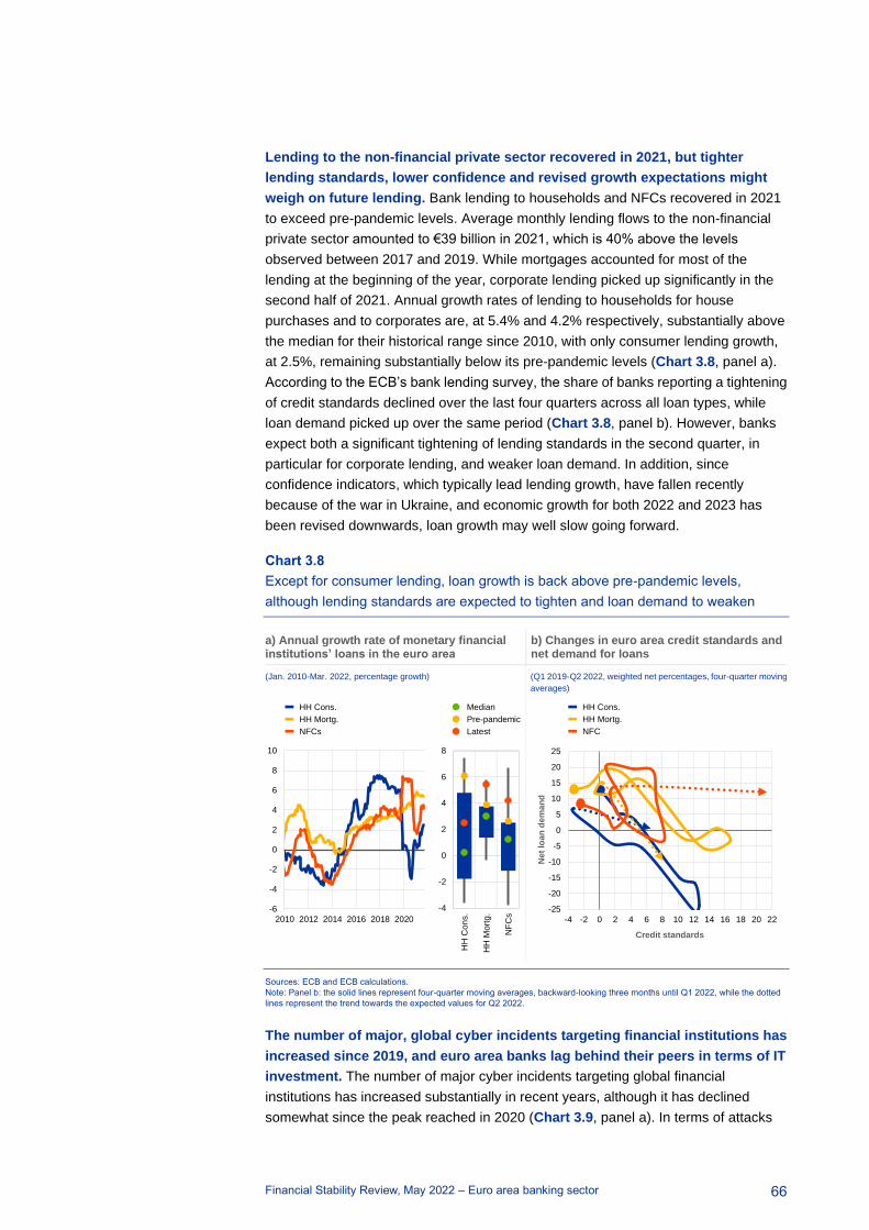
Financial Stability Review, May 2022 – Euro area banking sector
66
Lending to the non-financial private sector recovered in 2021, but tighter
lending standards, lower confidence and revised growth expectations might
weigh on future lending. Bank lending to households and NFCs recovered in 2021
to exceed pre-pandemic levels. Average monthly lending flows to the non-financial
private sector amounted to €39 billion in 2021, which is 40% above the levels
observed between 2017 and 2019. While mortgages accounted for most of the
lending at the beginning of the year, corporate lending picked up significantly in the
second half of 2021. Annual growth rates of lending to households for house
purchases and to corporates are, at 5.4% and 4.2% respectively, substantially above
the median for their historical range since 2010, with only consumer lending growth,
at 2.5%, remaining substantially below its pre-pandemic levels (Chart 3.8, panel a).
According to the ECB’s bank lending survey, the share of banks reporting a tightening
of credit standards declined over the last four quarters across all loan types, while
loan demand picked up over the same period (Chart 3.8, panel b). However, banks
expect both a significant tightening of lending standards in the second quarter, in
particular for corporate lending, and weaker loan demand. In addition, since
confidence indicators, which typically lead lending growth, have fallen recently
because of the war in Ukraine, and economic growth for both 2022 and 2023 has
been revised downwards, loan growth may well slow going forward.
Chart 3.8
Except for consumer lending, loan growth is back above pre-pandemic levels,
although lending standards are expected to tighten and loan demand to weaken
a) Annual growth rate of monetary financial institutions’ loans in the euro area
b) Changes in euro area credit standards and net demand for loans
(Jan. 2010-Mar. 2022, percentage growth) (Q1 2019-Q2 2022, weighted net percentages, four-quarter moving
averages)
Sources: ECB and ECB calculations.
Note: Panel b: the solid lines represent four-quarter moving averages, backward-looking three months until Q1 2022, while the dotted
lines represent the trend towards the expected values for Q2 2022.
The number of major, global cyber incidents targeting financial institutions has
increased since 2019, and euro area banks lag behind their peers in terms of IT
investment. The number of major cyber incidents targeting global financial
institutions has increased substantially in recent years, although it has declined
somewhat since the peak reached in 2020 (Chart 3.9, panel a). In terms of attacks
-6
-4
-2
0
2
4
6
8
10
2010 2012 2014 2016 2018 2020
HH Cons.
HH Mortg.
NFCs
-4
-2
0
2
4
6
8
HH
Co
ns.
HH
Mo
rtg
.
NF
Cs
Median
Pre-pandemic
Latest
-25
-20
-15
-10
-5
0
5
10
15
20
25
-4 -2 0 2 4 6 8 10 12 14 16 18 20 22
Net
loa
n d
em
an
d
Credit standards
HH Cons.
HH Mortg.
NFC
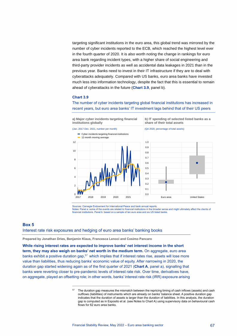
Financial Stability Review, May 2022 – Euro area banking sector
67
targeting significant institutions in the euro area, this global trend was mirrored by the
number of cyber incidents reported to the ECB, which reached the highest level ever
in the fourth quarter of 2020. It is also worth noting the change in rankings for euro
area bank regarding incident types, with a higher share of social engineering and
third-party provider incidents as well as accidental data leakages in 2021 than in the
previous year. Banks need to invest in their IT infrastructure if they are to deal with
cyberattacks adequately. Compared with US banks, euro area banks have invested
much less into information technology, despite the fact that this is essential to remain
ahead of cyberattacks in the future (Chart 3.9, panel b).
Chart 3.9
The number of cyber incidents targeting global financial institutions has increased in
recent years, but euro area banks’ IT investment lags behind that of their US peers
a) Major cyber incidents targeting financial institutions globally
b) IT spending of selected listed banks as a share of their total assets
(Jan. 2017-Dec. 2021, number per month) (Q4 2020, percentage of total assets)
Sources: Carnegie Endowment for International Peace and bank annual reports.
Notes: Panel a: some of the events are related to financial institutions in the broader sense and might ultimately affect the clients of
financial institutions. Panel b: based on a sample of ten euro area and six US listed banks.
Box 5
Interest rate risk exposures and hedging of euro area banks’ banking books
Prepared by Jonathan Dries, Benjamin Klaus, Francesca Lenoci and Cosimo Pancaro
While rising interest rates are expected to improve banks’ net interest income in the short
term, they may also weigh on banks’ net worth in the medium term. On aggregate, euro area
banks exhibit a positive duration gap,57 which implies that if interest rates rise, assets will lose more
value than liabilities, thus reducing banks’ economic value of equity. After narrowing in 2020, the
duration gap started widening again as of the first quarter of 2021 (Chart A, panel a), signalling that
banks were reverting closer to pre-pandemic levels of interest rate risk. Over time, derivatives have,
on aggregate, played an offsetting role; in other words, banks’ interest rate risk (IRR) exposure arising
57 The duration gap measures the mismatch between the repricing timing of cash inflows (assets) and cash
outflows (liabilities) of instruments which are already on banks’ balance sheet. A positive duration gap
indicates that the duration of assets is larger than the duration of liabilities. In this analysis, the duration
gap is computed as in Esposito et al. (see Notes to Chart A) using supervisory data on behavioural cash
flows for 62 euro area banks.
0
2
4
6
8
10
12
2017 2018 2019 2020 2021
Cyber incidents targeting financial institutions
12-month moving average
0.0
0.1
0.2
0.3
0.4
0.5
0.6
0.7
0.8
0.9
1.0
Euro area United States

Financial Stability Review, May 2022 – Euro area banking sector
68
from their non-derivative positioning was partly counterbalanced by their derivative positions in the
banking book.
Chart A
Euro area banks’ duration gap has widened recently, increasing their interest rate risk
Sources: ECB (Supervisory Banking Statistics) and ECB calculations.
Notes: Panel a: the duration gap is computed for the euro area aggregate based on Esposito et al.* and a sample of 62 significant institutions. Panel b: the
change in bank net worth is computed based on Esposito et al.* and a sample of 62 significant institutions. The left chart shows the change in net worth for euro
area banks on aggregate under the interest rate scenario considered, while the right chart plots the distribution across individual banks.
*) Esposito, L., Nobili, A. and Ropele, T., “The management of interest rate risk during the crisis: Evidence from Italian banks”, Journal of Banking and Finance,
Vol. 59, October 2015, pp. 486-504.
The aggregate impact of higher interest rates on bank net worth would be moderately
negative, but wide variations exist at the level of individual banks. The duration gap can be
translated into sensitivity of bank economic value to changes in interest rates. For example, a
steepening of the yield curve by 200 basis points at the longer end in the fourth quarter of 2021 would
have reduced banks’ aggregate net worth by around 4% of Common Equity Tier 1 (CET1) capital
(Chart A, panel b).58 More than 60% of the banks analysed would face a decline in their net worth
under this scenario, while for 25% the net worth would decline by more than 7% of CET1 capital. This
decline arises as, in the medium to long term, banks would have to pay higher funding costs to cover
legacy low-yielding assets. Changes in banks’ economic value of equity do not always translate into
accounting losses, but they do shed light on banks’ resilience to changes in interest rates over the
long run.
An empirical analysis of bank characteristics and IRR indicates that the share of exposures
with longer rate-fixation periods plays a prominent role in this relationship and shows that
derivatives are used to hedge IRR. The analysis59 finds that the decline in bank net worth under a
scenario of rising rates is more pronounced when the share of lending with fixation periods in excess
of ten years is higher. Furthermore, larger banks seem to face a smaller decline in their net worth,
possibly reflecting reduced hedging capabilities of smaller banks.60
58 This decline in net worth appears to be moderate overall, as the 2018 EBA guidelines on the
management of interest rate risk in the banking book suggest that an institution is exposed to excessive
IRR when its economic value of equity declines by more than 15% of its Tier 1 capital.
59 The analysis is based on different panel regressions covering 62 banks over the time period from Q4
2016 to Q3 2021 with time and bank fixed effects and a set of bank control variables.
60 Less significant institutions in Germany, such as savings banks and credit cooperatives, exhibited higher
IRR than large banks; see “Financial Stability Review”, Deutsche Bundesbank, November 2016.
a) Decomposition of duration gap by banking book category
b) Interest rate risk over time and distribution across banks under the steepening scenario
(Q1 2017-Q4 2021, percentages of CET1 capital) (left chart: Q1 2017-Q4 2021, percentages of CET1 capital;
right chart: Q4 2021, number of banks per buckets of interest rate risk)
-2
-1
0
1
2
3
4
5
2017 2018 2019 2020 2021
Net duration gap – assets and liabilities
Net duration gap – interest rate derivatives
Net duration gap – banking book
-7
-6
-5
-4
-3
-2
-1
0
03/17 06/18 09/19 12/20
0
5
10
15
20
25
30
-30
to
-2
0
-20
to
-1
0
-10
to
0
0 t
o 1
0
10
to
20
20
to
30

Financial Stability Review, May 2022 – Euro area banking sector
69
Chart B
Banks actively manage interest rate risk exposures by changing the maturity profile of IRS trading
Sources: ECB (Supervisory Banking Statistics and European Market Infrastructure Regulation) and ECB calculations.
Notes: Panel a: “Basis swaps” are IRS on floating interest rates, “EONIA and €STR OIS” are euro-denominated overnight index swaps, “Other-currency OIS” are
overnight index swaps denominated in other currencies, “Other-currency LIBOR” includes GBP-, JPY-, CHF- and USD-denominated LIBOR swaps, “Other
IRSs” includes fixed-to-fixed swaps, inflation swaps and other IRS. Right chart: net notional is aggregated in four maturity buckets. “NFCs” stands for
non-financial corporations and “IRS” for interest rate swaps. Panel b: outstanding trades excluding intragroup transactions. Outstanding refers to outstanding
contracts as of 31 December 2021, new refers to IRS trades initiated following March 2021. Trades with NCBs and counterparties with non-identifiable sectors
are excluded and represent less than 2% of gross notional traded by euro area banks. Breakdown by sector: “IF” stands for investment funds, “MMMF” for money
market mutual funds, “IC” for insurance companies, “PF” for pension funds, “NFC” for non-financial corporations, “OFI” for other financial institutions.
Euro area banks have held an increased volume of interest rate swaps over the last two years,
suggesting more active hedging of interest rate risk. Banks enter into interest rate swaps in order
to complement natural hedging, to take on more risk by means of directional exposures or to provide
liquidity through market making. When they do so to mitigate risk, banks transform future cash flows
generated from assets or liabilities from floating rates to fixed rates, or vice versa. By the end of 2021,
the gross notional outstanding on interest rate swaps held by banks had increased to €128 trillion,
while that on the most liquid euro-denominated contracts (EURIBOR swaps, EONIA OIS or €STR
OIS) had risen by 30% since the start of 2019 to €56 trillion (Chart B, panel a). These contracts are
more suited to reducing the volatility on banks’ balance sheets prompted by the repricing of
euro-denominated cash flows. Over the last three years, banks have reduced their net notional61
exposures to shorter-dated swap contracts (below one year), on which they pay fixed rates, and
increased the volume of longer-dated contracts, on which they receive floating rates (Chart B, panel
a). This evidence is consistent with the expectation of higher interest rates and the intention to hedge
low-yielding assets against rate hikes.
Interest rate swaps are used to spread risk within the banking sector and to transfer it to
insurance companies and pension funds. Focusing solely on euro-denominated interest rate
swaps written on the euro interbank offered rate (EURIBOR), the overnight index average rate
(EONIA) or the euro short-term rate (€STR), euro area banks trade most of these swaps with other
banks. Concerning risk transfers to other sectors, banks’ transactions are not evenly spread across
maturity buckets: insurance companies and pension funds receive fixed-rate payments for maturities
61 Net notional is computed as the difference between notional bought (pay fix) and notional sold (pay float)
by each bank, on each contract, on each bucket of maturities and on each floating tenor. Intragroup
transactions are excluded from net notional computations.
a) Interest rate swaps traded by euro area banks b) Sectoral breakdown of counterparties trading interest rate swaps with euro area banks
(left chart: Q1 2019-Q4 2021, € trillions, right chart: 2019, 2021, percentage
points, net notional as share of total loans to NFCs and households)
(Dec. 2021, percentage points, percentage of gross notional outstanding held
by euro area banks with other counterparties on EURIBOR swaps)
0
20
40
60
80
100
120
140
03
/19
06
/19
09
/19
12
/19
03
/20
06
/20
09
/20
12
/20
03
/21
06
/21
09
/21
12
/21
Thousands
EURIBOR
EONIA and €STR OIS
Basis swaps
Other-currency OIS
Other-currency LIBOR
Other IRSs
-10
-8
-6
-4
-2
0
2
4
6
8
20
19
20
21
20
19
20
21
20
19
20
21
20
19
20
21
< 1Y 1Y-5Y 5Y-10Y > 10Y
0%
10%
20%
30%
40%
50%
60%
70%
80%
90%
100%
Ou
tsta
nd
ing
Ne
w
Ou
tsta
nd
ing
Ne
w
Outs
tan
din
g
Ne
w
Ou
tsta
nd
ing
Ne
w
< 1Y 1Y-5Y 5Y-10Y >10Y
SSM bank
Non-SSM bank
IF
MMMF
IC
PF
NFC
OFI
Government

Financial Stability Review, May 2022 – Euro area banking sector
70
over ten years given their aggregate negative duration gap, which makes them a natural counterparty
for banks. For contracts initiated after March 2021, when inflation started to pick up, investment funds
have assumed more risk for short maturities while, for longer maturities, the share of insurance
companies and pension funds in swap trading has doubled (Chart B, panel b).
Banks’ IRR exposure appears moderate on aggregate, but wide variations exist across
individual institutions. While rising rates would negatively affect the net worth of more than half of
the banks analysed, their exposure has declined since 2017. Interest rate swap exposures, and
particularly the volume of longer-dated receiver floating swaps, have increased since inflation started
to pick up in March 2021, suggesting that euro area banks are using derivatives as hedging
instruments. A normalisation of monetary policy should not be a major concern in terms of aggregate
impact on the net worth of the euro area banking system, although it could have a negative effect on
banks exhibiting large IRR exposures.
3.3 Higher market funding costs and improved capital ratios
Low, stable deposit funding rates have insulated banks from the increase in
funding costs associated with a notable rise in bank bond yields since the end
of 2021. Higher risk-free rates, reflecting inflationary pressures, have brought the
yields of covered bonds for the euro area on aggregate back to levels last seen in
2014, while yields for riskier instruments have remained below those observed at the
start of the pandemic (Chart 3.10, panel a). This is because the risk premia
embedded in the more junior instruments have remained relatively contained
compared with March 2020. Low, stable deposit funding rates, coupled with an
increase in deposit volumes, have helped to keep banks’ overall funding costs
favourable. Banks have reduced their issuance of bail-inable debt, mainly as a
consequence of the substantial rise in market funding costs. For senior bail-inable
bonds, the cumulative issuance volume in the first four and a half months of this year
was almost 11% lower than the average observed in the period from 2017 to 2019,
while for Tier 2 (T2) and Additional Tier 1 (AT1) instruments volumes were close to
23% and 52% lower (Chart 3.10, panel b). Although forward rates suggest that
banks’ bond funding costs could rise further, the impact on funding costs will be
limited as the majority of maturing bonds were issued at higher yields (Chart 3.11,
panel a).
The expected reduction of banks’ Eurosystem funding is likely to return bank
balance sheet size and the composition of liquid assets to pre-pandemic levels.
Based on the median estimate obtained from the ECB Survey of Monetary Analysts62,
€700 billion of repayments of targeted longer-term refinancing operations (TLTRO)
are expected to be made by the end of December 2022. Since TLTRO repayments
are likely to be made using excess liquidity, this implies that liquidity coverage ratios
and the composition of high quality liquid assets (HQLA) will return to pre-pandemic
levels, with the share of government bonds in HQLA rising from 25% to 45%.
62 For more details, see the ECB Survey of Monetary Analysts, April 2022.

Financial Stability Review, May 2022 – Euro area banking sector
71
Chart 3.10
Banks’ bond funding costs have increased substantially since end-2021 amid higher
risk-free rates and have prompted banks to reduce their issuance of bail-inable debt
a) Bond funding costs of euro area banks across different seniorities
b) Cumulative volume of bank bonds issued between January and mid-May
(2 Jan. 2019-17 May 2022, yield per annum, percentages) (€ billions, percentages)
Sources: IHS Markit, Dealogic and ECB calculations.
Notes: NPS stands for non-preferred senior; HoldCo stands for holding company. Panel a: the T2 index shows no values between May
and October 2021 since at that time there were no Tier 2 bonds matching the eligibility criteria for being included in the index. Panel b: the
years 2020-21 are excluded from the benchmark of average issuance volumes shown as the blue bars since their values might be biased
due to the pandemic.
The phasing-out of favourable TLTRO funding rates in June is likely to weigh on
bank profitability in 2022. According to two scenarios which take into account the
new TLTRO rates and the distribution of excess liquidity between Tier 1 and Tier 2
reserves, bank profitability could be adversely impacted by between 60 basis points
and 130 basis points this year (Chart 3.11, panel b). In the first, most likely scenario,
banks meet the lending threshold and benefit from a TLTRO rate of -0.5%.
Depending on the magnitude of excess reserves, the net effect from the change in
TLTRO funding costs would result in profitability which is around 60 basis points
lower. In the more extreme scenario, banks fail to meet the lending threshold and
receive a TLTRO rate of 0%, leading to a greater reduction in profitability. However,
the expected earlier rise in interest rates compared to the beginning of the year
appears to reduce the incentive for banks to repay TLTRO funding sooner, which is
likely to reduce the resulting adverse impact on profitability.
0
2
4
6
8
10
12
14
16
18
-0.5
0.0
0.5
1.0
1.5
2.0
2.5
3.0
01/19 07/19 01/20 07/20 01/21 07/21 01/22
Covered
Senior unsecured
NPS/HoldCo
T2 (right-hand scale)
AT1 (right-hand scale)
0
20
40
60
80
100
120
140
0
10
20
30
40
50
60
70
Covered Seniorunsecured
NPS/HoldCo
T2 AT1
2017-19 average issuance
2022 issuance
Share of 2017-19 issuance (right-hand scale)

Financial Stability Review, May 2022 – Euro area banking sector
72
Chart 3.11
Rolling over maturing bonds would not affect overall bank funding costs, but the
phasing-out of special TLTRO discounts is likely to impact bank profitability in 2022
a) Issuance year and yields of bank bonds maturing in 2022 vis-à-vis current yields
b) Impact of scheduled end of special TLTRO discount on bank profitability under different scenarios
(left chart: € billions; right chart: yields per annum, percentages) (profitability: percentages; reduction in profitability: basis points)
Sources: Dealogic, IHS Markit, ECB (Statistics Bulletin and Supervisory Banking Statistics) and ECB calculations.
Euro area banks’ regulatory capital ratios increased slightly in 2021 on the back
of the de-risking initiated at the start of the pandemic. CET1 ratios for euro area
significant institutions rose by 50 basis points in 2021 to 15.2%.63 The positive
contributions from retained earnings and lower average risk weights more than offset
the negative impact of balance sheet expansion. The contribution from de-risking
shrank in 2021, however, due to a pick-up in lending activities and the associated
higher risk weights in the fourth quarter (Chart 3.12, panel a). The average CET1
capital requirement including Pillar 2 guidance amounted to 11.7% in the last quarter
of 2021, with an average trigger point for automatic restrictions on distributions
(maximum distributable amount, MDA) at around 10.6% (Chart 3.12, panel b).
Analysis suggests that the euro area banking system should be largely resilient
to any extreme macroeconomic risks emanating from the Russia-Ukraine war.
The invasion of Ukraine has led to disruptions in energy and commodity markets and
increased uncertainty around the outlook for euro area economic growth. A severe
impact on euro area production, prices and demand could adversely affect euro area
bank asset quality and solvency. A vulnerability analysis considering adverse and
severely adverse economic scenarios over a three-year horizon indicates that,
overall, the euro area banking sector is resilient, with the aggregate CET1 ratio
estimated to total around 11% even under the severely adverse scenario (Box 6).
63 In the Financial Stability Review, the four-quarter average of total equity is used in the denominator, while
net income is annualised using trailing four-quarter sums. In addition, to avoid composition effects, a
balanced sample of banks is used, which might result in a figure for headline profitability which is different
from that in the published supervisory banking statistics.
0
10
20
30
40
50
60
70
80
2001 2006 2011 2016
Covered
Senior preferred
NPS/HoldCo
T2
AT1
-1
0
1
2
3
4
5
6
7
8
9
10
Co
ve
red
Se
nio
rp
refe
rre
dN
PS
/H
old
Co
T2
AT
1
Median yield at issuance
Average yield in 2022
6.6-59
-126
0
1
2
3
4
5
6
7
Current profitability Scenario 1 Scenario 2
Profitability (ROE)
Reduction in profitability
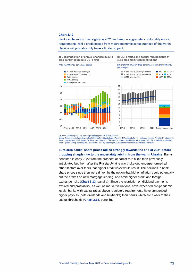
Financial Stability Review, May 2022 – Euro area banking sector
73
Chart 3.12
Bank capital ratios rose slightly in 2021 and are, on aggregate, comfortably above
requirements, while credit losses from macroeconomic consequences of the war in
Ukraine will probably only have a limited impact
a) Decomposition of annual changes in euro area banks’ aggregate CET1 ratio
b) CET1 ratios and capital requirements of euro area significant institutions
(Q4 2016-Q4 2021, percentage points) (left chart: Q4 2016-Q4 2021, percentages; right chart: Q4 2021,
percentages)
Sources: ECB (Supervisory Banking Statistics) and ECB calculations.
Notes: Based on a balanced sample of 89 significant institutions. Panel a: RWA stands for risk-weighted assets. Panel b: P1 stands for
Pillar 1 requirement; P2R stands for Pillar 2 requirement; CBR stands for combined buffer requirement; AT1 SF stands for shortfall of
Pillar 1 (AT1/T2) requirement; P2G stands for Pillar 2 guidance; MDA stands for maximum distributable amount.
Euro area banks’ share prices rallied strongly towards the end of 2021 before
dropping sharply due to the uncertainty arising from the war in Ukraine. Banks
benefited in early 2022 from the prospect of earlier rate hikes than previously
anticipated but then, after the Russia-Ukraine war broke out, underperformed all
other sectors over fears that higher credit risks would result. The declines in bank
share prices since then were driven by the notion that higher inflation could potentially
put the brakes on new mortgage lending, and amid higher credit and foreign
exchange risks (Chart 3.13, panel a). Since the restriction on dividend payments
expired and profitability, as well as market valuations, have exceeded pre-pandemic
levels, banks with capital ratios above regulatory requirements have announced
higher payouts (both dividends and buybacks) than banks which are closer to their
capital thresholds (Chart 3.13, panel b).
-1.0
-0.5
0.0
0.5
1.0
1.5
2.0
12/16 09/17 06/18 03/19 12/19 09/20 06/21
Capital (retained earnings)
Capital (other components)
Total assets
RWA density
Change in CET1 ratio
0
2
4
6
8
10
12
14
16
18
20
22
12/16 06/18 12/19 06/21
CET1 ratio 10th-25th percentile
CET1 ratio 25th-75th percentile
CET1 ratio median
Capital requirements
P1
P2R
CBR
AT1 SF
P2G
MDA

Financial Stability Review, May 2022 – Euro area banking sector
74
Chart 3.13
Bank share prices suffered at the outbreak of war in Ukraine amid credit risks, but
market valuations have improved and banks have increased payouts
a) Multifactor model decomposition of weekly euro area banking sector equity returns
b) Price-to-book ratios of global listed banks and excess capital against total payout ratios
(7 Jan.-13 May 2022, percentage point contributions) (left chart: 1 Jan. 2020-17 May 2022, ratio;
right chart: 2015-21, percentages of risk-weighted assets)
Sources: Refinitiv, Bloomberg Finance L.P., S&P Global Market Intelligence, bank financial reports and ECB calculations.
Notes: Panel a: the calculations are based on the Datastream Eurozone Banks index. Panel b: left chart: based on simple averages of a
sample of 32 listed euro area banks, 6 listed Nordic banks, 5 listed UK banks, 19 listed US banks and 12 listed Japanese banks; right
chart: the total payout ratio is the sum of dividends and share buybacks as a percentage of risk-weighted assets in the respective
financial year. Long-term averages (in yellow) are based on a sample of 36 listed euro area significant institutions. The blue dots refer to
15 banks that have already announced their distribution plans attributable to 2021 profits.
Box 6
Assessing the resilience of the euro area banking sector in light of the Russia-Ukraine war
This box presents an assessment of the euro area banking sector’s resilience to adverse
macroeconomic scenarios in the light of the Russian invasion of Ukraine. While euro area
banks’ direct exposures to Russia are limited overall, disruptions in energy and commodity markets
pose risks to economic activity in the euro area that could adversely affect banks’ balance sheets. To
examine these risks, the ECB has combined three macroeconomic scenarios (a baseline scenario,
an adverse scenario and a severely adverse scenario) with stress-testing tools to perform an
in-house assessment of the solvency of significant euro area banks. The resulting vulnerability
analysis (VA) is a desktop exercise which does not include interactions with banks. The exercise
estimates the impact on bank capital of potential losses arising from (i) exposures to euro area
economic sectors which have strong trade links with Russia or are dependent on commodity imports
from the region, (ii) broader macro-financial stress triggered by current events and (iii) revaluation
risks related to increased market volatility and reduced liquidity. For this purpose, top-down models,
which are consistent with the EBA 2021 Methodological Note64, were used to assess banks’ credit,
market and profitability risks. The estimated impacts are contingent on the underlying scenario
assumptions, which are characterised by a high degree of uncertainty.
64 See the EBA 2021 EU-Wide Stress Test Methodological Note for details.
-40
-30
-20
-10
0
10
20
30
07
/01
14
/01
21
/01
28
/01
04
/02
11
/02
18
/02
25
/02
04
/03
11
/03
18
/03
25
/03
01
/04
08
/04
15
/04
22
/04
29
/04
06
/05
13
/05
01
/01
-18/0
2
18
/02
-13/0
5
Alpha
Market
Real estate
Credit
Sovereign
Term structure
Short-term rates
Foreign exchange
Banking sector returns
0.2
0.4
0.6
0.8
1.0
1.2
1.4
1.6
1.8
2.0
01/20 10/20 07/21 04/22
Euro area
Nordic countries
United Kingdom
United States
Japan
0
1
2
3
4
5
6
0 2 4 6 8 10
To
tal p
ayo
ut
rati
o
Excess capital
2021
2015-19 average

Financial Stability Review, May 2022 – Euro area banking sector
75
Chart A
Key macro-financial features of the scenarios and their impact on credit risk parameters
Sources: Bloomberg Finance L.P., March 2022 ECB staff macroeconomic projections, Oxford Economics, OECD Input-Output tables and ECB calculations.
Notes: Financial shocks in panel a include shocks to commodities, the EUR/RUB exchange rate and the Russian stock market index (MOEX). Panel c shows the
interquartile interval for the sectoral probability of default (PD) estimates for the severely adverse scenario.
Relative to a baseline scenario of a modest slowdown in growth, two alternative adverse
economic scenarios explore the impact of additional commodity and equity price shocks.65
Under the VA-adverse and VA-severely adverse scenarios, oil and gas prices rise by around 80% and
180% respectively (Chart A, panel a), while euro area equity prices fall by more than 20%, matching
the sizeable drop observed in the immediate aftermath of the invasion.66 However, the same financial
shocks are assumed to affect the real economy differently: under the VA-adverse scenario
investment and consumption are affected only temporarily, while under the VA-severely adverse
scenario the effects last longer, giving rise to confidence shocks that further dampen economic
activity and match the severity of the 2021 EBA EU-wide stress test. Annual GDP growth turns
negative under the VA-adverse scenario in 2023, while the euro area economy is in recession in all
three years under the VA-severely adverse scenario (Chart A, panel b). The macro-financial
scenarios are fed into econometric models which capture the heterogenous exposure of euro area
firms to these shocks, yielding different probability of default paths for corporate exposures to
vulnerable67 and non-vulnerable sectors (Chart A, panel c).
65 The baseline scenario is anchored to the March 2022 ECB staff macroeconomic projections for the euro
area, which included a first assessment of the impact of the war. To account for the uncertainty
surrounding the evolution of the conflict and its economic ramifications, two adverse scenarios were
created. The three scenarios combined cover a wide spectrum of macroeconomic outcomes for the euro
area to offer insights into potential feedback effects on the banking system, also once the baseline
projections have been reappraised in the context of the Eurosystem staff macroeconomic projections for
the euro area, which are due to be released in June.
66 Mechanically, the adverse scenarios take as their starting point shocks to commodity and stock market
prices which are based on the actual increases observed in the immediate aftermath of the invasion.
They are likely to incorporate financial markets’ expectations that the shortages in the supply of Russian
commodities in Europe would worsen further, with the additional possibility of a full-scale embargo (as
reflected in financial market news in the early weeks of March).
67 Sectors are identified as (non-)vulnerable by combining information from the OECD Input-Output tables
and NACE 2-level projections of gross value added (GVA) at the country level produced by Oxford
Economics for its 2022 war scenario. Sectors that are highly exposed to Russian trade or experience a
negative GVA shock over the three-year horizon are classified as vulnerable in this exercise.
a) Size of financial shocks used to calibrate the scenarios
b) Euro area real GDP growth under the three scenarios
c) Euro area sectoral probability of default estimates for corporate exposures
(relative changes, percentages) (2022-24, percentage points) (2022-24. percentage points)
Variable
% change
relative to
baseline
included in
the two
adverse
scenarios
Observed %
change
between
23 February
and 6 April
Oil 80.1 11.8
Gas 179.9 22.1
Corn 37.3 11.0
Wheat 63.7 18.5
EUR/RUB 63.0 2.8
MOEX -39.6 -12.8
3.7
2.8
1.6
0.8
-0.8
1.5
-1.7
-3.3
-0.8
-4
-3
-2
-1
0
1
2
3
4
22 23 24 22 23 24 22 23 24
Baseline
VA-adverse
VA-severely adverse
2
3
4
5
Non
-vu
lne
rab
le
Vu
lne
rab
le
Non
-vu
lne
rab
le
Vu
lne
rab
le
Non
-vu
lne
rab
le
Vu
lne
rab
le
2022 2023 2024
Median

Financial Stability Review, May 2022 – Euro area banking sector
76
The results obtained from this exercise confirm that the euro area banking sector is resilient
to the macroeconomic ramifications of the war in Ukraine. The system-level Core Equity Tier 1
(CET1) ratio (in fully loaded terms) is estimated at 13.1% under the VA-adverse scenario and 11.6%
under the VA-severely adverse scenario (Chart B, panel a), with capital depletion amounting to
around 2.1 percentage points and 3.6 percentage points respectively. CET1 ratios fall below 7% for
just over 2% of banking sector assets under the VA-adverse scenario and for just over 8% under the
VA-severely adverse scenario (Chart B, panel b). Credit risk is the main driver of capital depletion in
both adverse scenarios, with sectoral concentration in vulnerable sectors68 amplifying credit losses
that materialise due to the macroeconomic shocks. In addition, the system’s income generating
capacity is weakened by funding cost increases, which also reflect the expiration of targeted
longer-term refinancing operations under all scenarios. These increases offset the gains expected
from rising rates on the asset side, resulting in an overall weakening of net interest income compared
with the starting point. At the bank level, higher capital depletion correlates strongly with a lower
return on equity and with higher cost/income ratios, reflecting the drag exerted by projected operating
costs on capital ratios (Chart B, panel c).
Chart B
The banking sector is resilient overall to the second-round effects arising from the Russia-Ukraine
war: capital depletion is higher for banks with ex ante higher operating costs and lower returns
Sources: ECB (Supervisory Banking Statistics) and ECB calculations.
Notes: NPL stands for non-performing loans. Panel c shows results based on the severely adverse scenario and displays banks grouped by interquartile
buckets, with <25 capturing banks with a CET1 ratio depletion below the 25th percentile, 25-50 capturing banks with a CET1 ratio depletion above the 25th
percentile and below the median, 50-75 banks above the median and below the 75th percentile and >75 banks above the 75th percentile.
68 Sectoral impairments are projected using a combination of (i) micro-econometric models for sector-level
probabilities of default and (ii) proxies capturing bank-level concentration to vulnerable sectors.
a) System-level CET1 and NPL ratios under different scenarios
b) Share of banking sector assets below selected CET1 ratios
c) CET1 ratio depletion relative to bank cost/income ratio and return on equity by quartiles
(percentage points) (percentage points) (percentage points)
0
2
4
6
8
10
12
14
16
CET1 ratio(fully loaded)
NPL ratio
Q4 2021
Adverse
Severely adverse
2.08.76.4
13.014.8
19.0
33.3
27.7
43.531.6
0
20
40
60
80
100
Adverse Severelyadverse
Below 7%
Between 7% and 9%
Between 9% and 11%
Between 11% and 13%
Above 13%
30
35
40
45
50
55
60
65
70
75
<25 25-50 50-75 >75
Interquartile range
Median
Cost/income ratio
0.0
0.5
1.0
1.5
2.0
2.5
3.0
<25 25-50 50-75 >75
Return on equity

Financial Stability Review, May 2022 – Non-bank financial sector
77
4 Non-bank financial sector
4.1 Non-bank financial sector faces higher credit risk as
duration risk starts to materialise
Duration risk in the non-bank financial sector has started to materialise recently
and valuation losses may increase further in an environment of rising interest
rates. Yields have continued on their upward trend that started at the end of 2021.
Over the course of the past year, rising rates have led to a decline in the value of
bond portfolios of around 3.7% for insurance corporations and pension funds (ICPFs)
and 0.4% for investment funds (IFs) (Chart 4.1, panel a). Given that the share of
6.9%
Q1 2020
Fund outflows may trigger
forced sales
Valuation losses from
rising rates
Exposures from synthetic
leverage
Increase in illiquid
holdings of insurers
Non-banks face duration risk amid low
liquidity and uncertain credit risk outlook
• Valuation losses from rising rates
• Fund outflows may trigger forced sales
• Increase in illiquid holdings of insurers
• Exposures from synthetic leverage
Holdings of NFC bonds
Cre
dit
ris
k
Sector energy
intensity
39%
29%
32%
447
561
Q4 18 Q3 21
Alternative asset holdings (€ bn)
4%
-9%
9%
-7%
2019 2020 2021 1 pp rateincrease
Portfolio revaluation
IF
ICPF
7 yrs
10 yrs
4%
3%
Q4 13 Q4 21
Avg. residual
maturity
Cash
holdings
Investment fund portfolio risks
27
48
40
116
01/20 03/22
Options
Futures
Gross notional value/initial margin
posted for equity derivatives

Financial Stability Review, May 2022 – Non-bank financial sector
78
interest rate sensitive assets in ICPF and IF portfolios remains high, in the absence of
hedging strategies a further rise of 1 percentage point in all yield to maturity would
imply additional bond portfolio valuation losses of around 9% for ICPFs and 7% for
IFs. ICPFs and IF shareholders are therefore increasingly shifting their investments
towards equities as well as towards alternative assets (Sections 4.2 and 4.3). In the
medium term, however, rising interest rates could reduce the incentives for the
non-bank sector to search for yield and could improve ICPFs’ capital positions,
mitigating overall financial stability risks.
Chart 4.1
Non-banks’ debt portfolios face revaluation losses amid rising rates, while direct
exposures to Russian assets and commodity derivatives are limited
a) Debt portfolio revaluations and estimated duration risk
b) Holdings of debt and equity issued by Russian entities
c) Derivative exposures by underlying asset class
(2019-Q4 2021, percentage of total bond
portfolio value)
(Q4 2021, left-hand scale: € billions;
right-hand scale: percentage of total assets)
(15 Mar. 2022, left-hand scale: notional
amounts outstanding, € billions; right-hand
scale: percentage increase)
Sources: Eurostat, ECB (Securities Holdings Statistics and European Market Infrastructure Regulation) and ECB calculations.
Notes: Panel a: estimated risk shown in the shaded bars assumes an increase of 1 percentage point in the yield to maturity of all
securities held at the end of 2021. Estimated values are calculated as the sum of modified durations multiplied by the amounts held at the
security level, multiplied by 0.01. Panel b: the chart includes all debt securities and equities issued by Russian-domiciled financial and
non-financial corporations (NFCs), as well as Russian sovereign debt securities. Panel c: initial margins include all margins posted with
euro area central counterparties.
The non-bank financial sector has so far proven to be resilient to increased
uncertainty following the Russian invasion of Ukraine. At the end of 2021, euro
area non-banks’ direct exposures to debt securities and equities issued by Russian
entities were below 1% of their total assets (Chart 4.1, panel b). While fund
categories with higher Russian exposure have experienced significant outflows and
some funds have had to be suspended, there have been no widespread redemptions
or spillovers to the broader euro area non-bank financial sector (Sections 4.2 and
4.3). Furthermore, the increase in volatility in derivatives markets has remained
contained to the commodity segment (Chapter 2), while margins on interest rate
derivatives – the segment to which non-banks are significantly exposed – have been
affected much less than those on commodity derivatives (Chart 4.1, panel c).
Nevertheless, the non-bank financial sector could face second-round effects
stemming from economic uncertainty and rising commodity prices.
-12
-8
-4
0
4
8
12
Q1
Q2
Q3
Q4
1 p
p r
ate
incre
ase
20192020 2021 Risk
ICPFs
IFs
0.00
0.05
0.10
0.15
0.20
0.25
0
5
10
15
20
25
ICPFs IFs
Thousands
Debt securities
Equities
Percentage of total assets (right-hand scale)
0
20
40
60
80
100
120
0
500
1,000
1,500
2,000
2,500
3,000
3,500
Commodities Interest rates
Bill
ions
ICPFs
IFs
Maximum increase in initial margin 15 Feb.-15 Mar. (right-hand scale)
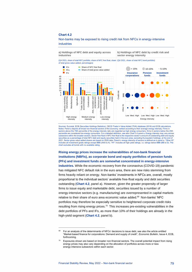
Financial Stability Review, May 2022 – Non-bank financial sector
79
Chart 4.2
Non-banks may be exposed to rising credit risk from NFCs in energy-intensive
industries
a) Holdings of NFC debt and equity across industries
b) Holdings of NFC debt by credit risk and sector energy intensity
(Q4 2021, share of total NFC portfolio, share of NFC free float, share
of total gross value added, percentages)
(Q4 2021, share of total NFC bond portfolio)
Sources: Eurostat, ECB (Securities Holdings Statistics), OECD Trade in Value Added (TiVA) database (2018) and ECB calculations.
Notes: Panel a depicts all broad non-financial sectors of the economy, ranked according to their average energy intensity. Firms in
sectors above the 75th percentile of the energy intensity ratio are regarded as high energy consumers, firms in sectors below the 25th
percentile are considered low energy consumers. For a detailed definition, see also Chart 3.4 panel a. Energy intensity may vary across
subsectors within the broader sectors. Sector free float in NFC free float is the respective sector’s amount of outstanding debt and equity
securities as a percentage of total NFC debt and equity securities held in the euro area, excluding Eurosystem holdings, at the end of
2021. Sector gross value added shares are based on 2020 data. Panel b: energy intensity of sectors is defined as in panel a. “Other IG”
includes all investment grade ratings except BBB (AAA to A). “HY” includes all high-yield ratings, i.e. ratings below BBB (BB to D). The
chart excludes all bonds with no available rating.
Rising energy prices increase the vulnerabilities of non-bank financial
institutions (NBFIs), as corporate bond and equity portfolios of pension funds
(PFs) and investment funds are somewhat concentrated in energy-intensive
industries. While the economic recovery from the coronavirus (COVID-19) pandemic
has mitigated NFC default risk in the euro area, there are new risks stemming from
firms heavily reliant on energy. Non-banks’ investments in NFCs are, overall, mostly
proportional to the individual sectors’ available free-float equity and debt securities
outstanding (Chart 4.2, panel a). However, given the greater propensity of larger
firms to issue equity and marketable debt, securities issued by a number of
energy-intensive sectors (e.g. manufacturing) are overrepresented in capital markets
relative to their share of euro area economic value added.69 Non-banks’ NFC
portfolios may therefore be especially sensitive to heightened corporate credit risks
resulting from rising energy prices.70 This increases pre-existing vulnerabilities in the
debt portfolios of PFs and IFs, as more than 10% of their holdings are already in the
high-yield segment (Chart 4.2, panel b).
69 For an analysis of the determinants of NFCs’ decisions to issue debt, see also the article entitled
“Market-based finance for corporations: Demand and supply of credit”, Economic Bulletin, Issue 4, ECB,
forthcoming.
70 Exposures shown are based on broader non-financial sectors. The overall potential impact from rising
energy prices may also vary depending on the allocation of portfolios across more or less
energy-intensive subsectors within each sector.
0
5
10
15
20
25
30
35
40
Indu
str
y e
xclu
din
g
m
an
ufa
ctu
rin
g
Man
ufa
ctu
rin
g
Ag
ricu
ltu
re
Tra
de
, fo
od
an
d a
ccom
mo
da
tio
n
Co
nstr
uctio
n
Art
s,
recre
atio
n a
nd
ente
rtain
me
nt
T
ech
nic
al a
nd
pro
fessio
nal se
rvic
es
Info
rmatio
n a
nd
co
mm
un
ica
tion
R
eal
esta
te
High energyintensity
Medium energyintensity
Low energyintensity
ICs
PFs
IFs
Share of NFC free float
Share of total gross value added
Oth
er
IGB
BB
HY
> 15% 10-15% 5-10%
Insurance corporations
Pension funds
Investment funds
Low Med. High Low Med. High Low Med. High
Energy intensityC
red
itri
sk

Financial Stability Review, May 2022 – Non-bank financial sector
80
4.2 Bond funds are vulnerable to rising yields and uncertain
second-round effects from the war
Recent fund flows reflect investors’ expectations of higher inflation and
financial fragmentation going forward. Although a higher interest rate environment
can bring benefits for financial stability as incentives to take on risk are reduced, the
transition to a new equilibrium could lead to losses on unhedged bond portfolios.
Investors had already started to rotate away from bond funds before the Russian
invasion of Ukraine, likely indicating concerns regarding duration and credit risk with
an emphasis on the latter, as outflows occurred primarily from corporate bond funds
(Chart 3, panel a, Overview). Inflation-linked bond funds, whose returns are hedged
against rising inflation, saw renewed inflows after the invasion, which turned negative
again in late April, in line with inflation expectations (Chart 4.3, panel a). The extent to
which continued outflows from bond funds will affect non-financial corporations’
financing needs remains to be seen, as their reliance on market-based and non-bank
credit has increased substantially over the past decade.71 Beyond sizeable outflows
from euro area bond markets, recent flows may also reflect an increase in the
perceived risk of financial fragmentation (Chapter 2). The gap between global fund
outflows from bond markets of lower-rated euro area countries compared with bond
markets of higher-rated euro area countries widened at the beginning of February, at
the same time as government bond spreads increased (Chart 4.3, panel b).
Chart 4.3
Fund investors reposition for higher inflation and financial fragmentation risks
a) Cumulative flows into inflation-protected bond funds
b) Cumulative global fund flows into higher- and lower-rated euro area bond markets
(2 Jan. 2019-11 May 2022, left-hand scale: percentage of total net
assets, right-hand scale: percentages)
(2 Nov. 2021-17 May 2022, left-hand scale: percentage of total net
assets, right-hand scale: percentage points)
Sources: EPFR Global, Bloomberg Finance L.P., Refinitiv and ECB calculations.
Notes: Panel a: inflation swap rates do not purely reflect inflation expectations, as they also include a risk premium. Panel b: a rating
above/below AA- is defined as higher/lower. The GDP-weighted government bond spread is the difference between the GDP-weighted
average of government bond yields of lower-rated countries and the GDP-weighted average of government bond yields of higher-rated
countries. There are slight differences in country samples for fund flows and GDP government bond spread due to data availability.
71 See the box entitled “Measuring market-based and non-bank financing of non-financial corporations in
the euro area”, Financial Integration and Structure in the Euro Area, ECB, April 2022.
0.0
0.5
1.0
1.5
2.0
2.5
3.0
-30
-20
-10
0
10
20
30
40
50
60
70
80
01/19 01/20 01/21 01/22
Euro area inflation-protected bond funds
US inflation-protected bond funds
5-year euro inflation swap rate (right-hand scale)
0.0
0.2
0.4
0.6
0.8
1.0
1.2
1.4
1.6
1.8
2.0
-2.0
-1.5
-1.0
-0.5
0.0
0.5
1.0
11/21 12/21 01/22 02/22 03/22 04/22 05/22
Higher-rated euro area countries
Lower-rated euro area countries
Difference
GDP-weighted government bond spread (right-hand scale)
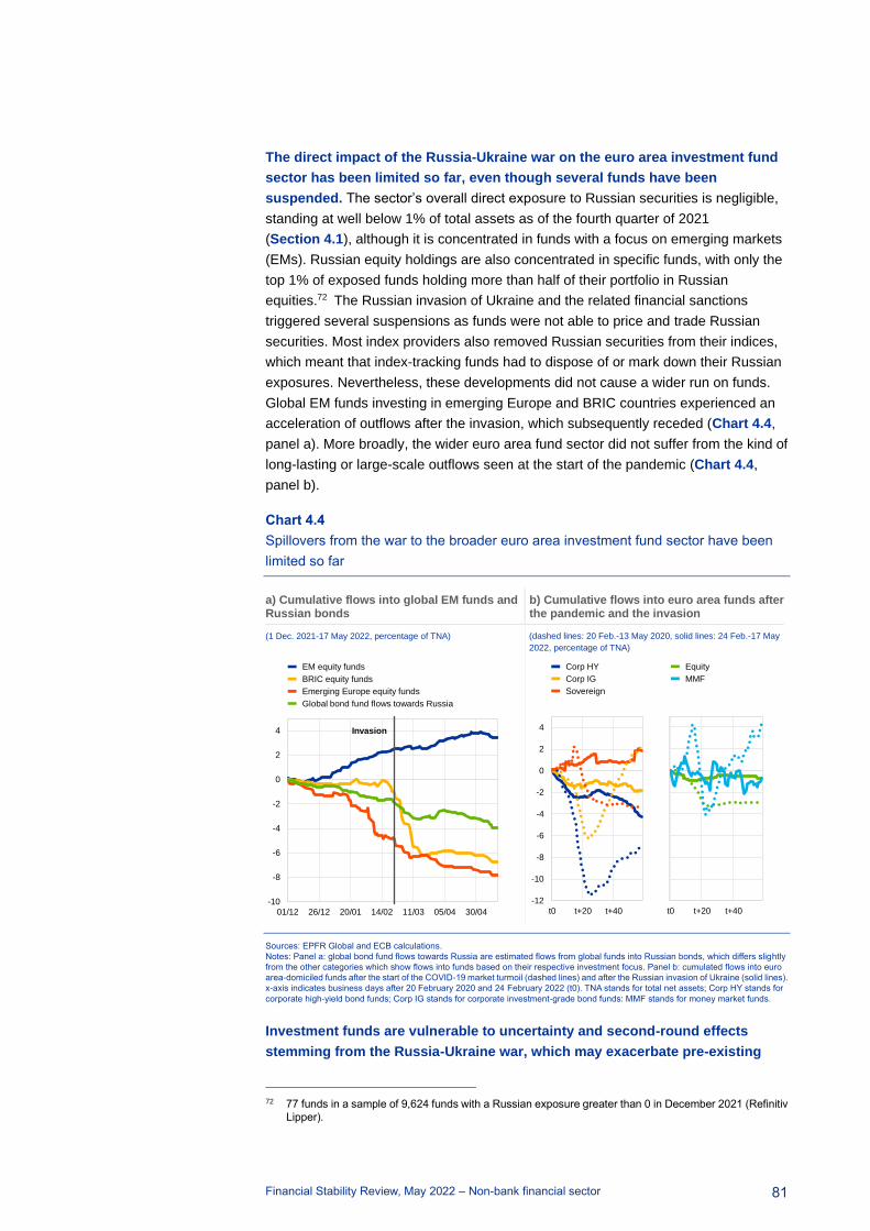
Financial Stability Review, May 2022 – Non-bank financial sector
81
The direct impact of the Russia-Ukraine war on the euro area investment fund
sector has been limited so far, even though several funds have been
suspended. The sector’s overall direct exposure to Russian securities is negligible,
standing at well below 1% of total assets as of the fourth quarter of 2021
(Section 4.1), although it is concentrated in funds with a focus on emerging markets
(EMs). Russian equity holdings are also concentrated in specific funds, with only the
top 1% of exposed funds holding more than half of their portfolio in Russian
equities.72 The Russian invasion of Ukraine and the related financial sanctions
triggered several suspensions as funds were not able to price and trade Russian
securities. Most index providers also removed Russian securities from their indices,
which meant that index-tracking funds had to dispose of or mark down their Russian
exposures. Nevertheless, these developments did not cause a wider run on funds.
Global EM funds investing in emerging Europe and BRIC countries experienced an
acceleration of outflows after the invasion, which subsequently receded (Chart 4.4,
panel a). More broadly, the wider euro area fund sector did not suffer from the kind of
long-lasting or large-scale outflows seen at the start of the pandemic (Chart 4.4,
panel b).
Chart 4.4
Spillovers from the war to the broader euro area investment fund sector have been
limited so far
a) Cumulative flows into global EM funds and Russian bonds
b) Cumulative flows into euro area funds after the pandemic and the invasion
(1 Dec. 2021-17 May 2022, percentage of TNA) (dashed lines: 20 Feb.-13 May 2020, solid lines: 24 Feb.-17 May
2022, percentage of TNA)
Sources: EPFR Global and ECB calculations.
Notes: Panel a: global bond fund flows towards Russia are estimated flows from global funds into Russian bonds, which differs slightly
from the other categories which show flows into funds based on their respective investment focus. Panel b: cumulated flows into euro
area-domiciled funds after the start of the COVID-19 market turmoil (dashed lines) and after the Russian invasion of Ukraine (solid lines).
x-axis indicates business days after 20 February 2020 and 24 February 2022 (t0). TNA stands for total net assets; Corp HY stands for
corporate high-yield bond funds; Corp IG stands for corporate investment-grade bond funds: MMF stands for money market funds.
Investment funds are vulnerable to uncertainty and second-round effects
stemming from the Russia-Ukraine war, which may exacerbate pre-existing
72 77 funds in a sample of 9,624 funds with a Russian exposure greater than 0 in December 2021 (Refinitiv
Lipper).
-10
-8
-6
-4
-2
0
2
4
01/12 26/12 20/01 14/02 11/03 05/04 30/04
Invasion
EM equity funds
BRIC equity funds
Emerging Europe equity funds
Global bond fund flows towards Russia
-12
-10
-8
-6
-4
-2
0
2
4
t0 t+20 t+40
Corp HY
Corp IG
Sovereign
t0 t+20 t+40
Equity
MMF
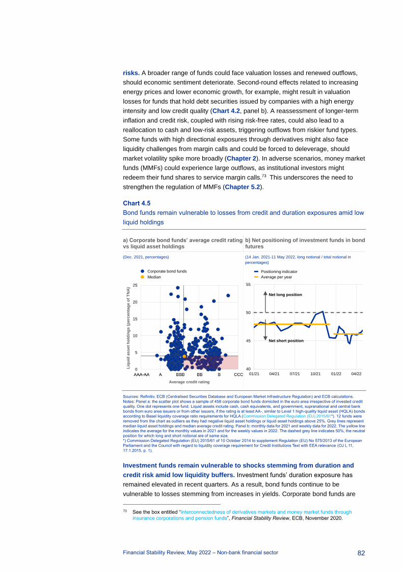
Financial Stability Review, May 2022 – Non-bank financial sector
82
risks. A broader range of funds could face valuation losses and renewed outflows,
should economic sentiment deteriorate. Second-round effects related to increasing
energy prices and lower economic growth, for example, might result in valuation
losses for funds that hold debt securities issued by companies with a high energy
intensity and low credit quality (Chart 4.2, panel b). A reassessment of longer-term
inflation and credit risk, coupled with rising risk-free rates, could also lead to a
reallocation to cash and low-risk assets, triggering outflows from riskier fund types.
Some funds with high directional exposures through derivatives might also face
liquidity challenges from margin calls and could be forced to deleverage, should
market volatility spike more broadly (Chapter 2). In adverse scenarios, money market
funds (MMFs) could experience large outflows, as institutional investors might
redeem their fund shares to service margin calls.73 This underscores the need to
strengthen the regulation of MMFs (Chapter 5.2).
Chart 4.5
Bond funds remain vulnerable to losses from credit and duration exposures amid low
liquid holdings
a) Corporate bond funds’ average credit rating vs liquid asset holdings
b) Net positioning of investment funds in bond futures
(Dec. 2021, percentages) (14 Jan. 2021-11 May 2022, long notional / total notional in
percentages)
Sources: Refinitiv, ECB (Centralised Securities Database and European Market Infrastructure Regulation) and ECB calculations.
Notes: Panel a: the scatter plot shows a sample of 458 corporate bond funds domiciled in the euro area irrespective of invested credit
quality. One dot represents one fund. Liquid assets include cash, cash equivalents, and government, supranational and central bank
bonds from euro area issuers or from other issuers, if the rating is at least AA-, similar to Level 1 high-quality liquid asset (HQLA) bonds
according to Basel liquidity coverage ratio requirements for HQLA (Commission Delegated Regulation (EU) 2015/61*). 12 funds were
removed from the chart as outliers as they had negative liquid asset holdings or liquid asset holdings above 25%. Grey lines represent
median liquid asset holdings and median average credit rating. Panel b: monthly data for 2021 and weekly data for 2022. The yellow line
indicates the average for the monthly values in 2021 and for the weekly values in 2022. The dashed grey line indicates 50%, the neutral
position for which long and short notional are of same size.
*) Commission Delegated Regulation (EU) 2015/61 of 10 October 2014 to supplement Regulation (EU) No 575/2013 of the European
Parliament and the Council with regard to liquidity coverage requirement for Credit Institutions Text with EEA relevance (OJ L 11,
17.1.2015, p. 1).
Investment funds remain vulnerable to shocks stemming from duration and
credit risk amid low liquidity buffers. Investment funds’ duration exposure has
remained elevated in recent quarters. As a result, bond funds continue to be
vulnerable to losses stemming from increases in yields. Corporate bond funds are
73 See the box entitled “Interconnectedness of derivatives markets and money market funds through
insurance corporations and pension funds”, Financial Stability Review, ECB, November 2020.
0
5
10
15
20
25
1 2 3 4 5 6
Liq
uid
as
se
t h
old
ing
s (
pe
rce
nta
ge
of
TN
A)
Average credit rating
Corporate bond funds
Median
40
45
50
55
01/21 04/21 07/21 10/21 01/22 04/22
Net long position
Net short position
Positioning indicator
Average per year
Financial Stability Review, May 2022 – Non-bank financial sector
83
also exposed to credit risk, while median liquid holdings remain low. Funds with low
credit quality and low liquid asset holdings – around a quarter of funds in the sample
observed – are especially vulnerable (Chart 4.5, panel a). Risks to such funds could
amplify adverse market developments going forward if the funds had to engage in
forced asset sales due to their low liquid holdings being insufficient to cover
large-scale redemptions triggered by portfolio losses. At the same time, the
investment fund sector has had a small, but increased, net short position in bond
futures since the beginning of the year. This indicates that direct portfolio revaluation
losses from higher interest rates might be partly mitigated by hedging strategies
(Chart 4.5, panel b).74
Some funds exhibit additional vulnerabilities from investments in crypto-assets
or heavy use of synthetic leverage. Asset managers have started to move into
Bitcoin and other crypto-assets in response to growing demand from their clients.
Should such exposures grow further, risks stemming from this asset class could spill
over to other financial institutions (Special Feature B). Funds can also take on further
risks by leveraging up their positions, either financially through borrowing or
synthetically through derivatives. Synthetic leverage, which is difficult to quantify, can
materialise through margin calls and uncovered counterparty exposure during
periods of high market volatility. In particular, while margining provides coverage for
counterparty exposure in derivative positions, a significant rise in margin calls can
result in a gap in such coverage and can also lead to potential liquidity stress (Box
7).75 The potential for spillover effects from the investment fund sector to the wider
financial system and real economy amid high liquidity mismatch and pockets of
leverage highlights the need to strengthen its resilience from a macroprudential
perspective (Chapter 5).
Box 7
Synthetic leverage and margining in non-bank financial institutions
Prepared by Annalaura Ianiro, Christian Weistroffer and Sebastiano Michele Zema76
Synthetic leverage has become an important feature of the financial system. It refers to the
exposure embedded in derivative contracts. These instruments enable market participants to take on
synthetic market exposure, sometimes at little cost (for certain types of derivatives and underlying
assets), and allow them to amplify gains at the risk of magnifying losses. Leverage tends to be less
strictly regulated in parts of the non-bank financial sector than it is for banks, and non-bank institutions
are able to increase leverage synthetically at little cost. During events such as the failure of
Long-Term Capital Management and the collapse of AIG, and more recently Archegos, losses on
derivative exposures spread to bank counterparties.
74 This does not rule out the possibility of individual funds taking a stronger net short position or other
interest rate derivatives such as swaps also being used for hedging purposes.
75 Further to the analysis on equity derivates in Box 7, there is evidence that some euro area bond funds
and hedge funds are highly leveraged (see the special feature entitled “Towards a framework for
calibrating macroprudential leverage limits for alternative investment funds”, Financial Stability Review,
ECB, November 2016 and “EU Alternative Investment Funds”, Annual Statistical Report, ESMA,
February 2022).
76 The authors express their gratitude to Linda Fache Rousová and Lorenzo Cappiello for their contributions
and valuable feedback.

Financial Stability Review, May 2022 – Non-bank financial sector
84
There are multiple ways of measuring the amount of leverage in the financial system.
Traditional leverage ratios at entity level do not fully capture the contingent commitments associated
with derivative positions, as future gains and losses can substantially exceed the market value at
which derivatives are recorded on the balance sheet. A generally accepted method used to capture
synthetic leverage applies the concept of cash-equivalent portfolios,77 which also forms the basis of
leverage metrics in EU fund regulation.78 Another approach, which is the focus of this box, considers
the derivative contracts themselves and assesses the extent to which such contracts can be used to
take positions which embed leverage.79
This box explores the link between synthetic leverage and margining from two angles. First,
we look at the ratio of derivatives’ gross notional value (GNV) to initial margins (IMs) posted, which
may be viewed as the level of synthetic leverage in a particular type of contract.80 Low levels of IMs
allow financial institutions to increase their market exposure via derivatives with very little initial
funding. During periods of elevated price volatility, IMs tend to increase relative to the GNV – this
offers the benefit of better protection against counterparty risk in stressed market conditions.
However, this can also intensify liquidity needs in a procyclical manner and create incentives for
deleveraging, which could contribute to the amplification of price declines. Second, we calculate the
ratio of the daily absolute flows of variation margins (VMs) to IMs, which may be seen as a proxy for
the amplification of profits and losses on a derivative portfolio.81 For a highly leveraged portfolio, this
ratio would increase more in times of high market volatility. Daily ratios greater than 1 suggest – ex
post – that the capital committed as IM would not have been sufficient to fully protect against losses if
the counterparty had failed. These two metrics are calculated for portfolios of equity derivatives held
by non-bank financial institutions to capture risks similar those faced by Archegos.82
The high GNV/IM multipliers for equity derivatives suggest that these instruments could entail
potentially high leverage-like risk. Multipliers range between 10 and 80 across instruments during
most of the period covered, with equity options displaying the largest multipliers (Chart A, panel a).
Although the GNV/IM ratio decreased for equity futures during the March 2020 market turmoil, it did
not decline significantly for swaps and options, the difference probably stemming from the models
used to calculate IMs.83 Following this episode, the GNV/IM ratio for both options and futures rose
throughout most of 2020 and 2021, with the increase accelerating in the fourth quarter of 2021.The
increase in the ratio for options seems to have been driven by a decrease in IMs as the associated
GNV remained relatively stable during this period. The GNV/IM ratio for swaps was relatively stable.
The ratios between daily absolute VM flows and IMs at the instrument level increased
significantly in March 2020, reaching over 1 for some NBFIs (Chart A, panel b). While the
77 See Breuer, P., “Measuring off-balance-sheet leverage”, Journal of Banking and Finance, Vol. 26 (2-3),
2002, pp. 223-242.
78 For example, the “commitment approach” in the Undertakings for Collective Investment in Transferable
Securities (UCITS) Directive and the Alternative Investment Fund Managers Directive (AIFMD). Other
common metrics include gross notional over net asset value and value-at-risk concepts. See the box
entitled “Synthetic leverage in the investment fund sector”, Financial Stability Review, ECB, May 2015.
79 See Frazzini, A. and Pedersen, L.H., “Embedded Leverage”, NBER Working Papers, No 18558,
November 2012.
80 This recalls the standard definition of the leverage ratio, which is market exposure (the GNV captures the
synthetic market exposure) over unit of committed capital (here represented by IMs).
81 By definition, the leverage ratio amplifies returns on equity: 𝑟(𝐸) = 𝐿 ∙ 𝑟(𝐴).
82 Gross notional and margin data are obtained from the EMIR dataset. The sample comprises a broad
range of institutions including investment funds, pension funds, insurance companies and other financial
institutions. The bulk of such derivatives are held by investment funds.
83 The differences between the models used to compute IMs depend heavily on the calibration choices
made by central counterparties (for centrally cleared transactions – mostly options and futures in our
sample) or counterparties (for non-centrally cleared transactions – swaps in our sample). In particular,
the models used by the latter are less responsive to short-term fluctuations in market volatility. For further
information, see the box entitled “Lessons learned from initial margin calls during the March 2020 market
turmoil”, Financial Stability Review, ECB, November 2021.
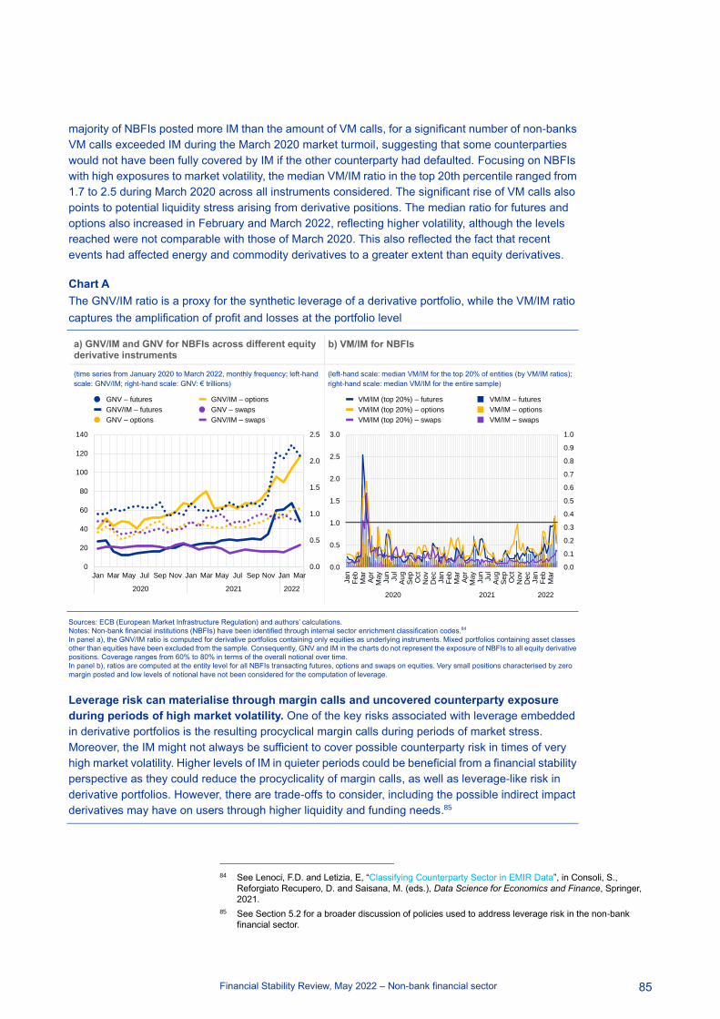
Financial Stability Review, May 2022 – Non-bank financial sector
85
majority of NBFIs posted more IM than the amount of VM calls, for a significant number of non-banks
VM calls exceeded IM during the March 2020 market turmoil, suggesting that some counterparties
would not have been fully covered by IM if the other counterparty had defaulted. Focusing on NBFIs
with high exposures to market volatility, the median VM/IM ratio in the top 20th percentile ranged from
1.7 to 2.5 during March 2020 across all instruments considered. The significant rise of VM calls also
points to potential liquidity stress arising from derivative positions. The median ratio for futures and
options also increased in February and March 2022, reflecting higher volatility, although the levels
reached were not comparable with those of March 2020. This also reflected the fact that recent
events had affected energy and commodity derivatives to a greater extent than equity derivatives.
Chart A
The GNV/IM ratio is a proxy for the synthetic leverage of a derivative portfolio, while the VM/IM ratio
captures the amplification of profit and losses at the portfolio level
Sources: ECB (European Market Infrastructure Regulation) and authors’ calculations.
Notes: Non-bank financial institutions (NBFIs) have been identified through internal sector enrichment classification codes.84
In panel a), the GNV/IM ratio is computed for derivative portfolios containing only equities as underlying instruments. Mixed portfolios containing asset classes
other than equities have been excluded from the sample. Consequently, GNV and IM in the charts do not represent the exposure of NBFIs to all equity derivative
positions. Coverage ranges from 60% to 80% in terms of the overall notional over time.
In panel b), ratios are computed at the entity level for all NBFIs transacting futures, options and swaps on equities. Very small positions characterised by zero
margin posted and low levels of notional have not been considered for the computation of leverage.
Leverage risk can materialise through margin calls and uncovered counterparty exposure
during periods of high market volatility. One of the key risks associated with leverage embedded
in derivative portfolios is the resulting procyclical margin calls during periods of market stress.
Moreover, the IM might not always be sufficient to cover possible counterparty risk in times of very
high market volatility. Higher levels of IM in quieter periods could be beneficial from a financial stability
perspective as they could reduce the procyclicality of margin calls, as well as leverage-like risk in
derivative portfolios. However, there are trade-offs to consider, including the possible indirect impact
derivatives may have on users through higher liquidity and funding needs.85
84 See Lenoci, F.D. and Letizia, E, “Classifying Counterparty Sector in EMIR Data”, in Consoli, S.,
Reforgiato Recupero, D. and Saisana, M. (eds.), Data Science for Economics and Finance, Springer,
2021.
85 See Section 5.2 for a broader discussion of policies used to address leverage risk in the non-bank
financial sector.
a) GNV/IM and GNV for NBFIs across different equity derivative instruments
b) VM/IM for NBFIs
(time series from January 2020 to March 2022, monthly frequency; left-hand
scale: GNV/IM; right-hand scale: GNV: € trillions)
(left-hand scale: median VM/IM for the top 20% of entities (by VM/IM ratios);
right-hand scale: median VM/IM for the entire sample)
0.0
0.5
1.0
1.5
2.0
2.5
0
20
40
60
80
100
120
140
Jan Mar May Jul Sep Nov Jan Mar May Jul Sep Nov Jan Mar
2020 2021 2022
GNV – futures
GNV/IM – futures
GNV – options
GNV/IM – options
GNV – swaps
GNV/IM – swaps
0.0
0.1
0.2
0.3
0.4
0.5
0.6
0.7
0.8
0.9
1.0
0.0
0.5
1.0
1.5
2.0
2.5
3.0
Jan
Feb
Mar
Ap
rM
ay
Ju
nJu
lA
ug
Se
pO
ct
Nov
De
cJa
nF
eb
Mar
Ap
rM
ay
Ju
nJu
lA
ug
Se
pO
ct
No
vD
ec
Ja
nF
eb
Mar
2020 2021 2022
VM/IM (top 20%) – futures
VM/IM (top 20%) – options
VM/IM (top 20%) – swaps
VM/IM – futures
VM/IM – options
VM/IM – swaps

Financial Stability Review, May 2022 – Non-bank financial sector
86
4.3 Insurers face near-term headwinds from inflation, while
benefiting from rising interest rates
Euro area insurers are indirectly affected by the Russia-Ukraine war and
associated sanctions amid pre-existing elevated vulnerabilities. In the weeks
preceding the Russian invasion of Ukraine, insurance companies’ stock prices had
started to decline on the back of growing uncertainty and continued to do so after the
event (Chart 4.6, panel a). As was the case for other financial sectors, insurers’
equity prices fell by more than the broad market before temporarily recovering in
mid-March and falling again amid high market uncertainty. While aggregate direct
exposures to Russian assets are very limited (Chart 4.1, panel b), the war has
exacerbated inflation risks (Chapter 2), increased uncertainty and could be a catalyst
for broader asset repricing, especially in energy-intensive sectors (Chart 4.2, panel
a). These developments could dampen insurers’ near-term profitability and solvency.
Chart 4.6
Insurers’ equity prices declined by more than broad market indices, but profitability
and solvency positions remain solid
a) Insurance stock prices in the euro area
b) SCR ratio c) Return on common equity
(1 Jan.-17 May 2022, index: 1 Jan. 2022 =
100) (Q2 2019-Q4 2021, percentages) (Q2 2019-Q4 2021, percentages)
Sources: Refinitiv, Bloomberg Finance L.P. and ECB calculations.
Notes: Panel a: the chart shows daily observations. Panels b and c: the charts are based on a sample of 25 large euro area insurers
offering life and non-life products.
Despite these threats, insurers’ solvency and profitability remain strong. At the
end of 2021, euro area insurers’ Solvency Capital Requirement (SCR) ratio remained
well above the regulatory minimum of 100% (Chart 4.6, panel b), despite a small
decrease in the second half of 2021 amid more general risk-off sentiment. The SCR
ratio is likely to decrease further in the first months of 2022 on account of lower equity
valuations and higher credit spreads. This decline might be offset by rising interest
rates and the volatility adjustment.86 Profitability was above pre-pandemic levels at
86 A regulatory mechanism that allows insurers to moderate the effect of falling bond prices on their capital
under Solvency II.
75
80
85
90
95
100
105
110
115
120
01/22 02/22 03/22 04/22 05/22
Invasion
Euro area life insurance index
Euro area non-life insurance index
Euro area reinsurance index
EURO STOXX 50
180
190
200
210
220
230
240
250
Q2
20
19
Q4
20
19
Q2
20
20
Q4
20
20
Q2
20
21
Q4
20
21
Median
Interquartile range
2
4
6
8
10
12
14
Q2 2
01
9
Q4 2
01
9
Q2
20
20
Q4
20
20
Q2
20
21
Q4
20
21
Median
Interquartile range
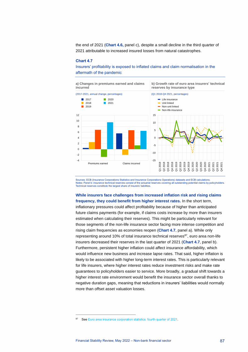
Financial Stability Review, May 2022 – Non-bank financial sector
87
the end of 2021 (Chart 4.6, panel c), despite a small decline in the third quarter of
2021 attributable to increased insured losses from natural catastrophes.
Chart 4.7
Insurers’ profitability is exposed to inflated claims and claim normalisation in the
aftermath of the pandemic
a) Changes in premiums earned and claims incurred
b) Growth rate of euro area insurers’ technical reserves by insurance type
(2017-2021, annual change, percentages) (Q1 2018-Q4 2021, percentages)
Sources: ECB (Insurance Corporations Statistics and Insurance Corporations Operations) datasets and ECB calculations.
Notes: Panel b: insurance technical reserves consist of the actuarial reserves covering all outstanding potential claims by policyholders.
Technical reserves constitute the largest share of insurers’ liabilities.
While insurers face challenges from increased inflation risk and rising claims
frequency, they could benefit from higher interest rates. In the short term,
inflationary pressures could affect profitability because of higher than anticipated
future claims payments (for example, if claims costs increase by more than insurers
estimated when calculating their reserves). This might be particularly relevant for
those segments of the non-life insurance sector facing more intense competition and
rising claim frequencies as economies reopen (Chart 4.7, panel a). While only
representing around 10% of total insurance technical reserves87, euro area non-life
insurers decreased their reserves in the last quarter of 2021 (Chart 4.7, panel b).
Furthermore, persistent higher inflation could affect insurance affordability, which
would influence new business and increase lapse rates. That said, higher inflation is
likely to be associated with higher long-term interest rates. This is particularly relevant
for life insurers, where higher interest rates reduce investment risks and make rate
guarantees to policyholders easier to service. More broadly, a gradual shift towards a
higher interest rate environment would benefit the insurance sector overall thanks to
negative duration gaps, meaning that reductions in insurers’ liabilities would normally
more than offset asset valuation losses.
87 See Euro area insurance corporation statistics: fourth quarter of 2021.
-4
-2
0
2
4
6
8
10
12
Premiums earned Claims incurred
2017
2018
2019
2020
2021
-15
-10
-5
0
5
10
15
Q1 2
01
8
Q2
20
18
Q3
20
18
Q4 2
01
8
Q1
20
19
Q2
20
19
Q3
20
19
Q4
20
19
Q1
20
20
Q2
20
20
Q3
20
20
Q4
20
20
Q1
20
21
Q2
20
21
Q3 2
02
1
Q4
20
21
Life insurance
Unit linked
Non-unit linked
Non-life insurance
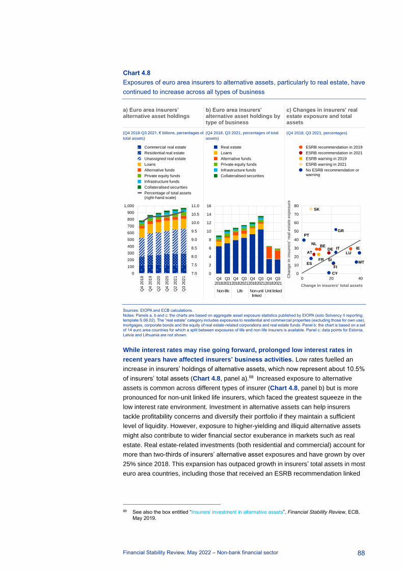
Financial Stability Review, May 2022 – Non-bank financial sector
88
Chart 4.8
Exposures of euro area insurers to alternative assets, particularly to real estate, have
continued to increase across all types of business
a) Euro area insurers’ alternative asset holdings
b) Euro area insurers’ alternative asset holdings by type of business
c) Changes in insurers’ real estate exposure and total assets
(Q4 2018-Q3 2021, € billions, percentages of
total assets) (Q4 2018, Q3 2021, percentages of total
assets) (Q4 2018, Q3 2021, percentages)
Sources: EIOPA and ECB calculations.
Notes: Panels a, b and c: the charts are based on aggregate asset exposure statistics published by EIOPA (solo Solvency II reporting;
template S.06.02). The “real estate” category includes exposures to residential and commercial properties (excluding those for own use),
mortgages, corporate bonds and the equity of real estate-related corporations and real estate funds. Panel b: the chart is based on a set
of 14 euro area countries for which a split between exposures of life and non-life insurers is available. Panel c: data points for Estonia,
Latvia and Lithuania are not shown.
While interest rates may rise going forward, prolonged low interest rates in
recent years have affected insurers’ business activities. Low rates fuelled an
increase in insurers’ holdings of alternative assets, which now represent about 10.5%
of insurers’ total assets (Chart 4.8, panel a).88 Increased exposure to alternative
assets is common across different types of insurer (Chart 4.8, panel b) but is more
pronounced for non-unit linked life insurers, which faced the greatest squeeze in the
low interest rate environment. Investment in alternative assets can help insurers
tackle profitability concerns and diversify their portfolio if they maintain a sufficient
level of liquidity. However, exposure to higher-yielding and illiquid alternative assets
might also contribute to wider financial sector exuberance in markets such as real
estate. Real estate-related investments (both residential and commercial) account for
more than two-thirds of insurers’ alternative asset exposures and have grown by over
25% since 2018. This expansion has outpaced growth in insurers’ total assets in most
euro area countries, including those that received an ESRB recommendation linked
88 See also the box entitled “Insurers’ investment in alternative assets”, Financial Stability Review, ECB,
May 2019.
7.0
7.5
8.0
8.5
9.0
9.5
10.0
10.5
11.0
0
100
200
300
400
500
600
700
800
900
1,000
Q4
20
18
Q4
20
19
Q2
20
20
Q4
20
20
Q2
20
21
Q3
20
21
Thousands
Commercial real estate
Residential real estate
Unassigned real estate
Loans
Alternative funds
Private equity funds
Infrastructure funds
Collateralised securities
Percentage of total assets (right-hand scale)
0
2
4
6
8
10
12
14
16
Q4 2018
Q3 2021
Q4 2018
Q3 2021
Q4 2018
Q3 2021
Q4 2018
Q3 2021
Non-life Life Non-unit linked
Unit linked
Real estate
Loans
Alternative funds
Private equity funds
Infrastructure funds
Collateralised securities
BE
FI
LU
NL
ATDE
FR
SK
CY
ES
GR
IEIT
MT
PT
SI
0
10
20
30
40
50
60
70
80
0 20 40Ch
an
ge
in
in
su
rers
' re
al
es
tate
ex
po
su
re
Change in insurers' total assets
ESRB recommendation in 2019
ESRB recommendation in 2021
ESRB warning in 2019
ESRB warning in 2021
No ESRB recommendation or warning

Financial Stability Review, May 2022 – Non-bank financial sector
89
to real estate in December 2021 (Chart 4.8, panel c).89 Property price corrections are
more likely to occur in overvalued markets, increasing the risk of material valuation
losses in insurers’ portfolios in such countries (Chapter 1).
Over the longer term, insurers will continue to face several structural
vulnerabilities, such as climate change and cyber security. Estimated global
insured losses of USD 111 billion made 2021 one of the costliest years ever in terms
of natural catastrophes, particularly for some euro area countries.90 Last summer’s
floods in Belgium, Germany and the Netherlands generated economic losses of more
than USD 40 billion and insured losses of USD 13 billion, putting the insured loss
potential from a single flood on a par with losses from primary peril events such as
earthquakes or winter storms. The rising frequency of severe flood events due to
climate change and the growing magnitude of associated losses have also pushed up
reinsurance prices. This adds to the profitability challenges faced by non-life insurers
and might widen protection gaps (the proportion of economic losses that are not
covered by insurance), with potential adverse consequences for the wider
macroeconomy.91 Insurers are also struggling to provide coverage against cyber risk
amid growing demand driven by the increased frequency and severity of ransomware
incidents in 2021. In addition, the war in Ukraine may increase the risk of large
cyberattacks. Available insurance capacity for cyber risk currently appears to be
limited by lack of expertise, data availability issues and inappropriate modelling.92
89 See ESRB issues new warnings and recommendations on medium-term residential real estate
vulnerabilities, ESRB, February 2022.
90 See, for example, Natural catastrophes in 2021: the floodgates are open, Swiss Re Institute, March 2022.
91 See Fache Rousová et al., “Climate change, catastrophes and the macroeconomic benefits of
insurance”, Financial Stability Report, EIOPA, July 2021.
92 See the special theme entitled “Cyber risk and the European insurance sector”, Financial Stability
Report, EIOPA, December 2021.

Financial Stability Review, May 2022 – Macroprudential policy issues
90
5 Macroprudential policy issues
5.1 Setting the appropriate pace of policy action to address
medium-term vulnerabilities
Several euro area macroprudential authorities had already started to tighten
some of their policies prior to the outbreak of war in Ukraine. At the end of 2021
and beginning of 2022, the near-term economic outlook revolved around the strong
recovery continuing, on the back of robust labour markets and gradually receding
pandemic headwinds. At the same time, vulnerabilities with macroprudential policy
relevance continued to build-up. This was especially significant for residential real
estate markets, but also occurred more broadly, on the back of robust credit growth
and increasing indebtedness in the non-financial private sector (Chart 5.1, panel a).93
93 See “Vulnerabilities in the residential real estate sectors of the EEA countries”, ESRB, February 2022 and
the associated recommended further policy actions in a number of European countries.
Timing of macroprudential policies conditioned by the war in
Ukraine and economic headwinds
• Comprehensively address risks
from liquidity mismatch, margining
practices and leverage in the non-
bank financial sector
• As country-specific economic conditions allow, building resilience remains a
sound strategy since macroprudential policies should continue to address
accumulated medium-term vulnerabilities
Medium-term resilience to be supported by
regulatory enhancement
• Augment the regulatory framework
for banks with policy options for
creating macroprudential space
and increasing the effectiveness of
existing capital buffers
• Enhance the overall design and
functioning of the buffer framework
and address missing and obsolete
instruments, internal market
considerations and global risks
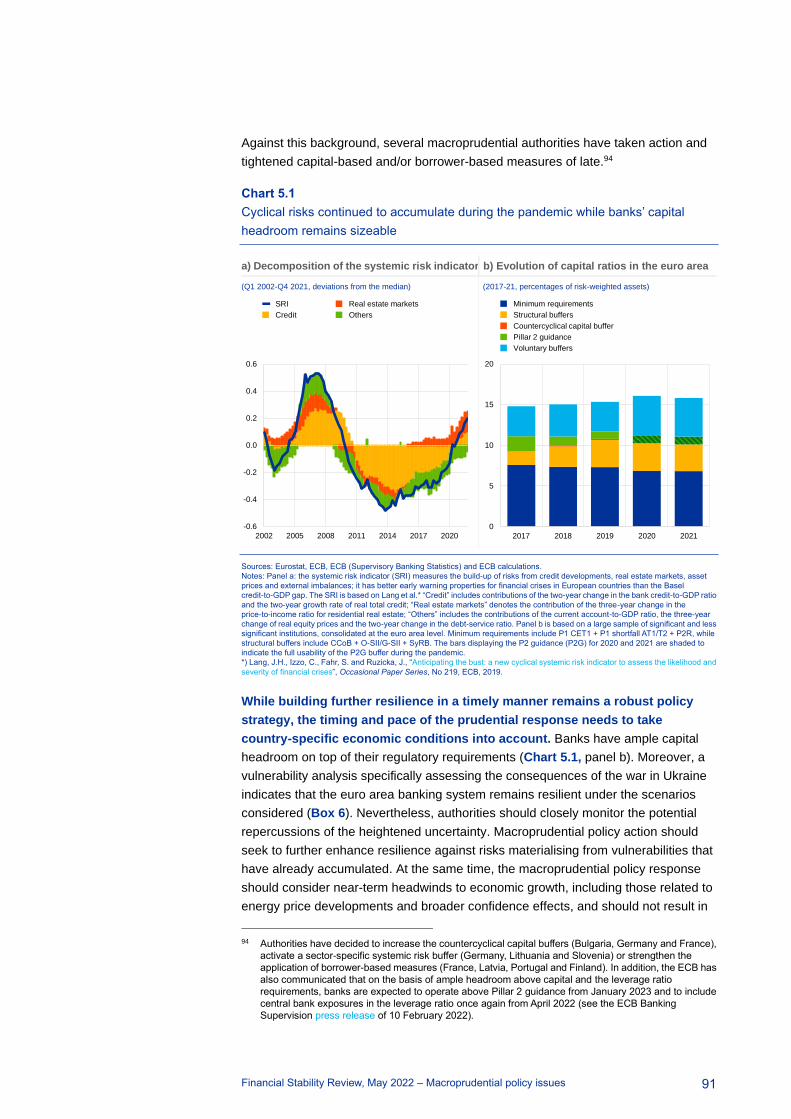
Financial Stability Review, May 2022 – Macroprudential policy issues
91
Against this background, several macroprudential authorities have taken action and
tightened capital-based and/or borrower-based measures of late.94
Chart 5.1
Cyclical risks continued to accumulate during the pandemic while banks’ capital
headroom remains sizeable
a) Decomposition of the systemic risk indicator b) Evolution of capital ratios in the euro area
(Q1 2002-Q4 2021, deviations from the median) (2017-21, percentages of risk-weighted assets)
Sources: Eurostat, ECB, ECB (Supervisory Banking Statistics) and ECB calculations.
Notes: Panel a: the systemic risk indicator (SRI) measures the build-up of risks from credit developments, real estate markets, asset
prices and external imbalances; it has better early warning properties for financial crises in European countries than the Basel
credit-to-GDP gap. The SRI is based on Lang et al.* “Credit” includes contributions of the two-year change in the bank credit-to-GDP ratio
and the two-year growth rate of real total credit; “Real estate markets” denotes the contribution of the three-year change in the
price-to-income ratio for residential real estate; “Others” includes the contributions of the current account-to-GDP ratio, the three-year
change of real equity prices and the two-year change in the debt-service ratio. Panel b is based on a large sample of significant and less
significant institutions, consolidated at the euro area level. Minimum requirements include P1 CET1 + P1 shortfall AT1/T2 + P2R, while
structural buffers include CCoB + O-SII/G-SII + SyRB. The bars displaying the P2 guidance (P2G) for 2020 and 2021 are shaded to
indicate the full usability of the P2G buffer during the pandemic.
*) Lang, J.H., Izzo, C., Fahr, S. and Ruzicka, J., “Anticipating the bust: a new cyclical systemic risk indicator to assess the likelihood and
severity of financial crises”, Occasional Paper Series, No 219, ECB, 2019.
While building further resilience in a timely manner remains a robust policy
strategy, the timing and pace of the prudential response needs to take
country-specific economic conditions into account. Banks have ample capital
headroom on top of their regulatory requirements (Chart 5.1, panel b). Moreover, a
vulnerability analysis specifically assessing the consequences of the war in Ukraine
indicates that the euro area banking system remains resilient under the scenarios
considered (Box 6). Nevertheless, authorities should closely monitor the potential
repercussions of the heightened uncertainty. Macroprudential policy action should
seek to further enhance resilience against risks materialising from vulnerabilities that
have already accumulated. At the same time, the macroprudential policy response
should consider near-term headwinds to economic growth, including those related to
energy price developments and broader confidence effects, and should not result in
94 Authorities have decided to increase the countercyclical capital buffers (Bulgaria, Germany and France),
activate a sector-specific systemic risk buffer (Germany, Lithuania and Slovenia) or strengthen the
application of borrower-based measures (France, Latvia, Portugal and Finland). In addition, the ECB has
also communicated that on the basis of ample headroom above capital and the leverage ratio
requirements, banks are expected to operate above Pillar 2 guidance from January 2023 and to include
central bank exposures in the leverage ratio once again from April 2022 (see the ECB Banking
Supervision press release of 10 February 2022).
-0.6
-0.4
-0.2
0.0
0.2
0.4
0.6
2002 2005 2008 2011 2014 2017 2020
SRI
Credit
Real estate markets
Others
0
5
10
15
20
2017 2018 2019 2020 2021
Minimum requirements
Structural buffers
Countercyclical capital buffer
Pillar 2 guidance
Voluntary buffers

Financial Stability Review, May 2022 – Macroprudential policy issues
92
an unintended tightening of credit conditions. If economic conditions were to
deteriorate markedly, macroprudential authorities could still act swiftly to provide
banks with the necessary flexibility, although additional macroprudential tools could
further enhance the toolkit, including for exceptional circumstances.95
Notwithstanding the uncertainty, macroprudential authorities should continue
to address existing vulnerabilities, as conditions allow. Prior to the outbreak of
the war, conditions for addressing the continued build-up of vulnerabilities in several
euro area countries appeared to be favourable. The economic cost (via the impact on
credit conditions) of activating additional capital buffers appeared to be low,
especially set against the benefits of enhancing resilience sufficiently early to counter
identified vulnerabilities (without necessarily reducing them in the near term) and to
facilitate the response to the materialisation of systemic risk (Box 8). Moreover,
capital buffers are important complements to borrower-based measures when
addressing real estate vulnerabilities,96 in particular over the short term, as the
additional resilience benefits of the borrower-based policies accumulate only
gradually over time. Accordingly, authorities should stand ready to respond promptly
to accumulated vulnerabilities, taking into account the uncertainty surrounding the
economic developments. The associated calibration of instruments should balance
risk signals, uncertainty in risk measurement and the possible costs of policy action in
terms of reduced credit supply. Overall, existing bank capital generation capacity and
headroom should mitigate a detrimental impact on credit supply from increasing
capital buffers, as long economic conditions do not deteriorate significantly.
Moreover, there are also costs associated with delayed action, in particular if
uncertainty persisted into the medium term and vulnerabilities remained unaddressed
or continued to build.
Over the medium term, the resilience of the financial system would be
reinforced by creating more macroprudential space through an increase in the
amount of releasable buffers, complemented by enhancing the effectiveness of
the existing countercyclical capital buffer (CCyB). Recent experience, including
from the coronavirus (COVID-19) pandemic, shows that at the onset of severe stress
episodes, banks that have limited capital space above regulatory buffers relative to
their peers tend to adjust their balance sheets by reducing lending.97 In its recent
response to the European Commission’s call for advice on the review of the
macroprudential framework, the ECB called for more macroprudential policy space in
the form of a higher amount of releasable capital buffers. It argued that this would
further improve banks’ capacity to absorb losses while maintaining the provision of
key services in a downturn. The policy options identified in the ECB response were
(a) a fully or partially releasable capital conservation buffer (CCoB); (b) a positive
95 The policy chapters of the ECB’s Financial Stability Reviews in 2020 and 2021 provide an overview of the
substance and the sequencing of prudential support measures during the pandemic. On the need to
enhance the macroprudential toolkit, see the ECB response to the European Commission’s call for
advice on the review of the EU macroprudential framework.
96 Borrower-based measures have been called for in the context of addressing the build-up of vulnerabilities
in real estate markets (see the above ESRB report on vulnerabilities in residential real estate or the
Financial Stability Review, ECB, November 2021).
97 See the special feature entitled “Bank capital buffers and lending in the euro area during the pandemic”,
Financial Stability Review, ECB, November 2021; and Couaillier et al., “Caution do not cross! Capital
buffers and lending in Covid-19 times”, Working Paper Series, No 2644, ECB, 2022.
Financial Stability Review, May 2022 – Macroprudential policy issues
93
neutral rate for, or more active use of, the countercyclical capital buffer (CCyB); (c) a
core rate for the releasable systemic risk buffer (SyRB); or a possible combination of
the three.98 In addition, the response suggested that flexibility in the CCyB framework
be increased to foster timely policy action in both the activation and the release
phases. This could be achieved by adjusting the design or the calibration of existing
buffers.99
Box 8
Transmission and effectiveness of capital-based macroprudential policies
Prepared by Markus Behn, Jan Hannes Lang and Eugen Tereanu
One important lesson learned from the use of capital-based macroprudential policies in
recent years is that tightening such policies during boom phases is unlikely to have a notable
impact on credit supply and the build-up of imbalances, while the accumulated resilience and
the release of buffers in downturns produces large benefits. Capital-based policies are
particularly relevant to the ECB since they are a focal point for the ECB’s macroprudential tasks as
enshrined in European legislation.100 A prime example of a capital-based tool is the countercyclical
capital buffer (CCyB). This instrument was designed in the aftermath of the global financial crisis to
enhance the resilience of the financial system and reduce procyclicality.101 Enacting capital-based
policies such as the CCyB directly enhances banking system resilience by inducing banks to increase
their capital ratios. Further transmission to the real economy by way of effects on bank credit supply
depends on overall economic conditions and the relevance of capital constraints in the banking
sector. While such constraints are unlikely to be binding when capital buffers are activated during
economic booms, the coronavirus (COVID-19) pandemic has shown that the release of buffers and
other requirements in a downturn can ease binding constraints and effectively support credit supply
and economic activity.102
During periods of solid economic activity, an appropriate tightening of macroprudential
capital buffer requirements is unlikely to lead to binding bank capital constraints and should
98 The ECB is aware that creating more macroprudential policy space and facilitating the effective use of
released buffers may also require additional work at the international level to better address shocks that
may go beyond the unwinding of domestic imbalances and to ensure a global level playing field.
99 This can be achieved by moderating the dominant role of the credit-to-GDP ratio in the CCyB rate-setting
practices of national authorities and by allowing for a shorter transitional period than one year for the
implementation of CCyB decisions.
100 For an overview of the ECB’s macroprudential policy framework, see the chapter entitled “Topical issue:
The ECB’s macroprudential policy framework”, Macroprudential Bulletin, Issue 1, ECB, 2016; for an
overview of macroprudential policy and powers within the Eurosystem, see the box entitled
“Macroprudential policy and powers within the Eurosystem”, Financial Stability Review, ECB, November
2019.
101 For a comprehensive discussion of the objectives and the rationale of the capital buffer framework, see,
for example, the article entitled “Macroprudential capital buffers – objectives and usability”,
Macroprudential Bulletin, ECB, October 2020.
102 For an analysis on the effects of capital release measures during the pandemic see, for example, the
special feature entitled “Bank capital buffers and lending in the euro area during the pandemic”, Financial
Stability Review, ECB, November 2021. Besides the CCyB, which made up only 0.1% of risk-weighted
assets in the banking union before the COVID-19 pandemic, the analysis also considers the release of
other buffers (such as the Systemic Risk Buffer) and the one-off change in the composition of
microprudential Pillar 2 requirements (which effectively decreased banks’ CET1 capital requirements).
The coupling of capital release measures with monetary policy action in the form of liquidity provision can
help to further ease binding constraints and enhance banks’ risk-bearing capacity. See, for example,
Altavilla, C. et al., “The great lockdown: pandemic response policies and bank lending conditions”,
Working Paper Series, No 2465, ECB, September 2020, for an analysis of the complementarities
between monetary policy and prudential policy.
Financial Stability Review, May 2022 – Macroprudential policy issues
94
therefore not have a large dampening effect on credit supply or the build-up of imbalances.103
Banks usually respond to higher capital buffer requirements by increasing their capital targets and
capital ratios.104 This directly enhances their overall resilience, as more capital will be available in the
banking system for a given set of exposures. Furthermore, capital-based measures may affect bank
credit supply and the build-up of imbalances over the cycle. This occurs if banks pass on higher
funding costs to customers by raising lending rates (“price channel”, resting on the observation that
bank capital is usually considered more costly than debt) or if they directly limit the quantity of credit
when they are unable to meet higher capital requirements (“quantity channel”). When economic
conditions are favourable, banks tend to have a high capacity for internal capital generation through
retained earnings and can also raise new equity in markets, both of which reduce the likelihood of
banks being subject to binding capital constraints. Moreover, available capital headroom allows
banks to smooth adjustments to higher capital ratio targets over time. Therefore, transmission via
both the price channel and the quantity channel is expected to be limited in economic booms,105 and
tightening capital buffers during upswings is likely to have low costs in terms of reduced economic
activity (via the limited impact on credit supply), with correspondingly limited effects on the build-up of
imbalances (Chart A, panel a).
In periods of crisis, the availability of and ability to release macroprudential capital buffers
can ease bank capital constraints and effectively support credit supply and economic activity.
The materialisation of systemic risk is usually associated with high economic uncertainty and sizeable
bank losses. These, in turn, depress capital ratios closer to prudential requirements and hamper
banks’ internal capital generation capacity as well as their ability to raise new equity. This means that
banks are more likely to become capital-constrained and react by reducing credit supply via the
quantity channel, with potentially large negative repercussions for the real economy. In such
situations, releasing capital buffers that were built up in good times increases capital headroom and
eases regulatory pressure on banks, enabling them to absorb losses while continuing to provide key
financial services. This channel is particularly relevant for banks that have little capital headroom and
would therefore become capital-constrained without the releases (Chart A, panel b).106 The support
to bank credit supply through the release of capital buffers can, in turn, help cushion the economic
downturn and avoid additional losses in the banking sector.
These transmission mechanisms offer important lessons for the effectiveness of
capital-based measures and the design of the macroprudential capital buffer framework. First,
building capital buffers in good times will be effective in that it will increase banking system resilience,
but the muting effect on the build-up of financial imbalances is likely to be limited. Second, and related
to the first point, the economic cost of building capital buffers is likely to be low when the economy is
experiencing an upswing or when banking sector conditions are favourable. The possible magnitude
103 On the state dependence of the effects of changes in capital requirements on lending, see the box
entitled “A macroprudential perspective on replenishing capital buffers”, Financial Stability Review, ECB,
November 2020, which also provides an overview of the academic literature on this topic.
104 See, for example, Couaillier, C., “What are banks’ actual capital targets”, Working Paper Series,
No 2618, ECB, December 2021.
105 Under the assumptions of a full pass-through of funding costs to lending rates, constant lending spreads,
a constant equity premium and a constant risk weight, the change in lending rates is given by ∆it+1 = ∆CRt+1 ∙ ρ ∙ RW , where ∆CR is the policy-induced change in the capital requirement, ρ is the constant
equity premium and RW is the risk weight. For a 10% equity premium and a 50% risk weight, a 1
percentage point increase in the capital ratio should therefore increase bank lending rates by only 5 basis
points. Such an increase in lending rates corresponds to just one-fifth of a standard monetary policy
tightening step and is unlikely to lead to a large drop in credit demand based on standard elasticity
estimates from the literature. This is consistent with many empirical findings showing that lending rates
only increase by a few basis points in response to a 1 percentage point increase in capital requirements;
see, for example, Dagher, J. et al., “Benefits and costs of bank capital”, Staff Discussion Note, No 16/04,
IMF, 2016 or Budnik et al., “The benefits and costs of adjusting bank capitalisation: evidence from euro
area countries”, Working Paper Series, ECB, No 2261, April 2019.
106 See the special feature entitled “Bank capital buffers and lending in the euro area during the pandemic”,
Financial Stability Review, ECB, November 2021.
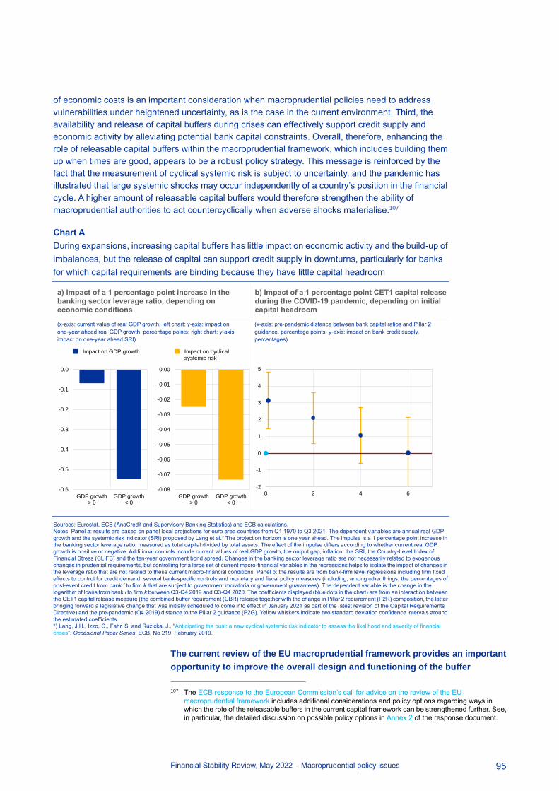
Financial Stability Review, May 2022 – Macroprudential policy issues
95
of economic costs is an important consideration when macroprudential policies need to address
vulnerabilities under heightened uncertainty, as is the case in the current environment. Third, the
availability and release of capital buffers during crises can effectively support credit supply and
economic activity by alleviating potential bank capital constraints. Overall, therefore, enhancing the
role of releasable capital buffers within the macroprudential framework, which includes building them
up when times are good, appears to be a robust policy strategy. This message is reinforced by the
fact that the measurement of cyclical systemic risk is subject to uncertainty, and the pandemic has
illustrated that large systemic shocks may occur independently of a country’s position in the financial
cycle. A higher amount of releasable capital buffers would therefore strengthen the ability of
macroprudential authorities to act countercyclically when adverse shocks materialise.107
Chart A
During expansions, increasing capital buffers has little impact on economic activity and the build-up of
imbalances, but the release of capital can support credit supply in downturns, particularly for banks
for which capital requirements are binding because they have little capital headroom
Sources: Eurostat, ECB (AnaCredit and Supervisory Banking Statistics) and ECB calculations.
Notes: Panel a: results are based on panel local projections for euro area countries from Q1 1970 to Q3 2021. The dependent variables are annual real GDP
growth and the systemic risk indicator (SRI) proposed by Lang et al.* The projection horizon is one year ahead. The impulse is a 1 percentage point increase in
the banking sector leverage ratio, measured as total capital divided by total assets. The effect of the impulse differs according to whether current real GDP
growth is positive or negative. Additional controls include current values of real GDP growth, the output gap, inflation, the SRI, the Country-Level Index of
Financial Stress (CLIFS) and the ten-year government bond spread. Changes in the banking sector leverage ratio are not necessarily related to exogenous
changes in prudential requirements, but controlling for a large set of current macro-financial variables in the regressions helps to isolate the impact of changes in
the leverage ratio that are not related to these current macro-financial conditions. Panel b: the results are from bank-firm level regressions including firm fixed
effects to control for credit demand, several bank-specific controls and monetary and fiscal policy measures (including, among other things, the percentages of
post-event credit from bank i to firm k that are subject to government moratoria or government guarantees). The dependent variable is the change in the
logarithm of loans from bank i to firm k between Q3-Q4 2019 and Q3-Q4 2020. The coefficients displayed (blue dots in the chart) are from an interaction between
the CET1 capital release measure (the combined buffer requirement (CBR) release together with the change in Pillar 2 requirement (P2R) composition, the latter
bringing forward a legislative change that was initially scheduled to come into effect in January 2021 as part of the latest revision of the Capital Requirements
Directive) and the pre-pandemic (Q4 2019) distance to the Pillar 2 guidance (P2G). Yellow whiskers indicate two standard deviation confidence intervals around
the estimated coefficients.
*) Lang, J.H., Izzo, C., Fahr, S. and Ruzicka, J., “Anticipating the bust: a new cyclical systemic risk indicator to assess the likelihood and severity of financial
crises”, Occasional Paper Series, ECB, No 219, February 2019.
The current review of the EU macroprudential framework provides an important
opportunity to improve the overall design and functioning of the buffer
107 The ECB response to the European Commission’s call for advice on the review of the EU
macroprudential framework includes additional considerations and policy options regarding ways in
which the role of the releasable buffers in the current capital framework can be strengthened further. See,
in particular, the detailed discussion on possible policy options in Annex 2 of the response document.
a) Impact of a 1 percentage point increase in the banking sector leverage ratio, depending on economic conditions
b) Impact of a 1 percentage point CET1 capital release during the COVID-19 pandemic, depending on initial capital headroom
(x-axis: current value of real GDP growth; left chart: y-axis: impact on
one-year ahead real GDP growth, percentage points; right chart: y-axis:
impact on one-year ahead SRI)
(x-axis: pre-pandemic distance between bank capital ratios and Pillar 2
guidance, percentage points; y-axis: impact on bank credit supply,
percentages)
-0.6
-0.5
-0.4
-0.3
-0.2
-0.1
0.0
GDP growth> 0
GDP growth< 0
Impact on GDP growth
-0.08
-0.07
-0.06
-0.05
-0.04
-0.03
-0.02
-0.01
0.00
GDP growth> 0
GDP growth< 0
Impact on cyclical systemic risk
-2
-1
0
1
2
3
4
5
0 2 4 6
Financial Stability Review, May 2022 – Macroprudential policy issues
96
framework and address missing and obsolete instruments, internal market
considerations and global risks.108 The ECB has proposed actions to fill other
gaps in the policy toolkit, promote the enhanced use of instruments at the national
level (including supporting national authorities in using borrower-based measures by
enhancing the comparability of both risk assessments and policy actions across
jurisdictions, achieved by harmonising lending standards indicators), enhance
information-sharing, streamline the activation and coordination procedures of
macroprudential measures and address global risks. The set of legislative proposals
potentially resulting from the review would aim to make the regulatory framework
more consistent and streamlined, which would allow macroprudential authorities to
react to emerging risks to financial stability in a more effective, flexible and timely
manner.
Timely macroprudential policy action complements a data-dependent approach
to monetary policy normalisation. If the need to counter inflation leads to gradual
monetary policy normalisation under fragile economic conditions, medium-term risks
could materialise earlier than anticipated. In this context, timely and cautious
macroprudential policy action can help to build the necessary additional resilience
against the materialising risks when needed, while avoiding procyclical effects if
economic conditions deteriorate. Over a longer-term horizon, risks to financial
stability could decline under monetary policy normalisation, as some of the factors
driving the build-up of vulnerabilities, such as historically low borrowing costs or
search-for-yield behaviour, could be mitigated. However, such potential longer-term
developments should not preclude macroprudential action in the short to medium
term if conditions allow, as this may be needed to address vulnerabilities that have
already built up or may continue to build going forward.
5.2 Addressing both liquidity mismatch and leverage in the
non-bank financial sector
It is essential to develop the policy framework for non-bank financial
intermediation from a macroprudential perspective if structural vulnerabilities
are to be tackled and the sector’s resilience strengthened. In particular, risks
related to liquidity mismatches, leverage and margining practices have become
evident during periods of market stress over recent years, including during the March
2020 market turmoil.109 Given the increasing role played by non-bank financial
institutions in financing the real economy110 and their interconnections with the wider
108 See the ECB response to the European Commission’s call for advice on the review of the EU
macroprudential framework. The European Commission is required to review the macroprudential
provisions in the European legislation by June 2022 and is expected to prepare a legislative proposal by
December 2022. In this context, the Commission addressed a call for advice to the European Systemic
Risk Board (ESRB), the European Banking Authority (EBA) and also the ECB, acknowledging the
important role the ECB plays in macroprudential policy in the banking union.
109 See, for example, “Holistic Review of the March Market Turmoil”, Financial Stability Board, 17 November
2020.
110 See the box entitled “Measuring market-based and non-bank financing of non-financial corporations in
the euro area”, Financial Integration and Structure in the Euro Area, ECB, April 2022.

Financial Stability Review, May 2022 – Macroprudential policy issues
97
financial system111, these vulnerabilities need to be tackled to mitigate system-wide
risks.
During the past year, important progress has been made on reforming money
market funds (MMFs), which came under severe stress in March 2020. The
Financial Stability Board (FSB) has issued policy proposals aimed at tackling
vulnerabilities in MMFs internationally.112 These proposals aim to increase the
resilience of MMFs by reducing liquidity mismatches and cliff effects arising from
possible breaches of regulatory thresholds. In response to a consultation launched by
the European Securities and Markets Authority (ESMA), a discussion of the reform
proposals from the Eurosystem was also published in 2021113, followed by a similar
document from the ECB earlier this year.114 The Eurosystem supports increasing the
share of liquid assets and better diversifying liquidity buffers through minimum public
debt requirements, which would strengthen MMF resilience. These proposals are
also reflected in the recent ESRB recommendation115, which serves to inform the
European Commission’s ongoing review of the EU’s Money Market Fund
Regulation.116
The focus of the international policy agenda has now shifted to structural
liquidity mismatches in the broader investment fund sector. During 2022, the
FSB will assess the effectiveness of its 2017 recommendations on liquidity mismatch
in open-ended funds and consider what additional steps may be needed to address
potential shortcomings.117 A key priority should be to better align asset liquidity with
redemption terms. There are various ways to achieve this, depending on the type of
fund or underlying assets involved. These include mandating minimum notice
periods, implementing lower redemption frequencies and requiring a certain level of
portfolio liquidity by setting limits on less liquid assets or stipulating liquidity buffers.
Liquidity management tools, such as swing pricing, anti-dilution levies, gates and
suspensions, can usefully complement such measures, but they might be less
effective in reducing systemic risk and mitigating the build-up of structural
vulnerabilities before the event.118
The recent sharp increases in margin calls related to energy and commodity
derivatives have further underlined the need to review margining practices.
Clearing members and their clients faced high margin calls both following recent
111 See the box entitled “The role of bank and non-bank interconnections in amplifying recent financial
contagion”, Financial Stability Review, ECB, May 2020.
112 See “Policy Proposals to Enhance Money Market Fund Resilience – Final report”, Financial Stability
Board, 11 October 2021.
113 See “Eurosystem contribution to the European Securities and Markets Authority (ESMA) consultation on
the framework for EU money market funds”, 30 June 2021.
114 See “Mind the liquidity gap: a discussion of money market fund reform proposals” and “Assessing the
impact of a mandatory public debt quota for private debt money market funds”, Macroprudential Bulletin,
Issue 16, ECB, 21 January 2022.
115 See “Recommendation of the European Systemic Risk Board of 2 December 2021 on reform of money
market funds”, ESRB, published 25 January 2022.
116 See “Targeted consultation on the functioning of the Money Market Fund Regulation”, European
Commission, 12 April 2022.
117 See the letter of the FSB chair to G20 finance ministers and central bank governors, 14 February 2022.
118 See the article “Macroprudential liquidity tools for investment funds - A preliminary discussion”,
Macroprudential Bulletin, Issue 6, ECB, 3 October 2018.
Financial Stability Review, May 2022 – Macroprudential policy issues
98
increases in volatility in energy and commodity prices and previously during the
March 2020 market turmoil with respect to a broader set of underlying assets.119
Although the recent episode has not yet resulted in a wider dash for cash, it has once
again highlighted the need to advance international work on margining practices as a
matter of priority. This work should focus in particular on increasing the transparency
of initial margin models, evaluating the initial margin model’s responsiveness to
market stress and enhancing the preparedness of non-banks from a liquidity risk
perspective.120, 121
The use of leverage in a highly interconnected global financial system is a key
financial stability concern which needs to be tackled using a comprehensive
set of measures across entities and activities. Excessive leverage in the non-bank
financial sector can increase the likelihood of default, with possible spillovers to banks
and the broader financial system. The default of the Archegos family office in March
2021, and associated losses for banks, highlighted the close interconnections across
bank and non-bank financial institutions globally. It also underlined how derivatives
can be used to create leverage synthetically, including the important role of margining
(Box 7). Furthermore, leverage in open-ended investment funds, even at moderate
levels, can have a procyclical effect on the behaviour of asset managers and
investors and thereby amplify other vulnerabilities, such as those arising from liquidity
mismatches.122 Given the complexities of addressing risks stemming from non-bank
leverage, the policy framework should be enhanced along three main dimensions – a
non-bank (“client”), a bank and an activity dimension.
• First, policies should aim at ensuring a consistent approach to leverage rules for
non-bank entities, such as across the Alternative Investment Fund Managers
Directive (AIFMD) and the Undertakings for the Collective Investment in
Transferable Securities (UCITS) Directive. Supervisors should also take an
active role in identifying excessively leveraged institutions and tackling the
resulting risk. These measures would help to limit systemic risk from leveraged
non-bank entities, while allowing for differentiated levels of permissible leverage,
depending on the type of institution.123 It is also important for such issues to be
further discussed at the global level as part of the FSB agenda.
• Second, it is important to enhance risk management practices and regulation for
dealer banks which either lend to non-bank financial institutions facing lighter or
no leverage constraints or act as counterparties in derivatives transactions which
embed synthetic leverage. Such rules usually aim at safeguarding banks from
119 See the box entitled “Lessons learned from initial margin calls during the March 2020 market turmoil”,
Financial Stability Review, ECB, November 2021.
120 See “Review of margining practices”, BCBS, CPMI and IOSCO consultative report, Bank for International
Settlements, October 2021.
121 At European level, ESMA is consulting on central counterparty anti-procyclicality measures; see
“Consultation Paper – Review of RTS No 153/2013 with respect to procyclicality of margin”, ESMA, 27
January 2022.
122 See Molestina Vivar, L., Wedow, M. and Weistroffer, C., “Burned by leverage? Flows and fragility in bond
mutual funds”, Working Paper Series, No 2413, ECB, May 2020.
123 For example, ESMA published guidelines aimed at addressing leverage risk in the alternative investment
fund sector; see “Final Report – Guidelines on Article 25 of Directive 2011/61/EU”, 17 December 2020.
Other rules apply to investment funds under the UCITS Directive.

Financial Stability Review, May 2022 – Macroprudential policy issues
99
concentrated exposures and should be calibrated to the clients’ total risk position,
including from leverage.
• Third, policies around haircuts and margins should reflect the possible indirect
impact on synthetic leverage in derivatives portfolios. For instance, if initial
margin requirements are set at very low levels in “good times”, this can allow
entities that face limited leverage restrictions to magnify their exposure at low
cost and with little additional funding. In this respect Archegos was a case in
point. A higher level of initial margin in good times would increase the funding
needs for leveraged positions, ultimately reducing the attractiveness of such
trades while strengthening counterparty protection. In addition, further measures
taken by central clearing counterparties or clearing members could be assessed
in terms of their effectiveness in avoiding the build-up of large unbalanced
positions. Any exploration of such policy options should also consider broader
effects, including any possible side effects on the users of derivatives, such as
limiting hedging opportunities, acknowledging the concentrated CCP market
structure.
Moreover, globally consistent metrics and better data are needed to monitor synthetic
leverage across the system, which should complement the International Organization
of Securities Commissions’ (IOSCO) previous work on investment funds.124 This may
be supported by better international mechanisms for sharing data on leverage and
derivatives across authorities.
5.3 Other ongoing policy initiatives that support euro area
financial stability
Policy initiatives on climate change and crypto-assets
Topic Recent initiatives
Climate change European and global initiatives are ongoing to develop consistent sustainability disclosures for corporates
via the Corporate Sustainability Reporting Directive (CSRD) and the International Financial Reporting
Standards (IFRS) Foundation. In addition, the European Commission is working on the EU green bond
standard and the EU Ecolabel for Retail Financial Products. The ECB Opinion on the EU green bond
standard flags that, while the proposal represents a first step towards the design of harmonised standards
across jurisdictions, a clear commitment to making the standard mandatory within a reasonable period of
time and an enhancement of issuer/fund accountability would help to reduce the risk of greenwashing,
while supporting the transition to a low-carbon economy.
The Basel Committee on Banking Supervision (BCBS) and the EBA have launched initiatives to explore
whether the current regulatory framework for banks can sufficiently capture the unique features of climate
risks. With regard to disclosure rules, the EBA has recently published binding standards on Pillar 3
disclosures on ESG risks and the BCBS is exploring the use of the Pillar 3 framework to promote a common
disclosure baseline for climate-related financial risks. Regarding supervision, the BCBS has launched a
public consultation on principles for the effective management and supervision of climate-related financial
risks and the EBA has released a Report on management and supervision of ESG risks for credit
institutions and investment firms. For the non-bank financial sector, the European Insurance and
Occupational Pensions Authority (EIOPA) and ESMA are promoting the integration of sustainability risks in
the prudential framework for insurers and investment funds, while supporting adaptation to climate change
and mitigation of climate-related risks. In addition, further work is ongoing to assess the role of insurance in
mitigating the macroeconomic costs of climate-related catastrophes and designing effective related
policies. Since the systemic nature of climate-related risks calls for a macroprudential and system-wide
perspective, the FSB is investigating whether the authorities can address climate-related risks to financial
stability in a more effective manner. In the context of the review of the macroprudential framework in the EU,
124 See “Recommendations for a Framework Assessing Leverage in Investment Funds”, Final Report, No
18/2019, IOSCO, December 2019.
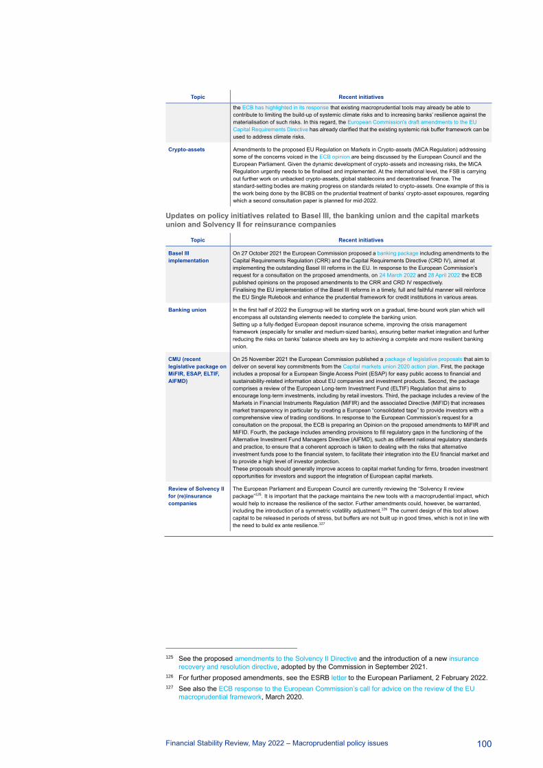
Financial Stability Review, May 2022 – Macroprudential policy issues
100
Topic Recent initiatives
the ECB has highlighted in its response that existing macroprudential tools may already be able to
contribute to limiting the build-up of systemic climate risks and to increasing banks’ resilience against the
materialisation of such risks. In this regard, the European Commission's draft amendments to the EU
Capital Requirements Directive has already clarified that the existing systemic risk buffer framework can be
used to address climate risks.
Crypto-assets Amendments to the proposed EU Regulation on Markets in Crypto-assets (MiCA Regulation) addressing
some of the concerns voiced in the ECB opinion are being discussed by the European Council and the
European Parliament. Given the dynamic development of crypto-assets and increasing risks, the MiCA
Regulation urgently needs to be finalised and implemented. At the international level, the FSB is carrying
out further work on unbacked crypto-assets, global stablecoins and decentralised finance. The
standard-setting bodies are making progress on standards related to crypto-assets. One example of this is
the work being done by the BCBS on the prudential treatment of banks’ crypto-asset exposures, regarding
which a second consultation paper is planned for mid-2022.
Updates on policy initiatives related to Basel III, the banking union and the capital markets
union and Solvency II for reinsurance companies
Topic Recent initiatives
Basel III
implementation
On 27 October 2021 the European Commission proposed a banking package including amendments to the
Capital Requirements Regulation (CRR) and the Capital Requirements Directive (CRD IV), aimed at
implementing the outstanding Basel III reforms in the EU. In response to the European Commission’s
request for a consultation on the proposed amendments, on 24 March 2022 and 28 April 2022 the ECB
published opinions on the proposed amendments to the CRR and CRD IV respectively.
Finalising the EU implementation of the Basel III reforms in a timely, full and faithful manner will reinforce
the EU Single Rulebook and enhance the prudential framework for credit institutions in various areas.
Banking union In the first half of 2022 the Eurogroup will be starting work on a gradual, time-bound work plan which will
encompass all outstanding elements needed to complete the banking union.
Setting up a fully-fledged European deposit insurance scheme, improving the crisis management
framework (especially for smaller and medium-sized banks), ensuring better market integration and further
reducing the risks on banks’ balance sheets are key to achieving a complete and more resilient banking
union.
CMU (recent
legislative package on
MiFIR, ESAP, ELTIF,
AIFMD)
On 25 November 2021 the European Commission published a package of legislative proposals that aim to
deliver on several key commitments from the Capital markets union 2020 action plan. First, the package
includes a proposal for a European Single Access Point (ESAP) for easy public access to financial and
sustainability-related information about EU companies and investment products. Second, the package
comprises a review of the European Long-term Investment Fund (ELTIF) Regulation that aims to
encourage long-term investments, including by retail investors. Third, the package includes a review of the
Markets in Financial Instruments Regulation (MiFIR) and the associated Directive (MiFID) that increases
market transparency in particular by creating a European “consolidated tape” to provide investors with a
comprehensive view of trading conditions. In response to the European Commission’s request for a
consultation on the proposal, the ECB is preparing an Opinion on the proposed amendments to MiFIR and
MiFID. Fourth, the package includes amending provisions to fill regulatory gaps in the functioning of the
Alternative Investment Fund Managers Directive (AIFMD), such as different national regulatory standards
and practice, to ensure that a coherent approach is taken to dealing with the risks that alternative
investment funds pose to the financial system, to facilitate their integration into the EU financial market and
to provide a high level of investor protection.
These proposals should generally improve access to capital market funding for firms, broaden investment
opportunities for investors and support the integration of European capital markets.
Review of Solvency II
for (re)insurance
companies
The European Parliament and European Council are currently reviewing the “Solvency II review
package”125. It is important that the package maintains the new tools with a macroprudential impact, which
would help to increase the resilience of the sector. Further amendments could, however, be warranted,
including the introduction of a symmetric volatility adjustment.126 The current design of this tool allows
capital to be released in periods of stress, but buffers are not built up in good times, which is not in line with
the need to build ex ante resilience.127
125 See the proposed amendments to the Solvency II Directive and the introduction of a new insurance
recovery and resolution directive, adopted by the Commission in September 2021.
126 For further proposed amendments, see the ESRB letter to the European Parliament, 2 February 2022.
127 See also the ECB response to the European Commission’s call for advice on the review of the EU
macroprudential framework, March 2020.

Financial Stability Review, May 2022 – Special Features
101
Special Features
Climate-related risks to financial stability
Prepared by Tina Emambakhsh, Margherita Giuzio, Luca Mingarelli,
Dilyara Salakhova and Martina Spaggiari128
The ECB is continuing its work on incorporating climate-related risks into assessments
of financial stability. This includes a new analysis of disclosure, pricing and
greenwashing risks in financial markets, as well as continued monitoring of financial
institutions’ exposure to transition and physical risks. There is some encouraging
evidence of better disclosure by non-financial corporations and increasing awareness
of climate-related risks in financial markets. Progress made by banks, however, has
been more limited. Established and newer metrics show no clear evidence of a
reduction in climate-related risks, revealing instead a potential for amplification
mechanisms stemming from exposure concentration, cross-hazard correlation and
financial institutions’ overlapping portfolios. These findings can inform evidence-based
international and European policy debates around climate-related corporate
disclosure, standards for sustainable financial instruments and climate-related
prudential policies. More generally, amid high uncertainty around governments’
transition policies in an environment of volatile energy prices, further investments in
the transition to a net-zero economy would also have a positive impact on
medium-term growth and energy security.
Introduction
Climate change has, for a number of years, been identified as a source of systemic
risk, with potentially severe consequences for financial institutions and financial
markets alike.129 As our awareness of this risk has grown, the ECB has enhanced its
approaches to understanding, monitoring and assessing the nature of climate risks
and how such risks are evolving over time. Furthermore, the recent price increases
and volatility seen in energy markets have underlined the wider value of supporting
the transition to a net-zero economy. This special feature presents the latest
developments, starting with a focus on green financing, which is needed to support
128 This special feature has benefited from input received from Olimpia Carradori, Alberto Grassi, Giulio
Mazzolini and Allegra Pietsch.
129 This special feature builds on the analysis presented in previous editions of the Financial Stability Review
published since 2019 (see the special feature entitled “Climate change and financial stability”, Financial
Stability Review, ECB, May 2019, and the special feature entitled “Climate-related risk to financial
stability”, Financial Stability Review, ECB, May 2021). It complements recent ECB initiatives, including
the decision to disclose climate-related information relating to Eurosystem central banks’ investments in
non-monetary policy portfolios by the first quarter of 2023 (see the press release of 4 February 2021), the
consideration of climate-related factors in the monetary policy strategy review (see the press release of 8
July 2021), the need for a macroprudential response (see Macroprudential Bulletin, Issue 15, ECB,
October 2021) and the supervisory assessment of the progress made by European banks in considering
climate and environmental risks (see “The state of climate and environmental risk management in the
banking sector”, ECB, November 2021, and “Supervisory assessment of institutions’ climate-related and
environmental risks disclosures”, ECB, March 2022).
Financial Stability Review, May 2022 – Special Features
102
the transition to a net-zero economy. The subsequent sections then provide updated
assessments of bank and non-bank exposures to climate risks, by introducing
aspects such as the link between climate risk and financial risk in exposures,
concentration of exposures and correlations between hazards.
Increasing role of green finance in supporting the transition to a
low-carbon economy
Sustainable markets continued to grow globally in 2021, mostly thanks to an
increased volume of euro area ESG funds and green bonds (Chart A.1, panel a).
Their growth has accelerated over the last two years, with euro area sustainable
assets doubling since 2019, although sustainable markets still only account for 10%
of the euro area investment fund sector and 3% of outstanding bonds. These
developments reflect the expected green investment through the EU recovery fund
(NextGenerationEU), and the sharp increase in the number of financial institutions
that have made net-zero commitments.130 However, maintaining such momentum
requires that decisive regulatory action be taken to strengthen capital markets
beyond the sustainable finance segment and help channel investments towards
green projects.131
130 See the Glasgow Financial Alliance for Net Zero (GFANZ), which encompasses the
UN-convened Net-Zero Banking Alliance, Net-Zero Asset Owner Alliance, and Net-Zero Insurance
Alliance, and the Net Zero Asset Managers initiative. The GFANZ aims at mobilising the necessary
capital to build a global net-zero economy and deliver on the goals of the Paris Agreement. In addition,
see the “Supervisory assessment of institutions’ climate-related and environmental risks disclosures”,
ECB, March 2022.
131 See “Towards a green capital markets union: developing sustainable, integrated and resilient European
capital markets”, Macroprudential Bulletin, Issue 15, ECB, October 2021.

Financial Stability Review, May 2022 – Special Features
103
Chart A.1
Sustainable financial markets continue to grow, while firms are increasingly disclosing
climate information
a) Outstanding amount of green and sustainability-linked bonds, and assets under management of ESG funds in the euro area
b) Disclosure of NFCs’ GHG emission data by type of emitter
(2015-21, left chart: outstanding amounts for bonds; right chart:
assets under management for funds; € trillions)
(left chart: share of listed NFCs disclosing GHG emissions, share
of audited disclosures, percentages; right chart: share of NFCs
disclosing emission-reduction targets, percentages, market
capitalisation, USD trillions)
Sources: Bloomberg Finance L.P., Urgentem, Refinitiv and ECB calculations.
Notes: Panel a: ESG funds correspond to all sustainable funds identified using Morningstar intentions attributes based on information
provided in funds’ prospectuses. Panel b: the sample includes NFCs listed in the S&P 500 and STOXX Europe 600 indices. “GHG”
stands for greenhouse gas, “NFCs” stands for non-financial corporations.
Empirical evidence suggests that (green) finance supports green investment
and the reduction of emissions, with some differences across financing
instruments and firm types.132 While research has suggested that a higher share of
equity financing is associated with greater reductions in countries’ carbon footprints,
debt is the primary source of external financing for NFCs in the EU and is also used to
support the development and adoption of new (greener) technologies. An analysis of
changes in emissions at over 4,000 European carbon-intensive firms between 2013
and 2019 provides evidence that, up to a certain point, debt has a positive impact on
environmental performance in subsequent years: firms reduce their emissions by
investing in green technologies, without reducing economic activity. However, when a
firm is too indebted, higher leverage is associated with higher emissions as firms then
tend to invest less in energy efficiency.133
In recent years, more firms have been disclosing both their exposure to
transition risk and their emission reduction targets, but gaps in disclosure
132 See De Haas, R. and Popov, A., “Finance and carbon emissions,” Working Paper Series, No 2318, ECB,
September 2019; Fatica, S. and Panzica, R., “Green bonds as a tool against climate change?”, Business
Strategy and the Environment, March 2021; and Flammer, C., “Corporate green bonds”, Journal of
Financial Economics, Vol. 142, Issue 2, November 2021, pp. 499-516.
133 The ECB analysis covers the sample of 4,000 European carbon-intensive NFCs that are included in the
European Union Transaction Log database and are subject to the EU Emissions Trading System. The
database includes information on verified GHG emissions. Firms’ revenues, profitability, and the age and
number of plants with carbon-intensive activities, alongside country-specific factors such as fossil fuel
subsidies, are also found to influence their ability to reduce emissions by investing in new green
technologies.
0.0
0.2
0.4
0.6
0.8
1.0
1.2
1.4
1.6
1.8
20
15
20
16
20
17
20
18
20
19
20
20
20
21
Tri
llio
ns
Equity ESG funds
Bond ESG funds
Other ESG funds
0.0
0.2
0.4
0.6
0.8
1.0
1.2
1.4
1.6
1.8
20
15
20
16
20
17
20
18
20
19
20
20
20
21
Trilli
ons
Green bonds
Sustainability-linked bonds
0
10
20
30
40
50
60
70
80
90
100
20
10
20
11
20
12
20
13
20
14
20
15
20
16
20
17
20
18
20
19
20
20
Listed NFCs disclosing emissions
Of which audited
0
10
20
30
40
50
60
70
80
90
100
20
10
20
11
20
12
20
13
20
14
20
15
20
16
20
17
20
18
20
19
20
20
Listed NFCs disclosing emission-reductiontargets
Combined market capitalisation
1 5 27
Financial Stability Review, May 2022 – Special Features
104
practices remain significant, signalling the need for international standards.
More NFCs have been disclosing data on GHG emissions and setting
emission-reduction targets over time, with high-emitting firms disclosing the most
data, likely reflecting their greater exposure to public scrutiny (Chart A.1, panel b).
Although a large part of this disclosure is verified by a third party, the risk of
greenwashing remains high in the absence of global mandatory reporting
requirements. In addition, although there has been an improvement in the
climate-related disclosures of European banks since 2020, banks are not fully
meeting supervisory expectations and gaps remain, especially regarding banks’
emission-reduction targets and interim milestones.134 The prompt adoption of
international disclosure standards across jurisdictions would allow investors to price
and measure transition risk more effectively, while also supporting the transition to a
low-carbon economy.135 In particular, although there is evidence that firms which set
an emission-reduction target have a lower credit risk and tend to reduce emissions
more than other firms in subsequent years, the credibility of firms’ targets and their
alignment with the Paris Agreement goals are difficult to assess.136
Against this background, capital markets remain susceptible to greenwashing,
and only the most credible green bonds seem to benefit from cheaper funding.
The growth of green bond markets could help stimulate the integration of European
capital markets.137 But the credibility of green bonds and/or their issuers appears to
determine whether green bonds trade at a greenium – with lower spreads than for
conventional bonds – in secondary markets (Chart A.2, panel a). Only green bonds
with an external review, issued by firms in green sectors (e.g. alternative energy) or
by banks which are members of the United Nations Environment Programme Finance
Initiative (UNEP FI) exhibit a greenium. As ESG and green funds keep attracting new
investors, the demand for green bonds and the greenium has also increased over
time (Chart A.2, panel b).138 New instruments, such as sustainability-linked bonds,
which link borrowing costs to specific company-level sustainability targets, partly
address investor concerns about greenwashing in the green bond market.
Greenwashing also poses a risk to financial stability because it could lead to an
undervaluation of transition risk and to potential fire-sales of green bonds. A common
regulatory standard that requires regular standardised reporting, impact assessment
and review by approved external reviewers, as proposed under the EU Green Bond
Standard, would provide assurance that green bonds effectively finance the transition
and alleviate risks to financial stability. Implementing this standard and making it
mandatory within a reasonable period of time could enhance investor confidence in
134 See the Supervisory assessment of institutions’ climate-related and environmental risks disclosures,
ECB, March 2022.
135 The climate change-related disclosure standards under the proposed European Union’s Corporate
Sustainability Reporting Directive is expected to be used by companies for the first time in 2024, for the
2023 financial year.
136 See Carbone, S., Giuzio, M., Kapadia, S., Krämer, J., Nyholm, K. and Vozian, K., “The low-carbon
transition, climate commitments and firm credit risk”, Working Paper Series, No 2631, ECB, December
2021.
137 See the box entitled “Home bias in green bond markets”, Financial Integration and Structure in the Euro
Area Report, ECB, April 2022.
138 From Pietsch, A. and Salakhova, D., “Pricing of green bonds – drivers and dynamics of the greenium”,
Working Paper Series, ECB, forthcoming.
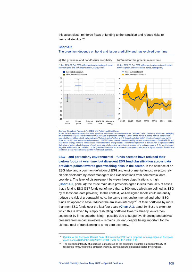
Financial Stability Review, May 2022 – Special Features
105
this asset class, reinforce flows of funding to the transition and reduce risks to
financial stability.139
Chart A.2
The greenium depends on bond and issuer credibility and has evolved over time
a) The greenium and bond/issuer credibility b) Trend for the greenium over time
(1 Jan. 2016-30 Oct. 2021, difference in option-adjusted spread
between green and conventional bonds, basis points)
(1 Sep. 2018-31 Oct. 2021, difference in option-adjusted spread
between green and conventional bonds, basis points)
Sources: Bloomberg Finance L.P., CSDB, and Pietsch and Salakhova.
Notes: Panel a: negative values indicate a greenium, as indicated by the shaded area. “All bonds” refers to all euro area bonds satisfying
the International Capital Market Association (ICMA) use-of-proceeds principle, “Simple green” refers to bonds that are classified as
green but have not been third-party reviewed, “External review” refers to only those bonds that satisfy all principles promoted by the
ICMA and which have been externally reviewed, “UNEP FI bank” refers to bonds issued by banks that are members of the UNEP FI, and
“Alternative energy” refers to bonds issued by the alternative energy sector. The estimated greenium is derived from a regression of the
daily closing option-adjusted spread of each bond on multiple control variables and a green bond indicator equal to 1 if a bond is green.
Negative estimates of the coefficient on the green bond indicator show a greenium as green bonds trade at tighter spreads. Panel b: the
coefficient of this indicator is depicted for monthly sub-samples.
ESG – and particularly environmental – funds seem to have reduced their
carbon footprint over time, but divergent ESG fund classification across data
providers points towards greenwashing risks in the sector. In the absence of an
ESG label and a common definition of ESG and environmental funds, investors rely
on self-disclosure by asset managers and classifications from commercial data
providers. The level of disagreement between these classifications is high
(Chart A.3, panel a): the three main data providers agree in less than 20% of cases
that a fund is ESG (317 funds out of more than 1,800 funds which are defined as ESG
by at least one data provider). In this context, well-designed labels could materially
reduce the risk of greenwashing. At the same time, environmental and other ESG
funds do appear to have reduced the emission intensity140 of their portfolios by more
than non-ESG funds over the last four years (Chart A.3, panel b). But the extent to
which this is driven by simply reshuffling portfolios towards already low-carbon
sectors or by firms decarbonising – possibly due to supportive financing and activist
pressure from impact investors – remains unclear, despite being important for the
ultimate goal of transitioning to a net-zero economy.
139 Opinion of the European Central Bank of 5 November 2021 on a proposal for a regulation on European
green bonds (CON/2021/30) 2022/C 27/04 (OJ C 27, 19.1.2022, p 4).
140 The emission intensity of a portfolio is measured as the exposure-weighted emission intensity of
respective firms, with firm’s emission intensity being absolute emissions scaled by revenues.
UNEP FIbank
Simplegreen
Externalreview
-30
-25
-20
-15
-10
-5
0
5
10
15
20
Allbonds
Estimated greenium
95% confidence interval
Alternative energy
-20
-15
-10
-5
0
5
10
15
20
09/18 03/19 09/19 03/20 09/20 03/21 09/21
Greenium coefficient
95% confidence interval

Financial Stability Review, May 2022 – Special Features
106
Chart A.3
Agreement of data providers on ESG designation of funds is limited, although ESG
funds have tended to reduce the emission intensities of their portfolios
a) Funds classified as ESG by three providers b) Change of emission intensity by fund strategy over time
(number of funds per category) (tCO2e per USD million revenues, scope 1, 2 and 3 emissions)
Sources: Morningstar, Bloomberg Finance L.P., Refinitiv Lipper for Investment Management and ECB calculations.
Notes: Panel a: each bubble represents the number of different funds classified as ESG according to the providers (Morningstar,
Bloomberg and Lipper). The numbers in the overlapping areas of the bubbles correspond to the funds identified either by two or by all
three providers. Panel b: the chart shows average emission intensity of funds in each category. Categories are identified using
Morningstar intentions attributes based on information provided in funds’ prospectuses. E funds are identified using environmental
attributes; ESG funds correspond to all sustainable funds; “tCO2e” stands for tonnes of carbon dioxide equivalent.
Limited change in financial system exposures to transition risk
While firms’ emissions have been decreasing, exposures of euro area banks to
currently high-emitting firms have remained broadly stable. Around two-thirds of
the corporate credit exposures held by euro area banks are still directed towards
high-emitting firms, which are mainly concentrated in the manufacturing, real estate
and retail sectors (Chart A.4, panel a).141 Also, around 30% of both bank and
non-bank holdings of securities issued by NFCs with known emission levels are
currently issued by high-emitting firms, a share which has only decreased slightly
over the last five years. At the same time, the recent increases and volatility in energy
markets have underlined the urgency of supporting the transition to a net-zero
economy.
Metrics commonly used to assess corporate sector climate risks point to a
small increase in carbon intensity in bank portfolios. Only a few (mainly large and
highly exposed) banks have significantly decarbonised their credit portfolios since
2018, as measured by the loan-weighted emissions of the respective borrowers
(Chart A.4, panel b). By contrast, two-thirds of banks have increased their
loan-weighted emissions. The measures may still be missing the interaction between
climate risk and financial risk of loans.
141 High-emitting firms are defined here as firms with reported emission intensity in the top 33% of the
distribution as of end-2020, i.e. firms with 2020 emission intensity in excess of 556 tCO2e/USD million.
Lipper479
Morningstar257
Bloomberg35
6824
317
640
0
50
100
150
200
250
E funds ESG funds No-strategy funds
2018
2019
2020
2021

Financial Stability Review, May 2022 – Special Features
107
Chart A.4
While firms’ emissions have been decreasing, the financial system’s exposures to
high-emitting firms have remained broadly stable
a) Bank exposure to/securities holdings of high-emitting and low-emitting firms
b) Change in the loan-weighted emissions of bank portfolios between 2018 and 2021
(left chart: share of total credit exposures, percentages; right chart:
share of total securities holdings, percentages)
(tCO2e)
Sources: AnaCredit, Securities Holdings Statistics by Sector, Urgentem and ECB calculations.
Notes: Panel a: high/low emitters are defined here as firms with reported emission intensity in the top/bottom 33% of the distribution
across euro area bank borrowers as of end-2020, i.e. firms with an annual emission intensity registered in 2020 above 556 tCO2e/USD
million and below 47 tCO2e/USD million. “ICPFs” stands for insurance corporations and pension funds; “IFs” stands for investment funds.
Panel b: ”G-SIBs” stands for global systemically important banks.
Information on carbon emissions can be combined with the existing probability
of default (PD) so a corporate borrower can provide a credit risk-adjusted
metric of transition risk. The resulting score can be computed at bank level by
aggregating loan-weighted borrowers’ emissions multiplied by their PDs over the
bank’s entire corporate portfolio.142 The PDs are included as a measure of credit risk
and the GHG emissions are included as a measure of vulnerability to transition risk.
Overall, the higher a firm’s contribution to the transition risk score, the higher its
contribution to the bank’s financial risk induced by the combination of credit and
transition risk, as long as PDs have not already accounted for the latter.143
142 The credit-risk-weighted metric of transition risk for a bank 𝑗 is defined as:
∑ 𝐺𝐻𝐺 𝑒𝑚𝑖𝑠𝑠𝑖𝑜𝑛𝑠𝑖
∙ 𝑃𝐷𝑖𝑗 ∙
𝑙𝑜𝑎𝑛𝑠𝑖𝑗
∑ 𝑙𝑜𝑎𝑛𝑠𝑖𝑗𝑖𝑖
,
where 𝑖 is (one of) the borrower(s), 𝐺𝐻𝐺 𝑒𝑚𝑖𝑠𝑠𝑖𝑜𝑛𝑠 is the level of (relative or absolute) GHG emissions
produced by the borrower and 𝑃𝐷 is the probability of default assigned to the borrower by the bank
concerned. An alternative for the credit risk component would be to use loan loss provisions as a
proportion of loans instead of PD. In the present case, PDs are used because they capture credit risk
from a more forward-looking perspective. An alternative for the climate risk component would be to use
emission targets alongside or instead of current emission levels. This choice would also improve the
forward-looking power of the metric.
143 Transition risk can materialise in the form of higher operating expenditures and investment requirements
for firms, the purpose being to reduce their emissions. These higher monetary costs can manifest
themselves in transitional risk metrics (e.g. credit risk parameters such as PDs), although it is assumed
that banks do not currently explicitly account for the contribution of transition risk to firms’ credit risk.
0
10
20
30
40
50
60
70
80
90
100
20
18
20
19
20
20
20
21
Banks
High emitters
Medium emitters
Low emitters
0
10
20
30
40
50
60
70
80
90
100
20
16
20
17
20
18
20
19
20
20
Banks
20
16
20
17
20
18
20
19
20
20
ICPFs
20
16
20
17
20
18
20
19
20
20
IFs
0
5
10
15
20
0 5 10 15 20
Lo
an
-we
igh
ted
em
iss
ion
s 2
02
1
Loan-weighted emissions 2018
G-SIBs
Others

Financial Stability Review, May 2022 – Special Features
108
Chart A.5
PD-weighted measures of emissions can capture the financial component of banks’
climate risks and round out the picture provided by emissions-to-loans ratios
a) PD-weighted and simple emissions-to-loans ratio by bank
b) Breakdown of euro area aggregate PD-weighted emissions-to-loans ratio by NACE sector over time and compared with the simple emissions-to-loans ratios
(2020) (left chart: normalised PD-weighted and simple emissions-to-loans
ratios by sector in 2020 (averages weighted by exposures); right
chart: 2012-20, sectoral shares of aggregate euro area
PD-weighted emissions-to-loans ratio, absolute score)
Sources: AnaCredit, Urgentem, Register of Institutions and Affiliates Database and ECB calculations.
Notes: Emissions refer to firm-level relative and absolute (loan carbon intensity) scope 1, 2 and 3 emissions. Panel b) uses two different
underlying firm samples. The bar chart comprises inferred emissions for around 2.5 million firms in 2018, covering around 80% of total
AnaCredit exposures. The capital letters refer to NACE codes as follows: A – Agriculture; B – Mining; C – Manufacturing; D – Electricity;
F – Construction; G – Wholesale and retail trade; H – Transport. The time series covers both inferred and reported emissions for 1,250
firms, which comprise on average 10% of AnaCredit exposures over time. “NACE” stands for Nomenclature statistique des activités
économiques dans la Communauté Européenne (Statistical classification of economic activities in the European Community).
The credit risk-adjusted measure supports signals obtained from
emissions-to-loans ratio measures indicating that risk has increased over
time.144 Once adjusted for financial risk using borrowers’ PDs, estimated transition
risk has increased since 2012, with significant increases in sectors that face more
underlying transition risk. This has some correlation with the signals from unadjusted
measures of transition risk (Chart A.5, panel a). Exposures to the mining,
manufacturing and electricity sectors together account for around 70% of the euro
area aggregate (Chart A.5, panel b). Some of these sectors make an almost
negligible contribution to the emissions-to-loans ratio but they play an important role
when the financial risk component is considered.
144 The bank-level emissions-to-loans ratio is computed by aggregating borrowers’ emissions and dividing
this figure by the total value of the bank’s corporate loan portfolio.
0.0
0.2
0.4
0.6
0.8
1.0
0.0 0.2 0.4 0.6 0.8 1.0
Significant institutions
No
rma
lis
ed
sim
ple
em
iss
ion
s-t
o-l
oa
ns
ra
tio
Normalised PD-weighted emissions-to-loans ratio
0
5
10
15
20
25
30
35
40
20
12
20
13
20
14
20
15
20
16
20
17
20
18
20
19
20
20
Agriculture
Mining
Manufacturing
Electricity
Construction
Wholesale and retail
Transport
Other
Euro area aggregate
0.0
0.2
0.4
0.6
0.8
1.0
1.2
A B C D F G H
Oth
er
PD-weighted emissions-to-loans ratio
Simple emissions-to-loans ratio

Financial Stability Review, May 2022 – Special Features
109
Chart A.6
Climate-related concentration risk is a new form of concentration risk simultaneously
affecting multiple, seemingly unrelated, exposures
a) Correlation between banks’ sensitivity to carbon price increases, expected losses and climate-risk concentration
b) Distribution of default correlations for increasing transition risk intensity α
(2020-50, upper chart: percentages, lower chart: bubble size:
absolute expected losses)
(y-axis: percentages)
Sources: AnaCredit, Urgentem, NGFS, Moody’s Credit Edge and ECB calculations.
Notes: Panel a: corporate loan portfolios of euro area significant institutions which represent 60% of total AnaCredit exposures. Panel b:
euro area sample based on 500,000 Monte Carlo iterations. The parameter α = (1 − β)T incorporates both the transition risk shock
T (€/tCO2) as well as a pass-through factor β capturing the degree to which firms can pass the cost of a transition risk shock on to
consumers (Belloni et al., see footnote 146).
Since climate-related risks simultaneously affect multiple seemingly unrelated
exposures, their concentration in individual institutions plays a significant role.
Climate-related concentration risks can arise from exposures that share similar
sensitivities to physical risks (e.g. due to their location or activity) or transition risks
(e.g. due to their sector allocation or level of emissions). Focusing on transition risk
and assuming a disorderly transition scenario,145 it appears that higher
concentrations of exposures to firms with high emission intensity coincide with higher
expected losses at bank level over a 30-year period (Chart A.6, panel a). Around
35% of system-wide expected losses are incurred by the 10% of banks with the
highest sensitivity to carbon price increases. In addition, carbon price shocks trigger a
145 This exercise measures a bank's sensitivity to carbon price increases under the NGFS Phase I disorderly
transition scenario over a 30-year period, leveraging on model parameters developed in the ECB
economy-wide climate stress test (see “ECB economy-wide climate stress test”, Occasional Paper
Series, No 281, ECB, September 2021). The increase in banks’ expected losses stemming from carbon
price increases is calculated for each of its credit exposure as
bank′s sensitivity to carbon price increases =𝑒𝑥𝑝𝑒𝑐𝑡𝑒𝑑 𝑙𝑜𝑠𝑠𝑒𝑠𝑡0
𝐸𝐴𝐷𝑡0
[ 𝛽𝑃 ∆(𝑝𝑟𝑜𝑓𝑖𝑡𝑎𝑏𝑖𝑙𝑖𝑡𝑦)𝑡 + 𝛽𝐿∆(𝑙𝑒𝑣𝑒𝑟𝑎𝑔𝑒)𝑡]
where 𝛽𝑃 and 𝛽𝐿 are coefficients determining the extent to which borrower PDs react to changes in
profitability and leverage.
0 20 40 60 80 100
Share ofsystem-wide
expectedlosses
Top 5% banks with highest sensitivity
Top 10% banks with highest sensitivity (excluding top 5%)
Rest of sample
0.0
0.1
0.2
0.3
0.4
0.5
0.6
0.7
0.0 0.2 0.4 0.6 0.8 1.0
Sh
are
of
ex
po
su
res
to
hig
h
em
itte
rs
Banks' sensitivity to carbon price increases
Significant institutions
Financial Stability Review, May 2022 – Special Features
110
significant increase in firms’ default correlations.146 For a transition risk intensity of
200€/tCO2, capturing the cost due to increases in the cost of carbon borne by firms
causes estimated average (median) correlations to double (Chart A.6, panel b).
Transition risk not only leads to a source of novel correlation between previously
uncorrelated or weakly correlated firms in general, but also increases correlations for
high emitters147 by ten times more than it does for low emitters.
Systemic amplifications could result from interconnected physical
risks arising from climate change
Financial stability risks arising from physical hazards are exacerbated by the
fact that some investors hold assets which are vulnerable to multiple hazards.
The occurrence of natural hazards is characterised by interactions between hazards
in the form of either correlations or causal links (Chart A.7, panel a) which can
generate self-reinforcing or feedback mechanisms. For example, the joint
combination of thunderstorms and droughts (both captured by the “Heat stress”
category in Chart A.7, panel a) can cause wildfires which, in turn, both increase the
likelihood of more wildfires and exacerbate heat stress.148 Future intensification of
climate risk, especially when clustered hazards occur, may create hard-to-price
tipping points and impair options for diversification, potentially posing financial
stability risks, especially for securities with wider protection gaps.
In addition to the direct exposure to physical risk, the impact of physical
hazards could be amplified by fire-sale dynamics. In the event of a sudden
reassessment of risks affecting portfolios, the liquidation of securities exposed to
potential hazards may affect market prices. This could result in contagion losses
spreading by way of the common holdings of different market participants and, in
worst-case scenarios, spiralling deleveraging pressures.149 Constructing estimates of
the common asset holdings (overlapping portfolios) exposed to the different physical
risks150 of different market participants (Chart A.7, panel b) reveals a range of
estimates running from 2% of overlapping portfolios for the hurricanes and typhoons
category to an average of 45% for portfolios weighted for wildfires.151 In addition, the
146 Firms’ default correlations are estimated using a multi-firm Merton model calibrated on historical data for
a large sample of euro area firms. Via 500,000 Monte Carlo iterations, the model simulates the default
events of thousands of firms for which the asset value process is modelled as correlated geometric
Brownian motions. The transition risk intensity α = (1 − β )T, capturing the fraction of transition cost
borne by firms for each tonne of CO2 emitted, incorporates both the transition risk shock T (€/tCO2) and a
pass-through factor β capturing the degree to which firms can pass the cost of a transition risk shock on
to consumers, and impacts the value of assets (see Belloni, M., Kuik, F. and Mingarelli, L., “Euro area
banks’ sensitivity to changes in carbon price”, Working Paper Series, No 2654, ECB, March 2022). Under
the simplifying assumption that firms would bear the full cost of an increase in carbon prices (β = 0), the
transition risk intensity would be equivalent to this increase in the cost of carbon, i.e. α = T.
147 Firms with emission intensities above (below) the sample’s 75th percentile are referred to as high (low)
emitters.
148 Another example is typhoons and rainfall, which can trigger ground subsidence. This has the potential to
start landslides which can, in turn, cause flooding.
149 Cont, R. and Schaanning, E., “Monitoring indirect contagion”, Journal of Banking and Finance, Vol. 104,
Issue C, July 2019, pp. 85-102.
150 Firm-level risk scores for over four million firms worldwide, from Moody’s Four Twenty Seven, are used.
151 The degree to which the share of portfolios exposed to natural hazards will concretely be at risk is unclear
as firms can implement physical risk-mitigation measures to reduce impacts.

Financial Stability Review, May 2022 – Special Features
111
concentration of overlapping portfolios in specific sectors may further exacerbate
such risks, as in the case of financial corporates, which are much more exposed to
wildfires than other sectors.
Chart A.7
Interdependencies between natural hazards and financial sectors could lead to
hard-to-price tipping points triggering concurrent revaluations affecting different
investors
a) Natural hazard interdependencies b) Physical risk-weighted overlapping portfolios
(arrows based on hazard correlations and causal relations) (as a share of common asset holdings, percentages; mean in
parenthesis)
Sources: Gill and Malamud*, ECB (securities holdings statistics), Moody’s 427 and ECB calculations.
Notes: Panel a: links refer to both correlations and causal links. Arrow thickness is proportional to a score capturing either increased
probability or causal trigger of hazards, in terms of both spatial overlaps and temporal likelihood. Aggregated from Gill and Malamud*.
Self-loops refer to the increased likelihood of a given hazard conditional on the materialisation of the hazard itself due to associated
self-reinforcing mechanisms. Panel b: overlapping portfolios weighted by physical hazard scores as a share of common asset holdings
by aggregate sectors. The physical-risk-weighted overlapping portfolios between sectors i and j are reported as a share of common
asset holdings, that is �̃�ij/𝒪ij = ∑ Πk(Sik ∧ Sjk)k / ∑ (Sik ∧ Sjk)k where Sik denotes the holdings by sector i of security k, and Πk the
physical risk weight associated with the issuer of security k. Sectors considered are credit institutions (CI), financial corporations (FC),
governments (GOV), households (HH), and non-financial corporations (NFC). Securities include both bonds and equities. Note that a
different scale applies to each hazard (right-hand scale of each heatmap, percentages). Group averages (in parentheses) give a sense
of the relative importance of each hazard at system-wide level.
*) Gill, J.C. and Malamoud, B.D., “Reviewing and visualizing the interactions of natural hazards”, Reviews of Geophysics, Vol. 52, Issue
4, 2014, pp. 680-772.
Climate-related tipping points may translate into a financial tipping point in the
form of a sudden risk repricing which would strain investors with overlapping
portfolios. In the event of a sudden reassessment of risk following clustered hazard
events, common holdings may cause several different investor segments to face
large mark-to-market losses at once, which could be amplified by fire-sales and other
portfolio rebalancing actions. This system-wide risk highlights the relevance of a
macroprudential approach to prudential responses aimed at mitigating the impact of
climate change on financial stability. This risk runs in parallel with the insurance
protection gap relating to climate-related catastrophes.152
152 See “Climate change, catastrophes and the macroeconomic benefits of insurance”, Financial Stability
Report, EIOPA, July 2021, pp 105-123.

Financial Stability Review, May 2022 – Special Features
112
Conclusions and policy implications
This special feature contributes to the ECB’s monitoring of climate risks by
examining the role of green finance in supporting the transition to a low-carbon
economy, the currently limited financial adaptation to transition risk and the
financial system amplifiers of physical risk. While further progress on consistent
climate data is required, especially for forward-looking metrics, granular physical risk
exposures and insurance coverage, there is encouraging evidence of greater
disclosure by NFCs and an increasing awareness of climate-related risks in financial
markets. Yet the risk of greenwashing remains a concern and may be rising fast – in
both the green bond market and the investment fund sector – given the absence of
well-designed, consistent standards for sustainable financial instruments. The
dynamic exposures of financial institutions to transition and physical risks, together
with their risk metrics, show no clear evidence of financial institutions experiencing a
significant reduction in risk. In addition, exposure concentration, cross-hazard
correlation and institutions’ overlapping portfolios are shown to act as amplifiers of
such risks.
This analysis can contribute to the policy debate around disclosures, standards
for sustainable financial instruments and climate-related prudential policies.
The development of consistent sustainability disclosures via the Corporate
Sustainability Reporting Directive and the IFRS Foundation, as well as the
convergence of these requirements in common minimum international standards, are
important factors allowing firms, investors and financial institutions to effectively
measure and manage transition risk. Regulatory standards on sustainable financial
instruments, such as the EU GBS and ESG/environmental fund labels, are key to
reducing the risk of greenwashing and thus helping to scale up sustainable financing.
Finally, based on the systemic aspect and possible amplification mechanisms
originating from climate-related physical and transition risks, there should be further
reflection on how to close any material gaps in the prudential framework.153 Future
work will focus on the extent to which existing macroprudential tools, including the
systemic risk buffer, could be readily deployed to capture climate risks. New tools,
such as concentration risk measures, may also be needed to address climate-related
risks from a systemic perspective.154
153 See Baranović et al., “The challenge of capturing climate risks in the banking regulatory framework: is
there a need for a macroprudential response?”, Macroprudential Bulletin, ECB, October 2021.
154 See “ECB response to the European Commission’s call for advice on the review of the EU
macroprudential framework”, March 2022.
Financial Stability Review, May 2022 – Special Features
113
Decrypting financial stability risks in crypto-asset markets
Prepared by Lieven Hermans, Annalaura Ianiro, Urszula Kochanska,
Veli-Matti Törmälehto, Anton van der Kraaij and Josep M. Vendrell
Simón155
The stellar growth, volatility and financial innovation currently seen in the crypto-asset
ecosystem, as well as the rising involvement of institutional investors, show how
important it is to gain a better understanding of the potential risks that crypto-assets
could pose to financial stability if trends continue on this trajectory. Systemic risk
increases in line with the level of interconnectedness between crypto-assets and the
traditional financial sector, the use of leverage and lending activity. It is important to
close regulatory and data gaps in the crypto-asset ecosystem to mitigate such
systemic risks.
Introduction
Crypto-assets are currently the subject of intense policy debate. The different
segments of crypto-asset markets include unbacked crypto-assets (such as Bitcoin),
decentralised finance (DeFi) and stablecoins.156 Crypto-assets lack intrinsic
economic value or reference assets, while their frequent use as an instrument of
speculation, their high volatility and energy consumption, and their use in financing
illicit activities make crypto-assets highly risky instruments. This also raises concerns
over money laundering, market integrity and consumer protection, and may have
implications for financial stability.
Despite the risks, investor demand for crypto-assets has been increasing. This
exuberance stems from, among other things, perceived opportunities for quick gains,
the unique characteristics of crypto-assets (for instance programmability) compared
with conventional asset classes, and the benefits perceived by institutional investors
with regard to portfolio diversification. Major players in the payments industry have
also stepped up their crypto-asset-based services, enabling easier retail access.
While crypto-asset markets currently represent less than 1% of the global financial
system in terms of size, they have grown significantly since the end of 2020. Despite
recent declines, they remain similar in size to, for example, the securitised sub-prime
mortgage markets that triggered the global financial crisis of 2007-08.
Risks to financial stability in the euro area stemming from crypto-assets were
seen as limited in the past.157 This special feature provides an update on
crypto-asset market developments and a general overview of risks stemming from
unbacked crypto-assets and DeFi, given the way in which they have evolved and
their specific characteristics and risks. This article therefore abstracts from a specific
155 The authors are grateful to France Marie Alix De Pradier d’Agrain, Lorenzo Pangallo and Antonella
Pellicani for data support.
156 See the definitions used in “Crypto-assets and Global ‘Stablecoins'”, Financial Stability Board, last
updated February 2022.
157 For previous assessments, see the box entitled “Financial stability implications of crypto-assets”,
Financial Stability Review, ECB, May 2018.

Financial Stability Review, May 2022 – Special Features
114
discussion on risks and developments in stablecoins which, as shown by the recent
TerraUSD crash and Tether de-peg, are not as stable as their name suggests and
cannot guarantee their peg at all times.158 Following a deep dive into crypto-asset
leverage and crypto lending, we conclude that if the present trajectory of growth in the
size and complexity of the crypto-asset ecosystem continues, and if financial
institutions become increasingly involved with crypto-assets, then crypto-assets will
pose a risk to financial stability.
Market developments in recent years
The crypto-asset universe has increased dramatically in both size and
complexity since the end of 2020, expanding beyond Bitcoin. Despite recent
market developments, the overall market capitalisation of the crypto-asset class is still
around seven times bigger than it was at the start of 2020, having reached a high of
over €2.5 trillion on aggregate in late 2021 (Chart B.1, panel a). Although the
crypto-asset universe is still relatively small compared with the biggest stock
exchanges (e.g. around 10% of STOXX Europe 600 market capitalisation), by
November 2021 Bitcoin and Ether were among the largest assets globally (Chart B.1,
panel b). Trading volumes for the most representative crypto-assets (including
Bitcoin, Ether and Tether) have at times been comparable with or even surpassed
those of the New York Stock Exchange or euro area sovereign bond quarterly trading
volumes. There are now more than 16,000 crypto-assets in existence (ten new
crypto-assets are launched every day on average), although only around 25
crypto-assets have a market capitalisation comparable with that of a large cap equity.
At the same time, selected subsegments within the crypto-asset ecosystem such as
stablecoins, non-fungible tokens (NFTs) and DeFi grew particularly strongly in 2021,
indicating that the potential functionalities of crypto-assets are expanding.
However, crypto-asset markets also continue to be characterised by high levels
of volatility. Over the last few years, the historical volatility of crypto-assets has
continued to dwarf the volatility of the diversified European stock and bond markets.
For example, while the volatility of the Bitcoin price has declined over the years, it is
still significantly higher than for commodities such as silver and gold. Despite volatile
movements and bouts of speculation (Chart B.1, panel a), crypto-assets trended
upwards throughout most of 2021, leading to all-time-high prices for most individual
crypto-assets. However, since early November the price of Bitcoin, as well as that of
the other main unbacked crypto-assets, has more than halved amid a changing
environment (US monetary tightening and increasing geopolitical tensions).
158 For a discussion on the risks of the third segment of crypto-asset markets (stablecoins) and their
interconnectedness with the general crypto-asset ecosystem and the traditional financial sector, see, for
example, the article entitled “The expanding functions and uses of stablecoins”, Financial Stability
Review, ECB, November 2021; and the article entitled “A regulatory and financial stability perspective on
global stablecoins”, Macroprudential Bulletin, No 10, ECB, May 2020.
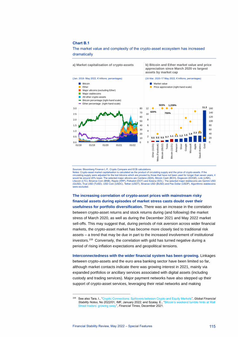
Financial Stability Review, May 2022 – Special Features
115
Chart B.1
The market value and complexity of the crypto-asset ecosystem has increased
dramatically
a) Market capitalisation of crypto-assets b) Bitcoin and Ether market value and price appreciation since March 2020 vs largest assets by market cap
(Jan. 2018- May 2022, € trillions; percentages) (16 Mar. 2020-17 May 2022, € trillions, percentages)
Sources: Bloomberg Finance L.P., Crypto Compare and ECB calculations.
Notes: Crypto-asset market capitalisation is calculated as the product of circulating supply and the price of crypto-assets. If the
circulating supply were adjusted for the lost bitcoins which are proxied by those that have not been used for longer than seven years, it
would be around 20% lower. The selected major altcoins are Cardano (ADA), Bitcoin Cash (BCH), Dogecoin (DOGE), Link (LINK),
Litecoin (LTC), Binance Coin (BNB), Ripple (XRP), Polkadot (DOT) and Solana (SOL). The selected major stablecoins are Gemini USD
(GUSD), True USD (TUSD), USD Coin (USDC), Tether (USDT), Binance USD (BUSD) and Pax Dollar (USDP). Algorithmic stablecoins
were excluded.
The increasing correlation of crypto-asset prices with mainstream risky
financial assets during episodes of market stress casts doubt over their
usefulness for portfolio diversification. There was an increase in the correlation
between crypto-asset returns and stock returns during (and following) the market
stress of March 2020, as well as during the December 2021 and May 2022 market
sell-offs. This may suggest that, during periods of risk aversion across wider financial
markets, the crypto-asset market has become more closely tied to traditional risk
assets – a trend that may be due in part to the increased involvement of institutional
investors.159 Conversely, the correlation with gold has turned negative during a
period of rising inflation expectations and geopolitical tensions.
Interconnectedness with the wider financial system has been growing. Linkages
between crypto-assets and the euro area banking sector have been limited so far,
although market contacts indicate there was growing interest in 2021, mainly via
expanded portfolios or ancillary services associated with digital assets (including
custody and trading services). Major payment networks have also stepped up their
support of crypto-asset services, leveraging their retail networks and making
159 See also Tara, I., “Cryptic Connections: Spillovers between Crypto and Equity Markets”, Global Financial
Stability Notes, No 2022/01, IMF, January 2022; and Szalay, E., “Bitcoin’s weekend tumble hints at Wall
Street traders’ growing sway”, Financial Times, December 2021.
0
10
20
30
40
50
60
70
80
0.0
0.5
1.0
1.5
2.0
2.5
3.0
01/18 01/19 01/20 01/21 01/22
Bitcoin
Ether
Major altcoins (excluding Ether)
Major stablecoins
All other crypto-assets
Bitcoin percentage (right-hand scale)
Ether percentage (right-hand scale)
0.5 0.5 0.5 0.7 1.1 1.1 1.2 1.51.9
2.3 2.3
11.3
0
20
40
60
80
100
120
140
160
0
2
4
6
8
10
12
Eth
er
(11
/21
)
Meta
(F
ace
boo
k)
Bitco
in (
05
/22
)
Tesla
Bitco
in (
11
/21
)
Am
azo
n
Silv
er
Go
og
le
Mic
roso
ft
Ap
ple
Sa
ud
i A
ram
co
Go
ld
503%
755%420%
Market value
Price appreciation (right-hand scale)
1,239%

Financial Stability Review, May 2022 – Special Features
116
crypto-assets more easily accessible to consumers and businesses. Some
institutional investors (hedge funds, family offices, some non-financial firms and asset
managers) are now also investing in Bitcoin and crypto-assets more generally.160 In
addition, market intelligence suggests that the growing involvement of asset
managers is largely in response to demand from their own clients.
Demand from institutional investors in Europe has also risen. For example, 56%
of European institutional investors surveyed by custody and execution services
provider Fidelity Digital Assets161 indicated that they have some level of exposure to
digital assets – up from 45% in 2020 – with their intention to invest also trending
upwards. One reason could be that measures taken by the public authorities may
have been interpreted as endorsing crypto-assets, even though the latter remain
largely unregulated. For example, since July 2021 German institutional investment
funds have been allowed to invest up to 20% of their holdings in crypto-assets. This is
further aided by the increasing availability of crypto-based derivatives and securities
on regulated exchanges, such as futures, exchange-traded notes, exchange-traded
funds and OTC-traded trusts, which have increased in popularity over the last few
years in Europe and the United States. These products, together with clearing
facilities, have made crypto-assets more accessible to investors as they can be
traded on traditional stock exchanges, with the end user no longer having to deal with
the complexities of custody and storage. However, the European crypto-asset
management landscape is still relatively limited and is home to only 20% of total
global crypto-assets funds in terms of primary office location.
Retail investors represent a significant part of the crypto-asset investor base.
Recent results from the ECB’s Consumer Expectations Survey (CES)162 for six large
euro area countries163 indicate, based on experimental questions, that as many as
10% of households may own crypto-assets (Chart B.2, panel a). Most crypto-asset
owners reported holding less then €5,000 in crypto-assets, with a slight
predominance of smaller holdings (below €1,000) in this group. At the other end of
the spectrum, around 6% of crypto-asset owners confirmed that they held more than
€30,000 in crypto-assets (Chart B.2, panel b). Looking at the income quintiles of the
respondents, the pattern is largely U-shaped: the higher a household’s income, the
more likely it is to hold crypto-assets, with lower-income households more likely to
hold crypto than middle-income households (Chart B.2, panel c). On average, young
adult males and highly educated respondents were more likely to invest in
crypto-assets in the countries surveyed. With regard to financial literacy, respondents
who scored either at the top level or the bottom level in terms of financial literacy
scores were highly likely to hold crypto-assets.
160 See Fletcher, L., “Hedge funds expect to hold 7% of assets in crypto within five years”, Financial Times,
June 2021. A recent survey of 100 hedge fund CFOs by fund administrator Intertrust Group found that
they expected to allocate, on average, 7.2% of their assets to crypto-assets by 2026. A Goldman Sachs
survey carried out in 2021 showed that 15% of family offices have exposures to crypto-assets, while
nearly half of all family offices are interested in taking on exposures.
161 See “Institutional Investor Digital Assets”, Fidelity Digital Assets, 2021.
162 The CES collects high-frequency information on the perceptions and expectations of households in the
euro area, as well as on households’ economic and financial behaviour.
163 Belgium, Germany, Spain, France, Italy and the Netherlands.
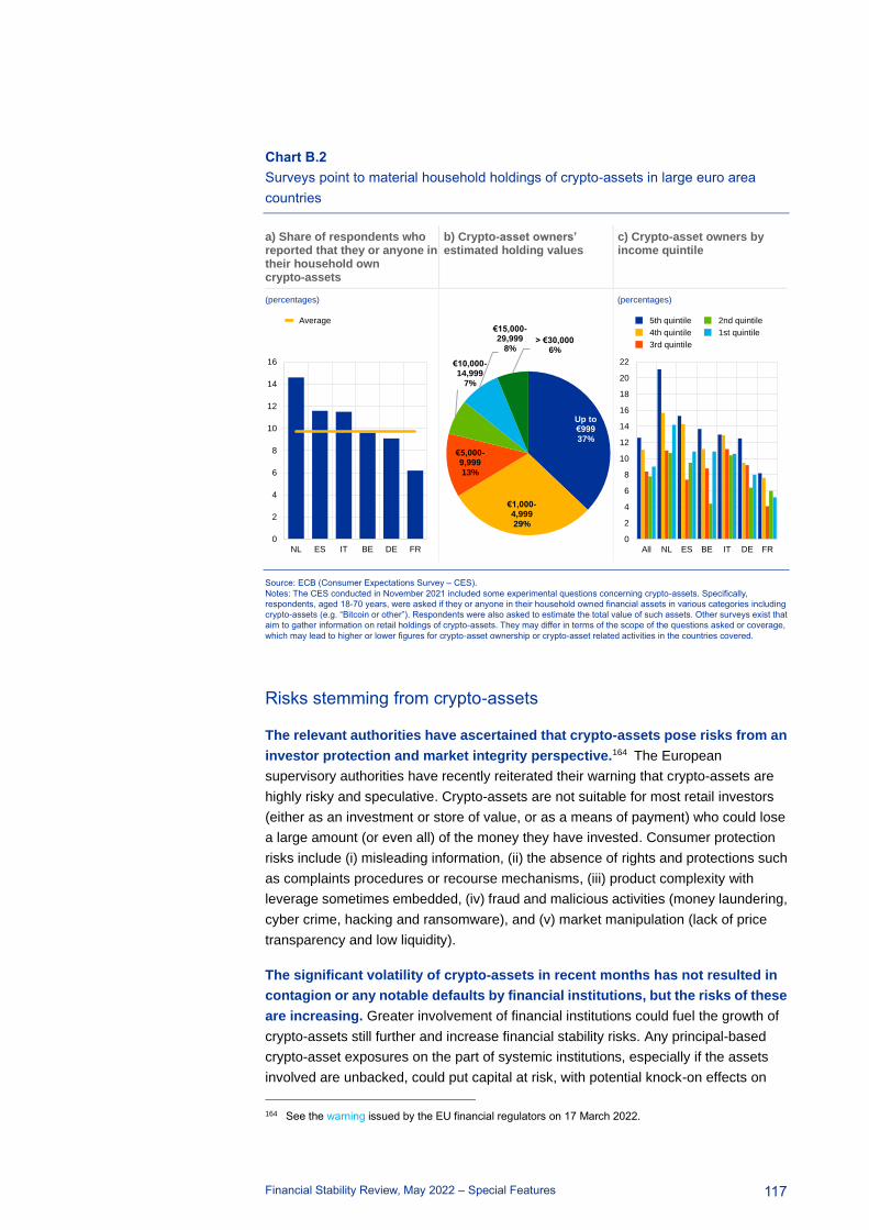
Financial Stability Review, May 2022 – Special Features
117
Chart B.2
Surveys point to material household holdings of crypto-assets in large euro area
countries
a) Share of respondents who reported that they or anyone in their household own crypto-assets
b) Crypto-asset owners’ estimated holding values
c) Crypto-asset owners by income quintile
(percentages) (percentages)
Source: ECB (Consumer Expectations Survey – CES).
Notes: The CES conducted in November 2021 included some experimental questions concerning crypto-assets. Specifically,
respondents, aged 18-70 years, were asked if they or anyone in their household owned financial assets in various categories including
crypto-assets (e.g. “Bitcoin or other”). Respondents were also asked to estimate the total value of such assets. Other surveys exist that
aim to gather information on retail holdings of crypto-assets. They may differ in terms of the scope of the questions asked or coverage,
which may lead to higher or lower figures for crypto-asset ownership or crypto-asset related activities in the countries covered.
Risks stemming from crypto-assets
The relevant authorities have ascertained that crypto-assets pose risks from an
investor protection and market integrity perspective.164 The European
supervisory authorities have recently reiterated their warning that crypto-assets are
highly risky and speculative. Crypto-assets are not suitable for most retail investors
(either as an investment or store of value, or as a means of payment) who could lose
a large amount (or even all) of the money they have invested. Consumer protection
risks include (i) misleading information, (ii) the absence of rights and protections such
as complaints procedures or recourse mechanisms, (iii) product complexity with
leverage sometimes embedded, (iv) fraud and malicious activities (money laundering,
cyber crime, hacking and ransomware), and (v) market manipulation (lack of price
transparency and low liquidity).
The significant volatility of crypto-assets in recent months has not resulted in
contagion or any notable defaults by financial institutions, but the risks of these
are increasing. Greater involvement of financial institutions could fuel the growth of
crypto-assets still further and increase financial stability risks. Any principal-based
crypto-asset exposures on the part of systemic institutions, especially if the assets
involved are unbacked, could put capital at risk, with potential knock-on effects on
164 See the warning issued by the EU financial regulators on 17 March 2022.
0
2
4
6
8
10
12
14
16
NL ES IT BE DE FR
Average
Up to €99937%
€1,000-4,99929%
€5,000-9,99913%
€10,000-14,999
7%
€15,000-29,999
8%> €30,000
6%
0
2
4
6
8
10
12
14
16
18
20
22
All NL ES BE IT DE FR
5th quintile
4th quintile
3rd quintile
2nd quintile
1st quintile
Financial Stability Review, May 2022 – Special Features
118
investor confidence, lending and financial markets if the exposures are of a sufficient
scale. Financial institutions themselves could face reputational risks as well as
climate transition risks. Some international banks (including euro area banks) are
already trading and clearing regulated crypto derivatives, even if they do not hold an
underlying crypto-asset inventory. Market intelligence suggests that other EU banks
and financial institutions are interested in offering custody, trading and market-making
services once regulatory uncertainty diminishes with the entry into force of the
Markets in Crypto-Assets (MiCA) Regulation. This will further increase
interconnectedness.
If current growth and market integration trends persist, then crypto-assets will
pose a risk to financial stability. Unbacked crypto-assets can have financial
stability implications through four main transmission channels: wealth effects,
confidence effects, financial sector exposures and the use of crypto-assets as a form
of payment.165 While all these channels are increasing in size and complexity, they
lack internal shock absorbers that could provide liquidity at times of stress. For
example, the wider involvement of financial institutions or the use of crypto-assets as
a form of payment would increase the potential for spillover to the wider economy,
particularly if leverage were employed.
Although EU regulation has been proposed to mitigate the risks posed by
crypto-assets, agreement on this is yet to be reached. In the EU, the
Commission’s proposal for the MiCA Regulation, first published in September 2020,
has not yet been agreed by EU co-legislators. This means the Regulation will not be
applied before 2024 at the earliest, as it is not expected to be applied until 18 months
after it enters into force. Given the speed of crypto developments and the increasing
risks, it is important to bring crypto-assets into the regulatory perimeter and under
supervision as a matter of urgency. In addition, it will be important to review the
sectoral regulations to ensure that any financial stability risks posed by crypto-assets,
particularly those arising from their interconnectedness with traditional financial
institutions, are mitigated.
Significant informational and data shortcomings persist, hindering the proper
assessment of financial stability risks. These shortcomings include not only
quantitative issues but also the reliability and consistency of data, and the fact that a
significant proportion of activities take place outside the regulatory perimeter. Most
publications from crypto-asset service providers (including platforms, exchanges and
data aggregators) are not verifiable and should be treated with caution, while the
limited regulatory data currently available (e.g. data for derivatives and alternative
investment funds) offer only a partial (and potentially inaccurate) picture. As long as
there continue to be no official statistics on crypto-assets or reporting of underlying
data to a supervisory or oversight authority, the reliability of the metrics from the
above sources and the full extent of possible contagion channels with the traditional
165 See the updated “Assessment of Risks to Financial Stability from Crypto-assets”, Financial Stability
Board, February 2022; and Chapter 2 entitled “The Crypto Ecosystem and Financial Stability
Challenges”, Global Financial Stability Report, IMF, October 2021.
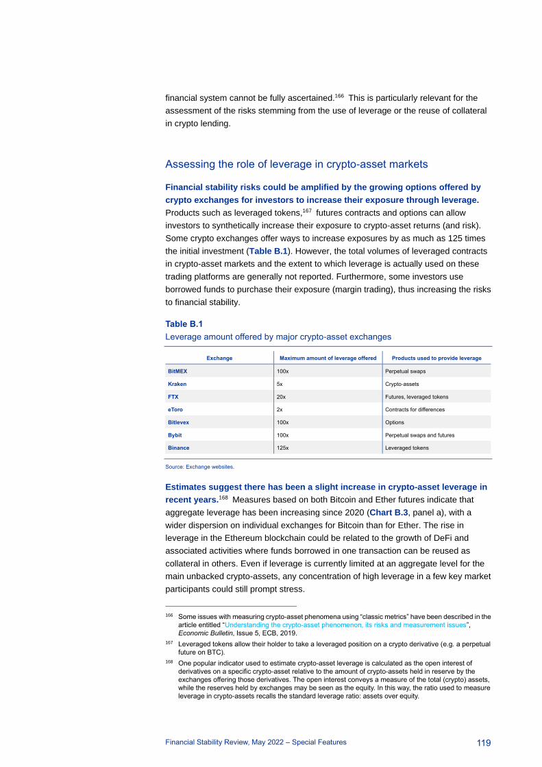
Financial Stability Review, May 2022 – Special Features
119
financial system cannot be fully ascertained.166 This is particularly relevant for the
assessment of the risks stemming from the use of leverage or the reuse of collateral
in crypto lending.
Assessing the role of leverage in crypto-asset markets
Financial stability risks could be amplified by the growing options offered by
crypto exchanges for investors to increase their exposure through leverage.
Products such as leveraged tokens,167 futures contracts and options can allow
investors to synthetically increase their exposure to crypto-asset returns (and risk).
Some crypto exchanges offer ways to increase exposures by as much as 125 times
the initial investment (Table B.1). However, the total volumes of leveraged contracts
in crypto-asset markets and the extent to which leverage is actually used on these
trading platforms are generally not reported. Furthermore, some investors use
borrowed funds to purchase their exposure (margin trading), thus increasing the risks
to financial stability.
Table B.1
Leverage amount offered by major crypto-asset exchanges
Exchange Maximum amount of leverage offered Products used to provide leverage
BitMEX 100x Perpetual swaps
Kraken 5x Crypto-assets
FTX 20x Futures, leveraged tokens
eToro 2x Contracts for differences
Bitlevex 100x Options
Bybit 100x Perpetual swaps and futures
Binance 125x Leveraged tokens
Source: Exchange websites.
Estimates suggest there has been a slight increase in crypto-asset leverage in
recent years.168 Measures based on both Bitcoin and Ether futures indicate that
aggregate leverage has been increasing since 2020 (Chart B.3, panel a), with a
wider dispersion on individual exchanges for Bitcoin than for Ether. The rise in
leverage in the Ethereum blockchain could be related to the growth of DeFi and
associated activities where funds borrowed in one transaction can be reused as
collateral in others. Even if leverage is currently limited at an aggregate level for the
main unbacked crypto-assets, any concentration of high leverage in a few key market
participants could still prompt stress.
166 Some issues with measuring crypto-asset phenomena using “classic metrics” have been described in the
article entitled “Understanding the crypto-asset phenomenon, its risks and measurement issues”,
Economic Bulletin, Issue 5, ECB, 2019.
167 Leveraged tokens allow their holder to take a leveraged position on a crypto derivative (e.g. a perpetual
future on BTC).
168 One popular indicator used to estimate crypto-asset leverage is calculated as the open interest of
derivatives on a specific crypto-asset relative to the amount of crypto-assets held in reserve by the
exchanges offering those derivatives. The open interest conveys a measure of the total (crypto) assets,
while the reserves held by exchanges may be seen as the equity. In this way, the ratio used to measure
leverage in crypto-assets recalls the standard leverage ratio: assets over equity.
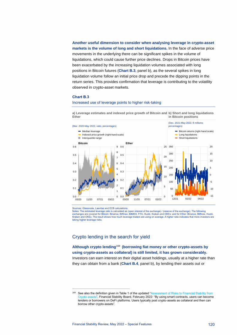
Financial Stability Review, May 2022 – Special Features
120
Another useful dimension to consider when analysing leverage in crypto-asset
markets is the volume of long and short liquidations. In the face of adverse price
movements in the underlying there can be significant spikes in the volume of
liquidations, which could cause further price declines. Drops in Bitcoin prices have
been exacerbated by the increasing liquidation volumes associated with long
positions in Bitcoin futures (Chart B.3, panel b), as the several spikes in long
liquidation volume follow an initial price drop and precede the dipping points in the
return series. This provides confirmation that leverage is contributing to the volatility
observed in crypto-asset markets.
Chart B.3
Increased use of leverage points to higher risk-taking
a) Leverage estimates and indexed price growth of Bitcoin and Ether
b) Short and long liquidations in Bitcoin positions
(Mar. 2020-May 2022, ratio, percentages)
(Dec. 2021-May 2022, € millions;
percentages)
Sources: Glassnode, Laevitas and ECB calculations.
Notes: The estimated leverage ratio is calculated as (open interest of the exchange) / (reserve of the exchange). The following
exchanges are covered for Bitcoin: Binance, Bitfinex, BitMEX, FTX, Huobi, Kraken and OKEx; and for Ether: Binance, Bitfinex, Huobi,
Kraken and OKEx. The result shows how much leverage traders are using on average. A higher ratio indicates that more investors are
taking higher leverage risks.
Crypto lending in the search for yield
Although crypto lending169 (borrowing fiat money or other crypto-assets by
using crypto-assets as collateral) is still limited, it has grown considerably.
Investors can earn interest on their digital asset holdings, usually at a higher rate than
they can obtain from a bank (Chart B.4, panel b), by lending their assets out or
169 See also the definition given in Table 1 of the updated “Assessment of Risks to Financial Stability from
Crypto-assets”, Financial Stability Board, February 2022: “By using smart contracts, users can become
lenders or borrowers on DeFi platforms. Users typically post crypto-assets as collateral and then can
borrow other crypto-assets”.
0
1
2
3
4
5
6
7
8
9
0.0
0.1
0.2
0.3
0.4
0.5
0.6
03/20 11/20 07/21 03/22
Median leverage
Indexed price growth (right-hand scale)
Interquartile range
Bitcoin
0
5
10
15
20
25
0.0
0.1
0.2
0.3
0.4
0.5
0.6
03/20 11/20 07/21 03/22
Ether
-15
-10
-5
0
5
10
15
20
0
50
100
150
200
250
300
350
12/21 02/22 04/22
Bitcoin returns (right-hand scale)
Long liquidations
Short liquidations

Financial Stability Review, May 2022 – Special Features
121
borrowing against their digital asset holdings through overcollateralisation.170 This
crypto lending is offered by both centralised and decentralised service providers and
usually takes place without any formal supervision or regulatory checks and
balances, such as the need to provide a credit score. Loan-to-value (LTV) ratios,
which are voluntarily set by the holders of the governance tokens of a DeFi
application, are set quite low to mitigate risks (typically in the range of 25-50%)
considering the high volatility of crypto. Crypto credit on DeFi platforms grew by a
factor of 14 in 2021, while the total value locked171 was hovering at around €70 billion
(Chart B.4, panel a) until very recently, on a par with small domestic peripheral
European banks. Crypto lending has spurred “yield farming” investment strategies
such as incentivising investors to lend their crypto-assets to a pool that helps provide
liquidity to DeFi systems, while offering potential investors the highest possible
returns at all times. Currently, the crypto-asset deposit/lending industry is still quite
small compared with traditional banking, although it could continue to grow rapidly.
Crypto lending may fall under existing financial regulation and has come under
increased regulatory scrutiny. In the United States, the Securities and Exchange
Commission (SEC) fined the centralised BlockFi service USD 100 million for failing to
register the offers and sales of its retail crypto lending product as required under US
securities law.172 Previously, Coinbase dropped the launch of a new lending product
following SEC warnings that it constituted an unregistered security. Although such
cases are still unknown in the EU, these developments show that regulation is, in
principle, technology-neutral. DeFi platforms that mimic traditional financial services
would do well to ensure they comply with existing EU financial regulation before
offering their services to EU clients to avoid the risk of any legal action.
170 Although it seems rather counterintuitive, users facing unforeseen funding needs may prefer not to sell
their holdings, as they expect the crypto-asset to increase in value in the future. Another advantage of
borrowing is potentially avoiding or delaying the payment of capital gains taxes. Lastly, individuals can
use funds borrowed via such platforms to increase their leverage on certain trading positions.
171 Total value locked represents the sum of all assets deposited in DeFi protocols earning rewards, interest,
new coins and tokens, fixed income, etc.
172 See the press release entitled “BlockFi Agrees to Pay $100 Million in Penalties and Pursue Registration
of its Crypto Lending Product”, US Securities and Exchange Commission, 14 February 2022.

Financial Stability Review, May 2022 – Special Features
122
Chart B.4
DeFi credit is currently small but is growing rapidly as investors search for yields
above bank deposit rates
a) Total value locked in DeFi credit b) Crypto lending and MFI deposit interest rates
(Jan. 2021-May 2022, € billions) (Jan. 2021-Mar. 2022, percentages)
Sources: DefiLlama, Compound, DeFi Rate, ECB MFI MIR and ECB calculations.
Notes: Panel a: total value locked might be overestimated due to reuse of tokens. Panel b: crypto lending rates are calculated as the
average of the 30-day average offered interest rate in 13 DeFi and CeFi (centralised) platforms. Not all platforms offer lending for all of
the selected crypto-assets. Abbreviations are as follows: stablecoins: Tether (USDT), Dai (DAI) and USD Coin (USDC); unbacked
crypto-assets: Bitcoin (BTC) and Ether (ETH). The deposit rate is the average interest rate offered by monetary financial institutions
(MFIs) in the euro area to households and non-profit organisations.
Rehypothecation (where collateral for a loan can be re-pledged in order to
obtain another loan)173 increases the chances of a breach of LTV limits and
could cause liquidity to vanish very quickly in the case of a big shock. The high
volatility of crypto-assets means that LTV limits may be exceeded in a market
downturn and that more collateral needs to be posted by borrowers, who could
potentially lose that collateral. In addition, if borrowers are not able to pay back their
loans, investors may seek to withdraw their funds in a panic, potentially leading to an
investor run. The likelihood of such a run could be exacerbated by the high degree of
concentration in liquidity provision in decentralised protocols. As they are outside the
regulatory perimeter, there is no guarantee in such instances that investors would get
their money back (or borrowers their collateral) as they would in the case of a bank
deposit, given the existence of deposit guarantee schemes. This reflects the lack, in
many cases, of investor protection regulation, the highly technical and fast-moving
nature of the market segment, and the use of different tokens in terms of assets
purchased, collateral posted or interest paid. Although the risks are currently small,
they could rise significantly if platforms started to offer services to the real economy,
instead of remaining confined to the crypto universe. In such a scenario, a decline in
value of the collateral could lead to margin calls, borrower/lender defaults and
reduced borrowing, potentially affecting economic activity (particularly if crypto-assets
were used as collateral for consumer and business loans).
173 As an example, borrowers can pledge crypto to obtain a stablecoin loan. This loan can be used as
collateral in another liquidity pool in exchange for liquidity pool tokens, which are, in effect, a form of
derivative. The liquidity pool tokens can be pledged in yet another liquidity pool to obtain another
stablecoin loan, and so on.
0
10
20
30
40
50
60
70
80
90
01/21 04/21 07/21 10/21 01/22 04/22
0.0
0.2
0.4
0.6
0.8
1.0
1.2
0
2
4
6
8
10
12
01/21 04/21 07/21 10/21 01/22
DAI
BTC
ETH
USDC
USDT
Household deposits (right-hand scale)

Financial Stability Review, May 2022 – Special Features
123
Conclusions
The nature and scale of crypto-asset markets are evolving rapidly, and if
current trends continue, crypto-assets will pose risks to financial stability.
While interconnectedness between unbacked crypto-assets and the traditional
financial sector has grown considerably, interconnections and other contagion
channels have so far remained sufficiently small. Investors have been able to handle
the €1.3 trillion fall in the market capitalisation of unbacked crypto-assets since
November 2021 without any financial stability risks being incurred. However, at this
rate, a point will be reached where unbacked crypto-assets represent a risk to
financial stability.
Systemic risk increases in line with the level of interconnectedness between
the financial sector and the crypto-asset market, the use of leverage and
lending activity. Based on the developments observed to date, crypto-asset markets
currently show all the signs of an emerging financial stability risk. It is therefore key for
regulators and supervisors to monitor developments attentively and close regulatory
gaps or arbitrage possibilities. As this is a global market and therefore a global issue,
global coordination of regulatory measures is necessary.
It is important to close regulatory and data gaps in the crypto-asset ecosystem.
In the EU, the MiCA Regulation should be approved by the co-legislators as a matter
of urgency to ensure it is applied sooner rather than later. However, MiCA is only a
first step. The sectoral regulations will need to be reviewed to ensure financial
stability risks posed by crypto-assets are mitigated. Any further steps that allow the
traditional financial sector to increase its interconnectedness with the crypto-asset
market space should be carefully weighed up, and priority should be given to avoiding
financial stability risks. This holds in particular when considering interconnections with
parts of the financial system that are strictly regulated and benefit from a public safety
net. Data gaps should be closed. The challenges faced in monitoring financial stability
risks from crypto-assets developments and interconnectedness with the traditional
financial sector will persist as long as there are no standardised reporting or
disclosure requirements.174
174 The Financial Stability Board’s 2022 Data Gaps Initiative envisages the development of prospective data
collections for crypto-assets. Some statistical initiatives are also geared towards the appropriate
treatment and possible identification of crypto-asset activities and players.
Acknowledgements
The Financial Stability Review assesses the sources of risks to and vulnerabilities in the euro area financial system based on regular
surveillance activities, analysis and findings from discussions with market participants and academic researchers.
The preparation of the Review was coordinated by the ECB’s Directorate General Macroprudential Policy and Financial Stability. The
Review has benefited from input, comments and suggestions from other business areas across the ECB. Comments from members of the
ESCB Financial Stability Committee are gratefully acknowledged.
The Review was endorsed by the ECB’s Governing Council on 18 May 2022.
Its contents were prepared by Katharina Cera, Nander de Vette, John Fell, Sándor Gardó, Benjamin Klaus, Julian Metzler, Benjamin Mosk,
Tamarah Shakir, Manuela Storz, Eugen Tereanu, Josep M. Vendrell Simón and Jonas Wendelborn.
With additional contributions from Luca Bacciarelli, Emil Bandoni, Markus Behn, Paul Bochmann, Othman Bouabdallah, Lorenzo
Cappiello, Olimpia Carradori, Dimitris Drollas, Michal Dvořák, Linda Fache Rousová, Maciej Grodzicki, Margherita Giuzio, Matilda Gjirja,
Lieven Hermans, Paul Hiebert, Barbara Jarmulska, Sujit Kapadia, Jan Hannes Lang, Francesca Lenoci, Marco Lo Duca, Giulio Mazzolini,
Barbara Meller, Luca Mingarelli, Seán O’Sullivan, Lorenzo Pangallo, Rita Periquito da Fonseca, Allegra Pietsch, Aurea Ponte Marques,
Petya Radulova, Ellen Ryan, Julius Schneider, Martina Spaggiari, Mika Tujula, Dominik Vu, Michael Wedow, Christian Weistroffer and
Balázs Zsámboki.
Editorial, multimedia and production assistance was provided by Anna Heckler, Will Knowles, Peter Nicholson, Katie Ranger, Simon
Spornberger and Sophia Suh.
© European Central Bank, 2022
Postal address 60640 Frankfurt am Main, Germany
Telephone +49 69 1344 0
Website www.ecb.europa.eu
All rights reserved. Reproduction for educational and non-commercial purposes is permitted provided that the source is acknowledged.
For specific terminology please refer to the ECB glossary (available in English only).
PDF ISSN 1830-2025, QB-XU-22-001-EN-N
HTML ISSN 1830-2025, QB-XU-22-001-EN-Q
Related Documents