Financial Risks of Climate Change Technical Annexes June 2005 Prepared by Climate Risk Management Limited for the Association of British Insurers in association with

Welcome message from author
This document is posted to help you gain knowledge. Please leave a comment to let me know what you think about it! Share it to your friends and learn new things together.
Transcript
Financial Risks of Climate Change
Technical Annexes
June 2005
Prepared by
Climate Risk Management Limited
for the
Association of British Insurers
in association with
Report for:
Dr. Sebastian Catovsky,The Association of British Insurers,51 Gresham Street,London,EC2V 7HQ
Main Contributors:
John Firth Climate Risk ManagementAmy Parsons Climate Risk ManagementAlistair Hunt MetroeconomicaRichard Boyd Metroeconomica
Issued by:
……………………………………………………………………....John Firth, Director,Climate Risk Management Limited
Climate Risk Management Limited
6 Nursery End,Southwell,Nottinghamshire,NG25 0BY
Tel: +44 (0) 1636 812868Fax: +44 (0) 1636 812702Email: [email protected]: www.climaterisk.co.uk
© Copyright Climate Risk Management Limited 2005
An electronic copy of this report and the published Summary Report are available from:
http://www.abi.org.uk/climatechange
http://www.climaterisk.co.uk
The Association of British Insurers (ABI) commissioned Climate Risk Management toundertake this project. The project was undertaken in association with Metroeconomica.
AIR Worldwide Corporation (AIR) provided project support through stress-testing of theircatastrophes models. Climate Risk Management is grateful to AIR for their involvement in theproject.
Acknowledgements
Climate Risk Management and Metroeconomica would like to acknowledge the assistance ofthe following organisations, particularly through provision of data:
AIR Worldwide Corporation
Swiss Re
Munich Re
Lloyd’s Corporation
Commission Européen des Assurances
UK Climate Impacts Programme
Climate Risk Management and Metroeconomica are grateful to the members of the ProjectBoard for their advice and guidance:
Jane Milne, ABI
Alex Roy, ABI
Vinay Mistry, Group Reinsurance Risk and Exposure Analyst, Aviva
Andy Challoner, Head of General Insurance Risk Management, Aviva
Peter Dower, Underwriting Manager, Zurich
Jens Mehlhorn, Head of Floods Group, Swiss Re
Eberhard Faust, Head of Climate Risks, Munich Re
James Orr, Manager, Loss Modelling, Lloyd’s
Paul Nunn, Catastrophe Risk Manager, ACE
David Russell, Adviser for Responsible Investment, Universities Superannuation Scheme
Michele Pittini, Economic Adviser, Defra
Richenda Connell, Technical Director. United Kingdom Climate Impacts Programme
Climate Risk Management and Metroeconomica would like to thank the following individualsfor their advice:
Angelika Wirtz, Munich Re
Clair Hanson, UEA

Deepak Vatvani, Delft Hydraulics
Evan Mills, Lawrence Berkeley National Laboratory
Herve Castella, Partner Re
Ivo Menzinger, Swiss Re
James Boyce, Lloyds
Jane Toothill, Guy Carpenter
Jay Guin, Air Worldwide
Jean Palutikof, Met Office
Josette Nougier, Commission Européen des Assurances
Junsang Choi, Lloyds
Milan Simic, Benfield Group
Peter Cheesman, Glencairn Group
Peter Hausman, Swiss Re
Rudolf Enz, Swiss Re
Tom Downing, Stockholm Environmental Institute
Thomas Loster, Munich Re
The contents of this report represent the views of Climate Risk Management andMetroeconomica and not necessarily those of the individuals and organisations namedabove.

ABI Financial Costs of Climate Change June 2005 www.climaterisk.co.uk
CONTENTS PAGE
1.0 Introduction 1
1.1 Project Scope1.2 Project Objectives1.3 Climate change and extreme weather1.4 Main Issues1.5 Insurance as a measure of financial costs
2.0 Paying for natural catastrophes – who bears the costs? 4
2.1 Insurance coverage2.2 Insurance industry in practice2.3 Reinsurance arrangements2.4 Alternative risk transfer2.5 Catastrophe models
3.0 Impacts of climate change on costs of extreme weather 14around the world
3.1 Introduction3.2 What is a tropical cyclone3.3 Analysis of historical activity3.4 Tropical cyclones and climate change3.5 European windstorms3.6 Summary of climate science
3.6.1 Tropical cyclones3.6.2 Extra-tropical cyclones
3.7 Financial impacts of changes in the character of storms3.8 Tropical cyclones3.9 Investigating the impacts of mitigation3.10 Extra-tropical cyclones3.11 Total financial versus insured losses3.12 Socio-economic developments3.13 Investigating the impacts of adaptation
3.13.1 Building codes3.13.2 Building code enforcement3.13.3 Planning
3.14 Appendices3.15 References
4.0 Impacts of climate change on costs of UK extreme weather 64
4.1 Flooding4.2 Results: fluvial and coastal flooding4.3 Intra-urban flood risks4.4 Mitigation and adaptation of flood impacts4.5 Subsidence4.6 Adaptation4.7 Conclusions
ABI Financial Costs of Climate Change June 2005 www.climaterisk.co.uk
5.0 Wider economic Impacts of climate change 75
5.1 Health5.2 Heat Waves5.3 Agriculture5.4 Impact estimate techniques5.5 Impacts
5.5.1 Global impacts5.5.2 Regional impacts
5.6 Summary5.7 Flooding5.8 Case study on the River Rhine5.9 Summary5.10 Sea level rise5.11 Storm surge
6.0 Financial implications of climate change 99
6.1 Introduction6.2 Characteristics of natural catastrophe insurance6.3 Managing natural catastrophe risk6.4 Managing catastrophic exposure
6.4.1 Location and geographical concentration6.4.2 Policy forms and coverage6.4.3 Transferring risk to third parties
6.5 Implications of stress test6.6 Capital requirements6.7 Premium prices6.8 Short run versus long run impacts6.9 Economic value of insurance6.10 Appendices

ABI Financial Costs of Climate Change June 2005 Page 1Introduction www.climaterisk.co.uk
1.0 Introduction
This report comprises a series of technical annexes prepared to assist with a projectcommissioned by the Association of British Insurers (ABI). The project has beenundertaken to inform the debate on climate change and extreme events in relation tothe insurance industry. The project seeks to quantify the financial costs of extremeweather events over the coming decades under various climate scenarios (with andwithout policy responses on mitigation and adaptation), and assess the implicationsfor the insurance industry, their policyholders and capital markets.
1.1 Project scope
The ABI and the Project Board in defining the scope agreed that the study shouldfocus on the most costly aspects of weather today and that a quantitative analysis beundertaken for:
Tropical cyclones
o North Atlantic
o North Pacific Basin
Extra tropical cyclones
o Europe
The project concentrated on the major property insurance markets in Europe, NorthAmerica and Japan – to the extent that resources and the availability of data from theinsurance industry permitted.
A separate analysis of the following extreme events relative to the United Kingdomhas also been included within the project.
Flooding
Subsidence
In addition to the above a qualitative review based on existing published sourceswould explore current views on the impacts arising from:
Heat waves
Health
Agriculture
European flooding
The analyses contained in this report do not include the increase in exposure toclimate risks arising from changes in socio-economic factors.
1.2 Project Objectives
The project had three main objectives:
to add to current estimates of the global financial costs of climate change byproviding estimates of the future costs of extreme weather based on currentscientific evidence
to examine the secondary effect of climate change on extreme weatherevents on global insurance markets. Increases in the volatility of extreme

ABI Financial Costs of Climate Change June 2005 Page 2Introduction www.climaterisk.co.uk
weather could also result in changes in the amount of capital that theinsurance industry needs to hold for claims
to quantify the impact of taking action today to limit the causes andconsequences of climate change on extreme weather events, including stepsto reduce carbon emissions and adaptation measures.
1.3 Climate change and extreme weather
The Earth’s climate is changing and will continue to change over this century. The1990s were the warmest decade globally since records began, with the four warmestyears all occurring since 1998. In 2003, Europe experienced its hottest summer for atleast 500 years, with temperatures more than 2°C warmer than the average. In theUK, temperatures reached a record-breaking 38°C. Temperatures could increase bya further 6 °C by the end of the century if there is no action to tackle climate change.
Whilst extreme events cannot be used to prove climate change, a trend towardsmore extreme and intense weather events is consistent with the developments thatscientists expect in a warmer climate. Research by the Intergovernmental Panel onClimate Change (IPCC) suggests that the increase in the surface temperature for theNorthern hemisphere during the 20th Century was probably greater than that of anyother century in the last thousand years. IPCC projections put the increase inaverage global surface temperature in the range of 1.4 to 5.8°C over the period 1990to 2100.1
Its is accepted by the majority of the world’s scientists that man-made emissions ofgreenhouse gases are changing our climate, bringing higher temperatures, changingrainfall, rising sea levels and possibly more storms. Although some uncertainty stillexists with regard to the extent of the impact of climate change on extreme weather,it is clear that this is becoming a major challenge for the insurance industry
A review of the existing climate science has been undertaken which is presented inSection 3 ‘Impacts of climate change on costs of extreme weather’.
1.4 Main issues
One of the main threats of increased extreme events is a risk of increased propertylosses. The Intergovernmental Panel on Climate Change (IPCC) has confirmed thatthe combined effects of increasingly severe climatic events and underlying socio-economic trends (such as population growth and unplanned urbanization) have thepotential to undermine the value of business assets, diminish investment viability andstress insurers, reinsurers, and banks to the point of impaired profitability andinsolvency. As UNEPFI have stated that even in the extreme case, whole regionsmay become unviable for commercial financial services. 2
The major issue for insurers is that the climate is inherently unpredictable to theextent that the existing probability of ‘normal’ extreme events is difficult to estimate.As the climate continues to change the usual method of using historical information
1 Intergovernmental panel on climate change. www.ippc.ch
2 Climate change and the Financial Services Industry. Module 1 Threats and Opportunities. UNEP FIClimate change working group.

ABI Financial Costs of Climate Change June 2005 Page 3Introduction www.climaterisk.co.uk
to predict forward becomes unfeasible for pricing. The climate will continue to changeas greenhouse gases continue to increase.
Global warming could increase the frequency and severity of extreme weather eventsin some regions around the world, such as floods, storms and very dry summers.These types of events are exactly those which insurance provides some financialprotection for. If the financial impacts of climate change are not understood it willmean that insurers will have greater uncertainty. This will lead to greater risk aversione.g. higher premium rates, withdrawal from the market on the part of the insurer. Toremain competitive and ultimately to provide the best service to the customer theimpacts of climate change need to be fully costed.
1.5 Insurance as a measure of financial costs
Insurance is a good indicator of financial costs as it allows a price to be put onevents, in particular to assess the amount of damage each event causes. In aprevious study the ABI points out that insurance offers important economic benefitswhere activities are seen as risky and a risk control or transfer mechanism isneeded.3 It allows companies and individuals to continue to undertake risky activities,which otherwise they would not undertake. Insurance plays an important role byproviding a risk transfer mechanism which otherwise would fall to the state. Anyimpact on the insurance industry has wider implications for other stakeholders.
The insurance industry is well placed to lead the way in the debate on the costs ofclimate change. Insured and non insured losses can be used to indicate financialcosts of extreme events. The costs can be used to look at the potentialconsequences of not taking any action as losses increase.
Initial estimates on cost of climate change were undertaken by the United NationsEnvironmental Programme Finance Initiative (UNEP FI) who put the cost to theglobal economy of climate change-driven natural disasters at $150 billion per yearwithin the next decade, based on current trends.4
3 The Economic Value of General Insurance. ABI December 20044 UNEP FI CEO briefing: Climate risk to global economy. UNEP FI www.unepfi.net

ABI: Financial Costs of Climate Change June 2005 Page 4Paying for natural catastrophes – who bears the cost? www.climaterisk.co.uk
2.0 Paying for natural catastrophes – who bears the costs?
2.1 Insurance coverage
The industry opinion on climate change varies according to location. Insurers in Europe andAsia are giving significant consideration to climate change and the implications that this willhave on their business.
Not only are there widely dispersed agreements on the effects of climate change and theimpact on the insurance industry, but also the extent to which private insurancearrangements cover property damage varies substantially between countries. In somecases, the private market covers much of the risk, while in others, the government is moreclosely involved.
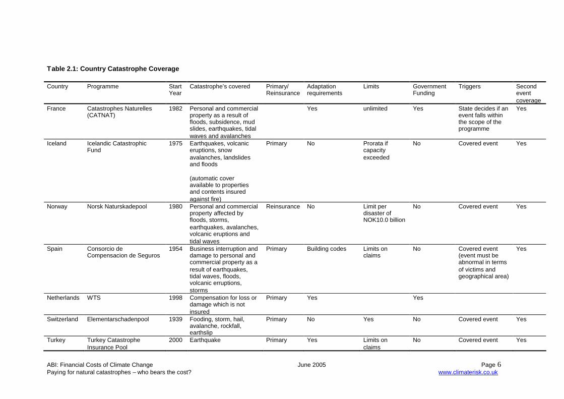
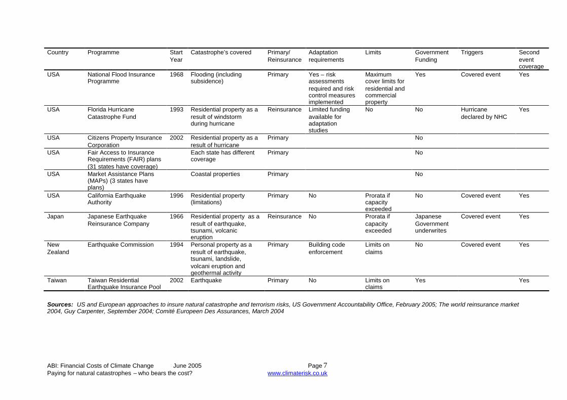
There are a wide variety of approaches used by governments to address catastrophic risk.Some governments require insurers to provide natural catastrophe insurance and providefinancial assistance to the insurers in the wake of catastrophic events, while others generallyrely on the private market. A summary is provided in Table 2.1.
Within Europe coverage varies from country to country. Natural catastrophe coverage ismandatory in France and Spain and the national governments are explicitly committed toproviding financial support to insurers through state-backed entities and state guarantees.Other governments, such as Germany, neither require natural catastrophe insurance norprovide explicit financial commitments.5
In the UK, commercial and residential property policies mainly cover the full array of naturalperils. Flooding has become an issue within the UK with insurers who warned government in2000 that they would not cover business in flood prone areas unless flood defences wereimproved and buildings protected more efficiently. A two-year plan was agreed but it stillremains an issue. 6
In the Caribbean property policies cover fire and allied perils such as windstorms andearthquake. Each island is subject to local regulations and customs and so differentcoverage is available on different islands. For example on Puerto Rico flooding is generallyexcluded in residential and commercial but it is included on other islands.
The system in the USA is unique and has not been copied by other countries. The USAproperty policies usually cover wind, including tornadoes and hurricanes as well as fire andexplosion. Flood and earthquake hazards are normally excluded. In most states earthquakecover is available as separate cover. A special program, underwritten by the federalgovernment covers the flood peril up to $250,000 in insured value for residential exposuresand up to $500,000 for non-residential exposures.7 Special programs have also been set upwhich are state funded. These include the Florida Windstorm Underwriting Association(FWUA).
5 Catastrophe risk. US and European approaches to insure natural catastrophe and terrorism risks. GAO UnitedStates Government Accountability Office.6 World Catastrophe markets 2004. Guy Carpenter. www.guycarp.com7 Climate Change and the Insurance Industry. The Changing Risk Landscape:Implications for Insurance RiskManagement 1999. Andrew Dlugolecki
ABI: Financial Costs of Climate Change June 2005 Page 5Paying for natural catastrophes – who bears the cost? www.climaterisk.co.uk
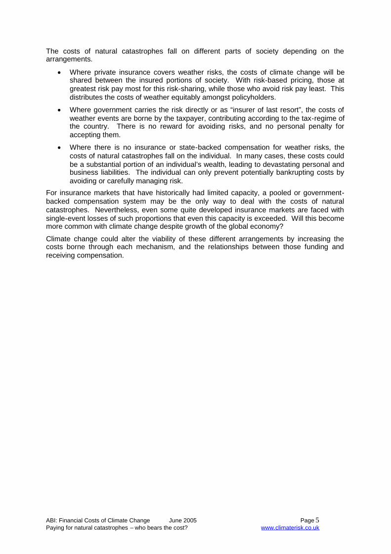
The costs of natural catastrophes fall on different parts of society depending on thearrangements.
Where private insurance covers weather risks, the costs of climate change will beshared between the insured portions of society. With risk-based pricing, those atgreatest risk pay most for this risk-sharing, while those who avoid risk pay least. Thisdistributes the costs of weather equitably amongst policyholders.
Where government carries the risk directly or as “insurer of last resort”, the costs ofweather events are borne by the taxpayer, contributing according to the tax-regime ofthe country. There is no reward for avoiding risks, and no personal penalty foraccepting them.
Where there is no insurance or state-backed compensation for weather risks, thecosts of natural catastrophes fall on the individual. In many cases, these costs couldbe a substantial portion of an individual’s wealth, leading to devastating personal andbusiness liabilities. The individual can only prevent potentially bankrupting costs byavoiding or carefully managing risk.
For insurance markets that have historically had limited capacity, a pooled or government-backed compensation system may be the only way to deal with the costs of naturalcatastrophes. Nevertheless, even some quite developed insurance markets are faced withsingle-event losses of such proportions that even this capacity is exceeded. Will this becomemore common with climate change despite growth of the global economy?
Climate change could alter the viability of these different arrangements by increasing thecosts borne through each mechanism, and the relationships between those funding andreceiving compensation.
ABI: Financial Costs of Climate Change June 2005 Page 6Paying for natural catastrophes – who bears the cost? www.climaterisk.co.uk
Table 2.1: Country Catastrophe Coverage
Country Programme StartYear
Catastrophe’s covered Primary/Reinsurance
Adaptationrequirements
Limits GovernmentFunding
Triggers Secondeventcoverage
France Catastrophes Naturelles(CATNAT)
1982 Personal and commercialproperty as a result offloods, subsidence, mudslides, earthquakes, tidalwaves and avalanches
Yes unlimited Yes State decides if anevent falls withinthe scope of theprogramme
Yes
Iceland Icelandic CatastrophicFund
1975 Earthquakes, volcaniceruptions, snowavalanches, landslidesand floods
(automatic coveravailable to propertiesand contents insuredagainst fire)
Primary No Prorata ifcapacityexceeded
No Covered event Yes
Norway Norsk Naturskadepool 1980 Personal and commercialproperty affected byfloods, storms,earthquakes, avalanches,volcanic eruptions andtidal waves
Reinsurance No Limit perdisaster ofNOK10.0 billion
No Covered event Yes
Spain Consorcio deCompensacion de Seguros
1954 Business interruption anddamage to personal andcommercial property as aresult of earthquakes,tidal waves, floods,volcanic erruptions,storms
Primary Building codes Limits onclaims
No Covered event(event must beabnormal in termsof victims andgeographical area)
Yes
Netherlands WTS 1998 Compensation for loss ordamage which is notinsured
Primary Yes Yes
Switzerland Elementarschadenpool 1939 Fooding, storm, hail,avalanche, rockfall,earthslip
Primary No Yes No Covered event Yes
Turkey Turkey CatastropheInsurance Pool
2000 Earthquake Primary Yes Limits onclaims
No Covered event Yes
ABI: Financial Costs of Climate Change June 2005 Page 7Paying for natural catastrophes – who bears the cost? www.climaterisk.co.uk
Country Programme StartYear
Catastrophe’s covered Primary/Reinsurance
Adaptationrequirements
Limits GovernmentFunding
Triggers Secondeventcoverage
USA National Flood InsuranceProgramme
1968 Flooding (includingsubsidence)
Primary Yes – riskassessmentsrequired and riskcontrol measuresimplemented
Maximumcover limits forresidential andcommercialproperty
Yes Covered event Yes
USA Florida HurricaneCatastrophe Fund
1993 Residential property as aresult of windstormduring hurricane
Reinsurance Limited fundingavailable foradaptationstudies
No No Hurricanedeclared by NHC
Yes
USA Citizens Property InsuranceCorporation
2002 Residential property as aresult of hurricane
Primary No
USA Fair Access to InsuranceRequirements (FAIR) plans(31 states have coverage)
Each state has differentcoverage
Primary No
USA Market Assistance Plans(MAPs) (3 states haveplans)
Coastal properties Primary No
USA California EarthquakeAuthority
1996 Residential property(limitations)
Primary No Prorata ifcapacityexceeded
No Covered event Yes
Japan Japanese EarthquakeReinsurance Company
1966 Residential property as aresult of earthquake,tsunami, volcaniceruption
Reinsurance No Prorata ifcapacityexceeded
JapaneseGovernmentunderwrites
Covered event Yes
NewZealand
Earthquake Commission 1994 Personal property as aresult of earthquake,tsunami, landslide,volcani eruption andgeothermal activity
Primary Building codeenforcement
Limits onclaims
No Covered event Yes
Taiwan Taiwan ResidentialEarthquake Insurance Pool
2002 Earthquake Primary No Limits onclaims
Yes Yes
Sources: US and European approaches to insure natural catastrophe and terrorism risks, US Government Accountability Office, February 2005; The world reinsurance market2004, Guy Carpenter, September 2004; Comité Europeen Des Assurances, March 2004

ABI: Financial Costs of Climate Change June 2005 Page 8Paying for natural catastrophes – who bears the cost? www.climaterisk.co.uk
2.2 The insurance industry in practice
The insurance market is cyclical. “Soft” market conditions, when premium rates decrease(usually due to over capacity) are followed by generally shorter and sharper periods of “hard”market conditions. In recent years, increasing frequency and size of loss events, coupledwith falls in investment income within the insurance industry has meant a return to “hard”conditions (with the reduction / withdrawal of cover and an increase in premiums).
The cyclical nature of the industry is further enhanced as these extreme events happensporadically. The lessons learned diminish over time, and as new extreme events occur themarket tends to react quickly to cover itself.
In principle, insurance premiums look to cover expected claims (for the correspondingpolicies), operating and administrative costs and a return on investment for the capitalproviders: this is known as the fair premium. In strong equity markets, any underwritinglosses are usually covered by strong investment income making up the shortfall. In addition,providing losses are not catastrophic, the annual cycle of premium renewal means that theeffects of one year’s loss could be reduced the following year by increasing premiums.8
9
2.3 Reinsurance arrangements
To cover the most extreme events, insurers rely on reinsurance – either through the privatemarket or from the state. The reinsurer assumes responsibility for covering a portion of therisk, especially for rare but extreme event losses. This enables insurers to access greatercapital in a cost-effective way, and assists in managing liquidity following a large claim event.In most markets, regulation by the state setting out capital requirements ensures solvency forall but the most unusual events.
Extreme weather events place significant demands on the financial capacity of the insuranceindustry. The loss potential from these types of events can be enormous, with severefinancial consequences. After Hurricane Andrew hit Miami Dade Florida in 1992 causing $16bn of insured damage, 11 reinsurers went into receivership. The size of the globalreinsurance market for property in 2004 is around $55 bn.10
2.4 Alternative risk transfer
Conventional reinsurance arrangements will be tested if extreme events increase infrequency and/or severity. There may be insufficient capital in insurance markets to coverthese losses. Insurers are looking to other alternative risk transfer mechanisms to helpdiversify their capital and manage liquidity problems following a series of large claims. Thesemechanisms will become increasingly valuable as climate risk increases.
8 Earth Observation responses to geo-information market drivers. Aon Insurance sector summary report.www.aon.com9 Catastrophe risk. US and European approaches to insure natural catastrophe and terrorism risks. GAO UnitedStates government accountability office.10 The management of losses arising from extreme events. GIRO 2002.

ABI: Financial Costs of Climate Change June 2005 Page 9Paying for natural catastrophes – who bears the cost? www.climaterisk.co.uk
Insurers could limit risk exposure by transferring natural catastrophe risk into the capitalmarkets. Due to their size, financial markets offer enormous potential for insurers to diversifyrisks: the value of global financial markets currently stands at close to $120,000 bn11. Buttransaction costs can be considerable, and the unfamiliarity of investors with insurance risksmeans that they currently demand a relatively large risk premium.
Alternative risk transfer markets are considered one mechanism by which the risk exposurecan be transferred. These are seen to be expanding, particularly in the USA, as customersseek cost effective ways to deal with their increasing weather exposures. Alternative RiskTransfer (ART) is the term given to unconventional insurance arrangements.
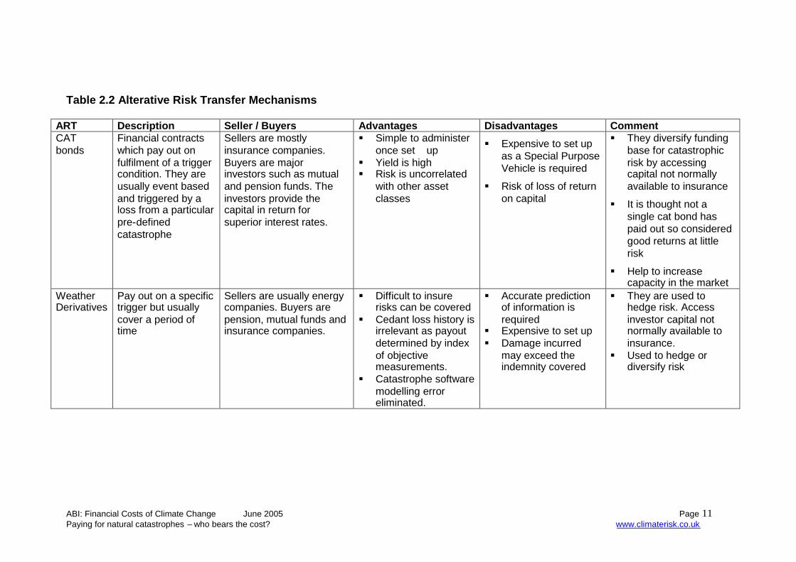
Insurers and large corporations are already experimenting with catastrophe bonds as anART mechanism. A catastrophe bond or CAT bond is a high-yield debt instrument that raisesmoney in case of a catastrophe such as a hurricane or earthquake. These pay out, not onproof of loss, but on fulfilment of a trigger condition, for example a Category 4 hurricanestriking mainland USA. Investors provide the capital and in return receive a superior interestrate. However they run the risk of losing their return and even the capital in some contracts.
It has been stated that some insurers and re-insurers benefit from catastrophe bondsbecause the bonds diversify their funding base for catastrophic risk. However, these bondscurrently occupy a small niche in the global catastrophe reinsurance market and manyinsurers view the costs associated with issuing them as significantly exceeding traditionalreinsurance.12
The advantages of CAT bonds are that they are not closely linked with the stock market oreconomic conditions and offer significant attractions to investors. For example, for the samelevel of risk, investors can usually obtain a higher yield with CAT bonds relative to alternativeinvestments. Another benefit is that the insurance risk securities of CATs show nocorrelation with equities or corporate bonds, meaning they'd provide a good diversification ofrisks.
Guy Carpenter13 states that the catastrophe bond market witnessed yet another record yearin 2003, with total issuance of $1.73 billion, an impressive 42 percent year-on-year increasefrom 2002’s record of $1.22 billion. During the year, a total of eight transactions werecompleted, with three originating from first-time issuers. Since 1997, when the market beganin earnest, 54 catastrophe bond issues have been completed with total risk limits of almost$8bn. The sustainability of CAT bonds has yet to be tested by a trigger event, requiringpayment to the bondholders. The current enthusiastic investor interest in CAT bonds maychange.
Weather derivatives are another financial instrument used by companies to hedge againstthe risk of weather-related losses. The investor who sells a weather derivative accepts therisk by charging the buyer a premium. If nothing happens, then the investor makes a profit.They pay out on a specified trigger, for example, temperature over a specified period, not onproof of loss. This is different from insurance, which is for low probability events such ashurricanes and tornados. These are more established in the USA than Europe, although themarket for them is beginning to pick up.
11 Taking Stock of the World’s Capital Markets, McKinsey & Company, February 2005,http://www.mckinsey.com/mgi/publications12 Catastrophe risk. US and European approaches to insure natural catastrophe and terrorism risks. GAO UnitedStates government accountability office.13 Market Update:The Catastrophe Bond Market at Year-End 2003. April 2004 Guy Carpenter
ABI: Financial Costs of Climate Change June 2005 Page 10Paying for natural catastrophes – who bears the cost? www.climaterisk.co.uk
An overview of the key issues for weather derivatives and CAT bonds is provided in Table2.2. Further information on alternative mechanisms and sources of capital is provided inSection 6 Appendix A.
ABI: Financial Costs of Climate Change June 2005 Page 11Paying for natural catastrophes – who bears the cost? www.climaterisk.co.uk
Table 2.2 Alterative Risk Transfer Mechanisms
ART Description Seller / Buyers Advantages Disadvantages CommentCATbonds
Financial contractswhich pay out onfulfilment of a triggercondition. They areusually event basedand triggered by aloss from a particularpre-definedcatastrophe
Sellers are mostlyinsurance companies.Buyers are majorinvestors such as mutualand pension funds. Theinvestors provide thecapital in return forsuperior interest rates.
Simple to administeronce set up
Yield is high Risk is uncorrelated
with other assetclasses
Expensive to set upas a Special PurposeVehicle is required
Risk of loss of returnon capital
They diversify fundingbase for catastrophicrisk by accessingcapital not normallyavailable to insurance
It is thought not asingle cat bond haspaid out so consideredgood returns at littlerisk
Help to increasecapacity in the market
WeatherDerivatives
Pay out on a specifictrigger but usuallycover a period oftime
Sellers are usually energycompanies. Buyers arepension, mutual funds andinsurance companies.
Difficult to insurerisks can be covered
Cedant loss history isirrelevant as payoutdetermined by indexof objectivemeasurements.
Catastrophe softwaremodelling erroreliminated.
Accurate predictionof information isrequired
Expensive to set up Damage incurred
may exceed theindemnity covered
They are used tohedge risk. Accessinvestor capital notnormally available toinsurance.
Used to hedge ordiversify risk

ABI: Financial Costs of Climate Change June 2005 Page 12Paying for natural catastrophes – who bears the cost? www.climaterisk.co.uk
2.5 Catastrophe models
The growth trends in climate related losses have been increasing over the last fewdecades. The forecasting and timing of these events is difficult and is made even themore so under climate change. Historic records cannot be used to project the futureimpact of these extreme weather events under climate change.
The modelling companies and re-insurers use probabilistic models to determine therelationship between loss frequency and intensity. In the past, losses were assessedprimarily by way of scenarios of selected large events, which were generally basedon historic storms. The drawback of this approach is that it does not supply anyinformation about the expected return period and does not have any input of futureclimate change. By contrast, probabilistic models are able to do so because theiranalyses are based on a vast number of events of differing severity within a clearlydefined observation period. This allows an explicit calculation of the frequency (orreturn period) or each possible loss level. This approach ultimately generates anintegrated view of the size and frequency of all possible events, represented by theloss frequency curve. 14 However, these models are based on historic records.
One of the ways in which extreme hazards have come to be addressed is throughthe use of catastrophe models. Catastrophe models were developed in response to aprevious need by insurers to try and understand extreme events. Although theexisting catastrophe models are also based on historic occurrence, they also havebuilt in possible scenarios. The models simulate all the possible events that couldunfold, and then weight them by chance of occurrence to produce a picture ofaverage and extreme costs from these events (see Table 2.3).
14 Storm over Europe An underestimated risk. Swiss Re 2000. www.swissre.com

ABI: Financial Costs of Climate Change June 2005 Page 13Paying for natural catastrophes – who bears the cost? www.climaterisk.co.uk
Table 2.3 Basic structure of an insurance model for natural catastrophes.
Source: Natural catastrophes and reinsurance, Swiss Re, August 2003
The models typically comprise three basic building blocks:15
Hazard – Where, how often and with what intensity do events occur? This isusually the initial input to the model, represented as a frequency distributionof different event intensities
Vulnerability – What is the extent of damage for a given event intensity?
Exposure – What is the value at risk, and what proportion of the loss isinsured?
15 Natural catastrophes and reinsurance, Swiss Re, August 2003,http://www.swissre.com/INTERNET/pwswpspr.nsf/alldocbyidkeylu/ESTR-5LUA2R?OpenDocument
Source data Hazard Vulnerability ExposureSource data Hazard Vulnerability Exposure
Initial output Lossamount
Frequency ofoccurrence
Initial output Lossamount
Frequency ofoccurrence
Secondary output Probability
Annual loss
Secondary output Probability
Annual loss

ABI: Financial Costs of Climate Change June 2005 Page 14Impacts of Climate change on costs of extreme weather around the world www.climaterisk.co.uk
3.0 Impacts of climate change on extreme weather around theworld
3.1 Introduction
The North Atlantic hurricane season in 2004 was one of the most active and destructive inhistory. By the end of the season there had been a total of 14 tropical storms and 8hurricanes, of which 7 were "major" (with wind speeds of at least 50 ms-1). Moreover,three of these "intense" hurricanes and one lesser hurricane made landfall in the U.S,resulting in insured losses of just over US$ 17 billion16. At the same time, the 2004typhoon season in the Western North Pacific was also highly unusual, seeing a total of 21typhoons. The number is not unusual in itself, but the intensity of the most severetyphoons and the frequency that they crossed land was. Japan, for example, generallyaverages 2.6 typhoon strikes annually, but was struck by 10 typhoons in 2004, surpassingthe 6 strikes it experienced during its previous worst season. More strikingly, 9 of these 10typhoons were “severe” by virtue of their high wind speeds. Insured losses are estimatedat about US$ 6 billion17. Globally, insured losses from windstorms in 2004 totalled US$ 38.To put 2004 in context, in 1992, the previous most expensive year for windstorms, insuredlosses amounted to US$ 30 billion, of which US$ 22 billion resulted from a single storm,Hurricane Andrew18.
The events of 2004 have lead to much speculation about the relationship betweenanthropogenic climate change and the frequency and intensity of these extreme weatherevents. Was 2004 a sign of things to come with global warming? Global temperatures arerising as a result of an accumulation of greenhouse gases in the atmosphere, with 1998,2002, 2003 and 2004 being among the warmest years on record. Surface seatemperatures are also rising, which increases moisture evaporation, making theatmosphere more humid. All this is fuel for tropical storms. This has lead to the followinghypothesis: since global warming provides more energy to fuel tropical storms, should wenot expect to see an intensification of storm activity in a warming world. Although themechanism that generates windstorms that affect Europe is different to that of tropicalcyclones, they still derive energy from the atmosphere. So, as the amount of energy in theclimate system increases with global warming, should we not also expect to see anincrease in windstorm activity over Europe.
In this section, we consider what the climate science says about this hypothesis, andestimate the financial costs and insured losses if storms were to be affected as some ofthe climate science suggests. We focus on the big three extreme weather events –hurricanes, typhoons and European windstorms, given the potential of these events tocause catastrophic socio-economic impacts. Future climate change can be avoided ifprojected global greenhouse emissions are reduced significantly in the near future.However, we are already “locked-in” to some amount of climate change as the effects ofhistoric emissions are still working their way through the climate system. The impacts ofunavoidable climate variability and change can only be managed through adaptation. Inthis section, we therefore also examine the impact on financial costs and insured losses ofmoving to lower emissions scenarios, as well ways in which we can reduce ourvulnerability to extreme storms, should they intensify with climate change.
16 Sigma Database, Swiss Re.17 Sigma Database, Swiss Re.18 Swiss Re, Sigma, No 1, 2005.
ABI: Financial Costs of Climate Change June 2005 Page 15Impacts of Climate change on costs of extreme weather around the world www.climaterisk.co.uk
3.2 What is a tropical cyclone?
Hurricanes and typhoons are familiar to most of us from satellite images, as giganticcolumns of clouds (up to 16 km high) that spiral around a distinct centre – the so-called“eye”. The spiral of clouds generally has a diameter of between 200 and 600 km, but canbe as large as 1,000 km in diameter. The scientific community refers to such storms astropical cyclones (see Box 1).
Box 1: What is a Tropical Cyclone?
Tropical cyclones refer to non-frontal synoptic scale low-pressure systems with organisedconvection (i.e. thunderstorm activity) and well-defined cyclonic surface wind circulation. They formin tropical waters to the north and south of the equator when warm air creates rising air current,producing large cumulonimbus clouds, which are often characteristic of thunderstorms.Tropical cyclones with maximum sustained wind speeds19 not exceeding 18 ms-1 are known astropical depressions. Once the wind speed near the centre of the depression reaches 18 ms-1,the cyclone is called a tropical storm and given a name. If wind speeds reach 33 ms-1 then thestorm is called a hurricane in the Atlantic Ocean and east of the International Date Line in thePacific, and a typhoon west of the International Date Line in the Northwest Pacific.The bulk of major hurricanes that develop in the Northwest Atlantic Basin originate from mid-tropospheric easterly low pressure disturbances that move off West Africa. If meteorologicalconditions are favourable, these disturbances intensify and grow into hurricanes that move westand north-westward. About 60 easterly low pressure disturbances form off West Africa eachseason, but only a small number of these typically develop into hurricanes when they reach theCentral Atlantic.Tropical cyclones generated in the Pacific form in four distinct Basins: Northeast, Central,Northwest and South Pacific Ocean. The Northwest Pacific Basin covers the Pacific Ocean north ofthe equator and west of the International Date Line, and storms occur in this basin throughout theyear, although the main season extends from July to November, with a peak in late August-earlySeptember. This basin is the most active in the world, accounting for approximately one third ofglobal cyclone activity. On average, this basin will see 23 storms in a normal season.
Sources: Holland (1993), Henderson-Sellers, A. et al (1998), CSU (2004) and NOAA National Hurricane Centre
Tropical cyclones pack a huge amount of energy that gives them particularly destructivepowers, with extremely strong winds, heavy rainfall and storm surges20. The mostpowerful storms can have sustained wind speeds in excess of 70 ms -1 and produce stormsurges 6 metres or more above normal. Simulated cyclones can produce between 15 and20 trillion litres of rain per day.
The intensity of tropical cyclones is typically measured with respect to the Saffir-SimpsonHurricane Scale (see Table 3.1). The scale is applicable to storms with sustained windspeeds in excess of 33 ms-1. As noted above, storms with wind speeds below thisthreshold are simply called tropical storms. A tropical cyclone is classified as “intense” or“major” if sustained wind speeds exceed 50 ms -1 (that is, Category 3, 4 or 5 storms on theSaffir-Simpson scale).
19 That is, the top speed sustained for one minute at 10 metres above the surface. Peak wind speeds wouldtypically be 20-25 per cent higher (www.noaa.gov).20 The NOAA define a storm surge as the onshore rush of sea caused by both the high winds associated with alandfalling storm and the low pressure of the storm. The strongest winds around the centre of a tropical cycloneforce masses of water into surges. Moreover, the low pressure in the centre causes the sea level to rise. While astorm surge is distinct from a tidal surge (which is independent of the prevailing weather), it is during high tidethat storm surges are most destructive.

ABI: Financial Costs of Climate Change June 2005 Page 16Impacts of Climate change on costs of extreme weather around the world www.climaterisk.co.uk
Table 3.1: The Saffir-Simpson Hurricane Scale
Category Winds Pressure Storm Surge Relative PotentialDestruction
Example
(miles h-1)(m s-1)
(mbar) (ft above normal)(m above normal)
One 74-9533-44
> 980 4-51.0-1.7
1 Danny (1997)Allison (1995)
Two 96-11043-49
965-979 6-81.8-2.6
10 Bonnie (1998)Georges (1998)
Three 111-13050-58
945-964 9-122.7-3.8
50 Fran (1996)Roxanne (1995)
Four 131-15559-69
920-944 13-183.9-5.6
100 Felix (1995)Opal (1995)
Five > 155> 69
< 920 > 18> 5.6
250 Mitch (1998)Gilbert (1988)
3.3 Analysis of historical activityWhat does the recent past tell us about the potential impact of climate change on thecharacter of hurricanes? Meteorologists working at the National Oceanic andAtmospheric Administration (NOAA) and Colorado State University21 have shown that thenumber and intensities of tropical cyclones in the North Atlantic Basin exhibit substantialinter-decadal variability (see Figure 3.1 and Figure 3.2)22. This inter-decadal variabilityalso extends to landfall locations.
As the figures show, the number of hurricanes and their intensity vary greatly acrosstime. During the last half century the annual number of hurricanes forming in the AtlanticBasin has been as low as 2 and as high as 12. The number of hurricanes making landfallper year in the U.S. ranges from a low of zero to a high of 6 (indeed, in 1985, 6 out of 7hurricanes made landfall). On closer inspection it is evident that hurricane activity isrelated to the periodically recurring warm and cold cycle in the Atlantic. This cycle, calledthe Atlantic Multi-decadal Oscillation (AMO), is controlled by gradual changes in theNorth Atlantic Ocean currents. When seawater in high latitudes is warm and salty, theweight of the extra salt allows it to sink easily and the thermohaline circulation, whichmoves warm water northward in the Atlantic Ocean, runs quickly and warm water movesnorthward freely. When seawater in high latitudes is relatively fresh, it has to be colder inorder to sink, and the circulation runs more leisurely.
A faster circulation during a warm phase causes the mid-latitude westerlies to stay northof the tropical Atlantic. As a result, tropical Trade Winds, which blow steadily from theeast, produce conditions that are favourable for hurricane genesis. When thethermohaline circulation is weaker, as during a cold phase, the westerlies bend farthersouthward above the Trade Winds, which causes increased wind-shear that suppresseshurricane activity. That was the AMO phase we were in during the relatively inactive1970s through early 1990s period. As shown in figures 3.3 and 3.4, during this period, the
21 Goldenberg, S.B., C.W. Landsea, A.M. Mestas-Nunez and W.M. Gray (2001) "The Recent Increase inAtlantic Hurricane Activity: Causes and Implications", Science, 293: 474-479.22 The natural variability of hurricanes and tropical cyclones generally has been subject to much research (seealso, for example, Chan and Shi 1996, Chang 1996, Landsea et al 1999, Chu and Clark 1999, Meehl et al 2000,Elsner et al 2001, Chia and Ropelewski 2002 and Tsutsui et al 2004).
ABI: Financial Costs of Climate Change June 2005 Page 17Impacts of Climate change on costs of extreme weather around the world www.climaterisk.co.uk
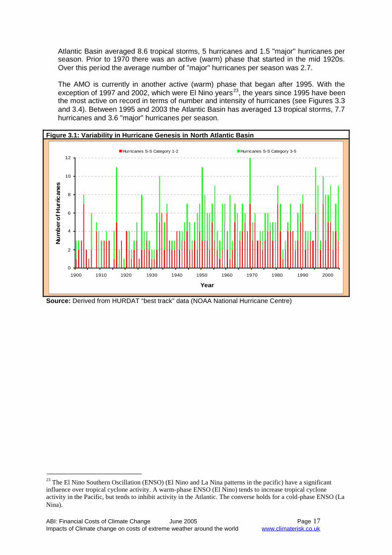
Atlantic Basin averaged 8.6 tropical storms, 5 hurricanes and 1.5 "major" hurricanes perseason. Prior to 1970 there was an active (warm) phase that started in the mid 1920s.Over this period the average number of "major" hurricanes per season was 2.7.
The AMO is currently in another active (warm) phase that began after 1995. With theexception of 1997 and 2002, which were El Nino years23, the years since 1995 have beenthe most active on record in terms of number and intensity of hurricanes (see Figures 3.3and 3.4). Between 1995 and 2003 the Atlantic Basin has averaged 13 tropical storms, 7.7hurricanes and 3.6 "major" hurricanes per season.
Figure 3.1: Variability in Hurricane Genesis in North Atlantic Basin
0
2
4
6
8
10
12
1900 1910 1920 1930 1940 1950 1960 1970 1980 1990 2000
Year
Nu
mb
ero
fHur
rican
es
Hurricanes S-S Category 1-2 Hurricanes S-S Category 3-5
Source: Derived from HURDAT “best track” data (NOAA National Hurricane Centre)
23 The El Nino Southern Oscillation (ENSO) (El Nino and La Nina patterns in the pacific) have a significantinfluence over tropical cyclone activity. A warm-phase ENSO (El Nino) tends to increase tropical cycloneactivity in the Pacific, but tends to inhibit activity in the Atlantic. The converse holds for a cold-phase ENSO (LaNina).

ABI: Financial Costs of Climate Change June 2005 Page 18Impacts of Climate change on costs of extreme weather around the world www.climaterisk.co.uk
Figure 3.2: Variability in North Atlantic Basin Hurricanes Making Landfall in the U.S.
0
1
2
3
4
5
6
7
1900 1910 1920 1930 1940 1950 1960 1970 1980 1990 2000
Year
Nu
mb
erof
Hu
rric
anes
Hurricanes S-S Category 1-2 Hurricanes S-S Category 3-5
Source: Derived from HURDAT “best track” data (NOAA National Hurricane Centre)
Figure 3.3: Inter-decadal Variability in Hurricane Genesis in the North Atlantic Basin and ThoseMaking Landfall in the U.S.
3.5 3.43.8
4.75.0
6.8
6.2
5.6
5.1
6.3
7.2
0.0
1.0
2.0
3.0
4.0
5.0
6.0
7.0
8.0
1900-1909
1910-1919
1920-1929
1930-1939
1940-1949
1950-1959
1960-1969
1970-1979
1980-1989
1990-1999
2000-2004
Decade
Ave
rage
Nu
mb
ero
fH
urr
ican
esP
erY
ear
0.0
1.0
2.0
3.0
4.0
5.0
6.0
7.0
8.0
Hurricanes S-S Category 1-5 Landfalling Hurricanes S-S Category 1-5
Source: Derived from HURDAT “best track” data (NOAA National Hurricane Centre)
ABI: Financial Costs of Climate Change June 2005 Page 19Impacts of Climate change on costs of extreme weather around the world www.climaterisk.co.uk
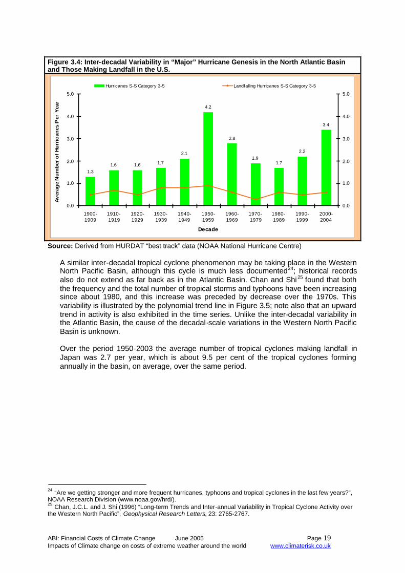
Figure 3.4: Inter-decadal Variability in “Major” Hurricane Genesis in the North Atlantic Basinand Those Making Landfall in the U.S.
1.3
1.6 1.6 1.7
2.1
4.2
2.8
1.91.7
2.2
3.4
0.0
1.0
2.0
3.0
4.0
5.0
1900-1909
1910-1919
1920-1929
1930-1939
1940-1949
1950-1959
1960-1969
1970-1979
1980-1989
1990-1999
2000-2004
Decade
Av
erag
eN
um
ber
of
Hu
rric
anes
Per
Yea
r
0.0
1.0
2.0
3.0
4.0
5.0
Hurricanes S-S Category 3-5 Landfalling Hurricanes S-S Category 3-5
Source: Derived from HURDAT “best track” data (NOAA National Hurricane Centre)
A similar inter-decadal tropical cyclone phenomenon may be taking place in the WesternNorth Pacific Basin, although this cycle is much less documented24; historical recordsalso do not extend as far back as in the Atlantic Basin. Chan and Shi 25 found that boththe frequency and the total number of tropical storms and typhoons have been increasingsince about 1980, and this increase was preceded by decrease over the 1970s. Thisvariability is illustrated by the polynomial trend line in Figure 3.5; note also that an upwardtrend in activity is also exhibited in the time series. Unlike the inter-decadal variability inthe Atlantic Basin, the cause of the decadal-scale variations in the Western North PacificBasin is unknown.
Over the period 1950-2003 the average number of tropical cyclones making landfall inJapan was 2.7 per year, which is about 9.5 per cent of the tropical cyclones formingannually in the basin, on average, over the same period.
24 “Are we getting stronger and more frequent hurricanes, typhoons and tropical cyclones in the last few years?”,NOAA Research Division (www.noaa.gov/hrd/).25 Chan, J.C.L. and J. Shi (1996) “Long-term Trends and Inter-annual Variability in Tropical Cyclone Activity overthe Western North Pacific”, Geophysical Research Letters, 23: 2765-2767.

ABI: Financial Costs of Climate Change June 2005 Page 20Impacts of Climate change on costs of extreme weather around the world www.climaterisk.co.uk
Figure 3.5: Variability and Trend in Tropical Cyclone Genesis in Western North Pacific Basin
0
5
10
15
20
25
30
35
40
45
50
1945 1950 1955 1960 1965 1970 1975 1980 1985 1990 1995 2000
Year
Nu
mbe
ro
fE
ven
ts
0
5
10
15
20
25
30
35
40
45
50Tropical Cyclones
Annual Average 1950-2003
Annual Average Landfalling in Japan 1950-2003
Source: Derived from “best track” data (Joint Typhoon Warning Centre).
Figure 3.6: Inter-decadal Variability in Tropical Cyclone Genesis in Western North Pacific Basin
35.0
31.1
26.4
29.5
26.0
22.2
0
5
10
15
20
25
30
35
40
1945-1955 1955-1964 1965-1974 1975-1984 1985-1994 1995-2004
Year
Num
ber
ofT
rop
ical
Cyc
lone
s
Tropical Cyclones
Source: Derived from “best track” data (Joint Typhoon Warning Centre). NB there are some doubtsabout the quality of the track data prior to 1972.
3.4 Tropical cyclones and climate change
Over the last 100 years the tropical North Atlantic has experienced a gradual warmingtrend (with sea surface temperatures increasing by about 0.3oC). However, hurricaneactivity in the basin has not exhibited a distinct trend, but rather discrete inter-decadalvariability. Moreover, this variability is much greater than one might anticipate from such agradual warming trend. This raises questions about whether the increased activitycurrently being experienced in the North Atlantic results from anthropogenic global

ABI: Financial Costs of Climate Change June 2005 Page 21Impacts of Climate change on costs of extreme weather around the world www.climaterisk.co.uk
warming. Nonetheless, the average number of hurricanes and “major” hurricanes duringthe current AMO (warm) phase is higher than during the previous AMO (as demonstratedin Figures 3.7 and 3.8). In fact, the average number of hurricanes during the precedingAMO cold phase was also higher than during the last AMO cold phase. One couldreasonably ask whether the observed inter-decadal variability in hurricane activity, inaccordance with the AMO (warm and cold phase) cycle, is actually masking an upwardtrend in hurricane activity as a result of global warming. Figure 3.9, which plots the five-year moving average of hurricane activity in the Atlantic Basin, does suggest a slightupward trend in activity.
Figure 3.7: Hurricane Genesis in the North Atlantic Basin and Those Making Landfall in the U.S.During Atlantic Warm and Cold Phases
3.4
5.7
5.0
7.7
0.0
1.0
2.0
3.0
4.0
5.0
6.0
7.0
8.0
1900-1925 1926-1970 1971-1995 1996-2004
Time Period
Ave
rag
eN
um
ber
ofH
urr
ica
nes
Per
Ye
ar
0.0
1.0
2.0
3.0
4.0
5.0
6.0
7.0
8.0Hurricanes S-S Category 1-5
Landfalling Hurricanes S-S Category 1-5
Source: Derived from HURDAT “best track” data (NOAA National Hurricane Centre)

ABI: Financial Costs of Climate Change June 2005 Page 22Impacts of Climate change on costs of extreme weather around the world www.climaterisk.co.uk
Figure 3.8: “Major” Hurricane Genesis in the North Atlantic Basin and Those Making Landfall inthe U.S. During Atlantic Warm and Cold Phases
1.3
2.7
1.5
3.6
0.0
0.5
1.0
1.5
2.0
2.5
3.0
3.5
4.0
4.5
5.0
1900-1925 1926-1970 1971-1995 1996-2004
Time Period
Av
erag
eN
um
ber
of
Hu
rric
anes
Per
Yea
r
0.0
1.0
2.0
3.0
4.0
5.0Hurricanes S-S Category 3-5
Landfalling Hurricanes S-S Category 3-5
Source: Derived from HURDAT “best track” data (NOAA National Hurricane Centre)
Figure 3.9: Trends in Hurricane Genesis in the North Atlantic Basin (5-year moving average)
0
1
2
3
4
5
6
7
8
9
1900 1906 1912 1918 1924 1930 1936 1942 1948 1954 1960 1966 1972 1978 1984 1990 1996 2002
Year
Nu
mb
ero
fHu
rric
ane
s
Hurricanes S-S Category 3-5 Hurricanes S-S Category 1-2 Hurricanes S-S Category 1-5
Source: Derived from HURDAT “best track” data (NOAA National Hurricane Centre)
ABI: Financial Costs of Climate Change June 2005 Page 23Impacts of Climate change on costs of extreme weather around the world www.climaterisk.co.uk
3.5 European windstorms
Windstorms are the main cause of insured losses due to natural events in Europe; since1970 there have been 55 significant windstorms in Europe, resulting in total insuredlosses of about US$ 44.4 billion. The scientific community refers to European windstormsas extra-tropical cyclones. Also, as they typically occur between October and March theyare often referred to as winter storms.
The majority of windstorms affecting Europe originate in the North East Atlantic (along the45o of latitude or the “polar front”) and then move east, pushed along by the Jet Stream.As they move forward, at speeds of up to 40 ms-1, the wind field becomes elongated. Thehighest wind speeds are observed to the right-hand side of the storm track directly behindthe advancing cold front (sometimes up to several hundred kilometres from the track). Theheaviest precipitation is found along the warm front. The storms themselves can havediameters of 1,000 to 2,000 kilometres.
While several hundred storms form annually, most of them dissipate before they reachEurope; around 180 low pressure systems cross the Atlantic per annum, which typicallyresult in three major windstorms. Whether the storms cross Europe depends on the stateof the Icelandic low and the Azores high pressure systems. In general, when the Icelandiclow is well developed, more low pressure systems (and thus windstorms) will advanceacross Europe, as opposed to drifting northeast between Iceland and the top of the UK(see Box 2).
Box 2: The North Atlantic Oscillation
The North Atlantic Oscillation (NAO) characterises natural variability in air pressure over the NorthAtlantic. It also has a significant influence on the development and path of extra-tropical cyclones.The NAO is described as an index that measures the pressure differential between the Icelandiclow and the Azores high. When the Icelandic low is well developed there is a marked difference inair pressure with the Azores high, and the NAO index is positive. High positive index values areassociated with strong westerly air flows, which carry warm humid air, as well as more storms, wellinto Europe. During positive phases of the NAO index, Europe therefore experiences relatively mildand windy winters.In contrast, when the NAO index is negative, the westerly air flows are weaker and the aboveconditions are reversed. That is, during a negative phase of the NAO index Europe will tend toexperience relatively dry, cool and less windy winters.Fluctuations in the NAO index are irregular; it switches between negative and positive phasesevery 5 to 25 years.While the influence of the NAO on winter storms reaching into Europe is not in doubt, the realquestion in the context of climate change is whether anthropogenic GHG emissions are influencingthe phases of the index. (We return to this below.)
In contrast to tropical cyclones, which are fuelled by condensation over warm waters,European windstorms are fuelled by the temperature differential between cold (arctic)and warm (tropical) air. As a result, European windstorms do not necessarily reduce inintensity when making landfall in the same way that hurricanes do. The larger thetemperature differential between the cold air mass and the warm air mass, the larger thewindstorm. Moreover, since the temperature differential is larger in winter (October toMarch), European windstorms tend to be stronger during this period.

ABI: Financial Costs of Climate Change June 2005 Page 24Impacts of Climate change on costs of extreme weather around the world www.climaterisk.co.uk
As mentioned above, since 1970 there have been 55 windstorm events in Europegenerating sufficient losses to be recorded by Swiss Re’s Sigma series26. In total, theseevents have resulted in total insured losses of US$ 44.4 billion. Seven events account forUS$ 28.4 billion: windstorm 87J (US$ 5.0 billion), windstorm Daria (US$ 6.6 billion),windstorm Herta (US$ 1.2 billion), windstorm Vivian (US$ 4.6 billion), windstorm Anatol(US$ 1.7 billion), windstorm Lothar (US$ 6.6 billion) and windstorm Martin (US$ 2.7billion). That is, 64 per cent of total insured losses resulted from 13 per cent ofwindstorms.
In looking at Figure 3.10 there is no real discernible year-on-year trend over the period1970-2004, in either the number of events or insured losses; any pattern in insuredlosses over such a relatively short time period is very unlikely given the scale of lossesresulting from the big 7 storms. There is, however, an upward trend in the number ofwindstorm events when we consider inter-decadal trends; the average number of eventsbetween 1970 and 1979 was 0.4 per annum, rising to 2.8 per annum between 1990 and1999 (see Figure 3.11).
One should be cautious in drawing any conclusions regarding the role of climate changewhen looking at trends in insured events however. To date, trends in insured losses havebeen driven predominantly by socio-economic factors, including population growth,concentrations of population in urban areas, and rising quantities of increasingly valuableassets in risk prone areas. There have also been improvements in monitoring, so thatmore events are identified and recorded annually.
26 For example, for the 2004 reporting year, Swiss Re, Sigma only records events with insured losses greater thanUS$ 37.5 million, total losses greater than US$ 74.9 million or 20 or more fatalities.

ABI: Financial Costs of Climate Change June 2005 Page 25Impacts of Climate change on costs of extreme weather around the world www.climaterisk.co.uk
Figure 3.10: Number of Severe Windstorm Events and Associated Insured Losses in Europe1970-2004
-
1
2
3
4
5
6
7
8
9
10
11
1970 1974 1978 1982 1986 1990 1994 1998 2002
Year
Num
ber
ofE
ven
ts
0
2
4
6
8
10
12
14
16
Insu
red
Lo
sses
(US
D20
04B
illio
n)Events Insured Losses
Source: Sigma Database, Swiss Re
Figure 3.11: Annual Average Number of Severe Windstorm Events and Annual Average InsuredLosses By Decade in Europe (1970-2004)(a) With “Big” Seven (a) Without “Big” Seven
2.2
2.8
1.2
0.4
0.6
3.1
0.9
0.2
0.0
1.0
2.0
3.0
1970-1979 1980-1989 1990-1999 2000-2004
Year
An
nu
alA
vera
ge
Nu
mb
er
of
Eve
nts
0.0
0.5
1.0
1.5
2.0
2.5
3.0
3.5
An
nua
lA
ver
age
Ins
ure
dLo
sse
s(U
SD
200
4B
illio
n)
Events Insured Losses
2.22.2
1.1
0.4
0.2
0.4
0.7
0.6
0.0
0.5
1.0
1.5
2.0
2.5
1970-1979 1980-1989 1990-1999 2000-2004
Year
Ann
ua
lA
vera
ge
Nu
mb
er
of
Eve
nts
0.0
0.2
0.4
0.6
0.8
1.0
An
nu
alA
ver
age
Insu
red
Los
ses
(US
D2
004
Bil
lion
)
Events Insured Losses
Source: Sigma Database, Swiss Re

ABI: Financial Costs of Climate Change June 2005 Page 26Impacts of Climate change on costs of extreme weather around the world www.climaterisk.co.uk
3.6 Summary of climate science
Broadly, concern over the possible future changes in cyclone activity as a result of climatechange relates to changes in27:
the frequency and area of occurrence;
the mean intensity;
the maximum intensity; and
the rain and wind structure.
Several approaches have been used to assess the potential impact of climate change onthese aspects of cyclone activity, including: using global climate models to directlysimulate cyclone activity, empirical downscaling, estimates based on theoretical maximumpotential, and nested high resolution simulation experiments (see Box 3).
Box 3: Approaches to Assess the Impact of Climate Change on Cyclone Activity
Coupled Ocean-Atmosphere General Circulation Models (OAGCM) and AtmosphericGeneral Circulation Models (AGCM) linked to Mixed-Layer Ocean (MLO) sub-models oremploying sea surface temperature predictions from OAGCM. These models have beenused to directly simulate cyclone activity. However, published studies –particularly earlierstudies, as shown below – do not exhibit much consistency. Some studies showfrequency increasing, while others find a decrease in frequency, depending on the modelused. These inconsistent results have brought into question the capacity of these(coarse) models to realistically simulate cyclogenesis.
An alternative to using global climate models to directly simulate cyclone activity is toinfer cyclogenesis from the climatic output of these models using meteorological-basedempirical methods, such as Gray’s genesis parameters. One such study (reference)finds that a doubling of CO2 concentrations results in an increase of cyclone frequencyof between 4 and 7 per cent. However, these meteorological-based empirical methodswere developed for the present climate and need to be modified for application to futureclimates. There is thus some uncertainty over the reliability of these modified empiricalmethods.
'Up-scaling’ thermodynamic models, such as those of Emanuel (1986) and Holland(1997). The maximum intensity that a tropical cyclone can achieve in any givenatmospheric (thermodynamic) environment is called the maximum potential intensity(MPI). The basic Carnot model of MPI, as developed by Emanuel (1986 and 1995),predicts that the maximum tropical cyclone wind speed will increase with global warming.The MPI essentially places an upper (‘speed’) limit on the magnitude of the change inwind speed. However, these models are known not to capture all the relevant processes.
Meso-scale models driven off-line from the output of OAGCM or AGCM have greaterresolution and are better at capturing cyclone climatology than the coarser models.
Sources: Henderson-Sellers, A. et al12 and Knutson28
27 Henderson-Sellers, A., H. Zhang, G. Berz, K. Emanuel, W. Gray, C. Landsea, G. Holland, J.Lighthill, S.-L. Shieh, P. Webster and K. McGuffie (1998) “Tropical Cyclones and Global ClimateChange: A Post-IPCC Assessment, Bulletin of the American Meteorological Society, 79(1): 19-38.28 Knutson, T.R. (2002) “Modelling the Impact of Future Warming on Tropical Cyclone Activity”, IPCCWorkshop on Extreme Weather and Climate Events, Workshop Report, Beijing, China, 11-13 June,2002.

ABI: Financial Costs of Climate Change June 2005 Page 27Impacts of Climate change on costs of extreme weather around the world www.climaterisk.co.uk
3.6.1 Tropical cyclones
Up to 2001, the results of research into the possible impact of climate change on thefrequency and character of tropical cyclones is best captured in the conclusions of theIPCC (First, Second and Third) Assessment Reports. A selection of key studiesunderlying the IPCC Reports are summarised in Box A1 in Appendix A.
The First Assessment Report (FAR) from the IPCC29 (IPCC, 1990) stated that: “…climatemodels give no consistent indication whether tropical storms will increase or decrease infrequency or intensity as climate changes; neither is there any evidence that this hasoccurred over the past few decades”.
The Intergovernmental Panel on Climate Change published its Second AssessmentReport (SAR) in 1996. The “Science of Climate Change” report stated that (Houghton etal, 1996, p. 334):“…the-state-of-the-science [tropical cyclone simulations in enhanced greenhouseconditions] remains poor because: (i) tropical cyclones cannot be adequately simulated inpresent GCMs [General Circulation Model or Global Climate Model]; (ii) some aspects ofENSO [El Niño Southern Oscillation] are not well simulated in GCMs; (iii) other large-scale changes in the atmospheric general circulation which could affect tropical cyclonescannot yet be discounted ; and (iv) natural variability of tropical storms is very large, sosmall trends are likely to be lost in the noise.”
It went on to say:“In conclusion, it is not possible to say whether the frequency, area of occurrence, time ofoccurrence, mean intensity or maximum intensity of tropical cyclones will change”.
In the Technical Summary the IPCC state: “Although some models now represent tropicalstorms with some realism for present day climate, the state of the science does not allowassessment of future changes” (IPCC, 1996, p. 44).
However, by the time of the IPCC Third Assessment Report (TAR) in 2001 - the “Scienceof Climate Change” concluded that: “… there is some evidence that regional frequenciesof tropical cyclones may change, but none that their locations will change. There is alsoevidence that the peak intensity may increase by 5% to 10% and precipitation rates mayincrease by 20% to 30%” (IPCC, 2001, Box 10.2). The IPCC went on to say, however,that “There is a need for much more work in this area to provide more robust results.”
Indeed, more research into the possible links between climate change and future tropicalcyclone activity has been undertaken. A selection of key post IPCC TAR studies aresummarised in Box A2 at Appendix A. However, these studies do not change the mainconclusions of the TAR. Specifically, the literature (and expert opinion) remainsinconclusive on changes to the frequency of tropical cyclones under global warming; therange of estimates and uncertainties is still very large. Hence, in this study we do notconsider simulating changes to the frequency of tropical cyclones.
Further evidence is emerging to support the TAR conclusions on tropical cycloneintensity, that both wind speeds and precipitation rates are likely to increase in anatmosphere with higher levels of CO2 concentrations. One such recent study, by Knutsonand Tuleya (2004), found that in moving from a control (base) case to a "high-CO2"(roughly 2.2 x CO2 concentrations) case:
The minimum central pressure of tropical storms (averaged over hours 97-120)drops by an average of 10 mb, from 934 mb to 924 mb.
29 www.ipcc.ch Intergovernmental Panel on Climate change

ABI: Financial Costs of Climate Change June 2005 Page 28Impacts of Climate change on costs of extreme weather around the world www.climaterisk.co.uk
The pressure fall (i.e. the difference between the minimum central pressure andthe environmental surface pressure) is 14 per cent greater (range is 13 to 15 percent greater).
"Intense" (Category 3-5) tropical cyclones increase, on average, by half a Saffir-Simpson Category.
Maximum surface wind speeds increase by an average of 3.4 ms-1, from 59.3 ms-1
to 62.7 ms-1. Equivalent to an increase of 6 per cent (range is +5 to +7 per cent). The mean instantaneous precipitation rate (averaged over all grid points within a
100 km of the storm centre at hour 120) increases from 80 to 95 cmd-1. Equivalentto an increase of 18 per cent (range is +12 to +26 per cent).
The maximum precipitation rate anywhere in the storm domain increases from, onaverage, 706 to 875 cmd-1. Equivalent to an increase of 24 per cent (range is +17to +33 per cent).
Regarding the tracking of tropical cyclones there is little evidence of any change in theNorth Atlantic, although one recent study suggests that sea surface warming may inhibitthe landfall of hurricanes over Southeast Florida. Likewise, there is little evidence ofsignificantly different storm tracks in the Western North Pacific, although the storms trackslightly more pole ward.
3.6.2 Extra-tropical cyclones
There are a growing number of studies addressing possible changes in extra-tropicalcyclone activity - a selection of these are summarised in Box A3 at Appendix A. However,there are still large uncertainties in model predictions, despite a growing body of worksince the IPCC TAR. For example, simulations of the north Atlantic storm track in presentday climate simulations differ considerably from observed data. This means thatpredictions of future changes in the location of the track have to be treated with somecaution. The results of different models are also inconsistent, with some models (e.g.HadAM3P) showing a southward shift in the north Atlantic storm track, while other models(e.g. HadCM2) show a shortening of the north Atlantic track. The former tends to increasethe number of storms over the UK, whereas the latter would lead to fewer storms over theUK. There is also uncertainty with respect to the mechanisms governing the climatesignals.
Nonetheless, some consensus is emerging (although still incomplete) between modelsthat points towards an increase in the frequency of "deep" winter storms (with centralpressure less than 970 mb) over the north Atlantic. Moreover, we may see these "deep"storms tracking further south over the UK and further into western and central Europe,with the North Atlantic Oscillation (NAO) possibly intensifying as CO2 concentrationsincrease in the future30. One study, by Leckebusch and Ulbrich (2004), simulated CO2-induced changes to the activity of extreme storms and found that31:
There is a 20 per cent increase in storms in the 95th percentile (sea level pressure)that track across southern England, France, Germany, northern Switzerland, andthe Benelux countries.
95th percentile maximum wind speeds in storms that track across southernEngland, France, Germany, northern Switzerland, and the Benelux countriesincrease by 10 per cent.
30 See, for example, Kuzmina et al (2005).31 Although the study did not attempt to quantify the impact on less intense storms (i.e. windstorms in the lowerpercentiles of the distribution of possible events), it implied that these may also be affected.
ABI: Financial Costs of Climate Change June 2005 Page 29Impacts of Climate change on costs of extreme weather around the world www.climaterisk.co.uk
These climate change signals in storm activity were observed under IPCC SRES emissionscenario A2 (see below) towards the end of the century.
3.7 Financial impacts of changes in the character of storms
As evident from the above discussion, considerable uncertainty remains over theinfluence of projected climate change on tropical and extra-tropical cyclone activity. Whileit is premature to treat any (emerging) link between climate change and storm activity /character as definitive, it is at least worth evaluating the potential impacts, if some of themore recent estimates of climate-induced changes in the character of storms were indeedto be realised.
To this end, we simulate three simple climate-stress tests using insurance industry naturalcatastrophe models, based on the Knutson and Tuleya (2004) and Leckebusch andUlbrich (2004) findings32:
The maximum surface wind speeds in hurricanes in the Atlantic Basin have beenincreased by 6 per cent.
The maximum surface wind speeds in typhoons in the Western North PacificBasin have also been increased by 6 per cent.
There is a 20 per cent increase in the top 5 per cent (in terms of sea levelpressure) of windstorms affecting Western Europe. This does not imply anincrease in the total number of storms, but rather a shift in the existingdistribution towards more intense storms, with higher winds.
Wind speed is not the only hazard associated with these storms. As noted above,damage from tropical cyclones and European windstorms is also caused by storm surgesand intense precipitation, in combination with the high winds. Furthermore, there isincreasing evidence that both the storm surge and rainfall generated by these stormsmay increase as a result of climate change. In order to generate a more complete pictureof the potential financial costs of stronger storms, the predicted changes in these othertwo hazards should be simulated simultaneously. The results presented below willtherefore tend to underestimate the true financial cost and insured losses of the stormevents simulated. (There are other reasons why the results will tend to understate thetrue damages; these are discussed below).
The studies from which the proposed stress tests for hurricanes and typhoons are basedrelate solely to a future world in which CO2 concentrations essentially double. However,in this study we are also interested in the implications of moving from higher emissionscenarios to lower ones, and therefore must be able to scale the results of thesimulations to alternative CO2 concentrations. To facilitate this we also undertook acouple of sensitivity tests, involving: (a) increasing the 6 per cent change in wind speedby 50 per cent, and (b) decreasing the 6 per cent change in wind speed by 30 per cent.Adjustments of this order are representative of the changes in CO 2 concentrations (andcorresponding radiative forcing) required to move from roughly a doubl ing ofconcentrations to specific emission scenarios.
The simulations were undertaken by the natural catastrophe modelling team at AIR-worldwide33. Using their natural catastrophe models for hurricanes, typhoons and
32 Converium Re performed a similar exercise for a particular portfolio of typhoon events in the NorthwestPacific Basin. Converium estimated that expected annual losses in a warmer climate (in which sea surfacetemperatures increase by about 2.2oC, inducing tropical cyclones to increase in intensity by between 5-12 percent) could be between 40-50 per cent higher by the end of the century, ceteris paribus (Converium, 2004).

ABI: Financial Costs of Climate Change June 2005 Page 30Impacts of Climate change on costs of extreme weather around the world www.climaterisk.co.uk
European windstorms, AIR estimated the incremental impact on property (includingresidential, commercial and industrial facilities, and automobiles) of moving from abaseline (or current) storm event set, to one in which the above climate-stress tests areincluded.
3.8 Tropical cyclonesThe results of the simulated climate-stress tests for hurricanes and typhoons arepresented in Table 3.2. Since the natural catastrophe models used were essentially builtto service the insurance industry, the output is in terms of insured losses. That is, thelosses represent damages to insured properties after the application of insurance policyconditions, such as deductibles, coverage limits, loss triggers, coinsurance, and risk orpolicy specific reinsurance terms. Also, since the models are fully probabilistic, the lossestimates are annual expected (or average) losses, derived from probability lossdistributions.
Table 3.2: Increment in Average Annual Insured Losses
Climate Stress-test Hurricanes AffectingU.S.
Typhoons AffectingJapan
(US$ 2004 Billion) (US$ 2004 Billion)
Central case: Wind speeds increase by 6% 3.9 1.6
Sensitivity: Wind speeds increase by 4% 2.6 1.0
Sensitivity: Wind speeds increase by 9% 6.5 2.6
Source: AIR-worldwide
Insurers and reinsurers are hugely interested in the insured losses associated withextreme possibilities; typically measured as the losses arising once every 100 years (orlosses with a 1 per cent exceedance probability) or losses arising once every 250 years(or losses with a 0.4 per cent exceedance probability). Table 3.3 and Table 3.4 presentthe results for both these extreme possibilities, respectively. Looking at Table 3.3, forexample, a 6 per cent increase in maximum surface wind speeds is estimated to increase1-in-250 year insured losses from hurricanes by US$ 61.8 billion. If wind speeds were toincrease by 9 per cent (which is within the range cited in the scientific literature) 1-in-250year insured losses from hurricanes are estimated to increase by US$ 97.5 billion.
33 While AIR-Worldwide Corporation kindly simulated the climate-stress tests using their models, the scenariossimulated should in no way be interpreted as being representative of AIR-Worldwide Corporation’s view on theeffects of climate change on hurricanes, typhoons or European windstorms.

ABI: Financial Costs of Climate Change June 2005 Page 31Impacts of Climate change on costs of extreme weather around the world www.climaterisk.co.uk
Table 3.3: Increment in Insured Losses with a 1 Per Cent Exceedance Probability
Climate Stress-test Hurricanes AffectingU.S.
Typhoons AffectingJapan
(US$ 2004 Billion) (US$ 2004 Billion)
Central case: Wind speeds increase by 6% 40.8 10.1
Sensitivity: Wind speeds increase by 4% 26.6 6.6
Sensitivity: Wind speeds increase by 9% 68.3 17.3
Source: AIR-worldwide
Table 3.4: Increment in Insured Losses with a 0.4 Per Cent Exceedance Probability
Climate Stress-test Hurricanes AffectingU.S.
Typhoons AffectingJapan
(US$ 2004 Billion) (US$ 2004 Billion)
Central case: Wind speeds increase by 6% 61.8 14.4
Sensitivity: Wind speeds increase by 4% 41.9 9.0
Sensitivity: Wind speeds increase by 9% 97.5 24.9
Source: AIR-worldwide
In order to approximate the costs of changes in wind speed different to those directlysimulated, we have fitted curves to the data points and extrapolated them forward andbackward to encompass increases in wind speed ranging from zero to 10 per cent (with apower function offering the best fit in all cases); noting that this is a rather crudeapproximation. The resulting loss functions are provided at Appendix B.
3.9 Investigating the impacts of mitigation
The 6 per cent increase in maximum surface wind speed is the average increaseobserved across 3 tropical cyclone basins (including the Western North Pacific and NorthAtlantic) in an experiment in which CO2 concentrations increase over an 80-year period ata compound rate of 1 per cent per annum. This results in CO2 concentrations that arehigher by a factor of 2.22 by year 80; concentrations double at year 70. Unfortunately, theexperiment is not based on a specific starting concentration, and therefore the 6 per centincrease wind speed cannot be related directly to a specific IPCC SRES emissionscenario (or specific future year) on the basis of CO2 concentrations (see Box 4).However, by year 80 in the experiment radiative forcing34 is approximately 4.2 Wm-2, and
34 The IPCC (IPCC, 1996) use the following definition: “The radiative forcing of the surface-troposphere systemdue to the perturbation in, or the introduction of, an agent (say, a change in greenhouse gas concentrations) is thechange in net (down minus up) irradiance (solar plus long-wave; in Wm-2) at the tropopause after allowing for

ABI: Financial Costs of Climate Change June 2005 Page 32Impacts of Climate change on costs of extreme weather around the world www.climaterisk.co.uk
each of the SRES emission scenarios has a specific profile of radiative forcing. Thisprovides us with the basis of a link between (a) estimated changes in wind speed, (b)radiative forcing, (c) CO2 concentrations and (d) the SRES emissions scenarios; withchanges in wind speed linked to expected insured losses through the loss curves found atAppendix B.
Box 4: Summary of the IPCC SRES Emission Scenarios
In 2000 the IPCC published a set of greenhouse gas emission scenarios. The scenarios are basedaround four different storylines, which describe consistently the relationships between thedeterminants of emissions and their evolution over time, and to provide context for quantification ofthe scenarios.A1The A1 storyline describes a future world of very rapid economic growth, global population thatpeaks in mid-century and declines thereafter, and the rapid introduction of new and more efficienttechnologies. Major underlying themes are convergence among regions, capacity building andincreased cultural and social interactions, with a substantial reduction in regional differences in percapita income. The A1 scenario develops into three groups that describe alternative directions oftechnological change in the energy system. The three A1 groups are distinguished by theirtechnological emphasis: fossil intensive (A1FI), non-fossil energy sources (A1T), or a balanceacross all sources (A1B)A2The A2 storyline describes a very heterogeneous world. The underlying theme is self-reliance andpreservation of local identities. Fertility patterns across regions converge very slowly, which resultsin continuously increasing population. Economic development is primarily regionally oriented andper capita economic growth and technological change are more fragmented and slower than otherstorylines.B1The B1 storyline describes a convergent world with the same global population, that peaks in mid-century and declines thereafter, as in the A1 storyline, but with rapid change in economicstructures toward a service and information economy, with reductions in material intensity and theintroduction of clean and resource-efficient technologies. The emphasis is on global solutions toeconomic, social and environmental sustainability, including improved equity, but without additionalclimate initiatives.B2The B2 storyline and scenario family describes a world in which the emphasis is on local solutionsto economic, social and environmental sustainability. It is a world with continuously increasingglobal population, at a rate lower than A2, intermediate levels of economic development, and lessrapid and more diverse technological change than in the A1 and B1 storylines. While the scenariois also oriented towards environmental protection and social equity, it focuses on local and regionallevels.
Sources: p. 63 IPCC Technical Summary of the Working Group I Report.
stratospheric temperatures to readjust to radiative equilibrium, but with surface and tropospheric temperaturesand state held fixed at the unperturbed values.”

ABI: Financial Costs of Climate Change June 2005 Page 33Impacts of Climate change on costs of extreme weather around the world www.climaterisk.co.uk
Figure 3.12 contains the projected CO 2 concentrations for the six illustrative SRESscenarios, based on the ISAM model. The figure also shows the concentration profilescorresponding to an emission path designed to move the A1 SRES emissions scenariostowards stabilisation of CO2 concentrations at 550 ppm by 2200. We have computed theassociated radiative forcing using the following simplified expression from Table 6.2 inIPCC Technical Summary of Working Group I:
Δ F = α ln ( C / Co )
Where Δ F is the change in radiative forcing (in Wm -2), αis a constant equal to 5.35, C isthe concentration of CO2 in ppm, and the subscript zero denotes the unperturbedconcentration. Starting in 2000 the estimated radiative forcing for the six illustrative SRESemissions scenarios shown in Figure 3.12 is displayed in Figure 3.13. Of note, radiativeforcing (of 4.2 Wm-2) that gives rise to the 6 per cent increase in wind speeds is onlyreached under A1F1 and A2, and not until after 2080.
Figure 3.12: Atmospheric Concentrations of CO2 for the Six Illustrative IPCC SRES EmissionsScenarios, the IS92a Scenario and 550 Stabilisation Scenario
Source: ISAM Model (reference case)
300
400
500
600
700
800
900
1,000
1990 2000 2010 2020 2030 2040 2050 2060 2070 2080 2090 2100
Year
Carb
on
Dio
xide
Concentration
(ppm
v) A1B
A1T
A1FI
A2
B1
IS92a
B2
550

ABI: Financial Costs of Climate Change June 2005 Page 34Impacts of Climate change on costs of extreme weather around the world www.climaterisk.co.uk
Figure 3.13: Estimated Radiative Forcing for the Six Illustrative IPCC SRES EmissionsScenarios, the IS92a Scenario and Two 550 Stabilisation Scenarios
In order to extrapolate changes in wind speed to different magnitudes of radiative forcingit is necessary to make the simplifying assumption that a 1 per cent decrease (increase)in radiative forcing results in a 1 per cent decrease (increase) in the change in windspeed. This assumption allows us to map changes in wind speed (from zero per cent to10 per cent) to the full range of radiative forcing displayed in Figure 3.13; the lower theradiative forcing relative to 4.2 Wm-2, the lower the change in the maximum surface windspeeds for hurricanes and typhoons. It is then a matter of using the loss functions atAppendix B to calculate the increment in annual average insured losses (or the incrementin 1-in-100 or 1-250 year insured losses) for the full range of wind speed changesassociated with each emissions scenario.
The above procedure is probably best illustrated though an example: Under the A1F1emission scenario CO2 concentrations in 2070 are estimated to be about 716 ppm. Thecorresponding level of radiative forcing relative to 2000 is about 3.5 Wm -2. This level ofradiative forcing is estimated to increase maximum surface wind speeds by roughly 5 percent. According to the relevant loss function, a 5 per cent increase in hurricane windspeeds, in turn, is simulated to increase average annual losses by about US$ 3.2 billion.This procedure had been undertaken for all the emissions scenarios shown in Figure3.12. The results for various future time slices are found at Appendix C.
The figures at Appendix C show the three measures of incremental insured losses foreach emission scenario averaged over 20 year time slices. As expected, the emissionscenario with the highest radiative forcing, A1F1, also results in the highest increment inaverage losses. As Table 3.5 shows, under A1F1, annual average insured losses fromincreased wind speeds in hurricanes are estimated to increase by US$ 4.3 billion perannum, on average, over the period 2080-2099. However, if emission were to reduce inaccordance with the 550 stabilisation emission profile, annual average insured lossesfrom increased wind speeds in hurricanes would increase by only US$ 0.8 billion perannum, on average, over the same period. The corresponding increments in annualaverage insured losses for typhoons are US$ 1.7 billion (A1F1) and 0.3 billion (A1 550)per annum.
0.0
1.0
2.0
3.0
4.0
5.0
6.0
2000 2010 2020 2030 2040 2050 2060 2070 2080 2090 2100
Year
Ra
dia
tive
Fo
rcin
gC
O2
(Wm
-2)
A1B
A1T
A1FI
A2
B1
B2
IS92a
550

ABI: Financial Costs of Climate Change June 2005 Page 35Impacts of Climate change on costs of extreme weather around the world www.climaterisk.co.uk
To put these insured loss estimates into context, based on industry experience, insuredlosses from Atlantic hurricanes since 1995 averaged US$ 5.5 billion per year. Japanesetyphoons produce average insured losses of US$ 2.5 billion per year over the sameperiod. By the end of the century, annual average insured losses from typhoons, forexample, would therefore increase by nearly 70 per cent under emission scenario A1F1,ceteris paribus, if climate change were to induce wind speeds to increase by 6 per centper 4.2 Wm-2 of radiative forcing. Under a medium emission scenario like IS92a, annualaverage insured losses from typhoons would increase by 40 per cent.
Table 3.5: Increment in Average Annual Insured Losses over the Time Slice 2080-2099
Emission Scenario Hurricanes Typhoons
(US$ 2004 Billion Per Year) (US$ 2004 Billion Per Year)
A1B 2.8 1.1
A1T 1.2 0.5
A1F1 4.3 1.7
A2 3.5 1.4
B1 0.8 0.3
B2 1.4 0.5
550 0.8 0.3
IS92a 2.6 1.0
Figure 3.14 and Figure 3.15 show the change in incremental annual average losses inmoving from the A1 scenario group to a specific 550 stabilisation emissions profile forboth (a) hurricanes and (b) typhoons. For example, if in the absence of action globalemissions were to evolve along the A1B emission path, but international action wasintroduced to reduce carbon emissions sufficiently to put us on the specified 550stabilisation path, then the increment in annual average insured losses from hurricanesover the period 2080-2099 would be reduced by just under US$ 2.0 billion. That is,instead of annual average insured losses increasing by US$ 2.8 billion per year, theywould only increase by US$ 0.8 billion per year.
The change in incremental probable maximum losses in moving from the A1 scenariogroup to the 550 stabilisation emissions profile, for both hurricanes and typhoons, isprovided at Appendix D.

ABI: Financial Costs of Climate Change June 2005 Page 36Impacts of Climate change on costs of extreme weather around the world www.climaterisk.co.uk
Figure 3.14: Illustration of the Benefits of Moving to a Lower Emission Path For Various FutureTime Slices: Change in Annual Average Insured Losses(a) Hurricanes (b) Typhoons
0.0 0.5 1.0 1.5 2.0 2.5 3.0 3.5
Reduction in Annual Average Losses (USD2004 Billion)
2020-2039
2040-2059
2060-2079
2080-2099
Tim
eS
lice
A1B A1T A1FI
0.0 0.5 1.0 1.5 2.0 2.5 3.0 3.5
Reduction in Annual Average Losses (USD2004 Billion)
2020-2039
2040-2059
2060-2079
2080-2099
Tim
eS
lice
A1B A1T A1FI
Figure 3.15: Illustration of the Benefits of Moving to a Lower Emission Path For 2080-2099 TimeSlice: Percentage Reduction in Annual Average Insured Losses(a) Hurricanes (b) Typhoons
3.10 Extra-tropical cyclones
The results of the simulated climate-stress test for European windstorms are presented inTable 3.6. If climate change were to induce a 20 per cent increase in the top 5 per ofwindstorms (by central pressure) annual average insured losses are simulated to increaseby just under US$ 0.4 billion. The insured losses airing from a 1-in-100 and 1-in-250 yearinsured loss are estimated to increase by about US$ 2.0 and 2.3 billion, respectively.
To put these losses in context, the average annual insured losses from windstormsaffecting Europe over the period 1970-2004 was roughly US$ 1.5 billion, including the"big" seven events. Removing the "big" seven events, average annual insured losses dropto just under US$ 0.5 billion per year.
0% 20% 40% 60% 80% 100%
Reduction in Annual Average InsuredLosses (Reduction betw een A1F1, A1T and
A1B, and 550 as % of A1F1, A1T and A1B)
2080-2099
Tim
eS
lice
2080
-20
99
A1FI
A1T
A1B
0% 20% 40% 60% 80% 100%
Reduction in Annual Average InsuredLosses (Reduction between A1F1, A1T and
A1B, and 550 as % of A1F1, A1T and A1B)
2080-2099
Tim
eS
lice
2080
-20
99
A1FI
A1T
A1B

ABI: Financial Costs of Climate Change June 2005 Page 37Impacts of Climate change on costs of extreme weather around the world www.climaterisk.co.uk
Table 3.6: Increment in Insured Losses for Climate-Stress Tests: Extra-tropicalCyclones Affecting Western Europe
Measure of Insurance Loss Insured Losses
(US$ 2004 Billion)
Annual average losses 0.4
1 per cent exceedence probability (1-in-100 yearstorm)
2.0
0.4 per cent exceedence probability (1-in-250 yearstorm)
2.3
Source: AIR-worldwide
It was not possible to conduct the same sensitivity tests for European windstorms thatwere performed for hurricanes and typhoons. As a consequence, we are unable toquantify the increment in insured losses for each of the different emissions scenarios, orfrom moving from a relatively high emission scenario to a relatively low (stabilisation)scenario. The increase in extreme European windstorms simulated in this study wasobserved under the A2 emissions scenario, but the same climate signal was much lesspronounced under the B2 scenario. This implies that reducing emissions, in moving fromthe relatively high A2 scenario to the lower B2 scenario, will reduce annual averageinsured losses; we just do not know by how much.
Recall, that the stress-tests on tropical cyclones were applied to the entire distribution ofall possible hurricanes and typhoons, whereas the stress-test on European windstormswas restricted to the extreme upper tail of the distribution of all possible storms. Theimpacts of climate change on less intense European windstorms were not modelled, dueto a lack of quantitative information about the possible impacts. In comparing Table 3.6with Tables 3.2- 3.4, for example, one should not conclude that the climate signalconcerning European windstorms is weak relative to the signal for tropical cyclones.
3.11 Total financial versus insured losses
Above we focused on insured losses, which are only a fraction of total financial costs.Specifically, insured losses comprise the proportion of total financial losses covered byan insurance contract. Financial losses, as measured by insurers, refer to total damagesarising from impacts on financial assets or activities, such as property, infrastructure,business interruption, etc. Insured losses as a percentage of total financial losses fromwindstorms affecting each of Japan, the U.S and Europe, based on current industryexperience, are roughly 60-65 per cent, 55-60 per cent and 50-55 per cent, respectively.Put another way, total financial losses in, for example, Europe, are about twice as muchas the insured loss estimates presented above.
We have used these ratios to re-scale the estimated increments to annual averageinsured losses in order to approximate the increment to annual average total financiallosses for the various climate-stress tests. The results are presented below. It isimportant to note, however, that these loss estimates do not fully reflect the total“economic” (as measured by economists) losses associated with hurricanes, typhoonsand European windstorms. First, we have only explicitly simulated increases to onehazard (i.e. wind), ignoring precipitation and storm surge. Second, we have onlyconsidered the damage caused by this one hazard on one receptor (i.e. property), thus

ABI: Financial Costs of Climate Change June 2005 Page 38Impacts of Climate change on costs of extreme weather around the world www.climaterisk.co.uk
ignoring impacts on, for example, human health and ecosystems. And third, we arevaluing all losses on the basis of market prices (e.g. replacement cost), which may notaccurately reflect the full welfare losses associated with property damage; as measuredby society’s maximum willingness-to-pay to avoid damage from windstorms, or theminimum compensation that society is willing-to-accept in order to tolerate damage fromwindstorms. The loss estimates presented below are therefore likely to considerablyunderstate the true welfare costs, if we were to see windstorms intensify as a result ofclimate change.
The estimated increment in financial losses for the simulated climate-stress tests forhurricanes and typhoons are presented in Table 3.7. If climate change were to increasemaximum surface wind speeds by 6 per cent, annual average financial losses areestimated to increase be about US$ 6.8 billion and US$ 1.6 billion for hurricanes andtyphoons, respectively.
If climate change were to induce a 20 per cent increase in the top 5 per of Europeanwindstorms (by central pressure) annual average financial losses are simulated toincrease by just under US$ 0.8 billion.
Table 3.7: Increment in Average Annual Financial Losses
Climate Stress-test Hurricanes AffectingU.S.
Typhoons AffectingJapan
(US$ 2004 Billion) (US$ 2004 Billion)
Central case: Wind speeds increase by 6% 6.8 2.5
Sensitivity: Wind speeds increase by 4% 4.4 1.6
Sensitivity: Wind speeds increase by 9% 11.3 4.1
Figure 3.16 and Figure 3.17 show the incremental total financial losses for each of thevarious emissions scenarios considered, averaged over 20 year time slices, forhurricanes and typhoons, respectively. As with insured losses, the emissions scenariowith the highest radiative forcing, A1F1, also results in the highest increment in averageannual financial losses.
Figure 3.18 and Figure 3.19 show the change in incremental annual average financiallosses in moving from the A1 scenario group to a specific 550 stabilisation emissionsprofile for both (a) hurricanes and (b) typhoons. If, under business-as-usual, globalemissions were to evolve along the A1B emission path, and international action wasintroduced to reduce carbon emissions sufficiently to put us on the specified 550stabilisation path, then the increment in annual average financial losses from hurricanesover the period 2080-2099 would be reduced by about US$ 3.3 billion, on average, peryear. That is, instead of annual average financial losses increasing by US$ 4.8 billion peryear, they would only increase by US$ 1.5 billion per year. Moving from A1B to the 550stabilisation path, reduces the increment in annual average financial losses fromtyphoons over the period 2080-2099 by about US$ 1.2 billion, on average, per year.

ABI: Financial Costs of Climate Change June 2005 Page 39Impacts of Climate change on costs of extreme weather around the world www.climaterisk.co.uk
Figure 3.16: Hurricanes: Average Annual Increment in Average Annual Financial Losses
Figure 3.17: Typhoons: Average Annual Increment in Average Annual Financial Losses
0.0 1.0 2.0 3.0 4.0 5.0 6.0 7.0 8.0
Increment in Annual Average Total Financial Losses (USD2004 Billion)
2020-2039
2040-2059
2060-2079
2080-2099
Tim
eS
lice
550
IS92a
B2
B1
A2
A1FI
A1T
A1B
0.0 0.5 1.0 1.5 2.0 2.5 3.0
Increment in Annual Average Total Financial Losses (USD2004 Billion)
2020-2039
2040-2059
2060-2079
2080-2099
Tim
eS
lice
550
IS92a
B2
B1
A2
A1FI
A1T
A1B

ABI: Financial Costs of Climate Change June 2005 Page 40Impacts of Climate change on costs of extreme weather around the world www.climaterisk.co.uk
Figure 3.18: Illustration of the Benefits of Moving to a Lower Emission Path For Various FutureTime Slices: Change in Annual Average Financial Losses(a) Hurricanes (b) Typhoons
Figure 3.19: Illustration of the Benefits of Moving to a Lower Emission Path For 2080-2099Future Time Slice: Percentage Reduction in Annual Average Financial Losses(a) Hurricanes (b) Typhoons
3.12 Socio-economic developments
In viewing the trend data for windstorms outlined above it would be easy to conclude thatwindstorms have become more severe over time. However, reported insured andeconomic losses fail to account for socio-economic developments that may actually beincreasing society’s vulnerability to windstorms. The following factors will make the lossesresulting from the same storm, hitting the same area, higher today than 20 years ago:
First, population patterns within a defined area change with time. And morepeople are locating in vulnerable coastal areas. For example, the NOAAestimates that from 1980 to 2003 the coastal population in the U.S. grew by 33million, and the coastal population is projected to increase by a further 12 millionby 2015. Household sizes are also decreasing. This means that the stock-at-riskto the windstorm hazard is increasing with time.
Second, one dollar will buy you less land, residential and commercial property,building materials, etc. today than it did 20 years ago, as a result of increases inthe general price level. In other words, the nominal (and possibly, real) value ofthe (increasing) stock-at-risk to windstorms will tend to (also) increase with time.
0.0 1.0 2.0 3.0 4.0 5.0 6.0
Reduction in Annual Average FinancialLosses (USD 2004 Billion)
2020-2039
2040-2059
2060-2079
2080-2099
Tim
eS
lice
A1B A1T A1FI
0.0 0.5 1.0 1.5 2.0 2.5
Reduction in Annual Average FinancialLosses (USD 2004 Billion)
2020-2039
2040-2059
2060-2079
2080-2099
Tim
eS
lice
A1B A1T A1FI
0% 20% 40% 60% 80%
Reduction in Annual Average FinancialLosses (Reduction between A1F1, A1T and
A1B, and 550 as % of A1F1, A1T and A1B)
31%
Tim
eS
lice
208
0-20
99
A1FI
A1T
A1B
0% 20% 40% 60% 80% 100%
Reduction in Annual Average FinancialLosses (Reduction between A1F1, A1T and
A1B, and 550 as % of A1F1, A1T and A1B)
2080-2099
Tim
eSl
ice
208
0-2
099
A1FI
A1T
A1B

ABI: Financial Costs of Climate Change June 2005 Page 41Impacts of Climate change on costs of extreme weather around the world www.climaterisk.co.uk
Third, real incomes are also increasing with time. That is, people are simplywealthier, and therefore tend to have more (physical) assets. Houses, forexample, are becoming bigger and more elaborate. People therefore have moreto lose.
Failure to account for these factors over time will lead one to misread the historic record.In the context of the present study, failure to account for the same factors will understatethe simulated losses, which is indeed the case, since the climate-stress tests are appliedto a static exposure data set. That is, the stock-at-risk and the value of that stock areassumed to remain constant, despite the fact that we are looking at time periods nearly100 years into the future.
To gain some insight as to the extent to which the losses are underestimated considerTable 3.8, which contains one set of projections for per capita incomes (in PurchasingPower Parity 1995 US$), which is an indicator of real income, for Western Europe, Japanand the U.S. Table 9 contains population projections for the EU15 and Poland, Japan andsouth and southeast U.S. coastal states.
Table 3.8: Index: Projected Per Capita Incomes 2000-2100 (2004 = 100) (PPP 1995 US$)
Year Western Europe Japan U.S.
2000 89 91 94
2025 159 146 134
2050 220 202 176
2075 271 238 219
2100 323 280 262
Source: IMAGE 2.2 (www.rivm.nl)
Table 3.9: Index: Estimated Projected Populations 2000-2100 (2004 = 100)
Year EU15 and Poland a Japan b S & SE U.S. Statesc
2000 100 100 96
2025 104 95 124
2050 99 79 160
2075 99 62 207
2100 99 50 267
Source: (a) Projections from Eurostat to 2050; extrapolation to 2100 based on annualised growth rate 2000-2050.(b) Medium variant projection 2000-2100 made by the National Institute of Population and Security Research(www.ipss.go.jp). (c) Medium variant projection 2000-2050 made by US Census Bureau (www.census.gov);extrapolation to 2100 based on annualised growth rate 2000-2050.
Looking at Europe, for example, population (as an indicator of the size of the stock-at-risk) is projected to remain virtually constant till the end of the century. However, percapita incomes (as an indicator of individuals’ wealth or a proxy for the value stock-at-risk) are projected to more than triple. Although this does not necessarily mean that theinsured and financial loss estimates presented above for European windstorms wouldnecessarily be three times higher, it does provide an indication of the extent to which theycould be underestimated.

ABI: Financial Costs of Climate Change June 2005 Page 42Impacts of Climate change on costs of extreme weather around the world www.climaterisk.co.uk
The potential for the losses given in Tables 3.2- 3.4 and Table 3.7 to be underestimatedappears to be an even greater issue for the U.S. Both the population in states vulnerableto hurricanes and their wealth are forecast to nearly triple by 2100, relative to 2004.
We have not used the indices in Table 3.8 and Table 3.9 to adjust the incrementalinsured and financial loss estimates reported above for two reasons:
Each emissions scenario has a specific underlying socio-economic scenario,which would include, for example, scenario specific forecasts of per capitaincome. To use indices of socio-economic variables that were not specific to anemissions scenario would introduce inconsistencies to the analysis.
Both the “quantity” and “price” component of the loss estimates should beprojected separately though time, and at a level of resolution that is consistentwith the catastrophe model. To apply an “aggregate” index of price and quantityat a coarse resolution would fail to (a) reflect the appropriate weighting of“quantity” and “price” in the total loss estimates, and (b) account for spatialvariations in the vulnerable of specific “quantity” and “price” combinations.
Future work in this area should strive to accurately accommodate the evolution of socio-economic variables over time.
3.13 Investigating the impacts of adaptation
Just as failing to account for the above socio-economic factors will lead us tounderestimate the future incremental economic and insured losses of changing stormactivity, failing to allow for adaptation will lead us to overestimate the incremental losses.The impact of windstorms depends on the frequency, intensity and duration of landfallingsystems, and on the degree of preparedness and types of mitigation measures availableto, and employed by, different groups within the population at risk (Diaz and Pulwarty,1997). The latter set of measures will reduce the vulnerability of the affected population towindstorm damage, thereby reducing the impact of the climate signal on future stormactivity.
When discussing adaptation to windstorms it is useful to distinguish between whatinsurers can do to mitigate (insured) losses, and what individuals can do to preventdamages from storms and reduce costs following a storm. The former is discussed morein the Section 6, although some of the measures that insurers can employ to mitigatelosses can also be designed so as to provide households with economic incentives toimplement preventative measures; essentially rewarding clients who do so. We highlightthe role of insurers in providing the right incentives.

ABI: Financial Costs of Climate Change June 2005 Page 43Impacts of Climate change on costs of extreme weather around the world www.climaterisk.co.uk
Table 3.10: Selection of Loss Mitigation Measures Adopted in Florida
Type of Measure Examples
Financial Discounts available through special windstorm underwriters. Forexample, Florida Windstorm Underwriting Association (FWUA)offers discounts to policyholders based on specific mitigationdevices designed to protect their homes. Discounts range between3 per cent and 18 per cent.Mandatory windstorm deductibles, typically 2 per cent of any loss(as opposed to traditional, fixed dollar deductible).
Informational Continuous direct education of policyholders.Countless educational efforts aimed at teaching homeowners howto protect their property against windstorm damage by retrofittingexisting or building new properties.Funding of educational initiatives through third parties.Use of industry trade associations to promote awareness andmitigation (e.g. IBHS, III)Federal initiatives (e.g. Federal Emergency Management Agency’sProject Impact)
Building Codes Florida’s building code adopted new, higher standards for homes,including the 116 mph wind standard.Codes strengthened increasing wind resistance for roofs.More building and roofing inspectors were hired to increasecompliance with building standards in some counties (e.g. DadeCounty).New regulations require review of building plans by a structuralengineer.Supporting/funding research into wind-resistant designs.Federal initiatives (e.g. FEMA’s Project Impact)
Public/Fiscal Florida legislature established and funded a trust to provide supportfor recovery and mitigation efforts not covered by federal grants.Dade County passed a special sales tax to generate revenue forlocal recovery and mitigation efforts.Dade County created a hazard mitigation plan in order to receivefederal disaster assistance under FEMA’s 404 Hazard MitigationGrant Program.
Partnerships Insurers assist government and relief organisations with mitigationprograms.Activate network of communication with many organisations in theevent a hurricane appears imminent (e.g. relief and weatherorganizations add web link to insurer organization web sites withmitigation information).
Source: Insurance Information Institute

ABI: Financial Costs of Climate Change June 2005 Page 44Impacts of Climate change on costs of extreme weather around the world www.climaterisk.co.uk
3.13.1 Building codes
When windstorms make landfall some property damage is inevitable. However, differentbuilding materials and construction techniques - wooden frame and masonry - are morevulnerable to wind damage than others. Other factors, such as building height, thereinforcement of walls and the strength of steel frames, also affect the vulnerability ofstructures to wind damage. High winds that enter a property through an opening in thebuilding’s envelope (e.g. window or door) raise the internal air pressure, which can causethe building to blow apart. Construction practices that take account of these factors, alongwith the addition of protective devices, such as approved storm shutters, can thus helpbuildings become more resistant to winds.
According to a study commissioned by the Institute for Business and Home Safety, if allproperties in south Florida meet the strong building code requirements for Miami-Dadeand Broward counties, damages from a repeat of Hurricane Andrew (taking the sametrack in 2002 as it did in 1992) would drop by nearly 50 per cent for residential propertyand about 40 per cent for commercial property35. Overall, damages would drop by justover 45 per cent if all residences and businesses were retro-fitted or built to meet themore stringent code.
It is estimated that, in Florida, to construct a home that better withstands hurricaneswould cost from 4 to 9 per cent more than a conventional home. At the same time,surveys show that, on average, individuals are prepared to pay up to 6 per cent more fora "fortified" dwelling.
Storm shutters and other protective devices for doors, windows, skylights and vents havealso proved effective in reducing damage from high winds, by preventing them frompenetrating the building’s envelope and stopping rain from damaging the building’sinterior and contents. In recognition of this, insurers offer credits to clients who installsuch devices, which reduces their premiums. To qualify for credits, homeowners inFlorida must install devices that are able to resist specified wind pressures. Additionalcredits can be gained by installing further measures that are able to withstand impactsfrom wind-blown debris.
3.13.2 Building code enforcement
In 1983 hurricane Alicia made landfall over Texas, causing US$ (current prices) 675million in insured losses By contrast, Hurricane Diana, which hit North Carolina 1984,caused insured losses of US$ 36 (current prices) million. Given that the storms wereroughly equal in size and intensity, why were the losses so different? A later study foundthat the level of building code enforcement was a key factor explaining the difference inclaim costs. In North Carolina, building codes were found to be effectively enforced, anda as result only 3 percent of homes in suffered major structural damage from thehurricane. This was not the case with the area affected by hurricane Alicia, where closeto 70 per cent of insured losses was attributed to poor code enforcement.
These findings promoted the former National Committee on Property Insurance (now theInstitute for Business and Home Safety) to investigate the level of building codeenforcement in Southern states. They found that officials and inspectors in about half ofthe counties surveyed were not enforcing the building code wind-resistance standards. Itwas estimated that between 25 and 40 percent of the losses from Hurricane Andrewcould have been avoided with proper enforcement of building codes: Indeed, a Dade
35 See IBHS News Release, 25.08.2002 (www.ibhs.org).
ABI: Financial Costs of Climate Change June 2005 Page 45Impacts of Climate change on costs of extreme weather around the world www.climaterisk.co.uk
County, Florida Grand Jury report issued in December 1992 confirmed that much of thedamage was due to lax code enforcement.
As a result, the insurance industry began to develop a building code compliance ratingsystem - the Building Code Effectiveness Grading Schedule (BCEGS). Under thisscheme the building codes in an area are assessed, as well as how the code is enforced.An areas is then assigned a score out of ten, with 1 = robust enforcement of a strongcode, and 10 = no recognisable code. Credits are they allocated on the basis of thescore; with a score of 10 not qualifying for credits. The underlying principle is simple:buildings in areas with strong codes that are effectively enforced should incur lowerlosses on average, and therefore should be rewarded with lower premiums. Thus,communities are given an economic incentive (in the form of lower premiums and lowerlosses) to introduce, and enforce, strong building codes.
Preliminary indications from the 2004 hurricane season highlight the value of strongercodes, with most of the severely damaged structures (and sources of loss) being builtprior to Hurricane Andrew, after which the BCEGS was initiated. Comparing homes builtbetween 1994 and 2002, with those built after 2002, showed that those built after 2002suffered about 40 percent less damage.
3.13.3 Planning
The NOAA found that in 2003, 53 per cent of the population in the U.S. lived in coastalcounties, which collectively account for 17 per cent of the country’s land mass. Twenty-three of the 25 most densely populated areas in the U.S. are on the coast. As mentionedabove, between 1980 and 2003, the population of coastal counties grew by 33 millionpeople, or 28 per cent. The population of Florida grew by 75 percent and Texas by 52percent; two states that are at high risk to hurricanes. Furthermore, growth is expected tocontinue. Between 2003 and 2008 the coastal population in those states most vulnerableto windstorms is expected to grow by 1.1 million, or 8 percent, with the highest growthexpected in the southern Florida. Coastal counties in the Carolinas and Georgia are alsoexpected to see considerable population increases. Large Increases are forecast for theHouston, Texas area and Florida’s central Gulf Coast. Globally, the U.N. estimates thatnearly 40 per cent of the world's population live within 100 km of the coast, and that thisproportion is increasing.
The growth and concentration of buildings (and wealth) in windstorm-prone areas raisesquestions about public policy regarding coastal development / planning. Also, allowingsuch development to continue potential gives rise to hidden subsidies within insurancetransactions36.
Insurers can make people who live in high risk (coastal) areas pay their fair share of thecost of windstorms by introducing higher deductibles for storm damage. Thesedeductibles, which exist in regions prone to hail as well as hurricane damage, aregenerally equal to a percentage of the structure's insured value. Seventeen states andthe District of Columbia have hurricane deductibles. In Florida rates for windstormcoverage are now based on the structure's ability to withstand damage by high winds,calculated using computer models, instead of the likelihood of fire damage.
Insurers in catastrophe-vulnerable states now require percentage deductibles onhomeowners’ insurance policies for wind damage losses, as opposed to a dollardeductible, to limit their exposure to catastrophic losses from natural disasters.
36 For instance, hidden subsidies would arise if rates for property insurance are no longer commensurate with riskbecause, for example, regulators prevented insurers from raising rates to actuarially justified levels.
ABI: Financial Costs of Climate Change June 2005 Page 46Impacts of Climate change on costs of extreme weather around the world www.climaterisk.co.uk
Percentage deductibles, which are now mandatory in some coastal areas, vary from 1per cent of a home's insured value to 15 per cent, depending on many factors, includingthe "trigger" - i.e. the event to which the deductible applies. In some states, homeownershave a "buy back" option, which allows them to pay a higher premium in return for a fixedrather than percentage deductible.
Although these deductibles are primarily designed to mitigate insurers' losses, they stillprovide an economic incentive to individuals when deciding where to locate and howmuch wealth to invest in a high-risk area.
ABI: Financial Costs of Climate Change June 2005 Page 47Impacts of Climate change on costs of extreme weather around the world www.climaterisk.co.uk
3.15 Appendices
Appendix A
Summary of Selected Studies into the Possible Impact of Climate Change on CycloneActivity
Box A1: Some Key Studies into the Impact of Climate Change on the Frequency andCharacter of Tropical Cyclones
Pre IPCC FARIn 1986, Kerry Emanuel, a hurricane scientist at MIT, published a paper in the Journal of theAtmospheric Sciences (Emanuel 1986), which showed that if the sea-surface temperature fallsbelow approximately 26.5ºC intense hurricanes become a theoretical impossibility. Cooler sea-surface temperatures limit the growth of convective clouds in the hurricane system, which isnecessary to fuel the tropical cyclone heat engine. Emanuel further showed that a hurricane has awell-defined Maximum Potential Intensity (MPI) that is governed by the thermodynamicenvironment – specifically, the degree of disequilibrium between the atmosphere and theunderlying ocean. In short, a warmer sea-surface could theoretically increase the MPI of a storm.However, most hurricanes, most of the time, will not reach this upper limit either because of storm-caused cooling of the sea or because of wind shear.The following year, Emanuel showed that an increase in greenhouse gases increases thethermodynamic disequilibrium between the atmosphere and the underlying ocean, which in turnincreases the theoretical MPI of storms. For example, for a 3ºC increase in sea-surfacetemperatures, the potential destructive power of storms that approach their MPI could increase by40-50 per cent (Emanuel, 1987).More recently, Emanuel stated that the critical, physical factor in hurricane intensity is sea surfacetemperature. Sea surface temperature “sets a speed limit for storms, in that the maximum surfacetemperature of the water resource governs the maximum possible wind speed” (Boulder, Colorado,Sept. 13 2004, UPI). He went on to say that “If you increase the sea surface temperature limit 10per cent, the maximum wind speed achieved by a hurricane will increase by 10 per cent”.Furthermore, “If we know the climate we can calculate the speed limit”. As an example, if adoubling of atmospheric concentrations of CO2 doubled and sea surface temperatures increasedby about 2oC in the tropics, “That would give hurricanes a roughly 10 per cent higher wind speed”.In 1990, another hurricane scientist, William Gray, published an article in Science dealing with thelandfall of intense hurricanes in the United States. Atlantic hurricane activity from 1970 to 1987 wasless than half of the activity observed from 1947 to 1969 (Gray, 1990). Over this period however,the greenhouse gas concentration went up exponentially and, yet, there was a decrease in numberof intense hurricanes.Also in 1990, a group of researchers at Arizona State University challenged the prediction ofincreasing numbers and intensities of hurricanes due to an enhanced greenhouse effect. Idso et al(1990, p. 261) found that “…there is basically no trend of any sort in the number of hurricanesexperienced in any of the four regions [the central Atlantic, the east coast of the U.S., the Gulf ofMexico, and the Caribbean Sea for the period from 1947 to 1987] with respect to variations intemperature”. Indeed, they found that warmer years produced the lowest numbers of hurricanedays, whereas, cooler years produced more than the average number of hurricane days. Idso et al(1990, p. 262) also examined trends within different intensity classes and concluded that: “Forglobal warming on the order of ½ to 1oC, our analyses suggest that there would be no change inthe frequency of occurrence of Atlantic/Caribbean hurricanes, but that there would be a significantdecrease in the intensities of such storms”.More research raised further doubts about the relationship between the enhanced greenhouseeffect and hurricane activity. Broccoli and Manabe (1990) found that, when they allowed certaincloud-related feedbacks to be included in their modelling experiments, they found a 15 per centreduction in the number of hurricane days in a 2 x CO2 environment. However, their results werehighly dependent upon how cloud processes were represented within the modelling, which hassubsequently been questioned.
ABI: Financial Costs of Climate Change June 2005 Page 48Impacts of Climate change on costs of extreme weather around the world www.climaterisk.co.uk
IPCC FAR – IPCC SARRyan et al (1992) proposed that areas conducive to cyclogenesis could expand in a warmer world.In addition, O'Brien et al (1992) suggested that tropical sea surface temperatures would increasefrom 1ºC to 4ºC in a 2 x CO2 environment. This, in turn, would double the number of hurricanes,increase their strength by 40-60 per cent, and extend the hurricane season. Using an 11-layered,GCM coupled with an ocean model, Haarsma et al (1993) found that in a 2 x CO2 environment, thefrequency of hurricanes would increase by 50 per cent and the mean intensity (the maximumsimulated wind speed) of the storms by 20 per cent. The number of intense hurricanes developingwould also increase.However, contrasting conclusions arose from the work of Lighthill et al (1994), who examined botha list of conditions that permit the formation and development of hurricanes , and outturn data onhurricane activity since 1944 in the Atlantic and since 1970 in the Pacific. Both analyses led to theconclusion that “…even though the possibility of some minor effects of global warming on tropicalcyclone frequency and intensity cannot be excluded, they must effectively be ‘swamped’ by largenatural variability” (Lighthill et al, 1994, p. 214). Both Emanuel (1995) and Broccoli et al (1995)questioned the underlying evaluation, with the former arguing that both the basic physics andoutturn data on hurricane activity actually suggests that warming in the tropical oceans would leadto an increase in the MPI of hurricanes.Bengtsson et al (1995 and 1996) used high-resolution (T106) simulations with a coupled ocean-atmosphere model to demonstrate that the enhanced greenhouse effect would strengthen theupper-level westerlies in the vicinity of hurricane development, which would inhibit hurricaneactivity. In a 2 x CO2 environment they found no change in the current global distribution andseasonality of hurricanes. However, the number of hurricanes in the northern hemisphere fell by 25per cent per annum in the 2 x CO2 environment, while in the southern hemisphere, the number ofhurricanes dropped by 57 per cent per annum. Regarding storm intensity, there seems to be noreduction in their overall strength. The difference in the hemispheric responses has raisedquestions about the ability of the model used to properly represent tropical cyclones. Landsea(1997) also raised methodological concerns about the experimental design.An article by Landsea et al (1996) examined hurricanes in the North Atlantic Basin since 1944 andfound that “…a long-term (five decade) downward trend continues to be evident primarily in thefrequency of intense hurricanes. In addition, the mean maximum intensity (i.e. averaged over allcyclones in a season), has decreased” (Landsea et al, 1996, p. 1700). This re-confirmed hisprevious findings (Landsea, 1993) that hurricane frequency and intensity in this basin have notincreased over the past five decades.Li (1996) applied the Emanuel (1986) and Holland (1997) thermodynamic models of MPI within aCGM and found increased maximum potential cyclone intensities in both cases, although theincreases in MPI found in the analysis are within the uncertainty range derived from individualmodel predictions.Karl et al (1995 and 1996) examined outturn data on the number and intensity of hurricanes thatmade landfall on the U.S over the past century. They also found that the number decreased overthe period 1940s-1980s. However, prior to the 1940s the records showed an increase in thenumber of storms. Similar conclusions were also reached by Elsner et al (1996).Using the NCAR Climate System Model, a coupled atmosphere-ocean GCM, Tsutsui andKasahara (1996) performed a +1 per cent CO2 per annum transient experiment to comparetropical cyclone intensity and frequency under the present and a 2 x CO2 climate. Globally, thedifference in total days of cyclone occurrences per annum (524 in the present vs. 538 with globalwarming) is not statistically significant. The North Atlantic Basin experiences a decrease (from 98to 86 days per annum) while the Western North Pacific Basin experiences an increase (from 176 to196 days per annum). However, there is a statistically significant increase in intense cyclones anddecrease in weak cyclones. Thus, global warming appears to increase the mean intensity oftropical cyclones.IPCC SAR – IPCC TARSaunders and Harris (1997) reviewed the literature on environmental factors likely to affect thenumber of tropical cyclones in the North Atlantic Basin. They identified the following key factors:tropospheric wind shear, ENSO, the stratospheric quasi-biennial oscillation, monsoon rainfall in thewestern Sahel, Caribbean sea-level pressure anomalies, and sea-surface temperatures in thetropical latitudes where cyclogenesis occurs. Using regression techniques, they evaluated therelationship between these factors and the number of tropical cyclones in the records, and found

ABI: Financial Costs of Climate Change June 2005 Page 49Impacts of Climate change on costs of extreme weather around the world www.climaterisk.co.uk
that sea-surface temperature played a significant role. This led Saunders and Harris to concludethat unusually warm sea-surface temperatures in 1995 were largely to blame for the large numberof tropical storms and hurricanes observed in the North Atlantic in that year. By implication,warming of the sea surface with climate change could result in a larger number of tropical cyclonesin the future. However, in the same year a paper by Karl et al (1997) concluded that “Overall, itseems unlikely that tropical cyclones will increase significantly on a global scale. In some regions,activity may escalate; in others, it will lessen” (Karl et al, 1997, p. 83).Henderson-Sellers et al (1998), members of the steering committee of the WMO Commission forAtmospheric Sciences (CAS), prepared a paper that synthesised post IPCC SAR research on thepotential for changes in tropical cyclone activity in a warming climate. They concluded thatprogress has been made towards advancing our understanding of the possible impacts of theenhanced greenhouse effect on tropical cyclone activity. Since the publication of the IPCC SAR,the state of knowledge has advanced enough to permit the following conclusions (Henderson-Sellers et al, 1998):
There are no apparent global trends in tropical cyclone frequency, intensity or locationfrom analyses of historical records.
There is no evidence to suggest any major changes in the area or global location oftropical cyclone genesis in an enhanced greenhouse environment.
Thermodynamic ‘up-scaling’ models seem to have some skill in predicting maximumpotential intensity (MPI) and these models predict an increase in MPI of 10-20 per centfor a 2 x CO2 environment. However, the known omissions from these models act toreduce these increases.
Knutson et al (1998) and Knutson and Tuleya (1999) examined how the character of hurricanescould change in response to global warming. Specifically, they used a regional, high-resolution,hurricane prediction model nested within a GCM to investigate the impact of warming on hurricaneintensities in the Western North Pacific Basin. For a sea surface temperature increase of about2.2oC on average (induced by a +1 per cent CO2 per annum transient experiment using theGeophysical Fluid Dynamics Laboratory R30 coupled ocean-atmosphere climate model) aselection of simulated case study hurricanes were more intense than a set of control storms by 3 to7 ms-1 (equivalent to 5 to 11 per cent) for the maximum wind speed and 7 to 24 hPa for centralsurface pressure.The latter study also noted that near-storm (i.e. along the storm track) precipitation was 28 per centhigher in the high-CO2 sample of hurricanes relative to the control sample, and the mean radius ofthe hurricane force winds was also 2-3 per cent wider. Knutson and Tuleya (1999) also concludedthat the results for the Western North Pacific Basin are “qualitatively applicable to other tropicalstorm basins”.The above studies neglect the possible feedback of sea surface cooling induced by the cyclone,which would be expected to reduce the intensity of tropical storms. However, Knutson et al (2001),using a hurricane model with ocean coupling, found that even though ocean-coupling reduced theintensity of simulated tropical cyclones, the net impact on the simulated CO2 warming-inducedintensification of tropical cyclones is relatively minor. For both coupled and uncoupled simulations,maximum surface wind speeds are on average about 5-6 per cent higher in the high-CO2 sampleof cyclones over the six basins, and are 3-10 per cent higher across the different basins. Both thecoupled and uncoupled simulations also show significant increases in near-storm precipitation inthe high-CO2 sample of cyclones relative to the control sample. In other words, the CO2 warming-induced intensification of cyclones would still occur even when the sea surface cooling feedback isincluded.Royer et al (1998) examined cyclogenesis bounded by large-scale atmospheric and oceanicconditions and found that only small changes in tropical cyclone frequencies would occur for a 2 xCO2 environment: up to a 10 per cent increase in the Northern Hemisphere (primarily in theWestern North Pacific Basin) and up to a 5 per cent decrease in the Southern Hemisphere.
Sources: Various in box

ABI: Financial Costs of Climate Change June 2005 Page 50Impacts of Climate change on costs of extreme weather around the world www.climaterisk.co.uk
Box A2: Some Key Studies into the Impact of Climate Change on the Frequency andCharacter of Tropical Cyclones Post IPCC TAR
Jun Yoshimura, a senior researcher at the Meteorological Research Institute in Tsukuba, Japan,simulated the impact of global warming on tropical cyclones using the NEC Earth Simulator. Theresults that are available in English show that in CO2 enhanced climate (the change in CO2concentrations is unknown), in which sea surface temperatures rise by an average of 1.7oC, theannual average number of cyclones (defined by the researchers as having wind speeds in excessof 61.2 kph) will drop by 20 per cent by the end of the century (from 83.6 to 66.5) (IHT / Asashi,2004). The reduction in cyclones is due to a smaller temperature differential between the seasurface temperature and the air above. There will, however, be an increase in intense storms withmaximum wind speeds exceeding 144 kph. Storms will be stronger because there will be morewater vapour in the air.At the recent 2nd International Workshop on the Kyosei Project, 24-26th February 2005, twopapers were presented on the impact of global warming on tropical cyclone activity. Again usingthe NEC Earth Simulator, in which tropical cyclone climatology was simulated within a 20-km gridcell GCM, Yoshimura et al (2005) concluded that, by the end of the century, tropical cycloneformation globally will decrease by approximately 30 per cent. But the frequency of intense tropicalcyclones (e.g. with wind speeds greater than 45 ms-1) will increase significantly, with the maximumwind speed increasing by 8.8 ms-1 on average.The second paper by Hasegawa (2005) used the CCSR/NIES/FRCGC T106L56 AGCM to simulatetropical cyclone activity in a high CO2 environment. CO2 concentrations in the control experimentwere 345 ppmv and 690 ppmv under a 2 x CO2 climate. Both simulations covered the 20 yearperiod 1979-1998 and were limited to the Western North Pacific Basin. The simulation found thatthe number of days per annum with typhoons greater than 1000 hPa was unchanged, but typhoonswith pressures less than 1000 hPa declined by about 26 per cent. Overall, total typhoon days perannum fell by 8 per cent under a 2 x CO2 climate. The simulation also found that mean and peakprecipitation increased in the 2 x CO2 sample. Typhoons of the same intensity (minimum pressure)bring heavier precipitation (with mean precipitation increasing by 3.43 mm per day or +14 per cent)due to increased moisture holding capacity. Thus, despite the fall in typhoon numbers per annum,the mean precipitation actually increases by about 8 per cent.A recent study by Knutson and Tuleya (2004) explores the sensitivity of their earlier work to thechoice of climate model used to define the CO2 warmed climate (previously only one GCM wasused), as well as to the choice of convective parameterisation used in the nested regional modelthat simulates the hurricanes. The authors simulated just under 1300 five-day duration tropicalcyclones using a high-resolution version of the GFDL hurricane prediction system (with gridspacing as fine as 9 km and with 42 levels). All simulated storms were embedded in a uniform 5ms-11 easterly flow. The large-scale thermodynamic boundary conditions for the simulations werederived from nine different GCMs. The CO2-induced changes in sea surface temperature from allnine GCMs, based on 80-yr linear trends from +1 per cent CO2 per annum transient experiments,range from about +0.8oC to +2.4oC in the three tropical storm basins studied (Western NorthPacific, North East Pacific and North Atlantic) . Four different moist convection parameterisationsare tested in the hurricane prediction model. Nearly all combinations of climate model boundaryconditions and hurricane model convection schemes show a CO2-induced increase in both stormintensity and near-storm precipitation rates. The aggregate results, averaged across allexperiments, indicate a 14 per cent (a range of 13-15 per cent) increase in central pressure fall (themean for the high-CO2 storms is 10.4 mb lower than the mean for the control storms) , a 6 per cent(a range of 5-7 per cent) increase in the maximum surface wind speed , and an 18 per centincrease in the instantaneous precipitation rate averaged over 100 km of the storm centre at hour120 . The percentage change in precipitation is more sensitive to the choice of convectiveparameterisation than is the percentage change of intensity (with a range of 12 per cent to 26 percent). In all cases, the shift in the high CO2 distributions is statistically significant.The intensification of major storms under the high-CO2 case is roughly equivalent to half acategory upward shift on the Saffir-Simpson hurricane intensity scale (Knutson and Tuleya, 2004).In other words, if the frequency of tropical cyclones remains the same over time, the authorssuggest that global warming may result in a gradual increase in the risk of seeing more category 4and 5 storms. Examples of what to expect then are Ivan and Isabel of 2003.Elsner and Jagger (2004) suggested that warming sea surface temperatures lead to an

ABI: Financial Costs of Climate Change June 2005 Page 51Impacts of Climate change on costs of extreme weather around the world www.climaterisk.co.uk
atmosphere with less humidity, and in turn less large-scale ascent and deep convection, whichleads to drying-aloft and circulation anomalies, both of which inhibit cyclogenesis and encouragecyclones to miss Southeast Florida. The authors tested this hypothesis by establishing a significantrelationship between sea surface temperatures (in the Greater Antilles) and annual counts ofhurricanes over Southeast Florida. They found that during the 27 years in which temperature wasbelow the long-term trend, there were 8 hurricanes over this region (4 of which were "major") Bycontrast, during the 28 years when temperatures were above the long-term trend there was only 1hurricane, which was not and "major". The authors therefore concluded that "surface warming [as aresult of global warming] over the Greater Antilles is statistically linked to fewer hurricanes over[Southeast] Florida".
Sources: Various in box
Box A3: Some Recent Studies into the Impact of Climate Change on the Frequency andCharacter of Extra-tropical Cyclones
North Atlantic extra-tropical cyclones can lead to high surface wind speeds in western and centralEurope, especially over the seas or in coastal and mountainous regions.Hanson et al (2004) investigated the potential changes in windstorm occurrence over the NorthAtlantic and Europe as a result of greenhouse gas induced climate change. This study lookedspecifically at cyclones or depressions.Reanalysis data from the National Centres for Environmental Prediction (NCEP) was used as aproxy for the observed data and this was used to validate the Hadley Centre HadAM3H globalatmosphere model for the baseline period 1961-90. Climate models were then used to constructclimatologies of cyclones over this baseline period and for the end of the century (2070-2099).Simulations run for the future period were based on scenarios A2 and B2 from the IPCC SRES.The study area extended from 80ºN-20ºN and 80º-30ºE and the project looked at the extendedwinter period October to March. Two measures of intensity were used to examine changes in thecharacter of cyclones. The minimum central pressure (hPa) achieved at any time during the lifespan of a cyclone and the maximum deepening rate of each cyclone (hPa per 12 hr period).Validation of the model indicated that HadAM3H underestimates the number of cyclones per yearby up to 30 per cent, but replicates the general distribution of cyclones well.For the A2 scenario there was a statistically significant increase in the number of cyclones andextreme cyclones found over the Labrador Sea, Iceland and to the north and west of the UK, andalso over south-eastern England for cyclones achieving at least 1,000 hPa. Significant decreaseswere found to the north of Newfoundland and over Greenland. Similar changes were found for theB2 scenario, although there was no significant change in the frequency of cyclones with centralpressures less than or equal to 1,000 hPa over the southeast of England. Overall cyclones werepredicted to become weaker in the future under both scenarios.
Percentage Changes in Future Monthly Cyclone Frequency Across the North Atlantic (A2 futureminus A2 present and B2 future minus B2 present)
A general reduction in cyclone frequency was predicted for both scenarios throughout the extendedwinter period. But significant decreases (i.e. those beyond the range of natural variability) werefound only in October (under A2) and November and March (under both A2 and B2) for cyclones
Scenario Cyclone Intensity Oct Nov Dec Jan Feb Mar
A2 less than 1000hPa -11% -5% 0 -12% -4% -4%
B2 less than 1000hPa -4% -5% +2% 0 -3% -3%
A2 less than 970hPa -30% +11% -20% -18% -7% +23%
B2 less than 970hPa -7% +11% +4% -5% -15% -5%Source: Hanson et al (2004)
ABI: Financial Costs of Climate Change June 2005 Page 52Impacts of Climate change on costs of extreme weather around the world www.climaterisk.co.uk
with central pressures less than or equal to 1,000 hPa and in February (under B2) for cyclones withcentral pressures less than or equal to 970 hPa. Otherwise all changes lie within the present dayrange of natural variability.Hanson at el (2004) also looked at the UK in more detail, comparing the results from HadAM3Hwith the results from a regional model (HadRM3H). They found no evidence from either model tosupport a conclusion that cyclones over the UK will become more intense in the future. However,they state the robustness of this result is questionable in light of the fact that both climate modelsunderestimate the current levels of cyclone activity across the study area.HadRM3H predicts that in the future, during the winter (December to February), cyclones withcentral pressures less than or equal to 1,000 hPa will increase on average from 7 per year toaround 9 under the A2 scenario and to 8 under B2. Results from HadAM3H are less conclusive,where 4.5 events occur on average at the moment, this may increase to 5 per year under A2 andmay fall to 4 per year under B2. During the autumn (September to November) HadRM3H shows adecrease from 4.5 to 3.5 (under A2) and 3 (under B2) and HadAM3H also predicts a decrease.However, there was some evidence from HadRM3H to support a seasonal shift in extremecyclones, with this model predicting an increase in extreme cyclones in the autumn and a decreasein the winter. HadAM3H produces different results suggesting the overall number of cyclones willincrease in the future in the UK, but the proportion of weak and intense cyclones will remain thesame indicating an increase in intense cyclones. The two scenarios showed no consistent changein future monthly activity, however, they did show that any changes in the B2 scenario in the futuretended to be smaller than those for the A2 scenario.There were conflicting results from the two models for the potential changes in cyclone frequencyacross the UK under the A2 scenario. HadAM3H indicates that the frequency of cyclones withcentral pressures less than or equal to 1,000 hPa will increase in the northern and eastern areas ofthe UK, whilst the central and southern areas will experience a decrease. HadRM3H showed anincrease in frequency across most of the regions with the largest increase in the central region(Scotland, Northern and South-western England). For B2, the results were a little more consistent.HadAM3H indicated an increase in frequency across the entire region, apart from the far north andover Southern Wales and south-western England. HadRM3H shows an increase across the entireregion in the future with the greatest concentration over western England, Wales and Scotland. Forextreme cyclones (with central pressures less than or equal to 970 hPa), both models show ageneral decrease in activity over eastern UK and an increase over the north for A2. Similar resultsare also seen for B2, apart from in the southern region, where HadRM3H indicates an increase incyclone activity and HadAM3H indicates no change in activity.HadRM3 was also used to estimate changes in wind speeds under A2 and B2. They concludedthat for the UK overall there is likely to be little noticeable effect of global warming on extreme windspeeds. However, from Southern Ireland, through Wales and central England, to East Anglia, thehigh emission A2 scenario is associated with reduced frequency and reduced intensity of extremewind events. Under lower emissions with the B2 scenario, this mitigation of high wind speeds isdiminished and there is some evidence of increased wind speeds.Overall, Hanson et al (2004) concluded that the Hadley Centre Regional Climate Model indicatesthat there will be no significant change in storm activity or intensity towards the end of the century(2070-2099), and therefore current climatology could be used by the insurance industry to assesspotential damage in the future.Leckebusch and Ulbrich (2000) studied the relationship between cyclones and extreme windevents over the winter period (October to March) in Europe under a control period (1960-1989) anda future period (2070 to 2099), again based on the IPCC SRES A2 and B2 emission scenarios.Cyclone systems over the Northeast Atlantic and Europe were identified from the Hadley CentreHadCM3 model using a cyclone identification algorithm developed by Murray and Simmonds(1991), which is based on the search of the maxima of the Laplacian of the mean sea levelpressure (MSLP). Extreme cyclone systems were defined as exceedance of the 95th percentile.Extreme wind speeds were also analysed, these were defined as values above the 95th percentileof the daily maximum wind speed at the lowest level, and related to the core pressure of thenearest cyclone system.As with Hanson et al (2004) the findings were validated against the track density climatology of theNCEP re-analysis data. Although HadCM3 underestimates the number of tracks, realistic patternsof track density over the investigation area are simulated. An analysis of all cyclones under an A2scenario identified a 6.9 per cent reduction of tracks compared to the present day climate and a

ABI: Financial Costs of Climate Change June 2005 Page 53Impacts of Climate change on costs of extreme weather around the world www.climaterisk.co.uk
similar trend under was found in the B2 scenario. However, the study then concentrated onextreme events related to mid-latitude cyclone development and this work showed that extremecyclones were particularly affected under increased greenhouse gas conditions. Extreme or highlyextreme depressions that surpassed the 95th or 99th percentile value once in their lifetime wereinvestigated. The results showed changes for extreme cyclone systems under the A2 emissionsscenario, while for the B2 the changes are less pronounced.The results indicated an increase in track density under A2, notably above western parts of CentralEurope and the Northeast Atlantic, where the maximum was reached with an approximate increaseof 20 per cent. Indicating the pathways of extreme cyclones will shift to the south, resulting in anincreasing amount of strong depressions, which in particular affect western parts of central Europe.These changes were less pronounced in the B2 scenario, especially over western Central Europe,the British Isles, and the Northeast Atlantic. Tests of statistical significance showed that relevantchanges over England between A2 and B2 scenarios, whereas the positive A2 climate signal withrespect to the control period is of statistical significance only for small areas.For highly extreme cyclones (99th percentile value) more explicit results were attained. Thenumber of highly extreme cyclones in the control climate is small with a maximum of about 1.5cyclones per winter, situated over Iceland and the Norwegian Sea. For the A2 scenario there wasan increase in highly extreme cyclone above the Northeast Atlantic south of 60ºN, with themaximum increase south of Iceland, with increased values of up to nearly 50 per cent. Thesepositive changes of highly extreme cyclone system occurrence extend eastward to western CentralEurope. Tests of statistical significance showed significant changes over Western Central Europein the A2 scenario compared with control climate and with B2.To summarise, climate change conditions according to the A2 scenario reveal a clear signaltowards more extreme cyclone systems affecting Western and Central Europe. The results showthat changes occur in particular for the A2 scenario for extreme cyclone systems, while for the B2scenario the changes are less pronounced. Over western parts of Central Europe the track densityof extreme cyclones increases for A2, accompanied towards a tendency towards more intensesystems. With respect to A2, the tendency towards more extreme wind events caused bydeepening cyclones is identified for several regions of Western Europe such as Spain, France, UKor Germany.Leckebusch and Ulbrich (2000) found that their results were in general agreement with the resultsof former studies about North Atlantic and Europe storm climatic variability. Carnell and Senior(1998) used a previous version of the global model (HadCM2), under a similar climate changescenario, and found a shortening of the climatological tracks at their north eastern ends when allsystems were considered. Additionally they found a tendency towards deeper low centres,although the amount of storms in the model reduced. In contrast, Knippertz et al. (2000) revealedincreased cyclone frequency above Northern Europe, corresponding to an enlargement of theupper tropospheric storm track to the northeast Atlantic from a greenhouse gas simulation of theECHAM4/OPYC3 model. Schubert et al (1998) identified a shift of the cyclone track densitynorthward in a climate change scenario run by ECHAM3 atmospheric global circulation model.MICE (Modelling the Impact of Climate Extremes) is a EU funded project, which uses informationfrom climate models to explore future changes in extreme events across Europe in response toglobal warming. Under MICE, two GIS based storm damage models have been developed,building upon the work done by Hanson et al (2004) and Leckebusch and Ulbrich (2000). GIS-based storm model 1, based on the approach of Klawa and Ulbrich (2003), will be used to estimatestorm related property damages over different regions of Central Europe. The University of EastAnglia have constructed GIS-based storm model 2 – a high resolution storm damage model forGreat Britain, based on the work done in Hanson et al. (2004) and Hanson (2001).
Sources: Various in box

ABI: Financial Costs of Climate Change June 2005 Page 54Impacts of Climate change on costs of extreme weather around the world www.climaterisk.co.uk
Appendix B
Approximated Loss Curves for Changes in Wind Speed
Hurricanes: Increment in Average Annual (Insured) Loss for Climate-Stress Tests
0.0
1.0
2.0
3.0
4.0
5.0
6.0
7.0
8.0
0 1 2 3 4 5 6 7 8 9 10
Increase in Wind Speed (Percentage Change)
Cha
nge
inA
nnu
alA
vera
ge
Loss
(US
D20
04B
illio
n)
Increment in Annual Average Loss
Pow er (Increment in Annual Average Loss)
Hurricanes: Increment in 1 Per Cent Exceedance Probability for Climate-Stress Tests
0.0
10.0
20.0
30.0
40.0
50.0
60.0
70.0
80.0
90.0
0 1 2 3 4 5 6 7 8 9 10
Increase in Wind Speed (Percentage Change)
Cha
nge
in1.
0%E
xcee
den
ce
Pro
babi
lity
(US
D20
04B
illio
n) Increment in 1.0% EP
Pow er (Increment in 1.0% EP)
Hurricanes: Increment in 0.4 Per Cent Exceedance Probability for Climate-Stress Tests
0.0
20.0
40.0
60.0
80.0
100.0
120.0
0 1 2 3 4 5 6 7 8 9 10
Increase in Wind Speed (Percentage Change)
Ch
ange
in0.
4%E
xcee
den
ceP
roba
bili
ty(U
SD
2004
Bill
ion
) Increment in 0.4% EP
Pow er (Increment in 0.4% EP)

ABI: Financial Costs of Climate Change June 2005 Page 55Impacts of Climate change on costs of extreme weather around the world www.climaterisk.co.uk
Typhoons: Increment in Average Annual (Insured) Loss for Climate-Stress Tests
0.0
0.5
1.0
1.5
2.0
2.5
3.0
3.5
0 1 2 3 4 5 6 7 8 9 10
Increase in Wind Speed (Percentage Change)
Ch
ange
inA
nnu
alA
vera
geL
oss
(US
D20
04Bi
llio
n)Increment in Annual Average Loss
Pow er (Increment in Annual Average Loss)
Typhoons: Increment in 1 Per Cent Exceedance Probability for Climate-Stress Tests
0.0
5.0
10.0
15.0
20.0
25.0
0 1 2 3 4 5 6 7 8 9 10
Increase in Wind Speed (Percentage Change)
Chan
gein
1.0%
Exce
eden
ce
Pro
babi
lity
(US
D20
04B
illio
n) Increment in 1.0% EP
Pow er (Increment in 1.0% EP)
Typhoons: Increment in 0.4 Per Cent Exceedance Probability for Climate-Stress Tests
0.0
5.0
10.0
15.0
20.0
25.0
30.0
0 1 2 3 4 5 6 7 8 9 10
Increase in Wind Speed (Percentage Change)
Cha
nge
in0.
4%E
xcee
den
ceP
rob
abili
ty(U
SD
2004
Bil
lion) Increment in 0.4% EP
Pow er (Increment in 0.4% EP)
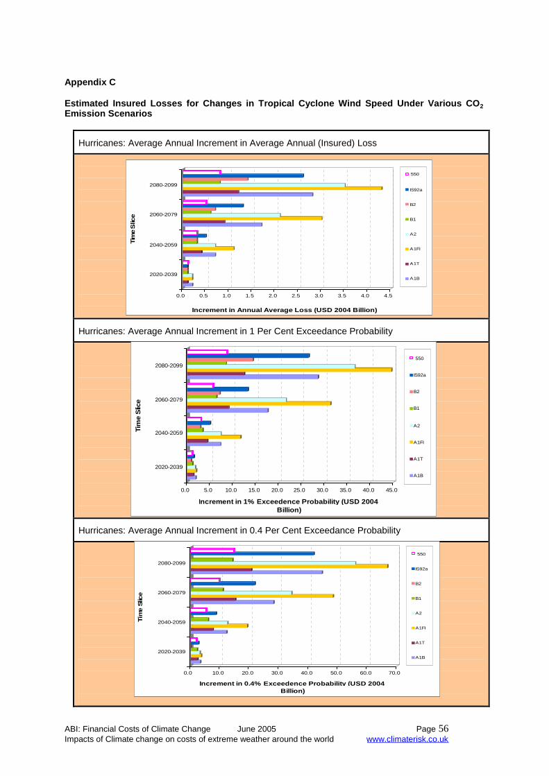
ABI: Financial Costs of Climate Change June 2005 Page 56Impacts of Climate change on costs of extreme weather around the world www.climaterisk.co.uk
Appendix C
Estimated Insured Losses for Changes in Tropical Cyclone Wind Speed Under Various CO2Emission Scenarios
Hurricanes: Average Annual Increment in Average Annual (Insured) Loss
Hurricanes: Average Annual Increment in 1 Per Cent Exceedance Probability
Hurricanes: Average Annual Increment in 0.4 Per Cent Exceedance Probability
0.0 0.5 1.0 1.5 2.0 2.5 3.0 3.5 4.0 4.5
Increment in Annual Average Loss (USD 2004 Billion)
2020-2039
2040-2059
2060-2079
2080-2099
Tim
eS
lice
550
IS92a
B2
B1
A2
A1FI
A1T
A1B
0.0 5.0 10.0 15.0 20.0 25.0 30.0 35.0 40.0 45.0
Increment in 1% Exceedence Probability (USD 2004Billion)
2020-2039
2040-2059
2060-2079
2080-2099
Tim
eS
lice
550
IS92a
B2
B1
A2
A1FI
A1T
A1B
0.0 10.0 20.0 30.0 40.0 50.0 60.0 70.0
Increment in 0.4% Exceedence Probability (USD 2004Billion)
2020-2039
2040-2059
2060-2079
2080-2099
Tim
eSlic
e
550
IS92a
B2
B1
A2
A1FI
A1T
A1B
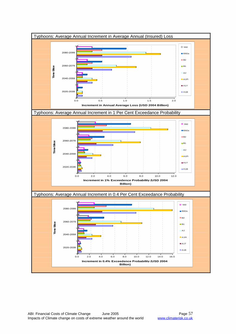
ABI: Financial Costs of Climate Change June 2005 Page 57Impacts of Climate change on costs of extreme weather around the world www.climaterisk.co.uk
Typhoons: Average Annual Increment in Average Annual (Insured) Loss
Typhoons: Average Annual Increment in 1 Per Cent Exceedance Probability
Typhoons: Average Annual Increment in 0.4 Per Cent Exceedance Probability
0.0 0.5 1.0 1.5 2.0
Increment in Annual Average Loss (USD 2004 Billion)
2020-2039
2040-2059
2060-2079
2080-2099Tim
eSlic
e
550
IS92a
B2
B1
A2
A1FI
A1T
A1B
0.0 2.0 4.0 6.0 8.0 10.0 12.0
Increment in 1% Exceedence Probability (USD 2004Billion)
2020-2039
2040-2059
2060-2079
2080-2099
Tim
eS
lice
550
IS92a
B2
B1
A2
A1FI
A1T
A1B
0.0 2.0 4.0 6.0 8.0 10.0 12.0 14.0 16.0
Increment in 0.4% Exceedence Probability (USD 2004Billion)
2020-2039
2040-2059
2060-2079
2080-2099
Tim
eSlic
e
550
IS92a
B2
B1
A2
A1FI
A1T
A1B

ABI: Financial Costs of Climate Change June 2005 Page 58Impacts of Climate change on costs of extreme weather around the world www.climaterisk.co.uk
Appendix D
Reduction in Probable Maximum (Insured) Losses in Moving from IPCC SRESA1 Family Group to 550 Stabilisation Scenario: Hurricanes and Typhoons
Illustration of the Benefits of Moving to a Lower Emission Path For Various Future TimeSlices: Change in 1% Exceedence Probability(a) Hurricanes (b) Typhoons
Illustration of the Benefits of Moving to a Lower Emission Path For Various Future TimeSlices: Change in 0.4% Exceedence Probability(a) Hurricanes (b) Typhoons
0.0 10.0 20.0 30.0 40.0
Reduction in 1% Exceedence Probability(USD 2004 Billion)
2020-2039
2040-2059
2060-2079
2080-2099
Tim
eS
lice
A1FI
A1T
A1B
0.0 2.0 4.0 6.0 8.0 10.0
Reduction in 1% Exceedence Probability(USD 2004 Billion)
2020-2039
2040-2059
2060-2079
2080-2099
Tim
eS
lice
A1FI
A1T
A1B
0.0 10.0 20.0 30.0 40.0 50.0 60.0
Reduction in 0.4% Exceedence Probability(USD 2004 Billion)
2020-2039
2040-2059
2060-2079
2080-2099
Tim
eS
lice
A1FI
A1T
A1B
0.0 2.0 4.0 6.0 8.0 10.0 12.0 14.0
Reduction in 0.4% Exceedence Probability(USD 2004 Billion)
2020-2039
2040-2059
2060-2079
2080-2099
Tim
eS
lice
A1FI
A1T
A1B
ABI: Financial Costs of Climate Change June 2005 Page 59Impacts of Climate change on costs of extreme weather around the world www.climaterisk.co.uk
3.16 References
Beniston, M., Stephenson, D. B., Christensen, O. B., Ferro, C. A. T., Frei, C., Goyette, S.,Halsnaes, K., Holt, T., Jylha, K., Koffi, B., Palutiokof, J., Scholl, R., Semmler, T. and Woth, K.(2004) Future Extreme Evnets in European Climate: An Exploration of Regional ClimateModel Projections. Joint Paper PRUDENCE WP5.
Broccoli, A.J. and S. Manabe (1990) “Can Existing Climate Models be Used to StudyAnthropogenic Changes in Tropical Cyclone Intensity?”, Geophysical Research Letters, 17:1917-20.
Broccoli, A.J., S. Manabe, J.F.B. Mitchell and L. Bengtsson (1995) Comments on “Global:Climate Change and Tropical Cyclones: Part II”, Bulletin of the American MeteorologicalSociety, 76:2243-45.
Carnell, R. E. and C.A. Senior (1998) "Changes in Mid-latitude Variability due to IncreasingGreenhouse Gases and Sulphate Aerosols", Climate Dynamics, 14: 369-383.
Chan, J.C.L. (1985) “Tropical Cyclone Activity in the Northwest Pacific in Relation to the ElNiño/Southern Oscillation Phenomenon”, Monthly Weather Review, 113: 599-606.
Chan, J.C.L. and J. Shi (1996) “Long-term Trends and Inter-annual Variability in TropicalCyclone Activity over the Western North Pacific”, Geophysical Research Letters, 23: 2765-2767.
Chang, J-C. (1996) “An Exploratory Study of the Relationship Between Annual Frequency ofInvaded Typhoons in Taiwan and El Niño/Southern Oscillation”, Terrestrial, Atmospheric andOceanic Sciences, 7: 83-105.
Chia, H.H. and C.F. Ropelewski (2002) "The Inter-annual Variability in the Genesis Locationof Tropical Cyclone sin the Northwest Pacific", Journal of Climate, 15: 2934-2944.
Chu, P.-S. and J.D. Clark (1999) “Decadal Variations of Tropical Cyclone Activity over theCentral North Pacific”, Bulletin of American Meteorological Society, 80(9): 2717-1881.
Coles, S. (2001) An Introduction to Statistical Modelling of Extreme Values, Springer: LondonBerlin Heidelberg.
Converium (2004) “Climate Change and Its Impact on Tropical Cyclones”, Global NaturalHazards, Converium Re, Zurich, Switzerland.
CSU (2004) “Forecast of Atlantic Hurricane Activity from October 2004 and Seasonal Updatethrough September”, Department of Atmospheric Science, Colorado State University.
Diaz, H. F. and R.S. Pulwarty (editors) (1997) Hurricanes: Climate and Socio-economicImpacts, New York: Springer-Verlag: 292.
Elsner, J.B. and T.H. Jagger (2004) "Florida Hurricane Decline Linked to Surface Warming",26th Conference on Hurricanes and Tropical Meteorology, 2-7 May 2004, Miami, FL.
Elsner, J.B., B.H. Bossak and X. Niu (2001) "Secular Changes to the ENSO-US HurricaneRelationship", Geophysical Research Letters, 28: 4123-4126.
Elsner, J.B., G.S. Lehmiller and T.B. Kimberlain (1996) “Objective Classification of AtlanticHurricanes”, Journal of Climate, 9: 2880-88.
Emanuel, K.A. (1986) “An Air-sea Interaction Theory for Tropical Cyclones. Part I: Steady-state maintenance”, Journal of the Atmospheric Sciences, 43: 585-604.
ABI: Financial Costs of Climate Change June 2005 Page 60Impacts of Climate change on costs of extreme weather around the world www.climaterisk.co.uk
Emanuel, K.A. (1995) Comments on “Global Climate Change and Tropical Cyclones: Part II”,Bulletin of the American Meteorological Society, 76: 2241-43.
Flather, R. and J. Smith (1998) "First Estimates of Changes in Extreme Storm SurgeElevation due to Doubling CO2", Global Atmos. Ocean Systems, 6:193-208.
Goldenberg, S.B., C.W. Landsea, A.M. Mestas-Nunez and W.M. Gray (2001) "The RecentIncrease in Atlantic Hurricane Activity: Causes and Implications", Science, 293: 474-479.
Gray, W.M. (1968) “Global View of the Origin of Tropical Disturbances and Storms”, MonthlyWeather Review, 96: 669-700.
Gray, W.M. (1979) “Hurricanes: Their Formation, Structure and Likely Role in the GeneralCirculation”, Meteorology Over the Tropical Oceans, D.B. Shaw (Editor), Royal MeteorologicalSociety, Berks: 155-218.
Gray, W.M. (1990) “Strong Association Between West African Rainfall and U.S. Landfall ofIntense Hurricanes”, Science, 249: 1251-56.
Haarsma, R.J., J.F.B. Mitchell and C.A. Senior (1993) “Tropical Disturbances in a GCM”,Climate Dynamics, 8: 247-57.
Hanson, C. E. (2001) "A Cyclone Climatology of the North Atlantic and its Implications for theInsurance Market", PhD Thesis, University of East Anglia, UK.
Hanson, C. E., T. Holt and J.P. Palutikof (2004) "An Integrated Assessment of the Potentialfor Change in Storm Activity over Europe: Implications for Insurance and Forestry in the UK",Tyndall Centre for Climate Change Research, UK.
Hasegawa, A. (2005) “Tropical Cyclone and Heavy Precipitation Over the Western NorthPacific in Present and Doubled CO2 Climate Simulations”, 2nd International Workshop on theKyosei Project, 24-26th February 2005, Hawaii.
Henderson-Sellers, A., H. Zhang, G. Berz, K. Emanuel, W. Gray, C. Landsea, G. Holland, J.Lighthill, S.-L. Shieh, P. Webster and K. McGuffie (1998) “Tropical Cyclones and GlobalClimate Change: A Post-IPCC Assessment, Bulletin of the American Meteorological Society,79(1): 19-38.
Holland, G.J. (1997) “The Maximum Potential Intensity of Tropical Cyclones”, Journal ofAtmospheric Science, 54: 2519-2541.
Houghton, J.T., L.G. Meira Filho, B.A. Callander, N. Harris, A. Kattenberg, and K. Maskell(1996) Climate Change 1995: The Science of Climate Change, Contribution of WorkingGroup I to the Second Assessment of the Intergovernmental Panel on Climate Change,Cambridge University Press, pp. 572.
Idso, S.B., R.C. Balling Jr. and R.S. Cerveny (1990) “Carbon Dioxide and Hurricanes:Implications of Northern Hemispheric Warming for Atlantic/Caribbean Storms”, Meteorologyand Atmospheric Physics, 42: 259-63.
IHT / Asahi (2004) “Typhoons: Fewer But Stronger?”, The Asahi Shibum, September 28th
2004 (www.asahi.com/english/).
Karl, T.R., N. Nicholls and J. Gregory (1997) “The Coming Climate”, Scientific American , 276:79-83.
Karl, T.R., R.W. Knight, D.R. Easterling and R.G. Quayle (1995) “Trends in U.S. ClimateDuring the Twentieth Century”, Consequences, 1: 3-12.

ABI: Financial Costs of Climate Change June 2005 Page 61Impacts of Climate change on costs of extreme weather around the world www.climaterisk.co.uk
Karl, T.R., R.W. Knight, D.R. Easterling and R.G. Quayle (1996) “Indices of Climate Changefor the United States”, Bulletin of the American Meteorological Society, 77: 279-291.
Klawa, M. and U. Ulbrich (2003) "A Model for the Estimation of Storm Losses and theIdentification of Severe Storms in Germany", Natural Hazards and Earth System Sciences, 3:725-732.
Knippertz, P., U. Ulbrich and P. Speth (2000) "Changing Cyclones and Surface Wind Speedsover North Atlantic and Europe in a Transient GHG Experiment", Climate Research, 15(2):109-122.
Knutson, T.R. (2002) “Modelling the Impact of Future Warming on Tropical Cyclone Activity”,IPCC Workshop on Extreme Weather and Climate Events, Workshop Report, Beijing, China,11-13 June, 2002.
Knutson, T.R. and R.E. Tuleya (1999) “Increased Hurricane Intensities with CO2-inducedWarming as Simulated Using the GFDL Hurricane Prediction System”, Climate Dynamics 15:503-519.
Knutson, T.R. and R.E. Tuleya (2004) “Impact of CO2 Induced Warming on SimulatedHurricane Intensity and Precipitation: Sensitivity to the Choice of Climate Model andConvective Parameterisation”, Journal of Climate, 17(18): 3477–3495.
Knutson, T.R., R.E. Tuleya and Y. Kurihara (1999) “Simulated Increase of HurricaneIntensities in a CO2-warmed Climate”, Science, 279: 1018-1020.
Knutson, T.R., R.E. Tuleya, W. Shen and I. Ginis (2001) “Impact of CO2 Induced Warming onHurricane Intensities as Simulated in a Hurricane Model with Ocean Coupling”, Journal ofClimate, 14: 2458–2468.
Kuzmina, S., L. Bengtsson, O. Johannessen, H. Drange, L. Bobylev and M. Miles (2005) ”TheNorth Atlantic Oscillation and Greenhouse Gas Forcing”, submitted to Geophysical ResearchLetter.
Lambert, S. J. (1996) "Intense Extra-tropical Northern Hemisphere Winter Cyclone Events:1899-1991", Journal Geophysical Research, 101(16): 21319-21325.
Landsea, C.W. (1993) “A Climatology of Intense (or Major) Atlantic Hurricanes”, MonthlyWeather Review, 121: 1703-13.
Landsea, C.W., N. Nicholls, W.M. Gray and L.A. Avila (1996) “Downward Trends in theFrequency of Intense Atlantic Hurricanes During the Past Five Decades”, GeophysicalResearch Letters, 23: 1697-700.
Landsea, C.W., R.A. Pielke Jr., A.M. Mestas Nunez and J.A. Knaff (1999) “Atlantic BasinHurricanes: Indices of Climate Changes”, Climatic Change, 42: 89-129.
Langenberg, H., A. Pfizenmayer, H. Von Storch, and J. Sundermann, (1999) "Storm RelatedSea Level Variations Along the North Sea Coast: Natural Variability and AnthropogenicChange", Cont. Shelf Research, 19: 821-842.
Leckebusch, G. C. and U. Ulbrich (2004) "On the Relationship Between Cyclones andExtreme Wind Storms over Europe Under Climate Change", submitted to Global andPlanetary Change.
Li, S. (1996) “Estimating Tropical Cyclone Intensity from Climate Models”, M.Sc. (Honours)Thesis, Climatic Impacts Centre, Macquarie University, Sydney, Australia, pp. 136.
ABI: Financial Costs of Climate Change June 2005 Page 62Impacts of Climate change on costs of extreme weather around the world www.climaterisk.co.uk
Lighthill, J., G. Holland, W. Gray, C. Landsea, G. Craig, J. Evans, Y. Kurihara and C. Guard(1994) “Global Climate Change and Tropical Cyclones”, Bulletin of the AmericanMeteorological Society, 75: 2147-57.
Lowe, J. A., J.M. Gregory and R.A. Flather (2001) Changes in the Occurrence of StormSurges in the United Kingdom under a Future Climate Scenario using a Dynamic StormSurge Model Driven by the Hadley Centre Climate Models", Climate Dynamics, 18: 197-188.
Malmquist, D. L. (editor) (1999) European Windstorms and the North Atlantic Oscillation:Impacts, Characteristics, and Predictability, Risk Prediction Initiative, Bermuda BiologicalStation for Research, Inc, RPI Series No. 2, pp. 21.
Meehl, G.A., F. Zwiers, J. Evans, T. Knutson, L. Mearns and P. Whetton (2000) “Trends inExtreme Weather and Climate Events: Issues Related to Modelling Extremes in Projections ofFuture Climate Change”, Bulletin of the American Meteorological Society, 81(3): 427-436.
Murray, R. J. and I. Simmonds (1991) "A Numerical Scheme for Tracking Cyclone Centresfrom Digital Data. Part I: Development and Operation of the Scheme", Aust. Met. Mag., 39:155-166.
Neumann, C.J. (1993) Global Guide to Tropical Cyclone Forecasting, WMO/TC-No. 560,Report No., TCP-31, World Meteorological Organisation, Geneva.
O'Brien, S.T., B.P. Hayden and H.H. Shugart (1992) “Global Climatic Change, Hurricanes,and a Tropical Forest”, Climatic Change, 22: 175-90.
Rauthe, M., A. Hense and H. Paethe (2004) "A Model Inter-comparison Study of ClimateChange Signals in Extra-tropical Circulation", International Journal of Climatology, 24: 643-662.
Ryan, B.F., I.G. Watterson and J.L. Evans (1992) “Tropical Cyclone Frequencies Inferredfrom Gray's Yearly Genesis Parameter: Validation of GCM Tropical Climates”, GeophysicalResearch Letters, 19: 1831-34.
Saunders, M.A. and A.R. Harris (1997) “Statistical Evidence Links Exceptional 1995 AtlanticHurricane Season to Record Sea Warming”, Geophysical Research Letters, 24: 1255-58.
Schinke, H. (1993) "On the Occurrence of Deep Cyclones over Europe and the North Atlanticfor the Period 1930-1991", Beitr. Phys. Atmosph, 66: 223-237.
Schubert, M., R. Perlwitz, R. Blender, K. Fraedrich and F. Lunkeit (1998) "North AtlanticCyclones in CO2-induced Warm Climate Simulations: Frequency, Intensity and Tracks",Climate Dynamics, 14: 827-837.
Senior, C. (2002) “Modelling Changes in Extreme Events”, IPCC Workshop on ExtremeWeather and Climate Events, Workshop Report, Beijing, China, 11-13 June, 2002.
STOWASUS-Group (2001) "Regional Storm, Wave and Surge Scenarios for the 2100Century", Stowasus-Final Report, DMI, EU commission.
Tsutsui, J. and A. Kasahara (1996) “Simulated Tropical Cyclones Using the National Centrefor Atmospheric Research Community Climate Model”, Journal Geophysical Research,101(10): 15013-15-032.
Tsutsui, J., H. Hatsushika and H. Kitabata (2004) "Inter-annual Variability or Tropical CycloneFrequencies Implied from an Ensemble Climate Simulation with the NCAR CommunityAtmosphere Model", 26th Conference on Hurricanes and Tropical Meteorology, 2-7 May 2004,Miami, FL.

ABI: Financial Costs of Climate Change June 2005 Page 63Impacts of Climate change on costs of extreme weather around the world www.climaterisk.co.uk
UKCIP (2002) Climate Change Scenarios for the United Kingdom, The UKCIP02 ScientificReport, the UK Climate Impacts Programmes, Oxford.
Walsh, K.J.E., K.C. Nguyen and J.L. McGregor (2004) "Climate Change, Tropical Cyclonesand ENSO", 26th Conference on Hurricanes and Tropical Meteorology, 2-7 May 2004, Miami,FL.
WASA-Group (1998) "Changing Waves and Storms in the Northern Atlantic?", Bulletin of theAmerican Meteorological Society, 79: 741-760.
Yoshimura, J., Oouchi, K., Yoshimura, H., Mizuta, R., Kusunoki, S. and A. Noda (2005)“Influences of Global Warming on the Tropical Cyclone Climatology as Simulated in a 20-km-mesh Global Atmosphere Model”, 2nd International Workshop on the Kyosei Project, 24-26th
February 2005, Hawaii.

ABI: Financial Costs of Climate Change June 2005 Page 64Impacts of climate change on costs of UK extreme weather www.climaterisk.co.uk
4.0 Impacts of climate change on costs of UK extremeweather
The consequences of climate change may have significant economic effects at thenational scale. This section considers the flooding and subsidence impacts onproperty caused by climate change and estimates the costs of this for the UK.
4.1 Flooding
In this section we present cost estimates of the climate change-induced futureimpacts of flooding on property in the UK. These estimates are derived principallyfrom the outputs of the DTI-sponsored Foresight Study entitled the Flood and CoastalDefence project37. Four specific sources of damage to property are considered:coastal flooding; intra-urban flooding and fluvial flooding. We assume that all propertyis insured and insurable.
Method
Step 1. Physical impact assessment
Estimation of the physical flood damage within the Foresight project was made basedon a bottom-up process that primarily made use of the Risk Assessment for flood andcoastal defence systems for Strategic Planning (RASP) system previously developedfor Defra. Essentially, the RASP system allows climate and socio-economic changesto be imposed on geographically mapped physical receptors on a national (English)scale, thereby generating estimates of the number of physical units impacted byflooding. A similar although much more approximate attempt was made in the projectto assess the risks of urban flooding, where simple urban drainage models were up-scaled to generate national estimates of the risks of urban flooding. Risks due tocoastal erosion, using the outputs of the Future Coast project, another Defraresearch project38. The data necessary to apply these risk analysis methods were notuniversally available in Scotland and Northern Ireland, and where this was the casemore approximate analyses were conducted.
The principal determinants – or drivers - of the size of impacts of flood risk identifiedin the Foresight study included:
Climate change (precipitation and temperature) Catchment run-off Fluvial systems and processes Flood management Human behaviour Socio-economics Coastal processes (including coastal climate change factors)
37 Future flooding, Office of Science and Technology Foresight Programme, April 2004,http://www.foresight.gov.uk/previous_projects/flood_and_coastal_defence38 www.defra.gov.uk /environ/fcd/futurecoast.htm

ABI: Financial Costs of Climate Change June 2005 Page 65Impacts of climate change on costs of UK extreme weather www.climaterisk.co.uk
The UKCIP02 climate scenarios39 have been employed. These scenarios are basedon four emissions scenarios corresponding to the SRES scenarios – as identifiedbelow. The Foresight Futures socio-economic scenarios developed by researchers atthe Science and Technology Policy Research, University of Sussex (SPRU) for theOffice of Science and Technology (OST, 2002) were employed. These scenarios arebroadly consistent with the UKCIP socio-economic scenarios, and can also bemapped on to the climate scenarios – as shown in Table 4.1.
Table 4.1: Correspondence between SRES, UKCIP02 scenarios and Foresight Futures
SRES UKCIP02 ForesightFutures 2020
Commentary
B1 Lowemissions
Globalsustainability
Medium-high growth, but low primary energyconsumption. High emphasis on international actionfor environmental goals (e.g. greenhouse gasemissions control). Innovation of new and renewableenergy sources.
B2 Medium-lowemissions
Localstewardship
Low growth. Low consumption. However, lesseffective international action. Low innovation.
A2 Medium-highemissions
Nationalenterprise
Medium-low growth, but with no action to limitemissions. Increasing and unregulated emissionsfrom newly industrialised countries.
A1F1 Highemissions
World markets Highest national and global growth. No action to limitemissions. Price of fossil fuels may drivedevelopment of alternatives in the long term.
The Foresight project focussed on two of the three time slices used in the UKCIP02scenarios, corresponding to the 2050s and 2080s. In the section below, we providean extrapolation of the cost estimates for these time-slices back to the 2020s to givea first indication of the possible scale of costs in this time period.
In order to quantify the effect of climate change induced flooding on property – bothresidential and business - we need to be able to isolate it from non-climate change-induced flooding. The non-climate change baseline was therefore estimated byidentifying i) the present day property impacts associated with a given weather event,and ii) the frequency of such an event in a non-climate change context (i.e. historicalfrequency). In the Foresight study, the baseline assumption on the future course offlood management was that current flood and coastal management policy was keptthe same across all scenarios, including the current pattern of expenditure andtechnical approach. This present day flood and coastal management policy isreferred to as the baseline flood management policy. Analysis of changing climateand socio-economic scenarios were superimposed on this fixed flood managementpolicy, in order to assess the capacity of the current policy to cope with long-termchanges.
Once the number of properties subject to flooding as a consequence of given presentday weather events are estimated, the Foresight method estimates the frequency ofthe weather event under climate change scenarios in future time periods, enablingcomparison of total physical property impacts under non-climate change and climatechange frequencies of the weather events. The difference between the two totals
39 Climate change scenarios for the United Kingdom, UK Climate Impacts Programme. Hulme et al. April2002. www.ukcip.org.uk
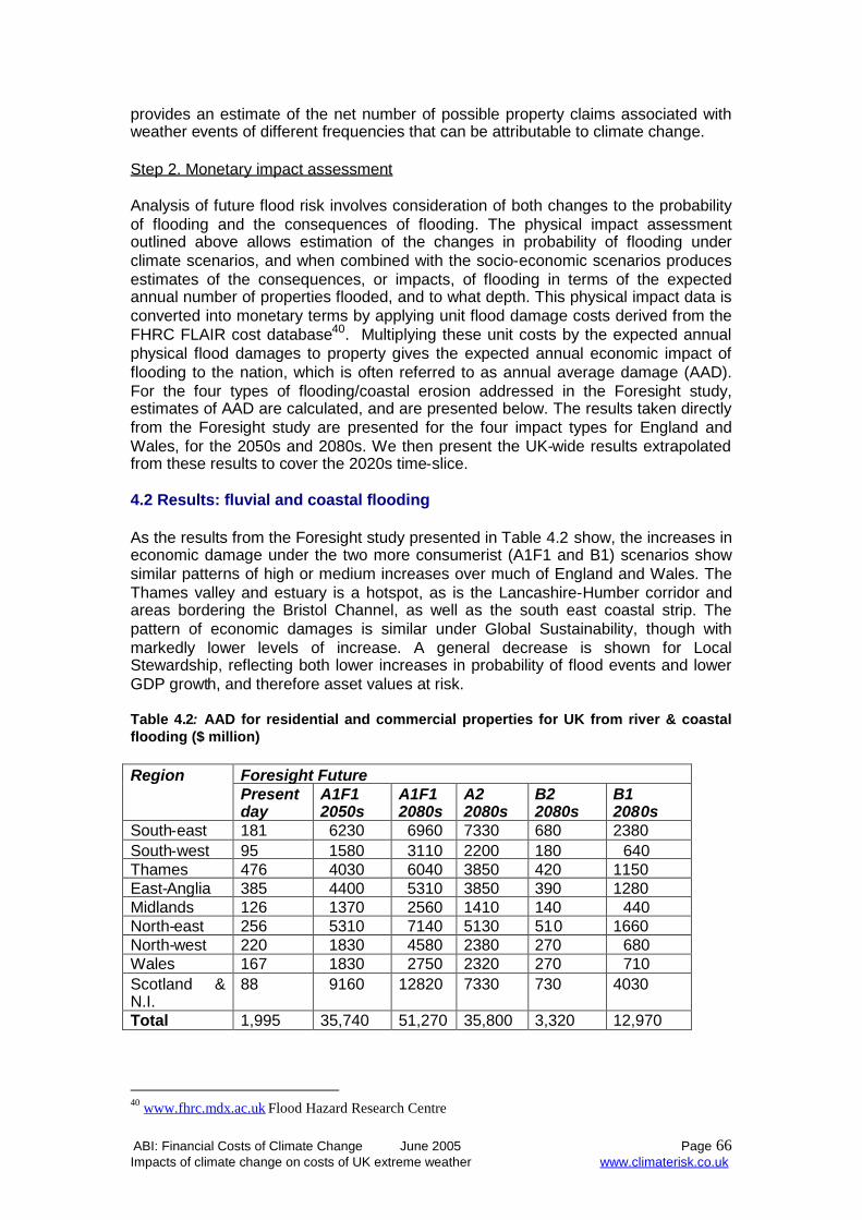
ABI: Financial Costs of Climate Change June 2005 Page 66Impacts of climate change on costs of UK extreme weather www.climaterisk.co.uk
provides an estimate of the net number of possible property claims associated withweather events of different frequencies that can be attributable to climate change.
Step 2. Monetary impact assessment
Analysis of future flood risk involves consideration of both changes to the probabilityof flooding and the consequences of flooding. The physical impact assessmentoutlined above allows estimation of the changes in probability of flooding underclimate scenarios, and when combined with the socio-economic scenarios producesestimates of the consequences, or impacts, of flooding in terms of the expectedannual number of properties flooded, and to what depth. This physical impact data isconverted into monetary terms by applying unit flood damage costs derived from theFHRC FLAIR cost database40. Multiplying these unit costs by the expected annualphysical flood damages to property gives the expected annual economic impact offlooding to the nation, which is often referred to as annual average damage (AAD).For the four types of flooding/coastal erosion addressed in the Foresight study,estimates of AAD are calculated, and are presented below. The results taken directlyfrom the Foresight study are presented for the four impact types for England andWales, for the 2050s and 2080s. We then present the UK-wide results extrapolatedfrom these results to cover the 2020s time-slice.
4.2 Results: fluvial and coastal flooding
As the results from the Foresight study presented in Table 4.2 show, the increases ineconomic damage under the two more consumerist (A1F1 and B1) scenarios showsimilar patterns of high or medium increases over much of England and Wales. TheThames valley and estuary is a hotspot, as is the Lancashire-Humber corridor andareas bordering the Bristol Channel, as well as the south east coastal strip. Thepattern of economic damages is similar under Global Sustainability, though withmarkedly lower levels of increase. A general decrease is shown for LocalStewardship, reflecting both lower increases in probability of flood events and lowerGDP growth, and therefore asset values at risk.
Table 4.2: AAD for residential and commercial properties for UK from river & coastalflooding ($ million)
Foresight FutureRegionPresentday
A1F12050s
A1F12080s
A22080s
B22080s
B12080s
South-east 181 6230 6960 7330 680 2380South-west 95 1580 3110 2200 180 640Thames 476 4030 6040 3850 420 1150East-Anglia 385 4400 5310 3850 390 1280Midlands 126 1370 2560 1410 140 440North-east 256 5310 7140 5130 510 1660North-west 220 1830 4580 2380 270 680Wales 167 1830 2750 2320 270 710Scotland &N.I.
88 9160 12820 7330 730 4030
Total 1,995 35,740 51,270 35,800 3,320 12,970
40 www.fhrc.mdx.ac.uk Flood Hazard Research Centre

ABI: Financial Costs of Climate Change June 2005 Page 67Impacts of climate change on costs of UK extreme weather www.climaterisk.co.uk
Using a process of linear extrapolation from the time slice centred on the 2080s tothose centred on the 2020s and 2050s we derive estimates of the total AADs for riverand coastal flooding in the UK, as presented in table 4.3
Table 4.3: AAD estimates for fluvial and coastal flooding under the low (B1) and high(A1F1) climate emission scenarios in UK ($m).
B1 A1F12020s 6,000 22,0002050s 9,000 37,0002080s 13,000 50,000
4.3 Intra-urban flood risk
Table 4.4 below shows estimated changes in the AAD in the UK from intra-urbanflooding. It should be noted that this does not include the cost of household or localflooding as a result of direct pluvial effects or of flood waves from sources external tothe urban area.
Table 4.4: AAD in the UK due to Intra-urban Flooding ($ million)
Pres. A1F1 A2 B2 B12050s 2080s 2050s 2080s 2050s 2080s 2050s 2080s
UK 900 9,700 27,500 9,700 18,300 1,600 2,400 2,900 6,400
Using a process of linear extrapolation from the time slice centred on the 2080s tothose centred on the 2020s and 2050s we derive estimates of the total AADs forintra-urban flooding in the UK, as presented in Table 4.5.
Table 4.5: AAD estimates for intra-urban flooding under the low (B1) and high (A1F1)climate emission scenarios in UK ($m).
B1 A1F12020s 1,800 5,0002050s 2,900 9,7002080s 6,400 27,500
4.4 Mitigation and adaptation of flood impacts
The future costs associated with the three impact types discussed above arepresented together over the three time-slices. The two climate scenarios featured arerepresentative of high (A1F1) and low (B1) emission (and their corresponding socio-economic) scenarios, and therefore give an idea of the range of uncertaintysurrounding the estimates of future flood and erosion costs. One may want to takethe difference between two scenarios as being a representation of the benefits of amitigation policy that allowed emissions to move from a high to a low emissionsscenario. The problem with this approach is that the A and B socio-economic story-lines which underlie these emission scenarios are inconsistent with each other sothat emission reductions between the two are nonsensical. We therefore includethem simply to illustrate the range of costs associated with high and low emissionscenarios.

ABI: Financial Costs of Climate Change June 2005 Page 68Impacts of climate change on costs of UK extreme weather www.climaterisk.co.uk
On the basis of the evidence in the Foresight study (specifically, Chart 2.10 in theExecutive Summary) of the relative importance of different climate and socio-economic drivers in determining the size of flood risks we make a crude assumptionthat a maximum of 50% of the total costs are specifically related to climate change.We make an adjustment on this basis in Table 4.6.
Table 4.6: Total AADs for time-dependent flood impacts in the UK under high and lowemission scenarios
B1 A1F12020sriver & coast flooding 3,600 11,900intra-urban flooding 640 2,2002050sriver & coast flooding 5,500 17,400intra-urban flooding 1,190 4,6002080sriver & coast flooding 7,300 26,600intra-urban flooding 2,900 13,500
The Foresight study also compares the baseline – i.e. no change from present floodmanagement strategies - impact costs for riverine and coastal flooding presentedabove with the residual impact costs that would result from the imposition of anintegrated portfolio of responses that includes elements of catchment-wide storage,land-use planning and realignment of coastal defences. This comparison betweenthe impact costs in the baseline and from an integrated adaptation response to riverand coastal flooding is presented for the 2080s time-slice in table 4.7.
Table 4.7: AADs for net climate flooding in baseline and adapted 2080s futures ($m)
A1F1 B1
Baseline - river 26,600 7,300-intra-urban 13,500 2,900Integratedresponse -river 1,800 3,300-intra-urban 5,500 550
Table 4.7 indicates the extent to which river, coastal and intra-urban flood impactsmay be reduced by appropriate measures. However, it should be borne in mind thatthe cost reduction does not include any costs associated with the introduction of theadaptation measures themselves. Engineering costs of flood management additionalto those under present regimes were estimated within the Foresight study to bebetween $18 million (£10 million) and $54 million (£30 million) per year over theperiod to 2100, suggesting – dependent on the cost of non-engineering responses –that an integrated adaptation response of the type investigated by Foresight iseconomically efficient.

ABI: Financial Costs of Climate Change June 2005 Page 69Impacts of climate change on costs of UK extreme weather www.climaterisk.co.uk
4.5 Subsidence
In this sub-section we present estimates of the economic costs associated with thesubsidence impacts on households in the UK under future climate change scenarios.This note is based on the findings of a recently completed case study undertaken forABI and UKCIP41. Economic costs are split into two elements: insured and non-insured. Subsidence impacts to domestic property42 are likely to arise from thecombination of reduced rainfall and above-average temperatures predicted tobecome more frequent in the UKCIP02 climate change scenarios43. As the basis ofsuch estimates we initially take the unusually dry and warm conditions that existed inthe UK in summer 2003 as an historical analogue.
Method
Step 1. Physical impact assessment
In order to quantify the effect of climate change on subsidence we need to be able toisolate it from non-climate change-induced subsidence. We therefore estimate thenon-climate change baseline by identifying i) the subsidence incidence associatedwith a given weather event as an historical analogue, and ii) the frequency of such anevent in a non-climate change context (i.e. historical frequency).
i) We assume that the summer 2003 warm weather event is representative of a typeof weather event that results in an increased incidence of subsidence in the UK.Thus, if we are able to identify the claims additional to those expected in a year ofaverage temperatures we can estimate the excess number of claims that can beattributed to such a weather event of a given non-climate change frequency. Toidentify these additional claims we use the historical aggregate claim series datacompiled by the ABI. We derive an estimate of 22,000 excess claims, whichrepresents an increase of 69% on the average annual number of claims.
In order to estimate the total physical impact in future time periods under climate andnon-climate change scenarios we consider the possible effects of socio-economicchange on the number of properties that might be vulnerable to subsidence. We usethe UKCIP (2001) socio-economic scenarios (SESs) developed for climate impactassessment as a starting point. The resulting estimates are driven solely by theinformation given in these scenarios relating to population and household size.Estimates for future time periods and scenarios range from approximately 15,000 to35,000 cases of subsidence for a summer 2003 warm weather event.
ii) Once the number of properties subject to subsidence as a consequence of a givenweather event - Summer 2003 is characterised as a 1 in 100 year event - has beenderived, we estimate the frequency of the weather event under climate changescenarios in future time periods. We can then compare total expected annualsubsidence incidence, (i.e. number of subsidence claims associated with a givenevent severity * frequency of the given event), under non-climate change and climatechange frequencies of the weather event, aggregated over the time period to 2100.The difference between these two totals provides an estimate of the net number ofclaims associated with a weather event of this severity that can be attributable to
41 Metroeconomica (forthcoming). Property & Insurance Case Study. UKCIP42 Graves and Phillipson (2000) report that it is primarily the domestic building stock that is affected bysubsidence since commercial and industrial buildings tend to have deeper foundations and be moreheavily loaded, thereby eliminating the potential for subsidence.43 Climate change scenarios for the United Kingdom, UK Climate Impacts Programme. Hulme et al. April2002. www.ukcip.org.uk

ABI: Financial Costs of Climate Change June 2005 Page 70Impacts of climate change on costs of UK extreme weather www.climaterisk.co.uk
climate change. The output of this calculation is an input into the monetary impactassessment.
Step 2. Monetary impact assessment
The second step is to identify and estimate the expenditure incurred to replace (orrestore) the asset damaged as a result of climate change, in unit cost terms. In thebuilding subsidence context, domestic householders spread the risk of the cost bymaking annual payments (premiums) to insurance companies in return for coverageof the repair cost in the event of subsidence44. Aggregate historical data onsubsidence claims supplied by the ABI for Great Britain are used to derive unit valuesin a range between $12,800 (£7000) and $22,000 (£12,000). These figures comparewith a unit value of £10,000 adopted by Graves & Phillipson45 (2000) and Driscoll &Crilly46 (2000) in their analyses of climate change impacts on subsidence incidencefor the Building Research Establishment, themselves derived from the typical costs ofundertaking specific remedial work in the event of property subsidence. We assume$18,000 (£10,000) as a central value.
Note that the ABI aggregate data does not include all the cost of the subsidencedamage. It is currently standard practice in the arrangements for buildings insurancecoverage in the UK to require the policy holder (the householder) to contribute aninitial increment of the cost of subsidence damage that is being claimed against thepolicy. Typical increment payments average about $1,800 (£1000) per property.Thus, the $18,000 (£10,000) total replacement cost per case of subsidence mayreasonably be disaggregated into two components: $1,800 (£1000) borne by thehousehold; $16,200 (£9000) borne by the insurance company in order to reflect therelative cost burdens.
Step 3. Aggregation
At this point, the aggregate number of properties estimated to be subject tosubsidence under alternative non-climate and climate scenarios are multiplied by theunit cost of $18,000 (£10,000) per property and the probability of the weather eventin the respective climate scenario to give an annual expected subsidence damagecost. i.e.
No. of properties X probability of weather event X unit cost of subsidence
We estimate the annual expected subsidence damage cost for the non-climatechange reference scenario (under alternative socio-economic scenarios) and climatechange scenarios corresponding to the IPCC SRES scenarios – as labelled. We thensubtract the non-climate change costs from the costs attributed to the climatescenarios to produce the net climate change cost. The un-discounted annual totalsthat result are presented in table 4.8.
44 Note that in practice premiums are calculated as an aggregate sum to provide financialprotection for the risk of suffering from other forms of property damage or loss in addition tosubsidence. Thus, it is not possible to calculate the costs of subsidence from estimates of thepremiums paid, but rather to look at the value of the claims made by households followingsubsidence to repair damage.45 Graves H.M. and M.C. Phillipson (2000) Potential implications of climate change in the builtenvironment. FBE Report 2. December 2000.46 Driscoll & Crilly (2000) Subsidence damage to domestic buildings: lessons learned andquestions remaining. BRE & FBE. September 2000.
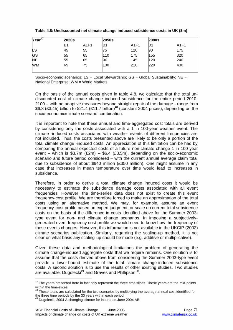
ABI: Financial Costs of Climate Change June 2005 Page 71Impacts of climate change on costs of UK extreme weather www.climaterisk.co.uk
Table 4.8: Undiscounted net climate change induced subsidence costs in UK ($m)
Year47 2020s 2050s 2080sB1 A1F1 B1 A1F1 B1 A1F1
LS 45 55 75 120 90 175GS 55 65 110 175 155 320NE 55 65 90 145 120 240WM 65 75 130 210 220 430
Socio-economic scenarios: LS = Local Stewardship; GS = Global Sustainability; NE =National Enterprise; WM = World Markets
On the basis of the annual costs given in table 4.8, we calculate that the total un-discounted cost of climate change induced subsidence for the entire period 2010-2100 – with no adaptive measures beyond straight repair of the damage - range from$6.3 (£3.45) billion to $21.4 (£11.7 billion)48 (constant 2004 prices), depending on thesocio-economic/climate scenario combination.
It is important to note that these annual and time-aggregated cost totals are derivedby considering only the costs associated with a 1 in 100-year weather event. Theclimate -induced costs associated with weather events of different frequencies arenot included. Thus, the costs presented above are likely to be only a portion of thetotal climate change -induced costs. An appreciation of this limitation can be had bycomparing the annual expected costs of a future non-climate change 1 in 100 yearevent – which is $3.7m (£2m) – $6.4 (£3.5m), depending on the socio-economicscenario and future period considered – with the current annual average claim totaldue to subsidence of about $640 million (£350 million). One might assume in anycase that increases in mean temperature over time would lead to increases insubsidence.
Therefore, in order to derive a total climate change induced costs it would benecessary to estimate the subsidence damage costs associated with all eventfrequencies. However, the time-series data does not exist to create this eventfrequency-cost profile. We are therefore forced to make an approximation of the totalcosts using an alternative method. We may, for example, assume an eventfrequency-cost profile based on expert judgment, or scale up current total subsidencecosts on the basis of the difference in costs identified above for the Summer 2003-type event for non- and climate change scenarios. In imposing a subjectively-generated event frequency-cost profile we would need to know how the frequency ofthese events changes. However, this information is not available in the UKCIP (2002)climate scenarios publication. Similarly, regarding the scaling-up method, it is notclear on what basis any scaling-up should be made (e.g. additive or multiplicative).
Given these data and methodological limitations the problem of generating theclimate change-induced aggregate costs that we require remains. One solution is toassume that the costs derived above from considering the Summer 2003-type eventprovide a lower-bound estimate of the total climate change-induced subsidencecosts. A second solution is to use the results of other existing studies. Two studiesare available: Dugolecki49 and Graves and Phillipson50.
47 The years presented here in fact only represent the three time-slices. These years are the mid-pointswithin the time-slices.48 These totals are calculated for the two scenarios by multiplying the average annual cost identified forthe three time periods by the 30 years within each period.49 Dugolecki, 2004 A changing climate for insurance.June 2004 ABI

ABI: Financial Costs of Climate Change June 2005 Page 72Impacts of climate change on costs of UK extreme weather www.climaterisk.co.uk
Dugolecki13 refers to research – unspecified – wherein a relationship betweenmeteorological conditions and historical claims costs, based on insurance companydata, was derived. When applied to climate scenario futures, this relationshipgenerated climate change induced subsidence costs of $550million (£300 million) peryear by the 2080s. Similarly, Graves and Phillipson estimate an increase in costsover today’s average annual total of between $360 million (£200 million) and $730million (£400 million) per year by the 2080s. These results compare with the range ofcosts of $165 million (£90 million) – $440 million (£240 million) per year we derive forthe Summer 2003-type event from the low emissions-global sustainability and highemissions-world markets scenarios respectively, for the time-slice centred on the2080s, and therefore appear to be broadly consistent. In the absence of otherevidence that would allow us to extend our method to other event frequencies wetherefore suggest to use the range provided by Graves and Phillipson of $360 million(£200 million) - $720 million (£400 million) per year, an effective up-scaling bybroadly a factor of 2. We adopt this scalar in Table 4.9 below.
Table 4.9: Total AADs for time-dependent subsidence impacts in the UK and potentialmitigation benefits
Time slice B1 A1F12020s 130 1602050s 220 4402080s 330 880
4.6 Adaptation
As mentioned above, the cost estimates we present are based on the assumptionthat no adaptive measures beyond straight repair of the subsidence damage areimplemented. However, this assumption may be unrealistic since a greaterawareness and understanding of climate change is likely to lead to consideration ofcost-effective adaptation. Indeed, it should be noted that the UK Government haverecently recognized the threat of increased subsidence from climate change byintroducing a new building regulation, (Building Regulation 2000 (2004 up-date)Structure A), requiring new building on clay soils to have foundations to a depth of0.75m, revised from 0.5m previously. This is part-way to the foundation depth of 1metre suggested by Driscoll & Crilly51 as being sufficient to eliminate subsidence riskto 2100.
Recent work by Metroeconomica52 provides some initial estimates of the costs andbenefits of adaptation measures in response to a summer as dry and hot as 2003,where there was an increase in subsidence claims (Table 4.10).
50 Graves H.M. and M.C. Phillipson (2000) Potential implications of climate change in the builtenvironment. FBE Report 2. December 2000.51 Driscoll & Crilly (2000) Subsidence damage to domestic buildings: lessons learned andquestions remaining. BRE & FBE. September 2000.52 Metroeconomica (forthcoming). Property & Insurance Case Study. UKCIP

ABI: Financial Costs of Climate Change June 2005 Page 73Impacts of climate change on costs of UK extreme weather www.climaterisk.co.uk
Table 4.10. Aggregate Benefits & Costs (and their distribution) of alternativeadaptation options to property subsidence. (2004 prices)
AdaptationMeasure
Benefit Cost Bearer of CostBurden
Higher insurancepremiums to coverhigher remediationcosts
Insurer covers costsof increased numberof claims
$6.6 – $22.2bnIncreased householdinsurance costs
House-owner bearsincreased costs
Withdrawal of insurancecover for propertiesvulnerable tosubsidence
Insurer avoidsincreased exposure
$6.6 – $22.2bnLoss of property value
House-owner bearsfull remediation costsand loss of propertyvaluePossible exclusion forlow income groups
Underpinning andstructural measures
$6.6 – $22.2bnMaximum avoidedloss.
$28 - $69bnTotal cost of measuresfor all properties at risk
Benefit borne byinsurer and house-ownerCost borne by house-builder or owner
Building regulationsfor:- deeper foundationsof 1 metre- building materials
$2.7 – $10.3bnNot known
$3.7 – $6.4bnNot known
Benefit borne byinsurer and house-ownerCost borne by house-builder or owner
Spatial planning policy $2.7 – $10.3bnMaximum avoided loss
Loss of land valuesand possible socialcosts of higher densityhousing
Benefit borne byinsurer and house-ownerCost borne by houseand land-owners
Clearance of nearbyvegetation orrestrictions on futureplanting
$6.6 – $22.2bnMaximum avoided loss
Not known Cost borne by houseand land owners
Regular watersprinkling ofvegetation
$6.6 – $22.2bnMax avoided loss
Not known Cost borne by houseand land owners
Note: ranges reflect cost and benefit estimates made under low and high emission scenariosassociated with a 1 in 100 year event only
These results suggest that an option of requiring deeper foundations for new-buildproperties such as the newly introduced Building Regulation is – on balance – likelyto produce a net benefit. However, spatial planning options and vegetationmanagement options need to be studied further before an economically efficientadaptation strategy can be developed. Options of withdrawal of insurance coverageor increasing premiums to reflect the higher expected costs are not attractive optionson either economic or social criteria.
ABI: Financial Costs of Climate Change June 2005 Page 74Impacts of climate change on costs of UK extreme weather www.climaterisk.co.uk
4.7 Conclusions: climate-induced flooding, erosion and subsidence impacts inthe UK.
The preceding sub-sections have summarised the findings of recent research on thecosts of climate change of three impact types on property in the UK likely to beimportant to the operations of the insurance industry: flooding, coastal erosion andsubsidence. The aggregate annual average damage estimates are presented in forthe three 30-year time-slices to 2100. Note that the results for flooding andsubsidence are not readily comparable with each other since the flooding estimatesaccount for assumed increases in the value of the assets at risk over time whilst thesubsidence estimates do not.
In the case of adaptation, evidence from the Foresight study suggests that –depending on the size of non-engineering costs involved – an integrated portfolioapproach to flood prevention may be cost-efficient. Similarly for subsidence, deeperfoundations may have a positive net benefit, though non-engineering approachessuch as spatial planning policy may also have a role in future adaptation strategies.

ABI: Financial Costs of Climate Change June 2005 Page 75Wider Economic Impacts of Climate Change www.climaterisk.co.uk
5.0 Wider economic impacts of climate change
Sectoral impactsThe project scope has been confined to areas and issues for which a quantitativeanalysis could be undertaken, such as specific geographical areas, the propertymarket and extreme events. Climate change will, however, have direct effects on allareas of insurance where the underwriting of risks is important e.g. general insurance(motor, travel, construction, corporate liability, business disruption), marine, health,and life and pensions. To give an indication, this section provides a brief qualitativereview of some of the climate change impacts on, as examples, health, heat wave,agriculture and flooding. This section is intended to be illustrative of the range andscale of impacts and does not provide a comprehensive position statement.
5.1 Health
The net effect on health insurance is uncertain. The impacts of climate change varydependent upon, for example, the characteristics and vulnerabilities of the populationgroup, geographical region, national GDP, prosperity, and availability of medicalservices.. Some factors affecting the health of a population may be beneficial, otherspotentially damaging.
There is a growing scientific literature on health impacts, which explores the effectsof a changing climate on disease, illness and vectors. The complexity of thisliterature and the specific impacts relevant to geographical regions require a moredetailed assessment. Although the research work on disease impacts etc., isextensive, in comparison there have been relatively few attempts to understand howclimate change will affect the provision of health care services.
Initial findings show that globally there is an increase in health risks with an increasein temperature. Smith and Hitz53 review some of the main impacts on human health.Headline findings are:
Globally – increase in health risks with increase in temperature; Spread of malaria seems linear and increasing with temperature6
Increase in waterborne disease may be significant source of health risk – withincreased water stress and reduced water quality in some areas leading toincreased incidence of waterborne diseases.
Rising temperatures may lead to decrease in cold-related mortality and increasein heat related mortality, with reduction in cold-related mortality greater thanincrease in heat-related deaths in first instance. Mortality estimates peak by2050, with marginal changes from then on being positive55
Tol56 presents estimates based on empirical linkages between climate and health.These estimates are shown in Table 5.1 below. These show that reductions in coldrelated mortality will outstrip heat related mortality in North America and the OECDPacific nations. In other regions the same will be true in Latin America and Eastern
53 Smith, J. and S. Hitz (2003) Background Paper: Estimating Global Impacts from Climate Change.OECD Workshop on the Benefits of Climate Policy: Improving Information for Policy Makers. OECD,Paris.

ABI: Financial Costs of Climate Change June 2005 Page 76Wider Economic Impacts of Climate Change www.climaterisk.co.uk
Europe. Mortality will increase overall in Europe and all other regions of the world,with South and South East Asia and Africa being the worst affected. 54
Table 5.1: Number of additional deaths (1000s) per 1oC increase in global meantemperature
Malaria Schisto Dengue
Heat relatedcardiovascularmortality
Cold relatedcardiovascularmortality
Heat relatedrespiratorymortality Total
OECD-A 0 0 0 11.4 -64.4 3 -50OECD-E 0 0 0 11.7 -9.8 -2.8 -0.9OECD-P 0 0 0 3.5 -13.1 1 -8.6CEE and FSU 0 0 0 10.7 -87.5 4.5 -72.3ME 0.2 -0.1 0 2.5 -8.9 9.9 3.6LA 1.1 -0.1 0 8.1 -20 11.1 0.2S&SEA 8.2 -0.1 6.7 17.5 -63.8 141.2 109.7CPA 0 -0.1 0.4 24.3 -103.4 62.8 -16AFR 56.5 -0.5 0.3 4.7 -18.2 24.8 68.3Source: Tol (2002a)54
In a dynamic model, Tol55 presents the impacts of climate change on health overtime. For vector borne disease, the costs initially increase but then decrease ashealth care is assumed to improve with GDP. This is shown in Figure 5.1.
54 Tol, R. S. J. (2002a) “Estimates of the Damage Costs of Climate Change: Part I: BenchmarkEstimates” Environmental and Resource Economics 21:47-73.55 Tol, R. S. J. (2002b) “Estimates of the Damage Costs of Climate Change: Part II Dynamic Estimates”Environmental and Resource Economics 21:135-160.
Figure 5.1

ABI: Financial Costs of Climate Change June 2005 Page 77Wider Economic Impacts of Climate Change www.climaterisk.co.uk
For heat and cold stress, the impacts over time are shown in Figure 5.2 below. In thecentral case, climate change reduces mortality. In 2200, climate change may have anet impact of a reduction of 1.5 million premature deaths56.
56 Tol, R. S. J. (2002b) “Estimates of the Damage Costs of Climate Change: Part II Dynamic Estimates”Environmental and Resource Economics 21:135-160
Fig 5.2

ABI: Financial Costs of Climate Change June 2005 Page 78Wider Economic Impacts of Climate Change www.climaterisk.co.uk
The provision and funding of state health care is already a major political, social andeconomic issue. The effect of climate change may be to add further dynamics intothe relationship between state and private health care providers and the future roleof, and requirements placed upon, government to provide adequate funding. Thereis a role for the insurance industry to play in working with governments to developpublic policy responses to the emerging climate change driven risks.
Insurers will need to review their risk models to gain a better understanding of howthe risks are changing. Modelling based on historic trends is no longer appropriate, ifunderwriting is to reflect risk characteristics. Assessments at regional level and overtime are required to build a better risk profile of the market. These assessments needto be integrated with other economic and social factors.
5.2 Heat waves
The heat wave in Europe in 2003 served as a clear reminder of the perils ofconsistently high temperatures over an extended period and the impacts on health,utility services, transport, agriculture and the economy. The impacts on theinsurance industry arising from a prolonged heat wave in developed countries are notwell defined. The 2003 heat wave lasted three months and resulted in over 22,000fatalities. Property damage was in the region of $13 billion. Other consequencesincluded severe wildfires across Portugal, Spain and France, and economic losseswere estimated at around US$15 billion.57
Some of the main impacts from 2003 listed below demonstrate how widespread theeffects can be:
The heat wave lasted three months resulting in over 20,000 fatalities $13bn property damage Disruption to inland shipping Impact on tourism – cancellations Disruption to manufacturing processes Power plants shut down through lack of cooling water Hydroelectric generating capacity affected Interruptions in energy supplies Low river flows Agricultural outputs reduced Reduction in worker efficiency
Climate change has already doubled the chance of a very-hot summer in Europe(e.g. 2003), and by the 2040s, more than half of all European summers will bewarmer than that of 2003.58 Table 5.2 gives examples of recent heat waves inEurope and some of their impacts.
57 Climate change 2004. Technical paper 02. Benfield Hazard Research Centre58 Uncertainty, risk and dangerous climate change, Hadley Centre, Met Office, December 2004,http://www.metoffice.com/research/hadleycentre/pubs/brochures/B2004/global.pdf

ABI: Financial Costs of Climate Change June 2005 Page 79Wider Economic Impacts of Climate Change www.climaterisk.co.uk
Table 5.2 Impact of heat-stress on premature deaths in Europe
Heatwave Attributable mortality Reference
Birmingham, UK 1976 Number of deaths increased by 10%: excessseen primarily in men and women aged 70-79years
Ellis and others (1980)
London, UK 1976 9.7% increase in England and Wales and15.4% in Greater London. Almost two-foldincrease in mortality rate among elderlyhospital inpatients (but not other inpatients).
Lye and Kamal (1977)
Portugal, 1981 1906 excess deaths (all causes, all ages) inPortugal, 406 in Lisbon in July including 63heat deaths.
Garcia and others (1999)
Rome, Italy 1983 65 heat stroke deaths during heat-wave in theLatio region. 35% increase in deaths in July1983 compared with July 1982 among those65 years or older in Rome.
Todisco (1983)
Athens, Greece 1987 2690 heat-related hospital admissions and926 heat-related deaths, estimated excessmortality >2000.
Katsouyanni and others(1988)
London, UK 1995 619 excess deaths: 8.9% increase in all-cause mortality and 15.4% in Greater Londoncompared with moving average of 31 days forthat period in all age groups.
Rooney and others (1998)
Europe 2003 Over 22,000 premature deaths in UK, France,Portugal, and Italy; Death rates doubled inParis during 11-12 August when night-timetemperatures reached 25.5 °C.
Kovats and others (2004)
Source: Kovats and Koppe (forthcoming)
The risk of severe heat waves in Europe will increase significantly bringing with itnew challenges for those insurers providing health, property, business interruption,and fire cover. The limited availability of information indicates that further researchand a greater understanding of the costs in this area is required.
National catastrophe programmes do not yet include heat wave as a relevant event.Is there a need for new programmes to be developed or for existing programmes tobe extended? The complex inter relationships between social, economic and naturalresource systems together with the market needs of consumers make it extremelydifficult for a full risk assessment to be undertaken. Quantification of risk, which isthe key to risk based pricing will remain difficult, unless adequate integratedassessment models can be developed. If the insurance industry feels unable toquantify the risks it may well see heat wave catastrophes as an event wheregovernments need to take the leading role in providing insurance.

ABI: Financial Costs of Climate Change June 2005 Page 80Wider Economic Impacts of Climate Change www.climaterisk.co.uk
5.3 Agriculture
Climate change is likely to have important implications for world agriculture. Impactshave been predicted through a number of different pathways, some of which havebeen positive (e.g. increased CO2 leading to increased yields) but most of whichhave been negative (e.g. reductions in water available for irrigation).
The possible effect of climate change on agricultural prices will be of importance tothe insurance industry, given that agricultural products are significant inputs into awide range of products and risks of crop failure or price changes may be offsetthrough use of hedging.
Examples of the effects of extreme weather include: In the UK in 1995 the grain harvest was exceptionally good in some areas,
whereas in others there were substantial crop failures. Particularly hard hitwere cattle breeding and trout farming. Overall, British farmers sustainedlosses of GBP 180 million due to this climatic anomaly.59
The heat wave across Europe in 2003 led to severe wildfires across Portugal,Spain and France that affected forestry and property. This resulted ineconomic losses of around US$15 bn.60
The unusually warm summer of 1992 in northern Germany caused cropfailures generating losses of approximately DEM 4 billion (US$ 3.1bn) at thethen prevailing price levels.
5.4 Impact estimation techniques
A number of techniques have been applied in estimating the impacts of agriculture.Crop-climate experiments have been applied - using controlled conditions to estimatethe impacts of different ambient levels of CO2, different levels of temperature anddifferent levels of irrigation on crop yield. The conditions examined in crop-climateexperiments are commonly based on general circulation models (GCMs), which aremodels of the atmosphere and oceans that are used to forecast impacts of increasedemissions or concentrations of greenhouse gases on climate.
Integrated assessment models (IAMs) have also been applied in the agriculturalcontext, drawing on computer modeling, scenario analysis and qualitativeassessments to yield estimates of the impacts of climate change on different sectorsin the economy. Spatial analogues have also been used to assess the impacts ofclimate change on agriculture. This technique assumes that the geographicaldistribution of crops is primarily a function of temperature and precipitationconditions. By matching current crop production patterns with current climateconditions, one can project how current production patterns will change underalternative temperature and precipitation conditions. Clearly, there are advantagesand disadvantages to the use of these different modeling techniques, and careshould be taken in their application.
59 Opportunities and Risks of Climate Change, Swiss Re.200260 Climate change 2004. Benfield Hazard Research Centre 2004

ABI: Financial Costs of Climate Change June 2005 Page 81Wider Economic Impacts of Climate Change www.climaterisk.co.uk
5.5 ImpactsThe principal impacts of climate change on agriculture that have been identifiedderive from the following factors: increased CO2 concentrations affecting yields increased likelihood of extreme weather events increased temperature soil degradation water availability spread of pests direct impacts on livestock
Studies have focused on the interactions between different elements of climatechange - as there are important inter-linkages between the effects on crop growth ofCO2 elevation, temperature increase and water shortages. There are considerableuncertainties over the impact of climate change on crop yield, particularly with anincrease in ambient temperature. The IPCC suggest that temperature may increaseby between 1.4 to 5.8C by 210061. Such a temperature increase may interact withdifferent crops to impact the yields, as shown in Table 5.3. Horie et al62 found that amoderate temperature increase, with a doubling of CO2, would lead to a 30 percentincrease in the rice yield. However, as temperature increase over 26C then yieldfalls. The impact is variable dependent on crop as well, for soybean Vu et. al.63 founda 95% increase in net photosynthesis, whilst for wheat the predicted increase from adoubling of CO2 concentrations ranged from 15 to 29% depending on the underlyingconditions.
Climate change and elevated CO2 levels may have important implications for thequality of crops. A number of impacts have been suggested in the literature, bothpositive and negative impacts have been predicted. However, in terms of nutrition theevidence presented in the IPCC61 suggests an overall negative impact on cropquality, with decreased protein, iron and zinc levels resulting from increased levels ofambient CO2.
The direct impact of water availability on crop productivity has to be consideredalongside the impacts of increases in the level of ambient CO2 as some complexinteractions may be identified. With some crops, like cotton and spring wheat, theimpact of CO2 increases, have been shown to be small. However, in the case of rice,the impact is variable dependent on the temperature. For maize, some studies haveshown that a reduction in water use per plant results from increased CO2 levels64.These interactions are complex, and under drought conditions relative enhancementof growth due to increased CO2 levels may be greater, as increased CO2 levelsmitigate against the impact of the closure of stomata on photosynthesis.
61 IPCC(2001a) Climate Change 2001: Impacts, Adaptation and Vulnerability. Cambridge UniversityPress, Cambridge.62 Horie, T., J.T. Baker, H. Nakagawa, and T. Matsui (2000) "Crop ecosystem responses to climatechange: rice" in K.R. Reddy and H.F. Hodges (eds.) Climate Change and Global Crop Productivity, CABInternational, Wallingford, UK.63 Vu, J.C.V. , Allen, L.H. Jr, K. J. Boote and G. Bowes (1997) "Effects of elevated CO2 and temperatureon photosynthesis and Rubisco in rice and soybean" Plant, Cell and Environment, 20:1 pp68-76.64 Samarakoon, A. and R. M. Gifford (1996) "Elevated CO2 effects on water use and growth of maize inwet and drying soil" Australian Journal of Plant Physiology Volume 23 pp 53-62

ABI: Financial Costs of Climate Change June 2005 Page 82Wider Economic Impacts of Climate Change www.climaterisk.co.uk
Table 5.3: Impact of CO2 increase on crop yield
.
Rosenweig et al65 examined the issue of how warmer temperatures and an increasein extreme weather events may affect agriculture. They found that extreme weatherevents have led to significant crop damage in the US. Soil degradation is likely toresult from climate change, as changes in windspeeds and rainfall lead to increasederosion. This is likely to have an overall negative impact on agriculture, and willaggravate losses caused by increased temperature in drought-prone areas. Pestsand diseases are likely to spread as a result of climate change. These will reduceyields.
Climate change is likely to have a significant impact on water resources throughchanges in precipitation, evaporation, the level of groundwater resources, changes inriver flow and frequency and changes in water quality. Precipitation is very importantfor agriculture, and climate models predict a number of impacts, varying by region.Carter et al66 predict an increase in annual precipitation in high and mid latitudes andin most equatorial regions. A general decrease in rainfall is expected in the tropics.However, climate change-induced changes are likely to be small compared withnatural variability. Scenarios for the UK suggest an increase in the relative variabilityof seasonal and annual rainfall totals as a result of climate change. The incidence ofheavy rainfall is also likely to increase.
65 Rosenweig, C., A. Iglesias, X.B. Yang, P. Epstein and E. Chivian (2000) Climate Change and USAgriculture: The Impacts of Warming and Extreme Weather Events on Productivity, Plant Diseases andPests, Centre for Health and the Global Environment, Boston.66 Carter, T.R., M. Hulme, J.F. Crossley, S. Malyshev, M.G. New, M.E. Schlesinger and H. Tuomenvirta(2000) Climate Change in the 21st Century - Interim Characterizations based on the New IPCCEmissions Scenarios. The Finnish Environment 433, Finnish Environment Institute, Helsinki.
Crop Study AssumedCO2 increase
Interaction Impact
2xCO2 Moderatetemperatureincrease
30% increase in rice yield but10% reduction for every degreeabove 26C
2xCO2 Extremetemperatureincrease (above36.5C)
Negative impact on rice yield
Vu et al (1997) 2xCO2 Temperatureincrease over 6Crange
55-65% increase in netphotosynthesis
Soybean Vu et al, 1997 2xCO2 Temperatureincrease 28C to40C
95% increase in netphotosynthesis (linearrelationship)
2xCO2 None 29% increase in grain mass
2xCO2 Increased O3 Less than 5% increase in grainmass
2xCO2 Nitrogen variation 15% increase in yield at ambienttemperature with high N
None Temperatureincrease by 4Cover ambient
19% decrease in yield at high N
Mitchell et al, 1993
Wheat Mckee et al, 1997
Horie et al (2000)Rice

ABI: Financial Costs of Climate Change June 2005 Page 83Wider Economic Impacts of Climate Change www.climaterisk.co.uk
5.5.1 Global impacts
Climate change is likely to have impacts on the global yield. Parry et al67 investigatedthis using two climate scenarios - HadCM2 and HadCM3. Under HadCM2 scenariosthe effects on climate change on crop yields appear to be broadly beneficial whilstHadCM3 scenarios show a general decline in yields. Globally, Parry et al predict achange in cereal production of between -4 and +2 percent and project priceincreases in cereals of between 13 and 45 percent. However, aggregated regionalresults hide other, distinct, patterns. For instance, if temperature increases are formore than a few days, it is expected that even high, mid-latitudes will witnessadverse effects of climate change on agriculture.
Moreover, the more favourable effects on yield in temperate regions depend to alarge extent on full realisation of the potentially beneficial direct effects of CO2 oncrop growth. These regional differences are likely to grow stronger over time, leadingto a significant polarisation of effects, with beneficial effects on yields occurring in thedeveloped world and negative effects in the developing world (excluding China).Decreases in potential crop yields are likely to be caused largely by shortening of thecrop growing period, and decreases in water availability due to higher rates ofevaporation.
The key uncertainties identified in Parry et al67 that affect the results are: Climate change at the regional level Effects of future technological change on agricultural productivity Potential realisation of any benefits from the CO2 fertilisation effect Water availability for irrigation in future Trends in demand and the wide array of possible adaptations.
Rosenweig and Iglesias68 investigated the global impact on rice, wheat, maize andsoybean. They found that as temperature increases become larger, the beneficialeffects on yields - caused by elevated CO2 - are outweighed by negative effects -brought about by higher evaporation rates and water deficiencies). It is also clear thatif the modelling allows transient adjustment to a changing climate, the yielddecreases are not as great as under a 2 X CO2 stabilization scenario. The bestperforming crop was soybean, with yield changes of between -4 and +23 percentdepending on the scenario considered.
Darwin69 investigates the impact of climate change scenarios on GDP when croplandexpansions are and are not allowed. When cropland expansion is allowed, worldGDP increase or decreases depending on the scenario. The size of the impacts arerelatively small, ranging from about -0.1 to +0.1 percent of 1990 GDP. Worldeconomic welfare appears to increase at relatively low levels of climate change andto decrease at higher levels.
67 Parry, M., C. Rosenzweig, A. Iglesias, G. Fischer and M. Livermore (1999) Climate Change and worldfood security: a new assessment. Global Environmental Change 9, 51-6768 Rosenzweig, C. and A. Iglesias (1998) The use of crop models for international climate change impctassessment. In: Understading Options for Agricultural Production, Tsuji, G.Y., G.Hoogrnboom, and P.K.Thorton (eds.) J.Kluwer Academic Publishers, Dortrecht, The Netherlands, 267-292.69 Darwin, R. (1999) "A farmer's view of the Ricardian approach to measuring agricultural effects ofclimatic change" Climatic Change 41:371-411.

ABI: Financial Costs of Climate Change June 2005 Page 84Wider Economic Impacts of Climate Change www.climaterisk.co.uk
The impact of climate change on yields in different regions and the resultant priceshock was investigated by Winters et al70. The results are shown in Table 5.4 below.As can be seen from the table, significant impacts on both crop yield and price arepredicted, with yield impacts for major crops decreasing in all cases bar three - cocoain Africa and soybean in Africa and Latin America. Impacts on price vary from -42percent for tobacco to +24.7 percent for tea. These indicate significant impacts oncommodity markets as a result of climate change, and Winters et al suggest thatthese may have a negative impact on GDP per capita in these areas of between -1.6percent and -6.5 percent when both impacts on prices and yields are taken intoaccount.
Table 5.4: Yield and Price changes as a result of climate change
Source: Winters et al (1999)
5.5.2 Regional impacts
As shown above, climate change is likely to have a varying impact on agriculturedepending on the region being considered. For Europe the main impacts shown inthe literature include impacts of increased CO2 on crops, which were investigated bythe EC CLAIRE project. Their findings were that for the four crops considered theyields were likely to increase: grapevine (+23%), onion (+24%), sugar beet (+34%)and wheat (+25%). Quality impacts appear to be crop-specific. For instance, thequality of grapes is found to be positively affected by increased CO2 concentration inthe middle of the ripening season by 8 - 10%, though at maturity stage the qualityeffect almost completely disappears. Other factors such as temperature increase,water availability and pests may also impact on the yields of crops.
70 Winters, P., R. Murgai, A. de Janvry, E. Sadoulet, and G. Frisvold (1999) "Climate change andagriculture: effects on developing countries" in Frisvold and Kuhn (eds) Global Environmental Changeand Agriculture, Edward Elgar, Cheltenham.
Food crops Africa Latin America AsiaMaize -23 -19.9 -33.8 1.3Rice 0 -15.5 -12.2 24.2Wheat -15 -28.7 -18.5 -21.8Coarse grains -25 -21.4 -34.1 -6.7Soybeans 8 11.6 -8.9 -20.3Cash cropsCotton -3 -11.6 -16.8 -22.2Tobacco 0 -10.9 -10.5 -42Sugar -12 -17.4 -17.8 14.5
Oilseeds -1 -10.1 -7.8 -22.8Coffee -5 -6 -9 16.7Cocoa 7 0 0 -12Tea -5 -5.7 -9 24.7Bananas -3 -7.3 -8.6 16.1
Crop type WorldPriceshock(%)
Crop yield change (%)Scenario: GISS
ABI: Financial Costs of Climate Change June 2005 Page 85Wider Economic Impacts of Climate Change www.climaterisk.co.uk
A summary of the main regional impacts is provided below:
Northern Europe The growth of spring cereals is likely to be enhanced Cultivation of high-yielding autumn sown crops can be expected to increase, and
a longer growing season may enable cultivation of higher yielding cultivars. The zones of suitability for crop species will expand northwards, including zones
of crops not currently grown. Existing pests, diseases and weeds are likely to become more abundant and
currently exotic species may appear. The need for plant protection will grow and the use of pesticides and fungicides
may increase. The breakdown of soil organic matter will accelerate, increasing problems of
maintaining good soil structure. On balance, the overall impact on crop yields in the northern countries is likely to
be beneficial.
Southern Europe The combined increase in temperature and the decrease in precipitation during
summer may enhance the problem of water shortage Increases in climatic inter annual variability and extreme events may affect crop
production No area may become unsuitable for agricultural production though a reduction of
suitable areas is predicted. These constraints may be overcome by theintroduction of new crops.
North America
For North America the main predictions are as follows: Food production is projected to benefit from a warmer climate, but there will
probably be strong regional effects. There is potential for increased drought in the U.S. Great Plains/Canadian
Prairies and opportunities for a limited northward shift in production areas inCanada.
The negative effects of climate change on agriculture in North America areprobably over-estimated where behavioural, economic and institutionaladjustments are not considered.
Fischer et al71 estimate +6 to +9% increases in cereal production in NorthAmerica as a consequence of climate change.
Including the direct physiological effects of CO2 has a significant effect on the netimpact estimated from climate change.
AsiaFor Asia the main predictions are as follows: In Japan enhanced CO2 in a warmer atmosphere will substantially increase rice
yields and yield stability in northern and north-west Japan. In south central andsouth-western Japan, however, rice yields are expected to decline by at least30% because of spikelet sterility and shorter rice growing duration72
71 Fischer, G., M. Shah and H. van Velthuizen (2002) Climate Change and Agricultural Vulnerability.Vienna: IAASA.72 Matsui T. and T. Horie, (1992) Effects of elevated and high temperature on growth and yield of ricepart 2: sensitive period and pollen germination rate in high temperature steriliy of rice spikelets atflowering. Japan Journal of Crop Science, 61, 148-149.
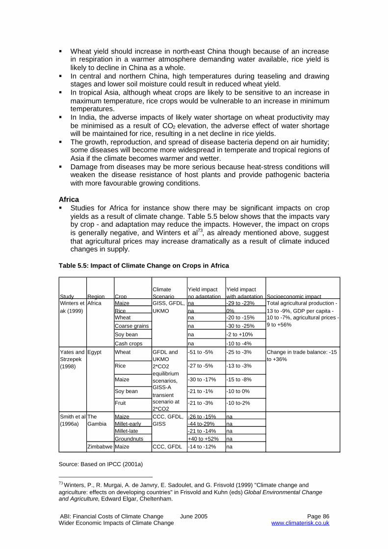
ABI: Financial Costs of Climate Change June 2005 Page 86Wider Economic Impacts of Climate Change www.climaterisk.co.uk
Wheat yield should increase in north-east China though because of an increasein respiration in a warmer atmosphere demanding water available, rice yield islikely to decline in China as a whole.
In central and northern China, high temperatures during teaseling and drawingstages and lower soil moisture could result in reduced wheat yield.
In tropical Asia, although wheat crops are likely to be sensitive to an increase inmaximum temperature, rice crops would be vulnerable to an increase in minimumtemperatures.
In India, the adverse impacts of likely water shortage on wheat productivity maybe minimised as a result of CO2 elevation, the adverse effect of water shortagewill be maintained for rice, resulting in a net decline in rice yields.
The growth, reproduction, and spread of disease bacteria depend on air humidity;some diseases will become more widespread in temperate and tropical regions ofAsia if the climate becomes warmer and wetter.
Damage from diseases may be more serious because heat-stress conditions willweaken the disease resistance of host plants and provide pathogenic bacteriawith more favourable growing conditions.
Africa Studies for Africa for instance show there may be significant impacts on crop
yields as a result of climate change. Table 5.5 below shows that the impacts varyby crop - and adaptation may reduce the impacts. However, the impact on cropsis generally negative, and Winters et al73, as already mentioned above, suggestthat agricultural prices may increase dramatically as a result of climate inducedchanges in supply.
Table 5.5: Impact of Climate Change on Crops in Africa
Source: Based on IPCC (2001a)
73 Winters, P., R. Murgai, A. de Janvry, E. Sadoulet, and G. Frisvold (1999) "Climate change andagriculture: effects on developing countries" in Frisvold and Kuhn (eds) Global Environmental Changeand Agriculture, Edward Elgar, Cheltenham.
Study Region CropClimateScenario
Yield impactno adaptation
Yield impactwith adaptation Socioeconomic impact
Maize na -29 to -23%Rice na 0%Wheat na -20 to -15%
Coarse grains na -30 to -25%
Soy bean na -2 to +10%
Cash crops na -10 to -4%
Wheat -51 to -5% -25 to -3%
Rice -27 to -5% -13 to -3%
Maize -30 to -17% -15 to -8%
Soy bean -21 to -1% -10 to 0%
Fruit -21 to -3% -10 to-2%
Maize -26 to -15% naMillet-early -44 to-29% naMillet-late -21 to -14% naGroundnuts +40 to +52% na
Zimbabwe Maize CCC, GFDL -14 to -12% na
Total agricultural production -13 to -9%, GDP per capita -10 to -7%, agricultural prices -9 to +56%
GISS, GFDL,UKMO
Winters etak (1999)
Africa
GFDL andUKMO2*CO2equilibriumscenarios,GISS-Atransientscenario at2*CO2
Change in trade balance: -15to +36%
EgyptYates andStrzepek(1998)
Smith et al(1996a)
TheGambia
CCC, GFDL,GISS

ABI: Financial Costs of Climate Change June 2005 Page 87Wider Economic Impacts of Climate Change www.climaterisk.co.uk
Impacts on livestock in Africa may have cultural and economic costs. The followingimpacts on livestock can be predicted: As water supply reduces there will be directly proportional impacts in the livestock
population As soil nutrient level increases due to increased CO2 concentration then animal
numbers may increase, offsetting negative impacts of water supply - Scholes etal74 show a balancing of these two effects in Southern Africa
Animal productivity is limited by protein (nitrogen) content of fodder. IncreasedCO2 concentrations will decrease the carbon-to-nitrogen ratio of forage, thoughthis may not impact on the palatability of the fodder as this represents increasedstarch content.
In high altitude and latitude regions of Africa, death of livestock is caused by lowtemperatures. Thus as the frequency of cold periods fall, so livestock productivitywill increase.
Vector borne diseases such as trypanosomiasis may extend their distribution. Forexample the tsetse fly is predicted to extend its distribution within Africa.
Latin America
Impacts in Latin America are similar to those shown in other continents. Cropyield is predicted to change as a result of climate change, though this variesdepending on the location and the crop in question. Studies to date have shownthat yields of wheat are expected to decrease, with a range of -50 to -5 percentdepending on location. For maize the impact is likely to be positive in someregions (e.g. Chile) but negative in others (Argentina, Brazil), the forecast rangeis from -61 to +2 percent of yield. For soybean the range of impact varies from -22 to + 40 percent depending on region, with Brazil more likely to gain thanArgentina.
In terms of livestock, climate change is likely to have an impact on both thequantity and quality of produce - and both are predicted by country and byregions within countries. In Argentina, for example, alfalfa is used as feedalongside other forage crops. A temperature increase of 1oC on this crop isanticipated to vary by region, with the crop yield in the area north of 36o degreesSouth decreasing by 16 to 25 percent and that in the south increasing by 50 to100 percent. The average impact will be between 4 to 8%. This will clearly havedifferential impacts on livestock production75.
Australia and New Zealand For Australia various impacts have been identified in the literature. Howden et.
al76 estimated the increase in wheat yield resulting from a doubling of actualatmospheric CO2 at 24%. Impacts are also predicted on grain quality, with proteincontent expected to fall by between 4 to 14 percent without additional nitrogen-based fertilisers. This is predicted to lead to an increase in gross margins
74 Scholes, R.J., G. Midgeley, and S. Wand (2000) "The impacts of climate change on South Africanrangelands" in South African Country Studies on Climate Change. Department of Environmental Affairsand Tourism, Pretoria75 Magrin, G. et al (1997b) Proyecto de Estudio sobre el Cambio Climatico en Argentina. Secretaria deCiencia y Tecnologia, Buones Aires.76 Howden, S., P. Reyenga, H. Meinke and G. M. Mckeon (1999) "Integrated Global Change ImpactAssessment on Australian Terrestrial Ecosystems: Overview Report" Working Paper 99/14 CSIRO,Canberra.

ABI: Financial Costs of Climate Change June 2005 Page 88Wider Economic Impacts of Climate Change www.climaterisk.co.uk
(assuming constant prices- a questionable assumption) of between 28 percentand 95 percent. Livestock in Australia is also likely to be impacted as increases inCO2 concentrations, coupled with warmer conditions, are predicted to lengthenthe growing season of pasture - thus having a potential to increase the weight oflivestock. However, forage quality is predicted to decrease and increased heatstress of livestock is forecast. These two factors may mitigate against gainsresulting from increased growth of pasture76.
For New Zealand, it is predicted that drier conditions will have an importantimpact on cereals, particularly in the Canterbury region. For maize production,rising temperatures may reduce the risk of growing this crop in the south, thoughwater shortages in Canterbury77.
5.6 Summary
This section reviews the principal factors that are thought to influence the effect ofclimate change on agriculture. These factors include:
photosynthetic effects of elevated CO2 on crops, which tend to raise cropyield
temperature effects on crop growth which appear to raise yield, and thendecrease yield beyond a certain temperature increase
changes in rainfall patterns affecting water availability for crops and livestock,with less rainfall tending to lead to falls in yield, and
climate variability.
In addition, weeds, pests and diseases may be affected by changes in climatethough in this case the evidence of net effect on yields is unclear. The humanresponse to these factors (e.g. by changing crops) may then determine the extent ofthese various effects. Clearly, the greater are the possibilities for adaptation, thehigher are likely to be the net benefits, and the lower are the net negative effects.
The range of impacts identified is very wide and it has led IPCC78 to draw a singleconclusion: that, with very low confidence in its robustness, a global temperature riseof greater than 2.5oC is likely to exceed the capacity of the global food productionsystem to adapt without price increases. However, results are judged to be too mixedto support a defensible conclusion regarding the vulnerability of the global balance ofagricultural supply and demand to smaller amounts of warming than 2.5oC
Different crops are expected to face different impacts. For certain crops, e.g. rice andwheat, the predicted impact ranges from a strongly negative impact in some regionsof the world to a positive impact in other regions, depending on the conditions underconsideration. For soybeans, the projected impact ranges from negative in someparts of the world to positive in others - and the overall impact may be expected to bepositive.
77 IPCC(2001a) Climate Change 2001: Impacts, Adaptation and Vulnerability. Cambridge UniversityPress, Cambridge78 IPCC(2001a) Climate Change 2001: Impacts, Adaptation and Vulnerability. Cambridge UniversityPress, Cambridge

ABI: Financial Costs of Climate Change June 2005 Page 89Wider Economic Impacts of Climate Change www.climaterisk.co.uk
The impact on prices of climate change has been estimated in two studies. Winterset al79 predicted increases in price are projected for tea(24.7%), rice(24.2%),coffee(16.7%), bananas(16.1%), sugar(14.5%) and maize(1.3%). The same studysuggested there would be decreases in price are projected for tobacco(-42%),oilseeds(-22.8%), cotton(-22.2%), wheat(-21.8%), soybeans(-20.3%), cocoa(-12%)and coarse grains(-6.7%). Parry et al80 predict an increase in the price of cereals ofbetween 13 and 45 percent. There are considerable uncertainties in these estimates,particularly when non-climate related factors are taken into account.
It is clear, when looking at these results, that they are highly sensitive to alternativeclimate model inputs, reflecting the wide range of yield impacts that have beenestimated from crop models. In addition the limited sensitivity analyses that havebeen performed suggest that uncertainties in economic models alone are large andfurther imply that the economic impacts of climate change on agriculture are givenlow confidence. Further sensitivity analyses need to be taken to determine keyassumptions and parameters and focus quantitative uncertainty analysis on thosedimensions of the models before this confidence rating in the model results can beimproved.
Improvements in the modelling of adaptive responses to climate change may alsolead to better estimates of the impacts of climate change on agriculture. Strategiesthat could impact on the outcome include:
Research and development into crops that will have better yields under changedclimatic conditions;
Sowing crops earlier in the year to maximise yield gain; Changing fertilising strategy to adapt to changing ambient CO2 levels; and Investment in irrigation infrastructure to ensure water supply for crops, amongst
others.
The use of agriculture as a source of sinks under the Bonn Agreement may alsohave important short term implications for agriculture in the developing world, notablyin terms of changing incentives for cropland management, grazing land managementand re-vegetation.
79 Winters, P., R. Murgai, A. de Janvry, E. Sadoulet, and G. Frisvold (1999) "Climate change andagriculture: effects on developing countries" in Frisvold and Kuhn (eds) Global Environmental Changeand Agriculture, Edward Elgar, Cheltenham.80 Parry, M., C. Rosenzweig, A. Iglesias, G. Fischer and M. Livermore (1999) Climate Change and worldfood security: a new assessment. Global Environmental Change 9, 51-67.

ABI: Financial Costs of Climate Change June 2005 Page 90Wider Economic Impacts of Climate Change www.climaterisk.co.uk
5.7 Flooding
Flooding in the UK has been considered in this report in the previous section. Thissection reviews information on the impact of climate change of flooding in Europe.
Flood events can take many forms, including slow-onset riverine floods, rapid-onsetflash floods, accumulation of rainwater in poorly-drained environments, and coastalfloods caused by tidal and wave extremes, sometimes referred to as storm surges.Rising temperatures brought about by climate change have a direct impact on risingsea levels causing coastal flooding. The current thinking also indicates that climatechange will cause an increase in rainfall intensity and changes in precipitationpatterns that will lead to greater risk of floods. Although there is still uncertainty as tothe extent of the impacts there are, however, a number of findings that haveconcluded that events such as major river floods could indeed become morefrequent. This is summarized in table 5.6.
Table 5.6A collection of views showing current thinking as regards changes in climate patterns on floodsA general increase in mean precipitation between 30oN and 70oN hasbeen observed. Mean precipitation has increased over northern Europeand decreased over southern Europe. Rainstorm intensity has increasedover the past decades.
P. Vellinga and W. J. vanVerseveld, Climate Changeand extreme Weatherevents, WWF, September2000) and (Groisman et al.,1999).
Changes in mean precipitation are associated with disproportionatelylarge changes in the extremes. The increase in the probability of heavyprecipitation is four times the increase in mean precipitation.
Groisman at al., Changesin the Probability of HeavyPrecipitation: ImportantIndicators of ClimateChange, Climatic Change,42, 1999) and (ChrisFolland et al. 2002)
There is a significant trend in the temperature difference between thelower and upper troposphere, globally and over North America, Europeand Australia. There is a 60%– 90% chance that the frequency of heavyprecipitation events has increased by 2 to 4% over the past 50 years.
Folland et al., Observedclimate variability andchange, Weather, RoyalMet Society, 2002
The above points led the IPCC work group II to release followingstatements:It is very likely (90%– 99% chance) that there will be an increase in floodand flood runoff, landslide and avalanche.There is a medium to high confidence that river flood hazard will increaseacross much of Europe.
Summary for Policymakers,Climate Change 2001:Impacts, Adaption andVulnerability, WorkingGroup II, IPCC
There has been an increase in the number and duration of westerlycyclonic circulation types over the past 100 years. This circulation type ismost likely to cause heavy precipitation events.
G. Tetzlaff, Institute ofMeteorology, PIK report no.17, University Leipzig
Total summer time precipitation amounts will be substantially reducedover major parts of Southern and central Europe. However, intensive rainevents - like those leading to the flooding in the Moldova, Danube, Elbeand Rhone in 2002 - will become more frequent and even more intensive.
Prudence: Prediction ofRegional scenarios andUncertainties for DefiningEuropeaN Climate changerisks and Effects
Source: Partner Re. 2002. Floods – Causes, Effects and Risk assessment and Prudencework.http://prudence.dmi.dk/

ABI: Financial Costs of Climate Change June 2005 Page 91Wider Economic Impacts of Climate Change www.climaterisk.co.uk
Climate change studies typically study the likely change in global temperatures overthe coming decades, whereas river flood hazard is related to exceptional levels ofrainfall in the catchment of one or more river basins. The exact link between risingtemperature and enhanced levels of rainfall is difficult to quantify, and even morecomplex is to determine any increase in likelihood of extreme rainfall events (asopposed to annual mean values). In addition, generalisations are difficult, especiallysince the characteristics and response to rainfall of a river system vary per river basinaccording to factors such as topography, land use, types of precipitation, geology,local climate etc.
However it is clear from recent work and reported studies that we are seeing anincrease in the costs of these types of events. Swiss Re estimated economic lossescaused by floods amounted to $61 billion for the period from 1995 to 2004 (all lossesinflated to 2005 prices). Since only the larger events are monitored in the Sigmadatabase, and during this period there were no losses attributable to storm surge, thetotal amount is certainly higher.
The European 2002 floods caused an economic loss of €15 billion for Germanyalone81. Approximately 20% of this was insured, two-thirds of which was thenreinsured internationally. The economic loss in the Czech Republic has beenestimated at up to 90 billion Crowns (€3 billion), approximately 30% higher than in1997. The insurance loss is believed to be in the region of €800 million. In Austria,economic loss estimates stand in excess of €5 billion (€3 billion private; €2 billioncommercial)81.
Large river basin floods develop over huge areas following weeks of unusually highrainfall. In July and August 1997, flooding in central Europe caused 54 fatalities inPoland and required the evacuation of 162,000 people. The value of the economiclosses throughout central Europe amounted to approximately US$5 billion, withinsured losses of US$940 million.82
In France the 2003 summer heat wave was followed by severe flash floods inDecember, causing total losses of around US$1.5 billion (including insured loss ofUS$ 0.9 billion)83.
Socio economic factors such as increased wealth, building alongside rivers, in floodplains and increased urbanisation also play a large part in contributing to the costs offlooding. Growing human vulnerability to flood events, combined with theuncertainties of climate change, should give cause for concern.
Catastrophic floods can create huge losses, which could potential exceed theinsurance industry’s ability to pay. Partner Re in 2002 showed that predicted potentialinsured losses from European floods to be as high as US$ 20 billion.84 Pressures oncapital requirements are more likely to arise through increases in the costs offlooding. This is discussed further in the following section.
There has been limited academic work that has been carried out to attempt toquantify the potential impact of climate change on river flood hazard in Europe. Onesuch study has been carried out for the Rhine River as part of the Dutch funded
81 Partner Re. 2002. Floods – Causes, Effects and Risk assessment82 Insurance and other Financial Services. Pier Vellinga and Evan Mills83 Natural Catastrophes and man made disasters in 2003. Swiss Re Sigma Report no. 1/200484 Partner re, 2002. Floods – Causes, Effects and Risk assessment

ABI: Financial Costs of Climate Change June 2005 Page 92Wider Economic Impacts of Climate Change www.climaterisk.co.uk
project ADAPT. Although specific to the Rhine, the conclusions of this report mayapply more generally across Europe.
5.8 Case study: River Rhine
As part of the Dutch funded project ADAPT, the River Rhine has been analysed as acase study. One of the main objectives was to compare historic weather data withSRES climate change projections for the periods 2010-2039 and 2070-2099 andadjust, if necessary, SRES projections. A summary of the key findings from this workis outlined below.85
The Climate change scenarios that were run indicated that there would be adecrease in summer discharge and an increase in winter discharge. Figure 5.3shows the change in precipitation patterns up to 2099. There is a projected increasein the frequency of extreme events in the variability bands around the mean run off inthe projected periods.
The results of the simulations show a clear increase in both frequency andmagnitude of the high water situations. Overall, an increased frequency of moresevere droughts and flood events is to be expected as a result of the climate changescenarios. The study stated that the results are in accordance with earlier resultsobtained with the RHINEFLOW models for slightly different scenarios.85
In general the annual discharge regime of the River Rhine is expected to alter as aresult of climate change. During wintertime, discharges are likely to increase and insummer time a decrease in river flows is expected. An increase in rainfall duringperiods when soils are saturated (i.e. winter and spring), along with earlier snowmelt,could increase the frequency and severity of floods. An increase in large-scaleprecipitation might lead to increased flood risks in winter. The increasedtemperatures expected in summer could lead to higher local precipitation extremesand associated flood risks in small catchment areas.
Currently, the estimated cost of at risk stock is estimated to be at €1,500 billion withinthe flood risk prone areas. If winter discharges increase significant adaptation actionswill be needed. The impacts and effects of extreme peak flows can be enormous.Inundations with subsequent damages and losses will occur along river stretcheswhere design criteria for flood protection are exceeded. Further research is requiredinto the actual costs that will be associated with these flooding events.
85 Water, climate, food and environment in the Rhine Basin, contribution to ADAPT Project, Han Klein,Klaas Jan Douben, Willem van Deursen, Erik de Ruyter van Steveninck as part of Netherlands ClimateChange Studies Assistance Programme (NCCSAP). Delft Hydraulics March 2005http://www.falw.vu.nl/Onderzoeksinstituten/index.cfm?home_file.cfm?fileid=0F213F3D-AA60-4C81-A755BAC7895E046E&subsectionid=602C4835-C246-41FA-8DD706E7084B0D06
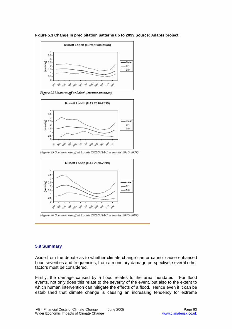
ABI: Financial Costs of Climate Change June 2005 Page 93Wider Economic Impacts of Climate Change www.climaterisk.co.uk
Figure 5.3 Change in precipitation patterns up to 2099 Source: Adapts project
5.9 Summary
Aside from the debate as to whether climate change can or cannot cause enhancedflood severities and frequencies, from a monetary damage perspective, several otherfactors must be considered.
Firstly, the damage caused by a flood relates to the area inundated. For floodevents, not only does this relate to the severity of the event, but also to the extent towhich human intervention can mitigate the effects of a flood. Hence even if it can beestablished that climate change is causing an increasing tendency for extreme

ABI: Financial Costs of Climate Change June 2005 Page 94Wider Economic Impacts of Climate Change www.climaterisk.co.uk
discharges in river systems, the resultant effect on damage/loss may be reduced ifadequate flood defence measures are put in place.
Recent events do prove, however, that flood losses have increased during recentyears. There are many potential reasons for this. Monetary loss resulting fromflooding depends on the values of the properties affected, and property prices aresteadily increasing across Europe. In addition, in many countries, there is increasingpressure on governments to build in flood plain areas due to lack of building spaceelsewhere. Growing human vulnerability to flood events, combined with theuncertainties of climate change, should give cause for concern.
Flood events are currently, the second most costly weather related catastrophes afterstorms. Further research is needed on the science and also to quantify the cost ofclimate change on these events. This will enable further modeling to assist insurersto understand the financial costs of these events.
5.10 Sea level riseOne area that has been researched in recent years is that of the impacts of sea levelrise.
Nicholls86 presents an overview of the likely impacts due to sea level rise. Table 5.6below presents a summary of the aggregated results from various country studies,showing the capital values and protection costs. The estimated total loss amounts toUS$1,146,310 million – with the worst impacted being Japan ($849,000 million). Interms of impact relative to GNP, Guyana fairs worst with 11 times its annual GNP inestimated capital losses.
86 Nicholls, R. (2003) "Case study on sea-level rise impacts", OECD Workshopon the Benefits of Climate Policy: Improving Information for Policy Makers,ENV/EPOC/GSP(2003)9/FINAL, OECD: Paris.

ABI: Financial Costs of Climate Change June 2005 Page 95Wider Economic Impacts of Climate Change www.climaterisk.co.uk
For the case of the United States of America, Table 5.7 presents an overview ofrecent studies44. Estimates of annual damages in 2065 range from $0.33bn to$1.37bn, with more recent estimates being at the conservative end of the scale.
Table 5.6
Table 5.7

ABI: Financial Costs of Climate Change June 2005 Page 96Wider Economic Impacts of Climate Change www.climaterisk.co.uk
Costs for the impacts of sea level rise have been estimated by Darwin and Tol87. Theresults are presented below in table 5.8 for various regions. It can be seen that theresults depend on the values used for land and capital. Total damages rangebetween $24bn to $42bn annually, where there is no protection assumed. The role ofadaptation is shown by the impact of introducing protection, which lowers theseimpact estimates to $8bn and $10bn respectively.
87 Darwin, R. and R. Tol (2001), 'Estimates of the Economic Effects of Sea Level Rise', Environmentaland Resource Economics, 19 (2), 113-129.
Table 5.8

ABI: Financial Costs of Climate Change June 2005 Page 97Wider Economic Impacts of Climate Change www.climaterisk.co.uk
The breakdown of the welfare cost is reflected in Table 5.9. The direct cost may bearound $4bn and the equivalent variation lost around $5bn. The largest OECDimpacts are in the EU, where $1.4bn are lost annually.
5.11 Storm surge
Storm surge is another area, which will be effected by climate change. Windstormsgenerate storm surges that result in coastal flooding and tidal waves. Nicholls88
summarises storm surges as follows:
“Surges are changes in sea level (either positive or negative) resulting fromvariations in atmospheric pressure and associated winds. They are additional tonormal tides and when added to high tides they can cause extreme water levels andflooding: flooding would be most severe when a surge coincided with spring tides.Surges are most commonly produced by the passage of atmospheric tropical orextra-tropical depressions… Surges can reach 2 to 3 m as they did in the stormsurge of 31 January/1 February 1953 when over 300 people lost their lives in theUnited Kingdom [add web site] and nearly 2,000 people were killed in theNetherlands (Smith and Ward, 1998)”
88 Nicholls, R. (2003) "Case study on sea-level rise impacts", OECD Workshop on the Benefits ofClimate Policy: Improving Information for Policy Makers, ENV/EPOC/GSP(2003)9/FINAL, OECD: Paris.
Table 5.9
ABI: Financial Costs of Climate Change June 2005 Page 98Wider Economic Impacts of Climate Change www.climaterisk.co.uk
Vulnerability to storm surges is a fact of life for over 200 million people globally, withthe bulk living in South, East and South East Asia. Nicholls88 estimates that 60% ofthose vulnerable are in these areas and that approximately 90% of those affected byflooding are from these areas.
Dawson et al89 presents an estimate of £150 billion for a global mean sea level rise of5-6m combined with a 1 in 1000 year storm surge event for the impact on propertiesprotected by the Thames Barrier.
89Dawson, R., J. Hall, P. Bates and R. Nicholls (undated) “Quantified Analysis of the Probability of
Flooding in the Thames Estuary under imaginable worst-case sea-level rise scenarios”.Available online at http://www.uni-hamburg.de/Wiss/FB/15/Sustainability/annex5.pdf.
ABI: Financial Costs of Climate Change June 2005 Page 99Financial Implications of climate change www.climaterisk.co.uk
6.0 Financial implications of climate change
6.1 Introduction
Insurance is one of the main mechanisms used by individuals and business tomanage risks, including the threat posed by natural hazards such as windstorms andfloods. Insurance markets work by pooling risks across a large and diversepopulation. Each individual or business protects themselves against an uncertainloss by paying a “price” (an annual premium) for a pro rata share of the pool’sexpected losses. The premiums are held by the insurer in a fund, which is used,along with investment income and capital, to compensate those individuals orbusinesses that actually do experience losses.
Traditional insurance risk management is based on statistically measurable andpredictable distributions of events and losses, which allows insurers to finance lossesof randomly occurring events of relatively modest size through policy premiums.However, natural catastrophes, occur infrequently, but have very large loss potential.The diversification of very large losses, even across the global insurance pool, isdifficult where such events have the potential to absorb huge quantities of capital. Sowhat can we expect if climate change increases average and extreme losses fromextreme weather events?
In this section we attempt to provide some answers to this question. First, we look atthe characteristics of natural catastrophe insurance. This provides a framework forevaluating the impacts of intensifying windstorms on insurance pricing and capitalcapacity, as well as exploring how insurers manage catastrophe risks. We thenassess how capital capacity and premiums could change subject to the climate-stress tests simulated in Section 3. The section concludes by briefly considering thewider economic effects of changes in the demand and supply of insurance.
6.2 Characteristics of natural catastrophe insurance
Insurance is unique. In contrast to other sectors in the economy, prices must be setand coverage sold before costs (claims) are known. Future costs must therefore beaccurately estimated ex ante. In most cases insurers can use historical data togenerate useful statistics, such as average annual loss per policy, that allow it setpremiums that cover these expected losses plus administrative expense, and providean adequate rate of return on capital. To this end two conditions are desirable: (a) thefrequency of claims over time should be predictable and (b) losses experienced byone policy should be independent of losses experienced by another.
Natural catastrophes do not, however, comply with these two conditions. For a start,natural catastrophes are infrequent events, resulting in large losses in a few yearsand no losses in most years. Losses are therefore not predictable over time. Naturalcatastrophes are also sufficiently large in scale to affect many policies at once.Hence, losses across policies are highly correlated; a violation of the secondcondition.
In addition, natural catastrophes, while infrequent, typically result in very large losses,which can present a significant financial risk to insurers, including – in rare cases –insolvency.

ABI: Financial Costs of Climate Change June 2005 Page 100Financial Implications of climate change www.climaterisk.co.uk
Insurers that offer to cover natural catastrophes have therefore developed specialisttools to assess, and strategies to manage, such risks.
6.3 Managing Natural Catastrophe Risk
Strategies used by insurers to manage natural catastrophe risk generally encompassthe following elements: first, defining “risk appetite” for natural catastrophe exposure;second, measuring and pricing the exposure; and third, managing the exposure.
Defining risk appetite
Each insurer will decide, for a specified period of time, how much loss it is willing (orable) to absorb without putting the business at unacceptable financial risk. This levelof risk – in insurance jargon - defines the insurer’s “risk appetite”, which is frequentlyexpressed in terms of the maximum acceptable reduction in capital per year from aspecific hazard (e.g. a European windstorm) or set of hazards. Risk appetite can alsobe described in term of the maximum loss that is acceptable over a determinedperiod of time (e.g. US$ 1 billion of loss only to be exceeded once in 100 years).
Many factors determine an insurers’ risk appetite, including: the availability and costof reinsurance, rate and solvency regulations, rating agency assessments, marketconditions, the capital base and how it is allocated across business lines, and thecost of capital. For instance, some rating agencies may require insurers to set asideenough capital to pay for at least a 1-in-100, or even a 1-in-250, year insured loss90.
As well as ensuring that insurance is affordable, regulators also want to make surethat insurers can cover their promises, even if a significant (e.g. 1-in-100 year loss)natural catastrophe occurs. One approach is to require insurers that write naturalcatastrophes to hold additional capital or reserves. Of course, holding more capitalraises capital costs, which in turn raises cost of the catastrophe coverage. Anappropriate balance must therefore be struck between imposing excessive safetymargins, which can inflict deadweight losses on the economy, and assuring that thepromises of insurers will be kept. Hence, insurers are not required to hold an amountof capital sufficient to cover all potential losses.
Measuring and pricing exposure
Once an insurer has defined its natural catastrophe risk appetite, but before it entersinto a contract with the insured to compensate them for specified losses in return forpaying an annual premium, the insurer must determine the likelihood that losses ofassorted sizes will occur, in order to set premiums that are actuarially sound. That is,premiums that allow the insurer to meet its financial obligations in the event of a loss.To set such premiums insurers must be in a position to assess risk across the fulldistribution of future hazards that could occur, including those arising from events,which have a very small chance of occurring, but have significant consequences ifthey do take place.
A hypothetical example of this process is provided in Box 1. In reality, the process ismuch more complex. The purpose of the example is solely to illustrate, in generalterms, the role of the loss distribution in the pricing process and in determining aninsurer’s capital requirements. This will provide a framework for looking at the results
90 For example, A. M. Best, a rating agency that assesses the financial strength of insurers, applies a stress test aspart of the assessment process. This test involves reducing an insurer’s surplus by the net after -tax catastrophe lossincurred once every 100 years to see its effect.

ABI: Financial Costs of Climate Change June 2005 Page 101Financial Implications of climate change www.climaterisk.co.uk
of the simulated climate-stress tests. The loss distribution itself is typically generatedby natural catastrophe models, such as those discussed in Section 3.
As the example in Box 1 shows, when assessing the relationship between losspotential and the likelihood of a loss event occurring, insurers consider:
Average (or Expected) Annual Losses: The insurer needs to know theamount they can expect to payout, on average, per annum for an insureditem (e.g. building) or portfolio of items. The expected loss is a keycomponent of the premium calculation.
Extreme (or Maximum Probable) Losses: The insurer needs to know howmuch it would need to payout should a significant catastrophe occur.Information on extreme losses is used by insurers to define their capitalbase91, including reinsurance cover, and is also factored into the premiumcalculation.
Regarding the latter point, as insured losses from natural catastrophes are highlyvariable, insurers need to hold sufficient capital to pay claims in the event thataggregate losses during a year are significantly worse than average. Thedeterminants of an insurer’s risk appetite will influence exactly how much capital isheld.
While the price of insurance will vary according to market location (depending on theregulatory regime and competitive nature of the local market), premiums will, ingeneral, comprise:
The cost of annual average losses. The administrative expenses of policy writing and settling claims. Payments for capital that would be at risk if annual losses exceeded
premium and investment income. All relevant taxes.
An insurer may also opt to transfer the risk of larger losses to reinsurers, in exchangefor paying a premium92. The net cost of reinsurance93 to the insurer will also berecouped from the insured, as part of the latter’s premiums.
Therefore, other things being equal, increases in the mean or variance of the lossdistribution, as anticipated with climate change, will tend to increase insurancepremiums.
91 As mentioned above, a unique feature of natural catastrophes is that they tend to impose losses on alarge number of individuals, in close proximity in time and space, or put another way, the risks arecorrelated with one another. The more correlated the risks, the larger the variability of an insurer’slosses, and the more capital that must be held in reserve. Thus, covering natural catastrophes, withuncertain and volatile losses, places significant capital demands on insurers.92 The reinsurers’ premium will have a similar structure to the primary insurers’ premium, albeit, basedon different loss functions.93 That is, the premium paid to the reinsurer to accept the natural catastrophe exposure, less theexpected loss transferred to the reinsurer.

ABI: Financial Costs of Climate Change June 2005 Page 102Financial Implications of climate change www.climaterisk.co.uk
Box 1: An Example of How Insurers Assess Risk For Natural Hazards
The Role of the Loss Distribution
A range of uncertain insurance claims, each with their own probability of occurrence, can becharacterised as one distribution. An example of such a distribution is shown in the figure below.
Example Loss Distribution
For the purpose of writing an insurance policy, it is useful to consider the distribution as two distinctparts94:
The central portion of the distribution, which deals with normal insured losses (claims).
The tail end of the distribution, which deals with infrequent events with large insured losses,such as “intense” landfalling hurricanes or other natural catastrophes.
Insurers, reinsurers and regulators are most interested in the latter, since such extreme outcomescan adversely affect profitability and, in acute cases, solvency. Typical extreme outcomes of interestto the industry are 1-in100 and 1-in-250 year losses, with annual probabilities of 1.0 per cent and 0.4per cent, respectively. Such events represent an “unexpected” loss, in that the corresponding claimfar exceeds the expected or average insured loss. Unexpected losses are a risk to the insurer.
In the example distribution shown in the above figure the annual expected insured loss is 3.0 and thestandard deviation of 1.095. Clearly, in this example, the standard deviation provides aninappropriate measure of risk, since it only amounts to 1/10th of the insured losses that could berealised once in 250 years (where losses equal to 10.0).If an insurer wants to be sure that it can pay claims in 99.6 per cent of all cases (i.e. that is, lossesincurred once every 250 years), it needs access to sufficient resources to pay 10.0, as opposed to3.0. The risk, in this case, is 7.0, which is the difference between the unexpected insured loss (10.0)and expected insured loss (3.0).The insurer could seek 10.0 from prospective policyholders. However, they are unlikely to buy apolicy in which the premiums vastly exceed their expected losses. As a result, the insurer will needto provide itself with sufficient capital to cover unexpected insured losses up to chosen threshold (i.e.the 1-in-250 year loss). In the example the insurer will need to allocate 7.0 to this line of business.The role of the capital is essentially to ensure that the insurer can pay its liabilities, even following acatastrophe.
Annua l Insure d Losse s
0
1
2 4 6 8 1 0 1 2
Pro
babi
lity
Den
sity
1 99.6 %
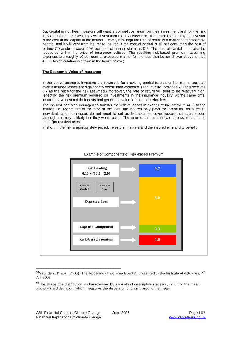
ABI: Financial Costs of Climate Change June 2005 Page 103Financial Implications of climate change www.climaterisk.co.uk
But capital is not free; investors will want a competitive return on their investment and for the riskthey are taking, otherwise they will invest their money elsewhere. The return required by the investoris the cost of the capital to the insurer. Exactly how high the rate of return is a matter of considerabledebate, and it will vary from insurer to insurer. If the cost of capital is 10 per cent, then the cost ofsetting 7.0 aside to cover 99.6 per cent of annual claims is 0.7. The cost of capital must also berecovered within the price of insurance policies. The resulting risk-based premium, assumingexpenses are roughly 10 per cent of expected claims, for the loss distribution shown above is thus4.0. (This calculation is shown in the figure below.)
The Economic Value of Insurance
In the above example, investors are rewarded for providing capital to ensure that claims are paideven if insured losses are significantly worse than expected. (The investor provides 7.0 and receives0.7 as the price for the risk assumed.) Moreover, the rate of return will tend to be relatively high,reflecting the risk premium required on investments in the insurance industry. At the same time,insurers have covered their costs and generated value for their shareholders.The insured has also managed to transfer the risk of losses in excess of the premium (4.0) to theinsurer; i.e. regardless of the size of the loss, the insured only pays the premium. As a result,individuals and businesses do not need to set aside capital to cover losses that could occur;although it is very unlikely that they would occur. The insured can thus allocate accessible capital toother (productive) uses.
In short, if the risk is appropriately priced, investors, insurers and the insured all stand to benefit.
Example of Components of Risk-based Premium
__________________________________94Saunders, D.E.A. (2005) “The Modelling of Extreme Events”, presented to the Institute of Actuaries, 4th
Aril 2005.95The shape of a distribution is characterised by a variety of descriptive statistics, including the meanand standard deviation, which measures the dispersion of claims around the mean.
Ex pense Compo nent
Ex pected Loss
Risk Loading
0.10 x (10.0 – 3.0)
R isk-based Premium
3.0
4 .0
0.7
0.3
C ost ofC apital
Value atRisk

ABI: Financial Costs of Climate Change June 2005 Page 104Financial Implications of climate change www.climaterisk.co.uk
6.4 Managing catastrophic exposures
Once an insurer has assessed its exposure to natural catastrophe losses and setappropriate premium rates, it may need to reduce exposure, subject to its riskappetite. Ranges of options are available to insurers to control their exposure tonatural catastrophe risk where capital capacity has been exceeded, including:
Managing location and geographic concentration. Changing policy forms and coverage. Transferring exposure to reinsurers or capital markets.
6.4.1 Location and geographical concentration
Natural catastrophes, like hurricanes, are infrequent events that may or may notstrike a particulate area during a year. An insurer with many exposures written over alarge geographical area has a high likelihood of experiencing losses in any givenyear. A hurricane making landfall is likely to damage some of the properties coveredby this insurer. However, in any one year, only a fraction of the properties over awidely distributed set of exposures will be affected. Thus, the chance of that insurersuffering substantial losses across its entire book of business is relatively low. Incontrast, if an insurer has a concentration of properties in one location, it may notexperience losses in a given year, but could face significant losses if that particularlocation is hit by a hurricane. Basically, the latter insurer will have less overallcapacity than the former insurer. Thus, one way to increase capacity is to managethe geographic concentration and location of exposure.
6.4.2 Policy forms and coverage
Insurers can control losses from natural catastrophes, while making affordablecoverage available, by changing policy conditions. Following Hurricane Andrew, forexample, insurers changed the structure of deductibles and limits (see Section 6).From the point of view of the insurer these changes have two effects: first, they limitthe amount the insurer is obliged to pay in the event of a loss; and second, they helpreduce administrative expenses by limiting the number of small claims received.Natural catastrophes, such as severe European windstorms, result in numeroussmall claims. In these cases, the administrative effort to settle these claims can bedisproportionate relative to the actual size of the loss incurred (e.g. the average claimafter the European windstorm Lothar was only US$ 1,500).
Traditional deductibles are based on relatively low fixed amount; averaging US$ 100in many markets exposed to European windstorms (Swiss Re, 2000)96. In Florida,after Hurricane Andrew, many insurers switched to mandatory windstormdeductibles, typically 2 per cent of any loss (as opposed to traditional, fixed dollardeductibles). While higher deductibles reduce insurers’ exposure, by keeping costsdown they also keep premiums down, which means that limited, affordable insurancecan still be offered in risk-prone areas, where it might not otherwise be available.
__________________________________
96 Swiss Re (2000) “Storm over Europe: An underestimated risk”, Swiss Reinsurance Company, Zurich

ABI: Financial Costs of Climate Change June 2005 Page 105Financial Implications of climate change www.climaterisk.co.uk
In addition, reducing the number of claims received speeds up processing times,which also benefits the insured. In short, insurers’ resources are freed-up to assistthose individuals and businesses suffering relatively large losses. In addition, suitablydesigned deductibles simultaneously provide policyholders with incentives to preventor mitigate losses; reducing costs (and premiums) further.
Another option is to review coverage limits (i.e. the maximum amount payable, aseither a fixed amount or percentage of the insured sum) in a policy, to mitigate thepotential for adverse coverage determinations after a natural catastrophe; especiallygiven the potential for significant catastrophes to induce “demand surge” for inputs tothe repair and replacement of damaged properties.
Insurers could also reduce future exposure by participating in programmes to reduceor prevent property damage from natural catastrophes. A good example of suchprogrammes is building codes and their enforcement. Insurers can provide thenecessary economic incentives to private agents to ensure that these programmes,which are often developed jointly with public agencies, are successfully implemented.These loss mitigation or adaptation programmes were discussed in Section 3.
In response to increasing flood risks, attempts have been made to controldevelopment in some risk-prone areas. While no attempts have yet been made tocontrol exposures to other perils by imposing legal restrictions on development withinareas prone to, for example, hurricanes, the mitigation of losses in the long-run maybe most effectively accomplished by limiting the accumulation of exposure in risk-prone areas. This option to mitigate losses takes on added significance given thepotential socio-economic developments highlighted in Section 3.
6.4.3 Transferring risk to third parties
The traditional method for insurers to reduce exposure or transfer risk to a third partyis to purchase reinsurance (see Box 2). In doing so insurers protect their capital baseagainst large deviations in expected losses. Furthermore, insurers can write morebusiness for the same amount of capital, since they no longer need to allocate capitalto the risks that have been transferred to the reinsurer. However, the capacity of theglobal reinsurance market is finite, so there is a limit to the amount of risk thatinsurers can transfer to reinsurers; the price of reinsurance may also be prohibitive athigher layers of cover.
Box 2: Types of ReinsuranceThere are basically two forms of reinsurance for natural catastrophes: treaty andfacultative. With treaty reinsurance, the insurer cedes (transfers) all risks that meet certaincriteria within a portfolio. In contrast, with facultative reinsurance insurers negotiatereinsurance on a policy-by-policy basis, with each policy being priced individually by thereinsurer. Coverage is also generally split between “proportional” and “non-proportional”cover. Under proportional (or pro-rata) cover, both premiums and losses are shared byreinsurer and insurer according to a contractually defined percentage for each policywritten. With treaty insurance proportional cover is still reasonably common. Non-proportional cover is typically written on a per risk, per event, or per aggregate excessbasis. Excess-of-loss reinsurance is a form of non-proportional cover that has beenspecifically designed for natural catastrophes. With a Cat XL treaty – as they are known -the reinsurer agrees to pay the insurer – per event – for that proportion of total losses thatexceeds a specified minimum loss (i.e. the retention), but fall below a specified ceiling (i.e.upper limit of cover). Cat XL reinsurance typically involves very large sums of money. As aresult, the cover tends to be divided into a number of distinct layers, which can be sharedamong several reinsurers.

ABI: Financial Costs of Climate Change June 2005 Page 106Financial Implications of climate change www.climaterisk.co.uk
The size of the global reinsurance market in 2004 (based on a survey of 43significant reinsurance groups), as measured by gross written premiums, has beenput at around US$ 150 billion97, of which US$ 118 billion relates to non-life businesslines (IAIS, 2004)98. Of the non-life amount, property accounts for about US$ 53billion. Proportional cover in property reinsurance showed gross written premiums ofclose to US$ 36 billion, whereas gross written premiums for non-proportional covertotalled around US$ 17 billion. The total capital available to cover unanticipatedlosses held by the same group of reinsurers is about US$ 244 billion.
With the global P & C insurance sector expecting, on average, US$ 20 billion innatural catastrophe losses per annum, this would represent nearly 40 per cent ofproperty gross written reinsurance premiums, and fewer than 10 per cent of the totalcapital available to reinsurers to cover losses across all lines of business. Industrywide measures of reinsurers’ ability to cover losses is misleading, however, since it isindividual firms that pay claims and not the industry as a whole; claims from a naturalcatastrophe could be concentrated in a few firms.
Insurers can also limit risk exposure to an acceptable level by transferring naturalcatastrophe risk into the capital markets, using innovative financial instruments, suchas catastrophe bonds, contingent surplus notes, exchange-traded options andcatastrophe equity puts. The process of “packaging” natural catastrophe risk assecurities to sell in the capital markets is, rather appropriately, referred to as“securitisation”.
These innovative risk transfer instruments are discussed at Appendix A. Due to theirsize financial markets offer enormous potential for insurers to diversify risks: thevalue of global financial markets currently stands at about US$ 118 trillion99. A US$100 billion loss event therefore does not even represent one-tenth of one per cent ofthe total value of global financial markets. Nonetheless, by the middle of 2004 onlyabout US$ 8 billion in catastrophe bonds had been issued since 1997. Nearly half ofthe bonds (by dollar value) cover earthquakes, with about a third covering hurricanes.Two-thirds of the bonds (by dollar value) cover perils in the U.S.
Each instrument has its unique advantages and disadvantages, in terms of, forexample, transaction costs, basis risk, moral hazard and adverse selection.Transaction costs can be considerable, and it is not likely that investors will know asmuch about an insurer’s portfolio of risks as the insurer itself. Thus, there is alwaysthe potential for adverse selection in which the insurer offloads only unfavourablerisks, keeping favourable risks on its books. The unfamiliarity of investors withinsurance risks means that they currently demand a relatively large risk premium.This acts to hinder market development.
In general, whether securitising natural catastrophe risk proves successful willdepend on: whether insurers find that securitisation provides a cost-effectivemechanisms for transferring risk and increasing capacity, and whether investors findthat securitising natural catastrophe risk improves the performance of their portfolios.________________________________97 It has also been estimated as high as USD 175.5 billion (USD 146.0 billion in non-life gross writtenpremiums).98IAIS (2004) “Global Reinsurance Market Report 2003”, International Association of InsuranceSupervisors, December 2004.99McKinsey & Company, “Taking Stock of the World’s Capital Markets”, February 2005(www.mckinsey.com/mgi/publications).

ABI: Financial Costs of Climate Change June 2005 Page 107Financial Implications of climate change www.climaterisk.co.uk
6.5 Implications of climate-stress tests
Using the framework described above we can now consider the implications of theestimated increments in average and extreme losses, as outlined in Section 3,resulting from our climate-stress tests. Starting with the loss distribution displayed inBox 1, increases in the average annual insured loss and extreme losses will, aspredicted under our climate-stress tests for hurricanes, typhoons and Europeanwindstorms, shift (or elongate) the loss distribution to the right – as shown in Figure6.1. In the figure we assume the insurer wants to be sure that it can pay claims in99.6 per cent of all cases (i.e. including those arising from a 1-in-250 year lossshould it occur). The point to note is that increases in average insured losses andextreme insured losses, as a result of climate change, will tend to increase theamount of risk-capital needed to satisfy the insurer’s risk appetite, at whatever level itis defined.
Figure 6.1: Illustration of Impact of Climate Change on the Loss Distribution forWindstorms
6.6 Capital requirements
Before considering the impact of climate change on the capital requirements ofinsurers of Atlantic hurricanes, Japanese typhoons and European windstorms, wefirst need information on the baseline average annual losses and extreme losses.Table 6.1 presents baseline losses for these three storm perils, based on currentindustry experience.
A n n ua l I ns u re d L o s se s
0 4 8 1 2 1 6 2 0 2 4
Pro
babi
lity
den
sity
C l im ate c h an g eC u r r e n t c l im a teIn c re a s e in a n n u a l
a v e ra g e lo s se s
In c re a s e in e xt re me lo s s e s
99 .6 % o fc la ims
99 .6 % o fc la ims
R is k-b a s e dc a p ita l n e e d
R is k-b a s e dc a p it a l n e e d

ABI: Financial Costs of Climate Change June 2005 Page 108Financial Implications of climate change www.climaterisk.co.uk
Table 6.1: Current Loss Experience for Atlantic Hurricanes, Japanese Typhoons andEuropean Windstorms
AnnualAverage TotalFinancial Loss
AnnualAverage
Insured Loss
Insured Losswith a Chanceof Once Every100 Years (1%
EP)
Insured Losswith a Chanceof Once Every
250 Years(0.4% EP)
(US$ 2004billion)
(US$ 2004billion)
(US$ 2004billion)
(US$ 2004billion)
Atlantic hurricanes 9.4 5.4 60 85
Japanese typhoons 4.2 2.3 15 20
European windstorms 3.1 1.7 30 35
The simulated climate-induced increments in annual average and extreme insuredlosses for each of the tropical cyclone perils, under a high-emissions scenario (AIF1)and a low-emissions scenario (550) are shown in Table 6.2. Note that the radiativeforcing under a 550 stabilisation emissions scenario and under the IPCC SRES B1scenario are roughly equivalent over the time period 2080-2099. Consequently, theresults presented below for the low-emissions scenario are very similar to those thatwould have been obtained under B1.
Table 6.2: Impact of Climate-stress Tests on Insured Losses from Atlantic Hurricanesand Japanese Typhoons under a High- and Low-emissions Scenario (2080-2099)
Annual AverageInsured Loss
Insured Losswith a Chance ofOnce Every 100Years (1% EP)
Insured Losswith a Chance ofOnce Every 250Years (0.4% EP)
(US$ 2004 billion) (US$ 2004 billion) (US$ 2004 billion)
Atlantic hurricanes
High-emissions scenario 4.3 44.5 66.7
Low-emissions scenario 0.8 8.6 14.5
Japanese typhoons
High-emissions scenario 1.7 11.1 15.8
Low-emissions scenario 0.3 2.1 2.7
Looking at Atlantic hurricanes, Figure 6.2 and Figure 6.3 illustrate graphically theimpact of combining the loss data listed in Table 6.1 and Table 6.2. As Figure 6.2shows, under the A1F1 scenario, the maximum insured loss with a 1 per cent and 0.4per cent chance of being exceeded annually is simulated to increase to US$ 105billion and US$ 152 billion, respectively. Under a 550 stabilisation scenario however(shown in Figure 3), insured losses for the 1 per cent and 0.4 per cent exceedenceprobabilities are only estimated to increase to US$ 69 billion and US$ 100 billion. Thesimulated 1-250 year insured losses for hurricanes by the end of the century, forexample, are nearly 35 per cent less under a 550 stabilisation path than under A1F1.

ABI: Financial Costs of Climate Change June 2005 Page 109Financial Implications of climate change www.climaterisk.co.uk
Figure 6.2: Simulated Change in “Right-hand Tail” of Exceedence Probability Curve forAtlantic Basin Hurricanes Affecting U.S. Under IPCC SRES A1F1 By End of Century(2080-2099)
Figure 6.3: Simulated Change in “Right-hand Tail” of Exceedence Probability Curve forAtlantic Basin Hurricanes Affecting U.S. Under 550 Stabilisation Scenario By End ofCentury (2080-2099)
What about capital requirements? Based on the simple framework outlined in Box 1above, for hurricane insurance markets at the end of the century, the additional risk-capital (RC) required under the A1F1 emission scenario for an industry risk appetitedefined by a 1 per cent and 0.4 per cent exceedence probability is shown in the tablebelow (rounded to the nearest billion US$):
0.010
0.004
0.020
0 .030
0.040
0.050
Exc
eede
nce
Prob
abil
ity
+ 45 + 67
Insured Loss (USD 2004 Billion)
Current Climate
Climate SRES A1F1
AAL = + US D 4.3 billion
60 105 15285
0.010
0.004
0.020
0.030
0.040
0.050
Exc
eede
nce
Pro
babi
lity
+ 9
+ 15
Insured Loss (USD 2004 Billion)
Current Climate
Climate 550 ppmv
AAL = + US D 0.8 billion
60 85 10069
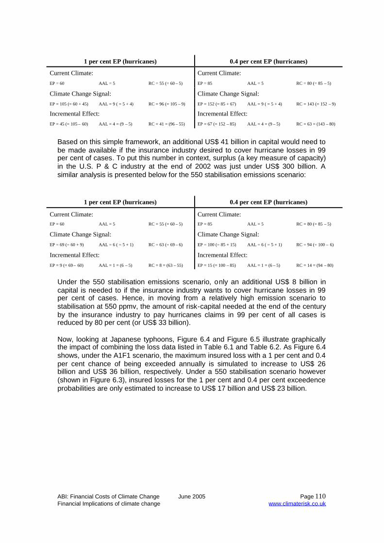
ABI: Financial Costs of Climate Change June 2005 Page 110Financial Implications of climate change www.climaterisk.co.uk
1 per cent EP (hurricanes) 0.4 per cent EP (hurricanes)
Current Climate: Current Climate:EP = 60 AAL = 5 RC = 55 (= 60 – 5) EP = 85 AAL = 5 RC = 80 (= 85 – 5)
Climate Change Signal: Climate Change Signal:EP = 105 (= 60 + 45) AAL = 9 ( = 5 + 4) RC = 96 (= 105 – 9) EP = 152 (= 85 + 67) AAL = 9 ( = 5 + 4) RC = 143 (= 152 – 9)
Incremental Effect: Incremental Effect:EP = 45 (= 105 – 60) AAL = 4 = (9 – 5) RC = 41 = (96 – 55) EP = 67 (= 152 – 85) AAL = 4 = (9 – 5) RC = 63 = (143 – 80)
Based on this simple framework, an additional US$ 41 billion in capital would need tobe made available if the insurance industry desired to cover hurricane losses in 99per cent of cases. To put this number in context, surplus (a key measure of capacity)in the U.S. P & C industry at the end of 2002 was just under US$ 300 billion. Asimilar analysis is presented below for the 550 stabilisation emissions scenario:
1 per cent EP (hurricanes) 0.4 per cent EP (hurricanes)
Current Climate: Current Climate:EP = 60 AAL = 5 RC = 55 (= 60 – 5) EP = 85 AAL = 5 RC = 80 (= 85 – 5)
Climate Change Signal: Climate Change Signal:EP = 69 (= 60 + 9) AAL = 6 ( = 5 + 1) RC = 63 (= 69 – 6) EP = 100 (= 85 + 15) AAL = 6 ( = 5 + 1) RC = 94 (= 100 – 6)
Incremental Effect: Incremental Effect:EP = 9 (= 69 – 60) AAL = 1 = (6 – 5) RC = 8 = (63 – 55) EP = 15 (= 100 – 85) AAL = 1 = (6 – 5) RC = 14 = (94 – 80)
Under the 550 stabilisation emissions scenario, only an additional US$ 8 billion incapital is needed to if the insurance industry wants to cover hurricane losses in 99per cent of cases. Hence, in moving from a relatively high emission scenario tostabilisation at 550 ppmv, the amount of risk-capital needed at the end of the centuryby the insurance industry to pay hurricanes claims in 99 per cent of all cases isreduced by 80 per cent (or US$ 33 billion).
Now, looking at Japanese typhoons, Figure 6.4 and Figure 6.5 illustrate graphicallythe impact of combining the loss data listed in Table 6.1 and Table 6.2. As Figure 6.4shows, under the A1F1 scenario, the maximum insured loss with a 1 per cent and 0.4per cent chance of being exceeded annually is simulated to increase to US$ 26billion and US$ 36 billion, respectively. Under a 550 stabilisation scenario however(shown in Figure 6.3), insured losses for the 1 per cent and 0.4 per cent exceedenceprobabilities are only estimated to increase to US$ 17 billion and US$ 23 billion.

ABI: Financial Costs of Climate Change June 2005 Page 111Financial Implications of climate change www.climaterisk.co.uk
Figure 6.4: Simulated Change in “Right-hand Tail” of Exceedence Probability Curve forJapanese Typhoons Affecting U.S. Under IPCC SRES A1F1 By End of Century (2080-2099)
Figure 6.5: Simulated Change in “Right-hand Tail” of Exceedence Probability Curve forJapanese Typhoons Affecting U.S. Under 550 Stabilisation Scenario By End of Century(2080-2099)
0.010
0.004
0.020
0 .030
0.040
0.050
Exc
eede
nce
Pro
bab
ility
+ 11 + 16
Insured Loss (USD 2004 Billion)
Current Climate
Climate SRES A1F1
AAL = + US D 1.7 billion
15 26 3620
0.010
0.004
0.020
0.030
0.040
0.050
Exc
eede
nce
Pro
babi
lity
+ 2
+ 3
Insured Loss (USD 2004 Billion)
Current Climate
Climate 550 ppmv
AAL = + US D 0.3 billion
15 20 2317
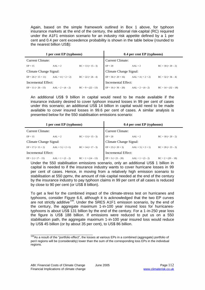
ABI: Financial Costs of Climate Change June 2005 Page 112Financial Implications of climate change www.climaterisk.co.uk
Again, based on the simple framework outlined in Box 1 above, for typhooninsurance markets at the end of the century, the additional risk-capital (RC) requiredunder the A1F1 emission scenario for an industry risk appetite defined by a 1 percent and 0.4 per cent exceedence probability is shown in the table below (rounded tothe nearest billion US$):
1 per cent EP (typhoons) 0.4 per cent EP (typhoons)
Current Climate: Current Climate:EP = 15 AAL = 2 RC = 13 (= 15 – 3) EP = 20 AAL = 2 RC = 18 (= 20 – 2)
Climate Change Signal: Climate Change Signal:EP = 26 (= 15 + 11) AAL = 4 ( = 2 + 2) RC = 22 (= 26 – 4) EP = 36 (= 20 + 16) AAL = 4 ( = 2 + 2) RC = 32 (= 36 – 4)
Incremental Effect: Incremental Effect:EP = 11 (= 26 – 15) AAL = 2 = (4 – 2) RC = 9 = (22 – 13) EP = 16 (= 36 – 20) AAL = 2 = (4 – 2) RC = 14 = (32 – 18)
An additional US$ 9 billion in capital would need to be made available if theinsurance industry desired to cover typhoon insured losses in 99 per cent of casesunder this scenario; an additional US$ 14 billion in capital would need to be madeavailable to cover insured losses in 99.6 per cent of cases. A similar analysis ispresented below for the 550 stabilisation emissions scenario:
1 per cent EP (typhoons) 0.4 per cent EP (typhoons)
Current Climate: Current Climate:EP = 15 AAL = 2 RC = 13 (= 15 – 3) EP = 20 AAL = 2 RC = 18 (= 20 – 2)
Climate Change Signal: Climate Change Signal:EP = 17 (= 15 + 2) AAL = 3 ( = 2 +1) RC = 14 (= 17 – 3) EP = 23 (= 20 + 3) AAL = 3 ( = 2 + 1) RC = 20 (= 23 – 3)
Incremental Effect: Incremental Effect:EP = 2 (= 17 – 15) AAL = 1 = (3 – 2) RC = 1 = (14 – 13) EP = 3 (= 23 – 20) AAL = 1 = (3 – 2) RC = 2 = (20 – 18)
Under the 550 stabilisation emissions scenario, only an additional US$ 1 billion incapital is needed to if the insurance industry wants to cover hurricane losses in 99per cent of cases. Hence, in moving from a relatively high emission scenario tostabilisation at 550 ppmv, the amount of risk-capital needed at the end of the centuryby the insurance industry to pay typhoon claims in 99 per cent of all cases is reducedby close to 90 per cent (or US$ 8 billion).
To get a feel for the combined impact of the climate-stress test on hurricanes andtyphoons, consider Figure 6.6, although it is acknowledged that the two EP curvesare not strictly additive100. Under the SRES A1F1 emission scenario, by the end ofthe century, the aggregate maximum 1-in-100 year insured loss for hurricanes-typhoons is about US$ 131 billion by the end of the century. For a 1-in-250 year lossthe figure is US$ 188 billion. If emissions were reduced to put us on a 550stabilisation path, the aggregate maximum 1-in-100 year insured loss would reduceby US$ 45 billion (or by about 35 per cent), to US$ 86 billion.
______________________________100As a result of the “portfolio effect”, the losses at various EPs in a combined (aggregate) portfolio ofperi l regions will be (considerably) lower than the sum of the corresponding loss EPs in the individualregions.

ABI: Financial Costs of Climate Change June 2005 Page 113Financial Implications of climate change www.climaterisk.co.uk
Figure 6.6: Simulated Change in “Right-hand Tail” of Approximate AggregateExceedence Probability Curve for Hurricanes and Typhoons Under IPCC SRES A1F1and 550 By End of Century (2080-2099)
The amount of risk-capital all insurers writing hurricane and typhoon cover need tohave available at the end of the century if they want to pay claims in 99.6 per cent ofall cases, under the high and low emission scenarios, is shown in the table below:
A1F1: 0.4 per cent EP (hurricanes and typhoons) 550: 0.4 per cent EP (hurricanes and typhoons)
Current Climate: Current Climate:EP = 105 AAL = 8 RC = 97 (= 105 – 8) EP = 105 AAL = 8 RC = 97 (= 105 – 8)
Climate Change Signal: Climate Change Signal:EP = 188 (= 105 + 83) AAL = 14 ( = 8 + 6) RC = 174 (= 188 – 14) EP = 123 (= 105 + 18) AAL = 9 ( = 8 + 1) RC = 114 (= 123 – 9)
Incremental Effect: Incremental Effect:EP = 83 (= 188 – 105) AAL = 6 = (14 – 8) RC = 77 = (174 – 97) EP = 18 (= 123 – 105) AAL = 1 = (9 – 8) RC = 17 = (114 – 97)
Under the A1F1 emission scenario, by the end of the century, the insurance industrywould need to make an additional US$ 77 billion in risk-capital available if it wantedto cover hurricane and typhoon losses in 99.6 per cent of all cases. In contrast, underthe 550 stabilisation scenario, only an additional US$ 17 billion in capital is required.In moving from the high A1F1 emission scenario to stabilisation at 550 ppmv, theamount of risk-capital needed for these two insurance markets is thus reduced byover 75 per cent (or by US$ 60 billion).
The simulated climate-induced (under IPCC SRES A2) increment in the 1 per centand 0.4 per cent exceedence probabilities for European windstorms is US$ 2.0 billionand US$ 2.3 billion, respectively, which roughly represents a 5 per cent increase oncurrent exceedence probabilities. This may seem small, but the climate-stress testsimulated was limited to the extreme “upper tail” of the full distribution of all feasiblewindstorm events. Potential impacts of climate change on less intense windstorms
0.010
0.004
0.020
0.030
0.040
0.050
Ex
ceed
ence
Pro
babi
lity
- 45
Insured Loss (USD 2004 Billion)
Climate SRES A 1F1
86
Climate 550 ppmv
123 131 188
- 65
188 = (85 + 67) + (20 + 16)123 = (85 + 15) + (20 + 3)
131 = (60 + 45) + (15 + 11)
86 = (60 + 9) + (15 + 2)
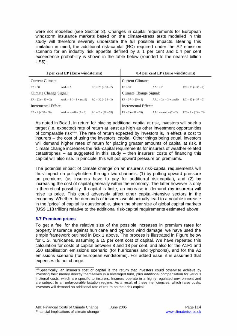
ABI: Financial Costs of Climate Change June 2005 Page 114Financial Implications of climate change www.climaterisk.co.uk
were not modelled (see Section 3). Changes in capital requirements for Europeanwindstorm insurance markets based on the climate-stress tests modelled in thisstudy will therefore severely understate the full possible impacts. Bearing thislimitation in mind, the additional risk-capital (RC) required under the A2 emissionscenario for an industry risk appetite defined by a 1 per cent and 0.4 per centexceedence probability is shown in the table below (rounded to the nearest billionUS$):
1 per cent EP (Euro windstorms) 0.4 per cent EP (Euro windstorms)
Current Climate: Current Climate:EP = 30 AAL = 2 RC = 28 (= 30 – 2) EP = 35 AAL = 2 RC = 33 (= 35 – 2)
Climate Change Signal: Climate Change Signal:EP = 32 (= 30 + 2) AAL = 2 ( = 2 + small) RC = 30 (= 32 – 2) EP = 37 (= 35 + 2) AAL = 2 ( = 2 + small) RC = 35 (= 37 – 2)
Incremental Effect: Incremental Effect:EP = 2 (= 32 – 30) AAL = small = (2 – 2) RC = 2 = (30 – 28) EP = 2 (= 37 – 35) AAL = small = (2 – 2) RC = 2 = (35 – 33)
As noted in Box 1, in return for placing additional capital at risk, investors will seek atarget (i.e. expected) rate of return at least as high as other investment opportunitiesof comparable risk101. The rate of return expected by investors is, in effect, a cost toinsurers – the cost of using the investors’ capital. Other things being equal, investorswill demand higher rates of return for placing greater amounts of capital at risk. Ifclimate change increases the risk-capital requirements for insurers of weather-relatedcatastrophes – as suggested in this study – then insurers’ costs of financing thiscapital will also rise. In principle, this will put upward pressure on premiums.
The potential impact of climate change on an insurer’s risk-capital requirements willthus impact on policyholders through two channels: (1) by putting upward pressureon premiums (as insurers have to pay for additional risk-capital), and (2) byincreasing the cost of capital generally within the economy. The latter however is onlya theoretical possibility. If capital is finite, an increase in demand (by insurers) willraise its price. This could adversely affect other capital-intensive sectors in theeconomy. Whether the demands of insurers would actually lead to a notable increasein the “price” of capital is questionable, given the shear size of global capital markets(US$ 118 trillion) relative to the additional risk-capital requirements estimated above.
6.7 Premium pricesTo get a feel for the relative size of the possible increases in premium rates forproperty insurance against hurricane and typhoon wind damage, we have used thesimple framework outlined in Box 1 above. The process is illustrated in Figure belowfor U.S. hurricanes, assuming a 15 per cent cost of capital. We have repeated thiscalculation for costs of capital between 8 and 18 per cent, and also for the A1F1 and550 stabilisation emissions scenario (for hurricanes and typhoons), and for the A2emissions scenario (for European windstorms). For added ease, it is assumed thatexpenses do not change.________________________101Specifically, an insurer’s cost of capital is the return that investors could otherwise achieve byinvesting their money directly themselves in a leveraged fund, plus additional compensation for variousfrictional costs, which are specific to insurers. Insurers operate in a highly regulated environment andare subject to an unfavourable taxation regime. As a result of these inefficiencies, which raise costs,investors will demand an additional rate of return on their risk capital.

ABI: Financial Costs of Climate Change June 2005 Page 115Financial Implications of climate change www.climaterisk.co.uk
Assuming that insurers want to meet claims in 99.6 per cent of all cases, thissimplified analysis shows, other things being equal:
Hurricanes: The simulated climate-stress tests under the A1F1 emissionsscenario could increase aggregate market premiums by 2080-2099 relativeto levels without the climate change signal by between US$ 9 and US$ 16billion, depending on the cost of capital (the higher the cost of capital, thelarger the increase in premiums).
Hurricanes: The same climate-stress tests under the lower 550stabilisation emissions scenario could increase premiums relative to levelswithout the climate change signal by between US$ 1 and US$ 2 billion,depending on the cost of capital.
Typhoons: The simulated climate-stress tests under the A1F1 emissionsscenario could increase aggregate market premiums by 2080-2099 relativeto levels without the climate change signal by between US$ 3 and US$ 4billion, depending on the cost of capital.
Typhoons: The same climate-stress tests under the lower 550stabilisation emissions scenario could increase premiums relative to levelswithout the climate change signal by between US$ 0.5 and US$ 0.7 billion,depending on the cost of capital.
European Windstorms: The simulated climate-stress tests under the A2emissions scenario could increase aggregate market premiums by 2080-2099 relative to levels without the climate change signal by between US$0.6 and US$ 0.8 billion, depending on the cost of capital.
It must be stressed, however, that prices are unlikely to change in theproportions suggested in this simplified analysis. Market dynamics – where theinteraction of supply and demand can lead to marked price cycles – mean that actualpremium rates often diverge from “technical premium”. This commonly observedprice cycle for natural catastrophe insurance is discussed below.

ABI: Financial Costs of Climate Change June 2005 Page 116Financial Implications of climate change www.climaterisk.co.uk
Figure 6.7: Simplified Illustration of the Relative Impact on Aggregate Premiums forHurricane Insurance Markets Under IPCC SRES A1F1 By End of Century (2080-2099)Assuming Insurers Want to Meet Claims in 99.6 Per Cent of All Cases
(a) Current climate (b) Simulated climate-stress tests
6.8 Short-run versus long-run impacts
The previous discussion essentially described the long-run response of insurancemarkets to the possible impacts of climate change on capital requirements andpremiums. But the short-run response is more volatile. Broadly, in the short-run,following large unanticipated losses from an extreme weather event, insurers’ capitalis reduced, as the catastrophe leads to big claim payments, which are unlikely to bemet through premium and investment income. As a consequence, insurers are not aswilling, or as able, to offer the same level of coverage at current premium rates. Thesupply of insurance thus decreases. At the same time, having recently suffered fromthe impacts of the catastrophe, the insured’s demand for cover is likely to increase.Falling supply and increasing demand act to push up premium rates. In time, thehigher premium rates attract additional capital in search of improved returns. As aresult, supply begins to recover, and premium rates begin to decline.
The big unanticipated losses heighten insurers’ uncertainty about future losses. Thisprompts insurers to re-assess the risk of similar events occurring again, and thistypically raises insurers’ perceived risk of expected and extreme losses. So, eventhough prices begin to decline in the long-run following a catastrophe, they will notnecessarily return to pre-catastrophe levels. This predictable sequence of events inresponse to an unanticipated extreme weather catastrophe is summarised in Figure8, and illustrated with the example of hurricane Andrew in Box 3.
Therefore, not only might climate change put upward pressure on insurancepremiums over time, it could also lead to increased volatility in insurance markets inthe short-run, in the wake of increasingly severe, and variable weather. Especially, if
Expenses
Expected Loss
Risk Loading0.15 x (85 – 5)
Risk-basedPremium
5
17
12
-
Cost ofCapital
Valueat Risk
Risk Loading0.15 x (152 – 9)
21
9
-
30
Expected Loss
Expenses
Risk-basedPremium
Cost ofCapital
Valueat Risk
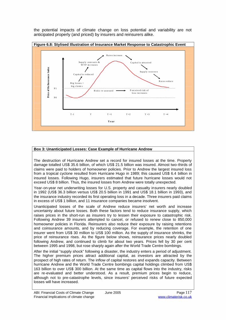
ABI: Financial Costs of Climate Change June 2005 Page 117Financial Implications of climate change www.climaterisk.co.uk
the potential impacts of climate change on loss potential and variability are notanticipated properly (and priced) by insurers and reinsurers alike.
Figure 6.8: Stylised Illustration of Insurance Market Response to Catastrophic Event
Box 3: Unanticipated Losses: Case Example of Hurricane Andrew
The destruction of Hurricane Andrew set a record for insured losses at the time. Propertydamage totalled US$ 35.6 billion, of which US$ 21.5 billion was insured. Almost two-thirds ofclaims were paid to holders of homeowner policies. Prior to Andrew the largest insured lossfrom a tropical cyclone resulted from Hurricane Hugo in 1989; this caused US$ 6.4 billion ininsured losses. Following Hugo, insurers estimated that future hurricane losses would notexceed US$ 8 billion. Thus, the insured losses from Andrew were totally unexpected.Year-on-year net underwriting losses for U.S. property and casualty insurers nearly doubledin 1992 (US$ 36.3 billion versus US$ 20.5 billion in 1991 and US$ 18.1 billion in 1993), andthe insurance industry recorded its first operating loss in a decade. Three insurers paid claimsin excess of US$ 1 billion, and 11 insurance companies became insolvent.Unanticipated losses of the scale of Andrew reduce insurers’ net worth and increaseuncertainty about future losses. Both these factors tend to reduce insurance supply, whichraises prices in the short-run as insurers try to lessen their exposure to catastrophic risk.Following Andrew 39 insurers attempted to cancel, or refused to renew close to 850,000homeowner policies in Florida. Reinsurers also reduce their exposure by raising retentionsand coinsurance amounts, and by reducing coverage. For example, the retention of oneinsurer went from US$ 30 million to US$ 100 million. As the supply of insurance shrinks, theprice of reinsurance rises. As the figure below shows, reinsurance prices nearly doubledfollowing Andrew, and continued to climb for about two years. Prices fell by 30 per centbetween 1995 and 1998, but rose sharply again after the World Trade Centre bombings.After the initial “supply shock” following a disaster, the industry enters a period of adjustment.The higher premium prices attract additional capital, as investors are attracted by theprospect of high rates of return. The inflow of capital restores and expands capacity. Betweenhurricane Andrew and the World Trade Centre bombings capital holdings climbed from US$163 billion to over US$ 300 billion. At the same time as capital flows into the industry, risksare re-evaluated and better understood. As a result, premium prices begin to reduce,although not to pre-catastrophe levels, since insurers’ perceived risks of future expectedlosses will have increased.
Pric
eof
Re/
Insu
ranc
eIn
dex
T T +1 T +2 T +3T -1
Y e ar
P 0
P 1
Sup p ly cont r act s &W T P in c r ea se s
R a t e s inc r ea se
C a p it a l is r e duc e d
B ig lo sse s =big c la im s
R isk s r e- as se sse d
C a p it a l is attr a ct e d
Sup p ly r e co ve r s
R a t e s r e duc e
T +4
P erc e iv e d r isk oflo ss inc r ea se s

ABI: Financial Costs of Climate Change June 2005 Page 118Financial Implications of climate change www.climaterisk.co.uk
“Paragon” Catastrophic Reinsurance Price Index (1984 = 100)102
0
50
100
150
200
250
1984 1986 1988 1990 1992 1994 1996 1998 2000 2002
Year
Re
Pri
ce
Ind
ex
-30%
-20%
-10%
0%
10%
20%
30%
40%
50%
60%
70%
Yea
r-o
n-Y
ear
Ch
ang
e
Year-on-year Change
Price Index
6.9 Economic value of insurance
The example in Box 1 also illustrated the economic value of insurance. Insurance, ingeneral, is capable of generating significant beneficial impacts within the economy,which are not necessarily captured by simply measuring the added value of thesector103. Broadly, these benefits are: risk transfer and indemnification, risk-basedpricing and financial intermediation.
Risk transfer
By offering risk transfer and indemnification insurance allows risk-averse individualsor businesses to purchase large expensive items, such as houses or commercialpremises. It allows them to make such purchases without needing to withhold largeliquid contingency funds in order to pay for unexpected damages. Instead thesefunds can be used to make further purchases or productive investments. Insurancealso facilitates innovation with the economy by underwriting new – relatively risky –research and technology. Basically, insurance allows individuals and businesses toundertake activities that they might not have otherwise engaged. Moreover, becauseinsurance provides security against loss, less pressure might be placed on the statewelfare system to the same end.
______________________________102Paragon Reinsurance Risk Management Services, Inc. ("Paragon"). The Catastrophe Price Index is arelative measure of composite domestic U.S. property catastrophe prices. It compares the averagemarket price at each renewal date with the average market price of one year prior. The January 2002Catastrophe Price Index is based on a sample of over 150 companies representing almost 550 treaties,and approximately 40% of estimated industry subject premium. A standardized industry distributionreflecting variation in region, company size, limits, and retentions is used to compare the price ofreinsurance over time. The index reflects overall market prices separate from shifts in actual reinsurancepurchased. Weights used to compute the index are adjusted periodically and will reflect changes in thedistribution of market purchases over an extended period of time.103For example, according to a recent ABI study by the Centre for Risk and Insurance Studies at theUniversity of Nottingham, the UK insurance industry contributes only about 0.3 per cent of UK GDP.
Hurricane Andrew
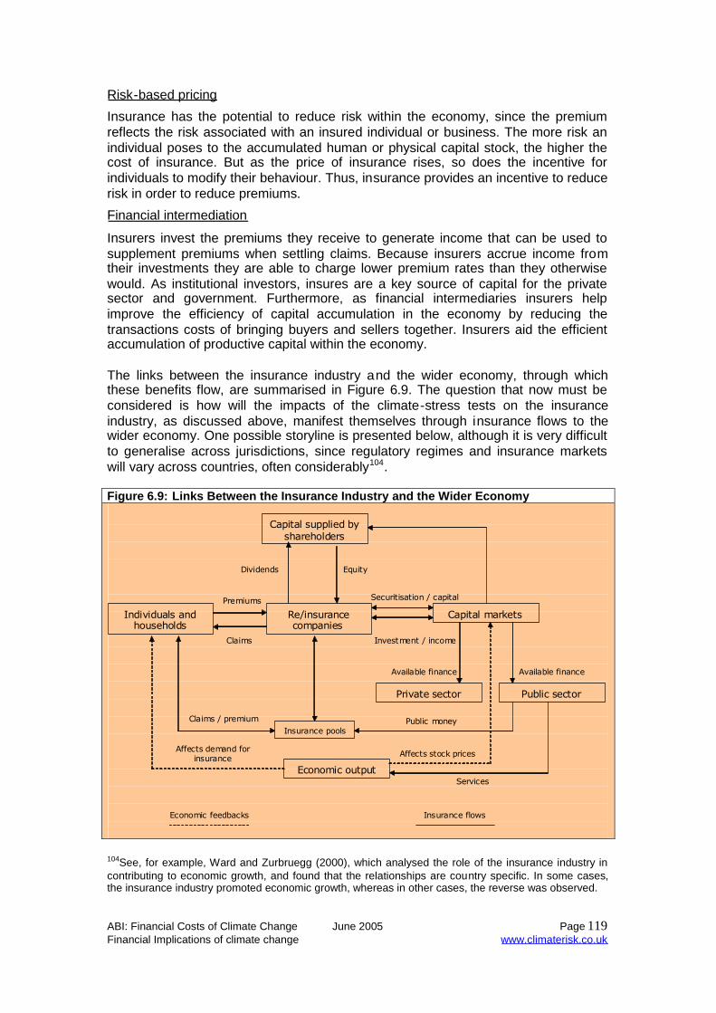
ABI: Financial Costs of Climate Change June 2005 Page 119Financial Implications of climate change www.climaterisk.co.uk
Risk-based pricing
Insurance has the potential to reduce risk within the economy, since the premiumreflects the risk associated with an insured individual or business. The more risk anindividual poses to the accumulated human or physical capital stock, the higher thecost of insurance. But as the price of insurance rises, so does the incentive forindividuals to modify their behaviour. Thus, insurance provides an incentive to reducerisk in order to reduce premiums.
Financial intermediation
Insurers invest the premiums they receive to generate income that can be used tosupplement premiums when settling claims. Because insurers accrue income fromtheir investments they are able to charge lower premium rates than they otherwisewould. As institutional investors, insures are a key source of capital for the privatesector and government. Furthermore, as financial intermediaries insurers helpimprove the efficiency of capital accumulation in the economy by reducing thetransactions costs of bringing buyers and sellers together. Insurers aid the efficientaccumulation of productive capital within the economy.
The links between the insurance industry and the wider economy, through whichthese benefits flow, are summarised in Figure 6.9. The question that now must beconsidered is how will the impacts of the climate-stress tests on the insuranceindustry, as discussed above, manifest themselves through insurance flows to thewider economy. One possible storyline is presented below, although it is very difficultto generalise across jurisdictions, since regulatory regimes and insurance marketswill vary across countries, often considerably104.
Figure 6.9: Links Between the Insurance Industry and the Wider Economy
104See, for example, Ward and Zurbruegg (2000), which analysed the role of the insurance industry incontributing to economic growth, and found that the relationships are country specific. In some cases,the insurance industry promoted economic growth, whereas in other cases, the reverse was observed.
Capital supplied byshareholders
Re/insurancecompanies
Individuals andhouseholds
Private sector Public sector
Economic output
Capital markets
Affects demand forinsurance Affects stock prices
Available financeAvailable finance
Investment / income
Securitisation / capital
EquityDividends
Premiums
Claims
Services
Insurance pools
Economic feedbacks
Claims / premium
Insurance flows
Public money

ABI: Financial Costs of Climate Change June 2005 Page 120Financial Implications of climate change www.climaterisk.co.uk
The prospect of potentially much larger damages from more intense windstormscould lead to an expansion in demand for insurance. The increase in demand willhave direct and indirect economic impacts that manifest themselves through:
Increased intermediary demand by the insurance industry.o In order to provide for additional cover and the associated extreme
contingencies more financial capital will be required, which in turnwill raise the real price of capital to both the private and publicsector. Sectors in the economy that are relatively capital-intensivewill thus have to offer higher rates of return, increasing their costs,in turn potentially leading to a decrease in output.
o The higher rates of return will lead to an expansion in life insurance,and other products, depending on how they are linked in demandwith property insurance (i.e. whether they are substitutes orcomplements to the goods whose price increases).
o Those sectors that supply inputs to insurance (e.g. “businessservices” and “construction”) will experience an increase in output.
Increases in insurance prices.o As a result, the quantity of insurance demanded by existing
policyholders is reduced. That is, the higher prices “crowd” somepolicyholders out of the market. In these cases, expenditure will beswitched to other products, benefiting the sectors that producethose products.
o Sectors that are intensive purchasers of insurance will alsoexperience an increase in costs, which could lead to a reduction inoutput. These sectors may have to reduce consumption of otherinputs (including imports) in order to continue purchasing the morecostly insurance. This would reduce both intermediary demand andthe employment of labour. Reductions in the employment of labourwill reduce the real wage rate.
The overall net impact on price levels, output, and employment will dependon the structure of the economy. In the case of the UK, a 10 per centexpansion in demand for property insurance, raised the cost of capital by0.03 per cent, reduced the wage rate by 0.02 per cent and increased GDPby 0.01 per cent. Insurance industry output increased by US$ 1,750million; regarding other sectors, the biggest winner was “businessservices” where output increased by US$ 30 million, while the biggest loserwas “finance”, where output fell by US$ 155 million.

ABI: Financial Costs of Climate Change June 2005 Page 121Financial Implications of climate change www.climaterisk.co.uk
6.10 Appendix A
Alternative Sources of Capital: Financial Markets
After Hurricane Andrew reduced the supply of traditional reinsurance, insurers wereforced to look for new sources of capital capacity that could not be borne by insurersand reinsurers. Financial markets were the natural place to look for such capacitybecause of their sheer size. For example, a US$ 100 billion loss would amount toclose to 30 per cent of the equity capital in the U.S. insurance market and about 40per cent of the total capital of the global reinsurance market. However, such as losswould be less than ½ of 1 per cent of the U.S. stock and bond markets, and an evensmaller fraction of the value of global securities market. Thus, the U.S. equity anddebt markets alone far exceed the combined capacity of the global insuranceindustry.
Moreover, daily fluctuations in financial markets exceed the largest insured lossesfrom natural catastrophes to date. Financial markets should therefore be able toabsorb losses from extreme weather events without causing any significantdisruption.
In addition, re/insurance markets are also subject to price and availability cycles,often resulting in price increases and supply restrictions following catastrophes, asdiscussed above. From the point of view of the economy, price volatility is, in general,undesirable. Additional capital would serve to dampen price volatility (Froot, 1999)105.
Raising additional equity capital in the re/insurance industry to finance catastrophiclosses, however, is costly and not necessarily efficient (Jaffee and Russell, 1997)106.For example, tax and accounting rules often penalise insurers for holding capital tocover infrequent events. Capital held by insurers is also subject to regulatory costs.Capital markets represent a more efficient source of additional capacity; for a start,they are more efficient at reducing informational asymmetries and facilitating pricediscovery (Cummins et al, 2002)107.
Securities linked to natural catastrophes also offer investors a major advantage-portfolio diversification, since losses from natural disasters are largely uncorrelatedwith changes in the stock and bond markets (Canter et al, 1997).
The new products developed by financial markets to spread catastrophic risk amonginvestors can be grouped into three categories: insurance linked bonds and notes,exchange-traded products and other structured products.
_______________________________
105Kenneth A. Froot, The Evolving Market for Catastrophic Event Risk, Working Paper No. 7287(Cambridge, Mass.: National Bureau of Economic Research, August 1999)
106Dwight M. Jaffee and Thomas Russell, "Catastrophe Insurance, Capital Markets, and UninsurableRisks," Journal of Risk and Insurance, vol. 64, no. 2 (June 1997), pp. 205-230
107Cummins, J.D., D. Lalonde and R.D. Phillips (2002) “Managing Risk Using Indexed-LinkedCatastrophic Loss Securities”, Department of Risk Management and Insurance, Georgia StateUniversity.

ABI: Financial Costs of Climate Change June 2005 Page 122Financial Implications of climate change www.climaterisk.co.uk
Catastrophe Bonds and Notes
Catastrophe bonds are subject to default on interest and principal, in part or in full, inthe event of specified catastrophe during the life of the bond. Following an eventcovered by a bond, the default provisions enable the issuer – a special purposevehicle - to use the money that would have otherwise been paid to bondholders toinstead pay loss claims. For the issuer, such bonds not only provide additionalreinsurance capacity, they also provide protection against the risk of counterparty(reinsurer) default. Bondholders are compensated for the default provision (whichhave low probabilities) by receiving high rates of return before the event occurs.
One disadvantage of catastrophe bonds is that they are susceptible to moral hazard:they give an insurer the incentive to relax underwriting and claims settlementstandards, which can lead to higher than anticipated losses.
The general approach in the capital markets has been to create a reinsurancecontract between the ceding insurer and a special purpose vehicle, which theneffectively securitises the contract on the market (see Figure A1). This structureallows primary insurers to treat the bonds as reinsurance rather than debt for tax andaccounting purposes. However, it also increases the transaction costs.
Figure A1: Structure of Basic Catastrophe Bond
Between 1997 and early 2004, a total of US$ 8 billion in catastrophe bonds wereissued (see Figure A2). Most of the issues were for losses with 1-in100 year returnperiods. To date, the default provisions have not been triggered on any bonds.
Ceding Insurer
Special PurposeVehicle
Bondholder
Premiums Default: call option onprinciple and interest
PrincipleNon-default:
contingent payment ofprinciple and interest

ABI: Financial Costs of Climate Change June 2005 Page 123Financial Implications of climate change www.climaterisk.co.uk
Figure A2: Summary of Catastrophe Bond Transactions (as at middle of 2004)
0
1,000
2,000
3,000
4,000
5,000
6,000
7,000
8,000
9,000
1997 1998 1999 2000 2001 2002 2003 2004
Year
Acc
umul
ated
Ris
kA
mo
unt(
USD
mill
ion)
-200
800
1,800
1997 1998 1999 2000 2001 2002 2003 2004
Source: Guy Carpenter
Figure A3: Summary of Catastrophe Bond Transactions (as at middle of 2004)(a) Distribution of Accumulated Risk
Amount By Risk Location(b) Distribution of Risk Accumulated
Amount By Peril
10%11%9%
1%
69%
Europe Japan Multiple
Taiwan U.S.
43% 29%
8%1%19%
Earthquake Hurricane Windstorm
Typhoon Multiple
Source: Guy Carpenter
Catastrophe Options
Catastrophe options give the holder a right to demand payment under an optionscontract, if a catastrophe-related claims index exceeds some pre-specified threshold(i.e. the strike price). In this way, they differ from traditional reinsurance in their use ofa loss index to trigger payouts, rather than losses for a particular insurer.
Use of an industry-wide loss index significantly reduces moral hazard and adverseselection because settlement is not based on the losses of a specific insurer.However, it does create basis risk, which arises because the options are notdesigned to match the losses of any individual portfolio, and, as a result, insurerscould be exposed to a mismatch between their losses and the option's payout.

ABI: Financial Costs of Climate Change June 2005 Page 124Financial Implications of climate change www.climaterisk.co.uk
Catastrophe options have further disadvantages compared with other financialinstruments used by insurers. For insurers, the cost of the options cannot bededucted from income until the options are exercised or expire. In contrast,reinsurance premiums can be deducted immediately. Some regulators may also nottreat the options as reinsurance, which means that they may not necessarily be ableto increase the level of coverage they have issued after purchasing options. Inaddition, for potential investors, the cost of informing oneself about catastrophe risksmay be prohibitive. This is, nonetheless, a drawback with most capital marketproducts for catastrophe risks.
In principle, catastrophe options can be traded at short notice and at relatively lowcost. The options that were traded on the Chicago Board of Trade protected insurersfrom total insured losses of up to US$ 50 billion. However, trading activity ceasedafter December 2000 due to low trading volumes; the same happened to anothertrading venue, the Bermuda Commodities Exchange.
Other Structured Products
Contingent Surplus NoteDebt financing can also help insurers avoid financial distress following a catastrophe.Contingent surplus notes are essentially “put” rights, where insurers agree to sell,and purchasers agree to purchase, a debt note at a price agreed in advance. If theevent does not occur, no debt note is issued. The debt note is thus a mechanism forrisk financing, as opposed to risk transfer. The issuance of debt notes can be inexchange for cash or liquid assets, which are kept in a trust account. In the event of acatastrophe these liquid assets are exchanged, typically through a financialintermediary, for the debt note issued by the insurer, who in turn uses the funds tofinance loss claims.
To induce investors to commit funds and compensate them for the risk of only partialrepayment, they receive a high rate of return, or an up-front fee.
Contingent Equity PutsEquity puts are another form of “option”, in which investors, for a fee, agree topurchase equity shares at the request of an insurer in the wake of a catastrophe108.Insurers use the funds received from the sale of those shares to pay loss claims. Thefee is designed to compensate the investor for the risk that the agreed price at whichthey agreed to buy the shares would actually be higher than the share's market priceat the time the option was exercised.
As with surplus notes, equity puts are a form of risk financing (i.e. providingimmediate liquidity), and do not perform the traditional reinsurance role of risktransfer.
Contingent equity put have a significant drawback for investors, in that it exposesthem to the general business risk of the insurer. A catastrophe could occur after aperiod in which the insurer's shares have performed relatively poorly for reasonscompletely independent of the catastrophe, such as poor management.
Catastrophe Swaps
Swaps are another way of paying premiums for catastrophe reinsurance. In a swaparrangement, insurers essentially trade exposures and in doing so, diversify theirholdings, thus reducing the risk that they could become insolvent after a disaster. Forexample, a UK based insurer might swap a portion of its flood exposure for some

ABI: Financial Costs of Climate Change June 2005 Page 125Financial Implications of climate change www.climaterisk.co.uk
windstorm risk from a German-based insurer. Thus, swaps do not change aninsurer's cash flows.
Most large swaps are negotiated directly between companies, but they must have agood understanding of counterparty risk. Swiss Re and Tokio Marine & FireInsurance, for example, recently agreed to a US$ 450 million swap, which involvedthree exchanges of US$ 150 million each to cover losses from the followingcatastrophes: a Japanese earthquake for a California earthquake; a Japanesetyphoon for a Florida hurricane; and a Japanese typhoon for a French storm109.
109Swiss Re, "Swiss Re and Tokio Marine Arrange Unique USD 450 Million Cat Risk Swap" (pressrelease, Zurich, July 12, 2001)

ABI: Financial Costs of Climate Change June 2005 Page 126Financial Implications of climate change www.climaterisk.co.uk
Related Documents