Financial Risk Analysis and its practical ... - DNV GL Risk Analysis and its... · ([email protected] ) and Mike Johnson ... (QRA) have been ... Figure 6 is created from the EAAL

Financial Risk Analysis and its practical application to improved business performance.

Dr Nic Cavanagh ([email protected]), Dr Pascal Le Gal, ([email protected]), Dr Jeremy Linn, ([email protected]) and Mike Johnson ([email protected]), DNV Software, London

Keywords: Quantitative Risk Analysis, Financial Risk Analysis, Safeti Financial,

Introduction Software tools supporting the classical approach to chemical process Quantitative Risk Analysis (QRA)

have been available for close to 30 years. But today’s business environment is far more competitive, demanding continuous improvement to financial performance as well as requiring compliance with safety legislation. The focus on Corporate Social Responsibility (CSR) and the move to reporting on social, environmental and financial performance - the so-called triple-bottom-line concept - means that investment in risk analysis must deliver to all these reporting needs. As safety professionals, we recognise that “Good safety means good business”, but demonstrating this to stakeholders is not always straightforward. By extending the tools available for QRA to assess the financial impact of the risks to which a plant is exposed, we can demonstrate direct benefits to the financial performance of the business. Further, by including risks to the surrounding population and environment in a financial risk analysis, the contribution from investment in plant safety to managing social and environmental performance can be measured and reported on.

We have developed a methodology and tool which is able to do just this, extending traditional QRA to assess financial impacts; we refer to this as Financial Risk Analysis (FRA) (Cavanagh and Linn, 2005, Cavanagh and Linn, 2006). This paper briefly describes the methodology and tool, Safeti Financial, and identifies a number of areas in which this can be used to improve financial performance with examples demonstrating the practical application of FRA. Three key areas are described where FRA can demonstrate tangible benefits; these are broadly defined as “insurance risk”, “land use planning” and “process configuration”. An example of each is presented illustrating some of the key benefits. The first case study uses FRA to assess both expected maximum losses and likely minimum financial risk exposure and explores how these can be used to justify reducing insurance premiums. The second case study looks at how FRA can be used to help in land use planning decisions. By considering the location of on-site infrastructure, like control rooms and buildings, we can minimise the exposure of these to financial risk. The final case study demonstrates how we can optimise our plant configuration applying Cost-Benefit-Analysis to help mitigate highest risk activities as economically as possible. By exploring a number of options for the storage method of hazardous materials, for example, we can better understand our operational risks and ensure these are managed in the most effective way.

Methodology The classical approach to QRA is well documented (Cavanagh, 2001; Worthington and Cavanagh, 2003)

and has been implemented in commercial software tools like Safeti from DNV Software (Cavanagh and Linn, 2005) for many years. Traditional QRA focus on consequence and risks to life, so-called fatality risk. But the industry today is also interested in other risks which impact on financial performance. We have extended the classical approach to QRA to consider the broader “business” or financial risks associated with the operation of hazardous facilities. Typical questions to be answered by FRA are; “If I have an accident, what will it cost?”, “What is the maximum financial risk to which my operation is exposed?” and “What is the frequency with which I can expect to incur losses in excess of a given cost?” Typical outputs from FRA are Frequency-Cost curves (Evans and Thakorlal, 2003), analogous with the F-N curves from QRA, or industry standard metrics such as Estimated Annual Average Loss (EAAL) (Chippindall and Butts, 2004).

The financial risk associated with an operation is the integration of the individual risks from impacts on people in terms of fatalities and injuries, impact on equipment and other assets in terms of repair and replacement cost, cost of business interruption, environmental impact and other outcomes such as legal fees, fines, brand damage and loss of share value. The Safeti Financial model considers financial risk in terms of population, original source equipment (i.e. sources of hazardous release), specific equipment, other assets (e.g. buildings, infrastructure, piping and non-specific plant) and user defined costs. In order to assess the financial impact of individual release scenarios the model uses the damage level and vulnerability factor concept for each outcome type (flammable, explosive and toxic) which will be familiar to users of Safeti (Worthington and Witlox, 2002). Additional Information on the model has been provided by Cavanagh and Linn (2006). The model provides a way of estimating the overall financial risks associated with hazardous facilities, providing safety professionals with an ideal tool for presenting to management the broader value of “safety management”, demonstrating that “Good safety means good business”. Three case studies are presented below to illustrate the benefits of FRA.

Case Study 1: Managing Insurance Risks Insuring hazardous installations such as refineries can be very costly. FRA provides an extremely

valuable tool when negotiating insurance premiums or deciding on the structure of policies to suit particular situations in terms of maximum insured loss and appropriate excess or deductible levels. This particular application of FRA has been described in detail by Chippindall and Butts (2004). Figure 1 shows a simple refining and offloading facility with a number of plant equipment items, assets and populated areas defined which is used to illustrate these concepts. The EAAL and F-Cost curves are particularly useful in helping to decide on appropriate insurance parameters like excess or deductible and maximum insured value.

In this example we investigate the effect of bunding storage vessels on the overall F-Cost curves and the EAAL by cost category since this will reduce the environmental impact. Figure 2 compares the overall financial risks for the bunded and unbunded cases, indicating that the maximum expected loss is decreased from nearly $2M to just over $1M for bunded vessels; the individual cost category curves show that this reduction is largely due to reduced risks to the environment and, on this basis, we can expect to incur this level of loss on average once every 2000 years. If our maximum insured value is of similar magnitude, as one would expect, this justifies an equivalent reduction, thus reducing our overall premiums. Furthermore, if this method of mitigating environmental risks is used, there is very little benefit from insuring the plant for more than $1M (note this example uses a limited number of scenarios to illustrate the concept, so the values are far lower than would be expected from a comprehensive FRA). This model thus enables us to perform cost benefit analysis on cost of mitigation against reduced insurance costs, for example.

Considering Figure 3, we can see that the addition of bunds reduces the EAAL by around $4k per annum and this can be used in assessing the benefit of off-setting an increased deductible against reduced insurance premiums. Since a typical plant is likely to experience a number of small loss events during its life-time, the prediction of losses from small loss events is far more representative than those from large loss events and the EAAL should be comparable to the insurance premium. It follows that if we are able to reduce the EAAL for the entire plant then we can use this as a basis for negotiating reduced premiums, or for self insured operators, reducing the overall insurance pool across all our plants accordingly.

Case Study 2: Land use planning from an optimal financial risk perspective The second case study demonstrates how financial risk analysis can be used in helping to make land

use planning decisions based on minimising the overall financial risk exposure whilst not compromising on safety. In this case study the operator of the storage facility illustrated in Figure 4 wishes to construct a new warehouse and offices. There are a number of options under consideration with similar overall costs of implementation. Two possible options are also illustrated in Figure 4, along with individual fatality risk contours from a QRA model. The model was subsequently populated with additional information about the location and value of a range of equipment and assets. Each storage tank represents a potential source of hazardous release as well as a receptor to all other possible releases from all other sources. The potential financial consequences of each release scenario in terms of the source and receptor costs are assessed and then integrated with wind rose, population, ignition source and other background data to generate a number of financial risk measures including F-Cost curves, maximum cost per scenario and EAAL.

The individual risk contours shown in Figure 4 will not be affected, irrespective of option selected, since no additional hazardous equipment is proposed. However, from a qualitative standpoint it can be seen that some of the higher risk contours, specifically 1e

-7 and 1e

-8, extend into the warehouse and offices being

proposed for Option 2 but not Option 1. We would therefore expect Option 2 to have a larger overall societal fatality risk as confirmed by F-N curves for this study.

By extending this example to include financial information about assets, equipment and population we can illustrate how the operator can make use of FRA to, firstly, assess quantitatively the most cost effective of the two alternative options and, secondly, identify the main contributors to additional financial risk in terms of both scenario and cost category. This combination of financial and fatality risk measures enables us to demonstrate that this development is both as safe as possible complying with any relevant legislation, and ensures that we are able to minimise our exposure to additional financial risk. Traditional F-N curves confirm that Option 2 exposes us to much higher societal risk than Option 1.

Figure 5 illustrates the overall financial risk for each option confirming that Option 2 exposes us to by far the highest increase in overall financial risk. Indeed, we can also conclude that the main increase in financial risk exposure is in the high cost, low frequency domain. Based on this analysis, we may decide to review our maximum insured loss irrespective of which option is selected, as described in more detail in the first case study. An initial conclusion would be that Option 1 is preferable from this standpoint, but we may still want to drill-down to identify the main contributors to the increase in terms of both scenario and cost category. Breaking this down by cost category we can see that high frequency low cost events for both options are dominated by environmental costs, costs due to business interruption and lost inventory whilst the lower frequency, higher cost domain is dominated by fatality and injury costs.

Even if Option 1 is selected, we may decide to look in more depth at contributors to the EAAL. This can help us in assessing which scenarios and cost contributors we should focus on if we want to bring the

financial risks associated with Option 1 closer to those for our existing facility. The reports available in Safeti Financial make this very easy to do. Figure 6 is created from the EAAL financial risk report and shows the EAAL contribution for each of the seven cost categories for the base case, Option 1 and Option 2. From this figure we can see that the main additional risk for Option 2 is the contribution of fatality cost of around $3,000/year, whilst the largest contributor in all cases is the environmental cost of around $20,000/year. From the standpoint of risk in terms of fatalities, we may decide to provide additional fire protection to the warehouse in Option 2 if there are other reasons why this may be preferable to Option 1, for example, thus reducing the risks to personnel within these buildings. Investigating the scenarios contributing most to the overall financial risk, Figure 7 shows EAAL per scenario and indicates that the main contributor to the increased financial risk in Option 2 is rupture of the LPG storage vessel. If this is the preferred option we may consider re-locating this vessel in the north of the plant or providing additional safeguards to reduce the likelihood of this event or additional barriers to mitigate its consequences.

Case Study 3: Selection of storage configuration to minimise financial risk exposure This ethylene case study has been designed to show the effect of selecting different process design

options on the financial risk exposure of a plant. The only difference between the two scenarios is that the one large storage bullet in Option 2 is replaced with three smaller bullets in Option 1. The total storage capacity and inventory in the two scenarios are the same. It is assumed that the bullets are bounded to the North by the sea, East by process facilities, South East by offices, South by a control room, car park and workshops and to the West by atmospheric storage tanks as illustrated in Figure 8. The facilities have not been modelled in detail but each asset group, whether process or other infrastructure, has been assigned costs in the event of an accident for repair/replace, inventory loss and business interruption. It is also assumed that the largest hazard zones for either option do not extend beyond the plant boundary so offsite risks are not considered. For each option a range of scenarios were considered including representative leaks from small, medium and large holes and a catastrophic failure.

When modelling the financial risks from these two design options we can very quickly see that the maximum loss from Option 2 with one bullet is significantly greater than for Option 1 with three. The reason for this is that the largest events cause significantly more damage to the other assets in Option 2 as there is a much larger inventory available. The losses to other assets are greater than the losses to the extra two bullets in Option 1 and are not offset by the greater overall frequency of release as we have three bullets with the same failure frequency as the single bullet in Option 2. In this hypothetical example the maximum loss was reduced by nearly 30% from $22M in Option 2 to $16M in Option 1 as can be seen from Figure 9. This information can be used in making risk informed design decisions as well as in insurance negotiations as described in Case Study 1.

The key parameter affecting maximum loss in this case study is the relative cost of the storage bullets and their loss in comparison to the asset losses that can be avoided by having smaller inventories and thereby smaller hazard zones. There is a trade-off between reducing the maximum loss from the assets compared with the storage bullets. There are many other parameters that could be varied such as layout and other process or design options. The EAAL for both options in this case is approximately $50k since, despite there being less major asset loss in Option 1, there was an increased frequency of incidents created by having three bullets rather than one in Option 2. Ultimately there are many other factors that need to be considered when deciding on the most cost effective configuration such as construction costs, maintenance costs and operational costs. This Case Study demonstrates how we can use financial risk modelling to help determine the optimum design for a plant to minimise financial losses and overall financial risk.

Conclusions Financial Risk Analysis provides a method for extending the application of traditional QRA to help in

making broader business decisions based on financial risk exposure. We have developed a software tool based on Safeti, the industry standard QRA software, which enables us to extend traditional QRA to include financial risk information. We present three simple case studies illustrating how this can be used to facilitate risk informed decision making and cost/benefit analysis. The three areas we have focussed on are managing insurance risks, land use planning and storage configuration for minimising financial risk exposure. We have also illustrated that this provides an excellent means for showing that “Good Safety Means Good Business” and of demonstrating this to key stakeholders.

References Cavanagh, N. June 2001, Calculating Risks, Hydrocarbon Engineering, Volume 6, Number 6, Palladian Publications, London, pp 41-46 Worthington, D.R.E. and Witlox, H., October 2002, SAFETI Risk Modelling Documentation – Impact of Toxic and Flammable Effects, DNV Software Risk Management Solutions.

Worthington, D.R.E. and Cavanagh, N.J., June 2003, The development of software tools for chemical process quantitative risk assessment over two decades, ESREL 2003 Conference, Safety and Reliability, Maastricht, The Netherlands. Evans, J. and Thakorlal, G., May 2004, Total Loss Prevention – Developing Identification and Assessment Methods for Business Risks, 11

th International Loss Prevention Symposium, Prague, pp 1207-1214.

Chippindal, L. and Butts, D., June 2004, Managing the Financial Risks of Major Accidents, Annual Conference of Centre for Chemical Process Safety, Emergency Planning: Preparedness, Prevention and Response, Orlando, Florida, pp 321-326. Cavanagh, NJ. and Linn J., April 2005, Beyond Compliance – The Future Role of Risk Tools, AIChE Global Safety Symposium, Annual Conference of Centre for Chemical Process Safety, Atlanta, Georgia, USA, pp 129-140 Cavanagh, NJ. and Linn, J., April 2006, Process Business Risk - A methodology for assessing and mitigating the financial impact of process plant accidents, AIChE Global Safety Symposium, Annual Conference of Centre for Chemical Process Safety, Orlando, Florida, pp 237-256

Figure 4 - Layout for Options 1 and 2 considered in

Case Study 2 showing individual risk contours.

Figure 1 – Plant layout for Case Study 1.

Figure 2 - Comparison of financial risks for the bunded and unbunded vessels for Case Study 1.

Figure 6 - Cumulative EAAL by cost category for Case Study 2.

Figure 3 - EAAL per cost category with and without bund for Case Study 1.

Figure 5 - F-Cost curve comparison for Options 1 and 2 for Case Study 2.

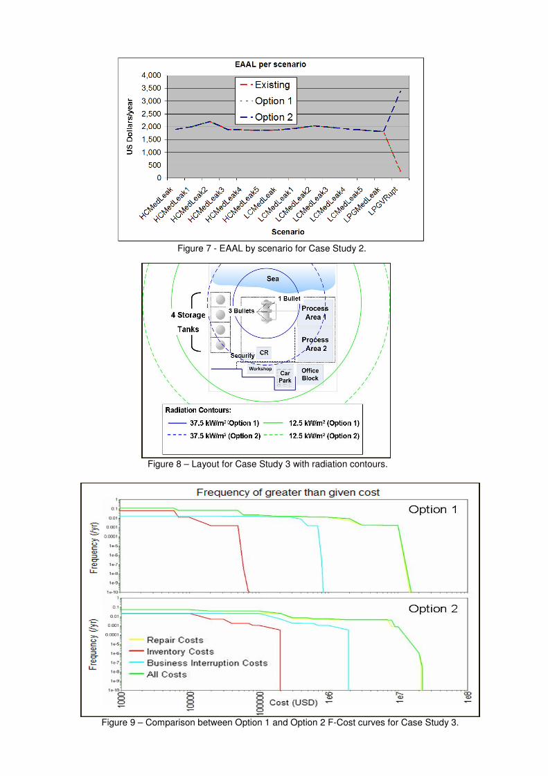
Figure 7 - EAAL by scenario for Case Study 2.

Figure 8 – Layout for Case Study 3 with radiation contours.

Figure 9 – Comparison between Option 1 and Option 2 F-Cost curves for Case Study 3.