Financial Output as Economic Input: Resolving the Inconsistent Treatment of Financial Services in the National Accounts

Jacob Assa

Financial Output as Economic Input: Resolving the Inconsistent Treatment of Financial Services in the National Accounts

February 2015 Working Paper 01/2015 Department of Economics The New School for Social Research

The views expressed herein are those of the author(s) and do not necessarily reflect the views of the New School for Social Research. © 2015 by Jacob Assa. All rights reserved. Short sections of text may be quoted without explicit permission provided that full credit is given to the source.

Financial Output as Economic Input: Resolving the Inconsistent Treatment of Financial Services in the National Accounts

Jacob Assa

February 2015 Abstract This paper investigates the inconsistent treatment of financial services in the national accounts. While net interest income from financial intermediation is netted out as input to other industries and thus does not affect the overall level and trend of Gross Domestic Product (GDP), fee-based net income from financial services is included as value-added, inflating GDP by the same amount. A new measure of economic activity which resolves this inconsistency is introduced, treating all financial income as a cost or intermediate input to the rest of the economy. The resulting aggregate tracks employment and median income far more closely than GDP.

Keywords: measurement of real output; employment; national accounting; finance. JEL Codes: E01, E20.

2

1. Introduction

The three major types of financial services are treated in the standard national accounts in three different ways. Capital gains are excluded à priori from the production accounts; interest flows generated by financial intermediation are treated as an input to other industries and deducted from total value-added to arrive at Gross Domestic Product (GDP); and fee-based financial services are considered productive and are imputed a value-added based on net revenue. While there is consensus regarding the exclusion of capital gains since there is no productive activity associated with them, the other two treatments – of interest-based financial intermediation and fee-based financial services – are more controversial. Furthermore, there is an inconsistency in how the standard accounting framework treats these two sources of financial income. While the netting out of interest-based income does not affect overall GDP, the value added imputation for the fee-based income inflates GDP by its amount, leading to a divergence of this measure of output from its historic correlation with other variables such as employment and median income. After reviewing some of the technical issues involved in the debate over the assumed productiveness (or lack thereof) of interest-yielding financial intermediation services, the discussion turns to the fee-based financial revenues which have received less attention. Unlike the interest-based part of financial incomes, the fees generated from financial services are not netted out of GDP and show up as value added on the production (output) side of the accounts. We assess the differences between finance and the other sectors for which value added is imputed, both conceptually and empirically, and argue that it is always an input (or a cost) for other industries and the economy as a whole, having no final use value. We then construct an alternative measure of overall economic activity which treats finance as a cost to be netted out from total value added, consistent with the way financial intermediation services indirectly measured (FISIM) income is treated in the standard accounts. The resulting adjusted measure of output – Final Gross Domestic Product or FGDP – includes only final goods and services, and is further reconciled with the expenditure and income side of the accounting framework. Empirical estimates of FGDP are constructed using data from input-output (I/O) tables, with the result that FGDP tracks both employment and median income (as a proxy for the standard of living) far better than GDP. Further research is outlined for empirical and policy implications.

2. Accounting for Finance

GDP “is the primary indicator of economic activity and...can be estimated in three ways, which are theoretically equal” (Lee 2012) and must identically agree, thus also providing mutual control for each other. In compiling national income statistics from various sources using the three methods, however, the results inevitably disagree, and are reconciled by including a “statistical discrepancy” in the accounts. The expenditure approach to GDP is the sum of all final expenditures, and is denoted by the familiar equation below:

(1) GDP = C + I + G + X - M That is, GDP equals the sum of consumption or final expenditure by households,

investment by firms, final consumption by government, and net exports. The income approach, by contrast, is as follows:

(2) GDP = CE + NT + GOS

3

Here GDP equals the sum of compensation of employees (wages plus benefits), net taxes (taxes on production and imports less subsidies), and gross operating surplus (profits). Finally, the production (output) approach to GDP sums up all activities deemed productive across industries:

(3) GDP = ∑(Y i – ICi) + NT where Y stands for output, IC for intermediate consumption, and the term in the summation expression represents value added for each industry i. GDP is thus equal to value added plus taxes minus subsidies. As Lee explains, “[o]utput is all the goods and services produced, whilst intermediate consumption comprises all the goods and services consumed or transformed in a production process. The net taxes are included in order to put all three approaches on a consistent valuation basis” (ibid). In other words, value added itself is not directly comparable to GDP by the expenditure or income approaches, and we must use GDP by the output approach (i.e. value added + taxes - subsidies) to make comparisons with the other two GDP measures more consistent.

Next, when discussing value added in ‘finance’, the official System of National Accounts (SNA) includes financial intermediation, insurance and pension funds, and other activities such as administration of financial markets. Some authors (e.g. Basu and Foley 2013) add real-estate, resulting in the FIRE acronym. It is important to note, however, that even the narrow definition of finance which refers only to financial services (and does not include real-estate, insurance or other business services) itself comprises three types of activities performed by the financial industry (including non-bank financial institutions):

1. Services for which banks explicitly charge a fee, and are thus relatively

straightforward to record in the national accounts. These services include overdraft fees, foreign exchange commissions, consulting on mergers and acquisitions, underwriting securities, as well as market-making activities (Akritidis, 2007, Haldane 2010).

2. Financial intermediation resulting in net interest income – this part of banks’ business is not as easily captured. “Finance – and commercial banking in particular – relies heavily on interest flows as a means of payment for the services they provide. Banks charge an interest rate margin to capture these intermediation services” (Haldane 91), which gives rise to the FISIM income mentioned above.

3. Net Spread Earnings (NSE), e.g. capital gains or dealing profits from spot trading in the foreign exchange market.

These three major types of financial services are treated in the national accounts in

three different ways. Capital gains are excluded à priori from the production accounts; interest flows generated by financial intermediation are treated as an input to other industries and deducted from total value-added to arrive at GDP; and fee-based financial services are considered productive and are imputed a value-added based on net revenue. While there is consensus regarding the exclusion of capital gains since there is no productive activity associated with them, the other two treatments – of interest-based financial intermediation and of fee-based financial services – are more controversial. Furthermore, there is an inconsistency in how the standard accounting framework treats these two sources of financial income.

Since fees paid for financial services are easily captured by national accountants, most of the debate has recently focused on the (non-fee based) net interest part - financial

4

intermediation and the imputation of its output through FISIM. Financial intermediation has long been problematic to measure. Christophers (2011) describes the history of the so-called ‘banking problem’ - the fact that, without imputations, the value-added of the financial sector (that is, output minus intermediate consumption) would be negligible or even negative (since if its costs are deducted from fee-based revenues alone, the former would often exceed the latter). At a first stage in the history of this question (SNA 53 and before), all financial intermediation activities were excluded from calculations of national output based on the value-added approach, since they were considered to be mere transfers of funds (similar to social security payments) and hence unproductive. An intermediate approach followed with the SNA 68, where the output of the financial sector was considered to be an input to a notional (i.e. imaginary) industry which has no output. In spite of the bizarre nature of this approach, “ascribing a negative income to an imaginary industry sector...has probably been the most used for financial intermediation services in the entire history of Western national accounting” (Christophers 130).

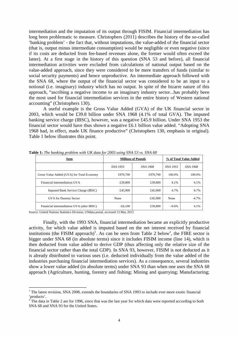
A useful example is the Gross Value Added (GVA) of the UK financial sector in 2003, which would be £39.8 billion under SNA 1968 (4.1% of total GVA). The imputed banking service charge (IBSC), however, was a negative £45.9 billion. Under SNA 1953 the financial sector would have thus shown a negative £6.1 billion value added. “Adopting SNA 1968 had, in effect, made UK finance productive” (Christophers 130, emphasis in original). Table 1 below illustrates this point.

Table 1: The banking problem with UK data for 2003 using SNA 53 vs. SNA 68

Item Millions of Pounds % of Total Value Added

SNA 1953 SNA 1968 SNA 1953 SNA 1968

Gross Value Added (GVA) for Total Economy £970,700 £970,700 100.0% 100.0%

Financial intermediation GVA £39,800 £39,800 4.1% 4.1%

Imputed Bank Service Charge (IBSC) £45,900 £45,900 4.7% 4.7%

GVA for Dummy Sector None -£45,900 None -4.7%

Financial intermediation GVA (after IBSC) -£6,100 £39,800 -0.6% 4.1%

Source: United Nations Statistics Division, UNdata portal, accessed 13 May 2013

Finally, with the 1993 SNA, financial intermediation became an explicitly productive

activity, for which value added is imputed based on the net interest received by financial institutions (the FISIM approach)1. As can be seen from Table 2 below2, the FIRE sector is bigger under SNA 68 (in absolute terms) since it includes FISIM income (line 14), which is then deducted from value added to derive GDP (thus affecting only the relative size of the financial sector rather than the total GDP). In SNA 93, however, FISIM is not deducted as it is already distributed to various uses (i.e. deducted individually from the value added of the industries purchasing financial intermediation services). As a consequence, several industries show a lower value added (in absolute terms) under SNA 93 than when one uses the SNA 68 approach (Agriculture, hunting, forestry and fishing; Mining and quarrying; Manufacturing;

1 The latest revision, SNA 2008, extends the boundaries of SNA 1993 to include ever more exotic financial ‘products’. 2 The data in Table 2 are for 1996, since that was the last year for which data were reported according to both SNA 68 and SNA 93 for the United States.

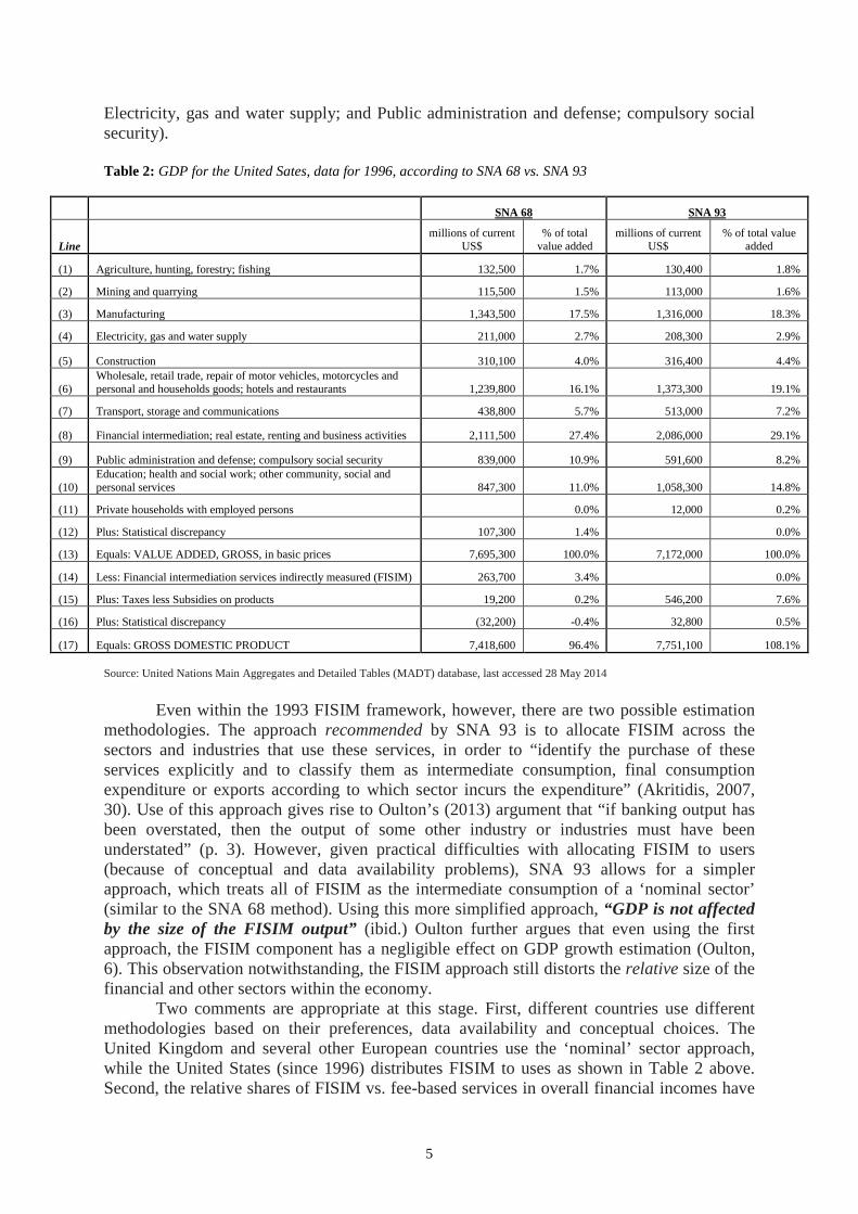
5

Electricity, gas and water supply; and Public administration and defense; compulsory social security).

Table 2: GDP for the United Sates, data for 1996, according to SNA 68 vs. SNA 93

SNA 68 SNA 93

Line millions of current

US$ % of total

value added millions of current

US$ % of total value

added

(1) Agriculture, hunting, forestry; fishing 132,500 1.7% 130,400 1.8%

(2) Mining and quarrying 115,500 1.5% 113,000 1.6%

(3) Manufacturing 1,343,500 17.5% 1,316,000 18.3%

(4) Electricity, gas and water supply 211,000 2.7% 208,300 2.9%

(5) Construction 310,100 4.0% 316,400 4.4%

(6) Wholesale, retail trade, repair of motor vehicles, motorcycles and personal and households goods; hotels and restaurants 1,239,800 16.1% 1,373,300 19.1%

(7) Transport, storage and communications 438,800 5.7% 513,000 7.2%

(8) Financial intermediation; real estate, renting and business activities 2,111,500 27.4% 2,086,000 29.1%

(9) Public administration and defense; compulsory social security 839,000 10.9% 591,600 8.2%

(10) Education; health and social work; other community, social and personal services 847,300 11.0% 1,058,300 14.8%

(11) Private households with employed persons 0.0% 12,000 0.2%

(12) Plus: Statistical discrepancy 107,300 1.4% 0.0%

(13) Equals: VALUE ADDED, GROSS, in basic prices 7,695,300 100.0% 7,172,000 100.0%

(14) Less: Financial intermediation services indirectly measured (FISIM) 263,700 3.4% 0.0%

(15) Plus: Taxes less Subsidies on products 19,200 0.2% 546,200 7.6%

(16) Plus: Statistical discrepancy (32,200) -0.4% 32,800 0.5%

(17) Equals: GROSS DOMESTIC PRODUCT 7,418,600 96.4% 7,751,100 108.1% Source: United Nations Main Aggregates and Detailed Tables (MADT) database, last accessed 28 May 2014

Even within the 1993 FISIM framework, however, there are two possible estimation

methodologies. The approach recommended by SNA 93 is to allocate FISIM across the sectors and industries that use these services, in order to “identify the purchase of these services explicitly and to classify them as intermediate consumption, final consumption expenditure or exports according to which sector incurs the expenditure” (Akritidis, 2007, 30). Use of this approach gives rise to Oulton’s (2013) argument that “if banking output has been overstated, then the output of some other industry or industries must have been understated” (p. 3). However, given practical difficulties with allocating FISIM to users (because of conceptual and data availability problems), SNA 93 allows for a simpler approach, which treats all of FISIM as the intermediate consumption of a ‘nominal sector’ (similar to the SNA 68 method). Using this more simplified approach, “GDP is not affected by the size of the FISIM output” (ibid.) Oulton further argues that even using the first approach, the FISIM component has a negligible effect on GDP growth estimation (Oulton, 6). This observation notwithstanding, the FISIM approach still distorts the relative size of the financial and other sectors within the economy.

Two comments are appropriate at this stage. First, different countries use different methodologies based on their preferences, data availability and conceptual choices. The United Kingdom and several other European countries use the ‘nominal’ sector approach, while the United States (since 1996) distributes FISIM to uses as shown in Table 2 above. Second, the relative shares of FISIM vs. fee-based services in overall financial incomes have

6

changed over time. As Akritidis observes, the share of FISIM income in total banking income declined from 72% in 1992 to 66% in 2004, while “the share taken by explicit charges, such as fees and commissions, rose” (Akritidis, 30). This fact, as well as the existence of a simpler FISIM approach which does not affect overall GDP, raises the following question: why are fee-based financial services treated as value added, while interest-based financial intermediation is netted out of GDP as intermediate consumption (of either a nominal sector or the total economy?) This inconsistency is understandable from a measurement point of view, since fee-based financial services are easy to capture and therefore present less of an empirical problem than the FISIM issue. From a theoretical point of view, however, the non-FISIM part of financial services, that is, the fee-based income in the GDP-by-output approach, is as problematic as interest-based income. Finance, in its various manifestations, ultimately involves the transfer of money. Unlike other commodities, money has no use value, only an exchange value. In fact it is exchange value par excellence. Gold and silver still had some practical uses when they were the common means of payment, but fiat money is merely symbolic. As the textbooks tell us, money serves as a unit of account, means of exchange, and store of value. Neither consumers nor firms can directly consume money, but rather purchase goods and services with it, either for final consumption or for intermediate consumption in a production process3. From a Keynesian point of view, this notion may seem problematic as money provides people (both consumers and investors) with a liquidity premium, allowing them to hedge against an uncertain future. This notion, however, runs into two problems, one conceptual and one empirical. First, money may indeed confer a feeling of security (or ‘psychic income’) on its holder because of uncertainty, but its contribution to the holder’s well-being emanates from its ability to be spent at a future moment, on goods and services. Money itself cannot be directly consumed, but performs the function of store of value in the face of uncertainty. Secondly, from a practical point of view, even if we accept that money has use-value based on the liquidity premium idea, measuring it would be hard given that its opportunity cost – interest income – is not fixed. Aside from the existence of multiple interest rates for various assets, even changes in the headline or reference interest rate would change the value of money as measured by the liquidity premium. This gives rise to the FISIM problem mentioned above.

Furthermore, fiat money is not really ‘produced’ in the way other goods and services are. In a fractional reserve system, commercial banks lend out more than the high-powered money they have on reserve with the central bank, thus ‘creating’ money. They make their profits by lending out money at a higher interest rate than that which they pay on deposits taken in, and doing other, more complicated things, all of which, however, are ultimately connected to the provision of money. In addition to reinforcing money’s lack of use value, this also suggests that finance may not have the same relationship between output and employment as other sectors whose output has final use value. Thus we need to empirically examine whether finance is indeed exceptional in this sense vis-à-vis others sectors of the economy.

3. Finance versus Other Service Sectors for which Value Added is Imputed

As the discussion above suggests, our focus here is on the political economy of the treatment of finance in national accounting, rather than on imputation issues per se. Finance is 3 Not all production is undertaken by enterprises. For example, dwelling-owning households are considered to be producing housing services for themselves, the imputation of which is included in GDP and is equal to the rents they would otherwise pay (reflecting their opportunity cost).

7

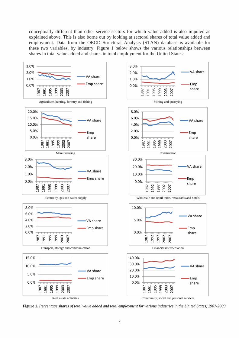
conceptually different than other service sectors for which value added is also imputed as explained above. This is also borne out by looking at sectoral shares of total value added and employment. Data from the OECD Structural Analysis (STAN) database is available for these two variables, by industry. Figure 1 below shows the various relationships between shares in total value added and shares in total employment for the United States:

Agriculture, hunting, forestry and fishing Mining and quarrying

Manufacturing Construction

Electricity, gas and water supply Wholesale and retail trade, restaurants and hotels

Transport, storage and communication Financial intermediation

Real estate activities Community, social and personal services

Figure 1. Percentage shares of total value added and total employment for various industries in the United States, 1987-2009

0.0%

1.0%

2.0%

3.0%

19

87

19

91

19

95

19

99

20

03

20

07

VA share

Emp share 0.0%

1.0%

2.0%

3.0%

19

87

19

91

19

95

19

99

20

03

20

07

VA share

Emp

share

0.0%

5.0%

10.0%

15.0%

20.0%

19

87

19

91

19

95

19

99

20

03

20

07

VA share

Emp

share 0.0%

2.0%

4.0%

6.0%

8.0%

19

87

19

91

19

95

19

99

20

03

20

07

VA share

Emp

share

0.0%

1.0%

2.0%

3.0%

19

87

19

91

19

95

19

99

20

03

20

07

VA share

Emp share0.0%

10.0%

20.0%

30.0%

19

87

19

92

19

97

20

02

20

07

VA share

Emp

share

0.0%

2.0%

4.0%

6.0%

8.0%

19

87

19

91

19

95

19

99

20

03

20

07

VA share

Emp share0.0%

5.0%

10.0%

19

87

19

92

19

97

20

02

20

07

VA share

Emp

share

0.0%

5.0%

10.0%

15.0%

19

87

19

91

19

95

19

99

20

03

20

07

VA share

Emp share0.0%

10.0%

20.0%

30.0%

40.0%

19

87

19

91

19

95

19

99

20

03

20

07

VA share

Emp

share

8

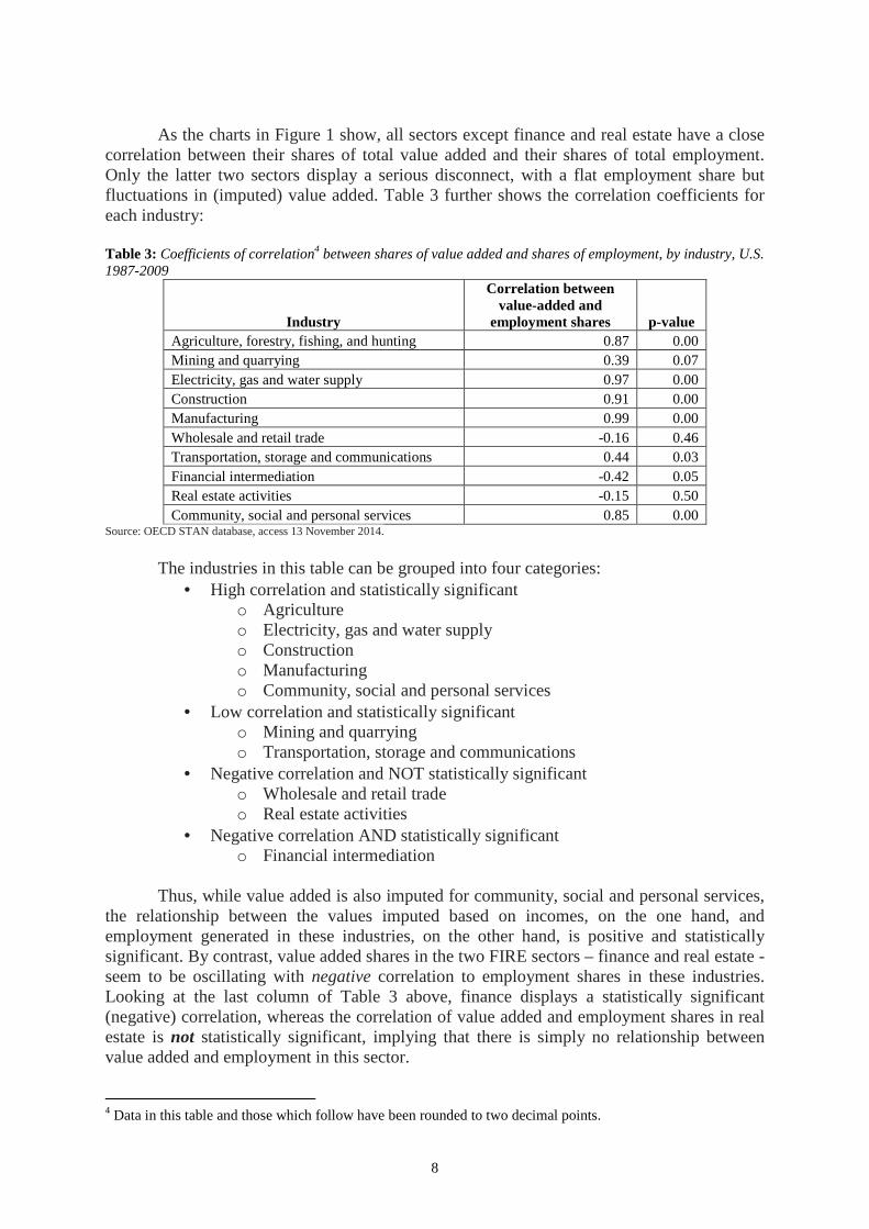
As the charts in Figure 1 show, all sectors except finance and real estate have a close

correlation between their shares of total value added and their shares of total employment. Only the latter two sectors display a serious disconnect, with a flat employment share but fluctuations in (imputed) value added. Table 3 further shows the correlation coefficients for each industry:

Table 3: Coefficients of correlation4 between shares of value added and shares of employment, by industry, U.S. 1987-2009

Industry

Correlation between value-added and

employment shares p-value Agriculture, forestry, fishing, and hunting 0.87 0.00 Mining and quarrying 0.39 0.07 Electricity, gas and water supply 0.97 0.00 Construction 0.91 0.00 Manufacturing 0.99 0.00 Wholesale and retail trade -0.16 0.46 Transportation, storage and communications 0.44 0.03 Financial intermediation -0.42 0.05 Real estate activities -0.15 0.50 Community, social and personal services 0.85 0.00

Source: OECD STAN database, access 13 November 2014.

The industries in this table can be grouped into four categories:

• High correlation and statistically significant o Agriculture o Electricity, gas and water supply o Construction o Manufacturing o Community, social and personal services

• Low correlation and statistically significant o Mining and quarrying o Transportation, storage and communications

• Negative correlation and NOT statistically significant o Wholesale and retail trade o Real estate activities

• Negative correlation AND statistically significant o Financial intermediation

Thus, while value added is also imputed for community, social and personal services,

the relationship between the values imputed based on incomes, on the one hand, and employment generated in these industries, on the other hand, is positive and statistically significant. By contrast, value added shares in the two FIRE sectors – finance and real estate - seem to be oscillating with negative correlation to employment shares in these industries. Looking at the last column of Table 3 above, finance displays a statistically significant (negative) correlation, whereas the correlation of value added and employment shares in real estate is not statistically significant, implying that there is simply no relationship between value added and employment in this sector.

4 Data in this table and those which follow have been rounded to two decimal points.

9

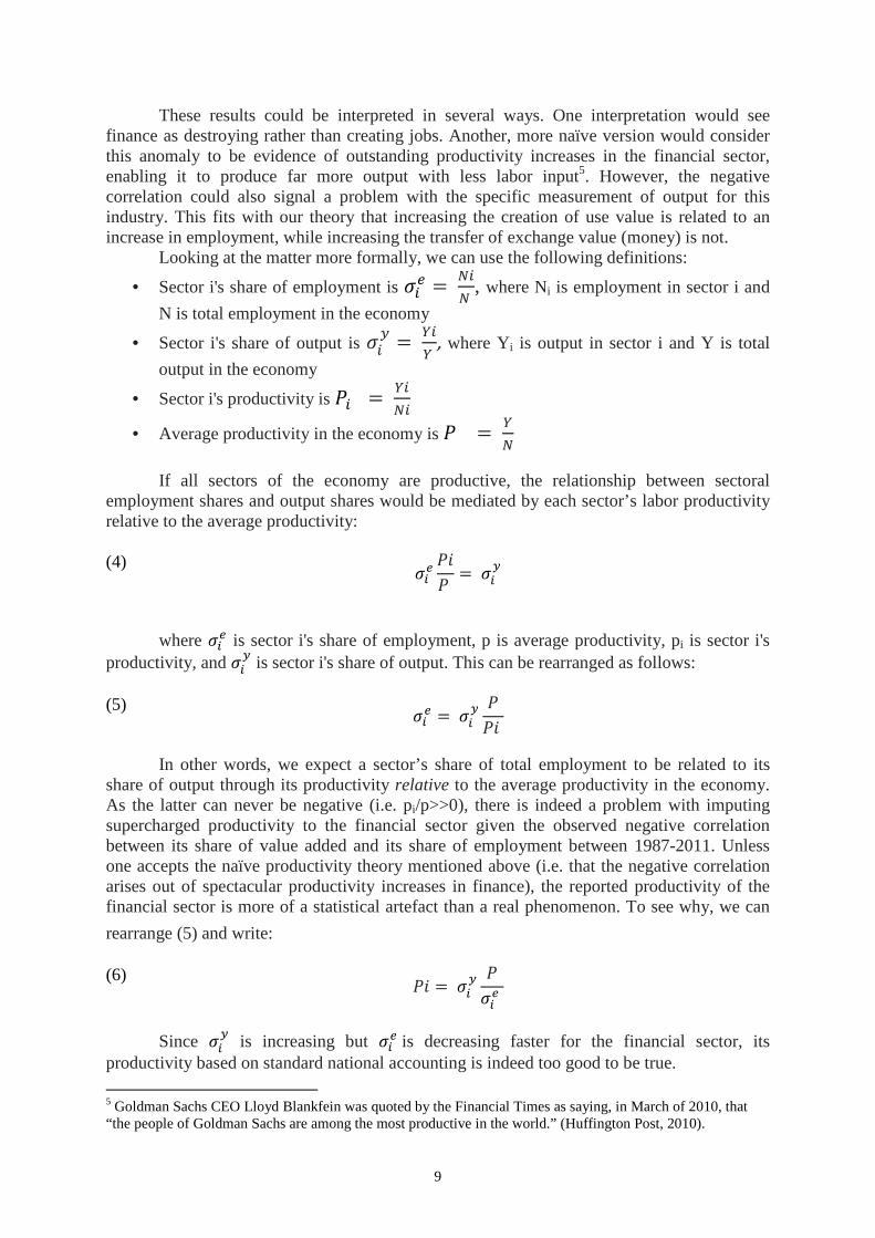
These results could be interpreted in several ways. One interpretation would see finance as destroying rather than creating jobs. Another, more naïve version would consider this anomaly to be evidence of outstanding productivity increases in the financial sector, enabling it to produce far more output with less labor input5. However, the negative correlation could also signal a problem with the specific measurement of output for this industry. This fits with our theory that increasing the creation of use value is related to an increase in employment, while increasing the transfer of exchange value (money) is not.

Looking at the matter more formally, we can use the following definitions:

• Sector i's share of employment is ��� =

��

�, where Ni is employment in sector i and

N is total employment in the economy

• Sector i's share of output is ���=

��

�,where Yi is output in sector i and Y is total

output in the economy

• Sector i's productivity is � =��

��

• Average productivity in the economy is =�

�

If all sectors of the economy are productive, the relationship between sectoral

employment shares and output shares would be mediated by each sector’s labor productivity relative to the average productivity:

(4)

����

= ��

�

where ��� is sector i's share of employment, p is average productivity, pi is sector i's

productivity, and ��� is sector i's share of output. This can be rearranged as follows:

(5)

��� =��

�

�

In other words, we expect a sector’s share of total employment to be related to its

share of output through its productivity relative to the average productivity in the economy. As the latter can never be negative (i.e. pi/p>>0), there is indeed a problem with imputing supercharged productivity to the financial sector given the observed negative correlation between its share of value added and its share of employment between 1987-2011. Unless one accepts the naïve productivity theory mentioned above (i.e. that the negative correlation arises out of spectacular productivity increases in finance), the reported productivity of the financial sector is more of a statistical artefact than a real phenomenon. To see why, we can

rearrange (5) and write:

(6) � = ��

�

���

Since ��

� is increasing but ���is decreasing faster for the financial sector, its

productivity based on standard national accounting is indeed too good to be true.

5 Goldman Sachs CEO Lloyd Blankfein was quoted by the Financial Times as saying, in March of 2010, that “the people of Goldman Sachs are among the most productive in the world.” (Huffington Post, 2010).

10

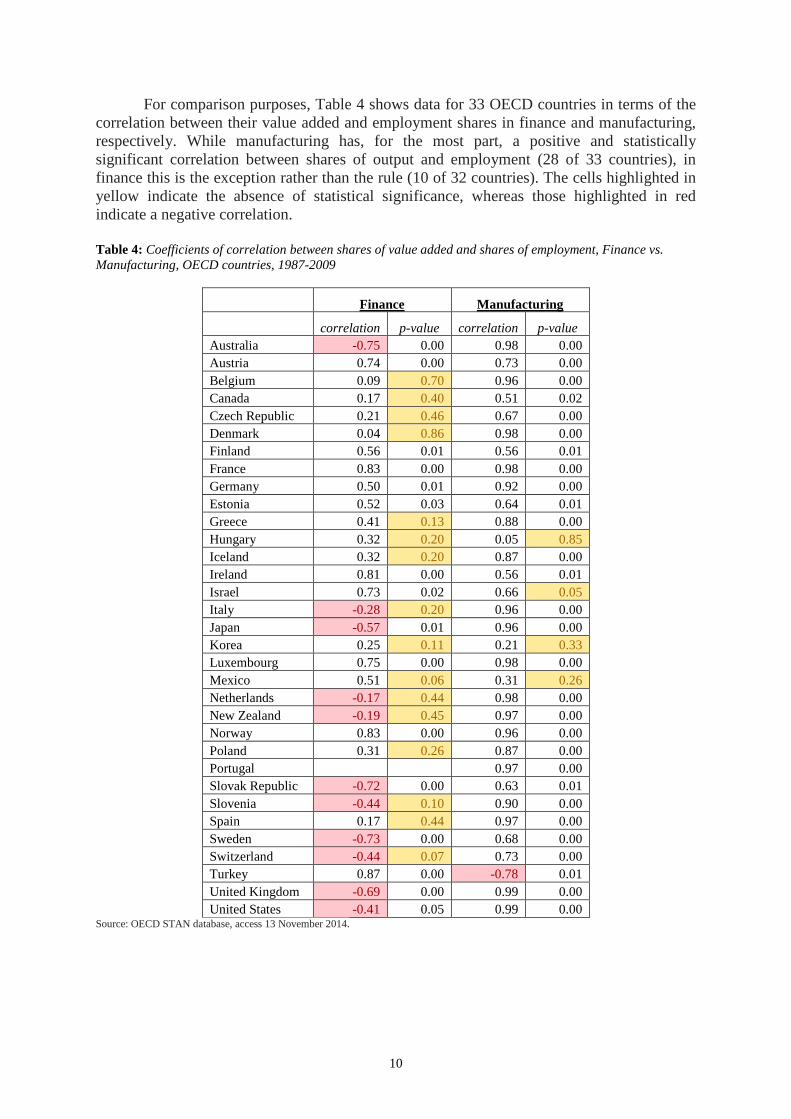
For comparison purposes, Table 4 shows data for 33 OECD countries in terms of the correlation between their value added and employment shares in finance and manufacturing, respectively. While manufacturing has, for the most part, a positive and statistically significant correlation between shares of output and employment (28 of 33 countries), in finance this is the exception rather than the rule (10 of 32 countries). The cells highlighted in yellow indicate the absence of statistical significance, whereas those highlighted in red indicate a negative correlation.

Table 4: Coefficients of correlation between shares of value added and shares of employment, Finance vs. Manufacturing, OECD countries, 1987-2009

Finance Manufacturing

correlation p-value correlation p-value Australia -0.75 0.00 0.98 0.00 Austria 0.74 0.00 0.73 0.00 Belgium 0.09 0.70 0.96 0.00 Canada 0.17 0.40 0.51 0.02 Czech Republic 0.21 0.46 0.67 0.00 Denmark 0.04 0.86 0.98 0.00 Finland 0.56 0.01 0.56 0.01 France 0.83 0.00 0.98 0.00 Germany 0.50 0.01 0.92 0.00 Estonia 0.52 0.03 0.64 0.01 Greece 0.41 0.13 0.88 0.00 Hungary 0.32 0.20 0.05 0.85 Iceland 0.32 0.20 0.87 0.00 Ireland 0.81 0.00 0.56 0.01 Israel 0.73 0.02 0.66 0.05 Italy -0.28 0.20 0.96 0.00 Japan -0.57 0.01 0.96 0.00 Korea 0.25 0.11 0.21 0.33 Luxembourg 0.75 0.00 0.98 0.00 Mexico 0.51 0.06 0.31 0.26 Netherlands -0.17 0.44 0.98 0.00 New Zealand -0.19 0.45 0.97 0.00 Norway 0.83 0.00 0.96 0.00 Poland 0.31 0.26 0.87 0.00 Portugal 0.97 0.00 Slovak Republic -0.72 0.00 0.63 0.01 Slovenia -0.44 0.10 0.90 0.00 Spain 0.17 0.44 0.97 0.00 Sweden -0.73 0.00 0.68 0.00 Switzerland -0.44 0.07 0.73 0.00 Turkey 0.87 0.00 -0.78 0.01 United Kingdom -0.69 0.00 0.99 0.00 United States -0.41 0.05 0.99 0.00

Source: OECD STAN database, access 13 November 2014.

11

4. Output and Final Use Value

Given this logic as well as the observed empirical patterns, the next question is, do financial services really have an output at all? The standard national accounts answer in the affirmative, and treat finance like any other sector. Specifically, as mentioned above, value added in the financial sector is calculated in the same way it is for other industries:

(7) VA = Y - IC where Y is output imputed based on the sum of fee-based revenues of financial

institutions and IC is intermediate consumption imputed based on their related costs (making ‘value added’ in this case nothing more than an imputation based on financial profits from fee-based services). Basu and Foley’s Non-Financial Value Added (NFVA) and Narrow-Measured Value Added (NMVA) indicators, on the other hand, leave out the value-added of fee-based finance on the assumption that it is not directly measurable and thus cannot be linked to generating aggregate demand6.

Should finance be included in or excluded from total value added? And what happens when a commodity does not have a final use value, that is, what if it cannot be used in final consumption? As mentioned above, money cannot be consumed at all, only serve to purchase other commodities which are then used (in either intermediate or final consumption). It can therefore neither be considered an output (for final consumption) nor a productive input (for intermediate consumption in the production process), implying there is no economic value added from selling money7. Thus, we cannot use the VA = Y – IC formula as in other industries. Should we exclude the imputed financial ‘value-added’ then, as Basu and Foley do?

Financial services are, however, paid for by households and firms. Thus, financial revenues (from which financial ‘output’ is imputed) are not simply non-productive for the economy – they represent an opportunity cost (similar to the SNA treatment of dwelling-owning households as described above) in that the money paid for them could have been spent on productive activities elsewhere. This, coupled with the observed negative correlation between finance’s shares in output and employment, suggests that the sector is extractive rather than productive. It is therefore more accurate to account for the financial sector as a cost of producing the rest of GDP, that is, a cost involved in generating all true value added. In other words, the ‘output’ of finance should be deducted, not merely excluded, from GDP as it is the ultimate and ubiquitous intermediate input (albeit an intermediate cost rather than an input for intermediate consumption) to all industries producing a use-value output of either goods or services.

This methodology goes beyond the SNA 53 approach which merely treated finance as non-productive. Also, while novel, it builds on two elements already existing in SNA 68 and SNA 93. From SNA 68 it takes the concept of applying the output (not value added) of the financial sector as an input with a negative sign, though in our proposed measure it is an input to the rest of the economy rather than to an imaginary sector. Even more importantly, it mirrors the treatment recommended for the FISIM income by SNA 93, here applied

6 Basu and Foley (2013) focus more specifically on the question of the discrepancy between indices of output and employment, rather than trying to develop an aggregate that consistently represents the contribution of various sectors to net output as is the case here. 7 Standard national accounts, by contrast, impute value added for fee-based financial services (not including FISIM) by deducting the costs of financial institutions from their fee-based revenues (the latter being the source of financial imputed ‘output’). This procedure is based on the neoclassical assumption that where there is income there must be production, or where there is profit there must be value added.

12

symmetrically to the fee-based part of financial incomes. Recall that FISIM in SNA 93 is distributed to uses, so several industries which pay for financial services show a lower value added than they otherwise would. This clearly shows that the amount of revenue received by financial institutions is a cost of production to other sectors. Applying this logic to the fee-based (non-FISIM) part of financial incomes (in the aggregate) would mean deducting the total revenue of financial transactions (from which financial ‘output’ is imputed) from the total value added in the economy, making the treatment of all financial activities in the SNA consistent.

We believe that both the standard national accounts as well as the NFVA/NMVA indexes overestimate the contribution of finance to total value-added and therefore overstate GDP in the process. The NFVA/NMVA method is neutral to finance in the sense that it only avoids imputing it a value-added, rather than treating it as a cost of producing all other output. Standard GDP errs twice, first in failing to net out financial output (revenue) as a cost, and again in adding financial ‘value-added’ to total value added, thus inflating GDP by the amount of the imputation.

The approach proposed here, then, differs from the NFVA/NMVA framework in three ways. First, it does not stop at excluding the value added imputed to finance but additionally gives its (imputed) total ‘output’ a negative sign since it is a cost of producing all other value added in the economy8. Secondly, it does not exclude other sectors for which value added is imputed. The reasoning here is that such sectors, e.g. government, education, health etc. do provide very concrete final use value (in the form of defense, law and order, instruction, medical care) and thus have outputs. Their measurement is indeed a contested issue as there is no independent measure of their output, but unlike finance, these sectors do not merely transfer exchange value, but actually produce final use value, measureable or not. This logic is also based on the fact that education, health and government services all produce employment-intensive tangible services, such as classes taught, medical checkups and surgeries, and military and police activities. The greater the volume of such services that is produced, the more employment is required to carry them out. In finance, however, the core activities involve managing, transferring and repackaging money in ever more ingenious ways. A financial firm handling one billion dollars in assets with 100 employees may not need to hire 900 more staff if its asset base increased to 10 billion dollars (as can be seen from the correlation shown in Table 3 above).

Third and finally, Basu and Foley compare their measures of value added (either narrow measured of non-financial) to standard GDP measures, but as mentioned above, GDP includes taxes net of subsidies while value added does not. Our approach will thus adjust the proposed final-use value added measure to derive Final GDP, or FGDP.

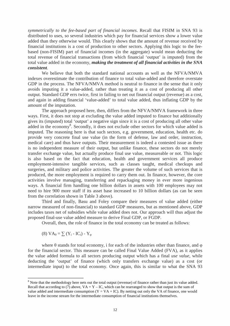
Overall, then, the role of finance in the total economy can be treated as follows: (8) VAθ = ∑ (Yi - ICi) - Yφ where θ stands for total economy, i for each of the industries other than finance, and φ

for the financial sector. This measure can be called Final Value Added (FVA), as it applies the value added formula to all sectors producing output which has a final use value, while deducting the ‘output’ of finance (which only transfers exchange value) as a cost (or intermediate input) to the total economy. Once again, this is similar to what the SNA 93

8 Note that the methodology here nets out the total output (revenue) of finance rather than just its value added. Recall that according to (7) above, VA = Y – IC, which can be rearranged to show that output is the sum of value added and intermediate consumption (Y = VA + IC). By netting out only the VA of finance, one would leave in the income stream for the intermediate consumption of financial institutions themselves.

13

recommends for the FISIM part of financial incomes, even as it neglects to treat the fee-based incomes of the sector similarly (applying the standard value added formula instead).

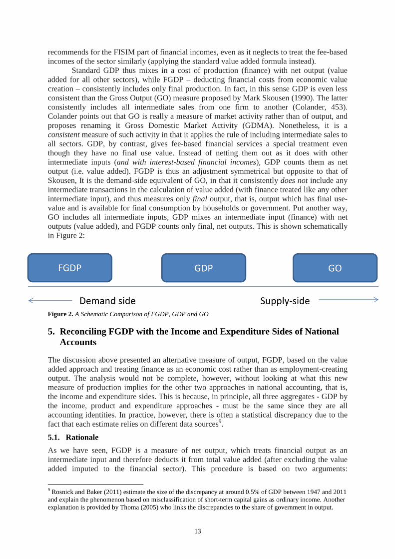
Standard GDP thus mixes in a cost of production (finance) with net output (value added for all other sectors), while FGDP – deducting financial costs from economic value creation – consistently includes only final production. In fact, in this sense GDP is even less consistent than the Gross Output (GO) measure proposed by Mark Skousen (1990). The latter consistently includes all intermediate sales from one firm to another (Colander, 453). Colander points out that GO is really a measure of market activity rather than of output, and proposes renaming it Gross Domestic Market Activity (GDMA). Nonetheless, it is a consistent measure of such activity in that it applies the rule of including intermediate sales to all sectors. GDP, by contrast, gives fee-based financial services a special treatment even though they have no final use value. Instead of netting them out as it does with other intermediate inputs (and with interest-based financial incomes), GDP counts them as net output (i.e. value added). FGDP is thus an adjustment symmetrical but opposite to that of Skousen, It is the demand-side equivalent of GO, in that it consistently does not include any intermediate transactions in the calculation of value added (with finance treated like any other intermediate input), and thus measures only final output, that is, output which has final use-value and is available for final consumption by households or government. Put another way, GO includes all intermediate inputs, GDP mixes an intermediate input (finance) with net outputs (value added), and FGDP counts only final, net outputs. This is shown schematically in Figure 2:

1.

Figure 2. A Schematic Comparison of FGDP, GDP and GO

5. Reconciling FGDP with the Income and Expenditure Sides of National Accounts

The discussion above presented an alternative measure of output, FGDP, based on the value added approach and treating finance as an economic cost rather than as employment-creating output. The analysis would not be complete, however, without looking at what this new measure of production implies for the other two approaches in national accounting, that is, the income and expenditure sides. This is because, in principle, all three aggregates - GDP by the income, product and expenditure approaches - must be the same since they are all accounting identities. In practice, however, there is often a statistical discrepancy due to the fact that each estimate relies on different data sources9.

5.1. Rationale

As we have seen, FGDP is a measure of net output, which treats financial output as an intermediate input and therefore deducts it from total value added (after excluding the value added imputed to the financial sector). This procedure is based on two arguments:

9 Rosnick and Baker (2011) estimate the size of the discrepancy at around 0.5% of GDP between 1947 and 2011 and explain the phenomenon based on misclassification of short-term capital gains as ordinary income. Another explanation is provided by Thoma (2005) who links the discrepancies to the share of government in output.

Demand side Supply-side

FGDP GO GDP

14

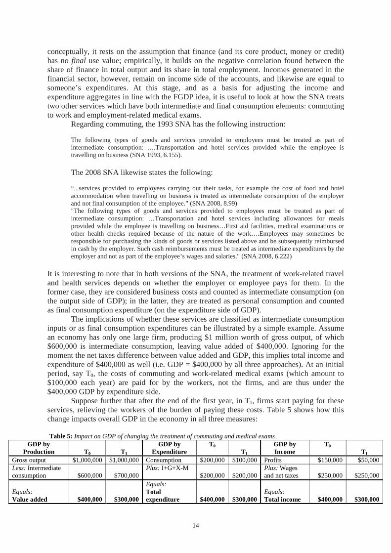
conceptually, it rests on the assumption that finance (and its core product, money or credit) has no final use value; empirically, it builds on the negative correlation found between the share of finance in total output and its share in total employment. Incomes generated in the financial sector, however, remain on income side of the accounts, and likewise are equal to someone’s expenditures. At this stage, and as a basis for adjusting the income and expenditure aggregates in line with the FGDP idea, it is useful to look at how the SNA treats two other services which have both intermediate and final consumption elements: commuting to work and employment-related medical exams.

Regarding commuting, the 1993 SNA has the following instruction: The following types of goods and services provided to employees must be treated as part of intermediate consumption: ….Transportation and hotel services provided while the employee is travelling on business (SNA 1993, 6.155). The 2008 SNA likewise states the following: “...services provided to employees carrying out their tasks, for example the cost of food and hotel accommodation when travelling on business is treated as intermediate consumption of the employer and not final consumption of the employee.” (SNA 2008, 8.99) "The following types of goods and services provided to employees must be treated as part of intermediate consumption: …Transportation and hotel services including allowances for meals provided while the employee is travelling on business…First aid facilities, medical examinations or other health checks required because of the nature of the work….Employees may sometimes be responsible for purchasing the kinds of goods or services listed above and be subsequently reimbursed in cash by the employer. Such cash reimbursements must be treated as intermediate expenditures by the employer and not as part of the employee’s wages and salaries." (SNA 2008, 6.222)

It is interesting to note that in both versions of the SNA, the treatment of work-related travel and health services depends on whether the employer or employee pays for them. In the former case, they are considered business costs and counted as intermediate consumption (on the output side of GDP); in the latter, they are treated as personal consumption and counted as final consumption expenditure (on the expenditure side of GDP). The implications of whether these services are classified as intermediate consumption inputs or as final consumption expenditures can be illustrated by a simple example. Assume an economy has only one large firm, producing $1 million worth of gross output, of which $600,000 is intermediate consumption, leaving value added of $400,000. Ignoring for the moment the net taxes difference between value added and GDP, this implies total income and expenditure of $400,000 as well (i.e. GDP = $400,000 by all three approaches). At an initial period, say T0, the costs of commuting and work-related medical exams (which amount to $100,000 each year) are paid for by the workers, not the firms, and are thus under the $400,000 GDP by expenditure side. Suppose further that after the end of the first year, in T1, firms start paying for these services, relieving the workers of the burden of paying these costs. Table 5 shows how this change impacts overall GDP in the economy in all three measures: Table 5: Impact on GDP of changing the treatment of commuting and medical exams

GDP by Production T0 T1

GDP by Expenditure

T0 T1

GDP by Income

T0 T1

Gross output $1,000,000 $1,000,000 Consumption $200,000 $100,000 Profits $150,000 $50,000 Less: Intermediate consumption $600,000 $700,000

Plus: I+G+X-M $200,000 $200,000

Plus: Wages and net taxes $250,000 $250,000

Equals: Value added $400,000 $300,000

Equals: Total expenditure $400,000 $300,000

Equals: Total income $400,000 $300,000

15

Reclassifying the $100,000 cost of commuting or work-related medical services from the final consumption of workers to an intermediate consumption of firms has three effects: reducing value added by $100,000 (since value added = gross output – intermediate consumption, and the latter has been increased by $100,000); reducing total expenditure by $100,000 (since final consumption expenditure is now lower by $100,000, with the other parts – G, I and X and M – unchanged); and reducing profits, taxes and wages by $100,000 (since profits = revenues – costs, and business costs have just risen by $100,000). In all three measures, GDP has gone down from $400,000 to $300,000, simply because of the reclassification of the services under question. Why does the SNA allow multiple ways to treat the same service (commuting or work-related medical exams) depending on who pays for it? Empirically, one explanation could be that it would be more difficult to attribute such costs to consumers than to firms. At a more conceptual level, however, this may be explained either by a radical appeal to the idea of workers spending on contributions to their human capital, or more reasonably by the fact that the activities in question can be undertaken both by consumers in their free time, and by workers in work-related situations. That is, these services have both a final use (for personal consumption) and an intermediate use (as an input or intermediate cost of production), depending on the context. This is explained by the SNA as follows:

“An employer, whether government or not, may provide an employee with equipment that is necessary to carrying out the labor services the employee provides. Examples are uniforms or small tools, such as scissors for hairdressers or bicycles for delivering mail. This equipment is recorded as intermediate consumption of the employing enterprise and is never recorded as being acquired by the household to which the employee belongs. The same convention applies to services provided to employees carrying out their tasks” (SNA 2008, 8.99).

But does this logic apply to financial services? SNA 2008 implies that it does. A section dealing with charging for financial services reads as follows:

“Explicit fees should always be recorded as payable by the unit to whom the services are rendered to the institution performing the service. If the services are rendered to a corporation or to government, the costs will form part of intermediate consumption. If they are rendered to households they will be treated as final consumption unless the financial service is performed in relation to an unincorporated enterprise, including the owning and occupying of a dwelling.” (SNA 2008 - 17.234)

This is similar to the commute and medical-exam cases, in that the classification of the services is based on who is paying, i.e. the SNA allocates fee-based financial incomes based on whether the buyer of these services is a household, on the one hand, or firms and government, on the other hand. The implication is that fee-based services provided to the latter are already netted out as intermediate input, while services provided to households (except in their capacity as home-owners) show up on the expenditure and income sides. However, there is a gross inconsistency here. In both the commute and work-related medical exam cases, it is a firm (the employer) either paying for services consumed by its employees (in which case these services show up as intermediate consumption) or not paying (in which case the employees pay and the services show up as final consumption expenditure). In contrast, financial services to corporations and governments are services paid for by one firm to another, rather than by a firm for its employees. This asymmetry (firm to firm vs. firm to employees) has political economy implications. When financial corporations deal with non-financial corporations, “there is scope for systematic mutual gains in arms-length relationships” between them (dos Santos, 16), while the relationship between financial firms and individuals or households is far more unequal (ibid. 12).

16

Furthermore, financial services to individuals or households are not final (having no direct use value) and should therefore not be considered as final consumption. Even outside of financing mortgages (for owner-occupier households), financial services such as student-loans, car loans, and even credit cards are not services producing a final consumable output. What these services do is provide households with the money they need to purchase other goods and services, such as an education, a car or groceries. Finance is therefore mediating between borrowing households’ current incomes and consumption needs. On the saving side, finance can be seen as offering savers a form of deferred consumption (similar to what Keynes advocated in his 1940 book How to Pay for the War), once again not current final consumption. More broadly, in terms of aggregate demand analysis, finance falls into the same pool of leakages as savings, taxes and imports – which are only offset by injections of demand from investment, government spending and exports – because it diverts spending away from current consumption on other, final goods and services to paying financing fees. For all these reasons, the ‘output’ of fee-based financial services – imputed as mentioned above from their gross revenues – needs to be removed from GDP by expenditure – since the expenditure is not on a final good or service - and from GDP by income – since finance is an intermediate cost of firms and therefore a reduction of their gross profits. The amount to be adjusted, as demonstrated on the output side, is equal to sum of the imputed ‘output’ and ‘value added’ of the FIRE sectors, around $7.5 trillion in 2013 (in 2009 dollars)10.

5.2. Reconciling FGDP on the Expenditure Side

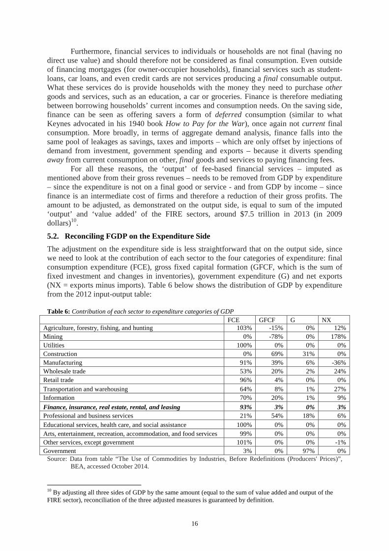
The adjustment on the expenditure side is less straightforward that on the output side, since we need to look at the contribution of each sector to the four categories of expenditure: final consumption expenditure (FCE), gross fixed capital formation (GFCF, which is the sum of fixed investment and changes in inventories), government expenditure (G) and net exports (NX = exports minus imports). Table 6 below shows the distribution of GDP by expenditure from the 2012 input-output table: Table 6: Contribution of each sector to expenditure categories of GDP

FCE GFCF G NX Agriculture, forestry, fishing, and hunting 103% -15% 0% 12% Mining 0% -78% 0% 178% Utilities 100% 0% 0% 0% Construction 0% 69% 31% 0% Manufacturing 91% 39% 6% -36% Wholesale trade 53% 20% 2% 24% Retail trade 96% 4% 0% 0%

Transportation and warehousing 64% 8% 1% 27% Information 70% 20% 1% 9%

Finance, insurance, real estate, rental, and leasing 93% 3% 0% 3% Professional and business services 21% 54% 18% 6%

Educational services, health care, and social assistance 100% 0% 0% 0% Arts, entertainment, recreation, accommodation, and food services 99% 0% 0% 0% Other services, except government 101% 0% 0% -1% Government 3% 0% 97% 0%

Source: Data from table “The Use of Commodities by Industries, Before Redefinitions (Producers' Prices)”, BEA, accessed October 2014.

10 By adjusting all three sides of GDP by the same amount (equal to the sum of value added and output of the FIRE sector), reconciliation of the three adjusted measures is guaranteed by definition.

17

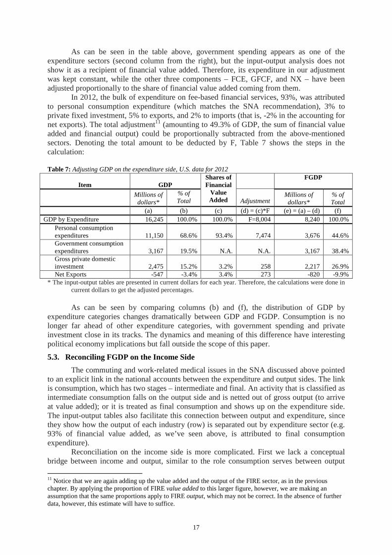
As can be seen in the table above, government spending appears as one of the expenditure sectors (second column from the right), but the input-output analysis does not show it as a recipient of financial value added. Therefore, its expenditure in our adjustment was kept constant, while the other three components – FCE, GFCF, and NX – have been adjusted proportionally to the share of financial value added coming from them.

In 2012, the bulk of expenditure on fee-based financial services, 93%, was attributed to personal consumption expenditure (which matches the SNA recommendation), 3% to private fixed investment, 5% to exports, and 2% to imports (that is, -2% in the accounting for net exports). The total adjustment11 (amounting to 49.3% of GDP, the sum of financial value added and financial output) could be proportionally subtracted from the above-mentioned sectors. Denoting the total amount to be deducted by F, Table 7 shows the steps in the calculation:

Table 7: Adjusting GDP on the expenditure side, U.S. data for 2012

Item GDP Shares of Financial

Value Added

FGDP

Millions of

dollars* % of Total

Adjustment

Millions of dollars*

% of Total

(a) (b) (c) (d) = (c)*F (e) = (a) – (d) (f) GDP by Expenditure 16,245 100.0% 100.0% F=8,004 8,240 100.0%

Personal consumption expenditures 11,150 68.6% 93.4% 7,474 3,676 44.6% Government consumption expenditures 3,167 19.5% N.A. N.A. 3,167 38.4% Gross private domestic investment 2,475 15.2% 3.2% 258 2,217 26.9% Net Exports -547 -3.4% 3.4% 273 -820 -9.9%

* The input-output tables are presented in current dollars for each year. Therefore, the calculations were done in current dollars to get the adjusted percentages. As can be seen by comparing columns (b) and (f), the distribution of GDP by

expenditure categories changes dramatically between GDP and FGDP. Consumption is no longer far ahead of other expenditure categories, with government spending and private investment close in its tracks. The dynamics and meaning of this difference have interesting political economy implications but fall outside the scope of this paper.

5.3. Reconciling FGDP on the Income Side

The commuting and work-related medical issues in the SNA discussed above pointed to an explicit link in the national accounts between the expenditure and output sides. The link is consumption, which has two stages – intermediate and final. An activity that is classified as intermediate consumption falls on the output side and is netted out of gross output (to arrive at value added); or it is treated as final consumption and shows up on the expenditure side. The input-output tables also facilitate this connection between output and expenditure, since they show how the output of each industry (row) is separated out by expenditure sector (e.g. 93% of financial value added, as we’ve seen above, is attributed to final consumption expenditure).

Reconciliation on the income side is more complicated. First we lack a conceptual bridge between income and output, similar to the role consumption serves between output

11 Notice that we are again adding up the value added and the output of the FIRE sector, as in the previous chapter. By applying the proportion of FIRE value added to this larger figure, however, we are making an assumption that the same proportions apply to FIRE output, which may not be correct. In the absence of further data, however, this estimate will have to suffice.

18

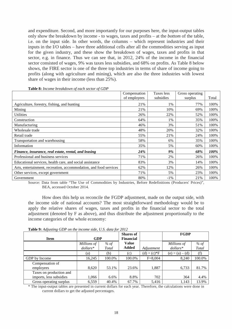
and expenditure. Second, and more importantly for our purposes here, the input-output tables only show the breakdown by income - to wages, taxes and profits – at the bottom of the table, i.e. on the input side. In other words, the columns – which represent industries and their inputs in the I/O tables – have three additional cells after all the commodities serving as input for the given industry, and these show the breakdown of wages, taxes and profits in that sector, e.g. in finance. Thus we can see that, in 2012, 24% of the income in the financial sector consisted of wages, 9% was taxes less subsidies, and 68% on profits. As Table 8 below shows, the FIRE sector is one of the three top industries in terms of share of income going to profits (along with agriculture and mining), which are also the three industries with lowest share of wages in their income (less than 25%). Table 8: Income breakdown of each sector of GDP

Compensation of employees

Taxes less subsidies

Gross operating surplus Total

Agriculture, forestry, fishing, and hunting 21% 1% 77% 100% Mining 21% 10% 69% 100% Utilities 26% 22% 52% 100% Construction 64% 1% 35% 100% Manufacturing 46% 3% 51% 100% Wholesale trade 48% 20% 32% 100% Retail trade 55% 21% 24% 100% Transportation and warehousing 58% 6% 35% 100% Information 35% 5% 60% 100%

Finance, insurance, real estate, rental, and leasing 24% 9% 68% 100% Professional and business services 71% 2% 26% 100%

Educational services, health care, and social assistance 83% 3% 14% 100% Arts, entertainment, recreation, accommodation, and food services 62% 12% 26% 100% Other services, except government 71% 5% 23% 100% Government 80% -1% 21% 100%

Source: Data from table “The Use of Commodities by Industries, Before Redefinitions (Producers' Prices)”, BEA, accessed October 2014. How does this help us reconcile the FGDP adjustment, made on the output side, with

the income side of national accounts? The most straightforward methodology would be to apply the relative shares of wages, taxes and profits in the financial sector to the total adjustment (denoted by F as above), and thus distribute the adjustment proportionally to the income categories of the whole economy:

Table 9: Adjusting GDP on the income side, U.S. data for 2012

Item GDP Shares of Financial

Value Added

FGDP

Millions of

dollars* % of Total

Adjustment

Millions of dollars*

% of Total

(a) (b) (c) (d) = (c)*F (e) = (a) – (d) (f) GDP by Income 16,245 100.0% 100.0% F=8,004 8,240 100.0%

Compensation of employees 8,620 53.1% 23.6% 1,887 6,733 81.7% Taxes on production and imports, less subsidies 1,066 6.6% 8.8% 702 364 4.4% Gross operating surplus 6,559 40.4% 67.7% 5,416 1,143 13.9%

* The input-output tables are presented in current dollars for each year. Therefore, the calculations were done in current dollars to get the adjusted percentages.

19

Once again, as on the expenditure side, the application of the FGDP adjustment to the income side results in different relative shares of income. In this case, the results are quite dramatic, with the wage share12 going up from 53.1% of GDP to 81.7% of FGDP, while gross profits decreased from 40.4% of GDP to a mere 13.9% of FGDP. While both categories have been reduced in absolute terms in the adjustment process, gross profits were reduced far more (as explained above, due to the large share of profits in financial value added, 67.7%, compared to wages’ share of 23.6%). The implications of this new structure of income can be the subject of further research.

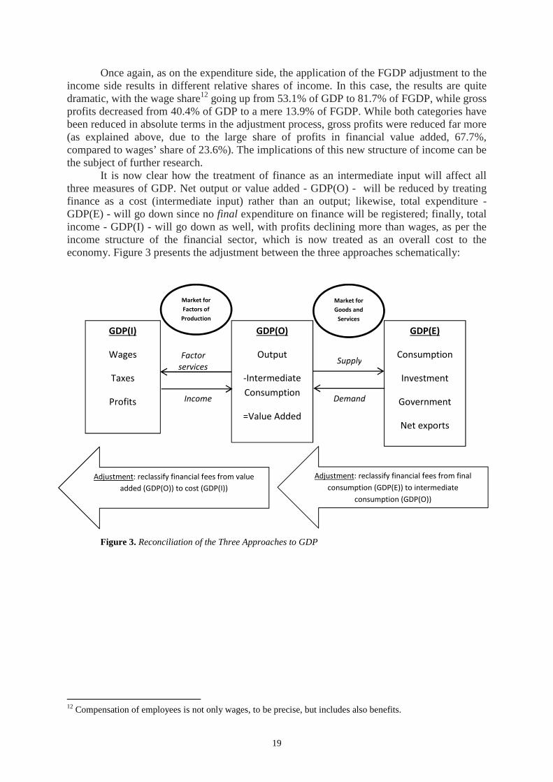
It is now clear how the treatment of finance as an intermediate input will affect all three measures of GDP. Net output or value added - GDP(O) - will be reduced by treating finance as a cost (intermediate input) rather than an output; likewise, total expenditure - GDP(E) - will go down since no final expenditure on finance will be registered; finally, total income - GDP(I) - will go down as well, with profits declining more than wages, as per the income structure of the financial sector, which is now treated as an overall cost to the economy. Figure 3 presents the adjustment between the three approaches schematically:

Figure 3. Reconciliation of the Three Approaches to GDP

12 Compensation of employees is not only wages, to be precise, but includes also benefits.

Factor

services

Demand Income

GDP(I)

Wages

Taxes

Profits

GDP(O)

Output

-Intermediate

Consumption

=Value Added

GDP(E)

Consumption

Investment

Government

Net exports

Supply

Market for

Factors of

Production

Market for

Goods and

Services

Adjustment: reclassify financial fees from final

consumption (GDP(E)) to intermediate

consumption (GDP(O))

Adjustment: reclassify financial fees from value

added (GDP(O)) to cost (GDP(I))

20

6. Empirical Estimates of FGDP

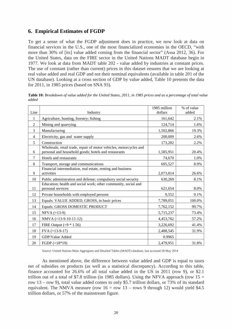
To get a sense of what the FGDP adjustment does in practice, we now look at data on financial services in the U.S., one of the most financialized economies in the OECD, “with more than 30% of [its] value added coming from the financial sector” (Assa 2012, 36). For the United States, data on the FIRE sector in the United Nations MADT database begin in 1977. We look at data from MADT table 202 - value added by industries at constant prices. The use of constant (rather than current) prices in this dataset ensures that we are looking at real value added and real GDP and not their nominal equivalents (available in table 201 of the UN database). Looking at a cross section of GDP by value added, Table 10 presents the data for 2011, in 1985 prices (based on SNA 93).

Table 10: Breakdown of value added for the United States, 2011, in 1985 prices and as a percentage of total value added

Line Industry 1985 million

dollars % of value

added

1 Agriculture, hunting, forestry; fishing 161,642 2.1%

2 Mining and quarrying 124,714 1.6%

3 Manufacturing 1,502,866 19.3%

4 Electricity, gas and water supply 200,009 2.6%

5 Construction 173,282 2.2%

6 Wholesale, retail trade, repair of motor vehicles, motorcycles and personal and household goods; hotels and restaurants 1,585,951 20.4%

7 Hotels and restaurants 74,670 1.0%

8 Transport, storage and communications 695,527 8.9%

9 Financial intermediation, real estate, renting and business activities 2,073,814 26.6%

10 Public administration and defense; compulsory social security 630,269 8.1%

11 Education; health and social work; other community, social and personal services 621,654 8.0%

12 Private households with employed persons 9,552 0.1%

13 Equals: VALUE ADDED, GROSS, in basic prices 7,789,051 100.0%

14 Equals: GROSS DOMESTIC PRODUCT 7,762,152 99.7%

15 NFVA (=13-9) 5,715,237 73.4%

16 NMVA (=13-9-10-11-12) 4,453,762 57.2%

17 FIRE Output (=9 * 1.56) 3,226,692 41.4%

18 FVA (=13-9-17) 2,488,545 31.9%

19 GDP/Value Added 0.9965

20 FGDP (=18*19) 2,479,951 31.8% Source: United Nations Main Aggregates and Detailed Tables (MADT) database, last accessed 28 May 2014

As mentioned above, the difference between value added and GDP is equal to taxes

net of subsidies on products (as well as a statistical discrepancy). According to this table, finance accounted for 26.6% of all total value added in the US in 2011 (row 9), or $2.1 trillion out of a total of $7.8 trillion (in 1985 dollars). Using the NFVA approach (row 15 = row 13 – row 9), total value added comes to only $5.7 trillion dollars, or 73% of its standard equivalent. The NMVA measure (row 16 = row 13 – rows 9 through 12) would yield $4.5 trillion dollars, or 57% of the mainstream figure.

21

In order to compare these numbers to the FVA measure, which not only excludes the ‘value added’ of the FIRE sector but also deducts its ‘output’, the data from MADT table 202 is not sufficient, since it gives only the value added for the FIRE sector (calculated as output minus intermediate consumption). To get the data for output before intermediation consumption is netted out, table 203 of the MADT database was used. While this table is in current prices, it can be used to calculate the proportion of output to value added in each year since both variables are in the same prices. For example, reported financial output in the United States for 2011 was $7.736 trillion. From this, $2.764 trillion of intermediate consumption is deducted to arrive at value added of $4.972 trillion, meaning the ratio of output to value added in 2011 was 7.736/4.972=1.56 (or, conversely, value added was 1/1.56 of output, i.e. 64%). Applying this to our constant price data of $2.1 trillion we get financial output in constant prices (for 2011) of $3.2 trillion. Deducting this figure from the reported 2011 total value added gives total Final Value Added (for FVA) of $2.5 trillion, or 32% of standard value added. Thus the FVA measure ends up below both NFVA and NMVA, as a percentage of standard value added. As mentioned above, however, to be consistent with the other three approaches to GDP, value added must be adjusted by adding taxes and subtracting subsidies. In 2011 the reported ratio of GDP to value added was 0.9965, so applying this to our FVA measure yields Final GDP (or FGDP) of $2.5 trillion (compared to $7.8 trillion in the official figure). This calculation (as well as those involved in deriving GDP from value added, NFGDP from NFVA and NMGDP from NMVA) is illustrated in Table 11 below.

Table 11: Value added and GDP for the United States (2011, millions of 1985 dollars) using four approaches

Standard Non-financial Narrow-measured Final use value Initial value added (total economy) 7,789,051 7,789,051 7,789,051 7,789,051

1. Deduct value added of finance (and other imputed sectors in NMVA*) -2,073,814 -3,335,289 -2,073,814

2. Deduct gross output of finance -3,226,692 New value added 7,789,051 5,715,237 4,453,762 2,488,545

Taxes minus subsidies factor 0.9965 0.9965 0.9965 0.9965 GDP equivalent 7,762,152 5,695,500 4,438,381 2,479,951

* Financial intermediation, real estate, renting and business activities; Public administration and defense; compulsory social security; Education; health and social work; other community, social and personal services; Other community, social and personal services; Private households with employed persons.

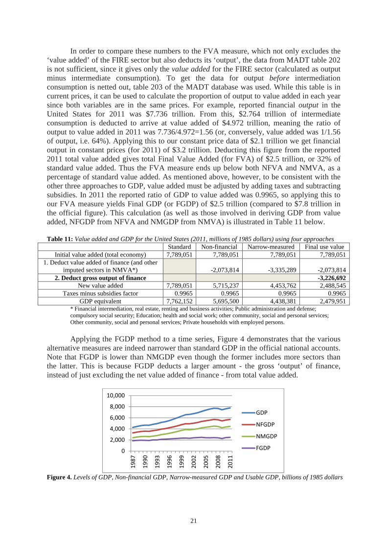
Applying the FGDP method to a time series, Figure 4 demonstrates that the various

alternative measures are indeed narrower than standard GDP in the official national accounts. Note that FGDP is lower than NMGDP even though the former includes more sectors than the latter. This is because FGDP deducts a larger amount - the gross ‘output’ of finance, instead of just excluding the net value added of finance - from total value added.

Figure 4. Levels of GDP, Non-financial GDP, Narrow-measured GDP and Usable GDP, billions of 1985 dollars

0

2,000

4,000

6,000

8,000

10,000

19

87

19

90

19

93

19

96

19

99

20

02

20

05

20

08

20

11

GDP

NFGDP

NMGDP

FGDP

22

In addition to the different size of the U.S. economy implied by Figure 4, there is a dramatic difference in the growth rates of the economy according to each measure. While GDP and NMGDP show a cumulative growth of 82% and 84% over the period 1987-2011, respectively, NFGDP suggests a more moderate increase of 74%, with FGDP far more pessimistic at 34%. By comparison, total nonfarm employment grew by 29.1% over the same period, strengthening the case for FGDP as a more realistic measure of real net output.

Furthermore, FGDP has the lowest mean growth rate and highest standard deviation of all measures. This is in line with our theory of finance as a having a negative contribution to total output.

Table 12: Mean and standard deviation of growth rates using GDP, NMGDP, NFGDP and FGDP

GDP NFGDP NMGDP FGDP Mean growth rate 2.6% 2.3% 2.6% 1.3% Standard deviation 1.8% 2.0% 2.6% 2.8%

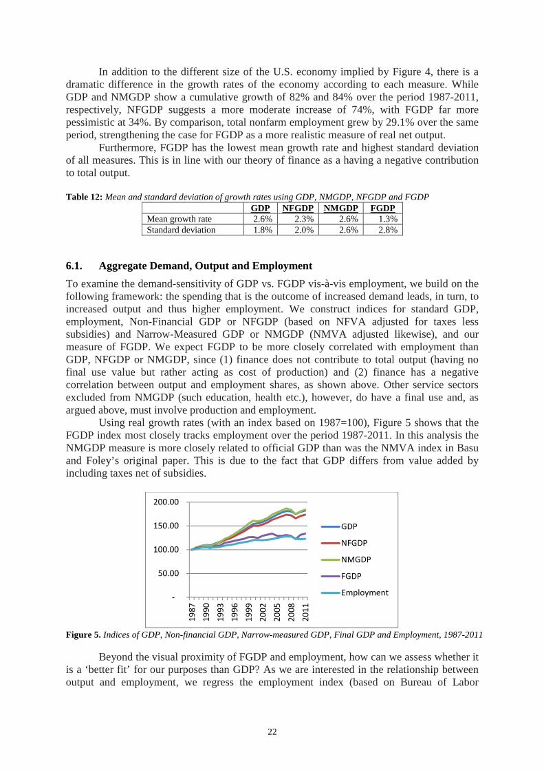
6.1. Aggregate Demand, Output and Employment

To examine the demand-sensitivity of GDP vs. FGDP vis-à-vis employment, we build on the following framework: the spending that is the outcome of increased demand leads, in turn, to increased output and thus higher employment. We construct indices for standard GDP, employment, Non-Financial GDP or NFGDP (based on NFVA adjusted for taxes less subsidies) and Narrow-Measured GDP or NMGDP (NMVA adjusted likewise), and our measure of FGDP. We expect FGDP to be more closely correlated with employment than GDP, NFGDP or NMGDP, since (1) finance does not contribute to total output (having no final use value but rather acting as cost of production) and (2) finance has a negative correlation between output and employment shares, as shown above. Other service sectors excluded from NMGDP (such education, health etc.), however, do have a final use and, as argued above, must involve production and employment.

Using real growth rates (with an index based on 1987=100), Figure 5 shows that the FGDP index most closely tracks employment over the period 1987-2011. In this analysis the NMGDP measure is more closely related to official GDP than was the NMVA index in Basu and Foley’s original paper. This is due to the fact that GDP differs from value added by including taxes net of subsidies.

Figure 5. Indices of GDP, Non-financial GDP, Narrow-measured GDP, Final GDP and Employment, 1987-2011

Beyond the visual proximity of FGDP and employment, how can we assess whether it is a ‘better fit’ for our purposes than GDP? As we are interested in the relationship between output and employment, we regress the employment index (based on Bureau of Labor

-

50.00

100.00

150.00

200.00

19

87

19

90

19

93

19

96

19

99

20

02

20

05

20

08

20

11

GDP

NFGDP

NMGDP

FGDP

Employment

23

Statistics data) on each of the four output indices shown in Figure 5, with the following results:

Table 13: Regression coefficients. OLS, using observations 1987-2011 (T = 25), Dependent variable: Employment. HAC standard errors, bandwidth 2 (Bartlett kernel)

Coefficient

GDP 0.301547

NFGDP 0.339159

NMGDP 0.288879

FGDP 0.760439 All regression coefficients are statistically significant at the 1% level, but FGDP has a

far better fit with the independent variable – employment – than the other three measures (in fact its coefficient is more than twice as large as that of GDP). FGDP can thus help explain the otherwise mysterious phenomena of jobless recoveries and job-loss downturns mentioned by Basu and Foley (2013), where employment moves much more slowly than what changes in standard GDP would imply. Using FGDP, the ‘jobless’ recoveries appear as periods of stagnation, where job creation is naturally minimal, resolving the puzzle.

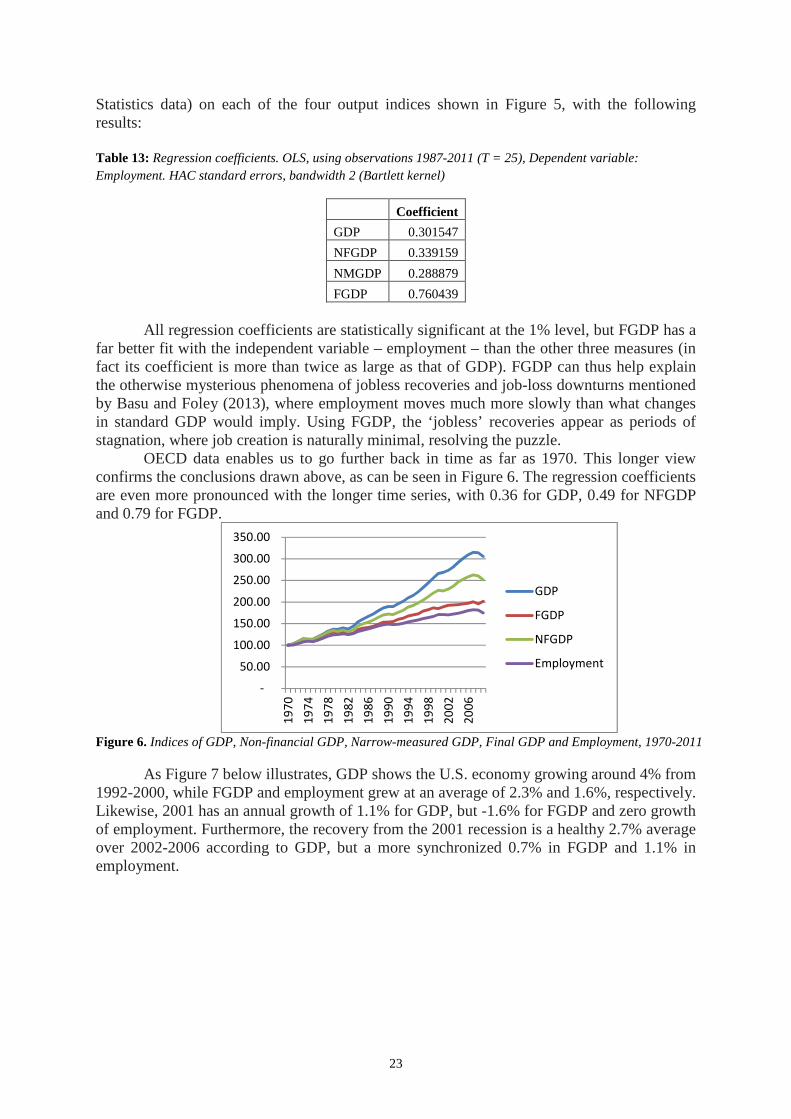
OECD data enables us to go further back in time as far as 1970. This longer view confirms the conclusions drawn above, as can be seen in Figure 6. The regression coefficients are even more pronounced with the longer time series, with 0.36 for GDP, 0.49 for NFGDP and 0.79 for FGDP.

Figure 6. Indices of GDP, Non-financial GDP, Narrow-measured GDP, Final GDP and Employment, 1970-2011

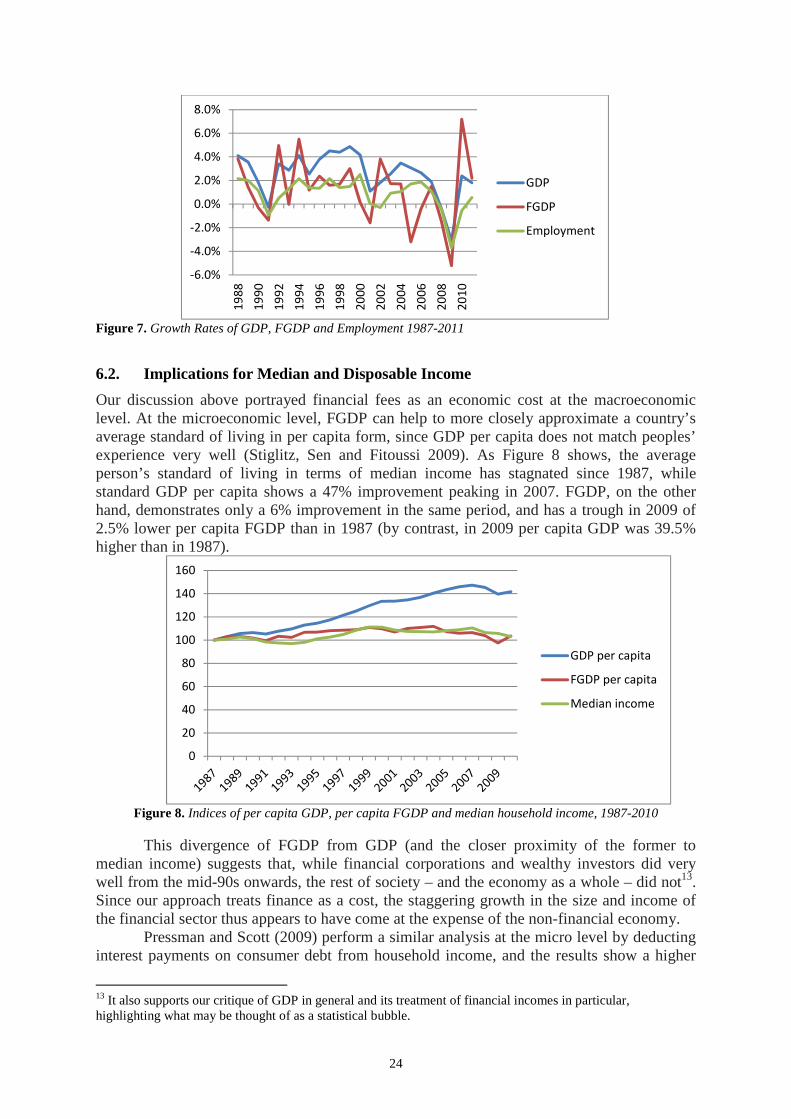
As Figure 7 below illustrates, GDP shows the U.S. economy growing around 4% from 1992-2000, while FGDP and employment grew at an average of 2.3% and 1.6%, respectively. Likewise, 2001 has an annual growth of 1.1% for GDP, but -1.6% for FGDP and zero growth of employment. Furthermore, the recovery from the 2001 recession is a healthy 2.7% average over 2002-2006 according to GDP, but a more synchronized 0.7% in FGDP and 1.1% in employment.

-

50.00

100.00

150.00

200.00

250.00

300.00

350.00

19

70

19

74

19

78

19

82

19

86

19

90

19

94

19

98

20

02

20

06

GDP

FGDP

NFGDP

Employment

24

Figure 7. Growth Rates of GDP, FGDP and Employment 1987-2011

6.2. Implications for Median and Disposable Income

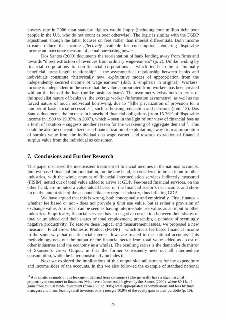
Our discussion above portrayed financial fees as an economic cost at the macroeconomic level. At the microeconomic level, FGDP can help to more closely approximate a country’s average standard of living in per capita form, since GDP per capita does not match peoples’ experience very well (Stiglitz, Sen and Fitoussi 2009). As Figure 8 shows, the average person’s standard of living in terms of median income has stagnated since 1987, while standard GDP per capita shows a 47% improvement peaking in 2007. FGDP, on the other hand, demonstrates only a 6% improvement in the same period, and has a trough in 2009 of 2.5% lower per capita FGDP than in 1987 (by contrast, in 2009 per capita GDP was 39.5% higher than in 1987).

Figure 8. Indices of per capita GDP, per capita FGDP and median household income, 1987-2010

This divergence of FGDP from GDP (and the closer proximity of the former to median income) suggests that, while financial corporations and wealthy investors did very well from the mid-90s onwards, the rest of society – and the economy as a whole – did not13. Since our approach treats finance as a cost, the staggering growth in the size and income of the financial sector thus appears to have come at the expense of the non-financial economy.

Pressman and Scott (2009) perform a similar analysis at the micro level by deducting interest payments on consumer debt from household income, and the results show a higher

13 It also supports our critique of GDP in general and its treatment of financial incomes in particular, highlighting what may be thought of as a statistical bubble.

-6.0%

-4.0%

-2.0%

0.0%

2.0%

4.0%

6.0%

8.0%

19

88

19

90

19

92

19

94

19

96

19

98

20

00

20

02

20

04

20

06

20

08

20

10

GDP

FGDP

Employment

0

20

40

60

80

100

120

140

160

GDP per capita

FGDP per capita

Median income

25

poverty rate in 2006 than standard figures would imply (including four million debt poor people in the U.S. who do not count as poor otherwise). The logic is similar with the FGDP adjustment, though the latter focuses on fees rather than interest differentials. Both income streams reduce the income effectively available for consumption, rendering disposable income an inaccurate measure of actual purchasing power.

Dos Santos (2009) documents the reorientation of bank lending away from firms and towards “direct extraction of revenues from ordinary wage-earners” (p. 2). Unlike lending by financial corporations to non-financial corporations – which tends to be a “mutually beneficial, arms-length relationship” – the asymmetrical relationship between banks and individuals constitute “historically new, exploitative modes of appropriation from the independently secured income of wage earners” (ibid, 3, emphasis in original). Workers’ income is independent in the sense that the value appropriated from workers has been created without the help of the loan (unlike business loans). The asymmetry exists both in terms of the specialist nature of banks vs. the average worker (information asymmetry), as well as the forced nature of much individual borrowing, due to “[t]he privatization of provision for a number of basic social necessities”, such as housing, education and pensions (ibid. 13). Dos Santos documents the increase in household financial obligations (from 15.36% of disposable income in 1980 to 19.35% in 2007), which – seen in the light of our view of financial fees as a form of taxation – suggests another reason for the weakening of aggregate demand14. This could be also be conceptualized as a financialization of exploitation, away from appropriation of surplus value from the individual qua wage earner, and towards extraction of financial surplus value from the individual as consumer.

7. Conclusions and Further Research

This paper discussed the inconsistent treatment of financial incomes in the national accounts. Interest-based financial intermediation, on the one hand, is considered to be an input to other industries, with the whole amount of financial intermediation services indirectly measured (FISIM) netted out of total value added to arrive at GDP. Fee-based financial services, on the other hand, are imputed a value-added based on the financial sector’s net income, and show up on the output side of the accounts like any regular industry, thus inflating GDP. We have argued that this is wrong, both conceptually and empirically. First, finance – whether fee based or not - does not provide a final use value, but is rather a provision of exchange value. At most it can be seen as having intermediate use value, as an input to other industries. Empirically, financial services have a negative correlation between their shares of total value added and their shares of total employment, presenting a paradox of seemingly negative productivity. To resolve these logical and measurement issues, we proposed a new measure – Final Gross Domestic Product (FGDP) – which treats fee-based financial income in the same way that net financial interest flows are treated in the national accounts. This methodology nets out the output of the financial sector from total value added as a cost of other industries (and the economy as a whole). The resulting series is the demand-side mirror of Skousen’s Gross Output, in that the former consistently nets out all intermediate consumption, while the latter consistently includes it.

Next we explored the implications of this output-side adjustment for the expenditure and income sides of the accounts. In this we also followed the example of standard national

14 A dramatic example of this leakage of demand from consumers (who generally have a high marginal propensity to consume) to financiers (who have a lower one) is given by dos Santos (2009), where 89.1% of gains from mutual funds investment (from 1980 to 2005) were appropriated as commissions and fees by fund managers and firms, leaving retail investors only a meagre 10.9% of the equity gain in their portfolio (p. 19).

26

accounting, and used the cases of commuting costs and employer-provided medical services as models. Financial services provided for a fee were reclassified in our FGDP framework from final consumption expenditure to intermediate consumption, thus reducing total expenditure as well as value added. On the income side, the relative shares of wages, taxes and profits in the financial sector were applied to the total adjustment amount in order to remove this component from total income. Since the income structure of the financial sector is profit heavy, this adjustment results in a higher wage share and lower profit share in the revised view of the economy through FGDP.

Finally, the fitness-for-purpose of FGDP was evaluated based on how closely it tracked both employment and median income (the latter serving as a proxy for the average standard of living). FGDP is more closely correlated with employment than GDP, NFGDP or NMGDP, which is expected given its netting out of finance – a sector with no final use value and a negative correlation between output and employment shares. Furthermore, when regressing employment on the four alternative measures, FGDP yields the highest coefficient, which is more than double that for GDP. The mean and standard deviation of FGDP growth rates are also much closer to those of employment than the corresponding moments for GDP.

Likewise, while per capita GDP has diverged from median income – the former rising nearly 50% since 1987 while the latter stagnating – FGDP tracks median income very closely. This finding supports the view that financial incomes benefited the very wealthy at the expense of the middle-class, and mirrors Pressman and Scott’s analysis of debt-adjusted poverty rates. It also reflects the reorientation of banking in recent decades, away from generating most of their income from dealing with non-financial firms and towards charging fees to households (who paid 93% of such fees in 2012).

The concept of FGDP thus sheds light on two of several puzzles featuring in recent debate. Further research is needed to examine whether this new methodology can help explain other hotly discussed questions. Some interesting applications could include whether there has been indeed a great moderation in terms of reduced output volatility; the continuing relevance (or lack thereof) of Okun’s Law (relating changes in unemployment to changes in output); and what FGDP implies for changes in the multiplier and in overall the structure of demand. FGDP can also be further tested against GDP as a forecasting tool, with a view to identifying the strengths and weaknesses of each indicator.

27

References

Akritidis, L. (2007). Improving the measurement of banking services in the UK National Accounts, Economic & Labour Market Review, Vol. 1, No 5, May.

Assa, J. (2012). Financialization and its Consequences: the OECD Experience, Finance Research, Vol. 1, No. 1, January.

Basu, D. and Foley, D. K. (2013). Dynamics of output and employment in the US economy, Cambridge Journal of Economics, 37, 1077–1106.

Bureau of Labor Statistics (BLS) website. URL: http://www.bls.gov. Retrieved on 30 July, 2013.

Christophers, B. (2011). Making finance productive, Economy and Society, Volume 40 Number 1, February: 112-140.

Colander, D. (2014). Gross Output: A New Revolutionary Way to Confuse Students about Measuring the Economy, Eastern Economic Journal, 40, 451-55.

dos Santos, P. (2009). On the Content of Banking in Contemporary Capitalism, Historical Materialism 17, 1–34.

Haldane, A. (2010). What is the contribution of the financial sector: Miracle or mirage? In The Future of Finance: The LSE Report, London School of Economics and Political Science.

Lee, P. (2012). Balancing the Three Approaches to Measuring Gross Domestic Product, Office for National Statistics, 31 July.

Oulton, N. (2013). Has the Growth of Real GDP in the UK been Overstated because of Mis-Measurement of Banking Output? Centre for Economic Performance, Occasional Paper #33, January.

Pressman, S. and Scott, R. (2009). Consumer Debt and the Measurement of Poverty and Inequality in the US, Review of Social Economy, Volume 67, Issue 2.

Skousen, M. (1990). The Structure of Production, New York University Press. Stiglitz, J. E, Sen, A. and Fitoussi, J.P. (2009). Report by the Commission on the

Measurement of Economic Performance and Social Progress, available from http://www.stiglitz-sen-fitoussi.fr