Financial intermediation, variability and the development process

Facultad de Ciencias Económicas y EmpresarialesUniversidad de Navarra

Working Paper nº 04/02

Financial Intermediation, Variability and theDevelopment Process

Luis CarranzaJosé E. Galdón-Sánchez

Facultad de Ciencias Económicas y EmpresarialesUniversidad de Navarra

Financial Intermediation, Variability and the Development ProcessLuis Carranza and José E. Galdón-SánchezWorking Paper No.04/02June 2002JEL Codes: E00, O11, O16, O40

ABSTRACT

In this paper we build a model of financial intermediation that explains the GDPvariability pattern of an economy during the development process. We find evidencethat per capita output is more volatile in middle-income economies than in both lowand high-income economies. We show that, if the model economy is in the early or inthe mature stages of development, there is a unique equilibrium. However, in themiddle stages of development, multi-ple equilibria arise. Moreover, we find that ineconomies with imperfect credit markets, per capita output volatility tends to be higherthan in economies with perfect or non-existent credit markets.

Luis Carranza José E. Galdón-SánchezUniversidad de Navarra Universidad Pública de NavarraDepartamento de Economía Departamento de EconomíaCampus Universitario Campus Arrosadía31080 Pamplona 31006 Pamplonaand BBVA Banco Continental [email protected]@grupobbv.com.pe

1 Introduction

In this paper we investigate the pattern of GDP variability during the development

process. We find evidence that per capita GDP variability is low in both low and high

income economies, yet high in middle-income ones. We provide a theoretical model of

financial intermediation that explains the high variability of per capita GDP displayed

by middle-income countries, relative to the low variability of per capita GDP shown

by both low and high income economies.

While there is a substantial literature on the role that financial intermediation has

in growth (see the excellent survey by Levine, 1997), little attention has been paid to

its effect on the dynamics of GDP during the development process. Our model high-

lights the link between the variability of output and the degree of development of the

financial sector. We find that in economies with perfect credit markets, or economies

in which credit markets are non-existent, the equilibrium is unique. However, when a

credit market exists, but is imperfect, there can be more than one equilibrium. This

multiplicity arises in the middle stages of development.

We build a model of financial intermediation with borrowing constraints and

strategic complementarities that generates multiple equilibria, and in which agents

rely on a sunspot to coordinate their actions at intermediate stages of development.

This sunspot is a random variable with its own variance, which drives the variance in

the model. The more agents have access to credit, the larger is the advanced technol-

ogy sector in the economy and the higher are wages. Higher wages relax borrowing

constraints for agents who want to invest in the more advanced sector, and that gen-

erates growth. At the same time, higher wages do not decrease profits or discourage

investment, because the size of the advanced sector is itself a productive strategic

complementarity in that sector. Then, since agents must decide in advance whether

to invest in the advanced sector, the return to their investment depends on how many

1

people today choose to go into the advanced sector. This is the source of the coordi-

nation failure and the need for the sunspot to determine the equilibrium. Finally, a

multiplicity arises because the number of agents who are credit constrained depends

on the number of agents who invest, and if there is no constraint, the multiplicity

disappears, because only resource constraints matter.

Our model is a two-period overlapping generations model. In the first period, the

agents are heterogeneous in their ability to work and, therefore, in their endowments.

In the second period, they become entrepreneurs and have to decide whether to use an

advanced technology or a subsistence technology. The use of the advanced technology

entails a fixed cost, while the use of the subsistence technology does not. The agents

who want to become entrepreneurs in the advanced sector but do not have enough

resources to pay the entry cost can borrow these resources.

We also assume in our model that lenders cannot force borrowers to repay their

debts unless the debts are secured, and that the returns from investment are only

partially collateralizable. Given this credit market imperfection, the strategic com-

plementarity in the productive sector will be reflected in the financial sector: the

larger the fraction of people in the advanced technology sector, the larger the frac-

tion of people that will have access to the credit market. The reason is that the

borrowing constraint is relaxed as the returns in the advanced technology increase.

This is the source of multiple equilibria in the model which arise in the middle stage

of the development process. By contrast, in early and mature stages of development,

the multiplicity does not appear.1

The paper also explores the relationship between the borrowing constraints faced

by individuals and per capita GDP variability. We find that, in economies where

individuals face no borrowing constraints, or those in which the credit market is non-

1The idea that multiplicity is important for understanding development is not new, see for ex-ample Murphy et al. (1989) and Azariadis and Drazen (1990).

2

existent, the equilibrium is unique. However, when the credit market exists but is

imperfect, i.e. where there are borrowing constraints, there can be more than one

equilibrium. In this case, we find that multiplicity of equilibria arises in middle stages

of development.

Note that, if the credit market does not exist or if there are no borrowing con-

straints, there is no interaction between the strategic complementarity in the produc-

tive sector and the borrowing constraint. In the first case, only the fraction of people

with wealth greater than the cost of entry will become entrepreneurs. In the second

case, since there are no borrowing constraints, all the resources are used to finance

the payment of the entry cost for those who want to use the advanced technology.

Moreover, the interest rate will be such that the agents are indifferent between using

the advanced or the subsistence technology.

In an economy with borrowing constraints, the income distribution plays a very

important role in determining the equilibrium. In that sense, this paper follows the

line of work of Galor and Zeira (1993), Banerjee and Newman (1993), Carranza (1995)

and Aghion et al. (1998), in which income distribution is an important instrument

to explain the economy’s behavior in the development process. In our model, the

income distribution and the strategic complementarity effect determine the number

of equilibria and the stage at which the multiplicity of equilibria arises and when it

vanishes.

In order to deal with the presence of multiplicity of equilibria, we assume the exis-

tence of a sunspot process. In our model, this sunspot process coordinates the actions

of the agents. In that respect, this paper is related to Cooper and Ejarque (1995),

Sorger (1994), and Spear (1991). The paper by Cooper and Ejarque (1995) presents

a model in which the indeterminacy of equilibrium is resolved by a sunspot process.

There, the multiplicity of equilibria arises from the existence of non-convexities in

3

the intermediation process. In Sorger (1994), a one-sector neoclassical growth model

with borrowing constraints and heterogeneous agents is used to show that there can

exist sunspot equilibria. Spear (1991) analyzes a dynamic model of pure capital ac-

cumulation to show the existence of sunspot equilibria in a way that prevents the

model from collapsing to an overlapping generations equivalent.

Therefore, in our model, there are two central elements: strategic complementari-

ties and market imperfections, and both are necessary conditions for the existence of

multiple equilibria. The way in which the sunspot mechanism affects the equilibrium

will depend on both the degree of imperfection and the size of the economy. It is also

important to note that, in our model, the set of equilibria changes over time. It is

not constant. Moreover, the number of equilibria depends on the size of the economy.

Finally, the paper shows that the introduction of a new “technology”, a financial

technology in our case, could positively affect the growth rate in the economy and,

at the same time, be a source of higher variability if the markets were not complete.

The Mexican crisis in a globalized market environment illustrates this point.

The paper is organized as follows. In Section 2, we analyze the empirical evidence.

Section 3 presents the environment: a description of the model and a discussion on

the problem of occupational choice. The analysis of the economy’s labor and credit

markets, and the definition of equilibrium is performed in Section 4. Section 5 explains

the dynamics of the economy: the relationship between the level and variability of

GDP per capita in an economy with imperfect credit markets, an analysis of the

behavior of wages, interest rates, and entrepreneurial choice during the development

process, and a discussion of the perfect credit market and non-credit market cases.

Finally, the conclusions are presented in Section 6.

4

2 Empirical Evidence

In this section, we argue that poor and rich countries exhibit lower per capita GDP

variability than middle-income countries. Poor countries tend to grow slowly because

rapid growth is simply not possible. When a poor country grows long enough to

achieve a certain minimum income level, rapid growth becomes a possibility but not

a certainty. During this stage, the poor country may continue on its slow growth

path or it may “take-off” and grow rapidly. On the other hand, it is possible that a

rapidly growing country may suddenly “reverse course” and begin declining. But, if

rapid growth is sustained for a while, the once-poor country passes a second income

threshold beyond which economic decline is no longer a possibility.

We use the Summers and Heston (1991)2 data base for the period 1960-1985.

Following Parente and Prescott (1993 and 1994), OPEC members, countries with

less than one million citizens and countries without a complete data set were dropped

from the data.

Since we do not want to impose any functional form on our data, we will perform a

nonparametric regression with kernel smoothing, by which we do not impose any func-

tional restriction but smoothness (see Härdle, 1990).3 We estimate the conditional

expectation function of the absolute deviation from a linear trend, conditional on the

natural logarithm of per capita GDP. We perform a kernel estimation of the condi-

2We are interested in long term variability and, for our purposes, it would be ideal to have growthseries of 150 or 200 years for developed countries that were previously underdeveloped. That is, thespan period should cover from underdevelopment to development. The problem is that there arevery few (if any) countries, which were not already developed 150 years ago, that have series of GDPthat long. However, as Carranza (1995) reports, we could get the experiences of Japan and SouthKorea that, in few years, evolved from underdevelopment to development. But this evidence wouldonly show one or two trajectories of growth of all the multiple possibilities that there are. Since, aswe will see later, we have multiple equilibria, we cannot have only one or two trajectories, and thisevidence would not suit our purposes. Given that, we use the only evidence available: cross-countrydata for a group of countries that differ in their stages of development. And we calculate theirvariability for the period available.

3This method has also been used by Banerjee and Duflo (2000) to explore the relationship betweeninequality and growth.

5

tional expectation function using the Nadaraya-Watson window and Silverman’s rule

of thumb. The advantage of our method is that we estimate the empirical regression

curve without forcing the data into a parametric window, letting the data to speak by

themselves as much as possible.4 As will be seen, the shape of our kernel estimation

of the conditional expectation function clearly follows a nonlinear pattern.5

In order to perform our kernel estimation, we first regress separately for each

country the natural logarithm of per capita GDP on a constant and a linear trend,

in order to calculate absolute deviations from such trends as the fitted values from

these regressions. Given the obvious heterogeneity among the different countries,

we perform separate regressions by country in order to allow the coefficients to differ

among them. In addition to this trend, we also allow for dummies which are associated

with extraordinary events that occurred in those countries in particular years (years of

independence; civil, ethnic or other kind of wars; natural catastrophes; assassination

of the head of state or coups d’état). All the dummies that we include are significant

at the 5 percent level. That is, any dummy reporting an event such as those described

above must be significant at the 5 percent level in order to be included.6 There are 21

dummies in a set of 2,574 observations (around 0.8 percent).7 Then, we calculate the

4For instance, the exercise done by Acemoglu and Zilibotti (1997) imposes linearity when usingOLS estimation. Our results clearly show that the linearity assumption is not appropriate.

5We also calculated a variability index for different groups of countries. We first regressed percapita GDP levels in dollars against time for each country, calculating its trend afterwards. Theresults still hold when the series are filtered with the Hodrick-Prescott filter. The statistic we usedconsists of the sum of each country’s squared per capita GDP deviations from its trend, divided bythe average per capita GDP. These statistics yield variability indices for each of the countries in ourdata set. Finally, countries are decomposed in four groups by income levels (≤ $999; $1, 000−$4, 999;$5, 000 − $9, 999; and ≥ $10, 000) and an average variability index for each group of countries isobtained. Similar results are obtained if we calculate standard deviations of growth rates. Theresult is a very similar shape to those that will appear next in Figures 1 and 2.

6In a first step, we introduced dummies for all events of the nature described above, for everycountry of the data set. However, there are events that will not be reported with a dummy becausethose dummies were not found significant. For instance, although we initially allowed a dummyfor the coups d’état in Argentina and Chile (1976 and 1973 respectively), this dummies were notstatistically different from zero and are not included.

7For more details on the specific dummies included see Table A1 in Appendix 1.

6

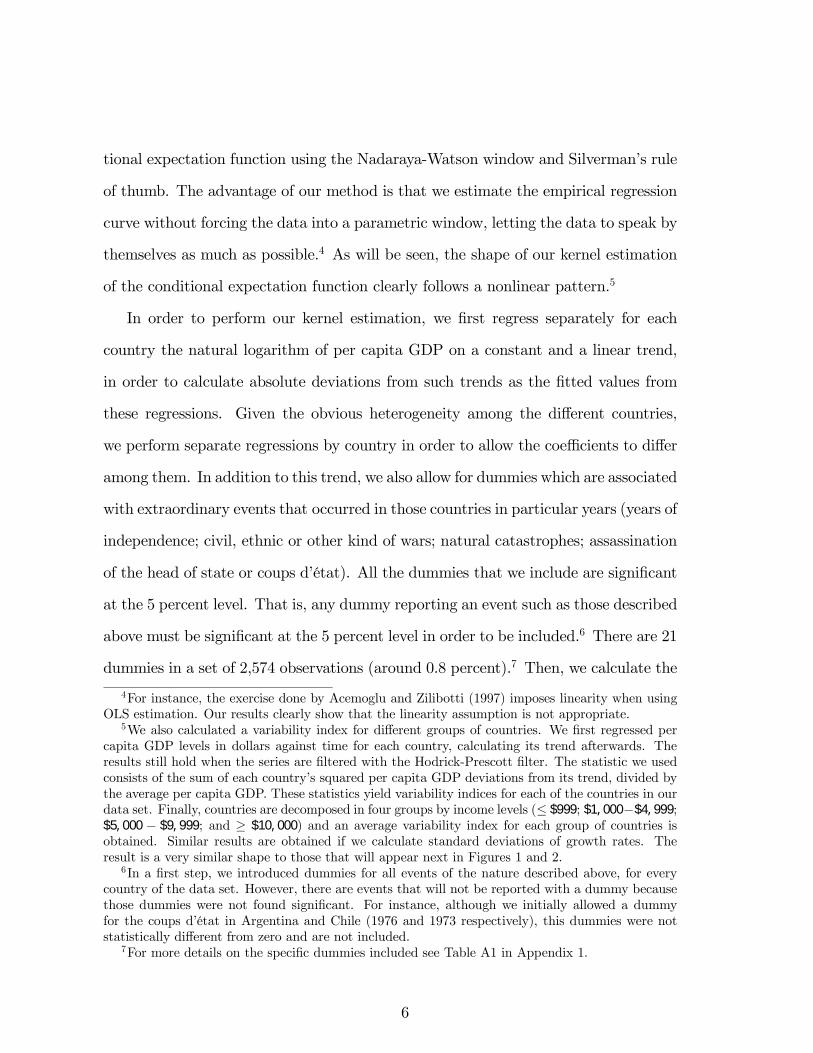
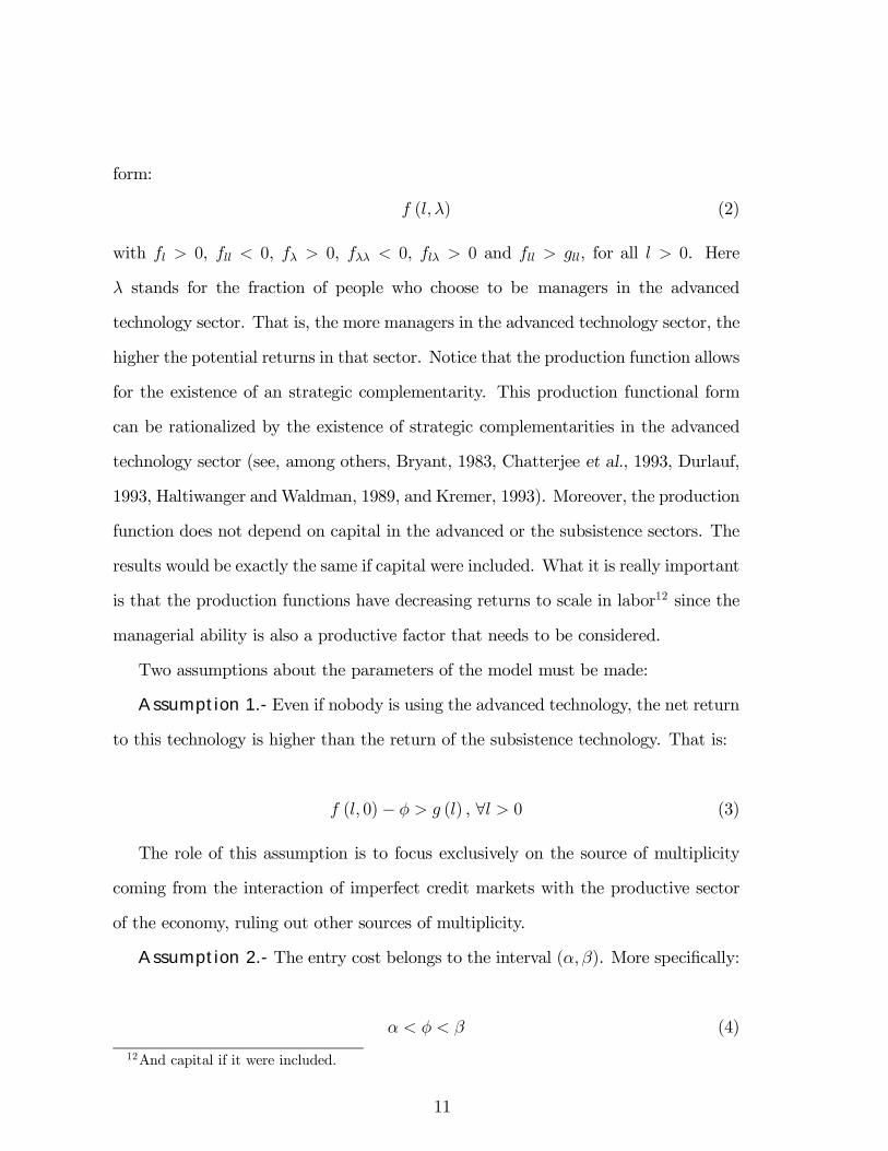
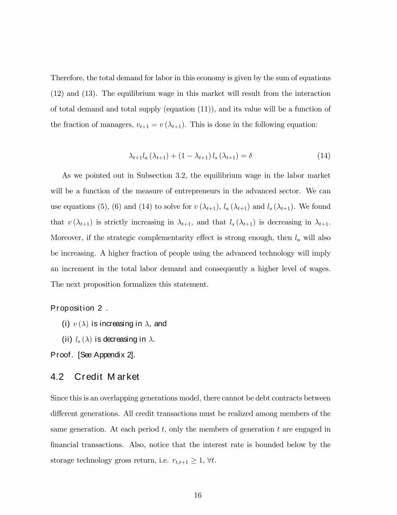
conditional expectation of the absolute value of the deviation from the trend. The

results are reported in Figure 1.

[FIGURE 1 HERE]

These events are typically concentrated in low-income countries. This is the rea-

son why we believe that if we do not correct for them, the results of the exercise are

being distorted. That is, the effect of these events could result in a higher variability

of output totally unrelated to our story. Therefore, the fact that the kernel esti-

mation shows an inverted-U shape after controlling for these dummies suggests that

these specific, relevant events generate a transitory increase in the riskiness for very

poor countries. If we did not introduced these dummies, these events would appear

included in the general volatility.

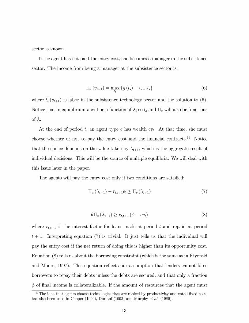
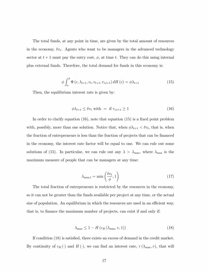
In addition, we also estimated second-order polynomials in the log of real GDP

per capita for the absolute percentage deviation from the GDP trend, for six different

years. We do not perform a nonparametric kernel regression here since we have few

observations in each of those exercises. In all cases, the quadratic term was strongly

significant, yielding evidence against the restricted linear model. In Figure 2, we

have plotted the predicted values from the regressions and their 95 percent confi-

dence bands for each year. From this figure, the inverted U-shape becomes apparent,

although the high variability of the data gives evidence of important unobserved het-

erogeneity that cannot be explained by the quadratic specification (and much less by

the restricted linear specification).

[FIGURE 2 HERE]

A version of Figures 1 and 2 has already been documented by Chari et al. (1996)

and Quah (1993). Both papers construct a mobility matrix whose (j, k) entries repre-

sent the probabilities that an economy in a bin j transits to a state k. Those matrices

7

show that countries in the middle income groups tend to move up or down more fre-

quently than countries in the extremes. Thus, very poor countries tend to stay very

poor and the rich countries tend to stay rich, but there are much more dynamics in

the middle of the distribution. Quah also speaks of a closely connected issue: the

emergence of a twin-peaks distribution. This bimodal shape can be interpreted as ev-

idence of a higher level of variability in middle income countries. A similar approach

is followed by McGrattan and Schmitz (1998).

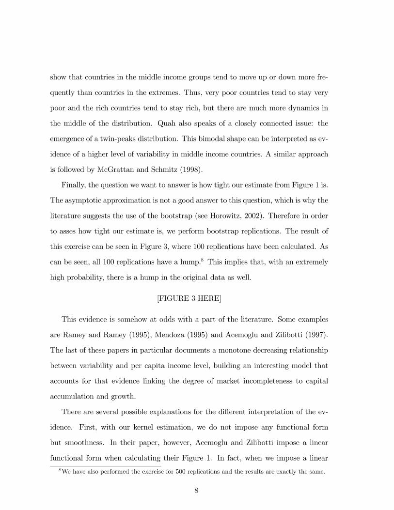
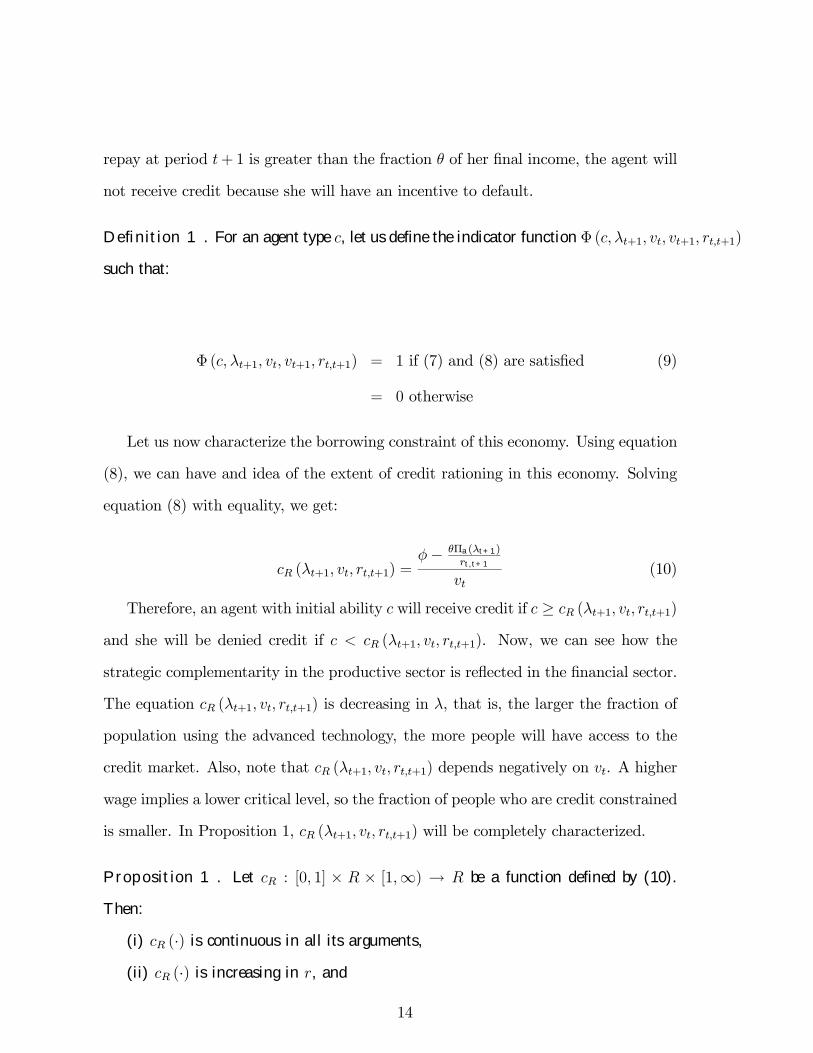
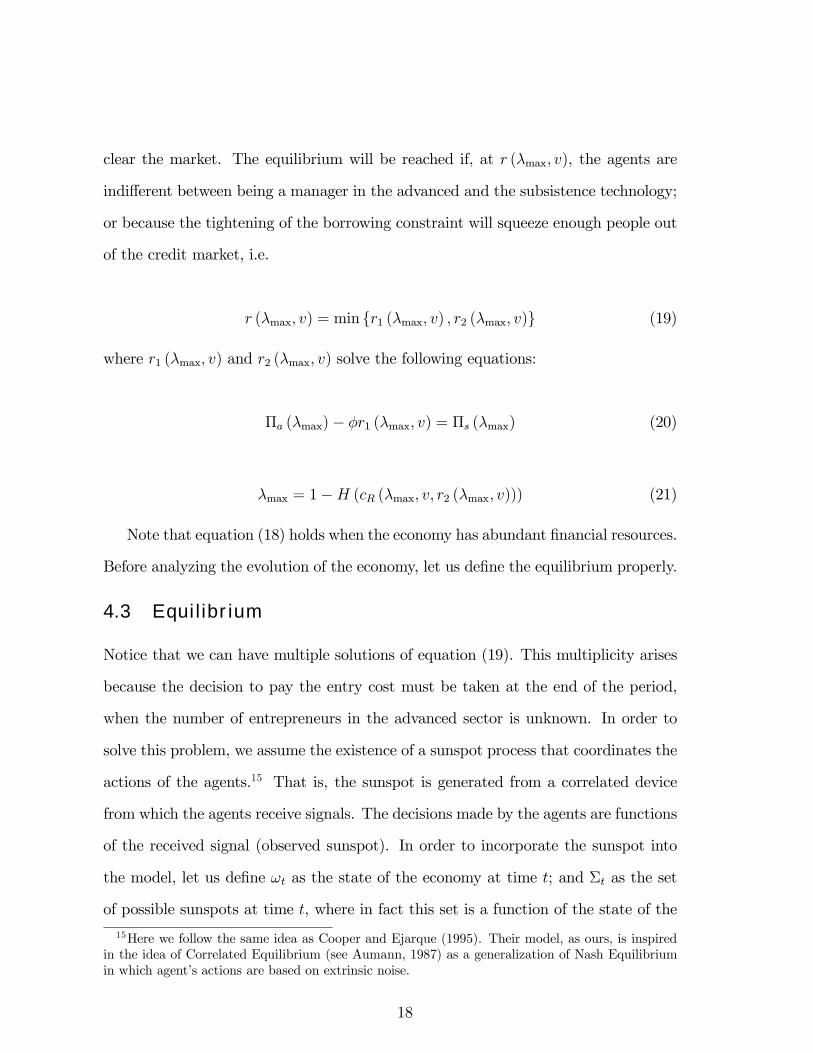
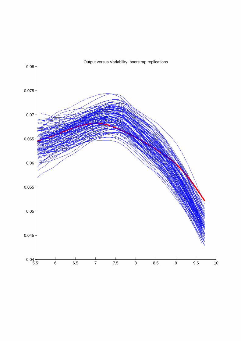
Finally, the question we want to answer is how tight our estimate from Figure 1 is.

The asymptotic approximation is not a good answer to this question, which is why the

literature suggests the use of the bootstrap (see Horowitz, 2002). Therefore in order

to asses how tight our estimate is, we perform bootstrap replications. The result of

this exercise can be seen in Figure 3, where 100 replications have been calculated. As

can be seen, all 100 replications have a hump.8 This implies that, with an extremely

high probability, there is a hump in the original data as well.

[FIGURE 3 HERE]

This evidence is somehow at odds with a part of the literature. Some examples

are Ramey and Ramey (1995), Mendoza (1995) and Acemoglu and Zilibotti (1997).

The last of these papers in particular documents a monotone decreasing relationship

between variability and per capita income level, building an interesting model that

accounts for that evidence linking the degree of market incompleteness to capital

accumulation and growth.

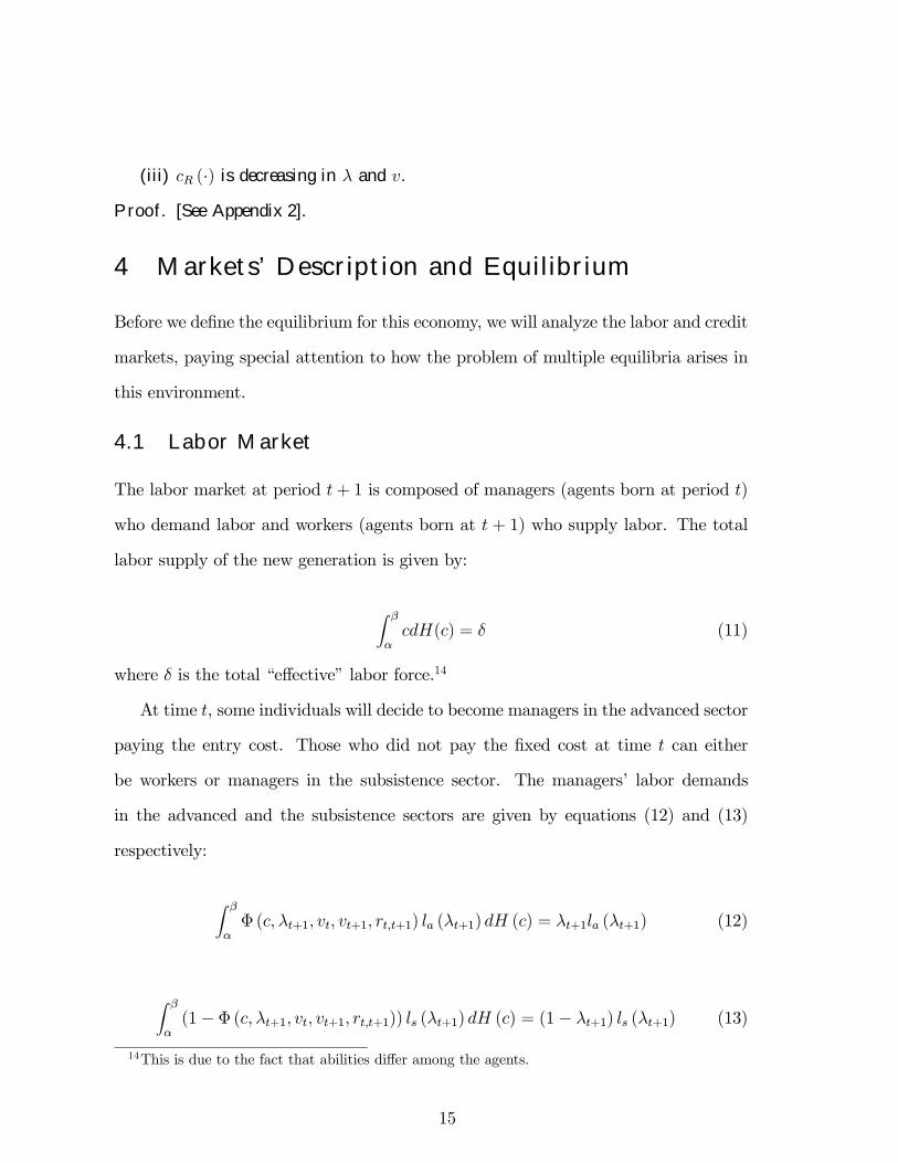
There are several possible explanations for the different interpretation of the ev-

idence. First, with our kernel estimation, we do not impose any functional form

but smoothness. In their paper, however, Acemoglu and Zilibotti impose a linear

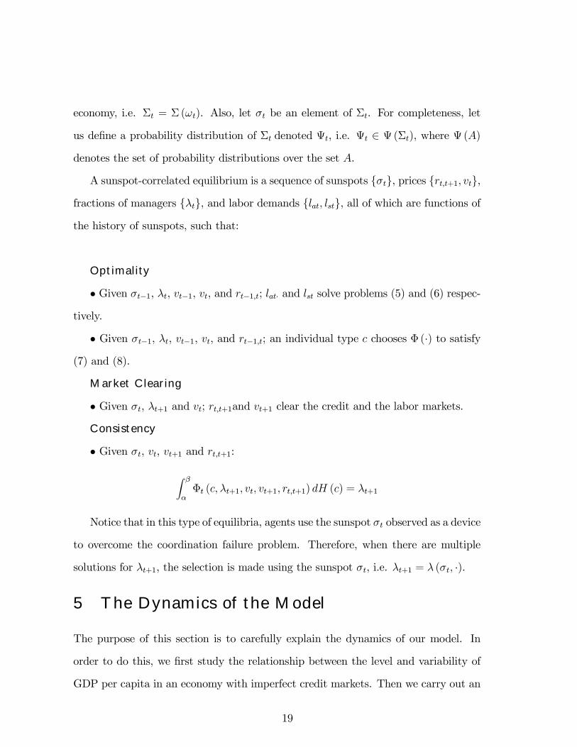
functional form when calculating their Figure 1. In fact, when we impose a linear8We have also performed the exercise for 500 replications and the results are exactly the same.

8

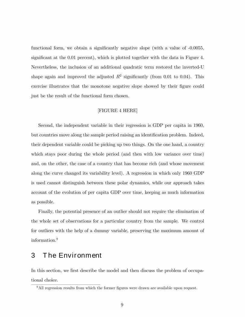
functional form, we obtain a significantly negative slope (with a value of -0.0055,

significant at the 0.01 percent), which is plotted together with the data in Figure 4.

Nevertheless, the inclusion of an additional quadratic term restored the inverted-U

shape again and improved the adjusted R2 significantly (from 0.01 to 0.04). This

exercise illustrates that the monotone negative slope showed by their figure could

just be the result of the functional form chosen.

[FIGURE 4 HERE]

Second, the independent variable in their regression is GDP per capita in 1960,

but countries move along the sample period raising an identification problem. Indeed,

their dependent variable could be picking up two things. On the one hand, a country

which stays poor during the whole period (and then with low variance over time)

and, on the other, the case of a country that has become rich (and whose movement

along the curve changed its variability level). A regression in which only 1960 GDP

is used cannot distinguish between these polar dynamics, while our approach takes

account of the evolution of per capita GDP over time, keeping as much information

as possible.

Finally, the potential presence of an outlier should not require the elimination of

the whole set of observations for a particular country from the sample. We control

for outliers with the help of a dummy variable, preserving the maximum amount of

information.9

3 The Environment

In this section, we first describe the model and then discuss the problem of occupa-

tional choice.9All regression results from which the former figures were drawn are available upon request.

9

3.1 The Model

The model is a two-period overlapping generations model. At each date t, a con-

tinuum of agents of measure one is born. Each agent is endowed with one unit of

labor at each period. In the first period, the individuals can only be workers. They

have some capacity (or ability) c with support on the interval [α, β], where α and β

are both positive numbers, a continuous probability distribution function h (c), and

a continuous cumulative distribution function H (c). As agents will be rewarded ac-

cording to c, this parameter affects labor income in the first period. In the second

period, the agents can only be managers either in the advanced or the subsistence

sector (and managers are all the same by technology managed).10 At t = 0, the initial

‘old’ are endowed with cv0, where c is the same random variable as before, and v0 is

a non-negative number.

The agents born at time t receive utility only from consumption at t+1. This is an

innocuous11 assumption that simplifies the algebra. Each agent can choose between

managing an advanced or a subsistence technology. If the agent chooses to manage

the subsistence technology, she will have access to the following production function:

g (l) (1)

with gl > 0 and gll < 0. Where l stands for labor input, gl is the first derivative with

respect to l, and gll is the second derivative with respect to l, for all l > 0.

If the agent wants to manage the advanced technology, she must pay an entry

cost φ at the end of the initial period. That is, the agent must commit herself to this

technology. In the second period, she will have access to a production function of the

10This is just a simplifying assumption. If we allow the agents in the second period the possibilityto be either workers or entrepreneurs, we complicate the model without altering our result.11Innocuous for our multiple equilibria result.

10

form:

f (l,λ) (2)

with fl > 0, fll < 0, fλ > 0, fλλ < 0, flλ > 0 and fll > gll, for all l > 0. Here

λ stands for the fraction of people who choose to be managers in the advanced

technology sector. That is, the more managers in the advanced technology sector, the

higher the potential returns in that sector. Notice that the production function allows

for the existence of an strategic complementarity. This production functional form

can be rationalized by the existence of strategic complementarities in the advanced

technology sector (see, among others, Bryant, 1983, Chatterjee et al., 1993, Durlauf,

1993, Haltiwanger andWaldman, 1989, and Kremer, 1993). Moreover, the production

function does not depend on capital in the advanced or the subsistence sectors. The

results would be exactly the same if capital were included. What it is really important

is that the production functions have decreasing returns to scale in labor12 since the

managerial ability is also a productive factor that needs to be considered.

Two assumptions about the parameters of the model must be made:

Assumption 1.- Even if nobody is using the advanced technology, the net return

to this technology is higher than the return of the subsistence technology. That is:

f (l, 0)− φ > g (l) , ∀l > 0 (3)

The role of this assumption is to focus exclusively on the source of multiplicity

coming from the interaction of imperfect credit markets with the productive sector

of the economy, ruling out other sources of multiplicity.

Assumption 2.- The entry cost belongs to the interval (α,β). More specifically:

α < φ < β (4)

12And capital if it were included.

11

There also exists a storage technology. By using this technology, the agents can

transform date t goods into date t+ 1 goods at a one-to-one rate.

The individual can borrow resources to pay the entry cost, with the obligation to

repay the loan in the next period. However, since credit markets are imperfect, there

exists an enforcement problem. The lenders can not force the borrowers to repay the

debt, but they can seize a fraction θ of the borrowers’ managerial income. Also, it is

assumed that there exists perfect information about the initial wealth of each agent.

In this model, the decisions are simultaneous within each period. Agents born in

period t work for managers who were born in period t− 1. They are paid accordingto their ability. At the end of period t, they make their financial decisions (lend,

borrow or invest in the storage technology) and decide whether or not to pay the

entry cost. At period t + 1, those who paid the entry cost can manage the advance

technology, otherwise they manage the subsistence technology. Managers will hire

labor at a competitive wage and, at the end of the period, will execute the financial

obligations and consume whatever is left.

3.2 Optimal Behavior

In this subsection, we are going to analyze the optimal decisions of an agent type c

born at period t. This can be done solving the model backwards. Let us start with

the assumption that the agent has paid the entry cost at time t. This means she is a

manager in the advanced sector, and she will try to maximize her managerial income

taking as given the wage rate, vt+1. That is:

Πa (vt+1,λt+1) = maxla{f (la,λt+1)− vt+1la} (5)

where la (vt+1,λt+1) is labor in the advanced technology sector and the solution to this

problem. Notice that, at this stage, the fraction of total managers in the advanced

12

sector is known.

If the agent has not paid the entry cost, she becomes a manager in the subsistence

sector. The income from being a manager at the subsistence sector is:

Πs (vt+1) = maxls{g (ls)− vt+1ls} (6)

where ls (vt+1) is labor in the subsistence technology sector and the solution to (6).

Notice that in equilibrium v will be a function of λ; so ls and Πs will also be functions

of λ.

At the end of period t, an agent type c has wealth cvt. At that time, she must

choose whether or not to pay the entry cost and the financial contracts.13 Notice

that the choice depends on the value taken by λt+1, which is the aggregate result of

individual decisions. This will be the source of multiple equilibria. We will deal with

this issue later in the paper.

The agents will pay the entry cost only if two conditions are satisfied:

Πa (λt+1)− rt,t+1φ ≥ Πs (λt+1) (7)

θΠa (λt+1) ≥ rt,t+1 (φ− cvt) (8)

where rt,t+1 is the interest factor for loans made at period t and repaid at period

t + 1. Interpreting equation (7) is trivial. It just tells us that the individual will

pay the entry cost if the net return of doing this is higher than its opportunity cost.

Equation (8) tells us about the borrowing constraint (which is the same as in Kiyotaki

and Moore, 1997). This equation reflects our assumption that lenders cannot force

borrowers to repay their debts unless the debts are secured, and that only a fraction

φ of final income is collateralizable. If the amount of resources that the agent must13The idea that agents choose technologies that are ranked by productivity and entail fixed costs

has also been used in Cooper (1994), Durlauf (1993) and Murphy et al. (1989).

13

repay at period t+ 1 is greater than the fraction θ of her final income, the agent will

not receive credit because she will have an incentive to default.

Definition 1 . For an agent type c, let us define the indicator function Φ (c,λt+1, vt, vt+1, rt,t+1)

such that:

Φ (c,λt+1, vt, vt+1, rt,t+1) = 1 if (7) and (8) are satisfied (9)

= 0 otherwise

Let us now characterize the borrowing constraint of this economy. Using equation

(8), we can have and idea of the extent of credit rationing in this economy. Solving

equation (8) with equality, we get:

cR (λt+1, vt, rt,t+1) =φ− θΠa(λt+1)

rt,t+1

vt(10)

Therefore, an agent with initial ability c will receive credit if c ≥ cR (λt+1, vt, rt,t+1)and she will be denied credit if c < cR (λt+1, vt, rt,t+1). Now, we can see how the

strategic complementarity in the productive sector is reflected in the financial sector.

The equation cR (λt+1, vt, rt,t+1) is decreasing in λ, that is, the larger the fraction of

population using the advanced technology, the more people will have access to the

credit market. Also, note that cR (λt+1, vt, rt,t+1) depends negatively on vt. A higher

wage implies a lower critical level, so the fraction of people who are credit constrained

is smaller. In Proposition 1, cR (λt+1, vt, rt,t+1) will be completely characterized.

Proposition 1 . Let cR : [0, 1] × R × [1,∞) → R be a function defined by (10).

Then:

(i) cR (·) is continuous in all its arguments,

(ii) cR (·) is increasing in r, and

14

(iii) cR (·) is decreasing in λ and v.

Proof. [See Appendix 2].

4 Markets’ Description and Equilibrium

Before we define the equilibrium for this economy, we will analyze the labor and credit

markets, paying special attention to how the problem of multiple equilibria arises in

this environment.

4.1 Labor Market

The labor market at period t+ 1 is composed of managers (agents born at period t)

who demand labor and workers (agents born at t + 1) who supply labor. The total

labor supply of the new generation is given by:

Z β

αcdH(c) = δ (11)

where δ is the total “effective” labor force.14

At time t, some individuals will decide to become managers in the advanced sector

paying the entry cost. Those who did not pay the fixed cost at time t can either

be workers or managers in the subsistence sector. The managers’ labor demands

in the advanced and the subsistence sectors are given by equations (12) and (13)

respectively:

Z β

αΦ (c,λt+1, vt, vt+1, rt,t+1) la (λt+1) dH (c) = λt+1la (λt+1) (12)

Z β

α(1−Φ (c,λt+1, vt, vt+1, rt,t+1)) ls (λt+1) dH (c) = (1− λt+1) ls (λt+1) (13)

14This is due to the fact that abilities differ among the agents.

15

Therefore, the total demand for labor in this economy is given by the sum of equations

(12) and (13). The equilibrium wage in this market will result from the interaction

of total demand and total supply (equation (11)), and its value will be a function of

the fraction of managers, vt+1 = v (λt+1). This is done in the following equation:

λt+1la (λt+1) + (1− λt+1) ls (λt+1) = δ (14)

As we pointed out in Subsection 3.2, the equilibrium wage in the labor market

will be a function of the measure of entrepreneurs in the advanced sector. We can

use equations (5), (6) and (14) to solve for v (λt+1), la (λt+1) and ls (λt+1). We found

that v (λt+1) is strictly increasing in λt+1, and that ls (λt+1) is decreasing in λt+1.

Moreover, if the strategic complementarity effect is strong enough, then la will also

be increasing. A higher fraction of people using the advanced technology will imply

an increment in the total labor demand and consequently a higher level of wages.

The next proposition formalizes this statement.

Proposition 2 .

(i) v (λ) is increasing in λ, and

(ii) ls (λ) is decreasing in λ.

Proof. [See Appendix 2].

4.2 Credit Market

Since this is an overlapping generations model, there cannot be debt contracts between

different generations. All credit transactions must be realized among members of the

same generation. At each period t, only the members of generation t are engaged in

financial transactions. Also, notice that the interest rate is bounded below by the

storage technology gross return, i.e. rt,t+1 ≥ 1, ∀t.

16

The total funds, at any point in time, are given by the total amount of resources

in the economy, δvt. Agents who want to be managers in the advanced technology

sector at t+ 1 must pay the entry cost, φ, at time t. They can do this using internal

plus external funds. Therefore, the total demand for funds in this economy is:

φZ β

αΦ (c,λt+1, vt, vt+1, rt,t+1) dH (c) = φλt+1 (15)

Then, the equilibrium interest rate is given by:

φλt+1 ≤ δvt with = if rt,t+1 ≥ 1 (16)

In order to clarify equation (16), note that equation (15) is a fixed point problem

with, possibly, more than one solution. Notice that, when φλt+1 < δvt, that is, when

the fraction of entrepreneurs is less than the fraction of projects that can be financed

in the economy, the interest rate factor will be equal to one. We can rule out some

solutions of (15). In particular, we can rule out any λ > λmax, where λmax is the

maximum measure of people that can be managers at any time:

λmax,t = min

Ãδvtφ, 1

!(17)

The total fraction of entrepreneurs is restricted by the resources in the economy,

so it can not be greater than the funds available per project at any time, or the actual

size of population. An equilibrium in which the resources are used in an efficient way,

that is, to finance the maximum number of projects, can exist if and only if:

λmax ≤ 1−H (cR (λmax, v, 1)) (18)

If condition (18) is satisfied, there exists an excess of demand in the credit market.

By continuity of cR (·) and H (·), we can find an interest rate, r (λmax, v), that will

17

clear the market. The equilibrium will be reached if, at r (λmax, v), the agents are

indifferent between being a manager in the advanced and the subsistence technology;

or because the tightening of the borrowing constraint will squeeze enough people out

of the credit market, i.e.

r (λmax, v) = min {r1 (λmax, v) , r2 (λmax, v)} (19)

where r1 (λmax, v) and r2 (λmax, v) solve the following equations:

Πa (λmax)− φr1 (λmax, v) = Πs (λmax) (20)

λmax = 1−H (cR (λmax, v, r2 (λmax, v))) (21)

Note that equation (18) holds when the economy has abundant financial resources.

Before analyzing the evolution of the economy, let us define the equilibrium properly.

4.3 Equilibrium

Notice that we can have multiple solutions of equation (19). This multiplicity arises

because the decision to pay the entry cost must be taken at the end of the period,

when the number of entrepreneurs in the advanced sector is unknown. In order to

solve this problem, we assume the existence of a sunspot process that coordinates the

actions of the agents.15 That is, the sunspot is generated from a correlated device

from which the agents receive signals. The decisions made by the agents are functions

of the received signal (observed sunspot). In order to incorporate the sunspot into

the model, let us define ωt as the state of the economy at time t; and Σt as the set

of possible sunspots at time t, where in fact this set is a function of the state of the

15Here we follow the same idea as Cooper and Ejarque (1995). Their model, as ours, is inspiredin the idea of Correlated Equilibrium (see Aumann, 1987) as a generalization of Nash Equilibriumin which agent’s actions are based on extrinsic noise.

18

economy, i.e. Σt = Σ (ωt). Also, let σt be an element of Σt. For completeness, let

us define a probability distribution of Σt denoted Ψt, i.e. Ψt ∈ Ψ (Σt), where Ψ (A)denotes the set of probability distributions over the set A.

A sunspot-correlated equilibrium is a sequence of sunspots {σt}, prices {rt,t+1, vt},fractions of managers {λt}, and labor demands {lat, lst}, all of which are functions ofthe history of sunspots, such that:

Optimality

• Given σt−1, λt, vt−1, vt, and rt−1,t; lat· and lst solve problems (5) and (6) respec-tively.

• Given σt−1, λt, vt−1, vt, and rt−1,t; an individual type c chooses Φ (·) to satisfy(7) and (8).

Market Clearing

• Given σt, λt+1 and vt; rt,t+1and vt+1 clear the credit and the labor markets.Consistency

• Given σt, vt, vt+1 and rt,t+1:Z β

αΦt (c,λt+1, vt, vt+1, rt,t+1) dH (c) = λt+1

Notice that in this type of equilibria, agents use the sunspot σt observed as a device

to overcome the coordination failure problem. Therefore, when there are multiple

solutions for λt+1, the selection is made using the sunspot σt, i.e. λt+1 = λ (σt, ·).

5 The Dynamics of the Model

The purpose of this section is to carefully explain the dynamics of our model. In

order to do this, we first study the relationship between the level and variability of

GDP per capita in an economy with imperfect credit markets. Then we carry out an

19

analysis of the behavior of wages, interest rates, and entrepreneurial choice during

the development process. Finally, we discuss the perfect credit market and non credit

market cases.

5.1 Multiple Equilibria in the Development Process

In this subsection, we study the process of economic development. We find that, in

the early stages of development, there is only one equilibrium. The multiplicity of

equilibria arises when the economy reaches a minimum level of wealth that allows a

non-trivial fraction of people to obtain credit. Once the economy is at this stage, due

to the existence of a strategic complementarity in the productive sector, there will be

more than one equilibrium. As we will prove in the next section, this problem does

not arise if the credit market is perfect or if it does not exist. The reason for this

result is that, in these cases, the connection between the strategic complementarity

effect and the credit market is broken. The multiplicity of equilibria will remain until

the economy reaches a new threshold level. At that point, some individuals will have

access to the credit market even though the measure of entrepreneurs is zero.

Before analyzing the development process, let us define the function γ (·) by:

γ (λ, v, r) = 1−H (cR (λ, v, r)) (22)

The next proposition characterizes this function γ (·). Note that the slope of thisfunction with respect to λ is always positive, but the magnitude of the slope will

depend on the sign of the first derivative of h (c) with respect to c, hc (c), and the

relative strength of the strategic complementarity effect.

Proposition 3 . The function γ (·) defined in (22) is:

(i) a continuous function of λ, v and r,

(ii) increasing in λ and v,

20

(iii) decreasing in r, and

(iv) γλ > 0.

Proof. [See Appendix 2].

Next, we will analyze the equilibrium along the development process for an econ-

omy that satisfies the following assumptions:

Assumption 3.- h (c) is uniform.

Assumption 4.- There is an strategic complementarity effect: fλ > B, for some

B and λ close to zero.

Assumption 3 is for simplicity. Moreover, it can be shown that if h is uniform and

Πa is a concave function of λ, then γλλ < 0.

To find an equilibrium, we need to find the fixed point of equation (15). We can

find a set of wages close to zero such that, even though the fraction of entrepreneurs is

equal to one, there is no agent who can have access to the credit market. No matter

how big the strategic complementarity is, we can always have wages close enough

to zero such that the critical level of ability to get credit is greater than β. In this

situation, there exists a unique equilibrium in this economy. This equilibrium is given

by λ = 0.

For a higher wage, and given a strong strategic complementarity effect, we can

have a situation in which a positive fraction of entrepreneurs can overcome the credit

constraint just because the same fraction of people becomes managers in the advanced

technology sector. This will be an equilibrium if and only if the resources of the

economy are big enough to finance this measure of entrepreneurs. If this is not the

case, the economy has still a unique equilibrium. As the economy grows, we find two

positive measures of entrepreneurs that could be considered as equilibria. We will

show that, at some point, the resources in the economy will be big enough to finance

21

the lowest of these fractions of managers. At that point, we have two equilibria. One

is given by the lowest of these positive measures, the other given by λ = 0. Remember

that even if the measure of entrepreneurs is zero, nobody can overcome the borrowing

constraint.

From this period, the number of equilibria will increase to three, the first two

being as the ones obtained before, and the third one given by the resources in the

economy: λt = δvt

φ. In this situation, such measure of entrepreneurs implies that a

much bigger fraction of people can have access to the credit market. Since there are

not enough resources in the economy to finance all these projects, the interest rate

must rise to clear this excess demand. We will prove that, for the relevant range of

wages, the highest fixed point of this problem will always be above the economy’s

resources. This situation will persist until the economy reaches some level of wage at

which, even though nobody is using the advanced technology, the richest agent in the

economy will be able to get credit. From this moment, the bad equilibrium (λ = 0)

disappears. The unique equilibrium will be given by λ = λmax. Theorem 4 formalizes

this statement.

Theorem 4 . If Assumptions 3 and 4 are satisfied, there exist two wage levels, v1

and v2, with v1 < v2, such that:

cR (1, v1, 1) = cR (0, v2, 1) = β (23)

Then:

(i) For any v < v1, there exists only one equilibrium.

(ii) For some v ∈ (v1, v2), there are multiple equilibria.

(iii) For some v > v2, there exists only one equilibrium.

Proof. [See Appendix 2].

22

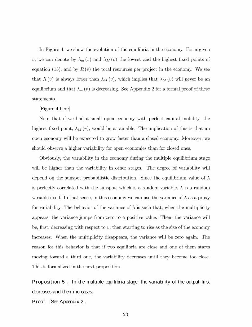
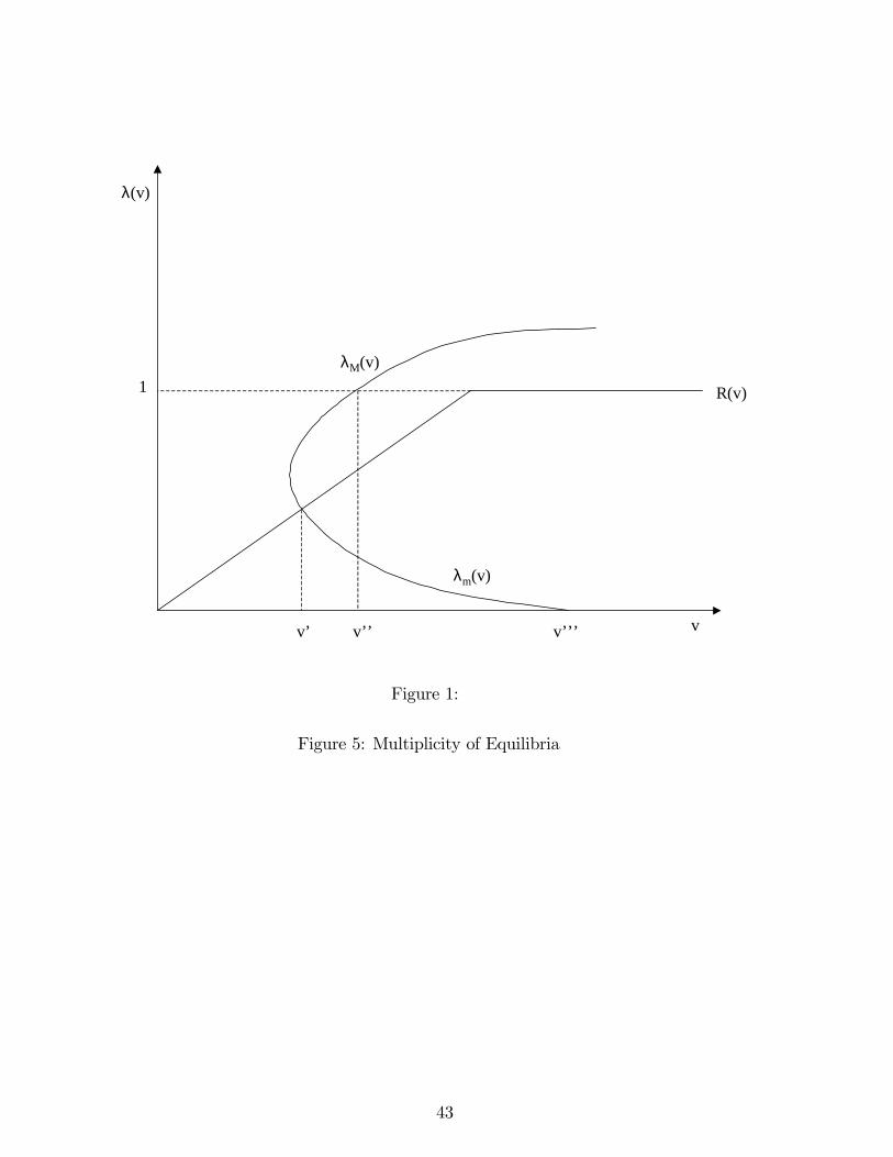
In Figure 4, we show the evolution of the equilibria in the economy. For a given

v, we can denote by λm (v) and λM (v) the lowest and the highest fixed points of

equation (15), and by R (v) the total resources per project in the economy. We see

that R (v) is always lower than λM (v), which implies that λM (v) will never be an

equilibrium and that λm (v) is decreasing. See Appendix 2 for a formal proof of these

statements.

[Figure 4 here]

Note that if we had a small open economy with perfect capital mobility, the

highest fixed point, λM (v), would be attainable. The implication of this is that an

open economy will be expected to grow faster than a closed economy. Moreover, we

should observe a higher variability for open economies than for closed ones.

Obviously, the variability in the economy during the multiple equilibrium stage

will be higher than the variability in other stages. The degree of variability will

depend on the sunspot probabilistic distribution. Since the equilibrium value of λ

is perfectly correlated with the sunspot, which is a random variable, λ is a random

variable itself. In that sense, in this economy we can use the variance of λ as a proxy

for variability. The behavior of the variance of λ is such that, when the multiplicity

appears, the variance jumps from zero to a positive value. Then, the variance will

be, first, decreasing with respect to v, then starting to rise as the size of the economy

increases. When the multiplicity disappears, the variance will be zero again. The

reason for this behavior is that if two equilibria are close and one of them starts

moving toward a third one, the variability decreases until they become too close.

This is formalized in the next proposition.

Proposition 5 . In the multiple equilibria stage, the variability of the output first

decreases and then increases.

Proof. [See Appendix 2].

23

In order to prove Proposition 5, we use a time-invariant probability distribution

in which each sunspot has the same probability each period. The results are the

same if we use symmetric first-order Markov probabilities in which the probability

of observing a given sunspot this period will depend on the sunspot observed last

period. The results are not robust to all non-symmetric Markov probabilities or

other time-depending probabilities.

5.2 Wages, Interest Rates and Entrepreneurship

In this subsection, we will study the equilibrium values of wages, interest rates, and

measure of entrepreneurs during the development process. We will prove that, if

an economy satisfies two conditions for growth, then, for any initial condition v0,

the economy will converge to the long run equilibrium with positive probability. The

conditions for growth imply that there exists a minimum required level of productivity

in the subsistence technology, and that the set of sunspots that implies the “good”

equilibrium with probability zero has measure zero.

The conditions for growth are the following:

gl (δ) > w0 and m (A) > 0

where m (A) is the measure of a set A, and A = {σt : Pr [λ (σt) = R (vt)] > 0}. Thefirst condition guarantees that the economy will reach the multiple equilibria stage.

The second implies that the economy will leave that stage.

If the condition for growth is satisfied, the economy will reach the multiple equi-

libria stage and, with positive probability, will be at the highest equilibrium. The

main mechanism is that the more agents have access to credit, the larger is the high

productivity sector in the economy and the higher are wages. Higher wages relax

borrowing constraints for agents who want to invest in the more productive sector

and that generates growth. At the same time, higher wages do not decrease profits

24

and discourage investment because the size of the advance sector is itself a productive

externality in that sector.

We can construct a sequence of λt from t equals one to T , in which λT takes

the highest value. This sequence has a positive probability if T < ∞. Since λt isincreasing at some finite rate, the economy will leave this stage and will converge to

the long run equilibrium: λ∗ = 1, r∗ = 1 and v∗ = fl (δ,λ∗). This fact is proved in

the next theorem.

Theorem 6 . If the condition for growth is satisfied, for any initial v0 and with

positive probability, when t goes to ∞:

(i) λt converges to 1

(ii) rt converges to 1, and

(iii) vt converges to v∗, where v∗ = fl (δ,λ∗).

Proof. [See Appendix 2].

5.3 Credit Market and Variability

The purpose of this subsection is to analyze how different degrees of imperfection

in the credit market will affect the equilibrium of the economy. In Subsection 5.1,

we have already seen that, when there exist imperfections in the credit market (i.e.

0 < θ < 1), we could have multiple equilibria. Now, we show that when the credit

market is perfect, i.e. θ = 1, or when the credit market does not exist, i.e. θ = 0, the

equilibrium will be unique. The reason for this is that, when there is no credit market,

there is no interaction between the strategic complementarity in the productive sector

and the borrowing constraint. Only the fraction of people with wealth greater than

the entry cost will become entrepreneurs. Also, when the credit market is perfect,

there are no longer borrowing constraints and, therefore, all the resources are used

to finance the payment of the entry cost of those who want to use the advanced

25

technology. The interest rate will be such that the agents are indifferent between

using the advanced or the subsistence technology. Subsubsections 5.3.1 and 5.3.2 will

study both cases.

5.3.1 Perfect-Credit Market Economy

Suppose that v0 <φδ. This condition means that the initial resources are not enough

to finance all the people in this economy. The fraction of people who become man-

agers in the advanced technology sector is given by λ0 = δv0

φ. Since, by assumption,

it is profitable to be a manager when the interest rate is one, everybody will demand

credit for investment. In order for the credit market to clear, the interest rate will

have to rise.

Once we have λ0, the wage rate for the next period, v1, can be uniquely determined

using v1 = v (λ) (see Section 4). Notice that, even though we have a strategic

complementarity in the productive sector, each time the measure of entrepreneurs is

only determined by the resource constraints in the economy. The next proposition

formalizes this statement.

Proposition 7 . Given some endowment cv0 for the initial old people such that

v0 <φδ, if the credit market is perfect, then:

(i) At each t, there is only one equilibrium, i.e. vt, λt+1, and rt,t+1 are uniquely

determined.

(ii) The equilibrium sequences {vt} and {λt} are non decreasing and converge to

the long run equilibrium.

Proof. [See Appendix 2].

It is worthwhile to notice the behavior of the interest rate. When λ < 1, rt,t+1 (λ)

is increasing in λ. The reason for this is that, as the total fraction of managers

increases in this economy, the managerial profits also increase (due to the strategic

26

complementarity). As a result, the interest rate needed to clear this market is higher.

However, as soon as λ reaches the value of one, the financial resources are abundant

relative to the population resources (the fraction of managers can not be greater than

one) and the interest rate will drop abruptly to one (the storage technology return).

Notice that we can observe the same situation when there exist multiple equilibria. In

that case, the drastic change in interest rate will be accompanied by a drastic change

in λ. However, when the credit market is perfect, a drastic change in interest rate will

be caused by a change of regime. The economy moves from a resource-constrained

economy to a resource-unconstrained economy. In this case, a large movement in the

interest rate is accompanied by a small change in λ.

5.3.2 Non Credit Market Economy

Suppose now that the initial condition over v0 is such that β v0 < φ, which implies

that nobody will become an entrepreneur in period one. The wage rate in that period

will be given by v1 = gl (δ). In this case, the condition for growth is that v1 > φβ;

otherwise the advanced technology will never be used. Notice that, when there is no

credit market or when the credit market is incomplete, there are some conditions on

the productivity of the subsistence sector (see Subsection 5.2) to guarantee that the

economy will take off. This is not the case when the credit market is perfect.

Since people cannot borrow, the entry cost must be self-financed. Then, given

vt, only a fraction of people equal to 1 − H³φvt

´will become managers in the next

period. Once λt−1 is known, the wage rate vt+1 can be easily determined (see Section

4). Then the sequences of wages {vt} and measures of managers {λt} are uniquelydetermined, and they will converge to the long-run equilibrium. The next proposition

formalizes this statement.

Proposition 8 . Given some endowment cv0 for the initial old people such that

27

v0 <φβ, if the credit market does not exist and gl (δ) > φ

β, then:

(i) At each period t, there is only one equilibrium, i.e. vt and λt+1 are uniquely

determined.

(ii) The equilibrium sequences {vt} and {λt} are non decreasing and converge to

the long run equilibrium.

Proof. [See Appendix 2].

6 Conclusion

This paper explains the GDP variability pattern of an economy during the devel-

opment process. We show that, at the middle stages of development, the economy

experiences high levels of GDP variability. On the other hand, in early and ma-

ture stages of development, we observe a much lower variability in per capita GDP.

This variability is explained because, in an imperfect credit market environment, the

number of equilibria will depend on the size of the economy. In particular, when

the economy is very poor, there is only one possible equilibrium. After the economy

reaches some threshold level, there can be multiple equilibria. This multiplicity dis-

appears when the economy is fully developed. The existence of multiple equilibria is

due to the fact that the strategic complementarity in the productive sector will be re-

flected in the financial one. A larger fraction of people using the advanced technology

will imply a larger fraction of people with access to the credit market.

The relationship between the degree of development of the financial sector and

the variability in the economy is also analyzed. We show that, in the case of either

economies with perfect credit markets or economies in which the credit markets are

non-existent, the equilibrium is unique. However, when the credit market exists but

is imperfect, there could be more than one equilibrium. In the latter case, the multi-

plicity arises in the middle stages of development. This is due to the fact that when

28

there is no credit market, there is no interaction between the strategic complementar-

ity in the productive sector and the borrowing constraint. Only the fraction of people

with wealth greater than the entry cost will become entrepreneurs. Also, when the

credit market is perfect, there are no borrowing constraints, and all the resources are

used to finance the payment of the entry cost for those who want to use the advanced

technology.

29

APPENDIX 1

Table A1. Country DummiesCountry Dummy’s Year Historical FactBurundi 1960 Pre-independence political unrest and confrontation (Hutus vs. Tutsis)

1961 Pre-independence political unrest and confrontation (Hutus vs. Tutsis)1965 Rebellion of Hutus (civil war)1970 Purge of Tutsis

Chad 1960 Year of independece1973 Starts Libyan occupation of the Tibesti (North) region (1973-94)1976 Political unrrest following the assessination of the head of state1977 Libia annexed strip of Chadian teritory1978 War with Libia and political unrest1979 War with Libia and political unrest1982 Government overthrow and civil war1983 Civil war1984 Civil war

Lesotho 1970 Coup d’état1971 Political unrest and confrontation following the coup d’état

Mali 1960 Year of independence1961 Political unrest and confrontation following the year of independence

Rwanda 1964 Raid from Burundi1965 Confrontation Tutsis vs. Hutus

Togo 1963 Assessination of the head of stateMyanmar 1963 Military took over the governmentSource: Encyclopedia Britanica (2000).

30

APPENDIX 2

Proof of Proposition 1: First of all, we need to prove that Πa (λ) is a contin-uous function of λ.

Claim: Πa (λ) is a continuous and increasing function of λ.Proof. In order to prove this claim, we need to use a result that will be provedlater (Proposition 2): v (λ) is a continuous and increasing function of λ. Giventhat f (l,λ)−v (λ) l is bounded from above, continuous in l and λ, and with compactrange, we can apply the Theorem of the Maximum to show that Πa (λ) is a continuousfunction. To see that it is increasing in λ, just take derivatives with respect to λ andapplying the Envelope Theorem we get:

∂Π (λ)

∂λ= fλ − ∂v (λ)

∂λl (v (λ) ,λ) (24)

This is positive if the average labor productivity is greater than the marginal laborproductivity, which is the present case (see Proposition 2).

(i) By our claim, it is easy to see that cR (·) is continuous in λ, r, and v.(ii) Moreover, we can take partial derivatives with respect to r, and we get:

∂cR (·)∂r

=θΠa (λ)

vt (r)2 > 0 (25)

(iii) Now, taking derivatives with respect to λ and v, respectively:

∂cR (·)∂v

=−cR (·)v

< 0 (26)

∂cR (·)∂λ

=−θvr

Ã∂Πa (λ)

∂λ

!< 0 (27)

Q.E.D.

Proof of Proposition 2: Given that all the conditions are satisfied for the The-orem of the Maximum, we can apply it to equations (5) and (6). After maximizing,we get the following equations:

fl (la (v,λ) ,λ) = v (28)

31

gl (ls (v)) = v (29)

Now, using the equilibrium market condition (14), we have a system of threeequations with three unknowns: la (λ, δ), ls (λ, δ) and v (λ, δ). This can be reducedto a system of two equations (solving for ls (λ, δ)). Taking derivatives with respect toλ, we get:

à −1 fll−1 −gll λ

(1−λ)

!Ã∂v∂λ∂la∂λ

!=

à −flλ−gll δ−la(1−λ)2

!(30)

Solving (30), we have:

Ã∂v∂λ∂la∂λ

!=

1

|A|

−flλgll λ1−λ − fllgll δ−la(1−λ)2

flλ − gll δ−la(1−λ)2

(31)

Where |A| = −³fll + gll

λ(1−λ)

´. Notice that since it must be the case that for any

(v,λ) when λ > 0, la > ls, then la > δ. Therefore, it is easy to see that ∂v∂λ> 0.

Moreover, if the strategic complementarity effect is strong enough, i.e. if flλ is largeenough, then la will also be increasing.Now, it follows from (6) that ls (v) is a decreasing function of v, and since v is

an increasing function of λ, it must be the case that ls is a decreasing function of λ.Q.E.D.

Proof of Proposition 3:(i) The continuity of γ (·) follows from the continuity of H (·) and the continuity

of cR (·).(ii) Since cR (·) is decreasing in λ and v, and H (·) is increasing in c, this proves

that γ (·) is increasing in λ and v.(iii) To prove that γ (·) is decreasing in r, just note that cR (·) is increasing in r

and H (·) is increasing in c.(iv) Taking derivatives with respect to γ (·):

∂γ (·)∂λ

= −h (cR (λ, v, r)) ∂cR (λ, v, r)∂λ

> 0 (32)

Equation (32) is positive because of Proposition 1 part (iii). Q.E.D.

Proof of Theorem 4:(i) For any v < v1, we have that cR (1, v, 1) > β. Then γ (λ, v, 1) = 0 for any λ.

The only equilibrium is λ = 0.

32

(ii) Because of (23) and the continuity of cR (·), we can define a function λz (v)for v ∈ (v1, v2) such that:

cR (λz (v) , v, 1) = β (33)

Notice that λz (·) is decreasing in v, γλ (·) = 0 for λ ≤ λz (v), and γλ (·) > 0 forλ > λz (v). Notice also that, for λ ∈ (λz (v) ,β), γλλ < 0. Since h (·) and ∂cR(·)

∂λare

continuous functions, we can have v0 and λ0 such that:

λ0 = γ (λ0, v0, 1) and γλ (λ0, v0, 1) = 1 (34)

Assuming that cR (1, v2, 1) > α (we can pick α close enough to zero), we can definetwo functions: λm : [v0, v2]→ [0,λ0] and λM : [v0, v2]→ [λ0,λ00], such that:

λj (v) = γ (λj (v) , v, 1) for j = m,M (35)

Claim: The functions in equation (35) exist and are well defined.Proof. Note that for any v ∈ (v0, v2): λz (v) > γ (λz (v) , v, 1); γ (λ0, v, 1) > λ0 andγ (1, v, 1) < 1. Then, due to the continuity of γ, for each v, there exist two func-tions λm and λM , such that they are the fixed points of equation (35). Moreover,λm (v) ∈ (λz (v) ,λ0), and λM ∈ (λ0, 1).

Claim: λm (v) is a decreasing function and λM (v) is an increasing function.Proof. For λm (v), suppose not. Take w1 < w2. Then, for any λ ∈ (λm (v) ,λ0),γ (λ, w1, 1) > λ. But, γ (λm (w2) , w2, 1) > γ (λm (w2) , w1, 1) > λm (w2). A contradic-tion.For λM (v), suppose not. Take w1 < w2. Then, for any λ ∈ (λ0,λM (v)),

γ (λ, w1, 1) > λ. But, γ (λM (w2) , w2, 1) > γ (λM (w2) , w1, 1) > λM (w2). A con-tradiction.

Those fixed points will be equilibria if and only if λj (v) < R (v), where we candefine R (v) as:

R (v) =δv

φ(36)

Assume that v0 is such that λ0 > δv0φ. Then, at v0, the only equilibrium is given

by λ = 0. Since λm (v) is decreasing, R (v) is increasing and R (v2) > λm (v2) = 0,then, there exists a level of wage w0 such that R (w0) = λm (w0). At w0, there are twoequilibria: λ = 0 and λ = R (w0) = λm (w0).

33

For any v ∈ (w0, v2) there are three equilibria: λ = 0, λ = λm (w0), and λ =

min {R (v) ,λM (v)}. The first two equilibria are obvious. We need to show that thethird equilibrium exists. Then, we will show that for any v ≤ v2, R (v) < λM (v).First, suppose that R (v) < λM (v). Then, λM (v) is not an equilibrium. Sinceγ (R (v) , v, 1) > R (v), there exists r = r0 (R (v)) such that γ (R (v) , v, r0 (R (v))) =R (v). The continuity of γ (·) guarantees the existence of such interest rate. SeeSection 4 for a proper definition of r0 (R (v)). Now, suppose that λM (v) < R (v).Then, by definition, λM (v) is an equilibrium. Since γ (R (v) , v, 1) < R (v), thenR (v) can not be an equilibrium. Note that, at v = v2, λm (v2) = 0. That means thatat v = v2, there are only two equilibria.It is easy to see that, in fact, R (v) < λM (v) for all v < v2. First, define v00

as: cR (1, v00, 1) = α. It is trivial to show that v00 > v2. Then, we can extend thedomain of the function λM (v) from [v0, v2] to [v0, v00]. Obviously, λM (v00) = 1 andR (v00) < 1. Now, since λM (v) and R (v) are both increasing and (weakly) concavefunctions, then:

R (v) < λM (v) for all v ∈ (v0, v00) (37)

(iii) First, note that for some v000 > v2, γ (0, v000, 1) > 0. Then, for any v > v000, thebad equilibrium vanishes from the economy. Now, since we have proved in (ii) thatR (v) < λM (v), then the only equilibrium in this stage will be given by: λt = δvt

φand

rt,t+1 = r0³δvt

φ

´. Note that when v = φ

δ, λt = 1 and rt,t+1 = 1, for all t. Q.E.D.

Proof of Proposition 5: Let us denote by Πg and Πb, the probabilities ofchoosing the good and the bad equilibrium, respectively, with Πg + Πb < 1. Then,the variance of the equilibrium value, for a given v ∈ (w0, v2), is given by the nextequation:

V (λ (v)) = (1− Πg − Πb) (Πg +Πb) (λm (v))2 + (1− Πg)Πg (R (v))2 (38)

−2 (1−Πg −Πb)ΠgλmR (v)

When v is close to w0, taking derivatives and assuming, for simplicity, that Πg =1− Πg − Πb, we have that:

∂V (λ (v))

∂v∼= 2Π

Ã1− Π− Πδw

0

φ

!Ãδ

φ+∂λm (v)

∂v

!< 0 (39)

34

This is true since it can be showed that ∂λm(v)∂v

→ −∞ as v → w0. Now, if v is closeto v2, and noting that

∂λm(v)∂v

→ 0 as v → v2, we have that:

∂V (λ (v))

∂v∼= 2Π (1− Π) δ

φ> 0 (40)

Q.E.D.

Proof of Theorem 6: Assume, without loss of generality, that v0 < w0. Thenλ1 = 0. Since gl (δ) > w0, then with positive probability λ2 = δv1

φ> λ1 = 0.

By induction, we can construct increasing sequences for λt and vt, with positiveprobability. Since ls (λ) is decreasing in λ, gl (ls) is decreasing in ls, and gl (ε) →∞as ε→ 0, at some point τ , given λτ , vτ ≥ φ

δ. If such λτ exists with positive probability,

then λτ+1 = 1 with the same probability. Once the economy reaches this stage, forall t ≥ τ + 1, λτ = 1 = λ∗ and vt = fl (δ, 1) = v∗. At this point, rt,t+1 = 1.The behavior of the interest rate is as follows. If λt+1 = R (vt), then rt,t+1 =

r0 (R (vt)). If λt+1 < R (vt), then rt,t+1 = 1. If R (vt) > 1, then λt+1 = 1 andrt,t+1 = 1. Q.E.D.

Proof of Proposition 7:(i) Just note that the equilibrium will be given by: λt+1 = max

nδvt

φ

o; rt,t+1 =

rl³δvt

φ

´if δvt

φ< 1 and rt,t+1 = 1 if δvt

φ≥ 1; and vt+1 = fl

³la³δvt

φ

´, δvt

φ

´. All the

variables depend on just vt.(ii) Assume, without loss of generality, that v0 = 0. Then, since v1 > v0, we

have λ2 > λ1. We can continue this reasoning by induction. If vt−1 < vt < δφ, then

λt < λt+1. Since ls (λ) is decreasing in λ, gl (ls (λ)) is decreasing in ls, and gl (ε)→∞as ε→ 0, at some point τvt ≥ δ

φ. Then, λt+1 = 1 and vt+1 = fl (δ, 1). Then, for any

t ≥ τ + 1, λt = λ∗ and vt = v∗. Notice that rt,t+1 = rl³δvt

φ

´is strictly increasing

when vt < δφ. To prove this, just note that ∂Πa(λ)

∂λ> 0 and ∂Πs(λ)

∂λ< 0. When vt > δ

φ,

rt,t+1 = 1. This drastic change in the interest rate is associated to a change in theregime: from a constrained to an unconstrained economy. Q.E.D.

Proof of Proposition 8:(i) Since, by assumption, f (l, 0) − φ > g (l) for all l; all the agents with wealth

greater than φ (i.e. with ability greater than φvt) will pay the entry cost at t and

become entrepreneurs at t+ 1. Then:

35

λt+1 = 1−HÃφ

vt

!(41)

Given λt+1, then vt+1 = v (λt+1), where v (λ) is the function defined in Proposition 2.(ii) Note that, in equation (41), λt+1 is an increasing function of vt. Also, v (λ)

is an increasing function of λ. Given the condition for growth in this economy,v1 = gl (δ) >

φβ. Then, λ2 = 1−H

³φ

gl(δ)

´> λ1 = 0. Following by induction, we can

establish increasing sequences for λt and vt when vt < φα. Since ls (λ) is decreasing

and gl (ε)→∞ as ε→ 0, there exists some finite τ at which vt ≥ φα. From then on,

λt = 1 = λ∗, for all t, and vt = fl (δ, 1) = v∗, for all t. Q.E.D.

REFERENCES

Acemoglu, D. and F. Zilibotti (1997), Was Prometheus Unbound by Chance?Risk, Diversification and Growth, Journal of Political Economy, vol. 105, No. 4, pp.709-751.

Aghion, P., A. Banerjee and T. Piketty (1999), Dualism and MacroeconomicVolatility, Quarterly Journal of Economics, vol. 114, pp. 1359-1397.

Azariadis, C. and A. Drazen (1990), Threshold Externalities in Economic Devel-opment, Quarterly Journal of Economics, vol. 105, pp. 501-526.

Aumann, R. (1987), Correlated Equilibrium as an Expression of Bayesian Ratio-nality, Econometrica, vol. 55, pp. 1-18.

Banerjee, A.V. and A.F. Newman (1993), Occupational Choice and the Processof Development, Journal of Political Economy, vol. 101, pp. 274-298.

Banerjee, A.V. and E. Duflo (2000), A Reassessment of the Relationship BetweenInequality and Growth: Comment, MIT manuscript.

Bencivenga, V. and B. Smith (1991), Financial Intermediation and EndogenousGrowth, Review of Economic Studies, vol.58, pp. 195-209.

Bryant, J. (1983), A Simple Rational Expectations Keynes-Type Model, Quar-terly Journal of Economics, vol. 98, pp. 525-528.

Carranza, L. (1995), Credit Imperfections, Inequality and Economic Growth, Cen-ter for Economic Research Discussion Paper No. 286, University of Minnesota.

Carranza, L and J. E. Galdón-Sánchez (1998), Multiple Equilibrium, Variabil-ity, and the Development Process, International Monetary Fund Working Paper,WP/98/62.

Chari, V.V., P. Kehoe and E. McGrattan (1996), Poverty of Nations: A Quanti-tative Exploration, NBER Working Paper, No. 5414.

36

Chatterjee, S., R. Cooper and B. Ravikumar (1993), Strategic Complementarityin Business Formation: Aggregate Fluctuations and Sunspot Equilibria, Review ofEconomic Studies, vol. 60, pp. 795-811.

Cooper, R. (1994), Equilibrium Selection in Imperfectly Competitive Economieswith Multiple Equilibria, Economic Journal, vol. 104, pp. 1106-1122.

Cooper, R. and J. Ejarque (1995), Financial Intermediation and the Great Depres-sion: A Multiple Equilibrium Interpretation, Carnegie-Rochester Conference Serieson Public Policy, vol. 43, pp. 285-324.

De Long, J. and L. Summers (1984), The Changing Cyclical Variability of Eco-nomic Activity in the United States, NBER Working Paper, No. 1450.

Durlauf, S.N. (1993), Nonergodic Economic Growth, Review of Economic Studies,vol. 60, pp. 349-366.

Encyclopedia Britannica (1999).

Galor, O. and J. Zeira (1993), Income Distribution and Macroeconomics, Reviewof Economic Studies, vol. 60, pp. 35-52.

Haltiwanger, J.C. and M. Waldman (1989), Limited Rationality and StrategicComplements: The Implications for Macroeconomics, Quarterly Journal of Eco-nomics, vol. 104, pp. 463-483.

Hansen, G.D. (1986), Growth and Fluctuations, Working Paper University of Cal-ifornia, Santa Barbara.

Härdle, W. (1990), Applied Nonparametric Regression. Econometric SocietyMonographs. Cambridge University Press.

Horowitz, J.L. (2002), The Bootstrap, Handbook of Econometrics, Vol. 5, editedby D. J. Heckman and E. Leamer. Elsevier, Amsterdam.

Kremer, M. (1993), The O-Ring Theory of Economic Development, QuarterlyJournal of Economics, vol. 108, pp. 551-575.

Kiyotaki, N. and J. Moore (1997), Credit Cycles, Journal of Political Economy,vol. 105, pp. 211-248.

Levine, R. (1997), Financial Development and Economic Growth: Views andAgenda, Journal of Economic Literature, vol. 35, pp. 688-726.

Lucas, R. (1988), On the Mechanics of Economic Development, Journal of Mon-etary Economics, vol. 22, pp. 3-42.

McGrattan, E. and J. Schmitz (1998), Explaining Cross-Country Income Differ-ences, Federal Reserve Bank of Minneapolis Staff Report, No. 250.

Mendoza, E. (1995), The Terms of Trade, the Real Exchange Rate, and EconomicFluctuations, International Economic Review, vol. 36, No. 1pp. 101-137.

37

Murphy, K.M., A. Shleifer and R.W. Vishny (1989), Industrialization and the BigPush, Journal of Political Economy, vol. 97, pp. 1003-1026.

Parente, S. and E. Prescott (1993), Changes in the Wealth of Nations, FederalReserve Bank of Minneapolis Quarterly Review, vol. 17(2).

Parente, S. and E. Prescott (1994), Barriers to Technology Adoption and Devel-opment, Journal of Political Economy, vol. 102, pp. 298-321.

Quah, D. (1993), Empirical Cross-section Dynamics in Economic Growth, Euro-pean Economic Review, vol.37, pp. 426-434.

Ramey, G. and V. Ramey (1995), Cross-Country Evidence on the Link BetweenVolatility and Growth, American Economic Review, vol. 85, No. 5, pp. 1138-1151.

Romer, C. (1986), Is the Stabilization of the Postwar Economy a Figment of theData?, American Economic Review, vol. 76, pp. 314-334.

Sorger, G. (1994), On the Structure of Ramsey Equilibrium: Cycles, Indetermi-nacy, and Sunspots, Economic Theory, vol. 4, pp. 745-764.

Spear, S. (1991), Growth, Externalities, and Sunspots, Journal of Economic The-ory, vol. 54, pp. 215-223.

Summers, A. and R. Heston (1991), The Penn World Table (Mark 5): An Ex-panded Set of International Comparisons, 1950-1988, Quarterly Journal of Economics,vol. 106, pp. 327-368.

38

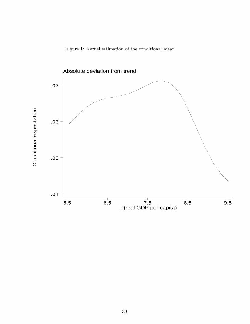
Figure 1: Kernel estimation of the conditional mean

Absolute deviation from trend

Con

ditio

nal e

xpec

tatio

n

ln(real GDP per capita)5.5 6.5 7.5 8.5 9.5

.04

.05

.06

.07

39

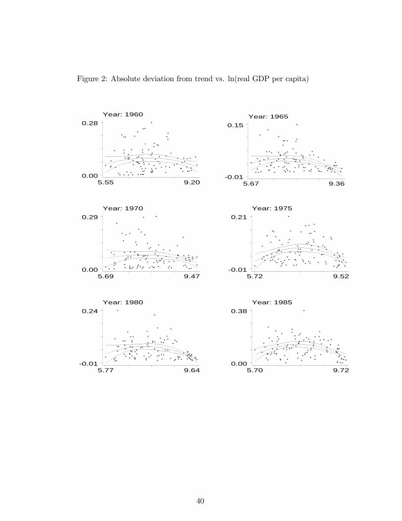
Figure 2: Absolute deviation from trend vs. ln(real GDP per capita)

Year: 1960

5.55 9.200.00

0.28Year: 1965

5.67 9.36-0.01

0.15

Year: 1970

5.69 9.470.00

0.29Year: 1975

5.72 9.52-0.01

0.21

Year: 1980

5.77 9.64-0.01

0.24Year: 1985

5.70 9.720.00

0.38

40

5.5 6 6.5 7 7.5 8 8.5 9 9.5 100.04

0.045

0.05

0.055

0.06

0.065

0.07

0.075

0.08Output versus Variability: bootstrap replications

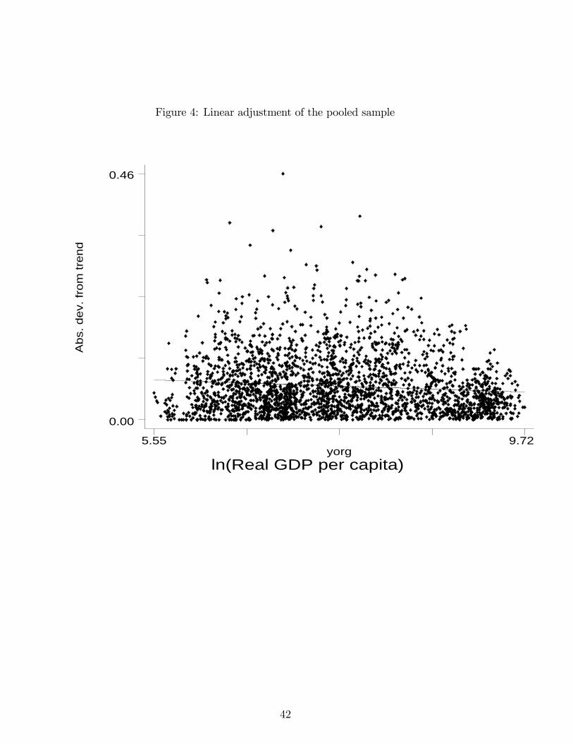
Figure 4: Linear adjustment of the pooled sample

Abs

. dev

. fro

m tr

end

ln(Real GDP per capita)yorg

5.55 9.72

0.00

0.46

42

1

λ(v)

vv’ v’’ v’’’

R(v)

λm(v)

λM(v)

Figure 1:

Figure 5: Multiplicity of Equilibria

43