Financial Integration for India Stock Market, a Fractional Cointegration Approach

Department of Economics Working Paper No. 0501

http://nt2.fas.nus.edu.sg/ecs/pub/wp/wp0501.pdf

Financial Integration for India Stock Market, a Fractional Cointegration Approach

Wing-Keung Wong

Department of Economics National University of

Singapore

Aman Agarwal IIF Business School

GGS Indraprastha University

Jun Du Department of Economics

National University of Singapore

Abstract: The Indian stock market is one of the earliest in Asia being in operation since 1875, but remained largely outside the global integration process until the late 1980s. A number of developing countries in concert with the International Finance Corporation and the World Bank took steps in the 1980s to establish and revitalize their stock markets as an effective way of mobilizing and allocation of finance. In line with the global trend, reform of the Indian stock market began with the establishment of Securities and Exchange Board of India in 1988. This paper empirically investigates the long-run equilibrium relationship and short-run dynamic linkage between the Indian stock market and the stock markets in major developed countries (United States, United Kingdom and Japan) after 1990 by examining the Granger causality relationship and the pairwise, multiple and fractional cointegrations between the Indian stock market and the stock markets from these three developed markets. We conclude that Indian stock market is integrated with mature markets and sensitive to the dynamics in these markets in a long run. In a short run, both US and Japan Granger causes the Indian stock market but not vice versa. In addition, we find that the Indian stock index and the mature stock indices form fractionally cointegrated relationship in the long run with a common fractional, nonstationary component and find that the Johansen method is the best reveal their cointegration relationship. Keywords: unit root test, cointegration, Error Correction Model, Vector Autoregression Model,

Johansen Multivariate Cointegration, Fractional Cointegration © 2005 Wing-Keung Wong, Aman Agarwal and Jun Du. Views expressed herein are those of the authors and do not necessarily reflect the views of the Department of Economics, National University of Singapore.

3

1. INTRODUCTION

One of the most profound and far-reaching financial phenomenon in the late twentieth

century and the forepart of this century is the explosive growth in international financial

transactions and capital flows among various financial markets in developed and

developing countries. This phenomenon in international finance is not only a result of the

liberalization of capital markets in developed and developing countries and the increasing

variety and complexity of financial instruments, but also a result of the increasing

relativity of the developing and developed economies as developing countries become

more integrated in international flows of trade and payments. More freedom in the

moving of capital flows improves the allocation of capital globally, allowing resources to

move to areas with higher rates of return. Contrarily, attempts to restrict capital flows

lead to distortions of capital structure that are generally costly to the economies imposing

the controls. Thus, the boost in international capital flows and financial transaction is an

underway and, to certain extent, irreversible process.

Since the work from Grubel (1968) on expounding the benefits from international

portfolio diversification, the relationship among national stock markets has been widely

studied. The relationship among different stock markets has great influence on

investment because diversification theory assumes that prices of different stock markets

do not move together so that investors could buy shares in foreign as well as domestic

markets seek to reduce risk through global diversification.

In addition, the ever closer relationship among international capital markets and the

increasing international portfolio investment have important implications for

macroeconomic policies. While contributing to build-up of foreign exchange reserves,

international portfolio investments can influence the exchange rate and could lead to

appreciation of local currency. Thus, it has great influence on trade and fiscal imbalances

among countries. Also, foreign portfolio investments are amenable to sudden withdrawals

4

and therefore these have the potential for destabilizing an economy, with good examples

from the Mexican and East Asian financial crisis in 1990s. Moreover, supported by

technological advances in information and transaction, the growing internationalization

of finance and the tremendous increase in the speed and volume of international capital

flows have allowed much more rapid assessment of and response to the real growth

possibilities in many countries.

Since its independence in 1947, a multitude of social and political problems have

stood in India’s way of realizing its true economic potential. However, it has recently

made tremendous strides in the economic field through both economic and political

reforms. The most significant policy should be the opening of the economy to foreign

investment on very liberal terms for the first time in independent India’s history. The

policy soon harvested positive results as its industrial exports and foreign investment

today are growing at the country’s fastest rate ever. The country’s foreign exchange

reserves rose to US$51 billion in March 2002 from less than US$1 billion in June 1991.

As now the globalization of capital flows has led to the growing relevance of emerging

capital markets, India is one of the countries with an expanding capital market that is

increasingly attracting funds from the foreign countries. Actually, in line with the global

trend, reform of the Indian stock market began with the establishment of Securities and

Exchange Board of India (SEBI) in 1988 to frame rules and guidelines for various

operations of the stock exchange in India. Nevertheless, the reform process gained

momentum only in the aftermath of the external payments crisis of 1991 followed by the

securities scam of 1992.

Among the significant measures of opening up capital market, portfolio

investment by foreign indirect investors (FIIs) such as pension funds, mutual funds,

investments trusts, asset management companies, nominee companies and incorporated

portfolio managers allowed since September 1992 have made the turning point for the

Indian stock markets. As of now FIIs are allowed to invest in all categories of securities

5

traded in the primary and secondary segments and in the derivatives segment. The ceiling

on aggregate equity of FIIS including non-resident Indians and overseas corporate bodies

in a company engaged in activities other than agriculture and plantation has been

enhanced in phases from 24 percent to 49 per cent in February 2001. Attracting foreign

capital appears to be the main reason for opening up of the stock markets for FIIs.

Progressively the liberal policies have led to increasing inflow of foreign investment in

India, both in terms of direct investment increasing from US$4 million in 1991 to

US$2021 million in 2001, as well as portfolio investment increasing from US$1 million

in 1992 to US$1505 million in 2001.1

In general, the deregulation and market liberalization measures and the increasing

activities of multinational companies will continually accelerate the growth of Indian

stock market. Given the newfound interest in the Indian stock markets, an intriguing

question is how far India has gone down the road towards international financial

integration, and whether the linkages exist among the stock indices of India and world’s

major stock indices. To answer these questions, we examine the interrelationship between

Indian stock markets and major developed stock markets and study the underlying

mechanism through which the Indian stock indices interact with international stock

indices by analyzing empirically the long-run the pairwise, multiple and fractional

cointegration relationship and short-run dynamic Granger causality linkage between the

Indian stock market and the world major developed markets including US, UK and Japan

in the post-liberalization period. We conclude that Indian stock market is integrated with

mature markets and sensitive to the dynamics in these markets in a long run. In a short

run, both US and Japan Granger causes the Indian stock market but not vice versa. In

addition, we find that the Indian stock index and the mature stock indices form

fractionally cointegrated relationship in the long run with a common fractional,

nonstationary component and find that the Johansen method is the best reveal their

cointegration relationship.

1 Source: India, Ministry of Finance, Economic Survey: 2002-2003

6

The rest of the paper is organized as follows: Section 2 presents a snapshot of the

literature on stock market cointegration and Granger causality, Section 3 discusses the

data and gives a sketch of the methodology being employed, Section 4 summarizes the

findings and interprets the results and Section 5 concludes.

2. LITERATURE REVIEW

The financial markets, especially the stock markets, for developing and developed

markets have now become more closely interlinked despite the uniqueness of the specific

markets or the country profile. Literature has shown strong interest on the linkages

among international stock markets and the interest has increased considerably after the

loose of financial regulations in both mature and emerging markets, the technological

developments in communications and trading systems, and the introduction of innovative

financial products, creating more opportunities for international portfolio investments.

The interest can also be attributed to the globalization which gives another impetus to the

higher intertwinement of international economies and financial markets. In recent years,

the new remunerative emerging equity markets have attracted the attention of

international fund managers as an opportunity for portfolio diversification. This

intensifies the curiosity of academics in exploring international market linkages.

Earlier studies by Ripley (1973), Lessard (1976), and Hilliard (1979) generally find

low correlations between national stock markets, supporting the benefits of international

diversification. The links between national stock markets have been of heightened

interest in the wake of the October 1987 international market crash globally. The crash

has made people realize that various national equity markets are so closely connected as

the developed markets like the US stock market exert a strong influence on other markets.

Applying the vector autoregression models, Eun and Shim (1989) find evidence of

co-movements between the US stock market and other world equity markets. Cheung and

Ng (1992) investigate the dynamic properties of stock returns in Tokyo and New York

and find that the US market is an important global factor from January 1985 to December

7

1989. Lee and Kim (1994) examine the effect of the October 1987 crash and conclude

that national stock markets became more interrelated after the crash and find that the

co-movements among national stock markets were stronger when the US stock market is

more volatile. Applying the VAR approach and the impulse response function analysis,

Jeon and Von-Furstenberg (1990) show that the degree of international co-movement in

stock price indices has increased significantly since the 1987 crash. On the other hand,

Koop (1994) uses Bayesian methods to conclude that there are no common trends in

stock prices across countries. Also, Corhay, et al (1995) study the stock markets of

Australia, Japan, Hong Kong, New Zealand and Singapore and find no evidence of a

single stochastic trend for these countries.

Only a few studies have examined the co-movement of Indian stock market with

international markets. For example, Sharma and Kennedy (1977) examine the price

behavior of Indian market with the US and UK markets and conclude that the behavior of

the Indian market is statistically indistinguishable from that of the US and UK markets

and find no evidence of systematic cyclical component or periodicity for these markets.

Rao and Naik (1990) apply the Cross-Spectral analysis and find that for the Indian stock

index, the gains estimates from either the US or the Japan indices are ‘independent’ and

hence they conclude that the relationship of Indian market with international markets is

poor reflecting the institutional fact that the Indian economy has been characterized by

heavy controls throughout the entire seventies with liberalization measures initiated only

in the late eighties.

Above studies were carried out over decade ago. As the Indian stock market becomes

more open to the rest of the world since early 1990s, the relationship between the Indian

market and the developed stock markets may change and hence our paper reexamine the

nature of co-movement between Indian market and the others main stock indices.

8

3. DATA AND METHODOLOGY

Weekly indices of the stock exchanges from Datastream for India and the three most

developed countries including the United States, the United Kingdom and Japan are used

as proxies to measure the stock market for each country, specifically, BSE 200 (India)2,

S&P 500 (the United States), FTSE 100 (the United Kingdom) and Nikkei 225 Stock

Average (Japan). Our sample covers the period from January 1, 1991 through December

31, 2003, a total of 13 years and the indices are adjusted to be in terms of US dollars for

better comparison. The weekly indices as opposed to daily data is used to avoid

representation bias from some thinly traded stocks, i.e., the problems of non-trading and

non-synchronous trading and to avoid the serious bid/ask spreads in daily data. In

addition, we use Wednesday indices to avoid the day-of-the-Week effect of stock returns

(Lo and MacKinlay 1988).

To examine the co-movements between the Indian stock market and the developed

markets, we first study their relationship by the simple regression:

tDt

It ebyay ++= (1)

where the endogenous variable Ity represents the India’s stock index; the exogenous

variable Dty is the stock index of any of the developed countries including the United

States, the United Kingdom and Japan; and te is the error term. In order to study the

joint effect from all the developed stock markets on the Indian market, we further study

the following multiple regression:

tDt

Dt

Dt

It eybybybay ++++= 3

32

21

1 (2)

where Dity are the stock indices for the United States, the United Kingdom and Japan

for i = 1, 2 and 3 respectively.

2 See detail introduction of BSE200 from http://www.bseindia.com/about/abindices/bse200.asp. We have analyzed other major Indian stock indices and the results are similar.

9

The validity and reliability of the regression relationship require the examination of

the trend characteristics of the variables and cointegration test as the presence of unit root

processes in the stock indices results in the spurious regression problem. Cointegration

tests consist of two steps. The first step is to examine the stationary properties of the

various stock indices in our study. If a series, say yt, has a stationary, invertible and

stochastic ARMA representation after differencing d times, it is said to be integrated of

order d, and denoted by yt = I(d). To test the null hypothesis H0: yt = I(1) versus the

alternative hypothesis H1 : yt = I(0), we apply the Dickey-Fuller (1979,1981) (DF) and

the augmented Dickey-Fuller (ADF) unit root tests based on the following regression

∑=

−− +∆+++=∆p

itititt ybyataby

11100 ε (3)

where 1−−=∆ ttt yyy and yt can be Ity , D

ty or Dity , tε is the error term.

Regression (3) includes a drift term ( 0b ) and a deterministic trend ( 0a t). Integer p is

chosen in (3) to achieve white noise residuals for the ADF test and when p=0, the test is

known as the Dickey-Fuller (DF) test. Testing the null hypothesis of the presence of a

unit root in yt is equivalent to testing the hypothesis that 01 =a . If 1a is significantly

less than zero, the null hypothesis of a unit root is rejected. In addition, we test the

hypothesis that yt is a random walk with drift, i.e. ( ) ( )0,0,,, 0100 baab = and yt is random

walk without drift, ( ) ( )0,0,0,, 100 =aab using the likelihood ratio test statistics 3Φ and

2Φ respectively. If the hypotheses that 1a = 0, ( ) ( )0,0,,, 0100 baab = or

( ) ( )0,0,0,, 100 =aab are accepted, we can conclude that yt is I(1). If we cannot reject the

hypotheses that yt is I(1), we need to further test the null hypothesis H0 : yt = I(2) versus

the alternative hypothesis H1 : yt = I(1). Note that most series are integrated of order at

most one.

10

In addition, we apply the PP test3 developed by Phillips and Perron (1988) to detect

the presence of a unit root. The PP test is nonparametric with respect to nuisance

parameters and thereby is suitable for a very wide class of weakly dependent and possibly

heterogeneously distributed data.

If both Ity and D

ty ( Dity ) are of the same order, say I(d) , with d > 0, we then

estimate the cointegrating parameter in (1) or (2) by OLS regression. If the residuals are

stationary, the series, Ity and D

ty ( Dity ) are said to be cointegrated. Otherwise, I

ty

and Dty ( Di

ty ) are not cointegrated.

Cointegration exists for variables means despite variables are individually

nonstationary, a linear combination of two or more time series can be stationary and there

is a long-run equilibrium relationship between these variables. If the error term in (1) or

(2) is stationary while the regressors are individually trending, there may be some

transitory correlation between the individual regressors and the error term. However, in

the long run, the correlation must be zero because of the fact that trending variables must

eventually diverge from stationary ones. Thus the regression on the levels of the variables

is meaningful and not spurious.

The most common tests for stationarity of estimated residuals are Dickey-Fuller

(CRDF), and Augmented Dickey-Fuller (CRADF) tests based on the regression:

t

p

ititt eee ξγγ +∆+=∆ ∑

=−−

111 ˆˆˆ (4)

where te are residuals from the cointegrating regression (1) or (2) and p is chosen to

achieve empirical white noise residuals for CRADF and set to zero for CRDF test.

Engle and Granger (1987) pointed out that when a set of variables is cointegrated,

3 Refer to Phillips and Perron (1988) for the detail of the test statistics.

11

a vector autoregression in first differences will be misspecified. The first differencing of

all the nonstationary variables puts too many unit roots and any potentially important

long-term relationship between the variables will be unclear. Thus, inferences based on

vector autoregression in first differences may lead to incorrect conclusions (Granger,

1981, 1988 and Sims, et al, 1990). However, there exists an alternative representation, an

error correction representation of such variables, which takes account of a short- and

long-run equilibrium relationship shared by those variables.

If the Indian stock market and the other markets are not cointegrated, one can adopt

the bivariate VAR model, see Granger et al (2000), to test for the Granger causality.

When a set of variables is cointegrated, Engle and Granger (1987) point out that a vector

autoregression in first difference will be misspecified because first differencing of all the

nonstationary variables imposes too many unit roots and any potentially important

long-term relationship between the variables will be obscured. Thus inferences based on

this model may lead to incorrect conclusions (Granger 1981, 1988 and Sims et al. 1990).

Nevertheless, there exists an alternative representation, an error correction model (ECM)

to test for the Granger causality between these variables by taking account of a long-run

equilibrium relationship shared by the variables.

As shown in the next section, the Indian market is cointegrated with other markets

and hence we can only use the ECM model to test the Granger causality in the following

equation:

t

m

i

Diti

n

i

Iitit

It yyaey 1

12

1110 εααα +∆+∆++=∆ ∑∑

=−

=−−

t

m

i

Iiti

n

i

Ditit

Dt yybey 2

12

1110 εβββ +∆+∆++=∆ ∑∑

=−

=−− , (5)

where 1−te is the residual for equation (1) and 1−tae and 1−tbe are called the error

correction terms.

12

According to Engle and Granger (1987), the existence of the cointegration implies a

causality among the set of variables as manifested by 0|||| >+ ba , so a and b actually

denotes the speed of adjustment. An error correction model allows us to study the

long-term relationship between Ity and D

ty . Equation (7) incorporates both the

short-run and long-run information in modeling the data. Failing to reject the H0:

022221 ==…== mααα and a=0 implies that Dty do not Granger cause I

ty . Similarly,

failing to reject the H0: 022221 ==…== nβββ and b=0 suggests that Ity do not

Granger cause Dty .

The minimum final prediction error criterion (FPE), see Hsiao (1979 and 1981),

is then used to determine the optimum lag structures for the equations in (5). In these

two equations n and m denotes the numbers of lags in the explained variable and

explanatory variable respectively; and t1ε and t2ε are disturbance terms obeying the

assumptions of the classical linear regression model. The final prediction error statistic

of Ity∆ for n lags of I

ty∆ and m lags of Dty∆ is

NmnNyymnN

mnFPEIt

It

y It )1(

)()1(),(

2

−−−

∆−∆+++= ∑

∆ (6)

where N is the number of observations. The FPE statistic for Dty∆ is found by the same

way. To determine the minimum ItyFPE

∆, the first step is to run the regressions in (5). But

the terms for the lags of Dty∆ should be excluded, and only the lags of I

ty∆ are

included, which means the calculation begins from m=0 and n=1. The same step is

repeated until n=n* where FPE value is minimized for m=0. Then by fixing on n=n*,

FPE value for different m will be calculated until m=m* which companied by a minimum

FPE value. The same procedure is repeated with equation (9) where n=n** and m=m**

minimize DtyFPE

∆.

13

We further apply the multivariate cointegrated system developed by Johansen

(1988a,b). Assume each component tiy , i=1,…, k, of a vector time series process ty is

a unit root process, but there exists a k×r matrix β with rank r<k such that ty'β is

stationary. Clive Granger has shown that under some regularity conditions we can write a

cointegrated process ty as a Vector Error Correction Model (VECM):

tptptpttt yyyyy ε+Π−∆Γ++∆Γ+∆Γ=∆ −−−−−− )1(12211 ... , (9)

where the tε ’s are assumed to be independent and identical distributed as multi-normal

distribution with mean zero and variance Ω. The core idea of the Johansen procedure is

simply to decompose Π into two matrices α and β , both of which are k×r such that

'αβ=Π and so the rows of β may be defined as the r distinct cointegrating vectors.

Then a valid cointegrating vector will produce a significantly non-zero eigenvalue and

the estimate of the cointegrating vector will be given by the corresponding eigenvector4.

Johansen proposes a trace test for determining the cointegrating rank r. such that:

1,...,2,1,0),1ln()(1

−=−−= ∑+=

nrTrk

riitrace λλ . (10)

and proposes another likelihood ratio test to test whether there is a maximum of r

cointegrating vectors against r+1 such that:

)1ln()1,( 1max +−−=+ rTrr λλ . (11)

with critical values given in Johansen (1995).

At last, we apply a generalized form of cointegration, known as fractional

cointegration, as a characterization of the long run dynamics of the system of the stock

indices in our study. In fractional cointegration context, the integration order of the error

correction term is not necessarily 0 or 1, but it can be any real number in between. This

allows obtaining more various mean reverting 5 . More specifically, a fractionally

4 See Johansen (1995) for more detail. 5 see Chou and Shih (1997) for detail discussion.

14

integrated error correction term implies the existence of a long run equilibrium

relationship, as it can be shown to be mean reverting, though not exactly I(0). Despite its

significant persistence in the short run, the effect of a shock to the system eventually

dissipates, so that an equilibrium relationship among the system’s variables prevails in

the long run.

A series is said to be integrated of order d, denoted by I(d), if it has a stationary,

invertible autoregressive moving average (ARMA) representation after applying the

differencing operator dL)1( − . The series is said to be fractionally integrated if d is not

an integer. A system of variables ntttt yyyy ,...,, 21= is said to be cointegrated of order

I(d, b) if the linear combination tyα is I(d-b) with b>0. So our interest is to find out the

characteristic pattern of the error correction term. A flexible and parsimonious way to

model short term and long term behavior of time series is by means of an autoregressive

fractionally integrated moving average (AFIMA) model. A time series y follows an

AFIMA process of order (p, d, q), if

),0.(..~,)()1)(( 2εσεε diiLyLL ttt

d Θ=−Φ (12)

where L is the backward-shift operator, pp LLL φφ −−−=Φ ...1)( 1 ,

qq LLL υυ +++=Θ ...1)( 1 . The stochastic process y is both stationary and invertible if all

roots of )(LΘ and )(LΦ are outside the unit circle, and -0.5<d<0.5. The process is

nonstationary but mean-reverting for 0.5< d <1.

Cheung and Lai (1993) use this method and extend the alternative hypothesis to all

order if integration less than one. In this paper, we follow the way by Cheung and Lai

(1993) to analyze the dynamic relationship by applying the fractional testing

methodology suggested by Geweke and Porter-Hudak (GPH, 1983) to obtain an estimate

of d based on the slope of the spectral density function around the angular frequency

0=ξ . More specifically, let )(ξI be the periodogram of y at frequency ξ defined by

15

2

1)(

21)( ∑

=

−=T

tt

it yyeT

I ξ

πξ ,

where 1−=i . Then the periodogram can be transformed to:

−−+−= ∑ ∑ ∑

=

−

=

−

=+

T

t

T

k

kT

jkjjt kyyyy

Tyy

TI

1

1

1 1

2 )cos())((12)(121)( ξπ

ξ ,

which can be easily obtained based one T observations. Then the spectral regression is

defined by

λλ

λ ηξ

ββξ +

+=

2sinln)(ln 2

10I , λ=1, …, v (13)

where Tπλξλ

2= (λ=0,…,T-1) denotes the Fourier frequencies of the sample, and

uTv = is the sample size of the GPH spectral regression (u is usually set as 0.55, 0.575

and 0.60). The negative of the slope coefficient in (19) provides an estimate of d. The

theoretical asymptotic variance of the spectral regression error term in known to be

62π .

The GPH test can also be used as a test of the unit root hypothesis with I(1) processes

imposing a test on d(GPH) from the first-differenced form of the series being

significantly different from zero. The differencing parameter in the first-differenced data

is denoted by d~ in which case the fractional differencing parameter for the level series

is dd ~1+= . In this respect, the GPH procedure poses an alternative viewpoint from

which to scrutinize the unit root hypothesis. To test the statistical significance of the d~

estimates, we have imposed the known theoretical variance of the spectral regression

error 62π in the construction of the t-statistic for d~ and it is well-known that the

asymptotic result are:

)6,0()ˆ( 2πNddT ⇒− . (14)

Therefore, the asymptotic standard deviation of d~ is given by 26 πT .

16

4 Empirical Results and Interpretation

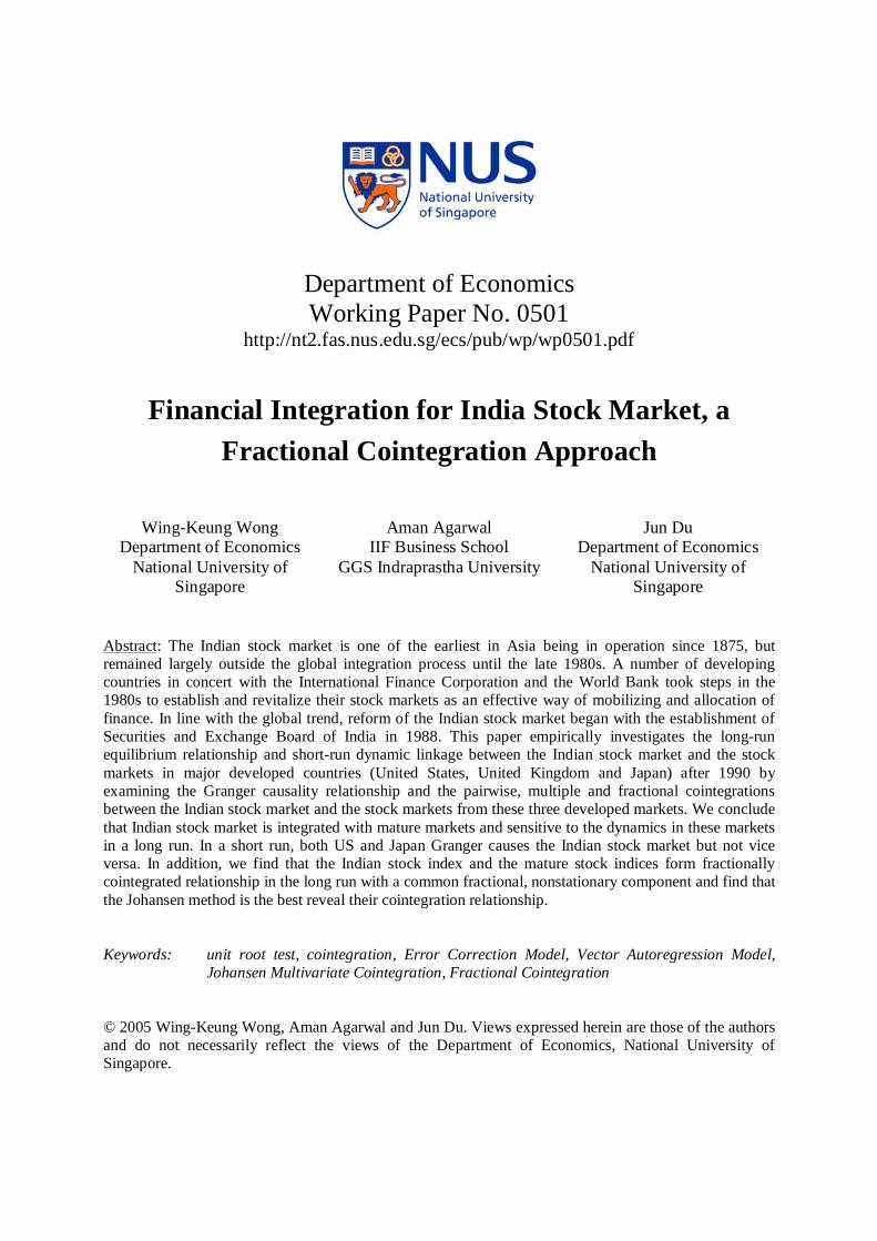
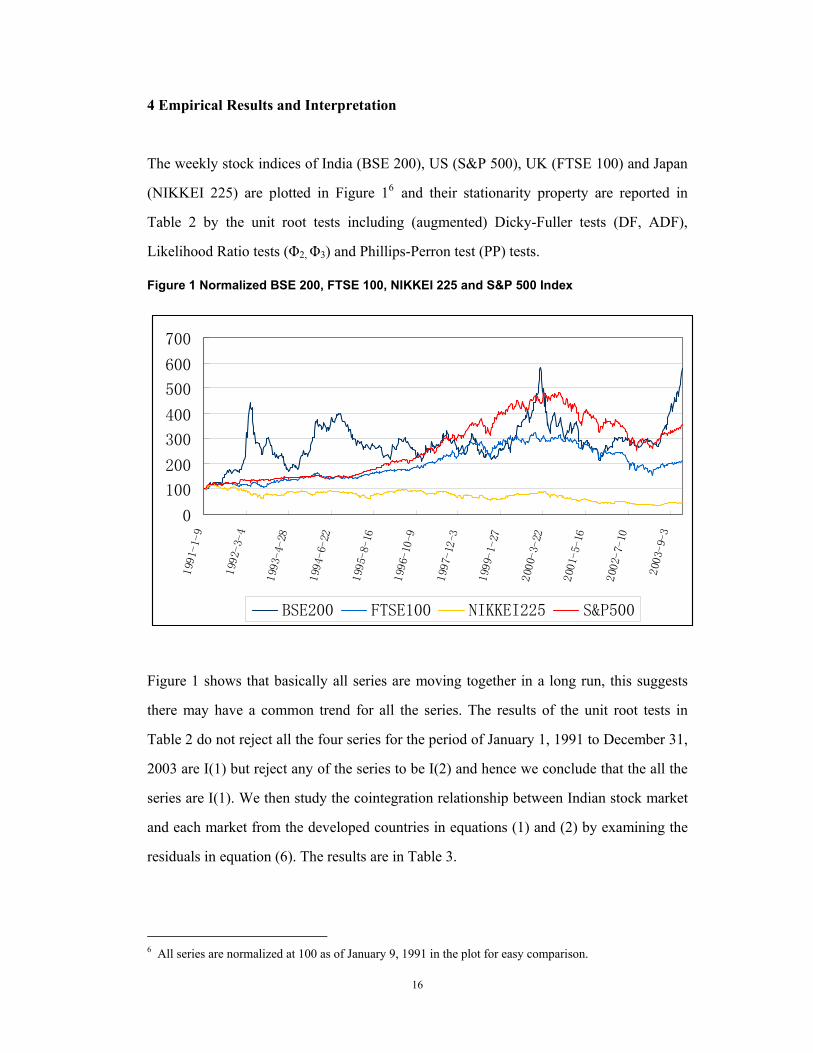
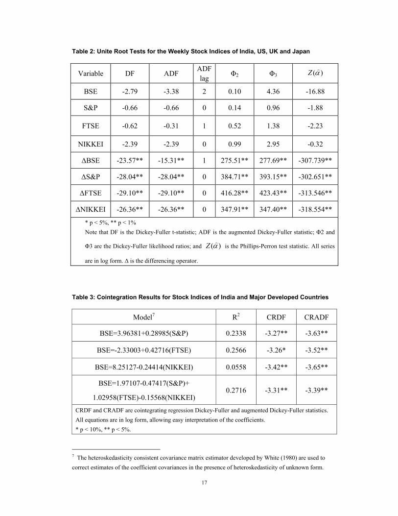
The weekly stock indices of India (BSE 200), US (S&P 500), UK (FTSE 100) and Japan

(NIKKEI 225) are plotted in Figure 16 and their stationarity property are reported in

Table 2 by the unit root tests including (augmented) Dicky-Fuller tests (DF, ADF),

Likelihood Ratio tests (Φ2, Φ3) and Phillips-Perron test (PP) tests.

Figure 1 Normalized BSE 200, FTSE 100, NIKKEI 225 and S&P 500 Index

0

100

200

300

400

500

600

700

1991-1-9

1992-3-4

1993-4-28

1994-6-22

1995-8-16

1996-10-9

1997-12-3

1999-1-27

2000-3-22

2001-5-16

2002-7-10

2003-9-3

BSE200 FTSE100 NIKKEI225 S&P500

Figure 1 shows that basically all series are moving together in a long run, this suggests

there may have a common trend for all the series. The results of the unit root tests in

Table 2 do not reject all the four series for the period of January 1, 1991 to December 31,

2003 are I(1) but reject any of the series to be I(2) and hence we conclude that the all the

series are I(1). We then study the cointegration relationship between Indian stock market

and each market from the developed countries in equations (1) and (2) by examining the

residuals in equation (6). The results are in Table 3.

6 All series are normalized at 100 as of January 9, 1991 in the plot for easy comparison.

17

Table 2: Unite Root Tests for the Weekly Stock Indices of India, US, UK and Japan

Variable DF ADF ADF lag Φ2 Φ3 )(αZ

BSE -2.79 -3.38 2 0.10 4.36 -16.88

S&P -0.66 -0.66 0 0.14 0.96 -1.88

FTSE -0.62 -0.31 1 0.52 1.38 -2.23

NIKKEI -2.39 -2.39 0 0.99 2.95 -0.32

∆BSE -23.57** -15.31** 1 275.51** 277.69** -307.739**

∆S&P -28.04** -28.04** 0 384.71** 393.15** -302.651**

∆FTSE -29.10** -29.10** 0 416.28** 423.43** -313.546**

∆NIKKEI -26.36** -26.36** 0 347.91** 347.40** -318.554**

* p < 5%, ** p < 1% Note that DF is the Dickey-Fuller t-statistic; ADF is the augmented Dickey-Fuller statistic; Φ2 and

Φ3 are the Dickey-Fuller likelihood ratios; and )(αZ is the Phillips-Perron test statistic. All series

are in log form. ∆ is the differencing operator.

Table 3: Cointegration Results for Stock Indices of India and Major Developed Countries

Model7 R2 CRDF CRADF

BSE=3.96381+0.28985(S&P) 0.2338 -3.27** -3.63**

BSE=-2.33003+0.42716(FTSE) 0.2566 -3.26* -3.52**

BSE=8.25127-0.24414(NIKKEI) 0.0558 -3.42** -3.65**

BSE=1.97107-0.47417(S&P)+

1.02958(FTSE)-0.15568(NIKKEI) 0.2716 -3.31** -3.39**

CRDF and CRADF are cointegrating regression Dickey-Fuller and augmented Dickey-Fuller statistics. All equations are in log form, allowing easy interpretation of the coefficients. * p < 10%, ** p < 5%.

7 The heteroskedasticity consistent covariance matrix estimator developed by White (1980) are used to correct estimates of the coefficient covariances in the presence of heteroskedasticity of unknown form.

18

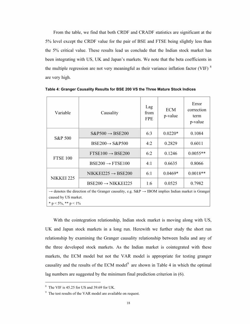
From the table, we find that both CRDF and CRADF statistics are significant at the

5% level except the CRDF value for the pair of BSE and FTSE being slightly less than

the 5% critical value. These results lead us conclude that the Indian stock market has

been integrating with US, UK and Japan’s markets. We note that the beta coefficients in

the multiple regression are not very meaningful as their variance inflation factor (VIF) 8

are very high.

Table 4: Granger Causality Results for BSE 200 VS the Three Mature Stock Indices

Variable Causality Lag from FPE

ECM p-value

Error correction

term p-value

S&P500 → BSE200 6:3 0.0220* 0.1084 S&P 500

BSE200→ S&P500 4:2 0.2829 0.6011

FTSE100 → BSE200 6:2 0.1246 0.0055** FTSE 100

BSE200 → FTSE100 4:1 0.6635 0.8066

NIKKEI225 → BSE200 6:1 0.0469* 0.0018** NIKKEI 225

BSE200 → NIKKEI225 1:6 0.0525 0.7982

→ denotes the direction of the Granger causality, e.g. S&P → IBOM implies Indian market is Grangercaused by US market.

* p < 5%, ** p < 1%

With the cointegration relationship, Indian stock market is moving along with US,

UK and Japan stock markets in a long run. Herewith we further study the short run

relationship by examining the Granger causality relationship between India and any of

the three developed stock markets. As the Indian market is cointegrated with these

markets, the ECM model but not the VAR model is appropriate for testing granger

causality and the results of the ECM model9 are shown in Table 4 in which the optimal

lag numbers are suggested by the minimum final prediction criterion in (6).

8 The VIF is 45.25 for US and 39.69 for UK. 9 The test results of the VAR model are available on request.

19

The results in Table 4 conclude that there are unidirectional causality runs from both

the US stock market and the Japan stock market but not from the UK stock market to the

Indian stock market and there is no causality run from the Indian stock market to any of

the market from the US, UK or Japan.

The results between the US and Indian stock markets are rather intuitive as the US

stock market is the world’s foremost securities market and has heavy influence on other

stock markets. Hence, we are not surprised that US Granger causes the Indian stock

market in a short run (Table 4) and leads the Indian stock market in a long run (Table 3).

More rationally, several macroeconomic factors may give good explanation to the causal

relationship between the two stock markets. They include economic connection,

regulatory structures similarity, exchange rate policy and trade flows. Coincided with the

start of the liberalization of the Indian economy, there is a steady improvement in

India-US trade relations during last decade. US government has identified India as one of

the 10 major emerging markets. The volume of India-US bilateral trade also started to

grow at a steady pace with the export from India to the US grows from US$2922 million

in 1991 to US$11,318 million in 2002.10

On the other hand, the India-US trade volume still remains a small fraction of US's

global trade. While US’s exports to India account for over 10% of India's non-oil imports

and US is the destination of one-fifth of India’s exports, US's trade turnover with India

constitutes less than 1% of its global trade. India's percentage share in US imports has

remained stable over the last few years; it was 0.88% during 2000. In 2000, India ranked

21st among countries that export to the US.11 These economic figures show that US

economy is very important to Indian economy, but not conversely. This is consistent with

our finding of unidirectional causality from S&P 500 to BSE 200.

10 Data are quoted from ADB http://ww.adb.org/Documents/Books/Key_Indicators/2003/pdf/IND.pdf 11 All data cited here is from India-US embassy http://www.indianembassy.org/indusrel/trade.htm

20

The results in Table 3 indicate that in the long run UK stock market leads Indian

stock market at the 1% significant level, but no evidence of short-run impact from UK

stock market to Indian stock market can be found from Table 4. Simultaneously, Indian

stock market almost cannot exert any long-run or short-run influence on UK stock market.

Except the centuries-long colonial economic connection, India-UK bilateral trade volume

has been increasing constantly since India’s economic opening up since 1991.

From the data of bilateral trade and FDI12, UK continues to be India's second largest

trading partner after US and continues to be the largest cumulative investor in India, and

the third largest investor post-1991. As Indian economy is linked with UK’s economy

closely, it is not surprised that Indian stock market has long-run lead-lag relationship with

UK stock market. But, unlike the US and Japan stock markets, there is no impact from

the UK stock market to the Indian stock market in a short run. One possible reason could

be due to the fact that the UK market opens after the Indian market.

Table 4 also shows that there exists unidirectional causality from Japanese stock

market to Indian stock market. This could be attributed to Japan-India economic relations

which have been expanding both in quality and quantity notably since early nineties,

keeping pace with the progress in economic liberalization in India. For example, exports

from India to Japan stood at US$1.9 billion in 1998 which accounted for 4.9 per cent of

India's total exports. Japan is the 6th largest importer from India after the US, Germany,

UAE, UK and Hong Kong. As for India's imports from Japan, they stood at US$2.7

billion in 1998, an increase of 25.8 per cent over the previous year, accounting for 5.5 per

cent of India's total imports. Japan is the 5th largest exporter to India after the US,

Switzerland, Belgium and UK. Thus Japan is an important trading partner for India.

While the bilateral trade is maintaining a steady growth in the recent years, Japanese

direct investment in India has been increasing quite significantly. On approval basis, 12 Data are obtained from High Commission of India, London http://www.hcilondon.net/business-with-india/india-uk-economic-relations.html

21

Japan occupies 4th position after US, Mauritius and UK among the major FDI providers.

With the opening up of the Indian economy, Japanese investments in India have been

steadily increasing. Deregulation of foreign capital by India has been progressing

smoothly and India has emerged as an attractive investment destination for Japanese

investors. According to a survey by the EXIM Bank of Japan on promising FDI

destination figured by the industries in 1999, India ranked fourth on the medium term

(next three years) and third on the long term (next 10 years). As the bilateral economic

relations are strengthened year by year, the stock markets of these two countries should

also be connected more and more closely. These support there are both long-run lead-lag

effect and short-run lead-lag effect from Japanese stock market to Indian stock market by

using the Nikkei 225 and BSE 200 data of the 1991-2003 period.

As Johansen (1988) is a powerful way of analyzing complex interaction of causality

and structure among variables in a system, this process is further applied to determine

whether any cointegrating relationship exists among Indian, US, UK and Japanese stock

markets as all the indices from these markets are integrated of order one (Table 1). As the

stock indices exhibit a trend, a constant is included in this model. Lag structures are

chosen according to the both Schwarz-Bayes criterion (SBC) and Akaike’s information

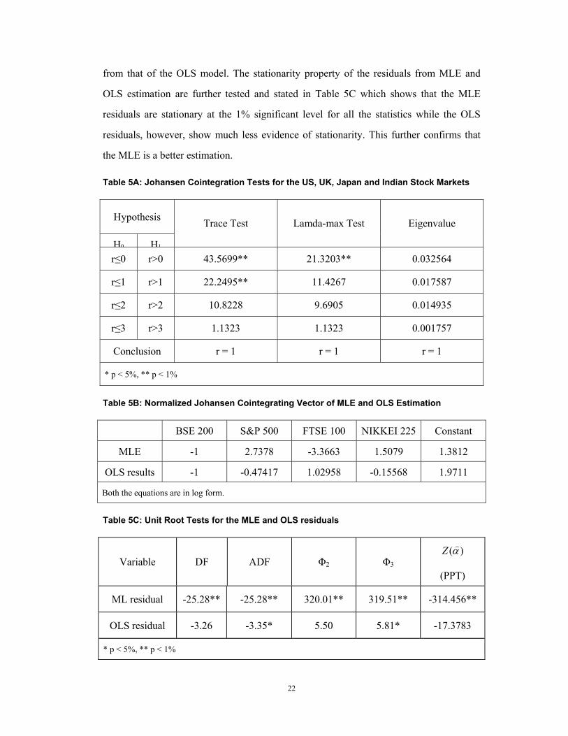
criterion (AIC) and the results are shown in Table 5A.

From Table 5A, the hypothesis of zero cointegrating vectors against the alternative of

one or more cointegrating vectors is rejected while the hypothesis of one cointegrating

vector is rejected by Johansen Trace test but cannot be rejected by Lamda-max test.

These results show strong evidence that there is at least one set of cointegrating vector

existing in four-variable system. The cointegrating vector, whose coefficients are

normalized on the Indian stock market for both the MLE and OLS estimation methods

given in Table 5B shows significant difference between the estimates from the two

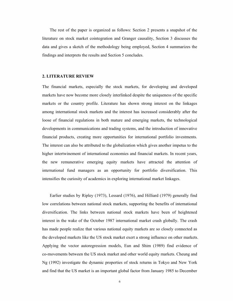
methods. It might be interesting to compare the performance of the two methods. A

comparison of two residuals plotted in Figure 2 shows that the fit of the Johansen MLE

model and the stationarity of the Johansen MLE residual have improved dramatically

22

from that of the OLS model. The stationarity property of the residuals from MLE and

OLS estimation are further tested and stated in Table 5C which shows that the MLE

residuals are stationary at the 1% significant level for all the statistics while the OLS

residuals, however, show much less evidence of stationarity. This further confirms that

the MLE is a better estimation.

Table 5A: Johansen Cointegration Tests for the US, UK, Japan and Indian Stock Markets

Table 5B: Normalized Johansen Cointegrating Vector of MLE and OLS Estimation

Table 5C: Unit Root Tests for the MLE and OLS residuals

Variable DF ADF Φ2 Φ3 )(αZ

(PPT)

ML residual -25.28** -25.28** 320.01** 319.51** -314.456**

OLS residual -3.26 -3.35* 5.50 5.81* -17.3783

* p < 5%, ** p < 1%

Hypothesis

H0 H1

Trace Test Lamda-max Test Eigenvalue

r≤0 r>0 43.5699** 21.3203** 0.032564

r≤1 r>1 22.2495** 11.4267 0.017587

r≤2 r>2 10.8228 9.6905 0.014935

r≤3 r>3 1.1323 1.1323 0.001757

Conclusion r = 1 r = 1 r = 1

* p < 5%, ** p < 1%

BSE 200 S&P 500 FTSE 100 NIKKEI 225 Constant

MLE -1 2.7378 -3.3663 1.5079 1.3812

OLS results -1 -0.47417 1.02958 -0.15568 1.9711

Both the equations are in log form.

23

Figure 2: Plot of the OLS and Johansen MLE Residuals

-0.8

-0.6

-0.4

-0.2

0

0.2

0.4

0.6

0.8

1

OLS residual Johansen ML reisdual

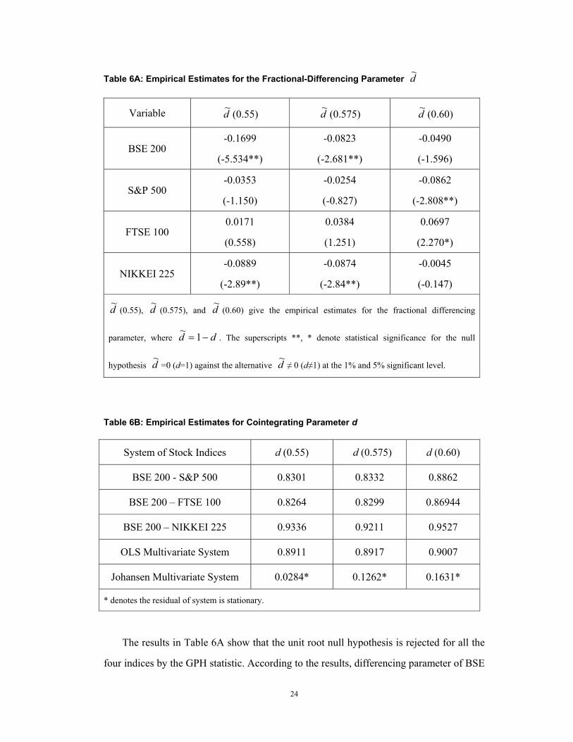
As the unit root tests employed above allow for only integer orders of integration, the

four stock indices are each checked for a fractional exponent in the differencing process

using the GPH test. The unit root hypothesis is tested by determining if the GPH estimate

of d~ 13 from the first-differenced stock indices series is significantly differently from

zero. Table 6A reports the empirical estimates for the fractional differencing parameter

dd −= 1~ as well as their corresponding GPH test statistics.14

13 Refer to the Data and Methodology Section for the explanation. 14 See equation (14) for its asymptotic standard deviation.

24

Table 6A: Empirical Estimates for the Fractional-Differencing Parameter d~

Variable d~ (0.55) d~ (0.575) d~ (0.60)

BSE 200 -0.1699

(-5.534**)

-0.0823

(-2.681**)

-0.0490

(-1.596)

S&P 500 -0.0353

(-1.150)

-0.0254

(-0.827)

-0.0862

(-2.808**)

FTSE 100 0.0171

(0.558)

0.0384

(1.251)

0.0697

(2.270*)

NIKKEI 225 -0.0889

(-2.89**)

-0.0874

(-2.84**)

-0.0045

(-0.147)

d~ (0.55), d~ (0.575), and d~ (0.60) give the empirical estimates for the fractional differencing

parameter, where dd −= 1~. The superscripts **, * denote statistical significance for the null

hypothesis d~ =0 (d=1) against the alternative d~ ≠ 0 (d≠1) at the 1% and 5% significant level.

Table 6B: Empirical Estimates for Cointegrating Parameter d

System of Stock Indices d (0.55) d (0.575) d (0.60)

BSE 200 - S&P 500 0.8301 0.8332 0.8862

BSE 200 – FTSE 100 0.8264 0.8299 0.86944

BSE 200 – NIKKEI 225 0.9336 0.9211 0.9527

OLS Multivariate System 0.8911 0.8917 0.9007

Johansen Multivariate System 0.0284* 0.1262* 0.1631*

* denotes the residual of system is stationary.

The results in Table 6A show that the unit root null hypothesis is rejected for all the

four indices by the GPH statistic. According to the results, differencing parameter of BSE

25

200, S&P 500, and NIKKEI 225 are slightly higher than integer one, and hence the

integrated order of FTSE 100 is slightly less than one (but bigger than 0.5). Because the

deviation of the integrated orders from one is miniature, we still think the four stock

indices roughly follow a I(1) process.

We now turn to investigate the fractional cointegration in the error term of the

system of stock indices. In the conventional cointegration framework, the system

variables should be I(1) and the error correction term should be I(0). This criterion for

cointegration relationship is strict and ad hoc as the error correction term can be mean

reverting rather than exactly I(0). The hypothesis of fractional cointegration requires

testing for fractional integration in the error correction term. The GPH test can be used

for the used here, but the critical values for the GPH test derived from the standard

normal distribution cannot be used in testing for fractional cointegration. This is due to

the factor that the error term is not actually observed but estimated by minimizing the

residual variance of the cointegration regression. So we only include the GPH statistics in

our results. Table 6B reports the empirical results of the GPH test for cointegration in all

the systems we have considered previously. The findings in Table 6B show that there is

evidence of stationarity only for Johansen Multivariate System. The error terms of all

other systems is not covariance stationary as 0.5<d<1 but they are mean reverting. So

there is evidence of fractional cointegration for all the systems in this study. Additionally,

this GPH test seems to prove from another dimension that the performance of Johansen

method is much better than that of OLS method.

5. CONCLUSION

We investigate the long run equilibrium relationship and short run dynamic inter linkages

between the Indian stock market and world major developed stock market by using the

weekly data of BSE 200 (India), S&P 500 (US), FTSE 100 (UK) and Nikkei 225 (Japan)

from January 1991 to December 2003. Our main findings are as follows: First, Indian

stock market is statistically significantly cointegrated with stock markets in United States,

26

United Kingdom and Japan by using OLS estimation. Second, there exit unidirectional

granger causality running from the US, UK and Japanese stock markets to the Indian

stock market. Third, the Johansen ML estimation method suggests there is only one set of

cointegrating vector for the four-variable system. Lastly, we reexamine the long run

dynamics of all the stock indices systems by using the fractionally integrating technique

and find that the Indian stock index and the mature stock indices form fractionally

cointegrated relationship in the long run with the Johansen model generates a stationary

error term and all other systems appear to possess a common fractional, mean-reverting

component. In addition, the fact that only Johansen Multivariate model can generate

stationary error term shows the superiority of Johansen method over others from another

dimension. Generally speaking, long term equilibrium and short term dynamics have

been detected in this study, which confirms Indian financial liberalization since 1991 has

successfully opened up Indian stock market towards the outside world and hence its stock

market is influenced by other markets.

Note that the cointegration and causality tests employed in our paper work well

due to the large sample size. However, they may not be applicable when the sample size

is small. In this situation, one may use the Modified Maximum Likelihood Estimator

approach to modify the test (Tiku, et al 2000 and Wong and Bian 2005). Another

alternative is to use the robust Bayesian sampling estimators (Matsumura, et al 1990 and

Wong and Bian 2000) to improve the results. One can also use a ‘distribution-free’

approach to as an improvement for the test, for example, see Wong and Miller (1990) to

improve the estimation and the test.

The cointegration and causality findings in our paper enable investors in their

investment decision making in Indian stock market. Investors could further enhance their

investment by incorporating our results with the findings in other approaches, like

technical analysis (Wong et al 2001, 2003). Another way to improve the decision making

on stock markets is to include the fundamental analysis (Thompson and Wong 1991,

1996, Wong and Chan 2004) or to incorporate the stochastic dominance approach (Wong

27

and Li 1999, Li and Wong 1999) or a study on the economy situation (Manzur, et al 1999,

Wan and Wong 2001) or on other financial anomalies (Fong et al 2005 and Wong, et al

2005).

References Cheung, Y. and K. Lai (1993), “A fractional cointegration analysis of purchasing power parity”, Journal of Business and Economic Statistics, Vol. 11, pp. 103-112. Cheung, Yin-Wong and Lilian K. Ng (1992), “Stock price dynamics and firm size: an empirical investigation”, The Journal of Finance, Vol. 47, 1985-1997. Chou, W. and Y. Shih, (1997), “Long-run purchasing power parity and long-term memory: evidence from Asian newly industrialized countries”, Applied Economics Letters, Vol. 4, 575-578.

Corhay, A., A. Rad and J. Urbain (1995), “Long-run behavior of Pacific-Basin stock prices”, Applied Financial Economics, Vol. 5, pp.11-18.

Dickey, D.A. and W.A. Fuller (1979), “Distribution of the estimators for autoregressive time series with a unit root”, Journal of the American Statistical Association, Vol. 74, pp. 427-431.

Dickey, D.A. and W.A. Fuller (1981), “Likelihood ratio statistics for autoregressive time series with a unit root”, Econometrica, Vol. 49, 1057-1072.

Engle, R. and C.W.J. Granger (1987), “Cointegration and error correction: representation, estimation and testing”, Econometrica, Vol. 55, pp.251-276. Eun, C. S. and S. Shim (1989), “International transmission of stock market movements”, Journal of Financial and Quantitative Analysis, Vol. 24, pp. 41-56. Fong, Wai Mun, Hooi Hooi Lean and Wing-Keung Wong, (2005), Stochastic dominance and the rationality of the momentum effect across markets, Journal of Financial Markets, (forthcoming). Geweke J. and S. Porter-Hudak (1983), “The estimation and application of long memory time series models”, Journal of Time Series Analysis, Vol. 4, 221-238.

Granger, C. W. J. (1981), “Long memory relationships and the aggregation of dynamic models”, Journal of Econometric, Vol. 14, pp. 227-238.

28

Granger, C. W. J. (1988), “Some recent development in a concept of causality”, Journal of Econometrics, Vol. 39, pp. 213-28.

Granger, C. W. J., B. N. Huang and C. W. Yang (2000), “A bivariate causality between stock prices and exchange rates: evidence from recent Asian flu”, The Quarterly Review of Economics and Finance, Vol. 40, pp. 337-354.

Grubel, Herber G. (1968), “Internationally diversified portfolios: welfare gains and capital flows”, American Economic Review, Vol. 58, no. 5, pp. 1299-1314.

Hilliard, J. (1979), “The relationship between equity indices on world exchanges”, Journal of Finance (March 1979), pp. 103-114. Hsiao, C. (1979), “Autoregressive modeling of Canadian money and income data”, Journal of the American Statistical Association, Vol. 74, pp. 553-560. Hsiao, C. (1981), “Autoregressive modelling of money income causality detection”, Journal of Monetary Economics, Vol. 7, No.1, pp. 85-106. Jeon, Bang and Von Furstenberg (1990), “Growing international co-movement in stock price indexes”, Quarterly Review of Economics and Finance, Vol. 30, No. 30, pp. 17-30. Johansen, S. (1988a), “The mathematical structure of error correction models”, Contemporary Mathemetics, Vol. 8, pp. 359-86. Johansen, S. (1988b), “Statistical analysis of cointegration vector”, Journal of Economic Dynamics and Control, Vol. 12, pp. 231-254. Johansen, S. (1995), “Likelihood-inference in cointegrated vector auto-regressive models”, Oxford: OUP. Koop, Gary. (1994), “An objective Bayesian analysis of common stochastic trends in international stock prices and exchange rates”, Journal of Empirical Finance, Vol. 1, pp. 343-364. Lee, S.B., and K.J. Kim (1994), “Does the October 1987 crash strengthen the co-movement in stock price indexes”, Quarterly Review of Economics and Business, Vol.3, No.1-2, pp. 89-102. Lessard, D. R. (1976), “World, country and industry factors in equity returns: implications for risk reductions through international diversifiction”, Financial Analysis Journal, Vol. 32, pp. 32-38. Li, C K and W K Wong, (1999), “A note on stochastic dominance for risk averters and risk takers”, RAIRO Recherche Operationnelle, Vol. 33, pp. 509-524.

29

Lo, A. W. and A. C. MacKinlay (1988), “Stock market prices do not follow random walks: evidence from a simple specification test”, Review of Financial Studies, Vol. 1, pp. 41-66. Manzur, M., W.K. Wong and I.C. Chau (1999), “Measuring international competitiveness: experience from East Asia”, Applied Economics, Vol. 31, pp. 1383-91. Matsumura, E M, K W Tsui and W K Wong, (1990), “An extended Multinomial-Dirichlet model for error bounds for dollar-unit sampling”, Contemporary Accounting Research, Vol. 6, No. 2-I, pp. 485-500. Phillips, P.C.B. and Perron, P. (1988), “Testing for a unit root in time series regression”, Biometrika, Vol. 75, No. 2, pp. 335–346. Rao, B.S.R. and Umesh Naik (1990), “Inter-relatedness of stock market spectral investigation of USA, Japan and Indian markets note”, Artha Vignana, Vol. 32, No. 3&4, pp. 309-321. Ripley, Duncan M. (1973), “Systematic elements in the linkage of national stock market indices”, Review of Economics and Statistics, Vol. 55, No. 3, pp. 356-361. Sharma, J.L. and R.E. Kennedy (1977), “Comparative analysis of stock price behavior on the Bombay, London & New York Stock Exchanges”, JFQA, Sept 1977, pp. 391-403. Sims, C. and J. H. Stock (1990), “Inference in linear time series models with some unit roots”, Econometrica, Vol. 58, pp. 113-144. Thompson, H. E. and W. K. Wong, (1991), “On the unavoidability of `unscientific' judgment in estimating the cost of capital”, Managerial and Decision Economics, Vol. 12, pp. 27-42. Thompson, H. E. and W. K. Wong, (1996), “Revisiting ‘dividend yield plus growth’ and its applicability”, Engineering Economist, Winter, Vol. 41, No. 2, pp. 123-147. Tiku, M. L., W. K. Wong, D. C. Vaughan and G. Bian (2000), “Time series models with nonnormal innovations: symmetric location-scale distributions,” Journal of Time Series Analysis, Vol. 21, No. 5, pp. 571-596. Wan, Henry Jr and W K Wong, (2001), “Contagion or inductance: crisis 1997 reconsidered,” Japanese Economic Review, Vol. 52, No. 4, pp. 372-380. White, H. (1980), “A heteroskadesticity-consistent covariance matrix estimator and a direct test for heteroskedasticity”, Econometrica, Vol. 48, pp. 817-838.

30

Wong W K and G Bian, (2000), “Robust Bayesian inference in asset pricing estimation”, Journal of Applied Mathematics & Decision Sciences, Vol. 4, No. 1, pp. 65-82. Wong, Wing-Keung and Guorui Bian, (2005), “Estimating parameters in autoregressive models with asymmetric innovations”, Statistics and Probability Letters, (forthcoming). Wong, W. K. and R. Chan, (2004), “The estimation of the cost of capital and its reliability”, Quantitative Finance, Vol. 4, No. 3, pp. 365 – 372. Wong W. K., B. K. Chew and D. Sikorski (2001), “Can P/E ratio and bond yield be used to beat stock markets?” Multinational Finance Journal, Vol. 5, No. 1, pp. 59-86. Wong W K and C K Li, (1999), “A note on convex stochastic dominance theory”, Economics Letters, Vol. 62, pp. 293-300. Wong W K, Manzur, M and Chew B K, (2003), “How rewarding is technical analysis? evidence from Singapore stock market”, Applied Financial Economics, Vol. 13, No. 7, pp. 543-551. Wong, W K and R B Miller, (1990), “Analysis of ARIMA-Noise models with repeated time series”, Journal of Business and Economic Statistics, Vol. 8, No 2, pp. 243-250. Wong, W K, H E Thompson, S Wei and Y F Chow, Do winners perform better than losers? a stochastic dominance approach, (2005), Advances in Quantitative Analysis of Finance and Accounting, (forthcoming).