FEDERAL RESERVE BANK OF SAN FRANCISCO WORKING PAPER SERIES Financial Frictions, the Housing Market, and Unemployment William A. Branch University of California Irvine Nicolas Petrosky-Nadeau Federal Reserve Bank of San Francisco and Carnegie Mellon University Guillaume Rocheteau University of California Irvine November 2014 The views in this paper are solely the responsibility of the authors and should not be interpreted as reflecting the views of the Federal Reserve Bank of San Francisco or the Board of Governors of the Federal Reserve System. Working Paper 2014-26 http://www.frbsf.org/economic-research/publications/working-papers/wp2014-26.pdf

Welcome message from author
This document is posted to help you gain knowledge. Please leave a comment to let me know what you think about it! Share it to your friends and learn new things together.
Transcript

FEDERAL RESERVE BANK OF SAN FRANCISCO
WORKING PAPER SERIES
Financial Frictions, the Housing Market, and Unemployment
William A. Branch
University of California Irvine
Nicolas Petrosky-Nadeau Federal Reserve Bank of San Francisco
and Carnegie Mellon University
Guillaume Rocheteau University of California Irvine
November 2014
The views in this paper are solely the responsibility of the authors and should not be interpreted as reflecting the views of the Federal Reserve Bank of San Francisco or the Board of Governors of the Federal Reserve System.
Working Paper 2014-26 http://www.frbsf.org/economic-research/publications/working-papers/wp2014-26.pdf

Financial Frictions, the Housing Market, and Unemployment.�
William A. BranchUniversity of California - Irvine
Nicolas Petrosky-NadeauFederal Reserve Bank of San Francisco
and Carnegie Mellon University
Guillaume RocheteauUniversity of California - Irvine
First draft: March 2013This version: November 2014
Abstract
We develop a two-sector search-matching model of the labor market with imperfect mobility of work-ers, augmented to incorporate a housing market and a frictional goods market. Homeowners use homeequity as collateral to �nance idiosyncratic consumption opportunities. A �nancial innovation that raisesthe acceptability of homes as collateral raises house prices and reduces unemployment. It also triggers areallocation of workers, with the direction of the change depending on �rms�market power in the goodsmarket. A calibrated version of the model under adaptive learning can account for house prices, sectorallabor �ows, and unemployment rate changes over 1996-2010.
JEL Classi�cation: D82, D83, E40, E50
Keywords: credit, unemployment, limited commitment, liquidity.
�This paper has bene�ted from useful discussions with Aleksander Berentsen, Allen Head, and Murat Tasci. We also thankfor their comments seminar participants at the Bank of Canada, at the universities of Basel, Bern, California at Irvine, Hawaiiat Manoa, Carleton the 2012 cycles, adjustment, and policy conference on credit, unemployment, supply and demand, andfrictions, and the 2014 Workshop on Expectations in Dynamic Macroeconomics at the Bank of Finland. These views are thoseof the authors and do not necessarily re�ect the views of the Federal Reserve System.

1 Introduction
The Mortensen and Pissarides (1994) model of equilibrium unemployment captures several frictions that
plague labor markets, including imperfect competition, costly search, and matching frictions. Yet, it abstracts
from �nancial frictions and borrowing constraints that provide powerful linkages between key markets of the
macroeconomy, namely housing, goods, and labor markets. These linkages seem to have played an important
role in the emergence of a housing boom/bust cycle and the Great Recession. Indeed, preceding the Great
Recession, house prices doubled from 1991 to 2005, while households increased their consumption �nanced
with home equity lines of credit by $530 billion annually. In the meantime the demand for residential
construction grew from supporting 4.2% of all U.S. employment in 1996 to 5.1% of total employment in 2005
(Byun, 2010). Following the burst of the "housing bubble," residential construction-related employment fell
to 3.0% of total U.S. jobs, while home equity extraction plummeted. Moreover, the spending decline during
the Great Recession was concentrated in counties that experienced the largest house price declines, which
led to employment losses throughout the entire economy (Mian and Su�, 2014a).
The objective of this paper is to incorporate borrowing constraints into a model with frictional labor
and goods markets. We focus on �nancial frictions that a¤ect households�ability to borrow when facing
unforeseen spending shocks. Speci�cally, we emphasize consumer loans collateralized with residential prop-
erties because housing wealth is the main source of collateral to households� it represents about one-half
of total household net worth (Iacoviello, 2011)� and the availability of such loans increased steadily over
time during the housing boom. According to Greenspan and Kennedy (2007), expenditures �nanced with
home equity extraction increased from 3.13% of disposable income in 1991 to 8.29% in 2005.1 ;2 We will
study, both analytically and quantitatively, how �nancial innovations and deregulation that make housing
assets more liquid a¤ect equilibrium unemployment, labor market �ows and sectoral reallocations, and house
prices. We then consider whether our model can account for the magnitude of the changes in unemployment
and house prices during the housing boom that preceded the Great Recession and the housing market crash
1Dugan (2008) explain the increase in home equity loans by the fact that underwriting standards have been relaxed to helpmore people to qualify for loans. Ducca et al. (2011) attribute the steady increase in average loan-to-value ratios in the U.S. totwo �nancial innovations: the development of collateralized debt obligations and credit default swap protection. Abdallah andLastrapes (2012) document a constitutional amendment in 1997-98 in Texas that relaxed severe restrictions on home equitylending. Prior to 1997 lenders were prohibited from foreclosing on home mortgages except for the original purchase of the homeand home improvements.
2Mian and Su� (2009) estimate that the average U.S. homeowner extracted 25 to 30 cents for every dollar increase in homeequity from 2002 to 2006. They argue that the extracted money was not used to pay down debt or purchase new real estate butfor real outlays. Moreover, Mian and Su� (2014b) �nd that this marginal propensity to borrow is the largest for homeownerswith the lowest cash on hand. Using household level data for the U.K., Campbell and Cocco (2007) �nd that a large positivee¤ect of house prices on consumption of old households who are homeowners� the house price elasticity of consumption canbe up to 1.7� and an e¤ect that is close to zero for the cohort of young households who are renters. Moreover, they �nd thatconsumption responds to predictable changes in house prices, which is consistent with a borrowing constraint channel.
1
that followed.
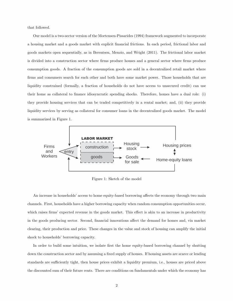
Our model is a two-sector version of the Mortensen-Pissarides (1994) framework augmented to incorporate
a housing market and a goods market with explicit �nancial frictions. In each period, frictional labor and
goods markets open sequentially, as in Berentsen, Menzio, and Wright (2011). The frictional labor market
is divided into a construction sector where �rms produce houses and a general sector where �rms produce
consumption goods. A fraction of the consumption goods are sold in a decentralized retail market where
�rms and consumers search for each other and both have some market power. Those households that are
liquidity constrained (formally, a fraction of households do not have access to unsecured credit) can use
their home as collateral to �nance idiosyncratic spending shocks. Therefore, homes have a dual role: (i)
they provide housing services that can be traded competitively in a rental market; and, (ii) they provide
liquidity services by serving as collateral for consumer loans in the decentralized goods market. The model
is summarized in Figure 1.
construction
goods
LABOR MARKET
Firmsand
Workersentry
Housingstock
Goodsfor sale
Housing prices
Homeequity loans
Figure 1: Sketch of the model
An increase in households�access to home equity-based borrowing a¤ects the economy through two main
channels. First, households have a higher borrowing capacity when random consumption opportunities occur,
which raises �rms�expected revenue in the goods market. This e¤ect is akin to an increase in productivity
in the goods producing sector. Second, �nancial innovations a¤ect the demand for homes and, via market
clearing, their production and price. These changes in the value and stock of housing can amplify the initial
shock to households�borrowing capacity.
In order to build some intuition, we isolate �rst the home equity-based borrowing channel by shutting
down the construction sector and by assuming a �xed supply of houses. If housing assets are scarce or lending
standards are su¢ ciently tight, then house prices exhibit a liquidity premium, i.e., houses are priced above
the discounted sum of their future rents. There are conditions on fundamentals under which the economy has
2

multiple steady-state equilibria across which unemployment and house prices are negatively correlated. Intu-
itively, �rms�decision to open job vacancies in the retail sector depends positively on households�borrowing
capacity and hence home equity. But households�demand for homes as collateral also depends positively on
the aggregate activity in the retail sector, thereby creating strategic complementarities between households�
and �rms�decisions. A new regulation that increases the eligibility of homes as collateral raises the housing
liquidity premium and reduces unemployment.
We next re-open the construction sector, so that the supply of homes is endogenous. We consider two
polar cases that allow us to identify the conditions under which the unemployment rate is a¤ected by
aggregate demand in the goods market: a "competitive" case where �rms have no market power in the retail
market, and a "monopoly" case where �rms have all the market power. In the competitive case, house prices,
which are determined by the relative productivities in the two sectors, are una¤ected by �nancial innovations.
Relaxing lending standards does not a¤ect unemployment but it does lead to a reallocation of workers toward
the construction sector. In the monopoly case, housing assets are priced at their "fundamental" value� the
discounted sum of the rental rates. An increase in the eligibility of homes as collateral reduces aggregate
unemployment, increases house prices, and drives workers away from the construction sector.
To conclude our analysis we calibrate the model to the U.S. economy over the period 1996 to 2010.
The calibration of the labor market is standard based on targets coming from the Job Openings and Labor
Turnover Survey (JOLTS). In addition we adopt two key targets: the ratio of household equity-�nanced
expenditure to disposable income from Greenspan and Kennedy (2007), and the ratio of the aggregate
housing stock to GDP based on the Federal Reserve�s Flow of Funds. Our experiments consist of using a
simple identity for the share of consumption �nanced through home equity extraction to estimate changes
in the eligibility of homes as collateral over the period. We feed this sequence of eligibility coe¢ cients
into the model and solve for the dynamic equilibrium path under rational expectations. While the model
broadly captures the trend features of U.S. data over the period it fails to account for the magnitude of
house price changes observed in the data and, as a result, it generates insu¢ cient volatility in the aggregate
unemployment rate.
Macroeconomic models under rational expectations are notorious for having a hard time explaining the
dynamics of house prices and the dynamics of job openings and unemployment. Thus, in order to properly
match U.S. data we replace our perfect foresight assumption with an adaptive learning rule, in the spirit
of Evans and Honkapohja (2001) and Hommes (2013), that has been able to generate large swings in asset
3

prices and excess volatility in other contexts.3 We calibrate the learning model to U.S. data, solve for the
learning path and show that the model generates a house price boom of the same magnitude as exhibited in
the data. Moreover, the model provides a good �t to sectoral labor �ows and the unemployment rate.
1.1 Related literature
Our study is related to research on unemployment and �nancial frictions. Wasmer and Weil (2004) and
Petrosky-Nadeau (2013) extend the Mortensen-Pissarides model to incorporate a credit market where �rms
search for investors in order to �nance the cost of opening a job vacancy. Our model di¤ers from that
literature in that in ours the credit frictions a¤ect households, taking the form of limited commitment
and lack of record-keeping, rather than search frictions between lenders and borrowers. We also explicitly
formalize a frictional goods market.
Our paper is also related to the literature on unemployment and money. Shi (1998) constructs a model
with frictional labor and goods markets where large households insure their members against idiosyncratic
risks in both markets. Berentsen, Menzio, and Wright (2011) have a related model in which individuals
endowed with quasi-linear preferences readjust their money holdings in a competitive market that opens
periodically as in Lagos and Wright (2005).4 In Rocheteau, Rupert, and Wright (2007) only the goods
market is subject to search frictions but unemployment emerges due to indivisible labor. In all of these
models credit is not incentive feasible because of the lack of record keeping and, therefore, �at money plays a
role in overcoming a double-coincidence of wants problem in the goods market. Our model adopts structure
similar to Berentsen, Menzio, and Wright (2011), but we add a construction sector and a housing market
and introduce home equity-based borrowing in the decentralized goods market.
The macroeconomic implications of the dual role of assets as collateral have been explored in a series of
papers, starting with Kiyotaki and Moore (1997). Applications to the recent �nancial crisis include Midrigan
and Philippon (2011) and Garriga et al. (2012) based on standard neoclassical models. Our formalization
follows the search-theoretic approach to liquidity and �nancial frictions, including Ferraris and Watanabe
(2008), Lagos (2010, 2011), and Rocheteau andWright (2013). In addition we formalize a two-sector frictional
labor market and unemployment.5
3See, for example, Timmermann (1994) and Branch and Evans (2011).4Rocheteau and Wright (2005, 2013) extended the Lagos-Wright model to allow for the free entry of sellers/�rms in a
decentralized goods market. This free-entry condition was reminiscent of the one in the Pissarides model. Berentsen, Menzio,and Wright (2011) tightened the connection to the labor search literature by requiring that �rms search for indivisible labor ina market with matching frictions before entering the goods markets.
5 In Rocheteau and Wright (2013) the asset used as collateral is a Lucas tree. He, Wright, and Yu (2013) reinterpret themodel as one where the asset enters the utility function directly. As we show in this paper, provided that there is a rentalmarket for homes the two interpretations are equivalent.
4

The �rst search model to account for sectoral reallocation is Lucas and Prescott (1974). In this model
sectoral labor markets are competitive and workers�mobility across sectors is limited. Models in which
sectoral labor markets have search frictions include Phelan and Trejos (2000) and Chang (2012). Relative
to this literature our model explains workers�reallocation across sectors by changes in �nancial conditions.
Finally, there is a literature linking households�transitions in the labor and housing markets. For instance,
Rupert and Wasmer (2012) explain di¤erences in labor market mobility between the United States and
Europe by di¤erences in commuting costs. Head and Lloyd-Ellis (2011) develop a model with search frictions
in both housing and labor markets. Karahan and Rhee (2012) consider a two-city model where the low
mobility of highly leveraged homeowners reduces the reallocation of labor. None of these models study the
joint determination of house prices and unemployment in liquidity-constrained economies.
This paper is also related to a burgeoning literature that incorporates constant gain adaptive learning in
studies of monetary policy and asset pricing: see, for example, Branch and Evans (2011); Sargent (1999).6
Branch (2014), in particular, studies a related search-based asset pricing model subject to stochastic dividends
and asset supply. In this model, asset price booms and crashes can arise as an over-shooting in response
to structural changes in the liquidity properties of the asset or as an endogenous response to fundamental
shocks.
2 Environment
The set of agents consists of a [0; 1] continuum of households and a large continuum of �rms. Time is discrete
and is indexed by t 2 N. Each period of time is divided into three stages. In the �rst stage, households
and �rms trade indivisible labor services in a labor market (LM) with search and matching frictions. In
the second stage, they trade consumption goods in a decentralized market (DM) with home equity-based
borrowing. In the last stage, �rms sell unsold inventories, debts are settled, wages are paid, households trade
assets and housing services in a competitive market (CM), and workers make mobility decisions. We take
the consumption good traded in the CM as the numéraire good. The sequence of markets in a representative
period is summarized in Figure 2.
The utility of a household is
E1Xt=0
�t [�(yt) + ct + #(dt)] ; (1)
where � = 11+r 2 (0; 1) is a discount factor, yt 2 R+ is the consumption of the DM good, ct 2 R is the
6For an early contribution see Marcet and Sargent (1989) and for an exhaustive treatment see Evans and Honkapohja (2001).
5

Labor Market
(LM)
DecentralizedGoods Market
(DM)
Competitive MarketsSettlement
(CM)
Entry of firms Matching ofworkers and firms Wage bargaining
Matching of firms and consumers Home equitybased borrowing Negotiation of prices and quantities
Sales of unsold inventories Rental of housing Payment of debt and wages Portfolio choices Occupational choice
Figure 2: Timing of a representative period
consumption of the numéraire good, and dt is the consumption of housing services.7 The utility function in
the DM, �(yt), is twice continuously di¤erentiable, strictly increasing, and concave, with �(0) = 0, �0(0) =1,
and �0(1) = 0. We denote y� > 0 the quantity such that �0(y�) = 1. The utility for housing services is
increasing and concave with #0(0) =1 and #0(1) = 0.
There are two sectors in the economy denoted by � 2 fg; hg: a sector producing perishable consumption
goods (� = g), and a sector producing durable housing goods (� = h). Firms are free to enter either sector.
Each �rm is composed of one job. In order to participate in the LM at t, �rms must advertise a vacant
position, which costs k� > 0 units of the numéraire good at t� 1.8
Households have sector-speci�c skills allowing them to work in a given sector. At the end of a period,
each household from sector � who is unemployed can make a human capital investment, i 2 [0; 1], in order
to migrate to sector �0 with probability i. The cost of this investment in terms of the numéraire good is
�(i), with �0 > 0, �00 > 0, �0(0) = 0 and �0(1) = +1. The assumption �0(0) = 0 will guarantee that at a
steady state households are indi¤erent between the two sectors.9 We denote P�t the measure of households
in sector � at the beginning of t.
The measure of matches between vacant jobs and unemployed households in period t is given bym�(s�t ; o�t ),
where s�t is the measure of job seekers in sector � and o�t is the measure of vacant �rms (openings). The
7We do not impose the nonnegativity of c in the CM. If c < 0, the household produces the numéraire good. In this casec < 0 can be interpreted as self-employment or as a reduction in the household�s illiquid wealth (i.e., wealth that cannot serveas collateral in the DM). One can also impose conditions on primitives so that c � 0 holds, e.g., by assuming su¢ ciently largeendowments of the numéraire good in every period. As in Mortensen and Pissarides (1994) and Lagos and Wright (2005) thisassumption of quasi-linear utility makes the model tractable. In our context it implies that trading histories in both the laborand goods market do not matter for households�choice of asset holdings in the CM. As a result, equilibria will feature degeneratedistribution of asset holdings. Under strictly concave preferences households would accumulate precautionary savings becauseof both idiosyncratic shocks in the labor and goods market, and the dynamics of individual asset holdings would become muchmore complex. Even though households in our analysis will have no need for insurance due to idiosyncratic employment riskthey will have a precautionary demand for assets due to idiosyncratic spending shocks. While wealth e¤ects and employmentrisks are important our analysis emphasizes an "aggregate demand" channel according to which the availability of collateralizedloans to households a¤ects �rms�expected revenue.
8An alternative assumption is that recruiting is labor intensive (instead of goods intensive). In our context our assumptionimplies that changes in lending standards and �nancial frictions do not a¤ect the cost of hiring, such as wages of workers inhuman resources.
9For a similar formalization of the mobility decision in a two-sector labor market model, see Chang (2012).
6

matching function, m�, has constant returns to scale, and it is strictly increasing and strictly concave with
respect to each of its arguments. Moreover, m�(0; o�t ) = m�(s�t ; 0) = 0 and m�(s�t ; o�t ) � min(s�t ; o
�t ).
The job �nding probability of an unemployed worker in sector � is p�t = m�(s�t ; o
�t )=s
�t = m
�(1; ��t ) where
��t � o�t =s�t is referred to as labor market tightness. The vacancy �lling probability for a �rm in sector �
is f�t = m�(s�t ; o�t )=o
�t = m� (1=��t ; 1). The employment in sector � (measured after the matching phase
at the beginning of the DM) is denoted n�t and the economy-wide unemployment rate (measured after the
matching phase) is ut. Therefore,
ut + ngt + n
ht = 1: (2)
The unemployment rate in sector � is 1�n�t =P�t . An existing match in sector � is destroyed at the beginning
of a period with probability ��. A worker who lost his job in period t becomes a job seeker in period t+ 1.
Therefore,
ut = sgt+1 + s
ht+1: (3)
A household that is employed in sector � in period t receives a wage in terms of the numéraire good, w�1;t,
paid in the subsequent CM. A household that is unemployed after the matching phase in period t receives
an income in terms of the numéraire good, w�0 , interpreted as the sum of unemployment bene�ts and the
value of leisure.
Each �lled job in the consumption-good sector produces �zg � y� units of a good that is storable within
the period. These goods can be sold and consumed either in the DM or in the CM. In the latter case they
are perfect substitutes to the numéraire good. So the opportunity cost of selling yt 2 [0; �zg] in the DM is yt.
The aggregate stock of real estate at the beginning of period t is denoted At. Each �lled job in the
construction sector produces �zh units of housing that are added to the existing stock at the end of the
period. Housing goods are durable, and each unit of a housing good generates one unit of housing services
at the beginning of the CM. These services can be traded in a competitive housing rental market at the
price Rt. Following the rental market and the consumption of housing services, housing assets depreciate
at rate �. While all households can rent housing services, we assume that households are heterogeneous in
terms of their access to homeownership. Only a fraction, �, of households can participate in the market and
purchase real estate. Participating households are called homeowners while nonparticipating households are
called renters. The market for homeownership opens after the rental market, and housing assets in period t
are traded at the price qt.10
10Arguably, one would like to introduce search-matching frictions in the housing market as well. We choose to keep this
7

The DM goods market involves bilateral random matching between retailers (�rms) and consumers
(households).11 Because each �rm corresponds to one job, the measure of �rms in the goods market in
period t is equal to the measure of employed households in the goods producing sector, ngt . The matching
probabilities for households and �rms are � = �(ngt ) and �(ngt )=n
gt , respectively. We assume �
0 > 0, �00 < 0,
�(0) = 0, �0(0) = 1, and �(1) � 1. The search frictions in the goods market capture random spending
opportunities for households and will generate a precautionary demand for liquid assets. Moreover, the
endogenous frequency of trading opportunities, �(ngt ), generates a link between the labor market and the
DM goods market: in economies with tight labor markets households experience more frequent trading
opportunities.
In a fraction � of all matches there is a technology to enforce debt repayment, in which case consumer
loans do not need to be collateralized. In the remaining 1� � matches, �rms are willing to extend credit to
households only if the loan is collateralized with some assets.12 In order to formalize home equity extraction,
we assume that the only (partially) liquid asset in the DM is housing.13 (See the discussion below.) The
limited ability to collateralize housing assets is formalized as follows. First, there is a probability, 1� �, that
the housing assets of a homeowner are not accepted as collateral.14 Second, in accordance with Kiyotaki
and Moore (2005), a household that owns a units of housing as collateral can borrow only a fraction of the
value of its assets. More speci�cally, the household can borrow �at [qt(1� �) +Rt], where qt(1� �) + Rt is
the value of a home in the DM of period t (the CM price of homes net of depreciation and augmented of
the rent), and � 2 [0; 1] captures the limited pledgeability of assets. The parameter, �, is a loan-to-value
ratio which represents various transaction costs and informational asymmetries regarding the resale value of
homes.15 In case the consumer defaults on the loan, the producer can seize the collateral at the beginning
market competitive for tractability. Moreover, while search-matching frictions are likely to matter for housing prices, we wantto focus on the liquidity premium for housing prices arising from home-equity based borrowing and its e¤ect on the goods andlabor markets.11The assumption of random bilateral matching and bargaining has several advantages. First, the description of a credit
relationship as a bilateral match is more realistic. Second, the existence of a match surplus that can be partially captured by�rms creates a stronger channel from home-equity-based consumption and �rm�s productivity. Third, the idiosyncratic riskgenerated by the matching process is isomorphic to household preference shocks. In our context the frequency of those shocksis endogenous and depends on the state of the labor market.12Mian and Su� (2014b) �nd that the marginal propensity to borrow varies with homeowners�"cash on hand" where they
de�ne "cash on hand" as cash holdings, liquid debt capacity, or income that can be easily accessed and converted into spending.In our model households who have access to unsecured credit have the largest "cash on hand" and are not liquidity constrained.13This formalization is analogous to the one in Telyukova and Wright (2008) where some matches have perfect enforcement
while others don�t. Following Geromichalos, Licari, and Suarez-Lledo (2007), Lagos (2011), or Li and Li (2013) we couldintroduce �at money alongside housing assets. We chose to abstract from the coexistence of collateralized loans and currencybecause our primary focus is not on monetary policy and asset prices.14A similar assumption is used in Lagos (2010). For microfoundations for this constraint, see Lester, Postlewaite, and Wright
(2012). Taking � as exogeneous is consistent with the view that movements in � over the recent period are due to regulatorychanges (e.g., Dugan, 2008; Abdallah and Lastrapes, 2012).15Microfoundations for such resalability constraints are provided in Rocheteau (2011) based on an adverse selection problem
and in Li, Rocheteau, and Weill (2012) based on a moral hazard problem.
8
of the CM before it can be rented. We restrict our attention to loans that are repaid within the period in
the CM, i.e., the debt is not rolled over across periods.
3 Equilibrium
In the following we characterize an equilibrium by moving backward from agents�portfolio problem in the
competitive housing and goods markets (CM), to the determination of prices and quantities in the retail
goods market (DM), and �nally the entry of �rms and the determination of wages in the labor market (LM).
3.1 Housing and goods markets
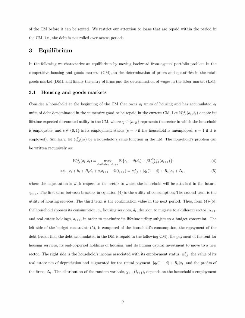
Consider a household at the beginning of the CM that owns at units of housing and has accumulated bt
units of debt denominated in the numéraire good to be repaid in the current CM. Let W�e;t(at; bt) denote its
lifetime expected discounted utility in the CM, where � 2 fh; gg represents the sector in which the household
is employable, and e 2 f0; 1g is its employment status (e = 0 if the household is unemployed, e = 1 if it is
employed). Similarly, let U�e;t(at) be a household�s value function in the LM. The household�s problem can
be written recursively as:
W�e;t(at; bt) = max
ct;dt;it+1;at+1E�ct + #(dt) + �U
�t+1e;t+1(at+1)
(4)
s.t. ct + bt +Rtdt + qtat+1 +�(it+1) = w�e;t + [qt(1� �) +Rt] at +�t; (5)
where the expectation is with respect to the sector to which the household will be attached in the future,
�t+1. The �rst term between brackets in equation (4) is the utility of consumption; The second term is the
utility of housing services; The third term is the continuation value in the next period. Thus, from (4)-(5),
the household chooses its consumption, ct, housing services, dt, decision to migrate to a di¤erent sector, it+1,
and real estate holdings, at+1, in order to maximize its lifetime utility subject to a budget constraint. The
left side of the budget constraint, (5), is composed of the household�s consumption, the repayment of the
debt (recall that the debt accumulated in the DM is repaid in the following CM), the payment of the rent for
housing services, its end-of-period holdings of housing, and its human capital investment to move to a new
sector. The right side is the household�s income associated with its employment status, w�e;t, the value of its
real estate net of depreciation and augmented for the rental payment, [qt(1 � �) + Rt]at, and the pro�ts of
the �rms, �t. The distribution of the random variable, �t+1(it+1), depends on the household�s employment
9

status, et, and its relocation e¤ort, it+1, as follows:
Pr��t+1 = � j�t = �, et = 0
�= 1� Pr
��t+1 = �
0 j�t = �, et = 0�= 1� it+1 (6)
Pr��t+1 = � j�t = �, et = 1
�= 1: (7)
So a household can move to a di¤erent sector only if it is unemployed. Moreover, its probability to join a
new sector is equal to its relocation e¤ort, it+1 > 0.
Substitute ct from (5) into (4) to obtain
W�e;t(at; bt) = [qt(1� �) +Rt] at � bt + w�e;t +�t +max
dt�0f#(dt)�Rtdtg (8)
+ maxit+1;at+1
��qtat+1 � �(it+1) + �EU
�t+1e;t+1 (at+1)
:
In the case where the household does not have access to homeownership the choice of asset holdings is
restricted to at+1 = 0. (The homeownership status is left implicit when writing the value functions.) From
(8) ;W�e;t is linear in the household�s wealth, which includes its real estate and its labor income net of the debt
incurred in the DM; the choice of real estate for the following period, at+1, is independent of the household�s
asset holdings in the current period, at. Finally, the quantity of housing services rented by the household
solves #0(dt) = Rt, where dt is independent of both the household�s housing wealth and its employment
status.
From the last term on the right side of (8), the optimal mobility decision for an unemployed worker in
sector �, i�t+1, solves
�0�i�t+1
�= max
n�hU�
0
0;t+1 (at+1)� U�0;t+1 (at+1)
i; 0o: (9)
From equation (9) the marginal relocation cost must equal the discounted surplus from moving to a di¤erent
sector. It will be convenient in the following to write the expected discounted surplus of the household net
of the cost to acquire new skills as (i) = i�0 (i)� � (i).
The expected discounted pro�ts of a �rm in the consumption-goods sector in the CM with xt units of
inventories (the di¤erence between the �zg units of good produced in the LM and the yt units sold in the
DM), bt units of a household�s debt, and a promise to pay a wage wg1;t, are
�gt (xt; bt; wg1;t) = xt + bt � w
g1;t + �(1� �g)J
gt+1: (10)
The �rm�s x units of inventories are worth x units of numéraire good; the household�s debt, b, is worth b
units of numéraire good. So the total value of the �rm�s sales within the period is x+ b. In order to compute
10

the period pro�ts, we subtract the wage promised to the worker, wg1 . If the �rm remains productive, with
probability 1 � �g, then the expected pro�ts of the �rm at the beginning of the next period are Jgt+1. The
expected discounted pro�ts of a �rm in the housing sector are
�ht (wh1;t) = �z
hqt � wh1;t + �(1� �h)Jht+1: (11)
A �rm in the housing sector produces �zh units of housing that can be sold at the end of the CM at the price
qt, and pays the worker a wage wh1;t.
3.2 Home equity loan contract
We now turn to the retail goods market, DM. Consider a match between a �rm and a household holding at
units of housing assets in the DM goods market and suppose that loan repayment cannot be enforced. A
home-equity loan contract is a pair, (yt; bt), that speci�es the output produced by the �rm for the household,
yt, and the size of the loan (expressed in the numéraire good) to be repaid by the household in the following
CM, bt. The terms of the contract are determined by bilateral bargaining. We use a simple proportional
bargaining rule according to which the household�s surplus from a match is equal to �=(1 � �) times the
surplus of the �rm, i.e., (1� �) [�(y)� b] = � (b� y) where � 2 [0; 1].16 Equivalently, b = (1� �) �(y) + �y.
The bargaining solution is
yt = argmaxy� [�(y)� y] (12)
s.t. b(y) � (1� �) �(y) + �y � � [qt(1� �) +Rt] at: (13)
From (12), output is chosen to maximize the household�s surplus, which is a fraction of the total surplus
of the match, taking as given the nonlinear pricing rule (13) and subject to the borrowing constraint, b �
� [qt(1� �) +Rt] at, according to which the household can only borrow against a fraction of its housing assets.
According to (13) the price of one unit of DM output in terms of the numéraire good is 1+(1��) [�(y)=y � 1],
which is decreasing with y. The solution to the bargaining problem is y = y� if b(y�) � � [q(1� �) +R] a
and b(y) = � [q(1� �) +R] a otherwise. Provided that the household has enough borrowing capacity, agents
trade the �rst-best level of output. If the borrowing capacity of the household is not large enough, either
because the household doesn�t own enough housing wealth or the loan-to-value ratio is too low, the household
hits its borrowing constraint and its DM consumption is less than the �rst-best level.
16For a review of the merits of the proportional bargaining solution relative to Nash bargaining, see Aruoba, Rocheteau, andWaller (2007).
11

In a match where debt repayment can be enforced, the debt contract, (y; b), solves (12)-(13) without the
inequality on the right side of (13). The solution is y = y� and b = (1� �) �(y�) + �y�. With perfect credit
agents maximize the gains from trade in the DM by producing and consuming the socially e¢ cient quantity,
y�.
Using the linearity of W�e;t, the expected discounted utility of a household in the DM holding at units of
housing assets is
V �e;t(at) = E f� (yt)� b(yt)g+ [qt(1� �) +Rt] at +W�e;t(0; 0); (14)
where the expected surplus in the DM is
E f� (yt)� b(yt)g = �� f(1� �)� [� (yt)� yt] + � [� (y�)� y�]g ;
and where yt depends on the household�s housing wealth as indicated by the household�s problem, (12)-(13).
According to (14) the household is matched with a �rm in the retail goods market with probability �(ngt ).
With probability, �, the household has access to unsecured credit and consumes y�. With complement
probability, 1� �, the loan needs to be collateralized, and with probability � the seller accepts the housing
assets of the buyer as collateral.
3.3 Labor market
The description of the labor market corresponds to a two-sector version of the Pissarides (2000) model with
imperfect mobility of workers across sectors, as in Chang (2012).
Households. Consider a household with at units of housing assets that is employed at the beginning of a
period. Its lifetime expected utility is
U�1;t(at) = (1� ��)V�1;t(at) + �
�V �0;t(at); � 2 fh; gg: (15)
With probability 1���, the household remains employed and o¤ers its labor services to the �rm in exchange
for a wage in the next CM. With probability ��, the household loses its job and becomes unemployed. In
this case the household will not have a chance to �nd another job before the next LM in the following period.
Substituting V �1;t(at) and V�0;t(at) by their expressions given by (14),
U�1;t(at) = E f� (yt)� b(yt)g+ [qt(1� �) +Rt] at + (1� ��)W�1;t(0; 0) + �
�W�0;t(0; 0); (16)
where yt = yt(at) is the DM consumption as a function of the household�s housing wealth, at. By a similar
reasoning the expected lifetime utility of an unemployed household with at units of housing looking for a job
12
in sector � is
U�0;t(at) = E f� (yt)� b(yt)g+ [qt(1� �) +Rt] at +W�0;t(0; 0) + p
�t
�W�1;t(0; 0)�W
�0;t(0; 0)
�; (17)
where p�t is the probability of an unemployed in sector � �nding a job.
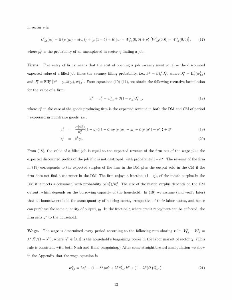
Firms. Free entry of �rms means that the cost of opening a job vacancy must equalize the discounted
expected value of a �lled job times the vacancy �lling probability, i.e., k� = �f�t J�t , where J
ht = �
ht (w
h1;t)
and Jgt = E�gt
��zg � yt; b(yt); wg1;t
�. From equations (10)-(11), we obtain the following recursive formulation
for the value of a �rm:
J�t = z�t � w
�1;t + �(1� ��)J
�t+1; (18)
where z�t in the case of the goods producing �rm is the expected revenue in both the DM and CM of period
t expressed in numéraire goods, i.e.,
zgt =�(ngt )
ngt(1� �) f(1� �)�� [� (yt)� yt] + � [� (y�)� y�]g+ �zg (19)
zht = �zhqt: (20)
From (18), the value of a �lled job is equal to the expected revenue of the �rm net of the wage plus the
expected discounted pro�ts of the job if it is not destroyed, with probability 1���. The revenue of the �rm
in (19) corresponds to the expected surplus of the �rm in the DM plus the output sold in the CM if the
�rm does not �nd a consumer in the DM. The �rm enjoys a fraction, (1 � �), of the match surplus in the
DM if it meets a consumer, with probability �(ngt )=ngt . The size of the match surplus depends on the DM
output, which depends on the borrowing capacity of the household. In (19) we assume (and verify later)
that all homeowners hold the same quantity of housing assets, irrespective of their labor status, and hence
can purchase the same quantity of output, yt. In the fraction � where credit repayment can be enforced, the
�rm sells y� to the household.
Wage. The wage is determined every period according to the following rent sharing rule: V �1;t � V�0;t =
��J�t =(1� ��), where �� 2 [0; 1] is the household�s bargaining power in the labor market of sector �. (This
rule is consistent with both Nash and Kalai bargaining.) After some straightforward manipulation we show
in the Appendix that the wage equation is
w�1;t = �z�t + (1� ��)w
�0 + �
���t+1k� + (1� ��)
�i�t+1
�: (21)
13

The wage is a weighted average of a �rm�s revenue, z�t , and a household�s �ow utility from being unemployed,
w�0 , augmented by a term proportional to �rms�average recruiting expenses per unemployed worker, ��t+1k
�.
There are two novelties relative to the standard Pissarides model. First, the �rm�s marginal revenue is
endogenous and will depend on frictions in the DM market and house prices. Second, the last component of
the wage equation captures the fact that households in a shrinking sector can ask for a higher wage given
that they have the (costly) possibility of moving to the expanding sector.
Sectoral reallocation The worker�s mobility decision is determined by the size of the surplus from moving
to another sector, �U�t � ��U�
0
0;t � U�0;t
�with �0 6= �. Following some straightforward calculation (see
Appendix), �U�t obeys the following recursion:
�U�t = �hw�
0
0 � w�0 +�i�
0
t+1
��
�i�t+1
�+�U�t+1
i+
��0
1� ��0��
0
t k�0 � ��
1� �� ��t k
�: (22)
From (9), the optimal reallocation decision is given by
�0 (i�t ) = max f�U�t ; 0g : (23)
In an equilibrium where there is reallocation of households from sector � to sector �0, i.e, �U�t > 0 for all
t, the intensity of the reallocation, i�t , solves
�0 (i�t ) = �hw�
0
0 � w�0 � �i�t+1
�+�0
�i�t+1
�i+
��0
1� ��0��
0
t k�0 � ��
1� �� ��t k
�: (24)
In the case of perfect mobility across sectors, � = �0 = 0,
�wg0 +�g
1� �g �gt kg = �wh0 +
�h
1� �h�ht k
h: (25)
If sectors are symmetric in terms of income when unemployed, wg0 = wh0 , bargaining powers, �
g = �h, and
costs of opening job vacancies, kg = kh, then (25) reduces to �gt = �ht .
Market tightness. Market tightness is determined by the free-entry condition, �f�t J�t = k
�, where J�t is
given by (18). Substituting w�1;t by its expression from (21) into (18),
k�
�m��1��t; 1� = (1� ��) �z�t � w�0 � �i�t+1��� ����t+1k� + (1� ��)k�
m��
1��t+1
; 1� : (26)
The �nancial frictions in the DM a¤ect �rms�entry decision in the consumption goods sector through zg. If
credit is more limited, then households have a lower payment capacity, the price of DM goods falls, which
reduces zg. As zg is reduced, fewer �rms �nd it pro�table to enter the market.
14

3.4 Housing prices
In order to determine the demand for real estate from homeowners, substitute U�e;t(at) given by (16) and
(17) into (8)� noticing that only the �rst two terms on the right sides of (16) and (17) depend on a and are
independent of � and e� to obtain
maxat+1�0
f�fqt � � [qt+1(1� �) +Rt+1]g at+1 + ���(1� �)� [� (yt+1)� yt+1]g ; (27)
where yt+1 is given by the solution to the bargaining problem in the DM goods market, (12)-(13). According
to (27) households choose their holdings of real estate in order to maximize their expected surplus in the
DM net of the cost of holding these assets. The cost of holding real estate is approximately equal to
the di¤erence between the gross rate of time preference, ��1, and the gross rate of return of real estate,
[(1� �)qt+1 +Rt+1] =qt. Notice that the problem in (27) is independent of the employment status of the
household. This suggests that both employed and unemployed households (provided they have access to
homeownership) will hold the same quantity of housing assets.
From the bargaining problem in the DM, (12)-(13), dyt+1=dat+1 = [qt+1(1� �) +Rt+1] �=b0(yt+1), when-
ever yt+1 < y�. Therefore, the �rst-order condition associated with (27), assuming an interior solution,
is
qt =(1� �)qt+1 +Rt+1
1 + r
�1 + L(ngt+1; yt+1)
�; (28)
where we de�ne the liquidity premium for housing assets as
L(ngt+1; yt+1) = �(ngt+1)(1� �)���
��0 (yt+1)� 1b0(yt+1)
�. (29)
The price of housing is determined by a liquidity-augmented asset pricing equation (28). The price of one
unit of housing is equal to its future discounted price net of depreciation plus the rental value of housing
services, everything multiplied by the liquidity premium on housing. The liquidity premium, L, measures
the increase in the household�s surplus in the DM from holding an additional unit of housing wealth.
3.5 Equilibrium dynamics
We now provide a de�nition of dynamic equilibrium for our economy. The population of households is
divided according to (2). The dynamics for the population in each sector is
P�t+1 = P�t +
�P�
0
t � n�0
t
�i�
0
t+1 � (P�t � n
�t ) i
�t+1; � 2 fg; hg: (30)
15

According to (30) the change in the measure of households in sector �, P�t+1 � P�t , is equal to the in�ow
from sector �0,�P�
0
t � n�0
t
�i�
0
t+1, net of the out�ow from sector �, (P�t � n�t ) i
�t+1. The law of motion for
the measure of employed in sector � is
n�t+1 = (1� ��)n�t +m
�(1; ��t+1)s�t+1; � 2 fg; hg: (31)
According to (31) the measure of employed households in sector � in period t + 1, following the matching
phase, is equal to the measure of employed households in sector � in period t net of the households who lost
their jobs in sector � at the beginning of t + 1 plus the measure of job seekers in sector � �nding a job in
t+ 1. The population in sector � is divided between employed workers and job seekers,
P�t = n�t�1 + s
�t ; � 2 fg; hg: (32)
Clearing of the housing market implies the quantity of assets held by households with access to home-
ownership is at = At=�. From (12)-(13) the quantities traded in the DM solve
b (yt) = min
�� [qt(1� �) +Rt]At
�; b (y�)
�(33)
From (8) and the clearing of the rental housing market, dt = At, the rental price of housing solves
Rt = #0(At): (34)
Housing prices solve (28), i.e.,
qt =(1� �)qt+1 + #0(At+1)
1 + r
�1 + �(ngt+1)(1� �)���
��0 (yt+1)� 1b0(yt+1)
��: (35)
Finally, the dynamics for the stock of housing are
At+1 = (1� �)At + nht �zh. (36)
From (36) the stock of housing in t + 1 is equal to the stock of housing in t net of depreciation augmented
by the production of new houses.
De�nition 1 An equilibrium is a bounded sequence, fn�t ; s�t ; �
�t ;�U
�t ; i
�t ;P
�t ; qt; yt; Rt; Atg1t=0, that solves
(2), (22), (23), (26), and (30)-(36).
4 Sectoral reallocation and home equity-based borrowing
In order to better understand the mechanics of the model, we will �rst isolate the e¤ects of sector-speci�c
shocks on the reallocation of jobs by shutting down home equity-based borrowing. Second, we will isolate
16

the home equity-based borrowing channel by assuming a �xed supply of housing assets. Finally, we will
conclude this section by having two active sectors, and hence an endogenous supply of housing, and home
equity-based borrowing together. Throughout this section we restrict ourselves to steady-state equilibria
and we set � = 0 so that all trades in the DM are collateralized.
4.1 Sectoral reallocation
In this example, we assume that the two sectors are symmetric in terms of matching technologies, entry
costs, incomes when unemployed, bargaining weights, and separation rates, i.e., mg = mh = m, kg = kh = k,
wg0 = wh0 = w0, �h = �g = �, and �g = �h = �. Sectors only di¤er in their productivity, �z�. From (25),
and assuming that both sectors are active, �g = �h = � so that households enjoy the same surplus in both
sectors. From (26) market tightness solves
(r + �) k
m���1; 1
� + ��k = (1� �) (zg � w0) : (37)
We shut down the home equity-based borrowing channel by setting � = 0 so that housing assets are illiquid
and cannot be used to �nance consumption in the DM.
The model is solved as follows. From (33) � = 0 implies y = 0, and from (19), zg = �zg. From (26)
�g = �h implies �zg = �zhq. Housing prices, q = �zg=�zh, adjust so that labor productivity in all sectors
are equalized. Market tightness is uniquely determined by (37). Moreover, � > 0 if and only if (1 �
�) (�zg � w0) � (r + �) k > 0. From (28) the rental price of housing is R = (r + �)q = (r + �)�zg=�zh, and
from (34) the stock of housing is A = #0�1(R) = #0�1�(r + �)�zg=�zh
�. The stock of housing increases with
productivity in the construction sector, and it decreases with the real interest rate, the depreciation rate,
and the productivity in the consumption goods sector. The size of the housing sector is determined by (36),
nh = �A=�zh = �#0�1�(r + �)�zg=�zh
�=�zh. The size of the goods sector is obtained from (32), nh+ng = 1�u,
where from (31) u(�) = �= [m(1; �) + �]. Both sectors are active if nh < 1� u, i.e.,
�#0�1�(r + �)�zg=�zh
��zh
<m(1; �)
m(1; �) + �: (38)
There is a threshold, z> w0 + (r + �) k=(1 � �), for �zg such that the previous inequality holds with an
equality. For all �zg >z, ng > 0.
Proposition 1 (No home-equity extraction) Suppose that � = 0 and (38) holds. There exists a unique
17

steady-state equilibrium with nh > 0 and ng > 0. Comparative statics are summarized in the following table:
�zg �zh � w0 � k #0
� + 0 - - - - 0ng + +/- - - - - -nh - +/- 0 0 0 0 +u - 0 + + + + 0q + - 0 0 0 0 0A - + 0 0 0 0 +
In Figure 3 we represent graphically the determination of the equilibrium. The curve labeled JC (for job
creation) indicates the aggregate level of employment, nh+ng = 1� u(�). As is standard in the Mortensen-
Pissarides model, an increase in labor productivity (�zg) moves the job creation curve outward, while an
increase in a worker�s bargaining power (�), income when unemployed (w0), and a �rm�s recruiting cost (k)
move the job creation curve inward. The curve labeled NH (for nh) indicates the level of employment in
the construction sector. If labor productivity in the goods sector (�zg) increases, then NH moves downward,
while if the marginal utility of housing services (#0) increases, then NH moves upward.
We have seen from (19) that a �nancial innovation that increases households�borrowing capacity raises
�rms� productivity in the goods sector. An increase in �zg leads to higher market tightness and lower
unemployment. Labor mobility across sectors guarantees that productivities are equalized: employment
increases in the consumption goods sector but decreases in the construction sector. As a result of the decline
of the supply of housing assets, rental rates and house prices increase. In Figure 3 the JC curve moves
outward while the NH curve moves downward.
hn
gn
1 ( )u
1 ( )u
gz ↑
gz ↑
'ϑ ↑
0, ,w kλ ↑
Figure 3: Equilibrium with no equity extraction
18

A second e¤ect from a �nancial innovation that allows households to use homes as collateral is to increase
the marginal value of housing assets for homeowners. As a �rst pass� before we study this e¤ect explicitly in
the next section� we consider an increase of the marginal utility for housing services, #0. The productivities in
the two sectors are unchanged. Therefore, market tightness and unemployment are una¤ected. Graphically,
the curve JC does not shift. The increase in the demand for housing services generates a reallocation of
labor toward the construction sector. Graphically, the curve NH moves upward. In the long run the stock
of housing increases.
4.2 Home equity-based borrowing
In order to isolate the home equity-based borrowing channel, we now consider the case of a one-sector economy
with a �xed stock of housing, A. We set the depreciation rate to � = 0 and omit all the superscripts indicating
the sector � = g.
We �rst show that a steady-state equilibrium can be summarized by two equations that determine market
tightness, �, and house prices, q. From (19) and (37) market tightness solves
(r + �) k
m���1; 1
� + ��k = (1� �)��� [n(�)]n(�)
�(1� �) [� (y)� y] + �z � w0�; (39)
where n(�) = m(1; �)= [m(1; �) + �] is an increasing function of � with n(0) = 0, and y is determined by (33).
We impose the following inequality:
��(1� �) [� (y�)� y�] + �z � w0 >(r + �)k
1� � : (40)
Condition (40) guarantees that there is a positive measure of �rms participating in the labor market if
households are not liquidity constrained. Let �q be the house price above which homeowners have enough
wealth to purchase y� in the DM, i.e., (�q +R) �A=� = b(y�) if R�A=� < b(y�) and �q = 0 otherwise. For
all q > �q, y = y� and � = ��, where �� is the unique solution to (39) with y = y�. In this case the liquidity
provided by the housing stock is abundant and homeowners can trade the �rst-best level of output in the
DM. In contrast, for all q < �q, liquidity is scarce and y < y� is increasing with q so that (39) gives a positive
relationship between � and q (provided that � > 0). Intuitively, higher house prices allow households to
�nance a higher level of DM consumption, which raises �rms�expected revenue and therefore the entry of
�rms in the labor market. The condition (39) is represented by the curve JC (job creation) in Figure 4.
Let us turn to the determination of house prices. From (28) with � = 0, the price of housing solves
rq = #0(A) +�q + #0(A)
�� [n(�)] ���
��0 (y)� 1b0(y)
�: (41)
19

If � = 0, then � [n(�)] = 0 and homes are priced at their "fundamental" value, q = q� = #0(A)=r. Suppose
q� � �q, i.e., the fundamental price of housing is large enough to allow households to �nance y� in the DM.
This condition can be expressed in terms of fundamentals as
#0(A)A � r�b(y�)
(1 + r) �: (42)
If (42) holds, then q = q� and � = ��. Suppose next that q� < �q, i.e., (42) does not hold. From (41) there
is a positive relationship between house prices and market tightness.17 If the labor market is tight, then
households have frequent trading opportunities in the DM. As a consequence, they have a high value for the
liquidity services provided by homes and q > q� increases. As � tends to in�nity, q approaches some limit
q̂ > q�. The condition (41) is represented by the curve HP (house prices) in Figure 4.
θθHPHP
JCJC θθ
*q*q
, , ,z µ ρ ν ↑
,µ ν ↑0, ,w kλ ↑
q
Figure 4: Fixed supply of housing. Left: Multiple steady-state equilibria. Right: Comparative statics.
As shown in Figure 4 the two equilibrium conditions, (39) and (41), are upward sloping. So a steady-
state equilibrium might not be unique. In the left panel of Figure 4 we represent a case with two active
equilibria. Across equilibria there is a negative correlation between house prices and unemployment. Similar
multiplicity has been analyzed in Rocheteau and Wright�s (2005, 2013) models of liquidity with free-entry
of sellers. If the following condition holds,
��(1� �) f� [y(q�)]� y(q�)g+ �z � w0 �(r + �)k
1� � ; (43)
then there is an equilibrium with an inactive labor market, � = 0, where homes are priced at their fundamental
17To see this, notice that (41) can be rewritten as [rq � #0(A)] = [q + #0(A)] = � [n(�)] ��� [�0 (y)� 1] =b0(y), where[�0 (y)� 1] =b0(y) is decreasing in y and y is increasing with q. So the left side of the equality is increasing in q, while theright side is decreasing in q. A higher value of market tightness raises the right side, which leads to a higher value for q.
20

value, q = q�. Indeed, if q = q�, then �rms do not open vacancies and, as a consequence, homes have no
liquidity role. There are also an even number of equilibria (possibly zero) with � > 0 and q > q�. We
summarize our results in the following proposition.
Proposition 2 (Fixed supply of housing) Suppose (40) holds.
1. If #0(A)A � r�b(y�)= (1 + r) �, then there is a unique steady-state equilibrium with q = q� = #0(A)=r,
y = y�, and � = �� > 0.
2. Suppose #0(A)A < r�b(y�)= (1 + r) �.
(a) If (43) fails to hold, then q > q�, y 2 (0; y�), and � > 0 at any steady-state equilibrium.
(b) If (43) holds, then there is an inactive equilibrium, q = q� and � = 0, and an even number of
active equilibria with q > q�, y 2 (0; y�), and � 2�0; ���.
The comparative statics at the highest active equilibrium, if it exists, are given by:
�z � w0 � k � � �� + - - - - + + +u - + + + + - - -q + - - - - + +/- +
When investigating the comparative statics we assume that #0(A)A < r�b(y�)= (1 + r) �, i.e., the supply
of housing is scarce in the sense that homeowners do not have enough housing wealth in order to �nance
y�. Consider �rst a �nancial innovation that increases the eligibility of homes as collateral. An increase
in � moves the HP curve to the right because the liquidity premium of homes goes up; it moves the JC
curve upward as the frequency of sale opportunities in the DM increases. Consequently, market tightness
and house prices increase, and unemployment decreases.
Lax lending standards can also take the form of high loan-to-value ratios. An increase in � moves the JC
curve upward because households can borrow a larger amount against their home equity, which allows �rms
to sell more output in the DM. But an increase in � has an ambiguous e¤ect on the home-pricing curve,
HP . On the one hand, holding the marginal utility of DM consumption constant, households are willing
to pay more for housing wealth because they obtain larger loans when their home is used as collateral to
�nance their DM consumption. On the other hand, the fact that households hold more liquid wealth implies
that the wedge between �0 and the seller�s cost, one, is reduced, which leads to a reduction in the size of the
liquidity premium.
21

4.3 Sectoral reallocation induced by �nancial innovations
We now allow for both home equity �nancing and an endogenous supply of housing. As in our �rst example,
the two sectors are assumed to be symmetric in terms of matching technologies, entry costs, incomes when
unemployed, bargaining weights, and separation rates. Moreover, we assume a logarithmic utility function
for housing services, i.e., #(A) = #0 ln(A). From (34) the rental price of homes is then R = #0=A. In order
to derive analytical results we consider two special cases for the pricing protocol in the DM: a "competitive"
case where �rms have no market power to set prices; and a "monopoly" case where �rms can set prices (or
terms of trade) unilaterally.18
The "competitive" case. Suppose �rst that �rms have no bargaining power in the DM, 1 � � = 0.
Following the same reasoning as in Section 4.1, the model can be solved recursively. From (19) the �rm�s
productivity in the nonhousing sector is zg = �zg. From (25) and (26) the mobility across sectors implies
�zhq = �zg, i.e., q = �zg=�zh. Market tightness, which is determined by (37), is not a¤ected by the availability of
home equity loans. The size of the housing sector is nh = �A=�zh = �qA=�zg, and the size of the nonhousing
sector is ng = 1� u(�)� nh. An active goods market, ng > 0, requires that Aq 2 [0; [1� u(�)] �zg=�). From
(35), Aq solves
(1 + r)Aq
(1� �)Aq + #0= 1 + ��
�1� u(�)� �qA
�zg
�� [�0 (y)� 1] ; (44)
where from (33), y = min f� [Aq(1� �) + #0] =�; y�g. An equilibrium with both sectors being active exists
and is unique if the left side of (44) evaluated at Aq = [1� u(�)] �zg=� is greater than the right side of (44)
(which equals one for this value of Aq), i.e.,
[1� u(�)] �zg > �#0r + �
: (45)
This condition requires that the productivity in the goods sector, �zg, is su¢ ciently large.
If liquidity is abundant, � [Aq(1� �) + #0] =� � y�, agents can trade the �rst best in the DM, y =
y�, and from (44) Aq = #0=(r + �). The condition for such an equilibrium with unconstrained credit is
(1 + r)#0=(r + �) � �y�=�. Suppose in contrast that liquidity is scarce, (1 + r)#0=(r + �) < �y�=�. Higher
values for � or � increase the right side of (44). So Aq and nh = �qA=�zg increase. Hence if the eligibility for
home equity loans increases, or if homeownership increases, then labor is reallocated from the general sector
18Our "competitive" case should be distinguished from the notion of competitive search where it is assumed that contractsare posted before matches are formed and search is directed. For this concept of equilibrium in a related model, see Rocheteauand Wright (2005).
22

to the construction sector. For these two experiments changes in �nancial frictions a¤ect the composition of
the labor market, but aggregate employment and unemployment are unchanged.
The "monopoly" case. We now consider the opposite case where households have no bargaining power
in the DM goods market, � = 0. Since households do not enjoy any surplus from their DM trades, the
asset price has no liquidity premium, q = #0=A(r + �). Households are indi¤erent in terms of their holdings
of housing, so we focus on symmetric equilibria where all homeowners hold A=�. To simplify the analysis
further, assume that the matching function in the DM is linear, �(n) = n, so that all �rms are matched with
one household, �(n)=n = 1. The productivity in the goods sector is
zg = �� [� (y)� y] + �zg; (46)
where from (33), �(y) = min f� [Aq(1� �) + #0] =�; �(y�)g. Assuming (1 + r)#0=(r + �) < ��(y�)=�, house-
holds do not own enough housing assets to trade the e¢ cient output level in the DM. In this case,
�(y) =�#0(1 + r)
�(r + �): (47)
If the LM is active, then market tightness is determined by (37) and (46)-(47),
(r + �) k
m(��1; 1)+ ��k = (1� �)
���
��#0(1 + r)
�(r + �)� ��1
��#0(1 + r)
�(r + �)
��+ �zg � w0
�: (48)
An increase in the loan-to-value ratio, �, in the acceptability of homes as collateral, �, or in homeownership,
�, raises market tightness and aggregate employment.
As before the mobility across sectors implies that q = zg=�zh. The size of the housing sector is determined
by nh = �A=�zh = �qA=zg = �#0=(r + �)zg. Therefore, ng = 1 � u(�) � nh. An equilibrium with an active
goods market exists if
u(�) +�#0
(r + �)zg< 1; (49)
where � is the solution to (48) and zg is given by (46)-(47). Condition (49) will be satis�ed if �zg is su¢ ciently
large. A reduction in �nancial frictions (i.e., an increase in �, �, and �) leads to a reallocation of workers
from the construction sector to the goods sector. In the context of Figure 3, the NH curve moves downward
and the JC curve moves outward as �, �, or � increase. We summarize the results above in the following
proposition.
Proposition 3 (Financial innovations in two limiting economies.) Assume #(A) = #0 ln(A).
23

1. Suppose � = 1. If (45) holds, then an equilibrium with two active sectors exists and is unique. If
liquidity is scarce, (1 + r)#0=(r + �) < �y�=�, an increase in the acceptability of collateral, �, or
homeownership, �, has no e¤ect on unemployment but it raises employment in the construction sector,
nh, and reduces employment in the goods sector, ng.
2. Suppose � = 0, and �(n) = n. If (49) holds, then an equilibrium with two active sectors exists and
is unique. If liquidity is scarce, (1 + r)#0=(r + �) < ��(y�)=�, an increase in the acceptability of
collateral, �, the loan-to-value ratio, �, or homeownership, �, increases market tightness, �, aggregate
employment, 1� u, and house prices, q, but it reduces employment in the construction sector, nh.
5 Calibration
We now turn to a quantitative evaluation of the e¤ects of �nancial innovations and regulations on the labor
and housing markets by calibrating our economy to the United States. We interpret, in the context of the
model, these innovations/regulations as changes in eligibility criteria for home-equity loans.
5.1 Calibrating the Labor Market
The basic unit of time is a month.19 The economy is calibrated to the U.S. averages in 1996. However, we
use the averages over the period 2000:12 to 2012:9 for transition rates in the labor market as we do not have
relevant data prior to the Jobs Opening and Labor Turnover Survey (JOLTS) from the Bureau of Labor and
Statistics (BLS).20
The average job destruction rates from the JOLTS over this period were 6.1% per month in the construc-
tion sector, �h = 0:061, and 3.6% per month in the nonfarm sector, �g = 0:036. The job �nding probabilities
are computed from (31) as p� = ��n�=s�. The BLS Establishment Survey provides construction and non-
farm employment, Eh and E, respectively, as well as aggregate and construction industry unemployment
numbers, U and Uh, respectively.21 We use this information to compute the shares of employment in each
sector, as n� = E�=(E + U) for the year 1996, along with the shares of unemployment. The results are
reported in Table 1. Finally, we target a value fg = 0:7 for the job �lling probability in the general sector,
corresponding to the value in Den Haan et al. (2000). For the job �lling probability in the construction
19We choose a short unit of time to target transition probabilities in the labor market (in particular vacancy �lling probabil-ities). Even though households in the model repay their loans every period, we reinterpret the model as one where householdscan stagger the repayment of their loans over multiple periods, and we will choose the average duration between two tradingopportunities in the DM to be consistent with the average maturity of home lines of credit.20See Davis et al. (2010) for a discussion of JOLTS data. The data we use are: Total Separations rate - Total Nonfarm (Fred
II series I.D. JTSTSR); Total Separations rate - Construction (Fred II series I.D. JTU2300TSR).21The series we use are: All Employees - Total nonfarm (Fred II series I.D. PAYEMS); All Employees - Construction (Fred
II series I.D. USCONS); Unemployed (Fred II series I.D. UNEMPLOY).
24
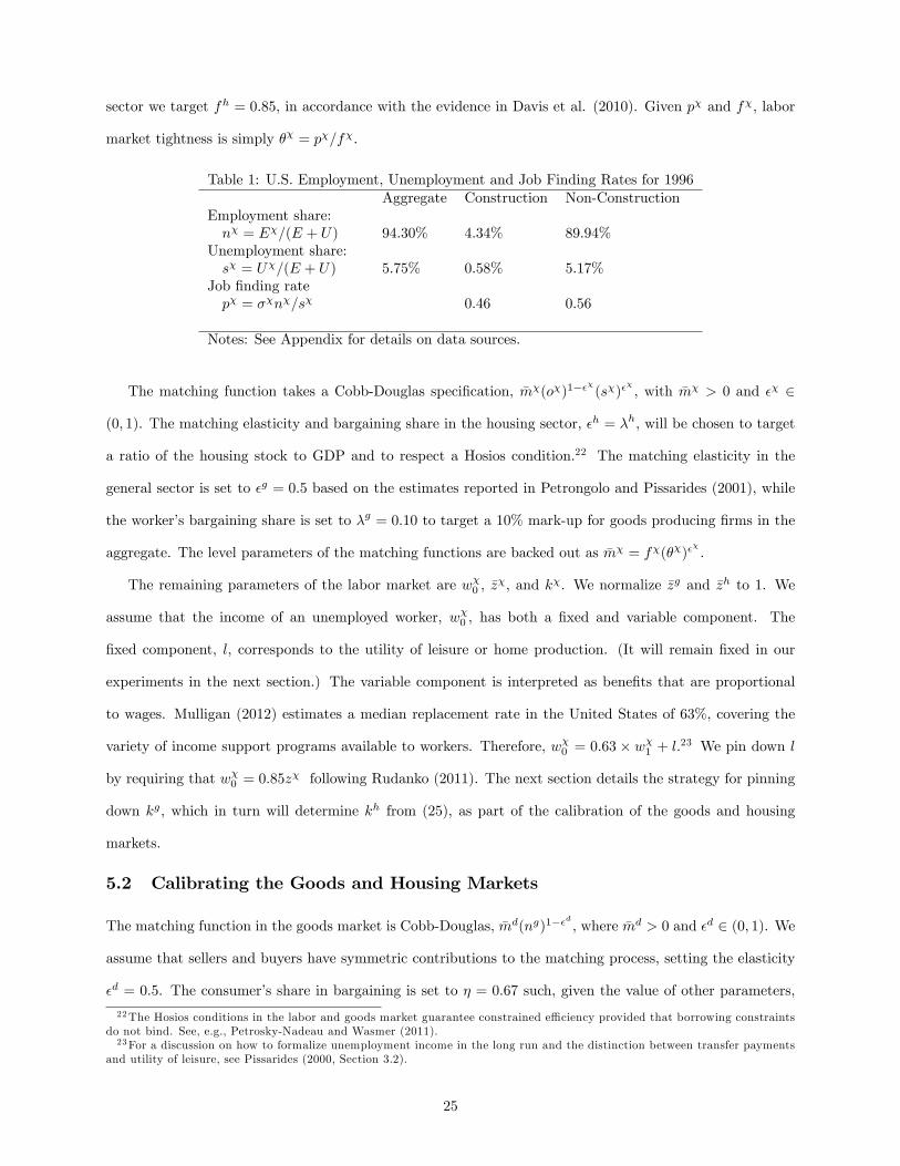
sector we target fh = 0:85, in accordance with the evidence in Davis et al. (2010). Given p� and f�, labor
market tightness is simply �� = p�=f�.
Table 1: U.S. Employment, Unemployment and Job Finding Rates for 1996Aggregate Construction Non-Construction
Employment share:n� = E�=(E + U) 94.30% 4.34% 89.94%
Unemployment share:s� = U�=(E + U) 5.75% 0.58% 5.17%
Job �nding ratep� = ��n�=s� 0.46 0.56
Notes: See Appendix for details on data sources.
The matching function takes a Cobb-Douglas speci�cation, �m�(o�)1���
(s�)��
, with �m� > 0 and �� 2
(0; 1). The matching elasticity and bargaining share in the housing sector, �h = �h, will be chosen to target
a ratio of the housing stock to GDP and to respect a Hosios condition.22 The matching elasticity in the
general sector is set to �g = 0:5 based on the estimates reported in Petrongolo and Pissarides (2001), while
the worker�s bargaining share is set to �g = 0:10 to target a 10% mark-up for goods producing �rms in the
aggregate. The level parameters of the matching functions are backed out as �m� = f�(��)��
.
The remaining parameters of the labor market are w�0 , �z�, and k�. We normalize �zg and �zh to 1. We
assume that the income of an unemployed worker, w�0 , has both a �xed and variable component. The
�xed component, l, corresponds to the utility of leisure or home production. (It will remain �xed in our
experiments in the next section.) The variable component is interpreted as bene�ts that are proportional
to wages. Mulligan (2012) estimates a median replacement rate in the United States of 63%, covering the
variety of income support programs available to workers. Therefore, w�0 = 0:63 � w�1 + l.
23 We pin down l
by requiring that w�0 = 0:85z� following Rudanko (2011). The next section details the strategy for pinning
down kg, which in turn will determine kh from (25), as part of the calibration of the goods and housing
markets.
5.2 Calibrating the Goods and Housing Markets
The matching function in the goods market is Cobb-Douglas, �md(ng)1��d
, where �md > 0 and �d 2 (0; 1). We
assume that sellers and buyers have symmetric contributions to the matching process, setting the elasticity
�d = 0:5. The consumer�s share in bargaining is set to � = 0:67 such, given the value of other parameters,
22The Hosios conditions in the labor and goods market guarantee constrained e¢ ciency provided that borrowing constraintsdo not bind. See, e.g., Petrosky-Nadeau and Wasmer (2011).23For a discussion on how to formalize unemployment income in the long run and the distinction between transfer payments
and utility of leisure, see Pissarides (2000, Section 3.2).
25

the borrowing constraints in pairs requiring a collateralized loan binds. The level parameter of the matching
function, �md, is calibrated to a low frequency of spending shocks, �, such that on average consumption events
�nanced by equity occur every 4 to 5 years, i.e., � = md(ng)1��d
= 0:06. This low frequency is motivated
by an average maturity of home lines of credit of 5 years. In addition, we assume that only one quarter of
all trades require collateral by setting � = 0:75.
The eligibility probability of homes as collateral, 0 < � < 1, is calibrated so that the amount of household
equity �nanced expenditure matches the evidence in Greenspan and Kennedy (2007), who provide quarterly
estimates from 1991:1 to 2008:4. That is, we de�ne aggregate consumption expenditure in the DM as
CDM � ��� [(1� �)�(y) + �y], and disposable income as Y D � ngzg + nhzh � kgog � khoh. We target
CDM=YD = 0:025, at the lower end of its value observed for the period of interest. The homeownership rate
is set to � = 0:654 as reported for the year 1996 in by the U.S. Census Bureau.
We express the parameter � as the product of two components, �� and �a. We think of �� as a standard
loan-to-value (LTV) ratio. Adelino et al. (2012) �nd that during the period 1998-2001, on average 60% of
transactions where at a LTV of exactly 0.8. We choose a more conservative value of �� = 0:6, and we will
consider experiments relaxing lending standards. The second component, �a, is interpreted as the equity
share of a home that can be pledged. The Survey of Consumer Finance (2012) indicates that the median
household debt secured by a primary residential property of $ 112,100 in 2010 U.S. dollars. The same
household holdings of non-�nancial wealth, amounts to $ 209,500 dollars in a primary residence.24 Based on
this, we assume �a = 0:5, resulting in � = ��� �a = 0:6� 0:5 = 0:3.
We choose the bargaining share in the construction sector, �h, to target the ratio of the value of the
aggregate housing stock to GDP in 1996, before the large run-up in housing prices, qA=�ngzg + nhzh
�= 1:65,
based on the Flow of Fund.25 To see why the bargaining share, �h, will allow us to reach this target, notice
that the target implies relative productivities in the two sectors,
zg
zh=nh
ng
�GDP
�qA� 1�;
where we have used (20) and (36), i.e., q = �zh=zh and A = nh�zh=�, to express the value of the housing stock
as qA = zhnh=�. The depreciation rate of the housing stock over 1996-2001 is taken from the Harding et al.
24See Survey of Consumer Finance (2012), Table 13 page 59 and Table 9 page 45.25For comparison, this ratio was equal to 2 on average over the period 2000 to 2012. The data for the U.S. stock of housing:
Real Estate - Assets - Balance Sheet of Households and Nonpro�t Organizations (FRED series I.D. REABSHNO), billions ofdollars. These data comes from the Z.1 Flow of Funds release of the Board of Governors in Table B.100. Model-consistentGDP is constructed as personal consumption expenditures (FRED series I.D. PCE) plus residential investment (FRED seriesI.D. PRFI). By comparison, Midrigan and Philippon (2001) target a housing stock to consumption expenditure ratio of 2.11.
26

(2007) estimate of 0:0275 per year, i.e., � = 0:002 3.26
The functional form for the utility of housing services is #(A) = & lnA, in accordance with Rosen (1979)
and Mankiw and Weil (1989), and the level parameter is & = RA. We compute the rental rate as R =
(R=q)data � q ,where the rent to price ratio is given by the Lincoln Institute of Land Policy estimate of
4.92%.27
The utility function in the DM takes the form �(y) = y1�!1=(1 � !1) with !1 2 (0; 1). We choose !1
so that the model�s liquidity premium is consistent with the one in the data. From (28) we compute the
liquidity premium in the data as L=q = r + � �R=q. In the model it is given by (29). Therefore,
r + � � Rq=
�1� � + R
q
��(1� �)���
�y�!1 � 1
(1� �)y�!1 + �
�;
where, from (33), y solves (1� �)y1�!1=(1� !1) + �y = [q(1� �) +R] �A=�. From (19) this implies a value
for the productivity in the goods sector,
zg = �zg +�(ng)
ng�(1� �)(1� �)�
�y1�!1
1� !1� y
�:
We make this value consistent with �g obtained above and the free-entry condition, (26), by adjusting the
vacancy cost parameter, kg. Table 2 presents the baseline parameter values.
26This is lower than the rate of 3.6% used in Midrigan and Philippon (2011), and greater than the value of 1.6% in Gommeand Rupert (2007).27The Lincoln Institute of Land Policy provides reliable time series of the Rent-Price ratio, the average ratio of estimated
annual rents to house prices for the aggregate stock of housing in the U.S. (the rental data are gross and do not account forincome taxes or depreciation).
27

Table 2: Baseline CalibrationParameter De�nition Value Source/TargetPanel A: Labor Market Parameters�g Job destruction rate - general 0.032 JOLTS�h Job destruction rate - housing 0.061 JOLTSwg0 Value of non-employment - general 0:85zg Rudanko (2011)wh0 Value of non-employment - housing 0:85zh Rudanko (2011)kg Vacancy cost - general goods 3.17 Job �lling ratekh Vacancy cost - housing 1.30 Job �lling rate�g Elasticity, labor matching - general 0.50 Petrongolo and Pissarides (2001)�h Elasticity, labor matching - housing 0.31 Hosios condition / Competitive searchmg Level, labor matching - general 0.63 Job �nding ratemh Level, labor matching - housing 0.71 Job �nding rate�g Worker�s wage bargaining weight 0.10 Aggregate markup�h Worker�s wage bargaining weight 0.31 Housing stock to GDP
Panel B: Housing Market Parameterszh Technology in housing sector 1� Home ownership rate 0.65 Survey of Consumer Finance& Level, housing services utility 0.14 Rent to price ratio� Housing stock depreciation rate 0.002 Harding et al. (2006)
Panel C: Goods and Credit Market Parameterszg Technology in general sector 1!1 Curvature, DM good utility 0.98 Housing liquidity premium� DM bargaining weight, consumer 0.67 Binding borrowing constraintmd Level, DM matching function 0.06 Frequency of spending opportunities�d Curvature, DM matching function 0.50 Balanced matching function� Frequency of credit in DM transactions 0.75� Acceptability of collateral 0.22 Equity �nanced consumption� Loan to value of net equity �� �a 0.30 Adelino et al (2012) and
net equity for collateral
6 Quantitative Results
We now turn to the quantitative evaluation of the e¤ects of �nancial innovations and regulations, interpreted
as changes in �t, on the labor and housing markets. We calibrate our model to the U.S. economy focusing on
the period 1996-2010. This section reports on the following experiment. We imagine the economy beginning
in a steady state in 1996.04, that is, the steady state to which the model was calibrated in the previous
section. We then consider a series of permanent, unanticipated shocks to the eligibility of homes as collateral,
�. We estimate the monthly sequence, f�tg2008:12t=1996:04, to match the model-implied home equity extraction,
i.e., the ratio of consumption �nanced with home equity loans to income, to the data reported in Greenspan
and Kennedy (2007), denoted HEEGK . In the model, aggregate home equity-�nanced consumption is
28

�(ng)� [q(1� �) +R]A, and disposable income is Y D � ngzg + nhzh � kgog � khoh. Hence,
�t =Y Dt
�(ngt )� [qt(1� �) +Rt]At�HEEGKt :
Figure 5 plots the estimated sequence of ��s. The estimated �t series exhibits a relaxing of �nancial constraints
with an acceptability ratio of 0:25 in 1996 and peaking in late 2003 before a steady decrease that is accelerated
during the �nancial crisis in 2007-2008. Both the �t series and the equity extraction data peak in 2003-
2004, roughly two years in advance of the peak in house prices.28 Following the bust in house prices,
home equity-�nanced consumption collapses and so we set �t = 0 over 2009:01 � 2010:12. We use the
estimated f�tg2010:12t=1996:04 in the parameterization of the model and study the transitional dynamics under
rational expectations and under adaptive learning.
1995 2000 2005 2010
Equi
ty e
xtra
ctio
n an
d ac
cept
abilit
y
0
1
2
3
4
5
6
7
8Equity extractions (%)Acceptability ( t 10)
1995 2000 2005 2010
Hou
sing
pric
e in
dex
100
150
200
Housing price
Figure 5: House prices, home equity extraction, and collateral eligibility
6.1 Perfect foresight
This section presents equilibrium results under perfect foresight. To solve for the perfect foresight path we
proceed as follows. At date t = 1996:05, we take �t from the estimated sequence, assuming the economy is in
steady state in t� 1 = 1996:04, and solve for the perfect foresight path assuming that � will not change over
time.29 This transition path generates the values for the state variables at t = 1996:06. We then repeat for
28These data are from the Federal Housing Finance Agency�s index of existing home sale prices.29On average, it takes 12 periods to transition from one steady state to another. The transition length depends on the
distance between steady-state values for the aggregate housing stock At, as with a very small monthly depreciation rate thetransition length can be quite slow.
29

the subsequent period by calculating the transition path from the state in 1996.06 to the new steady state
obtained assuming that �t is constant and equal to �1996:06. We keep repeating this procedure until 2010.12
under the assumption that each change in �t is treated as an unanticipated, permanent shock by households
and �rms who subsequently solve for their optimal policy functions.30
The sectoral labor �ows and aggregate unemployment rate depend on the reallocation cost between
sectors. We adopt the functional form �(i) = (�0=�1) i�1 . The parameter values �0 and �1 are calibrated
to minimize the mean-squared distance between the model-implied paths for retail and construction labor
with their U.S. data counterparts. We �nd that �0 = 2:1275 and �1 = 1:4781 provide the closest �t.
Figure 6 plots the results. The solid lines in each plot correspond to the model-implied data and the
dashed lines are U.S. data. The increase in � over the period 1996-2003 leads to a 3.5% increase in house
prices followed by a relatively steep decline that brings house prices 4.5% below their 1996 value.31 While the
path for house prices generated by the calibrated model is qualitatively consistent with the data� an increase
in prices followed by a sharp decline� the model is unable to replicate the magnitude of these changes� the
60% increase to peak house prices in the data dwarfs the 3.5% increase from the model.
The second row in Figure 6 shows the sectoral labor shares. The left panel plots the fraction of the
population employed in the general (nonconstruction) sector, and the right panel plots the fraction of the
population employed in the construction sector. The data show an initial increase in the general sector
employment and an increase in construction employment. Over the sample, the employment share in the
general sector decreased while it increased in the construction sector until 2007 before dropping below its
1996 share. The model captures an initial increase in the employment shares in the goods sector followed by
a decreasing share� though the experiment under consideration does not account for the 2001 recession. The
model also reproduces the general features of construction employment with a roughly 0:75% drop in the
construction share of employment over the whole period, though not quite matching the initial pace of labor
�ows. The aggregate unemployment rate, plotted in the upper right panel, is constructed as 1�ng �nh. In
particular, the collapse in house prices coincides with a sizable increase in the unemployment rate, though
well below the peak rate in the data.
The bottom right panel plots the endogenous �rm revenues, z�, by sector. The relaxing of �nancial
30We also computed the perfect foresight path under the assumptions that agents know f�tg. The results presented beloware robust to this alternative approach. The dynamics are qualitatively similar but we �nd calibrating the values for �0; �1to be computationally burdensome. Moreover, we prefer to interpret these �nancial innovations as permanent, unanticipatedstructural shocks to the economic environment.31 In contrast, the steady-state price sequence corresponding to the various values of � feature a roughly 2% peak appreciation
rate.
30
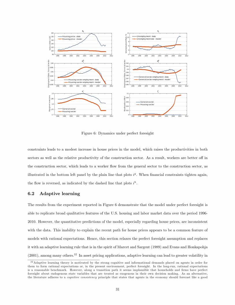
1996 1998 2000 2002 2004 2006 2008 2010 2012
Inde
x 199
6=10
0
80
100
120
140
160
180
200qt
Hous ing price dataHous ing price model
1996 1998 2000 2002 2004 2006 2008 2010 2012
Une
mp
loym
ent R
ate
, %
2
4
6
8
10
12ut
Unemployment dataUnemployment rate model
1996 1998 2000 2002 2004 2006 2008 2010 2012Empl
oym
ent R
ate
, Gen
eral
sec
tor
0.035
0.04
0.045
0.05
0.055
0.06nh
t
Hous ing sector employment dataHous ing sector employment model
1996 1998 2000 2002 2004 2006 2008 2010 2012Empl
oym
ent R
ate
, Gen
eral
sec
tor
0.85
0.86
0.87
0.88
0.89
0.9
0.91
0.92ng
t
General sector employment dataGeneral sector employment model
1996 1998 2000 2002 2004 2006 2008 2010 2012
Mar
gina
l re
venu
es
1.7
1.75
1.8
1.85
1.9z@t
General sectorHous ing sector
1996 1998 2000 2002 2004 2006 2008 2010 2012
Rea
lloca
tion
effo
rt
0
0.02
0.04
0.06
0.08
0.1i@t
General sectorHous ing sector
Figure 6: Dynamics under perfect foresight
constraints leads to a modest increase in house prices in the model, which raises the productivities in both
sectors as well as the relative productivity of the construction sector. As a result, workers are better o¤ in
the construction sector, which leads to a worker �ow from the general sector to the construction sector, as
illustrated in the bottom left panel by the plain line that plots ig. When �nancial constraints tighten again,
the �ow is reversed, as indicated by the dashed line that plots ih.
6.2 Adaptive learning
The results from the experiment reported in Figure 6 demonstrate that the model under perfect foresight is
able to replicate broad qualitative features of the U.S. housing and labor market data over the period 1996-
2010. However, the quantitative predictions of the model, especially regarding house prices, are inconsistent
with the data. This inability to explain the recent path for house prices appears to be a common feature of
models with rational expectations. Hence, this section relaxes the perfect foresight assumption and replaces
it with an adaptive learning rule that is in the spirit of Marcet and Sargent (1989) and Evans and Honkapohja
(2001), among many others.32 In asset pricing applications, adaptive learning can lead to greater volatility in
32Adaptive learning theory is motivated by the strong cognitive and informational demands placed on agents in order forthem to form rational expectations or, in the present environment, perfect foresight. In the long-run, rational expectationsis a reasonable benchmark. However, along a transition path it seems implausible that households and �rms have perfectforesight about endogenous state variables that are treated as exogenous in their own decision making. As an alternative,the literature adheres to a cognitive consistency principle that states that agents in the economy should forecast like a good
31

response to economic shocks because these models are self-referential and impart a key role to forward-looking
expectations.
To make decisions, households and �rms must form expectations about house prices, qt+1, sector-speci�c
market tightness, ��t+1, and the value of intersector mobility4Ut+1. Regarding the last two variables, �� and
4U , we assume a simple model of learning that preserves many of the features of rational expectations: agents
in the economy know the new steady-state values for the variables of economic interest but are uncertain
about the transition path. These assumptions lead us to propose a simple �anchoring and adjustment�rule
of the form identi�ed by Hommes (2013). Letting xet+1 denote forecasts of the next period value of a state
variable xt, the forecast rule is as follows,
xet+1 = �x+ xgxt�1 (xt�1 � �x) (50)
gxt = gxt�1 + g
�xtxt�1
� gxt�1�; (51)
where �x is the steady-state value of the state x, gxt is a measure of the gross-growth rate of x at time t (details
to be speci�ed below), and x � 0. The anchoring-and-adjustment learning rule, (50), has two components.
The �rst component, the "anchor," is the new steady-state value of the variable, xt, given �t. Hence, agents
are quite sophisticated in that they know the long-run fundamental value of the variable they are forecasting
but are uncertain about its transition path. The second component in (50) is a persistent, or trend-following
component according to which beliefs extrapolate based on deviations from steady state at a rate depending
on the slope of the transition path, gx.33 The adaptive learning rule for the gross growth rate of x, gx, is
given by (51). The parameter g is called a �gain�coe¢ cient as it parameterizes how strongly the learning
rule discounts past data in estimating gx.
Regarding the forecasting model for house prices we need a learning rule able to generate a large house
price appreciation followed by a crash. To capture this feature of the data, we extend the learning model to
incorporate strongly extrapolative house-price expectations:
qet+1 = 1gqt�1qt�1: (52)
In (52), agents forecast house prices as the growth rate times the most recent data point with an extrapolating
coe¢ cient 1, where the estimate for the gross growth rate, gq, is given by (51). When 1 = 1, this rule
econometrician, or Bayesian, by specifying a forecasting model and revising their speci�cation in light of recent data. Typically,these forecasting models are econometric forecasting equations whose parameters are updated using a version of ordinary ordiscounted least-squares.33 It is worth noticing that the learning rule (50) nests rational expectations in a steady state, thus asymptotically these beliefs
converge to their rational expectations values.
32

nests the rational expectations equilibrium.34 In our calibration exercise, we allow for 1 � 1, which can
be justi�ed in two ways. First, we interpret (52) as an approximation to a fully speci�ed learning rule that
might arise for a �nite stretch of time in a stochastic model where 1 is estimated over time via discounted
least-squares in an AR(1) regression of the growth rate. The approximate learning rule (52) implies that a
self-ful�lling drift can arise that leads agents to perceive a trend in house prices.35 Second, we restrict 1 so
that in the steady state agents�forecast errors are small, on the order of 0:2% in the calibration exercise.
In the calibration exercise, we select 1; �; 4U ; �1 to minimize the mean-squared distance between
model-implied paths for qt; ngt ; n
ht ; ut, and their counterparts in the data. To avoid over�tting, we impose
that �0 = 1; g = 4U . We �nd that the best �tting parameters are �1 = 1:295; 4U = 0:16; 1 = 1:0025,
and � = 1:2. The values for the learning-rule parameters lead to a stable steady state, i.e., the learning
economy converges to the steady state. Figure 7 plots the equilibrium dynamics under learning.36
As before, the solid lines are the equilibrium paths and the dashed lines are the corresponding data
series. Under learning house prices in the model capture the peak house price appreciation in the data. The
magnitude of the drop in prices from 2005-2010 is in line with data.The improved �t in house prices leads to
a much improved �t in construction employment shares. Revenues in the construction sector (bottom right
panel) increase signi�cantly from 1996-2005, which leads to an increase in employment and labor mobility
from the general to the construction sector. Employment in the construction sector broadly follows the same
increase as the one observed in the data over this period, about one percentage point. From 2006-2010,
the data and the model feature an even greater drop in construction employment. The model also captures
the trend in nonconstruction employment. The initial increase in the general sector productivity, zg, that
arises from the increased � leads to a strong increase in ng. However, the strong house price appreciation
eventually leads to a relative increase in the share of construction sector employment, nh=(nh + ng), and
a reallocation of workers toward the construction sector. Moreover, as the housing boom crashes, so does
34This rule is of the same form as the one used by Adam, Marcet and Nicolini (2013) to study asset pricing under learning.35Learning dynamics with self-ful�lling volatility are a general feature of learning models along the lines described above in
a wide class of forward-looking stochastic models. Branch (2014) studies a stochastic search-based asset pricing model with apricing equation very similar to the house price equation in this paper and where rational expectations replaced by an AR(1)econometric learning rule. The parameters of this learning rule are updated using discounted least-squares. He shows thatbubbles can arise from an overshooting e¤ect from structural changes to the asset�s liquidity, such as its acceptability �. Thesebubbles arise as beliefs endogenously evolve to perceive the asset price as following a random walk without drift � in this case,recent price innovations are temporarily perceived to be permanent leading to an overshooting of the new fundamental pricethat will eventually collapse and return to its fundamental value. Thus, the learning rule (52) captures in a nonstochasticenvironment this general feature in learning models (See Sargent, 1999).36We checked for robustness across a wide range of learning model speci�cations, including a model where all expectations are
of the form (50), a model without the growth rate terms, �constant gain�algorithms that take a geometric average of past data,and even learning models that include contemporaneous endogenous variables in the forecasts. Across all of these speci�cationsthere is a consistent set of quantitative results: house prices increase modestly, goods sector employment matches up well withthe data, and there is a slight increase in construction sector employment share. The key to a good empirical �t is a model ofexpectation formation that leads to a housing price boom, such as (52).
33

1996 1998 2000 2002 2004 2006 2008 2010 2012
Inde
x 199
6=10
0
100
120
140
160
180
200qt
Hous ing price dataHous ing price model
1996 1998 2000 2002 2004 2006 2008 2010 2012
Unem
ploy
men
t Ra
te, %
2
4
6
8
10
12ut
Unemployment dataUnemployment rate model
1996 1998 2000 2002 2004 2006 2008 2010 2012Empl
oym
ent R
ate,
Hou
sing
sect
or
0.035
0.04
0.045
0.05
0.055nh
t
Hous ing sector employment dataHous ing sector employment model
1996 1998 2000 2002 2004 2006 2008 2010 2012Empl
oym
ent R
ate,
Gen
eral
sec
tor
0.84
0.86
0.88
0.9
0.92ng
t
General sec tor employment dataGeneral sec tor employment model
1996 1998 2000 2002 2004 2006 2008 2010 2012
Mar
gina
l rev
enue
s
1.5
2
2.5
3
3.5z@t
General sec torHous ing sector
1996 1998 2000 2002 2004 2006 2008 2010 2012
Real
loca
tion
effo
rt
10 3
0
0.5
1
1.5
2
2.5
3i@t
General sec torHous ing sector
Figure 7: Equilibrium dynamics under learning
employment in the non-construction goods sector.
The lower right panel plots the model implied unemployment against actual U.S. unemployment rate
(dashed line). The aggregate unemployment rate in the model declines about 1.5% from 1996 to 2005 and
it increases above 10% in 2010, which is consistent with the data. Not surprisingly, the model misses the
�uctuations of the unemployment rate following the 2001 recession. Since the housing market was insulated
from this recession there is no mechanism in the model that can capture the changes in unemployment over
that period.
7 Conclusion
We have studied the e¤ects of changes in household �nance on the labor and housing markets. We have
constructed a tractable general equilibrium model that generalizes the Mortensen-Pissarides framework along
several dimensions: The labor market has two sectors, including a construction sector. There is a frictional
goods market, where household consumption is �nanced with collateralized or unsecured loans. There is a
housing market where households can rent housing services and buy and sell homes. The model has generated
a variety of new insights� e.g., how �nancial frictions and liquidity constraints provide new linkages between
goods, housing, and labor markets� and it has been used to study analytically how changes in households�
34

eligibility for home equity loans a¤ect the dynamics of house prices and aggregate unemployment.
We calibrated the model to the U.S. economy and showed that it could capture salient features of U.S.
housing and labor market data, including: a sustained increase, followed by sharp decrease, in home equity
�nanced consumption; a large house price boom/crash; a sustained decrease in the aggregate unemployment
rate during the house price boom followed by a sharp increase in the unemployment rate as house prices
collapse; and a sizable increase in the share of employment in the construction sector during the house
price boom. Figure 6 obtained under perfect foresight captures these empirical regularities and the learning
version, Figure 7, provides a good quantitative �t. Therefore, the model presented here, with explicit a
housing market, labor and goods market with explicit frictions, can capture many of the salient features of
housing prices, unemployment, and sectoral labor �ows.
35

References
[1] Abdallah, Chadi, and William Lastrapes (2012). "Home equity lending and retail spending: Evidence
from a natural experiment in Texas," American Economic Journal: Macroeconomics 4, 94-125.
[2] Adam, Klaus, Albert Marcet and Juan-Pablo Nicolini (2013). �Stock Market Volatility and Learning,�
working paper.
[3] Adelino, Manuel, Antoinette Schoar and Felipe Severino (2012). "Credit supply and house prices: Evi-
dence from mortgage market segmentation," Mineo, Duque University.
[4] Aruoba, Boragan, Guillaume Rocheteau and Christopher Waller (2007). "Bargaining and the value of
money," Journal of Monetary Economics 54, 2636�2655.
[5] Berentsen, Aleksander, Guido Menzio and Randall Wright (2011). �In�ation and unemployment in the
long run,�American Economic Review, 101, 371�98.
[6] Bethune, Zach, Guillaume Rocheteau, and Peter Rupert (2013). "Unemployment and household unse-
cured debt," Working Paper, University of California, Irvine.
[7] Branch, William A. and George W. Evans (2011). �Learning about Risk and Return: A Simple Model
of Bubbles and Crashes,�American Economic Journal: Macroeconomics, 3, 159-191.
[8] Branch, William A. (2014). �Imperfect Knowledge, Liquidity and Bubbles,�working paper.
[9] Byun, Kathryn (2010). "The U.S. housing bubble and bust: impacts on employment," Bureau of Labor
and Statistics Monthly Review (December), 3-17.
[10] Campbell, John, and Joao Cocco (2007). "How do house prices a¤ect consumption? Evidence from
micro data," Journal of Monetary Economics 54, 591�621.
[11] Chang, Briana (2012). "A search theory of sectoral reallocation," Working Paper.
[12] Davis, Steven, Jason Faberman and John Haltiwanger (2010). "The establishment-level behavior of
vacancies and hiring," NBER working Paper No. 16265.
[13] Den Haan, Wouter, Garey Ramey, and Joel Watson (2000). "Job destruction and propagation of shocks,"
American Economic Review 90, 482-498.
36
[14] Ducca, John, John Muellbauer and Anthony Murphy (2011). " House prices and credit constraints:
making sense of the US experience," Economic Journal 121, 533-551.
[15] Dugan, John (2008). "Rising losses in home equity lending," Remarks by the Comptroller of the Currency
Before the Housing Policy Council of the Financial Services Roundtable, May 22, 2008. Available at:
http://www.occ.gov/news-issuances/speeches/2008/pub-speech-2008-58.pdf
[16] Evans, George W., and Seppo Honkapohja (2001). Learning and Expectations in Macroeconomics.
Princeton, NJ: Princeton University Press.
[17] Evans, George W., and Bruce McGough (2014). �Learning to Optimize,�working paper.
[18] Ferraris, Leo, and Makoto Watanabe (2008). "Collateral secured loans in a monetary economy," Journal
of Economic Theory 143, 405-424.
[19] Garriga, Carlos, Rodolfo Manuelli, and Adrian Peralta-Alva (2012). "A model of price swings in the
housing market," Federal Reserve Bank of St Louis Working Paper 2012-022A.
[20] Geromichalos, A., J. M. Licari and J. Suarez-Lledo (2007). �Monetary policy and asset prices,�Review
of Economic Dynamics 10, 761�779.
[21] Gomme, Paul, and Peter Rupert (2007). "Theory, measurement and calibration of macroeconomic
models". Journal of Monetary Economics 54, 460-497.
[22] Greenspan, Alan, and James Kennedy (2007). "Sources and uses of equity extracted from homes," Sta¤
Working Papers in the Finance and Economics Discussion Series of the Federal Reserve Board 2007-20.
[23] Harding, John, Stuart Rosenthal, and C.F. Sirmans (2007). "Depreciation of housing capital, mainte-
nance, and house price in�ation: Estimates from a repeat sales model," Journal of Urban Economics
61, 193�217.
[24] He, Chao, Randall Wright, and Yu Zhu (2013). "Housing and liquidity," Working Paper of the University
of Wisconsin.
[25] Head, Allen and Huw Lloyd-Ellis (2011). "Housing liquidity, mobility, and the labour market," Review
of Economic Studies (Forthcoming).
[26] Hommes, Cars (2013). Behavioral Rationality and Heterogeneous Expectations in Complex Economic
Systems. Cambridge, UK: Cambridge University Press.
37

[27] Iacoviello, Matteo (2011). �Housing wealth and consumption,� International Encyclopedia of Housing
and Home, Elsevier.
[28] Karahan, Fatih, and Serena Rhee (2012). "Housing and the labor market: The role of migration on
aggregate unemployment," Working Paper.
[29] Kiyotaki, Nobuhiro, and John Moore (1997). "Credit cycles," Journal of Political Economy 105, 211-248.
[30] Kiyotaki, Nobuhiro, and John Moore (2005). �Liquidity and asset prices,� International Economic
Review 46, 317-349.
[31] Lagos, Ricardo (2010). "Asset prices and liquidity in an exchange economy," Journal of Monetary
Economics 57, 913-30.
[32] Lagos, Ricardo (2011). "Asset prices, liquidity, and monetary policy in an exchange economy," Journal
of Money, Credit, and Banking 43, 521-552.
[33] Lagos, Ricardo and Randall Wright (2005). "A uni�ed framework for monetary theory and policy
analysis," Journal of Political Economy 113, 463�484.
[34] Lester, Ben, Postlewaite, Andrew, Wright, Randall (2012). "Information, liquidity, asset prices and
monetary policy," Review of Economic Studies 79, 1209-1238.
[35] Li, Ying-Syuan and Li, Yiting, 2013. "Liquidity and asset prices: A new monetarist approach," Journal
of Monetary Economics 60, 426-438.
[36] Li, Yiting, Guillaume Rocheteau, and Pierre-Olivier Weill (2012). "Liquidity and the threat of fraudulent
assets," Journal of Political Economy 120, 815-846.
[37] Lucas, Robert, and Prescott, Ed (1974). "Equilibrium search and unemployment," Journal of Economic
Theory 7, 188�209.
[38] Mankiw, Gregory and David Weil (1989). "The baby boom, the baby bust, and the housing market,"
Regional Science and Urban Economics 19, 235-258.
[39] Marcet, Albert and Thomas J. Sargent (1989). �Convergence of Least-Squares Learning Mechanisms in
Self-Referential Models,�Journal of Economic Theory, 48, 337-368.
38

[40] Mian, Atif, and Amir Su� (2009). "House prices, home equity-based borrowing, and the U.S. household
leverage crisis," NBER Working Paper 15283.
[41] Mian, Atif, and Amir Su�(2012). "What explains high unemployment? The aggregate demand channel,"
NBER Working Paper 17830.
[42] Mian, Atif, and Amir Su� (2014a). House of Debt. Chicago, IL: University of Chicago Press.
[43] Mian, Atif, and Amir Su� (2014b). �House Price Gains and U.S. Household Spending from 2002 to
2006,�working paper.
[44] Midrigan, Virgiliu and Thomas Philippon (2011). "Household leverage and the recession," Working
Paper.
[45] Mortensen, Dale, and Christopher Pissarides (1994). "Job creation and job destruction in the theory of
unemployment," The Review of Economic Studies 61, 397-415.
[46] Mulligan, Casey (2012). "Do welfare policies matter for labor market aggregates? Quantifying safety
net work incentives since 2007," NBER working paper 18088.
[47] Petrosky-Nadeau, Nicolas (2013). "TFP During a Credit Crunch," Journal of Economic Theory, 148,3,
1150-1178.
[48] Petrosky-Nadeau, Nicolas, and Etienne Wasmer (2011). "Macroeconomic dynamics in a model of goods,
labor and credit market frictions," mimeo, Carnegie Mellon University.
[49] Petrongolo, Barbara and Pissarides, Christopher A. (2001). "Looking into the black box: A survey of
the matching function," Journal of Economic Literature 39, 390�431.
[50] Petrosky-Nadeau, Nicolas, and Etienne Wasmer (2012). "The cyclical volatility of labor markets under
frictional �nancial markets," American Economics Journal: Macroeconomics, forthcoming.
[51] Phelan, Christopher, and Alberto Trejos (2000). "The aggregate e¤ects of sectoral reallocations," Journal
of Monetary Economics 45, 249-268.
[52] Pissarides, Christopher (2000). Equilibrium Unemployment Theory. (Second Ed.). Cambridge, MA:
MIT Press.
39

[53] Rocheteau, Guillaume (2011). "Payments and liquidity under adverse selection," Journal of Monetary
Economics 58, 191-205.
[54] Rocheteau, Guillaume, Peter Rupert and Randall Wright (2007). "In�ation and unemployment in gen-
eral equilibrium," Scandavian Journal of Economics 109, 837�855.
[55] Rocheteau, Guillaume and Randall Wright (2005). "Money in search equilibrium, in competitive equi-
librium, and in competitive search equilibrium," Econometrica 73, 175�202.
[56] Rocheteau, Guillaume and Randall Wright (2013). "Liquidity and asset-market dynamics," Journal of
Monetary Economics 60, 275-294.
[57] Rosen, Harvey (1979). "Housing decisions and the US. income tax," Journal of Public Economics 11,
1-23.
[58] Rudanko, Leena (2011). "Aggregate and idiosyncratic risk in a frictional labor market," American
Economic Review 101, 2823-2843.
[59] Rupert, Peter, and Etienne Wasmer (2012). "Housing and the labor market: Time to move and aggregate
unemployment," Journal of Monetary Economics 59, 24-36.
[60] Sargent, Thomas J. (1999). The Conquest of American In�ation. Princeton, NJ: Princeton University
Press.
[61] Shi, Shouyong (1998). "Search for a monetary propagation mechanism," Journal of Economic Theory
81, 314-352.
[62] Telyukova, Irina and Randall Wright (2008). "A model of money and credit, with application to the
credit card debt puzzle," Review of Economic Studies 75, 629�647.
[63] Timmermann, Allan (1994). �Excess Volatility and Predictability of Stock Returns in Autoregressive
Dividend Models with Learning,�Review of Economic Studies, 523-447.
[64] Wasmer, Etienne, and Philippe Weil (2004). "The macroeconomics of labor and credit market imper-
fections," American Economic Review 94, 944-963.
40

Appendix: Proofs of propositions
Proof of Proposition 1. As it has been shown in the text Condition (38) guarantees the existence of
an equilibrium with two active markets. Market tightness, �, is the unique solution to (37). The left side of
(37) is increasing in � and the right side is increasing in �zg. Therefore, @�=@�zg > 0. By a similar reasoning
one obtains the comparative statics for � in the second row of the table. The unemployment rate is u =
�= [m(1; �) + �]. The comparative statics for u are obtained from the comparative statics for �. For instance,
since u is decreasing in �, @u=@�zg < 0. Employment in the housing sector is nh = �#0�1�(r + �)�zg=�zh
�=�zh.
Since #0 is decreasing it follows that @nh=@�zg < 0. Moreover, di¤erentiating #0�nh�zh=�
�= (r+ �)�zg=�zh and
using that �zhnh=� = A, we obtain the following elasticity:
@nh=nh
@�zh=�zh=�#0 (A)A#00 (A)
� 1:
So @nh=@�zh > 0 if��#0 (A) =A#00 (A)�� > 1. An increase in the marginal utility of housing services, #0, leads to
an increase in nh. Employment in the consumption goods sector is determined by ng = 1�u�nh. Therefore,
@ng=@�zg = �@u=@�zg � @nh=@�zg > 0. The rest of the comparative statics for ng follow a same logic. The
stock of housing is given by A = #0�1�(r + �)�zg=�zh
�. Since #0 is decreasing, @A=@�zg < 0 and @A=@�zh > 0.
An increase in the marginal utility for housing services increases the supply of homes. Finally, house prices
are q = �zg=�zh so that @q=@�zg > 0 and @q=@�zh < 0.
Proof of Proposition 2. The statements in the proposition are proven in the text. In the follow-
ing we explain how we obtained the comparative statics for the case where liquidity is scarce, #0(A)A <
r�b(y�)= (1 + r) �. The pair of endogenous variables, (q; �), is jointly determined by (39) and (41). Both
equations give a positive relationship between � and q. Since the equilibrium might not be unique, we focus
on equilibria where the HP curve �representing (41)� intersects the JC curve �representing (39)� from
below, in the space (q; �). From (39), given q an increase in �z or � raises �. Graphically JC moves upward.
From (41), given � an increase in �z or � does not a¤ect q. Graphically, HP does not shift. It follows that
the equilibrium values of � and q increase. By a similar reasoning, an increase in �, w0, �, or k moves JC
downward without a¤ecting HP . Therefore, � and q decrease. We show in the text that an increase in
� shifts JC upward. From (41) an increase in � reduces the stock of housing of homeowners, A=�, which
reduces y and increases the liquidity premium on housing for a given �. Therefore, HP moves to the right.
The overall e¤ect is an increase in both � and q. An increase in � raises market tightness given by (39) for a
given q. So HP moves upward. The e¤ect on house prices given by (41) is ambiguous. Finally, given � the
41

unemployment rate is determined by u = �= [m(1; �) + �].
Derivation of the wage equation (21) The �rm�s surplus, J�, is given by (18). From (8), (14), and
(15) the value of an employed household holding its optimal level of liquid assets solves
V �1;t = w�1;t +$t + �
�(1� ��)V �1;t+1 + ��V
�0;t+1
�; � 2 fh; gg; (53)
where
$t = E [� (yt)� yt] + [qt (1� �) +Rt] at � qtat+1 +maxdt�0
f#(dt)�Rtdtg+�t: (54)
From the �rst two terms on the right side of (53) the period-t utility of an employed household is the sum of
the wage paid by the �rm, the expected surplus in the DM goods market, the return on its real estate net of
depreciation, the utility of housing services net of the rental cost, and �rms�pro�ts. The third term on the
right side of (53) describes the transitions in the next LM. With probability 1 � �� the household remains
employed in the following period and enjoys the discounted utility �V �1;t+1; with complement probability,
��, the household loses its job and its discounted utility is �V �0;t+1. Substract V�0;t on both sides to obtain
the surplus of an employed worker,
V �1;t � V�0;t = w
�1;t +$t + �
�(1� ��)V �1;t+1 + ��V
�0;t+1
�� V �0;t: (55)
From (18) and (55) the total surplus of a match, S�t � V�1;t � V
�0;t + J
�t , solves the following recursion:
S�t = z�t +$t � V �0;t + �V
�0;t+1 + �(1� ��)S
�t+1: (56)
From the bargaining solution, V �1;t � V�0;t = ��S�t , which from (55) and (56) gives the following expression
for the wage:
w�1;t = ��z�t + (1� ��)
�V �0;t � �V
�0;t+1 �$t
�: (57)
The wage is a weighted average of the �rm�s expected revenue, z�t , and the worker�s reservation wage is
de�ned as V �0;t � �V�0;t+1 �$t.
Using the same reasoning as above, the expected discounted utility of an unemployed household at the
beginning of the LM is
V �0;t = w�0 +$t + �
�V �0;t+1 + p
�t+1
�V �1;t+1 � V
�0;t+1
��+
�i�t+1
�: (58)
The third term on the right side of (58) is the household continuation value if it does not relocate to a
new sector. The last term on the right side of (58) captures the net expected gain that a household enjoys
42

from moving to a di¤erent sector. From the bargaining solution, V �1;t � V�0;t =
��
1��� J�t ; from free entry,
J�t = k�=�f�t . Therefore, from (58), the value of an unemployed household can be expressed as
V �0;t = �V�0;t+1 + w
�0 +$t +
��
1� �� ��t+1k
� +�i�t+1
�: (59)
Substitute V �0;t � �V�0;t+1 from (59) into (57) to obtain (21).
Sectoral reallocation: Derivation of Equation (22) From the Bellman equation, U�0;t(at) = p�t V
�1;t(at)+
(1� p�t )V�0;t(at), and the surplus sharing rule, �p
�t
�V �1;t � V
�0;t
�= ����t k
�=(1 � ��), the gain from moving
to a di¤erent sector, �U�t � ��U�
0
0;t � U�0;t
�, can be expressed as
�U�t = ��V �
0
0;t � V�0;t
�+
��0
1� ��0��
0
t k�0 � ��
1� �� ��t k
�:
This is equal to the surplus an unemployed worker would enjoy in the DM from being in a di¤erent sector
augmented by a term proportional to the di¤erence of average recruiting costs across sectors. Using the fact
that V �0;t = w�0 +$t + �U
�0;t+1 +
�i�t+1
�, one obtains (22).
43

For Online Publication
A Data Appendix
The data used in calibrating the model are the following:
Job destruction rates: Total Separation - Non-Farm; FRED II I.D. JTSTSR. Total Separation - Construc-
tion; FRED II I.D. JTU2300TSR
Employment: All Employees - Total Non-Farml; FRED II I.D. PAYEMS. All Employees - Constructions;
FRED II I.D. USCONS
Unemployment: Aggregate Unemployment: UNEMPLOY. Construction Unemployment; FRED II I.D.
LNU03032231.
Housing Stock and GPD: Real Estate Assets, Balance Sheet of Households and Non-Pro�t Organizations;
FRED II I.D. REABSHNO. Gross Domestic Product; FRED II I.D. GDP.
Rent to Price Ratio: Lincoln Institute of Land Policy.
Equity Financed Consumption: Greenspan and Kennedy (2007).
44

Appendix: Model with Adaptive Learning
This Appendix details the key equations in the model under adaptive learning. Households and �rms are
assumed to form forecasts, generated by learning rule (50), for payo¤-relevant aggregate variables that are
taken as exogenous when making their optimal decisions. As in the perfect foresight case, agents take the �t
shock to be unanticipated and permanent. Given a �t they calculate the new steady state and, then, using
the most recently observed data, form expectations about the next realization of the aggregate state variables
qt; �gt ; �
ht ;4Ut. Adaptive learning models are sometimes complicated by the evolving beliefs of optimizing
agents and the literature di¤ers on whether to treat the agents as fully Bayesian decision-makers that account
for the future evolution of their beliefs when formulating their optimal plans.37 In the present environment,
these issues are not directly relevant since the (temporary) equilibrium equations are nonstochastic and the
quasi-linearity assumptions in the CM utility function eliminate wealth e¤ects. Agents in this model are able
to iterate their forecasts forward as the coe¢ cients in the forecasting model are �xed. There are, however,
two key behavioral assumptions that we impose on agents. First, households and �rms form their forecasts
after observing �t but before observing contemporaneous market-clearing state variables. This is a standard
assumption in the literature and is designed to break the simultaneity between beliefs and outcomes that
are natural in a rational expectations setting but implausible in a learning environment. Second, agents
hold point expectations when satisfying their optimization conditions. Again, because of the nonstochastic
nature of the model this assumption is natural.
The timing of the model is as follows. At the beginning of period t, a new unanticipated shock to �t
occurs. Agents observe this, calculate the new steady state, and update their expectations conditional on
observing data that were realized at the end of the CM in t � 1, i.e. qt�1;4Ut�1. Subsequently, the LM
opens with �rms choosing to post vacancies given their expectations about trade in the DM in period t, as
well as the vacancy rate in t + 1. The pool of unemployed workers in each sector depends on the previous
pool of unemployed and the aggregate mobility decisions of agents that were made at the end of period t�1.
These decisions depend on the expected value of mobility, 4Ut, that are made conditional on data through
the end of t � 1. The labor market clears and �t is realized. Agents subsequently revise their expectations
about �t+1 given this new data point. The DM then opens, �rms and households are matched, and they
bargain given their expectations. After the DM closes, the CM opens and households payo¤ their debts from
37See Evans and McGough (2014) for discussion of various decision theoretic issues in boundedly rational macroeconomicmodels.
45
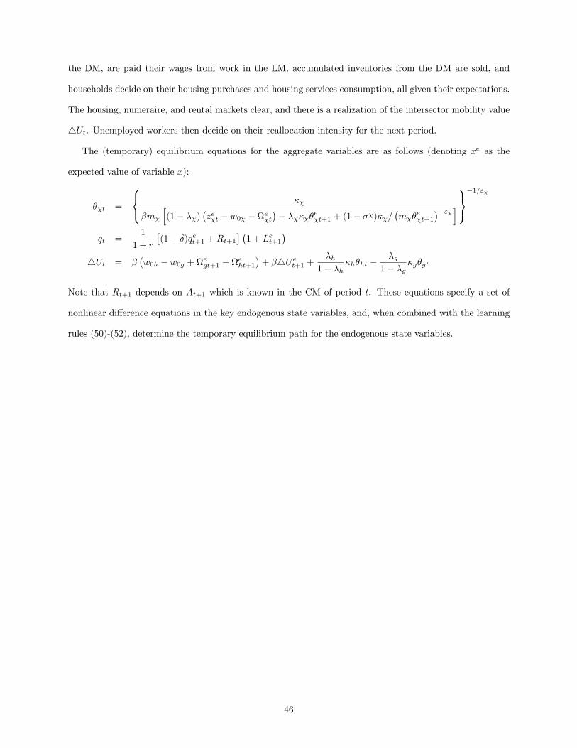
the DM, are paid their wages from work in the LM, accumulated inventories from the DM are sold, and
households decide on their housing purchases and housing services consumption, all given their expectations.
The housing, numeraire, and rental markets clear, and there is a realization of the intersector mobility value
4Ut. Unemployed workers then decide on their reallocation intensity for the next period.
The (temporary) equilibrium equations for the aggregate variables are as follows (denoting xe as the
expected value of variable x):
��t =
8<: ��
�m�
h(1� ��)
�ze�t � w0� � e�t
�� �����e�t+1 + (1� ��)��=
�m��
e�t+1
��"�i9=;�1="�
qt =1
1 + r
�(1� �)qet+1 +Rt+1
� �1 + Let+1
�4Ut = �
�w0h � w0g +egt+1 � eht+1
�+ �4Uet+1 +
�h1� �h
�h�ht ��g
1� �g�g�gt
Note that Rt+1 depends on At+1 which is known in the CM of period t. These equations specify a set of
nonlinear di¤erence equations in the key endogenous state variables, and, when combined with the learning
rules (50)-(52), determine the temporary equilibrium path for the endogenous state variables.
46
Related Documents


