Financial Fragility with Rational and Irrational Exuberance

Financial Fragility with Rational and Irrational Exuberance

ROGER LAGUNOFF AND STACEY L. SCHREFT*

October 1998Last Revised: January 1999

Abstract

This article formalizes investor rationality and irrationality, exuberance and apprehension, toconsider the implications of belief formation for the fragility of an economy’s financial structure.The model presented generates a financial structure with portfolio linkages that make it susceptibleto contagious financial crises, despite the absence of coordination failures. Investors forecast thelikelihood of loss from contagion and may shift preemptively to safer portfolios, breaking portfoliolinkages in the process. The entire financial structure collapses when the last group of investorsreallocates their portfolios. If some investors are irrationally exuberant, the financial structureremains intact longer. In fact, financial collapse occurs sooner when almost all investors arerationally exuberant than when they are irrationally exuberant. Additionally, a financial crisisinitiated by real shocks is indistinguishable from one caused solely by the presence of rationallyapprehensive investors in a fundamentally sound economy. Policies that make portfolio linkagesmore resilient can improve welfare.

JEL Codes: E44, G1, C73Key Words: financial fragility, contagion, irrational exuberance, financial crises

* Lagunoff, Department of Economics, Georgetown University, Washington, D.C., 20057, 202-687-1510,[email protected]; Schreft, Research Department, Federal Reserve Bank of Kansas City, Kansas City,MO 64198, 816-881-2581, [email protected]. The authors thank John Golob, Tom Humphrey, Will Roberds,discussants John Weinberg and Narayana Kocherlakota, and the referees for their comments. The views expressed inthis paper are not necessarily those of the Federal Reserve Bank of Kansas City or the Federal Reserve System.

[W]hat does it mean to say that markets are rational? Is it assumed that mostmarkets behave rationally most of the time, or that each and every participant in themarket has the same intelligence, the same information, the same purposes, and thesame economic model in mind, or that all markets behave rationally all the time? … .Frequently the argument seems to be between two polar positions, one that holds thatno market is ever rational, the other that all markets are always so. [Kindleberger,1996, p. 20]

I. Introduction

Economists from Cantillon to Kindleberger have speculated about whether financial markets

are fully rational or with some frequency over- or undervalue assets relative to the assets’

fundamentals.1 This interest in the rationality of financial markets has been fueled by repeated

episodes of apparent irrationality, from the Dutch Tulipmania in 1637, to the British South Sea

bubble in 1720, to the Japanese real estate bubble in the late 1980s.2 And it has not been confined

to academic circles. In December 1996, with the Dow Jones Industrial Average reaching new

heights, Federal Reserve Board Chairman Alan Greenspan suggested that “irrational exuberance”

could lead to “unduly escalated asset values, which then become subject to unexpected and

prolonged contractions,” and questioned how such a situation could be identified and how monetary

policy should react. In April 1998, Eisuke Sakakibara, Japan’s vice finance minister for

international affairs, described the Japanese economy as suffering from “irrational pessimism.”

Since then, economists worldwide have pondered what it means for financial-market participants to

hold irrational beliefs and whether their doing so is bad in some appropriate sense.

This article attempts to address these questions. Given the nature of the questions, the

answers necessarily depend on how rationality and exuberance— or the lack thereof— are

interpreted. The approach adopted regarding rationality is the one common to much of late-20th-

century macroeconomics.3 Specifically, rational investors are assumed to have rational

expectations. That is, they maximize an objective function subject to perceived constraints, and

1 Eighteenth-century economist Richard Cantillon is likely the first economist to have written on this subject. In hisEssai sur la Nature du Commerce en Général, published posthumously in 1755, Cantillon writes about the role ofexpectations and differences in information across investors in foreign exchange speculation, the tendency of people tohold incorrect beliefs about fundamentals, and the South Sea bubble. He describes, albeit indirectly, the circumstancesthat generated the Mississippi bubble (1719-20), circumstances from which he profited greatly (Bordo 1983, Murphy1986).2 Kindleberger (1996) provides an extensive discussion of the relevant historical experience.3 What it means, however, for agents to be rational remains an open question within the economics profession generally.Arrow et al (1996) provide an overview of some of the unresolved issues.

2

they use all the information available to them, including the true probability distributions of the

economy’s random variables, when forming expectations. The implication, of course, is that

irrational, or boundedly rational, investors do not have rational expectations.4 In particular, they are

assumed to optimize, but to form expectations given their subjective, and incorrect, beliefs about the

distributions governing random variables. The subjective priors assumed generate posterior beliefs

that are the opposite of the beliefs held by rational investors.

The macroeconomics literature provides little guidance, however, regarding the modeling of

exuberance. Dictionaries define “exuberance” as the state of being joyously unrestrained and

enthusiastic. This definition is applied here by considering exuberant investors to be those who are

very optimistic about the prospects for the economy and thus for their investment portfolios. To

better isolate the effect of exuberance in financial markets, the implications of there being a fraction

of investors who are not exuberant are also examined. These apprehensive investors, as they are

called, perceive the economy’s fundamentals as poor and so expect losses on their portfolios.

To model rationality, exuberance, and apprehension under these interpretations, this paper

uses a variant of the model in Lagunoff and Schreft (1998). That model consists of many projects

that require funding to operate, and many investors who provide the necessary funds. The investors

initially hold portfolios that are linked in the sense that an investor’s expected and actual portfolio

returns depend on the portfolio choices of other investors. Identically and independently distributed

shocks to the projects’ operations can cause some projects to fail initially. All investors know the

probability of project failure and thus know the economy’s fundamentals. Realized project failures

break some portfolio linkages, which causes some investors to incur losses and reallocate their

portfolios, thereby breaking additional linkages. The initial project failures thus spark a contagious

financial crisis. Investors who foresee the crisis reducing their portfolio returns can protect

themselves if desired by preemptively shifting to a portfolio that is safer in that it reduces their

exposure to any ongoing contagion. Since all investors are identical, if one takes such preemptive

action, then they all do, causing the instantaneous collapse of all remaining portfolio linkages,

despite the absence of coordination failures. An economy is considered more fragile the earlier this

total financial collapse occurs.

4 This formulation of the distinction between rationality and irrationality is consistent with Sargent (1993).

3

The model presented below in Section II departs from the Lagunoff and Schreft model in

three critical respects. First, here the economy’s fundamentals are uncertain in that the probability

of project failure, the parameter that characterizes the iid stochastic process, is not known. This

requires investors to form expectations about both the fundamentals and their exposure to contagion

risk. Second, investors’ information about the fundamentals comes from a noisy signal that they

observe and use in forming their expectations. Since different investors can observe different

signals, heterogeneous beliefs are possible here, in contrast to the Lagunoff and Schreft paper. This

heterogeneity can apply to posterior beliefs about fundamentals, about other investors’ beliefs, and

about the representation of beliefs within the population. Finally, the equilibrium concept used here

differs from that in Lagunoff and Schreft in a subtle way. In Lagunoff and Schreft the goal is to

look at the inherent fragility of an economy, so the focus is on the set of equilibria that keeps the

economy’s financial structure intact the longest. As a device for finding such an equilibrium,

investors are assumed to make relatively optimistic forecasts. That is, they foresee the possibility of

contagion, but not of preemptive behavior. In contrast, in this paper investors make forecasts that

account for the possibility of both contagion and total financial collapse.

Two variants of the economy are studied. The first, presented in Section III, takes investors

to be rational as defined above and looks at fragility when the fundamentals are strong, so

exuberance is justified. The second, which is the subject of Section IV, assumes irrationality and

weak fundamentals. This organization is motivated by von Hayek’s (1937) belief that “[B]efore we

can explain why people commit mistakes, we must first explain why they should ever be right.”

Several intriguing findings emerge. First, exuberant investors remain invested at least as

long as their apprehensive counterparts, regardless of whether everyone is rational or irrational. As

a result, the portfolio choices of the exuberant investors necessarily determine the date of total

financial collapse, and thus the economy’s fragility. But the presence of apprehensive investors

also plays a critical role in determining fragility. An increase in the presence of apprehensive

investors in the economy makes the economy at least as fragile. This too is true whether everyone

is rational or irrational. And if there is at least one apprehensive investor in the economy, total

financial collapse can occur, regardless of the fundamentals and the rationality of investors. This is

the case even in an economy where all investors are rational and where the fundamentals are so

strong that nothing in the physical environment ever sparks a contagion. The reason is rooted in the

4

factors that generate apprehension. Investors who receive misleading information about the

fundamentals, even if they know the true model of the economy (i.e., have the correct prior),

perceive a contagious financial crisis as more likely than it actually is. Given this perception, they

believe they benefit from reallocating their portfolios to preempt experiencing portfolio losses. This

behavior by itself initiates a contagious financial crisis. The rationally exuberant investors in this

economy correctly forecast that the fundamentals make financial crises unlikely, but must respond

strategically to the portfolio reallocations they expect by the apprehensive investors. They choose

to reallocate their own portfolios to protect themselves against losses due to the contagion the

apprehensive investors initiate.

Interestingly, rationally exuberant investors who live in a fundamentally strong economy

reallocate their portfolios sooner than irrationally exuberant investors who live in a fundamentally

weak economy, which makes the strong economy the more fragile one. This finding stems from the

effect of irrationality on beliefs. Investors who form expectations irrationally misforecast the

behavior of other investors and thus misforecast the fundamentals by a larger margin than they

would if all investors were identical. As a result, irrational investors’ sentiments about the

fundamentals are more extreme than those of rational investors.

These results have some disturbing implications for policymakers concerned about

irrationality in financial markets. First, an economy with rationality is indistinguishable from one

with irrationality in terms of the types of financial crises experienced. Thus, an observer looking at

the realization of crises after the fact cannot tell whether the initial exuberance was rational or

irrational. Second, an economy with sound fundamentals and rational investors experiences total

financial collapse at the same date as some economy with particular weak fundamentals and

identical investors who know those fundamentals. This is discouraging news because it means that

a financial crisis that looks as if it were initiated by real shocks to the economy instead could have

been caused solely by the presence of rational, but unjustifiably apprehensive, investors.

Section V discusses the implications of these findings for welfare and policy. Since all

investors, whether rational or irrational, optimize, they are as well off as possible, conditional on the

signals they observe and their beliefs. There will always be some, however, who regret their

decisions. They are the ones who do not preemptively reallocate their portfolios in time to avoid

incurring losses from contagion. To reduce the likelihood of such regrets, policymakers can try to

5

eliminate contagion. A short-run policy option is for a lender of last resort to make loans to ensure

that no project lacks sufficient funding to operate solely because of contagious portfolio

reallocations. Section V explains that such a policy is problematic and ineffective because the

model, as specified, requires that loans go to investors. At best, the policy can stop contagion for a

period or two. Alternatively, if the model allowed for agents who operated the projects, loans could

go to them instead. That approach, however, brings with it moral-hazard problems. It remains an

open question whether the benefits from such a lending policy exceed the costs.

In the long run, policies aimed at strengthening an economy’s financial infrastructure can

prove effective. Examples include programs to obtain information about existing portfolio linkages

and to encourage diversification. Such policies reduce the likelihood of contagion by increasing the

resiliency of portfolio linkages and reducing the cost to investors if links do break. These policies,

like the lender-of-last-resort policy, must be implemented by an institution whose authority

encompasses all portfolio linkages.

A natural question, given the model’s results, is how this paper differs from the papers in the

large literature on bubbles. A bubble is said to exist when the price of an asset is inconsistent with

market fundamentals. In a narrow sense, then, the model presented here does not generate bubbles

because its asset prices are fixed. In a broader sense, however, this model is about bubbles.

Bubbles arise when the demands for assets deviate from what is justified by market fundamentals,

and such deviations in asset demands do occur in this model. When the demand for a project is

sufficiently high, the project operates and pays a positive net return. But when the demand falls

sufficiently, the project fails to operate, paying a zero return and having zero value thereafter.

When rational exuberance is the dominant sentiment, there is a period during which the demand for

projects is lower than what market fundamentals dictate. Likewise, when irrational exuberance is

prevalent, the demand for projects is sustained for a period of time beyond that justified by

fundamentals. Yet there still exists a date, although possibly infinity, at which the mere anticipation

of a sharp decline in the demand for some projects leads investors to dramatically reduce the

demand for all projects, driving their values to zero. In this sense, then, this paper is consistent with

the bubble literature.

6

II. The Economy

The model presented below is a variant of that in Lagunoff and Schreft that is more complex

in one sense and less so in another. The added complexity derives from the differences in the

models’ state variables. In Lagunoff and Schreft, the focus was on defining and characterizing

fragility and on assessing how fragility changes as an economy increases in size. Consequently, the

size of the economy was a key state variable, and the economy’s fundamentals were assumed

known to all investors. In this paper, in contrast, the objective is to see if investment behavior is

consistent with market fundamentals. As a result, the economy’s size is fixed, but there is

uncertainty about the fundamentals. Additionally, because different agents can observe different

signals about the fundamentals, heterogeneous beliefs are possible. This means that agents must

forecast not only the risk of loss associated with the various portfolios, but also the forecasts of

other investors about investment risks. To offset some of this added complexity, the model

presented here takes agents’ initial portfolio allocations as exogenous. Lagunoff and Schreft show,

however, that there exist economies for which the initial portfolios assumed here are held in

equilibria of the type studied in both papers.

A. The Physical Environment

Time is discrete and represented by t = 0, 1, … . The economy consists of k investors, each

endowed at date 0 with two units of an indivisible object known as dollars and with nothing at later

dates. Investors can provide for future consumption by investing their dollars in one of the

economy’s safe or risky assets. Each investor has access to a safe asset that pays zero interest. He

also has the option of investing in the economy’s k risky projects, which offer the chance of a higher

return.

Specifically, at each date a project yields a random return of R(I) dollars per dollar invested,

where I denotes the total number of dollars invested. Each project can be operated only if it has

sufficient funding. For simplicity, the critical level of funding— the level at which a project

operates and pays the maximum return per dollar, R — is taken to be $2. Projects that have less

than two dollars invested in them pay a gross return per dollar of zero. Once a project has been

insufficiently funded, it becomes inoperable at all future dates. When a project is overfunded, with

7

more than two dollars invested in it, decreasing returns are realized and the project yields a return

per dollar of 2 R /I.

At date 0 only, there is a second way by which a project can become inoperable:

independently and identically distributed shocks can cause projects to fail, pay a zero return, and

permanently cease operation. The true probability of a project’s failing from an exogenous shock is

represented by the random variable ℘ , which can take one of two values, either zero or p , where 0

< p ≤ 1. Once a project fails, it is forever inoperable. If a project succeeds at date 0, it pays a

return that depends on the amount invested, as described above.

In summary, then, a project’s return per dollar, assuming the project has not previously

ceased operation, satisfies

R I

RI

t I

RI

t I

t I

( )

,

,

,

=

℘ − ℘ ≥

> ≥

≥ <

R

S|||

T|||

02

1 2

22

0 2

with probability and with probability at = 0 if

at 0 if

at 0 if

where Rmax > R > 1. The upper bound Rmax is imposed for simplicity and assumed to be such that

no portfolio ever yields a dollar in interest, thus leaving investors with $3 to invest, and that no

investor who sustains a loss of any magnitude ever reinvests in more than one project. Given that

investors are initially endowed with $2 and that dollars are indivisible, the first condition implies

that R < 1.5, while the second, which rules out an unusual situation for notational simplicity,

requires R < 1.2.

The state of the economy depends on which value of ℘ is realized. The set of possible

states is ω ω1 2,l q , where state ω 1 represents the case of ℘ = 0 and ω 2 corresponds to the case of

℘ = p . Each state occurs with probability 0.5. Investors know that iid shocks are possible at date

0, but observe only a noisy signal of the true state, not the state itself. The set of possible signals is

x x1 2,l q . Investors differ based on which signal they observe: those observing signal x1 are of

type 1, while those observing x2 are of type 2. The probability that a random investor observes

signal xi in state ω j is Pr |xi jωd i. More specifically, Pr |xi iωb g = 1− ε and Pr |x j iωd i = ε, j ≠ i,

where ε is a known constant less than 0.5. That is, signal xi is more likely to be observed in state

ω i than in state ω j , and there is no aggregate uncertainty in the distribution of investor types. It

8

follows that if state ωi occurs, then a fraction 1− ε of investors is randomly selected to observe xi ,

while a fraction ε is randomly selected to observe x j . Investors thus can use the signal they

observe in forming expectations of the likelihood of each state and of the fraction of investors of

each type in the population. Investors who forecast that the state is ω 1 are taken to be exuberant

because they think the economy’s fundamentals, as measured by the probability of shocks at date 0,

are strong. Likewise, those who forecast state ω 2 are taken to be apprehensive.

While the true unconditional prior distribution over states is Pr ω ib g = 0.5, much of the

analysis of rational and irrational exuberance in subsequent sections is concerned with implications

that stem from whether Pr ⋅b g is known and common knowledge, and thus whether investors are

rational. To account for the possibility that investors’ subjective beliefs about Pr ⋅b g are in error,

Pr i ⋅b g denotes type i’s subjective prior. If, indeed, Pr ⋅b g is common knowledge, then

Pr Pr Pr1 2⋅ = ⋅ = ⋅b g b g b g = 0.5. It is assumed that type i believes that his model of the world is known

to be the true model in the sense that he thinks Pr i ⋅b g is the true prior and common knowledge.5

Given the information available to him, an investor chooses at each date how to divide his

remaining wealth between consumption in the current period and an investment portfolio that hepurchases at the beginning of the next date. A portfolio at date t ≥ 0 is a triple a a aht jt st, ,d i, where

aht denotes dollars invested in risky project h at t, a jt denotes dollars invested in risky project j, j ≠

h, and ast denotes dollars invested in the safe asset. Because dollars are indivisible, there are a

limited number of portfolios that can be held at any point in time.6 An investor who chooses to

invest $2, for example, can hold any of the following portfolios: a diversified loan portfolio

((1,1,0)), an undiversified loan portfolio ((2,0,0) or (0,2,0)), a part-safe-part-risky portfolio ((1,0,1),

(0,1,1), (1,0,0), or (0,1,0) since only part of the investor’s total wealth is at risk with these

portfolios), or a safe portfolio ((0,0,2), (0,0,1), or (0,0,0) since none of the investor’s wealth is at

risk with these portfolios). An investor who chooses to invest $1 can hold an undiversified loan

portfolio ((1,0,0) or (0,1,0)) or a safe portfolio ((0,0,1) or (0,0,0)). The gross return on portfolioa a aht jt st, ,d i, which is realized at t, is r a a aht jt st, ,d i and is used to fund future consumption.

Without loss of generality, all investments are assumed to be for one period.

5 Brandenburger and Deckel (1990) discuss the role of common-knowledge assumptions.6 The assumption that dollars are indivisible is equivalent to an assumption that investments must be made in $1increments.

9

At each date t ≥ 0 then, an investor with post-return wealth yt (or endowment wealth y-1)chooses a sequence a a a ch t j t s t t+ + +1 1 1, , ,d io t to solve

max ( ), ,E u ctt

tβ βη

ηη

−

=

∞∑ < <0 1

subject toc a a a y

y y c a a a r a a a

a a a c y

h j s

h j s h j s

h j s

η η η η η

η η η η η η η η η

η η η η

+ + + ≤

= − − + + +∈ ≥ =

+ + +

+ + + + + + +

+ + + −

1 1 1

1 1 1 1 1 1 1

1 1 1 10 0

,

, , ,

, , ,$1,$2 , , $2,, , , , , ,d i d il q

where ct is wealth consumed at t, and u( )⋅ is an increasing, strictly concave, and time-separable von

Neumann-Morgenstern utility function with u(0) = 0. The first constraint states that total

expenditures on consumption and investment cannot exceed available wealth. The second describes

the evolution of post-return wealth and reflects the fact that investors can consume or reinvest their

portfolio returns. The final set of conditions states that investments must be made in increments of

$1, that consumption must be nonnegative, and that an investor’s initial wealth is $2.

Investors are assumed to know k, the number of projects available initially, when they

choose their first portfolios. These portfolio choices, as well as all later ones, are assumed to be

private information: investors know their own portfolio allocations, but not those of others. This

assumption is made to capture the notion of large, anonymous economies. Investors also are

assumed to have limited ability to communicate and thus to overcome the information restrictions to

share risk. Since investors do not know the true state, these assumptions on information and

communication imply that they also do not know the realization of shocks at date 0 or how many

projects are left at any time after the shocks hit. They are aware, however, of the fate of the projects

in which they have invested.

Figure 1 below, which illustrates the timing of economic activity, provides a summary of the

physical environment just described. Investors begin date 0 with $2, which they invest in a

portfolio of assets. They then observe a signal regarding the probability of the iid shocks being

realized. Next, the shocks are realized, causing some projects to fail. If a project fails, the agents

who invested in it lose their entire investment. After returns are realized, both at date 0 and at all

later dates, investors choose how to divide their remaining wealth between current consumption and

investment at the next date. This completes the description of the physical environment.

10

t = 0 t = 1Investors are endowed Investors observe Iid shocks to investment Project returns are realized.with $2 with which a signal, which projects are realized. Projects that failed becomethey purchase a determines their forever inoperable.portfolio of assets. type. The consumption-investment

decision is made, andconsumption occurs.

t ≥ 1 t + 1Investment occurs. Project returns are realized. Insufficiently funded projects

become forever inoperable. The consumption-investmentdecision is made, and consumption occurs.

Figure 1— The Timing of Economic Activity

B. Strategies

It remains to consider investor behavior. The solution to the investor’s dynamic choice

problem depends on the functional form of utility, on the values of the model’s parameters, and on

the investor’s forecast about the behavior of other investors. Complicating matters is the fact,

illustrated by Figure 1, that the investor’s problem is recursive after the shocks are realized, but not

before. Since the goal here is to study the impact of rational and irrational exuberance on fragility,

this paper follows the approach of Lagunoff and Schreft. It considers an economy to exhibit

financial fragility if the economy possesses a propagation mechanism that allows small exogenous

shocks at the initial date to generate financial crises that have large-scale effects on the financial

structure and thus on real activity. Lagunoff and Schreft argue that to capture this notion of

fragility, a model first must give rise to portfolios that are linked, and second must incorporate some

mechanism that breaks linkages. Thus, in what follows attention is restricted to economies with

these two features. The first feature arises as long as each investor holds diversified portfolios at

the start of date 0; otherwise, an investor has his wealth in at most one risky project. In this model,

investors who think that ℘ = 0 based on the signal they observe are indifferent between holding

diversified and undiversified portfolios, but prefer either portfolio to the alternatives. Investors who

think that ℘ = >p 0 may prefer to hold a diversified portfolio, depending on their preferences and

the values of the economy’s parameters. To focus most directly on economies that could possibly

be fragile, in what follows investors are assumed to start date 0 with their $2 endowment invested in

11

the best diversified portfolio— namely a maximum-return diversified portfolio. This portfolio

consists of two $1 investments in projects that receive exactly $2 in funding and thus pay the

maximum return of R per dollar.7 An advantage of this assumption is that, in an economy where

℘ = 0 is common knowledge, investors holding such portfolios never choose to reallocate their

portfolios at later dates.

Another advantage of this assumption is that it allows the economy’s initial portfolio

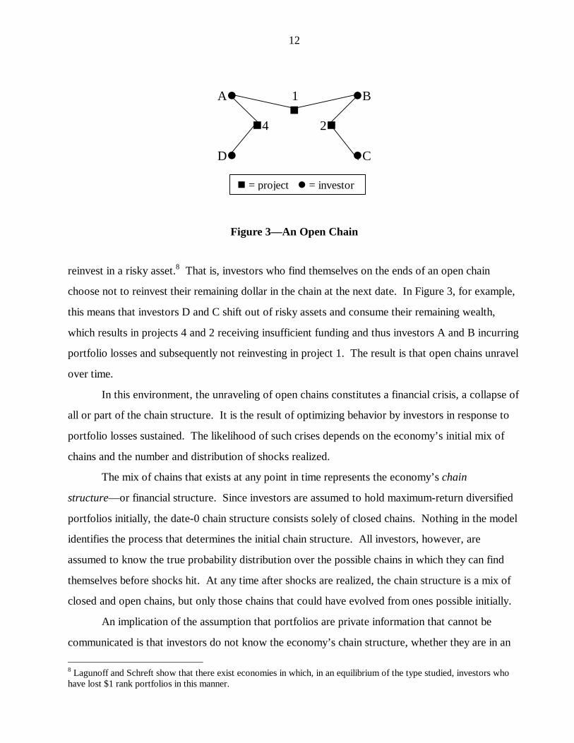
allocations to be represented by a collection of closed chains. A closed chain is a set of projects and

investors such that each project is fully funded, each investor is fully invested and diversified, and

investor portfolios are all linked. Figure 2 depicts a closed four-link chain, since every investor is

linked directly or indirectly to four projects.

Al 1 lBn

n4 2nn

Dl 3 lC

Figure 2— A Closed Chain

When a shock at date 0 causes a project to fail, it turns the closed chain in which the project

resides into an open chain. An open chain is the same as a closed chain, except that some investors

are not diversified because they lost $1 when a project failed. Figure 3 depicts the open chain that

arises when project 3 in Figure 2 fails.

While the shocks at date 0 initiate linkage breaks, fragility requires that there be a

propagation mechanism that magnifies the effects of the shocks. In what follows, attention is

restricted to economies in which such a propagation mechanism exists. More precisely, attention is

restricted to economies in which, at each date t ≥ 0, an investor who has lost $1 prefers not to

7 Lagunoff and Schreft show that there are economies (i.e., specifications of the utility function and ranges of parameterspace) for which an equilibrium exists with maximum-return diversified portfolios chosen by investors at the start ofdate 0.

n = project l = investor

12

Al 1 lBn

n4 2n

Dl lC

Figure 3— An Open Chain

reinvest in a risky asset.8 That is, investors who find themselves on the ends of an open chain

choose not to reinvest their remaining dollar in the chain at the next date. In Figure 3, for example,

this means that investors D and C shift out of risky assets and consume their remaining wealth,

which results in projects 4 and 2 receiving insufficient funding and thus investors A and B incurring

portfolio losses and subsequently not reinvesting in project 1. The result is that open chains unravel

over time.

In this environment, the unraveling of open chains constitutes a financial crisis, a collapse of

all or part of the chain structure. It is the result of optimizing behavior by investors in response to

portfolio losses sustained. The likelihood of such crises depends on the economy’s initial mix of

chains and the number and distribution of shocks realized.

The mix of chains that exists at any point in time represents the economy’s chain

structure— or financial structure. Since investors are assumed to hold maximum-return diversified

portfolios initially, the date-0 chain structure consists solely of closed chains. Nothing in the model

identifies the process that determines the initial chain structure. All investors, however, are

assumed to know the true probability distribution over the possible chains in which they can find

themselves before shocks hit. At any time after shocks are realized, the chain structure is a mix of

closed and open chains, but only those chains that could have evolved from ones possible initially.

An implication of the assumption that portfolios are private information that cannot be

communicated is that investors do not know the economy’s chain structure, whether they are in an

8 Lagunoff and Schreft show that there exist economies in which, in an equilibrium of the type studied, investors whohave lost $1 rank portfolios in this manner.

n = project l = investor

13

open or a closed chain, or their location within their chain. Investors can, however, contemplate the

possibilities of their being in the various locations in the various chains and thus can evaluate their

exposure to contagious losses and strategically act to protect themselves. It remains to specify

investors’ behavior in the dynamic recursive game that is played at each decision point after the

shocks have been realized.

In addition to observing a signal about the state of the economy, an individual investor

observes st, the post-return state of his portfolio, that prevailing after returns are realized and when

he has to make his consumption-investment decision. That is, he knows at each date, after realizing

his returns, whether he has incurred a loss of any or all of his initial $2 endowment. His state st is

from the set {Wt, Ht, Zt}, where Wt is the state in which he still has his whole initial endowment, Ht

is the state in which he has half of his initial endowment because he has incurred a $1 loss, and Zt is

the state in which he has zero dollars left. Based on the signal observed xib g and the state of his

portfolio, the investor chooses an action a regarding his portfolio, where a is from the set {D, U, P,

S}. Action D is the choice to continue holding a diversified portfolio at the beginning of the next

date. Action U is the choice to deviate to an undiversified portfolio; action P, a part-safe-part-risky

portfolio; and action S, a safe portfolio (Section II-A describes these portfolios). With this

specification of actions, a symmetric strategy for type i is a sequence f fiti

t≡

=

∞m r 0, where

f s xti

t i,b g denotes the action taken by investor type i in state st at time t. Type i’s forecast of

others’ behavior is a symmetric strategy profile denoted ~f i ≡ ~ , , ~ ,f s x f s xit

it1 2b g b gd i, with

~ ,f s xti

t jd i representing i’s forecast at date t of type j’s (j = 1,2) strategy when j is in state st.

Forecast ~f i is a conditionally correct forecast if it coincides with strategy f j that j chooses if j

thinks i’s prior Pr i ⋅b g is the true prior. The notion of equilibrium defined in the next subsection

assumes that all investors’ forecasts are conditionally correct.

Finally, type i’s post-return expected lifetime utility at t from strategy f s xti

t i,b g and

forecast ~f i is denoted V f f s xti i

t i, ~ | ,d i. Appendix A presents the expressions for these expected

utilities for each possible state and each possible action an investor can take.

C. Equilibrium and Fragility

The preceding specification of strategies and forecasts implies symmetry in the strategies of

14

investors of the same type. In what follows, then, only symmetric equilibria are studied, and they

all share two features. First, as stated previously, to ensure the existence of a propagation

mechanism that can permit small shocks to have large-scale effects, the economies studied have the

property that investors who lose $1 do not reinvest in the chain structure. That is, in equilibrium,f H x St

it i,b g= . Second, since all investors are assumed to hold diversified portfolios before the

realization of shocks and to maximize utility, those in state Wt compare the expected lifetime utility

at the end of date t from continuing to hold a diversified portfolio at t + 1 to that from the best

portfolio of each alternative type. If f i a, denotes the strategy of a type-i investor who chooses

action a at date t, given state Wt and signal xi, then the expected utilities associated with the variousportfolios can be denoted V f f W xt

i a it i

, , ~ | ,d i, for a = D,U,P,S. Thus, investors continue to hold

diversified portfolios as long as

V f f W x V f f W x V f f W xti D i

t i ti U i

t i ti P i

t i, , ,, ~ | , max , ~ | , , , ~ | , ,d i d i d io≥ V f f W xt

i S it i

, , ~ | ,d it .

The following definition captures these features of a symmetric equilibrium.

DEFINITION. A maximal sustainable equilibrium with conditionally correct forecasts is a symmetric

strategy f i* for each investor type i = 1,2, such that

i. For each date t and each state s, f s xt t ii* ,b g is chosen to maximize V f f s xt

i it i, ~ | ,d i, where

~f i is a conditionally correct forecast.

ii. For each t, ~ ,f W x Dti

t jd i= , provided that for each j = 1,2,

V f f W x V f f W x V f f W xtjD i

t j tjU i

t j tjP i

t j, ~ | , max , ~ | , , , ~ | , ,d i d i d io≥ V f f W xtjS i

t j, ~ | ,d it .

iii. Investors start date 0 holding maximum-return diversified portfolios.

iv. For each t, f H x St t ii* ,b g= .

By construction, then, in a symmetric equilibrium there exists some first date at which

investors of type i decide to switch from a diversified portfolio to the next-best alternative, which is

necessarily safer in that it involves less exposure to contagion risk (fewer dollars at risk, or dollars

at risk from contagion from fewer directions). And by the equilibrium’s symmetry, if one investor

of type i decides to reallocate his portfolio, then all investors of type i do so. The exit-decision date

at which type i investors all decide to reallocate and thus exit, or disconnect from, the chain

15

structure at the next opportunity, given ε, is denoted by τi(ε).

The effect of ε on τi(ε) is complicated because ε represents both an investor’s uncertainty

about the true probability of project failure at date 0 and his belief about the fraction of investors of

each type. To sort out the effect of ε on τi(ε), it proves useful to look at the exit-decision date in an

economy in which all investors share the same beliefs and assign probability 1 to the event ℘ = p

for some p > 0. This is exactly the Lagunoff and Schreft economy. In what follows, the exit-

decision date for this economy with homogeneous beliefs and certainty about the fundamentals isdenoted by τ pb g. By construction, it is the first date t for which9

V f f W x V f f W xti D i

t i a D ti a i

t i, ,, ~ | , max , ~ | ,d i d i<

≠.

The exit-decision date τ pb g isolates the effect of ε on uncertainty about ℘ . Consequently, the

difference between dates τ pb g and τ εi b g measures the effect of ε on the existence of heterogeneous

beliefs within the population. The smaller is ε, the farther apart are the beliefs of the type-1 and

type-2 investors, as are their exit dates, τ ε1b g and τ ε2 b g, respectively. As ε → 0.5, the beliefs of

the two investor types converge, as do their exit-decision dates: τ τ1 205 05. .b g b g= .

When τ ε1b g and τ ε2 b g differ, the early exiting of some investors has the same effect on the

economy as would a second round of shocks to projects. The only difference is each realization of a

shock at date 0 causes a single project to fail, whereas each investor in state Wt who exits the chain

structure causes two projects to fail, the two that were in his portfolio. The decision at the latter of

the τ εi b g of some investors to exit induces a financial crisis involving the simultaneous collapse of

all remaining chains, whether open or closed, when the investors actually reallocate at the next date( max

i iτ εb g+ 1 ). The crisis occurs because optimizing investors strategically choose to reallocate

their portfolios as protection against possible losses, even if they have not experienced losses

themselves and do not know for sure that losses are occurring. Thus, it can occur in addition to the

crisis associated with the unraveling of chains, simply because investors act preemptively to protect

themselves against the event that their own chain might unravel. And one would expect, as is

shown below, that the early exiting of some investors causes it to occur at least as soon as it

9 The exit-decision date τ p( ) is an equilibrium in pure strategies in the Lagunoff-Schreft economy with homogeneousbeliefs of the type specified here. This equilibrium involves a two-action-best-response cycle between strategies U andS at the exit-decision date. There thus must exist an equilibrium in which investors use mixed strategies at the exit-decision date. It is conjectured, but not proven here, that for some preferences and parameter values, an equilibriumexists in pure strategies as well.

16

otherwise would have.

It follows that an economy may be characterized as more fragile the earlier the date at whichits entire chain structure collapses (i.e., the earlier max

i iτ εb g+ 1 ). This does not mean, however,

that every economy’s financial structure collapses. While maxi iτ εb g can be zero, in which case the

economy’s chain structure collapses with certainty when investors reinvest at date 1, it also can be

infinity, which means the economy never suffers a complete financial collapse due to strategic

investor behavior.

A desirable feature of a maximal sustainable equilibrium is that it gives rise to a date of

certain and complete financial collapse later than that of any other equilibrium. Lagunoff and

Schreft introduce the concept because their goal is to assess the inherent fragility of an economy.

As a modeling device to find such an equilibrium, Lagunoff and Schreft assume that an investor

makes an optimistic forecast— a forecast ~f i such that, for all t ≥ 0 and each type i = 1,2,~ ,f W x Dt

it jd i= and ~ ,f H x Dt

it jd i≠ . An investor with this forecast expects that other investors

continue to hold diversified and linked portfolios until they personally experience losses and then

shift to safer portfolios. The optimistic forecast implies that investors foresee the contagious

financial crisis initiated by shocks to projects, but not the preemptive behavior that instantaneously

induces total collapse. In contrast, the equilibrium concept defined above assumes that investors

make conditionally correct forecasts. Such forecasts arise when investors have foresight about both

the contagious crisis and the preemptive behavior, and so are less optimistic than optimistic

forecasts. These forecasts are necessarily correct conditional on the signal investors observe and on

the model they use in forming expectations. If investors observe the better signal, given the true

state, and use the true probability distributions in forming expectations, then their forecasts also are

unconditionally correct. In subsequent sections, all references to correct or incorrect forecasts refer

to unconditional accuracy.

Interestingly, the optimistic forecast can be used to construct bounds on the exit-decision

date of an investor with conditionally correct forecasts. The reason stems from the difference

between an investor with an optimistic forecast and one with a conditionally correct forecast. The

latter recognizes that there is a date at which everyone else in the economy exits; the former does

not. An investor with an optimistic forecast thus never exits sooner than one with a conditionally

correct forecast. And a type-i investor with a conditionally correct forecast remains diversified at

17

all dates t < τ εi b g because, by equilibrium condition ii, he expects everyone of type i to do so. It

follows that the portfolio reallocations at τ εi b g+ 1 are due solely to beliefs about fundamentals, not

to any coordination failure. When ε = 0, there is only one type of conditionally correct investor, so

his exit-decision date is the same as that in an economy with identical investors with optimisticforecasts. That is, for a type-i investor who thinks ℘ = p with probability 1, τ i 0b g = τ pb g by

definition of τ pb g. Thus, in subsequent sections, the optimistic forecast is used to find τ i 0b g.

This completes the description of the economy. It remains to analyze rational and irrational

exuberance. This is done in the remainder of the paper by studying two special cases of the

economy: one with strong fundamentals and rational investors, and one with weak fundamentals

and irrational investors. For each case, bounds on the exit-decision date for each investor type arefound, making use of the case ε = 0 and its associated exit-decision date τ pb g.

III. Rationality, Exuberance, and Apprehension

A special case of the economy described above is used in this section to study rational

exuberance and apprehension. Specifically, the true state of the economy is assumed to be ω 1 , so

that the economy’s fundamentals truly are strong (℘ = 0), and investors are assumed to have

rational expectations as commonly defined. That is, investors are assumed to optimize and to formexpectations using the true distributions Pr ω ib g and Pr |xi jωd i, for i, j = 1,2.

In this rational economy, the investors who observe signal x1 believe Pr |ω 1 1xb g = 1 − ε by

Bayes’ Rule, and thus for ε < 0.5 believe, correctly, that the true state is most likely ω 1 and that

shocks are unlikely to be realized at date 0. Given Pr |xi jωd i, they believe, also correctly, that the

other type-1 investors constitute a fraction 1 2 2− +ε εb g of the population and therefore that the type

1s are in the majority.

Similarly, investors who observe signal x2 believe Pr |ω 1 2xb g = ε by Bayes’ Rule, and thus

believe that the true state is most likely ω 2 . That is, unlike the exuberant type-1 investors, the type

2s believe that shocks most likely are realized at date 0 and thus are apprehensive about their

portfolios’ prospects. Given their type and their beliefs about the state, they also believe that the

other type-2 investors represent a fraction 1 2 2− +ε εb g of the population. They are incorrect, of

course, about which state is most likely and about their type’s majority status in the economy, but

18

their beliefs are nonetheless rational.

If ε = 0, this economy is characterized by pure rational exuberance: all investors observe

signal x1 and believe correctly that the true state is ω 1 . No financial crises occur because no

shocks initiate the unraveling of chains and no investors anticipate incurring losses because ofcontagion. The exit-decision date for these rational investors, represented by τ1 0R b g, equals τ 0b g,which is infinity.

For economies with ε > 0, no matter how small, the analysis is significantly more difficult

because there are two types of investors in the economy, each forecasting the state, the presence of

investors of other types, and the beliefs of those other types. Because a total collapse of the

economy’s financial structure occurs when the last group of investors reallocates their portfolios, it

is easiest to start by examining the apprehensive investors— the ones who expect shocks to be

realized at date 0. As stated above, the apprehensive investors (type 2) think that there is a fraction

ε of the population of type 1. To make conditionally correct forecasts of the type 1s’ behavior, the

apprehensive investors use their own priors, but since their priors are common to all investors, their

forecasts are accurate: they believe that the type 1s expect no shocks to be realized and thus to

remain diversified at least as long as they themselves do. Each apprehensive investor also forecasts

correctly that the other apprehensive investors all make the same forecasts that he makes and find it

a best response to hold a diversified portfolio when they expect everyone else to do so. With these

beliefs, the environment in which an apprehensive investor pictures himself is the same as that in

Lagunoff and Schreft when shocks are realized with probability p and investors think everyone

else remains diversified at least as long as he does (the optimistic forecast). It follows that an

apprehensive (type 2) investor’s exit-decision date, denoted τ ε2R b g, is simply τ pb g ≥ 0.

Like their apprehensive counterparts, the exuberant type-1 investors accurately forecast the

beliefs of the type 2s because they use the true and common prior Pr ω ib g. As a result, they

anticipate the apprehensive investors deciding at date τ pb g to exit and initiating a contagion at

τ pb g + 1. The best response for the exuberant investors is to decide to exit at some date τ ε1R b g,

where τ ε1R b g ≤ τ1 0R b g = ∞ .

The date τ ε1R b g is a function of how many projects the type-1 investors expect to fail at

τ pb g, which depends, in turn, on which portfolio the type 2s switch to and how many type-2

investors exist. Type-1 investors correctly believe that the type 2s constitute a faction ε of the

19

population, and they can accurately forecast the portfolio to which the type 2s switch. If, forexample, the apprehensive type 2s decide at date τ pb g to switch to a safe portfolio, then at date

τ pb g + 1 they do not reinvest in any of their previously held projects. The worst-case scenario in

terms of fragility occurs when the ε type-2 investors have no projects in common in their portfolios.In this case, 2ε projects fail when the type 2s exit at τ pb g + 1. In the best case, all the type 2s are in

adjacent projects in chains, and their portfolio reallocations cause ε + 1/k projects to fail. If, instead,

the apprehensive investors deviate to a part-safe-part-risky portfolio at date τ pb g+1, then each

immediately consumes a dollar (because the safe asset pays zero interest and investors discount the

future) and reinvests a dollar in one project. This causes ε projects to fail at τ pb g+1 in the worst

case, ε 2 to fail in the best case, and type 2s to find themselves with at most R dollars to allocate

at τ pb g+1 between current consumption and future investment. By equilibrium condition iv, the

type 2s do not reinvest at date τ pb g+2, causing the failure of another εk 2 to εk of all projects.

In choosing strategies, exuberant investors use their forecasts of the type 2s’ date-(τ pb g+1)

portfolio allocations and of how investors of different types are distributed around chains.

Whatever these forecasts, it is clear that the type 1s’ best response to the type 2s exiting at τ pb g + 1

is to exit themselves at some date τ ε1R b g + 1, where ∞ ≥ τ ε1

R b g ≥ τ ε2R b g = τ pb g ≥ 0, even though

they correctly believe that the economy’s fundamentals most likely do not warrant it. This result is

summarized in the following proposition, which is proven in Appendix B along with all other

results.

PROPOSITION 1. If p is sufficiently large that τ pb g< ∞ , then there exists ε > 0 such that

τ ε τ ε1 2R Rb g b g≥ for all ε ε∈ 0, g.

The exiting of the rationally exuberant investors from the economy brings about total

financial collapse because they are the last of all investors to exit. The economy could collapse at

an earlier date by chance if the right mix of shocks is realized at date 0 and all chains happen to

unravel before τ ε1R b g+1, but it collapses with certainty at date τ ε1

R b g+1. And, as the following

proposition states, date τ ε1R b g is nonincreasing in ε.

PROPOSITION 2. τ ε τ ε1 1 1 2R Rb g b g≥ if ε ε1 2≤ .

20

Intuitively, when ε is higher, type-1 investors assign lower probability to state ω 1 , with ℘ = 0, and

they believe that a smaller fraction of the population expects that ℘ = 0. Thus, an increased

presence of apprehensive investors in the economy does not reduce fragility.

A third, and striking, finding is that the financial collapse that occurs because type-1

investors decide at τ ε1R b g to exit is indistinguishable from the collapse that occurs in an economy

with homogeneous beliefs and certainty that ℘ = ′p for some ′p . Formally:

PROPOSITION 3. There exists ′p such that τ τ ε′=p Rb g b g1 .

That is, a financial crisis that looks as if it had been initiated by real shocks actually could have

been caused solely by the presence of a small share of investors who were apprehensive— though

rationally so— about the economy’s prospects. Without knowledge of the true fundamentals, an

observer cannot determine whether a crisis occurred because of less-than-pure rational exuberance

in a fundamentally sound economy.

IV. Irrationality, Exuberance, and Apprehension

A second special case of the economy of Section II is suitable for the analysis of irrational

exuberance and apprehension. In this variant, the true state of the economy is ω 2 , the state in

which the fundamentals are poor (℘ = p ), and investors’ expectations are formed irrationally in the

following sense: investors optimize and know the true likelihoods (that is, they know thatPr |xi iωb g = 1− ε and Pr |x j iωd i = ε for j ≠ i), but they do not use the true priors over the ω i .

Instead, a type-i investor updates his beliefs using the subjective prior

Pr iiω ε

ε εb g b g=

− +

2

2 21,

while type j ≠ i updates from the prior

Pr jiω ε

ε εb g b g

b g= −− +1

1

2

2 2.

That is, a type-1 investor uses a pessimistic prior, one that assigns more probability weight to the

21

worse state, ω 2 , while a type-2 investor uses an optimistic prior, assigning greater probability

weight to state ω 1 . In addition, investors believe that their own priors are the ones used by all

investors, and they do not recognize the dependence of their priors on the state.

Clearly, many subjective priors are consistent with investors forming expectations

irrationally in some sense. The priors assumed here are used because they generate beliefs about

the probability of the states ω i that are the exact opposite of those held by the rational agents of

Section III. Specifically, given these priors, the application of Bayes’ Rule yields the posteriorsPr |i

i ixω εb g= and Pr |ji jxω εd i= −1 after investors observe their private signals. This implies,

given that the true state is ω 2 , that a fraction 1 − ε of investors observes signal x2 and so is of type

2. The type 2s believe, given their optimistic subjective priors, that the true state is ω 1 with

probability 1 − ε and ω 2 with probability ε . Likewise, a fraction ε observes x1 and is of type 1.

They pessimistically assign probability ε to state ω 1 and probability 1 − ε to state ω 2 . Thus, in this

economy with irrational investors, it is the type 2s who end up with posterior beliefs that are

unjustifiably exuberant and the type 1s who have posteriors that are apprehensive and relatively

more correct, at least about the state.

The use of the subjective priors introduces an interesting complication into the analysis.

Since investors believe, incorrectly, that their subjective priors are the priors used by all investors,

they make incorrect forecasts of both the distribution of investor types in the economy and the

beliefs of investors not of their type. Specifically, in forecasting the beliefs of the type 2s, the

pessimistic type-1 investors, who think the state is most likely ω 2 , use Bayes’ Rule with their

subjective prior, Pr jiω ε ε εb g b g b ge j= − − +1 12 2 2 , and conclude that the type-2 investors assign

probability ε ε ε3 3 31 − +b g , which is less than ε for ε < 0.5, to state ω 1 . That is, the type 1s

believe, incorrectly, that the type 2s think state ω 1 , with ℘ = 0, is even less likely than they

themselves believe it to be, and thus that the type 2s are the most apprehensive investors in theeconomy. But given the known likelihoods Pr |x j iωd i = ε and Pr |xi iωb g = 1 − ε , the type 1s think

their type is a minority of the population and that the type 2s are the majority.10 In this, at least,

they are correct, since the true state is ω 2 . The optimistic type 2s, who think the true state is ω 1 ,

use the same approach to forecasting the beliefs of the type-1 investors. They wrongly conclude

10 It can readily be verified that a type i investor assigns probability 2 1ε ε−( ) to other investors being of type i.

22

that the type 1s assign probability 1 13 3 3− − +ε ε εb g b g , which exceeds 1− ε for ε < 0.5, to state

ω 1 . As a result, the type 2s think the type 1s are the most exuberant investors in the economy. And

they wrongly believe that the type 1s are in the majority. Every investor, then, incorrectly believes

that his own type is the minority and that everyone else is at least as exuberant or apprehensive as

he is.

Investors use these irrational forecasts in determining their strategies. The true apprehensive

investors, the type 1s, think that shocks most likely are realized at date 0, but they also think that the

type 2s assign even higher probability to such an outcome and believe themselves to be in the

majority. The type 1s thus predict that the type 2s believe that the majority of the population thinks

a contagious financial crisis to be very likely and decides at some date to exit. If, for example, ε =

1/k, which approaches zero as k approaches infinity, there is one type-1 investor in the economy.

This sole type 1 believes first that everyone else (the type 2s) thinks that virtually everyone is of

type 2, and second, that the type 2s think ℘ = p > 0 is at least as likely as he thinks it is.11 The

type 1 also perceives type-2 investors as thinking that all investors continue to hold a diversified

portfolio as long as their expected lifetime utility from doing so exceeds that from switching to the

next-best alternative portfolio. But this is exactly what an investor in the Lagunoff and Schreft

economy thinks when the probability of shocks is believed to be p . Consequently, the type-1

investor forecasts that the type 2s’ exit-decision date is τ pb g ≥ 0. This is an ominous forecast for

the type-1 investor because the exiting of the type 2s causes projects to fail at τ pb g + 1 in addition

to those the type-1 investor expects to fail from the contagion induced by date-0 shocks. The best

response for the type-1 investor in this environment is to choose an exit-decision date τ ε1I b g, where

τ ε1I b g ≥ τ1 1I kb g = τ pb g ≥ 0. In summary, although the type 1s correctly forecast which state is

most likely, they incorrectly forecast the forecasts of the type 2s, and thus perceive the risks to their

portfolios as greater than they are in actuality. That is, their prior about the state is pessimistic, but

they end up even more pessimistic about the prospects for their portfolios because they incorrectly

forecast the beliefs of others. Type-1 investors thus personify Chicken Little, thinking that the sky

is falling and reacting accordingly, contributing to the economy’s fragility by exiting at least as

11 It does not make sense to analyze the case of ε = 0 in this irrational economy because all investors, thinking that theirtype is a fraction ε of the population, would thus think that they did not exist. Such thinking would reflect insanity, notirrationality. Thus, the smallest ε can reasonably be is 1/k.

23

early as they would if they recognized the type 2s’ true exuberance.

The exuberant type 2s do not fare any better in forecasting the type 1s’ behavior. They think

it unlikely that any shocks are realized at date 0, and they perceive the type 1s as viewing shock

realizations as even less likely and thinking type 1s are in the majority. The type 2s therefore think

that the type 1s are likely to continue to hold diversified portfolios at least as long as the type 2s.

Again, if, for example, ε = 1/k, then each type-2 investor believes incorrectly that he is the only

type-2 investor, is virtually certain that no shocks hit at date 0, and thinks that everyone else in the

economy is at least as certain that no shocks are realized. This is the economy of Lagunoff and

Schreft with a true probability of project failure of zero. In the limit, as k approaches ∞ , the exit-

decision date of the type 2s, denoted τ 2 1I kb g, equals τ 0b g, which is infinity. Thus, for any ε, τ ε2I b g

satisfies 0 ≤ τ pb g ≤ τ ε1I b g ≤ τ ε2

I b g ≤ τ 0b g ≤ ∞ . In summary, type-2 investors’ prior about the state

is optimistic, but they end up even more optimistic about the prospects for their portfolios because

of their incorrect forecasts. Type-2 investors, then, are the quintessential Cockeyed Optimists,

sustaining the economy’s financial structure longer than they would if they recognized the type 1s’

true apprehension. The following proposition formalizes these results:

PROPOSITION 4. If p is sufficiently large that τ pb g< ∞ , then there exists ε > 0 such that

τ ε τ ε1 2I Ib g b g≤ for all ε ε∈ 0, g.

Since total financial collapse occurs with certainty when the last investors reallocate their

portfolios, the behavior of the type-2 investors determines the date of collapse in the economy with

irrationality. Total collapse occurs at date τ ε2I b g + 1, where τ ε τ ε2 1 1I Ib g b g≥ ≥ . Of course, as ε

increases, type 2s think all investors assign less probability to state ω 1 and believe that there are

more type 2s around to exit early. That is,

PROPOSITION 5. τ ε τ ε2 1 2 2I Ib g b g≥ if ε ε1 2≤ .

It follows that the economy is at least as fragile the greater is ε.

Furthermore, the irrational type-2 investors are not only irrationally exuberant; they are also

more exuberant than the rational type-1 investors are in an economy in which the true state is ω1

24

(i.e., the type-1 investors studied in Section III). This result arises because the irrationally

exuberant type-2 investors misforecast by a large margin both the likelihood of the true state and the

beliefs of the minority group (the type-1 investors). Because these type 2s believe the irrationally

apprehensive type 1s to be the truly irrationally exuberant investors in the economy, the type 2s are

more irrationally exuberant than they would be otherwise. Thus, irrational type-2 investors exit

later than rational type-1 investors, which means that the economy with irrational exuberance is less

fragile than that with rational exuberance, given ε. Similarly, the irrationally apprehensive type-1

investors are even more apprehensive than the rationally apprehensive type-2 investors. The

following proposition formally states these results.

PROPOSITION 6. (a) τ ε τ ε2 1 0I Rb g b g> ≥ , and (b) 0 1 2≤ <τ ε τ εI Rb g b g.

V. Implications for Policy

The preceding sections examine economies with particular combinations of the state and

beliefs for the purpose of characterizing rational and irrational exuberance. Collectively, the results

yield a ranking of exit-decision dates:12

0 01 2 1 2≤ ≤ < ≤ < ≤ = ∞τ τ ε τ ε τ ε τ ε τp I R R Ib g b g b g b g b g b g .

Since these dates are independent of the true state, they can be applied to more general economies

that consist of both rational and irrational, type-1 and type-2 investors.13

By using these exit-decision dates, investors maximize their expected lifetime utility, given

the signal they observe about the state and their priors. In some sense, then, they are as well off as

possible if they use these exit dates. This is true even though some of them exit too early or too late

12 More specifically, this ranking of exit-decision dates follows from Propositions 1, 4, and 6. Thus, it applies toeconomies for which those propositions hold. Such economies must have two features. First, they must have the twocritical properties discussed in section IIb, namely that portfolios are initially linked and that there is a mechanism forbreaking linkages. Lagunoff and Schreft have shown that these properties characterize the equilibrium of some, but notall, economies. Second, they must have the property, required for Proposition 1 to hold (the proof is in Appendix B),that the true probability of a project’s failure due to a shock, p , be large enough that, if all investors believe that p is

the true probability with certainty, then they have a finite exit-decision date τ p( ) that is decreasing in p .13 These exit-decision dates are for an economy of a given size k (i.e., measured in terms of number of investors andprojects). Lagunoff and Schreft show that for sufficiently large economies, the exit-decision date of type i investordecreases as the economy becomes even larger. This result applies to each investor type here as well. The ranking ofexit-decision dates remains the same as the economy becomes larger since it was derived for any given economy size.

25

relative to what is appropriate based on the true state. For example, if the true state is ω 1 , ε is

approximately zero, and k is very large (approaching infinity), then approximately all investors

observe signal x1 and the exit-decision dates are simply τ τ τp I Rb g≅ < ≅∞1 1 . If investors discover

the true state after the collapse is over, the irrational ones realize that no shocks were realized and

regret having exited preemptively.

Even if investors never discover the true state, there will always be some who regret their

decisions. They are the ones who incur losses from contagion before their scheduled exit date.

Depending on the realization of shocks and the initial chain structure, there could be many such

investors, or just a few. These investors will look to policymakers for remedies and for assurances

that such a crisis will not occur again. Of course, no such assurances can be given because shocks

and beliefs are exogenous and the chain structure is unknown, but there are some policy options.

In the short term, policymakers are limited to trying to stem any ongoing contagion. A

commonly used approach is for some institution to serve as a lender of last resort who lends funds

immediately after shocks are realized to prevent additional losses. In the economy of Section II,

such an institution could be modeled as being known to and able to provide information to all

investors, but having no greater knowledge of the economy than anyone else (i.e., it does not know

the chain structure or realization of shocks). It could announce that it stands ready to extend

emergency credit and could raise resources to fund its activities either by creating funds (e.g.,

issuing a fiat currency) or taxing the return on projects. Agents would reveal themselves to the

lender of last resort to obtain credit. Since investors are the only agents in the economy, they are

the ones to whom any loans must go. This by itself makes the policy problematic. The reason is

that loans must go to investors who actually incur losses and, by equilibrium condition iv, are about

to reallocate their portfolios, initiating the first round of contagion. But portfolios are private

information, so all investors, whether or not they have incurred losses, have an incentive to request

loans under such a policy, and policymakers have no way to identify the legitimate borrowers. The

policy also is ineffective because at best it postpones the contagion for two periods.14 This stems

14 It is instructive to see why lending to investors does not work here because the reason highlights the role portfoliolinkages play in generating contagion. Someone who incurs losses on both investments because of shocks, and thusborrows $2, cannot reinvest in his formerly held projects because they are no longer operative. He instead must put thefunds into a safe portfolio, which means he either consumes them immediately or consumes $1 and puts $1 in the safeasset for one period. An investor who only loses $1 from shocks still has a project in which he can reinvest. In the best-case scenario for reducing contagion, he invests the $1 he borrows plus the remaining dollar of his endowment into the

26

from the simplicity of the model and the nature of the chain structure.

A lender of last resort conceivably could end contagion, at least on average, by making loans

to projects. This policy could be used if the model is modified by adding agents who operate

projects and can reveal themselves if their projects do not receive sufficient funding to operate.

There typically is a moral-hazard problem, however, in making loans to such agents, so it is unclear

whether the policy can improve welfare on net.

The model also suggests some longer-term measures that a lender of last resort or

government entity can take to reduce the likelihood of contagion. For example, monitoring lenders’

portfolios provides information about the economy’s linkages that a lender of last resort can use to

identify projects at risk of receiving insufficient funding and to coordinate a response among

investors. The supervision of banks by governmental regulatory organizations is an example of a

policy that achieves this end. A second example is policies that result in greater diversification and

thus increase the number of shock-induced project failures needed to initiate a crisis. An

implementation of such a policy in the United States is the restriction that allows money-market

mutual funds to hold only a limited share of their portfolios in the commercial paper of a single

issuer. These types of long-term measures can result in a stronger, more resilient chain structure

and thus can reduce the likelihood and severity of contagious financial crises.

For such policies to be effective, however, they must be adopted by an entity with authority

regarding all possible portfolio linkages because all linkages contribute to an economy’s fragility.

Thus, if the model is taken to be one of a small closed economy with strict capital controls, then the

entity could be a domestic institution. For open economies with global linkages, fighting contagion

requires an organization of international scope.

Appendix A

This appendix presents the expected lifetime utilities associated with an investor’s

one project that is left in his portfolio. But his former coinvestor also reinvests either $1 or $2. As a result, his pre-taxreturn is at most 4 3R . Given the bounds on R , the tax rate, and equilibrium condition iv, he at best only consumeshis interest and reinvests $1 for one additional period. Thus, a policy of extending emergency credit to investors whoincurred losses at most postpones the contagion for a period or two.

27

continuing to hold diversified portfolios or deviating to another portfolio in the dynamic recursive

game that begins after the shocks are realized. As explained in Section II-C, the bounds on the exit-

decision dates τ εi b g are the exit-decision dates from an economy with investors who make

optimistic forecasts and are homogeneous (ε = 0) and where the true probability of shocks ℘ is

believed to be p. That economy is the one described in Lagunoff and Schreft. Hence, the expected

utilities for all t < τ εi b g here are those from Lagunoff and Schreft, who provide a thorough

derivation in their Appendix A.15

In this model, the expected lifetime utility from any portfolio must depend on both the

probabilities of being in the various chains and the expected utilities associated with those chains.

Calculating the latter for open chains requires considering the utility associated with the various

positions in the chain and the likelihood of an investor’s being in each position. An open r-link

chain has r − 1 investors who are in state Wt. Two of them will lose $1 because their coinvestors

are in state Ht and will not reinvest, while the rest will not incur losses if they remain diversified

another period but will incur losses eventually as their chain shrinks and their coinvestors end up in

state Ht. The expected lifetime utility from remaining diversified if in an open r-link chain, denoted

π D rb g, is thus

π β βπD r ru R u R u

ru R r r

r( )

max , ( ) ,

.= −

− + + −−

FH IKFHG

IKJ − + − ≥

=

RS|T|

21

1 1 12

12 2 2 3

0 2

c h c h b gn s a fc h if

if

In contrast, investors in closed chains can remain diversified permanently, enjoying the lifetimeutility of π ≡ u R2 2 1− −c h a fβ .

With Crt N rtb g denoting the event that an investor is in a closed (open) r-link chain at the

beginning of date t, the probability of an investor’s being in a closed (open) chain at the beginning

of date t, conditional on his being in state Wt and having observed signal xi , can be denoted

Pr ,C W xrt t i− 1c h Pr ,N W xrt t i− 1c hd i.16 A closed r-link chain after returns are realized at t ≥ 0 must

have evolved from a closed r-link chain that existed at the start of date 0 and had no project failures

15 Investors’ strategies at date τ εi

( ) in this model may differ from those in Lagunoff and Schreft because here type i

investors correctly forecast that at τ εi( ) all investors of type i decide to exit, whereas in Lagunoff and Schreft investors

forecast that everyone remains diversified who has not incurred a loss. This difference is immaterial, however, becausethe focus here is only on the date at which investors exit, not on which portfolio they switch to at that date.16 The probabilities are unchanged if they are calculated after returns are realized at date t − 1, when the investor makeshis consumption-investment decision.

28

due to shocks. If q r k,b g denotes the probability of an investor belonging to a closed r-link chain

before the shocks, then Pr | , ,C W x q r kr i0 1− =b g b g. And, at the start of any t ≥ 1, the nonnormalized

conditional probability of a closed r-link chain, denoted Pr | ,C W xrt t i− 1b g, is q r k p r,b gb g1 2− − if 2 ≤ r

≤ k and zero otherwise.

Likewise, an open r-link chain at date t had to have evolved from an open chain that existed

immediately after the shocks were realized, which itself had to have come from a closed chain that

existed initially. The nonnormalized probability of an investor’s being in an open r-link chain at thestart of date 0, denoted Pr | ,N W xr i0 1−b g, is clearly zero. But

Pr | , , ,N W x r p p q m k pq r kr ir

m r

k

1 02 2

21 1 1b g b gb g b g b g= − − ∑ + +LNM OQP

−

= +

because an open r-link chain at date 1 could have come about by exactly one shock hitting a closed

(r + 1)-link chain at date 0, or two shocks hitting a closed chain with at least r + 2 links at date 0.

This expression makes use of two facts: only the two shocks that create the endpoints of an open

chain matter, and an investor knows his own portfolio and thus that, if he is in state Wt, the two

projects in his portfolio could not have been hit by shocks. The probability of open chains at later

dates takes into consideration that an open chain will have lost two projects in each preceding

period. Thus, Pr | ,N W xrt t i− 1b g= Pr | ,N W xn t i1 1−b g, where n = r + 2(t− 1).

These probabilities can be normalized by dividing them by Λt , the total probability weight

attached to all r-link chains at date t, where

Λt rt t ir

k

rt t ir

k

rt t ir

k

r ir t

k

C W x N W x

C W x N W x

≡ ∑ + ∑

= ∑ + ∑

−=

−=

−= =

Pr | , Pr | ,

Pr | , Pr | , .

12

12

12

1 02

b g b gb g b g

The normalized probabilities are thus

Pr | ,Pr | ,

C W xC W x r k

rt t irt t i t

−−= ≤ ≤RS|T|1

1 2

0b g b g Λ if

otherwise,

and

Pr | ,Pr | ,

N W xN W x r k t

rt t ir i t

− = ≤ ≤ − − −RS|T|11 0 2 1 2 1

0b g b g b gΛ if

otherwise.

Making use of these expressions, the expected lifetime utilities from an investor’s taking

various strategies in various states can now be specified:

29

V f f Z xti i

t i, ~ | ,d i= 0 .

V f f H x

u R u R u f H x S

u R N H x V f f H x

f H x P

ti i

t i

ti

t i

t t i ti i

t i

ti

t i

, ~ | ,

max , , ,

Pr | , , ~ | ,

, .

d ic h c h b gn s b g

c h d i d i{ }b g

=

− + =

− + −

=

RS||

T||

+ + +

1 1

1 1 1 1 1 1

β

β

if

if

V f f W x

u R u R u u R u u R u u

f W x S

u R N W xr

V f f H x

N W xr

ti i

t i

ti

t i

r t t i ti i

t ir

k

r t t ir

k

, ~ | ,

max , , ,

, ,

Pr | , , ~ | ,

Pr | ,

d i

c h c h b g c h b g c h b g b gn sb g

c h d i d i

d i

=

− + − + − + +

=

− +−

FHG

IKJ∑RST

+ −−

FHG

IKJ+

+ + +=

+=

2 2 1 1 2 2 2 2 2 1 1

2 22

1

12

1

2

1 1 13

13

β β β β

β

if

∑ ∑LNM

OQP

+ =

− + −−

FHG

IKJ+

−FHG

IKJ

LNM∑

LNM

RS|T|+

+=

+ +

+ + +

+ +=

Pr | , , ~ | ,

Pr | , , ~ | , , ,

Pr | , . Pr | ,

Pr

C W x V f f W x

N W x V f f Z x f H x D

u R N W xr

N W xr

C

r t t ir

k

ti i

t i

t t i ti i

t i ti

t i

r t t i r t t ir

k

r

12

1 1

2 1 1 1

1 13

2 1 12

105

21

d i d id i d it b g

c h d i d i if

β

t t ir

k

ti i

t i

t t i ti i

t i ti

t i

r t t ir

k

r t t ir

k

r t t i

W x V f f H x

N W x V f f Z x f H x P

u R N W xr

C W x uR

N W x

+=

+ +

+ + +

+=

+=

+

∑ OQP+ =

− + −−

FHG

IKJ∑ + ∑L

NMOQPFHG

IKJ

RST+

12

1 1

2 1 1 1

13

12

1

2 2 12

143

| , , ~ | ,

Pr | , , ~ | , , ,

Pr | , Pr | ,

Pr | ,

d i d id i d it b g

c h d i d i if

β

d i c h

b g

21

12

2 2

112

432 r

u Ru

R

f H x U

r

k

ti

t i

−FHG

IKJ

−−

FHG

IKJ+ F

HGIKJ

LNMM

OQPP∑UV|W|

=

R

S

|||||||||||||||

T

|||||||||||||||= β

if , .

Appendix B

This appendix proves the propositions, making use of the expected utility functions specified

in Appendix A. For notational simplicity in what follows, first define

30

v u R u R u≡ − +max ,c h c h b gn s1 1β ,

v u R u R u u R u u R u u≡ − + − + − + +max , , ,2 2 1 1 2 2 2 2 2 1 12c h c h b g c h b g c h b g b gn sβ β β β .

Further, define probability weights

δt r t t i r t t ir

k

r

kN W x

rC W x≡ −

−FHG

IKJ+ ∑∑ + +

==Pr | , Pr | ,1 1

231

21d i d i,

γt r t t ir

kN W x

r≡

−FHG

IKJ∑ +

=Pr | ,1

3

21d i .

It follows that1 2 1− − = +δ γt t t t iN W xPr | ,d i.

Let f i a, denote a strategy in which investor i chooses action a at date t in state Wt. A

necessary condition for f i a, to induce a maximal sustainable equilibrium from date t + 1 on is that

equilibrium condition iv— that f H x Sti

t i+ =1 ,b g , or equivalently, V f f H x vti S i

t i+ + =1 1, , ~ | ,d i — holds.

Hence, the expected lifetime utility in state Wt from a strategy f i a, that induces a maximal

sustainable equilibrium from date t + 1 on is, for each a = D,U,P,S and for each t < τ pb g V f f W x vt

i S it i

, , ~ | ,d i= ,

V f f W x u R V f f W x vti D i

t i t ti D i

t i t, ,, ~ | , , ~ | ,d i c h d io t= − + ++ +2 2 1 1β δ γ ,

V f f W x u R vti P i

t i t t, , ~ | ,d i c h l q= − + +2 1 β δ γ , (1)

V f f W x u R uR

uR u R u R

ti U i

t i t

t t t

, , ~ | ,

. . .

d i c hc h b g c h

= − + FHG

IKJ

RST+ F

HGIKJ

FHG

IKJ+

−−

FHG

IKJ+ − −

−−

UV|W|

2 243

0543

052 2

11

2 2

1

β δ

γβ

δ γβ

The next lemma is used in the proofs of the proposition that follow.

LEMMA. Suppose that v v≥ 15. . Then τ ⋅b g is decreasing in p.

PROOF. Fix an equilibrium strategy f i* such that investor i chooses action D at date t. Let

f i a, * denote the equilibrium strategy identical to f i* except that the investor chooses action a at

date t. Let Vtp b g denote the expected lifetime utility from a strategy, so the dependence on p is

explicit.

Given p, observe that τ pb g is the first date t for which

V f f W x V f f W xtp i

t i a D tp i a i

t ii* *, ~ | , max , ~ | ,,d i d i<

≠.

31

To show that τ pb g is decreasing, it suffices to show that if V f f W xtp i

t ii* , ~ | ,d i ≥

V f f W xtp i a i

t i, * , ~ | ,d i for each a D≠ , then V f f W xt

p it i

i* , ~ | ,d i − V f f W xtp i a i

t i, * , ~ | ,d i is decreasing

in p for each a D≠ .

Case (i). a S= .From (1), the difference V f f W xt

p it i

i* , ~ | ,d i − V f f W xtp i S i

t i, * , ~ | ,d i may be expressed as

u R v V f f W x vt tp i

t ii2 2 1 1− − + ++ +c h d io tβ δ γ* , ~ | , . (2)

By definition, V f f W x v vtp i

t ii

+ + ≥ ≥1 1* , ~ | ,d i since f i* induces an equilibrium from date t + 1 on

such that the investor does no worse than he would from choosing S at time t + 1 and thus gettingutility of v . Also, it is clearly the case that V f f W xt

p it i

i* , ~ | ,d i ≥ V f f Z xtp i

t ii* , ~ | ,d i = 0.

To show that (2) is decreasing in p, two facts must be established. First, for r ≥ 3, it must beshown that the probability weight assigned to V f f W xt

p it i

i+ +1 1

* , ~ | ,d i in (2), which is given by

Pr | , Pr | ,N W x r C W xr t t i r t t i+ +− − +1 11 2 1d i b gc h d i, decreases relative to the probability weight

assigned to v , which is Pr | ,N W x rr t t i+ −1 2 1d i b gc h. That is, it must be shown that

Pr | , Pr | ,

Pr | ,

N W xr

C W x

N W xr

r t t i r t t i

r t t i

+ +

+

−−

FHG

IKJ+

−FHG

IKJ

1 1

1

12

12

1

d i d id i

(3)

is decreasing in p for r ≥ 3. Second, it must be shown that for r = 2, the weight onV f f W xt

p it i

i+ +1 1

* , ~ | ,d i, which is Pr | ,C W xt t i2 1+d i, decreases relative to the weight on zero. That is,

Pr | ,

Pr | ,

C W x

N W xt t i

t t i

2 1

2 1

+

+

d id i (4)

must be shown to be decreasing in p.Both Pr | ,N W xr t t i+ 1d i and Pr | ,C W xr t t i+ 1d i, defined in Appendix A, are continuous in p.

Using these formulas, expression (3) can be writtenr q r k

p q m k pq r km r

− ++ +∑FH IK≥ +

32 2 12

2

,

, ,

b gb g b g

,

while (4) can be written

32

q k

p q m k pq km r

2

2 32

2

,

, ,

b gb g b g+∑FH IK≥ +

.

Both are clearly decreasing in p. By demonstrating term by term in the sum over r that the

probability weight shifts to smaller expected utilities as p increases, it can be established thatV f f W xt

p it i

i* , ~ | ,d i − V f f W xtp i S i

t i, * , ~ | ,d i decreases in p. This concludes the proof of Case (i).

Case (ii). a P= .From (1), the difference V f f W xt

p it i

i* , ~ | ,d i − V f f W xtp i P i

t i, * , ~ | ,d i may be expressed as

u R u R V f f W x v vt tp i

t iti2 2 2 1

21− − − + − +RSTUVW+c h c h d iβ δ γ* , ~ | , . (5)

Using the same term-by-term arguments given in Case (i), it suffices to show thatV f f W xt

p it i

i+ +1 1

* , ~ | ,d i− v v≥ 2b g, or V f f W x vtp i

t ii

+ + ≥1 1 15* , ~ | , .d i . As stated before, f i* induces an

equilibrium from date t + 1 on in which the investor can do no worse than to choose S at time t + 1,getting utility v . Hence, V f f W x v vt

p it i

i+ + ≥ ≥1 1 15* , ~ | , .d i , the latter inequality following from the

hypothesis.

Case (iii). a U= .From (1), the difference V f f W xt

p it i

i* , ~ | ,d i − V f f W xtp i U i

t i, * , ~ | ,d i may be expressed as

β δ

δ γβ

γ β

t tP i i

t i

t t

V f f W x uR

u Rt v u R u R

+ − FHG

IKJ

LNM

OQP

RS|T|FHG

IKJ

FHG

IKJ

LNMM

OQPP − − −

−−

LNMM

OQPPUV|W|

+ − +−

− +

143

12 2

105 4

305

2 21

* , ~ | ,

.. .

d id i b g c h (6)

Observe that v u R u R≤ + − −05 4 3 05 2 2 1. .c hd i c h b gd iβ . But since V f f W xtp i

t ii* , ~ | ,d i ≥

V f f W xtp i U i

t i, * , ~ | ,d i at date t by supposition, it must be true that V f f W xt

p i it i+ +1 1

* , ~ | ,d i ≥ u R4 3c h.

Hence, the term-by-term argument of Case (i) can be used once again to establish the result.

QED. n

PROPOSITION 1. If p is sufficiently large that τ pb g< ∞ , then there exists ε > 0 such that

33

τ ε τ ε1 2R Rb g b g≥ for all ε ε∈ 0, g.

PROOF. Clearly, τ τ1 0 0R b g b g= = ∞ , and τ τ2 0R pb g b g= < ∞ , where p is again the true

probability of a shock in state ω2.

Suppose by contradiction that τ ε τ ε1 2R Rb g b g< . Letτ εi

R∗b g be the exit-decision date for

investors of type i who assign probability 1− ε to the value of ℘ consistent with state ωi, but assign

probability 0 to the existence of state j ≠ i.

From the supposition that τ ε τ ε1 2R Rb g b g< , it follows that τ ε τ ε2 2

R Rb g b g≤ ∗ . That is, since

type-2 investors exit later than type-1 investors, if type-2 investors think there are no type-1

investors— which is the case when their exit-decision date is τ ε2R∗b g— then type-2 investors need

not worry about earlier defaults created by type-1 investors exiting.Likewise, it follows that τ ε τ ε1 1

R Rb g b g≥ ∗ . That is, since the later exit of type-2 investors

does not affect type-1 investors at the earlier date at which the type-1 investors exit, type-1 investors

do not exit any later if they believe that there only exist type-1 investors.

In summary, it has been shown that

τ ε τ ε τ ε τ ε1 1 2 2R R R R∗ ∗≤ < ≤b g b g b g b g. (7)

But it is also the case that, by the Lemma, τ ε τ1 0R∗ → = ∞b g b g and τ ε τ2R p∗ → < ∞b g b g as ε → 0 ,

which contradicts the string of inequalities in (7). Therefore, τ ε τ ε1 2R Rb g b g≥ for sufficiently small

ε. n

COROLLARY. ∞ = ≥ ≥ ≥ ≥ ≥ =∗ ∗τ τ ε τ ε τ ε τ ε τ τ1 1 1 2 2 20 0R R R R R R pb g b g b g b g b g b g b g.

PROOF. These inequalities can be constructed from the proof of Proposition 1. n

PROPOSITION 2. τ ε τ ε1 1 1 2R Rb g b g≥ if ε ε1 2≤ .

PROOF. If ε ε1 2≤ , then by Bayes’ Rule, type-1 investors believe Pr | ,ω ε1 1x ib g = 1 − ε,

which is decreasing in ε. Hence, when ε ε= 1 , type 1s exit no earlier than when ε ε= 2 . n

PROPOSITION 3. There exists ′p such that τ τ ε′=p Rb g b g1 .

34

PROOF. By the proof of Proposition 1 (or its Corollary), τ τ ε τp Rb g b g b g≤ ≤ ≡ ∞1 0 .

Suppose τ τ εp Rb g b g< < ∞1 (otherwise the proof holds for each p or p = 0). It can now be

proven that if τ p t1 1b g= and τ p t2 2b g= , with t t1 2 1> + , then there exists p p p* ,∈ 1 2b g such that

τ p t*d i= +2 1 .

By the Lemma, it must be the case that p p1 2< . Let V atP b g denote V f f W xt

i a it i

, , ~ | ,d i,

where f i a, is the strategy with f W x ati

t i,b g= for a D U P S∈ , , ,l q . The proof of the Lemma shows

that V D V atp

a D tpb g b g−

≠max is continuously decreasing in p. By the Lemma and the definition of a

maximal sustainable equilibrium, V D V atp

tp

a D21

21 0b g b g− >

≠max , while V D V at

ptp

a D22

22 0b g b g− <

≠max . By

the Intermediate Value Theorem, there exists p p p* ,∈ 1 2b g with V D V atp

tp

a D2 20

* *maxb g b g− =

≠. Then

for some ε > 0, V D V atp

tp

a D2 21 1 0+ +− −− <

≠

* *maxε εb g b g . Therefore, τ p t*d i= +2 1 .

Now let τ p tb g= 2 and τ 0 1b g= ∞ = t . Applying the result τ p t*d i= +2 1 iteratively, for

each t with τ p tb g< < ∞ , there exists ′p such that τ ′=p tb g . Hence, ′p can be chosen such that

τ τ ε′=p Rb g b g1 . n

PROPOSITION 4. There exists ε > 0 such that ∀ ∈ε ε0, g, τ ε τ ε1 2I Ib g b g≤ .

PROOF. The proof is analogous to that for Proposition 1. n

PROPOSITION 5. τ ε τ ε2 1 2 2I Ib g b g≥ if ε ε1 2≤ .

PROOF. The proof is analogous to that for Proposition 2. n

PROPOSITION 6. (a) τ ε τ ε2 1 0I Rb g b g> ≥ , and (b) 0 1 2≤ <τ ε τ εI Rb g b g.PROOF OF (a). Label the economy with rational agents (presented in Section III) as economy

I and the economy with irrational agents (presented in Section IV) as economy II. Compare the

behavior of type-2 investors in state ω2 in economy II to that of type-1 investors in state ω1 in

economy I. Both groups constitute a fraction 1 − ε of the population and assign probability 1 − ε to

the state with favorable fundamentals, ω1. This implies that type-1 investors in economy I exit at

35

date τ ε1R∗b g (defined in the proof of Proposition 1) if they assign no weight to the existence of

investors unlike themselves, while type-2 investors in economy II exit at τ ε1I b g if they give zero

weight to the existence of investors like themselves.

In economy I, the smaller group, the type-2 investors, are known to assign probability ε to

state ω1. By contrast, in economy II, if the smaller group of type-1 investors acts according to the

prior held by type-2 investors, then they assign probability 1 13 3 3− − +ε ε εb g b g to ω1. Hence, the

smaller group in state ω2 of economy II is believed by the majority to be more optimistic than the

smaller group in state ω1 of economy I. Indeed, since ε < 0.5, 1 13 3 3− − +ε ε εb g b g > 1 − ε, which

means that type-1 investors are believed to be even more exuberant about state ω1 than type-2

investors. By accounting for type-2 investors’ beliefs about the smaller type-1 group in model II, it

follows that τ ε τ ε2 1I Rb g b g> * . Combining this inequality with the Corollary gives the desired result.

PROOF OF (b). The argument is completely analogous to that for (a), so most of the details

are omitted. Observe only that in economy I, type-1 investors believe type 2s have the same prior

as their own. Hence, type 1s believe that type 2s have posterior Pr |ω 2 2xb g= 1 13 3 3− − +ε ε εb g b g> 1 − ε. That is, type-2 investors are believed to be even more apprehensive than type 1s. Since

type 2s are believed to be the majority by type 1s, the type 1s are more apprehensive than the type2s in economy I. Reasoning analogous to that for case (a) establishes that τ ε τ ε1 2

I Rb g b g< * . n

References

Arrow, Kenneth J., Enrico Colombatto, Mark Perlman, and Christian Schmidt, eds. The Rational

Foundations of Economic Behaviour. New York: St. Martin’s Press, Inc., 1996.

Bordo, Michael David. “Some Aspects of the Monetary Economics of Richard Cantillon,” Journal

of Monetary Economics 12 (1983), 235-58.

Brandenburger, Adam, and Eddie Deckel. “The Role of Common Knowledge Assumptions in

Game Theory.” In The Economics of Missing Markets, Information, and Games, edited by

Frank Hahn, pp. 46-61. New York: Oxford University Press, 1990.

Greenspan, Alan. “The Challenge of Central Banking in a Democratic Society.” Remarks

delivered to The American Enterprise Institute for Public Policy Research, Washington,

36

D.C., December 5, 1996.

Kindleberger, Charles P. Manias, Panics, and Crashes: A History of Financial Crises. New York:

John Wiley & Sons, Inc., 1996.

Lagunoff, Roger D., and Stacey L. Schreft. “A Model of Financial Fragility,” Federal Reserve

Bank of Kansas City Research Working Paper No. 98-01, September 1998.

Murphy, Antoin E. Richard Cantillon: Entrepreneur and Economist. Oxford: Clarendon Press,

1986.

Sakakibara, Eisuke. Remarks made at a meeting with reporters in Tokyo, as reported in Dow Jones

Capital Markets Report via Dow Jones Newswires, April 23, 1998.

Sargent, Thomas J. Bounded Rationality in Macroeconomics. Oxford: Clarendon Press, 1993.

von Hayek, F. A. “Economics and Knowledge,” Economica 4 (1937), 33-54.