Financial disclosure and political selection: Evidence from India * Raymond Fisman † Florian Schulz ‡ Vikrant Vig § This version: May 2017 Abstract We study the effect of financial disclosure on the selection of politicians, exploiting the staggering of Indian state assembly elections to identify the effect of disclosure laws. We document a 13 percentage point increase in exit of winning candidates post-disclosure, indicating that disclosure has a large effect on politician self-selection. This selection coincides with higher probability of winning for remaining incumbents, relative to a set of counterfactual candidates, suggesting that voters interpreted the selection as positive. We also find that state which experience turnover post-disclosure have faster income growth, reinforcing our interpretation of disclosure leading to improved selection of legislators. JEL Classification : D72; D73; D78 Keywords : Information disclosure; Political selection; Indian politics * Acknowledgments: We would like to thank Arkodipta Sarkar, Andrew Siegel, as well as participants at Harvard’s positive political economy seminar, HEC Montreal, Massachusetts Institute of Technology, University of Chicago, and the University of Southern California for their helpful comments and suggestions. † Boston University. Email: [email protected] ‡ University of Washington. Email: [email protected] § London Business School. Email: [email protected]

Welcome message from author
This document is posted to help you gain knowledge. Please leave a comment to let me know what you think about it! Share it to your friends and learn new things together.
Transcript
Financial disclosure and political selection:
Evidence from India∗
Raymond Fisman†
Florian Schulz‡
Vikrant Vig§
This version: May 2017
Abstract
We study the effect of financial disclosure on the selection of politicians, exploiting the
staggering of Indian state assembly elections to identify the effect of disclosure laws. We
document a 13 percentage point increase in exit of winning candidates post-disclosure,
indicating that disclosure has a large effect on politician self-selection. This selection
coincides with higher probability of winning for remaining incumbents, relative to a set of
counterfactual candidates, suggesting that voters interpreted the selection as positive. We
also find that state which experience turnover post-disclosure have faster income growth,
reinforcing our interpretation of disclosure leading to improved selection of legislators.
JEL Classification: D72; D73; D78
Keywords: Information disclosure; Political selection; Indian politics
∗Acknowledgments: We would like to thank Arkodipta Sarkar, Andrew Siegel, as well as participants at
Harvard’s positive political economy seminar, HEC Montreal, Massachusetts Institute of Technology, University
of Chicago, and the University of Southern California for their helpful comments and suggestions.†Boston University. Email: [email protected]‡University of Washington. Email: [email protected]§London Business School. Email: [email protected]

1 Introduction
The role of information on the behavior of elected officials by voters is a central element
to agency theory in political economy. In theory, a better-informed electorate can mitigate
moral hazard among incumbents (e.g., Barro (1973); Ferejohn (1986)), elect more honest or
competent politicians (Besley (2005)), and even encourage positive self-selection by politicians
themselves (Dal Bo et al. (2016)).
With motivations of greater transparency and accountability, many countries require that
politicians provide financial asset disclosures on taking office.1 In some cases, including that
of India which is our focus here, public asset disclosures are required even to stand for office.
There is little evidence to date on whether these disclosure laws have any effect on political
selection, whether via self-selection of those who choose to stand for office or the selection
of politicians by voters. Interest in such questions has increased with the release of the
Panama Papers in early 2016, which brought unexpected transparency to the finances of
politicians in a number of countries. The disclosures from the leak resulted in the resignation
of Iceland’s prime minister and the shaming of many others. Great Britain’s Prime Minister
David Cameron initially resisted discussing his finances and called them a private matter.
His reaction suggests a negative consequence of disclosure requirements: they may discourage
otherwise qualified politicians from taking office.
This paper provides, to our knowledge, the first empirical analysis of the effects of asset
disclosure laws, by examining a change in the financial disclosure requirements for Indian
state-level Members of the Legislative Assembly (MLAs). Specifically, we study the selection
of politicians (both self-selection and selection by voters) around a Supreme Court ruling
on citizens’ right to information (RTI) that, since November 2003, has required all candi-
dates standing for state or national office disclose the value and composition of their assets.
Disclosure is mandatory, with punitive consequences for misreporting, and asset disclosures
are publicized via civil society organizations such as the Association for Democratic Reforms
1See Djankov et al. (2010) for a detailed list.
2

(ADR) as well as the media.
For the purposes of studying the impact of disclosure, the date of the ruling was fortuitous.
It went into effect on November 2003, in the midst of the 2002-2004 wave of state elections.
As a result, 10 states held elections in the 18 months prior to the change, and 10 states held
elections in the 18 months following. We argue that a comparison of changes in pre- and post-
disclosure states allows us to credibly distinguish the effects of disclosure rules from general
time trends.
We find that in the first post-RTI period (when asset disclosures were first required), we
find no effect on the fraction of MLAs standing for reelection (referred to henceforth as the
“rerun rate”). Note that these were disclosures that revealed the level, but not the growth, in
assets. In the second post-RTI period, however, we find a large (13 percentage point) decline
in the rerun rate. (We emphasize that our empirical analysis exploits differences in the timing
of (pre-determined) elections across states, to compare the trajectories of states that held
elections just before the passage of the RTI Act versus those with elections just after.) We
find no effect of disclosure laws on the willingness of a runner-up candidate to stand again for
election. The difference in patterns between winners and runners-up emphasizes that, among
otherwise comparable candidates, disclosure reduces the rerun probability only for elected
candidates.
If disclosure primarily discouraged candidates from standing for election due to privacy
concerns — as suggested by some of the Panama Papers fallout cited above — we would expect
to observe at least some immediate impact, and also an effect on non-incumbent candidates.
Our results are more easily reconciled with incumbents self-selecting out of office rather than
arousing suspicions of corruption by revealing asset accumulation in office.
We provide two further analyses which suggest that the increased exit rate of incumbents
was the result of positive self-selection of incumbent politicians. First, we show that politi-
cians who chose to continue standing for election post-RTI were preferred by voters, relative
to incumbents in the pre-RTI era: More specifically, we show that, while incumbents faced
3

an electoral disadvantage in the earlier part of our sample (consistent with prior work by,
for example, Linden (2004) and Anagol and Fujiwara (2016)), this incumbency disadvantage
disappears in the second election that follows the passage of the RTI Act, i.e., in the same
election when rerun rates decline sharply. Second, we present evidence which suggests that
candidates who self-select out of running for office are succeeded by higher-quality replace-
ments: Post-disclosure, turnover induced by retiring incumbents leads to higher local GDP
growth (relative to pre-disclosure), and that the replacement of retiring incumbents is associ-
ated with a shift toward development-focused government expenditures. These patterns are,
overall, consistent with politicians who might have been eliminated by voters (armed with
information on asset growth provided by disclosures) self-selecting out of running for office,
with their seats filled by higher-quality replacements.
Finally, we find that the relationship between recent economic growth and incumbent
reelection is attenuated with the introduction of disclosures, which we interpret as further
suggestive evidence that disclosures provide information to voters that may be used to evaluate
candidates.
Our work contributes most directly to research on the effects of increased transparency
and accountability on the quality of government. Notable contributions include several papers
that exploit experimental or quasi-experimental variation in information disclosure to study
the effects on incumbent reelection. These include Ferraz and Finan (2008), who focus on the
impact of corruption audits in Brazil, and Casey (2015), who studies the effect of information
on ethnic allegiances in Sierra Leone.
A number of studies have used asset disclosure data to study politicians’ wealth accu-
mulation.2 These studies exploit the data generated by disclosure laws to study politicians’
wealth, rather than studying the effects of disclosure itself.
Djankov et al. (2010) document the existence of disclosure laws and the extent of com-
pliance using cross-country data, and examine the correlates of these variables. Consistent
2See, for example, Fisman, Schulz, and Vig (2014) for an analysis of wealth accumulation by Indian MLAs;
Folke, Persson, and Rickne (2015) for Sweden, and Eggers and Hainmueller (2009) for the United Kingdom.
4

with our findings, they find that public disclosure is associated with better government and
less corruption. We are, to our knowledge, the first to go beyond cross-country correlations in
examining the impact of disclosure laws on the selection and behavior of politicians. Relative
to this earlier work, we provide a more compelling approach to identification, and can also
assess the channels through which disclosure impacts government performance.3
Finally, we contribute to the discussion on the determinants of politician selection and
performance. Ferraz and Finan (2009), Gagliarducci and Nannicini (2013), and Fisman et
al. (2015), for example, examine on the effect of bureaucratic pay on the quality of candidates,
as well as their performance once in office. Besley et al. (2013) and Banerjee and Pande (2007)
consider the role of competition, both within and across parties, while Beath et al. (2014)
study the role of electoral rules, exploiting a field experiment in Afghanistan. We share
with many of these papers an emphasis on microeconomic identification, taking advantage of
the timing of the RTI Act’s passage to credibly identify the effects of disclosure on political
selection.
2 Background and Data
2.1 Background on asset disclosure laws, and their potential impact on
political selection
Prompted by a general desire to increase transparency in the public sector, a movement for
freedom of information began during the 1990s in India. These efforts eventually resulted
in the enactment of the Right to Information Act (2005), which allows any citizen to re-
quest information from a “public authority,” among other types of organizations. During
this period, the Association for Democratic Reforms (ADR) successfully filed public inter-
est litigation with the Delhi High Court requesting disclosure of the criminal, financial, and
3A number of scholars have examined how greater transparency and information disclosure affect the func-
tioning of government transfer programs. Banerjee et al. (2015), for example, look at the effects of providing
Indonesian villagers with more information on a subsidized rice program, while Reinikka and Svensson (2011)
examine the impact of publicizing leakage of school fund transfers in Uganda.
5
educational backgrounds of candidates contesting state elections.4 Disclosure requirements
regarding politicians’ wealth, education and criminal records were de facto introduced across
all states beginning with the November 2003 assembly elections in the states of Chhattisgarh,
Delhi, Madhya Pradesh, Mizoram, and Rajasthan.
Candidate affidavits provide a snapshot of the market value of a contestant’s assets and
liabilities at a point in time, just prior to the election when candidacy is filed. In addition to
reporting their own assets and liabilities, a candidate must disclose the wealth and liabilities of
their spouse and dependent family members. This requirement prevents simple concealment
of assets by putting them under the names of immediate family members. Criminal records
(past and pending cases) and education must also be disclosed.
Punishment for inaccurate disclosures may include financial penalties, imprisonment for
up to six months, and disqualification from political office. While there have been a hand-
ful of revelations of politicians’ asset misstatements5 and at least one prosecution (against
Jharkhand minister Harinarayan Rai, for failing to disclose assets) for the most part, pop-
ular accounts focus instead on the very high level of asset accumulation implied by these
disclosures.6
High profile reports of politicians’ wealth accumulation began at least as early as November
2008, the first election cycle when asset growth could be calculated from public disclosures. For
example, Tribune India, an English language daily newspaper, reported on a Delhi Election
Watch study on MLAs’ wealth accumulation in office. The article reported that: “[The] DEW
found that a total of 45 sitting legislators were re-contesting elections and most have shown
a huge increase in their assets from 2003 to 2008. The study reveals that of these sitting
lawmakers, there are a few who have registered a growth of more than 1,000 per cent in their
assets in last five years.” The story illustrates both that watchdog groups made immediate
4http://adrindia.org/about-adr/5For example, Firstpost India reported that Himachal Pradesh MLA Anil Kumar failed to declare ownership
of a pair of properties in his 2007 disclosure.6See, for example, “How the political class has looted India,” The Hindu, July 30, 2012,
[http://www.thehindu.com/opinion/lead/how-the-political-class-has-looted-india/article3700211.ece].
6
use of the data produced by disclosures, and that they found a ready audience for their work.
Finally, the findings of Chauchard et al. (2016) indicate that this information is relevant
for Indian voters’ opinions of candidates. Using a vignette experiment conducted in 2015 in
the northern state of Bihar, Chauchard et al. (2016) show that voters associate politicians’
asset accumulation very directly with corruption, and voice strong disapproval of it. Based
on these results, it is plausible that information on incumbents’ wealth accumulation could
impact voters’ choices.
None of the preceding discussion rules out the existence of under-reporting or otherwise
misleading disclosures. However, overall it suggests that disclosures included at least some
information on candidate attributes that appeared to be relevant to voters and, furthermore,
that this information was then communicated to the public via the media and civil society
organizations. Noisy or inaccurate disclosures — to the extent that they are recognized as
such by the public — would, most obviously, bias our analysis against finding any relationship
between disclosure and political selection.
2.2 Data
2.2.1 State Assembly Election Data
The principal data on elections are collected from the Statistical Reports of Assembly Elections
provided by the Election Commission of India (ECI).7 Legislative Assembly elections are held
regularly in all of India’s 28 states as well as in two Union Territories (Delhi and Puducherry),
and Members of the State Legislative Assembly (MLAs) are elected from each of the state’s
assembly constituencies (ACs) in first-past-the-post voting.
The average electoral cycle is five years. Critical to our identification strategy, elections
are staggered across states with at least some elections being held in almost every year.
It is rare for elections to diverge from a cycle of exactly five years, alleviating concerns
about the sorting of elections around the passage of disclosure requirements. For example, all
7http://eci.nic.in/eci main1/ElectionStatistics.aspx
7

of the states that held elections in November 2003 (Chhattisgarh/Madhya Pradesh, NCT of
Delhi, Rajasthan, Mizoram) also held elections in the same month 5 years earlier (November
1998). The same is true for the states with elections in February 2003 (Himachal Pradesh,
Meghalaya, Nagaland, Tripura) which all had previous elections in February 1998. (Addition-
ally, election dates are set well in advance, making it that much less likely that sorting would
be a concern.)
For each state and union territory, we collect data from all available reports beginning
up to five elections prior to the first election with mandated disclosure of candidate affidavits
(henceforth referred to as election e(1)). Table 1 provides an overview of the state assembly
elections in our sample, along with some general descriptive statistics. For 13 of the 30 states,
we observe three elections following the implementation of disclosure requirements.
Overall, the data consist of 30,398 assembly constituency elections, comprising a total of
299,967 candidate observations with information on candidate name, gender, party, and vote
outcome, as well as information on constituency-level reservation status (Scheduled Caste
(SC), Scheduled Tribe (ST), or “General”)8, voter turnout, and electorate. For post-2003
elections, reports also include candidate age and caste category (i.e., Scheduled Caste, Sched-
uled Tribe, or General). On average, each constituency covers an electorate of about 145,000.
Voter turnout in ACs averages 65.26 percent (standard deviation of 13.61 percent) and just
less than five percent of candidates are women.
One crucial confound to our analysis is the outcome of India’s Delimitation Commis-
sion, which began the process of redrawing state and national election boundaries in 2001.
Elections with the newly created boundaries were first held in Karnataka in May, 2008 —
exactly one election cycle after disclosure requirements were put in place. Redistricting could
plausibly affect recontesting decisions, as candidates facing a very different electorate may
be less inclined to stand for reelection. This will make it critical in what follows to account
8SC and ST constituencies are reserved for candidates classified as SC or ST, in accordance with a policy
introduced to promote the representation of historically under-represented groups. General Caste candidates
cannot compete in these constituencies.
8

for constituencies’ degree of redistricting. The Delimitation Commission itself took it as its
explicit goal to redraw boundaries such that, “the population of each parliamentary and as-
sembly constituency in a State shall, so far as practicable, be the same throughout the State”
(Delimitation Commission of India, 2004). One particular constraint on the Delimitation
Commission was that all constituencies had to remain within administrative districts, mak-
ing the Commission’s task, in effect, one of equalizing constituency populations within each
district. Indeed, Iyer and Reddy (2013) show that deviation from the district average is an
extremely good predictor of the extent of redistricting. (Iyer and Reddy argue that, further-
more, delimitation was “politically neutral for the most part.”) We therefore include controls
for “propensity for delimitation” in our analyses below to account for the extent to which a
constituency is vulnerable to redistricting, based on its relative population.9
Matching Candidates: For each assembly constituency election, we match winners and
runners-up with candidates who contest in the subsequent election for that constituency. In
a first step, we employ a fuzzy matching algorithm that accounts for differential spelling of
names across elections. Due to the many commonalities across names, in the second step we
manually check the set of all probable matches, discarding those matches that prove unlikely
to be the same candidate. For example, “A.R.KRISHNAMURTHY” (Santhemarahalli AC
in Karnataka election 1999) is not the same candidate as “KRISHNA MURTHY MS” in the
subsequent election. On the other hand, “RATHOD ANIL (BHAIYYA) RAMKISAN” and
“ANILBHAIYYA RAMKISAN RATHOD (B.COM)” (Ahmednagar South constituency in
Maharashtra elections 1999 and 2004) are a match even though the names in the ECI reports
are somewhat distinct
After elections during the 1980s, five smaller states experienced reorganizations which
resulted in changes in the number and naming of constituencies (for example, Arunachal
Pradesh had 30 ACs in the 1984 election and 60 ACs in the 1990 election). We do not
attempt to match candidates in those years, which occur decades prior to the policy change
9Specifically, we will follow Iyer and Reddy in controlling for population and population squared. They
additionally find that share male and share literate are predictive of delimitation but unfortunately these
variables are not available at the constituency level for most states.
9
of interest in our paper.
Asset disclosure requirements commenced with the November 2003 state elections and
all assembly elections had mandatory disclosure of candidate affidavits by 2008. While we
match candidates within constituencies prior to disclosure, post-disclosure matching is done
within state. This accounts for politicians who choose to rerun but switch constituencies
within a state across elections. This is largely necessitated by renumbering and boundary-
shifting of constituencies between elections post-2003, and allows for a consistent comparison
of rerun probabilities of candidates at e(0) – the last election prior to disclosure – with rerun
probabilities of contestants at e(-1) and earlier.
This approach may cause an upward bias when comparing rerun probabilities of candidates
at e(1) – the first election with disclosure – with rerun probabilities of contestants at e(0), since
within-state matching is more likely to generate a candidate match than within-constituency
matching. Given this upward bias, we argue that our estimates of asset disclosure on rerun
propensity (which is negative) are plausibly biased toward zero. (This approach also alleviates
possible concerns of increased labor mobility over time and within state that would otherwise
not be accounted for in within-constituency matching.10)
For candidate i in state s who stood for election at time t, we define the indicator variable
RunNextist to denote whether i was also a candidate in the next election. We define the
state-election level variable Disclosurest to denote whether asset disclosures are required at
time t.
Recall that we will examine the impact of disclosure on both rerun probabilities as well as
electoral success conditional on standing for reelection. In our rerun analysis, our main interest
will be in studying the RunNext probabilities of MLAs. In a set of placebo regressions, we
will examine the rerun decisions of politicians who stood for office at t but came in second
(the “runners-up” sample). To study the impact of disclosure on electoral success, we define
Winnerist as an indicator variable denoting that candidate i in state s was elected at time t.
10We further verify that across-state mobility is virtually non-existent, i.e., politicians are state-bound.
10

Over the entire sample of assembly constituency elections, winners on average rerun 72.22
percent of the time while runners-up rerun 42.11 percent of the time. Focusing on the re-
stricted sample of constituencies in which both the incumbent and runner-up stand for office
in the next election, in the pre-disclosure period the incumbent is 5.7 percentage points less
likely to win than the runner-up. In the post-disclosure period, incumbents are 4.4 percentage
points more likely to win.11
Unfortunately, we are able to observe detailed candidate characteristics only in the post-
disclosure period, making it impossible to examine the effect of disclosure on wealth accumu-
lation. For the purposes of this paper, we thus focus primarily on variation in the state-level
introduction of financial disclosures rather than variation in the contents of the disclosures
themselves. We utilize the affidavits here for the purpose of matching candidates across elec-
tions, at the state level, in the post-RTI era as necessitated by the redistricting that took
place in 2008. These affidavits were gathered from either the GENESYS Archives of the Elec-
tion Commission of India (ECI)12 or the various websites of the Office of the Chief Electoral
Officer in each state. (A sample affidavit is shown in the Appendix. For further details, see
Fisman, Schulz, and Vig (2014).)
2.2.2 Additional state and local variables
We will include a number of variables in our analysis that reflect constituency, district, or
state-level attributes. Of particular importance, we use constituency population data from
the 2001 Census (used by the Delimitation Commission to determine constituency bound-
aries) to generate PopDev, the absolute deviation of constituency population from the district
average. This is the variable that Iyer and Reddy (2013) show is highly predictive of extent of
redistricting. Following Iyer and Reddy (2013), we will additionally include interactions for
Population and Population Squared as an alternative approach to controlling for delimitation
11If we use the entire sample of recontesting winners and runners-up (i.e., we do not condition on both
winner and runner-up recontesting in the same constituency), the pre-disclosure incumbency advantage is 1.5
percentage points, whereas the post-disclosure advantage is 10 percentage points.12http://eci.nic.in/archive/
11

propensity.
We also obtain local GDP information from Indicus Analytics, an Indian subsidiary of
Nielsen that offers data and economic analysis services. These district-level data, which are
built up from both government data and surveys across a range of sectors, are employed by
a range of users, from investors to marketing firms. Their data are also used by a number
of government agencies, including the Planning Commission and the Reserve Bank of India.
These data are available for 2002 - 2015. To put these data in a per capita form, we interpolate
district-level populations using the Censuses of 2001 and 2011, assuming constant percentage
growth.13
We include a number of additional variables (including literacy rates; state-level GDP
level and growth; SC/ST concentration; and measures of corruption) to compare states that
held elections just before versus just after disclosure rules went into effect, and to examine
the heterogeneity of responses to disclosure. Finally, to assess the potential role of legislators
in promoting GDP growth, we also collected data on state-level government budget alloca-
tions from the Reserve Bank of India. We use the RBI-generated categories of developmental
and non-developmental expenditures to demarcate government spending that aims to boost
economic development. For example, infrastructure spending, education, and urban devel-
opment are classified as developmental, while administrative services are non-developmental.
Overall, developmental expenditures comprise 64.3 percent of overall district spending, while
34.5 percent is non-developmental (a small residual fits neither category, and is classified as
other).
We provide definitions and sources for the variables employed in our analysis in Table 2.
13While district-level income data are partly available via government websites, these data are notoriously
unreliable, as reflected in the wide within-district variance in GDP growth rates. It is not uncommon to find
districts where growth veers from double-digit growth to double-digit decline from year to year. To take one
extreme example, Jalor district in Rajasthan, according to government statistics, had GDP growth in the
years 2001-2005 of 40.0, -24.3, 46.4, and -14.7 percent. This works out as a five year growth rate of just over
7 percent, but with unrealistically wild variation from year to year.
12
3 Hypotheses and Empirical Strategy
Our aim in this paper is primarily to explore empirically the consequences of disclosure for
political selection. Different modeling assumptions will yield distinct predictions on the effect
of disclosure. However, as a way of framing the results that follow, in the Appendix we lay
out a formal model of political selection under asymmetric information. The model generates
a set of intuitive predictions that will be useful for organizing our analysis, and illustrating
how our findings can be reconciled with a straightforward model of political selection. In
particular, our model yields the following results:
• (Increased Exit) There will be higher exit of incumbents in the second post-disclosure
election, when contesting requires the disclosure of asset returns.
• (Reelection) Since disclosure provides more information on candidate quality, under
disclosure re-contesting incumbents are more likely to be reelected, as only high quality
incumbents will choose to stand for election. Thus, disclosure leads to positive selection.
• (Improved Pool) Since only low ability incumbents choose to exit, their replacements,
even if chosen randomly, will be of higher expected ability.
• (Signal relevance) Under disclosure, observable signals of candidate quality — such
as local economic growth — are less predictive of incumbent reelection, since disclosures
provide voters with other information about incumbent quality.
Our main empirical challenge is distinguishing the effect of disclosure on incumbent exit
and reelection rates from general time trends. As noted in the preceding section, the precise
timing of elections is critical to making this distinction — if all state assembly elections took
place concurrently, it would be impossible to separate the effects of disclosure from the time
trends that are evident in the data.
As we detail in Section 2.1, five states held elections concurrent with the advent of asset
disclosure requirements (Chhattisgarh, Delhi, Madhya Pradesh, Mizoram, and Rajasthan) in
13
November 2003. In just the eight months preceding November 2003, four other states held
elections. In all of these cases, the election schedule was set well before the timing of disclosure
requirements, which were created as a result of a court ruling, became apparent. A total of
20 states held elections in the 36 month window around the November 2003 implementation
of disclosure requirements, 10 in the 18 months prior to this date (just before states), and 10
in the 18 months that followed (just after states). See Table 1 for details on timing.
Table 3 compares the basic attributes of just before and just after states. We observe no
significant differences between the two in terms of literacy, income, corruption (as measured
by Transparency International’s state-level ranking), population, Scheduled Caste concentra-
tion, or voter turnout. This lack of differences in observables between the two groups lends
credibility to our claim that sorting of elections around November 2003 is essentially random.14
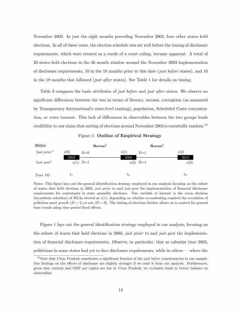
Figure 1: Outline of Empirical Strategy
2003 2008 2013
Rerun? Rerun?
D=0
D=1
D=1
D=1
e(0)
e(1)
t1
e(1)
e(2)
t2
e(2)
e(3)
t3
“just prior”
“just post”
States
Time FE:
Notes: This figure lays out the general identification strategy employed in our analysis focusing on the subset
of states that held elections in 2003, just prior to and just post the implementation of financial disclosure
requirements for contestants in state assembly elections. Our variable of interest is the rerun decision
(incumbent selection) of MLAs elected at e(τ), depending on whether re-contesting required the revelation of
politician asset growth (D = 1) or not (D = 0). The timing of elections further allows us to control for general
time trends using time period fixed effects.
Figure 1 lays out the general identification strategy employed in our analysis, focusing on
the subset of states that held elections in 2003, just prior to and just post the implementa-
tion of financial disclosure requirements. Observe, in particular, that at calendar time 2003,
politicians in some states had yet to face disclosure requirements, while in others — where the
14Note that Uttar Pradesh constitutes a significant fraction of the just before constituencies in our sample.
Our findings on the effects of disclosure are slightly stronger if we omit it from our analysis. Furthermore,
given that turnout and GDP per capita are low in Uttar Pradesh, its exclusion leads to better balance on
observables.
14

election occurred just months later — disclosures were already required. By 2008, all state
assembly candidates had to file asset disclosures. However, candidates in just post states were
making disclosures for the second time, thus revealing their asset accumulation while in office,
while candidates in just prior states made disclosures for the first time, revealing only their
wealth levels. Our estimating equation exploits this difference in the timing of elections to
separate disclosure effects from time trends.
The basic intuition of our analysis is captured in Table 4, where we show the RunNext
probability of MLAs as a function of elections relative to the advent of asset disclosures.
Focusing on elections immediately around the introduction of disclosure requirements, we
observe an increase in rerun probability between e(-2) and e(-1) for the just before subsample,
where elections span the years 1993 and 1997. For the just after subsample over approximately
the same time period (1993 - 1998), we similarly observe a small increase in the rerun rate.
(Rerun rates are also very similar for the last election of the 1980s in each group.) This
suggests some common time trend between the two groups. However, in 2003 the two sets of
states diverge – for politicians in the just before subsample elected in 2002-2003 at e(0), the
probability of standing for reelection continues to increase. By contrast, for those elected in
just after states in 2003-2004 at e(1), there is a steep drop in rerun probability. Interestingly,
one election cycle later, MLAs in just after states experience a drop in rerun probability.
The fact that the drop in rerun probability appears to be timed to election cycles relative
to disclosure requirements, rather than timed to calendar date, is the basis of our claim of a
causal effect of disclosure.
In Appendix Table A-1 we show a comparable table to examine the rerun probabilities for
runner-up candidates. For this group of “placebo” candidates, we observe no drop in their
odds of recontesting, indicating that the decrease in rerun rates for MLAs associated with
disclosure does not reflect a general decline in interest in running for office.
Before proceeding to our main specification, we note that Table 4 also shows some di-
vergences between the two subsamples in first two election cycles in the 1980s (we do not
15

have earlier data to extend the comparison further back in time). This will add noise to
the identification of a post-disclosure drop in RunNext. While these differences raise some
concerns about comparability, they occurred nearly two decades prior to the implementation
of disclosure laws, and are driven in large part by large increases in two large “just post”
states, Madhya Pradesh and Orissa. These increases led to near-identical rerun rates for the
two groups of states by the late 1980s.15
In summary, the clear similarity in rerun rates over the three election cycles preceding
the disclosure law, combined with the very strong balance between just before and just after
states, gives us confidence that unobserved differences are unlikely to be driving our results.
Our main specification for examining candidates’ rerun decisions is given by:16
RunNextist = αs + γt + βDisclosurest + δ′Controlsist + εist (1)
where RunNextist indicates whether a candidate who ran at t also chose to run for office
in the next election, while Disclosurest indicates that disclosures were required at time t in
state s. Throughout, we report bootstrapped standard errors clustered at the state level,
using the method of Cameron, Gelbach, and Miller (2008). The specification, by focusing
on the rerun decisions of politicians in office, thus assesses whether a candidate’s decision to
stand for office is affected by disclosures that would allow the public to infer his asset growth
while serving in office (since, by standing for reelection, a candidate will provide voters with
snapshots of wealth from the beginning and end of his term).
The time effect γt absorbs any time-specific effects. We include a total of seven time period
fixed effects to account for groupings of elections. For example, there is one time dummy for
the period 2002-2004, which allows us to absorb the effects of having an election in this time
period. This focuses our comparison of rerun rates of politicians in just before versus just
after states in those years.
15In unreported analyses, we confirm that our results are not sensitive to using this shorter time period
instead.16Results are essentially unchanged if we use a Probit or Logit instead of the linear model.
16
We provide several additional pieces of analysis in Section 4.2 on voter preferences, building
on the Reelection, Improved Pool, and Signal Relevance predictions above. These involve
examining how incumbency disadvantage is affected by disclosure, and also a more involved
discussion of how we expect positive self-selection to affect local conditions. This will require
a more involved discussion on the estimation of incumbency advantage and related issues,
which we defer to Section 4.2.1.
4 Results
4.1 Effect of disclosure on running for election
Table 5 provides results on the effect of asset disclosure on politicians choosing to exit, the
first prediction associated with our model (Increased Exit). If disclosure laws are effective in
providing voters or enforcement authorities with information on rent-seeking, we conjecture
that exit rates will increase post-disclosure.
The sample consists of those states that had elections between 2002 and 2004 (listed in
Panels (A) and (B) of Table 1). Controlling for time trends, column (1) of Table 5 estimates
that asset disclosures are associated with a 16.6 percentage point decrease in the re-contesting
probability of legislative assembly members. This decline, relative to a pre-disclosure base of
about 75 percent, is large in magnitude and significant at the 1 percent level. This estimate
increases to 19.87 percentage points (t-statistic of 5.7) when restricting the sample to only
those states with elections in 2003; see Appendix Table A-3.
When we add state fixed effects in column (2), the effect size drops to -0.132, still significant
at the 1 percent level. In columns (3) and (4), we add candidate-level and constituency-level
controls, respectively. These additions have little impact on the coefficient on Disclosure.
Finally, in columns (5) and (6) we aggregate data to the state-election level, using the state-
election average of Rerun as the dependent variable. The point estimates (and significance)
of the Disclosure coefficient are very similar to those obtained in our constituency-level
regressions.
17

In Appendix Table A-4 we repeat these analyses, further setting Rerun = 1 for incum-
bents who switch from state politics to running for the national legislature, the Lok Sabha
(on average, about 12 percent of exiting MLAs contest in the subsequent Lok Sabha election).
This leads to a slight increase of our point estimates on the effect of disclosure. In Appendix
Table A-5, we further control for district-level fixed effects; results are near-identical to those
reported in Table 5. Finally, in Appendix Figure A-1 we show point estimates for the coef-
ficient on Disclosure for subsamples that leave out one state at a time to ensure that the
results are not driven by a single large, influential state. We find that the point estimates
change little across subsamples.
We obtain a clearer sense of the pattern across elections in Figure 2, which plots rerun
probabilities of winners and runners-up over election cycle time. In Panel A, we show the
pattern for the winners sample, which reveals a drop in recontesting rates in the election
immediately following the advent of asset disclosure requirements (e(1)). In the second elec-
tion (e(2)), recontesting rates revert to close to their pre-disclosure level at e(0). It is difficult,
based on these patterns alone, to discern whether there is a one-time drop in recontesting
rates as certain “types” of candidates opt out of standing for office, or whether there is a
permanent drop, coupled with a secular increase in the rerun rate.
In Panel B of Figure 2 we show the analogous patterns for the runners-up sample. Notably,
there is no difference between pre- and post-disclosure rerun probabilities. In particular, there
is no difference between the probabilities of runners-up standing for reelection at e(0), e(1)
or e(2). Thus, while disclosure is associated with a drop in rerun rates of elected politicians,
it had no impact on the rerun decisions of runners-up who, we argue, present a credible
comparison set of political aspirants.
In Figure 3, we show the recontesting rates of MLAs and runners-up for just the 13
states for which we have data from the third post-disclosure election (i.e., e(3)). We observe
near-identical patterns to those of the full sample.
18

4.1.1 Robustness, and heterogeneous effects of disclosure on running for election
As we observe in Section 2, a crucial confound for our analysis is the redrawing of constituency
boundaries that took place one electoral cycle after asset disclosures became mandatory. If the
cost of standing for reelection increased when incumbents had their constituency boundaries
redrawn, this could account for the higher exit rates we associate with disclosure. As Iyer
and Reddy (2013) observe, delimitation had widely varying effects on constituency bound-
aries, in large part as a function of how far a constituency’s population deviated from the
district average (since, recall, the goal of the Delimitation Commission was to re-equate con-
stituency sizes within each district). We follow Iyer and Reddy in employing population
deviation from the district mean (scaled by the mean), as well as population and population
squared, as measures of constituency-level propensity for delimitation. In the first column
of Table 6, we allow the effect of Disclosure to vary with the absolute percentage deviation
of constituency population from the district average (PopDev). The coefficient on the inter-
action term Disclosure ∗ PopDev is small and statistically insignificant. In column (2) we
include interactions with population and population squared; again neither interaction term
approaches significance.17 Additionally, we note that if delimitation were driving the result,
we might expect to see a drop in the rerun rates of runners-up, who were similarly confronted
with redrawn constituency boundaries. Yet, as we observe at the end of the preceding section,
runners-up exhibit no such change in their rerun rates.
We next consider whether the effect of Disclosure on exit rates differs according to state-
level corruption. Corruption could, in theory, amplify or dampen the effects of disclosure on
selection. It could increase the effects of disclosure if, for example, corruption increases the
rents available to politicians. Alternatively, high corruption states may be corrupt precisely
because voters put less weight on rent seeking, in which case disclosure will have less effect
on exit if corruption is high.
Columns (3) and (4) of Table 6 include an interaction term, Disclosure ∗ Corruption,
17Results are robust and nearly unchanged when alternatively controlling for population and population
squared as measured in 2001 interacted with time dummies.
19
using two separate state-level measures of corruption. First, we use a perception-based cor-
ruption measure provided in a 2005 study on corruption by Transparency International India
(CorrIndex ). This report constructs an index for 20 Indian states based on perceived cor-
ruption in public services using comprehensive survey results from over 10,000 respondents.
We also use an indicator variable, BIMARU, to denote constituencies located in the states
of Bihar, Madhya Pradesh, Rajasthan, and Uttar Pradesh which have been singled out for
corruption and dysfunction (“bimar” means sick in Hindi; see Bose (2007)).
The coefficient on Disclosure ∗ CorrIndex is negative, significant at the 5 percent level.
Given the standard deviation on CorrIndex of 1.01 (the difference between, say, Gujarat
and Jharkhand, or Madhya Pradesh and Bihar), the coefficient of -0.044 implies that a one
standard deviation increase in corruption will result in Disclosure increasing incumbent exit
by 4.4 percentage points. We obtain qualitatively similar results (significant at the 10 per-
cent level) using BIMARU as our measure of corruption. These findings suggest that asset
disclosures, at least in the context of Indian reforms, had a greater effect on self-selection of
political candidates in high corruption environments.
In Column (5) we include the interaction of disclosure with margin of victory. If disclosure
served to weed out politically weak (low margin) candidates (which could also potentially
explain the incumbency effects we discuss below), we would expect this term to have a positive
effect. Its coefficient is instead very small, negative, and statistically insignificant. (We obtain
similar results if we measure political weakness in other ways, for example by whether the
politician’s party forms part of the state government.)
Finally, in Column (6) we include the interaction Disclosure*Newspaper Circulation,
which is marginally significant (at the 10 percent level) and positive. This implies that dis-
closure has less of an effect in areas with more readership.18 This is consistent with the view
that high circulation areas have better-informed voters and more responsive governments to
begin with, as suggested by Besley and Burgess (2002), as well as Gentzkow, Shapiro, and
18For completeness, we include in Appendix Table A-6 an additional set of results on the heterogeneity of
the effect of disclosure by candidate or constituency attributes.
20

Sinkinson (2011), leading to a more muted effect from greater transparency. The weaker im-
pact of disclosure in high circulation areas also fits with the recent theoretical contribution
of Boffa et al. (2016), which argues that rent extraction is a decreasing and convex function
of voter information. Thus, alternative sources of information may be substitutes in limited
rent extraction.19
4.2 Positive selection of candidates: Disclosure and incumbency disadvan-
tage
In organizing our analysis in Section 3, we argued that disclosure plausibly increases exit rates
because low ability (or high rent-seeking) politicians self-select out of office, anticipating that
they would not be reelected even if they chose to rerun. We examine whether the increased
exit rates documented above are associated with the positive selection of candidates, in the
sense of being more preferred by the electorate. That is, we explore whether disclosure leads
to higher reelection rates for incumbents (i.e., the politicians who choose to recontest). If it is
the case that disclosure leads to positive self-selection (i.e., an improved pool of candidates),
we also look at whether, post-disclosure, there is an improvement in local economic conditions
when a politician self-selects out of office.
4.2.1 Effect of disclosure on incumbency disadvantage
As Anagol and Fujiwara (2016) and Linden (2004) have shown, incumbents in India have
traditionally suffered from a disadvantage at the polls.20 If disclosure leads to positive selection
(from the electorate’s perspective) in who stands for office, the success of politicians who
choose to run for reelection will be higher, i.e., the incumbency disadvantage will decline.
We investigate this possibility by comparing the electoral success of incumbents against a
comparison group of politicians who were runners-up in the election in which the incumbent
19Of course, one might argue the opposite, since the media and disclosure may play complementary roles in
informing the electorate. As we have emphasized throughout, the theory is largely ambiguous on the predicted
effects of disclosure — our contribution is to document the observed patterns in a policy relevant setting.20Klasnja and Titiunik (2016) show that there is an incumbency disadvantage in a large number of developing
economies.
21

was elected. In our main analysis, we include in our sample all constituency elections in which
both the winner and runner-up choose to rerun. Below, we provide further discussion on the
rationale for using this approach to estimating incumbency advantage, and describe a series of
robustness checks to ensure that our findings are not sensitive to our specification or sample
restrictions.
The timing in our specification parallels that of our exit analysis. We thus estimate the
probability that an incumbent at time t is reelected at time t+ 1, and in particular examine
whether this probability is affected by disclosure at time t (implicitly assuming that asset
growth is the information of relevance to voters):
Winnerist+1 = αs + γt + β1Winnerist ∗Disclosurest + β2Winnerist (2)
+β3Disclosurest + δ′Controlsist + εist
The direct effect of Winner captures the incumbent (dis)advantage in an election where
disclosure is not required. The interaction term Winner ∗Disclosure captures the change in
incumbency advantage that comes with disclosure.
We present the results in Table 7. Column (1) indicates a pre-disclosure incumbent disad-
vantage of 5.7 percent (significant at the 10 percent level), comparable to estimates from Lin-
den (2004). The interaction term, Winner ∗Disclosure, has a coefficient of 0.101, indicating
that incumbents have a (weak) electoral advantage relative to challengers after the advent of
disclosure requirements. The inclusion of a range of controls (column (2)) has very little effect
on the estimated incumbency disadvantage, or how it is affected by disclosure. In columns (3)
- (5) we limit the sample to close elections: those won by 10, 5 and 3 percent respectively.
Unsurprisingly, the pre-disclosure incumbency disadvantage is far stronger in relatively close
elections, but in column (3) the coefficient on the interaction term Winner ∗ Disclosure is
largely unchanged. In columns (4) and (5), the interaction term shrinks in magnitude by
about a third (but remains significant at the 10 percent level). (When we split the sample of
constituencies based on distance from the mean district population (our measure for extent
of delimitation propensity) we observe if anything a bigger shift in incumbency disadvantage
22
among constituencies that are quite close to their district averages.)
Overall, our data thus support the prediction that disclosure leads to greater reelection
probabilities for incumbents.
In concluding this subsection, we observe that measuring incumbency advantage is a field
unto itself. First, we emphasize that, given the multi-candidate nature of Indian elections,
measuring incumbency advantage requires that we provide an appropriate benchmark against
which to measure incumbent electoral success. (This stands in contrast to, for example,
elections in the United States, in which there are generally only two viable candidates fielded
by the major parties. In two candidate systems, 50% provides a natural benchmark.) We argue
that the runner-up’s probability of victory serves as the most natural point of comparison.
To gain an appreciation of why this is so, consider a closely contested election between two
candidates that was essentially decided by a coin toss. If an equally preferred candidate
enters the subsequent race together with the current candidates (runner-up and incumbent)
and each candidate receives one-third of the vote in expectation, then simply comparing the
incumbent’s winning probability between two elections will present a misleading picture of
incumbency advantage. Our preferred approach, presented in Table 7, further restricts the
sample to cases in which the incumbent and the runner-up both recontest, allowing us to
further keep the counterfactual candidate constant.
We additionally note that our results are not sensitive to the method employed to estimate
incumbency advantage. If, following Anagol and Fujiwara (2016), we measure incumbency
advantage using a regression discontinuity design for Disclosure = 0 and Disclosure = 1
samples separately, we obtain very similar estimates of a change in incumbency disadvan-
tage associated with disclosure. The estimated discontinuities are -25.5% and -18.2% for the
Disclosure = 0 and Disclosure = 1 samples respectively, estimates that are close to the
incumbency disadvantage estimates in the narrow margin results presented in Table 7. Fi-
nally, in Appendix Table A-7 we present results paralleling those in Table 7, but including
all winners and runners-up in our analysis (rather than just winner and runner-up pairs of
23

constituencies in which both rerun). This has little impact on our measure of incumbency
disadvantage, nor on disclosure’s impact on incumbency advantage.
4.2.2 Performance in office
If lower-quality MLAs self-select out of politics as a result of disclosure, our model predicts
that incumbents who choose not to run will be replaced by, on average, higher quality entrants
(i.e., a random draw is better than a negatively selected incumbent).
Our empirical analysis aims to capture whether local economic outcomes, as measured by
district-level GDP per capita, are affected by disclosure.21 Observe that the positive selection
effects of disclosure are subtle, occurring only in cases in which the incumbent chooses to
opt out of rerunning — if he chooses to rerun, he is of the high quality type. We will
therefore be interested primarily in the interaction of Disclosure with RunNext. Identifying
the differential effect of disclosure on growth in high versus low turnover states is less clean
than that of our main analysis, which relies only on quasi-experimental variation in the timing
of state elections. We include the interaction term, however, because it allows us to probe
more directly our model’s intuition that the beneficial effects of disclosure are greater in places
where incumbents self-select out of office.
In our main results, we use state-time averages, since that is level for which government
expenditures are available. We further demean the RunNext variable so that the direct effect
of Disclosure is interpretable as the impact of introducing disclosure rules on GDP growth in
a state with an average rerun rate. (As a robustness check, we present district-level analyses
of our GDP growth results in Appendix Table A-8, using our district-level GDP data.) Our
specification is as follows:
GDPGrowthst+1 = β1(RunNextst −RunNextst) ∗Disclosurest + β2Disclosurest (3)
+β3(RunNextst −RunNextst) + αs + γt + εst
21Since we do not have data on candidate attributes in the pre-disclosure period, we cannot compare, say,
how candidate education changes with disclosure.
24
where GDPGrowthst+1 is per capita GDP growth in state s in the term following the
election when the rerun decision of the incumbent elected at time t is made. Note that the
timing is consistent with when we would expect to see an effect on politician quality, based
on our exit results above, as we measure GDP growth in the term after a large number of
incumbents self-select out (and hence avoid revealing their asset growth). The direct effect of
the fraction of incumbents that choose to run for election on per capita GDP growth is given
by RunNextst, the state-level average of RunNext. As noted above, in our regression we
demean RunNext so that β2 captures the direct effect of disclosure in an average state. The
differential effect of incumbents dropping out, post-disclosure, is captured by the coefficient
on the interaction term, β1: if disclosure leads to the selecting out of low ability candidates,
we expect β1 < 0.
We present the results in Table 8. The coefficient on the direct effect of disclosure, β2, is
positive and large in magnitude, implying a 1.7 percentage point increase in state-level growth
relative to a mean of 6.4%, though not statistically significant (p-value = 0.163). Our main
interest is in the consequences of disclosure for growth in states with high rates of politician
turnover. The coefficient on the interaction term, β1, is -0.231, significant at the 5 percent
level. This implies that disclosure was associated with a 3.5 percent higher level GDP growth
in a high turnover state like Rajasthan (RunNext = 0.6 in the second post-disclosure period)
relative to a low turnover state like Maharashtra (RunNext = 0.75).
To delve into the channels through which new political entrants might impact economic
growth, in columns (2) - (4) we present a set of regressions that use government expenditure
shares as the dependent variable, but otherwise following the same specification as in column
(1). We do not find any direct effect of disclosure on expenditure composition for an average
turnover state. However, analogous to our growth regressions, we find that budget allocations
for development-focused expenditures (such as infrastructure, education, and urban develop-
ment) increase in states with a high rate of political turnover (as reflected by lower values
of RunNext), particularly in states where disclosure is required. These findings are broadly
consistent with government decisions playing at least some role in the higher GDP growth
25
that we document in the preceding table.
Together, our performance regressions combined with those on reelection probabilities
suggest that disclosure led to improved selection of politicians.
4.3 Signal value of economic growth
We finally turn to the signal relevance hypothesis which holds that, if disclosures provide
additional information on candidate quality, other measures will receive less weight in assessing
candidates in the post-disclosure period. To operationalize this prediction, we focus on GDP
growth per capita as a signal on politicians’ performance. We examine whether growth affects
candidates’ reelection prospects, and whether this relationship is attenuated post-disclosure.
Since GDP growth is available only at the district level, we use the following (district-level)
specification:22
Winnerdst+1 = αs + γt + β1GDPGrowthdst ∗Disclosurest + β2GDPGrowthdst (4)
+β3Disclosurest + δ′Controlsdst + εdst
Winnerdst+1 captures the fraction of incumbents in district d that are reelected at t+ 1.
Observe that, in contrast to our incumbency advantage regressions above, the measure we
employ here captures both selection (RunNext) and success conditional on choosing to run. In
Appendix Table A-9, we disaggregate the effect of GDP growth into its impact on candidate
self-selection versus candidate success conditional on choosing to run. Our point estimates
suggest a larger role for GDP growth on electoral success than on self-selection, but these
results are too noisy to allow for any decisive interpretation.
In column (1) of Table 9, we begin by showing the relationship between district GDP
growth and the fraction of candidates reelected, excluding the interaction termGDPGrowthdst∗
Disclosurest. Consistent with the findings of, for example, Wolfers (2007) past economic per-
formance is a significant predictor of reelection. A one standard deviation increase in GDP
22We obtain very similar point estimates with similar standard errors in constituency-level specifications,
proxying for AC-level GDP growth with district-level growth.
26
growth (0.059) increases the fraction of politicians that remain in office by 2.5 percentage
points, or 11 percent of a standard deviation. When we add GDPGrowthdst ∗Disclosurest in
column (2), we find that the relationship between GDP growth and reelection rates exists only
in the pre-disclosure period: the coefficient on the direct effect of GDP growth increases from
0.428 to 0.584, while the coefficient on the interaction term is negative but of a near-identical
magnitude (significant at the 10 percent level). We add district-level controls in column (3),
which has only a modest effect on our point estimates (the interaction term is now significant
at the 5 percent level). Following Brender and Drazen (2008), in columns (4)-(6) we also
consider the role of GDP growth in the election year, to account for the electorate’s emphasis
on recent economic performance. Using election year growth generates very similar results.
Our results are thus consistent with voters using disclosures to assess candidates. In the
pre-disclosure period, GDP growth was predictive of electoral success. This pattern disappears
in the post-disclosure period, consistent with voters using alternative performance metrics to
evaluate politicians.
5 Conclusion
In this paper we provide, to our knowledge, the first empirical analysis of the effects of asset
disclosure laws on political selection, in the context of state-level legislative elections in India.
Because disclosure laws were implemented in November 2003 amidst a wave of state elections,
we are able to distinguish the impact of disclosure from general time trends.
We find that disclosure leads to a higher exit rate of incumbents, an improvement in the
reelection rate of those who remain, and an untethering of the correlation between economic
growth and electoral success. Moreover, these patterns are found only for incumbent MLAs
rather than runners-up candidates who, we argue, present a credible comparison group of
non-elected political aspirants. Our results are also robust to narrowing our sample to the set
of states that held elections in 2003, tempering concerns about broader, concurrent shifts in
the political landscape.
27

We argue that these findings are most easily reconciled with a model in which disclosure
leads to the selection of politicians more preferred by the electorate. In this sense, our findings
are optimistic: disclosure laws have the effect that models of electoral accountability—and
transparency advocates—would have hoped for.
There are several directions that we hope to take in future research. First, as we observe at
the outset, the efficacy of disclosure laws surely varies between countries and circumstances.
It will be useful to examine the effects of disclosure in other settings. We may also benefit
from a more intensive study of the consequences of India’s disclosure laws. Most obviously,
we have observed only a few electoral cycles since disclosure rules were put in place. It will
be illuminating to see how disclosure impacts Indian politics over a longer time horizon, as
more data becomes available in the future.
28
References
Anagol, Santosh and Thomas Fujiwara, forthcoming, The Runner-Up Effect, Journal of Political
Economy.
Banerjee, Abhijit, Rema Hanna, Jordan Kyle, Benjamin A. Olken and Sudarno Sumarto, 2015,
Tangible Information and Citizen Empowerment: Identification Cards and Food Subsidy Pro-
grams in Indonesia, Working Paper.
Banerjee, Abhijit and Rohini Pande, 2007, Parochial Politics: Ethnic Preferences and Politician
Corruption, Working Paper.
Barro, Robert, 1973, The Control of Politicians: An Economic Model, Public Choice 14, 19-42.
Beath, Andrew, Fotini Christia, Georgy Egorov and Ruben Enikolopov, 2014, Electoral Rules and
Political Selection: Theory and Evidence from a Field Experiment in Afghanistan, Working
Paper.
Besley, Timothy, 2005, Political Selection, Journal of Economic Perspectives 19(3), 43-60.
Besley, Timothy and Robin Burgess, 2002, The Political Economy of Government Responsiveness:
Theory and Evidence from India, Quarterly Journal of Economics 117(4), 1415-1451.
Besley, Timothy, Olle Folke, Torsten Persson and Johanna Rickne, 2013, Gender Quotas and the
Crisis of the Mediocre Man: Theory and Evidence from Sweden, Working Paper.
Boffa, Federico, Amedeo Piolatto, and Giacomo AM Ponzetto, 2016, Political centralization and
government accountability, Quarterly Journal of Economics 131(1), 381-422.
Brender, Adi and Allan Drazen, 2008, How Do Budget Deficits and Economic Growth Affect
Reelection Prospects? Evidence from a Large Panel of Countries, American Economic Review
98(5), 2203-2220.
Brennan, Geoffrey and James M. Buchanan, 1980, The Power to Tax: Analytical Foundations of
a Fiscal Constitution, Cambridge University Press.
Cameron, A. Colin, Jonah B. Gelbach and Douglas L. Miller, 2008, Bootstrap-Based Improvements
for Inference with Clustered Errors, The Review of Economics and Statistics 90(3), 414-427.
Casey, Katherine 2015, Crossing Party Lines: The Effects of Information on Redistributive Poli-
tics, American Economic Review 105(8), 2410-2448.
Chauchard, Simon, Marko Klasnja, and S.P. Harish, 2016, Private Gains, Public Office: A Vi-
gnette Experiment in India, Working Paper.
Dal Bo, Ernesto, Frederico Finan, Olle Folke, Torsten Persson and Johanna Rickne, 2016, Who
Becomes a Politician?, Working Paper.
Diamond, Douglas, 1991, Debt Maturity Structure and Liquidity Risk, Quarterly Journal of Eco-
nomics 106(3), 709-737.
Djankov, Simeon, Rafael La Porta, Florencio Lopez-de-Silanes and Andrei Shleifer, 2010, Disclo-
sure by Politicians, American Economic Journal: Applied Economics 2(2), 179-209.
Eggers, Andrew and Jens Hainmueller, 2009, MPs for Sale? Estimating Returns to Office in
Post-War British Politics, American Political Science Review 103(4), 513-533.
29
Ferejohn, John, 1986, Incumbent Performance and Electoral Control, Public Choice 50, 5-25.
Ferraz, Claudio and Frederico Finan, 2008, Exposing Corrupt Politicians: The Effects Of Brazil’s
Publicly Released Audits on Electoral Outcomes, Quarterly Journal of Economics 123(3), 703-
745.
Fisman, Raymond, Nikolaj Harmon, Emir Kamenica and Inger Munk, 2015, Labor Supply of
Politicians, Journal of the European Economic Association 13(5), 871-905.
Fisman, Raymond, Florian Schulz and Vikrant Vig, 2014, The Private Returns to Public Office,
Journal of Political Economy 122(4), 806-862.
Folke, Olle, Torsten Persson and Johanna Rickne, forthcoming, Preferential Voting and the Se-
lection of Party Leaders: Evidence from Sweden, American Political Science Review.
Gagliarducci, Stefano and Tommaso Nannicini, 2013, Do Better Paid Politicians Perform Better?
Disentangling Incentives from Selection, Journal of the European Economic Association 11(2),
369-398.
Gentzkow, Matthew, Jesse M. Shapiro and Michael Sinkinson, 2011, The Effect of Newspaper
Entry and Exit on Electoral Politics, American Economic Review 101(7), 2980-3018.
Iyer, Lakshmi and Maya Reddy, 2013, Redrawing the Lines: Did Political Incumbents Influence
Electoral Redistricting in the Worlds Largest Democracy?, Working Paper.
Klasnja, Marko, 2015, Corruption and the Incumbency Disadvantage: Theory and Evidence, Jour-
nal of Politics 77(4), 928-942.
Klasnja, Marko, 2016, Increasing rents and incumbency disadvantage, Journal of Theoretical Pol-
itics 28(2), 225-265.
Klasnja, Marko, and Rocio Titiunik, 2016, The Incumbency Curse: Weak Parties, Term Limits,
and Unfulfilled Accountability, American Political Science Review, forthcoming.
Linden, Leigh, 2004, Are Incumbents Always Advantaged? The Preference for Non-Incumbents in
India, Working Paper.
Persson, Torsten, and Guido Tabellini, 2000, Political Economics: Explaining Economic Policy,
MIT Press.
Reinikka, Ritva and Jakob Svensson, 2011, The power of information in public services: Evidence
from education in Uganda, Journal of Public Economics 95(7), 956-966.
Wolfers, Justin, 2007, Are Voters Rational? Evidence from Gubernatorial Elections, Working
Paper.
30

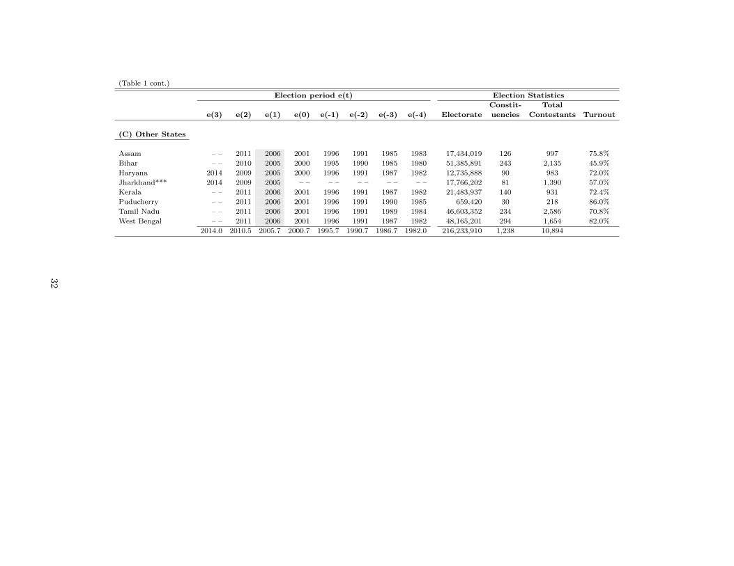
Table 1: Overview of State Assembly Elections
Notes: This Table provides an overview of the state assembly elections in our sample along with some general descriptive statistics (this data corresponds
to the gray-shaded election years). Election e(1) indicates the first election post the information disclosure reform of 2003. Panel (A) lists states that had
elections immediately following the disclosure reform (2003/04) and Panel (B) lists the subset of states that had elections just prior to the reform (2002/03).
Panel (C) list the remaining states in our sample. *Carved out of Madhya Pradesh; **carved out of Uttar Pradesh; ***carved out of Bihar (all in 2000).
Source: Statistical Reports on General Elections, Election Commission of India, New Delhi (various years).
Election period e(t) Election Statistics
Constit- Total
e(3) e(2) e(1) e(0) e(-1) e(-2) e(-3) e(-4) Electorate uencies Contestants Turnout
(A) Just post States
Andhra Pradesh 2014 2009 2004 1999 1994 1989 1985 1983 57,892,259 294 3,655 72.4%
Arunachal Pradesh 2014 2009 2004 1999 1995 1990 1984 1980 749,948 60 157 74.8%
Chhattisgarh* 2013 2008 2003 – – – – – – – – – – 15,218,560 90 1,066 70.5%
Delhi 2013 2008 2003 1998 1993 1983 1977 – – 10,726,573 70 875 57.6%
Karnataka 2013 2008 2004 1999 1994 1989 1985 1983 40,363,725 224 2,242 64.7%
Madhya Pradesh 2013 2008 2003 1998 1993 1990 1985 1980 36,266,969 230 3,179 69.3%
Maharashtra 2014 2009 2004 1999 1995 1990 1985 1980 75,968,312 288 3,559 59.5%
Mizoram 2013 2008 2003 1998 1993 1989 1987 1984 611,618 40 206 80.0%
Orissa 2014 2009 2004 2000 1995 1990 1985 1980 27,194,864 147 1,288 65.3%
Rajasthan 2013 2008 2003 1998 1993 1990 1985 1980 36,273,170 200 2,194 66.3%
Sikkim 2014 2009 2004 1999 1994 1989 1985 1979 300,584 32 167 81.8%
2013.5 2008.5 2003.6 1998.7 1993.9 1989.4 1984.8 1981.0 301,566,582 1,675 18,588
(B) Just prior States
Goa – – 2012 2007 2002 1999 1994 1989 1984 1,010,246 40 202 70.5%
Gujarat – – 2012 2007 2002 1998 1995 1990 1985 36,593,090 182 1,268 59.8%
Himachal Pradesh – – 2012 2007 2003 1998 1993 1990 1985 4,604,443 68 336 71.6%
Jammu & Kashmir – – 2014 2008 2002 1996 1987 1983 1977 6,461,757 87 1,354 61.2%
Manipur – – 2012 2007 2002 2000 1995 1990 1984 1,707,204 60 308 86.7%
Meghalaya – – 2013 2008 2003 1998 1993 1988 1983 1,214,636 60 331 89.5%
Nagaland – – 2013 2008 2003 1998 1993 1989 1987 1,302,266 60 218 87.2%
Punjab – – 2012 2007 2002 1997 1992 1985 1980 16,775,702 117 1,043 75.5%
Tripura – – 2013 2008 2003 1998 1993 1988 1983 2,037,998 60 313 92.5%
Uttar Pradesh – – 2012 2007 2002 1996 1993 1991 1989 113,549,350 403 6,086 46.0%
Uttarakhand** – – 2012 2007 2002 – – – – – – – – 5,985,302 70 785 59.5%
2012.2 2007.2 2002.2 1997.2 1993.0 1989.1 1985.3 191,241,994 1,207 12,244
(continued on next page)
31
(Table 1 cont.)
Election period e(t) Election Statistics
Constit- Total
e(3) e(2) e(1) e(0) e(-1) e(-2) e(-3) e(-4) Electorate uencies Contestants Turnout
(C) Other States
Assam – – 2011 2006 2001 1996 1991 1985 1983 17,434,019 126 997 75.8%
Bihar – – 2010 2005 2000 1995 1990 1985 1980 51,385,891 243 2,135 45.9%
Haryana 2014 2009 2005 2000 1996 1991 1987 1982 12,735,888 90 983 72.0%
Jharkhand*** 2014 2009 2005 – – – – – – – – – – 17,766,202 81 1,390 57.0%
Kerala – – 2011 2006 2001 1996 1991 1987 1982 21,483,937 140 931 72.4%
Puducherry – – 2011 2006 2001 1996 1991 1990 1985 659,420 30 218 86.0%
Tamil Nadu – – 2011 2006 2001 1996 1991 1989 1984 46,603,352 234 2,586 70.8%
West Bengal – – 2011 2006 2001 1996 1991 1987 1982 48,165,201 294 1,654 82.0%
2014.0 2010.5 2005.7 2000.7 1995.7 1990.7 1986.7 1982.0 216,233,910 1,238 10,894
32
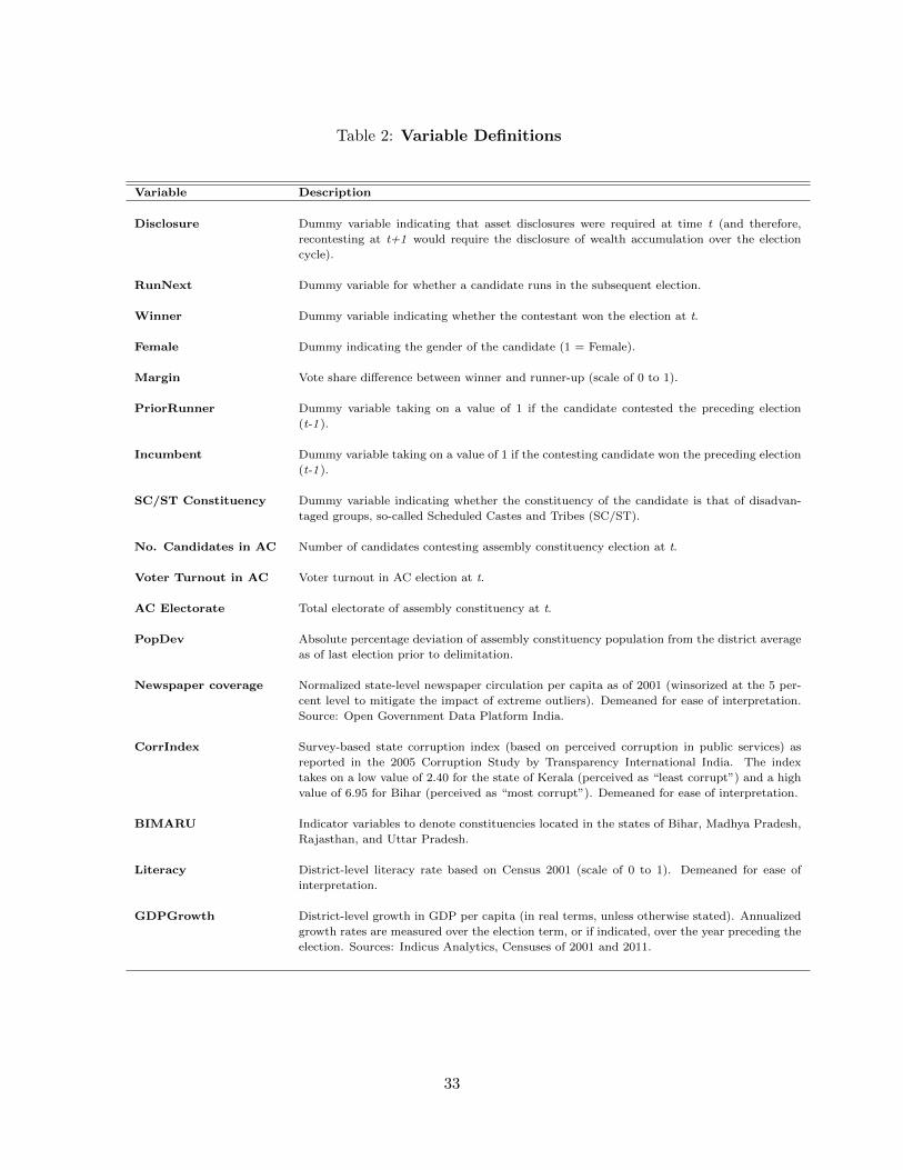
Table 2: Variable Definitions
Variable Description
Disclosure Dummy variable indicating that asset disclosures were required at time t (and therefore,
recontesting at t+1 would require the disclosure of wealth accumulation over the election
cycle).
RunNext Dummy variable for whether a candidate runs in the subsequent election.
Winner Dummy variable indicating whether the contestant won the election at t.
Female Dummy indicating the gender of the candidate (1 = Female).
Margin Vote share difference between winner and runner-up (scale of 0 to 1).
PriorRunner Dummy variable taking on a value of 1 if the candidate contested the preceding election
(t-1 ).
Incumbent Dummy variable taking on a value of 1 if the contesting candidate won the preceding election
(t-1 ).
SC/ST Constituency Dummy variable indicating whether the constituency of the candidate is that of disadvan-
taged groups, so-called Scheduled Castes and Tribes (SC/ST).
No. Candidates in AC Number of candidates contesting assembly constituency election at t.
Voter Turnout in AC Voter turnout in AC election at t.
AC Electorate Total electorate of assembly constituency at t.
PopDev Absolute percentage deviation of assembly constituency population from the district average
as of last election prior to delimitation.
Newspaper coverage Normalized state-level newspaper circulation per capita as of 2001 (winsorized at the 5 per-
cent level to mitigate the impact of extreme outliers). Demeaned for ease of interpretation.
Source: Open Government Data Platform India.
CorrIndex Survey-based state corruption index (based on perceived corruption in public services) as
reported in the 2005 Corruption Study by Transparency International India. The index
takes on a low value of 2.40 for the state of Kerala (perceived as “least corrupt”) and a high
value of 6.95 for Bihar (perceived as “most corrupt”). Demeaned for ease of interpretation.
BIMARU Indicator variables to denote constituencies located in the states of Bihar, Madhya Pradesh,
Rajasthan, and Uttar Pradesh.
Literacy District-level literacy rate based on Census 2001 (scale of 0 to 1). Demeaned for ease of
interpretation.
GDPGrowth District-level growth in GDP per capita (in real terms, unless otherwise stated). Annualized
growth rates are measured over the election term, or if indicated, over the year preceding the
election. Sources: Indicus Analytics, Censuses of 2001 and 2011.
33

Table 3: Comparison of just before and just after States
Notes: This table provides some descriptive statistics for the two subsets of states that had elections just
before and just after the disclosure event. Data are sourced from 2001 census publications by the Government
of India and from the Reserve Bank of India (RBI). Voter Turnout refers to the turnout in the 2002-2004
state elections and Change in Voter Turnout to the change in turnout between the 2002-2004 elections and
the previous elections. GDP p.c. measures the per capita net state domestic product at factor cost (Rs,
2003-04). Avg. GDP p.c. growth/year is the average yearly growth rate in GDP per capita in the three
years prior to 2003/04. Corruption Index measures state-level corruption (Source: Corruption Study 2005,
Transparency International India (June 30, 2005)). Delimitation Propensity is a measure of population size
imbalance and defined as the average of absolute differences (in percent) of constituency populations from the
average population of all constituencies within a district. Standard deviations are reported in brackets and
t-statistics for tests of differences in state-level means are shown in parentheses.
Variables Just after States Just before States (T-stat)
Total Constituencies (ACs) 1,675 1,207
% Reserved constituencies (SC/ST) 29.0% 29.8%
Population/AC 248,842 229,568
Size/AC (sq. kms.) 1,092 741
Literacy Rate 68.1% 68.5% (-0.09)
[10.3%] [8%]
GDP p.c. 22,203 24,203 (-0.43)
[9,905] [11,627]
Avg. GDP p.c. growth/year 6.2% 5.8% (0.47)
[1.7%] [1.9%]
Corruption Index 4.97 4.69 (0.57)
[0.64] [1.15]
SC/ST Concentration 37.6% 36.4% (0.11)
[23.3%] [27.8%]
Voter Turnout 67.8% 68.1% (-0.06)
[7.2%] [14.4%]
Change in Voter Turnout 0.8% -0.2% (0.37)
[4.8%] [5.6%]
Delimitation Propensity 15.4% 15.3% (0.03)
[4.7%] [4.9%]
34
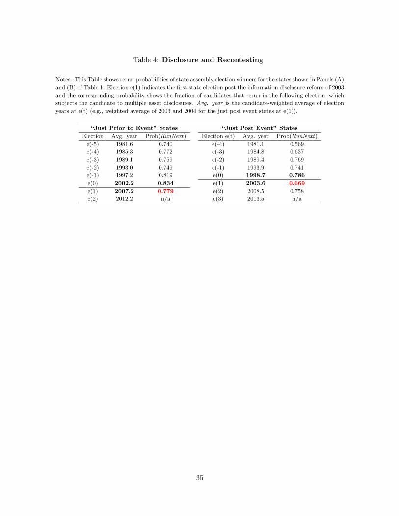
Table 4: Disclosure and Recontesting
Notes: This Table shows rerun-probabilities of state assembly election winners for the states shown in Panels (A)
and (B) of Table 1. Election e(1) indicates the first state election post the information disclosure reform of 2003
and the corresponding probability shows the fraction of candidates that rerun in the following election, which
subjects the candidate to multiple asset disclosures. Avg. year is the candidate-weighted average of election
years at e(t) (e.g., weighted average of 2003 and 2004 for the just post event states at e(1)).
“Just Prior to Event” States “Just Post Event” States
Election Avg. year Prob(RunNext) Election e(t) Avg. year Prob(RunNext)
e(-5) 1981.6 0.740 e(-4) 1981.1 0.569
e(-4) 1985.3 0.772 e(-3) 1984.8 0.637
e(-3) 1989.1 0.759 e(-2) 1989.4 0.769
e(-2) 1993.0 0.749 e(-1) 1993.9 0.741
e(-1) 1997.2 0.819 e(0) 1998.7 0.786
e(0) 2002.2 0.834 e(1) 2003.6 0.669
e(1) 2007.2 0.779 e(2) 2008.5 0.758
e(2) 2012.2 n/a e(3) 2013.5 n/a
35

Table 5: Disclosure and Recontesting of Winning Candidates
Notes: This Table investigates the effect of multiple asset disclosures on the re-contesting propensities of
members of the legislative state assemblies (MLAs). The sample includes MLAs of the 22 states shown in
Panels (A) and (B) of Table 1. The dependent variable is an indicator that takes on a value of 1 if an MLA ran
in the subsequent state election. Disclosure is an indicator that is defined as 1 if recontesting will require the
disclosure of subsequent affidavits (which allows measurement of wealth accumulation over the election cycle).
All specifications include time fixed effects to control for general time trends. Bootstrapped standard errors
clustered at the state level are given in parentheses (Cameron, Gelbach, and Miller (2008)). Coefficients with
***, **, and * are statistically significant at the 1%, 5%, and 10% levels, respectively.
(1) (2) (3) (4) (5) (6)
Variables RunNext
Disclosure -0.166*** -0.132*** -0.135*** -0.139*** -0.182*** -0.121**
(0.040) (0.046) (0.045) (0.045) (0.050) (0.047)
Female -0.057*** -0.054***
(0.019) (0.019)
Margin 0.048 0.064*
(0.032) (0.036)
PriorRunner 0.054*** 0.052***
(0.015) (0.016)
Incumbent 0.042*** 0.043***
(0.013) (0.013)
SC/ST Constituency -0.013
(0.009)
No. Candidates in AC -0.001
(0.001)
Voter Turnout in AC 0.118**
(0.050)
log(AC Electorate) 0.034**
(0.014)
Observations 18,195 18,195 17,584 17,584 127 127
Time FE Yes Yes Yes Yes Yes Yes
State FE No Yes Yes Yes No Yes
R-squared 0.024 0.04 0.051 0.052 0.229 0.582
36
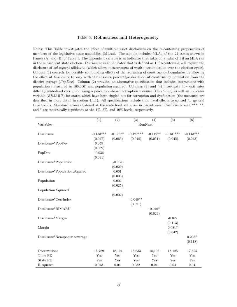
Table 6: Robustness and Heterogeneity
Notes: This Table investigates the effect of multiple asset disclosures on the re-contesting propensities of
members of the legislative state assemblies (MLAs). The sample includes MLAs of the 22 states shown in
Panels (A) and (B) of Table 1. The dependent variable is an indicator that takes on a value of 1 if an MLA ran
in the subsequent state election. Disclosure is an indicator that is defined as 1 if recontesting will require the
disclosure of subsequent affidavits (which allows measurement of wealth accumulation over the election cycle).
Column (1) controls for possibly confounding effects of the redrawing of constituency boundaries by allowing
the effect of Disclosure to vary with the absolute percentage deviation of constituency population from the
district average (PopDev). Column (2) provides an alternative specification that includes interactions with
population (measured in 100,000) and population squared. Columns (3) and (4) investigate how exit rates
differ by state-level corruption using a perception-based corruption measure (CorrIndex ) as well an indicator
variable (BIMARU ) for states which have been singled out for corruption and dysfunction (the measures are
described in more detail in section 4.1.1). All specifications include time fixed effects to control for general
time trends. Standard errors clustered at the state level are given in parentheses. Coefficients with ***, **,
and * are statistically significant at the 1%, 5%, and 10% levels, respectively.
(1) (2) (3) (4) (5) (6)
Variables RunNext
Disclosure -0.133*** -0.126** -0.127*** -0.119** -0.131*** -0.143***
(0.047) (0.063) (0.048) (0.051) (0.045) (0.043)
Disclosure*PopDev 0.059
(0.069)
PopDev -0.036
(0.031)
Disclosure*Population -0.005
(0.029)
Disclosure*Population Squared 0.001
(0.003)
Population 0.002
(0.025)
Population Squared 0
(0.002)
Disclosure*CorrIndex -0.046**
(0.021)
Disclosure*BIMARU -0.046*
(0.024)
Disclosure*Margin -0.022
(0.113)
Margin 0.081*
(0.042)
Disclosure*Newspaper coverage 0.205*
(0.118)
Observations 15,769 18,194 15,633 18,195 18,125 17,625
Time FE Yes Yes Yes Yes Yes Yes
State FE Yes Yes Yes Yes Yes Yes
R-squared 0.043 0.04 0.032 0.04 0.04 0.04
37

Table 7: Disclosure and Incumbency Advantage
Notes: This Table investigates the effect of the disclosure reform on the subsequent electoral success of re-
contesting candidates. This sample consists of paired constituency winners and runners-up of the “just post”
and “just prior” states shown in Table 1. Disclosure is an indicator that is defined as 1 if recontesting will
require the disclosure of subsequent affidavits (which allows measurement of wealth accumulation over the
election cycle). In columns (2) - (6) we add candidate-level and constituency-level controls as well as national
and state party fixed effects, and columns (3) - (6) further restrict the sample to elections decided by close
margins. All specifications include state fixed effects and time fixed effects to control for general time trends.
Standard errors clustered at the state level are given in parentheses. Coefficients with ***, **, and * are
statistically significant at the 1%, 5%, and 10% levels, respectively.
(1) (2) (3) (4) (5)
Variables Winnert+1
Disclosure*Winner 0.101*** 0.108*** 0.112*** 0.073* 0.068*
(0.032) (0.031) (0.033) (0.044) (0.036)
Winner -0.057* -0.060* -0.179*** -0.225*** -0.228***
(0.032) (0.032) (0.032) (0.035) (0.028)
Disclosure -0.066** -0.074** -0.080** -0.027 -0.009
(0.030) (0.033) (0.036) (0.037) (0.033)
Female -0.027* -0.025 -0.006 -0.02
(0.016) (0.021) (0.043) (0.051)
PriorRunner -0.015 -0.026 -0.004 -0.016
(0.014) (0.021) (0.024) (0.026)
Incumbent 0.056*** 0.055** 0.037 0.033
(0.020) (0.022) (0.023) (0.024)
SC/ST Constituency -0.021*** -0.027*** -0.021 -0.029
(0.008) (0.010) (0.016) (0.018)
No. Candidates in AC -0.001 -0.002* -0.002** -0.002**
(0.001) (0.001) (0.001) (0.001)
Voter Turnout in AC 0.105*** 0.110*** 0.063 0.028
(0.026) (0.040) (0.044) (0.081)
log(AC Electorate) 0.004 -0.001 0.005 0.008
(0.027) (0.036) (0.037) (0.034)
Close Elections: |Margin| ≤ 10 |Margin| ≤ 5 |Margin| ≤ 3
Observations 11,602 11,282 6,828 4,064 2,570
Time FE Yes Yes Yes Yes Yes
State FE Yes Yes Yes Yes Yes
R-squared 0.007 0.013 0.035 0.055 0.057
38

Table 8: Politician Selection, Economic Growth and State Budget Allocation
Notes: The table examines how state-level economic growth, as captured by state-level real GDP per capita, and state government expenditure allocation
respond to incumbent turnover. Since the dependent variables vary only at the state level, we similarly aggregate RunNext to the state-level and demean it
(RunNext−RunNext). The dependent variables in Columns (2), (3) and (4) capture the proportion of state expenditure that is allocated to Development
(including, for example, expenditure allocated to economic services, education, public health, and urban development), Non-Development (for example,
expenditure allocated to administrative services), and Other (defined as residual expenditure not explicitly designated as for either development or non-
development purposes). For reference, on average, 64.32% of state expenditure is allocated to Development, 34.53% to Non-Development, and 1.14% to
Other (Source: Reserve Bank of India). Standard errors clustered at the state level are given in parentheses. Coefficients with ***, **, and * are statistically
significant at the 1%, 5%, and 10% levels, respectively.
(1) (2) (3) (4)
State Government Expenditure Allocation (t+1)
Variables GDPGrowtht+1 Development Non-Development Other
Disclosure*(RunNext−RunNext) -0.231** -0.355** 0.389*** -0.034
(0.092) (0.140) (0.122) (0.022)
Disclosure 0.017 -0.004 0.011 -0.007
(0.012) (0.025) (0.023) (0.005)
(RunNext−RunNext) 0.233*** 0.045 -0.041 -0.004
(0.073) (0.072) (0.069) (0.010)
Observations 47 70 70 70
Time FE Yes Yes Yes Yes
State FE Yes Yes Yes Yes
R-squared 0.804 0.87 0.887 0.904
39
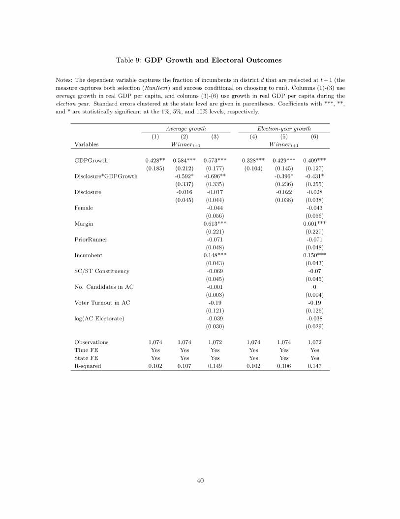
Table 9: GDP Growth and Electoral Outcomes
Notes: The dependent variable captures the fraction of incumbents in district d that are reelected at t+ 1 (the
measure captures both selection (RunNext) and success conditional on choosing to run). Columns (1)-(3) use
average growth in real GDP per capita, and columns (3)-(6) use growth in real GDP per capita during the
election year. Standard errors clustered at the state level are given in parentheses. Coefficients with ***, **,
and * are statistically significant at the 1%, 5%, and 10% levels, respectively.
Average growth Election-year growth
(1) (2) (3) (4) (5) (6)
Variables Winnert+1 Winnert+1
GDPGrowth 0.428** 0.584*** 0.573*** 0.328*** 0.429*** 0.409***
(0.185) (0.212) (0.177) (0.104) (0.145) (0.127)
Disclosure*GDPGrowth -0.592* -0.696** -0.396* -0.431*
(0.337) (0.335) (0.236) (0.255)
Disclosure -0.016 -0.017 -0.022 -0.028
(0.045) (0.044) (0.038) (0.038)
Female -0.044 -0.043
(0.056) (0.056)
Margin 0.613*** 0.601***
(0.221) (0.227)
PriorRunner -0.071 -0.071
(0.048) (0.048)
Incumbent 0.148*** 0.150***
(0.043) (0.043)
SC/ST Constituency -0.069 -0.07
(0.045) (0.045)
No. Candidates in AC -0.001 0
(0.003) (0.004)
Voter Turnout in AC -0.19 -0.19
(0.121) (0.126)
log(AC Electorate) -0.039 -0.038
(0.030) (0.029)
Observations 1,074 1,074 1,072 1,074 1,074 1,072
Time FE Yes Yes Yes Yes Yes Yes
State FE Yes Yes Yes Yes Yes Yes
R-squared 0.102 0.107 0.149 0.102 0.106 0.147
40

Figure 2: Recontesting
Notes: The following graphs show time series of re-run probabilities over election cycle time. Election e(0) indi-
cates the last election prior to disclosure and the figure plots the percentage of winners at e(t) that re-contested
in the subsequent election e(t+1). Election e(1) indicates the first election post the information disclosure
reform of 2003. Panel A plots probabilities for Members of the Legislative Assemblies (MLAs) and Panel B
plots probabilities for corresponding election runners-up. 95% confidence intervals are indicated by dotted lines.
Panel A: Winners
Panel B: Runners-up
41

Figure 3: Recontesting - States with 3 post-disclosure elections
Notes: The following graphs show time series of re-run probabilities over election cycle time for the subset of 13
states with three elections post disclosure. Election e(0) indicates the last election prior to disclosure and the
figure plots the percentage of winners at e(t) that re-contested in the subsequent election e(t+1). Election e(1)
indicates the first election post the information disclosure reform of 2003. Panel A plots probabilities for
Members of the Legislative Assemblies (MLAs) and Panel B plots probabilities for corresponding election
runners-up. 95% confidence intervals are indicated by dotted lines.
Panel A: Winners
Panel B: Runners-up
42
A Appendix: A model of disclosure and political selection
We present a stylized model of asymmetric information in which voters are forced to pool high-
and low-quality candidates (i.e., public-minded and rent-seeking) in the absence of disclosure.
Our model provides a set of intuitive predictions on the consequences of disclosure for political
selection, and the resultant economic consequences.23 The reader should not interpret our
model as generating a set of structural parameters to be estimated. Alternative modeling
assumptions or constraints on parameter values may generate distinct predictions — rather,
our purpose is to illustrate how our set of empirical analyses may be generated by a spare
and straightforward model of political selection.
A.1 Model Setup
We consider an economy with 2 periods (during which politicians hold office) and 3 dates
(t=1, t=2, t=3) marking the beginning and end of each period. A pool of incumbents is
assigned at t=1. Politician ability is given by θ, which can be high or low, i.e., θ ∈ {θH , θL}.Ability type is private information. For the pool of incumbents at t=1, the probability that
a politician is of high ability is given by p. This initial pool of officeholders can stand for
reelection at date t = 2. (We could base our model on different preferences or talents over rent
extraction rather than ability to generate public welfare. This would generate an identical set
of predictions.)
Each period, politicians invest public resources that generate publicly observable benefits
B, such as government-provided social services or economic growth. We assume that these
benefits are realized at the end of each period, with B ∈ {BH , BL}. The probability that
B = BH is given by θ and we assume that 1 > θH > θL = 0. That is, while the payoff is
risky for high ability types, the “investment returns” are low with certainty for low ability
politicians. We further assume that ability type is persistent and that (if relevant) public
benefits are drawn independently across periods. At the beginning of the legislative cycle,
a politician also chooses whether to engage in rent extraction, so that realized rents are
R ∈ {R, r}, where R > r, initially unobservable to voters. If the officeholder decides to
engage in rent seeking (R = R), then benefits will be low with certainty, i.e., B = BL.24
Politicians have preference over both public service and private rents. Each period a politi-
cian’s utility is given by U = α · B+R. We further assume that high ability politicians prefer
to “behave”, that is, α · θH · (BH − BL) > R − r. Following the first period realization of B,
at t = 2 politicians have the choice of standing for reelection. Running an election campaign
incurs costs of k (in our two-period setting there is no re-contesting at t = 3). For simplicity,
we normalize outside option wages and salaries to zero, assume a discount rate of zero, and
23The structure of our model is inspired by Diamond (1991).24This assumption can also be motivated based on non-verifiable “investment” in the community that is
stolen by the politician.
43

assume that all agents are risk-neutral. Figure 4 summarizes the time line for the model.
Figure 4: Timeline
Incumbent politicians choose
level of rent extraction (R1)
and invest public resources
Public benefits B1, observable
to electorate
Rerun decision of incumbent
(cost k) and voting
If elected, politician chooses level
of rent extraction (R2) and invests
public resources
Public benefits B2
MLA utility:
U1 = α · B1 +R1
MLA utility (if re-elected):
U2 = α · B2 +R2t=1 t=2 t=3
Electorate preferences and pool of challengers at t=2: We model elections at t = 2
as follows. An incumbent politician faces a single outside contestant who is of high ability
(θ = θH) with probability p. We think of this challenger as emerging as the result of a longer,
multi-candidate campaign, and hence p becomes apparent only as the election approaches.
We model this in practice as being reflected in uncertainty over the value of p, assuming that
it is distributed uniformly between 0 and 1 but initially unknown to both the electorate and
the candidate. Thus, only as the election campaign nears completion, (after incurring cost k
by the candidate but before voting) will the draw of p be learned by the electorate.
The electorate’s preference at t = 2 is to elect candidates to maximize expected public
benefits (B2) over the following period. While prior to the disclosure reform, voters observe
only B1 over the first period, the disclosure of politician asset returns allows the electorate to
observe the level of rent extraction, R1, as well. In the pre-disclosure period the probability
of reelection if past growth is low is thus simply p(H | BL), or(p−pθH1−pθH
).
We make two additional assumptions, to ensure that (1) campaigning expenses are low
enough that low ability candidates always recontest pre-disclosure, and that (2) post-disclosure
ofR, low ability politicians have insufficient incentive to “pretend” to be high type by choosing
R1 = r.
Assumption 1 (Running Incentives)(p−pθH1−pθH
)· (αBL +R) > k. That is, in the absence
of learning through asset return disclosures, campaign expenses are low enough to ensure that
low ability incumbents always choose to stand for reelection at t = 2.
Assumption 2 (No Mimicking/Pooling) α·BL+R > (α·BL+r)+(p−pθH1−pθH
)(α·BL+R)−k.
That is, it is suboptimal for low ability politicians to choose R1 = r.
44
Lemma 1 Let φ = Pr(θ = θH |I) where I is the information set of the electorate (e.g.,
realization of G only prior to disclosure). At t=2, before running a campaign, a re-contesting
incumbent politician expects to be reelected with probability φ.
Lemma 1 follows directly from the assumptions on recontesting at t = 2. Thus, a politi-
cian’s objective function can be succinctly written as: U = α·B1+R1+[φ · (α · B2 +R2)− k]·1{rerun} where 1{rerun} is an indicator for whether the incumbent recontests at t = 2.
A.2 Standing for reelection in the absence of disclosure
Conditional on being elected at t=2, H-type and L-type candidates choose RH2 = r and
RL2 = R, respectively (individual rationality). Further, if public benefits are high in the first
period (B1 = BH), the incumbent candidate type is revealed perfectly to the electorate as high
ability. The politician thus chooses to rerun and is elected with certainty. If public benefits
are low in the first period (B1 = BL), then the electorate cannot infer the incumbent’s type.
By Assumption 1, both high and low ability type candidates choose to rerun and are elected
with probability φ =(p−pθH1−pθH
)(which is less than unity).
Thus, pre-disclosure we get the following prediction: Observable public benefits serve as
a (noisy) signal of candidate ability and is thus predictive of electoral success. Further, the
rerun rate without disclosure (which, given our parameter assumptions, leads to the extreme
case where all incumbents recontest), serves as a benchmark to compare against the rerun
rates when disclosures are required.
A.3 Political selection with disclosure of asset growth
With disclosure of R1, incumbent type is perfectly revealed though the disclosure of asset
returns R1 alone (by Assumption 2 only low ability incumbents choose R1 = R). The
previously noisy signal of ability, B, loses relevance. Since types are revealed, by Lemma 1,
all low ability politicians exit the sample at t = 2.
Thus, we get the following additional predictions, summarized below as Proposition 1.
Proposition 1 Disclosure of asset growth of incumbents will result in the following:
• (Increased Exit) Relative to the pre-disclosure period, there will be higher exit of
incumbents at t = 2 when contesting requires the disclosure of asset returns.
• (Reelection) Since, under disclosure, only high ability incumbents choose to recontest
and are elected with probability 1, re-contesting incumbents are more likely to be reelected.
That is, disclosure leads to positive selection.
45
• (Improved Pool) Since only low ability incumbents choose to exit, their replacements,
even if chosen randomly, will be of higher expected ability.
• (Signal relevance) Under disclosure, observable public benefits B are less informative
as a signal of candidate ability, and hence is less predictive of incumbent reelection.
These intuitive propositions follow straightforwardly from the parameter restrictions, when
combined with Lemma 1. In particular, whereas there is pooling of high and low types
when B1 = BL in the absence of disclosure, all low ability incumbents exit under disclosure,
leading to higher exit. It immediately follows that the electoral success of incumbents who,
under disclosure, are revealed as high ability, will improve (reelection). Since only low ability
incumbents choose to exit, disclosure will also lead to politicians of higher expected ability
(and hence higher expected B) (improved pool). 25 The perfect separation of high and low
ability incumbents under disclosure leads to the irrelevance of alternative signals of quality
(or, under a more general model, revelation of an additional quality signal will reduce reliance
on existing signals) (signal relevance).
25Our arguments in this section are in line with the model of Klasnja (2016), which focuses directly on
corruption and the incumbency disadvantage. See also Klasnja (2015) for evidence from Romania.
46
Table A-1: Recontesting of Runners-up
Notes: This Table shows rerun-probabilities of state assembly election runners-up for the states shown in
Panels (A) and (B) of Table 1. Election e(1) indicates the first state election post the information disclosure
reform of 2003 and the corresponding probability shows the fraction of candidates that rerun in the following
election, which subjects the candidate to multiple asset disclosures. Avg. year is the candidate-weighted
average of election years at e(t) (e.g., weighted average of 2003 and 2004 for the just post event states at e(1)).
“Just Prior to Event” States “Just Post Event” States
Election Avg. year Prob(RunNext) Election e(t) Avg. year Prob(RunNext)
e(-5) 1981.6 0.400 e(-4) 1981.1 0.327
e(-4) 1985.3 0.461 e(-3) 1984.8 0.360
e(-3) 1989.1 0.450 e(-2) 1989.4 0.417
e(-2) 1993.0 0.459 e(-1) 1993.9 0.425
e(-1) 1997.1 0.486 e(0) 1998.7 0.440
e(0) 2002.2 0.501 e(1) 2003.6 0.444
e(1) 2007.2 0.509 e(2) 2008.5 0.452
e(2) 2012.2 n/a e(3) 2013.5 n/a
47

Table A-2: Disclosure and Recontesting of Runners-up
Notes: This Table investigates the effect of multiple asset disclosures on the re-contesting propensities of state
assembly election runners-up (“Placebo test”). The sample includes runners-up for the 22 states shown in
Panels (A) and (B) of Table 1. The dependent variable is an indicator that takes on a value of 1 if the
candidate ran in the subsequent state election. Disclosure is an indicator that is defined as 1 if recontesting
will require the disclosure of subsequent affidavits (which allows measurement of wealth accumulation over the
election cycle). All specifications include time fixed effects to control for general time trends. Standard errors
clustered at the state level are given in parentheses. Coefficients with ***, **, and * are statistically significant
at the 1%, 5%, and 10% levels, respectively.
(1) (2) (3) (4) (5)
Variables RunNext
Disclosure -0.057 -0.001 -0.005 -0.005 -0.005
(0.045) (0.034) (0.032) (0.032) (0.032)
Female -0.099*** -0.100*** -0.100***
(0.013) (0.013) (0.013)
Margin -0.716*** -0.721*** -0.723***
(0.058) (0.058) (0.060)
PriorRunner 0.084*** 0.084*** 0.084***
(0.013) (0.013) (0.013)
Incumbent 0.112*** 0.112*** 0.112***
(0.013) (0.013) (0.013)
SC/ST Constituency 0.022 0.021
(0.015) (0.014)
No. Candidates in AC -0.001 -0.001
(0.001) (0.001)
Voter Turnout in AC -0.015
(0.064)
log(AC Electorate) 0.004
(0.023)
Observations 18,125 18,125 17,584 17,584 17,584
Time FE Yes Yes Yes Yes Yes
State FE No Yes Yes Yes Yes
R-squared 0.007 0.033 0.1 0.1 0.1
48

Table A-3: Disclosure and Recontesting (States with elections in 2003 only)
Notes: This Table investigates the effect of multiple asset disclosures on the re-contesting propensities of
members of the legislative state assemblies (MLAs). The sample includes MLAs of the states that held
elections in 2003, prior to and post the implementation of disclosure requirements. The dependent variable
is an indicator that takes on a value of 1 if an MLA ran in the subsequent state election. Disclosure is an
indicator that is defined as 1 if recontesting will require the disclosure of subsequent affidavits (which allows
measurement of wealth accumulation over the election cycle). All specifications include time fixed effects to
control for general time trends. Standard errors clustered at the state level are given in parentheses. Coefficients
with ***, **, and * are statistically significant at the 1%, 5%, and 10% levels, respectively.
(1) (2) (3) (4) (5)
Variables RunNext
Disclosure -0.199*** -0.127* -0.134** -0.134** -0.135**
(0.035) (0.066) (0.066) (0.066) (0.062)
Female 0.006 0.008 0.009
(0.015) (0.015) (0.014)
Margin 0.033 0.048 0.051
(0.108) (0.109) (0.105)
PriorRunner 0.054*** 0.054*** 0.054***
(0.017) (0.017) (0.018)
Incumbent 0.043** 0.043** 0.044**
(0.020) (0.020) (0.020)
SC/ST Constituency -0.040*** -0.041***
(0.007) (0.012)
No. Candidates in AC 0 -0.001
(0.001) (0.001)
Voter Turnout in AC -0.034
(0.125)
log(AC Electorate) 0.073***
(0.018)
Observations 4,070 4,070 3,954 3,954 3,954
Time FE Yes Yes Yes Yes Yes
State FE No Yes Yes Yes Yes
R-squared 0.017 0.03 0.041 0.043 0.044
49
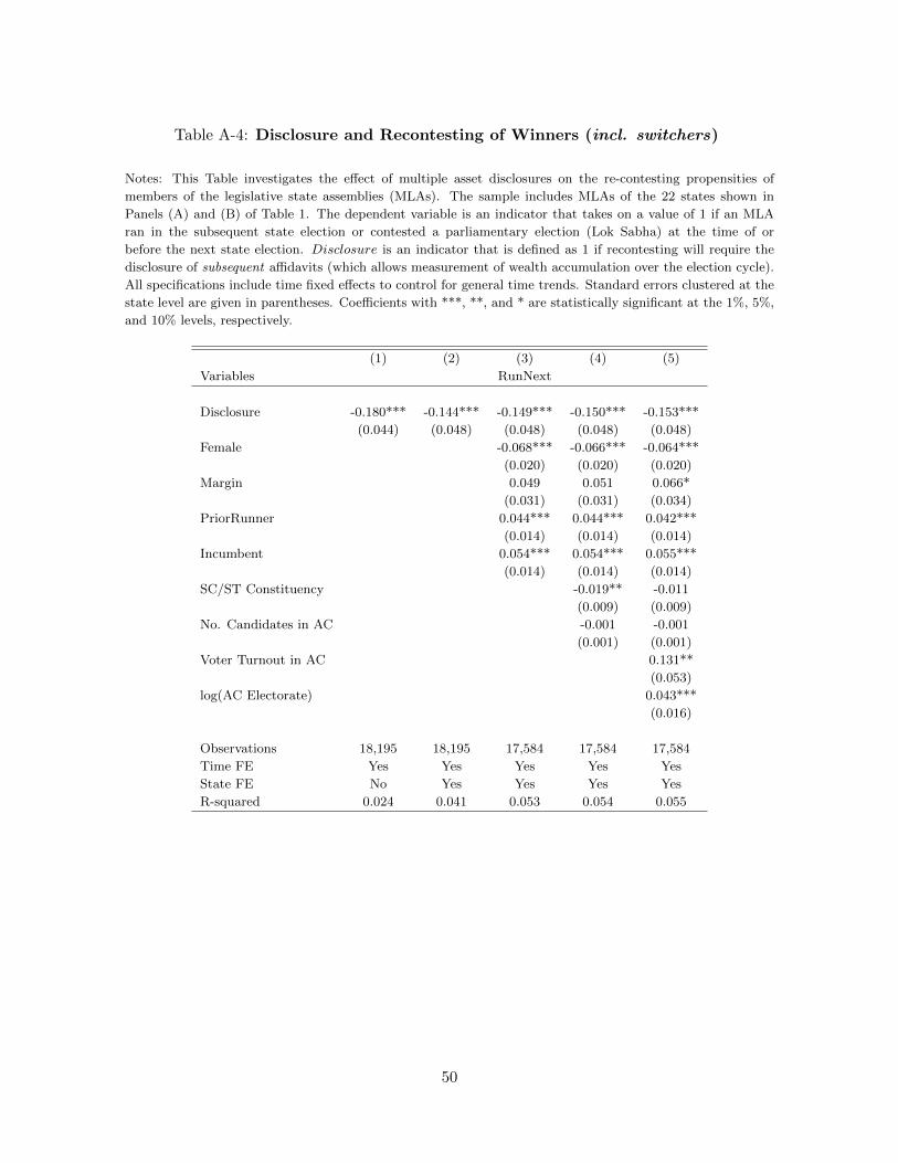
Table A-4: Disclosure and Recontesting of Winners (incl. switchers)
Notes: This Table investigates the effect of multiple asset disclosures on the re-contesting propensities of
members of the legislative state assemblies (MLAs). The sample includes MLAs of the 22 states shown in
Panels (A) and (B) of Table 1. The dependent variable is an indicator that takes on a value of 1 if an MLA
ran in the subsequent state election or contested a parliamentary election (Lok Sabha) at the time of or
before the next state election. Disclosure is an indicator that is defined as 1 if recontesting will require the
disclosure of subsequent affidavits (which allows measurement of wealth accumulation over the election cycle).
All specifications include time fixed effects to control for general time trends. Standard errors clustered at the
state level are given in parentheses. Coefficients with ***, **, and * are statistically significant at the 1%, 5%,
and 10% levels, respectively.
(1) (2) (3) (4) (5)
Variables RunNext
Disclosure -0.180*** -0.144*** -0.149*** -0.150*** -0.153***
(0.044) (0.048) (0.048) (0.048) (0.048)
Female -0.068*** -0.066*** -0.064***
(0.020) (0.020) (0.020)
Margin 0.049 0.051 0.066*
(0.031) (0.031) (0.034)
PriorRunner 0.044*** 0.044*** 0.042***
(0.014) (0.014) (0.014)
Incumbent 0.054*** 0.054*** 0.055***
(0.014) (0.014) (0.014)
SC/ST Constituency -0.019** -0.011
(0.009) (0.009)
No. Candidates in AC -0.001 -0.001
(0.001) (0.001)
Voter Turnout in AC 0.131**
(0.053)
log(AC Electorate) 0.043***
(0.016)
Observations 18,195 18,195 17,584 17,584 17,584
Time FE Yes Yes Yes Yes Yes
State FE No Yes Yes Yes Yes
R-squared 0.024 0.041 0.053 0.054 0.055
50

Table A-5: Disclosure and Recontesting (District fixed effects)
Notes: This Table investigates the effect of multiple asset disclosures on the re-contesting propensities of
members of the legislative state assemblies (MLAs). The sample includes MLAs of the 22 states shown in
Panels (A) and (B) of Table 1. The dependent variable is an indicator that takes on a value of 1 if an MLA
ran in the subsequent state election. Disclosure is an indicator that is defined as 1 if recontesting will require
the disclosure of subsequent affidavits (which allows measurement of wealth accumulation over the election
cycle). All specifications include time fixed effects to control for general time trends. In columns (5) and (6),
the dependent variable is measured as average of RunNext at the district-level. Bootstrapped standard errors
clustered at the state level are given in parentheses. Coefficients with ***, **, and * are statistically significant
at the 1%, 5%, and 10% levels, respectively.
(1) (2) (3) (4) (5) (6)
Variables RunNext
Disclosure -0.166*** -0.130*** -0.126*** -0.130*** -0.150*** -0.113**
(0.040) (0.045) (0.045) (0.044) (0.040) (0.049)
Female -0.055*** -0.052**
(0.021) (0.021)
Margin 0.075** 0.095***
(0.032) (0.034)
PriorRunner 0.049*** 0.047***
(0.015) (0.015)
Incumbent 0.031*** 0.031***
(0.012) (0.012)
SC/ST Constituency -0.018**
(0.008)
No. Candidates in AC -0.001*
(0.001)
Voter Turnout in AC 0.169**
(0.072)
log(AC Electorate) 0.057***
(0.021)
Observations 17,960 17,960 17,480 17,480 2,642 2,642
Time FE Yes Yes Yes Yes Yes Yes
District FE No Yes Yes Yes No Yes
R-squared 0.024 0.072 0.079 0.081 0.084 0.305
51
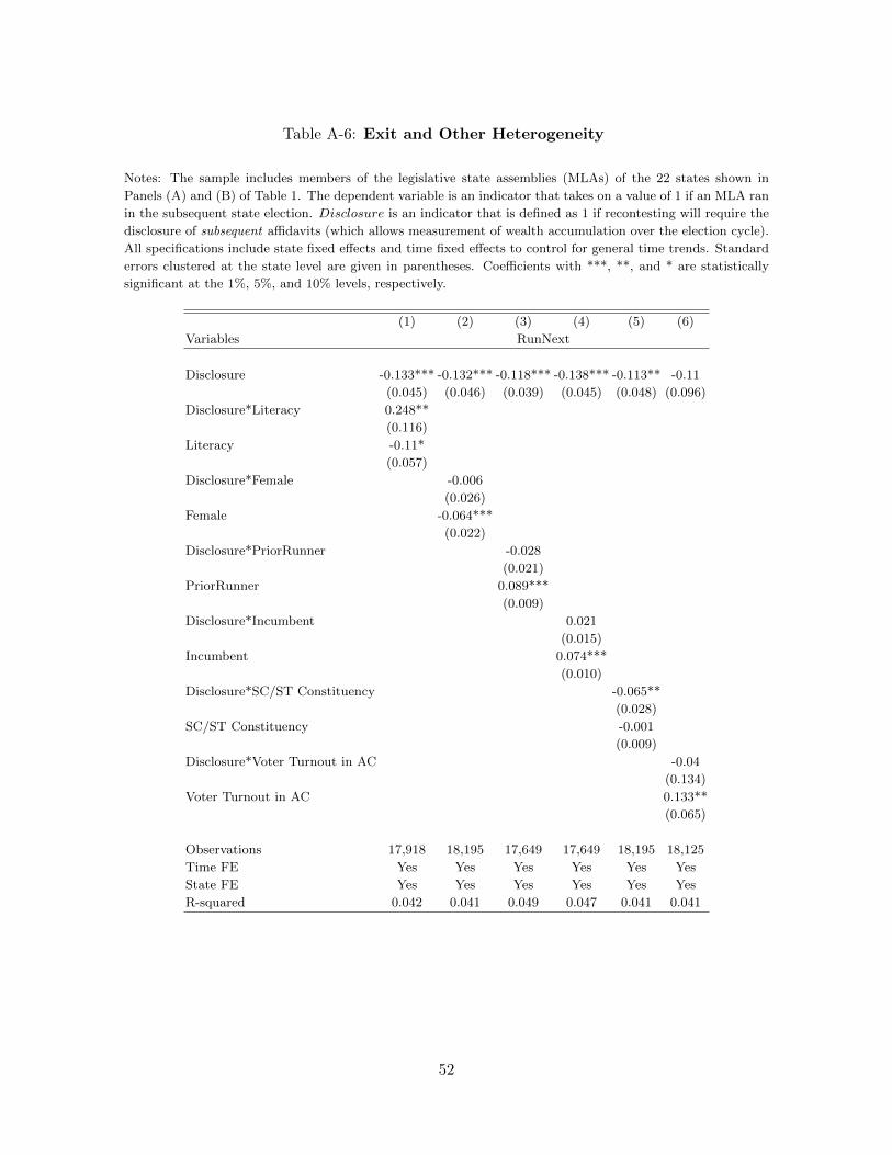
Table A-6: Exit and Other Heterogeneity
Notes: The sample includes members of the legislative state assemblies (MLAs) of the 22 states shown in
Panels (A) and (B) of Table 1. The dependent variable is an indicator that takes on a value of 1 if an MLA ran
in the subsequent state election. Disclosure is an indicator that is defined as 1 if recontesting will require the
disclosure of subsequent affidavits (which allows measurement of wealth accumulation over the election cycle).
All specifications include state fixed effects and time fixed effects to control for general time trends. Standard
errors clustered at the state level are given in parentheses. Coefficients with ***, **, and * are statistically
significant at the 1%, 5%, and 10% levels, respectively.
(1) (2) (3) (4) (5) (6)
Variables RunNext
Disclosure -0.133*** -0.132*** -0.118*** -0.138*** -0.113** -0.11
(0.045) (0.046) (0.039) (0.045) (0.048) (0.096)
Disclosure*Literacy 0.248**
(0.116)
Literacy -0.11*
(0.057)
Disclosure*Female -0.006
(0.026)
Female -0.064***
(0.022)
Disclosure*PriorRunner -0.028
(0.021)
PriorRunner 0.089***
(0.009)
Disclosure*Incumbent 0.021
(0.015)
Incumbent 0.074***
(0.010)
Disclosure*SC/ST Constituency -0.065**
(0.028)
SC/ST Constituency -0.001
(0.009)
Disclosure*Voter Turnout in AC -0.04
(0.134)
Voter Turnout in AC 0.133**
(0.065)
Observations 17,918 18,195 17,649 17,649 18,195 18,125
Time FE Yes Yes Yes Yes Yes Yes
State FE Yes Yes Yes Yes Yes Yes
R-squared 0.042 0.041 0.049 0.047 0.041 0.041
52
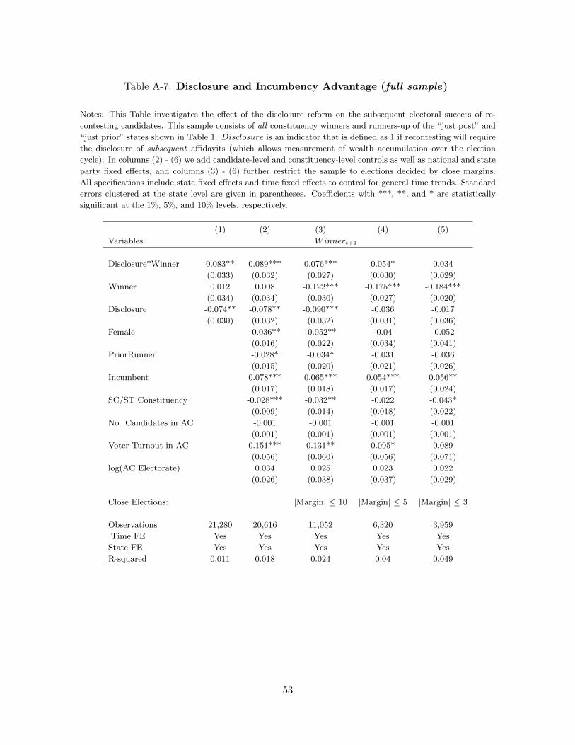
Table A-7: Disclosure and Incumbency Advantage (full sample)
Notes: This Table investigates the effect of the disclosure reform on the subsequent electoral success of re-
contesting candidates. This sample consists of all constituency winners and runners-up of the “just post” and
“just prior” states shown in Table 1. Disclosure is an indicator that is defined as 1 if recontesting will require
the disclosure of subsequent affidavits (which allows measurement of wealth accumulation over the election
cycle). In columns (2) - (6) we add candidate-level and constituency-level controls as well as national and state
party fixed effects, and columns (3) - (6) further restrict the sample to elections decided by close margins.
All specifications include state fixed effects and time fixed effects to control for general time trends. Standard
errors clustered at the state level are given in parentheses. Coefficients with ***, **, and * are statistically
significant at the 1%, 5%, and 10% levels, respectively.
(1) (2) (3) (4) (5)
Variables Winnert+1
Disclosure*Winner 0.083** 0.089*** 0.076*** 0.054* 0.034
(0.033) (0.032) (0.027) (0.030) (0.029)
Winner 0.012 0.008 -0.122*** -0.175*** -0.184***
(0.034) (0.034) (0.030) (0.027) (0.020)
Disclosure -0.074** -0.078** -0.090*** -0.036 -0.017
(0.030) (0.032) (0.032) (0.031) (0.036)
Female -0.036** -0.052** -0.04 -0.052
(0.016) (0.022) (0.034) (0.041)
PriorRunner -0.028* -0.034* -0.031 -0.036
(0.015) (0.020) (0.021) (0.026)
Incumbent 0.078*** 0.065*** 0.054*** 0.056**
(0.017) (0.018) (0.017) (0.024)
SC/ST Constituency -0.028*** -0.032** -0.022 -0.043*
(0.009) (0.014) (0.018) (0.022)
No. Candidates in AC -0.001 -0.001 -0.001 -0.001
(0.001) (0.001) (0.001) (0.001)
Voter Turnout in AC 0.151*** 0.131** 0.095* 0.089
(0.056) (0.060) (0.056) (0.071)
log(AC Electorate) 0.034 0.025 0.023 0.022
(0.026) (0.038) (0.037) (0.029)
Close Elections: |Margin| ≤ 10 |Margin| ≤ 5 |Margin| ≤ 3
Observations 21,280 20,616 11,052 6,320 3,959
Time FE Yes Yes Yes Yes Yes
State FE Yes Yes Yes Yes Yes
R-squared 0.011 0.018 0.024 0.04 0.049
53

Table A-8: Performance in Office
Notes: The table examines whether local economic growth, as captured by district-level GDP per capita,
responds to incumbent turnover. Since the dependent variable varies only at the district level, we similarly
aggregate RunNext as well as other candidate-level and constituency-level controls to the district-level. In
Columns (1), (2), (4) and (5), the dependent variable is measured on a real basis, while column (3) uses
growth in nominal GDP per capita. Standard errors clustered at the state level are given in parentheses.
Coefficients with ***, **, and * are statistically significant at the 1%, 5%, and 10% levels, respectively.
(1) (2) (3) (4) (5)
Variables GDPGrowtht+1
Disclosure*RunNext -0.027* -0.029** -0.035** -0.030** -0.027**
(0.014) (0.014) (0.014) (0.014) (0.013)
Disclosure 0.017 0.013 0.012 0.014 0.012
(0.013) (0.010) (0.011) (0.010) (0.010)
RunNext 0.017 0.024** 0.027** 0.027** 0.023**
(0.011) (0.012) (0.011) (0.012) (0.011)
Female 0.007 0.006
(0.007) (0.005)
Margin 0.063*** 0.072***
(0.019) (0.022)
PriorRunner -0.003 0.000
(0.006) (0.005)
Incumbent -0.007 -0.008
(0.005) (0.006)
SC/ST Constituency -0.012***
(0.004)
No. Candidates in AC 0.000
(0.000)
Voter Turnout in AC 0.017
(0.025)
log(AC Electorate) -0.020**
(0.008)
Observations 960 960 960 960 959
Time FE Yes Yes Yes Yes Yes
State FE No Yes Yes Yes Yes
R-squared 0.048 0.185 0.166 0.206 0.247
54
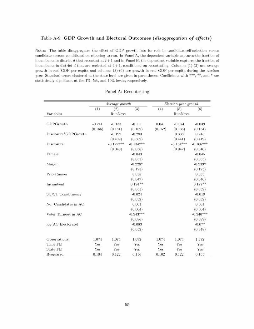
Table A-9: GDP Growth and Electoral Outcomes (disaggregation of effects)
Notes: The table disaggregates the effect of GDP growth into its role in candidate self-selection versus
candidate success conditional on choosing to run. In Panel A, the dependent variable captures the fraction of
incumbents in district d that recontest at t+ 1 and in Panel B, the dependent variable captures the fraction of
incumbents in district d that are reelected at t + 1, conditional on recontesting. Columns (1)-(3) use average
growth in real GDP per capita and columns (3)-(6) use growth in real GDP per capita during the election
year. Standard errors clustered at the state level are given in parentheses. Coefficients with ***, **, and * are
statistically significant at the 1%, 5%, and 10% levels, respectively.
Panel A: Recontesting
Average growth Election-year growth
(1) (2) (3) (4) (5) (6)
Variables RunNext RunNext
GDPGrowth -0.241 -0.133 -0.111 0.041 -0.074 -0.039
(0.166) (0.181) (0.169) (0.152) (0.136) (0.134)
Disclosure*GDPGrowth -0.192 -0.283 0.338 0.245
(0.409) (0.369) (0.441) (0.419)
Disclosure -0.122*** -0.134*** -0.154*** -0.166***
(0.040) (0.036) (0.042) (0.040)
Female -0.043 -0.045
(0.053) (0.053)
Margin -0.228* -0.239*
(0.123) (0.123)
PriorRunner 0.038 0.033
(0.047) (0.046)
Incumbent 0.124** 0.127**
(0.053) (0.052)
SC/ST Constituency -0.024 -0.019
(0.032) (0.032)
No. Candidates in AC 0.001 0.001
(0.004) (0.004)
Voter Turnout in AC -0.243*** -0.240***
(0.086) (0.089)
log(AC Electorate) -0.083 -0.077
(0.052) (0.048)
Observations 1,074 1,074 1,072 1,074 1,074 1,072
Time FE Yes Yes Yes Yes Yes Yes
State FE Yes Yes Yes Yes Yes Yes
R-squared 0.104 0.122 0.156 0.102 0.122 0.155
55
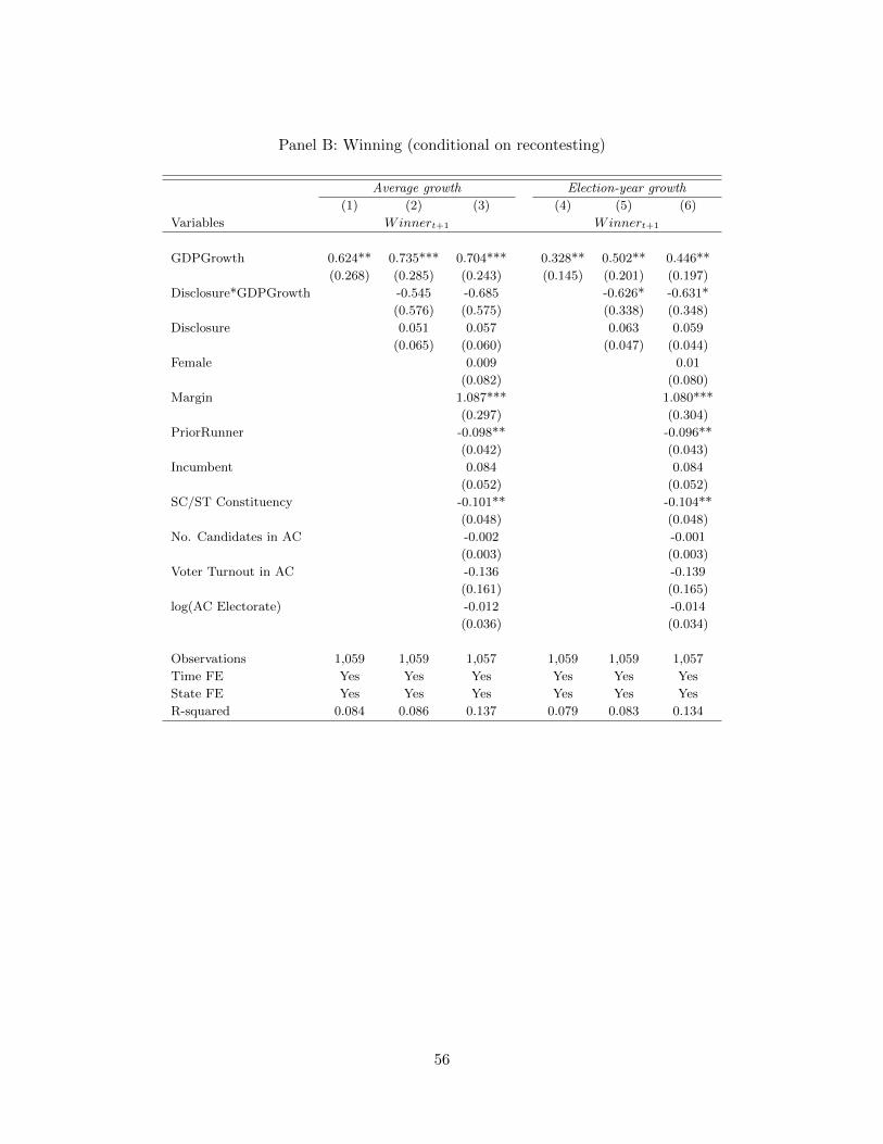
Panel B: Winning (conditional on recontesting)
Average growth Election-year growth
(1) (2) (3) (4) (5) (6)
Variables Winnert+1 Winnert+1
GDPGrowth 0.624** 0.735*** 0.704*** 0.328** 0.502** 0.446**
(0.268) (0.285) (0.243) (0.145) (0.201) (0.197)
Disclosure*GDPGrowth -0.545 -0.685 -0.626* -0.631*
(0.576) (0.575) (0.338) (0.348)
Disclosure 0.051 0.057 0.063 0.059
(0.065) (0.060) (0.047) (0.044)
Female 0.009 0.01
(0.082) (0.080)
Margin 1.087*** 1.080***
(0.297) (0.304)
PriorRunner -0.098** -0.096**
(0.042) (0.043)
Incumbent 0.084 0.084
(0.052) (0.052)
SC/ST Constituency -0.101** -0.104**
(0.048) (0.048)
No. Candidates in AC -0.002 -0.001
(0.003) (0.003)
Voter Turnout in AC -0.136 -0.139
(0.161) (0.165)
log(AC Electorate) -0.012 -0.014
(0.036) (0.034)
Observations 1,059 1,059 1,057 1,059 1,059 1,057
Time FE Yes Yes Yes Yes Yes Yes
State FE Yes Yes Yes Yes Yes Yes
R-squared 0.084 0.086 0.137 0.079 0.083 0.134
56

Figure A-1: Robustness
Notes: The following graphs show estimated effects of disclosure on recontesting probabilities of incumbents,
individually excluding each treatment state (Panel A) or control state (Panel B) from the estimation.
Specifically, the graphs show point estimates and 95 percent confidence intervals of the estimated effect of
disclosure (Table 5, Column (4)) for each subsample of states.
Panel A: Exclusion of “treatment” states
Panel B: Exclusion of “control” states
57

Sample Affidavit
58


Related Documents