Chapter 9 Break-Even Analysis Babita Goyal Key words: Profit planning, variable cost, fixed cost, VCP analysis, BEP point, contribution, margin of safety, P/V ratio, and marginal analysis. Suggested readings: 1. Chandra P. (1970), Appraisal Implementation, Tata-McGraw Hill Publishing Company Limited, New Delhi. 2. Gupta P.K. and Mohan M. (1987), Operations Research and Statistical Analysis, Sultan Chand and Sons, Delhi. 3. Hampton J.J. (1992), Financial Decision Making (4 th edition), Prentice hall of India Private Limited 4. Khan M.Y. and Jain P.K. (2004), Financial Management (4 th edition), Tata-McGraw Hill Publishing Company Limited. 5. Swarup K., Gupta P.K. and Mohan M. (2001), Operations Research, Sultan Chand and Sons, Delhi. 277

Welcome message from author
This document is posted to help you gain knowledge. Please leave a comment to let me know what you think about it! Share it to your friends and learn new things together.
Transcript

Chapter 9
Break-Even Analysis
Babita Goyal
Key words: Profit planning, variable cost, fixed cost, VCP analysis, BEP point, contribution,
margin of safety, P/V ratio, and marginal analysis.
Suggested readings:
1. Chandra P. (1970), Appraisal Implementation, Tata-McGraw Hill Publishing Company
Limited, New Delhi.
2. Gupta P.K. and Mohan M. (1987), Operations Research and Statistical Analysis, Sultan
Chand and Sons, Delhi.
3. Hampton J.J. (1992), Financial Decision Making (4th edition), Prentice hall of India Private
Limited
4. Khan M.Y. and Jain P.K. (2004), Financial Management (4th edition), Tata-McGraw Hill
Publishing Company Limited.
5. Swarup K., Gupta P.K. and Mohan M. (2001), Operations Research, Sultan Chand and Sons,
Delhi.
277
9.1 Introduction
Decision making is an integral part of most of the processes. One of the most important fields where
decision making is used is financial decision making. In this chapter and the following chapters, we
will study various aspects of financial decision making. We will learn processes and terms associated
with the financial decision making and will see how the aspects which we have learnt till now are
useful for the purpose of financial decision making. In this chapter, we will see how the firms can
maximize their profits.
An integral part of the financial decision making is profit planning. Profit planning is a function of
several components of production, which consists of the method, the cost of production, and the
quantity produced the cost of marketing, and the revenue generated from the sale of the product. The
Volume- cost - profit (VCP) analysis pertains to studying the relationships between the components of
the profit planning. One of the techniques of VCP analysis is Break- even analysis. In this chapter we
shall study the Break-even technique and the applications of this technique in financial decision-
making.
We define some basic terms associated with the break-even analysis
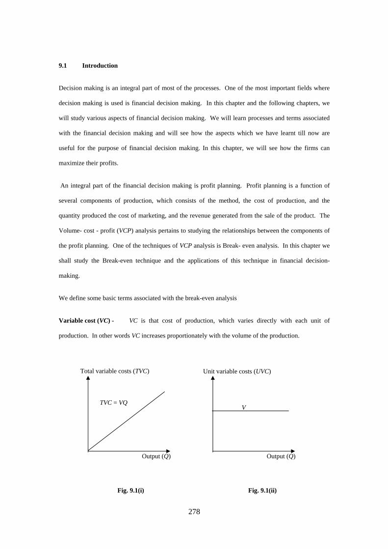
Variable cost (VC) - VC is that cost of production, which varies directly with each unit of
production. In other words VC increases proportionately with the volume of the production.
Total variable costs (TVC) Unit variable costs (UVC)
TVC = VQ
Output (Q)
V
Output (Q)
Fig. 9.1(i) Fig. 9.1(ii)
278
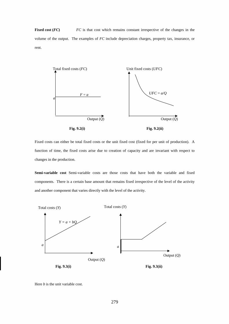
Fixed cost (FC) FC is that cost which remains constant irrespective of the changes in the
volume of the output. The examples of FC include depreciation charges, property tax, insurance, or
rent.
Output (Q)
Total fixed costs (FC)
a F = a
Unit fixed costs (UFC)
UFC = a/Q
Output (Q)
Fig. 9.2(i) Fig. 9.2(ii)
Fixed costs can either be total fixed costs or the unit fixed cost (fixed for per unit of production). A
function of time, the fixed costs arise due to creation of capacity and are invariant with respect to
changes in the production.
Semi-variable cost Semi-variable costs are those costs that have both the variable and fixed
components. There is a certain base amount that remains fixed irrespective of the level of the activity
and another component that varies directly with the level of the activity.
Total costs (Y) Total costs (Y)
Output (Q)
a
Y = a + bQ
a
Output (Q)
Fig. 9.3(i) Fig. 9.3(ii)
Here b is the unit variable cost.
279

Examples of the semi-variable costs can be the total amount paid to a sales agent who gets a fixed
salary as well as some commission on every deal he cracks.
Another variation of the semi-variable costs is the semi-fixed costs where the costs increases at certain
points of production in certain fixed amounts.
Total costs (TC)
Output (Q)
Fig. 9.4
Such costs arise whenever a new item is added to the infrastructure, e.g., installation of a new machine,
employment of a new personnel etc.
Break-even point (BEP) A BEP is that point at which total revenue is equal to the total cost
of production (fixed costs and variable costs). At this point, neither a profit is earned nor a loss is
incurred.
If all the costs are the variable costs, the BEP will be at zero level of production.
Operating profit Operating profit is the difference between the total revenue generated and
the total cost (total variable and total fixed costs) before the payment of income tax.
Contribution margin (CM) Contribution margin is the difference between selling price and
variable cost of one unit of product. This amount directly gives the amount that an additional unit of
production contributes to the total profit.
Margin of safety (MS) MS is the difference between the actual sales revenue (ASR) and the break-
even sales revenue (BESR) (off course, when ASR is more than BESR.) Larger is MS; safer is the
producer from making losses even if there is a temporary decrease in profit.
280

Break-even analysis and the financial decision-making Break-even analysis is a very widely
used technique for making effective financial decisions, particularly when we can obtain explicit
relationships between the three components of the profit planning. The financial decision-making may
be in reference to one or more of the following question
(i) Initial production does not result in profits since it is utilized in making for the expenses
incurred in order to start production. Then how much production should be there before it
results in (a certain amount of) operating profit?
(ii) For a new product, how much sales volume should be there in order to meet the (fixed) cost of
production before it starts making any profit?
(iii) Every production plant has a finite capacity of production. Then for a particular level of
production, how much is the operating profit or loss?
(iv) As a result of competition it may become necessary to reduce the prices of the products and
consequently the operating profit would be reduced. Then by what extent should the
production be increased so as to maintain the earlier levels of operating profit?
(v) Profit is a function of costs. How is profit affected by increase in the fixed costs or decrease
in the variable costs?
These and many more such questions can be answered with the help of break- even analysis.
9.2 Techniques of break-even analysis
Break-even analysis can be done by either of the following techniques:
(i) Graphic methods; and
(ii) Algebraic methods.
We shall discuss both the techniques in brief.
281

(i) Graphic method
Under certain assumptions, a break-even chart which is a graphic representation of the relationship
between the three components of the profit planning, is a strong tool for answering several questions
related with the problem pf profit planning
Assumptions of a VCP chart
(i) The costs can be divided into the fixed costs and the variable costs.
(ii) Within the range of the chart, the fixed costs will remain fixed (There is no new addition in
the infrastructure of the production).
(iii) Within the range of the chart, the unit variable cost will remain fixed irrespective of the
amount of production.
(iv) Within the range of the chart, the unit-selling price will remain fixed irrespective of the
amount of sale.
(v) If the production process involves production of more than one product (multi-product
production) the product-mix will remain constant within the range of the chart.
(vi) The production and the sales volume are the same, i.e., there is no wastage in marketing the
product.
Under these assumptions, now we demonstrate the construction of a VCP chart.
Consider the following data, which pertains to a production process:
Table 9.1
Selling price (per unit) Rs.10
Fixed costs Rs.60, 000
Variable costs (per unit) Rs.5
Lower limit 6,000 Relevant range of production
Upper limit 20,000
Break-up of variable costs (per unit) Direct material Rs.2
282

Direct labor Rs.1.50
Direct expenses Re.1
Selling expenses Rs.0.50
Actual sales (18,000 units) Rs.1, 80,000
Plant capacity (20,000 units) Rs.2, 00,000
Tax rate 50%
Upper limit Lower limit Relevant rangeSales revenue (Rs. ‘000) Margin of safety (Rs.)
Angle of incidence BEP
Margin of safety (Units)
Volume of sale
Fixed Cost Line 0 2 4 6 8 10 12 14 16 18 20
Profit area
200.
180.
160.
140.
40.
20.
120.
60.
100.
80. Loss area
. . . . . . . . . .
Sales Volume (‘000) Fig. 9.5
283

In this case, we represent total sales volume in rupees on the X-axis and the total revenue generated on
the Y-axis. Total cost line is starting from the point where fixed cost line is meeting the Y-axis. Fixed
cost line is independent of the volume of production Total sale line starts from the origin and goes till
the point of maximum production. Then the break –even point (BEP) lies at the intersection of the
total cost line and the total sale line. This is the point at which the production cost becomes equal to
the sales revenue. The area above this point is the profit area and the area below this point is the loss
area. The angle between the total cost line and the total sale line, which is subtended at the point of the
intersection of the two lines, is called the angle of incidence and it provides a measure of the degree
safety of the profit. Higher is the angle of incidence; the larger will be the profit after all costs have
been recovered. Lower angle shows that the profit is increasing at a low rate after BEP thus signifying
the fact that the variable costs form a large part of the cost of production.
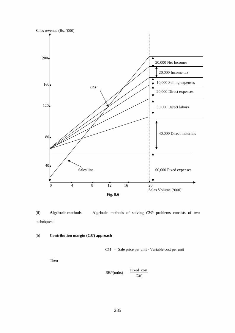
It is possible to read the details of the individual variable cost segments from a VCP graph. Calculating
the proportions of different variable costs to the total variable cost, we have the following table
Table 9.2
Cost type Amount Proportion Total cost
Total variable cost Rs. 5 1.00 1,00000
Direct material Rs.2 0.40 40,000
Direct labour Rs.1.50 0.30 30,000
Direct expenses Re.1 0.20 20,000
Selling expenses Rs.0.50 0.10 10,000
The corresponding points can be read from the graph
284
Sales revenue (Rs. ‘000)
20,000 Net Incomes
20,000 Income tax
10,000 Selling expenses BEP
20,000 Direct expenses 30,000 Direct labors
40,000 Direct materials Sales line 60,000 Fixed expenses 0 4 8 12 16 20
. . . . .
80.
40.
160.
120.
200.
Sales Volume (‘000) Fig. 9.6
(ii) Algebraic methods Algebraic methods of solving CVP problems consists of two
techniques:
(b) Contribution margin (CM) approach
= Sale price per unit - Variable cost per unitCM
Then
Fixed cost(units) = BEPCM
285

(sales revenue) = (units) per unit
Fixed cost = profit-volume ( / ) ratio
per unitwhere ( / ) ratio = per unit
BEP BEP SP
P V
CMP VSP
×
and
Variable costVariable cost to volume ( / ) ratio = sales revenue
/ / = 1
V V
P V V V+
Also
/ - M S ASR BESR=
where M/S is the margin of safety, ASR is the actual sales revenue and BESR is the break-even sales
revenue. Then profit can be calculated from any of the following expressions:
Profit = / (amount) P/V ratio
= / (units) per unit
M S
M S CM
×
×
Margin of safety (M/S) ratio
/ - / ratio = M S ASR BESRM SASR ASR
=
M/S ratio is the proportion by which the actual sales may fall before they become less than break-even
sales revenue. A high ratio is better from the firm’s point of view since it provides a cushion to firm’s
profitability, particularly in conditions of recession or depression.
(b) Equation approach This technique is based on the income equation.
Net profit ( ) = Sales revenue ( ) - Total cost ( )NP SR TC
where TC FC VC= +
SR FC VC NP⇒ = + +
If S is the number of units required for BESR, then
SR SP S FC VC S NI= × = + × +
286

where
= Selling price per unit
= Net income ( 0 at )
SP
NI BEP=
( )
( )
-
-
SP S FC VC S
SP VC S FC
FCSSP VC
⇒ × = + ×
⇒ × =
⇒ =
Thus the equation technique is same as the contribution approach.
Example 1: For XYZ publishers, who publish educational as well as fiction books, the following
data relates to their publishing cost and sales revenue for a year
Table 9.3
Particulars First half of the year (Rs. ’00,000) Second half of the year (Rs. ’00,000)
Sales 45 50
Total cost 40 43
Assuming that there is no change in input costs and the selling prices and that the fixed costs are
incurred equally during the two halves, calculate
(i) The P/V ratio;
(ii) Fixed costs;
(iii) Break-even sales; and
(iv) Percentage margin of safety.
Sol:
Table 9.4
Particulars First half of the year
(Rs. ’00,000)
Second half of the
year (Rs. ’00,000)
Change during the
two halves
Sales 45 50 5
Total cost 40 43 3
287

Net profit 5 7 2
Since the fixed costs have been distributed equally in the two halves, so the change in the costs (Rs.
3,00,000) is on account of the variable costs.
= Sale revenue - Variable costs
= Rs. 5,00,000 - Rs. 3,00,000
= Rs. 2,00,000
CM∴
(i) 2,00,000/ ratio = = 40%5,00,000
/ ratio = 1 - / ratio = 60% of the sale revenue
CMP VSR
V V P V
=
(ii)
60Variable cost for the first half = 45,00,000100
= Rs. 27,00,000
Variable cost for the second half = Variable cost for the first half +
×
Rs. 3,00,000
= Rs. 27,00,000 + Rs. 3,00,000
= Rs. 30,00,000
Now,
= Sales revenue - -
= Rs. 95,00,000 - Rs.57,00,000 - Rs.12,00,000
= Rs. 26,00,000
FC VC NP
(iii)
(amount) = / ratio
26,00,000 0.40
Rs. 65,00,000
FCBEPP V
=
=
288
(iv) - / ratio =
95,00,000 - 65,00,000 = 95,00,000
30 = 95
= 31.58%
ASR BESRM SASR
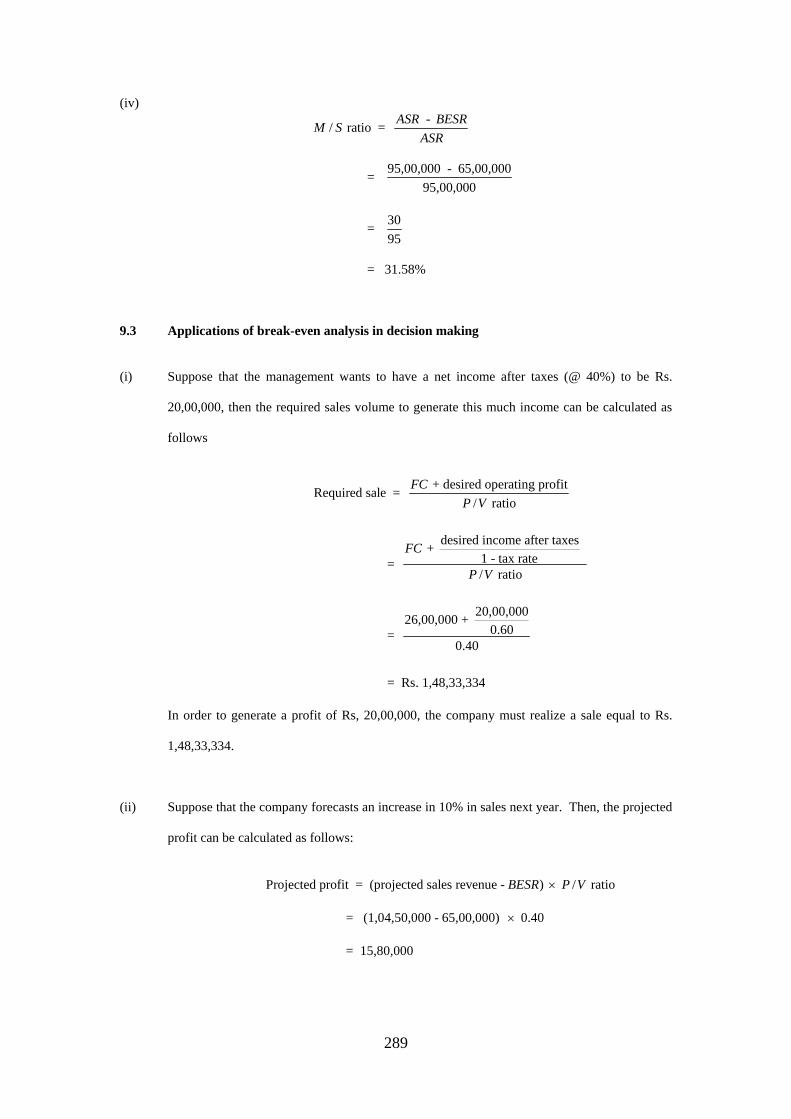
9.3 Applications of break-even analysis in decision making
(i) Suppose that the management wants to have a net income after taxes (@ 40%) to be Rs.
20,00,000, then the required sales volume to generate this much income can be calculated as
follows
+ desired operating profitRequired sale =
/ ratio
desired income after taxes+ 1 - tax rate = / ratio
20,00,00026,00,000 + 0.60 =
0.40
FCP V
FC
P V
= Rs. 1,48,33,334
In order to generate a profit of Rs, 20,00,000, the company must realize a sale equal to Rs.
1,48,33,334.
(ii) Suppose that the company forecasts an increase in 10% in sales next year. Then, the projected
profit can be calculated as follows:
Projected profit = (projected sales revenue - ) / ratio
= (1,04,50,000 - 65,00,000) 0.40
= 15,80,000
BESR P V×
×
289

(iii) Due to increasing competition in the market, suppose that the company wants to reduce the
unit-selling price from Rs. 50 to Rs. 45, still maintaining its presents operating profit. Then it
must increase its sales volume which can be calculated as follows:
Operating profit + Required sales volume =
revised / ratioFC
P V
Revised P/V ratio is calculated as follows
Unit = Rs. 50
Total sale = Rs. 95,00,000
Units sold = 190000
Total = Rs. 57,00,000
57,00,000Unit = = Rs. 30190000
Total new sale = 190000 40 = Rs. 76,00,000
per un revised / ratio =
SP
VC
VC
CMP V
×
∴it 40-30 1= =
per unit 30 3SP
12,00,000 + 26,00,000 Required sales volume = 13
= Rs. 1,14,00,000
1,14,00,000Sales (units) = = 2,85,00040
∴
9.4 The VCP analysis and the normal probability distribution
As we have seen, the VCP analysis can be used for forecasting the consequences of certain decisions or
events regarding costs, revenues, and profits.
The two variables affecting profit are costs and revenues. Although both the variables work within
certain range, still practically the management does not have much control over the revenue variable.
An efficient management can cost variable under control, at least up to some extent.
In fact the variable revenue is a random variable, and can be characterized by a probability distribution.
290
Consider the following data:
= Rs. 75
per unit = Rs. 45
per year = Rs, 1,50,00,000
SP
VC
FC
Then,
(units) = -
1,50,00,000 = 75 - 45
= 5,00,000
FCBEPSP VC
Thus 5,00,000 units of the product must be sold per year in order to break – even.
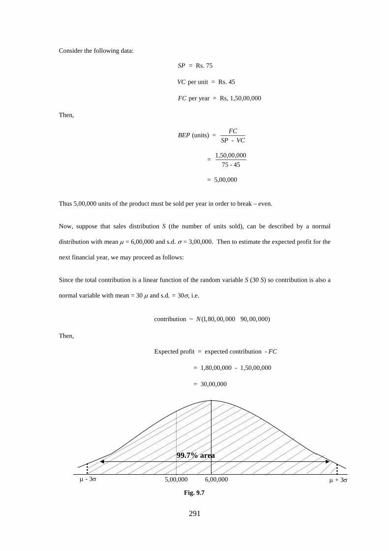
Now, suppose that sales distribution S (the number of units sold), can be described by a normal
distribution with mean µ = 6,00,000 and s.d. σ = 3,00,000. Then to estimate the expected profit for the
next financial year, we may proceed as follows:
Since the total contribution is a linear function of the random variable S (30 S) so contribution is also a
normal variable with mean = 30 µ and s.d. = 30σ, i.e.
contribution ~ (1,80,00,000 90,00,000)N
Then,
Expected profit = expected contribution -
= 1,80,00,000 - 1,50,00,000
= 30,00,000
FC
99.7% area
6,00,0005,00,000 µ + 3σµ - 3σ
Fig. 9.7
291

Now, we can use the sale distribution(s) to answer the queries of the management
(i) What is the probability of break-even sale?
( )
( )
6,00,000 5,00,000 6,00,000( 5,00,000) 3,00,000 3,00,000
= P Z -0.3334
= 0.5 + P 0 Z 0.3334
SP S P − −⎛ ⎞≥ = ≥⎜ ⎟⎝ ⎠
≥
≤ ≤
= 0.6293
Z = -0,33
-3 -2 -1 0 1 2 3 Fig. 9.8 (ii) With what probability can a profit of Rs. 50,00,000 be earned?
(profit 50,00,000) = (contribution 1,50,00,000 + 50,00,000)
= (contribution 2,00,00,000)
contribution - 1,80,0 =
P P
P
P
≥ ≥
≥
0,000 2,00,00,000- 1,80,00,000 90,00,000 90,00,000
⎛ ⎞≥⎜ ⎟
⎝ ⎠
( )
( )
= 0.11
= 0.5 - 0 0.11
= 0.4562
P Z
P Z
≥
≤ ≤
292

Z = 0.11
-3 -2 -1 0 1 2 3 Fig. 9.9
(iii) In order to increase the efficiency of the production, the management is interested in knowing
the probability that in case of losses; the loss will not exceed Rs. 20,00,000.
(loss 20,00,000) = (contribution - loss)
= (contribution 1,50,00,000 - 20,00,000)
= (contribution 1,30,00,000 )
P P FC
P
P
≤ ≤
≤
≤
contribution - 1,80,00,000 1,30,00,000- 1,80,00,000 = 90,00,000 90,00,000
= ( -0.56)
= (
P
P Z
P
⎛ ⎞≤⎜ ⎟
⎝ ⎠
≤
0.56)
= (0 0.44)
= 0.17
Z
P Z
≥
≤ ≤
Z =0.56
-3 -2 -1 0 1 2 3 Fig. 9.10
(iv) What is the probability that the sale will be within the interval (4,50,000, 7,50,000)?
293

(4,50,000 7,50,000)
4,50,000 6,00,000 7,50,000 6,00,000 = 3,00.000 3,00.000
= ( - 0.5 0.5)
= 2 ( 0.5)
P S
P Z
P Z
P Z
≤ ≤
− −⎛ ⎞≤ ≤⎜ ⎟⎝ ⎠
≤ ≤
≤
= 0.383
z = 0.5
-3 -2 -1 0 1 2 3 Fig. 9.11
Thus the management has gathered the following conclusions:
(i) There are 63% chances that sale will at least be equal to break-even sale
(ii) There are 46% chances that the profit will be at least Rs. 50,00,000.
(iii) Chances that the losses are up to Rs. 20,00,000 can be incurred are 17%.
(iv) The probability that the sale can be in range (4,50,000 7,50,000) is 0.383.
With these observations, the management may find the taking up of the product as an interesting
option.
The normal probability distribution can be used in determining the quantities computed in the earlier
examples also, if we can estimate the parameters of the distribution.
294
9.5 Marginal analysis
Marginal costing This is another technique of taking decisions on the basis of costs involved in a
production process. The marginal costs can be defined as the amount of any given volume of output by
which the aggregate costs are changed if the volume of output changes by one unit.
Thus the marginal costs are the costs associated with the production of additional units. So for this
purpose, in short run, only variable costs are taken into consideration. Hence marginal costing is also
known as variable costing. Variable costs include direct material, direct labor, variable direct expenses,
other variable overheads, and the variable portion of the semi-variable costs. However, in long run
fixed costs are also included in the marginal costs.
To illustrate the concept of marginal costs, consider the following example
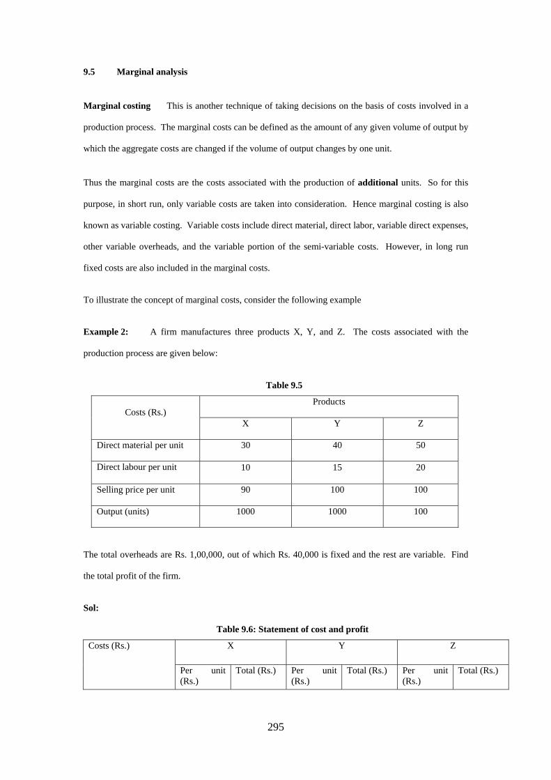
Example 2: A firm manufactures three products X, Y, and Z. The costs associated with the
production process are given below:
Table 9.5
Products Costs (Rs.)
X Y Z
Direct material per unit 30 40 50
Direct labour per unit 10 15 20
Selling price per unit 90 100 100
Output (units) 1000 1000 100
The total overheads are Rs. 1,00,000, out of which Rs. 40,000 is fixed and the rest are variable. Find
the total profit of the firm.
Sol:
Table 9.6: Statement of cost and profit
X Y Z Costs (Rs.)
Per unit (Rs.)
Total (Rs.) Per unit (Rs.)
Total (Rs.) Per unit (Rs.)
Total (Rs.)
295

Direct material 30 30,000 40 40,000 50 50,000
Direct labour 10 10,000 15 15,000 20 20,000
Variable overheads
(100000-40000)/3
20 20,000 20 20,000 20 20,000
Total marginal cost 60 60,000 75 75,000 90 90,000
Contribution
(SP – VC)
30 30,000 25 25,000 10 10,000
Selling price (SP) 90 90,000 100 1,00,000 100 1,00,000
Then, we have
Total profit = Total contribution - Fixed costs
= Rs. , , Rs. ,
= Rs. , ,
−2 90 000 40 000
2 90 000
9.6 Marginal analysis and decision-making
(i) Fixation of selling prices In general, the firm does not have very high control over
selling prices as the significant factors governing the selling prices are the prevailing market and the
economic conditions, yet the firm does have some control over the fixation of selling prices.
In normal circumstances, in fixing the selling prices, total cost is covered along with a sufficiently high
margin to cover the fixed costs and the required profit. But there may be situations when the product
may have to be sold at a price below the total price. Such situations may arise due to competition,
depression, existence of spare capacity, exploring of new markets etc. In such situations, the firm has to
decide about the price at which it is willing or afford to sell its products.
(a) Pricing in depression During depression, the demand falls and as a result the
prices also fall. In such situations, the product may have to be sold at a price below the total price. If
the product was in production, before the beginning of the depression, the fixed costs will be very
much there even if the production is discontinued. So if there is a temporary fall in the demand, the
296

production should be continued, and the product should be sold at a price equal to the marginal price of
the product. Consider the following example
Example 3: The following cost statement shows the prevailing market conditions for a firm
Table 9.7
Total sale (2500 units @ Rs. 30 per unit) Rs.75, 000
Direct material Rs.50, 000
Direct wages Rs. 15,000
Variable Rs. 5,000
Total cost
Overheads
Fixed Rs. 15,000 Rs. 20,000 Rs. 85,000
Total loss Rs. 10,000
There are no signs of the improvement of the situation and the losses are growing. Now the
management has to take a decision on whether to continue or discontinue production. Suggest the
management the optimal course of action.
Sol: If the production shuts down, still there will be losses of the extent Rs. 15,000 on account of
the fixed costs. This loss is greater then the loss incurred if the production is continued. So the
advisable course of action is to continue the production.
Table 9.8
Cost Unit price (Rs.) Total price (Rs.)
28 70,000 Marginal cost
Direct material
Direct labour
Variable expenses
20
6
2
50,000
15,000
5,000
Revenue 30 75,000
Contribution 2 5,000
297

Loss = Fixed costs - Contribution
= Rs. 15,000 - Rs. 5,000
= Rs. 10,000
As long as the price is above the marginal cost, the contribution would work to recover the fixed costs.
At this point a decision may be taken to decide about the minimum price at which the production may
be continued.
The minimum price at which the production may be continued is equal to the one at one the costs of
production can be recovered, i.e., the marginal cost. Thus the production should be continued till the
prices drop to Rs. 28 per unit, after which the production should be discontinued.
(b) Accepting additional orders Sometimes, in addition to the ongoing production, orders
are received in bulk from new or foreign markets, at a price lower than the prices prevailing in the local
market or even the total cost of the product. Then the management has to decide the minimum price at
which to accept such orders. Consider the following example.
Example 4: Given below is the cost statement of a product, which is being sold in the local
market:
Table 9.9
Total output 50,000
Selling price per unit Rs.20
Direct material Rs. 8
Direct wages Rs. 3
Variable Rs.1.50 Production overheads
Fixed Rs. 1.50 Rs. 3
Selling Rs. 0.50
Total cost
Administrative expenses
Distribution Re. 1.00 Rs. 1.50 Rs. 15.50
The total output corresponds to the demand of the product in the local markets. However, the plant has
a production capacity of 70,000 units. Now the management of the firm has been contacted by a
298
foreign firm, which is interested in buying 20,000 units at a price of Rs. 14.50. Since the quoted price is
less than the total cost of the product, the management is in a fix. What should be the decision of the
management? Will the same decision be valid for the home market also?
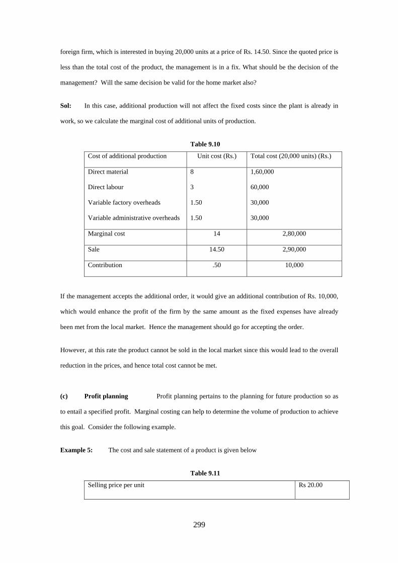
Sol: In this case, additional production will not affect the fixed costs since the plant is already in
work, so we calculate the marginal cost of additional units of production.
Table 9.10
Cost of additional production Unit cost (Rs.) Total cost (20,000 units) (Rs.)
Direct material
Direct labour
Variable factory overheads
Variable administrative overheads
8
3
1.50
1.50
1,60,000
60,000
30,000
30,000
Marginal cost 14 2,80,000
Sale 14.50 2,90,000
Contribution .50 10,000
If the management accepts the additional order, it would give an additional contribution of Rs. 10,000,
which would enhance the profit of the firm by the same amount as the fixed expenses have already
been met from the local market. Hence the management should go for accepting the order.
However, at this rate the product cannot be sold in the local market since this would lead to the overall
reduction in the prices, and hence total cost cannot be met.
(c) Profit planning Profit planning pertains to the planning for future production so as
to entail a specified profit. Marginal costing can help to determine the volume of production to achieve
this goal. Consider the following example.
Example 5: The cost and sale statement of a product is given below
Table 9.11
Selling price per unit Rs 20.00
299
Direct material Rs.6.00
Direct wages Rs. 3.00
Variable Rs. 1.00 Factory overheads
Fixed Rs. 1.00 Rs. 2.00
Variable Rs. 1.00
Cost per unit
Sales overheads
Fixed Rs. 1.00 Rs. 2.00 Rs. 13.00
Total sale (Units) 75,000
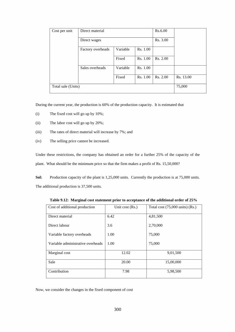
During the current year, the production is 60% of the production capacity. It is estimated that
(i) The fixed cost will go up by 10%;
(ii) The labor cost will go up by 20%;
(iii) The rates of direct material will increase by 7%; and
(iv) The selling price cannot be increased.
Under these restrictions, the company has obtained an order for a further 25% of the capacity of the
plant. What should be the minimum price so that the firm makes a profit of Rs. 15,50,000?
Sol: Production capacity of the plant is 1,25,000 units. Currently the production is at 75,000 units.
The additional production is 37,500 units.
Table 9.12: Marginal cost statement prior to acceptance of the additional order of 25%
Cost of additional production Unit cost (Rs.) Total cost (75,000 units) (Rs.)
Direct material
Direct labour
Variable factory overheads
Variable administrative overheads
6.42
3.6
1.00
1.00
4,81,500
2,70,000
75,000
75,000
Marginal cost 12.02 9,01,500
Sale 20.00 15,00,000
Contribution 7.98 5,98,500
Now, we consider the changes in the fixed component of cost
300
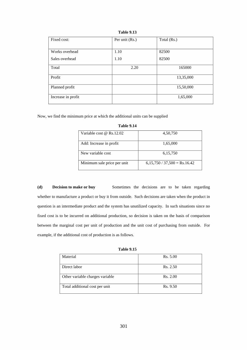
Table 9.13
Fixed cost: Per unit (Rs.) Total (Rs.)
Works overhead
Sales overhead
1.10
1.10
82500
82500
Total 2.20 165000
Profit 13,35,000
Planned profit 15,50,000
Increase in profit 1,65,000
Now, we find the minimum price at which the additional units can be supplied
Table 9.14
Variable cost @ Rs.12.02 4,50,750
Add: Increase in profit 1,65,000
New variable cost 6,15,750
Minimum sale price per unit 6,15,750 / 37,500 = Rs.16.42
(d) Decision to make or buy Sometimes the decisions are to be taken regarding
whether to manufacture a product or buy it from outside. Such decisions are taken when the product in
question is an intermediate product and the system has unutilized capacity. In such situations since no
fixed cost is to be incurred on additional production, so decision is taken on the basis of comparison
between the marginal cost per unit of production and the unit cost of purchasing from outside. For
example, if the additional cost of production is as follows.
Table 9.15
Material Rs. 5.00
Direct labor Rs. 2.50
Other variable charges variable Rs. 2.00
Total additional cost per unit Rs. 9.50
301
If the product is available outside at less than Rs. 9.50, it should be purchased from outside; if the
product is available at more than Rs. 9.50, it should be manufactured and if the product is available at
Rs. 9.50, the company is free to buy or manufacture.
(e) The problem of the key or limiting factor Theoretically, the production of a (most
profitable) product can be increased to any extent and there is no limitation in this regard, al least till
the plant production capacity allows. However, this is not the situation in general. There are other
factors that put a restriction on the production. Such factors are called the limiting or the key factor.
The examples of such key factors could be the availability of the material, skilled labor, capital, and
market capacity etc. since these factors affect the profitability of the firm, the management must know
about these factors. If the key factors are known, then the relative profitability of different products
can be worked out to find the most profitable combination of such factors.
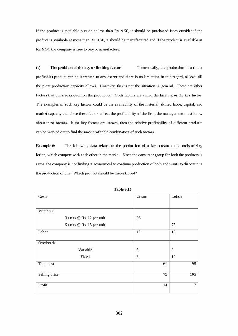
Example 6: The following data relates to the production of a face cream and a moisturizing
lotion, which compete with each other in the market. Since the consumer group for both the products is
same, the company is not finding it economical to continue production of both and wants to discontinue
the production of one. Which product should be discontinued?
Table 9.16
Costs Cream Lotion
Materials:
3 units @ Rs. 12 per unit
5 units @ Rs. 15 per unit
36
75
Labor 12 10
Overheads:
Variable
Fixed
5
8
3
10
Total cost 61 98
Selling price 75 105
Profit 14 7
302
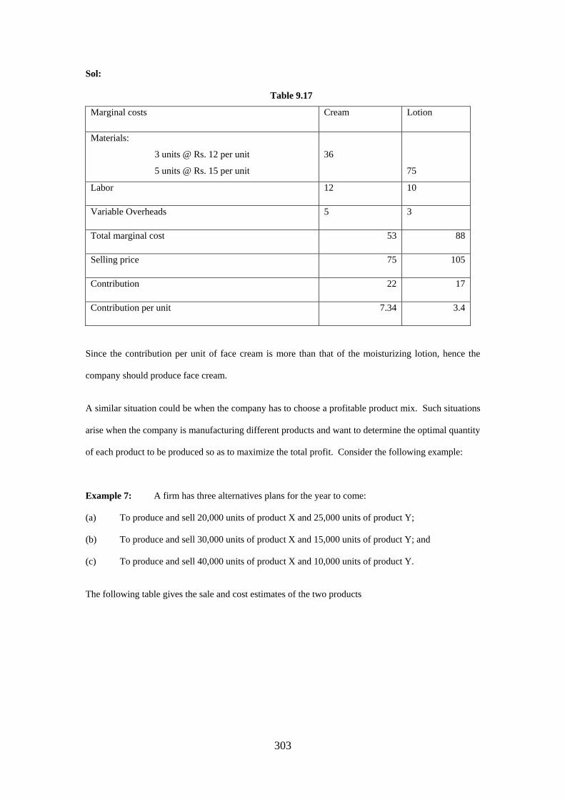
Sol:
Table 9.17
Marginal costs Cream Lotion
Materials:
3 units @ Rs. 12 per unit
5 units @ Rs. 15 per unit
36
75
Labor 12 10
Variable Overheads 5 3
Total marginal cost 53 88
Selling price 75 105
Contribution 22 17
Contribution per unit 7.34 3.4
Since the contribution per unit of face cream is more than that of the moisturizing lotion, hence the
company should produce face cream.
A similar situation could be when the company has to choose a profitable product mix. Such situations
arise when the company is manufacturing different products and want to determine the optimal quantity
of each product to be produced so as to maximize the total profit. Consider the following example:
Example 7: A firm has three alternatives plans for the year to come:
(a) To produce and sell 20,000 units of product X and 25,000 units of product Y;
(b) To produce and sell 30,000 units of product X and 15,000 units of product Y; and
(c) To produce and sell 40,000 units of product X and 10,000 units of product Y.
The following table gives the sale and cost estimates of the two products
303

Table 9.18
Costs (per unit) X Y
Material 3 4
Labour 2 1
Variable overheads 1.50 1
Total cost per unit 6.50 6
Selling price per unit 8 7
Fixed cost 12000 12000
Find the best plan for the firm for the year to come.
Sol:
Table 9.19
Costs (per unit) X Y
Total cost 6.50 6
Selling price per unit 8 7
Contribution 1.50 1
Plan (a):
Table 9.20
Description Cost (Rs.)
Total cost:
X (20,000 units)
Y (25,000 units)
1,30,000
1,50,000
2,80,000
Sale
X (20,000 units)
Y (25,000 units)
1,60,000
1,75.000
3,35,000
304

Total contribution
X (20,000 units)
Y (25,000 units)
30,000
25,000
55,000
Less: Fixed cost 12,000
Net profit 43,000
Plan (b):
Table 9.21
Description Cost (Rs.)
Total cost:
X (30,000 units)
Y (15,000 units)
1,95,000
90,000
2,85,000
Sale
X (30,000 units)
Y (15,000 units)
2,40,000
1,05.000
3,45,000
Total contribution
X (30,000 units)
Y (15,000 units)
45,000
15,000
60,000
Less: Fixed cost 12,000
Net profit 48,000
Plan (c):
Table 9.22
Description Cost (Rs.)
Total cost:
X (40,000 units)
Y (10,000 units)
2,60,000
60,000
3,20,000
305
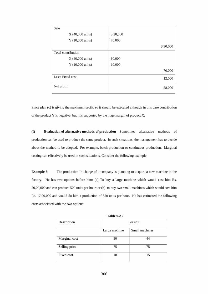
Sale
X (40,000 units)
Y (10,000 units)
3,20,000
70.000
3,90,000
Total contribution
X (40,000 units)
Y (10,000 units)
60,000
10,000
70,000
Less: Fixed cost 12,000
Net profit 58,000
Since plan (c) is giving the maximum profit, so it should be executed although in this case contribution
of the product Y is negative, but it is supported by the huge margin of product X.
(f) Evaluation of alternative methods of production Sometimes alternative methods of
production can be used to produce the same product. In such situations, the management has to decide
about the method to be adopted. For example, batch production or continuous production. Marginal
costing can effectively be used in such situations. Consider the following example:
Example 8: The production In-charge of a company is planning to acquire a new machine in the
factory. He has two options before him: (a) To buy a large machine which would cost him Rs.
20,00,000 and can produce 500 units per hour; or (b) to buy two small machines which would cost him
Rs. 17,00,000 and would do him a production of 350 units per hour. He has estimated the following
costs associated with the two options:
Table 9.23
Description Per unit
Large machine Small machines
Marginal cost 50 44
Selling price 75 75
Fixed cost 10 15
306

If the number of machine hours (per machine) available per year is 1500, which alternative should he
opt for?
Sol: We calculate the annual contribution expected for each of the two options
Table 9.24
Description Large machine
Small machines
Selling price per unit 75 75
Less: marginal cost 50 44
Contribution per unit 25 31
Output per hour 500 350
Contribution per hour 12,500 10,850
Machine hours per year 1,500 1,500
Annual contribution 1,87,50,000 1,62,75,000
Less fixed cost 75,00,000
(=10*500*1500)
78,75,000
(=15*350*1500)
Net profit 1,12,50,000 84,00,000
Thus a large machine should be opted.
307

Problems
1. For the following data, Find BEP units and BEP (Rs.)
SP = Rs. 5 per unit
Units sold = 2.8 million
VC per unit = Rs. 2.5
FC per year = Rs, 22,50,000
(a) What should be the fixed cost if the break-even point has to be 2.8 million units?
(b) How many units should the firm produce if it has to realize a profit of Rs. 10,00,000?
(c) What should be the SP per unit if the firm has to realize the same profit as in (b) if
the firm is producing at its full capacity?
2. For the following data, Find BEP units and BEP (Rs.)
(a)
= Rs. 240 per unit
per year = Rs, 10,00,000
Marginal contribution = 25%
SP
FC
(b) per year = Rs, 10,00,000
Variable cost = Rs. 12 per unit
Marginal contribution = 30%
FC
3. In problem 2, find the sale for parts (a) and (b) if the firm wants to make a profit of Rs. 50
million and the corporate tax is 35%.
4. Consider the following data
per unit = Rs. 50
= Rs, 22,00,000
Variable cost = Rs. 30 per unit
SP
FC
Find the profit if the company sells
308
(a) 1,00,000 units; (ii) 2,00,000 units; and (iii) 5,00,000 units.
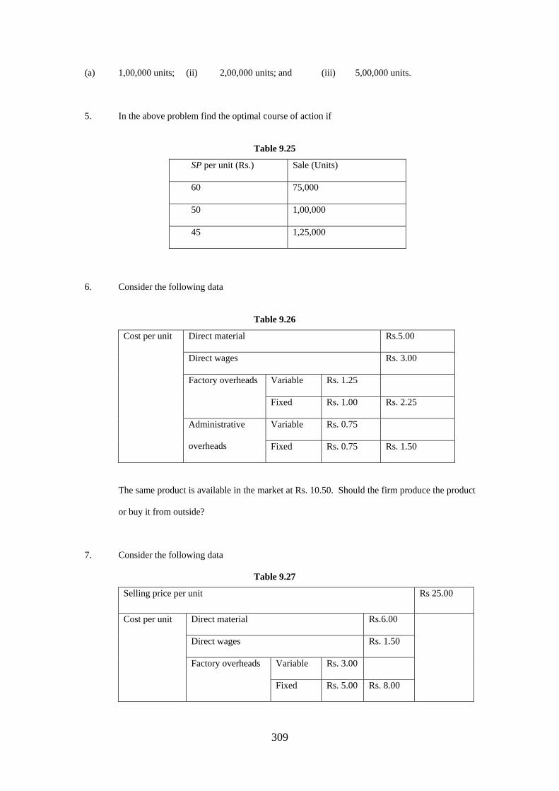
5. In the above problem find the optimal course of action if
Table 9.25
SP per unit (Rs.) Sale (Units)
60 75,000
50 1,00,000
45 1,25,000
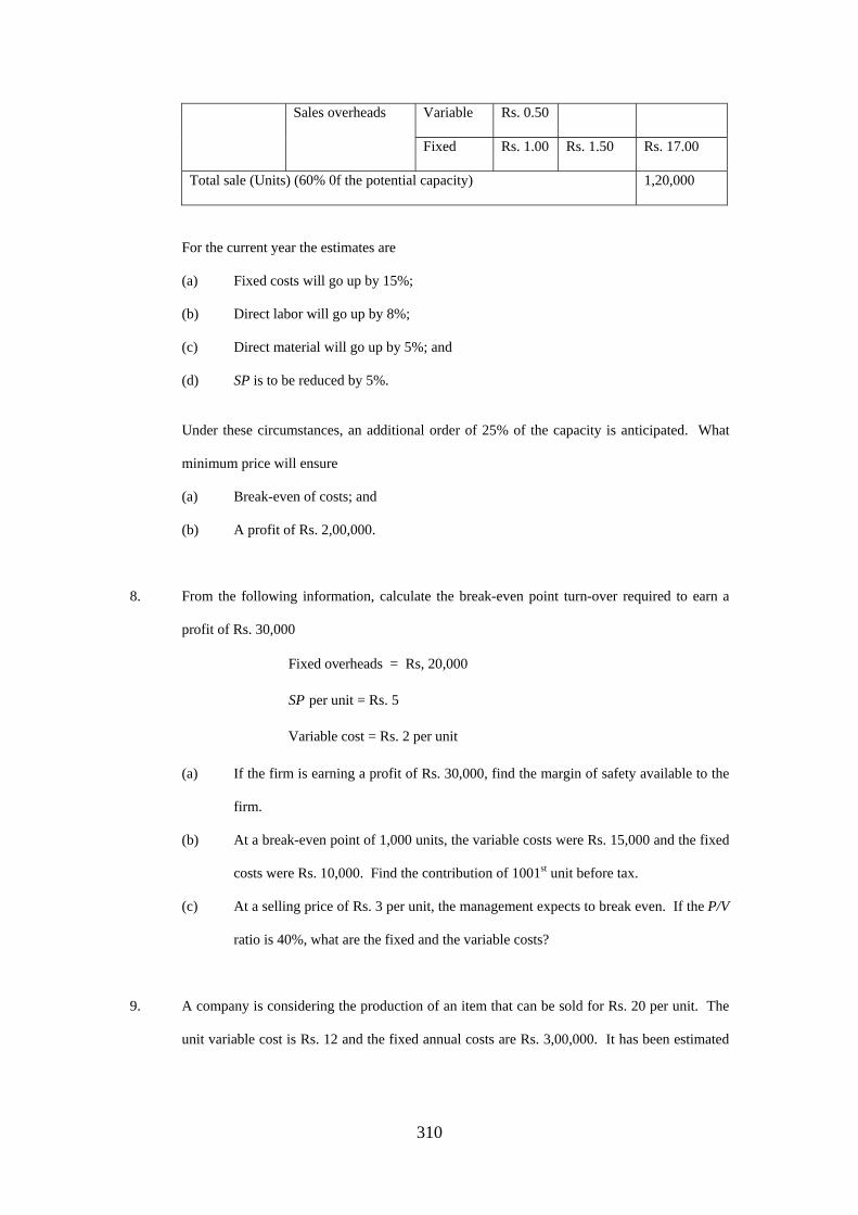
6. Consider the following data
Table 9.26
Direct material Rs.5.00
Direct wages Rs. 3.00
Variable Rs. 1.25 Factory overheads
Fixed Rs. 1.00 Rs. 2.25
Variable Rs. 0.75
Cost per unit
Administrative
overheads Fixed Rs. 0.75 Rs. 1.50
The same product is available in the market at Rs. 10.50. Should the firm produce the product
or buy it from outside?
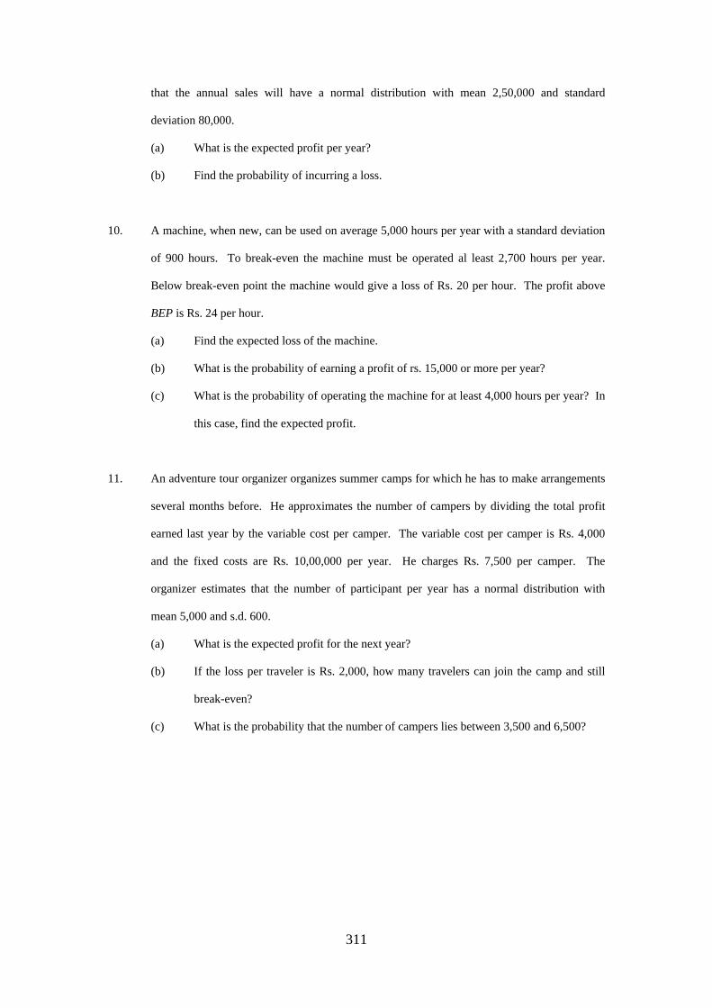
7. Consider the following data
Table 9.27
Selling price per unit Rs 25.00
Direct material Rs.6.00
Direct wages Rs. 1.50
Variable Rs. 3.00
Cost per unit
Factory overheads
Fixed Rs. 5.00 Rs. 8.00
309
Variable Rs. 0.50 Sales overheads
Fixed Rs. 1.00 Rs. 1.50 Rs. 17.00
Total sale (Units) (60% 0f the potential capacity) 1,20,000
For the current year the estimates are
(a) Fixed costs will go up by 15%;
(b) Direct labor will go up by 8%;
(c) Direct material will go up by 5%; and
(d) SP is to be reduced by 5%.
Under these circumstances, an additional order of 25% of the capacity is anticipated. What
minimum price will ensure
(a) Break-even of costs; and
(b) A profit of Rs. 2,00,000.
8. From the following information, calculate the break-even point turn-over required to earn a
profit of Rs. 30,000
Fixed overheads = Rs, 20,000
per unit = Rs. 5
Variable cost = Rs. 2 per unit
SP
(a) If the firm is earning a profit of Rs. 30,000, find the margin of safety available to the
firm.
(b) At a break-even point of 1,000 units, the variable costs were Rs. 15,000 and the fixed
costs were Rs. 10,000. Find the contribution of 1001st unit before tax.
(c) At a selling price of Rs. 3 per unit, the management expects to break even. If the P/V
ratio is 40%, what are the fixed and the variable costs?
9. A company is considering the production of an item that can be sold for Rs. 20 per unit. The
unit variable cost is Rs. 12 and the fixed annual costs are Rs. 3,00,000. It has been estimated
310
that the annual sales will have a normal distribution with mean 2,50,000 and standard
deviation 80,000.
(a) What is the expected profit per year?
(b) Find the probability of incurring a loss.
10. A machine, when new, can be used on average 5,000 hours per year with a standard deviation
of 900 hours. To break-even the machine must be operated al least 2,700 hours per year.
Below break-even point the machine would give a loss of Rs. 20 per hour. The profit above
BEP is Rs. 24 per hour.
(a) Find the expected loss of the machine.
(b) What is the probability of earning a profit of rs. 15,000 or more per year?
(c) What is the probability of operating the machine for at least 4,000 hours per year? In
this case, find the expected profit.
11. An adventure tour organizer organizes summer camps for which he has to make arrangements
several months before. He approximates the number of campers by dividing the total profit
earned last year by the variable cost per camper. The variable cost per camper is Rs. 4,000
and the fixed costs are Rs. 10,00,000 per year. He charges Rs. 7,500 per camper. The
organizer estimates that the number of participant per year has a normal distribution with
mean 5,000 and s.d. 600.
(a) What is the expected profit for the next year?
(b) If the loss per traveler is Rs. 2,000, how many travelers can join the camp and still
break-even?
(c) What is the probability that the number of campers lies between 3,500 and 6,500?
311
Related Documents