Financial conditions, strategic interaction and complex dynamics: a game-theoretic model of financially driven fluctuations

Journal of Economic Behavior & OrganizationVol. 53 (2004) 145–171

Financial conditions, strategic interaction andcomplex dynamics: a game-theoretic model of

financially driven fluctuations

Gian Italo Bischia, Domenico Delli Gattib,∗, Mauro Gallegatica Facoltà di Economica, Istituto di Scienze Economiche, Università di Urbino, Piazza Sassi, 61029 Urbino, Italyb Istituto di Teoria Economica e Metodi Quantitativi, Università Cattolica, Largo Gemelli 1, 20123 Milan, Italy

c Dipartimento di Economia, Università di Ancona, Piazzale Martelli 8, 60121 Ancona, Italy

Received 30 April 1999; received in revised form 1 July 2002

Abstract

We propose a game-theoretic model in which each firm chooses the level of economic activityon the basis of its own financial conditions and of the financial conditions of rival firms. The modelgenerates the laws of motion of firms’ net worth which may determine convergence to a symmetricsteady state or more complex dynamical behaviors, periodic or chaotic, depending on the values ofthe parameters.© 2003 Elsevier Science B.V. All rights reserved.

JEL classification:C7; E3; L1

Keywords:Financial conditions; Strategic interaction; Business fluctuations; Complex dynamics

1. Introduction

In the theoretical literature, financial fragility and instability have been associated withmodels of (sometimes vicious) interaction between financial and goods markets. This litera-ture has been pioneered by Minsky (seeMinsky, 1982) and recently revived in the new viewof the relationship between imperfect financial markets and the macroeconomy (Bernankeet al., 1999; Greenwald and Stiglitz, 1993; Kiyotaki and Moore, 1997). In the presenceof asymmetric information, in fact, financing constraints are important in investment andproduction decisions.

The more recent literature, however, is essentially concerned with the emergence offinancial fragility in a perfect competition setting. A remarkable example is the theoretical

∗ Corresponding author. Tel.:+39-02-7234-2499; fax:+39-02-7234-2923.E-mail address:[email protected] (D.D. Gatti).

0167-2681/$ – see front matter © 2003 Elsevier Science B.V. All rights reserved.doi:10.1016/S0167-2681(03)00023-4

146 G.I. Bischi et al. / J. of Economic Behavior & Org. 53 (2004) 145–171

framework put forward by Greenwald and Stiglitz (GS hereafter; seeGreenwald and Stiglitz,1993). They assume that each firm faces an infinitely elastic demand function subject to arandom idiosyncratic shock. Firms are unable to raise external finance on the Stock marketbecause of equity rationing (Greenwald et al., 1984; Myers and Majluf, 1984). Therefore,they rely first and foremost on internal funds in order to finance production and resort to bankcredit if internal funds are insufficient. As a consequence, firms run the risk of bankruptcy.By assumption the probability of bankruptcy is a decreasing function of net worth (or equitybase), which is a measure of financial robustness: the higher net worth (the lower financialfragility), the lower the probability of bankruptcy will be. Therefore, if bankruptcy is costlythe scale of production is increasing with net worth.

Assuming perfect competition (price taking firms), GS rule out strategic interaction. Inthis paper we follow a different route, allowing for imperfect competition and strategicinteraction among firms which take financial conditions into account when deciding theirscale of production. In our framework, each firm faces a negatively sloped demand functionsubject to a random idiosyncratic shock. The selling price of the firm, however, dependsalso on the quantity produced by the competitors. In an oligopolistic setting, we can showthat in (Nash) equilibrium the scale of production of each firm is a function not only of itsown net worth but also of the net worth of rival firms.

In principle a firm can be either financially constrained (incomplete collateralizationregime) or unconstrained (full collateralization). If internal funds are insufficient to payfor the wage bill, the firm is financially constrained, goes into debt and incurs bankruptcycosts. If net worth is more than enough to fund the wage bill, the firms is unconstrained andbenefits from a financial solidity bonus which plays a role symmetrical to that of bankruptcycosts for the constrained firm.

Each firm accumulates its own equity base according to a law of motion which canbe conceived of as an accounting identity: the absolute change in net worth is equal to(expected) retained profits. This law captures the simple idea according to which eachfirm accumulates net worth in as much as it retains profits instead of distributing them toshareholders as dividends.

The Nash equilibrium level of output of each firm is driven by endogenous fluctuationsin the equity bases of the firm itself and of its competitors. Therefore the game-theoreticframework is ideal for the study of composition and cascade effects which are crucial in thedevelopment of financially driven fluctuations.

It is worth noting that the endogenous dynamics implicit in our game-theoretic frameworkare a consequence of the evolution over time of net worth. So far, endogenous dynamics ina game-theoretic framework have been explored in the context of evolutionary game theorywhere they depend on myopic learning processes, a controversial assumption in a contextof rationality and widespread information.

The paper is organized as follows. InSection 2, we discuss the background assump-tions. We borrow some of them fromGreenwald and Stiglitz (1993), but we give up therepresentative agent-perfect competition hypothesis on which their framework is based. Inour framework, firms operate in a simple oligopolistic set-up. The strategic variable is thequantity produced (Cournot competition).

In Section 3, we examine the benchmark case in which constrained firms do not incurbankruptcy costs and unconstrained firms do not benefit from the solidity bonus. In this case,

G.I. Bischi et al. / J. of Economic Behavior & Org. 53 (2004) 145–171 147

the quantity produced in the Cournot–Nash equilibrium is the same for each oligopolist(Symmetric Nash Equilibrium (SNE)) and is independent of the financial condition (i.e. thelevel of the equity base) of the firm and of its rivals. As a consequence, the law of motion ofthe equity base of each firm is independent of the accumulation of net worth on the part ofrival firms. In the benchmark case, therefore, there are two types ofirrelevanceof financialconditions. First, financial conditions of the firms are irrelevant for the determination ofequilibrium output. Second, the accumulation of net worth on the part of rival firms doesnot affect the accumulation of net worth on the part of the individual firm.

In the general case, when firms incur bankruptcy costs/solidity bonuses, these irrelevanceresults do not hold true any more, as we show inSection 4. First, the quantity produced inNash equilibrium depends on the financial conditions (that is the equity bases) of the firmand of its rivals. Second, the Nash equilibrium is not symmetric, i.e. the quantity is differentfrom one firm to the other. Third, it is only temporary, because the equity bases of the firmsare changing over time. Fourth, the accumulation of the equity base of each firm is affectedby the accumulation of net worth on the part of rival firms.

The evolution of the firms’ equity bases is represented by a discrete-time dynamical sys-tem which can generate a wide range of dynamic patterns: convergence to a steady state,periodic orbits or more complex evolutions, even chaotic. In other words, we obtain en-dogenous fluctuations of the equity bases of the firms, which drive the dynamic patternof Cournot–Nash equilibrium. By analytical and numerical arguments we show that if theretention ratios are not uniform across firms and “sufficiently low” the equity bases of thefirms will converge to the Symmetric Steady state Nash Equilibrium (SSNE), i.e. in thelong run firms become homogeneous as far as the equity ratio and the level of output areconcerned. Increasing the value of at least one retention ratio, the equity base of each firmoscillates in a range which is different from one firm to the other. Further increases in atleast one of the retention ratios yield more complex, and consequently less predictable,dynamics of the equity bases.

Section 5is devoted to the analysis of the impact of changes in the retention ratios on thelong run dynamical properties of the system by means of bifurcation diagrams.Section 6concludes.

2. Background assumptions

We focus on the behavior of firms. The pricepi at which theith firm sells its good isuncertain.1 Price uncertainty is captured by assuming thatpi differs from the general (aver-age) price levelPbecause of a random idiosyncratic shockui, with support (umin, umax) dis-tributed according to a density functionf(ui)with expected valueE(ui) = ∫

uif(ui)dui =0. In symbols:

pi = ui + PTherefore, the expected value ofpi will be E(pi) = P .

1 Following a widely adopted convention, a tilde on a variable means that the variable is stochastic. For the sakeof notational simplicity, undated variables are referred to the current period (periodt).


The average price level, in turn, is a function of total production:P = P (∑iqi), where

qi is the quantity produced by theith firm andP(·) is a decreasing function. In the simplestcase in which the corporate sector consists only of two firms, assuming a linear functionalform, the inverse aggregate demand function is:

P = a− b(q1 + q2) (2.1)

wherea andb are positive parameters.In order to simplify the argument, we assume that production is carried out by means of

one-to-one technology:qi = ni whereni is employment. Firms finance production costs,i.e. the wage bill (wqi), at least partially by means of internally generated funds, which willbe referred to asnet worth or equity base(Ai). In the following we will keep the nominalwage constant.

We can envisage two financial regimes according to the relative magnitude of the wage billand the equity base. The first regime—which we will labelincomplete collateralization—occurs when net worth is not sufficient to pay the wage bill, i.e.Ai < wqi. In this casethe firm is financially constrained and has to resort to credit. The demand for loans isBi = wqi−Ai. The (gross) interest rateR = 1+ r is exogenous. At that interest rate, banksextend credit on demand. Moreover, debt must be repaid completely in one period (there isno accumulation of debt). In this case,RBi represent debt commitments for the firm and isa cost component.

Bankruptcy occurs if the firm is unable to service its debt. In order to simplify the analysis,in the following we will assume that the probability of bankruptcy is captured by the ratioof debt to the wage bill:

PBi = Bi

wqi= 1 − Ai

wqi(2.2)

According to (2.2) the probability of bankruptcy is increasing with output and decreasingwith net worth. (2.2) is a very simple way of linking the probability of bankruptcy to ameasure of financial fragility of the firm.2

Finally, we assume that bankruptcy is costly and that bankruptcy costs are a quadraticfunction of the scale of production:3

CBi = cq2i (2.3)

2 Defining leverage as the debt to equity ratio, we get

li = Bi

Ai= wqiAi

− 1 = PBi1 − PBi

and rearranging

PBi = li

1 + li .

The probability of bankruptcy therefore is an increasing concave function of leverage such that limli→0 PBi = 0and limli→+∞ PBi = 1 (as one would expect).

3 On bankruptcy cost, see (Altman, 1984; Gilson, 1990; Kaplan and Reishus, 1990).


In this regime, the objective function of the firm is equal to expected profit less bankruptcycost in case of default:

Vi = E(Πi)− CBi · PBi (2.4)

The individual price being stochastic, also profit is a random variable:

Πi = piqi − RBi = uiqi + Pqi − R(wqi − Ai) = (ui + P − Rw)qi + RAi (2.5)

Therefore, expected profit is:

E(Πi) = Pqi − RBi = Pqi − R(wqi − Ai) = (P − Rw)qi + RAi (2.6)

whereP is given by (2.1). Substituting (2.2), (2.3) and (2.6) into (2.4) we end up with:

Vi = (P − Rw)qi + RAi − cq2i + cqi

Ai

w(2.7)

The second regime, characterized byfull collateralization, occurs when net worth is morethan enough to fund the wage bill, i.e.Ai > wqi. In this case the firm has financial slackSi = Ai − wqi which it can invest at the going interest rate and get a return ofRSi. This isa revenue component.

The ratio of the financial slack to the wage bill captures the degree of financial robustnessof the firm FRi = (Ai − wqi)/wqi. We assume that in this regime the firm is granted asolidity bonusequal tocq2

i times the degree of financial robustness:cq2i FRi.

In this regime, the objective function of the firm is equal to expected profit plus thesolidity bonus:

Vi = E(Πi)+ cq2i FRi (2.8)

Expected profit is

E(Πi) = Pqi + RSi = Pqi + R(Ai − wqi) = (P − Rw)qi + RAi

whereP is given by (2.1). Substituting this expression into (2.8) and taking into accountthe definition of financial robustness we get:


Ai

w

which is identical to the objective function of the firm in the incomplete collateralizationcase (see (2.7) above).

In the end, the firm has the same quadratic objective function regardless of the financialregime it is experiencing. This conclusion greatly simplifies the analytic structure of themodel. Of course this is a consequence of the assumptions made above, in particular of theintroduction of a solidity bonus in the full collateralization regime. The rationale for the so-lidity bonus is symmetrical to that of the bankruptcy cost in the incomplete collateralizationregime.

Besides the legal and administrative costs of bankruptcy, according toDavis (1992, p. 46)there are indirect costs due to the fact that “imminent bankruptcy may change the firm’sstream of cash flow, owing to various factors, such as the inability to obtain trade credit,


inability to retain key employees, declining faith among the customers in the product,etc.” and wider costs, such as the “loss of reputation” that managers of a bankrupt firmface. Symmetrically, we assume that financial solidity makes the firm’s cash flow lesssusceptible to sudden changes and boosts the reputation of the managers, showing up as arevenue component in the objective function of the firm.

3. The benchmark case: c = 0

Let’s assume, as a convenient special case, the absence of bankruptcy costs for thefinancially constrained firm and of solidity bonuses for the unconstrained firm (c = 0). Inthis case, the objective function of theith firm is equal to the expected profit.

E(Πi) = Pqi − R(wqi − Ai) = (P − Rw)qi + RAi

whereP is given by (2.1).The output level is decided according to the following optimization problem

maxqiE(Πi) (3.1)

The first-order conditions are:

∂E(Π1)

∂q1= a− 2bq1 − bq2 − Rw = 0

∂E(Π2)

∂q2= a− 2bq2 − bq1 − Rw = 0.

(3.2)

TheEq. (3.2)represent the Best Reply Functions (BRF) of the two firms. They are bothlinear and negatively sloped, and they only depend on the parametersa, b of the demandfunction (2.1) and on the marginal costRw. These parameters are uniform across firms,hence the players are symmetric.

From (3.2) we obtain a unique equilibriumE∗ = (q∗1, q∗2), whereq∗1 andq∗2 are given by:

q∗1 = q∗2 = 1

3b(a− Rw) (3.3)

We will assume

a > Rw (3.4)

i.e. the maximum level of the average price is greater than the marginal cost in order toassure thatq∗1 andq∗2 positive quantities. With such assumption (3.3) defines the SymmetricNash Equilibrium, at which the equilibrium level of output is identical for the two firms.

It is worth noting that the equilibrium level of output does not depend on the individ-ual financial conditions. In principle, the two firms can differ in their degree of financialfragility/robustness as captured by the individual net worth. This difference, however, playsno role in the determination of the equilibrium level of output. In other words, the symmetrybetween the players, which is evident from (3.2), leads to identical equilibrium levels ofoutput and makes the individual financial conditions “irrelevant” for output determination.


The different degrees of financial robustness, however, play a role in the accumulationof net worth. For each firm, in fact, the law of motion of net worth is described by thedifference equation:

Ai,t+1 = Ai,t + viE(Πi,t) i = 1,2 (3.5)

wherevi ∈ [0,1] is theretention ratio, and (expected) profitE(Πi,t) in periodt is given by(2.6), i.e.

E(Π1,t) = (a− Rw)q1,t − bq21,t − bq1,tq2,t + RA1,t

and

E(Π2,t) = (a− Rw)q2,t − bq22,t − bq1,tq2,t + RA2,t

According to (3.5), the absolute change of net worth is equal to (expected) retained profits.This captures the simple idea that each firm accumulates net worth in as much as it retainsprofits instead of distributing them to shareholders as dividends.

At the Nash equilibriumE∗ = (q∗1, q∗2) with q∗1 andq∗2 given by (3.3), we have

E(Πi) = 1

9b(a− Rw)2 + RAi (3.6)

For each firm, profit “today” (and therefore net worth “tomorrow”, (see (3.5))) depends onthe individual net worth (the productRAi is a scale factor for the level of profit).

Assuming that both producers instantaneously move to the Nash equilibrium (3.3) ineach time period, so that (expected) profits are given by (3.6), the equation that governs theevolution of the equity base of each firm becomes:

Ai,t+1 = vi

9b(a− Rw)2 + (1 + viR)Ai,t (3.7)

Therefore, the law of motion of the equity base of theith firm is independent of the accu-mulation of its rivals’ net worth, and is expressed by a linear first-order difference equationwhose dynamical behavior is trivial. In fact, the graph of (3.7) on the (Ai,t, Ai,t+1) planeis a straight line with intercept(vi/9b)(a − Rw)2 > 0 and slope(1 + viR) > 1, so thatthe time evolution of each net worthAi, i = 1,2, is always characterized by an increasingsequence{Ai,t , t ≥ 0}. Notice that, according to (3.5), the conditionAi,t+1 = Ai,t , whichcharacterizes the steady states, is equivalent to the conditionE(Πi) = 0, that is, the steadystates are points of zero expected profit for each firm. From (3.7), however, it is clear thatthis cannot happen at the Nash equilibrium. In other words, at the Nash equilibrium eachfirm accumulates net worth at a pace equal to:

Ai,t+1 − Ai,t = vi

9b(a− Rw)2 + viRAi,t

The rate of net worth accumulation is:

gAi := Ai,t+1 − Ai,tAi,t

= vi

9bAi,t(a− Rw)2 + viR


The “long run” rate of net worth accumulation therefore is:

gAi := limAi,t→∞

Ai,t+1 − Ai,tAi,t

= viR

Notice that the expected profit of each firm is always positive. The long run rate of equityaccumulation is increasing with the individual retention ratio and the interest rate.

4. The general case: c �= 0

4.1. Nash equilibrium

If there are bankruptcy costs and solidity bonuses, the objective function of theith firm is:


Ai

w(4.1)

whereP is given by (2.1).The output level is decided according to the following optimization problem:

maxqiVi (4.2)

The first-order conditions are:∂V1

∂q1= a− 2bq1 − bq2 − Rw− 2cq1 + cA1

w= 0 (4.3)

∂V2

∂q2= a− 2bq2 − bq1 − Rw− 2cq2 + cA2

w= 0 (4.4)

These equations represent the Best Reply Functions of the two firms. They are linear andnegatively sloped, as in the case analyzed in the previous section. However, now the BRFof each player does not depend only on the parameters of the demand function (2.1) andon the marginal costRw, which are uniform across firms, but also on the equity base of theplayer. In as much as the equity bases are different, the symmetry between players whichcharacterized the benchmark case is lost. In fact, the optimal level of output of each firmis an increasing function of its own equity base in both regimes. In the incomplete collat-eralization regime, the higher is net worth, the lower the probability of bankruptcy and theassociated cost for the firm and the higher the volume of output. In the full collateralizationregime, the higher is net worth, the higher the degree of financial robustness and the soliditybonus for the firm and the higher the volume of output.

Solving (4.3) and (4.4) we obtain a unique Cournot–Nash equilibriumE∗ = (q∗1, q∗2).

whereq∗1 andq∗2 are given by the following linear functions of the equity basesA1 andA2:

q∗1 = 1

3b+ 2c

[a− Rw+ 2c(b+ c)

(b+ 2c)wA1 − bc

(b+ 2c)wA2

](4.5)

q∗2 = 1

3b+ 2c

[a− Rw− bc

(b+ 2c)wA1 + 2c(b+ c)

(b+ 2c)wA2

].


For each firm, the Nash equilibrium level of output is an increasing function of its ownequity base and a decreasing function of the equity base of the rival. This result is an obviousconsequence of thestrategic substitutabilityimplicit in Cournot competition: the higher thenet worth of the second firm, the higher its output, the lower the average price level and theoutput of the first firm.

As expected, other things being equal, the firm with lower equity base (thesmaller firm,for short) produces less, at the equilibrium, than the firm with higher equity base (thebiggerfirm). Therefore the Nash equilibrium (4.5) is not symmetric, unlessA1 = A2 by a fluke.

As in the benchmark case, we assume that both firms reach the Nash equilibrium (4.5)at each time period. In other words, we assume that the payoffs are known with certaintyand they are common knowledge. This is tantamount to assuming that in each time pe-riod both players know the parameters characterizing the demand function, the bankruptcycost/solidity bonus, the marginal cost and the equity bases. We rule out, therefore, thelearning process typical of evolutionary games.

Notice, however, that the equity base of each player is changing over time—as we will seein the following section—so that (4.5) is temporary, i.e. bound to change with the passing oftime. Summing up,the Nash equilibrium(4.5) is (generally) non-symmetric, instantaneousand temporary.

4.2. The equity base motion

For each firm, the accumulation of net worth is described by (3.5) and the expected profitE(Πi) in periodt is given by (2.6) as in the previous section.

At the Nash equilibriumE∗ = (q∗1, q∗2), the expected profit of each firm is:

E(Πi) = (a− bQ∗ − Rw)q∗1 + RAi (4.6)

whereQ∗ = q∗1 + q∗2. Substitutingq∗1 andq∗2 given by (4.5) into (4.6) we can specify theexpected profit function of the two firms as follows:

E(Π1) = h0 + h1A1 + h2A2 + h3A21 + h4A

22 + h5A1A2 (4.7)

where

h0 = 2c + b(3b+ 2c)2

(a− Rw)2 (4.8)

h1 = R+ c(2c + b)(3b+ 2c)2w

(a− Rw) (4.9)

h2 = − 2bc

(3b+ 2c)2w(a− Rw) (4.10)

h3 = − 2bc2(b+ c)(b+ 2c)(3b+ 2c)2w2

(4.11)

h4 = b2c2

(b+ 2c)(3b+ 2c)2w2(4.12)


h5 = h3 + h4 = − bc2

(3b+ 2c)2w2(4.13)

and

E(Π2) = h0 + h1A2 + h2A1 + h4A21 + h3A

22 + h5A1A2 (4.14)

h0 andh4 are positive parameters, whereash3 andh5 are negative. Furthermore, if (3.4)holds, thenh1 > 0 andh2 < 0.

Therefore, the expected profit of each firm depends in a complicated way on its ownequity base and on the equity base of the rival firm.

For instance, an increase in the equity base of firm 1 may increase or decrease its ownexpected profit because:

sign

(∂E(Π1)

∂A1

)= sign(h1 + 2h3A1 + h5A2) (4.15)

is undecided. More precisely,

∂E(Π1)

∂A1> 0 if h1 > −(2h3A1 + h5A2) (4.16)

In this case, we have a positive feedback of an increase in the equity base of the firm on the ac-cumulation of the equity base, which is consistent with our intuition. If (4.16) is not satisfied,on the contrary, an increase of the equity base of the firm will have a negative feedback onthe accumulation of the equity base, which is a counterintuitive but perfectly possible result.

Analogously, an increase in the equity base of firm 2 may increase or decrease the expectedprofit of firm 1, because:

sign

(∂E(Π1)

∂A2

)= sign(h2 + 2h4A2 + h5A1) (4.17)

is undecided. More precisely,

∂E(Π1)

∂A2< 0 if h2 + 2h4A2 < −h5A1 (4.18)

In this case, we have a negative feedback of an increase in the equity base of firm 2 onthe accumulation of equity base of firm 1. If (4.18) is violated, however, an increase of theequity base of firm 2 will have a positive feedback on the accumulation of the equity baseof firm 1.

Assuming that the change in the equity base is equal to expected profit time the retentionratio, the evolution of the equity bases of the two firms, governed byEq. (3.5), can beobtained by the iteration of a two-dimensional mapT : (A1,t , A2,t) → (A1,t+1, A2,t+1)

given by

T :

{A′

1 = v1h0 + (1 + v1h1)A1 + v1h2A2 + v1h3A21 + v1h4A

22 + v1h5A1A2

A′2 = v2h0 + (1 + v2h1)A2 + v2h2A1 + v2h3A

22 + v2h4A

21 + v2h5A1A2

(4.19)


where′ denotes the unit-time advancement operator. Starting from a given initial condition

A0 = (A1,0, A2,0) ∈ R2+ (4.20)

the iteration of map (4.19) generates a trajectory

τ(A0) = {(A1,t , A2,t) = T t(A1,0, A2,0), t ≥ 0}which may converge to a fixed point or to a periodic cycle or to a more complex attractingset, such as a strange (or chaotic) attractor, as we shall see in the following. Endogenousfluctuations of the equity basesA1(t) andA2(t) can occur. Therefore also the Cournot–NashequilibriumE∗ fluctuates. In fact, the dynamic behavior ofA1 andA2 determines, through(4.5), a sequence of Cournot–Nash equilibria. As we have emphasized above, each equilib-rium pointE∗ can be thought of as a temporary equilibrium, i.e. an equilibrium point whoseposition is driven by the dynamical behavior of net worth according to the law of motion(4.19).

4.3. Characterization of the state space

Each point of the state space—i.e. the positive orthant of the (A1, A2) plane—can becharacterized according to the financial regime of the firms. The first firm is incompletelycollateralized ifA1 < wq1. Recalling that

q∗1 = 1

3b+ 2c

[a− Rw+ 2c(b+ c)

(b+ 2c)wA1 − bc

(b+ 2c)wA2

]

(see (4.5)) the first firm is in the regime of incomplete collateralization ifA1 < h6 − h7A2where

h6 = (b+ 2c)w

3b(b+ 2c)+ 2c2(a− Rw), h7 = bc

3b(b+ 2c)+ 2c2

MeasuringA1 on the horizontal axis andA2 on the vertical axis, if the point (A1, A2) in thespace of equity bases is below (above) the negatively sloped line of equation

A1 + h7A2 = h6 (4.21)

the first firm is incompletely (fully) collateralized. Following a symmetrical reasoning, ifthe point (A1, A2) lies below (above) the straight line of equation

h7A1 + A2 = h6 (4.22)

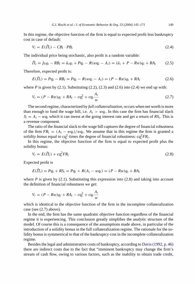
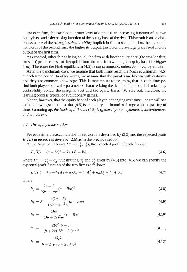
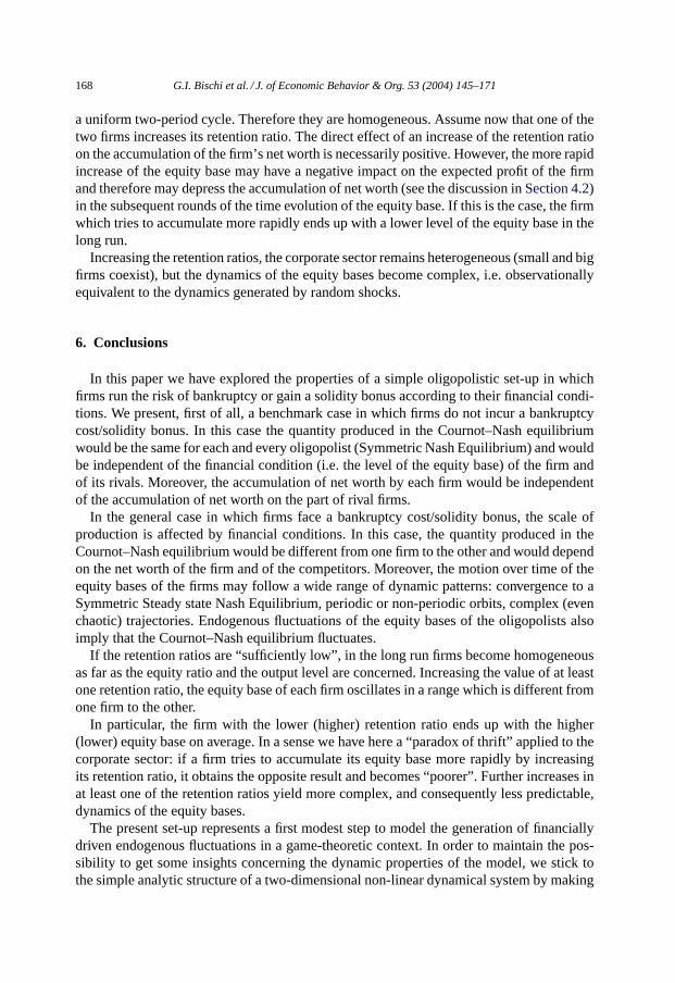
the second firm is incompletely (fully) collateralized.In the end, tracing the two straight lines (4.21) and (4.22) we can partition the space of

equity bases in four regions (seeFig. 1). When the equity base is “small” (“large”) for bothfirms—i.e. when the point of the state space lies below (above) both lines—both firms areincompletely (fully) collateralized. In these two cases the firms happen to be in the samefinancial regime. The two “mixed” cases where one firm is financially constrained and theother is not can be derived straightforwardly.


Fig. 1. The two straight lines (4.21) and (4.22) divide the space of equity bases (A1, A2) into four regions, accordingto the firm(s) which are incompletely or fully collaterized. This figure is obtained with parameters’ valuesa = 20,b = 0.2,R = 1.05,w = 1, c = 1.

Each point on the state space can be characterized also by the total quantity produced inthe economyQ = q1 +q2 and consequently by the price levelP = a−bQ. The price level

is non-negative ifQ ≤ Q whereQ ≡ a/b is the maximum amount which can be absorbedby market demand. In the Nash equilibrium, total quantity is

Q∗ = q∗1 + q∗2 = 1

3b+ 2c

[2(a− Rw)+ c(b+ 2c)

(b+ 2C)w(A1 + A2)

](4.23)

If, given A1 andA2, the amount the two firms jointly produce according to (4.23) happensto be greater thanQ, we assume that they will be forced to pay an extra-wage equal toθ(Q∗ − Q), whereθ is a positive constant. We can think ofQ as potential output, i.e. theamount producible in full employment at the going working schedule (working hours perday). If firms want to produce more thanQ, they have to pay an extra-wage to induce peopleto work extra-hours.

We can distinguish two regimes. In the underemployment regime,Q∗ < Q, the nominalwage is constant atw and the price level isa − bQ∗ > 0. In the full employment regimeQ∗ ≥ Q, the nominal wage isw+θ(Q∗ − Q), the firms produceQ∗ but they will be able tosell onlyQ at the pricea− bQ = 0. In other words, the nominal wage obeys the followingschedule:

wage={w if Q∗ < Qw+ θ(Q∗ − Q) if Q∗ ≥ Q

which is reminiscent of a Philips curve in wage-output space.


WhenQ∗ < Q (underemployment regime), the expected profit of each firm, whichgoverns the evolution over time of the equity base, is (4.6). WhenQ∗ ≥ Q, (full employmentregime), the expected profit is:

E(Πi) = (a− bQ)q∗i − R{[w+ θ(Q∗ − Q)]q∗i − Ai} =RAi − R[w+ θ(Q∗ − Q)]q∗i

If we make the technical assumption thatθ = b/R, the expression above becomes:

E(Πi) = (a− bQ)q∗i − Rwq∗i − b(Q∗ − Q)q∗i + RAi = (a− bQ∗ − Rw)q∗i + RAi

which is identical to (4.6). In the end, in our model the firm has the same expected profitfunction regardless of the employment regime it is experiencing. This conclusion greatlysimplifies the analytic structure of the model.

Given the characterization discussed above, the dynamics of the equity bases are governedby the system (4.19) in all the points of the state space, regardless of the financial oremployment regime. The trajectories generated by (4.19), however, may cross areas of thestate space characterized by different financial or employment regimes.

4.4. General dynamical properties

The first step in the study of the properties of a dynamical system is the computationof the steady states, i.e. the trajectories characterized byAi,t+1 = Ai,t , i = 1, 2, foreacht. The steady states are the fixed points of mapT, i.e. the solutions of the algebraicsystem obtained from (4.19) withA′

1 = A1 andA′2 = A2. We recall that, according to

(3.5), the fixed points of (4.19) are points of zero expected profit for both firms. From(4.7) and (4.14) it is straightforward to conclude that each equationE(Πi) = 0 representsan hyperbola in the plane (A1, A2). The fixed points ofT therefore are located on theintersections of the two hyperbolasE(Πi) = 0, i = 1, 2. The existence and the stabilityproperties of the fixed points are stated in the following proposition, which is proved inAppendix A.

Proposition 1. The map T defined by(4.19)has two and only two fixed points, located onthe diagonal∆ of equationA1 = A2, given by

S = (s, s), with s = −(h1 + h2)−√(h1 + h2)2 − 8h0h5

4h5> 0 (4.24)

and

N = (n, n), with n = −(h1 + h2)+√(h1 + h2)2 − 8h0h5

4h5< 0 (4.25)

The negative fixed point N is a repelling node, with eigenvaluesλ2(n) > λ1(n) > 1; thepositive fixed point S is an attracting node for sufficiently low values ofv1 or v2, and it


may lose stability through a period doubling(or flip) bifurcation4 at which S becomes asaddle point, with λ1(s) < −1 < λ2(s) < 1, and a stable cycle of period2 is creatednear S.

The coordinates of the fixed points are functions of theh-parameters which in turn arepolynomials of the parameters characterizing the aggregate demand function (2.1) (a andb), the bankruptcy cost/solidity bonus (c) and the interest rate augmented nominal wage(Rw). Notice that the coordinates of the fixed points are independent of the retention ratios.In other words, the fact that the two firms can differ in terms of their dividend policy isirrelevant for the determination of the steady state equity bases.

Of course, only the positive fixed pointS = (s, s) is economically meaningful. Since itbelongs to the bisector∆, in the steady state the financial conditions of the two firms, aswell as their equilibrium output levels, are identical. In fact, according to (4.5), at the steadystateSwe have a Symmetric Steady state Nash Equilibrium (SSNE)E∗ = (q∗, q∗), with

q∗ = 1

3b+ 2c(a− Rw+ cs) (4.26)

The steady stateSis stable if, starting from an initial configuration characterized by hetero-geneous financial conditions, i.e.A1,0 �= A2,0, the endogenous dynamics lead to identicalequity bases and outputs (4.26), provided that the initial condition (4.20) belongs to the basinof attractionB(S) of the stable fixed pointS. Thebasinof S is the set of initial conditionsthat generate a trajectory converging toE∗:

B(S) = {(A1,A2)|(A1,t , A2,t) = T t(A1,0, A2,0)→ S as t → +∞}In order to explore the dynamic behavior of the model we have to determine the domain,in the parameters’ space, for which the steady stateS is locally stable. Moreover, for a setof parameters for whichS is stable, we must detect the boundaries of the basinB(S) in thephase (A1, A2).

Due to the high number of parameters of the model, and the complicated dependence of theeigenvalues of the Jacobian matrix ((A.2) inAppendix A) on these parameters, a completestudy of the local stability ofSas the parameters are varied is not an easy task. Thus in thefollowing we run some numerical simulations, based on the local stability analysis givenin Appendix A, in order to explore the dynamic patterns of the model. A more completenumerical exploration of the influence of the retention ratios on the dynamical behaviorof the equity bases (and consequently of the temporary Nash equilibrium) is performed inSection 5.

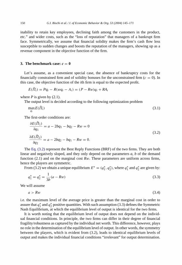
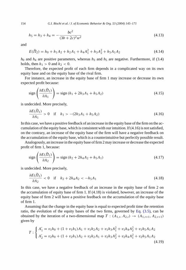
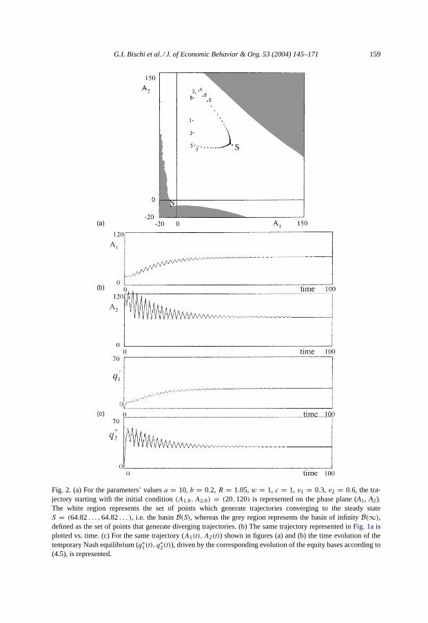
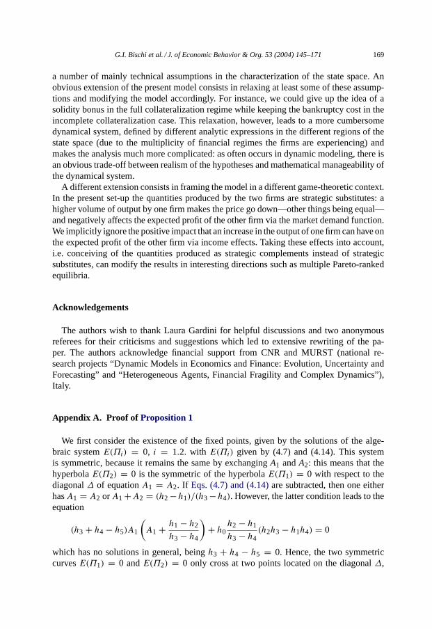
Setting the parameter values ata = 10, b = 0.2, R = 1.05, w = 1, c = 1, v1 =0.3, v2 = 0.6 we obtain the steady stateS = (64.82. . . ,64.82. . . ), which is repre-sented inFig. 2aon the phase plane (A1, A2) together with a typical trajectory converging

4 A period doubling bifurcation occurs when, by varying a parameter, an eigenvalue of a fixed point crosses theunit circle with valueλ = −1. At such bifurcation a cycle of period 2 is created near the fixed point. The bifurcationis supercriticalif a stable two-cycle is created around the unstable fixed point,subcriticalif an unstable two-cycleexists around the stable fixed point (seeLorenz, 1993, p. 111;Guckenheimer and Holmes, 1983, p. 158).


Fig. 2. (a) For the parameters’ valuesa = 10, b = 0.2, R = 1.05,w = 1, c = 1, v1 = 0.3, v2 = 0.6, the tra-jectory starting with the initial condition(A1,0, A2,0) = (20,120) is represented on the phase plane (A1, A2).The white region represents the set of points which generate trajectories converging to the steady stateS = (64.82. . . ,64.82. . . ), i.e. the basinB(S), whereas the grey region represents the basin of infinityB(∞),defined as the set of points that generate diverging trajectories. (b) The same trajectory represented inFig. 1aisplotted vs. time. (c) For the same trajectory (A1(t), A2(t)) shown in figures (a) and (b) the time evolution of thetemporary Nash equilibrium (q∗1(t), q

∗2(t)), driven by the corresponding evolution of the equity bases according to

(4.5), is represented.


to it. For this set of parameters the fixed pointS is locally stable, with eigenvaluesλ1(s) =−0.91. . . , λ2(s) = 0.98. . . . Its basinB(S) is represented by the white region, whereas thegrey region represents the basin of infinityB(∞), defined as the set of points that generatediverging trajectories. Even if only points (A1, A2) with positive coordinates are meaning-ful, in Fig. 2awe have also represented a portion of negative orthants in order to show thatthe unstable (and negative) fixed pointN belongs to the boundary that separates the greybasin of infinity from the white basin of bounded trajectories. The trajectory representedin Fig. 2astarts from the initial condition(A1,0, A2,0) = (20,120) ∈ B(S) (the black dotlabelled by 0) and then converges to the steady stateS through oscillations of decreasingamplitude (because−1 < λ1(s) < 0). This can be more easily seen inFig. 2b, where thesame trajectory is plotted versus time. Of course, the same kind of evolution holds for theoutputs of the two firms, computed according to (4.5). The time evolution of the temporaryNash equilibrium (4.5), driven by the corresponding evolution of the equity bases, is shownin Fig. 2c.

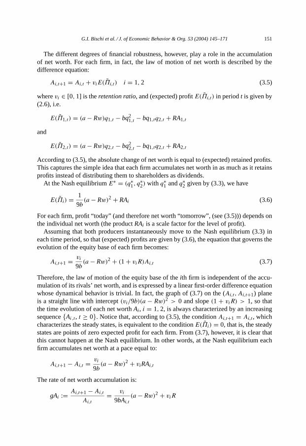
In the situation shown inFig. 2 even if the initial conditionsA1,0 and A2,0 are dif-ferent (i.e. the two firms areheterogeneouswith respect to the equity bases), the systemspontaneously evolves towards a steady state characterized by long run homogeneity ofthe equity base and output, provided the initial condition (A1,0, A2,0) is in the basin ofattraction ofS. This conclusion only applies whenS is stable. In fact if the parametersare changed until the fixed pointS loses stability (via a period doubling bifurcation, ac-cording toProposition 1) then the system tends to long run heterogeneity provided theretention ratios are different,v1 �= v2. In order to see this, we consider the same set ofparametersa, b, R, w, c andv2 as inFig. 2, and we increase the retention ratiov1. Forthis set of parameters the flip bifurcation at whichS loses stability occurs atv1 = v

f

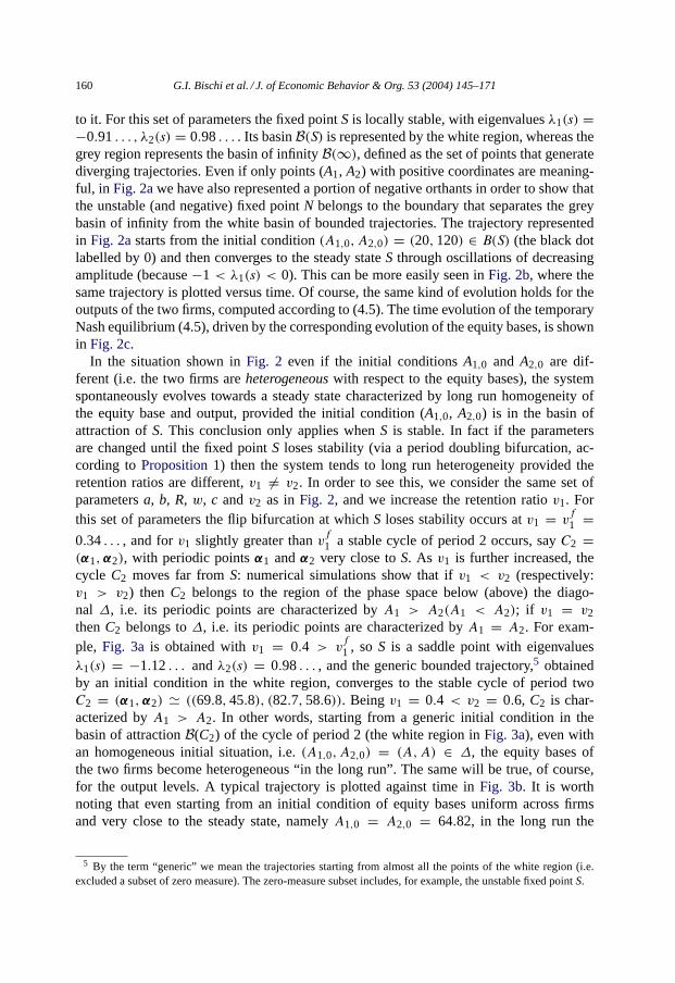
1 =0.34. . . , and forv1 slightly greater thanvf1 a stable cycle of period 2 occurs, sayC2 =(α1,α2), with periodic pointsα1 andα2 very close toS. As v1 is further increased, thecycle C2 moves far fromS: numerical simulations show that ifv1 < v2 (respectively:v1 > v2) then C2 belongs to the region of the phase space below (above) the diago-nal ∆, i.e. its periodic points are characterized byA1 > A2(A1 < A2); if v1 = v2thenC2 belongs to∆, i.e. its periodic points are characterized byA1 = A2. For exam-ple, Fig. 3a is obtained withv1 = 0.4 > v

f

1 , so S is a saddle point with eigenvaluesλ1(s) = −1.12. . . andλ2(s) = 0.98. . . , and the generic bounded trajectory,5 obtainedby an initial condition in the white region, converges to the stable cycle of period twoC2 = (α1,α2) � ((69.8,45.8), (82.7,58.6)). Beingv1 = 0.4 < v2 = 0.6, C2 is char-acterized byA1 > A2. In other words, starting from a generic initial condition in thebasin of attractionB(C2) of the cycle of period 2 (the white region inFig. 3a), even withan homogeneous initial situation, i.e.(A1,0, A2,0) = (A,A) ∈ ∆, the equity bases ofthe two firms become heterogeneous “in the long run”. The same will be true, of course,for the output levels. A typical trajectory is plotted against time inFig. 3b. It is worthnoting that even starting from an initial condition of equity bases uniform across firmsand very close to the steady state, namelyA1,0 = A2,0 = 64.82, in the long run the

5 By the term “generic” we mean the trajectories starting from almost all the points of the white region (i.e.excluded a subset of zero measure). The zero-measure subset includes, for example, the unstable fixed pointS.


Fig. 3. (a) For the same set of parametersa, b, R, w, c and v2 as in Fig. 1a and v1 = 0.4 ageneric trajectory starting from a point of the white region converges to the stable cycle of period 2C2 = (α1,α2) � ((69.8,45.8), (82.7,58.6)). (b) A typical trajectory is plotted against time starting from thehomogeneous initial conditionA1,0 = A2,0 = 64.8.

equity base of the first firm oscillates in the range (69.8, 82.7) while that of the secondfirm oscillates in the range (45.8, 58.6). Therefore, in the long run the first firm is bigger(its average equity base is about 76) than the second firm (whose average equity base isabout 52).


The situation is reversed if the stable cycleC2 occurs whenv1 > v2, due to the symmetricform of map (4.19), that remains the same swapping both the parametersv1 with v2 and thedynamic variablesA1 andA2. This implies that if we exchangev1 with v2 the trajectoriesof the new dynamical system are simply obtained from the previous ones by exchangingA1 with A2.

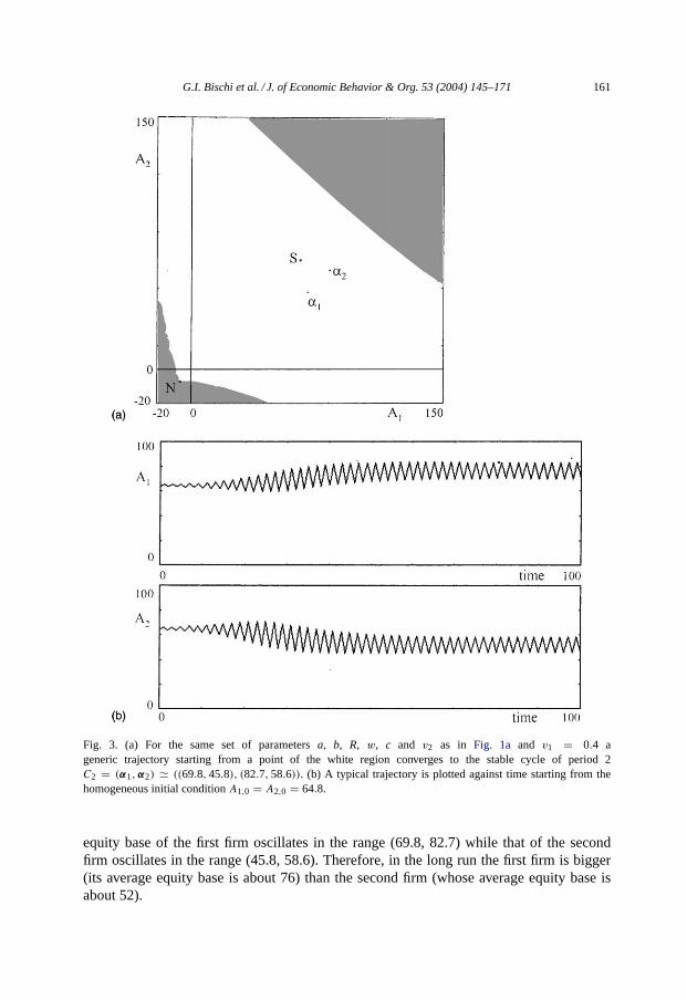
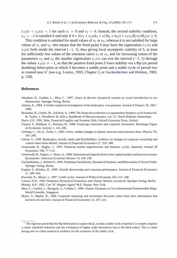
Numerical simulations show that if (at least) one of the retention ratios is increased,the first period doubling bifurcation is followed by a sequence of other period doublingbifurcations that create stable cycles of period 2k , k = 2,3, . . . (similar to the well knownFeigenbaum period doubling route to chaos occurring in one-dimensional maps). Sucha sequence of period doublings leads to chaotic attractors, i.e. invariant two-dimensionalsets inside which the trajectories of map (4.19) exhibit sensitive dependence on initialconditions.Fig. 4ashows the attracting set obtained with the same parametersa, b, R,c, andv2 as inFigs. 2 and 3, andv1 = 0.67. The dynamic behavior of a trajectory likethat of Fig. 4a, a part of which is plotted versus time inFig. 4b, appears to be ratherirregular, apparently chaotic. It can be noticed, however, that the attracting set consistsof two disjoint pieces. A trajectory moving on it cyclically visits these two pieces asshown inFig. 4b, where it is evident that a sort of cyclicality of period 2 occurs in thelong run. Such an attractor is also calledtwo-cyclic chaotic attractor. We notice thatin this case the average value ofA2 is greater than the average value ofA1, becausev1 > v2.

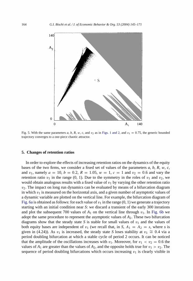
If v1 is further increased the two pieces of the chaotic area expand until they merge intoa one-piece chaotic area, as shown inFig. 5, obtained withv1 = 0.75. This is a remarkableglobal bifurcation,6 after which the generic bounded trajectory moves erratically along thebigger chaotic area, so that no cyclic pattern can be detected. Another consequence of theglobal bifurcation at which the two pieces form a one-piece chaotic area is that the boundaryof the chaotic area is more “fuzzy”, in the sense that “rare points” appear around a moredensely covered central part. In the versus time representation of the trajectory, the existenceof such rare points implies that some sudden jumps occur, which are of greater amplitudewith respect to the majority of the irregular oscillations. This kind of attracting set is calledmixed chaotic areain Mira et al. (1996).

In Fig. 5we also notice that the boundary which separates the basin of bounded trajectoriesfrom the basin of infinity is rather complex. This kind of complexity is another sources ofunpredictability, related to the fact that small changes in the initial conditions may yielda completely different asymptotic evolution if such changes cause a crossing of the basinboundaries. In fact, if a point is very close to a basin boundary (and many points are in sucha situation in the presence of complex basin boundaries) a small perturbation has a highprobability to cause a crossing of the boundary.

If v1 is further increased, the chaotic area expands until it has a contact with the bound-ary of the basin. This contact marks the occurrence of a global bifurcation, calledfinalbifurcation in Mira et al. (1996)andAbraham et al. (1997), or boundary crisesin Grebogiet al. (1983), which makes the chaotic area disappear. After this bifurcation, the chaotic

6 We call “global” the bifurcations which cannot be explained in terms of the linear approximation of thedynamical system, as opposed to the local bifurcations, which are revealed through the study of the eigenvaluesof the Jacobian matrix (used to represent the linearization of the dynamical system).


Fig. 4. With the same parametersa, b, R, w, c, andv2 as inFigs. 1 and 2, andv1 = 0.67, the generic boundedtrajectory converges to a two-cyclic chaotic attractor. In (a) such attracting set is represented by plotting a typicaltrajectory in the plane (A1, A2), in (b) a part of the same trajectory is plotted vs. time.

attractor is transformed into a chaotic repellor, whose “skeleton” is formed by the denseset of repelling periodic points which where inside the chaotic area that just disappearedGrebogi et al. (1983), and the generic initial condition generates a trajectory which divergesafter a chaotic transient.


Fig. 5. With the same parametersa, b, R, w, c, andv2 as inFigs. 1 and 2, andv1 = 0.75, the generic boundedtrajectory converges to a one-piece chaotic attractor.

5. Changes of retention ratios

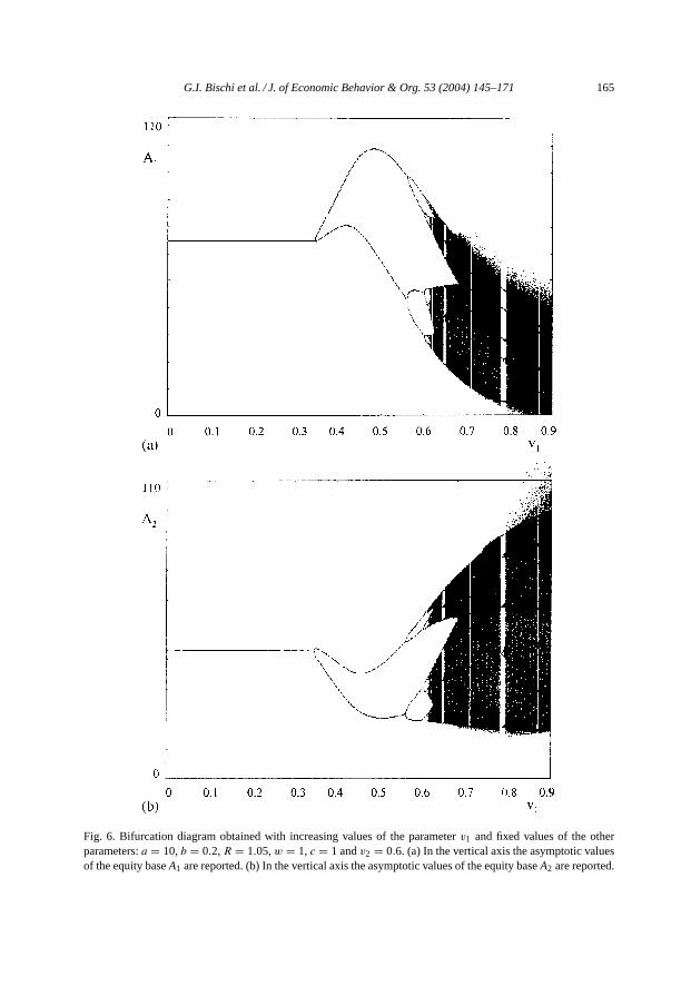
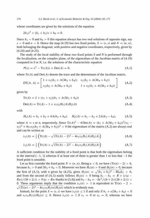
In order to explore the effects of increasing retention ratios on the dynamics of the equitybases of the two firms, we consider a fixed set of values of the parametersa, b, R, w, c,andv1, namelya = 10, b = 0.2, R = 1.05,w = 1, c = 1 andv2 = 0.6 and vary theretention ratiov1 in the range (0, 1). Due to the symmetry in the roles ofv1 andv2, wewould obtain analogous results with a fixed value ofv1 by varying the other retention ratiov2. The impact on long run dynamics can be evaluated by means of a bifurcation diagramin whichv1 is measured on the horizontal axis, and a given number of asymptotic values ofa dynamic variable are plotted on the vertical line. For example, the bifurcation diagram ofFig. 6ais obtained as follows: for each value ofv1 in the range (0, 1) we generate a trajectorystarting with an initial condition nearS: we discard a transient of the early 300 iterationsand plot the subsequent 700 values ofA1 on the vertical line throughv1. In Fig. 6b weadopt the same procedure to represent the asymptotic values ofA2. These two bifurcationdiagrams show that the steady stateS is stable for small values ofv1 and the values ofboth equity bases are independent ofv1 (we recall that, inS, A1 = A2 = s, wheres isgiven in (4.24)). Asv1 is increased, the steady stateS loses stability atv1 ∼= 0.4 via aperiod doubling bifurcation at which a stable cycle of period 2 occurs. It can be noticedthat the amplitude of the oscillations increases withv1. Moreover, forv1 < v2 = 0.6 thevalues ofA1 are greater than the values ofA2, and the opposite holds true forv1 > v2. Thesequence of period doubling bifurcations which occurs increasingv1 is clearly visible in


Fig. 6. Bifurcation diagram obtained with increasing values of the parameterv1 and fixed values of the otherparameters:a = 10,b = 0.2,R = 1.05,w = 1, c = 1 andv2 = 0.6. (a) In the vertical axis the asymptotic valuesof the equity baseA1 are reported. (b) In the vertical axis the asymptotic values of the equity baseA2 are reported.


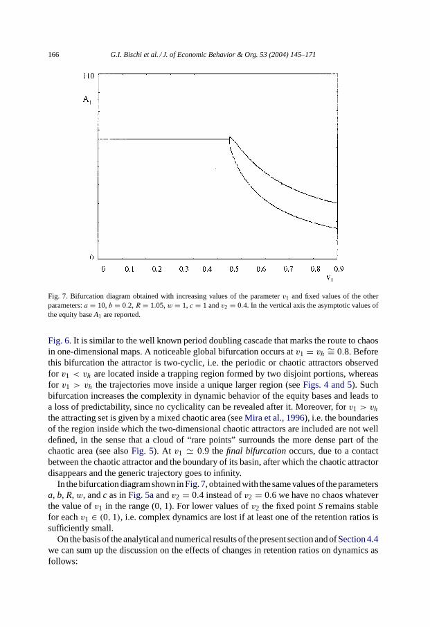
Fig. 7. Bifurcation diagram obtained with increasing values of the parameterv1 and fixed values of the otherparameters:a = 10,b = 0.2,R = 1.05,w = 1, c = 1 andv2 = 0.4. In the vertical axis the asymptotic values ofthe equity baseA1 are reported.

Fig. 6. It is similar to the well known period doubling cascade that marks the route to chaosin one-dimensional maps. A noticeable global bifurcation occurs atv1 = vh ∼= 0.8. Beforethis bifurcation the attractor is two-cyclic, i.e. the periodic or chaotic attractors observedfor v1 < vh are located inside a trapping region formed by two disjoint portions, whereasfor v1 > vh the trajectories move inside a unique larger region (seeFigs. 4 and 5). Suchbifurcation increases the complexity in dynamic behavior of the equity bases and leads toa loss of predictability, since no cyclicality can be revealed after it. Moreover, forv1 > vhthe attracting set is given by a mixed chaotic area (seeMira et al., 1996), i.e. the boundariesof the region inside which the two-dimensional chaotic attractors are included are not welldefined, in the sense that a cloud of “rare points” surrounds the more dense part of thechaotic area (see alsoFig. 5). At v1 � 0.9 thefinal bifurcationoccurs, due to a contactbetween the chaotic attractor and the boundary of its basin, after which the chaotic attractordisappears and the generic trajectory goes to infinity.

In the bifurcation diagram shown inFig. 7, obtained with the same values of the parametersa, b, R,w, andc as inFig. 5aandv2 = 0.4 instead ofv2 = 0.6 we have no chaos whateverthe value ofv1 in the range (0, 1). For lower values ofv2 the fixed pointS remains stablefor eachv1 ∈ (0,1), i.e. complex dynamics are lost if at least one of the retention ratios issufficiently small.

On the basis of the analytical and numerical results of the present section and ofSection 4.4we can sum up the discussion on the effects of changes in retention ratios on dynamics asfollows:


1. If the retention ratios are “sufficiently low”, the positive fixed pointS is stable. Even ifthe initial (financial) conditions and the dividend policy of the two firms are different(i.e.A1,0 �= A2,0 andv1 �= v2), the equity bases of the two firms will converge to theSSNE characterized byA1 = A2, provided that the initial conditions are inside the basinof attraction ofS. In the steady state, the two firms become homogeneous as far as theequity base and the level of output are concerned.

2. Increasing the value of at least one retention ratio, the fixed pointSbecomes unstable, thelong run dynamics is characterized by oscillations of period 2 such thatA1 > A2 (A1 <

A2) on average, as long asv1 < v2 (v1 > v2). In this case homogeneity is lost in thelong run, since the equity base oscillates in a range which is different from on firm to theother.

3. Only if the retention ratio is uniform across firms, i.e.v1 = v2, the long run dynamicsis characterized by oscillations such thatA1 = A2, on average. In fact, if the reten-tion ratios are uniform across firms the attractors are located on the 45◦ diagonal. Inthis case, and only in this case, long run homogeneity is preserved also in the caseof dynamics which are more complex than the simple convergence to a stable steadystate.

4. An increase of the retention ratios yields more complex, and consequently less pre-dictable, dynamics of the equity bases. Moreover, also the boundary that separatesthe set of points that generate bounded trajectories from the basin of infinity becomesmore complex, thus generating a greater uncertainty also with respect to the choiceof initial conditions, or, equivalently, with respect to the possible effects of randomshocks.

Therefore, the firms are heterogeneous in the long run if the retention ratios are notuniform across firms and not too small. Moreover, when heterogenous long run dynamicsoccur, the firm with the higher retention ratio ends up with the lower equity base (on average).This is broadly consistent with the stylized facts. In the real world, in fact, the corporatesector is heterogeneous, the retention ratios are different from one class of firms to the otherand the average retention ratio is relatively high. Moreover, “small” firms usually retaina higher proportion of their profits than “large” ones. For example, according toFazzariet al. (1988, p. 147), on average the retention ratio of the US manufacturing firms in the1970–1984 period has been 60%, with “small” firms retaining up to 80% of their profitswhile the retention ratio of “big” firms was approximately 50%.

The standard theoretical explanation of this stylized fact is based onthe financing hier-archy (or pecking order) assumption. When capital markets are affected by informationalimperfections such as asymmetric information, a financing hierarchy can be envisaged:internal finance is the most preferred source of finance while credit has a cost advantageover the issue of new equities as far as external sources of finance are concerned. Smallfirms, which have limited access to the credit and equity markets, rely first and foremost onretentions to fill their financing gap while large firms are less financially constrained andtherefore have a lower retention ratio.

The theoretical explanation of the same stylized fact in the present model is different.Let’s start from a benchmark case in which both firms have the same retention ratio. Theequity bases of the two firms therefore converge to the SSNE or—if they are not too low—to


a uniform two-period cycle. Therefore they are homogeneous. Assume now that one of thetwo firms increases its retention ratio. The direct effect of an increase of the retention ratioon the accumulation of the firm’s net worth is necessarily positive. However, the more rapidincrease of the equity base may have a negative impact on the expected profit of the firmand therefore may depress the accumulation of net worth (see the discussion inSection 4.2)in the subsequent rounds of the time evolution of the equity base. If this is the case, the firmwhich tries to accumulate more rapidly ends up with a lower level of the equity base in thelong run.

Increasing the retention ratios, the corporate sector remains heterogeneous (small and bigfirms coexist), but the dynamics of the equity bases become complex, i.e. observationallyequivalent to the dynamics generated by random shocks.

6. Conclusions

In this paper we have explored the properties of a simple oligopolistic set-up in whichfirms run the risk of bankruptcy or gain a solidity bonus according to their financial condi-tions. We present, first of all, a benchmark case in which firms do not incur a bankruptcycost/solidity bonus. In this case the quantity produced in the Cournot–Nash equilibriumwould be the same for each and every oligopolist (Symmetric Nash Equilibrium) and wouldbe independent of the financial condition (i.e. the level of the equity base) of the firm andof its rivals. Moreover, the accumulation of net worth by each firm would be independentof the accumulation of net worth on the part of rival firms.

In the general case in which firms face a bankruptcy cost/solidity bonus, the scale ofproduction is affected by financial conditions. In this case, the quantity produced in theCournot–Nash equilibrium would be different from one firm to the other and would dependon the net worth of the firm and of the competitors. Moreover, the motion over time of theequity bases of the firms may follow a wide range of dynamic patterns: convergence to aSymmetric Steady state Nash Equilibrium, periodic or non-periodic orbits, complex (evenchaotic) trajectories. Endogenous fluctuations of the equity bases of the oligopolists alsoimply that the Cournot–Nash equilibrium fluctuates.

If the retention ratios are “sufficiently low”, in the long run firms become homogeneousas far as the equity ratio and the output level are concerned. Increasing the value of at leastone retention ratio, the equity base of each firm oscillates in a range which is different fromone firm to the other.

In particular, the firm with the lower (higher) retention ratio ends up with the higher(lower) equity base on average. In a sense we have here a “paradox of thrift” applied to thecorporate sector: if a firm tries to accumulate its equity base more rapidly by increasingits retention ratio, it obtains the opposite result and becomes “poorer”. Further increases inat least one of the retention ratios yield more complex, and consequently less predictable,dynamics of the equity bases.

The present set-up represents a first modest step to model the generation of financiallydriven endogenous fluctuations in a game-theoretic context. In order to maintain the pos-sibility to get some insights concerning the dynamic properties of the model, we stick tothe simple analytic structure of a two-dimensional non-linear dynamical system by making


a number of mainly technical assumptions in the characterization of the state space. Anobvious extension of the present model consists in relaxing at least some of these assump-tions and modifying the model accordingly. For instance, we could give up the idea of asolidity bonus in the full collateralization regime while keeping the bankruptcy cost in theincomplete collateralization case. This relaxation, however, leads to a more cumbersomedynamical system, defined by different analytic expressions in the different regions of thestate space (due to the multiplicity of financial regimes the firms are experiencing) andmakes the analysis much more complicated: as often occurs in dynamic modeling, there isan obvious trade-off between realism of the hypotheses and mathematical manageability ofthe dynamical system.

A different extension consists in framing the model in a different game-theoretic context.In the present set-up the quantities produced by the two firms are strategic substitutes: ahigher volume of output by one firm makes the price go down—other things being equal—and negatively affects the expected profit of the other firm via the market demand function.We implicitly ignore the positive impact that an increase in the output of one firm can have onthe expected profit of the other firm via income effects. Taking these effects into account,i.e. conceiving of the quantities produced as strategic complements instead of strategicsubstitutes, can modify the results in interesting directions such as multiple Pareto-rankedequilibria.

Acknowledgements

The authors wish to thank Laura Gardini for helpful discussions and two anonymousreferees for their criticisms and suggestions which led to extensive rewriting of the pa-per. The authors acknowledge financial support from CNR and MURST (national re-search projects “Dynamic Models in Economics and Finance: Evolution, Uncertainty andForecasting” and “Heterogeneous Agents, Financial Fragility and Complex Dynamics”),Italy.

Appendix A. Proof of Proposition 1

We first consider the existence of the fixed points, given by the solutions of the alge-braic systemE(Πi) = 0, i = 1.2. with E(Πi) given by (4.7) and (4.14). This systemis symmetric, because it remains the same by exchangingA1 andA2: this means that thehyperbolaE(Π2) = 0 is the symmetric of the hyperbolaE(Π1) = 0 with respect to thediagonal∆ of equationA1 = A2. If Eqs. (4.7) and (4.14)are subtracted, then one eitherhasA1 = A2 orA1 +A2 = (h2 −h1)/(h3 −h4). However, the latter condition leads to theequation

(h3 + h4 − h5)A1

(A1 + h1 − h2

h3 − h4

)+ h0

h2 − h1

h3 − h4(h2h3 − h1h4) = 0

which has no solutions in general, beingh3 + h4 − h5 = 0. Hence, the two symmetriccurvesE(Π1) = 0 andE(Π2) = 0 only cross at two points located on the diagonal∆,


whose coordinates are given by the solutions of the equation

2h5x2 + (h1 + h2)x+ h0 = 0.

Sinceh5 < 0 andh0 > 0 this equation always has two real solutions of opposite sign, says > 0 andn < 0. Hence the map (4.19) has two fixed points,S = (s, s) andN = (n, n),both belonging the diagonal, with positive and negative coordinates, respectively, given by(4.24) and (4.25).

The study of the local stability of these two fixed pointsSandN is performed throughthe localization, on the complex plane, of the eigenvalues of the Jacobian matrix of (4.19)computed inSor N, i.e. the solutions of the characteristic equation

P(λ) = λ2 − Tr(A)λ+ Det(A) = 0, (A.1)

where Tr(A) and Det(A) denote the trace and the determinant of the Jacobian matrix.

DT(A,A) =[

1 + v1(h1 + A(3h3 + h4)) v1(h2 + A(3h4 + h3))

v2(h2 + A(3h4 + h3)) 1 + v2(h1 + A(3h3 + h4))

](A.2)

given by

Tr(A) = 2 + (v1 + v2)(h1 + A(3h3 + h4)) (A.3)

Det(A) = Tr(A)− 1 + v1v2H1(A)H2(A) (A.4)

with

H1(A) = h1 + h2 + 4A(h3 + h4); H2(A) = h1 − h2 + 2A(h3 − h4), (A.5)

whereA = s or n, respectively. Since Tr(A)2 − 4 Det(A) = (h1 + A(3h3 + h4))2(v1 −

v2)2 + 4v1v2(h2 +A(3h4 + h3))

2 > 0 the eigenvalues of the matrix (A.2) are always realand can be written as

λ1(A) = 12

(Tr(A)−

√(Tr(A)− 2)2 − 4v1v2H1(A)H2(A)

)(A.6)

λ2(A) = 12

(Tr(A)+

√(Tr(A)− 2)2 − 4v1v2H1(A)H2(A)

)(A.7)

A sufficient condition for the stability of a fixed point is that both the eigenvalues belongto the interval (−1, 1) whereas if at least one of them is greater than 1 or less that−1 thefixed point is unstable.

Let us first consider the fixed pointN = (n, n). Beingn < 0, we have(Tr(n)− 2) > 0,becauseh1 > 0 and 3h3 + h4 < 0. Moreover we haveH1(n) > 0 andH2(n) > 0, because

the first of (A.5), withn given by (4.25), givesH1(n) =√(h1 + h2)2 − 8h0h5 > 0,

and from the second of (A.5) easily followsH2(n) > 0 beingh1 − h2 = R + (c(a −Rw)/(3b+ 2c)) > 0 (a > Rw thanks to (3.4)) andh3 −h4 = −bc2/((b+ 2c)(3b+ 2c)) <0. These arguments imply that the conditionλ1(n) > 1 is equivalent to Tr(n) − 2 >√(Tr(n)− 2)2 − 4v1v2H1(n)H2(n) which is evidently true.Instead, for the pointS = (s, s) we haveλ2(s) ≤ 1 if and only ifh1 + s(3h3 + h4) < 0

and v1v2H1(s)H2(s) ≥ 0. Henceλ2(s) = 1 if v1 = 0 or v2 = 0, whereas we have


λ1(s) < λ2(s) < 1 for eachv1 > 0 andv2 > 0. Instead, the second stability condition,λ1 > −1 is satisfied if and only if 4+2(v1+v2)(h1+ s(3h3+h4))+v1v2H1(s)H2(s) ≥ 0.

This condition is satisfied for small values ofv1 or v2, whereas it is not satisfied for largevalues ofv1 andv2. this means that the fixed pointSmay have the eigenvaluesλ1(s) andλ2(s) both inside the interval (−1, 1), thus giving local asymptotic stability ofS, at leastfor sufficiently low values of the retention ratiosv1 or v2, and for increasing values of theparametersv1 andv2 the smaller eigenvaluesλ1(s) can exit the interval (−1, 1) throughthe valuesλ1(s) = −1, so that the positive fixed pointS loses stability via a flip (or perioddoubling) bifurcation at whichSbecomes a saddle point and a stable cycle of period twois created near it7 (see e.g.Lorenz, 1993, Chapter 3, orGuckenheimer and Holmes, 1983,p. 158).

References

Abraham, R., Gardini, L., Mira, C., 1997. Chaos in discrete dynamical systems (a visual introduction in twodimensions). Springer-Verlag, Berlin.

Altman, E., 1984. A further empirical investigation of the bankruptcy cost question. Journal of Finance 39, 1067–1089.

Bernanke, B., Gertler, M., Gilchrist, S., 1999. The financial accelerator in a quantitative business cycle framework.In: Taylor, J., Woodford, M. (Eds.), Handbook of Macroeconomics, vol. 1C. North Holland, Amsterdam.

Davis, E.P., 1992. Debt, Financial Fragility and Systemic Risk. Oxford University Press, Oxford.Fazzari, S., Hubbard, G., Petersen, B., 1988. Financing constraints and corporate investment. Brookings Papers

on Economic Activity 1, 141–206.Grebogi, C., Ott, E., Yorke, J., 1983. Crises, sudden changes in chaotic attractors and transient chaos. Physica 7D,

181–200.Gilson, S., 1990. Bankruptcy, boards, banks and blockholders: evidence on changes in corporate ownership and

control when firms default. Journal of Financial Economics 27, 355–388.Greenwald, B., Stiglitz, J., 1993. Financial market imperfections and business cycles. Quarterly Journal Of

Economics 108, 77–114.Greenwald, B., Stiglitz, J., Weiss, A., 1984. Informational imperfections in the capital markets and macroeconomic

fluctuations. American Economic Review 74, 194–199.Guckenheimer, J., Holmes P., 1983. Nonlinear Oscillations, Dynamical Systems, and Bifurcations of Vector Fields.

Springer-Verlag, Berlin.Kaplan, S., Reishus, D., 1990. Outside directorship and corporate performance. Journal of Financial Economics

27, 389–410.Kiyotaki, N., Moore, J., 1997. Credit cycles. Journal of Political Economy 105, 211–248.Lorenz, H.W., 1993. Nonlinear Dynamical Economics and Chaotic Motion, second ed. Springer-Verlag, Berlin.Minsky, H.P., 1982. Can “It” Happen Again? M.E. Sharpe, New York.Mira, C., Gardini, L., Barugola, A., Cathala J., 1996. Chaotic Dynamics in Two-dimensional Noninvertible Maps.

World Scientific, Singapore.Myers, S., Majluf, N., 1984. Corporate financing and investment decisions when firms have information that

investors do not have. Journal of Financial Economics 13, 187–221.

7 The rigorous proof that the flip bifurcation is supercritical, so that a stable cycle of period 2 is created, requiresa center manifold reduction and the evaluation of higher order derivatives (up to the third order). This is ratherboring and we claim numerical evidence for the existence of the stable cycle.

Financial conditions, strategic interaction and complex dynamics: a game-theoretic model of financially driven fluctuations

Documents