Finance McGraw-Hill Primis ISBN: 0-390-32000-5 Text: Corporate Finance, Sixth Edition Ross-Westerfield-Jaffe Corporate Fiance David Whitehurst UMIST Volume 1 McGraw-Hill/Irwin =>?

Welcome message from author
This document is posted to help you gain knowledge. Please leave a comment to let me know what you think about it! Share it to your friends and learn new things together.
Transcript

Finance
McGraw−Hill Primis
ISBN: 0−390−32000−5
Text: Corporate Finance, Sixth EditionRoss−Westerfield−Jaffe
Corporate Fiance
David Whitehurst
UMIST
Volume 1
McGraw-Hill/Irwin���

Finance
http://www.mhhe.com/primis/online/Copyright ©2003 by The McGraw−Hill Companies, Inc. All rights reserved. Printed in the United States of America. Except as permitted under the United States Copyright Act of 1976, no part of this publication may be reproduced or distributed in any form or by any means, or stored in a database or retrieval system, without prior written permission of the publisher. This McGraw−Hill Primis text may include materials submitted to McGraw−Hill for publication by the instructor of this course. The instructor is solely responsible for the editorial content of such materials.
111 FINA ISBN: 0−390−32000−5
This book was printed on recycled paper.
Finance
Volume 1
Ross−Westerfield−Jaffe • Corporate Finance, Sixth Edition
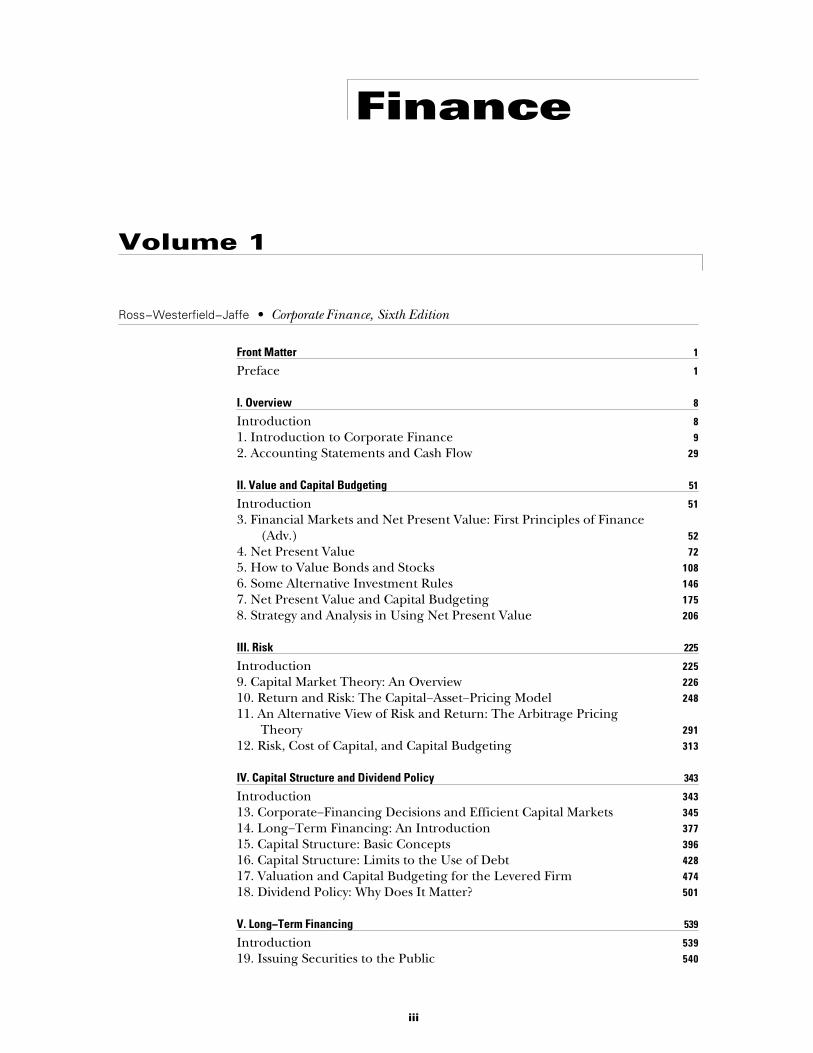
Front Matter 1
Preface 1
I. Overview 8
Introduction 81. Introduction to Corporate Finance 92. Accounting Statements and Cash Flow 29
II. Value and Capital Budgeting 51
Introduction 513. Financial Markets and Net Present Value: First Principles of Finance
(Adv.) 524. Net Present Value 725. How to Value Bonds and Stocks 1086. Some Alternative Investment Rules 1467. Net Present Value and Capital Budgeting 1758. Strategy and Analysis in Using Net Present Value 206
III. Risk 225
Introduction 2259. Capital Market Theory: An Overview 22610. Return and Risk: The Capital−Asset−Pricing Model 24811. An Alternative View of Risk and Return: The Arbitrage Pricing
Theory 29112. Risk, Cost of Capital, and Capital Budgeting 313
IV. Capital Structure and Dividend Policy 343
Introduction 34313. Corporate−Financing Decisions and Efficient Capital Markets 34514. Long−Term Financing: An Introduction 37715. Capital Structure: Basic Concepts 39616. Capital Structure: Limits to the Use of Debt 42817. Valuation and Capital Budgeting for the Levered Firm 47418. Dividend Policy: Why Does It Matter? 501
V. Long−Term Financing 539
Introduction 53919. Issuing Securities to the Public 540
iii
20. Long−Term Debt 56921. Leasing 592
VI. Options, Futures, and Corporate Finance 617
Introduction 61722. Options and Corporate Finance: Basic Concepts 61823. Options and Corporate Finance: Extensions and Applications 65624. Warrants and Convertibles 68025. Derivatives and Hedging Risk 701
VII. Financial Planning and Short−Term Finance 736
Introduction 73626. Corporate Financial Models and Long−Term Planning 73727. Short−Term Finance and Planning 75128. Cash Management 77629. Credit Management 803
VIII. Special Topics 820
Introduction 82030. Mergers and Acquisitions 82131. Financial Distress 85932. International Corporate Finance 877
iv
Ross−Westerfield−Jaffe: Corporate Finance, Sixth Edition
Front Matter Preface 1© The McGraw−Hill Companies, 2002
The teaching and the practicing of corporate finance are more challenging and excitingthan ever before. The last decade has seen fundamental changes in financial markets andfinancial instruments. In the early years of the 21st century, we still see announcements inthe financial press about such matters as takeovers, junk bonds, financial restructuring, ini-tial public offerings, bankruptcy, and derivatives. In addition, there is the new recognitionof “real” options (Chapters 21 and 22), private equity and venture capital (Chapter 19), andthe disappearing dividend (Chapter 18). The world’s financial markets are more integratedthan ever before. Both the theory and practice of corporate finance have been movingahead with uncommon speed, and our teaching must keep pace.
These developments place new burdens on the teaching of corporate finance. On onehand, the changing world of finance makes it more difficult to keep materials up to date.On the other hand, the teacher must distinguish the permanent from the temporary andavoid the temptation to follow fads. Our solution to this problem is to emphasize the mod-ern fundamentals of the theory of finance and make the theory come to life with contem-porary examples. Increasingly, many of these examples are outside the United States. Alltoo often, the beginning student views corporate finance as a collection of unrelated topicsthat are unified largely because they are bound together between the covers of one book.As in the previous editions, our aim is to present corporate finance as the working of asmall number of integrated and powerful institutions.
THE INTENDED AUDIENCE OF THIS BOOK
This book has been written for the introductory courses in corporate finance at the MBAlevel, and for the intermediate courses in many undergraduate programs. Some instructorswill find our text appropriate for the introductory course at the undergraduate level as well.
We assume that most students either will have taken, or will be concurrently enrolled in,courses in accounting, statistics, and economics. This exposure will help students understandsome of the more difficult material. However, the book is self-contained, and a prior knowl-edge of these areas is not essential. The only mathematics prerequisite is basic algebra.
NEW TO THE SIXTH EDITION
Following are the key revisions and updates to this edition:
• A complete update of all cost of capital discussions to emphasize its usefulness incapital budgeting, primarily in Chapters 12 and 17.
Preface

Ross−Westerfield−Jaffe: Corporate Finance, Sixth Edition
Front Matter Preface2 © The McGraw−Hill Companies, 2002
Preface vii
• A new appendix on performance evaluation and EVA in Chapter 12.• A new section on liquidity and the cost of capital in Chapter 12.• New evidence on efficient markets and CAPM in Chapter 13.• New treatment on why firms choose different capital structures and dividend poli-
cies: the case of Qualcomm in Chapters 16 and 18.• A redesign and rewrite of options and derivatives chapters into a new Part VI.• Extension of options theory to mergers and acquisitions in Chapter 22.• An expanded discussion of real options and their importance to capital budgeting in
Chapter 23.• New material on carveouts, spinoffs, and tracking stocks in Chapter 30.• Many new end-of-chapter problems throughout all chapters.
ATTENTION TO PEDAGOGY
Executive SummaryEach chapter begins with a “roadmap” that describes the objectives of the chapter and howit connects with concepts already learned in previous chapters. Real company examplesthat will be discussed are highlighted in this section.
Case StudyThere are 10 case studies that are highlighted in the Sixth Edition that present situationswith real companies and how they rationalized the decisions they made to solve variousproblems. They provide extended examples of the material covered in the chapter. Thecases are highlighted in the detailed Table of Contents.
In Their Own Words BoxesLocated throughout the Sixth Edition, this unique series consists of articles written by dis-tinguished scholars or practitioners on key topics in the text.
Concept QuestionsIncluded after each major section in a chapter, Concept Questions point to essential mater-ial and allow students to test their recall and comprehension before moving forward.
Key Terms Students will note that important words are highlighted in boldface type the first time theyappear. They are also listed at the end of the chapter, along with the page number on whichthey first appear, as well as in the glossary at the end of the book.
Demonstration ProblemsWe have provided worked-out examples throughout the text to give students a clear under-standing of the logic and structure of the solution process. These examples are clearlycalled out in the text.
Highlighted ConceptsThroughout the text, important ideas are pulled out and presented in a copper box—signal-ing to students that this material is particularly relevant and critical for their understanding.
Numbered EquationsKey equations are numbered and listed on the back end sheets for easy reference.
The end of-chapter material reflects and builds on the concepts learned from the chap-ter and study features:
Ross−Westerfield−Jaffe: Corporate Finance, Sixth Edition
Front Matter Preface 3© The McGraw−Hill Companies, 2002
Summary and ConclusionsThe numbered summary provides a quick review of key concepts in the chapter.
List of Key TermsA list of the boldfaced key terms with page numbers is included for easy reference.
Suggested ReadingsEach chapter is followed by a short, annotated list of books and articles to which interest-ed students can refer for additional information.
Questions and ProblemsBecause solving problems is so critical to a student’s learning, they have been revised, thor-oughly reviewed, and accuracy-checked. The problem sets are graded for difficulty, movingfrom easier problems intended to build confidence and skill to more difficult problemsdesigned to challenge the enthusiastic student. Problems have been grouped according to theconcepts they test on. Additionally, we have tried to make the problems in the critical “con-cept” chapters, such as those on value, risk, and capital structure, especially challenging andinteresting. We provide answers to selected problems in Appendix B at the end of the book.
MinicaseThis end-of-chapter feature, located in Chapters 12 and 30, parallels the Case Study featurefound in various chapters. These Minicases apply what is learned in a number of chaptersto a real-world type of scenario. After presenting the facts, the student is given guidance inrationalizing a sound business decision.
SUPPLEMENTS PACKAGE
As with the text, developing supplements of extraordinary quality and utility was the pri-mary objective. Each component in the supplement package underwent extensive reviewand revision.
FOR THE INSTRUCTOR
Instructor’s Manual (0-07-233882-2)Prepared by John Stansfield, University of Missouri, Columbia, this instructor’s tool hasbeen thoroughly revised and updated. Each chapter includes a list of transparencies/PowerPoint slides, a brief chapter outline, an introduction, and an annotated outline. Theannotated outline contains references to the transparencies/PowerPoint slides, additionalexplanations and examples, and teaching tips.
PowerPoint Presentation System (0-07-233883-0)This presentation system was developed in conjunction with the Instructor’s Manual by thesame author, allowing for a complete and integrated teaching package. These slides containuseful outlines, summaries, and exhibits from the text. If you have PowerPoint installed onyour PC, you have the ability to edit, print, or rearrange the complete transparency presen-tation to meet your specific needs.
Test Bank (0-07-233885-7)The Test Bank, prepared by David Burnie, Western Michigan University, includes an aver-age of 35 multiple-choice questions and problems per chapter, and 5 essay questions per
viii Preface

Ross−Westerfield−Jaffe: Corporate Finance, Sixth Edition
Front Matter Preface4 © The McGraw−Hill Companies, 2002
Preface ix
chapter. Each question is labeled with the level of difficulty. About 30–40 percent of theseproblems are new or revised.
Computerized Testing Software (0-07-233881-4)This software includes an easy-to-use menu system which allows quick access to all thepowerful features available. The Keyword Search option lets you browse through the ques-tion bank for problems containing a specific word or phrase. Password protection is avail-able for saved tests or for the entire database. Questions can be added, modified, or deleted.Available in Windows version.
Solutions Manual (0-07-233884-9)The Solutions Manual, prepared by John A. Helmuth, University of Michigan, containsworked-out solutions for all of the problems, and has been thoroughly reviewed for accu-racy. The Solutions Manual is also available to be purchased for your students.
Instructor CD-ROM (0-07-246238-8)You can receive all of the supplements in an electronic format! The Instructor’s Manual,PowerPoint, Test Bank, and Solutions Manual are all together on one convenient CD. Theinterface provides the instructor with a self-contained program that allows him or her toarrange the visual resources into his or her own presentation and add additional files as well.
Videos (0-07-250741-1)These finance videos are 10-minute case studies on topics such as Financial Markets,Careers, Rightsizing, Capital Budgeting, EVA (Economic Value Added), Mergers andAcquisitions, and International Finance. Questions to accompany these videos can befound on the book’s Online Learning Center.
FOR THE STUDENTS
Standard & Poor’s Educational Version of Market Insight. If you purchased a new book,you will have received a free passcode card that will give you access to the same companyand industry data that industry experts use. See www.mhhe.com/edumarketinsight fordetails on this exclusive partnership!
PowerWebIf you purchased a new book, free access to PowerWeb—a dynamic supplement specific toyour corporate finance course—is also available. Included are three levels of resourcematerials: articles from journals and magazines from the past year, weekly updates on cur-rent issues, and links to current news of the day. Also available is a series of study aids,such as quizzes, web links, and interactive exercises. See www.dushkin.com/powerweb formore details and access to this valuable resource.
Student Problem Manual (0-07-233880-6)Written by Robert Hanson, Eastern Michigan University, the Student Problem Manual is adirect companion to the text. It is uniquely designed to involve the student in the learningprocess. Each chapter contains a Mission Statement, an average of 20 fill-in-the-blankConcept Test questions and answers, and an average of 15 problems and worked-out solu-tions. This product can be purchased separately or packaged with the text.
Online Learning CenterVisit the full web resource now available with the Sixth Edition at www.mhhe.com/rwj. TheInformation Center includes information on this new edition, and links for special offers.
Ross−Westerfield−Jaffe: Corporate Finance, Sixth Edition
Front Matter Preface 5© The McGraw−Hill Companies, 2002
x Preface
The Instructor Center includes all of the teaching resources for the book, and the StudentCenter includes free online study materials—such as quizzes, study outlines, and spread-sheets—developed specifically for this edition. A feedback form is also available for yourquestions and comments.
ACKNOWLEDGMENTS
The plan for developing this edition began with a number of our colleagues who had an inter-est in the book and regularly teach the MBA introductory course. We integrated their com-ments and recommendations throughout the Sixth Edition. Contributors to this edition include:
R. Aggarwal, John Carroll University
Christopher Anderson, University ofMissouri–Columbia
James J. Angel, Georgetown University
Kevin Bahr, University of Wisconsin–Milwaukee
Michael Barry, Boston College
William O. Brown, Claremont McKenna College
Bill Callahan, Southern Methodist University
Steven Carvell, Cornell University
Indudeep S. Chhachhi, Western KentuckyUniversity
Jeffrey L. Coles, Arizona State University
Raymond Cox, Central Michigan University
John Crockett, George Mason University
Robert Duvic, The University of Texas at Austin
Steven Ferraro, Pepperdine University
Adlai Fisher, New York University
Yee-Tien Fu, Stanford University
Bruno Gerard, University of Southern California
Frank Ghannadian, Mercer University–Atlanta
John A. Helmuth, University ofMichigan–Dearborn
Edith Hotchkiss, Boston College
Charles Hu, Claremont McKenna College
Raymond Jackson, University ofMassachusetts–Dartmouth
Narayanan Jayaraman, Georgia Institute ofTechnology
Dolly King, University of Wisconsin–Milwaukee
Ronald Kudla, The University of Akron
Dilip Kumar Patro, Rutgers University
Youngsik Kwak, Delaware State University
Youngho Lee, Howard University
Yulong Ma, Cal State—Long Beach
Richard Miller, Wesleyan University
Naval Modani, University of Central Florida
Robert Nachtmann, University of Pittsburgh
Edward Nelling, Georgia Tech
Gregory Niehaus, University of South Carolina
Ingmar Nyman, Hunter College
Venky Panchapagesan, WashingtonUniversity–St. Louis
Bulent Parker, University of Wisconsin–Madison
Christo Pirinsky, Ohio State University
Jeffrey Pontiff, University of Washington
N. Prabhala, Yale University
Mao Qiu, University of Utah–Salt Lake City
Latha Ramchand, University of Houston
Gabriel Ramirez, Virginia CommonwealthUniversity
Stuart Rosenstein, University of Colorado atDenver
Bruce Rubin, Old Dominion University
Jaime Sabal, New York University
Andy Saporoschenko, University of Akron
William Sartoris, Indiana University
Faruk Selcuk, University of Bridgeport
Sudhir Singh, Frostburg State University
John S. Strong, College of William and Mary
Michael Sullivan, University of Nevada–Las Vegas
Andrew C. Thompson, Virginia PolytechnicInstitute
Karin Thorburn, Dartmouth College
Satish Thosar, University ofMassachusetts–Dorchester
Oscar Varela, University of New Orleans
Steven Venti, Dartmouth College
Susan White, University of Texas–Austin
Over the years, many others have contributed their time and expertise to the development andwriting of this text. We extend our thanks once again for their assistance and countless insights:

Ross−Westerfield−Jaffe: Corporate Finance, Sixth Edition
Front Matter Preface6 © The McGraw−Hill Companies, 2002
Preface xi
James J. Angel, Georgetown University
Nasser Arshadi, University of Missouri–St. Louis
Robert Balik, Western Michigan University
John W. Ballantine, Babson College
Thomas Bankston, Angelo State University
Swati Bhatt, Rutgers University
Roger Bolton, Williams College
Gordon Bonner, University of Delaware
Brad Borber, University of California–Davis
Oswald Bowlin, Texas Technical University
Ronald Braswell, Florida State University
Kirt Butler, Michigan State University
Andreas Christofi, Pennsylvania StateUniversity–Harrisburg
James Cotter, University of Iowa
Jay Coughenour, University ofMassachusetts–Boston
Arnold Cowan, Iowa State University
Mark Cross, Louisiana Technical University
Ron Crowe, Jacksonville University
William Damon, Vanderbilt University
Sudip Datta, Bentley College
Anand Desai, University of Florida
Miranda Lam Detzler, University ofMassachusetts–Boston
David Distad, University of California–Berkeley
Dennis Draper, University of Southern California
Jean-Francois Dreyfus, New York University
Gene Drzycimski, University ofWisconsin–Oshkosh
Robert Eldridge, Fairfield University
Gary Emery, University of Oklahoma
Theodore Eytan, City University of NewYork–Baruch College
Don Fehrs, University of Notre Dame
Andrew Fields, University of Delaware
Paige Fields, Texas A&M
Michael Fishman, Northwestern University
Michael Goldstein, University of Colorado
Indra Guertler, Babson College
James Haltiner, College of William and Mary
Delvin Hawley, University of Mississippi
Hal Heaton, Brigham Young University
John Helmuth, Rochester Institute of Technology
Michael Hemler, University of Notre Dame
Stephen Heston, Washington University
Andrea Heuson, University of Miami
Hugh Hunter, Eastern Washington University
James Jackson, Oklahoma State University
Prem Jain, Tulane University
Brad Jordan, University of Kentucky
Jarl Kallberg, New York University
Jonathan Karpoff, University of Washington
Paul Keat, American Graduate School ofInternational Management
Brian Kluger, University of Cincinnati
Narayana Kocherlakota, University of Iowa
Nelson Lacey, University of Massachusetts
Gene Lai, University of Rhode Island
Josef Lakonishok, University of Illinois
Dennis Lasser, SUNY–Binghamton
Paul Laux, Case Western Reserve University
Bong-Su Lee, University of Minnesota
James T. Lindley, University of SouthernMississippi
Dennis Logue, Dartmouth College
Michael Long, Rutgers University
Ileen Malitz, Fairleigh Dickinson University
Terry Maness, Baylor University
Surendra Mansinghka, San Francisco StateUniversity
Michael Mazzco, Michigan State University
Robert I. McDonald, Northwestern University
Hugh McLaughlin, Bentley College
Larry Merville, University of Texas–Richardson
Joe Messina, San Francisco State University
Roger Mesznik, City College of NewYork–Baruch College
Rick Meyer, University of South Florida
Richard Mull, New Mexico State University
Jim Musumeci, Southern IllinoisUniversity–Carbondale
Peder Nielsen, Oregon State University
Dennis Officer, University of Kentucky
Joseph Ogden, State University of New York
Ajay Patel, University of Missouri–Columbia
Glenn N. Pettengill, Emporia State University
Pegaret Pichler, University of Maryland
Franklin Potts, Baylor University
Annette Poulsen, University of Georgia
Latha Ramchand, University of Houston
Narendar Rao, Northeastern Illinois University
Steven Raymar, Indiana University
Stuart Rosenstein, Southern Illinois University
Ross−Westerfield−Jaffe: Corporate Finance, Sixth Edition
Front Matter Preface 7© The McGraw−Hill Companies, 2002
Patricia Ryan, Drake University
Anthony Sanders, Ohio State University
James Schallheim, University of Utah
Mary Jean Scheuer, California State Universityat Northridge
Lemma Senbet, University of Maryland
Kuldeep Shastri, University of Pittsburgh
Scott Smart, Indiana University
Jackie So, Southern Illinois University
John Stansfield, Columbia College
A. Charlene Sullivan, Purdue University
Timothy Sullivan, Bentley College
R. Bruce Swensen, Adelphi University
Ernest Swift, Georgia State University
Alex Tang, Morgan State University
Richard Taylor, Arkansas State University
Timothy Thompson, Northwestern University
Charles Trzcinka, State University of NewYork–Buffalo
Haluk Unal, University of Maryland–College Park
Avinash Verma, Washington University
Lankford Walker, Eastern Illinois University
Ralph Walkling, Ohio State University
F. Katherine Warne, Southern Bell College
Robert Whitelaw, New York University
Berry Wilson, Georgetown University
Thomas Zorn, University of Nebraska–Lincoln
Kent Zumwalt, Colorado State University
xii Preface
For their help on the Sixth Edition, we would like to thank Linda De Angelo, DennisDraper, Kim Dietrich, Alan Shapiro, Harry De Angelo, Aris Protopapadakis, AnathMadhevan, and Suh-Pyng Ku, all of the Marshall School of Business at the University ofSouthern California. We also owe a debt of gratitude to Edward I. Altman, of New YorkUniversity; Robert S. Hansen, of Virginia Tech; and Jay Ritter, of the University of Florida,who have provided several thoughtful comments and immeasurable help.
Over the past three years, readers have provided assistance by detecting and reportingerrors. Our goal is to offer the best textbook available on the subject, so this informationwas invaluable as we prepared the Sixth Edition. We want to ensure that all future editionsare error-free and therefore we will offer $10 per arithmetic error to the first individualreporting it. Any arithmetic error resulting in subsequent errors will be counted double. Allerrors should be reported using the Feedback Form on the Corporate Finance OnlineLearning Center at www.mhhe.com/rwj.
In addition, Sandra Robinson and Wendy Wat have given significant assistance inpreparing the manuscript.
Finally, we wish to thank our families and friends, Carol, Kate, Jon, Jan, Mark, andLynne for their forbearance and help.
Stephen A. RossRandolph W. WesterfieldJeffrey F. Jaffe
Ross−Westerfield−Jaffe: Corporate Finance, Sixth Edition
I. Overview Introduction8 © The McGraw−Hill Companies, 2002
Overview
PA
RT
I
1 Introduction to Corporate Finance 22 Accounting Statements and Cash Flow 22
TO engage in business the financial managers of a firm must find answers to threekinds of important questions. First, what long-term investments should the firm take
on? This is the capital budgeting decision. Second, how can cash be raised for the re-quired investments? We call this the financing decision. Third, how will the firm man-age its day-to-day cash and financial affairs? These decisions involve short-term financeand concern net working capital.
In Chapter 1 we discuss these important questions, briefly introducing the basicideas of this book and describing the nature of the modern corporation and why it hasemerged as the leading form of the business firm. Using the set-of-contracts perspective,the chapter discusses the goals of the modern corporation. Though the goals of share-holders and managers may not always be the same, conflicts usually will be resolved infavor of the shareholders. Finally, the chapter reviews some of the salient features ofmodern financial markets. This preliminary material will be familiar to students whohave some background in accounting, finance, and economics.
Chapter 2 examines the basic accounting statements. It is review material for stu-dents with an accounting background. We describe the balance sheet and the incomestatement. The point of the chapter is to show the ways of converting data from ac-counting statements into cash flow. Understanding how to identify cash flow from ac-counting statements is especially important for later chapters on capital budgeting.
Ross−Westerfield−Jaffe: Corporate Finance, Sixth Edition
I. Overview 1. Introduction to Corporate Finance
9© The McGraw−Hill Companies, 2002
Introduction to Corporate Finance
CH
AP
TE
R1
EXECUTIVE SUMMARY
The Video Product Company designs and manufactures very popular software forvideo game consoles. The company was started in 1999, and soon thereafter its game“Gadfly” appeared on the cover of Billboard magazine. Company sales in 2000 were
over $20 million. Video Product’s initial financing of $2 million came from Seed Ltd., aventure-capital firm, in exchange for a 15-percent equity stake in the company. Now the fi-nancial management of Video Product realizes that its initial financing was too small. In thelong run Video Product would like to expand its design activity to the education and busi-ness areas. It would also like to significantly enhance its website for future Internet sales.However, at present the company has a short-run cash flow problem and cannot even buy$200,000 of materials to fill its holiday orders.
Video Product’s experience illustrates the basic concerns of corporate finance:
1. What long-term investment strategy should a company take on?
2. How can cash be raised for the required investments?
3. How much short-term cash flow does a company need to pay its bills?
These are not the only questions of corporate finance. They are, however, among the mostimportant questions and, taken in order, they provide a rough outline of our book.
One way that companies raise cash to finance their investment activities is by sellingor “issuing” securities. The securities, sometimes called financial instruments or claims,may be roughly classified as equity or debt, loosely called stocks or bonds. The differencebetween equity and debt is a basic distinction in the modern theory of finance. All securi-ties of a firm are claims that depend on or are contingent on the value of the firm.1 In Section1.2 we show how debt and equity securities depend on the firm’s value, and we describethem as different contingent claims.
In Section 1.3 we discuss different organizational forms and the pros and cons of thedecision to become a corporation.
In Section 1.4 we take a close look at the goals of the corporation and discuss why max-imizing shareholder wealth is likely to be the primary goal of the corporation. Throughoutthe rest of the book, we assume that the firm’s performance depends on the value it createsfor its shareholders. Shareholders are better off when the value of their shares is increasedby the firm’s decisions.
A company raises cash by issuing securities to the financial markets. The market valueof outstanding long-term corporate debt and equity securities traded in the U.S. financialmarkets is in excess of $25 trillion. In Section 1.5 we describe some of the basic features ofthe financial markets. Roughly speaking, there are two basic types of financial markets: themoney markets and the capital markets. The last section of the chapter provides an outlineof the rest of the book.
1We tend to use the words firm, company, and business interchangeably. However, there is a difference betweena firm and a corporation. We discuss this difference in Section 1.3.
Ross−Westerfield−Jaffe: Corporate Finance, Sixth Edition
I. Overview 1. Introduction to Corporate Finance
10 © The McGraw−Hill Companies, 2002
Chapter 1 Introduction to Corporate Finance 3
1.1 WHAT IS CORPORATE FINANCE?
Suppose you decide to start a firm to make tennis balls. To do this, you hire managers tobuy raw materials, and you assemble a workforce that will produce and sell finished tennisballs. In the language of finance, you make an investment in assets such as inventory, ma-chinery, land, and labor. The amount of cash you invest in assets must be matched by anequal amount of cash raised by financing. When you begin to sell tennis balls, your firmwill generate cash. This is the basis of value creation. The purpose of the firm is to createvalue for you, the owner. The firm must generate more cash flow than it uses. The value isreflected in the framework of the simple balance-sheet model of the firm.
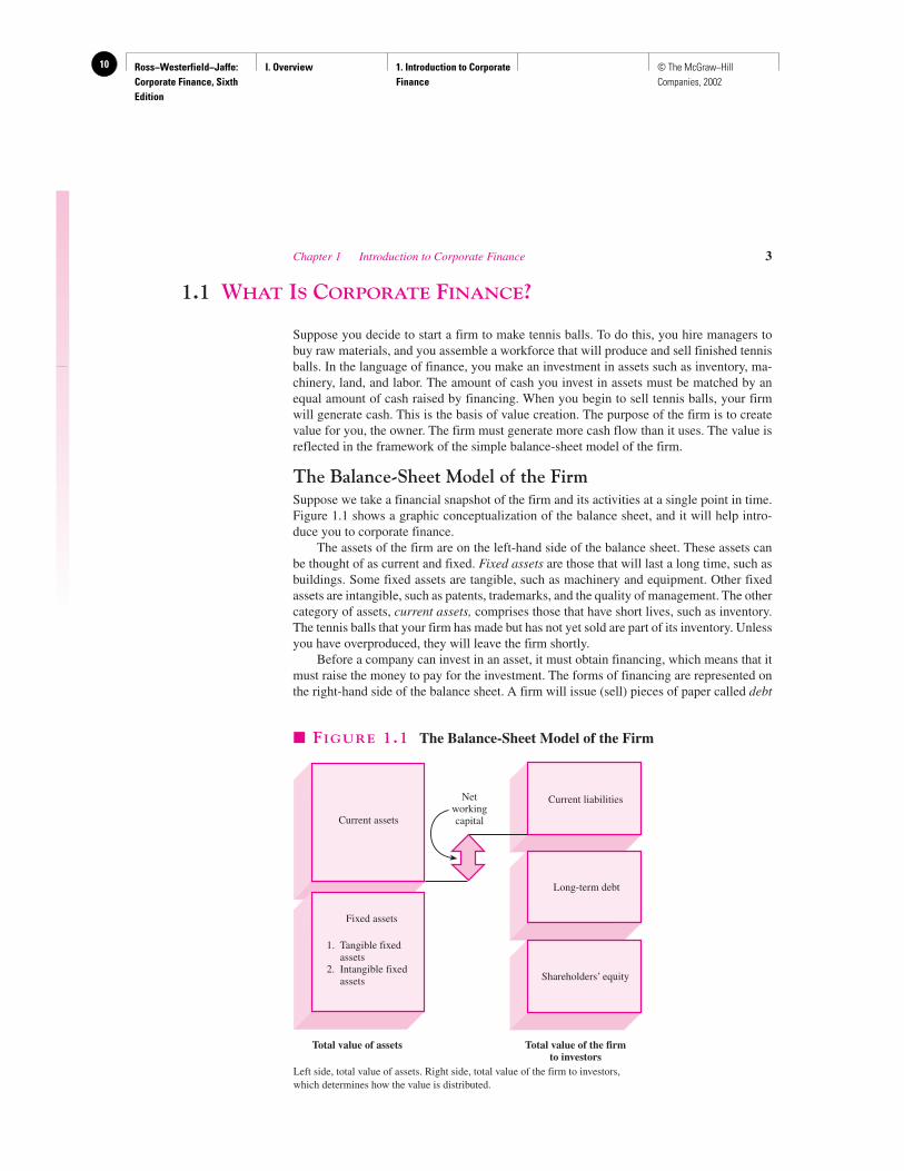
The Balance-Sheet Model of the FirmSuppose we take a financial snapshot of the firm and its activities at a single point in time.Figure 1.1 shows a graphic conceptualization of the balance sheet, and it will help intro-duce you to corporate finance.
The assets of the firm are on the left-hand side of the balance sheet. These assets canbe thought of as current and fixed. Fixed assets are those that will last a long time, such asbuildings. Some fixed assets are tangible, such as machinery and equipment. Other fixedassets are intangible, such as patents, trademarks, and the quality of management. The othercategory of assets, current assets, comprises those that have short lives, such as inventory.The tennis balls that your firm has made but has not yet sold are part of its inventory. Unlessyou have overproduced, they will leave the firm shortly.
Before a company can invest in an asset, it must obtain financing, which means that itmust raise the money to pay for the investment. The forms of financing are represented onthe right-hand side of the balance sheet. A firm will issue (sell) pieces of paper called debt
Long-term debt
Current assets
Fixed assets
1. Tangible fixedassets
2. Intangible fixedassets
Networkingcapital
Current liabilities
Shareholders’ equity
Total value of assets Total value of the firmto investors
� FIGURE 1.1 The Balance-Sheet Model of the Firm
Left side, total value of assets. Right side, total value of the firm to investors,which determines how the value is distributed.
Ross−Westerfield−Jaffe: Corporate Finance, Sixth Edition
I. Overview 1. Introduction to Corporate Finance
11© The McGraw−Hill Companies, 2002
(loan agreements) or equity shares (stock certificates). Just as assets are classified as long-lived or short-lived, so too are liabilities. A short-term debt is called a current liability.Short-term debt represents loans and other obligations that must be repaid within one year.Long-term debt is debt that does not have to be repaid within one year. Shareholders’ eq-uity represents the difference between the value of the assets and the debt of the firm. In thissense it is a residual claim on the firm’s assets.
From the balance-sheet model of the firm it is easy to see why finance can be thoughtof as the study of the following three questions:
1. In what long-lived assets should the firm invest? This question concerns the left-hand side of the balance sheet. Of course, the type and proportions of assets the firm needstend to be set by the nature of the business. We use the terms capital budgeting and capi-tal expenditures to describe the process of making and managing expenditures on long-lived assets.
2. How can the firm raise cash for required capital expenditures? This question con-cerns the right-hand side of the balance sheet. The answer to this involves the firm’s capi-tal structure, which represents the proportions of the firm’s financing from current andlong-term debt and equity.
3. How should short-term operating cash flows be managed? This question concernsthe upper portion of the balance sheet. There is often a mismatch between the timing of cashinflows and cash outflows during operating activities. Furthermore, the amount and timingof operating cash flows are not known with certainty. The financial managers must attemptto manage the gaps in cash flow. From a balance-sheet perspective, short-term managementof cash flow is associated with a firm’s net working capital. Net working capital is definedas current assets minus current liabilities. From a financial perspective, the short-term cashflow problem comes from the mismatching of cash inflows and outflows. It is the subjectof short-term finance.
Capital StructureFinancing arrangements determine how the value of the firm is sliced up. The persons orinstitutions that buy debt from the firm are called creditors.2 The holders of equity sharesare called shareholders.
Sometimes it is useful to think of the firm as a pie. Initially, the size of the pie will dependon how well the firm has made its investment decisions. After a firm has made its investmentdecisions, it determines the value of its assets (e.g., its buildings, land, and inventories).
The firm can then determine its capital structure. The firm might initially have raisedthe cash to invest in its assets by issuing more debt than equity; now it can consider chang-ing that mix by issuing more equity and using the proceeds to buy back some of its debt.Financing decisions like this can be made independently of the original investment deci-sions. The decisions to issue debt and equity affect how the pie is sliced.
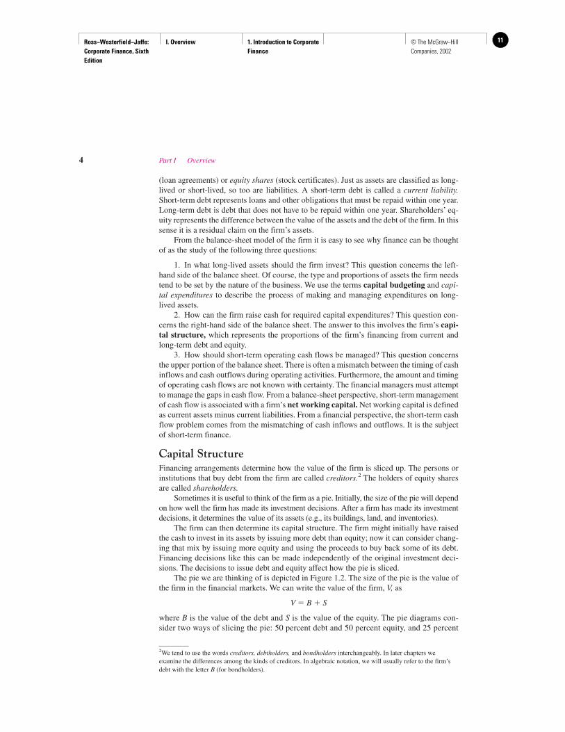
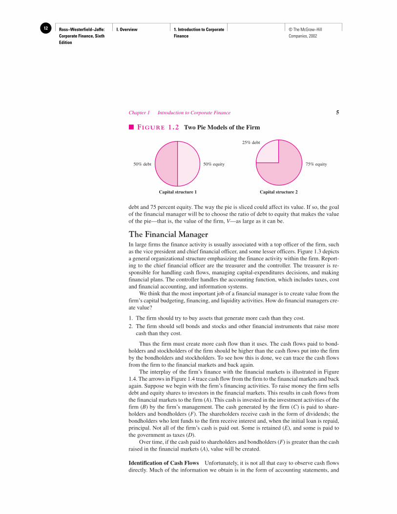
The pie we are thinking of is depicted in Figure 1.2. The size of the pie is the value ofthe firm in the financial markets. We can write the value of the firm, V, as
V � B � S
where B is the value of the debt and S is the value of the equity. The pie diagrams con-sider two ways of slicing the pie: 50 percent debt and 50 percent equity, and 25 percent
4 Part I Overview
2We tend to use the words creditors, debtholders, and bondholders interchangeably. In later chapters weexamine the differences among the kinds of creditors. In algebraic notation, we will usually refer to the firm’sdebt with the letter B (for bondholders).
Ross−Westerfield−Jaffe: Corporate Finance, Sixth Edition
I. Overview 1. Introduction to Corporate Finance
12 © The McGraw−Hill Companies, 2002
debt and 75 percent equity. The way the pie is sliced could affect its value. If so, the goalof the financial manager will be to choose the ratio of debt to equity that makes the valueof the pie—that is, the value of the firm, V—as large as it can be.
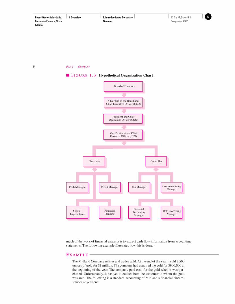
The Financial ManagerIn large firms the finance activity is usually associated with a top officer of the firm, suchas the vice president and chief financial officer, and some lesser officers. Figure 1.3 depictsa general organizational structure emphasizing the finance activity within the firm. Report-ing to the chief financial officer are the treasurer and the controller. The treasurer is re-sponsible for handling cash flows, managing capital-expenditures decisions, and makingfinancial plans. The controller handles the accounting function, which includes taxes, costand financial accounting, and information systems.
We think that the most important job of a financial manager is to create value from thefirm’s capital budgeting, financing, and liquidity activities. How do financial managers cre-ate value?
1. The firm should try to buy assets that generate more cash than they cost.
2. The firm should sell bonds and stocks and other financial instruments that raise morecash than they cost.
Thus the firm must create more cash flow than it uses. The cash flows paid to bond-holders and stockholders of the firm should be higher than the cash flows put into the firmby the bondholders and stockholders. To see how this is done, we can trace the cash flowsfrom the firm to the financial markets and back again.
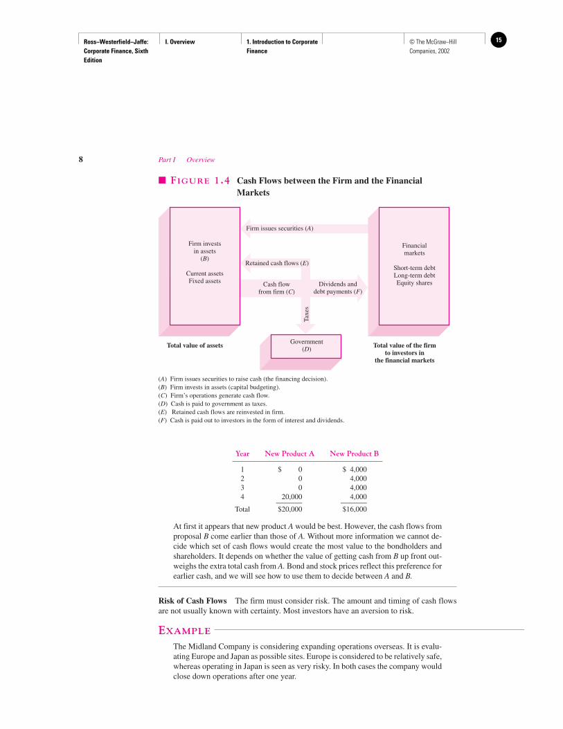
The interplay of the firm’s finance with the financial markets is illustrated in Figure1.4. The arrows in Figure 1.4 trace cash flow from the firm to the financial markets and backagain. Suppose we begin with the firm’s financing activities. To raise money the firm sellsdebt and equity shares to investors in the financial markets. This results in cash flows fromthe financial markets to the firm (A). This cash is invested in the investment activities of thefirm (B) by the firm’s management. The cash generated by the firm (C) is paid to share-holders and bondholders (F). The shareholders receive cash in the form of dividends; thebondholders who lent funds to the firm receive interest and, when the initial loan is repaid,principal. Not all of the firm’s cash is paid out. Some is retained (E), and some is paid tothe government as taxes (D).
Over time, if the cash paid to shareholders and bondholders (F) is greater than the cashraised in the financial markets (A), value will be created.
Identification of Cash Flows Unfortunately, it is not all that easy to observe cash flowsdirectly. Much of the information we obtain is in the form of accounting statements, and
Chapter 1 Introduction to Corporate Finance 5
50% debt 50% equity
25% debt
75% equity
Capital structure 1 Capital structure 2
� FIGURE 1.2 Two Pie Models of the Firm
Ross−Westerfield−Jaffe: Corporate Finance, Sixth Edition
I. Overview 1. Introduction to Corporate Finance
13© The McGraw−Hill Companies, 2002
much of the work of financial analysis is to extract cash flow information from accountingstatements. The following example illustrates how this is done.
EXAMPLE
The Midland Company refines and trades gold. At the end of the year it sold 2,500ounces of gold for $1 million. The company had acquired the gold for $900,000 atthe beginning of the year. The company paid cash for the gold when it was pur-chased. Unfortunately, it has yet to collect from the customer to whom the goldwas sold. The following is a standard accounting of Midland’s financial circum-stances at year-end:
6 Part I Overview
Board of Directors
Chairman of the Board andChief Executive Officer (CEO)
President and ChiefOperations Officer (COO)
Vice President and ChiefFinancial Officer (CFO)
Treasurer Controller
Cash Manager Credit Manager Tax Manager Cost AccountingManager
Data ProcessingManager
FinancialAccounting
Manager
FinancialPlanning
CapitalExpenditures
� FIGURE 1.3 Hypothetical Organization Chart
Ross−Westerfield−Jaffe: Corporate Finance, Sixth Edition
I. Overview 1. Introduction to Corporate Finance
14 © The McGraw−Hill Companies, 2002
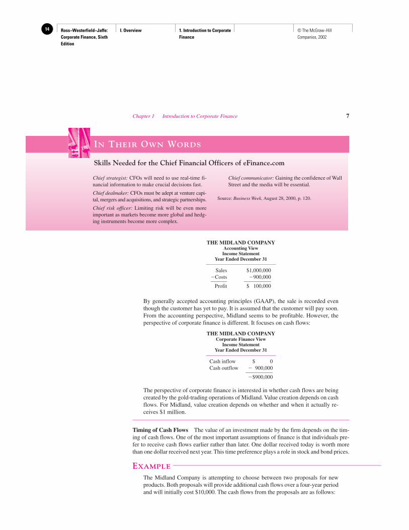
By generally accepted accounting principles (GAAP), the sale is recorded eventhough the customer has yet to pay. It is assumed that the customer will pay soon.From the accounting perspective, Midland seems to be profitable. However, theperspective of corporate finance is different. It focuses on cash flows:
The perspective of corporate finance is interested in whether cash flows are beingcreated by the gold-trading operations of Midland. Value creation depends on cashflows. For Midland, value creation depends on whether and when it actually re-ceives $1 million.
Timing of Cash Flows The value of an investment made by the firm depends on the tim-ing of cash flows. One of the most important assumptions of finance is that individuals pre-fer to receive cash flows earlier rather than later. One dollar received today is worth morethan one dollar received next year. This time preference plays a role in stock and bond prices.
EXAMPLE
The Midland Company is attempting to choose between two proposals for newproducts. Both proposals will provide additional cash flows over a four-year periodand will initially cost $10,000. The cash flows from the proposals are as follows:
THE MIDLAND COMPANYCorporate Finance View
Income StatementYear Ended December 31
Cash inflow $ 0Cash outflow � 900,000__________
�$900,000
THE MIDLAND COMPANYAccounting View
Income StatementYear Ended December 31
Sales $1,000,000�Costs �900,000______ __________
Profit $ 100,000
Chapter 1 Introduction to Corporate Finance 7
IN THEIR OWN WORDS
Skills Needed for the Chief Financial Officers of eFinance.com
Chief strategist: CFOs will need to use real-time fi-nancial information to make crucial decisions fast.
Chief dealmaker: CFOs must be adept at venture capi-tal, mergers and acquisitions, and strategic partnerships.
Chief risk officer: Limiting risk will be even moreimportant as markets become more global and hedg-ing instruments become more complex.
Chief communicator: Gaining the confidence of WallStreet and the media will be essential.
Source: Business Week, August 28, 2000, p. 120.
Ross−Westerfield−Jaffe: Corporate Finance, Sixth Edition
I. Overview 1. Introduction to Corporate Finance
15© The McGraw−Hill Companies, 2002
At first it appears that new product A would be best. However, the cash flows fromproposal B come earlier than those of A. Without more information we cannot de-cide which set of cash flows would create the most value to the bondholders andshareholders. It depends on whether the value of getting cash from B up front out-weighs the extra total cash from A. Bond and stock prices reflect this preference forearlier cash, and we will see how to use them to decide between A and B.
Risk of Cash Flows The firm must consider risk. The amount and timing of cash flowsare not usually known with certainty. Most investors have an aversion to risk.
EXAMPLE
The Midland Company is considering expanding operations overseas. It is evalu-ating Europe and Japan as possible sites. Europe is considered to be relatively safe,whereas operating in Japan is seen as very risky. In both cases the company wouldclose down operations after one year.
Year New Product A New Product B
1 $ 0 $ 4,0002 0 4,0003 0 4,0004 20,000 4,000_______ _______
Total $20,000 $16,000
8 Part I Overview
Firm investsin assets
(B)
Current assetsFixed assets
Financialmarkets
Short-term debtLong-term debtEquity shares
Government(D) Total value of the firm
to investors inthe financial markets
Dividends anddebt payments (F)
Firm issues securities (A)
Retained cash flows (E)
Cash flowfrom firm (C)
Total value of assets
Taxe
s
� FIGURE 1.4 Cash Flows between the Firm and the FinancialMarkets
(A) Firm issues securities to raise cash (the financing decision).(B) Firm invests in assets (capital budgeting).(C) Firm’s operations generate cash flow.(D) Cash is paid to government as taxes.(E) Retained cash flows are reinvested in firm.(F) Cash is paid out to investors in the form of interest and dividends.
Ross−Westerfield−Jaffe: Corporate Finance, Sixth Edition
I. Overview 1. Introduction to Corporate Finance
16 © The McGraw−Hill Companies, 2002
After doing a complete financial analysis, Midland has come up with the fol-lowing cash flows of the alternative plans for expansion under three equally likelyscenarios—pessimistic, most likely, and optimistic:
If we ignore the pessimistic scenario, perhaps Japan is the best alternative. Whenwe take the pessimistic scenario into account, the choice is unclear. Japan appearsto be riskier, but it also offers a higher expected level of cash flow. What is risk andhow can it be defined? We must try to answer this important question. Corporatefinance cannot avoid coping with risky alternatives, and much of our book is de-voted to developing methods for evaluating risky opportunities.
• What are three basic questions of corporate finance?• Describe capital structure.• How is value created?• List the three reasons why value creation is difficult.
1.2 CORPORATE SECURITIES AS CONTINGENT CLAIMS ON
TOTAL FIRM VALUE
What is the essential difference between debt and equity? The answer can be found by think-ing about what happens to the payoffs to debt and equity when the value of the firm changes.
The basic feature of a debt is that it is a promise by the borrowing firm to repay a fixeddollar amount by a certain date.
EXAMPLE
The Officer Corporation promises to pay $100 to the Brigham Insurance Companyat the end of one year. This is a debt of the Officer Corporation. Holders of the debtwill receive $100 if the value of the Officer Corporation’s assets is equal to or morethan $100 at the end of the year.
Formally, the debtholders have been promised an amount F at the end of theyear. If the value of the firm, X, is equal to or greater than F at year-end, debthold-ers will get F. Of course, if the firm does not have enough to pay off the promisedamount, the firm will be “broke.” It may be forced to liquidate its assets for what-ever they are worth, and the bondholders will receive X. Mathematically thismeans that the debtholders have a claim to X or F, whichever is smaller. Figure 1.5illustrates the general nature of the payoff structure to debtholders.
Suppose at year-end the Officer Corporation’s value is equal to $100. The firm haspromised to pay the Brigham Insurance Company $100, so the debtholders will get $100.
Now suppose the Officer Corporation’s value is $200 at year-end and the debthold-ers are promised $100. How much will the debtholders receive? It should be clear thatthey will receive the same amount as when the Officer Corporation was worth $100.
Suppose the firm’s value is $75 at year-end and debtholders are promised $100.How much will the debtholders receive? In this case the debtholders will get $75.
Pessimistic Most Likely Optimistic
Europe $75,000 $100,000 $125,000Japan 0 150,000 200,000
Chapter 1 Introduction to Corporate Finance 9
QUESTIONS
CO
NC
EP
T
?
Ross−Westerfield−Jaffe: Corporate Finance, Sixth Edition
I. Overview 1. Introduction to Corporate Finance
17© The McGraw−Hill Companies, 2002
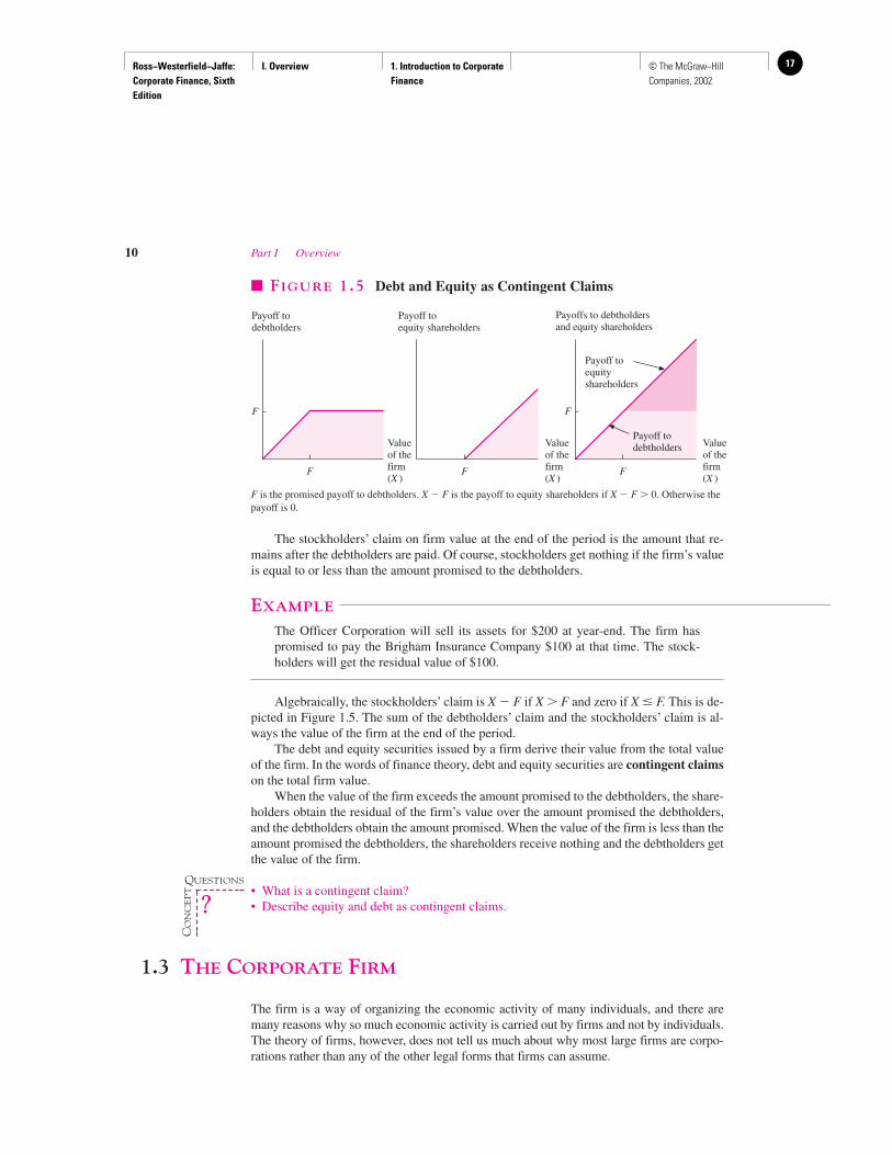
The stockholders’ claim on firm value at the end of the period is the amount that re-mains after the debtholders are paid. Of course, stockholders get nothing if the firm’s valueis equal to or less than the amount promised to the debtholders.
EXAMPLE
The Officer Corporation will sell its assets for $200 at year-end. The firm haspromised to pay the Brigham Insurance Company $100 at that time. The stock-holders will get the residual value of $100.
Algebraically, the stockholders’ claim is X � F if X � F and zero if X � F. This is de-picted in Figure 1.5. The sum of the debtholders’ claim and the stockholders’ claim is al-ways the value of the firm at the end of the period.
The debt and equity securities issued by a firm derive their value from the total valueof the firm. In the words of finance theory, debt and equity securities are contingent claimson the total firm value.
When the value of the firm exceeds the amount promised to the debtholders, the share-holders obtain the residual of the firm’s value over the amount promised the debtholders,and the debtholders obtain the amount promised. When the value of the firm is less than theamount promised the debtholders, the shareholders receive nothing and the debtholders getthe value of the firm.
• What is a contingent claim?• Describe equity and debt as contingent claims.
1.3 THE CORPORATE FIRM
The firm is a way of organizing the economic activity of many individuals, and there aremany reasons why so much economic activity is carried out by firms and not by individuals.The theory of firms, however, does not tell us much about why most large firms are corpo-rations rather than any of the other legal forms that firms can assume.
10 Part I Overview
F
F F F
F
Payoff todebtholders
Valueof thefirm(X )
Payoff toequity shareholders
Payoffs to debtholdersand equity shareholders
Payoff toequityshareholders
Payoff todebtholdersValue
of thefirm(X )
Valueof thefirm(X )
� FIGURE 1.5 Debt and Equity as Contingent Claims
F is the promised payoff to debtholders. X � F is the payoff to equity shareholders if X � F � 0. Otherwise thepayoff is 0.
QUESTIONS
CO
NC
EP
T
?
Ross−Westerfield−Jaffe: Corporate Finance, Sixth Edition
I. Overview 1. Introduction to Corporate Finance
18 © The McGraw−Hill Companies, 2002
A basic problem of the firm is how to raise cash. The corporate form of business, thatis, organizing the firm as a corporation, is the standard method for solving problems en-countered in raising large amounts of cash. However, businesses can take other forms. Inthis section we consider the three basic legal forms of organizing firms, and we see howfirms go about the task of raising large amounts of money under each form.
The Sole ProprietorshipA sole proprietorship is a business owned by one person. Suppose you decide to start abusiness to produce mousetraps. Going into business is simple: You announce to all whowill listen, “Today I am going to build a better mousetrap.”
Most large cities require that you obtain a business license. Afterward you can beginto hire as many people as you need and borrow whatever money you need. At year-end allthe profits and the losses will be yours.
Here are some factors that are important in considering a sole proprietorship:
1. The sole proprietorship is the cheapest business to form. No formal charter is required,and few government regulations must be satisfied for most industries.
2. A sole proprietorship pays no corporate income taxes. All profits of the business aretaxed as individual income.
3. The sole proprietorship has unlimited liability for business debts and obligations. Nodistinction is made between personal and business assets.
4. The life of the sole proprietorship is limited by the life of the sole proprietor.
5. Because the only money invested in the firm is the proprietor’s, the equity money thatcan be raised by the sole proprietor is limited to the proprietor’s personal wealth.
The PartnershipAny two or more persons can get together and form a partnership. Partnerships fall intotwo categories: (1) general partnerships and (2) limited partnerships.
In a general partnership all partners agree to provide some fraction of the work andcash and to share the profits and losses. Each partner is liable for the debts of the partner-ship. A partnership agreement specifies the nature of the arrangement. The partnershipagreement may be an oral agreement or a formal document setting forth the understanding.
Limited partnerships permit the liability of some of the partners to be limited to theamount of cash each has contributed to the partnership. Limited partnerships usually re-quire that (1) at least one partner be a general partner and (2) the limited partners do notparticipate in managing the business. Here are some things that are important when con-sidering a partnership:
1. Partnerships are usually inexpensive and easy to form. Written documents are requiredin complicated arrangements, including general and limited partnerships. Business li-censes and filing fees may be necessary.
2. General partners have unlimited liability for all debts. The liability of limited partners isusually limited to the contribution each has made to the partnership. If one general part-ner is unable to meet his or her commitment, the shortfall must be made up by the othergeneral partners.
3. The general partnership is terminated when a general partner dies or withdraws (but thisis not so for a limited partner). It is difficult for a partnership to transfer ownership with-out dissolving. Usually, all general partners must agree. However, limited partners maysell their interest in a business.
Chapter 1 Introduction to Corporate Finance 11
Ross−Westerfield−Jaffe: Corporate Finance, Sixth Edition
I. Overview 1. Introduction to Corporate Finance
19© The McGraw−Hill Companies, 2002
4. It is difficult for a partnership to raise large amounts of cash. Equity contributions areusually limited to a partner’s ability and desire to contribute to the partnership. Manycompanies, such as Apple Computer, start life as a proprietorship or partnership, but atsome point they choose to convert to corporate form.
5. Income from a partnership is taxed as personal income to the partners.
6. Management control resides with the general partners. Usually a majority vote is re-quired on important matters, such as the amount of profit to be retained in the business.
It is very difficult for large business organizations to exist as sole proprietorships orpartnerships. The main advantage is the cost of getting started. Afterward, the disadvan-tages, which may become severe, are (1) unlimited liability, (2) limited life of the enter-prise, and (3) difficulty of transferring ownership. These three disadvantages lead to (4) thedifficulty of raising cash.
The CorporationOf the many forms of business enterprises, the corporation is by far the most important. Itis a distinct legal entity. As such, a corporation can have a name and enjoy many of the le-gal powers of natural persons. For example, corporations can acquire and exchange prop-erty. Corporations can enter into contracts and may sue and be sued. For jurisdictional pur-poses, the corporation is a citizen of its state of incorporation. (It cannot vote, however.)
Starting a corporation is more complicated than starting a proprietorship or partner-ship. The incorporators must prepare articles of incorporation and a set of bylaws. The ar-ticles of incorporation must include the following:
1. Name of the corporation.
2. Intended life of the corporation (it may be forever).
3. Business purpose.
4. Number of shares of stock that the corporation is authorized to issue, with a statementof limitations and rights of different classes of shares.
5. Nature of the rights granted to shareholders.
6. Number of members of the initial board of directors.
The bylaws are the rules to be used by the corporation to regulate its own existence, andthey concern its shareholders, directors, and officers. Bylaws range from the briefest possi-ble statement of rules for the corporation’s management to hundreds of pages of text.
In its simplest form, the corporation comprises three sets of distinct interests: the share-holders (the owners), the directors, and the corporation officers (the top management).Traditionally, the shareholders control the corporation’s direction, policies, and activities.The shareholders elect a board of directors, who in turn selects top management. Membersof top management serve as corporate officers and manage the operation of the corporationin the best interest of the shareholders. In closely held corporations with few shareholdersthere may be a large overlap among the shareholders, the directors, and the top manage-ment. However, in larger corporations the shareholders, directors, and the top managementare likely to be distinct groups.
The potential separation of ownership from management gives the corporation severaladvantages over proprietorships and partnerships:
1. Because ownership in a corporation is represented by shares of stock, ownership can be read-ily transferred to new owners. Because the corporation exists independently of those whoown its shares, there is no limit to the transferability of shares as there is in partnerships.
12 Part I Overview
Ross−Westerfield−Jaffe: Corporate Finance, Sixth Edition
I. Overview 1. Introduction to Corporate Finance
20 © The McGraw−Hill Companies, 2002
2. The corporation has unlimited life. Because the corporation is separate from its owners,the death or withdrawal of an owner does not affect its legal existence. The corporationcan continue on after the original owners have withdrawn.
3. The shareholders’ liability is limited to the amount invested in the ownership shares. Forexample, if a shareholder purchased $1,000 in shares of a corporation, the potential losswould be $1,000. In a partnership, a general partner with a $1,000 contribution couldlose the $1,000 plus any other indebtedness of the partnership.
Limited liability, ease of ownership transfer, and perpetual succession are the major ad-vantages of the corporation form of business organization. These give the corporation anenhanced ability to raise cash.
There is, however, one great disadvantage to incorporation. The federal governmenttaxes corporate income. This tax is in addition to the personal income tax that shareholderspay on dividend income they receive. This is double taxation for shareholders when com-pared to taxation on proprietorships and partnerships.
CASE STUDY: Making the Decision to Become a Corporation:The Case of PLM International, Inc.3
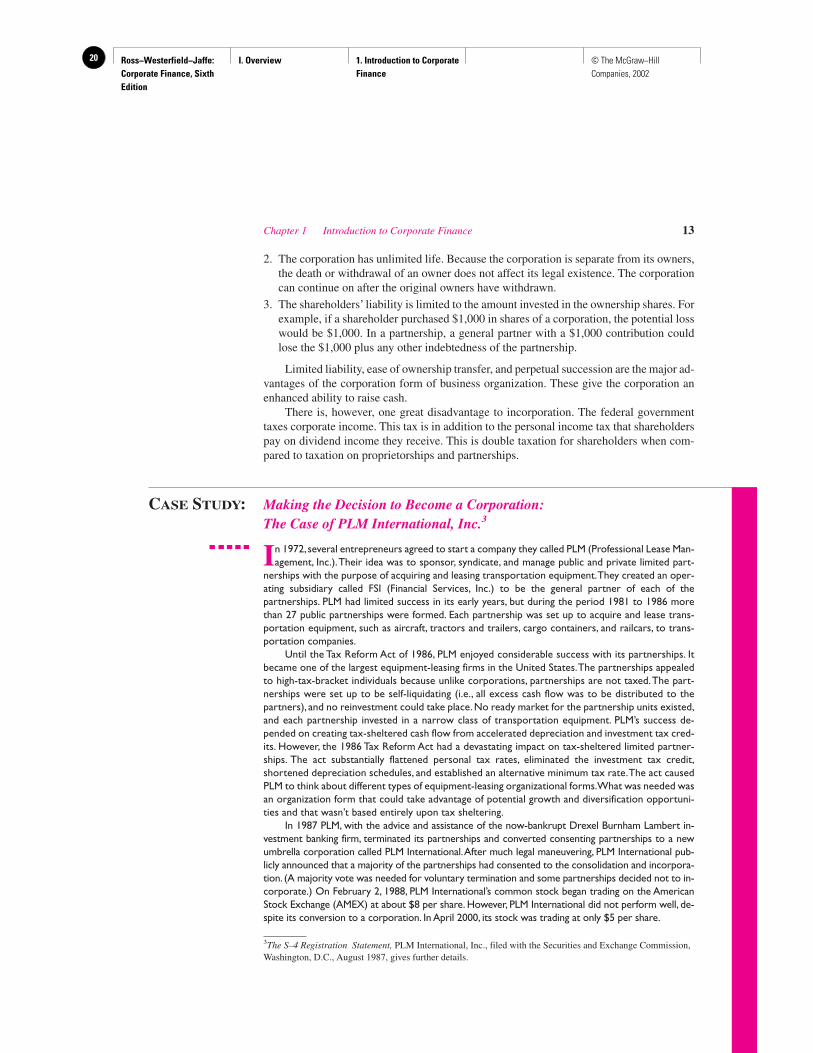
In 1972, several entrepreneurs agreed to start a company they called PLM (Professional Lease Man-agement, Inc.).Their idea was to sponsor, syndicate, and manage public and private limited part-
nerships with the purpose of acquiring and leasing transportation equipment.They created an oper-ating subsidiary called FSI (Financial Services, Inc.) to be the general partner of each of thepartnerships. PLM had limited success in its early years, but during the period 1981 to 1986 morethan 27 public partnerships were formed. Each partnership was set up to acquire and lease trans-portation equipment, such as aircraft, tractors and trailers, cargo containers, and railcars, to trans-portation companies.
Until the Tax Reform Act of 1986, PLM enjoyed considerable success with its partnerships. Itbecame one of the largest equipment-leasing firms in the United States.The partnerships appealedto high-tax-bracket individuals because unlike corporations, partnerships are not taxed.The part-nerships were set up to be self-liquidating (i.e., all excess cash flow was to be distributed to thepartners), and no reinvestment could take place.No ready market for the partnership units existed,and each partnership invested in a narrow class of transportation equipment. PLM’s success de-pended on creating tax-sheltered cash flow from accelerated depreciation and investment tax cred-its. However, the 1986 Tax Reform Act had a devastating impact on tax-sheltered limited partner-ships. The act substantially flattened personal tax rates, eliminated the investment tax credit,shortened depreciation schedules, and established an alternative minimum tax rate.The act causedPLM to think about different types of equipment-leasing organizational forms.What was needed wasan organization form that could take advantage of potential growth and diversification opportuni-ties and that wasn’t based entirely upon tax sheltering.
In 1987 PLM, with the advice and assistance of the now-bankrupt Drexel Burnham Lambert in-vestment banking firm, terminated its partnerships and converted consenting partnerships to a newumbrella corporation called PLM International.After much legal maneuvering, PLM International pub-licly announced that a majority of the partnerships had consented to the consolidation and incorpora-tion. (A majority vote was needed for voluntary termination and some partnerships decided not to in-corporate.) On February 2, 1988, PLM International’s common stock began trading on the AmericanStock Exchange (AMEX) at about $8 per share. However, PLM International did not perform well, de-spite its conversion to a corporation. In April 2000, its stock was trading at only $5 per share.
Chapter 1 Introduction to Corporate Finance 13
3The S–4 Registration Statement, PLM International, Inc., filed with the Securities and Exchange Commission,Washington, D.C., August 1987, gives further details.
Ross−Westerfield−Jaffe: Corporate Finance, Sixth Edition
I. Overview 1. Introduction to Corporate Finance
21© The McGraw−Hill Companies, 2002
The decision to become a corporation is complicated, and there are several pros and cons. PLMInternational cited several basic reasons to support the consolidation and incorporation of its trans-portation-equipment–leasing activities.
• Enhanced access to equity and debt capital for future growth.• The possibility of reinvestment for future profit opportunities.• Better liquidity for investors through common stock listing on AMEX.
These are all good reasons for incorporating, and they provided potential benefits to the newshareholders of PLM International that may have outweighed the disadvantages of double taxation thatcame from incorporating. However, not all the PLM partnerships wanted to convert to the corpora-tion. Sometimes it is not easy to determine whether a partnership or a corporation is the best orga-nizational form. Corporate income is taxable at the personal and corporation levels. Because of thisdouble taxation, firms having the most to gain from incorporation share the following characteristics:
• Low taxable income.• Low marginal corporate tax rates.• Low marginal personal tax rates among potential shareholders.
In addition, firms with high rates of reinvestment relative to current income are good candidatesfor the corporate form because corporations can more easily retain profits for reinvestment thanpartnerships.Also, it is easier for corporations to sell shares of stock on public stock markets to fi-nance possible investment opportunities.
14 Part I Overview
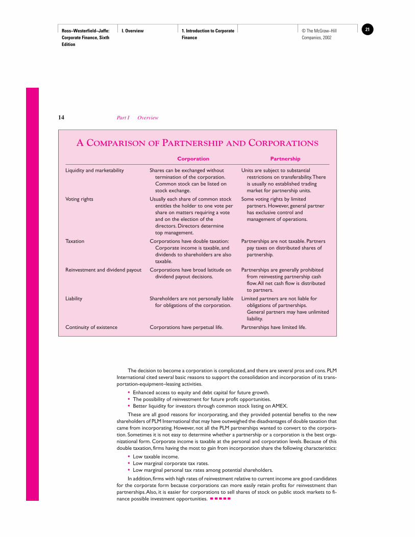
A COMPARISON OF PARTNERSHIP AND CORPORATIONS
Corporation Partnership
Liquidity and marketability Shares can be exchanged without Units are subject to substantial termination of the corporation. restrictions on transferability.There Common stock can be listed on is usually no established trading stock exchange. market for partnership units.
Voting rights Usually each share of common stock Some voting rights by limited entitles the holder to one vote per partners. However, general partner share on matters requiring a vote has exclusive control and and on the election of the management of operations.directors. Directors determine top management.
Taxation Corporations have double taxation: Partnerships are not taxable. Partners Corporate income is taxable, and pay taxes on distributed shares of dividends to shareholders are also partnership.taxable.
Reinvestment and dividend payout Corporations have broad latitude on Partnerships are generally prohibited dividend payout decisions. from reinvesting partnership cash
flow.All net cash flow is distributedto partners.
Liability Shareholders are not personally liable Limited partners are not liable for for obligations of the corporation. obligations of partnerships.
General partners may have unlimitedliability.
Continuity of existence Corporations have perpetual life. Partnerships have limited life.
Ross−Westerfield−Jaffe: Corporate Finance, Sixth Edition
I. Overview 1. Introduction to Corporate Finance
22 © The McGraw−Hill Companies, 2002
• Define a proprietorship, a partnership, and a corporation.• What are the advantages of the corporate form of business organization?
1.4 GOALS OF THE CORPORATE FIRM
What is the primary goal of the corporation? The traditional answer is that managers in acorporation make decisions for the stockholders because the stockholders own and controlthe corporation. If so, the goal of the corporation is to add value for the stockholders. Thisgoal is a little vague and so we will try to come up with a precise formulation. It is also im-possible to give a definitive answer to this important question because the corporation is anartificial being, not a natural person. It exists in the “contemplation of the law.”4
It is necessary to precisely identify who controls the corporation. We shall consider theset-of-contracts viewpoint. This viewpoint suggests the corporate firm will attempt tomaximize the shareholders’ wealth by taking actions that increase the current value pershare of existing stock of the firm.
Agency Costs and the Set-of-Contracts PerspectiveThe set-of-contracts theory of the firm states that the firm can be viewed as a set of con-tracts.5 One of the contract claims is a residual claim (equity) on the firm’s assets and cashflows. The equity contract can be defined as a principal-agent relationship. The membersof the management team are the agents, and the equity investors (shareholders) are the prin-cipals. It is assumed that the managers and the shareholders, if left alone, will each attemptto act in his or her own self-interest.
The shareholders, however, can discourage the managers from diverging from the share-holders’ interests by devising appropriate incentives for managers and then monitoring theirbehavior. Doing so, unfortunately, is complicated and costly. The cost of resolving the con-flicts of interest between managers and shareholders are special types of costs called agencycosts. These costs are defined as the sum of (1) the monitoring costs of the shareholders and(2) the costs of implementing control devices. It can be expected that contracts will be devisedthat will provide the managers with appropriate incentives to maximize the shareholders’wealth. Thus, the set-of-contracts theory suggests that managers in the corporate firm willusually act in the best interest of shareholders. However, agency problems can never be per-fectly solved and, as a consequence, shareholders may experience residual losses. Residuallosses are the lost wealth of the shareholders due to divergent behavior of the managers.
Managerial GoalsManagerial goals may be different from those of shareholders. What goals will managersmaximize if they are left to pursue their own rather than shareholders’ goals?
Williamson proposes the notion of expense preference.6 He argues that managers ob-tain value from certain kinds of expenses. In particular, company cars, office furniture, of-fice location, and funds for discretionary investment have value to managers beyond thatwhich comes from their productivity.
Chapter 1 Introduction to Corporate Finance 15
4These are the words of Chief Justice John Marshall from The Trustees of Dartmouth College v. Woodward, 4,Wheaton 636 (1819).5M. C. Jensen and W. Meckling, “Theory of the Firm: Managerial Behavior, Agency Costs and OwnershipStructure,” Journal of Financial Economics 3 (1976).6O. Williamson, “Managerial Discretion and Business Behavior,” American Economic Review 53 (1963).
QUESTIONS
CO
NC
EP
T
?
Ross−Westerfield−Jaffe: Corporate Finance, Sixth Edition
I. Overview 1. Introduction to Corporate Finance
23© The McGraw−Hill Companies, 2002
Donaldson conducted a series of interviews with the chief executives of several largecompanies.7 He concluded that managers are influenced by two basic motivations:
1. Survival. Organizational survival means that management will always try to commandsufficient resources to avoid the firm’s going out of business.
2. Independence and self-sufficiency. This is the freedom to make decisions without en-countering external parties or depending on outside financial markets. The Donaldsoninterviews suggested that managers do not like to issue new shares of stock. Instead, theylike to be able to rely on internally generated cash flow.
These motivations lead to what Donaldson concludes is the basic financial objective ofmanagers: the maximization of corporate wealth. Corporate wealth is that wealth overwhich management has effective control; it is closely associated with corporate growth andcorporate size. Corporate wealth is not necessarily shareholder wealth. Corporate wealthtends to lead to increased growth by providing funds for growth and limiting the extent towhich new equity is raised. Increased growth and size are not necessarily the same thing asincreased shareholder wealth.
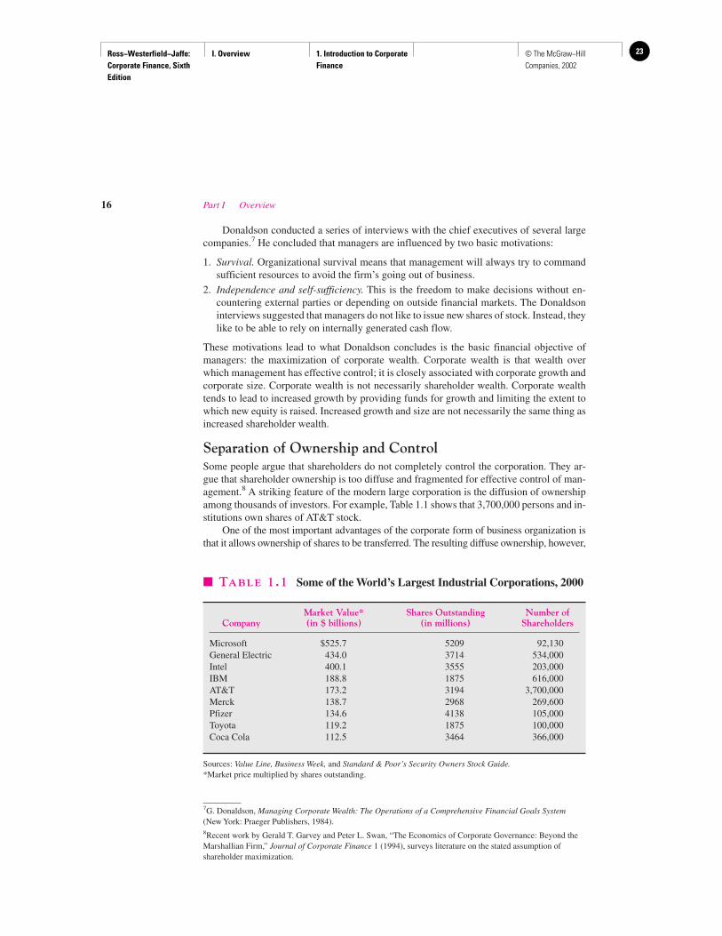
Separation of Ownership and ControlSome people argue that shareholders do not completely control the corporation. They ar-gue that shareholder ownership is too diffuse and fragmented for effective control of man-agement.8 A striking feature of the modern large corporation is the diffusion of ownershipamong thousands of investors. For example, Table 1.1 shows that 3,700,000 persons and in-stitutions own shares of AT&T stock.
One of the most important advantages of the corporate form of business organization isthat it allows ownership of shares to be transferred. The resulting diffuse ownership, however,
16 Part I Overview
7G. Donaldson, Managing Corporate Wealth: The Operations of a Comprehensive Financial Goals System(New York: Praeger Publishers, 1984).8Recent work by Gerald T. Garvey and Peter L. Swan, “The Economics of Corporate Governance: Beyond theMarshallian Firm,” Journal of Corporate Finance 1 (1994), surveys literature on the stated assumption ofshareholder maximization.
� TABLE 1.1 Some of the World’s Largest Industrial Corporations, 2000
Market Value* Shares Outstanding Number ofCompany (in $ billions) (in millions) Shareholders
Microsoft $525.7 5209 92,130General Electric 434.0 3714 534,000Intel 400.1 3555 203,000IBM 188.8 1875 616,000AT&T 173.2 3194 3,700,000Merck 138.7 2968 269,600Pfizer 134.6 4138 105,000Toyota 119.2 1875 100,000Coca Cola 112.5 3464 366,000
Sources: Value Line, Business Week, and Standard & Poor’s Security Owners Stock Guide.*Market price multiplied by shares outstanding.
Ross−Westerfield−Jaffe: Corporate Finance, Sixth Edition
I. Overview 1. Introduction to Corporate Finance
24 © The McGraw−Hill Companies, 2002
brings with it the separation of ownership and control of the large corporation. The possibleseparation of ownership and control raises an important question: Who controls the firm?
Do Shareholders Control Managerial Behavior?The claim that managers can ignore the interests of shareholders is deduced from the factthat ownership in large corporations is widely dispersed. As a consequence, it is oftenclaimed that individual shareholders cannot control management. There is some merit inthis argument, but it is too simplistic.
When a conflict of interest exists between management and shareholders, who wins?Does management or the shareholders control the firm? There is no doubt that ownershipin large corporations is diffuse when compared to the closely held corporation. However,several control devices used by shareholders bond management to the self-interest ofshareholders:
1. Shareholders determine the membership of the board of directors by voting. Thus, share-holders control the directors, who in turn select the management team.
2. Contracts with management and arrangements for compensation, such as stock option plans,can be made so that management has an incentive to pursue the goal of the shareholders. An-other device is called performance shares. These are shares of stock given to managers onthe basis of performance as measured by earnings per share and similar criteria.
3. If the price of a firm’s stock drops too low because of poor management, the firm maybe acquired by another group of shareholders, by another firm, or by an individual. Thisis called a takeover. In a takeover, the top management of the acquired firm may findthemselves out of a job. This puts pressure on the management to make decisions in thestockholders’ interests. Fear of a takeover gives managers an incentive to take actionsthat will maximize stock prices.
4. Competition in the managerial labor market may force managers to perform in the bestinterest of stockholders. Otherwise they will be replaced. Firms willing to pay the mostwill lure good managers. These are likely to be firms that compensate managers basedon the value they create.
The available evidence and theory are consistent with the ideas of shareholder controland shareholder value maximization. However, there can be no doubt that at times corpo-rations pursue managerial goals at the expense of shareholders. There is also evidence thatthe diverse claims of customers, vendors, and employees must frequently be considered inthe goals of the corporation.
• What are the two types of agency costs?• How are managers bonded to shareholders?• Can you recall some managerial goals?• What is the set-of-contracts perspective?
1.5 FINANCIAL MARKETS
As indicated in Section 1.1, firms offer two basic types of securities to investors. Debt se-curities are contractual obligations to repay corporate borrowing. Equity securities areshares of common stock and preferred stock that represent noncontractual claims to the
Chapter 1 Introduction to Corporate Finance 17
QUESTIONS
CO
NC
EP
T
?
Ross−Westerfield−Jaffe: Corporate Finance, Sixth Edition
I. Overview 1. Introduction to Corporate Finance
25© The McGraw−Hill Companies, 2002
residual cash flow of the firm. Issues of debt and stock that are publicly sold by the firm arethen traded on the financial markets.
The financial markets are composed of the money markets and the capital markets.Money markets are the markets for debt securities that will pay off in the short term (usu-ally less than one year). Capital markets are the markets for long-term debt (with a matu-rity at over one year) and for equity shares.
The term money market applies to a group of loosely connected markets. They aredealer markets. Dealers are firms that make continuous quotations of prices for which theystand ready to buy and sell money-market instruments for their own inventory and at theirown risk. Thus, the dealer is a principal in most transactions. This is different from a stock-broker acting as an agent for a customer in buying or selling common stock on most stockexchanges; an agent does not actually acquire the securities.
At the core of the money markets are the money-market banks (these are large banks inNew York), more than 30 government securities dealers (some of which are the large banks),a dozen or so commercial-paper dealers, and a large number of money brokers. Money bro-kers specialize in finding short-term money for borrowers and placing money for lenders. Thefinancial markets can be classified further as the primary market and the secondary markets.
The Primary Market: New IssuesThe primary market is used when governments and corporations initially sell securities.Corporations engage in two types of primary-market sales of debt and equity: public offer-ings and private placements.
Most publicly offered corporate debt and equity come to the market underwritten by a syn-dicate of investment banking firms. The underwriting syndicate buys the new securities from thefirm for the syndicate’s own account and resells them at a higher price. Publicly issued debt andequity must be registered with the Securities and Exchange Commission. Registration requiresthe corporation to disclose all of the material information in a registration statement.
The legal, accounting, and other costs of preparing the registration statement are not neg-ligible. In part to avoid these costs, privately placed debt and equity are sold on the basis ofprivate negotiations to large financial institutions, such as insurance companies and mutualfunds. Private placements are not registered with the Securities and Exchange Commission.
Secondary MarketsAfter debt and equity securities are originally sold, they are traded in the secondary markets.There are two kinds of secondary markets: the auction markets and the dealer markets.
The equity securities of most large U.S. firms trade in organized auction markets, suchas the New York Stock Exchange, the American Stock Exchange, and regional exchanges,such as the Midwest Stock Exchange. The New York Stock Exchange (NYSE) is the mostimportant auction exchange. It usually accounts for more than 85 percent of all sharestraded in U.S. auction exchanges. Bond trading on auction exchanges is inconsequential.
Most debt securities are traded in dealer markets. The many bond dealers communi-cate with one another by telecommunications equipment—wires, computers, and tele-phones. Investors get in touch with dealers when they want to buy or sell, and can negoti-ate a deal. Some stocks are traded in the dealer markets. When they are, it is referred to asthe over-the-counter (OTC) market.
In February 1971, the National Association of Securities Dealers made available todealers and brokers in the OTC market an automated quotation system called the NationalAssociation of Securities Dealers Automated Quotation (NASDAQ) system. The marketvalue of shares of OTC stocks in the NASDAQ system at the end of 1998 was about 25 per-cent of the market value of the shares on the NYSE.
18 Part I Overview
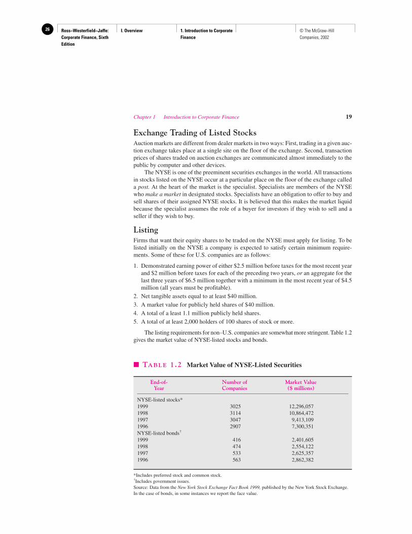
Ross−Westerfield−Jaffe: Corporate Finance, Sixth Edition
I. Overview 1. Introduction to Corporate Finance
26 © The McGraw−Hill Companies, 2002
Exchange Trading of Listed StocksAuction markets are different from dealer markets in two ways: First, trading in a given auc-tion exchange takes place at a single site on the floor of the exchange. Second, transactionprices of shares traded on auction exchanges are communicated almost immediately to thepublic by computer and other devices.
The NYSE is one of the preeminent securities exchanges in the world. All transactionsin stocks listed on the NYSE occur at a particular place on the floor of the exchange calleda post. At the heart of the market is the specialist. Specialists are members of the NYSEwho make a market in designated stocks. Specialists have an obligation to offer to buy andsell shares of their assigned NYSE stocks. It is believed that this makes the market liquidbecause the specialist assumes the role of a buyer for investors if they wish to sell and aseller if they wish to buy.
ListingFirms that want their equity shares to be traded on the NYSE must apply for listing. To belisted initially on the NYSE a company is expected to satisfy certain minimum require-ments. Some of these for U.S. companies are as follows:
1. Demonstrated earning power of either $2.5 million before taxes for the most recent yearand $2 million before taxes for each of the preceding two years, or an aggregate for thelast three years of $6.5 million together with a minimum in the most recent year of $4.5million (all years must be profitable).
2. Net tangible assets equal to at least $40 million.
3. A market value for publicly held shares of $40 million.
4. A total of a least 1.1 million publicly held shares.
5. A total of at least 2,000 holders of 100 shares of stock or more.
The listing requirements for non–U.S. companies are somewhat more stringent. Table 1.2gives the market value of NYSE-listed stocks and bonds.
Chapter 1 Introduction to Corporate Finance 19
� TABLE 1.2 Market Value of NYSE-Listed Securities
End-of- Number of Market ValueYear Companies ($ millions)
NYSE-listed stocks*1999 3025 12,296,0571998 3114 10,864,4721997 3047 9,413,1091996 2907 7,300,351NYSE-listed bonds†
1999 416 2,401,6051998 474 2,554,1221997 533 2,625,3571996 563 2,862,382
*Includes preferred stock and common stock.†Includes government issues.Source: Data from the New York Stock Exchange Fact Book 1999, published by the New York Stock Exchange.In the case of bonds, in some instances we report the face value.
Ross−Westerfield−Jaffe: Corporate Finance, Sixth Edition
I. Overview 1. Introduction to Corporate Finance
27© The McGraw−Hill Companies, 2002
20 Part I Overview
• Distinguish between money markets and capital markets.• What is listing?• What is the difference between a primary market and a secondary market?
1.6 OUTLINE OF THE TEXT
Now that we’ve taken the quick tour through all of corporate finance, we can take a closerlook at this book. The book is divided into eight parts. The long-term investment decisionis covered first. Financing decisions and working capital are covered next. Finally a seriesof special topics are covered. Here are the eight parts:
Part I OverviewPart II Value and Capital BudgetingPart III RiskPart IV Capital Structure and Dividend PolicyPart V Long-Term FinancingPart VI Options, Futures, and Corporate FinancePart VII Financial Planning and Short-Term FinancePart VIII Special Topics
Part II describes how investment opportunities are valued in financial markets. Thispart contains basic theory. Because finance is a subject that builds understanding from theground up, the material is very important. The most important concept in Part II is netpresent value. We develop the net present value rule into a tool for valuing investment al-ternatives. We discuss general formulas and apply them to a variety of different financialinstruments.
Part III introduces basic measures of risk. The capital-asset pricing model (CAPM) andthe arbitrage pricing theory (APT) are used to devise methods for incorporating risk in val-uation. As part of this discussion, we describe the famous beta coefficient. Finally, we usethe above pricing models to handle capital budgeting under risk.
Part IV examines two interrelated topics: capital structure and dividend policy. Capitalstructure is the extent to which the firm relies on debt. It cannot be separated from theamount of cash dividends the firm decides to pay out to its equity shareholders.
Part V concerns long-term financing. We describe the securities that corporations issueto raise cash, as well as the mechanics of offering securities for a public sale. Here we dis-cuss call provisions, warrants, convertibles, and leasing.
Part VI discusses special contractual arrangements called Options.Part VII is devoted to financial planning and short-term finance. The first chapter de-
scribes financial planning. Next we focus on managing the firm’s current assets and currentliabilities. We describe aspects of the firm’s short-term financial management. Separatechapters on cash management and on credit management are included.
Part VIII covers two important special topics: mergers and international corporatefinance.
QUESTIONS
CO
NC
EP
T
?

Ross−Westerfield−Jaffe: Corporate Finance, Sixth Edition
I. Overview 1. Introduction to Corporate Finance
28 © The McGraw−Hill Companies, 2002
Chapter 1 Introduction to Corporate Finance 21
KEY TERMS
Capital budgeting 4 Money markets 18Capital markets 18 Net working capital 4Capital structure 4 Partnership 11Contingent claims 10 Set-of-contracts viewpoint 15Corporation 12 Sole proprietorship 11
SUGGESTED READINGS
Evidence is provided on the tax factor in choosing to incorporate in:Mackie-Mason, J. K., and R. H. Gordon. “How Much Do Taxes Discourage Incorporation?”
Journal of Finance (June 1997).
Do American managers pay too little attention to shareholders? This is the question posed in:M. Miller. “Is American Corporate Governance Fatally Flawed?” Journal of Applied Corporate
Finance (Winter 1994).
What are the patterns of corporate ownership around the world? This is the question posed by:La Porta, R., F. Lopez-De-Silanes, and A. Shleiter. “Corporate Ownership Around the World.”
Journal of Finance 54 (1999).
Ross−Westerfield−Jaffe: Corporate Finance, Sixth Edition
I. Overview 2. Accounting Statements and Cash Flow
29© The McGraw−Hill Companies, 2002
Accounting Statementsand Cash Flow
CH
AP
TE
R2
EXECUTIVE SUMMARY
Chapter 2 describes the basic accounting statements used for reporting corporate ac-tivity. The focus of the chapter is the practical details of cash flow. It will becomeobvious to you in the next several chapters that knowing how to determine cash flow
helps the financial manager make better decisions. Students who have had accountingcourses will not find the material new and can think of it as a review with an emphasis onfinance. We will discuss cash flow further in later chapters.
2.1 THE BALANCE SHEET
The balance sheet is an accountant’s snapshot of the firm’s accounting value on a particu-lar date, as though the firm stood momentarily still. The balance sheet has two sides: on theleft are the assets and on the right are the liabilities and stockholders’ equity. The balancesheet states what the firm owns and how it is financed. The accounting definition that un-derlies the balance sheet and describes the balance is
Assets � Liabilities � Stockholders’ equity
We have put a three-line equality in the balance equation to indicate that it must alwayshold, by definition. In fact, the stockholders’ equity is defined to be the difference betweenthe assets and the liabilities of the firm. In principle, equity is what the stockholders wouldhave remaining after the firm discharged its obligations.
Table 2.1 gives the 20X2 and 20X1 balance sheet for the fictitious U.S. CompositeCorporation. The assets in the balance sheet are listed in order by the length of time it nor-mally would take an ongoing firm to convert them to cash. The asset side depends on thenature of the business and how management chooses to conduct it. Management must makedecisions about cash versus marketable securities, credit versus cash sales, whether to makeor buy commodities, whether to lease or purchase items, the types of business in which toengage, and so on. The liabilities and the stockholders’ equity are listed in the order inwhich they must be paid.
The liabilities and stockholders’ equity side reflects the types and proportions of fi-nancing, which depend on management’s choice of capital structure, as between debt andequity and between current debt and long-term debt.
When analyzing a balance sheet, the financial manager should be aware of three con-cerns: accounting liquidity, debt versus equity, and value versus cost.
Accounting LiquidityAccounting liquidity refers to the ease and quickness with which assets can be convertedto cash. Current assets are the most liquid and include cash and those assets that will beturned into cash within a year from the date of the balance sheet. Accounts receivable are
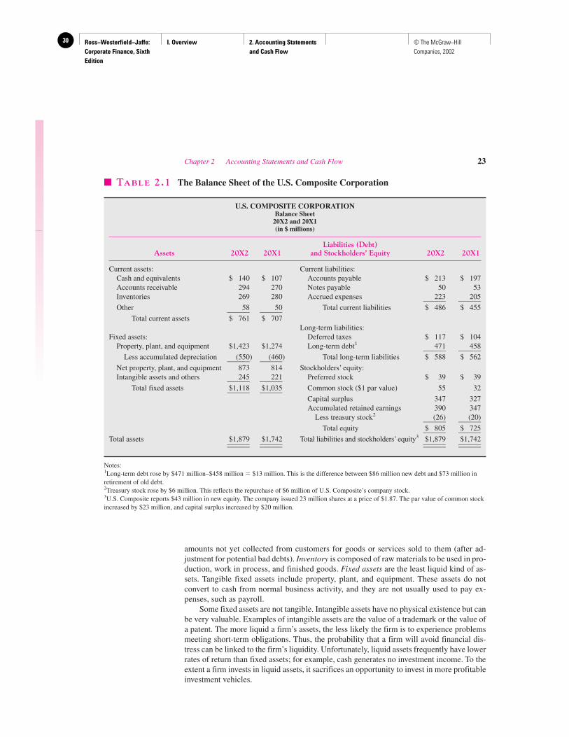
Ross−Westerfield−Jaffe: Corporate Finance, Sixth Edition
I. Overview 2. Accounting Statements and Cash Flow
30 © The McGraw−Hill Companies, 2002
Chapter 2 Accounting Statements and Cash Flow 23
amounts not yet collected from customers for goods or services sold to them (after ad-justment for potential bad debts). Inventory is composed of raw materials to be used in pro-duction, work in process, and finished goods. Fixed assets are the least liquid kind of as-sets. Tangible fixed assets include property, plant, and equipment. These assets do notconvert to cash from normal business activity, and they are not usually used to pay ex-penses, such as payroll.
Some fixed assets are not tangible. Intangible assets have no physical existence but canbe very valuable. Examples of intangible assets are the value of a trademark or the value ofa patent. The more liquid a firm’s assets, the less likely the firm is to experience problemsmeeting short-term obligations. Thus, the probability that a firm will avoid financial dis-tress can be linked to the firm’s liquidity. Unfortunately, liquid assets frequently have lowerrates of return than fixed assets; for example, cash generates no investment income. To theextent a firm invests in liquid assets, it sacrifices an opportunity to invest in more profitableinvestment vehicles.
� TABLE 2.1 The Balance Sheet of the U.S. Composite Corporation
U.S. COMPOSITE CORPORATIONBalance Sheet
20X2 and 20X1(in $ millions)
Liabilities (Debt)Assets 20X2 20X1 and Stockholders’ Equity 20X2 20X1
Current assets: Current liabilities:Cash and equivalents $ 140 $ 107 Accounts payable $ 213 $ 197Accounts receivable 294 270 Notes payable 50 53Inventories 269 280 Accrued expenses 223 205______ ______Other 58 50 Total current liabilities $ 486 $ 455______ ______
Total current assets $ 761 $ 707Long-term liabilities:
Fixed assets: Deferred taxes $ 117 $ 104Property, plant, and equipment $1,423 $1,274 Long-term debt1 471 458______ ______
Less accumulated depreciation (550) (460) Total long-term liabilities $ 588 $ 562______ ______Net property, plant, and equipment 873 814 Stockholders’ equity:Intangible assets and others 245 221 Preferred stock $ 39 $ 39______ ______
Total fixed assets $1,118 $1,035 Common stock ($1 par value) 55 32______ ______Capital surplus 347 327Accumulated retained earnings 390 347
Less treasury stock2 (26) (20)______ ______Total equity $ 805 $ 725______ ______
Total assets $1,879 $1,742 Total liabilities and stockholders’ equity3 $1,879 $1,742______ ______ ______ ____________ ______ ______ ______
Notes:1Long-term debt rose by $471 million–$458 million � $13 million. This is the difference between $86 million new debt and $73 million inretirement of old debt.2Treasury stock rose by $6 million. This reflects the repurchase of $6 million of U.S. Composite’s company stock.3U.S. Composite reports $43 million in new equity. The company issued 23 million shares at a price of $1.87. The par value of common stockincreased by $23 million, and capital surplus increased by $20 million.
Ross−Westerfield−Jaffe: Corporate Finance, Sixth Edition
I. Overview 2. Accounting Statements and Cash Flow
31© The McGraw−Hill Companies, 2002
Debt versus EquityLiabilities are obligations of the firm that require a payout of cash within a stipulated timeperiod. Many liabilities involve contractual obligations to repay a stated amount and inter-est over a period. Thus, liabilities are debts and are frequently associated with nominallyfixed cash burdens, called debt service, that put the firm in default of a contract if they arenot paid. Stockholders’ equity is a claim against the firm’s assets that is residual and notfixed. In general terms, when the firm borrows, it gives the bondholders first claim on thefirm’s cash flow.1 Bondholders can sue the firm if the firm defaults on its bond contracts.This may lead the firm to declare itself bankrupt. Stockholders’ equity is the residual dif-ference between assets and liabilities:
Assets � Liabilities � Stockholders’ equity
This is the stockholders’ share in the firm stated in accounting terms. The accounting valueof stockholders’ equity increases when retained earnings are added. This occurs when thefirm retains part of its earnings instead of paying them out as dividends.
Value versus CostThe accounting value of a firm’s assets is frequently referred to as the carrying value or thebook value of the assets.2 Under generally accepted accounting principles (GAAP), au-dited financial statements of firms in the United States carry the assets at cost.3 Thus theterms carrying value and book value are unfortunate. They specifically say “value,” whenin fact the accounting numbers are based on cost. This misleads many readers of financialstatements to think that the firm’s assets are recorded at true market values. Market value isthe price at which willing buyers and sellers trade the assets. It would be only a coincidenceif accounting value and market value were the same. In fact, management’s job is to createa value for the firm that is higher than its cost.
Many people use the balance sheet although the information each may wish to ex-tract is not the same. A banker may look at a balance sheet for evidence of accountingliquidity and working capital. A supplier may also note the size of accounts payable andtherefore the general promptness of payments. Many users of financial statements, in-cluding managers and investors, want to know the value of the firm, not its cost. This isnot found on the balance sheet. In fact, many of the true resources of the firm do not ap-pear on the balance sheet: good management, proprietary assets, favorable economic con-ditions, and so on.
• What is the balance-sheet equation?• What three things should be kept in mind when looking at a balance sheet?
24 Part I Overview
1Bondholders are investors in the firm’s debt. They are creditors of the firm. In this discussion, the termbondholder means the same thing as creditor.2Confusion often arises because many financial accounting terms have the same meaning. This presents aproblem with jargon for the reader of financial statements. For example, the following terms usually refer to thesame thing: assets minus liabilities, net worth, stockholders’ equity, owner’s equity, and equity capitalization.3Formally, GAAP requires assets to be carried at the lower of cost or market value. In most instances cost islower than market value.
QUESTIONS
CO
NC
EP
T
?
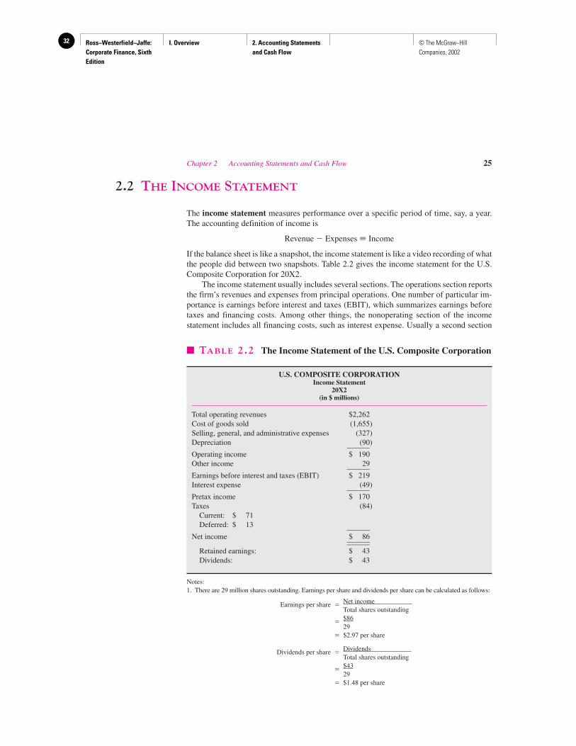
Ross−Westerfield−Jaffe: Corporate Finance, Sixth Edition
I. Overview 2. Accounting Statements and Cash Flow
32 © The McGraw−Hill Companies, 2002
2.2 THE INCOME STATEMENT
The income statement measures performance over a specific period of time, say, a year.The accounting definition of income is
Revenue � Expenses � Income
If the balance sheet is like a snapshot, the income statement is like a video recording of whatthe people did between two snapshots. Table 2.2 gives the income statement for the U.S.Composite Corporation for 20X2.
The income statement usually includes several sections. The operations section reportsthe firm’s revenues and expenses from principal operations. One number of particular im-portance is earnings before interest and taxes (EBIT), which summarizes earnings beforetaxes and financing costs. Among other things, the nonoperating section of the incomestatement includes all financing costs, such as interest expense. Usually a second section
Chapter 2 Accounting Statements and Cash Flow 25
� TABLE 2.2 The Income Statement of the U.S. Composite Corporation
U.S. COMPOSITE CORPORATIONIncome Statement
20X2(in $ millions)
Total operating revenues $2,262Cost of goods sold (1,655)Selling, general, and administrative expenses (327)Depreciation (90)______Operating income $ 190Other income 29______Earnings before interest and taxes (EBIT) $ 219Interest expense (49)______Pretax income $ 170Taxes (84)
Current: $ 71Deferred: $ 13 ______
Net income $ 86____________Retained earnings: $ 43Dividends: $ 43
Notes:1. There are 29 million shares outstanding. Earnings per share and dividends per share can be calculated as follows:
Earnings per share �Net incomeTotal shares outstanding
�$8629
� $2.97 per share
Dividends per share �DividendsTotal shares outstanding
�$4329
� $1.48 per share
Ross−Westerfield−Jaffe: Corporate Finance, Sixth Edition
I. Overview 2. Accounting Statements and Cash Flow
33© The McGraw−Hill Companies, 2002
reports as a separate item the amount of taxes levied on income. The last item on the in-come statement is the bottom line, or net income. Net income is frequently expressed pershare of common stock, that is, earnings per share.
When analyzing an income statement, the financial manager should keep in mindGAAP, noncash items, time, and costs.
Generally Accepted Accounting PrinciplesRevenue is recognized on an income statement when the earnings process is virtually com-pleted and an exchange of goods or services has occurred. Therefore, the unrealized appre-ciation in owning property will not be recognized as income. This provides a device forsmoothing income by selling appreciated property at convenient times. For example, if thefirm owns a tree farm that has doubled in value, then, in a year when its earnings from otherbusinesses are down, it can raise overall earnings by selling some trees. The matching prin-ciple of GAAP dictates that revenues be matched with expenses. Thus, income is reportedwhen it is earned, or accrued, even though no cash flow has necessarily occurred (for ex-ample, when goods are sold for credit, sales and profits are reported).
Noncash ItemsThe economic value of assets is intimately connected to their future incremental cash flows.However, cash flow does not appear on an income statement. There are several noncashitems that are expenses against revenues, but that do not affect cash flow. The most impor-tant of these is depreciation. Depreciation reflects the accountant’s estimate of the cost ofequipment used up in the production process. For example, suppose an asset with a five-year life and no resale value is purchased for $1,000. According to accountants, the $1,000cost must be expensed over the useful life of the asset. If straight-line depreciation is used,there will be five equal installments and $200 of depreciation expense will be incurred eachyear. From a finance perspective, the cost of the asset is the actual negative cash flow in-curred when the asset is acquired (that is, $1,000, not the accountant’s smoothed $200-per-year depreciation expense).
Another noncash expense is deferred taxes. Deferred taxes result from differences be-tween accounting income and true taxable income.4 Notice that the accounting tax shownon the income statement for the U.S. Composite Corporation is $84 million. It can be bro-ken down as current taxes and deferred taxes. The current tax portion is actually sent to thetax authorities (for example, the Internal Revenue Service). The deferred tax portion is not.However, the theory is that if taxable income is less than accounting income in the currentyear, it will be more than accounting income later on. Consequently, the taxes that are notpaid today will have to be paid in the future, and they represent a liability of the firm. Thisshows up on the balance sheet as deferred tax liability. From the cash flow perspective,though, deferred tax is not a cash outflow.
Time and CostsIt is often useful to think of all of future time as having two distinct parts, the short run andthe long run. The short run is that period of time in which certain equipment, resources, andcommitments of the firm are fixed; but the time is long enough for the firm to vary its out-put by using more labor and raw materials. The short run is not a precise period of time thatwill be the same for all industries. However, all firms making decisions in the short run have
26 Part I Overview
4One situation in which taxable income may be lower than accounting income is when the firm uses accelerateddepreciation expense procedures for the IRS but uses straight-line procedures allowed by GAAP for reportingpurposes.
Ross−Westerfield−Jaffe: Corporate Finance, Sixth Edition
I. Overview 2. Accounting Statements and Cash Flow
34 © The McGraw−Hill Companies, 2002
some fixed costs, that is, costs that will not change because of fixed commitments. In realbusiness activity, examples of fixed costs are bond interest, overhead, and property taxes.Costs that are not fixed are variable. Variable costs change as the output of the firm changes;some examples are raw materials and wages for laborers on the production line.
In the long run, all costs are variable.5 Financial accountants do not distinguish be-tween variable costs and fixed costs. Instead, accounting costs usually fit into a classifica-tion that distinguishes product costs from period costs. Product costs are the total produc-tion costs incurred during a period—raw materials, direct labor, and manufacturingoverhead—and are reported on the income statement as cost of goods sold. Both variableand fixed costs are included in product costs. Period costs are costs that are allocated to atime period; they are called selling, general, and administrative expenses. One period costwould be the company president’s salary.
• What is the income statement equation?• What are three things to keep in mind when looking at an income statement?• What are noncash expenses?
2.3 NET WORKING CAPITAL
Net working capital is current assets minus current liabilities. Net working capital is posi-tive when current assets are greater than current liabilities. This means the cash that will be-come available over the next 12 months will be greater than the cash that must be paid out.The net working capital of the U.S. Composite Corporation is $275 million in 20X2 and$252 million in 20X1:
Current assets Current liabilities Net working capital($ millions) � ($ millions) � ($ millions)
20X2 $761 � $486 � $27520X1 707 � 455 � 252
In addition to investing in fixed assets (i.e., capital spending), a firm can invest in net work-ing capital. This is called the change in net working capital. The change in net workingcapital in 20X2 is the difference between the net working capital in 20X2 and 20X1; thatis, $275 million � $252 million � $23 million. The change in net working capital is usu-ally positive in a growing firm.
• What is net working capital?• What is the change in net working capital?
2.4 FINANCIAL CASH FLOW
Perhaps the most important item that can be extracted from financial statements is the ac-tual cash flow of the firm. There is an official accounting statement called the statement ofcash flows. This statement helps to explain the change in accounting cash and equivalents,
Chapter 2 Accounting Statements and Cash Flow 27
5When one famous economist was asked about the difference between the long run and the short run, he said,“In the long run we are all dead.”
QUESTIONS
CO
NC
EP
T
?
QUESTIONS
CO
NC
EP
T
?
Ross−Westerfield−Jaffe: Corporate Finance, Sixth Edition
I. Overview 2. Accounting Statements and Cash Flow
35© The McGraw−Hill Companies, 2002
which for U.S. Composite is $33 million in 20X2. (See Appendix 2B.) Notice in Table 2.1that Cash and equivalents increases from $107 million in 20X1 to $140 million in 20X2.However, we will look at cash flow from a different perspective, the perspective of finance.In finance the value of the firm is its ability to generate financial cash flow. (We will talkmore about financial cash flow in Chapter 7.)
The first point we should mention is that cash flow is not the same as net working cap-ital. For example, increasing inventory requires using cash. Because both inventories andcash are current assets, this does not affect net working capital. In this case, an increase ina particular net working capital account, such as inventory, is associated with decreasingcash flow.
Just as we established that the value of a firm’s assets is always equal to the value ofthe liabilities and the value of the equity, the cash flows received from the firm’s assets (thatis, its operating activities), CF(A), must equal the cash flows to the firm’s creditors, CF(B),and equity investors, CF(S):
CF(A) � CF(B) � CF(S)
The first step in determining cash flows of the firm is to figure out the cash flow from op-erations. As can be seen in Table 2.3, operating cash flow is the cash flow generated by busi-ness activities, including sales of goods and services. Operating cash flow reflects tax pay-ments, but not financing, capital spending, or changes in net working capital.
Another important component of cash flow involves changes in fixed assets. For ex-ample, when U.S. Composite sold its power systems subsidiary in 20X2 it generated $25in cash flow. The net change in fixed assets equals sales of fixed assets minus the acquisi-tion of fixed assets. The result is the cash flow used for capital spending:
(� $149 � $24 � increasein property, plant, andequipment � increase inintangible assets)
Cash flows are also used for making investments in net working capital. In the U.S. Com-posite Corporation in 20X2, additions to net working capital are
Additions to net working capital $23
Total cash flows generated by the firm’s assets are the sum of
Operating cash flow $238Capital spending (173)Additions to net working capital (23)____
Total cash flow of the firm $42________
Acquisition of fixed assets $198Sales of fixed assets (25)____
Capital spending $173________
In $ Millions
Earnings before interest and taxes $219Depreciation 90____Current taxes (71)
Operating cash flow $238
28 Part I Overview
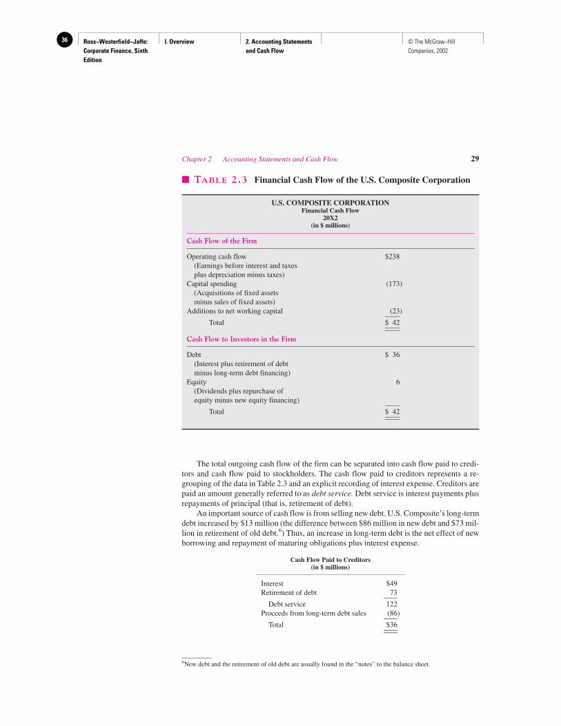
Ross−Westerfield−Jaffe: Corporate Finance, Sixth Edition
I. Overview 2. Accounting Statements and Cash Flow
36 © The McGraw−Hill Companies, 2002
The total outgoing cash flow of the firm can be separated into cash flow paid to credi-tors and cash flow paid to stockholders. The cash flow paid to creditors represents a re-grouping of the data in Table 2.3 and an explicit recording of interest expense. Creditors arepaid an amount generally referred to as debt service. Debt service is interest payments plusrepayments of principal (that is, retirement of debt).
An important source of cash flow is from selling new debt. U.S. Composite’s long-termdebt increased by $13 million (the difference between $86 million in new debt and $73 mil-lion in retirement of old debt.6) Thus, an increase in long-term debt is the net effect of newborrowing and repayment of maturing obligations plus interest expense.
Cash Flow Paid to Creditors(in $ millions)
Interest $49Retirement of debt 73____
Debt service 122Proceeds from long-term debt sales (86)____
Total $36________
Chapter 2 Accounting Statements and Cash Flow 29
� TABLE 2.3 Financial Cash Flow of the U.S. Composite Corporation
U.S. COMPOSITE CORPORATIONFinancial Cash Flow
20X2(in $ millions)
Cash Flow of the Firm
Operating cash flow $238(Earnings before interest and taxesplus depreciation minus taxes)
Capital spending (173)(Acquisitions of fixed assetsminus sales of fixed assets)
Additions to net working capital (23)____Total $ 42________
Cash Flow to Investors in the Firm
Debt $ 36(Interest plus retirement of debtminus long-term debt financing)
Equity 6(Dividends plus repurchase ofequity minus new equity financing) ____
Total $ 42________
6New debt and the retirement of old debt are usually found in the “notes” to the balance sheet.
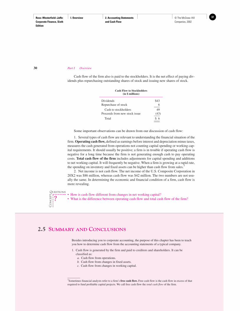
Ross−Westerfield−Jaffe: Corporate Finance, Sixth Edition
I. Overview 2. Accounting Statements and Cash Flow
37© The McGraw−Hill Companies, 2002
Cash flow of the firm also is paid to the stockholders. It is the net effect of paying div-idends plus repurchasing outstanding shares of stock and issuing new shares of stock.
Some important observations can be drawn from our discussion of cash flow:
1. Several types of cash flow are relevant to understanding the financial situation of thefirm. Operating cash flow, defined as earnings before interest and depreciation minus taxes,measures the cash generated from operations not counting capital spending or working cap-ital requirements. It should usually be positive; a firm is in trouble if operating cash flow isnegative for a long time because the firm is not generating enough cash to pay operatingcosts. Total cash flow of the firm includes adjustments for capital spending and additionsto net working capital. It will frequently be negative. When a firm is growing at a rapid rate,the spending on inventory and fixed assets can be higher than cash flow from sales.7
2. Net income is not cash flow. The net income of the U.S. Composite Corporation in20X2 was $86 million, whereas cash flow was $42 million. The two numbers are not usu-ally the same. In determining the economic and financial condition of a firm, cash flow ismore revealing.
• How is cash flow different from changes in net working capital?• What is the difference between operating cash flow and total cash flow of the firm?
2.5 SUMMARY AND CONCLUSIONS
Besides introducing you to corporate accounting, the purpose of this chapter has been to teachyou how to determine cash flow from the accounting statements of a typical company.
1. Cash flow is generated by the firm and paid to creditors and shareholders. It can beclassified as:a. Cash flow from operations.b. Cash flow from changes in fixed assets.c. Cash flow from changes in working capital.
Cash Flow to Stockholders(in $ millions)
Dividends $43Repurchase of stock 6____
Cash to stockholders 49Proceeds from new stock issue (43)____
Total $ 6________
30 Part I Overview
7Sometimes financial analysts refer to a firm’s free cash flow. Free cash flow is the cash flow in excess of thatrequired to fund profitable capital projects. We call free cash flow the total cash flow of the firm.
QUESTIONS
CO
NC
EP
T
?

Ross−Westerfield−Jaffe: Corporate Finance, Sixth Edition
I. Overview 2. Accounting Statements and Cash Flow
38 © The McGraw−Hill Companies, 2002
Chapter 2 Accounting Statements and Cash Flow 31
2. Calculations of cash flow are not difficult, but they require care and particular attention todetail in properly accounting for noncash expenses such as depreciation and deferred taxes. Itis especially important that you do not confuse cash flow with changes in net working capitaland net income.
KEY TERMS
Balance sheet 22 Income statement 25Cash flow 27 Noncash items 26Change in net working capital 27 Operating cash flow 30Free cash flow 30 Total cash flow of the firm 30Generally accepted accounting
principles (GAAP) 24
SUGGESTED READINGThere are many excellent textbooks on accounting. The one that we have found helpful is:Kieso, D. E., and J. J. Weygandt. Intermediate Accounting, 7th ed. New York: John Wiley. 1992.
QUESTIONS AND PROBLEMSThe Balance Sheet2.1 Prepare a December 31 balance sheet using the following data:
Cash $ 4,000Patents 82,000Accounts payable 6,000Accounts receivable 8,000Taxes payable 2,000Machinery 34,000Bonds payable 7,000Accumulated retained
earnings 6,000Capital surplus 19,000
The par value of the firm’s common stock is $100.
2.2 The following table presents the long-term liabilities and stockholders’ equity ofInformation Control Corp. of one year ago.
Long-term debt $50,000,000Preferred stock 30,000,000Common stock 100,000,000Retained earnings 20,000,000
During the past year, Information Control issued $10 million of new common stock. The firmgenerated $5 million of net income and paid $3 million of dividends. Construct today’s balancesheet reflecting the changes that occurred at Information Control Corp. during the year.
The Income Statement2.3 Prepare an income statement using the following data.
Sales $500,000Cost of goods sold 200,000Administrative
expenses 100,000Interest expense 50,000
The firm’s tax rate is 34 percent.
Chapter 2 Accounting Statements and Cash Flow 31
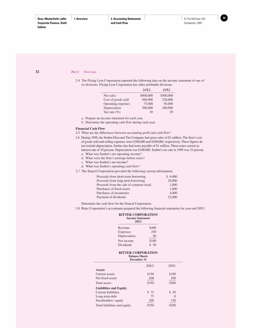
Ross−Westerfield−Jaffe: Corporate Finance, Sixth Edition
I. Overview 2. Accounting Statements and Cash Flow
39© The McGraw−Hill Companies, 2002
32 Part I Overview
2.4 The Flying Lion Corporation reported the following data on the income statement of one ofits divisions. Flying Lion Corporation has other profitable divisions.
a. Prepare an income statement for each year.b. Determine the operating cash flow during each year.
Financial Cash Flow2.5 What are the differences between accounting profit and cash flow?
2.6 During 1998, the Senbet Discount Tire Company had gross sales of $1 million. The firm’s costof goods sold and selling expenses were $300,000 and $200,000, respectively. These figures donot include depreciation. Senbet also had notes payable of $1 million. These notes carried aninterest rate of 10 percent. Depreciation was $100,000. Senbet’s tax rate in 1998 was 35 percent.a. What was Senbet’s net operating income?b. What were the firm’s earnings before taxes?c. What was Senbet’s net income?d. What was Senbet’s operating cash flow?
2.7 The Stancil Corporation provided the following current information.
Determine the cash flow for the Stancil Corporation.
2.8 Ritter Corporation’s accountants prepared the following financial statements for year-end 20X2.
RITTER CORPORATIONIncome Statement
20X2
Revenue $400Expenses 250Depreciation 50____Net income $100Dividends $ 50
RITTER CORPORATIONBalance SheetsDecember 31
20X2 20X1AssetsCurrent assets $150 $100Net fixed assets 200 100____ ____Total assets $350 $200
Liabilities and EquityCurrent liabilities $ 75 $ 50Long-term debt 75 0Stockholders’ equity 200 150____ ____Total liabilities and equity $350 $200
Proceeds from short-term borrowing $ 6,000Proceeds from long-term borrowing 20,000Proceeds from the sale of common stock 1,000Purchases of fixed assets 1,000Purchases of inventories 4,000Payment of dividends 22,000
20X2 20X1
Net sales $800,000 $500,000Cost of goods sold 560,000 320,000Operating expenses 75,000 56,000Depreciation 300,000 200,000Tax rate (%) 30 30
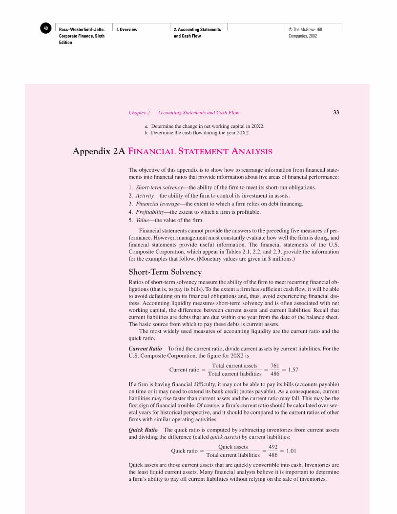
Ross−Westerfield−Jaffe: Corporate Finance, Sixth Edition
I. Overview 2. Accounting Statements and Cash Flow
40 © The McGraw−Hill Companies, 2002
a. Determine the change in net working capital in 20X2.b. Determine the cash flow during the year 20X2.
Appendix 2A FINANCIAL STATEMENT ANALYSIS
The objective of this appendix is to show how to rearrange information from financial state-ments into financial ratios that provide information about five areas of financial performance:
1. Short-term solvency—the ability of the firm to meet its short-run obligations.
2. Activity—the ability of the firm to control its investment in assets.
3. Financial leverage—the extent to which a firm relies on debt financing.
4. Profitability—the extent to which a firm is profitable.
5. Value—the value of the firm.
Financial statements cannot provide the answers to the preceding five measures of per-formance. However, management must constantly evaluate how well the firm is doing, andfinancial statements provide useful information. The financial statements of the U.S.Composite Corporation, which appear in Tables 2.1, 2.2, and 2.3, provide the informationfor the examples that follow. (Monetary values are given in $ millions.)
Short-Term SolvencyRatios of short-term solvency measure the ability of the firm to meet recurring financial ob-ligations (that is, to pay its bills). To the extent a firm has sufficient cash flow, it will be ableto avoid defaulting on its financial obligations and, thus, avoid experiencing financial dis-tress. Accounting liquidity measures short-term solvency and is often associated with networking capital, the difference between current assets and current liabilities. Recall thatcurrent liabilities are debts that are due within one year from the date of the balance sheet.The basic source from which to pay these debts is current assets.
The most widely used measures of accounting liquidity are the current ratio and thequick ratio.
Current Ratio To find the current ratio, divide current assets by current liabilities. For theU.S. Composite Corporation, the figure for 20X2 is
If a firm is having financial difficulty, it may not be able to pay its bills (accounts payable)on time or it may need to extend its bank credit (notes payable). As a consequence, currentliabilities may rise faster than current assets and the current ratio may fall. This may be thefirst sign of financial trouble. Of course, a firm’s current ratio should be calculated over sev-eral years for historical perspective, and it should be compared to the current ratios of otherfirms with similar operating activities.
Quick Ratio The quick ratio is computed by subtracting inventories from current assetsand dividing the difference (called quick assets) by current liabilities:
Quick assets are those current assets that are quickly convertible into cash. Inventories arethe least liquid current assets. Many financial analysts believe it is important to determinea firm’s ability to pay off current liabilities without relying on the sale of inventories.
Quick ratio �Quick assets
Total current liabilities�
492
486� 1.01
Current ratio �Total current assets
Total current liabilities�
761
486� 1.57
Chapter 2 Accounting Statements and Cash Flow 33
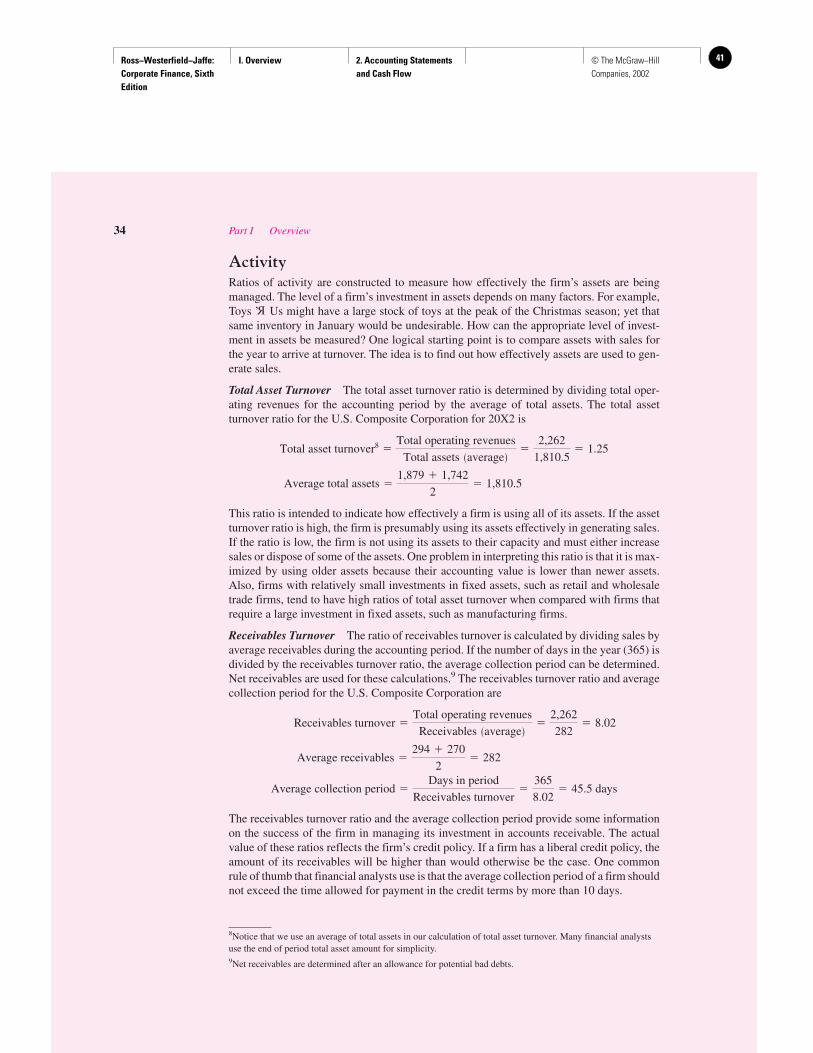
Ross−Westerfield−Jaffe: Corporate Finance, Sixth Edition
I. Overview 2. Accounting Statements and Cash Flow
41© The McGraw−Hill Companies, 2002
ActivityRatios of activity are constructed to measure how effectively the firm’s assets are beingmanaged. The level of a firm’s investment in assets depends on many factors. For example,Toys ’ Us might have a large stock of toys at the peak of the Christmas season; yet thatsame inventory in January would be undesirable. How can the appropriate level of invest-ment in assets be measured? One logical starting point is to compare assets with sales forthe year to arrive at turnover. The idea is to find out how effectively assets are used to gen-erate sales.
Total Asset Turnover The total asset turnover ratio is determined by dividing total oper-ating revenues for the accounting period by the average of total assets. The total assetturnover ratio for the U.S. Composite Corporation for 20X2 is
This ratio is intended to indicate how effectively a firm is using all of its assets. If the assetturnover ratio is high, the firm is presumably using its assets effectively in generating sales.If the ratio is low, the firm is not using its assets to their capacity and must either increasesales or dispose of some of the assets. One problem in interpreting this ratio is that it is max-imized by using older assets because their accounting value is lower than newer assets.Also, firms with relatively small investments in fixed assets, such as retail and wholesaletrade firms, tend to have high ratios of total asset turnover when compared with firms thatrequire a large investment in fixed assets, such as manufacturing firms.
Receivables Turnover The ratio of receivables turnover is calculated by dividing sales byaverage receivables during the accounting period. If the number of days in the year (365) isdivided by the receivables turnover ratio, the average collection period can be determined.Net receivables are used for these calculations.9 The receivables turnover ratio and averagecollection period for the U.S. Composite Corporation are
The receivables turnover ratio and the average collection period provide some informationon the success of the firm in managing its investment in accounts receivable. The actualvalue of these ratios reflects the firm’s credit policy. If a firm has a liberal credit policy, theamount of its receivables will be higher than would otherwise be the case. One commonrule of thumb that financial analysts use is that the average collection period of a firm shouldnot exceed the time allowed for payment in the credit terms by more than 10 days.
Average collection period �Days in period
Receivables turnover�
365
8.02� 45.5 days
Average receivables �294 � 270
2� 282
Receivables turnover �Total operating revenues
Receivables �average��
2,262
282� 8.02
Average total assets �1,879 � 1,742
2� 1,810.5
Total asset turnover8 �Total operating revenues
Total assets �average��
2,262
1,810.5� 1.25
R
34 Part I Overview
8Notice that we use an average of total assets in our calculation of total asset turnover. Many financial analystsuse the end of period total asset amount for simplicity.9Net receivables are determined after an allowance for potential bad debts.
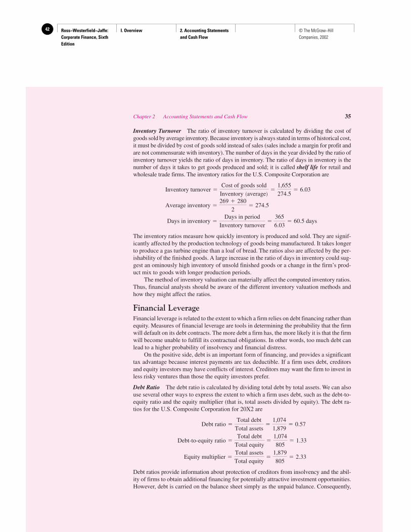
Ross−Westerfield−Jaffe: Corporate Finance, Sixth Edition
I. Overview 2. Accounting Statements and Cash Flow
42 © The McGraw−Hill Companies, 2002
Inventory Turnover The ratio of inventory turnover is calculated by dividing the cost ofgoods sold by average inventory. Because inventory is always stated in terms of historical cost,it must be divided by cost of goods sold instead of sales (sales include a margin for profit andare not commensurate with inventory). The number of days in the year divided by the ratio ofinventory turnover yields the ratio of days in inventory. The ratio of days in inventory is thenumber of days it takes to get goods produced and sold; it is called shelf life for retail andwholesale trade firms. The inventory ratios for the U.S. Composite Corporation are
The inventory ratios measure how quickly inventory is produced and sold. They are signif-icantly affected by the production technology of goods being manufactured. It takes longerto produce a gas turbine engine than a loaf of bread. The ratios also are affected by the per-ishability of the finished goods. A large increase in the ratio of days in inventory could sug-gest an ominously high inventory of unsold finished goods or a change in the firm’s prod-uct mix to goods with longer production periods.
The method of inventory valuation can materially affect the computed inventory ratios.Thus, financial analysts should be aware of the different inventory valuation methods andhow they might affect the ratios.
Financial LeverageFinancial leverage is related to the extent to which a firm relies on debt financing rather thanequity. Measures of financial leverage are tools in determining the probability that the firmwill default on its debt contracts. The more debt a firm has, the more likely it is that the firmwill become unable to fulfill its contractual obligations. In other words, too much debt canlead to a higher probability of insolvency and financial distress.
On the positive side, debt is an important form of financing, and provides a significanttax advantage because interest payments are tax deductible. If a firm uses debt, creditorsand equity investors may have conflicts of interest. Creditors may want the firm to invest inless risky ventures than those the equity investors prefer.
Debt Ratio The debt ratio is calculated by dividing total debt by total assets. We can alsouse several other ways to express the extent to which a firm uses debt, such as the debt-to-equity ratio and the equity multiplier (that is, total assets divided by equity). The debt ra-tios for the U.S. Composite Corporation for 20X2 are
Debt ratios provide information about protection of creditors from insolvency and the abil-ity of firms to obtain additional financing for potentially attractive investment opportunities.However, debt is carried on the balance sheet simply as the unpaid balance. Consequently,
Equity multiplier �Total assets
Total equity�
1,879
805� 2.33
Debt-to-equity ratio �Total debt
Total equity�
1,074
805� 1.33
Debt ratio �Total debt
Total assets�
1,074
1,879� 0.57
Days in inventory �Days in period
Inventory turnover�
365
6.03� 60.5 days
Average inventory �269 � 280
2� 274.5
Inventory turnover �Cost of goods sold
Inventory �average��
1,655
274.5� 6.03
Chapter 2 Accounting Statements and Cash Flow 35
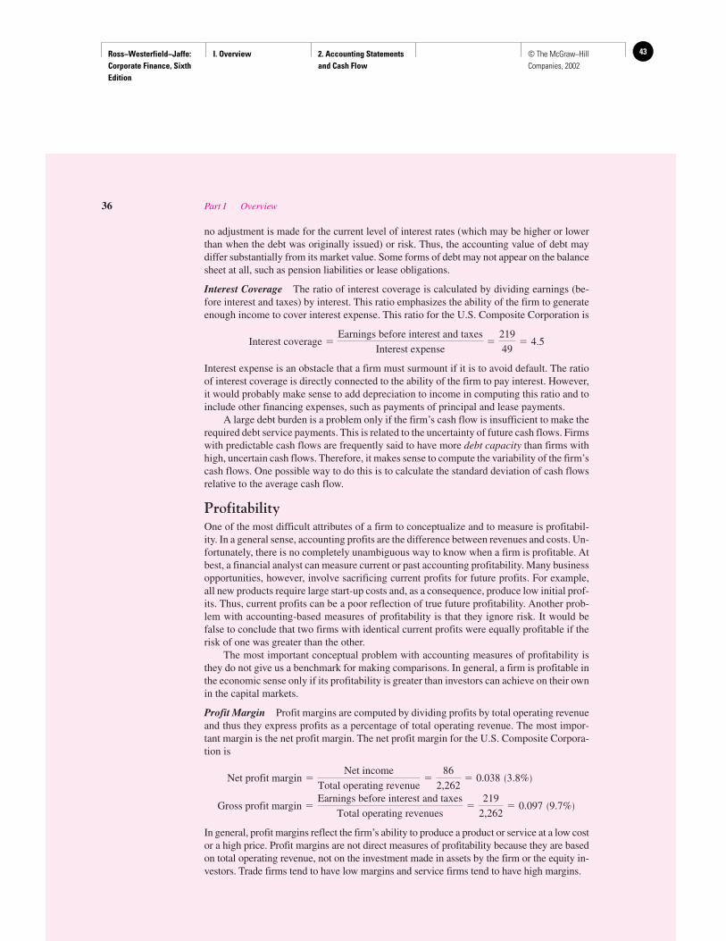
Ross−Westerfield−Jaffe: Corporate Finance, Sixth Edition
I. Overview 2. Accounting Statements and Cash Flow
43© The McGraw−Hill Companies, 2002
no adjustment is made for the current level of interest rates (which may be higher or lowerthan when the debt was originally issued) or risk. Thus, the accounting value of debt maydiffer substantially from its market value. Some forms of debt may not appear on the balancesheet at all, such as pension liabilities or lease obligations.
Interest Coverage The ratio of interest coverage is calculated by dividing earnings (be-fore interest and taxes) by interest. This ratio emphasizes the ability of the firm to generateenough income to cover interest expense. This ratio for the U.S. Composite Corporation is
Interest expense is an obstacle that a firm must surmount if it is to avoid default. The ratioof interest coverage is directly connected to the ability of the firm to pay interest. However,it would probably make sense to add depreciation to income in computing this ratio and toinclude other financing expenses, such as payments of principal and lease payments.
A large debt burden is a problem only if the firm’s cash flow is insufficient to make therequired debt service payments. This is related to the uncertainty of future cash flows. Firmswith predictable cash flows are frequently said to have more debt capacity than firms withhigh, uncertain cash flows. Therefore, it makes sense to compute the variability of the firm’scash flows. One possible way to do this is to calculate the standard deviation of cash flowsrelative to the average cash flow.
ProfitabilityOne of the most difficult attributes of a firm to conceptualize and to measure is profitabil-ity. In a general sense, accounting profits are the difference between revenues and costs. Un-fortunately, there is no completely unambiguous way to know when a firm is profitable. Atbest, a financial analyst can measure current or past accounting profitability. Many businessopportunities, however, involve sacrificing current profits for future profits. For example,all new products require large start-up costs and, as a consequence, produce low initial prof-its. Thus, current profits can be a poor reflection of true future profitability. Another prob-lem with accounting-based measures of profitability is that they ignore risk. It would befalse to conclude that two firms with identical current profits were equally profitable if therisk of one was greater than the other.
The most important conceptual problem with accounting measures of profitability isthey do not give us a benchmark for making comparisons. In general, a firm is profitable inthe economic sense only if its profitability is greater than investors can achieve on their ownin the capital markets.
Profit Margin Profit margins are computed by dividing profits by total operating revenueand thus they express profits as a percentage of total operating revenue. The most impor-tant margin is the net profit margin. The net profit margin for the U.S. Composite Corpora-tion is
In general, profit margins reflect the firm’s ability to produce a product or service at a low costor a high price. Profit margins are not direct measures of profitability because they are basedon total operating revenue, not on the investment made in assets by the firm or the equity in-vestors. Trade firms tend to have low margins and service firms tend to have high margins.
Gross profit margin �Earnings before interest and taxes
Total operating revenues�
219
2,262� 0.097 �9.7%�
Net profit margin �Net income
Total operating revenue�
86
2,262� 0.038 �3.8%�
Interest coverage �Earnings before interest and taxes
Interest expense�
219
49� 4.5
36 Part I Overview
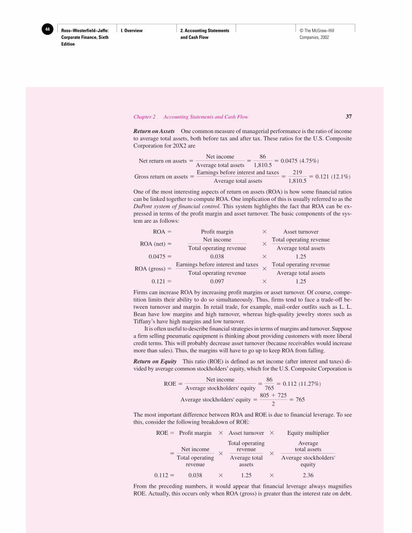
Ross−Westerfield−Jaffe: Corporate Finance, Sixth Edition
I. Overview 2. Accounting Statements and Cash Flow
44 © The McGraw−Hill Companies, 2002
Return on Assets One common measure of managerial performance is the ratio of incometo average total assets, both before tax and after tax. These ratios for the U.S. CompositeCorporation for 20X2 are
One of the most interesting aspects of return on assets (ROA) is how some financial ratioscan be linked together to compute ROA. One implication of this is usually referred to as theDuPont system of financial control. This system highlights the fact that ROA can be ex-pressed in terms of the profit margin and asset turnover. The basic components of the sys-tem are as follows:
ROA � Profit margin � Asset turnover
ROA (net) � �
0.0475 � 0.038 � 1.25
ROA (gross) � �
0.121 � 0.097 � 1.25
Firms can increase ROA by increasing profit margins or asset turnover. Of course, compe-tition limits their ability to do so simultaneously. Thus, firms tend to face a trade-off be-tween turnover and margin. In retail trade, for example, mail-order outfits such as L. L.Bean have low margins and high turnover, whereas high-quality jewelry stores such asTiffany’s have high margins and low turnover.
It is often useful to describe financial strategies in terms of margins and turnover. Supposea firm selling pneumatic equipment is thinking about providing customers with more liberalcredit terms. This will probably decrease asset turnover (because receivables would increasemore than sales). Thus, the margins will have to go up to keep ROA from falling.
Return on Equity This ratio (ROE) is defined as net income (after interest and taxes) di-vided by average common stockholders’ equity, which for the U.S. Composite Corporation is
The most important difference between ROA and ROE is due to financial leverage. To seethis, consider the following breakdown of ROE:
ROE � Profit margin � Asset turnover � Equity multiplier
Total operating Average
� � �
revenue assets equity
0.112 � 0.038 � 1.25 � 2.36
From the preceding numbers, it would appear that financial leverage always magnifiesROE. Actually, this occurs only when ROA (gross) is greater than the interest rate on debt.
total assets
Average stockholders'
revenue
Average total
Net income
Total operating
Average stockholders' equity �805 � 725
2� 765
ROE �Net income
Average stockholders' equity�
86
765� 0.112 �11.27%�
Total operating revenue
Average total assets
Earnings before interest and taxes
Total operating revenue
Total operating revenue
Average total assets
Net income
Total operating revenue
Gross return on assets �Earnings before interest and taxes
Average total assets�
219
1,810.5� 0.121 �12.1%�
Net return on assets �Net income
Average total assets�
86
1,810.5� 0.0475 �4.75%�
Chapter 2 Accounting Statements and Cash Flow 37
Ross−Westerfield−Jaffe: Corporate Finance, Sixth Edition
I. Overview 2. Accounting Statements and Cash Flow
45© The McGraw−Hill Companies, 2002
Payout Ratio The payout ratio is the proportion of net income paid out in cash dividends.For the U.S. Composite Corporation
The retention ratio for the U.S. Composite Corporation is
Retained earnings � Net income � Dividends
The Sustainable Growth RateOne ratio that is very helpful in financial analysis is called the sustainable growth rate.It is the maximum rate of growth a firm can maintain without increasing its financialleverage and using internal equity only. The precise value of sustainable growth can becalculated as
Sustainable growth rate � ROE � Retention ratio
For the U.S. Composite Company, ROE is 11.2 percent. The retention ratio is 1/2, so wecan calculate the sustainable growth rate as
Sustainable growth rate � 11.2 � (1/2) � 5.6%
The U.S. Composite Corporation can expand at a maximum rate of 5.6 percent per yearwith no external equity financing or without increasing financial leverage. (We discuss sus-tainable growth in Chapters 5 and 26.)
Market Value RatiosWe can learn many things from a close examination of balance sheets and income state-ments. However, one very important characteristic of a firm that cannot be found on an ac-counting statement is its market value.
Market Price The market price of a share of common stock is the price that buyers andsellers establish when they trade the stock. The market value of the common equity of afirm is the market price of a share of common stock multiplied by the number of sharesoutstanding.
Sometimes the words “fair market value” are used to describe market prices. Fair mar-ket value is the amount at which common stock would change hands between a willingbuyer and a willing seller, both having knowledge of the relevant facts. Thus, market pricesgive guesses about the true worth of the assets of a firm. In an efficient stock market, mar-ket prices reflect all relevant facts about firms, and thus market prices reveal the true valueof the firm’s underlying assets.
The market value of IBM is many times greater than that of Apple Computer. This maysuggest nothing more than the fact that IBM is a bigger firm than Apple (hardly a surpris-ing revelation). Financial analysts construct ratios to extract information that is independ-ent of a firm’s size.
Price-to-Earnings (P/E) Ratio One way to calculate the P/E ratio is to divide the currentmarket price by the earnings per share of common stock for the latest year. The P/E ratiosof some of the largest firms in the United States and Japan are as follows:
Retention ratio �Retained earnings
Net income�
43
86� 0.5
Payout ratio �Cash dividends
Net income�
43
86� 0.5
38 Part I Overview
Ross−Westerfield−Jaffe: Corporate Finance, Sixth Edition
I. Overview 2. Accounting Statements and Cash Flow
46 © The McGraw−Hill Companies, 2002
As can be seen, some firms have high P/E ratios (Sony, for example) and some firms havelow ones (General Motors).
Dividend Yield The dividend yield is calculated by annualizing the last observed dividendpayment of a firm and dividing by the current market price:
The dividend yields for several large firms in the United States and Japan are:
Dividend yields are related to the market’s perception of future growth prospects for firms.Firms with high growth prospects will generally have lower dividend yields.
Market-to-Book (M/B) Value and the Q ratio The market-to-book value ratio is calcu-lated by dividing the market price per share by the book value per share.
The market-to-book ratios of several of the largest firms in the United States andJapan are:
There is another ratio, called Tobin’s Q, that is very much like the M/B ratio.10 Tobin’s Qratio divides the market value of all of the firm’s debt plus equity by the replacement valueof the firm’s assets. The Q ratios for several firms are:
Q Ratio11
High Qs Coca-Cola 4.2IBM 4.2
Low Qs National Steel 0.53U.S. Steel 0.61
Market-to-Book Ratios2000
United States Japan
AT&T 1 Nippon Telegraph & Telephone 3.4General Motors 2.4 Toyota Motor 2.8Hewlett Packard 8 Sony 3.5
Dividend Yield (%)2000
United States Japan
AT&T 0.9 Nippon Telegraph & Telephone 0.4General Motors 2.0 Toyota Motor 0.5Hewlett Packard 0.6 Sony 0.3
Dividend yield �Dividend per share
Market price per share
P/E Ratios2000
United States Japan
AT&T 24 Nippon Telegraph & Telephone 53General Motors 8 Toyota Motor 44Hewlett Packard 43 Sony 72
Chapter 2 Accounting Statements and Cash Flow 39
10Kee H. Chung and Stephen W. Pruitt, “A Simple Approximation of Tobin’s Q,” Financial ManagementVol 23, No. 3 (Autumn 1994).11E. B. Lindberg and S. Ross, “Tobin’s Q and Industrial Organization,” Journal of Business 54 (January 1981).
Ross−Westerfield−Jaffe: Corporate Finance, Sixth Edition
I. Overview 2. Accounting Statements and Cash Flow
47© The McGraw−Hill Companies, 2002
The Q ratio differs from the M/B ratio in that the Q ratio uses market value of the debtplus equity. It also uses the replacement value of all assets and not the historical costvalue.
It should be obvious that if a firm has a Q ratio above 1 it has an incentive to in-vest that is probably greater than a firm with a Q ratio below 1. Firms with high Q ra-tios tend to be those firms with attractive investment opportunities or a significant com-petitive advantage.
SUMMARY AND CONCLUSIONS
Much research indicates that accounting statements provide important information aboutthe value of the firm. Financial analysts and managers learn how to rearrange financialstatements to squeeze out the maximum amount of information. In particular, analysts andmanagers use financial ratios to summarize the firm’s liquidity, activity, financial leverage,and profitability. When possible, they also use market values. This appendix describes themost popular financial ratios. You should keep in mind the following points when trying tointerpret financial statements:
1. Measures of profitability such as return on equity suffer from several potential deficien-cies as indicators of performance. They do not take into account the risk or timing ofcash flows.
2. Financial ratios are linked to one another. For example, return on equity is determinedfrom the profit margins, the asset turnover ratio, and the financial leverage.
Appendix 2B STATEMENT OF CASH FLOWS
There is an official accounting statement called the statement of cash flows. This statementhelps explain the change in accounting cash, which for U.S. Composite is $33 million in20X2. It is very useful in understanding financial cash flow. Notice in Table 2.1 that cashincreases from $107 million in 20X1 to $140 million in 20X2.
The first step in determining the change in cash is to figure out cash flow from operat-ing activities. This is the cash flow that results from the firm’s normal activities producingand selling goods and services. The second step is to make an adjustment for cash flow frominvesting activities. The final step is to make an adjustment for cash flow from financing ac-tivities. Financing activities are the net payments to creditors and owners (excluding inter-est expense) made during the year.
The three components of the statement of cash flows are determined below.
Cash Flow from Operating ActivitiesTo calculate cash flow from operating activities we start with net income. Net income canbe found on the income statement and is equal to 86. We now need to add back noncash ex-penses and adjust for changes in current assets and liabilities (other than cash). The resultis cash flow from operating activities.
40 Part I Overview
Ross−Westerfield−Jaffe: Corporate Finance, Sixth Edition
I. Overview 2. Accounting Statements and Cash Flow
48 © The McGraw−Hill Companies, 2002
Cash Flow from Investing ActivitiesCash flow from investing activities involves changes in capital assets: acquisition of fixedassets and sales of fixed assets (i.e., net capital expenditures). The result for U.S. Compos-ite is below.
Cash Flow from Financing ActivitiesCash flows to and from creditors and owners include changes in equity and debt.
The statement of cash flows is the addition of cash flows from operations, cash flowsfrom investing activities, and cash flows from financing activities, and is produced in Table2.4. There is a close relationship between the official accounting statement called the state-ment of cash flows and the total cash flow of the firm used in finance. The difference be-tween cash flow from financing activities and total cash flow of the firm (see Table 2.3) isinterest expense.
U.S. COMPOSITE CORPORATIONCash Flow from Financing Activities
20X2(in $ millions)
Retirement of debt (includes notes) $(73)Proceeds from long-term debt sales 86Dividends (43)Repurchase of stock (6)Proceeds from new stock issue 43____
Cash flow from financing activities $ 7________
U.S. COMPOSITE CORPORATIONCash Flow from Investing Activities
20X2(in $ millions)
Acquisition of fixed assets (198)Sales of fixed assets 25____
Cash flow from investing activities (173)________
U.S. COMPOSITE CORPORATIONCash Flow from Operating Activities
20X2(in $ millions)
Net income 86Depreciation 90Deferred taxes 13Change in assets and liabilities
Accounts receivable (24)Inventories 11Accounts payable 16Accrued expense 18Notes payable (3)Other (8)___
Cash flow from operating activities 199______
Chapter 2 Accounting Statements and Cash Flow 41
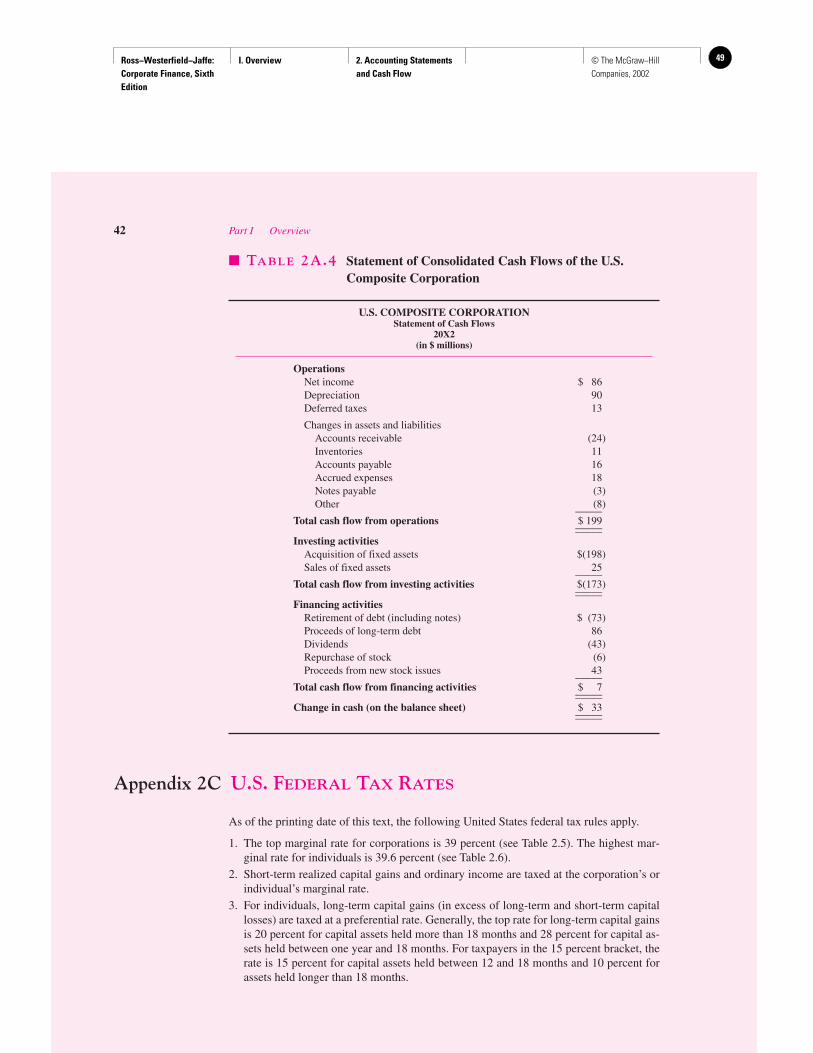
Ross−Westerfield−Jaffe: Corporate Finance, Sixth Edition
I. Overview 2. Accounting Statements and Cash Flow
49© The McGraw−Hill Companies, 2002
Appendix 2C U.S. FEDERAL TAX RATES
As of the printing date of this text, the following United States federal tax rules apply.
1. The top marginal rate for corporations is 39 percent (see Table 2.5). The highest mar-ginal rate for individuals is 39.6 percent (see Table 2.6).
2. Short-term realized capital gains and ordinary income are taxed at the corporation’s orindividual’s marginal rate.
3. For individuals, long-term capital gains (in excess of long-term and short-term capitallosses) are taxed at a preferential rate. Generally, the top rate for long-term capital gainsis 20 percent for capital assets held more than 18 months and 28 percent for capital as-sets held between one year and 18 months. For taxpayers in the 15 percent bracket, therate is 15 percent for capital assets held between 12 and 18 months and 10 percent forassets held longer than 18 months.
42 Part I Overview
� TABLE 2A.4 Statement of Consolidated Cash Flows of the U.S.Composite Corporation
U.S. COMPOSITE CORPORATIONStatement of Cash Flows
20X2(in $ millions)
OperationsNet income $ 86Depreciation 90Deferred taxes 13
Changes in assets and liabilitiesAccounts receivable (24)Inventories 11Accounts payable 16Accrued expenses 18Notes payable (3)Other (8)_____
Total cash flow from operations $ 199__________Investing activities
Acquisition of fixed assets $(198)Sales of fixed assets 25_____
Total cash flow from investing activities $(173)__________Financing activities
Retirement of debt (including notes) $ (73)Proceeds of long-term debt 86Dividends (43)Repurchase of stock (6)Proceeds from new stock issues 43_____
Total cash flow from financing activities $ 7__________Change in cash (on the balance sheet) $ 33__________
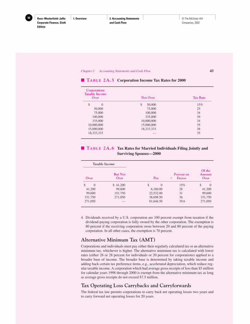
Ross−Westerfield−Jaffe: Corporate Finance, Sixth Edition
I. Overview 2. Accounting Statements and Cash Flow
50 © The McGraw−Hill Companies, 2002
4. Dividends received by a U.S. corporation are 100 percent exempt from taxation if thedividend-paying corporation is fully owned by the other corporation. The exemption is80 percent if the receiving corporation owns between 20 and 80 percent of the payingcorporation. In all other cases, the exemption is 70 percent.
Alternative Minimum Tax (AMT)Corporations and individuals must pay either their regularly calculated tax or an alternativeminimum tax, whichever is higher. The alternative minimum tax is calculated with lowerrates (either 26 or 28 percent for individuals or 20 percent for corporations) applied to abroader base of income. The broader base is determined by taking taxable income andadding back certain tax preference items, e.g., accelerated depreciation, which reduce reg-ular taxable income. A corporation which had average gross receipts of less than $5 millionfor calendar years 1998 through 2000 is exempt from the alternative minimum tax as longas average gross receipts do not exceed $7.5 million.
Tax Operating Loss Carrybacks and CarryforwardsThe federal tax law permits corporations to carry back net operating losses two years andto carry forward net operating losses for 20 years.
Chapter 2 Accounting Statements and Cash Flow 43
� TABLE 2A.5 Corporation Income Tax Rates for 2000
CorporationsTaxable Income
Over Not Over Tax Rate
$ 0 $ 50,000 15%50,000 75,000 2575,000 100,000 34
100,000 335,000 39335,000 10,000,000 34
10,000,000 15,000,000 3515,000,000 18,333,333 3818,333,333 — 35
� TABLE 2A.6 Tax Rates for Married Individuals Filing Jointly andSurviving Spouses—2000
Taxable Income
Of theBut Not Percent on Amount
Over Over Pay � Excess Over
$ 0 $ 41,200 $ 0 15% $ 041,200 99,600 6,180.00 28 41,20099,600 151,750 22,532.00 31 99,600
151,750 271,050 38,698.50 36 151,750271,050 — 81,646.50 39.6 271,050
Ross−Westerfield−Jaffe: Corporate Finance, Sixth Edition
II. Value and Capital Budgeting
Introduction 51© The McGraw−Hill Companies, 2002
Value and Capital Budgeting
PA
RT
II
3 Financial Markets and Net Present Value: First Principles of Finance (Advanced) 464 Net Present Value 665 How to Value Bonds and Stocks 1026 Some Alternative Investment Rules 1407 Net Present Value and Capital Budgeting 1698 Strategy and Analysis in Using Net Present Value 200
FIRMS and individuals invest in a large variety of assets. Some are real assets such asmachinery and land, and some are financial assets such as stocks and bonds. The ob-
ject of an investment is to maximize the value of the investment. In the simplest terms,this means to find assets that have more value to the firm than they cost. To do this weneed a theory of value. We develop a theory of value in Part II.
Finance is the study of markets and instruments that deal with cash flows over time.In Chapter 3 we describe how financial markets allow us to determine the value of fi-nancial instruments. We study some stylized examples of money over time and showwhy financial markets and financial instruments are created. We introduce the basic prin-ciples of rational decision making. We apply these principles to a two-period investment.Here we introduce one of the most important ideas in finance: net present value (NPV).We show why net present value is useful and the conditions that make it applicable.
In Chapter 4 we extend the concept of net present value to more than one time period.The mathematics of compounding and discounting are presented. In Chapter 5 we applynet present value to bonds and stocks. This is a very important chapter because net presentvalue can be used to determine the value of a wide variety of financial instruments.
Although we have made a strong case for using the NPV rule in Chapters 3 and 4,Chapter 6 presents four other rules: the payback rule, the accounting-rate-of-return rule,the internal rate of return (IRR), and the profitability index. Each of these alternativeshas some redeeming features, but these qualities aren’t sufficient to let any of the alter-natives replace the NPV rule.
In Chapter 7 we analyze how to estimate the cash flows required for capital budg-eting. We start the chapter with a discussion of the concept of incremental cash flows—the difference between the cash flows for the firm with and without the project. Chapter8 focuses on assessing the reliability and reasonableness of estimates of NPV. The chap-ter introduces techniques for dealing with uncertain incremental cash flows in capitalbudgeting, including break-even analysis, decision trees, and sensitivity analysis.
Ross−Westerfield−Jaffe: Corporate Finance, Sixth Edition
II. Value and Capital Budgeting
3. Financial Markets and Net Present Value: First Principles of Finance (Adv.)
52 © The McGraw−Hill Companies, 2002
Financial Markets andNet Present Value: FirstPrinciples of Finance(Advanced)
CH
AP
TE
R3
EXECUTIVE SUMMARY
Finance refers to the process by which special markets deal with cash flows over time.These markets are called financial markets. Making investment and financing deci-sions requires an understanding of the basic economic principles of financial markets.
This introductory chapter describes a financial market as one that makes it possible for indi-viduals and corporations to borrow and lend. As a consequence, financial markets can beused by individuals to adjust their patterns of consumption over time and by corporations toadjust their patterns of investment spending over time. The main point of this chapter is thatindividuals and corporations can use the financial markets to help them make investment de-cisions. We introduce one of the most important ideas in finance: net present value.
3.1 THE FINANCIAL MARKET ECONOMY
Financial markets develop to facilitate borrowing and lending between individuals. Here wetalk about how this happens. Suppose we describe the economic circumstances of two peo-ple, Tom and Leslie. Both Tom and Leslie have current income of $100,000. Tom is a verypatient person, and some people call him a miser. He wants to consume only $50,000 ofcurrent income and save the rest. Leslie is a very impatient person, and some people callher extravagant. She wants to consume $150,000 this year. Tom and Leslie have differentintertemporal consumption preferences.
Such preferences are personal matters and have more to do with psychology than withfinance. However, it seems that Tom and Leslie could strike a deal: Tom could give up someof his income this year in exchange for future income that Leslie can promise to give him.Tom can lend $50,000 to Leslie, and Leslie can borrow $50,000 from Tom.
Suppose that they do strike this deal, with Tom giving up $50,000 this year in exchangefor $55,000 next year. This is illustrated in Figure 3.1 with the basic cash flow time chart,a representation of the timing and amount of the cash flows. The cash flows that are receivedare represented by an arrow pointing up from the point on the time line at which the cashflow occurs. The cash flows paid out are represented by an arrow pointing down. In otherwords, for each dollar Tom trades away or lends, he gets a commitment to get it back aswell as to receive 10 percent more.
In the language of finance, 10 percent is the annual rate of interest on the loan. Whena dollar is lent out, the repayment of $1.10 can be thought of as being made up of two parts.First, the lender gets the dollar back; that is the principal repayment. Second, the lender re-ceives an interest payment, which is $0.10 in this example.
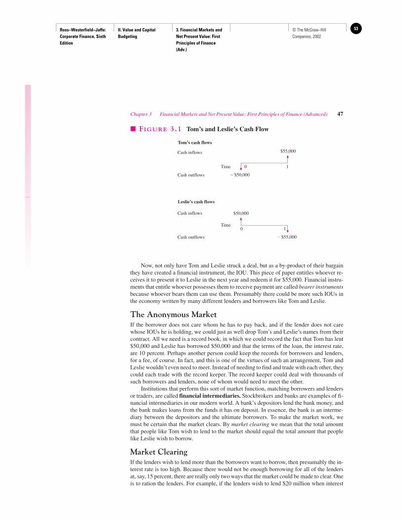
Ross−Westerfield−Jaffe: Corporate Finance, Sixth Edition
II. Value and Capital Budgeting
3. Financial Markets and Net Present Value: First Principles of Finance (Adv.)
53© The McGraw−Hill Companies, 2002
Chapter 3 Financial Markets and Net Present Value: First Principles of Finance (Advanced) 47
Now, not only have Tom and Leslie struck a deal, but as a by-product of their bargainthey have created a financial instrument, the IOU. This piece of paper entitles whoever re-ceives it to present it to Leslie in the next year and redeem it for $55,000. Financial instru-ments that entitle whoever possesses them to receive payment are called bearer instrumentsbecause whoever bears them can use them. Presumably there could be more such IOUs inthe economy written by many different lenders and borrowers like Tom and Leslie.
The Anonymous MarketIf the borrower does not care whom he has to pay back, and if the lender does not carewhose IOUs he is holding, we could just as well drop Tom’s and Leslie’s names from theircontract. All we need is a record book, in which we could record the fact that Tom has lent$50,000 and Leslie has borrowed $50,000 and that the terms of the loan, the interest rate,are 10 percent. Perhaps another person could keep the records for borrowers and lenders,for a fee, of course. In fact, and this is one of the virtues of such an arrangement, Tom andLeslie wouldn’t even need to meet. Instead of needing to find and trade with each other, theycould each trade with the record keeper. The record keeper could deal with thousands ofsuch borrowers and lenders, none of whom would need to meet the other.
Institutions that perform this sort of market function, matching borrowers and lendersor traders, are called financial intermediaries. Stockbrokers and banks are examples of fi-nancial intermediaries in our modern world. A bank’s depositors lend the bank money, andthe bank makes loans from the funds it has on deposit. In essence, the bank is an interme-diary between the depositors and the ultimate borrowers. To make the market work, wemust be certain that the market clears. By market clearing we mean that the total amountthat people like Tom wish to lend to the market should equal the total amount that peoplelike Leslie wish to borrow.
Market ClearingIf the lenders wish to lend more than the borrowers want to borrow, then presumably the in-terest rate is too high. Because there would not be enough borrowing for all of the lendersat, say, 15 percent, there are really only two ways that the market could be made to clear. Oneis to ration the lenders. For example, if the lenders wish to lend $20 million when interest
Tom’s cash flows
Cash inflows
Time 0 1
– $50,000
$55,000
Cash outflows
Leslie’s cash flows
Cash inflows
Time0 1
– $55,000
$50,000
Cash outflows
� FIGURE 3.1 Tom’s and Leslie’s Cash Flow
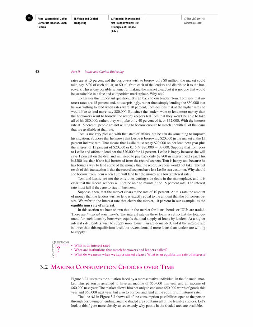
Ross−Westerfield−Jaffe: Corporate Finance, Sixth Edition
II. Value and Capital Budgeting
3. Financial Markets and Net Present Value: First Principles of Finance (Adv.)
54 © The McGraw−Hill Companies, 2002
rates are at 15 percent and the borrowers wish to borrow only $8 million, the market couldtake, say, 8/20 of each dollar, or $0.40, from each of the lenders and distribute it to the bor-rowers. This is one possible scheme for making the market clear, but it is not one that wouldbe sustainable in a free and competitive marketplace. Why not?
To answer this important question, let’s go back to our lender, Tom. Tom sees that in-terest rates are 15 percent and, not surprisingly, rather than simply lending the $50,000 thathe was willing to lend when rates were 10 percent, Tom decides that at the higher rates hewould like to lend more, say $80,000. But since the lenders want to lend more money thanthe borrowers want to borrow, the record keepers tell Tom that they won’t be able to takeall of his $80,000; rather, they will take only 40 percent of it, or $32,000. With the interestrate at 15 percent, people are not willing to borrow enough to match up with all of the loansthat are available at that rate.
Tom is not very pleased with that state of affairs, but he can do something to improvehis situation. Suppose that he knows that Leslie is borrowing $20,000 in the market at the 15percent interest rate. That means that Leslie must repay $20,000 on her loan next year plusthe interest of 15 percent of $20,000 or 0.15 � $20,000 � $3,000. Suppose that Tom goesto Leslie and offers to lend her the $20,000 for 14 percent. Leslie is happy because she willsave 1 percent on the deal and will need to pay back only $2,800 in interest next year. Thisis $200 less than if she had borrowed from the record keepers. Tom is happy too, because hehas found a way to lend some of the money that the record keepers would not take. The netresult of this transaction is that the record keepers have lost Leslie as a customer. Why shouldshe borrow from them when Tom will lend her the money at a lower interest rate?
Tom and Leslie are not the only ones cutting side deals in the marketplace, and it isclear that the record keepers will not be able to maintain the 15 percent rate. The interestrate must fall if they are to stay in business.
Suppose, then, that the market clears at the rate of 10 percent. At this rate the amountof money that the lenders wish to lend is exactly equal to the amount that the borrowers de-sire. We refer to the interest rate that clears the market, 10 percent in our example, as theequilibrium rate of interest.
In this section we have shown that in the market for loans, bonds or IOUs are traded.These are financial instruments. The interest rate on these loans is set so that the total de-mand for such loans by borrowers equals the total supply of loans by lenders. At a higherinterest rate, lenders wish to supply more loans than are demanded, and if the interest rateis lower than this equilibrium level, borrowers demand more loans than lenders are willingto supply.
• What is an interest rate?• What are institutions that match borrowers and lenders called?• What do we mean when we say a market clears? What is an equilibrium rate of interest?
3.2 MAKING CONSUMPTION CHOICES OVER TIME
Figure 3.2 illustrates the situation faced by a representative individual in the financial mar-ket. This person is assumed to have an income of $50,000 this year and an income of$60,000 next year. The market allows him not only to consume $50,000 worth of goods thisyear and $60,000 next year, but also to borrow and lend at the equilibrium interest rate.
The line AB in Figure 3.2 shows all of the consumption possibilities open to the personthrough borrowing or lending, and the shaded area contains all of the feasible choices. Let’slook at this figure more closely to see exactly why points in the shaded area are available.
48 Part II Value and Capital Budgeting
QUESTIONS
CO
NC
EP
T
?
Ross−Westerfield−Jaffe: Corporate Finance, Sixth Edition
II. Value and Capital Budgeting
3. Financial Markets and Net Present Value: First Principles of Finance (Adv.)
55© The McGraw−Hill Companies, 2002
We will use the letter r to denote the interest rate—the equilibrium rate—in this mar-ket. The rate is risk-free because we assume that no default can take place. Look at point Aon the vertical axis of Figure 3.2. Point A is a height of
A � $60,000 � [$50,000 � (1 � r)]
For example, if the rate of interest is 10 percent, then point A would be
A � $60,000 � [$50,000 � (1 � 0.1)]� $60,000 � $55,000� $115,000
Point A is the maximum amount of wealth that this person can spend in the second year.He gets to point A by lending the full income that is available this year, $50,000, and con-suming none of it. In the second year, then, he will have the second year’s income of$60,000 plus the proceeds from the loan that he made in the first year, $55,000, for a totalof $115,000.
Now let’s take a look at point B. Point B is a distance of
B � $50,000 � [$60,000/(1 � r)]
along the horizontal axis. If the interest rate is 10 percent, point B will be
B � $50,000 � [$60,000/(1 � 0.1)]� $50,000 � $54,545� $104,545
(We have rounded off to the nearest dollar.)Why do we divide next year’s income of $60,000 by (1 � r), or 1.1 in the preceding
computation? Point B represents the maximum amount available for this person to consumethis year. To achieve that maximum he would borrow as much as possible and repay the loanfrom the income, $60,000, that he was going to receive next year. Because $60,000 will beavailable to repay the loan next year, we are asking how much he could borrow this year atan interest rate of r and still be able to repay the loan. The answer is
$60,000/(1 � r)
Chapter 3 Financial Markets and Net Present Value: First Principles of Finance (Advanced) 49
Consumption next year
Slope = – (1 + r )
C
Y
D
B
$115,000
$71,000
$60,000
$49,000
$40,000 $60,000
$50,000
Consumption this year
Borrowing
Lending
A
$104,545
� FIGURE 3.2 Intertemporal Consumption Opportunities
Ross−Westerfield−Jaffe: Corporate Finance, Sixth Edition
II. Value and Capital Budgeting
3. Financial Markets and Net Present Value: First Principles of Finance (Adv.)
56 © The McGraw−Hill Companies, 2002
because if he borrows this amount, he must repay it next year with interest. Thus, next yearhe must repay
[$60,000/(1 � r)] � (1 � r) � $60,000
no matter what the interest rate, r, is. In our example we found that he could borrow $54,545and, sure enough,
$54,545 � 1.1 � $60,000
(after rounding off to the nearest dollar).Furthermore, by borrowing and lending different amounts the person can achieve any
point on the line AB. For example, point C is a point where he has chosen to lend $10,000of today’s income. This means that at point C he will have
Consumption this year at point C � $50,000 � $10,000 � $40,000
and
Consumption next year at point C � $60,000 � [$10,000 � (1 � r)] � $71,000
when the interest rate is 10 percent.Similarly, at point D, the individual has decided to borrow $10,000 and repay the loan
next year. At point D, then,
Consumption this year at point D � $50,000 � $10,000 � $60,000
and
Consumption next year at point D � $60,000 � [$10,000 � (1 � r)] � $49,000
at an interest rate of 10 percent.In fact, this person can consume any point on the line AB. This line has a slope of �(1 � r),
which means that for each dollar that is added to the x coordinate along the line, (1 � r) dol-lars are subtracted from the y coordinate. Moving along the line from point A, the initial pointof $50,000 this year and $60,000 next year, toward point B gives the person more consump-tion today and less next year. In other words, moving toward point B is borrowing. Similarly,moving up toward point A, he is consuming less today and more next year and is lending. Theline is a straight line because the individual has no effect on the interest rate. This is one of theassumptions of perfectly competitive financial markets.
Where will the person actually be? The answer to that question depends on the indi-vidual’s tastes and personal situation, just as it did before there was a market. If the personis impatient, he might wish to borrow money at a point such as D, and if he is patient, hemight wish to lend some of this year’s income and enjoy more consumption next year at,for example, a point such as C.
Notice that whether we think of someone as patient or impatient depends on the inter-est rate he or she faces in the market. Suppose that our individual was impatient and choseto borrow $10,000 and move to point D. Now suppose that we raise the interest rate to 20percent or even 50 percent. Suddenly our impatient person may become very patient andmight prefer to lend some of this year’s income to take advantage of the very high interestrate. The general result is depicted in Figure 3.3. We can see that lending at point C′ yieldsmuch greater future income and consumption possibilities than before.1
1Those familiar with consumer theory might be aware of the surprising case where raising the interest rate actuallymakes people borrow more or lowering the rate makes them lend more. The latter case might occur, for example, ifthe decline in the interest rate made the lenders have so little consumption next year that they have no choice but tolend out even more than they were lending before just to subsist. Nothing we do depends on excluding such cases,but it is much easier to ignore them, and the resulting analysis fits the real markets more closely.
50 Part II Value and Capital Budgeting
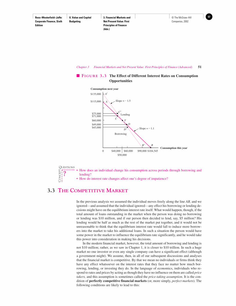
Ross−Westerfield−Jaffe: Corporate Finance, Sixth Edition
II. Value and Capital Budgeting
3. Financial Markets and Net Present Value: First Principles of Finance (Adv.)
57© The McGraw−Hill Companies, 2002
• How does an individual change his consumption across periods through borrowing andlending?
• How do interest rate changes affect one’s degree of impatience?
3.3 THE COMPETITIVE MARKET
In the previous analysis we assumed the individual moves freely along the line AB, and weignored—and assumed that the individual ignored—any effect his borrowing or lending de-cisions might have on the equilibrium interest rate itself. What would happen, though, if thetotal amount of loans outstanding in the market when the person was doing no borrowingor lending was $10 million, and if our person then decided to lend, say, $5 million? Hislending would be half as much as the rest of the market put together, and it would not beunreasonable to think that the equilibrium interest rate would fall to induce more borrow-ers into the market to take his additional loans. In such a situation the person would havesome power in the market to influence the equilibrium rate significantly, and he would takethis power into consideration in making his decisions.
In the modern financial market, however, the total amount of borrowing and lending isnot $10 million; rather, as we saw in Chapter 1, it is closer to $10 trillion. In such a hugemarket no one investor or even any single company can have a significant effect (althougha government might). We assume, then, in all of our subsequent discussions and analysesthat the financial market is competitive. By that we mean no individuals or firms think theyhave any effect whatsoever on the interest rates that they face no matter how much bor-rowing, lending, or investing they do. In the language of economics, individuals who re-spond to rates and prices by acting as though they have no influence on them are called pricetakers, and this assumption is sometimes called the price-taking assumption. It is the con-dition of perfectly competitive financial markets (or, more simply, perfect markets). Thefollowing conditions are likely to lead to this:
Chapter 3 Financial Markets and Net Present Value: First Principles of Finance (Advanced) 51
Consumption next year
Slope = – 1.5
YD
B
$115,000
$75,000
$60,000
$49,000
$40,000 $60,000
$50,000
Consumption this year
Borrowing
Lending
A′
$45,000
$71,000
A
B ′
D ′
C ′
$90,000
Slope = – 1.1
0 $104,545
$135,000
C
� FIGURE 3.3 The Effect of Different Interest Rates on ConsumptionOpportunities
QUESTIONS
CO
NC
EP
T
?
Ross−Westerfield−Jaffe: Corporate Finance, Sixth Edition
II. Value and Capital Budgeting
3. Financial Markets and Net Present Value: First Principles of Finance (Adv.)
58 © The McGraw−Hill Companies, 2002
1. Trading is costless. Access to the financial markets is free.
2. Information about borrowing and lending opportunities is available.
3. There are many traders, and no single trader can have a significant impact on market prices.
How Many Interest Rates Are There in a Competitive Market?An important point about this one-year market where no defaults can take place is that onlyone interest rate can be quoted in the market at any one time. Suppose that some competingrecord keepers decide to set up a rival market. To attract customers, their business plan is tooffer lower interest rates, say, 9 percent. Their business plan is based on the hope that theywill be able to attract borrowers away from the first market and soon have all of the business.
Their business plan will work, but it will do so beyond their wildest expectations. Theywill indeed attract the borrowers, all $11 million worth of them! But the matter doesn’t stopthere. By offering to borrow and lend at 9 percent when another market is offering 10 per-cent, they have created the proverbial money machine.
The world of finance is populated by sharp-eyed inhabitants who would not let this op-portunity slip by them. Any one of these, whether a borrower or a lender, would go to thenew market and borrow everything he could at the 9-percent rate. At the same time he wasborrowing in the new market, he would also be striking a deal to lend in the old market atthe 10-percent rate. If he could borrow $100 million at 9 percent and lend it at 10 percent,he would be able to net 1 percent, or $1 million, next year. He would repay the $109 mil-lion he owed to the new market from the $110 million he receives when the 10-percent loanshe made in the original market are repaid, pocketing $1 million profit.
This process of striking a deal in one market and an offsetting deal in another marketsimultaneously and at more favorable terms is called arbitrage, and doing it is called arbi-traging. Of course, someone must be paying for all this free money, and it must be the recordkeepers because the borrowers and the lenders are all making money. Our intrepid entre-preneurs will lose their proverbial shirts and go out of business. The moral of this is clear:As soon as different interest rates are offered for essentially the same risk-free loans, arbi-trageurs will take advantage of the situation by borrowing at the low rate and lending at thehigh rate. The gap between the two rates will be closed quickly, and for all practical pur-poses there will be only one rate available in the market.
• What is the most important feature of a competitive financial market?• What conditions are likely to lead to this?
3.4 THE BASIC PRINCIPLE
We have already shown how people use the financial markets to adjust their patterns of con-sumption over time to fit their particular preferences. By borrowing and lending, they cangreatly expand their range of choices. They need only to have access to a market with aninterest rate at which they can borrow and lend.
In the previous section we saw how these savings and consumption decisions dependon the interest rate. The financial markets also provide a benchmark against which proposedinvestments can be compared, and the interest rate is the basis for a test that any proposedinvestment must pass. The financial markets give the individual, the corporation, or eventhe government a standard of comparison for economic decisions. This benchmark is criti-cal when investment decisions are being made.
52 Part II Value and Capital Budgeting
QUESTIONS
CO
NC
EP
T
?
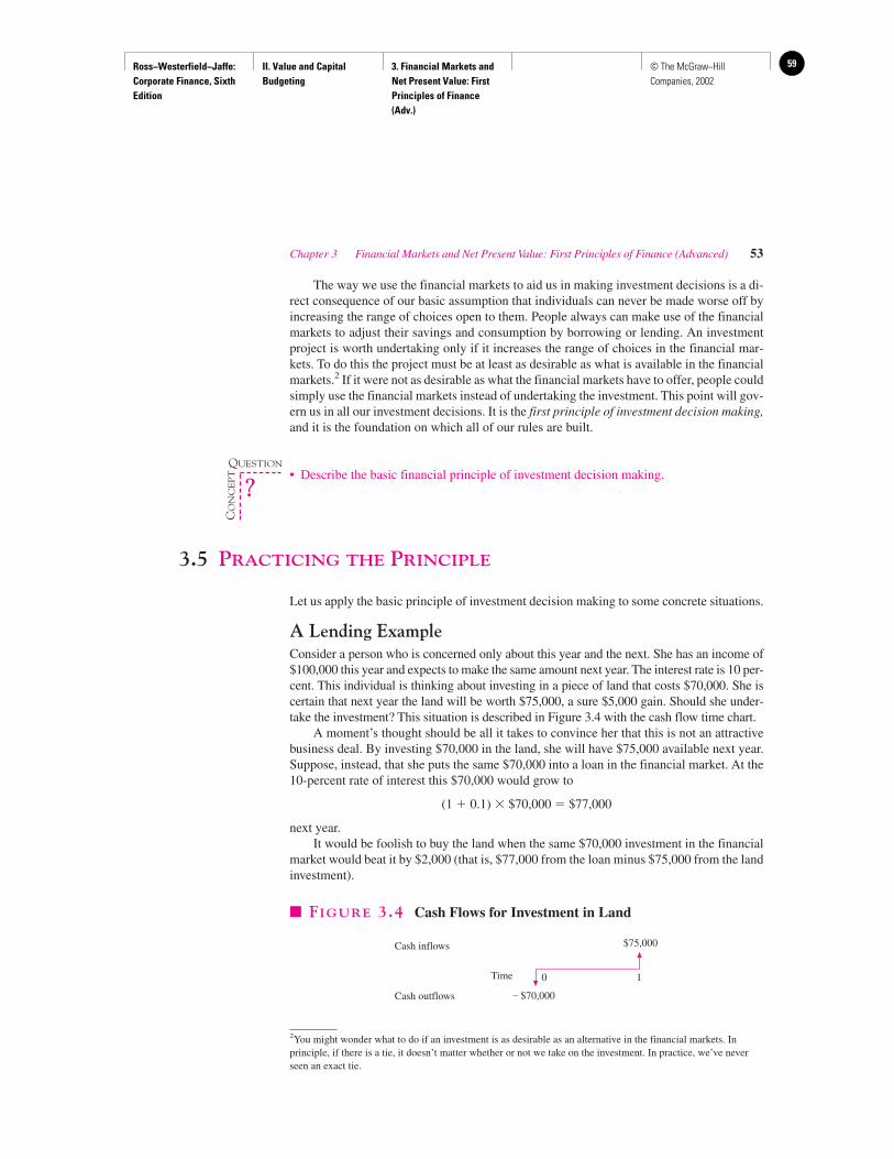
Ross−Westerfield−Jaffe: Corporate Finance, Sixth Edition
II. Value and Capital Budgeting
3. Financial Markets and Net Present Value: First Principles of Finance (Adv.)
59© The McGraw−Hill Companies, 2002
The way we use the financial markets to aid us in making investment decisions is a di-rect consequence of our basic assumption that individuals can never be made worse off byincreasing the range of choices open to them. People always can make use of the financialmarkets to adjust their savings and consumption by borrowing or lending. An investmentproject is worth undertaking only if it increases the range of choices in the financial mar-kets. To do this the project must be at least as desirable as what is available in the financialmarkets.2 If it were not as desirable as what the financial markets have to offer, people couldsimply use the financial markets instead of undertaking the investment. This point will gov-ern us in all our investment decisions. It is the first principle of investment decision making,and it is the foundation on which all of our rules are built.
• Describe the basic financial principle of investment decision making.
3.5 PRACTICING THE PRINCIPLE
Let us apply the basic principle of investment decision making to some concrete situations.
A Lending ExampleConsider a person who is concerned only about this year and the next. She has an income of$100,000 this year and expects to make the same amount next year. The interest rate is 10 per-cent. This individual is thinking about investing in a piece of land that costs $70,000. She iscertain that next year the land will be worth $75,000, a sure $5,000 gain. Should she under-take the investment? This situation is described in Figure 3.4 with the cash flow time chart.
A moment’s thought should be all it takes to convince her that this is not an attractivebusiness deal. By investing $70,000 in the land, she will have $75,000 available next year.Suppose, instead, that she puts the same $70,000 into a loan in the financial market. At the10-percent rate of interest this $70,000 would grow to
(1 � 0.1) � $70,000 � $77,000
next year.It would be foolish to buy the land when the same $70,000 investment in the financial
market would beat it by $2,000 (that is, $77,000 from the loan minus $75,000 from the landinvestment).
Chapter 3 Financial Markets and Net Present Value: First Principles of Finance (Advanced) 53
Cash inflows
Time 0 1
– $70,000
$75,000
Cash outflows
� FIGURE 3.4 Cash Flows for Investment in Land
2You might wonder what to do if an investment is as desirable as an alternative in the financial markets. Inprinciple, if there is a tie, it doesn’t matter whether or not we take on the investment. In practice, we’ve neverseen an exact tie.
QUESTION
CO
NC
EP
T
?
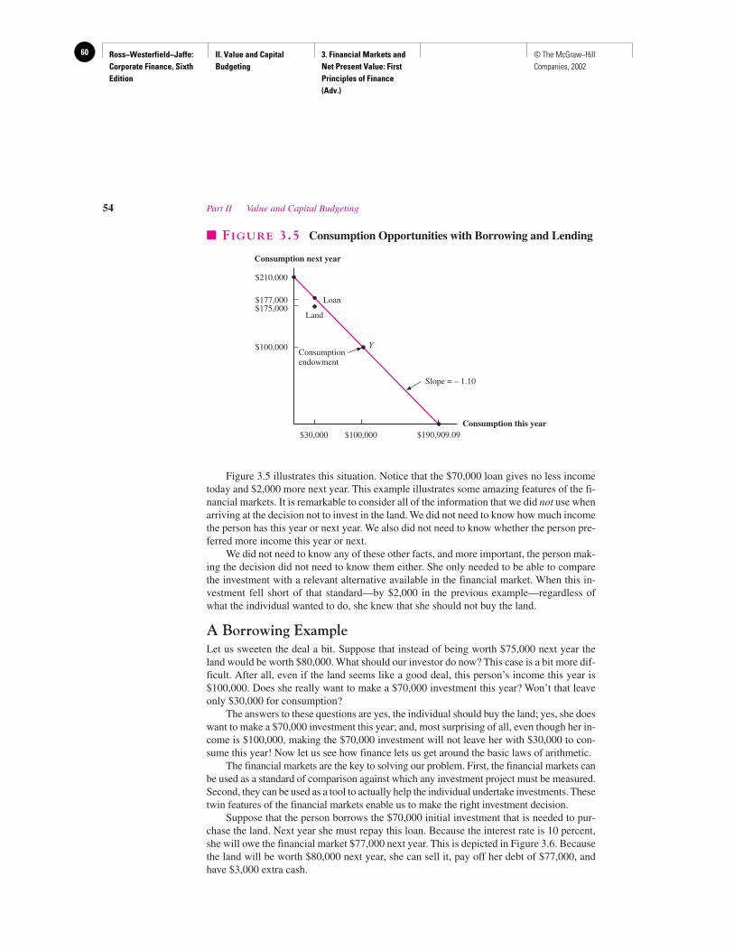
Ross−Westerfield−Jaffe: Corporate Finance, Sixth Edition
II. Value and Capital Budgeting
3. Financial Markets and Net Present Value: First Principles of Finance (Adv.)
60 © The McGraw−Hill Companies, 2002
Figure 3.5 illustrates this situation. Notice that the $70,000 loan gives no less incometoday and $2,000 more next year. This example illustrates some amazing features of the fi-nancial markets. It is remarkable to consider all of the information that we did not use whenarriving at the decision not to invest in the land. We did not need to know how much incomethe person has this year or next year. We also did not need to know whether the person pre-ferred more income this year or next.
We did not need to know any of these other facts, and more important, the person mak-ing the decision did not need to know them either. She only needed to be able to comparethe investment with a relevant alternative available in the financial market. When this in-vestment fell short of that standard—by $2,000 in the previous example—regardless ofwhat the individual wanted to do, she knew that she should not buy the land.
A Borrowing ExampleLet us sweeten the deal a bit. Suppose that instead of being worth $75,000 next year theland would be worth $80,000. What should our investor do now? This case is a bit more dif-ficult. After all, even if the land seems like a good deal, this person’s income this year is$100,000. Does she really want to make a $70,000 investment this year? Won’t that leaveonly $30,000 for consumption?
The answers to these questions are yes, the individual should buy the land; yes, she doeswant to make a $70,000 investment this year; and, most surprising of all, even though her in-come is $100,000, making the $70,000 investment will not leave her with $30,000 to con-sume this year! Now let us see how finance lets us get around the basic laws of arithmetic.
The financial markets are the key to solving our problem. First, the financial markets canbe used as a standard of comparison against which any investment project must be measured.Second, they can be used as a tool to actually help the individual undertake investments. Thesetwin features of the financial markets enable us to make the right investment decision.
Suppose that the person borrows the $70,000 initial investment that is needed to pur-chase the land. Next year she must repay this loan. Because the interest rate is 10 percent,she will owe the financial market $77,000 next year. This is depicted in Figure 3.6. Becausethe land will be worth $80,000 next year, she can sell it, pay off her debt of $77,000, andhave $3,000 extra cash.
54 Part II Value and Capital Budgeting
Consumption next year
$210,000
$30,000 $100,000Consumption this year
Loan$175,000$177,000
$190,909.09
Slope = – 1.10
Land
Consumptionendowment
Y$100,000
� FIGURE 3.5 Consumption Opportunities with Borrowing and Lending
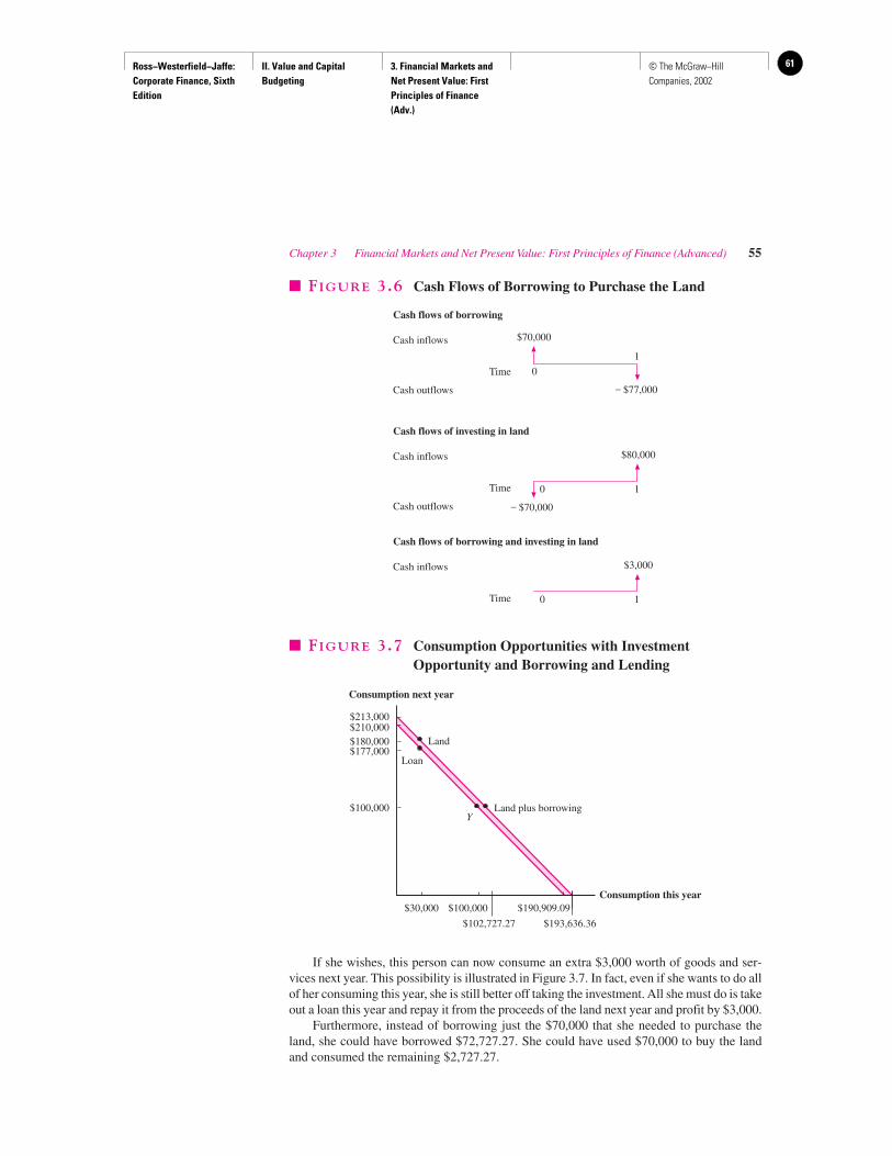
Ross−Westerfield−Jaffe: Corporate Finance, Sixth Edition
II. Value and Capital Budgeting
3. Financial Markets and Net Present Value: First Principles of Finance (Adv.)
61© The McGraw−Hill Companies, 2002
If she wishes, this person can now consume an extra $3,000 worth of goods and ser-vices next year. This possibility is illustrated in Figure 3.7. In fact, even if she wants to do allof her consuming this year, she is still better off taking the investment. All she must do is takeout a loan this year and repay it from the proceeds of the land next year and profit by $3,000.
Furthermore, instead of borrowing just the $70,000 that she needed to purchase theland, she could have borrowed $72,727.27. She could have used $70,000 to buy the landand consumed the remaining $2,727.27.
Chapter 3 Financial Markets and Net Present Value: First Principles of Finance (Advanced) 55
Cash flows of borrowing
0 1
– $70,000
$80,000
Cash inflows
Time 0
1
– $77,000
$70,000
Cash outflows
Cash flows of investing in land
Cash inflows
Time
Cash outflows
0 1
$3,000
Cash flows of borrowing and investing in land
Cash inflows
Time
� FIGURE 3.6 Cash Flows of Borrowing to Purchase the Land
Consumption next year
$213,000
$30,000 $100,000Consumption this year
$100,000
$180,000$210,000
$190,909.09
Y
$177,000
$193,636.36$102,727.27
Loan
Land
Land plus borrowing
� FIGURE 3.7 Consumption Opportunities with InvestmentOpportunity and Borrowing and Lending
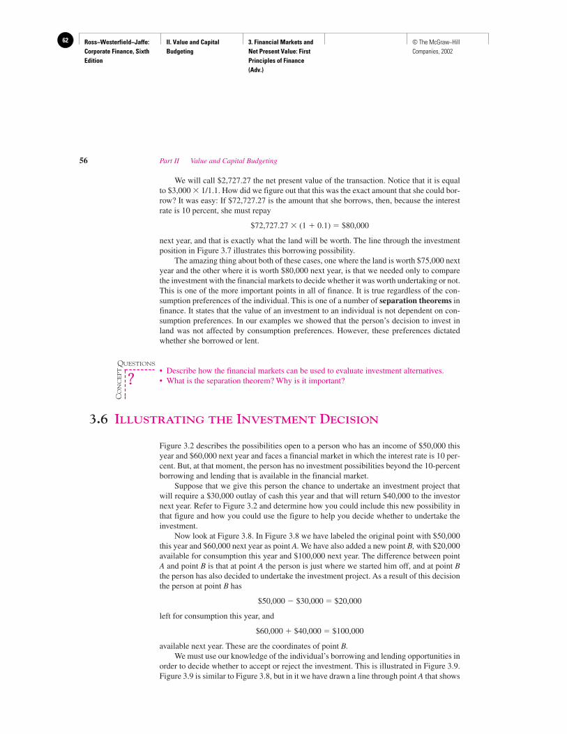
Ross−Westerfield−Jaffe: Corporate Finance, Sixth Edition
II. Value and Capital Budgeting
3. Financial Markets and Net Present Value: First Principles of Finance (Adv.)
62 © The McGraw−Hill Companies, 2002
We will call $2,727.27 the net present value of the transaction. Notice that it is equalto $3,000 � 1/1.1. How did we figure out that this was the exact amount that she could bor-row? It was easy: If $72,727.27 is the amount that she borrows, then, because the interestrate is 10 percent, she must repay
$72,727.27 � (1 � 0.1) � $80,000
next year, and that is exactly what the land will be worth. The line through the investmentposition in Figure 3.7 illustrates this borrowing possibility.
The amazing thing about both of these cases, one where the land is worth $75,000 nextyear and the other where it is worth $80,000 next year, is that we needed only to comparethe investment with the financial markets to decide whether it was worth undertaking or not.This is one of the more important points in all of finance. It is true regardless of the con-sumption preferences of the individual. This is one of a number of separation theorems infinance. It states that the value of an investment to an individual is not dependent on con-sumption preferences. In our examples we showed that the person’s decision to invest inland was not affected by consumption preferences. However, these preferences dictatedwhether she borrowed or lent.
• Describe how the financial markets can be used to evaluate investment alternatives.• What is the separation theorem? Why is it important?
3.6 ILLUSTRATING THE INVESTMENT DECISION
Figure 3.2 describes the possibilities open to a person who has an income of $50,000 thisyear and $60,000 next year and faces a financial market in which the interest rate is 10 per-cent. But, at that moment, the person has no investment possibilities beyond the 10-percentborrowing and lending that is available in the financial market.
Suppose that we give this person the chance to undertake an investment project thatwill require a $30,000 outlay of cash this year and that will return $40,000 to the investornext year. Refer to Figure 3.2 and determine how you could include this new possibility inthat figure and how you could use the figure to help you decide whether to undertake theinvestment.
Now look at Figure 3.8. In Figure 3.8 we have labeled the original point with $50,000this year and $60,000 next year as point A. We have also added a new point B, with $20,000available for consumption this year and $100,000 next year. The difference between pointA and point B is that at point A the person is just where we started him off, and at point Bthe person has also decided to undertake the investment project. As a result of this decisionthe person at point B has
$50,000 � $30,000 � $20,000
left for consumption this year, and
$60,000 � $40,000 � $100,000
available next year. These are the coordinates of point B.We must use our knowledge of the individual’s borrowing and lending opportunities in
order to decide whether to accept or reject the investment. This is illustrated in Figure 3.9.Figure 3.9 is similar to Figure 3.8, but in it we have drawn a line through point A that shows
56 Part II Value and Capital Budgeting
QUESTIONS
CO
NC
EP
T
?
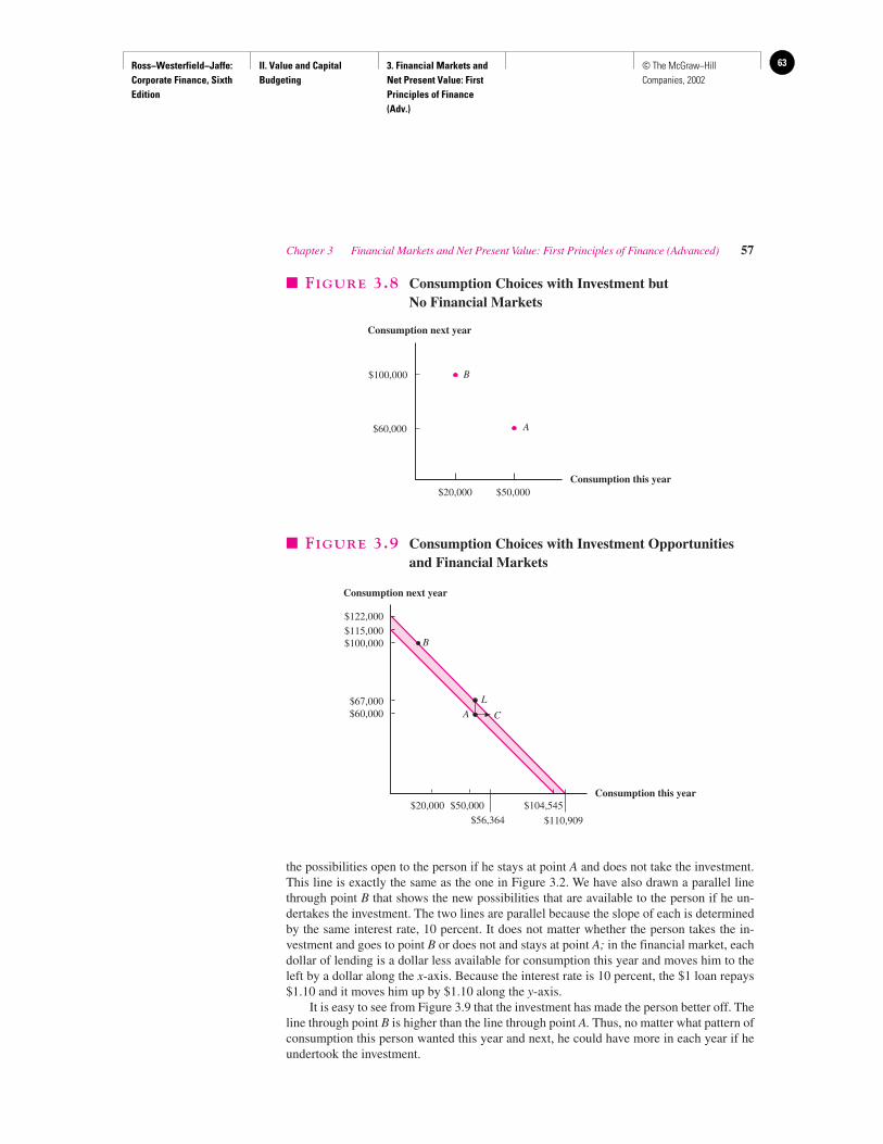
Ross−Westerfield−Jaffe: Corporate Finance, Sixth Edition
II. Value and Capital Budgeting
3. Financial Markets and Net Present Value: First Principles of Finance (Adv.)
63© The McGraw−Hill Companies, 2002
the possibilities open to the person if he stays at point A and does not take the investment.This line is exactly the same as the one in Figure 3.2. We have also drawn a parallel linethrough point B that shows the new possibilities that are available to the person if he un-dertakes the investment. The two lines are parallel because the slope of each is determinedby the same interest rate, 10 percent. It does not matter whether the person takes the in-vestment and goes to point B or does not and stays at point A; in the financial market, eachdollar of lending is a dollar less available for consumption this year and moves him to theleft by a dollar along the x-axis. Because the interest rate is 10 percent, the $1 loan repays$1.10 and it moves him up by $1.10 along the y-axis.
It is easy to see from Figure 3.9 that the investment has made the person better off. Theline through point B is higher than the line through point A. Thus, no matter what pattern ofconsumption this person wanted this year and next, he could have more in each year if heundertook the investment.
Chapter 3 Financial Markets and Net Present Value: First Principles of Finance (Advanced) 57
Consumption next year
$20,000Consumption this year
$100,000
$50,000
$60,000
B
A
� FIGURE 3.8 Consumption Choices with Investment but No Financial Markets
Consumption next year
$122,000
$20,000 $50,000Consumption this year
$60,000
$100,000$115,000
$104,545
B
$67,000 L
CA
$110,909$56,364
� FIGURE 3.9 Consumption Choices with Investment Opportunitiesand Financial Markets
Ross−Westerfield−Jaffe: Corporate Finance, Sixth Edition
II. Value and Capital Budgeting
3. Financial Markets and Net Present Value: First Principles of Finance (Adv.)
64 © The McGraw−Hill Companies, 2002
For example, suppose that our individual wanted to consume everything this year. If hedid not take the investment, the point where the line through point A intersected the x-axiswould give the maximum amount of consumption he could enjoy this year. This point has$104,545 available this year. To recall how we found this figure, review the analysis ofFigure 3.2. But in Figure 3.9 the line that goes through point B hits the x-axis at a higherpoint than the line that goes through point A. Along this line the person can have the $20,000that is left after investing $30,000, plus all that he can borrow and repay with both nextyear’s income and the proceeds from the investment. The total amount available to consumetoday is therefore
� $50,000 � $30,000 � ($60,000 � $40,000)/(1 � 0.1)� $20,000 � ($100,000/1.1)� $110,909
The additional consumption available this year from undertaking the investment and usingthe financial market is the difference on the x-axis between the points where these two linesintersect:
$110,909 � $104,545 � $6,364
This difference is an important measure of what the investment is worth to the person.It answers a variety of questions. For example, it is the answer to the question: How muchmoney would we need to give the investor this year to make him just as well off as he iswith the investment?
Because the line through point B is parallel to the line through point A but has beenmoved over by $6,364, we know that if we were to add this amount to the investor’s currentincome this year at point A and take away the investment, he would wind up on the linethrough point B and with the same possibilities. If we do this, the person will have $56,364this year and $60,000 next year, which is the situation of the point on the line through pointB that lies to the right of point A in Figure 3.9. This is point C.
We could also ask a different question: How much money would we need to give theinvestor next year to make him just as well off as he is with the investment?
This is the same as asking how much higher the line through point B is than the linethrough point A. In other words, what is the difference in Figure 3.9 between the pointwhere the line through A intercepts the y-axis and the point where the line through B inter-cepts the y-axis?
The point where the line through A intercepts the y-axis shows the maximum amountthe person could consume next year if all of his current income were lent out and the pro-ceeds of the loan were consumed along with next year’s income.
As we showed in our analysis of Figure 3.2, this amount is $115,000. How does thiscompare with what the person can have next year if he takes the investment? By takingthe investment we saw that he would be at point B where he has $20,000 left this yearand would have $100,000 next year. By lending the $20,000 that is left this year andadding the proceeds of this loan to the $100,000, we find the line through B interceptsthe y-axis at:
($20,000 � 1.1) � $100,000 � $122,000
The difference between this amount and $115,000 is
$122,000 � $115,000 � $7,000
which is the answer to the question of how much we would need to give the person nextyear to make him as well off as he is with the investment.
58 Part II Value and Capital Budgeting
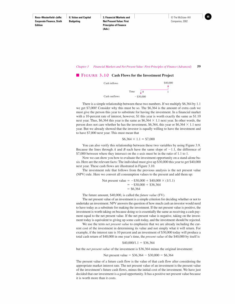
Ross−Westerfield−Jaffe: Corporate Finance, Sixth Edition
II. Value and Capital Budgeting
3. Financial Markets and Net Present Value: First Principles of Finance (Adv.)
65© The McGraw−Hill Companies, 2002
There is a simple relationship between these two numbers. If we multiply $6,364 by 1.1we get $7,000! Consider why this must be so. The $6,364 is the amount of extra cash wemust give the person this year to substitute for having the investment. In a financial marketwith a 10-percent rate of interest, however, $1 this year is worth exactly the same as $1.10next year. Thus, $6,364 this year is the same as $6,364 � 1.1 next year. In other words, theperson does not care whether he has the investment, $6,364, this year or $6,364 � 1.1 nextyear. But we already showed that the investor is equally willing to have the investment andto have $7,000 next year. This must mean that
$6,364 � 1.1 � $7,000
You can also verify this relationship between these two variables by using Figure 3.9.Because the lines through A and B each have the same slope of �1.1, the difference of$7,000 between where they intersect on the x-axis must be in the ratio of 1.1 to 1.
Now we can show you how to evaluate the investment opportunity on a stand-alone ba-sis. Here are the relevant facts: The individual must give up $30,000 this year to get $40,000next year. These cash flows are illustrated in Figure 3.10.
The investment rule that follows from the previous analysis is the net present value(NPV) rule. Here we convert all consumption values to the present and add them up:
Net present value � �$30,000 � $40,000 � (1/1.1)� �$30,000 � $36,364� $6,364
The future amount, $40,000, is called the future value (FV).The net present value of an investment is a simple criterion for deciding whether or not to
undertake an investment. NPV answers the question of how much cash an investor would needto have today as a substitute for making the investment. If the net present value is positive, theinvestment is worth taking on because doing so is essentially the same as receiving a cash pay-ment equal to the net present value. If the net present value is negative, taking on the invest-ment today is equivalent to giving up some cash today, and the investment should be rejected.
We use the term net present value to emphasize that we are already including the cur-rent cost of the investment in determining its value and not simply what it will return. Forexample, if the interest rate is 10 percent and an investment of $30,000 today will produce atotal cash return of $40,000 in one year’s time, the present value of the $40,000 by itself is
$40,000/1.1 � $36,364
but the net present value of the investment is $36,364 minus the original investment:
Net present value � $36,364 � $30,000 � $6,364
The present value of a future cash flow is the value of that cash flow after considering theappropriate market interest rate. The net present value of an investment is the present valueof the investment’s future cash flows, minus the initial cost of the investment. We have justdecided that our investment is a good opportunity. It has a positive net present value becauseit is worth more than it costs.
Chapter 3 Financial Markets and Net Present Value: First Principles of Finance (Advanced) 59
0 1
– $30,000
$40,000Cash inflows
Time
Cash outflows
� FIGURE 3.10 Cash Flows for the Investment Project
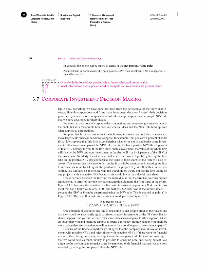
Ross−Westerfield−Jaffe: Corporate Finance, Sixth Edition
II. Value and Capital Budgeting
3. Financial Markets and Net Present Value: First Principles of Finance (Adv.)
66 © The McGraw−Hill Companies, 2002
In general, the above can be stated in terms of the net present value rule:
An investment is worth making if it has a positive NPV. If an investment’s NPV is negative, itshould be rejected.
• Give the definitions of net present value, future value, and present value.• What information does a person need to compute an investment’s net present value?
3.7 CORPORATE INVESTMENT DECISION MAKING
Up to now, everything we have done has been from the perspective of the individual in-vestor. How do corporations and firms make investment decisions? Aren’t their decisionsgoverned by a much more complicated set of rules and principles than the simple NPV rulethat we have developed for individuals?
We return to questions of corporate decision making and corporate governance later inthe book, but it is remarkable how well our central ideas and the NPV rule hold up evenwhen applied to corporations.
Suppose that firms are just ways in which many investors can pool their resources tomake large-scale business decisions. Suppose, for example, that you own 1 percent of somefirm. Now suppose that this firm is considering whether or not to undertake some invest-ment. If that investment passes the NPV rule, that is, if it has a positive NPV, then 1 percentof that NPV belongs to you. If the firm takes on this investment, the value of the whole firmwill rise by the NPV and your investment in the firm will rise by 1 percent of the NPV ofthe investment. Similarly, the other shareholders in the firm will profit by having the firmtake on the positive NPV project because the value of their shares in the firm will also in-crease. This means that the shareholders in the firm will be unanimous in wanting the firmto increase its value by taking on the positive NPV project. If you follow this line of rea-soning, you will also be able to see why the shareholders would oppose the firm taking onany projects with a negative NPV because this would lower the value of their shares.
One difference between the firm and the individual is that the firm has no consumptionendowment. In terms of our one-period consumption diagram, the firm starts at the origin.Figure 3.11 illustrates the situation of a firm with investment opportunity B. B is an invest-ment that has a future value of $33,000 and will cost $25,000 now. If the interest rate is 10percent, the NPV of B can be determined using the NPV rule. This is marked as point C inFigure 3.11. The cash flows of this investment are depicted in Figure 3.12.
Net present value ��$25,000 � [$33,000 � (1/1.1)] � $5,000
One common objection to this line of reasoning is that people differ in their tastes andthat they would not necessarily agree to take on or reject investments by the NPV rule. For in-stance, suppose that you and we each own some shares in a company. Further suppose that weare older than you and might be anxious to spend our money. Being younger, you might bemore patient than we are and more willing to wait for a good long-term investment to pay off.
Because of the financial markets we all agree that the company should take on invest-ments with positive NPVs and reject those with negative NPVs. If there were no financialmarkets, then, being impatient, we might want the company to do little or no investing sothat we could have as much money as possible to consume now, and, being patient, youmight prefer the company to make some investments. With financial markets, we are bothsatisfied by having the company follow the NPV rule.
60 Part II Value and Capital Budgeting
QUESTIONS
CO
NC
EP
T
?
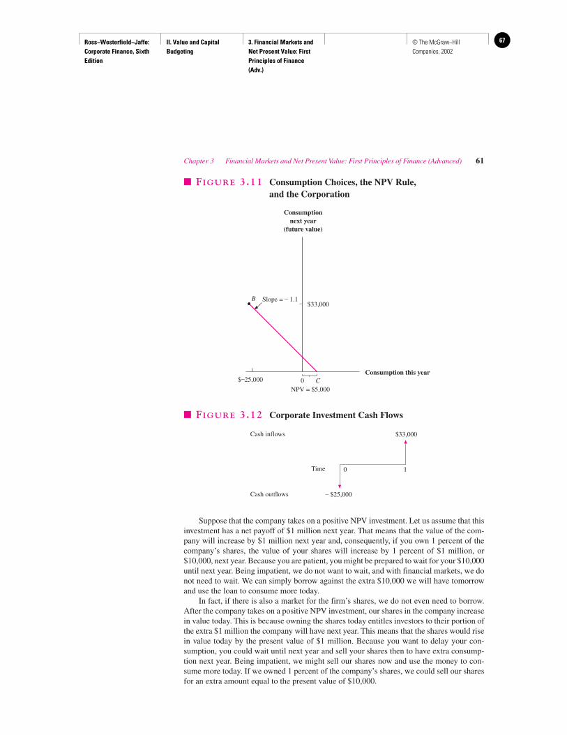
Ross−Westerfield−Jaffe: Corporate Finance, Sixth Edition
II. Value and Capital Budgeting
3. Financial Markets and Net Present Value: First Principles of Finance (Adv.)
67© The McGraw−Hill Companies, 2002
Suppose that the company takes on a positive NPV investment. Let us assume that thisinvestment has a net payoff of $1 million next year. That means that the value of the com-pany will increase by $1 million next year and, consequently, if you own 1 percent of thecompany’s shares, the value of your shares will increase by 1 percent of $1 million, or$10,000, next year. Because you are patient, you might be prepared to wait for your $10,000until next year. Being impatient, we do not want to wait, and with financial markets, we donot need to wait. We can simply borrow against the extra $10,000 we will have tomorrowand use the loan to consume more today.
In fact, if there is also a market for the firm’s shares, we do not even need to borrow.After the company takes on a positive NPV investment, our shares in the company increasein value today. This is because owning the shares today entitles investors to their portion ofthe extra $1 million the company will have next year. This means that the shares would risein value today by the present value of $1 million. Because you want to delay your con-sumption, you could wait until next year and sell your shares then to have extra consump-tion next year. Being impatient, we might sell our shares now and use the money to con-sume more today. If we owned 1 percent of the company’s shares, we could sell our sharesfor an extra amount equal to the present value of $10,000.
Chapter 3 Financial Markets and Net Present Value: First Principles of Finance (Advanced) 61
$–25,000 0 CNPV = $5,000
Consumption this year
B
Consumptionnext year
(future value)
$33,000Slope = – 1.1
� FIGURE 3.11 Consumption Choices, the NPV Rule,and the Corporation
0 1
– $25,000
$33,000Cash inflows
Time
Cash outflows
� FIGURE 3.12 Corporate Investment Cash Flows
Ross−Westerfield−Jaffe: Corporate Finance, Sixth Edition
II. Value and Capital Budgeting
3. Financial Markets and Net Present Value: First Principles of Finance (Adv.)
68 © The McGraw−Hill Companies, 2002
In reality, shareholders in big companies do not vote on every investment decision, andthe managers of big companies must have rules that they follow. We have seen that all share-holders in a company will be better off—no matter what their levels of patience or impa-tience—if these managers follow the NPV rule. This is a marvelous result because it makesit possible for many different owners to delegate decision-making powers to the managers.They need only tell the managers to follow the NPV rule, and if the managers do so, theywill be doing exactly what the stockholders want them to do. Sometimes this form of theNPV rule is stated as having the managers maximize the value of the company. As we ar-gued, the current value of the shares of the company will increase by the NPV of any in-vestments that the company undertakes. This means that the managers of the company canmake the shareholders as well off as possible by taking on all positive NPV projects and re-jecting projects with negative NPVs.
Separating investment decision making from the owners is a basic requirement of the mod-ern large firm. The separation theorem in financial markets says that all investors will want toaccept or reject the same investment projects by using the NPV rule, regardless of their per-sonal preferences. Investors can delegate the operations of the firm and require that managersuse the NPV rule. Of course, much remains for us to discuss about this topic. For example, whatinsurance do stockholders have that managers will actually do what is best for them?
We discussed this possibility in Chapter 1, and we take up this interesting topic later inthe book. For now, though, we no longer will consider our perspective to be that of the loneinvestor. Instead, thanks to the separation theorem, we will use the NPV rule for companiesas well as for investors. Our justification of the NPV rule depends on the conditions neces-sary to derive the separation theorem. These conditions are the ones that result in competi-tive financial markets. The analysis we have presented has been restricted to risk-free cashflows in one time period. However, the separation theorem also can be derived for risky cashflows that extend beyond one period.
For the reader interested in studying further about the separation theorem, we include sev-eral suggested readings at the end of this chapter that build on the material we have presented.
• In terms of the net present value rule, what is the essential difference between the indi-vidual and the corporation?
3.8 SUMMARY AND CONCLUSIONS
Finance is a subject that builds understanding from the ground up. Whenever you come upagainst a new problem or issue in finance, you can always return to the basic principles of thischapter for guidance.
1. Financial markets exist because people want to adjust their consumption over time. They dothis by borrowing and lending.
2. Financial markets provide the key test for investment decision making. Whether a particularinvestment decision should or should not be taken depends only on this test: If there is asuperior alternative in the financial markets, the investment should be rejected; if not, the
62 Part II Value and Capital Budgeting
QUESTION
CO
NC
EP
T
?
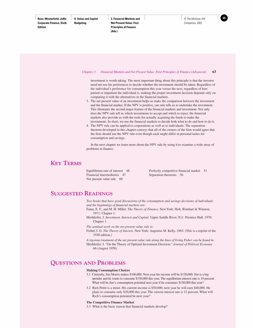
Ross−Westerfield−Jaffe: Corporate Finance, Sixth Edition
II. Value and Capital Budgeting
3. Financial Markets and Net Present Value: First Principles of Finance (Adv.)
69© The McGraw−Hill Companies, 2002
investment is worth taking. The most important thing about this principle is that the investorneed not use his preferences to decide whether the investment should be taken. Regardless ofthe individual’s preference for consumption this year versus the next, regardless of howpatient or impatient the individual is, making the proper investment decision depends only oncomparing it with the alternatives in the financial markets.
3. The net present value of an investment helps us make the comparison between the investmentand the financial market. If the NPV is positive, our rule tells us to undertake the investment.This illustrates the second major feature of the financial markets and investment. Not onlydoes the NPV rule tell us which investments to accept and which to reject, the financialmarkets also provide us with the tools for actually acquiring the funds to make theinvestments. In short, we use the financial markets to decide both what to do and how to do it.
4. The NPV rule can be applied to corporations as well as to individuals. The separationtheorem developed in this chapter conveys that all of the owners of the firm would agree thatthe firm should use the NPV rule even though each might differ in personal tastes forconsumption and savings.
In the next chapter we learn more about the NPV rule by using it to examine a wide array ofproblems in finance.
KEY TERMS
Equilibrium rate of interest 48 Perfectly competitive financial market 51Financial intermediaries 47 Separation theorems 56Net present value rule 60
SUGGESTED READINGS
Two books that have good discussions of the consumption and savings decisions of individualsand the beginnings of financial markets are:Fama, E. F., and M. H. Miller. The Theory of Finance. New York: Holt, Rinehart & Winston,
1971: Chapter 1.Hirshleifer, J. Investment, Interest and Capital. Upper Saddle River, N.J.: Prentice Hall, 1970:
Chapter 1.
The seminal work on the net present value rule is:Fisher, I. G. The Theory of Interest. New York: Augustus M. Kelly, 1965. (This is a reprint of the
1930 edition.)
A rigorous treatment of the net present value rule along the lines of Irving Fisher can be found in:Hirshleifer, J. “On the Theory of Optimal Investment Decision.” Journal of Political Economy
66 (August 1958).
QUESTIONS AND PROBLEMS
Making Consumption Choices3.1 Currently, Jim Morris makes $100,000. Next year his income will be $120,000. Jim is a big
spender and he wants to consume $150,000 this year. The equilibrium interest rate is 10 percent.What will be Jim’s consumption potential next year if he consumes $150,000 this year?
3.2 Rich Pettit is a miser. His current income is $50,000; next year he will earn $40,000. Heplans to consume only $20,000 this year. The current interest rate is 12 percent. What willRich’s consumption potential be next year?
The Competitive Finance Market3.3 What is the basic reason that financial markets develop?
Chapter 3 Financial Markets and Net Present Value: First Principles of Finance (Advanced) 63
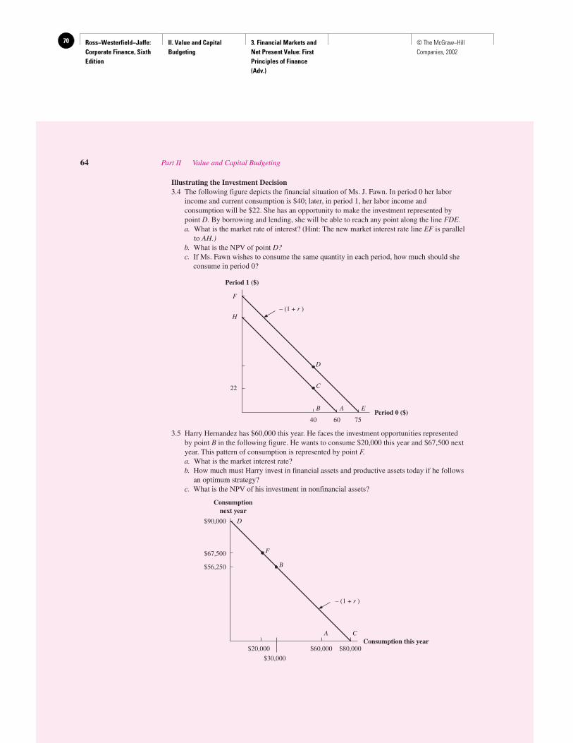
Ross−Westerfield−Jaffe: Corporate Finance, Sixth Edition
II. Value and Capital Budgeting
3. Financial Markets and Net Present Value: First Principles of Finance (Adv.)
70 © The McGraw−Hill Companies, 2002
Illustrating the Investment Decision3.4 The following figure depicts the financial situation of Ms. J. Fawn. In period 0 her labor
income and current consumption is $40; later, in period 1, her labor income andconsumption will be $22. She has an opportunity to make the investment represented bypoint D. By borrowing and lending, she will be able to reach any point along the line FDE.a. What is the market rate of interest? (Hint: The new market interest rate line EF is parallel
to AH.)b. What is the NPV of point D?c. If Ms. Fawn wishes to consume the same quantity in each period, how much should she
consume in period 0?
3.5 Harry Hernandez has $60,000 this year. He faces the investment opportunities representedby point B in the following figure. He wants to consume $20,000 this year and $67,500 nextyear. This pattern of consumption is represented by point F.a. What is the market interest rate?b. How much must Harry invest in financial assets and productive assets today if he follows
an optimum strategy?c. What is the NPV of his investment in nonfinancial assets?
Consumptionnext year
Consumption this year
D$90,000
$30,000
F
B
A C
$20,000 $60,000 $80,000
$67,500
$56,250
– (1 + r )
H
F
Period 1 ($)
Period 0 ($)75
22
6040
D
C
B E
– (1 + r )
A
64 Part II Value and Capital Budgeting
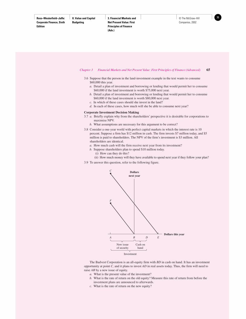
Ross−Westerfield−Jaffe: Corporate Finance, Sixth Edition
II. Value and Capital Budgeting
3. Financial Markets and Net Present Value: First Principles of Finance (Adv.)
71© The McGraw−Hill Companies, 2002
3.6 Suppose that the person in the land-investment example in the text wants to consume$60,000 this year.a. Detail a plan of investment and borrowing or lending that would permit her to consume
$60,000 if the land investment is worth $75,000 next year.b. Detail a plan of investment and borrowing or lending that would permit her to consume
$60,000 if the land investment is worth $80,000 next year.c. In which of these cases should she invest in the land?d. In each of these cases, how much will she be able to consume next year?
Corporate Investment Decision Making3.7 a. Briefly explain why from the shareholders’ perspective it is desirable for corporations to
maximize NPV.b. What assumptions are necessary for this argument to be correct?
3.8 Consider a one-year world with perfect capital markets in which the interest rate is 10percent. Suppose a firm has $12 million in cash. The firm invests $7 million today, and $5million is paid to shareholders. The NPV of the firm’s investment is $3 million. Allshareholders are identical.a. How much cash will the firm receive next year from its investment?b. Suppose shareholders plan to spend $10 million today.
(i) How can they do this?(ii) How much money will they have available to spend next year if they follow your plan?
3.9 To answer this question, refer to the following figure.
The Badvest Corporation is an all-equity firm with BD in cash on hand. It has an investmentopportunity at point C, and it plans to invest AD in real assets today. Thus, the firm will need toraise AB by a new issue of equity.
a. What is the present value of the investment?b. What is the rate of return on the old equity? Measure this rate of return from before the
investment plans are announced to afterwards.c. What is the rate of return on the new equity?
New issueof security
Dollars this year
F
Dollarsnext year
C
A B ED
Cash onhand
Investment
Chapter 3 Financial Markets and Net Present Value: First Principles of Finance (Advanced) 65
Ross−Westerfield−Jaffe: Corporate Finance, Sixth Edition
II. Value and Capital Budgeting
4. Net Present Value72 © The McGraw−Hill Companies, 2002
Net Present Value
CH
AP
TE
R4
EXECUTIVE SUMMARY
We now examine one of the most important concepts in all of corporate finance, therelationship between $1 today and $1 in the future. Consider the following exam-ple: A firm is contemplating investing $1 million in a project that is expected to pay
out $200,000 per year for nine years. Should the firm accept the project? One might say yes atfirst glance, since total inflows of $1.8 million (� $200,000 � 9) are greater than $1 millionoutflow. However, the $1 million is paid out immediately, whereas the $200,000 per year willbe received in the future. Also, the immediate payment is known with certainty, whereas thelater inflows can only be estimated. Thus, we need to know the relationship between a dollartoday and a (possibly uncertain) dollar in the future before deciding on the project.
This relationship is called the time-value-of-money concept. It is important in such ar-eas as capital budgeting, lease versus buy decisions, accounts receivable analysis, financ-ing arrangements, mergers, and pension funding.
The basics are presented in this chapter. We begin by discussing two fundamental con-cepts, future value and present value. Next, we treat simplifying formulas such as perpetu-ities and annuities.
4.1 THE ONE-PERIOD CASE
EXAMPLE
Don Simkowitz is trying to sell a piece of raw land in Alaska. Yesterday, he was of-fered $10,000 for the property. He was about ready to accept the offer when anotherindividual offered him $11,424. However, the second offer was to be paid a yearfrom now. Don has satisfied himself that both buyers are honest and financially sol-vent, so he has no fear that the offer he selects will fall through. These two offersare pictured as cash flows in Figure 4.1. Which offer should Mr. Simkowitz choose?
Mike Tuttle, Don’s financial advisor, points out that if Don takes the first of-fer, he could invest the $10,000 in the bank at an insured rate of 12 percent. At theend of one year, he would have
$10,000 � (0.12 � $10,000) � $10,000 � 1.12 � $11,200Return of Interestprincipal
Because this is less than the $11,424 Don could receive from the second offer, Mr.Tuttle recommends that he take the latter. This analysis uses the concept of futurevalue or compound value, which is the value of a sum after investing over one ormore periods. The compound or future value of $10,000 is $11,200.
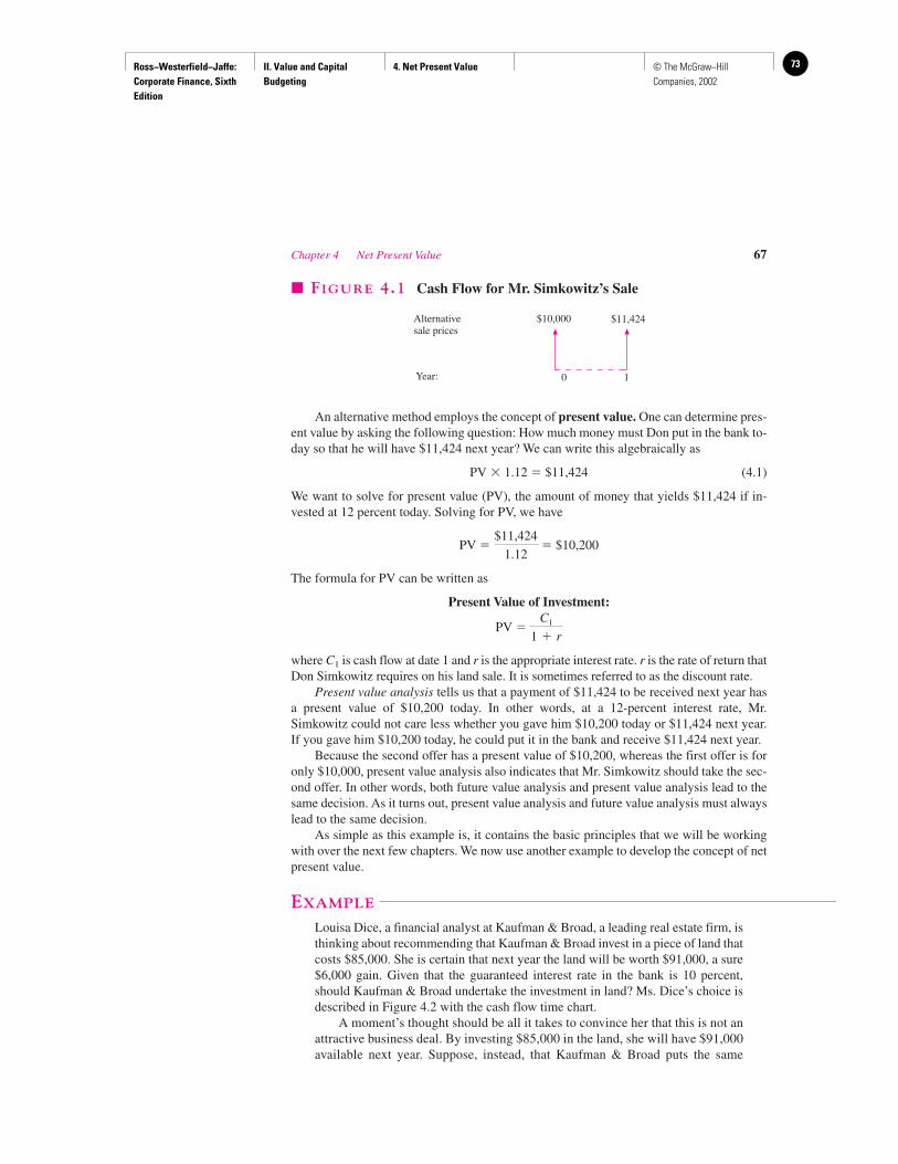
Ross−Westerfield−Jaffe: Corporate Finance, Sixth Edition
II. Value and Capital Budgeting
4. Net Present Value 73© The McGraw−Hill Companies, 2002
Chapter 4 Net Present Value 67
An alternative method employs the concept of present value. One can determine pres-ent value by asking the following question: How much money must Don put in the bank to-day so that he will have $11,424 next year? We can write this algebraically as
PV � 1.12 � $11,424 (4.1)
We want to solve for present value (PV), the amount of money that yields $11,424 if in-vested at 12 percent today. Solving for PV, we have
PV � � $10,200
The formula for PV can be written as
Present Value of Investment:
PV �
where C1 is cash flow at date 1 and r is the appropriate interest rate. r is the rate of return thatDon Simkowitz requires on his land sale. It is sometimes referred to as the discount rate.
Present value analysis tells us that a payment of $11,424 to be received next year hasa present value of $10,200 today. In other words, at a 12-percent interest rate, Mr.Simkowitz could not care less whether you gave him $10,200 today or $11,424 next year.If you gave him $10,200 today, he could put it in the bank and receive $11,424 next year.
Because the second offer has a present value of $10,200, whereas the first offer is foronly $10,000, present value analysis also indicates that Mr. Simkowitz should take the sec-ond offer. In other words, both future value analysis and present value analysis lead to thesame decision. As it turns out, present value analysis and future value analysis must alwayslead to the same decision.
As simple as this example is, it contains the basic principles that we will be workingwith over the next few chapters. We now use another example to develop the concept of netpresent value.
EXAMPLE
Louisa Dice, a financial analyst at Kaufman & Broad, a leading real estate firm, isthinking about recommending that Kaufman & Broad invest in a piece of land thatcosts $85,000. She is certain that next year the land will be worth $91,000, a sure$6,000 gain. Given that the guaranteed interest rate in the bank is 10 percent,should Kaufman & Broad undertake the investment in land? Ms. Dice’s choice isdescribed in Figure 4.2 with the cash flow time chart.
A moment’s thought should be all it takes to convince her that this is not anattractive business deal. By investing $85,000 in the land, she will have $91,000available next year. Suppose, instead, that Kaufman & Broad puts the same
C1
1 � r
$11,424
1.12
0 1
$10,000 $11,424Alternativesale prices
Year:
� FIGURE 4.1 Cash Flow for Mr. Simkowitz’s Sale
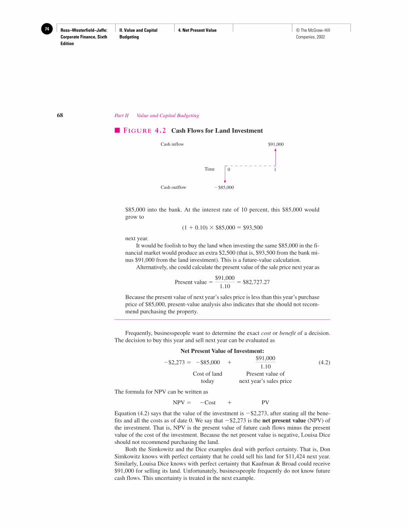
Ross−Westerfield−Jaffe: Corporate Finance, Sixth Edition
II. Value and Capital Budgeting
4. Net Present Value74 © The McGraw−Hill Companies, 2002
$85,000 into the bank. At the interest rate of 10 percent, this $85,000 wouldgrow to
(1 � 0.10) � $85,000 � $93,500
next year.It would be foolish to buy the land when investing the same $85,000 in the fi-
nancial market would produce an extra $2,500 (that is, $93,500 from the bank mi-nus $91,000 from the land investment). This is a future-value calculation.
Alternatively, she could calculate the present value of the sale price next year as
Present value � � $82,727.27
Because the present value of next year’s sales price is less than this year’s purchaseprice of $85,000, present-value analysis also indicates that she should not recom-mend purchasing the property.
Frequently, businesspeople want to determine the exact cost or benefit of a decision.The decision to buy this year and sell next year can be evaluated as
Net Present Value of Investment:
�$2,273 � �$85,000 � (4.2)
Cost of land Present value oftoday next year’s sales price
The formula for NPV can be written as
NPV � �Cost � PV
Equation (4.2) says that the value of the investment is �$2,273, after stating all the bene-fits and all the costs as of date 0. We say that �$2,273 is the net present value (NPV) ofthe investment. That is, NPV is the present value of future cash flows minus the presentvalue of the cost of the investment. Because the net present value is negative, Louisa Diceshould not recommend purchasing the land.
Both the Simkowitz and the Dice examples deal with perfect certainty. That is, DonSimkowitz knows with perfect certainty that he could sell his land for $11,424 next year.Similarly, Louisa Dice knows with perfect certainty that Kaufman & Broad could receive$91,000 for selling its land. Unfortunately, businesspeople frequently do not know futurecash flows. This uncertainty is treated in the next example.
$91,000
1.10
$91,000
1.10
68 Part II Value and Capital Budgeting
0 1
– $85,000
$91,000Cash inflow
Time
Cash outflow
� FIGURE 4.2 Cash Flows for Land Investment
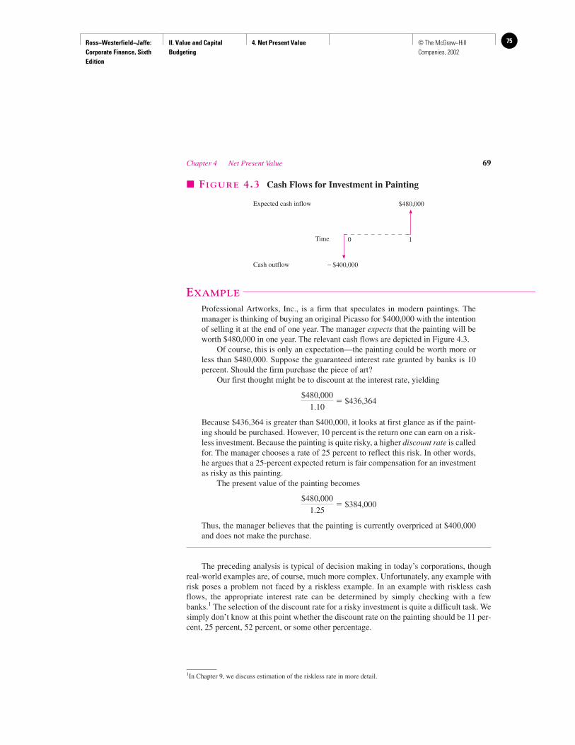
Ross−Westerfield−Jaffe: Corporate Finance, Sixth Edition
II. Value and Capital Budgeting
4. Net Present Value 75© The McGraw−Hill Companies, 2002
EXAMPLE
Professional Artworks, Inc., is a firm that speculates in modern paintings. Themanager is thinking of buying an original Picasso for $400,000 with the intentionof selling it at the end of one year. The manager expects that the painting will beworth $480,000 in one year. The relevant cash flows are depicted in Figure 4.3.
Of course, this is only an expectation—the painting could be worth more orless than $480,000. Suppose the guaranteed interest rate granted by banks is 10percent. Should the firm purchase the piece of art?
Our first thought might be to discount at the interest rate, yielding
� $436,364
Because $436,364 is greater than $400,000, it looks at first glance as if the paint-ing should be purchased. However, 10 percent is the return one can earn on a risk-less investment. Because the painting is quite risky, a higher discount rate is calledfor. The manager chooses a rate of 25 percent to reflect this risk. In other words,he argues that a 25-percent expected return is fair compensation for an investmentas risky as this painting.
The present value of the painting becomes
� $384,000
Thus, the manager believes that the painting is currently overpriced at $400,000and does not make the purchase.
The preceding analysis is typical of decision making in today’s corporations, thoughreal-world examples are, of course, much more complex. Unfortunately, any example withrisk poses a problem not faced by a riskless example. In an example with riskless cashflows, the appropriate interest rate can be determined by simply checking with a fewbanks.1 The selection of the discount rate for a risky investment is quite a difficult task. Wesimply don’t know at this point whether the discount rate on the painting should be 11 per-cent, 25 percent, 52 percent, or some other percentage.
$480,000
1.25
$480,000
1.10
Chapter 4 Net Present Value 69
0 1
– $400,000
$480,000Expected cash inflow
Time
Cash outflow
� FIGURE 4.3 Cash Flows for Investment in Painting
1In Chapter 9, we discuss estimation of the riskless rate in more detail.
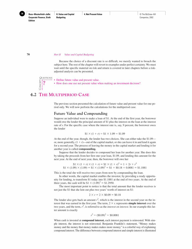
Ross−Westerfield−Jaffe: Corporate Finance, Sixth Edition
II. Value and Capital Budgeting
4. Net Present Value76 © The McGraw−Hill Companies, 2002
Because the choice of a discount rate is so difficult, we merely wanted to broach thesubject here. The rest of the chapter will revert to examples under perfect certainty. We mustwait until the specific material on risk and return is covered in later chapters before a risk-adjusted analysis can be presented.
• Define future value and present value.• How does one use net present value when making an investment decision?
4.2 THE MULTIPERIOD CASE
The previous section presented the calculation of future value and present value for one pe-riod only. We will now perform the calculations for the multiperiod case.
Future Value and CompoundingSuppose an individual were to make a loan of $1. At the end of the first year, the borrowerwould owe the lender the principal amount of $1 plus the interest on the loan at the interestrate of r. For the specific case where the interest rate is, say, 9 percent, the borrower owesthe lender
$1 � (1 � r) � $1 � 1.09 � $1.09
At the end of the year, though, the lender has two choices. She can either take the $1.09—or, more generally, (1 � r)—out of the capital market, or she can leave it in and lend it againfor a second year. The process of leaving the money in the capital market and lending it foranother year is called compounding.
Suppose that the lender decides to compound her loan for another year. She does thisby taking the proceeds from her first one-year loan, $1.09, and lending this amount for thenext year. At the end of next year, then, the borrower will owe her
$1 � (1 � r) � (1 � r) � $1 � (1 � r)2 � 1 � 2r � r2
$1 � (1.09) � (1.09) � $1 � (1.09)2 � $1 � $0.18 � 0.0081 � $1.1881
This is the total she will receive two years from now by compounding the loan.In other words, the capital market enables the investor, by providing a ready opportu-
nity for lending, to transform $1 today into $1.1881 at the end of two years. At the end ofthree years, the cash will be $1 � (1.09)3 � $1.2950.
The most important point to notice is that the total amount that the lender receives isnot just the $1 that she lent out plus two years’ worth of interest on $1:
2 � r � 2 � $0.09 � $0.18
The lender also gets back an amount r2, which is the interest in the second year on the in-terest that was earned in the first year. The term, 2 � r, represents simple interest over thetwo years, and the term, r2, is referred to as the interest on interest. In our example this lat-ter amount is exactly
r2 � ($0.09)2 � $0.0081
When cash is invested at compound interest, each interest payment is reinvested. With sim-ple interest, the interest is not reinvested. Benjamin Franklin’s statement, “Money makesmoney and the money that money makes makes more money,” is a colorful way of explainingcompound interest. The difference between compound interest and simple interest is illustrated
70 Part II Value and Capital Budgeting
QUESTIONS
CO
NC
EP
T
?
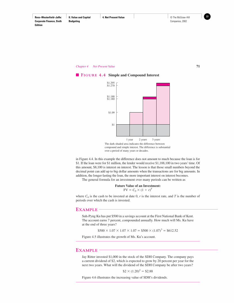
Ross−Westerfield−Jaffe: Corporate Finance, Sixth Edition
II. Value and Capital Budgeting
4. Net Present Value 77© The McGraw−Hill Companies, 2002
in Figure 4.4. In this example the difference does not amount to much because the loan is for$1. If the loan were for $1 million, the lender would receive $1,188,100 in two years’ time. Ofthis amount, $8,100 is interest on interest. The lesson is that those small numbers beyond thedecimal point can add up to big dollar amounts when the transactions are for big amounts. Inaddition, the longer-lasting the loan, the more important interest on interest becomes.
The general formula for an investment over many periods can be written as
Future Value of an Investment:FV � C0 � (1 � r)T
where C0 is the cash to be invested at date 0, r is the interest rate, and T is the number ofperiods over which the cash is invested.
EXAMPLE
Suh-Pyng Ku has put $500 in a savings account at the First National Bank of Kent.The account earns 7 percent, compounded annually. How much will Ms. Ku haveat the end of three years?
$500 � 1.07 � 1.07 � 1.07 � $500 � (1.07)3 � $612.52
Figure 4.5 illustrates the growth of Ms. Ku’s account.
EXAMPLE
Jay Ritter invested $1,000 in the stock of the SDH Company. The company paysa current dividend of $2, which is expected to grow by 20 percent per year for thenext two years. What will the dividend of the SDH Company be after two years?
$2 � (1.20)2 � $2.88
Figure 4.6 illustrates the increasing value of SDH’s dividends.
Chapter 4 Net Present Value 71
$1.295$1.270
$1.188$1.180
$1.09
$1
1 year 2 years 3 years
� FIGURE 4.4 Simple and Compound Interest
The dark-shaded area indicates the difference betweencompound and simple interest. The difference is substantialover a period of many years or decades.
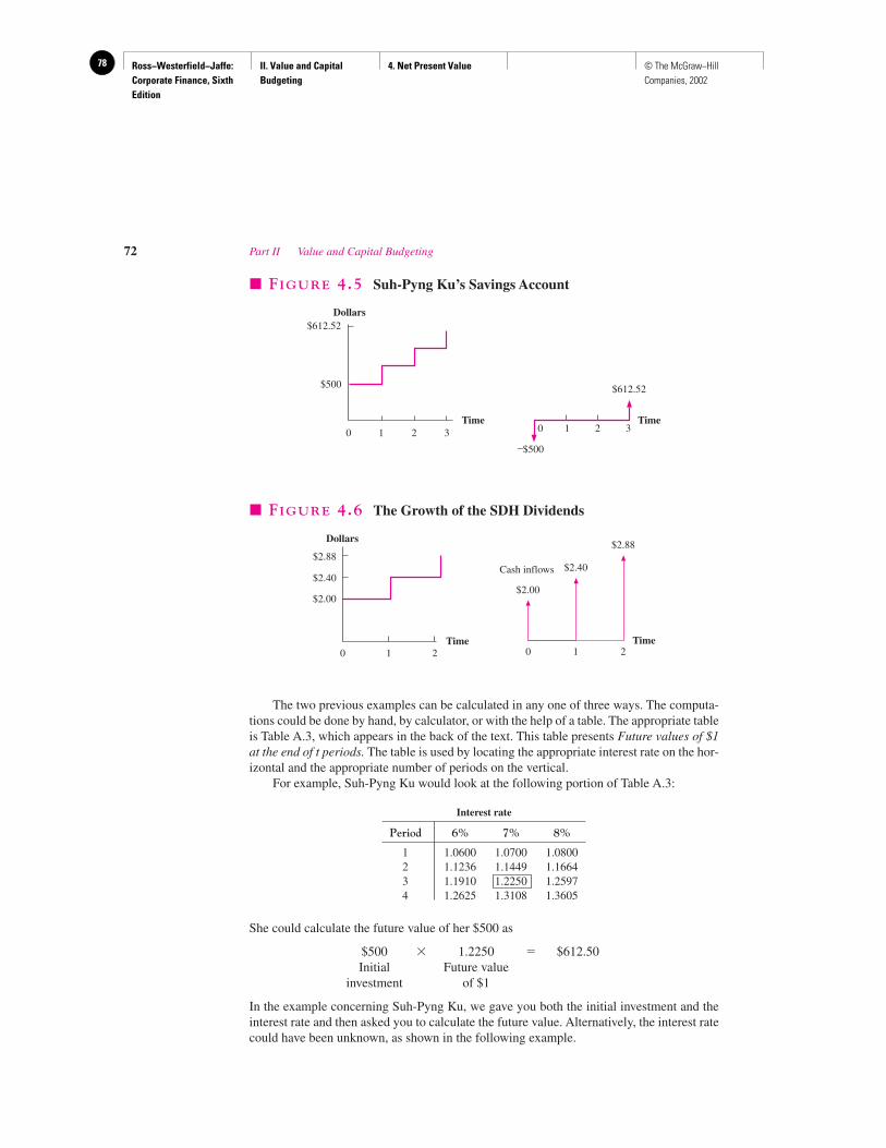
Ross−Westerfield−Jaffe: Corporate Finance, Sixth Edition
II. Value and Capital Budgeting
4. Net Present Value78 © The McGraw−Hill Companies, 2002
The two previous examples can be calculated in any one of three ways. The computa-tions could be done by hand, by calculator, or with the help of a table. The appropriate tableis Table A.3, which appears in the back of the text. This table presents Future values of $1at the end of t periods. The table is used by locating the appropriate interest rate on the hor-izontal and the appropriate number of periods on the vertical.
For example, Suh-Pyng Ku would look at the following portion of Table A.3:
She could calculate the future value of her $500 as
$500 � 1.2250 � $612.50Initial Future value
investment of $1
In the example concerning Suh-Pyng Ku, we gave you both the initial investment and theinterest rate and then asked you to calculate the future value. Alternatively, the interest ratecould have been unknown, as shown in the following example.
Interest rate
Period 6% 7% 8%
1 1.0600 1.0700 1.08002 1.1236 1.1449 1.16643 1.1910 1.2250 1.25974 1.2625 1.3108 1.3605
72 Part II Value and Capital Budgeting
0 1 2 3
$612.52
$500
Dollars
Time0 1 2 3
$612.52
–$500
Time
� FIGURE 4.5 Suh-Pyng Ku’s Savings Account
0 1 2
$2.00
Dollars
Time0 1 2
$2.88
Time
$2.40
$2.88$2.40
$2.00
Cash inflows
� FIGURE 4.6 The Growth of the SDH Dividends
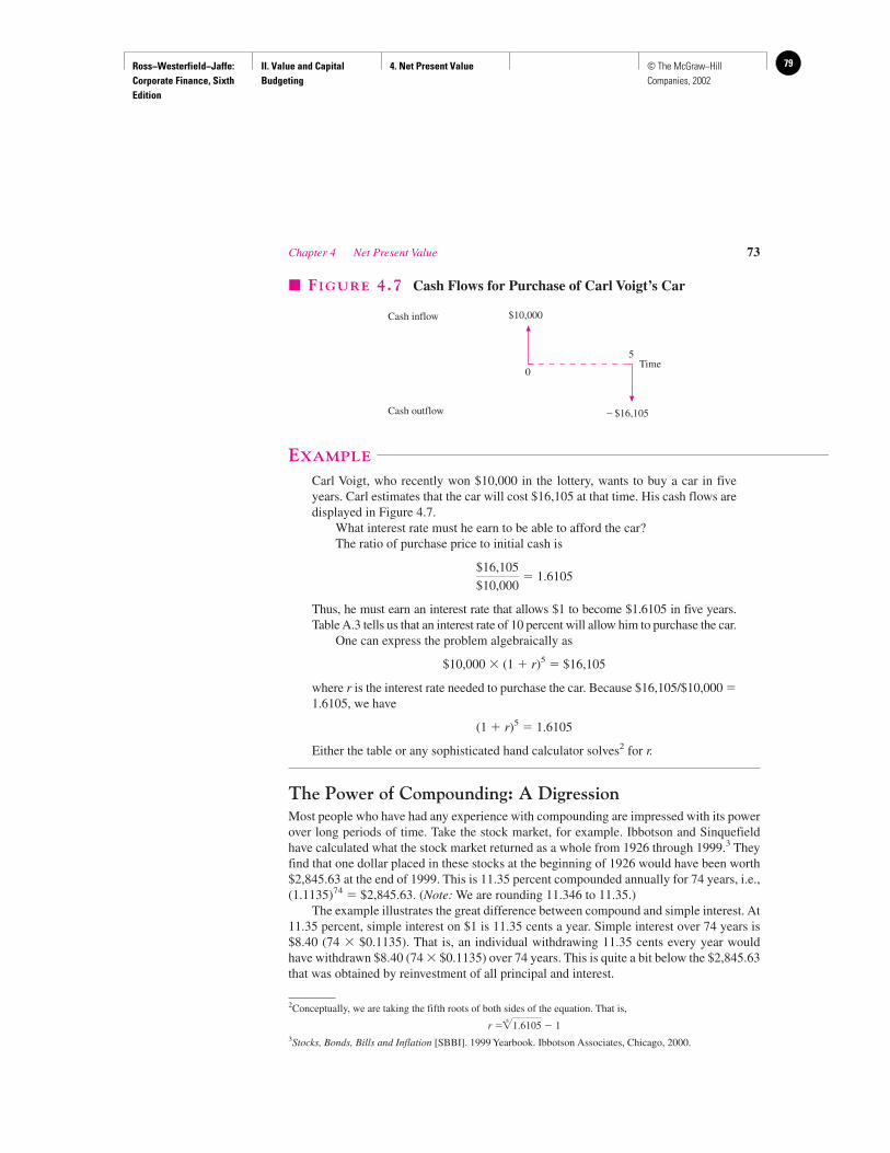
Ross−Westerfield−Jaffe: Corporate Finance, Sixth Edition
II. Value and Capital Budgeting
4. Net Present Value 79© The McGraw−Hill Companies, 2002
EXAMPLE
Carl Voigt, who recently won $10,000 in the lottery, wants to buy a car in fiveyears. Carl estimates that the car will cost $16,105 at that time. His cash flows aredisplayed in Figure 4.7.
What interest rate must he earn to be able to afford the car?The ratio of purchase price to initial cash is
� 1.6105
Thus, he must earn an interest rate that allows $1 to become $1.6105 in five years.Table A.3 tells us that an interest rate of 10 percent will allow him to purchase the car.
One can express the problem algebraically as
$10,000 � (1 � r)5 � $16,105
where r is the interest rate needed to purchase the car. Because $16,105/$10,000 �1.6105, we have
(1 � r)5 � 1.6105
Either the table or any sophisticated hand calculator solves2 for r.
The Power of Compounding: A DigressionMost people who have had any experience with compounding are impressed with its powerover long periods of time. Take the stock market, for example. Ibbotson and Sinquefieldhave calculated what the stock market returned as a whole from 1926 through 1999.3 Theyfind that one dollar placed in these stocks at the beginning of 1926 would have been worth$2,845.63 at the end of 1999. This is 11.35 percent compounded annually for 74 years, i.e.,(1.1135)74 � $2,845.63. (Note: We are rounding 11.346 to 11.35.)
The example illustrates the great difference between compound and simple interest. At11.35 percent, simple interest on $1 is 11.35 cents a year. Simple interest over 74 years is$8.40 (74 � $0.1135). That is, an individual withdrawing 11.35 cents every year wouldhave withdrawn $8.40 (74 � $0.1135) over 74 years. This is quite a bit below the $2,845.63that was obtained by reinvestment of all principal and interest.
$16,105
$10,000
Chapter 4 Net Present Value 73
0
5
– $16,105
Cash inflow
Time
Cash outflow
$10,000
� FIGURE 4.7 Cash Flows for Purchase of Carl Voigt’s Car
2Conceptually, we are taking the fifth roots of both sides of the equation. That is,
r �5
� 13Stocks, Bonds, Bills and Inflation [SBBI]. 1999 Yearbook. Ibbotson Associates, Chicago, 2000.
�1.6105
Ross−Westerfield−Jaffe: Corporate Finance, Sixth Edition
II. Value and Capital Budgeting
4. Net Present Value80 © The McGraw−Hill Companies, 2002
The results are more impressive over even longer periods of time. A person with no ex-perience in compounding might think that the value of $1 at the end of 148 years would betwice the value of $1 at the end of 74 years, if the yearly rate of return stayed the same.Actually the value of $1 at the end of 148 years would be the square of the value of $1 atthe end of 74 years. That is, if the annual rate of return remained the same, a $1 investmentin common stocks should be worth $8,097,610.1[$1 � (2845.63 � 2845.63)].
A few years ago an archaeologist unearthed a relic stating that Julius Caesar lent theRoman equivalent of one penny to someone. Since there was no record of the penny ever be-ing repaid, the archaeologist wondered what the interest and principal would be if a descen-dant of Caesar tried to collect from a descendant of the borrower in the 20th century. The ar-chaeologist felt that a rate of 6 percent might be appropriate. To his surprise, the principaland interest due after more than 2,000 years was far greater than the entire wealth on earth.
The power of compounding can explain why the parents of well-to-do families fre-quently bequeath wealth to their grandchildren rather than to their children. That is, theyskip a generation. The parents would rather make the grandchildren very rich than make thechildren moderately rich. We have found that in these families the grandchildren have amore positive view of the power of compounding than do the children.
EXAMPLE
Some people have said that it was the best real estate deal in history. Peter Minuit,director–general of New Netherlands, the Dutch West India Company’s Colony inNorth America, in 1626 allegedly bought Manhattan Island for 60 guilders worth oftrinkets from native Americans. By 1667 the Dutch were forced to exchange it forSuriname with the British (perhaps the worst real estate deal ever). This sounds cheapbut did the Dutch really get the better end of the deal? It is reported that 60 guilderswas worth about $24 at the prevailing exchange rate. If the native Americans had soldthe trinkets at a fair market value and invested the $24 at 5 percent (tax free), it wouldnow, 375 years later, be worth more than $2.0 billion. Today, Manhattan is un-doubtedly worth more than $2 billion, and so at a 5 percent rate of return, the nativeAmericans got the worst of the deal. However, if invested at 10 percent, the amountof money they received would be worth about
$24 (1 � r)T � 1.1375 � $72 quadrillion
This is a lot of money. In fact, $72 quadrillion is more than all the real estate in theworld is worth today. No one in the history of the world has ever been able to findan investment yielding 10% every year for 375 years.
Present Value and DiscountingWe now know that an annual interest rate of 9 percent enables the investor to transform $1today into $1.1881 two years from now. In addition, we would like to know:
How much would an investor need to lend today so that she could receive $1 two yearsfrom today?
Algebraically, we can write this as
PV � (1.09)2 � $1
In the preceding equation, PV stands for present value, the amount of money we must lendtoday in order to receive $1 in two years’ time.
74 Part II Value and Capital Budgeting
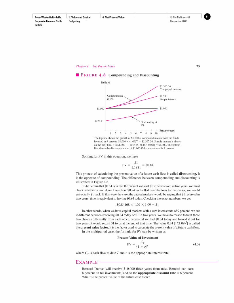
Ross−Westerfield−Jaffe: Corporate Finance, Sixth Edition
II. Value and Capital Budgeting
4. Net Present Value 81© The McGraw−Hill Companies, 2002
Solving for PV in this equation, we have
PV � � $0.84
This process of calculating the present value of a future cash flow is called discounting. Itis the opposite of compounding. The difference between compounding and discounting isillustrated in Figure 4.8.
To be certain that $0.84 is in fact the present value of $1 to be received in two years, we mustcheck whether or not, if we loaned out $0.84 and rolled over the loan for two years, we wouldget exactly $1 back. If this were the case, the capital markets would be saying that $1 received intwo years’ time is equivalent to having $0.84 today. Checking the exact numbers, we get
$0.84168 � 1.09 � 1.09 � $1
In other words, when we have capital markets with a sure interest rate of 9 percent, we areindifferent between receiving $0.84 today or $1 in two years. We have no reason to treat thesetwo choices differently from each other, because if we had $0.84 today and loaned it out fortwo years, it would return $1 to us at the end of that time. The value 0.84 [1/(1.09)2] is calledthe present value factor. It is the factor used to calculate the present value of a future cash flow.
In the multiperiod case, the formula for PV can be written as
Present Value of Investment
PV � (4.3)
where CT is cash flow at date T and r is the appropriate interest rate.
EXAMPLE
Bernard Dumas will receive $10,000 three years from now. Bernard can earn 8 percent on his investments, and so the appropriate discount rate is 8 percent.What is the present value of his future cash flow?
CT
�1 � r�T
$1
1.1881
Chapter 4 Net Present Value 75
Dollars
Future years
$1,000
101 2 3 4 5 6 7 8 9
Compoundingat 9%
$2,367.36Compound interest
Discounting at9%
$422.41
$1,900Simple interest
$1,000
� FIGURE 4.8 Compounding and Discounting
The top line shows the growth of $1,000 at compound interest with the fundsinvested at 9 percent: $1,000 � (1.09)10 � $2,367.36. Simple interest is shownon the next line. It is $1,000 � [10 � ($1,000 � 0.09)] � $1,900. The bottomline shows the discounted value of $1,000 if the interest rate is 9 percent.
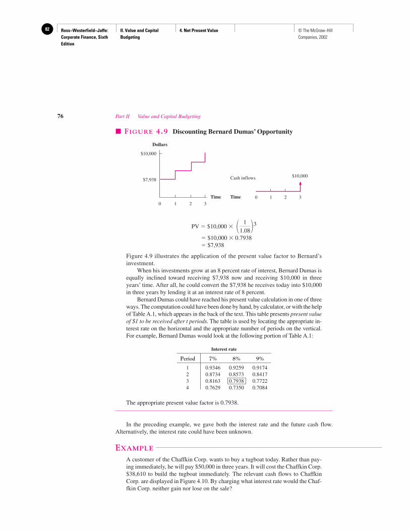
Ross−Westerfield−Jaffe: Corporate Finance, Sixth Edition
II. Value and Capital Budgeting
4. Net Present Value82 © The McGraw−Hill Companies, 2002
PV � $10,000 �
� $10,000 � 0.7938� $7,938
Figure 4.9 illustrates the application of the present value factor to Bernard’sinvestment.
When his investments grow at an 8 percent rate of interest, Bernard Dumas isequally inclined toward receiving $7,938 now and receiving $10,000 in threeyears’ time. After all, he could convert the $7,938 he receives today into $10,000in three years by lending it at an interest rate of 8 percent.
Bernard Dumas could have reached his present value calculation in one of threeways. The computation could have been done by hand, by calculator, or with the helpof Table A.1, which appears in the back of the text. This table presents present valueof $1 to be received after t periods. The table is used by locating the appropriate in-terest rate on the horizontal and the appropriate number of periods on the vertical.For example, Bernard Dumas would look at the following portion of Table A.1:
The appropriate present value factor is 0.7938.
In the preceding example, we gave both the interest rate and the future cash flow.Alternatively, the interest rate could have been unknown.
EXAMPLE
A customer of the Chaffkin Corp. wants to buy a tugboat today. Rather than pay-ing immediately, he will pay $50,000 in three years. It will cost the Chaffkin Corp.$38,610 to build the tugboat immediately. The relevant cash flows to ChaffkinCorp. are displayed in Figure 4.10. By charging what interest rate would the Chaf-fkin Corp. neither gain nor lose on the sale?
Interest rate
Period 7% 8% 9%
1 0.9346 0.9259 0.91742 0.8734 0.8573 0.84173 0.8163 0.7938 0.77224 0.7629 0.7350 0.7084
� 1
1.08�3
76 Part II Value and Capital Budgeting
0 1 2
$7,938
Dollars
Time 0 2 3
$10,000
$10,000
Cash inflows
13
Time
� FIGURE 4.9 Discounting Bernard Dumas’ Opportunity
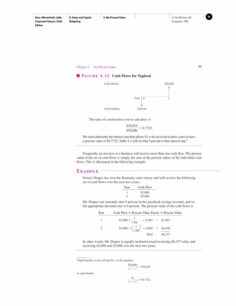
Ross−Westerfield−Jaffe: Corporate Finance, Sixth Edition
II. Value and Capital Budgeting
4. Net Present Value 83© The McGraw−Hill Companies, 2002
The ratio of construction cost to sale price is
� 0.7722
We must determine the interest rate that allows $1 to be received in three years to havea present value of $0.7722. Table A.1 tells us that 9 percent is that interest rate.4
Frequently, an investor or a business will receive more than one cash flow. The presentvalue of the set of cash flows is simply the sum of the present values of the individual cashflows. This is illustrated in the following example.
EXAMPLE
Dennis Draper has won the Kentucky state lottery and will receive the followingset of cash flows over the next two years:
Mr. Draper can currently earn 6 percent in his passbook savings account, and so,the appropriate discount rate is 6 percent. The present value of the cash flows is
Year Cash Flow � Present Value Factor � Present Value
1 $2,000 � � 0.943 � $1,887
2 $5,000 � � 0.890 � $4,450
Total $6,337
In other words, Mr. Draper is equally inclined toward receiving $6,337 today andreceiving $2,000 and $5,000 over the next two years.
� 1
1.06�2
1
1.06
Year Cash Flow
1 $2,0002 $5,000
$38,610
$50,000
Chapter 4 Net Present Value 77
0
– $38,610
$50,000Cash inflows
Time
Cash outflows
3
� FIGURE 4.10 Cash Flows for Tugboat
4Algebraically, we are solving for r in the equation
� $38,610
or, equivalently,
� $0.7722$1
�1 � r� 3
$50,000�1 � r� 3
Ross−Westerfield−Jaffe: Corporate Finance, Sixth Edition
II. Value and Capital Budgeting
4. Net Present Value84 © The McGraw−Hill Companies, 2002
EXAMPLE
Finance.com has an opportunity to invest in a new high-speed computer that costs$50,000. The computer will generate cash flows (from cost savings) of $25,000one year from now, $20,000 two years from now, and $15,000 three years fromnow. The computer will be worthless after three years, and no additional cashflows will occur. Finance.com has determined that the appropriate discount rate is7 percent for this investment. Should Finance.com make this investment in a newhigh-speed computer? What is the present value of the investment?
The cash flows and present value factors of the proposed computer are as follows.
Cash Flows Present Value Factor
Year 0 –$50,000 1 � 1
1 $25,000 � 0.9346
2 $20,000 � 0.8734
3 $15,000 � 0.8163
The present values of the cash flows are:
Cash flows � Present value factor � Present value
Year 0 –$50,000 � 1 � –$50,0001 $25,000 � 0.9346 � $23,3652 $20,000 � 0.8734 � $17,4683 $15,000 � 0.8163 � $12,244.5
Total: $ 3,077.5
Finance.com should invest in a new high-speed computer because the presentvalue of its future cash flows is greater than its cost. The NPV is $3,077.5.
The Algebraic FormulaTo derive an algebraic formula for net present value of a cash flow, recall that the PV of re-ceiving a cash flow one year from now is
PV � C1/(1 � r)
and the PV of receiving a cash flow two years from now is
PV � C2/(1 � r)2
We can write the NPV of a T-period project as
NPV � �C0 �
The initial flow, �C0, is assumed to be negative because it represents an investment. The� is shorthand for the sum of the series.
• What is the difference between simple interest and compound interest?• What is the formula for the net present value of a project?
C1
1 � r �
C2
�1 � r� 2 � ... � CT
�1 � r�T � � C0 � �T
i �1
Ci
�1 � r� i
� 1
1.07�3
� 1
1.07�2
1
1.07
78 Part II Value and Capital Budgeting
QUESTIONS
CO
NC
EP
T
?
Ross−Westerfield−Jaffe: Corporate Finance, Sixth Edition
II. Value and Capital Budgeting
4. Net Present Value 85© The McGraw−Hill Companies, 2002
4.3 COMPOUNDING PERIODS
So far we have assumed that compounding and discounting occur yearly. Sometimes com-pounding may occur more frequently than just once a year. For example, imagine that a bankpays a 10-percent interest rate “compounded semiannually.” This means that a $1,000 depositin the bank would be worth $1,000 � 1.05 � $1,050 after six months, and $1,050 � 1.05 �$1,102.50 at the end of the year.
The end-of-the-year wealth can be written as5
$1,000 � $1,000 � (1.05)2 � $1,102.50
Of course, a $1,000 deposit would be worth $1,100 ($1,000 � 1.10) with yearly com-pounding. Note that the future value at the end of one year is greater with semiannual com-pounding than with yearly compounding. With yearly compounding, the original $1,000 re-mains the investment base for the full year. The original $1,000 is the investment base onlyfor the first six months with semiannual compounding. The base over the second six monthsis $1,050. Hence, one gets interest on interest with semiannual compounding.
Because $1,000 � 1.1025 � $1,102.50, 10 percent compounded semiannually is thesame as 10.25 percent compounded annually. In other words, a rational investor could notcare less whether she is quoted a rate of 10 percent compounded semiannually, or a rate of10.25 percent compounded annually.
Quarterly compounding at 10 percent yields wealth at the end of one year of
$1,000 � $1,103.81
More generally, compounding an investment m times a year provides end-of-yearwealth of
(4.4)
where C0 is one’s initial investment and r is the stated annual interest rate. The stated an-nual interest rate is the annual interest rate without consideration of compounding. Banksand other financial institutions may use other names for the stated annual interest rate. An-nual percentage rate is perhaps the most common synonym.
EXAMPLE
What is the end-of-year wealth if Jane Christine receives a stated annual interestrate of 24 percent compounded monthly on a $1 investment?
Using (4.4), her wealth is
$1 � $1 � (1.02)12
� $1.2682
�1 � 0.24
12 �12
C0�1 � r
m�m
�1 � 0.10
4 �4
�1 � 0.10
2 �2
Chapter 4 Net Present Value 79
5In addition to using a calculator, one can still use Table A.3 when the compounding period is less than a year.Here, one sets the interest rate at 5 percent and the number of periods at two.
Ross−Westerfield−Jaffe: Corporate Finance, Sixth Edition
II. Value and Capital Budgeting
4. Net Present Value86 © The McGraw−Hill Companies, 2002
The annual rate of return is 26.82 percent. This annual rate of return is either calledthe effective annual interest rate or the effective annual yield. Due to com-pounding, the effective annual interest rate is greater than the stated annual interestrate of 24 percent. Algebraically, we can rewrite the effective annual interest rate as
Effective Annual Interest Rate:
� 1 (4.5)
Students are often bothered by the subtraction of 1 in (4.5). Note that end-of-yearwealth is composed of both the interest earned over the year and the original prin-cipal. We remove the original principal by subtracting one in (4.5).
EXAMPLE
If the stated annual rate of interest, 8 percent, is compounded quarterly, what is theeffective annual rate of interest?
Using (4.5), we have
� 1 � 0.0824 � 8.24%
Referring back to our original example where C0 � $1,000 and r � 10%, wecan generate the following table:
Effective AnnualInterest Rate �
C0 Compounding Frequency (m) C1
$1,000 Yearly (m � 1) $1,100.00 0.101,000 Semiannually (m � 2) 1,102.50 0.10251,000 Quarterly (m � 4) 1,103.81 0.103811,000 Daily (m � 365) 1,105.16 0.10516
Distinction between Stated Annual Interest Rate and Effective Annual Interest RateThe distinction between the stated annual interest rate (SAIR) and the effective annual in-terest rate (EAIR) is frequently quite troubling to students. One can reduce the confusionby noting that the SAIR becomes meaningful only if the compounding interval is given. Forexample, for an SAIR of 10 percent, the future value at the end of one year with semian-nual compounding is [1 � (.10/2)]2 � 1.1025. The future value with quarterly compound-ing is [1 � (.10/4)]4 � 1.1038. If the SAIR is 10 percent but no compounding interval isgiven, one cannot calculate future value. In other words, one does not know whether tocompound semiannually, quarterly, or over some other interval.
By contrast, the EAIR is meaningful without a compounding interval. For example, anEAIR of 10.25 percent means that a $1 investment will be worth $1.1025 in one year. Onecan think of this as an SAIR of 10 percent with semiannual compounding or an SAIR of10.25 percent with annual compounding, or some other possibility.
�1 �rm�
m � 1
�1 �r
m�m
� 1 � �1 �0.08
4 �4
�1 �r
m�m
80 Part II Value and Capital Budgeting
Ross−Westerfield−Jaffe: Corporate Finance, Sixth Edition
II. Value and Capital Budgeting
4. Net Present Value 87© The McGraw−Hill Companies, 2002
Compounding over Many YearsFormula (4.4) applies for an investment over one year. For an investment over one or more(T) years, the formula becomes
Future Value with Compounding:
FV � (4.6)
EXAMPLE
Harry DeAngelo is investing $5,000 at a stated annual interest rate of 12 percent peryear, compounded quarterly, for five years. What is his wealth at the end of five years?
Using formula (4.6), his wealth is
$5,000 � � $5,000 � (1.03)20 � $5,000 � 1.8061 � $9,030.50
Continuous Compounding (Advanced)The previous discussion shows that one can compound much more frequently than once ayear. One could compound semiannually, quarterly, monthly, daily, hourly, each minute, oreven more often. The limiting case would be to compound every infinitesimal instant,which is commonly called continuous compounding. Surprisingly, banks and other fi-nancial institutions frequently quote continuously compounded rates, which is why westudy them.
Though the idea of compounding this rapidly may boggle the mind, a simple formulais involved. With continuous compounding, the value at the end of T years is expressed as
C0 � erT (4.7)
where C0 is the initial investment, r is the stated annual interest rate, and T is the number ofyears over which the investment runs. The number e is a constant and is approximatelyequal to 2.718. It is not an unknown like C0, r, and T.
EXAMPLE
Linda DeFond invested $1,000 at a continuously compounded rate of 10 percentfor one year. What is the value of her wealth at the end of one year?
From formula (4.7) we have
$1,000 � e0.10 � $1,000 � 1.1052 � $1,105.20
This number can easily be read from our Table A.5. One merely sets r, the valueon the horizontal dimension, to 10% and T, the value on the vertical dimension, to1. For this problem, the relevant portion of the table is
Continuously compounded rate (r)
Period(T) 9% 10% 11%
1 1.0942 1.1052 1.11632 1.1972 1.2214 1.24613 1.3100 1.3499 1.3910
�1 � 0.12
4 �4�5
C0�1 �r
m�mT
Chapter 4 Net Present Value 81
Ross−Westerfield−Jaffe: Corporate Finance, Sixth Edition
II. Value and Capital Budgeting
4. Net Present Value88 © The McGraw−Hill Companies, 2002
Note that a continuously compounded rate of 10 percent is equivalent to anannually compounded rate of 10.52 percent. In other words, Linda DeFond couldnot care less whether her bank quoted a continuously compounded rate of 10 per-cent or a 10.52-percent rate, compounded annually.
EXAMPLE
Linda DeFond’s brother, Mark, invested $1,000 at a continuously compoundedrate of 10 percent for two years.
The appropriate formula here is
$1,000 � e0.10�2 � $1,000 � e0.20� $1,221.40
Using the portion of the table of continuously compounded rates reproducedabove, we find the value to be 1.2214.
Figure 4.11 illustrates the relationship among annual, semiannual, and continuouscompounding. Semiannual compounding gives rise to both a smoother curve and a higherending value than does annual compounding. Continuous compounding has both thesmoothest curve and the highest ending value of all.
EXAMPLE
The Michigan state lottery is going to pay you $1,000 at the end of four years. Ifthe annual continuously compounded rate of interest is 8 percent, what is the pres-ent value of this payment?
$1,000 � � $1,000 � � $726.16
• What is a stated annual interest rate?• What is an effective annual interest rate?• What is the relationship between the stated annual interest rate and the effective annual
interest rate?• Define continuous compounding.
1
1.3771
1
e0.08�4
82 Part II Value and Capital Budgeting
0 1 5
1
Dollars
2
3
2 3 4
4Interestearned
Years
Annual compounding
0 1 5
1
Dollars
2
3
2 3 4
4Interestearned
Years
Semiannual compounding
0 1 5
1
Dollars
2
3
2 3 4
4
Interestearned
Years
Continuous compounding
� FIGURE 4.11 Annual, Semiannual, and Continuous Compounding
QUESTIONS
CO
NC
EP
T
?
Ross−Westerfield−Jaffe: Corporate Finance, Sixth Edition
II. Value and Capital Budgeting
4. Net Present Value 89© The McGraw−Hill Companies, 2002
4.4 SIMPLIFICATIONS
The first part of this chapter has examined the concepts of future value and present value.Although these concepts allow one to answer a host of problems concerning the time valueof money, the human effort involved can frequently be excessive. For example, consider abank calculating the present value on a 20-year monthly mortgage. Because this mortgagehas 240 (20 � 12) payments, a lot of time is needed to perform a conceptually simple task.
Because many basic finance problems are potentially so time-consuming, we searchout simplifications in this section. We provide simplifying formulas for four classes of cashflow streams:
• Perpetuity• Growing perpetuity• Annuity• Growing annuity
PerpetuityA perpetuity is a constant stream of cash flows without end. If you are thinking that per-petuities have no relevance to reality, it will surprise you that there is a well-known case ofan unending cash flow stream: the British bonds called consols. An investor purchasing aconsol is entitled to receive yearly interest from the British government forever.
How can the price of a consol be determined? Consider a consol that pays a coupon ofC dollars each year and will do so forever. Simply applying the PV formula gives us
PV � � . . .
where the dots at the end of the formula stand for the infinite string of terms that continuesthe formula. Series like the preceding one are called geometric series. It is well known thateven though they have an infinite number of terms, the whole series has a finite sum be-cause each term is only a fraction of the preceding term. Before turning to our calculusbooks, though, it is worth going back to our original principles to see if a bit of financial in-tuition can help us find the PV.
The present value of the consol is the present value of all of its future coupons. In otherwords, it is an amount of money that, if an investor had it today, would enable him to achievethe same pattern of expenditures that the consol and its coupons would. Suppose that an in-vestor wanted to spend exactly C dollars each year. If he had the consol, he could do this.How much money must he have today to spend the same amount? Clearly he would needexactly enough so that the interest on the money would be C dollars per year. If he had anymore, he could spend more than C dollars each year. If he had any less, he would eventu-ally run out of money spending C dollars per year.
The amount that will give the investor C dollars each year, and therefore the presentvalue of the consol, is simply
PV � (4.8)
To confirm that this is the right answer, notice that if we lend the amount C/r, the interest itearns each year will be
Interest � � r � CC
r
C
r
C
1 � r �
C�1 � r� 2 �
C�1 � r� 3
Chapter 4 Net Present Value 83
Ross−Westerfield−Jaffe: Corporate Finance, Sixth Edition
II. Value and Capital Budgeting
4. Net Present Value90 © The McGraw−Hill Companies, 2002
which is exactly the consol payment.6 To sum up, we have shown that for a consol
Formula for Present Value of Perpetuity:
PV � � . . .
�
It is comforting to know how easily we can use a bit of financial intuition to solve this math-ematical problem.
EXAMPLE
Consider a perpetuity paying $100 a year. If the relevant interest rate is 8 percent,what is the value of the consol?
Using formula (4.8), we have
PV � � $1,250
Now suppose that interest rates fall to 6 percent. Using (4.8), the value of the per-petuity is
PV � � $1,666.67
Note that the value of the perpetuity rises with a drop in the interest rate. Con-versely, the value of the perpetuity falls with a rise in the interest rate.
Growing PerpetuityImagine an apartment building where cash flows to the landlord after expenses will be$100,000 next year. These cash flows are expected to rise at 5 percent per year. If one as-sumes that this rise will continue indefinitely, the cash flow stream is termed a growingperpetuity. The relevant interest rate is 11 percent. Therefore, the appropriate discount rateis 11 percent and the present value of the cash flows can be represented as
PV � � . . . � � . . .$100,000�1.05�N�1
�1.11�N
$100,000
1.11 �
$100,000�1.05��1.11� 2 �
$100,000�1.05� 2
�1.11� 3
$100
0.06
$100
0.08
C
r
C
1 � r �
C�1 � r� 2 �
C�1 � r� 3
84 Part II Value and Capital Budgeting
6We can prove this by looking at the PV equation:
PV � C/(1 � r) � C/(1 � r)2 � . . .
Let C/(1 � r) � a and 1/(1 � r) � x. We now have
PV � a(1 � x � x2 � . . .) (1)
Next we can multiply by x:
xPV � ax � ax2 � . . . (2)
Subtracting (2) from (1) gives
PV(1 � x) � a
Now we substitute for a and x and rearrange:
PV � C/r
Ross−Westerfield−Jaffe: Corporate Finance, Sixth Edition
II. Value and Capital Budgeting
4. Net Present Value 91© The McGraw−Hill Companies, 2002
Algebraically, we can write the formula as
PV � � . . . � � . . . (4.9)
where C is the cash flow to be received one period hence, g is the rate of growth per period,expressed as a percentage, and r is the appropriate discount rate.
Fortunately, formula (4.9) reduces to the following simplification:7
Formula for Present Value of Growing Perpetuity:
PV � (4.10)
From formula (4.10), the present value of the cash flows from the apartment building is
� $1,666,667
There are three important points concerning the growing perpetuity formula:
1. The Numerator. The numerator in (4.10) is the cash flow one period hence, not atdate 0. Consider the following example:
EXAMPLE
Rothstein Corporation is just about to pay a dividend of $3.00 per share. Investorsanticipate that the annual dividend will rise by 6 percent a year forever. The ap-plicable interest rate is 11 percent. What is the price of the stock today?
The numerator in formula (4.10) is the cash flow to be received next period.Since the growth rate is 6 percent, the dividend next year is $3.18 ($3.00 � 1.06).The price of the stock today is
$66.60 � $3.00 �
Imminent Present value of alldividend dividends beginning
a year from now
The price of $66.60 includes both the dividend to be received immediately and thepresent value of all dividends beginning a year from now. Formula (4.10) onlymakes it possible to calculate the present value of all dividends beginning a yearfrom now. Be sure you understand this example; test questions on this subject al-ways seem to trip up a few of our students.
$3.18
0.11 � 0.06
$100,000
0.11 � 0.05
C
r � g
C � �1 � g�N�1
�1 � r�N
C
1 � r �
C � �1 � g��1 � r� 2 �
C � �1 � g� 2
�1 � r� 3
Chapter 4 Net Present Value 85
7PV is the sum of an infinite geometric series:
PV � a(1 � x � x2 � . . .)
where a � C/(1 � r) and x � (1 � g)/(1 � r). Previously we showed that the sum of an infinite geometric seriesis a/(1 � x). Using this result and substituting for a and x, we find
PV � C/(r � g)
Note that this geometric series converges to a finite sum only when x is less than 1. This implies that the growthrate, g, must be less than the interest rate, r.
Ross−Westerfield−Jaffe: Corporate Finance, Sixth Edition
II. Value and Capital Budgeting
4. Net Present Value92 © The McGraw−Hill Companies, 2002
2. The Interest Rate and the Growth Rate. The interest rate r must be greater than thegrowth rate g for the growing perpetuity formula to work. Consider the case in which thegrowth rate approaches the interest rate in magnitude. Then the denominator in the grow-ing perpetuity formula gets infinitesimally small and the present value grows infinitelylarge. The present value is in fact undefined when r is less than g.
3. The Timing Assumption. Cash generally flows into and out of real-world firms bothrandomly and nearly continuously. However, formula (4.10) assumes that cash flows are re-ceived and disbursed at regular and discrete points in time. In the example of the apartment,we assumed that the net cash flows of $100,000 only occurred once a year. In reality, rentchecks are commonly received every month. Payments for maintenance and other expensesmay occur anytime within the year.
The growing perpetuity formula of (4.10) can be applied only by assuming a regularand discrete pattern of cash flow. Although this assumption is sensible because the formulasaves so much time, the user should never forget that it is an assumption. This point will bementioned again in the chapters ahead.
A few words should be said about terminology. Authors of financial textbooks gener-ally use one of two conventions to refer to time. A minority of financial writers treat cashflows as being received on exact dates, for example date 0, date 1, and so forth. Under thisconvention, date 0 represents the present time. However, because a year is an interval, nota specific moment in time, the great majority of authors refer to cash flows that occur at theend of a year (or alternatively, the end of a period). Under this end-of-the-year convention,the end of year 0 is the present, the end of year 1 occurs one period hence, and so on. (Thebeginning of year 0 has already passed and is not generally referred to.)8
The interchangeability of the two conventions can be seen from the following chart:
Date 0 Date 1 Date 2 Date 3 . . .� Now
End of year 0 End of year 1 End of year 2 End of year 3 . . .� Now
We strongly believe that the dates convention reduces ambiguity. However, we use bothconventions because you are likely to see the end-of-year convention in later courses. Infact, both conventions may appear in the same example for the sake of practice.
AnnuityAn annuity is a level stream of regular payments that lasts for a fixed number of periods.Not surprisingly, annuities are among the most common kinds of financial instruments. Thepensions that people receive when they retire are often in the form of an annuity. Leases andmortgages are also often annuities.
To figure out the present value of an annuity we need to evaluate the following equation:
� . . . �
The present value of only receiving the coupons for T periods must be less than the presentvalue of a consol, but how much less? To answer this we have to look at consols a bit moreclosely.
C�1 � r�T
C
1 � r �
C�1 � r� 2 �
C�1 � r� 3
86 Part II Value and Capital Budgeting
8Sometimes financial writers merely speak of a cash flow in year x. Although this terminology is ambiguous,such writers generally mean the end of year x.

Ross−Westerfield−Jaffe: Corporate Finance, Sixth Edition
II. Value and Capital Budgeting
4. Net Present Value 93© The McGraw−Hill Companies, 2002
Consider the following time chart:
Now
Date (or end of year) 0 1 2 3 T (T � 1) (T � 2)Consol 1 C C C . . . C C C . . .Consol 2 C C . . .Annuity C C C . . . C
Consol 1 is a normal consol with its first payment at date 1. The first payment of consol 2occurs at date T � 1.
The present value of having a cash flow of C at each of T dates is equal to the present valueof consol 1 minus the present value of consol 2. The present value of consol 1 is given by
PV � (4.11)
Consol 2 is just a consol with its first payment at date T � 1. From the perpetuity formula,this consol will be worth C/r at date T.9 However, we do not want the value at date T. Wewant the value now; in other words, the present value at date 0. We must discount C/r backby T periods. Therefore, the present value of consol 2 is
PV � (4.12)
The present value of having cash flows for T years is the present value of a consol with its firstpayment at date 1 minus the present value of a consol with its first payment at date T � 1. Thus,the present value of an annuity is formula (4.11) minus formula (4.12). This can be written as
This simplifies to
Formula for Present Value of Annuity:10, 11
PV � C (4.13)
EXAMPLE
Mark Young has just won the state lottery, paying $50,000 a year for 20 years. Heis to receive his first payment a year from now. The state advertises this as the Mil-lion Dollar Lottery because $1,000,000 � $50,000 � 20. If the interest rate is 8percent, what is the true value of the lottery?
�1
r �
1
r�1 � r�T
C
r �
C
r �1
�1 � r�T
C
r �1
�1 � r�T
C
r
Chapter 4 Net Present Value 87
9Students frequently think that C/r is the present value at date T � 1 because the consol’s first payment is atdate T � 1. However, the formula values the annuity as of one period prior to the first payment.10This can also be written as
C[1 � 1/(1 � r)T ]/r11We can also provide a formula for the future value of an annuity.
FV � C��1 � r�T
r �
1
r
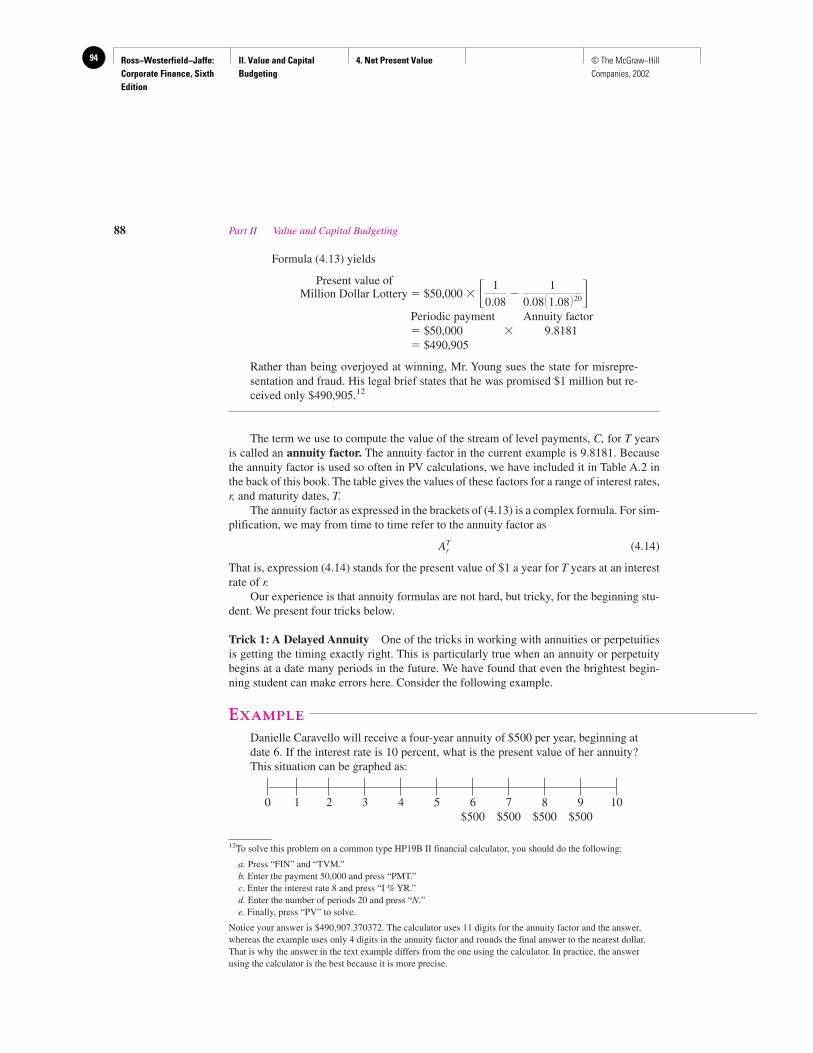
Ross−Westerfield−Jaffe: Corporate Finance, Sixth Edition
II. Value and Capital Budgeting
4. Net Present Value94 © The McGraw−Hill Companies, 2002
Formula (4.13) yields
Present value ofMillion Dollar Lottery � $50,000 �
Periodic payment Annuity factor� $50,000 � 9.8181� $490,905
Rather than being overjoyed at winning, Mr. Young sues the state for misrepre-sentation and fraud. His legal brief states that he was promised $1 million but re-ceived only $490,905.12
The term we use to compute the value of the stream of level payments, C, for T yearsis called an annuity factor. The annuity factor in the current example is 9.8181. Becausethe annuity factor is used so often in PV calculations, we have included it in Table A.2 inthe back of this book. The table gives the values of these factors for a range of interest rates,r, and maturity dates, T.
The annuity factor as expressed in the brackets of (4.13) is a complex formula. For sim-plification, we may from time to time refer to the annuity factor as
(4.14)
That is, expression (4.14) stands for the present value of $1 a year for T years at an interestrate of r.
Our experience is that annuity formulas are not hard, but tricky, for the beginning stu-dent. We present four tricks below.
Trick 1: A Delayed Annuity One of the tricks in working with annuities or perpetuitiesis getting the timing exactly right. This is particularly true when an annuity or perpetuitybegins at a date many periods in the future. We have found that even the brightest begin-ning student can make errors here. Consider the following example.
EXAMPLE
Danielle Caravello will receive a four-year annuity of $500 per year, beginning atdate 6. If the interest rate is 10 percent, what is the present value of her annuity?This situation can be graphed as:
0 1 2 3 4 5 6 7 8 9 10$500 $500 $500 $500
ATr
� 1
0.08 �
1
0.08�1.08� 20
88 Part II Value and Capital Budgeting
12To solve this problem on a common type HP19B II financial calculator, you should do the following:
a. Press “FIN” and “TVM.”b. Enter the payment 50,000 and press “PMT.”c. Enter the interest rate 8 and press “I % YR.”d. Enter the number of periods 20 and press “N.”e. Finally, press “PV” to solve.
Notice your answer is $490,907.370372. The calculator uses 11 digits for the annuity factor and the answer,whereas the example uses only 4 digits in the annuity factor and rounds the final answer to the nearest dollar.That is why the answer in the text example differs from the one using the calculator. In practice, the answerusing the calculator is the best because it is more precise.
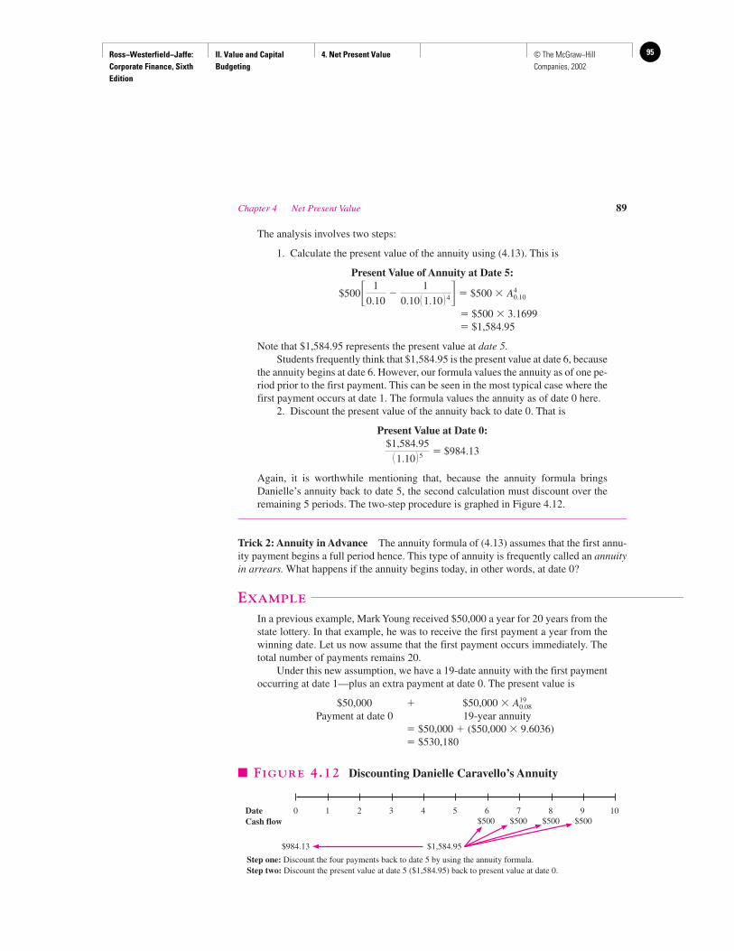
Ross−Westerfield−Jaffe: Corporate Finance, Sixth Edition
II. Value and Capital Budgeting
4. Net Present Value 95© The McGraw−Hill Companies, 2002
The analysis involves two steps:
1. Calculate the present value of the annuity using (4.13). This is
Present Value of Annuity at Date 5:
$500 � $500 �
� $500 � 3.1699� $1,584.95
Note that $1,584.95 represents the present value at date 5.Students frequently think that $1,584.95 is the present value at date 6, because
the annuity begins at date 6. However, our formula values the annuity as of one pe-riod prior to the first payment. This can be seen in the most typical case where thefirst payment occurs at date 1. The formula values the annuity as of date 0 here.
2. Discount the present value of the annuity back to date 0. That is
Present Value at Date 0:
� $984.13
Again, it is worthwhile mentioning that, because the annuity formula bringsDanielle’s annuity back to date 5, the second calculation must discount over theremaining 5 periods. The two-step procedure is graphed in Figure 4.12.
Trick 2: Annuity in Advance The annuity formula of (4.13) assumes that the first annu-ity payment begins a full period hence. This type of annuity is frequently called an annuityin arrears. What happens if the annuity begins today, in other words, at date 0?
EXAMPLE
In a previous example, Mark Young received $50,000 a year for 20 years from thestate lottery. In that example, he was to receive the first payment a year from thewinning date. Let us now assume that the first payment occurs immediately. Thetotal number of payments remains 20.
Under this new assumption, we have a 19-date annuity with the first paymentoccurring at date 1—plus an extra payment at date 0. The present value is
$50,000 � $50,000 �Payment at date 0 19-year annuity
� $50,000 � ($50,000 � 9.6036)� $530,180
A
190.08
$1,584.95�1.10� 5
A40.10� 1
0.10 �
1
0.10�1.10� 4
Chapter 4 Net Present Value 89
0 1 2 3 4 5 6 7 8 9 10DateCash flow
$984.13 $1,584.95
$500 $500 $500 $500
� FIGURE 4.12 Discounting Danielle Caravello’s Annuity
Step one: Discount the four payments back to date 5 by using the annuity formula.Step two: Discount the present value at date 5 ($1,584.95) back to present value at date 0.
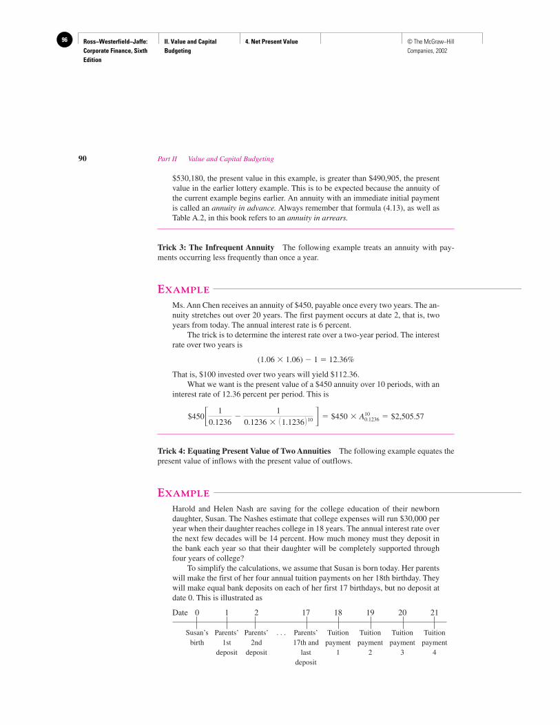
Ross−Westerfield−Jaffe: Corporate Finance, Sixth Edition
II. Value and Capital Budgeting
4. Net Present Value96 © The McGraw−Hill Companies, 2002
$530,180, the present value in this example, is greater than $490,905, the presentvalue in the earlier lottery example. This is to be expected because the annuity ofthe current example begins earlier. An annuity with an immediate initial paymentis called an annuity in advance. Always remember that formula (4.13), as well asTable A.2, in this book refers to an annuity in arrears.
Trick 3: The Infrequent Annuity The following example treats an annuity with pay-ments occurring less frequently than once a year.
EXAMPLE
Ms. Ann Chen receives an annuity of $450, payable once every two years. The an-nuity stretches out over 20 years. The first payment occurs at date 2, that is, twoyears from today. The annual interest rate is 6 percent.
The trick is to determine the interest rate over a two-year period. The interestrate over two years is
(1.06 � 1.06) � 1 � 12.36%
That is, $100 invested over two years will yield $112.36.What we want is the present value of a $450 annuity over 10 periods, with an
interest rate of 12.36 percent per period. This is
$450 $2,505.57
Trick 4: Equating Present Value of Two Annuities The following example equates thepresent value of inflows with the present value of outflows.
EXAMPLE
Harold and Helen Nash are saving for the college education of their newborndaughter, Susan. The Nashes estimate that college expenses will run $30,000 peryear when their daughter reaches college in 18 years. The annual interest rate overthe next few decades will be 14 percent. How much money must they deposit inthe bank each year so that their daughter will be completely supported throughfour years of college?
To simplify the calculations, we assume that Susan is born today. Her parentswill make the first of her four annual tuition payments on her 18th birthday. Theywill make equal bank deposits on each of her first 17 birthdays, but no deposit atdate 0. This is illustrated as
Date 0 1 2 17 18 19 20 21
Susan’s Parents’ Parents’ . . . Parents’ Tuition Tuition Tuition Tuitionbirth 1st 2nd 17th and payment payment payment payment
deposit deposit last 1 2 3 4deposit
� 1
0.1236�
1
0.1236 � �1.1236� 10 � $450 � A
100.1236 �
90 Part II Value and Capital Budgeting
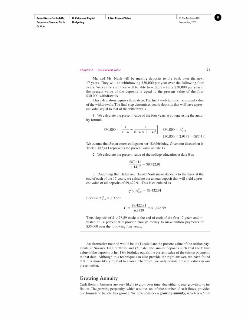
Ross−Westerfield−Jaffe: Corporate Finance, Sixth Edition
II. Value and Capital Budgeting
4. Net Present Value 97© The McGraw−Hill Companies, 2002
Mr. and Ms. Nash will be making deposits to the bank over the next 17 years. They will be withdrawing $30,000 per year over the following fouryears. We can be sure they will be able to withdraw fully $30,000 per year ifthe present value of the deposits is equal to the present value of the four$30,000 withdrawals.
This calculation requires three steps. The first two determine the present valueof the withdrawals. The final step determines yearly deposits that will have a pres-ent value equal to that of the withdrawals.
1. We calculate the present value of the four years at college using the annu-ity formula.
$30,000 � � $30,000 �
� $30,000 � 2.9137 � $87,411
We assume that Susan enters college on her 18th birthday. Given our discussion inTrick 1 $87,411 represents the present value at date 17.
2. We calculate the present value of the college education at date 0 as
� $9,422.91
3. Assuming that Helen and Harold Nash make deposits to the bank at theend of each of the 17 years, we calculate the annual deposit that will yield a pres-ent value of all deposits of $9,422.91. This is calculated as
C � � $9,422.91
Because � 6.3729,
� $1,478.59
Thus, deposits of $1,478.59 made at the end of each of the first 17 years and in-vested at 14 percent will provide enough money to make tuition payments of$30,000 over the following four years.
An alternative method would be to (1) calculate the present value of the tuition pay-ments at Susan’s 18th birthday and (2) calculate annual deposits such that the futurevalue of the deposits at her 18th birthday equals the present value of the tuition paymentsat that date. Although this technique can also provide the right answer, we have foundthat it is more likely to lead to errors. Therefore, we only equate present values in ourpresentation.
Growing AnnuityCash flows in business are very likely to grow over time, due either to real growth or to in-flation. The growing perpetuity, which assumes an infinite number of cash flows, providesone formula to handle this growth. We now consider a growing annuity, which is a finite
C �$9,422.91
6.3729
A
170.14
A
170.14
$87,411�1.14� 17
A
40.14� 1
0.14�
1
0.14 � �1.14� 4
Chapter 4 Net Present Value 91
Ross−Westerfield−Jaffe: Corporate Finance, Sixth Edition
II. Value and Capital Budgeting
4. Net Present Value98 © The McGraw−Hill Companies, 2002
number of growing cash flows. Because perpetuities of any kind are rare, a formula for agrowing annuity would be useful indeed. The formula is13
Formula for Present Value of Growing Annuity:
PV � C (4.15)
where, as before, C is the payment to occur at the end of the first period, r is the interestrate, g is the rate of growth per period, expressed as a percentage, and T is the number ofperiods for the annuity.
EXAMPLE
Stuart Gabriel, a second-year MBA student, has just been offered a job at $80,000a year. He anticipates his salary increasing by 9 percent a year until his retirementin 40 years. Given an interest rate of 20 percent, what is the present value of hislifetime salary?
We simplify by assuming he will be paid his $80,000 salary exactly one yearfrom now, and that his salary will continue to be paid in annual installments. Theappropriate discount rate is 20 percent. From (4.15), the calculation is
Present valueof Stuart’s � $80,000 � � $711,731
lifetime salary
Though the growing annuity is quite useful, it is more tedious than the other simpli-fying formulas. Whereas most sophisticated calculators have special programs forperpetuity, growing perpetuity, and annuity, there is no special program for growingannuity. Hence, one must calculate all the terms in formula (4.15) directly.
EXAMPLE
In a previous example, Harold and Helen Nash planned to make 17 identical pay-ments in order to fund the college education of their daughter, Susan. Alterna-tively, imagine that they planned to increase their payments at 4 percent per year.What would their first payment be?
� 1
0.20 � 0.09�
1
0.20 � 0.09�1.09
1.20�40
� 1
r � g�
1
r � g� �1 � g
1 � r�T
92 Part II Value and Capital Budgeting
13This can be proved as follows. A growing annuity can be viewed as the difference between two growingperpetuities. Consider a growing perpetuity A, where the first payment of C occurs at date 1. Next, considergrowing perpetuity B, where the first payment of C(1 � g)T is made at date T � 1. Both perpetuities grow at rate g.The growing annuity over T periods is the difference between annuity A and annuity B. This can be represented as:
Date 0 1 2 3 . . . T T � 1 T � 2 T � 3
Perpetuity A C C � (1 � g) C � (1 � g)2 . . . C � (1 � g)T�1 C � (1 � g)T C � (1 � g)T�1 C � (1 � g)T�2 . . .
Perpetuity B C � (1 � g)T C � (1 � g)T�1 C � (1 � g)T�2 . . .
Annuity C C � (1 � g) C � (1 � g)2 . . . C � (1 � g)T�1
The value of perpetuity A is
The value of perpetuity B is
The difference between the two perpetuities is given by (4.15).
C � �1 � g�T
r � g�
1�1 � r�T
C
r � g
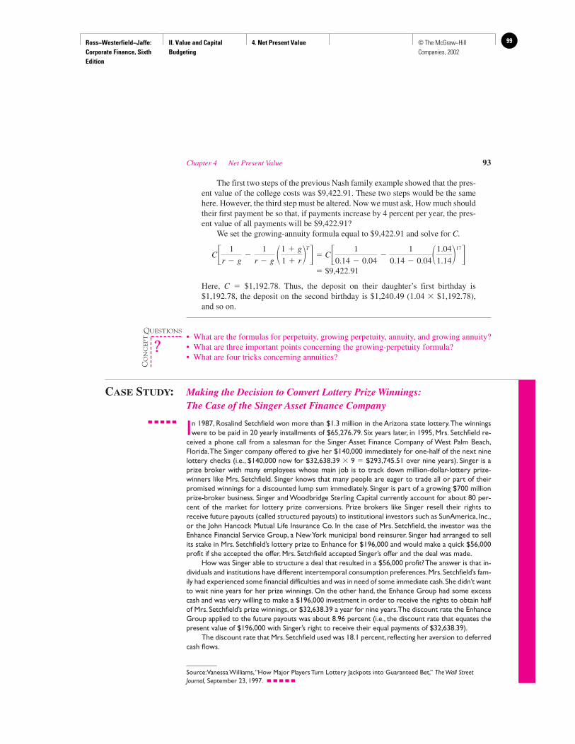
Ross−Westerfield−Jaffe: Corporate Finance, Sixth Edition
II. Value and Capital Budgeting
4. Net Present Value 99© The McGraw−Hill Companies, 2002
The first two steps of the previous Nash family example showed that the pres-ent value of the college costs was $9,422.91. These two steps would be the samehere. However, the third step must be altered. Now we must ask, How much shouldtheir first payment be so that, if payments increase by 4 percent per year, the pres-ent value of all payments will be $9,422.91?
We set the growing-annuity formula equal to $9,422.91 and solve for C.
�
� $9,422.91
Here, C � $1,192.78. Thus, the deposit on their daughter’s first birthday is$1,192.78, the deposit on the second birthday is $1,240.49 (1.04 � $1,192.78),and so on.
• What are the formulas for perpetuity, growing perpetuity, annuity, and growing annuity?• What are three important points concerning the growing-perpetuity formula?• What are four tricks concerning annuities?
CASE STUDY: Making the Decision to Convert Lottery Prize Winnings:The Case of the Singer Asset Finance Company
In 1987, Rosalind Setchfield won more than $1.3 million in the Arizona state lottery.The winningswere to be paid in 20 yearly installments of $65,276.79. Six years later, in 1995, Mrs. Setchfield re-
ceived a phone call from a salesman for the Singer Asset Finance Company of West Palm Beach,Florida.The Singer company offered to give her $140,000 immediately for one-half of the next ninelottery checks (i.e., $140,000 now for $32,638.39 � 9 � $293,745.51 over nine years). Singer is aprize broker with many employees whose main job is to track down million-dollar-lottery prize-winners like Mrs. Setchfield. Singer knows that many people are eager to trade all or part of theirpromised winnings for a discounted lump sum immediately. Singer is part of a growing $700 millionprize-broker business. Singer and Woodbridge Sterling Capital currently account for about 80 per-cent of the market for lottery prize conversions. Prize brokers like Singer resell their rights to receive future payouts (called structured payouts) to institutional investors such as SunAmerica, Inc.,or the John Hancock Mutual Life Insurance Co. In the case of Mrs. Setchfield, the investor was theEnhance Financial Service Group, a New York municipal bond reinsurer. Singer had arranged to sellits stake in Mrs. Setchfield’s lottery prize to Enhance for $196,000 and would make a quick $56,000profit if she accepted the offer. Mrs. Setchfield accepted Singer’s offer and the deal was made.
How was Singer able to structure a deal that resulted in a $56,000 profit? The answer is that in-dividuals and institutions have different intertemporal consumption preferences.Mrs. Setchfield’s fam-ily had experienced some financial difficulties and was in need of some immediate cash.She didn’t wantto wait nine years for her prize winnings. On the other hand, the Enhance Group had some excesscash and was very willing to make a $196,000 investment in order to receive the rights to obtain halfof Mrs. Setchfield’s prize winnings, or $32,638.39 a year for nine years.The discount rate the EnhanceGroup applied to the future payouts was about 8.96 percent (i.e., the discount rate that equates thepresent value of $196,000 with Singer’s right to receive their equal payments of $32,638.39).
The discount rate that Mrs. Setchfield used was 18.1 percent, reflecting her aversion to deferredcash flows.
Source:Vanessa Williams,“How Major Players Turn Lottery Jackpots into Guaranteed Bet,” The Wall StreetJournal, September 23, 1997.
C� 1
0.14 � 0.04�
1
0.14 � 0.04�1.04
1.14�17C� 1
r � g�
1
r � g �1 � g
1 � r�T
Chapter 4 Net Present Value 93
QUESTIONS
CO
NC
EP
T
?
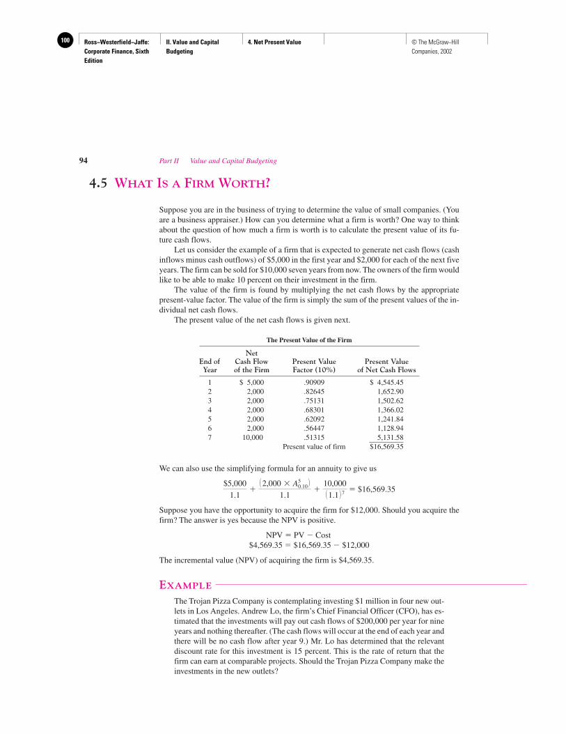
Ross−Westerfield−Jaffe: Corporate Finance, Sixth Edition
II. Value and Capital Budgeting
4. Net Present Value100 © The McGraw−Hill Companies, 2002
4.5 WHAT IS A FIRM WORTH?
Suppose you are in the business of trying to determine the value of small companies. (Youare a business appraiser.) How can you determine what a firm is worth? One way to thinkabout the question of how much a firm is worth is to calculate the present value of its fu-ture cash flows.
Let us consider the example of a firm that is expected to generate net cash flows (cashinflows minus cash outflows) of $5,000 in the first year and $2,000 for each of the next fiveyears. The firm can be sold for $10,000 seven years from now. The owners of the firm wouldlike to be able to make 10 percent on their investment in the firm.
The value of the firm is found by multiplying the net cash flows by the appropriatepresent-value factor. The value of the firm is simply the sum of the present values of the in-dividual net cash flows.
The present value of the net cash flows is given next.
We can also use the simplifying formula for an annuity to give us
� $16,569.35
Suppose you have the opportunity to acquire the firm for $12,000. Should you acquire thefirm? The answer is yes because the NPV is positive.
NPV � PV � Cost$4,569.35 � $16,569.35 � $12,000
The incremental value (NPV) of acquiring the firm is $4,569.35.
EXAMPLE
The Trojan Pizza Company is contemplating investing $1 million in four new out-lets in Los Angeles. Andrew Lo, the firm’s Chief Financial Officer (CFO), has es-timated that the investments will pay out cash flows of $200,000 per year for nineyears and nothing thereafter. (The cash flows will occur at the end of each year andthere will be no cash flow after year 9.) Mr. Lo has determined that the relevantdiscount rate for this investment is 15 percent. This is the rate of return that thefirm can earn at comparable projects. Should the Trojan Pizza Company make theinvestments in the new outlets?
$5,000
1.1�
�2,000 � A
50.10�
1.1�
10,000�1.1� 7
The Present Value of the Firm
NetEnd of Cash Flow Present Value Present ValueYear of the Firm Factor (10%) of Net Cash Flows
1 $ 5,000 .90909 $ 4,545.452 2,000 .82645 1,652.903 2,000 .75131 1,502.624 2,000 .68301 1,366.025 2,000 .62092 1,241.846 2,000 .56447 1,128.947 10,000 .51315 5,131.58
Present value of firm $16,569.35
94 Part II Value and Capital Budgeting
Ross−Westerfield−Jaffe: Corporate Finance, Sixth Edition
II. Value and Capital Budgeting
4. Net Present Value 101© The McGraw−Hill Companies, 2002
Chapter 4 Net Present Value 95
The decision can be evaluated as:
NPV � �$1,000,000 � � . . . �
� �$1,000,000 � $200,000 �� �$1,000,000 � $954,316.78� �$45,683.22
The present value of the four new outlets is only $954,316.78. The outlets areworth less than they cost. The Trojan Pizza Company should not make the invest-ment because the NPV is �$45,683.22. If the Trojan Pizza Company requires a15 percent rate of return, the new outlets are not a good investment.
4.6 SUMMARY AND CONCLUSIONS
1. Two basic concepts, future value and present value, were introduced in the beginning of thischapter. With a 10-percent interest rate, an investor with $1 today can generate a future valueof $1.10 in a year, $1.21 [$1 � (1.10)2] in two years, and so on. Conversely, present-valueanalysis places a current value on a later cash flow. With the same 10-percent interest rate, adollar to be received in one year has a present value of $0.909 ($1/1.10) in year 0. A dollar tobe received in two years has a present value of $0.826 [$1/(1.10)2].
2. One commonly expresses the interest rate as, say, 12 percent per year. However, one canspeak of the interest rate as 3 percent per quarter. Although the stated annual interest rateremains 12 percent (3 percent � 4), the effective annual interest rate is 12.55 percent[(1.03)4 � 1]. In other words, the compounding process increases the future value of aninvestment. The limiting case is continuous compounding, where funds are assumed to bereinvested every infinitesimal instant.
3. A basic quantitative technique for financial decision making is net present value analysis. Thenet present value formula for an investment that generates cash flows (Ci) in future periods is
NPV � �C0 � � . . . �
The formula assumes that the cash flow at date 0 is the initial investment (a cash outflow).4. Frequently, the actual calculation of present value is long and tedious. The computation of
the present value of a long-term mortgage with monthly payments is a good example of this.We presented four simplifying formulas:
Perpetuity: PV �
Growing perpetuity: PV �
Annuity: PV � C
Growing annuity: PV � C
5. We stressed a few practical considerations in the application of these formulas:
� 1
r � g�
1
r � g� �1 � g
1 � r�T
�1
r�
1
r � �1 � r�T
C
r � g
C
r
CN
�1 � r�N � � C0 � �N
i�1
Ci
�1 � r� i
C1
�1 � r��
C2
�1 � r� 2
A
90.15
$200,000�1.15� 9
$200,000
1.15�
$200,000�1.15� 2

Ross−Westerfield−Jaffe: Corporate Finance, Sixth Edition
II. Value and Capital Budgeting
4. Net Present Value102 © The McGraw−Hill Companies, 2002
a. The numerator in each of the formulas, C, is the cash flow to be received one full period hence.b. Cash flows are generally irregular in practice. To avoid unwieldy problems, assumptions
to create more regular cash flows are made both in this textbook and in the real world.c. A number of present value problems involve annuities (or perpetuities) beginning a few
periods hence. Students should practice combining the annuity (or perpetuity) formulawith the discounting formula to solve these problems.
d. Annuities and perpetuities may have periods of every two or every n years, rather thanonce a year. The annuity and perpetuity formulas can easily handle such circumstances.
e. One frequently encounters problems where the present value of one annuity must beequated with the present value of another annuity.
KEY TERMS
Annuity 86 Effective annual yield 80Annuity factor 88 Future value 66Annual percentage rate 79 Growing annuity 91Appropriate discount rate 75 Growing perpetuity 84Compounding 70 Net present value 68Compound interest 70 Perpetuity 83Compound value 66 Present value 67Continuous compounding 81 Present value factor 75Discounting 75 Simple interest 70Effective annual interest rate 80 Stated annual interest rate 79
SUGGESTED READINGS
To learn how to perform the mathematics of present value, we encourage you to see thehandbooks that come with the Hewlett-Packard HP 19BII calculator.
We also recommend:White, M. Financial Analysis with a Calculator. 3rd ed. Burr Ridge, Ill.: Irwin/McGraw-Hill, 1998.
QUESTIONS AND PROBLEMS14
Annual Compounding4.1 Compute the future value of $1,000 compounded annually for
a. 10 years at 5 percent.b. 10 years at 7 percent.c. 20 years at 5 percent.d. Why is the interest earned in part c not twice the amount earned in part a?
4.2 Calculate the present value of the following cash flows discounted at 10 percent.a. $1,000 received seven years from today.b. $2,000 received one year from today.c. $500 received eight years from today.
4.3 Would you rather receive $1,000 today or $2,000 in 10 years if the discount rate is 8 percent?
96 Part II Value and Capital Budgeting
14The following conventions are used in the questions and problems for this chapter.If more frequent compounding than once a year is indicated, the problem will either state: (1) both a stated
annual interest rate and a compounding period, or (2) an effective annual interest rate.If annual compounding is indicated, the problem will provide an annual interest rate. Since the stated annual
interest rate and the effective annual interest rate are the same here, we use the simpler annual interest rate.

Ross−Westerfield−Jaffe: Corporate Finance, Sixth Edition
II. Value and Capital Budgeting
4. Net Present Value 103© The McGraw−Hill Companies, 2002
4.4 The government has issued a bond that will pay $1,000 in 25 years. The bond will payno interim coupon payments. What is the present value of the bond if the discount rateis 10 percent?
4.5 A firm has an estimated pension liability of $1.5 million due 27 years from today. If thefirm can invest in a risk-free security that has a stated annual interest rate of 8 percent, howmuch must the firm invest today to be able to make the $1.5 million payment?
4.6 You have won the Florida state lottery. Lottery officials offer you the choice of thefollowing alternative payouts:
Alternative 1: $10,000 one year from now.
Alternative 2: $20,000 five years from now.
Which alternative should you choose if the discount rate is:a. 0 percent?b. 10 percent?c. 20 percent?d. What discount rate makes the two alternatives equally attractive to you?
4.7 You are selling your house. The Smiths have offered you $115,000. They will pay youimmediately. The Joneses have offered you $150,000, but they cannot pay you until threeyears from today. The interest rate is 10 percent. Which offer should you choose?
4.8 Suppose you bought a bond that will pay $1,000 in 20 years. No intermediate couponpayments will be made. If the appropriate discount rate for the bond is 8 percent,a. what is the current price of the bond?b. what will the price be 10 years from today?c. what will the price be 15 years from today?
4.9 Suppose you deposit $1,000 in an account at the end of each of the next four years. If theaccount earns 12 percent, how much will be in the account at the end of seven years?
4.10 Ann Woodhouse is considering the purchase of a house. She expects that she will own thehouse for 10 years and then sell it for $5 million. What is the most she would be willing topay for the house if the appropriate discount rate is 12 percent?
4.11 You have the opportunity to make an investment that costs $900,000. If you make thisinvestment now, you will receive $120,000 one year from today, $250,000 and $800,000two and three years from today, respectively. The appropriate discount rate for thisinvestment is 12 percent.a. Should you make the investment?b. What is the net present value (NPV) of this opportunity?c. If the discount rate is 11 percent, should you invest? Compute the NPV to support your
answer.
4.12 You have the opportunity to invest in a machine that will cost $340,000. The machine willgenerate cash flows of $100,000 at the end of each year and require maintenance costs of$10,000 at the beginning of each year. If the economic life of the machine is five years andthe relevant discount rate is 10 percent, should you buy the machine? What if the relevantdiscount rate is 9 percent?
4.13 Today a firm signed a contract to sell a capital asset for $90,000. The firm will receivepayment five years from today. The asset costs $60,000 to produce.a. If the appropriate discount rate is 10 percent, is the firm making a profit on this item?b. At what appropriate discount rate will the firm break even?
4.14 Your aunt owns an auto dealership. She promised to give you $3,000 in trade-in valuefor your car when you graduate one year from now, while your roommate offered you$3,500 for the car now. The prevailing interest rate is 12 percent. If the future value ofbenefit from owning the car for one year is expected to be $1,000, should you acceptyour aunt’s offer?
Chapter 4 Net Present Value 97

Ross−Westerfield−Jaffe: Corporate Finance, Sixth Edition
II. Value and Capital Budgeting
4. Net Present Value104 © The McGraw−Hill Companies, 2002
Compounding Periods4.15 What is the future value three years hence of $1,000 invested in an account with a stated
annual interest rate of 8 percent,a. compounded annually?b. compounded semiannually?c. compounded monthly?d. compounded continuously?e. Why does the future value increase as the compounding period shortens?
4.16 Compute the future value of $1,000 continuously compounded fora. 5 years at a stated annual interest rate of 12 percent.b. 3 years at a stated annual interest rate of 10 percent.c. 10 years at a stated annual interest rate of 5 percent.d. 8 years at a stated annual interest rate of 7 percent.
4.17 Calculate the present value of $5,000 in 12 years at a stated annual interest rate of 10percent, compounded quarterly.
4.18 Bank America offers a stated annual interest rate of 4.1 percent, compounded quarterly,while Bank USA offers a stated annual interest rate of 4.05 percent, compounded monthly.In which bank should you deposit your money?
Perpetuities and Growing Perpetuities4.19 The market interest rate is 15 percent. What is the price of a consol bond that pays
$120 annually?
4.20 A prestigious investment bank designed a new security that pays a quarterly dividend of$10 permanently. What is the price of the security if the stated annual interest rate is 12percent, compounded quarterly?
4.21 World Transportation, Inc., is expected to initiate its quarterly dividend of $1 five yearsfrom today and the dividend is expected to remain constant permanently. What is the priceof World Transportation stock if the stated annual interest rate is 15 percent, compoundedquarterly?
4.22 Assuming an interest rate of 10 percent, calculate the present value of the followingstreams of yearly payments:a. $1,000 per year forever, with the first payment one year from today.b. $500 per year forever, with the first payment two years from today.c. $2,420 per year forever, with the first payment three years from today.
4.23 Given an interest rate of 10 percent per year, what is the value at date t � 5 (i.e., the end ofyear 5) of a perpetual stream of $120 annual payments starting at date t � 9?
4.24 Harris, Inc., paid a $3 dividend yesterday. If the firm raises its dividend at 5 percent everyyear and the appropriate discount rate is 12 percent, what is the price of Harris stock?
4.25 In its most recent corporate report, Williams, Inc., apologized to its stockholders for notpaying a dividend. The report states that management will pay a $1 dividend next year.That dividend will grow at 4 percent every year thereafter. If the discount rate is 10percent, how much are you willing to pay for a share of Williams, Inc.?
4.26 Mark Weinstein has been working on an advanced technology in laser eye surgery. Thetechnology is expected to be available to the medical industry two years from today andwill generate annual income of $200,000 growing at 5 percent perpetually. What is thepresent value of the technology if the discount rate is 10 percent?
Annuities and Growing Annuities4.27 IDEC Pharmaceuticals is considering a drug project that costs $100,000 today and is
expected to generate end-of-year annual cash flow of $50,000 forever. At what discountrate would IDEC be indifferent between accepting or rejecting the project?
4.28 Should you buy an asset that will generate income of $1,200 per year for eight years? Theprice of the asset is $6,200 and the annual interest rate is 10 percent.
98 Part II Value and Capital Budgeting

Ross−Westerfield−Jaffe: Corporate Finance, Sixth Edition
II. Value and Capital Budgeting
4. Net Present Value 105© The McGraw−Hill Companies, 2002
Chapter 4 Net Present Value 99
4.29 What is the present value of end-of-year cash flows of $2,000 per year, with the first cashflow received three years from today and the last one 22 years from today? Use a discountrate of 8 percent.
4.30 What is the value of a 15-year annuity that pays $500 a year? The annuity’s first paymentis at the end of year 6 and the annual interest rate is 12 percent for years 1 through 5 and15 percent thereafter.
4.31 You are offered the opportunity to buy a note for $12,800. The note is certain to pay$2,000 at the end of each of the next 10 years. If you buy the note, what rate of interestwill you receive?
4.32 You need $25,000 five years from now. You budget to make equal payments at the end ofevery year into an account that pays an annual interest rate of 7 percent.a. What are your annual payments?b. Your rich uncle died and left you $20,000. How much of it must you put into the same
account as a lump sum today to meet your goal?
4.33 Nancy Ferris bought a building for $120,000. She paid 15 percent down and agreed to paythe balance in 20 equal annual installments. What are the equal installments if the annualinterest rate is 10 percent?
4.34 Jack Ferguson has signed a three-year contract to work for a computer software company.He expects to receive a base salary of $5,000 a month and a bonus of $10,000 at year-end.All payments are made at the end of periods. What is the present value of the contract ifthe stated annual interest rate, compounded monthly, is 12 percent?
4.35 Peter Green bought a $15,000 Honda Civic with 20 percent down and financed the restwith a four-year loan at 8 percent stated annual interest rate, compounded monthly. Whatis his monthly payment if he starts the payment one month after the purchase?
4.36 You have recently won the super jackpot in the Illinois state lottery. On reading the fineprint, you discover that you have the following two options:a. You receive $160,000 at the beginning of each year for 31 years. The income would be
taxed at a rate of 28 percent. Taxes are withheld when the checks are issued.b. You receive $1,750,000 now, but you do not have access to the full amount
immediately. The $1,750,000 would be taxed at 28 percent. You are able to take$446,000 of the after-tax amount now. The remaining $814,000 will be placed in a 30-year annuity account that pays $101,055 on a before-tax basis at the end of each year.
Using a discount rate of 10 percent, which option should you select?
4.37 On September 1, 1998, Susan Chao bought a motorcycle for $10,000. She paid $1,000down and financed the balance with a five-year loan at a stated annual interest rate of 9.6percent, compounded monthly. She started the monthly payment exactly one month afterthe purchase, i.e., October, 1998. In the middle of October, 2000, she got a new job anddecided to pay off the loan. If the bank charges her 1 percent prepayment penalty based onthe loan balance, how much should she pay the bank on November 1, 2000?
4.38 Assume that the cost of a college education will be $20,000 per year when your childenters college 12 years from now. You currently have $10,000 to invest. What rate ofinterest must your investment earn to pay the cost of a four-year college education for yourchild? For simplicity, assume the entire cost of the college education must be paid whenyour child enters college.
4.39 You are saving for the college education of your two children. They are two years apart inage; one will begin college in 15 years, the other will begin in 17 years. You estimate yourchildren’s college expenses to be $21,000 per year per child. The annual interest rate is 15percent. How much money must you deposit in an account each year to fund yourchildren’s education? You will begin payments one year from today. You will make yourlast deposit when your oldest child enters college.
4.40 A well-known insurance company offers a policy known as the “Estate Creator Six Pay.”Typically the policy is bought by a parent or grandparent for a child at the child’s birth.
Ross−Westerfield−Jaffe: Corporate Finance, Sixth Edition
II. Value and Capital Budgeting
4. Net Present Value106 © The McGraw−Hill Companies, 2002
The details of the policy are as follows: The purchaser (say, the parent) makes thefollowing six payments to the insurance company.
First birthday $750 Fourth birthday $800Second birthday $750 Fifth birthday $800Third birthday $750 Sixth birthday $800
No more payments are made after the child’s sixth birthday. When the child reaches age65, he or she receives $250,000. If the relevant interest rate is 6 percent for the first sixyears and 7 percent for all subsequent years, is the policy worth buying?
4.41 Your company is considering leasing a $120,000 piece of equipment for the next 10 years.Your company can buy the equipment outright or lease it. The annual lease payments of$15,000 are due at the beginning of each year. The lease includes an option for your companyto buy the equipment for $25,000 at the end of the leasing period (i.e., 10 years). Should yourcompany accept the lease offer if the appropriate discount rate is 8 percent a year?
4.42 You are saving for your retirement. You have decided that one year from today you willdeposit 2 percent of your annual salary in an account which will earn 8 percent per year.Your salary last year was $50,000, and it will increase at 4 percent per year throughout yourcareer. How much money will you have for your retirement, which will begin in 40 years?
4.43 You must decide whether or not to purchase new capital equipment. The cost of the machine is$5,000. It will produce the following cash flows. The appropriate discount rate is 10 percent.
Year Cash Flow
1 $ 7002 9003 1,0004 1,0005 1,0006 1,0007 1,2508 1,375
Should you purchase the equipment?
4.44 When Marilyn Monroe died, ex-husband Joe DiMaggio vowed to place fresh flowers onher grave every Sunday as long as he lived. A bunch of fresh flowers that the formerbaseball player thought appropriate for the star cost about $5 when she died in 1962.Based on actuarial tables, “Joltin’ Joe” could expect to live for 30 years after the actressdied. Assume that the stated annual interest rate, compounded weekly, is 10.4 percent.Also, assume that the rate of inflation is 3.9 percent per year, when expressed as a statedannual inflation rate, compounded weekly. Assuming that each year has exactly 52 weeks,what is the present value of this commitment?
4.45 Your younger brother has come to you for advice. He is about to enter college and has twooptions open to him. His first option is to study engineering. If he does this, hisundergraduate degree would cost him $12,000 a year for four years. Having obtained this,he would need to gain two years of practical experience: in the first year he would earn$20,000, in the second year he would earn $25,000. He would then need to obtain hismaster’s degree, which will cost $15,000 a year for two years. After that he will be fullyqualified and can earn $40,000 per year for 25 years.
His other alternative is to study accounting. If he does this, he would pay $13,000 ayear for four years and then he would earn $31,000 per year for 30 years.
The effort involved in the two careers is the same, so he is only interested in theearnings the jobs provide. All earnings and costs are paid at the end of the year. Whatadvice would you give him if the market interest rate is 5 percent? A day later he comesback and says he took your advice, but in fact, the market interest rate was 6 percent. Hasyour brother made the right choice?
100 Part II Value and Capital Budgeting

Ross−Westerfield−Jaffe: Corporate Finance, Sixth Edition
II. Value and Capital Budgeting
4. Net Present Value 107© The McGraw−Hill Companies, 2002
Chapter 4 Net Present Value 101
4.46 In January 1984, Richard “Goose” Gossage signed a contract to play for the San DiegoPadres that guaranteed him a minimum of $9,955,000. The guaranteed payments were$875,000 for 1984, $650,000 for 1985, $800,000 in 1986, $1 million in 1987, $1 millionin 1988, and $300,000 in 1989. In addition, the contract called for $5,330,000 in deferredmoney payable at the rate of $240,000 per year from 1990 through 2006 and then$125,000 a year from 2007 through 2016. If the effective annual rate of interest is 9percent and all payments are made on July 1 of each year, what would the present value ofthese guaranteed payments be on January 1, 1984? Assume an interest rate of 4.4 percentper six months. If he were to receive an equal annual salary at the end of each of the fiveyears from 1984 through 1988, what would his equivalent annual salary be? Ignore taxesthroughout this problem.
4.47 Ms. Adams has received a job offer from a large investment bank as an assistant to the vicepresident. Her base salary will be $35,000. She will receive her first annual salary paymentone year from the day she begins to work. In addition, she will get an immediate $10,000bonus for joining the company. Her salary will grow at 4 percent each year. Each year shewill receive a bonus equal to 10 percent of her salary. Ms. Adams is expected to work for25 years. What is the present value of the offer if the discount rate is 12 percent?
4.48 Justin Leonard has just arranged to purchase a $400,000 vacation home in the Bahamaswith a 20% down payment. The mortgage has an 8% annual percentage rate (APR) andcalls for equal monthly payments over the next 30 years. His first payment will be due onemonth from now. However, the mortgage has an 8-year balloon payment, meaning that theloan must be paid off then. There were no other transaction costs or finance charges. Howbig will Justin’s balloon payment be in 8 years?
4.49 You want to lease a set of golf clubs from Pings Ltd. for $4,000. The lease contract is inthe form of 24 months of equal payments at a 12% annual percentage rate (APR). Supposepayments are due in the beginning of the month and your first payment is dueimmediately. What will your monthly lease payment be?
4.50 A 10-year annuity pays $900 per year, with payments made at the end of each year. Thefirst $900 will be paid 5 years from now. If the APR is 8% and interest is compoundedquarterly, what is the present value of this annuity?
What Is a Firm Worth?4.51 Southern California Publishing Company is trying to decide whether or not to revise its
popular textbook, Financial Psychoanalysis Made Simple. They have estimated that therevision will cost $40,000. Cash flows from increased sales will be $10,000 the first year.These cash flows will increase by 7 percent per year. The book will go out of print fiveyears from now. Assume the initial cost is paid now and all revenues are received at theend of each year. If the company requires a 10 percent return for such an investment,should it undertake the revision?
4.52 Ernie Els wants to save money to meet two objectives. First, he would like to be able toretire 30 years from now with a retirement income of $300,000 per year for 20 yearsbeginning at the end of the 31 years from now. Second, he would like to purchase a cabinin the mountains 10 years from now at an estimated cost of $350,000. He can afford tosave only $40,000 per year for the first 10 years. He expects to earn 7 percent per yearfrom investments. Assuming he saves the same amount each year, what must Ernie saveannually from years 11 to 30 to meet his objectives?
Ross−Westerfield−Jaffe: Corporate Finance, Sixth Edition
II. Value and Capital Budgeting
5. How to Value Bonds and Stocks
108 © The McGraw−Hill Companies, 2002
How to Value Bonds and Stocks
CH
AP
TE
R5
EXECUTIVE SUMMARY
The previous chapter discussed the mathematics of compounding, discounting, andpresent value. We also showed how to value a firm. We now use the mathematics ofcompounding and discounting to determine the present values of financial obliga-
tions of the firm, beginning with a discussion of how bonds are valued. Since the future cashflows of bonds are known, application of net-present-value techniques is fairly straightfor-ward. The uncertainty of future cash flows makes the pricing of stocks according to NPVmore difficult.
5.1 DEFINITION AND EXAMPLE OF A BOND
A bond is a certificate showing that a borrower owes a specified sum. In order to repay themoney, the borrower has agreed to make interest and principal payments on designateddates. For example, imagine that Kreuger Enterprises just issued 100,000 bonds for $1,000each, where the bonds have a coupon rate of 5 percent and a maturity of two years. Intereston the bonds is to be paid yearly. This means that:
1. $100 million (100,000 � $1,000) has been borrowed by the firm.
2. The firm must pay interest of $5 million (5% � $100 million) at the end of one year.
3. The firm must pay both $5 million of interest and $100 million of principal at the end oftwo years.
We now consider how to value a few different types of bonds.
5.2 HOW TO VALUE BONDS
Pure Discount BondsThe pure discount bond is perhaps the simplest kind of bond. It promises a single payment,say $1, at a fixed future date. If the payment is one year from now, it is called a one-year dis-count bond; if it is two years from now, it is called a two-year discount bond, and so on. Thedate when the issuer of the bond makes the last payment is called the maturity date of thebond, or just its maturity for short. The bond is said to mature or expire on the date of its fi-nal payment. The payment at maturity ($1 in this example) is termed the bond’s face value.
Pure discount bonds are often called zero-coupon bonds or zeros to emphasize the factthat the holder receives no cash payments until maturity. We will use the terms zero, bullet,and discount interchangeably to refer to bonds that pay no coupons.
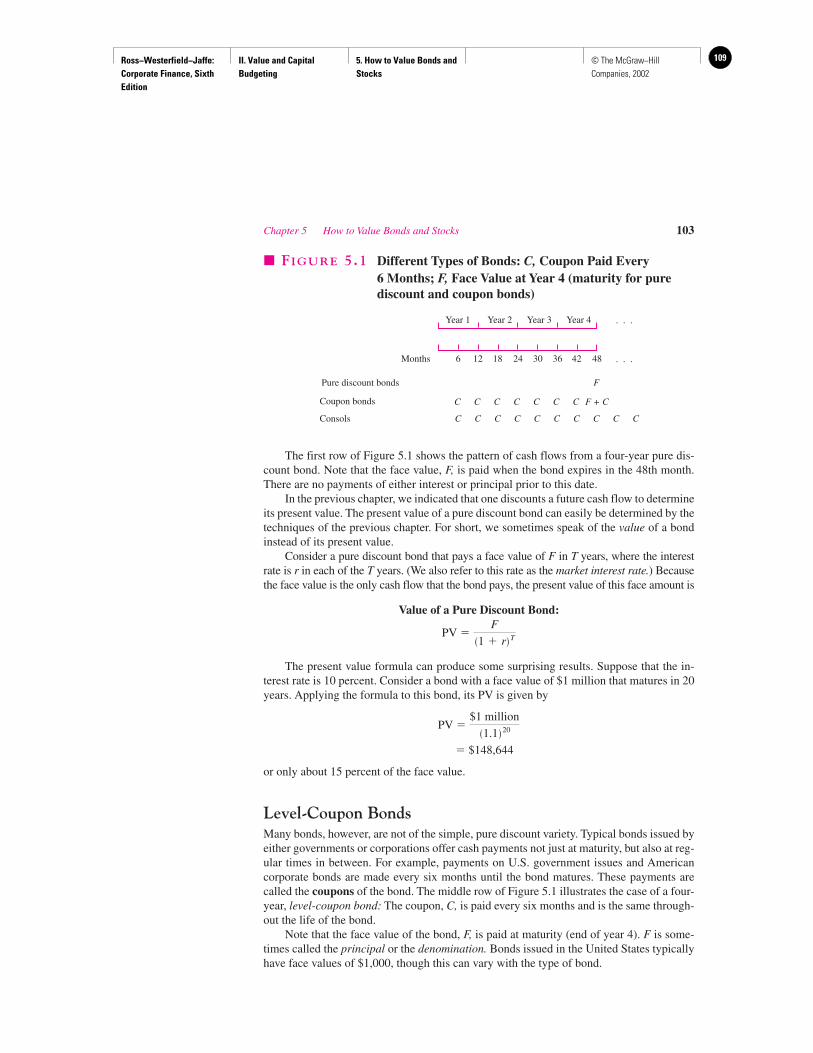
Ross−Westerfield−Jaffe: Corporate Finance, Sixth Edition
II. Value and Capital Budgeting
5. How to Value Bonds and Stocks
109© The McGraw−Hill Companies, 2002
Chapter 5 How to Value Bonds and Stocks 103
The first row of Figure 5.1 shows the pattern of cash flows from a four-year pure dis-count bond. Note that the face value, F, is paid when the bond expires in the 48th month.There are no payments of either interest or principal prior to this date.
In the previous chapter, we indicated that one discounts a future cash flow to determineits present value. The present value of a pure discount bond can easily be determined by thetechniques of the previous chapter. For short, we sometimes speak of the value of a bondinstead of its present value.
Consider a pure discount bond that pays a face value of F in T years, where the interestrate is r in each of the T years. (We also refer to this rate as the market interest rate.) Becausethe face value is the only cash flow that the bond pays, the present value of this face amount is
Value of a Pure Discount Bond:
PV �
The present value formula can produce some surprising results. Suppose that the in-terest rate is 10 percent. Consider a bond with a face value of $1 million that matures in 20years. Applying the formula to this bond, its PV is given by
PV �
� $148,644
or only about 15 percent of the face value.
Level-Coupon BondsMany bonds, however, are not of the simple, pure discount variety. Typical bonds issued byeither governments or corporations offer cash payments not just at maturity, but also at reg-ular times in between. For example, payments on U.S. government issues and Americancorporate bonds are made every six months until the bond matures. These payments arecalled the coupons of the bond. The middle row of Figure 5.1 illustrates the case of a four-year, level-coupon bond: The coupon, C, is paid every six months and is the same through-out the life of the bond.
Note that the face value of the bond, F, is paid at maturity (end of year 4). F is some-times called the principal or the denomination. Bonds issued in the United States typicallyhave face values of $1,000, though this can vary with the type of bond.
$1 million�1.1� 20
F�1 � r�T
6Months 12 18 24 30 36 42 48
Year 1 Year 2 Year 3 Year 4
Pure discount bonds
Coupon bonds
Consols C C C C C C C C
C C C C C C C F + C
F
C C
. . .
. . .
� FIGURE 5.1 Different Types of Bonds: C, Coupon Paid Every 6 Months; F, Face Value at Year 4 (maturity for purediscount and coupon bonds)
Ross−Westerfield−Jaffe: Corporate Finance, Sixth Edition
II. Value and Capital Budgeting
5. How to Value Bonds and Stocks
110 © The McGraw−Hill Companies, 2002
As we mentioned before, the value of a bond is simply the present value of its cashflows. Therefore, the value of a level-coupon bond is merely the present value of its streamof coupon payments plus the present value of its repayment of principal. Because a level-coupon bond is just an annuity of C each period, together with a payment at maturity of$1,000, the value of a level-coupon bond is
Value of a Level-Coupon Bond:
PV � � . . . �
where C is the coupon and the face value, F, is $1,000. The value of the bond can be rewritten as
Value of a Level-Coupon Bond:
PV � C �
As mentioned in the previous chapter, is the present value of an annuity of $1 per periodfor T periods at an interest rate per period of r.
EXAMPLE
Suppose it is November 2000 and we are considering a government bond. We seein The Wall Street Journal some 13s of November 2004. This is jargon that meansthe annual coupon rate is 13 percent.1 The face value is $1,000, implying that theyearly coupon is $130 (13% � $1,000). Interest is paid each May and November,implying that the coupon every six months is $65 ($130/2). The face value will bepaid out in November 2004, four years from now. By this we mean that the pur-chaser obtains claims to the following cash flows:
5/01 11/01 5/02 11/02 5/03 11/03 5/04 11/04
$65 $65 $65 $65 $65 $65 $65 $65 � $1,000
If the stated annual interest rate in the market is 10 percent per year, what is thepresent value of the bond?
Our work on compounding in the previous chapter showed that the interestrate over any six-month interval is one half of the stated annual interest rate. In thecurrent example, this semiannual rate is 5 percent (10%/2). Since the coupon pay-ment in each six-month period is $65, and there are eight of these six-month peri-ods from November 2000 to November 2004, the present value of the bond is
PV � � . . . �
� $65 � � $1,000/(1.05)8
� ($65 � 6.463) � ($1,000 � 0.677)� $420.095 � $677� $1,097.095
Traders will generally quote the bond as 109.7095,2 indicating that it is sell-ing at 109.7095 percent of the face value of $1,000.
A
80.05
$65�1.05� 8 �
$1,000�1.05� 8
$65�1.05�
�$65
�1.05� 2
A
Tr
�$1,000
�1 � r�TA
Tr
C�1 � r�T �
$1,000�1 � r�T
C
1 � r�
C�1 � r� 2
104 Part II Value and Capital Budgeting
1The coupon rate is specific to the bond. The coupon rate indicates what cash flow should appear in thenumerator of the NPV equation. The coupon rate does not appear in the denominator of the NPV equation.2Bond prices are actually quoted in 32nds of a dollar, so a quote this precise would not be given.
Ross−Westerfield−Jaffe: Corporate Finance, Sixth Edition
II. Value and Capital Budgeting
5. How to Value Bonds and Stocks
111© The McGraw−Hill Companies, 2002
At this point, it is worthwhile to relate the above example of bond-pricing to the dis-cussion of compounding in the previous chapter. At that time we distinguished between thestated annual interest rate and the effective annual interest rate. In particular, we pointed outthat the effective annual interest rate is
(1 � r/m)m � 1
where r is the stated annual interest rate and m is the number of compounding intervals.Since r � 10% and m � 2 (because the bond makes semiannual payments), the effectiveannual interest rate is
[1 � (0.10/2)]2 � 1 � (1.05)2 � 1 � 10.25%
In other words, because the bond is paying interest twice a year, the bondholder earns a10.25-percent return when compounding is considered.3
One final note concerning level-coupon bonds: Although the preceding example con-cerns government bonds, corporate bonds are identical in form. For example, DuPontCorporation has an 81⁄2-percent bond maturing in 2006. This means that DuPont will makesemiannual payments of $42.50 (81⁄2%/2 � $1,000) between now and 2006 for each facevalue of $1,000.
ConsolsNot all bonds have a final maturity date. As we mentioned in the previous chapter, consolsare bonds that never stop paying a coupon, have no final maturity date, and therefore nevermature. Thus, a consol is a perpetuity. In the 18th century the Bank of England issued suchbonds, called “English consols.” These were bonds that the Bank of England guaranteedwould pay the holder a cash flow forever! Through wars and depressions, the Bank of Eng-land continued to honor this commitment, and you can still buy such bonds in London to-day. The U.S. government also once sold consols to raise money to build the Panama Canal.Even though these U.S. bonds were supposed to last forever and to pay their coupons for-ever, don’t go looking for any. There is a special clause in the bond contract that gives thegovernment the right to buy them back from the holders, and that is what the governmenthas done. Clauses like that are call provisions, and we study them later.
An important example of a consol, though, is called preferred stock. Preferred stock isstock that is issued by corporations and that provides the holder a fixed dividend in perpe-tuity. If there were never any question that the firm would actually pay the dividend on thepreferred stock, such stock would in fact be a consol.
These instruments can be valued by the perpetuity formula of the previous chapter. Forexample, if the marketwide interest rate is 10 percent, a consol with a yearly interest pay-ment of $50 is valued at
� $500
• Define pure discount bonds, level-coupon bonds, and consols.• Contrast the stated interest rate and the effective annual interest rate for bonds paying
semiannual interest.
$50
0.10
Chapter 5 How to Value Bonds and Stocks 105
3For an excellent discussion of how to value semiannual payments, see J. T. Lindley, B. P. Helms, and M. Haddad, “A Measurement of the Errors in Intra-Period Compounding and Bond Valuation,” The FinancialReview 22 (February 1987). We benefited from several conversations with the authors of this article.
QUESTIONS
CO
NC
EP
T
?
Ross−Westerfield−Jaffe: Corporate Finance, Sixth Edition
II. Value and Capital Budgeting
5. How to Value Bonds and Stocks
112 © The McGraw−Hill Companies, 2002
5.3 BOND CONCEPTS
We complete our discussion on bonds by considering two concepts concerning them. First,we examine the relationship between interest rates and bond prices. Second, we define theconcept of yield to maturity.
Interest Rates and Bond PricesThe above discussion on level-coupon bonds allows us to relate bond prices to interest rates.Consider the following example.
EXAMPLE
The interest rate is 10 percent. A two-year bond with a 10-percent coupon pays in-terest of $100 ($1,000 � 10%). For simplicity, we assume that the interest is paidannually. The bond is priced at its face value of $1,000:
$1,000 �
If the interest rate unexpectedly rises to 12 percent, the bond sells at
$966.20 �
Because $966.20 is below $1,000, the bond is said to sell at a discount. This is asensible result. Now that the interest rate is 12 percent, a newly issued bond witha 12-percent coupon rate will sell at $1,000. This newly issued bond will havecoupon payments of $120 (0.12 � $1,000). Because our bond has interest pay-ments of only $100, investors will pay less than $1,000 for it.
If interest rates fell to 8 percent, the bond would sell at
$1,035.67 �
Because $1,035.67 is above $1,000, the bond is said to sell at a premium.
Thus, we find that bond prices fall with a rise in interest rates and rise with a fall in in-terest rates. Furthermore, the general principle is that a level-coupon bond sells in the fol-lowing ways.
1. At the face value of $1,000 if the coupon rate is equal to the marketwide interest rate.
2. At a discount if the coupon rate is below the marketwide interest rate.
3. At a premium if the coupon rate is above the marketwide interest rate.
Yield to MaturityLet’s now consider the previous example in reverse. If our bond is selling at $1,035.67, whatreturn is a bondholder receiving? This can be answered by considering the following equa-tion:
$1,035.67 �$100
1 � y�
$1,000 � $100�1 � y� 2
$100
1.08�
$1,000 � $100�1.08� 2
$100
1.12�
$1,000 � $100�1.12� 2
$100
1.10�
$1,000 � $100�1.10� 2
106 Part II Value and Capital Budgeting
Ross−Westerfield−Jaffe: Corporate Finance, Sixth Edition
II. Value and Capital Budgeting
5. How to Value Bonds and Stocks
113© The McGraw−Hill Companies, 2002
The unknown, y, is the discount rate that equates the price of the bond with the discountedvalue of the coupons and face value. Our earlier work implies that y � 8%. Thus, tradersstate that the bond is yielding an 8-percent return. Bond traders also state that the bond hasa yield to maturity of 8 percent. The yield to maturity is frequently called the bond’s yieldfor short. So we would say the bond with its 10-percent coupon is priced to yield 8 percentat $1,035.67.
Bond Market ReportingAlmost all corporate bonds are traded by institutional investors and are traded on theover-the-counter market (OTC for short). There is a corporate bond market associatedwith the New York Stock Exchange. This bond market is mostly a retail market for indi-vidual investors for smaller trades. It represents a very small fraction of total corporatebond trading.
Table 5.1 reproduces some bond data that can be found in The Wall Street Journal onany particular day. At the bottom of the list you will find AT&T and an entry AT&T 81⁄8 /22. This entry represents AT&T bonds that mature in the year 2022 and have a couponrate of 81⁄8. The coupon rate means 81⁄8 percent of the par value (or face value) of $1,000.Therefore, the annual coupon for AT&T bonds is $81.25.
Under the heading “Close,” you will find the last price for the AT&T bonds at the closeof this particular day. The price is quoted as a percentage of the par value. So the last pricefor the AT&T bonds on this particular day was 100 percent of $1,000 or $1,000.00. Thisbond is trading at a price less than its par value, and so it is trading at a “discount.” The lastcolumn is “Net Chg.” AT&T bonds traded up from the day before by 3⁄8 of 1 percent. TheAT&T bonds have a current yield of 8.1 percent. The current yield is simply the currentcoupon divided by the current price, or 81.25 divided by 1,000, equal to 8.1 percent(rounded to one decimal place).
You should know from our discussion of bond yields that the current yield is not thesame thing as the bonds’ yield to maturity. The yield to maturity is not usually reportedon a daily basis by the financial press. The “Vol” column is the daily volume of 97. Thisis the number of bonds that were traded on the New York Stock Exchange on this par-ticular day.
Chapter 5 How to Value Bonds and Stocks 107
THE PRESENT VALUE FORMULAS FOR BONDS
Pure Discount Bonds
PV �
Level-Coupon Bonds
PV � C
where F is typically $1,000 for a level-coupon bond.
Consols
PV �C
r
�1
r�
1
r � �1 � r�T �F
�1 � r�T � C � A
Tr �
F�1 � r�T
F�1 � r�T
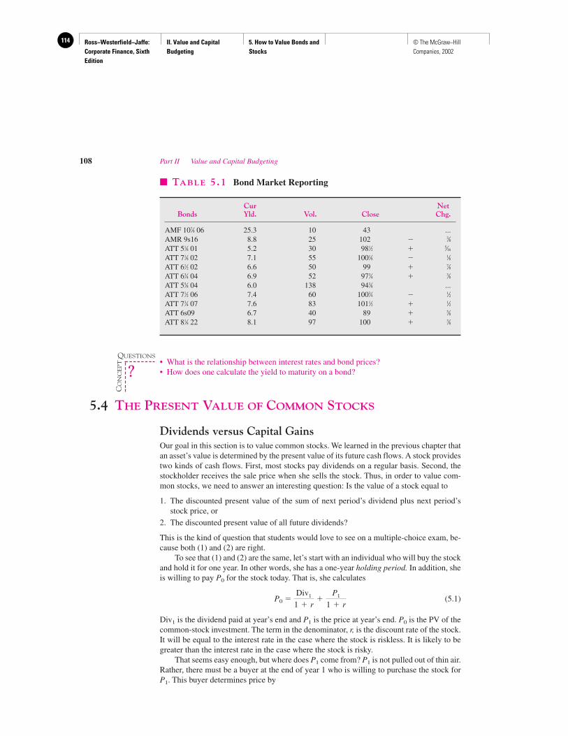
Ross−Westerfield−Jaffe: Corporate Finance, Sixth Edition
II. Value and Capital Budgeting
5. How to Value Bonds and Stocks
114 © The McGraw−Hill Companies, 2002
• What is the relationship between interest rates and bond prices?• How does one calculate the yield to maturity on a bond?
5.4 THE PRESENT VALUE OF COMMON STOCKS
Dividends versus Capital GainsOur goal in this section is to value common stocks. We learned in the previous chapter thatan asset’s value is determined by the present value of its future cash flows. A stock providestwo kinds of cash flows. First, most stocks pay dividends on a regular basis. Second, thestockholder receives the sale price when she sells the stock. Thus, in order to value com-mon stocks, we need to answer an interesting question: Is the value of a stock equal to
1. The discounted present value of the sum of next period’s dividend plus next period’sstock price, or
2. The discounted present value of all future dividends?
This is the kind of question that students would love to see on a multiple-choice exam, be-cause both (1) and (2) are right.
To see that (1) and (2) are the same, let’s start with an individual who will buy the stockand hold it for one year. In other words, she has a one-year holding period. In addition, sheis willing to pay P0 for the stock today. That is, she calculates
P0 � (5.1)
Div1 is the dividend paid at year’s end and P1 is the price at year’s end. P0 is the PV of thecommon-stock investment. The term in the denominator, r, is the discount rate of the stock.It will be equal to the interest rate in the case where the stock is riskless. It is likely to begreater than the interest rate in the case where the stock is risky.
That seems easy enough, but where does P1 come from? P1 is not pulled out of thin air.Rather, there must be a buyer at the end of year 1 who is willing to purchase the stock forP1. This buyer determines price by
Div1
1 � r�
P1
1 � r
108 Part II Value and Capital Budgeting
� TABLE 5.1 Bond Market Reporting
Cur NetBonds Yld. Vol. Close Chg.
AMF 107⁄8 06 25.3 10 43 ...AMR 9s16 8.8 25 102 � 3⁄8ATT 51⁄8 01 5.2 30 981⁄2 � 5⁄16
ATT 71⁄8 02 7.1 55 1001⁄8 � 1⁄8ATT 61⁄2 02 6.6 50 99 � 7⁄8ATT 63⁄4 04 6.9 52 973⁄4 � 3⁄8ATT 55⁄8 04 6.0 138 943⁄8 ...ATT 71⁄2 06 7.4 60 1003⁄4 � 1⁄2ATT 73⁄4 07 7.6 83 1011⁄2 � 1⁄2ATT 6s09 6.7 40 89 � 5⁄8ATT 81⁄8 22 8.1 97 100 � 3⁄8
QUESTIONS
CO
NC
EP
T
?
Ross−Westerfield−Jaffe: Corporate Finance, Sixth Edition
II. Value and Capital Budgeting
5. How to Value Bonds and Stocks
115© The McGraw−Hill Companies, 2002
P1 � (5.2)
Substituting the value of P1 from (5.2) into equation (5.1) yields
P0 �
� (5.3)
We can ask a similar question for formula (5.3): Where does P2 come from? An in-vestor at the end of year 2 is willing to pay P2 because of the dividend and stock price atyear 3. This process can be repeated ad nauseam.4 At the end, we are left with
P0 � � . . . � (5.4)
Thus the value of a firm’s common stock to the investor is equal to the present value of allof the expected future dividends.
This is a very useful result. A common objection to applying present value analysis tostocks is that investors are too shortsighted to care about the long-run stream of dividends.These critics argue that an investor will generally not look past his or her time horizon.Thus, prices in a market dominated by short-term investors will reflect only near-term div-idends. However, our discussion shows that a long-run dividend-discount model holds evenwhen investors have short-term time horizons. Although an investor may want to cash outearly, she must find another investor who is willing to buy. The price this second investorpays is dependent on dividends after his date of purchase.
Valuation of Different Types of StocksThe above discussion shows that the value of the firm is the present value of its future div-idends. How do we apply this idea in practice? Equation (5.4) represents a very generalmodel and is applicable regardless of whether the level of expected dividends is growing,fluctuating, or constant. The general model can be simplified if the firm’s dividends are ex-pected to follow some basic patterns: (1) zero growth, (2) constant growth, and (3) differ-ential growth. These cases are illustrated in Figure 5.2.
Case 1 (Zero Growth) The value of a stock with a constant dividend is given by
P0 � � . . . �
Here it is assumed that Div1 � Div2 � . . . � Div. This is just an application of the perpe-tuity formula of the previous chapter.
Case 2 (Constant Growth) Dividends grow at rate g, as follows:
End of Year 1 2 3 4 . . .
Dividend Div Div(1 � g) Div(1 � g)2 Div(1 � g)3
Note that Div is the dividend at the end of the first period.
Div
r
Div1
1 � r�
Div2
�1 � r� 2
t�1
Divt
�1 � r� t
Div1
1 � r�
Div2
�1 � r� 2 �Div3
�1 � r� 3
Div1
1 � r�
Div2
�1 � r� 2 �P2
�1 � r� 2
1
1 � r�Div1 � �Div2 � P2
1 � r �
Div2
1 � r�
P2
1 � r
Chapter 5 How to Value Bonds and Stocks 109
4This procedure reminds us of the physicist lecturing on the origins of the universe. He was approached by an elderlygentleman in the audience who disagreed with the lecture. The attendee said that the universe rests on the back of ahuge turtle. When the physicist asked what the turtle rested on, the gentleman said another turtle. Anticipating thephysicist’s objections, the attendee said, “Don’t tire yourself out, young fellow. It’s turtles all the way down.”
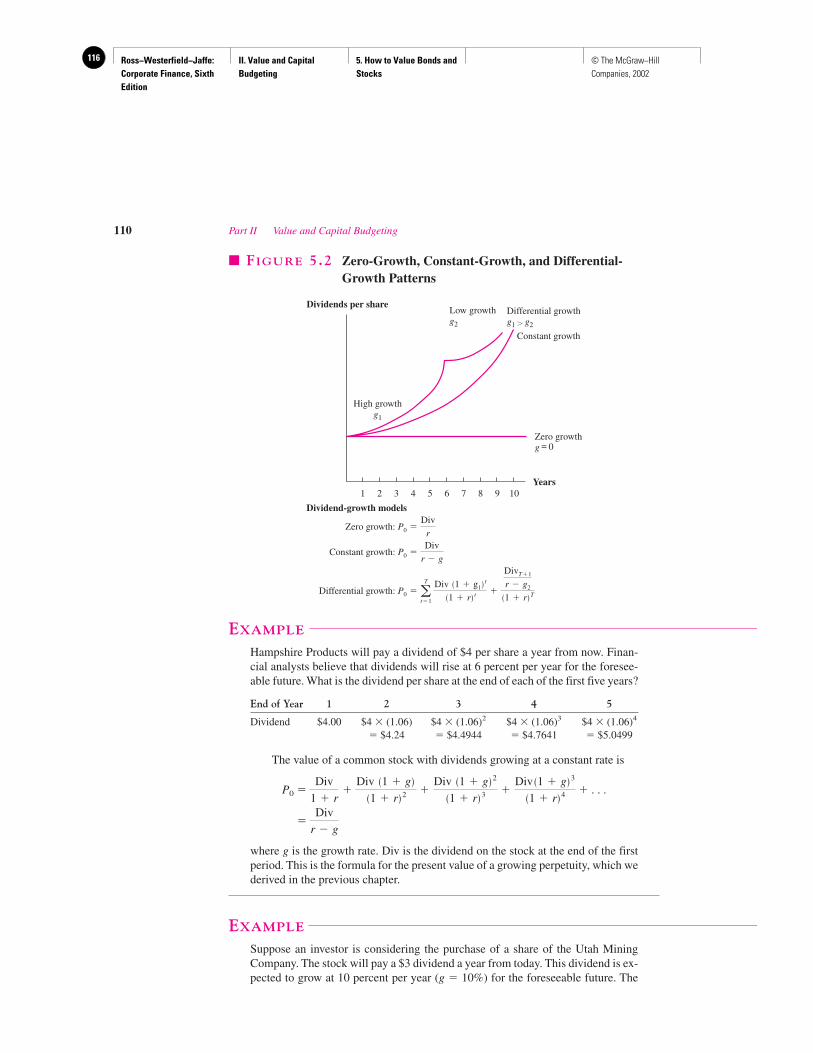
Ross−Westerfield−Jaffe: Corporate Finance, Sixth Edition
II. Value and Capital Budgeting
5. How to Value Bonds and Stocks
116 © The McGraw−Hill Companies, 2002
EXAMPLE
Hampshire Products will pay a dividend of $4 per share a year from now. Finan-cial analysts believe that dividends will rise at 6 percent per year for the foresee-able future. What is the dividend per share at the end of each of the first five years?
End of Year 1 2 3 4 5
Dividend $4.00 $4 � (1.06) $4 � (1.06)2 $4 � (1.06)3 $4 � (1.06)4
� $4.24 � $4.4944 � $4.7641 � $5.0499
The value of a common stock with dividends growing at a constant rate is
P0 � � . . .
�
where g is the growth rate. Div is the dividend on the stock at the end of the firstperiod. This is the formula for the present value of a growing perpetuity, which wederived in the previous chapter.
EXAMPLE
Suppose an investor is considering the purchase of a share of the Utah MiningCompany. The stock will pay a $3 dividend a year from today. This dividend is ex-pected to grow at 10 percent per year (g � 10%) for the foreseeable future. The
Div
r � g
Div
1 � r�
Div �1 � g��1 � r� 2 �
Div �1 � g� 2
�1 � r� 3 �Div �1 � g� 3
�1 � r� 4
110 Part II Value and Capital Budgeting
Low growthg2
Differential growthg1 � g2
Constant growth
High growthg1
Zero growthg = 0
Years1 2 3 4 5 6 7 8 9 10
Dividends per share
� FIGURE 5.2 Zero-Growth, Constant-Growth, and Differential-Growth Patterns
Dividend-growth models
Zero growth:
Constant growth:
Differential growth: P0 � T
t�1
Div �1 � g1� t
�1 � r� t �
DivT�1
r � g2
�1 � r�T
P0 �Div
r � g
P0 �Div
r
Ross−Westerfield−Jaffe: Corporate Finance, Sixth Edition
II. Value and Capital Budgeting
5. How to Value Bonds and Stocks
117© The McGraw−Hill Companies, 2002
investor thinks that the required return (r) on this stock is 15 percent, given her as-sessment of Utah Mining’s risk. (We also refer to r as the discount rate of thestock.) What is the value of a share of Utah Mining Company’s stock?
Using the constant growth formula of case 2, we assess the value to be $60:
$60 �
P0 is quite dependent on the value of g. If g had been estimated to be 121⁄2 per-cent, the value of the share would have been
$120 �
The stock price doubles (from $60 to $120) when g only increases 25 percent(from 10 percent to 12.5 percent). Because of P0’s dependency on g, one mustmaintain a healthy sense of skepticism when using this constant growth of divi-dends model.
Furthermore, note that P0 is equal to infinity when the growth rate, g, equalsthe discount rate, r. Because stock prices do not grow infinitely, an estimate of ggreater than r implies an error in estimation. More will be said of this point later.
Case 3 (Differential Growth) In this case, an algebraic formula would be too unwieldy.Instead, we present examples.
EXAMPLE
Consider the stock of Elixir Drug Company, which has a new back-rub ointmentand is enjoying rapid growth. The dividend for a share of stock a year from todaywill be $1.15. During the next four years, the dividend will grow at 15 percent peryear (g1 � 15%). After that, growth (g2) will be equal to 10 percent per year. Canyou calculate the present value of the stock if the required return (r) is 15 percent?
Figure 5.3 displays the growth in the dividends. We need to apply a two-stepprocess to discount these dividends. We first calculate the net present value of thedividends growing at 15 percent per annum. That is, we first calculate the presentvalue of the dividends at the end of each of the first five years. Second, we calcu-late the present value of the dividends beginning at the end of year 6.
Calculate Present Value of First Five Dividends The present value of dividendpayments in years 1 through 5 is as follows:
Future Growth Expected PresentYear Rate (g1) Dividend Value
1 0.15 $1.15 $12 0.15 1.3225 13 0.15 1.5209 14 0.15 1.7490 15 0.15 2.0114 1Years 1–5 The present value of dividends � $5
The growing-annuity formula of the previous chapter could normally be used in thisstep. However, note that dividends grow at 15 percent, which is also the discountrate. Since g � r, the growing-annuity formula cannot be used in this example.
$3
0.15 � 0.125
$3
0.15 � 0.10
Chapter 5 How to Value Bonds and Stocks 111
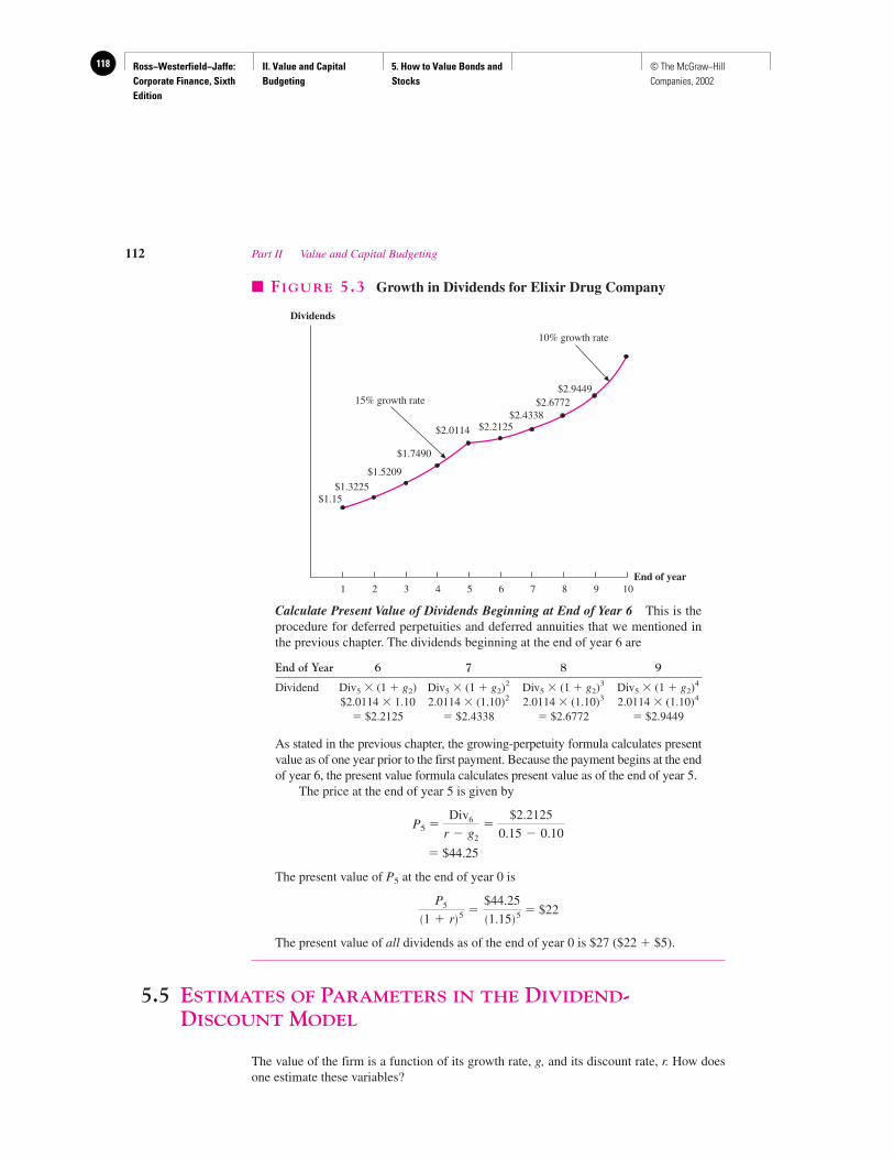
Ross−Westerfield−Jaffe: Corporate Finance, Sixth Edition
II. Value and Capital Budgeting
5. How to Value Bonds and Stocks
118 © The McGraw−Hill Companies, 2002
Calculate Present Value of Dividends Beginning at End of Year 6 This is theprocedure for deferred perpetuities and deferred annuities that we mentioned inthe previous chapter. The dividends beginning at the end of year 6 are
End of Year 6 7 8 9
Dividend Div5 � (1 � g2) Div5 � (1 � g2)2 Div5 � (1 � g2)3 Div5 � (1 � g2)4
$2.0114 � 1.10 2.0114 � (1.10)2 2.0114 � (1.10)3 2.0114 � (1.10)4
� $2.2125 � $2.4338 � $2.6772 � $2.9449
As stated in the previous chapter, the growing-perpetuity formula calculates presentvalue as of one year prior to the first payment. Because the payment begins at the endof year 6, the present value formula calculates present value as of the end of year 5.
The price at the end of year 5 is given by
P5 �
� $44.25
The present value of P5 at the end of year 0 is
� $22
The present value of all dividends as of the end of year 0 is $27 ($22 � $5).
5.5 ESTIMATES OF PARAMETERS IN THE DIVIDEND-DISCOUNT MODEL
The value of the firm is a function of its growth rate, g, and its discount rate, r. How doesone estimate these variables?
P5
�1 � r� 5 �$44.25�1.15� 5
Div6
r � g2
�$2.2125
0.15 � 0.10
112 Part II Value and Capital Budgeting
Dividends
End of year
15% growth rate
$1.15$1.3225
$1.5209
$1.7490
$2.0114 $2.2125$2.4338
$2.6772$2.9449
10% growth rate
1 2 3 4 5 6 7 8 9 10
� FIGURE 5.3 Growth in Dividends for Elixir Drug Company
Ross−Westerfield−Jaffe: Corporate Finance, Sixth Edition
II. Value and Capital Budgeting
5. How to Value Bonds and Stocks
119© The McGraw−Hill Companies, 2002
Where Does g Come From?The previous discussion on stocks assumed that dividends grow at the rate g. We nowwant to estimate this rate of growth. Consider a business whose earnings next year are ex-pected to be the same as earnings this year unless a net investment is made. This situationis likely to occur, because net investment is equal to gross, or total, investment less de-preciation. A net investment of zero occurs when total investment equals depreciation. Iftotal investment is equal to depreciation, the firm’s physical plant is maintained, consis-tent with no growth in earnings.
Net investment will be positive only if some earnings are not paid out as dividends, thatis, only if some earnings are retained.5 This leads to the following equation:
Earnings Earnings Retained Return onnext � this � earnings � retained (5.5)year year this year earnings
Increase in earnings
The increase in earnings is a function of both the retained earnings and the return on theretained earnings.
We now divide both sides of (5.5) by earnings this year, yielding
�
(5.6)
The left-hand side of (5.6) is simply one plus the growth rate in earnings, which we write as 1 � g.6 The ratio of retained earnings to earnings is called the retention ratio. Thus, we can write
1 � g � 1 � Retention ratio � Return on retained earnings (5.7)
It is difficult for a financial analyst to determine the return to be expected on currentlyretained earnings, because the details on forthcoming projects are not generally public in-formation. However, it is frequently assumed that the projects selected in the current yearhave an anticipated return equal to returns from projects in other years. Here, we can esti-mate the anticipated return on current retained earnings by the historical return on equity,or ROE. After all, ROE is simply the return on the firm’s entire equity, which is the returnon the cumulation of all the firm’s past projects.7
From (5.7), we have a simple way to estimate growth:
Formula for Firm’s Growth Rate:g � Retention ratio � Return on retained earnings (5.8)
Earnings this year
Earnings this year� �Retained earnings this year
Earnings this year � � Return on retained earnings
Earnings next year
Earnings this year
Chapter 5 How to Value Bonds and Stocks 113
5We ignore the possibility of the issuance of stocks or bonds in order to raise capital. These possibilities areconsidered in later chapters.6Previously g referred to growth in dividends. However, the growth in earnings is equal to the growth rate individends in this context, because as we will presently see, the ratio of dividends to earnings is held constant.7Students frequently wonder whether return on equity (ROE) or return on assets (ROA) should be used here.ROA and ROE are identical in our model because debt financing is ignored. However, most real-world firmshave debt. Because debt is treated in later chapters, we are not yet able to treat this issue in depth now. Suffice itto say that ROE is the appropriate rate, because both ROE for the firm as a whole and the return to equityholdersfrom a future project are calculated after interest has been deducted.
Ross−Westerfield−Jaffe: Corporate Finance, Sixth Edition
II. Value and Capital Budgeting
5. How to Value Bonds and Stocks
120 © The McGraw−Hill Companies, 2002
EXAMPLE
Pagemaster Enterprises just reported earnings of $2 million. It plans to retain 40 percentof its earnings. The historical return on equity (ROE) has been 0.16, a figure that is ex-pected to continue into the future. How much will earnings grow over the coming year?
We first perform the calculation without reference to equation (5.8). Then weuse (5.8) as a check.
Calculation without Reference to Equation (5.8) The firm will retain $800,000(40% � $2 million). Assuming that historical ROE is an appropriate estimate forfuture returns, the anticipated increase in earnings is
$800,000 � 0.16 � $128,000
The percentage growth in earnings is
This implies that earnings in one year will be $2,128,000 ($2,000,000 � 1.064).
Check Using Equation (5.8) We use g � Retention ratio � ROE. We have
g � 0.4 � 0.16 � 0.064
Where Does r Come From?In this section, we want to estimate r, the rate used to discount the cash flows of a particu-lar stock. There are two methods developed by academics. We present one method belowbut must defer the second until we give it extensive treatment in later chapters.
The first method begins with the concept that the value of a growing perpetuity is
P0 �
Solving for r, we have
r � � g (5.9)
As stated earlier, Div refers to the dividend to be received one year hence.Thus, the discount rate can be broken into two parts. The ratio, Div/P0, places the div-
idend return on a percentage basis, frequently called the dividend yield. The second term,g, is the growth rate of dividends.
Because information on both dividends and stock price is publicly available, the firstterm on the right-hand side of equation (5.9) can be easily calculated. The second term onthe right-hand side, g, can be estimated from (5.8).
EXAMPLE
Pagemaster Enterprises, the company examined in the previous example, has1,000,000 shares of stock outstanding. The stock is selling at $10. What is the re-quired return on the stock?
Because the retention ratio is 40 percent, the payout ratio is 60 percent (1 � Re-tention ratio). The payout ratio is the ratio of dividends/earnings. Because earnings ayear from now will be $2,128,000 ($2,000,000 � 1.064), dividends will be $1,276,800
Div
P0
Div
r � g
Change in earnings
Total earnings�
$128,000
$2 million� 0.064
114 Part II Value and Capital Budgeting
Ross−Westerfield−Jaffe: Corporate Finance, Sixth Edition
II. Value and Capital Budgeting
5. How to Value Bonds and Stocks
121© The McGraw−Hill Companies, 2002
(0.60 � $2,128,000). Dividends per share will be $1.28 ($1,276,800/1,000,000).Given our previous result that g � 0.064, we calculate r from (5.9) as follows:
0.192 � � 0.064
A Healthy Sense of SkepticismIt is important to emphasize that our approach merely estimates g; our approach does not determine g precisely. We mentioned earlier that our estimate of g is based on a number of as-sumptions. For example, we assume that the return on reinvestment of future retained earn-ings is equal to the firm’s past ROE. We assume that the future retention ratio is equal to thepast retention ratio. Our estimate for g will be off if these assumptions prove to be wrong.
Unfortunately, the determination of r is highly dependent on g. For example, if g is esti-mated to be 0, r equals 12.8 percent ($1.28/$10.00). If g is estimated to be 12 percent, r equals24.8 percent ($1.28/$10.00 � 12%). Thus, one should view estimates of r with a healthy senseof skepticism.
Because of the preceding, some financial economists generally argue that the estima-tion error for r or a single security is too large to be practical. Therefore, they suggest cal-culating the average r for an entire industry. This r would then be used to discount the div-idends of a particular stock in the same industry.
One should be particularly skeptical of two polar cases when estimating r for individ-ual securities. First, consider a firm currently paying no dividend. The stock price will beabove zero because investors believe that the firm may initiate a dividend at some point orthe firm may be acquired at some point. However, when a firm goes from no dividends toa positive number of dividends, the implied growth rate is infinite. Thus, equation (5.9) mustbe used with extreme caution here, if at all—a point we emphasize later in this chapter.
Second, we mentioned earlier that the value of the firm is infinite when g is equal to r.Because prices for stocks do not grow infinitely, an analyst whose estimate of g for a par-ticular firm is equal to or above r must have made a mistake. Most likely, the analyst’s highestimate for g is correct for the next few years. However, firms simply cannot maintain anabnormally high growth rate forever. The analyst’s error was to use a short-run estimate ofg in a model requiring a perpetual growth rate.
5.6 GROWTH OPPORTUNITIES
We previously spoke of the growth rate of dividends. We now want to address the relatedconcept of growth opportunities. Imagine a company with a level stream of earnings pershare in perpetuity. The company pays all of these earnings out to stockholders as divi-dends. Hence,
EPS � Div
where EPS is earnings per share and Div is dividends per share. A company of this type isfrequently called a cash cow.
From the perpetuity formula of the previous chapter, the value of a share of stock is:
Value of a Share of Stock when Firm Acts as a Cash Cow:
where r is the discount rate on the firm’s stock.
EPS
r�
Div
r
$1.28
$10.00
Chapter 5 How to Value Bonds and Stocks 115
Ross−Westerfield−Jaffe: Corporate Finance, Sixth Edition
II. Value and Capital Budgeting
5. How to Value Bonds and Stocks
122 © The McGraw−Hill Companies, 2002
This policy of paying out all earnings as dividends may not be the optimal one. Manyfirms have growth opportunities, that is, opportunities to invest in profitable projects.Because these projects can represent a significant fraction of the firm’s value, it would befoolish to forgo them in order to pay out all earnings as dividends.
Although firms frequently think in terms of a set of growth opportunities, let’s focuson only one opportunity, that is, the opportunity to invest in a single project. Suppose thefirm retains the entire dividend at date 1 in order to invest in a particular capital budgetingproject. The net present value per share of the project as of date 0 is NPVGO, which standsfor the net present value (per share) of the growth opportunity.
What is the price of a share of stock at date 0 if the firm decides to take on the projectat date 1? Because the per share value of the project is added to the original stock price, thestock price must now be:
Stock Price after Firm Commits to New Project:
� NPVGO (5.10)
Thus, equation (5.10) indicates that the price of a share of stock can be viewed as thesum of two different items. The first term (EPS/r) is the value of the firm if it rested on itslaurels, that is, if it simply distributed all earnings to the stockholders. The second term isthe additional value if the firm retains earnings in order to fund new projects.
EXAMPLE
Sarro Shipping, Inc., expects to earn $1 million per year in perpetuity if it undertakesno new investment opportunities. There are 100,000 shares of stock outstanding, soearnings per share equal $10 ($1,000,000/100,000). The firm will have an opportunityat date 1 to spend $1,000,000 in a new marketing campaign. The new campaign willincrease earnings in every subsequent period by $210,000 (or $2.10 per share). This isa 21-percent return per year on the project. The firm’s discount rate is 10 percent. Whatis the value per share before and after deciding to accept the marketing campaign?
The value of a share of Sarro Shipping before the campaign is
Value of a Share of Sarro when Firm Acts as a Cash Cow:
The value of the marketing campaign as of date 1 is:
Value of Marketing Campaign at Date 1:
�$1,000,000 � � $1,100,000 (5.11)
Because the investment is made at date 1 and the first cash inflow occurs at date2, equation (5.11) represents the value of the marketing campaign as of date 1. Wedetermine the value at date 0 by discounting back one period as follows:
Value of Marketing Campaign at Date 0:
� $1,000,000
Thus, NPVGO per share is $10 ($1,000,000/100,000).The price per share is
EPS/r � NPVGO � $100 � $10 � $110
$1,100,000
1.1
$210,000
0.1
EPS
r�
$10
0.1� $100
EPS
r
116 Part II Value and Capital Budgeting
Ross−Westerfield−Jaffe: Corporate Finance, Sixth Edition
II. Value and Capital Budgeting
5. How to Value Bonds and Stocks
123© The McGraw−Hill Companies, 2002
The calculation can also be made on a straight net-present-value basis. Because all theearnings at date 1 are spent on the marketing effort, no dividends are paid to stockholdersat that date. Dividends in all subsequent periods are $1,210,000 ($1,000,000 � $210,000).In this case, $1,000,000 is the annual dividend when Sarro is a cash cow. The additionalcontribution to the dividend from the marketing effort is $210,000. Dividends per share are$12.10 ($1,210,000/100,000). Because these dividends start at date 2, the price per share atdate 1 is $121 ($12.10/0.1). The price per share at date 0 is $110 ($121/1.1).
Note that value is created in this example because the project earned a 21-percent rateof return when the discount rate was only 10 percent. No value would have been createdhad the project earned a 10-percent rate of return. The NPVGO would have been zero, andvalue would have been negative had the project earned a percentage return below 10 per-cent. The NPVGO would be negative in that case.
Two conditions must be met in order to increase value.
1. Earnings must be retained so that projects can be funded.8
2. The projects must have positive net present value.
Surprisingly, a number of companies seem to invest in projects known to have negativenet present values. For example, Jensen has pointed out that, in the late 1970s, oil companiesand tobacco companies were flush with cash.9 Due to declining markets in both industries,high dividends and low investment would have been the rational action. Unfortunately, a num-ber of companies in both industries reinvested heavily in what were widely perceived to benegative-NPVGO projects. A study by McConnell and Muscarella documents this percep-tion.10 They find that, during the 1970s, the stock prices of oil companies generally decreasedon the days that announcements of increases in exploration and development were made.
Given that NPV analysis (such as that presented in the previous chapter) is commonknowledge in business, why would managers choose projects with negative NPVs? Oneconjecture is that some managers enjoy controlling a large company. Because paying divi-dends in lieu of reinvesting earnings reduces the size of the firm, some managers find itemotionally difficult to pay high dividends.
Growth in Earnings and Dividends versus Growth OpportunitiesAs mentioned earlier, a firm’s value increases when it invests in growth opportunities withpositive NPVGOs. A firm’s value falls when it selects opportunities with negative NPVGOs.However, dividends grow whether projects with positive NPVs or negative NPVs are se-lected. This surprising result can be explained by the following example.
EXAMPLE
Lane Supermarkets, a new firm, will earn $100,000 a year in perpetuity if it paysout all its earnings as dividends. However, the firm plans to invest 20 percent of itsearnings in projects that earn 10 percent per year. The discount rate is 18 percent.An earlier formula tells us that the growth rate of dividends is
g � Retention ratio � Return on retained earnings � 0.2 � 0.10 � 2%
Chapter 5 How to Value Bonds and Stocks 117
8Later in the text we speak of issuing stock or debt in order to fund projects.9M. C. Jensen, “Agency Costs of Free Cash Flows, Corporate Finance and Takeovers,” American EconomicReview (May 1986).10J. J. McConnell and C. J. Muscarella, “Corporate Capital Expenditure Decisions and the Market Value of theFirm,” Journal of Financial Economics 14 (1985).
Ross−Westerfield−Jaffe: Corporate Finance, Sixth Edition
II. Value and Capital Budgeting
5. How to Value Bonds and Stocks
124 © The McGraw−Hill Companies, 2002
For example, in this first year of the new policy, dividends are $80,000 [(1 � 0.2) �$100,000]. Dividends next year are $81,600 ($80,000 � 1.02). Dividends the fol-lowing year are $83,232 [$80,000 � (1.02)2] and so on. Because dividends repre-sent a fixed percentage of earnings, earnings must grow at 2 percent a year as well.
However, note that the policy reduces value because the rate of return on theprojects of 10 percent is less than the discount rate of 18 percent. That is, the firmwould have had a higher value at date 0 if it had a policy of paying all its earningsout as dividends. Thus, a policy of investing in projects with negative NPVs ratherthan paying out earnings as dividends will lead to growth in dividends and earn-ings, but will reduce value.
Dividends or Earnings: Which to Discount?As mentioned earlier, this chapter applied the growing-perpetuity formula to the valuationof stocks. In our application, we discounted dividends, not earnings. This is sensible sinceinvestors select a stock for what they can get out of it. They only get two things out of astock: dividends and the ultimate sales price, which is determined by what future investorsexpect to receive in dividends.
The calculated stock price would be too high were earnings to be discounted instead ofdividends. As we saw in our estimation of a firm’s growth rate, only a portion of earningsgoes to the stockholders as dividends. The remainder is retained to generate future divi-dends. In our model, retained earnings are equal to the firm’s investment. To discount earn-ings instead of dividends would be to ignore the investment that a firm must make today inorder to generate future returns.
The No-Dividend FirmStudents frequently ask the following questions: If the dividend-discount model is correct,why aren’t no-dividend stocks selling at zero? This is a good question and gets at the goalsof the firm. A firm with many growth opportunities is faced with a dilemma. The firm canpay out dividends now, or it can forgo dividends now so that it can make investments thatwill generate even greater dividends in the future.11 This is often a painful choice, because astrategy of dividend deferment may be optimal yet unpopular among certain stockholders.
Many firms choose to pay no dividends—and these firms sell at positive prices.12
Rational shareholders believe that they will either receive dividends at some point or theywill receive something just as good. That is, the firm will be acquired in a merger, with thestockholders receiving either cash or shares of stock at that time.
Of course, the actual application of the dividend-discount model is difficult for firmsof this type. Clearly, the model for constant growth of dividends does not apply. Though thedifferential growth model can work in theory, the difficulties of estimating the date of firstdividend, the growth rate of dividends after that date, and the ultimate merger price makeapplication of the model quite difficult in reality.
Empirical evidence suggests that firms with high growth rates are likely to pay lowerdividends, a result consistent with the above analysis. For example, consider McDonald’sCorporation. The company started in the 1950s and grew rapidly for many years. It paid itsfirst dividend in 1975, though it was a billion-dollar company (in both sales and market
118 Part II Value and Capital Budgeting
11A third alternative is to issue stock so that the firm has enough cash both to pay dividends and to invest. Thispossibility is explored in a later chapter.12For example, most Internet firms, such as Amazon.com, Earthlink, Inc., and Ebay, Inc., pay no dividends.
Ross−Westerfield−Jaffe: Corporate Finance, Sixth Edition
II. Value and Capital Budgeting
5. How to Value Bonds and Stocks
125© The McGraw−Hill Companies, 2002
value of stockholder’s equity) prior to that date. Why did it wait so long to pay a dividend?It waited because it had so many positive growth opportunities, that is, additional locationsfor new hamburger outlets, to take advantage of.
Utilities are an interesting contrast because, as a group, they have few growth oppor-tunities. Because of this, they pay out a large fraction of their earnings in dividends. For ex-ample, Consolited Edison, Sempra Energy, and Kansas City Power and Light have had pay-out ratios of over 70 percent in many recent years.
5.7 THE DIVIDEND-GROWTH MODEL AND THE NPVGOMODEL (ADVANCED)
This chapter has revealed that the price of a share of stock is the sum of its price as a cashcow plus the per-share value of its growth opportunities. The Sarro Shipping example illus-trated this formula using only one growth opportunity. We also used the growing-perpetuityformula to price a stock with a steady growth in dividends. When the formula is applied tostocks, it is typically called the dividend-growth model. A steady growth in dividends resultsfrom a continual investment in growth opportunities, not just investment in a single oppor-tunity. Therefore, it is worthwhile to compare the dividend-growth model with the NPVGOmodel when growth occurs through continual investing.
EXAMPLE
Cumberland Book Publishers has EPS of $10 at the end of the first year, a dividend-payout ratio of 40 percent, a discount rate of 16 percent, and a returnon its retained earnings of 20 percent. Because the firm retains some of itsearnings each year, it is selecting growth opportunities each year. This is dif-ferent from Sarro Shipping, which had a growth opportunity in only one year.We wish to calculate the price per share using both the dividend-growth modeland the NPVGO model.
The Dividend-Growth ModelThe dividends at date 1 are 0.40 � $10 � $4 per share. The retention ratio is 0.60 (1 � 0.40),implying a growth rate in dividends of 0.12 (0.60 � 0.20).
From the dividend-growth model, the price of a share of stock is
The NPVGO ModelUsing the NPVGO model, it is more difficult to value a firm with growth opportunitieseach year (like Cumberland) than a firm with growth opportunities in only one year (likeSarro). In order to value according to the NPVGO model, we need to calculate on a per-share basis (1) the net present value of a single growth opportunity, (2) the net presentvalue of all growth opportunities, and (3) the stock price if the firm acts as a cash cow, thatis, the value of the firm without these growth opportunities. The value of the firm is thesum of (2) � (3).
Div
r � g�
$4
0.16 � 0.12� $100
Chapter 5 How to Value Bonds and Stocks 119
Ross−Westerfield−Jaffe: Corporate Finance, Sixth Edition
II. Value and Capital Budgeting
5. How to Value Bonds and Stocks
126 © The McGraw−Hill Companies, 2002
1. Value per Share of a Single Growth Opportunity Out of the earnings per share of $10at date 1, the firm retains $6 (0.6 � $10) at that date. The firm earns $1.20 ($6 � 0.20) peryear in perpetuity on that $6 investment. The NPV from the investment is
Per-Share NPV Generated from Investment at Date 1:
�$6 � � $1.50 (5.12)
That is, the firm invests $6 in order to reap $1.20 per year on the investment. The earningsare discounted at 0.16, implying a value per share from the project of $1.50. Because theinvestment occurs at date 1 and the first cash flow occurs at date 2, $1.50 is the value of theinvestment at date 1. In other words, the NPV from the date 1 investment has not yet beenbrought back to date 0.
2. Value per Share of All Opportunities As pointed out earlier, the growth rate of earningsand dividends is 12 percent. Because retained earnings are a fixed percentage of total earn-ings, retained earnings must also grow at 12 percent a year. That is, retained earnings at date2 are $6.72 ($6 � 1.12), retained earnings at date 3 are $7.5264 [$6 � (1.12)2], and so on.
Let’s analyze the retained earnings at date 2 in more detail. Because projects will al-ways earn 20 percent per year, the firm earns $1.344 ($6.72 � 0.20) in each future year onthe $6.72 investment at date 2.
The NPV from the investment is
NPV per Share Generated from Investment at Date 2:
�$6.72 � � $1.68 (5.13)
$1.68 is the NPV as of date 2 of the investment made at date 2. The NPV from the date 2investment has not yet been brought back to date 0.
Now consider the retained earnings at date 3 in more detail. The firm earns $1.5053($7.5264 � 0.20) per year on the investment of $7.5264 at date 3.
The NPV from the investment is
NPV per Share Generated from Investment at Date 3:
�$7.5264 � � $1.882 (5.14)
From equations (5.12), (5.13), and (5.14), the NPV per share of all of the growth op-portunities, discounted back to date 0, is
� . . . (5.15)
Because it has an infinite number of terms, this expression looks quite difficult to com-pute. However, there is an easy simplification. Note that retained earnings are growing at12 percent per year. Because all projects earn the same rate of return per year, the NPVs in(5.12), (5.13), and (5.14) are also growing at 12 percent per year. Hence, we can write equa-tion (5.15) as
+ . . .
This is a growth perpetuity whose value is
NPVGO � $ � $37.501.50
0.16 � 0.12
$1.50
1.16�
$1.50 � 1.12�1.16� 2 �
$1.50 � �1.12� 2
�1.16� 3
$1.50
1.16�
$1.68�1.16� 2 �
$1.882�1.16� 3
$1.5053
0.16
$1.344
0.16
$1.20
0.16
120 Part II Value and Capital Budgeting
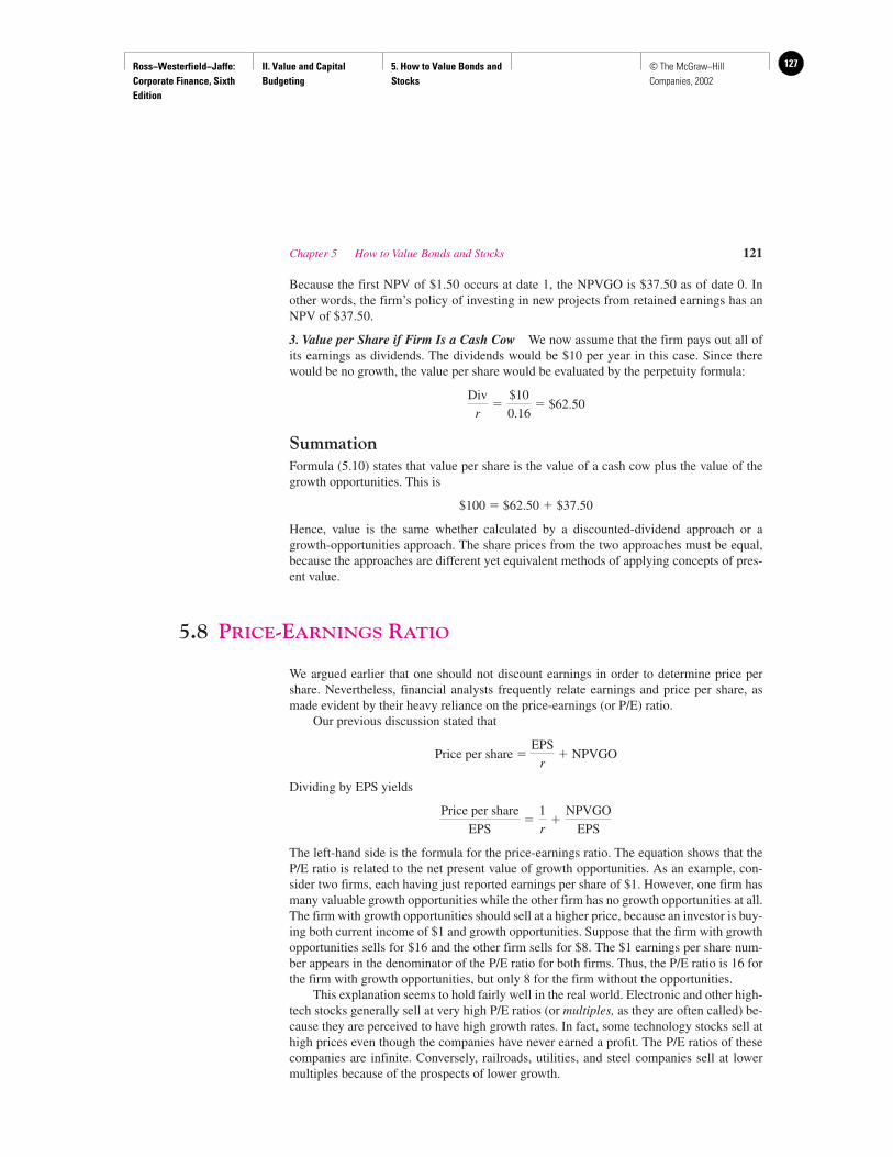
Ross−Westerfield−Jaffe: Corporate Finance, Sixth Edition
II. Value and Capital Budgeting
5. How to Value Bonds and Stocks
127© The McGraw−Hill Companies, 2002
Because the first NPV of $1.50 occurs at date 1, the NPVGO is $37.50 as of date 0. Inother words, the firm’s policy of investing in new projects from retained earnings has anNPV of $37.50.
3. Value per Share if Firm Is a Cash Cow We now assume that the firm pays out all ofits earnings as dividends. The dividends would be $10 per year in this case. Since therewould be no growth, the value per share would be evaluated by the perpetuity formula:
� $62.50
SummationFormula (5.10) states that value per share is the value of a cash cow plus the value of thegrowth opportunities. This is
$100 � $62.50 � $37.50
Hence, value is the same whether calculated by a discounted-dividend approach or agrowth-opportunities approach. The share prices from the two approaches must be equal,because the approaches are different yet equivalent methods of applying concepts of pres-ent value.
5.8 PRICE-EARNINGS RATIO
We argued earlier that one should not discount earnings in order to determine price pershare. Nevertheless, financial analysts frequently relate earnings and price per share, asmade evident by their heavy reliance on the price-earnings (or P/E) ratio.
Our previous discussion stated that
Price per share � � NPVGO
Dividing by EPS yields
The left-hand side is the formula for the price-earnings ratio. The equation shows that theP/E ratio is related to the net present value of growth opportunities. As an example, con-sider two firms, each having just reported earnings per share of $1. However, one firm hasmany valuable growth opportunities while the other firm has no growth opportunities at all.The firm with growth opportunities should sell at a higher price, because an investor is buy-ing both current income of $1 and growth opportunities. Suppose that the firm with growthopportunities sells for $16 and the other firm sells for $8. The $1 earnings per share num-ber appears in the denominator of the P/E ratio for both firms. Thus, the P/E ratio is 16 forthe firm with growth opportunities, but only 8 for the firm without the opportunities.
This explanation seems to hold fairly well in the real world. Electronic and other high-tech stocks generally sell at very high P/E ratios (or multiples, as they are often called) be-cause they are perceived to have high growth rates. In fact, some technology stocks sell athigh prices even though the companies have never earned a profit. The P/E ratios of thesecompanies are infinite. Conversely, railroads, utilities, and steel companies sell at lowermultiples because of the prospects of lower growth.
Price per share
EPS�
1
r�
NPVGO
EPS
EPS
r
Div
r�
$10
0.16
Chapter 5 How to Value Bonds and Stocks 121
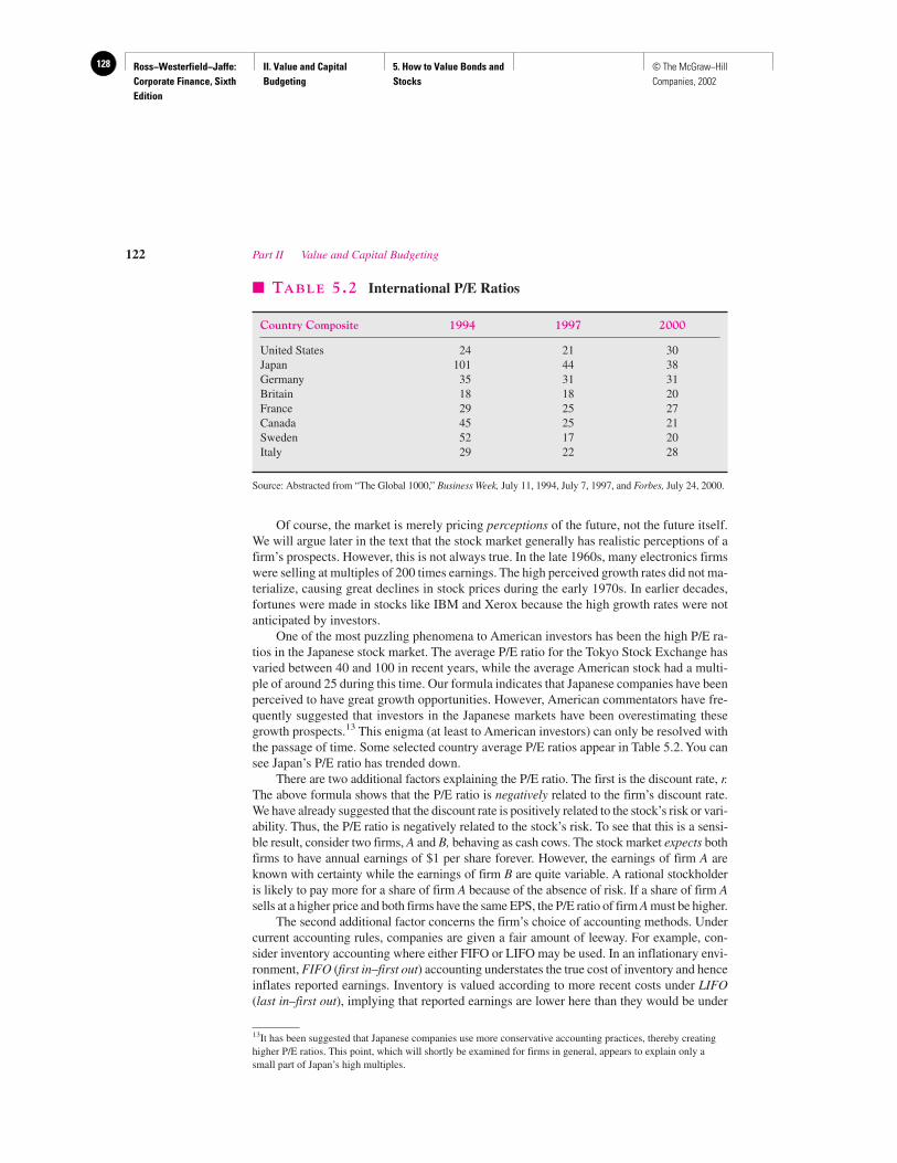
Ross−Westerfield−Jaffe: Corporate Finance, Sixth Edition
II. Value and Capital Budgeting
5. How to Value Bonds and Stocks
128 © The McGraw−Hill Companies, 2002
Of course, the market is merely pricing perceptions of the future, not the future itself.We will argue later in the text that the stock market generally has realistic perceptions of afirm’s prospects. However, this is not always true. In the late 1960s, many electronics firmswere selling at multiples of 200 times earnings. The high perceived growth rates did not ma-terialize, causing great declines in stock prices during the early 1970s. In earlier decades,fortunes were made in stocks like IBM and Xerox because the high growth rates were notanticipated by investors.
One of the most puzzling phenomena to American investors has been the high P/E ra-tios in the Japanese stock market. The average P/E ratio for the Tokyo Stock Exchange hasvaried between 40 and 100 in recent years, while the average American stock had a multi-ple of around 25 during this time. Our formula indicates that Japanese companies have beenperceived to have great growth opportunities. However, American commentators have fre-quently suggested that investors in the Japanese markets have been overestimating thesegrowth prospects.13 This enigma (at least to American investors) can only be resolved withthe passage of time. Some selected country average P/E ratios appear in Table 5.2. You cansee Japan’s P/E ratio has trended down.
There are two additional factors explaining the P/E ratio. The first is the discount rate, r.The above formula shows that the P/E ratio is negatively related to the firm’s discount rate.We have already suggested that the discount rate is positively related to the stock’s risk or vari-ability. Thus, the P/E ratio is negatively related to the stock’s risk. To see that this is a sensi-ble result, consider two firms, A and B, behaving as cash cows. The stock market expects bothfirms to have annual earnings of $1 per share forever. However, the earnings of firm A areknown with certainty while the earnings of firm B are quite variable. A rational stockholderis likely to pay more for a share of firm A because of the absence of risk. If a share of firm Asells at a higher price and both firms have the same EPS, the P/E ratio of firm A must be higher.
The second additional factor concerns the firm’s choice of accounting methods. Undercurrent accounting rules, companies are given a fair amount of leeway. For example, con-sider inventory accounting where either FIFO or LIFO may be used. In an inflationary envi-ronment, FIFO (first in–first out) accounting understates the true cost of inventory and henceinflates reported earnings. Inventory is valued according to more recent costs under LIFO(last in–first out), implying that reported earnings are lower here than they would be under
122 Part II Value and Capital Budgeting
13It has been suggested that Japanese companies use more conservative accounting practices, thereby creatinghigher P/E ratios. This point, which will shortly be examined for firms in general, appears to explain only asmall part of Japan’s high multiples.
� TABLE 5.2 International P/E Ratios
Country Composite 1994 1997 2000
United States 24 21 30Japan 101 44 38Germany 35 31 31Britain 18 18 20France 29 25 27Canada 45 25 21Sweden 52 17 20Italy 29 22 28
Source: Abstracted from “The Global 1000,” Business Week, July 11, 1994, July 7, 1997, and Forbes, July 24, 2000.
Ross−Westerfield−Jaffe: Corporate Finance, Sixth Edition
II. Value and Capital Budgeting
5. How to Value Bonds and Stocks
129© The McGraw−Hill Companies, 2002
FIFO. Thus, LIFO inventory accounting is a more conservative method than FIFO. Similaraccounting leeway exists for construction costs (completed-contracts versus percentage-of-completion methods) and depreciation (accelerated depreciation versus straight-line depreciation).
As an example, consider two identical firms, C and D. Firm C uses LIFO and reportsearnings of $2 per share. Firm D uses the less conservative accounting assumptions of FIFOand reports earnings of $3 per share. The market knows that both firms are identical andprices both at $18 per share. This price-earnings ratio is 9 ($18/$2) for firm C and 6 ($18/$3)for firm D. Thus, the firm with the more conservative principles has the higher P/E ratio.
This last example depends on the assumption that the market sees through differencesin accounting treatments. A significant portion of the academic community believes that themarket sees through virtually all accounting differences. These academics are adherents ofthe hypothesis of efficient capital markets, a theory that we explore in great detail later inthe text. Though many financial people might be more moderate in their beliefs regardingthis issue, the consensus view is certainly that many of the accounting differences are seenthrough. Thus, the proposition that firms with conservative accountants have high P/E ra-tios is widely accepted.
This discussion argued that the P/E ratio is a function of three different factors. A com-pany’s ratio or multiple is likely to be high if (1) it has many growth opportunities, (2) it haslow risk, and (3) it is accounted for in a conservative manner. While each of the three fac-tors is important, it is our opinion that the first factor is much more so. Thus, our discussionof growth is quite relevant in understanding price-earnings multiples.
• What are the three factors determining a firm’s P/E ratio?
5.9 STOCK MARKET REPORTING
The Wall Street Journal, the New York Times, or your own local newspaper provides useful in-formation on a large number of stocks in several stock exchanges. Table 5.3 reproduces whathas been reported on a particular day for several stocks listed on the New York Stock Ex-change. In Table 5.3, you can easily find the line for General Electric (i.e., “GenElec”). Read-ing left to right, the first two numbers are the high and low share prices over the last 52 weeks.For example, the highest price that General Electric traded for at the end of any particular day over the last 52 weeks was $6050. This is read as 60 and the decimal .50. The stock sym-bol for General Electric is GE. Its annual dividend is $0.55. Most dividend-paying companiessuch as General Electric pay dividends on a quarterly basis. So the annual dividend is actu-ally the last quarterly dividend of .138 multiplied by 4 (i.e., .138 � 4 � $0.55).
Some firms like GenenTech do not pay dividends. The Div column for GenenTech isblank. The “Yld” column stands for dividend yield. General Electric’s dividend yield is thecurrent annual dividend, $0.55, divided by the current closing daily price, which is $5663
(you can find the closing price for this particular day in the next to last column). Note that$0.55/5663 � 1.0 percent. The next column is labeled PE, which is the symbol for the price-earnings ratio. The price-earnings ratio is the closing price divided by the current earningsper share (based upon the latest quarterly earnings per share multiplied by 4). GeneralElectric’s price-earnings ratio is 51. If we were financial analysts or investment bankers, wewould say General Electric “sells for 51 times earnings.” The next column is the volume of
Chapter 5 How to Value Bonds and Stocks 123
QUESTION
CO
NC
EP
T
?
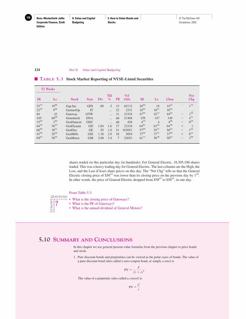
Ross−Westerfield−Jaffe: Corporate Finance, Sixth Edition
II. Value and Capital Budgeting
5. How to Value Bonds and Stocks
130 © The McGraw−Hill Companies, 2002
124 Part II Value and Capital Budgeting
� TABLE 5.3 Stock Market Reporting of NYSE-Listed Securities
52 Weeks
Yld Vol Net Hi Lo Stock Sym Div % PE 100s Hi Lo Close Chg
5375 1906 Gap Inc GPS .09 .5 15 65172 2050 19 1925 � 175
2225 956 GartnerGp IT ... 22 2331 1094 1031 1094 ...84 43 Gateway GTW ... 31 23354 4740 4215 4462 � 129
245 6688 Genentech DNA ... dd 21468 159 147 149 � 431
1544 250 GenDatacm GDC ... dd 456 425 4 406 � 025
6494 3625 GenDynam GD 1.04 1.6 17 23318 6481 6344 6456 � 16050 3821 GenElec GE .55 1.0 51 183051 5769 5531 5663 � 144
4394 2938 GenMills GIS 1.10 2.9 18 5054 3794 3731 3769 � 013
9463 5694 GenMotor GM 2.00 3.4 7 22653 6113 5838 5863 � 106
shares traded on this particular day (in hundreds). For General Electric, 18,305,100 sharestraded. This was a heavy trading day for General Electric. The last columns are the High, theLow, and the Last (Close) share prices on this day. The “Net Chg” tells us that the GeneralElectric closing price of $5663 was lower than its closing price on the previous day by 144.In other words, the price of General Electric dropped from $5807 to $5663, in one day.
From Table 5.3:
• What is the closing price of Gateways?• What is the PE of Gateways?• What is the annual dividend of General Motors?
5.10 SUMMARY AND CONCLUSIONS
In this chapter we use general present-value formulas from the previous chapter to price bondsand stock.
1. Pure discount bonds and perpetuities can be viewed as the polar cases of bonds. The value ofa pure discount bond (also called a zero-coupon bond, or simply a zero) is
PV �
The value of a perpetuity (also called a consol) is
PV �C
r
F�1 � r�T
QUESTIONS
CO
NC
EP
T
?

Ross−Westerfield−Jaffe: Corporate Finance, Sixth Edition
II. Value and Capital Budgeting
5. How to Value Bonds and Stocks
131© The McGraw−Hill Companies, 2002
2. Level-payment bonds can be viewed as an intermediate case. The coupon payments form anannuity and the principal repayment is a lump sum. The value of this type of bond is simplythe sum of the values of its two parts.
3. The yield to maturity on a bond is that single rate that discounts the payments on the bond toits purchase price.
4. A stock can be valued by discounting its dividends. We mention three types of situations:a. The case of zero growth of dividends.b. The case of constant growth of dividends.c. The case of differential growth.
5. An estimate of the growth rate of a stock is needed for formulas (4b) or (4c) above. A usefulestimate of the growth rate is
g � Retention ratio � Return on retained earnings
6. It is worthwhile to view a share of stock as the sum of its worth, if the company behaves likea cash cow (the company does no investing), and the value per share of its growthopportunities. We write the value of a share as
� NPVGO
We show that, in theory, share price must be the same whether the dividend-growth model orthe above formula is used.
7. From accounting, we know that earnings are divided into two parts: dividends and retainedearnings. Most firms continually retain earnings in order to create future dividends. Oneshould not discount earnings to obtain price per share since part of earnings must bereinvested. Only dividends reach the stockholders and only they should be discounted toobtain share price.
8. We suggest that a firm’s price-earnings ratio is a function of three factors:a. The per-share amount of the firm’s valuable growth opportunities.b. The risk of the stock.c. The type of accounting method used by the firm.
KEY TERMS
Coupons 103 Premium 106Discount 106 Pure discount bond 102Face value 102 Retention ratio 113Maturity date 102 Return on equity 113Payout ratio 114 Yield to maturity 107
SUGGESTED READINGS
The best place to look for additional information is in investment textbooks. A good one is:Bodie, Z., A. Kane, and A. Marcus. Investments. 5th ed. Burr Ridge, Ill.: Irwin/McGraw-Hill, 2002.
QUESTIONS AND PROBLEMS
How to Value Bonds5.1 What is the present value of a 10-year, pure discount bond that pays $1,000 at maturity and
is priced to yield the following rates?a. 5 percent
EPS
r
Chapter 5 How to Value Bonds and Stocks 125

Ross−Westerfield−Jaffe: Corporate Finance, Sixth Edition
II. Value and Capital Budgeting
5. How to Value Bonds and Stocks
132 © The McGraw−Hill Companies, 2002
b. 10 percentc. 15 percent
5.2 Microhard has issued a bond with the following characteristics:
Principal: $1,000Term to maturity: 20 yearsCoupon rate: 8 percentSemiannual payments
Calculate the price of the Microhard bond if the stated annual interest rate is:a. 8 percentb. 10 percentc. 6 percent
5.3 Consider a bond with a face value of $1,000. The coupon is paid semiannually and themarket interest rate (effective annual interest rate) is 12 percent. How much would you payfor the bond ifa. the coupon rate is 8 percent and the remaining time to maturity is 20 years?b. the coupon rate is 10 percent and the remaining time to maturity is 15 years?
5.4 Pettit Trucking has issued an 8-percent, 20-year bond that pays interest semiannually. If themarket prices the bond to yield an effective annual rate of 10 percent, what is the price ofthe bond?
5.5 A bond is sold at $923.14 (below its par value of $1,000). The bond has 15 years tomaturity and investors require a 10-percent yield on the bond. What is the coupon rate forthe bond if the coupon is paid semiannually?
5.6 You have just purchased a newly issued $1,000 five-year Vanguard Company bond at par.This five-year bond pays $60 in interest semiannually. You are also considering the purchaseof another Vanguard Company bond that returns $30 in semiannual interest payments andhas six years remaining before it matures. This bond has a face value of $1,000.a. What is effective annual return on the five-year bond?b. Assume that the rate you calculated in part (a) is the correct rate for the bond with six
years remaining before it matures. What should you be willing to pay for that bond?c. How will your answer to part (b) change if the five-year bond pays $40 in semiannual
interest?
Bond Concepts5.7 Consider two bonds, bond A and bond B, with equal rates of 10 percent and the same face
values of $1,000. The coupons are paid annually for both bonds. Bond A has 20 years tomaturity while bond B has 10 years to maturity.a. What are the prices of the two bonds if the relevant market interest rate is 10 percent?b. If the market interest rate increases to 12 percent, what will be the prices of the two bonds?c. If the market interest rate decreases to 8 percent, what will be the prices of the two bonds?
5.8 a. If the market interest rate (the required rate of return that investors demand)unexpectedly increases, what effect would you expect this increase to have on theprices of long-term bonds? Why?
b. What would be the effect of the rise in the interest rate on the general level of stockprices? Why?
5.9 Consider a bond that pays an $80 coupon annually and has a face value of $1,000.Calculate the yield to maturity if the bond hasa. 20 years remaining to maturity and it is sold at $1,200.b. 10 years remaining to maturity and it is sold at $950.
5.10 The Sue Fleming Corporation has two different bonds currently outstanding. Bond A has aface value of $40,000 and matures in 20 years. The bond makes no payments for the firstsix years and then pays $2,000 semiannually for the subsequent eight years, and finallypays $2,500 semiannually for the last six years. Bond B also has a face value of $40,000
126 Part II Value and Capital Budgeting
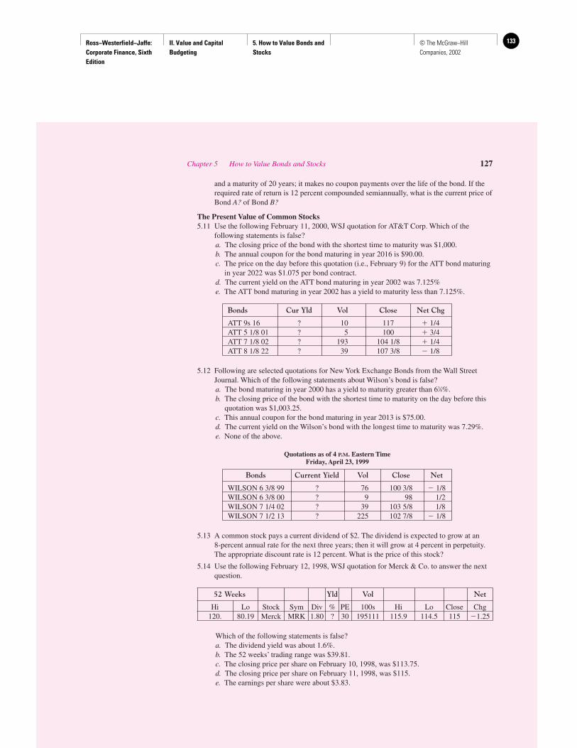
Ross−Westerfield−Jaffe: Corporate Finance, Sixth Edition
II. Value and Capital Budgeting
5. How to Value Bonds and Stocks
133© The McGraw−Hill Companies, 2002
and a maturity of 20 years; it makes no coupon payments over the life of the bond. If therequired rate of return is 12 percent compounded semiannually, what is the current price ofBond A? of Bond B?
The Present Value of Common Stocks5.11 Use the following February 11, 2000, WSJ quotation for AT&T Corp. Which of the
following statements is false?a. The closing price of the bond with the shortest time to maturity was $1,000.b. The annual coupon for the bond maturing in year 2016 is $90.00.c. The price on the day before this quotation (i.e., February 9) for the ATT bond maturing
in year 2022 was $1.075 per bond contract.d. The current yield on the ATT bond maturing in year 2002 was 7.125%e. The ATT bond maturing in year 2002 has a yield to maturity less than 7.125%.
Bonds Cur Yld Vol Close Net Chg
ATT 9s 16 ? 10 117 � 1/4ATT 5 1/8 01 ? 5 100 � 3/4ATT 7 1/8 02 ? 193 104 1/8 � 1/4ATT 8 1/8 22 ? 39 107 3/8 � 1/8
5.12 Following are selected quotations for New York Exchange Bonds from the Wall StreetJournal. Which of the following statements about Wilson’s bond is false?a. The bond maturing in year 2000 has a yield to maturity greater than 63⁄8%.b. The closing price of the bond with the shortest time to maturity on the day before this
quotation was $1,003.25.c. This annual coupon for the bond maturing in year 2013 is $75.00.d. The current yield on the Wilson’s bond with the longest time to maturity was 7.29%.e. None of the above.
Quotations as of 4 P.M. Eastern TimeFriday, April 23, 1999
Bonds Current Yield Vol Close Net
WILSON 6 3/8 99 ? 76 100 3/8 � 1/8WILSON 6 3/8 00 ? 9 98 1/2WILSON 7 1/4 02 ? 39 103 5/8 1/8WILSON 7 1/2 13 ? 225 102 7/8 � 1/8
5.13 A common stock pays a current dividend of $2. The dividend is expected to grow at an 8-percent annual rate for the next three years; then it will grow at 4 percent in perpetuity.The appropriate discount rate is 12 percent. What is the price of this stock?
5.14 Use the following February 12, 1998, WSJ quotation for Merck & Co. to answer the nextquestion.
52 Weeks Yld Vol Net
Hi Lo Stock Sym Div % PE 100s Hi Lo Close Chg120. 80.19 Merck MRK 1.80 ? 30 195111 115.9 114.5 115 �1.25
Which of the following statements is false?a. The dividend yield was about 1.6%.b. The 52 weeks’ trading range was $39.81.c. The closing price per share on February 10, 1998, was $113.75.d. The closing price per share on February 11, 1998, was $115.e. The earnings per share were about $3.83.
Chapter 5 How to Value Bonds and Stocks 127
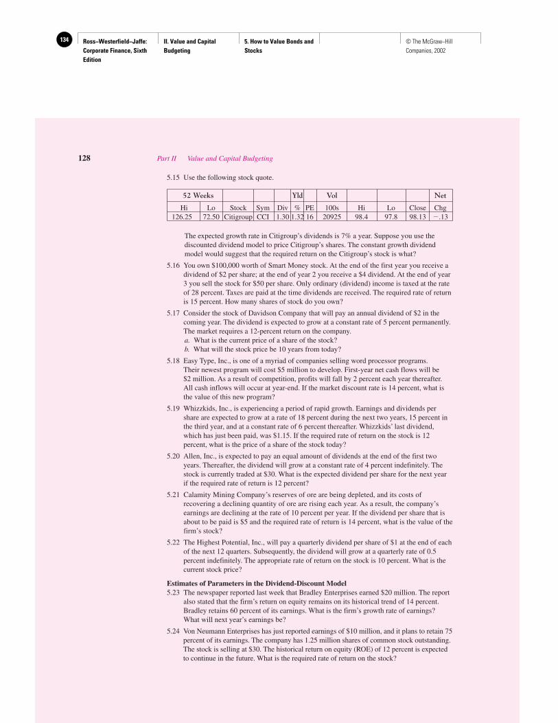
Ross−Westerfield−Jaffe: Corporate Finance, Sixth Edition
II. Value and Capital Budgeting
5. How to Value Bonds and Stocks
134 © The McGraw−Hill Companies, 2002
5.15 Use the following stock quote.
52 Weeks Yld Vol Net
Hi Lo Stock Sym Div % PE 100s Hi Lo Close Chg126.25 72.50 Citigroup CCI 1.30 1.32 16 20925 98.4 97.8 98.13 �.13
The expected growth rate in Citigroup’s dividends is 7% a year. Suppose you use thediscounted dividend model to price Citigroup’s shares. The constant growth dividendmodel would suggest that the required return on the Citigroup’s stock is what?
5.16 You own $100,000 worth of Smart Money stock. At the end of the first year you receive adividend of $2 per share; at the end of year 2 you receive a $4 dividend. At the end of year3 you sell the stock for $50 per share. Only ordinary (dividend) income is taxed at the rateof 28 percent. Taxes are paid at the time dividends are received. The required rate of returnis 15 percent. How many shares of stock do you own?
5.17 Consider the stock of Davidson Company that will pay an annual dividend of $2 in thecoming year. The dividend is expected to grow at a constant rate of 5 percent permanently.The market requires a 12-percent return on the company.a. What is the current price of a share of the stock?b. What will the stock price be 10 years from today?
5.18 Easy Type, Inc., is one of a myriad of companies selling word processor programs. Their newest program will cost $5 million to develop. First-year net cash flows will be $2 million. As a result of competition, profits will fall by 2 percent each year thereafter.All cash inflows will occur at year-end. If the market discount rate is 14 percent, what isthe value of this new program?
5.19 Whizzkids, Inc., is experiencing a period of rapid growth. Earnings and dividends pershare are expected to grow at a rate of 18 percent during the next two years, 15 percent inthe third year, and at a constant rate of 6 percent thereafter. Whizzkids’ last dividend,which has just been paid, was $1.15. If the required rate of return on the stock is 12percent, what is the price of a share of the stock today?
5.20 Allen, Inc., is expected to pay an equal amount of dividends at the end of the first twoyears. Thereafter, the dividend will grow at a constant rate of 4 percent indefinitely. Thestock is currently traded at $30. What is the expected dividend per share for the next yearif the required rate of return is 12 percent?
5.21 Calamity Mining Company’s reserves of ore are being depleted, and its costs ofrecovering a declining quantity of ore are rising each year. As a result, the company’searnings are declining at the rate of 10 percent per year. If the dividend per share that isabout to be paid is $5 and the required rate of return is 14 percent, what is the value of thefirm’s stock?
5.22 The Highest Potential, Inc., will pay a quarterly dividend per share of $1 at the end of eachof the next 12 quarters. Subsequently, the dividend will grow at a quarterly rate of 0.5percent indefinitely. The appropriate rate of return on the stock is 10 percent. What is thecurrent stock price?
Estimates of Parameters in the Dividend-Discount Model5.23 The newspaper reported last week that Bradley Enterprises earned $20 million. The report
also stated that the firm’s return on equity remains on its historical trend of 14 percent.Bradley retains 60 percent of its earnings. What is the firm’s growth rate of earnings?What will next year’s earnings be?
5.24 Von Neumann Enterprises has just reported earnings of $10 million, and it plans to retain 75percent of its earnings. The company has 1.25 million shares of common stock outstanding.The stock is selling at $30. The historical return on equity (ROE) of 12 percent is expectedto continue in the future. What is the required rate of return on the stock?
128 Part II Value and Capital Budgeting
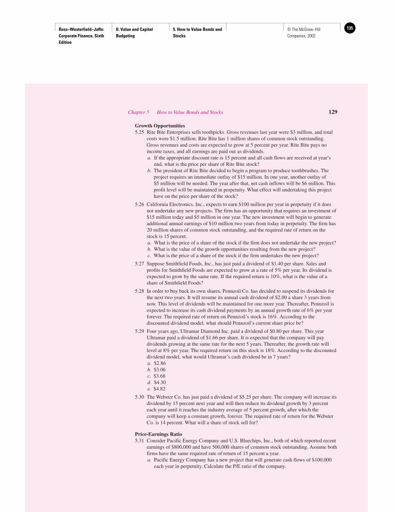
Ross−Westerfield−Jaffe: Corporate Finance, Sixth Edition
II. Value and Capital Budgeting
5. How to Value Bonds and Stocks
135© The McGraw−Hill Companies, 2002
Growth Opportunities5.25 Rite Bite Enterprises sells toothpicks. Gross revenues last year were $3 million, and total
costs were $1.5 million. Rite Bite has 1 million shares of common stock outstanding.Gross revenues and costs are expected to grow at 5 percent per year. Rite Bite pays noincome taxes, and all earnings are paid out as dividends.a. If the appropriate discount rate is 15 percent and all cash flows are received at year’s
end, what is the price per share of Rite Bite stock?b. The president of Rite Bite decided to begin a program to produce toothbrushes. The
project requires an immediate outlay of $15 million. In one year, another outlay of $5 million will be needed. The year after that, net cash inflows will be $6 million. Thisprofit level will be maintained in perpetuity. What effect will undertaking this projecthave on the price per share of the stock?
5.26 California Electronics, Inc., expects to earn $100 million per year in perpetuity if it doesnot undertake any new projects. The firm has an opportunity that requires an investment of$15 million today and $5 million in one year. The new investment will begin to generateadditional annual earnings of $10 million two years from today in perpetuity. The firm has20 million shares of common stock outstanding, and the required rate of return on thestock is 15 percent.a. What is the price of a share of the stock if the firm does not undertake the new project?b. What is the value of the growth opportunities resulting from the new project?c. What is the price of a share of the stock if the firm undertakes the new project?
5.27 Suppose Smithfield Foods, Inc., has just paid a dividend of $1.40 per share. Sales andprofits for Smithfield Foods are expected to grow at a rate of 5% per year. Its dividend isexpected to grow by the same rate. If the required return is 10%, what is the value of ashare of Smithfield Foods?
5.28 In order to buy back its own shares, Pennzoil Co. has decided to suspend its dividends forthe next two years. It will resume its annual cash dividend of $2.00 a share 3 years fromnow. This level of dividends will be maintained for one more year. Thereafter, Pennzoil isexpected to increase its cash dividend payments by an annual growth rate of 6% per yearforever. The required rate of return on Pennzoil’s stock is 16%. According to thediscounted dividend model, what should Pennzoil’s current share price be?
5.29 Four years ago, Ultramar Diamond Inc. paid a dividend of $0.80 per share. This yearUltramar paid a dividend of $1.66 per share. It is expected that the company will paydividends growing at the same rate for the next 5 years. Thereafter, the growth rate willlevel at 8% per year. The required return on this stock is 18%. According to the discounteddividend model, what would Ultramar’s cash dividend be in 7 years?a. $2.86b. $3.06c. $3.68d. $4.30e. $4.82
5.30 The Webster Co. has just paid a dividend of $5.25 per share. The company will increase itsdividend by 15 percent next year and will then reduce its dividend growth by 3 percenteach year until it reaches the industry average of 5 percent growth, after which thecompany will keep a constant growth, forever. The required rate of return for the WebsterCo. is 14 percent. What will a share of stock sell for?
Price-Earnings Ratio5.31 Consider Pacific Energy Company and U.S. Bluechips, Inc., both of which reported recent
earnings of $800,000 and have 500,000 shares of common stock outstanding. Assume bothfirms have the same required rate of return of 15 percent a year.a. Pacific Energy Company has a new project that will generate cash flows of $100,000
each year in perpetuity. Calculate the P/E ratio of the company.
Chapter 5 How to Value Bonds and Stocks 129
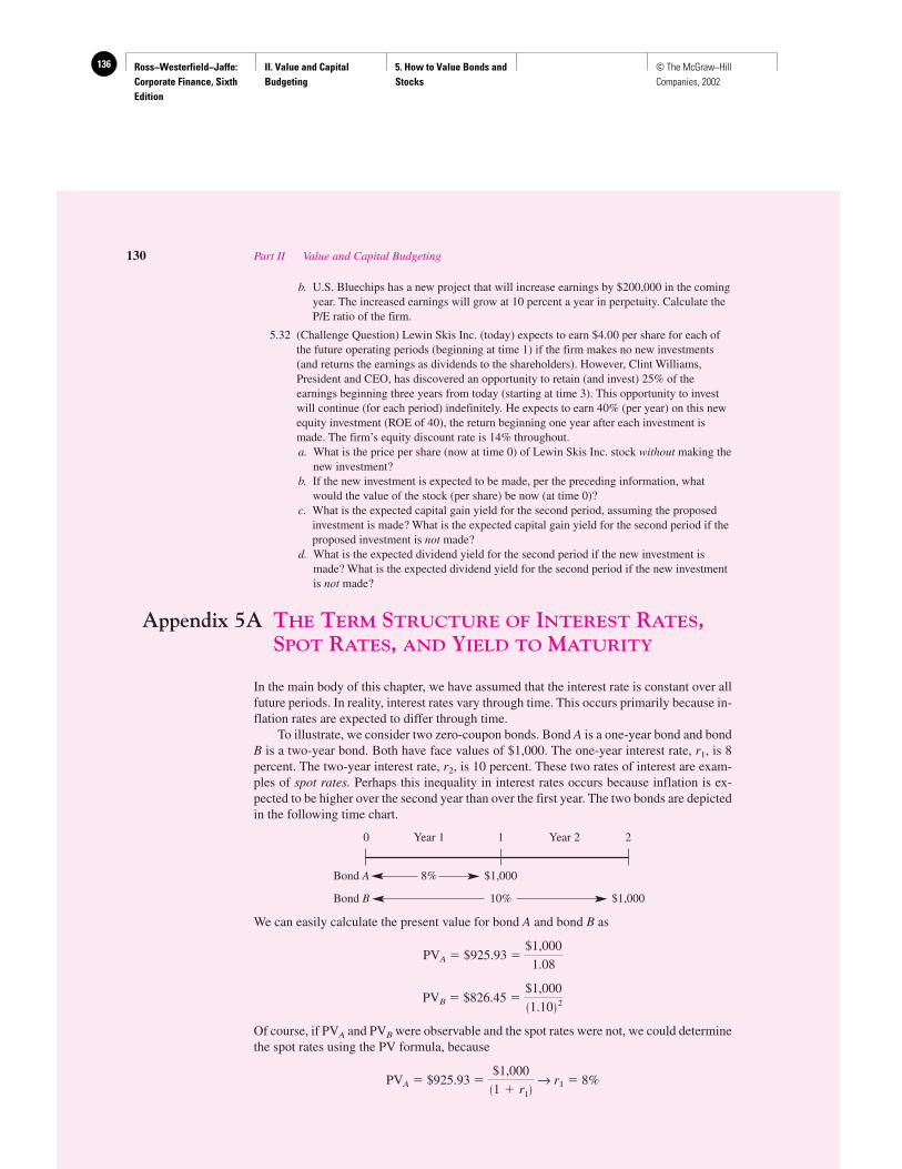
Ross−Westerfield−Jaffe: Corporate Finance, Sixth Edition
II. Value and Capital Budgeting
5. How to Value Bonds and Stocks
136 © The McGraw−Hill Companies, 2002
b. U.S. Bluechips has a new project that will increase earnings by $200,000 in the comingyear. The increased earnings will grow at 10 percent a year in perpetuity. Calculate theP/E ratio of the firm.
5.32 (Challenge Question) Lewin Skis Inc. (today) expects to earn $4.00 per share for each ofthe future operating periods (beginning at time 1) if the firm makes no new investments(and returns the earnings as dividends to the shareholders). However, Clint Williams,President and CEO, has discovered an opportunity to retain (and invest) 25% of theearnings beginning three years from today (starting at time 3). This opportunity to investwill continue (for each period) indefinitely. He expects to earn 40% (per year) on this newequity investment (ROE of 40), the return beginning one year after each investment ismade. The firm’s equity discount rate is 14% throughout.a. What is the price per share (now at time 0) of Lewin Skis Inc. stock without making the
new investment?b. If the new investment is expected to be made, per the preceding information, what
would the value of the stock (per share) be now (at time 0)?c. What is the expected capital gain yield for the second period, assuming the proposed
investment is made? What is the expected capital gain yield for the second period if theproposed investment is not made?
d. What is the expected dividend yield for the second period if the new investment ismade? What is the expected dividend yield for the second period if the new investmentis not made?
Appendix 5A THE TERM STRUCTURE OF INTEREST RATES,SPOT RATES, AND YIELD TO MATURITY
In the main body of this chapter, we have assumed that the interest rate is constant over allfuture periods. In reality, interest rates vary through time. This occurs primarily because in-flation rates are expected to differ through time.
To illustrate, we consider two zero-coupon bonds. Bond A is a one-year bond and bondB is a two-year bond. Both have face values of $1,000. The one-year interest rate, r1, is 8percent. The two-year interest rate, r2, is 10 percent. These two rates of interest are exam-ples of spot rates. Perhaps this inequality in interest rates occurs because inflation is ex-pected to be higher over the second year than over the first year. The two bonds are depictedin the following time chart.
0 Year 1 1 Year 2 2
Bond A 8% $1,000
Bond B 10% $1,000
We can easily calculate the present value for bond A and bond B as
PVA � $925.93 �
PVB � $826.45 �
Of course, if PVA and PVB were observable and the spot rates were not, we could determinethe spot rates using the PV formula, because
PVA � $925.93 � → r1 � 8%$1,000�1 � r1�
$1,000�1.10� 2
$1,000
1.08
130 Part II Value and Capital Budgeting
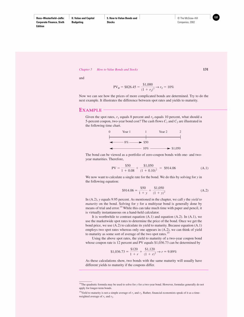
Ross−Westerfield−Jaffe: Corporate Finance, Sixth Edition
II. Value and Capital Budgeting
5. How to Value Bonds and Stocks
137© The McGraw−Hill Companies, 2002
and
PVB � $826.45 � → r2 � 10%
Now we can see how the prices of more complicated bonds are determined. Try to do thenext example. It illustrates the difference between spot rates and yields to maturity.
EXAMPLE
Given the spot rates, r1 equals 8 percent and r2 equals 10 percent, what should a5-percent coupon, two-year bond cost? The cash flows C1 and C2 are illustrated inthe following time chart.
0 Year 1 1 Year 2 2
8% $50
10% $1,050
The bond can be viewed as a portfolio of zero-coupon bonds with one- and two-year maturities. Therefore,
PV � (A.1)
We now want to calculate a single rate for the bond. We do this by solving for y inthe following equation:
$914.06 � (A.2)
In (A.2), y equals 9.95 percent. As mentioned in the chapter, we call y the yield tomaturity on the bond. Solving for y for a multiyear bond is generally done bymeans of trial and error.14 While this can take much time with paper and pencil, itis virtually instantaneous on a hand-held calculator.
It is worthwhile to contrast equation (A.1) and equation (A.2). In (A.1), weuse the marketwide spot rates to determine the price of the bond. Once we get thebond price, we use (A.2) to calculate its yield to maturity. Because equation (A.1)employs two spot rates whereas only one appears in (A.2), we can think of yieldto maturity as some sort of average of the two spot rates.15
Using the above spot rates, the yield to maturity of a two-year coupon bondwhose coupon rate is 12 percent and PV equals $1,036.73 can be determined by
$1,036.73 � → r � 9.89%
As these calculations show, two bonds with the same maturity will usually havedifferent yields to maturity if the coupons differ.
$120
1 � r�
$1,120�1 � r� 2
$50
1 � y�
$1,050�1 � y� 2
$50
1 � 0.08�
$1,050�1 � 0.10� 2 � $914.06
$1,000�1 � r2� 2
Chapter 5 How to Value Bonds and Stocks 131
14The quadratic formula may be used to solve for y for a two-year bond. However, formulas generally do notapply for longer-term bonds.15Yield to maturity is not a simple average of r1 and r2. Rather, financial economists speak of it as a time-weighted average of r1 and r2.
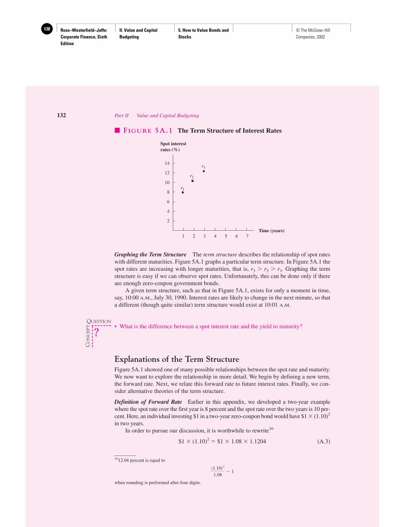
Ross−Westerfield−Jaffe: Corporate Finance, Sixth Edition
II. Value and Capital Budgeting
5. How to Value Bonds and Stocks
138 © The McGraw−Hill Companies, 2002
Graphing the Term Structure The term structure describes the relationship of spot rateswith different maturities. Figure 5A.1 graphs a particular term structure. In Figure 5A.1 thespot rates are increasing with longer maturities, that is, r3 � r2 � r1. Graphing the termstructure is easy if we can observe spot rates. Unfortunately, this can be done only if thereare enough zero-coupon government bonds.
A given term structure, such as that in Figure 5A.1, exists for only a moment in time,say, 10:00 A.M., July 30, 1990. Interest rates are likely to change in the next minute, so thata different (though quite similar) term structure would exist at 10:01 A.M.
• What is the difference between a spot interest rate and the yield to maturity?
Explanations of the Term StructureFigure 5A.1 showed one of many possible relationships between the spot rate and maturity.We now want to explore the relationship in more detail. We begin by defining a new term,the forward rate. Next, we relate this forward rate to future interest rates. Finally, we con-sider alternative theories of the term structure.
Definition of Forward Rate Earlier in this appendix, we developed a two-year examplewhere the spot rate over the first year is 8 percent and the spot rate over the two years is 10 per-cent. Here, an individual investing $1 in a two-year zero-coupon bond would have $1 � (1.10)2
in two years.In order to pursue our discussion, it is worthwhile to rewrite16
$1 � (1.10)2 � $1 � 1.08 � 1.1204 (A.3)
132 Part II Value and Capital Budgeting
1 2 3 4 5 6 7
2
4
6
8
10
12
14r3
r2
r1
Spot interestrates (%)
Time (years)
� FIGURE 5A.1 The Term Structure of Interest Rates
QUESTION
CO
NC
EP
T
?
1612.04 percent is equal to
when rounding is performed after four digits.
�1.10� 2
1.08� 1
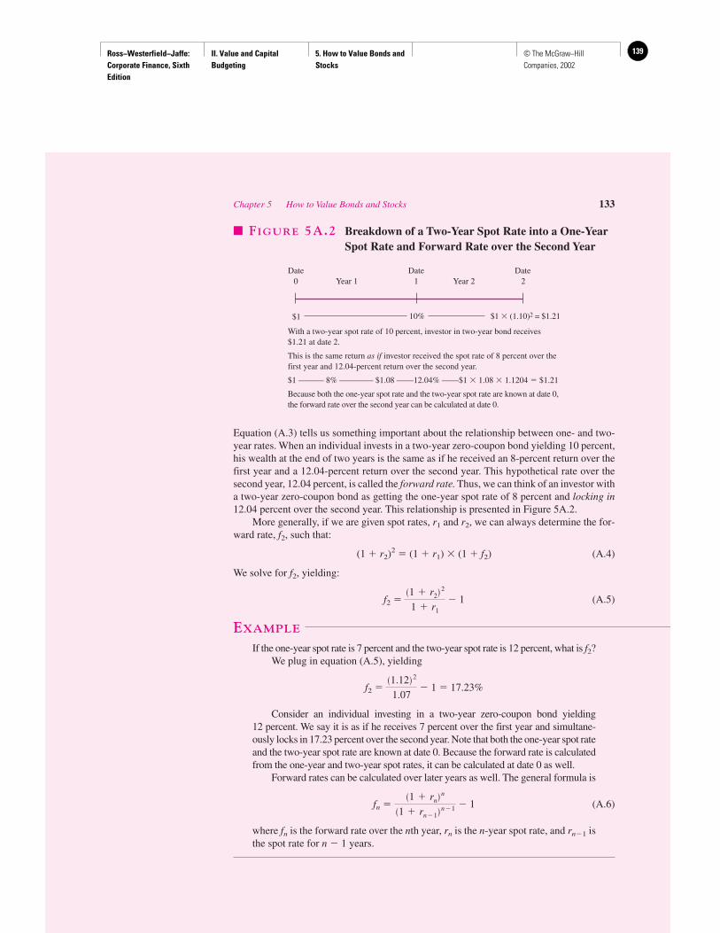
Ross−Westerfield−Jaffe: Corporate Finance, Sixth Edition
II. Value and Capital Budgeting
5. How to Value Bonds and Stocks
139© The McGraw−Hill Companies, 2002
Equation (A.3) tells us something important about the relationship between one- and two-year rates. When an individual invests in a two-year zero-coupon bond yielding 10 percent,his wealth at the end of two years is the same as if he received an 8-percent return over thefirst year and a 12.04-percent return over the second year. This hypothetical rate over thesecond year, 12.04 percent, is called the forward rate. Thus, we can think of an investor witha two-year zero-coupon bond as getting the one-year spot rate of 8 percent and locking in12.04 percent over the second year. This relationship is presented in Figure 5A.2.
More generally, if we are given spot rates, r1 and r2, we can always determine the for-ward rate, f2, such that:
(1 � r2)2 � (1 � r1) � (1 � f2) (A.4)
We solve for f2, yielding:
f2 � � 1 (A.5)
EXAMPLE
If the one-year spot rate is 7 percent and the two-year spot rate is 12 percent, what is f2?We plug in equation (A.5), yielding
f2 � � 1 � 17.23%
Consider an individual investing in a two-year zero-coupon bond yielding 12 percent. We say it is as if he receives 7 percent over the first year and simultane-ously locks in 17.23 percent over the second year. Note that both the one-year spot rateand the two-year spot rate are known at date 0. Because the forward rate is calculatedfrom the one-year and two-year spot rates, it can be calculated at date 0 as well.
Forward rates can be calculated over later years as well. The general formula is
fn � � 1 (A.6)
where fn is the forward rate over the nth year, rn is the n-year spot rate, and rn�1 isthe spot rate for n � 1 years.
�1 � rn� n
�1 � rn�1� n�1
�1.12� 2
1.07
�1 � r2� 2
1 � r1
Chapter 5 How to Value Bonds and Stocks 133
0 1 2Year 1 Year 2
10%$1 $1 � (1.10)2 = $1.21
Date Date Date
� FIGURE 5A.2 Breakdown of a Two-Year Spot Rate into a One-YearSpot Rate and Forward Rate over the Second Year
With a two-year spot rate of 10 percent, investor in two-year bond receives$1.21 at date 2.
This is the same return as if investor received the spot rate of 8 percent over thefirst year and 12.04-percent return over the second year.
$1 ——— 8% ———— $1.08 ——12.04% ——$1 � 1.08 � 1.1204 � $1.21
Because both the one-year spot rate and the two-year spot rate are known at date 0,the forward rate over the second year can be calculated at date 0.
Ross−Westerfield−Jaffe: Corporate Finance, Sixth Edition
II. Value and Capital Budgeting
5. How to Value Bonds and Stocks
140 © The McGraw−Hill Companies, 2002
EXAMPLE
Assume the following set of rates:
Year Spot Rate
1 5%2 63 74 6
What are the forward rates over each of the four years?The forward rate over the first year is, by definition, equal to the one-year spot
rate. Thus, we do not generally speak of the forward rate over the first year. Theforward rates over the later years are
f2 � � 1 � 7.01%
f3 � � 1 � 9.03%
f4 � � 1 � 3.06%
An individual investing $1 in the two-year zero-coupon bond receives$1.1236 [$1 � (1.06)2] at date 2. He can be viewed as receiving the one-yearspot rate of 5 percent over the first year and receiving the forward rate of 7.01percent over the second year. An individual investing $1 in a three-year zero-coupon bond receives $1.2250 [$1 � (1.07)3] at date 3. She can be viewed asreceiving the two-year spot rate of 6 percent over the first two years and re-ceiving the forward rate of 9.03 percent over the third year. An individual in-vesting $1 in a four-year zero-coupon bond receives $1.2625 [$1 � (1.06)4] atdate 4. He can be viewed as receiving the three-year spot rate of 7 percent overthe first three years and receiving the forward rate of 3.06 percent over thefourth year.
Note that all of the four spot rates in this problem are known at date 0. Be-cause the forward rates are calculated from the spot rates, they can be determinedat date 0 as well.
The material in this appendix is likely to be difficult for a student exposed to term struc-ture for the first time. It helps to state what the student should know at this point. Givenequations (A.5) and (A.6), a student should be able to calculate a set of forward rates givena set of spot rates. This can simply be viewed as a mechanical computation. In addition tothe calculations, a student should understand the intuition of Figure 5A.2.
We now turn to the relationship between the forward rate and the expected spot ratesin the future.
Estimating the Price of a Bond at a Future Date In the example from the body of thischapter, we considered zero-coupon bonds paying $1,000 at maturity and selling at adiscount prior to maturity. We now wish to change the example slightly. Now, each bond
�1.06� 4
�1.07� 3
�1.07� 3
�1.06� 2
�1.06� 2
1.05
134 Part II Value and Capital Budgeting
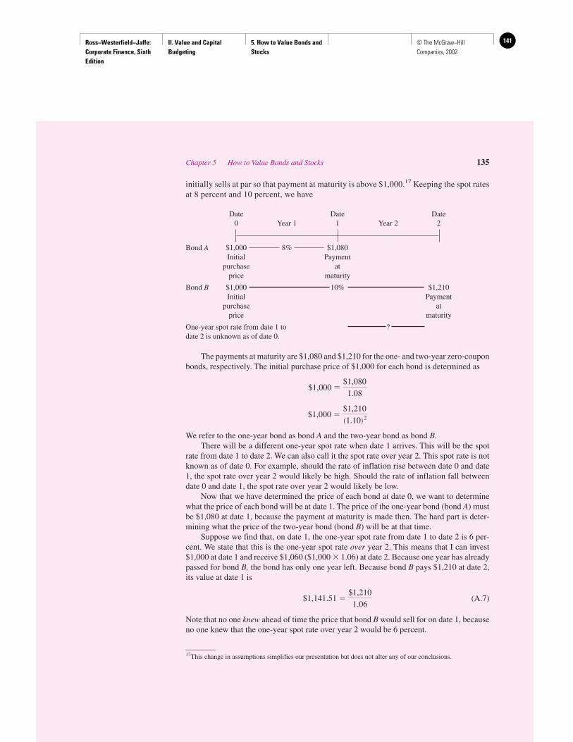
Ross−Westerfield−Jaffe: Corporate Finance, Sixth Edition
II. Value and Capital Budgeting
5. How to Value Bonds and Stocks
141© The McGraw−Hill Companies, 2002
initially sells at par so that payment at maturity is above $1,000.17 Keeping the spot ratesat 8 percent and 10 percent, we have
Date Date Date0 Year 1 1 Year 2 2
Bond A $1,000 8% $1,080Initial Payment
purchase atprice maturity
Bond B $1,000 10% $1,210Initial Payment
purchase atprice maturity
One-year spot rate from date 1 to ?date 2 is unknown as of date 0.
The payments at maturity are $1,080 and $1,210 for the one- and two-year zero-couponbonds, respectively. The initial purchase price of $1,000 for each bond is determined as
$1,000 �
$1,000 �
We refer to the one-year bond as bond A and the two-year bond as bond B.There will be a different one-year spot rate when date 1 arrives. This will be the spot
rate from date 1 to date 2. We can also call it the spot rate over year 2. This spot rate is notknown as of date 0. For example, should the rate of inflation rise between date 0 and date1, the spot rate over year 2 would likely be high. Should the rate of inflation fall betweendate 0 and date 1, the spot rate over year 2 would likely be low.
Now that we have determined the price of each bond at date 0, we want to determinewhat the price of each bond will be at date 1. The price of the one-year bond (bond A) mustbe $1,080 at date 1, because the payment at maturity is made then. The hard part is deter-mining what the price of the two-year bond (bond B) will be at that time.
Suppose we find that, on date 1, the one-year spot rate from date 1 to date 2 is 6 per-cent. We state that this is the one-year spot rate over year 2. This means that I can invest$1,000 at date 1 and receive $1,060 ($1,000 � 1.06) at date 2. Because one year has alreadypassed for bond B, the bond has only one year left. Because bond B pays $1,210 at date 2,its value at date 1 is
$1,141.51 � (A.7)
Note that no one knew ahead of time the price that bond B would sell for on date 1, becauseno one knew that the one-year spot rate over year 2 would be 6 percent.
$1,210
1.06
$1,210�1.10� 2
$1,080
1.08
Chapter 5 How to Value Bonds and Stocks 135
17This change in assumptions simplifies our presentation but does not alter any of our conclusions.
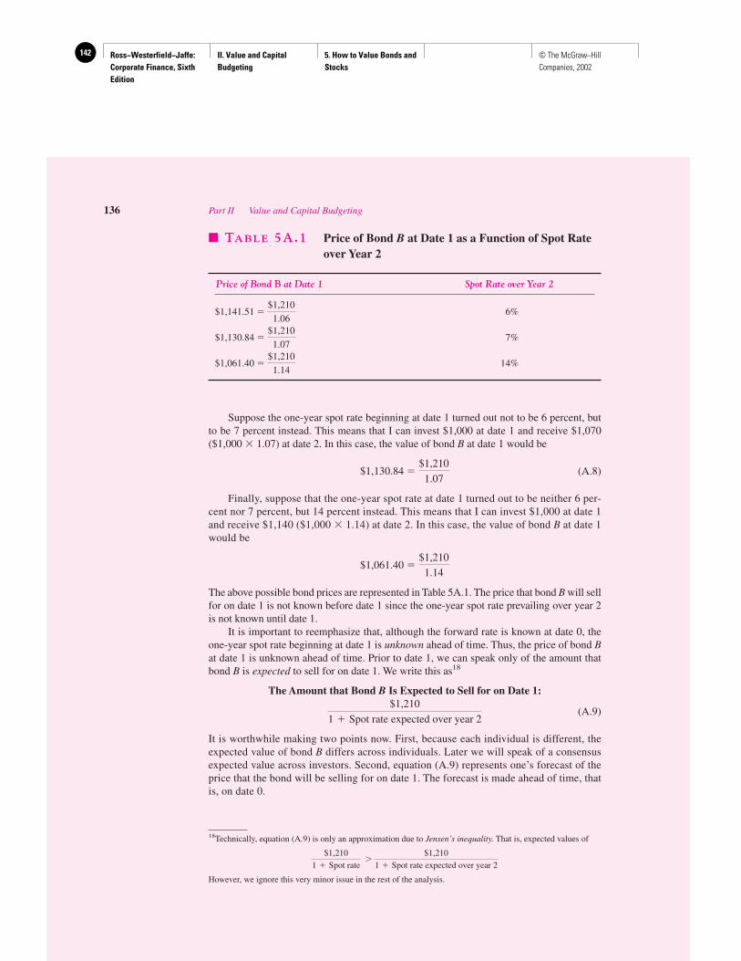
Ross−Westerfield−Jaffe: Corporate Finance, Sixth Edition
II. Value and Capital Budgeting
5. How to Value Bonds and Stocks
142 © The McGraw−Hill Companies, 2002
Suppose the one-year spot rate beginning at date 1 turned out not to be 6 percent, butto be 7 percent instead. This means that I can invest $1,000 at date 1 and receive $1,070($1,000 � 1.07) at date 2. In this case, the value of bond B at date 1 would be
$1,130.84 � (A.8)
Finally, suppose that the one-year spot rate at date 1 turned out to be neither 6 per-cent nor 7 percent, but 14 percent instead. This means that I can invest $1,000 at date 1and receive $1,140 ($1,000 � 1.14) at date 2. In this case, the value of bond B at date 1would be
$1,061.40 �
The above possible bond prices are represented in Table 5A.1. The price that bond B will sellfor on date 1 is not known before date 1 since the one-year spot rate prevailing over year 2is not known until date 1.
It is important to reemphasize that, although the forward rate is known at date 0, theone-year spot rate beginning at date 1 is unknown ahead of time. Thus, the price of bond Bat date 1 is unknown ahead of time. Prior to date 1, we can speak only of the amount thatbond B is expected to sell for on date 1. We write this as18
The Amount that Bond B Is Expected to Sell for on Date 1:
(A.9)
It is worthwhile making two points now. First, because each individual is different, theexpected value of bond B differs across individuals. Later we will speak of a consensusexpected value across investors. Second, equation (A.9) represents one’s forecast of theprice that the bond will be selling for on date 1. The forecast is made ahead of time, thatis, on date 0.
$1,210
1 � Spot rate expected over year 2
$1,210
1.14
$1,210
1.07
136 Part II Value and Capital Budgeting
� TABLE 5A.1 Price of Bond B at Date 1 as a Function of Spot Rateover Year 2
Price of Bond B at Date 1 Spot Rate over Year 2
$1,141.51 � 6%
$1,130.84 � 7%
$1,061.40 � 14%$1,210
1.14
$1,210
1.07
$1,210
1.06
18Technically, equation (A.9) is only an approximation due to Jensen’s inequality. That is, expected values of
However, we ignore this very minor issue in the rest of the analysis.
$1,210
1 � Spot rate �
$1,210
1 � Spot rate expected over year 2
Ross−Westerfield−Jaffe: Corporate Finance, Sixth Edition
II. Value and Capital Budgeting
5. How to Value Bonds and Stocks
143© The McGraw−Hill Companies, 2002
The Relationship between Forward Rate over Second Year andSpot Rate Expected over Second YearGiven a forecast of bond B’s price, an investor can choose one of two strategies at date 0:
I. Buy a one-year bond. Proceeds at date 1 would be
$1,080 � $1,000 � 1.08 (A.10)
II. Buy a two-year bond but sell at date 1. Expected proceeds would be
(A.11)
Given our discussion of forward rates, we can rewrite (A.11) as
(A.12)
(Remember that 12.04 percent was the forward rate over year 2; i.e., f2 � 12.04%.)Under what condition will the return from strategy I equal the expected return from
strategy II? In other words, under what condition will formula (A.10) equal formula (A.12)?The two strategies will yield the same expected return only when
12.04% � Spot rate expected over year 2 (A.13)
In other words, if the forward rate equals the expected spot rate, one would expect to earnthe same return over the first year whether one
1. invested in a one-year bond, or
2. invested in a two-year bond but sold after one year.
The Expectations HypothesisEquation (A.13) seems fairly reasonable. That is, it is reasonable that investors would setinterest rates in such a way that the forward rate would equal the spot rate expected by themarketplace a year from now.19 For example, imagine that individuals in the marketplacedo not concern themselves with risk. If the forward rate, f2, is less than the spot rate ex-pected over year 2, individuals desiring to invest for one year would always buy a one-yearbond. That is, our work above shows that an individual investing in a two-year bond butplanning to sell at the end of one year would expect to earn less than if he simply bought aone-year bond.
Equation (A.13) was stated for the specific case where the forward rate was 12.04 per-cent. We can generalize this to:
Expectations Hypothesis:f2 � Spot rate expected over year 2 (A.14)
Equation (A.14) says that the forward rate over the second year is set to the spot rate thatpeople expect to prevail over the second year. This is called the expectations hypothesis. Itstates that investors will set interest rates such that the forward rate over the second year isequal to the one-year spot rate expected over the second year.
$1,000 � 1.08 � 1.1204
1 � Spot rate expected over year 2
$1,000 � �1.10� 2
1 � Spot rate expected over year 2
Chapter 5 How to Value Bonds and Stocks 137
19Of course, each individual will have different expectations, so (A.13) cannot hold for all individuals. However,financial economists generally speak of a consensus expectation. This is the expectation of the market as a whole.
Ross−Westerfield−Jaffe: Corporate Finance, Sixth Edition
II. Value and Capital Budgeting
5. How to Value Bonds and Stocks
144 © The McGraw−Hill Companies, 2002
Liquidity-Preference HypothesisAt this point, many students think that equation (A.14) must hold. However, note that wedeveloped (A.14) by assuming that investors were risk-neutral. Suppose, alternatively, thatinvestors are adverse to risk.
Which strategy would appear more risky for an individual who wants to invest for one year?
I. Invest in a one-year bond.
II. Invest in a two-year bond but sell at the end of one year.
Strategy (I) has no risk because the investor knows that the rate of return must be r1. Conversely,strategy (II) has much risk; the final return is dependent on what happens to interest rates.
Because strategy (II) has more risk than strategy (I), no risk-averse investor will choosestrategy (II) if both strategies have the same expected return. Risk-averse investors can haveno preference for one strategy over the other only when the expected return on strategy (II)is above the return on strategy (I). Because the two strategies have the same expected re-turn when f2 equals the spot rate expected over year 2, strategy (II) can only have a higherrate of return when
Liquidity-Preference Hypothesis:f2 � Spot rate expected over year 2 (A.15)
That is, in order to induce investors to hold the riskier two-year bonds, the market setsthe forward rate over the second year to be above the spot rate expected over the secondyear. Equation (A.15) is called the liquidity-preference hypothesis.
We developed the entire discussion by assuming that individuals are planning to investover one year. We pointed out that for these types of individuals, a two-year bond has extrarisk because it must be sold prematurely. What about those individuals who want to investfor two years? (We call these people investors with a two-year time horizon.)
They could choose one of the following strategies:
III. Buy a two-year zero-coupon bond.
IV. Buy a one-year bond. When the bond matures, immediately buy another one-year bond.
Strategy (III) has no risk for an investor with a two-year time horizon, because the pro-ceeds to be received at date 2 are known as of date 0. However, strategy (IV) has risk sincethe spot rate over year 2 is unknown at date 0. It can be shown that risk-averse investors willprefer neither strategy (III) nor strategy (IV) over the other when
f2 Spot rate expected over year 2 (A.16)
Note that the assumption of risk aversion gives contrary predictions. Relationship(A.15) holds for a market dominated by investors with a one-year time horizon.Relationship (A.16) holds for a market dominated by investors with a two-year time hori-zon. Financial economists have generally argued that the time horizon of the typical in-vestor is generally much shorter than the maturity of typical bonds in the marketplace. Thus,economists view (A.15) as the best depiction of equilibrium in the bond market with risk-averse investors.
However, do we have a market of risk-neutral or risk-averse investors? In other words,can the expectations hypothesis of equation (A.14) or the liquidity-preference hypothesisof equation (A.15) be expected to hold? As we will learn later in this book, economists viewinvestors as being risk-averse for the most part. Yet economists are never satisfied with a ca-sual examination of a theory’s assumptions. To them, empirical evidence of a theory’s pre-dictions must be the final arbiter.
138 Part II Value and Capital Budgeting

Ross−Westerfield−Jaffe: Corporate Finance, Sixth Edition
II. Value and Capital Budgeting
5. How to Value Bonds and Stocks
145© The McGraw−Hill Companies, 2002
There has been a great deal of empirical evidence on the term structure of interest rates.Unfortunately (perhaps fortunately for some students), we will not be able to present the ev-idence in any detail. Suffice it to say that, in our opinion, the evidence supports the liquidity-preference hypothesis over the expectations hypothesis. One simple result might give students the flavor of this research. Consider an individual choosing between one of the fol-lowing two strategies:
I. Invest in a 1-year bond.
II′. Invest in a 20-year bond but sell at the end of 1 year.
(Strategy (II′) is identical to strategy (II), except that a 20-year bond is substituted fora 2-year bond.)
The expectations hypothesis states that the expected returns on both strategies are iden-tical. The liquidity-preference hypothesis states that the expected return on strategy (II′)should be above the expected return on strategy (I). Though no one knows what returns areactually expected over a particular time period, actual returns from the past may allow usto infer expectations. The results from January 1926 to December 1999 are illuminating.The average yearly return on strategy (I) is 3.8 percent and 5.5 percent on strategy (II′) over this time period.20, 21 This evidence is generally considered to be consistent with theliquidity-preference hypothesis and inconsistent with the expectations hypothesis.
• Define the forward rate.• What is the relationship between the one-year spot rate, the two-year spot rate, and the
forward rate over the second year?• What is the expectations hypothesis?• What is the liquidity-preference hypothesis?
QUESTIONS AND PROBLEMS
A.1 The appropriate discount rate for cash flows received one year from today is 10 percent. Theappropriate annual discount rate for cash flows received two years from today is 11 percent.a. What is the price of a two-year bond that pays an annual coupon of 6 percent?b. What is the yield to maturity of this bond?
A.2 The one-year spot rate equals 10 percent and the two-year spot rate equals 8 percent. Whatshould a 5-percent coupon two-year bond cost?
A.3 If the one-year spot rate is 9 percent and the two-year spot rate is 10 percent, what is theforward rate?
A.4 Assume the following spot rates:
Maturity Spot Rates (%)
1 52 73 10
What are the forward rates over each of the three years?
Chapter 5 How to Value Bonds and Stocks 139
20Taken from Stocks, Bonds, Bills and Inflation 2000 Yearbook (Chicago: Ibbotson Associates, Inc.). IbbotsonAssociates annually updates work by Roger G. Ibbotson and Rex A. Sinquefield.21It is important to note that strategy (II′) does not involve buying a 20-year bond and holding it to maturity.Rather, it consists of buying a 20-year bond and selling it 1 year later, that is, when it has become a 19-yearbond. This round-trip transaction occurs 74 times in the 74-year sample from January 1926 to December 1999.
QUESTIONS
CO
NC
EP
T
?
Ross−Westerfield−Jaffe: Corporate Finance, Sixth Edition
II. Value and Capital Budgeting
6. Some Alternative Investment Rules
146 © The McGraw−Hill Companies, 2002
Some AlternativeInvestment Rules
CH
AP
TE
R6
EXECUTIVE SUMMARY
Chapter 4 examined the relationship between $1 today and $1 in the future. For ex-ample, a corporate project generating a set of cash flows can be valued by discount-ing these flows, an approach called the net-present-value (NPV) approach. While we
believe that the NPV approach is the best one for evaluating capital budgeting projects, ourtreatment would be incomplete if we ignored alternative methods. This chapter examinesthese alternative methods. We first consider the NPV approach as a benchmark. Next we ex-amine three alternatives—payback, accounting rates of return, and internal rate of return.
6.1 WHY USE NET PRESENT VALUE?
Before examining competitors of the NPV approach, we should ask: Why consider usingNPV in the first place? Answering this question will put the rest of this chapter in a properperspective. There are actually a number of arguments justifying the use of NPV, and youmay have already seen the detailed one of Chapter 3. We now present one of the simplestjustifications through an example.
EXAMPLE
The Alpha Corporation is considering investing in a riskless project costing $100.The project pays $107 at date 1 and has no other cash flows. The managers of thefirm might contemplate one of two strategies:
1. Use $100 of corporate cash to invest in the project. The $107 will be paid as adividend in one period.
2. Forgo the project and pay the $100 of corporate cash as a dividend today.
If strategy 2 is employed, the stockholder might deposit the dividend in the bankfor one period. Because the project is riskless and lasts for one period, the stock-holder would prefer strategy 1 if the bank interest rate was below 7 percent. Inother words, the stockholder would prefer strategy 1 if strategy 2 produced lessthan $107 by the end of the year.
The comparison can easily be handled by NPV analysis. If the interest rate is 6 percent,the NPV of the project is
$0.94 � � $100 �$107
1.06
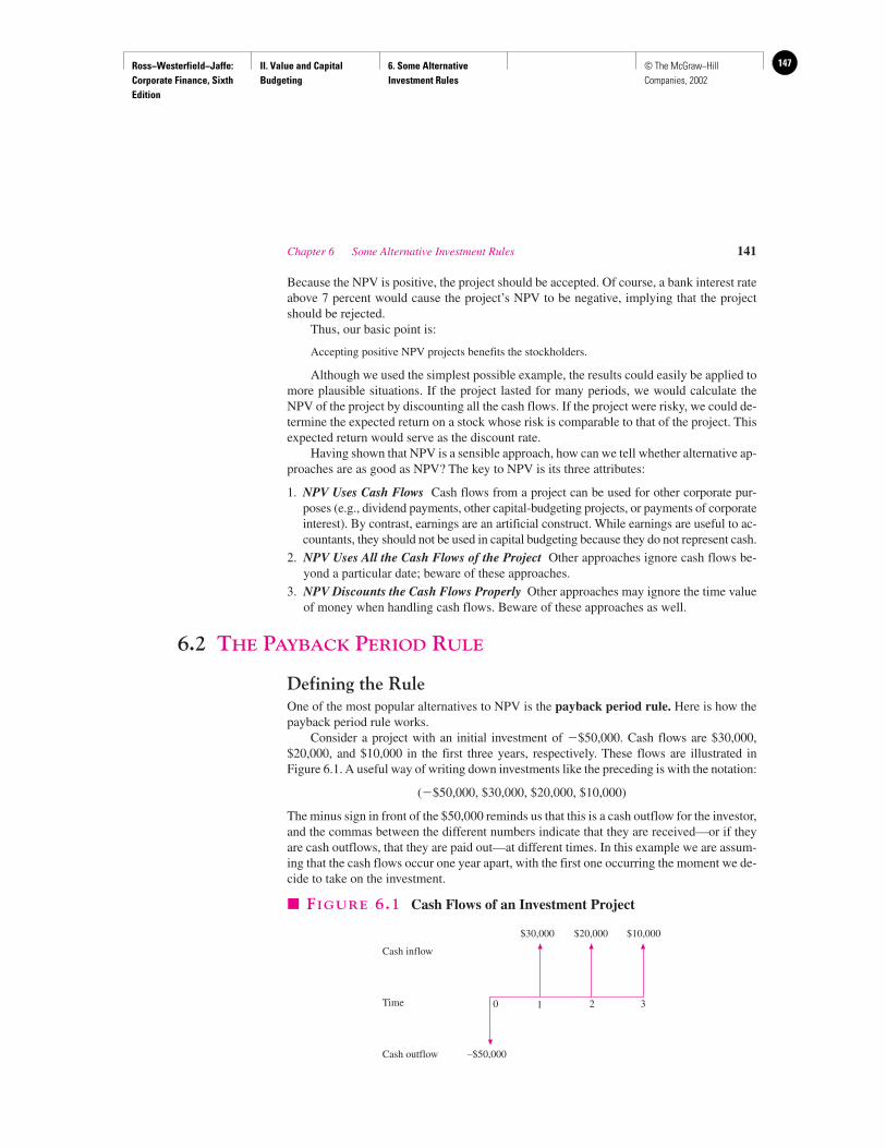
Ross−Westerfield−Jaffe: Corporate Finance, Sixth Edition
II. Value and Capital Budgeting
6. Some Alternative Investment Rules
147© The McGraw−Hill Companies, 2002
Chapter 6 Some Alternative Investment Rules 141
Because the NPV is positive, the project should be accepted. Of course, a bank interest rateabove 7 percent would cause the project’s NPV to be negative, implying that the projectshould be rejected.
Thus, our basic point is:
Accepting positive NPV projects benefits the stockholders.
Although we used the simplest possible example, the results could easily be applied tomore plausible situations. If the project lasted for many periods, we would calculate theNPV of the project by discounting all the cash flows. If the project were risky, we could de-termine the expected return on a stock whose risk is comparable to that of the project. Thisexpected return would serve as the discount rate.
Having shown that NPV is a sensible approach, how can we tell whether alternative ap-proaches are as good as NPV? The key to NPV is its three attributes:
1. NPV Uses Cash Flows Cash flows from a project can be used for other corporate pur-poses (e.g., dividend payments, other capital-budgeting projects, or payments of corporateinterest). By contrast, earnings are an artificial construct. While earnings are useful to ac-countants, they should not be used in capital budgeting because they do not represent cash.
2. NPV Uses All the Cash Flows of the Project Other approaches ignore cash flows be-yond a particular date; beware of these approaches.
3. NPV Discounts the Cash Flows Properly Other approaches may ignore the time valueof money when handling cash flows. Beware of these approaches as well.
6.2 THE PAYBACK PERIOD RULE
Defining the RuleOne of the most popular alternatives to NPV is the payback period rule. Here is how thepayback period rule works.
Consider a project with an initial investment of �$50,000. Cash flows are $30,000,$20,000, and $10,000 in the first three years, respectively. These flows are illustrated inFigure 6.1. A useful way of writing down investments like the preceding is with the notation:
(�$50,000, $30,000, $20,000, $10,000)
The minus sign in front of the $50,000 reminds us that this is a cash outflow for the investor,and the commas between the different numbers indicate that they are received—or if theyare cash outflows, that they are paid out—at different times. In this example we are assum-ing that the cash flows occur one year apart, with the first one occurring the moment we de-cide to take on the investment.
Cash inflow
Time
Cash outflow –$50,000
0 1 2 3
$30,000 $20,000 $10,000
� FIGURE 6.1 Cash Flows of an Investment Project
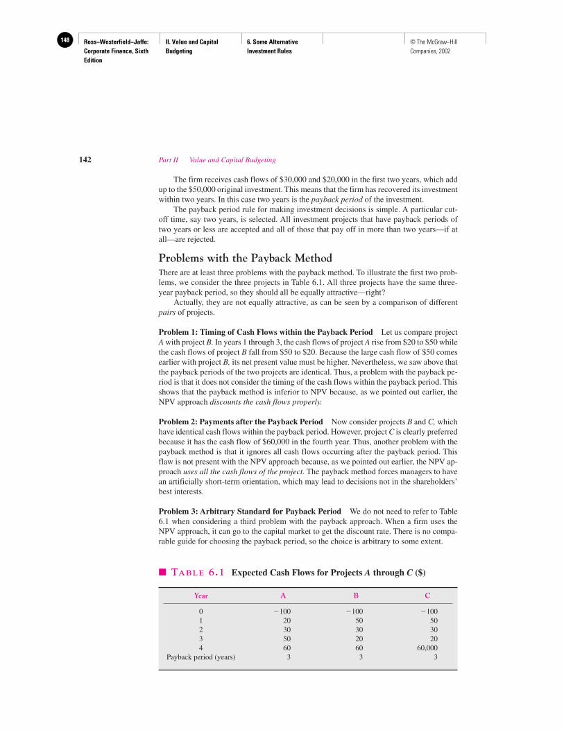
Ross−Westerfield−Jaffe: Corporate Finance, Sixth Edition
II. Value and Capital Budgeting
6. Some Alternative Investment Rules
148 © The McGraw−Hill Companies, 2002
The firm receives cash flows of $30,000 and $20,000 in the first two years, which addup to the $50,000 original investment. This means that the firm has recovered its investmentwithin two years. In this case two years is the payback period of the investment.
The payback period rule for making investment decisions is simple. A particular cut-off time, say two years, is selected. All investment projects that have payback periods oftwo years or less are accepted and all of those that pay off in more than two years—if atall—are rejected.
Problems with the Payback MethodThere are at least three problems with the payback method. To illustrate the first two prob-lems, we consider the three projects in Table 6.1. All three projects have the same three-year payback period, so they should all be equally attractive—right?
Actually, they are not equally attractive, as can be seen by a comparison of differentpairs of projects.
Problem 1: Timing of Cash Flows within the Payback Period Let us compare projectA with project B. In years 1 through 3, the cash flows of project A rise from $20 to $50 whilethe cash flows of project B fall from $50 to $20. Because the large cash flow of $50 comesearlier with project B, its net present value must be higher. Nevertheless, we saw above thatthe payback periods of the two projects are identical. Thus, a problem with the payback pe-riod is that it does not consider the timing of the cash flows within the payback period. Thisshows that the payback method is inferior to NPV because, as we pointed out earlier, theNPV approach discounts the cash flows properly.
Problem 2: Payments after the Payback Period Now consider projects B and C, whichhave identical cash flows within the payback period. However, project C is clearly preferredbecause it has the cash flow of $60,000 in the fourth year. Thus, another problem with thepayback method is that it ignores all cash flows occurring after the payback period. Thisflaw is not present with the NPV approach because, as we pointed out earlier, the NPV ap-proach uses all the cash flows of the project. The payback method forces managers to havean artificially short-term orientation, which may lead to decisions not in the shareholders’best interests.
Problem 3: Arbitrary Standard for Payback Period We do not need to refer to Table6.1 when considering a third problem with the payback approach. When a firm uses theNPV approach, it can go to the capital market to get the discount rate. There is no compa-rable guide for choosing the payback period, so the choice is arbitrary to some extent.
142 Part II Value and Capital Budgeting
� TABLE 6.1 Expected Cash Flows for Projects A through C ($)
Year A B C
0 �100 �100 �1001 20 50 502 30 30 303 50 20 204 60 60 60,000
Payback period (years) 3 3 3
Ross−Westerfield−Jaffe: Corporate Finance, Sixth Edition
II. Value and Capital Budgeting
6. Some Alternative Investment Rules
149© The McGraw−Hill Companies, 2002
Managerial PerspectiveThe payback rule is often used by large and sophisticated companies when making rela-tively small decisions. The decision to build a small warehouse, for example, or to pay fora tune-up for a truck is the sort of decision that is often made by lower-level management.Typically a manager might reason that a tune-up would cost, say, $200, and if it saved $120each year in reduced fuel costs, it would pay for itself in less than two years. On such a ba-sis the decision would be made.
Although the treasurer of the company might not have made the decision in the sameway, the company endorses such decision making. Why would upper management condoneor even encourage such retrograde activity in its employees? One answer would be that itis easy to make decisions using the payback rule. Multiply the tune-up decision into 50 suchdecisions a month, and the appeal of this simple rule becomes clearer.
Perhaps most important though, the payback rule also has some desirable features formanagerial control. Just as important as the investment decision itself is the company’s abil-ity to evaluate the manager’s decision-making ability. Under the NPV rule, a long time maypass before one decides whether or not a decision was correct. With the payback rule weknow in two years whether the manager’s assessment of the cash flows was correct.
It has also been suggested that firms with very good investment opportunities but no avail-able cash may justifiably use the payback method. For example, the payback method could beused by small, privately held firms with good growth prospects but limited access to the capi-tal markets. Quick cash recovery may enhance the reinvestment possibilities for such firms.
Notwithstanding all of the preceding rationale, it is not surprising to discover that asthe decision grows in importance, which is to say when firms look at bigger projects, theNPV becomes the order of the day. When questions of controlling and evaluating the man-ager become less important than making the right investment decision, the payback periodis used less frequently. For the big-ticket decisions, such as whether or not to buy a machine,build a factory, or acquire a company, the payback rule is seldom used.
Summary of the Payback Period RuleTo summarize, the payback period is not the same as the NPV rule and is therefore con-ceptually wrong. With its arbitrary cutoff date and its blindness to cash flows after that date,it can lead to some flagrantly foolish decisions if it is used too literally. Nevertheless, be-cause it is so simple, companies often use it as a screen for making the myriad of minor in-vestment decisions they continually face.
Although this means that you should be wary of trying to change rules like the paybackperiod when you encounter them in companies, you should probably be careful not to fall intothe sloppy financial thinking they represent. After this course you would do your company adisservice if you ever used the payback period instead of the NPV when you had a choice.
• List the problems of the payback period rule.• What are some advantages?
6.3 THE DISCOUNTED PAYBACK PERIOD RULE
Aware of the pitfalls of the payback approach, some decision makers use a variant called thediscounted payback period rule. Under this approach, we first discount the cash flows. Thenwe ask how long it takes for the discounted cash flows to equal the initial investment.
Chapter 6 Some Alternative Investment Rules 143
QUESTIONS
CO
NC
EP
T
?
Ross−Westerfield−Jaffe: Corporate Finance, Sixth Edition
II. Value and Capital Budgeting
6. Some Alternative Investment Rules
150 © The McGraw−Hill Companies, 2002
For example, suppose that the discount rate is 10 percent and the cash flows on a proj-ect are given by
(�$100, $50, $50, $20)
This investment has a payback period of two years, because the investment is paid back inthat time.
To compute the project’s discounted payback period, we first discount each of the cashflows at the 10-percent rate. In discounted terms, then, the cash flows look like
[�$100, $50/1.1, $50/(1.1)2, $20/(1.1)3] � (�$100, $45.45, $41.32, $15.03)
The discounted payback period of the original investment is simply the payback period forthese discounted cash flows. The payback period for the discounted cash flows is slightly lessthan three years since the discounted cash flows over the three years are $101.80 ($45.45 �$41.32 � $15.03). As long as the cash flows are positive, the discounted payback period willnever be smaller than the payback period, because discounting will lower the cash flows.
At first glance the discounted payback may seem like an attractive alternative, but oncloser inspection we see that it has some of the same major flaws as the payback. Like pay-back, discounted payback first requires us to make a somewhat magical choice of an arbi-trary cutoff period, and then it ignores all of the cash flows after that date.
If we have already gone to the trouble of discounting the cash flows, any small appealto simplicity or to managerial control that payback may have, has been lost. We might justas well add up the discounted cash flows and use the NPV to make the decision. Althoughdiscounted payback looks a bit like the NPV, it is just a poor compromise between the pay-back method and the NPV.
6.4 THE AVERAGE ACCOUNTING RETURN
Defining the RuleAnother attractive and fatally flawed approach to making financial decisions is the averageaccounting return. The average accounting return is the average project earnings aftertaxes and depreciation, divided by the average book value of the investment during its life.In spite of its flaws, the average accounting return method is worth examining because it isused frequently in the real world.
EXAMPLE
Consider a company that is evaluating whether or not to buy a store in a newly builtmall. The purchase price is $500,000. We will assume that the store has an esti-mated life of five years and will need to be completely scrapped or rebuilt at the endof that time. The projected yearly sales and expense figures are shown in Table 6.2.
It is worth looking carefully at this table. In fact, the first step in any project assessmentis a careful look at the projected cash flows. When the store starts up, it is estimated thatfirst-year sales will be $433,333 and that, after expenses, the before-tax cash flow will be$233,333. After the first year, sales are expected to rise and expenses are expected to fall,resulting in a before-tax cash flow of $300,000. After that, competition from other storesand the loss in novelty will drop before-tax cash flow to $166,667, $100,000, and $33,333,respectively, in the next three years.
144 Part II Value and Capital Budgeting
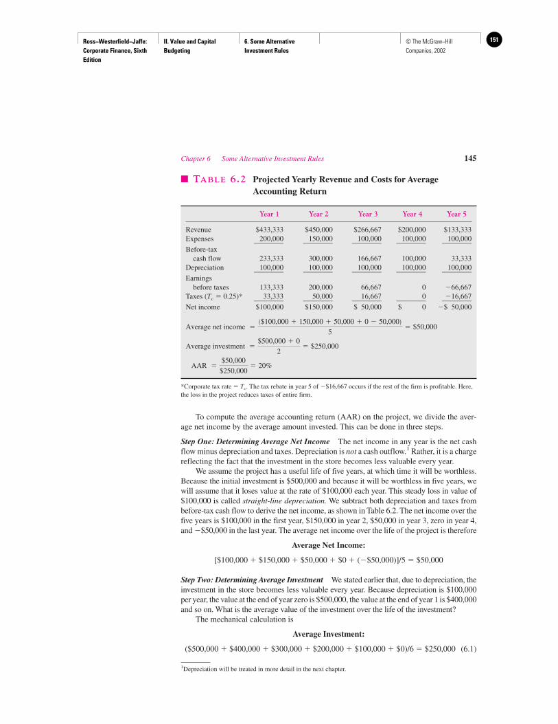
Ross−Westerfield−Jaffe: Corporate Finance, Sixth Edition
II. Value and Capital Budgeting
6. Some Alternative Investment Rules
151© The McGraw−Hill Companies, 2002
To compute the average accounting return (AAR) on the project, we divide the aver-age net income by the average amount invested. This can be done in three steps.
Step One: Determining Average Net Income The net income in any year is the net cashflow minus depreciation and taxes. Depreciation is not a cash outflow.1 Rather, it is a chargereflecting the fact that the investment in the store becomes less valuable every year.
We assume the project has a useful life of five years, at which time it will be worthless.Because the initial investment is $500,000 and because it will be worthless in five years, wewill assume that it loses value at the rate of $100,000 each year. This steady loss in value of$100,000 is called straight-line depreciation. We subtract both depreciation and taxes frombefore-tax cash flow to derive the net income, as shown in Table 6.2. The net income over thefive years is $100,000 in the first year, $150,000 in year 2, $50,000 in year 3, zero in year 4,and �$50,000 in the last year. The average net income over the life of the project is therefore
Average Net Income:
[$100,000 � $150,000 � $50,000 � $0 � (�$50,000)]/5 � $50,000
Step Two: Determining Average Investment We stated earlier that, due to depreciation, theinvestment in the store becomes less valuable every year. Because depreciation is $100,000per year, the value at the end of year zero is $500,000, the value at the end of year 1 is $400,000and so on. What is the average value of the investment over the life of the investment?
The mechanical calculation is
Average Investment:
($500,000 � $400,000 � $300,000 � $200,000 � $100,000 � $0)/6 � $250,000 (6.1)
Chapter 6 Some Alternative Investment Rules 145
� TABLE 6.2 Projected Yearly Revenue and Costs for AverageAccounting Return
Year 1 Year 2 Year 3 Year 4 Year 5
Revenue $433,333 $450,000 $266,667 $200,000 $133,333Expenses 200,000 150,000 100,000 100,000 100,000________ ________ ________ ________ ________Before-tax
cash flow 233,333 300,000 166,667 100,000 33,333Depreciation 100,000 100,000 100,000 100,000 100,000________ ________ ________ ________ ________Earnings
before taxes 133,333 200,000 66,667 0 �66,667Taxes (Tc � 0.25)* 33,333 50,000 16,667 0 �16,667________ ________ ________ ________ ________Net income $100,000 $150,000 $ 50,000 $ 0 �$ 50,000
*Corporate tax rate � Tc. The tax rebate in year 5 of �$16,667 occurs if the rest of the firm is profitable. Here,the loss in the project reduces taxes of entire firm.
AAR �$50,000
$250,000� 20%
Average investment �$500,000 � 0
2� $250,000
Average net income ��$100,000 � 150,000 � 50,000 � 0 � 50,000�
5� $50,000
1Depreciation will be treated in more detail in the next chapter.
Ross−Westerfield−Jaffe: Corporate Finance, Sixth Edition
II. Value and Capital Budgeting
6. Some Alternative Investment Rules
152 © The McGraw−Hill Companies, 2002
We divide by 6 and not 5, because $500,000 is what the investment is worth at the begin-ning of the five years and $0 is what it is worth at the beginning of the sixth year. In otherwords, there are six terms in the parenthesis of equation (6.1).
Step Three: Determining AAR The average return is simply
If the firm had a targeted accounting rate of return greater than 20 percent, the project wouldbe rejected, and if its targeted return were less than 20 percent, it would be accepted.
Analyzing the Average Accounting Return MethodBy now you should be able to see what is wrong with the AAR method of making invest-ment decisions.
The most important flaw in the AAR method is that it does not use the right raw mate-rials. It uses the net income figures and the book value of the investment (from the accoun-tant’s books) to figure out whether to take the investment. Conversely, the NPV rule usescash flows.
Second, AAR takes no account of timing. In the previous example, the AAR wouldhave been the same if the $100,000 net income in the first year had occurred in the last year.However, delaying an inflow for five years would have made the investment less attractiveunder the NPV rule as well as by the common sense of the time value of money. That is, theNPV approach discounts properly.
Third, just as the payback period requires an arbitrary choice of a cutoff date, the AARmethod offers no guidance on what the right targeted rate of return should be. It could bethe discount rate in the market. But then again, because the AAR method is not the same asthe present value method, it is not obvious that this would be the right choice.
Like the payback method, the AAR (and variations of it) is frequently used as a“backup” to discounted cash flow methods. Perhaps this is so because it is easy to calculateand uses accounting numbers readily available from the firm’s accounting system.
• What are the three steps in calculating AAR?• What are some flaws with the AAR approach?
6.5 THE INTERNAL RATE OF RETURN
Now we come to the most important alternative to the NPV approach, the internal rate ofreturn, universally known as the IRR. The IRR is about as close as you can get to the NPVwithout actually being the NPV. The basic rationale behind the IRR is that it tries to find asingle number that summarizes the merits of a project. That number does not depend on theinterest rate that prevails in the capital market. That is why it is called the internal rate ofreturn; the number is internal or intrinsic to the project and does not depend on anything ex-cept the cash flows of the project.
For example, consider the simple project (�$100, $110) in Figure 6.2. For a given rate,the net present value of this project can be described as
(6.2)NPV � � $100 �$110
1 � r
AAR �$50,000
$250,000� 20%
146 Part II Value and Capital Budgeting
QUESTIONS
CO
NC
EP
T
?
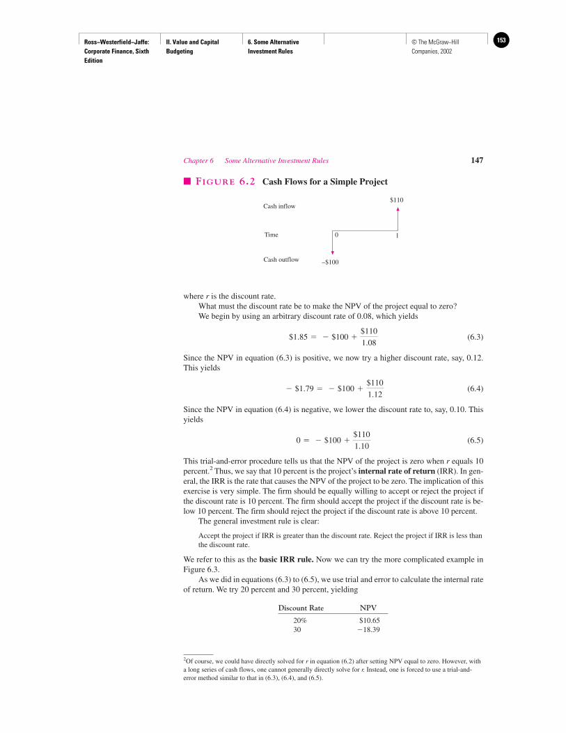
Ross−Westerfield−Jaffe: Corporate Finance, Sixth Edition
II. Value and Capital Budgeting
6. Some Alternative Investment Rules
153© The McGraw−Hill Companies, 2002
where r is the discount rate.What must the discount rate be to make the NPV of the project equal to zero?We begin by using an arbitrary discount rate of 0.08, which yields
(6.3)
Since the NPV in equation (6.3) is positive, we now try a higher discount rate, say, 0.12.This yields
(6.4)
Since the NPV in equation (6.4) is negative, we lower the discount rate to, say, 0.10. Thisyields
(6.5)
This trial-and-error procedure tells us that the NPV of the project is zero when r equals 10percent.2 Thus, we say that 10 percent is the project’s internal rate of return (IRR). In gen-eral, the IRR is the rate that causes the NPV of the project to be zero. The implication of thisexercise is very simple. The firm should be equally willing to accept or reject the project ifthe discount rate is 10 percent. The firm should accept the project if the discount rate is be-low 10 percent. The firm should reject the project if the discount rate is above 10 percent.
The general investment rule is clear:
Accept the project if IRR is greater than the discount rate. Reject the project if IRR is less thanthe discount rate.
We refer to this as the basic IRR rule. Now we can try the more complicated example inFigure 6.3.
As we did in equations (6.3) to (6.5), we use trial and error to calculate the internal rateof return. We try 20 percent and 30 percent, yielding
Discount Rate NPV
20% $10.6530 �18.39
0 � � $100 �$110
1.10
� $1.79 � � $100 �$110
1.12
$1.85 � � $100 �$110
1.08
Chapter 6 Some Alternative Investment Rules 147
Cash inflow
Time
Cash outflow –$100
0 1
$110
� FIGURE 6.2 Cash Flows for a Simple Project
2Of course, we could have directly solved for r in equation (6.2) after setting NPV equal to zero. However, witha long series of cash flows, one cannot generally directly solve for r. Instead, one is forced to use a trial-and-error method similar to that in (6.3), (6.4), and (6.5).
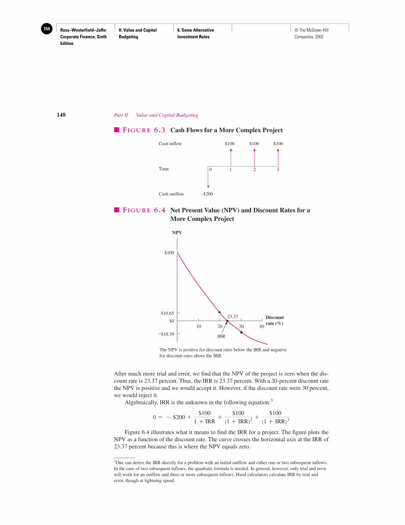
Ross−Westerfield−Jaffe: Corporate Finance, Sixth Edition
II. Value and Capital Budgeting
6. Some Alternative Investment Rules
154 © The McGraw−Hill Companies, 2002
After much more trial and error, we find that the NPV of the project is zero when the dis-count rate is 23.37 percent. Thus, the IRR is 23.37 percent. With a 20-percent discount ratethe NPV is positive and we would accept it. However, if the discount rate were 30 percent,we would reject it.
Algebraically, IRR is the unknown in the following equation:3
Figure 6.4 illustrates what it means to find the IRR for a project. The figure plots theNPV as a function of the discount rate. The curve crosses the horizontal axis at the IRR of23.37 percent because this is where the NPV equals zero.
0 � � $200 �$100
1 � IRR�
$100�1 � IRR� 2 �
$100�1 � IRR� 3
148 Part II Value and Capital Budgeting
Cash inflow
Time
Cash outflow –$200
0 1 2 3
$100 $100 $100
� FIGURE 6.3 Cash Flows for a More Complex Project
10 20 30 40
IRR
23.37
–$18.39
$0
$10.65
$100
Discountrate (%)
NPV
� FIGURE 6.4 Net Present Value (NPV) and Discount Rates for a More Complex Project
The NPV is positive for discount rates below the IRR and negativefor discount rates above the IRR.
3One can derive the IRR directly for a problem with an initial outflow and either one or two subsequent inflows.In the case of two subsequent inflows, the quadratic formula is needed. In general, however, only trial and errorwill work for an outflow and three or more subsequent inflows. Hand calculators calculate IRR by trial anderror, though at lightning speed.
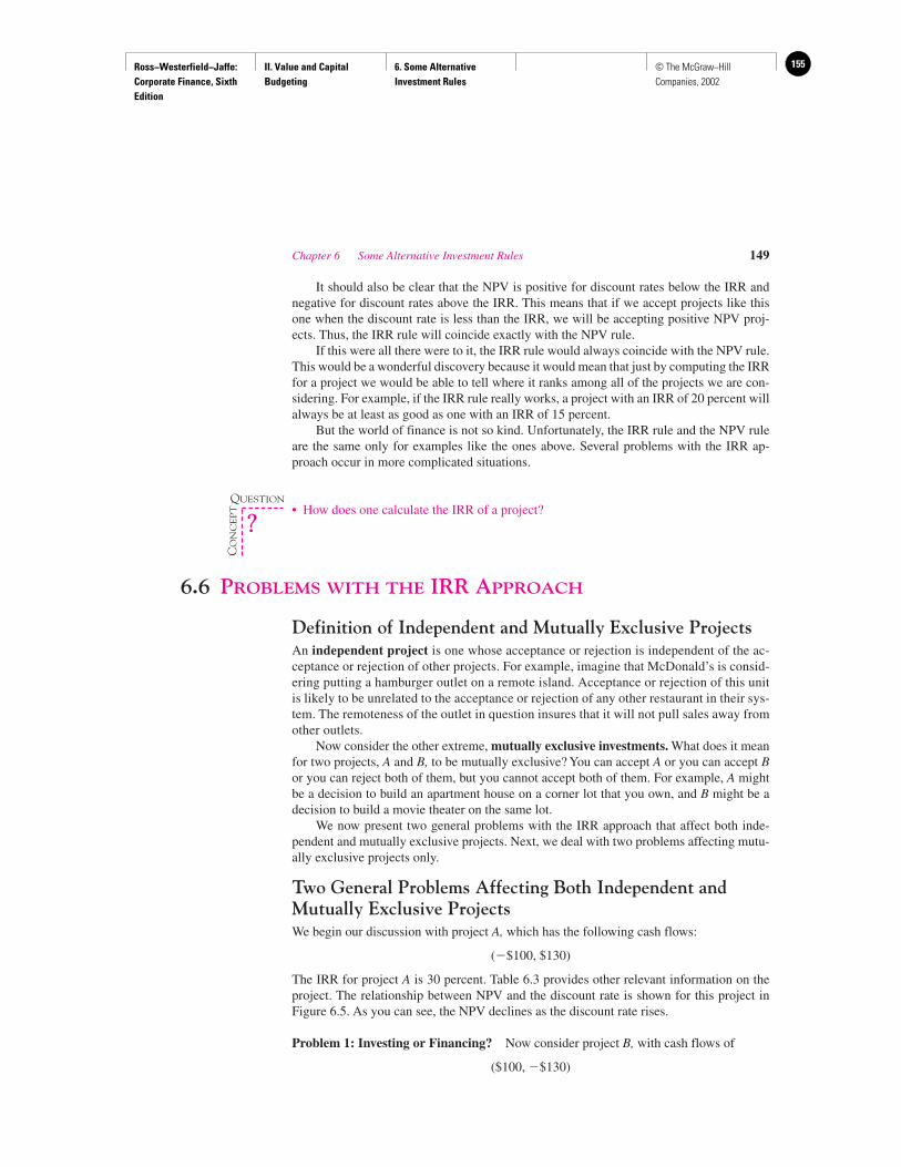
Ross−Westerfield−Jaffe: Corporate Finance, Sixth Edition
II. Value and Capital Budgeting
6. Some Alternative Investment Rules
155© The McGraw−Hill Companies, 2002
It should also be clear that the NPV is positive for discount rates below the IRR andnegative for discount rates above the IRR. This means that if we accept projects like thisone when the discount rate is less than the IRR, we will be accepting positive NPV proj-ects. Thus, the IRR rule will coincide exactly with the NPV rule.
If this were all there were to it, the IRR rule would always coincide with the NPV rule.This would be a wonderful discovery because it would mean that just by computing the IRRfor a project we would be able to tell where it ranks among all of the projects we are con-sidering. For example, if the IRR rule really works, a project with an IRR of 20 percent willalways be at least as good as one with an IRR of 15 percent.
But the world of finance is not so kind. Unfortunately, the IRR rule and the NPV ruleare the same only for examples like the ones above. Several problems with the IRR ap-proach occur in more complicated situations.
• How does one calculate the IRR of a project?
6.6 PROBLEMS WITH THE IRR APPROACH
Definition of Independent and Mutually Exclusive ProjectsAn independent project is one whose acceptance or rejection is independent of the ac-ceptance or rejection of other projects. For example, imagine that McDonald’s is consid-ering putting a hamburger outlet on a remote island. Acceptance or rejection of this unitis likely to be unrelated to the acceptance or rejection of any other restaurant in their sys-tem. The remoteness of the outlet in question insures that it will not pull sales away fromother outlets.
Now consider the other extreme, mutually exclusive investments. What does it meanfor two projects, A and B, to be mutually exclusive? You can accept A or you can accept Bor you can reject both of them, but you cannot accept both of them. For example, A mightbe a decision to build an apartment house on a corner lot that you own, and B might be adecision to build a movie theater on the same lot.
We now present two general problems with the IRR approach that affect both inde-pendent and mutually exclusive projects. Next, we deal with two problems affecting mutu-ally exclusive projects only.
Two General Problems Affecting Both Independent andMutually Exclusive ProjectsWe begin our discussion with project A, which has the following cash flows:
(�$100, $130)
The IRR for project A is 30 percent. Table 6.3 provides other relevant information on theproject. The relationship between NPV and the discount rate is shown for this project inFigure 6.5. As you can see, the NPV declines as the discount rate rises.
Problem 1: Investing or Financing? Now consider project B, with cash flows of
($100, �$130)
Chapter 6 Some Alternative Investment Rules 149
QUESTION
CO
NC
EP
T
?
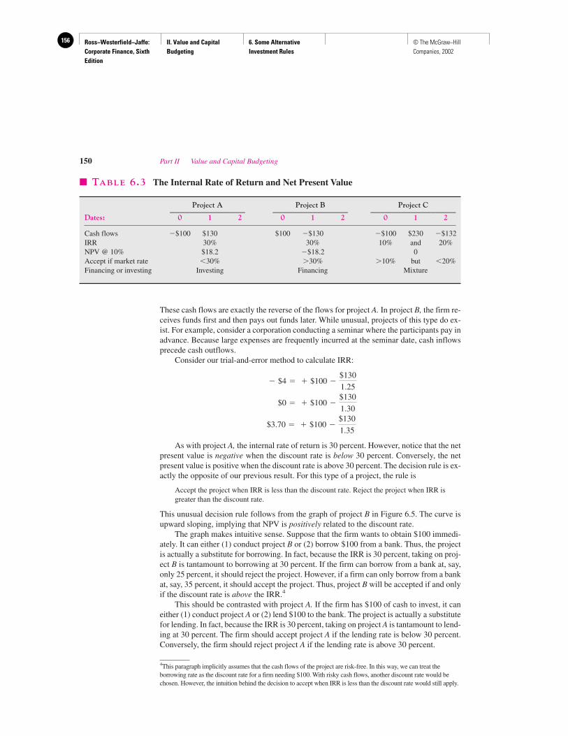
Ross−Westerfield−Jaffe: Corporate Finance, Sixth Edition
II. Value and Capital Budgeting
6. Some Alternative Investment Rules
156 © The McGraw−Hill Companies, 2002
These cash flows are exactly the reverse of the flows for project A. In project B, the firm re-ceives funds first and then pays out funds later. While unusual, projects of this type do ex-ist. For example, consider a corporation conducting a seminar where the participants pay inadvance. Because large expenses are frequently incurred at the seminar date, cash inflowsprecede cash outflows.
Consider our trial-and-error method to calculate IRR:
As with project A, the internal rate of return is 30 percent. However, notice that the netpresent value is negative when the discount rate is below 30 percent. Conversely, the netpresent value is positive when the discount rate is above 30 percent. The decision rule is ex-actly the opposite of our previous result. For this type of a project, the rule is
Accept the project when IRR is less than the discount rate. Reject the project when IRR isgreater than the discount rate.
This unusual decision rule follows from the graph of project B in Figure 6.5. The curve isupward sloping, implying that NPV is positively related to the discount rate.
The graph makes intuitive sense. Suppose that the firm wants to obtain $100 immedi-ately. It can either (1) conduct project B or (2) borrow $100 from a bank. Thus, the projectis actually a substitute for borrowing. In fact, because the IRR is 30 percent, taking on proj-ect B is tantamount to borrowing at 30 percent. If the firm can borrow from a bank at, say,only 25 percent, it should reject the project. However, if a firm can only borrow from a bankat, say, 35 percent, it should accept the project. Thus, project B will be accepted if and onlyif the discount rate is above the IRR.4
This should be contrasted with project A. If the firm has $100 of cash to invest, it caneither (1) conduct project A or (2) lend $100 to the bank. The project is actually a substitutefor lending. In fact, because the IRR is 30 percent, taking on project A is tantamount to lend-ing at 30 percent. The firm should accept project A if the lending rate is below 30 percent.Conversely, the firm should reject project A if the lending rate is above 30 percent.
$3.70 � � $100 �$130
1.35
$0 � � $100 �$130
1.30
� $4 � � $100 �$130
1.25
150 Part II Value and Capital Budgeting
� TABLE 6.3 The Internal Rate of Return and Net Present Value
Project A Project B Project C_______________ _______________ _________________Dates: 0 1 2 0 1 2 0 1 2
Cash flows �$100 $130 $100 �$130 �$100 $230 �$132IRR 30% 30% 10% and 20%NPV @ 10% $18.2 �$18.2 0Accept if market rate 30% �30% �10% but 20%Financing or investing Investing Financing Mixture
4This paragraph implicitly assumes that the cash flows of the project are risk-free. In this way, we can treat theborrowing rate as the discount rate for a firm needing $100. With risky cash flows, another discount rate would bechosen. However, the intuition behind the decision to accept when IRR is less than the discount rate would still apply.
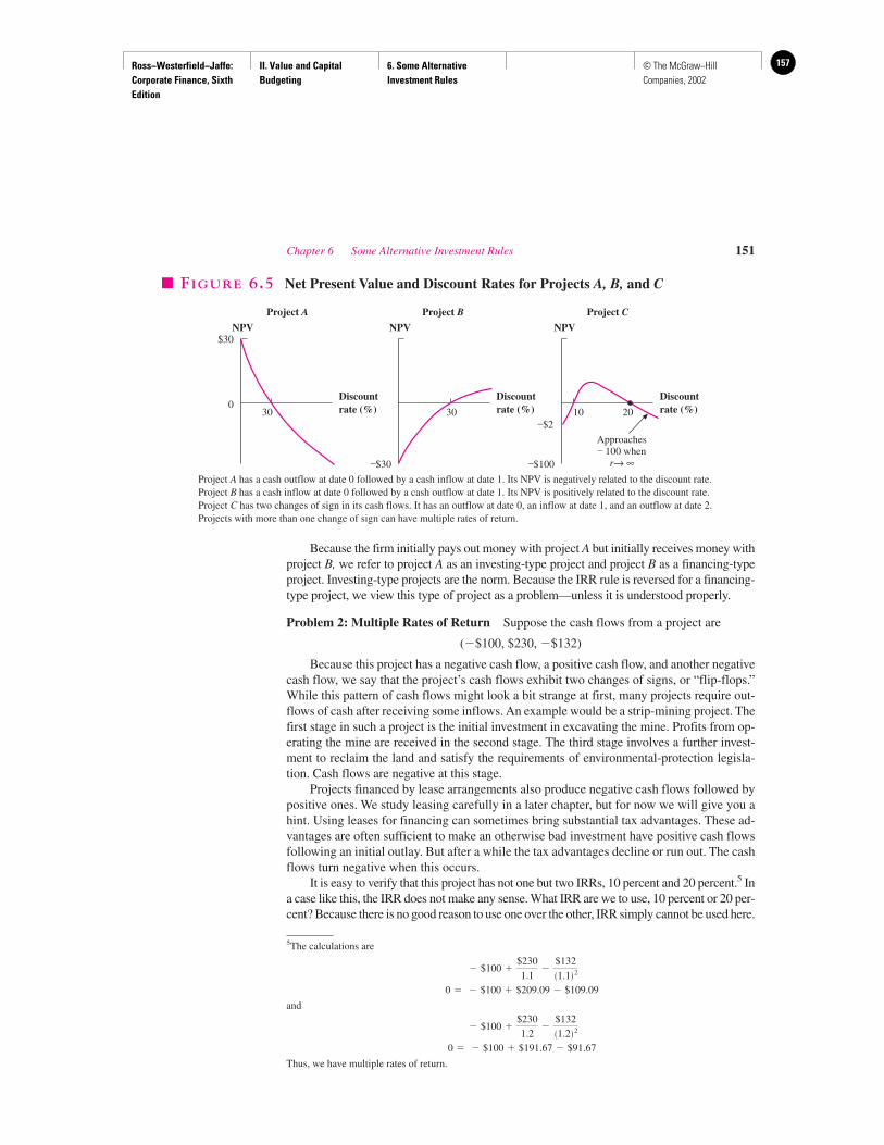
Ross−Westerfield−Jaffe: Corporate Finance, Sixth Edition
II. Value and Capital Budgeting
6. Some Alternative Investment Rules
157© The McGraw−Hill Companies, 2002
Because the firm initially pays out money with project A but initially receives money withproject B, we refer to project A as an investing-type project and project B as a financing-typeproject. Investing-type projects are the norm. Because the IRR rule is reversed for a financing-type project, we view this type of project as a problem—unless it is understood properly.
Problem 2: Multiple Rates of Return Suppose the cash flows from a project are
(�$100, $230, �$132)
Because this project has a negative cash flow, a positive cash flow, and another negativecash flow, we say that the project’s cash flows exhibit two changes of signs, or “flip-flops.”While this pattern of cash flows might look a bit strange at first, many projects require out-flows of cash after receiving some inflows. An example would be a strip-mining project. Thefirst stage in such a project is the initial investment in excavating the mine. Profits from op-erating the mine are received in the second stage. The third stage involves a further invest-ment to reclaim the land and satisfy the requirements of environmental-protection legisla-tion. Cash flows are negative at this stage.
Projects financed by lease arrangements also produce negative cash flows followed bypositive ones. We study leasing carefully in a later chapter, but for now we will give you ahint. Using leases for financing can sometimes bring substantial tax advantages. These ad-vantages are often sufficient to make an otherwise bad investment have positive cash flowsfollowing an initial outlay. But after a while the tax advantages decline or run out. The cashflows turn negative when this occurs.
It is easy to verify that this project has not one but two IRRs, 10 percent and 20 percent.5 Ina case like this, the IRR does not make any sense. What IRR are we to use, 10 percent or 20 per-cent? Because there is no good reason to use one over the other, IRR simply cannot be used here.
Chapter 6 Some Alternative Investment Rules 151
NPVNPV
Discountrate (%)
Project A Project B
NPV
Project C
Discountrate (%)
Discountrate (%)
$30
030
–$30
30 10 20
–$100
–$2
Approaches– 100 when
r→ ∞
� FIGURE 6.5 Net Present Value and Discount Rates for Projects A, B, and C
5The calculations are
and
Thus, we have multiple rates of return.
0 � � $100 � $191.67 � $91.67
� $100 �$230
1.2�
$132�1.2� 2
0 � � $100 � $209.09 � $109.09
� $100 �$230
1.1�
$132�1.1� 2
Project A has a cash outflow at date 0 followed by a cash inflow at date 1. Its NPV is negatively related to the discount rate.Project B has a cash inflow at date 0 followed by a cash outflow at date 1. Its NPV is positively related to the discount rate.Project C has two changes of sign in its cash flows. It has an outflow at date 0, an inflow at date 1, and an outflow at date 2.Projects with more than one change of sign can have multiple rates of return.
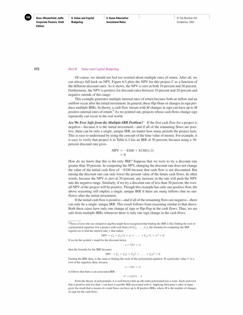
Ross−Westerfield−Jaffe: Corporate Finance, Sixth Edition
II. Value and Capital Budgeting
6. Some Alternative Investment Rules
158 © The McGraw−Hill Companies, 2002
Of course, we should not feel too worried about multiple rates of return. After all, wecan always fall back on NPV. Figure 6.5 plots the NPV for this project C as a function ofthe different discount rates. As it shows, the NPV is zero at both 10 percent and 20 percent.Furthermore, the NPV is positive for discount rates between 10 percent and 20 percent andnegative outside of this range.
This example generates multiple internal rates of return because both an inflow and anoutflow occur after the initial investment. In general, these flip-flops or changes in sign pro-duce multiple IRRs. In theory, a cash flow stream with M changes in sign can have up to Mpositive internal rates of return.6 As we pointed out, projects whose cash flows change signrepeatedly can occur in the real world.
Are We Ever Safe from the Multiple-IRR Problem? If the first cash flow for a project isnegative—because it is the initial investment—and if all of the remaining flows are posi-tive, there can be only a single, unique IRR, no matter how many periods the project lasts.This is easy to understand by using the concept of the time value of money. For example, itis easy to verify that project A in Table 6.3 has an IRR of 30 percent, because using a 30-percent discount rate gives
NPV � �$100 � $130/(1.3)� 0
How do we know that this is the only IRR? Suppose that we were to try a discount rategreater than 30 percent. In computing the NPV, changing the discount rate does not changethe value of the initial cash flow of �$100 because that cash flow is not discounted. Butraising the discount rate can only lower the present value of the future cash flows. In otherwords, because the NPV is zero at 30 percent, any increase in the rate will push the NPVinto the negative range. Similarly, if we try a discount rate of less than 30 percent, the over-all NPV of the project will be positive. Though this example has only one positive flow, theabove reasoning still implies a single, unique IRR if there are many inflows (but no out-flows) after the initial investment.
If the initial cash flow is positive—and if all of the remaining flows are negative—therecan only be a single, unique IRR. This result follows from reasoning similar to that above.Both these cases have only one change of sign or flip-flop in the cash flows. Thus, we aresafe from multiple IRRs whenever there is only one sign change in the cash flows.
152 Part II Value and Capital Budgeting
6Those of you who are steeped in algebra might have recognized that finding the IRR is like finding the root ofa polynomial equation. For a project with cash flows of (C0, . . . , Cr), the formula for computing the IRRrequires us to find the interest rate, r, that makes
If we let the symbol x stand for the discount factor,
x � 1/(1 � r)
then the formula for the IRR becomes
Finding the IRR, then, is the same as finding the roots of this polynomial equation. If a particular value x* is aroot of the equation, then, because
x � 1/(1 � r)
it follows that there is an associated IRR:
r* � (1/x*) � 1
From the theory of polynomials, it is well known that an nth-order polynomial has n roots. Each such rootthat is positive and less than 1 can have a sensible IRR associated with it. Applying Descartes’s rules of signsgives the result that a stream of n cash flows can have up to M positive IRRs, where M is the number of changesof sign for the cash flows.
NPV � C0 � C1x � C2x2 � . . . � CTxT � 0
NPV � C0 � C1��1 � r� � . . . � CT ��1 � r�T � 0
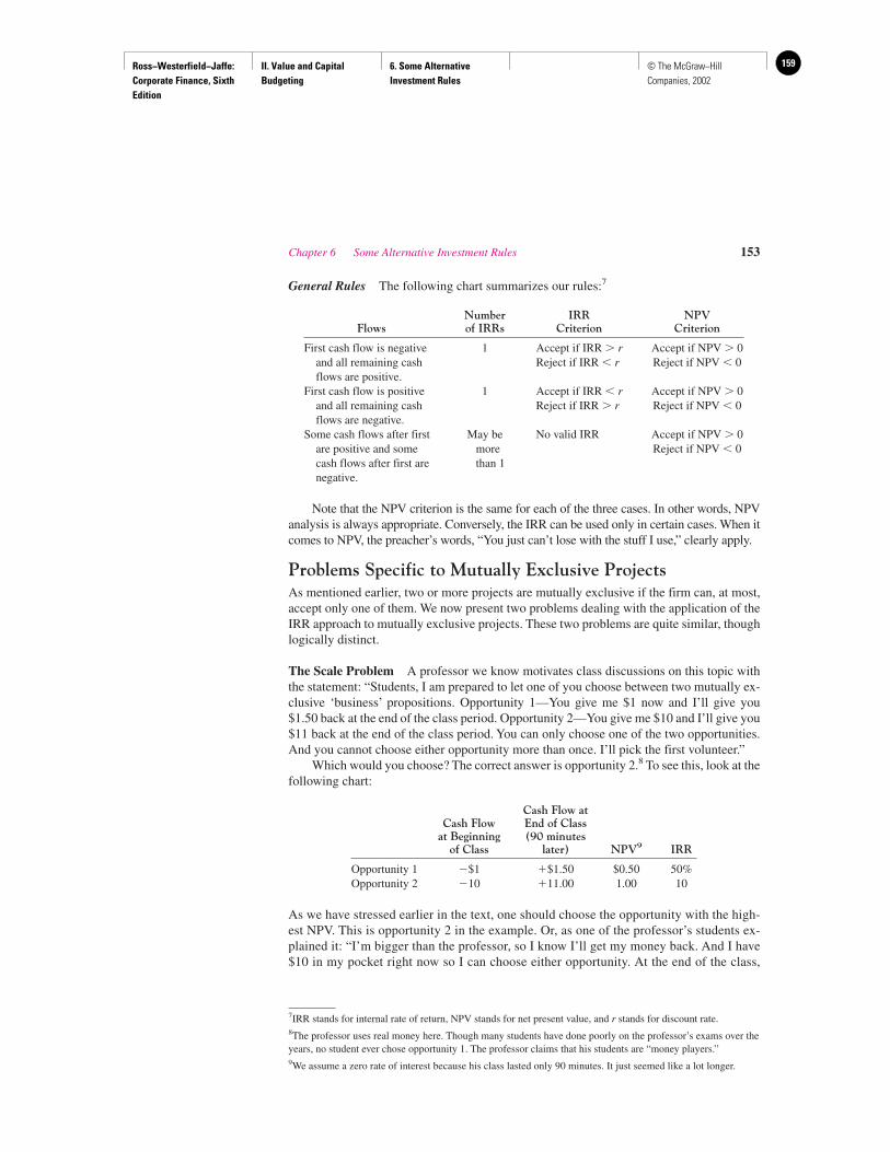
Ross−Westerfield−Jaffe: Corporate Finance, Sixth Edition
II. Value and Capital Budgeting
6. Some Alternative Investment Rules
159© The McGraw−Hill Companies, 2002
General Rules The following chart summarizes our rules:7
Number IRR NPVFlows of IRRs Criterion Criterion
First cash flow is negative 1 Accept if IRR � r Accept if NPV � 0and all remaining cash Reject if IRR r Reject if NPV 0flows are positive.
First cash flow is positive 1 Accept if IRR r Accept if NPV � 0and all remaining cash Reject if IRR � r Reject if NPV 0flows are negative.
Some cash flows after first May be No valid IRR Accept if NPV � 0are positive and some more Reject if NPV 0cash flows after first are than 1negative.
Note that the NPV criterion is the same for each of the three cases. In other words, NPVanalysis is always appropriate. Conversely, the IRR can be used only in certain cases. When itcomes to NPV, the preacher’s words, “You just can’t lose with the stuff I use,” clearly apply.
Problems Specific to Mutually Exclusive ProjectsAs mentioned earlier, two or more projects are mutually exclusive if the firm can, at most,accept only one of them. We now present two problems dealing with the application of theIRR approach to mutually exclusive projects. These two problems are quite similar, thoughlogically distinct.
The Scale Problem A professor we know motivates class discussions on this topic withthe statement: “Students, I am prepared to let one of you choose between two mutually ex-clusive ‘business’ propositions. Opportunity 1—You give me $1 now and I’ll give you$1.50 back at the end of the class period. Opportunity 2—You give me $10 and I’ll give you$11 back at the end of the class period. You can only choose one of the two opportunities.And you cannot choose either opportunity more than once. I’ll pick the first volunteer.”
Which would you choose? The correct answer is opportunity 2.8 To see this, look at thefollowing chart:
Cash Flow atCash Flow End of Class
at Beginning (90 minutesof Class later) NPV9 IRR
Opportunity 1 �$1 �$1.50 $0.50 50%Opportunity 2 �10 �11.00 1.00 10
As we have stressed earlier in the text, one should choose the opportunity with the high-est NPV. This is opportunity 2 in the example. Or, as one of the professor’s students ex-plained it: “I’m bigger than the professor, so I know I’ll get my money back. And I have$10 in my pocket right now so I can choose either opportunity. At the end of the class,
Chapter 6 Some Alternative Investment Rules 153
7IRR stands for internal rate of return, NPV stands for net present value, and r stands for discount rate.8The professor uses real money here. Though many students have done poorly on the professor’s exams over theyears, no student ever chose opportunity 1. The professor claims that his students are “money players.”9We assume a zero rate of interest because his class lasted only 90 minutes. It just seemed like a lot longer.
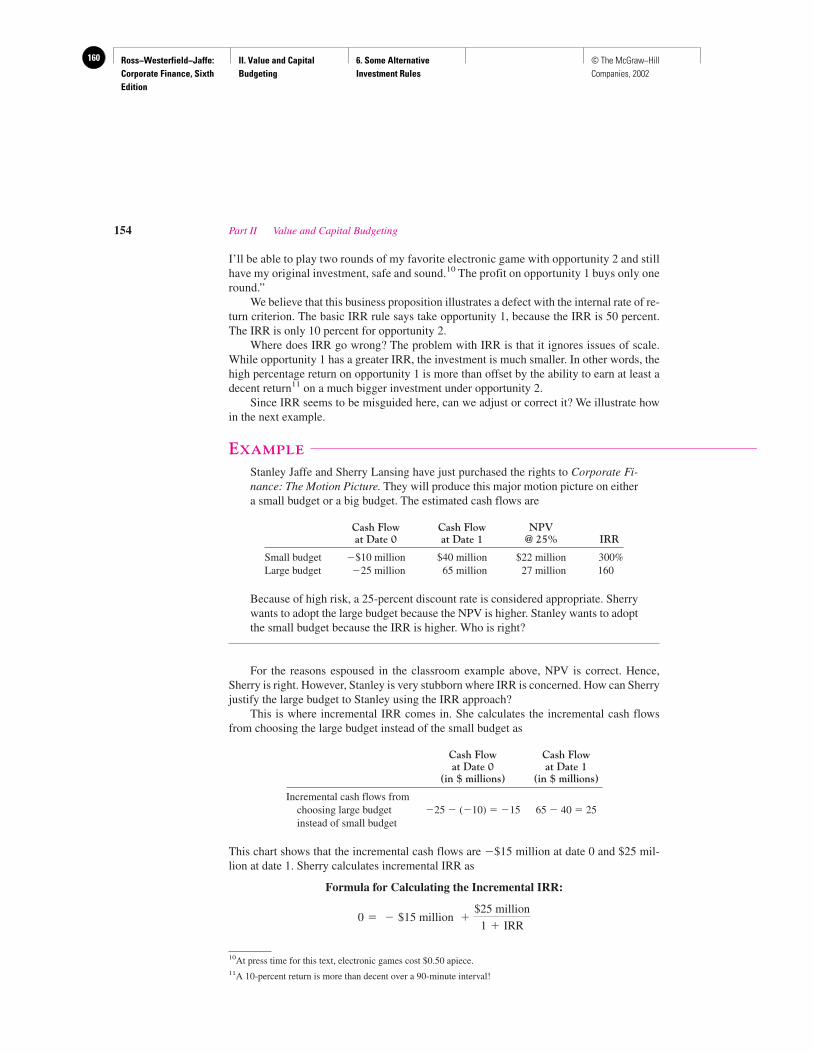
Ross−Westerfield−Jaffe: Corporate Finance, Sixth Edition
II. Value and Capital Budgeting
6. Some Alternative Investment Rules
160 © The McGraw−Hill Companies, 2002
I’ll be able to play two rounds of my favorite electronic game with opportunity 2 and stillhave my original investment, safe and sound.10 The profit on opportunity 1 buys only oneround.”
We believe that this business proposition illustrates a defect with the internal rate of re-turn criterion. The basic IRR rule says take opportunity 1, because the IRR is 50 percent.The IRR is only 10 percent for opportunity 2.
Where does IRR go wrong? The problem with IRR is that it ignores issues of scale.While opportunity 1 has a greater IRR, the investment is much smaller. In other words, thehigh percentage return on opportunity 1 is more than offset by the ability to earn at least adecent return11 on a much bigger investment under opportunity 2.
Since IRR seems to be misguided here, can we adjust or correct it? We illustrate howin the next example.
EXAMPLE
Stanley Jaffe and Sherry Lansing have just purchased the rights to Corporate Fi-nance: The Motion Picture. They will produce this major motion picture on eithera small budget or a big budget. The estimated cash flows are
Cash Flow Cash Flow NPVat Date 0 at Date 1 @ 25% IRR
Small budget �$10 million $40 million $22 million 300%Large budget �25 million 65 million 27 million 160
Because of high risk, a 25-percent discount rate is considered appropriate. Sherrywants to adopt the large budget because the NPV is higher. Stanley wants to adoptthe small budget because the IRR is higher. Who is right?
For the reasons espoused in the classroom example above, NPV is correct. Hence,Sherry is right. However, Stanley is very stubborn where IRR is concerned. How can Sherryjustify the large budget to Stanley using the IRR approach?
This is where incremental IRR comes in. She calculates the incremental cash flowsfrom choosing the large budget instead of the small budget as
Cash Flow Cash Flowat Date 0 at Date 1
(in $ millions) (in $ millions)
Incremental cash flows fromchoosing large budget �25 � (�10) � �15 65 � 40 � 25instead of small budget
This chart shows that the incremental cash flows are �$15 million at date 0 and $25 mil-lion at date 1. Sherry calculates incremental IRR as
Formula for Calculating the Incremental IRR:
0 � � $15 million �$25 million
1 � IRR
154 Part II Value and Capital Budgeting
10At press time for this text, electronic games cost $0.50 apiece.11A 10-percent return is more than decent over a 90-minute interval!
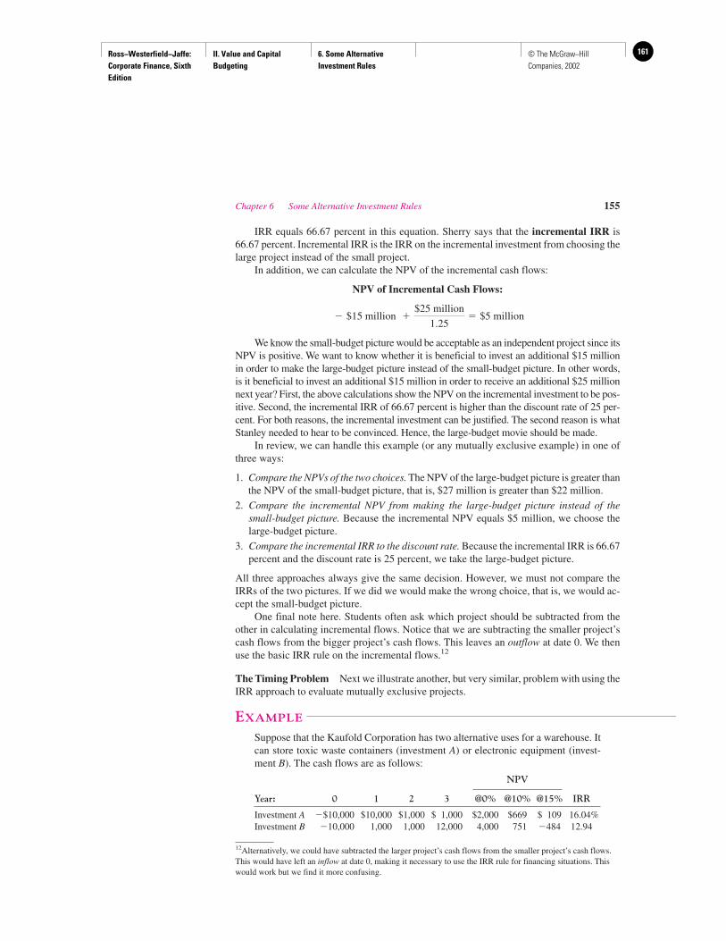
Ross−Westerfield−Jaffe: Corporate Finance, Sixth Edition
II. Value and Capital Budgeting
6. Some Alternative Investment Rules
161© The McGraw−Hill Companies, 2002
IRR equals 66.67 percent in this equation. Sherry says that the incremental IRR is66.67 percent. Incremental IRR is the IRR on the incremental investment from choosing thelarge project instead of the small project.
In addition, we can calculate the NPV of the incremental cash flows:
NPV of Incremental Cash Flows:
We know the small-budget picture would be acceptable as an independent project since itsNPV is positive. We want to know whether it is beneficial to invest an additional $15 millionin order to make the large-budget picture instead of the small-budget picture. In other words,is it beneficial to invest an additional $15 million in order to receive an additional $25 millionnext year? First, the above calculations show the NPV on the incremental investment to be pos-itive. Second, the incremental IRR of 66.67 percent is higher than the discount rate of 25 per-cent. For both reasons, the incremental investment can be justified. The second reason is whatStanley needed to hear to be convinced. Hence, the large-budget movie should be made.
In review, we can handle this example (or any mutually exclusive example) in one ofthree ways:
1. Compare the NPVs of the two choices. The NPV of the large-budget picture is greater thanthe NPV of the small-budget picture, that is, $27 million is greater than $22 million.
2. Compare the incremental NPV from making the large-budget picture instead of thesmall-budget picture. Because the incremental NPV equals $5 million, we choose thelarge-budget picture.
3. Compare the incremental IRR to the discount rate. Because the incremental IRR is 66.67percent and the discount rate is 25 percent, we take the large-budget picture.
All three approaches always give the same decision. However, we must not compare theIRRs of the two pictures. If we did we would make the wrong choice, that is, we would ac-cept the small-budget picture.
One final note here. Students often ask which project should be subtracted from theother in calculating incremental flows. Notice that we are subtracting the smaller project’scash flows from the bigger project’s cash flows. This leaves an outflow at date 0. We thenuse the basic IRR rule on the incremental flows.12
The Timing Problem Next we illustrate another, but very similar, problem with using theIRR approach to evaluate mutually exclusive projects.
EXAMPLE
Suppose that the Kaufold Corporation has two alternative uses for a warehouse. Itcan store toxic waste containers (investment A) or electronic equipment (invest-ment B). The cash flows are as follows:
NPV
Year: 0 1 2 3 @0% @10% @15% IRR
Investment A �$10,000 $10,000 $1,000 $ 1,000 $2,000 $669 $ 109 16.04%Investment B �10,000 1,000 1,000 12,000 4,000 751 �484 12.94
� $15 million �$25 million
1.25� $5 million
Chapter 6 Some Alternative Investment Rules 155
12Alternatively, we could have subtracted the larger project’s cash flows from the smaller project’s cash flows.This would have left an inflow at date 0, making it necessary to use the IRR rule for financing situations. Thiswould work but we find it more confusing.
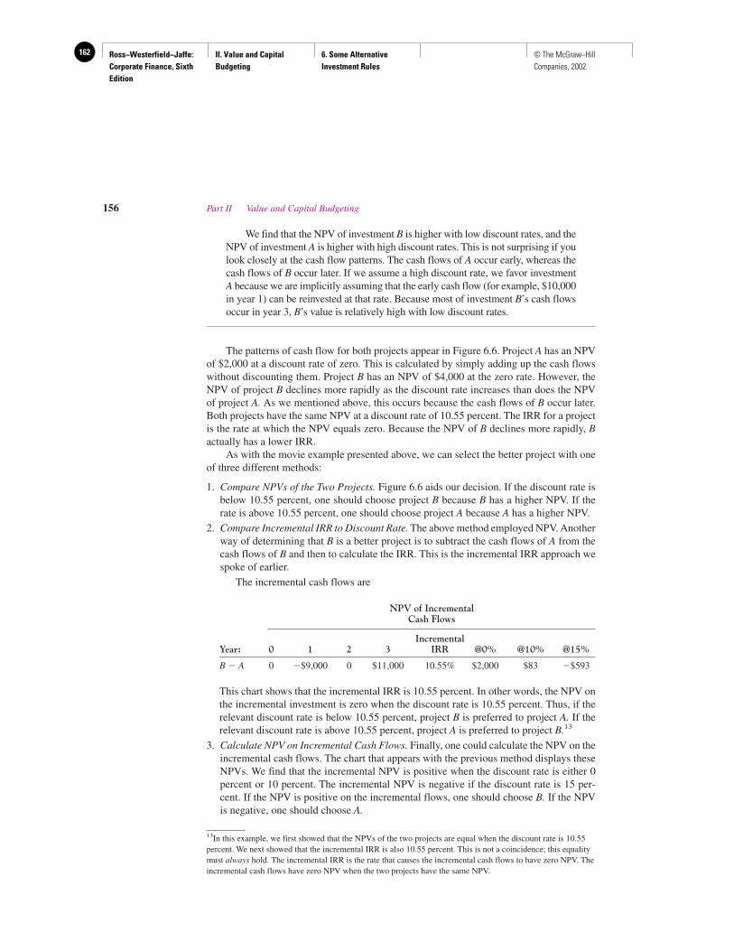
Ross−Westerfield−Jaffe: Corporate Finance, Sixth Edition
II. Value and Capital Budgeting
6. Some Alternative Investment Rules
162 © The McGraw−Hill Companies, 2002
We find that the NPV of investment B is higher with low discount rates, and theNPV of investment A is higher with high discount rates. This is not surprising if youlook closely at the cash flow patterns. The cash flows of A occur early, whereas thecash flows of B occur later. If we assume a high discount rate, we favor investmentA because we are implicitly assuming that the early cash flow (for example, $10,000in year 1) can be reinvested at that rate. Because most of investment B’s cash flowsoccur in year 3, B’s value is relatively high with low discount rates.
The patterns of cash flow for both projects appear in Figure 6.6. Project A has an NPVof $2,000 at a discount rate of zero. This is calculated by simply adding up the cash flowswithout discounting them. Project B has an NPV of $4,000 at the zero rate. However, theNPV of project B declines more rapidly as the discount rate increases than does the NPVof project A. As we mentioned above, this occurs because the cash flows of B occur later.Both projects have the same NPV at a discount rate of 10.55 percent. The IRR for a projectis the rate at which the NPV equals zero. Because the NPV of B declines more rapidly, Bactually has a lower IRR.
As with the movie example presented above, we can select the better project with oneof three different methods:
1. Compare NPVs of the Two Projects. Figure 6.6 aids our decision. If the discount rate isbelow 10.55 percent, one should choose project B because B has a higher NPV. If therate is above 10.55 percent, one should choose project A because A has a higher NPV.
2. Compare Incremental IRR to Discount Rate. The above method employed NPV. Anotherway of determining that B is a better project is to subtract the cash flows of A from thecash flows of B and then to calculate the IRR. This is the incremental IRR approach wespoke of earlier.
The incremental cash flows are
NPV of IncrementalCash Flows
IncrementalYear: 0 1 2 3 IRR @0% @10% @15%
B � A 0 �$9,000 0 $11,000 10.55% $2,000 $83 �$593
This chart shows that the incremental IRR is 10.55 percent. In other words, the NPV onthe incremental investment is zero when the discount rate is 10.55 percent. Thus, if therelevant discount rate is below 10.55 percent, project B is preferred to project A. If therelevant discount rate is above 10.55 percent, project A is preferred to project B.13
3. Calculate NPV on Incremental Cash Flows. Finally, one could calculate the NPV on theincremental cash flows. The chart that appears with the previous method displays theseNPVs. We find that the incremental NPV is positive when the discount rate is either 0percent or 10 percent. The incremental NPV is negative if the discount rate is 15 per-cent. If the NPV is positive on the incremental flows, one should choose B. If the NPVis negative, one should choose A.
156 Part II Value and Capital Budgeting
13In this example, we first showed that the NPVs of the two projects are equal when the discount rate is 10.55percent. We next showed that the incremental IRR is also 10.55 percent. This is not a coincidence; this equalitymust always hold. The incremental IRR is the rate that causes the incremental cash flows to have zero NPV. Theincremental cash flows have zero NPV when the two projects have the same NPV.
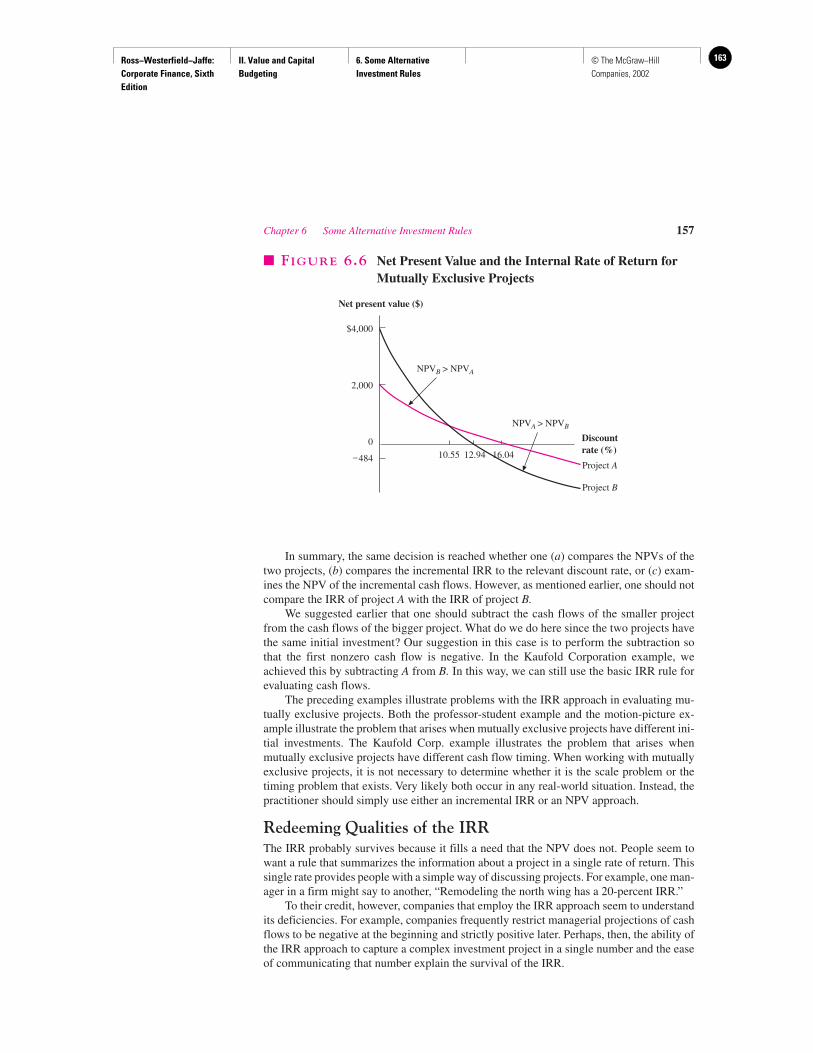
Ross−Westerfield−Jaffe: Corporate Finance, Sixth Edition
II. Value and Capital Budgeting
6. Some Alternative Investment Rules
163© The McGraw−Hill Companies, 2002
In summary, the same decision is reached whether one (a) compares the NPVs of thetwo projects, (b) compares the incremental IRR to the relevant discount rate, or (c) exam-ines the NPV of the incremental cash flows. However, as mentioned earlier, one should notcompare the IRR of project A with the IRR of project B.
We suggested earlier that one should subtract the cash flows of the smaller projectfrom the cash flows of the bigger project. What do we do here since the two projects havethe same initial investment? Our suggestion in this case is to perform the subtraction sothat the first nonzero cash flow is negative. In the Kaufold Corporation example, weachieved this by subtracting A from B. In this way, we can still use the basic IRR rule forevaluating cash flows.
The preceding examples illustrate problems with the IRR approach in evaluating mu-tually exclusive projects. Both the professor-student example and the motion-picture ex-ample illustrate the problem that arises when mutually exclusive projects have different ini-tial investments. The Kaufold Corp. example illustrates the problem that arises whenmutually exclusive projects have different cash flow timing. When working with mutuallyexclusive projects, it is not necessary to determine whether it is the scale problem or thetiming problem that exists. Very likely both occur in any real-world situation. Instead, thepractitioner should simply use either an incremental IRR or an NPV approach.
Redeeming Qualities of the IRRThe IRR probably survives because it fills a need that the NPV does not. People seem towant a rule that summarizes the information about a project in a single rate of return. Thissingle rate provides people with a simple way of discussing projects. For example, one man-ager in a firm might say to another, “Remodeling the north wing has a 20-percent IRR.”
To their credit, however, companies that employ the IRR approach seem to understandits deficiencies. For example, companies frequently restrict managerial projections of cashflows to be negative at the beginning and strictly positive later. Perhaps, then, the ability ofthe IRR approach to capture a complex investment project in a single number and the easeof communicating that number explain the survival of the IRR.
Chapter 6 Some Alternative Investment Rules 157
NPVA > NPVB
$4,000
Discountrate (%)
2,000
0
–484
Net present value ($)
NPVB > NPVA
10.55 12.94 16.04Project A
Project B
� FIGURE 6.6 Net Present Value and the Internal Rate of Return forMutually Exclusive Projects
Ross−Westerfield−Jaffe: Corporate Finance, Sixth Edition
II. Value and Capital Budgeting
6. Some Alternative Investment Rules
164 © The McGraw−Hill Companies, 2002
A TestTo test your knowledge, consider the following two statements:
1. You must know the discount rate to compute the NPV of a project but you compute theIRR without referring to the discount rate.
2. Hence, the IRR rule is easier to apply than the NPV rule because you don’t use the dis-count rate when applying IRR.
The first statement is true. The discount rate is needed to compute NPV. The IRR is com-puted by solving for the rate where the NPV is zero. No mention is made of the discountrate in the mere computation. However, the second statement is false. In order to apply IRR,you must compare the internal rate of return with the discount rate. Thus, the discount rateis needed for making a decision under either the NPV or IRR approach.
• What is the difference between independent projects and mutually exclusive projects?• What are two problems with the IRR approach that apply to both independent and mutu-
ally exclusive projects?• What are two additional problems applying only to mutually exclusive projects?
6.7 THE PROFITABILITY INDEX
Another method that is used to evaluate projects is called the profitability index. It is theratio of the present value of the future expected cash flows after initial investment dividedby the amount of the initial investment. The profitability index can be represented as
Profitability index (PI)
EXAMPLE
Hiram Finnegan, Inc., applies a 12-percent discount rate to two investment op-portunities.
PV @12% of CashFlows Subsequent
to Initial Profit-Investment ability NPV @ 12%
Project C0 C1 C2 ($000,000) Index ($000,000)
1 �20 70 10 70.5 3.53 50.52 �10 15 40 45.3 4.53 35.3
For example, the profitability index is calculated for project 1 as follows. The presentvalue of the cash flows after the initial investment are
(6.6)$70.5 �$70
1.12�
$10�1.12� 2
�PV of cash flows subsequent to initial investment
Initial investment
158 Part II Value and Capital Budgeting
Cash Flows($000,000)
QUESTIONS
CO
NC
EP
T
?
Ross−Westerfield−Jaffe: Corporate Finance, Sixth Edition
II. Value and Capital Budgeting
6. Some Alternative Investment Rules
165© The McGraw−Hill Companies, 2002
The profitability index is calculated by dividing the result of equation (6.6) by the initial in-vestment of $20. This yields
We consider three possibilities:
1. Independent Projects. We first assume that we have two independent projects. Accord-ing to the NPV criterion, both projects should be accepted since NPV is positive in eachcase. The NPV is positive whenever the profitability index (PI) is greater than one. Thus,the PI decision rule is
Accept an independent project if PI � 1.Reject if PI 1.
2. Mutually Exclusive Projects. Let us assume that you can now only accept one project.NPV analysis says accept project 1 because this project has the bigger NPV. Becauseproject 2 has the higher PI, the profitability index leads to the wrong selection.
The problem with the profitability index for mutually exclusive projects is the same asthe scale problem with the IRR that we mentioned earlier. Project 2 is smaller than project 1.Because the PI is a ratio, this index misses the fact that project 1 has a larger investment thanproject 2 has. Thus, like IRR, PI ignores differences of scale for mutually exclusive projects.
However, like IRR, the flaw with the PI approach can be corrected using incre-mental analysis. We write the incremental cash flows after subtracting project 2 fromproject 1 as follows:
PV @12% of CashFlows Subsequent Profit- NPV
to Initial Investment ability @ 12%Project C0 C1 C2 ($000,000) Index ($000,000)
1 � 2 �10 55 �30 25.2 2.52 15.2
Because the profitability index on the incremental cash flows is greater than 1.0, weshould choose the bigger project, that is, project 1. This is the same decision we get withthe NPV approach.
3. Capital Rationing. The two cases above implicitly assumed that the firm could alwaysattract enough capital to make any profitable investments. Now we consider the casewhen a firm does not have enough capital to fund all positive NPV projects. This is thecase of capital rationing.
Imagine that the firm has a third project, as well as the first two. Project 3 has the fol-lowing cash flows:
PV @12% of CashFlows Subsequent Profit- NPV
to Initial Investment ability @ 12%Project C0 C1 C2 ($000,000) Index ($000,000)
3 �10 �5 60 43.4 4.34 33.4
Further, imagine that (a) the projects of Hiram Finnegan, Inc., are independent, but (b)the firm has only $20 million to invest. Because project 1 has an initial investment of $20million, the firm cannot select both this project and another one. Conversely, because
3.53 �$70.5
$20
Chapter 6 Some Alternative Investment Rules 159
Cash Flows($000,000)
Cash Flows($000,000)
Ross−Westerfield−Jaffe: Corporate Finance, Sixth Edition
II. Value and Capital Budgeting
6. Some Alternative Investment Rules
166 © The McGraw−Hill Companies, 2002
projects 2 and 3 have initial investments of $10 million each, both these projects can bechosen. In other words, the cash constraint forces the firm to choose either project 1 orprojects 2 and 3.
What should the firm do? Individually, projects 2 and 3 have lower NPVs than project1 has. However, when the NPVs of projects 2 and 3 are added together, they are higher thanthe NPV of project 1. Thus, common sense dictates that projects 2 and 3 shall be accepted.
What does our conclusion have to say about the NPV rule or the PI rule? In the case oflimited funds, we cannot rank projects according to their NPVs. Instead, we should rankthem according to the ratio of present value to initial investment. This is the PI rule. Bothproject 2 and project 3 have higher PI ratios than does project 1. Thus, they should be rankedahead of project 1 when capital is rationed.
The usefulness of the profitability index under capital rationing can be explained inmilitary terms. The Pentagon speaks highly of a weapon with a lot of “bang for the buck.”In capital budgeting, the profitability index measures the bang (the dollar return) for thebuck invested. Hence, it is useful for capital rationing.
It should be noted that the profitability index does not work if funds are also limitedbeyond the initial time period. For example, if heavy cash outflows elsewhere in the firmwere to occur at date 1, project 3 might need to be rejected. In other words, the profitabil-ity index cannot handle capital rationing over multiple time periods.
• How does one calculate a project’s profitability index?• How is the profitability index applied to independent projects, mutually exclusive proj-
ects, and situations of capital rationing?
6.8 THE PRACTICE OF CAPITAL BUDGETING
Not all firms use capital budgeting procedures based on discounted cash flows. Some firmsuse the payback method, and others use the accounting-rate-of-return method. Most stud-ies find that the most frequently used capital budgeting technique for large corporations iseither the internal rate of return (IRR) or the net present value (NPV) or a combination ofboth.14 Table 6.4 summarizes the results of a survey of large U.S. multinational firms andshows that over 80 percent of the responding firms use either NPV or IRR. Payback is rarelyused as a primary method but it is the most frequently used secondary method.15 A recentsurvey of capital budgeting techniques used by a very large sample of U.S. and Canadianfirms is summarized in Table 6.5. Graham and Harvey find about 75 percent of all firms usethe NPV and IRR in capital budgeting. They report large-dividend-paying firms with highleverage are more likely to use the NPV and IRR than small firms with low debt ratios thatpay no dividends.16
Graham and Harvey find that the payback period is used by more than one-half of all firms.The payback criterion is more frequently used by small firms and by CEOs without an MBA.
160 Part II Value and Capital Budgeting
14This conclusion is consistent with the results of L.Schall and G. Sundem, “Capital Budgeting Methods andRisk: A Further Analysis,” Financial Management (Spring 1980). However, they report a tendency for firms touse less sophisticated capital budgeting methods in highly uncertain environments.15This result is similar to that of L. Schall, G. Sundem, and W. R. Gerjsbeek, Jr., “Survey and Analysis ofCapital Budgeting Methods,” Journal of Finance (March 1978). They found that 86 percent of their respondentsused discounted cash flow, but only 16 percent used it exclusively.16John R. Graham and Campbell R. Harvey, “The Theory and Practice of Corporate Finance: Evidence from theField,” Journal of Financial Economics (forthcoming).
QUESTIONS
CO
NC
EP
T
?
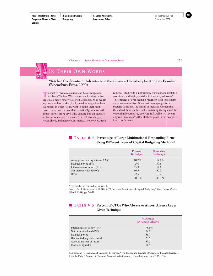
Ross−Westerfield−Jaffe: Corporate Finance, Sixth Edition
II. Value and Capital Budgeting
6. Some Alternative Investment Rules
167© The McGraw−Hill Companies, 2002
Chapter 6 Some Alternative Investment Rules 161
� TABLE 6.4 Percentage of Large Multinational Responding FirmsUsing Different Types of Capital Budgeting Methods*
Primary SecondaryTechnique Technique
Average accounting return (AAR) 10.7% 14.6%Payback period (PP) 5.0 37.6Internal rate of return (IRR) 65.3 14.6Net present value (NPV) 16.5 30.0Other 2.5 3.2_____ _____
100 % 100 %
*The number of responding firms is 121.Source: M. T. Stanley and S. B. Block, “A Survey of Multinational Capital Budgeting,” The Finance Review(March 1984), pp. 36–51.
� TABLE 6.5 Percent of CFOs Who Always or Almost Always Use aGiven Technique
% Alwaysor Almost Always
Internal rate of return (IRR) 75.6%Net present value (NPV) 74.9Payback period 56.7Discounted payback period 29.5Accounting rate of return 30.3Profitability index 11.9
Source: John R. Graham and Campbell R. Harvey, “The Theory and Practice of Corporate Finance: Evidencefrom the Field,” Journal of Financial Economics (forthcoming). Based on a survey of 392 CFOs.
IN THEIR OWN WORDS
“Kitchen Confidential”: Adventures in the Culinary Underbelly by Anthony Bourdain (Bloomsbury Press, 2000)
To want to own a restaurant can be a strange andterrible affliction. What causes such a destructive
urge in so many otherwise sensible people? Why wouldanyone who has worked hard, saved money, often beensuccessful in other fields, want to pump their hard-earned cash down a hole that statistically, at least, willalmost surely prove dry? Why venture into an industrywith enormous fixed expenses (rent, electricity, gas,water, linen, maintenance, insurance, license fees, trash
removal, etc.), with a notoriously transient and unstableworkforce and highly perishable inventory of assets?The chances of ever seeing a return on your investmentare about one in five. What insidious spongi-formbacteria so riddles the brains of men and women thatthey stand there on the tracks, watching the lights of theoncoming locomotive, knowing full well it will eventu-ally run them over? After all these years in the business,I still don’t know.
Ross−Westerfield−Jaffe: Corporate Finance, Sixth Edition
II. Value and Capital Budgeting
6. Some Alternative Investment Rules
168 © The McGraw−Hill Companies, 2002
Noncash flow factors may occasionally play a role in capital budgeting decisions.The easy answer, of course, is ego. The classic example is the retired dentist who wasalways told he threw a great dinner party. “You should open a restaurant,” his friends tellhim. And our dentist believes them. He wants to get in the business—not to make money,no really, but to swan about the dining room signing dinner checks, like Rick inCasablanca. (See our In Their Own Words box.)
The use of quantitative techniques in capital budgeting varies with the industry. Asone would imagine, firms that are better able to precisely estimate cash flows are morelikely to use NPV. For example, estimation of cash flow in certain aspects of the oil busi-ness is quite feasible. Because of this, energy-related firms were among the first to useNPV analysis. Conversely, the cash flows in the motion-picture business are very hard toproject. The grosses of the great hits like Rocky, Star Wars, ET, and Fatal Attraction werefar, far greater than anyone imagined. The big failures like Heaven’s Gate and Howard theDuck were unexpected as well. Because of this, NPV analysis is frowned upon in themovie business.
How does Hollywood perform capital budgeting? The information that a studio uses toaccept or reject a movie idea comes from the pitch. An independent movie producer sched-ules an extremely brief meeting with a studio to pitch his or her idea for a movie. Considerthe following four paragraphs of quotes concerning the pitch from the thoroughly delight-ful book Reel Power.17
“They [studio executives] don’t want to know too much,” says Ron Simpson. “They want to know concept . . . . They want to know what the three-liner is, because they wantit to suggest the ad campaign. They want a title . . . . They don’t want to hear any esoterica. And if the meeting lasts more than five minutes, they’re probably not going to do the project.”
“A guy comes in and says this is my idea: ‘Jaws on a spaceship,’ ” says writer ClayFrohman (Under Fire). “And they say, ‘Brilliant, fantastic.’ Becomes Alien. That is Jaws on aspaceship, ultimately . . . . And that’s it. That’s all they want to hear. Their attitude is ‘Don’tconfuse us with the details of the story.’ ”
“. . . Some high-concept stories are more appealing to the studios than others. The ideasliked best are sufficiently original that the audience will not feel it has already seen the movie,yet similar enough to past hits to reassure executives wary of anything too far-out. Thus, thefrequently used shorthand: It’s Flashdance in the country (Footloose) or High Noon in outerspace (Outland).”
“. . . One gambit not to use during a pitch,” says executive Barbara Boyle, “is to talkabout big box-office grosses your story is sure to make. Executives know as well as anyonethat it’s impossible to predict how much money a movie will make, and declarations to thecontrary are considered pure malarkey.”
162 Part II Value and Capital Budgeting
17Mark Litwak, Reel Power: The Struggle for Influence and Success in the New Hollywood (New York: WilliamMorrow and Company, Inc., 1986), pp. 73, 74, and 77.
Ross−Westerfield−Jaffe: Corporate Finance, Sixth Edition
II. Value and Capital Budgeting
6. Some Alternative Investment Rules
169© The McGraw−Hill Companies, 2002
Chapter 6 Some Alternative Investment Rules 163
6.9 SUMMARY AND CONCLUSIONS
1. In this chapter we cover different investment decision rules. We evaluate the most popularalternatives to the NPV: the payback period, the accounting rate of return, the internal rate ofreturn, and the profitability index. In doing so, we learn more about the NPV.
2. While we find that the alternatives have some redeeming qualities, when all is said and done,they are not the NPV rule; for those of us in finance, that makes them decidedly second-rate.
3. Of the competitors to NPV, IRR must be ranked above either payback or accounting rate ofreturn. In fact, IRR always reaches the same decision as NPV in the normal case where theinitial outflows of an independent investment project are only followed by a series of inflows.
4. We classified the flaws of IRR into two types. First, we considered the general case applying toboth independent and mutually exclusive projects. There appeared to be two problems here:a. Some projects have cash inflows followed by one or more outflows. The IRR rule is inverted
here:One should accept when the IRR is below the discount rate.
b. Some projects have a number of changes of sign in their cash flows. Here, there are likely tobe multiple internal rates of return. The practitioner must use NPV here.
Clearly, (b) is a bigger problem than (a). A new IRR criterion is called for with (a). No IRRcriterion at all will work under (b).
5. Next, we considered the specific problems with the NPV for mutually exclusive projects. Weshowed that, either due to differences in size or in timing, the project with the highest IRR neednot have the highest NPV. Hence, the IRR rule should not be applied. (Of course, NPV can stillbe applied.)
However, we then calculated incremental cash flows. For ease of calculation, we suggestedsubtracting the cash flows of the smaller project from the cash flows of the larger project. In thatway, the incremental initial cash flow is negative.
One can correctly pick the better of two mutually exclusive projects in three other ways:a. Choose the project with the highest NPV.b. If the incremental IRR is greater than the discount rate, choose the bigger project.c. If the incremental NPV is positive, choose the bigger project.
6. We describe capital rationing as a case where funds are limited to a fixed dollar amount. Withcapital rationing the profitability index is a useful method of adjusting the NPV.
KEY TERMS
Average accounting return 144 Independent project 149Basic IRR rule 147 Internal rate of return 147Capital rationing 159 Mutually exclusive investments 149Discounted payback period rule 143 Payback period rule 141Incremental IRR 155 Profitability index 158
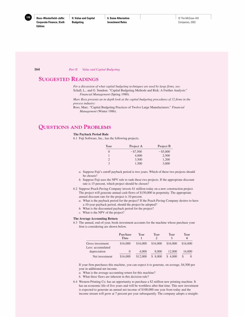
Ross−Westerfield−Jaffe: Corporate Finance, Sixth Edition
II. Value and Capital Budgeting
6. Some Alternative Investment Rules
170 © The McGraw−Hill Companies, 2002
SUGGESTED READINGS
For a discussion of what capital budgeting techniques are used by large firms, see:Schall, L., and G. Sundem. “Capital Budgeting Methods and Risk: A Further Analysis.”
Financial Management (Spring 1980).
Marc Ross presents an in-depth look at the capital budgeting procedures of 12 firms in theprocess industry:Ross, Marc. “Capital Budgeting Practices of Twelve Large Manufacturers.” Financial
Management (Winter 1986).
QUESTIONS AND PROBLEMS
The Payback Period Rule6.1 Fuji Software, Inc., has the following projects.
Year Project A Project B
0 �$7,500 �$5,0001 4,000 2,5002 3,500 1,2003 1,500 3,000
a. Suppose Fuji’s cutoff payback period is two years. Which of these two projects shouldbe chosen?
b. Suppose Fuji uses the NPV rule to rank these two projects. If the appropriate discountrate is 15 percent, which project should be chosen?
6.2 Suppose Peach Paving Company invests $1 million today on a new construction project.The project will generate annual cash flows of $150,000 in perpetuity. The appropriateannual discount rate for the project is 10 percent.a. What is the payback period for the project? If the Peach Paving Company desires to have
a 10-year payback period, should the project be adopted?b. What is the discounted payback period for the project?c. What is the NPV of the project?
The Average Accounting Return6.3 The annual, end-of-year, book-investment accounts for the machine whose purchase your
firm is considering are shown below.
Purchase Year Year Year YearDate 1 2 3 4
Gross investment $16,000 $16,000 $16,000 $16,000 $16,000Less: accumulated
depreciation 0 4,000 8,000 12,000 16,000_______ _______ _______ _______ ______Net investment $16,000 $12,000 $ 8,000 $ 4,000 $ 0
If your firm purchases this machine, you can expect it to generate, on average, $4,500 peryear in additional net income.a. What is the average accounting return for this machine?b. What three flaws are inherent in this decision rule?
6.4 Western Printing Co. has an opportunity to purchase a $2 million new printing machine. Ithas an economic life of five years and will be worthless after that time. This new investmentis expected to generate an annual net income of $100,000 one year from today and theincome stream will grow at 7 percent per year subsequently. The company adopts a straight-
164 Part II Value and Capital Budgeting
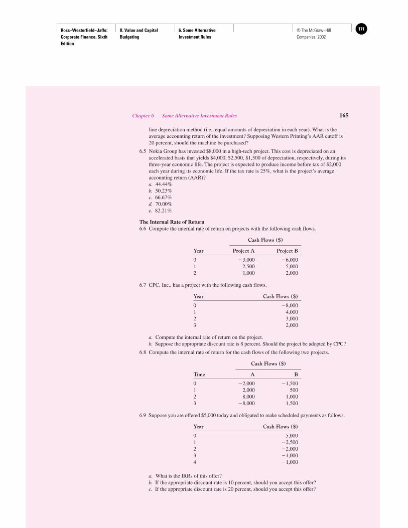
Ross−Westerfield−Jaffe: Corporate Finance, Sixth Edition
II. Value and Capital Budgeting
6. Some Alternative Investment Rules
171© The McGraw−Hill Companies, 2002
line depreciation method (i.e., equal amounts of depreciation in each year). What is theaverage accounting return of the investment? Supposing Western Printing’s AAR cutoff is20 percent, should the machine be purchased?
6.5 Nokia Group has invested $8,000 in a high-tech project. This cost is depreciated on anaccelerated basis that yields $4,000, $2,500, $1,500 of depreciation, respectively, during itsthree-year economic life. The project is expected to produce income before tax of $2,000each year during its economic life. If the tax rate is 25%, what is the project’s averageaccounting return (AAR)?a. 44.44%b. 50.23%c. 66.67%d. 70.00%e. 82.21%
The Internal Rate of Return6.6 Compute the internal rate of return on projects with the following cash flows.
Cash Flows ($)
Year Project A Project B
0 �3,000 �6,0001 2,500 5,0002 1,000 2,000
6.7 CPC, Inc., has a project with the following cash flows.
Year Cash Flows ($)
0 �8,0001 4,0002 3,0003 2,000
a. Compute the internal rate of return on the project.b. Suppose the appropriate discount rate is 8 percent. Should the project be adopted by CPC?
6.8 Compute the internal rate of return for the cash flows of the following two projects.
Cash Flows ($)
Time A B
0 �2,000 �1,5001 2,000 5002 8,000 1,0003 �8,000 1,500
6.9 Suppose you are offered $5,000 today and obligated to make scheduled payments as follows:
Year Cash Flows ($)
0 5,0001 �2,5002 �2,0003 �1,0004 �1,000
a. What is the IRRs of this offer?b. If the appropriate discount rate is 10 percent, should you accept this offer?c. If the appropriate discount rate is 20 percent, should you accept this offer?
Chapter 6 Some Alternative Investment Rules 165
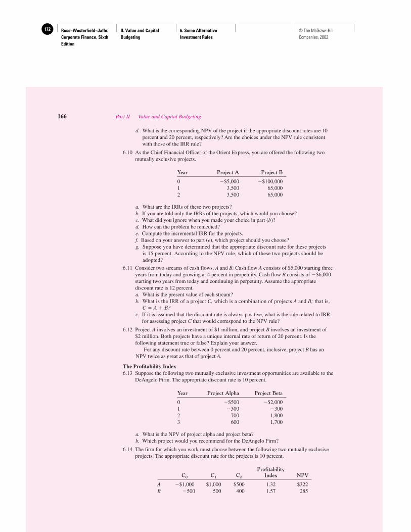
Ross−Westerfield−Jaffe: Corporate Finance, Sixth Edition
II. Value and Capital Budgeting
6. Some Alternative Investment Rules
172 © The McGraw−Hill Companies, 2002
d. What is the corresponding NPV of the project if the appropriate discount rates are 10percent and 20 percent, respectively? Are the choices under the NPV rule consistentwith those of the IRR rule?
6.10 As the Chief Financial Officer of the Orient Express, you are offered the following twomutually exclusive projects.
Year Project A Project B
0 �$5,000 �$100,0001 3,500 65,0002 3,500 65,000
a. What are the IRRs of these two projects?b. If you are told only the IRRs of the projects, which would you choose?c. What did you ignore when you made your choice in part (b)?d. How can the problem be remedied?e. Compute the incremental IRR for the projects.f. Based on your answer to part (e), which project should you choose?g. Suppose you have determined that the appropriate discount rate for these projects
is 15 percent. According to the NPV rule, which of these two projects should beadopted?
6.11 Consider two streams of cash flows, A and B. Cash flow A consists of $5,000 starting threeyears from today and growing at 4 percent in perpetuity. Cash flow B consists of �$6,000starting two years from today and continuing in perpetuity. Assume the appropriatediscount rate is 12 percent.a. What is the present value of each stream?b. What is the IRR of a project C, which is a combination of projects A and B; that is,
C � A � B?c. If it is assumed that the discount rate is always positive, what is the rule related to IRR
for assessing project C that would correspond to the NPV rule?
6.12 Project A involves an investment of $1 million, and project B involves an investment of$2 million. Both projects have a unique internal rate of return of 20 percent. Is thefollowing statement true or false? Explain your answer.
For any discount rate between 0 percent and 20 percent, inclusive, project B has anNPV twice as great as that of project A.
The Profitability Index6.13 Suppose the following two mutually exclusive investment opportunities are available to the
DeAngelo Firm. The appropriate discount rate is 10 percent.
Year Project Alpha Project Beta
0 �$500 �$2,0001 �300 �3002 700 1,8003 600 1,700
a. What is the NPV of project alpha and project beta?b. Which project would you recommend for the DeAngelo Firm?
6.14 The firm for which you work must choose between the following two mutually exclusiveprojects. The appropriate discount rate for the projects is 10 percent.
ProfitabilityC0 C1 C2 Index NPV
A �$1,000 $1,000 $500 1.32 $322B �500 500 400 1.57 285
166 Part II Value and Capital Budgeting
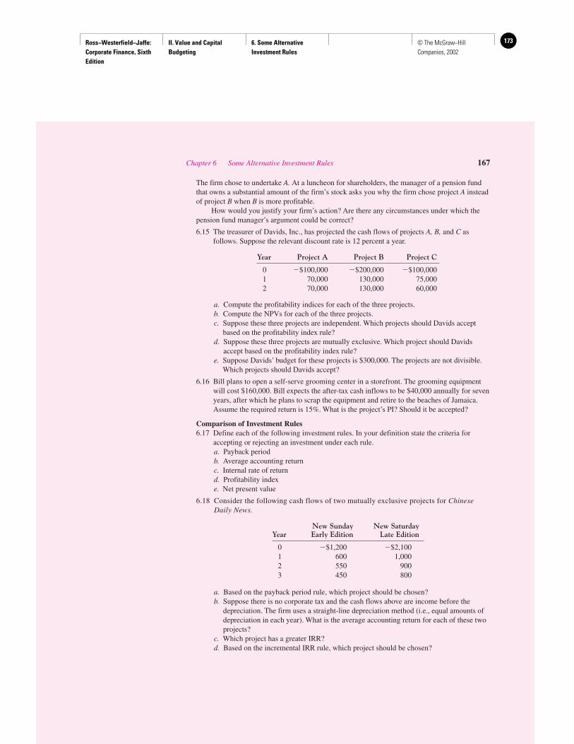
Ross−Westerfield−Jaffe: Corporate Finance, Sixth Edition
II. Value and Capital Budgeting
6. Some Alternative Investment Rules
173© The McGraw−Hill Companies, 2002
The firm chose to undertake A. At a luncheon for shareholders, the manager of a pension fundthat owns a substantial amount of the firm’s stock asks you why the firm chose project A insteadof project B when B is more profitable.
How would you justify your firm’s action? Are there any circumstances under which thepension fund manager’s argument could be correct?
6.15 The treasurer of Davids, Inc., has projected the cash flows of projects A, B, and C asfollows. Suppose the relevant discount rate is 12 percent a year.
Year Project A Project B Project C
0 �$100,000 �$200,000 �$100,0001 70,000 130,000 75,0002 70,000 130,000 60,000
a. Compute the profitability indices for each of the three projects.b. Compute the NPVs for each of the three projects.c. Suppose these three projects are independent. Which projects should Davids accept
based on the profitability index rule?d. Suppose these three projects are mutually exclusive. Which project should Davids
accept based on the profitability index rule?e. Suppose Davids’ budget for these projects is $300,000. The projects are not divisible.
Which projects should Davids accept?
6.16 Bill plans to open a self-serve grooming center in a storefront. The grooming equipmentwill cost $160,000. Bill expects the after-tax cash inflows to be $40,000 annually for sevenyears, after which he plans to scrap the equipment and retire to the beaches of Jamaica.Assume the required return is 15%. What is the project’s PI? Should it be accepted?
Comparison of Investment Rules6.17 Define each of the following investment rules. In your definition state the criteria for
accepting or rejecting an investment under each rule.a. Payback periodb. Average accounting returnc. Internal rate of returnd. Profitability indexe. Net present value
6.18 Consider the following cash flows of two mutually exclusive projects for ChineseDaily News.
New Sunday New SaturdayYear Early Edition Late Edition
0 �$1,200 �$2,1001 600 1,0002 550 9003 450 800
a. Based on the payback period rule, which project should be chosen?b. Suppose there is no corporate tax and the cash flows above are income before the
depreciation. The firm uses a straight-line depreciation method (i.e., equal amounts ofdepreciation in each year). What is the average accounting return for each of these twoprojects?
c. Which project has a greater IRR?d. Based on the incremental IRR rule, which project should be chosen?
Chapter 6 Some Alternative Investment Rules 167

Ross−Westerfield−Jaffe: Corporate Finance, Sixth Edition
II. Value and Capital Budgeting
6. Some Alternative Investment Rules
174 © The McGraw−Hill Companies, 2002
6.19 Consider the following cash flows on two mutually exclusive projects that require anannual return of 15 percent. Working in the financial planning department for the BahamasRecreation Corp., you are trying to compare different investment criteria to arrive at asensible choice of these two projects.
Deepwater New SubmarineYear Fishing Ride
0 �$600,000 �$1,800,0001 270,000 1,000,0002 350,000 700,0003 300,000 900,000
a. Based on the discounted payback period rule, which project should be chosen?b. If your decision rule is to accept the project with a greater IRR, which project should
you choose?c. Since you are fully aware of the IRR rule’s scale problem, you calculate the
incremental IRR for the cash flows. Based on your computation, which project shouldyou choose?
d. To be prudent, you compute the NPV for both projects. Which project should youchoose? Is it consistent with the incremental IRR rule?
6.20 The Utah Mining Corporation is set to open a gold mine near Provo, Utah. According tothe treasurer, Steven Sample, “This is a golden opportunity.” The mine will cost $600,000to open. It will generate a cash inflow of $100,000 during the first year and the cash flowsare projected to grow at 8 percent per year for 10 years. After 10 years the mine will beabandoned. Abandonment costs will be $50,000.a. What is the IRR for the gold mine?b. The Utah Mining Corporation requires a 10 percent return on such undertakings.
Should the mine be opened?
168 Part II Value and Capital Budgeting
Ross−Westerfield−Jaffe: Corporate Finance, Sixth Edition
II. Value and Capital Budgeting
7. Net Present Value and Capital Budgeting
175© The McGraw−Hill Companies, 2002
Net Present Value andCapital Budgeting
CH
AP
TE
R7
EXECUTIVE SUMMARY
In late 1990, the Boeing Company announced its intention to build the Boeing 777, acommercial airplane that would be able to carry up to 390 passengers and fly 7,600 miles.This was expected to be an enormous undertaking. Analysts believed the up-front in-
vestment and research and development expenditures necessary to manufacture the Boeing777 would be as much as $8 billion. Delivery of the first planes was expected to take placein 1995 and to continue for at least 35 years. Was the Boeing 777 a good project for Boeing?In 1990, was the NPV for the Boeing 777 positive? This chapter attempts to show you howBoeing and other firms should go about trying to answer these important questions. The Boe-ing 777 is an example of capital budgeting decision making at the Boeing Company.
Previous chapters discussed the basics of capital budgeting and the net present valueapproach. We now want to move beyond these basics into the real-world application ofthese techniques. We want to show you how to use discounted cash flow (DCF) analysisand net present value (NPV) in capital budgeting decision making.
In this chapter, we show how to identify the relevant cash flows of a project, includinginitial investment outlays, requirements for working capital, and operating cash flows. Welook at the effects of depreciation and taxes. We examine the impact of inflation on interestrates and on a project’s discount rate, and we show why inflation must be handled consis-tently in NPV analysis.
7.1 INCREMENTAL CASH FLOWS
Cash Flows—Not Accounting IncomeYou may not have thought about it, but there is a big difference between corporate financecourses and financial accounting courses. Techniques in corporate finance generally usecash flows, whereas financial accounting generally stresses income or earnings numbers.Certainly, our text has followed this tradition since our net present value techniques dis-counted cash flows, not earnings. When considering a single project, we discounted thecash flows that the firm receives from the project. When valuing the firm as a whole, wediscounted dividends—not earnings—because dividends are the cash flows that an in-vestor receives.
There are many differences between earnings and cash flows. In fact, much of a standardfinancial accounting course delineates these differences. Because we have no desire to dupli-cate such course material, we merely discuss one example of the differences. Consider a firmbuying a building for $100,000 today. The entire $100,000 is an immediate cash outflow.However, assuming straight-line depreciation over 20 years, only $5,000 ($100,000/20) isconsidered an accounting expense in the current year. Current earnings are thereby reducedonly by $5,000. The remaining $95,000 is expensed over the following 19 years.
Ross−Westerfield−Jaffe: Corporate Finance, Sixth Edition
II. Value and Capital Budgeting
7. Net Present Value and Capital Budgeting
176 © The McGraw−Hill Companies, 2002
Because the seller of the property demands immediate payment, the cost at date 0 ofthe project to the firm is $100,000. Thus, the full $100,000 figure should be viewed as animmediate outflow for capital budgeting purposes. This is not merely our opinion but theunanimous verdict of both academics and practitioners.
In addition, it is not enough to use cash flows. In calculating the NPV of a project, onlycash flows that are incremental to the project should be used. These cash flows are thechanges in the firm’s cash flows that occur as a direct consequence of accepting the proj-ect. That is, we are interested in the difference between the cash flows of the firm with theproject and the cash flows of the firm without the project.
The use of incremental cash flows sounds easy enough, but pitfalls abound in the realworld. In this section we describe how to avoid some of the pitfalls of determining incre-mental cash flows.
Sunk CostsA sunk cost is a cost that has already occurred. Because sunk costs are in the past, they can-not be changed by the decision to accept or reject the project. Just as we “let bygones bebygones,” we should ignore such costs. Sunk costs are not incremental cash outflows.
EXAMPLE
The General Milk Company is currently evaluating the NPV of establishing a lineof chocolate milk. As part of the evaluation the company had paid a consultingfirm $100,000 to perform a test-marketing analysis. This expenditure was madelast year. Is this cost relevant for the capital budgeting decision now confrontingthe management of General Milk Company?
The answer is no. The $100,000 is not recoverable, so the $100,000 expendi-ture is a sunk cost, or spilled milk. Of course, the decision to spend $100,000 fora marketing analysis was a capital budgeting decision itself and was perfectly rel-evant before it was sunk. Our point is that once the company incurred the expense,the cost became irrelevant for any future decision.
Opportunity CostsYour firm may have an asset that it is considering selling, leasing, or employing elsewhere inthe business. If the asset is used in a new project, potential revenues from alternative uses arelost. These lost revenues can meaningfully be viewed as costs. They are called opportunitycosts because, by taking the project, the firm forgoes other opportunities for using the assets.
EXAMPLE
Suppose the Weinstein Trading Company has an empty warehouse in Philadelphiathat can be used to store a new line of electronic pinball machines. The companyhopes to market the machines to affluent northeastern consumers. Should the costof the warehouse and land be included in the costs associated with introducing anew line of electronic pinball machines?
The answer is yes. The use of a warehouse is not free; it has an opportunitycost. The cost is the cash that could be raised by the company if the decision tomarket the electronic pinball machines were rejected and the warehouse and landwere put to some other use (or sold). If so, the NPV of the alternative uses becomesan opportunity cost of the decision to sell electronic pinball machines.
170 Part II Value and Capital Budgeting
Ross−Westerfield−Jaffe: Corporate Finance, Sixth Edition
II. Value and Capital Budgeting
7. Net Present Value and Capital Budgeting
177© The McGraw−Hill Companies, 2002
Side EffectsAnother difficulty in determining incremental cash flows comes from the side effects of theproposed project on other parts of the firm. The most important side effect is erosion. Ero-sion is the cash flow transferred to a new project from customers and sales of other prod-ucts of the firm.
EXAMPLE
Suppose the Innovative Motors Corporation (IMC) is determining the NPV of anew convertible sports car. Some of the customers who would purchase the car areowners of IMC’s compact sedan. Are all sales and profits from the new convert-ible sports car incremental?
The answer is no because some of the cash flow represents transfers fromother elements of IMC’s product line. This is erosion, which must be included inthe NPV calculation. Without taking erosion into account, IMC might erroneouslycalculate the NPV of the sports car to be, say, $100 million. If IMC’s managersrecognized that half the customers are transfers from the sedan and that lost sedansales have an NPV of �$150 million, they would see that the true NPV is �$50million ($100 million � $150 million).
• What are the three difficulties in determining incremental cash flows?• Define sunk costs, opportunity costs, and side effects.
7.2 THE BALDWIN COMPANY: AN EXAMPLE
We next consider the example of a proposed investment in machinery and related items. Ourexample involves the Baldwin Company and colored bowling balls.
The Baldwin Company, originally established in 1965 to make footballs, is now a lead-ing producer of tennis balls, baseballs, footballs, and golf balls. In 1973 the company in-troduced “High Flite,” its first line of high-performance golf balls. The Baldwin manage-ment has sought opportunities in whatever businesses seem to have some potential for cashflow. In 1999 W. C. Meadows, vice president of the Baldwin Company, identified anothersegment of the sports ball market that looked promising and that he felt was not adequatelyserved by larger manufacturers. That market was for brightly colored bowling balls, and hebelieved a large number of bowlers valued appearance and style above performance. Healso believed that it would be difficult for competitors to take advantage of the opportunitybecause of Baldwin’s cost advantages and because of its ability to use its highly developedmarketing skills.
As a result, in late 2000 the Baldwin Company decided to evaluate the marketing po-tential of brightly colored bowling balls. Baldwin sent a questionnaire to consumers in threemarkets: Philadelphia, Los Angeles, and New Haven. The results of the three questionnaireswere much better than expected and supported the conclusion that the brightly coloredbowling ball could achieve a 10- to 15-percent share of the market. Of course, some peopleat Baldwin complained about the cost of the test marketing, which was $250,000. However,Meadows argued that it was a sunk cost and should not be included in project evaluation.
Chapter 7 Net Present Value and Capital Budgeting 171
QUESTIONS
CO
NC
EP
T
?
Ross−Westerfield−Jaffe: Corporate Finance, Sixth Edition
II. Value and Capital Budgeting
7. Net Present Value and Capital Budgeting
178 © The McGraw−Hill Companies, 2002
In any case, the Baldwin Company is now considering investing in a machine to pro-duce bowling balls. The bowling balls would be produced in a building owned by the firmand located near Los Angeles. This building, which is vacant, and the land can be sold tonet $150,000 after taxes. The adjusted basis of this property, the original purchase price ofthe property less depreciation, is zero.1
Working with his staff, Meadows is preparing an analysis of the proposed new prod-uct. He summarizes his assumptions as follows: The cost of the bowling ball machine is$100,000. The machine has an estimated market value at the end of five years of $30,000.Production by year during the five-year life of the machine is expected to be as follows:5,000 units, 8,000 units, 12,000 units, 10,000 units, and 6,000 units. The price of bowlingballs in the first year will be $20. The bowling ball market is highly competitive, soMeadows believes that the price of bowling balls will increase at only 2 percent per year,as compared to the anticipated general inflation rate of 5 percent. Conversely, the plasticused to produce bowling balls is rapidly becoming more expensive. Because of this, pro-duction cash outflows are expected to grow at 10 percent per year. First-year productioncosts will be $10 per unit. Meadows has determined, based upon Baldwin’s taxable income,that the appropriate incremental corporate tax rate in the bowling ball project is 34 percent.
Net working capital is defined as the difference between current assets and current li-abilities. Baldwin finds that it must maintain an investment in working capital. Like anymanufacturing firm, it will purchase raw materials before production and sale, giving riseto an investment in inventory. It will maintain cash as a buffer against unforeseen expendi-tures. Its credit sales will generate accounts receivable. Management believes that the in-vestment in the different items of working capital totals $10,000 in year 0, rises somewhatin the early years of the project, and falls to $0 by the project’s end. In other words, the in-vestment in working capital is completely recovered by the end of the project’s life.
Projections based on these assumptions and Meadows’s analysis appear in Tables 7.1through 7.4. In these tables all cash flows are assumed to occur at the end of the year.Because of the large amount of data in these tables, it is important to see how the tables arerelated. Table 7.1 shows the basic data for both investment and income. Supplementaryschedules on operations and depreciation, as presented in Tables 7.2 and 7.3, help explainwhere the numbers in Table 7.1 come from. Our goal is to obtain projections of cash flow.The data in Table 7.1 are all that are needed to calculate the relevant cash flows, as shownin Table 7.4.
An Analysis of the ProjectInvestments The investment outlays required for the project are summarized in the topsegment of Table 7.1. They consist of three parts:
1. The Bowling Ball Machine. The purchase requires a cash outflow of $100,000 atyear 0. The firm realizes a cash inflow when the machine is sold in year 5. These cash flowsare shown in line 1 of Table 7.1. As indicated in the footnote to the table, taxes are incurredwhen the asset is sold.
2. The Opportunity Cost of Not Selling the Warehouse. If Baldwin accepts the bowling-ball project, it will use a warehouse and land that could otherwise be sold. The estimatedsales price of the warehouse and land is therefore included as an opportunity cost, as
172 Part II Value and Capital Budgeting
1We use the term adjusted basis rather than book value because we are concerned with the firm’s tax books, notits accounting books. This point is treated later in the chapter in the section entitled “Which Set of Books?” Thecurrent market value of the building and land is $227,272.73. We will assume the corporate tax rate is 34percent, the basis is zero, and the after-tax net is $227,272.73 � (1 � 0.34) � $150,000.
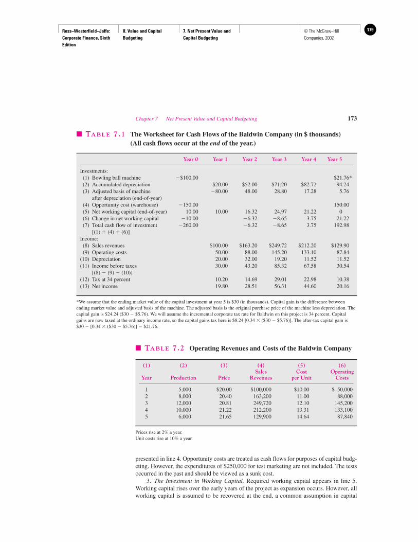
Ross−Westerfield−Jaffe: Corporate Finance, Sixth Edition
II. Value and Capital Budgeting
7. Net Present Value and Capital Budgeting
179© The McGraw−Hill Companies, 2002
presented in line 4. Opportunity costs are treated as cash flows for purposes of capital budg-eting. However, the expenditures of $250,000 for test marketing are not included. The testsoccurred in the past and should be viewed as a sunk cost.
3. The Investment in Working Capital. Required working capital appears in line 5.Working capital rises over the early years of the project as expansion occurs. However, allworking capital is assumed to be recovered at the end, a common assumption in capital
Chapter 7 Net Present Value and Capital Budgeting 173
� TABLE 7.1 The Worksheet for Cash Flows of the Baldwin Company (in $ thousands) (All cash flows occur at the end of the year.)
Year 0 Year 1 Year 2 Year 3 Year 4 Year 5
Investments:(1) Bowling ball machine �$100.00 $21.76*(2) Accumulated depreciation $20.00 $52.00 $71.20 $82.72 94.24(3) Adjusted basis of machine �80.00 48.00 28.80 17.28 5.76
after depreciation (end-of-year)(4) Opportunity cost (warehouse) �150.00 150.00(5) Net working capital (end-of-year) 10.00 10.00 16.32 24.97 21.22 0(6) Change in net working capital �10.00 �6.32 �8.65 3.75 21.22(7) Total cash flow of investment �260.00 �6.32 �8.65 3.75 192.98
[(1) � (4) � (6)]Income:
(8) Sales revenues $100.00 $163.20 $249.72 $212.20 $129.90(9) Operating costs 50.00 88.00 145.20 133.10 87.84
(10) Depreciation 20.00 32.00 19.20 11.52 11.52(11) Income before taxes 30.00 43.20 85.32 67.58 30.54
[(8) � (9) � (10)](12) Tax at 34 percent 10.20 14.69 29.01 22.98 10.38(13) Net income 19.80 28.51 56.31 44.60 20.16
*We assume that the ending market value of the capital investment at year 5 is $30 (in thousands). Capital gain is the difference betweenending market value and adjusted basis of the machine. The adjusted basis is the original purchase price of the machine less depreciation. Thecapital gain is $24.24 ($30 � $5.76). We will assume the incremental corporate tax rate for Baldwin on this project is 34 percent. Capitalgains are now taxed at the ordinary income rate, so the capital gains tax here is $8.24 [0.34 � ($30 � $5.76)]. The after-tax capital gain is $30 � [0.34 � ($30 � $5.76)] � $21.76.
� TABLE 7.2 Operating Revenues and Costs of the Baldwin Company
(1) (2) (3) (4) (5) (6)Sales Cost Operating
Year Production Price Revenues per Unit Costs
1 5,000 $20.00 $100,000 $10.00 $ 50,0002 8,000 20.40 163,200 11.00 88,0003 12,000 20.81 249,720 12.10 145,2004 10,000 21.22 212,200 13.31 133,1005 6,000 21.65 129,900 14.64 87,840
Prices rise at 2% a year.Unit costs rise at 10% a year.
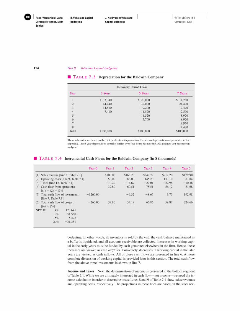
Ross−Westerfield−Jaffe: Corporate Finance, Sixth Edition
II. Value and Capital Budgeting
7. Net Present Value and Capital Budgeting
180 © The McGraw−Hill Companies, 2002
budgeting. In other words, all inventory is sold by the end, the cash balance maintained asa buffer is liquidated, and all accounts receivable are collected. Increases in working capi-tal in the early years must be funded by cash generated elsewhere in the firm. Hence, theseincreases are viewed as cash outflows. Conversely, decreases in working capital in the lateryears are viewed as cash inflows. All of these cash flows are presented in line 6. A morecomplete discussion of working capital is provided later in this section. The total cash flowfrom the above three investments is shown in line 7.
Income and Taxes Next, the determination of income is presented in the bottom segmentof Table 7.1. While we are ultimately interested in cash flow—not income—we need the in-come calculation in order to determine taxes. Lines 8 and 9 of Table 7.1 show sales revenuesand operating costs, respectively. The projections in these lines are based on the sales rev-
174 Part II Value and Capital Budgeting
� TABLE 7.3 Depreciation for the Baldwin Company
Recovery Period Class
Year 3 Years 5 Years 7 Years
1 $ 33,340 $ 20,000 $ 14,2802 44,440 32,000 24,4903 14,810 19,200 17,4904 7,410 11,520 12,5005 11,520 8,9206 5,760 8,9207 8,9208 4,480
Total $100,000 $100,000 $100,000
These schedules are based on the IRS publication Depreciation. Details on depreciation are presented in theappendix. Three-year depreciation actually carries over four years because the IRS assumes you purchase inmidyear.
� TABLE 7.4 Incremental Cash Flows for the Baldwin Company (in $ thousands)
Year 0 Year 1 Year 2 Year 3 Year 4 Year 5
(1) Sales revenue [line 8, Table 7.1] $100.00 $163.20 $249.72 $212.20 $129.90(2) Operating costs [line 9, Table 7.1] �50.00 �88.00 �145.20 �133.10 �87.84(3) Taxes [line 12, Table 7.1] �10.20 �14.69 �29.01 �22.98 �10.38(4) Cash flow from operations 39.80 60.51 75.51 56.12 31.68
[(1) � (2) � (3)](5) Total cash flow of investment �$260.00 �6.32 �8.65 3.75 192.98
[line 7, Table 7.1](6) Total cash flow of project �260.00 39.80 54.19 66.86 59.87 224.66
[(4) � (5)]NPV @ 4% 123.641
10% 51.58815% 5.47220% �31.351
Ross−Westerfield−Jaffe: Corporate Finance, Sixth Edition
II. Value and Capital Budgeting
7. Net Present Value and Capital Budgeting
181© The McGraw−Hill Companies, 2002
enues and operating costs computed in columns 4 and 6 of Table 7.2. The estimates of rev-enues and costs follow from assumptions made by the corporate planning staff at Baldwin.In other words, the estimates critically depend on the fact that product prices are projectedto increase at 2 percent per year and costs are projected to increase at 10 percent per year.
Depreciation of the $100,000 capital investment is based on the amount allowed by the1986 Tax Reform Act.2 Depreciation schedules under the act for three-year, five-year, andseven-year recovery periods are presented in Table 7.3. The IRS ruled that Baldwin is to de-preciate its capital investment over five years, so the middle column of the table applies tothis case. Depreciation from this middle column is reproduced in line 10 of Table 7.1.Income before taxes is calculated in line 11 of Table 7.1. Taxes are provided in line 12 ofthis table, and net income is calculated in line 13.
Cash Flow Cash flow is finally determined in Table 7.4. We begin by reproducing lines8, 9, and 12 in Table 7.1 as lines 1, 2, and 3 in Table 7.4. Cash flow from operations, whichis sales minus both operating costs and taxes, is provided in line 4 of Table 7.4. Total in-vestment cash flow, taken from line 7 of Table 7.1, appears as line 5 of Table 7.4. Cash flowfrom operations plus total cash flow of the investment equals total cash flow of the project,which is displayed as line 6 of Table 7.4. The bottom of the table presents the NPV of thesecash flows for different discount rates.
Net Present Value It is possible to calculate the NPV of the Baldwin bowling ball proj-ect from these cash flows. As can be seen at the bottom of Table 7.4, the NPV is $51,588 if10 percent is the appropriate discount rate and �$31,351 if 20 percent is the appropriatediscount rate. If the discount rate is 15.67 percent, the project will have a zero NPV. In otherwords, the project’s internal rate of return is 15.67 percent. If the discount rate of the Bald-win bowling ball project is above 15.67 percent, it should not be accepted because its NPVwould be negative.
Which Set of Books?It should be noted that the firm’s management generally keeps two sets of books, one forthe IRS (called the tax books) and another for its annual report (called the stockholders’books). The tax books follow the rules of the IRS. The stockholders’ books follow the rulesof the Financial Accounting Standards Board (FASB), the governing body in accounting.The two sets of rules differ widely in certain areas. For example, income on municipalbonds is ignored for tax purposes while being treated as income by the FASB. The differ-ences almost always benefit the firm, because the rules permit income on the stockholders’books to be higher than income on the tax books. That is, management can look profitableto the stockholders without needing to pay taxes on all of the reported profit. In fact, thereare plenty of large companies that consistently report positive earnings to the stockholderswhile reporting losses to the IRS.
We present a synopsis of the IRS rules on depreciation in the appendix. The rules ondepreciation for the stockholders’ books differ, as they do in many other accounting areas.Which of the two sets of rules on depreciation do we want in order to create the previoustables for Baldwin? Clearly, we are interested in the IRS rules. Our purpose is to determinenet cash flow, and tax payments are a cash outflow. The FASB regulations determine thecalculation of accounting income, not cash flow.
Chapter 7 Net Present Value and Capital Budgeting 175
2Depreciation rules are discussed in detail in the appendix to this chapter.
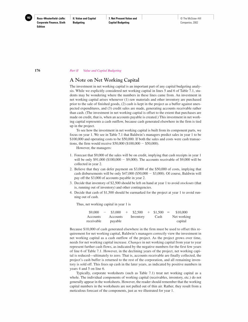
Ross−Westerfield−Jaffe: Corporate Finance, Sixth Edition
II. Value and Capital Budgeting
7. Net Present Value and Capital Budgeting
182 © The McGraw−Hill Companies, 2002
A Note on Net Working CapitalThe investment in net working capital is an important part of any capital budgeting analy-sis. While we explicitly considered net working capital in lines 5 and 6 of Table 7.1, stu-dents may be wondering where the numbers in these lines came from. An investment innet working capital arises whenever (1) raw materials and other inventory are purchasedprior to the sale of finished goods, (2) cash is kept in the project as a buffer against unex-pected expenditures, and (3) credit sales are made, generating accounts receivable ratherthan cash. (The investment in net working capital is offset to the extent that purchases aremade on credit, that is, when an accounts payable is created.) This investment in net work-ing capital represents a cash outflow, because cash generated elsewhere in the firm is tiedup in the project.
To see how the investment in net working capital is built from its component parts, wefocus on year 1. We see in Table 7.1 that Baldwin’s managers predict sales in year 1 to be$100,000 and operating costs to be $50,000. If both the sales and costs were cash transac-tions, the firm would receive $50,000 ($100,000 � $50,000).
However, the managers:
1. Forecast that $9,000 of the sales will be on credit, implying that cash receipts in year 1will be only $91,000 ($100,000 � $9,000). The accounts receivable of $9,000 will becollected in year 2.
2. Believe that they can defer payment on $3,000 of the $50,000 of costs, implying thatcash disbursements will be only $47,000 ($50,000 � $3,000). Of course, Baldwin willpay off the $3,000 of accounts payable in year 2.
3. Decide that inventory of $2,500 should be left on hand at year 1 to avoid stockouts (thatis, running out of inventory) and other contingencies.
4. Decide that cash of $1,500 should be earmarked for the project at year 1 to avoid run-ning out of cash.
Thus, net working capital in year 1 is
$9,000 � $3,000 � $2,500 � $1,500 � $10,000Accounts Accounts Inventory Cash Net workingreceivable payable capital
Because $10,000 of cash generated elsewhere in the firm must be used to offset this re-quirement for net working capital, Baldwin’s managers correctly view the investment innet working capital as a cash outflow of the project. As the project grows over time,needs for net working capital increase. Changes in net working capital from year to yearrepresent further cash flows, as indicated by the negative numbers for the first few yearsof line 6 of Table 7.1. However, in the declining years of the project, net working capi-tal is reduced—ultimately to zero. That is, accounts receivable are finally collected, theproject’s cash buffer is returned to the rest of the corporation, and all remaining inven-tory is sold off. This frees up cash in the later years, as indicated by positive numbers inyears 4 and 5 on line 6.
Typically, corporate worksheets (such as Table 7.1) treat net working capital as awhole. The individual components of working capital (receivables, inventory, etc.) do notgenerally appear in the worksheets. However, the reader should remember that the workingcapital numbers in the worksheets are not pulled out of thin air. Rather, they result from ameticulous forecast of the components, just as we illustrated for year 1.
176 Part II Value and Capital Budgeting
Ross−Westerfield−Jaffe: Corporate Finance, Sixth Edition
II. Value and Capital Budgeting
7. Net Present Value and Capital Budgeting
183© The McGraw−Hill Companies, 2002
Interest ExpenseIt may have bothered you that interest expense was ignored in the Baldwin example. After all,many projects are at least partially financed with debt, particularly a bowling ball machine thatis likely to increase the debt capacity of the firm. As it turns out, our approach of assuming nodebt financing is rather standard in the real world. Firms typically calculate a project’s cashflows under the assumption that the project is financed only with equity. Any adjustments fordebt financing are reflected in the discount rate, not the cash flows. The treatment of debt incapital budgeting will be covered in depth later in the text. Suffice it to say at this time that thefull ramifications of debt financing are well beyond our current discussion.
• What are the items leading to cash flow in any year?• Why did we determine income when NPV analysis discounts cash flows, not income?• Why is working capital viewed as a cash outflow?
EXAMPLE
In late 1990, when the Boeing Company announced its intention to build a newpassenger airplane called the Boeing 777, it anticipated it could sell several thou-sand planes over a 35-year period. Table 7.5 describes one set of possible (and hy-pothetical) cash flows of the Boeing 777. Although Boeing incurred several hun-dred million dollars of research and development prior to 1991, we ignore thesecosts because they are sunk costs. Notice also that we have subtracted deprecia-tion from sales revenue for tax purposes but added it back for total cash flow.
It is possible to calculate the NPV of the Boeing 777 from these cash flows.If the discount rate is 10 percent, the NPV is positive whereas if the appropriatediscount rate is 30 percent, the NPV is negative. The break-even discount rate is19 percent. (Recall we also call the break-even discount rate the IRR.)
In May 2000, Boeing had delivered 282 777s—somewhat less than the deliveries hy-pothesized in Table 7.5.
7.3 INFLATION AND CAPITAL BUDGETING
Inflation is an important fact of economic life, and it must be considered in capital budget-ing. We begin our examination of inflation by considering the relationship between interestrates and inflation.
Interest Rates and InflationSuppose that the one-year interest rate that the bank pays is 10 percent. This means that anindividual who deposits $1,000 at date 0 will get $1,100 ($1,000 � 1.10) in one year. While10 percent may seem like a handsome return, one can only put it in perspective after ex-amining the rate of inflation.
Suppose that the rate of inflation is 6 percent over the year and it affects all goodsequally. For example, a restaurant that charges $1.00 for a hamburger at date 0 charges$1.06 for the same hamburger at the end of the year. You can use your $1,000 to buy 1,000
Chapter 7 Net Present Value and Capital Budgeting 177
QUESTIONS
CO
NC
EP
T
?

Ross−Westerfield−Jaffe: Corporate Finance, Sixth Edition
II. Value and Capital Budgeting
7. Net Present Value and Capital Budgeting
184 © The McGraw−Hill Companies, 2002
178
�T
AB
LE
7.5
Incr
emen
tal C
ash
Flo
ws:
Boe
ing
777
Num
ber
Inco
me
of P
lane
sSa
les
Ope
rati
ngbe
fore
Cha
nge
Cap
ital
Dep
reci
atio
nT
otal
Yea
rD
eliv
ered
Rev
enue
Cos
tsD
epre
ciat
ion
Tax
esT
axes
in N
WC
Exp
endi
ture
Inve
stm
ent
Add
-bac
kC
ash
Flow
1991
$86
5.00
$40
.00
$ (9
05.0
0)$
(307
.70)
$400
.00
$40
0.00
$40
.00
$(9
57.3
0)19
921,
340.
0096
.00
(1,4
36.0
0)(4
88.2
4)60
0.00
600.
0096
.00
(1,4
51.7
6)19
931,
240.
0011
6.40
(1,3
56.4
0)(4
61.1
8)30
0.00
300.
0011
6.40
(1,0
78.8
2)19
9484
0.00
124.
76(9
64.7
6)(3
28.0
2)20
0.00
200.
0012
4.76
(711
.98)
1995
14$
1,84
7.55
1,97
6.69
112.
28(2
41.4
2)(8
2.08
)$
181.
061.
8518
2.91
112.
28(2
29.9
7)19
9614
519
,418
.96
17,8
65.4
510
1.06
1,45
2.45
493.
831,
722.
0019
.42
1,74
1.42
101.
0668
1.74
1997
140
19,2
44.2
316
,550
.04
90.9
52,
603.
2488
5.10
(17.
12)
19.4
22.
3090
.95
1,80
6.79
1998
111
15,7
37.9
513
,377
.26
82.7
22,
277.
9777
4.51
(343
.62)
15.7
4(3
27.8
8)82
.72
1,91
4.06
1999
107
16,2
57.3
513
,656
.17
77.7
52,
523.
4385
7.97
50.9
016
.26
67.1
677
.75
1,67
6.05
2000
102
15,3
33.4
212
,726
.74
75.6
32,
531.
0586
0.56
90.5
415
.33
105.
8775
.63
1,64
0.25
2001
9214
,289
.29
11,8
60.1
175
.00
2,35
4.18
800.
42(1
02.3
3)14
.29
(88.
04)
75.0
01,
716.
8020
0292
14,7
17.9
712
,068
.74
75.0
02,
574.
2387
5.24
42.0
114
.72
56.7
375
.00
1,71
7.26
2003
105
17,2
33.9
714
,131
.85
99.4
63,
002.
661,
020.
9024
6.57
244.
6449
1.21
99.4
61,
590.
0120
0489
15,0
66.4
212
,354
.47
121.
482,
590.
4788
0.76
(212
.42)
244.
6432
.22
121.
481,
798.
9720
0511
119
,468
.56
17,9
11.0
711
6.83
1,44
0.66
489.
8243
1.41
19.4
745
0.88
116.
8361
6.79
2006
130
23,3
07.5
320
,510
.63
112.
652,
684.
2591
2.65
376.
2223
.31
399.
5311
2.65
1,48
4.73
2007
118
21,9
11.4
018
,843
.81
100.
202,
967.
391,
008.
91(1
36.8
2)21
.91
(114
.91)
100.
202,
173.
5920
0894
17,9
44.0
015
,252
.40
129.
202,
562.
4087
1.22
(388
.81)
567.
2217
8.41
129.
201,
641.
9720
0912
324
,103
.23
22,1
74.9
896
.99
1,83
1.26
622.
6360
3.60
24.1
062
7.70
96.9
967
7.92
2010
125
25,3
16.9
722
,278
.94
76.8
42,
961.
191,
006.
8011
8.95
25.3
214
4.27
76.8
41,
886.
9620
1112
526
,076
.48
22,4
25.7
765
.81
3,58
4.90
1,21
8.87
74.4
326
.08
100.
5165
.81
2,33
1.33
2012
9821
,133
.07
17,9
63.1
061
.68
3,10
8.29
1,05
6.82
(484
.45)
21.1
3(4
63.3
2)61
.68
2,57
6.47
2013
8418
,550
.25
15,5
82.2
157
.96
2,91
0.08
989.
43(2
53.1
2)18
.55
(234
.57)
57.9
62,
213.
1820
1489
20,3
21.6
416
,866
.97
54.6
13,
400.
061,
156.
0217
3.60
20.3
219
3.92
54.6
12,
104.
7320
1589
20,9
31.2
917
,372
.97
52.8
33,
505.
491,
191.
8759
.75
20.9
380
.68
52.8
32,
285.
7720
1689
21,5
59.2
317
,894
.16
52.8
33,
612.
241,
228.
1661
.54
21.5
683
.10
52.8
32,
353.
8120
1789
22,2
06.0
018
,430
.98
52.8
33,
722.
191,
265.
5463
.38
22.2
185
.59
52.8
32,
423.
8920
1889
22,8
72.1
818
,983
.92
52.8
33,
835.
431,
304.
0565
.29
22.8
788
.16
52.8
32,
496.
0520
1989
23,5
58.3
519
,553
.43
47.5
23,
957.
401,
345.
5267
.24
23.5
690
.80
47.5
22,
568.
6020
2089
24,2
65.1
020
,140
.03
35.2
84,
089.
791,
390.
5369
.26
24.2
793
.53
35.2
82,
641.
0120
2189
24,9
93.0
520
,744
.23
28.3
64,
220.
461,
434.
9671
.34
24.9
996
.33
28.3
62,
717.
5320
2289
25,7
42.8
521
,366
.56
28.3
64,
347.
931,
478.
3073
.48
25.7
499
.22
28.3
62,
798.
7720
2389
26,5
15.1
322
,007
.56
28.3
64,
479.
211,
522.
9375
.68
26.5
210
2.20
28.3
62,
882.
4420
2489
$27,
310.
58$2
2,66
7.78
$16
.05
$ 4,
626.
75$1
,573
.10
$77
.95
$27
.31
$10
5.26
$16
.05
$2,
964.
45
Not
es:
Tax
rate
is 3
4 pe
rcen
t of
taxa
ble
inco
me.
Tota
l cas
h fl
ow c
an b
e de
term
ined
by
addi
ng a
cros
s th
e ro
ws.
Rec
all t
hat t
otal
cas
h fl
ow is
equ
al to
Sal
es r
even
ue �
Ope
ratin
g co
sts
�Ta
xes
�In
vest
men
t.So
urce
:Rob
ert B
rum
er,C
ase
Stud
ies
in F
inan
ce(B
urr
Rid
ge,I
ll.:T
imes
Mir
ror/
Irw
in,1
997)
.
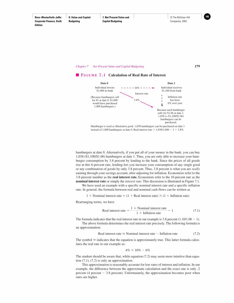
Ross−Westerfield−Jaffe: Corporate Finance, Sixth Edition
II. Value and Capital Budgeting
7. Net Present Value and Capital Budgeting
185© The McGraw−Hill Companies, 2002
hamburgers at date 0. Alternatively, if you put all of your money in the bank, you can buy1,038 ($1,100/$1.06) hamburgers at date 1. Thus, you are only able to increase your ham-burger consumption by 3.8 percent by lending to the bank. Since the prices of all goodsrise at this 6-percent rate, lending lets you increase your consumption of any single goodor any combination of goods by only 3.8 percent. Thus, 3.8 percent is what you are reallyearning through your savings account, after adjusting for inflation. Economists refer to the3.8-percent number as the real interest rate. Economists refer to the 10-percent rate as thenominal interest rate or simply the interest rate. This discussion is illustrated in Figure 7.1.
We have used an example with a specific nominal interest rate and a specific inflationrate. In general, the formula between real and nominal cash flows can be written as
1 � Nominal interest rate � (1 � Real interest rate) � (1 � Inflation rate)
Rearranging terms, we have
(7.1)
The formula indicates that the real interest rate in our example is 3.8 percent (1.10/1.06 � 1).The above formula determines the real interest rate precisely. The following formula is
an approximation:
Real interest rate � Nominal interest rate � Inflation rate (7.2)
The symbol � indicates that the equation is approximately true. This latter formula calcu-lates the real rate in our example as:
4% � 10% � 6%
The student should be aware that, while equation (7.2) may seem more intuitive than equa-tion (7.1), (7.2) is only an approximation.
This approximation is reasonably accurate for low rates of interest and inflation. In ourexample, the difference between the approximate calculation and the exact one is only .2percent (4 percent � 3.8 percent). Unfortunately, the approximation becomes poor whenrates are higher.
Real interest rate �1 � Nominal interest rate
1 � Inflation rate� 1
Chapter 7 Net Present Value and Capital Budgeting 179
Date 0 Date 1
Individual invests$1,000 in bank
Individual receives$1,100 from bank
Inflation ratehas been
6% over year
(Because hamburgers sellfor $1 at date 0, $1,000would have purchased
1,000 hamburgers.)Because each hamburgersells for $1.06 at date 1,1,038 (= $1,100/$1.06)
hamburgers can bepurchased.
Interest rate
3.8%
10%
� FIGURE 7.1 Calculation of Real Rate of Interest
Hamburger is used as illustrative good. 1,038 hamburgers can be purchased on date 1instead of 1,000 hamburgers at date 0. Real interest rate � 1,038/1,000 � 1 � 3.8%.
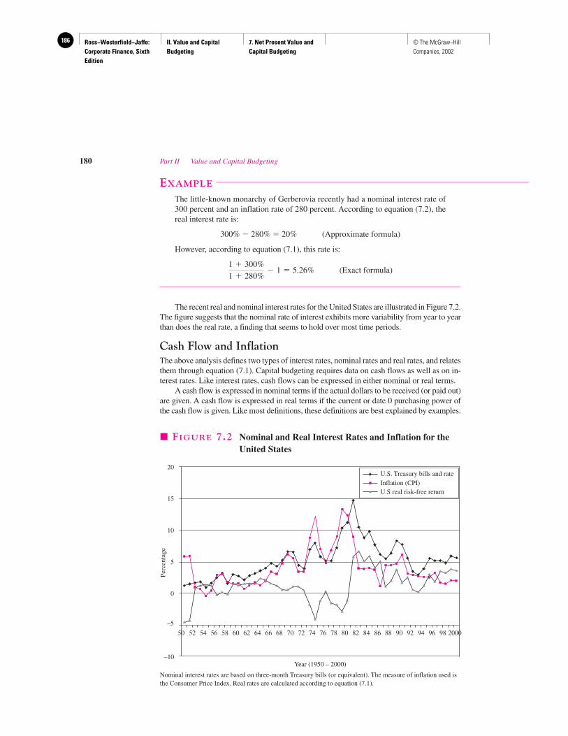
Ross−Westerfield−Jaffe: Corporate Finance, Sixth Edition
II. Value and Capital Budgeting
7. Net Present Value and Capital Budgeting
186 © The McGraw−Hill Companies, 2002
EXAMPLE
The little-known monarchy of Gerberovia recently had a nominal interest rate of300 percent and an inflation rate of 280 percent. According to equation (7.2), thereal interest rate is:
300% � 280% � 20% (Approximate formula)
However, according to equation (7.1), this rate is:
(Exact formula)
The recent real and nominal interest rates for the United States are illustrated in Figure 7.2.The figure suggests that the nominal rate of interest exhibits more variability from year to yearthan does the real rate, a finding that seems to hold over most time periods.
Cash Flow and InflationThe above analysis defines two types of interest rates, nominal rates and real rates, and relatesthem through equation (7.1). Capital budgeting requires data on cash flows as well as on in-terest rates. Like interest rates, cash flows can be expressed in either nominal or real terms.
A cash flow is expressed in nominal terms if the actual dollars to be received (or paid out)are given. A cash flow is expressed in real terms if the current or date 0 purchasing power ofthe cash flow is given. Like most definitions, these definitions are best explained by examples.
1 � 300%
1 � 280%� 1 � 5.26%
180 Part II Value and Capital Budgeting
U.S. Treasury bills and rateInflation (CPI)U.S real risk-free return
20
15
10
Perc
enta
ge
5
0
–5
–10Year (1950 – 2000)
787674727068666462605856545250 98969492908886848280 2000
� FIGURE 7.2 Nominal and Real Interest Rates and Inflation for theUnited States
Nominal interest rates are based on three-month Treasury bills (or equivalent). The measure of inflation used isthe Consumer Price Index. Real rates are calculated according to equation (7.1).
Ross−Westerfield−Jaffe: Corporate Finance, Sixth Edition
II. Value and Capital Budgeting
7. Net Present Value and Capital Budgeting
187© The McGraw−Hill Companies, 2002
EXAMPLE
Burrows Publishing has just purchased the rights to the next book of famed ro-mantic novelist Barbara Musk. Still unwritten, the book should be available to thepublic in four years. Currently, romantic novels sell for $10.00 in softcover. Thepublishers believe that inflation will be 6 percent a year over the next four years.Since romantic novels are so popular, the publishers anticipate that the prices ofromantic novels will rise about 2 percent per year more than the inflation rate overthe next four years. Not wanting to overprice, Burrows Publishing plans to sell thenovel at $13.60 [(1.08)4 � $10.00] four years from now. The firm anticipates sell-ing 100,000 copies.
The expected cash flow in the fourth year of $1.36 million ($13.60 � 100,000)is a nominal cash flow. That is because the firm expects to receive $1.36 million atthat time. In other words, a nominal cash flow reflects the actual dollars to be re-ceived in the future.
We determine the purchasing power of $1.36 million in four years as
The figure $1.08 million is a real cash flow since it is expressed in terms ofdate 0 purchasing power. Extending our hamburger example, the $1.36 mil-lion to be received in four years will only buy 1.08 million hamburgers be-cause the price of a hamburger will rise from $1 to $1.26 [$1 � (1.06)4] overthe period.
EXAMPLE
EOBII Publishers, a competitor of Burrows, recently bought a printing press for$2,000,000 to be depreciated by the straight-line method over five years. This im-plies yearly depreciation of $400,000 ($2,000,000/5). Is this $400,000 figure a realor nominal quantity?
Depreciation is a nominal quantity because $400,000 is the actual tax deduc-tion over each of the next four years. Depreciation becomes a real quantity if it isadjusted for purchasing power. Hence, $316,837 ($400,000/(1.06)4) is deprecia-tion in the fourth year, expressed as a real quantity.
Discounting: Nominal or Real?Our previous discussion showed that interest rates can be expressed in either nominal orreal terms. Similarly, cash flows can be expressed in either nominal or real terms. Giventhese choices, how should one express interest rates and cash flows when performing cap-ital budgeting?
Financial practitioners correctly stress the need to maintain consistency between cashflows and discount rates. That is,
Nominal cash flows must be discounted at the nominal rate.Real cash flows must be discounted at the real rate.
$1.08 million �$1.36 million
�1.06� 4
Chapter 7 Net Present Value and Capital Budgeting 181
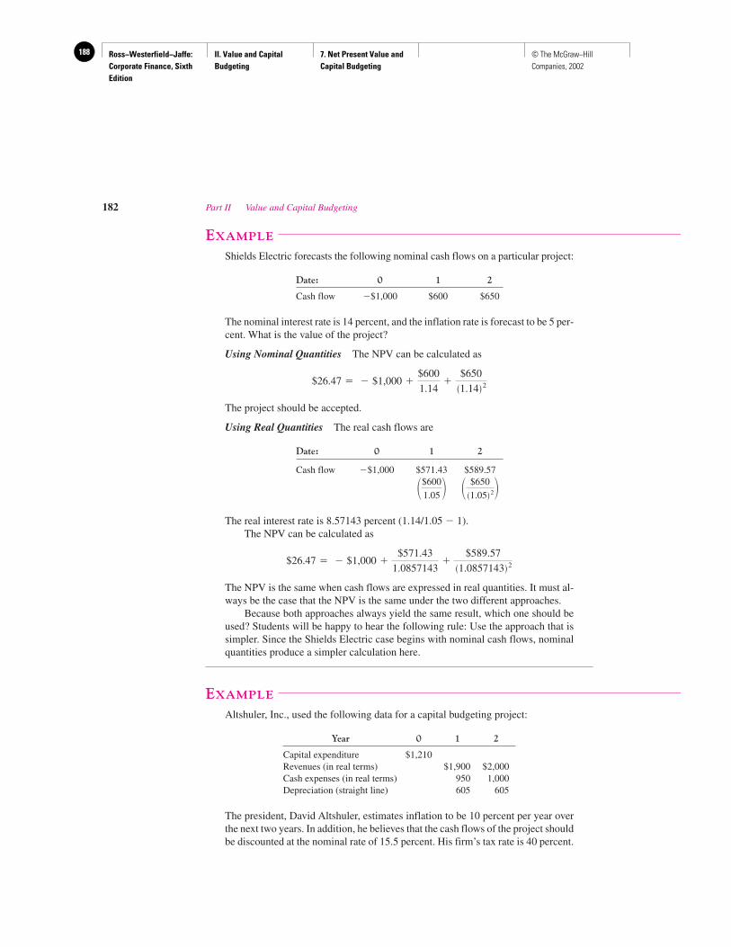
Ross−Westerfield−Jaffe: Corporate Finance, Sixth Edition
II. Value and Capital Budgeting
7. Net Present Value and Capital Budgeting
188 © The McGraw−Hill Companies, 2002
EXAMPLE
Shields Electric forecasts the following nominal cash flows on a particular project:
Date: 0 1 2
Cash flow �$1,000 $600 $650
The nominal interest rate is 14 percent, and the inflation rate is forecast to be 5 per-cent. What is the value of the project?
Using Nominal Quantities The NPV can be calculated as
The project should be accepted.
Using Real Quantities The real cash flows are
Date: 0 1 2
Cash flow �$1,000 $571.43 $589.57
The real interest rate is 8.57143 percent (1.14/1.05 � 1).The NPV can be calculated as
The NPV is the same when cash flows are expressed in real quantities. It must al-ways be the case that the NPV is the same under the two different approaches.
Because both approaches always yield the same result, which one should beused? Students will be happy to hear the following rule: Use the approach that issimpler. Since the Shields Electric case begins with nominal cash flows, nominalquantities produce a simpler calculation here.
EXAMPLE
Altshuler, Inc., used the following data for a capital budgeting project:
Year 0 1 2
Capital expenditure $1,210Revenues (in real terms) $1,900 $2,000Cash expenses (in real terms) 950 1,000Depreciation (straight line) 605 605
The president, David Altshuler, estimates inflation to be 10 percent per year overthe next two years. In addition, he believes that the cash flows of the project shouldbe discounted at the nominal rate of 15.5 percent. His firm’s tax rate is 40 percent.
$26.47 � � $1,000 �$571.43
1.0857143�
$589.57�1.0857143� 2
� $650�1.05� 2��$600
1.05 �
$26.47 � � $1,000 �$600
1.14�
$650�1.14� 2
182 Part II Value and Capital Budgeting
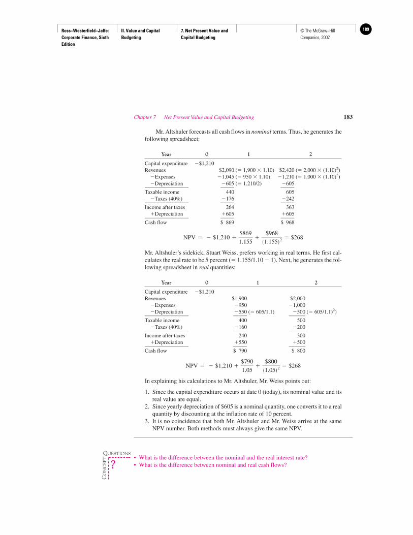
Ross−Westerfield−Jaffe: Corporate Finance, Sixth Edition
II. Value and Capital Budgeting
7. Net Present Value and Capital Budgeting
189© The McGraw−Hill Companies, 2002
Mr. Altshuler forecasts all cash flows in nominal terms. Thus, he generates thefollowing spreadsheet:
Year 0 1 2
Capital expenditure �$1,210Revenues $2,090 (� 1,900 � 1.10) $2,420 (� 2,000 � (1.10)2)
�Expenses �1,045 (� 950 � 1.10) �1,210 (� 1,000 � (1.10)2)�Depreciation �605 (� 1.210/2) �605________________ _____ _____
Taxable income 440 605�Taxes (40%) �176 �242________________ _____ _____
Income after taxes 264 363�Depreciation �605 �605________________ _____ _____
Cash flow $ 869 $ 968
Mr. Altshuler’s sidekick, Stuart Weiss, prefers working in real terms. He first cal-culates the real rate to be 5 percent (� 1.155/1.10 � 1). Next, he generates the fol-lowing spreadsheet in real quantities:
Year 0 1 2
Capital expenditure �$1,210Revenues $1,900 $2,000
�Expenses �950 �1,000�Depreciation �550 (� 605/1.1) �500 (� 605/1.1)2)________________ _____ ______
Taxable income 400 500�Taxes (40%) �160 �200________________ _____ ______
Income after taxes 240 300�Depreciation �550 �500________________ _____ ______
Cash flow $ 790 $ 800
In explaining his calculations to Mr. Altshuler, Mr. Weiss points out:
1. Since the capital expenditure occurs at date 0 (today), its nominal value and itsreal value are equal.
2. Since yearly depreciation of $605 is a nominal quantity, one converts it to a realquantity by discounting at the inflation rate of 10 percent.
3. It is no coincidence that both Mr. Altshuler and Mr. Weiss arrive at the sameNPV number. Both methods must always give the same NPV.
• What is the difference between the nominal and the real interest rate?• What is the difference between nominal and real cash flows?
NPV � � $1,210 �$790
1.05�
$800�1.05� 2 � $268
NPV � � $1,210 �$869
1.155�
$968�1.155� 2 � $268
Chapter 7 Net Present Value and Capital Budgeting 183
QUESTIONS
CO
NC
EP
T
?
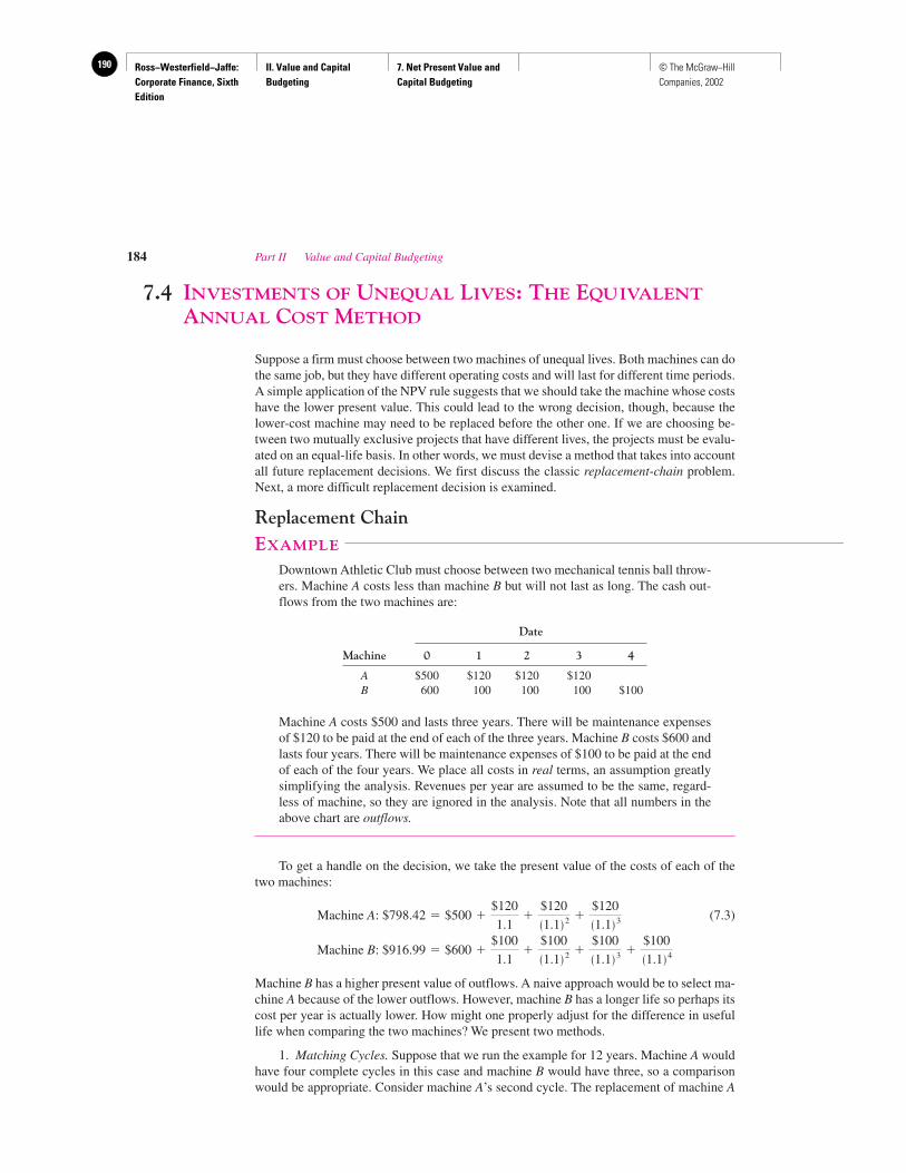
Ross−Westerfield−Jaffe: Corporate Finance, Sixth Edition
II. Value and Capital Budgeting
7. Net Present Value and Capital Budgeting
190 © The McGraw−Hill Companies, 2002
7.4 INVESTMENTS OF UNEQUAL LIVES: THE EQUIVALENT
ANNUAL COST METHOD
Suppose a firm must choose between two machines of unequal lives. Both machines can dothe same job, but they have different operating costs and will last for different time periods.A simple application of the NPV rule suggests that we should take the machine whose costshave the lower present value. This could lead to the wrong decision, though, because thelower-cost machine may need to be replaced before the other one. If we are choosing be-tween two mutually exclusive projects that have different lives, the projects must be evalu-ated on an equal-life basis. In other words, we must devise a method that takes into accountall future replacement decisions. We first discuss the classic replacement-chain problem.Next, a more difficult replacement decision is examined.
Replacement ChainEXAMPLE
Downtown Athletic Club must choose between two mechanical tennis ball throw-ers. Machine A costs less than machine B but will not last as long. The cash out-flows from the two machines are:
Date
Machine 0 1 2 3 4
A $500 $120 $120 $120B 600 100 100 100 $100
Machine A costs $500 and lasts three years. There will be maintenance expensesof $120 to be paid at the end of each of the three years. Machine B costs $600 andlasts four years. There will be maintenance expenses of $100 to be paid at the endof each of the four years. We place all costs in real terms, an assumption greatlysimplifying the analysis. Revenues per year are assumed to be the same, regard-less of machine, so they are ignored in the analysis. Note that all numbers in theabove chart are outflows.
To get a handle on the decision, we take the present value of the costs of each of thetwo machines:
Machine A: $798.42 (7.3)
Machine B: $916.99
Machine B has a higher present value of outflows. A naive approach would be to select ma-chine A because of the lower outflows. However, machine B has a longer life so perhaps itscost per year is actually lower. How might one properly adjust for the difference in usefullife when comparing the two machines? We present two methods.
1. Matching Cycles. Suppose that we run the example for 12 years. Machine A wouldhave four complete cycles in this case and machine B would have three, so a comparisonwould be appropriate. Consider machine A’s second cycle. The replacement of machine A
� $600 �$100
1.1�
$100�1.1� 2 �
$100�1.1� 3 �
$100�1.1� 4
� $500 �$120
1.1�
$120�1.1� 2 �
$120�1.1� 3
184 Part II Value and Capital Budgeting
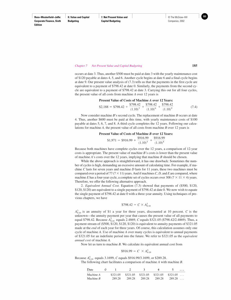
Ross−Westerfield−Jaffe: Corporate Finance, Sixth Edition
II. Value and Capital Budgeting
7. Net Present Value and Capital Budgeting
191© The McGraw−Hill Companies, 2002
occurs at date 3. Thus, another $500 must be paid at date 3 with the yearly maintenance costof $120 payable at dates 4, 5, and 6. Another cycle begins at date 6 and a final cycle beginsat date 9. Our present value analysis of (7.3) tells us that the payments in the first cycle areequivalent to a payment of $798.42 at date 0. Similarly, the payments from the second cy-cle are equivalent to a payment of $798.42 at date 3. Carrying this out for all four cycles,the present value of all costs from machine A over 12 years is
Present Value of Costs of Machine A over 12 Years:
(7.4)
Now consider machine B’s second cycle. The replacement of machine B occurs at date4. Thus, another $600 must be paid at this time, with yearly maintenance costs of $100payable at dates 5, 6, 7, and 8. A third cycle completes the 12 years. Following our calcu-lations for machine A, the present value of all costs from machine B over 12 years is
Present Value of Costs of Machine B over 12 Years:
Because both machines have complete cycles over the 12 years, a comparison of 12-yearcosts is appropriate. The present value of machine B’s costs is lower than the present valueof machine A’s costs over the 12 years, implying that machine B should be chosen.
While the above approach is straightforward, it has one drawback: Sometimes the num-ber of cycles is high, demanding an excessive amount of calculating time. For example, if ma-chine C lasts for seven years and machine D lasts for 11 years, these two machines must becompared over a period of 77 (7 � 11) years. And if machines C, D, and E are compared, wheremachine E has a four-year cycle, a complete set of cycles occurs over 308 (7 � 11 � 4) years.Therefore, we offer the following alternative approach.
2. Equivalent Annual Cost. Equation (7.3) showed that payments of ($500, $120,$120, $120) are equivalent to a single payment of $798.42 at date 0. We now wish to equatethe single payment of $798.42 at date 0 with a three-year annuity. Using techniques of pre-vious chapters, we have
is an annuity of $1 a year for three years, discounted at 10 percent. C is the unknown—the annuity payment per year that causes the present value of all payments toequal $798.42. Because equals 2.4869, C equals $321.05 ($798.42/2.4869). Thus, apayment stream of ($500, $120, $120, $120) is equivalent to annuity payments of $321.05made at the end of each year for three years. Of course, this calculation assumes only onecycle of machine A. Use of machine A over many cycles is equivalent to annual paymentsof $321.05 for an indefinite period into the future. We refer to $321.05 as the equivalentannual cost of machine A.
Now let us turn to machine B. We calculate its equivalent annual cost from
Because equals 3.1699, C equals $916.99/3.1699, or $289.28.The following chart facilitates a comparison of machine A with machine B.
Date 0 1 2 3 4 5 . . .
Machine A $321.05 $321.05 $321.05 $321.05 $321.05 . . .Machine B 289.28 289.28 289.28 289.28 289.28 . . .
A
40.10
$916.99 � C � A
40.10
A
30.10
A
30.10
$798.42 � C � A
30.10
$1,971 � $916.99 �$916.99�1.10� 4 �
$916.99�1.10� 8
$2,188 � $798.42 �$798.42�1.10� 3 �
$798.42�1.10� 6 �
$798.42�1.10� 9
Chapter 7 Net Present Value and Capital Budgeting 185
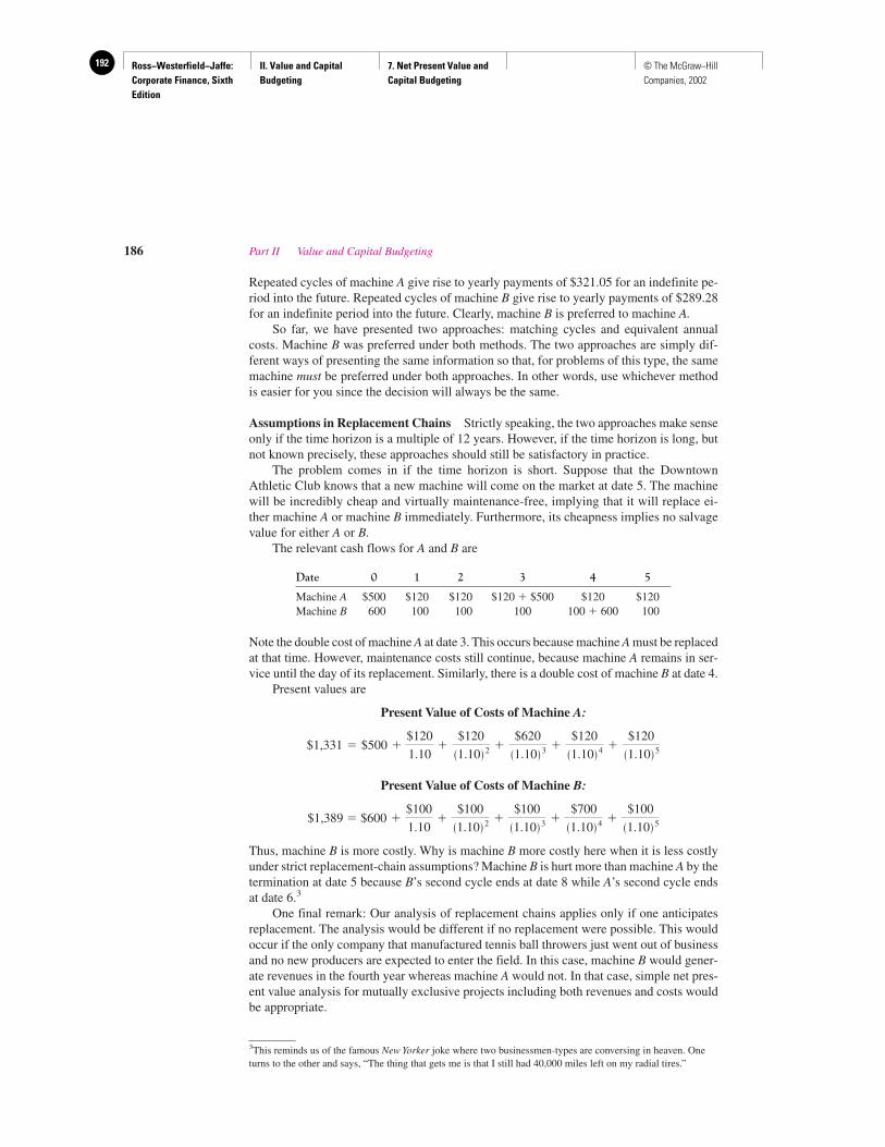
Ross−Westerfield−Jaffe: Corporate Finance, Sixth Edition
II. Value and Capital Budgeting
7. Net Present Value and Capital Budgeting
192 © The McGraw−Hill Companies, 2002
Repeated cycles of machine A give rise to yearly payments of $321.05 for an indefinite pe-riod into the future. Repeated cycles of machine B give rise to yearly payments of $289.28for an indefinite period into the future. Clearly, machine B is preferred to machine A.
So far, we have presented two approaches: matching cycles and equivalent annualcosts. Machine B was preferred under both methods. The two approaches are simply dif-ferent ways of presenting the same information so that, for problems of this type, the samemachine must be preferred under both approaches. In other words, use whichever methodis easier for you since the decision will always be the same.
Assumptions in Replacement Chains Strictly speaking, the two approaches make senseonly if the time horizon is a multiple of 12 years. However, if the time horizon is long, butnot known precisely, these approaches should still be satisfactory in practice.
The problem comes in if the time horizon is short. Suppose that the DowntownAthletic Club knows that a new machine will come on the market at date 5. The machinewill be incredibly cheap and virtually maintenance-free, implying that it will replace ei-ther machine A or machine B immediately. Furthermore, its cheapness implies no salvagevalue for either A or B.
The relevant cash flows for A and B are
Date 0 1 2 3 4 5
Machine A $500 $120 $120 $120 � $500 $120 $120Machine B 600 100 100 100 100 � 600 100
Note the double cost of machine A at date 3. This occurs because machine A must be replacedat that time. However, maintenance costs still continue, because machine A remains in ser-vice until the day of its replacement. Similarly, there is a double cost of machine B at date 4.
Present values are
Present Value of Costs of Machine A:
Present Value of Costs of Machine B:
Thus, machine B is more costly. Why is machine B more costly here when it is less costlyunder strict replacement-chain assumptions? Machine B is hurt more than machine A by thetermination at date 5 because B’s second cycle ends at date 8 while A’s second cycle endsat date 6.3
One final remark: Our analysis of replacement chains applies only if one anticipatesreplacement. The analysis would be different if no replacement were possible. This wouldoccur if the only company that manufactured tennis ball throwers just went out of businessand no new producers are expected to enter the field. In this case, machine B would gener-ate revenues in the fourth year whereas machine A would not. In that case, simple net pres-ent value analysis for mutually exclusive projects including both revenues and costs wouldbe appropriate.
$1,389 � $600 �$100
1.10�
$100�1.10� 2 �
$100�1.10� 3 �
$700�1.10� 4 �
$100�1.10� 5
$1,331 � $500 �$120
1.10�
$120�1.10� 2 �
$620�1.10� 3 �
$120�1.10� 4 �
$120�1.10� 5
186 Part II Value and Capital Budgeting
3This reminds us of the famous New Yorker joke where two businessmen-types are conversing in heaven. Oneturns to the other and says, “The thing that gets me is that I still had 40,000 miles left on my radial tires.”
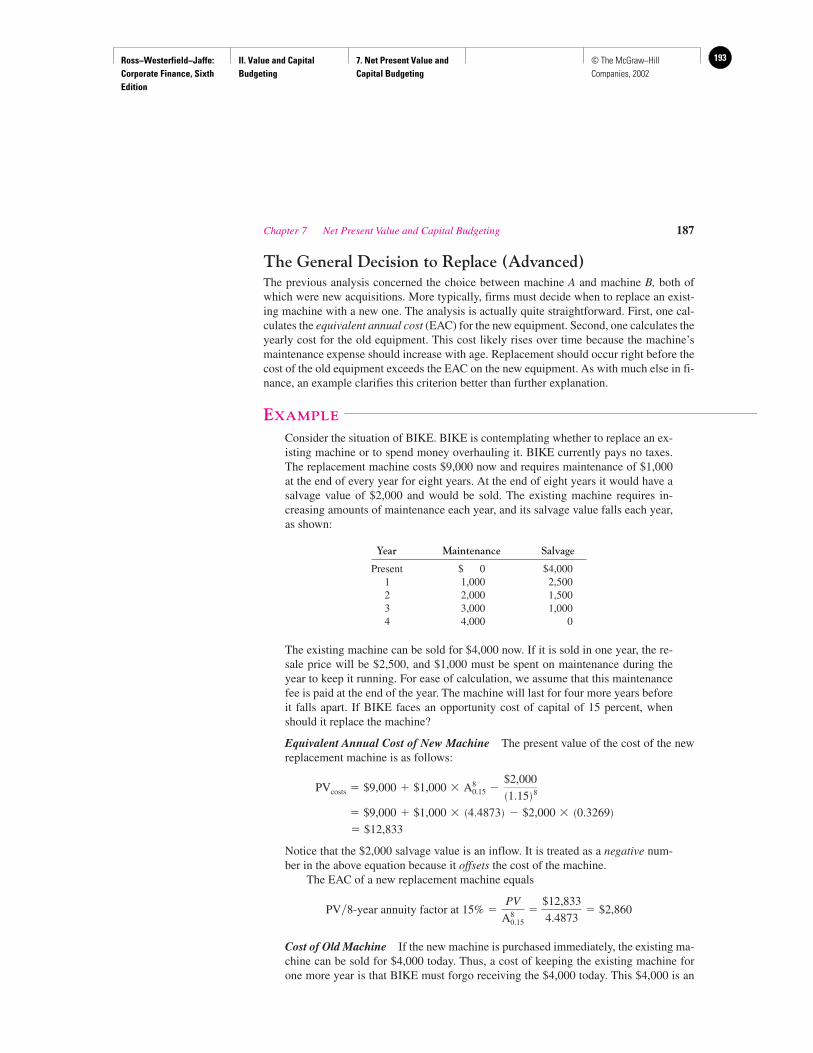
Ross−Westerfield−Jaffe: Corporate Finance, Sixth Edition
II. Value and Capital Budgeting
7. Net Present Value and Capital Budgeting
193© The McGraw−Hill Companies, 2002
The General Decision to Replace (Advanced)The previous analysis concerned the choice between machine A and machine B, both ofwhich were new acquisitions. More typically, firms must decide when to replace an exist-ing machine with a new one. The analysis is actually quite straightforward. First, one cal-culates the equivalent annual cost (EAC) for the new equipment. Second, one calculates theyearly cost for the old equipment. This cost likely rises over time because the machine’smaintenance expense should increase with age. Replacement should occur right before thecost of the old equipment exceeds the EAC on the new equipment. As with much else in fi-nance, an example clarifies this criterion better than further explanation.
EXAMPLE
Consider the situation of BIKE. BIKE is contemplating whether to replace an ex-isting machine or to spend money overhauling it. BIKE currently pays no taxes.The replacement machine costs $9,000 now and requires maintenance of $1,000at the end of every year for eight years. At the end of eight years it would have asalvage value of $2,000 and would be sold. The existing machine requires in-creasing amounts of maintenance each year, and its salvage value falls each year,as shown:
Year Maintenance Salvage
Present $ 0 $4,0001 1,000 2,5002 2,000 1,5003 3,000 1,0004 4,000 0
The existing machine can be sold for $4,000 now. If it is sold in one year, the re-sale price will be $2,500, and $1,000 must be spent on maintenance during theyear to keep it running. For ease of calculation, we assume that this maintenancefee is paid at the end of the year. The machine will last for four more years beforeit falls apart. If BIKE faces an opportunity cost of capital of 15 percent, whenshould it replace the machine?
Equivalent Annual Cost of New Machine The present value of the cost of the newreplacement machine is as follows:
Notice that the $2,000 salvage value is an inflow. It is treated as a negative num-ber in the above equation because it offsets the cost of the machine.
The EAC of a new replacement machine equals
Cost of Old Machine If the new machine is purchased immediately, the existing ma-chine can be sold for $4,000 today. Thus, a cost of keeping the existing machine forone more year is that BIKE must forgo receiving the $4,000 today. This $4,000 is an
PV�8-year annuity factor at 15% �PV
A
80.15
�$12,833
4.4873� $2,860
� $12,833
� $9,000 � $1,000 � �4.4873� � $2,000 � �0.3269�
PVcosts � $9,000 � $1,000 � A
80.15 �
$2,000�1.15� 8
Chapter 7 Net Present Value and Capital Budgeting 187
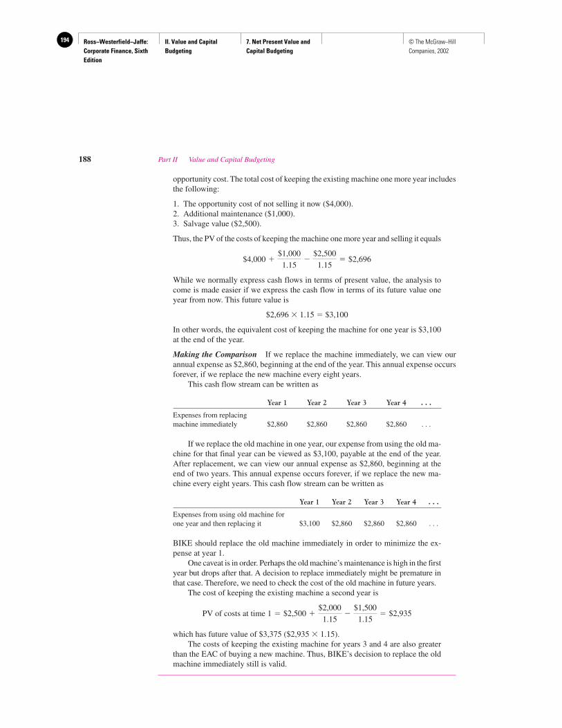
Ross−Westerfield−Jaffe: Corporate Finance, Sixth Edition
II. Value and Capital Budgeting
7. Net Present Value and Capital Budgeting
194 © The McGraw−Hill Companies, 2002
opportunity cost. The total cost of keeping the existing machine one more year includesthe following:
1. The opportunity cost of not selling it now ($4,000).2. Additional maintenance ($1,000).3. Salvage value ($2,500).
Thus, the PV of the costs of keeping the machine one more year and selling it equals
While we normally express cash flows in terms of present value, the analysis tocome is made easier if we express the cash flow in terms of its future value oneyear from now. This future value is
$2,696 � 1.15 � $3,100
In other words, the equivalent cost of keeping the machine for one year is $3,100at the end of the year.
Making the Comparison If we replace the machine immediately, we can view ourannual expense as $2,860, beginning at the end of the year. This annual expense occursforever, if we replace the new machine every eight years.
This cash flow stream can be written as
Year 1 Year 2 Year 3 Year 4 . . .
Expenses from replacing machine immediately $2,860 $2,860 $2,860 $2,860 . . .
If we replace the old machine in one year, our expense from using the old ma-chine for that final year can be viewed as $3,100, payable at the end of the year.After replacement, we can view our annual expense as $2,860, beginning at theend of two years. This annual expense occurs forever, if we replace the new ma-chine every eight years. This cash flow stream can be written as
Year 1 Year 2 Year 3 Year 4 . . .
Expenses from using old machine for one year and then replacing it $3,100 $2,860 $2,860 $2,860 . . .
BIKE should replace the old machine immediately in order to minimize the ex-pense at year 1.
One caveat is in order. Perhaps the old machine’s maintenance is high in the firstyear but drops after that. A decision to replace immediately might be premature inthat case. Therefore, we need to check the cost of the old machine in future years.
The cost of keeping the existing machine a second year is
which has future value of $3,375 ($2,935 � 1.15).The costs of keeping the existing machine for years 3 and 4 are also greater
than the EAC of buying a new machine. Thus, BIKE’s decision to replace the oldmachine immediately still is valid.
PV of costs at time 1 � $2,500 �$2,000
1.15�
$1,500
1.15� $2,935
$4,000 �$1,000
1.15�
$2,500
1.15� $2,696
188 Part II Value and Capital Budgeting

Ross−Westerfield−Jaffe: Corporate Finance, Sixth Edition
II. Value and Capital Budgeting
7. Net Present Value and Capital Budgeting
195© The McGraw−Hill Companies, 2002
• What is the equivalent annual cost method of capital budgeting?• Can you list the assumptions that we must make to use EAC?
7.5 SUMMARY AND CONCLUSIONS
This chapter discusses a number of practical applications of capital budgeting.
1. Capital budgeting must be placed on an incremental basis. This means that sunk costs mustbe ignored, while both opportunity costs and side effects must be considered.
2. In the Baldwin case, we computed NPV using the following two steps:a. Calculate the net cash flow from all sources for each period.b. Calculate the NPV using the cash flows calculated above.
3. Inflation must be handled consistently. One approach is to express both cash flows and thediscount rate in nominal terms. The other approach is to express both cash flow and thediscount rate in real terms. Because either approach yields the same NPV calculation, thesimpler method should be used. The simpler method will generally depend on the type ofcapital budgeting problem.
4. When a firm must choose between two machines of unequal lives, the firm can apply eitherthe matching cycle approach or the equivalent annual cost approach. Since both approachesare different ways of presenting the same information, the same machine must be preferredunder both approaches.
KEY TERMS
Erosion 171 Opportunity cost 170Net working capital 172 Real cash flow 181Nominal cash flow 181 Real interest rate 179Nominal interest rate 179 Sunk cost 170
SUGGESTED READING
An excellent in-depth examination of the capital budgeting decision is contained in:Copeland, T., T. Koller, and J. Murrin. Valuation: Measuring and Managing the Value of
Companies, 2nd ed. The McKinsey Company, 1994.
QUESTIONS AND PROBLEMS
NPV and Capital Budgeting7.1 Which of the following cash flows should be treated as incremental cash flows when
computing the NPV of an investment?a. The reduction in the sales of the company’s other products.b. The expenditure on plant and equipment.
Chapter 7 Net Present Value and Capital Budgeting 189
QUESTIONS
CO
NC
EP
T
?
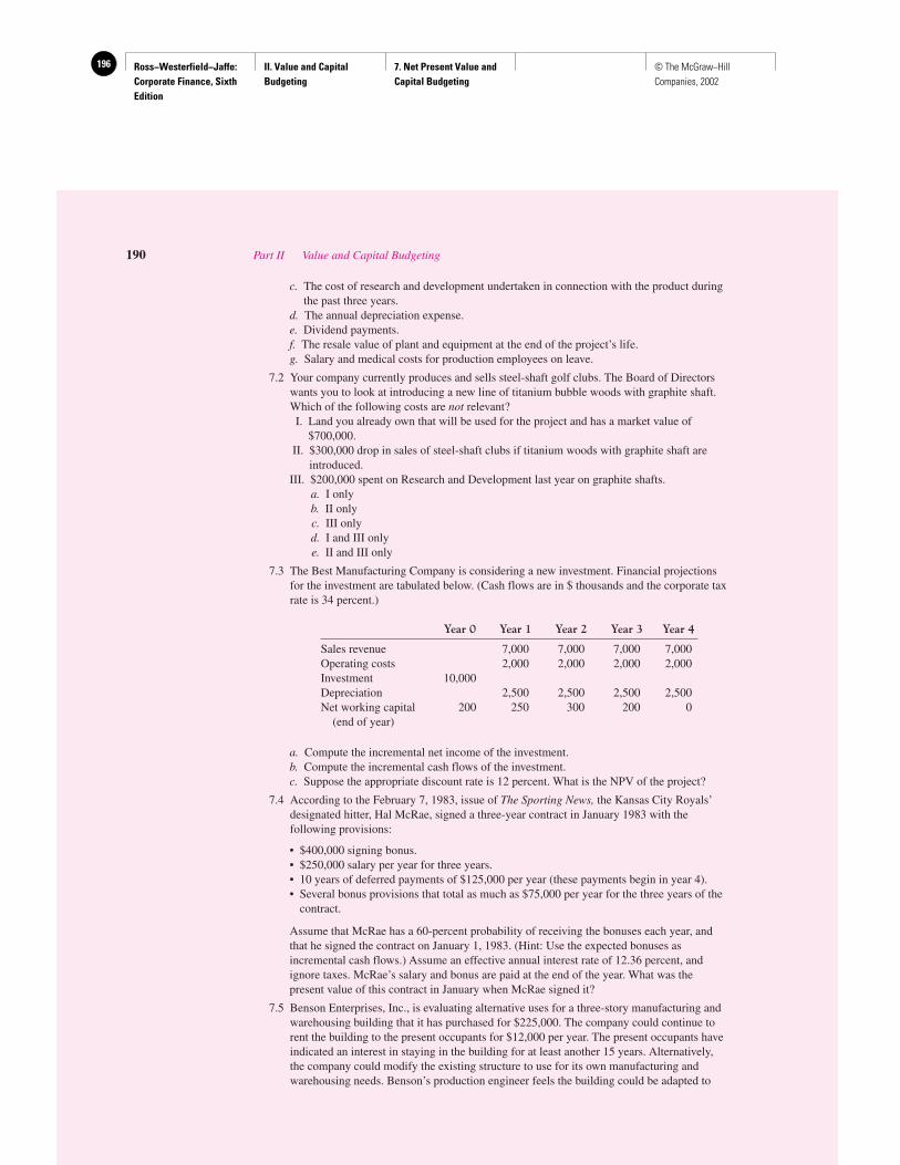
Ross−Westerfield−Jaffe: Corporate Finance, Sixth Edition
II. Value and Capital Budgeting
7. Net Present Value and Capital Budgeting
196 © The McGraw−Hill Companies, 2002
c. The cost of research and development undertaken in connection with the product duringthe past three years.
d. The annual depreciation expense.e. Dividend payments.f. The resale value of plant and equipment at the end of the project’s life.g. Salary and medical costs for production employees on leave.
7.2 Your company currently produces and sells steel-shaft golf clubs. The Board of Directorswants you to look at introducing a new line of titanium bubble woods with graphite shaft.Which of the following costs are not relevant?I. Land you already own that will be used for the project and has a market value of
$700,000.II. $300,000 drop in sales of steel-shaft clubs if titanium woods with graphite shaft are
introduced.III. $200,000 spent on Research and Development last year on graphite shafts.
a. I onlyb. II onlyc. III onlyd. I and III onlye. II and III only
7.3 The Best Manufacturing Company is considering a new investment. Financial projectionsfor the investment are tabulated below. (Cash flows are in $ thousands and the corporate taxrate is 34 percent.)
Year 0 Year 1 Year 2 Year 3 Year 4
Sales revenue 7,000 7,000 7,000 7,000Operating costs 2,000 2,000 2,000 2,000Investment 10,000Depreciation 2,500 2,500 2,500 2,500Net working capital 200 250 300 200 0
(end of year)
a. Compute the incremental net income of the investment.b. Compute the incremental cash flows of the investment.c. Suppose the appropriate discount rate is 12 percent. What is the NPV of the project?
7.4 According to the February 7, 1983, issue of The Sporting News, the Kansas City Royals’designated hitter, Hal McRae, signed a three-year contract in January 1983 with thefollowing provisions:
• $400,000 signing bonus.• $250,000 salary per year for three years.• 10 years of deferred payments of $125,000 per year (these payments begin in year 4).• Several bonus provisions that total as much as $75,000 per year for the three years of the
contract.
Assume that McRae has a 60-percent probability of receiving the bonuses each year, andthat he signed the contract on January 1, 1983. (Hint: Use the expected bonuses asincremental cash flows.) Assume an effective annual interest rate of 12.36 percent, andignore taxes. McRae’s salary and bonus are paid at the end of the year. What was thepresent value of this contract in January when McRae signed it?
7.5 Benson Enterprises, Inc., is evaluating alternative uses for a three-story manufacturing andwarehousing building that it has purchased for $225,000. The company could continue torent the building to the present occupants for $12,000 per year. The present occupants haveindicated an interest in staying in the building for at least another 15 years. Alternatively,the company could modify the existing structure to use for its own manufacturing andwarehousing needs. Benson’s production engineer feels the building could be adapted to
190 Part II Value and Capital Budgeting
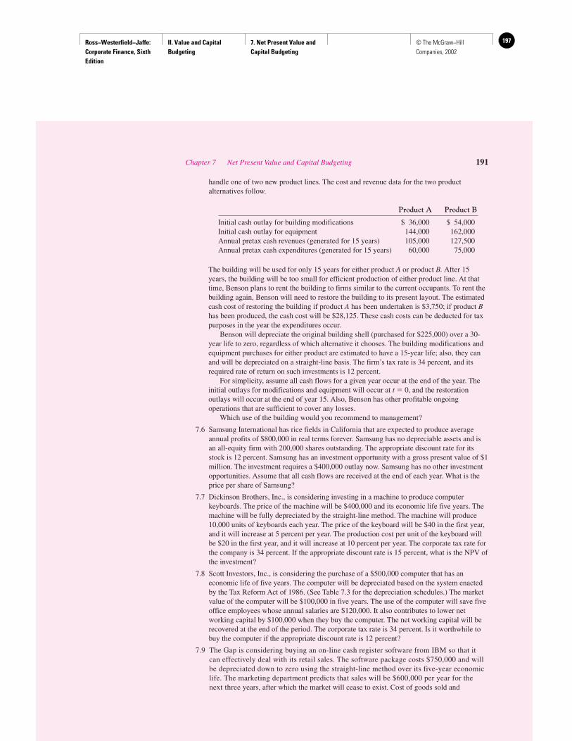
Ross−Westerfield−Jaffe: Corporate Finance, Sixth Edition
II. Value and Capital Budgeting
7. Net Present Value and Capital Budgeting
197© The McGraw−Hill Companies, 2002
handle one of two new product lines. The cost and revenue data for the two productalternatives follow.
Product A Product B
Initial cash outlay for building modifications $ 36,000 $ 54,000Initial cash outlay for equipment 144,000 162,000Annual pretax cash revenues (generated for 15 years) 105,000 127,500Annual pretax cash expenditures (generated for 15 years) 60,000 75,000
The building will be used for only 15 years for either product A or product B. After 15years, the building will be too small for efficient production of either product line. At thattime, Benson plans to rent the building to firms similar to the current occupants. To rent thebuilding again, Benson will need to restore the building to its present layout. The estimatedcash cost of restoring the building if product A has been undertaken is $3,750; if product Bhas been produced, the cash cost will be $28,125. These cash costs can be deducted for taxpurposes in the year the expenditures occur.
Benson will depreciate the original building shell (purchased for $225,000) over a 30-year life to zero, regardless of which alternative it chooses. The building modifications andequipment purchases for either product are estimated to have a 15-year life; also, they canand will be depreciated on a straight-line basis. The firm’s tax rate is 34 percent, and itsrequired rate of return on such investments is 12 percent.
For simplicity, assume all cash flows for a given year occur at the end of the year. Theinitial outlays for modifications and equipment will occur at t � 0, and the restorationoutlays will occur at the end of year 15. Also, Benson has other profitable ongoingoperations that are sufficient to cover any losses.
Which use of the building would you recommend to management?
7.6 Samsung International has rice fields in California that are expected to produce averageannual profits of $800,000 in real terms forever. Samsung has no depreciable assets and isan all-equity firm with 200,000 shares outstanding. The appropriate discount rate for itsstock is 12 percent. Samsung has an investment opportunity with a gross present value of $1million. The investment requires a $400,000 outlay now. Samsung has no other investmentopportunities. Assume that all cash flows are received at the end of each year. What is theprice per share of Samsung?
7.7 Dickinson Brothers, Inc., is considering investing in a machine to produce computerkeyboards. The price of the machine will be $400,000 and its economic life five years. Themachine will be fully depreciated by the straight-line method. The machine will produce10,000 units of keyboards each year. The price of the keyboard will be $40 in the first year,and it will increase at 5 percent per year. The production cost per unit of the keyboard willbe $20 in the first year, and it will increase at 10 percent per year. The corporate tax rate forthe company is 34 percent. If the appropriate discount rate is 15 percent, what is the NPV ofthe investment?
7.8 Scott Investors, Inc., is considering the purchase of a $500,000 computer that has aneconomic life of five years. The computer will be depreciated based on the system enactedby the Tax Reform Act of 1986. (See Table 7.3 for the depreciation schedules.) The marketvalue of the computer will be $100,000 in five years. The use of the computer will save fiveoffice employees whose annual salaries are $120,000. It also contributes to lower networking capital by $100,000 when they buy the computer. The net working capital will berecovered at the end of the period. The corporate tax rate is 34 percent. Is it worthwhile tobuy the computer if the appropriate discount rate is 12 percent?
7.9 The Gap is considering buying an on-line cash register software from IBM so that itcan effectively deal with its retail sales. The software package costs $750,000 and willbe depreciated down to zero using the straight-line method over its five-year economiclife. The marketing department predicts that sales will be $600,000 per year for thenext three years, after which the market will cease to exist. Cost of goods sold and
Chapter 7 Net Present Value and Capital Budgeting 191
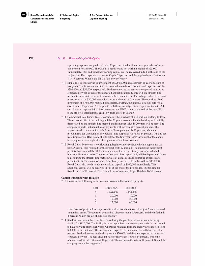
Ross−Westerfield−Jaffe: Corporate Finance, Sixth Edition
II. Value and Capital Budgeting
7. Net Present Value and Capital Budgeting
198 © The McGraw−Hill Companies, 2002
operating expenses are predicted to be 25 percent of sales. After three years the softwarecan be sold for $40,000. The Gap also needs to add net working capital of $25,000immediately. This additional net working capital will be recovered in full at the end of theproject life. The corporate tax rate for Gap is 35 percent and the required rate of return onit is 17 percent. What is the NPV of the new software?
7.10 Etonic Inc. is considering an investment of $250,000 in an asset with an economic life offive years. The firm estimates that the nominal annual cash revenues and expenses will be$200,000 and $50,000, respectively. Both revenues and expenses are expected to grow at 3 percent per year as that of the expected annual inflation. Etonic will use straight-linemethod to depreciate its asset to zero over the economic life. The salvage value of the assetis estimated to be $30,000 in nominal terms at the end of five years. The one-time NWCinvestment of $10,000 is required immediately. Further, the nominal discount rate for allcash flows is 15 percent. All corporate cash flows are subject to a 35 percent tax rate. Allcash flows, except the initial investment and the NWC, occur at the end of the year. Whatis the project’s total nominal cash flow from assets in year 5?
7.11 Commercial Real Estate, Inc., is considering the purchase of a $4 million building to lease.The economic life of the building will be 20 years. Assume that the building will be fullydepreciated by the straight-line method and its market value in 20 years will be zero. Thecompany expects that annual lease payments will increase at 3 percent per year. Theappropriate discount rate for cash flows of lease payments is 13 percent, while thediscount rate for depreciation is 9 percent. The corporate tax rate is 34 percent. What is theleast Commercial Real Estate should ask for the first-year lease? Assume that the annuallease payment starts right after the signature of the lease contract.
7.12 Royal Dutch Petroleum is considering going into a new project, which is typical for thefirm. A capital tool required for the project costs $2 million. The marketing departmentpredicts that sales will be $1.2 million per year for the next four years, after which themarket will cease to exist. The tool, a five-year class capital tool, will be depreciated downto zero using the straight-line method. Cost of goods sold and operating expenses arepredicted to be 25 percent of sales. After four years the tool can be sold for $150,000.Royal Dutch also needs to add net working capital of $100,000 immediately. Thisadditional capital will be received in full at the end of the project life. The tax rate forRoyal Dutch is 35 percent. The required rate of return on Royal Dutch is 16.55 percent.
Capital Budgeting with Inflation7.13 Consider the following cash flows on two mutually exclusive projects.
Year Project A Project B
0 �$40,000 �$50,0001 20,000 10,0002 15,000 20,0003 15,000 40,000
Cash flows of project A are expressed in real terms while those of project B are expressedin nominal terms. The appropriate nominal discount rate is 15 percent, and the inflation is4 percent. Which project should you choose?
7.14 Sanders Enterprises, Inc., has been considering the purchase of a new manufacturingfacility for $120,000. The facility is to be depreciated on a seven-year basis. It is expectedto have no value after seven years. Operating revenues from the facility are expected to be$50,000 in the first year. The revenues are expected to increase at the inflation rate of 5percent. Production costs in the first year are $20,000, and they are expected to increase at7 percent per year. The real discount rate for risky cash flows is 14 percent, while thenominal riskless interest rate is 10 percent. The corporate tax rate is 34 percent. Should thecompany accept the suggestion?
192 Part II Value and Capital Budgeting
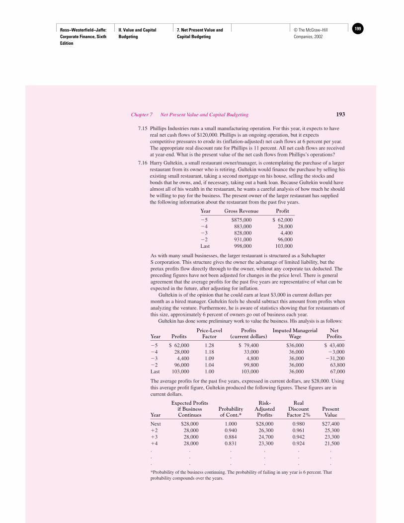
Ross−Westerfield−Jaffe: Corporate Finance, Sixth Edition
II. Value and Capital Budgeting
7. Net Present Value and Capital Budgeting
199© The McGraw−Hill Companies, 2002
7.15 Phillips Industries runs a small manufacturing operation. For this year, it expects to havereal net cash flows of $120,000. Phillips is an ongoing operation, but it expectscompetitive pressures to erode its (inflation-adjusted) net cash flows at 6 percent per year.The appropriate real discount rate for Phillips is 11 percent. All net cash flows are receivedat year-end. What is the present value of the net cash flows from Phillips’s operations?
7.16 Harry Gultekin, a small restaurant owner/manager, is contemplating the purchase of a largerrestaurant from its owner who is retiring. Gultekin would finance the purchase by selling hisexisting small restaurant, taking a second mortgage on his house, selling the stocks andbonds that he owns, and, if necessary, taking out a bank loan. Because Gultekin would havealmost all of his wealth in the restaurant, he wants a careful analysis of how much he shouldbe willing to pay for the business. The present owner of the larger restaurant has suppliedthe following information about the restaurant from the past five years.
Year Gross Revenue Profit
�5 $875,000 $ 62,000�4 883,000 28,000�3 828,000 4,400�2 931,000 96,000Last 998,000 103,000
As with many small businesses, the larger restaurant is structured as a Subchapter S corporation. This structure gives the owner the advantage of limited liability, but thepretax profits flow directly through to the owner, without any corporate tax deducted. Thepreceding figures have not been adjusted for changes in the price level. There is generalagreement that the average profits for the past five years are representative of what can beexpected in the future, after adjusting for inflation.
Gultekin is of the opinion that he could earn at least $3,000 in current dollars permonth as a hired manager. Gultekin feels he should subtract this amount from profits whenanalyzing the venture. Furthermore, he is aware of statistics showing that for restaurants ofthis size, approximately 6 percent of owners go out of business each year.
Gultekin has done some preliminary work to value the business. His analysis is as follows:
Price-Level Profits Imputed Managerial NetYear Profits Factor (current dollars) Wage Profits
�5 $ 62,000 1.28 $ 79,400 $36,000 $ 43,400�4 28,000 1.18 33,000 36,000 �3,000�3 4,400 1.09 4,800 36,000 �31,200�2 96,000 1.04 99,800 36,000 63,800Last 103,000 1.00 103,000 36,000 67,000
The average profits for the past five years, expressed in current dollars, are $28,000. Usingthis average profit figure, Gultekin produced the following figures. These figures are incurrent dollars.
Expected Profits Risk- Realif Business Probability Adjusted Discount Present
Year Continues of Cont.* Profits Factor 2% Value
Next $28,000 1.000 $28,000 0.980 $27,400�2 28,000 0.940 26,300 0.961 25,300�3 28,000 0.884 24,700 0.942 23,300�4 28,000 0.831 23,300 0.924 21,500. . . . . .. . . . . .. . . . . .
*Probability of the business continuing. The probability of failing in any year is 6 percent. Thatprobability compounds over the years.
Chapter 7 Net Present Value and Capital Budgeting 193
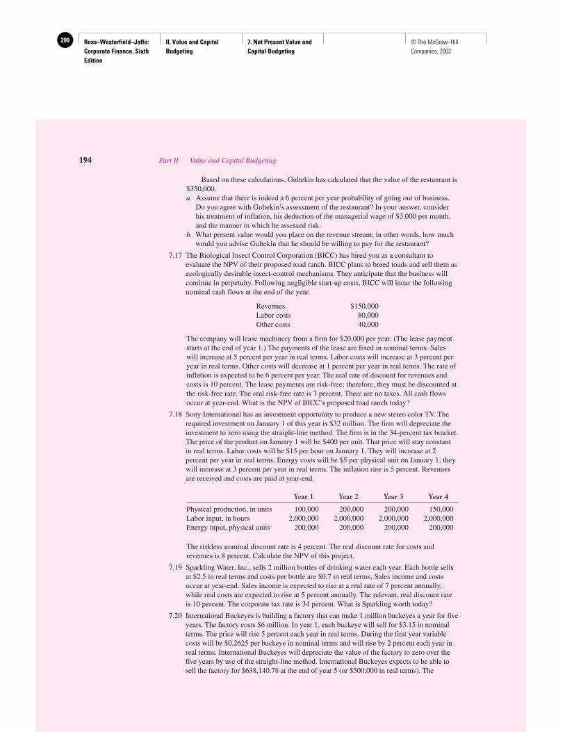
Ross−Westerfield−Jaffe: Corporate Finance, Sixth Edition
II. Value and Capital Budgeting
7. Net Present Value and Capital Budgeting
200 © The McGraw−Hill Companies, 2002
Based on these calculations, Gultekin has calculated that the value of the restaurant is$350,000.a. Assume that there is indeed a 6 percent per year probability of going out of business.
Do you agree with Gultekin’s assessment of the restaurant? In your answer, considerhis treatment of inflation, his deduction of the managerial wage of $3,000 per month,and the manner in which he assessed risk.
b. What present value would you place on the revenue stream; in other words, how muchwould you advise Gultekin that he should be willing to pay for the restaurant?
7.17 The Biological Insect Control Corporation (BICC) has hired you as a consultant toevaluate the NPV of their proposed toad ranch. BICC plans to breed toads and sell them asecologically desirable insect-control mechanisms. They anticipate that the business willcontinue in perpetuity. Following negligible start-up costs, BICC will incur the followingnominal cash flows at the end of the year.
Revenues $150,000Labor costs 80,000Other costs 40,000
The company will lease machinery from a firm for $20,000 per year. (The lease paymentstarts at the end of year 1.) The payments of the lease are fixed in nominal terms. Saleswill increase at 5 percent per year in real terms. Labor costs will increase at 3 percent peryear in real terms. Other costs will decrease at 1 percent per year in real terms. The rate ofinflation is expected to be 6 percent per year. The real rate of discount for revenues andcosts is 10 percent. The lease payments are risk-free; therefore, they must be discounted atthe risk-free rate. The real risk-free rate is 7 percent. There are no taxes. All cash flowsoccur at year-end. What is the NPV of BICC’s proposed toad ranch today?
7.18 Sony International has an investment opportunity to produce a new stereo color TV. Therequired investment on January 1 of this year is $32 million. The firm will depreciate theinvestment to zero using the straight-line method. The firm is in the 34-percent tax bracket.The price of the product on January 1 will be $400 per unit. That price will stay constantin real terms. Labor costs will be $15 per hour on January 1. They will increase at 2percent per year in real terms. Energy costs will be $5 per physical unit on January 1; theywill increase at 3 percent per year in real terms. The inflation rate is 5 percent. Revenuesare received and costs are paid at year-end.
Year 1 Year 2 Year 3 Year 4
Physical production, in units 100,000 200,000 200,000 150,000Labor input, in hours 2,000,000 2,000,000 2,000,000 2,000,000Energy input, physical units 200,000 200,000 200,000 200,000
The riskless nominal discount rate is 4 percent. The real discount rate for costs andrevenues is 8 percent. Calculate the NPV of this project.
7.19 Sparkling Water, Inc., sells 2 million bottles of drinking water each year. Each bottle sellsat $2.5 in real terms and costs per bottle are $0.7 in real terms. Sales income and costsoccur at year-end. Sales income is expected to rise at a real rate of 7 percent annually,while real costs are expected to rise at 5 percent annually. The relevant, real discount rateis 10 percent. The corporate tax rate is 34 percent. What is Sparkling worth today?
7.20 International Buckeyes is building a factory that can make 1 million buckeyes a year for fiveyears. The factory costs $6 million. In year 1, each buckeye will sell for $3.15 in nominalterms. The price will rise 5 percent each year in real terms. During the first year variablecosts will be $0.2625 per buckeye in nominal terms and will rise by 2 percent each year inreal terms. International Buckeyes will depreciate the value of the factory to zero over thefive years by use of the straight-line method. International Buckeyes expects to be able tosell the factory for $638,140.78 at the end of year 5 (or $500,000 in real terms). The
194 Part II Value and Capital Budgeting

Ross−Westerfield−Jaffe: Corporate Finance, Sixth Edition
II. Value and Capital Budgeting
7. Net Present Value and Capital Budgeting
201© The McGraw−Hill Companies, 2002
nominal discount rate for risky cash flows is 20 percent. The nominal discount rate forriskless cash flows is 11 percent. The rate of inflation is 5 percent. Cash flows, except theinitial investment, occur at the end of the year. The corporate tax rate is 34 percent; capitalgains are also taxed at 34 percent. What is the net present value of this project?
7.21 Majestic Mining Company (MMC) is negotiating for the purchase of a new piece ofequipment for their current operations. MMC wants to know the maximum price that itshould be willing to pay for the equipment. That is, how high must the price be for theequipment to have an NPV of zero? You are given the following facts:a. The new equipment would replace existing equipment that has a current market value
of $20,000.b. The new equipment would not affect revenues, but before-tax operating costs would be
reduced by $10,000 per year for eight years. These savings in cost would occur at year-end.c. The old equipment is now five years old. It is expected to last for another eight years, and
it is expected to have no resale value at the end of those eight years. It was purchased for$40,000 and is being depreciated to zero on a straight-line basis over 10 years.
d. The new equipment will be depreciated to zero using straight-line depreciation overfive years. MMC expects to be able to sell the equipment for $5,000 at the end of eightyears. The proceeds from this sale would be subject to taxes at the ordinary corporateincome tax rate of 34 percent.
e. MMC has profitable ongoing operations.f. The appropriate discount rate is 8 percent.
7.22 After extensive medical and marketing research, Pill, Inc., believes it can penetrate the painreliever market. It can follow one of two strategies. The first is to manufacture a medicationaimed at relieving headache pain. The second strategy is to make a pill designed to relieveheadache and arthritis pain. Both products would be introduced at a price of $4 per packagein real terms. The broader remedy would probably sell 10 million packages a year. This istwice the sales rate for the headache-only medication. Cash costs of production in the firstyear are expected to be $1.50 per package in real terms for the headache-only brand.Production costs are expected to be $1.70 in real terms for the more general pill. All pricesand costs are expected to rise at the general inflation rate of 5 percent.
Either strategy would require further investment in plant. The headache-only pill couldbe produced using equipment that would cost $10.2 million, last three years, and have noresale value. The machinery required to produce the broader remedy would cost $12million and last three years. At this time the firm would be able to sell it for $1 million (inreal terms). The production machinery would need to be replaced every three years, atconstant real costs.
Suppose that for both projects the firm will use straight-line depreciation. The firmfaces a corporate tax rate of 34 percent. The firm believes the appropriate real discountrate is 13 percent. Capital gains are taxed at the ordinary corporate tax rate of 34 percent.Which pain reliever should the firm produce?
7.23 A machine that lasts four years has the following net cash outflows. $12,000 is the cost ofpurchasing the machine, and $6,000 is the annual year-end operating cost. At the end offour years, the machine is sold for $2,000; thus, the cash flow at year 4, C4, is only $4,000.
C0 C1 C2 C3 C4
$12,000 $6,000 $6,000 $6,000 $4,000
The cost of capital is 6 percent. What is the present value of the costs of operating a seriesof such machines in perpetuity?
7.24 A machine costs $60,000 and requires $5,000 maintenance for each year of its three-yearlife. After three years, this machine will be replaced. Assume a tax rate of 34 percent and adiscount rate of 14 percent. If the machine is depreciated with a three-year straight-linewithout a salvage value, what is the equivalent annual cost (EAC)?
Chapter 7 Net Present Value and Capital Budgeting 195
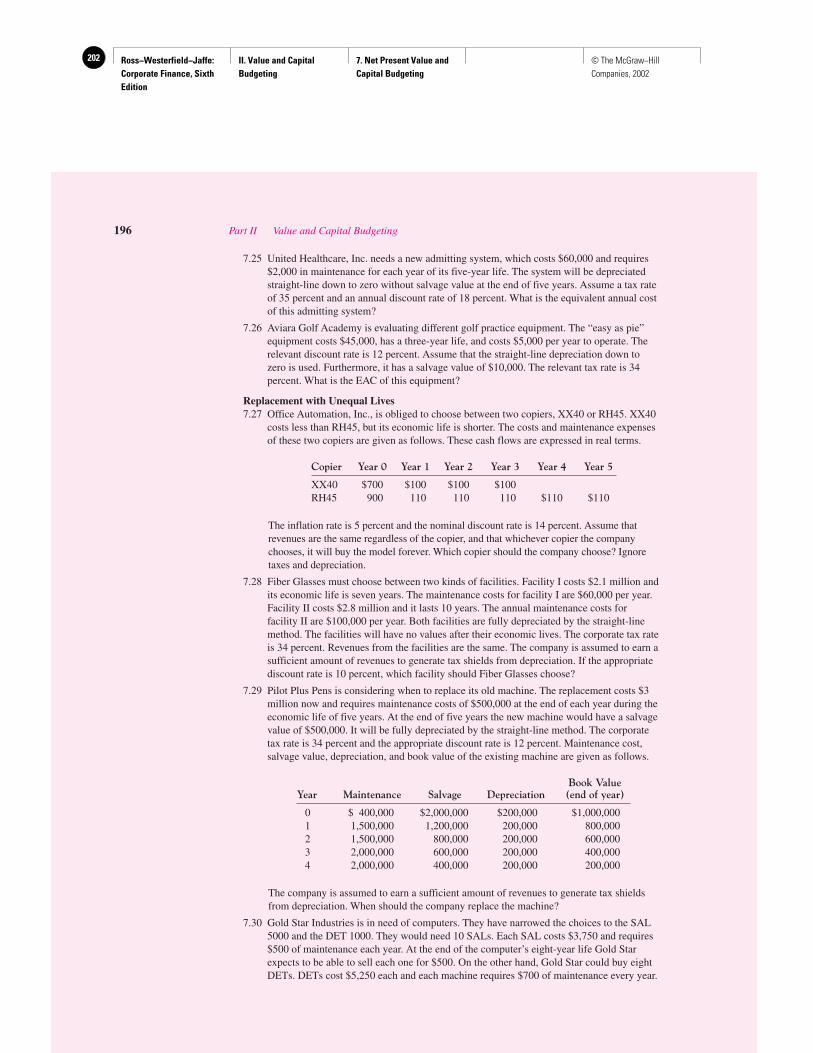
Ross−Westerfield−Jaffe: Corporate Finance, Sixth Edition
II. Value and Capital Budgeting
7. Net Present Value and Capital Budgeting
202 © The McGraw−Hill Companies, 2002
7.25 United Healthcare, Inc. needs a new admitting system, which costs $60,000 and requires$2,000 in maintenance for each year of its five-year life. The system will be depreciatedstraight-line down to zero without salvage value at the end of five years. Assume a tax rateof 35 percent and an annual discount rate of 18 percent. What is the equivalent annual costof this admitting system?
7.26 Aviara Golf Academy is evaluating different golf practice equipment. The “easy as pie”equipment costs $45,000, has a three-year life, and costs $5,000 per year to operate. Therelevant discount rate is 12 percent. Assume that the straight-line depreciation down tozero is used. Furthermore, it has a salvage value of $10,000. The relevant tax rate is 34percent. What is the EAC of this equipment?
Replacement with Unequal Lives7.27 Office Automation, Inc., is obliged to choose between two copiers, XX40 or RH45. XX40
costs less than RH45, but its economic life is shorter. The costs and maintenance expensesof these two copiers are given as follows. These cash flows are expressed in real terms.
Copier Year 0 Year 1 Year 2 Year 3 Year 4 Year 5
XX40 $700 $100 $100 $100RH45 900 110 110 110 $110 $110
The inflation rate is 5 percent and the nominal discount rate is 14 percent. Assume thatrevenues are the same regardless of the copier, and that whichever copier the companychooses, it will buy the model forever. Which copier should the company choose? Ignoretaxes and depreciation.
7.28 Fiber Glasses must choose between two kinds of facilities. Facility I costs $2.1 million andits economic life is seven years. The maintenance costs for facility I are $60,000 per year.Facility II costs $2.8 million and it lasts 10 years. The annual maintenance costs forfacility II are $100,000 per year. Both facilities are fully depreciated by the straight-linemethod. The facilities will have no values after their economic lives. The corporate tax rateis 34 percent. Revenues from the facilities are the same. The company is assumed to earn asufficient amount of revenues to generate tax shields from depreciation. If the appropriatediscount rate is 10 percent, which facility should Fiber Glasses choose?
7.29 Pilot Plus Pens is considering when to replace its old machine. The replacement costs $3million now and requires maintenance costs of $500,000 at the end of each year during theeconomic life of five years. At the end of five years the new machine would have a salvagevalue of $500,000. It will be fully depreciated by the straight-line method. The corporatetax rate is 34 percent and the appropriate discount rate is 12 percent. Maintenance cost,salvage value, depreciation, and book value of the existing machine are given as follows.
Book ValueYear Maintenance Salvage Depreciation (end of year)
0 $ 400,000 $2,000,000 $200,000 $1,000,0001 1,500,000 1,200,000 200,000 800,0002 1,500,000 800,000 200,000 600,0003 2,000,000 600,000 200,000 400,0004 2,000,000 400,000 200,000 200,000
The company is assumed to earn a sufficient amount of revenues to generate tax shieldsfrom depreciation. When should the company replace the machine?
7.30 Gold Star Industries is in need of computers. They have narrowed the choices to the SAL5000 and the DET 1000. They would need 10 SALs. Each SAL costs $3,750 and requires$500 of maintenance each year. At the end of the computer’s eight-year life Gold Starexpects to be able to sell each one for $500. On the other hand, Gold Star could buy eightDETs. DETs cost $5,250 each and each machine requires $700 of maintenance every year.
196 Part II Value and Capital Budgeting
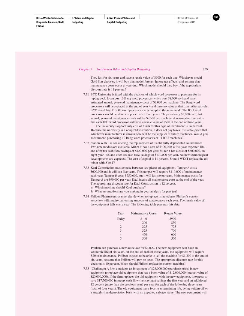
Ross−Westerfield−Jaffe: Corporate Finance, Sixth Edition
II. Value and Capital Budgeting
7. Net Present Value and Capital Budgeting
203© The McGraw−Hill Companies, 2002
They last for six years and have a resale value of $600 for each one. Whichever modelGold Star chooses, it will buy that model forever. Ignore tax effects, and assume thatmaintenance costs occur at year-end. Which model should they buy if the appropriatediscount rate is 11 percent?
7.31 BYO University is faced with the decision of which word processor to purchase for itstyping pool. It can buy 10 Bang word processors which cost $8,000 each and haveestimated annual, year-end maintenance costs of $2,000 per machine. The Bang wordprocessors will be replaced at the end of year 4 and have no value at that time. Alternatively,BYO could buy 11 IOU word processors to accomplish the same work. The IOU wordprocessors would need to be replaced after three years. They cost only $5,000 each, butannual, year-end maintenance costs will be $2,500 per machine. A reasonable forecast isthat each IOU word processor will have a resale value of $500 at the end of three years.
The university’s opportunity cost of funds for this type of investment is 14 percent.Because the university is a nonprofit institution, it does not pay taxes. It is anticipated thatwhichever manufacturer is chosen now will be the supplier of future machines. Would yourecommend purchasing 10 Bang word processors or 11 IOU machines?
7.32 Station WJXT is considering the replacement of its old, fully depreciated sound mixer.Two new models are available. Mixer X has a cost of $400,000, a five-year expected life,and after-tax cash flow savings of $120,000 per year. Mixer Y has a cost of $600,000, aneight-year life, and after-tax cash flow savings of $130,000 per year. No new technologicaldevelopments are expected. The cost of capital is 11 percent. Should WJXT replace the oldmixer with X or Y?
7.33 Kaul Construction must choose between two pieces of equipment. Tamper A costs$600,000 and it will last five years. This tamper will require $110,000 of maintenanceeach year. Tamper B costs $750,000, but it will last seven years. Maintenance costs forTamper B are $90,000 per year. Kaul incurs all maintenance costs at the end of the year.The appropriate discount rate for Kaul Construction is 12 percent.a. Which machine should Kaul purchase?b. What assumptions are you making in your analysis for part (a)?
7.34 Philben Pharmaceutics must decide when to replace its autoclave. Philben’s currentautoclave will require increasing amounts of maintenance each year. The resale value ofthe equipment falls every year. The following table presents this data.
Year Maintenance Costs Resale Value
Today $ 0 $9001 200 8502 275 7753 325 7004 450 6005 500 500
Philben can purchase a new autoclave for $3,000. The new equipment will have aneconomic life of six years. At the end of each of those years, the equipment will require$20 of maintenance. Philben expects to be able to sell the machine for $1,200 at the end ofsix years. Assume that Philben will pay no taxes. The appropriate discount rate for thisdecision is 10 percent. When should Philben replace its current machine?
7.35 (Challenge) A firm considers an investment of $28,000,000 (purchase price) in newequipment to replace old equipment that has a book value of $12,000,000 (market value of$20,000,000). If the firm replaces the old equipment with the new equipment, it expects tosave $17,500,000 in pretax cash flow (net savings) savings the first year and an additional12 percent (more than the previous year) per year for each of the following three years(total of four years). The old equipment has a four-year remaining life, being written off ona straight-line depreciation basis with no expected salvage value. The new equipment will
Chapter 7 Net Present Value and Capital Budgeting 197
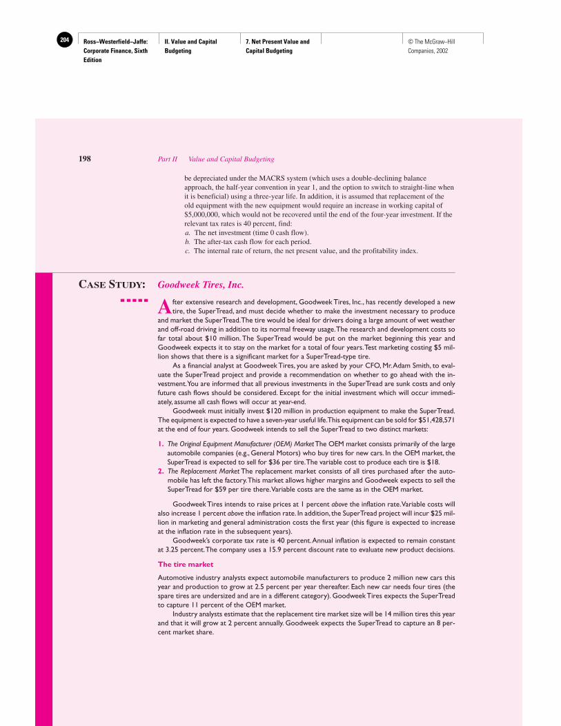
Ross−Westerfield−Jaffe: Corporate Finance, Sixth Edition
II. Value and Capital Budgeting
7. Net Present Value and Capital Budgeting
204 © The McGraw−Hill Companies, 2002
be depreciated under the MACRS system (which uses a double-declining balanceapproach, the half-year convention in year 1, and the option to switch to straight-line whenit is beneficial) using a three-year life. In addition, it is assumed that replacement of theold equipment with the new equipment would require an increase in working capital of$5,000,000, which would not be recovered until the end of the four-year investment. If therelevant tax rates is 40 percent, find:a. The net investment (time 0 cash flow).b. The after-tax cash flow for each period.c. The internal rate of return, the net present value, and the profitability index.
CASE STUDY: Goodweek Tires, Inc.
After extensive research and development, Goodweek Tires, Inc., has recently developed a newtire, the SuperTread, and must decide whether to make the investment necessary to produce
and market the SuperTread.The tire would be ideal for drivers doing a large amount of wet weatherand off-road driving in addition to its normal freeway usage.The research and development costs sofar total about $10 million. The SuperTread would be put on the market beginning this year andGoodweek expects it to stay on the market for a total of four years.Test marketing costing $5 mil-lion shows that there is a significant market for a SuperTread-type tire.
As a financial analyst at Goodweek Tires, you are asked by your CFO, Mr.Adam Smith, to eval-uate the SuperTread project and provide a recommendation on whether to go ahead with the in-vestment.You are informed that all previous investments in the SuperTread are sunk costs and onlyfuture cash flows should be considered. Except for the initial investment which will occur immedi-ately, assume all cash flows will occur at year-end.
Goodweek must initially invest $120 million in production equipment to make the SuperTread.The equipment is expected to have a seven-year useful life.This equipment can be sold for $51,428,571at the end of four years. Goodweek intends to sell the SuperTread to two distinct markets:
1. The Original Equipment Manufacturer (OEM) MarketThe OEM market consists primarily of the largeautomobile companies (e.g., General Motors) who buy tires for new cars. In the OEM market, theSuperTread is expected to sell for $36 per tire.The variable cost to produce each tire is $18.
2. The Replacement Market The replacement market consists of all tires purchased after the auto-mobile has left the factory.This market allows higher margins and Goodweek expects to sell theSuperTread for $59 per tire there.Variable costs are the same as in the OEM market.
Goodweek Tires intends to raise prices at 1 percent above the inflation rate.Variable costs willalso increase 1 percent above the inflation rate. In addition, the SuperTread project will incur $25 mil-lion in marketing and general administration costs the first year (this figure is expected to increaseat the inflation rate in the subsequent years).
Goodweek’s corporate tax rate is 40 percent.Annual inflation is expected to remain constantat 3.25 percent.The company uses a 15.9 percent discount rate to evaluate new product decisions.
The tire market
Automotive industry analysts expect automobile manufacturers to produce 2 million new cars thisyear and production to grow at 2.5 percent per year thereafter. Each new car needs four tires (thespare tires are undersized and are in a different category). Goodweek Tires expects the SuperTreadto capture 11 percent of the OEM market.
Industry analysts estimate that the replacement tire market size will be 14 million tires this yearand that it will grow at 2 percent annually. Goodweek expects the SuperTread to capture an 8 per-cent market share.
198 Part II Value and Capital Budgeting
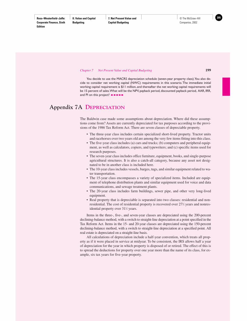
Ross−Westerfield−Jaffe: Corporate Finance, Sixth Edition
II. Value and Capital Budgeting
7. Net Present Value and Capital Budgeting
205© The McGraw−Hill Companies, 2002
You decide to use the MACRS depreciation schedule (seven-year property class).You also de-cide to consider net working capital (NWC) requirements in this scenario. The immediate initialworking capital requirement is $11 million, and thereafter the net working capital requirements willbe 15 percent of sales.What will be the NPV, payback period, discounted payback period, AAR, IRR,and PI on this project?
Appendix 7A DEPRECIATION
The Baldwin case made some assumptions about depreciation. Where did these assump-tions come from? Assets are currently depreciated for tax purposes according to the provi-sions of the 1986 Tax Reform Act. There are seven classes of depreciable property.
• The three-year class includes certain specialized short-lived property. Tractor unitsand racehorses over two years old are among the very few items fitting into this class.
• The five-year class includes (a) cars and trucks; (b) computers and peripheral equip-ment, as well as calculators, copiers, and typewriters; and (c) specific items used forresearch purposes.
• The seven-year class includes office furniture, equipment, books, and single-purposeagricultural structures. It is also a catch-all category, because any asset not desig-nated to be in another class is included here.
• The 10-year class includes vessels, barges, tugs, and similar equipment related to wa-ter transportation.
• The 15-year class encompasses a variety of specialized items. Included are equip-ment of telephone distribution plants and similar equipment used for voice and datacommunications, and sewage treatment plants.
• The 20-year class includes farm buildings, sewer pipe, and other very long-livedequipment.
• Real property that is depreciable is separated into two classes: residential and non-residential. The cost of residential property is recovered over 271⁄2 years and nonres-idential property over 311⁄2 years.
Items in the three-, five-, and seven-year classes are depreciated using the 200-percent declining-balance method, with a switch to straight-line depreciation at a point specified in theTax Reform Act. Items in the 15- and 20-year classes are depreciated using the 150-percent declining-balance method, with a switch to straight-line depreciation at a specified point. Allreal estate is depreciated on a straight-line basis.
All calculations of depreciation include a half-year convention, which treats all prop-erty as if it were placed in service at midyear. To be consistent, the IRS allows half a yearof depreciation for the year in which property is disposed of or retired. The effect of this isto spread the deductions for property over one year more than the name of its class, for ex-ample, six tax years for five-year property.
Chapter 7 Net Present Value and Capital Budgeting 199
Ross−Westerfield−Jaffe: Corporate Finance, Sixth Edition
II. Value and Capital Budgeting
8. Strategy and Analysis in Using Net Present Value
206 © The McGraw−Hill Companies, 2002
Strategy and Analysis inUsing Net Present Value
CH
AP
TE
R8
EXECUTIVE SUMMARY
The previous chapter discussed how to identify the incremental cash flows involvedin capital budgeting decisions. In this chapter we look more closely at what it isabout a project that produces a positive net present value (NPV). The process of ask-
ing about the sources of positive NPV in capital budgeting is often referred to as corporatestrategy analysis. We talk about corporate strategy analysis in the first part of the chapter.Next, we consider several analytical tools that help managers deal with the effects of un-certainty on incremental cash flows. The concepts of decision trees, scenario analysis, andbreak-even analysis are discussed.
8.1 CORPORATE STRATEGY AND POSITIVE NPV
The intuition behind discounted cash flow analysis is that a project must generate a higherrate of return than the one that can be earned in the capital markets. Only if this is true willa project’s NPV be positive. A significant part of corporate strategy analysis is seeking in-vestment opportunities that can produce positive NPV.
Simple “number crunching” in a discounted cash flow analysis can sometimes erro-neously lead to a positive NPV calculation. In calculating discounted cash flows, it is al-ways useful to ask: What is it about this project that produces a positive NPV? or Wheredoes the positive NPV in capital budgeting come from? In other words, we must be able topoint to the specific sources of positive increments to present value in doing discountedcash flow analysis. In general, it is sensible to assume that positive NPV projects are hardto find and that most project proposals are “guilty until proven innocent.”
Here are some ways that firms create positive NPV:
1. Be the first to introduce a new product.
2. Further develop a core competency to produce goods or services at lower cost thancompetitors.
3. Create a barrier that makes it difficult for other firms to compete effectively.
4. Introduce variations on existing products to take advantage of unsatisfied demand.
5. Create product differentiation by aggressive advertising and marketing networks.
6. Use innovation in organizational processes to do all of the above.
This is undoubtedly a partial list of potential sources of positive NPV. However, it isimportant to keep in mind the fact that positive NPV projects are probably not common.Our basic economic intuition should tell us that it will be harder to find positive NPV proj-ects in a competitive industry than a noncompetitive industry.
Now we ask another question: How can someone find out whether a firm is obtainingpositive NPV from its operating and investment activities? First we talk about how share
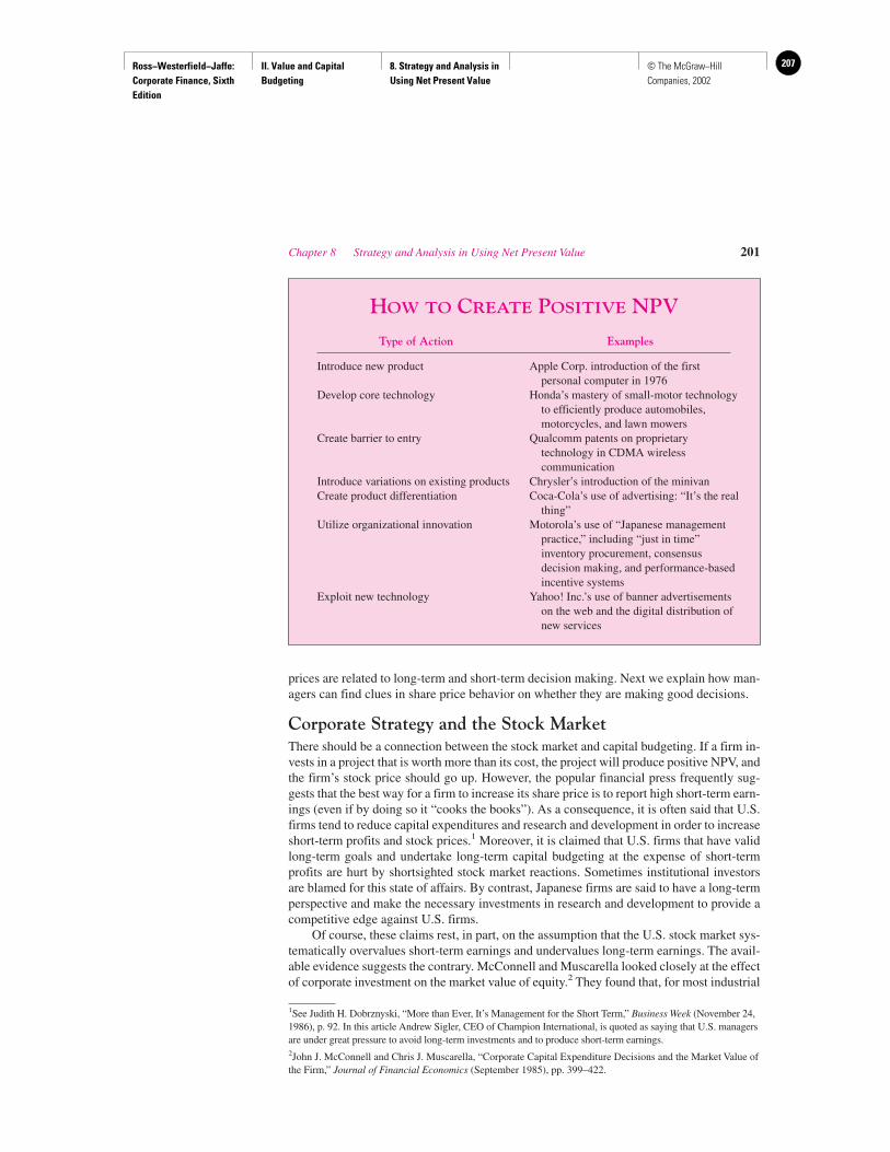
Ross−Westerfield−Jaffe: Corporate Finance, Sixth Edition
II. Value and Capital Budgeting
8. Strategy and Analysis in Using Net Present Value
207© The McGraw−Hill Companies, 2002
Chapter 8 Strategy and Analysis in Using Net Present Value 201
prices are related to long-term and short-term decision making. Next we explain how man-agers can find clues in share price behavior on whether they are making good decisions.
Corporate Strategy and the Stock MarketThere should be a connection between the stock market and capital budgeting. If a firm in-vests in a project that is worth more than its cost, the project will produce positive NPV, andthe firm’s stock price should go up. However, the popular financial press frequently sug-gests that the best way for a firm to increase its share price is to report high short-term earn-ings (even if by doing so it “cooks the books”). As a consequence, it is often said that U.S.firms tend to reduce capital expenditures and research and development in order to increaseshort-term profits and stock prices.1 Moreover, it is claimed that U.S. firms that have validlong-term goals and undertake long-term capital budgeting at the expense of short-termprofits are hurt by shortsighted stock market reactions. Sometimes institutional investorsare blamed for this state of affairs. By contrast, Japanese firms are said to have a long-termperspective and make the necessary investments in research and development to provide acompetitive edge against U.S. firms.
Of course, these claims rest, in part, on the assumption that the U.S. stock market sys-tematically overvalues short-term earnings and undervalues long-term earnings. The avail-able evidence suggests the contrary. McConnell and Muscarella looked closely at the effectof corporate investment on the market value of equity.2 They found that, for most industrial
HOW TO CREATE POSITIVE NPV
Type of Action Examples
Introduce new product Apple Corp. introduction of the first personal computer in 1976
Develop core technology Honda’s mastery of small-motor technologyto efficiently produce automobiles,motorcycles, and lawn mowers
Create barrier to entry Qualcomm patents on proprietary technology in CDMA wirelesscommunication
Introduce variations on existing products Chrysler’s introduction of the minivanCreate product differentiation Coca-Cola’s use of advertising: “It’s the real
thing”Utilize organizational innovation Motorola’s use of “Japanese management
practice,” including “just in time”inventory procurement, consensusdecision making, and performance-basedincentive systems
Exploit new technology Yahoo! Inc.’s use of banner advertisements on the web and the digital distribution ofnew services
1See Judith H. Dobrznyski, “More than Ever, It’s Management for the Short Term,” Business Week (November 24,1986), p. 92. In this article Andrew Sigler, CEO of Champion International, is quoted as saying that U.S. managersare under great pressure to avoid long-term investments and to produce short-term earnings.2John J. McConnell and Chris J. Muscarella, “Corporate Capital Expenditure Decisions and the Market Value ofthe Firm,” Journal of Financial Economics (September 1985), pp. 399–422.
Ross−Westerfield−Jaffe: Corporate Finance, Sixth Edition
II. Value and Capital Budgeting
8. Strategy and Analysis in Using Net Present Value
208 © The McGraw−Hill Companies, 2002
firms, announcements of increases in planned capital spending were associated with sig-nificant increases in the market value of the common stock and that announcements of decreases in capital spending had the opposite effect. The McConnell and Muscarella re-search suggests that the stock market does pay close attention to corporate capital spendingand it reacts positively to firms making long-term investments.
In another highly regarded study, Woolridge studied the stock market reaction to thestrategic capital spending programs of several hundred U.S. firms.3 He looked at firms an-nouncing joint ventures, research and development spending, new-product strategies, andcapital spending for expansion and modernization. He found a strong positive stock reac-tion to these types of announcements. This finding provides significant support for the no-tion that the stock market encourages managers to make long-term strategic investment de-cisions in order to maximize shareholders’ value. It strongly opposes the viewpoint thatmarkets and managers are myopic.
CASE STUDY: How Firms Can Learn about NPV from the Stock Market:The AT&T Decision to Acquire NCR and to Change Its CEO
Basic economic common sense tells us that the market value of a firm’s outstanding shares re-flects the stock market’s assessment of future cash flows from the firm’s investing activities.
Therefore, it is not surprising that the stock market usually reacts positively to the proposed capitalbudgeting programs of U.S. firms. However, this is not always the case. Sometimes the stock marketprovides negative clues to a new project’s NPV.
Consider AT&T’s repeated attempts to penetrate the computer-manufacturing industry. OnDecember 6, 1990, AT&T made a $90 per share or $6.12 billion cash offer for all of NCR Corpo-ration’s common stock. From December 4, 1990, to December 11, 1990, AT&T’s stock droppedfrom $303⁄8 per share to $291⁄2, representing a loss of about $1 billion to the shareholders of AT&T.Five months later, when these firms finally agreed to a deal, AT&T’s stock dropped again.
Why did AT&T buy NCR, a large computer manufacturer? Why did the stock market reactionsuggest that the acquisition was a negative NPV investment for AT&T? AT&T was apparently con-vinced that the telecommunications and computer industries were becoming one industry. AT&T’sbasic idea was that telephone switches are big computers and success in computers means successin telephones.The message from the stock market is that AT&T could be wrong. That is, makingcomputers is basically a manufacturing business and telephone communications is basically a servicebusiness. The core competency4 of making computers (efficient manufacturing) is different fromthat of providing telecommunications for business (service support and software). Of course, evenif AT&T had acquired NCR for the “right” reasons, it is possible that it paid too much. The negativestock market reaction suggests that AT&T shareholders believed that NCR was worth less than itscost to AT&T. On September 20, 1995, when AT&T announced its intention to spin off NCR (as wellas Lucent), its stock price increased by about 11 percent.
On the other hand,when it was announced,on November 5,1992, that AT&T was negotiating thepurchase of one-third of McCaw Cellular Communications with the option to obtain voting control,
202 Part II Value and Capital Budgeting
3J. Randall Woolridge, “Competitive Decline: Is a Myopic Stock Market to Blame?” Journal of Applied CorporateFinance (Spring 1988), pp. 26–36. Another interesting study has been conducted by Su Han Chan, John Martin,and John Kensinger, “Corporate Research and Development Expenditures and Share Value,” Journal of FinancialEconomics 26 (1990), pp. 255–76. They report that the share-price responses to announcements of increasedresearch and development are significantly positive, even when the firm’s earnings were decreasing.4Gregg Jarrell, (“For a Higher Share Price, Focus Your Business,” The Wall Street Journal, September 13, 1991)reports that an increase in “focus” by a firm is typically associated with increases in its share price. Thosecompanies that reduced their number of business lines from 1979 to 1988 had better stock market performancethan other firms.
Ross−Westerfield−Jaffe: Corporate Finance, Sixth Edition
II. Value and Capital Budgeting
8. Strategy and Analysis in Using Net Present Value
209© The McGraw−Hill Companies, 2002
AT&T’s stock price jumped from $426⁄8 to $443⁄8, representing a gain in market value close to $2 billion.Two years later, the Federal Communications Commission approved the acquisition of all of McCaw byAT&T, and AT&T’s stock price was holding at over $55 per share. The positive stock market reactionsuggests that the shareholders of AT&T believe that AT&T’s acquisition of McCaw is a positive NPVdecision. AT&T could use McCaw’s cellular telephone network to bypass local telephone companiesfor completing long distance telephone calls, eliminating the access fees normally paid to them.Perhapsbecause of AT&T’s spotty acquisition record, its stock price rose 13.5 percent when on October 17,1997, it was learned that Robert Allen would step down and Michael Armstrong would become thenew CEO.On June 24, 1998,when it was disclosed that AT&T appeared close to a deal to acquire TCIfor $30 billion, AT&T’s stock jumped 4 percent.The market believed that by buying TCI, which owneda large portfolio of cable lines, AT&T might be able to bypass the local phone monopolies of the “babybells.” TCI would offer AT&T a detour around the “last mile” and ultimately be part of AT&T’s broad-band strategy. AT&T’s market share of long-distance business continues to fall and there have been re-ports of pressure by the credit rating agencies for it to reduce its $62 billion of debt and $3 billion ofinterest costs.
AT&T’s stock price fell by more than 60 percent during the year 2000, a year that includedAT&T’s announced breakup into three companies: wireless, broadband, and business services.Thestock market appeared to be very skeptical of AT&T’s ability to carry out its long term strategy.
At the end of the year, it was reported that AT&T was expected to reduce its dividend byabout 60 percent from its current level. This would be the first time in the company’s more than100-year history that it had cut its dividend.Upon the report of a dividend cut, AT&T’s stock priceincreased.
Overall, the evidence suggests that firms can use the stock market to help potentially short-sighted managers make positive net present value decisions. Unfortunately only a few firms use themarket as effectively as they could to help them make capital budgeting decisions.
• What are the ways a firm can create positive NPV projects?• How can managers use the market to help them screen out negative NPV projects?
8.2 DECISION TREES
We have considered potential sources of value in NPV analysis. Moreover, we pointed outthat there is a connection between the stock market and a firm’s capital budgeting decisions.A savvy CEO can learn from the stock market. Now our interest is in coming up with esti-mates of NPV for a proposed project. A fundamental problem in NPV analysis is dealingwith uncertain future outcomes. Furthermore, there is usually a sequence of decisions inNPV project analysis. This section introduces the device of decision trees for identifyingthe sequential decisions in NPV analysis.
Imagine you are the treasurer of the Solar Electronics Corporation (SEC), and the engi-neering group has recently developed the technology for solar-powered jet engines. The jet en-gine is to be used with 150-passenger commercial airplanes. The marketing staff has proposedthat SEC develop some prototypes and conduct test marketing of the engine. A corporate plan-ning group, including representatives from production, marketing, and engineering, has rec-ommended that the firm go ahead with the test and development phase. They estimate that thispreliminary phase will take a year and will cost $100 million. Furthermore, the group believesthere is a 75-percent chance that the reproduction and marketing tests will prove successful.
Based on its experience in the industry, the company has a fairly accurate idea of howmuch the development and testing expenditures will cost. Sales of jet engines, however, aresubject to (1) uncertainty about the demand for air travel in the future, (2) uncertainty about
Chapter 8 Strategy and Analysis in Using Net Present Value 203
QUESTIONS
CO
NC
EP
T
?
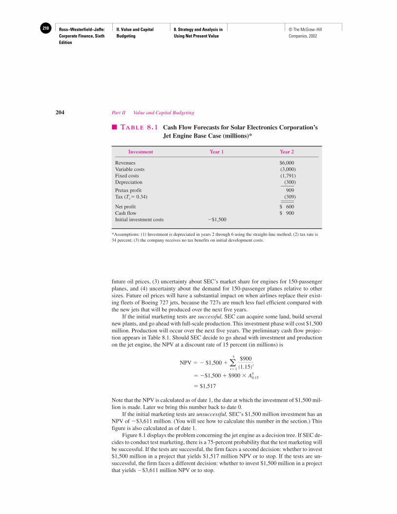
Ross−Westerfield−Jaffe: Corporate Finance, Sixth Edition
II. Value and Capital Budgeting
8. Strategy and Analysis in Using Net Present Value
210 © The McGraw−Hill Companies, 2002
future oil prices, (3) uncertainty about SEC’s market share for engines for 150-passengerplanes, and (4) uncertainty about the demand for 150-passenger planes relative to othersizes. Future oil prices will have a substantial impact on when airlines replace their exist-ing fleets of Boeing 727 jets, because the 727s are much less fuel efficient compared withthe new jets that will be produced over the next five years.
If the initial marketing tests are successful, SEC can acquire some land, build severalnew plants, and go ahead with full-scale production. This investment phase will cost $1,500million. Production will occur over the next five years. The preliminary cash flow projec-tion appears in Table 8.1. Should SEC decide to go ahead with investment and productionon the jet engine, the NPV at a discount rate of 15 percent (in millions) is
NPV � � $1,500 �
� �$1,500 � $900 �
� $1,517
Note that the NPV is calculated as of date 1, the date at which the investment of $1,500 mil-lion is made. Later we bring this number back to date 0.
If the initial marketing tests are unsuccessful, SEC’s $1,500 million investment has anNPV of �$3,611 million. (You will see how to calculate this number in the section.) Thisfigure is also calculated as of date 1.
Figure 8.1 displays the problem concerning the jet engine as a decision tree. If SEC de-cides to conduct test marketing, there is a 75-percent probability that the test marketing willbe successful. If the tests are successful, the firm faces a second decision: whether to invest$1,500 million in a project that yields $1,517 million NPV or to stop. If the tests are un-successful, the firm faces a different decision: whether to invest $1,500 million in a projectthat yields �$3,611 million NPV or to stop.
A
50.15
5
t�1
$900�1.15� t
204 Part II Value and Capital Budgeting
� TABLE 8.1 Cash Flow Forecasts for Solar Electronics Corporation’sJet Engine Base Case (millions)*
Investment Year 1 Year 2
Revenues $6,000Variable costs (3,000)Fixed costs (1,791)Depreciation (300)_____Pretax profit 909Tax (Tc� 0.34) (309)__________Net profit $ 600Cash flow $ 900Initial investment costs �$1,500
*Assumptions: (1) Investment is depreciated in years 2 through 6 using the straight-line method; (2) tax rate is34 percent; (3) the company receives no tax benefits on initial development costs.
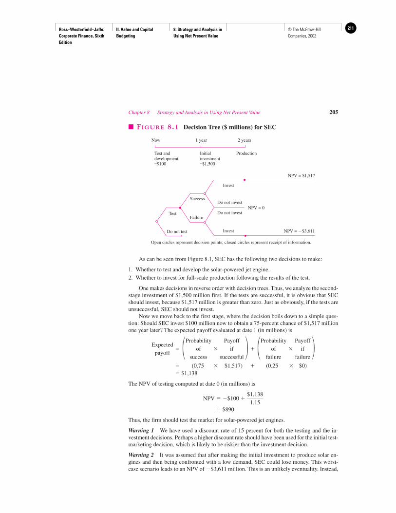
Ross−Westerfield−Jaffe: Corporate Finance, Sixth Edition
II. Value and Capital Budgeting
8. Strategy and Analysis in Using Net Present Value
211© The McGraw−Hill Companies, 2002
As can be seen from Figure 8.1, SEC has the following two decisions to make:
1. Whether to test and develop the solar-powered jet engine.
2. Whether to invest for full-scale production following the results of the test.
One makes decisions in reverse order with decision trees. Thus, we analyze the second-stage investment of $1,500 million first. If the tests are successful, it is obvious that SECshould invest, because $1,517 million is greater than zero. Just as obviously, if the tests areunsuccessful, SEC should not invest.
Now we move back to the first stage, where the decision boils down to a simple ques-tion: Should SEC invest $100 million now to obtain a 75-percent chance of $1,517 millionone year later? The expected payoff evaluated at date 1 (in millions) is
� (0.75 � $1,517) � (0.25 � $0)� $1,138
The NPV of testing computed at date 0 (in millions) is
NPV � �$100 �
� $890
Thus, the firm should test the market for solar-powered jet engines.
Warning 1 We have used a discount rate of 15 percent for both the testing and the in-vestment decisions. Perhaps a higher discount rate should have been used for the initial test-marketing decision, which is likely to be riskier than the investment decision.
Warning 2 It was assumed that after making the initial investment to produce solar en-gines and then being confronted with a low demand, SEC could lose money. This worst-case scenario leads to an NPV of �$3,611 million. This is an unlikely eventuality. Instead,
$1,138
1.15
Expected
payoff� �Probability
of
success
�
Payoff
if
successful� � �Probability
of
failure
�
Payoff
if
failure�
Chapter 8 Strategy and Analysis in Using Net Present Value 205
Now 1 year 2 years
Test anddevelopment–$100
Initialinvestment–$1,500
Production
NPV = $1,517
NPV = �$3,611
NPV = 0
Invest
Invest
Do not invest
Do not invest
Success
FailureTest
Do not test
� FIGURE 8.1 Decision Tree ($ millions) for SEC
Open circles represent decision points; closed circles represent receipt of information.
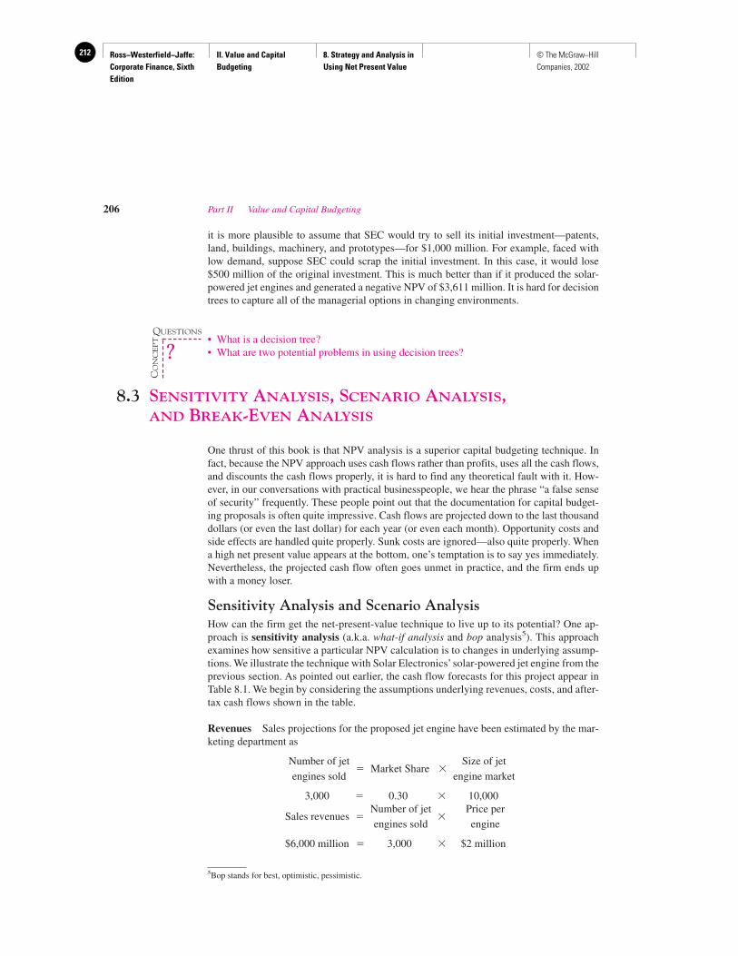
Ross−Westerfield−Jaffe: Corporate Finance, Sixth Edition
II. Value and Capital Budgeting
8. Strategy and Analysis in Using Net Present Value
212 © The McGraw−Hill Companies, 2002
it is more plausible to assume that SEC would try to sell its initial investment—patents,land, buildings, machinery, and prototypes—for $1,000 million. For example, faced withlow demand, suppose SEC could scrap the initial investment. In this case, it would lose$500 million of the original investment. This is much better than if it produced the solar-powered jet engines and generated a negative NPV of $3,611 million. It is hard for decisiontrees to capture all of the managerial options in changing environments.
• What is a decision tree?• What are two potential problems in using decision trees?
8.3 SENSITIVITY ANALYSIS, SCENARIO ANALYSIS, AND BREAK-EVEN ANALYSIS
One thrust of this book is that NPV analysis is a superior capital budgeting technique. Infact, because the NPV approach uses cash flows rather than profits, uses all the cash flows,and discounts the cash flows properly, it is hard to find any theoretical fault with it. How-ever, in our conversations with practical businesspeople, we hear the phrase “a false senseof security” frequently. These people point out that the documentation for capital budget-ing proposals is often quite impressive. Cash flows are projected down to the last thousanddollars (or even the last dollar) for each year (or even each month). Opportunity costs andside effects are handled quite properly. Sunk costs are ignored—also quite properly. Whena high net present value appears at the bottom, one’s temptation is to say yes immediately.Nevertheless, the projected cash flow often goes unmet in practice, and the firm ends upwith a money loser.
Sensitivity Analysis and Scenario AnalysisHow can the firm get the net-present-value technique to live up to its potential? One ap-proach is sensitivity analysis (a.k.a. what-if analysis and bop analysis5). This approachexamines how sensitive a particular NPV calculation is to changes in underlying assump-tions. We illustrate the technique with Solar Electronics’ solar-powered jet engine from theprevious section. As pointed out earlier, the cash flow forecasts for this project appear inTable 8.1. We begin by considering the assumptions underlying revenues, costs, and after-tax cash flows shown in the table.
Revenues Sales projections for the proposed jet engine have been estimated by the mar-keting department as
3,000 � 0.30 � 10,000
$6,000 million � 3,000 � $2 million
Sales revenues � Number of jet
engines sold �
Price per
engine
Number of jet
engines sold � Market Share �
Size of jet
engine market
206 Part II Value and Capital Budgeting
5Bop stands for best, optimistic, pessimistic.
QUESTIONS
CO
NC
EP
T
?
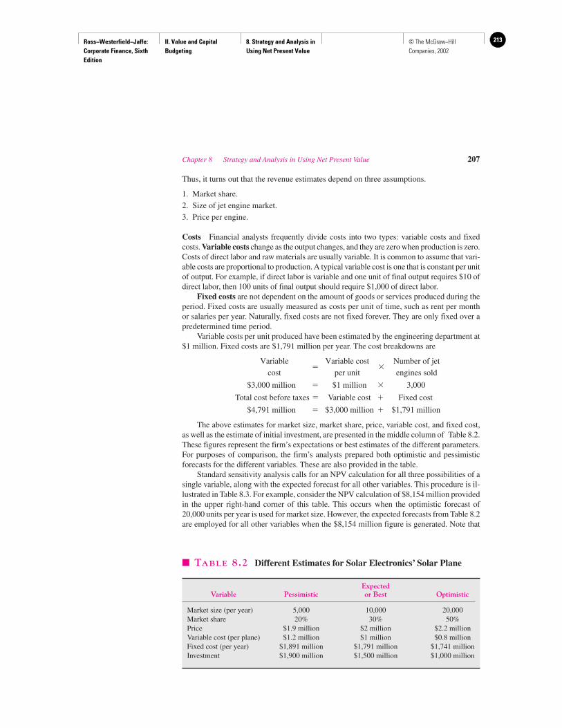
Ross−Westerfield−Jaffe: Corporate Finance, Sixth Edition
II. Value and Capital Budgeting
8. Strategy and Analysis in Using Net Present Value
213© The McGraw−Hill Companies, 2002
Thus, it turns out that the revenue estimates depend on three assumptions.
1. Market share.
2. Size of jet engine market.
3. Price per engine.
Costs Financial analysts frequently divide costs into two types: variable costs and fixedcosts. Variable costs change as the output changes, and they are zero when production is zero.Costs of direct labor and raw materials are usually variable. It is common to assume that vari-able costs are proportional to production. A typical variable cost is one that is constant per unitof output. For example, if direct labor is variable and one unit of final output requires $10 ofdirect labor, then 100 units of final output should require $1,000 of direct labor.
Fixed costs are not dependent on the amount of goods or services produced during theperiod. Fixed costs are usually measured as costs per unit of time, such as rent per monthor salaries per year. Naturally, fixed costs are not fixed forever. They are only fixed over apredetermined time period.
Variable costs per unit produced have been estimated by the engineering department at$1 million. Fixed costs are $1,791 million per year. The cost breakdowns are
$3,000 million � $1 million � 3,000
Total cost before taxes � Variable cost � Fixed cost
$4,791 million � $3,000 million � $1,791 million
The above estimates for market size, market share, price, variable cost, and fixed cost,as well as the estimate of initial investment, are presented in the middle column of Table 8.2.These figures represent the firm’s expectations or best estimates of the different parameters.For purposes of comparison, the firm’s analysts prepared both optimistic and pessimisticforecasts for the different variables. These are also provided in the table.
Standard sensitivity analysis calls for an NPV calculation for all three possibilities of asingle variable, along with the expected forecast for all other variables. This procedure is il-lustrated in Table 8.3. For example, consider the NPV calculation of $8,154 million providedin the upper right-hand corner of this table. This occurs when the optimistic forecast of20,000 units per year is used for market size. However, the expected forecasts from Table 8.2are employed for all other variables when the $8,154 million figure is generated. Note that
Variable
cost �
Variable cost
per unit �
Number of jet
engines sold
Chapter 8 Strategy and Analysis in Using Net Present Value 207
� TABLE 8.2 Different Estimates for Solar Electronics’ Solar Plane
ExpectedVariable Pessimistic or Best Optimistic
Market size (per year) 5,000 10,000 20,000Market share 20% 30% 50%Price $1.9 million $2 million $2.2 millionVariable cost (per plane) $1.2 million $1 million $0.8 millionFixed cost (per year) $1,891 million $1,791 million $1,741 millionInvestment $1,900 million $1,500 million $1,000 million
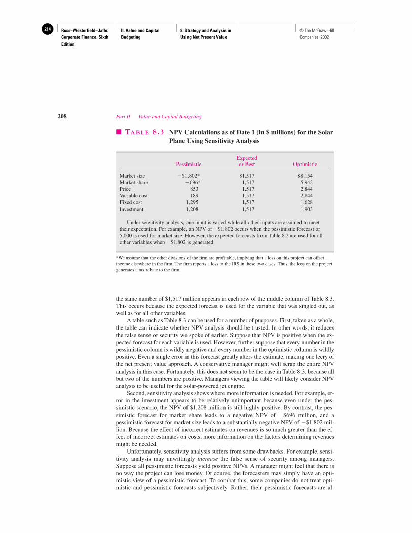
Ross−Westerfield−Jaffe: Corporate Finance, Sixth Edition
II. Value and Capital Budgeting
8. Strategy and Analysis in Using Net Present Value
214 © The McGraw−Hill Companies, 2002
the same number of $1,517 million appears in each row of the middle column of Table 8.3.This occurs because the expected forecast is used for the variable that was singled out, aswell as for all other variables.
A table such as Table 8.3 can be used for a number of purposes. First, taken as a whole,the table can indicate whether NPV analysis should be trusted. In other words, it reducesthe false sense of security we spoke of earlier. Suppose that NPV is positive when the ex-pected forecast for each variable is used. However, further suppose that every number in thepessimistic column is wildly negative and every number in the optimistic column is wildlypositive. Even a single error in this forecast greatly alters the estimate, making one leery ofthe net present value approach. A conservative manager might well scrap the entire NPVanalysis in this case. Fortunately, this does not seem to be the case in Table 8.3, because allbut two of the numbers are positive. Managers viewing the table will likely consider NPVanalysis to be useful for the solar-powered jet engine.
Second, sensitivity analysis shows where more information is needed. For example, er-ror in the investment appears to be relatively unimportant because even under the pes-simistic scenario, the NPV of $1,208 million is still highly positive. By contrast, the pes-simistic forecast for market share leads to a negative NPV of �$696 million, and apessimistic forecast for market size leads to a substantially negative NPV of �$1,802 mil-lion. Because the effect of incorrect estimates on revenues is so much greater than the ef-fect of incorrect estimates on costs, more information on the factors determining revenuesmight be needed.
Unfortunately, sensitivity analysis suffers from some drawbacks. For example, sensi-tivity analysis may unwittingly increase the false sense of security among managers.Suppose all pessimistic forecasts yield positive NPVs. A manager might feel that there isno way the project can lose money. Of course, the forecasters may simply have an opti-mistic view of a pessimistic forecast. To combat this, some companies do not treat opti-mistic and pessimistic forecasts subjectively. Rather, their pessimistic forecasts are al-
208 Part II Value and Capital Budgeting
� TABLE 8.3 NPV Calculations as of Date 1 (in $ millions) for the SolarPlane Using Sensitivity Analysis
ExpectedPessimistic or Best Optimistic
Market size �$1,802* $1,517 $8,154Market share �696* 1,517 5,942Price 853 1,517 2,844Variable cost 189 1,517 2,844Fixed cost 1,295 1,517 1,628Investment 1,208 1,517 1,903
Under sensitivity analysis, one input is varied while all other inputs are assumed to meettheir expectation. For example, an NPV of �$1,802 occurs when the pessimistic forecast of5,000 is used for market size. However, the expected forecasts from Table 8.2 are used for allother variables when �$1,802 is generated.
*We assume that the other divisions of the firm are profitable, implying that a loss on this project can offsetincome elsewhere in the firm. The firm reports a loss to the IRS in these two cases. Thus, the loss on the projectgenerates a tax rebate to the firm.
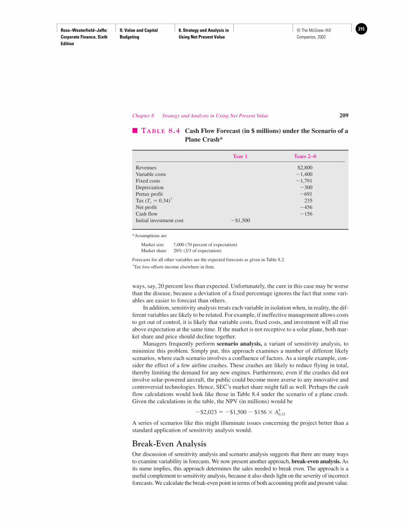
Ross−Westerfield−Jaffe: Corporate Finance, Sixth Edition
II. Value and Capital Budgeting
8. Strategy and Analysis in Using Net Present Value
215© The McGraw−Hill Companies, 2002
ways, say, 20 percent less than expected. Unfortunately, the cure in this case may be worsethan the disease, because a deviation of a fixed percentage ignores the fact that some vari-ables are easier to forecast than others.
In addition, sensitivity analysis treats each variable in isolation when, in reality, the dif-ferent variables are likely to be related. For example, if ineffective management allows coststo get out of control, it is likely that variable costs, fixed costs, and investment will all riseabove expectation at the same time. If the market is not receptive to a solar plane, both mar-ket share and price should decline together.
Managers frequently perform scenario analysis, a variant of sensitivity analysis, tominimize this problem. Simply put, this approach examines a number of different likelyscenarios, where each scenario involves a confluence of factors. As a simple example, con-sider the effect of a few airline crashes. These crashes are likely to reduce flying in total,thereby limiting the demand for any new engines. Furthermore, even if the crashes did notinvolve solar-powered aircraft, the public could become more averse to any innovative andcontroversial technologies. Hence, SEC’s market share might fall as well. Perhaps the cashflow calculations would look like those in Table 8.4 under the scenario of a plane crash.Given the calculations in the table, the NPV (in millions) would be
�$2,023 � �$1,500 � $156 �
A series of scenarios like this might illuminate issues concerning the project better than astandard application of sensitivity analysis would.
Break-Even AnalysisOur discussion of sensitivity analysis and scenario analysis suggests that there are many waysto examine variability in forecasts. We now present another approach, break-even analysis. Asits name implies, this approach determines the sales needed to break even. The approach is auseful complement to sensitivity analysis, because it also sheds light on the severity of incorrectforecasts. We calculate the break-even point in terms of both accounting profit and present value.
A
50.15
Chapter 8 Strategy and Analysis in Using Net Present Value 209
� TABLE 8.4 Cash Flow Forecast (in $ millions) under the Scenario of aPlane Crash*
Year 1 Years 2–6
Revenues $2,800Variable costs �1,400Fixed costs �1,791Depreciation �300Pretax profit �691Tax (Tc � 0.34)† 235Net profit �456Cash flow �156Initial investment cost �$1,500
*Assumptions are
Market size 7,000 (70 percent of expectation)Market share 20% (2/3 of expectation)
Forecasts for all other variables are the expected forecasts as given in Table 8.2.†Tax loss offsets income elsewhere in firm.
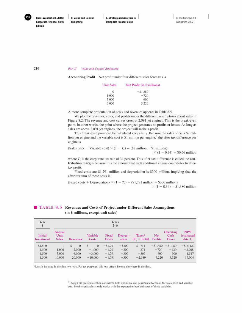
Ross−Westerfield−Jaffe: Corporate Finance, Sixth Edition
II. Value and Capital Budgeting
8. Strategy and Analysis in Using Net Present Value
216 © The McGraw−Hill Companies, 2002
Accounting Profit Net profit under four different sales forecasts is
Unit Sales Net Profit (in $ millions)
0 �$1,3801,000 �7203,000 600
10,000 5,220
A more complete presentation of costs and revenues appears in Table 8.5.We plot the revenues, costs, and profits under the different assumptions about sales in
Figure 8.2. The revenue and cost curves cross at 2,091 jet engines. This is the break-evenpoint, in other words, the point where the project generates no profits or losses. As long assales are above 2,091 jet engines, the project will make a profit.
This break-even point can be calculated very easily. Because the sales price is $2 mil-lion per engine and the variable cost is $1 million per engine,6 the after-tax difference perengine is
(Sales price � Variable cost) � (1 � Tc) � ($2 million � $1 million)� (1 � 0.34) � $0.66 million
where Tc is the corporate tax rate of 34 percent. This after-tax difference is called the con-tribution margin because it is the amount that each additional engine contributes to after-tax profit.
Fixed costs are $1,791 million and depreciation is $300 million, implying that the after-tax sum of these costs is
(Fixed costs � Depreciation) � (1 � Tc) � ($1,791 million � $300 million)� (1 � 0.34) � $1,380 million
210 Part II Value and Capital Budgeting
� TABLE 8.5 Revenues and Costs of Project under Different Sales Assumptions (in $ millions, except unit sales)
Year Years1 2–6
Annual Operating NPVInitial Unit Variable Fixed Depreci- Taxes* Net Cash (evaluated
Investment Sales Revenues Costs Costs ation (Tc � 0.34) Profits Flows date 1)
$1,500 0 $ 0 $ 0 �$1,791 �$300 $ 711 �$1,380 �$1,080 �$ 5,1201,500 1,000 2,000 �1,000 �1,791 �300 371 �720 �420 �2,9081,500 3,000 6,000 �3,000 �1,791 �300 �309 600 900 1,5171,500 10,000 20,000 �10,000 �1,791 �300 �2,689 5,220 5,520 17,004
*Loss is incurred in the first two rows. For tax purposes, this loss offsets income elsewhere in the firm.
6Though the previous section considered both optimistic and pessimistic forecasts for sales price and variablecost, break-even analysis only works with the expected or best estimates of these variables.
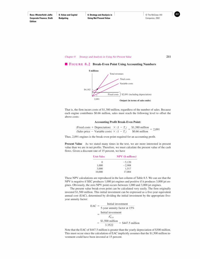
Ross−Westerfield−Jaffe: Corporate Finance, Sixth Edition
II. Value and Capital Budgeting
8. Strategy and Analysis in Using Net Present Value
217© The McGraw−Hill Companies, 2002
That is, the firm incurs costs of $1,380 million, regardless of the number of sales. Becauseeach engine contributes $0.66 million, sales must reach the following level to offset theabove costs:
Accounting Profit Break-Even Point:
Thus, 2,091 engines is the break-even point required for an accounting profit.
Present Value As we stated many times in the text, we are more interested in presentvalue than we are in net profits. Therefore, we must calculate the present value of the cashflows. Given a discount rate of 15 percent, we have
Unit Sales NPV ($ millions)
0 �5,1201,000 �2,9083,000 1,517
10,000 17,004
These NPV calculations are reproduced in the last column of Table 8.5. We can see that theNPV is negative if SEC produces 1,000 jet engines and positive if it produces 3,000 jet en-gines. Obviously, the zero NPV point occurs between 1,000 and 3,000 jet engines.
The present value break-even point can be calculated very easily. The firm originallyinvested $1,500 million. This initial investment can be expressed as a five-year equivalentannual cost (EAC), determined by dividing the initial investment by the appropriate five-year annuity factor:
Note that the EAC of $447.5 million is greater than the yearly depreciation of $300 million.This must occur since the calculation of EAC implicitly assumes that the $1,500 million in-vestment could have been invested at 15 percent.
�$1,500 million
3.3522� $447.5 million
�Initial investment
A
50.15
EAC �Initial investment
5-year annuity factor at 15%
�Fixed costs � Depreciation� � �1 � Tc��Sales price � Variable costs� � �1 � Tc�
�$1,380 million
$0.66 million� 2,091
Chapter 8 Strategy and Analysis in Using Net Present Value 211
$ millions
$4,182
Output (in terms of sales units)2,091
Total revenues
Variable costs
Total costs
$2,091 (including depreciation)Fixed costs
� FIGURE 8.2 Break-Even Point Using Accounting Numbers
Ross−Westerfield−Jaffe: Corporate Finance, Sixth Edition
II. Value and Capital Budgeting
8. Strategy and Analysis in Using Net Present Value
218 © The McGraw−Hill Companies, 2002
After-tax costs, regardless of output, can be viewed as
Fixed Depreci-� EAC � costs � (1 � Tc) � ation � Tc
That is, in addition to the initial investment’s equivalent annual cost of $447.5 million, thefirm pays fixed costs each year and receives a depreciation tax shield each year. The de-preciation tax shield is written as a negative number because it offsets the costs in the equa-tion. Because each plane contributes $0.66 million to after-tax profit, it will take the fol-lowing sales to offset the above costs:
Present Value Break-Even Point:
Thus, 2,315 planes is the break-even point from the perspective of present value. Why is the accounting break-even point different from the financial break-even point?
When we use accounting profit as the basis for the break-even calculation, we subtract de-preciation. Depreciation for the solar-jet-engines project is $300 million. If 2,091 solar jetengines are sold, SEC will generate sufficient revenues to cover the $300 million deprecia-tion expense plus other costs. Unfortunately, at this level of sales SEC will not cover the eco-nomic opportunity costs of the $1,500 million laid out for the investment. If we take into ac-count that the $1,500 million could have been invested at 15 percent, the true annual cost ofthe investment is $447.5 million and not $300 million. Depreciation understates the truecosts of recovering the initial investment. Thus, companies that break even on an accountingbasis are really losing money. They are losing the opportunity cost of the initial investment.
• What is a sensitivity analysis?• Why is it important to perform a sensitivity analysis?• What is a break-even analysis?• Describe how sensitivity analysis interacts with break-even analysis.
8.4 OPTIONS
The analysis we have presented so far is static. In fact, standard NPV analysis is somewhatstatic. Because corporations make decisions in a dynamic environment, they have optionsthat should be considered in project valuation.
The Option to ExpandOne of the most important options is the option to expand when economic prospects are good.The option to expand has value. Expansion pays off if demand is high. Recall the Solar Elec-tronics Corporation (SEC) in Section 8.2. SEC’s expenditure on the test-marketing programbuys an option to produce new jet engines. This turned out to be a very valuable option. SEChad the option to produce new jet engines depending on the results of the test marketing.
There are many real-world examples. In 1977 Saab was the first car maker to introduceturbo-charged automobile engines in its gasoline model. Sales of the Saab 900 almost dou-bled after the introduction. In response to this high demand, Saab has increased its capac-
EAC � Fixed costs � �1 � Tc� � Depreciation � Tc
�Sales price � Variable costs� � �1 � Tc��
$1,528 million
$0.66 million� 2,315
$1,528million
�$447.5million
�$1,791million
� 0.66 � $300million
� 0.34
212 Part II Value and Capital Budgeting
QUESTIONS
CO
NC
EP
T
?
Ross−Westerfield−Jaffe: Corporate Finance, Sixth Edition
II. Value and Capital Budgeting
8. Strategy and Analysis in Using Net Present Value
219© The McGraw−Hill Companies, 2002
ity and entered into joint ventures with other car makers to increase production. Now manyautomobile manufacturers use turbo chargers.
The Option to AbandonThe option to close a facility also has value. The SEC would not have been obligated to pro-duce jet engines if the test-marketing results had been negative. Instead, SEC had the op-tion to abandon the jet engine project if the results had been bad.
Take the case of General Motors (GM). On December 19, 1991, GM announced plans toclose 21 factories and cut 74,000 jobs by the end of 1995. It said that it also intended to sellnon-auto assets. Faced with low demand for its automobiles, GM decided to scrap the invest-ment it had made in automobile manufacturing capacity, and it will likely lose much of itsoriginal investment in the 21 factories. However, this outcome is much better than would haveoccurred if GM continued to operate these factories in a declining auto market. On the day thefactory closing was announced, GM’s stock was marginally down by $0.125 (from $27.875to $27.75). The stock market reaction was a signal that GM had waited too long to close itsfactories and that the declining demand GM was encountering was greater than expected.However, the market was relieved that GM had finally abandoned money-losing factories.
There is a special graveyard for abandoned products in the market for handheld com-puters. In October 1991, Momenta International Corporation introduced one of the very firsthandheld computers, a five-pound pen-based computer. Ten months later the company wentbankrupt. Eo, a company backed by AT&T, demonstrated a new personal communicator inNovember 1992. The project was terminated in 1994. In January 1994, Motorola began ship-ping its Envoy, a wireless communicator. The computer was discontinued two years later.The point of our examples of failed handheld computer products is that a firm will frequentlyexercise its option of abandoning a project rather than keeping a money-losing product onthe market in hopes that economic conditions will improve.
Discounted Cash Flows and OptionsConventional NPV analysis discounts a project’s cash flows estimated for a certain projectlife. The decision is whether to accept the project or reject it. In practice, managers can ex-pand or contract the scope of a project at various moments over its life. In theory, all suchmanagerial options should be included in the project’s value.
The market value of the project (M) will be the sum of the NPV of the project withoutoptions to expand or contract and the value of the managerial options (Opt):
M � NPV � Opt
EXAMPLE
Imagine two ways of producing Frisbees. Method A uses a conventional machinethat has an active secondary market. Method B uses highly specialized machinetools for which there is no secondary market. Method B has no salvage value, butis more efficient. Method A has a salvage value, but is inefficient.
If production of Frisbees goes on until the machines used in methods A and Bare used up, the NPV of B will be greater than that of A. However, if there is somepossibility that production of Frisbees will be stopped before the end of the usefullife of the Frisbee-making machines, method A may well be better. Method A’shigher value in the secondary market increases its NPV relative to B’s. There is avaluable embedded option to abandoning Method A.
Chapter 8 Strategy and Analysis in Using Net Present Value 213
Ross−Westerfield−Jaffe: Corporate Finance, Sixth Edition
II. Value and Capital Budgeting
8. Strategy and Analysis in Using Net Present Value
220 © The McGraw−Hill Companies, 2002
An ExampleSuppose we are analyzing a new product that will sell an expected 10 units a year in per-petuity at $10 net cash flow. In other words, we expect that cash flows will be $100 per year.At the end of the first year we will learn more about the economic viability of the new prod-uct. Specifically, we will know if the project will be a success or a failure. If the product isa success, unit sales will be revised to 20 and if the product is a failure, unit sales will be 0.Success and failure are equally likely. The discount rate is 10 percent and the initial invest-ment outlay is $1,050. The dismantled equipment originally purchased for the project canbe sold for scrap in one year for $500.
A standard discount cash flow analysis of the new product is very straightforward. Theexpected cash flows are $100 per year and the discount rate is 10 percent. The NPV of theproduct is:
$100/.10 � $1,050 � �$50
So we shouldn’t launch the new product. Correct? No! In one year we can sell out for $500and we can learn more about the success or failure of our new product. If it is a success, wecan continue to sell the product. But if it is a failure, we can abandon the product. The op-tion to abandon in one year is valuable.
In one year if the cash flows are revised to $0, the PV of the project will be $0 andwe will abandon the product for $500. The NPV will be $500. On the other hand, if welearn that we can sell 20 of the products, the PV of future cash flows will be $200/.10� $2,000. The PV exceeds the abandonment value of $500. So we will continue to sellthe product.
To sum up, we now have a new product that costs $1,050 today. In one year we ex-pect a cash flow of $100. After one year the new product will be worth either $500 (ifwe abandon the product) or $2,000 (if we continue to sell the product). These outcomesare equally likely so we expect the project to be worth $500 � $2,000/2 � $1,250. Thebottom line is that in one year we expect to have $100 in cash plus a project worth$1,250. At a 10-percent discount the project is worth $1,227.27 so the NPV is$1,227.27 � $1,050 � $177.27.
We should launch the new product! Notice the NPV of our new product has increasedfrom �$50 to $177.27 or, by $227.27. How did this happen? The original analysis implic-itly assumed we would launch the new product even though it was a failure. Actually, whenwe took a closer look, we saw that we were $500 better off if we abandoned the product.There was a 50-percent probability of this happening. So the expected cash flow from aban-donment is $250. The PV of this amount is $250/1.1 � $227.27. The value of the option toabandon after one year is $227.27.
Robichek and Van Horne and Dye and Long were among the first to recognize theabandonment value in project analysis.7 More recently, Myers and Majd constructed amodel of abandonment based on an American put option with varying dividend yields andan uncertain exercise price.8 They present a numerical procedure for calculating abandon-ment value in problems similar to that of the Frisbee-making machine.
214 Part II Value and Capital Budgeting
7A. Robichek and J. Van Horne, “Abandonment Value and Capital Budgeting,” Journal of Finance(December 1967); and E. Dye and H. Long, “Abandonment Value and Capital Budgeting: Comment,”Journal of Finance (March 1969).8S. C. Myers and S. Majd, “Calculating Abandonment Value Using Option Pricing Theory.” Unpublishedmanuscript (June 1985).
Ross−Westerfield−Jaffe: Corporate Finance, Sixth Edition
II. Value and Capital Budgeting
8. Strategy and Analysis in Using Net Present Value
221© The McGraw−Hill Companies, 2002
Brennan and Schwartz use a gold mine to illustrate the value of managerial operations.9
They show that the value of a gold mine will depend on management’s ability to shut itdown if the price of gold falls below a certain point, and the ability to reopen it subsequentlyif conditions are right. They show that valuation approaches that ignore these managerialoptions are likely to substantially underestimate the value of the project.
There are both qualitative and quantitative approaches to adjusting for option value incapital budgeting decisions. Most firms use qualitative approaches, such as subjective judg-ment. However, quantitative approaches are gaining acceptance. We talk about the quanti-tative approaches in Chapters 21 and 22.
8.5 SUMMARY AND CONCLUSIONS
This chapter discusses a number of practical applications of capital budgeting.
1. In Chapter 7, we observed how the net present value rule in capital budgeting is used. In Chapter 8, we ask about the sources of positive net present value and we explain what managers can do to create positive net present value.
2. Though NPV is the best capital budgeting approach conceptually, it has been criticized inpractice for providing managers with a false sense of security. Sensitivity analysis shows NPVunder varying assumptions, giving managers a better feel for the project’s risks. Unfortunately,sensitivity analysis modifies only one variable at a time, while many variables are likely to varytogether in the real world. Scenario analysis considers the joint movement of the differentfactors under different scenarios (e.g., war breaking out or oil prices skyrocketing). Finally,managers want to know how bad forecasts must be before a project loses money. Break-evenanalysis calculates the sales figure at which the project breaks even. Though break-even analysisis frequently performed on an accounting profit basis, we suggest that a net present value basis ismore appropriate.
3. We talk about hidden options in doing discounted cash flow analysis of capital budgeting. Wediscuss the option to expand and the option to abandon.
KEY TERMS
Break-even analysis 209 Scenario analysis 209Contribution margin 210 Sensitivity analysis 206Decision trees 203 Variable costs 207Fixed costs 207
Chapter 8 Strategy and Analysis in Using Net Present Value 215
9M. J. Brennan and E. S. Schwartz, “A New Approach to Evaluating Natural Resource Investments,” MidlandCorporate Finance Journal 3 (Spring 1985).
Ross−Westerfield−Jaffe: Corporate Finance, Sixth Edition
II. Value and Capital Budgeting
8. Strategy and Analysis in Using Net Present Value
222 © The McGraw−Hill Companies, 2002
SUGGESTED READING
The classic article on break-even analysis is:Reinhart, U. E. “Breakeven Analysis for Lockheed’s Tristar: An Application of Financial
Theory.” Journal of Finance (September 1977).
QUESTIONS AND PROBLEMS
Decision Trees8.1 Sony Electronics, Inc., has developed a new type of VCR. If the firm directly goes to the
market with the product, there is only a 50 percent chance of success. On the other hand, ifthe firm conducts test marketing of the VCR, it will take a year and will cost $2 million.Through the test marketing, however, the firm is able to improve the product and increase theprobability of success to 75 percent. If the new product proves successful, the present value(at the time when the firm starts selling it) of the payoff is $20 million, while if it turns out tobe a failure, the present value of the payoff is $5 million. Should the firm conduct testmarketing or go directly to the market? The appropriate discount rate is 15 percent.
8.2 The marketing manager for a growing consumer products firm is considering launching anew product. To determine consumers’ interest in such a product, the manager can conducta focus group that will cost $120,000 and has a 70 percent chance of correctly predictingthe success of the product, or hire a consulting firm that will research the market at a cost of$400,000. The consulting firm boasts a correct assessment record of 90 percent. Of coursegoing directly to the market with no prior testing will be the correct move 50 percent of thetime. If the firm launches the product, and it is a success, the payoff will be $1.2 million.Which action will result in the highest expected payoff for the firm?
8.3 Tandem Bicycles is noticing a decline in sales due to the increase of lower-priced importproducts from the Far East. The CFO is considering a number of strategies to maintain itsmarket share. The options she sees are the following:
• Price the products more aggressively, resulting in a $1.3 million decline in cash flows.The likelihood that Tandem will lose no cash flows to the imports is 55 percent; there is a45 percent probability that they will lose only $550,000 in cash flows to the imports.
• Hire a lobbyist to convince the regulators that there should be important tariffs placedupon overseas manufacturers of bicycles. This will cost Tandem $800,000 and will have a75 percent success rate, that is, no loss in cash flows to the importers. If the lobbyists donot succeed, Tandem Bicycles will lose $2 million in cash flows.
As the assistant to the CFO, which strategy would you recommend to your boss?
Accounting Break-Even Analysis8.4 Samuelson Inc. has invested in a facility to produce calculators. The price of the machine is
$600,000 and its economic life is five years. The machine is fully depreciated by thestraight-line method and will produce 20,000 units of calculators in the first year. Thevariable production cost per unit of the calculator is $15, while fixed costs are $900,000.The corporate tax rate for the company is 30 percent. What should the sales price per unit ofthe calculator be for the firm to have a zero profit?
8.5 What is the minimum number of units that a distributor of big-screen TVs must sell in agiven period to break even?
Sales price � $1,500Variable costs � $1,100
Fixed costs � $120,000Depreciation � $20,000
Tax rate � 35%
216 Part II Value and Capital Budgeting

Ross−Westerfield−Jaffe: Corporate Finance, Sixth Edition
II. Value and Capital Budgeting
8. Strategy and Analysis in Using Net Present Value
223© The McGraw−Hill Companies, 2002
8.6 You are considering investing in a fledgling company that cultivates abalone for sale tolocal restaurants. The proprietor says he’ll return all profits to you after covering operatingcosts and his salary. How many abalone must be harvested and sold in the first year ofoperations for you to get any payback? (Assume no depreciation.)
Price per adult abalone � $2.00Variable costs � $0.72
Fixed costs � $300,000Salaries � $40,000Tax rate � 35%
How much profit will be returned to you if he sells 300,000 abalone?
Present Value Break-Even Analysis8.7 Using the information in the problem above, what is the present value break-even point if
the discount rate is 15 percent, initial investment is $140,000, and the life of the project isseven years? Assume a straight-line depreciation method with a zero salvage value.
8.8 Kids & Toys Inc. has purchased a $200,000 machine to produce toy cars. The machine willbe fully depreciated by the straight-line method for its economic life of five years and will beworthless after its life. The firm expects that the sales price of the toy is $25 while its variablecost is $5. The firm should also pay $350,000 as fixed costs each year. The corporate tax ratefor the company is 25 percent, and the appropriate discount rate is 12 percent. What is thepresent value break-even point?
8.9 The Cornchopper Company is considering the purchase of a new harvester. Thecompany is currently involved in deliberations with the manufacturer and the partieshave not come to settlement regarding the final purchase price. The management ofCornchopper has hired you to determine the break-even purchase price of the harvester.This price is that which will make the NPV of the project zero. Base your analysis onthe following facts:
• The new harvester is not expected to affect revenues, but operating expenses will bereduced by $10,000 per year for 10 years.
• The old harvester is now 5 years old, with 10 years of its scheduled life remaining. It waspurchased for $45,000. It has been depreciated on a straight-line basis.
• The old harvester has a current market value of $20,000.• The new harvester will be depreciated on a straight-line basis over its 10-year life.• The corporate tax rate is 34 percent.• The firm’s required rate of return is 15 percent.• All cash flows occur at year-end. However, the initial investment, the proceeds from
selling the old harvester, and any tax effects will occur immediately. Capital gains andlosses are taxed at the corporate rate of 34 percent when they are realized.
• The expected market value of both harvesters at the end of their economic lives is zero.
Scenario Analysis8.10 Ms. Thompson, as the CFO of a clock maker, is considering an investment of a $420,000
machine that has a seven-year life and no salvage value. The machine is depreciated by astraight-line method with a zero salvage over the seven years. The appropriate discountrate for cash flows of the project is 13 percent, and the corporate tax rate of the company is35 percent. Calculate the NPV of the project in the following scenario. What is yourconclusion about the project?
Pessimistic Expected Optimistic
Unit sales 23,000 25,000 27,000Price $ 38 $ 40 $ 42Variable costs $ 21 $ 20 $ 19Fixed costs $320,000 $300,000 $280,000
Chapter 8 Strategy and Analysis in Using Net Present Value 217
Ross−Westerfield−Jaffe: Corporate Finance, Sixth Edition
II. Value and Capital Budgeting
8. Strategy and Analysis in Using Net Present Value
224 © The McGraw−Hill Companies, 2002
8.11 You are the financial analyst for a manufacturer of tennis rackets that has identified agraphite-like material that it is considering using in its rackets. Given the followinginformation about the results of launching a new racket, will you undertake the project?(Assumptions: Tax rate � 40%, Effective discount rate � 13%, Depreciation � $300,000per year, and production will occur over the next five years only.)
Pessimistic Expected Optimistic
Market size 110,000 120,000 130,000Market share 22% 25% 27%Price $ 115 $ 120 $ 125Variable costs $ 72 $ 70 $ 68Fixed costs $ 850,000 $ 800,000 $ 750,000Investment $1,500,000 $1,500,000 $1,500,000
8.12 What would happen to the analysis done above if your competitor introduces a graphitecomposite that is even lighter than your product? What factors would this likely affect? Doan NPV analysis assuming market size increases (due to more awareness of graphite-basedrackets) to the level predicted by the optimistic scenario but your market share decreases tothe pessimistic level (due to competitive forces). What does this tell you about the relativeimportance of market size versus market share?
The Option to Abandon8.13 You have been hired as a financial analyst to do a feasibility study of a new video game for
Passivision. Marketing research suggests Passivision can sell 12,000 units per year at$62.50 net cash flow per unit for the next 10 years. Total annual operating cash flow isforecasted to be $62.50 � 12,000 � $750,000. The relevant discount rate is 10 percent.The required initial investment is $10 million.a. What is the base case NPV?b. After one year, the video game project can be abandoned for $200,000. After one year,
expected cash flows will be revised upward to $1.5 million or to $0 with equalprobability. What is the option value of abandonment? What is the revised NPV?
8.14 Allied Products is thinking about a new product launch. The vice president of marketingsuggests that Allied Products can sell 2 million units per year at $100 net cash flow perunit for the next 10 years. Allied Products uses a 20-percent discount rate for new productlaunches and the required initial investment is $100 million.a. What is the base case NPV?b. After the first year, the project can be dismantled and sold for scrap for $50 million. If
expected cash flows can be revised based on the first year’s experience, when would itmake sense to abandon the project? (Hint: At what level of expected cash flows does itmake sense to abandon the project?)
218 Part II Value and Capital Budgeting

Ross−Westerfield−Jaffe: Corporate Finance, Sixth Edition
III. Risk Introduction 225© The McGraw−Hill Companies, 2002
Risk
PA
RT
III
9 Capital Market Theory: An Overview 22010 Return and Risk: The Capital-Asset-Pricing Model (CAPM) 24211 An Alternative View of Risk and Return: The Arbitrage Pricing Theory 28512 Risk, Cost of Capital, and Capital Budgeting 307
THIS part of the book examines the relationship between expected return and risk forportfolios and individual assets. When capital markets are in equilibrium, they de-
termine a trade-off between expected return and risk. The returns that shareholders canexpect to obtain in the capital markets are the ones they will require from firms when thefirms evaluate risky investment projects. The shareholders’ required return is the firm’scost of equity capital.
Chapter 9 examines the modern history of the U.S. capital markets. A central factemerges: The return on risky assets has been higher on average than the return on risk-free assets. This fact supports the perspective for our examination of risk and return. InChapter 9 we introduce several key intuitions of modern finance and show how they canbe useful in determining a firm’s cost of capital.
Chapters 10 and 11 contain more advanced discussions of risk and expected return.The chapters are self-contained and build on the material in Chapter 9.
Chapter 10 shows what determines the relationship between return and risk for port-folios. The model of risk and expected return used in the chapter is called the capital-asset-pricing model (CAPM).
Chapter 11 examines risk and return from another perspective: the arbitrage pricingtheory (APT). This approach yields insights that one cannot get from the CAPM. Thekey concept is that the total risk of individual stocks can be divided into two parts: sys-tematic and unsystematic. The fundamental principle of diversification is that, for highlydiversified portfolios, unsystematic risk disappears; only systematic risk survives.
The section on risk finishes with a discussion in Chapter 12 on estimating a firm’scost of equity capital and some of the problems that are encountered in doing so.
Ross−Westerfield−Jaffe: Corporate Finance, Sixth Edition
III. Risk 9. Capital Market Theory: An Overview
226 © The McGraw−Hill Companies, 2002
CH
AP
TE
R9
Capital Market Theory:An Overview
EXECUTIVE SUMMARY
We learned in Chapter 4 that riskless cash flows should be discounted at the risk-less rate of interest. Because most capital-budgeting projects involve risky flows,a different discount rate must be used. The next four chapters are devoted to de-
termining the discount rate for risky projects.Past experience indicates that students find the upcoming material among the most dif-
ficult in the entire textbook. Because of this, we always teach the material by presenting theresults and conclusions first. By seeing where we are going ahead of time, it is easier to ab-sorb the material when we get there. A synopsis of the four chapters follows:
1. Because our ultimate goal is to discount risky cash flows, we must first find a way tomeasure risk. In the current chapter we measure the variability of an asset by the vari-ance or standard deviation of its returns. If an individual holds only one asset, its vari-ance or standard deviation would be the appropriate measure of risk.
2. While Chapter 9 considers one type of asset in isolation, Chapter 10 examines a portfo-lio of many assets. In this case, we are interested in the contribution of the security to therisk of the entire portfolio. Because much of an individual security’s variance is dispersedin a large diversified portfolio, neither the security’s variance nor its standard deviationcan be viewed as the security’s contribution to the risk of a large portfolio. Rather, thiscontribution is best measured by the security’s beta (�). As an example, consider a stockwhose returns are high when the returns on a large, diversified portfolio are low—andvice versa. This stock has a negative beta. In other words, it acts as a hedge, implying thatthe stock actually tends to reduce the risk of the portfolio. However, the stock could havea high variance, implying high risk for an investor holding only this security.
3. Investors will only hold a risky security if its expected return is high enough to com-pensate for its risk. Given the above, the expected return on a security should be posi-tively related to the security’s beta. In fact, the relationship between risk and expectedreturn can be expressed more precisely by the following equation:
Expected return�
Risk-free� Beta � � Expected return on
�Risk-free �on a security rate market portfolio rate
Because the term in parentheses on the right-hand side is positive, this equation says thatthe expected return on a security is a positive function of its beta. This equation is fre-quently referred to as the capital-asset-pricing model (CAPM).
4. We derive the relationship between risk and return in a different manner in Chapter 11.However, many of the conclusions are quite similar. This chapter is based on the arbi-trage pricing theory (APT).
5. The theoretical ideas in Chapters 9, 10, and 11 are intellectually challenging. Fortunately,Chapter 12, which applies the above theory to the selection of discount rates, is much sim-pler. In a world where (a) a project has the same risk as the firm, and (b) the firm has no
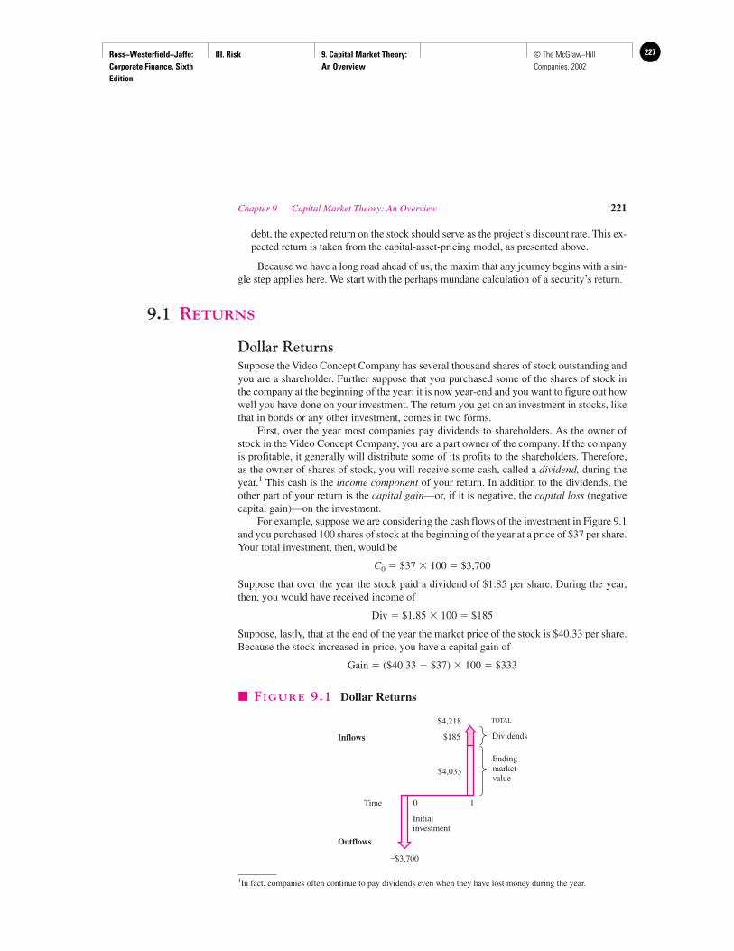
Ross−Westerfield−Jaffe: Corporate Finance, Sixth Edition
III. Risk 9. Capital Market Theory: An Overview
227© The McGraw−Hill Companies, 2002
Chapter 9 Capital Market Theory: An Overview 221
debt, the expected return on the stock should serve as the project’s discount rate. This ex-pected return is taken from the capital-asset-pricing model, as presented above.
Because we have a long road ahead of us, the maxim that any journey begins with a sin-gle step applies here. We start with the perhaps mundane calculation of a security’s return.
9.1 RETURNS
Dollar ReturnsSuppose the Video Concept Company has several thousand shares of stock outstanding andyou are a shareholder. Further suppose that you purchased some of the shares of stock inthe company at the beginning of the year; it is now year-end and you want to figure out howwell you have done on your investment. The return you get on an investment in stocks, likethat in bonds or any other investment, comes in two forms.
First, over the year most companies pay dividends to shareholders. As the owner ofstock in the Video Concept Company, you are a part owner of the company. If the companyis profitable, it generally will distribute some of its profits to the shareholders. Therefore,as the owner of shares of stock, you will receive some cash, called a dividend, during theyear.1 This cash is the income component of your return. In addition to the dividends, theother part of your return is the capital gain—or, if it is negative, the capital loss (negativecapital gain)—on the investment.
For example, suppose we are considering the cash flows of the investment in Figure 9.1and you purchased 100 shares of stock at the beginning of the year at a price of $37 per share.Your total investment, then, would be
C0 � $37 � 100 � $3,700
Suppose that over the year the stock paid a dividend of $1.85 per share. During the year,then, you would have received income of
Div � $1.85 � 100 � $185
Suppose, lastly, that at the end of the year the market price of the stock is $40.33 per share.Because the stock increased in price, you have a capital gain of
Gain � ($40.33 � $37) � 100 � $333
1In fact, companies often continue to pay dividends even when they have lost money during the year.
0Time
Initialinvestment
–$3,700
$4,033
$185
$4,218 TOTAL
Dividends
Endingmarketvalue
1
Inflows
Outflows
� FIGURE 9.1 Dollar Returns
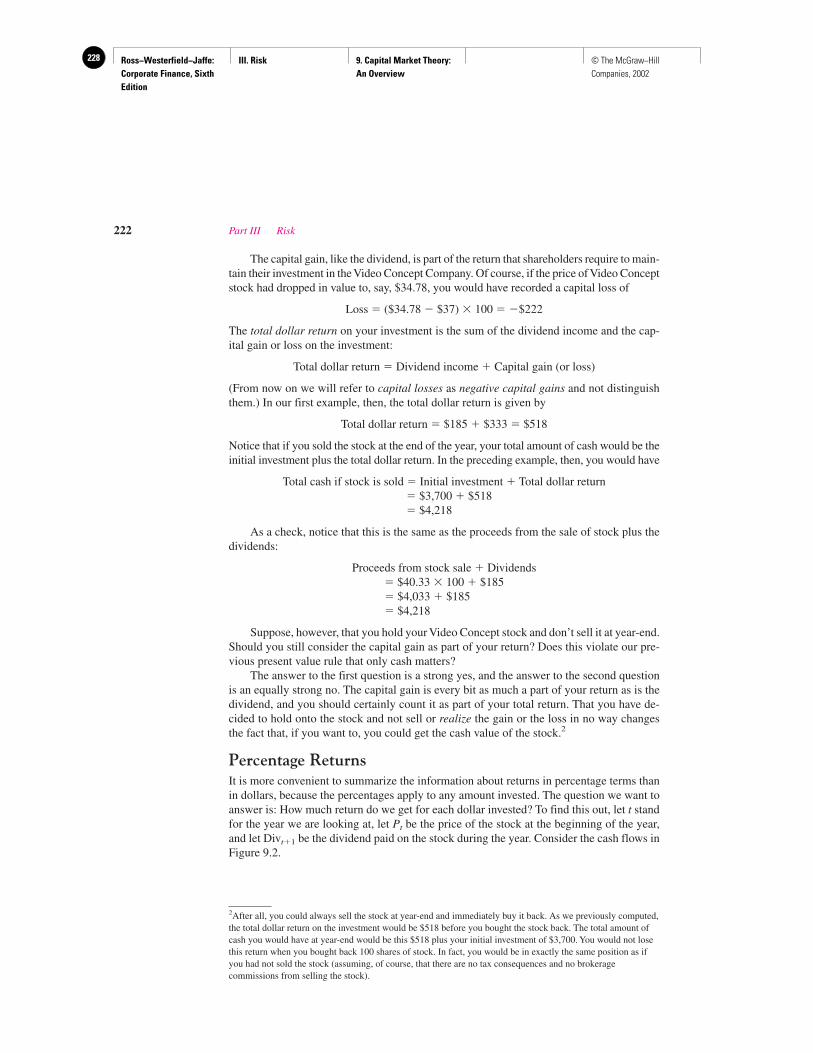
Ross−Westerfield−Jaffe: Corporate Finance, Sixth Edition
III. Risk 9. Capital Market Theory: An Overview
228 © The McGraw−Hill Companies, 2002
The capital gain, like the dividend, is part of the return that shareholders require to main-tain their investment in the Video Concept Company. Of course, if the price of Video Conceptstock had dropped in value to, say, $34.78, you would have recorded a capital loss of
Loss � ($34.78 � $37) � 100 � �$222
The total dollar return on your investment is the sum of the dividend income and the cap-ital gain or loss on the investment:
Total dollar return � Dividend income � Capital gain (or loss)
(From now on we will refer to capital losses as negative capital gains and not distinguishthem.) In our first example, then, the total dollar return is given by
Total dollar return � $185 � $333 � $518
Notice that if you sold the stock at the end of the year, your total amount of cash would be theinitial investment plus the total dollar return. In the preceding example, then, you would have
Total cash if stock is sold � Initial investment � Total dollar return� $3,700 � $518� $4,218
As a check, notice that this is the same as the proceeds from the sale of stock plus thedividends:
Proceeds from stock sale � Dividends� $40.33 � 100 � $185� $4,033 � $185� $4,218
Suppose, however, that you hold your Video Concept stock and don’t sell it at year-end.Should you still consider the capital gain as part of your return? Does this violate our pre-vious present value rule that only cash matters?
The answer to the first question is a strong yes, and the answer to the second questionis an equally strong no. The capital gain is every bit as much a part of your return as is thedividend, and you should certainly count it as part of your total return. That you have de-cided to hold onto the stock and not sell or realize the gain or the loss in no way changesthe fact that, if you want to, you could get the cash value of the stock.2
Percentage ReturnsIt is more convenient to summarize the information about returns in percentage terms thanin dollars, because the percentages apply to any amount invested. The question we want toanswer is: How much return do we get for each dollar invested? To find this out, let t standfor the year we are looking at, let Pt be the price of the stock at the beginning of the year,and let Divt�1 be the dividend paid on the stock during the year. Consider the cash flows inFigure 9.2.
222 Part III Risk
2After all, you could always sell the stock at year-end and immediately buy it back. As we previously computed,the total dollar return on the investment would be $518 before you bought the stock back. The total amount ofcash you would have at year-end would be this $518 plus your initial investment of $3,700. You would not losethis return when you bought back 100 shares of stock. In fact, you would be in exactly the same position as ifyou had not sold the stock (assuming, of course, that there are no tax consequences and no brokeragecommissions from selling the stock).
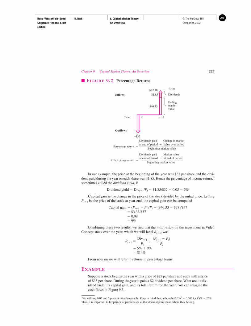
Ross−Westerfield−Jaffe: Corporate Finance, Sixth Edition
III. Risk 9. Capital Market Theory: An Overview
229© The McGraw−Hill Companies, 2002
In our example, the price at the beginning of the year was $37 per share and the divi-dend paid during the year on each share was $1.85. Hence the percentage of income return,3
sometimes called the dividend yield, is
Dividend yield � Divt�1/Pt � $1.85/$37 � 0.05 � 5%
Capital gain is the change in the price of the stock divided by the initial price. LettingPt�1 be the price of the stock at year-end, the capital gain can be computed
Capital gain � (Pt�1 � Pt)/Pt � ($40.33 � $37)/$37 � $3.33/$37� 0.09� 9%
Combining these two results, we find that the total return on the investment in VideoConcept stock over the year, which we will label Rt�1, was
� 5% � 9%� $14%
From now on we will refer to returns in percentage terms.
EXAMPLE
Suppose a stock begins the year with a price of $25 per share and ends with a priceof $35 per share. During the year it paid a $2 dividend per share. What are its div-idend yield, its capital gain, and its total return for the year? We can imagine thecash flows in Figure 9.3.
Rt�1 �Divt�1
Pt
��Pt�1 � Pt�
Pt
Chapter 9 Capital Market Theory: An Overview 223
Time
–$37
$40.33
$1.85
$42.18 TOTAL
Dividends
Endingmarketvalue
t �1
Inflows
Outflows
t
� FIGURE 9.2 Percentage Returns
Dividends paid Change in market
Percentage return
Dividends paid Market value
1 � Percentage return �at end of period � at end of period
Beginning market value
�at end of period � value over period
Beginning market value
3We will use 0.05 and 5 percent interchangeably. Keep in mind that, although (0.05)2 � 0.0025, (52)% � 25%.Thus, it is important to keep track of parentheses so that decimal points land where they belong.
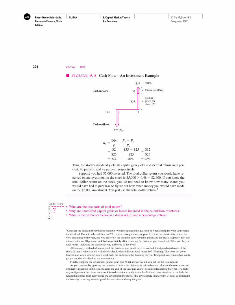
Ross−Westerfield−Jaffe: Corporate Finance, Sixth Edition
III. Risk 9. Capital Market Theory: An Overview
230 © The McGraw−Hill Companies, 2002
� 8% � 40% � 48%
Thus, the stock’s dividend yield, its capital gain yield, and its total return are 8 per-cent, 40 percent, and 48 percent, respectively.
Suppose you had $5,000 invested. The total dollar return you would have re-ceived on an investment in the stock is $5,000 � 0.48 � $2,400. If you know thetotal dollar return on the stock, you do not need to know how many shares youwould have had to purchase to figure out how much money you would have madeon the $5,000 investment. You just use the total dollar return.4
• What are the two parts of total return?• Why are unrealized capital gains or losses included in the calculation of returns?• What is the difference between a dollar return and a percentage return?
�$2
$25 �
$35 � $25
$25 �
$12
$25
R1 �Div1
P0
�P1 � P0
P0
224 Part III Risk
Time
$35
$2
TOTAL
Dividends (Div1)
Endingprice pershare (P1)
1
Cash inflows
Cash outflows
0
$37
–$25 (P0)
� FIGURE 9.3 Cash Flow—An Investment Example
4Consider the stock in the previous example. We have ignored the question of when during the year you receivethe dividend. Does it make a difference? To explore this question, suppose first that the dividend is paid at thevery beginning of the year, and you receive it the moment after you have purchased the stock. Suppose, too, thatinterest rates are 10 percent, and that immediately after receiving the dividend you loan it out. What will be yourtotal return, including the loan proceeds, at the end of the year?
Alternatively, instead of loaning out the dividend you could have reinvested it and purchased more of thestock. If that is what you do with the dividend, what will your total return be? (Warning: This does not go onforever, and when you buy more stock with the cash from the dividend on your first purchase, you are too late toget yet another dividend on the new stock.)
Finally, suppose the dividend is paid at year-end. What answer would you get for the total return?As you can see, by ignoring the question of when the dividend is paid when we calculate the return, we are
implicitly assuming that it is received at the end of the year and cannot be reinvested during the year. The rightway to figure out the return on a stock is to determine exactly when the dividend is received and to include thereturn that comes from reinvesting the dividend in the stock. This gives a pure stock return without confoundingthe issue by requiring knowledge of the interest rate during the year.
QUESTIONS
CO
NC
EP
T
?
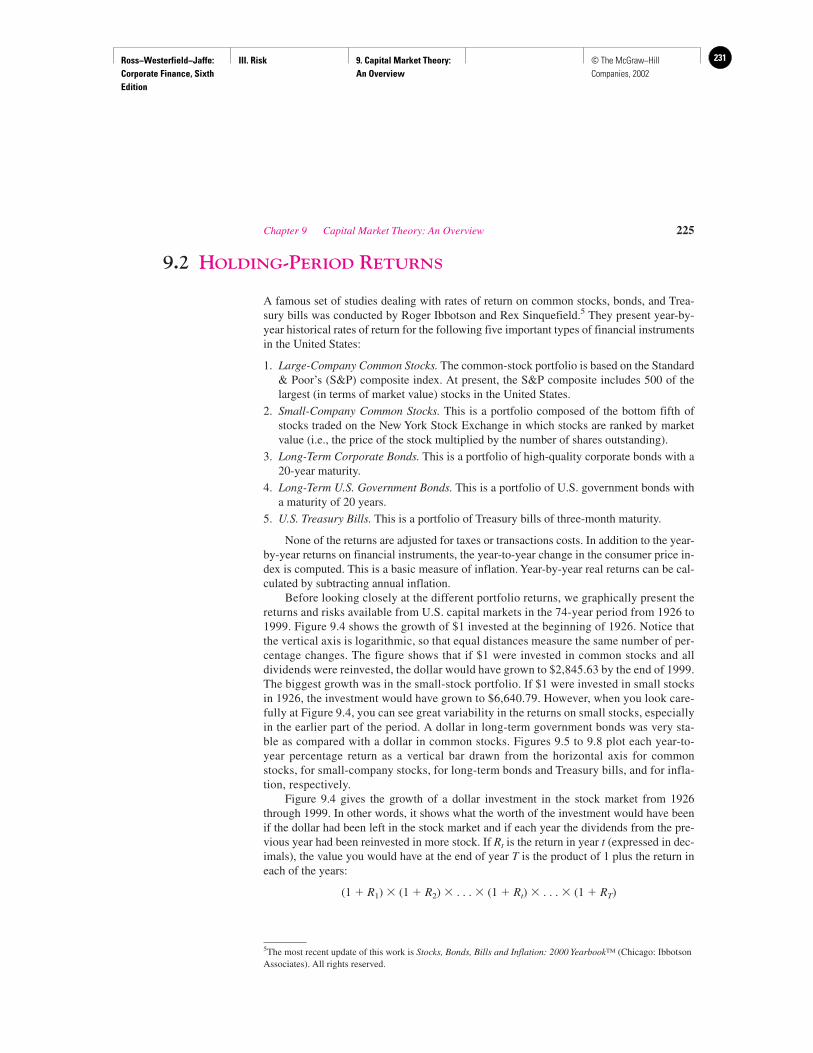
Ross−Westerfield−Jaffe: Corporate Finance, Sixth Edition
III. Risk 9. Capital Market Theory: An Overview
231© The McGraw−Hill Companies, 2002
9.2 HOLDING-PERIOD RETURNS
A famous set of studies dealing with rates of return on common stocks, bonds, and Trea-sury bills was conducted by Roger Ibbotson and Rex Sinquefield.5 They present year-by-year historical rates of return for the following five important types of financial instrumentsin the United States:
1. Large-Company Common Stocks. The common-stock portfolio is based on the Standard& Poor’s (S&P) composite index. At present, the S&P composite includes 500 of thelargest (in terms of market value) stocks in the United States.
2. Small-Company Common Stocks. This is a portfolio composed of the bottom fifth ofstocks traded on the New York Stock Exchange in which stocks are ranked by marketvalue (i.e., the price of the stock multiplied by the number of shares outstanding).
3. Long-Term Corporate Bonds. This is a portfolio of high-quality corporate bonds with a20-year maturity.
4. Long-Term U.S. Government Bonds. This is a portfolio of U.S. government bonds witha maturity of 20 years.
5. U.S. Treasury Bills. This is a portfolio of Treasury bills of three-month maturity.
None of the returns are adjusted for taxes or transactions costs. In addition to the year-by-year returns on financial instruments, the year-to-year change in the consumer price in-dex is computed. This is a basic measure of inflation. Year-by-year real returns can be cal-culated by subtracting annual inflation.
Before looking closely at the different portfolio returns, we graphically present thereturns and risks available from U.S. capital markets in the 74-year period from 1926 to1999. Figure 9.4 shows the growth of $1 invested at the beginning of 1926. Notice thatthe vertical axis is logarithmic, so that equal distances measure the same number of per-centage changes. The figure shows that if $1 were invested in common stocks and alldividends were reinvested, the dollar would have grown to $2,845.63 by the end of 1999.The biggest growth was in the small-stock portfolio. If $1 were invested in small stocksin 1926, the investment would have grown to $6,640.79. However, when you look care-fully at Figure 9.4, you can see great variability in the returns on small stocks, especiallyin the earlier part of the period. A dollar in long-term government bonds was very sta-ble as compared with a dollar in common stocks. Figures 9.5 to 9.8 plot each year-to-year percentage return as a vertical bar drawn from the horizontal axis for commonstocks, for small-company stocks, for long-term bonds and Treasury bills, and for infla-tion, respectively.
Figure 9.4 gives the growth of a dollar investment in the stock market from 1926through 1999. In other words, it shows what the worth of the investment would have beenif the dollar had been left in the stock market and if each year the dividends from the pre-vious year had been reinvested in more stock. If Rt is the return in year t (expressed in dec-imals), the value you would have at the end of year T is the product of 1 plus the return ineach of the years:
(1 � R1) � (1 � R2) � . . . � (1 � Rt) � . . . � (1 � RT)
Chapter 9 Capital Market Theory: An Overview 225
5The most recent update of this work is Stocks, Bonds, Bills and Inflation: 2000 Yearbook™ (Chicago: IbbotsonAssociates). All rights reserved.
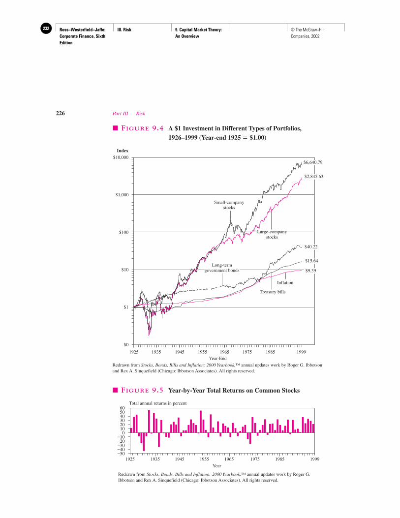
Ross−Westerfield−Jaffe: Corporate Finance, Sixth Edition
III. Risk 9. Capital Market Theory: An Overview
232 © The McGraw−Hill Companies, 2002
226 Part III Risk
$10,000
$1,000
$100
$10
$1
$0
1925
Index
1935 1945 1955 1965 1975 1985 1999Year-End
Long-termgovernment bonds
Small-companystocks
Large-companystocks
Treasury bills
Inflation
$6,640.79
$2,845.63
$40.22
$15.64
$9.39
� FIGURE 9.4 A $1 Investment in Different Types of Portfolios,1926–1999 (Year-end 1925 � $1.00)
Redrawn from Stocks, Bonds, Bills and Inflation: 2000 Yearbook,™ annual updates work by Roger G. Ibbotsonand Rex A. Sinquefield (Chicago: Ibbotson Associates). All rights reserved.
60
1925 1935 1945 1955 1965 1975 1985 1999
Year
50403020100
–10–20–30–40–50
Total annual returns in percent
� FIGURE 9.5 Year-by-Year Total Returns on Common Stocks
Redrawn from Stocks, Bonds, Bills and Inflation: 2000 Yearbook,™ annual updates work by Roger G.Ibbotson and Rex A. Sinquefield (Chicago: Ibbotson Associates). All rights reserved.
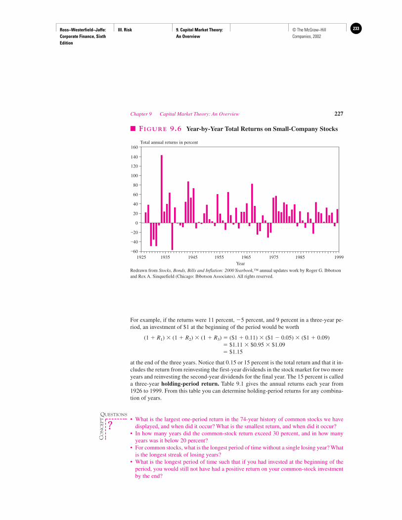
Ross−Westerfield−Jaffe: Corporate Finance, Sixth Edition
III. Risk 9. Capital Market Theory: An Overview
233© The McGraw−Hill Companies, 2002
For example, if the returns were 11 percent, �5 percent, and 9 percent in a three-year pe-riod, an investment of $1 at the beginning of the period would be worth
(1 � R1) � (1 � R2) � (1 � R3) � ($1 � 0.11) � ($1 � 0.05) � ($1 � 0.09)� $1.11 � $0.95 � $1.09� $1.15
at the end of the three years. Notice that 0.15 or 15 percent is the total return and that it in-cludes the return from reinvesting the first-year dividends in the stock market for two moreyears and reinvesting the second-year dividends for the final year. The 15 percent is calleda three-year holding-period return. Table 9.1 gives the annual returns each year from1926 to 1999. From this table you can determine holding-period returns for any combina-tion of years.
• What is the largest one-period return in the 74-year history of common stocks we havedisplayed, and when did it occur? What is the smallest return, and when did it occur?
• In how many years did the common-stock return exceed 30 percent, and in how manyyears was it below 20 percent?
• For common stocks, what is the longest period of time without a single losing year? Whatis the longest streak of losing years?
• What is the longest period of time such that if you had invested at the beginning of theperiod, you would still not have had a positive return on your common-stock investmentby the end?
Chapter 9 Capital Market Theory: An Overview 227
160
140
120
100
80
60
40
20
0
–20
–40
–601935 1945 1955 1965 1975 1985 19991925
Total annual returns in percent
Year
� FIGURE 9.6 Year-by-Year Total Returns on Small-Company Stocks
Redrawn from Stocks, Bonds, Bills and Inflation: 2000 Yearbook,™ annual updates work by Roger G. Ibbotsonand Rex A. Sinquefield (Chicago: Ibbotson Associates). All rights reserved.
QUESTIONS
CO
NC
EP
T
?
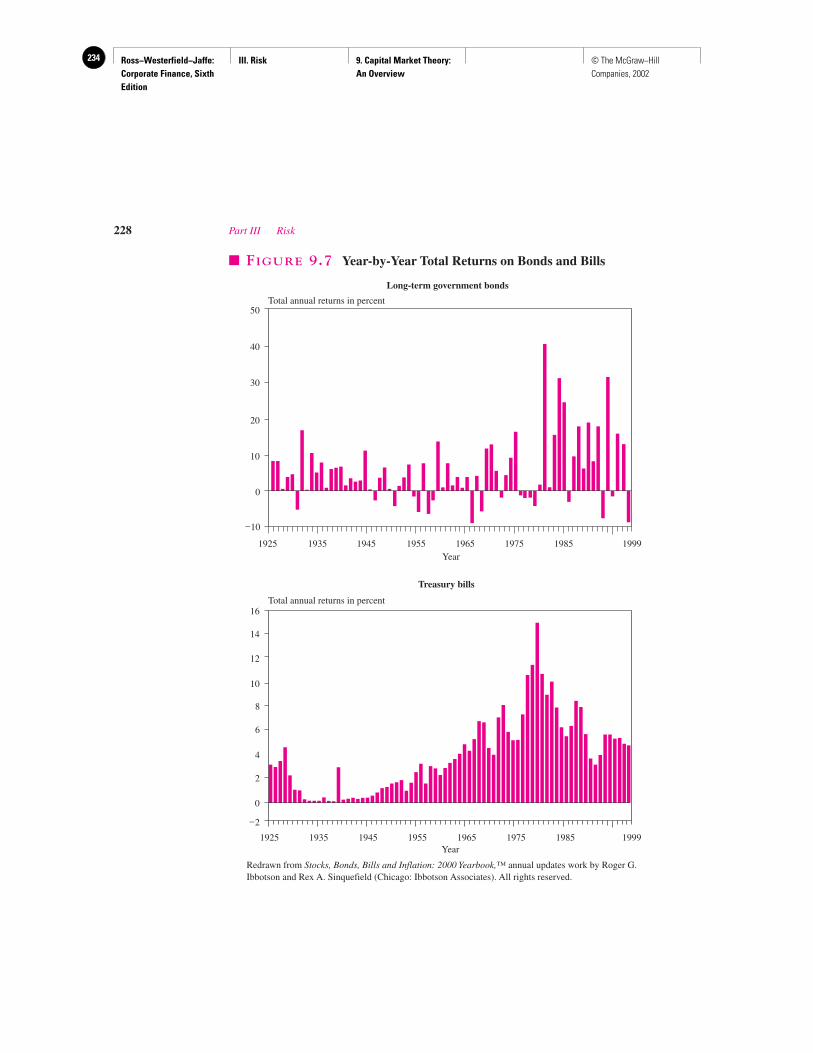
Ross−Westerfield−Jaffe: Corporate Finance, Sixth Edition
III. Risk 9. Capital Market Theory: An Overview
234 © The McGraw−Hill Companies, 2002
228 Part III Risk
Total annual returns in percent50
40
30
20
10
0
–10
1925 1935 1945 1955 1965 1975 1985 1999Year
1999
Long-term government bonds
Treasury bills
Total annual returns in percent16
12
10
4
0
–2
1925 1935 1945 1955 1965 1975 1985Year
2
6
8
14
� FIGURE 9.7 Year-by-Year Total Returns on Bonds and Bills
Redrawn from Stocks, Bonds, Bills and Inflation: 2000 Yearbook,™ annual updates work by Roger G.Ibbotson and Rex A. Sinquefield (Chicago: Ibbotson Associates). All rights reserved.
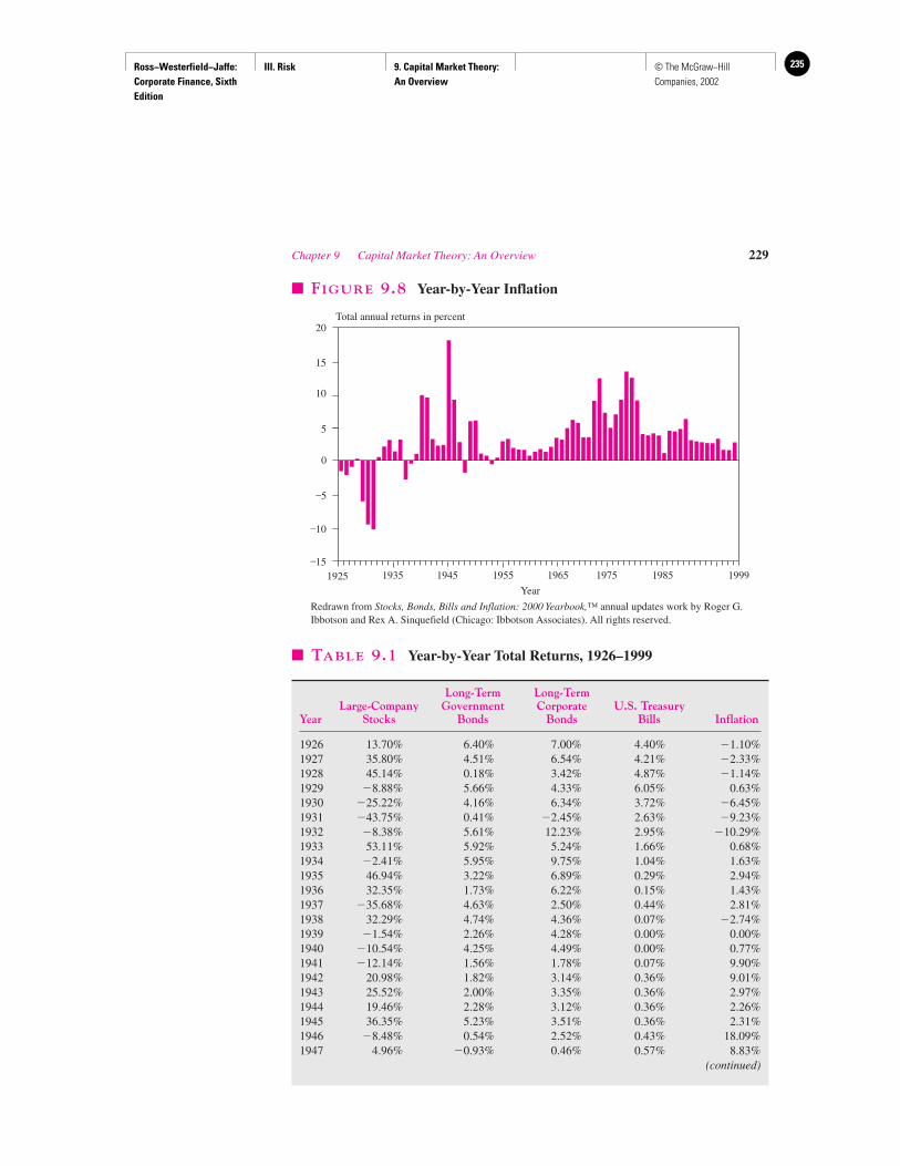
Ross−Westerfield−Jaffe: Corporate Finance, Sixth Edition
III. Risk 9. Capital Market Theory: An Overview
235© The McGraw−Hill Companies, 2002
Chapter 9 Capital Market Theory: An Overview 229
Total annual returns in percent
–15
0
5
10
15
20
1935 1945 1955 1965 1975 1985 19991925Year
–10
–5
� FIGURE 9.8 Year-by-Year Inflation
Redrawn from Stocks, Bonds, Bills and Inflation: 2000 Yearbook,™ annual updates work by Roger G.Ibbotson and Rex A. Sinquefield (Chicago: Ibbotson Associates). All rights reserved.
� TABLE 9.1 Year-by-Year Total Returns, 1926–1999
Long-Term Long-TermLarge-Company Government Corporate U.S. Treasury
Year Stocks Bonds Bonds Bills Inflation
1926 13.70% 6.40% 7.00% 4.40% �1.10%1927 35.80% 4.51% 6.54% 4.21% �2.33%1928 45.14% 0.18% 3.42% 4.87% �1.14%1929 �8.88% 5.66% 4.33% 6.05% 0.63%1930 �25.22% 4.16% 6.34% 3.72% �6.45%1931 �43.75% 0.41% �2.45% 2.63% �9.23%1932 �8.38% 5.61% 12.23% 2.95% �10.29%1933 53.11% 5.92% 5.24% 1.66% 0.68%1934 �2.41% 5.95% 9.75% 1.04% 1.63%1935 46.94% 3.22% 6.89% 0.29% 2.94%1936 32.35% 1.73% 6.22% 0.15% 1.43%1937 �35.68% 4.63% 2.50% 0.44% 2.81%1938 32.29% 4.74% 4.36% 0.07% �2.74%1939 �1.54% 2.26% 4.28% 0.00% 0.00%1940 �10.54% 4.25% 4.49% 0.00% 0.77%1941 �12.14% 1.56% 1.78% 0.07% 9.90%1942 20.98% 1.82% 3.14% 0.36% 9.01%1943 25.52% 2.00% 3.35% 0.36% 2.97%1944 19.46% 2.28% 3.12% 0.36% 2.26%1945 36.35% 5.23% 3.51% 0.36% 2.31%1946 �8.48% 0.54% 2.52% 0.43% 18.09%1947 4.96% �0.93% 0.46% 0.57% 8.83%
(continued)
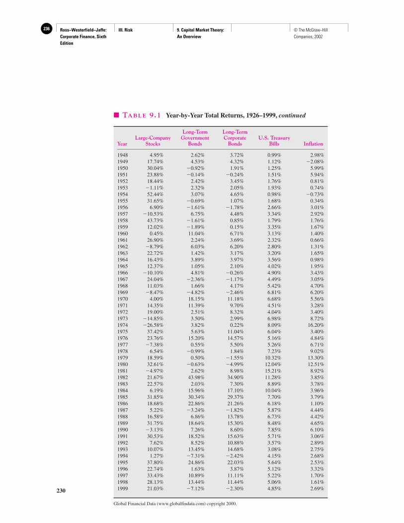
Ross−Westerfield−Jaffe: Corporate Finance, Sixth Edition
III. Risk 9. Capital Market Theory: An Overview
236 © The McGraw−Hill Companies, 2002
230
� TABLE 9.1 Year-by-Year Total Returns, 1926–1999, continued
Long-Term Long-TermLarge-Company Government Corporate U.S. Treasury
Year Stocks Bonds Bonds Bills Inflation
1948 4.95% 2.62% 3.72% 0.99% 2.98%1949 17.74% 4.53% 4.32% 1.12% �2.08%1950 30.04% �0.92% 1.91% 1.25% 5.99%1951 23.88% �0.14% �0.24% 1.51% 5.94%1952 18.44% 2.42% 3.45% 1.76% 0.81%1953 �1.11% 2.32% 2.05% 1.93% 0.74%1954 52.44% 3.07% 4.65% 0.98% �0.73%1955 31.65% �0.69% 1.07% 1.68% 0.34%1956 6.90% �1.61% �1.78% 2.66% 3.01%1957 �10.53% 6.75% 4.48% 3.34% 2.92%1958 43.73% �1.61% 0.85% 1.79% 1.76%1959 12.02% �1.89% 0.15% 3.35% 1.67%1960 0.45% 11.04% 6.71% 3.13% 1.40%1961 26.90% 2.24% 3.69% 2.32% 0.66%1962 �8.79% 6.03% 6.20% 2.80% 1.31%1963 22.72% 1.42% 3.17% 3.20% 1.65%1964 16.43% 3.89% 3.97% 3.56% 0.98%1965 12.37% 1.05% 2.10% 4.02% 1.95%1966 �10.10% 4.81% �0.26% 4.90% 3.43%1967 24.04% �2.36% �1.17% 4.49% 3.05%1968 11.03% 1.66% 4.17% 5.42% 4.70%1969 �8.47% �4.82% �2.46% 6.81% 6.20%1970 4.00% 18.15% 11.18% 6.68% 5.56%1971 14.35% 11.39% 9.70% 4.51% 3.28%1972 19.00% 2.51% 8.32% 4.04% 3.40%1973 �14.85% 3.50% 2.99% 6.98% 8.72%1974 �26.58% 3.82% 0.22% 8.09% 16.20%1975 37.42% 5.63% 11.04% 6.04% 3.40%1976 23.76% 15.20% 14.57% 5.16% 4.84%1977 �7.38% 0.55% 5.50% 5.26% 6.71%1978 6.54% �0.99% 1.84% 7.23% 9.02%1979 18.59% 0.50% �1.55% 10.32% 13.30%1980 32.61% �0.63% �4.99% 12.04% 12.51%1981 �4.97% 2.62% 8.98% 15.21% 8.92%1982 21.67% 43.98% 34.90% 11.28% 3.85%1983 22.57% 2.03% 7.30% 8.89% 3.78%1984 6.19% 15.96% 17.10% 10.04% 3.96%1985 31.85% 30.34% 29.37% 7.70% 3.79%1986 18.68% 22.86% 21.26% 6.18% 1.10%1987 5.22% �3.24% �1.82% 5.87% 4.44%1988 16.58% 6.86% 13.78% 6.73% 4.42%1989 31.75% 18.64% 15.30% 8.48% 4.65%1990 �3.13% 7.26% 8.60% 7.85% 6.10%1991 30.53% 18.52% 15.63% 5.71% 3.06%1992 7.62% 8.52% 10.88% 3.57% 2.89%1993 10.07% 13.45% 14.68% 3.08% 2.75%1994 1.27% �7.31% �2.42% 4.15% 2.68%1995 37.80% 24.86% 22.03% 5.64% 2.53%1996 22.74% 1.63% 3.87% 5.12% 3.32%1997 33.43% 10.89% 11.11% 5.22% 1.70%1998 28.13% 13.44% 11.44% 5.06% 1.61%1999 21.03% �7.12% �2.30% 4.85% 2.69%
Global Financial Data (www.globalfindata.com) copyright 2000.
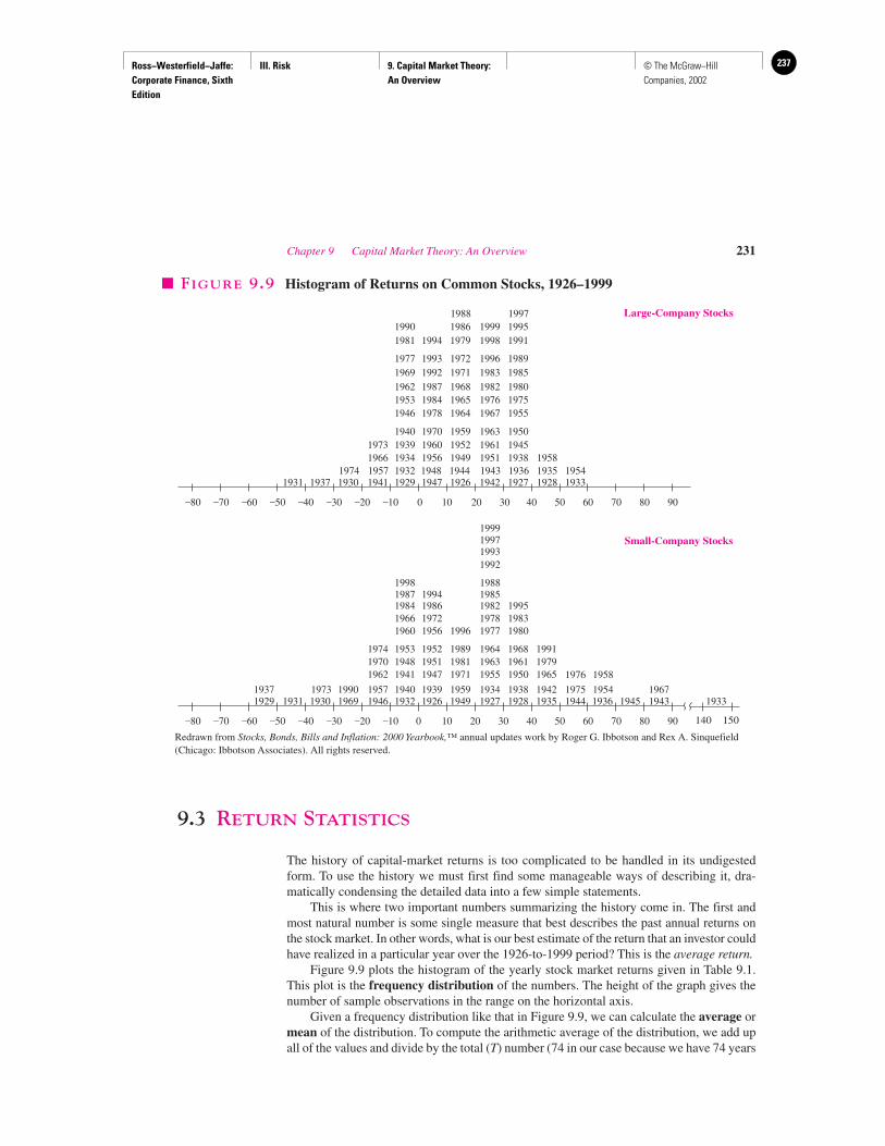
Ross−Westerfield−Jaffe: Corporate Finance, Sixth Edition
III. Risk 9. Capital Market Theory: An Overview
237© The McGraw−Hill Companies, 2002
9.3 RETURN STATISTICS
The history of capital-market returns is too complicated to be handled in its undigestedform. To use the history we must first find some manageable ways of describing it, dra-matically condensing the detailed data into a few simple statements.
This is where two important numbers summarizing the history come in. The first andmost natural number is some single measure that best describes the past annual returns onthe stock market. In other words, what is our best estimate of the return that an investor couldhave realized in a particular year over the 1926-to-1999 period? This is the average return.
Figure 9.9 plots the histogram of the yearly stock market returns given in Table 9.1.This plot is the frequency distribution of the numbers. The height of the graph gives thenumber of sample observations in the range on the horizontal axis.
Given a frequency distribution like that in Figure 9.9, we can calculate the average ormean of the distribution. To compute the arithmetic average of the distribution, we add upall of the values and divide by the total (T) number (74 in our case because we have 74 years
Chapter 9 Capital Market Theory: An Overview 231
Small-Company Stocks
Large-Company Stocks
–10 0–20–30–40–50–60–70–80 10 20 30 40 50 60 70 80 90
1931 1937 1930 1941 1929 1947 1926 1942 1927 1928 19331974 1957 1932 1948 1944 1943 1936 1935 1954
1966 1934 1956 1949 1951 1938 19581939 19601973 1952 1961 19451940 1970 1959 1963 1950
1946 1978 1964 1967 19551953 1984 1965 1976 19751962 1987 1968 1982 19801969 1992 1971 1983 19851977 1993 1972 1996
19981999
1989
1981 1994 1979 19911990 1986 1995
1988 1997
–10 0–20–30–40–50–60–70–80 10 20 30 40 50 60 70 80 90
1931 1930 1969 1946 1932 1926 1949 1927 1928 1935 19441957 1940 1939 1959 1934 1938 1942 1975
1962 1941 1947 1971 1955 1950 19651948 19511970 1981 1963 19611953 1952 1989 1964 1968
1960 1956 1996 1977 19801966 1972 1978 19831984 1986 1982 199519871998
1994 19851988
150140
1929 1936 1945 1943 19331937 1973 1954 1967
197419791991
1992199319971999
1976 1958
1990
� FIGURE 9.9 Histogram of Returns on Common Stocks, 1926–1999
Redrawn from Stocks, Bonds, Bills and Inflation: 2000 Yearbook,™ annual updates work by Roger G. Ibbotson and Rex A. Sinquefield(Chicago: Ibbotson Associates). All rights reserved.
Ross−Westerfield−Jaffe: Corporate Finance, Sixth Edition
III. Risk 9. Capital Market Theory: An Overview
238 © The McGraw−Hill Companies, 2002
of data). The bar over the R is used to represent the mean, and the formula is the ordinaryformula for the average:
The arithmetic mean of the 74 annual returns from 1926 to 1999 is 13.3 percent.
EXAMPLE
The returns on common stock from 1926 to 1929 are 0.1370, 0.3580, 0.4514, and�0.0888, respectively. (These numbers are taken from Table 9.1.) The average, ormean, return over these four years is
9.4 AVERAGE STOCK RETURNS AND RISK-FREE RETURNS
Now that we have computed the average return on the stock market, it seems sensible tocompare it with the returns on other securities. The most obvious comparison is with thelow-variability returns in the government-bond market. These are free of most of the volatil-ity we see in the stock market.
The government borrows money by issuing bonds, which the investing public holds.As we discussed in an earlier chapter, these bonds come in many forms, and the ones wewill look at here are called Treasury bills, or T-bills. Once a week the government sells somebills at an auction. A typical bill is a pure discount bond that will mature in a year or less.Because the government can raise taxes to pay for the debt it incurs—a trick that many ofus would like to be able to perform—this debt is virtually free of the risk of default. Thuswe will call this the risk-free return over a short time (one year or less).6
An interesting comparison, then, is between the virtually risk-free return on T-bills andthe very risky return on common stocks. This difference between risky returns and risk-freereturns is often called the excess return on the risky asset. It is called excess because it isthe additional return resulting from the riskiness of common stocks and is interpreted as arisk premium.
Table 9.2 shows the average stock return, bond return, T-bill return, and inflation ratefor the period from 1926 through 1999. From this we can derive excess returns. The averageexcess return from common stocks for the entire period was 9.5 percent (13.3% � 3.8%).
One of the most significant observations of stock market data is this long-run excess ofthe stock return over the risk-free return. An investor for this period was rewarded for in-vestment in the stock market with an extra or excess return over what would have beenachieved by simply investing in T-bills.
Why was there such a reward? Does it mean that it never pays to invest in T-bills andthat someone who invested in them instead of in the stock market needs a course in finance?A complete answer to these questions lies at the heart of modern finance, and Chapter 10is devoted entirely to this. However, part of the answer can be found in the variability of the
R �0.1370 � 0.3580 � 0.4514 � 0.0888
4� 0.2144
Mean � R ��R1 � . . . � RT�
T
232 Part III Risk
6A Treasury bill with a 90-day maturity is risk-free only during that particular time period.
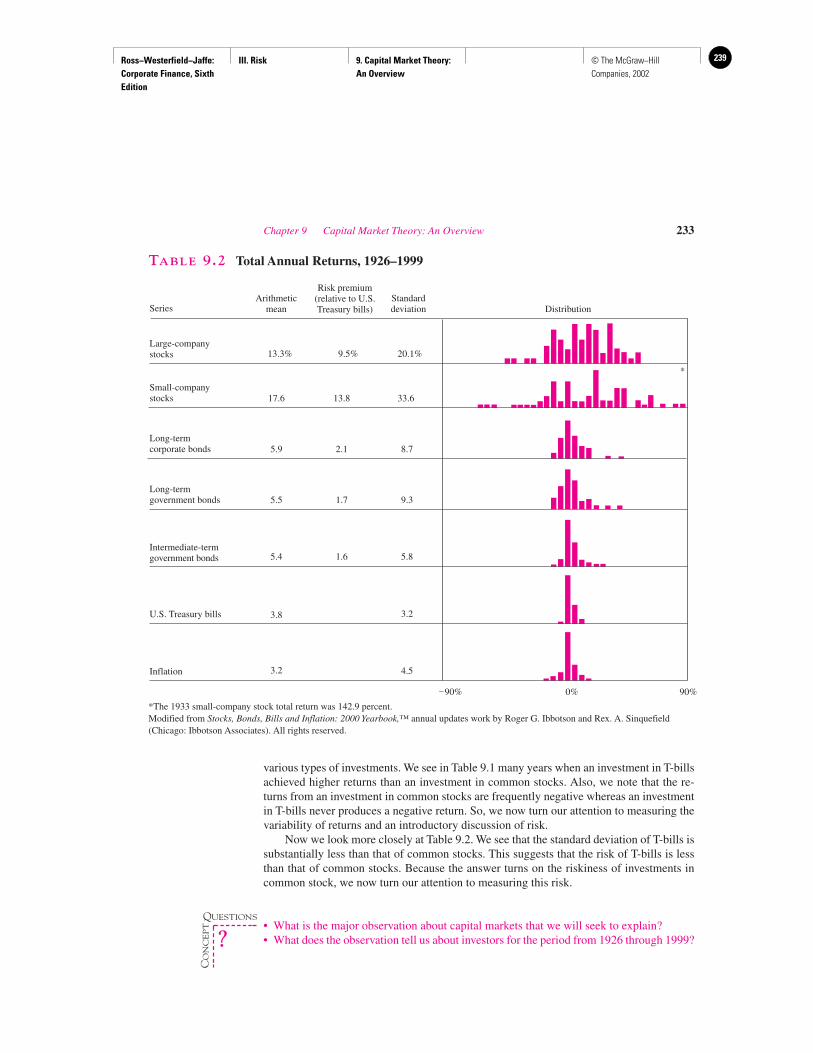
Ross−Westerfield−Jaffe: Corporate Finance, Sixth Edition
III. Risk 9. Capital Market Theory: An Overview
239© The McGraw−Hill Companies, 2002
various types of investments. We see in Table 9.1 many years when an investment in T-billsachieved higher returns than an investment in common stocks. Also, we note that the re-turns from an investment in common stocks are frequently negative whereas an investmentin T-bills never produces a negative return. So, we now turn our attention to measuring thevariability of returns and an introductory discussion of risk.
Now we look more closely at Table 9.2. We see that the standard deviation of T-bills issubstantially less than that of common stocks. This suggests that the risk of T-bills is lessthan that of common stocks. Because the answer turns on the riskiness of investments incommon stock, we now turn our attention to measuring this risk.
• What is the major observation about capital markets that we will seek to explain?• What does the observation tell us about investors for the period from 1926 through 1999?
Chapter 9 Capital Market Theory: An Overview 233
Series
Large-companystocks
Small-companystocks
Long-termcorporate bonds
Long-termgovernment bonds
Intermediate-termgovernment bonds
U.S. Treasury bills
Inflation
Arithmeticmean
Risk premium(relative to U.S.Treasury bills)
Standarddeviation
13.3%
17.6
5.9
5.5
5.4
3.8
3.2
13.8
2.1
1.7
1.6
9.5% 20.1%
33.6
8.7
9.3
5.8
3.2
4.5
Distribution
–90% 0% 90%
*
TABLE 9.2 Total Annual Returns, 1926–1999
*The 1933 small-company stock total return was 142.9 percent.Modified from Stocks, Bonds, Bills and Inflation: 2000 Yearbook,™ annual updates work by Roger G. Ibbotson and Rex. A. Sinquefield(Chicago: Ibbotson Associates). All rights reserved.
QUESTIONS
CO
NC
EP
T
?
Ross−Westerfield−Jaffe: Corporate Finance, Sixth Edition
III. Risk 9. Capital Market Theory: An Overview
240 © The McGraw−Hill Companies, 2002
9.5 RISK STATISTICS
The second number that we use to characterize the distribution of returns is a measure ofthe risk in returns. There is no universally agreed-upon definition of risk. One way to thinkabout the risk of returns on common stock is in terms of how spread out the frequency dis-tribution in Figure 9.9 is.7 The spread, or dispersion, of a distribution is a measure of howmuch a particular return can deviate from the mean return. If the distribution is very spreadout, the returns that will occur are very uncertain. By contrast, a distribution whose returnsare all within a few percentage points of each other is tight, and the returns are less uncer-tain. The measures of risk we will discuss are variance and standard deviation.
VarianceThe variance and its square root, the standard deviation, are the most common measuresof variability or dispersion. We will use Var and �2 to denote the variance and SD and � torepresent the standard deviation. � is, of course, the Greek letter sigma.
EXAMPLE
The returns on common stocks from 1926 to 1929 are (in decimals) 0.1370, 0.3580,0.4514, and �0.0888, respectively. The variance of this sample is computed as
0.0582 � 1⁄3[(0.1370 � 0.2144)2 � (0.3580 � 0.2144)2 �(0.4514 � 0.2144)2 � (�0.0888 � 0.2144)2]
SD � � 0.2413 (i.e., 24.13%)
This formula tells us just what to do: Take the T individual returns (R1, R2, . . .) and subtractthe average return , square the result, and add them up. Finally, this total must be dividedby the number of returns less one (T � 1). The standard deviation is always just the squareroot of the variance.
Using the actual stock returns in Table 9.1 for the 74-year period from 1926 through1999 in the above formula, the resulting standard deviation of stock returns is 20.1 percent.The standard deviation is the standard statistical measure of the spread of a sample, and itwill be the measure we use most of the time. Its interpretation is facilitated by a discussionof the normal distribution.
Normal Distribution and Its Implications for Standard DeviationA large enough sample drawn from a normal distribution looks like the bell-shaped curvedrawn in Figure 9.10. As you can see, this distribution is symmetric about its mean, notskewed, and it has a much cleaner shape than the actual distribution of yearly returns drawn
R
�0.0582
Var �1
T � 1 �R1 � R� 2 � �R2 � R� 2 � �R3 � R� 2 � �R4 � R� 2
234 Part III Risk
7Several condensed frequency distributions are also in the extreme right column of Table 9.2.
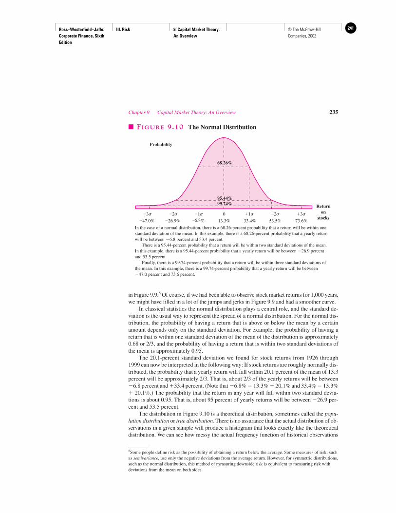
Ross−Westerfield−Jaffe: Corporate Finance, Sixth Edition
III. Risk 9. Capital Market Theory: An Overview
241© The McGraw−Hill Companies, 2002
in Figure 9.9.8 Of course, if we had been able to observe stock market returns for 1,000 years,we might have filled in a lot of the jumps and jerks in Figure 9.9 and had a smoother curve.
In classical statistics the normal distribution plays a central role, and the standard de-viation is the usual way to represent the spread of a normal distribution. For the normal dis-tribution, the probability of having a return that is above or below the mean by a certainamount depends only on the standard deviation. For example, the probability of having areturn that is within one standard deviation of the mean of the distribution is approximately0.68 or 2/3, and the probability of having a return that is within two standard deviations ofthe mean is approximately 0.95.
The 20.1-percent standard deviation we found for stock returns from 1926 through1999 can now be interpreted in the following way: If stock returns are roughly normally dis-tributed, the probability that a yearly return will fall within 20.1 percent of the mean of 13.3percent will be approximately 2/3. That is, about 2/3 of the yearly returns will be between�6.8 percent and �33.4 percent. (Note that �6.8% � 13.3% � 20.1% and 33.4% � 13.3%� 20.1%.) The probability that the return in any year will fall within two standard devia-tions is about 0.95. That is, about 95 percent of yearly returns will be between �26.9 per-cent and 53.5 percent.
The distribution in Figure 9.10 is a theoretical distribution, sometimes called the popu-lation distribution or true distribution. There is no assurance that the actual distribution of ob-servations in a given sample will produce a histogram that looks exactly like the theoreticaldistribution. We can see how messy the actual frequency function of historical observations
Chapter 9 Capital Market Theory: An Overview 235
8Some people define risk as the possibility of obtaining a return below the average. Some measures of risk, suchas semivariance, use only the negative deviations from the average return. However, for symmetric distributions,such as the normal distribution, this method of measuring downside risk is equivalent to measuring risk withdeviations from the mean on both sides.
Probability
Returnon
stocks–3� –2� –1�
–47.0% –26.9% –6.8% 13.3%
0 �1� �2� �3�
33.4% 53.5% 73.6%
68.26%
95.44%99.74%
� FIGURE 9.10 The Normal Distribution
In the case of a normal distribution, there is a 68.26-percent probability that a return will be within onestandard deviation of the mean. In this example, there is a 68.26-percent probability that a yearly returnwill be between �6.8 percent and 33.4 percent.
There is a 95.44-percent probability that a return will be within two standard deviations of the mean.In this example, there is a 95.44-percent probability that a yearly return will be between �26.9 percentand 53.5 percent.
Finally, there is a 99.74-percent probability that a return will be within three standard deviations ofthe mean. In this example, there is a 99.74-percent probability that a yearly return will be between�47.0 percent and 73.6 percent.
Ross−Westerfield−Jaffe: Corporate Finance, Sixth Edition
III. Risk 9. Capital Market Theory: An Overview
242 © The McGraw−Hill Companies, 2002
236 Part III Risk
is by observing Figure 9.9. If we were to keep on generating observations for a long enoughperiod of time, however, the aberrations in the sample would disappear, and the actual histor-ical distribution would start to look like the underlying theoretical distribution.
This points out that sampling error exists in any individual sample. In other words, thedistribution of the sample only approximates the true distribution: we always measure thetruth with some error. For example, we do not know what the true expected return was forcommon stocks in the 74-year history. However, we are sure that our 13.3 percent realizedreturn is very close to it.
• What is the definition of sample estimates of variance and standard deviation?• How does the normal distribution help us interpret standard deviation?
9.6 SUMMARY AND CONCLUSIONS
1. This chapter presents returns for a number of different asset classes. The general conclusionis that stocks have outperformed bonds over most of the 20th century, though stocks havealso exhibited more risk.
2. The statistical measures in this chapter are necessary building blocks for the material of thenext three chapters. In particular, standard deviation and variance measure the variability ofthe return on an individual security and on portfolios of securities. In the next chapter, wewill argue that standard deviation and variance are appropriate measures of the risk of anindividual security if an investor’s portfolio is composed of that security only.
KEY TERMS
Average (mean) 231 Normal distribution 234Capital gain 223 Risk premium 232Frequency distribution 231 Standard deviation 234Holding-period return 227 Variance 234
SUGGESTED READINGS
An important record of the performance of financial instruments in the U.S. capital markets canbe found in:Ibbotson, Roger G., and Rex A. Sinquefield. Stocks, Bonds, Bills and Inflation: 2000 Yearbook.™
Chicago: Ibbotson Associates.
What is the equity risk premium? This is the question addressed by:Cornell, Bradford. The Equity Risk Premium: The Long Term Future of the Stock Market. New York:
John Wiley, 1999 and Shiller, Robert S. Irrational Exuberance. Princeton, N.J.: PrincetonUniversity Press, 2000.
For a look at market risk premiums worldwide, see:Jorion, P., and W. N. Goetzmann, “Global Stock Markets in the Twentieth Century.” Journal of
Finance 54 (1999).
QUESTIONS
CO
NC
EP
T
?

Ross−Westerfield−Jaffe: Corporate Finance, Sixth Edition
III. Risk 9. Capital Market Theory: An Overview
243© The McGraw−Hill Companies, 2002
QUESTIONS AND PROBLEMS
Returns9.1 Last year, you bought 500 shares of Twedt El Dee stock at $37 per share. You have received
total dividends of $1,000 during the year. Currently, Twedt El Dee stock sells for $38.a. How much did you earn in capital gains?b. What was your total dollar return?c. What was your percentage return?d. Must you sell the Twedt El Dee stock to include the capital gains in your return?
Explain.
9.2 Mr. Alexander Bell invested $10,400 in 200 shares of First Industries stock a year ago and has received total dividends of $600 during the period. He sold the stock todayat $54.25.a. What was his total dollar return?b. What was his capital gain?c. What was his percentage return?d. What was the stock’s dividend yield?
9.3 Suppose a stock had an initial price of $42 per share. During the year, the stock paid adividend of $2.40 per share. At the end of the year, the price is $31 per share. What is thepercentage return on this stock?
9.4 Lydian Stock currently sells for $52 per share. You intend to buy the stock today and hold itfor two years. During those two years, you expect to receive dividends at the year-ends thattotal $5.50 per share. Finally, you expect to sell the Lydian stock for $54.75 per share. Whatis your expected holding-period return on Lydian stock?
9.5 Use the information from Ibbotson and Sinquefield provided in the text to compute thenominal and real annual returns from 1926 to 1997 for each of the following items.a. Common stockb. Long-term corporate bondsc. Long-term government bondsd. U.S. Treasury bills
9.6 Suppose the current interest rate on U.S. Treasury bills is 6.2 percent. Ibbotson andSinquefield found the average return on Treasury bills from 1926 through 1997 to be 3.8percent. The average return on common stock during the same period was 13.0 percent.Given this information, what is the current expected return on common stocks?
9.7 Two stocks, Koke and Pepsee, had the same prices two years ago. During the last two years,Koke’s stock price had first increased by 10 percent and then dropped by 10 percent, whilePepsee’s stock price had first dropped by 10 percent and then increased by 10 percent. Dothese two stocks have the same prices today? Explain.
9.8 S&P 500 index returns of common stocks for the period 1981–1985 are as follows.Calculate the five-year holding-period return.
1981 1982 1983 1984 1985
S&P 500 index return (%) �4.91 21.41 22.51 6.27 32.16
9.9 The Wall Street Journal announced yesterday that the current rate for one-year Treasurybills is 4.36 percent, while an Ibbotson and Sinquefield study shows that the average returnon Treasury bills for the period 1926–1997 is 3.8 percent. During the same period theaverage return on long-term corporate bonds is 6.1 percent. What is the risk premium of thelong-term corporate bonds? What is the expected return on the market of long-termcorporate bonds?
Chapter 9 Capital Market Theory: An Overview 237

Ross−Westerfield−Jaffe: Corporate Finance, Sixth Edition
III. Risk 9. Capital Market Theory: An Overview
244 © The McGraw−Hill Companies, 2002
Average Returns, Expected Returns, and Variance9.10 During the past seven years, the returns on a portfolio of long-term corporate bonds were
the following:
Year Long-Term Corporate Bonds
�7 �2.6%�6 �1.0�5 43.8�4 4.7�3 16.4�2 30.1Last 19.9
a. Calculate the average return for long-term corporate bonds over this period.b. Calculate the variance and the standard deviation of the returns for long-term corporate
bonds during this period.
9.11 The following are the returns during the past seven years on a market portfolio of commonstocks and on Treasury bills.
Common TreasuryYear Stocks Bills
�7 32.4% 11.2%�6 �4.9 14.7�5 21.4 10.5�4 22.5 8.8�3 6.3 9.9�2 32.2 7.7Last 18.5 6.2
The realized risk premium is the return on the common stocks less the return on theTreasury bills.a. Calculate the realized risk premium of common stocks over T-bills in each year.b. Calculate the average risk premium of common stocks over T-bills during the
period.c. Is it possible that this observed risk premium can be negative? Explain.
9.12 The probability that the economy will experience moderate growth next year is 0.6. Theprobability of a recession is 0.2, and the probability of a rapid expansion is also 0.2. If theeconomy falls into a recession, you can expect to receive a return on your portfolio of 5percent. With moderate growth your return will be 8 percent. If there is a rapid expansion,your portfolio will return 15 percent.a. What is your expected return?b. What is the standard deviation of that return?
9.13 The probability that the economy will experience moderate growth next year is 0.4. Theprobability of a recession is 0.3, and the probability of a rapid expansion is also 0.3. If theeconomy falls into a recession, you can expect to receive a return on your portfolio of 2percent. With moderate growth your return will be 5 percent. If there is a rapid expansion,your portfolio will return 10 percent.a. What is your expected return?b. What is the standard deviation of that return?
9.14 The returns on the market and on Trebli stock are shown below for the five possible statesof the economy that might prevail next year.
238 Part III Risk
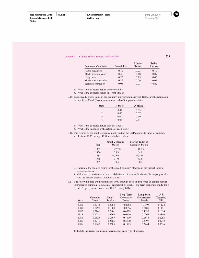
Ross−Westerfield−Jaffe: Corporate Finance, Sixth Edition
III. Risk 9. Capital Market Theory: An Overview
245© The McGraw−Hill Companies, 2002
Market TrebliEconomic Condition Probability Return Return
Rapid expansion 0.12 0.23 0.12Moderate expansion 0.40 0.18 0.09No growth 0.25 0.15 0.05Moderate contraction 0.15 0.09 0.01Serious contraction 0.08 0.03 �0.02
a. What is the expected return on the market?b. What is the expected return on Trebli stock?
9.15 Four equally likely states of the economy may prevail next year. Below are the returns onthe stocks of P and Q companies under each of the possible states.
State P Stock Q Stock
1 0.04 0.052 0.06 0.073 0.09 0.104 0.04 0.14
a. What is the expected return on each stock?b. What is the variance of the returns of each stock?
9.16 The returns on the small-company stocks and on the S&P composite index of commonstocks from 1935 through 1939 are tabulated below.
Small-Company Market Index ofYear Stocks Common Stocks
1935 47.7% 40.2%1936 33.9 64.81937 �35.0 �58.01938 31.0 32.81939 � 0.5 0.4
a. Calculate the average return for the small-company stocks and the market index ofcommon stocks.
b. Calculate the variance and standard deviation of returns for the small-company stocksand the market index of common stocks.
9.17 The following data are the returns for 1980 through 1986 on five types of capital-marketinstruments: common stocks, small-capitalization stocks, long-term corporate bonds, long-term U.S. government bonds, and U.S. Treasury bills.
Long-Term Long-Term U.S.Common Small Corporate Government Treasury
Year Stock Stocks Bonds Bonds Bills
1980 0.3242 0.3988 �0.0262 �0.0395 0.11241981 �0.0491 0.1388 �0.0096 0.0185 0.14711982 0.2141 0.2801 0.4379 0.4035 0.10541983 0.2251 0.3967 0.0470 0.0068 0.08801984 0.0627 �0.0667 0.1639 0.1543 0.09851985 0.3216 0.2466 0.3090 0.3097 0.07721986 0.1847 0.0685 0.1985 0.2444 0.0616
Calculate the average return and variance for each type of security.
Chapter 9 Capital Market Theory: An Overview 239
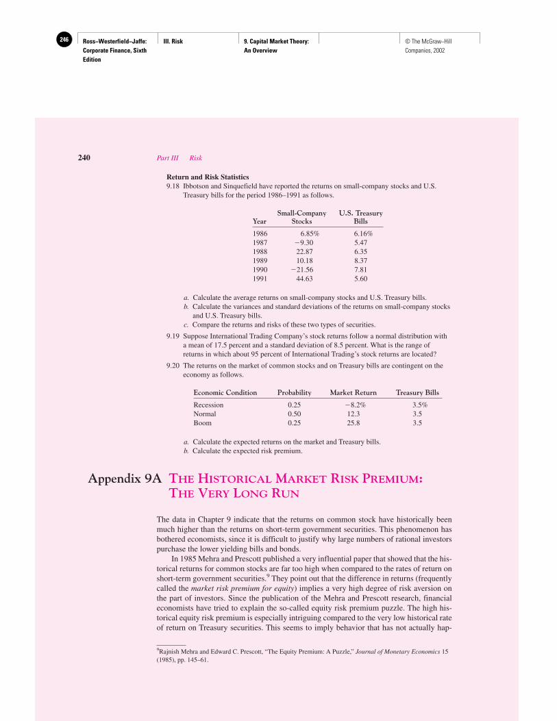
Ross−Westerfield−Jaffe: Corporate Finance, Sixth Edition
III. Risk 9. Capital Market Theory: An Overview
246 © The McGraw−Hill Companies, 2002
Return and Risk Statistics9.18 Ibbotson and Sinquefield have reported the returns on small-company stocks and U.S.
Treasury bills for the period 1986–1991 as follows.
Small-Company U.S. TreasuryYear Stocks Bills
1986 6.85% 6.16%1987 �9.30 5.471988 22.87 6.351989 10.18 8.371990 �21.56 7.811991 44.63 5.60
a. Calculate the average returns on small-company stocks and U.S. Treasury bills.b. Calculate the variances and standard deviations of the returns on small-company stocks
and U.S. Treasury bills.c. Compare the returns and risks of these two types of securities.
9.19 Suppose International Trading Company’s stock returns follow a normal distribution witha mean of 17.5 percent and a standard deviation of 8.5 percent. What is the range ofreturns in which about 95 percent of International Trading’s stock returns are located?
9.20 The returns on the market of common stocks and on Treasury bills are contingent on theeconomy as follows.
Economic Condition Probability Market Return Treasury Bills
Recession 0.25 �8.2% 3.5%Normal 0.50 12.3 3.5Boom 0.25 25.8 3.5
a. Calculate the expected returns on the market and Treasury bills.b. Calculate the expected risk premium.
Appendix 9A THE HISTORICAL MARKET RISK PREMIUM:THE VERY LONG RUN
The data in Chapter 9 indicate that the returns on common stock have historically beenmuch higher than the returns on short-term government securities. This phenomenon hasbothered economists, since it is difficult to justify why large numbers of rational investorspurchase the lower yielding bills and bonds.
In 1985 Mehra and Prescott published a very influential paper that showed that the his-torical returns for common stocks are far too high when compared to the rates of return onshort-term government securities.9 They point out that the difference in returns (frequentlycalled the market risk premium for equity) implies a very high degree of risk aversion onthe part of investors. Since the publication of the Mehra and Prescott research, financialeconomists have tried to explain the so-called equity risk premium puzzle. The high his-torical equity risk premium is especially intriguing compared to the very low historical rateof return on Treasury securities. This seems to imply behavior that has not actually hap-
240 Part III Risk
9Rajnish Mehra and Edward C. Prescott, “The Equity Premium: A Puzzle,” Journal of Monetary Economics 15(1985), pp. 145–61.
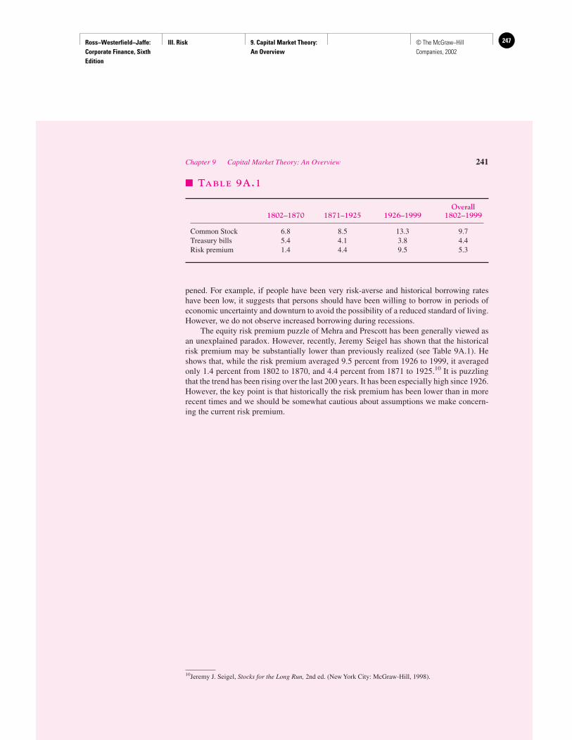
Ross−Westerfield−Jaffe: Corporate Finance, Sixth Edition
III. Risk 9. Capital Market Theory: An Overview
247© The McGraw−Hill Companies, 2002
pened. For example, if people have been very risk-averse and historical borrowing rateshave been low, it suggests that persons should have been willing to borrow in periods ofeconomic uncertainty and downturn to avoid the possibility of a reduced standard of living.However, we do not observe increased borrowing during recessions.
The equity risk premium puzzle of Mehra and Prescott has been generally viewed asan unexplained paradox. However, recently, Jeremy Seigel has shown that the historicalrisk premium may be substantially lower than previously realized (see Table 9A.1). Heshows that, while the risk premium averaged 9.5 percent from 1926 to 1999, it averagedonly 1.4 percent from 1802 to 1870, and 4.4 percent from 1871 to 1925.10 It is puzzlingthat the trend has been rising over the last 200 years. It has been especially high since 1926.However, the key point is that historically the risk premium has been lower than in morerecent times and we should be somewhat cautious about assumptions we make concern-ing the current risk premium.
Chapter 9 Capital Market Theory: An Overview 241
10Jeremy J. Seigel, Stocks for the Long Run, 2nd ed. (New York City: McGraw-Hill, 1998).
� TABLE 9A.1
Overall1802–1870 1871–1925 1926–1999 1802–1999
Common Stock 6.8 8.5 13.3 9.7Treasury bills 5.4 4.1 3.8 4.4Risk premium 1.4 4.4 9.5 5.3
Ross−Westerfield−Jaffe: Corporate Finance, Sixth Edition
III. Risk 10. Return and Risk: The Capital−Asset−Pricing Model
248 © The McGraw−Hill Companies, 2002
Return and Risk: TheCapital-Asset-PricingModel (CAPM)
CH
AP
TE
R10
EXECUTIVE SUMMARY
The previous chapter achieved two purposes. First, we acquainted you with the history ofU.S. capital markets. Second, we presented statistics such as expected return, variance,and standard deviation. Our ultimate goal in the next three chapters is to determine the
appropriate discount rate for capital budgeting projects. Because the discount rate on a projectis a function of its risk, the discussion in the previous chapter on standard deviation is a neces-sary first step. However, we shall see that standard deviation is not the final word on risk.
Our next step is to investigate the relationship between the risk and the return of indi-vidual securities when these securities are part of a large portfolio. This task is taken up inChapter 10. The actual treatment of the appropriate discount rate for capital budgeting is re-served for Chapter 12.
The crux of the current chapter can be summarized as follows: An individual who holdsone security should use expected return as the measure of the security’s return. Standard de-viation or variance is the proper measure of the security’s risk. An individual who holds adiversified portfolio cares about the contribution of each security to the expected return andthe risk of the portfolio. It turns out that a security’s expected return is the appropriate meas-ure of the security’s contribution to the expected return on the portfolio. However, neitherthe security’s variance nor the security’s standard deviation is an appropriate measure of asecurity’s contribution to the risk of a portfolio. The contribution of a security to the risk ofa portfolio is best measured by beta.
10.1 INDIVIDUAL SECURITIES
In the first part of Chapter 10 we will examine the characteristics of individual securities.In particular, we will discuss:
1. Expected Return. This is the return that an individual expects a stock to earn over thenext period. Of course, because this is only an expectation, the actual return may be eitherhigher or lower. An individual’s expectation may simply be the average return per period asecurity has earned in the past. Alternatively, it may be based on a detailed analysis of afirm’s prospects, on some computer-based model, or on special (or inside) information.
2. Variance and Standard Deviation. There are many ways to assess the volatility of asecurity’s return. One of the most common is variance, which is a measure of the squareddeviations of a security’s return from its expected return. Standard deviation is the squareroot of the variance.
3. Covariance and Correlation. Returns on individual securities are related to one another.Covariance is a statistic measuring the interrelationship between two securities. Alternatively,
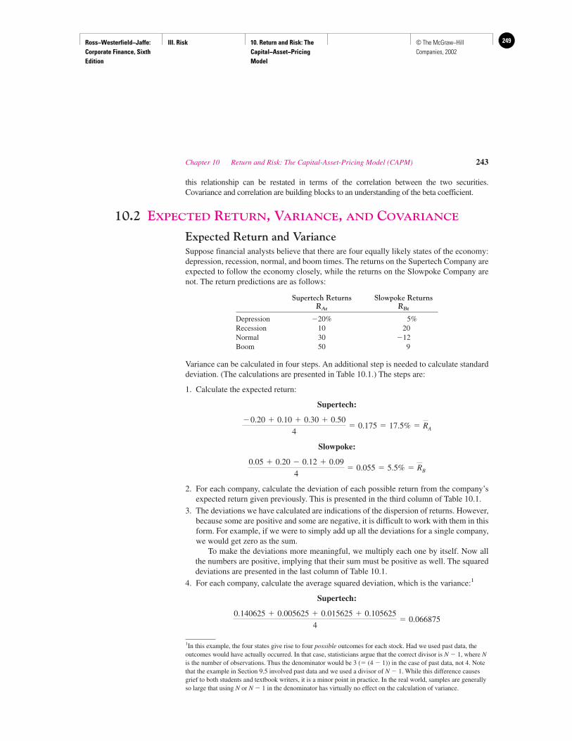
Ross−Westerfield−Jaffe: Corporate Finance, Sixth Edition
III. Risk 10. Return and Risk: The Capital−Asset−Pricing Model
249© The McGraw−Hill Companies, 2002
Chapter 10 Return and Risk: The Capital-Asset-Pricing Model (CAPM) 243
this relationship can be restated in terms of the correlation between the two securities.Covariance and correlation are building blocks to an understanding of the beta coefficient.
10.2 EXPECTED RETURN, VARIANCE, AND COVARIANCE
Expected Return and VarianceSuppose financial analysts believe that there are four equally likely states of the economy:depression, recession, normal, and boom times. The returns on the Supertech Company areexpected to follow the economy closely, while the returns on the Slowpoke Company arenot. The return predictions are as follows:
Supertech Returns Slowpoke ReturnsRAt RBt
Depression �20% 5%Recession 10 20Normal 30 �12Boom 50 9
Variance can be calculated in four steps. An additional step is needed to calculate standarddeviation. (The calculations are presented in Table 10.1.) The steps are:
1. Calculate the expected return:
Supertech:
Slowpoke:
2. For each company, calculate the deviation of each possible return from the company’sexpected return given previously. This is presented in the third column of Table 10.1.
3. The deviations we have calculated are indications of the dispersion of returns. However,because some are positive and some are negative, it is difficult to work with them in thisform. For example, if we were to simply add up all the deviations for a single company,we would get zero as the sum.
To make the deviations more meaningful, we multiply each one by itself. Now allthe numbers are positive, implying that their sum must be positive as well. The squareddeviations are presented in the last column of Table 10.1.
4. For each company, calculate the average squared deviation, which is the variance:1
Supertech:
0.140625 � 0.005625 � 0.015625 � 0.105625
4� 0.066875
0.05 � 0.20 � 0.12 � 0.09
4� 0.055 � 5.5% � RB
�0.20 � 0.10 � 0.30 � 0.50
4� 0.175 � 17.5% � RA
1In this example, the four states give rise to four possible outcomes for each stock. Had we used past data, theoutcomes would have actually occurred. In that case, statisticians argue that the correct divisor is N � 1, where Nis the number of observations. Thus the denominator would be 3 (� (4 � 1)) in the case of past data, not 4. Notethat the example in Section 9.5 involved past data and we used a divisor of N � 1. While this difference causesgrief to both students and textbook writers, it is a minor point in practice. In the real world, samples are generallyso large that using N or N � 1 in the denominator has virtually no effect on the calculation of variance.
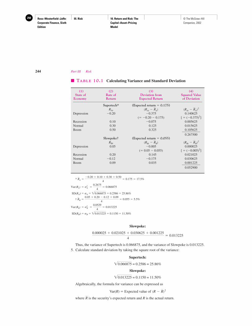
Ross−Westerfield−Jaffe: Corporate Finance, Sixth Edition
III. Risk 10. Return and Risk: The Capital−Asset−Pricing Model
250 © The McGraw−Hill Companies, 2002
Slowpoke:
Thus, the variance of Supertech is 0.066875, and the variance of Slowpoke is 0.013225.
5. Calculate standard deviation by taking the square root of the variance:
Supertech:
= 0.2586 = 25.86%
Slowpoke:
= 0.1150 = 11.50%
Algebraically, the formula for variance can be expressed as
Var(R) � Expected value of
where is the security’s expected return and R is the actual return.R
�R � R� 2
�0.013225
�0.066875
0.000025 � 0.021025 � 0.030625 � 0.001225
4� 0.013225
244 Part III Risk
� TABLE 10.1 Calculating Variance and Standard Deviation
(1) (2) (3) (4)State of Rate of Deviation from Squared Value
Economy Return Expected Return of Deviation
Supertech* (Expected return � 0.175)RAt
Depression �0.20 �0.375 0.140625(� �0.20 � 0.175) [ � (�0.375)2]
Recession 0.10 �0.075 0.005625Normal 0.30 0.125 0.015625Boom 0.50 0.325 0.105625___________
0.267500Slowpoke† (Expected return � 0.055)
RBt
Depression 0.05 �0.005 0.000025(� 0.05 � 0.055) [ � (�0.005)2]
Recession 0.20 0.145 0.021025Normal �0.12 �0.175 0.030625Boom 0.09 0.035 0.001225___________
0.052900
*
SD(RA) � �A � � 0.2586 � 25.86%
†
SD(RB) � �B � � 0.1150 � 11.50%�0.013225
Var �RB� � �2B �
0.0529
4� 0.013225
RB �0.05 � 0.20 � 0.12 � 0.09
4� 0.055 � 5.5%
�0.066875
Var �RA� � �2A �
0.2675
4� 0.066875
RA ��0.20 � 0.10 � 0.30 � 0.50
4� 0.175 � 17.5%
�RBt � RB� 2�RBt � RB�
�RAt � RA� 2�RAt � RA�
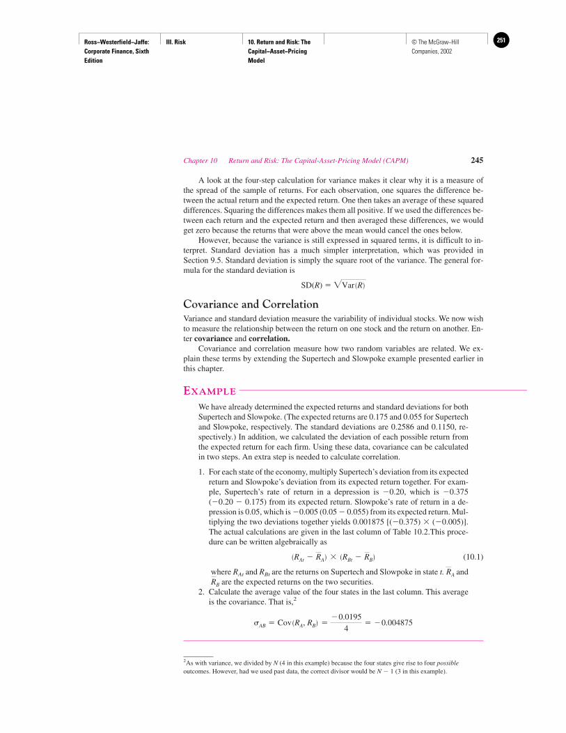
Ross−Westerfield−Jaffe: Corporate Finance, Sixth Edition
III. Risk 10. Return and Risk: The Capital−Asset−Pricing Model
251© The McGraw−Hill Companies, 2002
A look at the four-step calculation for variance makes it clear why it is a measure ofthe spread of the sample of returns. For each observation, one squares the difference be-tween the actual return and the expected return. One then takes an average of these squareddifferences. Squaring the differences makes them all positive. If we used the differences be-tween each return and the expected return and then averaged these differences, we wouldget zero because the returns that were above the mean would cancel the ones below.
However, because the variance is still expressed in squared terms, it is difficult to in-terpret. Standard deviation has a much simpler interpretation, which was provided inSection 9.5. Standard deviation is simply the square root of the variance. The general for-mula for the standard deviation is
SD(R) �
Covariance and CorrelationVariance and standard deviation measure the variability of individual stocks. We now wishto measure the relationship between the return on one stock and the return on another. En-ter covariance and correlation.
Covariance and correlation measure how two random variables are related. We ex-plain these terms by extending the Supertech and Slowpoke example presented earlier inthis chapter.
EXAMPLE
We have already determined the expected returns and standard deviations for bothSupertech and Slowpoke. (The expected returns are 0.175 and 0.055 for Supertechand Slowpoke, respectively. The standard deviations are 0.2586 and 0.1150, re-spectively.) In addition, we calculated the deviation of each possible return fromthe expected return for each firm. Using these data, covariance can be calculatedin two steps. An extra step is needed to calculate correlation.
1. For each state of the economy, multiply Supertech’s deviation from its expectedreturn and Slowpoke’s deviation from its expected return together. For exam-ple, Supertech’s rate of return in a depression is �0.20, which is �0.375(�0.20 � 0.175) from its expected return. Slowpoke’s rate of return in a de-pression is 0.05, which is �0.005 (0.05 � 0.055) from its expected return. Mul-tiplying the two deviations together yields 0.001875 [(�0.375) � (�0.005)].The actual calculations are given in the last column of Table 10.2.This proce-dure can be written algebraically as
(10.1)
where RAt and RBt are the returns on Supertech and Slowpoke in state t. andare the expected returns on the two securities.
2. Calculate the average value of the four states in the last column. This averageis the covariance. That is,2
�AB � Cov �RA, RB� ��0.0195
4� �0.004875
RB
RA
�RAt � RA� � �RBt � RB�
�Var �R�
Chapter 10 Return and Risk: The Capital-Asset-Pricing Model (CAPM) 245
2As with variance, we divided by N (4 in this example) because the four states give rise to four possibleoutcomes. However, had we used past data, the correct divisor would be N � 1 (3 in this example).
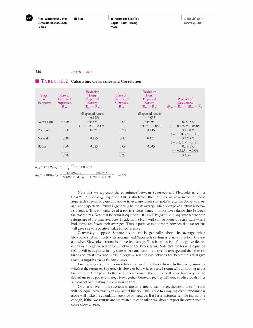
Ross−Westerfield−Jaffe: Corporate Finance, Sixth Edition
III. Risk 10. Return and Risk: The Capital−Asset−Pricing Model
252 © The McGraw−Hill Companies, 2002
Note that we represent the covariance between Supertech and Slowpoke as eitherCov(RA, RB) or �AB. Equation (10.1) illustrates the intuition of covariance. SupposeSupertech’s return is generally above its average when Slowpoke’s return is above its aver-age, and Supertech’s return is generally below its average when Slowpoke’s return is belowits average. This is indicative of a positive dependency or a positive relationship betweenthe two returns. Note that the term in equation (10.1) will be positive in any state where bothreturns are above their averages. In addition, (10.1) will still be positive in any state whereboth terms are below their averages. Thus, a positive relationship between the two returnswill give rise to a positive value for covariance.
Conversely, suppose Supertech’s return is generally above its average whenSlowpoke’s return is below its average, and Supertech’s return is generally below its aver-age when Slowpoke’s return is above its average. This is indicative of a negative depen-dency or a negative relationship between the two returns. Note that the term in equation(10.1) will be negative in any state where one return is above its average and the other re-turn is below its average. Thus, a negative relationship between the two returns will giverise to a negative value for covariance.
Finally, suppose there is no relation between the two returns. In this case, knowingwhether the return on Supertech is above or below its expected return tells us nothing aboutthe return on Slowpoke. In the covariance formula, then, there will be no tendency for thedeviations to be positive or negative together. On average, they will tend to offset each otherand cancel out, making the covariance zero.
Of course, even if the two returns are unrelated to each other, the covariance formulawill not equal zero exactly in any actual history. This is due to sampling error; randomnessalone will make the calculation positive or negative. But for a historical sample that is longenough, if the two returns are not related to each other, we should expect the covariance tocome close to zero.
246 Part III Risk
� TABLE 10.2 Calculating Covariance and Correlation
Deviation DeviationState Rate of from Rate of from
of Return of Expected Return of Expected Product ofEconomy Supertech Return Slowpoke Return Deviations
RAt RBt
(Expected return (Expected return� 0.175) � 0.055)
Depression �0.20 �0.375 0.05 �0.005 0.001875(� �0.20 � 0.175) (� 0.05 � 0.055) (� �0.375 � �0.005)
Recession 0.10 �0.075 0.20 0.145 �0.010875(� �0.075 � 0.145)
Normal 0.30 0.125 �0.12 �0.175 �0.021875(� 0.125 � �0.175)
Boom 0.50 0.325 0.09 0.035 0.011375(� 0.325 � 0.035) ____ ____ ________________
0.70 0.22 �0.0195
AB � Corr �RA, RB� �Cov �RA, RB�
SD �RA� � SD �RB��
�0.004875
0.2586 � 0.1150� �0.1639
�AB � Cov �RA, RB� ��0.0195
4� �0.004875
�RAt � RA� � �RBt � RB��RBt � RB��RAt � RA�
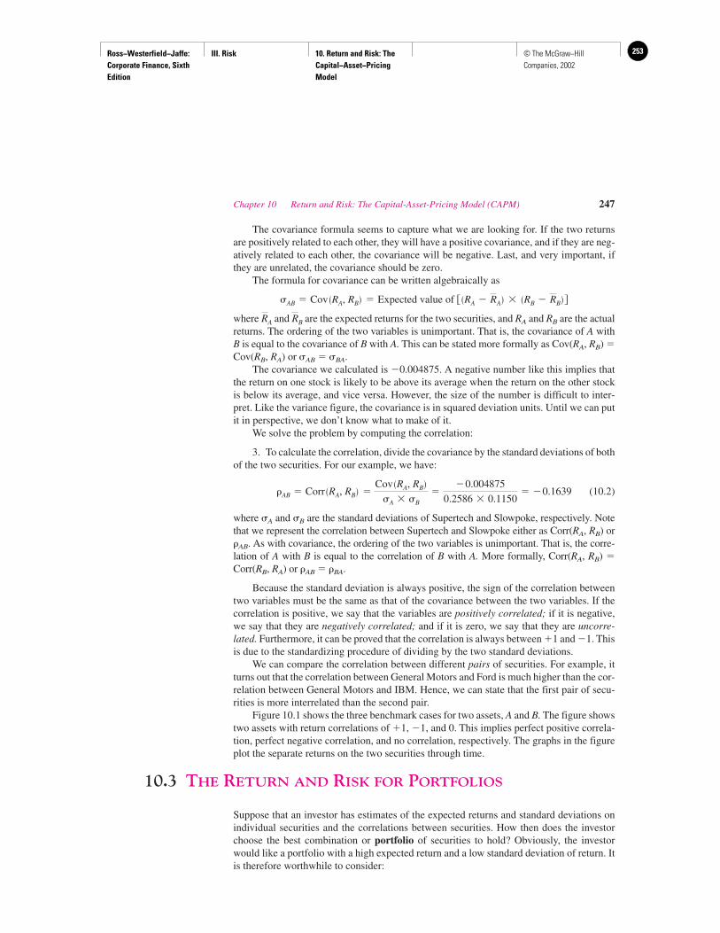
Ross−Westerfield−Jaffe: Corporate Finance, Sixth Edition
III. Risk 10. Return and Risk: The Capital−Asset−Pricing Model
253© The McGraw−Hill Companies, 2002
The covariance formula seems to capture what we are looking for. If the two returnsare positively related to each other, they will have a positive covariance, and if they are neg-atively related to each other, the covariance will be negative. Last, and very important, ifthey are unrelated, the covariance should be zero.
The formula for covariance can be written algebraically as
where and are the expected returns for the two securities, and RA and RB are the actualreturns. The ordering of the two variables is unimportant. That is, the covariance of A withB is equal to the covariance of B with A. This can be stated more formally as Cov(RA, RB) �Cov(RB, RA) or �AB � �BA.
The covariance we calculated is �0.004875. A negative number like this implies thatthe return on one stock is likely to be above its average when the return on the other stockis below its average, and vice versa. However, the size of the number is difficult to inter-pret. Like the variance figure, the covariance is in squared deviation units. Until we can putit in perspective, we don’t know what to make of it.
We solve the problem by computing the correlation:
3. To calculate the correlation, divide the covariance by the standard deviations of bothof the two securities. For our example, we have:
(10.2)
where �A and �B are the standard deviations of Supertech and Slowpoke, respectively. Notethat we represent the correlation between Supertech and Slowpoke either as Corr(RA, RB) or AB. As with covariance, the ordering of the two variables is unimportant. That is, the corre-lation of A with B is equal to the correlation of B with A. More formally, Corr(RA, RB) �Corr(RB, RA) or AB � BA.
Because the standard deviation is always positive, the sign of the correlation betweentwo variables must be the same as that of the covariance between the two variables. If thecorrelation is positive, we say that the variables are positively correlated; if it is negative,we say that they are negatively correlated; and if it is zero, we say that they are uncorre-lated. Furthermore, it can be proved that the correlation is always between �1 and �1. Thisis due to the standardizing procedure of dividing by the two standard deviations.
We can compare the correlation between different pairs of securities. For example, itturns out that the correlation between General Motors and Ford is much higher than the cor-relation between General Motors and IBM. Hence, we can state that the first pair of secu-rities is more interrelated than the second pair.
Figure 10.1 shows the three benchmark cases for two assets, A and B. The figure showstwo assets with return correlations of �1, �1, and 0. This implies perfect positive correla-tion, perfect negative correlation, and no correlation, respectively. The graphs in the figureplot the separate returns on the two securities through time.
10.3 THE RETURN AND RISK FOR PORTFOLIOS
Suppose that an investor has estimates of the expected returns and standard deviations onindividual securities and the correlations between securities. How then does the investorchoose the best combination or portfolio of securities to hold? Obviously, the investorwould like a portfolio with a high expected return and a low standard deviation of return. Itis therefore worthwhile to consider:
AB � Corr �RA, RB� �Cov �RA, RB�
�A � �B
��0.004875
0.2586 � 0.1150� �0.1639
RBRA
�AB � Cov �RA, RB� � Expected value of �RA � RA� � �RB � RB� �
Chapter 10 Return and Risk: The Capital-Asset-Pricing Model (CAPM) 247
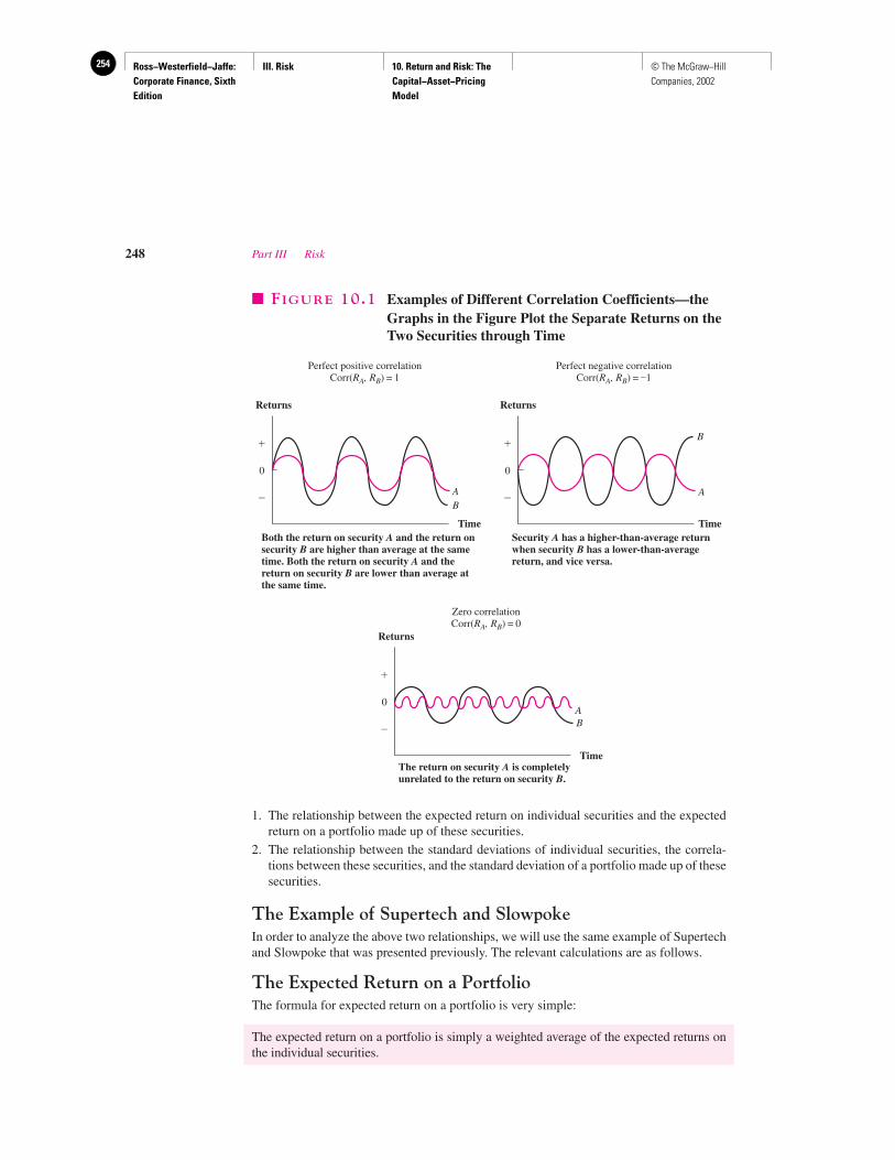
Ross−Westerfield−Jaffe: Corporate Finance, Sixth Edition
III. Risk 10. Return and Risk: The Capital−Asset−Pricing Model
254 © The McGraw−Hill Companies, 2002
1. The relationship between the expected return on individual securities and the expectedreturn on a portfolio made up of these securities.
2. The relationship between the standard deviations of individual securities, the correla-tions between these securities, and the standard deviation of a portfolio made up of thesesecurities.
The Example of Supertech and SlowpokeIn order to analyze the above two relationships, we will use the same example of Supertechand Slowpoke that was presented previously. The relevant calculations are as follows.
The Expected Return on a PortfolioThe formula for expected return on a portfolio is very simple:
The expected return on a portfolio is simply a weighted average of the expected returns onthe individual securities.
248 Part III Risk
�
�
0
Returns
Returns Returns
Time Time
Time
�
�
0
AB
�
�
0
Both the return on security A and the return onsecurity B are higher than average at the sametime. Both the return on security A and thereturn on security B are lower than average atthe same time.
Security A has a higher-than-average returnwhen security B has a lower-than-averagereturn, and vice versa.
AB
The return on security A is completelyunrelated to the return on security B.
Perfect positive correlationCorr(RA, RB) = 1
Perfect negative correlationCorr(RA, RB) = –1
Zero correlationCorr(RA, RB) = 0
A
B
� FIGURE 10.1 Examples of Different Correlation Coefficients—theGraphs in the Figure Plot the Separate Returns on theTwo Securities through Time
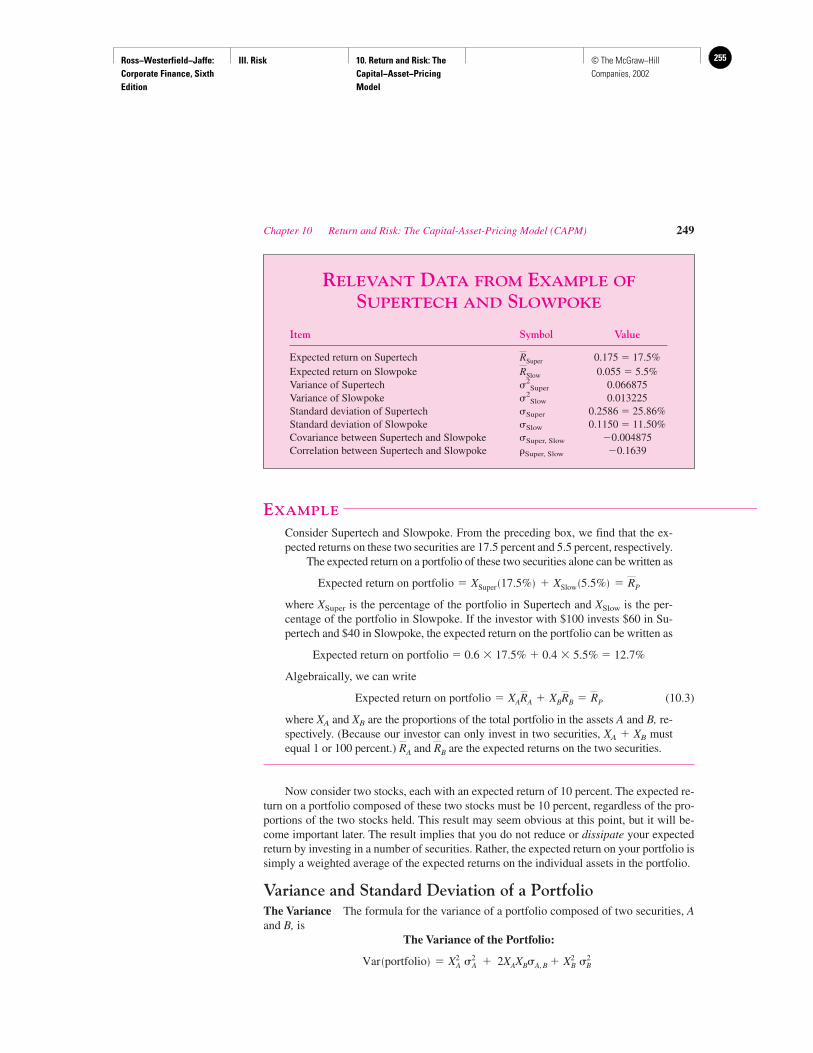
Ross−Westerfield−Jaffe: Corporate Finance, Sixth Edition
III. Risk 10. Return and Risk: The Capital−Asset−Pricing Model
255© The McGraw−Hill Companies, 2002
EXAMPLE
Consider Supertech and Slowpoke. From the preceding box, we find that the ex-pected returns on these two securities are 17.5 percent and 5.5 percent, respectively.
The expected return on a portfolio of these two securities alone can be written as
where XSuper is the percentage of the portfolio in Supertech and XSlow is the per-centage of the portfolio in Slowpoke. If the investor with $100 invests $60 in Su-pertech and $40 in Slowpoke, the expected return on the portfolio can be written as
Expected return on portfolio � 0.6 � 17.5% � 0.4 � 5.5% � 12.7%
Algebraically, we can write
(10.3)
where XA and XB are the proportions of the total portfolio in the assets A and B, re-spectively. (Because our investor can only invest in two securities, XA � XB mustequal 1 or 100 percent.) and are the expected returns on the two securities.
Now consider two stocks, each with an expected return of 10 percent. The expected re-turn on a portfolio composed of these two stocks must be 10 percent, regardless of the pro-portions of the two stocks held. This result may seem obvious at this point, but it will be-come important later. The result implies that you do not reduce or dissipate your expectedreturn by investing in a number of securities. Rather, the expected return on your portfolio issimply a weighted average of the expected returns on the individual assets in the portfolio.
Variance and Standard Deviation of a PortfolioThe Variance The formula for the variance of a portfolio composed of two securities, Aand B, is
The Variance of the Portfolio:
Var �portfolio� � X2A �2
A � 2XAXB�A, B � X2B �2
B
RBRA
Expected return on portfolio � XARA � XBRB � RP
Expected return on portfolio � XSuper �17.5%� � XSlow �5.5%� � RP
Chapter 10 Return and Risk: The Capital-Asset-Pricing Model (CAPM) 249
RELEVANT DATA FROM EXAMPLE OF
SUPERTECH AND SLOWPOKE
Item Symbol Value
Expected return on Supertech 0.175 � 17.5%Expected return on Slowpoke 0.055 � 5.5%Variance of Supertech �2
Super 0.066875Variance of Slowpoke �2
Slow 0.013225Standard deviation of Supertech �Super 0.2586 � 25.86%Standard deviation of Slowpoke �Slow 0.1150 � 11.50%Covariance between Supertech and Slowpoke �Super, Slow �0.004875Correlation between Supertech and Slowpoke Super, Slow �0.1639
RSlow
RSuper
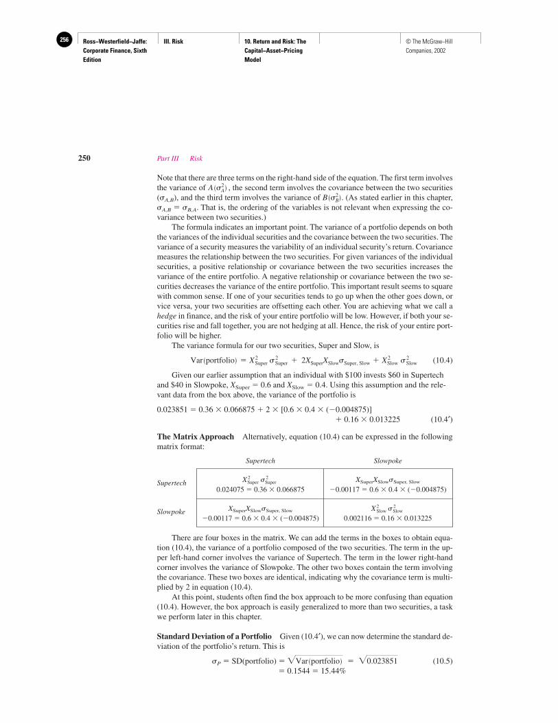
Ross−Westerfield−Jaffe: Corporate Finance, Sixth Edition
III. Risk 10. Return and Risk: The Capital−Asset−Pricing Model
256 © The McGraw−Hill Companies, 2002
Note that there are three terms on the right-hand side of the equation. The first term involvesthe variance of , the second term involves the covariance between the two securities(�A,B), and the third term involves the variance of . (As stated earlier in this chapter,�A,B � �B,A. That is, the ordering of the variables is not relevant when expressing the co-variance between two securities.)
The formula indicates an important point. The variance of a portfolio depends on boththe variances of the individual securities and the covariance between the two securities. Thevariance of a security measures the variability of an individual security’s return. Covariancemeasures the relationship between the two securities. For given variances of the individualsecurities, a positive relationship or covariance between the two securities increases thevariance of the entire portfolio. A negative relationship or covariance between the two se-curities decreases the variance of the entire portfolio. This important result seems to squarewith common sense. If one of your securities tends to go up when the other goes down, orvice versa, your two securities are offsetting each other. You are achieving what we call ahedge in finance, and the risk of your entire portfolio will be low. However, if both your se-curities rise and fall together, you are not hedging at all. Hence, the risk of your entire port-folio will be higher.
The variance formula for our two securities, Super and Slow, is
(10.4)
Given our earlier assumption that an individual with $100 invests $60 in Supertechand $40 in Slowpoke, XSuper � 0.6 and XSlow � 0.4. Using this assumption and the rele-vant data from the box above, the variance of the portfolio is
0.023851 � 0.36 � 0.066875 � 2 � [0.6 � 0.4 � (�0.004875)] � 0.16 � 0.013225 (10.4′)
The Matrix Approach Alternatively, equation (10.4) can be expressed in the followingmatrix format:
Supertech Slowpoke
Supertech XSuperXSlow�Super, Slow
0.024075 � 0.36 � 0.066875 �0.00117 � 0.6 � 0.4 � (�0.004875)
Slowpoke XSuperXSlow�Super, Slow
�0.00117 � 0.6 � 0.4 � (�0.004875) 0.002116 � 0.16 � 0.013225
There are four boxes in the matrix. We can add the terms in the boxes to obtain equa-tion (10.4), the variance of a portfolio composed of the two securities. The term in the up-per left-hand corner involves the variance of Supertech. The term in the lower right-handcorner involves the variance of Slowpoke. The other two boxes contain the term involvingthe covariance. These two boxes are identical, indicating why the covariance term is multi-plied by 2 in equation (10.4).
At this point, students often find the box approach to be more confusing than equation(10.4). However, the box approach is easily generalized to more than two securities, a taskwe perform later in this chapter.
Standard Deviation of a Portfolio Given (10.4′), we can now determine the standard de-viation of the portfolio’s return. This is
�P � SD(portfolio) � (10.5)� 0.1544 � 15.44%
�Var �portfolio� � �0.023851
X 2Slow � 2
Slow
X 2Super � 2
Super
Var �portfolio� � X 2Super � 2
Super � 2XSuperXSlow�Super, Slow � X 2Slow � 2
Slow
B ��2B�
A ��2A�
250 Part III Risk
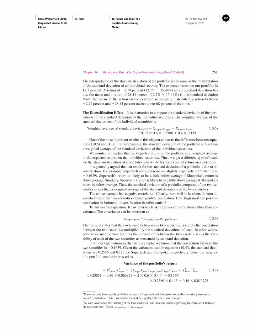
Ross−Westerfield−Jaffe: Corporate Finance, Sixth Edition
III. Risk 10. Return and Risk: The Capital−Asset−Pricing Model
257© The McGraw−Hill Companies, 2002
The interpretation of the standard deviation of the portfolio is the same as the interpretationof the standard deviation of an individual security. The expected return on our portfolio is12.7 percent. A return of �2.74 percent (12.7% � 15.44%) is one standard deviation be-low the mean and a return of 28.14 percent (12.7% � 15.44%) is one standard deviationabove the mean. If the return on the portfolio is normally distributed, a return between�2.74 percent and �28.14 percent occurs about 68 percent of the time.3
The Diversification Effect It is instructive to compare the standard deviation of the port-folio with the standard deviation of the individual securities. The weighted average of thestandard deviations of the individual securities is
Weighted average of standard deviations � XSuper�Super � XSlow�Slow (10.6)0.2012 � 0.6 � 0.2586 � 0.4 � 0.115
One of the most important results in this chapter concerns the difference between equa-tions (10.5) and (10.6). In our example, the standard deviation of the portfolio is less thana weighted average of the standard deviations of the individual securities.
We pointed out earlier that the expected return on the portfolio is a weighted averageof the expected returns on the individual securities. Thus, we get a different type of resultfor the standard deviation of a portfolio than we do for the expected return on a portfolio.
It is generally argued that our result for the standard deviation of a portfolio is due to di-versification. For example, Supertech and Slowpoke are slightly negatively correlated ( ��0.1639). Supertech’s return is likely to be a little below average if Slowpoke’s return isabove average. Similarly, Supertech’s return is likely to be a little above average if Slowpoke’sreturn is below average. Thus, the standard deviation of a portfolio composed of the two se-curities is less than a weighted average of the standard deviations of the two securities.
The above example has negative correlation. Clearly, there will be less benefit from di-versification if the two securities exhibit positive correlation. How high must the positivecorrelation be before all diversification benefits vanish?
To answer this question, let us rewrite (10.4) in terms of correlation rather than co-variance. The covariance can be rewritten as4
�Super, Slow � Super, Slow�Super�Slow (10.7)
The formula states that the covariance between any two securities is simply the correlationbetween the two securities multiplied by the standard deviations of each. In other words,covariance incorporates both (1) the correlation between the two assets and (2) the vari-ability of each of the two securities as measured by standard deviation.
From our calculations earlier in this chapter we know that the correlation between thetwo securities is �0.1639. Given the variances used in equation (10.4′), the standard devi-ations are 0.2586 and 0.115 for Supertech and Slowpoke, respectively. Thus, the varianceof a portfolio can be expressed as
Variance of the portfolio’s return
(10.8)
0.023851 � 0.36 � 0.066875 � 2 � 0.6 � 0.4 � (�0.1639)
� 0.2586 � 0.115 � 0.16 � 0.013225
� X 2Super � 2
Super � 2XSuperXSlow Super, Slow�Super�Slow � X 2Slow � 2
Slow
Chapter 10 Return and Risk: The Capital-Asset-Pricing Model (CAPM) 251
3There are only four equally probable returns for Supertech and Slowpoke, so neither security possesses anormal distribution. Thus, probabilities would be slightly different in our example.4As with covariance, the ordering of the two securities is not relevant when expressing the correlation betweenthe two securities. That is, Super,Slow � Slow,Super.
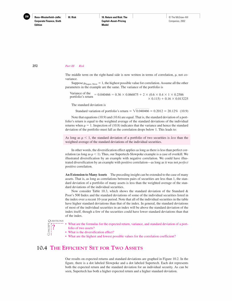
Ross−Westerfield−Jaffe: Corporate Finance, Sixth Edition
III. Risk 10. Return and Risk: The Capital−Asset−Pricing Model
258 © The McGraw−Hill Companies, 2002
The middle term on the right-hand side is now written in terms of correlation, , not co-variance.
Suppose Super, Slow � 1, the highest possible value for correlation. Assume all the otherparameters in the example are the same. The variance of the portfolio is
Variance of the � 0.040466 � 0.36 � 0.066875 � 2 � (0.6 � 0.4 � 1 � 0.2586 portfolio’s return
� 0.115) � 0.16 � 0.013225
The standard deviation is
Standard variation of portfolio’s return � � 0.2012 � 20.12% (10.9)
Note that equations (10.9) and (10.6) are equal. That is, the standard deviation of a port-folio’s return is equal to the weighted average of the standard deviations of the individualreturns when � 1. Inspection of (10.8) indicates that the variance and hence the standarddeviation of the portfolio must fall as the correlation drops below 1. This leads to:
As long as 1, the standard deviation of a portfolio of two securities is less than theweighted average of the standard deviations of the individual securities.
In other words, the diversification effect applies as long as there is less than perfect cor-relation (as long as 1). Thus, our Supertech-Slowpoke example is a case of overkill. Weillustrated diversification by an example with negative correlation. We could have illus-trated diversification by an example with positive correlation—as long as it was not perfectpositive correlation.
An Extension to Many Assets The preceding insight can be extended to the case of manyassets. That is, as long as correlations between pairs of securities are less than 1, the stan-dard deviation of a portfolio of many assets is less than the weighted average of the stan-dard deviations of the individual securities.
Now consider Table 10.3, which shows the standard deviation of the Standard &Poor’s 500 Index and the standard deviations of some of the individual securities listed inthe index over a recent 10-year period. Note that all of the individual securities in the tablehave higher standard deviations than that of the index. In general, the standard deviationsof most of the individual securities in an index will be above the standard deviation of theindex itself, though a few of the securities could have lower standard deviations than thatof the index.
• What are the formulas for the expected return, variance, and standard deviation of a port-folio of two assets?
• What is the diversification effect?• What are the highest and lowest possible values for the correlation coefficient?
10.4 THE EFFICIENT SET FOR TWO ASSETS
Our results on expected returns and standard deviations are graphed in Figure 10.2. In thefigure, there is a dot labeled Slowpoke and a dot labeled Supertech. Each dot representsboth the expected return and the standard deviation for an individual security. As can beseen, Supertech has both a higher expected return and a higher standard deviation.
�0.040466
252 Part III Risk
QUESTIONS
CO
NC
EP
T
?
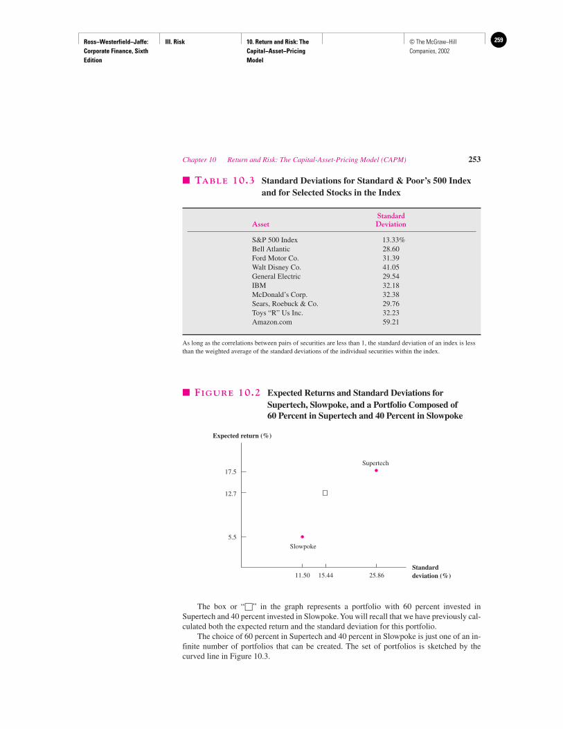
Ross−Westerfield−Jaffe: Corporate Finance, Sixth Edition
III. Risk 10. Return and Risk: The Capital−Asset−Pricing Model
259© The McGraw−Hill Companies, 2002
The box or “□” in the graph represents a portfolio with 60 percent invested inSupertech and 40 percent invested in Slowpoke. You will recall that we have previously cal-culated both the expected return and the standard deviation for this portfolio.
The choice of 60 percent in Supertech and 40 percent in Slowpoke is just one of an in-finite number of portfolios that can be created. The set of portfolios is sketched by thecurved line in Figure 10.3.
Chapter 10 Return and Risk: The Capital-Asset-Pricing Model (CAPM) 253
� TABLE 10.3 Standard Deviations for Standard & Poor’s 500 Indexand for Selected Stocks in the Index
StandardAsset Deviation
S&P 500 Index 13.33%Bell Atlantic 28.60Ford Motor Co. 31.39Walt Disney Co. 41.05General Electric 29.54IBM 32.18McDonald’s Corp. 32.38Sears, Roebuck & Co. 29.76Toys “R” Us Inc. 32.23Amazon.com 59.21
As long as the correlations between pairs of securities are less than 1, the standard deviation of an index is lessthan the weighted average of the standard deviations of the individual securities within the index.
Expected return (%)
17.5
12.7
5.5
11.50 15.44 25.86Standarddeviation (%)
Supertech
Slowpoke
� FIGURE 10.2 Expected Returns and Standard Deviations forSupertech, Slowpoke, and a Portfolio Composed of 60 Percent in Supertech and 40 Percent in Slowpoke
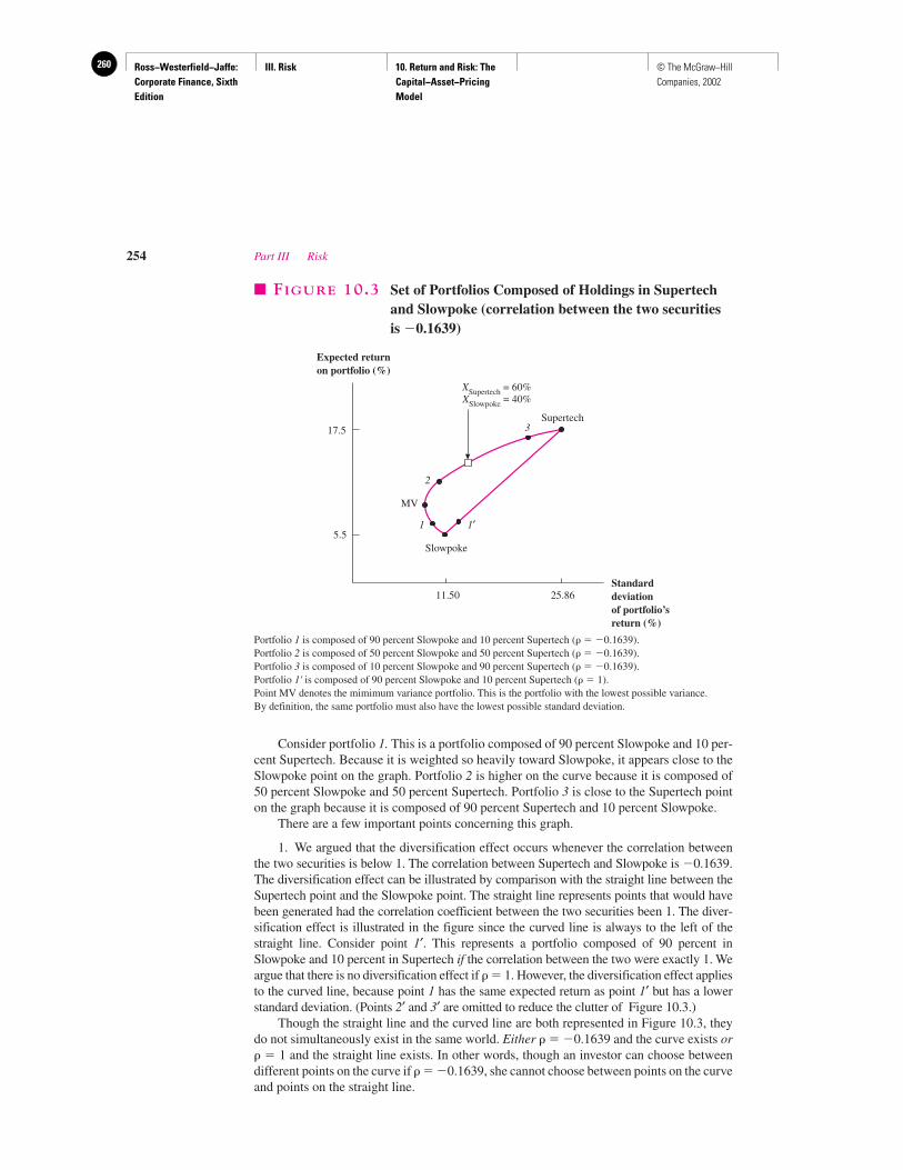
Ross−Westerfield−Jaffe: Corporate Finance, Sixth Edition
III. Risk 10. Return and Risk: The Capital−Asset−Pricing Model
260 © The McGraw−Hill Companies, 2002
Consider portfolio 1. This is a portfolio composed of 90 percent Slowpoke and 10 per-cent Supertech. Because it is weighted so heavily toward Slowpoke, it appears close to theSlowpoke point on the graph. Portfolio 2 is higher on the curve because it is composed of50 percent Slowpoke and 50 percent Supertech. Portfolio 3 is close to the Supertech pointon the graph because it is composed of 90 percent Supertech and 10 percent Slowpoke.
There are a few important points concerning this graph.
1. We argued that the diversification effect occurs whenever the correlation betweenthe two securities is below 1. The correlation between Supertech and Slowpoke is �0.1639.The diversification effect can be illustrated by comparison with the straight line between theSupertech point and the Slowpoke point. The straight line represents points that would havebeen generated had the correlation coefficient between the two securities been 1. The diver-sification effect is illustrated in the figure since the curved line is always to the left of thestraight line. Consider point 1′. This represents a portfolio composed of 90 percent inSlowpoke and 10 percent in Supertech if the correlation between the two were exactly 1. Weargue that there is no diversification effect if � 1. However, the diversification effect appliesto the curved line, because point 1 has the same expected return as point 1′ but has a lowerstandard deviation. (Points 2′ and 3′ are omitted to reduce the clutter of Figure 10.3.)
Though the straight line and the curved line are both represented in Figure 10.3, theydo not simultaneously exist in the same world. Either � �0.1639 and the curve exists or � 1 and the straight line exists. In other words, though an investor can choose betweendifferent points on the curve if � �0.1639, she cannot choose between points on the curveand points on the straight line.
254 Part III Risk
Expected returnon portfolio (%)
Standarddeviationof portfolio’sreturn (%)
XSupertech = 60%XSlowpoke = 40%
Supertech
Slowpoke
11.50 25.86
5.5
17.5
2
3
1 1′
MV
� FIGURE 10.3 Set of Portfolios Composed of Holdings in Supertechand Slowpoke (correlation between the two securitiesis �0.1639)
Portfolio 1 is composed of 90 percent Slowpoke and 10 percent Supertech ( � �0.1639).Portfolio 2 is composed of 50 percent Slowpoke and 50 percent Supertech ( � �0.1639).Portfolio 3 is composed of 10 percent Slowpoke and 90 percent Supertech ( � �0.1639).Portfolio 1' is composed of 90 percent Slowpoke and 10 percent Supertech ( � 1).Point MV denotes the mimimum variance portfolio. This is the portfolio with the lowest possible variance. By definition, the same portfolio must also have the lowest possible standard deviation.
Ross−Westerfield−Jaffe: Corporate Finance, Sixth Edition
III. Risk 10. Return and Risk: The Capital−Asset−Pricing Model
261© The McGraw−Hill Companies, 2002
2. The point MV represents the minimum variance portfolio. This is the portfolio withthe lowest possible variance. By definition, this portfolio must also have the lowest possi-ble standard deviation. (The term minimum variance portfolio is standard in the literature,and we will use that term. Perhaps minimum standard deviation would actually be better,because standard deviation, not variance, is measured on the horizontal axis of Figure 10.3.)
3. An individual contemplating an investment in a portfolio of Slowpoke andSupertech faces an opportunity set or feasible set represented by the curved line in Figure10.3. That is, he can achieve any point on the curve by selecting the appropriate mix be-tween the two securities. He cannot achieve any point above the curve because he cannotincrease the return on the individual securities, decrease the standard deviations of the se-curities, or decrease the correlation between the two securities. Neither can he achievepoints below the curve because he cannot lower the returns on the individual securities, in-crease the standard deviations of the securities, or increase the correlation. (Of course, hewould not want to achieve points below the curve, even if he were able to do so.)
Were he relatively tolerant of risk, he might choose portfolio 3. (In fact, he could evenchoose the end point by investing all his money in Supertech.) An investor with less toler-ance for risk might choose portfolio 2. An investor wanting as little risk as possible wouldchoose MV, the portfolio with minimum variance or minimum standard deviation.
4. Note that the curve is backward bending between the Slowpoke point and MV. Thisindicates that, for a portion of the feasible set, standard deviation actually decreases as oneincreases expected return. Students frequently ask, “How can an increase in the proportionof the risky security, Supertech, lead to a reduction in the risk of the portfolio?”
This surprising finding is due to the diversification effect. The returns on the two se-curities are negatively correlated with each other. One security tends to go up when theother goes down and vice versa. Thus, an addition of a small amount of Supertech acts as ahedge to a portfolio composed only of Slowpoke. The risk of the portfolio is reduced, im-plying backward bending. Actually, backward bending always occurs if � 0. It may ormay not occur when � 0. Of course, the curve bends backward only for a portion of itslength. As one continues to increase the percentage of Supertech in the portfolio, the highstandard deviation of this security eventually causes the standard deviation of the entireportfolio to rise.
5. No investor would want to hold a portfolio with an expected return below that of theminimum variance portfolio. For example, no investor would choose portfolio 1. This port-folio has less expected return but more standard deviation than the minimum variance port-folio has. We say that portfolios such as portfolio 1 are dominated by the minimum vari-ance portfolio. Though the entire curve from Slowpoke to Supertech is called the feasibleset, investors only consider the curve from MV to Supertech. Hence, the curve from MV toSupertech is called the efficient set or the efficient frontier.
Figure 10.3 represents the opportunity set where � �0.1639. It is worthwhile to ex-amine Figure 10.4, which shows different curves for different correlations. As can be seen,the lower the correlation, the more bend there is in the curve. This indicates that the diver-sification effect rises as declines. The greatest bend occurs in the limiting case where ��1. This is perfect negative correlation. While this extreme case where � �1 seems tofascinate students, it has little practical importance. Most pairs of securities exhibit positivecorrelation. Strong negative correlation, let alone perfect negative correlation, are unlikelyoccurrences indeed.5
Chapter 10 Return and Risk: The Capital-Asset-Pricing Model (CAPM) 255
5A major exception occurs with derivative securities. For example, the correlation between a stock and a put onthe stock is generally strongly negative. Puts will be treated later in the text.
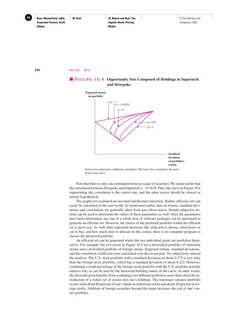
Ross−Westerfield−Jaffe: Corporate Finance, Sixth Edition
III. Risk 10. Return and Risk: The Capital−Asset−Pricing Model
262 © The McGraw−Hill Companies, 2002
Note that there is only one correlation between a pair of securities. We stated earlier thatthe correlation between Slowpoke and Supertech is �0.1639. Thus, the curve in Figure 10.4representing this correlation is the correct one, and the other curves should be viewed asmerely hypothetical.
The graphs we examined are not mere intellectual curiosities. Rather, efficient sets caneasily be calculated in the real world. As mentioned earlier, data on returns, standard devi-ations, and correlations are generally taken from past observations, though subjective no-tions can be used to determine the values of these parameters as well. Once the parametershave been determined, any one of a whole host of software packages can be purchased togenerate an efficient set. However, the choice of the preferred portfolio within the efficientset is up to you. As with other important decisions like what job to choose, what house orcar to buy, and how much time to allocate to this course, there is no computer program tochoose the preferred portfolio.
An efficient set can be generated where the two individual assets are portfolios them-selves. For example, the two assets in Figure 10.5 are a diversified portfolio of Americanstocks and a diversified portfolio of foreign stocks. Expected returns, standard deviations,and the correlation coefficient were calculated over the recent past. No subjectivity enteredthe analysis. The U.S. stock portfolio with a standard deviation of about 0.173 is less riskythan the foreign stock portfolio, which has a standard deviation of about 0.222. However,combining a small percentage of the foreign stock portfolio with the U.S. portfolio actuallyreduces risk, as can be seen by the backward-bending nature of the curve. In other words,the diversification benefits from combining two different portfolios more than offset the in-troduction of a riskier set of stocks into one’s holdings. The minimum variance portfoliooccurs with about 80 percent of one’s funds in American stocks and about 20 percent in for-eign stocks. Addition of foreign securities beyond this point increases the risk of one’s en-tire portfolio.
256 Part III Risk
Expected returnon portfolio
Standarddeviationof portfolio’sreturn
= – 1 = – 0.1639
= 0
= 0.5
= 1
� FIGURE 10.4 Opportunity Sets Composed of Holdings in Supertechand Slowpoke
Each curve represents a different correlation. The lower the correlation, the morebend in the curve.
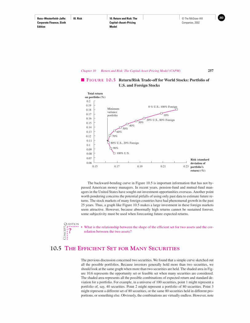
Ross−Westerfield−Jaffe: Corporate Finance, Sixth Edition
III. Risk 10. Return and Risk: The Capital−Asset−Pricing Model
263© The McGraw−Hill Companies, 2002
The backward-bending curve in Figure 10.5 is important information that has not by-passed American money managers. In recent years, pension-fund and mutual-fund man-agers in the United States have sought out investment opportunities overseas. Another pointworth pondering concerns the potential pitfalls of using only past data to estimate future re-turns. The stock markets of many foreign countries have had phenomenal growth in the past25 years. Thus, a graph like Figure 10.5 makes a large investment in these foreign marketsseem attractive. However, because abnormally high returns cannot be sustained forever,some subjectivity must be used when forecasting future expected returns.
• What is the relationship between the shape of the efficient set for two assets and the cor-relation between the two assets?
10.5 THE EFFICIENT SET FOR MANY SECURITIES
The previous discussion concerned two securities. We found that a simple curve sketched outall the possible portfolios. Because investors generally hold more than two securities, weshould look at the same graph when more than two securities are held. The shaded area in Fig-ure 10.6 represents the opportunity set or feasible set when many securities are considered.The shaded area represents all the possible combinations of expected return and standard de-viation for a portfolio. For example, in a universe of 100 securities, point 1 might represent aportfolio of, say, 40 securities. Point 2 might represent a portfolio of 80 securities. Point 3might represent a different set of 80 securities, or the same 80 securities held in different pro-portions, or something else. Obviously, the combinations are virtually endless. However, note
Chapter 10 Return and Risk: The Capital-Asset-Pricing Model (CAPM) 257
0.2
0.19
0.18
0.17
0.16
0.15
0.14
0.13
0.12
0.11
0.1
0.09
0.08
0.07
0.060.15 0.17 0.19 0.21 0.23
Total returnon portfolio (%)
Risk (standarddeviation ofportfolio’sreturn) (%)
Minimumvarianceportfolio
0 % U.S., 100% Foreign
20% U.S., 80% Foreign
80% U.S., 20% Foreign
100% U.S.
90%
70%
60%50%
40%30%
10%
� FIGURE 10.5 Return/Risk Trade-off for World Stocks: Portfolio ofU.S. and Foreign Stocks
QUESTION
CO
NC
EP
T
?
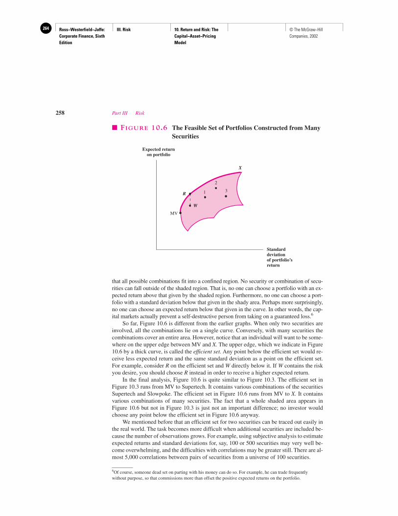
Ross−Westerfield−Jaffe: Corporate Finance, Sixth Edition
III. Risk 10. Return and Risk: The Capital−Asset−Pricing Model
264 © The McGraw−Hill Companies, 2002
that all possible combinations fit into a confined region. No security or combination of secu-rities can fall outside of the shaded region. That is, no one can choose a portfolio with an ex-pected return above that given by the shaded region. Furthermore, no one can choose a port-folio with a standard deviation below that given in the shady area. Perhaps more surprisingly,no one can choose an expected return below that given in the curve. In other words, the cap-ital markets actually prevent a self-destructive person from taking on a guaranteed loss.6
So far, Figure 10.6 is different from the earlier graphs. When only two securities areinvolved, all the combinations lie on a single curve. Conversely, with many securities thecombinations cover an entire area. However, notice that an individual will want to be some-where on the upper edge between MV and X. The upper edge, which we indicate in Figure10.6 by a thick curve, is called the efficient set. Any point below the efficient set would re-ceive less expected return and the same standard deviation as a point on the efficient set.For example, consider R on the efficient set and W directly below it. If W contains the riskyou desire, you should choose R instead in order to receive a higher expected return.
In the final analysis, Figure 10.6 is quite similar to Figure 10.3. The efficient set inFigure 10.3 runs from MV to Supertech. It contains various combinations of the securitiesSupertech and Slowpoke. The efficient set in Figure 10.6 runs from MV to X. It containsvarious combinations of many securities. The fact that a whole shaded area appears inFigure 10.6 but not in Figure 10.3 is just not an important difference; no investor wouldchoose any point below the efficient set in Figure 10.6 anyway.
We mentioned before that an efficient set for two securities can be traced out easily inthe real world. The task becomes more difficult when additional securities are included be-cause the number of observations grows. For example, using subjective analysis to estimateexpected returns and standard deviations for, say, 100 or 500 securities may very well be-come overwhelming, and the difficulties with correlations may be greater still. There are al-most 5,000 correlations between pairs of securities from a universe of 100 securities.
258 Part III Risk
6Of course, someone dead set on parting with his money can do so. For example, he can trade frequentlywithout purpose, so that commissions more than offset the positive expected returns on the portfolio.
Expected returnon portfolio
Standarddeviationof portfolio’sreturn
X
R 1
W
2
3
MV
� FIGURE 10.6 The Feasible Set of Portfolios Constructed from ManySecurities
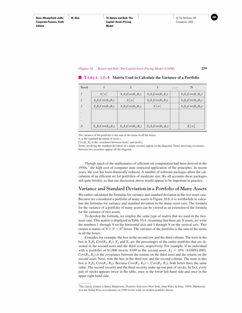
Ross−Westerfield−Jaffe: Corporate Finance, Sixth Edition
III. Risk 10. Return and Risk: The Capital−Asset−Pricing Model
265© The McGraw−Hill Companies, 2002
Though much of the mathematics of efficient-set computation had been derived in the1950s,7 the high cost of computer time restricted application of the principles. In recentyears, the cost has been drastically reduced. A number of software packages allow the cal-culation of an efficient set for portfolios of moderate size. By all accounts these packagessell quite briskly, so that our discussion above would appear to be important in practice.
Variance and Standard Deviation in a Portfolio of Many AssetsWe earlier calculated the formulas for variance and standard deviation in the two-asset case.Because we considered a portfolio of many assets in Figure 10.6, it is worthwhile to calcu-late the formulas for variance and standard deviation in the many-asset case. The formulafor the variance of a portfolio of many assets can be viewed as an extension of the formulafor the variance of two assets.
To develop the formula, we employ the same type of matrix that we used in the two-asset case. This matrix is displayed in Table 10.4. Assuming that there are N assets, we writethe numbers 1 through N on the horizontal axis and 1 through N on the vertical axis. Thiscreates a matrix of N � N � N2 boxes. The variance of the portfolio is the sum of the termsin all the boxes.
Consider, for example, the box in the second row and the third column. The term in thebox is X2X3 Cov(R2, R3). X2 and X3 are the percentages of the entire portfolio that are in-vested in the second asset and the third asset, respectively. For example, if an individualwith a portfolio of $1,000 invests $100 in the second asset, X2 � 10% ($100/$1,000).Cov(R3, R2) is the covariance between the returns on the third asset and the returns on thesecond asset. Next, note the box in the third row and the second column. The term in thisbox is X3X2 Cov(R3, R2). Because Cov(R3, R2) � Cov(R2, R3), both boxes have the samevalue. The second security and the third security make up one pair of stocks. In fact, everypair of stocks appears twice in the table, once in the lower left-hand side and once in theupper right-hand side.
Chapter 10 Return and Risk: The Capital-Asset-Pricing Model (CAPM) 259
7The classic treatise is Harry Markowitz, Portfolio Selection (New York: John Wiley & Sons, 1959). Markowitzwon the Nobel Prize in economics in 1990 for his work on modern portfolio theory.
� TABLE 10.4 Matrix Used to Calculate the Variance of a Portfolio
Stock 1 2 3 . . . N
1 X1X2Cov(R1,R2) X1X3Cov(R1,R3) X1XNCov(R1,RN)
2 X2X1Cov(R2,R1) X2X3Cov(R2,R3) X2XNCov(R2,RN)
3 X3X1Cov(R3,R1) X3X2Cov(R3,R2) X3XNCov(R3,RN)
.
.
.
N XNX1Cov(RN,R1) XNX2Cov(RN,R2) XNX3Cov(RN,R3)
The variance of the portfolio is the sum of the terms in all the boxes.�i is the standard deviation of stock i.Cov(Ri, Rj) is the covariance between stock i and stock j.Terms involving the standard deviation of a single security appear on the diagonal. Terms involving covariancebetween two securities appear off the diagonal.
X 2N � 2
N
X 23 � 2
3
X 22 � 2
2
X 21 � 2
1
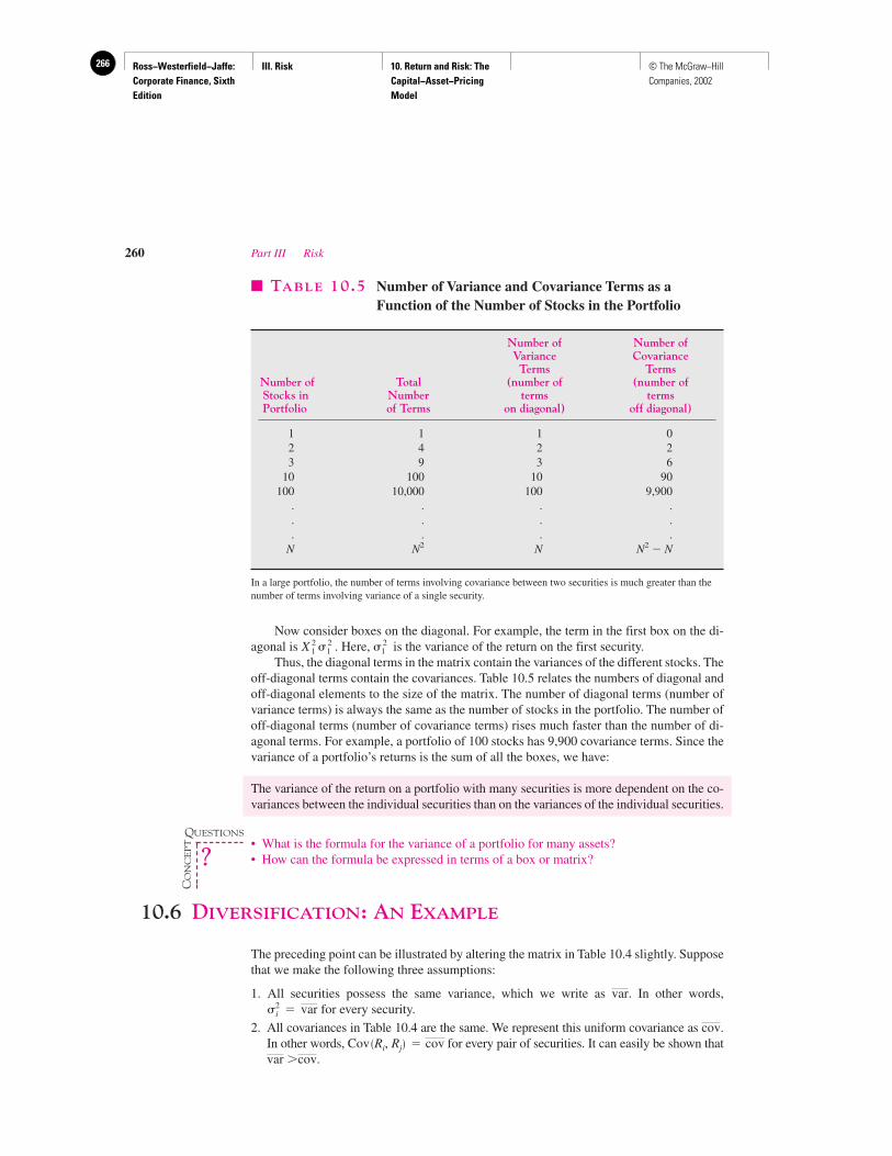
Ross−Westerfield−Jaffe: Corporate Finance, Sixth Edition
III. Risk 10. Return and Risk: The Capital−Asset−Pricing Model
266 © The McGraw−Hill Companies, 2002
Now consider boxes on the diagonal. For example, the term in the first box on the di-agonal is . Here, is the variance of the return on the first security.
Thus, the diagonal terms in the matrix contain the variances of the different stocks. Theoff-diagonal terms contain the covariances. Table 10.5 relates the numbers of diagonal andoff-diagonal elements to the size of the matrix. The number of diagonal terms (number ofvariance terms) is always the same as the number of stocks in the portfolio. The number ofoff-diagonal terms (number of covariance terms) rises much faster than the number of di-agonal terms. For example, a portfolio of 100 stocks has 9,900 covariance terms. Since thevariance of a portfolio’s returns is the sum of all the boxes, we have:
The variance of the return on a portfolio with many securities is more dependent on the co-variances between the individual securities than on the variances of the individual securities.
• What is the formula for the variance of a portfolio for many assets?• How can the formula be expressed in terms of a box or matrix?
10.6 DIVERSIFICATION: AN EXAMPLE
The preceding point can be illustrated by altering the matrix in Table 10.4 slightly. Supposethat we make the following three assumptions:
1. All securities possess the same variance, which we write as . In other words,for every security.
2. All covariances in Table 10.4 are the same. We represent this uniform covariance as .In other words, for every pair of securities. It can easily be shown that
.�covvarCov �Ri, Rj� � cov
cov
�2i � var
var
� 21X 2
1 � 21
260 Part III Risk
� TABLE 10.5 Number of Variance and Covariance Terms as aFunction of the Number of Stocks in the Portfolio
Number of Number ofVariance CovarianceTerms Terms
Number of Total (number of (number ofStocks in Number terms termsPortfolio of Terms on diagonal) off diagonal)
1 1 1 02 4 2 23 9 3 6
10 100 10 90100 10,000 100 9,900
. . . .
. . . .
. . . .N N2 N N2 � N
In a large portfolio, the number of terms involving covariance between two securities is much greater than thenumber of terms involving variance of a single security.
QUESTIONS
CO
NC
EP
T
?

Ross−Westerfield−Jaffe: Corporate Finance, Sixth Edition
III. Risk 10. Return and Risk: The Capital−Asset−Pricing Model
267© The McGraw−Hill Companies, 2002
3. All securities are equally weighted in the portfolio. Because there are N assets, theweight of each asset in the portfolio is 1/N. In other words, Xi � 1/N for each security i.
Table 10.6 is the matrix of variances and covariances under these three simplifyingassumptions. Note that all of the diagonal terms are identical. Similarly, all of the off-diagonal terms are identical. As with Table 10.4, the variance of the portfolio is the sumof the terms in the boxes in Table 10.6. We know that there are N diagonal terms in-volving variance. Similarly, there are N � (N � 1) off-diagonal terms involving covari-ance. Summing across all the boxes in Table 10.6 we can express the variances of theportfolio as
(10.10)
Number of Each Number of Eachdiagonal diagonal off-diagonal off-diagonal
terms term terms term
Equation (10.10) expresses the variance of our special portfolio as a weighted sum of theaverage security variance and the average covariance.8
� �1
N�var � �1 �1
N�cov
� �1
N�var � �N 2 � N
N2 �cov
Variance of portfolio � N � � 1
N 2�var � N �N � 1� � � 1
N 2�cov
Chapter 10 Return and Risk: The Capital-Asset-Pricing Model (CAPM) 261
8Equation (10.10) is actually a weighted average of the variance and covariance terms because the weights, 1/Nand 1 � 1/N, sum to 1.
� TABLE 10.6 Matrix Used to Calculate the Variance of a PortfolioWhen (a) All Securities Possess the Same Variance,Which We Represent as ; (b) All Pairs of SecuritiesPossess the Same Covariance, Which We Represent as
; (c) All Securities Are Held in the Same Proportion,Which Is 1/Ncov
var
Stock 1 2 3 . . . N
1
2
3
.
.
.
N �1/N2�var�1/N2�cov�1/N2�cov�1/N2�cov
�1/N2�cov�1/N2�var�1/N2�cov�1/N2�cov
�1/N2�cov�1/N2�cov�1/N2�var�1/N2�cov
�1/N2�cov�1/N2�cov�1/N2�cov�1/N2�var
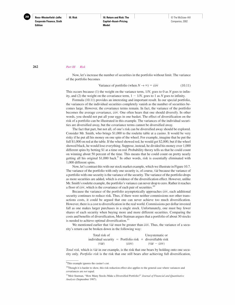
Ross−Westerfield−Jaffe: Corporate Finance, Sixth Edition
III. Risk 10. Return and Risk: The Capital−Asset−Pricing Model
268 © The McGraw−Hill Companies, 2002
Now, let’s increase the number of securities in the portfolio without limit. The varianceof the portfolio becomes
Variance of portfolio (when N → �) � (10.11)
This occurs because (1) the weight on the variance term, 1/N, goes to 0 as N goes to infin-ity, and (2) the weight on the covariance term, 1 � 1/N, goes to 1 as N goes to infinity.
Formula (10.11) provides an interesting and important result. In our special portfolio,the variances of the individual securities completely vanish as the number of securities be-comes large. However, the covariance terms remain. In fact, the variance of the portfoliobecomes the average covariance, . One often hears that one should diversify. In otherwords, you should not put all your eggs in one basket. The effect of diversification on therisk of a portfolio can be illustrated in this example. The variances of the individual securi-ties are diversified away, but the covariance terms cannot be diversified away.
The fact that part, but not all, of one’s risk can be diversified away should be explored.Consider Mr. Smith, who brings $1,000 to the roulette table at a casino. It would be veryrisky if he put all his money on one spin of the wheel. For example, imagine that he put thefull $1,000 on red at the table. If the wheel showed red, he would get $2,000, but if the wheelshowed black, he would lose everything. Suppose, instead, he divided his money over 1,000different spins by betting $1 at a time on red. Probability theory tells us that he could counton winning about 50 percent of the time. This means that he could count on pretty nearlygetting all his original $1,000 back.9 In other words, risk is essentially eliminated with1,000 different spins.
Now, let’s contrast this with our stock market example, which we illustrate in Figure 10.7.The variance of the portfolio with only one security is, of course, because the variance ofa portfolio with one security is the variance of the security. The variance of the portfolio dropsas more securities are added, which is evidence of the diversification effect. However, unlikeMr. Smith’s roulette example, the portfolio’s variance can never drop to zero. Rather it reachesa floor of , which is the covariance of each pair of securities.10
Because the variance of the portfolio asymptotically approaches , each additionalsecurity continues to reduce risk. Thus, if there were neither commissions nor other trans-actions costs, it could be argued that one can never achieve too much diversification.However, there is a cost to diversification in the real world. Commissions per dollar investedfall as one makes larger purchases in a single stock. Unfortunately, one must buy fewershares of each security when buying more and more different securities. Comparing thecosts and benefits of diversification, Meir Statman argues that a portfolio of about 30 stocksis needed to achieve optimal diversification.11
We mentioned earlier that must be greater than . Thus, the variance of a secu-rity’s return can be broken down in the following way:
Total risk of Unsystematic orindividual security � Portfolio risk � diversifiable risk
Total risk, which is in our example, is the risk that one bears by holding onto one secu-rity only. Portfolio risk is the risk that one still bears after achieving full diversification,
var
�var � cov��cov��var�
covvar
covcov
var
cov
cov
262 Part III Risk
9This example ignores the casino’s cut.10Though it is harder to show, this risk reduction effect also applies to the general case where variances andcovariances are not equal.11Meir Statman, “How Many Stocks Make a Diversified Portfolio?” Journal of Financial and QuantitativeAnalysis (September 1987).
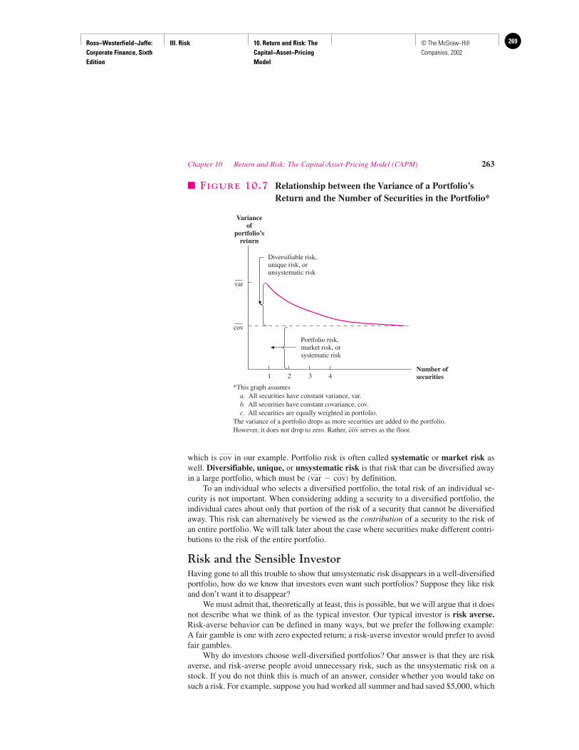
Ross−Westerfield−Jaffe: Corporate Finance, Sixth Edition
III. Risk 10. Return and Risk: The Capital−Asset−Pricing Model
269© The McGraw−Hill Companies, 2002
which is in our example. Portfolio risk is often called systematic or market risk aswell. Diversifiable, unique, or unsystematic risk is that risk that can be diversified awayin a large portfolio, which must be by definition.
To an individual who selects a diversified portfolio, the total risk of an individual se-curity is not important. When considering adding a security to a diversified portfolio, theindividual cares about only that portion of the risk of a security that cannot be diversifiedaway. This risk can alternatively be viewed as the contribution of a security to the risk ofan entire portfolio. We will talk later about the case where securities make different contri-butions to the risk of the entire portfolio.
Risk and the Sensible InvestorHaving gone to all this trouble to show that unsystematic risk disappears in a well-diversifiedportfolio, how do we know that investors even want such portfolios? Suppose they like riskand don’t want it to disappear?
We must admit that, theoretically at least, this is possible, but we will argue that it doesnot describe what we think of as the typical investor. Our typical investor is risk averse.Risk-averse behavior can be defined in many ways, but we prefer the following example:A fair gamble is one with zero expected return; a risk-averse investor would prefer to avoidfair gambles.
Why do investors choose well-diversified portfolios? Our answer is that they are riskaverse, and risk-averse people avoid unnecessary risk, such as the unsystematic risk on astock. If you do not think this is much of an answer, consider whether you would take onsuch a risk. For example, suppose you had worked all summer and had saved $5,000, which
�var � cov�
cov
Chapter 10 Return and Risk: The Capital-Asset-Pricing Model (CAPM) 263
Varianceof
portfolio’sreturn
Number ofsecurities
Diversifiable risk,unique risk, orunsystematic risk
Portfolio risk,market risk, orsystematic risk
var
cov
1 2 3 4
� FIGURE 10.7 Relationship between the Variance of a Portfolio’sReturn and the Number of Securities in the Portfolio*
*This graph assumesa. All securities have constant variance, var.b. All securities have constant covariance, cov.c. All securities are equally weighted in portfolio.
The variance of a portfolio drops as more securities are added to the portfolio.However, it does not drop to zero. Rather, serves as the floor.cov
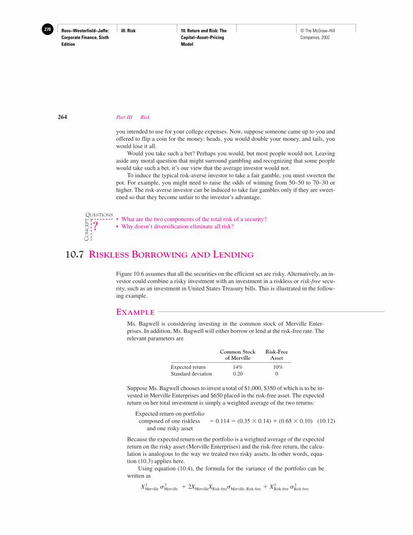
Ross−Westerfield−Jaffe: Corporate Finance, Sixth Edition
III. Risk 10. Return and Risk: The Capital−Asset−Pricing Model
270 © The McGraw−Hill Companies, 2002
you intended to use for your college expenses. Now, suppose someone came up to you andoffered to flip a coin for the money: heads, you would double your money, and tails, youwould lose it all.
Would you take such a bet? Perhaps you would, but most people would not. Leavingaside any moral question that might surround gambling and recognizing that some peoplewould take such a bet, it’s our view that the average investor would not.
To induce the typical risk-averse investor to take a fair gamble, you must sweeten thepot. For example, you might need to raise the odds of winning from 50–50 to 70–30 orhigher. The risk-averse investor can be induced to take fair gambles only if they are sweet-ened so that they become unfair to the investor’s advantage.
• What are the two components of the total risk of a security?• Why doesn’t diversification eliminate all risk?
10.7 RISKLESS BORROWING AND LENDING
Figure 10.6 assumes that all the securities on the efficient set are risky. Alternatively, an in-vestor could combine a risky investment with an investment in a riskless or risk-free secu-rity, such as an investment in United States Treasury bills. This is illustrated in the follow-ing example.
EXAMPLE
Ms. Bagwell is considering investing in the common stock of Merville Enter-prises. In addition, Ms. Bagwell will either borrow or lend at the risk-free rate. Therelevant parameters are
Common Stock Risk-Freeof Merville Asset
Expected return 14% 10%Standard deviation 0.20 0
Suppose Ms. Bagwell chooses to invest a total of $1,000, $350 of which is to be in-vested in Merville Enterprises and $650 placed in the risk-free asset. The expectedreturn on her total investment is simply a weighted average of the two returns:
Expected return on portfoliocomposed of one riskless � 0.114 � (0.35 � 0.14) � (0.65 � 0.10) (10.12)
and one risky asset
Because the expected return on the portfolio is a weighted average of the expectedreturn on the risky asset (Merville Enterprises) and the risk-free return, the calcu-lation is analogous to the way we treated two risky assets. In other words, equa-tion (10.3) applies here.
Using equation (10.4), the formula for the variance of the portfolio can bewritten as
X 2Merville � 2
Merville � 2XMervilleXRisk-free�Merville, Risk-free � X 2Risk-free � 2
Risk-free
264 Part III Risk
QUESTIONS
CO
NC
EP
T
?
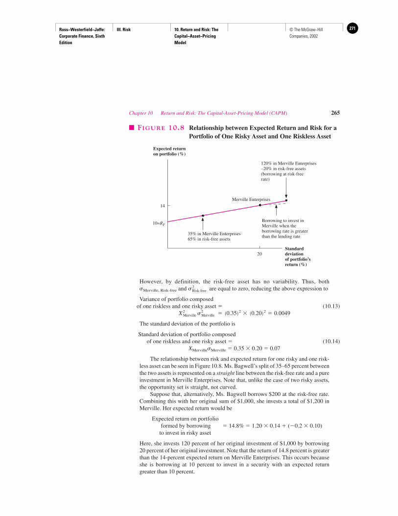
Ross−Westerfield−Jaffe: Corporate Finance, Sixth Edition
III. Risk 10. Return and Risk: The Capital−Asset−Pricing Model
271© The McGraw−Hill Companies, 2002
However, by definition, the risk-free asset has no variability. Thus, both �Merville, Risk-free and are equal to zero, reducing the above expression to
Variance of portfolio composedof one riskless and one risky asset � (10.13)
The standard deviation of the portfolio is
Standard deviation of portfolio composedof one riskless and one risky asset � (10.14)
XMerville�Merville � 0.35 � 0.20 � 0.07
The relationship between risk and expected return for one risky and one risk-less asset can be seen in Figure 10.8. Ms. Bagwell’s split of 35–65 percent betweenthe two assets is represented on a straight line between the risk-free rate and a pureinvestment in Merville Enterprises. Note that, unlike the case of two risky assets,the opportunity set is straight, not curved.
Suppose that, alternatively, Ms. Bagwell borrows $200 at the risk-free rate.Combining this with her original sum of $1,000, she invests a total of $1,200 inMerville. Her expected return would be
Expected return on portfolioformed by borrowing � 14.8% � 1.20 � 0.14 � (�0.2 � 0.10)to invest in risky asset
Here, she invests 120 percent of her original investment of $1,000 by borrowing20 percent of her original investment. Note that the return of 14.8 percent is greaterthan the 14-percent expected return on Merville Enterprises. This occurs becauseshe is borrowing at 10 percent to invest in a security with an expected returngreater than 10 percent.
X 2Merville �2
Merville � �0.35� 2 � �0.20� 2 � 0.0049
� 2Risk-free
Chapter 10 Return and Risk: The Capital-Asset-Pricing Model (CAPM) 265
Expected returnon portfolio (%)
Standarddeviationof portfolio’sreturn (%)
120% in Merville Enterprises–20% in risk-free assets(borrowing at risk-freerate)
Borrowing to invest inMerville when theborrowing rate is greaterthan the lending rate
Merville Enterprises
35% in Merville Enterprises65% in risk-free assets
20
14
10=RF
� FIGURE 10.8 Relationship between Expected Return and Risk for aPortfolio of One Risky Asset and One Riskless Asset
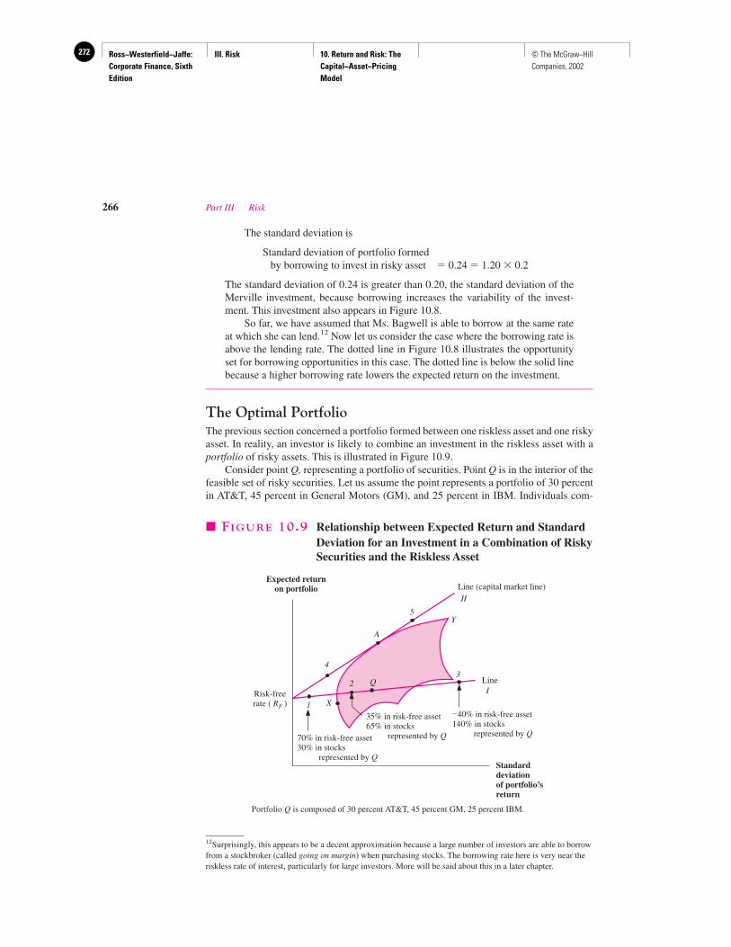
Ross−Westerfield−Jaffe: Corporate Finance, Sixth Edition
III. Risk 10. Return and Risk: The Capital−Asset−Pricing Model
272 © The McGraw−Hill Companies, 2002
The standard deviation is
Standard deviation of portfolio formedby borrowing to invest in risky asset � 0.24 � 1.20 � 0.2
The standard deviation of 0.24 is greater than 0.20, the standard deviation of theMerville investment, because borrowing increases the variability of the invest-ment. This investment also appears in Figure 10.8.
So far, we have assumed that Ms. Bagwell is able to borrow at the same rateat which she can lend.12 Now let us consider the case where the borrowing rate isabove the lending rate. The dotted line in Figure 10.8 illustrates the opportunityset for borrowing opportunities in this case. The dotted line is below the solid linebecause a higher borrowing rate lowers the expected return on the investment.
The Optimal PortfolioThe previous section concerned a portfolio formed between one riskless asset and one riskyasset. In reality, an investor is likely to combine an investment in the riskless asset with aportfolio of risky assets. This is illustrated in Figure 10.9.
Consider point Q, representing a portfolio of securities. Point Q is in the interior of thefeasible set of risky securities. Let us assume the point represents a portfolio of 30 percentin AT&T, 45 percent in General Motors (GM), and 25 percent in IBM. Individuals com-
266 Part III Risk
12Surprisingly, this appears to be a decent approximation because a large number of investors are able to borrowfrom a stockbroker (called going on margin) when purchasing stocks. The borrowing rate here is very near theriskless rate of interest, particularly for large investors. More will be said about this in a later chapter.
Risk-freerate ( RF )
Line (capital market line)
–40% in risk-free asset140% in stocks represented by Q
35% in risk-free asset65% in stocks represented by Q70% in risk-free asset
30% in stocks represented by Q
II
Y
A
X1
4
5
3
ILine
Expected returnon portfolio
Standarddeviationof portfolio’sreturn
2 Q
� FIGURE 10.9 Relationship between Expected Return and StandardDeviation for an Investment in a Combination of RiskySecurities and the Riskless Asset
Portfolio Q is composed of 30 percent AT&T, 45 percent GM, 25 percent IBM.
Ross−Westerfield−Jaffe: Corporate Finance, Sixth Edition
III. Risk 10. Return and Risk: The Capital−Asset−Pricing Model
273© The McGraw−Hill Companies, 2002
bining investments in Q with investments in the riskless asset would achieve points alongthe straight line from RF to Q. We refer to this as line I. For example, point 1 on the line rep-resents a portfolio of 70 percent in the riskless asset and 30 percent in stocks representedby Q. An investor with $100 choosing point 1 as his portfolio would put $70 in the risk-freeasset and $30 in Q. This can be restated as $70 in the riskless asset, $9 (0.3 � $30) in AT&T,$13.50 (0.45 � $30) in GM, and $7.50 (0.25 � $30) in IBM. Point 2 also represents a port-folio of the risk-free asset and Q, with more (65%) being invested in Q.
Point 3 is obtained by borrowing to invest in Q. For example, an investor with $100 of hisown would borrow $40 from the bank or broker in order to invest $140 in Q. This can be statedas borrowing $40 and contributing $100 of one’s money in order to invest $42 (0.3 � $140) inAT&T, $63 (0.45 � $140) in GM, and $35 (0.25 � $140) in IBM.
The above investments can be summarized as:
Point 1 Point 3Point Q (lending $70) (borrowing $40)
AT&T $ 30 $ 9 $ 42GM 45 13.50 63IBM 25 7.50 35Risk-free 0 70.00 �40____ _______ ____
Total investment $100 $100 $100
Though any investor can obtain any point on line I, no point on the line is optimal. Tosee this, consider line II, a line running from RF through A. Point A represents a portfolioof risky securities. Line II represents portfolios formed by combinations of the risk-free as-set and the securities in A. Points between RF and A are portfolios in which some money isinvested in the riskless asset and the rest is placed in A. Points past A are achieved by bor-rowing at the riskless rate to buy more of A than one could with one’s original funds alone.
As drawn, line II is tangent to the efficient set of risky securities. Whatever point an in-dividual can obtain on line I, he can obtain a point with the same standard deviation and ahigher expected return on line II. In fact, because line II is tangent to the efficient set of riskyassets, it provides the investor with the best possible opportunities. In other words, line II canbe viewed as the efficient set of all assets, both risky and riskless. An investor with a fair de-gree of risk aversion might choose a point between RF and A, perhaps point 4. An individualwith less risk aversion might choose a point closer to A or even beyond A. For example, point5 corresponds to an individual borrowing money to increase his investment in A.
The graph illustrates an important point. With riskless borrowing and lending, the port-folio of risky assets held by any investor would always be point A. Regardless of the in-vestor’s tolerance for risk, he would never choose any other point on the efficient set of riskyassets (represented by curve XAY) nor any point in the interior of the feasible region. Rather,he would combine the securities of A with the riskless assets if he had high aversion to risk.He would borrow the riskless asset to invest more funds in A had he low aversion to risk.
This result establishes what financial economists call the separation principle. Thatis, the investor’s investment decision consists of two separate steps:
1. After estimating (a) the expected returns and variances of individual securities, and(b) the covariances between pairs of securities, the investor calculates the efficient set ofrisky assets, represented by curve XAY in Figure 10.9. He then determines point A, the tan-gency between the risk-free rate and the efficient set of risky assets (curve XAY). Point Arepresents the portfolio of risky assets that the investor will hold. This point is determinedsolely from his estimates of returns, variances, and covariances. No personal characteris-tics, such as degree of risk aversion, are needed in this step.
Chapter 10 Return and Risk: The Capital-Asset-Pricing Model (CAPM) 267
Ross−Westerfield−Jaffe: Corporate Finance, Sixth Edition
III. Risk 10. Return and Risk: The Capital−Asset−Pricing Model
274 © The McGraw−Hill Companies, 2002
2. The investor must now determine how he will combine point A, his portfolio ofrisky assets, with the riskless asset. He might invest some of his funds in the riskless assetand some in portfolio A. He would end up at a point on the line between RF and A in thiscase. Alternatively, he might borrow at the risk-free rate and contribute some of his ownfunds as well, investing the sum in portfolio A. He would end up at a point on line II be-yond A. His position in the riskless asset, that is, his choice of where on the line he wantsto be, is determined by his internal characteristics, such as his ability to tolerate risk.
• What is the formula for the standard deviation of a portfolio composed of one riskless andone risky asset?
• How does one determine the optimal portfolio among the efficient set of risky assets?
10.8 MARKET EQUILIBRIUM
Definition of the Market-Equilibrium PortfolioThe above analysis concerns one investor. His estimates of the expected returns and vari-ances for individual securities and the covariances between pairs of securities are his and hisalone. Other investors would obviously have different estimates of the above variables. How-ever, the estimates might not vary much because all investors would be forming expectationsfrom the same data on past price movements and other publicly available information.
Financial economists often imagine a world where all investors possess the same estimateson expected returns, variances, and covariances. Though this can never be literally true, it canbe thought of as a useful simplifying assumption in a world where investors have access to sim-ilar sources of information. This assumption is called homogeneous expectations.13
If all investors had homogeneous expectations, Figure 10.9 would be the same for allindividuals. That is, all investors would sketch out the same efficient set of risky assets be-cause they would be working with the same inputs. This efficient set of risky assets is rep-resented by the curve XAY. Because the same risk-free rate would apply to everyone, all in-vestors would view point A as the portfolio of risky assets to be held.
This point A takes on great importance because all investors would purchase the riskysecurities that it represents. Those investors with a high degree of risk aversion might com-bine A with an investment in the riskless asset, achieving point 4, for example. Others withlow aversion to risk might borrow to achieve, say, point 5. Because this is a very importantconclusion, we restate it:
In a world with homogeneous expectations, all investors would hold the portfolio of riskyassets represented by point A.
If all investors choose the same portfolio of risky assets, it is possible to determine whatthat portfolio is. Common sense tells us that it is a market-value-weighted portfolio of allexisting securities. It is the market portfolio.
In practice, financial economists use a broad-based index such as the Standard &Poor’s (S&P) 500 as a proxy for the market portfolio. Of course all investors do not holdthe same portfolio in practice. However, we know that a large number of investors hold di-
268 Part III Risk
13The assumption of homogeneous expectations states that all investors have the same beliefs concerningreturns, variances, and covariances. It does not say that all investors have the same aversion to risk.
QUESTIONS
CO
NC
EP
T
?
Ross−Westerfield−Jaffe: Corporate Finance, Sixth Edition
III. Risk 10. Return and Risk: The Capital−Asset−Pricing Model
275© The McGraw−Hill Companies, 2002
versified portfolios, particularly when mutual funds or pension funds are included. A broad-based index is a good proxy for the highly diversified portfolios of many investors.
Definition of Risk When Investors Hold the Market PortfolioThe previous section states that many investors hold diversified portfolios similar to broad-based indices. This result allows us to be more precise about the risk of a security in thecontext of a diversified portfolio.
Researchers have shown that the best measure of the risk of a security in a large port-folio is the beta of the security. We illustrate beta by an example.
EXAMPLE
Consider the following possible returns on both the stock of Jelco, Inc., and on themarket:
Return on Return onType of Market Jelco, Inc.
State Economy (percent) (percent)
I Bull 15 25II Bull 15 15III Bear �5 �5IV Bear �5 �15
Though the return on the market has only two possible outcomes (15% and�5%), the return on Jelco has four possible outcomes. It is helpful to consider theexpected return on a security for a given return on the market. Assuming each stateis equally likely, we have
Return on Expected ReturnType of Market on Jelco, Inc.Economy (percent) (percent)
Bull 15% 20% � 25% � 1⁄2 � 15% � 1⁄2Bear �5% �10% � �5% � 1⁄2 � (�15%) � 1⁄2
Jelco, Inc., responds to market movements because its expected return is greaterin bullish states than in bearish states. We now calculate exactly how responsivethe security is to market movements. The market’s return in a bullish economy is20 percent [15% � (�5%)] greater than the market’s return in a bearish economy.However, the expected return on Jelco in a bullish economy is 30 percent [20% �(�10%)] greater than its expected return in a bearish state. Thus, Jelco, Inc., hasa responsiveness coefficient of 1.5 (30%/20%).
This relationship appears in Figure 10.10. The returns for both Jelco and themarket in each state are plotted as four points. In addition, we plot the expected re-turn on the security for each of the two possible returns on the market. These twopoints, each of which we designate by an X, are joined by a line called the char-acteristic line of the security. The slope of the line is 1.5, the number calculated inthe previous paragraph. This responsiveness coefficient of 1.5 is the beta of Jelco.
The interpretation of beta from Figure 10.10 is intuitive. The graph tells us thatthe returns of Jelco are magnified 1.5 times over those of the market. When the mar-ket does well, Jelco’s stock is expected to do even better. When the market doespoorly, Jelco’s stock is expected to do even worse. Now imagine an individual with
Chapter 10 Return and Risk: The Capital-Asset-Pricing Model (CAPM) 269
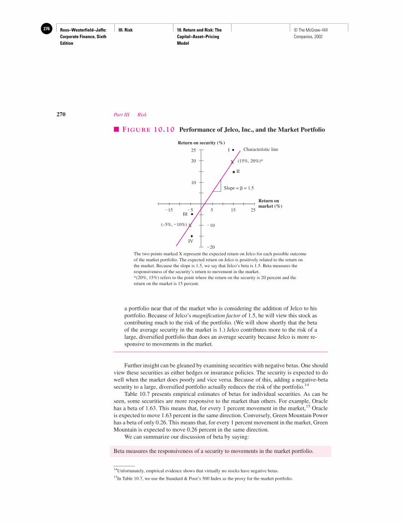
Ross−Westerfield−Jaffe: Corporate Finance, Sixth Edition
III. Risk 10. Return and Risk: The Capital−Asset−Pricing Model
276 © The McGraw−Hill Companies, 2002
a portfolio near that of the market who is considering the addition of Jelco to hisportfolio. Because of Jelco’s magnification factor of 1.5, he will view this stock ascontributing much to the risk of the portfolio. (We will show shortly that the betaof the average security in the market is 1.) Jelco contributes more to the risk of alarge, diversified portfolio than does an average security because Jelco is more re-sponsive to movements in the market.
Further insight can be gleaned by examining securities with negative betas. One shouldview these securities as either hedges or insurance policies. The security is expected to dowell when the market does poorly and vice versa. Because of this, adding a negative-betasecurity to a large, diversified portfolio actually reduces the risk of the portfolio.14
Table 10.7 presents empirical estimates of betas for individual securities. As can beseen, some securities are more responsive to the market than others. For example, Oraclehas a beta of 1.63. This means that, for every 1 percent movement in the market,15 Oracleis expected to move 1.63 percent in the same direction. Conversely, Green Mountain Powerhas a beta of only 0.26. This means that, for every 1 percent movement in the market, GreenMountain is expected to move 0.26 percent in the same direction.
We can summarize our discussion of beta by saying:
Beta measures the responsiveness of a security to movements in the market portfolio.
270 Part III Risk
Return on security (%)
Return onmarket (%)
Characteristic line
(15%, 20%)*
Slope = � = 1.5
(–5%, –10%)
20
25
10
–10
–20
–15 –5 5 15 25
I
II
III
IV
X
X
� FIGURE 10.10 Performance of Jelco, Inc., and the Market Portfolio
The two points marked X represent the expected return on Jelco for each possible outcomeof the market portfolio. The expected return on Jelco is positively related to the return onthe market. Because the slope is 1.5, we say that Jelco’s beta is 1.5. Beta measures theresponsiveness of the security’s return to movement in the market.*(20%, 15%) refers to the point where the return on the security is 20 percent and thereturn on the market is 15 percent.
14Unfortunately, empirical evidence shows that virtually no stocks have negative betas.15In Table 10.7, we use the Standard & Poor’s 500 Index as the proxy for the market portfolio.
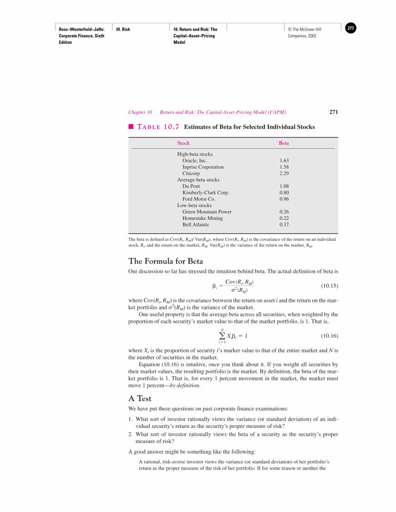
Ross−Westerfield−Jaffe: Corporate Finance, Sixth Edition
III. Risk 10. Return and Risk: The Capital−Asset−Pricing Model
277© The McGraw−Hill Companies, 2002
The Formula for BetaOur discussion so far has stressed the intuition behind beta. The actual definition of beta is
(10.15)
where Cov(Ri, RM) is the covariance between the return on asset i and the return on the mar-ket portfolio and �2(RM) is the variance of the market.
One useful property is that the average beta across all securities, when weighted by theproportion of each security’s market value to that of the market portfolio, is 1. That is,
(10.16)
where Xi is the proportion of security i’s market value to that of the entire market and N isthe number of securities in the market.
Equation (10.16) is intuitive, once you think about it. If you weight all securities bytheir market values, the resulting portfolio is the market. By definition, the beta of the mar-ket portfolio is 1. That is, for every 1 percent movement in the market, the market mustmove 1 percent—by definition.
A TestWe have put these questions on past corporate finance examinations:
1. What sort of investor rationally views the variance (or standard deviation) of an indi-vidual security’s return as the security’s proper measure of risk?
2. What sort of investor rationally views the beta of a security as the security’s propermeasure of risk?
A good answer might be something like the following:
A rational, risk-averse investor views the variance (or standard deviation) of her portfolio’s return as the proper measure of the risk of her portfolio. If for some reason or another the
N
i�1
Xi�i � 1
�i �Cov �Ri, RM�
�2 �RM�
Chapter 10 Return and Risk: The Capital-Asset-Pricing Model (CAPM) 271
� TABLE 10.7 Estimates of Beta for Selected Individual Stocks
Stock Beta
High-beta stocksOracle, Inc. 1.63Inprise Corporation 1.58Citicorp 2.29
Average-beta stocksDu Pont 1.08Kimberly-Clark Corp. 0.80Ford Motor Co. 0.96
Low-beta stocksGreen Mountain Power 0.26Homestake Mining 0.22Bell Atlantic 0.37
The beta is defined as Cov(Ri, RM)/ Var(RM), where Cov(Ri, RM) is the covariance of the return on an individualstock, Ri, and the return on the market, RM. Var(RM) is the variance of the return on the market, RM.
Ross−Westerfield−Jaffe: Corporate Finance, Sixth Edition
III. Risk 10. Return and Risk: The Capital−Asset−Pricing Model
278 © The McGraw−Hill Companies, 2002
investor can hold only one security, the variance of that security’s return becomes the varianceof the portfolio’s return. Hence, the variance of the security’s return is the security’s propermeasure of risk.
If an individual holds a diversified portfolio, she still views the variance (or standarddeviation) of her portfolio’s return as the proper measure of the risk of her portfolio.However, she is no longer interested in the variance of each individual security’s return.Rather, she is interested in the contribution of an individual security to the variance of theportfolio.
Under the assumption of homogeneous expectations, all individuals hold the marketportfolio. Thus, we measure risk as the contribution of an individual security to the varianceof the market portfolio. This contribution, when standardized properly, is the beta of the se-curity. While very few investors hold the market portfolio exactly, many hold reasonablydiversified portfolios. These portfolios are close enough to the market portfolio so that thebeta of a security is likely to be a reasonable measure of its risk.
• If all investors have homogeneous expectations, what portfolio of risky assets do theyhold?
• What is the formula for beta?• Why is beta the appropriate measure of risk for a single security in a large portfolio?
10.9 RELATIONSHIP BETWEEN RISK AND EXPECTED RETURN
(CAPM)
It is commonplace to argue that the expected return on an asset should be positively relatedto its risk. That is, individuals will hold a risky asset only if its expected return compensatesfor its risk. In this section, we first estimate the expected return on the stock market as awhole. Next, we estimate expected returns on individual securities.
Expected Return on MarketFinancial economists frequently argue that the expected return on the market can be repre-sented as:
In words, the expected return on the market is the sum of the risk-free rate plus some com-pensation for the risk inherent in the market portfolio. Note that the equation refers to theexpected return on the market, not the actual return in a particular month or year. Becausestocks have risk, the actual return on the market over a particular period can, of course, bebelow RF, or can even be negative.
Since investors want compensation for risk, the risk premium is presumably positive.But exactly how positive is it? It is generally argued that the best estimate for the risk pre-mium in the future is the average risk premium in the past. As reported in Chapter 9,Ibbotson and Sinquefield found that the expected return on common stocks was 13.3 per-cent over 1926–1999. The average risk-free rate over the same time interval was 3.8 per-cent. Thus, the average difference between the two was 9.5 percent (13.3% � 3.8%).
RM � RF � Risk premium
272 Part III Risk
QUESTIONS
CO
NC
EP
T
?
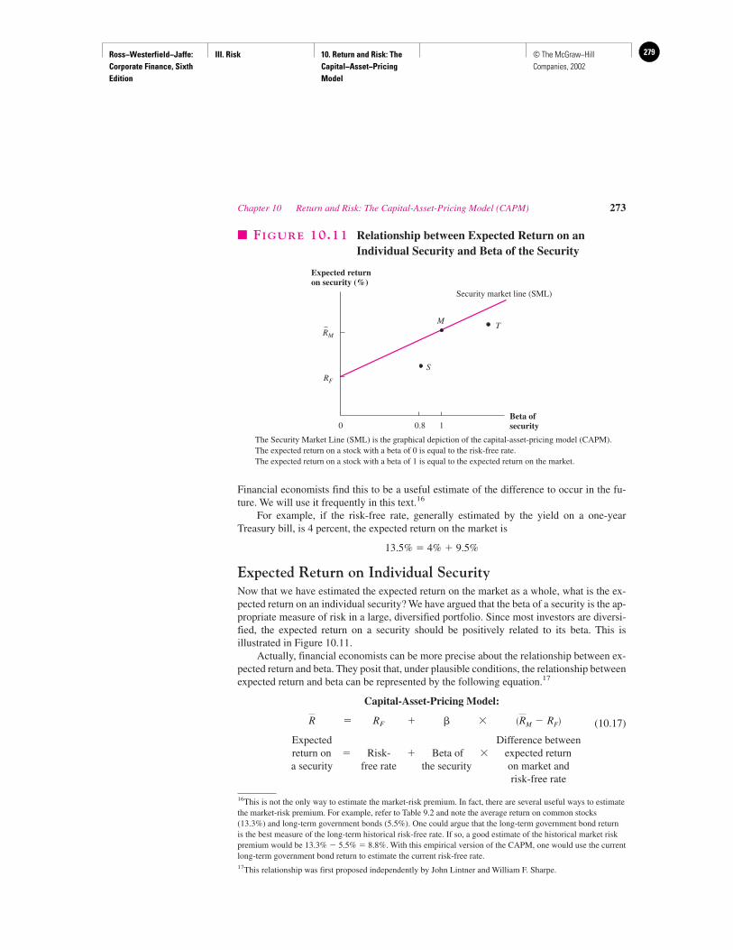
Ross−Westerfield−Jaffe: Corporate Finance, Sixth Edition
III. Risk 10. Return and Risk: The Capital−Asset−Pricing Model
279© The McGraw−Hill Companies, 2002
Financial economists find this to be a useful estimate of the difference to occur in the fu-ture. We will use it frequently in this text.16
For example, if the risk-free rate, generally estimated by the yield on a one-yearTreasury bill, is 4 percent, the expected return on the market is
13.5% � 4% � 9.5%
Expected Return on Individual SecurityNow that we have estimated the expected return on the market as a whole, what is the ex-pected return on an individual security? We have argued that the beta of a security is the ap-propriate measure of risk in a large, diversified portfolio. Since most investors are diversi-fied, the expected return on a security should be positively related to its beta. This isillustrated in Figure 10.11.
Actually, financial economists can be more precise about the relationship between ex-pected return and beta. They posit that, under plausible conditions, the relationship betweenexpected return and beta can be represented by the following equation.17
Capital-Asset-Pricing Model:
� RF � � � (10.17)
Expected Difference betweenreturn on � Risk- � Beta of � expected returna security free rate the security on market and
risk-free rate
�RM � RF�R
Chapter 10 Return and Risk: The Capital-Asset-Pricing Model (CAPM) 273
16This is not the only way to estimate the market-risk premium. In fact, there are several useful ways to estimatethe market-risk premium. For example, refer to Table 9.2 and note the average return on common stocks(13.3%) and long-term government bonds (5.5%). One could argue that the long-term government bond returnis the best measure of the long-term historical risk-free rate. If so, a good estimate of the historical market riskpremium would be 13.3% � 5.5% � 8.8%. With this empirical version of the CAPM, one would use the currentlong-term government bond return to estimate the current risk-free rate.17This relationship was first proposed independently by John Lintner and William F. Sharpe.
Expected returnon security (%)
Beta ofsecurity
Security market line (SML)
0 0.8 1
MT
S
RM
RF
� FIGURE 10.11 Relationship between Expected Return on anIndividual Security and Beta of the Security
The Security Market Line (SML) is the graphical depiction of the capital-asset-pricing model (CAPM).The expected return on a stock with a beta of 0 is equal to the risk-free rate.The expected return on a stock with a beta of 1 is equal to the expected return on the market.
Ross−Westerfield−Jaffe: Corporate Finance, Sixth Edition
III. Risk 10. Return and Risk: The Capital−Asset−Pricing Model
280 © The McGraw−Hill Companies, 2002
This formula, which is called the capital-asset-pricing model (or CAPM for short), impliesthat the expected return on a security is linearly related to its beta. Since the average return onthe market has been higher than the average risk-free rate over long periods of time,is presumably positive. Thus, the formula implies that the expected return on a security is pos-itively related to its beta. The formula can be illustrated by assuming a few special cases:
• Assume that � � 0. Here , that is, the expected return on the security is equalto the risk-free rate. Because a security with zero beta has no relevant risk, its ex-pected return should equal the risk-free rate.
• Assume that � � 1. Equation (10.17) reduces to . That is, the expected re-turn on the security is equal to the expected return on the market. This makes sensesince the beta of the market portfolio is also 1.
Formula (10.17) can be represented graphically by the upward-sloping line inFigure 10.11. Note that the line begins at RF and rises to when beta is 1. This line isfrequently called the security market line (SML).
As with any line, the SML has both a slope and an intercept. RF, the risk-free rate, isthe intercept. Because the beta of a security is the horizontal axis, is the slope. Theline will be upward-sloping as long as the expected return on the market is greater than therisk-free rate. Because the market portfolio is a risky asset, theory suggests that its expectedreturn is above the risk-free rate. In addition, the empirical evidence of the previous chap-ter showed that the average return per year on the market portfolio over the past 74 yearswas 9.5 percent above the risk-free rate.
EXAMPLE
The stock of Aardvark Enterprises has a beta of 1.5 and that of Zebra Enterpriseshas a beta of 0.7. The risk-free rate is 7 percent, and the difference between the ex-pected return on the market and the risk-free rate is 9.5 percent. The expected re-turns on the two securities are:
Expected Return for Aardvark:
21.25% � 7% � 1.5 � 9.5% (10.18)
Expected Return for Zebra:
13.65% � 7% � 0.7 � 9.5%
Three additional points concerning the CAPM should be mentioned:
1. Linearity. The intuition behind an upwardly sloping curve is clear. Because beta isthe appropriate measure of risk, high-beta securities should have an expected return abovethat of low-beta securities. However, both Figure 10.11 and equation (10.17) show some-thing more than an upwardly sloping curve; the relationship between expected return andbeta corresponds to a straight line.
It is easy to show that the line of Figure 10.11 is straight. To see this, consider securityS with, say, a beta of 0.8. This security is represented by a point below the security marketline in the figure. Any investor could duplicate the beta of security S by buying a portfoliowith 20 percent in the risk-free asset and 80 percent in a security with a beta of 1. However,the homemade portfolio would itself lie on the SML. In other words, the portfolio domi-nates security S because the portfolio has a higher expected return and the same beta.
Now consider security T with, say, a beta greater than 1. This security is also below theSML in Figure 10.11. Any investor could duplicate the beta of security T by borrowing to
RM � RF
RM
R � RM
R � RF
RM � RF
274 Part III Risk
Ross−Westerfield−Jaffe: Corporate Finance, Sixth Edition
III. Risk 10. Return and Risk: The Capital−Asset−Pricing Model
281© The McGraw−Hill Companies, 2002
invest in a security with a beta of 1. This portfolio must also lie on the SML, thereby dom-inating security T.
Because no one would hold either S or T, their stock prices would drop. This price ad-justment would raise the expected returns on the two securities. The price adjustment wouldcontinue until the two securities lay on the security market line. The preceding exampleconsidered two overpriced stocks and a straight SML. Securities lying above the SML areunderpriced. Their prices must rise until their expected returns lie on the line. If the SMLis itself curved, many stocks would be mispriced. In equilibrium, all securities would beheld only when prices changed so that the SML became straight. In other words, linearitywould be achieved.
2. Portfolios as well as securities. Our discussion of the CAPM considered individ-ual securities. Does the relationship in Figure 10.11 and equation (10.17) hold for portfo-lios as well?
Yes. To see this, consider a portfolio formed by investing equally in our two securities,Aardvark and Zebra. The expected return on the portfolio is
Expected Return on Portfolio:
17.45% � 0.5 � 21.25% � 0.5 � 13.65% (10.19)
The beta of the portfolio is simply a weighted average of the betas of the two securities.Thus we have
Beta of Portfolio:
1.1 � 0.5 � 1.5 � 0.5 � 0.7
Under the CAPM, the expected return on the portfolio is
17.45% � 7% � 1.1 � 9.5% (10.20)
Because the expected return in (10.19) is the same as the expected return in (10.20), the ex-ample shows that the CAPM holds for portfolios as well as for individual securities.
3. A potential confusion. Students often confuse the SML in Figure 10.11 with line IIin Figure 10.9. Actually, the lines are quite different. Line II traces the efficient set of port-folios formed from both risky assets and the riskless asset. Each point on the line representsan entire portfolio. Point A is a portfolio composed entirely of risky assets. Every otherpoint on the line represents a portfolio of the securities in A combined with the riskless as-set. The axes on Figure 10.9 are the expected return on a portfolio and the standard devia-tion of a portfolio. Individual securities do not lie along line II.
The SML in Figure 10.11 relates expected return to beta. Figure 10.11 differs fromFigure 10.9 in at least two ways. First, beta appears in the horizontal axis of Figure 10.11,but standard deviation appears in the horizontal axis of Figure 10.9. Second, the SML inFigure 10.11 holds both for all individual securities and for all possible portfolios, whereasline II in Figure 10.9 holds only for efficient portfolios.
We stated earlier that, under homogeneous expectations, point A in Figure 10.9 becomes the market portfolio. In this situation, line II is referred to as the capital mar-ket line (CML).
• Why is the SML a straight line?• What is the capital-asset-pricing model?• What are the differences between the capital market line and the security market line?
Chapter 10 Return and Risk: The Capital-Asset-Pricing Model (CAPM) 275
QUESTIONS
CO
NC
EP
T
?
Ross−Westerfield−Jaffe: Corporate Finance, Sixth Edition
III. Risk 10. Return and Risk: The Capital−Asset−Pricing Model
282 © The McGraw−Hill Companies, 2002
10.10 SUMMARY AND CONCLUSIONS
This chapter sets forth the fundamentals of modern portfolio theory. Our basic points are these:
1. This chapter shows us how to calculate the expected return and variance for individualsecurities, and the covariance and correlation for pairs of securities. Given these statistics, theexpected return and variance for a portfolio of two securities A and B can be written as
2. In our notation, X stands for the proportion of a security in one’s portfolio. By varying X, onecan trace out the efficient set of portfolios. We graphed the efficient set for the two-asset caseas a curve, pointing out that the degree of curvature or bend in the graph reflects thediversification effect: The lower the correlation between the two securities, the greater thebend. The same general shape of the efficient set holds in a world of many assets.
3. Just as the formula for variance in the two-asset case is computed from a 2�2 matrix, thevariance formula is computed from an N�N matrix in the N-asset case. We show that, with alarge number of assets, there are many more covariance terms than variance terms in thematrix. In fact, the variance terms are effectively diversified away in a large portfolio but thecovariance terms are not. Thus, a diversified portfolio can only eliminate some, but not all, ofthe risk of the individual securities.
4. The efficient set of risky assets can be combined with riskless borrowing and lending. In thiscase, a rational investor will always choose to hold the portfolio of risky securitiesrepresented by point A in Figure 10.9. Then he can either borrow or lend at the riskless rateto achieve any desired point on line II in the figure.
5. The contribution of a security to the risk of a large, well-diversified portfolio is proportionalto the covariance of the security’s return with the market’s return. This contribution, whenstandardized, is called the beta. The beta of a security can also be interpreted as theresponsiveness of a security’s return to that of the market.
6. The CAPM states that
In other words, the expected return on a security is positively (and linearly) related to thesecurity’s beta.
KEY TERMS
Beta 269 Homogeneous expectations 268Capital-asset-pricing model 274 Market portfolio 268Capital market line 275 Opportunity (feasible) set 255Characteristic line 269 Portfolio 247Correlation 245 Risk averse 263Covariance 245 Security market line 274Diversifiable (unique) Separation principle 267
(unsystematic) risk 263 Systematic (market) risk 263Efficient set (efficient frontier) 255
R � RF � � �RM � RF�
Var �portfolio� � X 2A � 2
A � 2XAXB�AB � X 2B � 2
B
Expected return on portfolio � XARA � XBRB
276 Part III Risk

Ross−Westerfield−Jaffe: Corporate Finance, Sixth Edition
III. Risk 10. Return and Risk: The Capital−Asset−Pricing Model
283© The McGraw−Hill Companies, 2002
SUGGESTED READINGS
The capital-asset-pricing model was originally published in these two classic articles:Lintner, J. “Security Prices, Risk and Maximal Gains from Diversification.” Journal of Finance
(December 1965).Sharpe, W. F. “Capital Asset Prices: A Theory of Market Equilibrium under Conditions of Risk.”
Journal of Finance (September 1964). (William F. Sharpe won the Nobel Prize inEconomics in 1990 for his development of CAPM.)
The seminal influence of Harry Markowitz is described in:Markowitz, H. “Travels along the Efficient Frontier.” Dow Jones Asset Management
(May/June 1997).
QUESTIONS AND PROBLEMS
Expected Return, Variance, and Covariance10.1 Ms. Sharp thinks that the distribution of rates of return on Q-mart stock is as follows.
State of Probability of Q-mart StockEconomy State Occurring Return (%)
Depression 0.10 �4.5%Recession 0.20 4.4Normal 0.50 12.0Boom 0.20 20.7
a. What is the expected return for the stock?b. What is the standard deviation of returns for the stock?
10.2 Suppose you have invested only in two stocks, A and B. You expect that returns on thestocks depend on the following three states of economy, which are equally likely to happen.
State of Return on Return onEconomy Stock A (%) Stock B (%)
Bear 6.3% �3.7%Normal 10.5 6.4Bull 15.6 25.3
a. Calculate the expected return of each stock.b. Calculate the standard deviation of returns of each stock.c. Calculate the covariance and correlation between the two stocks.
10.3 Mr. Henry can invest in Highbull stock or Slowbear stock. His projection of the returns onthese two stocks is as follows:
State of Probability of Return on Return onEconomy State Occurring Highbull Stock (%) Slowbear Stock (%)
Recession 0.25 �2.0% 5.0%Normal 0.60 9.2 6.2Boom 0.15 15.4 7.4
a. Calculate the expected return of each stock.b. Calculate the standard deviation of return of each stock.c. Calculate the covariance and correlation between the two stocks.
Chapter 10 Return and Risk: The Capital-Asset-Pricing Model (CAPM) 277
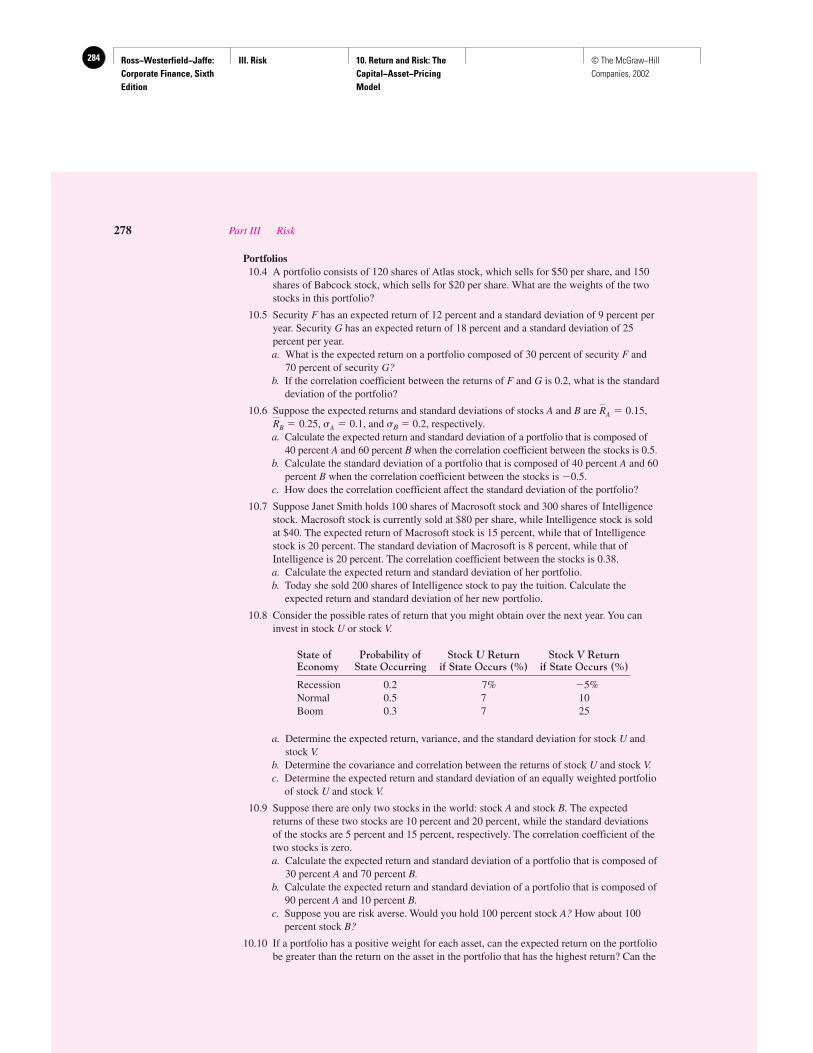
Ross−Westerfield−Jaffe: Corporate Finance, Sixth Edition
III. Risk 10. Return and Risk: The Capital−Asset−Pricing Model
284 © The McGraw−Hill Companies, 2002
Portfolios10.4 A portfolio consists of 120 shares of Atlas stock, which sells for $50 per share, and 150
shares of Babcock stock, which sells for $20 per share. What are the weights of the twostocks in this portfolio?
10.5 Security F has an expected return of 12 percent and a standard deviation of 9 percent peryear. Security G has an expected return of 18 percent and a standard deviation of 25percent per year.a. What is the expected return on a portfolio composed of 30 percent of security F and
70 percent of security G?b. If the correlation coefficient between the returns of F and G is 0.2, what is the standard
deviation of the portfolio?
10.6 Suppose the expected returns and standard deviations of stocks A and B are ,, , and �B � 0.2, respectively.
a. Calculate the expected return and standard deviation of a portfolio that is composed of40 percent A and 60 percent B when the correlation coefficient between the stocks is 0.5.
b. Calculate the standard deviation of a portfolio that is composed of 40 percent A and 60percent B when the correlation coefficient between the stocks is �0.5.
c. How does the correlation coefficient affect the standard deviation of the portfolio?
10.7 Suppose Janet Smith holds 100 shares of Macrosoft stock and 300 shares of Intelligencestock. Macrosoft stock is currently sold at $80 per share, while Intelligence stock is soldat $40. The expected return of Macrosoft stock is 15 percent, while that of Intelligencestock is 20 percent. The standard deviation of Macrosoft is 8 percent, while that ofIntelligence is 20 percent. The correlation coefficient between the stocks is 0.38.a. Calculate the expected return and standard deviation of her portfolio.b. Today she sold 200 shares of Intelligence stock to pay the tuition. Calculate the
expected return and standard deviation of her new portfolio.
10.8 Consider the possible rates of return that you might obtain over the next year. You caninvest in stock U or stock V.
State of Probability of Stock U Return Stock V ReturnEconomy State Occurring if State Occurs (%) if State Occurs (%)
Recession 0.2 7% �5%Normal 0.5 7 10Boom 0.3 7 25
a. Determine the expected return, variance, and the standard deviation for stock U andstock V.
b. Determine the covariance and correlation between the returns of stock U and stock V.c. Determine the expected return and standard deviation of an equally weighted portfolio
of stock U and stock V.
10.9 Suppose there are only two stocks in the world: stock A and stock B. The expectedreturns of these two stocks are 10 percent and 20 percent, while the standard deviationsof the stocks are 5 percent and 15 percent, respectively. The correlation coefficient of thetwo stocks is zero.a. Calculate the expected return and standard deviation of a portfolio that is composed of
30 percent A and 70 percent B.b. Calculate the expected return and standard deviation of a portfolio that is composed of
90 percent A and 10 percent B.c. Suppose you are risk averse. Would you hold 100 percent stock A? How about 100
percent stock B?
10.10 If a portfolio has a positive weight for each asset, can the expected return on the portfoliobe greater than the return on the asset in the portfolio that has the highest return? Can the
�A � 0.1RB � 0.25RA � 0.15
278 Part III Risk
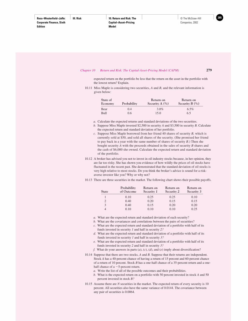
Ross−Westerfield−Jaffe: Corporate Finance, Sixth Edition
III. Risk 10. Return and Risk: The Capital−Asset−Pricing Model
285© The McGraw−Hill Companies, 2002
expected return on the portfolio be less that the return on the asset in the portfolio withthe lowest return? Explain.
10.11 Miss Maple is considering two securities, A and B, and the relevant information isgiven below:
State of Return on Return onEconomy Probability Security A (%) Security B (%)
Bear 0.4 3.0% 6.5%Bull 0.6 15.0 6.5
a. Calculate the expected returns and standard deviations of the two securities.b. Suppose Miss Maple invested $2,500 in security A and $3,500 in security B. Calculate
the expected return and standard deviation of her portfolio.c. Suppose Miss Maple borrowed from her friend 40 shares of security B, which is
currently sold at $50, and sold all shares of the security. (She promised her friendto pay back in a year with the same number of shares of security B.) Then shebought security A with the proceeds obtained in the sales of security B shares andthe cash of $6,000 she owned. Calculate the expected return and standard deviationof the portfolio.
10.12 A broker has advised you not to invest in oil industry stocks because, in her opinion, theyare far too risky. She has shown you evidence of how wildly the prices of oil stocks havefluctuated in the recent past. She demonstrated that the standard deviation of oil stocks isvery high relative to most stocks. Do you think the broker’s advice is sound for a risk-averse investor like you? Why or why not?
10.13 There are three securities in the market. The following chart shows their possible payoffs.
Probability Return on Return on Return onState of Outcome Security 1 Security 2 Security 3
1 0.10 0.25 0.25 0.102 0.40 0.20 0.15 0.153 0.40 0.15 0.20 0.204 0.10 0.10 0.10 0.25
a. What are the expected return and standard deviation of each security?b. What are the covariances and correlations between the pairs of securities?c. What are the expected return and standard deviation of a portfolio with half of its
funds invested in security 1 and half in security 2?d. What are the expected return and standard deviation of a portfolio with half of its
funds invested in security 1 and half in security 3?e. What are the expected return and standard deviation of a portfolio with half of its
funds invested in security 2 and half in security 3?f. What do your answers in parts (a), (c), (d), and (e) imply about diversification?
10.14 Suppose that there are two stocks, A and B. Suppose that their returns are independent.Stock A has a 40-percent chance of having a return of 15 percent and 60-percent chanceof a return of 10 percent. Stock B has a one-half chance of a 35-percent return and a one-half chance of a �5-percent return.a. Write the list of all of the possible outcomes and their probabilities.b. What is the expected return on a portfolio with 50 percent invested in stock A and 50
percent invested in stock B?
10.15 Assume there are N securities in the market. The expected return of every security is 10percent. All securities also have the same variance of 0.0144. The covariance betweenany pair of securities is 0.0064.
Chapter 10 Return and Risk: The Capital-Asset-Pricing Model (CAPM) 279
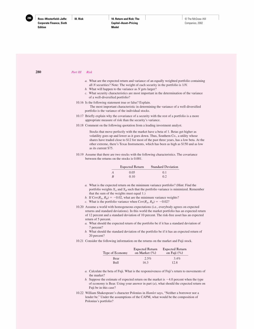
Ross−Westerfield−Jaffe: Corporate Finance, Sixth Edition
III. Risk 10. Return and Risk: The Capital−Asset−Pricing Model
286 © The McGraw−Hill Companies, 2002
a. What are the expected return and variance of an equally weighted portfolio containingall N securities? Note: The weight of each security in the portfolio is 1/N.
b. What will happen to the variance as N gets larger?c. What security characteristics are most important in the determination of the variance
of a well-diversified portfolio?
10.16 Is the following statement true or false? Explain.The most important characteristic in determining the variance of a well-diversified
portfolio is the variance of the individual stocks.
10.17 Briefly explain why the covariance of a security with the rest of a portfolio is a moreappropriate measure of risk than the security’s variance.
10.18 Comment on the following quotation from a leading investment analyst.
Stocks that move perfectly with the market have a beta of 1. Betas get higher asvolatility goes up and lower as it goes down. Thus, Southern Co., a utility whoseshares have traded close to $12 for most of the past three years, has a low beta. At theother extreme, there’s Texas Instruments, which has been as high as $150 and as lowas its current $75.
10.19 Assume that there are two stocks with the following characteristics. The covariancebetween the returns on the stocks is 0.001.
Expected Return Standard Deviation
A 0.05 0.1B 0.10 0.2
a. What is the expected return on the minimum variance portfolio? (Hint: Find theportfolio weights XA and XB such that the portfolio variance is minimized. Rememberthat the sum of the weights must equal 1.)
b. If Cov(RA, RB) � �0.02, what are the minimum variance weights?c. What is the portfolio variance when Cov(RA, RB) � �0.02?
10.20 Assume a world with homogeneous expectations (i.e., everybody agrees on expectedreturns and standard deviations). In this world the market portfolio has an expected returnof 12 percent and a standard deviation of 10 percent. The risk-free asset has an expectedreturn of 5 percent.a. What should the expected return of the portfolio be if it has a standard deviation of
7 percent?b. What should the standard deviation of the portfolio be if it has an expected return of
20 percent?
10.21 Consider the following information on the returns on the market and Fuji stock.
Expected Return Expected ReturnType of Economy on Market (%) on Fuji (%)
Bear 2.5% 3.4%Bull 16.3 12.8
a. Calculate the beta of Fuji. What is the responsiveness of Fuji’s return to movements ofthe market?
b. Suppose the estimate of expected return on the market is �4.0 percent when the typeof economy is Bear. Using your answer in part (a), what should the expected return onFuji be in this case?
10.22 William Shakespeare’s character Polonius in Hamlet says, “Neither a borrower nor alender be.” Under the assumptions of the CAPM, what would be the composition ofPolonius’s portfolio?
280 Part III Risk
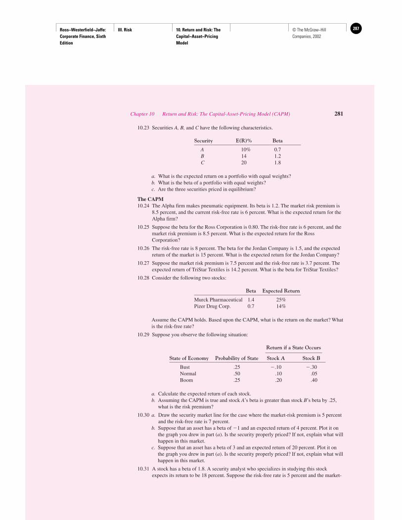
Ross−Westerfield−Jaffe: Corporate Finance, Sixth Edition
III. Risk 10. Return and Risk: The Capital−Asset−Pricing Model
287© The McGraw−Hill Companies, 2002
10.23 Securities A, B, and C have the following characteristics.
Security E(R)% Beta
A 10% 0.7B 14 1.2C 20 1.8
a. What is the expected return on a portfolio with equal weights?b. What is the beta of a portfolio with equal weights?c. Are the three securities priced in equilibrium?
The CAPM10.24 The Alpha firm makes pneumatic equipment. Its beta is 1.2. The market risk premium is
8.5 percent, and the current risk-free rate is 6 percent. What is the expected return for theAlpha firm?
10.25 Suppose the beta for the Ross Corporation is 0.80. The risk-free rate is 6 percent, and themarket risk premium is 8.5 percent. What is the expected return for the RossCorporation?
10.26 The risk-free rate is 8 percent. The beta for the Jordan Company is 1.5, and the expectedreturn of the market is 15 percent. What is the expected return for the Jordan Company?
10.27 Suppose the market risk premium is 7.5 percent and the risk-free rate is 3.7 percent. Theexpected return of TriStar Textiles is 14.2 percent. What is the beta for TriStar Textiles?
10.28 Consider the following two stocks:
Beta Expected Return
Murck Pharmaceutical 1.4 25%Pizer Drug Corp. 0.7 14%
Assume the CAPM holds. Based upon the CAPM, what is the return on the market? Whatis the risk-free rate?
10.29 Suppose you observe the following situation:
Return if a State Occurs
State of Economy Probability of State Stock A Stock B
Bust .25 �.10 �.30Normal .50 .10 .05Boom .25 .20 .40
a. Calculate the expected return of each stock.b. Assuming the CAPM is true and stock A’s beta is greater than stock B’s beta by .25,
what is the risk premium?
10.30 a. Draw the security market line for the case where the market-risk premium is 5 percentand the risk-free rate is 7 percent.
b. Suppose that an asset has a beta of �1 and an expected return of 4 percent. Plot it onthe graph you drew in part (a). Is the security properly priced? If not, explain what willhappen in this market.
c. Suppose that an asset has a beta of 3 and an expected return of 20 percent. Plot it onthe graph you drew in part (a). Is the security properly priced? If not, explain what willhappen in this market.
10.31 A stock has a beta of 1.8. A security analyst who specializes in studying this stockexpects its return to be 18 percent. Suppose the risk-free rate is 5 percent and the market-
Chapter 10 Return and Risk: The Capital-Asset-Pricing Model (CAPM) 281

Ross−Westerfield−Jaffe: Corporate Finance, Sixth Edition
III. Risk 10. Return and Risk: The Capital−Asset−Pricing Model
288 © The McGraw−Hill Companies, 2002
risk premium is 8 percent. Is the analyst pessimistic or optimistic about this stock relativeto the market’s expectations?
10.32 Suppose the expected return on the market is 13.8 percent and the risk-free rate is 6.4percent. Solomon Inc. stock has a beta of 1.2.a. What is the expected return on the Solomon stock?b. If the risk-free rate decreases to 3.5 percent, what is the expected return on the
Solomon stock?
10.33 The expected return on a portfolio that combines the risk-free asset and the asset at thepoint of tangency to the efficient set is 25 percent. The expected return was calculatedunder the following assumptions:
The risk-free rate is 5 percent.The expected return on the market portfolio of risky assets is 20 percent.The standard deviation of the efficient portfolio is 4 percent.
In this environment, what expected rate of return would a security earn if it had a 0.5correlation with the market and a standard deviation of 2 percent?
10.34 Suppose the current risk-free rate is 7.6 percent. Potpourri Inc. stock has a beta of 1.7 andan expected return of 16.7 percent. (Assume the CAPM is true.)a. What is the risk premium on the market?b. Magnolia Industries stock has a beta of 0.8. What is the expected return on the
Magnolia stock?c. Suppose you have invested $10,000 in both Potpourri and Magnolia, and the beta of
the portfolio is 1.07. How much did you invest in each stock? What is the expectedreturn on the portfolio?
10.35 Suppose the risk-free rate is 6.3 percent and the market portfolio has an expected rate ofreturn of 14.8 percent. The market portfolio has a variance of 0.0121. Portfolio Z has acorrelation coefficient with the market of 0.45 and a variance of 0.0169. According to theCAPM, what is the expected rate of return on portfolio Z?
10.36 The following data have been developed for the Durham Company.
Variance of market returns � 0.04326Covariance of the returns on Durham and the market � 0.0635
Suppose the market risk premium is 9.4 percent and the expected return on Treasury billsis 4.9 percent.a. Write the equation of the security market line.b. What is the required return of Durham Company?
10.37 Johnson Paint stock has an expected return of 19 percent with a beta of 1.7, whileWilliamson Tire stock has an expected return of 14 percent with a beta of 1.2. Assumethe CAPM is true. What is the expected return on the market? What is the risk-free rate?
10.38 Is the following statement true or false? Explain.A risky security cannot have an expected return that is less than the risk-free rate
because no risk-averse investor would be willing to hold this asset in equilibrium.
10.39 Suppose you have invested $30,000 in the following four stocks.
Security Amount Invested Beta
Stock A $ 5,000 0.75Stock B 10,000 1.10Stock C 8,000 1.36Stock D 7,000 1.88
The risk-free rate is 4 percent and the expected return on the market portfolio is 15 percent.Based on the CAPM, what is the expected return on the above portfolio?
282 Part III Risk
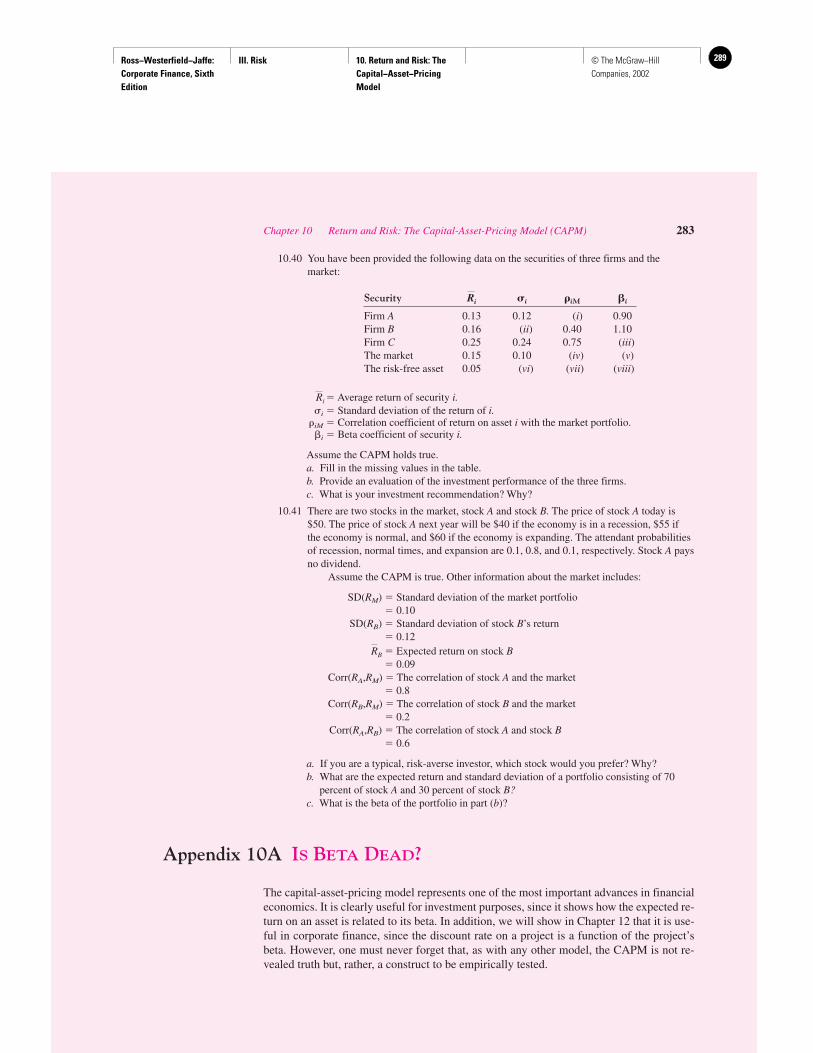
Ross−Westerfield−Jaffe: Corporate Finance, Sixth Edition
III. Risk 10. Return and Risk: The Capital−Asset−Pricing Model
289© The McGraw−Hill Companies, 2002
10.40 You have been provided the following data on the securities of three firms and themarket:
Security �i �iM �i
Firm A 0.13 0.12 (i) 0.90Firm B 0.16 (ii) 0.40 1.10Firm C 0.25 0.24 0.75 (iii)The market 0.15 0.10 (iv) (v)The risk-free asset 0.05 (vi) (vii) (viii)
� Average return of security i.�i � Standard deviation of the return of i.
iM � Correlation coefficient of return on asset i with the market portfolio.�i � Beta coefficient of security i.
Assume the CAPM holds true.a. Fill in the missing values in the table.b. Provide an evaluation of the investment performance of the three firms.c. What is your investment recommendation? Why?
10.41 There are two stocks in the market, stock A and stock B. The price of stock A today is$50. The price of stock A next year will be $40 if the economy is in a recession, $55 ifthe economy is normal, and $60 if the economy is expanding. The attendant probabilitiesof recession, normal times, and expansion are 0.1, 0.8, and 0.1, respectively. Stock A paysno dividend.
Assume the CAPM is true. Other information about the market includes:
SD(RM) � Standard deviation of the market portfolio� 0.10
SD(RB) � Standard deviation of stock B’s return� 0.12� Expected return on stock B� 0.09
Corr(RA,RM) � The correlation of stock A and the market� 0.8
Corr(RB,RM) � The correlation of stock B and the market� 0.2
Corr(RA,RB) � The correlation of stock A and stock B� 0.6
a. If you are a typical, risk-averse investor, which stock would you prefer? Why?b. What are the expected return and standard deviation of a portfolio consisting of 70
percent of stock A and 30 percent of stock B?c. What is the beta of the portfolio in part (b)?
Appendix 10A IS BETA DEAD?
The capital-asset-pricing model represents one of the most important advances in financialeconomics. It is clearly useful for investment purposes, since it shows how the expected re-turn on an asset is related to its beta. In addition, we will show in Chapter 12 that it is use-ful in corporate finance, since the discount rate on a project is a function of the project’sbeta. However, one must never forget that, as with any other model, the CAPM is not re-vealed truth but, rather, a construct to be empirically tested.
RB
Ri
Ri
Chapter 10 Return and Risk: The Capital-Asset-Pricing Model (CAPM) 283

Ross−Westerfield−Jaffe: Corporate Finance, Sixth Edition
III. Risk 10. Return and Risk: The Capital−Asset−Pricing Model
290 © The McGraw−Hill Companies, 2002
The first empirical tests of the CAPM occurred over 20 years ago and were quite sup-portive. Using data from the 1930s to the 1960s, researchers showed that the average returnon a portfolio of stocks was positively related to the beta of the portfolio,18 a finding con-sistent with the CAPM. Though some evidence in these studies was less consistent with theCAPM,19 financial economists were quick to embrace the CAPM following these empiri-cal papers.
While a large body of empirical work developed in the following decades, often withvarying results, the CAPM was not seriously called into question until the 1990s. Two pa-pers by Fama and French20 (yes, the same Fama whose joint paper in 1973 with JamesMacBeth supported the CAPM) present evidence inconsistent with the model. Their workhas received a great deal of attention, both in academic circles and in the popular press, withnewspaper articles displaying headlines such as “Beta Is Dead!” These papers make two re-lated points. First, they conclude that the relationship between average return and beta isweak over the period from 1941 to 1990 and virtually nonexistent from 1963 to 1990.Second, they argue that the average return on a security is negatively related to both thefirm’s price-to-earnings (P/E) ratio and the firm’s market value-to-book value (M/B) ratio.These contentions, if confirmed by other research, would be quite damaging to the CAPM.After all, the CAPM states that the expected returns on stocks should be related only to beta,and not to other factors such as P/E and M/B.
However, a number of researchers have criticized the Fama-French papers. While weavoid an in-depth discussion of the fine points of the debate, we mention a few issues. First,although Fama and French cannot reject the hypothesis that average returns are unrelatedto beta, one can also not reject the hypothesis that average returns are related to beta exactlyas specified by the CAPM. In other words, while 50 years of data seem like a lot, they maysimply not be enough to test the CAPM properly. Second, the result with P/E and M/B maybe due to a statistical fallacy called a hindsight bias.21 Third, P/E and M/B are merely twoof an infinite number of possible factors. Thus, the relationship between average return andboth P/E and M/B may be spurious, being nothing more than the result of data mining.Fourth, average returns are positively related to beta over the period from 1927 to the pres-ent. There appears to be no compelling reason for emphasizing a shorter period than thisone. Fifth, average returns are actually positively related to beta over shorter periods whenannual data, rather than monthly data, are used to estimate beta.22 There appears to be nocompelling reason for preferring either monthly data over annual data or vice versa. Thus,we believe that, while the results of Fama and French are quite intriguing, they cannot beviewed as the final word.
284 Part III Risk
18Perhaps the two most well-known papers were Fischer Black, Michael C. Jensen, and Myron S. Scholes, “TheCapital Asset Pricing Model: Some Empirical Tests,” in M. Jensen, ed., Studies in the Theory of Capital Markets(New York: Praeger, 1972), and Eugene F. Fama and James MacBeth, “Risk, Return and Equilibrium: SomeEmpirical Tests,” Journal of Political Economy 8 (1973), pp. 607–36.19For example, the studies suggest that the average return on a zero-beta portfolio is above the risk-free rate, afinding inconsistent with the CAPM.20Eugene F. Fama and Kenneth R. French, “The Cross-Section of Expected Stock Returns,” Journal of Finance47 (1992), pp. 427–66, and E. F. Fama and K. R. French, “Common Risk Factors in the Returns on Stocks andBonds,” Journal of Financial Economics 17 (1993), pp. 3–56.21For example, see William J. Breen and Robert A. Koraczyk, “On Selection Biases in Book-to-Market BasedTests of Asset Pricing Models,” unpublished paper. Northwestern University, November 1993; and S. P. Kothari,Jay Shanken, and Richard G. Sloan, “Another Look at the Cross-Section of Expected Stock Returns,” Journal ofFinance (March 1995).22Points 4 and 5 are addressed in the Kothari, Shanken, and Sloan paper.
Ross−Westerfield−Jaffe: Corporate Finance, Sixth Edition
III. Risk 11. An Alternative View of Risk and Return: The Arbitrage Pricing Theory
291© The McGraw−Hill Companies, 2002
An Alternative View ofRisk and Return: TheArbitrage Pricing Theory
CH
AP
TE
R11
EXECUTIVE SUMMARY
The previous two chapters mentioned the obvious fact that returns on securities arevariable. This variability is measured by variance and by standard deviation.Next, we mentioned the somewhat less obvious fact that the returns on securities
are interdependent. We measured the degree of interdependence between a pair of secu-rities by covariance and by correlation. This interdependence led to a number of inter-esting results. First, we showed that diversification in stocks can eliminate some, but notall, risk. By contrast, we showed that diversification in a casino can eliminate all risk.Second, the interdependence of returns led to the capital-asset-pricing model (CAPM).This model posits a positive (and linear) relationship between the beta of a security andits expected return.
The CAPM was developed in the early 1960s.1 An alternative to the CAPM, called thearbitrage pricing theory (APT), has been developed more recently.2 For our purposes, thedifferences between the two models stem from the APT’s treatment of interrelationshipamong the returns on securities.3 The APT assumes that returns on securities are generatedby a number of industrywide and marketwide factors. Correlation between a pair of secu-rities occurs when these two securities are affected by the same factor or factors. By con-trast, though the CAPM allows correlation among securities, it does not specify the under-lying factors causing the correlation.
Both the APT and the CAPM imply a positive relationship between expected returnand risk. In our (perhaps biased) opinion, the APT allows this relationship to be developedin a particularly intuitive manner. In addition, the APT views risk more generally than justthe standardized covariance or beta of a security with the market portfolio. Therefore, weoffer this approach as an alternative to the CAPM.
1In particular, see Jack Treynor, “Toward a Theory of the Market Value of Risky Assets,” unpublished manuscript(1961); William F. Sharpe, “Capital Asset Prices: A Theory of Market Equilibrium under Conditions of Risk,”Journal of Finance (September 1964); and John Lintner, “The Valuation of Risky Assets and the Selection ofRisky Investments in Stock Portfolios and Capital Budgets,” Review of Economics and Statistics (February 1965).2See Stephen A. Ross, “The Arbitrage Theory of Capital Asset Pricing,” Journal of Economic Theory (December 1976).3This is by no means the only difference in the assumptions of the two models. For example, the CAPM usuallyassumes either that the returns on assets are normally distributed or that investors have quadratic utilityfunctions. The APT does not require either assumption. While this and other differences are quite important inresearch, they are not relevant to the material presented in our text.
Ross−Westerfield−Jaffe: Corporate Finance, Sixth Edition
III. Risk 11. An Alternative View of Risk and Return: The Arbitrage Pricing Theory
292 © The McGraw−Hill Companies, 2002
11.1 FACTOR MODELS: ANNOUNCEMENTS, SURPRISES,AND EXPECTED RETURNS
We learned in the previous chapter how to construct portfolios and how to evaluate their re-turns. We now step back and examine the returns on individual securities more closely. Bydoing this we will find that the portfolios inherit and alter the properties of the securitiesthey comprise.
To be concrete, let us consider the return on the stock of a company called Flyers. Whatwill determine this stock’s return in, say, the coming month?
The return on any stock traded in a financial market consists of two parts. First, the nor-mal or expected return from the stock is the part of the return that shareholders in the mar-ket predict or expect. It depends on all of the information shareholders have that bears on thestock, and it uses all of our understanding of what will influence the stock in the next month.
The second part is the uncertain or risky return on the stock. This is the portion thatcomes from information that will be revealed within the month. The list of such informa-tion is endless, but here are some examples:
• News about Flyers’ research.• Government figures released on the gross national product (GNP).• Results of the latest arms-control talks.• Discovery that a rival’s product has been tampered with.• News that Flyers’ sales figures are higher than expected.• A sudden drop in interest rates.• The unexpected retirement of Flyers’ founder and president.
A way to write the return on Flyers’ stock in the coming month, then, is
where R is the actual total return in the month, is the expected part of the return, and Ustands for the unexpected part of the return.
Some care must be exercised in studying the effect of these or other news items on thereturn. For example, the government might give us GNP or unemployment figures for thismonth, but how much of that is new information for shareholders? Surely at the beginningof the month shareholders will have some idea or forecast of what the monthly GNP willbe. To the extent to which the shareholders had forecast the government’s announcement,that forecast should be factored into the expected part of the return as of the beginning ofthe month, . On the other hand, insofar as the announcement by the government is a sur-prise and to the extent to which it influences the return on the stock, it will be part of U, theunanticipated part of the return.
As an example, suppose shareholders in the market had forecast that the GNP increasethis month would be 0.5 percent. If GNP influences our company’s stock, this forecast willbe part of the information shareholders use to form the expectation, , of the monthly re-turn. If the actual announcement this month is exactly 0.5 percent, the same as the forecast,then the shareholders learned nothing new, and the announcement is not news. It is likehearing a rumor about a friend when you knew it all along. Another way of saying this isthat shareholders had already discounted the announcement. This use of the word discountis different from that in computing present value, but the spirit is similar. When we discounta dollar in the future, we say that it is worth less to us because of the time value of money.When we discount an announcement or a news item in the future, we mean that it has lessimpact on the market because the market already knew much of it.
R
R
R
R � R � U
286 Part III Risk
Ross−Westerfield−Jaffe: Corporate Finance, Sixth Edition
III. Risk 11. An Alternative View of Risk and Return: The Arbitrage Pricing Theory
293© The McGraw−Hill Companies, 2002
On the other hand, suppose the government announced that the actual GNP increaseduring the year was 1.5 percent. Now shareholders have learned something—that the in-crease is one percentage point higher than they had forecast. This difference between theactual result and the forecast, one percentage point in this example, is sometimes called theinnovation or surprise.
Any announcement can be broken into two parts, the anticipated or expected part andthe surprise or innovation:
Announcement � Expected part � Surprise
The expected part of any announcement is part of the information the market uses to formthe expectation, , of the return on the stock. The surprise is the news that influences theunanticipated return on the stock, U.
To give another example, if shareholders knew in January that the president of a firmwas going to resign, the official announcement in February will be fully expected and willbe discounted by the market. Because the announcement was expected before February, itsinfluence on the stock will have taken place before February. The announcement itself inFebruary will contain no surprise and the stock’s price should not change at all at the an-nouncement in February.
When we speak of news, then, we refer to the surprise part of any announcement andnot the portion that the market has expected and therefore has already discounted.
• What are the two basic parts of a return?• Under what conditions will some news have no effect on common stock prices?
11.2 RISK: SYSTEMATIC AND UNSYSTEMATIC
The unanticipated part of the return—that portion resulting from surprises—is the true riskof any investment. After all, if we got what we had expected, there would be no risk and nouncertainty.
There are important differences, though, among various sources of risk. Look at ourprevious list of news stories. Some of these stories are directed specifically at Flyers, andsome are more general. Which of the news items are of specific importance to Flyers?
Announcements about interest rates or GNP are clearly important for nearly all com-panies, whereas the news about Flyers’ president, its research, its sales, or the affairs of arival company are of specific interest to Flyers. We will divide these two types of an-nouncements and the resulting risk, then, into two components: a systematic portion, calledsystematic risk, and the remainder, which we call specific or unsystematic risk. The fol-lowing definitions describe the difference:
• A systematic risk is any risk that affects a large number of assets, each to a greateror lesser degree.
• An unsystematic risk is a risk that specifically affects a single asset or a small groupof assets.4
Uncertainty about general economic conditions, such as GNP, interest rates, or inflation,is an example of systematic risk. These conditions affect nearly all stocks to some degree.
R
Chapter 11 An Alternative View of Risk and Return: The Arbitrage Pricing Theory 287
4In the previous chapter, we briefly mentioned that unsystematic risk is risk that can be diversified away in alarge portfolio. This result will also follow from the present analysis.
QUESTIONS
CO
NC
EP
T
?
Ross−Westerfield−Jaffe: Corporate Finance, Sixth Edition
III. Risk 11. An Alternative View of Risk and Return: The Arbitrage Pricing Theory
294 © The McGraw−Hill Companies, 2002
An unanticipated or surprise increase in inflation affects wages and the costs of the suppliesthat companies buy, the value of the assets that companies own, and the prices at which com-panies sell their products. These forces to which all companies are susceptible are theessence of systematic risk.
In contrast, the announcement of a small oil strike by a company may very well affectthat company alone or a few other companies. Certainly, it is unlikely to have an effect onthe world oil market. To stress that such information is unsystematic and affects only somespecific companies, we sometimes call it an idiosyncratic risk.
The distinction between a systematic risk and an unsystematic risk is never as exact aswe make it out to be. Even the most narrow and peculiar bit of news about a company rip-ples through the economy. It reminds us of the tale of the war that was lost because onehorse lost a shoe; even a minor event may have an impact on the world. But this degree ofhair-splitting should not trouble us much. To paraphrase a Supreme Court Justice’s com-ment when speaking of pornography, we may not be able to define a systematic risk and anunsystematic risk exactly, but we know them when we see them.
This permits us to break down the risk of Flyers’ stock into its two components: thesystematic and the unsystematic. As is traditional, we will use the Greek epsilon, �, to rep-resent the unsystematic risk and write
where we have used the letter m to stand for the systematic risk. Sometimes systematic riskis referred to as market risk. This emphasizes the fact that m influences all assets in the mar-ket to some extent.
The important point about the way we have broken the total risk, U, into its two com-ponents, m and �, is that �, because it is specific to the company, is unrelated to the specificrisk of most other companies. For example, the unsystematic risk on Flyers’ stock, �F, is un-related to the unsystematic risk of Xerox’s stock, �X. The risk that Flyers’ stock will go upor down because of a discovery by its research team—or its failure to discover something—probably is unrelated to any of the specific uncertainties that affect Xerox stock.
Using the terms of the previous chapter, this means that the unsystematic risk of Flyers’stock and Xerox’s stock are unrelated to each other, or uncorrelated. In the symbols of statistics,
Corr(�F, �X) � 0
• Describe the difference between systematic risk and unsystematic risk.• Why is unsystematic risk sometimes referred to as idiosyncratic risk?
11.3 SYSTEMATIC RISK AND BETAS
The fact that the unsystematic parts of the returns on two companies are unrelated to eachother does not mean that the systematic portions are unrelated. On the contrary, becauseboth companies are influenced by the same systematic risks, individual companies’ sys-tematic risks and therefore their total returns will be related.
For example, a surprise about inflation will influence almost all companies to some ex-tent. How sensitive is Flyers’ stock return to unanticipated changes in inflation? If Flyers’stock tends to go up on news that inflation is exceeding expectations, we would say that itis positively related to inflation. If the stock goes down when inflation exceeds expectationsand up when inflation falls short of expectations, it is negatively related. In the unusual casewhere a stock’s return is uncorrelated with inflation surprises, inflation has no effect on it.
� R � m � �
R � R � U
288 Part III Risk
QUESTIONS
CO
NC
EP
T
?
Ross−Westerfield−Jaffe: Corporate Finance, Sixth Edition
III. Risk 11. An Alternative View of Risk and Return: The Arbitrage Pricing Theory
295© The McGraw−Hill Companies, 2002
We capture the influence of a systematic risk like inflation on a stock by using the betacoefficient. The beta coefficient, �, tells us the response of the stock’s return to a systematicrisk. In the previous chapter, beta measured the responsiveness of a security’s return to a spe-cific risk factor, the return on the market portfolio. We used this type of responsiveness to de-velop the capital-asset-pricing model. Because we now consider many types of systematicrisks, our current work can be viewed as a generalization of our work in the previous chapter.
If a company’s stock is positively related to the risk of inflation, that stock has a posi-tive inflation beta. If it is negatively related to inflation, its inflation beta is negative, and ifit is uncorrelated with inflation, its inflation beta is zero.
It’s not hard to imagine some stocks with positive inflation betas and other stocks withnegative inflation betas. The stock of a company owning gold mines will probably have apositive inflation beta because an unanticipated rise in inflation is usually associated withan increase in gold prices. On the other hand, an automobile company facing stiff foreigncompetition might find that an increase in inflation means that the wages it pays are higher,but that it cannot raise its prices to cover the increase. This profit squeeze, as the company’sexpenses rise faster than its revenues, would give its stock a negative inflation beta.
Some companies that have few assets and that act as brokers—buying items in com-petitive markets and reselling them in other markets—might be relatively unaffected by in-flation, because their costs and their revenues would rise and fall together. Their stockwould have an inflation beta of zero.
Some structure is useful at this point. Suppose we have identified three systematic riskson which we want to focus. We may believe that these three are sufficient to describe thesystematic risks that influence stock returns. Three likely candidates are inflation, GNP, andinterest rates. Thus, every stock will have a beta associated with each of these systematicrisks: an inflation beta, a GNP beta, and an interest-rate beta. We can write the return on thestock, then, in the following form:
where we have used the symbol �I to denote the stock’s inflation beta, �GNP for its GNPbeta, and �r to stand for its interest-rate beta. In the equation, F stands for a surprise,whether it be in inflation, GNP, or interest rates.
Let us go through an example to see how the surprises and the expected return add up toproduce the total return, R, on a given stock. To make it more familiar, suppose that the returnis over a horizon of a year and not just a month. Suppose that at the beginning of the year, infla-tion is forecast to be 5 percent for the year, GNP is forecast to increase by 2 percent, and interestrates are expected not to change. Suppose the stock we are looking at has the following betas:
�I � 2�GNP � 1
�r � �1.8
The magnitude of the beta describes how great an impact a systematic risk has on a stock’sreturns. A beta of �1 indicates that the stock’s return rises and falls one for one with the sys-tematic factor. This means, in our example, that because the stock has a GNP beta of 1, it ex-periences a 1-percent increase in return for every 1-percent surprise increase in GNP. If its GNPbeta were �2, it would fall by 2 percent when there was an unanticipated increase of 1 percentin GNP, and it would rise by 2 percent if GNP experienced a surprise 1-percent decline.
Finally, let us suppose that during the year the following occurs: Inflation rises by 7 percent, GNP rises by only 1 percent, and interest rates fall by 2 percent. Last, supposewe learn some good news about the company, perhaps that it is succeeding quickly with
� R � �IFI � �GNPFGNP � �rFr � �
� R � m � �
R � R � U
Chapter 11 An Alternative View of Risk and Return: The Arbitrage Pricing Theory 289
Ross−Westerfield−Jaffe: Corporate Finance, Sixth Edition
III. Risk 11. An Alternative View of Risk and Return: The Arbitrage Pricing Theory
296 © The McGraw−Hill Companies, 2002
some new business strategy, and that this unanticipated development contributes 5 percentto its return. In other words,
� � 5%
Let us assemble all of this information to find what return the stock had during the year.First, we must determine what news or surprises took place in the systematic factors.
From our information we know that
Expected inflation � 5%Expected GNP change � 2%
and
Expected change in interest rates � 0%
This means that the market had discounted these changes, and the surprises will be the dif-ference between what actually takes place and these expectations:
FI � Surprise in inflation� Actual inflation � Expected inflation� 7% � 5%� 2%
Similarly,
FGNP � Surprise in GNP� Actual GNP � Expected GNP� 1% � 2%� �1%
and
Fr � Surprise in change in interest rates� Actual change � Expected change� �2% � 0%� �2%
The total effect of the systematic risks on the stock return, then, is
m � Systematic risk portion of return� �IFI � �GNPFGNP � �rFr
� [2 � 2%] � [1 � (�1%)] � [(�1.8) � (�2%)]� 6.6%
Combining this with the unsystematic risk portion, the total risky portion of the return onthe stock is
m � � � 6.6% � 5% � 11.6%
Last, if the expected return on the stock for the year was, say, 4 percent, the total returnfrom all three components will be
� 4% � 6.6% � 5%� 15.6%
The model we have been looking at is called a factor model, and the systematicsources of risk, designated F, are called the factors. To be perfectly formal, a k-factor modelis a model where each stock’s return is generated by
R � R � m � �
290 Part III Risk

Ross−Westerfield−Jaffe: Corporate Finance, Sixth Edition
III. Risk 11. An Alternative View of Risk and Return: The Arbitrage Pricing Theory
297© The McGraw−Hill Companies, 2002
where � is specific to a particular stock and uncorrelated with the � term for other stocks.In our preceding example we had a three-factor model. We used inflation, GNP, and thechange in interest rates as examples of systematic sources of risk, or factors. Researchershave not settled on what is the correct set of factors. Like so many other questions, thismight be one of those matters that is never laid to rest.
In practice, researchers frequently use a one-factor model for returns. They do not useall of the sorts of economic factors we used previously as examples; instead, they use an in-dex of stock market returns—like the S&P 500, or even a more broadly based index withmore stocks in it—as the single factor. Using the single-factor model we can write returns as
Where there is only one factor (the returns on the S&P 500–portfolio index), we do not needto put a subscript on the beta. In this form (with minor modifications) the factor model iscalled a market model. This term is employed because the index that is used for the factoris an index of returns on the whole (stock) market. The market model is written as
where RM is the return on the market portfolio.5 The single � is called the beta coefficient.
• What is an inflation beta? A GNP beta? An interest-rate beta?• What is the difference between a k-factor model and the market model?• Define the beta coefficient.
11.4 PORTFOLIOS AND FACTOR MODELS
Now let us see what happens to portfolios of stocks when each of the stocks follows a one-factor model. For purposes of discussion, we will take the coming one-month period andexamine returns. We could have used a day or a year or any other time period. If the periodrepresents the time between decisions, however, we would rather it be short than long, anda month is a reasonable time frame to use.
We will create portfolios from a list of N stocks, and we will use a one-factor model tocapture the systematic risk. The ith stock in the list will therefore have returns
(11.1)
where we have subscripted the variables to indicate that they relate to the ith stock. Noticethat the factor F is not subscripted. The factor that represents systematic risk could be a sur-prise in GNP, or we could use the market model and let the difference between the S&P 500return and what we expect that return to be, , be the factor. In either case,the factor applies to all of the stocks.
RS&P500 � RS&P500
Ri � Ri � �iF � �i
R � R � � �RM � RM� � �
R � R � � �RS&P500 � RS&P500� � �
R � R � �1F1 � �2F2 � . . . � �kFk � �
Chapter 11 An Alternative View of Risk and Return: The Arbitrage Pricing Theory 291
5Alternatively, the market model could be written as
R � � � �RM � �
Here alpha (�) is an intercept term equal .R � �RM
QUESTIONS
CO
NC
EP
T
?
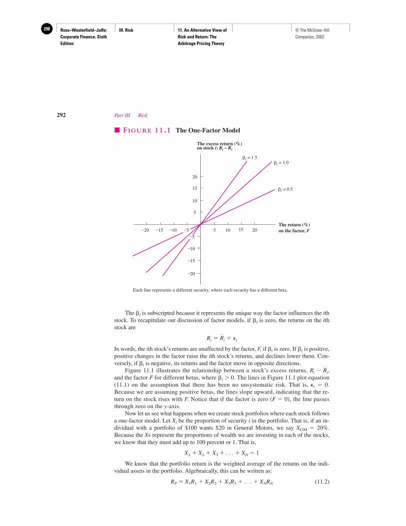
Ross−Westerfield−Jaffe: Corporate Finance, Sixth Edition
III. Risk 11. An Alternative View of Risk and Return: The Arbitrage Pricing Theory
298 © The McGraw−Hill Companies, 2002
The �i is subscripted because it represents the unique way the factor influences the ithstock. To recapitulate our discussion of factor models, if �i is zero, the returns on the ithstock are
In words, the ith stock’s returns are unaffected by the factor, F, if �i is zero. If �i is positive,positive changes in the factor raise the ith stock’s returns, and declines lower them. Con-versely, if �i is negative, its returns and the factor move in opposite directions.
Figure 11.1 illustrates the relationship between a stock’s excess returns, ,and the factor F for different betas, where �i � 0. The lines in Figure 11.1 plot equation(11.1) on the assumption that there has been no unsystematic risk. That is, �i � 0.Because we are assuming positive betas, the lines slope upward, indicating that the re-turn on the stock rises with F. Notice that if the factor is zero (F � 0), the line passesthrough zero on the y-axis.
Now let us see what happens when we create stock portfolios where each stock followsa one-factor model. Let Xi be the proportion of security i in the portfolio. That is, if an in-dividual with a portfolio of $100 wants $20 in General Motors, we say XGM � 20%.Because the Xs represent the proportions of wealth we are investing in each of the stocks,we know that they must add up to 100 percent or 1. That is,
X1 � X2 � X3 � . . . � XN � 1
We know that the portfolio return is the weighted average of the returns on the indi-vidual assets in the portfolio. Algebraically, this can be written as:
RP � X1R1 � X2R2 � X3R3 � . . . � XNRN (11.2)
Ri � Ri
Ri � Ri � �i
292 Part III Risk
The excess return (%)on stock i: Ri – Ri
The return (%)on the factor, F
–5
15
10
5
–10
–15
20
–20 –15 –10 –5 5 10 15 20
�i = 1.5�i = 1.0
�i = 0.5
–20
� FIGURE 11.1 The One-Factor Model
Each line represents a different security, where each security has a different beta.
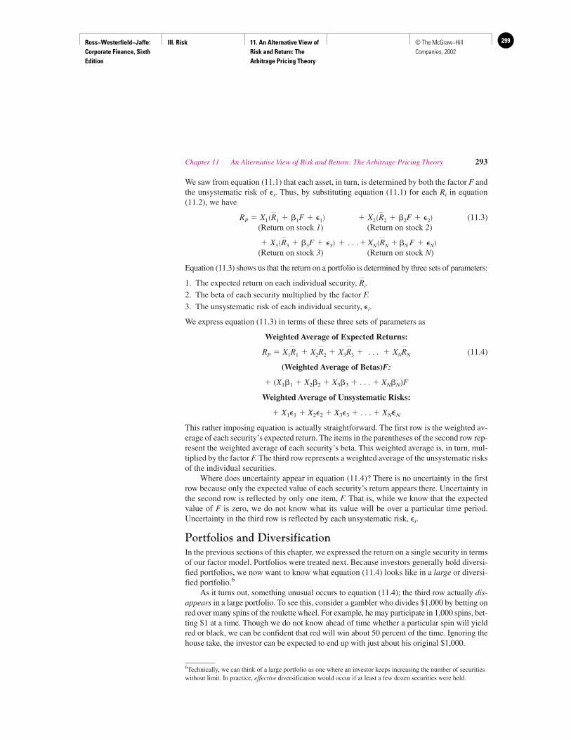
Ross−Westerfield−Jaffe: Corporate Finance, Sixth Edition
III. Risk 11. An Alternative View of Risk and Return: The Arbitrage Pricing Theory
299© The McGraw−Hill Companies, 2002
We saw from equation (11.1) that each asset, in turn, is determined by both the factor F andthe unsystematic risk of �i. Thus, by substituting equation (11.1) for each Ri in equation(11.2), we have
(11.3)(Return on stock 1) (Return on stock 2)
(Return on stock 3) (Return on stock N)
Equation (11.3) shows us that the return on a portfolio is determined by three sets of parameters:
1. The expected return on each individual security, .
2. The beta of each security multiplied by the factor F.
3. The unsystematic risk of each individual security, �i.
We express equation (11.3) in terms of these three sets of parameters as
Weighted Average of Expected Returns:
(11.4)
(Weighted Average of Betas)F:
� (X1�1 � X2�2 � X3�3 � . . . � XN�N)F
Weighted Average of Unsystematic Risks:
� X1�1 � X2�2 � X3�3 � . . . � XN�N
This rather imposing equation is actually straightforward. The first row is the weighted av-erage of each security’s expected return. The items in the parentheses of the second row rep-resent the weighted average of each security’s beta. This weighted average is, in turn, mul-tiplied by the factor F. The third row represents a weighted average of the unsystematic risksof the individual securities.
Where does uncertainty appear in equation (11.4)? There is no uncertainty in the firstrow because only the expected value of each security’s return appears there. Uncertainty inthe second row is reflected by only one item, F. That is, while we know that the expectedvalue of F is zero, we do not know what its value will be over a particular time period.Uncertainty in the third row is reflected by each unsystematic risk, �i.
Portfolios and DiversificationIn the previous sections of this chapter, we expressed the return on a single security in termsof our factor model. Portfolios were treated next. Because investors generally hold diversi-fied portfolios, we now want to know what equation (11.4) looks like in a large or diversi-fied portfolio.6
As it turns out, something unusual occurs to equation (11.4); the third row actually dis-appears in a large portfolio. To see this, consider a gambler who divides $1,000 by betting onred over many spins of the roulette wheel. For example, he may participate in 1,000 spins, bet-ting $1 at a time. Though we do not know ahead of time whether a particular spin will yieldred or black, we can be confident that red will win about 50 percent of the time. Ignoring thehouse take, the investor can be expected to end up with just about his original $1,000.
RP � X1R1 � X2R2 � X3R3 � . . . � XNRN
Ri
� X3 �R3 � �3F � �3� � . . . � XN �RN � �N F � �N�
RP � X1 �R1 � �1F � �1� � X2 �R2 � �2F � �2�
Chapter 11 An Alternative View of Risk and Return: The Arbitrage Pricing Theory 293
6Technically, we can think of a large portfolio as one where an investor keeps increasing the number of securitieswithout limit. In practice, effective diversification would occur if at least a few dozen securities were held.
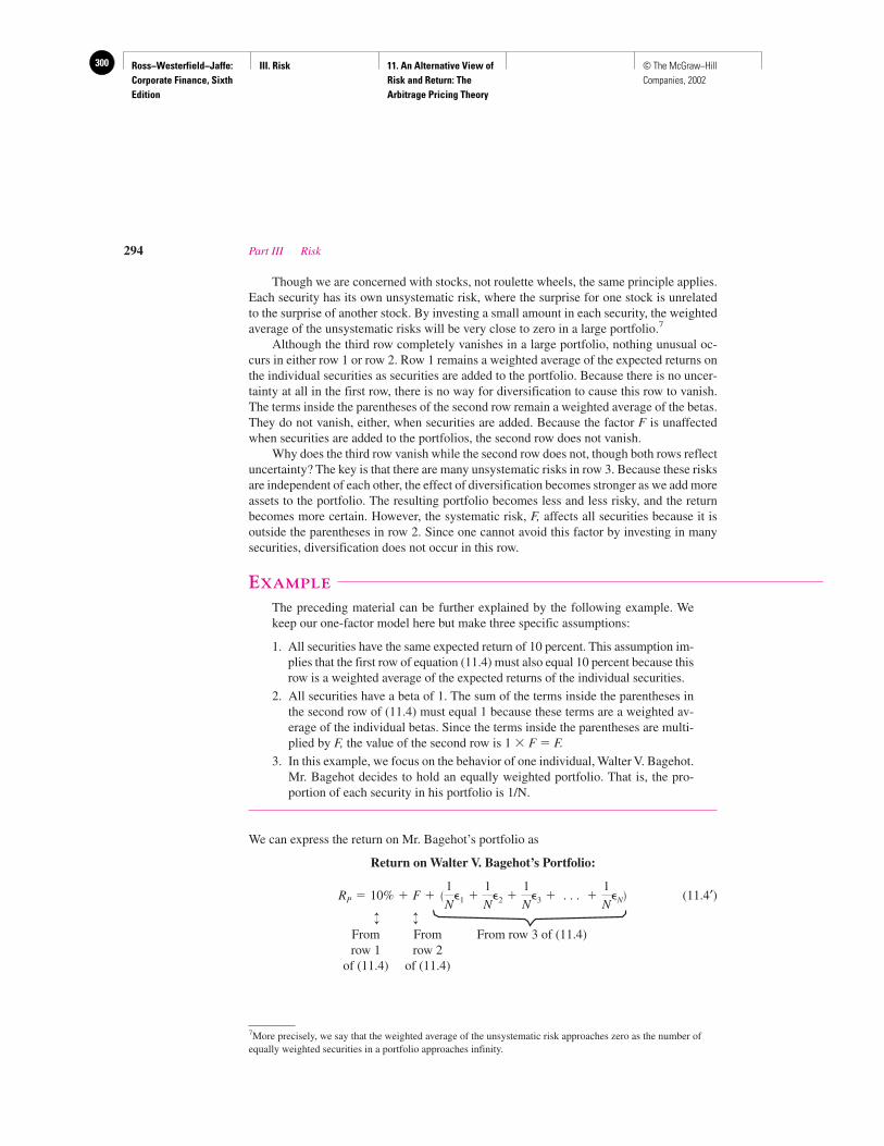
Ross−Westerfield−Jaffe: Corporate Finance, Sixth Edition
III. Risk 11. An Alternative View of Risk and Return: The Arbitrage Pricing Theory
300 © The McGraw−Hill Companies, 2002
Though we are concerned with stocks, not roulette wheels, the same principle applies.Each security has its own unsystematic risk, where the surprise for one stock is unrelatedto the surprise of another stock. By investing a small amount in each security, the weightedaverage of the unsystematic risks will be very close to zero in a large portfolio.7
Although the third row completely vanishes in a large portfolio, nothing unusual oc-curs in either row 1 or row 2. Row 1 remains a weighted average of the expected returns onthe individual securities as securities are added to the portfolio. Because there is no uncer-tainty at all in the first row, there is no way for diversification to cause this row to vanish.The terms inside the parentheses of the second row remain a weighted average of the betas.They do not vanish, either, when securities are added. Because the factor F is unaffectedwhen securities are added to the portfolios, the second row does not vanish.
Why does the third row vanish while the second row does not, though both rows reflectuncertainty? The key is that there are many unsystematic risks in row 3. Because these risksare independent of each other, the effect of diversification becomes stronger as we add moreassets to the portfolio. The resulting portfolio becomes less and less risky, and the returnbecomes more certain. However, the systematic risk, F, affects all securities because it isoutside the parentheses in row 2. Since one cannot avoid this factor by investing in manysecurities, diversification does not occur in this row.
EXAMPLE
The preceding material can be further explained by the following example. Wekeep our one-factor model here but make three specific assumptions:
1. All securities have the same expected return of 10 percent. This assumption im-plies that the first row of equation (11.4) must also equal 10 percent because thisrow is a weighted average of the expected returns of the individual securities.
2. All securities have a beta of 1. The sum of the terms inside the parentheses inthe second row of (11.4) must equal 1 because these terms are a weighted av-erage of the individual betas. Since the terms inside the parentheses are multi-plied by F, the value of the second row is 1 � F � F.
3. In this example, we focus on the behavior of one individual, Walter V. Bagehot.Mr. Bagehot decides to hold an equally weighted portfolio. That is, the pro-portion of each security in his portfolio is 1/N.
We can express the return on Mr. Bagehot’s portfolio as
Return on Walter V. Bagehot’s Portfolio:
(11.4′)
↕ ↕From From From row 3 of (11.4)row 1 row 2
of (11.4) of (11.4)
RP � 10% � F � �1
N�1 �
1
N�2 �
1
N�3 � . . . �
1
N�N�
294 Part III Risk
7More precisely, we say that the weighted average of the unsystematic risk approaches zero as the number ofequally weighted securities in a portfolio approaches infinity.
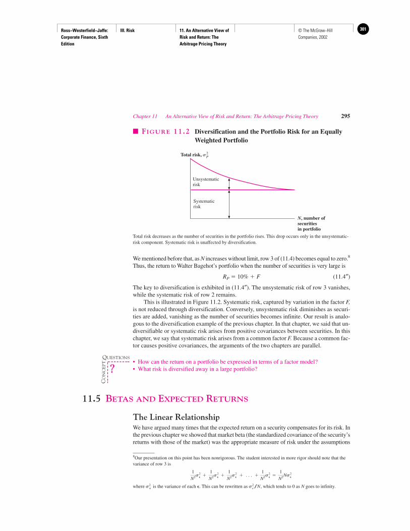
Ross−Westerfield−Jaffe: Corporate Finance, Sixth Edition
III. Risk 11. An Alternative View of Risk and Return: The Arbitrage Pricing Theory
301© The McGraw−Hill Companies, 2002
We mentioned before that, as N increases without limit, row 3 of (11.4) becomes equal to zero.8
Thus, the return to Walter Bagehot’s portfolio when the number of securities is very large is
RP � 10% � F (11.4″)
The key to diversification is exhibited in (11.4″). The unsystematic risk of row 3 vanishes,while the systematic risk of row 2 remains.
This is illustrated in Figure 11.2. Systematic risk, captured by variation in the factor F,is not reduced through diversification. Conversely, unsystematic risk diminishes as securi-ties are added, vanishing as the number of securities becomes infinite. Our result is analo-gous to the diversification example of the previous chapter. In that chapter, we said that un-diversifiable or systematic risk arises from positive covariances between securities. In thischapter, we say that systematic risk arises from a common factor F. Because a common fac-tor causes positive covariances, the arguments of the two chapters are parallel.
• How can the return on a portfolio be expressed in terms of a factor model?• What risk is diversified away in a large portfolio?
11.5 BETAS AND EXPECTED RETURNS
The Linear RelationshipWe have argued many times that the expected return on a security compensates for its risk. Inthe previous chapter we showed that market beta (the standardized covariance of the security’sreturns with those of the market) was the appropriate measure of risk under the assumptions
Chapter 11 An Alternative View of Risk and Return: The Arbitrage Pricing Theory 295
2
P
Systematicrisk
N, number ofsecuritiesin portfolio
Unsystematicrisk
Total risk, �
� FIGURE 11.2 Diversification and the Portfolio Risk for an EquallyWeighted Portfolio
Total risk decreases as the number of securities in the portfolio rises. This drop occurs only in the unsystematic-risk component. Systematic risk is unaffected by diversification.
8Our presentation on this point has been nonrigorous. The student interested in more rigor should note that thevariance of row 3 is
where is the variance of each �. This can be rewritten as , which tends to 0 as N goes to infinity.�2e /N�2
�
1
N2�2� �
1
N2�2� �
1
N2�2� � . . . �
1
N2�2� �
1
N2N�2�
QUESTIONS
CO
NC
EP
T
?
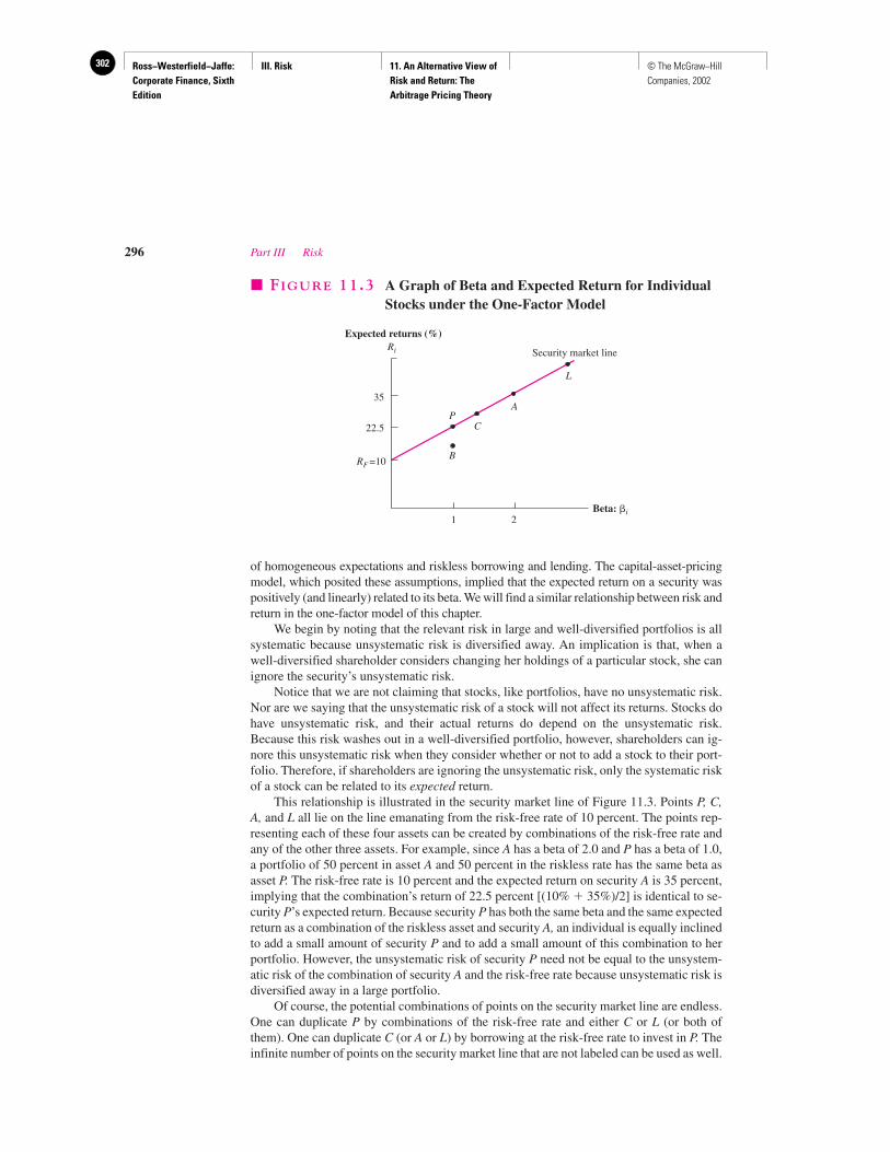
Ross−Westerfield−Jaffe: Corporate Finance, Sixth Edition
III. Risk 11. An Alternative View of Risk and Return: The Arbitrage Pricing Theory
302 © The McGraw−Hill Companies, 2002
of homogeneous expectations and riskless borrowing and lending. The capital-asset-pricingmodel, which posited these assumptions, implied that the expected return on a security waspositively (and linearly) related to its beta. We will find a similar relationship between risk andreturn in the one-factor model of this chapter.
We begin by noting that the relevant risk in large and well-diversified portfolios is allsystematic because unsystematic risk is diversified away. An implication is that, when awell-diversified shareholder considers changing her holdings of a particular stock, she canignore the security’s unsystematic risk.
Notice that we are not claiming that stocks, like portfolios, have no unsystematic risk.Nor are we saying that the unsystematic risk of a stock will not affect its returns. Stocks dohave unsystematic risk, and their actual returns do depend on the unsystematic risk.Because this risk washes out in a well-diversified portfolio, however, shareholders can ig-nore this unsystematic risk when they consider whether or not to add a stock to their port-folio. Therefore, if shareholders are ignoring the unsystematic risk, only the systematic riskof a stock can be related to its expected return.
This relationship is illustrated in the security market line of Figure 11.3. Points P, C,A, and L all lie on the line emanating from the risk-free rate of 10 percent. The points rep-resenting each of these four assets can be created by combinations of the risk-free rate andany of the other three assets. For example, since A has a beta of 2.0 and P has a beta of 1.0,a portfolio of 50 percent in asset A and 50 percent in the riskless rate has the same beta asasset P. The risk-free rate is 10 percent and the expected return on security A is 35 percent,implying that the combination’s return of 22.5 percent [(10% � 35%)/2] is identical to se-curity P’s expected return. Because security P has both the same beta and the same expectedreturn as a combination of the riskless asset and security A, an individual is equally inclinedto add a small amount of security P and to add a small amount of this combination to herportfolio. However, the unsystematic risk of security P need not be equal to the unsystem-atic risk of the combination of security A and the risk-free rate because unsystematic risk isdiversified away in a large portfolio.
Of course, the potential combinations of points on the security market line are endless.One can duplicate P by combinations of the risk-free rate and either C or L (or both ofthem). One can duplicate C (or A or L) by borrowing at the risk-free rate to invest in P. Theinfinite number of points on the security market line that are not labeled can be used as well.
296 Part III Risk
Beta: �i1 2
35
22.5
RF =10
Expected returns (%)Ri
L
A
C
B
P
Security market line
� FIGURE 11.3 A Graph of Beta and Expected Return for IndividualStocks under the One-Factor Model
Ross−Westerfield−Jaffe: Corporate Finance, Sixth Edition
III. Risk 11. An Alternative View of Risk and Return: The Arbitrage Pricing Theory
303© The McGraw−Hill Companies, 2002
Now consider security B. Because its expected return is below the line, no investorwould hold it. Instead, the investor would prefer security P, a combination of security Aand the riskless asset, or some other combination. Thus, security B’s price is too high. Itsprice will fall in a competitive market, forcing its expected return back up to the line inequilibrium.
The preceding discussion allows us to provide an equation for the security market lineof Figure 11.3. We know that a line can be described algebraically from two points. It is per-haps easiest to focus on the risk-free rate and asset P, since the risk-free rate has a beta of 0and P has a beta of 1.
Because we know that the return on any zero-beta asset is RF and the expected returnon asset P is , it can easily be shown that
(11.5)
In equation (11.5), can be thought of as the expected return on any security or portfoliolying on the security market line. � is the beta of that security or portfolio.
The Market Portfolio and the Single FactorIn the CAPM, the beta of a security measures the security’s responsiveness to move-ments in the market portfolio. In the one-factor model of the APT, the beta of a securitymeasures its responsiveness to the factor. We now relate the market portfolio to the sin-gle factor.
A large, diversified portfolio has no unsystematic risk because the unsystematic risksof the individual securities are diversified away. Assuming enough securities so that themarket portfolio is fully diversified and assuming that no security has a disproportionatemarket share, this portfolio is fully diversified and contains no unsystematic risk.9 In otherwords, the market portfolio is perfectly correlated with the single factor, implying that themarket portfolio is really a scaled-up or scaled-down version of the factor. After scalingproperly, we can treat the market portfolio as the factor itself.
The market portfolio, like every security or portfolio, lies on the security market line.When the market portfolio is the factor, the beta of the market portfolio is 1 by definition.This is shown in Figure 11.4. (We deleted the securities and the specific expected returnsfrom Figure 11.3 for clarity: the two graphs are otherwise identical.) With the market port-folio as the factor, equation (11.5) becomes
where is the expected return on the market. This equation shows that the expected re-turn on any asset, , is linearly related to the security’s beta. The equation is identical tothat of the CAPM, which we developed in the previous chapter.
• What is the relationship between the one-factor model and the CAPM?
RRM
R � RF � � �RM � RF�
R
R � RF � � �RP � RF�
RP
Chapter 11 An Alternative View of Risk and Return: The Arbitrage Pricing Theory 297
9This assumption is plausible in the real world. For example, even the market value of General Electric is only 3percent to 4 percent of the market value of the S&P 500 Index.
QUESTION
CO
NC
EP
T
?
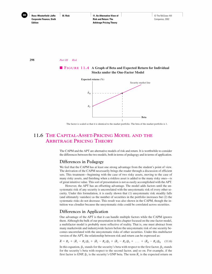
Ross−Westerfield−Jaffe: Corporate Finance, Sixth Edition
III. Risk 11. An Alternative View of Risk and Return: The Arbitrage Pricing Theory
304 © The McGraw−Hill Companies, 2002
11.6 THE CAPITAL-ASSET-PRICING MODEL AND THE
ARBITRAGE PRICING THEORY
The CAPM and the APT are alternative models of risk and return. It is worthwhile to considerthe differences between the two models, both in terms of pedagogy and in terms of application.
Differences in PedagogyWe feel that the CAPM has at least one strong advantage from the student’s point of view.The derivation of the CAPM necessarily brings the reader through a discussion of efficientsets. This treatment—beginning with the case of two risky assets, moving to the case ofmany risky assets, and finishing when a riskless asset is added to the many risky ones—isof great intuitive value. This sort of presentation is not as easily accomplished with the APT.
However, the APT has an offsetting advantage. The model adds factors until the un-systematic risk of any security is uncorrelated with the unsystematic risk of every other se-curity. Under this formulation, it is easily shown that (1) unsystematic risk steadily falls(and ultimately vanishes) as the number of securities in the portfolio increases but (2) thesystematic risks do not decrease. This result was also shown in the CAPM, though the in-tuition was cloudier because the unsystematic risks could be correlated across securities.
Differences in ApplicationOne advantage of the APT is that it can handle multiple factors while the CAPM ignoresthem. Although the bulk of our presentation in this chapter focused on the one-factor model,a multifactor model is probably more reflective of reality. That is, one must abstract frommany marketwide and industrywide factors before the unsystematic risk of one security be-comes uncorrelated with the unsystematic risks of other securities. Under this multifactorversion of the APT, the relationship between risk and return can be expressed as:
(11.6)
In this equation, �1 stands for the security’s beta with respect to the first factor, �2 standsfor the security’s beta with respect to the second factor, and so on. For example, if thefirst factor is GNP, �1 is the security’s GNP beta. The term is the expected return onR1
R � RF � �R1 � RF��1 � �R2 � RF��2 � �R3 � RF��3 � . . . � �RK � RF��K
298 Part III Risk
Expected returns (%)
Beta
Security market line
RM
RF
1
� FIGURE 11.4 A Graph of Beta and Expected Return for IndividualStocks under the One-Factor Model
The factor is scaled so that it is identical to the market portfolio. The beta of the market portfolio is 1.
Ross−Westerfield−Jaffe: Corporate Finance, Sixth Edition
III. Risk 11. An Alternative View of Risk and Return: The Arbitrage Pricing Theory
305© The McGraw−Hill Companies, 2002
a security (or portfolio) whose beta with respect to the first factor is 1 and whose betawith respect to all other factors is zero. Because the market compensates for risk,( ) will be positive in the normal case.10 (An analogous interpretation can begiven to , and so on.)
The equation states that the security’s expected return is related to the security’s factorbetas. The intuition in equation (11.6) is straightforward. Each factor represents risk thatcannot be diversified away. The higher a security’s beta with regard to a particular factor is,the higher is the risk that the security bears. In a rational world, the expected return on thesecurity should compensate for this risk. The above equation states that the expected returnis a summation of the risk-free rate plus the compensation for each type of risk that the se-curity bears.
As an example, consider a study where the factors were monthly growth in industrialproduction (IP), change in expected inflation (�EI), unanticipated inflation (UI), unantici-pated change in the risk premium between risky bonds and default-free bonds (URP), andunanticipated change in the difference between the return on long-term government bondsand the return on short-term government bonds (UBR).11 Using the period 1958–1984, theempirical results of the study indicated that the expected monthly return on any stock, ,can be described as
Suppose a particular stock had the following betas: �IP � 1.1, ��EI � 2, �UI � 3,�URP � 0.1, �UBR � 1.6. The expected monthly return on that security would be
Assuming that a firm is unlevered and that one of the firm’s projects has risk equivalent tothat of the firm, this value of 0.0095 (i.e., .95%) can be used as the monthly discount ratefor the project. (Because annual data are often supplied for capital budgeting purposes, theannual rate of 0.120 [(1.0095)12 � 1] might be used instead.)
Because many factors appear on the right-hand side of equation (11.5), the APT for-mulation has the potential to measure expected returns more accurately than does theCAPM. However, as we mentioned earlier, one cannot easily determine which are the ap-propriate factors. The factors in the above study were included for reasons of both commonsense and convenience. They were not derived from theory.
By contrast, the use of the market index in the CAPM formulation is implied by thetheory of the previous chapter. We suggested in earlier chapters that the S&P 500 Index mir-rors stock market movements quite well. Using the Ibbotson-Sinquefield results showingthat the yearly return on the S&P 500 Index was, on average, 9.2 percent greater than therisk-free rate, the last chapter easily calculated expected returns on different securities fromthe CAPM.12
� 0.0006 � 3 � 0.0072 � 0.1 � 0.0052 � 1.6 � 0.0095RS � 0.0041 � 0.0136 � 1.1 � 0.0001 � 2
RS � 0.0041 � 0.0136�IP � 0.0001��EI � 0.0006�UI � 0.0072�URP � 0.0052�UBR
RS
R2, R3
R1 � RF
Chapter 11 An Alternative View of Risk and Return: The Arbitrage Pricing Theory 299
10Actually, ( ) could be negative in the case where factor i is perceived as a hedge of some sort.11N. Chen, R. Roll, and S. Ross, “Economic Forces and the Stock Market,” Journal of Business (July 1986).12Though many researchers assume that surrogates for the market portfolio are easily found, Richard Roll,“A Critique of the Asset Pricing Theory’s Tests,” Journal of Financial Economics (March 1977), arguesthat the absence of a universally acceptable proxy for the market portfolio seriously impairs application ofthe theory. After all, the market must include real estate, racehorses, and other assets that are not in thestock market.
Ri � RF
Ross−Westerfield−Jaffe: Corporate Finance, Sixth Edition
III. Risk 11. An Alternative View of Risk and Return: The Arbitrage Pricing Theory
306 © The McGraw−Hill Companies, 2002
11.7 EMPIRICAL APPROACHES TO ASSET PRICING
Empirical ModelsThe CAPM and the APT by no means exhaust the models and techniques used in practiceto measure the expected return on risky assets. Both the CAPM and the APT are risk-basedmodels. They each measure the risk of a security by its beta(s) on some systematic factor(s),and they each argue that the expected excess return must be proportional to the beta(s).While we have seen that this is intuitively appealing and has a strong basis in theory, thereare alternative approaches.
Most of these alternatives can be lumped under the broad heading of parametric or em-pirical models. The word empirical refers to the fact that these approaches are based lesson some theory of how financial markets work and more on simply looking for regularitiesand relations in the history of market data. In these approaches the researcher specifiessome parameters or attributes associated with the securities in question and then examinesthe data directly for a relation between these attributes and expected returns. For example,an extensive amount of research has been done on whether the expected return on a firm isrelated to its size. Is it true that small firms have higher average returns than large firms?Researchers have also examined a variety of accounting measures such as the ratio of theprice of a stock to the accounting earnings, the P/E ratio, and the closely related ratio of themarket value of the stock to the book value of the company, the M/B ratio. Here it might beargued that companies with low P/E’s or low M/B’s are “undervalued” and can be expectedto have higher returns in the future.
To use the empirical approach to determine the expected return, we would estimate thefollowing equation:
where is the expected return of firm i, and where the k’s are coefficients that we estimatefrom stock market data. Notice that this is the same form as equation (11.6) with the firm’sattributes in place of betas and with the k’s in place of the excess factor portfolio returns.
When tested with data, these parametric approaches seem to do quite well. In fact,when comparisons are made between using parameters and using betas to predict stock re-turns, the parameters, such as P/E and M/B, seem to work better. There are a variety of pos-sible explanations for these results, and the issues have certainly not been settled. Critics ofthe empirical approach are skeptical of what they call data mining. The particular parame-ters that researchers work with are often chosen because they have been shown to be relatedto returns. For instance, suppose that you were asked to explain the change in SAT testscores over the past 40 years in some particular state. Suppose that to do this you searchedthrough all of the data series you could find. After much searching, you might discover, forexample, that the change in the scores was directly related to the jackrabbit population inArizona. We know that any such relation is purely accidental but if you search long enoughand have enough choices, you will find something even if it is not really there. It’s a bit likestaring at clouds. After a while you will see clouds that look like anything you want, clowns,bears, or whatever, but all you are really doing is data mining.
Needless to say, the researchers on these matters defend their work by arguing that theyhave not mined the data and have been very careful to avoid such traps by not snooping atthe data to see what will work.
Of course, as a matter of pure theory, since anyone in the market can easily look up theP/E ratio of a firm, one would certainly not expect to find that firms with low P/E’s did betterthan firms with high P/E’s simply because they were undervalued. In an efficient market, suchpublic measures of undervaluation would be quickly exploited and would not expect to last.
Ri
Ri � RF � kP/E �P/E� i � kM/B �M/B� i � ksize �size�P
300 Part III Risk
Ross−Westerfield−Jaffe: Corporate Finance, Sixth Edition
III. Risk 11. An Alternative View of Risk and Return: The Arbitrage Pricing Theory
307© The McGraw−Hill Companies, 2002
Perhaps a better explanation for the success of empirical approaches lies in a synthesisof the risk-based approaches and the empirical methods. In an efficient market, risk and re-turn are related, hence perhaps the parameters or attributes which appear to be related to re-turns are also better measures of risk. For example, if we were to find that low P/E firmsoutperformed high P/E firms and that this was true even for firms that had the same beta(s),then we have at least two possible explanations. First, we could simply discard the risk-based theories as incorrect. Furthermore, we could argue that markets are inefficient andthat buying low P/E stocks provides us with an opportunity to make higher than predictedreturns. Second, we could argue that both views of the world are correct and that the P/E isreally just a better way to measure systematic risk, i.e., beta(s), than directly estimating betafrom the data.
Style PortfoliosIn addition to their use as a platform for estimating expected returns, stock attributes arealso widely used as a way of characterizing money management styles. For example, aportfolio that has a P/E ratio much in excess of the market average might be characterizedas a high P/E or a growth stock portfolio. Similarly, a portfolio made up of stocks withan average P/E less than that for a market index might be characterized as a low P/E or avalue portfolio.
To evaluate how well a portfolio manager is doing, often their performance is com-pared with the performance of some basic indexes. For example, the portfolio returns of amanager who purchases large U.S. stocks might be compared to the performance of theS&P 500 Index. In such a case the S&P 500 is said to be the benchmark against which theirperformance is measured. Similarly, an international manager might be compared againstsome common index of international stocks. In choosing an appropriate benchmark, careshould be taken to identify a benchmark that contains only those types of stocks that themanager targets as representative of his or her style and that are also available to be pur-chased. A manager who was told not to purchase any stocks in the S&P 500 Index wouldnot consider it legitimate to be compared against the S&P 500.
Increasingly, too, managers are compared not only against an index, but also againsta peer group of similar managers. The performance of a fund that advertises itself as agrowth fund might be measured against the performance of a large sample of similarfunds. For instance, the performance over some period commonly is assigned to quar-tiles. The top 25 percent of the funds are said to be in the first quartile, the next 25 per-cent in the second quartile, the next 25 percent in the third quartile, and the worst per-forming 25 percent of the funds in the last quartile. If the fund we are examining happensto have a performance that falls in the second quartile, then we speak of it as a secondquartile manager.
Similarly, we call a fund that purchases low M/B stocks a value fund and would mea-sure its performance against a sample of similar value funds. These approaches to measur-ing performance are relatively new, and they are part of an active and exciting effort to re-fine our ability to identify and use investment skills.
• Empirical models are sometimes called factor models. What is the difference betweena factor as we have used it previously in this chapter and an attribute as we use it in thissection?
• What is data mining and why might it overstate the relation between some stock attrib-ute and returns?
• What is wrong with measuring the performance of a U.S. growth stock manager againsta benchmark composed of English stocks?
Chapter 11 An Alternative View of Risk and Return: The Arbitrage Pricing Theory 301
QUESTIONS
CO
NC
EP
T
?
Ross−Westerfield−Jaffe: Corporate Finance, Sixth Edition
III. Risk 11. An Alternative View of Risk and Return: The Arbitrage Pricing Theory
308 © The McGraw−Hill Companies, 2002
11.8 SUMMARY AND CONCLUSIONS
The previous chapter developed the capital-asset-pricing model (CAPM). As an alternative, thischapter develops the arbitrage pricing theory (APT).
1. The APT assumes that stock returns are generated according to factor models. For example,we might describe a stock’s return as
where I, GNP, and r stand for inflation, gross national product, and the interest rate,respectively. The three factors FI, FGNP, and Fr represent systematic risk because thesefactors affect many securities. The term � is considered unsystematic risk because it is uniqueto each individual security.
2. For convenience, we frequently describe a security’s return according to a one-factor model:
3. As securities are added to a portfolio, the unsystematic risks of the individual securities offseteach other. A fully diversified portfolio has no unsystematic risk but still has systematic risk.This result indicates that diversification can eliminate some, but not all, of the risk ofindividual securities.
4. Because of this, the expected return on a stock is positively related to its systematic risk. In aone-factor model, the systematic risk of a security is simply the beta of the CAPM. Thus, theimplications of the CAPM and the one-factor APT are identical. However, each security hasmany risks in a multifactor model. The expected return on a security is positively related tothe beta of the security with each factor.
5. Empirical or parametric models that capture the relations between returns and stock attributessuch as P/E or M/B ratios can be estimated directly from the data without any appeal totheory. These ratios are also used to measure the style of a portfolio manager and to constructbenchmarks and samples against which they are measured.
KEY TERMS
Benchmark 301 Growth stock portfolios 301Beta coefficient 289 Market model 291Empirical model 300 Value portfolios 301Factor model 290
SUGGESTED READINGS
Complete treatments of the APT can be found in both of the following articles:Ross, S. A. “Return, Risk and Arbitrage.” In Friend and Bicksler, eds., Risk and Return in
Finance. New York: Heath Lexington, 1974.Ross, S. A. “The Arbitrage Theory of Asset Pricing.” Journal of Economic Theory (December
1976).
Two less technical discussions of APT are:Bower, D. H.; R. S. Bower; and D. Logue. “A Primer on Arbitrage Pricing Theory.” Midland
Corporate Finance Journal (Fall 1984).
R � R � �F � �
R � R � �IFI � �GNPFGNP � �rFr � �
302 Part III Risk

Ross−Westerfield−Jaffe: Corporate Finance, Sixth Edition
III. Risk 11. An Alternative View of Risk and Return: The Arbitrage Pricing Theory
309© The McGraw−Hill Companies, 2002
Roll, R., and S. Ross. “The Arbitrage Pricing Theory Approach to Strategic Portfolio Planning.”Financial Analysts Journal (May/June 1984).
The following article describes the idea of style portfolios:Roll, R. “Style Return Differentials: Illusions, Risk Premia, or Investment Opportunities.” In
Fabozzi (ed.), Handbook of Equity Style Management. New Hope, PA: Frank FabozziAssociates, 1995.
QUESTIONS AND PROBLEMS
Factor Models and Risk11.1 You own stock in the Lewis-Striden Drug Company. Suppose you had expected the
following events to occur last month.a. The government would announce that real GNP would have grown 1.2 percent during
the previous quarter. The returns of Lewis-Striden are positively related to real GNP.b. The government would announce that inflation over the previous quarter was 3.7
percent. The returns of Lewis-Striden are negatively related to inflation.c. Interest rates would rise 2.5 percentage points. The returns of Lewis-Striden are
negatively related to interest rates.d. The president of the firm would announce his retirement. The retirement would be
effective six months from the announcement day. The president is well liked: in generalhe is considered an asset to the firm.
e. Research data would conclusively prove the efficacy of an experimental drug.Completion of the efficacy testing means the drug will be on the market soon.
Suppose the following events actually occurred.a. The government announced that real GNP grew 2. 3 percent during the previous quarter.b. The government announced that inflation over the previous quarter was 3.7 percent.c. Interest rates rose 2.1 percentage points.d. The president of the firm died suddenly of a heart attack.e. Research results in the efficacy testing were not as strong as expected. The drug must
be tested another six months and the efficacy results must be resubmitted to the FDA.f. Lab researchers had a breakthrough with another drug.g. A competitor announced that it will begin distribution and sale of a medicine that will
compete directly with one of Lewis-Striden’s top-selling products.i. Discuss how each of the actual occurrences affects the returns on your Lewis-
Striden stock.ii. Which events represent systematic risk?iii. Which events represent unsystematic risk?
11.2 Suppose a three-factor model is appropriate to describe the returns of a stock. Informationabout those three factors is presented in the following chart. Suppose this is the onlyinformation you have concerning the factors.
Beta of Expected ActualFactor Factor Value Value
GNP 0.0042 $4,416 $4,480Inflation �1.40 3.1% 4.3%Interest rate �0.67 9.5% 11.8%
a. What is the systematic risk of the stock return?b. Suppose unexpected bad news about the firm was announced that dampens the returns
by 2.6 percentage points. What is the unsystematic risk of the stock return?c. Suppose the expected return of the stock is 9.5 percent. What is the total return on this
stock?
Chapter 11 An Alternative View of Risk and Return: The Arbitrage Pricing Theory 303
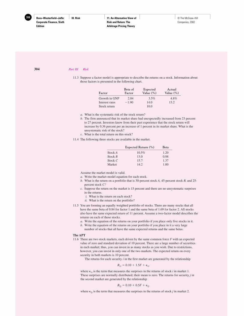
Ross−Westerfield−Jaffe: Corporate Finance, Sixth Edition
III. Risk 11. An Alternative View of Risk and Return: The Arbitrage Pricing Theory
310 © The McGraw−Hill Companies, 2002
11.3 Suppose a factor model is appropriate to describe the returns on a stock. Information aboutthose factors is presented in the following chart.
Beta of Expected ActualFactor Factor Value (%) Value (%)
Growth in GNP 2.04 3.5% 4.8%Interest rates �1.90 14.0 15.2Stock return 10.0
a. What is the systematic risk of the stock return?b. The firm announced that its market share had unexpectedly increased from 23 percent
to 27 percent. Investors know from their past experience that the stock return willincrease by 0.36 percent per an increase of 1 percent in its market share. What is theunsystematic risk of the stock?
c. What is the total return on this stock?
11.4 The following three stocks are available in the market.
Expected Return (%) Beta
Stock A 10.5% 1.20Stock B 13.0 0.98Stock C 15.7 1.37Market 14.2 1.00
Assume the market model is valid.a. Write the market-model equation for each stock.b. What is the return on a portfolio that is 30-percent stock A, 45-percent stock B, and 25-
percent stock C?c. Suppose the return on the market is 15 percent and there are no unsystematic surprises
in the returns.i. What is the return on each stock?ii. What is the return on the portfolio?
11.5 You are forming an equally weighted portfolio of stocks. There are many stocks that allhave the same beta of 0.84 for factor 1 and the same beta of 1.69 for factor 2. All stocksalso have the same expected return of 11 percent. Assume a two-factor model describes thereturns on each of these stocks.a. Write the equation of the returns on your portfolio if you place only five stocks in it.b. Write the equation of the returns on your portfolio if you place in it a very large
number of stocks that all have the same expected returns and the same betas.
The APT11.6 There are two stock markets, each driven by the same common force F with an expected
value of zero and standard deviation of 10 percent. There are a large number of securitiesin each market; thus, you can invest in as many stocks as you wish. Due to restrictions,however, you can invest in only one of the two markets. The expected return on everysecurity in both markets is 10 percent.
The returns for each security i in the first market are generated by the relationship
R1i � 0.10 � 1.5F � �1i
where �1i is the term that measures the surprises in the returns of stock i in market 1. These surprises are normally distributed; their mean is zero. The returns for security j inthe second market are generated by the relationship
R2j � 0.10 � 0.5F � �2j
where �2j is the term that measures the surprises in the returns of stock j in market 2.
304 Part III Risk
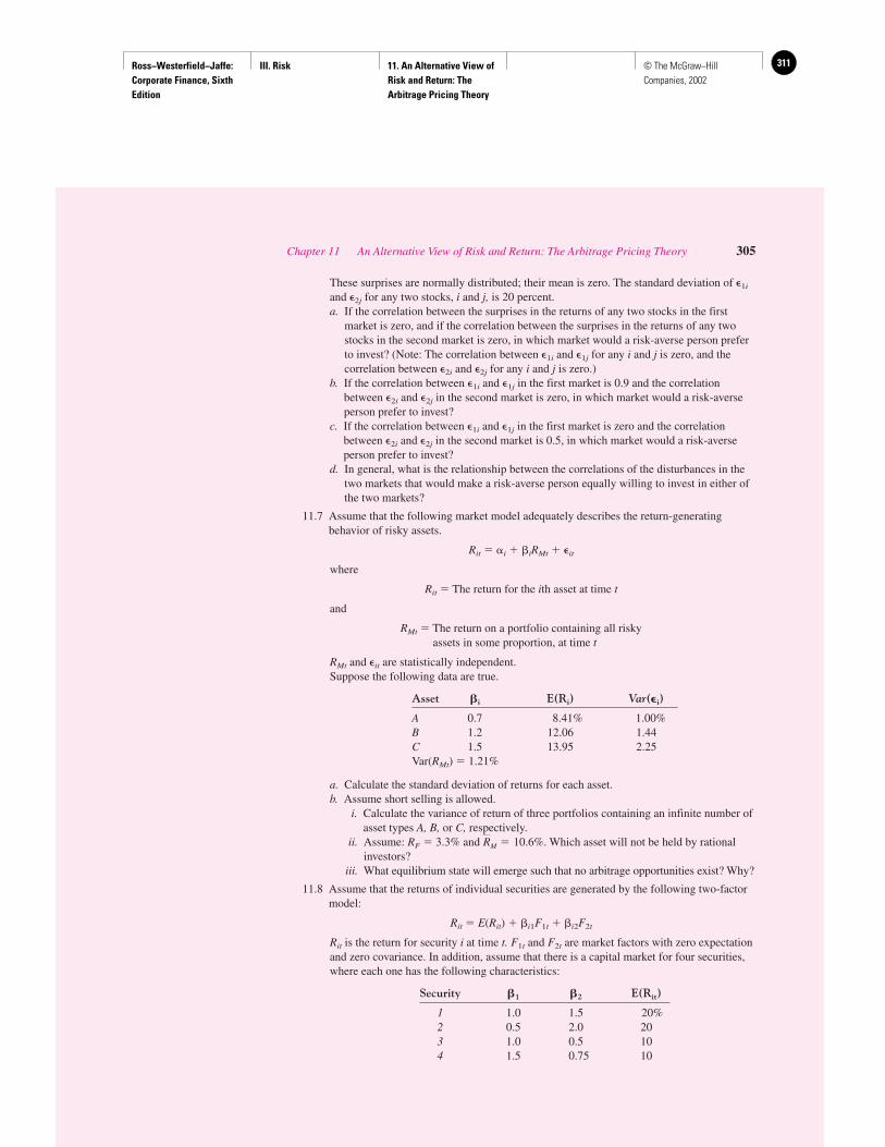
Ross−Westerfield−Jaffe: Corporate Finance, Sixth Edition
III. Risk 11. An Alternative View of Risk and Return: The Arbitrage Pricing Theory
311© The McGraw−Hill Companies, 2002
These surprises are normally distributed; their mean is zero. The standard deviation of �1i
and �2j for any two stocks, i and j, is 20 percent.a. If the correlation between the surprises in the returns of any two stocks in the first
market is zero, and if the correlation between the surprises in the returns of any twostocks in the second market is zero, in which market would a risk-averse person preferto invest? (Note: The correlation between �1i and �1j for any i and j is zero, and thecorrelation between �2i and �2j for any i and j is zero.)
b. If the correlation between �1i and �1j in the first market is 0.9 and the correlationbetween �2i and �2j in the second market is zero, in which market would a risk-averseperson prefer to invest?
c. If the correlation between �1i and �1j in the first market is zero and the correlationbetween �2i and �2j in the second market is 0.5, in which market would a risk-averseperson prefer to invest?
d. In general, what is the relationship between the correlations of the disturbances in thetwo markets that would make a risk-averse person equally willing to invest in either ofthe two markets?
11.7 Assume that the following market model adequately describes the return-generatingbehavior of risky assets.
Rit � �i � �iRMt � �it
where
Rit � The return for the ith asset at time t
and
RMt � The return on a portfolio containing all risky assets in some proportion, at time t
RMt and �it are statistically independent.Suppose the following data are true.
Asset �i E(Ri) Var(�i)
A 0.7 8.41% 1.00%B 1.2 12.06 1.44C 1.5 13.95 2.25Var(RMt) � 1.21%
a. Calculate the standard deviation of returns for each asset.b. Assume short selling is allowed.
i. Calculate the variance of return of three portfolios containing an infinite number ofasset types A, B, or C, respectively.
ii. Assume: RF � 3.3% and . Which asset will not be held by rationalinvestors?
iii. What equilibrium state will emerge such that no arbitrage opportunities exist? Why?
11.8 Assume that the returns of individual securities are generated by the following two-factormodel:
Rit � E(Rit) � �i1F1t � �i2F2t
Rit is the return for security i at time t. F1t and F2t are market factors with zero expectationand zero covariance. In addition, assume that there is a capital market for four securities,where each one has the following characteristics:
Security �1 �2 E(Rit)
1 1.0 1.5 20%2 0.5 2.0 203 1.0 0.5 104 1.5 0.75 10
RM � 10.6%
Chapter 11 An Alternative View of Risk and Return: The Arbitrage Pricing Theory 305

Ross−Westerfield−Jaffe: Corporate Finance, Sixth Edition
III. Risk 11. An Alternative View of Risk and Return: The Arbitrage Pricing Theory
312 © The McGraw−Hill Companies, 2002
The capital market for these four assets is perfect in the sense that there are notransactions costs and short sales can take place.a. Construct a portfolio containing (long or short) securities 1 and 2, with a return that
does not depend on the market factor, F1t, in any way. (Hint: Such a portfolio will have�1 � 0.) Compute the expected return and �2 coefficient for this portfolio.
b. Following the procedure in (a), construct a portfolio containing securities 3 and 4 witha return that does not depend on the market factor, F1t. Compute the expected returnand �2 coefficient for this portfolio.
c. Consider a risk-free asset with expected return equal to 5 percent, �1 � 0, and �2 � 0.Describe a possible arbitrage opportunity in such detail that an investor couldimplement it.
d. What effect would the existence of these kinds of arbitrage opportunities have on thecapital markets for these securities in the short and long run? Graph your analysis.
306 Part III Risk
Ross−Westerfield−Jaffe: Corporate Finance, Sixth Edition
III. Risk 12. Risk, Cost of Capital, and Capital Budgeting
313© The McGraw−Hill Companies, 2002
Risk, Cost of Capital, andCapital Budgeting
CH
AP
TE
R12
EXECUTIVE SUMMARY
Our text has devoted a number of chapters to net present value (NPV) analysis. Wepointed out that a dollar to be received in the future is worth less than a dollar re-ceived today for two reasons. First, there is the simple time-value-of-money argu-
ment in a riskless world. If you have a dollar today, you can invest it in the bank and receivemore than a dollar by some future date. Second, a risky dollar is worth less than a risklessdollar. Consider a firm expecting a $1 cash flow. If actuality exceeds expectations (revenuesare especially high or expenses are especially low), perhaps $1.10 or $1.20 will be received.If actuality falls short of expectations, perhaps only $0.80 or $0.90 will be received. Thisrisk is unattractive to the typical firm.
Our work on NPV allowed us to value riskless cash flows precisely. That is, we dis-counted by the riskless interest rate. However, because most real-world cash flows in thefuture are risky, business demands a procedure for discounting risky cash flows. This chap-ter applies the concept of net present value to risky cash flows.
Let us review what previous work in the text has to say about NPV. In earlier chapterswe learned that the basic NPV formula for an investment that generates cash flows (Ct) infuture periods is
For risky projects, expected incremental cash flows t are placed in the numerator, and theNPV formula becomes
In this chapter, we will learn that the discount rate used to determine the NPV of a riskyproject can be computed from the CAPM (or APT). For example, if an all-equity firm is seek-ing to value a risky project, such as renovating a warehouse, the firm will determine the re-quired return, rS, on the project by using the SML. We call rS the firm’s cost of equity capital.
When firms finance with both debt and equity, the discount rate to use is the project’soverall cost of capital. The overall cost of capital is a weighted average of the cost of debtand the cost of equity.
12.1 THE COST OF EQUITY CAPITAL
Whenever a firm has extra cash, it can take one of two actions. On the one hand, it can payout the cash immediately as a dividend. On the other hand, the firm can invest extra cash ina project, paying out the future cash flows of the project as dividends. Which procedurewould the stockholders prefer? If a stockholder can reinvest the dividend in a financial asset(a stock or bond) with the same risk as that of the project, the stockholders would desire the
NPV � C0 � T
t�1
Ct
�1 � r� t
C
NPV � C0 � T
t�1
Ct
�1 � r� t
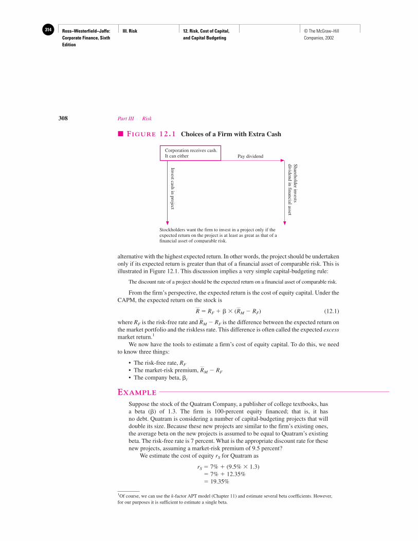
Ross−Westerfield−Jaffe: Corporate Finance, Sixth Edition
III. Risk 12. Risk, Cost of Capital, and Capital Budgeting
314 © The McGraw−Hill Companies, 2002
alternative with the highest expected return. In other words, the project should be undertakenonly if its expected return is greater than that of a financial asset of comparable risk. This isillustrated in Figure 12.1. This discussion implies a very simple capital-budgeting rule:
The discount rate of a project should be the expected return on a financial asset of comparable risk.
From the firm’s perspective, the expected return is the cost of equity capital. Under theCAPM, the expected return on the stock is
� RF � � � ( M � RF) (12.1)
where RF is the risk-free rate and M � RF is the difference between the expected return onthe market portfolio and the riskless rate. This difference is often called the expected excessmarket return.1
We now have the tools to estimate a firm’s cost of equity capital. To do this, we needto know three things:
• The risk-free rate, RF
• The market-risk premium, M � RF
• The company beta, �i
EXAMPLE
Suppose the stock of the Quatram Company, a publisher of college textbooks, hasa beta (�) of 1.3. The firm is 100-percent equity financed; that is, it has no debt. Quatram is considering a number of capital-budgeting projects that willdouble its size. Because these new projects are similar to the firm’s existing ones,the average beta on the new projects is assumed to be equal to Quatram’s existingbeta. The risk-free rate is 7 percent. What is the appropriate discount rate for thesenew projects, assuming a market-risk premium of 9.5 percent?
We estimate the cost of equity rS for Quatram as
rS � 7% � (9.5% � 1.3)� 7% � 12.35%� 19.35%
R
R
RR
308 Part III Risk
Corporation receives cash.It can either Pay dividend
Invest cash in project
Shareholder investsdividend in financial asset
Stockholders want the firm to invest in a project only if theexpected return on the project is at least as great as that of afinancial asset of comparable risk.
� FIGURE 12.1 Choices of a Firm with Extra Cash
1Of course, we can use the k-factor APT model (Chapter 11) and estimate several beta coefficients. However,for our purposes it is sufficient to estimate a single beta.
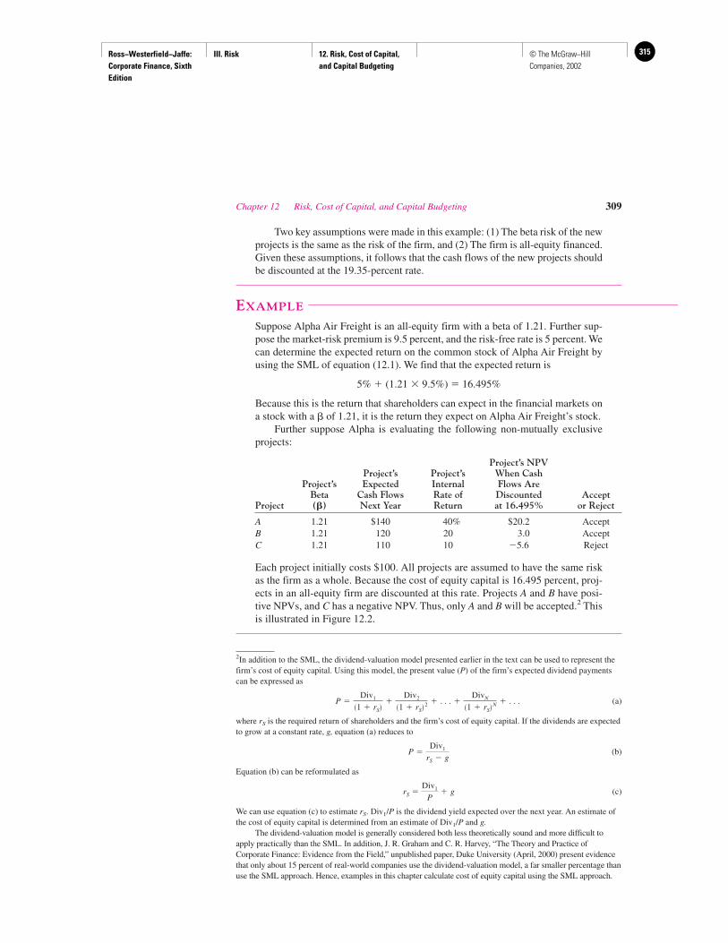
Ross−Westerfield−Jaffe: Corporate Finance, Sixth Edition
III. Risk 12. Risk, Cost of Capital, and Capital Budgeting
315© The McGraw−Hill Companies, 2002
Two key assumptions were made in this example: (1) The beta risk of the newprojects is the same as the risk of the firm, and (2) The firm is all-equity financed.Given these assumptions, it follows that the cash flows of the new projects shouldbe discounted at the 19.35-percent rate.
EXAMPLE
Suppose Alpha Air Freight is an all-equity firm with a beta of 1.21. Further sup-pose the market-risk premium is 9.5 percent, and the risk-free rate is 5 percent. Wecan determine the expected return on the common stock of Alpha Air Freight byusing the SML of equation (12.1). We find that the expected return is
5% � (1.21 � 9.5%) � 16.495%
Because this is the return that shareholders can expect in the financial markets ona stock with a � of 1.21, it is the return they expect on Alpha Air Freight’s stock.
Further suppose Alpha is evaluating the following non-mutually exclusiveprojects:
Project’s NPVProject’s Project’s When Cash
Project’s Expected Internal Flows AreBeta Cash Flows Rate of Discounted Accept
Project (�) Next Year Return at 16.495% or Reject
A 1.21 $140 40% $20.2 AcceptB 1.21 120 20 3.0 AcceptC 1.21 110 10 �5.6 Reject
Each project initially costs $100. All projects are assumed to have the same riskas the firm as a whole. Because the cost of equity capital is 16.495 percent, proj-ects in an all-equity firm are discounted at this rate. Projects A and B have posi-tive NPVs, and C has a negative NPV. Thus, only A and B will be accepted.2 Thisis illustrated in Figure 12.2.
Chapter 12 Risk, Cost of Capital, and Capital Budgeting 309
2In addition to the SML, the dividend-valuation model presented earlier in the text can be used to represent thefirm’s cost of equity capital. Using this model, the present value (P) of the firm’s expected dividend paymentscan be expressed as
(a)
where rS is the required return of shareholders and the firm’s cost of equity capital. If the dividends are expectedto grow at a constant rate, g, equation (a) reduces to
(b)
Equation (b) can be reformulated as
(c)
We can use equation (c) to estimate rS. Div1/P is the dividend yield expected over the next year. An estimate ofthe cost of equity capital is determined from an estimate of Div1/P and g.
The dividend-valuation model is generally considered both less theoretically sound and more difficult toapply practically than the SML. In addition, J. R. Graham and C. R. Harvey, “The Theory and Practice ofCorporate Finance: Evidence from the Field,” unpublished paper, Duke University (April, 2000) present evidencethat only about 15 percent of real-world companies use the dividend-valuation model, a far smaller percentage thanuse the SML approach. Hence, examples in this chapter calculate cost of equity capital using the SML approach.
rS �Div1
P� g
P �Div1
rS � g
P �Div1
�1 � rS��
Div2
�1 � rS� 2 � . . . �DivN
�1 � rS�N � . . .
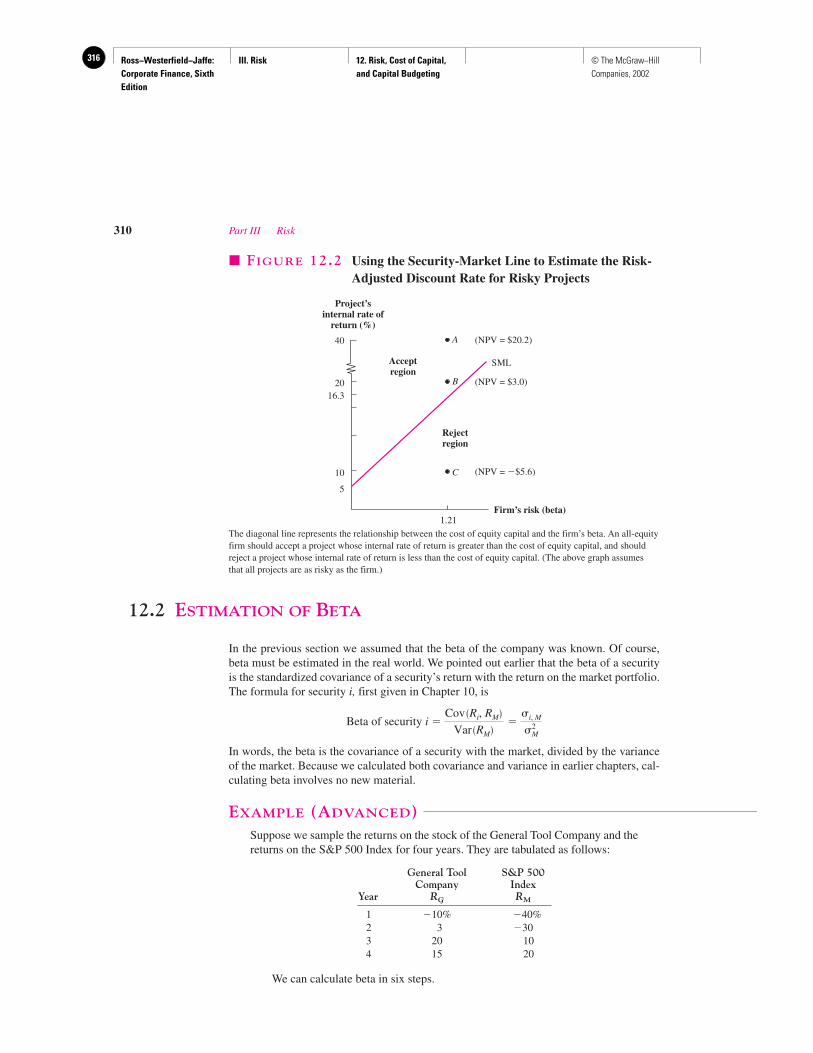
Ross−Westerfield−Jaffe: Corporate Finance, Sixth Edition
III. Risk 12. Risk, Cost of Capital, and Capital Budgeting
316 © The McGraw−Hill Companies, 2002
12.2 ESTIMATION OF BETA
In the previous section we assumed that the beta of the company was known. Of course,beta must be estimated in the real world. We pointed out earlier that the beta of a securityis the standardized covariance of a security’s return with the return on the market portfolio.The formula for security i, first given in Chapter 10, is
Beta of security i �
In words, the beta is the covariance of a security with the market, divided by the varianceof the market. Because we calculated both covariance and variance in earlier chapters, cal-culating beta involves no new material.
EXAMPLE (ADVANCED)Suppose we sample the returns on the stock of the General Tool Company and thereturns on the S&P 500 Index for four years. They are tabulated as follows:
General Tool S&P 500Company Index
Year RG RM
1 �10% �40%2 3 �303 20 104 15 20
We can calculate beta in six steps.
Cov �Ri, RM�Var �RM�
��i, M
�
2M
310 Part III Risk
Project’sinternal rate of
return (%)
40
Firm’s risk (beta)
2016.3
10
5
Acceptregion
Rejectregion
A
B
C
1.21
(NPV = $20.2)
(NPV = $3.0)
(NPV = �$5.6)
SML
� FIGURE 12.2 Using the Security-Market Line to Estimate the Risk-Adjusted Discount Rate for Risky Projects
The diagonal line represents the relationship between the cost of equity capital and the firm’s beta. An all-equityfirm should accept a project whose internal rate of return is greater than the cost of equity capital, and shouldreject a project whose internal rate of return is less than the cost of equity capital. (The above graph assumesthat all projects are as risky as the firm.)
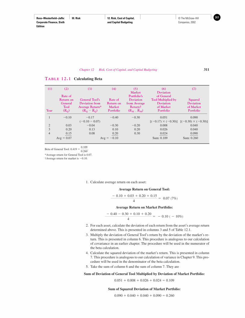
Ross−Westerfield−Jaffe: Corporate Finance, Sixth Edition
III. Risk 12. Risk, Cost of Capital, and Capital Budgeting
317© The McGraw−Hill Companies, 2002
1. Calculate average return on each asset:
Average Return on General Tool:
Average Return on Market Portfolio:
2. For each asset, calculate the deviation of each return from the asset’s average returndetermined above. This is presented in columns 3 and 5 of Table 12.1.
3. Multiply the deviation of General Tool’s return by the deviation of the market’s re-turn. This is presented in column 6. This procedure is analogous to our calculationof covariance in an earlier chapter. The procedure will be used in the numerator ofthe beta calculation.
4. Calculate the squared deviation of the market’s return. This is presented in column7. This procedure is analogous to our calculation of variance in Chapter 9. This pro-cedure will be used in the denominator of the beta calculation.
5. Take the sum of column 6 and the sum of column 7. They are
Sum of Deviation of General Tool Multiplied by Deviation of Market Portfolio:
0.051 � 0.008 � 0.026 � 0.024 � 0.109
Sum of Squared Deviation of Market Portfolio:
0.090 � 0.040 � 0.040 � 0.090 � 0.260
� 0.40 � 0.30 � 0.10 � 0.20
4� � 0.10 � � 10%�
� 0.10 � 0.03 � 0.20 � 0.15
4� 0.07 �7%�
Chapter 12 Risk, Cost of Capital, and Capital Budgeting 311
TABLE 12.1 Calculating Beta
(1) (2) (3) (4) (5) (6) (7)Market Deviation
Rate of Portfolio’s of GeneralReturn on General Tool’s Rate of Deviation Tool Multiplied by SquaredGeneral Deviation from Return on from Average Deviation Deviation
Tool Average Return* Market Return† of Market of MarketYear (RG) (RG � G) Portfolio (RM � M) Portfolio Portfolio
1 �0.10 �0.17 �0.40 �0.30 0.051 0.090(�0.10 � 0.07) [(�0.17) � (�0.30)] [(�0.30) � (�0.30)]
2 0.03 �0.04 �0.30 �0.20 0.008 0.0403 0.20 0.13 0.10 0.20 0.026 0.0404 0.15 0.08 0.20 0.30 0.024 0.090____ ____ _____ _____
Avg � 0.07 Avg � �0.10 Sum: 0.109 Sum: 0.260
Beta of General Tool: 0.419 � .
*Average return for General Tool is 0.07.†Average return for market is �0.10.
0.109
0.260
RR
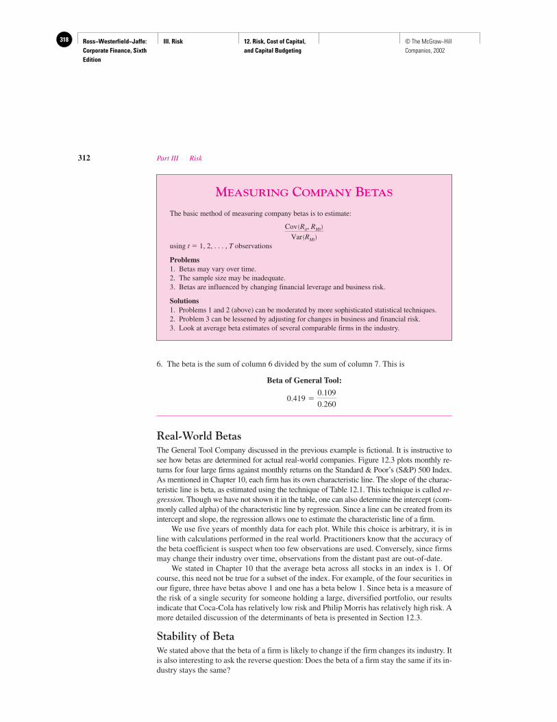
Ross−Westerfield−Jaffe: Corporate Finance, Sixth Edition
III. Risk 12. Risk, Cost of Capital, and Capital Budgeting
318 © The McGraw−Hill Companies, 2002
6. The beta is the sum of column 6 divided by the sum of column 7. This is
Beta of General Tool:
Real-World BetasThe General Tool Company discussed in the previous example is fictional. It is instructive tosee how betas are determined for actual real-world companies. Figure 12.3 plots monthly re-turns for four large firms against monthly returns on the Standard & Poor’s (S&P) 500 Index.As mentioned in Chapter 10, each firm has its own characteristic line. The slope of the charac-teristic line is beta, as estimated using the technique of Table 12.1. This technique is called re-gression. Though we have not shown it in the table, one can also determine the intercept (com-monly called alpha) of the characteristic line by regression. Since a line can be created from itsintercept and slope, the regression allows one to estimate the characteristic line of a firm.
We use five years of monthly data for each plot. While this choice is arbitrary, it is inline with calculations performed in the real world. Practitioners know that the accuracy ofthe beta coefficient is suspect when too few observations are used. Conversely, since firmsmay change their industry over time, observations from the distant past are out-of-date.
We stated in Chapter 10 that the average beta across all stocks in an index is 1. Ofcourse, this need not be true for a subset of the index. For example, of the four securities inour figure, three have betas above 1 and one has a beta below 1. Since beta is a measure ofthe risk of a single security for someone holding a large, diversified portfolio, our resultsindicate that Coca-Cola has relatively low risk and Philip Morris has relatively high risk. Amore detailed discussion of the determinants of beta is presented in Section 12.3.
Stability of BetaWe stated above that the beta of a firm is likely to change if the firm changes its industry. Itis also interesting to ask the reverse question: Does the beta of a firm stay the same if its in-dustry stays the same?
0.419 �0.109
0.260
312 Part III Risk
MEASURING COMPANY BETAS
The basic method of measuring company betas is to estimate:
using t � 1, 2, . . . , T observations
Problems1. Betas may vary over time.2. The sample size may be inadequate.3. Betas are influenced by changing financial leverage and business risk.
Solutions1. Problems 1 and 2 (above) can be moderated by more sophisticated statistical techniques.2. Problem 3 can be lessened by adjusting for changes in business and financial risk.3. Look at average beta estimates of several comparable firms in the industry.
Cov �Rit, RMt�Var �RMt�
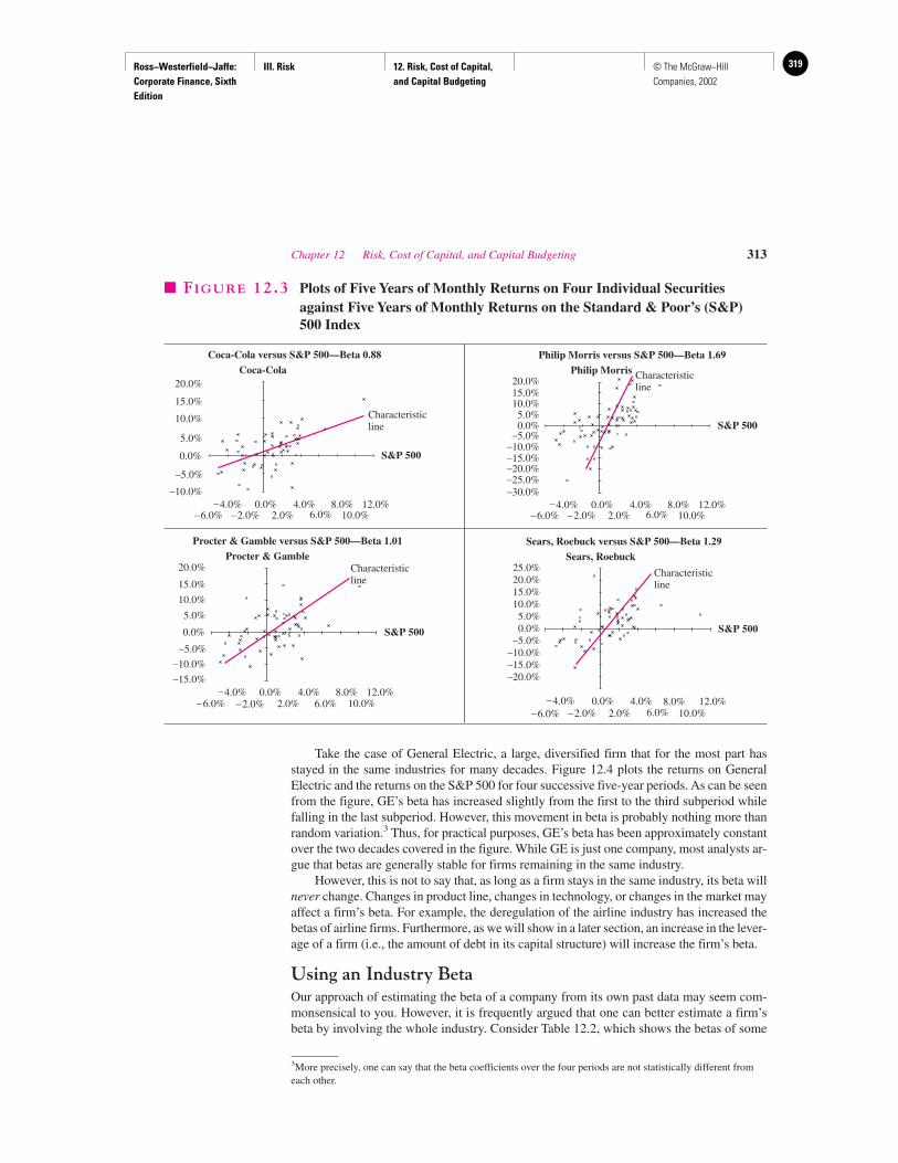
Ross−Westerfield−Jaffe: Corporate Finance, Sixth Edition
III. Risk 12. Risk, Cost of Capital, and Capital Budgeting
319© The McGraw−Hill Companies, 2002
Take the case of General Electric, a large, diversified firm that for the most part hasstayed in the same industries for many decades. Figure 12.4 plots the returns on GeneralElectric and the returns on the S&P 500 for four successive five-year periods. As can be seenfrom the figure, GE’s beta has increased slightly from the first to the third subperiod whilefalling in the last subperiod. However, this movement in beta is probably nothing more thanrandom variation.3 Thus, for practical purposes, GE’s beta has been approximately constantover the two decades covered in the figure. While GE is just one company, most analysts ar-gue that betas are generally stable for firms remaining in the same industry.
However, this is not to say that, as long as a firm stays in the same industry, its beta willnever change. Changes in product line, changes in technology, or changes in the market mayaffect a firm’s beta. For example, the deregulation of the airline industry has increased thebetas of airline firms. Furthermore, as we will show in a later section, an increase in the lever-age of a firm (i.e., the amount of debt in its capital structure) will increase the firm’s beta.
Using an Industry BetaOur approach of estimating the beta of a company from its own past data may seem com-monsensical to you. However, it is frequently argued that one can better estimate a firm’sbeta by involving the whole industry. Consider Table 12.2, which shows the betas of some
Chapter 12 Risk, Cost of Capital, and Capital Budgeting 313
0.0%
20.0%
15.0%
10.0%
5.0%
–5.0%
–10.0%
–6.0%–4.0%
–2.0%0.0%
2.0%4.0%
6.0%8.0%
10.0%12.0%
Characteristicline
S&P 500
Coca-Cola
Coca-Cola versus S&P 500—Beta 0.88
0.0%
20.0%
15.0%
10.0%
5.0%
–5.0%–10.0%
–6.0%–4.0%
–2.0%0.0%
2.0%4.0%
6.0%8.0%
10.0%12.0%
S&P 500
–15.0%
Characteristicline
Procter & GambleProcter & Gamble versus S&P 500—Beta 1.01
0.0%
20.0%15.0%10.0%
5.0%
–5.0%–10.0%
–6.0%–4.0%
–2.0%0.0%
2.0%4.0%
6.0%8.0%
10.0%12.0%
S&P 500
–15.0%–20.0%
Characteristicline
25.0%Sears, Roebuck
Sears, Roebuck versus S&P 500—Beta 1.29
0.0%
20.0%15.0%10.0%5.0%
–5.0%–10.0%
–6.0%–4.0%
–2.0%0.0%
2.0%4.0%
6.0%8.0%
10.0%12.0%
S&P 500
Philip Morris
–15.0%–20.0%–25.0%–30.0%
Characteristicline
Philip Morris versus S&P 500—Beta 1.69
� FIGURE 12.3 Plots of Five Years of Monthly Returns on Four Individual Securitiesagainst Five Years of Monthly Returns on the Standard & Poor’s (S&P)500 Index
3More precisely, one can say that the beta coefficients over the four periods are not statistically different fromeach other.
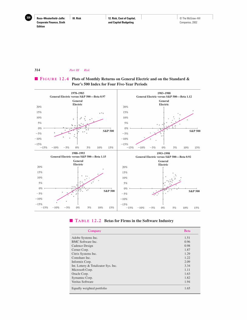
Ross−Westerfield−Jaffe: Corporate Finance, Sixth Edition
III. Risk 12. Risk, Cost of Capital, and Capital Budgeting
320 © The McGraw−Hill Companies, 2002
314 Part III Risk
0%
1978–1983General Electric versus S&P 500—Beta 0.97
20%
15%
10%
5%
�5%
�10%
S&P 500
�15%5% 10% 15%�15% �10% �5% 0%
GeneralElectric
0%
1988–1993General Electric versus S&P 500—Beta 1.15
20%
15%
10%
5%
�5%
�10%
S&P 500
�15%5% 10% 15%�15% �10% �5% 0%
GeneralElectric
0%
1993–1998General Electric versus S&P 500—Beta 0.92
20%
15%
10%
5%
�5%
�10%
S&P 500
�15%5% 10% 15%�15% �10% �5% 0%
GeneralElectric
0%
1983–1988General Electric versus S&P 500—Beta 1.12
20%
15%
10%
5%
�5%
�10%
S&P 500
�15%5% 10% 15%�15% �10% �5% 0%
GeneralElectric
� FIGURE 12.4 Plots of Monthly Returns on General Electric and on the Standard &Poor’s 500 Index for Four Five-Year Periods
� TABLE 12.2 Betas for Firms in the Software Industry
Company Beta
Adobe Systems Inc. 1.51BMC Software Inc. 0.96Cadence Design 0.98Cerner Corp. 1.87Citrix Systems Inc. 1.29Comshare Inc. 1.22Informix Corp. 2.09Int. Lottery & Totalizator Sys. Inc. 3.34Microsoft Corp. 1.11Oracle Corp. 1.63Symantec Corp. 1.82Veritas Software 1.94
Equally weighted portfolio 1.65
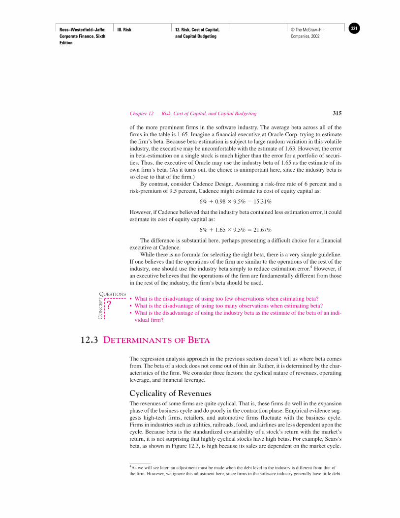
Ross−Westerfield−Jaffe: Corporate Finance, Sixth Edition
III. Risk 12. Risk, Cost of Capital, and Capital Budgeting
321© The McGraw−Hill Companies, 2002
of the more prominent firms in the software industry. The average beta across all of thefirms in the table is 1.65. Imagine a financial executive at Oracle Corp. trying to estimatethe firm’s beta. Because beta-estimation is subject to large random variation in this volatileindustry, the executive may be uncomfortable with the estimate of 1.63. However, the errorin beta-estimation on a single stock is much higher than the error for a portfolio of securi-ties. Thus, the executive of Oracle may use the industry beta of 1.65 as the estimate of itsown firm’s beta. (As it turns out, the choice is unimportant here, since the industry beta isso close to that of the firm.)
By contrast, consider Cadence Design. Assuming a risk-free rate of 6 percent and arisk-premium of 9.5 percent, Cadence might estimate its cost of equity capital as:
6% � 0.98 � 9.5% � 15.31%
However, if Cadence believed that the industry beta contained less estimation error, it couldestimate its cost of equity capital as:
6% � 1.65 � 9.5% � 21.67%
The difference is substantial here, perhaps presenting a difficult choice for a financialexecutive at Cadence.
While there is no formula for selecting the right beta, there is a very simple guideline.If one believes that the operations of the firm are similar to the operations of the rest of theindustry, one should use the industry beta simply to reduce estimation error.4 However, ifan executive believes that the operations of the firm are fundamentally different from thosein the rest of the industry, the firm’s beta should be used.
• What is the disadvantage of using too few observations when estimating beta?• What is the disadvantage of using too many observations when estimating beta?• What is the disadvantage of using the industry beta as the estimate of the beta of an indi-
vidual firm?
12.3 DETERMINANTS OF BETA
The regression analysis approach in the previous section doesn’t tell us where beta comesfrom. The beta of a stock does not come out of thin air. Rather, it is determined by the char-acteristics of the firm. We consider three factors: the cyclical nature of revenues, operatingleverage, and financial leverage.
Cyclicality of RevenuesThe revenues of some firms are quite cyclical. That is, these firms do well in the expansionphase of the business cycle and do poorly in the contraction phase. Empirical evidence sug-gests high-tech firms, retailers, and automotive firms fluctuate with the business cycle.Firms in industries such as utilities, railroads, food, and airlines are less dependent upon thecycle. Because beta is the standardized covariability of a stock’s return with the market’sreturn, it is not surprising that highly cyclical stocks have high betas. For example, Sears’sbeta, as shown in Figure 12.3, is high because its sales are dependent on the market cycle.
Chapter 12 Risk, Cost of Capital, and Capital Budgeting 315
4As we will see later, an adjustment must be made when the debt level in the industry is different from that ofthe firm. However, we ignore this adjustment here, since firms in the software industry generally have little debt.
QUESTIONS
CO
NC
EP
T
?
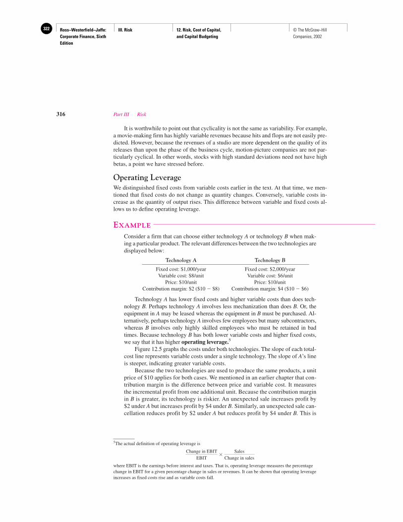
Ross−Westerfield−Jaffe: Corporate Finance, Sixth Edition
III. Risk 12. Risk, Cost of Capital, and Capital Budgeting
322 © The McGraw−Hill Companies, 2002
It is worthwhile to point out that cyclicality is not the same as variability. For example,a movie-making firm has highly variable revenues because hits and flops are not easily pre-dicted. However, because the revenues of a studio are more dependent on the quality of itsreleases than upon the phase of the business cycle, motion-picture companies are not par-ticularly cyclical. In other words, stocks with high standard deviations need not have highbetas, a point we have stressed before.
Operating LeverageWe distinguished fixed costs from variable costs earlier in the text. At that time, we men-tioned that fixed costs do not change as quantity changes. Conversely, variable costs in-crease as the quantity of output rises. This difference between variable and fixed costs al-lows us to define operating leverage.
EXAMPLE
Consider a firm that can choose either technology A or technology B when mak-ing a particular product. The relevant differences between the two technologies aredisplayed below:
Technology A Technology B
Fixed cost: $1,000/year Fixed cost: $2,000/yearVariable cost: $8/unit Variable cost: $6/unit
Price: $10/unit Price: $10/unitContribution margin: $2 ($10 � $8) Contribution margin: $4 ($10 � $6)
Technology A has lower fixed costs and higher variable costs than does tech-nology B. Perhaps technology A involves less mechanization than does B. Or, theequipment in A may be leased whereas the equipment in B must be purchased. Al-ternatively, perhaps technology A involves few employees but many subcontractors,whereas B involves only highly skilled employees who must be retained in badtimes. Because technology B has both lower variable costs and higher fixed costs,we say that it has higher operating leverage.5
Figure 12.5 graphs the costs under both technologies. The slope of each total-cost line represents variable costs under a single technology. The slope of A’s lineis steeper, indicating greater variable costs.
Because the two technologies are used to produce the same products, a unitprice of $10 applies for both cases. We mentioned in an earlier chapter that con-tribution margin is the difference between price and variable cost. It measuresthe incremental profit from one additional unit. Because the contribution marginin B is greater, its technology is riskier. An unexpected sale increases profit by$2 under A but increases profit by $4 under B. Similarly, an unexpected sale can-cellation reduces profit by $2 under A but reduces profit by $4 under B. This is
316 Part III Risk
5The actual definition of operating leverage is
where EBIT is the earnings before interest and taxes. That is, operating leverage measures the percentagechange in EBIT for a given percentage change in sales or revenues. It can be shown that operating leverageincreases as fixed costs rise and as variable costs fall.
Change in EBIT
EBIT�
Sales
Change in sales
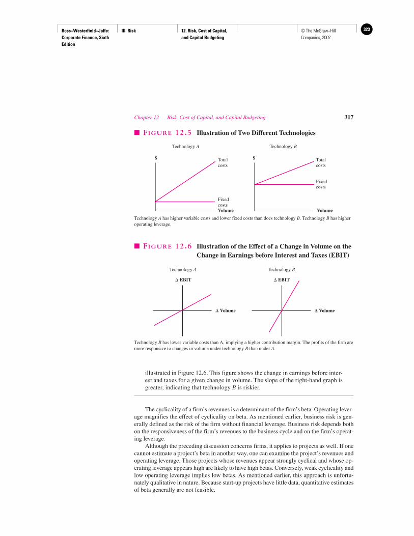
Ross−Westerfield−Jaffe: Corporate Finance, Sixth Edition
III. Risk 12. Risk, Cost of Capital, and Capital Budgeting
323© The McGraw−Hill Companies, 2002
illustrated in Figure 12.6. This figure shows the change in earnings before inter-est and taxes for a given change in volume. The slope of the right-hand graph isgreater, indicating that technology B is riskier.
The cyclicality of a firm’s revenues is a determinant of the firm’s beta. Operating lever-age magnifies the effect of cyclicality on beta. As mentioned earlier, business risk is gen-erally defined as the risk of the firm without financial leverage. Business risk depends bothon the responsiveness of the firm’s revenues to the business cycle and on the firm’s operat-ing leverage.
Although the preceding discussion concerns firms, it applies to projects as well. If onecannot estimate a project’s beta in another way, one can examine the project’s revenues andoperating leverage. Those projects whose revenues appear strongly cyclical and whose op-erating leverage appears high are likely to have high betas. Conversely, weak cyclicality andlow operating leverage implies low betas. As mentioned earlier, this approach is unfortu-nately qualitative in nature. Because start-up projects have little data, quantitative estimatesof beta generally are not feasible.
Chapter 12 Risk, Cost of Capital, and Capital Budgeting 317
Technology A Technology B
Totalcosts
Totalcosts
Fixedcosts
Fixedcosts
Volume Volume
$$
� FIGURE 12.5 Illustration of Two Different Technologies
Technology A has higher variable costs and lower fixed costs than does technology B. Technology B has higheroperating leverage.
Technology A
� EBIT � EBIT
� Volume � Volume
Technology B
� FIGURE 12.6 Illustration of the Effect of a Change in Volume on theChange in Earnings before Interest and Taxes (EBIT)
Technology B has lower variable costs than A, implying a higher contribution margin. The profits of the firm aremore responsive to changes in volume under technology B than under A.
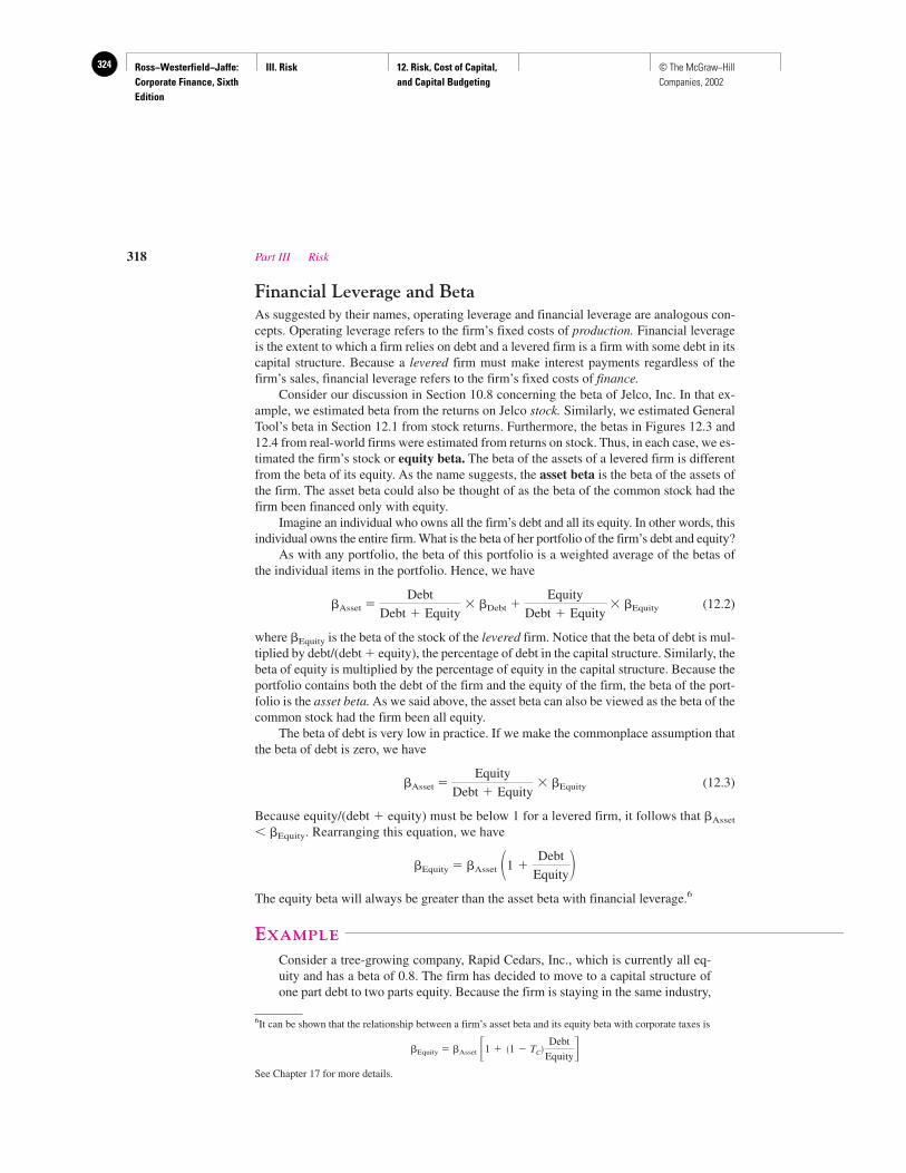
Ross−Westerfield−Jaffe: Corporate Finance, Sixth Edition
III. Risk 12. Risk, Cost of Capital, and Capital Budgeting
324 © The McGraw−Hill Companies, 2002
Financial Leverage and BetaAs suggested by their names, operating leverage and financial leverage are analogous con-cepts. Operating leverage refers to the firm’s fixed costs of production. Financial leverageis the extent to which a firm relies on debt and a levered firm is a firm with some debt in itscapital structure. Because a levered firm must make interest payments regardless of thefirm’s sales, financial leverage refers to the firm’s fixed costs of finance.
Consider our discussion in Section 10.8 concerning the beta of Jelco, Inc. In that ex-ample, we estimated beta from the returns on Jelco stock. Similarly, we estimated GeneralTool’s beta in Section 12.1 from stock returns. Furthermore, the betas in Figures 12.3 and12.4 from real-world firms were estimated from returns on stock. Thus, in each case, we es-timated the firm’s stock or equity beta. The beta of the assets of a levered firm is differentfrom the beta of its equity. As the name suggests, the asset beta is the beta of the assets ofthe firm. The asset beta could also be thought of as the beta of the common stock had thefirm been financed only with equity.
Imagine an individual who owns all the firm’s debt and all its equity. In other words, thisindividual owns the entire firm. What is the beta of her portfolio of the firm’s debt and equity?
As with any portfolio, the beta of this portfolio is a weighted average of the betas ofthe individual items in the portfolio. Hence, we have
�Asset � � �Debt � � �Equity (12.2)
where �Equity is the beta of the stock of the levered firm. Notice that the beta of debt is mul-tiplied by debt/(debt � equity), the percentage of debt in the capital structure. Similarly, thebeta of equity is multiplied by the percentage of equity in the capital structure. Because theportfolio contains both the debt of the firm and the equity of the firm, the beta of the port-folio is the asset beta. As we said above, the asset beta can also be viewed as the beta of thecommon stock had the firm been all equity.
The beta of debt is very low in practice. If we make the commonplace assumption thatthe beta of debt is zero, we have
�Asset � � �Equity (12.3)
Because equity/(debt � equity) must be below 1 for a levered firm, it follows that �Asset
�Equity. Rearranging this equation, we have
�Equity � �Asset
The equity beta will always be greater than the asset beta with financial leverage.6
EXAMPLE
Consider a tree-growing company, Rapid Cedars, Inc., which is currently all eq-uity and has a beta of 0.8. The firm has decided to move to a capital structure ofone part debt to two parts equity. Because the firm is staying in the same industry,
�1 �Debt
Equity�
Equity
Debt � Equity
Equity
Debt � Equity
Debt
Debt � Equity
318 Part III Risk
6It can be shown that the relationship between a firm’s asset beta and its equity beta with corporate taxes is
�Equity � �Asset
See Chapter 17 for more details.
�1 � �1 � TC�Debt
Equity
Ross−Westerfield−Jaffe: Corporate Finance, Sixth Edition
III. Risk 12. Risk, Cost of Capital, and Capital Budgeting
325© The McGraw−Hill Companies, 2002
its asset beta should remain at 0.8. However, assuming a zero beta for its debt, itsequity beta would become
�Equity � �Asset
1.2 � 0.8
If the firm had one part debt to one part equity in its capital structure, its equitybeta would be
1.6 � 0.8 (1 � 1)
However, as long as it stayed in the same industry, its asset beta would remain at0.8. The effect of leverage, then, is to increase the equity beta.
• What are determinants of equity betas?• What is the difference between an asset beta and an equity beta?
12.4 EXTENSIONS OF THE BASIC MODEL
The Firm versus the Project: Vive la DifférenceWe now assume that the risk of a project differs from that of the firm, while going back tothe all-equity assumption. We began the chapter by pointing out that each project should bepaired with a financial asset of comparable risk. If a project’s beta differs from that of thefirm, the project should be discounted at the rate commensurate with its own beta. This isa very important point because firms frequently speak of a corporate discount rate. (Hur-dle rate, cutoff rate, benchmark, and cost of capital are frequently used synonymously.) Un-less all projects in the corporation are of the same risk, choosing the same discount rate forall projects is incorrect.
EXAMPLE
D. D. Ronnelley Co., a publishing firm, may accept a project in computer soft-ware. Noting that computer software companies have high betas, the publishingfirm views the software venture as more risky than the rest of its business. It shoulddiscount the project at a rate commensurate with the risk of software companies.For example, it might use the average beta of a portfolio of publicly traded soft-ware firms. Instead, if all projects in D. D. Ronnelley Co. were discounted at thesame rate, a bias would result. The firm would accept too many high-risk projects(software ventures) and reject too many low-risk projects (books and magazines).This point is illustrated in Figure 12.7.
The D. D. Ronnelley example assumes that the proposed project has identical risk to thatof the software industry, allowing the industry beta to be used. However, the beta of a newproject may be greater than the beta of existing firms in the same industry because the verynewness of the project likely increases its responsiveness to economy wide movements. For
�1 �1
2��1 �
Debt
Equity�
Chapter 12 Risk, Cost of Capital, and Capital Budgeting 319
QUESTIONS
CO
NC
EP
T
?

Ross−Westerfield−Jaffe: Corporate Finance, Sixth Edition
III. Risk 12. Risk, Cost of Capital, and Capital Budgeting
326 © The McGraw−Hill Companies, 2002
example, a start-up computer venture may fail in a recession while IBM, Compaq, orHewlett-Packard will still be around. Conversely, in an economywide expansion, the venturemay grow much faster than the old-line computer firms.
Fortunately, a slight adjustment is all that is needed here. The new venture should beassigned a somewhat higher beta than that of the industry to reflect added risk. The adjust-ment is necessarily ad hoc, so no formula can be given. Our experience indicates that thisapproach is widespread in practice today.
However, a problem does arise for the rare project constituting its own industry. For ex-ample, consider the firms providing consumer shopping by television. Today, one can ob-tain a reasonable estimate for the beta of this industry, since a few of the firms have pub-licly traded stock. However, when the ventures began in the 1980s, any beta estimate wassuspect. At that time, no one knew whether shopping by TV belonged in the television in-dustry, the retail industry, or in an entirely new industry.
What beta should be used in the rare case when an industrywide beta is not appropri-ate? One approach, which considers the determinants of the project’s beta, was treated ear-lier in this chapter. Unfortunately, that approach is only qualitative in nature.
The Cost of Capital with DebtSection 12.1 showed how to choose the discount rate when a project is all-equity fi-nanced. In this section, we discuss an adjustment when the project is financed with bothdebt and equity.
Suppose a firm uses both debt and equity to finance its investments. If the firm pays rB
for its debt financing and rS for its equity, what is the overall or average cost of its capital?The cost of equity is rS, as discussed in earlier sections. The cost of debt is the firm’s bor-
320 Part III Risk
Software venture (SML)
Firm’s overallcost of capital
Discount ratefor project
Beta ofproject
RF
� FIGURE 12.7 Relationship between the Firm’s Cost of Capital andthe Security Market Line
Use of a firm’s cost of capital in calculations may lead to incorrect capital-budgetingdecisions. Projects with high risk, such as the software venture for D. D. Ronnelley Co.,should be discounted at a high rate. By using the firm’s cost of equity, the firm is likely toaccept too many high-risk projects.
Projects with low risk should be discounted at a low rate. By using the firm’s cost ofcapital, the firm is likely to reject too many low-risk projects.

Ross−Westerfield−Jaffe: Corporate Finance, Sixth Edition
III. Risk 12. Risk, Cost of Capital, and Capital Budgeting
327© The McGraw−Hill Companies, 2002
rowing rate, rB. If a firm uses both debt and equity, the cost of capital is a weighted averageof each. This works out to be
The weights in the formula are, respectively, the proportion of total value represented bythe equity
and the proportion of total value represented by debt
This is only natural. If the firm had issued no debt and was therefore an all-equity firm,its average cost of capital would equal its cost of equity, rS. At the other extreme, if the firmhad issued so much debt that its equity was valueless, it would be an all-debt firm, and itsaverage cost of capital would be its cost of debt, rB.
Of course, interest is tax deductible at the corporate level, a point to be treated in moredetail in Chapter 15. The after-tax cost of debt is
Cost of debt (after corporate tax) � rB � (1 � TC)
where TC is the corporation’s tax rate.
Assembling these results, we get the average cost of capital (after tax) for the firm:
Average cost of capital � � rS � � rB � (1 � TC) (12.4)
Because the average cost of capital is a weighting of its cost of equity and its cost ofdebt, it is usually referred to as the weighted average cost of capital, rWACC, and from nowon we will use this term.
EXAMPLE
Consider a firm whose debt has a market value of $40 million and whose stock hasa market value of $60 million (3 million outstanding shares of stock, each sellingfor $20 per share). The firm pays a 15-percent rate of interest on its new debt andhas a beta of 1.41. The corporate tax rate is 34 percent. (Assume that the SMLholds, that the risk premium on the market is 9.5 percent, and that the current Trea-sury bill rate is 11 percent.) What is this firm’s rWACC?
To compute the rWACC using equation (12.4), we must know (1) the after-taxcost of debt, rB � (1 � TC), (2) the cost of equity, rS, and (3) the proportions ofdebt and equity used by the firm. These three values are computed below.
1. The pretax cost of debt is 15 percent, implying an after-tax cost of 9.9 percent[15% � (1 � 0.34)].
2. The cost of equity capital is computed by using the SML:
rS � RF � � � [ M � RF]� 11% � 1.41 � 9.5%� 24.40%
R
� B
S � B�� S
S � B�
� B
S � B�
� S
S � B�
S
S � B� rS �
B
S � B� rB
Chapter 12 Risk, Cost of Capital, and Capital Budgeting 321

Ross−Westerfield−Jaffe: Corporate Finance, Sixth Edition
III. Risk 12. Risk, Cost of Capital, and Capital Budgeting
328 © The McGraw−Hill Companies, 2002
3. The proportions of debt and equity are computed from the market values ofdebt and equity. Because the market value of the firm is $100 million ($40million � $60 million), the proportions of debt and equity are 40 and 60 per-cent, respectively.
The cost of equity, rS, is 24.40 percent, and the after-tax cost of debt, rB �(1 � TC), is 9.9 percent. B is $40 million and S is $60 million. Therefore,
rWACC � � rB � (1 � TC) � � rS
�
This procedure is presented in chart form next:
(1) (2) (3) (4) (5)Financing Market Cost of Capital Weighted Cost
Components Values Weight (after corporate tax) of Capital
Debt $ 40,000,000 0.40 15% � (1 � 0.34) � 9.9% 3.96%Equity 60,000,000 0.60 11% � 1.41 � 9.5% � 24.40% 14.64___________ _____
$100,000,000 1.00 18.60%
The weights we used in the previous example were market-value weights.Market-value weights are more appropriate than book-value weights because themarket values of the securities are closer to the actual dollars that would be re-ceived from their sale. Actually it is usually useful to think in terms of “target”market weights. These are the market weights expected to prevail over the life ofthe firm or project.
EXAMPLE
Suppose that a firm has both a current and a target debt-equity ratio of 0.6, a costof debt of 15.15 percent, and a cost of equity of 20 percent. The corporate tax rateis 34 percent.
Our first step calls for transforming the debt-to-equity (B/S) ratio to a debt-to-value ratio. A B/S ratio of 0.6 implies 6 parts debt for 10 parts equity. Since value is
equal to the sum of the debt plus the equity, the debt-to-value ratio is � 0.375.
Similarly, the equity-to-value ratio is � 0.625. The rWACC will then be
rWACC � � rS � � rB � (1 � TC)
� .625 � 20% � .375 � 15.15% � (.66) � 16.25%
Suppose the firm is considering taking on a warehouse renovation costing$50 million that is expected to yield cost savings of $12 million a year for six
� B
S � B�� S
S � B�
10
6 � 10
6
6 � 10
� 40
100� 9.9%� � � 60
100� 24.40%� � 18.60%
S
B � S
B
B � S
322 Part III Risk
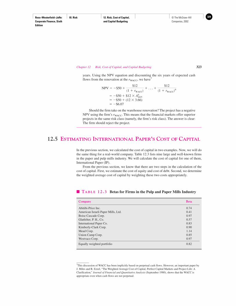
Ross−Westerfield−Jaffe: Corporate Finance, Sixth Edition
III. Risk 12. Risk, Cost of Capital, and Capital Budgeting
329© The McGraw−Hill Companies, 2002
years. Using the NPV equation and discounting the six years of expected cashflows from the renovation at the rWACC, we have7
NPV � �$50 � � . . . �
� �$50 � $12 �� �$50 � (12 � 3.66)� �$6.07
Should the firm take on the warehouse renovation? The project has a negativeNPV using the firm’s rWACC. This means that the financial markets offer superiorprojects in the same risk class (namely, the firm’s risk class). The answer is clear:The firm should reject the project.
12.5 ESTIMATING INTERNATIONAL PAPER’S COST OF CAPITAL
In the previous section, we calculated the cost of capital in two examples. Now, we will dothe same thing for a real-world company. Table 12.3 lists nine large and well-known firmsin the paper and pulp mills industry. We will calculate the cost of capital for one of them,International Paper (IP).
From the previous section, we know that there are two steps in the calculation of thecost of capital. First, we estimate the cost of equity and cost of debt. Second, we determinethe weighted average cost of capital by weighting these two costs appropriately.
A
61. 625
$12�1 � rWACC� 6
$12�1 � rWACC�
Chapter 12 Risk, Cost of Capital, and Capital Budgeting 323
7This discussion of WACC has been implicitly based on perpetual cash flows. However, an important paper byJ. Miles and R. Ezzel, “The Weighted Average Cost of Capital, Perfect Capital Markets and Project Life: AClarification,” Journal of Financial and Quantitative Analysis (September 1980), shows that the WACC isappropriate even when cash flows are not perpetual.
� TABLE 12.3 Betas for Firms in the Pulp and Paper Mills Industry
Company Beta
Abitibi-Price Inc. 0.74American Israeli Paper Mills, Ltd. 0.41Boise Cascade Corp. 0.97Glatfelter, P. H., Co. 0.57International Paper Co. 0.83Kimberly-Clark Corp. 0.90Mead Corp. 1.14Union Camp Corp. 0.85Westvaco Corp. 0.97
Equally weighted portfolio 0.82
Ross−Westerfield−Jaffe: Corporate Finance, Sixth Edition
III. Risk 12. Risk, Cost of Capital, and Capital Budgeting
330 © The McGraw−Hill Companies, 2002
Cost of Equity and DebtWe will tackle the cost of equity first. We need a beta estimate to determine InternationalPaper’s cost of equity and Table 12.3 shows the betas of the nine firms in the industry. Thetable tells us that IP’s beta is 0.83 and the industry’s average beta is 0.82. Which numbershould we use? We argued earlier in the chapter that there is less measurement error withthe industry beta. Therefore, we will work with 0.82, though IP’s beta is so close to the av-erage of the industry that either number would have been fine.
As discussed in Chapter 9, 9.5 percent is our best estimate of the market’s risk pre-mium. If the risk-free rate is 6 percent, our best estimate of International Paper’s cost of eq-uity capital is:
RF � � � [ M � RF]� 6% � 0.82 � 9.5%� 13.79%
The yield on the company’s debt is about 8 percent, which we will use as the (pretax)cost of debt capital, rB.
Determining rWACCNow that we have estimates of both rS, the cost of equity, and rB, the cost of debt, we areready to determine the weighted average cost of capital. However, we still need the per-centages of debt and equity in IP’s capital structure and the tax rate. We find that the ratioof debt-to-value is 32 percent and the ratio of equity-to-value is 68 percent. The tax rate is37 percent.8 These inputs allow us to calculate the weighted average cost of capital:
rWACC �
� 0.68 � 13.79% � 0.32 � 8% � (1 � .37)� 10.99%
Thus, 10.99 percent is International Paper’s cost of capital. It should be used to dis-count any project where one believes that the project’s risk is equal to the risk of the firmas a whole, and the project has the same leverage as the firm as a whole.
12.6 REDUCING THE COST OF CAPITAL
Chapters 9–12 develop the idea that both the expected return on a stock and the cost ofcapital of the firm are positively related to risk. Recently, a number of academics haveargued that expected return and cost of capital are negatively related to liquidity aswell.9 In addition, these scholars make the interesting point that, although it is quite dif-ficult to lower the risk of a firm, it is much easier to increase the liquidity of the firm’sstock. Therefore, they suggest that a firm can actually lower its cost of capital throughliquidity enhancement. We develop this idea next.
� S
S � B� � rS � � B
S � B� � rB � �1 � Tc�
R
324 Part III Risk
8These numbers were taken from Value Line Investment Survey. The tax rate includes both federal and local taxes.9For example, see Y. Amihud and H. Mendelson, “The Liquidity Route to a Lower Cost of Capital,” Journal ofApplied Corporate Finance (Winter 2000) and M. J. Brennan and C. Tamarowski, “Investor Relations,Liquidity, and Stock Prices,” Journal of Applied Corporate Finance (Winter 2000).
Ross−Westerfield−Jaffe: Corporate Finance, Sixth Edition
III. Risk 12. Risk, Cost of Capital, and Capital Budgeting
331© The McGraw−Hill Companies, 2002
What Is Liquidity?Anyone who owns his or her own home probably thinks of liquidity in terms of the time ittakes to buy or sell the home. For example, condominiums in large metropolitan areas aregenerally quite liquid. Particularly in good times, a condominium may sell within days ofbeing placed on the market. By contrast, single-family homes in suburban areas may takeweeks or months to sell. Special properties such as multimillion dollar mansions may takelonger still.
The concept of liquidity is similar, but not identical, in stocks. Here, we speak of the costof buying and selling instead. That is, those stocks that are expensive to trade are consideredless liquid than those that trade cheaply. What do we mean by the cost to trade? We gener-ally think of three costs here: brokerage fees, the bid-ask spread, and market-impact costs.
Brokerage fees are the easiest to understand, because you must pay a broker to executea trade. More difficult is the bid-ask spread. Consider the New York Stock Exchange(NYSE), where all trades on a particular stock must go through the stock’s specialist, whois physically on the floor of the exchange. If you want to trade 100 shares of XYZ Co., yourbroker must get the quote from XYZ’s specialist. Suppose the specialist provides a quoteof 100–1001⁄8. This means that you can buy from the specialist at $1001⁄8 per share and sellto the specialist at $100 per share. Note that the specialist makes money here, since she buysfrom you at $100 and sells to you (or to someone else) at $1001⁄8. The gain to the specialistis a cost to you, because you are losing 1⁄8 dollar per share over a round-trip transaction (overa purchase and a subsequent sale).
Finally, we have market-impact costs. Suppose that a trader wants to sell 10,000 sharesinstead of just 100 shares. Here, the specialist has to take on extra risk when buying. First,she has to pay out $100,000 (10,000 � $100), cash which may not be easily available toher. Second, the trader may be selling this large amount because she has special informa-tion that the stock will fall imminently. The specialist bears the risk of losing a lot of moneyon that trade. Consequently, to compensate for these risks, the specialist may not buy at$100/share but at a lower price. Similarly, the specialist may be willing to sell a large blockof stock only at a price above $1001⁄8. The price drop associated with a large sale and theprice rise associated with a large purchase are the market-impact costs.
Liquidity, Expected Returns, and the Cost of CapitalThe cost of trading a nonliquid stock reduces the total return that an investor receives. Thatis, if one buys a stock for $100 and sells it later for $105, the gain before trading costs is $5.If one must pay a dollar of commission when buying and another dollar when selling, thegain after trading costs is only $3. Both the bid-ask spread and market-impact costs wouldreduce this gain still further.
As we will see later, trading costs vary across securities. In the last four chapters, wehave stressed that investors demand a high expected return as compensation when investingin high risk, e.g., high-beta, stocks. Because the expected return to the investor is the cost ofcapital to the firm, the cost of capital is positively related to beta. Now, we are saying thesame thing for trading costs. Investors demand a high expected return when investing instocks with high trading costs, i.e., low liquidity. And, this high expected return implies ahigh cost of capital to the firm. This idea is illustrated in Figure 12.8.
Liquidity and Adverse SelectionLiquidity varies across stocks, because the factors determining liquidity vary across stocks.Although there are a number of factors, we focus on just one, adverse selection. As men-tioned before, the specialist will lose money on a trade if the trader has information that the
Chapter 12 Risk, Cost of Capital, and Capital Budgeting 325
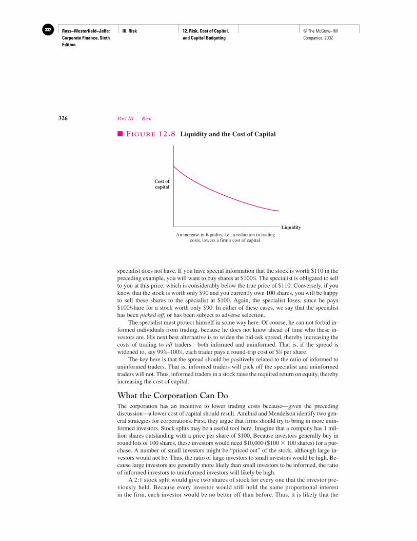
Ross−Westerfield−Jaffe: Corporate Finance, Sixth Edition
III. Risk 12. Risk, Cost of Capital, and Capital Budgeting
332 © The McGraw−Hill Companies, 2002
specialist does not have. If you have special information that the stock is worth $110 in thepreceding example, you will want to buy shares at $1001⁄8. The specialist is obligated to sellto you at this price, which is considerably below the true price of $110. Conversely, if youknow that the stock is worth only $90 and you currently own 100 shares, you will be happyto sell these shares to the specialist at $100. Again, the specialist loses, since he pays$100/share for a stock worth only $90. In either of these cases, we say that the specialisthas been picked off, or has been subject to adverse selection.
The specialist must protect himself in some way here. Of course, he can not forbid in-formed individuals from trading, because he does not know ahead of time who these in-vestors are. His next best alternative is to widen the bid-ask spread, thereby increasing thecosts of trading to all traders—both informed and uninformed. That is, if the spread iswidened to, say 997⁄8–1001⁄4, each trader pays a round-trip cost of $3⁄8 per share.
The key here is that the spread should be positively related to the ratio of informed touninformed traders. That is, informed traders will pick off the specialist and uninformedtraders will not. Thus, informed traders in a stock raise the required return on equity, therebyincreasing the cost of capital.
What the Corporation Can DoThe corporation has an incentive to lower trading costs because—given the preceding discussion—a lower cost of capital should result. Amihud and Mendelson identify two gen-eral strategies for corporations. First, they argue that firms should try to bring in more unin-formed investors. Stock splits may be a useful tool here. Imagine that a company has 1 mil-lion shares outstanding with a price per share of $100. Because investors generally buy inround lots of 100 shares, these investors would need $10,000 ($100 � 100 shares) for a pur-chase. A number of small investors might be “priced out” of the stock, although large in-vestors would not be. Thus, the ratio of large investors to small investors would be high. Be-cause large investors are generally more likely than small investors to be informed, the ratioof informed investors to uninformed investors will likely be high.
A 2:1 stock split would give two shares of stock for every one that the investor pre-viously held. Because every investor would still hold the same proportional interest in the firm, each investor would be no better off than before. Thus, it is likely that the
326 Part III Risk
Cost ofcapital
Liquidity
An increase in liquidity, i.e., a reduction in tradingcosts, lowers a firm's cost of capital.
� FIGURE 12.8 Liquidity and the Cost of Capital
Ross−Westerfield−Jaffe: Corporate Finance, Sixth Edition
III. Risk 12. Risk, Cost of Capital, and Capital Budgeting
333© The McGraw−Hill Companies, 2002
price per share will fall to $50 from $100. Here, an individual with 100 shares worth$10,000 ($100 � 100 shares) finds herself still worth $10,000 (� $50 � 200 shares)after the split.
However, a round lot becomes more affordable, thereby bringing more small and un-informed investors into the firm. Consequently, the adverse selection costs are reduced, al-lowing the specialist to lower the bid-ask spread. In turn, it is hoped that the expected re-turn on the stock, and the cost of equity capital, will fall as well. If this happens, the stockmight actually trade at a price slightly above $50.
This idea is a new one and empirical evidence is not yet in. Amihud and Mendelsonthemselves point out the possibility that this strategy might backfire, because brokeragecommissions are often higher on lower-priced securities. We must await confirmation ofthis intriguing suggestion.
Companies can also attract small investors by facilitating stock purchases through theInternet. Direct stock purchase plans and dividend reinvestment programs handled onlineallow small investors the opportunity to buy securities cheaply. In addition, Amihud andMendelson state, “And when these plans are administered over the Internet using web siteslike Stockpower.com, moneypaper.com and Netstockdirect.com, the process is fast and ef-ficient for both the company and the investor.”10
Secondly, companies can disclose more information. This narrows the gap between un-informed and informed investors, thereby lowering the cost of capital. Suggestions includeproviding greater financial data on corporate segments and more management forecasts. Aninteresting study by Coller and Yohn11 concludes that the bid-ask spread is reduced after therelease of these forecasts.
This section would not be complete without a discussion of security analysts. Theseanalysts are employed by brokerage houses to follow the companies in individual indus-tries. For example, an analyst for a particular brokerage house might follow all the firmsin, say, the auto industry. This analyst distributes reports and other information to theclients of the brokerage house. Virtually all brokerage houses have analysts following themajor industries. Again, through dissemination of the information, these analysts narrowthe gap between the informed and the uninformed investors, thereby tending to reduce thebid-ask spread.
Although all major industries are covered, the smaller firms in these industries are of-ten ignored, implying a higher bid-ask spread and a higher cost of capital for these firms.Analysts frequently state that they avoid following companies that release little informa-tion, pointing out that these companies are more trouble than they are worth. Thus, it be-hooves companies that are not followed to release as much information as possible to se-curity analysts in the hopes of attracting their interest. Friendliness toward security analystswould be very helpful as well. The argument here is not to get the analysts to make buy rec-ommendations. Rather, it is simply to interest the analysts in following the company,thereby reducing the information asymmetry between informed and uninformed investors.
• What is liquidity?• What is the relation between liquidity and expected returns?• What is adverse selection?• What can a corporation do to lower its cost of capital?
Chapter 12 Risk, Cost of Capital, and Capital Budgeting 327
10Ibid., p. 19.11M. Coller and T. Yohn, “Management Forecasts and Information Asymmetry: An Examination of Bid-AskSpreads,” Journal of Accounting Research (Fall 1997).
QUESTIONS
CO
NC
EP
T
?
Ross−Westerfield−Jaffe: Corporate Finance, Sixth Edition
III. Risk 12. Risk, Cost of Capital, and Capital Budgeting
334 © The McGraw−Hill Companies, 2002
12.7 SUMMARY AND CONCLUSIONS
Earlier chapters on capital budgeting assumed that projects generate riskless cash flows. Theappropriate discount rate in that case is the riskless interest rate. Of course, most cash flowsfrom real-world capital-budgeting projects are risky. This chapter discusses the discount ratewhen cash flows are risky.1. A firm with excess cash can either pay a dividend or make a capital expenditure. Because
stockholders can reinvest the dividend in risky financial assets, the expected return on acapital-budgeting project should be at least as great as the expected return on a financial assetof comparable risk.
2. The expected return on any asset is dependent upon its beta. Thus, we showed how toestimate the beta of a stock. The appropriate procedure employs regression analysis onhistorical returns.
3. We considered the case of a project whose beta risk was equal to that of the firm. If the firmis unlevered, the discount rate on the project is equal to
RF � � � ( M � RF)
where M is the expected return on the market portfolio and RF is the risk-free rate. In words,the discount rate on the project is equal to the CAPM’s estimate of the expected return on thesecurity.
4. If the project’s beta differs from that of the firm, the discount rate should be based on theproject’s beta. The project’s beta can generally be estimated by determining the average betaof the project’s industry.
5. The beta of a company is a function of a number of factors. Perhaps the three mostimportant are• Cyclicality of revenues• Operating leverage• Financial leverage
6. Sometimes one cannot use the average beta of the project’s industry as an estimate of thebeta of the project. For example, a new project may not fall neatly into any existing industry.In this case, one can estimate the project’s beta by considering the project’s cyclicality ofrevenues and its operating leverage. This approach is qualitative in nature.
7. If a firm uses debt, the discount rate to use is the rWACC. In order to calculate rWACC, the costof equity and the cost of debt applicable to a project must be estimated. If the project issimilar to the firm, the cost of equity can be estimated using the SML for the firm’s equity.Conceptually, a dividend-growth model could be used as well, though it is likely to be farless accurate in practice.
8. A number of academics have argued that expected returns are negatively related to liquidity,where high liquidity is equivalent to low costs of trading. These scholars have furthersuggested that firms can reduce their cost of capital by lowering these trading costs. Practicalsuggestions include stock splits, more complete dissemination of information, and moreeffective assistance to security analysts.
KEY TERMS
Asset beta 318 Operating leverage 316Cost of equity 307 Weighted average cost of capital (rWACC) 321Equity beta 318
R
R
328 Part III Risk

Ross−Westerfield−Jaffe: Corporate Finance, Sixth Edition
III. Risk 12. Risk, Cost of Capital, and Capital Budgeting
335© The McGraw−Hill Companies, 2002
SUGGESTED READINGS
The following article contains a superb discussion of some of the subtleties of using WACC forproject evaluation:Miles, J., and R. Ezzel. “The Weighted Average Cost of Capital, Perfect Capital Markets and
Project Life: A Clarification.” Journal of Financial and Quantitative Analysis 15(September 1980).
The following article provides a comprehensive survey of capital budgeting in practice,including the determination of the cost of capital:Graham, J. R., and C. R. Harvey, “The Theory and Practice of Corporate Finance: Evidence
from the Field,” unpublished paper, Duke University (April, 2000).
Estimates of the cost of capital under both the capital asset pricing model and the arbitragepricing theory are contained in:Fama, E. F., and K. R. French, “Industry Cost of Capital,” Journal of Financial Economics
(February 1997).
One of the best “how-to” guides is:Copeland, T.; T. Koller; and J. Murrin. Valuation: Measuring and Managing the Value of
Companies. 2nd ed. New York: John Wiley & Sons, 1995.
QUESTIONS AND PROBLEMS
Beta and the Cost of Equity12.1 Furniture Depot, Inc., is an all-equity firm with a beta of 0.95. The market-risk
premium is 9 percent and the risk-free rate is 5 percent. The company must decidewhether or not to undertake the project that requires an immediate investment of $1.2 million and will generate annual after-tax cash flows of $340,000 at year-end forfive years. If the project has the same risk as the firm as a whole, should FurnitureDepot undertake the project?
12.2 The returns for the past five years on Douglas stock and the New York Stock ExchangeComposite Index (NYSE) are listed below:
Douglas NYSE
�0.05 �0.120.05 0.010.08 0.060.15 0.100.10 0.05
a. What are the average returns on Douglas stock and on the market?b. Compute the beta of Douglas stock.
12.3 Mitsubishi Inc. is a levered firm with a debt-to-equity ratio of 0.25. The beta of commonstock is 1.15, while the beta of debt is 0.3. The market-risk premium is 10 percent andthe risk-free rate is 6 percent. The corporate tax rate is 35 percent. The SML holds forthe company.a. If a new project of the company has the same risk as the common stock of the firm,
what is the cost of equity on the project?b. If a new project of the company has the same risk as the overall firm, what is the
weighted average cost of capital on the project?
12.4 The correlation between the returns on Ceramics Craftsman, Inc., and the returns on theS&P 500 is 0.675. The variance of the returns on Ceramics Craftsman, Inc., is 0.004225,
Chapter 12 Risk, Cost of Capital, and Capital Budgeting 329
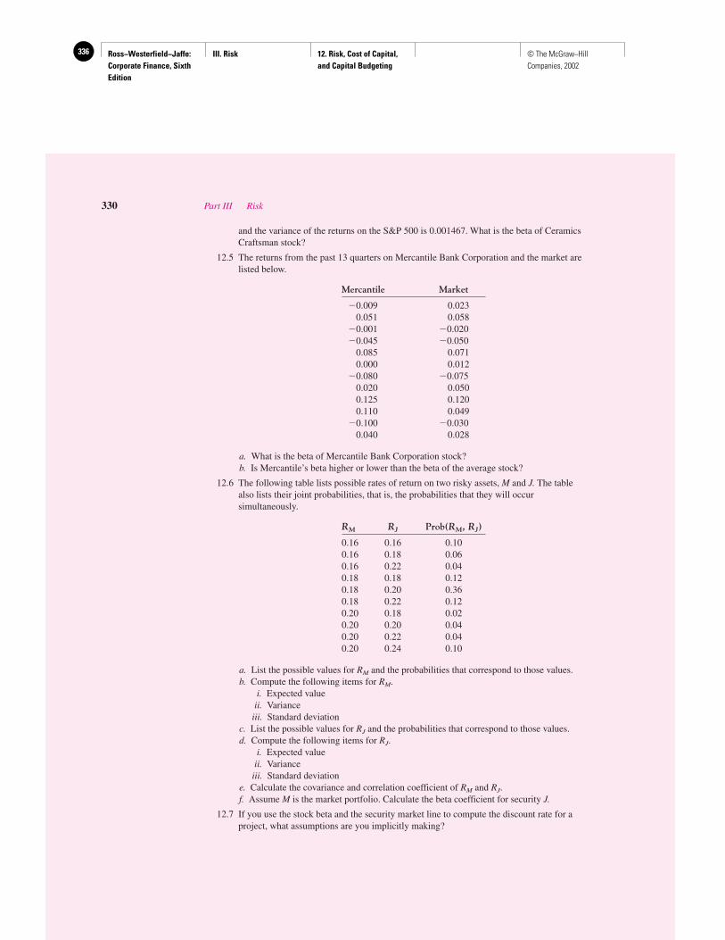
Ross−Westerfield−Jaffe: Corporate Finance, Sixth Edition
III. Risk 12. Risk, Cost of Capital, and Capital Budgeting
336 © The McGraw−Hill Companies, 2002
and the variance of the returns on the S&P 500 is 0.001467. What is the beta of CeramicsCraftsman stock?
12.5 The returns from the past 13 quarters on Mercantile Bank Corporation and the market arelisted below.
Mercantile Market
�0.009 0.0230.051 0.058
�0.001 �0.020�0.045 �0.050
0.085 0.0710.000 0.012
�0.080 �0.0750.020 0.0500.125 0.1200.110 0.049
�0.100 �0.0300.040 0.028
a. What is the beta of Mercantile Bank Corporation stock?b. Is Mercantile’s beta higher or lower than the beta of the average stock?
12.6 The following table lists possible rates of return on two risky assets, M and J. The tablealso lists their joint probabilities, that is, the probabilities that they will occursimultaneously.
RM RJ Prob(RM, RJ)
0.16 0.16 0.100.16 0.18 0.060.16 0.22 0.040.18 0.18 0.120.18 0.20 0.360.18 0.22 0.120.20 0.18 0.020.20 0.20 0.040.20 0.22 0.040.20 0.24 0.10
a. List the possible values for RM and the probabilities that correspond to those values.b. Compute the following items for RM.
i. Expected valueii. Varianceiii. Standard deviation
c. List the possible values for RJ and the probabilities that correspond to those values.d. Compute the following items for RJ.
i. Expected valueii. Varianceiii. Standard deviation
e. Calculate the covariance and correlation coefficient of RM and RJ.f. Assume M is the market portfolio. Calculate the beta coefficient for security J.
12.7 If you use the stock beta and the security market line to compute the discount rate for aproject, what assumptions are you implicitly making?
330 Part III Risk

Ross−Westerfield−Jaffe: Corporate Finance, Sixth Edition
III. Risk 12. Risk, Cost of Capital, and Capital Budgeting
337© The McGraw−Hill Companies, 2002
12.8 Pacific Cosmetics is evaluating a project to produce a perfume line. Pacific currentlyproduces no body-scent products. Pacific Cosmetics is an all-equity firm.a. Should Pacific Cosmetics use its stock beta to evaluate the project?b. How should Pacific Cosmetics compute the beta to evaluate the project?
12.9 The following table lists possible rates of return on Compton Technology’s stock and debt,and on the market portfolio. The corporate tax rate is 35 percent. The correspondingprobabilities are also listed.
Return on Return on Return onState Probability Equity (%) Debt (%) the Market (%)
1 0.1 3% 8% 5%2 0.3 8 8 103 0.4 20 10 154 0.2 15 10 20
a. What is the beta of Compton Technology debt?b. What is the beta of Compton Technology stock?c. If the debt-to-equity ratio of Compton Technology is 0.5, what is the asset beta of
Compton Technology?
12.10 Is the discount rate for the projects of a levered firm higher or lower than the cost ofequity computed using the security market line? Why? (Consider only projects that havesimilar risk to that of the firm.)
12.11 What factors determine the beta of a stock? Define and describe each.
Weighted Average Cost of Capital12.12 The equity beta for Adobe Online Company is 1.29. Adobe Online has a debt-to-equity
ratio of 1.0. The expected return on the market is 13 percent. The risk-free rate is 7 percent. The cost of debt capital is 7 percent. The corporate tax rate is 35 percent.a. What is Adobe Online’s cost of equity?b. What is Adobe Online’s weighted average cost of capital?
12.13 Calculate the weighted average cost of capital for the Luxury Porcelain Company. Thebook value of Luxury’s outstanding debt is $60 million. Currently, the debt is trading at120 percent of book value and is priced to yield 12 percent. The 5 million outstandingshares of Luxury stock are selling for $20 per share. The required return on Luxury stockis 18 percent. The tax rate is 25 percent.
12.14 First Data Co. has 20 million shares of common stock outstanding that are currently beingsold for $25 per share. The firm’s debt is publicly traded at 95 percent of its face value of$180 million. The cost of debt is 10 percent and the cost of equity is 20 percent. What is theweighted average cost of capital for the firm? Assume the corporate tax rate is 40 percent.
12.15 Calgary Industries, Inc., is considering a new project that costs $25 million. The projectwill generate after-tax (year-end) cash flows of $7 million for five years. The firm has a debt-to-equity ratio of 0.75. The cost of equity is 15 percent and the cost of debt is 9 percent. The corporate tax rate is 35 percent. It appears that the project has the samerisk as that of the overall firm. Should Calgary take on the project?
12.16 Suppose Garageband.com has a 28 percent cost of equity capital and a 10 percent before-tax cost of debt capital. The firm’s debt-to-equity ratio is 1.0. Garageband is interested ininvesting in a telecomm project that will cost $1,000,000 and will provide $600,000pretax annual earnings for 5 years. Given the project is an extension of its core business,the project risk is similar to the overall risk of the firm. What is the net present value ofthis project if Garageband’s tax rate is 35%?
Chapter 12 Risk, Cost of Capital, and Capital Budgeting 331
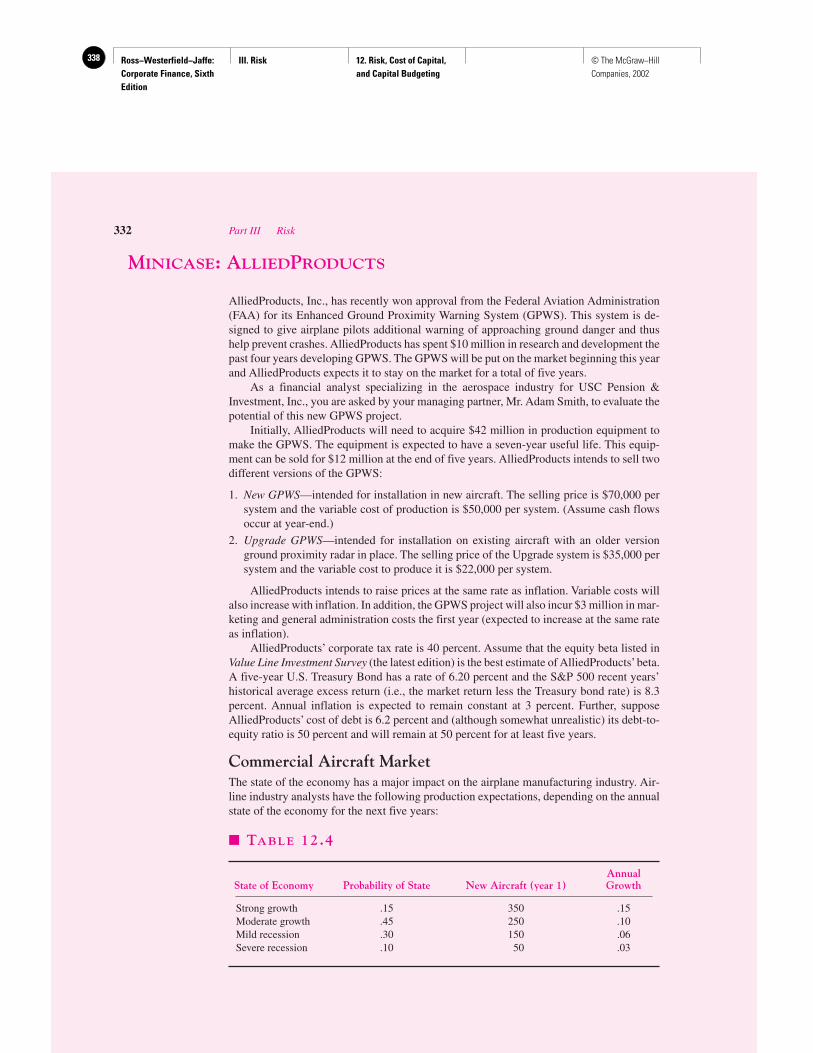
Ross−Westerfield−Jaffe: Corporate Finance, Sixth Edition
III. Risk 12. Risk, Cost of Capital, and Capital Budgeting
338 © The McGraw−Hill Companies, 2002
MINICASE: ALLIEDPRODUCTS
AlliedProducts, Inc., has recently won approval from the Federal Aviation Administration(FAA) for its Enhanced Ground Proximity Warning System (GPWS). This system is de-signed to give airplane pilots additional warning of approaching ground danger and thushelp prevent crashes. AlliedProducts has spent $10 million in research and development thepast four years developing GPWS. The GPWS will be put on the market beginning this yearand AlliedProducts expects it to stay on the market for a total of five years.
As a financial analyst specializing in the aerospace industry for USC Pension &Investment, Inc., you are asked by your managing partner, Mr. Adam Smith, to evaluate thepotential of this new GPWS project.
Initially, AlliedProducts will need to acquire $42 million in production equipment tomake the GPWS. The equipment is expected to have a seven-year useful life. This equip-ment can be sold for $12 million at the end of five years. AlliedProducts intends to sell twodifferent versions of the GPWS:
1. New GPWS—intended for installation in new aircraft. The selling price is $70,000 persystem and the variable cost of production is $50,000 per system. (Assume cash flowsoccur at year-end.)
2. Upgrade GPWS—intended for installation on existing aircraft with an older versionground proximity radar in place. The selling price of the Upgrade system is $35,000 persystem and the variable cost to produce it is $22,000 per system.
AlliedProducts intends to raise prices at the same rate as inflation. Variable costs willalso increase with inflation. In addition, the GPWS project will also incur $3 million in mar-keting and general administration costs the first year (expected to increase at the same rateas inflation).
AlliedProducts’ corporate tax rate is 40 percent. Assume that the equity beta listed inValue Line Investment Survey (the latest edition) is the best estimate of AlliedProducts’beta.A five-year U.S. Treasury Bond has a rate of 6.20 percent and the S&P 500 recent years’historical average excess return (i.e., the market return less the Treasury bond rate) is 8.3percent. Annual inflation is expected to remain constant at 3 percent. Further, supposeAlliedProducts’ cost of debt is 6.2 percent and (although somewhat unrealistic) its debt-to-equity ratio is 50 percent and will remain at 50 percent for at least five years.
Commercial Aircraft MarketThe state of the economy has a major impact on the airplane manufacturing industry. Air-line industry analysts have the following production expectations, depending on the annualstate of the economy for the next five years:
332 Part III Risk
� TABLE 12.4
AnnualState of Economy Probability of State New Aircraft (year 1) Growth
Strong growth .15 350 .15Moderate growth .45 250 .10Mild recession .30 150 .06Severe recession .10 50 .03
Ross−Westerfield−Jaffe: Corporate Finance, Sixth Edition
III. Risk 12. Risk, Cost of Capital, and Capital Budgeting
339© The McGraw−Hill Companies, 2002
While probabilities of each state of the economy will not change during the next fiveyears, airplane production for each category will increase, as shown in Table 12.4, each yearafter year 1. The FAA requires that these planes have new ground proximity warning sys-tems, of which there are a number of manufacturers besides AlliedProducts.
AlliedProducts estimates that there are approximately 12,500 existing aircraft thatcomprise the market for its GPWS Upgrade package. Due to FAA regulations, all ex-isting aircraft will be required to get an upgraded ground proximity warning systemwithin the next five years, again, not necessarily from AlliedProducts. AlliedProductsbelieves the upgrades of the existing aircraft fleet will be spread evenly over the fiveyears (the time value of money would suggest manufacturers defer purchasing up-grades until the fifth year; however, consumer demand for the additional safety will in-duce earlier upgrades).
AlliedProducts uses the MACRS depreciation schedule (seven-year property class).The immediate initial working capital requirement is $2 million and thereafter the net work-ing capital requirements will be 5 percent of sales.
AlliedProducts has a number of competitors both in the new GPWS and upgradeGPWS markets but expects to dominate the market with a 45 percent share.
Assignment:First, use the CAPM to determine the appropriate discount rate for this product. Then, usecomputer spreadsheets such as Excel or Lotus 1-2-3 to analyze the project.
Will the GPWS project improve the wealth of AlliedProducts’ shareholders, such asyour firm—USC Pension & Investment, Inc.?
Economic Value Added and the Measurement of Financial PerformanceChapter 12 shows how to calculate the appropriate discount rate for capital budgeting andother valuation problems. We now consider the measurement of financial performance. Weintroduce the concept of economic value added, which uses the same discount rate devel-oped for capital budgeting. We begin with a simple example.
Many years ago, Henry Bodenheimer started Bodie’s Blimps, one of the largest high-speed blimp manufacturers. Because growth was so rapid, Henry put most of his effort intocapital budgeting. His approach to capital budgeting paralleled that of Chapter 12. He fore-casted cash flows for various projects and discounted them at the cost of capital appropri-ate to the beta of the blimp business. However, these projects have grown rapidly, in somecases becoming whole divisions. He now needs to evaluate the performance of these divi-sions in order to reward his division managers. How does he perform the appropriateanalysis?
Henry is aware that capital budgeting and performance measurement are essen-tially mirror images of each other. Capital budgeting is forward-looking by nature be-cause one must estimate future cash flows to value a project. By contrast, performancemeasurement is backward-looking. As Henry stated to a group of his executives,“Capital budgeting is like looking through the windshield while driving a car. Youneed to know what lies further down the road to calculate a net present value.Performance measurement is like looking into the rearview mirror. You find out whereyou have been.”
Chapter 12 Risk, Cost of Capital, and Capital Budgeting 333

Ross−Westerfield−Jaffe: Corporate Finance, Sixth Edition
III. Risk 12. Risk, Cost of Capital, and Capital Budgeting
340 © The McGraw−Hill Companies, 2002
Henry first measured the performance of his various divisions by return on assets(ROA), an approach, which we treated in the appendix to Chapter 2. For example, if a di-vision had earnings after tax of $1,000 and had assets of $10,000, the ROA would be12
� 10%.
He calculated the ROA ratio for each of his divisions, paying a bonus to each of his di-vision managers based on the size of that division’s ROA. However, while ROA was gen-erally effective in motivating his managers, there were a number of situations where it ap-peared that ROA was counterproductive.
For example, Henry always believed that Sharon Smith, head of the supersonic divi-sion, was his best manager. The ROA of Smith’s division was generally in the high dou-ble digits, but the best estimate of the weighted average cost of capital for the division wasonly 20%. Furthermore, the division had been growing rapidly. However, as soon as Henrypaid bonuses based on ROA, the division stopped growing. At that time, Smith’s divisionhad after tax earnings of $2,000,000 on an asset base of $2,000,000, for an ROA of 100%($2 million/$2 million).
Henry found out why the growth stopped when he suggested a project to Smith thatwould earn $1,000,000 per year on an investment of $2,000,000. This was clearly an at-tractive project with an ROA of 50% ($1 million/$2 million). He thought that Smith wouldjump at the chance to place his project into her division, because the ROA of the projectwas much higher than the cost of capital of 20%. However, Smith did everything she couldto kill the project. And, as Henry later figured out, Smith was rational to do so. Smith musthave realized that if the project were accepted, the division’s ROA would become
� 75%
Thus, the ROA of Smith’s division would fall from 100% to 75% if the project wereaccepted, with Smith’s bonus falling in tandem.
Henry was later exposed to the economic-value-added (EVA) approach,13 which seemsto obviate this particular problem. The formula for EVA is
[ROA � Weighted average cost of capital] � Total capital
Without the new project, the EVA of Smith’s division would be:
[100% – 20%] � $2,000,000 � $1,600,000
This is an annual number. That is, the division would bring in $1.6 million above and be-yond the cost of capital to the firm each year.
With the new project included, the EVA jumps to
[75% � 20%] � $4,000,000 � $2,200,000
If Sharon Smith knew that her bonus was based on EVA, she would now have an in-centive to accept, not reject, the project. Although ROA appears in the EVA formula, EVAdiffers substantially from ROA. The big difference is that ROA is a percentage number and
$2,000,000 � $1,000,000
$2,000,000 � $2,000,000
$1,000
$10,000
334 Part III Risk
12Earnings after tax is EBIT (1 � Tc) where EBIT is earnings before interest and taxes and Tc is the tax rate.13Stern Stewart & Company have a copyright on the terms economic value added and EVA. Details on the SternSteward & Company EVA can be found in J. M. Stern, G. B. Stewart, and D. A. Chew, “The EVA FinancialManagement System,” Journal of Applied Corporate Finance (Summer 1999).

Ross−Westerfield−Jaffe: Corporate Finance, Sixth Edition
III. Risk 12. Risk, Cost of Capital, and Capital Budgeting
341© The McGraw−Hill Companies, 2002
EVA is a dollar value. In the preceding example, EVA increased when the new project wasadded even though the ROA actually decreased. In this situation, EVA correctly incorpo-rates the fact that a high return on a large division may be better than a very high return ona smaller division. The situation here is quite similar to the scale problem in capital budg-eting that we discussed in Section 6.6.
Further understanding of EVA can be achieved by rewriting the EVA formula. BecauseROA � total capital is equal to earnings after tax, we can write the EVA formula as:
Earnings after tax � Weighted average cost of capital � Total capital
Thus, EVA can simply be viewed as earnings after capital costs. Although accountantssubtract many costs (including depreciation) to get the earnings number shown in financialreports, they do not subtract out capital costs. One can see the logic of accountants, becausethe cost of capital is very subjective. By contrast, costs such as COGS (cost of goods sold),SGA (sales, general and administration), and even depreciation can be measured more ob-jectively. However, even if the cost of capital is difficult to estimate, it is hard to justify ig-noring it completely. After all, this textbook argues that the cost of capital is a necessary in-put to capital budgeting. Shouldn’t it also be a necessary input to performance measurement?
This example argues that EVA can increase investment for those firms that are currentlyunderinvesting. However, there are many firms in the reverse situation; the managers are sofocused on increasing earnings that they take on projects for which the profits do not justifythe capital outlays. These managers either are unaware of capital costs or, knowing thesecosts, choose to ignore them. Because the cost of capital is right in the middle of the EVAformula, managers will not easily ignore these costs when evaluated on an EVA system.
One other advantage of EVA is that it is so stark; the number is either positive or it isnegative. Plenty of divisions have negative EVAs for a number of years. Because these di-visions are destroying more value than they are creating, a strong point can be made for liq-uidating these divisions. Although managers are generally emotionally opposed to this typeof action, EVA analysis makes liquidation harder to ignore.
The preceding discussion puts EVA in a very positive light. However, one can certainlyfind much to criticize with EVA as well. We now focus on two well-known problems withEVA. First, the preceding example uses EVA for performance measurement, where we be-lieve it properly belongs. To us, EVA seems a clear improvement over ROA and other fi-nancial ratios. However, EVA has little to offer for capital budgeting because EVA focusesonly on current earnings. By contrast, net-present-value analysis uses projections of all fu-ture cash flows, where the cash flows will generally differ from year to year. Thus, as far ascapital budgeting is concerned, NPV analysis has a richness that EVA does not have.Although supporters may argue that EVA correctly incorporates the weighted average costof capital, one must remember that the discount rate in NPV analysis is the same weightedaverage cost of capital. That is, both approaches take the cost of equity capital based on betaand combine it with the cost of debt to get an estimate of this weighted average.
A second problem with EVA is that it may increase the shortsightedness of managers.Under EVA, a manager will be well rewarded today if earnings are high today. Future lossesmay not harm the manager, because there is a good chance that she will be promoted or haveleft the firm by then. Thus, the manager has an incentive to run a division with more regardfor short-term than long-term value. By raising prices or cutting quality, the manager mayincrease current profits (and, therefore, current EVA). However, to the extent that customersatisfaction is reduced, future profits (and therefore future EVA) are likely to fall. However,one should not be too harsh with EVA here, because the same problem occurs with ROA.A manager who raises prices or cuts quality will increase current ROA at the expense of fu-ture ROA. The problem, then, is not EVA per se but with the use of accounting numbers in
Chapter 12 Risk, Cost of Capital, and Capital Budgeting 335

Ross−Westerfield−Jaffe: Corporate Finance, Sixth Edition
III. Risk 12. Risk, Cost of Capital, and Capital Budgeting
342 © The McGraw−Hill Companies, 2002
general. Because stockholders want the discounted present value of all cash flows to bemaximized, managers with bonuses based on some function of current profits or currentcash flows are likely to behave in a shortsighted way.
EXAMPLE
Assume the following figures for the International Trade Corporation
EBIT � $2.5 billionTc � .4
rWACC � 11%Total capital contributed � Total debt � Equity
� $10 billion � $10 billion� $20 billion
Now we can calculate International Trade’s EVA:
EVA � EBIT (1 � Tc) � rWACC � Total capital� ($2.5 billion � .6) � (.11 � $20 billion)� $1.5 billion � $2.2 billion� �$700 million
336 Part III Risk
Ross−Westerfield−Jaffe: Corporate Finance, Sixth Edition
IV. Capital Structure and Dividend Policy
Introduction 343© The McGraw−Hill Companies, 2002
Capital Structure andDividend Policy
PA
RT
IV
13 Corporate-Financing Decisions and Efficient Capital Markets 33914 Long-Term Financing: An Introduction 37115 Capital Structure: Basic Concepts 39016 Capital Structure: Limits to the Use of Debt 42217 Valuation and Capital Budgeting for the Levered Firm 46818 Dividend Policy: Why Does It Matter? 495
PART II discussed the capital budgeting decisions of the firm. We argued that the ob-jective of the firm should be to create value from its capital budgeting decisions. To
do this the firm must find investments with a positive net present value. In Part IV weconcentrate on financing decisions. As with capital budgeting decisions, the firm seeksto create value with its financing decisions. To do this the firm must find positive NPVfinancing arrangements. However, financial markets do not provide as many opportuni-ties for positive NPV transactions as do nonfinancial markets. We show that the sourcesof NPV in financing are taxes, bankruptcy costs, and agency costs.
Chapter 13 introduces the concept of efficient markets, where current market pricesreflect available information. We describe several forms of efficiency: the weak form,the semistrong form, and the strong form. The chapter offers a number of important les-sons for the corporate financial manager in understanding the logic behind efficient fi-nancial markets.
In Chapter 14 we describe the basic types of long-term financing: common stock,preferred stock, and bonds. We then briefly analyze the major trends and patterns oflong-term financing.
We consider the firm’s overall capital-structure decision in Chapters 15 and 16. Ingeneral, a firm can choose any capital structure it desires: common stocks, bonds, pre-ferred stocks, and so on. How should a firm choose its capital structure? Changing thecapital structure of the firm changes the way the firm pays out its cash flows. Firms thatborrow pay lower taxes than firms that do not. Because of corporate taxes, the value ofa firm that borrows may be higher than the value of one that does not. However, withcostly bankruptcy, a firm that borrows may have lower value. The combined effects oftaxes and bankruptcy costs can produce an optimal capital structure.
Ross−Westerfield−Jaffe: Corporate Finance, Sixth Edition
IV. Capital Structure and Dividend Policy
Introduction344 © The McGraw−Hill Companies, 2002
338 Part IV Capital Structure and Dividend Policy
Chapter 17 discusses capital budgeting for firms with some debt in their capital struc-tures. It extends some of the material of Chapter 12. This chapter presents three alternativevaluation methods: the weighted-average-cost-of-capital approach, the flows-to-equity ap-proach, and the adjusted-present-value approach.
We discuss dividend policy in Chapter 18. It seems surprising that much empirical ev-idence and logic suggest that dividend policy does not matter. There are some good reasonsfor firms to pay low levels of dividends: lower taxes and costs of issuing new equity. How-ever, there are also some good reasons to pay high levels of dividends: to reduce agencycosts and to satisfy low-tax, high-income clienteles.
Ross−Westerfield−Jaffe: Corporate Finance, Sixth Edition
IV. Capital Structure and Dividend Policy
13. Corporate−Financing Decisions and Efficient Capital Markets
345© The McGraw−Hill Companies, 2002
Corporate-FinancingDecisions and EfficientCapital Markets
CH
AP
TE
R13
EXECUTIVE SUMMARY
The section on value concentrated on the firm’s capital budgeting decisions—theleft-hand side of the balance sheet of the firm. This chapter begins our analysis ofcorporate-financing decisions—the right-hand side of the balance sheet. We take
the firm’s capital budgeting decision as fixed in this section of the text.The point of this chapter is to introduce the concept of efficient capital markets and its
implications for corporate finance. Efficient capital markets are those in which current mar-ket prices reflect available information. This means that current market prices reflect theunderlying present value of securities, and there is no way to make unusual or excess prof-its by using the available information.
This concept has profound implications for financial managers, because market effi-ciency eliminates many value-enhancing strategies of firms. In particular, we show that inan efficient market
1. Financial managers cannot time issues of bonds and stocks.
2. The issuance of additional stock should not depress the stock’s market price.
3. Stock and bond prices should not be affected by a firm’s choice of accounting method.
Ultimately, whether or not capital markets are efficient is an empirical question. We will de-scribe several of the important studies that have been carried out to examine efficient markets.
13.1 CAN FINANCING DECISIONS CREATE VALUE?
Earlier parts of the book show how to evaluate projects according to the net present valuecriterion. The real world is a competitive one where projects with positive net present valueare not always easy to come by. However, through hard work or through good fortune, afirm can identify winning projects. For example, to create value from capital budgeting de-cisions, the firm is likely to
1. Locate an unsatisfied demand for a particular product or service.
2. Create a barrier to make it more difficult for other firms to compete.
3. Produce products or services at lower cost than the competition.
4. Be the first to develop a new product.
The next five chapters concern financing decisions. Typical financing decisions includehow much debt and equity to sell, what types of debt and equity to sell, and when to selldebt and equity. Just as the net present value criterion was used to evaluate capital budget-ing projects, we now want to use the same criterion to evaluate financing decisions.
Though the procedure for evaluating financing decisions is identical to the procedurefor evaluating projects, the results are different. It turns out that the typical firm has manymore capital-expenditure opportunities with positive net present values than financing
Ross−Westerfield−Jaffe: Corporate Finance, Sixth Edition
IV. Capital Structure and Dividend Policy
13. Corporate−Financing Decisions and Efficient Capital Markets
346 © The McGraw−Hill Companies, 2002
opportunities with positive net present values. In fact, we later show that some plausiblefinancial models imply that no valuable financial opportunities exist at all.
Though this dearth of profitable financing opportunities will be examined in detaillater, a few remarks are in order now. We maintain that there are basically three ways to cre-ate valuable financing opportunities:
1. Fool Investors. Assume that a firm can raise capital either by issuing stock or by is-suing a more complex security, say, a combination of stock and warrants. Suppose that, intruth, 100 shares of stock are worth the same as 50 units of our complex security. If investorshave a misguided, overly optimistic view of the complex security, perhaps the 50 units canbe sold for more than the 100 shares of stock can be. Clearly this complex security providesa valuable financing opportunity because the firm is getting more than fair value for it.
Financial managers try to package securities to receive the greatest value. A cynic mightview this as attempting to fool investors. However, empirical evidence suggests that investorscannot easily be fooled. Thus, one must be skeptical that value can easily be created here.
The theory of efficient capital markets expresses this idea. In its extreme form, it saysthat all securities are appropriately priced at all times, implying that the market as a wholeis very shrewd indeed. Thus, corporate managers should not attempt to create value by fool-ing investors. Instead, managers must create value in other ways.
2. Reduce Costs or Increase Subsidies. We show later in the book that certain forms offinancing have greater tax advantages than other forms. Clearly, a firm packaging securitiesto minimize taxes can increase firm value. In addition, any financing technique involvesother costs. For example, investment bankers, lawyers, and accountants must be paid. A firmpackaging securities to minimize these costs can also increase its value. Finally, any financ-ing vehicle that provides subsidies is valuable. This last possibility is illustrated below.
EXAMPLE
Suppose Vermont Electronics Company is thinking about relocating its plant toMexico where labor costs are lower. In the hope that it can stay in Vermont, thecompany has submitted an application to the State of Vermont to issue $2 millionin five-year, tax-exempt industrial bonds. The coupon rate on industrial revenuebonds in Vermont is currently 5 percent. This is an attractive rate because the nor-mal cost of debt capital for Vermont Electronics Company is 10 percent. What isthe NPV of this potential financing transaction?
If the application is accepted and the industrial revenue bonds are issued bythe Vermont Electronics Company, the NPV (ignoring corporate taxes) is
� $2,000,000 � $1,620,921� $379,079
This transaction has a positive NPV. The Vermont Electronics Company obtainssubsidized financing where the amount of the subsidy is $379,079.
3. Create a New Security. There has been a surge in financial innovation in recent years.For example, in a speech on financial innovation, Nobel laureate Merton Miller asked therhetorical question, “Can any twenty-year period in recorded history have witnessed evena tenth as much new development? Where corporations once issued only straight debt andstraight common stock, they now issue zero-coupon bonds, adjustable-rate notes, floating-
�$100,000
�1.1� 4 �$2,100,000
�1.1� 5 NPV � $2,000,000 � �$100,000
1.1�
$100,000�1.1� 2 �
$100,000�1.1� 3
340 Part IV Capital Structure and Dividend Policy
Ross−Westerfield−Jaffe: Corporate Finance, Sixth Edition
IV. Capital Structure and Dividend Policy
13. Corporate−Financing Decisions and Efficient Capital Markets
347© The McGraw−Hill Companies, 2002
rate notes, putable bonds, credit-enhanced debt securities, receivable-backed securities,adjusted-rate preferred stock, convertible adjustable preferred stock, auction-rate pre-ferred stock, single-point adjustable-rate stock, convertible exchangeable preferredstock, adjustable-rate convertible debt, zero-coupon convertible debt, debt with manda-tory common-stock-purchase contracts—to name just a few!”1 And, financial innovationhas occurred even more rapidly in the years following Miller’s speech.
Though the advantage of each instrument is different, one general theme is that thesenew securities cannot easily be duplicated by combinations of existing securities. Thus, apreviously unsatisfied clientele may pay extra for a specialized security catering to itsneeds. For example, putable bonds let the purchaser sell the bond at a fixed price back tothe firm. This innovation creates a price floor, allowing the investor to reduce his or herdownside risk. Perhaps risk-averse investors or investors with little knowledge of the bondmarket would find this feature particularly attractive.
Corporations gain from developing unique securities by issuing these securities at highprices. However, we believe that the value captured by the innovator is small in the long runbecause the innovator usually cannot patent or copyright his idea. Soon many firms are is-suing securities of the same kind, forcing prices down as a result.2
This brief introduction sets the stage for the next five chapters of the book. The rest ofthis chapter examines the efficient-capital-markets hypothesis. We show that if capital mar-kets are efficient, corporate managers cannot create value by fooling investors. This is quiteimportant, because managers must create value in other, perhaps more difficult, ways. Thefollowing four chapters concern the costs and subsidies of various forms of financing. Adiscussion of new financing instruments is postponed until later chapters of the text.
• List three ways financing decisions can create value.
13.2 A DESCRIPTION OF EFFICIENT CAPITAL MARKETS
An efficient capital market is one in which stock prices fully reflect available information.To illustrate how an efficient market works, suppose the F-stop Camera Corporation (FCC)is attempting to develop a camera that will double the speed of the auto-focusing systemnow available. FCC believes this research has positive NPV.
Chapter 13 Corporate-Financing Decisions and Efficient Capital Markets 341
1M. Miller, “Financial Innovation: The Last Twenty Years and the Next,” Journal of Financial and QuantitativeAnalysis (December 1986). However, Peter Tufano, “Securities Innovations: A Historical and FunctionalPerspective,” Journal of Applied Corporate Finance (Winter 1995), shows that many securities commonlybelieved to have been invented in the 1970s and 1980s can be traced as far back as the 1830s.2Most financial innovations originally come from investment banks and are then sold to firms. Peter Tufano,“Financial Innovation and First-Mover Advantages,” Journal of Financial Economics 25 (1990), pp. 213–40,looked at 58 financial innovations (including original-issue deep-discount bonds) to examine how wellinvestment banks are compensated for developing new financial products. He finds investment banks underwritesignificantly more public offerings of the products they create. His study does not directly address the questionof whether investment banks or corporations obtain most of the benefits of new financial products. However, itis clear that investment banks benefit substantially from creating new products.
Raj Varma and Donald Chambers, “The Role of Financial Innovation in Raising Capital,” Journal ofFinancial Economics 26 (1990), pp. 289–98, look at how firms have benefited from issuing original-issue deep-discount bonds after TEFRA. They report no gains.
QUESTION
CO
NC
EP
T
?
Ross−Westerfield−Jaffe: Corporate Finance, Sixth Edition
IV. Capital Structure and Dividend Policy
13. Corporate−Financing Decisions and Efficient Capital Markets
348 © The McGraw−Hill Companies, 2002
Now consider a share of stock in FCC. What determines the willingness of investors tohold shares of FCC at a particular price? One important factor is the probability that FCCwill be the company to develop the new auto-focusing system first. In an efficient marketwe would expect the price of the shares of FCC to increase if this probability increases.
Suppose a well-known engineer is hired by FCC to help develop the new auto-focusing system. In an efficient market, what will happen to FCC’s share price when thisis announced? If the well-known scientist is paid a salary that fully reflects his or hercontribution to the firm, the price of the stock will not necessarily change. Suppose, in-stead, that hiring the scientist is a positive NPV transaction. In this case, the price ofshares in FCC will increase because the firm can pay the scientist a salary below his orher true value to the company.
When will the increase in the price of FCC’s shares take place? Assume that the hiringannouncement is made in a press release on Wednesday morning. In an efficient market, theprice of shares in FCC will immediately adjust to this new information. Investors should notbe able to buy the stock on Wednesday afternoon and make a profit on Thursday. This wouldimply that it took the stock market a day to realize the implication of the FCC press release.The efficient-market hypothesis predicts that the price of shares of FCC stock onWednesday afternoon will already reflect the information contained in the Wednesdaymorning press release.
The efficient-market hypothesis (EMH) has implications for investors and for firms.
• Because information is reflected in prices immediately, investors should only expectto obtain a normal rate of return. Awareness of information when it is released doesan investor no good. The price adjusts before the investor has time to trade on it.
• Firms should expect to receive the fair value for securities that they sell. Fair meansthat the price they receive for the securities they issue is the present value. Thus, valu-able financing opportunities that arise from fooling investors are unavailable in effi-cient capital markets.
Some people spend their entire careers trying to pick stocks that will outperform theaverage. For any given stock, they can learn not only what has happened in the past to thestock price and dividends, but also what the company earnings have been, how much debtit owes, what taxes it pays, what businesses it is in, what market share it has for its prod-ucts, how well it is doing in each of its businesses, what new investments it has planned,how sensitive it is to the economy, and so on.
If you want to learn about a given company and its stock, an enormous amount of in-formation is available to you. The preceding list only scratches the surface. Not only is therea lot to know about any given company, there is also a powerful motive for doing so, theprofit motive. If you know more about a company than other investors in the marketplace,you can profit from that knowledge by investing in the company’s stock if you have goodnews or selling it if you have bad news.
There are other ways to use your information. If you could convince investors that youhave reliable information about the fortunes of the companies, you might start a newsletterand sell investors that information. You could even charge a varying rate depending on howfresh the information is. You could sell the monthly standard report for a subscription priceof $100 per year, but for an extra $300 a subscriber could get special interim once-a-weekreports. For $5,000 per year you could offer to telephone the customer as soon as you hada new idea or a new piece of information. This may sound a bit farfetched, but it is whatmany sellers of market information actually do.
The logical consequence of all of this information being available, studied, sold, andused in an effort to make profits from stock market trading is that the market becomes effi-cient. A market is efficient with respect to information if there is no way to make unusual
342 Part IV Capital Structure and Dividend Policy
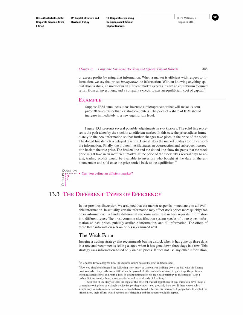
Ross−Westerfield−Jaffe: Corporate Finance, Sixth Edition
IV. Capital Structure and Dividend Policy
13. Corporate−Financing Decisions and Efficient Capital Markets
349© The McGraw−Hill Companies, 2002
or excess profits by using that information. When a market is efficient with respect to in-formation, we say that prices incorporate the information. Without knowing anything spe-cial about a stock, an investor in an efficient market expects to earn an equilibrium requiredreturn from an investment, and a company expects to pay an equilibrium cost of capital.3
EXAMPLE
Suppose IBM announces it has invented a microprocessor that will make its com-puter 30 times faster than existing computers. The price of a share of IBM shouldincrease immediately to a new equilibrium level.
Figure 13.1 presents several possible adjustments in stock prices. The solid line repre-sents the path taken by the stock in an efficient market. In this case the price adjusts imme-diately to the new information so that further changes take place in the price of the stock.The dotted line depicts a delayed reaction. Here it takes the market 30 days to fully absorbthe information. Finally, the broken line illustrates an overreaction and subsequent correc-tion back to the true price. The broken line and the dotted line show the paths that the stockprice might take in an inefficient market. If the price of the stock takes several days to ad-just, trading profits would be available to investors who bought at the date of the an-nouncement and sold once the price settled back to the equilibrium.4
• Can you define an efficient market?
13.3 THE DIFFERENT TYPES OF EFFICIENCY
In our previous discussion, we assumed that the market responds immediately to all avail-able information. In actuality, certain information may affect stock prices more quickly thanother information. To handle differential response rates, researchers separate informationinto different types. The most common classification system speaks of three types: infor-mation on past prices, publicly available information, and all information. The effect ofthese three information sets on prices is examined next.
The Weak FormImagine a trading strategy that recommends buying a stock when it has gone up three daysin a row and recommends selling a stock when it has gone down three days in a row. Thisstrategy uses information based only on past prices. It does not use any other information,
Chapter 13 Corporate-Financing Decisions and Efficient Capital Markets 343
3In Chapter 10 we analyzed how the required return on a risky asset is determined.4Now you should understand the following short story. A student was walking down the hall with his financeprofessor when they both saw a $20 bill on the ground. As the student bent down to pick it up, the professorshook his head slowly and, with a look of disappointment on his face, said patiently to the student, “Don’tbother. If it was really there, someone else would have already picked it up.”
The moral of the story reflects the logic of the efficient-market hypothesis: If you think you have found apattern in stock prices or a simple device for picking winners, you probably have not. If there were such asimple way to make money, someone else would have found it before. Furthermore, if people tried to exploit theinformation, their efforts would become self-defeating and the pattern would disappear.
QUESTION
CO
NC
EP
T
?
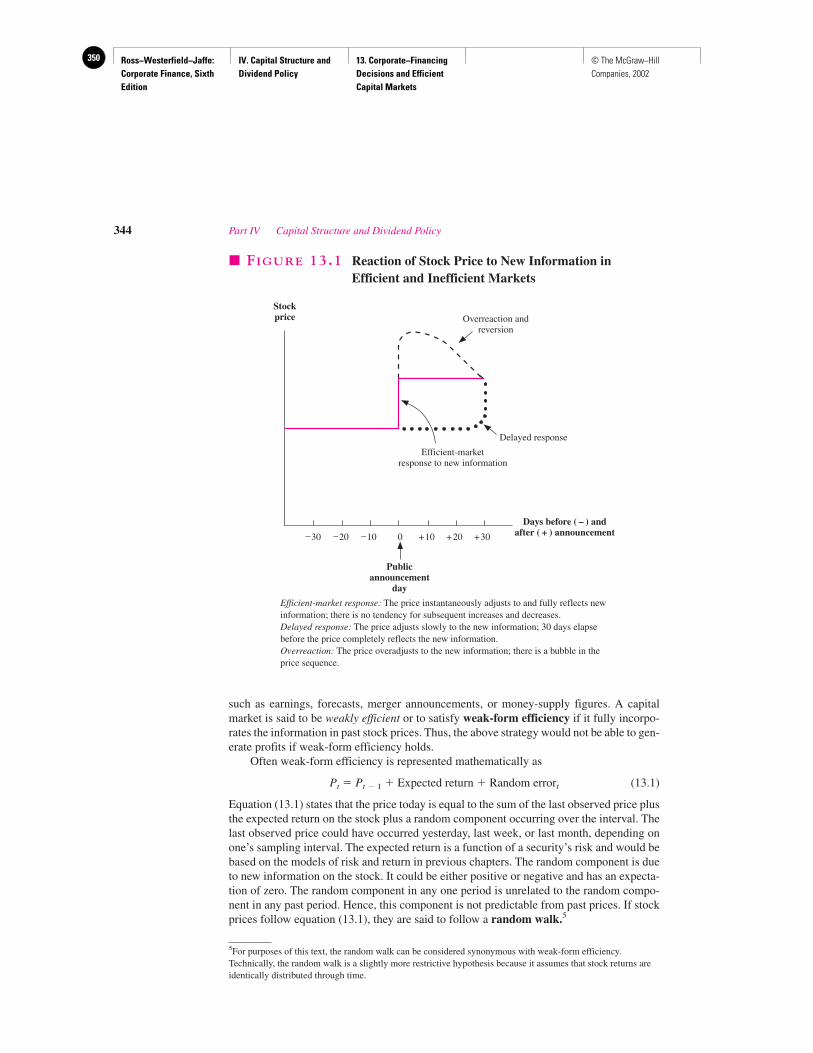
Ross−Westerfield−Jaffe: Corporate Finance, Sixth Edition
IV. Capital Structure and Dividend Policy
13. Corporate−Financing Decisions and Efficient Capital Markets
350 © The McGraw−Hill Companies, 2002
such as earnings, forecasts, merger announcements, or money-supply figures. A capitalmarket is said to be weakly efficient or to satisfy weak-form efficiency if it fully incorpo-rates the information in past stock prices. Thus, the above strategy would not be able to gen-erate profits if weak-form efficiency holds.
Often weak-form efficiency is represented mathematically as
Pt � Pt � 1 � Expected return � Random errort (13.1)
Equation (13.1) states that the price today is equal to the sum of the last observed price plusthe expected return on the stock plus a random component occurring over the interval. Thelast observed price could have occurred yesterday, last week, or last month, depending onone’s sampling interval. The expected return is a function of a security’s risk and would bebased on the models of risk and return in previous chapters. The random component is dueto new information on the stock. It could be either positive or negative and has an expecta-tion of zero. The random component in any one period is unrelated to the random compo-nent in any past period. Hence, this component is not predictable from past prices. If stockprices follow equation (13.1), they are said to follow a random walk.5
344 Part IV Capital Structure and Dividend Policy
–30
Stockprice
Publicannouncement
day
–20 –10 0 +20 +30+10
Days before ( – ) andafter ( + ) announcement
Efficient-marketresponse to new information
Overreaction andreversion
Delayed response
� FIGURE 13.1 Reaction of Stock Price to New Information inEfficient and Inefficient Markets
Efficient-market response: The price instantaneously adjusts to and fully reflects newinformation; there is no tendency for subsequent increases and decreases.Delayed response: The price adjusts slowly to the new information; 30 days elapsebefore the price completely reflects the new information.Overreaction: The price overadjusts to the new information; there is a bubble in theprice sequence.
5For purposes of this text, the random walk can be considered synonymous with weak-form efficiency.Technically, the random walk is a slightly more restrictive hypothesis because it assumes that stock returns areidentically distributed through time.
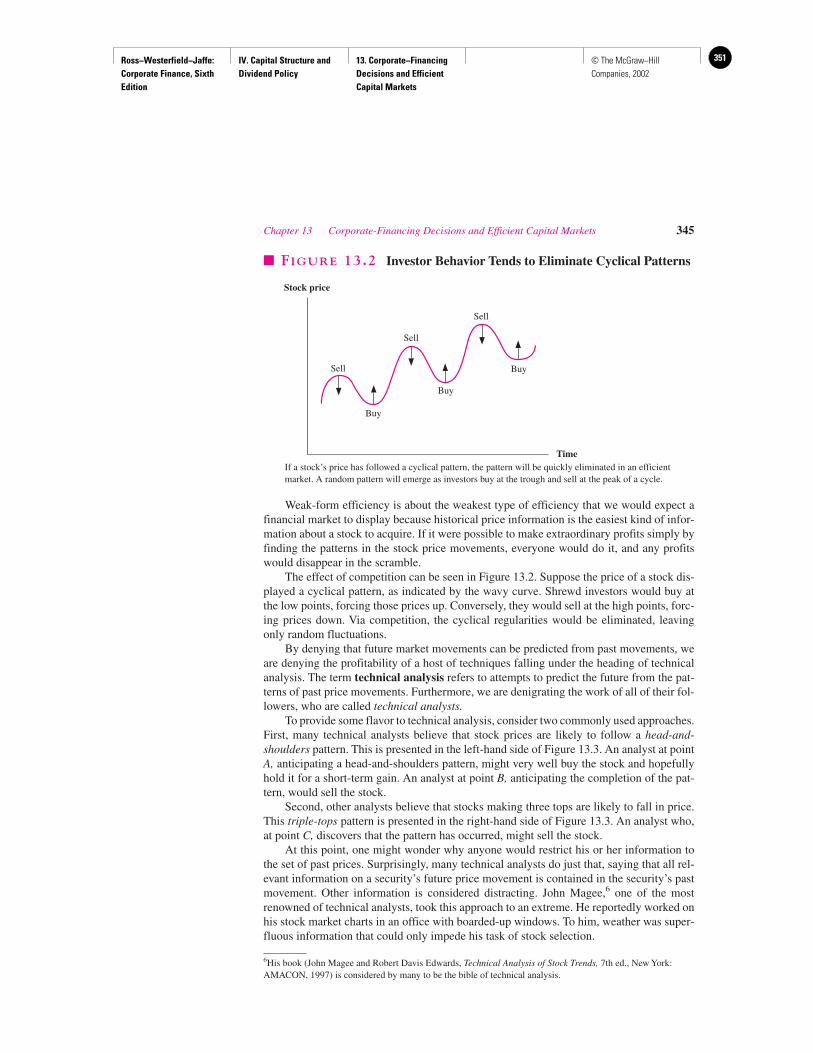
Ross−Westerfield−Jaffe: Corporate Finance, Sixth Edition
IV. Capital Structure and Dividend Policy
13. Corporate−Financing Decisions and Efficient Capital Markets
351© The McGraw−Hill Companies, 2002
Weak-form efficiency is about the weakest type of efficiency that we would expect afinancial market to display because historical price information is the easiest kind of infor-mation about a stock to acquire. If it were possible to make extraordinary profits simply byfinding the patterns in the stock price movements, everyone would do it, and any profitswould disappear in the scramble.
The effect of competition can be seen in Figure 13.2. Suppose the price of a stock dis-played a cyclical pattern, as indicated by the wavy curve. Shrewd investors would buy atthe low points, forcing those prices up. Conversely, they would sell at the high points, forc-ing prices down. Via competition, the cyclical regularities would be eliminated, leavingonly random fluctuations.
By denying that future market movements can be predicted from past movements, weare denying the profitability of a host of techniques falling under the heading of technicalanalysis. The term technical analysis refers to attempts to predict the future from the pat-terns of past price movements. Furthermore, we are denigrating the work of all of their fol-lowers, who are called technical analysts.
To provide some flavor to technical analysis, consider two commonly used approaches.First, many technical analysts believe that stock prices are likely to follow a head-and-shoulders pattern. This is presented in the left-hand side of Figure 13.3. An analyst at pointA, anticipating a head-and-shoulders pattern, might very well buy the stock and hopefullyhold it for a short-term gain. An analyst at point B, anticipating the completion of the pat-tern, would sell the stock.
Second, other analysts believe that stocks making three tops are likely to fall in price.This triple-tops pattern is presented in the right-hand side of Figure 13.3. An analyst who,at point C, discovers that the pattern has occurred, might sell the stock.
At this point, one might wonder why anyone would restrict his or her information tothe set of past prices. Surprisingly, many technical analysts do just that, saying that all rel-evant information on a security’s future price movement is contained in the security’s pastmovement. Other information is considered distracting. John Magee,6 one of the mostrenowned of technical analysts, took this approach to an extreme. He reportedly worked onhis stock market charts in an office with boarded-up windows. To him, weather was super-fluous information that could only impede his task of stock selection.
6His book (John Magee and Robert Davis Edwards, Technical Analysis of Stock Trends, 7th ed., New York:AMACON, 1997) is considered by many to be the bible of technical analysis.
Chapter 13 Corporate-Financing Decisions and Efficient Capital Markets 345
Stock price
Sell
Time
Sell
Sell
Buy
Buy
Buy
� FIGURE 13.2 Investor Behavior Tends to Eliminate Cyclical Patterns
If a stock’s price has followed a cyclical pattern, the pattern will be quickly eliminated in an efficientmarket. A random pattern will emerge as investors buy at the trough and sell at the peak of a cycle.
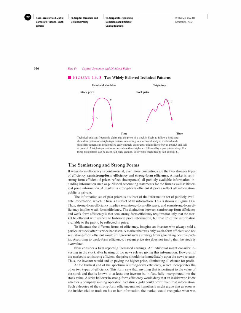
Ross−Westerfield−Jaffe: Corporate Finance, Sixth Edition
IV. Capital Structure and Dividend Policy
13. Corporate−Financing Decisions and Efficient Capital Markets
352 © The McGraw−Hill Companies, 2002
The Semistrong and Strong FormsIf weak-form efficiency is controversial, even more contentious are the two stronger typesof efficiency, semistrong-form efficiency and strong-form efficiency. A market is semi-strong-form efficient if prices reflect (incorporate) all publicly available information, in-cluding information such as published accounting statements for the firm as well as histor-ical price information. A market is strong-form efficient if prices reflect all information,public or private.
The information set of past prices is a subset of the information set of publicly avail-able information, which in turn is a subset of all information. This is shown in Figure 13.4.Thus, strong-form efficiency implies semistrong-form efficiency, and semistrong-form ef-ficiency implies weak-form efficiency. The distinction between semistrong-form efficiencyand weak-form efficiency is that semistrong-form efficiency requires not only that the mar-ket be efficient with respect to historical price information, but that all of the informationavailable to the public be reflected in price.
To illustrate the different forms of efficiency, imagine an investor who always sold aparticular stock after its price had risen. A market that was only weak-form efficient and notsemistrong-form efficient would still prevent such a strategy from generating positive prof-its. According to weak-form efficiency, a recent price rise does not imply that the stock isovervalued.
Now consider a firm reporting increased earnings. An individual might consider in-vesting in the stock after hearing of the news release giving this information. However, ifthe market is semistrong efficient, the price should rise immediately upon the news release.Thus, the investor would end up paying the higher price, eliminating all chance for profit.
At the furthest end of the spectrum is strong-form efficiency, which incorporates theother two types of efficiency. This form says that anything that is pertinent to the value ofthe stock and that is known to at least one investor is, in fact, fully incorporated into thestock value. A strict believer in strong-form efficiency would deny that an insider who knewwhether a company mining operation had struck gold could profit from that information.Such a devotee of the strong-form efficient-market hypothesis might argue that as soon asthe insider tried to trade on his or her information, the market would recognize what was
346 Part IV Capital Structure and Dividend Policy
Head and shoulders
B
Triple tops
A
C
Stock price Stock price
Time Time
� FIGURE 13.3 Two Widely Believed Technical Patterns
Technical analysts frequently claim that the price of a stock is likely to follow a head-and-shoulders pattern or a triple-tops pattern. According to a technical analyst, if a head-and-shoulders pattern can be identified early enough, an investor might like to buy at point A and sellat point B. A triple-tops pattern occurs when three highs are followed by a precipitous drop. If atriple-tops pattern can be identified early enough, an investor might like to sell at point C.
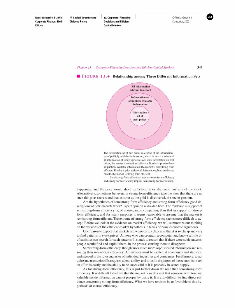
Ross−Westerfield−Jaffe: Corporate Finance, Sixth Edition
IV. Capital Structure and Dividend Policy
13. Corporate−Financing Decisions and Efficient Capital Markets
353© The McGraw−Hill Companies, 2002
happening, and the price would shoot up before he or she could buy any of the stock.Alternatively, sometimes believers in strong-form efficiency take the view that there are nosuch things as secrets and that as soon as the gold is discovered, the secret gets out.
Are the hypotheses of semistrong-form efficiency and strong-form efficiency good de-scriptions of how markets work? Expert opinion is divided here. The evidence in support ofsemistrong-form efficiency is, of course, more compelling than that in support of strong-form efficiency, and for many purposes it seems reasonable to assume that the market issemistrong-form efficient. The extreme of strong-form efficiency seems more difficult to ac-cept. Before we look at the evidence on market efficiency, we will summarize our thinkingon the versions of the efficient-market hypothesis in terms of basic economic arguments.
One reason to expect that markets are weak-form efficient is that it is so cheap and easyto find patterns in stock prices. Anyone who can program a computer and knows a little bitof statistics can search for such patterns. It stands to reason that if there were such patterns,people would find and exploit them, in the process causing them to disappear.
Semistrong-form efficiency, though, uses much more sophisticated information and rea-soning than weak-form efficiency. An investor must be skilled at economics and statistics,and steeped in the idiosyncrasies of individual industries and companies. Furthermore, to ac-quire and use such skills requires talent, ability, and time. In the jargon of the economist, suchan effort is costly and the ability to be successful at it is probably in scarce supply.
As for strong-form efficiency, this is just farther down the road than semistrong-formefficiency. It is difficult to believe that the market is so efficient that someone with true andvaluable inside information cannot prosper by using it. It is also difficult to find direct evi-dence concerning strong-form efficiency. What we have tends to be unfavorable to this hy-pothesis of market efficiency.
Chapter 13 Corporate-Financing Decisions and Efficient Capital Markets 347
All informationrelevant to a stock
Information setof publicly available
information
Informationset of
past prices
� FIGURE 13.4 Relationship among Three Different Information Sets
The information set of past prices is a subset of the informationset of publicly available information, which in turn is a subset ofall information. If today’s price reflects only information on pastprices, the market is weak-form efficient. If today’s price reflectsall publicly available information, the market is semistrong-formefficient. If today’s price reflects all information, both public andprivate, the market is strong-form efficient.
Semistrong-form efficiency implies weak-form efficiencyand strong-form efficiency implies semistrong-form efficiency.
Ross−Westerfield−Jaffe: Corporate Finance, Sixth Edition
IV. Capital Structure and Dividend Policy
13. Corporate−Financing Decisions and Efficient Capital Markets
354 © The McGraw−Hill Companies, 2002
Some Common Misconceptions about the Efficient-Market HypothesisNo idea in finance has attracted as much attention as that of efficient markets, and not allof the attention has been flattering. To a certain extent this is because much of the criticismhas been based on a misunderstanding of what the hypothesis does and does not say. We il-lustrate three misconceptions below.
The Efficacy of Dart Throwing When the notion of market efficiency was first publi-cized and debated in the popular financial press, it was often characterized by the follow-ing quote: “. . . throwing darts at the financial page will produce a portfolio that can be ex-pected to do as well as any managed by professional security analysts.”7, 8 This is almost,but not quite, true.
All the efficient-market hypothesis really says is that, on average, the manager will notbe able to achieve an abnormal or excess return. The excess return is defined with respect tosome benchmark expected return that comes from the security market line of Chapter 10(SML). The investor must still decide how risky a portfolio he or she wants and what ex-pected return it will normally have. A random dart thrower might wind up with all of the dartssticking into one or two high-risk stocks that deal in genetic engineering. Would you reallywant all of your stock investments in two such stocks? (Beware, though—a professionalportfolio manager could do the same.)
The failure to understand this has often led to a confusion about market efficiency. Forexample, sometimes it is wrongly argued that market efficiency means that it does not mat-ter what you do because the efficiency of the market will protect the unwary. However,someone once remarked, “The efficient market protects the sheep from the wolves, butnothing can protect the sheep from themselves.”
What efficiency does say is that the price that a firm will obtain when it sells a share ofits stock is a fair price in the sense that it reflects the value of that stock given the informa-tion that is available about it. Shareholders need not worry that they are paying too muchfor a stock with a low dividend or some other characteristic, because the market has alreadyincorporated it into the price. However, investors still have to worry about such things astheir level of risk exposure and their degree of diversification.
Price Fluctuations Much of the public is skeptical of efficiency because stock pricesfluctuate from day to day. However, daily price movement is in no way inconsistent withefficiency; a stock in an efficient market adjusts to new information by changing price. Agreat deal of new information comes into the stock market each day. In fact, the absence ofdaily price movements in a changing world might suggest an inefficiency.
Stockholder Disinterest Many laypersons are skeptical that the market price can be ef-ficient if only a fraction of the outstanding shares changes hands on any given day. How-ever, the number of traders in a stock on a given day is generally far less than the numberof people following the stock. This is true because an individual will trade only when hisappraisal of the value of the stock differs enough from the market price to justify incurringbrokerage commissions and other transaction costs. Furthermore, even if the number oftraders following a stock is small relative to the number of outstanding shareholders, the
348 Part IV Capital Structure and Dividend Policy
7B. G. Malkiel, A Random Walk Down Wall Street, 7th ed. (New York: Norton, 1999).8Older articles often referred to the benchmark of “dart-throwing monkeys.” As government involvement in thesecurities industry grew, the benchmark was oftentimes restated as “dart-throwing congressmen.”
Ross−Westerfield−Jaffe: Corporate Finance, Sixth Edition
IV. Capital Structure and Dividend Policy
13. Corporate−Financing Decisions and Efficient Capital Markets
355© The McGraw−Hill Companies, 2002
stock can be expected to be efficiently priced as long as a number of interested traders usethe publicly available information. That is, the stock price can reflect the available infor-mation even if many stockholders never follow the stock and are not considering trading inthe near future, and even if some stockholders trade with little or no information. Thus, theempirical findings suggesting that the stock market is predominantly efficient need not besurprising.
• Can you describe the three forms of the efficient-market hypothesis?• What kinds of things could make markets inefficient?• Does market efficiency mean you can throw darts at The Wall Street Journal listing of
New York Stock Exchange stocks to pick a portfolio?• What does it mean to say the price you pay for a stock is fair?
13.4 THE EVIDENCE
The record on the efficient-market hypothesis is extensive, and in large measure it is reas-suring to advocates of the efficiency of markets. The studies done by academicians fall intobroad categories. First, there is evidence as to whether changes of stock prices are random.Second are event studies. Third is the record of professionally managed investment firms.
The Weak FormThe random-walk hypothesis, as expressed in equation (13.1), implies that a stock’s pricemovement in the past is unrelated to its price movement in the future. The work of Chapter 10allows us to test this implication. In that chapter, we discussed the concept of correlation be-tween the returns on two different stocks. For example, the correlation between the return onGeneral Motors and the return on Ford is likely to be high because both stocks are in the sameindustry. Conversely, the correlation between the return on General Motors and the return onthe stock of, say, a European fast-food chain is likely to be low.
Financial economists frequently speak of serial correlation, which involves only onesecurity. This is the correlation between the current return on a security and the return on thesame security over a later period. A positive coefficient of serial correlation for a particularstock indicates a tendency toward continuation. That is, a higher-than-average return todayis likely to be followed by higher-than-average returns in the future. Similarly, a lower-than-average return today is likely to be followed by lower-than-average returns in the future.
A negative coefficient of serial correlation for a particular stock indicates a tendencytoward reversal. A higher-than-average return today is likely to be followed by lower-than-average returns in the future. Similarly, a lower-than-average return today is likely to be fol-lowed by higher-than-average returns in the future. Both significantly positive and signifi-cantly negative serial-correlation coefficients are indications of market inefficiencies; ineither case, returns today can be used to predict future returns.
Serial correlation coefficients for stock returns near zero would be consistent with therandom-walk hypothesis. Thus, a current stock return that is higher than average is as likelyto be followed by lower-than-average returns as by higher-than-average returns. Similarly,a current stock return that is lower than average is as likely to be followed by higher-than-average returns as by lower-than-average returns.
Table 13.1 shows the serial correlation for daily stock-price changes for 8 large U.S.companies. These coefficients indicate whether or not there are relationships between yester-day’s return and today’s return. As can be seen, the correlation coefficients are predominantly
Chapter 13 Corporate-Financing Decisions and Efficient Capital Markets 349
QUESTIONS
CO
NC
EP
T
?
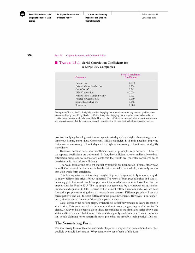
Ross−Westerfield−Jaffe: Corporate Finance, Sixth Edition
IV. Capital Structure and Dividend Policy
13. Corporate−Financing Decisions and Efficient Capital Markets
356 © The McGraw−Hill Companies, 2002
positive, implying that a higher-than-average return today makes a higher-than-average returntomorrow slightly more likely. Conversely, IBM’s coefficient is slightly negative, implyingthat a lower-than-average return today makes a higher-than-average return tomorrow slightlymore likely.
However, because correlation coefficients can, in principle, vary between �1 and 1,the reported coefficients are quite small. In fact, the coefficients are so small relative to bothestimation errors and to transactions costs that the results are generally considered to beconsistent with weak-form efficiency.
The weak form of the efficient-market hypothesis has been tested in many other waysas well. Our view of the literature is that the evidence, taken as a whole, is strongly consis-tent with weak-form efficiency.
This finding raises an interesting thought: If price changes are truly random, why doso many believe that prices follow patterns? The work of both psychologists and statisti-cians suggests that most people simply do not know what randomness looks like. For ex-ample, consider Figure 13.5. The top graph was generated by a computer using randomnumbers and equation (13.1). Because of this it must follow a random walk. Yet, we havefound that people examining the chart generally see patterns. Different people will see dif-ferent patterns and will forecast different future price movements. However, in our experi-ence, viewers are all quite confident of the patterns they see.
Next, consider the bottom graph, which tracks actual movements in Sears, Roebuck’sstock price. This graph may look quite nonrandom to some, suggesting weak-form ineffi-ciency. However, it also bears a close visual resemblance to the simulated series above, andstatistical tests indicate that it indeed behaves like a purely random series. Thus, in our opin-ion, people claiming to see patterns in stock-price data are probably seeing optical illusions.
The Semistrong FormThe semistrong form of the efficient-market hypothesis implies that prices should reflect allpublicly available information. We present two types of tests of this form.
350 Part IV Capital Structure and Dividend Policy
� TABLE 13.1 Serial Correlation Coefficients for 8 Large U.S. Companies
Serial CorrelationCompany Coefficient
Boeing Co. 0.038Bristol-Myers Squibb Co. 0.064Coca-Cola Co. 0.041IBM Corporation �0.004Philip Morris Companies Inc. 0.075Procter & Gamble Co. 0.030Sears, Roebuck & Co. 0.046Texaco Inc. 0.005
Boeing’s coefficient of 0.038 is slightly positive, implying that a positive return today makes a positive returntomorrow slightly more likely. IBM’s coefficient is negative, implying that a negative return today makes apositive return tomorrow slightly more likely. However, the coefficients are so small relative to estimation errorand transaction costs that the results are generally considered to be consistent with efficient capital markets.
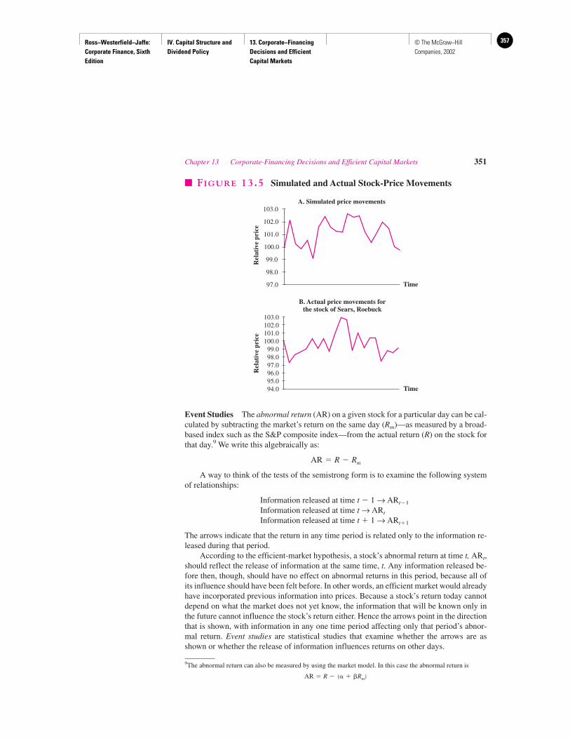
Ross−Westerfield−Jaffe: Corporate Finance, Sixth Edition
IV. Capital Structure and Dividend Policy
13. Corporate−Financing Decisions and Efficient Capital Markets
357© The McGraw−Hill Companies, 2002
Event Studies The abnormal return (AR) on a given stock for a particular day can be cal-culated by subtracting the market’s return on the same day (Rm)—as measured by a broad-based index such as the S&P composite index—from the actual return (R) on the stock forthat day.9 We write this algebraically as:
A way to think of the tests of the semistrong form is to examine the following systemof relationships:
Information released at time t � 1 → ARt�1
Information released at time t → ARt
Information released at time t � 1 → ARt�1
The arrows indicate that the return in any time period is related only to the information re-leased during that period.
According to the efficient-market hypothesis, a stock’s abnormal return at time t, ARt,should reflect the release of information at the same time, t. Any information released be-fore then, though, should have no effect on abnormal returns in this period, because all ofits influence should have been felt before. In other words, an efficient market would alreadyhave incorporated previous information into prices. Because a stock’s return today cannotdepend on what the market does not yet know, the information that will be known only inthe future cannot influence the stock’s return either. Hence the arrows point in the directionthat is shown, with information in any one time period affecting only that period’s abnor-mal return. Event studies are statistical studies that examine whether the arrows are asshown or whether the release of information influences returns on other days.
AR � R � Rm
Chapter 13 Corporate-Financing Decisions and Efficient Capital Markets 351
103.0
102.0
101.0
100.0
99.0
98.0
97.0
A. Simulated price movements
Rel
ativ
e pr
ice
Time
103.0102.0101.0100.0
99.098.097.0
B. Actual price movements forthe stock of Sears, Roebuck
Rel
ativ
e pr
ice
96.095.094.0 Time
� FIGURE 13.5 Simulated and Actual Stock-Price Movements
9The abnormal return can also be measured by using the market model. In this case the abnormal return is
AR � R � �� � �Rm�
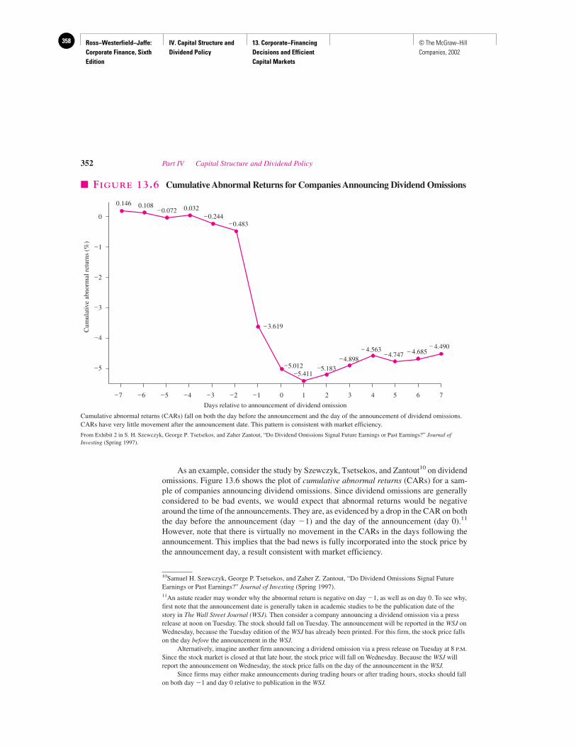
Ross−Westerfield−Jaffe: Corporate Finance, Sixth Edition
IV. Capital Structure and Dividend Policy
13. Corporate−Financing Decisions and Efficient Capital Markets
358 © The McGraw−Hill Companies, 2002
As an example, consider the study by Szewczyk, Tsetsekos, and Zantout10 on dividendomissions. Figure 13.6 shows the plot of cumulative abnormal returns (CARs) for a sam-ple of companies announcing dividend omissions. Since dividend omissions are generallyconsidered to be bad events, we would expect that abnormal returns would be negativearound the time of the announcements. They are, as evidenced by a drop in the CAR on boththe day before the announcement (day �1) and the day of the announcement (day 0).11
However, note that there is virtually no movement in the CARs in the days following theannouncement. This implies that the bad news is fully incorporated into the stock price bythe announcement day, a result consistent with market efficiency.
352 Part IV Capital Structure and Dividend Policy
10Samuel H. Szewczyk, George P. Tsetsekos, and Zaher Z. Zantout, “Do Dividend Omissions Signal FutureEarnings or Past Earnings?” Journal of Investing (Spring 1997).11An astute reader may wonder why the abnormal return is negative on day �1, as well as on day 0. To see why,first note that the announcement date is generally taken in academic studies to be the publication date of thestory in The Wall Street Journal (WSJ). Then consider a company announcing a dividend omission via a pressrelease at noon on Tuesday. The stock should fall on Tuesday. The announcement will be reported in the WSJ onWednesday, because the Tuesday edition of the WSJ has already been printed. For this firm, the stock price fallson the day before the announcement in the WSJ.
Alternatively, imagine another firm announcing a dividend omission via a press release on Tuesday at 8 P.M.Since the stock market is closed at that late hour, the stock price will fall on Wednesday. Because the WSJ willreport the announcement on Wednesday, the stock price falls on the day of the announcement in the WSJ.
Since firms may either make announcements during trading hours or after trading hours, stocks should fallon both day �1 and day 0 relative to publication in the WSJ.
0
–1
–2
–3
–4
–5
–7 –6 –5 –4 –3 –2 –1 0 1 2 3 4 5 6 7
0.146 0.108 0.032–0.072–0.244
–0.483
–3.619
–5.012–5.411
–5.183
–4.898
– 4.563–4.747 – 4.685
– 4.490
Cum
ulat
ive
abno
rmal
ret
urns
(%
)
Days relative to announcement of dividend omission
� FIGURE 13.6 Cumulative Abnormal Returns for Companies Announcing Dividend Omissions
Cumulative abnormal returns (CARs) fall on both the day before the announcement and the day of the announcement of dividend omissions.CARs have very little movement after the announcement date. This pattern is consistent with market efficiency.
From Exhibit 2 in S. H. Szewczyk, George P. Tsetsekos, and Zaher Zantout, “Do Dividend Omissions Signal Future Earnings or Past Earnings?” Journal ofInvesting (Spring 1997).
Ross−Westerfield−Jaffe: Corporate Finance, Sixth Edition
IV. Capital Structure and Dividend Policy
13. Corporate−Financing Decisions and Efficient Capital Markets
359© The McGraw−Hill Companies, 2002
Over the years this type of methodology has been applied to a large number of events.Announcements of dividends, earnings, mergers, capital expenditures, and new issues ofstock are a few examples of the vast literature in the area.12 Although there are exceptions,the event-study tests generally support the view that the market is semistrong-form (andtherefore also weak-form) efficient. In fact, the tests even tend to support the view that themarket is gifted with a certain amount of foresight. By this we mean that news tends to leakout and be reflected in stock prices even before the official release of the information.
Tests of market efficiency can be found in the oddest places. The price of frozen orangejuice depends to a large extent on the weather in Orlando, Florida, where many of the orangesthat are frozen for juice are grown. One researcher found that he could actually use frozen-orange-juice prices to improve the U.S. Weather Bureau’s forecast of the temperature for thefollowing night.13 Clearly the market knows something that the weather forecasters do not.
Another group of researchers found that, as expected, stock prices generally fall on thedate when the sudden death of a chief executive is announced.14 However, the stock pricegenerally rises for the sudden death of a company’s founder if he was still heading up thefirm prior to his death. The implication is that many of these individuals have outlived theirusefulness to their firms.
The Record of Mutual Funds If the market is efficient in the semistrong form, then nomatter what publicly available information mutual-fund managers rely on to pick stocks,their average returns should be the same as those of the average investor in the market as awhole. We can test efficiency, then, by comparing the performance of these professionalswith that of a market index.
Consider Figure 13.7, which presents the performance of various types of mutual fundsrelative to the stock market as a whole. The far left of the figure shows that the universe ofall funds covered in the study underperforms the market by 2.13 percent per year, after anappropriate adjustment for risk.15 Thus, rather than outperforming the market, the evidenceshows underperformance. This underperformance holds for a number of types of funds aswell. Returns in this study are net of fees, expenses, and commissions, so fund returnswould be higher if these costs were added back. However, the study shows no evidence thatfunds, as a whole, are beating the market.
Perhaps nothing rankles successful stock market investors more than to have some pro-fessor tell them that they are not necessarily smart, just lucky. However, while Figure 13.7represents only one study, there have been many papers on mutual funds. The overwhelm-ing evidence here is that mutual funds, on average, do not beat broad-based indices. Thisdoes not mean that no individual investor can beat the market average or that he or she lacksa special insight, only that proof seems difficult to find.
By and large, mutual-fund managers rely on publicly available information. Thus thefinding that they do not outperform the market indices is consistent with semistrong-form
Chapter 13 Corporate-Financing Decisions and Efficient Capital Markets 353
12In academic finance nothing is ever completely resolved, and some event studies suggest that stock marketprices respond to information too slowly for the market to be efficient. For example, Eli Bartov, SureshRadhakrishnan, and Itzhak Krinsky, “Investor Sophistication and Patterns in Stock Returns after EarningsAnnouncements,” The Accounting Review 75 (January 2000).13These findings are reported in R. Roll, “Orange Juice and Weather,” American Economic Review (December 1984).14W. B. Johnson, R. P. Magee, N. J. Nagarajan, and H. A. Newman, “An Analysis of the Stock Price Reaction toSudden Executive Deaths: Implications for the Managerial Labor Market,” Journal of Accounting andEconomics (April 1985).15This finding is similar to those reported by R. Wermers, “Mutual Fund Performance: An Empirical Decompositioninto Stock-Picking, Talent, Style, Transactions Costs, and Expenses,” Journal of Finance (August 2000).
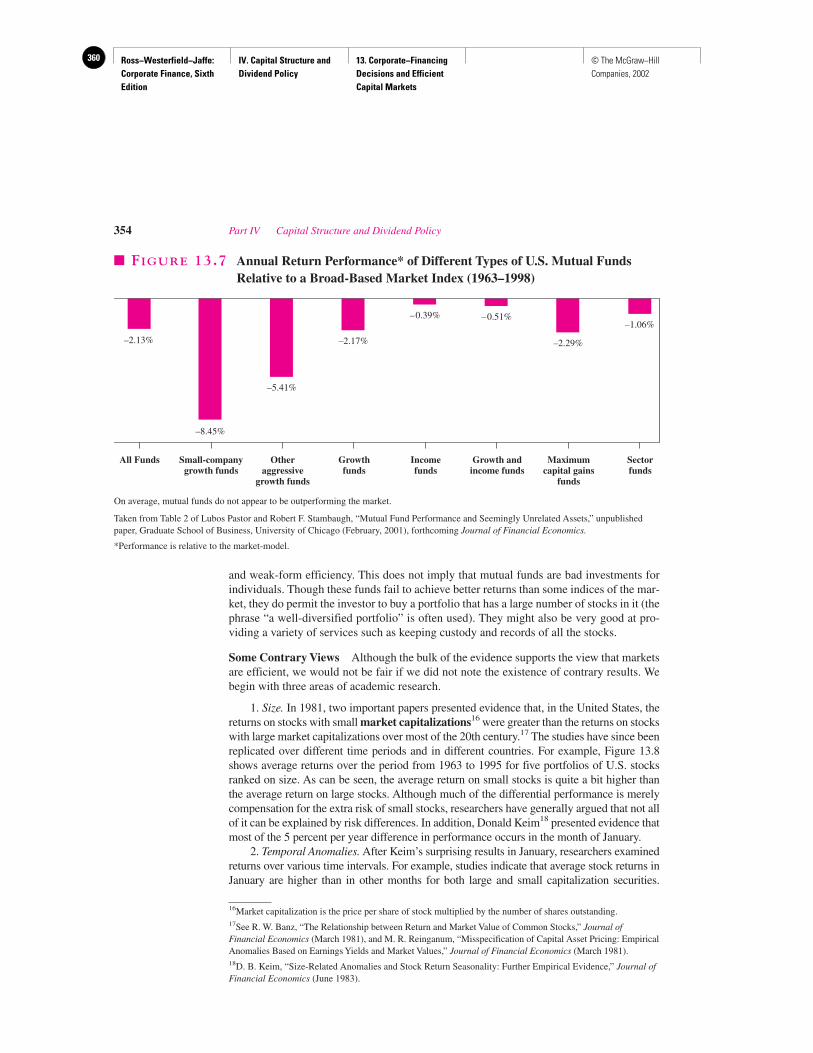
Ross−Westerfield−Jaffe: Corporate Finance, Sixth Edition
IV. Capital Structure and Dividend Policy
13. Corporate−Financing Decisions and Efficient Capital Markets
360 © The McGraw−Hill Companies, 2002
and weak-form efficiency. This does not imply that mutual funds are bad investments forindividuals. Though these funds fail to achieve better returns than some indices of the mar-ket, they do permit the investor to buy a portfolio that has a large number of stocks in it (thephrase “a well-diversified portfolio” is often used). They might also be very good at pro-viding a variety of services such as keeping custody and records of all the stocks.
Some Contrary Views Although the bulk of the evidence supports the view that marketsare efficient, we would not be fair if we did not note the existence of contrary results. Webegin with three areas of academic research.
1. Size. In 1981, two important papers presented evidence that, in the United States, thereturns on stocks with small market capitalizations16 were greater than the returns on stockswith large market capitalizations over most of the 20th century.17 The studies have since beenreplicated over different time periods and in different countries. For example, Figure 13.8shows average returns over the period from 1963 to 1995 for five portfolios of U.S. stocksranked on size. As can be seen, the average return on small stocks is quite a bit higher thanthe average return on large stocks. Although much of the differential performance is merelycompensation for the extra risk of small stocks, researchers have generally argued that not allof it can be explained by risk differences. In addition, Donald Keim18 presented evidence thatmost of the 5 percent per year difference in performance occurs in the month of January.
2. Temporal Anomalies. After Keim’s surprising results in January, researchers examinedreturns over various time intervals. For example, studies indicate that average stock returns inJanuary are higher than in other months for both large and small capitalization securities.
354 Part IV Capital Structure and Dividend Policy
–2.13%
–8.45%
–5.41%
–2.17%
–0.39% –0.51%
–2.29%
–1.06%
All Funds Small-companygrowth funds
Otheraggressive
growth funds
Growthfunds
Incomefunds
Growth andincome funds
Maximumcapital gains
funds
Sectorfunds
On average, mutual funds do not appear to be outperforming the market.
� FIGURE 13.7 Annual Return Performance* of Different Types of U.S. Mutual FundsRelative to a Broad-Based Market Index (1963–1998)
Taken from Table 2 of Lubos Pastor and Robert F. Stambaugh, “Mutual Fund Performance and Seemingly Unrelated Assets,” unpublishedpaper, Graduate School of Business, University of Chicago (February, 2001), forthcoming Journal of Financial Economics.
*Performance is relative to the market-model.
16Market capitalization is the price per share of stock multiplied by the number of shares outstanding.17See R. W. Banz, “The Relationship between Return and Market Value of Common Stocks,” Journal ofFinancial Economics (March 1981), and M. R. Reinganum, “Misspecification of Capital Asset Pricing: EmpiricalAnomalies Based on Earnings Yields and Market Values,” Journal of Financial Economics (March 1981).18D. B. Keim, “Size-Related Anomalies and Stock Return Seasonality: Further Empirical Evidence,” Journal ofFinancial Economics (June 1983).
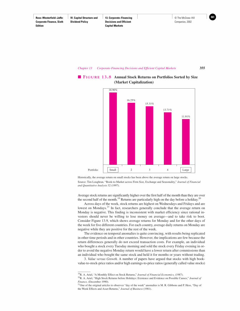
Ross−Westerfield−Jaffe: Corporate Finance, Sixth Edition
IV. Capital Structure and Dividend Policy
13. Corporate−Financing Decisions and Efficient Capital Markets
361© The McGraw−Hill Companies, 2002
Average stock returns are significantly higher over the first half of the month than they are overthe second half of the month.19 Returns are particularly high on the day before a holdiay.20
Across days of the week, stock returns are highest on Wednesdays and Fridays and arelowest on Mondays.21 In fact, researchers generally conclude that the average return onMonday is negative. This finding is inconsistent with market efficiency since rational in-vestors should never be willing to lose money on average—and to take risk to boot.Consider Figure 13.9, which shows average returns for Monday and for the other days ofthe week for five different countries. For each country, average daily returns on Monday arenegative while they are positive for the rest of the week.
The evidence on temporal anomalies is quite convincing, with results being replicatedin other time periods and in other countries. However, the implications are few because thereturn differences generally do not exceed transaction costs. For example, an individualwho bought a stock every Tuesday morning and sold the stock every Friday evening in or-der to avoid the negative Monday return would have a lower return after commissions thanan individual who bought the same stock and held it for months or years without trading.
3. Value versus Growth. A number of papers have argued that stocks with high book-value-to-stock-price ratios and/or high earnings-to-price ratios (generally called value stocks)
Chapter 13 Corporate-Financing Decisions and Efficient Capital Markets 355
Portfolio Small 2 3 4
18.90%
16.25%15.31%
13.71%
11.91%
Large
� FIGURE 13.8 Annual Stock Returns on Portfolios Sorted by Size(Market Capitalization)
Historically, the average return on small stocks has been above the average return on large stocks.
Source: Tim Loughran, “Book-to-Market across Firm Size, Exchange and Seasonality,” Journal of Financialand Quantitative Analysis 32 (1997).
19R. A. Ariel, “A Monthly Effect on Stock Returns,” Journal of Financial Economics, (1987).20R. A. Ariel, “High Stock Returns before Holidays: Existence and Evidence on Possible Causes,” Journal ofFinance, (December 1990).21One of the original articles to observce “day of the week” anomalies is M. R. Gibbons and P. Hess, “Day ofthe Week Effects and Asset Returns,” Journal of Business (1981).
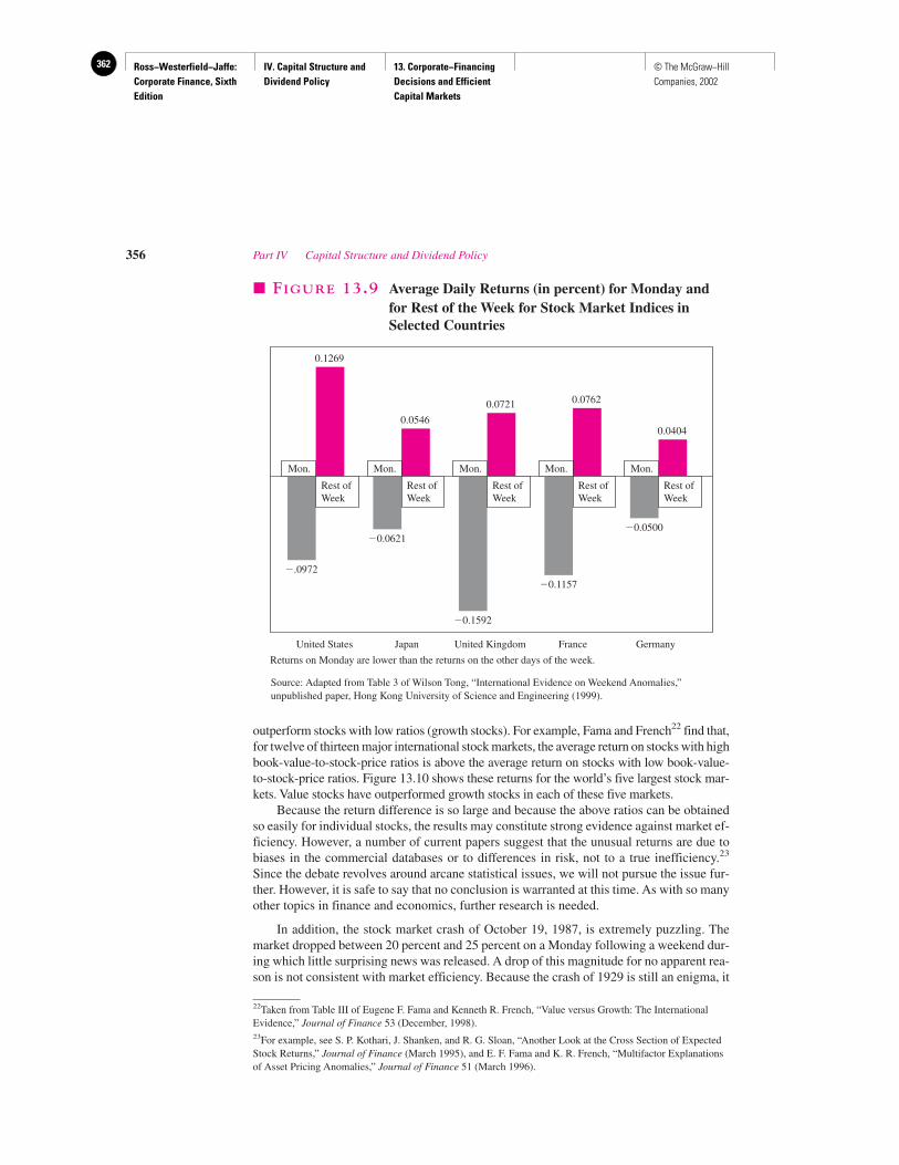
Ross−Westerfield−Jaffe: Corporate Finance, Sixth Edition
IV. Capital Structure and Dividend Policy
13. Corporate−Financing Decisions and Efficient Capital Markets
362 © The McGraw−Hill Companies, 2002
outperform stocks with low ratios (growth stocks). For example, Fama and French22 find that,for twelve of thirteen major international stock markets, the average return on stocks with highbook-value-to-stock-price ratios is above the average return on stocks with low book-value-to-stock-price ratios. Figure 13.10 shows these returns for the world’s five largest stock mar-kets. Value stocks have outperformed growth stocks in each of these five markets.
Because the return difference is so large and because the above ratios can be obtainedso easily for individual stocks, the results may constitute strong evidence against market ef-ficiency. However, a number of current papers suggest that the unusual returns are due tobiases in the commercial databases or to differences in risk, not to a true inefficiency.23
Since the debate revolves around arcane statistical issues, we will not pursue the issue fur-ther. However, it is safe to say that no conclusion is warranted at this time. As with so manyother topics in finance and economics, further research is needed.
In addition, the stock market crash of October 19, 1987, is extremely puzzling. Themarket dropped between 20 percent and 25 percent on a Monday following a weekend dur-ing which little surprising news was released. A drop of this magnitude for no apparent rea-son is not consistent with market efficiency. Because the crash of 1929 is still an enigma, it
356 Part IV Capital Structure and Dividend Policy
22Taken from Table III of Eugene F. Fama and Kenneth R. French, “Value versus Growth: The InternationalEvidence,” Journal of Finance 53 (December, 1998).23For example, see S. P. Kothari, J. Shanken, and R. G. Sloan, “Another Look at the Cross Section of ExpectedStock Returns,” Journal of Finance (March 1995), and E. F. Fama and K. R. French, “Multifactor Explanationsof Asset Pricing Anomalies,” Journal of Finance 51 (March 1996).
United Kingdom France GermanyJapanUnited States
Returns on Monday are lower than the returns on the other days of the week.
0.1269
�.0972
Rest ofWeek
Mon.
0.0546
�0.0621
Rest ofWeek
Mon.
0.0721
�0.1592
Rest ofWeek
Mon.
0.0762
�0.1157
Rest ofWeek
Mon.
0.0404
�0.0500
Rest ofWeek
Mon.
� FIGURE 13.9 Average Daily Returns (in percent) for Monday andfor Rest of the Week for Stock Market Indices inSelected Countries
Source: Adapted from Table 3 of Wilson Tong, “International Evidence on Weekend Anomalies,”unpublished paper, Hong Kong University of Science and Engineering (1999).
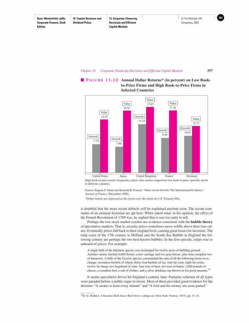
Ross−Westerfield−Jaffe: Corporate Finance, Sixth Edition
IV. Capital Structure and Dividend Policy
13. Corporate−Financing Decisions and Efficient Capital Markets
363© The McGraw−Hill Companies, 2002
is doubtful that the more recent debacle will be explained anytime soon. The recent com-ments of an eminent historian are apt here: When asked what, in his opinion, the effect ofthe French Revolution of 1789 was, he replied that it was too early to tell.
Perhaps the two stock market crashes are evidence consistent with the bubble theoryof speculative markets. That is, security prices sometimes move wildly above their true val-ues. Eventually prices fall back to their original level, causing great losses for investors. Thetulip craze of the 17th century in Holland and the South Sea Bubble in England the fol-lowing century are perhaps the two best-known bubbles. In the first episode, tulips rose tounheard-of prices. For example:
A single bulb of the Harlaem species was exchanged for twelve acres of building ground. . . .Another variety fetched 4,600 florins, a new carriage and two gray horses, plus nine complete setsof harnesses. A bulb of the Viceroy species commanded the sum of all the following items in ex-change: seventeen bushels of wheat, thirty-four bushels of rye, four fat oxen, eight fat swine,twelve fat sheep, two hogshead of wine, four tons of beer, two tons of butter, 1,000 pounds ofcheese, a complete bed, a suit of clothes, and a silver drinking cup thrown in for good measure.24
It seems speculative fervor hit England a century later. Fantastic schemes of all typeswere paraded before a public eager to invest. Most of them provided good evidence for thedictums: “A sucker is born every minute” and “A fool and his money are soon parted.”
Chapter 13 Corporate-Financing Decisions and Efficient Capital Markets 357
United Kingdom France GermanyJapanUnited States
14.55
7.75
16.91
7.06
17.87
13.25
High book-to-price stocks (frequently called value stocks) outperform low book-to-price (growth) stocksin different countries.
17.10
Value
9.46
12.77
10.01Growth
Growth
Growth
GrowthGrowth
ValueValue
Value
Value
� FIGURE 13.10 Annual Dollar Returns* (in percent) on Low Book-to-Price Firms and High Book-to-Price Firms inSelected Countries
Source: Eugene F. Fama and Kenneth R. French, “Value versus Growth: The International Evidence,”Journal of Finance (December 1998).
*Dollar returns are expressed as the excess over the return on U.S. Treasury bills.
24B. G. Malkiel, A Random Walk Down Wall Street, college ed. (New York: Norton, 1975), pp. 31–32.
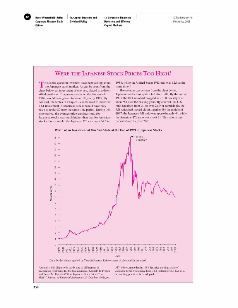
Ross−Westerfield−Jaffe: Corporate Finance, Sixth Edition
IV. Capital Structure and Dividend Policy
13. Corporate−Financing Decisions and Efficient Capital Markets
364 © The McGraw−Hill Companies, 2002
358
WERE THE JAPANESE STOCK PRICES TOO HIGH?
This is the question investors have been asking aboutthe Japanese stock market. As can be seen from the
chart below, an investment of one yen, placed in a diver-sified portfolio of Japanese stocks on the last day of1969, would have grown to about 18 yen by 1988. Bycontrast, the tables in Chapter 9 can be used to show thata $1 investment in American stocks would have onlyrisen to under $7 over the same time period. During thistime period, the average price-earnings ratio forJapanese stocks was much higher than that for Americanstocks. For example, the Japanese P/E ratio was 54.3 in
1988, while the United States P/E ratio was 12.9 at thesame time.*
However, as can be seen from the chart below,Japanese stocks took quite a fall after 1988. By the end of1993, the 18:1 ratio had dropped to 9:1. It has stayed atabout 9:1 over the ensuing years. By contrast, the U.S.ratio had risen from 7:1 to over 22. Not surprisingly, theP/E ratios had moved closer together. By the middle of1997, the Japanese P/E ratio was approximately 44, whilethe American P/E ratio was about 21. This pattern haspersisted into the year 2001.
*Actually, this disparity is partly due to differences inaccounting treatments for the two countries. Kenneth R. Frenchand James M. Poterba (“Were Japanese Stock Prices TooHigh?” Journal of Financial Economics 29 (October 1991), pp.
337–64) estimate that in 1988 the price-earnings ratio ofJapanese firms would have been 32.1 instead of 54.3 had U.S.accounting practices been adopted.
Worth of an Investment of One Yen Made at the End of 1969 in Japanese Stocks
18
17
16
15
14
13
12
11
10
9
8
7
6
5
4
3
2
1
0
1969
1970
1971
1972
1973
1974
1975
1976
1977
1978
1979
1980
1981
1982
1983
1984
1985
1986
1987
1988
1989
1990
1991
1992
1993
1995
1996
Wea
lth in
yen
Is thisa bubble?
Date
1994
1997
1999
2000
1998
Data for this chart supplied by Yasushi Hamao. Reinvestment of dividends is assumed.
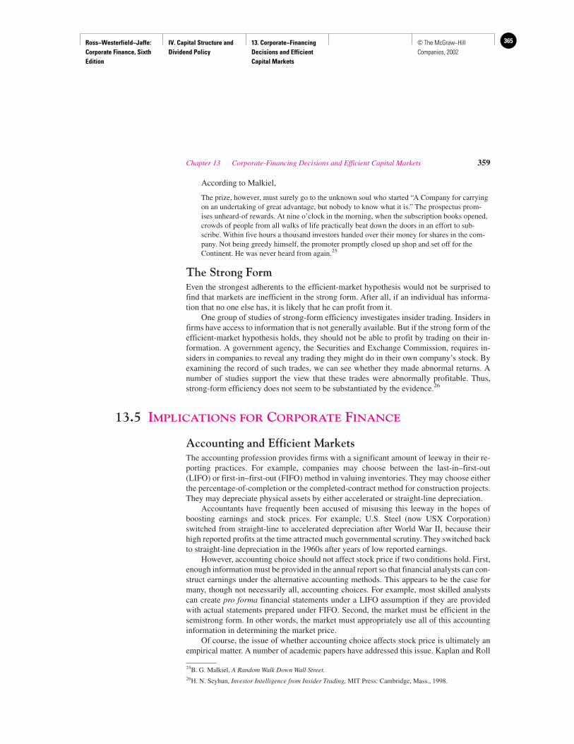
Ross−Westerfield−Jaffe: Corporate Finance, Sixth Edition
IV. Capital Structure and Dividend Policy
13. Corporate−Financing Decisions and Efficient Capital Markets
365© The McGraw−Hill Companies, 2002
According to Malkiel,
The prize, however, must surely go to the unknown soul who started “A Company for carryingon an undertaking of great advantage, but nobody to know what it is.” The prospectus prom-ises unheard-of rewards. At nine o’clock in the morning, when the subscription books opened,crowds of people from all walks of life practically beat down the doors in an effort to sub-scribe. Within five hours a thousand investors handed over their money for shares in the com-pany. Not being greedy himself, the promoter promptly closed up shop and set off for theContinent. He was never heard from again.25
The Strong FormEven the strongest adherents to the efficient-market hypothesis would not be surprised tofind that markets are inefficient in the strong form. After all, if an individual has informa-tion that no one else has, it is likely that he can profit from it.
One group of studies of strong-form efficiency investigates insider trading. Insiders infirms have access to information that is not generally available. But if the strong form of theefficient-market hypothesis holds, they should not be able to profit by trading on their in-formation. A government agency, the Securities and Exchange Commission, requires in-siders in companies to reveal any trading they might do in their own company’s stock. Byexamining the record of such trades, we can see whether they made abnormal returns. Anumber of studies support the view that these trades were abnormally profitable. Thus,strong-form efficiency does not seem to be substantiated by the evidence.26
13.5 IMPLICATIONS FOR CORPORATE FINANCE
Accounting and Efficient MarketsThe accounting profession provides firms with a significant amount of leeway in their re-porting practices. For example, companies may choose between the last-in–first-out(LIFO) or first-in–first-out (FIFO) method in valuing inventories. They may choose eitherthe percentage-of-completion or the completed-contract method for construction projects.They may depreciate physical assets by either accelerated or straight-line depreciation.
Accountants have frequently been accused of misusing this leeway in the hopes ofboosting earnings and stock prices. For example, U.S. Steel (now USX Corporation)switched from straight-line to accelerated depreciation after World War II, because theirhigh reported profits at the time attracted much governmental scrutiny. They switched backto straight-line depreciation in the 1960s after years of low reported earnings.
However, accounting choice should not affect stock price if two conditions hold. First,enough information must be provided in the annual report so that financial analysts can con-struct earnings under the alternative accounting methods. This appears to be the case formany, though not necessarily all, accounting choices. For example, most skilled analystscan create pro forma financial statements under a LIFO assumption if they are providedwith actual statements prepared under FIFO. Second, the market must be efficient in thesemistrong form. In other words, the market must appropriately use all of this accountinginformation in determining the market price.
Of course, the issue of whether accounting choice affects stock price is ultimately anempirical matter. A number of academic papers have addressed this issue. Kaplan and Roll
Chapter 13 Corporate-Financing Decisions and Efficient Capital Markets 359
25B. G. Malkiel, A Random Walk Down Wall Street.26H. N. Seyhun, Investor Intelligence from Insider Trading, MIT Press: Cambridge, Mass., 1998.
Ross−Westerfield−Jaffe: Corporate Finance, Sixth Edition
IV. Capital Structure and Dividend Policy
13. Corporate−Financing Decisions and Efficient Capital Markets
366 © The McGraw−Hill Companies, 2002
found that the switch from accelerated to straight-line depreciation generally did not sig-nificantly affect stock prices.27 Kaplan and Roll also looked at changes from the deferralmethod of accounting for the investment tax credit to the flow-through method.28 Theyfound that a switch would increase accounting earnings but had no effect on stock prices.
Several other accounting procedures have been studied. Hong, Kaplan, and Mandelkerfound no evidence that the stock market was affected by the artificially higher earnings re-ported using the pooling method, compared to the purchase method, for reporting mergersand acquisitions.29 Biddle and Lindahl found that firms switching to the LIFO method ofcosting inventory experienced an increase in stock price.30 This is to be expected in infla-tionary environments because LIFO inventory costing can reduce taxes, compared to FIFOinventory costing. They found that the larger the tax decrease resulting from the use ofLIFO, the greater was the increase in stock price. In summary, the above empirical evidencesuggests that accounting changes do not fool the market.
However, a recent study reaches different conclusions.31 Sloane points out that a firm’searnings can be broken up into the following two components:
Earnings � Cash flow � Accruals
This relationship implies that a firm with no cash flow but high earnings must have a highlevel of accruals. An increase in inventories, an increase in accounts receivable, and a re-duction in accounts payable would all be examples of a buildup in accruals. Conversely,accruals could be negative if either current assets are being reduced or if there is substan-tial depreciation.
Accountants have long argued that the “quality” of earnings is high for firms withlow (or even negative) accruals, while the quality of earnings is low for firms with highaccruals. Sloane finds that the one-year stock returns on firms that recently had a reduc-tion in accruals is quite high, while the one-year returns on firms experiencing an increasein accruals is negative. In fact, a strategy of buying stocks following a reduction in ac-cruals and simultaneously selling stocks following a buildup in accruals would have gen-erated an average return of about 10 percent per year. These results are not consistent withmarket efficiency. Thus, the Sloane paper suggests that investors react slowly to this typeof accounting information.
Accountants also argue that the quality of earnings is higher for firms with hidden re-serves, such as the reserve generated by companies on LIFO. Penman and Zhang32 find thata strategy of buying stocks experiencing an increase in these reserves and simultaneouslyselling stocks experiencing a decrease would have created an average return of about 9 per-cent a year. Both Sloane and Penman-Zhang show that an analysis of the quality of earn-ings can yield stock market profits.
360 Part IV Capital Structure and Dividend Policy
27R. S. Kaplan and R. Roll, “Investor Evaluation of Accounting Information: Some Empirical Evidence,”Journal of Business 45 (April 1972).28Before 1987, U.S. tax law allowed a 10-percent tax credit on the purchase of most kinds of capital equipment.29H. Hong, R. S. Kaplan, and G. Mandelker. “Pooling vs. Purchase: The Effects of Accounting for Mergers onStock Prices,” Accounting Review 53 (1978).30G. C. Biddle and F. W. Lindahl, “Stock Price Reactions to LIFO Adoptions: The Association between ExcessReturns and LIFO Tax Savings,” Journal of Accounting Research (1982).31Richard G. Sloane, “Do Stock Prices Fully Reflect Information in Accruals and Cash Flows about FutureEarnings?” The Accounting Review (July 1996).32Stephen H. Penman and Xiao-Jun Zhang, “Accounting Conservatism, the Quality of Earnings and StockReturns,” unpublished paper, University of California, Berkeley (December 1999).
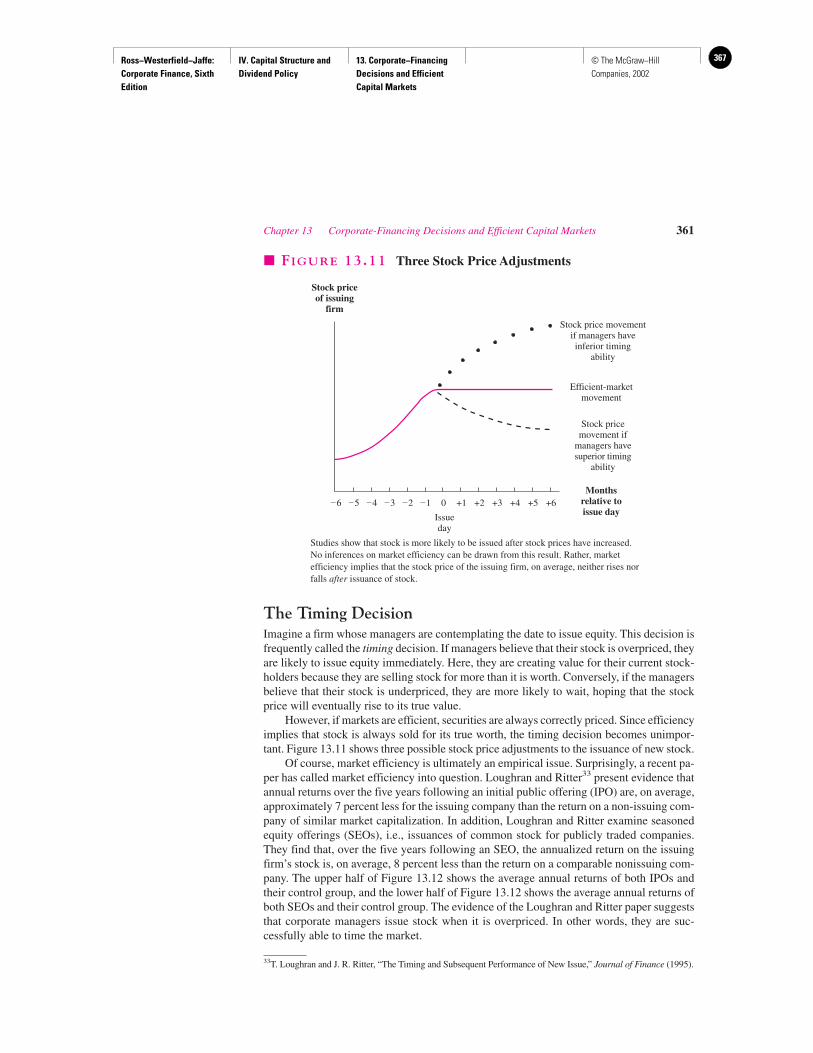
Ross−Westerfield−Jaffe: Corporate Finance, Sixth Edition
IV. Capital Structure and Dividend Policy
13. Corporate−Financing Decisions and Efficient Capital Markets
367© The McGraw−Hill Companies, 2002
The Timing DecisionImagine a firm whose managers are contemplating the date to issue equity. This decision isfrequently called the timing decision. If managers believe that their stock is overpriced, theyare likely to issue equity immediately. Here, they are creating value for their current stock-holders because they are selling stock for more than it is worth. Conversely, if the managersbelieve that their stock is underpriced, they are more likely to wait, hoping that the stockprice will eventually rise to its true value.
However, if markets are efficient, securities are always correctly priced. Since efficiencyimplies that stock is always sold for its true worth, the timing decision becomes unimpor-tant. Figure 13.11 shows three possible stock price adjustments to the issuance of new stock.
Of course, market efficiency is ultimately an empirical issue. Surprisingly, a recent pa-per has called market efficiency into question. Loughran and Ritter33 present evidence thatannual returns over the five years following an initial public offering (IPO) are, on average,approximately 7 percent less for the issuing company than the return on a non-issuing com-pany of similar market capitalization. In addition, Loughran and Ritter examine seasonedequity offerings (SEOs), i.e., issuances of common stock for publicly traded companies.They find that, over the five years following an SEO, the annualized return on the issuingfirm’s stock is, on average, 8 percent less than the return on a comparable nonissuing com-pany. The upper half of Figure 13.12 shows the average annual returns of both IPOs andtheir control group, and the lower half of Figure 13.12 shows the average annual returns ofboth SEOs and their control group. The evidence of the Loughran and Ritter paper suggeststhat corporate managers issue stock when it is overpriced. In other words, they are suc-cessfully able to time the market.
Chapter 13 Corporate-Financing Decisions and Efficient Capital Markets 361
Stock priceof issuing
firm
Monthsrelative toissue day
–6 –5 –4 –3 –2 –1 0 +1 +2 +3 +4 +5 +6
Issueday
Stock price movementif managers haveinferior timing
ability
Efficient-marketmovement
Stock pricemovement if
managers havesuperior timing
ability
� FIGURE 13.11 Three Stock Price Adjustments
Studies show that stock is more likely to be issued after stock prices have increased.No inferences on market efficiency can be drawn from this result. Rather, marketefficiency implies that the stock price of the issuing firm, on average, neither rises norfalls after issuance of stock.
33T. Loughran and J. R. Ritter, “The Timing and Subsequent Performance of New Issue,” Journal of Finance (1995).
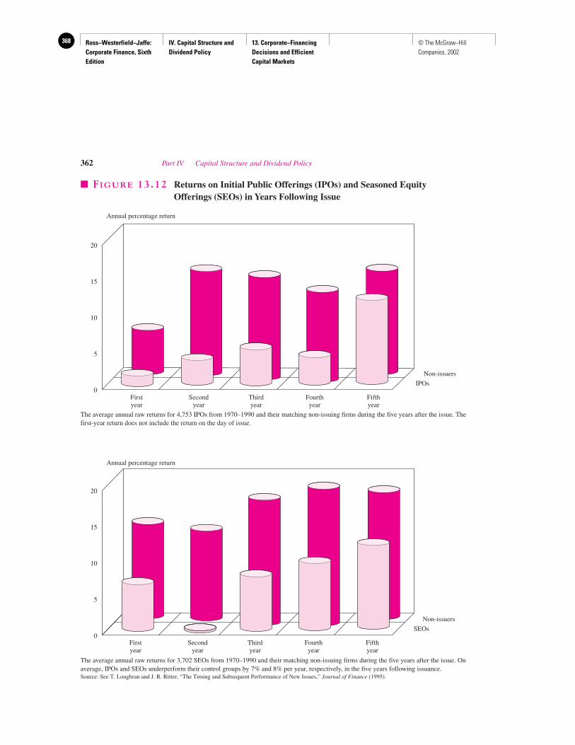
Ross−Westerfield−Jaffe: Corporate Finance, Sixth Edition
IV. Capital Structure and Dividend Policy
13. Corporate−Financing Decisions and Efficient Capital Markets
368 © The McGraw−Hill Companies, 2002
362 Part IV Capital Structure and Dividend Policy
15
10
5
0
20
15
10
5
0
20
Firstyear
Secondyear
Thirdyear
Fourthyear
Fifthyear
Non-issuers
SEOs
Firstyear
Secondyear
Thirdyear
Fourthyear
Fifthyear
Non-issuers
IPOs
Annual percentage return
Annual percentage return
� FIGURE 13.12 Returns on Initial Public Offerings (IPOs) and Seasoned EquityOfferings (SEOs) in Years Following Issue
The average annual raw returns for 4,753 IPOs from 1970–1990 and their matching non-issuing firms during the five years after the issue. Thefirst-year return does not include the return on the day of issue.
The average annual raw returns for 3,702 SEOs from 1970–1990 and their matching non-issuing firms during the five years after the issue. Onaverage, IPOs and SEOs underperform their control groups by 7% and 8% per year, respectively, in the five years following issuance.Source: See T. Loughran and J. R. Ritter, “The Timing and Subsequent Performance of New Issues,” Journal of Finance (1995).
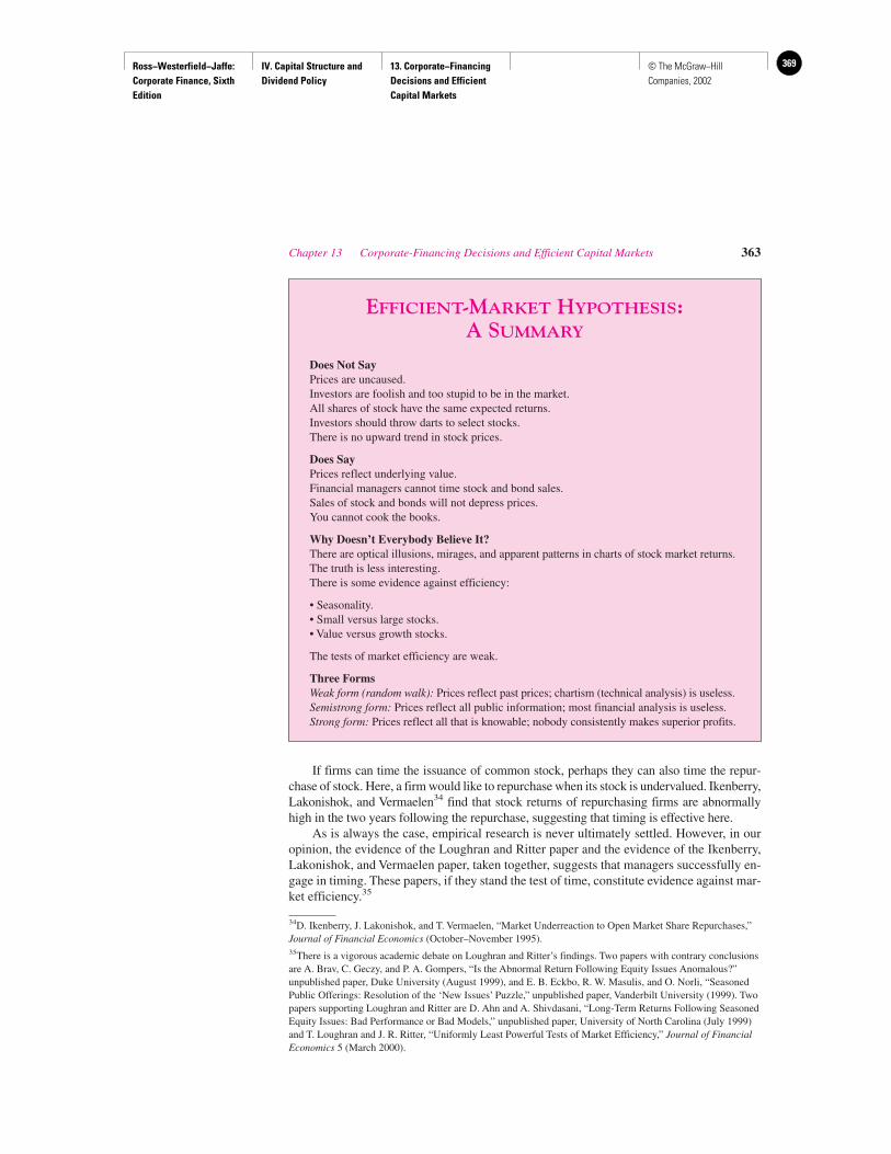
Ross−Westerfield−Jaffe: Corporate Finance, Sixth Edition
IV. Capital Structure and Dividend Policy
13. Corporate−Financing Decisions and Efficient Capital Markets
369© The McGraw−Hill Companies, 2002
If firms can time the issuance of common stock, perhaps they can also time the repur-chase of stock. Here, a firm would like to repurchase when its stock is undervalued. Ikenberry,Lakonishok, and Vermaelen34 find that stock returns of repurchasing firms are abnormallyhigh in the two years following the repurchase, suggesting that timing is effective here.
As is always the case, empirical research is never ultimately settled. However, in ouropinion, the evidence of the Loughran and Ritter paper and the evidence of the Ikenberry,Lakonishok, and Vermaelen paper, taken together, suggests that managers successfully en-gage in timing. These papers, if they stand the test of time, constitute evidence against mar-ket efficiency.35
Chapter 13 Corporate-Financing Decisions and Efficient Capital Markets 363
EFFICIENT-MARKET HYPOTHESIS: A SUMMARY
Does Not SayPrices are uncaused.Investors are foolish and too stupid to be in the market.All shares of stock have the same expected returns.Investors should throw darts to select stocks.There is no upward trend in stock prices.
Does SayPrices reflect underlying value.Financial managers cannot time stock and bond sales.Sales of stock and bonds will not depress prices.You cannot cook the books.
Why Doesn’t Everybody Believe It?There are optical illusions, mirages, and apparent patterns in charts of stock market returns.The truth is less interesting.There is some evidence against efficiency:
• Seasonality.• Small versus large stocks.• Value versus growth stocks.
The tests of market efficiency are weak.
Three FormsWeak form (random walk): Prices reflect past prices; chartism (technical analysis) is useless.Semistrong form: Prices reflect all public information; most financial analysis is useless.Strong form: Prices reflect all that is knowable; nobody consistently makes superior profits.
34D. Ikenberry, J. Lakonishok, and T. Vermaelen, “Market Underreaction to Open Market Share Repurchases,”Journal of Financial Economics (October–November 1995).35There is a vigorous academic debate on Loughran and Ritter’s findings. Two papers with contrary conclusionsare A. Brav, C. Geczy, and P. A. Gompers, “Is the Abnormal Return Following Equity Issues Anomalous?”unpublished paper, Duke University (August 1999), and E. B. Eckbo, R. W. Masulis, and O. Norli, “SeasonedPublic Offerings: Resolution of the ‘New Issues’ Puzzle,” unpublished paper, Vanderbilt University (1999). Twopapers supporting Loughran and Ritter are D. Ahn and A. Shivdasani, “Long-Term Returns Following SeasonedEquity Issues: Bad Performance or Bad Models,” unpublished paper, University of North Carolina (July 1999)and T. Loughran and J. R. Ritter, “Uniformly Least Powerful Tests of Market Efficiency,” Journal of FinancialEconomics 5 (March 2000).
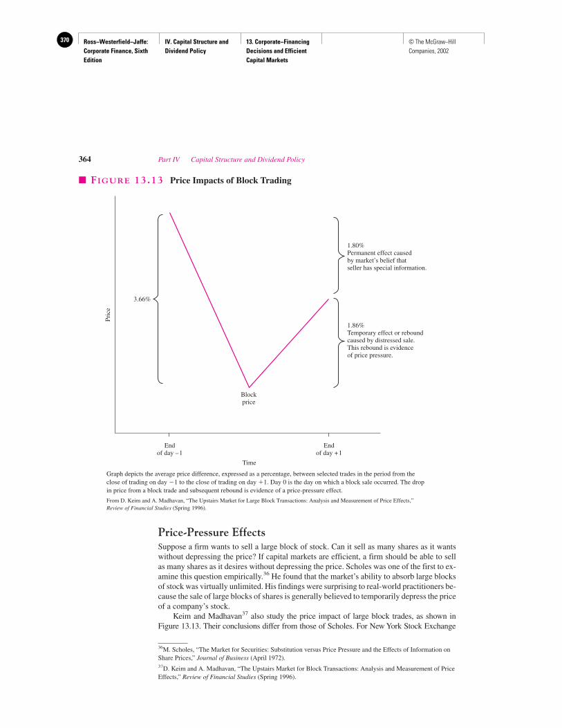
Ross−Westerfield−Jaffe: Corporate Finance, Sixth Edition
IV. Capital Structure and Dividend Policy
13. Corporate−Financing Decisions and Efficient Capital Markets
370 © The McGraw−Hill Companies, 2002
Price-Pressure EffectsSuppose a firm wants to sell a large block of stock. Can it sell as many shares as it wantswithout depressing the price? If capital markets are efficient, a firm should be able to sellas many shares as it desires without depressing the price. Scholes was one of the first to ex-amine this question empirically.36 He found that the market’s ability to absorb large blocksof stock was virtually unlimited. His findings were surprising to real-world practitioners be-cause the sale of large blocks of shares is generally believed to temporarily depress the priceof a company’s stock.
Keim and Madhavan37 also study the price impact of large block trades, as shown inFigure 13.13. Their conclusions differ from those of Scholes. For New York Stock Exchange
364 Part IV Capital Structure and Dividend Policy
Pric
e
Endof day –1
Endof day +1
Blockprice
Time
1.80%Permanent effect causedby market’s belief thatseller has special information.
1.86%Temporary effect or reboundcaused by distressed sale.This rebound is evidenceof price pressure.
3.66%
� FIGURE 13.13 Price Impacts of Block Trading
Graph depicts the average price difference, expressed as a percentage, between selected trades in the period from theclose of trading on day �1 to the close of trading on day �1. Day 0 is the day on which a block sale occurred. The dropin price from a block trade and subsequent rebound is evidence of a price-pressure effect.
From D. Keim and A. Madhavan, “The Upstairs Market for Large Block Transactions: Analysis and Measurement of Price Effects,”Review of Financial Studies (Spring 1996).
36M. Scholes, “The Market for Securities: Substitution versus Price Pressure and the Effects of Information onShare Prices,” Journal of Business (April 1972).37D. Keim and A. Madhavan, “The Upstairs Market for Block Transactions: Analysis and Measurement of PriceEffects,” Review of Financial Studies (Spring 1996).
Ross−Westerfield−Jaffe: Corporate Finance, Sixth Edition
IV. Capital Structure and Dividend Policy
13. Corporate−Financing Decisions and Efficient Capital Markets
371© The McGraw−Hill Companies, 2002
Chapter 13 Corporate-Financing Decisions and Efficient Capital Markets 365
and American Stock Exchange securities, they find that the stock price drops, on average, about3.66 percent from the closing trade on the previous day to the block trade itself. However, thestock rebounds by 1.86 percent by the close of the day after the block trade. Keim and Madhavanargue that the difference of 1.80 percent (� 3.66% � 1.86%) reflects the market’s belief that theblock seller has special (negative) information concerning the stock. This drop of 1.80 percentis a permanent effect. In addition, the block trader sells at a still lower price because of his needto sell quickly. This temporary or rebound effect (1.86% in this example) is similar to real estatesales at distressed prices when the seller needs cash immediately. This drop in price and subse-quent rebound of 1.86 percent is evidence of price pressure.
The preceding are just two of a large number of studies in the area. Because the mag-nitude of the price-pressure effect varies across the existing research, more work is neededto resolve the conflicting results.
• What are three implications of the efficient-market hypothesis for corporate finance?
13.6 SUMMARY AND CONCLUSIONS
1. An efficient financial market processes the information available to investors andincorporates it into the prices of securities. Market efficiency has two general implications.First, in any given time period, a stock’s abnormal return depends on information or newsreceived by the market in that period. Second, an investor who uses the same information asthe market cannot expect to earn abnormal returns. In other words, systems for playing themarket are doomed to fail.
2. What information does the market use to determine prices? The weak form of the efficient-market hypothesis says that the market uses the past history of prices and is thereforeefficient with respect to these past prices. This implies that stock selection based on patternsof past stock-price movements is not better than random stock selection.
3. A stronger theory of efficiency is semistrong-form efficiency, which states that the marketuses all publicly available information in setting prices.
4. The strongest theory of efficiency, strong-form efficiency, states that the market has availableto it and uses all of the information that anybody knows about stocks, even inside information.
5. The evidence from different financial markets supports weak-form and semistrong-formefficiency but not strong-form efficiency. This is no consolation to the army of investors thatuses publicly available information in attempts to beat the market.
6. In our study of efficient markets we stress the importance of distinguishing between theactual return on a stock and the expected return. The difference is called the abnormal returnand comes from the release of news to the market.
7. Not everybody completely believes the efficient-market hypothesis. It is a misunderstoodtheory. The boxed material (on page 363) summarizes what it does and does not say.
8. Three implications of efficient markets for corporate finance are listed below:a. The price of a company’s stock cannot be affected by a change in accounting.b. Financial managers cannot time issues of stocks and bonds using publicly available
information.c. A firm can sell as many bonds or shares of stock as it desires without depressing prices.There is conflicting empirical evidence on all three points.
9. Do we have a better theory? At the present time, we think the answer is no. However, overtime the theory will no doubt improve.
QUESTION
CO
NC
EP
T
?

Ross−Westerfield−Jaffe: Corporate Finance, Sixth Edition
IV. Capital Structure and Dividend Policy
13. Corporate−Financing Decisions and Efficient Capital Markets
372 © The McGraw−Hill Companies, 2002
KEY TERMS
Bubble theory 357 Serial correlation 349Efficient-market hypothesis 342 Strong-form efficiency 346Market capitalization 354 Technical analysis 345Random walk 344 Weak-form efficiency 344Semistrong-form efficiency 346
SUGGESTED READINGS
The concept of market efficiency is an important one. Perhaps the classic review articles areFama, E. F. “Efficient Capital Markets: A Review of Theory and Empirical Work.” Journal of
Finance (May 1970).Fama, E. F. “Efficient Capital Markets: II.” Journal of Finance (December 1991).Fama, E. F. “Market Efficiency, Long-Term Returns, and Behavioral Finance.” Journal of
Financial Economics (1998).
An entertaining, yet quite informative, book on efficient markets isMalkiel, B. G. A Random Walk Down Wall Street. 7th ed. New York: Norton, 1999.
QUESTIONS AND PROBLEMS
Can Financing Decisions Create Value?13.1 a. What rule should a firm follow when making financing decisions?
b. How can firms create valuable financing opportunities?
A Description of Efficient Capital Markets13.2 Define the three forms of market efficiency.
13.3 Which of the following statements are true about the efficient-market hypothesis?a. It implies perfect forecasting ability.b. It implies that prices reflect all available information.c. It implies an irrational market.d. It implies that prices do not fluctuate.e. It results from keen competition among investors.
13.4 Aerotech, an aerospace-technology research firm, announced this morning that it hashired the world’s most knowledgeable and prolific space researchers. Before today,Aerotech’s stock had been selling for $100.a. What do you expect will happen to Aerotech’s stock?b. Consider the following scenarios:
i. The stock price jumps to $118 on the day of the announcement. In subsequentdays it floats up to $123 then falls back to $116.
ii. The stock price jumps to $116 and remains there.iii. The stock price gradually climbs to $116 over the next week.
Which scenario(s) indicate market efficiency? Which do not? Why?
13.5 When the 56-year-old founder of Gulf & Western, Inc., died of a heart attack, the stockprice jumped from $18.00 a share to $20.25, a 12.5-percent increase. This is evidence ofmarket inefficiency, because an efficient stock market would have anticipated his deathand adjusted the price beforehand. Is this statement true or false? Explain.
13.6 On January 10, 1985, the following announcement was made: “Early today the JusticeDepartment reached a decision in the Universal Product Care (UPC) case. UPC has beenfound guilty of discriminatory practices in hiring. For the next five years, UPC must pay$2 million each year to a fund representing victims of UPC’s policies.” Should investors
366 Part IV Capital Structure and Dividend Policy

Ross−Westerfield−Jaffe: Corporate Finance, Sixth Edition
IV. Capital Structure and Dividend Policy
13. Corporate−Financing Decisions and Efficient Capital Markets
373© The McGraw−Hill Companies, 2002
Chapter 13 Corporate-Financing Decisions and Efficient Capital Markets 367
not buy UPC stock after the announcement because the litigation will cause anabnormally low rate of return? Why?
13.7 Newtech Corp. is going to adopt a new chip testing device that can greatly improve itsproduction efficiency. Do you think the lead engineer of this device can profit frompurchasing the firm’s stock before the news release on the implementation of the newtechnology? What if you rush to call your broker to buy the stock right after you learn ofthe announcement in The Wall Street Journal?
13.8 Trans Trust Corp. has changed how it accounts for inventory. The change does not changetax, but the resulting earnings report released this quarter is 20 percent higher than what itwould have been under the old accounting system. There is no other surprise in thisearnings report. Will the stock price be higher when the market learns that the earningsare higher?
13.9 Many empirical studies have documented that firms that issue stock usually experience aperiod of price run-up before the public stock offering. Alex Johnson invests primarily infirms that have just carried out new stock offerings. Based on the evidence that thesefirms have generally performed very well before the stock offering, can Alex makemoney using this strategy?
13.10 Sooners Investing Agency has been the hottest stock picker for the past two years.Before the rise to fame occurred, subscribers to the Sooners newsletter totaled only 200.Those subscribers beat the market consistently; they earned substantially higher returnsafter adjustment for risk and transaction costs. Subscriptions have now skyrocketed to10,000. Now when Sooners recommends a stock, the stock price instantly rises severalpoints. The subscribers now earn only a normal return when they buy recommendedstock because the price rises before anybody can act on the information. Briefly explainthis phenomenon.
13.11 In a recent discussion with you, your broker commented that well-managed firms are notnecessarily more profitable than firms with average management. To convince you ofthis, she presented you with evidence from a recent study conducted by the firm forwhich she works. The study examined the returns on 17 small manufacturing firms that,eight years earlier, an industry magazine had listed as the best-managed smallmanufacturers in the country. In the eight years since the publication of that issue of themagazine, the 17 firms have not earned more than the market. Your broker concluded thatif they were well-managed, they should have produced better-than-average returns. Doyou agree with your broker?
13.12 A famous economist just announced his findings that the recession is over and theeconomy is entering the expansion stage once again. Can you profit from investing inthe stock market after you learned this study result from reading The Wall StreetJournal?
13.13 Many investors (sometimes called technical analysts) claim to observe patterns instock market prices. Is technical analysis consistent with EMH? If the stock pricefollows a random walk model, can technical analysts systematically profit fromtrading rules based on patterns in the historical stock prices? If so, what form ofmarket efficiency is violated?
The Evidence13.14 Some people argue that the EMH can’t explain the 1987 market crash or the high price-
to-earnings ratio of the Japanese stock market. What alternative hypothesis is currentlyused for these two phenomena?
13.15 Prospectors, Inc., is a small publicly traded gold-prospecting company in Alaska.Usually its searches prove fruitless; however, occasionally the prospectors find a richvein of ore.a. What pattern would you expect to observe for Prospectors’ cumulative abnormal returns?
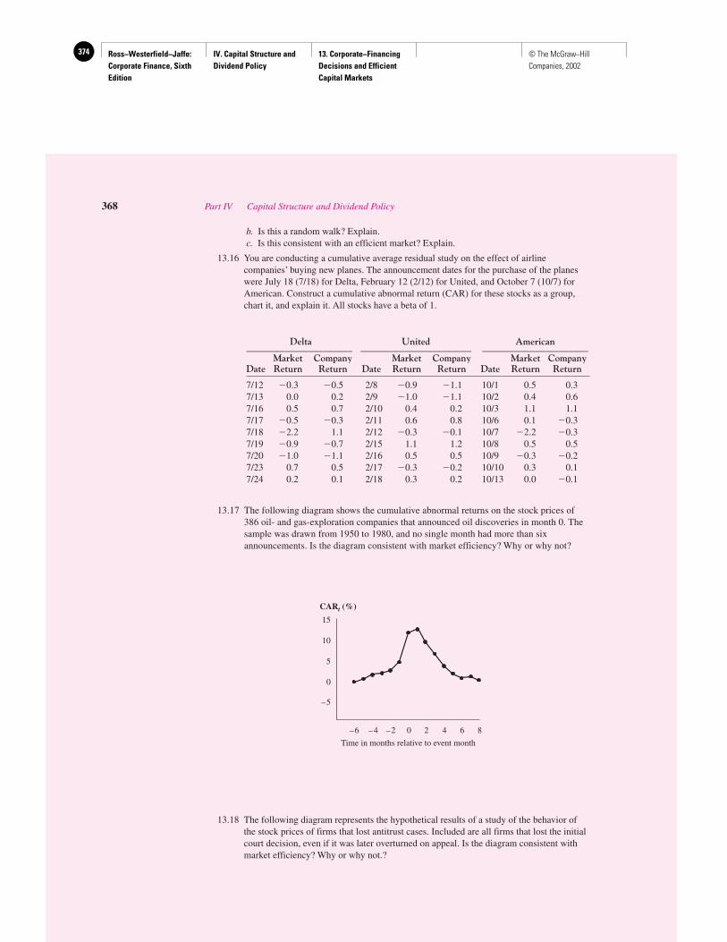
Ross−Westerfield−Jaffe: Corporate Finance, Sixth Edition
IV. Capital Structure and Dividend Policy
13. Corporate−Financing Decisions and Efficient Capital Markets
374 © The McGraw−Hill Companies, 2002
b. Is this a random walk? Explain.c. Is this consistent with an efficient market? Explain.
13.16 You are conducting a cumulative average residual study on the effect of airlinecompanies’ buying new planes. The announcement dates for the purchase of the planeswere July 18 (7/18) for Delta, February 12 (2/12) for United, and October 7 (10/7) forAmerican. Construct a cumulative abnormal return (CAR) for these stocks as a group,chart it, and explain it. All stocks have a beta of 1.
Delta United American______________________ _______________________ ______________________
Market Company Market Company Market CompanyDate Return Return Date Return Return Date Return Return
7/12 �0.3 �0.5 2/8 �0.9 �1.1 10/1 0.5 0.37/13 0.0 0.2 2/9 �1.0 �1.1 10/2 0.4 0.67/16 0.5 0.7 2/10 0.4 0.2 10/3 1.1 1.17/17 �0.5 �0.3 2/11 0.6 0.8 10/6 0.1 �0.37/18 �2.2 1.1 2/12 �0.3 �0.1 10/7 �2.2 �0.37/19 �0.9 �0.7 2/15 1.1 1.2 10/8 0.5 0.57/20 �1.0 �1.1 2/16 0.5 0.5 10/9 �0.3 �0.27/23 0.7 0.5 2/17 �0.3 �0.2 10/10 0.3 0.17/24 0.2 0.1 2/18 0.3 0.2 10/13 0.0 �0.1
13.17 The following diagram shows the cumulative abnormal returns on the stock prices of386 oil- and gas-exploration companies that announced oil discoveries in month 0. Thesample was drawn from 1950 to 1980, and no single month had more than sixannouncements. Is the diagram consistent with market efficiency? Why or why not?
13.18 The following diagram represents the hypothetical results of a study of the behavior ofthe stock prices of firms that lost antitrust cases. Included are all firms that lost the initialcourt decision, even if it was later overturned on appeal. Is the diagram consistent withmarket efficiency? Why or why not.?
CARt (%)
15
10
5
0
–5
–6 –4 –2 0 2 4 6 8
Time in months relative to event month
368 Part IV Capital Structure and Dividend Policy
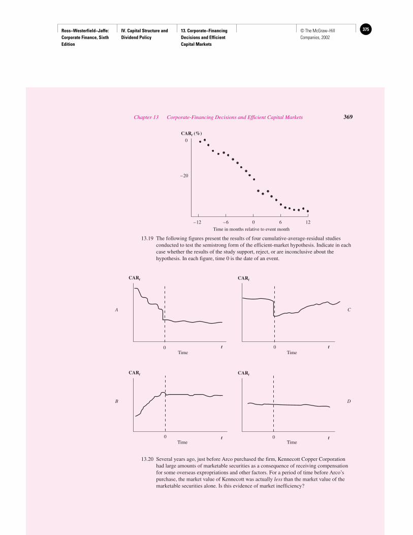
Ross−Westerfield−Jaffe: Corporate Finance, Sixth Edition
IV. Capital Structure and Dividend Policy
13. Corporate−Financing Decisions and Efficient Capital Markets
375© The McGraw−Hill Companies, 2002
Chapter 13 Corporate-Financing Decisions and Efficient Capital Markets 369
13.19 The following figures present the results of four cumulative-average-residual studiesconducted to test the semistrong form of the efficient-market hypothesis. Indicate in eachcase whether the results of the study support, reject, or are inconclusive about thehypothesis. In each figure, time 0 is the date of an event.
13.20 Several years ago, just before Arco purchased the firm, Kennecott Copper Corporationhad large amounts of marketable securities as a consequence of receiving compensationfor some overseas expropriations and other factors. For a period of time before Arco’spurchase, the market value of Kennecott was actually less than the market value of themarketable securities alone. Is this evidence of market inefficiency?
CARt CARt
B
A
t
t
Time
Time
CARt CARt
Time
Time
t
t
D
C
0 0
0 0
1260–6–12
Time in months relative to event month
0
–20
CARt (%)

Ross−Westerfield−Jaffe: Corporate Finance, Sixth Edition
IV. Capital Structure and Dividend Policy
13. Corporate−Financing Decisions and Efficient Capital Markets
376 © The McGraw−Hill Companies, 2002
13.21 Suppose the market is semistrong-form efficient. Can you expect to earn excess returns ifyou make trades based on:a. Your broker’s information about record earnings for a stock?b. Rumors about a merger of a firm?c. Yesterday’s announcement of a successful test of a new product?
13.22 Consider an efficient capital market in which a particular macroeconomic variable thatinfluences your firm’s net earnings is positively serially correlated. Would you expectprice changes in your stock to be serially correlated? Why or why not?
13.23 Although mutual fund managers frequently claim that they have investing strategies,under the EMH, mutual fund managers should obtain the same returns after adjusting forthe risk level of their respective investments. Therefore, we can simply pick mutual fundsat random. Is this statement true or false? Explain.
13.24 A pension manager intends to unload a large block of Bob’s Toy Inc. shares.a. What are the general empirical findings on the price effect of block trading?b. Do you consider it a good idea for the pension manager to break up the trades to
several lots instead of one big block at a time?c. What is the expected price effect if we assume that EMH holds?
13.25 Assume that markets are efficient. Suppose that during a trading day, important newinformation is released for the first time concerning American Golf Inc. This informationindicates that the firm has lost a contract for a large golf-course project that the marketwidely believed the firm had secured prior to the news. How would you expect the priceof a share of stock to react to this information?a. The value of a share decreases over an extended period of time as investors begin to
sell shares in the company.b. The value of a share will decrease to a price above what would be considered
appropriate, because of the greatly decreased demand for the shares. Eventually theprice would rise back up to the correct level.
c. The value of a share will decrease immediately to a price that reflects the value of thenew information.
d. More information would be needed to determine the movement in the price of the stock.
370 Part IV Capital Structure and Dividend Policy
Ross−Westerfield−Jaffe: Corporate Finance, Sixth Edition
IV. Capital Structure and Dividend Policy
14. Long−Term Financing: An Introduction
377© The McGraw−Hill Companies, 2002
Long-Term Financing: An Introduction
CH
AP
TE
R14
EXECUTIVE SUMMARY
This chapter introduces the basic sources of long-term financing: common stock, pre-ferred stock, and long-term debt. Later chapters discuss these topics in more detail.Perhaps no other area of corporate finance is more perplexing to new students of fi-
nance than corporate securities such as shares of stock, bonds, and debentures. Whereas theconcepts are simple and logical, the language is strange and unfamiliar.
The purpose of this chapter is to describe the basic features of long-term financing.We begin with a look at common stock, preferred stock, and long-term debt and thenbriefly consider patterns of the different kinds of long-term financing. Discussion ofnonbasic forms of long-term finance, such as convertibles and leases, is reserved forlater chapters.
14.1 COMMON STOCK
The term common stock has no precise meaning. It usually is applied to stock that has nospecial preference either in dividends or in bankruptcy. A description of the common stockof Anheuser-Busch in 1996 is presented below.
ANHEUSER-BUSCHCommon Stock and Other Shareholders’ Equity
December 31, 1999(in millions)
Common stock, $1 par value, authorized 1.6 billion shares, issued 716.1 million shares $ 716.1Capital in excess of par value 1,241.0Retained earnings 9,181.2Treasury stock, at cost (6,831.3)Other
ESOP debt guarantee (210.5)Foreign currency translation adjustment (175.0)_______
Total Equity $3,921.5
Par and No-Par StockOwners of common stock in a corporation are referred to as shareholders or stockholders.They receive stock certificates for the shares they own. There is usually a stated value oneach stock certificate called the par value. However, some stocks have no-par value. Thepar value of each share of the common stock of Anheuser-Busch is $1.
The total par value is the number of shares issued multiplied by the par value of eachshare and is sometimes referred to as the dedicated capital of a corporation. The dedicatedcapital of Anheuser-Busch is $1 � 716.1 million shares � $716.1 million.
Ross−Westerfield−Jaffe: Corporate Finance, Sixth Edition
IV. Capital Structure and Dividend Policy
14. Long−Term Financing: An Introduction
378 © The McGraw−Hill Companies, 2002
Authorized versus Issued Common StockShares of common stock are the fundamental ownership units of the corporation. The arti-cles of incorporation of a new corporation must state the number of shares of common stockthe corporation is authorized to issue.
The board of directors of the corporation, after a vote of the shareholders, can amend thearticles of incorporation to increase the number of shares authorized; there is no limit to thenumber of shares that can be authorized. In 1999 Anheuser-Busch had authorized 1.6 billionshares and had issued 716.1 million shares. There is no requirement that all of the authorizedshares actually be issued. Although there are no legal limits to authorizing shares of stock,some practical considerations may exist:
1. Some states impose taxes based on the number of authorized shares.
2. Authorizing a large number of shares may create concern on the part of investors, be-cause authorized shares can be issued later with the approval of the board of directorsbut without a vote of the shareholders.
Capital SurplusCapital surplus usually refers to amounts of directly contributed equity capital in excessof the par value.
EXAMPLE
Suppose 100 shares of common stock have a par value of $2 each and are sold toshareholders for $10 per share. The capital surplus would be ($10 � $2) � 100� $8 � 100 � $800, and the total par value would be $2 � 100 � $200. Whatdifference does it make if the total capital contribution is reported as par value orcapital surplus?
About the only difference is that in most states the par value is locked in and cannot bedistributed to stockholders except upon the liquidation of the corporation.
The capital surplus of Anheuser-Busch is $1,241 million. This figure indicates that theprice of new shares issued by Anheuser-Busch has exceeded the par value and the differencehas been entered as capital in excess of par value. In most states shares of stock cannot beissued below par value, implying that capital in excess of par value cannot be negative.
Retained EarningsAnheuser-Busch usually pays out less than one half of its net income as dividends; the restis retained in the business and is called retained earnings. The cumulative amount of re-tained earnings (since original incorporation) was $9,181.2 million in 1999.
The sum of the par value, capital surplus, and accumulated retained earnings is the com-mon equity of the firm, which is usually referred to as the firm’s book value. The book valuerepresents the amount contributed directly and indirectly to the corporation by equity investors.
EXAMPLE
Suppose Western Redwood Corporation was formed in 1906 with 10,000 sharesof stock issued and sold at its $1 par value. Because the stock was sold for $1, thefirst balance sheet showed a zero amount for capital surplus. By 1998 the company
372 Part IV Capital Structure and Dividend Policy
Ross−Westerfield−Jaffe: Corporate Finance, Sixth Edition
IV. Capital Structure and Dividend Policy
14. Long−Term Financing: An Introduction
379© The McGraw−Hill Companies, 2002
had become very profitable and had retained profits of $100,000. The stockhold-ers’ equity of Western Redwood Corporation in 1998 is as follows:
WESTERN REDWOOD CORPORATIONEquity AccountsJanuary 1, 1998
Common stock, $1 par, 10,000 shares outstanding $ 10,000Capital surplus 0Retained earnings 100,000________
Total stockholders’ equity $110,000
Suppose the company has profitable investment opportunities and decides to sell10,000 shares of new stock. The current market price is $20 per share. The effectof the sale of stock on the balance sheet will be
WESTERN REDWOOD CORPORATIONEquity Accounts
December 31, 1998
Common stock, $1 par, 20,000 shares outstanding $ 20,000Capital surplus ($20 � $1) � 10,000 shares 190,000Retained earnings 100,000________
Total stockholders’ equity $310,000
What happened?
1. Because 10,000 shares of new stock were issued with par value of $1, thepar value rose $10,000.
2. The total amount raised by the new issue was $20 � 10,000 � $200,000,and $190,000 was entered into capital surplus.
3. The book value per share increased because the market price of the newstock was higher than the book value of the old stock.
Market Value, Book Value, and Replacement ValueThe book value of Anheuser-Busch in 1999 was $3,921.5 million. This figure is based onthe number of shares outstanding. The company had issued 716.1 million shares andbought back approximately 263.4 million shares, so that the total number of outstandingshares was 716.1 million � 263.4 million � 452.7 million. The shares bought back arecalled treasury stock.
The book value per share was equal to
Anheuser-Busch is a publicly owned company. Its common stock trades on the New YorkStock Exchange (NYSE), and thousands of shares change hands every day. The recent mar-ket prices of Anheuser-Busch were between $75 and $84 per share. Thus the market priceswere above the book value.
Total common shareholders, equity
Shares outstanding�
$3,921.5 million
452.7 million� $8.66
Book value per share �$310,000
20,000� $15.5
Book value per share �$110,000
10,000� $11
Chapter 14 Long-Term Financing: An Introduction 373
Ross−Westerfield−Jaffe: Corporate Finance, Sixth Edition
IV. Capital Structure and Dividend Policy
14. Long−Term Financing: An Introduction
380 © The McGraw−Hill Companies, 2002
In addition to market and book values, you may hear the term replacement value. Thisrefers to the current cost of replacing the assets of the firm. Market, book, and replacementvalue are equal at the time when a firm purchases an asset. After that time, these values willdiverge. The market-to-book-value ratio of common stock and Tobin’s Q (market value ofassets/replacement value of assets) introduced in the appendix to Chapter 2 are indicatorsof the success of the firm. A market-to-book or Tobin’s Q ratio greater than 1 indicates thefirm has done well with its investment decisions.
Shareholders’ RightsThe conceptual structure of the corporation assumes that shareholders elect directors whoin turn elect corporate officers—more generally, the management—to carry out their di-rectives. It is the right to elect the directors of the corporation by vote that constitutes themost important control device of shareholders.
Directors are elected each year at an annual meeting by a vote of the holders of a ma-jority of shares who are present and entitled to vote. The exact mechanism for electing dif-fers among different companies. The most important difference is whether shares must bevoted cumulatively or must be voted straight.
EXAMPLE
Imagine that a corporation has two shareholders: Smith with 25 shares and Mar-shall with 75 shares. Both want to be on the board of directors. Marshall does notwant Smith to be a director. Let us assume that there are four directors to be electedand each shareholder nominates four candidates.
Cumulative Voting The effect of cumulative voting is to permit minority participa-tion. If cumulative voting is permitted, the total number of votes that each shareholdermay cast is determined first. That number is usually calculated as the number of shares(owned or controlled) multiplied by the number of directors to be elected. Each share-holder can distribute these votes as he or she wishes over one or more candidates. Smithwill get 25 � 4 � 100 votes, and Marshall is entitled to 75 � 4 � 300 votes. If Smithgives all his votes to himself, he is assured of a directorship. It is not possible for Mar-shall to divide 300 votes among the four candidates in such a way as to preclude Smith’selection to the board.
Straight Voting If straight voting is permitted, Smith may cast 25 votes for each candi-date and Marshall may cast 75 votes for each. As a consequence, Marshall will elect all ofthe candidates.
Straight voting can freeze out minority shareholders; that is the reason many stateshave mandatory cumulative voting. In states where cumulative voting is mandatory, deviceshave been worked out to minimize its impact. One such device is to stagger the voting forthe board of directors. Staggering permits a fraction of the directorships to come to a voteat a particular time. It has two basic effects:
1. Staggering makes it more difficult for a minority to elect a director when there is cumu-lative voting.
2. Staggering makes successful takeover attempts less likely by making the election of newdirectors more difficult.
374 Part IV Capital Structure and Dividend Policy
Ross−Westerfield−Jaffe: Corporate Finance, Sixth Edition
IV. Capital Structure and Dividend Policy
14. Long−Term Financing: An Introduction
381© The McGraw−Hill Companies, 2002
Proxy Voting A proxy is the legal grant of authority by a shareholder to someone else tovote his or her shares. For convenience, the actual voting in large public corporations usu-ally is done by proxy.
Many companies such as Anheuser-Busch have hundreds of thousands of sharehold-ers. Shareholders can come to the annual meeting and vote in person, or they can transfertheir right to vote to another party by proxy.
Obviously, management always tries to get as many proxies transferred to it as possi-ble. However, if shareholders are not satisfied with management, an outside group of share-holders can try to obtain as many votes as possible via proxy. They can vote to replace man-agement by adding enough directors. This is called a proxy fight.
Other Rights The value of a share of common stock in a corporation is directly relatedto the general rights of shareholders. In addition to the right to vote for directors, share-holders usually have the following rights:
1. The right to share proportionally in dividends paid.
2. The right to share proportionally in assets remaining after liabilities have been paid in aliquidation.
3. The right to vote on matters of great importance to stockholders, such as a merger, usu-ally decided at the annual meeting or a special meeting.
4. The right to share proportionally in any new stock sold. This is called the preemptiveright and will be discussed in detail in later chapters.
DividendsA distinctive feature of corporations is that they issue shares of stock and are authorized bylaw to pay dividends to the holders of those shares. Dividends paid to shareholders repre-sent a return on the capital directly or indirectly contributed to the corporation by the share-holders. The payment of dividends is at the discretion of the board of directors.
Here are some important characteristics of dividends:
1. Unless a dividend is declared by the board of directors of a corporation, it is not a lia-bility of the corporation. A corporation cannot default on an undeclared dividend. As aconsequence, corporations cannot become bankrupt because of nonpayment of divi-dends. The amount of the dividend—and even whether or not it is paid—are decisionsbased on the business judgment of the board of directors.
2. The payment of dividends by the corporation is not a business expense. Dividends arenot deductible for corporate tax purposes. In short, dividends are paid out of after-taxprofits of the corporation.
3. Dividends received by individual shareholders are for the most part considered ordinaryincome by the IRS and are fully taxable. However, corporations that own stock in othercorporations are permitted to exclude 70 percent of the amounts they receive as divi-dends. In other words, they are taxed only on the remaining 30 percent.
Classes of StockSome firms issue more than one class of common stock. The classes are usually created withunequal voting rights. The Ford Motor Company has Class B common stock, which is not pub-licly traded (it is held by Ford family interests and trusts). This class has about 40 percent of thevoting power, but these shares comprise only about 15 percent of the total outstanding stock.
Chapter 14 Long-Term Financing: An Introduction 375
Ross−Westerfield−Jaffe: Corporate Finance, Sixth Edition
IV. Capital Structure and Dividend Policy
14. Long−Term Financing: An Introduction
382 © The McGraw−Hill Companies, 2002
Many companies issue dual classes of common stock. The reason has to do with con-trol of the firm. Management of a firm can raise equity capital by issuing nonvoting com-mon stock while maintaining voting control. Harry and Linda DeAngelo found that man-agements’ holdings of common stock are usually tilted toward the stock with the superiorvoting rights.1 Thus, managerial vote ownership is an important element of corporate con-trol structure.
Lease, McConnell, and Mikkelson found the market prices of stocks with superior vot-ing rights to be about 5 percent higher than the prices of otherwise identical stocks with infe-rior voting rights.2 However, DeAngelo and DeAngelo found some evidence that the marketvalue of differences in voting rights may be much higher when control of the firm is involved.
• What is a company’s book value?• What rights do stockholders have?• What is a proxy?
14.2 CORPORATE LONG-TERM DEBT: THE BASICS
Securities issued by corporations may be classified roughly as equity securities and debt se-curities. The distinction between equity and debt is basic to much of the modern theory andpractice of corporate finance.
At its crudest level, debt represents something that must be repaid; it is the result ofborrowing money. When corporations borrow, they promise to make regularly scheduledinterest payments and to repay the original amount borrowed (that is, the principal). Theperson or firm making the loan is called a creditor or lender.
Interest versus DividendsThe corporation borrowing the money is called a debtor or borrower. The amount owed thecreditor is a liability of the corporation; however, it is a liability of limited value. The cor-poration can legally default at any time on its liability.3 This can be a valuable option. Thecreditors benefit if the assets have a value greater than the value of the liability, but this wouldhappen only if management were foolish. On the other hand, the corporation and the equityinvestors benefit if the value of the assets is less than the value of the liabilities, because eq-uity investors are able to walk away from the liabilities and default on their payment.
From a financial point of view, the main differences between debt and equity are thefollowing:
1. Debt is not an ownership interest in the firm. Creditors do not usually have votingpower. The device used by creditors to protect themselves is the loan contract (that is,the indenture).
2. The corporation’s payment of interest on debt is considered a cost of doing business andis fully tax-deductible. Thus interest expense is paid out to creditors before the corporatetax liability is computed. Dividends on common and preferred stock are paid to share-
376 Part IV Capital Structure and Dividend Policy
1H. DeAngelo and L. DeAngelo, “Managerial Ownership of Voting Rights: A Study of Public Corporations withDual Classes of Common Stock,” Journal of Financial Economics 14 (1985).2R. C. Lease, J. J. McConnell, and W. H. Mikkelson, “The Market Value of Control in Publicly TradedCorporations,” Journal of Financial Economics (April 1983).3In practice, creditors can make a claim against the assets of the firm and a court will administer the legal remedy.
QUESTIONS
CO
NC
EP
T
?
Ross−Westerfield−Jaffe: Corporate Finance, Sixth Edition
IV. Capital Structure and Dividend Policy
14. Long−Term Financing: An Introduction
383© The McGraw−Hill Companies, 2002
holders after the tax liability has been determined. Dividends are considered a return toshareholders on their contributed capital. Because interest expense can be used to reducetaxes, the government (that is, the IRS) is providing a direct tax subsidy on the use of debtwhen compared to equity. This point is discussed in detail in the next two chapters.
3. Unpaid debt is a liability of the firm. If it is not paid, the creditors can legally claim theassets of the firm. This action may result in liquidation and bankruptcy. Thus one of thecosts of issuing debt is the possibility of financial failure, which does not arise when eq-uity is issued.
Is It Debt or Equity?Sometimes it is not clear whether a particular security is debt or equity. For example, sup-pose a 50-year bond is issued with interest payable solely from corporate income if and onlyif earned, and repayment is subordinate to all other debts of the business. Corporations arevery adept at creating hybrid securities that look like equity but are called debt. Obviously,the distinction between debt and equity is important for tax purposes. When corporationstry to create a debt security that is really equity, they are trying to obtain the tax benefits ofdebt while eliminating its bankruptcy costs.
Basic Features of Long-Term DebtLong-term corporate debt usually is denominated in units of $1,000 called the principal orface value.4 Long-term debt is a promise by the borrowing firm to repay the principalamount by a certain date, called the maturity date. Long-term debt almost always has a parvalue equal to the face value, and debt price is often expressed as a percentage of the parvalue. For example, it might be said that General Motors debt is selling at 90, which meansthat a bond with a par value of $1,000 can be purchased for $900. In this case the debt isselling at a discount because the market price is less than the par value. Debt can also sellat a premium with respect to par value. The borrower using long-term debt generally paysinterest at a rate expressed as a fraction of par value. Thus, at $1,000 par value, General Mo-tors’7-percent debt means that $70 of interest is paid to holders of the debt, usually in semi-annual installments (for example, $35 on June 30 and December 31). The payment sched-ules are in the form of coupons that are detached from the debt certificates and sent to thecompany for payment.
Different Types of DebtTypical debt securities are called notes, debentures, or bonds. A debenture is an unsecuredcorporate debt, whereas a bond is secured by a mortgage on the corporate property. How-ever, in common usage the word bond is used indiscriminately and often refers to both se-cured and unsecured debt. A note usually refers to an unsecured debt with a maturity shorterthan that of a debenture, perhaps under 10 years.
Debentures and bonds are long-term debt. Long-term debt is any obligation that ispayable more than one year from the date it was originally issued. Sometimes long-termdebt—debentures and bonds—is called funded debt. Debt that is due in less than one yearis unfunded and is accounted for as a current liability. Some debt is perpetual and has nospecific maturity. This type of debt is referred to as a consol.
Chapter 14 Long-Term Financing: An Introduction 377
4Many government bonds have larger principal denominations, up to $10,000 or $25,000, and most municipalbonds come in denominations of $5,000.
Ross−Westerfield−Jaffe: Corporate Finance, Sixth Edition
IV. Capital Structure and Dividend Policy
14. Long−Term Financing: An Introduction
384 © The McGraw−Hill Companies, 2002
RepaymentLong-term debt is typically repaid in regular amounts over the life of the debt. The paymentof long-term debt by installments is called amortization. At the end of the amortization theentire indebtedness is said to be extinguished. Amortization is typically arranged by a sink-ing fund. Each year the corporation places money into a sinking fund, and the money is usedto buy back the bonds.
Debt may be extinguished before maturity by a call. Historically, almost all publiclyissued corporate long-term debt has been callable.5 These are debentures or bonds forwhich the firm has the right to pay a specific amount, the call price, to retire (extinguish)the debt before the stated maturity date. The call price is always higher than the par valueof the debt. Debt that is callable at 105 is debt that the firm can buy back from the holder ata price of $1,050 per debenture or bond, regardless of what the market value of the debtmight be. Call prices are always specified when the debt is originally issued. However,lenders are given a 5-year to 10-year call-protection period during which the debt cannot becalled away. Recently there has been a higher incidence of noncallable offerings.
SeniorityIn general terms seniority indicates preference in position over other lenders. Some debt issubordinated. In the event of default, holders of subordinated debt must give preference toother specified creditors. Usually, this means that the subordinated lenders will be paid offonly after the specified creditors have been compensated. However, debt cannot be subor-dinated to equity.
SecuritySecurity is a form of attachment to property; it provides that the property can be sold in theevent of default to satisfy the debt for which security is given. A mortgage is used for se-curity in tangible property; for example, debt can be secured by mortgages on plant andequipment. Holders of such debt have prior claim on the mortgaged assets in case of de-fault. Debentures are not secured by a mortgage. Thus, if mortgaged property is sold in theevent of default, debenture holders will obtain something only if the mortgage bondholdershave been fully satisfied.
IndentureThe written agreement between the corporate debt issuer and the lender, setting forth ma-turity date, interest rate, and all other terms, is called an indenture. We treat this in detail inlater chapters. For now, we note that
1. The indenture completely describes the nature of the indebtedness.
2. It lists all restrictions placed on the firm by the lenders. These restrictions are placed inrestrictive covenants.
Some typical restrictive covenants are the following:
1. Restrictions on further indebtedness.
2. A maximum on the amount of dividends that can be paid.
3. A minimum level of working capital.
378 Part IV Capital Structure and Dividend Policy
5When issued, callable industrial corporate debt typically has 10-year protection against being called.
Ross−Westerfield−Jaffe: Corporate Finance, Sixth Edition
IV. Capital Structure and Dividend Policy
14. Long−Term Financing: An Introduction
385© The McGraw−Hill Companies, 2002
EXAMPLE
The following table shows some of the many long-term debt securities of Anheuser-Busch at the end of 1999 (in millions).
Commercial paper (weighted average interest rates between 5.1% and 5.5%) . . . . . . . . . . . . . . . . . . . . . . . . . . . . . . . . . . . . . . . . . . $1,000.0
Medium-term notes due 2000 to 2001 (interest rates from 5.1% to 8.0%) . . . . . . . . . . . . . . . . . . . . . . . . . . . . . . . . . . . . . . . . . . . . . . . . . 32.5
4.1% dual-currency notes due 2001 . . . . . . . . . . . . . . . . . . . . . . . . . . . . . . . . . . . . . . . . 162.86.9% notes due 2002. . . . . . . . . . . . . . . . . . . . . . . . . . . . . . . . . . . . . . . . . . . . . . . . . . . . 200.06.75% notes due 2003. . . . . . . . . . . . . . . . . . . . . . . . . . . . . . . . . . . . . . . . . . . . . . . . . . . 200.06.75% notes due 2005. . . . . . . . . . . . . . . . . . . . . . . . . . . . . . . . . . . . . . . . . . . . . . . . . . . 200.07% notes due 2005 . . . . . . . . . . . . . . . . . . . . . . . . . . . . . . . . . . . . . . . . . . . . . . . . . . . . . 100.06.75% notes due 2006. . . . . . . . . . . . . . . . . . . . . . . . . . . . . . . . . . . . . . . . . . . . . . . . . . . 250.09% debentures due 2009. . . . . . . . . . . . . . . . . . . . . . . . . . . . . . . . . . . . . . . . . . . . . . . . . 350.07.25% debentures due 2015 . . . . . . . . . . . . . . . . . . . . . . . . . . . . . . . . . . . . . . . . . . . . . . 150.07.375% debentures due 2023 . . . . . . . . . . . . . . . . . . . . . . . . . . . . . . . . . . . . . . . . . . . . . 200.07% debentures due 2025. . . . . . . . . . . . . . . . . . . . . . . . . . . . . . . . . . . . . . . . . . . . . . . . . 200.0Industrial revenue bonds. . . . . . . . . . . . . . . . . . . . . . . . . . . . . . . . . . . . . . . . . . . . . . . . . 157.4ESOP debt guarantee . . . . . . . . . . . . . . . . . . . . . . . . . . . . . . . . . . . . . . . . . . . . . . . . . . . 210.5Other long-term debt . . . . . . . . . . . . . . . . . . . . . . . . . . . . . . . . . . . . . . . . . . . . . . . . . . . . 33.9
Anheuser-Busch has many different notes and debentures. As can be seen, thereis $1 billion of commercial paper. Commercial paper refers to short-term unse-cured notes. It is listed as long-term debt because it will be maintained on a long-term basis by “rolling it over.” Anheuser-Busch has $162.8 million of Japaneseyen/Australian dollar notes. The company will have the choice of using Japan-ese yen or Australian dollars for both interest and principal payments on thesenotes. There is also a $210.5 million guarantee of Employee Stock Option Plan(ESOP) debt.
• What is corporate debt? Describe its general features.• Why is it sometimes difficult to tell whether a particular security is debt or equity?
14.3 PREFERRED STOCK
Preferred stock represents equity of a corporation, but it is different from common stockbecause it has preference over common stock in the payment of dividends and in the assetsof the corporation in the event of bankruptcy. Preference means only that the holder of thepreferred share must receive a dividend (in the case of an ongoing firm) before holders ofcommon shares are entitled to anything.
Stated ValuePreferred shares have a stated liquidating value, usually $100 per share. The dividend pref-erence is described in terms of dollars per share. For example, General Motors “$5 pre-ferred” translates into a dividend yield of 5 percent of stated value.
Chapter 14 Long-Term Financing: An Introduction 379
QUESTIONS
CO
NC
EP
T
?
Ross−Westerfield−Jaffe: Corporate Finance, Sixth Edition
IV. Capital Structure and Dividend Policy
14. Long−Term Financing: An Introduction
386 © The McGraw−Hill Companies, 2002
Cumulative and Noncumulative DividendsA preferred dividend is not like interest on a bond. The board of directors may decide notto pay the dividends on preferred shares, and their decision may not have anything to dowith current net income of the corporation. Dividends payable on preferred stock are ei-ther cumulative or noncumulative. If preferred dividends are cumulative and are not paidin a particular year, they will be carried forward. Usually both the cumulated (past) pre-ferred dividends plus the current preferred dividends must be paid before the commonshareholders can receive anything. Unpaid preferred dividends are not debts of the firm.Directors elected by the common shareholders can defer preferred dividends indefinitely.However, if so,
1. Common shareholders must forgo dividends.
2. Though holders of preferred shares do not always have voting rights, they will typicallybe granted these rights if preferred dividends have not been paid for some time.
Because preferred stockholders receive no interest on the cumulated dividends, some haveargued that firms have an incentive to delay paying preferred dividends.
Is Preferred Stock Really Debt?A good case can be made that preferred stock is really debt in disguise. Preferred share-holders receive a stated dividend only, and if the corporation is liquidated, preferred share-holders get a stated value. In recent years, many new issues of preferred stock have hadobligatory sinking funds.
For all these reasons, preferred stock seems like debt, but, unlike debt, preferred stockdividends cannot be deducted as interest expense when determining taxable corporate in-come. From the individual investor’s point of view, preferred dividends are ordinary incomefor tax purposes. For corporate investors, however, 70 percent of the amounts they receiveas dividends from preferred stock are exempt from income taxes.
The yields on preferred stock are typically very low. For example, Citigroup has aSeries F preferred stock with a stated $3.18 dividend. This dividend is perpetual, that is, itwill be paid each year by Citigroup forever unless called. However, holders of Series F pre-ferred stock have no voting rights. Recently, the market price of the Citigroup preferredstock was $46. The current dividend yield on the Citigroup preferred of 6.9 percent($3.18/46) was slightly more than U.S. government bond yields on the same date. In fact,it was less than the yield on Citigroup’s long-term debt.
Corporate investors have an incentive to hold the preferred stock issued by other cor-porations over holding their debt because of the 70-percent income tax exemption theyreceive on preferred stock dividends. Because of this tax exclusion, corporate investorspay a premium for preferred stock; as a consequence, the yields are low. Because indi-vidual investors do not receive this tax break, most preferred stock in the United States isowned by corporate investors.
Thus, there are two offsetting tax effects to consider in evaluating preferred stock:
a. Dividends are not deducted from corporate income in computing the tax liability of theissuing corporation. This is the bad news.
b. When a corporation purchases preferred stock, 70 percent of the dividends received areexempt from corporate taxation. This is the good news.
380 Part IV Capital Structure and Dividend Policy
Ross−Westerfield−Jaffe: Corporate Finance, Sixth Edition
IV. Capital Structure and Dividend Policy
14. Long−Term Financing: An Introduction
387© The McGraw−Hill Companies, 2002
The Preferred-Stock PuzzleEffect (a) on page 380 represents a clear tax disadvantage to the issuance of preferred stock.While (b) represents a tax advantage, both academics and practitioners generally agree that(b) does not fully offset (a). In addition, preferred stock requires a regular dividend pay-ment and thus lacks the flexibility of common stock. For these reasons, some have arguedthat preferred stock should not exist.
Why then do firms issue preferred stock? While the nondeductibility of dividends fromtaxable corporate income is the most serious obstacle to issuing preferred stock, there areseveral reasons why preferred stock is issued.
1. Because of the way utility rates are determined in regulatory environments, regulated pub-lic utilities can pass the tax disadvantage of issuing preferred stock on to their customers.Consequently, a substantial amount of straight preferred stock is issued by utilities.
2. Companies reporting losses to the IRS may issue preferred stock. Because they have notaxable income from which interest on debt can be deducted, preferred stock imposes notax penalty relative to debt. In other words, (a) does not apply.
3. Firms issuing preferred stock can avoid the threat of bankruptcy that exists with debt fi-nancing. Unpaid preferred dividends are not debts of a corporation, and preferred share-holders cannot force a corporation into bankruptcy because of unpaid dividends.
• What is preferred stock?• Do you think it is more like debt or equity?• What are three reasons why preferred stock is issued?
Chapter 14 Long-Term Financing: An Introduction 381
EQUITY VERSUS DEBT
Feature Equity Debt
Income Dividends Interest
Tax status Dividends are taxed as personal Interest is taxed as personal income. Dividends are not a income. Interest is a business business expense. expense, and corporations can
deduct interest when computingcorporate tax liability.
Control Common stock and preferred Control is exercised with loan stock usually have voting rights. agreement.
Default Firms cannot be forced into Unpaid debt is a liability of the bankruptcy for nonpayment of firm. Nonpayment results in dividends. bankruptcy.
Bottom line: Tax status favors debt, but default favors equity. Control features of debtand equity are different, but one is not better than the other.
QUESTIONS
CO
NC
EP
T
?
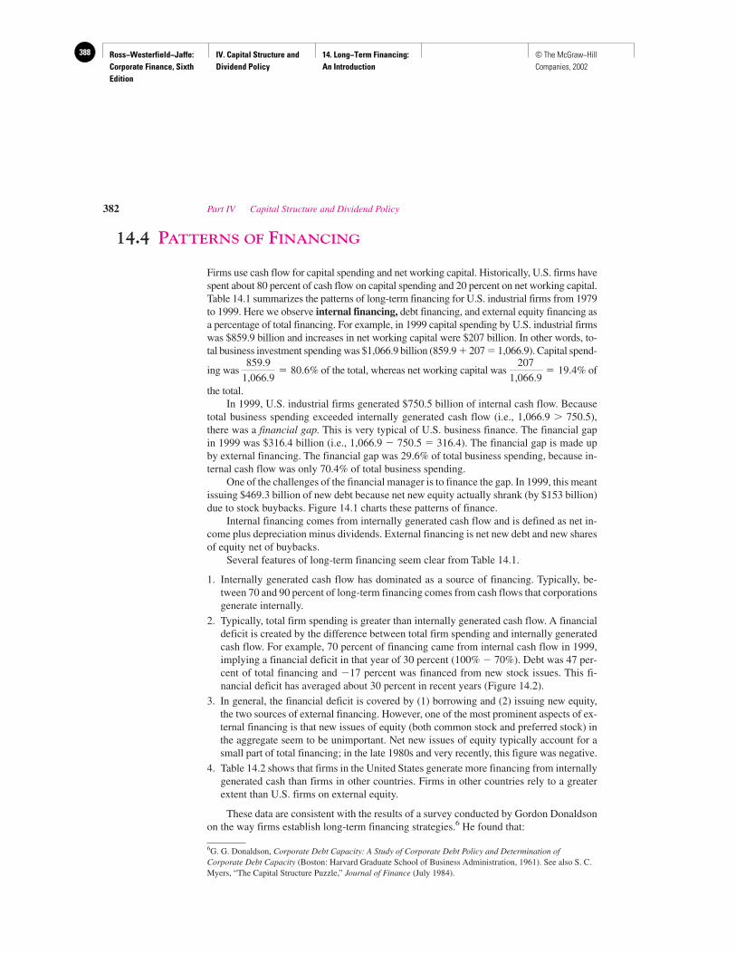
Ross−Westerfield−Jaffe: Corporate Finance, Sixth Edition
IV. Capital Structure and Dividend Policy
14. Long−Term Financing: An Introduction
388 © The McGraw−Hill Companies, 2002
14.4 PATTERNS OF FINANCING
Firms use cash flow for capital spending and net working capital. Historically, U.S. firms havespent about 80 percent of cash flow on capital spending and 20 percent on net working capital.Table 14.1 summarizes the patterns of long-term financing for U.S. industrial firms from 1979to 1999. Here we observe internal financing, debt financing, and external equity financing asa percentage of total financing. For example, in 1999 capital spending by U.S. industrial firmswas $859.9 billion and increases in net working capital were $207 billion. In other words, to-tal business investment spending was $1,066.9 billion (859.9 � 207 � 1,066.9). Capital spend-
ing was of the total, whereas net working capital was of
the total.In 1999, U.S. industrial firms generated $750.5 billion of internal cash flow. Because
total business spending exceeded internally generated cash flow (i.e., 1,066.9 � 750.5),there was a financial gap. This is very typical of U.S. business finance. The financial gapin 1999 was $316.4 billion (i.e., 1,066.9 � 750.5 � 316.4). The financial gap is made upby external financing. The financial gap was 29.6% of total business spending, because in-ternal cash flow was only 70.4% of total business spending.
One of the challenges of the financial manager is to finance the gap. In 1999, this meantissuing $469.3 billion of new debt because net new equity actually shrank (by $153 billion)due to stock buybacks. Figure 14.1 charts these patterns of finance.
Internal financing comes from internally generated cash flow and is defined as net in-come plus depreciation minus dividends. External financing is net new debt and new sharesof equity net of buybacks.
Several features of long-term financing seem clear from Table 14.1.
1. Internally generated cash flow has dominated as a source of financing. Typically, be-tween 70 and 90 percent of long-term financing comes from cash flows that corporationsgenerate internally.
2. Typically, total firm spending is greater than internally generated cash flow. A financialdeficit is created by the difference between total firm spending and internally generatedcash flow. For example, 70 percent of financing came from internal cash flow in 1999,implying a financial deficit in that year of 30 percent (100% � 70%). Debt was 47 per-cent of total financing and �17 percent was financed from new stock issues. This fi-nancial deficit has averaged about 30 percent in recent years (Figure 14.2).
3. In general, the financial deficit is covered by (1) borrowing and (2) issuing new equity,the two sources of external financing. However, one of the most prominent aspects of ex-ternal financing is that new issues of equity (both common stock and preferred stock) inthe aggregate seem to be unimportant. Net new issues of equity typically account for asmall part of total financing; in the late 1980s and very recently, this figure was negative.
4. Table 14.2 shows that firms in the United States generate more financing from internallygenerated cash than firms in other countries. Firms in other countries rely to a greaterextent than U.S. firms on external equity.
These data are consistent with the results of a survey conducted by Gordon Donaldsonon the way firms establish long-term financing strategies.6 He found that:
6G. G. Donaldson, Corporate Debt Capacity: A Study of Corporate Debt Policy and Determination ofCorporate Debt Capacity (Boston: Harvard Graduate School of Business Administration, 1961). See also S. C.Myers, “The Capital Structure Puzzle,” Journal of Finance (July 1984).
207
1,066.9� 19.4%
859.9
1,066.9� 80.6%
382 Part IV Capital Structure and Dividend Policy

Ross−Westerfield−Jaffe: Corporate Finance, Sixth Edition
IV. Capital Structure and Dividend Policy
14. Long−Term Financing: An Introduction
389© The McGraw−Hill Companies, 2002
383
�T
AB
LE
14
.1H
isto
rica
l U.S
. Fin
anci
ng P
atte
rns
(per
cent
),19
79 t
o 19
99
1979
1980
1981
1982
1983
1984
1985
1986
1987
1988
1989
1990
1991
1992
1993
1994
1995
1996
1997
1998
1999
Use
s of
fun
dsC
apita
l spe
ndin
g84
%80
%66
%86
%65
%64
%78
%72
%67
%70
%71
%76
%87
%72
%84
%76
%80
%92
%81
%92
%80
%N
et w
orki
ng c
apita
l16
2034
1435
3622
2833
3029
2413
2816
2420
819
820
Tota
l use
s10
010
010
010
010
010
010
010
010
010
010
010
010
010
010
010
010
010
010
010
010
0So
urce
s of
fun
dsIn
tern
al f
inan
cing
7965
6680
7471
8377
7980
7977
9786
8472
6787
7981
70E
xter
nal f
inan
cing
2135
3420
2629
1723
2120
2123
314
1628
3313
2119
30N
ew d
ebt
1831
3718
2045
3641
3746
4536
�1
912
3442
2335
5147
New
sto
ck3
4�
32
6�
16�
19�
18�
16�
26�
24�
134
54
�6
�9
�10
�14
�32
�17
Sour
ce:B
oard
of
Gov
erno
rs o
f th
e Fe
dera
l Res
erve
Sys
tem
,Flo
w o
f Fun
ds A
ccou
nts.
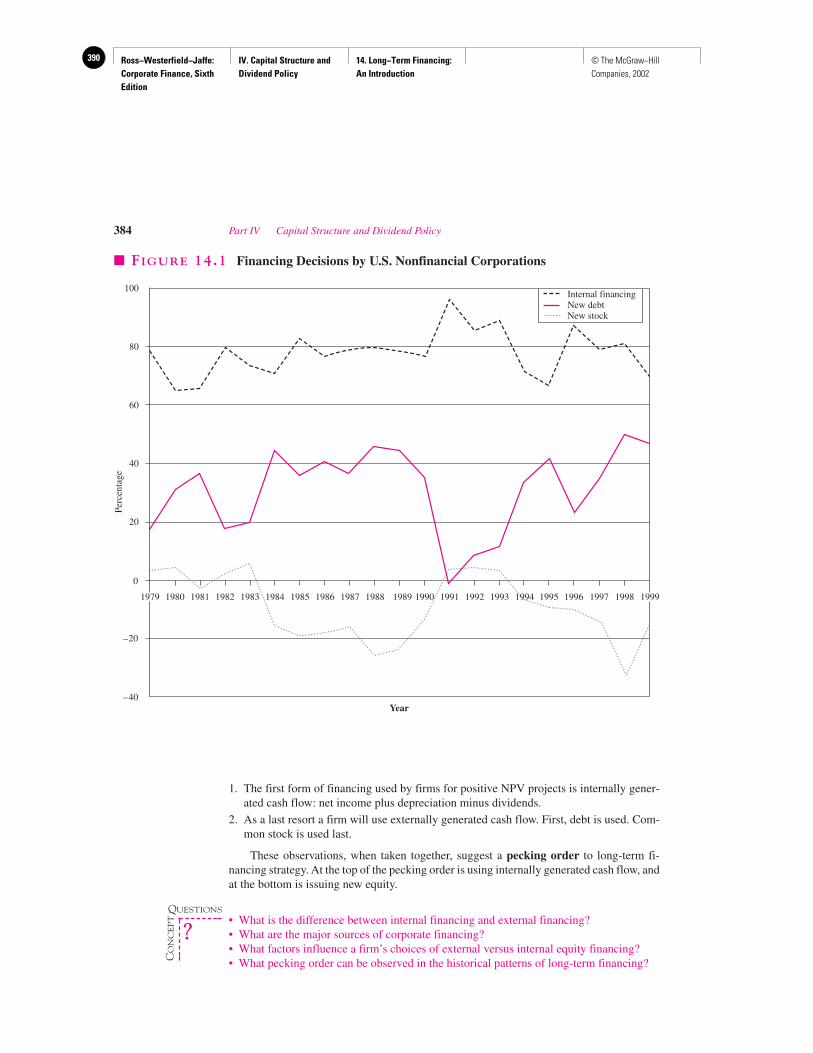
Ross−Westerfield−Jaffe: Corporate Finance, Sixth Edition
IV. Capital Structure and Dividend Policy
14. Long−Term Financing: An Introduction
390 © The McGraw−Hill Companies, 2002
384 Part IV Capital Structure and Dividend Policy
1. The first form of financing used by firms for positive NPV projects is internally gener-ated cash flow: net income plus depreciation minus dividends.
2. As a last resort a firm will use externally generated cash flow. First, debt is used. Com-mon stock is used last.
These observations, when taken together, suggest a pecking order to long-term fi-nancing strategy. At the top of the pecking order is using internally generated cash flow, andat the bottom is issuing new equity.
• What is the difference between internal financing and external financing?• What are the major sources of corporate financing?• What factors influence a firm’s choices of external versus internal equity financing?• What pecking order can be observed in the historical patterns of long-term financing?
Year
100
60
80
40
Perc
enta
ge
20
0
–20
–40
1979 1980 1981 1982 1983 1984 1985 1986 1987 1988 1989 1990 1991 1992 1993 1994 1995 1996 1997 1998
Internal financingNew debtNew stock
1999
� FIGURE 14.1 Financing Decisions by U.S. Nonfinancial Corporations
QUESTIONS
CO
NC
EP
T
?
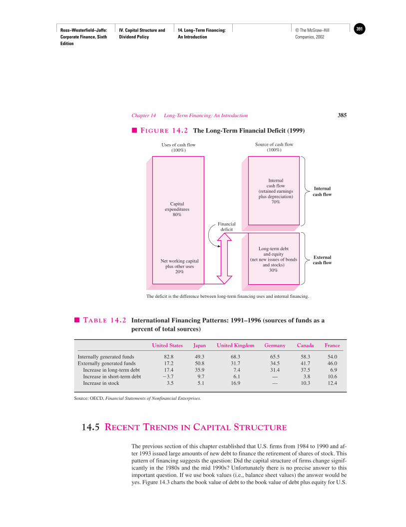
Ross−Westerfield−Jaffe: Corporate Finance, Sixth Edition
IV. Capital Structure and Dividend Policy
14. Long−Term Financing: An Introduction
391© The McGraw−Hill Companies, 2002
14.5 RECENT TRENDS IN CAPITAL STRUCTURE
The previous section of this chapter established that U.S. firms from 1984 to 1990 and af-ter 1993 issued large amounts of new debt to finance the retirement of shares of stock. Thispattern of financing suggests the question: Did the capital structure of firms change signif-icantly in the 1980s and the mid 1990s? Unfortunately there is no precise answer to this important question. If we use book values (i.e., balance sheet values) the answer would beyes. Figure 14.3 charts the book value of debt to the book value of debt plus equity for U.S.
Chapter 14 Long-Term Financing: An Introduction 385
Internalcash flow
Uses of cash flow(100%)
Source of cash flow(100%)
Financialdeficit
Externalcash flow
Internalcash flow
(retained earningsplus depreciation)
70%
Long-term debtand equity
(net new issues of bondsand stocks)
30%
Capitalexpenditures
80%
Net working capitalplus other uses
20%
� FIGURE 14.2 The Long-Term Financial Deficit (1999)
The deficit is the difference between long-term financing uses and internal financing.
� TABLE 14.2 International Financing Patterns: 1991–1996 (sources of funds as a percent of total sources)
United States Japan United Kingdom Germany Canada France
Internally generated funds 82.8 49.3 68.3 65.5 58.3 54.0Externally generated funds 17.2 50.8 31.7 34.5 41.7 46.0
Increase in long-term debt 17.4 35.9 7.4 31.4 37.5 6.9Increase in short-term debt �3.7 9.7 6.1 — 3.8 10.6Increase in stock 3.5 5.1 16.9 — 10.3 12.4
Source: OECD, Financial Statements of Nonfinancial Enterprises.
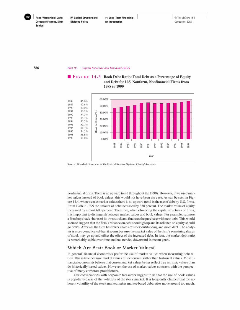
Ross−Westerfield−Jaffe: Corporate Finance, Sixth Edition
IV. Capital Structure and Dividend Policy
14. Long−Term Financing: An Introduction
392 © The McGraw−Hill Companies, 2002
nonfinancial firms. There is an upward trend throughout the 1990s. However, if we used mar-ket values instead of book values, this would not have been the case. As can be seen in Fig-ure 14.4, when we use market values there is no upward trend in the use of debt by U.S. firms.From 1988 to 1999 the amount of debt increased by 350 percent. The market value of equityincreased by almost 600 percent. Therefore, when observing the capital structures of firms,it is important to distinguish between market values and book values. For example, supposea firm buys back shares of its own stock and finances the purchase with new debt. This wouldseem to suggest that the firm’s reliance on debt should go up and its reliance on equity shouldgo down. After all, the firm has fewer shares of stock outstanding and more debt. The analy-sis is more complicated than it seems because the market value of the firm’s remaining sharesof stock may go up and offset the effect of the increased debt. In fact, the market debt ratiois remarkably stable over time and has trended downward in recent years.
Which Are Best: Book or Market Values?In general, financial economists prefer the use of market values when measuring debt ra-tios. This is true because market values reflect current rather than historical values. Most fi-nancial economists believe that current market values better reflect true intrinsic values thando historically based values. However, the use of market values contrasts with the perspec-tive of many corporate practitioners.
Our conversations with corporate treasurers suggest to us that the use of book valuesis popular because of the volatility of the stock market. It is frequently claimed that the in-herent volatility of the stock market makes market-based debt ratios move around too much.
386 Part IV Capital Structure and Dividend Policy
Boo
k de
bt r
atio
(%
)
Year
0.00%
1988
10.00%
20.00%
30.00%
40.00%
50.00%
60.00%198819891990199119921993199419951996199719981999
46.0%47.8%50.0%50.2%54.3%54.7%53.5%53.7%54.3%54.3%55.8%57.0%
1989
1990
1991
1992
1993
1994
1995
1996
1997
1998
1999
� FIGURE 14.3 Book Debt Ratio: Total Debt as a Percentage of Equityand Debt for U.S. Nonfarm, Nonfinancial Firms from1988 to 1999
Source: Board of Governors of the Federal Reserve System, Flow of Accounts.
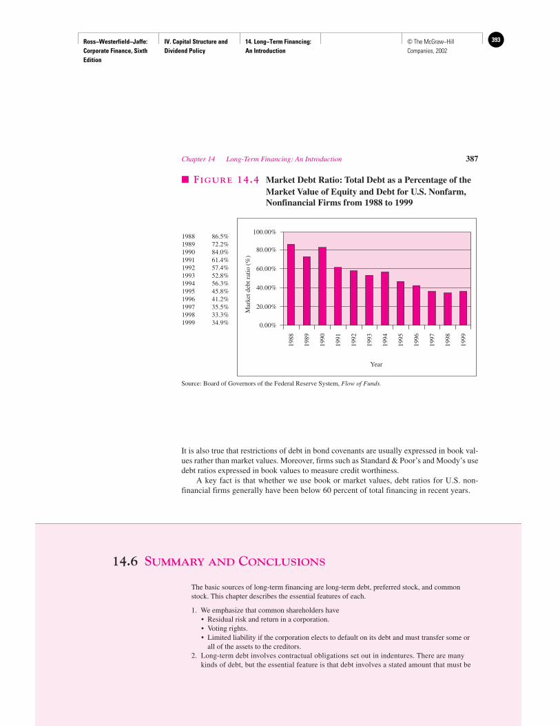
Ross−Westerfield−Jaffe: Corporate Finance, Sixth Edition
IV. Capital Structure and Dividend Policy
14. Long−Term Financing: An Introduction
393© The McGraw−Hill Companies, 2002
It is also true that restrictions of debt in bond covenants are usually expressed in book val-ues rather than market values. Moreover, firms such as Standard & Poor’s and Moody’s usedebt ratios expressed in book values to measure credit worthiness.
A key fact is that whether we use book or market values, debt ratios for U.S. non-financial firms generally have been below 60 percent of total financing in recent years.
14.6 SUMMARY AND CONCLUSIONS
The basic sources of long-term financing are long-term debt, preferred stock, and commonstock. This chapter describes the essential features of each.
1. We emphasize that common shareholders have• Residual risk and return in a corporation.• Voting rights.• Limited liability if the corporation elects to default on its debt and must transfer some or
all of the assets to the creditors.2. Long-term debt involves contractual obligations set out in indentures. There are many
kinds of debt, but the essential feature is that debt involves a stated amount that must be
Chapter 14 Long-Term Financing: An Introduction 387
Mar
ket d
ebt r
atio
(%
)
Year
0.00%
1988
20.00%
40.00%
60.00%
80.00%
100.00%198819891990199119921993199419951996199719981999
86.5%72.2%84.0%61.4%57.4%52.8%56.3%45.8%41.2%35.5%33.3%34.9%
1989
1990
1991
1992
1993
1994
1995
1996
1997
1998
1999
� FIGURE 14.4 Market Debt Ratio: Total Debt as a Percentage of theMarket Value of Equity and Debt for U.S. Nonfarm,Nonfinancial Firms from 1988 to 1999
Source: Board of Governors of the Federal Reserve System, Flow of Funds.
Ross−Westerfield−Jaffe: Corporate Finance, Sixth Edition
IV. Capital Structure and Dividend Policy
14. Long−Term Financing: An Introduction
394 © The McGraw−Hill Companies, 2002
repaid. Interest payments on debt are considered a business expense and are taxdeductible.
3. Preferred stock has some of the features of debt and some of the features of common equity.Holders of preferred stock have preference in liquidation and in dividend paymentscompared to holders of common equity.
4. Firms need financing for capital expenditures, working capital, and other long-term uses.Most of the financing is provided from internally generated cash flow. In the U.S., only about25 percent of financing comes from new debt and new equity. Only firms in Japan havehistorically relied more on external financing than on internal financing.
5. In the 1980s and recently, U.S. firms retired massive amounts of equity. These share buy-backs have been financed with new debt.
KEY TERMS
Book value 372 Preferred stock 379Capital surplus 372 Proxy 375Common stock 371 Retained earnings 372Cumulative voting 374 Seniority 378Dividends 375 Straight voting 374Internal financing 382 Subordinated 378Pecking order 384
SUGGESTED READING
The following provides some data on the financial structure of industrial corporations:Cost of Capital Quarterly. 1999 Yearbook. Ibbotson Associates, 2000.
QUESTIONS AND PROBLEMS
Common Stock14.1 Following are the equity accounts for Kerch Manufacturing.
Common stock, $2 par $ 135,430Capital surplus 203,145Retained earnings 2,370,025_________
Total $2,708,600
a. How many shares are outstanding?b. At what average price were the shares sold?c. What is the book value of Kerch stock?
14.2 The Eastern Spruce equity accounts for last year are as follows:
Common stock, $1 par, 500 shares outstanding (1)
Capital surplus $ 50,000Retained earnings 100,000________
Total (2)
a. Fill in the missing numbers.b. Eastern decided to issue 1,000 shares of new stock. The current price is $30 per share.
Show the effects of the new issue upon the equity accounts.
388 Part IV Capital Structure and Dividend Policy

Ross−Westerfield−Jaffe: Corporate Finance, Sixth Edition
IV. Capital Structure and Dividend Policy
14. Long−Term Financing: An Introduction
395© The McGraw−Hill Companies, 2002
14.3 Ulrich Inc.’s articles of incorporation authorize the firm to issue 500,000 shares of $5 par-value common stock, of which 325,000 shares have been issued. Those shares were sold atan average of 12 percent over par. In the quarter that ended last week, Ulrich earned$260,000 net income; 4 percent of that income was paid as a dividend. Prior to the close ofthe books, Ulrich had $3,545,000 in retained earnings. The company owns no treasury stock.a. Create the equity statement for Ulrich.b. Create a new equity statement that reflects the sale of 25,000 authorized but unissued
shares at the price of $4 per share.
14.4 The shareholders of the Unicorn Company need to elect seven new directors. There are2 million shares outstanding. How many shares do you need to be certain that you canelect at least one director ifa. Unicorn has straight voting?b. Unicorn has cumulative voting?
14.5 Power Inc. is going to elect six board members next month. Betty Brown owns 17.3 percentof the total shares outstanding. How confident can she be to have one of her candidatefriends be elected under the cumulative voting rule? And will her friend be elected forcertain if the voting procedure is changed to the staggering rule, under which shareholdersvote on three board members at a time?
14.6 a. An election is being held to fill two seats on the board of directors of a firm in whichyou hold stock. There is a total of 420 shares outstanding. If the election is conductedunder cumulative voting and you own 120 shares, how many more shares must youbuy to be assured of earning a seat on the board?
b. The shareholders of Motive Power Corp. need to elect three new directors to the board.There are 2,000,000 shares of common stock outstanding and current share price is $5.If Motive Power uses cumulative voting procedures, how much will it cost toguarantee yourself one seat on the Motive Power’s board?
Preferred Stock14.7 What are the differences between preferred stock and debt?
14.8 Preferred stock doesn’t offer corporate tax shield on the dividends paid. Why do we stillobserve some firms issuing preferred stock?
14.9 The yields on nonconvertible preferred stock are lower than the yields on corporate bonds.a. Why is there a difference?b. Which investors are the primary holders of preferred stock? Why?
Patterns of Financing14.10 What are the main differences between corporate debt and equity? Why do some firms
try to issue equity in the guise of debt?
Recent Trends in Capital Structure14.11 The Cable Company has $1 million of positive NPV projects it would like to take
advantage of. If Cable’s managers follow the historical pattern of long-term financing forU.S. industrial firms, what will their financing strategy be?
Chapter 14 Long-Term Financing: An Introduction 389
Ross−Westerfield−Jaffe: Corporate Finance, Sixth Edition
IV. Capital Structure and Dividend Policy
15. Capital Structure: Basic Concepts
396 © The McGraw−Hill Companies, 2002
Capital Structure: Basic Concepts
CH
AP
TE
R15
EXECUTIVE SUMMARY
Previous chapters of this book examined the capital-budgeting decision. We pointedout that this decision concerns the left-hand side of the balance sheet. The last twochapters began our discussion of the capital-structure decision,1 which deals with the
right-hand side of the balance sheet.In general, a firm can choose among many alternative capital structures. It can issue
a large amount of debt or it can issue very little debt. It can issue floating-rate preferredstock, warrants, convertible bonds, caps, and callers. It can arrange lease financing, bondswaps, and forward contracts. Because the number of instruments is so large, the varia-tions in capital structures are endless. We simplify the analysis by considering only com-mon stock and straight debt in this chapter. The “bells and whistles,” as they are called onWall Street, must await later chapters of the text. The capital-structure decision we con-sider is the decision to rely on debt. We examine the factors that are important in the choiceof a firm’s debt-to-equity ratio.
Our results in this chapter are basic. First we discuss the capital-structure decision in aworld with neither taxes nor other capital-market imperfections. Surprisingly, we find that thecapital-structure decision is a matter of indifference in this world. We next argue that there isa quirk in the U.S. tax code that subsidizes debt financing. Finally, we show that an increasein the firm’s value from debt financing leads to an increase in the value of the equity.
15.1 THE CAPITAL-STRUCTURE QUESTION AND THE
PIE THEORY
How should a firm choose its debt-equity ratio? We call our approach to the capital-struc-ture question the pie model. If you are wondering why we chose this name, just take a lookat Figure 15.1. The pie in question is the sum of the financial claims of the firm, debt andequity in this case. We define the value of the firm to be this sum. Hence, the value of thefirm, V, is
V � B � S (15.1)
where B is the market value of the debt and S is the market value of the equity. Figure 15.1presents two possible ways of slicing this pie between stock and debt: 40 percent–60 per-cent and 60 percent–40 percent. If the goal of the management of the firm is to make thefirm as valuable as possible, then the firm should pick the debt-equity ratio that makes thepie—the total value—as big as possible.
1It is conventional to refer to choices regarding debt and equity as capital-structure decisions. However, the termfinancial-structure decisions would be more accurate, and we use the terms interchangeably.
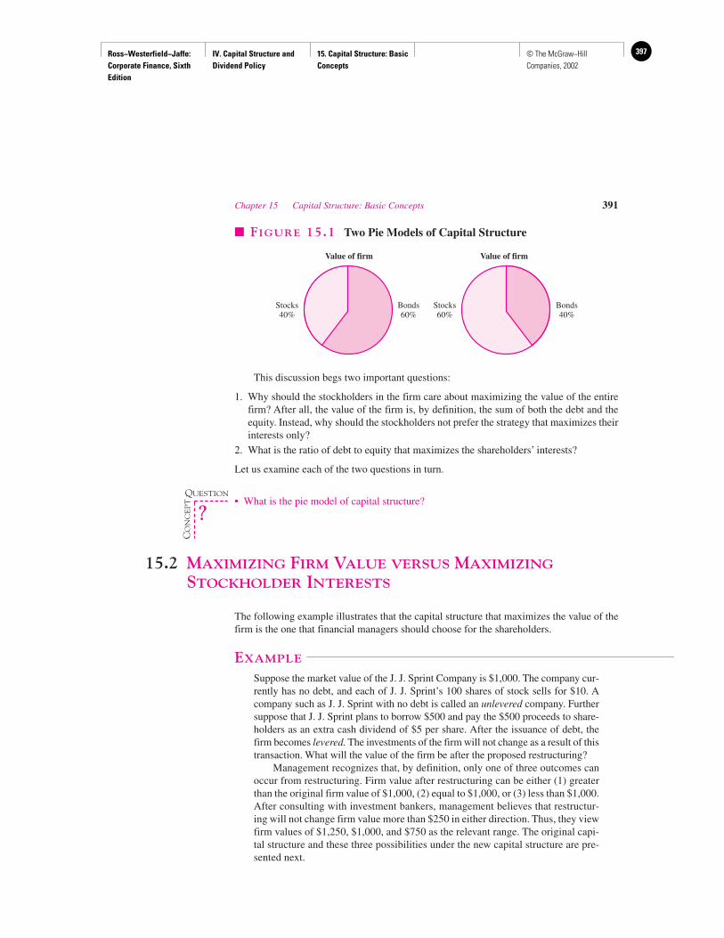
Ross−Westerfield−Jaffe: Corporate Finance, Sixth Edition
IV. Capital Structure and Dividend Policy
15. Capital Structure: Basic Concepts
397© The McGraw−Hill Companies, 2002
This discussion begs two important questions:
1. Why should the stockholders in the firm care about maximizing the value of the entirefirm? After all, the value of the firm is, by definition, the sum of both the debt and theequity. Instead, why should the stockholders not prefer the strategy that maximizes theirinterests only?
2. What is the ratio of debt to equity that maximizes the shareholders’ interests?
Let us examine each of the two questions in turn.
• What is the pie model of capital structure?
15.2 MAXIMIZING FIRM VALUE VERSUS MAXIMIZING
STOCKHOLDER INTERESTS
The following example illustrates that the capital structure that maximizes the value of thefirm is the one that financial managers should choose for the shareholders.
EXAMPLE
Suppose the market value of the J. J. Sprint Company is $1,000. The company cur-rently has no debt, and each of J. J. Sprint’s 100 shares of stock sells for $10. Acompany such as J. J. Sprint with no debt is called an unlevered company. Furthersuppose that J. J. Sprint plans to borrow $500 and pay the $500 proceeds to share-holders as an extra cash dividend of $5 per share. After the issuance of debt, thefirm becomes levered. The investments of the firm will not change as a result of thistransaction. What will the value of the firm be after the proposed restructuring?
Management recognizes that, by definition, only one of three outcomes canoccur from restructuring. Firm value after restructuring can be either (1) greaterthan the original firm value of $1,000, (2) equal to $1,000, or (3) less than $1,000.After consulting with investment bankers, management believes that restructur-ing will not change firm value more than $250 in either direction. Thus, they viewfirm values of $1,250, $1,000, and $750 as the relevant range. The original capi-tal structure and these three possibilities under the new capital structure are pre-sented next.
Chapter 15 Capital Structure: Basic Concepts 391
Value of firm Value of firm
Stocks40%
Stocks60%
Bonds60%
Bonds40%
� FIGURE 15.1 Two Pie Models of Capital Structure
QUESTION
CO
NC
EP
T
?
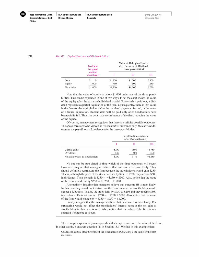
Ross−Westerfield−Jaffe: Corporate Finance, Sixth Edition
IV. Capital Structure and Dividend Policy
15. Capital Structure: Basic Concepts
398 © The McGraw−Hill Companies, 2002
Value of Debt plus EquityNo Debt after Payment of Dividend(original (three possibilities)capital
structure) I II III
Debt $ 0 $ 500 $ 500 $500Equity 1,000 750 500 250______ ______ ______ ____Firm value $1,000 $1,250 $1,000 $750
Note that the value of equity is below $1,000 under any of the three possi-bilities. This can be explained in one of two ways. First, the chart shows the valueof the equity after the extra cash dividend is paid. Since cash is paid out, a divi-dend represents a partial liquidation of the firm. Consequently, there is less valuein the firm for the equityholders after the dividend payment. Second, in the eventof a future liquidation, stockholders will be paid only after bondholders havebeen paid in full. Thus, the debt is an encumbrance of the firm, reducing the valueof the equity.
Of course, management recognizes that there are infinite possible outcomes.The above three are to be viewed as representative outcomes only. We can now de-termine the payoff to stockholders under the three possibilities.
Payoff to Shareholdersafter Restructuring
I II III
Capital gains �$250 �$500 �$750Dividends 500 500 500______ ______ ______Net gain or loss to stockholders $250 $ 0 �$250
No one can be sure ahead of time which of the three outcomes will occur.However, imagine that managers believe that outcome I is most likely. Theyshould definitely restructure the firm because the stockholders would gain $250.That is, although the price of the stock declines by $250 to $750, they receive $500in dividends. Their net gain is $250 � �$250 � $500. Also, notice that the valueof the firm would rise by $250 � $1,250 � $1,000.
Alternatively, imagine that managers believe that outcome III is most likely.In this case they should not restructure the firm because the stockholders wouldexpect a $250 loss. That is, the stock falls by $750 to $250 and they receive $500in dividends. Their net loss is �$250 � �$750 � $500. Also, notice that the valueof the firm would change by �$250 � $750 � $1,000.
Finally, imagine that the managers believe that outcome II is most likely. Re-structuring would not affect the stockholders’ interest because the net gain tostockholders in this case is zero. Also, notice that the value of the firm is un-changed if outcome II occurs.
This example explains why managers should attempt to maximize the value of the firm.In other words, it answers question (1) in Section 15.1. We find in this example that:
Changes in capital structure benefit the stockholders if and only if the value of the firm increases.
392 Part IV Capital Structure and Dividend Policy
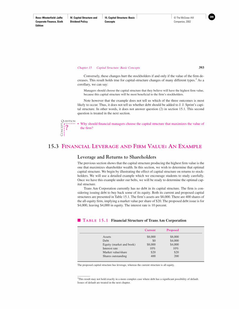
Ross−Westerfield−Jaffe: Corporate Finance, Sixth Edition
IV. Capital Structure and Dividend Policy
15. Capital Structure: Basic Concepts
399© The McGraw−Hill Companies, 2002
Conversely, these changes hurt the stockholders if and only if the value of the firm de-creases. This result holds true for capital-structure changes of many different types.2 As acorollary, we can say:
Managers should choose the capital structure that they believe will have the highest firm value,because this capital structure will be most beneficial to the firm’s stockholders.
Note however that the example does not tell us which of the three outcomes is mostlikely to occur. Thus, it does not tell us whether debt should be added to J. J. Sprint’s capi-tal structure. In other words, it does not answer question (2) in section 15.1. This secondquestion is treated in the next section.
• Why should financial managers choose the capital structure that maximizes the value ofthe firm?
15.3 FINANCIAL LEVERAGE AND FIRM VALUE: AN EXAMPLE
Leverage and Returns to ShareholdersThe previous section shows that the capital structure producing the highest firm value is theone that maximizes shareholder wealth. In this section, we wish to determine that optimalcapital structure. We begin by illustrating the effect of capital structure on returns to stock-holders. We will use a detailed example which we encourage students to study carefully.Once we have this example under our belts, we will be ready to determine the optimal cap-ital structure.
Trans Am Corporation currently has no debt in its capital structure. The firm is con-sidering issuing debt to buy back some of its equity. Both its current and proposed capitalstructures are presented in Table 15.1. The firm’s assets are $8,000. There are 400 shares ofthe all-equity firm, implying a market value per share of $20. The proposed debt issue is for$4,000, leaving $4,000 in equity. The interest rate is 10 percent.
Chapter 15 Capital Structure: Basic Concepts 393
2This result may not hold exactly in a more complex case where debt has a significant possibility of default.Issues of default are treated in the next chapter.
� TABLE 15.1 Financial Structure of Trans Am Corporation
Current Proposed
Assets $8,000 $8,000Debt $0 $4,000Equity (market and book) $8,000 $4,000Interest rate 10% 10%Market value/share $20 $20Shares outstanding 400 200
The proposed capital structure has leverage, whereas the current structure is all equity.
QUESTION
CO
NC
EP
T
?
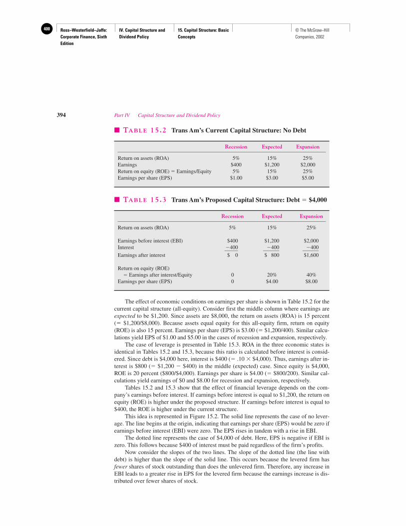
Ross−Westerfield−Jaffe: Corporate Finance, Sixth Edition
IV. Capital Structure and Dividend Policy
15. Capital Structure: Basic Concepts
400 © The McGraw−Hill Companies, 2002
The effect of economic conditions on earnings per share is shown in Table 15.2 for thecurrent capital structure (all-equity). Consider first the middle column where earnings areexpected to be $1,200. Since assets are $8,000, the return on assets (ROA) is 15 percent(� $1,200/$8,000). Because assets equal equity for this all-equity firm, return on equity(ROE) is also 15 percent. Earnings per share (EPS) is $3.00 (� $1,200/400). Similar calcu-lations yield EPS of $1.00 and $5.00 in the cases of recession and expansion, respectively.
The case of leverage is presented in Table 15.3. ROA in the three economic states isidentical in Tables 15.2 and 15.3, because this ratio is calculated before interest is consid-ered. Since debt is $4,000 here, interest is $400 (� .10 � $4,000). Thus, earnings after in-terest is $800 (� $1,200 � $400) in the middle (expected) case. Since equity is $4,000,ROE is 20 percent ($800/$4,000). Earnings per share is $4.00 (� $800/200). Similar cal-culations yield earnings of $0 and $8.00 for recession and expansion, respectively.
Tables 15.2 and 15.3 show that the effect of financial leverage depends on the com-pany’s earnings before interest. If earnings before interest is equal to $1,200, the return onequity (ROE) is higher under the proposed structure. If earnings before interest is equal to$400, the ROE is higher under the current structure.
This idea is represented in Figure 15.2. The solid line represents the case of no lever-age. The line begins at the origin, indicating that earnings per share (EPS) would be zero ifearnings before interest (EBI) were zero. The EPS rises in tandem with a rise in EBI.
The dotted line represents the case of $4,000 of debt. Here, EPS is negative if EBI iszero. This follows because $400 of interest must be paid regardless of the firm’s profits.
Now consider the slopes of the two lines. The slope of the dotted line (the line withdebt) is higher than the slope of the solid line. This occurs because the levered firm hasfewer shares of stock outstanding than does the unlevered firm. Therefore, any increase inEBI leads to a greater rise in EPS for the levered firm because the earnings increase is dis-tributed over fewer shares of stock.
394 Part IV Capital Structure and Dividend Policy
� TABLE 15.2 Trans Am’s Current Capital Structure: No Debt
Recession Expected Expansion
Return on assets (ROA) 5% 15% 25%Earnings $400 $1,200 $2,000Return on equity (ROE) � Earnings/Equity 5% 15% 25%Earnings per share (EPS) $1.00 $3.00 $5.00
� TABLE 15.3 Trans Am’s Proposed Capital Structure: Debt � $4,000
Recession Expected Expansion
Return on assets (ROA) 5% 15% 25%
Earnings before interest (EBI) $400 $1,200 $2,000Interest �400 �400 �400_____ ______ ______Earnings after interest $ 0 $ 800 $1,600
Return on equity (ROE)� Earnings after interest/Equity 0 20% 40%
Earnings per share (EPS) 0 $4.00 $8.00
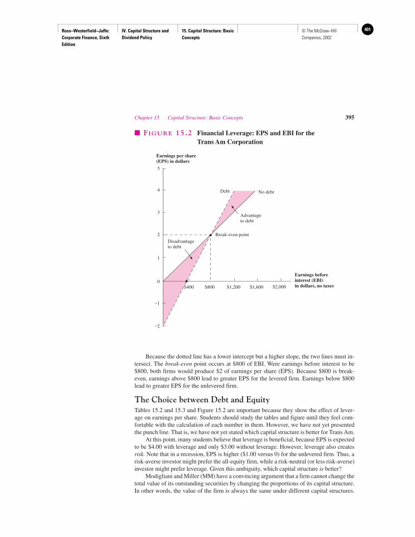
Ross−Westerfield−Jaffe: Corporate Finance, Sixth Edition
IV. Capital Structure and Dividend Policy
15. Capital Structure: Basic Concepts
401© The McGraw−Hill Companies, 2002
Because the dotted line has a lower intercept but a higher slope, the two lines must in-tersect. The break-even point occurs at $800 of EBI. Were earnings before interest to be$800, both firms would produce $2 of earnings per share (EPS). Because $800 is break-even, earnings above $800 lead to greater EPS for the levered firm. Earnings below $800lead to greater EPS for the unlevered firm.
The Choice between Debt and EquityTables 15.2 and 15.3 and Figure 15.2 are important because they show the effect of lever-age on earnings per share. Students should study the tables and figure until they feel com-fortable with the calculation of each number in them. However, we have not yet presentedthe punch line. That is, we have not yet stated which capital structure is better for Trans Am.
At this point, many students believe that leverage is beneficial, because EPS is expectedto be $4.00 with leverage and only $3.00 without leverage. However, leverage also createsrisk. Note that in a recession, EPS is higher ($1.00 versus 0) for the unlevered firm. Thus, arisk-averse investor might prefer the all-equity firm, while a risk-neutral (or less risk-averse)investor might prefer leverage. Given this ambiguity, which capital structure is better?
Modigliani and Miller (MM) have a convincing argument that a firm cannot change thetotal value of its outstanding securities by changing the proportions of its capital structure.In other words, the value of the firm is always the same under different capital structures.
Chapter 15 Capital Structure: Basic Concepts 395
Debt No debt
Advantageto debt
Break-even pointDisadvantageto debt
$400 $800 $1,200 $1,600 $2,000
–2
–1
0
1
2
3
4
5
Earnings per share(EPS) in dollars
Earnings beforeinterest (EBI)in dollars, no taxes
� FIGURE 15.2 Financial Leverage: EPS and EBI for the Trans Am Corporation
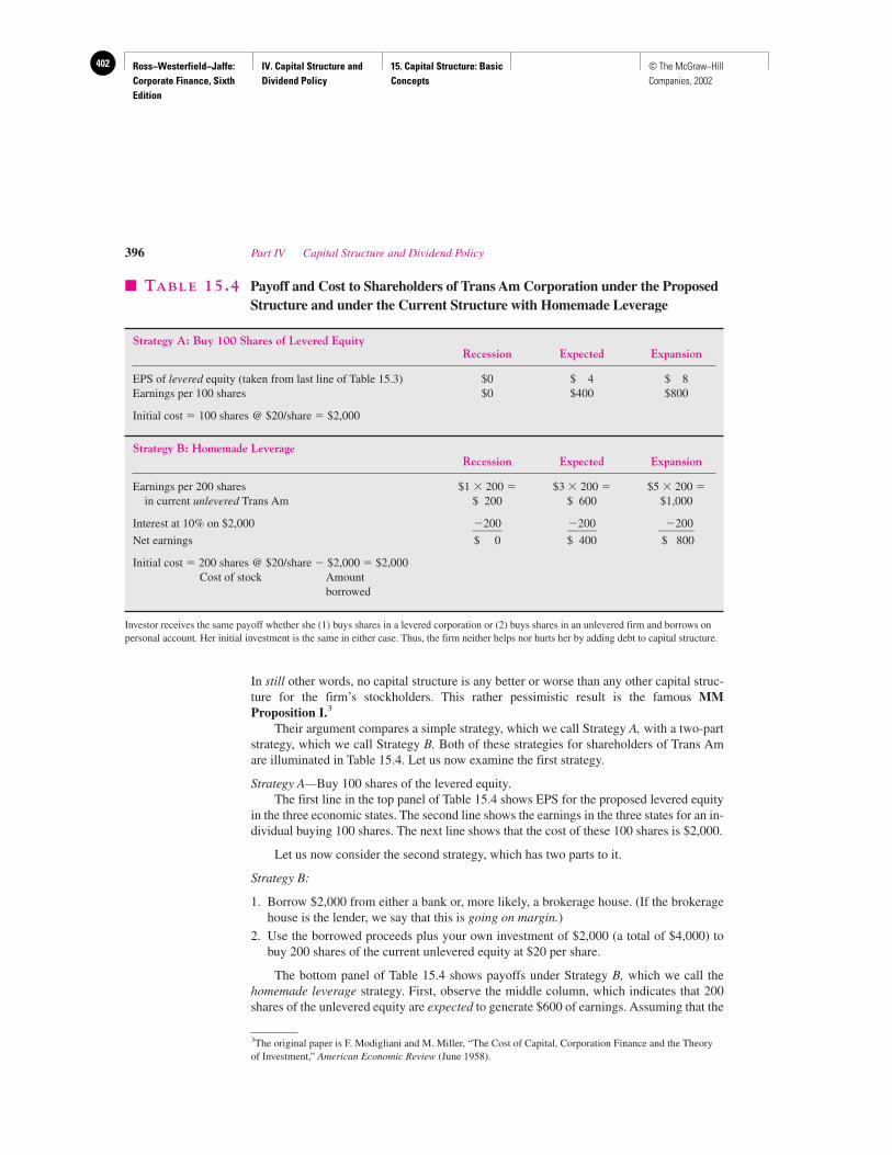
Ross−Westerfield−Jaffe: Corporate Finance, Sixth Edition
IV. Capital Structure and Dividend Policy
15. Capital Structure: Basic Concepts
402 © The McGraw−Hill Companies, 2002
In still other words, no capital structure is any better or worse than any other capital struc-ture for the firm’s stockholders. This rather pessimistic result is the famous MMProposition I.3
Their argument compares a simple strategy, which we call Strategy A, with a two-partstrategy, which we call Strategy B. Both of these strategies for shareholders of Trans Amare illuminated in Table 15.4. Let us now examine the first strategy.
Strategy A—Buy 100 shares of the levered equity.The first line in the top panel of Table 15.4 shows EPS for the proposed levered equity
in the three economic states. The second line shows the earnings in the three states for an in-dividual buying 100 shares. The next line shows that the cost of these 100 shares is $2,000.
Let us now consider the second strategy, which has two parts to it.
Strategy B:
1. Borrow $2,000 from either a bank or, more likely, a brokerage house. (If the brokeragehouse is the lender, we say that this is going on margin.)
2. Use the borrowed proceeds plus your own investment of $2,000 (a total of $4,000) tobuy 200 shares of the current unlevered equity at $20 per share.
The bottom panel of Table 15.4 shows payoffs under Strategy B, which we call thehomemade leverage strategy. First, observe the middle column, which indicates that 200shares of the unlevered equity are expected to generate $600 of earnings. Assuming that the
396 Part IV Capital Structure and Dividend Policy
3The original paper is F. Modigliani and M. Miller, “The Cost of Capital, Corporation Finance and the Theoryof Investment,” American Economic Review (June 1958).
� TABLE 15.4 Payoff and Cost to Shareholders of Trans Am Corporation under the ProposedStructure and under the Current Structure with Homemade Leverage
Strategy A: Buy 100 Shares of Levered EquityRecession Expected Expansion
EPS of levered equity (taken from last line of Table 15.3) $0 $ 4 $ 8Earnings per 100 shares $0 $400 $800
Initial cost � 100 shares @ $20/share � $2,000
Strategy B: Homemade LeverageRecession Expected Expansion
Earnings per 200 shares $1 � 200 � $3 � 200 � $5 � 200 �in current unlevered Trans Am $ 200 $ 600 $1,000
Interest at 10% on $2,000 �200 �200 �200_____ _____ ______Net earnings $ 0 $ 400 $ 800
Initial cost � 200 shares @ $20/share � $2,000 � $2,000Cost of stock Amount
borrowed
Investor receives the same payoff whether she (1) buys shares in a levered corporation or (2) buys shares in an unlevered firm and borrows onpersonal account. Her initial investment is the same in either case. Thus, the firm neither helps nor hurts her by adding debt to capital structure.
Ross−Westerfield−Jaffe: Corporate Finance, Sixth Edition
IV. Capital Structure and Dividend Policy
15. Capital Structure: Basic Concepts
403© The McGraw−Hill Companies, 2002
$2,000 is borrowed at a 10 percent interest rate, the interest expense is $200 (� 0.10 �$2,000). Thus, the net earnings are expected to be $400. A similar calculation generates netearnings of either $0 or $800 in recession or expansion, respectively.
Now, let us compare these two strategies, both in terms of earnings per year and interms of initial cost. The top panel of the table shows that Strategy A generates earnings of$0, $400, and $800 in the three states. The bottom panel of the table shows that Strategy Bgenerates the same net earnings in the three states.
The top panel of the table shows that Strategy A involves an initial cost of $2,000.Similarly, the bottom panel shows an identical net cost of $2,000 for Strategy B.
This shows a very important result. Both the cost and the payoff from the two strate-gies are the same. Thus, one must conclude that Trans Am is neither helping nor hurting itsstockholders by restructuring. In other words, an investor is not receiving anything fromcorporate leverage that he or she could not receive on their own.
Note that, as shown in Table 15.1, the equity of the unlevered firm is valued at $8,000.Since the equity of the levered firm is $4,000 and its debt is $4,000, the value of the leveredfirm is also $8,000. Now suppose that, for whatever reason, the value of the levered firm wereactually greater than the value of the unlevered firm. Here, Strategy A would cost more thanStrategy B. In this case, an investor would prefer to borrow on his own account and invest inthe stock of the unlevered firm. He would get the same net earnings each year as if he hadinvested in the stock of the levered firm. However, his cost would be less. The strategy wouldnot be unique to our investor. Given the higher value of the levered firm, no rational investorwould invest in the stock of the levered firm. Anyone desiring shares in the levered firmwould get the same dollar return more cheaply by borrowing to finance a purchase of the un-levered firm’s shares. The equilibrium result would be, of course, that the value of the lev-ered firm would fall, and the value of the unlevered firm would rise until they became equal.At this point, individuals would be indifferent between Strategy A and Strategy B.
This example illustrates the basic result of Modigliani-Miller (MM) and is commonlycalled their Proposition I. We state this proposition as:
MM Proposition I (no taxes): The value of the levered firm is the same as the value of the un-levered firm.
This is perhaps the most important result in all of corporate finance. In fact, it is gener-ally considered the beginning point of modern managerial finance. Before MM, the effect ofleverage on the value of the firm was considered complex and convoluted. Modigliani andMiller show a blindingly simple result: If levered firms are priced too high, rational investorswill simply borrow on their personal accounts to buy shares in unlevered firms. This substi-tution is oftentimes called homemade leverage. As long as individuals borrow (and lend) onthe same terms as the firms, they can duplicate the effects of corporate leverage on their own.
The example of Trans Am Corporation shows that leverage does not affect the value ofthe firm. Since we showed earlier that stockholders’ welfare is directly related to the firm’svalue, the example indicates that changes in capital structure cannot affect the stockhold-ers’ welfare.
A Key AssumptionThe MM result hinges on the assumption that individuals can borrow as cheaply as corpo-rations. If, alternatively, individuals can only borrow at a higher rate, one can easily showthat corporations can increase firm value by borrowing.
Is this assumption of equal borrowing costs a good one? Individuals who want to buystock and borrow can do so by establishing a margin account with the broker. Under thisarrangement, the broker loans the individual a portion of the purchase price. For example,
Chapter 15 Capital Structure: Basic Concepts 397
Ross−Westerfield−Jaffe: Corporate Finance, Sixth Edition
IV. Capital Structure and Dividend Policy
15. Capital Structure: Basic Concepts
404 © The McGraw−Hill Companies, 2002
the individual might buy $10,000 of stock by investing $6,000 of her own funds and bor-rowing $4,000 from the broker. Should the stock be worth $9,000 on the next day, the in-dividual’s net worth or equity in the account would be $5,000 � $9,000 � $4,000.4
The broker fears that a sudden price drop will cause the equity in the individual’s ac-count to be negative, implying that the broker may not get her loan repaid in full. To guardagainst this possibility, stock exchange rules require that the individual make additionalcash contributions (replenish her margin account) as the stock price falls. Because (1) theprocedures for replenishing the account have developed over many years, and (2) the bro-ker holds the stock as collateral, there is little default risk to the broker.5 In particular, ifmargin contributions are not made on time, the broker can sell the stock in order to satisfyher loan. Therefore, brokers generally charge low interest, with many rates being onlyslightly above the risk-free rate.
By contrast, corporations frequently borrow using illiquid assets (e.g., plant and equip-ment) as collateral. The costs to the lender of initial negotiation and ongoing supervision,as well as of working out arrangements in the event of financial distress, can be quite sub-stantial. Thus, it is difficult to argue that individuals must borrow at higher rates than cancorporations.6
• Describe financial leverage.• What is levered equity?• How can a shareholder of Trans Am undo the company’s financial leverage?
15.4 MODIGLIANI AND MILLER: PROPOSITION II (NO TAXES)
Risk to Equityholders Rises with LeverageAt a Trans Am corporate meeting, a corporate officer said, “Well, maybe it does not matterwhether the corporation or the individual levers—as long as some leverage takes place. Lever-age benefits investors. After all, an investor’s expected return rises with the amount of the lever-age present.” He then pointed out that, as shown in Tables 15.2 and 15.3, the expected returnon unlevered equity is 15 percent while the expected return on levered equity is 20 percent.
However, another officer replied, “Not necessarily. Though the expected return riseswith leverage, the risk rises as well.” This point can be seen from an examination of Tables15.2 and 15.3. With earnings before interest (EBI) varying between $400 and $2,000, earn-ings per share (EPS) for the stockholders of the unlevered firm vary between $1.00 and$5.00. EPS for the stockholders of the levered firm vary between $0 and $8.00. This greaterrange for the EPS of the levered firm implies greater risk for the levered firm’s stockhold-ers. In other words, levered stockholders have better returns in good times than do unlev-ered stockholders but have worse returns in bad times. The two tables also show greaterrange for the ROE of the levered firm’s stockholders. The above interpretation concerningrisk applies here as well.
398 Part IV Capital Structure and Dividend Policy
4We are ignoring the one-day interest charge on the loan.5Had this text been published before October 19, 1987, when stock prices declined by more than 20 percent, wemight have used the phrase “virtually no” risk instead of “little.”6One caveat is in order. Initial margin or borrowing is currently limited by law to 50 percent of value. Certaincompanies, like financial institutions, borrow over 90 percent of their firm’s market value. Individuals borrowingagainst the stock of all-equity corporations cannot duplicate the debt of these highly levered corporations.
QUESTIONS
CO
NC
EP
T
?

Ross−Westerfield−Jaffe: Corporate Finance, Sixth Edition
IV. Capital Structure and Dividend Policy
15. Capital Structure: Basic Concepts
405© The McGraw−Hill Companies, 2002
The same insight can be taken from Figure 15.2. The slope of the line for the leveredfirm is greater than the slope of the line for the unlevered firm. This means that the leveredstockholders have better returns in good times than do unlevered stockholders but haveworse returns in bad times, implying greater risk with leverage. In other words, the slope ofthe line measures the risk to stockholders, since the slope indicates the responsiveness ofROE to changes in firm performance (earnings before interest).
Proposition II: Required Return to Equityholders Rises with LeverageSince levered equity has greater risk, it should have a greater expected return as compen-sation. In our example, the market requires only a 15-percent expected return for the un-levered equity, but it requires a 20-percent expected return for the levered equity.
This type of reasoning allows us to develop MM Proposition II. Here, MM argue thatthe expected return on equity is positively related to leverage, because the risk to equity-holders increases with leverage.
To develop this position recall from Chapter 12 that the firm’s weighted average costof capital, rWACC, can be written as:7
(15.2)
where
rB is the interest rate, also called the cost of debtrS is the expected return on equity or stock, also called the cost of equity or the
required return on equityrWACC is the firm’s weighted average cost of capital
B is the value of the firm’s debt or bondsS is the value of the firm’s stock or equity
Formula (15.2) is quite intuitive. It simply says that a firm’s weighted average cost ofcapital is a weighted average of its cost of debt and its cost of equity. The weight applied todebt is the proportion of debt in the capital structure, and the weight applied to equity is theproportion of equity in the capital structure. Calculations of rWACC from formula (15.2) forboth the unlevered and the levered firm are presented in Table 15.5.
An implication of MM Proposition I is that rWACC is a constant for a given firm, re-gardless of the capital structure.8 For example, Table 15.5 shows that rWACC for Trans Amis 15 percent, with or without leverage.
Let us now define r0 to be the cost of capital for an all-equity firm. For the Trans AmCorp., r0 is calculated as:
As can be seen from Table 15.5, rWACC is equal to r0 for Trans Am. In fact, rWACC must al-ways equal r0 in a world without corporate taxes.
r0 �Expected earnings to unlevered firm
Unlevered equity�
$1,200
$8,000� 15%
B
B � S� rB �
S
B � S� rS
Chapter 15 Capital Structure: Basic Concepts 399
7Since we do not have taxes here, the cost of debt is rB, not rB(1 � TC) as it was in Chapter 12.8This statement holds in a world of no taxes. It does not hold in a world with taxes, a point to be brought outlater in this chapter (see Figure 15.6).
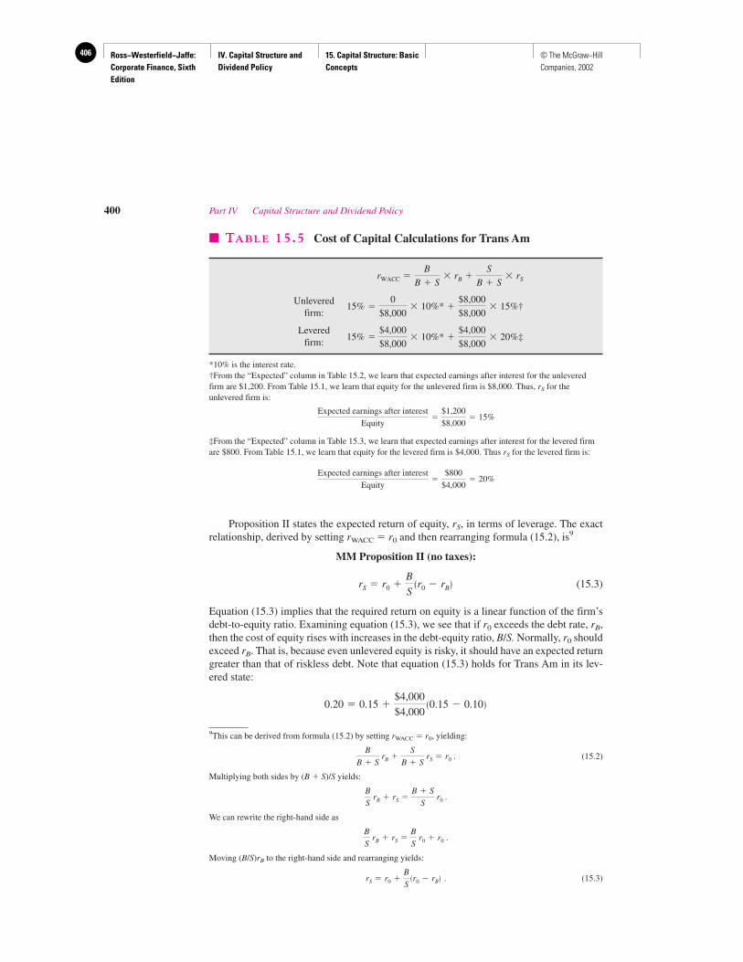
Ross−Westerfield−Jaffe: Corporate Finance, Sixth Edition
IV. Capital Structure and Dividend Policy
15. Capital Structure: Basic Concepts
406 © The McGraw−Hill Companies, 2002
Proposition II states the expected return of equity, rS, in terms of leverage. The exactrelationship, derived by setting rWACC � r0 and then rearranging formula (15.2), is9
MM Proposition II (no taxes):
(15.3)
Equation (15.3) implies that the required return on equity is a linear function of the firm’sdebt-to-equity ratio. Examining equation (15.3), we see that if r0 exceeds the debt rate, rB,then the cost of equity rises with increases in the debt-equity ratio, B/S. Normally, r0 shouldexceed rB. That is, because even unlevered equity is risky, it should have an expected returngreater than that of riskless debt. Note that equation (15.3) holds for Trans Am in its lev-ered state:
0.20 � 0.15 �$4,000
$4,000�0.15 � 0.10�
rS � r0 �B
S�r0 � rB�
400 Part IV Capital Structure and Dividend Policy
� TABLE 15.5 Cost of Capital Calculations for Trans Am
Unleveredfirm:
* †
Leveredfirm: * ‡
*10% is the interest rate.†From the “Expected” column in Table 15.2, we learn that expected earnings after interest for the unleveredfirm are $1,200. From Table 15.1, we learn that equity for the unlevered firm is $8,000. Thus, rS for theunlevered firm is:
‡From the “Expected” column in Table 15.3, we learn that expected earnings after interest for the levered firmare $800. From Table 15.1, we learn that equity for the levered firm is $4,000. Thus rS for the levered firm is:
Expected earnings after interest
Equity�
$800
$4,000� 20%
Expected earnings after interest
Equity�
$1,200
$8,000� 15%
�$4,000
$8,000� 20%15% �
$4,000
$8,000� 10%
�$8,000
$8,000� 15%15% �
0
$8,000� 10%
rWACC �B
B � S� rB �
S
B � S� rS
9This can be derived from formula (15.2) by setting rWACC � r0, yielding:
. (15.2)
Multiplying both sides by (B � S)/S yields:
.
We can rewrite the right-hand side as
.
Moving (B/S)rB to the right-hand side and rearranging yields:
. (15.3)rS � r0 �B
S�r0 � rB�
B
S rB � rS �
B
S r0 � r0
B
S rB � rS �
B � S
S r0
B
B � S rB �
S
B � S rS � r0
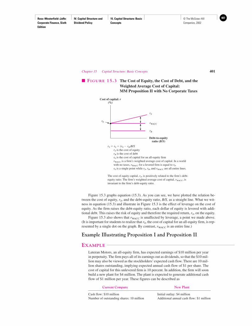
Ross−Westerfield−Jaffe: Corporate Finance, Sixth Edition
IV. Capital Structure and Dividend Policy
15. Capital Structure: Basic Concepts
407© The McGraw−Hill Companies, 2002
Figure 15.3 graphs equation (15.3). As you can see, we have plotted the relation be-tween the cost of equity, rS, and the debt-equity ratio, B/S, as a straight line. What we wit-ness in equation (15.3) and illustrate in Figure 15.3 is the effect of leverage on the cost ofequity. As the firm raises the debt-equity ratio, each dollar of equity is levered with addi-tional debt. This raises the risk of equity and therefore the required return, rS, on the equity.
Figure 15.3 also shows that rWACC is unaffected by leverage, a point we made above.(It is important for students to realize that r0, the cost of capital for an all-equity firm, is rep-resented by a single dot on the graph. By contrast, rWACC is an entire line.)
Example Illustrating Proposition I and Proposition II
EXAMPLE
Luteran Motors, an all-equity firm, has expected earnings of $10 million per yearin perpetuity. The firm pays all of its earnings out as dividends, so that the $10 mil-lion may also be viewed as the stockholders’ expected cash flow. There are 10 mil-lion shares outstanding, implying expected annual cash flow of $1 per share. Thecost of capital for this unlevered firm is 10 percent. In addition, the firm will soonbuild a new plant for $4 million. The plant is expected to generate additional cashflow of $1 million per year. These figures can be described as
Current Company New Plant
Cash flow: $10 million Initial outlay: $4 millionNumber of outstanding shares: 10 million Additional annual cash flow: $1 million
Chapter 15 Capital Structure: Basic Concepts 401
Debt-to-equityratio (B/S)
Cost of capital: r(%)
rS
rB
rWACCr0
� FIGURE 15.3 The Cost of Equity, the Cost of Debt, and theWeighted Average Cost of Capital:MM Proposition II with No Corporate Taxes
rS � r0 � (r0 � rB)B/SrS is the cost of equityrB is the cost of debtr0 is the cost of capital for an all-equity firmrWACC is a firm’s weighted average cost of capital. In a world with no taxes, rWACC for a levered firm is equal to r0.r0 is a single point while rS, rB, and rWACC are all entire lines.
The cost of equity capital, rS, is positively related to the firm’s debt-equity ratio. The firm’s weighted average cost of capital, rWACC, isinvariant to the firm’s debt-equity ratio.
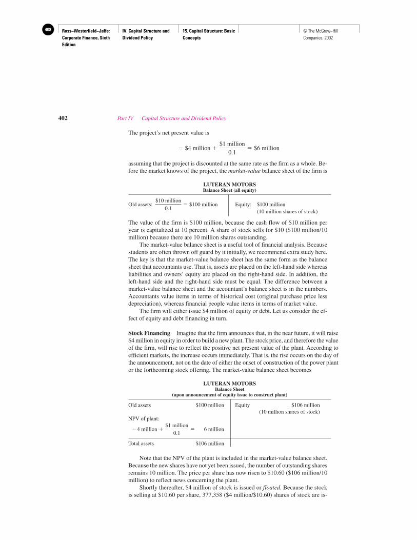
Ross−Westerfield−Jaffe: Corporate Finance, Sixth Edition
IV. Capital Structure and Dividend Policy
15. Capital Structure: Basic Concepts
408 © The McGraw−Hill Companies, 2002
The project’s net present value is
assuming that the project is discounted at the same rate as the firm as a whole. Be-fore the market knows of the project, the market-value balance sheet of the firm is
LUTERAN MOTORSBalance Sheet (all equity)
Equity: $100 million(10 million shares of stock)
The value of the firm is $100 million, because the cash flow of $10 million peryear is capitalized at 10 percent. A share of stock sells for $10 ($100 million/10million) because there are 10 million shares outstanding.
The market-value balance sheet is a useful tool of financial analysis. Becausestudents are often thrown off guard by it initially, we recommend extra study here.The key is that the market-value balance sheet has the same form as the balancesheet that accountants use. That is, assets are placed on the left-hand side whereasliabilities and owners’ equity are placed on the right-hand side. In addition, theleft-hand side and the right-hand side must be equal. The difference between amarket-value balance sheet and the accountant’s balance sheet is in the numbers.Accountants value items in terms of historical cost (original purchase price lessdepreciation), whereas financial people value items in terms of market value.
The firm will either issue $4 million of equity or debt. Let us consider the ef-fect of equity and debt financing in turn.
Stock Financing Imagine that the firm announces that, in the near future, it will raise$4 million in equity in order to build a new plant. The stock price, and therefore the valueof the firm, will rise to reflect the positive net present value of the plant. According toefficient markets, the increase occurs immediately. That is, the rise occurs on the day ofthe announcement, not on the date of either the onset of construction of the power plantor the forthcoming stock offering. The market-value balance sheet becomes
LUTERAN MOTORSBalance Sheet
(upon announcement of equity issue to construct plant)
Old assets $100 million Equity $106 million(10 million shares of stock)
NPV of plant:
6 million
Total assets $106 million
Note that the NPV of the plant is included in the market-value balance sheet.Because the new shares have not yet been issued, the number of outstanding sharesremains 10 million. The price per share has now risen to $10.60 ($106 million/10million) to reflect news concerning the plant.
Shortly thereafter, $4 million of stock is issued or floated. Because the stockis selling at $10.60 per share, 377,358 ($4 million/$10.60) shares of stock are is-
�4 million �$1 million
0.1�
Old assets: $10 million
0.1� $100 million
� $4 million �$1 million
0.1� $6 million
402 Part IV Capital Structure and Dividend Policy
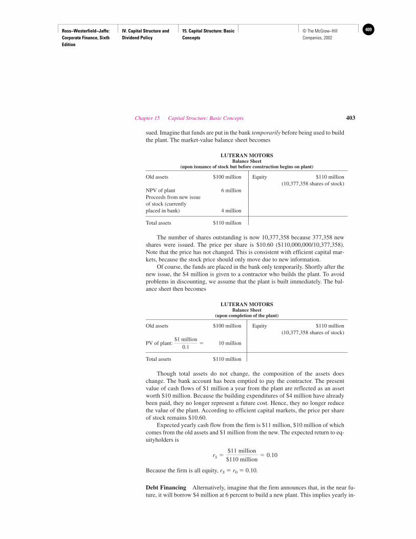
Ross−Westerfield−Jaffe: Corporate Finance, Sixth Edition
IV. Capital Structure and Dividend Policy
15. Capital Structure: Basic Concepts
409© The McGraw−Hill Companies, 2002
sued. Imagine that funds are put in the bank temporarily before being used to buildthe plant. The market-value balance sheet becomes
LUTERAN MOTORSBalance Sheet
(upon issuance of stock but before construction begins on plant)
Old assets $100 million Equity $110 million(10,377,358 shares of stock)
NPV of plant 6 millionProceeds from new issueof stock (currentlyplaced in bank) 4 million
Total assets $110 million
The number of shares outstanding is now 10,377,358 because 377,358 newshares were issued. The price per share is $10.60 ($110,000,000/10,377,358).Note that the price has not changed. This is consistent with efficient capital mar-kets, because the stock price should only move due to new information.
Of course, the funds are placed in the bank only temporarily. Shortly after thenew issue, the $4 million is given to a contractor who builds the plant. To avoidproblems in discounting, we assume that the plant is built immediately. The bal-ance sheet then becomes
LUTERAN MOTORSBalance Sheet
(upon completion of the plant)
Old assets $100 million Equity $110 million(10,377,358 shares of stock)
10 million
Total assets $110 million
Though total assets do not change, the composition of the assets doeschange. The bank account has been emptied to pay the contractor. The presentvalue of cash flows of $1 million a year from the plant are reflected as an assetworth $10 million. Because the building expenditures of $4 million have alreadybeen paid, they no longer represent a future cost. Hence, they no longer reducethe value of the plant. According to efficient capital markets, the price per shareof stock remains $10.60.
Expected yearly cash flow from the firm is $11 million, $10 million of whichcomes from the old assets and $1 million from the new. The expected return to eq-uityholders is
Because the firm is all equity, rS � r0 � 0.10.
Debt Financing Alternatively, imagine that the firm announces that, in the near fu-ture, it will borrow $4 million at 6 percent to build a new plant. This implies yearly in-
rS �$11 million
$110 million� 0.10
PV of plant: $1 million
0.1�
Chapter 15 Capital Structure: Basic Concepts 403
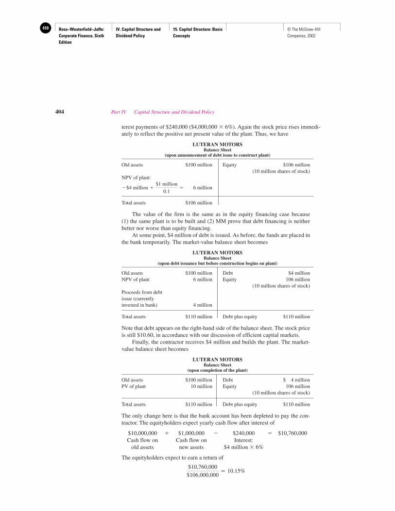
Ross−Westerfield−Jaffe: Corporate Finance, Sixth Edition
IV. Capital Structure and Dividend Policy
15. Capital Structure: Basic Concepts
410 © The McGraw−Hill Companies, 2002
terest payments of $240,000 ($4,000,000 � 6%). Again the stock price rises immedi-ately to reflect the positive net present value of the plant. Thus, we have
LUTERAN MOTORSBalance Sheet
(upon announcement of debt issue to construct plant)
Old assets $100 million Equity $106 million(10 million shares of stock)
NPV of plant:
6 million
Total assets $106 million
The value of the firm is the same as in the equity financing case because(1) the same plant is to be built and (2) MM prove that debt financing is neitherbetter nor worse than equity financing.
At some point, $4 million of debt is issued. As before, the funds are placed inthe bank temporarily. The market-value balance sheet becomes
LUTERAN MOTORSBalance Sheet
(upon debt issuance but before construction begins on plant)
Old assets $100 million Debt $4 millionNPV of plant 6 million Equity 106 million
(10 million shares of stock)Proceeds from debtissue (currentlyinvested in bank) 4 million
Total assets $110 million Debt plus equity $110 million
Note that debt appears on the right-hand side of the balance sheet. The stock priceis still $10.60, in accordance with our discussion of efficient capital markets.
Finally, the contractor receives $4 million and builds the plant. The market-value balance sheet becomes
LUTERAN MOTORSBalance Sheet
(upon completion of the plant)
Old assets $100 million Debt $ 4 millionPV of plant 10 million Equity 106 million
(10 million shares of stock)
Total assets $110 million Debt plus equity $110 million
The only change here is that the bank account has been depleted to pay the con-tractor. The equityholders expect yearly cash flow after interest of
$10,000,000 � $1,000,000 � $240,000 � $10,760,000Cash flow on Cash flow on Interest:
old assets new assets $4 million � 6%
The equityholders expect to earn a return of
$10,760,000
$106,000,000� 10.15%
�$4 million �$1 million
0.1�
404 Part IV Capital Structure and Dividend Policy
Ross−Westerfield−Jaffe: Corporate Finance, Sixth Edition
IV. Capital Structure and Dividend Policy
15. Capital Structure: Basic Concepts
411© The McGraw−Hill Companies, 2002
This return of 10.15 percent for levered equityholders is higher than the 10 percent re-turn for the unlevered equityholders. This result is sensible because, as we argued ear-lier, levered equity is riskier. In fact, the return of 10.15 percent should be exactly whatMM Proposition II predicts. This prediction can be verified by plugging values into
(15.3)
We obtain
This example was useful for two reasons. First, we wanted to introduce theconcept of market-value balance sheets, a tool that will prove useful elsewhere inthe text. Among other things, this technique allows one to calculate the price pershare of a new issue of stock. Second, the example illustrates three aspects ofModigliani and Miller:
1. The example is consistent with MM Proposition I because the value of the firmis $110 million after either equity or debt financing.
2. Students are often more interested in stock price than in firm value. We show thatthe stock price is always $10.60, regardless of whether debt or equity financingis used.
3. The example is consistent with MM Proposition II. The expected return to equi-tyholders rises from 10 to 10.15 percent, just as formula (15.3) states. This riseoccurs because the equityholders of a levered firm face more risk than do the eq-uityholders of an unlevered firm.
MM: An InterpretationThe Modigliani-Miller results indicate that managers cannot change the value of a firm byrepackaging the firm’s securities. Though this idea was considered revolutionary when itwas originally proposed in the late 1950s, the MM model and arbitrage proof have sincemet with wide acclaim.10
MM argue that the firm’s overall cost of capital cannot be reduced as debt is substitutedfor equity, even though debt appears to be cheaper than equity. The reason for this is that asthe firm adds debt, the remaining equity becomes more risky. As this risk rises, the cost ofequity capital rises as a result. The increase in the cost of the remaining equity capital off-sets the higher proportion of the firm financed by low-cost debt. In fact, MM prove that thetwo effects exactly offset each other, so that both the value of the firm and the firm’s over-all cost of capital are invariant to leverage.
MM use an interesting analogy to food. They consider a dairy farmer with two choices.On the one hand, he can sell whole milk. On the other hand, by skimming he can sell a com-bination of cream and low-fat milk. Though the farmer can get a high price for the cream, hegets a low price for the low-fat milk, implying no net gain. In fact, imagine that the proceedsfrom the whole-milk strategy were less than those from the cream–low-fat-milk strategy.Arbitrageurs would buy the whole milk, perform the skimming operation themselves, and
10.15% � 10% �$4,000,000
$106,000,000� �10% � 6%�
rS � r0 �B
S� �r0 � rB�
Chapter 15 Capital Structure: Basic Concepts 405
10Both Merton Miller and Franco Modigliani were awarded separate Nobel Prizes, in part for their work oncapital structure.

Ross−Westerfield−Jaffe: Corporate Finance, Sixth Edition
IV. Capital Structure and Dividend Policy
15. Capital Structure: Basic Concepts
412 © The McGraw−Hill Companies, 2002
resell the cream and low-fat milk separately. Competition between arbitrageurs would tendto boost the price of whole milk until proceeds from the two strategies became equal. Thus,the value of the farmer’s milk is invariant to the way in which the milk is packaged.
Food found its way into this chapter earlier, when we viewed the firm as a pie. MM ar-gue that the size of the pie does not change, no matter how stockholders and bondholdersdivide it. MM say that a firm’s capital structure is irrelevant; it is what it is by some histor-
406 Part IV Capital Structure and Dividend Policy
11Taken from GSB Chicago, University of Chicago (Autumn 1986).
IN THEIR OWN WORDS
In Professor Miller’s Words . . .
The Modigliani-Miller results are not easy to under-stand fully. This point is related in a story told by
Merton Miller.11
“How difficult it is to summarize briefly the contribu-tion of the [Modigliani-Miller] papers was brought hometo me very clearly last October after Franco Modiglianiwas awarded the Nobel Prize in Economics in part—but,of course, only in part—for the work in finance. The tele-vision camera crews from our local stations in Chicagoimmediately descended upon me. ‘We understand,’ theysaid, ‘that you worked with Modigliani some years backin developing these M and M theorems and we wonder ifyou could explain them briefly to our television viewers.’
“ ‘How briefly?’ I asked.“ ‘Oh, take ten seconds,’ was the reply.“Ten seconds to explain the work of a lifetime! Ten
seconds to describe two carefully reasoned articles, eachrunning to more than thirty printed pages and each withsixty or so long footnotes! When they saw the look ofdismay on my face, they said, ‘You don’t have to go intodetails. Just give us the main points in simple, common-sense terms.’
“The main point of the first or cost-of-capital articlewas, in principle at least, simple enough to make. It saidthat in an economist’s ideal world of complete andperfect capital markets and with full and symmetricinformation among all market participants, the totalmarket value of all the securities issued by a firm wasgoverned by the earning power and risk of its underlyingreal assets and was independent of how the mix of secu-rities issued to finance it was divided between debtinstruments and equity capital. . . .
“Such a summary, however, uses too many short-handed terms and concepts, like perfect capital markets,that are rich in connotations to economists but hardly so tothe general public. So I thought, instead, of an analogythat we ourselves had invoked in the original paper. . . .
“ ‘Think of the firm,’ I said, ‘as a gigantic tub of wholemilk. The farmer can sell the whole milk as is. Or he can
separate out the cream and sell it at a considerably higherprice than the whole milk would bring. (That’s the analogof a firm selling low-yield and hence high-priced debt secu-rities.) But, of course, what the farmer would have leftwould be skim milk with low butterfat content and thatwould sell for much less than whole milk. That correspondsto the levered equity. The M and M proposition says that ifthere were no costs of separation (and, of course, nogovernment dairy support programs), the cream plus theskim milk would bring the same price as the whole milk.’
“The television people conferred among themselvesand came back to inform me that it was too long, toocomplicated, and too academic.
“ ‘Don’t you have anything simpler?’ they asked. Ithought of another way that the M and M proposition ispresented these days, which emphasizes the notion ofmarket completeness and stresses the role of securities asdevices for ‘partitioning’ a firm’s payoffs in each possiblestate of the world among the group of its capital suppliers.
“ ‘Think of the firm,’ I said, ‘as a gigantic pizza,divided into quarters. If now you cut each quarter in halfinto eighths, the M and M proposition says that you willhave more pieces but not more pizza.’
“Again there was a whispered conference among thecamera crew, and the director came back and said:
“ ‘Professor, we understand from the press releasethat there were two M and M propositions. Can we trythe other one?’ ”
[Professor Miller tried valiantly to explain the secondproposition, though this was apparently even moredifficult to get across. After his attempt:]
“Once again there was a whispered conversation.They shut the lights off. They folded up theirequipment. They thanked me for giving them the time.They said that they’d get back to me. But I knew that Ihad somehow lost my chance to start a new career as apackager of economic wisdom for TV viewers inconvenient ten-second bites. Some have the talent forit . . . and some just don’t.”
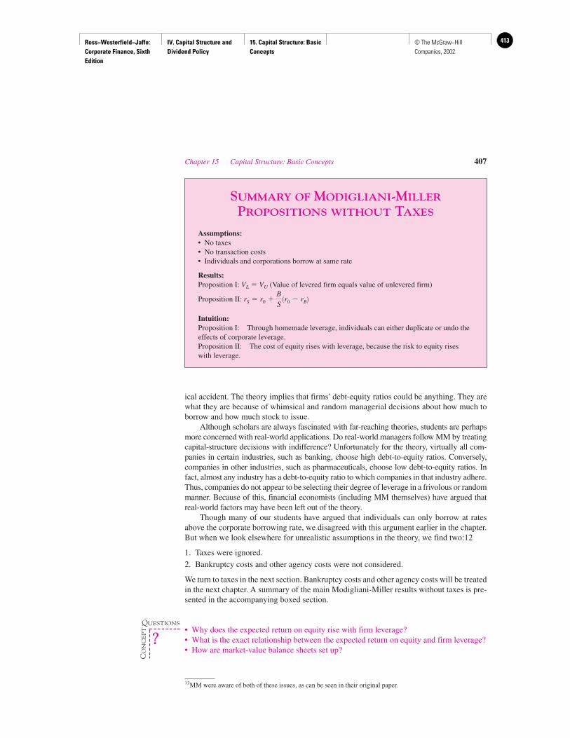
Ross−Westerfield−Jaffe: Corporate Finance, Sixth Edition
IV. Capital Structure and Dividend Policy
15. Capital Structure: Basic Concepts
413© The McGraw−Hill Companies, 2002
Chapter 15 Capital Structure: Basic Concepts 407
ical accident. The theory implies that firms’ debt-equity ratios could be anything. They arewhat they are because of whimsical and random managerial decisions about how much toborrow and how much stock to issue.
Although scholars are always fascinated with far-reaching theories, students are perhapsmore concerned with real-world applications. Do real-world managers follow MM by treatingcapital-structure decisions with indifference? Unfortunately for the theory, virtually all com-panies in certain industries, such as banking, choose high debt-to-equity ratios. Conversely,companies in other industries, such as pharmaceuticals, choose low debt-to-equity ratios. Infact, almost any industry has a debt-to-equity ratio to which companies in that industry adhere.Thus, companies do not appear to be selecting their degree of leverage in a frivolous or randommanner. Because of this, financial economists (including MM themselves) have argued thatreal-world factors may have been left out of the theory.
Though many of our students have argued that individuals can only borrow at ratesabove the corporate borrowing rate, we disagreed with this argument earlier in the chapter.But when we look elsewhere for unrealistic assumptions in the theory, we find two:12
1. Taxes were ignored.
2. Bankruptcy costs and other agency costs were not considered.
We turn to taxes in the next section. Bankruptcy costs and other agency costs will be treatedin the next chapter. A summary of the main Modigliani-Miller results without taxes is pre-sented in the accompanying boxed section.
• Why does the expected return on equity rise with firm leverage?• What is the exact relationship between the expected return on equity and firm leverage?• How are market-value balance sheets set up?
SUMMARY OF MODIGLIANI-MILLER
PROPOSITIONS WITHOUT TAXES
Assumptions:• No taxes• No transaction costs• Individuals and corporations borrow at same rate
Results:Proposition I: VL � VU (Value of levered firm equals value of unlevered firm)
Proposition II:
Intuition:Proposition I: Through homemade leverage, individuals can either duplicate or undo theeffects of corporate leverage.Proposition II: The cost of equity rises with leverage, because the risk to equity riseswith leverage.
rS � r0 �B
S�r0 � rB�
12MM were aware of both of these issues, as can be seen in their original paper.
QUESTIONS
CO
NC
EP
T
?
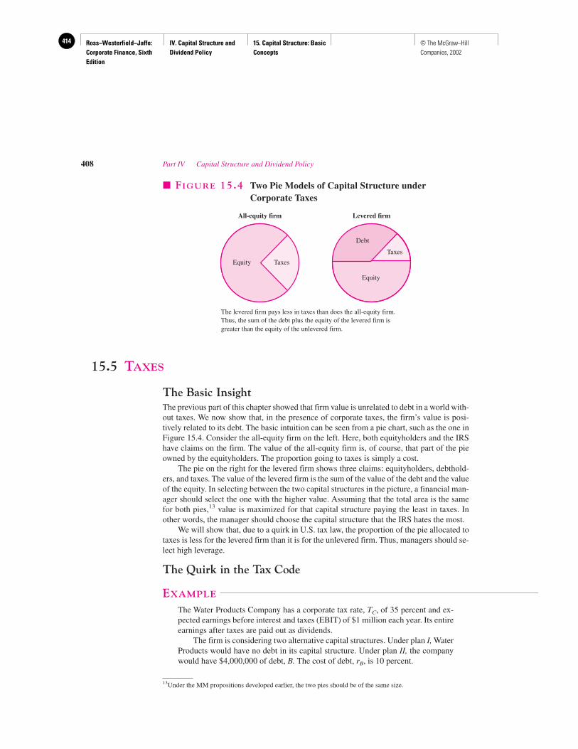
Ross−Westerfield−Jaffe: Corporate Finance, Sixth Edition
IV. Capital Structure and Dividend Policy
15. Capital Structure: Basic Concepts
414 © The McGraw−Hill Companies, 2002
15.5 TAXES
The Basic InsightThe previous part of this chapter showed that firm value is unrelated to debt in a world with-out taxes. We now show that, in the presence of corporate taxes, the firm’s value is posi-tively related to its debt. The basic intuition can be seen from a pie chart, such as the one inFigure 15.4. Consider the all-equity firm on the left. Here, both equityholders and the IRShave claims on the firm. The value of the all-equity firm is, of course, that part of the pieowned by the equityholders. The proportion going to taxes is simply a cost.
The pie on the right for the levered firm shows three claims: equityholders, debthold-ers, and taxes. The value of the levered firm is the sum of the value of the debt and the valueof the equity. In selecting between the two capital structures in the picture, a financial man-ager should select the one with the higher value. Assuming that the total area is the samefor both pies,13 value is maximized for that capital structure paying the least in taxes. Inother words, the manager should choose the capital structure that the IRS hates the most.
We will show that, due to a quirk in U.S. tax law, the proportion of the pie allocated totaxes is less for the levered firm than it is for the unlevered firm. Thus, managers should se-lect high leverage.
The Quirk in the Tax Code
EXAMPLE
The Water Products Company has a corporate tax rate, TC, of 35 percent and ex-pected earnings before interest and taxes (EBIT) of $1 million each year. Its entireearnings after taxes are paid out as dividends.
The firm is considering two alternative capital structures. Under plan I, WaterProducts would have no debt in its capital structure. Under plan II, the companywould have $4,000,000 of debt, B. The cost of debt, rB, is 10 percent.
408 Part IV Capital Structure and Dividend Policy
All-equity firm Levered firm
Equity Taxes
Debt
Taxes
Equity
� FIGURE 15.4 Two Pie Models of Capital Structure underCorporate Taxes
The levered firm pays less in taxes than does the all-equity firm.Thus, the sum of the debt plus the equity of the levered firm isgreater than the equity of the unlevered firm.
13Under the MM propositions developed earlier, the two pies should be of the same size.
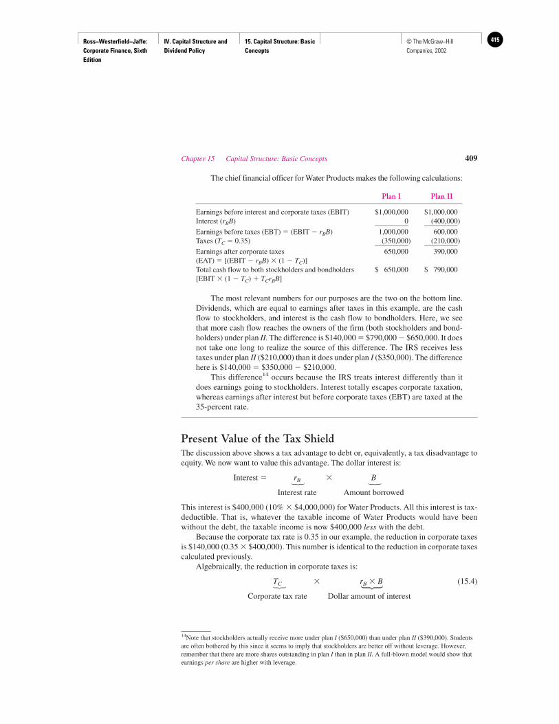
Ross−Westerfield−Jaffe: Corporate Finance, Sixth Edition
IV. Capital Structure and Dividend Policy
15. Capital Structure: Basic Concepts
415© The McGraw−Hill Companies, 2002
The chief financial officer for Water Products makes the following calculations:
Plan I Plan II
Earnings before interest and corporate taxes (EBIT) $1,000,000 $1,000,000Interest (rBB) 0 (400,000)_________ _________Earnings before taxes (EBT) � (EBIT � rBB) 1,000,000 600,000Taxes (TC � 0.35) (350,000) (210,000)_________ _________Earnings after corporate taxes 650,000 390,000(EAT) � [(EBIT � rBB) � (1 � TC)]Total cash flow to both stockholders and bondholders $ 650,000 $ 790,000[EBIT � (1 � TC) � TCrBB]
The most relevant numbers for our purposes are the two on the bottom line.Dividends, which are equal to earnings after taxes in this example, are the cashflow to stockholders, and interest is the cash flow to bondholders. Here, we seethat more cash flow reaches the owners of the firm (both stockholders and bond-holders) under plan II. The difference is $140,000 � $790,000 � $650,000. It doesnot take one long to realize the source of this difference. The IRS receives lesstaxes under plan II ($210,000) than it does under plan I ($350,000). The differencehere is $140,000 � $350,000 � $210,000.
This difference14 occurs because the IRS treats interest differently than itdoes earnings going to stockholders. Interest totally escapes corporate taxation,whereas earnings after interest but before corporate taxes (EBT) are taxed at the35-percent rate.
Present Value of the Tax ShieldThe discussion above shows a tax advantage to debt or, equivalently, a tax disadvantage toequity. We now want to value this advantage. The dollar interest is:
Interest � rB � B
Interest rate Amount borrowed
This interest is $400,000 (10% � $4,000,000) for Water Products. All this interest is tax-deductible. That is, whatever the taxable income of Water Products would have beenwithout the debt, the taxable income is now $400,000 less with the debt.
Because the corporate tax rate is 0.35 in our example, the reduction in corporate taxesis $140,000 (0.35 � $400,000). This number is identical to the reduction in corporate taxescalculated previously.
Algebraically, the reduction in corporate taxes is:
TC � rB � B (15.4)
Corporate tax rate Dollar amount of interest
Chapter 15 Capital Structure: Basic Concepts 409
14Note that stockholders actually receive more under plan I ($650,000) than under plan II ($390,000). Studentsare often bothered by this since it seems to imply that stockholders are better off without leverage. However,remember that there are more shares outstanding in plan I than in plan II. A full-blown model would show thatearnings per share are higher with leverage.
� �
� �
Ross−Westerfield−Jaffe: Corporate Finance, Sixth Edition
IV. Capital Structure and Dividend Policy
15. Capital Structure: Basic Concepts
416 © The McGraw−Hill Companies, 2002
That is, whatever the taxes that a firm would pay each year without debt, the firm will payTCrBB less with the debt of B. Expression (15.4) is often called the tax shield from debt.Note that it is an annual amount.
As long as the firm expects to be in a positive tax bracket, we can assume that the cashflow in expression (15.4) has the same risk as the interest on the debt. Thus, its value canbe determined by discounting at the interest rate, rB. Assuming that the cash flows are per-petual, the present value of the tax shield is
Value of the Levered FirmWe have just calculated the present value of the tax shield from debt. Our next step is to cal-culate the value of the levered firm. The annual after-tax cash flow of an unlevered firm is
EBIT � (1 � TC),
where EBIT is earnings before interest and taxes. The value of an unlevered firm (that is, afirm with no debt) is the present value of EBIT � (1 � TC),
where
VU � Present value of an unlevered firmEBIT � (1 � TC) � Firm cash flows after corporate taxes
TC � Corporate tax rater0 � The cost of capital to an all-equity firm. As can be seen from
the formula, r0 now discounts after-tax cash flows.
As shown previously, leverage increases the value of the firm by the tax shield, whichis TCB for perpetual debt. Thus, we merely add this tax shield to the value of the unleveredfirm to get the value of the levered firm.
We can write this algebraically as:15
MM Proposition I (corporate taxes):
(15.5)
� VU � TCB
Equation (15.5) is MM Proposition I under corporate taxes. The first term in equation (15.5)is the value of the cash flows of the firm with no debt tax shield. In other words, this termis equal to VU, the value of the all-equity firm. The value of the levered firm is the value ofan all-equity firm plus TCB, the tax rate times the value of the debt. TCB is the present value
VL �EBIT � �1 � TC�
r0
�TCrBB
rB
VU �EBIT � �1 � TC�
r0
TCrBB
rB
� TCB
410 Part IV Capital Structure and Dividend Policy
15This relationship holds when the debt level is assumed to be constant through time. A different formula wouldapply if the debt-equity ratio was assumed to be a non-constant over time. For a deeper treatment of this point,see J. A. Miles and J. R. Ezzel, “The Weighted Average Cost of Capital, Perfect Capital Markets and ProjectLife,” Journal of Financial and Quantitative Analysis (September 1980).
Ross−Westerfield−Jaffe: Corporate Finance, Sixth Edition
IV. Capital Structure and Dividend Policy
15. Capital Structure: Basic Concepts
417© The McGraw−Hill Companies, 2002
of the tax shield in the case of perpetual cash flows.16 Because the tax shield increases withthe amount of debt, the firm can raise its total cash flow and its value by substituting debtfor equity.
EXAMPLE
Divided Airlines is currently an unlevered firm. The company expects to generate$153.85 in earnings before interest and taxes (EBIT), in perpetuity. The corporatetax rate is 35 percent, implying after-tax earnings of $100. All earnings after taxare paid out as dividends.
The firm is considering a capital restructuring to allow $200 of debt. Its costof debt capital is 10 percent. Unlevered firms in the same industry have a cost ofequity capital of 20 percent. What will the new value of Divided Airlines be?
The value of Divided Airlines will be equal to17
� $500 � $70� $570
The value of the levered firm is $570, which is greater than the unleveredvalue of $500. Because VL � B � S, the value of levered equity, S, is equal to $570� $200 � $370. The value of Divided Airlines as a function of leverage is illus-trated in Figure 15.5.
Expected Return and Leverage under Corporate TaxesMM Proposition II under no taxes posits a positive relationship between the expected re-turn on equity and leverage. This result occurs because the risk of equity increases with
�$100
0.20� �0.35 � $200�
VL �EBIT � �1 � TC�
r0
� TCB
Chapter 15 Capital Structure: Basic Concepts 411
16The following example calculates the present value if we assume the debt has a finite life. Suppose theMaxwell Company has $1 million in debt with an 8-percent coupon rate. If the debt matures in two years andthe cost of debt capital, rB, is 10 percent, what is the present value of the tax shields if the corporate tax rate is35 percent? The debt is amortized in equal installments over two years.
Present Value ofYear Loan Balance Interest Tax Shield Tax Shield
0 $1,000,0001 500,000 $80,000 0.35 � $80,000 $25,454.542 0 40,000 0.35 � $40,000 11,570.25_________
$37,024.79
The present value of the tax savings is
The Maxwell Company’s value is higher than that of a comparable unlevered firm by $37,024.79.17Note that, in a world with taxes, r0 is used to discount after-tax cash flows.
PV �0.35 � $80,000
1.10�
0.35 � $40,000�1.10� 2 � $37,024.79
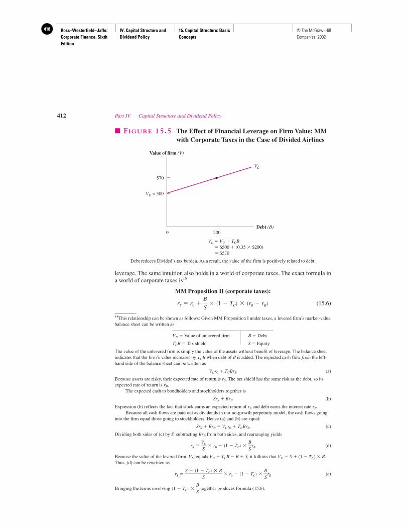
Ross−Westerfield−Jaffe: Corporate Finance, Sixth Edition
IV. Capital Structure and Dividend Policy
15. Capital Structure: Basic Concepts
418 © The McGraw−Hill Companies, 2002
leverage. The same intuition also holds in a world of corporate taxes. The exact formula ina world of corporate taxes is18
MM Proposition II (corporate taxes):
(15.6)rS � r0 �B
S� �1 � TC� � �r0 � rB�
412 Part IV Capital Structure and Dividend Policy
Value of firm (V)
Debt (B)
570
VU = 500
0 200
VL
� FIGURE 15.5 The Effect of Financial Leverage on Firm Value: MMwith Corporate Taxes in the Case of Divided Airlines
VL � VU � TCB� $500 � (0.35 � $200)� $570
Debt reduces Divided’s tax burden. As a result, the value of the firm is positively related to debt.
18This relationship can be shown as follows: Given MM Proposition I under taxes, a levered firm’s market-valuebalance sheet can be written as
VU � Value of unlevered firm B � Debt
TCB � Tax shield S � Equity
The value of the unlevered firm is simply the value of the assets without benefit of leverage. The balance sheetindicates that the firm’s value increases by TCB when debt of B is added. The expected cash flow from the left-hand side of the balance sheet can be written as
VUr0 � TCBrB (a)
Because assets are risky, their expected rate of return is r0. The tax shield has the same risk as the debt, so itsexpected rate of return is rB.
The expected cash to bondholders and stockholders together is
SrS � BrB (b)
Expression (b) reflects the fact that stock earns an expected return of rS and debt earns the interest rate rB.Because all cash flows are paid out as dividends in our no-growth perpetuity model, the cash flows going
into the firm equal those going to stockholders. Hence (a) and (b) are equal:
SrS � BrB � VUr0 � TCBrB (c)
Dividing both sides of (c) by S, subtracting BrB from both sides, and rearranging yields
(d)
Because the value of the levered firm, VL, equals VU � TCB � B � S, it follows that VU � S � (1 � TC) � B.Thus, (d) can be rewritten as
(e)
Bringing the terms involving together produces formula (15.6).�1 � TC� �B
S
rS �S � �1 � TC� � B
S� r0 � �1 � TC� �
B
SrB
rS �VU
S� r0 � �1 � TC� �
B
SrB
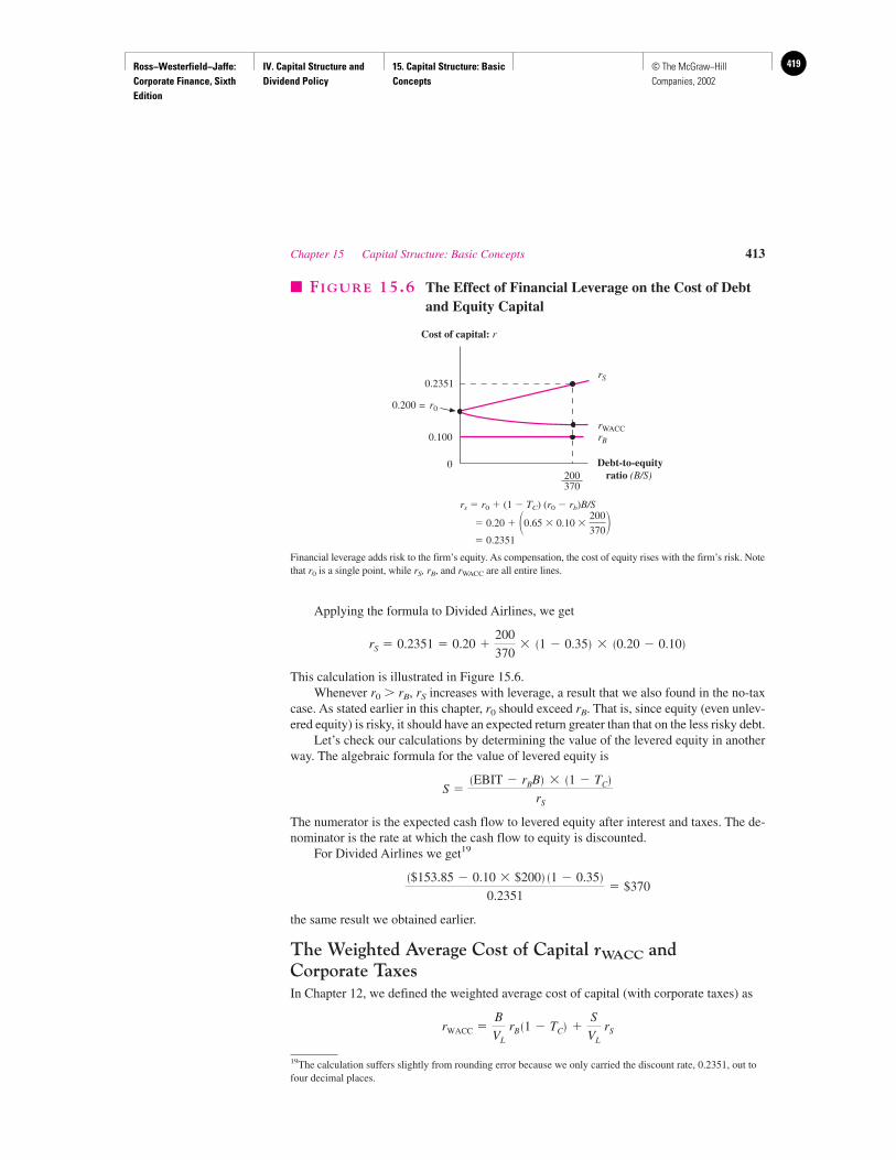
Ross−Westerfield−Jaffe: Corporate Finance, Sixth Edition
IV. Capital Structure and Dividend Policy
15. Capital Structure: Basic Concepts
419© The McGraw−Hill Companies, 2002
Applying the formula to Divided Airlines, we get
This calculation is illustrated in Figure 15.6.Whenever r0 � rB, rS increases with leverage, a result that we also found in the no-tax
case. As stated earlier in this chapter, r0 should exceed rB. That is, since equity (even unlev-ered equity) is risky, it should have an expected return greater than that on the less risky debt.
Let’s check our calculations by determining the value of the levered equity in anotherway. The algebraic formula for the value of levered equity is
The numerator is the expected cash flow to levered equity after interest and taxes. The de-nominator is the rate at which the cash flow to equity is discounted.
For Divided Airlines we get19
the same result we obtained earlier.
The Weighted Average Cost of Capital rWACC and Corporate TaxesIn Chapter 12, we defined the weighted average cost of capital (with corporate taxes) as
rWACC �B
VL
rB �1 � TC� �S
VL
rS
�$153.85 � 0.10 � $200� �1 � 0.35�0.2351
� $370
S ��EBIT � rBB� � �1 � TC�
rS
rS � 0.2351 � 0.20 �200
370� �1 � 0.35� � �0.20 � 0.10�
Chapter 15 Capital Structure: Basic Concepts 413
Debt-to-equityratio (B/S)
Cost of capital: r
rS
rB
rWACC
0.200 = r0
0
0.100
0.2351
200——370
� FIGURE 15.6 The Effect of Financial Leverage on the Cost of Debtand Equity Capital
rs � r0 � (1 � TC) (r0 � rb)B/S
� 0.20 � 0.65 � 0.10 �
� 0.2351
Financial leverage adds risk to the firm’s equity. As compensation, the cost of equity rises with the firm’s risk. Notethat r0 is a single point, while rS, rB, and rWACC are all entire lines.
200
370��
19The calculation suffers slightly from rounding error because we only carried the discount rate, 0.2351, out tofour decimal places.
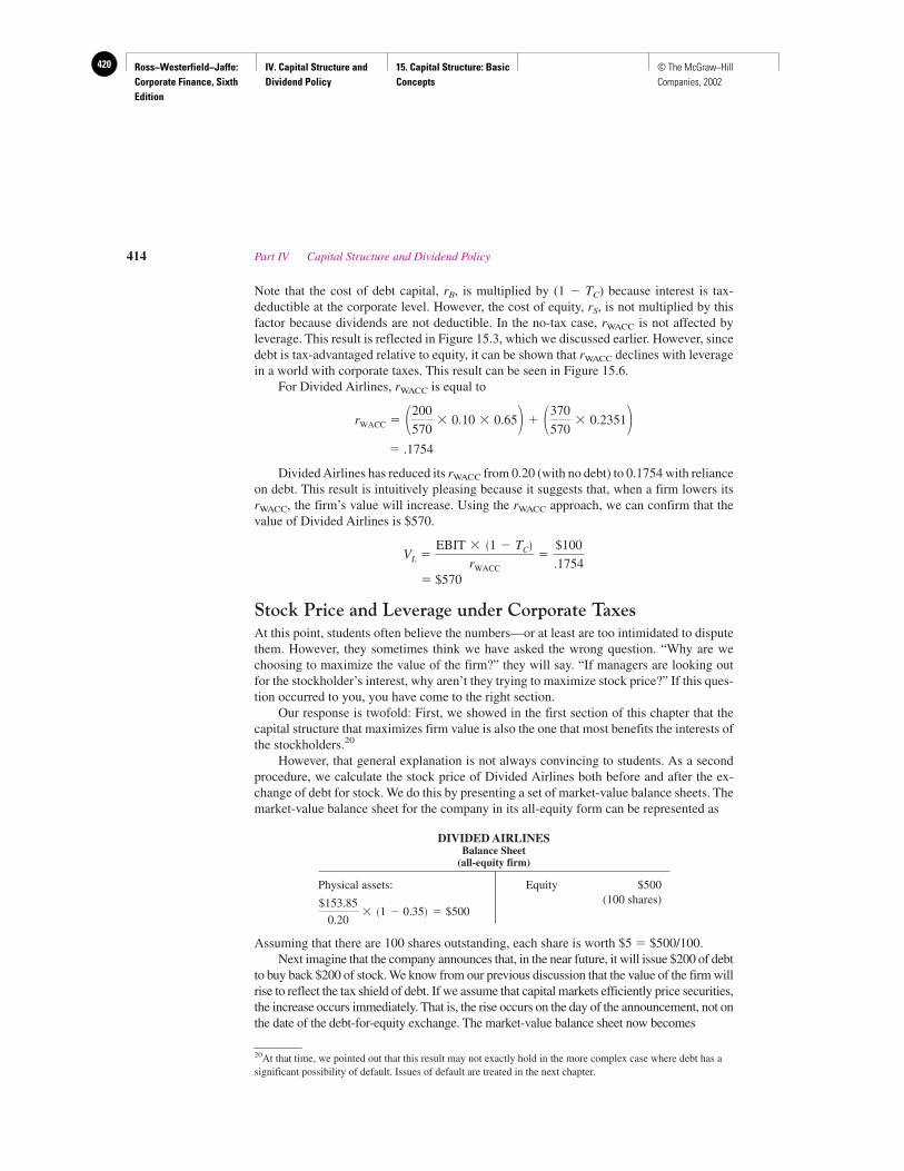
Ross−Westerfield−Jaffe: Corporate Finance, Sixth Edition
IV. Capital Structure and Dividend Policy
15. Capital Structure: Basic Concepts
420 © The McGraw−Hill Companies, 2002
Note that the cost of debt capital, rB, is multiplied by (1 � TC) because interest is tax-deductible at the corporate level. However, the cost of equity, rS, is not multiplied by thisfactor because dividends are not deductible. In the no-tax case, rWACC is not affected byleverage. This result is reflected in Figure 15.3, which we discussed earlier. However, sincedebt is tax-advantaged relative to equity, it can be shown that rWACC declines with leveragein a world with corporate taxes. This result can be seen in Figure 15.6.
For Divided Airlines, rWACC is equal to
� .1754
Divided Airlines has reduced its rWACC from 0.20 (with no debt) to 0.1754 with relianceon debt. This result is intuitively pleasing because it suggests that, when a firm lowers itsrWACC, the firm’s value will increase. Using the rWACC approach, we can confirm that thevalue of Divided Airlines is $570.
� $570
Stock Price and Leverage under Corporate TaxesAt this point, students often believe the numbers—or at least are too intimidated to disputethem. However, they sometimes think we have asked the wrong question. “Why are wechoosing to maximize the value of the firm?” they will say. “If managers are looking outfor the stockholder’s interest, why aren’t they trying to maximize stock price?” If this ques-tion occurred to you, you have come to the right section.
Our response is twofold: First, we showed in the first section of this chapter that thecapital structure that maximizes firm value is also the one that most benefits the interests ofthe stockholders.20
However, that general explanation is not always convincing to students. As a secondprocedure, we calculate the stock price of Divided Airlines both before and after the ex-change of debt for stock. We do this by presenting a set of market-value balance sheets. Themarket-value balance sheet for the company in its all-equity form can be represented as
DIVIDED AIRLINESBalance Sheet
(all-equity firm)
Physical assets: Equity $500(100 shares)
Assuming that there are 100 shares outstanding, each share is worth $5 � $500/100.Next imagine that the company announces that, in the near future, it will issue $200 of debt
to buy back $200 of stock. We know from our previous discussion that the value of the firm willrise to reflect the tax shield of debt. If we assume that capital markets efficiently price securities,the increase occurs immediately. That is, the rise occurs on the day of the announcement, not onthe date of the debt-for-equity exchange. The market-value balance sheet now becomes
$153.85
0.20� �1 � 0.35� � $500
VL �EBIT � �1 � TC�
rWACC
�$100
.1754
rWACC � �200
570� 0.10 � 0.65� � �370
570� 0.2351�
414 Part IV Capital Structure and Dividend Policy
20At that time, we pointed out that this result may not exactly hold in the more complex case where debt has asignificant possibility of default. Issues of default are treated in the next chapter.
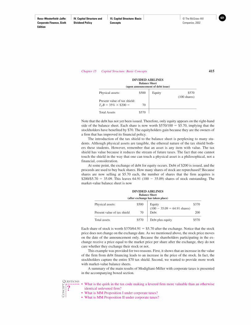
Ross−Westerfield−Jaffe: Corporate Finance, Sixth Edition
IV. Capital Structure and Dividend Policy
15. Capital Structure: Basic Concepts
421© The McGraw−Hill Companies, 2002
DIVIDED AIRLINESBalance Sheet
(upon announcement of debt issue)
Physical assets: $500 Equity $570(100 shares)
Present value of tax shield:TCB � 35% � $200 � 70
Total Assets $570
Note that the debt has not yet been issued. Therefore, only equity appears on the right-handside of the balance sheet. Each share is now worth $570/100 � $5.70, implying that thestockholders have benefited by $70. The equityholders gain because they are the owners ofa firm that has improved its financial policy.
The introduction of the tax shield to the balance sheet is perplexing to many stu-dents. Although physical assets are tangible, the ethereal nature of the tax shield both-ers these students. However, remember that an asset is any item with value. The taxshield has value because it reduces the stream of future taxes. The fact that one cannottouch the shield in the way that one can touch a physical asset is a philosophical, not afinancial, consideration.
At some point, the exchange of debt for equity occurs. Debt of $200 is issued, and theproceeds are used to buy back shares. How many shares of stock are repurchased? Becauseshares are now selling at $5.70 each, the number of shares that the firm acquires is$200/$5.70 � 35.09. This leaves 64.91 (100 � 35.09) shares of stock outstanding. Themarket-value balance sheet is now
DIVIDED AIRLINESBalance Sheet
(after exchange has taken place)
Physical assets: $500 Equity $370(100 � 35.09 � 64.91 shares)
Present value of tax shield 70 Debt 200
Total assets $570 Debt plus equity $570
Each share of stock is worth $370/64.91 � $5.70 after the exchange. Notice that the stockprice does not change on the exchange date. As we mentioned above, the stock price moveson the date of the announcement only. Because the shareholders participating in the ex-change receive a price equal to the market price per share after the exchange, they do notcare whether they exchange their stock or not.
This example was provided for two reasons. First, it shows that an increase in the valueof the firm from debt financing leads to an increase in the price of the stock. In fact, thestockholders capture the entire $70 tax shield. Second, we wanted to provide more workwith market-value balance sheets.
A summary of the main results of Modigliani-Miller with corporate taxes is presentedin the accompanying boxed section.
• What is the quirk in the tax code making a levered firm more valuable than an otherwiseidentical unlevered firm?
• What is MM Proposition I under corporate taxes?• What is MM Proposition II under corporate taxes?
Chapter 15 Capital Structure: Basic Concepts 415
QUESTIONS
CO
NC
EP
T
?

Ross−Westerfield−Jaffe: Corporate Finance, Sixth Edition
IV. Capital Structure and Dividend Policy
15. Capital Structure: Basic Concepts
422 © The McGraw−Hill Companies, 2002
15.6 SUMMARY AND CONCLUSIONS
1. We began our discussion of the capital-structure decision by arguing that the particularcapital structure that maximizes the value of the firm is also the one that provides the mostbenefit to the stockholders.
2. In a world of no taxes, the famous Proposition I of Modigliani and Miller proves that thevalue of the firm is unaffected by the debt-to-equity ratio. In other words, a firm’s capitalstructure is a matter of indifference in that world. The authors obtain their results by showingthat either a high or a low corporate ratio of debt to equity can be offset by homemadeleverage. The result hinges on the assumption that individuals can borrow at the same rate ascorporations, an assumption we believe to be quite plausible.
3. MM’s Proposition II in a world without taxes states
This implies that the expected rate of return on equity (also called the cost of equity or therequired return on equity) is positively related to the firm’s leverage. This makes intuitivesense, because the risk of equity rises with leverage, a point illustrated by the differentsloped lines of Figure 15.2.
4. While the above work of MM is quite elegant, it does not explain the empirical findings oncapital structure very well. MM imply that the capital-structure decision is a matter ofindifference, while the decision appears to be a weighty one in the real world. To achievereal-world applicability, we next considered corporate taxes.
5. In a world with corporate taxes but no bankruptcy costs, firm value is an increasing functionof leverage. The formula for the value of the firm is
VL � VU � TCB
rS � r0 �B
S�r0 � rB�
416 Part IV Capital Structure and Dividend Policy
SUMMARY OF MODIGLIANI-MILLER
PROPOSITIONS WITH CORPORATE TAXES
Assumptions:• Corporations are taxed at the rate TC, on earnings after interest.• No transaction costs.• Individuals and corporations borrow at same rate.
Results:Proposition I: VL � VU � TCB
(for a firm with perpetual debt)
Proposition II:
Intuition:Proposition I: Since corporations can deduct interest payments but not dividendpayments, corporate leverage lowers tax payments.Proposition II: The cost of equity rises with leverage, because the risk to equity riseswith leverage.
rS � r0 �B
S�1 � TC� �r0 � rB�

Ross−Westerfield−Jaffe: Corporate Finance, Sixth Edition
IV. Capital Structure and Dividend Policy
15. Capital Structure: Basic Concepts
423© The McGraw−Hill Companies, 2002
Expected return on levered equity can be expressed as
Here, value is positively related to leverage. This result implies that firms should have acapital structure almost entirely composed of debt. Because real-world firms select moremoderate levels of debt, the next chapter considers modifications to the results of this chapter.
KEY TERMS
MM Proposition I 396 MM Proposition II (corporate taxes) 412MM Proposition II 399 Pie model 390MM Proposition I (corporate taxes) 410
SUGGESTED READINGS
The classic papers by Modigliani and Miller areModigliani, F., and M. H. Miller. “The Cost of Capital, Corporation Finance, and the Theory of
Investment.” American Economic Review (June 1958).Modigliani, F., and M. H. Miller. “Corporate Income Taxes and the Cost of Capital: A
Correction.” American Economic Review (June 1963).
A more recent perspective on the above papers is provided byMiller, M. “The Modigliani-Miller Propositions after 30 Years” in D. Chew, ed., The New
Corporate Finance: Where Theory Meets Practice (New York: McGraw-Hill, 1993).
QUESTIONS AND PROBLEMS
Capital Structure without Taxes15.1 Nadus Corporation and Logis Corporation are identical in every way except their capital
structures. Nadus Corporation, an all-equity firm, has 5,000 shares of stock outstanding;each share sells for $20. Logis Corporation uses leverage in its capital structure. The marketvalue of Logis Corporation’s debt is $25,000. Logis’s cost of debt is 12 percent. Each firmis expected to have earnings before interest of $350,000. Neither firm pays taxes.
Suppose you want to purchase the same portion of the equity of each firm. Assumeyou can borrow money at 12 percent.a. What is the value of Nadus’s stock?b. What is the value of Logis’s stock?c. What will your costs and returns be if you buy 20 percent of each firm’s equity?d. Which investment is riskier? Why?e. Construct an investment strategy for Nadus stock that replicates the investment returns
of Logis stock.f. What is the value of Logis Corporation?g. If the value of Logis’s assets is $135,000 and you can invest in up to 20 percent of the
Logis stock, what should you do?
15.2 Acetate, Inc., has common stock with a market value of $20 million and debt with a marketvalue of $10 million. The cost of the debt is 14 percent. The current Treasury-bill rate is 8percent, and the expected market premium is 10 percent. The beta on Acetate’s equity is 0.9.a. What is Acetate’s debt-equity ratio?b. What is the firm’s overall required return?
rS � r0 � �1 � TC� � �r0 � rB� �B
S
Chapter 15 Capital Structure: Basic Concepts 417
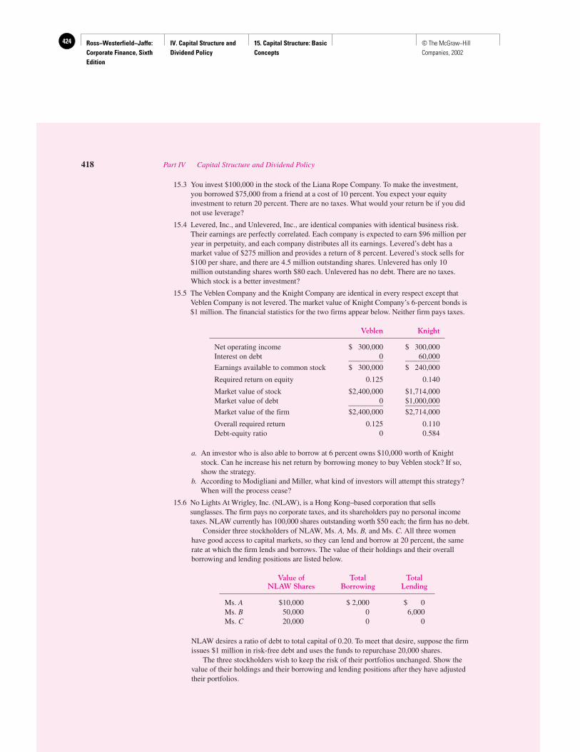
Ross−Westerfield−Jaffe: Corporate Finance, Sixth Edition
IV. Capital Structure and Dividend Policy
15. Capital Structure: Basic Concepts
424 © The McGraw−Hill Companies, 2002
15.3 You invest $100,000 in the stock of the Liana Rope Company. To make the investment,you borrowed $75,000 from a friend at a cost of 10 percent. You expect your equityinvestment to return 20 percent. There are no taxes. What would your return be if you didnot use leverage?
15.4 Levered, Inc., and Unlevered, Inc., are identical companies with identical business risk.Their earnings are perfectly correlated. Each company is expected to earn $96 million peryear in perpetuity, and each company distributes all its earnings. Levered’s debt has amarket value of $275 million and provides a return of 8 percent. Levered’s stock sells for$100 per share, and there are 4.5 million outstanding shares. Unlevered has only 10million outstanding shares worth $80 each. Unlevered has no debt. There are no taxes.Which stock is a better investment?
15.5 The Veblen Company and the Knight Company are identical in every respect except thatVeblen Company is not levered. The market value of Knight Company’s 6-percent bonds is$1 million. The financial statistics for the two firms appear below. Neither firm pays taxes.
Veblen Knight
Net operating income $ 300,000 $ 300,000Interest on debt 0 60,000_________ _________Earnings available to common stock $ 300,000 $ 240,000
Required return on equity 0.125 0.140
Market value of stock $2,400,000 $1,714,000Market value of debt 0 $1,000,000_________ _________Market value of the firm $2,400,000 $2,714,000
Overall required return 0.125 0.110Debt-equity ratio 0 0.584
a. An investor who is also able to borrow at 6 percent owns $10,000 worth of Knightstock. Can he increase his net return by borrowing money to buy Veblen stock? If so,show the strategy.
b. According to Modigliani and Miller, what kind of investors will attempt this strategy?When will the process cease?
15.6 No Lights At Wrigley, Inc. (NLAW), is a Hong Kong–based corporation that sellssunglasses. The firm pays no corporate taxes, and its shareholders pay no personal incometaxes. NLAW currently has 100,000 shares outstanding worth $50 each; the firm has no debt.
Consider three stockholders of NLAW, Ms. A, Ms. B, and Ms. C. All three womenhave good access to capital markets, so they can lend and borrow at 20 percent, the samerate at which the firm lends and borrows. The value of their holdings and their overallborrowing and lending positions are listed below.
Value of Total TotalNLAW Shares Borrowing Lending
Ms. A $10,000 $ 2,000 $ 0Ms. B 50,000 0 6,000Ms. C 20,000 0 0
NLAW desires a ratio of debt to total capital of 0.20. To meet that desire, suppose the firmissues $1 million in risk-free debt and uses the funds to repurchase 20,000 shares.
The three stockholders wish to keep the risk of their portfolios unchanged. Show thevalue of their holdings and their borrowing and lending positions after they have adjustedtheir portfolios.
418 Part IV Capital Structure and Dividend Policy

Ross−Westerfield−Jaffe: Corporate Finance, Sixth Edition
IV. Capital Structure and Dividend Policy
15. Capital Structure: Basic Concepts
425© The McGraw−Hill Companies, 2002
15.7 Rayburn Manufacturing is currently an all-equity firm. The firm’s equity is worth $2million. The cost of that equity is 18 percent. Rayburn pays no taxes.
Rayburn plans to issue $400,000 in debt and to use the proceeds to repurchase stock.The cost of debt is 10 percent.a. After Rayburn repurchases the stock, what will the firm’s overall cost of capital be?b. After the repurchase, what will the cost of equity be?c. Explain your result in (b).
15.8 Strom, Inc., has 250,000 outstanding shares of stock that sell for $20 per share. Strom,Inc., currently has no debt. The appropriate discount rate for the firm is 15 percent.Strom’s earnings last year were $750,000. The management expects that if no changesaffect the assets of the firm, the earnings will remain $750,000 in perpetuity. Strom paysno taxes.
Strom plans to buy out a competitor’s business at a cost of $300,000. Once added toStrom’s current business, the competitor’s facilities will generate earnings of $120,000 inperpetuity. The competitor has the same risk as Strom, Inc.a. Construct the market-value balance sheet for Strom before the announcement of the
buyout is made.b. Suppose Strom uses equity to fund the buyout.
i. According to the efficient-market hypothesis, what will happen to Strom’s price?ii. Construct the market-value balance sheet as it will look after the announcement.
iii. How many shares did Strom sell?iv. Once Strom sells the new shares of stock, how will its accounts look?v. After the purchase is finalized, how will the market-value balance sheet look?
vi. What is the return to Strom’s equityholders?c. Suppose Strom uses 10-percent debt to fund the buyout.
i. Construct the market-value balance sheet as it will look after the announcement.ii. Once Strom sells the bonds, how will its accounts look?
iii. What is the cost of equity?iv. Explain any difference in the cost of equity between the two plans.v. Use MM Proposition II to verify the answer in (iii).
15.9 The Gulf Power Company is an electric utility that is planning to build a new conventionalpower plant. The company has traditionally paid out all earnings to the stockholders asdividends, and has financed capital expenditures with new issues of common stock. Thereis no debt or preferred stock presently outstanding. Data on the company and the newpower plant follow. Assume all earnings streams are perpetuities.
Company DataCurrent annual earnings: $27 millionNumber of outstanding shares: 10 million
New Power PlantInitial outlay: $20 millionAdded annual earnings: $3 million
Management considers the power plant to have the same risk as existing assets. Thecurrent required rate of return on equity is 10 percent. Assume there are no taxes and nocosts of bankruptcy.a. What will the total market value of Gulf Power be if common stock is issued to finance
the plant?b. What will the total market value of the firm be if $20 million in bonds with an
interest rate of 8 percent are issued to finance the plant? Assume the bonds areperpetuities.
c. Suppose Gulf Power issues the bonds. Calculate the rate of return required bystockholders after the financing has occurred and the plant has been built.
Chapter 15 Capital Structure: Basic Concepts 419

Ross−Westerfield−Jaffe: Corporate Finance, Sixth Edition
IV. Capital Structure and Dividend Policy
15. Capital Structure: Basic Concepts
426 © The McGraw−Hill Companies, 2002
15.10 Suppose there are no taxes, no transaction costs, and no costs of financial distress. In sucha world, are the following statements true, false, or uncertain? Explain your answers.a. If a firm issues equity to repurchase some of its debt, the price of the remaining
shares will rise because those shares are less risky.b. Moderate borrowing does not significantly affect the probability of financial distress or
bankruptcy. Hence, moderate borrowing will not increase the required return on equity.
15.11 a. List the three assumptions that lie behind the Modigliani-Miller theory.b. Briefly explain the effect of each upon the conclusions of the theory for the real world.
15.12 The Digital Sound Corporation has 1 million shares of common stock outstanding at $10per share. It is an all-equity firm. Susan Wang is CEO at Wang Finance Ltd. She wants toacquire a stake of 1 percent of the firm but has not decided among the three possiblefinancing choices. She can borrow 20 percent, 40 percent, or 60 percent of the money sheneeds at a constant interest rate of 10 percent a year. The return on equity of the DigitalSound Corporation is 15 percent. Assume that she is in an MM no-tax world.a. How much dollar return can Susan expect to earn from her investment each year
under each of the three financing alternatives, respectively?b. What are Susan’s returns on equity on each financing choice, respectively?c. From parts (a) and (b), what inference can she draw about the return on equity of a
leveraged firm?
15.13 Old Fashion Corp. is an all-equity firm famous for its antique furniture business. If the firmuses 36-percent leverage through issuance of long-term debt, the CFO predicts that there is a20-percent chance that the ROE will be 10 percent, a 40-percent chance that the ROE will be15 percent, and a 40-percent chance that the ROE will be 20 percent. The firm is tax exempt.Explain whether the firm should change its capital structure if the forecast of the CFO changesto 30-percent, 50-percent, and 20-percent chances, respectively, for the three ROE possibilities.
15.14 Sunrise Industries Corp. is planning to repurchase part of its common stock in the openmarket by issuing corporate debt. As a result, the debt-to-equity ratio is expected to risefrom 40 percent to 50 percent. The annual interest payment on its outstanding debtamounts to $0.75 million with an interest rate at 10 percent. The expected earnings beforeinterest are $3.75 million. There are no taxes in the country where Sunrise operates.(Treat the debt and earnings as perpetuities to simplify calculation.)a. What is the total value of Sunrise Industries Corp.?b. What is the expected return on equity before and after the announcement of the stock
repurchase plan?c. How would the stock price change at the announcement of the repurchase?
Capital Structure with Corporate Taxes15.15 The market value of a firm with $500,000 of debt is $1,700,000. EBIT is expected to be a
perpetuity. The pretax interest rate on debt is 10 percent. The company is in the 34-percent tax bracket. If the company was 100-percent equity financed, the equityholderswould require a 20-percent return.a. What would the value of the firm be if it was financed entirely with equity?b. What is the net income to the stockholders of this levered firm?
15.16 An all-equity firm is subject to a 30-percent corporate tax rate. Its equityholders require a20-percent return. The firm’s initial market value is $3,500,000, and there are 175,000shares outstanding. The firm issues $1 million of bonds at 10 percent and uses the proceedsto repurchase common stock. Assume there is no change in the cost of financial distress forthe firm. According to MM, what is the new market value of the equity of the firm?
15.17 Streiber Publishing Company, an all-equity firm, generates perpetual earnings beforeinterest and taxes (EBIT) of $2.5 million per year. Streiber’s after-tax, all-equity discountrate is 20 percent. The company’s tax rate is 34 percent.a. What is the value of Streiber Publishing?b. If Streiber adjusts its capital structure to include $600,000 of debt, what is the value
of the firm?
420 Part IV Capital Structure and Dividend Policy

Ross−Westerfield−Jaffe: Corporate Finance, Sixth Edition
IV. Capital Structure and Dividend Policy
15. Capital Structure: Basic Concepts
427© The McGraw−Hill Companies, 2002
c. Explain any difference in your answers.d. What assumptions are you making when you are valuing Streiber?
15.18 Olbet, Inc., is a nongrowth company in the 35-percent tax bracket. Olbet’s perpetualEBIT is $1.2 million per annum. The firm’s pretax cost of debt is 8 percent and itsinterest expense per year is $200,000. Company analysts estimate that the unlevered costof Olbet’s equity is 12 percent.a. What is the value of this firm?b. What does the calculation in (a) imply about the correct level of debt?c. Is the conclusion correct? Why or why not?
15.19 Green Manufacturing, Inc., plans to announce that it will issue $2,000,000 of perpetual bonds.The bonds will have a 6-percent coupon rate. Green Manufacturing currently is an all-equityfirm. The value of Green’s equity is $10,000,000 and there are 500,000 shares outstanding.After the sale of the bonds, Green will maintain the new capital structure indefinitely. Theexpected annual pretax earnings of Green are $1,500,000. Those earnings are also expected toremain constant into the foreseeable future. Green is in the 40-percent tax bracket.a. What is Green’s current overall required return?b. Construct Green Manufacturing’s market-value balance sheet as it looks before the
announcement of the debt issue.c. What is the market-value balance sheet after the announcement?d. How many shares of stock will Green retire?e. What will the accounts show after the restructuring has taken place?f. What is Green’s cost of equity after the capital restructuring?
15.20 The Nikko Company has perpetual EBIT of $4 million per year. The after-tax, all-equitydiscount rate r0 is 15 percent. The company’s tax rate is 35 percent. The cost of debtcapital is 10 percent, and Nikko has $10 million of debt in its capital structure.a. What is Nikko’s value?b. What is Nikko’s rWACC?c. What is Nikko’s cost of equity?
15.21 AT&B has a debt-equity ratio of 2.5. Its rWACC is 15 percent and its cost of debt is 11percent. The corporate tax rate is 35 percent.a. What is AT&B’s cost of equity capital?b. What is AT&B’s unlevered cost of equity capital?c. What would the weighted average cost of capital be if the debt-to-equity ratio was .75?
What if it were 1.5?
15.22 General Tools (GT) expects EBIT to be $100,000 every year, in perpetuity. The firm canborrow at 10 percent. GT currently has no debt. Its cost of equity is 25 percent. If thecorporate tax rate is 40 percent, what is the value of the firm? What will the value be ifGT borrows $500,000 and uses the proceeds to repurchase shares?
15.23 Eureka Space Technology Group (an all-equity firm) is announcing a $100 million R&Dproject, which is expected to drastically improve its satellite launching technology byreducing its annual launching costs from $500 million to $475 million. The firm canfinance the project through either retained earnings or a new bond issue. The firm’s cost ofequity capital is 12.5 percent. The prevailing market rate of interest for comparablecorporate bonds is 8 percent. Currently, the firm has 15 million shares of stock outstandingat $32.5 a share. The firm has sufficient earnings to fully utilize the corporate tax shield ifthe project is debt financed. Assume the relevant marginal corporate tax rate is 35 percent.a. Which financing method, retained earnings or external debt financing, would you
recommend to the management and why?b. What is the resulting PV of the firm from each of these two financing methods?c. What do you expect will be the stock market stock price response to the two different
methods?d. Explain the intuition behind the results in part (c).
Chapter 15 Capital Structure: Basic Concepts 421
Ross−Westerfield−Jaffe: Corporate Finance, Sixth Edition
IV. Capital Structure and Dividend Policy
16. Capital Structure: Limits to the Use of Debt
428 © The McGraw−Hill Companies, 2002
Capital Structure: Limits to the Use of Debt
CH
AP
TE
R16
EXECUTIVE SUMMARY
One question a student might ask is, “Does the MM theory with taxes predict the cap-ital structure of typical firms?” The answer is, unfortunately, “no.” The theory statesthat VL � VU � TCB. According to this equation, one can always increase firm value
by increasing leverage, implying that firms should issue maximum debt. This is inconsistentwith the real world, where firms generally employ only moderate amounts of debt.
However, the MM theory tells us where to look when searching for the determinants ofcapital structure. For example, the theory ignores bankruptcy and its attendant costs.Because these costs are likely to get out of hand for a highly levered firm, the moderateleverage of most firms can now easily be explained. Our discussion leads quite naturally tothe idea that a firm’s capital structure can be thought of as a trade-off between the tax ben-efits of debt and the costs of financial distress and bankruptcy. This trade-off of benefits andcosts leads to an optimum amount of debt.
In addition, the MM theory ignores personal taxes. In the real world, the personal taxrate on interest is higher than the effective personal tax rate on equity distributions. Thus,the personal tax penalties to bondholders tend to offset the tax benefits to debt at the cor-porate level. Even when bankruptcy costs are ignored, this idea can be shown to imply thatthere is an optimal amount of debt for the economy as a whole. The implications of bank-ruptcy costs and personal taxes are examined in this chapter.
16.1 COSTS OF FINANCIAL DISTRESS
Bankruptcy Risk or Bankruptcy Cost?As mentioned throughout the previous chapter, debt provides tax benefits to the firm. How-ever, debt puts pressure on the firm, because interest and principal payments are obligations.If these obligations are not met, the firm may risk some sort of financial distress. The ulti-mate distress is bankruptcy, where ownership of the firm’s assets is legally transferred fromthe stockholders to the bondholders. These debt obligations are fundamentally different fromstock obligations. While stockholders like and expect dividends, they are not legally entitledto dividends in the way bondholders are legally entitled to interest and principal payments.
We show below that bankruptcy costs, or more generally financial distress costs, tendto offset the advantages to debt. We begin by positing a simple example of bankruptcy. Alltaxes are ignored to focus only on the costs of debt.
EXAMPLE
The Knight Corporation plans to be in business for one more year. It forecasts acash flow of either $100 or $50 in the coming year, each occurring with 50-percentprobability. The firm has no other assets. Previously issued debt requires payments
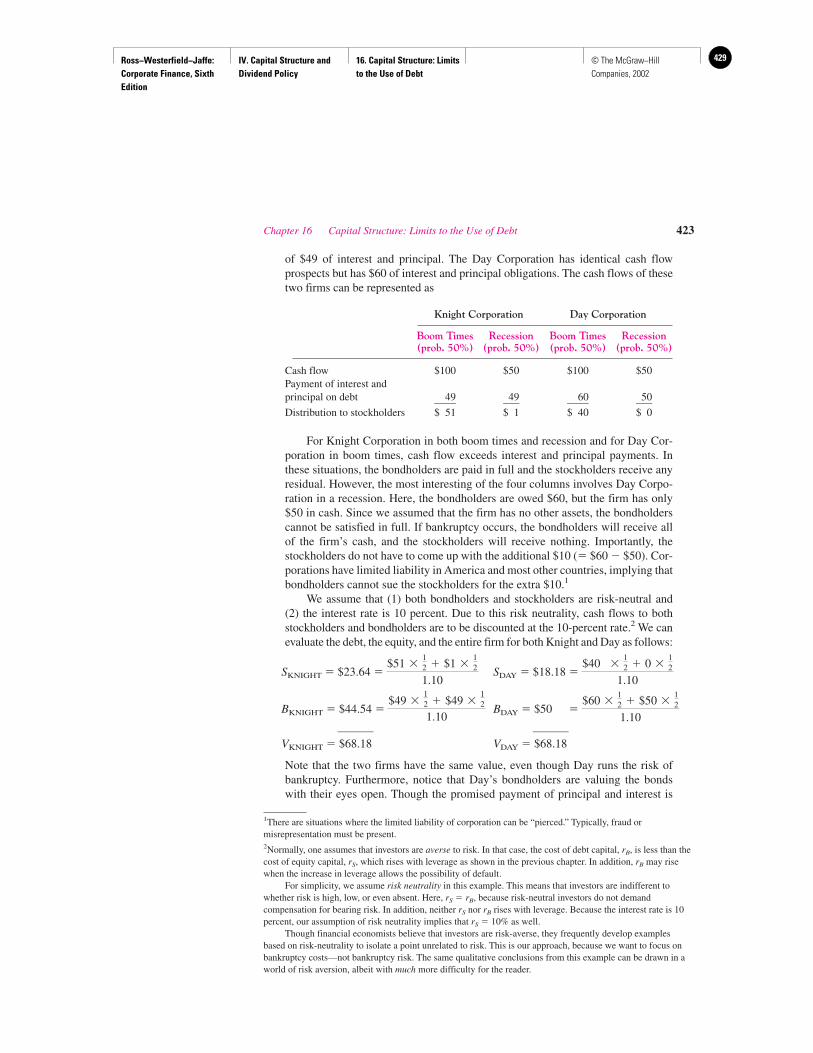
Ross−Westerfield−Jaffe: Corporate Finance, Sixth Edition
IV. Capital Structure and Dividend Policy
16. Capital Structure: Limits to the Use of Debt
429© The McGraw−Hill Companies, 2002
of $49 of interest and principal. The Day Corporation has identical cash flowprospects but has $60 of interest and principal obligations. The cash flows of thesetwo firms can be represented as
Knight Corporation Day Corporation
Boom Times Recession Boom Times Recession(prob. 50%) (prob. 50%) (prob. 50%) (prob. 50%)
Cash flow $100 $50 $100 $50Payment of interest and principal on debt 49 49 60 50____ ___ ____ ___Distribution to stockholders $ 51 $ 1 $ 40 $ 0
For Knight Corporation in both boom times and recession and for Day Cor-poration in boom times, cash flow exceeds interest and principal payments. Inthese situations, the bondholders are paid in full and the stockholders receive anyresidual. However, the most interesting of the four columns involves Day Corpo-ration in a recession. Here, the bondholders are owed $60, but the firm has only$50 in cash. Since we assumed that the firm has no other assets, the bondholderscannot be satisfied in full. If bankruptcy occurs, the bondholders will receive allof the firm’s cash, and the stockholders will receive nothing. Importantly, thestockholders do not have to come up with the additional $10 (� $60 � $50). Cor-porations have limited liability in America and most other countries, implying thatbondholders cannot sue the stockholders for the extra $10.1
We assume that (1) both bondholders and stockholders are risk-neutral and(2) the interest rate is 10 percent. Due to this risk neutrality, cash flows to bothstockholders and bondholders are to be discounted at the 10-percent rate.2 We canevaluate the debt, the equity, and the entire firm for both Knight and Day as follows:
SKNIGHT � $23.64 � SDAY � $18.18 �
BKNIGHT � $44.54 � BDAY � $50 �
______ ______
VKNIGHT � $68.18 VDAY � $68.18
Note that the two firms have the same value, even though Day runs the risk ofbankruptcy. Furthermore, notice that Day’s bondholders are valuing the bondswith their eyes open. Though the promised payment of principal and interest is
$60 �12 � $50 �
12
1.10
$49 �12 � $49 �
12
1.10
$40 �12 � 0 �
12
1.10
$51 �12 � $1 �
12
1.10
Chapter 16 Capital Structure: Limits to the Use of Debt 423
1There are situations where the limited liability of corporation can be “pierced.” Typically, fraud ormisrepresentation must be present.2Normally, one assumes that investors are averse to risk. In that case, the cost of debt capital, rB, is less than thecost of equity capital, rS, which rises with leverage as shown in the previous chapter. In addition, rB may risewhen the increase in leverage allows the possibility of default.
For simplicity, we assume risk neutrality in this example. This means that investors are indifferent towhether risk is high, low, or even absent. Here, rS � rB, because risk-neutral investors do not demandcompensation for bearing risk. In addition, neither rS nor rB rises with leverage. Because the interest rate is 10percent, our assumption of risk neutrality implies that rS � 10% as well.
Though financial economists believe that investors are risk-averse, they frequently develop examplesbased on risk-neutrality to isolate a point unrelated to risk. This is our approach, because we want to focus onbankruptcy costs—not bankruptcy risk. The same qualitative conclusions from this example can be drawn in aworld of risk aversion, albeit with much more difficulty for the reader.
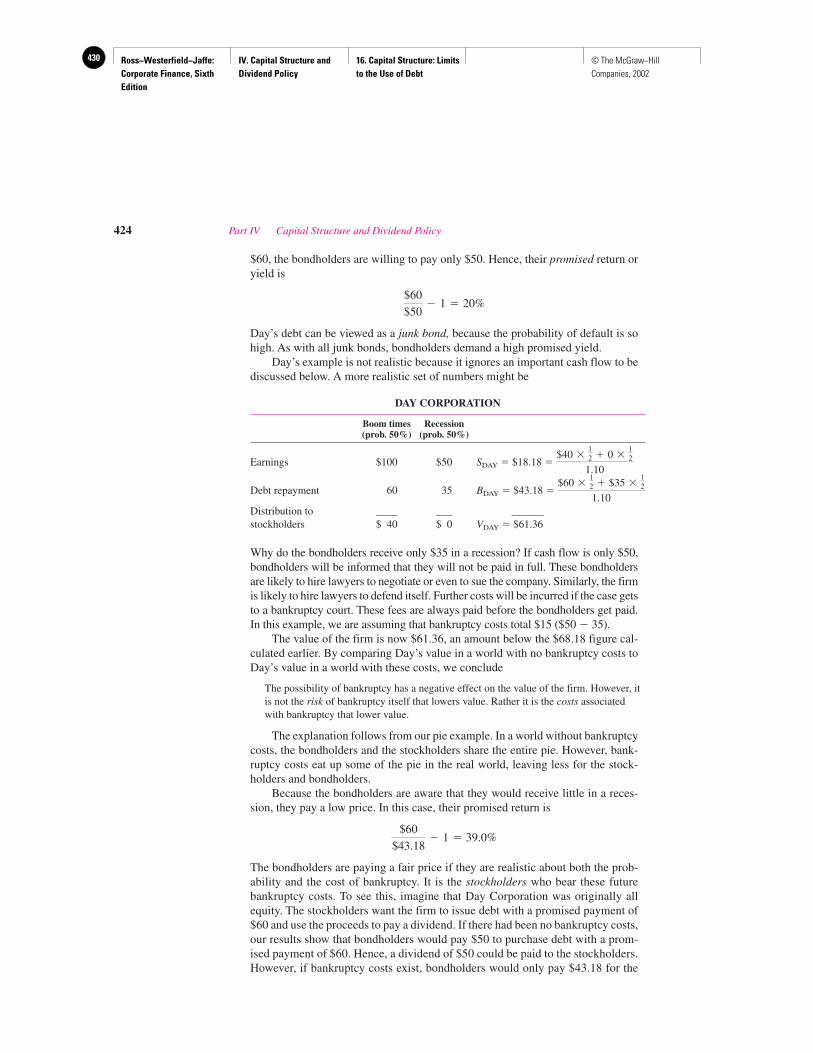
Ross−Westerfield−Jaffe: Corporate Finance, Sixth Edition
IV. Capital Structure and Dividend Policy
16. Capital Structure: Limits to the Use of Debt
430 © The McGraw−Hill Companies, 2002
$60, the bondholders are willing to pay only $50. Hence, their promised return oryield is
Day’s debt can be viewed as a junk bond, because the probability of default is sohigh. As with all junk bonds, bondholders demand a high promised yield.
Day’s example is not realistic because it ignores an important cash flow to bediscussed below. A more realistic set of numbers might be
DAY CORPORATION
Boom times Recession(prob. 50%) (prob. 50%)
Earnings $100 $50 SDAY � $18.18 �
Debt repayment 60 35 BDAY � $43.18 �
Distribution to ____ ___ ______stockholders $ 40 $ 0 VDAY � $61.36
Why do the bondholders receive only $35 in a recession? If cash flow is only $50,bondholders will be informed that they will not be paid in full. These bondholdersare likely to hire lawyers to negotiate or even to sue the company. Similarly, the firmis likely to hire lawyers to defend itself. Further costs will be incurred if the case getsto a bankruptcy court. These fees are always paid before the bondholders get paid.In this example, we are assuming that bankruptcy costs total $15 ($50 � 35).
The value of the firm is now $61.36, an amount below the $68.18 figure cal-culated earlier. By comparing Day’s value in a world with no bankruptcy costs toDay’s value in a world with these costs, we conclude
The possibility of bankruptcy has a negative effect on the value of the firm. However, itis not the risk of bankruptcy itself that lowers value. Rather it is the costs associatedwith bankruptcy that lower value.
The explanation follows from our pie example. In a world without bankruptcycosts, the bondholders and the stockholders share the entire pie. However, bank-ruptcy costs eat up some of the pie in the real world, leaving less for the stock-holders and bondholders.
Because the bondholders are aware that they would receive little in a reces-sion, they pay a low price. In this case, their promised return is
The bondholders are paying a fair price if they are realistic about both the prob-ability and the cost of bankruptcy. It is the stockholders who bear these futurebankruptcy costs. To see this, imagine that Day Corporation was originally allequity. The stockholders want the firm to issue debt with a promised payment of$60 and use the proceeds to pay a dividend. If there had been no bankruptcy costs,our results show that bondholders would pay $50 to purchase debt with a prom-ised payment of $60. Hence, a dividend of $50 could be paid to the stockholders.However, if bankruptcy costs exist, bondholders would only pay $43.18 for the
$60
$43.18� 1 � 39.0%
$60 �12 � $35 �
12
1.10
$40 �12 � 0 �
12
1.10
$60
$50� 1 � 20%
424 Part IV Capital Structure and Dividend Policy
Ross−Westerfield−Jaffe: Corporate Finance, Sixth Edition
IV. Capital Structure and Dividend Policy
16. Capital Structure: Limits to the Use of Debt
431© The McGraw−Hill Companies, 2002
debt. In that case, only a dividend of $43.18 could be paid to the stockholders.Because the dividend is smaller when bankruptcy costs exist, the stockholders arehurt by bankruptcy costs.
• What does risk neutrality mean?• Can one have bankruptcy risk without bankruptcy costs?• Why do we say that stockholders bear bankruptcy costs?
16.2 DESCRIPTION OF COSTS
The preceding example showed that bankruptcy costs can lower the value of the firm. Infact, the same general result holds even if a legal bankruptcy is prevented. Thus, financialdistress costs may be a better phrase than bankruptcy costs. It is worthwhile to describethese costs in more detail.
Direct Costs of Financial Distress: Legal and AdministrativeCosts of Liquidation or ReorganizationAs mentioned earlier, lawyers are involved throughout all the stages before and duringbankruptcy. With fees often in the hundreds of dollars an hour, these costs can add upquickly. A wag once remarked that bankruptcies are to lawyers what blood is to sharks. Inaddition, administrative and accounting fees can substantially add to the total bill. And if atrial takes place, we must not forget expert witnesses. Each side may hire a number of thesewitnesses to testify about the fairness of a proposed settlement. Their fees can easily rivalthose of lawyers or accountants. (However, we personally look upon these witnesses morekindly, because they are frequently drawn from the ranks of finance professors.)
Perhaps one of the most well-publicized bankruptcies in recent years concerned a mu-nicipality, Orange County, California, not a corporation. This bankruptcy followed largebond-trading losses in the county’s financial portfolio. The Los Angeles Times stated:
Orange County taxpayers lost $1.69 billion, and their government, one year ago today, sankinto bankruptcy. Now they are spending millions more to get out of it.
Accountants pore over fiscal ledgers at $325 an hour. Lawyers toil into the night—at$385 an hour. Financial advisors from one of the nation’s most prominent investment houseslabor for the taxpayers at $150,000 a month. Clerks stand by the photocopy machines, runningup bills that sometimes exceed $3,000.
Total so far: $29 million. And it’s nowhere near over.The multi-pronged effort to lift Orange County out of the nation’s worst municipal bank-
ruptcy has become a money-eating machine, gobbling up taxpayer funds at a rate of $2.4 mil-lion a month. That’s $115,000 a day.
County administrators are not alarmed.They say Orange County’s bankruptcy was an epic disaster that will require equally dra-
matic expenditures of taxpayer cash to help it survive. While they have refused to pay severalthousand dollars worth of claimed expenses—lavish dinners, big hotel bills—they have rarelyquestioned the sky-high hourly fees. They predict the costs could climb much higher.
Indeed, participants in the county’s investment pool have agreed to create a separate $50million fund to pay the costs of doing legal battle with Wall Street.3
Chapter 16 Capital Structure: Limits to the Use of Debt 425
QUESTIONS
CO
NC
EP
T
?
3“The High Cost of Going Bankrupt,” Los Angeles Times Orange County Edition, December 6, 1995. Takenfrom Lexis/Nexis.
Ross−Westerfield−Jaffe: Corporate Finance, Sixth Edition
IV. Capital Structure and Dividend Policy
16. Capital Structure: Limits to the Use of Debt
432 © The McGraw−Hill Companies, 2002
A number of academic studies have measured the direct costs of financial distress.While large in absolute amount, these costs are actually small as a percentage of firmvalue. White, Altman, and Weiss estimate the direct costs of financial distress to be about3 percent of the market value of the firm.4 In a study of direct financial distress costs of 20railroad bankruptcies, Warner finds that net financial distress costs were, on average, 1 per-cent of the market value of the firm seven years before bankruptcy and were somewhatlarger percentages as bankruptcy approached (for example, 2.5 percent of the market valueof the firm three years before bankruptcy).5 Of course, few firms end up in bankruptcy.Thus, the preceding cost estimates must be multiplied by the probability of bankruptcy toyield the expected cost of bankruptcy. Warner states:
Suppose, for example, that a given railroad picks a level of debt such that bankruptcy wouldoccur on average once every 20 years (i.e., the probability of going bankrupt is 5 percent inany given year). Assume that when bankruptcy occurs, the firm would pay a lump sum penaltyequal to 3 percent of its now current market value. . . .
[Then], the firm’s expected cost of bankruptcy is equal to fifteen one-hundredths of onepercent of its now current market value.
Indirect Costs of Financial DistressImpaired Ability to Conduct Business Bankruptcy hampers conduct with customersand suppliers. Sales are frequently lost because of both fear of impaired service and lossof trust. For example, many loyal Chrysler customers switched to other manufacturerswhen Chrysler skirted insolvency in the 1970s. These buyers questioned whether partsand servicing would be available were Chrysler to fail. Sometimes the taint of impend-ing bankruptcy is enough to drive customers away. For example, gamblers avoided At-lantis casino in Atlantic City after it became technically insolvent. Gamblers are a su-perstitious bunch. Many reasoned, “If the casino itself cannot make money, how can Iexpect to make money there?” A particularly outrageous story concerned two unrelatedstores both named Mitchells in New York City. When one Mitchells declared bankruptcy,customers stayed away from both stores. In time, the second store was forced to declarebankruptcy as well.
Though these costs clearly exist, it is quite difficult to measure them. Altman estimatesthat both direct and indirect costs of financial distress are frequently greater than 20 percentof firm value.6 Andrade and Kaplan7 estimate total distress costs to be between 10 percent and
426 Part IV Capital Structure and Dividend Policy
4M. J. White, “Bankruptcy Costs and the New Bankruptcy Code,” Journal of Finance (May 1983); and E. I.Altman, “ A Further Empirical Investigation of the Bankruptcy Cost Question,” Journal of Finance (September1984). More recently, Lawrence A. Weiss, “Bankruptcy Resolution: Direct Costs and Violation of Priority ofClaims,” Journal of Financial Economics 27 (1990), estimates that direct costs of bankruptcy are 3.1 percent ofthe value of the firm.5J. B. Warner, “Bankruptcy Costs: Some Evidence,” Journal of Finance (May 1977).6Altman, op. cit. “A Further Empirical Investigation.”
A fascinating and provacative set of articles by Robert Haugen and Lemma Senbet (“The Insignificance ofBankruptcy Costs to the Theory of Optimal Capital Structure.” Journal of Finance (May 1978); “NewPerspectives on Information Asymmetry and Agency Relationships.” Journal of Financial and QuantitativeAnalysis (November 1979); “Bankruptcy and Agency Costs: Their Significance to the Theory of OptimalCapital Structure,” Journal of Financial and Quantitative Analysis (March 1988)) argue that financial distressshould, at most, only slightly impair the firm’s ability to conduct business. They say that customers, employees,and so on, are concerned with the tenure of the firm, which is fundamentally a function of its assetcharacteristics. This tenure should not be dependent on the way the assets are financed.7Gregor Andrade and Steven N. Kaplan, “How Costly is Financial (Not Economic) Distress? Evidence fromHighly Leveraged Transactions that Became Distressed,” Journal of Finance (October 1998).
Ross−Westerfield−Jaffe: Corporate Finance, Sixth Edition
IV. Capital Structure and Dividend Policy
16. Capital Structure: Limits to the Use of Debt
433© The McGraw−Hill Companies, 2002
20 percent of firm value. Bar-Or8 estimates expected future distress costs for firms that arecurrently healthy to be 8 to 10 percent of operating value, a number below the estimates of ei-ther Altman or Andrade and Kaplan. However, unlike Bar-Or, these authors consider distresscosts for firms already in distress, not expected distress costs for currently healthy firms.
Cutler and Summers9 examine the costs of the well-publicized Texaco bankruptcy. InJanuary of 1984, Pennzoil reached what it believed to be a binding agreement to acquirethree-sevenths of Getty Oil. However, less than a week later, Texaco acquired all of Gettyat a higher per-share price. Pennzoil then sued Getty for breach of contract. Because Texacohad previously indemnified Getty against litigation, Texaco became liable for damages.
In November 1985, the Texas State Court awarded damages of $12 billion to Pennzoil, al-though this amount was later reduced. As a result, Texaco filed for bankruptcy. Cutler andSummers identify nine important events over the course of the litigation. They find that Texaco’smarket value (stock price times number of shares outstanding) fell a cumulative $4.1 billionover these events, whereas Pennzoil rose only $682 million. Thus, Pennzoil gained about one-sixth of what Texaco lost, resulting in a net loss to the two firms of almost $31⁄2 billion.
What could explain this net loss? Cutler and Summers suggest that it is likely due tocosts that Texaco and Pennzoil incurred from the litigation and subsequent bankruptcy. Theauthors argue that direct bankruptcy fees represent only a small part of these costs, esti-mating Texaco’s after-tax legal expenses to be about $165 million. Legal costs to Pennzoilwere more difficult to assess, because Pennzoil’s lead lawyer, Joe Jamail, stated publiclythat he had no set fee. However, using a clever statistical analysis, the authors estimate hisfee to be about $200 million. Thus, one must search elsewhere for the bulk of the costs.
Indirect costs of financial distress may be the culprit here. An affidavit by Texaco statedthat, following the lawsuit, some of its suppliers were demanding cash payment. Other sup-pliers halted or canceled shipments of crude oil. Certain banks restricted Texaco’s use of fu-tures contracts on foreign exchange. The affidavit stressed that these constraints were reduc-ing Texaco’s ability to run its business, leading to deterioration of its financial condition.Could these sorts of indirect costs explain the $31⁄2 billion disparity between Texaco’s drop andPennzoil’s rise in market value? Unfortunately, although it is quite likely that indirect costsplay a role here, there is simply no way to obtain a decent, quantitative estimate for them.
Agency CostsWhen a firm has debt, conflicts of interest arise between stockholders and bondholders. Becauseof this, stockholders are tempted to pursue selfish strategies. These conflicts of interest, whichare magnified when financial distress is incurred, impose agency costs on the firm. We describethree kinds of selfish strategies that stockholders use to hurt the bondholders and help them-selves. These strategies are costly because they will lower the market value of the whole firm.
Selfish Investment Strategy 1: Incentive to Take Large Risks Firms near bankruptcy of-tentimes takes great chances, because they believe that they are playing with someone else’smoney. To see this, imagine a levered firm considering two mutually exclusive projects, alow-risk one and a high-risk one. There are two equally likely outcomes, recession andboom. The firm is in such dire straits that should a recession hit, it will come near to bank-ruptcy with one project and actually fall into bankruptcy with the other. The cash flows forthe entire firm if the low-risk project is taken can be described as
Chapter 16 Capital Structure: Limits to the Use of Debt 427
8Yuval Bar-Or, “An Investigation of Expected Financial Distress Costs,” unpublished paper, Wharton School,University of Pennsylvania (March 2000).9David M. Cutler and Lawrence H. Summers, “The Costs of Conflict Resolution and Financial Distress:Evidence from the Texaco-Pennzoil Litigation,” Rand Journal of Economics (Summer 1988).
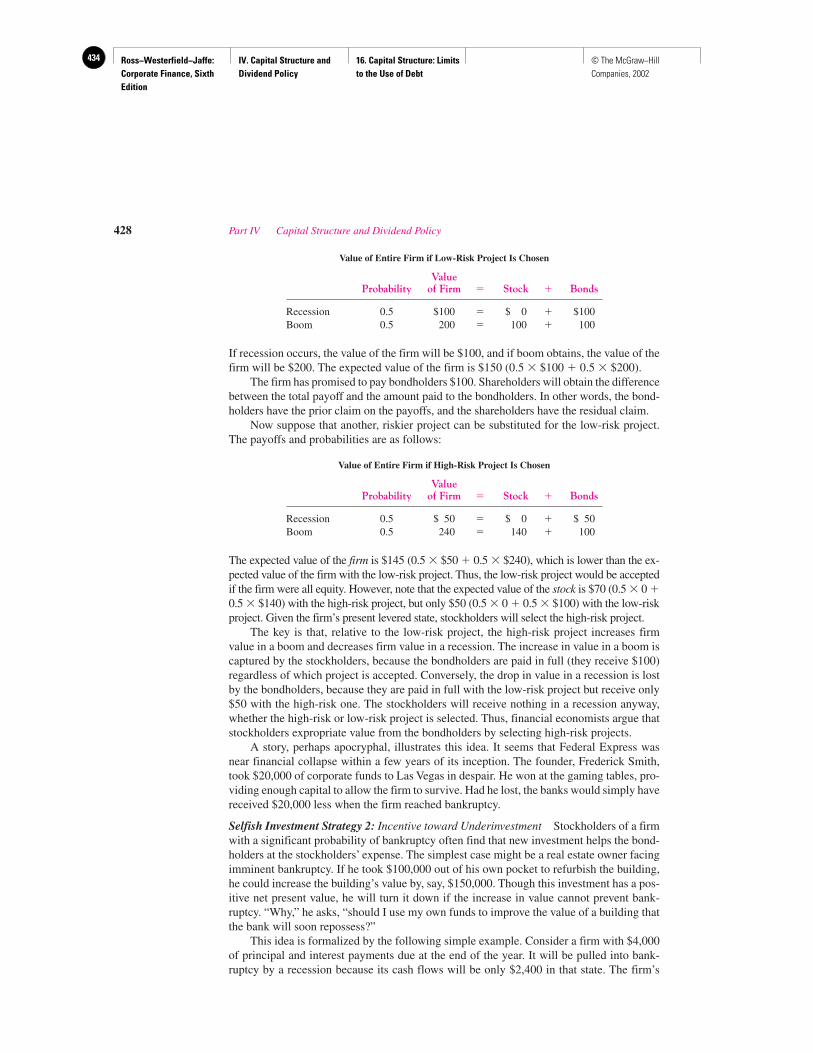
Ross−Westerfield−Jaffe: Corporate Finance, Sixth Edition
IV. Capital Structure and Dividend Policy
16. Capital Structure: Limits to the Use of Debt
434 © The McGraw−Hill Companies, 2002
Value of Entire Firm if Low-Risk Project Is Chosen
ValueProbability of Firm � Stock � Bonds
Recession 0.5 $100 � $ 0 � $100Boom 0.5 200 � 100 � 100
If recession occurs, the value of the firm will be $100, and if boom obtains, the value of thefirm will be $200. The expected value of the firm is $150 (0.5 � $100 � 0.5 � $200).
The firm has promised to pay bondholders $100. Shareholders will obtain the differencebetween the total payoff and the amount paid to the bondholders. In other words, the bond-holders have the prior claim on the payoffs, and the shareholders have the residual claim.
Now suppose that another, riskier project can be substituted for the low-risk project.The payoffs and probabilities are as follows:
Value of Entire Firm if High-Risk Project Is Chosen
ValueProbability of Firm � Stock � Bonds
Recession 0.5 $ 50 � $ 0 � $ 50Boom 0.5 240 � 140 � 100
The expected value of the firm is $145 (0.5 � $50 � 0.5 � $240), which is lower than the ex-pected value of the firm with the low-risk project. Thus, the low-risk project would be acceptedif the firm were all equity. However, note that the expected value of the stock is $70 (0.5 � 0 �0.5 � $140) with the high-risk project, but only $50 (0.5 � 0 � 0.5 � $100) with the low-riskproject. Given the firm’s present levered state, stockholders will select the high-risk project.
The key is that, relative to the low-risk project, the high-risk project increases firmvalue in a boom and decreases firm value in a recession. The increase in value in a boom iscaptured by the stockholders, because the bondholders are paid in full (they receive $100)regardless of which project is accepted. Conversely, the drop in value in a recession is lostby the bondholders, because they are paid in full with the low-risk project but receive only$50 with the high-risk one. The stockholders will receive nothing in a recession anyway,whether the high-risk or low-risk project is selected. Thus, financial economists argue thatstockholders expropriate value from the bondholders by selecting high-risk projects.
A story, perhaps apocryphal, illustrates this idea. It seems that Federal Express wasnear financial collapse within a few years of its inception. The founder, Frederick Smith,took $20,000 of corporate funds to Las Vegas in despair. He won at the gaming tables, pro-viding enough capital to allow the firm to survive. Had he lost, the banks would simply havereceived $20,000 less when the firm reached bankruptcy.
Selfish Investment Strategy 2: Incentive toward Underinvestment Stockholders of a firmwith a significant probability of bankruptcy often find that new investment helps the bond-holders at the stockholders’ expense. The simplest case might be a real estate owner facingimminent bankruptcy. If he took $100,000 out of his own pocket to refurbish the building,he could increase the building’s value by, say, $150,000. Though this investment has a pos-itive net present value, he will turn it down if the increase in value cannot prevent bank-ruptcy. “Why,” he asks, “should I use my own funds to improve the value of a building thatthe bank will soon repossess?”
This idea is formalized by the following simple example. Consider a firm with $4,000of principal and interest payments due at the end of the year. It will be pulled into bank-ruptcy by a recession because its cash flows will be only $2,400 in that state. The firm’s
428 Part IV Capital Structure and Dividend Policy
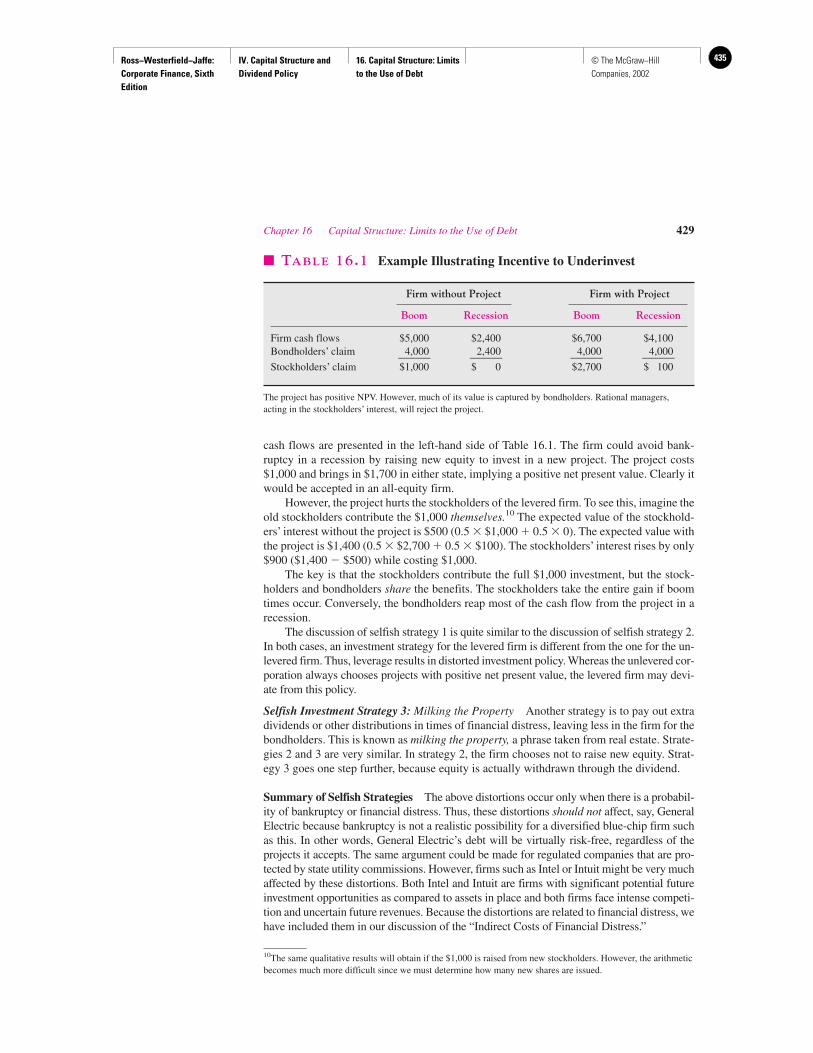
Ross−Westerfield−Jaffe: Corporate Finance, Sixth Edition
IV. Capital Structure and Dividend Policy
16. Capital Structure: Limits to the Use of Debt
435© The McGraw−Hill Companies, 2002
cash flows are presented in the left-hand side of Table 16.1. The firm could avoid bank-ruptcy in a recession by raising new equity to invest in a new project. The project costs$1,000 and brings in $1,700 in either state, implying a positive net present value. Clearly itwould be accepted in an all-equity firm.
However, the project hurts the stockholders of the levered firm. To see this, imagine theold stockholders contribute the $1,000 themselves.10 The expected value of the stockhold-ers’ interest without the project is $500 (0.5 � $1,000 � 0.5 � 0). The expected value withthe project is $1,400 (0.5 � $2,700 � 0.5 � $100). The stockholders’ interest rises by only$900 ($1,400 � $500) while costing $1,000.
The key is that the stockholders contribute the full $1,000 investment, but the stock-holders and bondholders share the benefits. The stockholders take the entire gain if boomtimes occur. Conversely, the bondholders reap most of the cash flow from the project in arecession.
The discussion of selfish strategy 1 is quite similar to the discussion of selfish strategy 2.In both cases, an investment strategy for the levered firm is different from the one for the un-levered firm. Thus, leverage results in distorted investment policy. Whereas the unlevered cor-poration always chooses projects with positive net present value, the levered firm may devi-ate from this policy.
Selfish Investment Strategy 3: Milking the Property Another strategy is to pay out extradividends or other distributions in times of financial distress, leaving less in the firm for thebondholders. This is known as milking the property, a phrase taken from real estate. Strate-gies 2 and 3 are very similar. In strategy 2, the firm chooses not to raise new equity. Strat-egy 3 goes one step further, because equity is actually withdrawn through the dividend.
Summary of Selfish Strategies The above distortions occur only when there is a probabil-ity of bankruptcy or financial distress. Thus, these distortions should not affect, say, GeneralElectric because bankruptcy is not a realistic possibility for a diversified blue-chip firm suchas this. In other words, General Electric’s debt will be virtually risk-free, regardless of theprojects it accepts. The same argument could be made for regulated companies that are pro-tected by state utility commissions. However, firms such as Intel or Intuit might be very muchaffected by these distortions. Both Intel and Intuit are firms with significant potential futureinvestment opportunities as compared to assets in place and both firms face intense competi-tion and uncertain future revenues. Because the distortions are related to financial distress, wehave included them in our discussion of the “Indirect Costs of Financial Distress.”
Chapter 16 Capital Structure: Limits to the Use of Debt 429
� TABLE 16.1 Example Illustrating Incentive to Underinvest
Firm without Project Firm with Project
Boom Recession Boom Recession
Firm cash flows $5,000 $2,400 $6,700 $4,100Bondholders’ claim 4,000 2,400 4,000 4,000______ ______ ______ ______Stockholders’ claim $1,000 $ 0 $2,700 $ 100
The project has positive NPV. However, much of its value is captured by bondholders. Rational managers,acting in the stockholders’ interest, will reject the project.
10The same qualitative results will obtain if the $1,000 is raised from new stockholders. However, the arithmeticbecomes much more difficult since we must determine how many new shares are issued.
Ross−Westerfield−Jaffe: Corporate Finance, Sixth Edition
IV. Capital Structure and Dividend Policy
16. Capital Structure: Limits to the Use of Debt
436 © The McGraw−Hill Companies, 2002
Who pays for the cost of selfish investment strategies? We argue that it is ultimately thestockholders. Rational bondholders know that, when financial distress is imminent, theycannot expect help from stockholders. Rather, stockholders are likely to choose investmentstrategies that reduce the value of the bonds. Bondholders protect themselves accordinglyby raising the interest rate that they require on the bonds. Because the stockholders mustpay these high rates, they ultimately bear the costs of selfish strategies. The relationship be-tween stockholders and bondholders is very similar to the relationship between Erroll Flynnand David Niven, good friends and movie stars in the 1930s. Niven reportedly said that thegood thing about Flynn was that you knew exactly where you stood with him. When youneeded his help, you could always count on him to let you down.
For firms that face these distortions, debt will be difficult and costly to obtain. Thesefirms will have low leverage ratios.
• What is the main direct cost of financial distress?• What are the indirect costs of financial distress?• Who pays the costs of selfish strategies?
16.3 CAN COSTS OF DEBT BE REDUCED?
As U.S. senators are prone to say, “A billion here, a billion there. Pretty soon it all addsup.”11 Each of the costs of financial distress we mentioned above is substantial in its ownright. The sum of them may well affect debt financing severely. Thus, managers have an in-centive to reduce these costs. We now turn to some of their methods. However, it should bementioned at the outset that the methods below can, at most, reduce the costs of debt. Theycannot eliminate them entirely.
Protective CovenantsBecause the stockholders must pay higher interest rates as insurance against their own self-ish strategies, they frequently make agreements with bondholders in hopes of lower rates.These agreements, called protective covenants, are incorporated as part of the loan docu-ment (or indenture) between stockholders and bondholders. The covenants must be takenseriously since a broken covenant can lead to default. Protective covenants can be classi-fied into two types: negative covenants and positive covenants.
A negative covenant limits or prohibits actions that the company may take. Here aresome typical negative covenants:
1. Limitations are placed on the amount of dividends a company may pay.
2. The firm may not pledge any of its assets to other lenders.
3. The firm may not merge with another firm.
4. The firm may not sell or lease its major assets without approval by the lender.
5. The firm may not issue additional long-term debt.
430 Part IV Capital Structure and Dividend Policy
QUESTIONS
CO
NC
EP
T
?
11The original quote is generally attributed to Senator Everett Dirksen. In the 1950s, he reportedly said, “Amillion here, a million there. Pretty soon it all adds up.” Government spending has increased since that time.
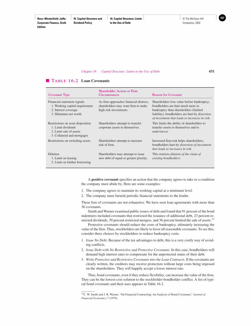
Ross−Westerfield−Jaffe: Corporate Finance, Sixth Edition
IV. Capital Structure and Dividend Policy
16. Capital Structure: Limits to the Use of Debt
437© The McGraw−Hill Companies, 2002
A positive covenant specifies an action that the company agrees to take or a conditionthe company must abide by. Here are some examples:
1. The company agrees to maintain its working capital at a minimum level.
2. The company must furnish periodic financial statements to the lender.
These lists of covenants are not exhaustive. We have seen loan agreements with more than30 covenants.
Smith and Warner examined public issues of debt and found that 91 percent of the bondindentures included covenants that restricted the issuance of additional debt, 23 percent re-stricted dividends, 39 percent restricted mergers, and 36 percent limited the sale of assets.12
Protective covenants should reduce the costs of bankruptcy, ultimately increasing thevalue of the firm. Thus, stockholders are likely to favor all reasonable covenants. To see this,consider three choices by stockholders to reduce bankruptcy costs.
1. Issue No Debt. Because of the tax advantages to debt, this is a very costly way of avoid-ing conflicts.
2. Issue Debt with No Restrictive and Protective Covenants. In this case, bondholders willdemand high interest rates to compensate for the unprotected status of their debt.
3. Write Protective and Restrictive Covenants into the Loan Contracts. If the covenants areclearly written, the creditors may receive protection without large costs being imposedon the shareholders. They will happily accept a lower interest rate.
Thus, bond covenants, even if they reduce flexibility, can increase the value of the firm.They can be the lowest-cost solution to the stockholder-bondholder conflict. A list of typi-cal bond covenants and their uses appears in Table 16.2.
Chapter 16 Capital Structure: Limits to the Use of Debt 431
12C. W. Smith and J. B. Warner, “On Financial Contracting: An Analysis of Bond Covenants,” Journal ofFinancial Economics 7 (1979).
� TABLE 16.2 Loan Covenants
Shareholder Action or FirmCovenant Type Circumstances Reason for Covenant
Financial-statement signals As firm approaches financial distress, Shareholders lose value before bankruptcy; 1. Working capital requirement shareholders may want firm to make bondholders are hurt much more in 2. Interest coverage high-risk investments. bankruptcy than shareholders (limited 3. Minimum net worth liability); bondholders are hurt by distortion
of investment that leads to increases in risk.
Restrictions on asset disposition Shareholders attempt to transfer This limits the ability of shareholders to 1. Limit dividends corporate assets to themselves. transfer assets to themselves and to 2. Limit sale of assets underinvest.3. Collateral and mortgages
Restrictions on switching assets Shareholders attempt to increase Increased firm risk helps shareholders;risk of firm. bondholders hurt by distortion of investment
that leads to increases in risk.
Dilution Shareholders may attempt to issue This restricts dilution of the claim of 1. Limit on leasing new debt of equal or greater priority. existing bondholders.2. Limit on further borrowing
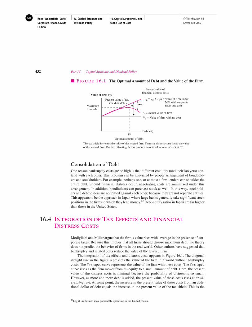
Ross−Westerfield−Jaffe: Corporate Finance, Sixth Edition
IV. Capital Structure and Dividend Policy
16. Capital Structure: Limits to the Use of Debt
438 © The McGraw−Hill Companies, 2002
Consolidation of DebtOne reason bankruptcy costs are so high is that different creditors (and their lawyers) con-tend with each other. This problem can be alleviated by proper arrangement of bondhold-ers and stockholders. For example, perhaps one, or at most a few, lenders can shoulder theentire debt. Should financial distress occur, negotiating costs are minimized under thisarrangement. In addition, bondholders can purchase stock as well. In this way, stockhold-ers and debtholders are not pitted against each other, because they are not separate entities.This appears to be the approach in Japan where large banks generally take significant stockpositions in the firms to which they lend money.13 Debt-equity ratios in Japan are far higherthan those in the United States.
16.4 INTEGRATION OF TAX EFFECTS AND FINANCIAL
DISTRESS COSTS
Modigliani and Miller argue that the firm’s value rises with leverage in the presence of cor-porate taxes. Because this implies that all firms should choose maximum debt, the theorydoes not predict the behavior of firms in the real world. Other authors have suggested thatbankruptcy and related costs reduce the value of the levered firm.
The integration of tax effects and distress costs appears in Figure 16.1. The diagonalstraight line in the figure represents the value of the firm in a world without bankruptcycosts. The �-shaped curve represents the value of the firm with these costs. The �-shapedcurve rises as the firm moves from all-equity to a small amount of debt. Here, the presentvalue of the distress costs is minimal because the probability of distress is so small.However, as more and more debt is added, the present value of these costs rises at an in-creasing rate. At some point, the increase in the present value of these costs from an addi-tional dollar of debt equals the increase in the present value of the tax shield. This is the
432 Part IV Capital Structure and Dividend Policy
13Legal limitations may prevent this practice in the United States.
Debt (B)
Value of firm (V)VL = VU + TCB =
Maximumfirm value
Present value of taxshield on debt
B*
Present value offinancial distress costs
Value of firm underMM with corporatetaxes and debt
V = Actual value of firm
VU = Value of firm with no debt
Optimal amount of debt
� FIGURE 16.1 The Optimal Amount of Debt and the Value of the Firm
The tax shield increases the value of the levered firm. Financial distress costs lower the valueof the levered firm. The two offsetting factors produce an optimal amount of debt at B*.
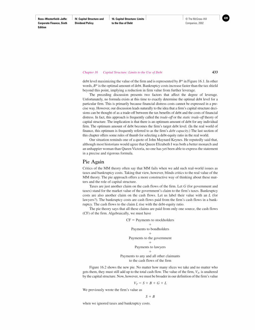
Ross−Westerfield−Jaffe: Corporate Finance, Sixth Edition
IV. Capital Structure and Dividend Policy
16. Capital Structure: Limits to the Use of Debt
439© The McGraw−Hill Companies, 2002
debt level maximizing the value of the firm and is represented by B* in Figure 16.1. In otherwords, B* is the optimal amount of debt. Bankruptcy costs increase faster than the tax shieldbeyond this point, implying a reduction in firm value from further leverage.
The preceding discussion presents two factors that affect the degree of leverage.Unfortunately, no formula exists at this time to exactly determine the optimal debt level for aparticular firm. This is primarily because financial distress costs cannot be expressed in a pre-cise way. However, our discussion leads naturally to the idea that a firm’s capital structure deci-sions can be thought of as a trade-off between the tax benefits of debt and the costs of financialdistress. In fact, this approach is frequently called the trade-off or the static trade-off theory ofcapital structure. The implication is that there is an optimum amount of debt for any individualfirm. The optimum amount of debt becomes the firm’s target debt level. (In the real world of finance, this optimum is frequently referred to as the firm’s debt capacity.) The last section ofthis chapter offers some rules of thumb for selecting a debt-equity ratio in the real world.
Our situation reminds one of a quote of John Maynard Keynes. He reputedly said that,although most historians would agree that Queen Elizabeth I was both a better monarch andan unhappier woman than Queen Victoria, no one has yet been able to express the statementin a precise and rigorous formula.
Pie AgainCritics of the MM theory often say that MM fails when we add such real-world issues astaxes and bankruptcy costs. Taking that view, however, blinds critics to the real value of theMM theory. The pie approach offers a more constructive way of thinking about these mat-ters and the role of capital structure.
Taxes are just another claim on the cash flows of the firm. Let G (for government andtaxes) stand for the market value of the government’s claim to the firm’s taxes. Bankruptcycosts are also another claim on the cash flows. Let us label their value with an L (forlawyers?). The bankruptcy costs are cash flows paid from the firm’s cash flows in a bank-ruptcy. The cash flows to the claim L rise with the debt-equity ratio.
The pie theory says that all these claims are paid from only one source, the cash flows(CF) of the firm. Algebraically, we must have
CF � Payments to stockholders�
Payments to bondholders�
Payments to the government�
Payments to lawyers�
Payments to any and all other claimants to the cash flows of the firm
Figure 16.2 shows the new pie. No matter how many slices we take and no matter whogets them, they must still add up to the total cash flow. The value of the firm, VT, is unalteredby the capital structure. Now, however, we must be broader in our definition of the firm’s value
VT � S � B � G � L
We previously wrote the firm’s value as
S � B
when we ignored taxes and bankruptcy costs.
Chapter 16 Capital Structure: Limits to the Use of Debt 433
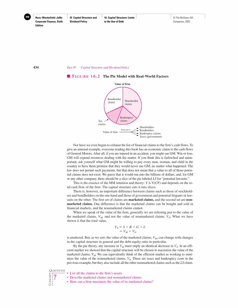
Ross−Westerfield−Jaffe: Corporate Finance, Sixth Edition
IV. Capital Structure and Dividend Policy
16. Capital Structure: Limits to the Use of Debt
440 © The McGraw−Hill Companies, 2002
Nor have we even begun to exhaust the list of financial claims to the firm’s cash flows. Togive an unusual example, everyone reading this book has an economic claim to the cash flowsof General Motors. After all, if you are injured in an accident, you might sue GM. Win or lose,GM will expend resources dealing with the matter. If you think this is farfetched and unim-portant, ask yourself what GM might be willing to pay every man, woman, and child in thecountry to have them promise that they would never sue GM, no matter what happened. Thelaw does not permit such payments, but that does not mean that a value to all of those poten-tial claims does not exist. We guess that it would run into the billions of dollars, and, for GMor any other company, there should be a slice of the pie labeled LS for “potential lawsuits.”
This is the essence of the MM intuition and theory: V is V(CF) and depends on the to-tal cash flow of the firm. The capital structure cuts it into slices.
There is, however, an important difference between claims such as those of stockhold-ers and bondholders on the one hand and those of government and potential litigants in law-suits on the other. The first set of claims are marketed claims, and the second set are non-marketed claims. One difference is that the marketed claims can be bought and sold infinancial markets, and the nonmarketed claims cannot.
When we speak of the value of the firm, generally we are referring just to the value ofthe marketed claims, VM, and not the value of nonmarketed claims, VN. What we haveshown is that the total value,
VT � S � B � G � L� VM � VN
is unaltered. But, as we saw, the value of the marketed claims, VM, can change with changesin the capital structure in general and the debt-equity ratio in particular.
By the pie theory, any increase in VM must imply an identical decrease in VN. In an effi-cient market we showed that the capital structure will be chosen to maximize the value of themarketed claims, VM. We can equivalently think of the efficient market as working to mini-mize the value of the nonmarketed claims, VN. These are taxes and bankruptcy costs in theprevious example, but they also include all the other nonmarketed claims such as the LS claim.
• List all the claims to the firm’s assets.• Describe marketed claims and nonmarketed claims.• How can a firm maximize the value of its marketed claims?
434 Part IV Capital Structure and Dividend Policy
Value of firm
Bondholderclaims Shareholder
claims
BankruptcyclaimsTax
claims
Value of firm
ShareholdersBondholdersBankruptcy claimsTaxes (government)
Paid out to
� FIGURE 16.2 The Pie Model with Real-World Factors
QUESTIONS
CO
NC
EP
T
?
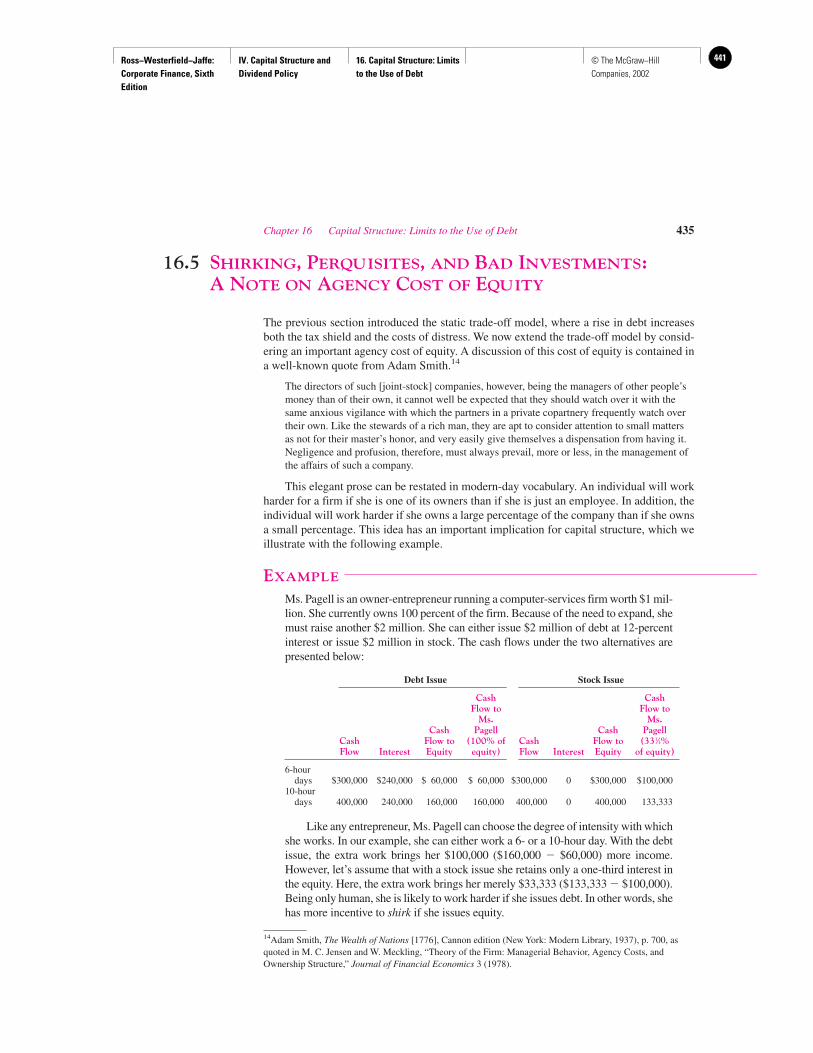
Ross−Westerfield−Jaffe: Corporate Finance, Sixth Edition
IV. Capital Structure and Dividend Policy
16. Capital Structure: Limits to the Use of Debt
441© The McGraw−Hill Companies, 2002
16.5 SHIRKING, PERQUISITES, AND BAD INVESTMENTS: A NOTE ON AGENCY COST OF EQUITY
The previous section introduced the static trade-off model, where a rise in debt increasesboth the tax shield and the costs of distress. We now extend the trade-off model by consid-ering an important agency cost of equity. A discussion of this cost of equity is contained ina well-known quote from Adam Smith.14
The directors of such [joint-stock] companies, however, being the managers of other people’smoney than of their own, it cannot well be expected that they should watch over it with thesame anxious vigilance with which the partners in a private copartnery frequently watch overtheir own. Like the stewards of a rich man, they are apt to consider attention to small mattersas not for their master’s honor, and very easily give themselves a dispensation from having it.Negligence and profusion, therefore, must always prevail, more or less, in the management ofthe affairs of such a company.
This elegant prose can be restated in modern-day vocabulary. An individual will workharder for a firm if she is one of its owners than if she is just an employee. In addition, theindividual will work harder if she owns a large percentage of the company than if she ownsa small percentage. This idea has an important implication for capital structure, which weillustrate with the following example.
EXAMPLE
Ms. Pagell is an owner-entrepreneur running a computer-services firm worth $1 mil-lion. She currently owns 100 percent of the firm. Because of the need to expand, shemust raise another $2 million. She can either issue $2 million of debt at 12-percentinterest or issue $2 million in stock. The cash flows under the two alternatives arepresented below:
Debt Issue Stock Issue
Cash CashFlow to Flow to
Ms. Ms.Cash Pagell Cash Pagell
Cash Flow to (100% of Cash Flow to (331⁄3%Flow Interest Equity equity) Flow Interest Equity of equity)
6-hour days $300,000 $240,000 $ 60,000 $ 60,000 $300,000 0 $300,000 $100,000
10-hour days 400,000 240,000 160,000 160,000 400,000 0 400,000 133,333
Like any entrepreneur, Ms. Pagell can choose the degree of intensity with whichshe works. In our example, she can either work a 6- or a 10-hour day. With the debtissue, the extra work brings her $100,000 ($160,000 � $60,000) more income.However, let’s assume that with a stock issue she retains only a one-third interest inthe equity. Here, the extra work brings her merely $33,333 ($133,333 � $100,000).Being only human, she is likely to work harder if she issues debt. In other words, shehas more incentive to shirk if she issues equity.
Chapter 16 Capital Structure: Limits to the Use of Debt 435
14Adam Smith, The Wealth of Nations [1776], Cannon edition (New York: Modern Library, 1937), p. 700, asquoted in M. C. Jensen and W. Meckling, “Theory of the Firm: Managerial Behavior, Agency Costs, andOwnership Structure,” Journal of Financial Economics 3 (1978).
Ross−Westerfield−Jaffe: Corporate Finance, Sixth Edition
IV. Capital Structure and Dividend Policy
16. Capital Structure: Limits to the Use of Debt
442 © The McGraw−Hill Companies, 2002
In addition, she is likely to obtain more perquisites (a big office, a companycar, more expense-account meals) if she issues stock. If she is a one-third stock-holder, two-thirds of these costs are paid for by the other stockholders. If she is thesole owner, any additional perquisites reduce her equity stake.
Finally, she is more likely to take on capital-budgeting projects with negativenet present values. It might seem surprising that a manager with any equity inter-est at all would take on negative NPV projects, since stock price would clearly fallhere. However, managerial salaries generally rise with firm size, indicating thatmanagers have an incentive to accept some unprofitable projects after all the prof-itable ones have been taken on. That is, when an unprofitable project is accepted,the loss in stock value to a manager with only a small equity interest may be lessthan the increase in salary. In fact, it is our opinion that losses from accepting badprojects are far greater than losses from either shirking or excessive perquisites.Hugely unprofitable projects have bankrupted whole firms, something that eventhe largest of expense accounts is unlikely to do.
Thus, as the firm issues more equity, our entrepreneur will likely increase leisuretime, work-related perquisites, and unprofitable investments. These three items arecalled agency costs, because managers of the firm are agents of the stockholders.15
This example is quite applicable to a small company considering a large stock offer-ing. Because a manager-owner will greatly dilute his or her share in the total equity in thiscase, a significant drop in work intensity or a significant increase in fringe benefits is pos-sible. However, the example may be less applicable for a large corporation with many stock-holders. For example, consider a large company such as General Motors going public forthe umpteenth time. The typical manager there already has such a small percentage stakein the firm that any temptation for negligence has probably been experienced before. An ad-ditional offering cannot be expected to increase this temptation.
Who bears the burden of these agency costs? If the new stockholders invest with theireyes open, they do not. Knowing that Ms. Pagell may work shorter hours, they will pay onlya low price for the stock. Thus, it is the owner who is hurt by agency costs. However, Ms.Pagell can protect herself to some extent. Just as stockholders reduce bankruptcy coststhrough protective covenants, an owner may allow monitoring by new stockholders.However, though proper reporting and surveillance may reduce the agency costs of equity,these techniques are unlikely to eliminate them.
It is commonly suggested that leveraged buyouts (LBOs) significantly reduce theabove cost of equity. In an LBO, a purchaser (usually a team of existing management) buysout the stockholders at a price above the current market. In other words, the company goesprivate since the stock is placed in the hands of only a few people. Because the managersnow own a substantial chunk of the business, they are likely to work harder than when theywere simply hired hands.16
436 Part IV Capital Structure and Dividend Policy
15As previously discussed, agency costs are generally defined as the costs from the conflicts of interest amongstockholders, bondholders, and managers.16One professor we know introduces his classes to LBOs by asking the students three questions:
1. How many of you have ever owned your own car?2. How many of you have ever rented a car?3. How many of you took better care of the car you owned than the car you rented?
Just as it is human nature to take better care of your own car, it is human nature to work harder when you ownmore of the company.
Ross−Westerfield−Jaffe: Corporate Finance, Sixth Edition
IV. Capital Structure and Dividend Policy
16. Capital Structure: Limits to the Use of Debt
443© The McGraw−Hill Companies, 2002
Effect of Agency Costs of Equity on Debt-Equity FinancingThe preceding discussion on the agency costs of equity should be viewed as an extension ofthe static trade-off model. That is, we stated in Section 16.4 that the change in the value of thefirm when debt is substituted for equity is the difference between (1) the tax shield on debtand (2) the increase in the costs of financial distress (including the agency costs of debt). Now,the change in the value of the firm is (1) the tax shield on debt plus (2) the reduction in theagency costs of equity minus (3) the increase in the costs of financial distress (including theagency costs of debt). The optimal debt-equity ratio would be higher in a world with agencycosts of equity than in a world without these costs. However, because costs of financial dis-tress are so significant, the costs of equity do not imply 100-percent debt financing.
Free Cash FlowAny reader of murder mysteries knows that a criminal must have both motive and opportu-nity. The above discussion was about motive. Managers with only a small ownership inter-est have an incentive for wasteful behavior. For example, they bear only a small portion ofthe costs of, say, excessive expense accounts, and reap all of the benefits.
Now let’s talk about opportunity. A manager can only pad his expense account if thefirm has the cash flow to cover it. Thus, we might expect to see more wasteful activity in afirm with a capacity to generate large cash flows than in one with a capacity to generateonly small flows. This very simple idea, which is formally called the free cash flow hy-pothesis, has recently attracted the attention of the academic community.17
A fair amount of academic work supports the hypothesis. For example, a frequentlycited paper found that firms with high free cash flow are more likely to make bad acquisi-tions than firms with low free cash flow.18
The hypothesis has important implications for capital structure. Since dividends leavethe firm, they reduce free cash flow. Thus, according to the free cash flow hypothesis, anincrease in dividends should benefit the stockholders by reducing the ability of managersto pursue wasteful activities. Furthermore, since interest and principal also leave the firm,debt reduces free cash flow as well. In fact, interest and principal should have a greater ef-fect than dividends have on the free-spending ways of managers, because bankruptcy willoccur if the firm is unable to make future debt payments. By contrast, a future dividend re-duction will cause fewer problems to the managers, since the firm has no legal obligationto pay dividends. Because of this, the free cash flow hypothesis argues that a shift from eq-uity to debt will boost firm value.
In summary, the free cash flow hypothesis provides still another reason for firms to is-sue debt. We previously discussed the cost of equity; new equity dilutes the holdings ofmanagers with equity interests, increasing their motive to waste corporate resources. Wenow state that debt reduces free cash flow, because the firm must make interest and princi-pal payments. The free cash flow hypothesis implies that debt reduces the opportunity formanagers to waste resources.
• What are agency costs?• Why are shirking and perquisites considered an agency cost of equity?• How do agency costs of equity affect the firm’s debt-equity ratio?• What is the free cash flow hypothesis?
Chapter 16 Capital Structure: Limits to the Use of Debt 437
17The seminal article is Michael C. Jensen, “Agency Costs of Free Cash Flow, Corporate Finance Takeovers,”American Economic Review 76 (1986), pp. 323–39.18L. Lang, R. Stulz, and R. Walkling, “Managerial Performance, Tobin’s Q and the Gains in Tender Offers,”Journal of Financial Economics (1989).
QUESTIONS
CO
NC
EP
T
?
Ross−Westerfield−Jaffe: Corporate Finance, Sixth Edition
IV. Capital Structure and Dividend Policy
16. Capital Structure: Limits to the Use of Debt
444 © The McGraw−Hill Companies, 2002
16.6 THE PECKING-ORDER THEORY
Although the trade-off theory has dominated corporate finance circles for a long time, at-tention is also being paid to the pecking-order theory.19 To understand this view of theworld, let’s put ourselves in the position of a corporate financial manager whose firm needsnew capital. The manager faces a choice between issuing debt and issuing equity. Previ-ously, we evaluated the choice in terms of tax benefits, distress costs, and agency costs.However, there is one consideration that we have so far neglected: timing.
Imagine the manager saying:
I want to issue stock in one situation only—when it is overvalued. If the stock of my firm isselling at $50 per share, but I think that it is actually worth $60, I will not issue stock. I wouldactually be giving new stockholders a gift, because they would receive stock worth $60, butwould only have to pay $50 for it. More importantly, my current stockholders would be upset,because the firm would be receiving $50 in cash, but giving away something worth $60. So if Ibelieve that my stock is undervalued, I would issue bonds. Bonds, particularly those with littleor no risk of default, are likely to be priced correctly. Their value is primarily determined bythe marketwide interest rate, a variable that is publicly known.
But, suppose that our stock is selling at $70. Now I’d like to issue stock. If I can get somefool to buy our stock for $70 while the stock is really only worth $60, I will be making $10 forour current shareholders.
Now, although this may strike you as a cynical view, it seems to square well with reality.Before the United States adopted insider trading and disclosure laws, many managers were al-leged to have unfairly trumpeted their firm’s prospects prior to equity issuance. And, even to-day, managers seem more willing to issue equity after the price of their stock has risen than af-ter their stock has fallen in price. Thus, timing might be an important motive in equity issuance,perhaps even more important than those motives in the trade-off model. After all, the firm inthe preceding example immediately makes $10 by properly timing the issuance of equity. Tendollars worth of agency costs and bankruptcy cost reduction might take many years to realize.
The key that makes the example work is asymmetric information; the manager mustknow more about his firm’s prospects than does the typical investor. If the manager’s esti-mate of the true worth of the company is no better than the estimate of a typical investor,any attempts by the manager to time will fail. This assumption of asymmetry is quite plau-sible. Managers should know more about their company than do outsiders, because man-agers work at the company every day. (One caveat is that some managers are perpetuallyoptimistic about their firm, blurring good judgment.)
But we are not done with this example yet; we must consider the investor. Imagine aninvestor saying:
I make investments carefully, because it involves my hard-earned money. However, even withall the time I put into studying stocks, I can’t possibly know what the managers themselvesknow. After all, I’ve got a day job to be concerned with. So, I watch what the managers do. If afirm issues stock, the firm was likely overvalued beforehand. If a firm issues debt, it was likelyovervalued.
When we look at both issuers and investors, we see a kind of poker game, with eachside trying to outwit the other. There are two prescriptions to the issuer in this poker game.The first one, which is fairly straightforward, is to issue debt instead of equity when the
438 Part IV Capital Structure and Dividend Policy
19The pecking order theory is generally attributed to S. C. Myers, “The Capital Structure Puzzle,” Journal ofFinance 39 (July 1984).
Ross−Westerfield−Jaffe: Corporate Finance, Sixth Edition
IV. Capital Structure and Dividend Policy
16. Capital Structure: Limits to the Use of Debt
445© The McGraw−Hill Companies, 2002
stock is undervalued. The second, which is more subtle, is to issue debt also when the firmis overvalued. After all, if a firm issues equity, investors will infer that the stock is overval-ued. They will not buy it until the stock has fallen enough to eliminate any advantage fromequity issuance. In fact, only the most overvalued firms have any incentive to issue equity.Should even a moderately overpriced firm issue equity, investors will infer that this firm isamong the most overpriced, causing the stock to fall more than is deserved. Thus, the endresult is that virtually no one will issue equity.20
This result that essentially all firms should issue debt is clearly an extreme one. It is asextreme as (1) the Modigliani-Miller (MM) result that, in a world without taxes, firms areindifferent to capital structure and (2) the MM result that, in a world of corporate taxes butno financial distress costs, all firms should be 100 percent debt-financed. Perhaps we in fi-nance have a penchant for extreme models!
But, just as one can temper MM’s conclusions by combining financial distress costswith corporate taxes, we can temper those of the pure pecking-order theory. This pure ver-sion assumes that timing is the financial manager’s only consideration. In reality, a man-ager must consider taxes, financial distress costs, and agency costs as well. Thus, a firm mayissue debt only up to a point. If financial distress becomes a real possibility beyond thatpoint, the firm may issue equity instead.
Rules of the Pecking OrderFor expository purposes, we have oversimplified by comparing equity to riskless debt.Managers cannot use special knowledge of their firm to determine if this type of debt ismispriced, because the price of riskless debt is determined solely by the marketwide inter-est rate. However, in reality, corporate debt has the possibility of default. Thus, just as man-agers have a tendency to issue equity when they think it is overvalued, managers also havea tendency to issue debt when they think it is overvalued.
When would managers view their debt as overvalued? Probably in the same situationswhen they think their equity is overvalued. For example, if the public thinks that the firm’sprospects are rosy but the managers see trouble ahead, these managers would view theirdebt—as well as their equity—as being overvalued. That is, the public might see the debtas nearly risk-free, whereas the managers see a strong possibility of default.
Thus, investors are likely to price a debt issue with the same skepticism that they havewhen pricing an equity issue. The way managers get out of this box is to finance projectsout of retained earnings. You don’t have to worry about investor skepticism if you can avoidgoing to investors in the first place. Thus, the first rule of the pecking order is:
Rule 1Use internal financing.
However, although investors fear mispricing of both debt and equity, the fear is muchgreater for equity. Corporate debt still has relatively little risk compared to equity because,if financial distress is avoided, investors receive a fixed return. Thus, the pecking-order the-ory implies that, if outside financing is required, debt should be issued before equity. Onlywhen the firm’s debt capacity is reached should the firm consider equity.
Of course, there are many types of debt. For example, because convertible debt is morerisky than straight debt, the pecking-order theory implies that one should issue straight debtbefore issuing convertibles. Thus, the second rule of pecking-order theory is:
Chapter 16 Capital Structure: Limits to the Use of Debt 439
20In the interest of simplicity, we have not presented our results in the form of a rigorous model. To the extentthat a reader wants a deeper explanation, we refer him or her to S. C. Myers. “The Capital Structure Puzzle,”Journal of Finance (July 1984).
Ross−Westerfield−Jaffe: Corporate Finance, Sixth Edition
IV. Capital Structure and Dividend Policy
16. Capital Structure: Limits to the Use of Debt
446 © The McGraw−Hill Companies, 2002
Rule 2Issue the safest securities first.
ImplicationsThere are a number of implications associated with the pecking-order theory that are at oddswith the trade-off theory.
1. There is no target amount of leverage. According to the trade-off model, each firmbalances the benefits of debt, such as the tax shield, with the costs of debt, such as distresscosts. The optimal amount of leverage occurs where the marginal benefit of debt equals themarginal cost of debt.
By contrast, the pecking-order theory does not imply a target amount of leverage.Rather, each firm chooses its leverage ratio based on financing needs. Firms first fund proj-ects out of retained earnings. This should lower the percentage of debt in the capital struc-ture, because profitable, internally funded projects raise both the book value and the mar-ket value of equity. Additional cash needs are met with debt, clearly raising the debt level.However, at some point the debt capacity of the firm may be exhausted, giving way to eq-uity issuance. Thus, the amount of leverage is determined by the happenstance of availableprojects. Firms do not pursue a target ratio of debt to equity.
2. Profitable firms use less debt. Profitable firms generate cash internally, implyingless need for outside financing. Because firms desiring outside capital turn to debt first,profitable firms end up relying on less debt. The trade-off model does not have this impli-cation. The greater cash flow of more profitable firms creates greater debt capacity. Thesefirms will use that debt capacity to capture the tax shield and the other benefits of leverage.Two recent papers find that in the real world, more profitable firms are less levered,21 a re-sult consistent with the pecking-order theory.
3. Companies like financial slack. The pecking-order theory is based on the difficul-ties of obtaining financing at a reasonable cost. A skeptical investing public thinks a stockis overvalued if the managers try to issue more of it, thereby leading to a stock-price de-cline. Because this happens with bonds only to a lesser extent, managers rely first on bondfinancing. However, firms can only issue so much debt before encountering the potentialcosts of financial distress.
Wouldn’t it be easier to have the cash ahead of time? This is the idea behind financialslack. Because firms know that they will have to fund profitable projects at various times inthe future, they accumulate cash today. They are then not forced to go to the capital mar-kets when a project comes up. However, there is a limit to the amount of cash a firm willwant to accumulate. As mentioned earlier in this chapter, too much free cash may temptmanagers to pursue wasteful activities.
• What is the pecking-order theory?• What are the problems of issuing equity according to this theory?• What is financial slack?
440 Part IV Capital Structure and Dividend Policy
21See L. S. Sunder and S. C. Myers, “Testing Static Trade-off Against Pecking Order Models of CapitalStructure,” Journal of Financial Economics (February 1999), and E. F. Fama and K. R. French, “Testing Trade-off and Pecking Order Predictions about Dividends and Debt,” unpublished paper, University of Chicago(November 1999). Most recently Armen Hovakimian, Tim Opler and Sheridan Titman, “The Debt-EquityChoice,” Journal of Financial and Quantitative Analysis (March 2001) find that while pecking orderconsiderations affect firm debt levels in the short run, firms tend to move to target debt ratios in a mannerconsistent with the trade-off model.
QUESTIONS
CO
NC
EP
T
?
Ross−Westerfield−Jaffe: Corporate Finance, Sixth Edition
IV. Capital Structure and Dividend Policy
16. Capital Structure: Limits to the Use of Debt
447© The McGraw−Hill Companies, 2002
16.7 GROWTH AND THE DEBT-EQUITY RATIO
While the trade-off between the tax shield and bankruptcy costs (as illustrated in Figure16.1) is often viewed as the “standard model” of capital structure, it has its critics. For ex-ample, some point out that bankruptcy costs in the real world appear to be much smallerthan the tax subsidy. Thus, the model implies that the optimal debt/value ratio should benear 100 percent, an implication at odds with reality.22
Perhaps the pecking-order theory is more consistent with the real world here. That is,firms are likely to have more equity in their capital structure than implied by the static trade-off theory, because internal financing is preferred to external financing.
In addition, a relatively recent article argues that growth implies significant equity fi-nancing, even in a world with low bankruptcy costs.23 To explain the idea, we first consideran example of a no-growth firm. Next, we examine the effect of growth on firm leverage.
No-GrowthImagine a world of perfect certainty24 where a firm has earnings before interest and taxes(EBIT) of $100. In addition, the firm has issued $1,000 of debt at an interest rate of 10 per-cent, implying interest payments of $100 per year. The cash flows to the firm are:
Date 1 2 3 4 . . .Earnings before interest and taxes (EBIT) $100 $100 $100 $100 . . .Interest �100 �100 �100 �100 . . .____ ____ ____ ________Taxable income $ 0 $ 0 $ 0 $ 0
The firm has issued just enough debt so that all EBIT is paid out as interest. Since interestis tax-deductible, the firm pays no taxes. In this example, the equity is worthless becausestockholders receive no cash flows. Since debt is worth $1,000, the firm is also valued at$1,000. Therefore, the debt-to-value ratio is 100 percent (� $1,000/$1,000).
Had the firm issued less than $1,000 of debt, the corporation would have positive tax-able income and, consequently, would have ended up paying some taxes. Had the firm is-sued more than $1,000 of debt, interest would have exceeded EBIT, causing default.Consequently, the optimal debt-to-value ratio is 100 percent.
GrowthNow imagine another firm that also has EBIT of $100 at date 1 but is growing at 5 per-cent per year.25 To eliminate taxes, this firm also wants to issue enough debt so that in-terest equals EBIT. Since EBIT is growing at 5 percent per year, interest must also grow
Chapter 16 Capital Structure: Limits to the Use of Debt 441
22See Merton Miller’s Presidential Address to the American Finance Association, reprinted as “Debt and Taxes,”Journal of Finance (May 1977).23This new idea is introduced and analyzed in J. L. Berens and C. L. Cuny, “Inflation, Growth and CapitalStructure,” Review of Financial Studies 8 (Winter 1995).24The same qualitative results occur under uncertainty, though the mathematics is more troublesome.25For simplicity, assume that growth is achieved without earnings retention. The same conclusions would bereached with retained earnings, though the arithmetic would become more involved. Of course, growth withoutearnings retention is less realistic than growth with retention.
Ross−Westerfield−Jaffe: Corporate Finance, Sixth Edition
IV. Capital Structure and Dividend Policy
16. Capital Structure: Limits to the Use of Debt
448 © The McGraw−Hill Companies, 2002
at this rate. This is achieved by increasing debt by 5 percent per year.26 The debt and in-come levels are:
Date 0 1 2 3 4 . . .Debt $1,000 $1,050 $1,102.50 $1,157.63 . . .New debt issued 50 52.50 55.13 . . .
EBIT $ 100 $ 105 $ 110.25 $115.76 . . .Interest �100 �105 �110.25 �115.76 . . ._____ ________ ___________ __________Taxable income $ 0 $ 0 $ 0 $ 0
Note that interest on a particular date is always 10 percent of the debt on the previous date.Debt is set so that interest is exactly equal to EBIT. As in the no-growth case, the leveredfirm has the maximum amount of debt at each date. Default would occur if interest pay-ments were increased.
Because growth is 5 percent per year, the value of the firm is:27
VFirm �
The equity at date 0 is the difference between the value of the firm at that time, $2,000, andthe debt of $1,000. Hence, equity must be equal to $1,000,28 implying a debt-to-value ratioof 50 percent (� $1,000/$2,000). Note the important difference between the no-growth andthe growth example. The no-growth example has no equity; the value of the firm is simplythe value of the debt. With growth, there is equity as well as debt.
We can also value the equity in another way. It may appear at first glance that the stock-holders receive nothing, because the EBIT is paid out as interest each year. However, the newdebt issued each year can be paid as a dividend to the stockholders. Because the new debt is$50 at date 1 and grows at 5 percent per year, the value of the stockholders’ interest is
the same number that we obtained in the previous paragraph.As we mentioned earlier, any further increase in debt above $1,000 at date 0 would
lower the value of the firm in a world with bankruptcy costs. Thus, with growth, the opti-mal amount of debt is less than 100 percent. Note, however, that bankruptcy costs need notbe as large as the tax subsidy. In fact, even with infinitesimally small bankruptcy costs, firmvalue would decline if promised interest rose above $100 in the first year. The key to thisexample is that today’s interest is set equal to today’s income. While the introduction of fu-ture growth opportunities increases firm value, it does not increase the current level of debtneeded to shield today’s income from today’s taxes. Since equity is the difference betweenfirm value and debt, growth increases the value of equity.
$50
0.10 � 0.05� $1,000
$100
0.10 � 0.05� $2,000
442 Part IV Capital Structure and Dividend Policy
26Since the firm makes no real investment, the new debt is used to buy back shares of stock.27The firm can also be valued by a variant of (15.7):
VL � VU � PVTS
Because of firm growth, both VU and PVTS are growing perpetuities.28Students are often surprised that equity has value when taxable income is zero. Actually, the equityholders arereceiving cash flow each period, since new debt is used to buy back stock.
�$100 �1 � TC�0.10 � 0.05
�TC � $100
0.10 � 0.05� $2,000
Ross−Westerfield−Jaffe: Corporate Finance, Sixth Edition
IV. Capital Structure and Dividend Policy
16. Capital Structure: Limits to the Use of Debt
449© The McGraw−Hill Companies, 2002
The preceding example captures an essential feature of the real world: growth. The sameconclusion is reached in a world of inflation but with no growth opportunities. The result of thissection, that 100 percent debt financing is suboptimal, holds whether growth opportunitiesand/or inflation is present. Since most firms have growth opportunities and since inflation hasbeen with us for most of this century, this section’s example is based on realistic assumptions.29
The basic point is this: High-growth firms will have lower debt ratios than low-growth firms.
• How do growth opportunities decrease the advantage of debt financing?
16.8 PERSONAL TAXES
So far in the chapter, we have considered corporate taxes only. Unfortunately, the IRS doesnot let us off that easily. Income to individuals is taxed at marginal rates up to 39.6 percent.To see the effect of personal taxes on capital structure, we have reproduced our Water Prod-ucts example (from Section 15.5) below.
Plan I Plan II
EBIT $1,000,000 $1,000,000Interest (rBB) 0 (400,000)_________ _________Earnings before taxes 1,000,000 600,000(EBT � EBIT � rBB)Taxes (TC � 0.35) (350,000) (210,000)_________ _________Earnings after taxes 650,000 390,000[EAT � (EBIT � rBB) � (1 � TC)]Add back interest (rBB) 0 400,000_________ _________Total cash flow to all investors $ 650,000 $ 790,000[EBIT � (1 � TC) � TCrBB]
As presented above, this example considers corporate but not personal taxes. To treat these per-sonal taxes, we first assume that all earnings after taxes are paid out as dividends. Because div-idends and interest are both taxed at the same personal rate (we assume 28 percent), we have
Plan I Plan II
Dividends $650,000 $390,000Personal taxes on dividends
(Personal rate � 28%) (182,000) (109,200)_______ _______Dividends after personal taxes $468,000 $280,800Interest 0 400,000Personal taxes on interest 0 (112,000)_______ _______Interest after personal taxes 0 288,000_________ _________Total cash flow to both bondholders
and stockholders after personal taxes $468,000 $568,800
Chapter 16 Capital Structure: Limits to the Use of Debt 443
29Our example assumes a single perpetual bond with level coupon payments. Berens and Cuny (BC) point out(p. 1201) that, with a number of different bonds, a firm might be able to construct an equally optimal capitalstructure with a greater debt-to-value (D/V) ratio. Because both capital structures are equally optimal, a firmmight choose either one.
Although the analysis with many financing instruments is more complex, a firm can still choose a low D/Vwith no ill effect. Thus, BC’s conclusion that firms can employ a significant amount of equity in a world with alow level of bankruptcy costs still holds.
QUESTION
CO
NC
EP
T
?
Ross−Westerfield−Jaffe: Corporate Finance, Sixth Edition
IV. Capital Structure and Dividend Policy
16. Capital Structure: Limits to the Use of Debt
450 © The McGraw−Hill Companies, 2002
Total taxes paid at both corporate and personal levels are
Plan I: $350,000 � $182,000 � $532,000Corporate taxes Personal taxes
on dividends
Plan II: $210,000 � $109,200 � $112,000 � $431,200Corporate taxes Personal taxes Personal taxes
on dividends on interest
Total cash flow to all investors after personal taxes is greater under plan II. This mustbe the case because (1) total cash flow was higher when personal taxes were ignored and(2) all cash flows (both interest and dividends) are taxed at the same personal tax rate. Thus,the conclusion that debt increases the value of the firm still holds. Note that the differencebetween the two plans in the total cash flow to all investors, $100,800 (� 568,800 �468,000), is exactly equal to the difference in taxes of $100,800 (� 532,000 � 431,200).Thus, the effect of leverage on cash flow is totally explained by taxes.
The above analysis assumed that all earnings are paid out in dividends. In reality, a firmmay repurchase shares in lieu of dividends, a strategy resulting in lower personal taxes thanwould have occurred with dividends.30 Alternatively, dividends may be deferred through re-tention of earnings. Thus, the effective personal tax rate on distributions to stockholders islikely to be below the personal tax rate on interest.
To illustrate this tax rate differential, let us assume that the effective personal tax rateon distributions to stockholders, TS, is 10 percent and the personal tax rate on interest, TB,is 50 percent.31 The cash flows for the two plans are
Plan I Plan II
Distributions to stockholders $650,000 $390,000Personal taxes on stockholder
distributions (at 10% tax rate) (65,000) (39,000)_______ _______Distribution to stockholders $585,000 $351,000
after personal taxesInterest 0 400,000Personal taxes on interest
(at 50% tax rate) 0 (200,000)_______ _______Interest after personal taxes 0 200,000_________ _________Total cash flow to both bond-
holders and stockholders after personal taxes $585,000 $551,000
444 Part IV Capital Structure and Dividend Policy
30Under the current U.S. tax code, dividends are taxed at an individual’s marginal tax rate. Long-term capitalgains are taxed at the lower of (a) the individual’s marginal tax bracket or (b) 28 percent.
Interestingly, individuals face higher taxes on a dividend than on a long-term capital gain of equal size,even if tax rates on the two forms of income are the same. To see this, imagine a firm where all stockholdersown 10 shares, each selling for $20. On the one hand, the firm can pay out a $2 dividend per share. Here, eachstockholder would receive $20 of dividends and pay taxes of
TS � $20
where TS is the tax rate on both dividends and capital gains. On the other hand, the firm could repurchase one tenthof all the outstanding shares at the market price. Assuming that all shareholders participate in the repurchase, eachshareholder would sell one share of stock. Because a share sells for $20, total payout from the firm is the same forthe repurchase as it is for the dividend. Upon receiving $20, the shareholder’s gain on the sale would be $20 � P0.Here P0 is the price at which the share was originally purchased. This implies a capital gains tax of
($20 � P0) � TS
31This 50-percent tax rate was possible under previous tax codes, where the highest marginal rate was 70percent. However, it is not possible today.
Ross−Westerfield−Jaffe: Corporate Finance, Sixth Edition
IV. Capital Structure and Dividend Policy
16. Capital Structure: Limits to the Use of Debt
451© The McGraw−Hill Companies, 2002
Total taxes paid at both personal and corporate levels are
Plan I: $350,000 � $65,000 � $415,000Corporate taxes Personal taxes
on dividends
Plan II: $210,000 � $39,000 � $200,000 � $449,000Corporate taxes Personal taxes Personal taxes
on dividends on interest
In this scenario, the total cash flows are higher under plan I than under plan II. Thoughthis example is expressed in terms of cash flows, we would expect the value of the firm tobe higher under plan I than under plan II. Which plan does the IRS dislike the most? Clearly,the IRS dislikes plan I more because total taxes are lower. The increase in corporate taxesunder the all-equity plan is more than offset by the decrease in personal taxes.
Interest receives a tax deduction at the corporate level. Equity distributions may be taxedat a lower rate than interest at the personal level. The above examples illustrate that total taxat all levels may either increase or decrease with debt, depending on the tax rates in effect.
The Miller ModelValuation under Personal and Corporate Taxes The previous example calculated cashflows for the two plans under personal and corporate taxes. However, we have made no at-tempt to determine firm value so far. It can be shown that the value of the levered firm canbe expressed in terms of an unlevered firm as32
(16.1)
TB is the personal tax rate on ordinary income, such as interest, and TS is the personal taxrate on equity distributions.
If we set TB � TS, (16.1) reduces to
VL � VU � TCB (16.2)
VL � VU � �1 ��1 � TC� � �1 � TS�
�1 � TB� � B
Chapter 16 Capital Structure: Limits to the Use of Debt 445
32Stockholders receive
(EBIT � rBB) � (1 � TC) � (1 � TS)
Bondholders receive
rBB � (1 � TB)
Thus, the total cash flow to all investors is
(EBIT � rBB) � (1 � TC) � (1 � TS) � rBB � (1 � TB)
which can be rewritten as
EBIT � (1 � TC) � (1 � TS) � rBB � (1 � TB) �(a)
The first term in (a) is the cash flow from an unlevered firm after all taxes. The value of this stream must be VU,the value of an unlevered firm. An individual buying a bond for B receives rBB � (1 � TB) after all taxes. Thus,the value of the second term in (a) must be
Therefore, the value of the stream in (a), which is the value of the levered firm, must be
VU � �1 ��1 � TC� � �1 � TS�
1 � TB � B
B � �1 ��1 � TC� � �1 � TS�
1 � TB
�1 ��1 � TC� � �1 � TS�
1 � TB
Ross−Westerfield−Jaffe: Corporate Finance, Sixth Edition
IV. Capital Structure and Dividend Policy
16. Capital Structure: Limits to the Use of Debt
452 © The McGraw−Hill Companies, 2002
which is the result we calculated for a world of no personal taxes. Hence, the introductionof personal taxes does not affect our valuation formula as long as equity distributions aretaxed identically to interest at the personal level.
However, the gain from leverage is reduced when TS TB. Here, more taxes arepaid at the personal level for a levered firm than for an unlevered firm. In fact, imaginethat (1 � TC) � (1 � TS) � 1 � TB. Formula (16.1) tells us there is no gain from lever-age at all! In other words, the value of the levered firm is equal to the value of the un-levered firm. This lack of gain occurs because the lower corporate taxes for a leveredfirm are exactly offset by higher personal taxes. The above results are presented inFigure 16.3. The Miller model is further examined in Appendix B of this chapter.
EXAMPLE
Acme Industries anticipates a perpetual pretax earnings stream of $100,000 and facesa 35-percent corporate tax rate. Investors discount the earnings stream after corporatetaxes at 15 percent. The personal tax rate on equity distributions is 12 percent, and thepersonal tax rate on interest is 28 percent. Acme currently has an all-equity capitalstructure but is considering borrowing $120,000 at 10 percent.
The value of the all-equity firm is33
The value of the levered firm is
VL � $433,333 � �1 ��1 � 0.35� � �1 � 0.12�
�1 � 0.28� � $120,000 � $458,000
VU �$100,000 � �1 � 0.35�
0.15� $433,333
446 Part IV Capital Structure and Dividend Policy
Value of firm (V)
VU
0 Debt (B)
VL = VU + TCB when TS = TB
VL < VU + TCBwhen TS < TB but (1 – TB) > (1 – TC) � (1 – TS)VL = VU when (1 – TB) = (1 – TC) � (1 – TS)
VL < VU when (1 – TB) < (1 – TC) � (1 – TS)
� FIGURE 16.3 Effect of Financial Leverage on Firm Value with BothCorporate and Personal Taxes
TC is the corporate tax rate.TB is the personal tax rate on interest.TS is the personal tax rate on dividends and other equity distributions.Both personal taxes and corporate taxes are included. Bankruptcy costs and agency costs are ignored.The effect of debt on firm value depends on TS, TC, and TB.
33Alternatively, we could have said that investors discount the earnings stream after both corporate and personaltaxes at 13.20 percent [15% � (1 � 0.12)]:
Thus, the same value for the unlevered firm would apply.
VU �$100,000 � �1 � 0.35� � �1 � 0.12�
0.1320� $433,333
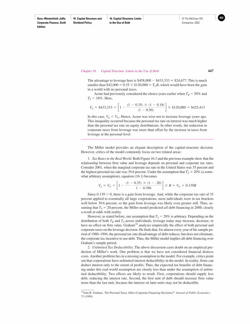
Ross−Westerfield−Jaffe: Corporate Finance, Sixth Edition
IV. Capital Structure and Dividend Policy
16. Capital Structure: Limits to the Use of Debt
453© The McGraw−Hill Companies, 2002
The advantage to leverage here is $458,000 � $433,333 � $24,677. This is muchsmaller than $42,000 � 0.35 � $120,000 � TCB, which would have been the gainin a world with no personal taxes.
Acme had previously considered the choice years earlier when TB � 50% andTS � 18%. Here,
In this case, VL VU. Hence, Acme was wise not to increase leverage years ago.This inequality occurred because the personal tax rate on interest was much higherthan the personal tax rate on equity distributions. In other words, the reduction incorporate taxes from leverage was more than offset by the increase in taxes fromleverage at the personal level.
The Miller model provides an elegant description of the capital-structure decision.However, critics of the model commonly focus on two related areas:
1. Tax Rates in the Real World. Both Figure 16.3 and the previous example show that therelationship between firm value and leverage depends on personal and corporate tax rates.Consider 2001, when the marginal corporate tax rate in the United States was 35 percent andthe highest personal tax rate was 39.6 percent. Under the assumption that TS � 20% (a some-what arbitrary assumption), equation (16.1) becomes
Since 0.139 � 0, there is a gain from leverage. And, while the corporate tax rate of 35percent applied to essentially all large corporations, most individuals were in tax bracketswell below 39.6 percent, so the gain from leverage was likely even greater still. Thus, as-suming that TS � 20 percent, the Miller model predicted all-debt financing in 2000, clearlya result at odds with reality.
However, as stated before, our assumption that TS � 20% is arbitrary. Depending on thedistribution of both TB and TS across individuals, leverage today may increase, decrease, orhave no effect on firm value. Graham34 analyzes empirically the effect of both personal andcorporate taxes on the leverage decision. He finds that, for almost every year of his sample pe-riod of 1980–1994, the personal tax rate disadvantage of debt reduces, but does not eliminate,the corporate tax incentive to use debt. Thus, the Miller model implies all-debt financing overGraham’s sample period.
2. Unlimited Tax Deductibility. The above discussion casts doubt on an empirical pre-diction of Miller’s work. One problem is that we have not considered financial distresscosts. Another problem lies in a missing assumption in the model. For example, critics pointout that corporations have unlimited interest deductibility in the model. In reality, firms candeduct interest only to the extent of profits. Thus, the expected tax benefits of debt financ-ing under this real-world assumption are clearly less than under the assumption of unlim-ited deductibility. Two effects are likely to result. First, corporations should supply lessdebt, reducing the interest rate. Second, the first unit of debt should increase firm valuemore than the last unit, because the interest on later units may not be deductible.
VL � VU � �1 ��1 � 0.35� � �1 � .20�
1 � 0.396 � B � VU � 0.139B
VL � $433,333 � �1 ��1 � 0.35� � �1 � 0.18�
�1 � 0.50� � $120,000 � $425,413
Chapter 16 Capital Structure: Limits to the Use of Debt 447
34John R. Graham, “Do Personal Taxes Affect Corporate Financing Decisions?” Journal of Public Economics73 (1999).
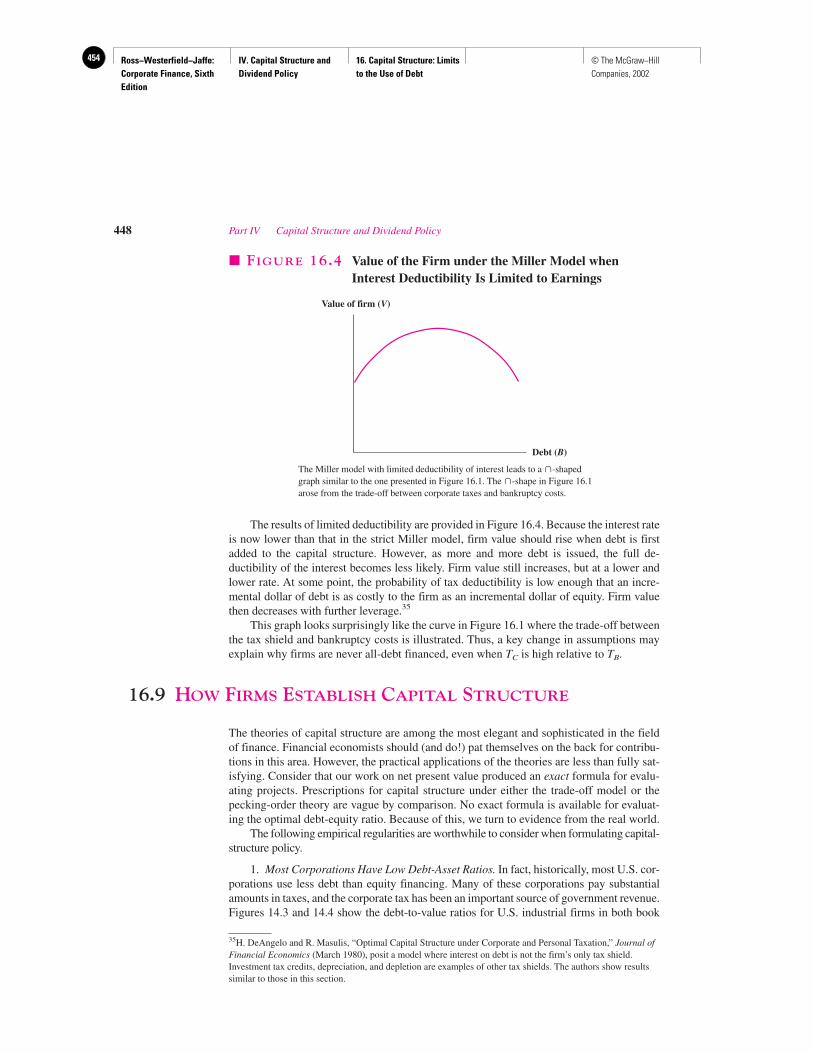
Ross−Westerfield−Jaffe: Corporate Finance, Sixth Edition
IV. Capital Structure and Dividend Policy
16. Capital Structure: Limits to the Use of Debt
454 © The McGraw−Hill Companies, 2002
The results of limited deductibility are provided in Figure 16.4. Because the interest rateis now lower than that in the strict Miller model, firm value should rise when debt is firstadded to the capital structure. However, as more and more debt is issued, the full de-ductibility of the interest becomes less likely. Firm value still increases, but at a lower andlower rate. At some point, the probability of tax deductibility is low enough that an incre-mental dollar of debt is as costly to the firm as an incremental dollar of equity. Firm valuethen decreases with further leverage.35
This graph looks surprisingly like the curve in Figure 16.1 where the trade-off betweenthe tax shield and bankruptcy costs is illustrated. Thus, a key change in assumptions mayexplain why firms are never all-debt financed, even when TC is high relative to TB.
16.9 HOW FIRMS ESTABLISH CAPITAL STRUCTURE
The theories of capital structure are among the most elegant and sophisticated in the fieldof finance. Financial economists should (and do!) pat themselves on the back for contribu-tions in this area. However, the practical applications of the theories are less than fully sat-isfying. Consider that our work on net present value produced an exact formula for evalu-ating projects. Prescriptions for capital structure under either the trade-off model or thepecking-order theory are vague by comparison. No exact formula is available for evaluat-ing the optimal debt-equity ratio. Because of this, we turn to evidence from the real world.
The following empirical regularities are worthwhile to consider when formulating capital-structure policy.
1. Most Corporations Have Low Debt-Asset Ratios. In fact, historically, most U.S. cor-porations use less debt than equity financing. Many of these corporations pay substantialamounts in taxes, and the corporate tax has been an important source of government revenue.Figures 14.3 and 14.4 show the debt-to-value ratios for U.S. industrial firms in both book
448 Part IV Capital Structure and Dividend Policy
35H. DeAngelo and R. Masulis, “Optimal Capital Structure under Corporate and Personal Taxation,” Journal ofFinancial Economics (March 1980), posit a model where interest on debt is not the firm’s only tax shield.Investment tax credits, depreciation, and depletion are examples of other tax shields. The authors show resultssimilar to those in this section.
Value of firm (V)
Debt (B)
� FIGURE 16.4 Value of the Firm under the Miller Model whenInterest Deductibility Is Limited to Earnings
The Miller model with limited deductibility of interest leads to a �-shapedgraph similar to the one presented in Figure 16.1. The �-shape in Figure 16.1arose from the trade-off between corporate taxes and bankruptcy costs.
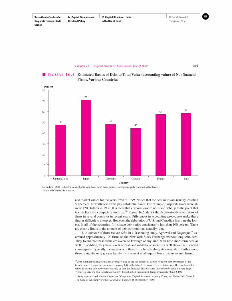
Ross−Westerfield−Jaffe: Corporate Finance, Sixth Edition
IV. Capital Structure and Dividend Policy
16. Capital Structure: Limits to the Use of Debt
455© The McGraw−Hill Companies, 2002
and market values for the years 1988 to 1999. Notice that the debt ratios are usually less than50 percent. Nevertheless firms pay substantial taxes. For example, corporate taxes were al-most $200 billion in 1996. It is clear that corporations do not issue debt up to the point thattax shelters are completely used up.36 Figure 16.5 shows the debt-to-total-value ratios offirms in several countries in recent years. Differences in accounting procedures make thesefigures difficult to interpret. However, the debt ratios of U.S. and Canadian firms are the low-est. In all of the countries, firms have debt ratios considerably less than 100 percent. Thereare clearly limits to the amount of debt corporations actually issue.
2. A number of firms use no debt. In a fascinating study, Agrawal and Nagarajan37 ex-amined approximately 100 firms on the New York Stock Exchange without long-term debt.They found that these firms are averse to leverage of any kind, with little short-term debt aswell. In addition, they have levels of cash and marketable securities well above their leveredcounterparts. Typically, the managers of these firms have high equity ownership. Furthermore,there is significantly greater family involvement in all-equity firms than in levered firms.
Chapter 16 Capital Structure: Limits to the Use of Debt 449
80
70
60
50
40
30
20
10
0
Percent
Country
United States
48
Japan
72
Germany
49
Canada
45
France
58
Italy
59
� FIGURE 16.5 Estimated Ratios of Debt to Total Value (accounting value) of NonfinancialFirms, Various Countries
Definition: Debt is short-term debt plus long-term debt. Total value is debt plus equity (in book-value terms).Source: OECD financial statistics.
36John Graham estimates that the average value of the tax benefit of debt is no more than 10 percent of thefirm’s value. He asks the question: Is money left in the table? His answer is a tentative yes. He concludes thateither firms use debt too conservatively or that the financial distress costs (and related costs) are very large.“How Big Are the Tax Benefits of Debt?” Unpublished manuscript, Duke University (June 2002).37Anup Agrawal and Nandu Nagarajan, “Corporate Capital Structure, Agency Costs, and Ownership Control:The Case of All-Equity Firms,” Journal of Finance 45 (September 1990).
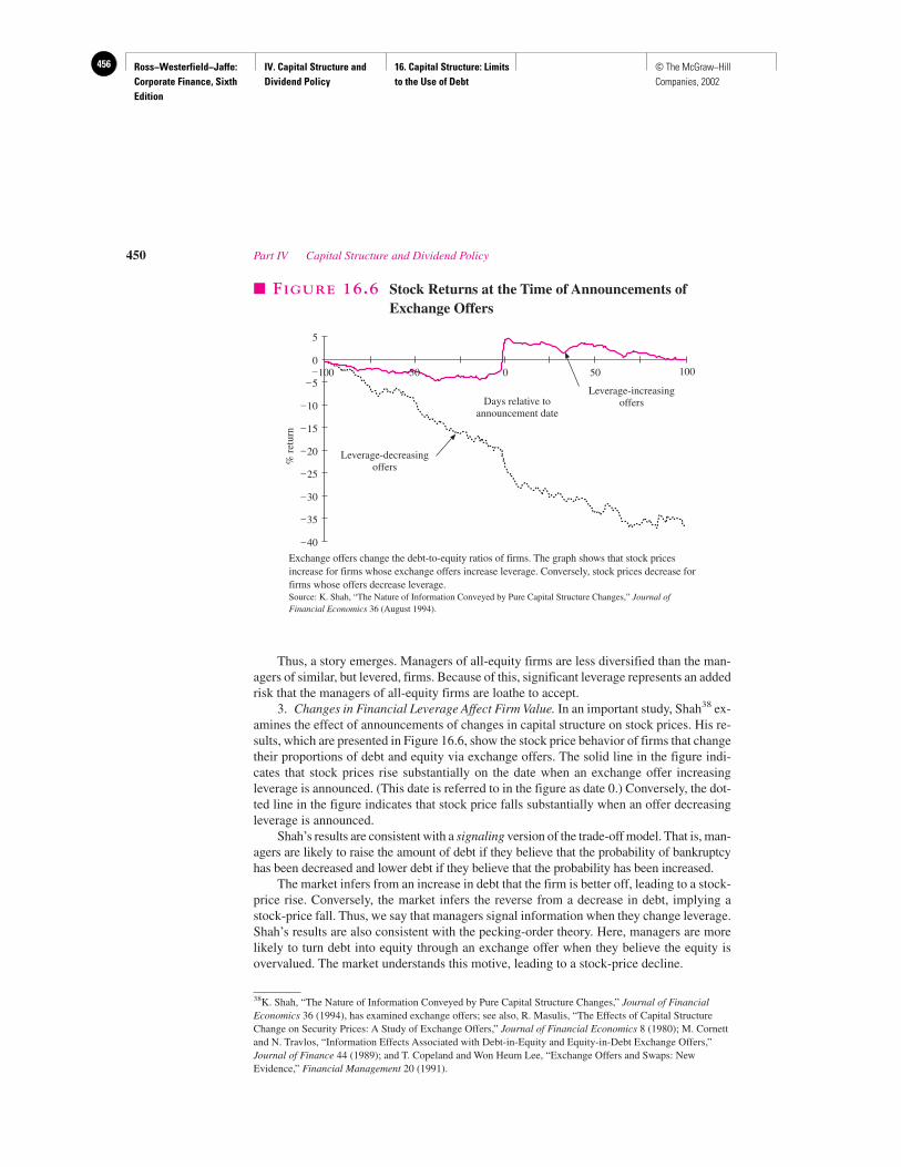
Ross−Westerfield−Jaffe: Corporate Finance, Sixth Edition
IV. Capital Structure and Dividend Policy
16. Capital Structure: Limits to the Use of Debt
456 © The McGraw−Hill Companies, 2002
Thus, a story emerges. Managers of all-equity firms are less diversified than the man-agers of similar, but levered, firms. Because of this, significant leverage represents an addedrisk that the managers of all-equity firms are loathe to accept.
3. Changes in Financial Leverage Affect Firm Value. In an important study, Shah38 ex-amines the effect of announcements of changes in capital structure on stock prices. His re-sults, which are presented in Figure 16.6, show the stock price behavior of firms that changetheir proportions of debt and equity via exchange offers. The solid line in the figure indi-cates that stock prices rise substantially on the date when an exchange offer increasingleverage is announced. (This date is referred to in the figure as date 0.) Conversely, the dot-ted line in the figure indicates that stock price falls substantially when an offer decreasingleverage is announced.
Shah’s results are consistent with a signaling version of the trade-off model. That is, man-agers are likely to raise the amount of debt if they believe that the probability of bankruptcyhas been decreased and lower debt if they believe that the probability has been increased.
The market infers from an increase in debt that the firm is better off, leading to a stock-price rise. Conversely, the market infers the reverse from a decrease in debt, implying astock-price fall. Thus, we say that managers signal information when they change leverage.Shah’s results are also consistent with the pecking-order theory. Here, managers are morelikely to turn debt into equity through an exchange offer when they believe the equity isovervalued. The market understands this motive, leading to a stock-price decline.
450 Part IV Capital Structure and Dividend Policy
38K. Shah, “The Nature of Information Conveyed by Pure Capital Structure Changes,” Journal of FinancialEconomics 36 (1994), has examined exchange offers; see also, R. Masulis, “The Effects of Capital StructureChange on Security Prices: A Study of Exchange Offers,” Journal of Financial Economics 8 (1980); M. Cornettand N. Travlos, “Information Effects Associated with Debt-in-Equity and Equity-in-Debt Exchange Offers,”Journal of Finance 44 (1989); and T. Copeland and Won Heum Lee, “Exchange Offers and Swaps: NewEvidence,” Financial Management 20 (1991).
Leverage-decreasingoffers
5
0
–5
–10
–15
–20
–25
–30
–35
–40
Leverage-increasingoffers
–100 –50 0 50 100
Days relative toannouncement date
% r
etur
n� FIGURE 16.6 Stock Returns at the Time of Announcements of
Exchange Offers
Exchange offers change the debt-to-equity ratios of firms. The graph shows that stock pricesincrease for firms whose exchange offers increase leverage. Conversely, stock prices decrease forfirms whose offers decrease leverage.Source: K. Shah, “The Nature of Information Conveyed by Pure Capital Structure Changes,” Journal ofFinancial Economics 36 (August 1994).
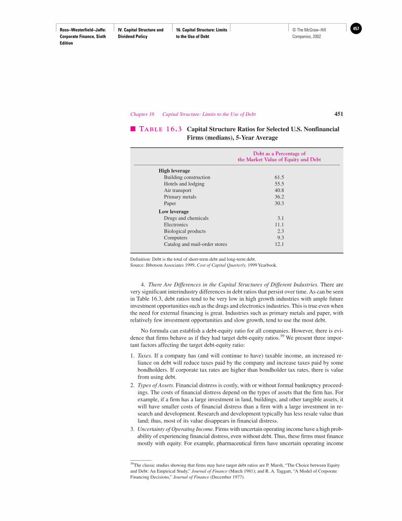
Ross−Westerfield−Jaffe: Corporate Finance, Sixth Edition
IV. Capital Structure and Dividend Policy
16. Capital Structure: Limits to the Use of Debt
457© The McGraw−Hill Companies, 2002
4. There Are Differences in the Capital Structures of Different Industries. There arevery significant interindustry differences in debt ratios that persist over time. As can be seenin Table 16.3, debt ratios tend to be very low in high growth industries with ample futureinvestment opportunities such as the drugs and electronics industries. This is true even whenthe need for external financing is great. Industries such as primary metals and paper, withrelatively few investment opportunities and slow growth, tend to use the most debt.
No formula can establish a debt-equity ratio for all companies. However, there is evi-dence that firms behave as if they had target debt-equity ratios.39 We present three impor-tant factors affecting the target debt-equity ratio:
1. Taxes. If a company has (and will continue to have) taxable income, an increased re-liance on debt will reduce taxes paid by the company and increase taxes paid by somebondholders. If corporate tax rates are higher than bondholder tax rates, there is valuefrom using debt.
2. Types of Assets. Financial distress is costly, with or without formal bankruptcy proceed-ings. The costs of financial distress depend on the types of assets that the firm has. Forexample, if a firm has a large investment in land, buildings, and other tangible assets, itwill have smaller costs of financial distress than a firm with a large investment in re-search and development. Research and development typically has less resale value thanland; thus, most of its value disappears in financial distress.
3. Uncertainty of Operating Income. Firms with uncertain operating income have a high prob-ability of experiencing financial distress, even without debt. Thus, these firms must financemostly with equity. For example, pharmaceutical firms have uncertain operating income
Chapter 16 Capital Structure: Limits to the Use of Debt 451
� TABLE 16.3 Capital Structure Ratios for Selected U.S. NonfinancialFirms (medians), 5-Year Average
Debt as a Percentage ofthe Market Value of Equity and Debt
High leverageBuilding construction 61.5Hotels and lodging 55.5Air transport 40.8Primary metals 36.2Paper 30.3
Low leverageDrugs and chemicals 3.1Electronics 11.1Biological products 2.3Computers 9.3Catalog and mail-order stores 12.1
Definition: Debt is the total of short-term debt and long-term debt.Source: Ibbotson Associates 1999, Cost of Capital Quarterly, 1999 Yearbook.
39The classic studies showing that firms may have target debt ratios are P. Marsh, “The Choice between Equityand Debt: An Empirical Study,” Journal of Finance (March 1981); and R. A. Taggart, “A Model of CorporateFinancing Decisions,” Journal of Finance (December 1977).
Ross−Westerfield−Jaffe: Corporate Finance, Sixth Edition
IV. Capital Structure and Dividend Policy
16. Capital Structure: Limits to the Use of Debt
458 © The McGraw−Hill Companies, 2002
because no one can predict whether today’s research will generate new drugs. Conse-quently, these firms issue little debt. By contrast, the operating income of utilities generallyhas little uncertainty. Relative to other industries, utilities use a great deal of debt.
One final note is in order. Because no formula supports them, the preceding points mayseem too nebulous to assist financial decision making. Instead, many real-world firms sim-ply base their capital structure decisions on industry averages. While this may strike someas a cowardly approach, it at least keeps firms from deviating far from accepted practice.After all, the existing firms in any industry are the survivors. Therefore, one should at leastpay some attention to their decisions.
• List the empirical regularities we observe for corporate capital structure.• What are the factors to consider in establishing a debt-equity ratio?
16.10 SUMMARY AND CONCLUSIONS
1. We mentioned in the last chapter that, according to theory, firms should create all-debt capitalstructures under corporate taxation. Because firms generally assume moderate amounts ofdebt in the real world, the theory must have been missing something at that point. We pointout in this chapter that costs of financial distress cause firms to restrain their issuance of debt.These costs are of two types: direct and indirect. Lawyers’ and accountants’ fees during thebankruptcy process are examples of direct costs. We mention four examples of indirect costs:
Impaired ability to conduct business.
Incentive to take on risky projects.
Incentive toward underinvestment.
Distribution of funds to stockholders prior to bankruptcy.
2. Because the above costs are substantial and the stockholders ultimately bear them, firms havean incentive for cost reduction. We suggest three cost-reduction techniques:
Protective covenants.
Repurchase of debt prior to bankruptcy.
Consolidation of debt.
3. Because costs of financial distress can be reduced but not eliminated, firms will not financeentirely with debt. Figure 16.1 illustrates the relationship between firm value and debt. In thefigure, firms select the debt-to-equity ratio at which firm value is maximized.
4. The pecking-order theory implies that managers prefer internal to external financing. Ifexternal financing is required, managers tend to choose the safest securities, such as debt.Firms may accumulate slack to avoid external equity.
5. Berens and Cuny argue that significant equity financing can be explained by real growth andinflation, even in a world of low bankruptcy costs.
6. The results so far have ignored personal taxes. If distributions to equityholders are taxed at alower effective personal tax rate than are interest payments, the tax advantage to debt at thecorporate level is partially offset. In fact, the corporate tax advantage to debt is eliminated if
(1 � TC) � (1 � TS) � (1 � TB)
452 Part IV Capital Structure and Dividend Policy
QUESTIONS
CO
NC
EP
T
?
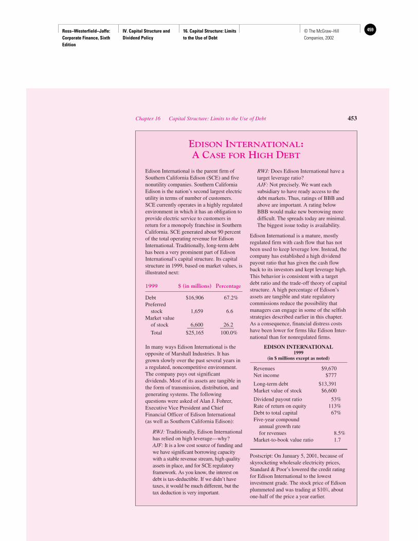
Ross−Westerfield−Jaffe: Corporate Finance, Sixth Edition
IV. Capital Structure and Dividend Policy
16. Capital Structure: Limits to the Use of Debt
459© The McGraw−Hill Companies, 2002
Chapter 16 Capital Structure: Limits to the Use of Debt 453
EDISON INTERNATIONAL: A CASE FOR HIGH DEBT
Edison International is the parent firm ofSouthern California Edison (SCE) and fivenonutility companies. Southern CaliforniaEdison is the nation’s second largest electricutility in terms of number of customers.SCE currently operates in a highly regulatedenvironment in which it has an obligation toprovide electric service to customers inreturn for a monopoly franchise in SouthernCalifornia. SCE generated about 90 percentof the total operating revenue for EdisonInternational. Traditionally, long-term debthas been a very prominent part of EdisonInternational’s capital structure. Its capitalstructure in 1999, based on market values, isillustrated next:
1999 $ (in millions) Percentage
Debt $16,906 67.2%Preferred
stock 1,659 6.6Market value
of stock 6,600 26.2______ _____Total $25,165 100.0%
In many ways Edison International is theopposite of Marshall Industries. It hasgrown slowly over the past several years ina regulated, noncompetitive environment.The company pays out significantdividends. Most of its assets are tangible inthe form of transmission, distribution, andgenerating systems. The followingquestions were asked of Alan J. Fohrer,Executive Vice President and ChiefFinancial Officer of Edison International(as well as Southern California Edison):
RWJ: Traditionally, Edison Internationalhas relied on high leverage—why?AJF: It is a low cost source of funding andwe have significant borrowing capacitywith a stable revenue stream, high qualityassets in place, and for SCE regulatoryframework. As you know, the interest ondebt is tax-deductible. If we didn’t havetaxes, it would be much different, but thetax deduction is very important.
RWJ: Does Edison International have atarget leverage ratio?AJF: Not precisely. We want eachsubsidiary to have ready access to thedebt markets. Thus, ratings of BBB andabove are important. A rating belowBBB would make new borrowing moredifficult. The spreads today are minimal.The biggest issue today is availability.
Edison International is a mature, mostlyregulated firm with cash flow that has notbeen used to keep leverage low. Instead, thecompany has established a high dividendpayout ratio that has given the cash flowback to its investors and kept leverage high.This behavior is consistent with a targetdebt ratio and the trade-off theory of capitalstructure. A high percentage of Edison’sassets are tangible and state regulatorycommissions reduce the possibility thatmanagers can engage in some of the selfishstrategies described earlier in this chapter.As a consequence, financial distress costshave been lower for firms like Edison Inter-national than for nonregulated firms.
EDISON INTERNATIONAL1999
(in $ millions except as noted)
Revenues $9,670Net income $777
Long-term debt $13,391Market value of stock $6,600
Dividend payout ratio 53%Rate of return on equity 113%Debt to total capital 67%Five-year compound
annual growth rate for revenues 8.5%
Market-to-book value ratio 1.7
Postscript: On January 5, 2001, because ofskyrocketing wholesale electricity prices,Standard & Poor’s lowered the credit ratingfor Edison International to the lowestinvestment grade. The stock price of Edisonplummeted and was trading at $103⁄4, aboutone-half of the price a year earlier.

Ross−Westerfield−Jaffe: Corporate Finance, Sixth Edition
IV. Capital Structure and Dividend Policy
16. Capital Structure: Limits to the Use of Debt
460 © The McGraw−Hill Companies, 2002
454 Part IV Capital Structure and Dividend Policy
QUALCOMM: A CASE FOR LOW DEBT
Qualcomm is a supplier of digital wirelesscommunications products and services. It isthe innovator and implementer of theproprietary code-division multiple access(CDMA), a digital wireless technology.CDMA generates licensing fees, royalties,and chip sales. In addition, Qualcomm hasa new high-data-rate (HDR) technologythat it expects to transmit data at very highspeeds for Internet use and access. Itsprimary U.S. competitor uses anotherwireless technology called TDMA. Itcompetes with suppliers of alternativewireless technologies, such as GSM usedby Pac Bell and TDMA used by AT&T.
Qualcomm employs about 7,000 peopleand is headquartered in San Diego. ByMarch 2000, Qualcomm had redeemed allits convertible preferred securities and hadvery little long-term debt. Its capitalstructure was:
Long-term debt Nil
Market value of stock $112 billion
Why does Qualcomm rely so little on long-term debt? This question was asked ofAnthony S. Thornley, Executive VicePresident and Chief Financial Officer ofQualcomm.
RWJ: One thing that stands out from afinancial point of view aboutQualcomm is that it has almost nolong-term debt. Why?AST: There currently isn’t any reason toleverage the company. We can financeour growth from retained earnings andoutside equity.RWJ: Outside equity?AST: With our high P/E ratio we have avery low cost of equity.RWJ: Qualcomm is in a very competi-tive business. Is this a factor in thecapital structure?AST: We are conservative financiallyand have relied largely on equity tofinance the company. However, we haveused debt at times when the relative costwas lower than equity.
RWJ: Many of the assets of Qualcommare intangible, such as the value of itspatents and its highly skilled engineers.Does this limit Qualcomm’s debtcapacity?AST: Intangible assets have less collat-eral value than bricks and mortar, butQualcomm’s patents throw off a steadystream of cash flow. Qualcomm has agreat deal of debt capacity. We justprefer flexibility at this time.RWJ: Thanks.
What Can We Learn from Qualcomm?First, Qualcomm is a firm with veryuncertain future outcomes in a verycompetitive business and with significantintangible assets. This would suggestQualcomm has a relatively low debtcapacity when compared to, say, EdisonInternational. Moreover, the financialmanagement of Qualcomm is conservativeby nature. Qualcomm’s patents generate asteady stream of cash flow, which enhancesdebt capacity, but the competitive and fast-paced nature of the telecommunicationsindustry suggests a need for financial slackand flexibility. Second, Qualcomm hasexperienced a rapid growth in profit andsales over the past five years—greater than60 percent per annum. As a consequence,the tax potential benefits of debt have onlyrecently materialized. Finally, Qualcomm’svery high stock price and price-earningsratio suggest (to its financial management)that this is an opportune time to rely moreon equity financing than debt.
A Financial Profile of Qualcomm(April 2000)
(in $ millions except as noted)
Revenues 3,937.3Net income 391.9Long-term debt —Dividend payout (%) 0Return on equity (ROE) (%) 13.6Five-year compound annual growth in revenues 62.5%Recent price-to-earnings ratio 40–100
Ross−Westerfield−Jaffe: Corporate Finance, Sixth Edition
IV. Capital Structure and Dividend Policy
16. Capital Structure: Limits to the Use of Debt
461© The McGraw−Hill Companies, 2002
7. Debt-to-equity ratios vary across industries. We present three factors determining the targetdebt-to-equity ratio:a. Taxes. Firms with high taxable income should rely more on debt than firms with low
taxable income.b. Types of Assets. Firms with a high percentage of intangible assets such as research and
development should have low debt. Firms with primarily tangible assets should havehigher debt.
c. Uncertainty of Operating Income. Firms with high uncertainty of operating incomeshould rely mostly on equity.
KEY TERMS
Agency costs 427 Nonmarketed claims 434Marketed claims 434 Positive covenant 431Negative covenant 430 Protective covenants 430
SUGGESTED READINGS
An excellent collection of recent articles appears inChew, D. The New Corporate Finance: Where Theory Meets Practice (New York: McGraw-Hill,
1993).
Merton Miller’s Nobel lecture is reprinted asMiller, M. “Leverage.” Journal of Finance (June 1991).
An extremely influential set of articles arguing that bankruptcy costs are low areHaugen, R. A., and L. Senbet. “The Insignificance of Bankruptcy Costs to the Theory of
Optimal Capital Structure.” Journal of Finance (May 1978).Haugen, R. A., and L. Senbet. “Bankruptcy and Agency Costs: Their Significance to the Theory of
Optimal Capital Structure.” Journal of Financial and Quantitative Analysis (March 1988).
The following excellent paper surveys the various capital-structure theories:Rajan, Raghuram G., and Luigi Zingales. “What Do We Know about Capital Structure?”
Journal of Finance (December 1995).
In several recent articles, John R. Graham estimates effective corporate tax rates and their inputon corporate financing policy.“Do Personal Taxes Affect Corporate Financing Decisions.” Journal of Public Economics 73
(1999).“Debt and the MTR.” Journal of Financial Economics 4 (1996).Graham, John R.; Michael Lemmon; and James Schollheirn. “Debt, Leases, Taxes and the
Endogeneity of Corporate Tax Status.” Journal of Finance 53 (1998).
QUESTIONS AND PROBLEMS
Costs of Financial Distress16.1 Good Time Co. is a regional chain department store. It will remain in business for one
more year. The estimated probability of a boom year is 60 percent and that of a recessionis 40 percent. It is projected that Good Time will have total cash flow of $250 million in aboom year and $100 million in a recession. Its required debt payment is $150 million perannum. Assume a one-period model.
Assume risk neutrality and an annual discount rate of 12 percent for both the stock andthe bond.
Chapter 16 Capital Structure: Limits to the Use of Debt 455
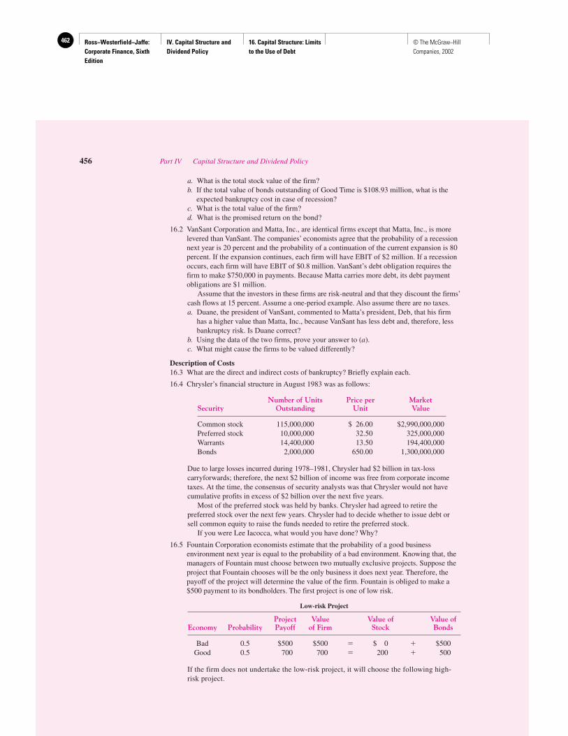
Ross−Westerfield−Jaffe: Corporate Finance, Sixth Edition
IV. Capital Structure and Dividend Policy
16. Capital Structure: Limits to the Use of Debt
462 © The McGraw−Hill Companies, 2002
456 Part IV Capital Structure and Dividend Policy
a. What is the total stock value of the firm?b. If the total value of bonds outstanding of Good Time is $108.93 million, what is the
expected bankruptcy cost in case of recession?c. What is the total value of the firm?d. What is the promised return on the bond?
16.2 VanSant Corporation and Matta, Inc., are identical firms except that Matta, Inc., is morelevered than VanSant. The companies’ economists agree that the probability of a recessionnext year is 20 percent and the probability of a continuation of the current expansion is 80percent. If the expansion continues, each firm will have EBIT of $2 million. If a recessionoccurs, each firm will have EBIT of $0.8 million. VanSant’s debt obligation requires thefirm to make $750,000 in payments. Because Matta carries more debt, its debt paymentobligations are $1 million.
Assume that the investors in these firms are risk-neutral and that they discount the firms’cash flows at 15 percent. Assume a one-period example. Also assume there are no taxes.a. Duane, the president of VanSant, commented to Matta’s president, Deb, that his firm
has a higher value than Matta, Inc., because VanSant has less debt and, therefore, lessbankruptcy risk. Is Duane correct?
b. Using the data of the two firms, prove your answer to (a).c. What might cause the firms to be valued differently?
Description of Costs16.3 What are the direct and indirect costs of bankruptcy? Briefly explain each.
16.4 Chrysler’s financial structure in August 1983 was as follows:
Number of Units Price per MarketSecurity Outstanding Unit Value
Common stock 115,000,000 $ 26.00 $2,990,000,000Preferred stock 10,000,000 32.50 325,000,000Warrants 14,400,000 13.50 194,400,000Bonds 2,000,000 650.00 1,300,000,000
Due to large losses incurred during 1978–1981, Chrysler had $2 billion in tax-losscarryforwards; therefore, the next $2 billion of income was free from corporate incometaxes. At the time, the consensus of security analysts was that Chrysler would not havecumulative profits in excess of $2 billion over the next five years.
Most of the preferred stock was held by banks. Chrysler had agreed to retire thepreferred stock over the next few years. Chrysler had to decide whether to issue debt orsell common equity to raise the funds needed to retire the preferred stock.
If you were Lee Iacocca, what would you have done? Why?
16.5 Fountain Corporation economists estimate that the probability of a good businessenvironment next year is equal to the probability of a bad environment. Knowing that, themanagers of Fountain must choose between two mutually exclusive projects. Suppose theproject that Fountain chooses will be the only business it does next year. Therefore, thepayoff of the project will determine the value of the firm. Fountain is obliged to make a$500 payment to its bondholders. The first project is one of low risk.
Low-risk Project
Project Value Value of Value ofEconomy Probability Payoff of Firm Stock Bonds
Bad 0.5 $500 $500 � $ 0 � $500Good 0.5 700 700 � 200 � 500
If the firm does not undertake the low-risk project, it will choose the following high-risk project.
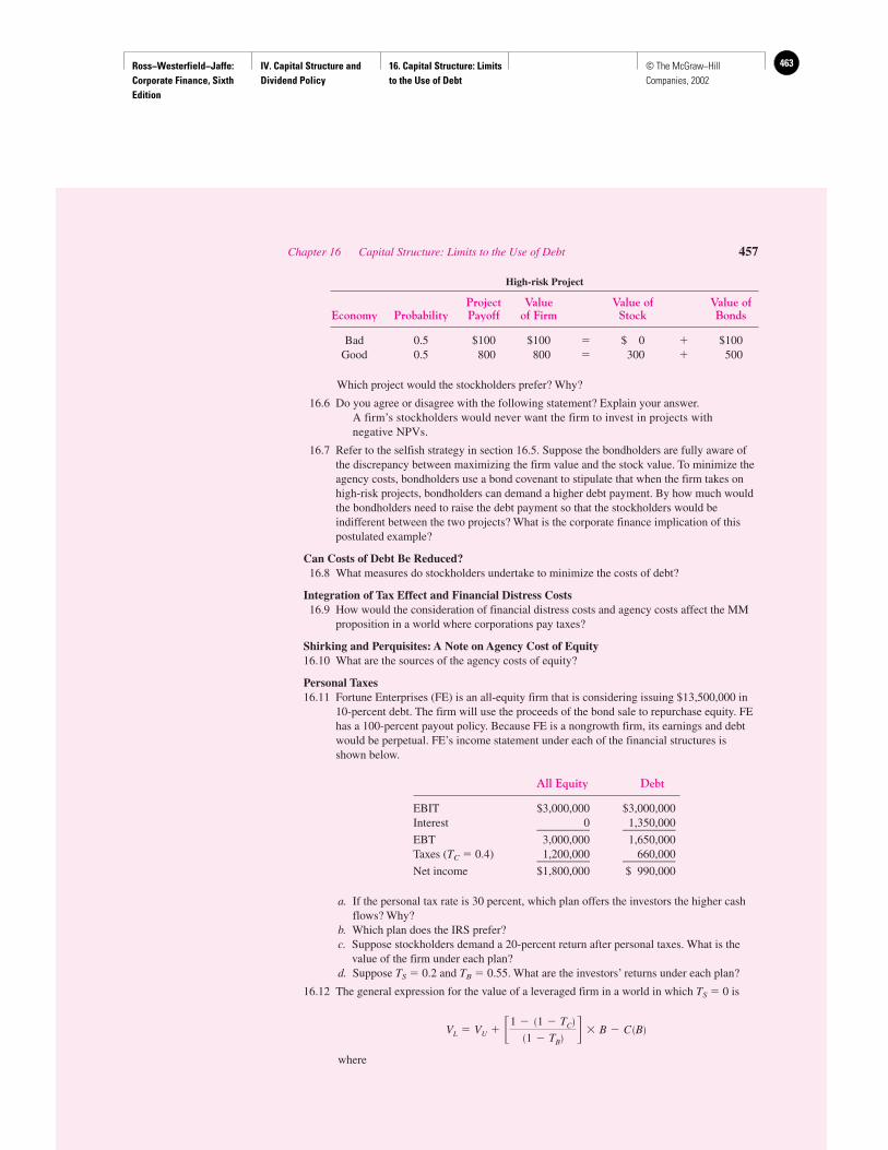
Ross−Westerfield−Jaffe: Corporate Finance, Sixth Edition
IV. Capital Structure and Dividend Policy
16. Capital Structure: Limits to the Use of Debt
463© The McGraw−Hill Companies, 2002
Chapter 16 Capital Structure: Limits to the Use of Debt 457
High-risk Project
Project Value Value of Value ofEconomy Probability Payoff of Firm Stock Bonds
Bad 0.5 $100 $100 � $ 0 � $100Good 0.5 800 800 � 300 � 500
Which project would the stockholders prefer? Why?
16.6 Do you agree or disagree with the following statement? Explain your answer.A firm’s stockholders would never want the firm to invest in projects with negative NPVs.
16.7 Refer to the selfish strategy in section 16.5. Suppose the bondholders are fully aware ofthe discrepancy between maximizing the firm value and the stock value. To minimize theagency costs, bondholders use a bond covenant to stipulate that when the firm takes onhigh-risk projects, bondholders can demand a higher debt payment. By how much wouldthe bondholders need to raise the debt payment so that the stockholders would beindifferent between the two projects? What is the corporate finance implication of thispostulated example?
Can Costs of Debt Be Reduced?16.8 What measures do stockholders undertake to minimize the costs of debt?
Integration of Tax Effect and Financial Distress Costs16.9 How would the consideration of financial distress costs and agency costs affect the MM
proposition in a world where corporations pay taxes?
Shirking and Perquisites: A Note on Agency Cost of Equity16.10 What are the sources of the agency costs of equity?
Personal Taxes16.11 Fortune Enterprises (FE) is an all-equity firm that is considering issuing $13,500,000 in
10-percent debt. The firm will use the proceeds of the bond sale to repurchase equity. FEhas a 100-percent payout policy. Because FE is a nongrowth firm, its earnings and debtwould be perpetual. FE’s income statement under each of the financial structures isshown below.
All Equity Debt
EBIT $3,000,000 $3,000,000Interest 0 1,350,000_________ _________EBT 3,000,000 1,650,000Taxes (TC � 0.4) 1,200,000 660,000_________ _________Net income $1,800,000 $ 990,000
a. If the personal tax rate is 30 percent, which plan offers the investors the higher cashflows? Why?
b. Which plan does the IRS prefer?c. Suppose stockholders demand a 20-percent return after personal taxes. What is the
value of the firm under each plan?d. Suppose TS � 0.2 and TB � 0.55. What are the investors’ returns under each plan?
16.12 The general expression for the value of a leveraged firm in a world in which TS � 0 is
where
VL � VU � �1 � �1 � TC��1 � TB� � B � C �B�

Ross−Westerfield−Jaffe: Corporate Finance, Sixth Edition
IV. Capital Structure and Dividend Policy
16. Capital Structure: Limits to the Use of Debt
464 © The McGraw−Hill Companies, 2002
458 Part IV Capital Structure and Dividend Policy
VU � Value of an unlevered firmTC � Effective corporate tax rate for the firmTB � Personal tax rate of the marginal bondholderB � Debt level of the firm
C(B) � Present value of the costs of financial distress for the firm as a function of itsdebt level. [Note: C(B) encompasses all non–tax-related effects of leverage onthe firm’s value.]
Assume all investors are risk-neutral.a. In their no-tax model, what do Modigliani and Miller assume about TC, TB, and C(B)?
What do these assumptions imply about a firm’s optimal debt-equity ratio?b. In their model that includes corporate taxes, what do Modigliani and Miller assume
about TC, TB, and C(B)? What do these assumptions imply about a firm’s optimaldebt-equity ratio?
c. Assume that IBM is certain to be able to use its interest deductions to reduce itscorporate tax bill. What would the change in the value of IBM be if the companyissued $1 billion in debt and used the proceeds to repurchase equity? Assume that thepersonal tax rate on bond income is 20 percent, the corporate tax rate is 34 percent,and the costs of financial distress are zero.
d. Assume that USX is virtually certain not to be able to use interest deductions. Whatwould the change in the value of the company be from adding $1 of perpetual debtrather than $1 of equity? Assume that the personal tax rate on bond income is 20percent, the corporate tax rate is 35 percent, and the costs of financial distress are zero.
e. For companies that may or may not be able to use the interest deduction, what wouldthe change in the value of the company be from adding $1 of perpetual debt ratherthan $1 of equity? Assume that the personal tax rate on bond income is 20 percent, thecorporate tax rate is 35 percent, and the costs of financial distress are zero. Alsoassume the probability of using the incremental deduction is 65 percent.
16.13 Because of the large cash inflows from the sales of its cookbook, Fear of Frying, theOvernight Publishing Company (OPC) has decided to retire all of its outstanding debt.The debt is made up of consul bonds; its maturity date is indefinitely far away. The debtis also considered risk-free. It carries a 10-percent coupon rate and has a book value of $3million. Because market rates on long-term bonds are 15 percent, the market value of thebonds is only $2 million. All of the debt is held by one institution that will sell it back toOPC for $2 million cash. The institution will not charge OPC any transaction costs, andthere are no tax consequences from retiring the debt. Once OPC becomes an all-equityfirm, it will remain unlevered forever.
If OPC does not return the debt, the company will use the $2 million in cash to buyback some of its stock on the open market. Repurchasing stock also has no transactioncosts. Investors expect OPC to repurchase some stock, so they will be completelysurprised when the debt-retirement plan is announced.
The required rate of return of the equity holders after OPC becomes all equity will be20 percent. The expected annual earnings before interest and taxes for the firm are$1,100,000; those earnings are expected to remain constant in perpetuity. OPC has nogrowth opportunities, and the company is subject to a 35-percent corporate tax rate.Assume that TB � 10% and TS � 0. Also assume that bankruptcy costs do not change forOPC as a result of this capital-structure change. How much does the market value of thecompany change?
16.14 The EXES Company is assessing its present capital structure and that structure’simplications for the welfare of its investors. EXES is currently financed entirely withcommon stock, of which 1,000 shares are outstanding. Given the risk of the underlyingcash flows (EBIT) generated by EXES, investors currently require a 20-percent returnon the EXES common stock. The company pays out all earnings as dividends tocommon stockholders.

Ross−Westerfield−Jaffe: Corporate Finance, Sixth Edition
IV. Capital Structure and Dividend Policy
16. Capital Structure: Limits to the Use of Debt
465© The McGraw−Hill Companies, 2002
Chapter 16 Capital Structure: Limits to the Use of Debt 459
EXES estimates that operating income may be $1,000, $2,000, or $4,200 withrespective probabilities of 0.1, 0.4, and 0.5. Assume the firm’s expectations aboutearnings will be met and that they will be unchanged in perpetuity. Also, assume that thecorporate and personal tax rates are equal to zero.a. What is the value of EXES Company?b. The president of EXES has decided that shareholders would be better off if the
company had equal proportions of debt and equity. He therefore proposes to issue$7,500 of debt at an interest rate of 10 percent. He will use the proceeds to repurchase500 shares of common stock.
i. What will the new value of the firm be?ii. What will the value of EXES’s debt be?
iii. What will the value of EXES’s equity be?c. Suppose the president’s proposal is implemented.
i. What is the required rate of return on equity?ii. What is the firm’s overall required return?
d. Suppose the corporate tax rate is 40 percent.i. Use the Modigliani-Miller framework that includes taxes to find the value of the firm.
ii. Does the presence of taxes increase or decrease the value of the firm? Why?iii. Verbally explain how the presence of bankruptcy costs would change the effect of
taxes on the value of the firm, if at all.e. Suppose interest income is taxed at 40 percent while the effective tax on returns to
equityholders is zero. Assume that the introduction of the personal tax rate does notaffect the required return on equity.
i. What is the value of EXES in a world with personal taxes?ii. Under the Miller model, what will happen to the value of the firm as the tax on
interest income rises?
16.15 Mueller Brewing Company has been ordered by the EPA to stop polluting theMenomenie River. It must now spend $100 million on pollution-control equipment. Thecompany has three alternatives for obtaining the needed $100 million.1. Sell $100 million of perpetual, taxable corporate bonds with a 20-percent coupon rate.2. Sell $100 million of perpetual pollution-control bonds with a 10-percent coupon rate.
The interest on these bonds is not taxable to investors.3. Sell $100 million of common stock with a 9.5-percent current dividend yield.Mueller Brewing Company is in the 35-percent tax bracket.
The president of Mueller Brewing wants to sell the common stock because it has thelowest rate. Mr. Daniels, the company’s treasurer, suggests bond financing because of thetax shield offered by the debt. His analysis shows that the value of the firm wouldincrease rBBTC/rB � ($100 million) � (0.35) � $35 million if Mueller issues bondsinstead of equity. A newly hired financial analyst, Ms. Harris, argues that it does notmatter which type of bond is issued. She claims that the yields will be bid up to reflecttaxes and, thus, the financing choice will not matter.a. Comment on the analyses of the president, Mr. Daniels, and Ms. Harris.b. Should Mueller be indifferent about which financing plan it chooses? If not, rank the
three alternatives and give the benefits and costs of each.
16.16 Melvin Clark, CFO of the Matsushita Corp., is evaluating the value of the firm’s currentcapital structure. Being conservative, he expects that Matsushita will have a perpetualEBIT of $800,000, with an after-tax discount rate of 10 percent if it is all-equity financed.Currently, the firm has $1.2 million debt. The corporate tax rate is 35 percent. Theuniform personal tax rate in the economy is 15 percent. Personal tax rates on equityincome are effectively zero because of the possibility of infinite deferral of the realizationof capital gains. The combined financial distress and agency costs associated with thedebt are approximately 5 percent of the total debt value.a. What is the added value of the debt?b. What is the firm value of Matsushita?
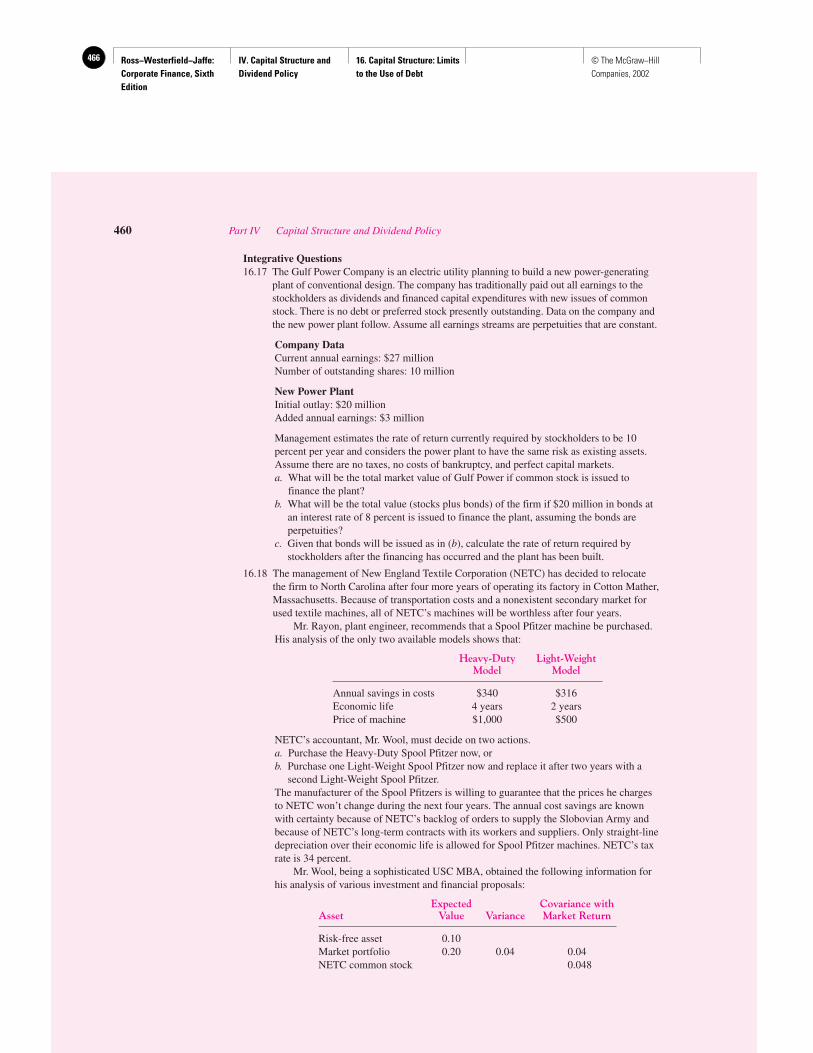
Ross−Westerfield−Jaffe: Corporate Finance, Sixth Edition
IV. Capital Structure and Dividend Policy
16. Capital Structure: Limits to the Use of Debt
466 © The McGraw−Hill Companies, 2002
460 Part IV Capital Structure and Dividend Policy
Integrative Questions16.17 The Gulf Power Company is an electric utility planning to build a new power-generating
plant of conventional design. The company has traditionally paid out all earnings to thestockholders as dividends and financed capital expenditures with new issues of commonstock. There is no debt or preferred stock presently outstanding. Data on the company andthe new power plant follow. Assume all earnings streams are perpetuities that are constant.
Company DataCurrent annual earnings: $27 millionNumber of outstanding shares: 10 million
New Power PlantInitial outlay: $20 millionAdded annual earnings: $3 million
Management estimates the rate of return currently required by stockholders to be 10percent per year and considers the power plant to have the same risk as existing assets.Assume there are no taxes, no costs of bankruptcy, and perfect capital markets.a. What will be the total market value of Gulf Power if common stock is issued to
finance the plant?b. What will be the total value (stocks plus bonds) of the firm if $20 million in bonds at
an interest rate of 8 percent is issued to finance the plant, assuming the bonds areperpetuities?
c. Given that bonds will be issued as in (b), calculate the rate of return required bystockholders after the financing has occurred and the plant has been built.
16.18 The management of New England Textile Corporation (NETC) has decided to relocatethe firm to North Carolina after four more years of operating its factory in Cotton Mather,Massachusetts. Because of transportation costs and a nonexistent secondary market forused textile machines, all of NETC’s machines will be worthless after four years.
Mr. Rayon, plant engineer, recommends that a Spool Pfitzer machine be purchased.His analysis of the only two available models shows that:
Heavy-Duty Light-WeightModel Model
Annual savings in costs $340 $316Economic life 4 years 2 yearsPrice of machine $1,000 $500
NETC’s accountant, Mr. Wool, must decide on two actions.a. Purchase the Heavy-Duty Spool Pfitzer now, orb. Purchase one Light-Weight Spool Pfitzer now and replace it after two years with a
second Light-Weight Spool Pfitzer.The manufacturer of the Spool Pfitzers is willing to guarantee that the prices he chargesto NETC won’t change during the next four years. The annual cost savings are knownwith certainty because of NETC’s backlog of orders to supply the Slobovian Army andbecause of NETC’s long-term contracts with its workers and suppliers. Only straight-linedepreciation over their economic life is allowed for Spool Pfitzer machines. NETC’s taxrate is 34 percent.
Mr. Wool, being a sophisticated USC MBA, obtained the following information forhis analysis of various investment and financial proposals:
Expected Covariance withAsset Value Variance Market Return
Risk-free asset 0.10Market portfolio 0.20 0.04 0.04NETC common stock 0.048
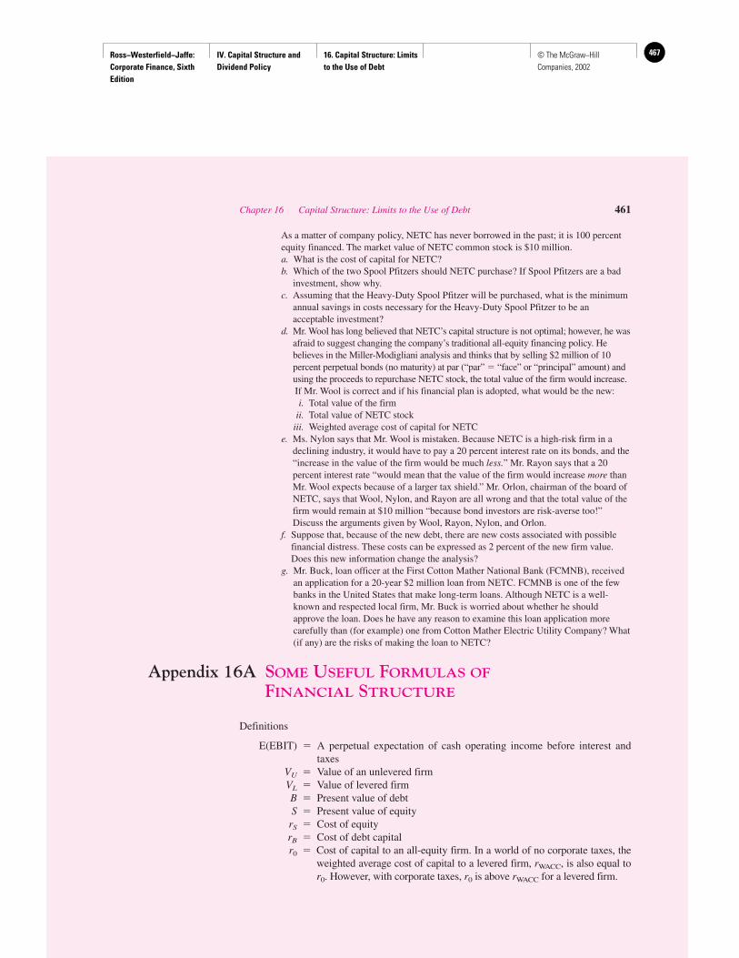
Ross−Westerfield−Jaffe: Corporate Finance, Sixth Edition
IV. Capital Structure and Dividend Policy
16. Capital Structure: Limits to the Use of Debt
467© The McGraw−Hill Companies, 2002
Chapter 16 Capital Structure: Limits to the Use of Debt 461
As a matter of company policy, NETC has never borrowed in the past; it is 100 percentequity financed. The market value of NETC common stock is $10 million.a. What is the cost of capital for NETC?b. Which of the two Spool Pfitzers should NETC purchase? If Spool Pfitzers are a bad
investment, show why.c. Assuming that the Heavy-Duty Spool Pfitzer will be purchased, what is the minimum
annual savings in costs necessary for the Heavy-Duty Spool Pfitzer to be anacceptable investment?
d. Mr. Wool has long believed that NETC’s capital structure is not optimal; however, he wasafraid to suggest changing the company’s traditional all-equity financing policy. Hebelieves in the Miller-Modigliani analysis and thinks that by selling $2 million of 10percent perpetual bonds (no maturity) at par (“par” � “face” or “principal” amount) andusing the proceeds to repurchase NETC stock, the total value of the firm would increase. If Mr. Wool is correct and if his financial plan is adopted, what would be the new:i. Total value of the firm
ii. Total value of NETC stockiii. Weighted average cost of capital for NETC
e. Ms. Nylon says that Mr. Wool is mistaken. Because NETC is a high-risk firm in adeclining industry, it would have to pay a 20 percent interest rate on its bonds, and the“increase in the value of the firm would be much less.” Mr. Rayon says that a 20percent interest rate “would mean that the value of the firm would increase more thanMr. Wool expects because of a larger tax shield.” Mr. Orlon, chairman of the board ofNETC, says that Wool, Nylon, and Rayon are all wrong and that the total value of thefirm would remain at $10 million “because bond investors are risk-averse too!”Discuss the arguments given by Wool, Rayon, Nylon, and Orlon.
f. Suppose that, because of the new debt, there are new costs associated with possiblefinancial distress. These costs can be expressed as 2 percent of the new firm value.Does this new information change the analysis?
g. Mr. Buck, loan officer at the First Cotton Mather National Bank (FCMNB), receivedan application for a 20-year $2 million loan from NETC. FCMNB is one of the fewbanks in the United States that make long-term loans. Although NETC is a well-known and respected local firm, Mr. Buck is worried about whether he shouldapprove the loan. Does he have any reason to examine this loan application morecarefully than (for example) one from Cotton Mather Electric Utility Company? What(if any) are the risks of making the loan to NETC?
Appendix 16A SOME USEFUL FORMULAS OF
FINANCIAL STRUCTURE
Definitions
E(EBIT) � A perpetual expectation of cash operating income before interest andtaxes
VU � Value of an unlevered firmVL � Value of levered firmB � Present value of debtS � Present value of equity
rS � Cost of equityrB � Cost of debt capitalr0 � Cost of capital to an all-equity firm. In a world of no corporate taxes, the
weighted average cost of capital to a levered firm, rWACC, is also equal tor0. However, with corporate taxes, r0 is above rWACC for a levered firm.

Ross−Westerfield−Jaffe: Corporate Finance, Sixth Edition
IV. Capital Structure and Dividend Policy
16. Capital Structure: Limits to the Use of Debt
468 © The McGraw−Hill Companies, 2002
462 Part IV Capital Structure and Dividend Policy
Model I (No Tax)
rS � r0 � (r0 � rB) � B/S
Model II (Corporate Tax, TC � 0; No Personal Taxes, TS � TB � 0)
rS � r0 � (1 � TC) � (r0 � rB) � B/S
Model III (Corporate Tax, TC � 0; Personal Tax, TB � 0; TS � 0)
Appendix 16B THE MILLER MODEL AND THE GRADUATED
INCOME TAX
In our previous discussion, we assumed a flat personal income tax on interest income. Inother words, we assumed that all individuals are subject to the same personal tax rate on in-terest income. Merton Miller derived the results of the previous section in a classic paper.40
However, the genius of his paper was to consider the implications of personal taxes whentax rates differ across individuals.
This graduated income tax is consistent with the real world. For example, individualsare currently taxed at rates of 0, 15, 28, 31, 36, and 39.6 percent in the United States, de-pending on income. In addition, other entities, such as corporate pension funds, individualretirement accounts (IRAs), and universities, are tax-exempt.
To illustrate Miller’s model with graduated taxes, we consider a world where all firmsinitially only issue equity. We assume that TC � 35% and TS � 0.41 The required return onstock, rS, is 10 percent. In addition, we posit a graduated personal income tax, where taxrates vary between 0 and 50 percent. All individuals are risk-neutral.
Now consider a courageous firm contemplating a $1,000 issue of debt. What is the in-terest rate that the firm can pay and still be as well off as if it issued equity? Because debtis tax deductible, the after–corporate tax cost of debt is (1 � TC) � rB. However, equity isnot deductible at the corporate level, so the after-tax cost of equity is rS. Thus, the firm isindifferent to whether it issues debt or equity when
(1 � TC) � rB � rS (16.3)
Because TC � 35% and rS � 10%, the firm could afford to pay a rate on debt as high as15.38 percent.
Miller argues that those in the lowest tax brackets (tax-exempt in our example) will buythe debt because they pay the least personal tax on interest. These tax-exempt investors willbe indifferent to whether they buy the stock or purchase bonds also yielding 10 percent.
VL � VU � �1 ��1 � TC� � �1 � TS�
�1 � TB� � B
VL �E EBIT� � �1 � TC�
r0
�TCrBB
rB
� VU � TCB
VL � VU �E �EBIT�
r0
40M. Miller, “Debt and Taxes,” Journal of Finance (May 1977). Yes, this is the same Miller of MM.41The assumption that TS � 0 is perhaps an extreme one. However, it is commonly made in the literature,justified by the investor’s ability to defer realization of capital gains indefinitely. Besides, the same qualitativeconclusions hold if TS � 0, though the explanation would be more involved.
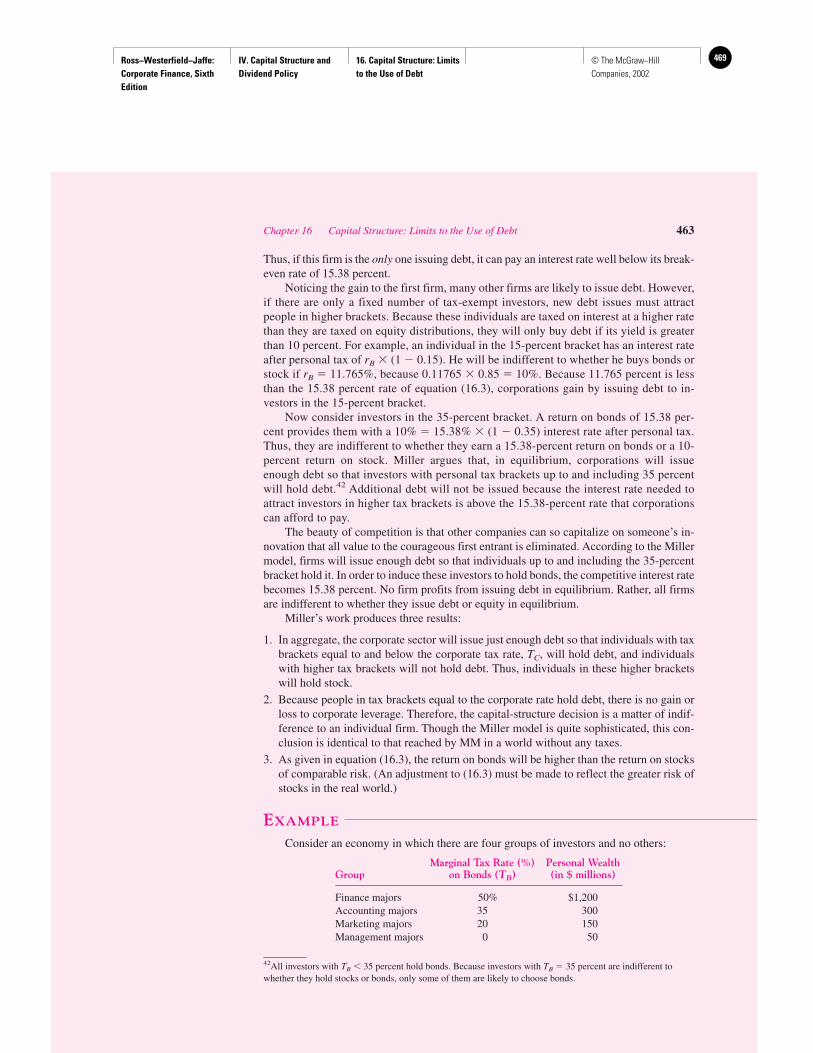
Ross−Westerfield−Jaffe: Corporate Finance, Sixth Edition
IV. Capital Structure and Dividend Policy
16. Capital Structure: Limits to the Use of Debt
469© The McGraw−Hill Companies, 2002
Chapter 16 Capital Structure: Limits to the Use of Debt 463
Thus, if this firm is the only one issuing debt, it can pay an interest rate well below its break-even rate of 15.38 percent.
Noticing the gain to the first firm, many other firms are likely to issue debt. However,if there are only a fixed number of tax-exempt investors, new debt issues must attractpeople in higher brackets. Because these individuals are taxed on interest at a higher ratethan they are taxed on equity distributions, they will only buy debt if its yield is greaterthan 10 percent. For example, an individual in the 15-percent bracket has an interest rateafter personal tax of rB � (1 � 0.15). He will be indifferent to whether he buys bonds orstock if rB � 11.765%, because 0.11765 � 0.85 � 10%. Because 11.765 percent is lessthan the 15.38 percent rate of equation (16.3), corporations gain by issuing debt to in-vestors in the 15-percent bracket.
Now consider investors in the 35-percent bracket. A return on bonds of 15.38 per-cent provides them with a 10% � 15.38% � (1 � 0.35) interest rate after personal tax.Thus, they are indifferent to whether they earn a 15.38-percent return on bonds or a 10-percent return on stock. Miller argues that, in equilibrium, corporations will issueenough debt so that investors with personal tax brackets up to and including 35 percentwill hold debt.42 Additional debt will not be issued because the interest rate needed toattract investors in higher tax brackets is above the 15.38-percent rate that corporationscan afford to pay.
The beauty of competition is that other companies can so capitalize on someone’s in-novation that all value to the courageous first entrant is eliminated. According to the Millermodel, firms will issue enough debt so that individuals up to and including the 35-percentbracket hold it. In order to induce these investors to hold bonds, the competitive interest ratebecomes 15.38 percent. No firm profits from issuing debt in equilibrium. Rather, all firmsare indifferent to whether they issue debt or equity in equilibrium.
Miller’s work produces three results:
1. In aggregate, the corporate sector will issue just enough debt so that individuals with taxbrackets equal to and below the corporate tax rate, TC, will hold debt, and individualswith higher tax brackets will not hold debt. Thus, individuals in these higher bracketswill hold stock.
2. Because people in tax brackets equal to the corporate rate hold debt, there is no gain orloss to corporate leverage. Therefore, the capital-structure decision is a matter of indif-ference to an individual firm. Though the Miller model is quite sophisticated, this con-clusion is identical to that reached by MM in a world without any taxes.
3. As given in equation (16.3), the return on bonds will be higher than the return on stocksof comparable risk. (An adjustment to (16.3) must be made to reflect the greater risk ofstocks in the real world.)
EXAMPLE
Consider an economy in which there are four groups of investors and no others:
Marginal Tax Rate (%) Personal WealthGroup on Bonds (TB) (in $ millions)
Finance majors 50% $1,200Accounting majors 35 300Marketing majors 20 150Management majors 0 50
42All investors with TB 35 percent hold bonds. Because investors with TB � 35 percent are indifferent towhether they hold stocks or bonds, only some of them are likely to choose bonds.

Ross−Westerfield−Jaffe: Corporate Finance, Sixth Edition
IV. Capital Structure and Dividend Policy
16. Capital Structure: Limits to the Use of Debt
470 © The McGraw−Hill Companies, 2002
464 Part IV Capital Structure and Dividend Policy
We assume that investors are risk-neutral and that equity income is untaxed at the per-sonal level for all investors (i.e., TS � 0). All investors can earn a tax-free return of5.4 percent by investing in foreign real estate; therefore, this is the return on equity.The corporate tax rate is 35 percent. Interest payments are tax deductible at the cor-porate level and taxable at the individual level. Corporations receive a total of $120million in cash flow before tax and interest. There are no growth opportunities, andevery year is the same in perpetuity. What is the range of possible debt-equity ratios?
The return on equity, rS, will be set equal to the return on foreign real estate,which is 0.054. In a Miller equilibrium, rS � (1 � TC) � rB. Therefore,
Given the tax brackets of the different groups of investors, we would expect thatfinance majors would hold equity and foreign real estate, and accounting majors wouldbe indifferent to whether they held equity or debt. Marketing and management majorswould hold bonds because their personal tax rates are below 0.35. Because accountingmajors are indifferent to whether they hold bonds or stocks, we must learn what hap-pens if they invest in bonds or equity. If accounting majors use their $300 to buy bonds,B � $300 � $150 � $50 � $500. Then the following calculations can be made.
� $944
If accounting majors buy stocks and foreign real estate (B � $150 � $50 � $200),
� $1,244
B � $200
VL � S � B � $1,244 � $200 � $1,444
Thus, depending on the amount of bonds held by accounting majors, the debt-equity ratio in the economy can lie in the range of 0.161 to 0.530.
B
S�
$200
$1,244� 0.161
S ��EBIT � rBB� � �1 � TC�
rS
� $120 � �0.0831 � $200� � � �1 � 0.35�
0.054
B
S�
$500
$944� 0.530
VL � S � B � $944 � $500 � $1,444
B �rBB
rB
� $500
S ��EBIT � rBB� � �1 � TC�
rS
� $120 � �0.0831 � $500� � � �1 � 0.35�
0.054
rB �0.054
1 � 0.35� 0.0831

Ross−Westerfield−Jaffe: Corporate Finance, Sixth Edition
IV. Capital Structure and Dividend Policy
16. Capital Structure: Limits to the Use of Debt
471© The McGraw−Hill Companies, 2002
Chapter 16 Capital Structure: Limits to the Use of Debt 465
QUESTIONS AND PROBLEMS
The Miller Model and the Graduated Income Tax16.19 Consider an economy with three investor groups with marginal personal tax rate of 10
percent, 20 percent, and 40 percent, respectively. The corporate tax rate is 35 percent.Assume zero personal tax rate on equity income. The required rate of return on all-equityfinanced projects is 11 percent.a. What is the prevailing equilibrium interest rate?b. What is the investment pattern for each of the three investor groups?c. If Quantex Corp. has an EBIT of $1 million in perpetuity, what is its firm value?
Does the firm value vary with different capital structure choices?
16.20 Assume that there are three groups of investors with the following tax rates andinvestable funds:
Investable FundsGroup (in $ millions) Tax Rate (percent)
A 375 50B 220 32.5C 105 10
Each group requires a minimum after-tax return of 8.1 percent on any security. The onlytypes of securities available are common stock and perpetual corporate bonds. Incomefrom corporate bonds is subject to a personal tax, but it is deductible for corporate taxpurposes. Capital gains from common stock are untaxed at the personal level. Inequilibrium, common stock yields an 8.1 percent pretax return; foreign real estate alsoearns this rate. All funds not invested in stocks or bonds will be invested in foreign realestate. Assume the common stock and the bonds are both risk-free.
Corporate earnings before interest and taxes total $85 million each year inperpetuity. The corporate tax rate is 35 percent.a. What is the equilibrium market rate of interest on corporate bonds, rB?b. In equilibrium, what is the composition of each of the groups’ portfolios?c. What is the total market value of all companies?d. What is the total tax bill?
16.21 Consider an economy in which there are four groups of people:
Marginal Tax WealthGroup Rate (percent) (in $ millions)
L 50 700M 40 300N 20 200O 0 500
All investors can earn a tax-free return of 6 percent by investing in foreign real estate.Interest payments are taxable at the individual level, but equity income is untaxed at thepersonal level for all investors.
Corporations receive pretax cash flows of interest totaling $150 million. Interestpayments are tax deductible at the corporate level. There are no depreciation deductions.Firms have no growth opportunities, and their plants are everlasting. The corporate taxrate is 40 percent.a. What is the range of possible aggregate debt-equity ratios in the economy?b. What would your answer to (a) be if the corporate tax rate is 30 percent?
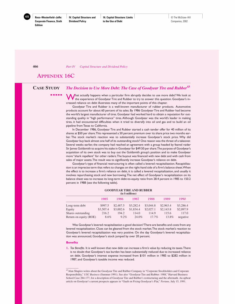
Ross−Westerfield−Jaffe: Corporate Finance, Sixth Edition
IV. Capital Structure and Dividend Policy
16. Capital Structure: Limits to the Use of Debt
472 © The McGraw−Hill Companies, 2002
466 Part IV Capital Structure and Dividend Policy
APPENDIX 16C
CASE STUDY The Decision to Use More Debt: The Case of Goodyear Tire and Rubber43
What actually happens when a particular firm abruptly decides to use more debt? We look atthe experience of Goodyear Tire and Rubber to try to answer this question. Goodyear’s in-
creased reliance on debt illustrates many of the important points of this chapter.Goodyear Tire and Rubber is a well-known manufacturer of rubber products. Automotive
products account for about 60 percent of its sales. By 1986 Goodyear Tire and Rubber had becomethe world’s largest manufacturer of tires. Goodyear had worked hard to obtain a reputation for out-standing quality in “high performance” tires.Although Goodyear was the world’s leader in makingtires, it had encountered difficulties when it tried to diversify into oil and gas and to build an oilpipeline from Texas to California.
In December 1986, Goodyear Tire and Rubber started a cash tender offer for 40 million of itsshares at $50 per share.This represented a 50 percent premium over its share price two months ear-lier. The stock market’s reaction was to substantially increase Goodyear’s stock price. Why didGoodyear buy back almost one half of its outstanding stock? One reason was the threat of a takeover.Several weeks earlier, the company had reached an agreement with a group headed by feared raiderSir James Goldsmith to acquire his stake in Goodyear for $49.50 per share.The purpose of Goodyear’sacquisition of its own stock was to buy out the Goldsmith group’s position and to make Goodyearmore “shark repellent” for other raiders.The buyout was financed with new debt and with cash fromsales of major assets.The result was to significantly increase Goodyear’s reliance on debt.
Goodyear’s type of financial restructuring is often called a levered recapitalization. Recapitiliza-tion is an imprecise term that refers to changes on the right-hand side of a firm’s balance sheet.Whenthe effect is to increase a firm’s reliance on debt, it is called a levered recapitalization, and usually itinvolves repurchasing stock and new borrowing.The net effect of Goodyear’s recapitalization on itsbalance sheet was to increase its long-term debt-to-equity ratio from 28.4 percent in 1985 to 150.2percent in 1988 (see the following table).
GOODYEAR TIRE AND RUBBER(in $ millions)
1985 1986 1987 1988 1989 1990
Long-term debt $997.5 $2,487.5 $3,282.4 $3,044.8 $2,963.4 $3,286.4Equity $3,507.4 $3,002.6 $1,834.4 $2,027.1 $2,143.8 $2,097.9Shares outstanding 216.2 194.2 114.0 114.9 115.6 117.0Return on equity (ROE) 8.6% 9.2% 24.0% 17.7% 13.8% negative
Was Goodyear’s levered recapitalization a good decision? There are benefits and costs from anylevered recapitalization. Clues can be gleaned from the stock market.The stock market’s reaction toGoodyear’s levered recapitalization was very positive. On the day Goodyear’s levered recapitaliza-tion was announced, Goodyear’s stock jumped by over 20 percent.
Benefits
1. Tax Benefits. It is well known that new debt can increase a firm’s value by reducing its taxes.Thereis no doubt that Goodyear’s tax burden has been substantially reduced due to increased relianceon debt. Goodyear’s interest expense increased from $101 million in 1985 to $282 million in1987, and Goodyear’s taxable income was reduced.
43Alan Shapiro writes about the Goodyear Tire and Rubber Company in “Corporate Stockholders and CorporateResponsibility,” USC Business (Summer 1991). See also “Goodyear Tire and Rubber: 1988,” Harvard BusinessSchool Case 284-177, for a description of Goodyear Tire and Rubber’s restructuring and the aftermath. An upbeatarticle on Goodyear’s current prospects appears in “Gault on Fixing Goodyear’s Flat,” Fortune, July 15, 1991.
Ross−Westerfield−Jaffe: Corporate Finance, Sixth Edition
IV. Capital Structure and Dividend Policy
16. Capital Structure: Limits to the Use of Debt
473© The McGraw−Hill Companies, 2002
2. Lower Agency Costs. It is often argued that leverage reduces the agency costs arising between man-agement and shareholders. Therefore, the new debt from the levered recapitalization can bethought of as a type of a control device for the shareholders of Goodyear. In 1982 Goodyear hadembarked on a diversification program by acquiring Celeron, an oil and gas company.The acqui-sition of Celeron was followed by several other diversification attempts. Most importantly,Goodyear decided to construct a crude oil pipeline from Texas to California. Shareholders didnot react favorably to Goodyear’s diversification program, and its stock price fell 65 percent (rel-ative to the S&P 500 Index) over the three and one-half years after 1982. It can be argued thatthis is a classic case of management pursuing selfish shortsighted goals at the expense of share-holders. Goodyear’s diversification program imposed agency costs on its shareholders.Goodyear’s levered recapitalization probably prevented it from further diversification becauseGoodyear was forced to sell most of its non-tire assets to service its new debt. It sold CeleronOil in December 1987. By borrowing an amount equal to the present value of Goodyear’s excesscash flow that could be used to acquire other firms, Goodyear’s management has been effectivelyprevented from further diversification.
Costs
1. Financial Distress.When firms such as Goodyear increase their reliance on debt, they also increase thelikelihood of financial distress. Financial distress can be formal bankruptcy. So far, Goodyear has notfiled for bankruptcy.However, financial distress may occur without bankruptcy. After the levered re-capitalization, Goodyear’s debt was downgraded by Moody’s and Standard & Poor’s.This may be ev-idence of financial distress.Goodyear lost money in 1990 and its ROE was negative.More importantly,financial distress means doing particularly harmful things such as the selfish strategies that we talkedabout previously.Goodyear has said that it has been forced to cut down on planned research and de-velopment and capital spending because of its reliance on debt. Its level of capital spending decreasedfrom about $1.5 billion in 1986 to $754 million in 1988.This may be evidence of financial distress. Ifso, this is one of the costs imposed upon Goodyear because of its levered recapitalization.
2. Financial Slack. The new debt has increased Goodyear’s leverage well beyond traditional industrynorms. Up to 1985 Goodyear had relied on little debt, leading some industry analysts in 1985 tocontend that Goodyear had excess debt capacity (i.e., financial slack). However, the excess cashflows that supported Goodyear’s borrowing in 1986 and 1987 disappeared in 1988. By the endof 1988 Goodyear had used up all of its financial slack. Loss of financial slack can preclude strate-gic options if competitors increase capital spending or lower prices. Many analysts believe this iswhat happened when in 1989 Bridgestone, Goodyear’s main competitor, announced its intentionto increase its capital spending in the North American tire market. Goodyear could not counterby increasing its own level of capital spending.The only way Goodyear could do so would havebeen by issuing new equity. But firms do not like to issue new equity because it is very expensiveand it is the lowest financing option on the pecking order.
Part of Goodyear’s decision to use more debt can be analyzed in terms of a trade-off betweenthe tax benefits of debt and the costs of financial distress.However, the Goodyear experience showsthat agency costs and financial slack are also factors in a firm’s decision to use debt.
Postscript
Goodyear almost went broke in 1990–1991 and was forced to cut its dividend for the first time sincethe 1930s. In 1991 it hired a new CEO, Stanley Gault, who was hailed as CEO of the year in 1992 (byFinancial World). In 1997 Goodyear’s ROE was close to 20 percent and its long-term debt reduced toabout $1 billion. Capital spending remained very low at about $620 million. Its oil pipeline was prof-itable for the first time in 1994. (But, in 1997 Goodyear finally found a buyer for its pipeline.) TodayGoodyear is still the world’s largest rubber manufacturer. Its market capitalization is about $3 billionand it has increased its dividend payout from 20¢ in 1991 to $1.20 in 1999. Its ROE is 10%.
Chapter 16 Capital Structure: Limits to the Use of Debt 467
Ross−Westerfield−Jaffe: Corporate Finance, Sixth Edition
IV. Capital Structure and Dividend Policy
17. Valuation and Capital Budgeting for the Levered Firm
474 © The McGraw−Hill Companies, 2002
Valuation and CapitalBudgeting for the Levered Firm
CH
AP
TE
R17
EXECUTIVE SUMMARY
Instructors often structure the basic course in corporate finance around the two sides of thebalance sheet. The left-hand side of the balance sheet contains assets. Chapters 4, 5, 6, 7, and8 of this textbook treat the capital-budgeting decision, which is a decision concerning the as-
sets of the firm. Chapters 9, 10, 11, and 12 treat the discount rate for a project, so those chaptersalso concern the left-hand side of the balance sheet. The right-hand side of the balance sheet con-tains liabilities and owner’s equity. Chapters 13, 14, 15, and 16 of this textbook examine the debt-versus-equity decision, which is a decision about the right-hand side of the balance sheet.
While the preceding chapters of this textbook have, for the most part, treated the capital-budgeting decision separately from the capital-structure decision, the two decisions are actu-ally related. As we will see, a project of an all-equity firm might be rejected, while the sameproject might be accepted for a levered but otherwise identical firm. This occurs because thecost of capital frequently decreases with leverage, thereby turning some negative NPV proj-ects into positive NPV projects.
Chapters 4 through 8 implicitly assumed that the firm is financed with only equity. Thegoal of this chapter is to value a project, or the firm itself, when leverage is employed. Wepoint out that there are three standard approaches to valuation under leverage: the adjusted-present-value (APV) method, the flow-to-equity (FTE) method, and the weighted-average-cost-of-capital (WACC) method. These three approaches may seem, at first glance, to bequite different. However, we show that, if applied correctly, all three approaches providethe same value estimate.
The three methods discussed next can be used to value either the firm as a whole or aproject. The example below discusses project value, though everything we say applies to anentire firm as well.
17.1 ADJUSTED-PRESENT-VALUE APPROACH
The adjusted-present-value (APV) method is best described by the following formula:
APV � NPV � NPVF
In words, the value of a project to a levered firm (APV) is equal to the value of the projectto an unlevered firm (NPV) plus the net present value of the financing side effects (NPVF).One can generally think of four side effects:
1. The Tax Subsidy to Debt. This was discussed in Chapter 15, where we pointed out that,for perpetual debt, the value of the tax subsidy is TCB. (TC is the corporate tax rate, andB is the value of the debt. ) The material on valuation under corporate taxes in Chapter15 is actually an application of the APV approach.
Ross−Westerfield−Jaffe: Corporate Finance, Sixth Edition
IV. Capital Structure and Dividend Policy
17. Valuation and Capital Budgeting for the Levered Firm
475© The McGraw−Hill Companies, 2002
2. The Costs of Issuing New Securities. As we will discuss in detail in Chapter 20, invest-ment bankers participate in the public issuance of corporate debt. These bankers mustbe compensated for their time and effort, a cost that lowers the value of the project.
3. The Costs of Financial Distress. The possibility of financial distress, and bankruptcy inparticular, arises with debt financing. As stated in the previous chapter, financial distressimposes costs, thereby lowering value.
4. Subsidies to Debt Financing. The interest on debt issued by state and local governmentsis not taxable to the investor. Because of this, the yield on tax-exempt debt is generallysubstantially below the yield on taxable debt. Frequently, corporations are able to obtainfinancing from a municipality at the tax-exempt rate because the municipality can bor-row at that rate as well. As with any subsidy, this subsidy adds value.
While each of the preceding four side effects is important, the tax deduction to debt al-most certainly has the highest dollar value in practice. For this reason, the following exam-ple considers the tax subsidy, but not the other three side effects.1
Consider a project of the P. B. Singer Co. with the following characteristics:
Cash inflows: $500,000 per year for the indefinite futureCash costs: 72% of salesInitial investment: $475,000TC � 34%r0 � 20%, where r0 is the cost of capital for a project of an all-equity firm.
If both the project and the firm are financed with only equity, the project’s cash flow is
Cash inflows $500,000Cash costs �360,000________Operating income 140,000Corporate tax (.34 tax rate) �47,600________Unlevered cash flow (UCF) $92,400
The distinction in Chapter 4 between present value and net present value is importantfor this example. As pointed out in Chapter 4, the present value of a project is determinedbefore the initial investment at date 0 is subtracted. The initial investment is subtracted forthe calculation of net present value.
Given a discount rate of 20 percent, the present value of the project is
The net present value (NPV) of the project, that is, the value of the project to an all-equityfirm, is
$462,000 � $475,000 � �$13,000
Since the NPV is negative, the project would be rejected by an all-equity firm.Now imagine that the firm finances the project with exactly $126,229.50 in debt, so
that the remaining investment of $348,770.50 ($475,000 � $126,229.50) is financed withequity. The net present value of the project under leverage, which we call the adjusted pres-ent value, or the APV, is
APV � NPV � TC � B$29,918 � �$13,000 � 0.34 � $126,229.50
$92,400
0.20� $462,000
Chapter 17 Valuation and Capital Budgeting for the Levered Firm 469
1The Bicksler Enterprises example of Section 17.6 handles both flotation costs and interest subsidies.
Ross−Westerfield−Jaffe: Corporate Finance, Sixth Edition
IV. Capital Structure and Dividend Policy
17. Valuation and Capital Budgeting for the Levered Firm
476 © The McGraw−Hill Companies, 2002
That is, the value of the project when financed with some leverage is equal to the value ofthe project when financed with all equity plus the tax shield from the debt. Since this num-ber is positive, the project should be accepted.
You may be wondering why we chose such a precise amount of debt. Actually, wechose it so that the ratio of debt to the present value of the project under leverage is 0.25.2
In this example, debt is a fixed proportion of the present value of the project, not a fixedproportion of the initial investment of $475,000. This is consistent with the goal of a targetdebt-to-market-value ratio, which we find in the real world. For example, commercial bankstypically lend to real estate developers a fixed percentage of the market value of a project,not a fixed percentage of the initial investment.
• How is the APV method applied?• What additional information beyond NPV does one need to calculate APV?
17.2 FLOW-TO-EQUITY APPROACH
The flow-to-equity (FTE) approach is an alternative capital-budgeting approach. The for-mula simply calls for discounting the cash flow from the project to the equityholders of thelevered firm at the cost of equity capital, rS. For a perpetuity, this becomes
There are three steps to the FTE approach.
Step 1: Calculating Levered Cash Flow (LCF)3
Assuming an interest rate of 10 percent, the perpetual cash flow to equityholders in our ex-ample is
Cash inflows $500,000.00Cash costs �360,000.00Interest (10% � $126,229.50) �12,622.95__________Income after interest 127,377.05Corporate tax (.34 tax rate) �43,308.20__________Levered cash flow (LCF) $ 84,068.85
Cash flow from project to equityholders of the levered firm
rS
470 Part IV Capital Structure and Dividend Policy
2That is, the present value of the project after the initial investment has been made is $504,918 ($29,918 �$475,000). Thus, the debt-to-value ratio of the project is 0.25 ($126,229.50/$504,918).
This level of debt can be calculated directly. Note that
Present value of levered project � Present value of unlevered project � TC � B
VWith debt � $462,000 � 0.34 � .25 � VWith debt
Rearranging the last line, we have
VWith debt(1 � 0.34 � 0.25) � $462,000VWith debt � $504,918
Since debt is 0.25 of value, debt is $126,229.50 (0.25 � $504,918).3We use the term levered cash flow (LCF) for simplicity. A more complete term would be cash flow from theproject to the equityholders of a levered firm. Similarly, a more complete term for unlevered cash flow (UCF)would be cash flow from the project to the equityholders of an unlevered firm.
QUESTIONS
CO
NC
EP
T
?
Ross−Westerfield−Jaffe: Corporate Finance, Sixth Edition
IV. Capital Structure and Dividend Policy
17. Valuation and Capital Budgeting for the Levered Firm
477© The McGraw−Hill Companies, 2002
Alternatively, one can calculate levered cash flow (LCF) directly from unlevered cashflow (UCF). The key here is that the difference between the cash flow that equityholders re-ceive in an unlevered firm and the cash flow that equityholders receive in a levered firm isthe after-tax interest payment. (Repayment of principal does not appear in this example,since the debt is perpetual.) One writes this algebraically as
UCF � LCF � (1 � TC)rBB
The term on the right-hand side of this expression is the after-tax interest payment. Thus, sincecash flow to the unlevered equityholders (UCF) is $92,400 and the after-tax interest paymentis $8,331.15 [(.66).10 � $126,229.50], cash flow to the levered equityholders (LCF) is
$92,400 � $8,331.15 � $84,068.85
which is exactly the number we calculated earlier.
Step 2: Calculating rSThe next step is to calculate the discount rate, rS. Note that we assumed that the discountrate on unlevered equity, r0, is .20. As we saw in Chapter 15, the formula for rS is
Note that our target debt-to-value ratio of 1/4 implies a target debt-to-equity ratio of 1/3.Applying the preceding formula to this example, we have
Step 3: ValuationThe present value of the project’s LCF is
Since the initial investment is $475,000 and $126,299.50 is borrowed, the firm must ad-vance the project $348,770.50 ($475,000 � $126,229.50) out of its own cash reserves. Thenet present value of the project is simply the difference between the present value of theproject’s LCF and the investment not borrowed. Thus, the NPV is
$378,688.50 � $348,770.50 � $29,918
which is identical to the result found with the APV approach.
• How is the FTE method applied?• What information is needed to calculate FTE?
17.3 WEIGHTED-AVERAGE-COST-OF-CAPITAL METHOD
Finally, one can value a project using the weighted-average-cost-of-capital (WACC)method. While this method was discussed in Chapters 12 and 15, it is worthwhile to re-view it here. The WACC approach begins with the insight that projects of levered firms are
LCF
rS
�$84,068.85
.222� $378,688.50
rS � .222 � .20 �1
3�.66� �.20 � .10�
rS � r0 �B
S�1 � TC� �r0 � rB�
Chapter 17 Valuation and Capital Budgeting for the Levered Firm 471
QUESTIONS
CO
NC
EP
T
?

Ross−Westerfield−Jaffe: Corporate Finance, Sixth Edition
IV. Capital Structure and Dividend Policy
17. Valuation and Capital Budgeting for the Levered Firm
478 © The McGraw−Hill Companies, 2002
simultaneously financed with both debt and equity. The cost of capital is a weighted av-erage of the cost of debt and the cost of equity. As seen in Chapters 12 and 15, the costof equity is rS. Ignoring taxes, the cost of debt is simply the borrowing rate, rB. How-ever, with corporate taxes, the appropriate cost of debt is (1 � TC)rB, the after-tax costof debt.
The formula for determining the weighted average cost of capital, rWACC, is
The weight for equity, , and the weight for debt, , are target ratios. Target
ratios are generally expressed in terms of market values, not accounting values. (Recall thatanother phrase for accounting value is book value.)
The formula calls for discounting the unlevered cash flow of the project (UCF) at theweighted average cost of capital, rWACC. The net present value of the project can be writtenalgebraically as
Initial investment
If the project is a perpetuity, the net present value is
Initial investment
We previously stated that the target debt-to-value ratio of our project is 1/4 and the cor-porate tax rate is .34, implying that the weighted average cost of capital is
Note that rWACC, 0.183, is lower than the cost of equity capital for an all-equity firm, 0.20.This must always be the case, since debt financing provides a tax subsidy that lowers theaverage cost of capital.
We previously determined the UCF of the project to be $92,400, implying that the pres-ent value of the project is
Since this initial investment is $475,000, the NPV of the project is
$504,918 � $475,000 � $29,918
In this example, all three approaches yield the same value.
• How is the WACC method applied?
$92,400
0.183� $504,918
rWACC � 3
4� 0.222 �
1
4� 0.10 �0.66� � 0.183
UCF
rWACC
�
t�1
UCFt
�1 � rWACC� t �
B
S � B
S
S � B
rWACC �S
S � B rS �
B
S � B rB �1 � TC�
472 Part IV Capital Structure and Dividend Policy
QUESTION
CO
NC
EP
T
?
Ross−Westerfield−Jaffe: Corporate Finance, Sixth Edition
IV. Capital Structure and Dividend Policy
17. Valuation and Capital Budgeting for the Levered Firm
479© The McGraw−Hill Companies, 2002
17.4 A COMPARISON OF THE APV, FTE, AND WACC APPROACHES
Capital-budgeting techniques in the early chapters of this text applied to all-equity firms.Capital budgeting for the levered firm could not be handled early in the book because theeffects of debt on firm value were deferred until the previous two chapters. We learned therethat debt increases firm value through tax benefits but decreases value through bankruptcyand related costs.
In this chapter we provide three approaches to capital budgeting for the levered firm.The adjusted-present-value (APV) approach first values the project on an all-equity ba-sis. That is, the project’s after-tax cash flows under all-equity financing (called unleveredcash flows, or UCF) are placed in the numerator of the capital-budgeting equation. Thediscount rate, assuming all-equity financing, appears in the denominator. At this point,the calculation is identical to that performed in the early chapters of this book. We thenadd the net present value of the debt. We point out that the net present value of the debtis likely to be the sum of four parameters: tax effects, flotation costs, bankruptcy costs,and interest subsidies.
The flow-to-equity (FTE) approach discounts the after-tax cash flow from a project go-ing to the equityholders of a levered firm (LCF). LCF, which stands for levered cash flow,is the residual to equityholders after interest has been deducted. The discount rate is rS, thecost of capital to the equityholders of a levered firm. For a firm with leverage, rS must begreater than r0, the cost of capital for an unlevered firm. This follows from our material inChapter 15 showing that leverage raises the risk to the equityholders.
The last approach is the weighted-average-cost-of-capital (WACC) method. This tech-nique calculates the project’s after-tax cash flows assuming all-equity financing (UCF). TheUCF is placed in the numerator of the capital-budgeting equation. The denominator, rWACC,is a weighted average of the cost of equity capital and the cost of debt capital. The tax ad-vantage of debt is reflected in the denominator because the cost of debt capital is determinednet of corporate tax. The numerator does not reflect debt at all.
All three approaches perform the same task: valuation in the presence of debt financ-ing. And, as illustrated by the previous example, all three provide the same valuation esti-mate. However, as we saw before, the approaches are markedly different in technique.Because of this, students often ask questions of the following sort: “How can this be? Howcan the three approaches look so different and yet give the same answer?” We believe thatthe best way to handle questions like these is through the following two points.
1. APV versus WACC. Of the three approaches, APV and WACC display the greatestsimilarity. After all, both approaches put the unlevered cash flow (UCF) in the nu-merator. However, the APV approach discounts these flows at r0, yielding the valueof the unlevered project. Adding the present value of the tax shield gives the value ofthe project under leverage. The WACC approach discounts UCF at rWACC, which islower than r0.
Thus, both approaches adjust the basic NPV formula for unlevered firms in order toreflect the tax benefit of leverage. The APV approach makes this adjustment directly. Itsimply adds in the present value of the tax shield as a separate term. The WACC ap-proach makes the adjustment in a more subtle way. Here, the discount rate is lowered be-low r0. Although we do not provide a proof in the textbook, it can be shown that thesetwo adjustments always have the same quantitative effect.
Chapter 17 Valuation and Capital Budgeting for the Levered Firm 473
Ross−Westerfield−Jaffe: Corporate Finance, Sixth Edition
IV. Capital Structure and Dividend Policy
17. Valuation and Capital Budgeting for the Levered Firm
480 © The McGraw−Hill Companies, 2002
2. Entity Being Valued. The FTE approach appears at first glance to be far different fromthe other two. For both the APV and the WACC approaches, the initial investment issubtracted out in the final step ($475,000 in our example). However, for the FTE ap-proach, only the firm’s contribution to the initial investment ($348,770.50 � $475,000� $126,229.50) is subtracted out. This occurs because under the FTE approach, onlythe future cash flows to the levered equityholders (LCF) are valued. By contrast, fu-ture cash flows to the unlevered equityholders (UCF) are valued in both the APV andWACC approaches. Thus, since LCFs are net of interest payments, whereas UCFs arenot, the initial investment under the FTE approach is correspondingly reduced by debtfinancing. In this way, the FTE approach produces the same answer that the other twoapproaches do.
A Suggested GuidelineThe net present value of our project is exactly the same under each of the three methods. Intheory, this should always be the case.4 However, one method usually provides an easier com-putation than another, and, in many cases, one or more of the methods are virtually impossi-ble computationally. We first consider when it is best to use the WACC and FTE approaches.
If the risk of a project stays constant throughout its life, it is plausible to assume thatr0 remains constant throughout the project’s life. This assumption of constant risk appearsto be reasonable for most real-world projects. In addition, if the debt-to-value ratio remainsconstant over the life of the project, both rS and rWACC will remain constant as well. Underthis latter assumption, either the FTE or the WACC approach is easy to apply. However, ifthe debt-to-value ratio varies from year to year, both rS and rWACC vary from year to year aswell. Using the FTE or the WACC approach when the denominator changes every year iscomputationally quite complex, and when computations become complex, the error raterises. Thus, both the FTE and WACC approaches present difficulties when the debt-to-valueratio changes over time.
The APV approach is based on the level of debt in each future period. Consequently,when the debt level can be specified precisely for future periods, the APV approach is quiteeasy to use. However, when the debt level is uncertain, the APV approach becomes moreproblematic. For example, when the debt-to-value ratio is constant, the debt level varieswith the value of the project. Since the value of the project in a future year cannot be eas-ily forecast, the level of debt cannot be easily forecast either.
Thus, we suggest the following guideline:
Use WACC or FTE if the firm’s target debt-to-value ratio applies to the project over its life.Use APV if the project’s level of debt is known over the life of the project.
There are a number of situations where the APV approach is preferred. For example,in a leveraged buyout (LBO) the firm begins with a large amount of debt but rapidly paysdown the debt over a number of years. Since the schedule of debt reduction in the future isknown when the LBO is arranged, tax shields in every future year can be easily forecast.Thus, the APV approach is easy to use here. (An illustration of the APV approach appliedto LBOs is provided in the appendix to this chapter.) By contrast, the WACC and FTE ap-proaches are virtually impossible to apply here, since the debt-to-equity value cannot be ex-pected to be constant over time. In addition, situations involving interest subsidies and flota-tion costs are much easier to handle with the APV approach. (The Bicksler Enterprises
474 Part IV Capital Structure and Dividend Policy
4See I. Inselbag and H. Kaufold, “Two DCF Approaches for Valuing Companies under Alternative FinancialStrategies (and How to Choose Between Them)” Journal of Applied Corporate Finance (Spring 1997).
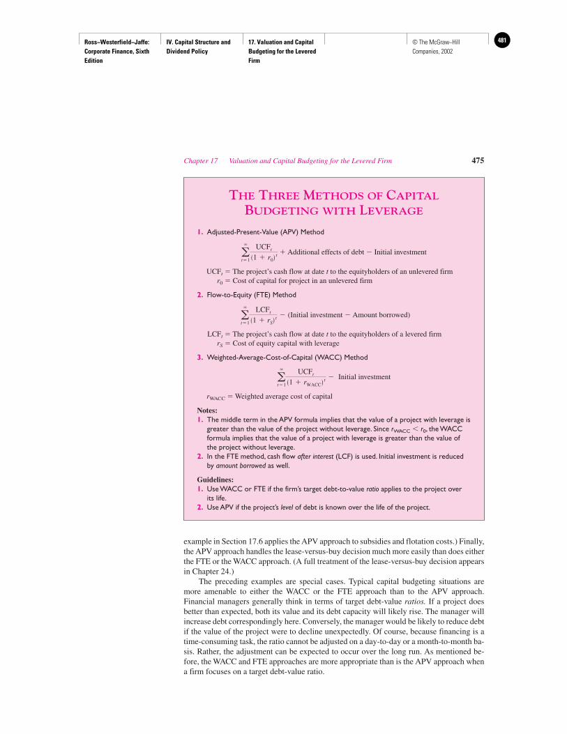
Ross−Westerfield−Jaffe: Corporate Finance, Sixth Edition
IV. Capital Structure and Dividend Policy
17. Valuation and Capital Budgeting for the Levered Firm
481© The McGraw−Hill Companies, 2002
example in Section 17.6 applies the APV approach to subsidies and flotation costs.) Finally,the APV approach handles the lease-versus-buy decision much more easily than does eitherthe FTE or the WACC approach. (A full treatment of the lease-versus-buy decision appearsin Chapter 24.)
The preceding examples are special cases. Typical capital budgeting situations aremore amenable to either the WACC or the FTE approach than to the APV approach.Financial managers generally think in terms of target debt-value ratios. If a project doesbetter than expected, both its value and its debt capacity will likely rise. The manager willincrease debt correspondingly here. Conversely, the manager would be likely to reduce debtif the value of the project were to decline unexpectedly. Of course, because financing is atime-consuming task, the ratio cannot be adjusted on a day-to-day or a month-to-month ba-sis. Rather, the adjustment can be expected to occur over the long run. As mentioned be-fore, the WACC and FTE approaches are more appropriate than is the APV approach whena firm focuses on a target debt-value ratio.
Chapter 17 Valuation and Capital Budgeting for the Levered Firm 475
THE THREE METHODS OF CAPITAL
BUDGETING WITH LEVERAGE
1. Adjusted-Present-Value (APV) Method
� Additional effects of debt � Initial investment
UCFt � The project’s cash flow at date t to the equityholders of an unlevered firmr0 � Cost of capital for project in an unlevered firm
2. Flow-to-Equity (FTE) Method
(Initial investment � Amount borrowed)
LCFt � The project’s cash flow at date t to the equityholders of a levered firmrS � Cost of equity capital with leverage
3. Weighted-Average-Cost-of-Capital (WACC) Method
Initial investment
rWACC � Weighted average cost of capital
Notes:1. The middle term in the APV formula implies that the value of a project with leverage is
greater than the value of the project without leverage. Since rWACC r0, the WACCformula implies that the value of a project with leverage is greater than the value ofthe project without leverage.
2. In the FTE method, cash flow after interest (LCF) is used. Initial investment is reducedby amount borrowed as well.
Guidelines:1. Use WACC or FTE if the firm’s target debt-to-value ratio applies to the project over
its life.2. Use APV if the project’s level of debt is known over the life of the project.
t�1
UCFt
�1 � rWACC� t �
t�1
LCFt
�1 � rS� t �
t�1
UCFt
�1 � r0� t
Ross−Westerfield−Jaffe: Corporate Finance, Sixth Edition
IV. Capital Structure and Dividend Policy
17. Valuation and Capital Budgeting for the Levered Firm
482 © The McGraw−Hill Companies, 2002
Because of this, we recommend that the WACC and the FTE approaches, rather thanthe APV approach, be used in most real-world situations. In addition, frequent discussionswith business executives have convinced us that the WACC is the most widely used methodin the real world, by far. Thus, practitioners seem to agree with us that, outside of the spe-cial situations mentioned above, the APV approach is a less important method of capitalbudgeting.
• What is the main difference between APV and WACC?• What is the main difference between the FTE approach and the other two approaches?• When should the APV method be used?• When should the FTE and WACC approaches be used?
17.5 CAPITAL BUDGETING WHEN THE DISCOUNT RATE
MUST BE ESTIMATED
The previous sections of this chapter introduced APV, FTE, and WACC—the three basicapproaches to valuing a levered firm. However, one important detail remains. The examplein Sections 17.1 through 17.3 assumed a discount rate. We now want to show how this rateis determined for real-world firms with leverage, with an application to the three precedingapproaches. The example in this section brings together the work in Chapters 9–12 on thediscount rate for unlevered firms with that in Chapter 15 on the effect of leverage on thecost of capital.
EXAMPLE
World-Wide Enterprises (WWE) is a large conglomerate thinking of entering thewidget business, where it plans to finance projects with a debt-to-value ratio of25 percent (or, alternatively, a debt-to-equity ratio of 1/3). There is currently onefirm in the widget industry, American Widgets (AW). This firm is financed with40-percent debt and 60-percent equity. The beta of AW’s equity is 1.5. AW has aborrowing rate of 12 percent, and WWE expects to borrow for its widget ventureat 10 percent. The corporate tax rate for both firms is 0.40, the market-risk pre-mium is 8.5 percent, and the riskless interest rate is 8 percent. What is the appro-priate discount rate for WWE to use for its widget venture?
As shown in Sections 17.1–17.3, a corporation may use one of three capitalbudgeting approaches: APV, FTE, or WACC. The appropriate discount rates forthese three approaches are r0, rS, and rWACC, respectively. Since AW is WWE’sonly competitor in widgets, we look at AW’s cost of capital to calculate r0, rS, andrWACC for WWE’s widget venture. The four-step procedure below will allow us tocalculate all three discount rates.
1. Determining AW’s Cost of Equity Capital. First, we determine AW’s cost of eq-uity capital, using the security market line (SML) of Chapter 10:
AW’s Cost of Equity Capital:
rS � RF � � � ( M � RF)20.75% � 8% � 1.5 � 8.5%
where M is the expected return on the market portfolio and RF is the risk-free rate.R
R
476 Part IV Capital Structure and Dividend Policy
QUESTIONS
CO
NC
EP
T
?
Ross−Westerfield−Jaffe: Corporate Finance, Sixth Edition
IV. Capital Structure and Dividend Policy
17. Valuation and Capital Budgeting for the Levered Firm
483© The McGraw−Hill Companies, 2002
2. Determining AW’s Hypothetical All-Equity Cost of Capital. We must standard-ize the preceding number in some way, since AW and WWE’s widget venturehave different target debt-to-value ratios. The easiest approach is to calculate thehypothetical cost of equity capital for AW, assuming all-equity financing. Thiscan be determined from MM’s Proposition II under taxes (see Chapter 15):
AW’s Cost of Capital if All-Equity:
In the examples of Chapter 15, the unknown in this equation was rS.However, for this example, the unknown is r0. By solving the equation, onefinds that r0 � 0.1825. Of course, r0 is less than rS because the cost of equitycapital would be less when the firm employs no leverage.
At this point, firms in the real world generally make the assumption thatthe business risk of their venture is about equal to the business risk of the firmsalready in the business. Applying this assumption to our problem, we assert thatthe hypothetical discount rate of WWE’s widget venture if all-equity financedis also 0.1825.5 This discount rate would be employed if WWE uses the APVapproach, since the APV approach calls for r0, the project’s cost of capital in afirm with no leverage.
3. Determining rS for WWE’s Widget Venture. Alternatively, WWE might use theFTE approach, where the discount rate for levered equity is determined from:
Cost of Equity Capital for WWE’s Widget Venture:
Note that the cost of equity capital for WWE’s widget venture, 0.199, isless than the cost of equity capital for AW, 0.2075. This occurs because AW hasa higher debt-to-equity ratio. (As mentioned above, both firms are assumed tohave the same business risk.)
4. Determining rWACC for WWE’s Widget Venture. Finally, WWE might use theWACC approach. The appropriate calculation here is
rWACC for WWE’s Widget Venture:
16.425% �1
4 10% �0.60� �
3
4 19.9%
rWACC �B
S � BrB �1 � TC� �
S
S � BrS
19.9% � 18.25% �1
3�0.60� �18.25% � 10%�
rS � r0 �B
S�1 � TC� �r0 � rB�
20.75% � r0 �0.4
0.6�0.60� �r0 � 12%�
rS � r0 �B
S�1 � TC� �r0 � rB�
Chapter 17 Valuation and Capital Budgeting for the Levered Firm 477
5Alternatively, a firm might assume that its venture would be somewhat riskier since it is a new entrant. Thus,the firm might select a discount rate slightly higher than 0.1825. Of course, no exact formula exists for adjustingthe discount rate upwards.
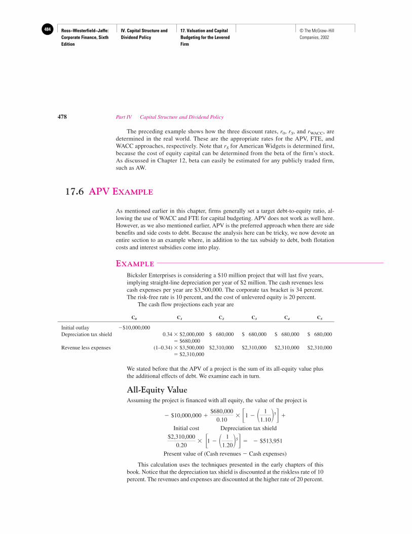
Ross−Westerfield−Jaffe: Corporate Finance, Sixth Edition
IV. Capital Structure and Dividend Policy
17. Valuation and Capital Budgeting for the Levered Firm
484 © The McGraw−Hill Companies, 2002
The preceding example shows how the three discount rates, r0, rS, and rWACC, aredetermined in the real world. These are the appropriate rates for the APV, FTE, andWACC approaches, respectively. Note that rS for American Widgets is determined first,because the cost of equity capital can be determined from the beta of the firm’s stock.As discussed in Chapter 12, beta can easily be estimated for any publicly traded firm,such as AW.
17.6 APV EXAMPLE
As mentioned earlier in this chapter, firms generally set a target debt-to-equity ratio, al-lowing the use of WACC and FTE for capital budgeting. APV does not work as well here.However, as we also mentioned earlier, APV is the preferred approach when there are sidebenefits and side costs to debt. Because the analysis here can be tricky, we now devote anentire section to an example where, in addition to the tax subsidy to debt, both flotationcosts and interest subsidies come into play.
EXAMPLE
Bicksler Enterprises is considering a $10 million project that will last five years,implying straight-line depreciation per year of $2 million. The cash revenues lesscash expenses per year are $3,500,000. The corporate tax bracket is 34 percent.The risk-free rate is 10 percent, and the cost of unlevered equity is 20 percent.
The cash flow projections each year are
C0 C1 C2 C3 C4 C5
Initial outlay �$10,000,000Depreciation tax shield 0.34 � $2,000,000 $ 680,000 $ 680,000 $ 680,000 $ 680,000
� $680,000Revenue less expenses (1–0.34) � $3,500,000 $2,310,000 $2,310,000 $2,310,000 $2,310,000
� $2,310,000
We stated before that the APV of a project is the sum of its all-equity value plusthe additional effects of debt. We examine each in turn.
All-Equity ValueAssuming the project is financed with all equity, the value of the project is
Initial cost Depreciation tax shield
Present value of (Cash revenues � Cash expenses)
This calculation uses the techniques presented in the early chapters of thisbook. Notice that the depreciation tax shield is discounted at the riskless rate of 10percent. The revenues and expenses are discounted at the higher rate of 20 percent.
$2,310,000
0.20� �1 � � 1
1.20�5 � � $513,951
� $10,000,000 �$680,000
0.10� �1 � � 1
1.10�5 �
478 Part IV Capital Structure and Dividend Policy
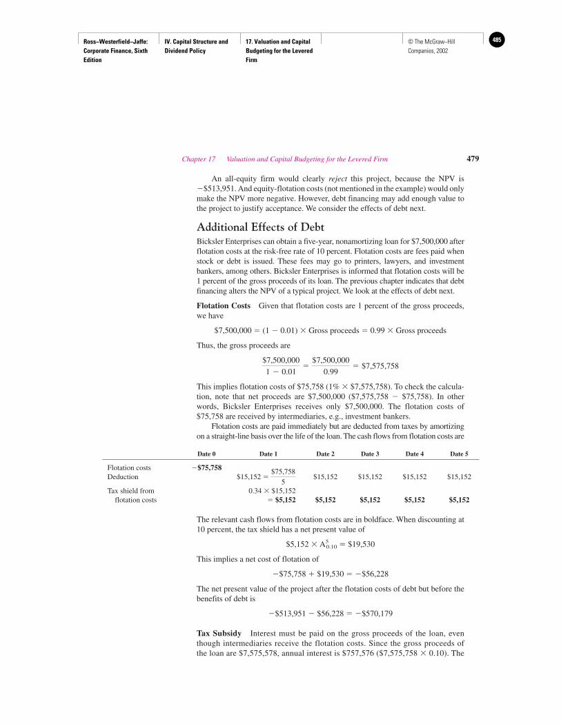
Ross−Westerfield−Jaffe: Corporate Finance, Sixth Edition
IV. Capital Structure and Dividend Policy
17. Valuation and Capital Budgeting for the Levered Firm
485© The McGraw−Hill Companies, 2002
An all-equity firm would clearly reject this project, because the NPV is�$513,951. And equity-flotation costs (not mentioned in the example) would onlymake the NPV more negative. However, debt financing may add enough value tothe project to justify acceptance. We consider the effects of debt next.
Additional Effects of DebtBicksler Enterprises can obtain a five-year, nonamortizing loan for $7,500,000 afterflotation costs at the risk-free rate of 10 percent. Flotation costs are fees paid whenstock or debt is issued. These fees may go to printers, lawyers, and investmentbankers, among others. Bicksler Enterprises is informed that flotation costs will be1 percent of the gross proceeds of its loan. The previous chapter indicates that debtfinancing alters the NPV of a typical project. We look at the effects of debt next.
Flotation Costs Given that flotation costs are 1 percent of the gross proceeds,we have
$7,500,000 � (1 � 0.01) � Gross proceeds � 0.99 � Gross proceeds
Thus, the gross proceeds are
This implies flotation costs of $75,758 (1% � $7,575,758). To check the calcula-tion, note that net proceeds are $7,500,000 ($7,575,758 � $75,758). In otherwords, Bicksler Enterprises receives only $7,500,000. The flotation costs of$75,758 are received by intermediaries, e.g., investment bankers.
Flotation costs are paid immediately but are deducted from taxes by amortizingon a straight-line basis over the life of the loan. The cash flows from flotation costs are
Date 0 Date 1 Date 2 Date 3 Date 4 Date 5
Flotation costs �$75,758Deduction $15,152 � $15,152 $15,152 $15,152 $15,152
Tax shield from 0.34 � $15,152flotation costs � $5,152 $5,152 $5,152 $5,152 $5,152
The relevant cash flows from flotation costs are in boldface. When discounting at10 percent, the tax shield has a net present value of
$5,152 � A50.10 � $19,530
This implies a net cost of flotation of
�$75,758 � $19,530 � �$56,228
The net present value of the project after the flotation costs of debt but before thebenefits of debt is
�$513,951 � $56,228 � �$570,179
Tax Subsidy Interest must be paid on the gross proceeds of the loan, eventhough intermediaries receive the flotation costs. Since the gross proceeds ofthe loan are $7,575,578, annual interest is $757,576 ($7,575,758 � 0.10). The
$75,758
5
$7,500,000
1 � 0.01�
$7,500,000
0.99� $7,575,758
Chapter 17 Valuation and Capital Budgeting for the Levered Firm 479
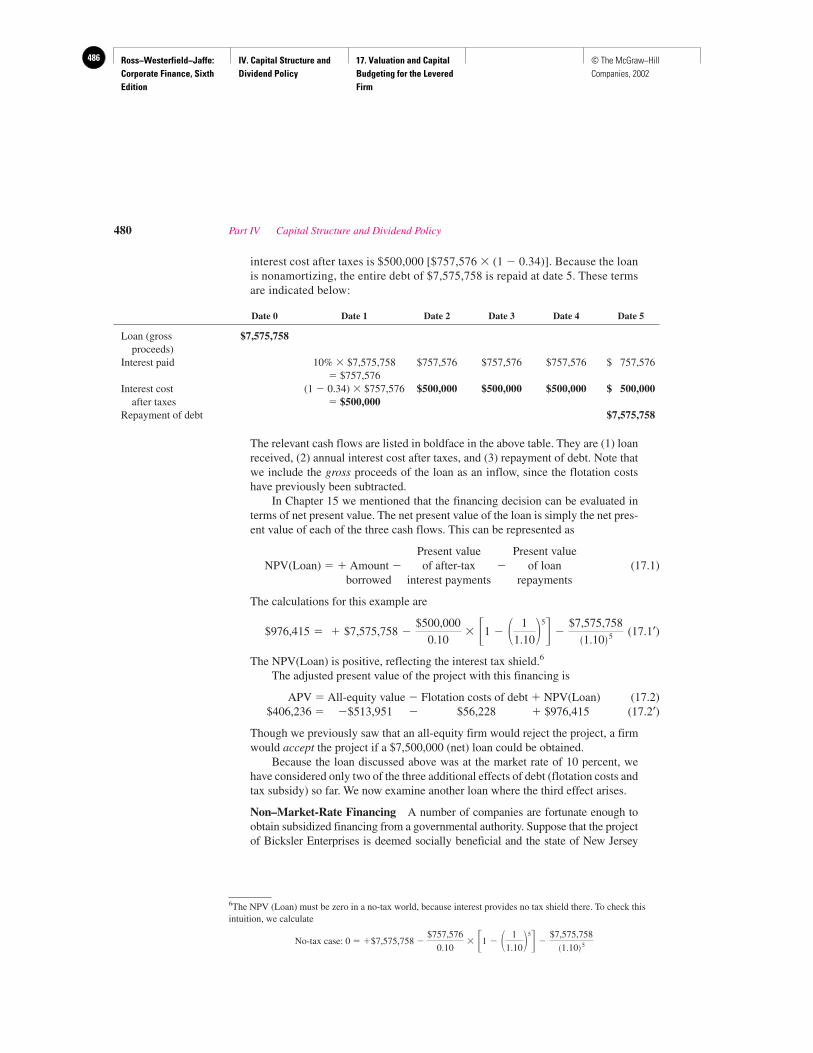
Ross−Westerfield−Jaffe: Corporate Finance, Sixth Edition
IV. Capital Structure and Dividend Policy
17. Valuation and Capital Budgeting for the Levered Firm
486 © The McGraw−Hill Companies, 2002
interest cost after taxes is $500,000 [$757,576 � (1 � 0.34)]. Because the loanis nonamortizing, the entire debt of $7,575,758 is repaid at date 5. These termsare indicated below:
Date 0 Date 1 Date 2 Date 3 Date 4 Date 5
Loan (gross $7,575,758proceeds)
Interest paid 10% � $7,575,758 $757,576 $757,576 $757,576 $ 757,576� $757,576
Interest cost (1 � 0.34) � $757,576 $500,000 $500,000 $500,000 $ 500,000after taxes � $500,000
Repayment of debt $7,575,758
The relevant cash flows are listed in boldface in the above table. They are (1) loanreceived, (2) annual interest cost after taxes, and (3) repayment of debt. Note thatwe include the gross proceeds of the loan as an inflow, since the flotation costshave previously been subtracted.
In Chapter 15 we mentioned that the financing decision can be evaluated interms of net present value. The net present value of the loan is simply the net pres-ent value of each of the three cash flows. This can be represented as
Present value Present valueNPV(Loan) � � Amount � of after-tax � of loan (17.1)
borrowed interest payments repayments
The calculations for this example are
(17.1′)
The NPV(Loan) is positive, reflecting the interest tax shield.6
The adjusted present value of the project with this financing is
APV � All-equity value � Flotation costs of debt � NPV(Loan) (17.2)$406,236 � �$513,951 � $56,228 � $976,415 (17.2′)
Though we previously saw that an all-equity firm would reject the project, a firmwould accept the project if a $7,500,000 (net) loan could be obtained.
Because the loan discussed above was at the market rate of 10 percent, wehave considered only two of the three additional effects of debt (flotation costs andtax subsidy) so far. We now examine another loan where the third effect arises.
Non–Market-Rate Financing A number of companies are fortunate enough toobtain subsidized financing from a governmental authority. Suppose that the projectof Bicksler Enterprises is deemed socially beneficial and the state of New Jersey
$976,415 � � $7,575,758 �$500,000
0.10� �1 � � 1
1.10�5 �
$7,575,758�1.10� 5
480 Part IV Capital Structure and Dividend Policy
6The NPV (Loan) must be zero in a no-tax world, because interest provides no tax shield there. To check thisintuition, we calculate
No-tax case: 0 � �$7,575,758 �$757,576
0.10� �1 � � 1
1.10�5 �
$7,575,758�1.10� 5
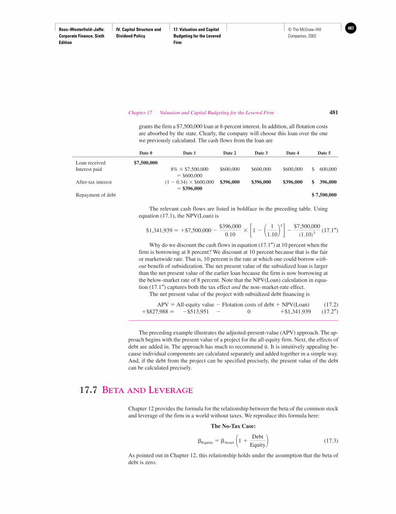
Ross−Westerfield−Jaffe: Corporate Finance, Sixth Edition
IV. Capital Structure and Dividend Policy
17. Valuation and Capital Budgeting for the Levered Firm
487© The McGraw−Hill Companies, 2002
grants the firm a $7,500,000 loan at 8-percent interest. In addition, all flotation costsare absorbed by the state. Clearly, the company will choose this loan over the onewe previously calculated. The cash flows from the loan are
Date 0 Date 1 Date 2 Date 3 Date 4 Date 5
Loan received $7,500,000Interest paid 8% � $7,500,000 $600,000 $600,000 $600,000 $ 600,000
� $600,000After-tax interest (1 � 0.34) � $600,000 $396,000 $396,000 $396,000 $ 396,000
� $396,000Repayment of debt $ 7,500,000
The relevant cash flows are listed in boldface in the preceding table. Usingequation (17.1), the NPV(Loan) is
$1,341,939 � �$7,500,000 � (17.1″)
Why do we discount the cash flows in equation (17.1″) at 10 percent when thefirm is borrowing at 8 percent? We discount at 10 percent because that is the fairor marketwide rate. That is, 10 percent is the rate at which one could borrow with-out benefit of subsidization. The net present value of the subsidized loan is largerthan the net present value of the earlier loan because the firm is now borrowing atthe below-market rate of 8 percent. Note that the NPV(Loan) calculation in equa-tion (17.1″) captures both the tax effect and the non–market-rate effect.
The net present value of the project with subsidized debt financing is
APV � All-equity value � Flotation costs of debt � NPV(Loan) (17.2)�$827,988 � �$513,951 � 0 �$1,341,939 (17.2″)
The preceding example illustrates the adjusted-present-value (APV) approach. The ap-proach begins with the present value of a project for the all-equity firm. Next, the effects ofdebt are added in. The approach has much to recommend it. It is intuitively appealing be-cause individual components are calculated separately and added together in a simple way.And, if the debt from the project can be specified precisely, the present value of the debtcan be calculated precisely.
17.7 BETA AND LEVERAGE
Chapter 12 provides the formula for the relationship between the beta of the common stockand leverage of the firm in a world without taxes. We reproduce this formula here:
The No-Tax Case:
�Equity � �Asset (17.3)
As pointed out in Chapter 12, this relationship holds under the assumption that the beta ofdebt is zero.
�1 �Debt
Equity�
$396,000
0.10� �1 � � 1
1.10�5 �
$7,500,000�1.10� 5
Chapter 17 Valuation and Capital Budgeting for the Levered Firm 481
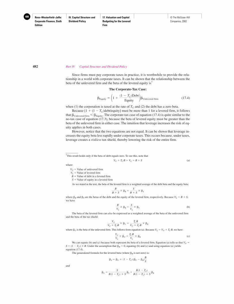
Ross−Westerfield−Jaffe: Corporate Finance, Sixth Edition
IV. Capital Structure and Dividend Policy
17. Valuation and Capital Budgeting for the Levered Firm
488 © The McGraw−Hill Companies, 2002
Since firms must pay corporate taxes in practice, it is worthwhile to provide the rela-tionship in a world with corporate taxes. It can be shown that the relationship between thebeta of the unlevered firm and the beta of the levered equity is7
The Corporate-Tax Case:
�Equity � Unlevered firm (17.4)
when (1) the corporation is taxed at the rate of TC and (2) the debt has a zero beta.Because [1 � (1 � TC)debt/equity] must be more than 1 for a levered firm, it follows
that �Unlevered firm �Equity. The corporate-tax case of equation (17.4) is quite similar to theno-tax case of equation (17.3), because the beta of levered equity must be greater than thebeta of the unlevered firm in either case. The intuition that leverage increases the risk of eq-uity applies in both cases.
However, notice that the two equations are not equal. It can be shown that leverage in-creases the equity beta less rapidly under corporate taxes. This occurs because, under taxes,leverage creates a riskless tax shield, thereby lowering the risk of the entire firm.
�1 ��1 � TC�Debt
Equity ��
482 Part IV Capital Structure and Dividend Policy
7This result holds only if the beta of debt equals zero. To see this, note that
VU � TC B � VL � B � S (a)
where
VU � Value of unlevered firmVL � Value of levered firmB � Value of debt in a levered firmS � Value of equity in a levered firm
As we stated in the text, the beta of the levered firm is a weighted average of the debt beta and the equity beta:
where �B and �S are the betas of the debt and the equity of the levered firm, respectively. Because VL � B � S,we have
(b)
The beta of the levered firm can also be expressed as a weighted average of the beta of the unlevered firmand the beta of the tax shield:
where �U is the beta of the unlevered firm. This follows from equation (a). Because VL � VU � TC B, we have
(c)
We can equate (b) and (c) because both represent the beta of a levered firm. Equation (a) tells us that VU �
S � (1 � TC) � B. Under the assumption that �B � 0, equating (b) and (c) and using equation (a) yieldsequation (17.4).
The generalized formula for the levered beta (where �B is not zero) is:
and
�U �S
B �1 � TC� � S �S �
B �1 � TC�B �1 � TC� � S
�B
�S � �U � �1 � TC� ��U � �B�B
S
VU
VL
� �U �TC B
VL
� �B
VU
VU � TC B� �U �
TC B
VU � TC B� �B
B
VL
� �B �S
VL
� �S
B
B � S� �B �
S
B � S� �S
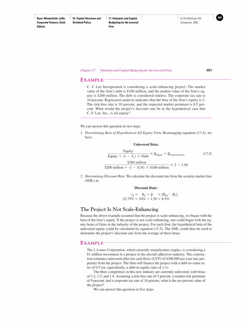
Ross−Westerfield−Jaffe: Corporate Finance, Sixth Edition
IV. Capital Structure and Dividend Policy
17. Valuation and Capital Budgeting for the Levered Firm
489© The McGraw−Hill Companies, 2002
EXAMPLE
C. F. Lee Incorporated is considering a scale-enhancing project. The marketvalue of the firm’s debt is $100 million, and the market value of the firm’s eq-uity is $200 million. The debt is considered riskless. The corporate tax rate is34 percent. Regression analysis indicates that the beta of the firm’s equity is 2.The risk-free rate is 10 percent, and the expected market premium is 8.5 per-cent. What would the project’s discount rate be in the hypothetical case that C. F. Lee, Inc., is all-equity?
We can answer this question in two steps.
1. Determining Beta of Hypothetical All-Equity Firm. Rearranging equation (17.4), wehave
Unlevered Beta:
(17.5)
2. Determining Discount Rate. We calculate the discount rate from the security market line(SML) as
Discount Rate:
rS � RF � � � [ M � RF]22.75% � 10% � 1.50 � 8.5%
The Project Is Not Scale-EnhancingBecause the above example assumed that the project is scale-enhancing, we began with thebeta of the firm’s equity. If the project is not scale-enhancing, one could begin with the eq-uity betas of firms in the industry of the project. For each firm, the hypothetical beta of theunlevered equity could be calculated by equation (17.5). The SML could then be used todetermine the project’s discount rate from the average of these betas.
EXAMPLE
The J. Lowes Corporation, which currently manufactures staples, is considering a$1 million investment in a project in the aircraft adhesives industry. The corpora-tion estimates unlevered after-tax cash flows (UCF) of $300,000 per year into per-petuity from the project. The firm will finance the project with a debt-to-value ra-tio of 0.5 (or, equivalently, a debt-to-equity ratio of 1:1).
The three competitors in this new industry are currently unlevered, with betasof 1.2, 1.3, and 1.4. Assuming a risk-free rate of 5 percent, a market-risk premiumof 9 percent, and a corporate tax rate of 34 percent, what is the net present value ofthe project?
We can answer this question in five steps.
R
$200 million
$200 million � �1 � 0.34� � $100 million� 2 � 1.50
Equity
Equity � �1 � TC� � Debt� �Equity � �Unlevered firm
Chapter 17 Valuation and Capital Budgeting for the Levered Firm 483

Ross−Westerfield−Jaffe: Corporate Finance, Sixth Edition
IV. Capital Structure and Dividend Policy
17. Valuation and Capital Budgeting for the Levered Firm
490 © The McGraw−Hill Companies, 2002
1. Calculating the Average Unlevered Beta in the Industry. The average un-levered beta across all three existing competitors in the aircraft adhesivesindustry is
2. Calculating the Levered Beta for J. Lowes’s New Project. Assuming thesame unlevered beta for this new project as for the existing competitors,we have, from equation (17.4),
Levered Beta:
3. Calculating the Cost of Levered Equity for the New Project. We calculatethe discount rate from the security market line (SML) as
Discount Rate:
rS � RF � � � [ M � RF]0.244 � 0.05 � 2.16 � 0.09
4. Calculating the WACC for the New Project. The formula for determiningthe weighted average cost of capital, rWACC, is
5. Determining the Project’s Value. Because the cash flows are perpetual, theNPV of the project is
Initial investment
$1 million � $1.16 million
17.8 SUMMARY AND CONCLUSIONS
Earlier chapters of this text showed how to calculate net present value for projects of all-equity firms. We pointed out in the last two chapters that the introduction of taxes andbankruptcy costs changes a firm’s financing decisions. Rational corporations should employsome debt in a world of this type. Because of the benefits and costs associated with debt, the
$300,000
0.139�
Unlevered cash flows �UCF�rWACC
�
0.139 �1
2� 0.05 � 0.66 �
1
2� 0.244
rWACC �B
VrB �1 � TC� �
S
V rS
R
2.16 � �1 �0.66 � 1
1� � 1.3
�Equity � �1 ��1 � TC�Debt
Equity��Unlevered firm
1.2 � 1.3 � 1.4
3� 1.3
484 Part IV Capital Structure and Dividend Policy

Ross−Westerfield−Jaffe: Corporate Finance, Sixth Edition
IV. Capital Structure and Dividend Policy
17. Valuation and Capital Budgeting for the Levered Firm
491© The McGraw−Hill Companies, 2002
capital-budgeting decision is different for levered firms than for unlevered firms. The presentchapter has discussed three methods for capital budgeting by levered firms: the adjusted-present-value (APV), flows-to-equity (FTE), and weighted-average-cost-of-capital (WACC)approaches.
1. The APV formula can be written as
Additional effects of debt � Initial investment
There are four additional effects of debt:• Tax shield from debt financing• Flotation costs• Bankruptcy costs• Benefit of non–market-rate financing
2. The FTE formula can be written as
(Initial investment � Amount borrowed)
3. The WACC formula can be written as
Initial investment
4. Corporations frequently follow the guideline:Use WACC or FTE if the firm’s target debt-to-value ratio applies to the project over its life.Use APV if the project’s level of debt is known over the life of the project.
5. The APV method is used frequently for special situations like interest subsidies, LBOs,and leases. The WACC and FTE methods are commonly used for more typical capital-budgeting situations. The APV approach is a rather unimportant method for typicalcapital-budgeting situations.
6. The beta of the equity of the firm is positively related to the leverage of the firm.
KEY TERMS
Adjusted present value (APV) 468 Weighted average cost of capital 471Flow to equity (FTE) 470
SUGGESTED READINGS
The following article contains a superb discussion of some of the subtleties of using WACC forproject valuation:Miles, J., and R. Ezzel. “The Weighted Average Cost of Capital, Perfect Capital Markets and
Project Life: A Clarification.” Journal of Financial and Quantitative Analysis 15(September 1980).
The following article presents the practical aspects of the APV approach:T. A. Luehrman. “Using APV: A Better Tool for Valuing Operations.” Harvard Business Review
(May/June 1997).
A fascinating article on the merits of the APV and WACC approaches is:Inselbag, I., and H. Kaufold. “Two DCF Approaches in Valuing Companies under Alternative
Financing Strategies (and How to Choose between Them).” Journal of Applied CorporateFinance (Summer 1997).
t�1
UCFt
�1 � rWACC� t �
t�1
LCFt
�1 � rS� t �
t�1
UCFt
�1 � r0� t �
Chapter 17 Valuation and Capital Budgeting for the Levered Firm 485

Ross−Westerfield−Jaffe: Corporate Finance, Sixth Edition
IV. Capital Structure and Dividend Policy
17. Valuation and Capital Budgeting for the Levered Firm
492 © The McGraw−Hill Companies, 2002
QUESTIONS AND PROBLEMS
Adjusted-Present-Value Approach17.1 Honda and GM are competing to sell a fleet of cars to Hertz. Hertz’s policies on its rental
cars include use of straight-line depreciation and disposing of the cars after five years.Hertz expects that the autos will have no salvage value. The firm expects a fleet of 25 carsto generate $100,000 per year in pretax income. Hertz is in the 34-percent tax bracket, andthe firm’s overall required return is 10 percent. The addition of the new fleet will not addto the risk of the firm. Treasury bills are priced to yield 6 percent.a. What is the maximum price that Hertz should be willing to pay for the fleet of cars?b. Suppose the price of the fleet (in U.S. dollars) is $325,000; both suppliers are charging
this price. Hertz is able to issue $200,000 in debt to finance the project. The bonds canbe issued at par and will carry an 8-percent interest rate. Hertz will incur no costs toissue the debt and no costs of financial distress. What is the APV of this project if Hertzuses debt to finance the auto purchase?
c. To entice Hertz to buy the cars from Honda, the Japanese government is willing to lendHertz $200,000 at 5 percent. Now what is the maximum price that Hertz is willing topay Honda for the fleet of cars?
17.2 Peatco, Inc., is considering a $2.1 million project that will be depreciated according to thestraight-line method over the three-year life of the project. The project will generate pretaxearnings of $900,000 per year, and it will not change the risk level of the firm. Peatco canobtain a three-year, 12.5-percent loan to finance the project; the bank will charge Peatcoflotation fees of 1 percent of the gross proceeds of the loan. The fee must be paid up front,not from the loan proceeds. If Peatco financed the project with all equity, its cost of capitalwould be 18 percent. The tax rate is 30 percent, and the risk-free rate is 6 percent.a. Using the APV method, determine whether or not Peatco should undertake the project.b. After hearing that Peatco would not be initiating the project in their town, the city
council voted to subsidize Peatco’s loan. Under the city’s proposal, Peatco will pay thesame flotation costs, but the rate on the loan will be 10 percent. Should Peatco acceptthe city’s offer and begin the project?
17.3 MEO Foods, Inc., has made cat food for over 20 years. The company currently has a debt-equity ratio of 25 percent, borrows at a 10-percent interest rate, and is in the 40-percent taxbracket. Its shareholders require an 18-percent return.
MEO is planning to expand cat food production capacity. The equipment to bepurchased would last three years and generate the following unlevered cash flows (UCF):
Unlevered Cash Flows by Year (in $ millions)0 1 2 3 4�
�15 5 8 10 0
MEO has also arranged a $6 million debt issue to partially finance the expansion.Under the loan, the company would pay 10 percent annually on the outstanding balance.The firm would also make year-end principal payments of $2 million per year, completelyretiring the issue at the end of the third year.
Ignoring costs of financial distress and issue costs, should MEO proceed with theexpansion plan?
17.4 Roller and Decker Corp. has established a joint venture with Malaysia Road ConstructionCompany to build a toll road in Malaysia. The initial investment in paving equipment is$20 million. Straight-line depreciation will be used, and the equipment has an economiclife of five years with no salvage value. The annual construction costs are estimated to be$10 million. The project will be finished in two years. Net toll revenue collected from theusage of the road is projected to be $6 million per annum for 20 years starting from theend of the first year of usage. The local preferential corporate tax rate for joint ventures is
486 Part IV Capital Structure and Dividend Policy
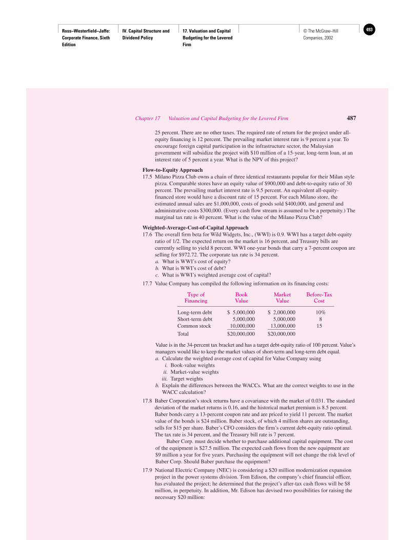
Ross−Westerfield−Jaffe: Corporate Finance, Sixth Edition
IV. Capital Structure and Dividend Policy
17. Valuation and Capital Budgeting for the Levered Firm
493© The McGraw−Hill Companies, 2002
25 percent. There are no other taxes. The required rate of return for the project under all-equity financing is 12 percent. The prevailing market interest rate is 9 percent a year. Toencourage foreign capital participation in the infrastructure sector, the Malaysiangovernment will subsidize the project with $10 million of a 15-year, long-term loan, at aninterest rate of 5 percent a year. What is the NPV of this project?
Flow-to-Equity Approach17.5 Milano Pizza Club owns a chain of three identical restaurants popular for their Milan style
pizza. Comparable stores have an equity value of $900,000 and debt-to-equity ratio of 30percent. The prevailing market interest rate is 9.5 percent. An equivalent all-equity-financed store would have a discount rate of 15 percent. For each Milano store, theestimated annual sales are $1,000,000, costs of goods sold $400,000, and general andadministrative costs $300,000. (Every cash flow stream is assumed to be a perpetuity.) Themarginal tax rate is 40 percent. What is the value of the Milano Pizza Club?
Weighted-Average-Cost-of-Capital Approach17.6 The overall firm beta for Wild Widgets, Inc., (WWI) is 0.9. WWI has a target debt-equity
ratio of 1/2. The expected return on the market is 16 percent, and Treasury bills arecurrently selling to yield 8 percent. WWI one-year bonds that carry a 7-percent coupon areselling for $972.72. The corporate tax rate is 34 percent.a. What is WWI’s cost of equity?b. What is WWI’s cost of debt?c. What is WWI’s weighted average cost of capital?
17.7 Value Company has compiled the following information on its financing costs:
Type of Book Market Before-TaxFinancing Value Value Cost
Long-term debt $ 5,000,000 $ 2,000,000 10%Short-term debt 5,000,000 5,000,000 8Common stock 10,000,000 13,000,000 15__________ __________Total $20,000,000 $20,000,000
Value is in the 34-percent tax bracket and has a target debt-equity ratio of 100 percent. Value’smanagers would like to keep the market values of short-term and long-term debt equal.a. Calculate the weighted average cost of capital for Value Company using
i. Book-value weightsii. Market-value weights
iii. Target weightsb. Explain the differences between the WACCs. What are the correct weights to use in the
WACC calculation?
17.8 Baber Corporation’s stock returns have a covariance with the market of 0.031. The standarddeviation of the market returns is 0.16, and the historical market premium is 8.5 percent.Baber bonds carry a 13-percent coupon rate and are priced to yield 11 percent. The marketvalue of the bonds is $24 million. Baber stock, of which 4 million shares are outstanding,sells for $15 per share. Baber’s CFO considers the firm’s current debt-equity ratio optimal.The tax rate is 34 percent, and the Treasury bill rate is 7 percent.
Baber Corp. must decide whether to purchase additional capital equipment. The costof the equipment is $27.5 million. The expected cash flows from the new equipment are$9 million a year for five years. Purchasing the equipment will not change the risk level ofBaber Corp. Should Baber purchase the equipment?
17.9 National Electric Company (NEC) is considering a $20 million modernization expansionproject in the power systems division. Tom Edison, the company’s chief financial officer,has evaluated the project; he determined that the project’s after-tax cash flows will be $8million, in perpetuity. In addition, Mr. Edison has devised two possibilities for raising thenecessary $20 million:
Chapter 17 Valuation and Capital Budgeting for the Levered Firm 487
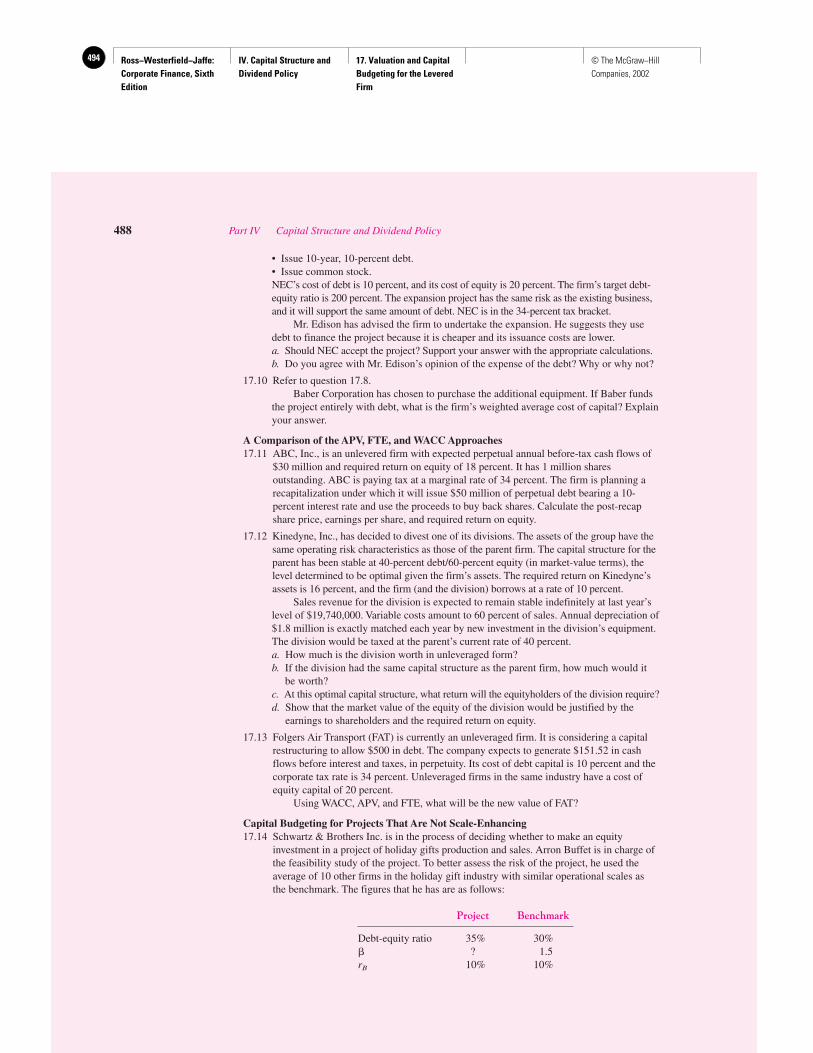
Ross−Westerfield−Jaffe: Corporate Finance, Sixth Edition
IV. Capital Structure and Dividend Policy
17. Valuation and Capital Budgeting for the Levered Firm
494 © The McGraw−Hill Companies, 2002
• Issue 10-year, 10-percent debt.• Issue common stock.NEC’s cost of debt is 10 percent, and its cost of equity is 20 percent. The firm’s target debt-equity ratio is 200 percent. The expansion project has the same risk as the existing business,and it will support the same amount of debt. NEC is in the 34-percent tax bracket.
Mr. Edison has advised the firm to undertake the expansion. He suggests they usedebt to finance the project because it is cheaper and its issuance costs are lower.a. Should NEC accept the project? Support your answer with the appropriate calculations.b. Do you agree with Mr. Edison’s opinion of the expense of the debt? Why or why not?
17.10 Refer to question 17.8.Baber Corporation has chosen to purchase the additional equipment. If Baber funds
the project entirely with debt, what is the firm’s weighted average cost of capital? Explainyour answer.
A Comparison of the APV, FTE, and WACC Approaches17.11 ABC, Inc., is an unlevered firm with expected perpetual annual before-tax cash flows of
$30 million and required return on equity of 18 percent. It has 1 million sharesoutstanding. ABC is paying tax at a marginal rate of 34 percent. The firm is planning arecapitalization under which it will issue $50 million of perpetual debt bearing a 10-percent interest rate and use the proceeds to buy back shares. Calculate the post-recapshare price, earnings per share, and required return on equity.
17.12 Kinedyne, Inc., has decided to divest one of its divisions. The assets of the group have thesame operating risk characteristics as those of the parent firm. The capital structure for theparent has been stable at 40-percent debt/60-percent equity (in market-value terms), thelevel determined to be optimal given the firm’s assets. The required return on Kinedyne’sassets is 16 percent, and the firm (and the division) borrows at a rate of 10 percent.
Sales revenue for the division is expected to remain stable indefinitely at last year’slevel of $19,740,000. Variable costs amount to 60 percent of sales. Annual depreciation of$1.8 million is exactly matched each year by new investment in the division’s equipment.The division would be taxed at the parent’s current rate of 40 percent.a. How much is the division worth in unleveraged form?b. If the division had the same capital structure as the parent firm, how much would it
be worth?c. At this optimal capital structure, what return will the equityholders of the division require?d. Show that the market value of the equity of the division would be justified by the
earnings to shareholders and the required return on equity.
17.13 Folgers Air Transport (FAT) is currently an unleveraged firm. It is considering a capitalrestructuring to allow $500 in debt. The company expects to generate $151.52 in cashflows before interest and taxes, in perpetuity. Its cost of debt capital is 10 percent and thecorporate tax rate is 34 percent. Unleveraged firms in the same industry have a cost ofequity capital of 20 percent.
Using WACC, APV, and FTE, what will be the new value of FAT?
Capital Budgeting for Projects That Are Not Scale-Enhancing17.14 Schwartz & Brothers Inc. is in the process of deciding whether to make an equity
investment in a project of holiday gifts production and sales. Arron Buffet is in charge ofthe feasibility study of the project. To better assess the risk of the project, he used theaverage of 10 other firms in the holiday gift industry with similar operational scales asthe benchmark. The figures that he has are as follows:
Project Benchmark
Debt-equity ratio 35% 30%� ? 1.5rB 10% 10%
488 Part IV Capital Structure and Dividend Policy
Ross−Westerfield−Jaffe: Corporate Finance, Sixth Edition
IV. Capital Structure and Dividend Policy
17. Valuation and Capital Budgeting for the Levered Firm
495© The McGraw−Hill Companies, 2002
The expected market return is 17 percent, and the risk-free interest rate is 9 percent.Corporate tax rate is 40 percent. The initial investment in the project is estimated at$325,000, and the cash flow at the end of the first year is $55,000. Annual cash flow willgrow at a constant rate of 5 percent till the end of the fifth year and remain constantforever thereafter. Should Schwartz & Brothers invest in this project (assume that thebond beta is zero)?
APV Example17.15 Brenda Lynch, CFO of Hunter Enterprises, is evaluating a 10-year, 9-percent loan. The
projected net proceeds after flotation costs to be raised by the loan are $4,250,000. Theflotation costs are estimated to be 1.25 percent of the gross proceeds and will beamortized using a straight-line schedule over the life of the loan. The cost of similar debtis 9.4 percent. The applicable corporate tax is 40 percent. Suppose that the loan will notincrease the financial distress cost of the firm. What is the net present value of this loan?
Beta and Leverage17.16 North Pole Fishing Equipment Corp. and South Pole Fishing Equipment Corp. would
have identical � of 1.2 if both of them were all-equity financed. The capital structures ofthe two firms are as follows:
North Pole Fishing South Pole FishingEquipment Corp. Equipment Corp.
Debt $1,000,000 $1,500,000Equity 1,500,000 1,000,000
The expected market rate of return is 12.75 percent, and the three-month Treasury billrate is 4.25 percent. Corporate tax rate is 35 percent (assume that bond beta is zero).a. What are the �s of the two firms, respectively?b. What are the required rates of return on the two firms’ equity?c. Try to give an intuitive explanation of the different �s and the returns on equity
obtained in parts (a) and (b).
APPENDIX 17A THE ADJUSTED-PRESENT-VALUE APPROACH
TO VALUING LEVERAGED BUYOUTS8
IntroductionA leveraged buyout (LBO) is the acquisition by a small group of equity investors of a pub-lic or private company financed primarily with debt. The equityholders service the heavyinterest and principal payments with cash from operations and/or asset sales. The share-holders generally hope to reverse the LBO within three to seven years by way of a publicoffering or sale of the company to another firm. A buyout is therefore likely to be success-ful only if the firm generates enough cash to serve the debt in the early years, and if the com-pany is attractive to other buyers as the buyout matures.
In a leveraged buyout, the equity investors are expected to pay off outstanding princi-pal according to a specific timetable. The owners know that the firm’s debt-equity ratio willfall and can forecast the dollar amount of debt needed to finance future operations. Under
Chapter 17 Valuation and Capital Budgeting for the Levered Firm 489
8This appendix has been adapted by Isik Inselbag and Howard Kaufold. The Wharton School, University ofPennsylvania, from their unpublished manuscript entitled “Analyzing the RJR Nabisco Buyout: An AdjustedPresent Value Approach.”

Ross−Westerfield−Jaffe: Corporate Finance, Sixth Edition
IV. Capital Structure and Dividend Policy
17. Valuation and Capital Budgeting for the Levered Firm
496 © The McGraw−Hill Companies, 2002
these circumstances, the adjusted-present-value (APV) approach is more practical than theweighted-average-cost-of-capital (WACC) approach because the capital structure is chang-ing. In this appendix, we illustrate the use of this procedure in valuing the RJR Nabiscotransaction, the largest LBO in history.
The RJR Nabisco Buyout In the summer of 1988, the price of RJR stock was hover-ing around $55 a share. The firm had $5 billion of debt. The firm’s CEO, acting in con-cert with some other senior managers of the firm, announced a bid of $75 per share totake the firm private in a management buyout. Within days of management’s offer,Kohlberg, Kravis and Roberts (KKR) entered the fray with a $90 bid of their own. Bythe end of November, KKR emerged from the ensuing bidding process with an offer of$109 a share, or $25 billion total. We now use the APV technique to analyze KKR’s win-ning strategy.
The APV method as described in this chapter can be used to value companies as wellas projects. Applied in this way, the maximum value of a levered firm (VL) is its value as anall-equity entity (VU) plus the discounted value of the interest tax shields from the debt itsassets will support (PVTS).9 This relation can be stated as
VL � VU � PVTS
In the second part of this equation, UCFt is the unlevered cash flow from operations for yeart. Discounting these cash flows by the required return on assets, r0, yields the all-equityvalue of the company. Bt�1 represents the debt balance remaining at the end of year (t � 1).Because interest in a given year is based on the debt balance remaining at the end of the pre-vious year, the interest paid in year t is rBBt�1. The numerator of the second term, TCrBBt�1,is therefore the tax shield for year t. We discount this series of annual tax shields using therate at which the firm borrows, rB.10
KKR planned to sell several of RJR’s food divisions and operate the remainingparts of the firm more efficiently. Table 17A.1 presents KKR’s projected unleveredcash flows for RJR under the buyout, adjusting for planned asset sales and operationalefficiencies.
With respect to financial strategy, KKR planned a significant increase in leverage withaccompanying tax benefits. Specifically, KKR issued almost $24 billion of new debt tocomplete the buyout, raising annual interest costs to more than $3 billion.11 Table 17A.2presents the projected interest expense and tax shields for the transaction.
�
t�1
UCFt
�1 � r0� t �
t�1
TCrBBt�1
�1 � rB� t
490 Part IV Capital Structure and Dividend Policy
9One should also deduct from this value any costs of financial distress. However, we would expect these costs tobe small in the case of RJR for two reasons. As a firm in the tobacco and food industries, its cash flows arerelatively stable and recession resistant. Furthermore, the firm’s assets are divisible and attractive to a number ofpotential buyers, allowing the firm to receive full value if disposition is required.10The pretax borrowing rate, rB, represents the appropriate discount rate for the interest tax shields when there isa precommitment to a specific debt repayment schedule under the terms of the LBO. If debt covenants requirethat the entire free cash flow be dedicated to debt service, the amount of debt outstanding and, therefore, theinterest tax shield at any point in time are a direct function of the operating cash flows of the firm. Since thedebt balance is then as risky as the cash flows, the required return on assets should be used to discount theinterest tax shields.11A significant portion of this debt was of the payment in kind (PIK) variety, which offers lenders additionalbonds instead of cash interest. This PIK debt financing provided KKR with significant tax shields whileallowing it to postpone the cash burden of debt service to future years. For simplicity of presentation, Table17A.2 does not separately show cash versus noncash interest charges.
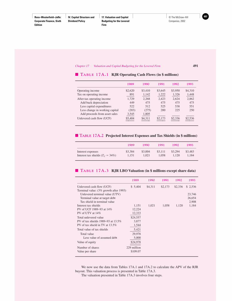
Ross−Westerfield−Jaffe: Corporate Finance, Sixth Edition
IV. Capital Structure and Dividend Policy
17. Valuation and Capital Budgeting for the Levered Firm
497© The McGraw−Hill Companies, 2002
Chapter 17 Valuation and Capital Budgeting for the Levered Firm 491
� TABLE 17A.1 RJR Operating Cash Flows (in $ millions)
1989 1990 1991 1992 1993
Operating income $2,620 $3,410 $3,645 $3,950 $4,310Tax on operating income 891 1,142 1,222 1,326 1,448_____ _____ _____ _____ _____After-tax operating income 1,729 2,268 2,423 2,624 2,862
Add back depreciation 449 475 475 475 475Less capital expenditures 522 512 525 538 551Less change in working capital (203) (275) 200 225 250Add proceeds from asset sales 3,545 1,805_____ _____ _____ _____ _____
Unlevered cash flow (UCF) $5,404 $4,311 $2,173 $2,336 $2,536______ ______ ______ ______ ____________ ______ ______ ______ ______
� TABLE 17A.3 RJR LBO Valuation (in $ millions except share data)
1989 1990 1991 1992 1993
Unlevered cash flow (UCF) $ 5,404 $4,311 $2,173 $2,336 $ 2,536Terminal value: (3% growth after 1993)
Unlevered terminal value (UTV) 23,746Terminal value at target debt 26,654Tax shield in terminal value 2,908
Interest tax shields 1,151 1,021 1,058 1,120 1,184PV of UCF 1989–93 at 14% 12,224PV of UTV at 14% 12,333_______Total unlevered value $24,557PV of tax shields 1989–93 at 13.5% 3,877PV of tax shield in TV at 13.5% 1,544_______Total value of tax shields 5,421_______
Total value 29,978Less value of assumed debt 5,000_______
Value of equity $24,978______________Number of shares 229 millionValue per share $109.07
� TABLE 17A.2 Projected Interest Expenses and Tax Shields (in $ millions)
1989 1990 1991 1992 1993
Interest expenses $3,384 $3,004 $3,111 $3,294 $3,483Interest tax shields (TC � 34%) 1,151 1,021 1,058 1,120 1,184
We now use the data from Tables 17A.1 and 17A.2 to calculate the APV of the RJRbuyout. This valuation process is presented in Table 17A.3.
The valuation presented in Table 17A.3 involves four steps.

Ross−Westerfield−Jaffe: Corporate Finance, Sixth Edition
IV. Capital Structure and Dividend Policy
17. Valuation and Capital Budgeting for the Levered Firm
498 © The McGraw−Hill Companies, 2002
Step 1: Calculating the present value of unlevered cash flows for 1989–93 The unleveredcash flows for 1989–93 are shown in the last line of Table 17A.1 and the first line of Table17A.3. These flows are discounted by the required asset return, r0, which at the time of thebuyout was approximately 14 percent. The value as of the end of 1988 of the unlevered cashflows expected from 1989 through 1993 is
Step 2: Calculating the present value of the unlevered cash flows beyond 1993 (unleveredterminal value) We assume the unlevered cash flows grow at the modest annual rate of 3percent after 1993. The value, as of the end of 1993, of these cash flows is equal to the fol-lowing discounted value of a growing perpetuity:
This translates to a 1988 value of
As in Step 1, the discount rate is the required asset rate of 14 percent.The total unlevered value of the firm is therefore ($12.224 � $12.333 �) $24.557 billion.To calculate the total buyout value, we must add the interest tax shields expected to be
realized by debt financing.
Step 3: Calculating the present value of interest tax shields for 1989–93 Under the pre-vailing U.S. tax laws in 1989, every dollar of interest reduces taxes by 34 cents. The pres-ent value of the interest tax shield for the period from 1989–93 can be calculated by dis-counting the annual tax savings at the pretax average cost of debt, which was approximately13.5 percent. Using the tax shields from Table 17A.2, the discounted value of these taxshields is calculated as
Step 4: Calculating the present value of interest tax shields beyond 1993 Finally, wemust calculate the value of tax shields associated with debt used to finance the operationsof the company after 1993. We assume that debt will be reduced and maintained at 25 per-cent of the value of the firm from that date forward.12 Under this assumption it is appro-priate to use the WACC method to calculate a terminal value for the firm at the target cap-ital structure. This in turn can be decomposed into an all-equity value and a value fromtax shields.
1.151
1.135�
1.021
1.1352 �1.058
1.1353 �1.120
1.1354 �1.184
1.1355 � $3.877 billion
23.746
1.145 � $12.333 billion
2.536 �1.03�0.14 � 0.03
� $23.746 billion
5.404
1.14�
4.311
1.142 �2.173
1.143 �2.336
1.144 �2.536
1.145 � $12.224 billion
492 Part IV Capital Structure and Dividend Policy
12This 25-percent figure is consistent with the debt utilization in industries in which RJR Nabisco isinvolved. In fact, that was the debt-to-total-market-value ratio for RJR immediately before management’sinitial buyout proposal. The firm can achieve this target by 1993 if a significant portion of the convertibledebt used to finance the buyout is exchanged for equity by that time. Alternatively, KKR could issue newequity (as would occur, for example, if the firm were taken public) and use the proceeds to retire some ofthe outstanding debt.

Ross−Westerfield−Jaffe: Corporate Finance, Sixth Edition
IV. Capital Structure and Dividend Policy
17. Valuation and Capital Budgeting for the Levered Firm
499© The McGraw−Hill Companies, 2002
If, after 1993, RJR uses 25-percent debt in its capital structure, its WACC at this targetcapital structure would be approximately 12.8 percent.13 Then the levered terminal value asof the end of 1993 can be estimated as
� $26.654 billion
Since the levered value of the company is the sum of the unlevered value plus the valueof interest tax shields, it is the case that
Value of tax shields (end 1993) � VL (end 1993) � VU (end 1993)� $26.654 billion � $23.746 billion� $2.908 billion
To calculate the value, as of the end of 1988, of these future tax shields, we again discountby the borrowing rate of 13.5 percent to get14
� $1.544 billion
The total value of interest tax shields therefore equals ($3.877 � $1.544) $5.421 billion.Adding all of these components together, the total value of RJR under the buyout pro-
posal is $29.978 billion. Deducting the $5 billion market value of assumed debt yields avalue for equity of $24.978 billion, or $109.07 per share.
2.908
1.1355
2.536 �1.03�0.128 � 0.03
Chapter 17 Valuation and Capital Budgeting for the Levered Firm 493
13To calculate this rate, use the weighted average cost of capital from this chapter:
and substitute the appropriate values for the proportions of debt and equity used, as well as their respective costs.
Specifically, at the target debt-value ratio, , and . Given this blend,
Using these findings plus the borrowing rate of 13.5 percent in rWACC, we find
rWACC � 0.75(0.141) � 0.25(0.135)(1 � 0.34) � 0.128
In fact, this value is an approximation to the true weighted average cost of capital when the market debt-valueblend is constant, or when the cash flows are growing. For a detailed discussion of this issue, see Isik Inselbagand Howard Kaufold, “A Comparison of Alternative Discounted Cash Flow Approaches to Firm Valuation.” TheWharton School, University of Pennsylvania (June 1990), unpublished paper.14A good argument can be made that since post-1993 debt levels are proportional to firm value, the tax shieldsare as risky as the firm and should be discounted at the rate r0.
� 0.14 �0.25
0.75�1 � 0.34� �0.14 � 0.135� � 0.141
rS � r0 �B
S�1 � TC� �r0 � rB�
S
S � B� �1 �
B
S � B� � 75%B
S � B� 25%
rWACC �S
S � BrS �
B
S � BrB �1 � TC�

Ross−Westerfield−Jaffe: Corporate Finance, Sixth Edition
IV. Capital Structure and Dividend Policy
17. Valuation and Capital Budgeting for the Levered Firm
500 © The McGraw−Hill Companies, 2002
Concluding Comments on LBO Valuation Methods As mentioned earlier in this chap-ter, the WACC method is by far the most widely applied approach to capital budgeting. Onecould analyze an LBO and generate the results of the second section of this appendix usingthis technique, but it would be a much more difficult process. We have tried to show thatthe APV approach is the preferred way to analyze a transaction in which the capital struc-ture is not stable over time.
Consider the WACC approach to valuing the KKR bid for RJR. One could discount theoperating cash flows of RJR by a set of weighted average costs of capital and arrive at thesame $30 billion total value for the company. To do this, one would need to calculate the ap-propriate rate for each year since the WACC rises as the buyout proceeds. This occurs becausethe value of the tax subsidy declines as debt principal is repaid. In other words, there is no sin-gle return that represents the cost of capital when the firm’s capital structure is changing.
There is also a theoretical problem with the WACC approach to valuing a buyout. Tocalculate the changing WACC, one must know the market value of a firm’s debt and equity.But if the debt and equity values are already known, the total market value of the companyis also known. That is, one must know the value of the company to calculate the WACC. Onemust therefore resort to using book-value measures for debt and equity, or make assumptionsabout the evolution of their market values, in order to implement the WACC method.
494 Part IV Capital Structure and Dividend Policy
Ross−Westerfield−Jaffe: Corporate Finance, Sixth Edition
IV. Capital Structure and Dividend Policy
18. Dividend Policy: Why Does It Matter?
501© The McGraw−Hill Companies, 2002
Dividend Policy: Why Does It Matter?
CH
AP
TE
R18
EXECUTIVE SUMMARY
In recent years, U.S. corporations have paid out about 50 percent of their net income ascash dividends. However, a significant number of corporations pay no cash dividendsand many pay more dividends than their net income.Corporations view the dividend decision as quite important because it determines what
funds flow to investors and what funds are retained by the firm for reinvestment. Dividendpolicy can also provide information to the stockholder concerning the firm’s performance.The bulk of this chapter considers the rationale both for a policy of high dividend payoutand for a policy of low dividend payout.
In part, all discussions of dividends are plagued by the “two-handed lawyer” problem.President Truman, while discussing the legal implications of a possible presidential deci-sion, asked his staff to set up a meeting with a lawyer. Supposedly Mr. Truman said, “ButI don’t want one of those two-handed lawyers.” When asked what a two-handed lawyer was,he replied, “You know, a lawyer who says, ‘On the one hand I recommend you do so-and-so because of the following reasons, but on the other hand I recommend that you don’t doit because of these other reasons.’ ” Unfortunately, any sensible treatment of dividend pol-icy will appear to be written by a two-handed lawyer. On the one hand there are many goodreasons for corporations to pay high dividends, but on the other hand there are many goodreasons to pay low dividends.
We begin this chapter with a discussion of some practical aspects of dividend pay-ments. Next we treat dividend policy. Before delineating the pros and cons of different div-idend levels, we examine a benchmark case in which the choice of the level of dividends isnot important. Surprisingly, we will see that this conceptual setup is not merely an academiccuriosity but, instead, quite applicable to the real world. Next we consider personal taxes,an imperfection generally inducing a low level of dividends. This is followed by reasonsjustifying a high dividend level. Finally, we study the history of dividends of the AppleComputer Company. The case provides some clues as to why firms pay dividends.
18.1 DIFFERENT TYPES OF DIVIDENDS
The term dividend usually refers to a cash distribution of earnings. If a distribution is madefrom sources other than current or accumulated retained earnings, the term distribution ratherthan dividend is used. However, it is acceptable to refer to a distribution from earnings as adividend and a distribution from capital as a liquidating dividend. More generally, any directpayment by the corporation to the shareholders may be considered part of dividend policy.
The most common type of dividend is in the form of cash. Public companies usuallypay regular cash dividends four times a year. Sometimes firms will pay a regular cash div-idend and an extra cash dividend. Paying a cash dividend reduces the corporate cash andretained earnings shown in the balance sheet—except in the case of a liquidating dividend(where paid-in capital may be reduced).
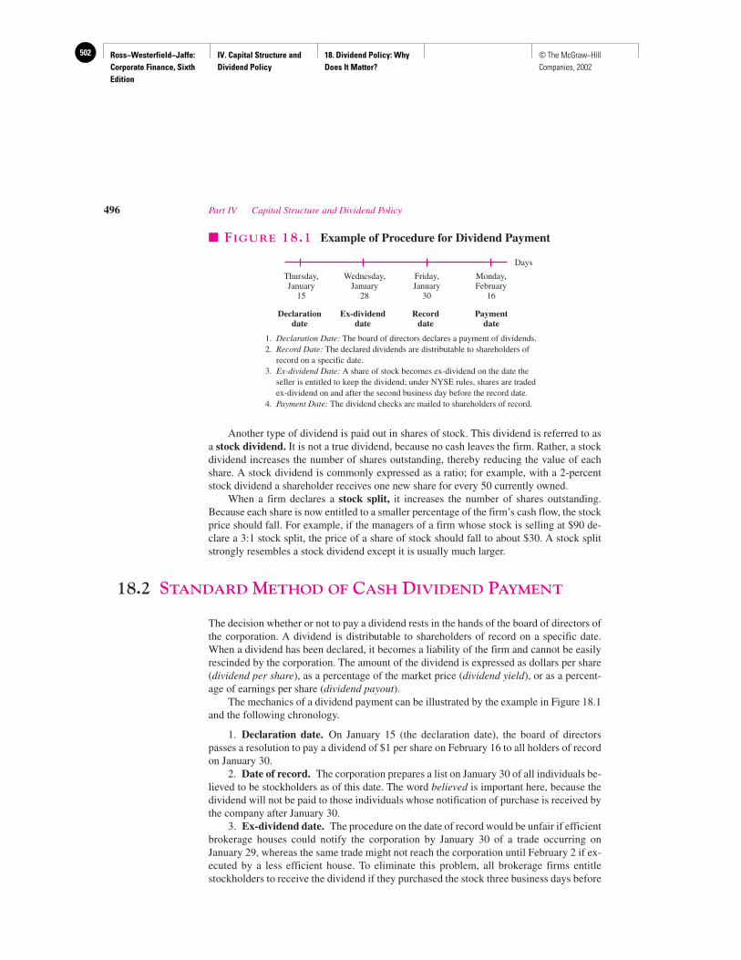
Ross−Westerfield−Jaffe: Corporate Finance, Sixth Edition
IV. Capital Structure and Dividend Policy
18. Dividend Policy: Why Does It Matter?
502 © The McGraw−Hill Companies, 2002
Another type of dividend is paid out in shares of stock. This dividend is referred to asa stock dividend. It is not a true dividend, because no cash leaves the firm. Rather, a stockdividend increases the number of shares outstanding, thereby reducing the value of eachshare. A stock dividend is commonly expressed as a ratio; for example, with a 2-percentstock dividend a shareholder receives one new share for every 50 currently owned.
When a firm declares a stock split, it increases the number of shares outstanding.Because each share is now entitled to a smaller percentage of the firm’s cash flow, the stockprice should fall. For example, if the managers of a firm whose stock is selling at $90 de-clare a 3:1 stock split, the price of a share of stock should fall to about $30. A stock splitstrongly resembles a stock dividend except it is usually much larger.
18.2 STANDARD METHOD OF CASH DIVIDEND PAYMENT
The decision whether or not to pay a dividend rests in the hands of the board of directors ofthe corporation. A dividend is distributable to shareholders of record on a specific date.When a dividend has been declared, it becomes a liability of the firm and cannot be easilyrescinded by the corporation. The amount of the dividend is expressed as dollars per share(dividend per share), as a percentage of the market price (dividend yield), or as a percent-age of earnings per share (dividend payout).
The mechanics of a dividend payment can be illustrated by the example in Figure 18.1and the following chronology.
1. Declaration date. On January 15 (the declaration date), the board of directorspasses a resolution to pay a dividend of $1 per share on February 16 to all holders of recordon January 30.
2. Date of record. The corporation prepares a list on January 30 of all individuals be-lieved to be stockholders as of this date. The word believed is important here, because thedividend will not be paid to those individuals whose notification of purchase is received bythe company after January 30.
3. Ex-dividend date. The procedure on the date of record would be unfair if efficientbrokerage houses could notify the corporation by January 30 of a trade occurring onJanuary 29, whereas the same trade might not reach the corporation until February 2 if ex-ecuted by a less efficient house. To eliminate this problem, all brokerage firms entitlestockholders to receive the dividend if they purchased the stock three business days before
496 Part IV Capital Structure and Dividend Policy
Days
Thursday,January
15
Wednesday,January
28
Friday,January
30
Monday,February
16
Declarationdate
Ex-dividenddate
Recorddate
Paymentdate
� FIGURE 18.1 Example of Procedure for Dividend Payment
1. Declaration Date: The board of directors declares a payment of dividends.2. Record Date: The declared dividends are distributable to shareholders of
record on a specific date.3. Ex-dividend Date: A share of stock becomes ex-dividend on the date the
seller is entitled to keep the dividend; under NYSE rules, shares are tradedex-dividend on and after the second business day before the record date.
4. Payment Date: The dividend checks are mailed to shareholders of record.
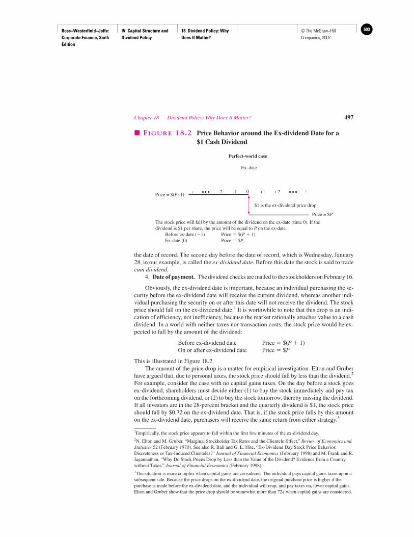
Ross−Westerfield−Jaffe: Corporate Finance, Sixth Edition
IV. Capital Structure and Dividend Policy
18. Dividend Policy: Why Does It Matter?
503© The McGraw−Hill Companies, 2002
the date of record. The second day before the date of record, which is Wednesday, January28, in our example, is called the ex-dividend date. Before this date the stock is said to tradecum dividend.
4. Date of payment. The dividend checks are mailed to the stockholders on February 16.
Obviously, the ex-dividend date is important, because an individual purchasing the se-curity before the ex-dividend date will receive the current dividend, whereas another indi-vidual purchasing the security on or after this date will not receive the dividend. The stockprice should fall on the ex-dividend date.1 It is worthwhile to note that this drop is an indi-cation of efficiency, not inefficiency, because the market rationally attaches value to a cashdividend. In a world with neither taxes nor transaction costs, the stock price would be ex-pected to fall by the amount of the dividend:
Before ex-dividend date Price � $(P � 1)On or after ex-dividend date Price � $P
This is illustrated in Figure 18.2.The amount of the price drop is a matter for empirical investigation. Elton and Gruber
have argued that, due to personal taxes, the stock price should fall by less than the dividend.2
For example, consider the case with no capital gains taxes. On the day before a stock goesex-dividend, shareholders must decide either (1) to buy the stock immediately and pay taxon the forthcoming dividend, or (2) to buy the stock tomorrow, thereby missing the dividend.If all investors are in the 28-percent bracket and the quarterly dividend is $1, the stock priceshould fall by $0.72 on the ex-dividend date. That is, if the stock price falls by this amounton the ex-dividend date, purchasers will receive the same return from either strategy.3
Chapter 18 Dividend Policy: Why Does It Matter? 497
– t –2 –1 0 +1 +2 t
$1 is the ex-dividend price drop
Price = $(P+1)
Price = $P
Perfect-world case
Ex-date
� FIGURE 18.2 Price Behavior around the Ex-dividend Date for a $1 Cash Dividend
The stock price will fall by the amount of the dividend on the ex-date (time 0). If thedividend is $1 per share, the price will be equal to P on the ex-date.
Before ex-date (�1) Price � $(P � 1)Ex-date (0) Price � $P
1Empirically, the stock price appears to fall within the first few minutes of the ex-dividend day.2N. Elton and M. Gruber, “Marginal Stockholder Tax Rates and the Clientele Effect,” Review of Economics andStatistics 52 (February 1970). See also R. Bali and G. L. Hite, “Ex-Dividend Day Stock Price Behavior:Discreteness or Tax-Induced Clienteles?” Journal of Financial Economics (February 1998) and M. Frank and R.Jagannathan, “Why Do Stock Prices Drop by Less than the Value of the Dividend? Evidence from a Countrywithout Taxes,” Journal of Financial Economics (February 1998).3The situation is more complex when capital gains are considered. The individual pays capital gains taxes upon asubsequent sale. Because the price drops on the ex-dividend date, the original purchase price is higher if thepurchase is made before the ex-dividend date, and the individual will reap, and pay taxes on, lower capital gains.Elton and Gruber show that the price drop should be somewhat more than 72¢ when capital gains are considered.
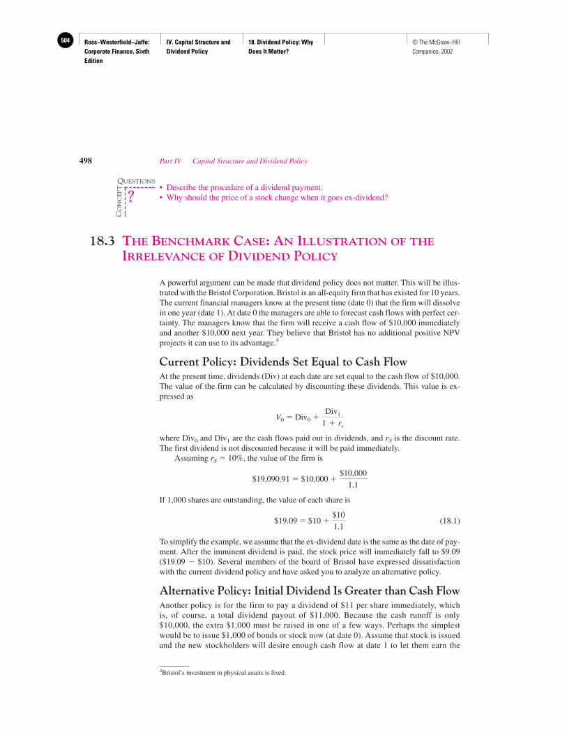
Ross−Westerfield−Jaffe: Corporate Finance, Sixth Edition
IV. Capital Structure and Dividend Policy
18. Dividend Policy: Why Does It Matter?
504 © The McGraw−Hill Companies, 2002
• Describe the procedure of a dividend payment.• Why should the price of a stock change when it goes ex-dividend?
18.3 THE BENCHMARK CASE: AN ILLUSTRATION OF THE
IRRELEVANCE OF DIVIDEND POLICY
A powerful argument can be made that dividend policy does not matter. This will be illus-trated with the Bristol Corporation. Bristol is an all-equity firm that has existed for 10 years.The current financial managers know at the present time (date 0) that the firm will dissolvein one year (date 1). At date 0 the managers are able to forecast cash flows with perfect cer-tainty. The managers know that the firm will receive a cash flow of $10,000 immediatelyand another $10,000 next year. They believe that Bristol has no additional positive NPVprojects it can use to its advantage.4
Current Policy: Dividends Set Equal to Cash FlowAt the present time, dividends (Div) at each date are set equal to the cash flow of $10,000.The value of the firm can be calculated by discounting these dividends. This value is ex-pressed as
V0 � Div0 �
where Div0 and Div1 are the cash flows paid out in dividends, and rS is the discount rate.The first dividend is not discounted because it will be paid immediately.
Assuming rS � 10%, the value of the firm is
$19,090.91 � $10,000 �
If 1,000 shares are outstanding, the value of each share is
$19.09 � $10 � (18.1)
To simplify the example, we assume that the ex-dividend date is the same as the date of pay-ment. After the imminent dividend is paid, the stock price will immediately fall to $9.09($19.09 � $10). Several members of the board of Bristol have expressed dissatisfactionwith the current dividend policy and have asked you to analyze an alternative policy.
Alternative Policy: Initial Dividend Is Greater than Cash FlowAnother policy is for the firm to pay a dividend of $11 per share immediately, whichis, of course, a total dividend payout of $11,000. Because the cash runoff is only$10,000, the extra $1,000 must be raised in one of a few ways. Perhaps the simplestwould be to issue $1,000 of bonds or stock now (at date 0). Assume that stock is issuedand the new stockholders will desire enough cash flow at date 1 to let them earn the
$10
1.1
$10,000
1.1
Div1
1 � rs
498 Part IV Capital Structure and Dividend Policy
QUESTIONS
CO
NC
EP
T
?
4Bristol’s investment in physical assets is fixed.
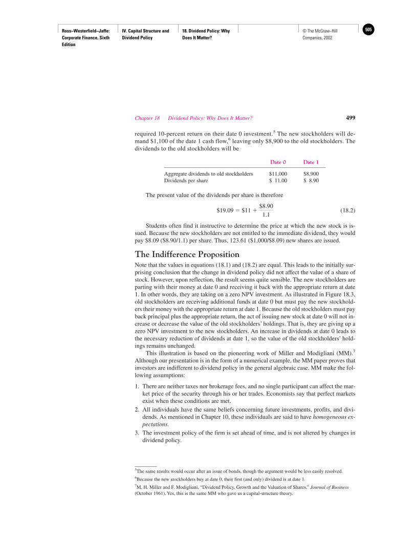
Ross−Westerfield−Jaffe: Corporate Finance, Sixth Edition
IV. Capital Structure and Dividend Policy
18. Dividend Policy: Why Does It Matter?
505© The McGraw−Hill Companies, 2002
required 10-percent return on their date 0 investment.5 The new stockholders will de-mand $1,100 of the date 1 cash flow,6 leaving only $8,900 to the old stockholders. Thedividends to the old stockholders will be
Date 0 Date 1
Aggregate dividends to old stockholders $11,000 $8,900Dividends per share $ 11.00 $ 8.90
The present value of the dividends per share is therefore
$19.09 � $11 � (18.2)
Students often find it instructive to determine the price at which the new stock is is-sued. Because the new stockholders are not entitled to the immediate dividend, they wouldpay $8.09 ($8.90/1.1) per share. Thus, 123.61 ($1,000/$8.09) new shares are issued.
The Indifference PropositionNote that the values in equations (18.1) and (18.2) are equal. This leads to the initially sur-prising conclusion that the change in dividend policy did not affect the value of a share ofstock. However, upon reflection, the result seems quite sensible. The new stockholders areparting with their money at date 0 and receiving it back with the appropriate return at date1. In other words, they are taking on a zero NPV investment. As illustrated in Figure 18.3,old stockholders are receiving additional funds at date 0 but must pay the new stockhold-ers their money with the appropriate return at date 1. Because the old stockholders must payback principal plus the appropriate return, the act of issuing new stock at date 0 will not in-crease or decrease the value of the old stockholders’ holdings. That is, they are giving up azero NPV investment to the new stockholders. An increase in dividends at date 0 leads tothe necessary reduction of dividends at date 1, so the value of the old stockholders’ hold-ings remains unchanged.
This illustration is based on the pioneering work of Miller and Modigliani (MM).7
Although our presentation is in the form of a numerical example, the MM paper proves thatinvestors are indifferent to dividend policy in the general algebraic case. MM make the fol-lowing assumptions:
1. There are neither taxes nor brokerage fees, and no single participant can affect the mar-ket price of the security through his or her trades. Economists say that perfect marketsexist when these conditions are met.
2. All individuals have the same beliefs concerning future investments, profits, and divi-dends. As mentioned in Chapter 10, these individuals are said to have homogeneous ex-pectations.
3. The investment policy of the firm is set ahead of time, and is not altered by changes individend policy.
$8.90
1.1
Chapter 18 Dividend Policy: Why Does It Matter? 499
5The same results would occur after an issue of bonds, though the argument would be less easily resolved.6Because the new stockholders buy at date 0, their first (and only) dividend is at date 1.7M. H. Miller and F. Modigliani, “Dividend Policy, Growth and the Valuation of Shares,” Journal of Business(October 1961). Yes, this is the same MM who gave us a capital-structure theory.
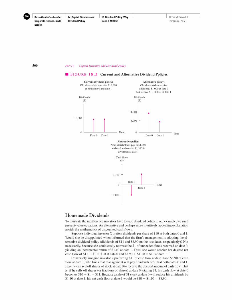
Ross−Westerfield−Jaffe: Corporate Finance, Sixth Edition
IV. Capital Structure and Dividend Policy
18. Dividend Policy: Why Does It Matter?
506 © The McGraw−Hill Companies, 2002
Homemade DividendsTo illustrate the indifference investors have toward dividend policy in our example, we usedpresent-value equations. An alternative and perhaps more intuitively appealing explanationavoids the mathematics of discounted cash flows.
Suppose individual investor X prefers dividends per share of $10 at both dates 0 and 1.Would she be disappointed when informed that the firm’s management is adopting the al-ternative dividend policy (dividends of $11 and $8.90 on the two dates, respectively)? Notnecessarily, because she could easily reinvest the $1 of unneeded funds received on date 0,yielding an incremental return of $1.10 at date 1. Thus, she would receive her desired netcash flow of $11 � $1 � $10 at date 0 and $8.90 � $1.10 � $10 at date 1.
Conversely, imagine investor Z preferring $11 of cash flow at date 0 and $8.90 of cashflow at date 1, who finds that management will pay dividends of $10 at both dates 0 and 1.Here he can sell off shares of stock at date 0 to receive the desired amount of cash flow. Thatis, if he sells off shares (or fractions of shares) at date 0 totaling $1, his cash flow at date 0becomes $10 � $1 � $11. Because a sale of $1 stock at date 0 will reduce his dividends by$1.10 at date 1, his net cash flow at date 1 would be $10 � $1.10 � $8.90.
500 Part IV Capital Structure and Dividend Policy
Dividends($)
Dividends($)
Current dividend policy:Old shareholders receive $10,000
at both date 0 and date 1
10,000
0
11,000
0
8,900
Date 0 Date 1 Date 0 Date 1Time Time
Alternative policy:Old shareholders receive
additional $1,000 at date 0but receive $1,100 less at date 1
Time
1,100
Cash flows($)
Alternative policy:New shareholders pay in $1,000at date 0 and receive $1,100 in
dividends at date 1
0
–1,000
Date 0
Date 1
� FIGURE 18.3 Current and Alternative Dividend Policies
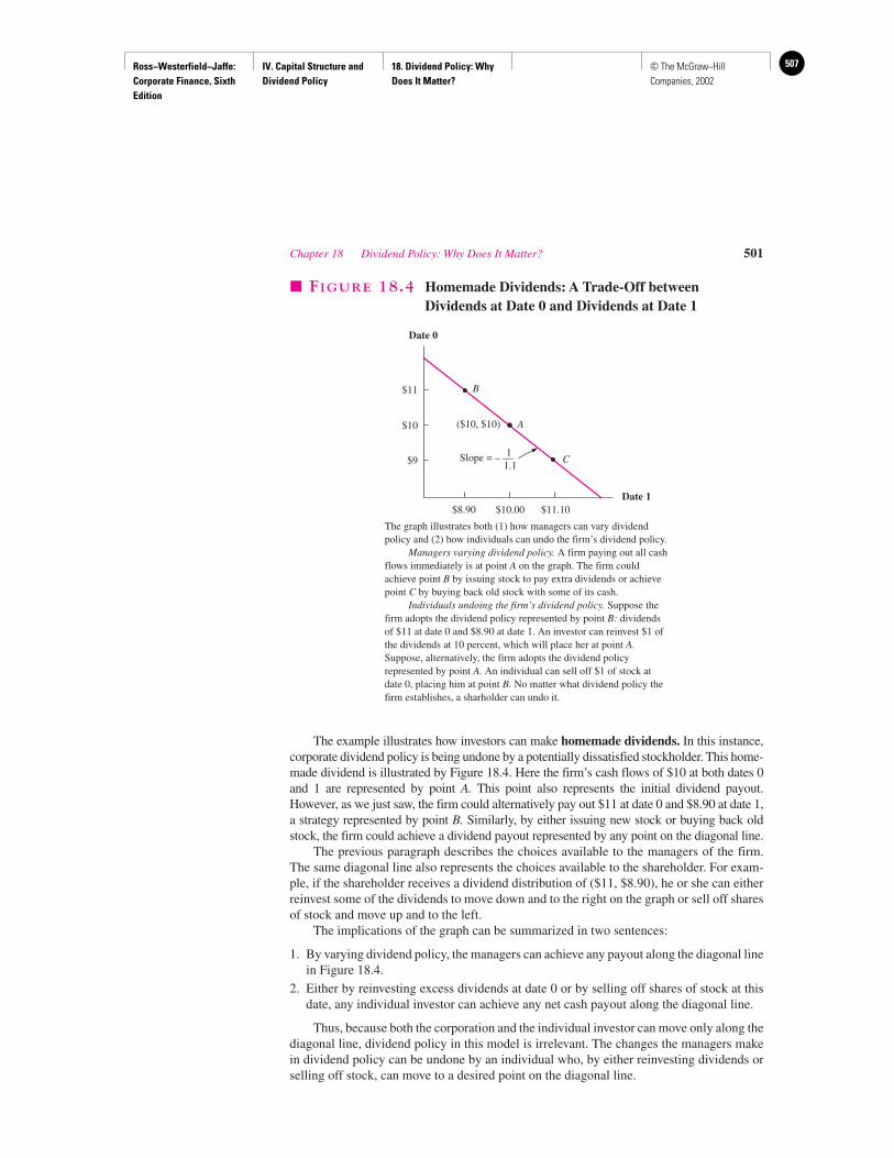
Ross−Westerfield−Jaffe: Corporate Finance, Sixth Edition
IV. Capital Structure and Dividend Policy
18. Dividend Policy: Why Does It Matter?
507© The McGraw−Hill Companies, 2002
The example illustrates how investors can make homemade dividends. In this instance,corporate dividend policy is being undone by a potentially dissatisfied stockholder. This home-made dividend is illustrated by Figure 18.4. Here the firm’s cash flows of $10 at both dates 0and 1 are represented by point A. This point also represents the initial dividend payout.However, as we just saw, the firm could alternatively pay out $11 at date 0 and $8.90 at date 1,a strategy represented by point B. Similarly, by either issuing new stock or buying back oldstock, the firm could achieve a dividend payout represented by any point on the diagonal line.
The previous paragraph describes the choices available to the managers of the firm.The same diagonal line also represents the choices available to the shareholder. For exam-ple, if the shareholder receives a dividend distribution of ($11, $8.90), he or she can eitherreinvest some of the dividends to move down and to the right on the graph or sell off sharesof stock and move up and to the left.
The implications of the graph can be summarized in two sentences:
1. By varying dividend policy, the managers can achieve any payout along the diagonal linein Figure 18.4.
2. Either by reinvesting excess dividends at date 0 or by selling off shares of stock at thisdate, any individual investor can achieve any net cash payout along the diagonal line.
Thus, because both the corporation and the individual investor can move only along thediagonal line, dividend policy in this model is irrelevant. The changes the managers makein dividend policy can be undone by an individual who, by either reinvesting dividends orselling off stock, can move to a desired point on the diagonal line.
Chapter 18 Dividend Policy: Why Does It Matter? 501
$11
$10
$9
$8.90 $10.00 $11.10Date 1
Date 0
B
A
C
($10, $10)
1Slope = – —
1.1
� FIGURE 18.4 Homemade Dividends: A Trade-Off betweenDividends at Date 0 and Dividends at Date 1
The graph illustrates both (1) how managers can vary dividendpolicy and (2) how individuals can undo the firm’s dividend policy.
Managers varying dividend policy. A firm paying out all cashflows immediately is at point A on the graph. The firm couldachieve point B by issuing stock to pay extra dividends or achievepoint C by buying back old stock with some of its cash.
Individuals undoing the firm’s dividend policy. Suppose thefirm adopts the dividend policy represented by point B: dividendsof $11 at date 0 and $8.90 at date 1. An investor can reinvest $1 ofthe dividends at 10 percent, which will place her at point A.Suppose, alternatively, the firm adopts the dividend policyrepresented by point A. An individual can sell off $1 of stock atdate 0, placing him at point B. No matter what dividend policy thefirm establishes, a sharholder can undo it.
Ross−Westerfield−Jaffe: Corporate Finance, Sixth Edition
IV. Capital Structure and Dividend Policy
18. Dividend Policy: Why Does It Matter?
508 © The McGraw−Hill Companies, 2002
A TestYou can test your knowledge of this material by examining these true statements:
1. Dividends are relevant.
2. Dividend policy is irrelevant.
The first statement follows from common sense. Clearly, investors prefer higher dividendsto lower dividends at any single date if the dividend level is held constant at every otherdate. In other words, if the dividend per share at a given date is raised while the dividendper share for each other date is held constant, the stock price will rise. This act can be ac-complished by management decisions that improve productivity, increase tax savings, orstrengthen product marketing. In fact, you may recall in Chapter 5 we argued that the valueof a firm’s equity is equal to the discounted present value of all its future dividends.
The second statement is understandable once we realize that dividend policy cannotraise the dividend per share at one date while holding the dividend level per share constantat all other dates. Rather, dividend policy merely establishes the trade-off between divi-dends at one date and dividends at another date. As we saw in Figure 18.4, an increase indate 0 dividends can be accomplished only by a decrease in date 1 dividends. The extent ofthe decrease is such that the present value of all dividends is not affected.
Thus, in this simple world, dividend policy does not matter. That is, managers choos-ing either to raise or to lower the current dividend do not affect the current value of theirfirm. The above theory is a powerful one, and the work of MM is generally considered aclassic in modern finance. With relatively few assumptions, a rather surprising result isshown to be perfectly true.8 Because we want to examine many real-world factors ignoredby MM, their work is only a starting point in this chapter’s discussion of dividends. Thenext part of the chapter investigates these real-world considerations.
Dividends and Investment PolicyThe preceding argument shows that an increase in dividends through issuance of new sharesneither helps nor hurts the stockholders. Similarly, a reduction in dividends through sharerepurchase neither helps nor hurts stockholders.
What about reducing capital expenditures to increase dividends? Earlier chapters showthat a firm should accept all positive net-present-value projects. To do otherwise would re-duce the value of the firm. Thus, we have an important point:
Firms should never give up a positive NPV project to increase a dividend (or to pay a dividendfor the first time).
This idea was implicitly considered by Miller and Modigliani. As we pointed out, one ofthe assumptions underlying their dividend-irrelevance proposition was, “The investmentpolicy of the firm is set ahead of time and is not altered by changes in dividend policy.”
• How can an investor make homemade dividends?• Are dividends irrelevant?• What assumptions are needed to show that dividend policy is irrelevant?
502 Part IV Capital Structure and Dividend Policy
8One of the real contributions of MM has been to shift the burden of proof. Before MM, firm value was believedto be influenced by its dividend policy. After MM, it became clear that establishing a correct dividend policywas not obvious at all.
QUESTIONS
CO
NC
EP
T
?
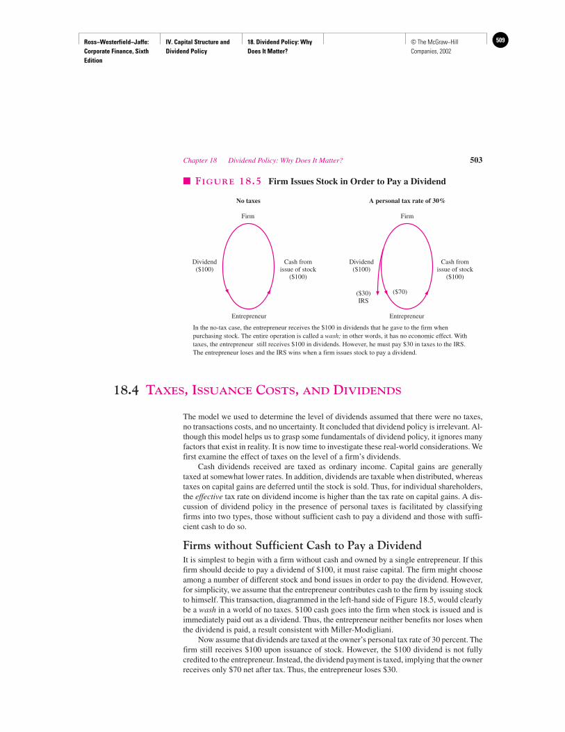
Ross−Westerfield−Jaffe: Corporate Finance, Sixth Edition
IV. Capital Structure and Dividend Policy
18. Dividend Policy: Why Does It Matter?
509© The McGraw−Hill Companies, 2002
18.4 TAXES, ISSUANCE COSTS, AND DIVIDENDS
The model we used to determine the level of dividends assumed that there were no taxes,no transactions costs, and no uncertainty. It concluded that dividend policy is irrelevant. Al-though this model helps us to grasp some fundamentals of dividend policy, it ignores manyfactors that exist in reality. It is now time to investigate these real-world considerations. Wefirst examine the effect of taxes on the level of a firm’s dividends.
Cash dividends received are taxed as ordinary income. Capital gains are generallytaxed at somewhat lower rates. In addition, dividends are taxable when distributed, whereastaxes on capital gains are deferred until the stock is sold. Thus, for individual shareholders,the effective tax rate on dividend income is higher than the tax rate on capital gains. A dis-cussion of dividend policy in the presence of personal taxes is facilitated by classifyingfirms into two types, those without sufficient cash to pay a dividend and those with suffi-cient cash to do so.
Firms without Sufficient Cash to Pay a DividendIt is simplest to begin with a firm without cash and owned by a single entrepreneur. If thisfirm should decide to pay a dividend of $100, it must raise capital. The firm might chooseamong a number of different stock and bond issues in order to pay the dividend. However,for simplicity, we assume that the entrepreneur contributes cash to the firm by issuing stockto himself. This transaction, diagrammed in the left-hand side of Figure 18.5, would clearlybe a wash in a world of no taxes. $100 cash goes into the firm when stock is issued and isimmediately paid out as a dividend. Thus, the entrepreneur neither benefits nor loses whenthe dividend is paid, a result consistent with Miller-Modigliani.
Now assume that dividends are taxed at the owner’s personal tax rate of 30 percent. Thefirm still receives $100 upon issuance of stock. However, the $100 dividend is not fullycredited to the entrepreneur. Instead, the dividend payment is taxed, implying that the ownerreceives only $70 net after tax. Thus, the entrepreneur loses $30.
Chapter 18 Dividend Policy: Why Does It Matter? 503
Firm Firm
Dividend($100)
Cash fromissue of stock
($100)
Dividend($100)
Cash fromissue of stock
($100)
No taxes A personal tax rate of 30%
($30)IRS
($70)
Entrepreneur Entrepreneur
� FIGURE 18.5 Firm Issues Stock in Order to Pay a Dividend
In the no-tax case, the entrepreneur receives the $100 in dividends that he gave to the firm whenpurchasing stock. The entire operation is called a wash; in other words, it has no economic effect. Withtaxes, the entrepreneur still receives $100 in dividends. However, he must pay $30 in taxes to the IRS.The entrepreneur loses and the IRS wins when a firm issues stock to pay a dividend.
Ross−Westerfield−Jaffe: Corporate Finance, Sixth Edition
IV. Capital Structure and Dividend Policy
18. Dividend Policy: Why Does It Matter?
510 © The McGraw−Hill Companies, 2002
Though the example is clearly contrived and unrealistic, similar results can be reachedfor more plausible situations. Thus, financial economists generally agree that, in a world ofpersonal taxes, one should not issue stock to pay a dividend.
The direct costs of issuance will add to this effect. Investment bankers must be paidwhen new capital is raised. Thus, the net receipts due to the firm from a new issue are lessthan 100 percent of total capital raised. These costs are examined in a later chapter. Becausethe size of new issues can be lowered by a reduction in dividends, we have another argu-ment in favor of a low-dividend policy.
An increase in dividends may lead to a decline in stock price for still another reason.The market price of a stock is determined by the interaction of the demand for and the sup-ply of stock. New issues increase the outstanding supply of the stock, putting downwardpressure on the market price of existing shares. Therefore, to the extent that dividends arefinanced by new issues, an increase in dividends may well contribute to a stock-price re-duction. However, in an efficient stock market, changes in the supply of stock should havea negligible effect on stock price.
Of course, our advice not to finance dividends through new stock issues might need tobe modified somewhat in the real world. A company with a large and steady cash flow formany years in the past might be paying a regular dividend. If the cash flow unexpectedlydried up for a single year, should new stock be issued so that dividends could be continued?While our above discussion would imply that new stock should not be issued, many man-agers might issue the stock anyway for practical reasons. In particular, stockholders appearto prefer dividend stability. Thus, managers might be forced to issue stock to achieve thisstability, knowing full well the adverse tax consequences.
Firms with Sufficient Cash to Pay a DividendThe previous discussion argues that, in a world with personal taxes, one should not issuestock to pay a dividend. Does the tax disadvantage of dividends imply the stronger policy,“Never pay dividends in a world with personal taxes”?
We argue below that this prescription does not necessarily apply to firms with excesscash. To see this, imagine a firm with $1 million in extra cash after selecting all positiveNPV projects and determining the level of prudent cash balances. The firm might considerthe following alternatives to a dividend:
1. Select Additional Capital-Budgeting Projects. Because the firm has taken all the availablepositive NPV projects already, it must invest its excess cash in negative NPV projects. Thisis clearly a policy at variance with principles of corporate finance. In spite of our distastefor this strategy, Professor Michael Jensen of Harvard University has suggested that manymanagers choose to take on negative NPV projects in lieu of paying dividends, doing theirstockholders a disservice in the process.9 Oil companies and tobacco companies appear tobe particularly guilty of this policy. It is frequently argued that managers who adopt nega-tive NPV projects are ripe for takeover, leveraged buyouts, and proxy fights.
2. Acquire Other Companies. To avoid the payment of dividends, a firm might use excesscash to acquire another company. This strategy has the advantage of acquiring profitableassets. However, a firm often incurs heavy costs when it embarks on an acquisition pro-gram. In addition, acquisitions are invariably made above the market price. Premiums of20 to 80 percent are not uncommon. Because of this, a number of researchers have ar-gued that mergers are not generally profitable to the acquiring company, even when
504 Part IV Capital Structure and Dividend Policy
9M. C. Jensen, “Agency Costs of Free Cash Flows, Corporate Finance and Takeovers,” American EconomicReview (May 1986).
Ross−Westerfield−Jaffe: Corporate Finance, Sixth Edition
IV. Capital Structure and Dividend Policy
18. Dividend Policy: Why Does It Matter?
511© The McGraw−Hill Companies, 2002
firms are merged for a valid business purpose.10 Therefore, a company making an ac-quisition merely to avoid a dividend is unlikely to succeed.
3. Purchase Financial Assets. The strategy of purchasing financial assets in lieu of a div-idend payment can be illustrated with the following example.
EXAMPLE
The Regional Electric Company has $1,000 of extra cash. It can retain the cash andinvest it in Treasury bills yielding 10 percent, or it can pay the cash to sharehold-ers as a dividend. Shareholders can also invest in Treasury bills with the sameyield. Suppose the corporate tax rate is 34 percent, and the individual tax rate is 28percent. How much cash will investors have after five years under each policy?
If dividends are paid now, shareholders will receive
$1,000 � (1 � 0.28) � $720
today after personal tax. Because their return after personal tax is 7.2 percent, they will have
$720 � (1.072)5 � $1,019.31 (18.3)
in five years. If Regional Electric Company retains the cash to invest in Treasury bills andpays out the proceeds five years from now, the firm will have
$1,000 � (1.066)5 � $1,376.53
in five years.If this is paid as a dividend, the stockholders will receive
$1,376.53 � (1 � 0.28) � $991.10 (18.4)
after personal taxes at date 5. The result in formula (18.3) is greater than that in (18.4), im-plying that cash to stockholders will be greater if the firm pays the dividend now.
This example shows that, for a firm with extra cash, the dividend-payout decision will de-pend on personal and corporate tax rates. If personal tax rates are higher than corporate tax rates,a firm will have an incentive to reduce dividend payouts. However, if personal tax rates are lowerthan corporate tax rates, a firm will have an incentive to pay out any excess cash as dividends.
There is a quirk in the tax law benefiting firms that invest in stock rather than bonds.For a company investing in less than 20 percent of the stock of other firms, 70 percent ofthe dividends received are excluded from corporate tax.11 If Regional Electric invested$1,000 in a one-year preferred stock yielding 10 percent, only $30 of the $100 in dividendswould be subject to tax. Corporate tax would be
$30 � 0.34 � $1,000 � 0.10 � 0.3 � 0.34 � $10.20
Thus, Regional Electric would have
$1,000 � 1.10 � $1,000 � 0.10 � 0.3 � 0.34� $1,000 � [1 � 0.10 � (1 � 0.3 � 0.34)]� $1,100 � $10.20 � $1,089.80
Chapter 18 Dividend Policy: Why Does It Matter? 505
10Richard Roll, “The Hubris Hypothesis of Corporate Takeovers,” Journal of Business (1986), pp. 197–216,explores this idea in depth.11The exclusion is 100 percent if a company owns 80 percent or more of the stock of another firm. It is 80percent if a company holds more than 20 percent and less than 80 percent of another company.
Ross−Westerfield−Jaffe: Corporate Finance, Sixth Edition
IV. Capital Structure and Dividend Policy
18. Dividend Policy: Why Does It Matter?
512 © The McGraw−Hill Companies, 2002
at the end of one year. Regional is being taxed at an effective rate of 0.30 � 0.34 � 10.2%.At the end of five years, Regional would have
$1,000 � [1 � 0.10 � (1 � 0.30 � 0.34)]5
� $1,000 � [1 � 0.10 � (1 � 0.1020)]5
� $1,537.21
If this is paid as a dividend, the stockholders would receive
$1,537.21 � (1 � 0.28) � $1,106.79 (18.5)
at that time.Because individual investors are not allowed this dividend exclusion, they would re-
ceive the same amount whether they invested date 0 dividends in 10-percent T-bills or 10-percent preferred stock. Because the result in equation (18.5) is greater than the one in(18.4), Regional should invest in preferred stock rather than pay a dividend at date 0.
Because this dividend-exclusion percentage is so large, most real-world examples fa-vor retention rather than payment of dividends. However, there appear to be very few, if any,companies that hoard cash in this manner without limit. This occurs because Section 532of the Internal Revenue Code penalizes firms with “improper accumulation of surplus.”
The above example suggests that, because of personal taxes, firms have an incentive toreduce their payment of dividends. For example, they might increase capital expenditures,repurchase shares, acquire other firms, or buy financial assets. However, due to financialconsiderations and legal constraints, rational firms at some point may bite the bullet and paysome dividends. In other words, we are arguing that firms with large cash flows may paydividends simply because they have run out of better things to do with their funds.
Summary on TaxesMiller and Modigliani argue that dividend policy is irrelevant in a perfect capital market.However, because dividends are taxed as ordinary income, the MM irrelevance principledoes not hold in the presence of personal taxes.
We make three points for a regime of personal taxes:
1. A firm should not issue stock to pay a dividend.
2. Managers have an incentive to seek alternative uses for funds to reduce dividends.
3. Though personal taxes mitigate against the payment of dividends, these taxes are notsufficient to lead firms to eliminate all dividends.
We argue that a manager should only avoid dividends if the alternative use of the funds isless costly. Though this point may seem obvious to some, it has been missed by many fi-nancial people. A number of them have argued, incorrectly in our view, that personal taxesimply that no firm should ever pay dividends.
18.5 REPURCHASE OF STOCK
Instead of paying cash dividends, a firm can rid itself of excess cash by repurchasing sharesof its own stock. Recently share repurchase has become an important way of distributingearnings to shareholders.12 The repurchase of stock is a potentially useful adjunct to divi-
506 Part IV Capital Structure and Dividend Policy
12Adam Dunsby, “Share Repurchases, Dividends, and Corporate Distribution Policy,” unpublished manuscript,The Wharton School, University of Pennsylvania, November 29, 1994, shows a dramatic increase in sharerepurchase since 1983. See also Laurie S. Bagwell and John B. Shoven, “Cash Distribution to Shareholders,”Journal of Economic Perspective 3 (1989).
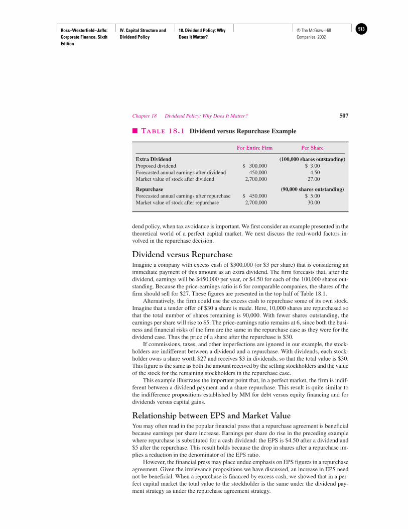
Ross−Westerfield−Jaffe: Corporate Finance, Sixth Edition
IV. Capital Structure and Dividend Policy
18. Dividend Policy: Why Does It Matter?
513© The McGraw−Hill Companies, 2002
dend policy, when tax avoidance is important. We first consider an example presented in thetheoretical world of a perfect capital market. We next discuss the real-world factors in-volved in the repurchase decision.
Dividend versus RepurchaseImagine a company with excess cash of $300,000 (or $3 per share) that is considering animmediate payment of this amount as an extra dividend. The firm forecasts that, after thedividend, earnings will be $450,000 per year, or $4.50 for each of the 100,000 shares out-standing. Because the price-earnings ratio is 6 for comparable companies, the shares of thefirm should sell for $27. These figures are presented in the top half of Table 18.1.
Alternatively, the firm could use the excess cash to repurchase some of its own stock.Imagine that a tender offer of $30 a share is made. Here, 10,000 shares are repurchased sothat the total number of shares remaining is 90,000. With fewer shares outstanding, theearnings per share will rise to $5. The price-earnings ratio remains at 6, since both the busi-ness and financial risks of the firm are the same in the repurchase case as they were for thedividend case. Thus the price of a share after the repurchase is $30.
If commissions, taxes, and other imperfections are ignored in our example, the stock-holders are indifferent between a dividend and a repurchase. With dividends, each stock-holder owns a share worth $27 and receives $3 in dividends, so that the total value is $30.This figure is the same as both the amount received by the selling stockholders and the valueof the stock for the remaining stockholders in the repurchase case.
This example illustrates the important point that, in a perfect market, the firm is indif-ferent between a dividend payment and a share repurchase. This result is quite similar tothe indifference propositions established by MM for debt versus equity financing and fordividends versus capital gains.
Relationship between EPS and Market ValueYou may often read in the popular financial press that a repurchase agreement is beneficialbecause earnings per share increase. Earnings per share do rise in the preceding examplewhere repurchase is substituted for a cash dividend: the EPS is $4.50 after a dividend and$5 after the repurchase. This result holds because the drop in shares after a repurchase im-plies a reduction in the denominator of the EPS ratio.
However, the financial press may place undue emphasis on EPS figures in a repurchaseagreement. Given the irrelevance propositions we have discussed, an increase in EPS neednot be beneficial. When a repurchase is financed by excess cash, we showed that in a per-fect capital market the total value to the stockholder is the same under the dividend pay-ment strategy as under the repurchase agreement strategy.
Chapter 18 Dividend Policy: Why Does It Matter? 507
� TABLE 18.1 Dividend versus Repurchase Example
For Entire Firm Per Share
Extra Dividend (100,000 shares outstanding)Proposed dividend $ 300,000 $ 3.00Forecasted annual earnings after dividend 450,000 4.50Market value of stock after dividend 2,700,000 27.00
Repurchase (90,000 shares outstanding)Forecasted annual earnings after repurchase $ 450,000 $ 5.00Market value of stock after repurchase 2,700,000 30.00
Ross−Westerfield−Jaffe: Corporate Finance, Sixth Edition
IV. Capital Structure and Dividend Policy
18. Dividend Policy: Why Does It Matter?
514 © The McGraw−Hill Companies, 2002
TaxesThe examples we have just described show that repurchase does not raise the wealth of theremaining shareholders in a world without taxes and transactions costs. However, stock-holders generally prefer a repurchase to a dividend under current tax law. For example, adividend of $1 per share is taxed at ordinary income rates. Investors in the 28 percent taxbracket who own 100 shares of the security would pay as much as $28 in taxes. Sellingstockholders would pay far lower taxes under a repurchase of $100 of existing shares. Thisis because taxes are paid only on the profit from a sale. Thus the gain on a sale would beonly $40 if the shares sold at $100 were originally purchased at $60. In addition, the capi-tal gains tax rate is usually lower than the ordinary income tax rate. In this example, the cap-ital gains tax rate is 20 percent. The capital gains tax would be (0.20 � $40) � $8.
If the example strikes you as being too good to be true, you are quite likely right. TheIRS is aware that the stockholders of a corporation engaging in a continuous repurchasingprogram pay far less in taxes than stockholders receiving dividends. Thus the IRS is likelyto penalize corporations repurchasing their own stocks if the only reason is to avoid thetaxes that would be levied on dividends. However, a one-time-only repurchase of shareswill most often avoid IRS scrutiny.
Targeted RepurchaseOur previous discussion concerned companies that make nonselective repurchases, usuallyexecuted through tender offers13 or open-market purchases. In addition, firms have repur-chased shares from specific individual stockholders. This procedure has been called a “tar-geted repurchase.” For example, suppose the International Biotechnology Corporation pur-chased approximately 10 percent of the outstanding stock of the Prime Robotics Company(P-R Co.) in April at around $38 per share. At that time, International Biotechnology an-nounced to the Securities and Exchange Commission that it might eventually try to takecontrol of P-R Co. In May, P-R Co. repurchased the International Biotechnology holdingsat $48 per share, well above the market price at that time. This offer was not extended toother shareholders.
Companies engage in this type of repurchase for a variety of reasons. In some rarecases a single large stockholder can be bought out at a price lower than that in a tender of-fer. The legal fees in a targeted repurchase may also be lower than those in a more typicalbuyback. More frequently, the repurchasing firm has argued that certain stockholders hadbeen nuisances. Though targeted repurchases executed for these reasons are in the interestof the remaining shareholders, the shares of large stockholders are often repurchased toavoid a takeover unfavorable to management.
Repurchase as InvestmentMany companies buy back stock because they believe that a repurchase is their best in-vestment. This occurs more frequently when managers believe that the stock price is tem-porarily depressed. Here, it is likely thought that (1) investment opportunities in nonfinan-cial assets are few, and (2) the firm’s own stock price should rise with the passage of time.
The fact that some companies repurchase their stock when they believe it is undervalueddoes not imply that the management of the company must be correct; only empirical studiescan make this determination. The immediate stock market reaction to the announcement of a
508 Part IV Capital Structure and Dividend Policy
13In a tender offer, shareholders send in (tender) their shares in exchange for a specified price per share.
Ross−Westerfield−Jaffe: Corporate Finance, Sixth Edition
IV. Capital Structure and Dividend Policy
18. Dividend Policy: Why Does It Matter?
515© The McGraw−Hill Companies, 2002
stock repurchase is usually quite favorable. In addition, recent empirical work has shown thatthe long-term stock price performance of securities after a buyback is significantly better thanthe stock price performance of comparable companies that do not repurchase.14
• Why does a stock repurchase make more sense than paying dividends?• Why don’t all firms use stock repurchases?
18.6 EXPECTED RETURN, DIVIDENDS, AND PERSONAL TAXES
The material presented so far in this chapter can properly be called a discussion of dividendpolicy. That is, it is concerned with the level of dividends chosen by a firm. A related, butdistinctly different, question is, “What is the relationship between the expected return on asecurity and its dividend yield?” To answer this question, we consider an extreme situationwhere dividends are taxed as ordinary income and capital gains are not taxed. Corporatetaxes are ignored.
Suppose every shareholder is in a 25-percent tax bracket and is considering the stocksof firm g and firm d. Firm g pays no dividend; firm d does. Suppose the current price of thestock of firm g is $100 and next year’s price is expected to be $120. The shareholder in firmg expects a $20 capital gain, implying a 20-percent return. If capital gains are not taxed, thepretax and after-tax returns must be the same.15
Suppose firm d will pay a $20 dividend per share next year. The price of firm d’s stockis expected to be $100 after the dividend payment. If the stocks of firm g and firm d areequally risky, the market prices must be set so that their after-tax expected returns are equal,in this case, to 20 percent. What will the current price of stock in firm d equal?
The current market price of a share in firm d can be calculated as follows:
The first term in the numerator is $100, the expected price of the stock at date 1. The secondterm represents the dividend after personal tax, where Td is the personal tax rate on dividends.(The tax on capital gains is ignored under our assumption of no capital gains tax.) By dis-counting at 20 percent, we are ensuring that the after-tax rate on stock d is 20 percent, the sameas the rate of return (both pre- and post-tax) for firm g. Setting Td � 0.25, P0 � $95.83.
Because the investor receives $120 from firm d at date 1 ($100 in value of stock plus$20 in dividends) before personal taxes, the expected pretax return on the security equals
� 1 � 25.22%
These calculations are presented in Table 18.2.
$120
$95.83
P0 �$100 � $20 �1 � Td�
1.20
Chapter 18 Dividend Policy: Why Does It Matter? 509
14For example, see David Ikenberry, Joseph Lakonishok, and Theo Vermaelen, “Market Underreaction to OpenMarket Share Repurchases,” Journal of Financial Economics 39 (1995).15Under current tax law, taxes on capital gains are not paid until the owner sells. Because the owner may waitindefinitely, the effective tax on capital gains in the real world is quite low. For example, A. Protopapadakis(“Some Indirect Evidence on Effective Capital Gains Tax Rates,” Journal of Business, April 1983) finds that“the effective marginal tax rates on capital gains fluctuated between 3.4 percent and 6.6 percent between 1960and 1978 and that capital gains are held, on average, between 24 and 31 years before they are reported” (p. 127).
QUESTIONS
CO
NC
EP
T
?
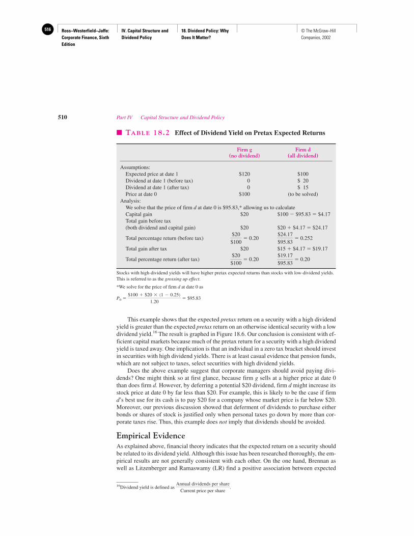
Ross−Westerfield−Jaffe: Corporate Finance, Sixth Edition
IV. Capital Structure and Dividend Policy
18. Dividend Policy: Why Does It Matter?
516 © The McGraw−Hill Companies, 2002
This example shows that the expected pretax return on a security with a high dividendyield is greater than the expected pretax return on an otherwise identical security with a lowdividend yield.16 The result is graphed in Figure 18.6. Our conclusion is consistent with ef-ficient capital markets because much of the pretax return for a security with a high dividendyield is taxed away. One implication is that an individual in a zero tax bracket should investin securities with high dividend yields. There is at least casual evidence that pension funds,which are not subject to taxes, select securities with high dividend yields.
Does the above example suggest that corporate managers should avoid paying divi-dends? One might think so at first glance, because firm g sells at a higher price at date 0than does firm d. However, by deferring a potential $20 dividend, firm d might increase itsstock price at date 0 by far less than $20. For example, this is likely to be the case if firmd’s best use for its cash is to pay $20 for a company whose market price is far below $20.Moreover, our previous discussion showed that deferment of dividends to purchase eitherbonds or shares of stock is justified only when personal taxes go down by more than cor-porate taxes rise. Thus, this example does not imply that dividends should be avoided.
Empirical EvidenceAs explained above, financial theory indicates that the expected return on a security shouldbe related to its dividend yield. Although this issue has been researched thoroughly, the em-pirical results are not generally consistent with each other. On the one hand, Brennan aswell as Litzenberger and Ramaswamy (LR) find a positive association between expected
510 Part IV Capital Structure and Dividend Policy
� TABLE 18.2 Effect of Dividend Yield on Pretax Expected Returns
Firm g Firm d(no dividend) (all dividend)
Assumptions:Expected price at date 1 $120 $100Dividend at date 1 (before tax) 0 $ 20Dividend at date 1 (after tax) 0 $ 15Price at date 0 $100 (to be solved)
Analysis:We solve that the price of firm d at date 0 is $95.83,* allowing us to calculate Capital gain $20 $100 � $95.83 � $4.17Total gain before tax(both dividend and capital gain) $20 $20 � $4.17 � $24.17
Total percentage return (before tax) � 0.20 � 0.252
Total gain after tax $20 $15 � $4.17 � $19.17
Total percentage return (after tax) � 0.20 � 0.20
Stocks with high-dividend yields will have higher pretax expected returns than stocks with low-dividend yields.This is referred to as the grossing up effect.
*We solve for the price of firm d at date 0 as
P0 � � $95.83$100 � $20 � �1 � 0.25�
1.20
$19.17
$95.83
$20
$100
$24.17
$95.83
$20
$100
16Dividend yield is defined as .Annual dividends per share
Current price per share
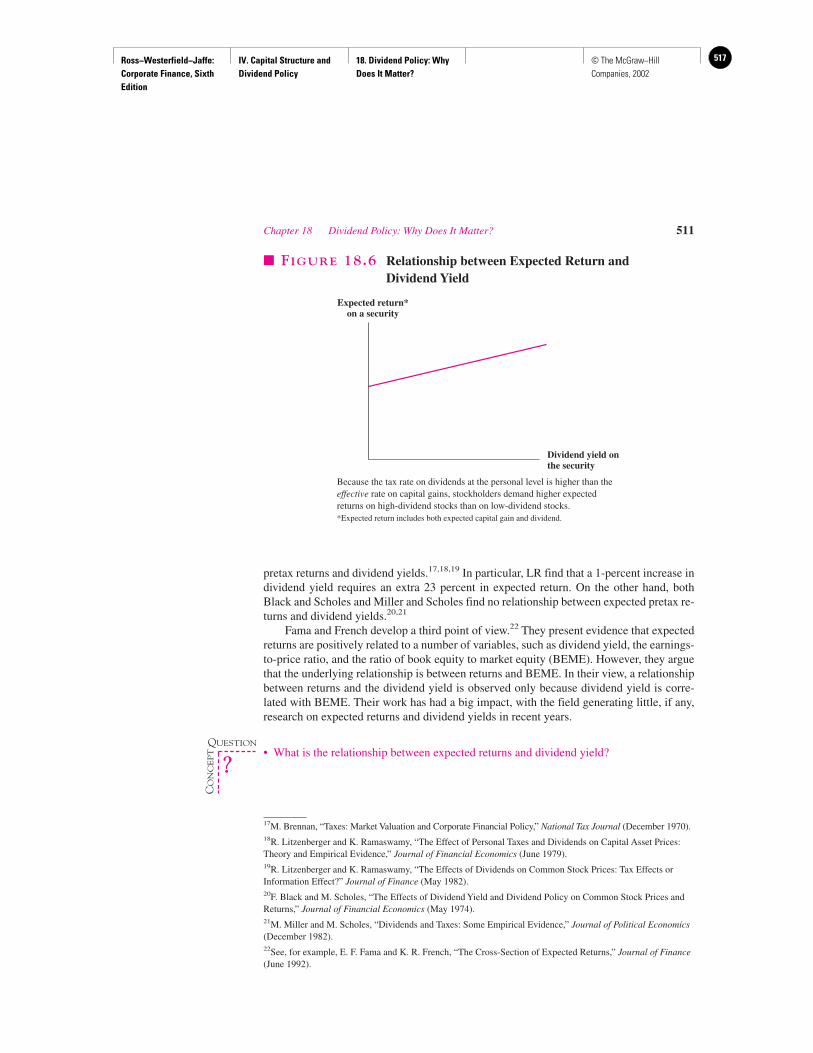
Ross−Westerfield−Jaffe: Corporate Finance, Sixth Edition
IV. Capital Structure and Dividend Policy
18. Dividend Policy: Why Does It Matter?
517© The McGraw−Hill Companies, 2002
pretax returns and dividend yields.17,18,19 In particular, LR find that a 1-percent increase individend yield requires an extra 23 percent in expected return. On the other hand, bothBlack and Scholes and Miller and Scholes find no relationship between expected pretax re-turns and dividend yields.20,21
Fama and French develop a third point of view.22 They present evidence that expectedreturns are positively related to a number of variables, such as dividend yield, the earnings-to-price ratio, and the ratio of book equity to market equity (BEME). However, they arguethat the underlying relationship is between returns and BEME. In their view, a relationshipbetween returns and the dividend yield is observed only because dividend yield is corre-lated with BEME. Their work has had a big impact, with the field generating little, if any,research on expected returns and dividend yields in recent years.
• What is the relationship between expected returns and dividend yield?
Chapter 18 Dividend Policy: Why Does It Matter? 511
Expected return*on a security
Dividend yield onthe security
� FIGURE 18.6 Relationship between Expected Return and Dividend Yield
Because the tax rate on dividends at the personal level is higher than theeffective rate on capital gains, stockholders demand higher expectedreturns on high-dividend stocks than on low-dividend stocks. *Expected return includes both expected capital gain and dividend.
17M. Brennan, “Taxes: Market Valuation and Corporate Financial Policy,” National Tax Journal (December 1970).18R. Litzenberger and K. Ramaswamy, “The Effect of Personal Taxes and Dividends on Capital Asset Prices:Theory and Empirical Evidence,” Journal of Financial Economics (June 1979).19R. Litzenberger and K. Ramaswamy, “The Effects of Dividends on Common Stock Prices: Tax Effects orInformation Effect?” Journal of Finance (May 1982).20F. Black and M. Scholes, “The Effects of Dividend Yield and Dividend Policy on Common Stock Prices andReturns,” Journal of Financial Economics (May 1974).21M. Miller and M. Scholes, “Dividends and Taxes: Some Empirical Evidence,” Journal of Political Economics(December 1982).22See, for example, E. F. Fama and K. R. French, “The Cross-Section of Expected Returns,” Journal of Finance(June 1992).
QUESTION
CO
NC
EP
T
?
Ross−Westerfield−Jaffe: Corporate Finance, Sixth Edition
IV. Capital Structure and Dividend Policy
18. Dividend Policy: Why Does It Matter?
518 © The McGraw−Hill Companies, 2002
18.7 REAL-WORLD FACTORS FAVORING A
HIGH-DIVIDEND POLICY
In a previous section, we pointed out that dividends are taxed at the personal level. This im-plies that financial managers will seek out ways to reduce dividends, though a completeelimination of dividends would be unlikely for firms with strong cash flow. We also pointedout that share repurchase is a way financial managers can convey many of the same bene-fits of a dividend without the tax disadvantage. In this section, we consider reasons why afirm might pay its shareholders high dividends, even in the presence of high personal taxeson dividends.
Desire for Current IncomeIt has been argued that many individuals desire current income. The classic example is thegroup of retired people and others living on a fixed income, proverbially known as “wid-ows and orphans.” The argument further states that these individuals would bid up the stockprice should dividends rise and bid down the stock price should dividends fall.
Miller and Modigliani point out that this argument is not relevant to their theoreticalmodel. An individual preferring high current cash flow but holding low-dividend securitiescould easily sell off shares to provide the necessary funds. Thus, in a world of no transac-tions costs, a high–current-dividend policy would be of no value to the stockholder.However, the current income argument does have relevance in the real world. Here the saleof low-dividend stocks would involve brokerage fees and other transactions costs—directcash expenses that could be avoided by an investment in high-dividend securities. In addi-tion, the expenditure of the stockholder’s own time when selling securities and the natural(but not necessarily rational) fear of consuming principal might further lead many investorsto buy high-dividend securities.
However, to put this argument in perspective, it should be remembered that financialintermediaries such as mutual funds can perform these repackaging transactions for indi-viduals at very low cost. Such intermediaries could buy low-dividend stocks and, by a con-trolled policy of realizing gains, pay their investors at a higher rate.
Uncertainty ResolutionWe have just pointed out that investors with substantial needs for current consumption willprefer high current dividends. Gordon originally argued that a high-dividend policy alsobenefits stockholders because it resolves uncertainty.23 He states that investors price a se-curity by forecasting and discounting future dividends. According to Gordon, forecasts ofdividends to be received in the distant future have greater uncertainty than do forecasts ofnear-term dividends. Because the discount rate is positively related to the degree of uncer-tainty surrounding dividends, the stock price should be low for those companies that paysmall dividends now in order to remit higher dividends at later dates.
Dividends are easier to predict than capital gains; however, it would be false to con-clude that increased dividends can make the firm less risky. A firm’s overall cash flows arenot necessarily affected by dividend policy—as long as capital spending and borrowing arenot changed. It is hard to see how the risks of the overall cash flows can be changed with achange in dividend policy.
512 Part IV Capital Structure and Dividend Policy
23M. Gordon, The Investment, Financing, and Valuation of the Corporation (Homewood, Ill.: Richard D.Irwin, 1961).
Ross−Westerfield−Jaffe: Corporate Finance, Sixth Edition
IV. Capital Structure and Dividend Policy
18. Dividend Policy: Why Does It Matter?
519© The McGraw−Hill Companies, 2002
Tax ArbitrageMiller and Scholes (MS) argue that a two-step procedure eliminates the taxes ordinarily dueon investments in high-yield securities.24 The MS strategy is as follows. First, buy stockswith high dividend yields, borrowing enough of the purchase price so that the interest paidis equal to the dividends received. The benefit of this strategy is that no taxes would be duebecause dividends are taxable whereas interest is deductible. The problem with the strategyis that the resulting position is quite risky due to the leverage involved. Second, to offset theleverage, invest an amount equivalent to the debt already incurred in a tax-deferred account(such as a Keogh account). Because income in a tax-deferred account avoids taxes, no taxesare paid when the two steps are done simultaneously.
If enough investors are able to take advantage of the strategy, corporate managers neednot view dividends as tax-disadvantaged. Thus, only a slight preference for current incomeand for resolution of uncertainty among investors causes responsive managers to providehigh dividends.
Agency CostsAlthough stockholders, bondholders, and management form firms for mutually beneficial rea-sons, one party may later gain at the other’s expense. For example, take the potential conflictbetween bondholders and stockholders. Bondholders would like stockholders to leave asmuch cash as possible in the firm so that this cash would be available to pay the bondholdersduring times of financial distress. Conversely, stockholders would like to keep this extra cashfor themselves. That’s where dividends come in. Managers, acting on behalf of the stock-holders, may pay dividends simply to keep the cash away from the bondholders. In otherwords, a dividend can be viewed as a wealth transfer from bondholders to stockholders. Thereis empirical evidence for this view of things. For example, DeAngelo and DeAngelo25 findthat firms in financial distress are reluctant to cut dividends. Of course, bondholders know ofthe propensity of stockholders to transfer money out of the firm. To protect themselves, bond-holders frequently create loan agreements stating that dividends can be paid only if the firmhas earnings, cash flow, and working capital above prespecified levels.
Although the managers may be looking out for the stockholders in any conflict withbondholders, the managers may pursue selfish goals at the expense of stockholders in othersituations. For example, as discussed in Chapter 16, managers might pad expense accounts,take on pet projects with negative NPVs, or, more simply, not work very hard. Managersfind it easier to pursue these selfish goals when the firm has plenty of free cash flow. Afterall, one can not squander funds if the funds are not available in the first place. And, that iswhere dividends come in. Several scholars have suggested that dividends can serve as a wayto reduce agency costs.26 By paying dividends equal to the amount of “surplus” cash flow,a firm can reduce management’s ability to squander the firm’s resources.
• What are the real-world factors favoring a high-dividend policy?
Chapter 18 Dividend Policy: Why Does It Matter? 513
24M. Miller and M. Scholes, “Dividends and Taxes,” Journal of Financial Economics (December 1978).25H. De Angelo and L. De Angelo, “Dividend Policy and Financial Distress: An Empirical Investigation ofTroubled NYSE Firms,” Journal of Finance 45 (1990).26Michael Rozeff, “How Companies Set Their Dividend Payout Ratios,” in The Revolution in CorporateFinance, edited by Joel M. Stern and Donald H. Chew (New York: Basel Blackwell, 1986). See also Robert S.Hansen, Raman Kumar, and Dilip K. Shome, “Dividend Policy and Corporate Monitoring: Evidence from theRegulated Electric Utility Industry,” Financial Management (Spring 1994).
QUESTION
CO
NC
EP
T
?
Ross−Westerfield−Jaffe: Corporate Finance, Sixth Edition
IV. Capital Structure and Dividend Policy
18. Dividend Policy: Why Does It Matter?
520 © The McGraw−Hill Companies, 2002
18.8 A RESOLUTION OF REAL-WORLD FACTORS?
In the previous sections, we pointed out that the existence of personal taxes favors a low-dividend policy after all positive NPV projects are taken, whereas other factors favor high div-idends. The financial profession had hoped that it would be easy to determine which of thesesets of factors dominates. Unfortunately, after years of research, no one has been able to con-clude which of the two is more important. Thus, the dividend-policy question is not resolved.
A discussion of two important concepts—the information content of dividends and theclientele effect—will give the reader an appreciation of some of the relevant issues. The firsttopic both illustrates the difficulty in interpreting empirical results on dividends and pro-vides another reason for dividends. The second topic suggests that the dividend-payout ra-tio may not be as important as we originally imagined.
Information Content of Dividends: A Brainteaser withPractical ApplicationsThe present topic is fascinating, because it is a brainteaser. To begin let us quickly review someof our earlier discussion. Previously, we examined three different positions on dividends:
1. From the homemade-dividend argument of MM, dividend policy is irrelevant, given thatfuture earnings are held constant.
2. Because of tax effects, a firm’s stock price may be negatively related to the current div-idend when future earnings are held constant.
3. Because of the desire for current income and related factors, a firm’s stock price may bepositively related to its current dividend, even when future earnings are held constant.
It has been empirically established that the price of a firm’s stock will generally risewhen its current dividend is increased and fall when its current dividend has been reducedor omitted. For example, Asquith and Mullins estimate that stock prices rise about 3 per-cent following announcements of dividend initiations. Healy and Palepu27 and Michaely,Thaler, and Womack28 find that stock prices fall about 7 percent following announcementsof dividend omissions.
At first glance, this observation may seem consistent with position 3 and inconsistentwith positions 1 and 2. In fact, many writers have argued this. However, other authors havecountered that the observation itself is consistent with all three positions. They point outthat companies do not like to cut a dividend. Thus, firms will raise the dividend only whenfuture earnings, cash flow, and so on are expected to rise enough so that the dividend is notlikely to be reduced later to its original level. A dividend increase is management’s signalto the market that the firm is expected to do well.
It is the expectation of good times, and not only the stockholder’s affinity for currentincome, that raises stock price. The rise in the stock price following the dividend signal iscalled the information-content effect of the dividend. To recapitulate, imagine that thestock price is unaffected or negatively affected by the level of dividends, given that future
514 Part IV Capital Structure and Dividend Policy
27P. Asquith and D. Mullins, Jr., “The Impact of Initiating Dividend Payments on Shareholder Wealth,” Journalof Business (January 1983).28P. M. Healy and K. G. Palepu, “Earnings Information Conveyed by Dividend Initiations and Omissions,”Journal of Financial Economics 21 (1988); and R. Michaely, R. H. Thaler, and K. Womack, “Price Reactions toDividend Initiations and Omissions: Overreactions or Drift,” Journal of Finance 50 (1995).
Ross−Westerfield−Jaffe: Corporate Finance, Sixth Edition
IV. Capital Structure and Dividend Policy
18. Dividend Policy: Why Does It Matter?
521© The McGraw−Hill Companies, 2002
earnings are held constant. Nevertheless, the information-content effect implies that stockprice may rise when dividends are raised—if dividends simultaneously cause stockholdersto upwardly adjust their expectations of future earnings.
Several theoretical models of dividend policy incorporate managerial incentive tocommunicate information via dividends.29 Here, dividends serve to signal to shareholdersthe firm’s current and future performance.
The Clientele EffectIn the first part of this chapter we established the MM proposition that dividend policy isirrelevant when certain conditions hold. Later sections dealt with those imperfections likelyto make dividend policy relevant. Because many imperfections were presented there, thereader might be skeptical that the imperfections could cancel each other out so perfectlythat dividend policy would become irrelevant. However, the argument presented below sug-gests the irrelevance of dividend policy in the real world.
Those individuals in high tax brackets are likely to prefer either no or low dividends.We can classify low–tax-bracket investors into three types. First, there are individual in-vestors in low brackets. They are likely to prefer some dividends if they desire current in-come or favor resolution of uncertainty. Second, pension funds pay no taxes on either div-idends or capital gains. Because they face no tax consequences, pension funds will alsoprefer dividends if they have a preference for current income. Finally, corporations can ex-clude at least 70 percent of their dividend income but cannot exclude any of their capitalgains. Thus, corporations would prefer to invest in high-dividend stocks, even without a de-sire to resolve uncertainty or a preference for current income.
Suppose that 40 percent of all investors prefer high dividends and 60 percent prefer lowdividends, yet only 20 percent of firms pay high dividends while 80 percent pay low divi-dends. Here, the high-dividend firms will be in short supply; thus their stock should be bidup while the stock of low-dividend firms should be bid down.
However, the dividend policies of all firms need not be fixed in the long run. In thisexample, we would expect enough low-dividend firms to increase their payout so that40 percent of the firms pay high dividends and 60 percent of the firms pay low divi-dends. After this has occurred, no type of firm will be better off from changing its dividend policy. Once payouts of corporations conform to the desires of stockholders,no single firm can affect its market value by switching from one dividend strategy toanother.
Clienteles are likely to form in the following way:
Group Stocks
Individuals in high tax brackets Zero-to-low-payout stocksIndividuals in low tax brackets Low-to-medium-payout stocksTax-free institutions Medium-payout stocksCorporations High-payout stocks
Chapter 18 Dividend Policy: Why Does It Matter? 515
29S. Bhattacharya, “Imperfect Information, Dividend Policy, and ‘the Bird in the Hand’ Fallacy,” Bell Journal ofEconomics 10 (1979); S. Bhattacharya, “Nondissipative Signaling Structure and Dividend Policy,” QuarterlyJournal of Economics 95 (1980), p. 1; S. Ross, “The Determination of Financial Structure: The IncentiveSignalling Approach,” Bell Journal of Economics 8 (1977), p. 1; M. Miller and K. Rock, “Dividend Policyunder Asymmetric Information,” Journal of Finance (1985).
Ross−Westerfield−Jaffe: Corporate Finance, Sixth Edition
IV. Capital Structure and Dividend Policy
18. Dividend Policy: Why Does It Matter?
522 © The McGraw−Hill Companies, 2002
An interesting case for the clientele effect on dividend policy is made by John Childsof Kidder Peabody in the following exchange:30
Joseph T. Willet: John, you’ve been around public utilities for a good many years. Why do youthink that utilities have such high dividend payout ratios?
John Childs: They’re raising dividends so they can raise capital. . . . If you take the divi-dends out of utilities today, you’ll never sell another share of stock. That’s how important it is.In fact, if a few major utilities (with no special problems) cut their dividends, small investorswould lose faith in the utility industry and that would finish the sales of utility stocks.
John Childs (again): What you are trying to do with dividend policy is to enhance andstrengthen the natural interest of investors in your company. The type of stockholders you at-tract will depend on the type of company you are. If you’re Genentech, you are going to attractthe type of stockholders who have absolutely no interest in dividends. In fact, you would hurtthe stockholders if you paid dividends. On the other hand, you go over to the other extremesuch as utilities’ and the yield bank’s stocks. There the stockholders are extremely interested individends, and these dividends have an effect on market price.
However, despite the preceding exchange, a desire for dividends on the part of exist-ing shareholders should not be sufficient to justify a high-dividend payout policy.
To see if you understand the clientele effect, consider the following question: “In spiteof the theoretical argument that dividend policy is irrelevant or that firms should not paydividends, many investors like high dividends. Because of this fact, a firm can boost itsshare price by having a higher dividend payout ratio.” True or false?
The statement is likely to be false. As long as enough high-dividend firms satisfy dividend-loving investors, a firm will not be able to boost its share price by paying high dividends. Afirm can boost its stock price only if an unsatisfied clientele exists. There is no evidence thatthis is the case.
Our discussion on clienteles followed from the fact that tax brackets vary across in-vestors. If shareholders care about taxes, stock should attract tax clienteles based on divi-dend yield. This appears to be true. Surveys by Blume, Crockett, and Friend, and byLewellen, Stanley, Lease, and Schlarbaum in Table 18.3, show that stocks with the highestdividend yields tend to be held by individual investors in low tax brackets.31
• Do dividends have information content?• What are tax clienteles?
18.9 WHAT WE KNOW AND DO NOT KNOW ABOUT
DIVIDEND POLICY
Corporate Dividends Are SubstantialWe pointed out earlier in the chapter that dividends are tax-disadvantaged relative to capi-tal gains for two reasons. First, dividends are taxed at the ordinary income-tax rate, whereascapital gains are taxed at a lower rate. Second, taxes on dividends are paid in the year in
516 Part IV Capital Structure and Dividend Policy
30Joseph T. Willett, moderator, “A Discussion of Corporate Dividend Policy,” in Six Roundtable Discussions ofCorporate Finance with Joel Stern, ed. by D. H. Chew (New York: Basel Blackwell, 1986). The panelistsincluded Robert Litzenberger, Pat Hess, Bill Kealy, John Childs, and Joel Stern.31M. Blume, J. Crockett, and I. Friend, “Stockownership in the United States: Characteristics and Trends,”Survey of Current Business 54 (1974), p. 11. W. Lewellen, K. L. Stanley, R. C. Lease, and G. C. Schlarbaum,“Some Direct Evidence on the Dividend Clientele Phenomenon,” Journal of Finance 33 (December 1978), p. 5.
QUESTIONS
CO
NC
EP
T
?
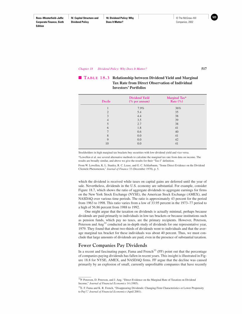
Ross−Westerfield−Jaffe: Corporate Finance, Sixth Edition
IV. Capital Structure and Dividend Policy
18. Dividend Policy: Why Does It Matter?
523© The McGraw−Hill Companies, 2002
which the dividend is received while taxes on capital gains are deferred until the year ofsale. Nevertheless, dividends in the U.S. economy are substantial. For example, considerFigure 18.7, which shows the ratio of aggregate dividends to aggregate earnings for firmson the New York Stock Exchange (NYSE), the American Stock Exchange (AMEX), andNASDAQ over various time periods. The ratio is approximately 43 percent for the periodfrom 1963 to 1998. This ratio varies from a low of 33.95 percent in the 1973–77 period toa high of 56.86 percent from 1988 to 1992.
One might argue that the taxation on dividends is actually minimal, perhaps becausedividends are paid primarily to individuals in low tax brackets or because institutions suchas pension funds, which pay no taxes, are the primary recipients. However, Peterson,Peterson and Ang32 conducted an in-depth study of dividends for one representative year,1979. They found that about two-thirds of dividends went to individuals and that the aver-age marginal tax bracket for these individuals was about 40 percent. Thus, we must con-clude that large amounts of dividends are paid, even in the presence of substantial taxation.
Fewer Companies Pay DividendsIn a recent and fascinating paper, Fama and French33 (FF) point out that the percentageof companies paying dividends has fallen in recent years. This insight is illustrated in Fig-ure 18.8 for NYSE, AMEX, and NASDAQ firms. FF argue that the decline was causedprimarily by an explosion of small, currently unprofitable companies that have recently
Chapter 18 Dividend Policy: Why Does It Matter? 517
� TABLE 18.3 Relationship between Dividend Yield and Marginal Tax Rate from Direct Observation of IndividualInvestors’ Portfolios
Dividend Yield Marginal Tax*Decile (% per annum) Rate (%)
1 7.9% 36%2 5.4 353 4.4 384 3.5 395 2.7 386 1.8 417 0.6 408 0.0 419 0.0 42
10 0.0 41
Stockholders in high marginal tax brackets buy securities with low-dividend yield and vice versa.
*Lewellen et al. use several alternative methods to calculate the marginal tax rate from data on income. Theresults are broadly similar, and above we give the results for their “Tax-l” definition.
From W. Lewellen, K. L. Stanley, R. C. Lease, and G. C. Schlarbaum, “Some Direct Evidence on the DividendClientele Phenomenon,” Journal of Finance 33 (December 1978), p. 5.
32P. Peterson, D. Peterson, and J. Ang, “Direct Evidence on the Marginal Rate of Taxation on DividendIncome,” Journal of Financial Economics 14 (1985).33E. F. Fama and K. R. French, “Disappearing Dividends: Changing Firm Characteristics or Lower Propensityto Pay?,” Journal of Financial Economics (April 2001).
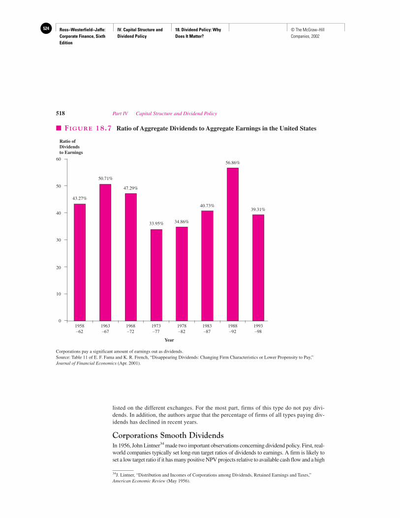
Ross−Westerfield−Jaffe: Corporate Finance, Sixth Edition
IV. Capital Structure and Dividend Policy
18. Dividend Policy: Why Does It Matter?
524 © The McGraw−Hill Companies, 2002
listed on the different exchanges. For the most part, firms of this type do not pay divi-dends. In addition, the authors argue that the percentage of firms of all types paying div-idends has declined in recent years.
Corporations Smooth DividendsIn 1956, John Lintner34 made two important observations concerning dividend policy. First, real-world companies typically set long-run target ratios of dividends to earnings. A firm is likely toset a low target ratio if it has many positive NPV projects relative to available cash flow and a high
518 Part IV Capital Structure and Dividend Policy
60
50
40
30
20
10
0
Ratio ofDividendsto Earnings
Year
1958–62
1963–67
1968–72
1973–77
1978–82
1983–87
1988–92
43.27%
50.71%
47.29%
33.95% 34.86%
40.73%
56.86%
39.31%
1993–98
� FIGURE 18.7 Ratio of Aggregate Dividends to Aggregate Earnings in the United States
34J. Lintner, “Distribution and Incomes of Corporations among Dividends, Retained Earnings and Taxes,”American Economic Review (May 1956).
Corporations pay a significant amount of earnings out as dividends.Source: Table 11 of E. F. Fama and K. R. French, “Disappearing Dividends: Changing Firm Characteristics or Lower Propensity to Pay,”Journal of Financial Economics (Apr. 2001).
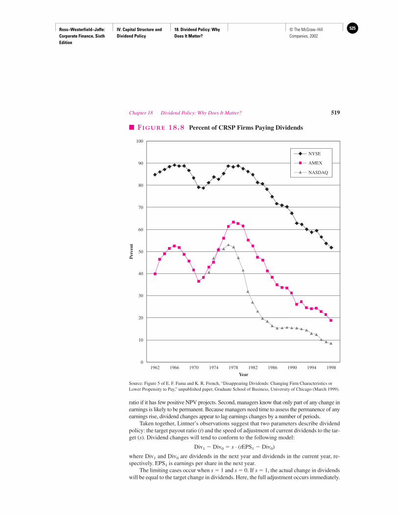
Ross−Westerfield−Jaffe: Corporate Finance, Sixth Edition
IV. Capital Structure and Dividend Policy
18. Dividend Policy: Why Does It Matter?
525© The McGraw−Hill Companies, 2002
ratio if it has few positive NPV projects. Second, managers know that only part of any change inearnings is likely to be permanent. Because managers need time to assess the permanence of anyearnings rise, dividend changes appear to lag earnings changes by a number of periods.
Taken together, Lintner’s observations suggest that two parameters describe dividendpolicy: the target payout ratio (t) and the speed of adjustment of current dividends to the tar-get (s). Dividend changes will tend to conform to the following model:
Div1 � Div0 � s ⋅ (tEPS1 � Div0)
where Div1 and Div0 are dividends in the next year and dividends in the current year, re-spectively. EPS1 is earnings per share in the next year.
The limiting cases occur when s � 1 and s � 0. If s � 1, the actual change in dividendswill be equal to the target change in dividends. Here, the full adjustment occurs immediately.
Chapter 18 Dividend Policy: Why Does It Matter? 519
100
90
80
70
60
50
40
30
20
10
0
NYSE
AMEX
NASDAQ
1962 1966 1970 1974 1978 1982 1986 1990 1994 1998
Per
cent
Year
� FIGURE 18.8 Percent of CRSP Firms Paying Dividends
Source: Figure 5 of E. F. Fama and K. R. French, “Disappearing Dividends: Changing Firm Characteristics orLower Propensity to Pay,” unpublished paper, Graduate School of Business, University of Chicago (March 1999).

Ross−Westerfield−Jaffe: Corporate Finance, Sixth Edition
IV. Capital Structure and Dividend Policy
18. Dividend Policy: Why Does It Matter?
526 © The McGraw−Hill Companies, 2002
If s � 0, Div1 � Div0. In other words, there is no change in dividends at all. Real-world com-panies can be expected to set s between 0 and 1.
An implication of Lintner’s model is that the dividends-to-earnings ratio rises when acompany begins a period of bad times, and the ratio falls when a company reaches a periodof good times. Thus, dividends display less variability than do earnings. In other words,firms smooth dividends.
Dividends Provide Information to the MarketWe previously observed that the price of a firm’s stock frequently rises when its current div-idend is increased. Conversely, the price of a firm’s stock can fall significantly when its div-idend is cut. In other words, there is information content in dividend changes. For example,consider what happened to Pacific Enterprises a number of years ago. Faced with poor op-erating results, Pacific Enterprises omitted its regular quarterly dividend. The next day thecommon stock dropped from 247⁄8 to 187⁄8. One reason may be that investors are looking atcurrent dividends for clues concerning the level of future earnings and dividends.
A Sensible Dividend PolicyThe knowledge of the finance profession varies across topic areas. For example, capital-budgeting techniques are both powerful and precise. A single net-present-value equationcan accurately determine whether a multimillion dollar project should be accepted or re-jected. The capital-asset-pricing model and the arbitrage-pricing model provide empiricallyvalidated relationships between expected return and risk.
Conversely, the field has less knowledge of capital-structure policy. Though a numberof elegant theories relate firm value to the level of debt, no formula can be used to calculatethe firm’s optimum debt-equity ratio. Our profession is forced too frequently to employ
520 Part IV Capital Structure and Dividend Policy
IN THEIR OWN WORDS
Anthony S. Thornley on Why Qualcomm Pays No Dividends
Qualcomm has consistently been able to generate forits shareholders a significantly higher return than the
shareholders could get from being paid a dividend. It hasno “excess” cash for dividends. If Qualcomm paid adividend, our shareholders would view it very negatively.Qualcomm would be saying, “We have run out of goodprofit opportunities.” Our shareholders don’t like
dividends as much as they like the capital gains fromQualcomm’s growth and profitability.
Anthony S. Thornley is Executive Vice President and ChiefFinancial Officer of Qualcomm. Qualcomm trades on NASDAQand is part of the Standard & Poor’s 500 Index. Its averageannual growth rate in earnings over the past five years has been65 percent.
Utility investors like dividends. Historically, EdisonInternational has paid out considerably more than
50 percent of its earnings as dividends. Investors haveviewed utilities such as Edison as defensive stocks wheredividends are a cushion against stock market volatility.As a utility, Edison has had limited growth opportunitiesand has been able to finance their growth out of retained
earnings and new stock. In 1994, Edison reduced itsdividend reflecting changes in the utility business andEdison’s increasing participation in higher growth, nonu-tility business.
Alan J. Fohrer is Executive Vice President and Chief FinancialOfficer of Edison International.
Alan J. Fohrer on Why Edison International Pays Dividends
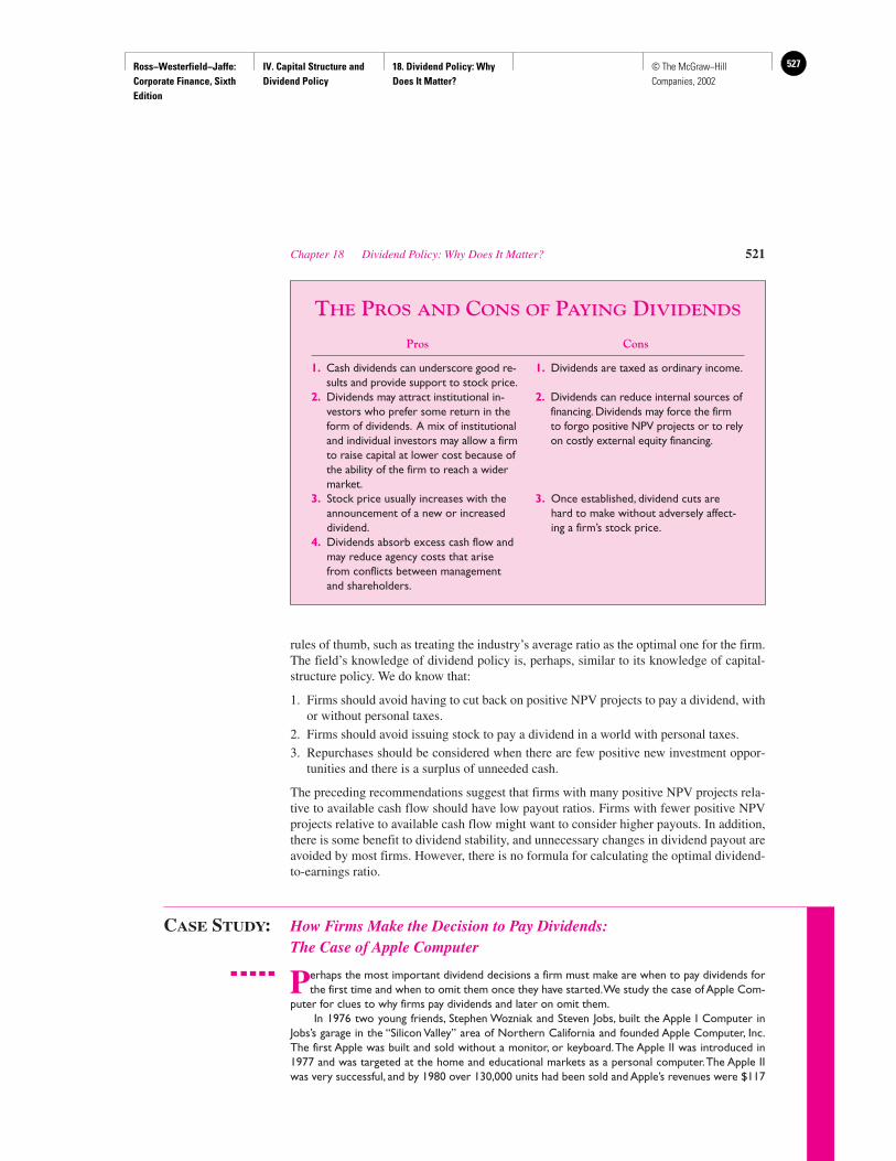
Ross−Westerfield−Jaffe: Corporate Finance, Sixth Edition
IV. Capital Structure and Dividend Policy
18. Dividend Policy: Why Does It Matter?
527© The McGraw−Hill Companies, 2002
rules of thumb, such as treating the industry’s average ratio as the optimal one for the firm.The field’s knowledge of dividend policy is, perhaps, similar to its knowledge of capital-structure policy. We do know that:
1. Firms should avoid having to cut back on positive NPV projects to pay a dividend, withor without personal taxes.
2. Firms should avoid issuing stock to pay a dividend in a world with personal taxes.
3. Repurchases should be considered when there are few positive new investment oppor-tunities and there is a surplus of unneeded cash.
The preceding recommendations suggest that firms with many positive NPV projects rela-tive to available cash flow should have low payout ratios. Firms with fewer positive NPVprojects relative to available cash flow might want to consider higher payouts. In addition,there is some benefit to dividend stability, and unnecessary changes in dividend payout areavoided by most firms. However, there is no formula for calculating the optimal dividend-to-earnings ratio.
CASE STUDY: How Firms Make the Decision to Pay Dividends:The Case of Apple Computer
Perhaps the most important dividend decisions a firm must make are when to pay dividends forthe first time and when to omit them once they have started.We study the case of Apple Com-
puter for clues to why firms pay dividends and later on omit them.In 1976 two young friends, Stephen Wozniak and Steven Jobs, built the Apple I Computer in
Jobs’s garage in the “Silicon Valley” area of Northern California and founded Apple Computer, Inc.The first Apple was built and sold without a monitor, or keyboard.The Apple II was introduced in1977 and was targeted at the home and educational markets as a personal computer.The Apple IIwas very successful, and by 1980 over 130,000 units had been sold and Apple’s revenues were $117
Chapter 18 Dividend Policy: Why Does It Matter? 521
THE PROS AND CONS OF PAYING DIVIDENDS
Pros Cons
1. Cash dividends can underscore good re-sults and provide support to stock price.
2. Dividends may attract institutional in-vestors who prefer some return in theform of dividends. A mix of institutionaland individual investors may allow a firmto raise capital at lower cost because ofthe ability of the firm to reach a widermarket.
3. Stock price usually increases with theannouncement of a new or increaseddividend.
4. Dividends absorb excess cash flow andmay reduce agency costs that arisefrom conflicts between managementand shareholders.
1. Dividends are taxed as ordinary income.
2. Dividends can reduce internal sources offinancing. Dividends may force the firmto forgo positive NPV projects or to relyon costly external equity financing.
3. Once established, dividend cuts arehard to make without adversely affect-ing a firm’s stock price.
Ross−Westerfield−Jaffe: Corporate Finance, Sixth Edition
IV. Capital Structure and Dividend Policy
18. Dividend Policy: Why Does It Matter?
528 © The McGraw−Hill Companies, 2002
million. In 1980 Apple “went public” with an initial public offering (IPO) of common stock. Shortlythereafter,Wozniak left Apple and John Scully was hired from Pepsi to become president.Apple didnot do well with its Lisa (1983) and Apple III computers, but the Macintosh (1984) was a huge hit—primarily in the home and educational markets. In 1985, after a widely publicized struggle for powerwith Scully, Jobs left to start another computer company called Next.
In many ways 1986 was a watershed year for Apple. By the end of 1986,Apple had revenues of$1.9 billion and net income of $154 million. From 1980 to 1986 its annual growth rate in net incomewas 53 percent. In 1986, with Mac Plus, Apple launched an aggressive effort to penetrate the ex-panding office computer market—the domain of its main rival IBM. However, its future prospectswere not necessarily bright. Much depended on Apple’s ability to do well in the business market.Competition was very intense in early 1987, and Sun Microsystems slashed the price of its leastcostly computer workstation to try to stop encroachment by the Apple Mac. However,Apple sur-prised everyone with large earnings gains in the final quarter of 1987 and by disclosing the fact thatthe sales on Macintosh models had increased by 41 percent.
To demonstrate its faith in its future, to underscore the recent success of the Mac, and to at-tract more institutional investors, on April 23, 1987,Apple declared its first ever quarterly dividendof $.12 per share. It also announced a two-for-one stock split.The stock market reacted very posi-tively to the announcement of Apple’s initial dividend. On the day of the announcements, its stockincreased by $1.75. Over a four-day time span the stock rose by about 8 percent.
The initial dividend turned out to be a positive portent, and the next four years were good yearsfor Apple. At the end of 1990, Apple’s revenues, profits, and capital spending had achieved record highs.
Growth per Annum Growth per Annum 1986 1990 from 1986 to 1990 1997 from 1990 to 1997
Revenues (in millions) $1,902 $5,558 31% $7,081 4%Net income (in millions) 154 475 33 �379 NACapital spending (in millions) 66 223 36 63 �16Stock price $ 20 $ 48 24 $ 24 �10Long-term debt (in millions) 0 0 0 950 NADividends per share 0 $ .45 0 �100
Why do firms like Apple decide to pay dividends? There is no single answer to this question. InApple’s case, one part of the answer can be traced to Apple’s attempt to “signal” the stock marketabout the potential growth and positive NPV prospects of its attempt to penetrate the office com-puter market.The payment of dividends can also “ratify” good results.Apple’s initial dividend servedto convince the market that Apple’s success was not temporary.
Why did Apple announce a two-for-one stock split at the same time of its announcement of aninitial cash dividend? It is often said that a stock split without a cash dividend is like giving share-holders two five-dollar bills for a $10 bill.Your wallet feels thicker but you are no better off. How-ever, a stock split accompanied by a cash dividend can amplify the positive signal and pack a morepowerful message than would be true otherwise. In addition, firms sometimes split their shares, be-cause they believe a low stock price may attract more individual investors and as a consequence in-crease liquidity.However, the evidence is not clear on this point, and some firms like Berkshire Hath-away disdain stock splits. (Its stock was recently selling at $67,000 a share.)
Was Apple’s decision to offer an initial dividend the best decision for the company? This is animpossible question to answer precisely. However, the stock market’s positive reaction and Apple’ssubsequent performance suggest it was a good decision.Unfortunately, the years since 1990 have notbeen as good for Apple. Its revenue growth has moderated and its profits have declined due to a dif-ficult transition from a high-priced, high-quality producer of personal computers to a more compet-itively priced producer. It experienced losses in 1996 and 1997.Apple’s small market share has be-come a problem because software developers have been more interested in producing products thatcould run on Intel-based machines.At the end of 1997,Apple’s stock price was at $24 per share—lower than in 1990. In Figure 18.9, we plot Apple’s earnings per share and dividends per share from
522 Part IV Capital Structure and Dividend Policy
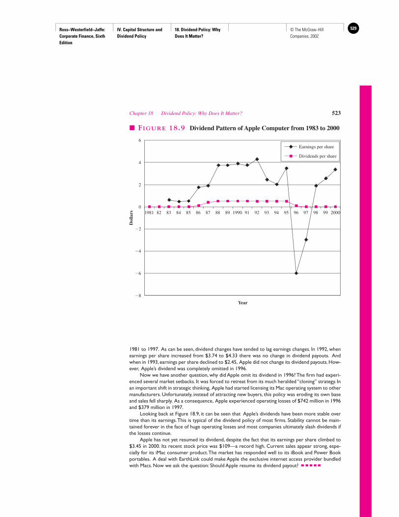
Ross−Westerfield−Jaffe: Corporate Finance, Sixth Edition
IV. Capital Structure and Dividend Policy
18. Dividend Policy: Why Does It Matter?
529© The McGraw−Hill Companies, 2002
1981 to 1997. As can be seen, dividend changes have tended to lag earnings changes. In 1992, whenearnings per share increased from $3.74 to $4.33 there was no change in dividend payouts. Andwhen in 1993, earnings per share declined to $2.45, Apple did not change its dividend payouts.How-ever, Apple’s dividend was completely omitted in 1996.
Now we have another question, why did Apple omit its dividend in 1996? The firm had experi-enced several market setbacks. It was forced to retreat from its much heralded “cloning” strategy. Inan important shift in strategic thinking, Apple had started licensing its Mac operating system to othermanufacturers. Unfortunately, instead of attracting new buyers, this policy was eroding its own baseand sales fell sharply. As a consequence, Apple experienced operating losses of $742 million in 1996and $379 million in 1997.
Looking back at Figure 18.9, it can be seen that Apple’s dividends have been more stable overtime than its earnings.This is typical of the dividend policy of most firms. Stability cannot be main-tained forever in the face of huge operating losses and most companies ultimately slash dividends ifthe losses continue.
Apple has not yet resumed its dividend, despite the fact that its earnings per share climbed to$3.45 in 2000. Its recent stock price was $109—a record high. Current sales appear strong, espe-cially for its iMac consumer product.The market has responded well to its iBook and Power Bookportables. A deal with EarthLink could make Apple the exclusive internet access provider bundledwith Macs. Now we ask the question: Should Apple resume its dividend payout?
Chapter 18 Dividend Policy: Why Does It Matter? 523
1981 82 83 84 85 86 87 88 89 1990 91 92 93 94 95 96 97 98 99 2000
Year
6
4
2
0
�2
�4
�6
�8
Earnings per share
Dividends per share
Dol
lars
� FIGURE 18.9 Dividend Pattern of Apple Computer from 1983 to 2000
Ross−Westerfield−Jaffe: Corporate Finance, Sixth Edition
IV. Capital Structure and Dividend Policy
18. Dividend Policy: Why Does It Matter?
530 © The McGraw−Hill Companies, 2002
18.10 SUMMARY AND CONCLUSIONS
1. The dividend decision is important because it determines the payout received by shareholdersand the funds retained by the firm for investment. Dividend policy is usually reflected by thecurrent dividend-to-earnings ratio. This is referred to as the payout ratio. Unfortunately, theoptimal payout ratio cannot be determined quantitatively. Rather, one can only indicatequalitatively what factors lead to low- or high-dividend policies.
2. The dividend policy of the firm is irrelevant in a perfect capital market because theshareholder can effectively undo the firm’s dividend strategy. If a shareholder receives agreater dividend than desired, he or she can reinvest the excess. Conversely, if theshareholder receives a smaller dividend than desired, he or she can sell off extra shares ofstock. This argument is due to MM and is similar to their homemade-leverage concept,discussed in Chapter 15.
3. Even in a perfect capital market, a firm should not reject positive NPV projects to increasedividend payments.
4. Although the MM argument is useful in introducing the topic of dividends, it ignores manyfactors in practice. We show that personal taxes and new-issue costs are real-worldconsiderations that favor low dividend payouts. With personal taxes and new-issue costs, the firmshould not issue stock to pay a dividend. However, our discussion does not imply that all firmsshould avoid dividends. Rather, those with high cash flow relative to positive NPV opportunitiesmight pay dividends due to legal constraints and/or a dearth of investment opportunities.
5. The expected return on a security is positively related to its dividend yield in a world withpersonal taxes. This result suggests that individuals in low or zero tax brackets shouldconsider investing in high-yielding stocks. However, the result does not imply that firmsshould avoid all dividends.
6. The general consensus among financial analysts is that the tax effect is the strongest argumentin favor of low dividends and the preference for current income is the strongest argument infavor of high dividends. Unfortunately, no empirical work has determined which of these twofactors dominates, perhaps because the clientele effect argues that dividend policy is quiteresponsive to the needs of stockholders. For example, if 40 percent of the stockholders preferlow dividends and 60 percent prefer high dividends, approximately 40 percent of companieswill have a low dividend payout, and 60 percent will have a high payout. This sharply reducesthe impact of an individual firm’s dividend policy on its market price.
7. Research has shown that many firms appear to have a long-run target dividend-payout policy.Firms that have few (many) positive NPV projects relative to available cash flow will havehigh (low) payouts. In addition, firms try to reduce the fluctuations in the level of dividends.There appears to be some value in dividend stability and smoothing.
8. The stock market reacts positively to increases in dividends (or an initial dividend payment)and negatively to decreases in dividends. This suggests that there is information content individend payments.
KEY TERMS
Clienteles 515 Homemade dividends 501Date of payment 497 Information-content effect 514Date of record 496 Regular cash dividends 495Declaration date 496 Stock dividend 496Ex-dividend date 496 Stock split 496
524 Part IV Capital Structure and Dividend Policy

Ross−Westerfield−Jaffe: Corporate Finance, Sixth Edition
IV. Capital Structure and Dividend Policy
18. Dividend Policy: Why Does It Matter?
531© The McGraw−Hill Companies, 2002
SUGGESTED READINGS
The breakthrough in the theory of dividend policy is contained in Miller, M., and F. Modigliani. “Dividend Policy, Growth and the Valuation of Shares.” Journal
of Business (October 1961).
A survey of dividend policy can be found inAllen, Franklin, and Roni Michaely. “Dividend Policy.” In R. A. Jarrow, V. Maksimovic, and
W. T. Ziemba (eds.). Handbooks in Operations Research and Management Science:Finance. Amsterdam: Elsevier Science (1995), 793–838.
Current trends in dividend policy are examined inFama, Eugene F., and Kenneth R. French. “Disappearing Dividends: Changing Firm
Characteristics or Lower Propensity to Pay?” (March 1999). Graduate School of Business,University of Chicago, Unpublished paper.
QUESTIONS AND PROBLEMS
The Mechanics of Dividend Payouts18.1 Identify and describe each of the following dates that are associated with a dividend
payment on common stock:
February 16February 24February 26March 14
18.2 On April 5, the board of directors of Capital City Golf Club declared a dividend of $.75per share payable on Tuesday, May 4, to shareholders of record as of Tuesday, April 20.Suppose you bought 350 shares of Capital City stock on April 6 for $8.75 a share. Assumethere are no taxes, no transaction costs, and no news between your purchase and sale of thestock. If you were to sell your stocks on April 16, how much would you be able to sellyour stock for?
18.3 The Mann Company belongs to a risk class for which the appropriate discount rate is 10percent. Mann currently has 100,000 outstanding shares selling at $100 each. The firm iscontemplating the declaration of a $5 dividend at the end of the fiscal year that just began.Answer the following questions based on the Miller and Modigliani model, which isdiscussed in the text.a. What will be the price of the stock on the ex-dividend date if the dividend is declared?b. What will be the price of the stock at the end of the year if the dividend is not declared?c. If Mann makes $2 million of new investments at the beginning of the period, earns net
income of $1 million, and pays the dividend at the end of the year, how many shares ofnew stock must the firm issue to meet its funding needs?
d. Is it realistic to use the MM model in the real world to value stock? Why or why not?
18.4 On February 17, the board of directors of Exertainment Corp. declared a dividend of $1.25per share payable on March 18 to all holders of record on March 1. All investors are in the31-percent tax bracket.a. What is the ex-dividend date?b. Ignoring personal taxes, how much should the stock price drop on the ex-dividend date?
The Benchmark Case: An Illustration of the Irrelevance of Dividend Policy18.5 The growing-perpetuity model expresses the value of a share of stock as the present value
of the expected dividends from that stock. How can you conclude that dividend policy isirrelevant when this model is valid?
Chapter 18 Dividend Policy: Why Does It Matter? 525

Ross−Westerfield−Jaffe: Corporate Finance, Sixth Edition
IV. Capital Structure and Dividend Policy
18. Dividend Policy: Why Does It Matter?
532 © The McGraw−Hill Companies, 2002
18.6 Andahl Corporation stock, of which you own 500 shares, will pay a $2-per-share dividendone year from today. Two years from now Andahl will close its doors; stockholders willreceive liquidating dividends of $17.5375 per share. The required rate of return on Andahlstock is 15 percent.a. What is the current price of Andahl stock?b. You prefer to receive equal amounts of money in each of the next two years. How will
you accomplish this?
18.7 The net income of Novis Corporation, which has 10,000 outstanding shares and a 100-percent payout policy, is $32,000. The expected value of the firm one year hence is$1,545,600. The appropriate discount rate for Novis is 12 percent.a. What is the current value of the firm?b. What is the ex-dividend price of Novis’s stock if the board follows its current policy?c. At the dividend declaration meeting, several board members claimed that the dividend
is too meager and is probably depressing Novis’s price. They proposed that Novis sellenough new shares to finance a $4.25 dividend.
i. Comment on the claim that the low dividend is depressing the stock price. Supportyour argument with calculations.
ii. If the proposal is adopted, at what price will the new shares sell and how many willbe sold?
18.8 Gibson Co. has a current period cash flow of $1.2 million and pays no dividends, and thepresent value of forecasted future cash flows is $15 million. It is an all-equity-financedcompany with 1 million shares outstanding. Assume the effective personal tax rate is zero.a. What is the share price of the Gibson stock?b. Suppose the board of directors of Gibson Co. announces its plan to pay out 50 percent
of its current cash flow as cash dividends to its shareholders. How can Jeff Miller, whoowns 1,000 shares of Gibson stock, achieve a zero payout policy on his own?
Taxes, Issuances Costs, and Dividends18.9 National Business Machine Co. (NBM) has $2 million of extra cash. NBM has two
choices to make use of this cash. One alternative is to invest the cash in financial assets.The resulted investment income will be paid out as a special dividend at the end of threeyears. In this case, the firm can invest in Treasury bills yielding 7 percent, or an 11percent preferred stock. Only 30 percent of the dividends from investing in preferredstock would be subject to corporate taxes. Another alternative is to pay out the cash asdividends and let the shareholders invest on their own in Treasury bills with the sameyield. The corporate tax rate is 35 percent, and the individual tax rate is 31 percent.Should the cash be paid today or in three years? Which of the two options generates thehighest after-tax income for the shareholders?
18.10 The University of Pennsylvania pays no taxes on capital gains, dividend income, orinterest payments. Would you expect to find low-dividend, high-growth stock in theuniversity’s portfolio? Would you expect to find tax-free municipal bonds in the portfolio?
18.11 In their 1970 paper on dividends and taxes, Elton and Gruber reported that the ex-dividend–date drop in a stock’s price as a percentage of the dividend should equal theratio of 1 minus the ordinary income tax rate to 1 minus the capital gains rate; that is,
where
Pe � The ex-dividend stock pricePb � The stock price before it trades ex-dividendD � The amount of the dividendTo � The tax rate on ordinary incomeTc � The effective tax rate on capital gains
Pe � Pb
D�
1 � To
1 � Tc
526 Part IV Capital Structure and Dividend Policy

Ross−Westerfield−Jaffe: Corporate Finance, Sixth Edition
IV. Capital Structure and Dividend Policy
18. Dividend Policy: Why Does It Matter?
533© The McGraw−Hill Companies, 2002
Note: As we pointed out in the text, effective tax rate of capital gains is less than theactual tax rate, because their realization may be postponed. Indeed, because investorscould postpone their realizations indefinitely, the effective rate could be zero.
a. If To � Tc � 0, how much will the stock’s price fall?b. If To � 0 and Tc � 0, how much will it fall?c. Explain the results you found in (a) and (b).d. Do the results of Elton and Gruber’s study imply that firms will maximize shareholder
wealth by not paying dividends?
18.12 After completing its capital spending for the year, Carlson Manufacturing has $1,000extra cash. Carlson’s managers must choose between investing the cash in Treasurybonds that yield 8 percent or paying the cash out to investors who would invest in thebonds themselves.a. If the corporate tax rate is 35 percent, what tax rate on ordinary income would make
the investors equally willing to receive the dividend and to let Carlson invest themoney?
b. Is the answer to part (a) reasonable? Why or why not?c. Suppose the only investment choice is stock that yields 12 percent. What personal
tax rate will make the stockholders indifferent to the outcome of Carlson’s dividenddecision?
d. Is this a compelling argument for a low dividend payout ratio? Why or why not?
Expected Return, Dividends, and Personal Taxes18.13 A political advisory committee recently recommended wage and price controls to prevent
the spiraling inflation that was experienced in the 1970s. Members of the investmentcommunity and several labor unions have sent the committee reports that discuss whetheror not dividends should be under the controls.
The reports from the investment community demonstrated that the value of a shareof stock is equal to the discounted value of its expected dividend stream. Thus, theyargued that any legislation that caps dividends will also hold down share prices, therebyincreasing companies’ costs of capital.
The union reports conceded that dividend policy is important to firms that are tryingto control costs. They also felt that dividends are important to stockholders, but onlybecause the dividend is the shareholder’s wage. In order to be fair, the unions argued, ifthe government controls labor’s wage, it should also control dividends.
Discuss these arguments and explain the fallacy in them.
18.14 Deaton Co. and Grebe, Inc., are in the same risk class. Shareholders expect Deaton topay a $4 dividend next year when the stock will sell for $20. Grebe has a no-dividendpolicy. Currently, Grebe stock is selling for $20 per share. Grebe shareholders expecta $4 capital gain over the next year. Capital gains are not taxed, but dividends aretaxed at 25 percent.a. What is the current price of Deaton Co. stock?b. If capital gains are also taxed at 25 percent, what is the price of Deaton Co. stock?c. Explain the result you found in part (b).
18.15 Payall Inc., Payless Inc., and Paynone Inc. are equally risky. They follow a 100-percent,50-percent, and zero payout policy, respectively. The expected share prices at dates 0 and1 for Paynone Inc. are $100 and $125. The market prices are set so that their after-taxexpected returns are equal. What should the current share prices of Payless Inc. andPayall Inc. be? Assume the marginal personal tax rate on dividends is 25 percent, and theeffective tax rate on capital gain is zero.
18.16 Suppose the Du Pont Company currently has outstanding series 4.50, nonconvertiblepreferred stock that pays an annual dividend of $4.50. Du Pont has also issued 11-percentbonds that will mature in 10 years. The stock and bonds have about the same risk.a. The current price of the 4.50 preferred stock is 50 1⁄2. What is its dividend yield?b. The bonds were sold at par. What is their yield to maturity?
Chapter 18 Dividend Policy: Why Does It Matter? 527
Ross−Westerfield−Jaffe: Corporate Finance, Sixth Edition
IV. Capital Structure and Dividend Policy
18. Dividend Policy: Why Does It Matter?
534 © The McGraw−Hill Companies, 2002
c. As a financial consultant, you want to know the after-tax yields for each of theseinvestments. The corporate tax rate is 34 percent and the personal tax rate is 28percent. Compute the after-tax yields on Du Pont’s preferred stock and its bonds foreach of the following groups:
i. General Motors’s tax-exempt pension.ii. General Motors Corporation.
d. Which group do you believe owns the most Du Pont stock?
Real-World Factors Favoring a High-Dividend Policy18.17 The bird-in-the-hand argument, which states that a dividend today is safer than the
uncertain prospect of a capital gain tomorrow, is often used to justify high dividend-payout ratios. Explain the fallacy behind the argument.
18.18 The desire for current income is not a valid explanation for preference for high-current-dividend policy, as investors can always create homemade dividends by selling a portionof their stocks. Comment.
18.19 Your aunt is in a high tax bracket and would like to minimize the tax burden of herinvestment portfolio. She is willing to buy and sell in order to maximize her after-taxreturns and she has asked for your advice. What would you suggest she do?
A Resolution of Real-World Factors?18.20 In the May 4, 1981, issue of Fortune, an article entitled “Fresh Evidence That Dividends
Don’t Matter” stated, “All told, 115 companies of the 500 [largest industrial corporations]raised their payout every year during the period [1970–1989]. Investors in this . . . groupwould have fared somewhat better than investors in the 500 as a whole: the median total[annual compound] return of the 115 was 10.7% during the decade versus 9.4% for the 500.”
Is this evidence that investors prefer dividends to capital gains? Why or why not?
18.21 Last month Central Virginia Power Company, which had been having trouble with costoverruns on a nuclear plant that it had been building, announced that it was “temporarilysuspending dividend payments due to the cash flow crunch associated with its investmentprogram.” When the announcement was made, the company’s stock price dropped from28 1⁄2 to 25. What do you suspect caused the change in the stock price?
18.22 Southern Established Inc. has been paying out regular quarterly dividends ever since1983. It just slashed the dividend by half in the current fiscal quarter and a more severecut is to be underway. Southern’s stock price dropped from $35.25 to $31.75 when thedividend cut was announced. Explain the possible reasons for this price drop.
18.23 Cap Henderson owns Neotech stock because its price has been steadily rising over thepast few years and he expects its performance to continue. Cap is trying to convinceWidow Jones to purchase some Neotech stock, but she is reluctant because Neotech hasnever paid a dividend. She depends on steady dividends to provide her with income.a. What preferences are these two investors demonstrating?b. What argument should Cap use to convince Widow Jones that Neotech stock is the
stock for her?c. Why might Cap’s argument not convince Widow Jones?
18.24 If the market places the same value on $1 of dividends as on $1 of capital gains, thenfirms with different payout ratios will appeal to different clienteles of investors. Oneclientele is as good as another; therefore, a firm cannot increase its value by changing itsdividend policy. Yet empirical investigations reveal a strong correlation between dividendpayout ratios and other firm characteristics. For example, small, rapidly growing firmsthat have recently gone public almost always have payout ratios that are zero; all earningsare reinvested in the business. Explain this phenomenon if dividend policy is irrelevant.
18.25 In spite of the theoretical argument that dividend policy should be irrelevant, the factremains that many investors like high dividends. If this preference exists, a firm can boostits share price by increasing its dividend-payout ratio. Explain the fallacy in this argument.
528 Part IV Capital Structure and Dividend Policy
Ross−Westerfield−Jaffe: Corporate Finance, Sixth Edition
IV. Capital Structure and Dividend Policy
18. Dividend Policy: Why Does It Matter?
535© The McGraw−Hill Companies, 2002
What We Know and Do Not Know about Dividend Policy18.26 The Sharpe Co. has a period 0 dividend of $1.25. Its target payout ratio is 40 percent. The
period 1 EPS is expected to be $4.5.a. If the adjustment rate is 0.3 as defined in the Lintner Model, what will be the Sharpe
Co. dividend in period 1?b. If the adjustment rate is 0.6 instead, what is the dividend in period 1?
18.27 Empirical research found that there have been significant increases in stock price on theday an initial dividend (i.e., the first time a firm pays a cash dividend) is announced.What does this finding imply about the information content of initial dividends?
Appendix 18A STOCK DIVIDENDS AND STOCK SPLITS
In addition to the cash dividend, companies may issue stock dividends or split their stock.Since stock dividends and stock splits are quite similar, we treat them together. We beginwith examples of these two strategies. Next, their benefits and costs to the firm are discussed.
Example of a Stock DividendImagine a company with 10,000 shares of stock, each selling at $60. With a stock dividendof 10 percent, each stockholder receives one additional share for each 10 that he or she orig-inally owned. Therefore the total number of shares outstanding after the dividend is 11,000.Note that the stockholders receive no cash and that each shareholder’s percentage of the to-tal outstanding stock remains the same. Thus a case can be made that a stock dividend is ofno value to the firm. More will be said on this later.
Imagine that, before the stock dividend, the equity portion of the firm’s balance sheetlooks like this:
Common stock (par value set at $12 per share) $120,000Capital in excess of par value 200,000Retained earnings 180,000
Total owner’s equity $500,000
A seemingly arbitrary accounting procedure is used to adjust the balance sheet afterthe stock dividend. Since 1,000 new shares are issued, $12,000 (1,000 � $12) is trans-ferred to common stock after the dividend. The market price of $60 is $48 above the parvalue. Thus $48 � 1,000 � $48,000 is shifted to the excess capital account. Because thetotal value of owner’s equity is unchanged by a stock dividend, $60,000 is withdrawn fromretained earnings.
After the stock dividend, owner’s equity for the firm is represented as:
Common stock (par value set at $12 per share) $132,000Capital in excess of par value 248,000Retained earnings 120,000
Total owner’s equity $500,000
There is actually a good reason behind this procedure. Accountants fear that stock div-idends could be used to impress a naive stockholder, even if the firm is doing poorly. Thistype of accounting treatment limits this possibility, since a stock dividend can never begreater than retained earnings.
Chapter 18 Dividend Policy: Why Does It Matter? 529

Ross−Westerfield−Jaffe: Corporate Finance, Sixth Edition
IV. Capital Structure and Dividend Policy
18. Dividend Policy: Why Does It Matter?
536 © The McGraw−Hill Companies, 2002
Example of a Stock SplitA stock split is similar conceptually to a stock dividend. In a three-for-one split, each share-holder receives two additional shares of stock for each one held originally. Again, no cashis paid out, and the percentage of the entire firm that each shareholder owns is unaffected.However, the accounting of splits differs from the accounting of stock dividends. Imaginein our previous example that a three-for-one-split occurs, raising the number of shares to30,000. The owner’s equity after the split is represented as:
Common stock (30,000 shares with par value set at $4 per share) $120,000
Capital in excess of par value 200,000Retained earnings 180,000
Total owner’s equity $500,000
Note that for three of the categories the figures on the right are completely unaffected bythe split. Only the par value is changed, being reduced here to $4 per share.
Since stock dividends and stock splits are similar, the dividing point between them isarbitrary.
Value of Stock Splits and Stock DividendsThe laws of logic tell us that stock splits and stock dividends can (1) leave the firm’s value un-affected, (2) increase the value of the firm, or (3) decrease its value. Unfortunately, the issuesare complex enough that one cannot easily determine which of the three relationships holds.
The Benchmark CaseA strong case can be made that stock dividends and splits do not change either the wealthof any shareholder or the wealth of the firm as a whole. For example, imagine a firm with$100 of earnings and 100 shares outstanding, implying EPS of $1. With a price-earnings ra-tio of 10, the price per share is $10 and the total market value of the firm is $1,000. Nowimagine a 2-for-1 stock split where the number of shares rises to 200 and EPS falls to $0.50.Given the same P/E ratio of 10, the value of each share of stock is now $5. However, withtwice the number of shares, the value of the entire firm is still $1,000. The wealth of eachstockholder remains the same since the doubling in the number of shares is offset by thehalving of the stock price. This result is sensible because (1) total earnings of the firm areheld constant, and (2) the percentage of the firm owned by each investor is unchanged.
The same results would hold for a stock dividend. Imagine that the total number ofshares is increased by 10 percent to 110. Given that EPS drops to $100/110 � $0.90909,the price per share should fall to $9.0909. Therefore the total value of the firm should re-main at $1,000. The wealth of each stockholder should not change because, as with a split,the percentage of the firm that each investor owns remains the same.
Although these results are relatively obvious, they are developed in the idealized worldof a perfect capital market. The typical financial manager is aware of many real-world com-plexities, and for that reason the stock split or stock dividend decision is not treated lightlyin practice.
Popular Trading RangeProponents of stock dividends and stock splits frequently argue that a security has a propertrading range. When the security is priced above this level, many investors do not have thefunds to buy the common trading unit of 100 shares, called a round lot. Although securitiescan be purchased in odd-lot form (fewer than 100 shares), the commissions are more ex-pensive here. Thus firms will split the stock to keep its price in this trading range.
530 Part IV Capital Structure and Dividend Policy
Ross−Westerfield−Jaffe: Corporate Finance, Sixth Edition
IV. Capital Structure and Dividend Policy
18. Dividend Policy: Why Does It Matter?
537© The McGraw−Hill Companies, 2002
Although this argument is a popular one, its validity has recently been questioned.35
Mutual funds, pension funds, and other institutions have steadily increased their trading ac-tivity since World War II and now handle a sizable percentage of total trading volume.Because these institutions can buy and sell in such huge amounts, they would not regard se-curities in the popular trading range with any special favor. In fact, whether because of therise of institutions or some other factor, odd-lot trades comprise a quite small proportion ofthe market today.
Costs with Stock Splits or Stock DividendsThe reasoning in the previous paragraph minimizes the benefits of a stock split or dividend.In addition, some authors state that there are costs associated with these financial proce-dures. For example, Copeland argues that two types of transaction costs rise following astock split. He further reasons that both of these cost increases ultimately reduce the liq-uidity of the stock, an unexpected result because a rise in liquidity through a broadening ofthe stockholder base often is given as a reason for a split.36
Copeland finds that brokerage fees, measured in percentages, increase after a split.This result is not surprising, since most published price lists of commissions show that bro-kerage fees for low-priced securities are a larger percentage of sales price than they are forhigh-priced securities. For example, commissions are generally higher for 400 shares of asecurity selling at $10 than for 100 shares of a security selling at $40.
The bid-ask spread is the difference between the price at which you sell a security to adealer and the price at which you buy a security from a dealer. For example, a bid-ask spreadof 49 1/2–50 means that an individual can sell a share to the dealer at $49.50 and buy a shareat $50, implying a round-trip loss to the investor of $0.50. Copeland finds that the bid-askspread, expressed as a percentage of sales price, rises after a stock split. This finding is con-sistent with other work showing that the bid-ask spread is higher in percentage terms forlower-proceed securities.37 The data suggest that the benefits to the stockholder associatedwith a stock dividend or stock split are not clearly greater than the costs to him.
Reverse SplitA less frequently encountered financial maneuver is the reverse split. In a one-for-three re-verse split, each investor exchanges three old shares for one new share. The par value istripled in the process. As mentioned previously with stock splits and stock dividends, a casecan be made that, in a theoretical model, a reverse split changes nothing substantial aboutthe company.
Given real-world imperfections, three related reasons are cited for reverse splits. First,transactions costs to shareholders are often less after the reverse split. This follows the con-clusions of Copeland that brokerage commissions per dollar traded rise as the price of thestock falls. Second, the liquidity and marketability of a company’s stock are improved whenits price is raised to the “popular trading range.” Third, stocks selling below a certain levelare not considered “respectable,” implying that investors bias downward their estimates ofthese firms’ earnings, cash flow, growth, and stability. Some financial analysts argue that areverse split can achieve instant respectability.
Chapter 18 Dividend Policy: Why Does It Matter? 531
35For example, see T. Copeland, “Liquidity Changes Following Stock Splits,” Journal of Finance (March 1979).36Although Copeland’s empirical work included only stock splits, the same factors should apply to the stockdividend case.37See H. Demsetz, “The Cost of Transacting,” Quarterly Journal of Economics 82 (February 1968); and H.Stoll, “The Supply of Dealer Services in Securities Markets,” Journal of Finance 33 (September 1978).

Ross−Westerfield−Jaffe: Corporate Finance, Sixth Edition
IV. Capital Structure and Dividend Policy
18. Dividend Policy: Why Does It Matter?
538 © The McGraw−Hill Companies, 2002
• What is a stock dividend? A stock split?• What are the values of a stock dividend and a stock split?
KEY TERMS
Reverse split 531Trading range 530
SUGGESTED READING
New evidence on how the market reacts to stock splits and stock dividends is inRanking, G., and Earl Stice. “The Market Reaction to the Choice of Accounting Method for
Stock Splits and Large Stock Dividends.” Journal of Financial and Quantitative Analysis(June 1997).
532 Part IV Capital Structure and Dividend Policy
QUESTIONS
CO
NC
EP
T
?
Ross−Westerfield−Jaffe: Corporate Finance, Sixth Edition
V. Long−Term Financing Introduction 539© The McGraw−Hill Companies, 2002
Long-Term Financing
PA
RT
V
19 Issuing Securities to the Public 53420 Long-Term Debt 56321 Leasing 586
PART IV discussed capital structure; we determined the relationship between thefirm’s debt-equity ratio and the firm’s value. The debt we used in Part IV was styl-
ized. In fact, there are many different types of debt. In Part V we discuss how financialmanagers choose the type of debt that makes the most sense, including straight debt, debtwith options, and leasing.
In Chapter 19 we describe the ways firms sell securities to the public. In general, apublic issue can be sold as a general cash offer to investors at large, as a privately placedissue with a few institutions, or as a privileged subscription (in the case of equities). Wedescribe the features of these methods and point out some puzzling trends.
In Chapter 20 we describe some basic features of long-term debt. One of the spe-cial features of most long-term bonds is that they can be called by the firms before thematurity date. We try to explain why call provisions exist. There are many types of long-term debt, including floating-rate bonds, income bonds, and original-issue discountbonds. We discuss why they exist.
Chapter 21 describes a special form of long-term debt called leasing. In general, arental agreement that lasts for more than one year is a lease. Leases are a source of fi-nancing and displace debt in the balance sheet. Many silly reasons are given for leasing,and we present some of them. The major reason for long-term leasing is to lower taxes.
Ross−Westerfield−Jaffe: Corporate Finance, Sixth Edition
V. Long−Term Financing 19. Issuing Securities to the Public
540 © The McGraw−Hill Companies, 2002
Issuing Securities to the Public
CH
AP
TE
R19
EXECUTIVE SUMMARY
This chapter looks at how corporations issue securities to the investing public. Thegeneral procedures for debt and equity are quite similar. This chapter focuses on eq-uity, but the procedures for debt and equity are basically the same.
Before securities can be traded on a securities market, they must be issued to the pub-lic. A firm making an issue to the public must satisfy requirements set out in various federallegislation and statutes and enforced by the Securities and Exchange Commission (SEC). Ingeneral, investors must be given all material information in the form of a registration state-ment and prospectus. In the first part of this chapter we discuss what this entails.
A public issue of equity can be sold directly to the public with the help of underwrit-ers. This is called a general cash offer. Alternatively, a public equity issue can be sold to thefirm’s existing stockholders by what is called a rights offer. This chapter examines the dif-ference between a general cash offer and a rights offer.
Stock of companies going public for the first time is typically underpriced. We describethis unusual phenomenon and provide a possible explanation.
19.1 THE PUBLIC ISSUE
The basic steps in a public offering are depicted in Table 19.1. The Securities Act of 1933sets forth the federal regulation for all new interstate securities issues. The Securities Ex-change Act of 1934 is the basis for regulating securities already outstanding. The SEC ad-ministers both acts.
The Basic Procedure for a New Issue1. Management’s first step in any issue of securities to the public is to obtain approval
from the board of directors.2. Next, the firm must prepare and file a registration statement with the SEC. This state-
ment contains a great deal of financial information, including a financial history, details of theexisting business, proposed financing, and plans for the future. It can easily run to 50 or morepages. The document is required for all public issues of securities with two principal exceptions:
a. Loans that mature within nine months.b. Issues that involve less than $5.0 million.The second exception is known as the small-issues exemption. Issues of less than $5.0
million are governed by Regulation A, for which only a brief offering statement—ratherthan the above registration statement—is needed. For Regulation A to be operative, no morethan $1.5 million may be sold by insiders.
3. The SEC studies the registration statement during a waiting period. During thistime, the firm may distribute copies of a preliminary prospectus. The preliminary prospec-tus is called a red herring because bold red letters are printed on the cover. A prospectus
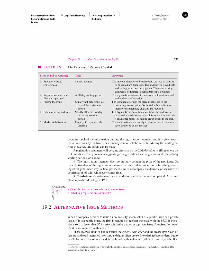
Ross−Westerfield−Jaffe: Corporate Finance, Sixth Edition
V. Long−Term Financing 19. Issuing Securities to the Public
541© The McGraw−Hill Companies, 2002
contains much of the information put into the registration statement, and it is given to po-tential investors by the firm. The company cannot sell the securities during the waiting pe-riod. However, oral offers can be made.
A registration statement will become effective on the 20th day after its filing unless theSEC sends a letter of comment suggesting changes. After the changes are made, the 20-daywaiting period starts anew.
4. The registration statement does not initially contain the price of the new issue. Onthe effective date of the registration statement, a price is determined and a full-fledged sell-ing effort gets under way. A final prospectus must accompany the delivery of securities orconfirmation of sale, whichever comes first.
5. Tombstone advertisements are used during and after the waiting period. An exam-ple is reproduced in Figure 19.1.
• Describe the basic procedures in a new issue.• What is a registration statement?
19.2 ALTERNATIVE ISSUE METHODS
When a company decides to issue a new security, it can sell it as a public issue or a privateissue. If it is a public issue, the firm is required to register the issue with the SEC. If the is-sue is sold to fewer than 35 investors, it can be treated as a private issue. A registration state-ment is not required in this case.1
There are two kinds of public issues: the general cash offer and the rights offer. Cash of-fers are sold to all interested investors, and rights offers are sold to existing shareholders. Equityis sold by both the cash offer and the rights offer, though almost all debt is sold by cash offer.
Chapter 19 Issuing Securities to the Public 535
� TABLE 19.1 The Process of Raising Capital
Steps in Public Offering Time Activities
1. Preunderwriting Several months The amount of money to be raised and the type of security conferences to be issued are discussed. The underwriting syndicate
and selling group are put together. The underwritingcontract is negotiated. Board approval is obtained.
2. Registration statements A 20-day waiting period The registration statement contains all relevant financial filed and approved and business information.
3. Pricing the issue Usually not before the last For seasoned offerings the price is set close to the day of the registration prevailing market price. For initial public offerings period intensive research and analysis are required.
4. Public offering and sale Shortly after the last day In a typical firm commitment contract, the underwriter of the registration buys a stipulated amount of stock from the firm and sells period it at a higher price. The selling group assists in the sale.
5. Market stabilization Usually 30 days after the The underwriter stands ready to place orders to buy at a offering specified price on the market.
QUESTIONS
CO
NC
EP
T
?
1However, regulation significantly restricts the resale of unregistered securities. The purchaser must hold thesecurities at least two years.
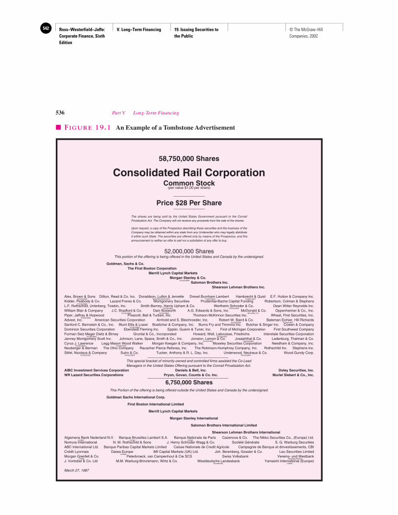
Ross−Westerfield−Jaffe: Corporate Finance, Sixth Edition
V. Long−Term Financing 19. Issuing Securities to the Public
542 © The McGraw−Hill Companies, 2002
536 Part V Long-Term Financing
58,750,000 Shares
Consolidated Rail CorporationCommon Stock
(per value $1.00 per share)
Price $28 Per Share
The shares are being sold by the United States Government pursuant to the ConrailPrivatization Act. The Company will not receive any proceeds from the sale of the shares.
Upon request, a copy of the Prospectus describing these securities and the business of theCompany may be obtained within any state from any Underwriter who may legally distributeit within such State. The securities are offered only by means of the Prospectus, and thisannouncement is neither an offer to sell nor a solicitation of any offer to buy.
52,000,000 SharesThis portion of the offering is being offered in the United States and Canada by the undersigned.
Goldman, Sachs & Co.The First Boston Corporation
Merrill Lynch Capital MarketsMorgan Stanley & Co.
Salomon Brothers Inc.Shearson Lehman Brothers Inc.
Alex, Brown & Sons Dillion, Read & Co. Inc. Donaldson, Lufkin & Jenrette Drexel Burnham Lambert Hambrecht & Quist E.F. Hutton & Company Inc.Kidder, Peabody & Co. Lazard Freres & Co. Montgomery Securities Prudential-Bache Capital Funding Robertson, Colman & StephensL.F. Rothschild, Unterberg, Towbin, Inc. Smith Barney, Harris Upham & Co. Wertheim Schroder & Co. Dean Witter Reynolds Inc.William Blair & Company J.C. Bradford & Co. Dain Bosworth A.G. Edwards & Sons, Inc. McDonald & Co. Oppenheimer & Co., Inc.Piper, Jaffray & Hopwood Prescott, Ball & Turben, Inc. Thomson McKinnon Securities Inc. Wheat, First Securities, Inc.Advest, Inc. American Securities Corporation Arnhold and S. Bleichroeder, Inc. Robert W. Baird & Co. Bateman Eichier, Hill RichardsSanford C. Bernstein & Co., Inc. Blunt Ellis & Loewi Boettcher & Company, Inc. Burns Fry and Timmins Inc. Butcher & Singer Inc. Cowen & CompanyDominion Securities Corporation Eberstadt Fleming Inc. Eppler, Guerin & Tuner, Inc. First of Michigan Corporation First Southwest CompanyFurman Seiz Mager Dietz & Birney Gruntal & Co., Incorporated Howard, Well, Labouisse, Friedrichs Interstate Securities CorporationJanney Montgomery Scott Inc. Johnson, Lane, Space, Smith & Co., Inc. Jonston, Lemon & Co. Josephthal & Co. Ladenburg, Thalman & Co.Cyrus J. Lawrence Legg Mason Wood Walker Morgan Keegan & Company, Inc. Moseley Securities Corporation Needham & Company, Inc.Neuberger & Berman The Ohio Company Rauscher Pierce Refsnes, Inc. The Robinson-Humphrey Company, Inc. Rothschild Inc. Stephens Inc.Stifel, Nicolaus & Company Sutro & Co. Tucker, Anthony & R. L. Day, Inc. Underwood, Neuhaus & Co. Wood Gundy Corp.
This special bracket of minority-owned and controlled firms assisted the Co-LeadManagers in the United States Offering pursuant to the Conrail Privatization Act.
AIBC Investment Services Corporation Daniels & Bell, Inc. Doley Securities, Inc.WR Lazard Securities Corporations Pryon, Govan, Counts & Co. Inc. Muriel Siebert & Co., Inc.
6,750,000 SharesThis Portion of the offering is being offered outside the United States and Canada by the undersigned.
Goldman Sachs International Corp.
First Boston International Limited
Merrill Lynch Capital Markets
Morgan Stanley International
Salomon Brothers International Limited
Shearson Lehman Brothers International
Algemene Bank Nederland N.V. Banque Bruxelles Lambert S.A. Banque Nationale de Paris Cazenove & Co. The Nikko Securities Co., (Europe) Ltd.Nomura International N. M. Rothschild & Sons J. Henry Schroder Wagg & Co. Soclété Générate S. G. Warburg SecuritiesABC International Ltd. Banque Paribas Capital Markets Limited Caisse Nationale de Credit Agricole Campagnie de Banque et dinvestissements, CBICrédit Lyonnais Daiwa Europe IMI Capital Markets (UK) Ltd. Joh. Berenberg, Gossler & Co. Leu Securities LimitedMorgan Grenfell & Co. Peterbroeck, van Campenhout & Cie SCS Swiss Volksbank Vereins- und WestbankJ. Vontobel & Co. Ltd M.M. Warburg-Brinckmann, Wirtz & Co. Westdeutsche Landesbank Yamaichi International (Europe)
March 27, 1987
Incorporated Securities Corporation Incorporated Incorporated
Incorporated
Incorporated Incorporated
Incorporated Incorporated Securities, Inc.
Incorporated
Limited Limited Limited
Limited
Limited Aktiengesellschaft
Girozentrale Limited
Incorporated Incorporated
Incorporated
Incorporated Incorporated
Incorporated Incorporated
Incorporated Incorporated
Incorporated Incorporated Incorporated
Incorporated
� FIGURE 19.1 An Example of a Tombstone Advertisement
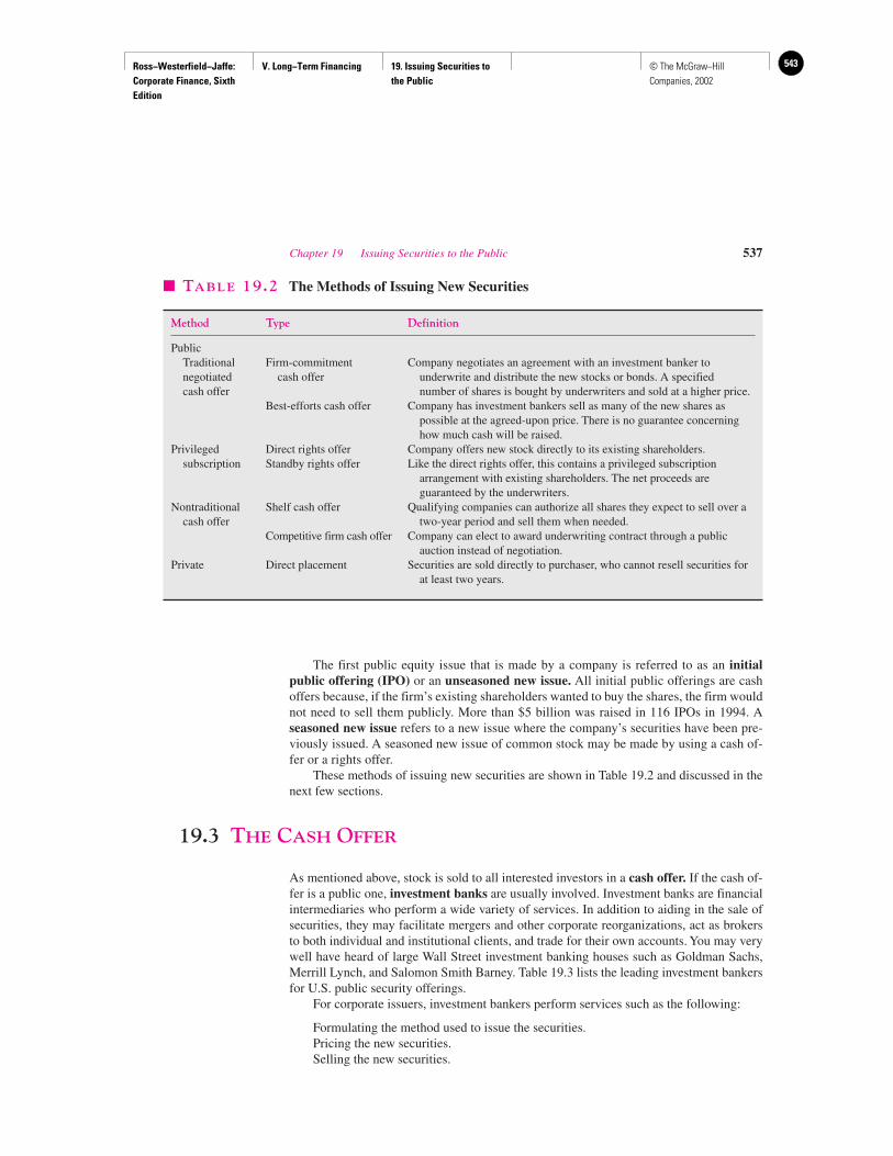
Ross−Westerfield−Jaffe: Corporate Finance, Sixth Edition
V. Long−Term Financing 19. Issuing Securities to the Public
543© The McGraw−Hill Companies, 2002
The first public equity issue that is made by a company is referred to as an initial public offering (IPO) or an unseasoned new issue. All initial public offerings are cashoffers because, if the firm’s existing shareholders wanted to buy the shares, the firm wouldnot need to sell them publicly. More than $5 billion was raised in 116 IPOs in 1994. A seasoned new issue refers to a new issue where the company’s securities have been pre-viously issued. A seasoned new issue of common stock may be made by using a cash of-fer or a rights offer.
These methods of issuing new securities are shown in Table 19.2 and discussed in thenext few sections.
19.3 THE CASH OFFER
As mentioned above, stock is sold to all interested investors in a cash offer. If the cash of-fer is a public one, investment banks are usually involved. Investment banks are financialintermediaries who perform a wide variety of services. In addition to aiding in the sale ofsecurities, they may facilitate mergers and other corporate reorganizations, act as brokersto both individual and institutional clients, and trade for their own accounts. You may verywell have heard of large Wall Street investment banking houses such as Goldman Sachs,Merrill Lynch, and Salomon Smith Barney. Table 19.3 lists the leading investment bankersfor U.S. public security offerings.
For corporate issuers, investment bankers perform services such as the following:
Formulating the method used to issue the securities.Pricing the new securities.Selling the new securities.
Chapter 19 Issuing Securities to the Public 537
� TABLE 19.2 The Methods of Issuing New Securities
Method Type Definition
PublicTraditional Firm-commitment Company negotiates an agreement with an investment banker to negotiated cash offer underwrite and distribute the new stocks or bonds. A specified cash offer number of shares is bought by underwriters and sold at a higher price.
Best-efforts cash offer Company has investment bankers sell as many of the new shares as possible at the agreed-upon price. There is no guarantee concerning how much cash will be raised.
Privileged Direct rights offer Company offers new stock directly to its existing shareholders.subscription Standby rights offer Like the direct rights offer, this contains a privileged subscription
arrangement with existing shareholders. The net proceeds areguaranteed by the underwriters.
Nontraditional Shelf cash offer Qualifying companies can authorize all shares they expect to sell over a cash offer two-year period and sell them when needed.
Competitive firm cash offer Company can elect to award underwriting contract through a public auction instead of negotiation.
Private Direct placement Securities are sold directly to purchaser, who cannot resell securities for at least two years.
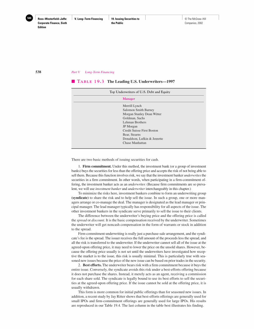
Ross−Westerfield−Jaffe: Corporate Finance, Sixth Edition
V. Long−Term Financing 19. Issuing Securities to the Public
544 © The McGraw−Hill Companies, 2002
There are two basic methods of issuing securities for cash.
1. Firm commitment. Under this method, the investment bank (or a group of investmentbanks) buys the securities for less than the offering price and accepts the risk of not being able tosell them. Because this function involves risk, we say that the investment banker underwrites thesecurities in a firm commitment. In other words, when participating in a firm-commitment of-fering, the investment banker acts as an underwriter. (Because firm commitments are so preva-lent, we will use investment banker and underwriter interchangeably in this chapter.)
To minimize the risks here, investment bankers combine to form an underwriting group(syndicate) to share the risk and to help sell the issue. In such a group, one or more man-agers arrange or co-manage the deal. The manager is designated as the lead manager or prin-cipal manager. The lead manager typically has responsibility for all aspects of the issue. Theother investment bankers in the syndicate serve primarily to sell the issue to their clients.
The difference between the underwriter’s buying price and the offering price is calledthe spread or discount. It is the basic compensation received by the underwriter. Sometimesthe underwriter will get noncash compensation in the form of warrants or stock in additionto the spread.
Firm-commitment underwriting is really just a purchase-sale arrangement, and the syndi-cate’s fee is the spread. The issuer receives the full amount of the proceeds less the spread, andall the risk is transferred to the underwriter. If the underwriter cannot sell all of the issue at theagreed-upon offering price, it may need to lower the price on the unsold shares. However, be-cause the offering price usually is not set until the underwriters have investigated how recep-tive the market is to the issue, this risk is usually minimal. This is particularly true with sea-soned new issues because the price of the new issue can be based on prior trades in the security.
2. Best efforts. The underwriter bears risk with a firm commitment because it buys theentire issue. Conversely, the syndicate avoids this risk under a best-efforts offering becauseit does not purchase the shares. Instead, it merely acts as an agent, receiving a commissionfor each share sold. The syndicate is legally bound to use its best efforts to sell the securi-ties at the agreed-upon offering price. If the issue cannot be sold at the offering price, it isusually withdrawn.
This form is more common for initial public offerings than for seasoned new issues. Inaddition, a recent study by Jay Ritter shows that best-efforts offerings are generally used forsmall IPOs and firm-commitment offerings are generally used for large IPOs. His resultsare reproduced in our Table 19.4. The last column in the table best illustrates his finding.
538 Part V Long-Term Financing
� TABLE 19.3 The Leading U.S. Underwriters—1997
Top Underwriters of U.S. Debt and Equity
Manager
Merrill LynchSalomon Smith BarneyMorgan Stanley Dean WitterGoldman, SachsLehman BrothersJP MorganCredit Suisse First BostonBear, StearnsDonaldson, Lufkin & JenretteChase Manhattan
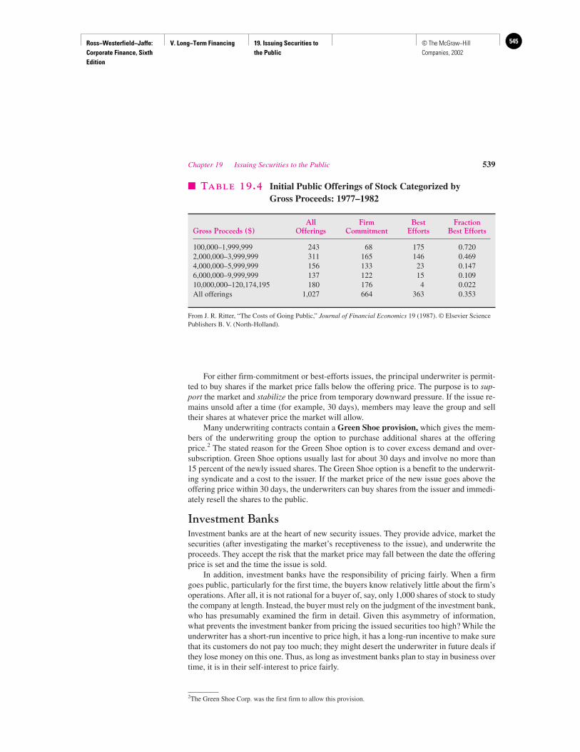
Ross−Westerfield−Jaffe: Corporate Finance, Sixth Edition
V. Long−Term Financing 19. Issuing Securities to the Public
545© The McGraw−Hill Companies, 2002
For either firm-commitment or best-efforts issues, the principal underwriter is permit-ted to buy shares if the market price falls below the offering price. The purpose is to sup-port the market and stabilize the price from temporary downward pressure. If the issue re-mains unsold after a time (for example, 30 days), members may leave the group and selltheir shares at whatever price the market will allow.
Many underwriting contracts contain a Green Shoe provision, which gives the mem-bers of the underwriting group the option to purchase additional shares at the offeringprice.2 The stated reason for the Green Shoe option is to cover excess demand and over-subscription. Green Shoe options usually last for about 30 days and involve no more than15 percent of the newly issued shares. The Green Shoe option is a benefit to the underwrit-ing syndicate and a cost to the issuer. If the market price of the new issue goes above theoffering price within 30 days, the underwriters can buy shares from the issuer and immedi-ately resell the shares to the public.
Investment BanksInvestment banks are at the heart of new security issues. They provide advice, market thesecurities (after investigating the market’s receptiveness to the issue), and underwrite theproceeds. They accept the risk that the market price may fall between the date the offeringprice is set and the time the issue is sold.
In addition, investment banks have the responsibility of pricing fairly. When a firmgoes public, particularly for the first time, the buyers know relatively little about the firm’soperations. After all, it is not rational for a buyer of, say, only 1,000 shares of stock to studythe company at length. Instead, the buyer must rely on the judgment of the investment bank,who has presumably examined the firm in detail. Given this asymmetry of information,what prevents the investment banker from pricing the issued securities too high? While theunderwriter has a short-run incentive to price high, it has a long-run incentive to make surethat its customers do not pay too much; they might desert the underwriter in future deals ifthey lose money on this one. Thus, as long as investment banks plan to stay in business overtime, it is in their self-interest to price fairly.
Chapter 19 Issuing Securities to the Public 539
� TABLE 19.4 Initial Public Offerings of Stock Categorized by Gross Proceeds: 1977–1982
All Firm Best FractionGross Proceeds ($) Offerings Commitment Efforts Best Efforts
100,000–1,999,999 243 68 175 0.7202,000,000–3,999,999 311 165 146 0.4694,000,000–5,999,999 156 133 23 0.1476,000,000–9,999,999 137 122 15 0.10910,000,000–120,174,195 180 176 4 0.022All offerings 1,027 664 363 0.353
From J. R. Ritter, “The Costs of Going Public,” Journal of Financial Economics 19 (1987). © Elsevier SciencePublishers B. V. (North-Holland).
2The Green Shoe Corp. was the first firm to allow this provision.
Ross−Westerfield−Jaffe: Corporate Finance, Sixth Edition
V. Long−Term Financing 19. Issuing Securities to the Public
546 © The McGraw−Hill Companies, 2002
In other words, financial economists argue that each investment bank has a reservoir of“reputation capital.”3 Mispricing of new issues, as well as unethical dealings, is likely to re-duce this reputation capital.
One measure of this reputation capital is the pecking order among the investmentbanks. MBA students are aware of this order because they know that accepting a job witha top-tier firm is universally regarded as more prestigious than accepting a job with a lower-tier firm. This pecking order can be seen in Figure 19.1. The investment banks listed diag-onally in the figure are considered the most prestigious. These appear alphabetically so thatone cannot distinguish the relative status of these firms from the figure. The next set offirms, running from Alex. Brown & Sons to Dean Witter Reynolds, is also in alphabeticalorder. By noting when the alphabetical order begins anew, one can determine the numberof firms in each tier.
Investment banks put great importance in their relative rankings and view downwardmovement in their placement with much distaste. While this jockeying for position mayseem as unimportant as the currying of royal favor in the court of Louis XVI, it is explainedby the above discussion. In any industry where reputation is so important, the firms in theindustry must guard theirs with great vigilance.
540 Part V Long-Term Financing
IN THEIR OWN WORDS
Robert S. Hansen on The Economic Rationale for the Firm Commitment Offer
Underwriters provide four main functions: certifica-tion, monitoring, marketing, and risk bearing.
Certification assures investors that the offer price isfair. Investors have concerns about whether the offerprice is unfairly above the stock’s intrinsic value. Certifi-cation increases issuer value by reducing investor doubtabout fairness, making a better offer price possible.
Monitoring of issuing firm management and perform-ance builds value because it adds to shareholders’ordinary monitoring. Underwriters provide collectivemonitoring on behalf of both capital suppliers andcurrent shareholders. Individual shareholder monitoringis limited because the shareholder bears the entire cost,whereas all owners collectively share the benefit, prorata. By contrast, in underwriter monitoring all stock-holders share both the costs and benefits, pro rata.
Due diligence and legal liability for the proceeds giveinvestors assurance. However, what makes certificationand monitoring credible is lead bank reputation incompetitive capital markets, where they are disciplinedover time. Evidence that irreputable behavior is damagingto a bank’s future abounds. Capital market participants
punish poorly performing banks by refusing to hire them.The participants pay banks for certification and mean-ingful monitoring in “quasi-rents” in the spread, whichrepresent the fair cost of “renting” the reputations.
Marketing is finding long-term investors who can bepersuaded to buy the securities at the offer price. Thiswould not be needed if demand for new shares were“horizontal.” There is much evidence that issuers andsyndicates repeatedly invest in costly marketingpractices, such as expensive road shows to identify andexpand investor interest. Another is organizing membersto avoid redundant pursuit of the same customers. Leadbanks provide trading support in the issuer’s stock forseveral weeks after the offer.
Underwriting risk is like the risk of selling a putoption. The syndicate agrees to buy all new shares at theoffer price and resell them at that price or at the marketprice, whichever is lower. Thus, once the offer begins,the syndicate is exposed to potential losses on unsoldinventory should the market price fall below the offerprice. The risk is likely to be small, because offerings aretypically well prepared for quick sale.
3For example, see R. Carter and S. Manaster, “Initial Public Offerings and Underwriter Reputation,”unpublished Iowa State and University of Utah working paper (1988); and R. Beatty and J. Ritter, “InvestmentBanking, Reputation and the Underpricing of Initial Public Offerings,” Journal of Financial Economics (1986).
Robert S. Hansen is the Freeman Senior Research Professor of Finance at Tulane University.
Ross−Westerfield−Jaffe: Corporate Finance, Sixth Edition
V. Long−Term Financing 19. Issuing Securities to the Public
547© The McGraw−Hill Companies, 2002
There are two basic methods for selecting the syndicate. In a competitive offer, theissuing firm can offer its securities to the underwriter bidding highest. In a negotiatedoffer, the issuing firm works with one underwriter. Because the firm generally does notnegotiate with many underwriters concurrently, negotiated deals may suffer from lackof competition.
While competitive bidding occurs frequently in other areas of commerce, it may sur-prise you that negotiated deals in investment banking occur with all but the largest issuingfirms. Investment bankers argue that they must expend much time and effort learning aboutthe issuer before setting an issue price and a fee schedule. Except in the case of large issues,these underwriters could not expend the time and effort without the near certainty of re-ceiving the contract.
Studies generally show that issuing costs are higher in negotiated deals than in com-petitive ones. However, many financial economists argue that issuing firms are not neces-sarily hurt by negotiated deals. They point out that the underwriter gains much informationabout the issuing firm through negotiation, information likely to increase the probability ofa successful offering.4
The Offering PriceDetermining the correct offering price is the most difficult thing the lead investment bankmust do for an initial public offering. The issuing firm faces a potential cost if the offeringprice is set too high or too low. If the issue is priced too high, it may be unsuccessful andbe withdrawn. If the issue is priced below the true market price, the issuer’s existing share-holders will experience an opportunity loss.
Ibbotson has found that unseasoned new equity issues typically have been offered at11 percent below their true market price.5 Underpricing helps new shareholders earn ahigher return on the shares they buy. However, the existing shareholders of the issuingfirm are not necessarily helped by underpricing. To them it is an indirect cost of issuingnew securities.
Several studies have confirmed the early research of Ibbotson. For example, Ritter ex-amined approximately 1,030 firms that went public from 1977 through 1982 in the UnitedStates.6 He finds that the average firm-commitment IPO rose in price 14.8 percent in the firstday of trading following issuance. The comparable figure is 47.8 percent for best-effortsIPOs. These figures are not annualized! Both of these results are clearly consistent with sub-stantial underpricing.
Another recent dramatic example of underpricing came with the IPO of ShivaCorporation. Shiva makes hardware and software that allow desktop and laptop computersto hook directly into a local area network from outside the office. The initial offering, onNovember 18, 1994, of 2.76 million shares priced at $15 rose $161⁄2 to $311⁄2 by the end ofthe first trading day. Goldman Sachs, head of the underwriting syndicate that underwrote
Chapter 19 Issuing Securities to the Public 541
4This choice has been studied recently by Robert S. Hansen and Naveen Khanna, “Why Negotiation with aSingle Syndicate May Be Preferred to Making Syndicates Compete: The Problem of Trapped Bidders,” Journalof Business 67 (1994) and S. Bhagat, “The Effect of Management’s Choice between Negotiated andCompetitive Equity Offerings on Shareholder Wealth,” Journal of Financial and Quantitative Analysis (1986);and D. Logue and R. Jarrow, “Negotiation vs. Competitive Bidding in the Sales of Securities by PublicUtilities,” Financial Management 7 (1978).5R. Ibbotson, “Price Performance of Common Stock New Issues,” Journal of Financial Economics 2 (1975).6J. R. Ritter, “The Costs of Going Public,” Journal of Financial Economics (1987). Underpricing also exists fornew issues of seasoned stock, but to a much smaller extent. See J. Parsons and A. Raviv, “Underpricing ofSeasoned Issues,” Journal of Financial Economics 14 (1985).
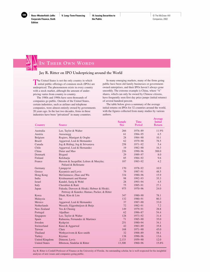
Ross−Westerfield−Jaffe: Corporate Finance, Sixth Edition
V. Long−Term Financing 19. Issuing Securities to the Public
548 © The McGraw−Hill Companies, 2002
IN THEIR OWN WORDS
Jay R. Ritter on IPO Underpricing around the World
The United States is not the only country in whichinitial public offerings of common stock (IPOs) are
underpriced. The phenomenon exists in every countrywith a stock market, although the amount of under-pricing varies from country to country.
The 1980s and 1990s have seen thousands ofcompanies go public. Outside of the United States,certain industries, such as airlines and telephonecompanies, were almost entirely owned by governments20 years ago. In the last two decades, firms in theseindustries have been “privatized” in many countries.
In many emerging markets, many of the firms goingpublic have been old family businesses or government-owned enterprises, and their IPOs haven’t always gonesmoothly. The extreme example is China, where “A”shares, which can only be owned by Chinese citizens,have frequently seen first day price jumps (initial returns)of several hundred percent.
The table below gives a summary of the averageinitial returns on IPOs for 32 countries around the world,with the figures collected from many studies by variousauthors.
AverageSample Time Initial
Country Source Size Period Return
Australia Lee, Taylor & Walter 266 1976–89 11.9%Austria Aussenegg 61 1984–95 6.5Belgium Rogiers, Manigart & Ooghe 28 1984–90 10.1Brazil Aggarwal, Leal & Hernandez 62 1979–90 78.5Canada Jog & Riding; Jog & Srivastava 258 1971–92 5.4Chile Aggarwal, Leal & Hernandez 19 1982–90 16.3China Datar and Mao 226 1990–96 388.0Denmark Bisgard 29 1989–97 8.0Finland Keloharju 85 1984–92 9.6France Husson & Jacquillat; Leleux & Muzyka; 187 1983–92 4.2
Paliard & BelletanteGermany Ljungqvist 170 1978–92 10.9Greece Kazantzis and Levis 79 1987–91 48.5Hong Kong McGuinness; Zhao and Wu 334 1980–96 15.9India Krishnamurti and Kumar 98 1992–93 35.3Israel Kandel, Sarig & Wohl 28 1993–94 4.5Italy Cherubini & Ratti 75 1985–91 27.1Japan Fukuda; Dawson & Hiraki; Hebner & Hiraki; 975 1970–96 24.0
Pettway & Kaneko; Hamao, Packer, & RitterKorea Dhatt, Kim & Lim 347 1980–90 78.1Malaysia Isa 132 1980–91 80.3Mexico Aggarwal, Leal & Hernandez 37 1987–90 33.0Netherlands Wessels; Eijgenhuijsen & Buijs 72 1982–91 7.2New Zealand Vos & Cheung 149 1979–91 28.8Portugal Alpalhao 62 1986–87 54.4Singapore Lee, Taylor & Walter 128 1973–92 31.4Spain Rahnema, Fernandez & Martinez 71 1985–90 35.0Sweden Rydqvist 251 1980–94 34.1Switzerland Kunz & Aggarwal 42 1983–89 35.8Taiwan Chen 168 1971–90 45.0Thailand Wethyavivorn & Koo-smith 32 1988–89 58.1Turkey Kiymaz 138 1990–96 13.6United Kingdom Dimson; Levis 2,133 1959–90 12.0United States Ibbotson, Sindelar & Ritter 13,308 1960–96 15.8%
Jay R. Ritter is Cordell Professor of Finance at the University of Florida. An outstanding scholar, he is well-respected for his insightfulanalyses of new issues and companies going public.
Ross−Westerfield−Jaffe: Corporate Finance, Sixth Edition
V. Long−Term Financing 19. Issuing Securities to the Public
549© The McGraw−Hill Companies, 2002
the issue, was quoted as saying that pricing an IPO is not just about what the market willbear at the time, but “we are trying to get the company launched for the long term and builda good investor base.”7
Underpricing: A Possible ExplanationWhen the price of a new issue is too low, the issue is often oversubscribed. This means in-vestors will not be able to buy all of the shares they want, and the underwriters will allocatethe shares among investors. The average investor will find it difficult to get shares in anoversubscribed offering because there will not be enough shares to go around. While initialpublic offerings have positive initial returns on average, a significant fraction of them haveprice drops. An investor submitting an order for all new issues may find that he or she willbe allocated more shares in issues that go down in price.
Consider this tale of two investors. Ms. Smarts knows precisely what companies areworth when their shares are offered. Mr. Average knows only that prices usually rise onemonth after the IPO. Armed with this information, Mr. Average decides to buy 1,000 sharesof every IPO. Does Mr. Average actually earn an abnormally high average return across allinitial offerings?
The answer is no, and at least one reason is Ms. Smarts. For example, because Ms.Smarts knows that company XYZ is underpriced, she invests all her money in its IPO. Whenthe issue is oversubscribed, the underwriters must allocate the shares between Ms. Smartsand Mr. Average. If they do it on a pro rata basis and if Ms. Smarts has bid for twice as manyshares as Mr. Average, she will get two shares for each one Mr. Average receives. The net re-sult is that when an issue is underpriced, Mr. Average cannot buy as much of it as he wants.
Ms. Smarts also knows that company ABC is overpriced. In this case she avoids its IPOaltogether, and Mr. Average ends up with a full 1,000 shares. To summarize, Mr. Averagereceives fewer shares when more knowledgeable investors swarm to buy an underpriced is-sue, but he gets all he wants when the smart money avoids the issue.
This is called the winner’s curse, and it explains much of the reason why IPOs havesuch a large average return. When the average investor wins and gets his allocation, it is be-cause those who knew better avoided the issue. To counteract the winner’s curse and attractthe average investor, underwriters underprice issues.8
• Describe a firm-commitment underwriting and a best-efforts underwriting.• Suppose that a stockbroker calls you up out of the blue and offers to sell you some shares
of a new issue. Do you think the issue will do better or worse than average?
19.4 THE ANNOUNCEMENT OF NEW EQUITY AND THE
VALUE OF THE FIRM
It seems reasonable to believe that new long-term financing is arranged by firms after posi-tive net present value projects are put together. As a consequence, when the announcement ofexternal financing is made, the firm’s market value should go up. As we mentioned in an ear-lier chapter, this is precisely the opposite of what actually happens in the case of new equity
Chapter 19 Issuing Securities to the Public 543
7The New York Times, February 19, 1995, “Anatomy of a High Flying IPO, Problems and All,” p. 7.8This explanation was first suggested in K. Rock, “Why New Issues Are Underpriced,” Journal of FinancialEconomics 15 (1986).
QUESTIONS
CO
NC
EP
T
?
Ross−Westerfield−Jaffe: Corporate Finance, Sixth Edition
V. Long−Term Financing 19. Issuing Securities to the Public
550 © The McGraw−Hill Companies, 2002
financing. Asquith and Mullins, Masulis and Korwar, and Mikkelson and Partch have allfound that the market value of existing equity drops on the announcement of a new issue ofcommon stock.9 Plausible reasons for this strange result include:
1. Managerial Information. If managers have superior information about the marketvalue of the firm, they may know when the firm is overvalued. If they do, they might at-tempt to issue new shares of stock when the market value exceeds the correct value. Thiswill benefit existing shareholders. However, the potential new shareholders are not stupid.They will infer overvaluation from the new issue, thereby bidding down the stock price onthe announcement date of the issue.
2. Debt Capacity. The stereotypical firm chooses a debt-to-equity ratio that balancesthe tax shield from the debt with the cost of financial distress. When the managers of a firmhave special information that the probability of financial distress has risen, the firm is morelikely to raise capital through stock than through debt. If the market infers this chain ofevents, the stock price should fall on the announcement date of an equity issue.
3. Falling Earnings.10 When managers raise capital in amounts that are unexpectedlylarge (as most unanticipated financings will be) and if investors have a reasonable fix on thefirm’s upcoming investments and dividend payouts (as they do because capital expenditureannouncements are often well known, as are future dividends), the unanticipated financingsare roughly equal to unanticipated shortfalls in earnings (this follows directly from thefirm’s sources and uses of funds identity). Therefore, an announcement of a new stock is-sue will also reveal a future earnings shortfall.
• What are some reasons that the price of stock drops on the announcement of a new equity issue?
19.5 THE COST OF NEW ISSUES
Issuing securities to the public is not free, and the costs of different issuing methods are im-portant determinants of which will be used. The costs fall into six categories.
1. Spread or underwriting discount The spread is the difference between the pricethe issue receives and the price offered to thepublic.
2. Other direct expenses These are costs incurred by the issuer that arenot part of the compensation to underwriters.They include filing fees, legal fees, and taxes—all reported in the prospectus.
3. Indirect expenses These costs are not reported in the prospectusand include management time on the new issue.
544 Part V Long-Term Financing
9P. Asquith and D. Mullins, “Equity Issues and Offering Dilution,” Journal of Financial Economics 15 (1986);R. Masulis and A. N. Korwar, “Seasoned Equity Offerings: An Empirical Investigation,” Journal of FinancialEconomics 15 (1986); and W. H. Mikkelson and M. M. Partch, “The Valuation Effects of Security Offerings andthe Issuance Process,” Journal of Financial Economics 15 (1986).10Robert S. Haugen and Claire Crutchley, “Corporate Earnings and Financings, An Empirical Analysis,”Journal of Business 20 (1990).
QUESTION
CO
NC
EP
T
?
Ross−Westerfield−Jaffe: Corporate Finance, Sixth Edition
V. Long−Term Financing 19. Issuing Securities to the Public
551© The McGraw−Hill Companies, 2002
4. Abnormal returns In a seasoned issue of stock, the price drops by3 percent to 4 percent upon the announcementof the issue. The drop protects new sharehold-ers against the firm’s selling overpriced stockto new shareholders.
5. Underpricing For initial public offerings, the stock typicallyrises substantially after the issue date. This is acost to the firm because the stock is sold forless than its efficient price in the aftermarket.11
6. Green Shoe option The Green Shoe option gives the underwritersthe right to buy additional shares at the offerprice to cover overallotments. This is a cost tothe firm because the underwriter will only buyadditional shares when the offer price is belowthe price in the aftermarket.
An interesting study by Lee, Lockhead, Ritter, and Zhao reports two of these sixcosts: underwriting discount and other direct expenses.12 Their findings for both equityofferings and debt offerings are reproduced in Table 19.5. Three conclusions emergefrom the table.
1. The costs in each category, for both equity offerings and debt offerings, decline asthe gross proceeds of the offering increase. Thus, it appears that issuance costs are subjectto substantial economies of scale.13
2. The bottom line of Table 19.5 indicates that, across all offerings, direct expenses arehigher for equity offers than for debt offers.
3. Last, and perhaps most important, the costs of issuing securities to the public arequite large. For example, total direct expenses are approximately 17 percent for an initialpublic offering of less than $10,000,000. In addition, Table 19.6 establishes that underpric-ing costs are another 16.36 percent. This implies that going public for the first time is aweighty decision. While there are many benefits, such as raising needed capital and spread-ing ownership, the costs cannot be ignored.
• Describe the costs of a new issue of common stock.• What conclusions emerge from analyses of Tables 19.6 and 19.7?
Chapter 19 Issuing Securities to the Public 545
11Some people have argued that the price in the aftermarket is not efficient after all. However, R. Ibbotson,“Price Performance of Common Stock New Issues,” Journal of Financial Economics 2 (1975), shows that, onaverage, new issues exhibit no abnormal price performance over the first five years following issuance. Thisresult is generally viewed as being consistent with market efficiency. That is, the stock obtains an efficient priceimmediately following issuance and remains at an efficient price.12The notion of economies of scale has been contested by Oya Altinkilic and Robert S. Hansen “Are ThereScale Economies in Underwriting Spreads? Evidence of Rising External Financing Costs,” Review of FinancialStudies 13 (2000). They provide data and analysis that underwriter cost will be U-shaped.13Among the most interesting developments in the initial public offering market is that almost all underwriterspreads in recent offerings have been exactly 7 percent. This is documented in H. C. Chen and Jay R. Ritter,“The Seven-Percent Solution,” Journal of Finance (June 2000); and Robert S. Hansen, “Do Investment BanksCompete in IPO’s? The Advent of the 7% Plus Contract,” Journal of Financial Economics (forthcoming).
QUESTIONS
CO
NC
EP
T
?
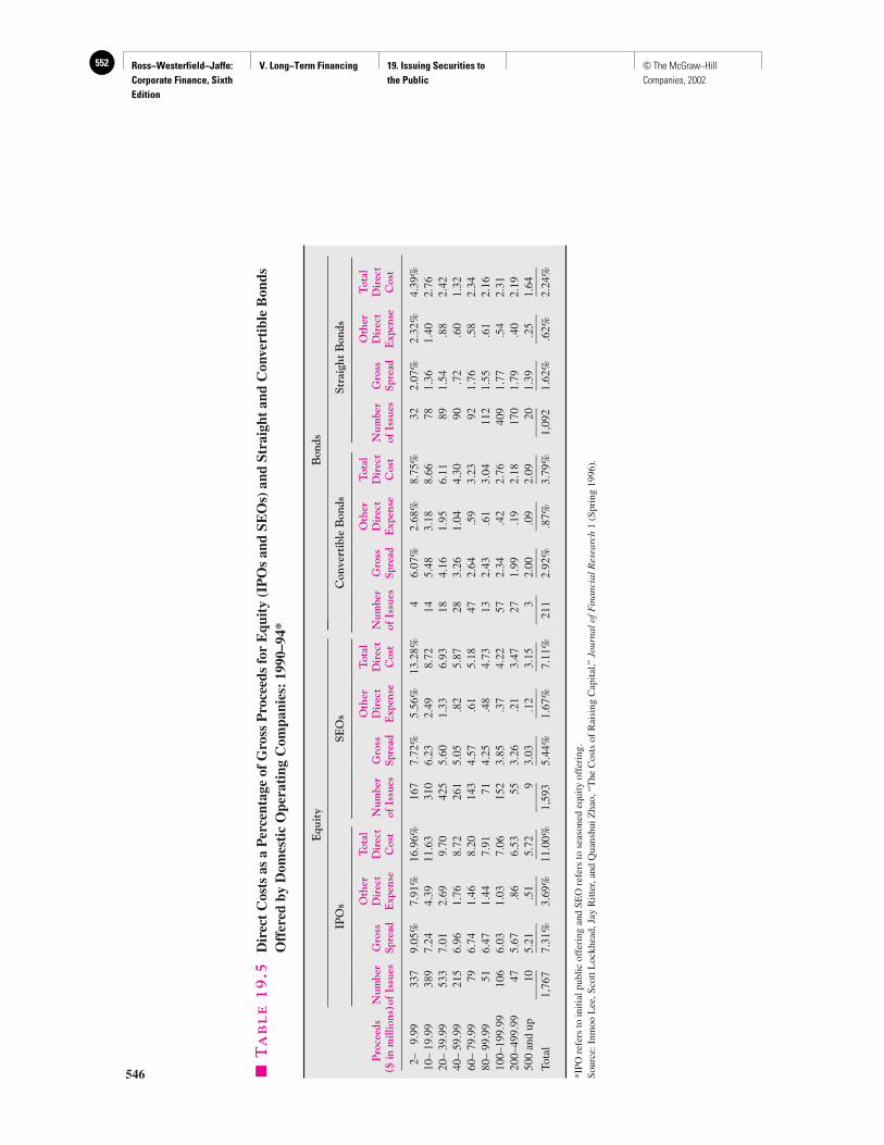
Ross−Westerfield−Jaffe: Corporate Finance, Sixth Edition
V. Long−Term Financing 19. Issuing Securities to the Public
552 © The McGraw−Hill Companies, 2002
546 �T
AB
LE
19
.5D
irec
t C
osts
as
a P
erce
ntag
e of
Gro
ss P
roce
eds
for
Equ
ity
(IP
Os
and
SEO
s) a
nd S
trai
ght
and
Con
vert
ible
Bon
dsO
ffer
ed b
y D
omes
tic
Ope
rati
ng C
ompa
nies
:19
90–9
4*
Equ
ity
Bon
ds
IPO
sSE
Os
Con
vert
ible
Bon
dsSt
raig
ht B
onds
____
____
____
____
____
___
____
____
____
____
____
___
____
____
____
____
____
____
____
____
____
____
____
____
Oth
erT
otal
Oth
erT
otal
Oth
erT
otal
Oth
erT
otal
Pro
ceed
sN
umbe
rG
ross
Dir
ect
Dir
ect
Num
ber
Gro
ssD
irec
tD
irec
tN
umbe
rG
ross
Dir
ect
Dir
ect
Num
ber
Gro
ssD
irec
tD
irec
t($
in m
illio
ns)o
f Is
sues
Spre
adE
xpen
seC
ost
of I
ssue
sSp
read
Exp
ense
Cos
tof
Iss
ues
Spre
adE
xpen
seC
ost
of I
ssue
sSp
read
Exp
ense
Cos
t
2–9.
9933
79.
05%
7.91
%16
.96%
167
7.72
%5.
56%
13.2
8%4
6.07
%2.
68%
8.75
%32
2.07
%2.
32%
4.39
%10
– 19
.99
389
7.24
4.39
11.6
331
06.
232.
498.
7214
5.48
3.18
8.66
781.
361.
402.
7620
– 39
.99
533
7.01
2.69
9.70
425
5.60
1.33
6.93
184.
161.
956.
1189
1.54
.88
2.42
40–
59.9
921
56.
961.
768.
7226
15.
05.8
25.
8728
3.26
1.04
4.30
90.7
2.6
01.
3260
– 79
.99
796.
741.
468.
2014
34.
57.6
15.
1847
2.64
.59
3.23
921.
76.5
82.
3480
– 99
.99
516.
471.
447.
9171
4.25
.48
4.73
132.
43.6
13.
0411
21.
55.6
12.
1610
0–19
9.99
106
6.03
1.03
7.06
152
3.85
.37
4.22
572.
34.4
22.
7640
91.
77.5
42.
3120
0–49
9.99
475.
67.8
66.
5355
3.26
.21
3.47
271.
99.1
92.
1817
01.
79.4
02.
1950
0 an
d up
105.
21.5
15.
729
3.03
.12
3.15
32.
00.0
92.
0920
1.39
.25
1.64
____
___
___
____
___
___
____
___
___
____
___
___
____
___
___
____
___
___
____
___
___
____
___
___
Tota
l1,
767
7.31
%3.
69%
11.0
0%1,
593
5.44
%1.
67%
7.11
%21
12.
92%
.87%
3.79
%1,
092
1.62
%.6
2%2.
24%
*IPO
ref
ers
to in
itial
pub
lic o
ffer
ing
and
SEO
ref
ers
to s
easo
ned
equi
ty o
ffer
ing.
Sour
ce:I
nmoo
Lee
,Sco
tt L
ockh
ead,
Jay
Ritt
er,a
nd Q
uans
hui Z
hao,
“The
Cos
ts o
f R
aisi
ng C
apita
l,”Jo
urna
l of F
inan
cial
Res
earc
h1
(Spr
ing
1996
).
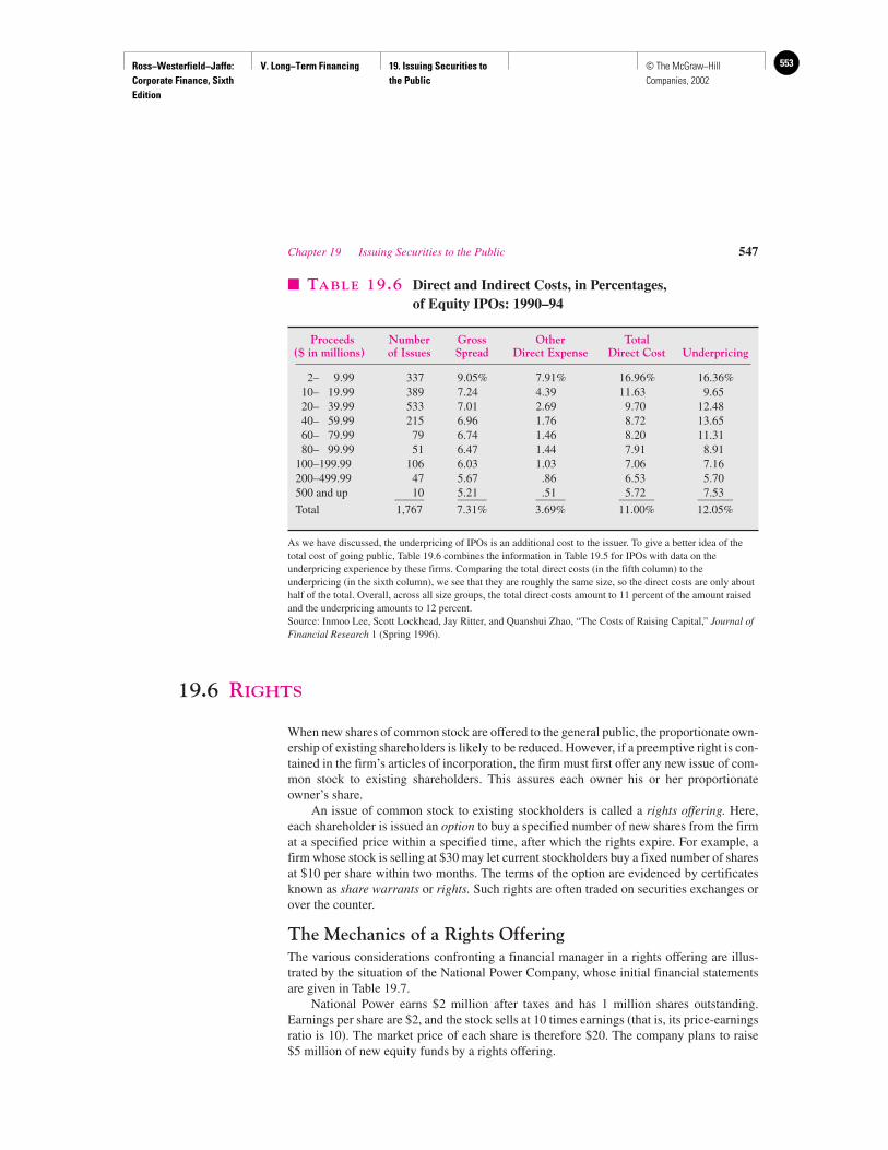
Ross−Westerfield−Jaffe: Corporate Finance, Sixth Edition
V. Long−Term Financing 19. Issuing Securities to the Public
553© The McGraw−Hill Companies, 2002
19.6 RIGHTS
When new shares of common stock are offered to the general public, the proportionate own-ership of existing shareholders is likely to be reduced. However, if a preemptive right is con-tained in the firm’s articles of incorporation, the firm must first offer any new issue of com-mon stock to existing shareholders. This assures each owner his or her proportionateowner’s share.
An issue of common stock to existing stockholders is called a rights offering. Here,each shareholder is issued an option to buy a specified number of new shares from the firmat a specified price within a specified time, after which the rights expire. For example, afirm whose stock is selling at $30 may let current stockholders buy a fixed number of sharesat $10 per share within two months. The terms of the option are evidenced by certificatesknown as share warrants or rights. Such rights are often traded on securities exchanges orover the counter.
The Mechanics of a Rights OfferingThe various considerations confronting a financial manager in a rights offering are illus-trated by the situation of the National Power Company, whose initial financial statementsare given in Table 19.7.
National Power earns $2 million after taxes and has 1 million shares outstanding.Earnings per share are $2, and the stock sells at 10 times earnings (that is, its price-earningsratio is 10). The market price of each share is therefore $20. The company plans to raise $5 million of new equity funds by a rights offering.
Chapter 19 Issuing Securities to the Public 547
� TABLE 19.6 Direct and Indirect Costs, in Percentages,of Equity IPOs: 1990–94
Proceeds Number Gross Other Total($ in millions) of Issues Spread Direct Expense Direct Cost Underpricing
2– 9.99 337 9.05% 7.91% 16.96% 16.36%10– 19.99 389 7.24 4.39 11.63 9.6520– 39.99 533 7.01 2.69 9.70 12.4840– 59.99 215 6.96 1.76 8.72 13.6560– 79.99 79 6.74 1.46 8.20 11.3180– 99.99 51 6.47 1.44 7.91 8.91
100–199.99 106 6.03 1.03 7.06 7.16200–499.99 47 5.67 .86 6.53 5.70500 and up 10 5.21 .51 5.72 7.53_____ _____ _____ ______ ______Total 1,767 7.31% 3.69% 11.00% 12.05%
As we have discussed, the underpricing of IPOs is an additional cost to the issuer. To give a better idea of thetotal cost of going public, Table 19.6 combines the information in Table 19.5 for IPOs with data on theunderpricing experience by these firms. Comparing the total direct costs (in the fifth column) to theunderpricing (in the sixth column), we see that they are roughly the same size, so the direct costs are only abouthalf of the total. Overall, across all size groups, the total direct costs amount to 11 percent of the amount raisedand the underpricing amounts to 12 percent.Source: Inmoo Lee, Scott Lockhead, Jay Ritter, and Quanshui Zhao, “The Costs of Raising Capital,” Journal ofFinancial Research 1 (Spring 1996).
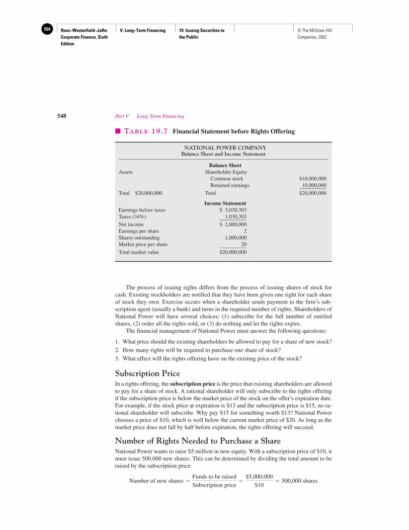
Ross−Westerfield−Jaffe: Corporate Finance, Sixth Edition
V. Long−Term Financing 19. Issuing Securities to the Public
554 © The McGraw−Hill Companies, 2002
The process of issuing rights differs from the process of issuing shares of stock forcash. Existing stockholders are notified that they have been given one right for each shareof stock they own. Exercise occurs when a shareholder sends payment to the firm’s sub-scription agent (usually a bank) and turns in the required number of rights. Shareholders ofNational Power will have several choices: (1) subscribe for the full number of entitledshares, (2) order all the rights sold, or (3) do nothing and let the rights expire.
The financial management of National Power must answer the following questions:
1. What price should the existing shareholders be allowed to pay for a share of new stock?
2. How many rights will be required to purchase one share of stock?
3. What effect will the rights offering have on the existing price of the stock?
Subscription PriceIn a rights offering, the subscription price is the price that existing shareholders are allowedto pay for a share of stock. A rational shareholder will only subscribe to the rights offeringif the subscription price is below the market price of the stock on the offer’s expiration date.For example, if the stock price at expiration is $13 and the subscription price is $15, no ra-tional shareholder will subscribe. Why pay $15 for something worth $13? National Powerchooses a price of $10, which is well below the current market price of $20. As long as themarket price does not fall by half before expiration, the rights offering will succeed.
Number of Rights Needed to Purchase a ShareNational Power wants to raise $5 million in new equity. With a subscription price of $10, itmust issue 500,000 new shares. This can be determined by dividing the total amount to beraised by the subscription price:
Number of new shares �Funds to be raised
Subscription price�
$5,000,000
$10� 500,000 shares
548 Part V Long-Term Financing
� TABLE 19.7 Financial Statement before Rights Offering
NATIONAL POWER COMPANYBalance Sheet and Income Statement
Balance SheetAssets Shareholder Equity
Common stock $10,000,000Retained earnings 10,000,000__________
Total $20,000,000 Total $20,000,000
Income StatementEarnings before taxes $ 3,030,303Taxes (34%) 1,030,303__________Net income $ 2,000,000Earnings per share 2Shares outstanding 1,000,000Market price per share 20__________Total market value $20,000,000
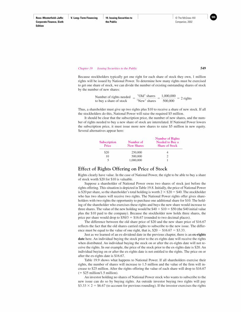
Ross−Westerfield−Jaffe: Corporate Finance, Sixth Edition
V. Long−Term Financing 19. Issuing Securities to the Public
555© The McGraw−Hill Companies, 2002
Because stockholders typically get one right for each share of stock they own, 1 millionrights will be issued by National Power. To determine how many rights must be exercisedto get one share of stock, we can divide the number of existing outstanding shares of stockby the number of new shares:
Number of rights neededto buy a share of stock
Thus, a shareholder must give up two rights plus $10 to receive a share of new stock. If allthe stockholders do this, National Power will raise the required $5 million.
It should be clear that the subscription price, the number of new shares, and the num-ber of rights needed to buy a new share of stock are interrelated. If National Power lowersthe subscription price, it must issue more new shares to raise $5 million in new equity.Several alternatives appear here:
Number of RightsSubscription Number of Needed to Buy a
Price New Shares Share of Stock
$20 250,000 410 500,000 25 1,000,000 1
Effect of Rights Offering on Price of StockRights clearly have value. In the case of National Power, the right to be able to buy a shareof stock worth $20 for $10 is valuable.
Suppose a shareholder of National Power owns two shares of stock just before therights offering. This situation is depicted in Table 19.8. Initially, the price of National Poweris $20 per share, so the shareholder’s total holding is worth 2 � $20 � $40. The stockholderwho has two shares will receive two rights. The National Power rights offer gives share-holders with two rights the opportunity to purchase one additional share for $10. The hold-ing of the shareholder who exercises these rights and buys the new share would increase tothree shares. The value of the new holding would be $40 � $10 � $50 (the $40 initial valueplus the $10 paid to the company). Because the stockholder now holds three shares, theprice per share would drop to $50/3 � $16.67 (rounded to two decimal places).
The difference between the old share price of $20 and the new share price of $16.67reflects the fact that the old shares carried rights to subscribe to the new issue. The differ-ence must be equal to the value of one right, that is, $20 � $16.67 � $3.33.
Just as we learned of an ex-dividend date in the previous chapter, there is an ex-rightsdate here. An individual buying the stock prior to the ex-rights date will receive the rightswhen distributed. An individual buying the stock on or after the ex-rights date will not re-ceive the rights. In our example, the price of the stock prior to the ex-rights date is $20. Anindividual buying on or after the ex-rights date is not entitled to the rights. The price on orafter the ex-rights date is $16.67.
Table 19.9 shows what happens to National Power. If all shareholders exercise theirrights, the number of shares will increase to 1.5 million and the value of the firm will in-crease to $25 million. After the rights offering the value of each share will drop to $16.67(� $25 million/1.5 million).
An investor holding no shares of National Power stock who wants to subscribe to thenew issue can do so by buying rights. An outside investor buying two rights will pay$3.33 � 2 � $6.67 (to account for previous rounding). If the investor exercises the rights
�"Old" shares
"New" shares�
1,000,000
500,000� 2 rights
Chapter 19 Issuing Securities to the Public 549
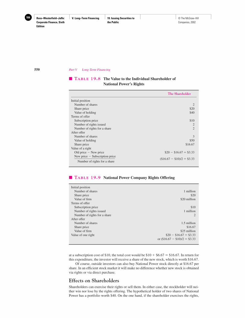
Ross−Westerfield−Jaffe: Corporate Finance, Sixth Edition
V. Long−Term Financing 19. Issuing Securities to the Public
556 © The McGraw−Hill Companies, 2002
at a subscription cost of $10, the total cost would be $10 � $6.67 � $16.67. In return forthis expenditure, the investor will receive a share of the new stock, which is worth $16.67.
Of course, outside investors can also buy National Power stock directly at $16.67 pershare. In an efficient stock market it will make no difference whether new stock is obtainedvia rights or via direct purchase.
Effects on ShareholdersShareholders can exercise their rights or sell them. In either case, the stockholder will nei-ther win nor lose by the rights offering. The hypothetical holder of two shares of NationalPower has a portfolio worth $40. On the one hand, if the shareholder exercises the rights,
550 Part V Long-Term Financing
� TABLE 19.8 The Value to the Individual Shareholder of National Power’s Rights
The Shareholder
Initial positionNumber of shares 2Share price $20Value of holding $40
Terms of offerSubscription price $10Number of rights issued 2Number of rights for a share 2
After offerNumber of shares 3Value of holding $50Share price $16.67
Value of a rightOld price � New price $20 � $16.67 � $3.33New price � Subscription price
($16.67 � $10)/2 � $3.33_________________________Number of rights for a share
� TABLE 19.9 National Power Company Rights Offering
Initial positionNumber of shares 1 millionShare price $20Value of firm $20 million
Terms of offerSubscription price $10Number of rights issued 1 millionNumber of rights for a share 2
After offerNumber of shares 1.5 millionShare price $16.67Value of firm $25 million
Value of one right $20 � $16.67 � $3.33or ($16.67 � $10)/2 � $3.33
Ross−Westerfield−Jaffe: Corporate Finance, Sixth Edition
V. Long−Term Financing 19. Issuing Securities to the Public
557© The McGraw−Hill Companies, 2002
he or she ends up with three shares worth a total of $50. In other words, by spending $10,the investor increases the value of the holding by $10, which means that he or she is neitherbetter nor worse off.
On the other hand, a shareholder who sells the two rights for $3.33 each obtains$3.33 � 2 � $6.67 in cash. Because the two shares are each worth $16.67, the holdingsare valued at
Shares � 2 � $16.67 � $33.33Sold rights � 2 � $ 3.33 � $ 6.67Total � $40.00
The new $33.33 market value plus $6.67 in cash is exactly the same as the original holdingof $40. Thus, stockholders can neither lose nor gain from exercising or selling rights.
It is obvious that the new market price of the firm’s stock will be lower after the rightsoffering than it was before the rights offering. The lower the subscription price, the greaterthe price decline of a rights offering. However, our analysis shows that the stockholdershave suffered no loss because of the rights offering.
The Underwriting ArrangementsUndersubscription can occur if investors throw away rights or if bad news causes the mar-ket price of the stock to fall below the subscription price. To ensure against these possibil-ities, rights offerings are typically arranged by standby underwriting. Here, the under-writer makes a firm commitment to purchase the unsubscribed portion of the issue at thesubscription price less a take-up fee. The underwriter usually receives a standby fee ascompensation for his risk-bearing function.
In practice, the subscription price is usually set well below the current market price,making the probability of a rights failure quite small. Though a small percentage (less than10 percent) of shareholders fail to exercise valuable rights, shareholders are usually allowedto purchase unsubscribed shares at the subscription price. This oversubscription privilegemakes it unlikely that the corporate issuer would need to turn to its underwriter for help.
• Describe the details of a rights offering.• What are the questions that financial management must answer in a rights offering?• How is the value of a right determined?
19.7 THE RIGHTS PUZZLE
Smith calculated the issuance costs from three alternative methods: an equity issue with un-derwriting, a rights issue with standby underwriting, and a pure rights issue.14 The resultsof his study, which appear in Table 19.10, suggest that a pure rights issue is the cheapest ofthe three alternatives. The bottom line of the table shows that total costs as a percentage ofproceeds is 6.17 percent, 6.05 percent, and 2.45 percent for the three alternatives, respec-tively. As the body of the table indicates, this disparity holds when issues of different sizesare separated.
Chapter 19 Issuing Securities to the Public 551
QUESTIONS
CO
NC
EP
T
?
14C. W. Smith, Jr., “Alternative Methods for Raising Capital: Rights versus Underwritten Offerings,” Journal ofFinancial Economics 5 (December 1977).
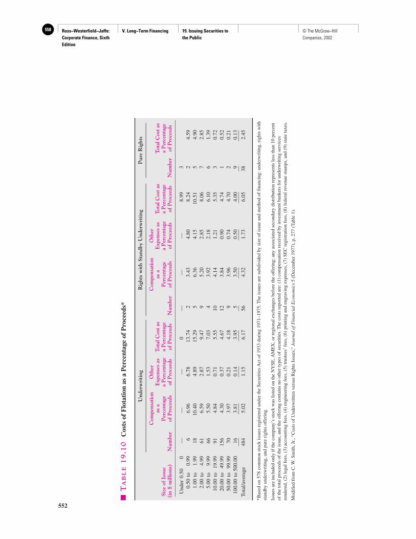
Ross−Westerfield−Jaffe: Corporate Finance, Sixth Edition
V. Long−Term Financing 19. Issuing Securities to the Public
558 © The McGraw−Hill Companies, 2002
552
�T
AB
LE
19
.10
Cos
ts o
f F
lota
tion
as
a P
erce
ntag
e of
Pro
ceed
s*
Und
erw
riti
ngR
ight
s w
ith
Stan
dby
Und
erw
riti
ngP
ure
Rig
hts
____
____
____
____
____
____
____
____
____
____
____
____
____
____
____
____
____
____
____
____
____
___
Com
pens
atio
nO
ther
Com
pens
atio
nO
ther
as a
Exp
ense
s as
Tot
al C
ost
asas
aE
xpen
ses
asT
otal
Cos
t as
Tot
al C
ost
asSi
ze o
f Is
sue
Per
cent
age
a P
erce
ntag
ea
Per
cent
age
Per
cent
age
a P
erce
ntag
ea
Per
cent
age
a P
erce
ntag
e(i
n $
mill
ions
)N
umbe
rof
Pro
ceed
sof
Pro
ceed
sof
Pro
ceed
sN
umbe
rof
Pro
ceed
sof
Pro
ceed
sof
Pro
ceed
sN
umbe
rof
Pro
ceed
s
Und
er0.
500
——
—0
——
—8.
993
0.50
to
0.99
66.
966.
7813
.74
23.
434.
808.
242
4.59
1.00
to
1.99
1810
.40
4.89
15.2
95
6.36
4.15
10.5
15
4.90
2.00
to
4.99
616.
592.
879.
479
5.20
2.85
8.06
72.
855.
00to
9.
9966
5.50
1.53
7.03
43.
922.
186.
106
1.39
10.0
0to
19
.99
914.
840.
715.
5510
4.14
1.21
5.35
30.
7220
.00
to
49.9
915
64.
300.
374.
6712
3.84
0.90
4.74
10.
5250
.00
to99
.99
703.
970.
214.
189
3.96
0.74
4.70
20.
2110
0.00
to 5
00.0
016
3.81
0.14
3.95
53.
500.
504.
009
0.13
___
____
____
____
____
____
____
____
____
Tota
l/ave
rage
484
5.02
1.15
6.17
564.
321.
736.
0538
2.45
*Bas
ed o
n 57
8 co
mm
on s
tock
issu
es r
egis
tere
d un
der
the
Secu
ritie
s A
ct o
f 19
33 d
urin
g 19
71–1
975.
The
issu
es a
re s
ubdi
vide
d by
siz
e of
issu
e an
d m
etho
d of
fin
anci
ng:u
nder
wri
ting,
righ
ts w
ithst
andb
y un
derw
ritin
g,an
d pu
re r
ight
s of
feri
ng.
Issu
es a
re in
clud
ed o
nly
if th
e co
mpa
ny’s
sto
ck w
as li
sted
on
the
NY
SE,A
ME
X,o
r re
gion
al e
xcha
nges
bef
ore
the
offe
ring
; any
ass
ocia
ted
seco
ndar
y di
stri
butio
n re
pres
ents
less
than
10
perc
ent
of th
e to
tal p
roce
eds
of th
e is
sue,
and
the
offe
ring
con
tain
s no
oth
er ty
pes
of s
ecur
ities
. The
cos
ts r
epor
ted
are:
(1)
com
pens
atio
n re
ceiv
ed b
y in
vest
men
t ban
kers
for
und
erw
ritin
g se
rvic
esre
nder
ed,(
2)le
gal f
ees,
(3)
acco
untin
g fe
es,(
4)en
gine
erin
g fe
es,(
5)tr
uste
es’f
ees,
(6)
prin
ting
and
engr
avin
g ex
pens
es,(
7)SE
C r
egis
trat
ion
fees
,(8)
fede
ral r
even
ue s
tam
ps,a
nd (
9)st
ate
taxe
s.
Mod
ifie
d fr
om C
.W. S
mith
,Jr.,
“Cos
ts o
f U
nder
wri
tten
vers
us R
ight
s Is
sues
,”Jo
urna
l of F
inan
cial
Eco
nom
ics
5 (D
ecem
ber
1977
),p.
277
(Tab
le 1
).
Ross−Westerfield−Jaffe: Corporate Finance, Sixth Edition
V. Long−Term Financing 19. Issuing Securities to the Public
559© The McGraw−Hill Companies, 2002
If corporate executives are rational, they will raise equity in the cheapest manner. Thus,the above evidence suggests that issues of pure rights should dominate. Surprisingly, Smithpoints out that over 90 percent of new issues are underwritten. This is generally viewed asan anomaly in the finance profession, though a few explanations have been advanced.15
1. Underwriters increase the stock price. This is supposedly accomplished because ofincreased public confidence or by the selling effort of the underwriting group. However,Smith could find no evidence of this in an examination of 52 rights offerings and 344 un-derwritten offerings.
2. Because the underwriter buys the shares at the agreed-upon price, it is providing in-surance to the firm. That is, the underwriter loses if it is unable to sell all the shares to thepublic. This potential loss might mean that the underwriter’s effective compensation is lessthan that measured in Table 19.10. However, the potential economic loss is probably notlarge. In most cases, the offer price is set within 24 hours of the offering, by which time theunderwriter has usually made a careful assessment of the market for the shares.
3. Other arguments include (a) the proceeds of underwritten issues are availablesooner than are the proceeds from a rights offer, (b) underwriters provide a wider distribu-tion of ownership than would be true with a rights offering, (c) consulting advice from in-vestment bankers may be beneficial, and (d) stockholders find exercising rights a nuisance.
All of the preceding arguments are pieces of the puzzle, but none seems very convinc-ing. Recently, Booth and Smith identified a function of the underwriter that had not beentaken into account in previous cost studies.16 They argue that the underwriter certifies thatthe offering price is consistent with the true value of the issue. This certification is impliedin the underwriting relationship and is provided when the underwriting firm gets access toinside information and puts its reputation for correct pricing on the line.
• Why might a firm prefer a general cash offering to a rights offering?
19.8 SHELF REGISTRATION
To simplify the procedures for issuing securities, the SEC currently allows shelf registra-tion. Shelf registration permits a corporation to register an offering that it reasonably ex-pects to sell within the next two years. A master registration statement is filed at the timeof registration. The company is permitted to sell the issue whenever it wants over those twoyears as long as it distributes a short-form statement.
Not all companies are allowed shelf registration. The major qualifications are as follows:
1. The company must be rated investment grade.
2. The firm cannot have defaulted on its debt in the past 12 months.
3. The aggregate market value of the firm’s outstanding stock must be more than $75 million.
4. The firm must not have violated the Securities Act of 1934 in the past 12 months.
Chapter 19 Issuing Securities to the Public 553
15It is even more anomalous because rights offerings are used around the world. In fact, they are required by lawin many other countries.16Booth and R. Smith, “The Certification Role of the Investment Banker in New Issue Pricing,” MidlandCorporate Finance Journal (Spring 1986).
QUESTION
CO
NC
EP
T
?
Ross−Westerfield−Jaffe: Corporate Finance, Sixth Edition
V. Long−Term Financing 19. Issuing Securities to the Public
560 © The McGraw−Hill Companies, 2002
Hershman reports on the use of the dribble method of new equity issuance.17 With drib-bling, a company registers the issue and hires an underwriter to be its selling agent. Thecompany sells shares in small amounts from time to time via a stock exchange. Companiesthat have dribble programs include Middle South Utilities, Niagara Mohawk, Pacific Gasand Electric, and the Southern Company. However, the evidence is that shelf registration isalmost never used for equity but is used about one-half of the time for debt.18
The rule has been very controversial. Several arguments have been made against shelfregistration.
1. The timeliness of disclosure is reduced with shelf registration, because the masterregistration statement may have been prepared up to two years before the actual issue occurs.
2. Some investment bankers have argued that shelf registration will cause a marketoverhang, because registration informs the market of future issues. It has been suggestedthat this overhang will depress market prices. However, an empirical analysis by Bhagat,Marr, and Thompson found that shelf registration is less costly than conventional under-writing and found no evidence to suggest a market-overhang effect.19 Surprisingly, few el-igible companies are currently selling equity by using shelf registration.20
• Describe shelf registration.• What are the arguments against shelf registration?
19.9 THE PRIVATE EQUITY MARKET
The previous sections of this chapter assumed that a company is big enough, successfulenough, and old enough to raise capital in the public equity market. Of course, there aremany firms that have not reached this stage and cannot use the public equity market. Forstart-up firms or firms in financial trouble, the public equity market is often not available.The market for venture capital is part of the private equity market.21
Private PlacementPrivate placements avoid the costly procedures associated with the registration require-ments that are part of public issues. The Securities and Exchange Commission (SEC) re-stricts private placement issues to no more than a couple of dozen knowledgeable in-vestors including institutions such as insurance companies and pension funds. Thebiggest drawback of privately placed securities is that the securities cannot be easilyresold. Most private placements involve debt securities, but equity securities can also beprivately placed.
554 Part V Long-Term Financing
17A. Hershman, “New Strategies in Equity Financing,” Dunn’s Business Monthly (June 1983).18D. J. Dennis, “Shelf Registration and the Market in Seasonal Equity Offerings,” Journal of Business 64 (1991).19S. Bhagat, M. W. Marr, and G. R. Thompson, “The Rule 415 Experiment: Equity Markets,” Journal ofFinance 19 (December 1985).20R. Rogowski and E. Sorenson, “Deregulation in Investment Banking: Shelf Registration, Structure, andPerformance,” Financial Management (Spring 1985).21S. E. Pratt, “Overview and Introduction to the Venture Capital Industry,” Guide to Venture Capital Sources,10th ed., 1987 (Venture Economics. Laurel Avenue, Box 348, Wellesley Hills, MA 02181).
QUESTIONS
CO
NC
EP
T
?
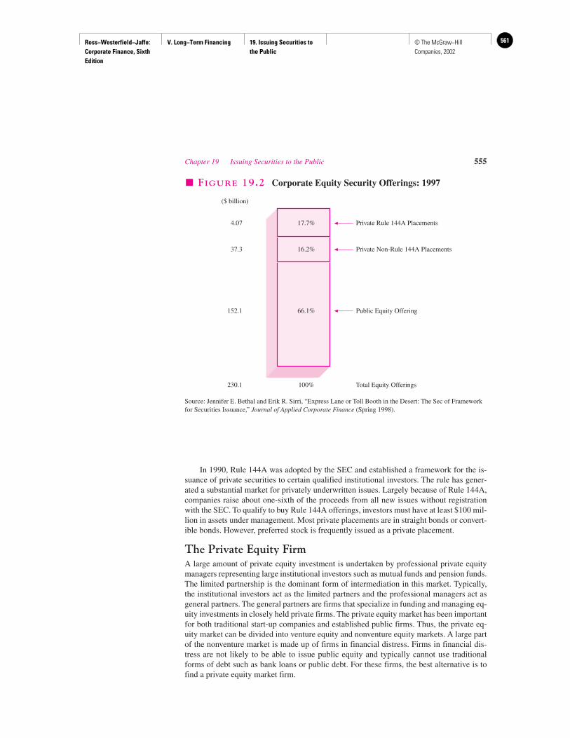
Ross−Westerfield−Jaffe: Corporate Finance, Sixth Edition
V. Long−Term Financing 19. Issuing Securities to the Public
561© The McGraw−Hill Companies, 2002
In 1990, Rule 144A was adopted by the SEC and established a framework for the is-suance of private securities to certain qualified institutional investors. The rule has gener-ated a substantial market for privately underwritten issues. Largely because of Rule 144A,companies raise about one-sixth of the proceeds from all new issues without registrationwith the SEC. To qualify to buy Rule 144A offerings, investors must have at least $100 mil-lion in assets under management. Most private placements are in straight bonds or convert-ible bonds. However, preferred stock is frequently issued as a private placement.
The Private Equity FirmA large amount of private equity investment is undertaken by professional private equitymanagers representing large institutional investors such as mutual funds and pension funds.The limited partnership is the dominant form of intermediation in this market. Typically,the institutional investors act as the limited partners and the professional managers act asgeneral partners. The general partners are firms that specialize in funding and managing eq-uity investments in closely held private firms. The private equity market has been importantfor both traditional start-up companies and established public firms. Thus, the private eq-uity market can be divided into venture equity and nonventure equity markets. A large partof the nonventure market is made up of firms in financial distress. Firms in financial dis-tress are not likely to be able to issue public equity and typically cannot use traditionalforms of debt such as bank loans or public debt. For these firms, the best alternative is tofind a private equity market firm.
Chapter 19 Issuing Securities to the Public 555
17.7%
16.2%
66.1%
4.07
($ billion)
37.3
152.1
100%230.1
Private Rule 144A Placements
Private Non-Rule 144A Placements
Public Equity Offering
Total Equity Offerings
� FIGURE 19.2 Corporate Equity Security Offerings: 1997
Source: Jennifer E. Bethal and Erik R. Sirri, “Express Lane or Toll Booth in the Desert: The Sec of Frameworkfor Securities Issuance,” Journal of Applied Corporate Finance (Spring 1998).
Ross−Westerfield−Jaffe: Corporate Finance, Sixth Edition
V. Long−Term Financing 19. Issuing Securities to the Public
562 © The McGraw−Hill Companies, 2002
Suppliers of Venture CapitalAs we have pointed out, venture capital is an important part of the private equity market.There are at least four types of suppliers of venture capital. First, a few old-line, wealthyfamilies have traditionally provided start-up capital to promising businesses. For example,over the years, the Rockefeller family has made the initial capital contribution to a numberof successful businesses. These families have been involved in venture capital for the bet-ter part of this century, if not longer.
Second, a number of private partnerships and corporations have been formed to provideinvestment funds. The organizer behind the partnership might raise capital from institutionalinvestors, such as insurance companies and pension funds. Alternatively, a group of individ-uals might provide the funds to be ultimately invested with budding entrepreneurs.
Of the early partnerships, the most well-known is clearly American Research andDevelopment (ARD), which was formed in 1946. Though ARD invested in many companies,its success was largely due to its investment in Digital Equipment Company (DEC). WhenTextron acquired ARD in 1972, over 85 percent of the shareholders’distribution was due to theinvestment in DEC.22 Among the more recent venture capitalists, Arthur Rock & Co. of SanFrancisco may very well be the best known. Because of its huge success with Apple Computerand other high-tech firms, it has achieved near mythic stature in the venture-capital industry.
Recent estimates put the number of venture-capital firms at about 2,000. Pratt’s Guideto Venture Capital (Venture Economics) provides a list of the names of many of thesefirms.23 The average amount invested per venture has been estimated to be between $1 mil-lion and $2 million. However, one should not make too much of this figure, because theamount of financing varies considerably with the venture to be funded.
Stories used to abound about how easily an individual could obtain venture capital.Though that may have been the case in an earlier era, it is certainly not the case today.Venture-capital firms employ various screening procedures to prevent inappropriate fund-ing. For example, because of the large demand for funds, many venture capitalists have atleast one employee whose full-time job consists of reading business plans. Only the verybest plans can expect to attract funds. Maier and Walker indicate that only about 2 percentof requests actually receive financing.24
Third, large industrial or financial corporations have established venture-capital sub-sidiaries. The Lambda Fund of Drexel Burnham Lambert, Manufacturers Hanover VentureCapital Corp., Citicorp Venture Capital, and Chemical Venture Capital Corporation ofChemical Bank are examples of this type. However, subsidiaries of this type appear to makeup only a small portion of the venture-capital market.
Fourth, participants in an informal venture-capital market have recently been identi-fied.25 Rather than belonging to any venture-capital firm, these investors (often referred toas angels) act as individuals when providing financing. However, they should not, by anymeans, be viewed as isolated. Wetzel and others indicate that there is a rich network of an-gels, continually relying on each other for advice. A number of researchers have stressedthat, in any informal network, there is likely one knowledgeable and trustworthy individualwho, when backing a venture, brings a few less experienced investors in with him.
556 Part V Long-Term Financing
22H. Stevenson, D. Muzka, and J. Timmons, “Venture Capital in Transition: A Monte-Carlo Simulation ofChanges in Investment Patterns,” Journal of Business Venturing (Spring 1987).23Pratt, “Overview and Introduction to the Venture Capital Industry.”24J. B. Maier and D. Walker, “The Role of Venture Capital in Financing Small Business,” Journal of BusinessVenturing (Summer 1987).25See W. E. Wetzel, “The Informal Venture Capital Market: Aspects of Scale and Market Efficiency,” Journal ofBusiness Venturing (Fall 1987).
Ross−Westerfield−Jaffe: Corporate Finance, Sixth Edition
V. Long−Term Financing 19. Issuing Securities to the Public
563© The McGraw−Hill Companies, 2002
The venture-capital community has unfortunately chosen to refer to these individualsas “dumb dentists.” Although a number indeed may be dentists, their intelligence shouldnot be called into question. Wetzel argues that the prototypical angel has income over$100,000, net worth over $1,000,000, and substantial business experience and knowledge.As one might expect, the informal venture capitalist is able to tolerate high risks.
Though this informal market may seem small and unimportant, it is perhaps the largestof all sources of venture capital. Wetzel argues that aggregate investments from this sourcetotal around $50 billion, about twice the amount invested by more professional venture cap-italists. The size of each contribution is smaller here. Perhaps, on average, only $250,000per venture is raised when the informal market is tapped.
Stages of FinancingA. V. Bruno and T. T. Tyebjee identify six stages in venture-capital financing:26
1. Seed-Money Stage. A small amount of financing needed to prove a concept or developa product. Marketing is not included in this stage.
2. Start-Up. Financing for firms that started within the past year. Funds are likely to payfor marketing and product development expenditures.
3. First-Round Financing. Additional money to begin sales and manufacturing after a firmhas spent its start-up funds.
4. Second-Round Financing. Funds earmarked for working capital for a firm that is cur-rently selling its product but still losing money.
5. Third-Round Financing. Financing for a company that is at least breaking even and iscontemplating an expansion. This is also known as mezzanine financing.
6. Fourth-Round Financing. Money provided for firms that are likely to go public withinhalf a year. This round is also known as bridge financing.
Although these categories may seem vague to the reader, we have found that the termsare well-accepted within the industry. For example, the venture-capital firms listed in Pratt’sGuide to Venture Capital indicate which of the above stages they are interested in financing.
The penultimate stage in venture capital finance is the initial public offering.27
Venture capitalists are very important participants in initial public offerings. Venture cap-italists rarely sell all of the shares they own at the time of the initial public offering.Instead, they usually sell out in subsequent public offerings. However, there is consider-able evidence that venture capitalists can successfully time IPOs by taking firms publicwhen the market values are at the highest. Figure 19.3 shows the number of IPOs of pri-vately held venture-capital-backed biotechnology companies in each month from 1978 to1992. The venture-capital-backed IPOs clearly coincide with the ups and downs in thebiotech market index in the top panel.
• What are the different sources of venture-capital financing?• What are the different stages for companies seeking venture-capital financing?• What is the private equity market?• What is Rule 144A?
Chapter 19 Issuing Securities to the Public 557
26A. V. Bruno and T. T. Tyebjee, “The Entrepreneur’s Search for Capital,” Journal of Business Venturing (Winter 1985).27A very influential paper by Christopher Barry, Chris J. Muscarella, John W. Peavey III, and Michael R.Vetsuypens, “The Role of Venture Capital in the Creation of Public Companies: Evidence from the Going PublicProcess,” Journal of Financial Economics 27 (1990), shows that venture capitalists do not usually sell shares atthe time of the initial public offering, but they usually have board seats and act as advisors to managers.
QUESTIONS
CO
NC
EP
T
?
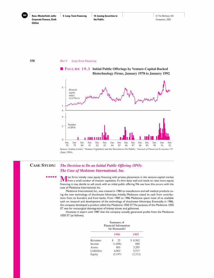
Ross−Westerfield−Jaffe: Corporate Finance, Sixth Edition
V. Long−Term Financing 19. Issuing Securities to the Public
564 © The McGraw−Hill Companies, 2002
CASE STUDY: The Decision to Do an Initial Public Offering (IPO):The Case of Medstone International, Inc.
Most firms initially raise equity financing with private placements in the venture-capital marketfrom a small number of investor capitalists. If a firm does well and needs to raise more equity
financing, it may decide to sell stock with an initial public offering.We see how this occurs with thecase of Medstone International, Inc.
Medstone International, Inc., was created in 1984 to manufacture and sell medical products us-ing the new technology of shockwave lithotripsy. Initially, Medstone raised its cash from contribu-tions from its founders and from banks. From 1984 to 1986 Medstone spent most of its availablecash on research and development of the technology of shockwave lithotripsy. Eventually, in 1986,the company developed a product called the Medstone 1050 ST.The purpose of the Medstone 1050ST was for nonsurgical disintegration of kidney stones and gallstones.
However, it wasn’t until 1987 that the company actually generated profits from the Medstone1050 ST (as follows).
Summary ofFinancial Information
(in thousands)
1986 1987
Revenues $ 25 $ 6,562Income (1,698) 680Assets 865 3,205Liabilities 6,062 5,517Equity (5,197) (2,312)
558 Part V Long-Term Financing
Biotechequityindex(1/1/78=1)
Numberof IPOs
5
1
0
9
5
0Jan.78
Jan.79
Jan.80
Jan.81
Jan.82
Jan.83
Jan.84
Jan.85
Jan.86
Jan.87
Jan.88
Jan.89
Jan.90
Jan.91
Jan.92
� FIGURE 19.3 Initial Public Offerings by Venture-Capital-BackedBiotechnology Firms, January 1978 to January 1992
Source: Joshua Lerner, “Venture Capitalists and the Decision to Go Public,” Journal of Financial Economics 35(June 1994).
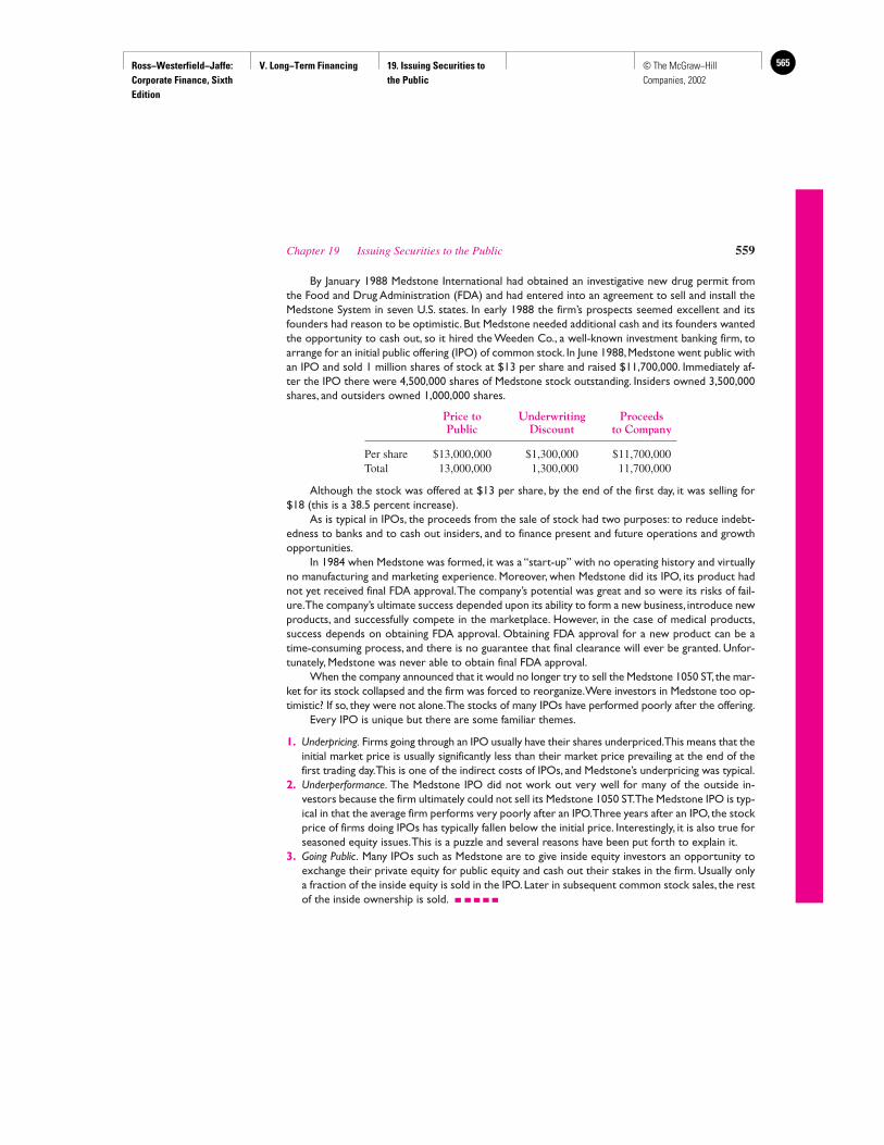
Ross−Westerfield−Jaffe: Corporate Finance, Sixth Edition
V. Long−Term Financing 19. Issuing Securities to the Public
565© The McGraw−Hill Companies, 2002
By January 1988 Medstone International had obtained an investigative new drug permit fromthe Food and Drug Administration (FDA) and had entered into an agreement to sell and install theMedstone System in seven U.S. states. In early 1988 the firm’s prospects seemed excellent and itsfounders had reason to be optimistic. But Medstone needed additional cash and its founders wantedthe opportunity to cash out, so it hired the Weeden Co., a well-known investment banking firm, toarrange for an initial public offering (IPO) of common stock. In June 1988,Medstone went public withan IPO and sold 1 million shares of stock at $13 per share and raised $11,700,000. Immediately af-ter the IPO there were 4,500,000 shares of Medstone stock outstanding. Insiders owned 3,500,000shares, and outsiders owned 1,000,000 shares.
Price to Underwriting ProceedsPublic Discount to Company
Per share $13,000,000 $1,300,000 $11,700,000Total 13,000,000 1,300,000 11,700,000
Although the stock was offered at $13 per share, by the end of the first day, it was selling for$18 (this is a 38.5 percent increase).
As is typical in IPOs, the proceeds from the sale of stock had two purposes: to reduce indebt-edness to banks and to cash out insiders, and to finance present and future operations and growthopportunities.
In 1984 when Medstone was formed, it was a “start-up” with no operating history and virtuallyno manufacturing and marketing experience. Moreover, when Medstone did its IPO, its product hadnot yet received final FDA approval.The company’s potential was great and so were its risks of fail-ure.The company’s ultimate success depended upon its ability to form a new business, introduce newproducts, and successfully compete in the marketplace. However, in the case of medical products,success depends on obtaining FDA approval. Obtaining FDA approval for a new product can be atime-consuming process, and there is no guarantee that final clearance will ever be granted. Unfor-tunately, Medstone was never able to obtain final FDA approval.
When the company announced that it would no longer try to sell the Medstone 1050 ST, the mar-ket for its stock collapsed and the firm was forced to reorganize.Were investors in Medstone too op-timistic? If so, they were not alone.The stocks of many IPOs have performed poorly after the offering.
Every IPO is unique but there are some familiar themes.
1. Underpricing. Firms going through an IPO usually have their shares underpriced.This means that theinitial market price is usually significantly less than their market price prevailing at the end of thefirst trading day.This is one of the indirect costs of IPOs, and Medstone’s underpricing was typical.
2. Underperformance. The Medstone IPO did not work out very well for many of the outside in-vestors because the firm ultimately could not sell its Medstone 1050 ST.The Medstone IPO is typ-ical in that the average firm performs very poorly after an IPO.Three years after an IPO, the stockprice of firms doing IPOs has typically fallen below the initial price. Interestingly, it is also true forseasoned equity issues.This is a puzzle and several reasons have been put forth to explain it.
3. Going Public. Many IPOs such as Medstone are to give inside equity investors an opportunity toexchange their private equity for public equity and cash out their stakes in the firm. Usually onlya fraction of the inside equity is sold in the IPO.Later in subsequent common stock sales, the restof the inside ownership is sold.
Chapter 19 Issuing Securities to the Public 559

Ross−Westerfield−Jaffe: Corporate Finance, Sixth Edition
V. Long−Term Financing 19. Issuing Securities to the Public
566 © The McGraw−Hill Companies, 2002
19.10 SUMMARY AND CONCLUSIONS
This chapter looks closely at how equity is issued. The main points follow.
1. Large issues have proportionately much lower costs of issuing equity than small ones.2. Firm-commitment underwriting is far more prevalent for large issues than is best-efforts
underwriting. Smaller issues probably primarily use best efforts because of the greateruncertainty of these issues. For an offering of a given size, the direct expenses of best-effortsunderwriting and firm-commitment underwriting are of the same magnitude.
3. Rights offerings are cheaper than general cash offers and eliminate the problem ofunderpricing. Yet, most new equity issues are underwritten general cash offers.
4. Shelf registration is a new method of issuing new debt and equity. The direct costs of shelfissues seem to be substantially lower than those of traditional issues.
5. Venture capitalists are an increasingly important influence in start-up firms and subsequentfinancing.
KEY TERMS
Best efforts 538 Registration statement 534Cash offer 537 Regulation A 534Competitive offer 541 Seasoned new issue 537Ex-rights date 549 Shelf registration 553Firm commitment 538 Standby fee 551Green Shoe provision 539 Standby underwriting 551Initial public offering (IPO) 537 Subscription price 548Investment banks 537 Syndicate 538Negotiated offer 541 Tombstone 535Oversubscription privilege 551 Unseasoned new issue 537Prospectus 534 Venture capital 554Red herring 534
SUGGESTED READINGS
Here are several significant recent articles that have helped shape our understanding of howcapital is raised.Altinkilic, Oya, and Robert S. Hansen. “Are There Economies of Scale in Underwriting Fees?
Evidence of Rising External Financing Costs.” Review of Financial Studies 13 (2000).Ellis, Katrina, Roni Michaely, and Maureen O’Hara. “When the Underwriter is the Market Maker:
An Examination of Trading in the IPO After Market.” Journal of Finance (June 2000).Chen, Hsuan-Chi, and Jay R. Ritter. “The Seven Percent Solution,” Journal of Finance (June 2000).Aggarwal, Reena. “Stabilization Activities by Underwriters After Initial Public Offerings.”
Journal of Finance (June 2000).
QUESTIONS AND PROBLEMS
The Public Issue19.1 Define the following terms related to the issuance of public securities.
a. General cash offerb. Rights offer
560 Part V Long-Term Financing

Ross−Westerfield−Jaffe: Corporate Finance, Sixth Edition
V. Long−Term Financing 19. Issuing Securities to the Public
567© The McGraw−Hill Companies, 2002
c. Registration statementd. Prospectuse. Initial public offeringf. Seasoned new issueg. Shelf registration
19.2 a. What does the Securities Exchange Act of 1933 regulate?b. What does the Securities Exchange Act of 1934 regulate?
The Cash Offer19.3 What are the comparative advantages of a competitive offer and a negotiated offer,
respectively?
19.4 Define the following terms related to underwriting.a. Firm commitmentb. Syndicatec. Spreadd. Best efforts
19.5 a. Who bears the risk in firm-commitment underwriting? Explain.b. Who bears the risk in best-efforts underwriting? Explain.
19.6 Suppose the Newton Company has 10,000 shares of stock. Each share is worth $40, andthe company’s market value of equity is $400,000. Suppose the firm issues 5,000 sharesof the new stock at the following prices: $40, $20, and $10. What will be the effect ofeach of the alternative offering prices on the existing price per share?
19.7 In 1980 a certain assistant professor of finance bought 12 initial public offerings of commonstock. He held each of these for approximately one month and then sold them. Theinvestment rule he followed was to submit a purchase order for every firm-commitmentinitial public offering of oil- and gas-exploration companies. There were 22 such offerings,and he submitted a purchase order for approximately $1,000 of stock for each one. With 10of these, no shares were allocated to this assistant professor. With five of the 12 offeringsthat were purchased, fewer than the requested number of shares were allocated.
The year 1980 was very good for oil- and gas-exploration company owners. For the22 stocks that went public, the stock was selling on average for 80 percent above theoffering price within a month. Yet, this assistant professor looked at his performance recordand found the $8,400 invested in 12 companies had grown to only $10,100, a return ofonly about 20 percent. (Commissions were negligible.) Did he have bad luck, or should hehave expected to do worse than the average initial-public-offering investor? Explain.
The Announcement of New Equity and the Value of the Firm19.8 What are the possible reasons for why the stock price typically drops on the announcement
of a seasoned new equity issue?
The Cost of New Issues19.9 What are the costs of new issues?
Rights19.10 Bountiful Beef Processors (BBP) wants to raise equity through a rights offering. BBP has
2,400,000 shares of common stock outstanding, and must raise $12,000,000. Thesubscription price of the rights will be $15.a. How many new shares of stock must BBP issue?b. How many rights will be necessary to purchase one share of stock?c. What must a shareholder remit to receive one share of stock?
19.11 Jelly Beans, Inc., is proposing a rights offering. There are 100,000 outstanding shares at$25 each. There will be 10,000 new shares issued at a $20 subscription price.a. What is the value of a right?b. What is the ex-rights price?c. What is the new market value of the company?d. Why might a company have a rights offering rather than a common stock offering?
Chapter 19 Issuing Securities to the Public 561
Ross−Westerfield−Jaffe: Corporate Finance, Sixth Edition
V. Long−Term Financing 19. Issuing Securities to the Public
568 © The McGraw−Hill Companies, 2002
19.12 Superior, Inc., is a manufacturer of beta-blockers. Management has concluded thatadditional equity financing is required to increase production capacity, and that thesefunds are best attained through a rights offering. It has correctly concluded that, as aresult of the rights offering, share price will fall from $50 to $45 ($50 is the rights-onprice; $45 is the ex-rights price, also known as the when-issued price). The company isseeking $5 million in additional funds with a per-share subscription price equal to $25.a. How many shares were there before the offering?
19.13 A company’s stock currently sells for $45 per share. Last week the firm issued rights toraise new equity. To purchase a new share, a stockholder must remit $10 and three rights.a. What is the ex-rights stock price?b. What is the price of one right?c. When will the price drop occur? Why will it occur then?
19.14 Summit Corp.’s stock is currently selling at $13 per share. There are 1 million sharesoutstanding. The firm is planning to raise $2 million to finance a new project. What is theex-right stock price, the value of a right, and the appropriate subscription prices, ifa. Two shares of outstanding stock are entitled to purchase one additional share of the
new issue.b. Four shares of outstanding stock are entitled to purchase one additional share of the
new issue.c. How does the stockholders’ wealth change from a to b?
The New Issue Puzzle19.15 Megabucks Industries is planning to raise fresh equity capital by selling a large new issue
of common stock. Megabucks is a publicly traded corporation, and is trying to choosebetween an underwritten cash offer and a rights offering (not underwritten) to currentshareholders. Megabucks’ management is interested in maximizing the wealth of currentshareholders and has asked you for advice on the choice of issue methods. What is yourrecommendation? Why?
Shelf Registration19.16 Explain why shelf registration has been used by many firms instead of syndication.
Venture Capital19.17 Who are the different suppliers of venture capital?
The Decision to Do an Initial Public Offering (IPO): The Case of MedstoneInternational, Inc.19.18 What are the uses for the proceeds from an IPO?
19.19 Every IPO is unique, but what are the basic empirical regularities in IPOs?
562 Part V Long-Term Financing
Ross−Westerfield−Jaffe: Corporate Finance, Sixth Edition
V. Long−Term Financing 20. Long−Term Debt 569© The McGraw−Hill Companies, 2002
Long-Term Debt
CH
AP
TE
R20
EXECUTIVE SUMMARY
The previous chapter introduced the mechanics of new long-term financing, withan emphasis on equity. This chapter takes a closer look at long-term debt instruments.
The chapter begins with a review of the basic features of long-term debt, and a de-scription of some important aspects of publicly issued long-term bonds. We also discussforms of long-term financing that are not publicly issued: term loans and private-placementbonds. These are directly placed with lending institutions, such as a commercial bank or alife insurance company.
All bond agreements have protective covenants. These are restrictions on the firm thatprotect the bondholder. We present several types of protective covenants in this chapter.
A large number of publicly issued industrial bonds have call provisions, which enablea company to buy back its bonds at a predetermined call price. This chapter attempts to an-swer two questions about call provisions.
1. Should firms issue callable bonds?
2. When should such bonds be called?
There are many different kinds of long-term bonds. We discuss three—floating-ratebonds, income bonds, and deep-discount bonds—and analyze what types of bonds are bestin different circumstances.
20.1 LONG-TERM DEBT: A REVIEW
Long-term debt securities are promises by the issuing firm to pay interest and principal onthe unpaid balance. The maturity of a long-term debt instrument refers to the length of timethe debt remains outstanding with some unpaid balance. Debt securities can be short-term(maturities of one year or less) or long-term (maturities of more than one year).1 Short-termdebt is sometimes referred to as unfunded debt and long-term debt as funded debt.2
The two major forms of long-term debt are public issue and privately placed debt. Wediscuss public-issue bonds first, and most of what we say about them holds true for privatelyplaced long-term debt as well. The main difference between publicly issued and privatelyplaced debt is that private debt is directly placed with a lending institution.
There are many other attributes to long-term debt, including security, call features, sink-ing funds, ratings, and protective covenants. The boxed material illustrates these attributes.
1In addition, people often refer to intermediate-term debt, which has a maturity of more than one year and lessthan three to five years.2The word funding generally implies long-term. Thus, a firm planning to fund its debt requirements may bereplacing short-term debt with long-term debt.
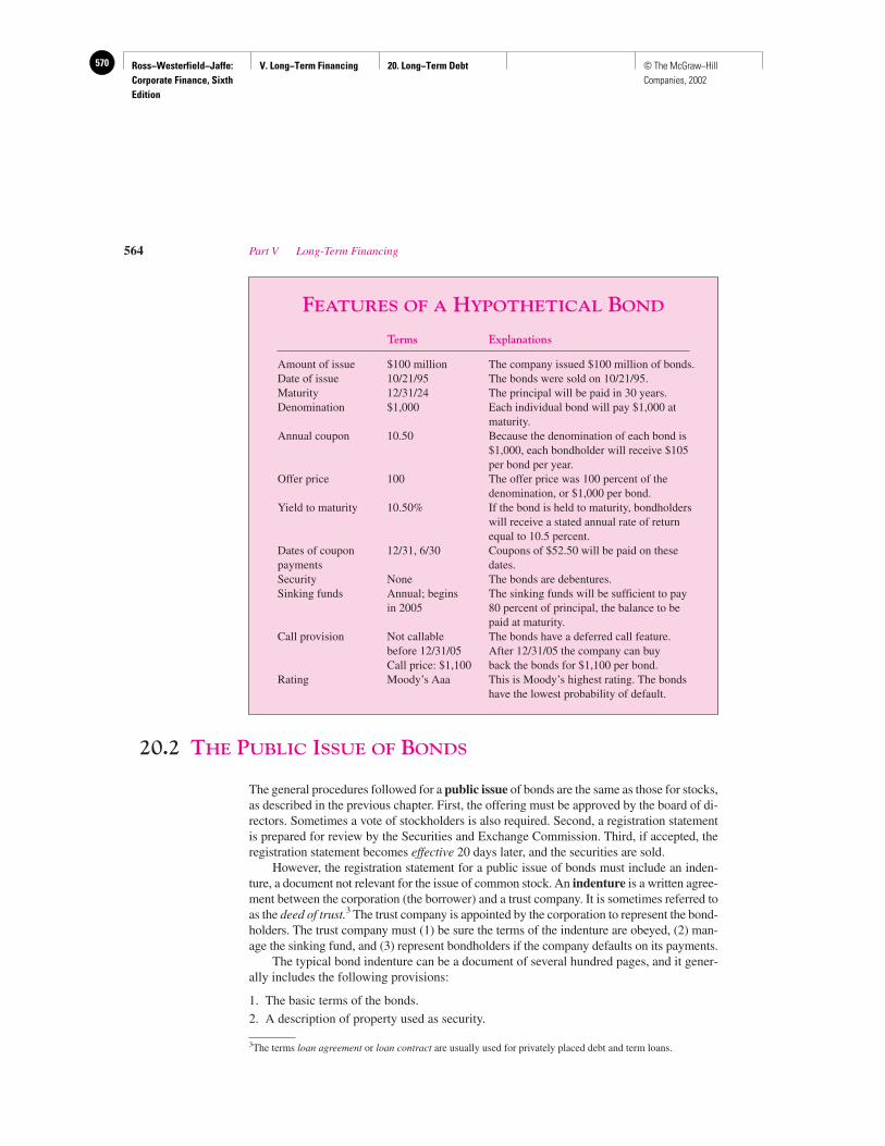
Ross−Westerfield−Jaffe: Corporate Finance, Sixth Edition
V. Long−Term Financing 20. Long−Term Debt570 © The McGraw−Hill Companies, 2002
20.2 THE PUBLIC ISSUE OF BONDS
The general procedures followed for a public issue of bonds are the same as those for stocks,as described in the previous chapter. First, the offering must be approved by the board of di-rectors. Sometimes a vote of stockholders is also required. Second, a registration statementis prepared for review by the Securities and Exchange Commission. Third, if accepted, theregistration statement becomes effective 20 days later, and the securities are sold.
However, the registration statement for a public issue of bonds must include an inden-ture, a document not relevant for the issue of common stock. An indenture is a written agree-ment between the corporation (the borrower) and a trust company. It is sometimes referred toas the deed of trust.3 The trust company is appointed by the corporation to represent the bond-holders. The trust company must (1) be sure the terms of the indenture are obeyed, (2) man-age the sinking fund, and (3) represent bondholders if the company defaults on its payments.
The typical bond indenture can be a document of several hundred pages, and it gener-ally includes the following provisions:
1. The basic terms of the bonds.
2. A description of property used as security.
564 Part V Long-Term Financing
FEATURES OF A HYPOTHETICAL BOND
Terms Explanations
Amount of issue $100 million The company issued $100 million of bonds.Date of issue 10/21/95 The bonds were sold on 10/21/95.Maturity 12/31/24 The principal will be paid in 30 years.Denomination $1,000 Each individual bond will pay $1,000 at
maturity.Annual coupon 10.50 Because the denomination of each bond is
$1,000, each bondholder will receive $105per bond per year.
Offer price 100 The offer price was 100 percent of the denomination, or $1,000 per bond.
Yield to maturity 10.50% If the bond is held to maturity, bondholders will receive a stated annual rate of returnequal to 10.5 percent.
Dates of coupon 12/31, 6/30 Coupons of $52.50 will be paid on these payments dates.Security None The bonds are debentures.Sinking funds Annual; begins The sinking funds will be sufficient to pay
in 2005 80 percent of principal, the balance to bepaid at maturity.
Call provision Not callable The bonds have a deferred call feature. before 12/31/05 After 12/31/05 the company can buy Call price: $1,100 back the bonds for $1,100 per bond.
Rating Moody’s Aaa This is Moody’s highest rating. The bonds have the lowest probability of default.
3The terms loan agreement or loan contract are usually used for privately placed debt and term loans.
Ross−Westerfield−Jaffe: Corporate Finance, Sixth Edition
V. Long−Term Financing 20. Long−Term Debt 571© The McGraw−Hill Companies, 2002
3. Details of the protective covenants.
4. The sinking-fund arrangements.
5. The call provision.
Each of these is discussed next.
The Basic TermsBonds usually have a face value of $1,000. This is also called the principal value or the de-nomination and it is stated on the bond certificate. In addition, the par value (i.e., initial ac-counting value) of a bond is almost always the same as the face value.
Transactions between bond buyers and bond sellers determine the market value of thebond. Actual bond-market values depend on the general level of interest rates, among otherfactors, and need not equal the face value. The bond price is quoted as a percentage of thedenomination. Though interest is paid only twice a year, interest accrues continually overthe year, and the quoted prices of a bond usually include accrued interest. This is illustratedin the example below.
EXAMPLE
Suppose the Black Corporation has issued 100 bonds. The amount stated on eachbond certificate is $1,000. The total face value or principal value of the bonds is$100,000. Further suppose the bonds are currently priced at 100, which means100 percent of $1,000. This means that buyers and sellers are holding bonds at aprice per bond of $1,000. If interest rates rise, the price of the bond might fall to,say, 97, which means 97 percent of $1,000, or $970.
Suppose the bonds have a stated interest rate of 12 percent due on January 1, 2050. Thebond indenture might read as follows:
The bond will mature on January 1, 2050, and will be limited in aggregate principal amount to$100,000. Each bond will bear interest at the rate of 12.0% per annum from January 1, 1990,or from the most recent Interest Payment Date to which interest has been paid or provided for.Interest is payable semiannually on July 1 and January 1 of each year.
Suppose an investor buys the bonds on April 1. Since the last interest payment, onJanuary 1, three months of interest at 12 percent per year would have accrued. Becauseinterest of 12 percent a year works out to 1 percent per month, interest over the threemonths is 3 percent. Therefore, the buyer of the bond must pay a price of 100 percent plusthe 3 percent of accrued interest ($30). On July 1 the buyer will receive an interest pay-ment of $60. This can be viewed as the sum of the $30 he or she paid the seller plus thethree months of interest, $30, for holding the bond from April 1 to July 1.
As is typical of industrial bonds, the Black bonds are registered. The indenture mightread as follows:
Interest is payable semiannually on July 1 and January 1 of each year to the person inwhose name the bond is registered at the close of business on June 15 or December 15,respectively.
This means that the company has a registrar who will record the ownership of each bond.The company will pay the interest and principal by check mailed directly to the address ofthe owner of record.
Chapter 20 Long-Term Debt 565
Ross−Westerfield−Jaffe: Corporate Finance, Sixth Edition
V. Long−Term Financing 20. Long−Term Debt572 © The McGraw−Hill Companies, 2002
When a bond is registered with attached coupons, the bondholder must separate acoupon from the bond certificate and send it to the company registrar (paying agent). Somebonds are in bearer form. This means that ownership is not recorded in the company books.As with a registered bond with attached coupons, the holder of the bond certificate sepa-rates the coupon and sends it in to the company to receive payment.
There are two drawbacks to bearer bonds. First, they can be easily lost or stolen.Second, because the company does not know who owns its bonds, it cannot notify bond-holders of important events. Consider, for example, Mr. and Mrs. Smith, who go to theirsafe-deposit box and clip the coupon on their 12-percent, $1,000 bond issued by the BlackCorporation. They send the coupon to the paying agent and feel richer. A few days later, anotice comes from the paying agent that the bond was retired and its principal paid off oneyear earlier. In other words, the bond no longer exists. Mr. and Mrs. Smith must forfeit oneyear of interest. (Of course, they can turn their bond in for $1,000.)
However, bearer bonds have the advantage of secrecy because even the issuing com-pany does not know who the bond’s owners are. This secrecy is particularly vexing to tax-ing authorities because tax collection on interest is difficult if the holder is unknown.
SecurityDebt securities are also classified according to the collateral protecting the bondholder. Col-lateral is a general term for the assets that are pledged as a security for payment of debt. Forexample, collateral trust bonds involve a pledge of common stock held by the corporation.
EXAMPLE
Suppose Railroad Holding Company owns all of the common stock of Track, Inc.;that is, Track, Inc., is a wholly owned subsidiary of the Railroad Holding Com-pany. Railroad issues debt securities that pledge the common stock of Track, Inc.,as collateral. The debts are collateral trust bonds; U.S. Sur Bank will hold them. IfRailroad Holding Company defaults on the debt, U.S. Sur Bank will be able to sellthe stock of Track, Inc., to satisfy Railroad’s obligation.
Mortgage securities are secured by a mortgage on real estate or other long-term assetsof the borrower.4 The legal document that describes that mortgage is called a mortgage-trust indenture or trust deed. The mortgage can be closed-end, so that there is a limit as tothe amount of bonds that can be issued. More frequently it is open-end, without limit to theamount of bonds that may be issued.
EXAMPLE
Suppose the Miami Bond Company has buildings and land worth $10 million anda $4 million mortgage on these properties. If the mortgage is closed-end, the Mi-ami Bond Company cannot issue more bonds on this property.
If the bond indenture contains no clause limiting the amount of additionalbonds that can be issued, it is an open-end mortgage. In this case the Miami BondCompany can issue additional bonds on its property, making the existing bondsriskier. For example, if additional mortgage bonds of $2 million are issued, the
566 Part V Long-Term Financing
4A set of railroad cars is an example of “other long-term assets” used as security.
Ross−Westerfield−Jaffe: Corporate Finance, Sixth Edition
V. Long−Term Financing 20. Long−Term Debt 573© The McGraw−Hill Companies, 2002
property has been pledged for a total of $6 million of bonds. If Miami Bond Com-pany must liquidate its property for $4 million, the original bondholders will re-ceive 4⁄6, or 67 percent, of their investment. If the mortgage had been closed-end,they would have received 100 percent of the stated value.
The value of a mortgage depends on the market value of the underlying property.Because of this, mortgage bonds sometimes require that the property be properly main-tained and insured. Of course, a building and equipment bought in 1914 for manufacturingslide rules might not have much value no matter how well the company maintains it. Thevalue of any property ultimately depends on its next best economic use. Bond indenturescannot easily insure against losses in economic value.
Sometimes mortgages are on specific property, for example, a single building. Moreoften, blanket mortgages are used. A blanket mortgage pledges many assets owned by thecompany.
Some bonds represent unsecured obligations of the company. A debenture is an unse-cured bond, where no specific pledge of property is made. Debenture holders have a claimon property not otherwise pledged: the property that remains after mortgages and collateraltrusts are taken into account. At the current time, almost all public bonds issued by indus-trial and finance companies are debentures. However, most utility and railroad bonds aresecured by a pledge of assets.
Protective CovenantsA protective covenant is that part of the indenture or loan agreement that limits certain ac-tions of the borrowing company. Protective covenants can be classified into two types: neg-ative covenants and positive covenants. A negative covenant limits or prohibits actions thatthe company may take. Here are some typical examples:
1. Limitations are placed on the amount of dividends a company may pay.
2. The firm cannot pledge any of its assets to other lenders.
3. The firm cannot merge with another firm.
4. The firm may not sell or lease its major assets without approval by the lender.
5. The firm cannot issue additional long-term debt.
A positive covenant specifies an action that the company agrees to take or a condition thecompany must abide by. Here are some examples:
1. The company agrees to maintain its working capital at a minimum level.
2. The company must furnish periodic financial statements to the lender.
The financial implications of protective covenants were treated in detail in the chapterson capital structure. In that discussion, we argued that protective covenants can benefitstockholders because, if bondholders are assured that they will be protected in times of fi-nancial stress, they will accept a lower interest rate.
The Sinking FundBonds can be entirely repaid at maturity, at which time the bondholder will receive the statedvalue of the bond, or they can be repaid before maturity. Early repayment is more typical.
In a direct placement of debt the repayment schedule is specified in the loan contract. Forpublic issues, the repayment takes place through the use of a sinking fund and a call provision.
Chapter 20 Long-Term Debt 567
Ross−Westerfield−Jaffe: Corporate Finance, Sixth Edition
V. Long−Term Financing 20. Long−Term Debt574 © The McGraw−Hill Companies, 2002
A sinking fund is an account managed by the bond trustee for the purpose of repayingthe bonds. Typically, the company makes yearly payments to the trustee. The trustee canpurchase bonds in the market or can select bonds randomly using a lottery and purchasethem, generally at face value. There are many different kinds of sinking-fund arrangements:
• Most sinking funds start between 5 and 10 years after the initial issuance.• Some sinking funds establish equal payments over the life of the bond.• Most high-quality bond issues establish payments to the sinking fund that are not
sufficient to redeem the entire issue. As a consequence, there is the possibility of alarge balloon payment at maturity.
Sinking funds have two opposing effects on bondholders:
1. Sinking Funds Provide Extra Protection to Bondholders. A firm experiencing financialdifficulties would have trouble making sinking-fund payments. Thus, sinking-fund pay-ments provide an early warning system to bondholders.
2. Sinking Funds Give the Firm an Attractive Option. If bond prices fall below the facevalue, the firm will satisfy the sinking fund by buying bonds at the lower market prices.If bond prices rise above the face value, the firm will buy the bonds back at the lowerface value.
The Call ProvisionA call provision lets the company repurchase or call the entire bond issue at a predeter-mined price over a specified period.
Generally, the call price is above the bond’s face value of $1,000. The difference be-tween the call price and the face value is the call premium. For example, if the call priceis 105, that is, 105 percent of $1,000, the call premium is 50. The amount of the call pre-mium usually becomes smaller over time. One typical arrangement is to set the call pre-mium initially equal to the annual coupon payment and then make it decline to zero overthe life of the bond.
Call provisions are not usually operative during the first few years of a bond’s life. Forexample, a company may be prohibited from calling its bonds for the first 10 years. This isreferred to as a deferred call. During this period the bond is said to be call-protected.
• Do bearer bonds have any advantage? Why might Mr. “I Like to Keep My Affairs Private”prefer to hold bearer bonds?
• What advantages and what disadvantages do bondholders derive from provisions of sink-ing funds?
• What is a call provision? What is the difference between the call price and the stated price?
20.3 BOND REFUNDING
Replacing all or part of an issue of outstanding bonds is called bond refunding. Usually,the first step in a typical bond refunding is to call the entire issue of bonds at the call price.Bond refunding raises two questions:
1. Should firms issue callable bonds?
2. Given that callable bonds have been issued, when should the bonds be called?
We attempt to answer these questions in this section.
568 Part V Long-Term Financing
QUESTIONS
CO
NC
EP
T
?
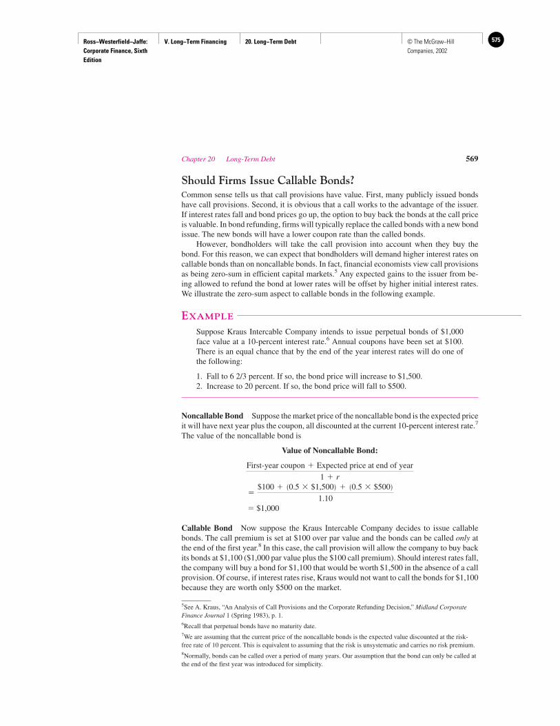
Ross−Westerfield−Jaffe: Corporate Finance, Sixth Edition
V. Long−Term Financing 20. Long−Term Debt 575© The McGraw−Hill Companies, 2002
Should Firms Issue Callable Bonds?Common sense tells us that call provisions have value. First, many publicly issued bondshave call provisions. Second, it is obvious that a call works to the advantage of the issuer.If interest rates fall and bond prices go up, the option to buy back the bonds at the call priceis valuable. In bond refunding, firms will typically replace the called bonds with a new bondissue. The new bonds will have a lower coupon rate than the called bonds.
However, bondholders will take the call provision into account when they buy thebond. For this reason, we can expect that bondholders will demand higher interest rates oncallable bonds than on noncallable bonds. In fact, financial economists view call provisionsas being zero-sum in efficient capital markets.5 Any expected gains to the issuer from be-ing allowed to refund the bond at lower rates will be offset by higher initial interest rates.We illustrate the zero-sum aspect to callable bonds in the following example.
EXAMPLE
Suppose Kraus Intercable Company intends to issue perpetual bonds of $1,000face value at a 10-percent interest rate.6 Annual coupons have been set at $100.There is an equal chance that by the end of the year interest rates will do one ofthe following:
1. Fall to 6 2/3 percent. If so, the bond price will increase to $1,500.2. Increase to 20 percent. If so, the bond price will fall to $500.
Noncallable Bond Suppose the market price of the noncallable bond is the expected priceit will have next year plus the coupon, all discounted at the current 10-percent interest rate.7
The value of the noncallable bond is
Value of Noncallable Bond:
� $1,000
Callable Bond Now suppose the Kraus Intercable Company decides to issue callablebonds. The call premium is set at $100 over par value and the bonds can be called only atthe end of the first year.8 In this case, the call provision will allow the company to buy backits bonds at $1,100 ($1,000 par value plus the $100 call premium). Should interest rates fall,the company will buy a bond for $1,100 that would be worth $1,500 in the absence of a callprovision. Of course, if interest rates rise, Kraus would not want to call the bonds for $1,100because they are worth only $500 on the market.
�$100 � �0.5 � $1,500� � �0.5 � $500�
1.10
First-year coupon � Expected price at end of year
1 � r
Chapter 20 Long-Term Debt 569
5See A. Kraus, “An Analysis of Call Provisions and the Corporate Refunding Decision,” Midland CorporateFinance Journal 1 (Spring 1983), p. 1.6Recall that perpetual bonds have no maturity date.7We are assuming that the current price of the noncallable bonds is the expected value discounted at the risk-free rate of 10 percent. This is equivalent to assuming that the risk is unsystematic and carries no risk premium.8Normally, bonds can be called over a period of many years. Our assumption that the bond can only be called atthe end of the first year was introduced for simplicity.

Ross−Westerfield−Jaffe: Corporate Finance, Sixth Edition
V. Long−Term Financing 20. Long−Term Debt576 © The McGraw−Hill Companies, 2002
Suppose rates fall and Kraus calls the bonds by paying $1,100. If the firm simultane-ously issues new bonds with a coupon of $100, it will bring in $1,500 ($100/0.0667) at the6 2/3-percent interest rate. This will allow Kraus to pay an extra dividend to shareholdersof $400 ($1,500 � $1,100). In other words, if rates fall from 10 percent to 6 2/3 percent,exercise of the call will transfer $400 of potential bondholder gains to the shareholders.
When investors purchase callable bonds, they realize that they will forfeit their antici-pated gains to shareholders if the bonds are called. As a consequence, they will not pay$1,000 for a callable bond with a coupon of $100.
How high must the coupon on the callable bond be so that it can be issued at the parvalue of $1,000? We can answer this in three steps.
Step 1: Determining End-of-Year Value if Interest Rates Drop If the interest rate dropsto 6 2/3 percent by the end of the year, the bond will be called for $1,100. The bondholderwill receive both this and the annual coupon payment. If we let C represent the coupon onthe callable bond, the bondholder gets the following at the end of the year:
$1,100 � C
Step 2: Determining End-of-Year Value if Interest Rates Rise If interest rates rise to 20percent, the value of the bondholder’s position at the end of the year is:
That is, the perpetuity formula tells us that the bond will sell at C/0.20. In addition, thebondholder receives the coupon payment at the end of the year.
Step 3: Solving for C Because interest rates are equally likely to rise or to fall, the ex-pected value of the bondholder’s end-of-year position is
Using the current interest rate of 10 percent, we set the present value of these paymentsequal to par:
C is the unknown in the equation. The equation holds if C � $157.14. In other words,callable bonds can sell at par only if their coupon rate is 15.714 percent.
The Paradox Restated If Kraus issues a noncallable bond, it will only need to pay a10-percent interest rate. By contrast, Kraus must pay an interest rate of 15.7 percent on acallable bond. The interest-rate differential makes an investor indifferent whether shebuys one of the two bonds in our example or the other. Because the return to the investoris the same with either bond, the cost of debt capital is the same to Kraus with either bond.Thus, our example suggests that there is neither an advantage nor a disadvantage from is-suing callable bonds.
Why, therefore, are callable bonds issued in the real world? This question has vexed fi-nancial economists for a long time. We now consider four specific reasons why a companymight use a call provision:
1. Superior interest-rate predictions.
2. Taxes.
$1,000 �
�$1,100 � C� � 0.5 � � C
0.20� C� � 0.5
1.10
�$1,100 � C� � 0.5 � � C
0.20� C� � 0.5
C
0.20� C
570 Part V Long-Term Financing
Ross−Westerfield−Jaffe: Corporate Finance, Sixth Edition
V. Long−Term Financing 20. Long−Term Debt 577© The McGraw−Hill Companies, 2002
3. Financial flexibility for future investment opportunities.
4. Less interest-rate risk.
Superior Interest-Rate Forecasting Company insiders may know more about interest-rate changes on its bonds than does the investing public. For example, managers may bebetter informed about potential changes in the firm’s credit rating. Thus, a company mayprefer the call provision at a particular time because it believes that the expected fall in in-terest rates (the probability of a fall multiplied by the amount of the fall) is greater than thebondholders believe.
Although this is possible, there is reason to doubt that inside information is the ration-ale for call provisions. Suppose firms really had superior ability to predict changes thatwould affect them. Bondholders would infer that a company expected an improvement inits credit rating whenever it issued callable bonds. Bondholders would require an increasein the coupon rate to protect them against a call if this occurred. As a result, we would ex-pect that there would be no financial advantage to the firm from callable bonds over non-callable bonds.
Of course, there are many non–company-specific reasons why interest rates can fall.For example, the interest-rate level is connected to the anticipated inflation rate. But it isdifficult to see how companies could have more information about the general level of in-terest rates than other participants in the bond markets.
Taxes Call provisions may have tax advantages if the bondholder is taxed at a lower ratethan the company. We have seen that callable bonds have higher coupon rates than non-callable bonds. Because the coupons provide a deductible interest expense to the corpora-tion and are taxable income to the bondholder, the corporation will gain more than a bond-holder in a low tax bracket will lose. Presumably, some of the tax saving can be passed onto the bondholders in the form of a high coupon.
Future Investment Opportunities As we have explained, bond indentures contain pro-tective covenants that restrict a company’s investment opportunities. For example, protec-tive covenants may limit the company’s ability to acquire another firm or to sell certain as-sets (for example, a division of the company). If the covenants are sufficiently restrictive,the cost to the shareholders in lost net present value can be large. However, if bonds arecallable, the company can buy back the bonds at the call price and take advantage of a su-perior investment opportunity.9
Less Interest-Rate Risk The call provision will reduce the sensitivity of a bond’s valueto changes in the level of interest rates. As interest rates increase, the value of a noncallablebond will fall. Because the callable bond has a higher coupon rate, the value of a callablebond will fall less than the value of a noncallable bond. Kraus has argued that, by reducingthe sensitivity of a bond’s value to changes in interest rates, the call provision may reducethe risk of shareholders as well as bondholders.10 He argues that, because the bond is a li-ability of the corporation, the equityholders bear risk as the bond changes value over time.Thus, it can be shown that, under certain conditions, reducing the risk of bonds through acall provision will also reduce the risk of equity.
Chapter 20 Long-Term Debt 571
9This argument is from Z. Bodie and R. A. Taggart, “Future Investment Opportunities and the Value of the CallProvision on a Bond,” Journal of Finance 33 (1978), p. 4.10A. Kraus, “An Analysis of Call Provisions and the Corporate Refunding Decision,” Midland Corporate FinanceJournal 1 (Spring 1983). Kraus points out that the call provision will not always reduce the equity’s interest-raterisk. If the firm as a whole bears interest-rate risk, more of this risk may be shifted from equityholders tobondholders with noncallable debt. In this case, equityholders may actually bear more risk with callable debt.
Ross−Westerfield−Jaffe: Corporate Finance, Sixth Edition
V. Long−Term Financing 20. Long−Term Debt578 © The McGraw−Hill Companies, 2002
Calling Bonds: When Does It Make Sense?The value of the company is the value of the stock plus the value of the bonds. From theModigliani-Miller theory and the pie model in earlier chapters, we know that firm value is un-changed by how it is divided between these two instruments. Therefore, maximizing share-holder wealth means minimizing the value of the callable bond. In a world with no transac-tion costs, it can be shown that the company should call its bonds whenever the callable-bondvalue exceeds the call price. This policy minimizes the value of the callable bonds.
The preceding analysis is modified slightly by including the costs from issuing newbonds. These extra costs change the refunding rule to allow bonds to trade at prices above thecall price. The objective of the company is to minimize the sum of the value of the callablebonds plus new issue costs. It has been observed that many real-world firms do not call theirbonds when the market value of the bonds reaches the call price. Instead, they wait until themarket value of the bonds exceeds the call price. Perhaps these issue costs are an explanation.Also, when a bond is called, the holder has about 30 days to surrender the bond and receivethe call price in cash. In 30 days the market value of the bonds could fall below the call price.If so, the firm is giving away money. To forestall this possibility, it can be argued that firmsshould wait until the market value of the bond exceeds the call price before calling bonds.
• What are the advantages to a firm of having a call provision?• What are the disadvantages to bondholders of having a call provision?
20.4 BOND RATINGS
Firms frequently pay to have their debt rated. The two leading bond-rating firms are Moody’sInvestors Service and Standard & Poor’s. The debt ratings depend upon (1) the likelihoodthat the firm will default and (2) the protection afforded by the loan contract in the event ofdefault. The ratings are constructed from information supplied by the corporation, primarilythe financial statements of the firm. The rating classes are shown in the accompanying box.
The highest rating debt can have is AAA or Aaa. Debt rated AAA or Aaa is judged tobe the best quality and to have the lowest degree of risk. The lowest rating is D, which indi-cates that the firm is in default. Since the 1980s, a growing part of corporate borrowing hastaken the form of low-grade bonds. These bonds are also known as either high-yield bondsor junk bonds. Low-grade bonds are corporate bonds that are rated below investment gradeby the major rating agencies (that is, below BBB for Standard & Poor’s or Baa for Moody’s).
Bond ratings are important, because bonds with lower ratings tend to have higher in-terest costs. However, the most recent evidence is that bond ratings merely reflect bond risk.There is no conclusive evidence that bond ratings affect risk.11 It is not surprising that thestock prices and bond prices of firms do not show any unusual behavior on the days arounda rating change. Because the ratings are based on publicly available information, they prob-ably do not, in themselves, supply new information to the market.12
572 Part V Long-Term Financing
QUESTIONS
CO
NC
EP
T
?
11M. Weinstein, “The Systematic Risk of Corporate Bonds,” Journal of Financial and Quantitative Analysis(September 1981); J. P. Ogden, “Determinants of Relative Interest Rate Sensitivity of Corporate Bonds,”Financial Management (Spring 1987); and F. Reilly and M. Joehnk, “The Association between Market-BasedRisk Measures for Bonds and Bond Ratings,” Journal of Finance (December 1976).12M. Weinstein, “The Effect of a Ratings Change Announcement on Bond Price,” Journal of FinancialEconomics 5 (1977). However, Robert W. Holthausen and Richard W. Leftwich, “The Effect of Bond RatingChanges on Common Stock Prices,” Journal of Financial Economics 17 (September 1986), find that bond ratingdowngrades are associated with abnormal negative returns of the stock of the issuing firm.
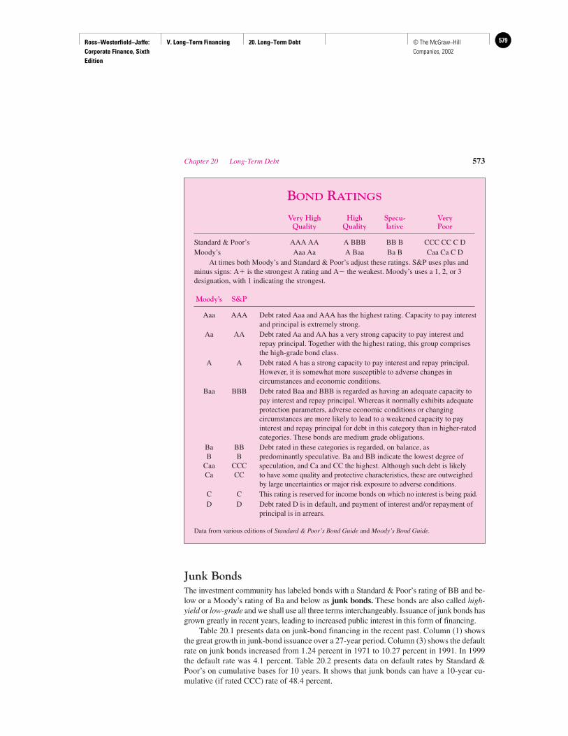
Ross−Westerfield−Jaffe: Corporate Finance, Sixth Edition
V. Long−Term Financing 20. Long−Term Debt 579© The McGraw−Hill Companies, 2002
Junk BondsThe investment community has labeled bonds with a Standard & Poor’s rating of BB and be-low or a Moody’s rating of Ba and below as junk bonds. These bonds are also called high-yield or low-grade and we shall use all three terms interchangeably. Issuance of junk bonds hasgrown greatly in recent years, leading to increased public interest in this form of financing.
Table 20.1 presents data on junk-bond financing in the recent past. Column (1) showsthe great growth in junk-bond issuance over a 27-year period. Column (3) shows the defaultrate on junk bonds increased from 1.24 percent in 1971 to 10.27 percent in 1991. In 1999the default rate was 4.1 percent. Table 20.2 presents data on default rates by Standard &Poor’s on cumulative bases for 10 years. It shows that junk bonds can have a 10-year cu-mulative (if rated CCC) rate of 48.4 percent.
Chapter 20 Long-Term Debt 573
BOND RATINGS
Very High High Specu- VeryQuality Quality lative Poor
Standard & Poor’s AAA AA A BBB BB B CCC CC C DMoody’s Aaa Aa A Baa Ba B Caa Ca C D
At times both Moody’s and Standard & Poor’s adjust these ratings. S&P uses plus andminus signs: A� is the strongest A rating and A� the weakest. Moody’s uses a 1, 2, or 3 designation, with 1 indicating the strongest.
Moody’s S&P
Aaa AAA Debt rated Aaa and AAA has the highest rating. Capacity to pay interestand principal is extremely strong.
Aa AA Debt rated Aa and AA has a very strong capacity to pay interest andrepay principal. Together with the highest rating, this group comprisesthe high-grade bond class.
A A Debt rated A has a strong capacity to pay interest and repay principal.However, it is somewhat more susceptible to adverse changes incircumstances and economic conditions.
Baa BBB Debt rated Baa and BBB is regarded as having an adequate capacity topay interest and repay principal. Whereas it normally exhibits adequateprotection parameters, adverse economic conditions or changingcircumstances are more likely to lead to a weakened capacity to payinterest and repay principal for debt in this category than in higher-ratedcategories. These bonds are medium grade obligations.
Ba BB Debt rated in these categories is regarded, on balance, as B B predominantly speculative. Ba and BB indicate the lowest degree of
Caa CCC speculation, and Ca and CC the highest. Although such debt is likely Ca CC to have some quality and protective characteristics, these are outweighed
by large uncertainties or major risk exposure to adverse conditions.C C This rating is reserved for income bonds on which no interest is being paid.D D Debt rated D is in default, and payment of interest and/or repayment of
principal is in arrears.
Data from various editions of Standard & Poor’s Bond Guide and Moody’s Bond Guide.
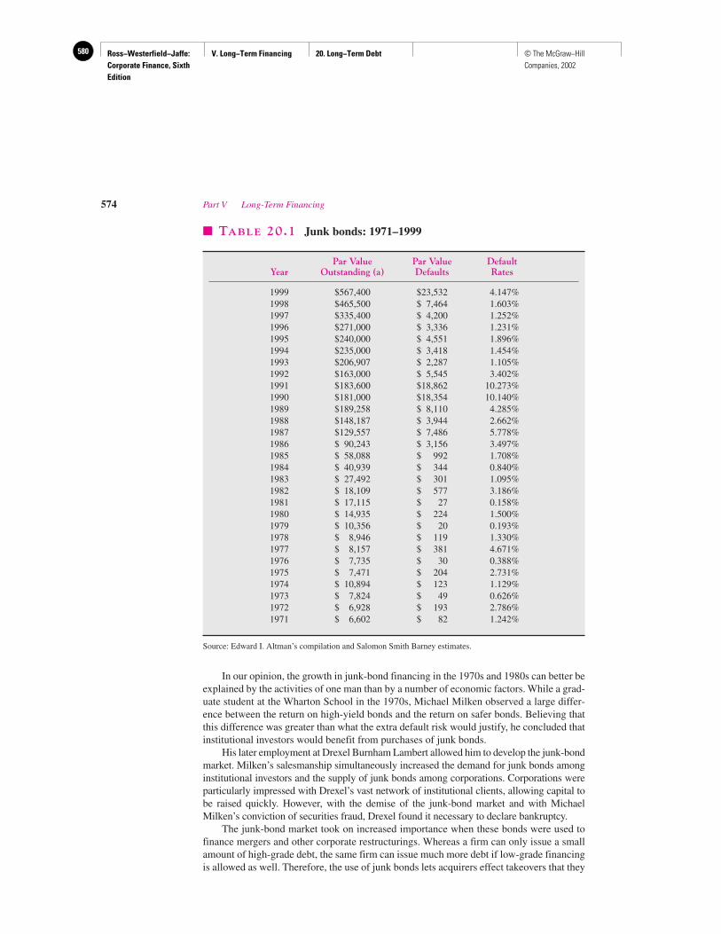
Ross−Westerfield−Jaffe: Corporate Finance, Sixth Edition
V. Long−Term Financing 20. Long−Term Debt580 © The McGraw−Hill Companies, 2002
In our opinion, the growth in junk-bond financing in the 1970s and 1980s can better beexplained by the activities of one man than by a number of economic factors. While a grad-uate student at the Wharton School in the 1970s, Michael Milken observed a large differ-ence between the return on high-yield bonds and the return on safer bonds. Believing thatthis difference was greater than what the extra default risk would justify, he concluded thatinstitutional investors would benefit from purchases of junk bonds.
His later employment at Drexel Burnham Lambert allowed him to develop the junk-bondmarket. Milken’s salesmanship simultaneously increased the demand for junk bonds amonginstitutional investors and the supply of junk bonds among corporations. Corporations wereparticularly impressed with Drexel’s vast network of institutional clients, allowing capital tobe raised quickly. However, with the demise of the junk-bond market and with MichaelMilken’s conviction of securities fraud, Drexel found it necessary to declare bankruptcy.
The junk-bond market took on increased importance when these bonds were used tofinance mergers and other corporate restructurings. Whereas a firm can only issue a smallamount of high-grade debt, the same firm can issue much more debt if low-grade financingis allowed as well. Therefore, the use of junk bonds lets acquirers effect takeovers that they
� TABLE 20.1 Junk bonds: 1971–1999
Par Value Par Value DefaultYear Outstanding (a) Defaults Rates
1999 $567,400 $23,532 4.147%1998 $465,500 $ 7,464 1.603%1997 $335,400 $ 4,200 1.252%1996 $271,000 $ 3,336 1.231%1995 $240,000 $ 4,551 1.896%1994 $235,000 $ 3,418 1.454%1993 $206,907 $ 2,287 1.105%1992 $163,000 $ 5,545 3.402%1991 $183,600 $18,862 10.273%1990 $181,000 $18,354 10.140%1989 $189,258 $ 8,110 4.285%1988 $148,187 $ 3,944 2.662%1987 $129,557 $ 7,486 5.778%1986 $ 90,243 $ 3,156 3.497%1985 $ 58,088 $ 992 1.708%1984 $ 40,939 $ 344 0.840%1983 $ 27,492 $ 301 1.095%1982 $ 18,109 $ 577 3.186%1981 $ 17,115 $ 27 0.158%1980 $ 14,935 $ 224 1.500%1979 $ 10,356 $ 20 0.193%1978 $ 8,946 $ 119 1.330%1977 $ 8,157 $ 381 4.671%1976 $ 7,735 $ 30 0.388%1975 $ 7,471 $ 204 2.731%1974 $ 10,894 $ 123 1.129%1973 $ 7,824 $ 49 0.626%1972 $ 6,928 $ 193 2.786%1971 $ 6,602 $ 82 1.242%
Source: Edward I. Altman’s compilation and Salomon Smith Barney estimates.
574 Part V Long-Term Financing

Ross−Westerfield−Jaffe: Corporate Finance, Sixth Edition
V. Long−Term Financing 20. Long−Term Debt 581© The McGraw−Hill Companies, 2002
IN THEIR OWN WORDS
Edward I. Altman on Junk Bonds
One of the most important developments in corporatefinance over the last 20 years has been the reemer-
gence of publicly owned and traded low-rated corporatedebt. Originally offered to the public in the early 1900sto help finance some of our emerging growth industries,these high-yield/high-risk bonds virtually disappearedafter the rash of bond defaults during the Depression.Recently, however, the junk-bond market has been cata-pulted from an insignificant element in the corporatefixed income market to one of the fastest growing andmost controversial types of financing mechanisms.
The term junk emanates from the dominant type oflow-rated bond issues outstanding prior to 1977 when the“market” consisted almost exclusively of original-issueinvestment-grade bonds that fell from their lofty status toa higher default risk, speculative-grade level. These so-called “fallen angels” amounted to about $8.5 billion in1977. At the beginning of 1998, fallen angels comprisedabout 10 percent of the $450 billion publicly ownedjunk-bond market.
Beginning in 1977, issuers began to go directly to thepublic to raise capital for growth purposes. Early users ofjunk bonds were energy-related firms, cable TVcompanies, airlines, and assorted other industrialcompanies. The emerging growth company rationale,coupled with relatively high returns to early investors,helped legitimize this sector. Most investment banksignored junk bonds until 1983–1984, when their meritsand profit potential became more evident.
Synonymous with the market’s growth was theemergence of the investment banking firm Drexel BurnhamLambert, and its junk-bond wizard, Michael Milken. Drexelestablished a potent network of issuers and investors androde the wave of new financing and the consequent surge insecondary trading to become one of the powerful invest-ment banks in the late 1980s. The incredible rise in powerof this firm was followed by an equally incredible fall,resulting first in government civil and criminal convictionsand huge fines for various misdealings and, finally, thefirm’s total collapse and bankruptcy in February 1990.
By far the most controversial aspect of junk-bondfinancing was its role in the corporate restructuringmovement from 1985–1989. High-leverage transactions,such as leveraged buyouts (LBOs), which occur when afirm is taken private, transformed the face of corporateAmerica, leading to a heated debate as to the economicand social consequences of corporate control changeswith debt/equity ratios of at least 6:1.
These transactions involved increasingly largecompanies, and the multibillion dollar takeover became
fairly common, capped by the huge $25 billion RJRNabisco LBO in 1989. LBOs were typically financed with60-percent senior bank and insurance company debt, about25–30-percent subordinated public debt (junk bonds), and10–15-percent equity. The junk-bond segment is sometimesreferred to as “mezzanine” financing because it lies betweenthe “balcony” senior debt and the “basement” equity.
These restructurings resulted in large fees to advisorsand underwriters and huge premiums to the old share-holders, and they continued as long as the market waswilling to buy these new debt offerings at what appeared tobe a favorable risk/return trade-off. The bottom fell out ofthe market in the last six months of 1989 due to a number offactors including a marked increase in defaults, governmentregulation against S&Ls holding junk bonds, higher interestrates, a recession, and, finally, the growing realization of theleverage excesses of certain ill-conceived restructurings.
The default rate rose dramatically to over 4 percent in1989 and then skyrocketed in 1990 and 1991 to over 10percent each year, with about $19 billion of defaults in1991. Throughout 1990, the pendulum of growth in thenew junk-bond issues and returns to investors swungdramatically downward as prices plummeted and the newissue market all but dried up. The following year (1991)was a pivotal period in that despite record defaults, bondprices and new issues rebounded strongly as theprospects for the future brightened.
In the early 1990s, the financial market was ques-tioning the very survival of the junk-bond market. Theanswer was a resounding “Yes,” as the amount of newissuance soared to record annual levels of $38 billion in1992 and has steadily grown to an incredible $120 billionin 1997! Coupled with plummeting annual default rates(under 2.0 percent from 1993–1997 compared to 3.5percent for 1971–1997) and returns in these years between10–20 percent, the risk-return characteristics have beenextremely favorable. Newer dimensions of the junk-bondmarket include the pooling of large numbers of bonds intocollateralized bond obligations (CBOs), the establishmentof emerging market international issuance, and the nowcommon use of the nonregistered 144A new issuancemechanism. The junk-bond market in the late 1990s is aquieter one compared to the 1980s, but, in terms of growthand returns, it is healthier than ever before.
Dr. Edward I. Altman is Max L. Heine Professor of Finance andVice Director of the Salomon Center at the Stern School ofBusiness of New York University. He is widely recognized asone of the world’s experts on bankruptcy and credit analysis aswell as the high-yield or junk-bond market.
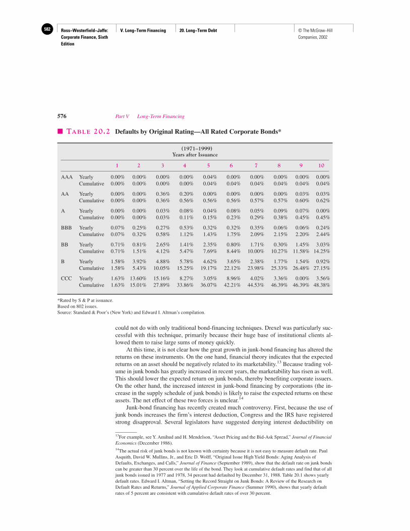
Ross−Westerfield−Jaffe: Corporate Finance, Sixth Edition
V. Long−Term Financing 20. Long−Term Debt582 © The McGraw−Hill Companies, 2002
could not do with only traditional bond-financing techniques. Drexel was particularly suc-cessful with this technique, primarily because their huge base of institutional clients al-lowed them to raise large sums of money quickly.
At this time, it is not clear how the great growth in junk-bond financing has altered thereturns on these instruments. On the one hand, financial theory indicates that the expectedreturns on an asset should be negatively related to its marketability.13 Because trading vol-ume in junk bonds has greatly increased in recent years, the marketability has risen as well.This should lower the expected return on junk bonds, thereby benefiting corporate issuers.On the other hand, the increased interest in junk-bond financing by corporations (the in-crease in the supply schedule of junk bonds) is likely to raise the expected returns on theseassets. The net effect of these two forces is unclear.14
Junk-bond financing has recently created much controversy. First, because the use ofjunk bonds increases the firm’s interest deduction, Congress and the IRS have registeredstrong disapproval. Several legislators have suggested denying interest deductibility on
576 Part V Long-Term Financing
13For example, see Y. Amihud and H. Mendelson, “Asset Pricing and the Bid-Ask Spread,” Journal of FinancialEconomics (December 1986).14The actual risk of junk bonds is not known with certainty because it is not easy to measure default rate. PaulAsquith, David W. Mullins, Jr., and Eric D. Wolff, “Original Issue High Yield Bonds: Aging Analysis ofDefaults, Exchanges, and Calls,” Journal of Finance (September 1989), show that the default rate on junk bondscan be greater than 30 percent over the life of the bond. They look at cumulative default rates and find that of alljunk bonds issued in 1977 and 1978, 34 percent had defaulted by December 31, 1988. Table 20.1 shows yearlydefault rates. Edward I. Altman, “Setting the Record Straight on Junk Bonds: A Review of the Research onDefault Rates and Returns,” Journal of Applied Corporate Finance (Summer 1990), shows that yearly defaultrates of 5 percent are consistent with cumulative default rates of over 30 percent.
� TABLE 20.2 Defaults by Original Rating—All Rated Corporate Bonds*
(1971–1999)Years after Issuance
1 2 3 4 5 6 7 8 9 10
AAA Yearly 0.00% 0.00% 0.00% 0.00% 0.04% 0.00% 0.00% 0.00% 0.00% 0.00%Cumulative 0.00% 0.00% 0.00% 0.00% 0.04% 0.04% 0.04% 0.04% 0.04% 0.04%
AA Yearly 0.00% 0.00% 0.36% 0.20% 0.00% 0.00% 0.00% 0.00% 0.03% 0.03%Cumulative 0.00% 0.00% 0.36% 0.56% 0.56% 0.56% 0.57% 0.57% 0.60% 0.62%
A Yearly 0.00% 0.00% 0.03% 0.08% 0.04% 0.08% 0.05% 0.09% 0.07% 0.00%Cumulative 0.00% 0.00% 0.03% 0.11% 0.15% 0.23% 0.29% 0.38% 0.45% 0.45%
BBB Yearly 0.07% 0.25% 0.27% 0.53% 0.32% 0.32% 0.35% 0.06% 0.06% 0.24%Cumulative 0.07% 0.32% 0.58% 1.12% 1.43% 1.75% 2.09% 2.15% 2.20% 2.44%
BB Yearly 0.71% 0.81% 2.65% 1.41% 2.35% 0.80% 1.71% 0.30% 1.45% 3.03%Cumulative 0.71% 1.51% 4.12% 5.47% 7.69% 8.44% 10.00% 10.27% 11.58% 14.25%
B Yearly 1.58% 3.92% 4.88% 5.78% 4.62% 3.65% 2.38% 1.77% 1.54% 0.92%Cumulative 1.58% 5.43% 10.05% 15.25% 19.17% 22.12% 23.98% 25.33% 26.48% 27.15%
CCC Yearly 1.63% 13.60% 15.16% 8.27% 3.05% 8.96% 4.02% 3.36% 0.00% 3.56%Cumulative 1.63% 15.01% 27.89% 33.86% 36.07% 42.21% 44.53% 46.39% 46.39% 48.38%
*Rated by S & P at issuance.Based on 802 issues.Source: Standard & Poor’s (New York) and Edward I. Altman’s compilation.
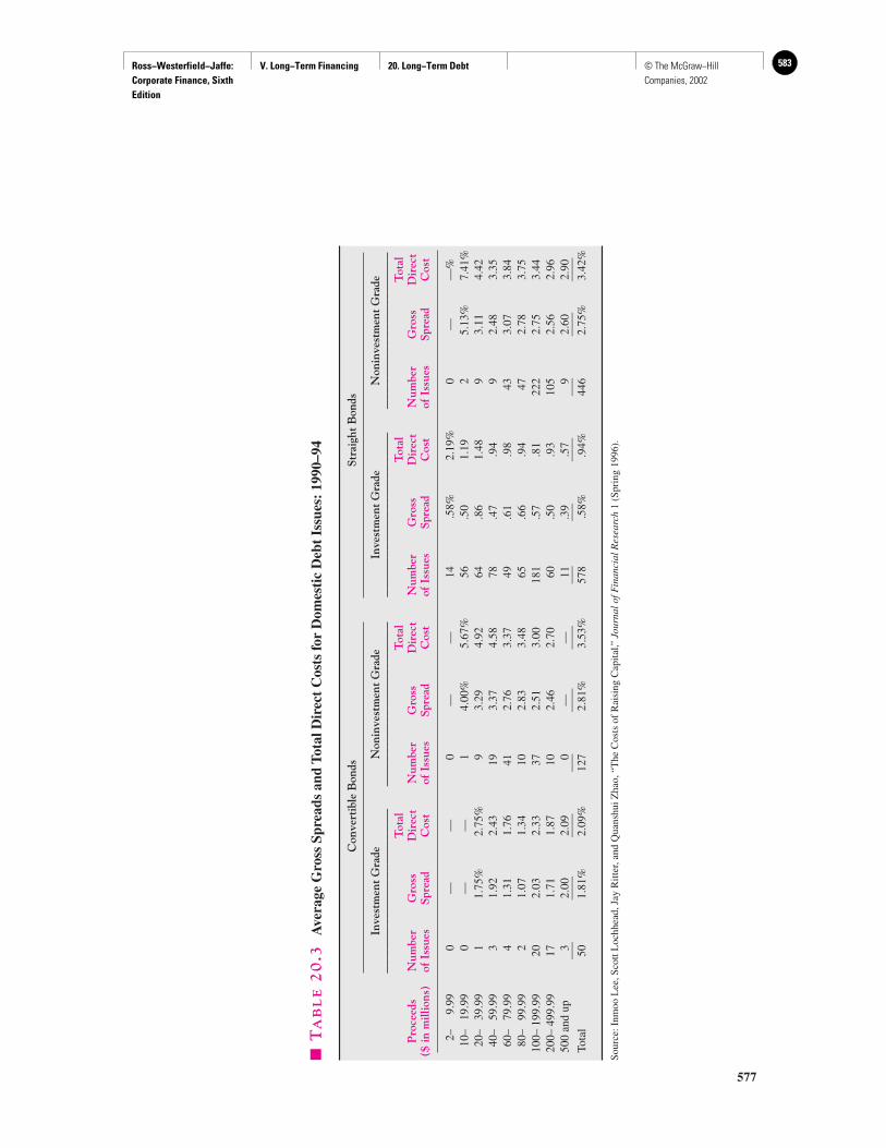
Ross−Westerfield−Jaffe: Corporate Finance, Sixth Edition
V. Long−Term Financing 20. Long−Term Debt 583© The McGraw−Hill Companies, 2002
577
�T
AB
LE
20
.3A
vera
ge G
ross
Spr
eads
and
Tot
al D
irec
t C
osts
for
Dom
esti
c D
ebt
Issu
es:
1990
–94
Con
vert
ible
Bon
dsSt
raig
ht B
onds
Inve
stm
ent
Gra
deN
onin
vest
men
t G
rade
Inve
stm
ent
Gra
deN
onin
vest
men
t G
rade
____
____
____
____
____
___
____
____
____
____
___
____
____
____
____
____
___
____
____
____
____
__T
otal
Tot
alT
otal
Tot
alP
roce
eds
Num
ber
Gro
ssD
irec
tN
umbe
rG
ross
Dir
ect
Num
ber
Gro
ssD
irec
tN
umbe
rG
ross
Dir
ect
($ in
mill
ions
)of
Iss
ues
Spre
adC
ost
of I
ssue
sSp
read
Cos
tof
Iss
ues
Spre
adC
ost
of I
ssue
sSp
read
Cos
t
2–9.
990
——
0—
—14
.58%
2.19
%0
——
%10
– 19
.99
0—
—1
4.00
%5.
67%
56.5
01.
192
5.13
%7.
41%
20–
39.9
91
1.75
%2.
75%
93.
294.
9264
.86
1.48
93.
114.
4240
– 59
.99
31.
922.
4319
3.37
4.58
78.4
7.9
49
2.48
3.35
60–
79.9
94
1.31
1.76
412.
763.
3749
.61
.98
433.
073.
8480
– 99
.99
21.
071.
3410
2.83
3.48
65.6
6.9
447
2.78
3.75
100–
199
.99
202.
032.
3337
2.51
3.00
181
.57
.81
222
2.75
3.44
200–
499
.99
171.
711.
8710
2.46
2.70
60.5
0.9
310
52.
562.
9650
0 an
d up
32.
002.
090
——
11.3
9.5
79
2.60
2.90
___
____
____
___
____
____
___
___
____
___
____
____
Tota
l50
1.81
%2.
09%
127
2.81
%3.
53%
578
.58%
.94%
446
2.75
%3.
42%
Sour
ce:I
nmoo
Lee
,Sco
tt L
ochh
ead,
Jay
Ritt
er,a
nd Q
uans
hui Z
hao,
“The
Cos
ts o
f R
aisi
ng C
apita
l,”Jo
urna
l of F
inan
cial
Res
earc
h1
(Spr
ing
1996
).
Ross−Westerfield−Jaffe: Corporate Finance, Sixth Edition
V. Long−Term Financing 20. Long−Term Debt584 © The McGraw−Hill Companies, 2002
junk bonds, particularly when the bonds are used to finance mergers. Second, the media hasfocused on the effect of junk-bond financing on corporate solvency. Clearly, this form of fi-nancing permits the possibility of higher debt-equity ratios. Whether or not this increasedleverage will lead to wholesale defaults in an economic downturn, as some commentatorshave suggested, remains to be seen. Third, the recent wave of mergers has often resulted indislocations and loss of jobs. Because junk-bond financing has played a role in mergers, ithas come under much criticism. The social policy implications of mergers are quite com-plex, and any final judgment on them is likely to be reserved for the distant future. At anyrate, junk-bond financing should not be implicated too strongly in either the social benefitsor the social costs of the recent wave of mergers. Perry and Taggart point out that, contraryto popular belief, this form of financing accounts for only a few percent of all mergers.15
We discussed the costs of issuing securities in Chapter 19 and established that the costsof issuing debt are substantially less than the costs of issuing equity. Table 20.3 clarifies sev-eral questions regarding the costs of issuing debt securities. It contains a breakdown of directcosts for bond issues after the investment and noninvestment grades have been separated.
First, there are substantial economies of scale here as well. Second, investment-grade is-sues have much lower direct costs, particularly for straight bonds. Finally, there are relativelyfew noninvestment-grade issues in the smaller size categories, reflecting the fact that such is-sues are more commonly handled as private placements, which we discuss in a later section.
• List and describe the different bond-rating classes.• Why don’t bond prices change when bond ratings change?• Are the costs of bond issues related to their ratings?
20.5 SOME DIFFERENT TYPES OF BONDS
Until now we have considered “plain vanilla” bonds. In this section we look at some moreunusual types: floating-rate bonds, deep-discount bonds, and income bonds.
Floating-Rate BondsThe conventional bonds we have discussed in this chapter have fixed-dollar obligations.That is, the coupon rate is set as a fixed percentage of the par value.
With floating-rate bonds, the coupon payments are adjustable. The adjustments are tied toan interest-rate index such as the Treasury-bill interest rate or the 30-year Treasury-bond rate.For example, in 1974 Citibank issued $850 million of floating-rate notes maturing in 1989. Thecoupon rate was set at 1 percent above the 90-day Treasury-bill rate and adjusted semiannually.
In most cases the coupon adjusts with a lag to some base rate. For example, suppose acoupon-rate adjustment is made on June 1. The adjustment may be from a simple averageof yields on six-month Treasury bills issued during March, April, and May. In addition, themajority of these floaters have put provisions and floor-and-ceiling provisions:
1. With a put provision the holder has the right to redeem his or her note at par on thecoupon payment date. Frequently, the investor is prohibited from redeeming at par dur-ing the first few years of the bond’s life.
2. With floor-and-ceiling provisions the coupon rate is subject to a minimum and maxi-mum. For example, the minimum coupon rate might be 8 percent and the maximum ratemight be 14 percent.
578 Part V Long-Term Financing
15K. Perry and R. Taggart, “The Growing Role of Junk Bonds in Corporate Finance,” Journal of AppliedCorporate Finance (Spring 1988).
QUESTIONS
CO
NC
EP
T
?
Ross−Westerfield−Jaffe: Corporate Finance, Sixth Edition
V. Long−Term Financing 20. Long−Term Debt 585© The McGraw−Hill Companies, 2002
The popularity of floating-rate bonds is connected to inflation risk. When inflation ishigher than expected, issuers of fixed-rate bonds tend to make gains at the expense oflenders, and when inflation is less than expected, lenders make gains at the expense of bor-rowers. Because the inflation risk of long-term bonds is borne by both issuers and bond-holders, it is in their interests to devise loan agreements that minimize inflation risk.16
Floaters reduce inflation risk because the coupon rate is tied to the current interest rate,which, in turn, is influenced by the rate of inflation. This can most clearly be seen by consider-ing the formula for the present value of a bond. As inflation increases the interest rate (the denominator of the formula), inflation increases a floater’s coupon rate (the numerator of the for-mula). Hence, bond value is hardly affected by inflation. Conversely, the coupon rate of fixed-ratebonds cannot change, implying that the prices of these bonds are at the mercy of inflation.
As an alternative, an individual who is concerned with inflation risk can invest in short-term notes, such as Treasury bills, and roll them over.17 The investor can accomplish es-sentially the same objective by buying a floater that is adjusted to the Treasury-bill rate.However, the purchaser of a floater can reduce transactions costs relative to rolling overshort-term Treasury bills because floaters are long-term bonds. The same type of reductionin transactions costs makes floaters attractive to some corporations.18 They benefit from is-suing a floater instead of issuing a series of short-term notes.
In an earlier section, we discussed callable bonds. Because the coupon on floatersvaries with marketwide interest rates, floaters always sell at or near par. Therefore, it is notsurprising that floaters do not generally have call features.
Deep-Discount BondsA bond that pays no coupon must be offered at a price that is much lower than its facevalue. Such bonds are known as original-issue discount bonds, deep-discount bonds,pure-discount bonds, or zero-coupon bonds. They are frequently called zeros for short.
Suppose the DDB Company issues $1,000 of five-year deep-discount bonds when themarketwide interest rate is 10 percent. These bonds do not pay any coupons. The initialprice is set at $621 because $621 � $1,000/(1.10)5.
Because these bonds have no intermediate coupon payments, they are quite attractiveto certain investors and quite unattractive to others. For example, consider an insurancecompany forecasting death-benefit payments of $1,000,000 five years from today. Thecompany would like to be sure that it will have the funds to pay off the liability in five years’time. The company could buy five-year zero-coupon bonds with a face value of $1,000,000.The company is matching assets with liabilities here, a procedure that eliminates interest-rate risk. That is, regardless of the movement of interest rates, the firm’s set of zeros will al-ways be able to pay off the $1,000,000 liability.
Conversely, the firm would be at risk if it bought coupon bonds instead. For example,if it bought five-year coupon bonds, it would need to reinvest the coupon payments throughto the fifth year. Because interest rates in the future are not known with certainty today, onecannot be sure if these bonds will be worth more or less than $1,000,000 by the fifth year.
Now, consider a couple saving for their child’s college education in 15 years. They ex-pect that, with inflation, four years of college should cost $150,000 in 15 years. Thus, they
Chapter 20 Long-Term Debt 579
16See B. Cornell, “The Future of Floating Rate Bonds,” in The Revolution in Corporate Finance, ed. by J. M.Stern and D. H. Chew, Jr. (New York: Basil Blackwell, 1986).17That is, the investor could buy a bill, receive the face value at maturity, use these proceeds to buy a secondbill, receive the face value from the second bill at maturity, and so on.18Cox, Ingersoll, and Ross developed a framework for pricing floating-rate notes; see J. Cox, J. Ingersoll, andS. A. Ross, “An Analysis of Variable Rate Loan Contracts,” Journal of Finance 35 (May 1980).
Ross−Westerfield−Jaffe: Corporate Finance, Sixth Edition
V. Long−Term Financing 20. Long−Term Debt586 © The McGraw−Hill Companies, 2002
580 Part V Long-Term Financing
buy 15-year zero-coupon bonds with a face value of $150,000.19 If they have forecasted in-flation perfectly (and if college costs keep pace with inflation), their child’s tuition will befully funded. However, if inflation rises more than expected, the tuition would be more than$150,000. Because the zero-coupon bonds produce a shortfall, the child might end up work-ing his way through school. As an alternative, the parents might have considered rollingover Treasury bills. Because the yields on Treasury bills rise and fall with the inflation rate,this simple strategy is likely to cause less risk than the strategy with zeros.
The key to these examples concerns the distinction between nominal and real quantities.The insurance company’s liability is $1,000,000 in nominal dollars. Because the face valueof a zero-coupon bond is a nominal quantity, the purchase of zeros eliminates risk. However,it is easier to forecast college costs in real terms than in nominal terms. Thus, a zero-couponbond is a poor choice to reduce the financial risk of a child’s college education.
Income BondsIncome bonds are similar to conventional bonds, except that coupon payments are de-pendent on company income. Specifically, coupons are paid to bondholders only if thefirm’s income is sufficient.
Income bonds are a financial puzzle because, from the firm’s standpoint, they appear tobe a cheaper form of debt than conventional bonds. Income bonds provide the same tax ad-vantage to corporations from interest deductions that conventional bonds do. However, a com-pany that issues income bonds is less likely to experience financial distress. When a couponpayment is omitted because of insufficient corporate income, an income bond is not in default.
Why don’t firms issue more income bonds? Two explanations have been offered:
1. The “Smell of Death” Explanation. Firms that issue income bonds signal the capitalmarkets of their increased prospect of financial distress.
2. The “Dead-Weight Costs” Explanation. The calculation of corporate income is crucialto determining the status of bondholders’ income, and stockholders and bondholderswill not necessarily agree on how to calculate the income. This creates agency costs as-sociated with the firm’s accounting methods.
Although these are possibilities, the work of McConnell and Schlarbaum suggests that notruly satisfactory reason exists for the lack of more investor interest in income bonds.20
• Create an idea of an unusual bond and analyze its features.
20.6 DIRECT PLACEMENT COMPARED TO PUBLIC ISSUES
Earlier in this chapter, we described the mechanics of issuing debt to the public. However,more than 50 percent of all debt is privately placed. There are two basic forms of direct pri-vate long-term financing: term loans and private placement.
Term loans are direct business loans with maturities of between 1 year and 15 years. Thetypical term loan is amortized over the life of the loan. That is, the loan is repaid by equal
QUESTION
CO
NC
EP
T
?
19A more precise strategy would be to buy zeros maturing in years 15, 16, 17, and 18, respectively. In this way,the bonds might mature just in time to meet tuition payments.20J. McConnell and G. Schlarbaum, “The Income Bond Puzzle,” in The Revolution in Corporate Finance. ed. byJ. M. Stern and D. H. Chew, Jr. (New York: Basil Blackwell, 1986).
Ross−Westerfield−Jaffe: Corporate Finance, Sixth Edition
V. Long−Term Financing 20. Long−Term Debt 587© The McGraw−Hill Companies, 2002
Chapter 20 Long-Term Debt 581
annual payments of interest and principal. The lenders are commercial banks and insurancecompanies. A private placement, which also involves the sale of a bond or loan directly toa limited number of investors, is very similar to a term loan except that the maturity is longer.
Some important differences between direct long-term financing and public issues are:
1. A direct long-term loan avoids the cost of registration with the Securities and ExchangeCommission.
2. Direct placement is likely to have more restrictive covenants.
3. It is easier to renegotiate a term loan and a private placement in the event of a default. Itis harder to renegotiate a public issue because hundreds of holders are usually involved.
4. Life insurance companies and pension funds dominate the private-placement segment ofthe bond market. Commercial banks are significant participants in the term-loan market.
5. The costs of distributing bonds are lower in the private market.
The interest rates on term loans and private placements are usually higher than those onan equivalent public issue. Hayes, Joehnk, and Melicher found that the yield to maturity onprivate placements was 0.46 percent higher than on similar public issues.21 This finding re-flects the trade-off between a higher interest rate and more flexible arrangements in the eventof financial distress, as well as the lower transaction costs associated with private placements.
• What are the differences between private and public bond issues?• A private placement is more likely to have restrictive covenants than is a public issue. Why?
20.7 LONG-TERM SYNDICATED BANK LOANS
Most bank loans are for less than a year. They serve as a short-term “bridge” for the acqui-sition of inventory and are typically self-liquidating—that is, when the firm sells the in-ventory, the cash is used to repay the bank loan. We talk about the need for short-term bankloans in the next section of the text. Now we focus on long-term bank loans.
First, we introduce the concept of commitment. Most bank loans are made with a com-mitment to a firm. That commitment establishes a line of credit and allows the firm to borrowup to a predetermined limit. Most commitments are in the form of a revolving credit commit-ment (i.e., a revolver) with a fixed term of up to three years or more. Revolving credit com-mitments are drawn or undrawn depending on whether the firm has a current need for the funds.
Now we turn to the concept of syndication. Very large banks such as Citigroup typi-cally have a larger demand for loans than they can supply, and small regional banks fre-quently have more funds on hand than they can profitably lend to existing customers.Basically, they cannot generate enough good loans with the funds they have available. As aresult, a very large bank may arrange a loan with a firm or country and then sell portions ofit to a syndicate of other banks. With a syndicated loan, each bank has a separate loan agree-ment with the borrowers.
A syndicated loan is a corporate loan made by a group (or syndicate) of banks and otherinstitutional investors. A syndicated loan may be publicly traded. It may be a line of creditand be “undrawn” or it may be drawn and be used by a firm. Syndicated loans are alwaysrated investment grade. However, a leveraged syndicated loan is rated speculative grade(i.e., it is “junk”). Every week, The Wall Street Journal reports on the number of syndicated
21P. A. Hayes, M. D. Joehnk, and R. W. Melicher, “Determinants of Risk Premiums in the Public and PrivateBond Market,” Journal of Financial Research (Fall 1979).
QUESTIONS
CO
NC
EP
T
?
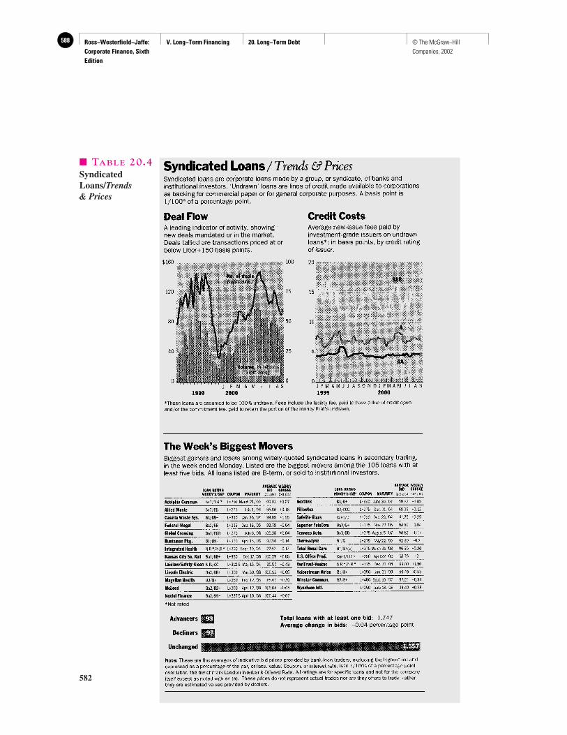
Ross−Westerfield−Jaffe: Corporate Finance, Sixth Edition
V. Long−Term Financing 20. Long−Term Debt588 © The McGraw−Hill Companies, 2002
582
� TABLE 20.4SyndicatedLoans/Trends & Prices

Ross−Westerfield−Jaffe: Corporate Finance, Sixth Edition
V. Long−Term Financing 20. Long−Term Debt 589© The McGraw−Hill Companies, 2002
loan deals, credit costs, and yields, as seen in Table 20.4. In addition, syndicated loan pricesare reported for a group of publicly traded loans. Altman and Suggitt report slightly higherdefault rates for syndicated loans when compared to comparable corporate bonds.22
20.8 SUMMARY AND CONCLUSIONS
This chapter describes some important aspects of long-term debt financing.
1. The written agreement describing the details of the long-term debt contract is called anindenture. Some of the main provisions are security, repayment, protective covenants, andcall provisions.
2. There are many ways that shareholders can take advantage of bondholders. Protectivecovenants are designed to protect bondholders from management decisions that favorstockholders at bondholders’ expense.
3. Unsecured bonds are called debentures or notes. They are general claims on the company’svalue. Most public industrial bonds are unsecured. In contrast, utility bonds are usuallysecured. Mortgage bonds are secured by tangible property, and collateral trust bonds aresecured by financial securities such as stocks and bonds. If the company defaults on securedbonds, the trustee can repossess the assets. This makes secured bonds more valuable.
4. Long-term bonds usually provide for repayment of principal before maturity. This isaccomplished by a sinking fund. With a sinking fund, the company retires a certain numberof bonds each year. A sinking fund protects bondholders because it reduces the averagematurity of the bond, and its payment signals the financial condition of the company.
5. Most publicly issued bonds are callable. A callable bond is less attractive to bondholders thana noncallable bond. A callable bond can be bought back by the company at a call price that isless than the true value of the bond. As a consequence, callable bonds are priced to obtainhigher stated interest rates for bondholders than noncallable bonds.
Generally, companies should exercise the call provision whenever the bond’s value isgreater than the call price.
There is no single reason for call provisions. Some sensible reasons include taxes, greaterflexibility, management’s ability to predict interest rates, and the fact that callable bonds areless sensitive to interest-rate changes.
6. There are many different types of bonds, including floating-rate bonds, deep-discount bonds,and income bonds. This chapter also compares private placement with public issuance.
KEY TERMS
Bearer 566 Negative covenant 567Call premium 568 Original-issue discount bonds 579Call-protected 568 Positive covenant 567Debenture 567 Private placement 581Deep-discount bonds 579 Protective covenant 567Deferred call 568 Public issue 564Floating-rate bonds 578 Pure-discount bonds 579Income bonds 580 Refunding 568Indenture 564 Zero-coupon bonds 579Junk bonds 573
Chapter 20 Long-Term Debt 583
22Edward I. Altman and Heather J. Suggitt, “Default Rates in the Syndicated Bank Loan Market: ALongitudinal Analysis,” Journal of Banking and Finance 24 (2000).

Ross−Westerfield−Jaffe: Corporate Finance, Sixth Edition
V. Long−Term Financing 20. Long−Term Debt590 © The McGraw−Hill Companies, 2002
SUGGESTED READING
The following provides a complete coverage of bonds and the bond market:Fabozzi, F. J., and T. D. Fabozzi, eds. The Handbook of Fixed Income Securities. 4th ed.
Homewood, Ill.: Irwin Professional Publishing, 1995.
QUESTIONS AND PROBLEMS
The Public Issue of Bonds20.1 Raeo Corp. bonds trade at 100 today. The bonds pay semiannual interest that is paid on
January 1 and July 1. The coupon on the bonds is 10 percent. How much will you pay fora Raeo bond if today isa. March 1.b. October 1.c. July 1.d. August 15.
20.2 Define the following terms:a. Protective covenantb. Negative covenantc. Positive covenantd. Sinking fund
20.3 Sinking funds have both positive and negative characteristics to the bondholders. Why?
20.4 Which is riskier to a prospective creditor, an open-end mortgage or closed-endmortgage? Why?
20.5 What is call premium? During what period of time is a bond said to be call-protected?
Bond Refunding20.6 KIC, Inc., plans to issue $5 million of perpetual bonds. The face value of each bond is
$1,000. The annual coupon on the bonds is 12 percent. Market interest rates on one-yearbonds are 11 percent. With equal probability, the long-term market interest rate will beeither 14 percent or 7 percent next year. Assume investors are risk-neutral.a. If the KIC bonds are noncallable, what is the price of the bonds?b. If the bonds are callable one year from today at $1,450, will their price be greater than
or less than the price you computed in part (a)? Why?
20.7 Bowdeen Manufacturing intends to issue callable, perpetual bonds. The bonds are callableat $1,250. One-year interest rates are 12 percent. There is a 60-percent probability thatlong-term interest rates one year from today will be 15 percent. With a 40-percentprobability, long-term interest rates will be 8 percent. To simplify the firm’s accounting,Bowdeen would like to issue the bonds at par ($1,000). What must the coupon on thebonds be for Bowdeen to be able to sell them at par?
20.8 Illinois Industries has decided to borrow money by issuing perpetual bonds. The face valueof the bonds will be $1,000. The coupon will be 8 percent, payable annually. The one-yearinterest rate is 8 percent. It is known that next year there is a 65-percent chance thatinterest rates will decline to 6 percent, and that there is a 35-percent chance that they willrise to 9 percent.a. What will the market value of these bonds be if they are noncallable?b. If the company instead decides to make the bonds callable, what coupon will be
demanded by the bondholders for the bonds to sell at par? Assume that the bonds canbe called in one year (i.e., the call date is one year from now) and that the call premiumis equal to the annual coupon.
c. What will be the value of the call provision to Illinois Industries?
584 Part V Long-Term Financing
Ross−Westerfield−Jaffe: Corporate Finance, Sixth Edition
V. Long−Term Financing 20. Long−Term Debt 591© The McGraw−Hill Companies, 2002
20.9 New Business Ventures, Inc., has an outstanding perpetual bond with a face value equalto $1,000 and a 9-percent coupon rate. The bond cannot be called for one year. The callpremium is set at $150 over par value. It is forecasted that there is a 40-percent chancethat the interest rate will rise to 12-percent, and a 60-percent chance that the interest ratewill fall down to 6 percent next year. The current interest rate is 10 percent. What is thecurrent market price of this callable bond?
20.10 Hudson River Electronics has $500 million of 9-percent perpetual bonds outstanding. Thesebonds can be called at a price of $1,090 for each $1,000 of face value. Under present marketconditions, the outstanding bonds can be replaced by $500 million of 7-percent perpetualbonds. The underwriting and legal expenses of this new issue would be $80 million. Whatwould be the net present value of this refunding? Assume that there are no taxes.
20.11 An outstanding issue of Public Express Airlines debentures has a call provision attached.The total principal value of the bonds is $250 million, and the bonds pay an annualcoupon of $80 for each $1,000 of face value. The total cost of refunding would be 12percent of the principal amount raised. The appropriate tax rate for the company is 35percent. How low does the borrowing cost of Public Express need to drop to justifyrefunding with a new bond issue?
20.12 Margret Kimberly, CFO of Charles River Associates, is considering whether or not torefinance the two currently outstanding corporate bonds of the firm. The first one is an8-percent perpetual bond with a $1,000 face value with $75 million outstanding. Thesecond one is a 9-percent perpetual bond with the same face value with $87.5 millionoutstanding. The call premiums for the two bonds are 8.5 percent and 9.5 percent ofthe face value, respectively. The transaction costs of the refundings are $10 million and$12 million, respectively. The current interest rates for the two bonds are 7 percent and7.25 percent, respectively. Which bond should Ms. Kimberly recommend berefinanced? What is the NPV of the refunding?
Some Different Types of Bonds20.13 What is a “junk bond”? What are some of the controversies created by junk-bond financing?20.14 Describe the following types of bonds:
a. Floating rateb. Deep discountc. Income
Direct Placement Compared to Public Issues20.15 Which of the following are characteristics of public issues, and which are characteristics
of direct financing?a. SEC registration requiredb. Higher interest costc. Higher fixed costd. Quicker access to fundse. Active secondary marketf. Easily renegotiatedg. Lower flotation costsh. Regular amortization requiredi. Ease of repurchase at favorable pricesj. High total cost to small borrowersk. Flexible termsl. Less intensive investigation required
General Topics20.16 a. In an efficient market callable and noncallable bonds will be priced in such a way that
there will be no advantage or disadvantage to the call provision. Comment.b. If interest rates fall, will the price of noncallable bonds move up higher than that of
callable bonds? Why or why not?
Chapter 20 Long-Term Debt 585
Ross−Westerfield−Jaffe: Corporate Finance, Sixth Edition
V. Long−Term Financing 21. Leasing592 © The McGraw−Hill Companies, 2002
Leasing
CH
AP
TE
R21
EXECUTIVE SUMMARY
Almost any asset that can be purchased can be leased, from aircraft to zithers. Whenwe take vacations or business trips, renting a car for a few days frequently seems aconvenient thing to do. This is an example of a short-term lease. After all, buying
a car and selling it a few days later would be a great nuisance.Corporations lease both short-term and long-term, but this chapter is primarily con-
cerned with long-term leasing over a term of more than five years. Long-term leasing is amethod of financing property, plant, and equipment. More equipment is financed today bylong-term leases than by any other method of equipment financing.1
Every lease contract has two parties: the lessee and the lessor. The lessee is the user ofthe equipment, and the lessor is the owner. Typically, the lessee first decides on the assetneeded and then negotiates a lease contract with a lessor. From the lessee’s standpoint, long-term leasing is similar to buying the equipment with a secured loan. The terms of the leasecontract are compared to what a banker might arrange with a secured loan. Thus, long-termleasing is a form of financing.
Many questionable advantages are claimed for long-term leasing, such as “leasing pro-vides 100-percent financing,” or “leasing conserves capital.” However, the principal bene-fit of long-term leasing is tax reduction. Leasing allows the transfer of tax benefits fromthose who need equipment but cannot take full advantage of the tax benefits associated withownership to a party who can. If the corporate income tax were repealed, long-term leasingwould virtually disappear.
21.1 TYPES OF LEASES
The BasicsA lease is a contractual agreement between a lessee and lessor. The agreement establishesthat the lessee has the right to use an asset and in return must make periodic payments tothe lessor, the owner of the asset. The lessor is either the asset’s manufacturer or an inde-pendent leasing company. If the lessor is an independent leasing company, it must buy theasset from a manufacturer. Then the lessor delivers the asset to the lessee, and the lease goesinto effect.
As far as the lessee is concerned, it is the use of the asset that is most important, notwho owns the asset. The use of an asset can be obtained by a lease contract. Because theuser can also buy the asset, leasing and buying involve alternative financing arrangementsfor the use of an asset. This is illustrated in Figure 21.1.
1P. K. Nevitt and F. J. Fabozzi, Equipment Leasing, 2nd ed. (Homewood, Ill.: Dow Jones-Irwin, 1985).
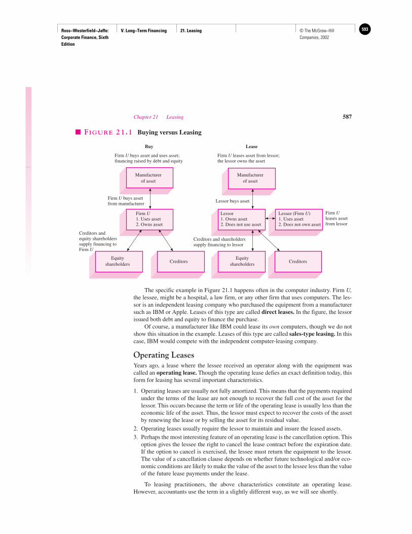
Ross−Westerfield−Jaffe: Corporate Finance, Sixth Edition
V. Long−Term Financing 21. Leasing 593© The McGraw−Hill Companies, 2002
Chapter 21 Leasing 587
The specific example in Figure 21.1 happens often in the computer industry. Firm U,the lessee, might be a hospital, a law firm, or any other firm that uses computers. The les-sor is an independent leasing company who purchased the equipment from a manufacturersuch as IBM or Apple. Leases of this type are called direct leases. In the figure, the lessorissued both debt and equity to finance the purchase.
Of course, a manufacturer like IBM could lease its own computers, though we do notshow this situation in the example. Leases of this type are called sales-type leasing. In thiscase, IBM would compete with the independent computer-leasing company.
Operating LeasesYears ago, a lease where the lessee received an operator along with the equipment wascalled an operating lease. Though the operating lease defies an exact definition today, thisform for leasing has several important characteristics.
1. Operating leases are usually not fully amortized. This means that the payments requiredunder the terms of the lease are not enough to recover the full cost of the asset for thelessor. This occurs because the term or life of the operating lease is usually less than theeconomic life of the asset. Thus, the lessor must expect to recover the costs of the assetby renewing the lease or by selling the asset for its residual value.
2. Operating leases usually require the lessor to maintain and insure the leased assets.
3. Perhaps the most interesting feature of an operating lease is the cancellation option. Thisoption gives the lessee the right to cancel the lease contract before the expiration date.If the option to cancel is exercised, the lessee must return the equipment to the lessor.The value of a cancellation clause depends on whether future technological and/or eco-nomic conditions are likely to make the value of the asset to the lessee less than the valueof the future lease payments under the lease.
To leasing practitioners, the above characteristics constitute an operating lease.However, accountants use the term in a slightly different way, as we will see shortly.
Firm U buys asset and uses asset;financing raised by debt and equity
Creditors andequity shareholderssupply financing toFirm U
Manufacturerof asset
Firm U1. Uses asset2. Owns asset
Firm U leases asset from lessor;the lessor owns the asset
Firm U buys assetfrom manufacturer Lessor buys asset
Manufacturerof asset
Lessor1. Owns asset2. Does not use asset
Lessee (Firm U)1. Uses asset2. Does not own asset
Firm Uleases assetfrom lessor
Creditors and shareholderssupply financing to lessor
Equityshareholders
CreditorsEquity
shareholdersCreditors
Buy Lease
� FIGURE 21.1 Buying versus Leasing
Ross−Westerfield−Jaffe: Corporate Finance, Sixth Edition
V. Long−Term Financing 21. Leasing594 © The McGraw−Hill Companies, 2002
Financial LeasesFinancial leases are the exact opposite of operating leases, as is seen from their importantcharacteristics:
1. Financial leases do not provide for maintenance or service by the lessor.
2. Financial leases are fully amortized.
3. The lessee usually has a right to renew the lease on expiration.
4. Generally, financial leases cannot be canceled. In other words, the lessee must make allpayments or face the risk of bankruptcy.
Because of the above characteristics, particularly (2), this lease provides an alternativemethod of financing to purchase. Hence, its name is a sensible one. Two special types of fi-nancial leases are the sale and lease-back arrangement and the leveraged lease.
Sale and Lease-Back A sale and lease-back occurs when a company sells an asset itowns to another firm and immediately leases it back. In a sale and lease-back, two thingshappen:
1. The lessee receives cash from the sale of the asset.
2. The lessee makes periodic lease payments, thereby retaining use of the asset.
An example of a sale and lease-back occurred when the city of Oakland, California,used the proceeds of a sale of its city hall and 23 other buildings to help meet the liabilitiesof the $150 million Police and Retirement System. As part of the same transaction, Oaklandleased back the buildings to obtain their continued use.
Leveraged Leases A leveraged lease is a three-sided arrangement among the lessee, thelessor, and the lenders:
1. As in other leases, the lessee uses the assets and makes periodic lease payments.
2. As in other leases, the lessor purchases the assets, delivers them to the lessee, and col-lects the lease payments. However, the lessor puts up no more than 40 to 50 percent ofthe purchase price.
3. The lenders supply the remaining financing and receive interest payments from the les-sor. Thus, the arrangement on the right-hand side of Figure 24.1 would be a leveragedlease if the bulk of the financing was supplied by creditors.
The lenders in a leveraged lease typically use a nonrecourse loan. This means that thelessor is not obligated to the lender in case of a default. However, the lender is protected intwo ways:
1. The lender has a first lien on the asset.
2. In the event of loan default, the lease payments are made directly to the lender.
The lessor puts up only part of the funds but gets the lease payments and all the taxbenefits of ownership. These lease payments are used to pay the debt service of the nonre-course loan. The lessee benefits because, in a competitive market, the lease payment is low-ered when the lessor saves taxes.
• What are some reasons that assets like automobiles would be leased with operatingleases, whereas machines or real estate would be leased with financial leases?
• What are the differences between an operating lease and a financial lease?
588 Part V Long-Term Financing
QUESTIONS
CO
NC
EP
T
?
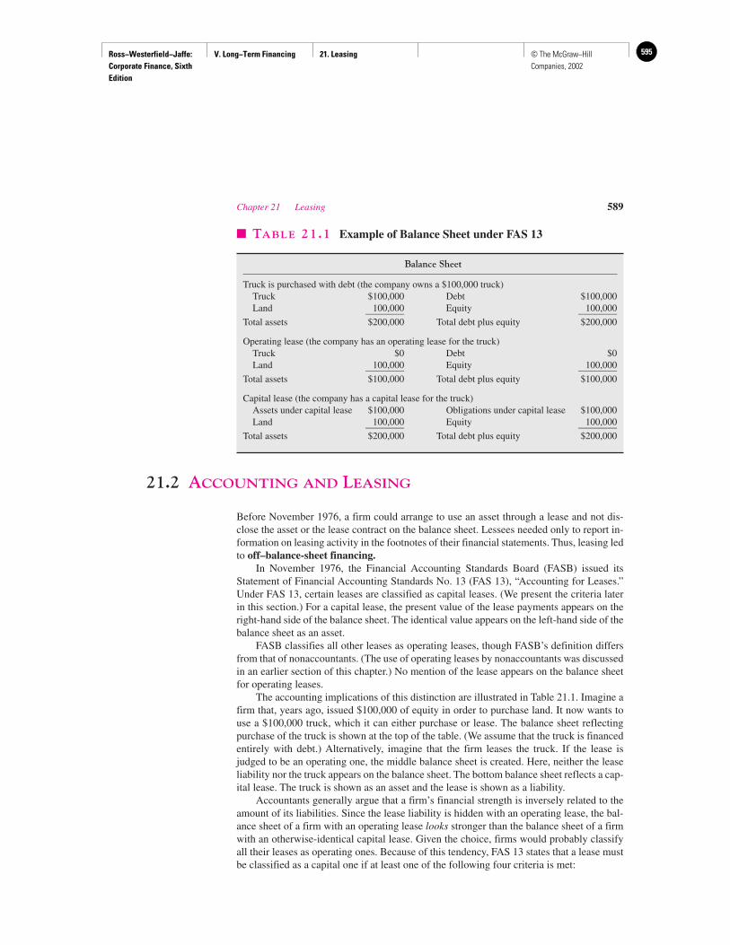
Ross−Westerfield−Jaffe: Corporate Finance, Sixth Edition
V. Long−Term Financing 21. Leasing 595© The McGraw−Hill Companies, 2002
Chapter 21 Leasing 589
21.2 ACCOUNTING AND LEASING
Before November 1976, a firm could arrange to use an asset through a lease and not dis-close the asset or the lease contract on the balance sheet. Lessees needed only to report in-formation on leasing activity in the footnotes of their financial statements. Thus, leasing ledto off–balance-sheet financing.
In November 1976, the Financial Accounting Standards Board (FASB) issued itsStatement of Financial Accounting Standards No. 13 (FAS 13), “Accounting for Leases.”Under FAS 13, certain leases are classified as capital leases. (We present the criteria laterin this section.) For a capital lease, the present value of the lease payments appears on theright-hand side of the balance sheet. The identical value appears on the left-hand side of thebalance sheet as an asset.
FASB classifies all other leases as operating leases, though FASB’s definition differsfrom that of nonaccountants. (The use of operating leases by nonaccountants was discussedin an earlier section of this chapter.) No mention of the lease appears on the balance sheetfor operating leases.
The accounting implications of this distinction are illustrated in Table 21.1. Imagine afirm that, years ago, issued $100,000 of equity in order to purchase land. It now wants touse a $100,000 truck, which it can either purchase or lease. The balance sheet reflectingpurchase of the truck is shown at the top of the table. (We assume that the truck is financedentirely with debt.) Alternatively, imagine that the firm leases the truck. If the lease isjudged to be an operating one, the middle balance sheet is created. Here, neither the leaseliability nor the truck appears on the balance sheet. The bottom balance sheet reflects a cap-ital lease. The truck is shown as an asset and the lease is shown as a liability.
Accountants generally argue that a firm’s financial strength is inversely related to theamount of its liabilities. Since the lease liability is hidden with an operating lease, the bal-ance sheet of a firm with an operating lease looks stronger than the balance sheet of a firmwith an otherwise-identical capital lease. Given the choice, firms would probably classifyall their leases as operating ones. Because of this tendency, FAS 13 states that a lease mustbe classified as a capital one if at least one of the following four criteria is met:
� TABLE 21.1 Example of Balance Sheet under FAS 13
Balance Sheet
Truck is purchased with debt (the company owns a $100,000 truck)Truck $100,000 Debt $100,000Land 100,000 Equity 100,000________ ________
Total assets $200,000 Total debt plus equity $200,000
Operating lease (the company has an operating lease for the truck)Truck $0 Debt $0Land 100,000 Equity 100,000________ ________
Total assets $100,000 Total debt plus equity $100,000
Capital lease (the company has a capital lease for the truck)Assets under capital lease $100,000 Obligations under capital lease $100,000Land 100,000 Equity 100,000________ ________
Total assets $200,000 Total debt plus equity $200,000
Ross−Westerfield−Jaffe: Corporate Finance, Sixth Edition
V. Long−Term Financing 21. Leasing596 © The McGraw−Hill Companies, 2002
1. The present value of the lease payments is at least 90 percent of the fair market value ofthe asset at the start of the lease.
2. The lease transfers ownership of the property to the lessee by the end of the term of thelease.
3. The lease term is 75 percent or more of the estimated economic life of the asset.
4. The lessee can purchase the asset at a price below fair market value when the lease ex-pires. This is frequently called a bargain-purchase-price option.
These rules capitalize those leases that are similar to purchases. For example, the first tworules capitalize leases where the asset is likely to be purchased at the end of the lease pe-riod. The last two rules capitalize long-term leases.
Some firms have tried to cook the books by exploiting this classification scheme.Suppose a trucking firm wants to lease a $200,000 truck that it expects to use for 15 years.A clever financial manager could try to negotiate a lease contract for 10 years with leasepayments having a present value of $178,000. These terms would get around criteria (1) and(3). If criteria (2) and (4) could be circumvented, the arrangement would be an operatinglease and would not show up on the balance sheet.
Does this sort of gimmickry pay? The semistrong form of the efficient-capital-marketshypothesis implies that stock prices reflect all publicly available information. As we dis-cussed earlier in this text, the empirical evidence generally supports this form of the hy-pothesis. Though operating leases do not appear in the firm’s balance sheet, information onthese leases must be disclosed elsewhere in the annual report. Because of this, attempts tokeep leases off the balance sheet will not affect stock price in an efficient capital market.
• Define capital lease.• Define operating lease.
21.3 TAXES, THE IRS, AND LEASES
The lessee can deduct lease payments for income tax purposes if the lease is qualified bythe Internal Revenue Service. Because tax shields are critical to the economic viability ofany lease, all interested parties generally obtain an opinion from the IRS before agreeing toa major lease transaction. The opinion of the IRS will reflect the following guidelines:
1. The term of the lease must be less than 30 years. If the term is greater than 30 years, thetransaction will be regarded as a conditional sale.
2. The lease should not have an option to acquire the asset at a price below its fair marketvalue. This type of bargain option would give the lessee the asset’s residual scrap value,implying an equity interest.
3. The lease should not have a schedule of payments that is very high at the start of the leaseterm and thereafter very low. Early balloon payments would be evidence that the leasewas being used to avoid taxes and not for a legitimate business purpose.
4. The lease payments must provide the lessor with a fair market rate of return. The profitpotential of the lease to the lessor should be apart from the deal’s tax benefits.
5. The lease should not limit the lessee’s right to issue debt or pay dividends while the leaseis operative.
590 Part V Long-Term Financing
QUESTIONS
CO
NC
EP
T
?
Ross−Westerfield−Jaffe: Corporate Finance, Sixth Edition
V. Long−Term Financing 21. Leasing 597© The McGraw−Hill Companies, 2002
Chapter 21 Leasing 591
6. Renewal options must be reasonable and reflect fair market value of the asset. This re-quirement can be met by granting the lessee the first option to meet a competing out-side offer.
The reason the IRS is concerned about lease contracts is that many times they appearto be set up solely to avoid taxes. To see how this could happen, suppose that a firm plansto purchase a $1 million bus that has a five-year class life. Depreciation expense would be$200,000 per year, assuming straight-line depreciation. Now suppose that the firm can leasethe bus for $500,000 per year for two years and buy the bus for $1 at the end of the two-year term. The present value of the tax benefits from acquiring the bus would clearly be lessthan if the bus were leased. The speedup of lease payments would greatly benefit the firmand de facto give it a form of accelerated depreciation. If the tax rates of the lessor and les-see are different, leasing can be a form of tax avoidance.
• What are the IRS guidelines for treating a lease contract as a lease for tax purposes?
21.4 THE CASH FLOWS OF LEASING
In this section we identify the basic cash flows used in evaluating a lease. Consider thedecision confronting the Xomox corporation, which manufactures pipe. Business hasbeen expanding, and Xomox currently has a five-year backlog of pipe orders for theTrans-Honduran Pipeline.
The International Boring Machine Corporation (IBMC) makes a pipe-boring machinethat can be purchased for $10,000. Xomox has determined that it needs a new machine, andthe IBMC model will save Xomox $6,000 per year in reduced electricity bills for the nextfive years. These savings are known with certainty because Xomox has a long-term elec-tricity purchase agreement with State Electric Utilities, Inc.
Xomox has a corporate tax rate of 34 percent. We assume that five-year straight-linedepreciation is used for the pipe-boring machine, and the machine will be worthless afterfive years.2
However, Friendly Leasing Corporation has offered to lease the same pipe-boring ma-chine to Xomox for $2,500 per year for five years. With the lease, Xomox would remain re-sponsible for maintenance, insurance, and operating expenses.3
Simon Smart, a recently hired MBA, has been asked to calculate the incremental cashflows from leasing the IBMC machine in lieu of buying it. He has prepared Table 21.2,which shows the direct cash flow consequences of buying the pipe-boring machine and alsosigning the lease agreement with Friendly Leasing.
To simplify matters, Simon Smart has prepared Table 21.3, which subtracts the directcash flows of buying the pipe-boring machine from those of leasing it. Noting that only thenet advantage of leasing is relevant to Xomox, he concludes the following from his analysis:
QUESTION
CO
NC
EP
T
?
2This is a simplifying assumption because current tax law allows the accelerated method as well. Theaccelerated method will almost always be the best choice.3For simplicity, we have assumed that lease payments are made at the end of each year. Actually, most leasesrequire lease payments to be made at the beginning of the year.
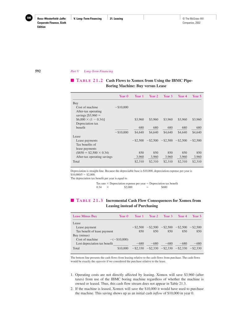
Ross−Westerfield−Jaffe: Corporate Finance, Sixth Edition
V. Long−Term Financing 21. Leasing598 © The McGraw−Hill Companies, 2002
1. Operating costs are not directly affected by leasing. Xomox will save $3,960 (aftertaxes) from use of the IBMC boring machine regardless of whether the machine isowned or leased. Thus, this cash flow stream does not appear in Table 21.3.
2. If the machine is leased, Xomox will save the $10,000 it would have used to purchasethe machine. This saving shows up as an initial cash inflow of $10,000 in year 0.
592 Part V Long-Term Financing
� TABLE 21.2 Cash Flows to Xomox from Using the IBMC Pipe-Boring Machine: Buy versus Lease
Year 0 Year 1 Year 2 Year 3 Year 4 Year 5
BuyCost of machine �$10,000After-tax operating savings [$3,960 �$6,000 � (1 � 0.34)] $3,960 $3,960 $3,960 $3,960 $3,960Depreciation tax benefit 680 680 680 680 680________ ______ ______ ______ ______ ______
�$10,000 $4,640 $4,640 $4,640 $4,640 $4,640Lease
Lease payments �$2,500 �$2,500 �$2,500 �$2,500 �$2,500Tax benefits of lease payments ($850 � $2,500 � 0.34) 850 850 850 850 850After-tax operating savings 3,960 3,960 3,960 3,960 3,960______ ______ ______ ______ ______
Total $2,310 $2,310 $2,310 $2,310 $2,310
Depreciation is straight-line. Because the depreciable base is $10,000, depreciation expense per year is$10,000/5 � $2,000.The depreciation tax benefit per year is equal to
Tax rate � Depreciation expense per year � Depreciation tax benefit0.34 � $2,000 � $680
� TABLE 21.3 Incremental Cash Flow Consequences for Xomox fromLeasing instead of Purchasing
Lease Minus Buy Year 0 Year 1 Year 2 Year 3 Year 4 Year 5
LeaseLease payment �$2,500 �$2,500 �$2,500 �$2,500 �$2,500Tax benefit of lease payment 850 850 850 850 850
Buy (minus)Cost of machine �(�$10,000)Lost depreciation tax benefit �680 �680 �680 �680 �680_________ _______ _______ _______ _______ _______
Total $10,000 �$2,330 �$2,330 �$2,330 �$2,330 �$2,330
The bottom line presents the cash flows from leasing relative to the cash flows from purchase. The cash flowswould be exactly the opposite if we considered the purchase relative to the lease.
Ross−Westerfield−Jaffe: Corporate Finance, Sixth Edition
V. Long−Term Financing 21. Leasing 599© The McGraw−Hill Companies, 2002
Chapter 21 Leasing 593
3. If Xomox leases the pipe-boring machine, it will no longer own this machine and mustgive up the depreciation tax benefits. These tax benefits show up as an outflow.
4. If Xomox chooses to lease the machine, it must pay $2,500 per year for five years. Thefirst payment is due at the end of the first year. (This is a break, because sometimes thefirst payment is due immediately.) The lease payments are tax-deductible and, as a con-sequence, generate tax benefits of $850 (0.34 � $2,500).
The net cash flows have been placed in the bottom line of Table 21.3. These numbersrepresent the cash flows from leasing relative to the cash flows from the purchase. It is ar-bitrary that we express the flows in this way. We could have expressed the cash flows fromthe purchase relative to the cash flows from leasing. These cash flows would be
Year 0 Year 1 Year 2 Year 3 Year 4 Year 5
Net cash flows from purchase alternative relative to lease alternative �$10,000 $2,330 $2,330 $2,330 $2,330 $2,330
Of course, the cash flows here are the opposite of those in the bottom line of Table 21.3.Depending on our purpose, we may look at either the purchase relative to the lease or viceversa. Thus, the student should become comfortable with either viewpoint.
Now that we have the cash flows, we can make our decision by discounting the flowsproperly. However, because the discount rate is tricky, we take a detour in the next sectionbefore moving back to the Xomox case. In this next section, we show that cash flows in thelease-versus-buy decision should be discounted at the after-tax interest rate (i.e., the after-tax cost of debt capital).
21.5 A DETOUR ON DISCOUNTING AND DEBT CAPACITY
WITH CORPORATE TAXES
The analysis of leases is difficult, and both financial practitioners and academics have madeconceptual errors. These errors revolve around taxes. We hope to avoid their mistakes bybeginning with the simplest type of example, a loan for one year. Though this example isunrelated to our lease-versus-buy situation, principles developed here will apply directly tolease-buy analysis.
Present Value of Riskless Cash FlowsConsider a corporation that lends $100 for a year. If the interest rate is 10 percent, the firmwill receive $110 at the end of the year. Of this amount, $10 is interest and the remaining$100 is the original principal. A corporate tax rate of 34 percent implies taxes on the inter-est of $3.40 (0.34 � $10). Thus, the firm ends up with $106.60 ($110 � $3.40) after taxeson a $100 investment.
Now, consider a company that borrows $100 for a year. With a 10-percent interest rate,the firm must pay $110 to the bank at the end of the year. However, the borrowing firm cantake the $10 of interest as a tax deduction. The corporation pays $3.40 (0.34 � $10) less intaxes than it would have paid had it not borrowed the money at all. Thus, considering thisreduction in taxes, the firm must pay $106.60 ($110 � $3.40) on a $100 loan. The cashflows from both lending and borrowing are displayed in Table 21.4.
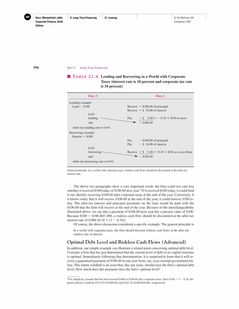
Ross−Westerfield−Jaffe: Corporate Finance, Sixth Edition
V. Long−Term Financing 21. Leasing600 © The McGraw−Hill Companies, 2002
The above two paragraphs show a very important result: the firm could not care lesswhether it received $100 today or $106.60 next year.4 If it received $100 today, it could lendit out, thereby receiving $106.60 after corporate taxes at the end of the year. Conversely, ifit knows today that it will receive $106.60 at the end of the year, it could borrow $100 to-day. The after-tax interest and principal payments on the loan would be paid with the$106.60 that the firm will receive at the end of the year. Because of the interchangeabilityillustrated above, we say that a payment of $106.60 next year has a present value of $100.Because $100 � $106.60/1.066, a riskless cash flow should be discounted at the after-taxinterest rate of 0.066 [0.10 � (1 � 0.34)].
Of course, the above discussion considered a specific example. The general principle is
In a world with corporate taxes, the firm should discount riskless cash flows at the after-taxriskless rate of interest.
Optimal Debt Level and Riskless Cash Flows (Advanced)In addition, our simple example can illustrate a related point concerning optimal debt level.Consider a firm that has just determined that the current level of debt in its capital structureis optimal. Immediately following that determination, it is surprised to learn that it will re-ceive a guaranteed payment of $106.60 in one year from, say, a tax-exempt government lot-tery. This future windfall is an asset that, like any asset, should raise the firm’s optimal debtlevel. How much does this payment raise the firm’s optimal level?
594 Part V Long-Term Financing
� TABLE 21.4 Lending and Borrowing in a World with CorporateTaxes (interest rate is 10 percent and corporate tax rateis 34 percent)
Date 0 Date 1
Lending exampleLend � $100 Receive � $100.00 of principal
Receive � $ 10.00 of interest6.6%lending Pay � $ 3.40 (� �0.34 � $10) in taxes_________rate � $106.60
After-tax lending rate is 6.6%.
Borrowing exampleBorrow � $100
Pay � $100.00 of principalPay � $ 10.00 of interest
6.6% borrowing Receive � $ 3.40 (� 0.34 � $10) as a tax rebate_________rate � $106.60
After-tax borrowing rate is 6.6%.
General principle: In a world with corporate taxes, riskless cash flows should be discounted at the after-taxinterest rate.
4For simplicity, assume that the firm received $100 or $106.60 after corporate taxes. Since 0.66 � 1 � 0.34, thepretax inflows would be $151.52 ($100/0.66) and $161.52 ($106.60/0.66), respectively.
Ross−Westerfield−Jaffe: Corporate Finance, Sixth Edition
V. Long−Term Financing 21. Leasing 601© The McGraw−Hill Companies, 2002
Chapter 21 Leasing 595
Our preceding analysis implies that the firm’s optimal debt level must be $100 morethan it previously was. That is, the firm could borrow $100 today, perhaps paying the entireamount out as a dividend. It would owe the bank $110 at the end of the year. However, be-cause it receives a tax rebate of $3.40 (0.34 � $10), its net repayment will be $106.60. Thus,its borrowing of $100 today is fully offset by next year’s government lottery proceeds of$106.60. In other words, the lottery proceeds act as an irrevocable trust that can service theincreased debt. Note that we need not know the optimal debt level before the lottery wasannounced. We are merely saying that, whatever this prelottery optimal level was, the op-timal debt level is $100 more after the lottery announcement.
Of course, this is just one example. The general principle is5
In a world with corporate taxes, one determines the increase in the firm’s optimal debt level bydiscounting a future guaranteed after-tax inflow at the after-tax riskless interest rate.
Conversely, suppose that a second and unrelated firm is surprised to learn that it mustpay $106.60 next year to the government for back taxes. Clearly, this additional liability im-pinges on the second firm’s debt capacity. By the above reasoning, it follows that the sec-ond firm’s optimal debt level must be lowered by exactly $100.
• How should one discount a riskless cash flow?
21.6 NPV ANALYSIS OF THE LEASE-VERSUS-BUY DECISION
The detour leads to a simple method for evaluating leases: discount all cash flows at the af-ter-tax interest rate. From the bottom line of Table 21.3, Xomox’s incremental cash flowsfrom leasing versus purchasing are
Year 0 Year 1 Year 2 Year 3 Year 4 Year 5
Net cash flows from leasealternative relative topurchase alternative $10,000 �$2,330 �$2,330 �$2,330 �$2,330 �$2,330
Let us assume that Xomox can either borrow or lend at the interest rate of 7.57575 percent.If the corporate tax rate is 34 percent, the correct discount rate is the after-tax rate of 5 per-cent [7.57575% � (1 � 0.34)]. When 5 percent is used to compute the NPV of the lease,we have
NPV � $10,000 � $2,330 � � �$87.68 (21.1)
Because the net present value of the incremental cash flows from leasing relative to pur-chasing is negative, Xomox prefers to purchase.
Equation (21.1) is the correct approach to lease-versus-buy analysis. However, studentsare often bothered by two things. First, they question whether the cash flows in Table 21.3are truly riskless. We examine this issue below. Second, they feel that this approach lacksintuition. We address this concern a little later.
A
50.05
5This principle holds for riskless or guaranteed cash flows only. Unfortunately, there is no easy formula fordetermining the increase in optimal debt level from a risky cash flow.
QUESTION
CO
NC
EP
T
?
Ross−Westerfield−Jaffe: Corporate Finance, Sixth Edition
V. Long−Term Financing 21. Leasing602 © The McGraw−Hill Companies, 2002
The Discount RateBecause we discounted at the after-tax riskless rate of interest, we have implicitly assumedthat the cash flows in the Xomox example are riskless. Is this appropriate?
A lease payment is like the debt service on a secured bond issued by the lessee, and thediscount rate should be approximately the same as the interest rate on such debt. In general,this rate will be slightly higher than the riskless rate considered in the previous section. Thevarious tax shields could be somewhat riskier than the lease payments for two reasons. First,the value of the depreciation tax benefits depends on the ability of Xomox to generate enoughtaxable income to use them. Second, the corporate tax rate may change in the future, just asit fell in 1986 and increased in 1993. For these two reasons, a firm might be justified in dis-counting the depreciation tax benefits at a rate higher than that used for the lease payments.However, our experience is that real-world companies discount both the depreciation shieldand lease payments at the same rate. This implies that financial practitioners view the abovetwo risks as minor. We adopt the real-world convention of discounting the two flows at thesame rate. This rate is the after-tax interest rate on secured debt issued by the lessee.
At this point some students still ask the question: Why not use rWACC as the discountrate in lease-versus-buy analysis? Of course, rWACC should not be used for lease analysisbecause the cash flows are more like debt-service cash flows than operating cash flows and,as such, the risk is much less. The discount rate should reflect the risk of the incrementalcash flows.
21.7 DEBT DISPLACEMENT AND LEASE VALUATION
The Basic Concept of Debt Displacement (Advanced)The previous analysis allows one to calculate the right answer in a simple manner. Thisclearly must be viewed as an important benefit. However, the analysis has little intuitive ap-peal. To remedy this, we hope to make lease-buy analysis more intuitive by considering theissue of debt displacement.
A firm that purchases equipment will generally issue debt to finance the purchase. Thedebt becomes a liability of the firm. A lessee incurs a liability equal to the present value ofall future lease payments. Because of this, we argue that leases displace debt. The balancesheets in Table 21.5 illustrate how leasing might affect debt.
Suppose a firm initially has $100,000 of assets and a 150-percent optimal debt-equityratio. The firm’s debt is $60,000, and its equity is $40,000. As in the Xomox case, supposethe firm must use a new $10,000 machine. The firm has two alternatives:
1. The Firm Can Purchase the Machine. If it does, it will finance the purchase with a se-cured loan and with equity. The debt capacity of the machine is assumed to be the sameas for the firm as a whole.
2. The Firm Can Lease the Asset and Get 100-Percent Financing. That is, the present valueof the future lease payments will be $10,000.
If the firm finances the machine with both secured debt and new equity, its debt willincrease by $6,000 and its equity by $4,000. Its optimal debt-equity ratio of 150 percentwill be maintained.
Conversely, consider the lease alternative. Because the lessee views the lease paymentas a liability, the lessee thinks in terms of a liability-to-equity ratio, not just a debt-to-equityratio. As mentioned above, the present value of the lease liability is $10,000. If the leasing
596 Part V Long-Term Financing
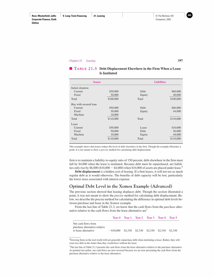
Ross−Westerfield−Jaffe: Corporate Finance, Sixth Edition
V. Long−Term Financing 21. Leasing 603© The McGraw−Hill Companies, 2002
Chapter 21 Leasing 597
firm is to maintain a liability-to-equity ratio of 150 percent, debt elsewhere in the firm mustfall by $4,000 when the lease is instituted. Because debt must be repurchased, net liabili-ties only rise by $6,000 ($10,000 � $4,000) when $10,000 of assets are placed under lease.6
Debt displacement is a hidden cost of leasing. If a firm leases, it will not use as muchregular debt as it would otherwise. The benefits of debt capacity will be lost, particularlythe lower taxes associated with interest expense.
Optimal Debt Level in the Xomox Example (Advanced)The previous section showed that leasing displaces debt. Though the section illustrated apoint, it was not meant to show the precise method for calculating debt displacement. Be-low, we describe the precise method for calculating the difference in optimal debt levels be-tween purchase and lease in the Xomox example.
From the last line of Table 21.3, we know that the cash flows from the purchase alter-native relative to the cash flows from the lease alternative are7
Year 0 Year 1 Year 2 Year 3 Year 4 Year 5
Net cash flows frompurchase alternative relativeto lease alternative �$10,000 $2,330 $2,330 $2,330 $2,330 $2,330
� TABLE 21.5 Debt Displacement Elsewhere in the Firm When a LeaseIs Instituted
Assets Liabilities
Initial situationCurrent $50,000 Debt $60,000Fixed 50,000 Equity 40,000________ ________
Total $100,000 Total $100,000
Buy with secured loanCurrent $50,000 Debt $66,000Fixed 50,000 Equity 44,000Machine 10,000________ ________
Total $110,000 Total $110,000
LeaseCurrent $50,000 Lease $10,000Fixed 50,000 Debt 56,000Machine 10,000 Equity 44,000________ ________
Total $110,000 Total $110,000
This example shows that leases reduce the level of debt elsewhere in the firm. Though the example illustrates apoint, it is not meant to show a precise method for calculating debt displacement.
6Growing firms in the real world will not generally repurchase debt when instituting a lease. Rather, they willissue less debt in the future than they would have without the lease.7The last line of Table 21.3 presents the cash flows form the lease alternative relative to the purchase alternative.As pointed out earlier, our cash flows are now reversed because we are now presenting the cash flows from thepurchase alternative relative to the lease alternative.
Ross−Westerfield−Jaffe: Corporate Finance, Sixth Edition
V. Long−Term Financing 21. Leasing604 © The McGraw−Hill Companies, 2002
An increase in the optimal debt level at year 0 occurs because the firm learns at thattime of guaranteed cash flows beginning at year 1. Our detour on discounting and debt ca-pacity told us to calculate this increased debt level by discounting the future riskless cashinflows at the after-tax interest rate.8 Thus, additional debt level of the purchase alternativerelative to the lease alternative is
Increase in optimal debt level from purchase alternativerelative to leasealternative:
That is, whatever the optimal amount of debt would be under the lease alternative, the op-timal amount of debt would be $10,087.68 more under the purchase alternative.
This result can be stated in another way. Imagine there are two identical firms exceptthat one firm purchases the boring machine and the other leases it. From Table 21.3, weknow that the purchasing firm generates $2,330 more cash flow after taxes in each of thefive years than does the leasing firm. Further imagine that the same bank lends money toboth firms. The bank should lend the purchasing firm more money because it has a greatercash flow each period. How much extra money should the bank loan the purchasing firm sothat the incremental loan can be paid off by the extra cash flows of $2,330 per year? Theanswer is exactly $10,087.68, the increase in the optimal debt level we calculated earlier.
To see this, let us work through the example on a year-by-year basis. Because the pur-chasing firm borrows $10,087.68 more at year 0 than does the leasing firm, the purchasingfirm will pay interest of $764.22 ($10,087.68 � 0.0757575) at year 1 on the additional debt.The interest allows the firm to reduce its taxes by $259.83 ($764.22 � 0.34), leaving an after-tax outflow of $504.39 ($764.22 � $259.83) at year 1.
We know from Table 21.3 that the purchasing firm generates $2,330 more cash at year1 than does the leasing firm. Because the purchasing firm has the extra $2,330 coming in atyear 1 but must pay interest on its loan, how much of the loan can the firm repay at year 1and still have the same cash flow as the leasing firm has? The purchasing firm can repay$1,825.61 ($2,330 � $504.39) of the loan at year 1 and still have the same net cash flowthat the leasing firm has. After the repayment, the purchasing firm will have a remainingbalance of $8,262.07 ($10,087.68 � $1,825.61) at year 1. For each of the five years, thissequence of cash flows is displayed in Table 21.6. The outstanding balance goes to zero overthe five years. Thus, the annual cash flow of $2,330, which represents the extra cash frompurchasing instead of leasing, fully amortizes the loan of $10,087.68.
Our analysis on debt capacity has two purposes. First, we want to show the additionaldebt capacity from purchasing. We just completed this task. Second, we want to determinewhether or not the lease is preferred to the purchase. This decision rule follows easily fromthe above discussion. By leasing the equipment and having $10,087.68 less debt than un-der the purchase alternative, the firm has exactly the same cash flow in years 1 to 5 that itwould have through a levered purchase. Thus, we can ignore cash flows beginning in year1 when comparing the lease alternative with the purchase with debt alternative. However,the cash flows differ between the alternatives at year 0. These differences are
1. The Purchase Cost at Year 0 of $10,000 Is Avoided by Leasing. This should be viewedas a cash inflow under the leasing alternative.
$2,330�1.05� 3 �
$2,330�1.05� 4 �
$2,330�1.05� 5$10,087.68 �
$2,330
1.05�
$2,330�1.05� 2 �
598 Part V Long-Term Financing
8Though our detour considered only riskless cash flows, the cash flows in a leasing example are not necessarilyriskless. As we explained earlier, we therefore adopt the real-world convention of discounting at the after-taxinterest rate on secured debt issued by the lessee.
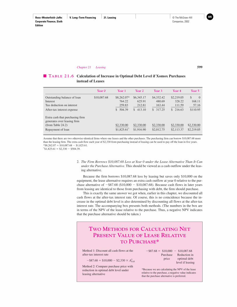
Ross−Westerfield−Jaffe: Corporate Finance, Sixth Edition
V. Long−Term Financing 21. Leasing 605© The McGraw−Hill Companies, 2002
Chapter 21 Leasing 599
2. The Firm Borrows $10,087.68 Less at Year 0 under the Lease Alternative Than It Canunder the Purchase Alternative. This should be viewed as a cash outflow under the leas-ing alternative.
Because the firm borrows $10,087.68 less by leasing but saves only $10,000 on theequipment, the lease alternative requires an extra cash outflow at year 0 relative to the pur-chase alternative of �$87.68 ($10,000 � $10,087.68). Because cash flows in later yearsfrom leasing are identical to those from purchasing with debt, the firm should purchase.
This is exactly the same answer we got when, earlier in this chapter, we discounted allcash flows at the after-tax interest rate. Of course, this is no coincidence because the in-crease in the optimal debt level is also determined by discounting all flows at the after-taxinterest rate. The accompanying box presents both methods. (The numbers in the box arein terms of the NPV of the lease relative to the purchase. Thus, a negative NPV indicatesthat the purchase alternative should be taken.)
� TABLE 21.6 Calculation of Increase in Optimal Debt Level if Xomox Purchases instead of Leases
Year 0 Year 1 Year 2 Year 3 Year 4 Year 5
Outstanding balance of loan $10,087.68 $8,262.07* $6,345.17 $4,332.42 $2,219.05 $ 0Interest 764.22 625.91 480.69 328.22 168.11Tax deduction on interest 259.83 212.81 163.44 111.59 57.16________ ________ ________ ________ _______After-tax interest expense $ 504.39 $ 413.10 $ 317.25 $ 216.63 $110.95
Extra cash that purchasing firm generates over leasing firm(from Table 24.2) $2,330.00 $2,330.00 $2,330.00 $2,330.00 $2,330.00________ ________ ________ ________ _______Repayment of loan $1,825.61† $1,916.90 $2,012.75 $2,113.37 $2,219.05
Assume that there are two otherwise-identical firms where one leases and the other purchases. The purchasing firm can borrow $10,087.68 morethan the leasing firm. The extra cash flow each year of $2,330 from purchasing instead of leasing can be used to pay off the loan in five years.*$8,262.07 � $10,087.68 � $1,825.61.†$1,825.61 � $2,330 � $504.39.
TWO METHODS FOR CALCULATING NET
PRESENT VALUE OF LEASE RELATIVE
TO PURCHASE*
Method 1: Discount all cash flows at theafter-tax interest rate
�$87.68 � $10,000 � $2,330 �
Method 2: Compare purchase price withreduction in optimal debt level underleasing alternative
�$87.68 � $10,000 � $10,087.68Purchase Reduction in
price optimal debt level if leasing
*Because we are calculating the NPV of the leaserelative to the purchase, a negative value indicatesthat the purchase alternative is preferred.
A
50.05
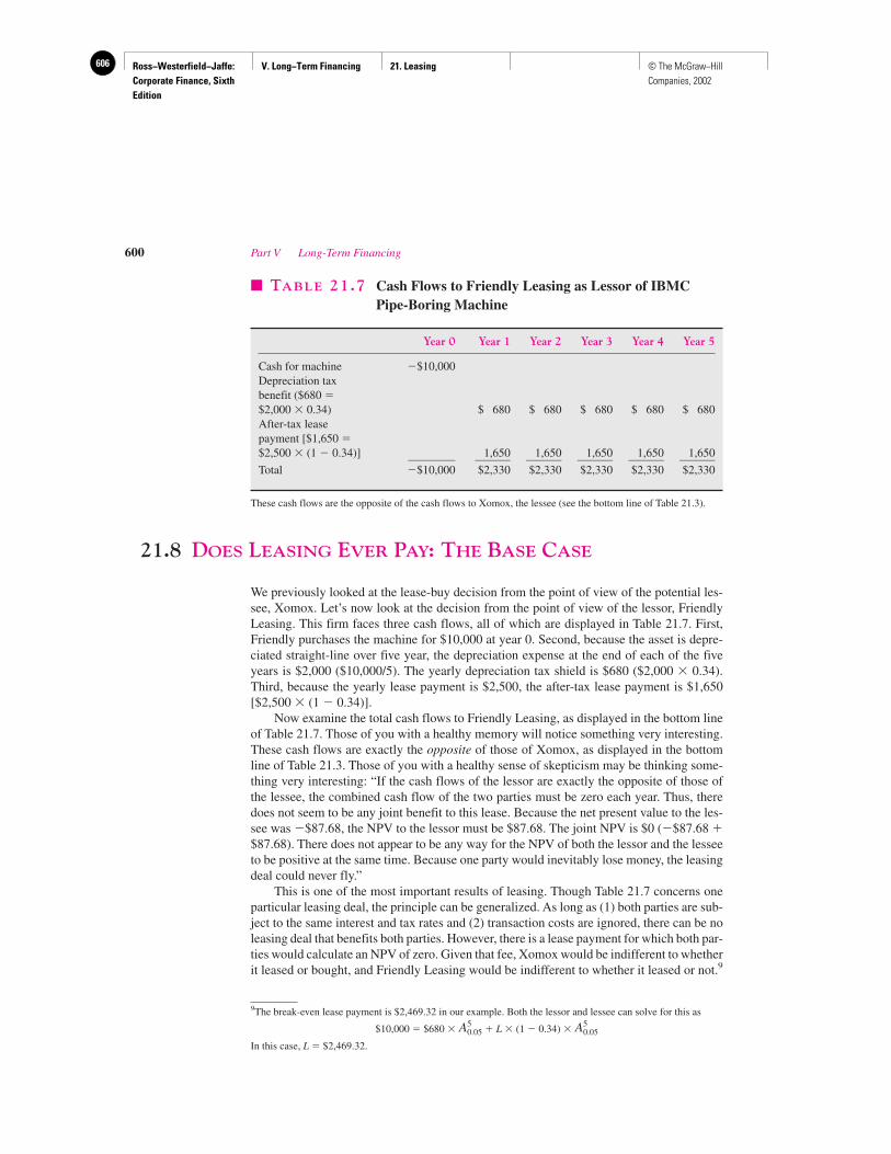
Ross−Westerfield−Jaffe: Corporate Finance, Sixth Edition
V. Long−Term Financing 21. Leasing606 © The McGraw−Hill Companies, 2002
21.8 DOES LEASING EVER PAY: THE BASE CASE
We previously looked at the lease-buy decision from the point of view of the potential les-see, Xomox. Let’s now look at the decision from the point of view of the lessor, FriendlyLeasing. This firm faces three cash flows, all of which are displayed in Table 21.7. First,Friendly purchases the machine for $10,000 at year 0. Second, because the asset is depre-ciated straight-line over five year, the depreciation expense at the end of each of the fiveyears is $2,000 ($10,000/5). The yearly depreciation tax shield is $680 ($2,000 � 0.34).Third, because the yearly lease payment is $2,500, the after-tax lease payment is $1,650[$2,500 � (1 � 0.34)].
Now examine the total cash flows to Friendly Leasing, as displayed in the bottom lineof Table 21.7. Those of you with a healthy memory will notice something very interesting.These cash flows are exactly the opposite of those of Xomox, as displayed in the bottomline of Table 21.3. Those of you with a healthy sense of skepticism may be thinking some-thing very interesting: “If the cash flows of the lessor are exactly the opposite of those ofthe lessee, the combined cash flow of the two parties must be zero each year. Thus, theredoes not seem to be any joint benefit to this lease. Because the net present value to the les-see was �$87.68, the NPV to the lessor must be $87.68. The joint NPV is $0 (�$87.68 �$87.68). There does not appear to be any way for the NPV of both the lessor and the lesseeto be positive at the same time. Because one party would inevitably lose money, the leasingdeal could never fly.”
This is one of the most important results of leasing. Though Table 21.7 concerns oneparticular leasing deal, the principle can be generalized. As long as (1) both parties are sub-ject to the same interest and tax rates and (2) transaction costs are ignored, there can be noleasing deal that benefits both parties. However, there is a lease payment for which both par-ties would calculate an NPV of zero. Given that fee, Xomox would be indifferent to whetherit leased or bought, and Friendly Leasing would be indifferent to whether it leased or not.9
600 Part V Long-Term Financing
� TABLE 21.7 Cash Flows to Friendly Leasing as Lessor of IBMCPipe-Boring Machine
Year 0 Year 1 Year 2 Year 3 Year 4 Year 5
Cash for machine �$10,000Depreciation taxbenefit ($680 �$2,000 � 0.34) $ 680 $ 680 $ 680 $ 680 $ 680After-tax leasepayment [$1,650 �$2,500 � (1 � 0.34)] 1,650 1,650 1,650 1,650 1,650________ ______ ______ ______ ______ ______Total �$10,000 $2,330 $2,330 $2,330 $2,330 $2,330
These cash flows are the opposite of the cash flows to Xomox, the lessee (see the bottom line of Table 21.3).
9The break-even lease payment is $2,469.32 in our example. Both the lessor and lessee can solve for this as
$10,000 � $680 � � L � (1 � 0.34) �
In this case, L � $2,469.32.
A
50.05A
50.05
Ross−Westerfield−Jaffe: Corporate Finance, Sixth Edition
V. Long−Term Financing 21. Leasing 607© The McGraw−Hill Companies, 2002
Chapter 21 Leasing 601
A student with an even healthier sense of skepticism might be thinking, “This textbookappears to be arguing that leasing is not beneficial. Yet, we know that leasing occurs fre-quently in the real world. Maybe, just maybe, the textbook is wrong.” Although we will notadmit to being wrong (what textbook would?!), we freely admit to being incomplete at thispoint. The next section considers factors that give benefits to leasing.
21.9 REASONS FOR LEASING
Proponents of leasing make many claims about why firms should lease assets ratherthan buy them. Some of the reasons given to support leasing are good, and some arenot. We discuss here the reasons for leasing we think are good and some of the ones wethink aren’t.
Good Reasons for LeasingIf leasing is a good choice, it will be because one or more of the following will be true:
1. Taxes may be reduced by leasing.
2. The lease contract may reduce certain types of uncertainty.
3. Transactions costs can be higher for buying an asset and financing it with debt or equitythan for leasing the asset.
Tax Advantages The most important reason for long-term leasing is tax reduction. If thecorporate income tax were repealed, long-term leasing would probably disappear. The taxadvantages of leasing exist because firms are in different tax brackets.
Should a user in a low tax bracket purchase, he will receive little tax benefit from de-preciation and interest deductions. Should the user lease, the lessor will receive the de-preciation shield and the interest deductions. In a competitive market, the lessor mustcharge a low lease payment to reflect these tax shields. Thus, the user is likely to leaserather than purchase.
In our example with Xomox and Friendly Leasing, the value of the lease to Friendlywas $87.68. That is,
$87.68 � �$10,000 � $2,330 �
However, the value of the lease to Xomox was exactly the opposite (�$87.68). Because thelessor’s gains came at the expense of the lessee, no deal could be arranged.
However, if Xomox pays no taxes and the lease payments are reduced to $2,475 from$2,500, both Friendly and Xomox will find there is positive NPV in leasing. Xomox can re-work Table 21.3 with Tc � 0, finding that its cash flows from leasing are
Year 0 Year 1 Year 2 Year 3 Year 4 Year 5
Cost of machine $10,000Lease payment �$2,475 �$2,475 �$2,475 �$2,475 �$2,475
The value of the lease to Xomox is
Value of lease � $10,000 � $2,475 �
� $6.55
A
50.0757575
A
50.05
Ross−Westerfield−Jaffe: Corporate Finance, Sixth Edition
V. Long−Term Financing 21. Leasing608 © The McGraw−Hill Companies, 2002
Notice that the discount rate is the interest rate of 7.57575 percent because tax rates are zero.In addition, the full lease payment of $2,475—and not some lower, after-tax number—is used since there are no taxes. Finally, note that depreciation is ignored, also because notaxes apply.
Given a lease payment of $2,475, the cash flows to Friendly Leasing are
Year 0 Year 1 Year 2 Year 3 Year 4 Year 5
Cost of machine �$10,000Depreciation tax shield($680 � $2,000 � 0.34) $ 680 $ 680 $ 680 $ 680 $ 680After-tax lease payment [$1,633.50 �$2,475 � (1 � 0.34)] $1,633.50 $1,633.50 $1,633.50 $1,633.50 $1,633.50________ ________ ________ ________ ________Total $2,313.50 $2,313.50 $2,313.50 $2,313.50 $2,313.50
The value of the lease to Friendly is
Value of lease � �$10,000 � $2,313.50 �
� �$10,000 � $10,016.24
� $16.24
As a consequence of different tax rates, the lessee (Xomox) gains $6.55 and the lessor(Friendly) gains $16.24. Both the lessor and the lessee can gain if their tax rates are differ-ent, because the lessor uses the depreciation and interest tax shields that cannot be used bythe lessee. The IRS loses tax revenue, and some of the tax gains to the lessor are passed onto the lessee in the form of lower lease payments.
Because both parties can gain when tax rates differ, the lease payment is agreed uponthrough negotiation. Before negotiation begins, each party needs to know the reservationpayment of both parties. This is the payment such that one party will be indifferent towhether it entered the lease deal or not. In other words, this is the payment such that thevalue of the lease is zero. These payments are calculated below.
Reservation Payment of Lessee We now solve for LMAX, the payment such that the valueof the lease to the lessee is zero. When the lessee is in a zero tax bracket, his cash flows, interms of LMAX, are
Year 0 Year 1 Year 2 Year 3 Year 4 Year 5
Cost of machine $10,000Lease payment �LMAX �LMAX �LMAX �LMAX �LMAX
This chart implies that
Value of lease � $10,000 � LMAX �
The value of the lease equals zero when
LMAX
After performing this calculation, the lessor knows that he will never be able to charge apayment above $2,476.62.
�$10,000
A
50.0757575
� $2,476.62
A
50.0757575
A
50.05
602 Part V Long-Term Financing
Ross−Westerfield−Jaffe: Corporate Finance, Sixth Edition
V. Long−Term Financing 21. Leasing 609© The McGraw−Hill Companies, 2002
Chapter 21 Leasing 603
Reservation Payment of Lessor We now solve for LMIN, the payment such that the valueof the lease to the lessor is zero. The cash flows to the lessor, in terms of LMIN, are
Year 0 Year 1 Year 2 Year 3 Year 4 Year 5
Cost of machine �$10,000Depreciation tax shield($680 � $2,000 � 0.34) $680 $680 $680 $680 $680After-tax lease payment (Tc � 0.34) LMIN � (0.66) LMIN � (0.66) LMIN � (0.66) LMIN � (0.66) LMIN � (0.66)
This chart implies that
Value of lease � �$10,000 � $680 � � LMIN � (0.66) �
The value of the lease equals zero when
LMIN �
� $3,499.62 � $1,030.30
� $2,469.32
After performing this calculation, the lessee knows that the lessor will never agree to a leasepayment below $2,469.32.
A Reduction of Uncertainty We have noted that the lessee does not own the propertywhen the lease expires. The value of the property at this time is called the residual value, andthe lessor has a firm claim to it. When the lease contract is signed, there may be substantialuncertainty as to what the residual value of the asset will be. Thus, under a lease contract,this residual risk is borne by the lessor. Conversely, the user bears this risk when purchasing.
It is common sense that the party best able to bear a particular risk should do so. If theuser has little risk aversion, he will not suffer by purchasing. However, if the user is highlyaverse to risk, he should find a third-party lessor more capable of assuming this burden.
This latter situation frequently arises when the user is a small and/or newly formedfirm. Because the risk of the entire firm is likely to be quite high and because the principalstockholders are likely to be undiversified, the firm desires to minimize risk wherever pos-sible. A potential lessor, such as a large and publicly held financial institution, is far morecapable of bearing the risk. Conversely, this situation is not expected to happen when theuser is a blue chip corporation. That potential lessee is more able to bear risk.
Transactions Costs The costs of changing an asset’s ownership are generally greaterthan the costs of writing a lease agreement. Consider the choice that confronts a person wholives in Los Angeles but must do business in New York for two days. It will clearly becheaper to rent a hotel room for two nights than it would be to buy an apartment condo-minium for two days and then to sell it.
Unfortunately, leases generate agency costs as well. For example, the lessee might mis-use or overuse the asset, since she has no interest in the asset’s residual value. This cost willbe implicitly paid by the lessee through a high lease payment. Although the lessor can re-duce these agency costs through monitoring, monitoring itself is costly.
Thus, leasing is most beneficial when the transaction costs of purchase and resale out-weigh the agency costs and monitoring costs of a lease. Flath argues that this occurs inshort-term leases but not in long-term leases.10
10D. Flath, “The Economics of Short Term Leasing,” Economic Inquiry 18 (April 1980).
$10,000
0.66 � A
50.05
�$680
0.066
A
50.05A
50.05
Ross−Westerfield−Jaffe: Corporate Finance, Sixth Edition
V. Long−Term Financing 21. Leasing610 © The McGraw−Hill Companies, 2002
Bad Reasons for LeasingLeasing and Accounting Income In our discussion on “Accounting and Leasing,” wepointed out that a firm’s balance sheet shows fewer liabilities with an operating lease thanwith either a capitalized lease or a purchase financed with debt. We indicated that a firm de-siring to project a strong balance sheet might select an operating lease. In addition, thefirm’s return on assets (ROA) is generally higher with an operating lease than with either acapitalized lease or a purchase. To see this, we look at the numerator and denominator ofthe ROA formula in turn.
With an operating lease, lease payments are treated as an expense. If the asset is pur-chased, both depreciation and interest charges are expenses. At least in the early part of theasset’s life, the yearly lease payment is generally less than the sum of yearly depreciationand yearly interest. Thus, accounting income, the numerator of the ROA formula, is higherwith an operating lease than with a purchase. Because accounting expenses with a capital-ized lease are analogous to depreciation and interest with a purchase, the increase in ac-counting income does not occur when a lease is capitalized.
In addition, leased assets do not appear on the balance sheet with an operating lease.Thus, the total asset value of a firm, the denominator of the ROA formula, is less with anoperating lease than it is with either a purchase or a capitalized lease. The two preceding ef-fects imply that the firm’s ROA should be higher with an operating lease than with either apurchase or a capitalized lease.
Of course, in an efficient capital market, accounting information cannot be used to foolinvestors. It is unlikely, then, that leasing’s impact on accounting numbers should createvalue for the firm. Savvy investors should be able to see through attempts by managementto improve the firm’s financial statements.
One Hundred-Percent Financing It is often claimed that leasing provides 100-percentfinancing, whereas secured equipment loans require an initial down payment. However, weargued earlier that leases tend to displace debt elsewhere in the firm. Our earlier analysissuggests that leases do not permit a greater level of total liabilities than do purchases withborrowing.
Other Reasons There are, of course, many special reasons that some companies find ad-vantages in leasing. In one celebrated case, the U.S. Navy leased a fleet of tankers insteadof asking Congress for appropriations. Thus, leasing may be used to circumvent capital-expenditure control systems set up by bureaucratic firms.
• Summarize the good and bad arguments for leasing.
21.10 SOME UNANSWERED QUESTIONS
Our analysis suggests that the primary advantage of long-term leasing results from the dif-ferential tax rates of the lessor and the lessee. Other valid reasons for leasing are lower con-tracting costs and risk reduction. There are several questions our analysis has not specifi-cally answered.
604 Part V Long-Term Financing
QUESTION
CO
NC
EP
T
?
Ross−Westerfield−Jaffe: Corporate Finance, Sixth Edition
V. Long−Term Financing 21. Leasing 611© The McGraw−Hill Companies, 2002
Chapter 21 Leasing 605
Are the Uses of Leases and of Debt Complementary?Ang and Peterson find that firms with high debt tend to lease frequently as well.11 This re-sult should not be puzzling. The corporate attributes that provide high debt capacity mayalso make leasing advantageous. Thus, even though leasing displaces debt (that is, leasingand borrowing are substitutes) for an individual firm, high debt and high leasing can be pos-itively associated when one looks at a number of firms.
Why Are Leases Offered by Both Manufacturers and Third-Party Lessors?The offsetting effects of taxes can explain why both manufacturers (for example, computerfirms) and third-party lessors offer leases.
1. For manufacturer lessors, the basis for determining depreciation is the manufacturer’scost. For third-party lessors, the basis is the sales price that the lessor paid to the manu-facturer. Because the sales price is generally greater than the manufacturer’s cost, this isan advantage to third-party lessors.
2. However, the manufacturer must recognize a profit for tax purposes when selling the assetto the third-party lessor. The manufacturer’s profit for some equipment can be deferred ifthe manufacturer becomes the lessor. This provides an incentive for manufacturers to lease.
Why Are Some Assets Leased More than Others?Certain assets appear to be leased more frequently than others. Smith and Wakeman havelooked at nontax incentives affecting leasing.12 Their analysis suggests many asset and firmcharacteristics that are important in the lease-or-buy decision. The following are among thethings they mention:
1. The more sensitive the value of an asset is to use and maintenance decisions, the morelikely it is that the asset will be purchased instead of leased. They argue that ownershipprovides a better incentive to minimize maintenance costs than does leasing.
2. Price-discrimination opportunities may be important. Leasing may be a way of circum-venting laws against charging too low a price.
21.11 SUMMARY AND CONCLUSIONS
A large fraction of America’s equipment is leased rather than purchased. This chapter both describesthe institutional arrangements surrounding leases and shows how to evaluate leases financially.
1. Leases can be separated into two polar types. Though operating leases allow the lessee to usethe equipment, ownership remains with the lessor. Although the lessor in a financial leaselegally owns the equipment, the lessee maintains effective ownership because financial leasesare fully amortized.
11J. Ang and P. P. Peterson, “The Leasing Puzzle,” Journal of Finance 39 (September 1984).12C. W. Smith, Jr., and L. M. Wakeman, “Determinants of Corporate Leasing Policy,” Journal of Finance (July 1985)
Ross−Westerfield−Jaffe: Corporate Finance, Sixth Edition
V. Long−Term Financing 21. Leasing612 © The McGraw−Hill Companies, 2002
606 Part V Long-Term Financing
2. When a firm purchases an asset with debt, both the asset and the liability appear on the firm’sbalance sheet. If a lease meets at least one of a number of criteria, it must be capitalized. Thismeans that the present value of the lease appears as both an asset and a liability. A leaseescapes capitalization if it does not meet any of these criteria. Leases not meeting the criteriaare called operating leases, though the accountant’s definition differs somewhat from thepractitioner’s definition. Operating leases do not appear on the balance sheet. For cosmeticreasons, many firms prefer that a lease be called operating.
3. Firms generally lease for tax purposes. To protect its interests, the IRS allows financialarrangements to be classified as leases only if a number of criteria are met.
4. We showed that risk-free cash flows should be discounted at the after-tax risk-free rate.Because both lease payments and depreciation tax shields are nearly riskless, all relevantcash flows in the lease-buy decision should be discounted at a rate near this after-tax rate. Weuse the real-world convention of discounting at the after-tax interest rate on the lessee’ssecured debt.
5. Though this method is simple, it lacks certain intuitive appeal. In an optional section, wepresented an alternative method in the hopes of increasing the reader’s intuition. Relative to alease, a purchase generates debt capacity. This increase in debt capacity can be calculated bydiscounting the difference between the cash flows of the purchase and the cash flows of thelease by the after-tax interest rate. The increase in debt capacity from a purchase is comparedto the extra outflow at year 0 from a purchase.
6. If the lessor is in the same tax bracket as the lessee, the cash flows to the lessor are exactlythe opposite of the cash flows to the lessee. Thus, the sum of the value of the lease to thelessee plus the value of the lease to the lessor must be zero. While this suggests that leasescan never fly, there are actually at least three good reasons for leasing:a. Differences in tax brackets between lessor and lessee.b. Shift of risk-bearing to the lessor.c. Minimization of transaction costs.We also document a number of bad reasons for leasing.
KEY TERMS
Debt displacement 597 Leveraged lease 588Direct leases 587 Off–balance-sheet financing 589Financial leases 588 Operating lease 587Lessee 586 Sales and lease-back 588Lessor 586 Sales-type leases 587
SUGGESTED READINGS
Some evidence on the determination of discount rates used in leasing is found inSchallheim, J. S.; R. E. Johnson; R. C. Lease; and J. J. McConnell. “The Determinants of Yields
on Financial Leasing Contracts.” Journal of Financial Economics (1987).
Other good articles on leasing areBowman, R. G. “The Debt Equivalence of Leases: An Empirical Investigation.” Accounting
Review 55 (April 1980).Crawford, P. J.; C. P. Harper; and J. J. McConnell. “Further Evidence on the Terms of Financial
Leases.” Financial Management 10 (Autumn 1981).Franks, J. R., and S. D. Hodges. “Valuation of Financial Lease Contracts: A Note.” Journal of
Finance (May 1978).Myers, S.; D. A. Dill; and A. J. Bautista. “Valuation of Financial Lease Contracts.” Journal of
Finance (June 1976).

Ross−Westerfield−Jaffe: Corporate Finance, Sixth Edition
V. Long−Term Financing 21. Leasing 613© The McGraw−Hill Companies, 2002
Chapter 21 Leasing 607
Other important readings areAng, J., and P. P. Peterson. “The Leasing Puzzle.” Journal of Finance 39 (September 1984).McConnell, J. J., and J. S. Schallheim. “Valuation of Asset Leasing Contracts.” Journal of
Financial Economics 12 (August 1983).Schall, L. D. “The Lease-or-Buy and Asset Acquisition Decisions.” Journal of Finance 29
(September 1974).Sivarama, K. V., and R. C. Moyer. “Bankruptcy Costs and Financial Leasing Decisions.”
Financial Management (1994).Smith, C. W., Jr., and L. M. Wakeman. “Determinations of Corporate Leasing Policy.” Journal
of Finance (July 1985).Sorenson, I. W., and R. E. Johnson. “Equipment Financial Leasing Practices and Costs: An
Empirical Study.” Financial Management (Spring 1977).
A complete guide to the lease-versus-buy decision is inSchallheim, James S. Lease or Buy. Boston, Mass.: Harvard Business School Press, 1994.
QUESTIONS AND PROBLEMS
21.1 Discuss the validity of each of the following statements.a. Leasing reduces risk and can reduce a firm’s cost of capital.b. Leasing provides 100-percent financing.c. Firms that do a large amount of leasing will not do much borrowing.d. If the tax advantages of leasing were eliminated, leasing would disappear.
21.2 Quartz Corporation is a relatively new firm. Quartz has experienced enough losses duringits early years to provide it with at least eight years of tax-loss carryforwards. Thus,Quartz’s effective tax rate is zero. Quartz plans to lease equipment from New LeasingCompany. The term of the lease is five years. The purchase cost of the equipment is$250,000. New Leasing Company is in the 35-percent tax bracket. There are no transactioncosts to the lease. Each firm can borrow at 8 percent.a. What is Quartz’s reservation price?b. What is New Leasing Company’s reservation price?c. Explain why these reservation prices determine the negotiating range of the lease.
21.3 Super Sonics Entertainment is considering borrowing money at 11 percent and purchasinga machine that costs $350,000. The machine will be depreciated over five years by thestraight-line method and will be worthless in five years. Super Sonics can lease themachine with the year-end payments of $94,200. The corporate tax rate is 35 percent.Should Super Sonics buy or lease?
21.4 Maxwell, Inc., is entering negotiations for the lease of equipment that has a $200,000purchase price. Maxwell’s effective tax rate is zero. Maxwell will be negotiating the leasewith Mercer Leasing Corp. The term of the lease is five years. Mercer Leasing Corp. is inthe 35-percent tax bracket. There are no transaction costs to the lease. Each firm canborrow at 10 percent. What is the negotiating range of the lease?
21.5 Raymond Rayon Corporation wants to expand its manufacturing facilities. Liberty LeasingCorporation has offered Raymond Rayon the opportunity to lease a machine for $100,000for five years. The machine will be fully depreciated by the straight-line method. Thecorporate tax rate for Raymond Rayon is 25 percent, while Liberty Leasing’s corporate taxrate is 35 percent. The appropriate before-tax interest rate is 8 percent. Assume leasepayments occur at year-end. What is Raymond’s reservation price? What is Liberty’sreservation price? What is the negotiating range of the lease?
21.6 An asset costs $86.87. Only straight-line depreciation is allowed for this asset. The asset’suseful life is two years. It will have no salvage value. The corporate tax rate on ordinaryincome is 34 percent. The interest rate on risk-free cash flows is 10 percent.
Ross−Westerfield−Jaffe: Corporate Finance, Sixth Edition
V. Long−Term Financing 21. Leasing614 © The McGraw−Hill Companies, 2002
a. What set of lease payments will make the lessee and the lessor equally well off?b. Show the general condition that will make the value of a lease to the lessor the negative
of the value to the lessee.c. Assume that the lessee pays no taxes and the lessor is in the 34-percent tax bracket. For
what range of lease payments does the lease have a positive NPV for both parties?
21.7 High electricity costs have made Farmer Corporation’s chicken-plucking machineeconomically worthless. There are only two machines available to replace it.
The International Plucking Machine (IPM) model is available only on a lease basis.The annual, end-of-year payments are $2,100 for five years. This machine will saveFarmer $6,000 per year through reductions in electricity costs in each of the five years.
As an alternative, Farmer can purchase a more energy-efficient machine from BasicMachine Corporation (BMC) for $15,000. This machine will save $9,000 per year inelectricity costs. A local bank has offered to finance the machine with a $15,000 loan. Theinterest rate on the loan will be 10 percent on the remaining balance and five annualprincipal payments of $3,000.
Farmer has a target debt-to-asset ratio of 67 percent. Farmer is in the 34-percent taxbracket. After five years, both machines are worthless. Only straight-line depreciation isallowed for chicken-plucking machines. The savings that Farmer will enjoy are knownwith certainty, because Farmer has a long-term chicken purchase agreement with StateFood Products, Inc., and a four-year backlog of orders.a. Should Farmer lease the IPM machine or purchase the more efficient BMC machine?b. Does your answer depend on the form of financing for direct purchase?c. How much debt is displaced by this lease?
21.8 Redwood Timberland Corporation is a furniture manufacturer that is considering installinga milling machine for $420,000. The machine will be straight-line depreciated over sevenyears and will be worthless after its economic life. Redwood has been financiallydistressed and thus the company does not appear to get tax shields over the next sevenyears. American Leasing Company has offered to lease the machine over seven years. Thecorporate tax rate for Redwood is 35 percent. The appropriate before-tax interest rate is 6percent for both firms. Lease payments occur at the beginning of the year. What isRedwood’s reservation price? What is American’s reservation price? What is thenegotiating range of the lease?
21.9 Wolfson Corporation has decided to purchase a new machine that costs $3 million. Themachine will be worthless after three years. Only straight-line method is allowed by theIRS for this type of machine. Wolfson is in the 35-percent tax bracket.
The Sur Bank has offered Wolfson a three-year loan for $3 million. The repaymentschedule is three yearly principal repayments of $1 million and an interest charge of 12percent on the outstanding balance of the loan at the beginning of each year. Twelvepercent is the marketwide rate of interest. Both principal repayments and interest are dueat the end of each year.
Cal Leasing Corporation offers to lease the same machine to Wolfson. Leasepayments of $1.2 million per year are due at the end of each of the three years of the lease.a. Should Wolfson lease the machine or buy it with bank financing?b. What is the annual lease payment that will make Wolfson indifferent to whether it
leases the machine or purchases it?
Appendix 21A APV APPROACH TO LEASING
The box that appeared earlier in this chapter showed two methods for calculating the NPVof the lease relative to the purchase:
1. Discount all cash flows at the after-tax interest rate.
608 Part V Long-Term Financing

Ross−Westerfield−Jaffe: Corporate Finance, Sixth Edition
V. Long−Term Financing 21. Leasing 615© The McGraw−Hill Companies, 2002
Chapter 21 Leasing 609
2. Compare the purchase price with reduction in optimal debt level under the leasingalternative.
Surprisingly (and perhaps unfortunately) there is still another method. We feel com-pelled to present this third method, because it has important links with the adjusted presentvalue (APV) approach discussed earlier in this text. We illustrate this approach using theXomox example developed in Table 21.3.
In a previous chapter, we learned that the APV of any project can be expressed as
APV � All-equity value � Additional effects of debt
In other words, the adjusted present value of a project is the sum of the net presentvalue of the project when financed by all equity plus the additional effects from debt fi-nancing. In the context of the lease-versus-buy decision, the APV method can be ex-pressed as
Net present value ofAdjusted present value the lease relative to the Additional effects whenof the lease relative to � purchase when � purchase is financed
the purchase purchase is financed with some debtby all equity
All-Equity ValueFrom an earlier chapter, we know that the all-equity value is simply the NPV of the cashflows discounted at the pretax interest rate. For the Xomox example, we know from Table21.3 that this value is
$592.03 � $10,000 � $2,330 �
This calculation is identical to method 1 in the earlier box except that we are now dis-counting at the pretax interest rate. The calculation states that the lease is preferred over thepurchase by $592.03 if the purchase is financed by all equity. Because debt financing gen-erates a tax subsidy, it is not surprising that the lease alternative would be preferred by al-most $600 over the purchase alternative if debt were not allowed.
Additional Effects of DebtWe learned earlier in the text that the interest tax shield in any year is the interest multipliedby the corporate tax rate. Taking the interest in each of the five years from Table 21.6, thepresent value of the interest tax shield is
This tax shield must be subtracted from the NPV of the lease because it represents in-terest deductions not available under the lease alternative. The adjusted present value of thelease relative to the purchase is
�$87.68 � $592.03 � $679.71
This value is the same as our calculations from the previous two approaches, implyingthat all three approaches are equivalent. The accompanying box presents the APV approach.
�$328.21
�1.0757575� 4 �$168.11
�1.0757575� 5$679.71 � 0.34 � $764.22
1.0757575�
$625.91�1.0757575� 2 �
$480.69�1.0757575� 3
A
50.0757575
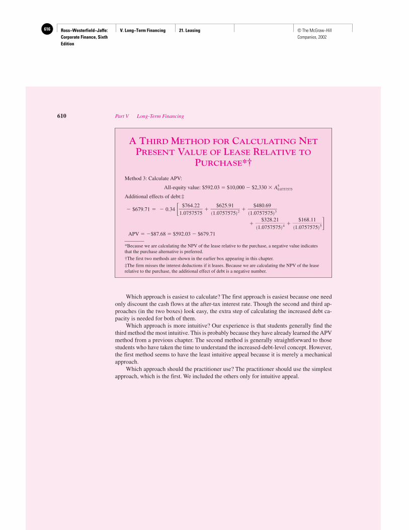
Ross−Westerfield−Jaffe: Corporate Finance, Sixth Edition
V. Long−Term Financing 21. Leasing616 © The McGraw−Hill Companies, 2002
Which approach is easiest to calculate? The first approach is easiest because one needonly discount the cash flows at the after-tax interest rate. Though the second and third ap-proaches (in the two boxes) look easy, the extra step of calculating the increased debt ca-pacity is needed for both of them.
Which approach is more intuitive? Our experience is that students generally find thethird method the most intuitive. This is probably because they have already learned the APVmethod from a previous chapter. The second method is generally straightforward to thosestudents who have taken the time to understand the increased-debt-level concept. However,the first method seems to have the least intuitive appeal because it is merely a mechanicalapproach.
Which approach should the practitioner use? The practitioner should use the simplestapproach, which is the first. We included the others only for intuitive appeal.
610 Part V Long-Term Financing
A THIRD METHOD FOR CALCULATING NET
PRESENT VALUE OF LEASE RELATIVE TO
PURCHASE*†
Method 3: Calculate APV:
All-equity value: $592.03 � $10,000 � $2,330 �
Additional effects of debt:‡
APV � �$87.68 � $592.03 � $679.71
*Because we are calculating the NPV of the lease relative to the purchase, a negative value indicatesthat the purchase alternative is preferred.
†The first two methods are shown in the earlier box appearing in this chapter.
‡The firm misses the interest deductions if it leases. Because we are calculating the NPV of the leaserelative to the purchase, the additional effect of debt is a negative number.
�$328.21
�1.0757575� 4 �$168.11
�1.0757575� 5� $679.71 � � 0.34 � $764.22
1.0757575�
$625.91�1.0757575� 2 �
$480.69�1.0757575� 3
A
50.0757575
Ross−Westerfield−Jaffe: Corporate Finance, Sixth Edition
VI. Options, Futures, and Corporate Finance
Introduction 617© The McGraw−Hill Companies, 2002
Options, Futures, andCorporate Finance
PA
RT
VI
22 Options and Corporate Finance: Basic Concepts 61223 Options and Corporate Finance: Extensions and Applications 65024 Warrants and Convertibles 67425 Derivatives and Hedging Risk 695
THE public has often viewed options and futures as exotic and risky instruments thatindividuals enter into at their peril. Although these derivatives can increase risk, they
also have important uses to corporations. In Part VI, we discuss these instruments in de-tail, showing three basic ideas: Recent advances allow options and futures to be easilypriced. Options are frequently embedded or hidden in the everyday activities of corpo-rations. Firms can actually use derivatives to reduce risk.
In Chapter 22 we examine options. First we describe the options that trade on or-ganized exchanges. Options are contingent claims on the value of an underlying asset.Every issue of corporate security has option features. Later in the chapter we present aformal model that can be used to value options. The model bears no resemblance to netpresent value (NPV). Our goal is to present the underlying logic of option valuation. Thisis important because NPV does not work well for contingent claims.
In Chapter 23, we describe some extensions of option pricing theory. There areoption-like features in most investing and financing decisions.
In Chapter 24 we look at bonds with special option features. These bonds are soldas bonds with warrants and as bonds convertible into common stock. A warrant gives theholder a right to buy shares of common stock for cash, and a convertible bond gives theholder the right to exchange it for shares of common stock.
Previous chapters of this text assume that the volatility of the firm is fixed. Chapter25 shows how firms can use financial instruments to reduce their risk, specifically dis-cussing financial futures.
Ross−Westerfield−Jaffe: Corporate Finance, Sixth Edition
VI. Options, Futures, and Corporate Finance
22. Options and Corporate Finance: Basic Concepts
618 © The McGraw−Hill Companies, 2002
Options and CorporateFinance: Basic Concepts
CH
AP
TE
R22
EXECUTIVE SUMMARY
In the summer of 2000, General Mills (GM) made an offer to acquire the Pillsbury divi-sion of Diageo PLC. Although the offer was generous, the managers of Diageo wereworried about the possibility of a decline in GM’s stock price. The deal eventually went
through, due to a creative financing technique called a contingent value rights (CVR). Al-though CVRs may seem arcane, they are really straightforward applications of options, atopic to be examined in this chapter.
Options are special contractual arrangements giving the owner the right to buy or sellan asset at a fixed price anytime on or before a given date. Stock options, the most familiartype, are options to buy and sell shares of common stock. Ever since 1973, stock optionshave been traded on organized exchanges.
Corporate securities are very similar to the stock options that are traded on organized ex-changes. Almost every issue of corporate bonds and stocks has option features. In addition,capital-structure decisions and capital-budgeting decisions can be viewed in terms of options.
We start this chapter with a description of different types of publicly traded options.We identify and discuss the factors that determine their values. Next, we show how com-mon stocks and bonds can be thought of as options on the underlying value of the firm. Thisleads to several new insights concerning corporate finance. For example, we show how cer-tain corporate decisions can be viewed as options. General Mills’ issuance of a CVR is oneof these corporate decisions.
22.1 OPTIONS
An option is a contract giving its owner the right to buy or sell an asset at a fixed price onor before a given date. For example, an option on a building might give the buyer the rightto buy the building for $1 million on or anytime before the Saturday prior to the thirdWednesday in January 2010. Options are a unique type of financial contract because theygive the buyer the right, but not the obligation, to do something. The buyer uses the optiononly if it is advantageous to do so; otherwise the option can be thrown away.
There is a special vocabulary associated with options. Here are some important definitions:
1. Exercising the Option. The act of buying or selling the underlying asset via the optioncontract is referred to as exercising the option.
2. Striking or Exercise Price. The fixed price in the option contract at which the holdercan buy or sell the underlying asset is called the striking price or exercise price.
3. Expiration Date. The maturity date of the option is referred to as the expiration date.After this date, the option is dead.
4. American and European Options. An American option may be exercised anytime upto the expiration date. A European option differs from an American option in that it canbe exercised only on the expiration date.
Ross−Westerfield−Jaffe: Corporate Finance, Sixth Edition
VI. Options, Futures, and Corporate Finance
22. Options and Corporate Finance: Basic Concepts
619© The McGraw−Hill Companies, 2002
22.2 CALL OPTIONS
The most common type of option is a call option. A call option gives the owner the right tobuy an asset at a fixed price during a particular time period. There is no restriction on the kindof asset, but the most common ones traded on exchanges are options on stocks and bonds.
For example, call options on IBM stock can be purchased on the Chicago Board OptionsExchange. IBM does not issue (that is, sell) call options on its common stock. Instead, indi-vidual investors are the original buyers and sellers of call options on IBM common stock. Arepresentative call option on IBM stock enables an investor to buy 100 shares of IBM on orbefore July 15, at an exercise price of $100. This is a valuable option if there is some prob-ability that the price of IBM common stock will exceed $100 on or before July 15.
The Value of a Call Option at ExpirationWhat is the value of a call-option contract on common stock at expiration? The answer de-pends on the value of the underlying stock at expiration.
Let’s continue with the IBM example. Suppose the stock price is $130 at expiration.The buyer1 of the call option has the right to buy the underlying stock at the exercise priceof $100. In other words, he has the right to exercise the call. Having the right to buy some-thing for $100 when it is worth $130 is obviously a good thing. The value2 of this right is$30 ($130–$100) on the expiration day.
The call would be worth even more if the stock price were higher on expiration day.For example, if IBM were selling for $150 on the date of expiration, the call would be worth$50 ($150–$100) at that time. In fact, the call’s value increases $1 for every $1 rise in thestock price.
If the stock price is greater than the exercise price, we say that the call is in the money.Of course, it is also possible that the value of the common stock will turn out to be less thanthe exercise price. In this case, we say that the call is out of the money. The holder will notexercise in this case. For example, if the stock price at the expiration date is $90, no rationalinvestor would exercise. Why pay $100 for stock worth only $90? Because the option holderhas no obligation to exercise the call, she can walk away from the option. As a consequence,if IBM’s stock price is less than $100 on the expiration date, the value of the call option willbe 0. In this case the value of the call option is not the difference between IBM’s stock priceand $100, as it would be if the holder of the call option had the obligation to exercise the call.
The payoff of a call option at expiration is
Payoff on the Expiration Date
If Stock Price Is Less Than $100 If Stock Price Is Greater Than $100
Call-option value: 0 Stock price �$100
Figure 22.1 plots the value of the call at expiration against the value of IBM’s stock. Itis referred to as the hockey-stick diagram of call-option values. If the stock price is less than$100, the call is out of the money and worthless. If the stock price is greater than $100, thecall is in the money and its value rises one-for-one with increases in the stock price. Noticethat the call can never have a negative value. It is a limited-liability instrument, which meansthat all the holder can lose is the initial amount she paid for it.
Chapter 22 Options and Corporate Finance: Basic Concepts 613
1We use buyer, owner, and holder interchangeably.2This example assumes that the call lets the holder purchase one share of stock at $100. In reality, a call lets theholder purchase 100 shares @ $100 per share. The profit would then equal $3000 [($130 � $100) � 100].
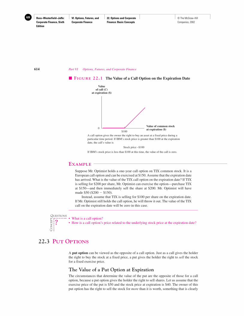
Ross−Westerfield−Jaffe: Corporate Finance, Sixth Edition
VI. Options, Futures, and Corporate Finance
22. Options and Corporate Finance: Basic Concepts
620 © The McGraw−Hill Companies, 2002
EXAMPLE
Suppose Mr. Optimist holds a one-year call option on TIX common stock. It is aEuropean call option and can be exercised at $150. Assume that the expiration datehas arrived. What is the value of the TIX call option on the expiration date? If TIXis selling for $200 per share, Mr. Optimist can exercise the option—purchase TIXat $150—and then immediately sell the share at $200. Mr. Optimist will havemade $50 ($200 � $150).
Instead, assume that TIX is selling for $100 per share on the expiration date.If Mr. Optimist still holds the call option, he will throw it out. The value of the TIXcall on the expiration date will be zero in this case.
• What is a call option?• How is a call option’s price related to the underlying stock price at the expiration date?
22.3 PUT OPTIONS
A put option can be viewed as the opposite of a call option. Just as a call gives the holderthe right to buy the stock at a fixed price, a put gives the holder the right to sell the stockfor a fixed exercise price.
The Value of a Put Option at ExpirationThe circumstances that determine the value of the put are the opposite of those for a calloption, because a put option gives the holder the right to sell shares. Let us assume that theexercise price of the put is $50 and the stock price at expiration is $40. The owner of thisput option has the right to sell the stock for more than it is worth, something that is clearly
614 Part VI Options, Futures, and Corporate Finance
$100
Value of common stockat expiration ($)0
Valueof call (C)
at expiration ($)
� FIGURE 22.1 The Value of a Call Option on the Expiration Date
A call option gives the owner the right to buy an asset at a fixed price during aparticular time period. If IBM’s stock price is greater than $100 at the expirationdate, the call’s value is
Stock price –$100
If IBM’s stock price is less than $100 at this time, the value of the call is zero.
QUESTIONS
CO
NC
EP
T
?
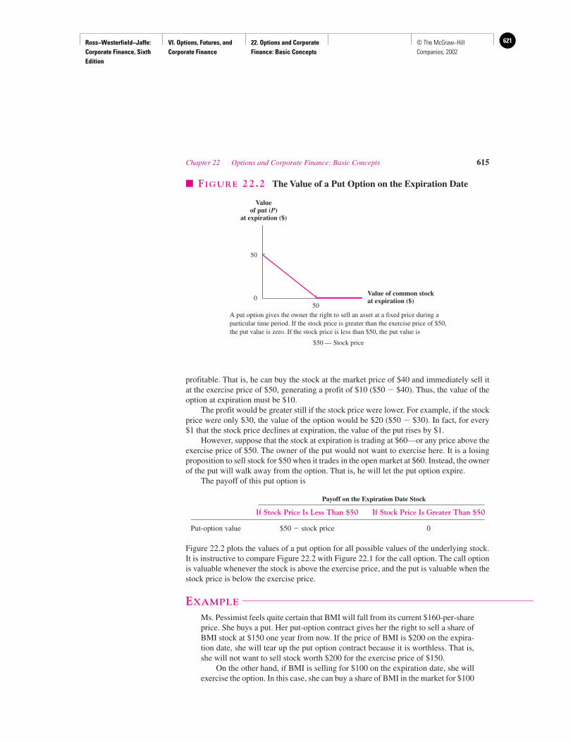
Ross−Westerfield−Jaffe: Corporate Finance, Sixth Edition
VI. Options, Futures, and Corporate Finance
22. Options and Corporate Finance: Basic Concepts
621© The McGraw−Hill Companies, 2002
profitable. That is, he can buy the stock at the market price of $40 and immediately sell itat the exercise price of $50, generating a profit of $10 ($50 � $40). Thus, the value of theoption at expiration must be $10.
The profit would be greater still if the stock price were lower. For example, if the stockprice were only $30, the value of the option would be $20 ($50 � $30). In fact, for every$1 that the stock price declines at expiration, the value of the put rises by $1.
However, suppose that the stock at expiration is trading at $60—or any price above theexercise price of $50. The owner of the put would not want to exercise here. It is a losingproposition to sell stock for $50 when it trades in the open market at $60. Instead, the ownerof the put will walk away from the option. That is, he will let the put option expire.
The payoff of this put option is
Payoff on the Expiration Date Stock
If Stock Price Is Less Than $50 If Stock Price Is Greater Than $50
Put-option value $50 � stock price 0
Figure 22.2 plots the values of a put option for all possible values of the underlying stock.It is instructive to compare Figure 22.2 with Figure 22.1 for the call option. The call optionis valuable whenever the stock is above the exercise price, and the put is valuable when thestock price is below the exercise price.
EXAMPLE
Ms. Pessimist feels quite certain that BMI will fall from its current $160-per-shareprice. She buys a put. Her put-option contract gives her the right to sell a share ofBMI stock at $150 one year from now. If the price of BMI is $200 on the expira-tion date, she will tear up the put option contract because it is worthless. That is,she will not want to sell stock worth $200 for the exercise price of $150.
On the other hand, if BMI is selling for $100 on the expiration date, she willexercise the option. In this case, she can buy a share of BMI in the market for $100
Chapter 22 Options and Corporate Finance: Basic Concepts 615
50
Value of common stockat expiration ($)0
Valueof put (P)
at expiration ($)
50
� FIGURE 22.2 The Value of a Put Option on the Expiration Date
A put option gives the owner the right to sell an asset at a fixed price during aparticular time period. If the stock price is greater than the exercise price of $50,the put value is zero. If the stock price is less than $50, the put value is
$50 — Stock price
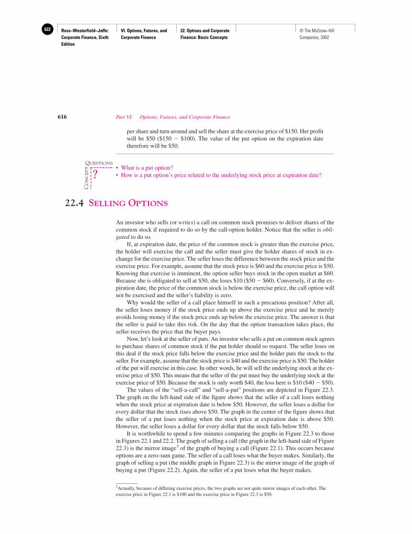
Ross−Westerfield−Jaffe: Corporate Finance, Sixth Edition
VI. Options, Futures, and Corporate Finance
22. Options and Corporate Finance: Basic Concepts
622 © The McGraw−Hill Companies, 2002
per share and turn around and sell the share at the exercise price of $150. Her profitwill be $50 ($150 � $100). The value of the put option on the expiration datetherefore will be $50.
• What is a put option?• How is a put option’s price related to the underlying stock price at expiration date?
22.4 SELLING OPTIONS
An investor who sells (or writes) a call on common stock promises to deliver shares of thecommon stock if required to do so by the call-option holder. Notice that the seller is obli-gated to do so.
If, at expiration date, the price of the common stock is greater than the exercise price,the holder will exercise the call and the seller must give the holder shares of stock in ex-change for the exercise price. The seller loses the difference between the stock price and theexercise price. For example, assume that the stock price is $60 and the exercise price is $50.Knowing that exercise is imminent, the option seller buys stock in the open market at $60.Because she is obligated to sell at $50, she loses $10 ($50 � $60). Conversely, if at the ex-piration date, the price of the common stock is below the exercise price, the call option willnot be exercised and the seller’s liability is zero.
Why would the seller of a call place himself in such a precarious position? After all,the seller loses money if the stock price ends up above the exercise price and he merelyavoids losing money if the stock price ends up below the exercise price. The answer is thatthe seller is paid to take this risk. On the day that the option transaction takes place, theseller receives the price that the buyer pays.
Now, let’s look at the seller of puts. An investor who sells a put on common stock agreesto purchase shares of common stock if the put holder should so request. The seller loses onthis deal if the stock price falls below the exercise price and the holder puts the stock to theseller. For example, assume that the stock price is $40 and the exercise price is $50. The holderof the put will exercise in this case. In other words, he will sell the underlying stock at the ex-ercise price of $50. This means that the seller of the put must buy the underlying stock at theexercise price of $50. Because the stock is only worth $40, the loss here is $10 ($40 � $50).
The values of the “sell-a-call” and “sell-a-put” positions are depicted in Figure 22.3.The graph on the left-hand side of the figure shows that the seller of a call loses nothingwhen the stock price at expiration date is below $50. However, the seller loses a dollar forevery dollar that the stock rises above $50. The graph in the center of the figure shows thatthe seller of a put loses nothing when the stock price at expiration date is above $50.However, the seller loses a dollar for every dollar that the stock falls below $50.
It is worthwhile to spend a few minutes comparing the graphs in Figure 22.3 to thosein Figures 22.1 and 22.2. The graph of selling a call (the graph in the left-hand side of Figure22.3) is the mirror image3 of the graph of buying a call (Figure 22.1). This occurs becauseoptions are a zero-sum game. The seller of a call loses what the buyer makes. Similarly, thegraph of selling a put (the middle graph in Figure 22.3) is the mirror image of the graph ofbuying a put (Figure 22.2). Again, the seller of a put loses what the buyer makes.
616 Part VI Options, Futures, and Corporate Finance
3Actually, because of differing exercise prices, the two graphs are not quite mirror images of each other. Theexercise price in Figure 22.1 is $100 and the exercise price in Figure 22.3 is $50.
QUESTIONS
CO
NC
EP
T
?
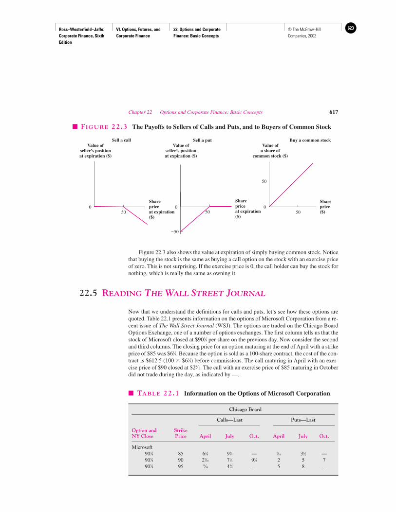
Ross−Westerfield−Jaffe: Corporate Finance, Sixth Edition
VI. Options, Futures, and Corporate Finance
22. Options and Corporate Finance: Basic Concepts
623© The McGraw−Hill Companies, 2002
Figure 22.3 also shows the value at expiration of simply buying common stock. Noticethat buying the stock is the same as buying a call option on the stock with an exercise priceof zero. This is not surprising. If the exercise price is 0, the call holder can buy the stock fornothing, which is really the same as owning it.
22.5 READING THE WALL STREET JOURNAL
Now that we understand the definitions for calls and puts, let’s see how these options arequoted. Table 22.1 presents information on the options of Microsoft Corporation from a re-cent issue of The Wall Street Journal (WSJ). The options are traded on the Chicago BoardOptions Exchange, one of a number of options exchanges. The first column tells us that thestock of Microsoft closed at $903⁄8 per share on the previous day. Now consider the secondand third columns. The closing price for an option maturing at the end of April with a strikeprice of $85 was $61⁄8. Because the option is sold as a 100-share contract, the cost of the con-tract is $612.5 (100 � $61⁄8) before commissions. The call maturing in April with an exer-cise price of $90 closed at $29⁄16. The call with an exercise price of $85 maturing in Octoberdid not trade during the day, as indicated by —.
Chapter 22 Options and Corporate Finance: Basic Concepts 617
50
Sharepriceat expiration($)
0
Value ofseller’s positionat expiration ($)
Sell a call
50
Sharepriceat expiration($)
0
Value ofseller’s positionat expiration ($)
Sell a put
50
Shareprice($)
0
Value ofa share of
common stock ($)
Buy a common stock
50
–50
� FIGURE 22.3 The Payoffs to Sellers of Calls and Puts, and to Buyers of Common Stock
� TABLE 22.1 Information on the Options of Microsoft Corporation
Chicago Board
Calls—Last Puts—Last
Option and StrikeNY Close Price April July Oct. April July Oct.
Microsoft903⁄8 85 61⁄8 93⁄4 — 9⁄16 31⁄2 —903⁄8 90 29⁄16 71⁄4 97⁄8 2 5 7903⁄8 95 11⁄16 43⁄4 — 5 8 —
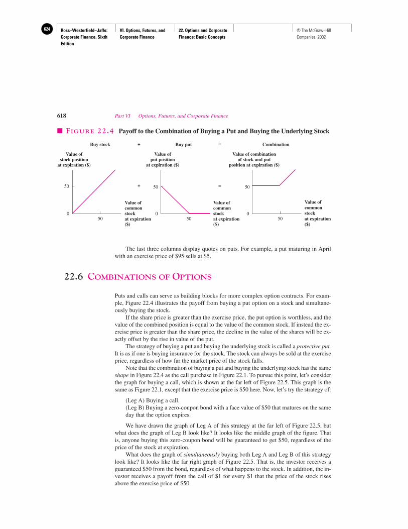
Ross−Westerfield−Jaffe: Corporate Finance, Sixth Edition
VI. Options, Futures, and Corporate Finance
22. Options and Corporate Finance: Basic Concepts
624 © The McGraw−Hill Companies, 2002
The last three columns display quotes on puts. For example, a put maturing in Aprilwith an exercise price of $95 sells at $5.
22.6 COMBINATIONS OF OPTIONS
Puts and calls can serve as building blocks for more complex option contracts. For exam-ple, Figure 22.4 illustrates the payoff from buying a put option on a stock and simultane-ously buying the stock.
If the share price is greater than the exercise price, the put option is worthless, and thevalue of the combined position is equal to the value of the common stock. If instead the ex-ercise price is greater than the share price, the decline in the value of the shares will be ex-actly offset by the rise in value of the put.
The strategy of buying a put and buying the underlying stock is called a protective put.It is as if one is buying insurance for the stock. The stock can always be sold at the exerciseprice, regardless of how far the market price of the stock falls.
Note that the combination of buying a put and buying the underlying stock has the sameshape in Figure 22.4 as the call purchase in Figure 22.1. To pursue this point, let’s considerthe graph for buying a call, which is shown at the far left of Figure 22.5. This graph is thesame as Figure 22.1, except that the exercise price is $50 here. Now, let’s try the strategy of:
(Leg A) Buying a call.(Leg B) Buying a zero-coupon bond with a face value of $50 that matures on the sameday that the option expires.
We have drawn the graph of Leg A of this strategy at the far left of Figure 22.5, butwhat does the graph of Leg B look like? It looks like the middle graph of the figure. Thatis, anyone buying this zero-coupon bond will be guaranteed to get $50, regardless of theprice of the stock at expiration.
What does the graph of simultaneously buying both Leg A and Leg B of this strategylook like? It looks like the far right graph of Figure 22.5. That is, the investor receives aguaranteed $50 from the bond, regardless of what happens to the stock. In addition, the in-vestor receives a payoff from the call of $1 for every $1 that the price of the stock risesabove the exercise price of $50.
618 Part VI Options, Futures, and Corporate Finance
50
Value ofcommonstockat expiration($)
0
Value ofstock position
at expiration ($)
Buy stock
50
Value ofcommonstockat expiration($)
0
Value ofput position
at expiration ($)
Buy put
50
Value ofcommonstockat expiration($)
0
Value of combinationof stock and put
position at expiration ($)
Combination
50 50 50
+
+
=
=
� FIGURE 22.4 Payoff to the Combination of Buying a Put and Buying the Underlying Stock
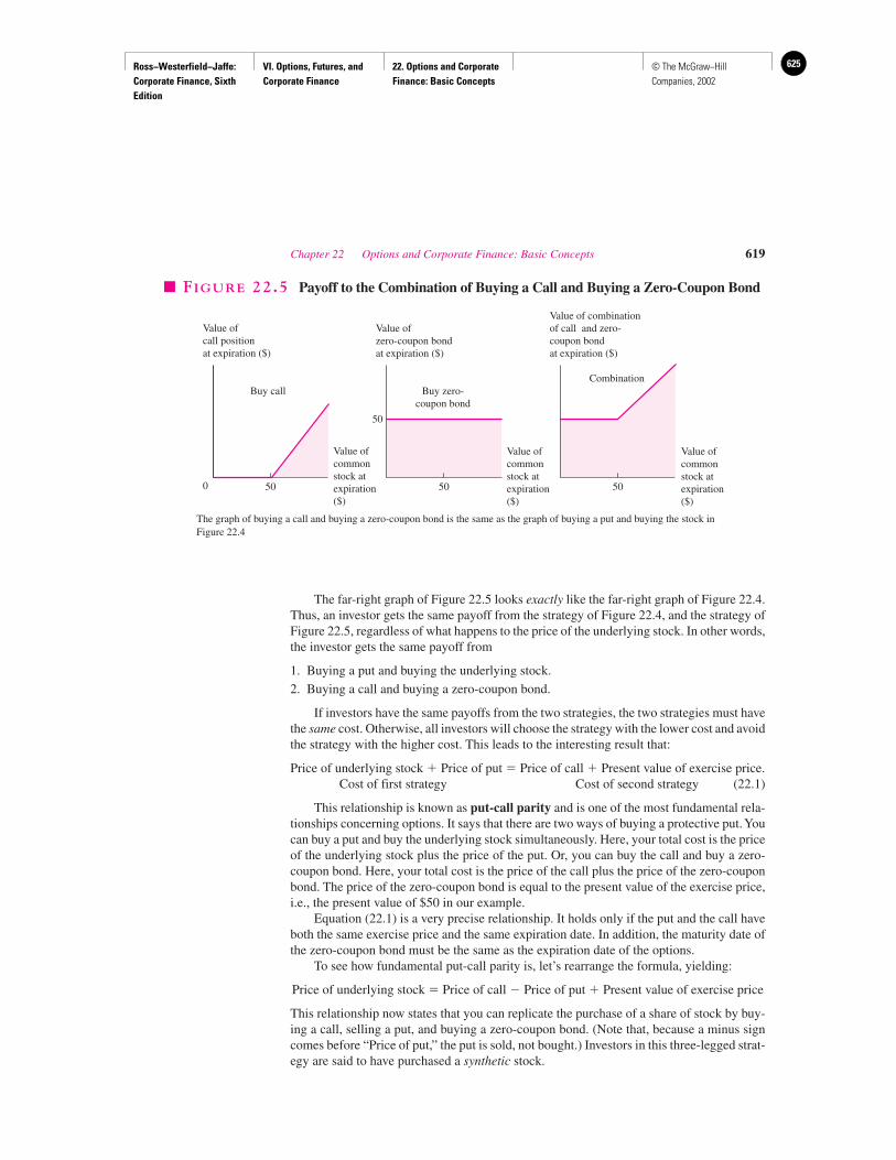
Ross−Westerfield−Jaffe: Corporate Finance, Sixth Edition
VI. Options, Futures, and Corporate Finance
22. Options and Corporate Finance: Basic Concepts
625© The McGraw−Hill Companies, 2002
The far-right graph of Figure 22.5 looks exactly like the far-right graph of Figure 22.4.Thus, an investor gets the same payoff from the strategy of Figure 22.4, and the strategy ofFigure 22.5, regardless of what happens to the price of the underlying stock. In other words,the investor gets the same payoff from
1. Buying a put and buying the underlying stock.
2. Buying a call and buying a zero-coupon bond.
If investors have the same payoffs from the two strategies, the two strategies must havethe same cost. Otherwise, all investors will choose the strategy with the lower cost and avoidthe strategy with the higher cost. This leads to the interesting result that:
Price of underlying stock � Price of put � Price of call � Present value of exercise price.Cost of first strategy Cost of second strategy (22.1)
This relationship is known as put-call parity and is one of the most fundamental rela-tionships concerning options. It says that there are two ways of buying a protective put. Youcan buy a put and buy the underlying stock simultaneously. Here, your total cost is the priceof the underlying stock plus the price of the put. Or, you can buy the call and buy a zero-coupon bond. Here, your total cost is the price of the call plus the price of the zero-couponbond. The price of the zero-coupon bond is equal to the present value of the exercise price,i.e., the present value of $50 in our example.
Equation (22.1) is a very precise relationship. It holds only if the put and the call haveboth the same exercise price and the same expiration date. In addition, the maturity date ofthe zero-coupon bond must be the same as the expiration date of the options.
To see how fundamental put-call parity is, let’s rearrange the formula, yielding:
Price of underlying stock � Price of call � Price of put � Present value of exercise price
This relationship now states that you can replicate the purchase of a share of stock by buy-ing a call, selling a put, and buying a zero-coupon bond. (Note that, because a minus signcomes before “Price of put,” the put is sold, not bought.) Investors in this three-legged strat-egy are said to have purchased a synthetic stock.
Chapter 22 Options and Corporate Finance: Basic Concepts 619
50
50
Buy call Buy zero-coupon bond
50
Value ofcall positionat expiration ($)
Value ofzero-coupon bondat expiration ($)
Combination
50
Value of combinationof call and zero-coupon bondat expiration ($)
Value ofcommonstock atexpiration ($)
Value ofcommonstock atexpiration ($)
Value ofcommonstock atexpiration ($)
0
� FIGURE 22.5 Payoff to the Combination of Buying a Call and Buying a Zero-Coupon Bond
The graph of buying a call and buying a zero-coupon bond is the same as the graph of buying a put and buying the stock inFigure 22.4
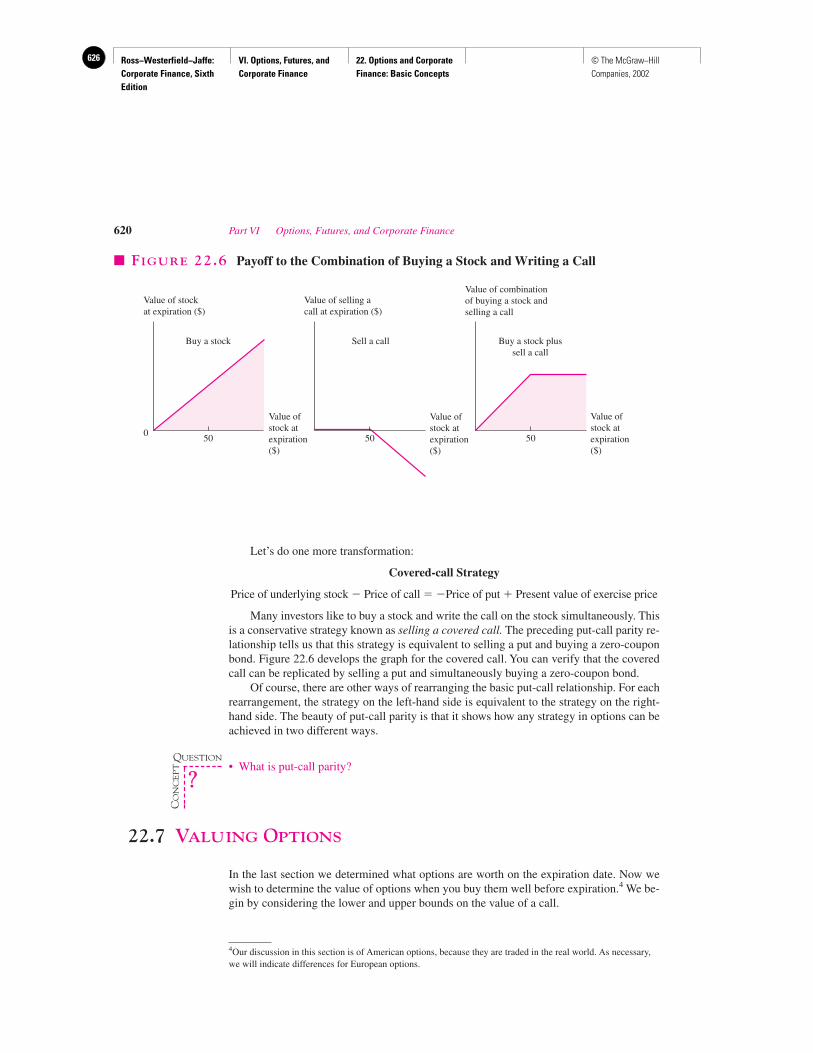
Ross−Westerfield−Jaffe: Corporate Finance, Sixth Edition
VI. Options, Futures, and Corporate Finance
22. Options and Corporate Finance: Basic Concepts
626 © The McGraw−Hill Companies, 2002
Let’s do one more transformation:
Covered-call Strategy
Price of underlying stock � Price of call � �Price of put � Present value of exercise price
Many investors like to buy a stock and write the call on the stock simultaneously. Thisis a conservative strategy known as selling a covered call. The preceding put-call parity re-lationship tells us that this strategy is equivalent to selling a put and buying a zero-couponbond. Figure 22.6 develops the graph for the covered call. You can verify that the coveredcall can be replicated by selling a put and simultaneously buying a zero-coupon bond.
Of course, there are other ways of rearranging the basic put-call relationship. For eachrearrangement, the strategy on the left-hand side is equivalent to the strategy on the right-hand side. The beauty of put-call parity is that it shows how any strategy in options can beachieved in two different ways.
• What is put-call parity?
22.7 VALUING OPTIONS
In the last section we determined what options are worth on the expiration date. Now wewish to determine the value of options when you buy them well before expiration.4 We be-gin by considering the lower and upper bounds on the value of a call.
620 Part VI Options, Futures, and Corporate Finance
50 50
Value of stockat expiration ($)
Buy a stock Sell a call Buy a stock plussell a call
Value of selling acall at expiration ($)
50
Value of combinationof buying a stock andselling a call
Value ofstock atexpiration($)
Value ofstock atexpiration($)
Value ofstock atexpiration($)
0
� FIGURE 22.6 Payoff to the Combination of Buying a Stock and Writing a Call
4Our discussion in this section is of American options, because they are traded in the real world. As necessary,we will indicate differences for European options.
QUESTION
CO
NC
EP
T
?
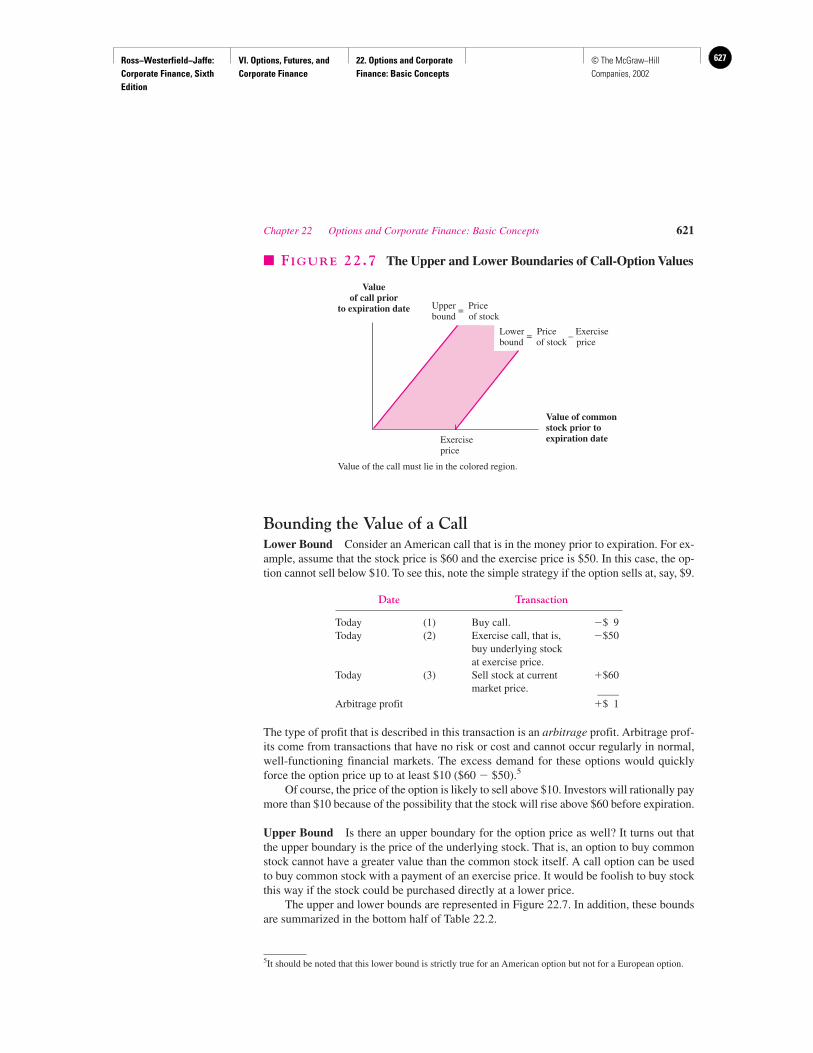
Ross−Westerfield−Jaffe: Corporate Finance, Sixth Edition
VI. Options, Futures, and Corporate Finance
22. Options and Corporate Finance: Basic Concepts
627© The McGraw−Hill Companies, 2002
Bounding the Value of a CallLower Bound Consider an American call that is in the money prior to expiration. For ex-ample, assume that the stock price is $60 and the exercise price is $50. In this case, the op-tion cannot sell below $10. To see this, note the simple strategy if the option sells at, say, $9.
Date Transaction
Today (1) Buy call. �$ 9Today (2) Exercise call, that is, �$50
buy underlying stock at exercise price.
Today (3) Sell stock at current �$60market price. ____
Arbitrage profit �$ 1
The type of profit that is described in this transaction is an arbitrage profit. Arbitrage prof-its come from transactions that have no risk or cost and cannot occur regularly in normal,well-functioning financial markets. The excess demand for these options would quicklyforce the option price up to at least $10 ($60 � $50).5
Of course, the price of the option is likely to sell above $10. Investors will rationally paymore than $10 because of the possibility that the stock will rise above $60 before expiration.
Upper Bound Is there an upper boundary for the option price as well? It turns out thatthe upper boundary is the price of the underlying stock. That is, an option to buy commonstock cannot have a greater value than the common stock itself. A call option can be usedto buy common stock with a payment of an exercise price. It would be foolish to buy stockthis way if the stock could be purchased directly at a lower price.
The upper and lower bounds are represented in Figure 22.7. In addition, these boundsare summarized in the bottom half of Table 22.2.
Chapter 22 Options and Corporate Finance: Basic Concepts 621
5It should be noted that this lower bound is strictly true for an American option but not for a European option.
Exerciseprice
Value of commonstock prior toexpiration date
Valueof call prior
to expiration date Upper = Pricebound of stock
Lower = Price – Exercisebound of stock price
� FIGURE 22.7 The Upper and Lower Boundaries of Call-Option Values
Value of the call must lie in the colored region.
Ross−Westerfield−Jaffe: Corporate Finance, Sixth Edition
VI. Options, Futures, and Corporate Finance
22. Options and Corporate Finance: Basic Concepts
628 © The McGraw−Hill Companies, 2002
The Factors Determining Call-Option ValuesThe previous discussion indicated that the price of a call option must fall somewhere in theshaded region of Figure 22.7. We now will determine more precisely where in the shadedregion it should be. The factors that determine a call’s value can be broken into two sets.The first set contains the features of the option contract. The two basic contractual featuresare the expiration price and the exercise date. The second set of factors affecting the callprice concerns characteristics of the stock and the market.
Exercise Price An increase in the exercise price reduces the value of the call. For exam-ple, imagine that there are two calls on a stock selling at $60. The first call has an exerciseprice of $50 and the second one has an exercise price of $40. Which call would you ratherhave? Clearly, you would rather have the call with an exercise price of $40, because thatone is $20 ($60 � $40) in the money. In other words, the call with an exercise price of $40should sell for more than an otherwise-identical call with an exercise price of $50.
Expiration Date The value of an American call option must be at least as great as thevalue of an otherwise identical option with a shorter term to expiration. Consider two Amer-ican calls: One has a maturity of nine months and the other expires in six months. Obvi-ously, the nine-month call has the same rights as the six-month call, and also has an addi-tional three months within which these rights can be exercised. It cannot be worth less andwill generally be more valuable.6
Stock Price Other things being equal, the higher the stock price, the more valuable thecall option will be. For example, if a stock is worth $80, a call with an exercise price of $100isn’t worth very much. If the stock soars to $120, the call becomes much more valuable.
Now consider Figure 22.8, which shows the relationship between the call price and thestock price prior to expiration. The curve indicates that the call price increases as the stockprice increases. Furthermore, it can be shown that the relationship is represented, not by astraight line, but by a convex curve. That is, the increase in the call price for a given changein the stock price is greater when the stock price is high than when the stock price is low.
There are two special points on the curve in Figure 22.8:
1. The Stock Is Worthless. The call must be worthless if the underlying stock is worthless.That is, if the stock has no chance of attaining any value, it is not worthwhile to pay theexercise price in order to obtain the stock.
2. The Stock Price Is Very High Relative to the Exercise Price. In this situation, the ownerof the call knows that he will end up exercising the call. He can view himself as the ownerof the stock now, with one difference. He must pay the exercise price at expiration.
Thus, the value of his position, i.e., the value of the call, is:
Stock price � Present value of exercise price
These two points on the curve are summarized in the bottom half of Table 22.2.
622 Part VI Options, Futures, and Corporate Finance
6This relationship need not hold for a European call option. Consider a firm with two otherwise identicalEuropean call options, one expiring at the end of May and the other expiring a few months later. Further assumethat a huge dividend is paid in early June. If the first call is exercised at the end of May, its holder will receivethe underlying stock. If he does not sell the stock, he will receive the large dividend shortly thereafter. However,the holder of the second call will receive the stock through exercise after the dividend is paid. Because themarket knows that the holder of this option will miss the dividend, the value of the second call option could beless than the value of the first.
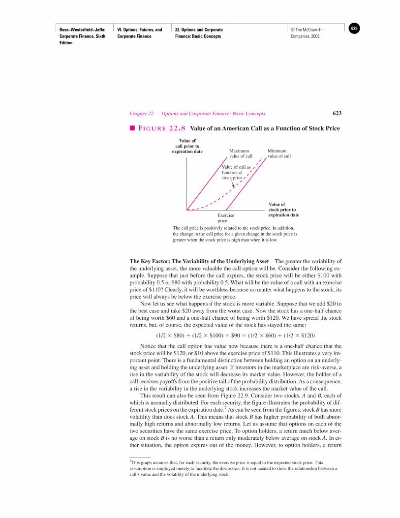
Ross−Westerfield−Jaffe: Corporate Finance, Sixth Edition
VI. Options, Futures, and Corporate Finance
22. Options and Corporate Finance: Basic Concepts
629© The McGraw−Hill Companies, 2002
The Key Factor: The Variability of the Underlying Asset The greater the variability ofthe underlying asset, the more valuable the call option will be. Consider the following ex-ample. Suppose that just before the call expires, the stock price will be either $100 withprobability 0.5 or $80 with probability 0.5. What will be the value of a call with an exerciseprice of $110? Clearly, it will be worthless because no matter what happens to the stock, itsprice will always be below the exercise price.
Now let us see what happens if the stock is more variable. Suppose that we add $20 tothe best case and take $20 away from the worst case. Now the stock has a one-half chanceof being worth $60 and a one-half chance of being worth $120. We have spread the stockreturns, but, of course, the expected value of the stock has stayed the same:
(1/2 � $80) � (1/2 � $100) � $90 � (1/2 � $60) � (1/2 � $120)
Notice that the call option has value now because there is a one-half chance that thestock price will be $120, or $10 above the exercise price of $110. This illustrates a very im-portant point. There is a fundamental distinction between holding an option on an underly-ing asset and holding the underlying asset. If investors in the marketplace are risk-averse, arise in the variability of the stock will decrease its market value. However, the holder of acall receives payoffs from the positive tail of the probability distribution. As a consequence,a rise in the variability in the underlying stock increases the market value of the call.
This result can also be seen from Figure 22.9. Consider two stocks, A and B, each ofwhich is normally distributed. For each security, the figure illustrates the probability of dif-ferent stock prices on the expiration date.7 As can be seen from the figures, stock B has morevolatility than does stock A. This means that stock B has higher probability of both abnor-mally high returns and abnormally low returns. Let us assume that options on each of thetwo securities have the same exercise price. To option holders, a return much below aver-age on stock B is no worse than a return only moderately below average on stock A. In ei-ther situation, the option expires out of the money. However, to option holders, a return
Chapter 22 Options and Corporate Finance: Basic Concepts 623
Exerciseprice
Value ofstock prior toexpiration date
Value ofcall prior to
expiration date Maximumvalue of call
Minimumvalue of call
Value of call asfunction ofstock price
� FIGURE 22.8 Value of an American Call as a Function of Stock Price
The call price is positively related to the stock price. In addition,the change in the call price for a given change in the stock price isgreater when the stock price is high than when it is low.
7This graph assumes that, for each security, the exercise price is equal to the expected stock price. Thisassumption is employed merely to facilitate the discussion. It is not needed to show the relationship between acall’s value and the volatility of the underlying stock.
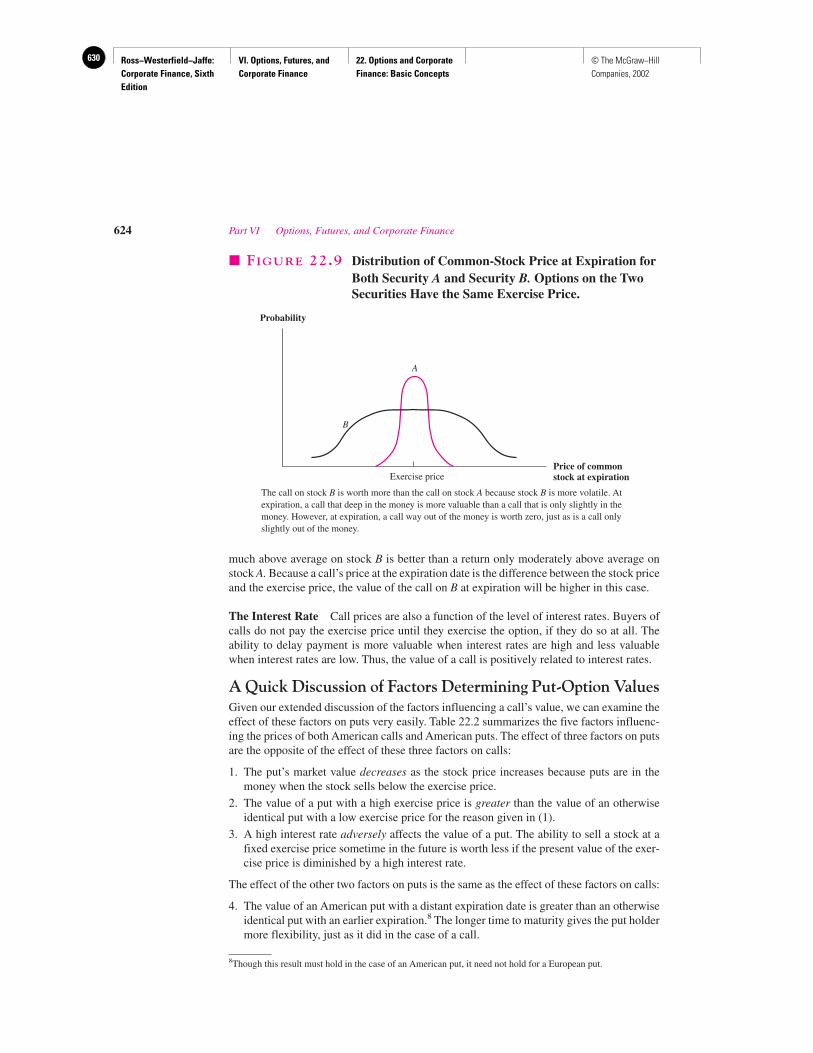
Ross−Westerfield−Jaffe: Corporate Finance, Sixth Edition
VI. Options, Futures, and Corporate Finance
22. Options and Corporate Finance: Basic Concepts
630 © The McGraw−Hill Companies, 2002
much above average on stock B is better than a return only moderately above average onstock A. Because a call’s price at the expiration date is the difference between the stock priceand the exercise price, the value of the call on B at expiration will be higher in this case.
The Interest Rate Call prices are also a function of the level of interest rates. Buyers ofcalls do not pay the exercise price until they exercise the option, if they do so at all. Theability to delay payment is more valuable when interest rates are high and less valuablewhen interest rates are low. Thus, the value of a call is positively related to interest rates.
A Quick Discussion of Factors Determining Put-Option ValuesGiven our extended discussion of the factors influencing a call’s value, we can examine theeffect of these factors on puts very easily. Table 22.2 summarizes the five factors influenc-ing the prices of both American calls and American puts. The effect of three factors on putsare the opposite of the effect of these three factors on calls:
1. The put’s market value decreases as the stock price increases because puts are in themoney when the stock sells below the exercise price.
2. The value of a put with a high exercise price is greater than the value of an otherwiseidentical put with a low exercise price for the reason given in (1).
3. A high interest rate adversely affects the value of a put. The ability to sell a stock at afixed exercise price sometime in the future is worth less if the present value of the exer-cise price is diminished by a high interest rate.
The effect of the other two factors on puts is the same as the effect of these factors on calls:
4. The value of an American put with a distant expiration date is greater than an otherwiseidentical put with an earlier expiration.8 The longer time to maturity gives the put holdermore flexibility, just as it did in the case of a call.
624 Part VI Options, Futures, and Corporate Finance
Probability
Price of commonstock at expirationExercise price
A
B
� FIGURE 22.9 Distribution of Common-Stock Price at Expiration forBoth Security A and Security B. Options on the TwoSecurities Have the Same Exercise Price.
The call on stock B is worth more than the call on stock A because stock B is more volatile. Atexpiration, a call that deep in the money is more valuable than a call that is only slightly in themoney. However, at expiration, a call way out of the money is worth zero, just as is a call onlyslightly out of the money.
8Though this result must hold in the case of an American put, it need not hold for a European put.
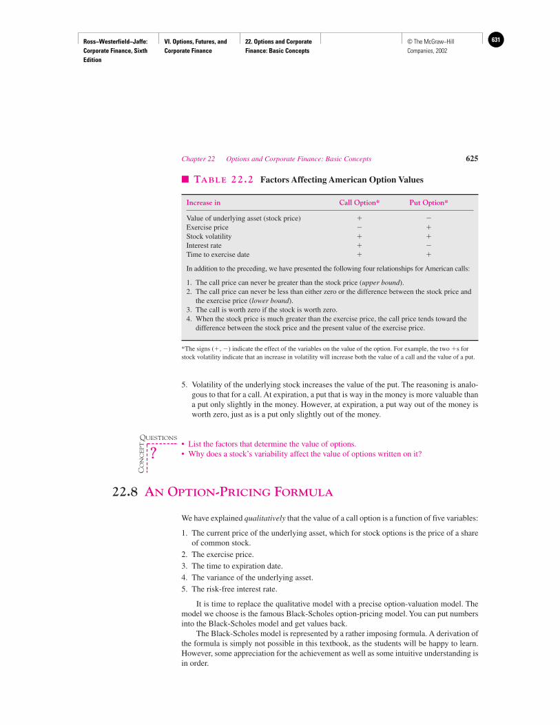
Ross−Westerfield−Jaffe: Corporate Finance, Sixth Edition
VI. Options, Futures, and Corporate Finance
22. Options and Corporate Finance: Basic Concepts
631© The McGraw−Hill Companies, 2002
5. Volatility of the underlying stock increases the value of the put. The reasoning is analo-gous to that for a call. At expiration, a put that is way in the money is more valuable thana put only slightly in the money. However, at expiration, a put way out of the money isworth zero, just as is a put only slightly out of the money.
• List the factors that determine the value of options.• Why does a stock’s variability affect the value of options written on it?
22.8 AN OPTION-PRICING FORMULA
We have explained qualitatively that the value of a call option is a function of five variables:
1. The current price of the underlying asset, which for stock options is the price of a shareof common stock.
2. The exercise price.
3. The time to expiration date.
4. The variance of the underlying asset.
5. The risk-free interest rate.
It is time to replace the qualitative model with a precise option-valuation model. Themodel we choose is the famous Black-Scholes option-pricing model. You can put numbersinto the Black-Scholes model and get values back.
The Black-Scholes model is represented by a rather imposing formula. A derivation ofthe formula is simply not possible in this textbook, as the students will be happy to learn.However, some appreciation for the achievement as well as some intuitive understanding isin order.
Chapter 22 Options and Corporate Finance: Basic Concepts 625
� TABLE 22.2 Factors Affecting American Option Values
Increase in Call Option* Put Option*
Value of underlying asset (stock price) � �Exercise price � �Stock volatility � �Interest rate � �Time to exercise date � �
In addition to the preceding, we have presented the following four relationships for American calls:
1. The call price can never be greater than the stock price (upper bound).2. The call price can never be less than either zero or the difference between the stock price and
the exercise price (lower bound).3. The call is worth zero if the stock is worth zero.4. When the stock price is much greater than the exercise price, the call price tends toward the
difference between the stock price and the present value of the exercise price.
*The signs (�, �) indicate the effect of the variables on the value of the option. For example, the two �s forstock volatility indicate that an increase in volatility will increase both the value of a call and the value of a put.
QUESTIONS
CO
NC
EP
T
?
Ross−Westerfield−Jaffe: Corporate Finance, Sixth Edition
VI. Options, Futures, and Corporate Finance
22. Options and Corporate Finance: Basic Concepts
632 © The McGraw−Hill Companies, 2002
In the early chapters of this book, we showed how to discount capital-budgeting proj-ects using the net-present-value formula. We also used this approach to value stocks andbonds. Why, students sometimes ask, can’t the same NPV formula be used to value puts andcalls? It is a good question because the earliest attempts at valuing options used NPV.Unfortunately, the attempts were simply not successful because no one could determine theappropriate discount rate. An option is generally riskier than the underlying stock but noone knew exactly how much riskier.
Black and Scholes attacked the problem by pointing out that a strategy of borrowing tofinance a stock purchase duplicates the risk of a call. Then, knowing the price of a stock al-ready, one can determine the price of a call such that its return is identical to that of thestock-with-borrowing alternative.
We illustrate the intuition behind the Black-Scholes approach by considering a simpleexample where a combination of a call and a stock eliminates all risk. This example worksbecause we let the future stock price be one of only two values. Hence, the example is calleda two-state option model. By eliminating the possibility that the stock price can take onother values, we are able to duplicate the call exactly.
A Two-State Option ModelConsider the following example. Suppose the current market price of a stock is $50 and thestock will either be $60 or $40 at the end of the year. Further, imagine a call option on thisstock with a one-year expiration date and a $50 exercise price. Investors can borrow at 10percent. Our goal is to determine the value of the call.
In order to value the call correctly, we need to examine two strategies. The first is tosimply buy the call. The second is to:
a. Buy one-half a share of stock.
b. Borrow $18.18, implying a payment of principal and interest at the end of the year of$20 ($18.18 � 1.10).
As you will see shortly, the cash flows from the second strategy exactly match the cashflows from buying a call. (A little later we will show how we came up with the exact frac-tion of a share of stock to buy and the exact borrowing amount.) Because the cash flowsmatch, we say that we are duplicating the call with the second strategy.
At the end of the year, the future payoffs are set out as follows:
Future Payoffs
Initial Transactions If Stock Price Is $60 If Stock Price Is $40
1. Buy a call $60 � $50 � $10 0
2. Buy 1⁄2 share of stock 1⁄2 � $60 � $30 1⁄2 � $40 � $20Borrow $18.18 at 10% �($18.18 � 1.10) � �$20 �$20_____ _____
Total from stock and borrowing strategy $10 0
Note that the future payoff structure of the “buy-a-call” strategy is duplicated by thestrategy of “buy stock” and “borrow.” That is, under either strategy, an investor would endup with $10 if the stock price rose and $0 if the stock price fell. Thus, these two strategiesare equivalent as far as traders are concerned.
Now, if two strategies always have the same cash flows at the end of the year, how musttheir initial costs be related? The two strategies must have the same initial cost. Otherwise,there will be an arbitrage possibility. We can easily calculate this cost for our strategy ofbuying stock and borrowing. This cost is:
626 Part VI Options, Futures, and Corporate Finance
Ross−Westerfield−Jaffe: Corporate Finance, Sixth Edition
VI. Options, Futures, and Corporate Finance
22. Options and Corporate Finance: Basic Concepts
633© The McGraw−Hill Companies, 2002
Buy 1⁄2 share of stock 1⁄2 � $50 � $25.00Borrow $18.18 �$18.18_______
$6.82
Because the call option provides the same payoffs at expiration as does the strategy ofbuying stock and borrowing, the call must be priced at $6.82. This is the value of the calloption in a market without arbitrage profits.
We left two issues unexplained in the preceding example.
Determining the Delta How did we know to buy one-half share of stock in the duplicat-ing strategy? Actually, the answer is easier than it might at first appear. The call price at theend of the year will be either $10 or $0, whereas the stock price will be either $60 or $40.Thus, the call price has a potential swing of $10 ($10 � $0) next period, whereas the stockprice has a potential swing of $20 ($60 � $40). We can write this in terms of the followingratio:
Delta
1⁄2
This ratio is called the delta of the call. In words, a $1 swing in the price of the stock givesrise to a $1/2 swing in the price of the call. Because we are trying to duplicate the call withthe stock, it seems sensible to buy one-half share of stock instead of buying one call. In otherwords, the risk of buying one-half share of stock should be the same as the risk of buyingone call.
Determining the Amount of Borrowing How did we know how much to borrow? Buy-ing one-half share of stock brings us either $30 or $20 at expiration, which is exactly $20more than the payoffs of $10 and $0, respectively, from the call. To duplicate the callthrough a purchase of stock, we should also borrow enough money so that we have to payback exactly $20 of interest and principal. This amount of borrowing is merely the presentvalue of $20, which is $18.18 ($20/1.10).
Now that we know how to determine both the delta and the borrowing, we can writethe value of the call as:
Value of call � Stock price � Delta � Amount borrowed (22.2)$6.82 � $50 � 1⁄2 � $18.18
We will find this intuition very useful in explaining the Black-Scholes model.
Risk-Neutral Valuation Before leaving this simple example, we should comment on aremarkable feature. We found the exact value of the option without even knowing the prob-ability that the stock would go up or down! If an optimist thought the probability of an upmove was very high and a pessimist thought it was very low, they would still agree on theoption value. How could that be? The answer is that the current $50 stock price already bal-ances the views of the optimists and the pessimists. The option reflects that balance becauseits value depends on the stock price.
This insight provides us with another approach to valuing the call. If we don’t need theprobabilities of the two states to value the call, perhaps we can select any probabilities wewant and still come up with the right answer. Suppose we selected probabilities such thatthe return on the stock is equal to the risk-free rate of 10 percent. We know that the stock
Swing of call
Swing of stock�
$10 � $0
$60 � $40�
Chapter 22 Options and Corporate Finance: Basic Concepts 627
Ross−Westerfield−Jaffe: Corporate Finance, Sixth Edition
VI. Options, Futures, and Corporate Finance
22. Options and Corporate Finance: Basic Concepts
634 © The McGraw−Hill Companies, 2002
return given a rise is 20 percent ($60/$50 � 1) and the stock return given a fall is �20 per-cent ($40/$50 � 1). Thus, we can solve for the probability of a rise necessary to achieve anexpected return of 10 percent as:
10% � Probability of a rise � 20% � (1 � Probability of rise) � �20%
Solving this formula, we find that the probability of a rise is 3/4 and the probability ofa fall is 1/4. If we apply these probabilities to the call, we can value it as:
the same value that we got from the duplicating approach.Why did we select probabilities such that the expected return on the stock is 10 percent?
We wanted to work with the special case where investors are risk-neutral. This case occurswhere the expected return on any asset (including both the stock and the call) is equal to therisk-free rate. In other words, this case occurs when investors demand no additional com-pensation beyond the risk-free rate, regardless of the risk of the asset in question.
What would have happened if we had assumed that the expected return on a stock wasgreater than the risk-free rate? The value of the call would still be $6.82. However, the cal-culations would be difficult. For example, if we assumed that the expected return on thestock was, say, 11 percent, we would have had to derive the expected return on the call.Although the expected return on the call would be higher than 11 percent, it would take alot of work to determine it precisely. Why do any more work than you have to? Because wecan’t think of any good reason, we (and most other financial economists) choose to assumerisk-neutrality.
Thus, the preceding material allows us to value a call in the following two ways:
1. Determine the cost of a strategy to duplicate the call. This strategy involves an invest-ment in a fractional share of stock financed by partial borrowing.
2. Calculate the probabilities of a rise and a fall under the assumption of risk-neutrality.
Use those probabilities, in conjunction with the risk-free rate, to discount the payoffs of thecall at expiration.
The Black-Scholes ModelThe preceding example illustrates the duplicating strategy. Unfortunately, a strategy such asthis will not work in the real world over, say, a one-year time frame, because there are manymore than two possibilities for next year’s stock price. However, the number of possibilitiesis reduced as the time period is shortened. In fact, the assumption that there are only two pos-sibilities for the stock price over the next infinitesimal instant is quite plausible.9
In our opinion, the fundamental insight of Black and Scholes is to shorten the time pe-riod. They show that a specific combination of stock and borrowing can indeed duplicate acall over an infinitesimal time horizon. Because the price of the stock will change over thefirst instant, another combination of stock and borrowing is needed to duplicate the call overthe second instant and so on. By adjusting the combination from moment to moment, theycan continually duplicate the call. It may boggle the mind that a formula can (1) determinethe duplicating combination at any moment and (2) value the option based on this dupli-cating strategy. Suffice it to say that their dynamic strategy allows them to value a call inthe real world just as we showed how to value the call in the two-state model.
Value of call �3�4 � $10 � 1�4 � $0
1.10� $6.82
628 Part VI Options, Futures, and Corporate Finance
9A full treatment of this assumption can be found in John C. Hull, Options, Futures and Other Derivatives, 4thed. Upper Saddle River, N.J.: Prentice Hall (1999).
Ross−Westerfield−Jaffe: Corporate Finance, Sixth Edition
VI. Options, Futures, and Corporate Finance
22. Options and Corporate Finance: Basic Concepts
635© The McGraw−Hill Companies, 2002
This is the basic intuition behind the Black-Scholes (BS) model. Because the actualderivation of their formula is, alas, far beyond the scope of this text, we simply present theformula itself. The formula is
Black-Scholes Model:
C � SN(d1) � Ee�rt N(d2)
where d1 � [ln(S/E) � (r � 1/2�2)t]/
d2 � d1 �
This formula for the value of a call, C, is one of the most complex in finance. However,it involves only five parameters:
1. S � Current stock price
2. E � Exercise price of call
3. r � Annual risk-free rate of return, continually compounded
4. �2 � Variance (per year) of the continuous return on the stock
5. t � Time (in years) to expiration date
In addition, there is the statistical concept:
N(d) � Probability that a standardized, normally distributed,random variable will be less than or equal to d
Rather than discuss the formula in its algebraic state, we illustrate the formula with anexample.
EXAMPLE
Consider Private Equipment Company (PEC). On October 4, of year 0, the PECApril 49 call option had a closing value of $4. The stock itself is selling at $50. OnOctober 4 the option had 199 days to expiration (maturity date � April 21,Year 1).The annual risk-free interest rate, continually compounded, is 7 percent.
This information determines three variables directly:
1. The stock price, S, is $50.2. The exercise price, E, is $49.3. The risk-free rate, r, is 0.07.
In addition, the time to maturity, t, can be calculated quickly: The formula calls fort to be expressed in years.
4. We express the 199-day interval in years as t � 199/365.
In the real world, an option trader would know S and E exactly. Traders gen-erally view U.S. Treasury bills as riskless, so a current quote from The Wall StreetJournal or a similar newspaper would be obtained for the interest rate. The traderwould also know (or could count) the number of days to expiration exactly. Thus,the fraction of a year to expiration, t, could be calculated quickly.
The problem comes in determining the variance of the stock’s return. The for-mula calls for the variance in operation between the purchase date of October 4and the expiration date. Unfortunately, this represents the future, so the correctvalue for variance is simply not available. Instead, traders frequently estimate vari-ance from past data, just as we calculated variance in an earlier chapter. In addi-tion, some traders may use intuition to adjust their estimate. For example, if an-ticipation of an upcoming event is currently increasing the volatility of the stock,
��2t
��2t
Chapter 22 Options and Corporate Finance: Basic Concepts 629
Ross−Westerfield−Jaffe: Corporate Finance, Sixth Edition
VI. Options, Futures, and Corporate Finance
22. Options and Corporate Finance: Basic Concepts
636 © The McGraw−Hill Companies, 2002
the trader might adjust her estimate of variance upward to reflect this. (This prob-lem was most severe right after the October 19, 1987, crash. The stock market wasquite risky in the aftermath, so estimates using precrash data were too low.)
The above discussion was intended merely to mention the difficulties in vari-ance estimation, not to present a solution. For our purposes, we assume that atrader has come up with an estimate of variance:
5. The variance of Private Equipment Co. has been estimated to be 0.09 per year.
Using the above five parameters, we calculate the Black-Scholes value of thePEC option in three steps:
Step 1: Calculate d1 and d2. These values can be determined by a straightfor-ward, albeit tedious, insertion of our parameters into the basic formula. We have
� [0.0202 � 0.0627]/0.2215 � 0.3742
d2 � d1 �� 0.1527
Step 2: Calculate N(d1) and N(d2). The values N(d1) and N(d2) can best be un-derstood by examining Figure 22.10. The figure shows the normal distributionwith an expected value of 0 and a standard deviation of 1. This is frequently calledthe standardized normal distribution. We mentioned in an earlier chapter thatthe probability that a drawing from this distribution will be between �1 and �1(within one standard deviation of its mean, in other words) is 68.26 percent.
Now, let us ask a different question. What is the probability that a drawingfrom the standardized normal distribution will be below a particular value? For ex-ample, the probability that a drawing will be below 0 is clearly 50 percent becausethe normal distribution is symmetric. Using statistical terminology, we say that thecumulative probability of 0 is 50 percent. Statisticians also say that N(0) � 50%.It turns out that
N(d1) � N(0.3742) � 0.6459N(d2) � N(0.1527) � 0.5607
��2t
� �ln�50
49� � �0.07 � 1�2 � 0.09� �199
365 ��0.09 �199
365
d1 � �ln�S
E� � �r � 1 �2�2� t ���2t
630 Part VI Options, Futures, and Corporate Finance
Probability
Value–1 0 0.3742 1
� FIGURE 22.10 Graph of Cumulative Probability
Shaded area represents cumulative probability. Because the probability is 0.6459that a drawing from the standard normal distribution will be below 0.3742, we saythat N(0.3742) � 0.6459. That is, the cumulative probability of 0.3742 is 0.6459.
Ross−Westerfield−Jaffe: Corporate Finance, Sixth Edition
VI. Options, Futures, and Corporate Finance
22. Options and Corporate Finance: Basic Concepts
637© The McGraw−Hill Companies, 2002
The first value means that there is a 64.59-percent probability that a drawing fromthe standardized normal distribution will be below 0.3742. The second valuemeans that there is a 56.07-percent probability that a drawing from the standard-ized normal distribution will be below 0.1527. More generally, N(d) is the nota-tion that a drawing from the standardized normal distribution will be below d. Inother words, N(d) is the cumulative probability of d. Note that d1 and d2 in our ex-ample are slightly above zero, so N(d1) and N(d2) are slightly greater than 0.50.
Perhaps the easiest way to determine N(d1) and N(d2) is from the EXCELfunction NORMSDIST. In our example, NORMSDIST (0.3742) and NORMS-DIST (0.1527) are 0.6459 and 0.5607, respectively.
We can also determine the cumulative probability from Table 22.3. For ex-ample, consider d � 0.37. This can be found in the table as 0.3 on the vertical and0.07 on the horizontal. The value in the table for d � 0.37 is 0.1443. This value isnot the cumulative probability of 0.37. One must first make an adjustment to de-termine cumulative probability. That is,
N(0.37) � 0.50 � 0.1443 � 0.6443N(�0.37) � 0.50 � 0.1443 � 0.3557
Unfortunately, our table handles only two significant digits, whereas ourvalue of 0.3742 has four significant digits. Hence, we must interpolate to findN(0.3742). Because N(0.37) � 0.6443 and N(0.38) � 0.6480, the difference be-tween the two values is 0.0037 (0.6480 � 0.6443). Because 0.3742 is 42 percentof the way between 0.37 and 0.38, we interpolate as10
N(0.3742) � 0.6443 � 0.42 � 0.0037 � 0.6459
Step 3: Calculate C. We have
C � S � [N(d1)] � Ee�rt � [N(d2)]
� $50 � [N(d1)] � $49 � [e�0.07 � (199/365)] � N(d2)
� ($50 � 0.6459) � ($49 � 0.9626 � 0.5607)
� $32.295 � $26.447
� $5.85
The estimated price of $5.85 is greater than the $4 actual price, implying that thecall option is underpriced. A trader believing in the Black-Scholes model wouldbuy a call. Of course, the Black-Scholes model is fallible. Perhaps the disparity be-tween the model’s estimate and the market price reflects error in the trader’s esti-mate of variance.
The previous example stressed the calculations involved in using the Black-Scholesformula. Is there any intuition behind the formula? Yes, and that intuition follows from thestock purchase and borrowing strategy in our binomial example. The first line of the Black-Scholes equation is:
C � S � N(d1) � Ee�rt N(d2)
which is exactly analogous to equation (22.2):
Value of call � Stock price � Delta � Amount borrowed (22.2)
Chapter 22 Options and Corporate Finance: Basic Concepts 631
10This method is called linear interpolation. It is only one of a number of possible methods of interpolation.

Ross−Westerfield−Jaffe: Corporate Finance, Sixth Edition
VI. Options, Futures, and Corporate Finance
22. Options and Corporate Finance: Basic Concepts
638 © The McGraw−Hill Companies, 2002
that we presented in the binomial example. It turns out that N(d1) is the delta in the Black-Scholes model. N(d1) is 0.6459 in the previous example. In addition, Ee�rtN(d1) is theamount that an investor must borrow to duplicate a call. In the previous example, this valueis $26.45 ($49 � 0.9626 � 0.5607). Thus, the model tells us that we can duplicate the callof the preceding example by both:
1. Buying 0.6459 share of stock.
2. Borrowing $26.45.
It is no exaggeration to say that the Black-Scholes formula is among the most impor-tant contributions in finance. It allows anyone to calculate the value of an option given afew parameters. The attraction of the formula is that four of the parameters are observable:the current price of stock, S, the exercise price, E, the interest rate, r, and the time to expi-ration date, t. Only one of the parameters must be estimated: the variance of return, �2.
632 Part VI Options, Futures, and Corporate Finance
� TABLE 22.3 Cumulative Probabilities of the Standard Normal Distribution Function
d 0.00 0.01 0.02 0.03 0.04 0.05 0.06 0.07 0.08 0.09
0.0 0.0000 0.0040 0.0080 0.0120 0.0160 0.0199 0.0239 0.0279 0.0319 0.03590.1 0.0398 0.0438 0.0478 0.0517 0.0557 0.0596 0.0636 0.0675 0.0714 0.07530.2 0.0793 0.0832 0.0871 0.0910 0.0948 0.0987 0.1026 0.1064 0.1103 0.11410.3 0.1179 0.1217 0.1255 0.1293 0.1331 0.1368 0.1406 0.1443 0.1480 0.15170.4 0.1554 0.1591 0.1628 0.1664 0.1700 0.1736 0.1772 0.1808 0.1844 0.18790.5 0.1915 0.1950 0.1985 0.2019 0.2054 0.2088 0.2123 0.2157 0.2190 0.22240.6 0.2257 0.2291 0.2324 0.2357 0.2389 0.2422 0.2454 0.2486 0.2517 0.25490.7 0.2580 0.2611 0.2642 0.2673 0.2704 0.2734 0.2764 0.2794 0.2823 0.28520.8 0.2881 0.2910 0.2939 0.2967 0.2995 0.3023 0.3051 0.3078 0.3106 0.31330.9 0.3159 0.3186 0.3212 0.3238 0.3264 0.3289 0.3315 0.3340 0.3365 0.33891.0 0.3413 0.3438 0.3461 0.3485 0.3508 0.3531 0.3554 0.3577 0.3599 0.36211.1 0.3643 0.3665 0.3686 0.3708 0.3729 0.3749 0.3770 0.3790 0.3810 0.38301.2 0.3849 0.3869 0.3888 0.3907 0.3925 0.3944 0.3962 0.3980 0.3997 0.40151.3 0.4032 0.4049 0.4066 0.4082 0.4099 0.4115 0.4131 0.4147 0.4162 0.41771.4 0.4192 0.4207 0.4222 0.4236 0.4251 0.4265 0.4279 0.4292 0.4306 0.43191.5 0.4332 0.4345 0.4357 0.4370 0.4382 0.4394 0.4406 0.4418 0.4429 0.44411.6 0.4452 0.4463 0.4474 0.4484 0.4495 0.4505 0.4515 0.4525 0.4535 0.45451.7 0.4554 0.4564 0.4573 0.4582 0.4591 0.4599 0.4608 0.4616 0.4625 0.46331.8 0.4641 0.4649 0.4656 0.4664 0.4671 0.4678 0.4686 0.4693 0.4699 0.47061.9 0.4713 0.4719 0.4726 0.4732 0.4738 0.4744 0.4750 0.4756 0.4761 0.47672.0 0.4773 0.4778 0.4783 0.4788 0.4793 0.4798 0.4803 0.4808 0.4812 0.48172.1 0.4821 0.4826 0.4830 0.4834 0.4838 0.4842 0.4846 0.4850 0.4854 0.48572.2 0.4861 0.4866 0.4830 0.4871 0.4875 0.4878 0.4881 0.4884 0.4887 0.48902.3 0.4893 0.4896 0.4898 0.4901 0.4904 0.4906 0.4909 0.4911 0.4913 0.49162.4 0.4918 0.4920 0.4922 0.4925 0.4927 0.4929 0.4931 0.4932 0.4934 0.49362.5 0.4938 0.4940 0.4941 0.4943 0.4945 0.4946 0.4948 0.4949 0.4951 0.49522.6 0.4953 0.4955 0.4956 0.4957 0.4959 0.4960 0.4961 0.4962 0.4963 0.49642.7 0.4965 0.4966 0.4967 0.4968 0.4969 0.4970 0.4971 0.4972 0.4973 0.49742.8 0.4974 0.4975 0.4976 0.4977 0.4977 0.4978 0.4979 0.4979 0.4980 0.49812.9 0.4981 0.4982 0.4982 0.4982 0.4984 0.4984 0.4985 0.4985 0.4986 0.49863.0 0.4987 0.4987 0.4987 0.4988 0.4988 0.4989 0.4989 0.4989 0.4990 0.4990
N(d) represents areas under the standard normal distribution function. Suppose that d1 � 0.24. This table implies a cumulative probability of0.5000 � 0.0948 � 0.5948. If d1 is equal to 0.2452, we must estimate the probability by interpolating between N(0.25) and N(0.24).
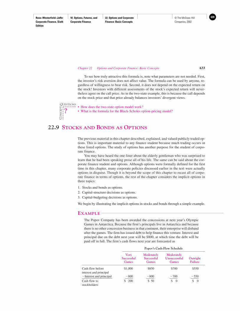
Ross−Westerfield−Jaffe: Corporate Finance, Sixth Edition
VI. Options, Futures, and Corporate Finance
22. Options and Corporate Finance: Basic Concepts
639© The McGraw−Hill Companies, 2002
To see how truly attractive this formula is, note what parameters are not needed. First,the investor’s risk aversion does not affect value. The formula can be used by anyone, re-gardless of willingness to bear risk. Second, it does not depend on the expected return onthe stock! Investors with different assessments of the stock’s expected return will never-theless agree on the call price. As in the two-state example, this is because the call dependson the stock price and that price already balances investors’ divergent views.
• How does the two-state option model work?• What is the formula for the Black-Scholes option-pricing model?
22.9 STOCKS AND BONDS AS OPTIONS
The previous material in this chapter described, explained, and valued publicly traded op-tions. This is important material to any finance student because much trading occurs inthese listed options. The study of options has another purpose for the student of corpo-rate finance.
You may have heard the one-liner about the elderly gentleman who was surprised tolearn that he had been speaking prose all of his life. The same can be said about the cor-porate finance student and options. Although options were formally defined for the firsttime in this chapter, many corporate policies discussed earlier in the text were actuallyoptions in disguise. Though it is beyond the scope of this chapter to recast all of corpo-rate finance in terms of options, the rest of the chapter considers the implicit options inthree topics:
1. Stocks and bonds as options.
2. Capital-structure decisions as options.
3. Capital-budgeting decisions as options.
We begin by illustrating the implicit options in stocks and bonds through a simple example.
EXAMPLE
The Popov Company has been awarded the concessions at next year’s OlympicGames in Antarctica. Because the firm’s principals live in Antarctica and becausethere is no other concession business in that continent, their enterprise will disbandafter the games. The firm has issued debt to help finance this venture. Interest andprincipal due on the debt next year will be $800, at which time the debt will bepaid off in full. The firm’s cash flows next year are forecasted as
Popov’s Cash-Flow Schedule
Very Moderately ModeratelySuccessful Successful Unsuccessful Outright
Games Games Games Failure
Cash flow before $1,000 $850 $700 $550interest and principal�Interest and principal �800 �800 �700 �550___________________ _____ _____ _____ _____Cash flow to $ 200 $ 50 $ 0 $ 0stockholders
Chapter 22 Options and Corporate Finance: Basic Concepts 633
QUESTIONS
CO
NC
EP
T
?
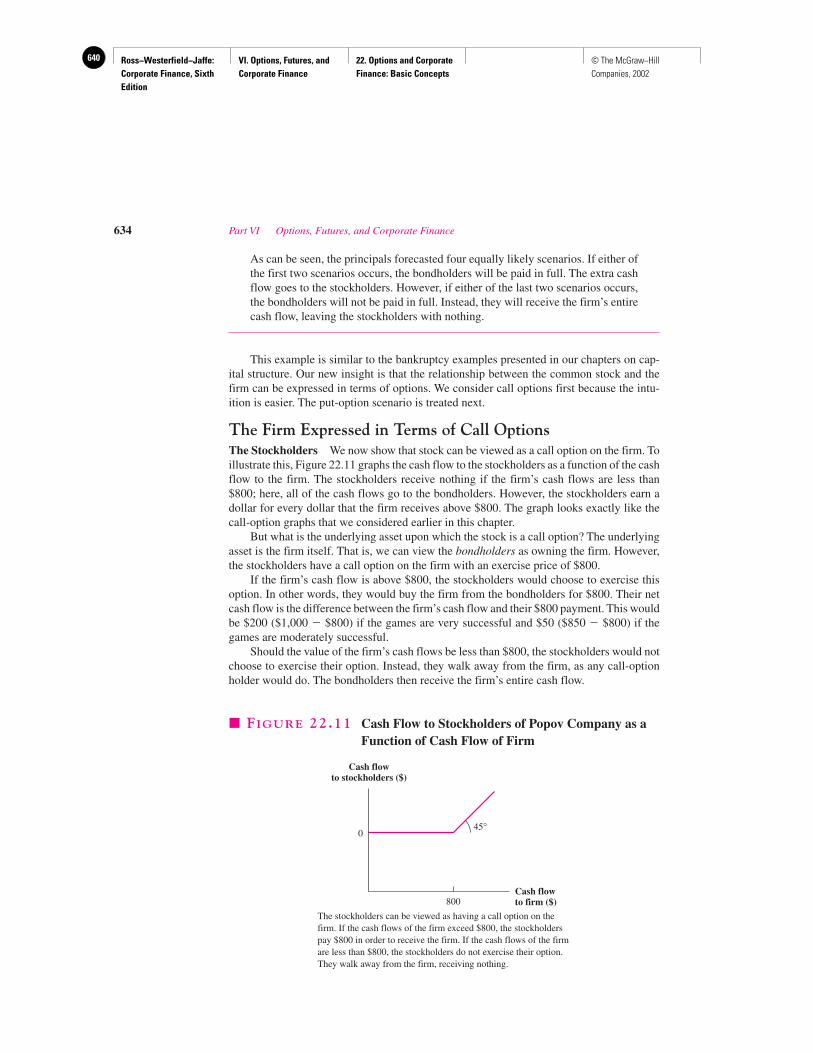
Ross−Westerfield−Jaffe: Corporate Finance, Sixth Edition
VI. Options, Futures, and Corporate Finance
22. Options and Corporate Finance: Basic Concepts
640 © The McGraw−Hill Companies, 2002
As can be seen, the principals forecasted four equally likely scenarios. If either ofthe first two scenarios occurs, the bondholders will be paid in full. The extra cashflow goes to the stockholders. However, if either of the last two scenarios occurs,the bondholders will not be paid in full. Instead, they will receive the firm’s entirecash flow, leaving the stockholders with nothing.
This example is similar to the bankruptcy examples presented in our chapters on cap-ital structure. Our new insight is that the relationship between the common stock and thefirm can be expressed in terms of options. We consider call options first because the intu-ition is easier. The put-option scenario is treated next.
The Firm Expressed in Terms of Call OptionsThe Stockholders We now show that stock can be viewed as a call option on the firm. Toillustrate this, Figure 22.11 graphs the cash flow to the stockholders as a function of the cashflow to the firm. The stockholders receive nothing if the firm’s cash flows are less than$800; here, all of the cash flows go to the bondholders. However, the stockholders earn adollar for every dollar that the firm receives above $800. The graph looks exactly like thecall-option graphs that we considered earlier in this chapter.
But what is the underlying asset upon which the stock is a call option? The underlyingasset is the firm itself. That is, we can view the bondholders as owning the firm. However,the stockholders have a call option on the firm with an exercise price of $800.
If the firm’s cash flow is above $800, the stockholders would choose to exercise thisoption. In other words, they would buy the firm from the bondholders for $800. Their netcash flow is the difference between the firm’s cash flow and their $800 payment. This wouldbe $200 ($1,000 � $800) if the games are very successful and $50 ($850 � $800) if thegames are moderately successful.
Should the value of the firm’s cash flows be less than $800, the stockholders would notchoose to exercise their option. Instead, they walk away from the firm, as any call-optionholder would do. The bondholders then receive the firm’s entire cash flow.
634 Part VI Options, Futures, and Corporate Finance
0
800
45°
Cash flowto firm ($)
Cash flowto stockholders ($)
� FIGURE 22.11 Cash Flow to Stockholders of Popov Company as aFunction of Cash Flow of Firm
The stockholders can be viewed as having a call option on thefirm. If the cash flows of the firm exceed $800, the stockholderspay $800 in order to receive the firm. If the cash flows of the firmare less than $800, the stockholders do not exercise their option.They walk away from the firm, receiving nothing.
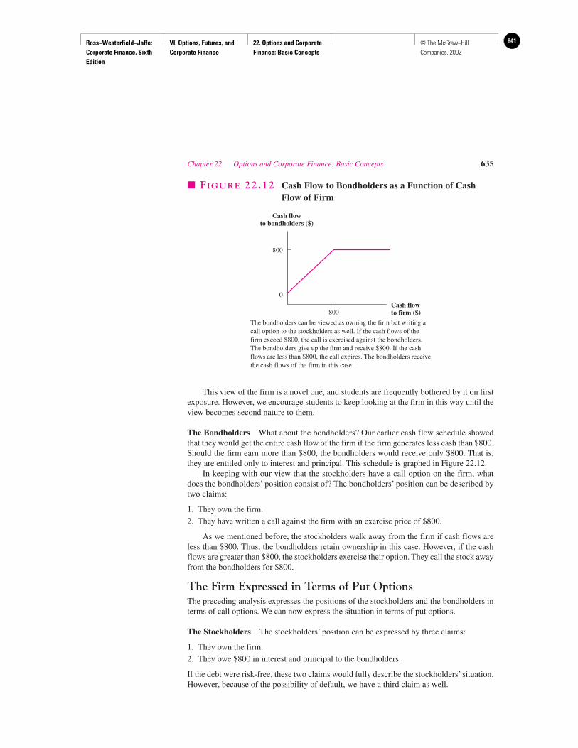
Ross−Westerfield−Jaffe: Corporate Finance, Sixth Edition
VI. Options, Futures, and Corporate Finance
22. Options and Corporate Finance: Basic Concepts
641© The McGraw−Hill Companies, 2002
This view of the firm is a novel one, and students are frequently bothered by it on firstexposure. However, we encourage students to keep looking at the firm in this way until theview becomes second nature to them.
The Bondholders What about the bondholders? Our earlier cash flow schedule showedthat they would get the entire cash flow of the firm if the firm generates less cash than $800.Should the firm earn more than $800, the bondholders would receive only $800. That is,they are entitled only to interest and principal. This schedule is graphed in Figure 22.12.
In keeping with our view that the stockholders have a call option on the firm, whatdoes the bondholders’ position consist of? The bondholders’ position can be described bytwo claims:
1. They own the firm.
2. They have written a call against the firm with an exercise price of $800.
As we mentioned before, the stockholders walk away from the firm if cash flows areless than $800. Thus, the bondholders retain ownership in this case. However, if the cashflows are greater than $800, the stockholders exercise their option. They call the stock awayfrom the bondholders for $800.
The Firm Expressed in Terms of Put OptionsThe preceding analysis expresses the positions of the stockholders and the bondholders interms of call options. We can now express the situation in terms of put options.
The Stockholders The stockholders’ position can be expressed by three claims:
1. They own the firm.
2. They owe $800 in interest and principal to the bondholders.
If the debt were risk-free, these two claims would fully describe the stockholders’ situation.However, because of the possibility of default, we have a third claim as well.
Chapter 22 Options and Corporate Finance: Basic Concepts 635
800
Cash flowto bondholders ($)
Cash flowto firm ($)
0
800
� FIGURE 22.12 Cash Flow to Bondholders as a Function of CashFlow of Firm
The bondholders can be viewed as owning the firm but writing acall option to the stockholders as well. If the cash flows of thefirm exceed $800, the call is exercised against the bondholders.The bondholders give up the firm and receive $800. If the cashflows are less than $800, the call expires. The bondholders receivethe cash flows of the firm in this case.
Ross−Westerfield−Jaffe: Corporate Finance, Sixth Edition
VI. Options, Futures, and Corporate Finance
22. Options and Corporate Finance: Basic Concepts
642 © The McGraw−Hill Companies, 2002
3. The stockholders own a put option on the firm with an exercise price of $800. The groupof bondholders is the seller of the put.
Now consider two possibilities.
Cash Flow Is Less than $800 Because the put has an exercise price of $800, the put is inthe money. The stockholders “put,” that is, sell, the firm to the bondholders. Normally, theholder of a put receives the exercise price when the asset is sold. However, the stockhold-ers already owe $800 to the bondholders. Thus, the debt of $800 is simply canceled—andno money changes hands—when the stock is delivered to the bondholders. Because thestockholders give up the stock in exchange for extinguishing the debt, the stockholders endup with nothing if the cash flow is below $800.
Cash Flow Is Greater than $800 Because the put is out of the money here, the stock-holders do not exercise. Thus, the stockholders retain ownership of the firm but pay $800to the bondholders as interest and principal.
The Bondholders The bondholders’ position can be described by two claims:
1. The bondholders are owed $800.
2. They have sold a put option on the firm to the stockholders with an exercise price of $800.
Cash Flow Is Less than $800 As mentioned before, the stockholders will exercise the putin this case. This means that the bondholders are obligated to pay $800 for the firm. Be-cause they are owed $800, the two obligations offset each other. Thus, the bondholders sim-ply end up with the firm in this case.
Cash Flow Is Greater than $800 Here, the stockholders do not exercise the put. Thus, thebondholders merely receive the $800 that is due them.
Expressing the bondholders’ position in this way is illuminating. With a riskless de-fault-free bond, the bondholders are owed $800. Thus, we can express the risky bond interms of a riskless bond and a put:
Value of�
Value of�
Value ofrisky bond default-free bond put option
That is, the value of the risky bond is the value of the default-free bond less the value of thestockholders’ option to sell the company for $800.
A Resolution of the Two ViewsWe have argued above that the positions of the stockholders and the bondholders can beviewed either in terms of calls or in terms of puts. These two viewpoints are summarized inTable 22.4.
We have found from past experience that it is generally harder for students to think ofthe firm in terms of puts than in terms of calls. Thus, it would be helpful if there were a wayto show that the two viewpoints are equivalent. Fortunately there is put-call parity. In anearlier section we presented the put-call parity relationship as equation (22.1), which wenow repeat:
Price of underlying stock � Price of put � Price of call � Present value of exercise price (22.1)
Using the results of this section, equation (22.1) can be rewritten as:
636 Part VI Options, Futures, and Corporate Finance
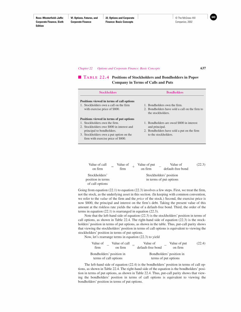
Ross−Westerfield−Jaffe: Corporate Finance, Sixth Edition
VI. Options, Futures, and Corporate Finance
22. Options and Corporate Finance: Basic Concepts
643© The McGraw−Hill Companies, 2002
Value of call�
Value of�
Value of put�
Value of (22.3)on firm firm on firm default-free bond
Stockholders’ Stockholders’ positionposition in terms in terms of put options
of call options
Going from equation (22.1) to equation (22.3) involves a few steps. First, we treat the firm,not the stock, as the underlying asset in this section. (In keeping with common convention,we refer to the value of the firm and the price of the stock.) Second, the exercise price isnow $800, the principal and interest on the firm’s debt. Taking the present value of thisamount at the riskless rate yields the value of a default-free bond. Third, the order of theterms in equation (22.1) is rearranged in equation (22.3).
Note that the left-hand side of equation (22.3) is the stockholders’ position in terms ofcall options, as shown in Table 22.4. The right-hand side of equation (22.3) is the stock-holders’ position in terms of put options, as shown in the table. Thus, put-call parity showsthat viewing the stockholders’ position in terms of call options is equivalent to viewing thestockholders’ position in terms of put options.
Now, let’s rearrange terms in equation (22.3) to yield
Value of�
Value of call�
Value of�
Value of put (22.4)firm on firm default-free bond on firm
Bondholders’ position in Bondholders’ position interms of call options terms of put options
The left-hand side of equation (22.4) is the bondholders’ position in terms of call op-tions, as shown in Table 22.4. The right-hand side of the equation is the bondholders’ posi-tion in terms of put options, as shown in Table 22.4. Thus, put-call parity shows that view-ing the bondholders’ position in terms of call options is equivalent to viewing thebondholders’ position in terms of put options.
Chapter 22 Options and Corporate Finance: Basic Concepts 637
� TABLE 22.4 Positions of Stockholders and Bondholders in PopovCompany in Terms of Calls and Puts
Stockholders Bondholders
Positions viewed in terms of call options1. Stockholders own a call on the firm 1. Bondholders own the firm.
with exercise price of $800. 2. Bondholders have sold a call on the firm tothe stockholders.
Positions viewed in terms of put options1. Stockholders own the firm. 1. Bondholders are owed $800 in interest 2. Stockholders owe $800 in interest and and principal.
principal to bondholders. 2. Bondholders have sold a put on the firm 3. Stockholders own a put option on the to the stockholders.
firm with exercise price of $800.
Ross−Westerfield−Jaffe: Corporate Finance, Sixth Edition
VI. Options, Futures, and Corporate Finance
22. Options and Corporate Finance: Basic Concepts
644 © The McGraw−Hill Companies, 2002
A Note on Loan GuaranteesIn the Popov example given earlier, the bondholders bore the risk of default. Of course,bondholders generally ask for an interest rate that is enough to compensate them forbearing risk. When firms experience financial distress, they can no longer attract newdebt at moderate interest rates. Thus, firms experiencing distress have frequently soughtloan guarantees from the government. Our framework can be used to understand theseguarantees.
If the firm defaults on a guaranteed loan, the government must make up the difference.In other words, a government guarantee converts a risky bond into a riskless bond. What isthe value of this guarantee?
Recall that, with option pricing,
Value of�
Value of�
Value ofdefault-free bond risky bond put option
This equation shows that the government is assuming an obligation that has a cost equal tothe value of a put option.
This analysis differs from that of either politicians or company spokespeople. Theygenerally say that the guarantee will cost the taxpayer nothing because the guarantee en-ables the firm to attract debt, thereby staying solvent. However, it should be pointed out that,although solvency may be a strong possibility, it is never a certainty. Thus, at the time theguarantee is made, the government’s obligation has a cost in terms of present value. To saythat a government guarantee costs the government nothing is like saying a put on the stockof Microsoft has no value because the stock is likely to rise in price.
Actually, the government has had good fortune with loan guarantees. Its two biggestguarantees were to the Lockheed Corporation in 1971 and the Chrysler Corporation in1980. Both firms nearly ran out of cash and defaulted on loans. In both cases the U.S. gov-ernment came to the rescue by agreeing to guarantee new loans. Under the guarantees, ifLockheed and Chrysler had defaulted on new loans, the lenders could have obtained the fullvalue of their claims from the U.S. government. From the lender’s point of view, the loansbecame as risk-free as Treasury bonds. These guarantees enabled Lockheed and Chryslerto borrow large amounts of cash and to get through a difficult time. As it turned out, neitherfirm defaulted.
Who benefits from a typical loan guarantee?
1. If existing risky bonds are guaranteed, all gains accrue to the existing bondholders.The stockholders gain nothing because the limited liability of corporations absolves thestockholders of any obligation in bankruptcy.
2. If new debt is being issued and guaranteed, the new debtholders do not gain. Rather,in a competitive market, they must accept a low interest rate because of the debt’s low risk.The stockholders gain here because they are able to issue debt at a low interest rate. In ad-dition, some of the gains accrue to the old bondholders because the firm’s value is greaterthan would otherwise be true. Therefore, if shareholders want all the gains from loan guar-antees, they should renegotiate or retire existing bonds before the guarantee is in place. Thishappened in the Chrysler case.
• How can the value of the firm be expressed in terms of call options?• How can the value of the firm be expressed in terms of put options?• How does put-call parity relate these two expressions?
638 Part VI Options, Futures, and Corporate Finance
QUESTIONS
CO
NC
EP
T
?
Ross−Westerfield−Jaffe: Corporate Finance, Sixth Edition
VI. Options, Futures, and Corporate Finance
22. Options and Corporate Finance: Basic Concepts
645© The McGraw−Hill Companies, 2002
22.10 CAPITAL-STRUCTURE POLICY AND OPTIONS
Recall our chapters on capital structure where we showed how managers, acting on behalfof the stockholders, can take advantage of bondholders. A number of these strategies canbe explained in terms of options. As an illustration, this section examines one such strategy,the choice between a high-risk project and a low-risk project.
Selecting High-Risk ProjectsImagine a levered firm considering two mutually exclusive projects, a low-risk one and ahigh-risk one. There are two equally likely outcomes, recession and boom. The firm is insuch dire straits that, should a recession hit, it will come near to bankruptcy if the low-riskproject is selected and actually fall into bankruptcy if the high-risk project is selected. Thecash flows for the firm if the low-risk project is undertaken can be described as
Low-Risk Project
ValueProbability of Firm � Stock � Bonds
Recession 0.5 $400 � 0 � $400Boom 0.5 $800 � $400 � $400
If recession occurs, the value of the firm will be $400, and if boom occurs, the value of thefirm will be $800. The expected value of the firm is $600 (0.5 � $400 � 0.5 � $800). Thefirm has promised to pay the bondholders $400. Shareholders will obtain the differencebetween the total payoff and the amount paid to the bondholders. The bondholders havethe prior claim on the payoffs, and the shareholders have the residual claim.
Now suppose that another, riskier project can be substituted for the low-risk project.The payoffs and probabilities are as follows:
High-Risk Project
ValueProbability of Firm � Stock � Bonds
Recession 0.5 $ 200 � 0 � $200Boom 0.5 $1,000 � $600 � $400
The expected value of the firm is $600 (0.5 � $200 � 0.5 � $1,000), which is identical tothe value of the firm with the low-risk project. However, note that the expected value of thestock is $300 (0.5 � 0 � 0.5 � $600) with the high-risk project, but only $200 (0.5 � 0 �0.5 � $400) with the low-risk project. Given the firm’s present levered state, stockholderswill select the high-risk project.
The stockholders benefit at the expense of the bondholders when the high-risk projectis accepted. The explanation is quite clear: The bondholders suffer dollar for dollar whenthe firm’s value falls short of the $400 bond obligation. However, the bondholders’ pay-ments are capped at $400 when the firm does well.
This can be explained in terms of call options. We argued earlier in this chapter that thevalue of a call rises with an increase in the volatility of the underlying asset. Because the stockis a call option on the firm, a rise in the volatility of the firm increases the value of the stock.In our example, the value of the stock is higher if the high-risk project is accepted.
Chapter 22 Options and Corporate Finance: Basic Concepts 639
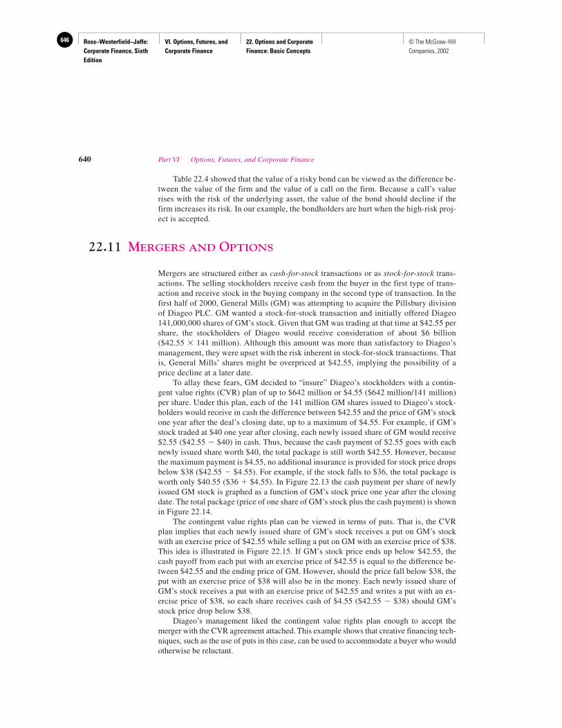
Ross−Westerfield−Jaffe: Corporate Finance, Sixth Edition
VI. Options, Futures, and Corporate Finance
22. Options and Corporate Finance: Basic Concepts
646 © The McGraw−Hill Companies, 2002
Table 22.4 showed that the value of a risky bond can be viewed as the difference be-tween the value of the firm and the value of a call on the firm. Because a call’s valuerises with the risk of the underlying asset, the value of the bond should decline if thefirm increases its risk. In our example, the bondholders are hurt when the high-risk proj-ect is accepted.
22.11 MERGERS AND OPTIONS
Mergers are structured either as cash-for-stock transactions or as stock-for-stock trans-actions. The selling stockholders receive cash from the buyer in the first type of trans-action and receive stock in the buying company in the second type of transaction. In thefirst half of 2000, General Mills (GM) was attempting to acquire the Pillsbury divisionof Diageo PLC. GM wanted a stock-for-stock transaction and initially offered Diageo141,000,000 shares of GM’s stock. Given that GM was trading at that time at $42.55 pershare, the stockholders of Diageo would receive consideration of about $6 billion($42.55 � 141 million). Although this amount was more than satisfactory to Diageo’smanagement, they were upset with the risk inherent in stock-for-stock transactions. Thatis, General Mills’ shares might be overpriced at $42.55, implying the possibility of aprice decline at a later date.
To allay these fears, GM decided to “insure” Diageo’s stockholders with a contin-gent value rights (CVR) plan of up to $642 million or $4.55 ($642 million/141 million)per share. Under this plan, each of the 141 million GM shares issued to Diageo’s stock-holders would receive in cash the difference between $42.55 and the price of GM’s stockone year after the deal’s closing date, up to a maximum of $4.55. For example, if GM’sstock traded at $40 one year after closing, each newly issued share of GM would receive$2.55 ($42.55 � $40) in cash. Thus, because the cash payment of $2.55 goes with eachnewly issued share worth $40, the total package is still worth $42.55. However, becausethe maximum payment is $4.55, no additional insurance is provided for stock price dropsbelow $38 ($42.55 � $4.55). For example, if the stock falls to $36, the total package isworth only $40.55 ($36 � $4.55). In Figure 22.13 the cash payment per share of newlyissued GM stock is graphed as a function of GM’s stock price one year after the closingdate. The total package (price of one share of GM’s stock plus the cash payment) is shownin Figure 22.14.
The contingent value rights plan can be viewed in terms of puts. That is, the CVRplan implies that each newly issued share of GM’s stock receives a put on GM’s stockwith an exercise price of $42.55 while selling a put on GM with an exercise price of $38.This idea is illustrated in Figure 22.15. If GM’s stock price ends up below $42.55, thecash payoff from each put with an exercise price of $42.55 is equal to the difference be-tween $42.55 and the ending price of GM. However, should the price fall below $38, theput with an exercise price of $38 will also be in the money. Each newly issued share ofGM’s stock receives a put with an exercise price of $42.55 and writes a put with an ex-ercise price of $38, so each share receives cash of $4.55 ($42.55 � $38) should GM’sstock price drop below $38.
Diageo’s management liked the contingent value rights plan enough to accept themerger with the CVR agreement attached. This example shows that creative financing tech-niques, such as the use of puts in this case, can be used to accommodate a buyer who wouldotherwise be reluctant.
640 Part VI Options, Futures, and Corporate Finance
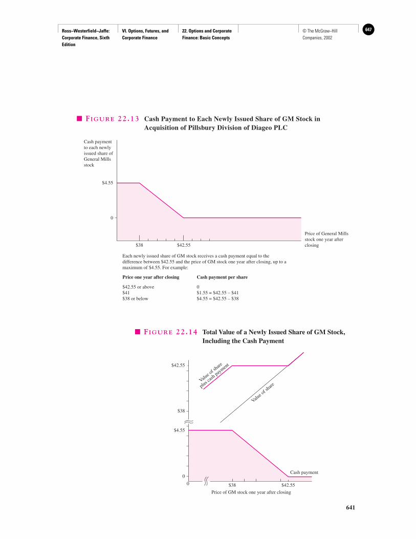
Ross−Westerfield−Jaffe: Corporate Finance, Sixth Edition
VI. Options, Futures, and Corporate Finance
22. Options and Corporate Finance: Basic Concepts
647© The McGraw−Hill Companies, 2002
641
$38 $42.55
Cash paymentto each newlyissued share ofGeneral Millsstock
Price of General Millsstock one year afterclosing
Each newly issued share of GM stock receives a cash payment equal to thedifference between $42.55 and the price of GM stock one year after closing, up to amaximum of $4.55. For example:
Price one year after closing
$42.55 or above$41$38 or below
Cash payment per share
0$1.55 = $42.55 – $41$4.55 = $42.55 – $38
0
$4.55
� FIGURE 22.13 Cash Payment to Each Newly Issued Share of GM Stock inAcquisition of Pillsbury Division of Diageo PLC
$38
Price of GM stock one year after closing
$42.55
Cash payment0
0
$4.55
$42.55
$38
Value of share
Value of sh
areplus cash
paymen
t
� FIGURE 22.14 Total Value of a Newly Issued Share of GM Stock,Including the Cash Payment
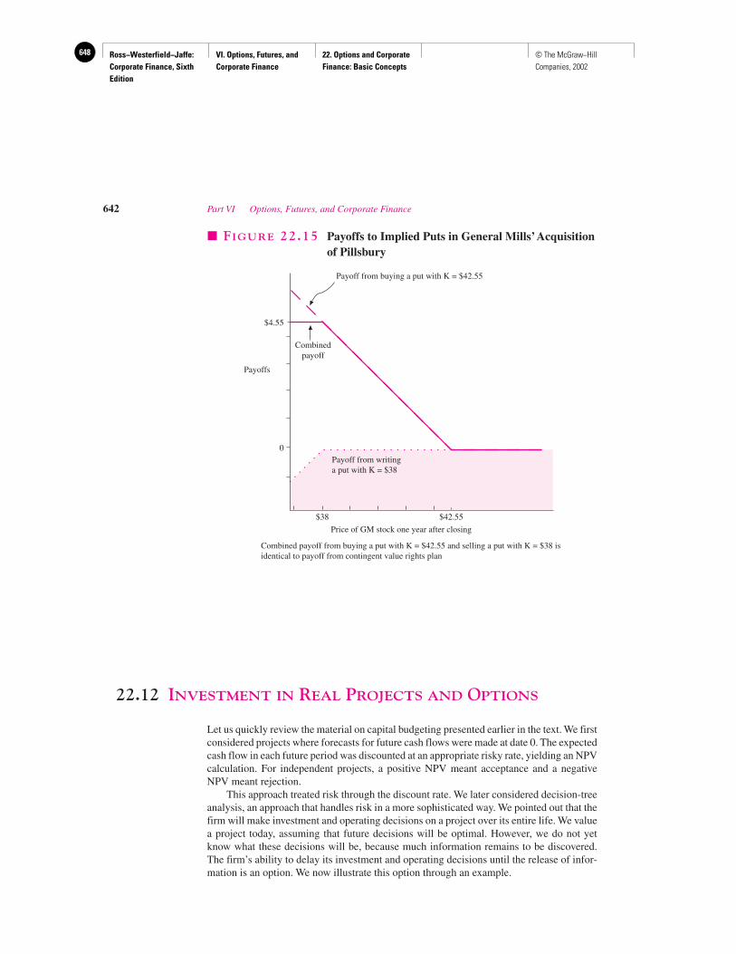
Ross−Westerfield−Jaffe: Corporate Finance, Sixth Edition
VI. Options, Futures, and Corporate Finance
22. Options and Corporate Finance: Basic Concepts
648 © The McGraw−Hill Companies, 2002
22.12 INVESTMENT IN REAL PROJECTS AND OPTIONS
Let us quickly review the material on capital budgeting presented earlier in the text. We firstconsidered projects where forecasts for future cash flows were made at date 0. The expectedcash flow in each future period was discounted at an appropriate risky rate, yielding an NPVcalculation. For independent projects, a positive NPV meant acceptance and a negativeNPV meant rejection.
This approach treated risk through the discount rate. We later considered decision-treeanalysis, an approach that handles risk in a more sophisticated way. We pointed out that thefirm will make investment and operating decisions on a project over its entire life. We valuea project today, assuming that future decisions will be optimal. However, we do not yetknow what these decisions will be, because much information remains to be discovered.The firm’s ability to delay its investment and operating decisions until the release of infor-mation is an option. We now illustrate this option through an example.
642 Part VI Options, Futures, and Corporate Finance
$38
Price of GM stock one year after closing
Combined payoff from buying a put with K = $42.55 and selling a put with K = $38 isidentical to payoff from contingent value rights plan
$42.55
Payoff from writinga put with K = $38
Combinedpayoff
Payoffs
Payoff from buying a put with K = $42.55
0
$4.55
� FIGURE 22.15 Payoffs to Implied Puts in General Mills’Acquisitionof Pillsbury
Ross−Westerfield−Jaffe: Corporate Finance, Sixth Edition
VI. Options, Futures, and Corporate Finance
22. Options and Corporate Finance: Basic Concepts
649© The McGraw−Hill Companies, 2002
EXAMPLE
Exoff Oil Corporation is considering the purchase of an oil field in a remote part ofAlaska. The seller has listed the property for $10,000 and is eager to sell immedi-ately. Initial drilling costs are $500,000. The firm anticipates that 10,000 barrels ofoil can be extracted each year for many decades. Because the termination date is sofar in the future and so hard to estimate, the firm views the cash flow stream fromthe oil as a perpetuity. With oil prices at $20 per barrel and extraction costs at $16a barrel, the firm anticipates a net margin of $4 per barrel. Because oil prices areexpected to rise at the inflation rate, the firm assumes that its cash flow per barrelwill always be $4 in real terms. The appropriate real discount rate is 10 percent. Thefirm has enough tax credits from bad years in the past that it will not need to paytaxes on any profits from the oil field. Should Exoff buy the property?
The NPV of the oil field to Exoff is
According to this analysis, Exoff should not purchase the land.Though this approach uses the standard capital-budgeting techniques of this and
other textbooks, it is actually inappropriate for this situation. To see this, consider theanalysis of Kirtley Thornton, a consultant to Exoff. He agrees that the price of oil is ex-pected to rise at the rate of inflation. However, he points out that the next year is quiteperilous for oil prices. On the one hand, OPEC is considering a long-term agreementthat would raise oil prices to $35 per barrel in real terms for many years in the future.On the other hand, National Motors recently indicated that cars using a mixture of sandand water for fuel are currently being tested. Thornton argues that oil will be priced at$5 in real terms for many years, should this development prove successful. Full infor-mation on both these developments will be released in exactly one year.
Should oil prices rise to $35 a barrel, the NPV of the project would be
However, should oil prices fall to $5 a barrel, the NPV of the oil field will be evenmore negative than it is today.
Mr. Thornton makes two recommendations to Exoff’s board. He argues that
1. The land should be purchased.2. The drilling decision should be delayed until information on both OPEC’s new
agreement and National Motors’ new automobile is released.
Kirtley explains his recommendations to the board by first assuming that the landhas already been purchased. He argues that, under this assumption, the drillingdecision should be delayed. Second, he investigates his assumption that the landshould have been purchased in the first place. This approach of examining thesecond decision (whether to drill) after assuming that the first decision (to buy theland) had been made was also used in our earlier presentation on decision trees.Let us now work through Mr. Thornton’s analysis.
Assume the land has already been purchased. If the land has already been pur-chased, should drilling begin immediately? If drilling begins immediately, theNPV is �$110,000. If the drilling decision is delayed until new information is re-leased in a year, the optimal choice can be made at that time. If oil prices drop to
$1,390,000 � � $10,000 � $500,000 ��$35 � $16� � 10,000
0.10
� $110,000 � � $10,000 � $500,000 �$4 � 10,000
0.10
Chapter 22 Options and Corporate Finance: Basic Concepts 643
Ross−Westerfield−Jaffe: Corporate Finance, Sixth Edition
VI. Options, Futures, and Corporate Finance
22. Options and Corporate Finance: Basic Concepts
650 © The McGraw−Hill Companies, 2002
$5 a barrel, Exoff should not drill. Instead, the firm should walk away from theproject, losing nothing beyond its $10,000 purchase price for the land. If oil pricesrise to $35, drilling should begin.
Mr. Thornton points out that, by delaying, the firm will only invest the$500,000 of drilling costs if oil prices rise. Thus, by delaying, the firm saves$500,000 in the case where oil prices drop. Kirtley concludes that, once the landis purchased, the drilling decision should be delayed.11
Should the land have been purchased in the first place? We now know that ifthe land had been purchased, it is optimal to defer the drilling decision until the re-lease of information. Given that we know this optimal decision concerningdrilling, should the land be purchased in the first place? Without knowing the ex-act probability that oil prices will rise, Mr. Thornton is nevertheless confident thatthe land should be purchased. The NPV of the project at $35 oil prices is$1,390,000 whereas the cost of the land is only $10,000. Kirtley believes that anoil price rise is possible, though by no means probable. Even so, he argues that thehigh potential return is clearly worth the risk.
This example presents an approach that is similar to our decision-tree analysis of theSolar Equipment Company in a previous chapter. Our purpose in this section is to discussthis type of decision in an option framework. When Exoff purchases the land, it is actuallypurchasing a call option. That is, once the land has been purchased, the firm has an optionto buy an active oil field at an exercise price of $500,000. As it turns out, one should gen-erally not exercise a call option immediately.12 In this case, the firm should delay exerciseuntil relevant information concerning future oil prices is released.
This section points out a serious deficiency in classical capital budgeting; net-present-value calculations typically ignore the flexibility that real-world firms have. In our exam-ple, the standard techniques generated a negative NPV for the land purchase. Yet, by al-lowing the firm the option to change its investment policy according to new information,the land purchase can easily be justified.
We entreat the reader to look for hidden options in projects. Because options are ben-eficial, managers are shortchanging their firm’s projects if capital-budgeting calculationsignore flexibility.
• Why are the hidden options in projects valuable?
644 Part VI Options, Futures, and Corporate Finance
11Actually, there are three separate effects here. First, the firm avoids drilling costs in the case of low oil pricesby delaying the decision. This is the effect discussed by Mr. Thornton. Second, the present value of the$500,000 payment is less when the decision is delayed, even if drilling eventually takes place. Third, the firmloses one year of cash inflows through delay.
The first two arguments support delaying the decision. The third argument supports immediate drilling. Inthis example, the first argument greatly outweighs the other two arguments. Thus, Mr. Thornton avoided thesecond and third arguments in his presentation.12Actually, it can be shown that a call option that pays no dividend should never be exercised before expiration.However, for a dividend-paying stock, it may be optimal to exercise prior to the ex-dividend date. The analogyapplies to our example of an option in real assets.
The firm would receive cash flows from oil earlier if drilling begins immediately. This is equivalent to thebenefit from exercising a call on a stock prematurely in order to capture the dividend. However, in our example,this dividend effect is far outweighed by the benefits from waiting.
QUESTION
CO
NC
EP
T
?

Ross−Westerfield−Jaffe: Corporate Finance, Sixth Edition
VI. Options, Futures, and Corporate Finance
22. Options and Corporate Finance: Basic Concepts
651© The McGraw−Hill Companies, 2002
22.13 SUMMARY AND CONCLUSIONS
This chapter serves as an introduction to options.
1. The most familiar options are puts and calls. These options give the holder the right to sell orbuy shares of common stock at a given exercise price. American options can be exercised anytime up to and including the expiration date. European options can be exercised only on theexpiration date.
2. We showed that a strategy of buying a stock and buying a put is equivalent to a strategy ofbuying a call and buying a zero-coupon bond. From this, the put-call–parity relationship wasestablished:
Value of � Value of � Value of � Present value of stock put call exercise price
3. The value of an option depends on five factors:• The price of the underlying asset.• The exercise price.• The expiration date.• The variability of the underlying asset.• The interest rate on risk-free bonds.The Black-Scholes model can determine the intrinsic price of an option from these fivefactors.
4. Much of corporate financial theory can be presented in terms of options. In this chapter wepointed out thata. Common stock can be represented as a call option on the firm.b. Stockholders enhance the value of their call by increasing the risk of their firm.c. Real projects have hidden options that enhance value.
KEY TERMS
American options 612 Option 612Call option 613 Put-call parity 619Cumulative probability 630 Put option 614European options 612 Standardized normal distribution 630Exercising the option 612 Striking or exercise price 612Expiration date 612
SUGGESTED READINGS
The path-breaking article on options is:Black, Fischer, and Myron Scholes. “The Pricing of Options and Corporate Liabilities.” Journal
of Political Economy 81 (May–June 1973).
For a detailed discussion of options, readHull, John C. Options, Futures, and Other Derivatives, 4th Ed. Upper Saddle River, N.J.:
Prentice Hall, 1999.
Chapter 22 Options and Corporate Finance: Basic Concepts 645

Ross−Westerfield−Jaffe: Corporate Finance, Sixth Edition
VI. Options, Futures, and Corporate Finance
22. Options and Corporate Finance: Basic Concepts
652 © The McGraw−Hill Companies, 2002
QUESTIONS AND PROBLEMS
Options: General22.1 Define the following terms associated with options:
a. Optionb. Exercisec. Strike priced. Expiration datee. Call optionf. Put option
22.2 What is the difference between American options and European options?
22.3 Mr. Goodie holds American put options on Delta Triangle stock. The exercise price of theput is $40 and Delta stock is selling for $35 per share. If the put sells for $41⁄2, what is thebest strategy for Mr. Goodie?
22.4 A call option on Futura Corporation stock currently trades for $4. The expiration date isFebruary 18 of next year. The exercise price of the option is $45.a. If this is an American option, on what dates can the option be exercised?b. If this is a European option, on what dates can the option be exercised?c. Suppose the current price of Futura Corporation stock is $35. Is this option
worthless?
22.5 Mrs. Gerard sold 10 IBM put contracts and bought 5 IBM call contracts with theproceeds of the sales. Both options have the same exercise price of $80 and the sameexpiration date. Draw the payoff diagram of her zero-investment portfolio.
22.6 The strike price of a call option on Simpsons Entertainment common stock is $50.a. What is the payoff at expiration of this call if, on the expiration date, Simpsons stock
sells for $55?b. What is the payoff at expiration of this call if, on the expiration date, Simpsons stock
sells for $45?c. Draw the payoff diagram for this option.
22.7 A put is trading on Simpsons Entertainment stock. It has a strike price of $50.a. What is the payoff at expiration of this put if, on the expiration date, Simpsons stock
sells for $55?b. What is the payoff at expiration of this put if, on the expiration date, Simpsons stock
sells for $45?c. Draw the payoff diagram for this option.
22.8 Suppose you bought two Xerox call contracts and one Xerox put contract, both of whichwill expire in three months. The exercise price of the call is $70 and the exercise price ofthe put is $75. Each option is sold as a 100-share contract.a. What is your payoff at expiration of your investment if Xerox stock sells for $65 on
the expiration date? What if it sells for $72? What if it sells for $80?b. Draw the payoff diagram for the investment.
22.9 You hold a six-month European call-option contract on Sertile stock. The exercise priceof the call is $100 per share. The option will expire in moments. Assume there are notransactions costs or taxes associated with this contract.a. What is your profit on this contract if the stock is selling for $130?b. If Sertile stock is selling for $90, what will you do?
22.10 General Furnishings, Inc., has both call and put options traded on the Chicago BoardOptions Exchange. Both options have the same exercise price of $40 and the sameexpiration date. The options will expire in one year. The call is currently selling for $8 per share and the put is selling for $2 per share. The interest rate is 10 percent. Whatshould the stock price of General Furnishings be in order to prevent arbitrageopportunities?
646 Part VI Options, Futures, and Corporate Finance

Ross−Westerfield−Jaffe: Corporate Finance, Sixth Edition
VI. Options, Futures, and Corporate Finance
22. Options and Corporate Finance: Basic Concepts
653© The McGraw−Hill Companies, 2002
22.11 Piersol Paper Mill’s common stock currently sells for $145. Both puts and calls onPiersol Paper are being traded. These options all expire eight months from today, andthey have a strike price of $160. Eight months from today, Piersol Paper common stockwill sell for $172 with a probability of 0.5. It will sell for $138 with a probability of0.5. You own a put on Piersol Paper. Now, you are becoming nervous about the risk towhich you are exposed.a. What other transactions should you make to eliminate this risk?b. What is the expected payoff at expiration of the strategy you developed in (a)?
22.12 Suppose you observe the following market prices:
American call (Strike � $50) $8Stock $60
a. What should you do?b. What is your profit or loss?c. What do opportunities such as this imply about the lower bound on the price of
American calls?d. What is the upper bound on the price of American calls? Explain.
22.13 List the factors that determine the value of an American call option. State how a changein each factor alters the option’s value.
22.14 List the factors that determine the value of an American put option. State how a change ineach factor alters the option’s value.
22.15 a. If the risk of a stock increases, what is likely to happen to the prices of call options onthe stock? Why?
b. If the risk of a stock increases, what is likely to happen to the price of put options onthe stock? Why?
The Two-State Option Model22.16 You bought a 100-share call contract three weeks ago. The expiration date of the calls is
five weeks from today. On that date, the price of the underlying stock will be either $120or $95. The two states are equally likely to occur. Currently, the stock sells for $96; itsstrike price is $112. You are able to purchase 32 shares of stock. You are able to borrowmoney at 10 percent per annum.
What is the value of your call contract?
22.17 Wellington Company stock is currently selling for $30 per share. It is expected that thestock price will be either $25 or $35 in six months. Treasury bills that will mature in sixmonths yield 5 percent. What is the price of Wellington put option per share that has anexercise price of $32? Wellington put is a European option.
22.18 Assume only two states will exist one year from today when a call on DeltaTransportation, Inc., stock expires. The price of Delta stock will be either $60 or $40on that date. Today, Delta stock trades for $55. The strike price of the call is $50. Therate at which you can borrow is 9 percent. How much are you willing to pay for acontract of this call?
The Black-Scholes Option Model22.19 Use the Black-Scholes model to price a call with the following characteristics:
Stock price � $62Strike price � $70Time to expiration � 4 weeksStock-price variance � 0.35Risk-free interest rate � 0.05
Chapter 22 Options and Corporate Finance: Basic Concepts 647

Ross−Westerfield−Jaffe: Corporate Finance, Sixth Edition
VI. Options, Futures, and Corporate Finance
22. Options and Corporate Finance: Basic Concepts
654 © The McGraw−Hill Companies, 2002
22.20 Use the Black-Scholes model to price a call with the following characteristics:
Stock price � $52Strike price � $48Time to expiration � 120 daysStock-price variance � 0.04Risk-free interest rate � 0.05
22.21 a. Use the Black-Scholes model to price a call with the following characteristics:
Stock price � $45Strike price � $52Time to expiration � 6 monthsStock-price variance � 0.40Risk-free interest rate � 0.065
b. What does put-call parity imply the price of the corresponding put will be?
22.22 a. Use the Black-Scholes model to price a call with the following characteristics:
Stock price � $70Strike price � $90Time to expiration � 6 monthsStock-price variance � 0.25Risk-free interest rate � 0.06
b. What does put-call parity imply the price of the corresponding put will be?
22.23 Consider a call option on Computer Plus Company stock. The option will expire oneyear from today and the exercise price is $35. The risk-free rate is 7 percent. ComputerPlus stock is selling for $37 per share and your estimate of variance of the return on thestock is 0.004.a. Use the Black-Scholes model to price the call.b. You have found out that the estimate of the variance should be revised to 0.0064.
What should the new price of the call be?c. The stock price dropped to $35 after the announcement that the company is about to
shut down three factories in California. Using the result in part (b), what should thenew price of the call be?
22.24 You have been asked by a client to determine the maximum price he should be willing topay to purchase a Kingsley call. The options have an exercise price of $25, and theyexpire in 120 days. The current price of Kingsley stock is $27, the annual risk-free rate is7 percent, and the estimated variance of the stock is 0.0576. No dividends are expected tobe declared over the next six months. What is the maximum price your client should pay?
648 Part VI Options, Futures, and Corporate Finance

Ross−Westerfield−Jaffe: Corporate Finance, Sixth Edition
VI. Options, Futures, and Corporate Finance
22. Options and Corporate Finance: Basic Concepts
655© The McGraw−Hill Companies, 2002
Application of Options to Corporate Finance22.25 It is said that the equity in a levered firm is like a call option on the underlying assets.
Explain what is meant by this statement.
22.26 Global Real Estate Partners, LTD., is undertaking a new project. If the project issuccessful, the value of the firm in a year will be $650 million, but if it turns out to be afailure, the firm will be worth only $250 million. The current value of the firm is $400million. The firm has outstanding bonds due in a year with a face value of $300 million.The T-bill rate is 7 percent. What is the value of the equity? What is the value of the debt?
22.27 Suppose Global Real Estate Partners, LTD., in the above problem decided to undertake ariskier project: The value of the firm in a year will be either $800 million or $100 million,depending on the success of the project. What is the value of the equity? What is thevalue of the debt? Which project is preferred by bondholders?
Chapter 22 Options and Corporate Finance: Basic Concepts 649
Ross−Westerfield−Jaffe: Corporate Finance, Sixth Edition
VI. Options, Futures, and Corporate Finance
23. Options and Corporate Finance: Extensions and Applications
656 © The McGraw−Hill Companies, 2002
Options and CorporateFinance: Extensions and Applications
CH
AP
TE
R23
EXECUTIVE SUMMARY
This chapter extends the analysis of options contained in Chapter 22. We describe fourdifferent types of options found in common corporate finance decisions.
• Executive stock options and compensation.• The embedded option in a start-up company.• The option in simple business contracts.• The option to shut down and reopen a project.
Option features are pervasive in corporate finance decisions. They are involved in decisionsof whether to build, expand, or close a factory, to buy productive assets like trucks or ma-chines, to drill for oil or mine for gold, or to build a building. Sometimes they are involvedin decisions about how to pay managers and other employees. In this chapter we do not ar-gue that the NPV approach should be completely jettisoned. In fact, many decisions havefew embedded options and, in these cases, optionality can be ignored. However, in manycases, options are an important aspect of the decision and must be separately valued. Inpractice, there is a decision continuum. At one end of the continuum are decisions with lit-tle optionality and at the other are decisions with significant optionality.
In the previous chapter, we presented a few examples of options in corporate finance.We saw that stock is a call option on the firm. We showed that the value of this option couldbe increased by selecting high-risk rather than low-risk projects. We discussed the embed-ded option in oil exploration.
However, although the previous chapter presented these options, we made no attempt tovalue them. In this chapter, we will value four embedded options. The first two are handled withthe Black-Scholes model. We use the binomial model to value the last two options. Although theBlack-Scholes model is more well known, the binomial model is probably used more frequentlyin the real world. The Black-Scholes model works well on only a narrow set of problems. Theflexibility of the binomial model allows it to be applied to a wider range of situations. However,binomial approaches often use complex numerical analyses involving large amounts of com-puter time. In this regard, binomial approaches are less elegant than the Black-Scholes approach.
23.1 EXECUTIVE STOCK OPTIONS
Why Options?Executive compensation is usually made up of base salary plus some or all of the follow-ing elements:
1. Long-term compensation
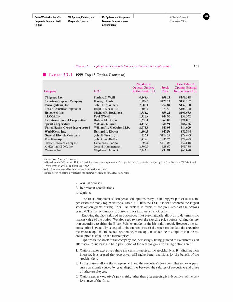
Ross−Westerfield−Jaffe: Corporate Finance, Sixth Edition
VI. Options, Futures, and Corporate Finance
23. Options and Corporate Finance: Extensions and Applications
657© The McGraw−Hill Companies, 2002
2. Annual bonuses
3. Retirement contributions
4. Options
The final component of compensation, options, is by far the biggest part of total com-pensation for many top executives. Table 23.1 lists the 15 CEOs who received the largeststock option grants during 1999. The rank is in terms of the face value of the optionsgranted. This is the number of options times the current stock price.
Knowing the face value of an option does not automatically allow us to determine themarket value of the option. We also need to know the exercise price before valuing the op-tion according to either the Black-Scholes model or the binomial model. However, the ex-ercise price is generally set equal to the market price of the stock on the date the executivereceives the options. In the next section, we value options under the assumption that the ex-ercise price is equal to the market price.
Options in the stock of the company are increasingly being granted to executives as analternative to increases in base pay. Some of the reasons given for using options are:
1. Options make executives share the same interests as the stockholders. By aligning theirinterests, it is argued that executives will make better decisions for the benefit of thestockholders.
2. Using options allows the company to lower the executive’s base pay. This removes pres-sures on morale caused by great disparities between the salaries of executives and thoseof other employees.
3. Options put an executive’s pay at risk, rather than guaranteeing it independent of the per-formance of the firm.
Chapter 23 Options and Corporate Finance: Extensions and Applications 651
� TABLE 23.1 1999 Top 15 Option Grants (a)
Number of Face Value ofOptions Granted Stock Options Granted
Company CEO (in thousands) (b) Price (in thousands) (c)
Citigroup Inc. Sanford I. Weill 6,868.4 $51.15 $351,318American Express Company Harvey Golub 1,089.2 $123.12 $134,102Cisco Systems, Inc. John T. Chambers 2,500.0 $52.84 $132,100Bank of America Corporation Hugh L. McColl, Jr. 1,400.0 $74.50 $104,300Honeywell Inc. Michael R. Bosignore 1,781.2 $58.21 $103,683ALCOA Inc. Paul O’Neill 1,928.6 $49.96 $96,352American General Corporation Robert M. Devlin 1,350.0 $68.06 $91,881Sprint Corporation William T. Esrey 2,473.4 $34.91 $86,346UnitedHealth Group Incorporated William W. McGuire, M.D. 2,075.0 $40.93 $84,929WorldCom, Inc. Bernard J. Ebbers 1,800.0 $46.58 $83,844General Electric Company John F. Welch, Jr. 625.0 $119.19 $74,493U.S. Bancorp John Grundhofer 1,919.3 $36.73 $70,495Hewlett-Packard Company Carleton S. Fiorina 600.0 $113.03 $67,818McKesson HBOC, Inc. John H. Hammergree 2,300.0 $28.60 $65,780Conseco, Inc. Stephen C. Hibert 2,047.4 $30.81 $63,080
Source: Pearl Meyer & Partners.(a) Based on the 200 largest U.S. industrial and service corporations. Companies in bold awarded “mega options” to the same CEO in fiscal
year 1998 as well as in fiscal year 1999.(b) Stock option award includes reload/restoration options.(c) Face value of options granted is the number of options times the stock price.
Ross−Westerfield−Jaffe: Corporate Finance, Sixth Edition
VI. Options, Futures, and Corporate Finance
23. Options and Corporate Finance: Extensions and Applications
658 © The McGraw−Hill Companies, 2002
4. Options are a tax-efficient way to pay employees. Under current tax law, if an executiveis given options to purchase company stock and the options are “at the money,” they arenot considered part of taxable income. The options are taxed only when and if they areeventually exercised.
EXAMPLE
The granting of stock options is not restricted to the highest ranking executives.Starbucks, the coffee chain that started in Seattle, has pushed stock options downto the lowest level employees. To quote its founder, Howard Schultz, “Even thoughwe were a private company, we would grant stock options to every employee com-panywide, from the top managers to the baristas, in proportion to their level of basepay. They could then, through their efforts, help make Starbucks more successfulevery year, and if Starbucks someday went public, their options could eventuallybe worth a good sum of money.”
Valuing Executive CompensationWe now attempt to value the options granted to executives. Not surprisingly, the complex-ity of the total compensation package often makes this a very difficult task. The actual eco-nomic value of the options depends on other factors such as the volatility of the underlyingstock and the exact terms of the option grant.
Using Table 23.1, we will attempt to estimate the economic value of the options heldby the executives listed. To do so we will employ the Black-Scholes option pricing for-mula from Chapter 22. Of course, we are missing many features of the particular plansand the best we can hope for is a rough estimate. Simple matters such as requiring the ex-ecutive to hold the option for a fixed period, the freeze-out period, before exercising, cansignificantly diminish the value of a standard option. Equally important, the Black-Scholes formula has to be modified if the stock pays dividends. Intuitively, a call optionon a dividend-paying stock is worth less than a call on a stock that pays no dividends,since, all other things being equal, the dividends will lower the stock price. Nevertheless,let us see what we can do.
We will assume that all of the options are “at the money,” so that their exercise pricesare the current stock values. The total exercise prices are thus equal to the reported face value.We will take the risk-free interest rate as 7 percent and assume that the options all have a ma-turity of five years. Finally, we will ignore the dilution from exercising them as warrants andvalue them as call options. The last required input, the volatility or standard deviation of thestock, �, was estimated from the historical returns on each of the stocks. Table 23.2 lists thevolatilities for each stock and the estimated value of the stock grants. As can be seen, thesevalues, while large by ordinary standards, are significantly less than the corresponding facevalues. Notice that the ordering by face value is not the same as that by economic value. Forexample, the high volatility of Conseco raises its option value to over $37 million, the tenthhighest in the table, even though its rank by face value alone is fifteenth.
EXAMPLE
Consider Sandy Weill, the chief executive officer (CEO) of Citigroup, who wasgranted 6.8684 million options. The stock price at the time of the options grant was51.15. We will assume that his options are at the money. The risk-free rate is 7 per-cent and the options expire in five years. The preceding information implies that:
652 Part VI Options, Futures, and Corporate Finance
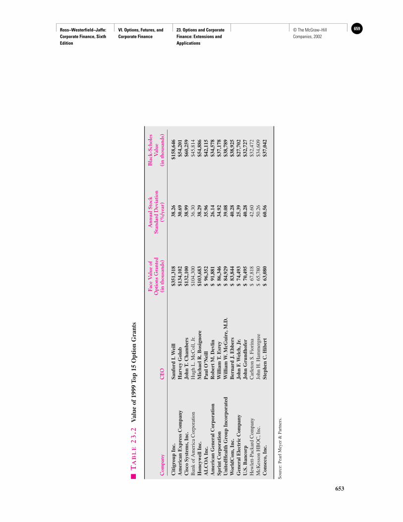
Ross−Westerfield−Jaffe: Corporate Finance, Sixth Edition
VI. Options, Futures, and Corporate Finance
23. Options and Corporate Finance: Extensions and Applications
659© The McGraw−Hill Companies, 2002
653
�T
AB
LE
23
.2V
alue
of
1999
Top
15
Opt
ion
Gra
nts
Face
Val
ue o
fA
nnua
l Sto
ckB
lack
-Sch
oles
O
ptio
ns G
rant
edSt
anda
rd D
evia
tion
Val
ueC
ompa
nyC
EO
(in
thou
sand
s)(%
/yea
r)(i
n th
ousa
nds)
Cit
igro
up I
nc.
Sanf
ord
I. W
eill
$351
,318
38.2
6$1
58,6
46A
mer
ican
Exp
ress
Com
pany
Har
vey
Gol
ub$1
34,1
0230
.69
$54,
201
Cis
co S
yste
ms,
Inc.
John
T. C
ham
bers
$132
,100
38.9
9$6
0,25
9B
ank
of A
mer
ica
Cor
pora
tion
Hug
h L
. McC
oll,
Jr.
$104
,300
36.3
0$4
5,81
4H
oney
wel
l Inc
.M
icha
el R
. Bos
igno
re$1
03,6
8338
.29
$54,
886
AL
CO
A I
nc.
Pau
l O’N
eill
$96
,352
35.9
6$4
2,11
5A
mer
ican
Gen
eral
Cor
pora
tion
Rob
ert
M. D
evlin
$91
,881
26.1
4$3
4,57
8Sp
rint
Cor
pora
tion
Will
iam
T. E
srey
$86
,346
34.9
2$3
7,17
8U
nite
dHea
lth
Gro
up I
ncor
pora
ted
Will
iam
W. M
cGui
re,M
.D.
$84
,929
39.0
8$3
8,78
9W
orld
Com
,Inc
.B
erna
rd J
. Ebb
ers
$83
,844
40.2
8$3
8,92
5G
ener
al E
lect
ric
Com
pany
John
F. W
elch
,Jr.
$74
,493
25.3
9$2
7,70
2U
.S. B
anco
rpJo
hn G
rund
hofe
r$
70,4
9540
.28
$32,
727
Hew
lett-
Pack
ard
Com
pany
Car
leto
n S.
Fio
rina
$67
,818
42.6
0$3
2,47
2M
cKes
son
HB
OC
,Inc
.Jo
hn H
. Ham
mer
gree
$65
,780
50.2
6$3
4,60
9C
onse
co,I
nc.
Step
hen
C. H
iber
t$
63,0
8060
.56
$37,
042
Sour
ce:P
earl
Mey
er &
Par
tner
s.

Ross−Westerfield−Jaffe: Corporate Finance, Sixth Edition
VI. Options, Futures, and Corporate Finance
23. Options and Corporate Finance: Extensions and Applications
660 © The McGraw−Hill Companies, 2002
1. The stock price (S) of $51.15 equals the exercise price (E).2. The risk-free rate (r) is 0.07.3. The five-year time interval is t � 5.
In addition, the variance of Citigroup stock is estimated to be (0.3826)2 � 0.1464.The above information allows us to estimate the value of Sandy Weill’s op-
tions using the Black-Scholes model.
C � SN(d1) � Ee�rtN(d2)d1 � [(r � 1/2�2)t]/ � 0.8369d2 � d1 � � �0.0186
N(d1) � 0.7987N(d2) � 0.4926
e�.07 � 5 � 0.7047C � $51.15 � 0.7987 � $51.15 � (0.7047 � 0.4926)� $23.098
Thus, the value of a call option on one share of Citigroup stock was $23.098. SinceMr. Weill was granted options on 6.8684 million shares, his grant has a marketvalue of $158,646,000 (6.8684 million � $23.098).
The values we have computed in Table 23.2 are the economic values of the options ifthey were to trade in the market. The real question is, whose value are we talking about?Are these the costs of the options to the company? Are they the values of the options to theexecutives?
Suppose that a company computes the fair market value of the options as we have donein Table 23.2. For purposes of illustration, assume that the options are in the money, andthat they are worth $25 each. Suppose, too, that the CEO holds 1 million such options fora total value of $25 million. This is the amount that the options would trade at in the finan-cial markets and that traders and investors would be willing to pay for them.1 If the com-pany were very large, it would not be unreasonable for it to view this as the cost of grant-ing the options to the CEO. Of course, in return, the company would expect the CEO toimprove the value of the company to its shareholders by more than this amount. As we haveseen, perhaps the main purpose of options is to align the interests of management with thoseof the shareholders of the firm. Under no circumstances, though, is the $25 million neces-sarily a fair measure of what the options are worth to the CEO.
As an illustration, suppose that the CEO of ABC has options on $1 million in shareswith an exercise price of $30 per share, and the current price of ABC stock is $50 per share.If the options were exercised today, they would be worth $20 million (an underestimationof their market value). Suppose, in addition, that the CEO owns $5 million in companystock and has $5 million in other assets. The CEO clearly has a very undiversified personalportfolio. By the standards of modern portfolio theory having 25/30 or about 83 percent ofyour personal wealth in one stock and its options is unnecessarily risky.
While the CEO is wealthy by most standards, significant shifts in the stock value willhave dramatic impacts on the CEO’s economic well-being. If the value drops from $50 pershare to $30 per share, the current exercise value of the options on 1 million shares dropsfrom $20 million down to zero. Ignoring the fact that if the options would have more timeto mature they will not lose all of this value, we nevertheless have a rather startling declinein the CEO’s net worth from about $30 million to $8 million ($5 million in other assets plusstock that is now worth $3 million). But that is the purpose of giving the options and the
��2t��2t
654 Part VI Options, Futures, and Corporate Finance
1We ignore warrant dilution in this example. See Chapter 24 for a discussion of warrant dilution.
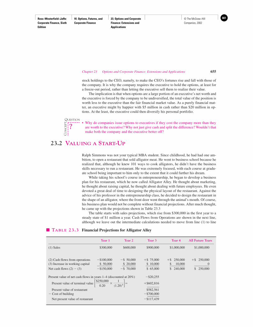
Ross−Westerfield−Jaffe: Corporate Finance, Sixth Edition
VI. Options, Futures, and Corporate Finance
23. Options and Corporate Finance: Extensions and Applications
661© The McGraw−Hill Companies, 2002
stock holdings to the CEO, namely, to make the CEO’s fortunes rise and fall with those ofthe company. It is why the company requires the executive to hold the options, at least fora freeze-out period, rather than letting the executive sell them to realize their value.
The implication is that when options are a large portion of an executive’s net worth andthe executive is forced by the company to be undiversified, the total value of the position isworth less to the executive than the fair financial market value. As a purely financial mat-ter, an executive might by happier with $5 million in cash rather than $20 million in op-tions. At the least, the executive could then diversify his personal portfolio.
• Why do companies issue options to executives if they cost the company more than theyare worth to the executive? Why not just give cash and split the difference? Wouldn’t thatmake both the company and the executive better off?
23.2 VALUING A START-UP
Ralph Simmons was not your typical MBA student. Since childhood, he had had one am-bition, to open a restaurant that sold alligator meat. He went to business school because herealized that, although he knew 101 ways to cook alligators, he didn’t have the businessskills necessary to run a restaurant. He was extremely focused, with each course at gradu-ate school being important to him only to the extent that it could further his dream.
While taking his school’s course in entrepreneurship, he began to develop a businessplan for his restaurant, which he now called Alligator Alley. He thought about marketing,he thought about raising capital, he thought about dealing with future employees. He evendevoted a great deal of time to designing the physical layout of the restaurant. Against theadvice of his professor in the entrepreneurship class, he decided to design the restaurant inthe shape of an alligator, where the front door went through the animal’s mouth. Of course,his business plan would not be complete without financial projections. After much thought,he came up with the projections shown in Table 23.3
The table starts with sales projections, which rise from $300,000 in the first year to asteady state of $1 million a year. Cash Flows from Operations are shown in the next line,although we leave out the intermediate calculations needed to move from line (1) to line
Chapter 23 Options and Corporate Finance: Extensions and Applications 655
QUESTION
CO
NC
EP
T
?
� TABLE 23.3 Financial Projections for Alligator Alley
Year 1 Year 2 Year 3 Year 4 All Future Years
(1) Sales $300,000 $600,000 $900,000 $1,000,000 $1,000,000
(2) Cash flows from operations �$100,000 �$ 50,000 �$ 75,000 �$ 250,000 �$ 250,000(3) Increase in working capital $ 50,000 $ 20,000 $ 10,000 $ 10,000 0_________ ________ ________ _________ _________Net cash flows (2) � (3) �$150,000 �$ 70,000 $ 65,000 $ 240,000 $ 250,000
Present value of net cash flows in years 1–4 (discounted at 20%) �$20,255
Present value of terminal value � �$602,816
Present value of restaurant $582,561� Cost of building �$700,000_______
Net present value of restaurant �$117,439
�$250,000
0.20�
1�1.20� 4
Ross−Westerfield−Jaffe: Corporate Finance, Sixth Edition
VI. Options, Futures, and Corporate Finance
23. Options and Corporate Finance: Extensions and Applications
662 © The McGraw−Hill Companies, 2002
(2). After subtracting Working Capital, the table shows Net Cash Flows in line 4. Net CashFlows are negative initially, as is quite common in start-ups, but they become positive byYear 3. However, the rest of the table presents the unfortunate truth. The cash flows fromthe restaurant yield a present value of $582,561, assuming a discount rate of 20 percent.Unfortunately, the cost of the building is greater, at $700,000, implying a negative net pres-ent value of �$117,439.
The projections indicate that Ralph’s lifelong dream may not come to pass. He cannotexpect to raise the capital needed to open his restaurant, and if he did obtain the funding, therestaurant would likely go under anyway. Ralph checked and rechecked the numbers, hopingvainly to discover either a numerical error or a cost-saving omission that would move his ven-ture from the red to the black. In fact, Ralph saw that, if anything, his forecasts are generous,because a 20 percent discount rate and an infinitely lived building are on the optimistic side.
It wasn’t until Ralph took a course in corporate strategy that he realized the hiddenvalue in his venture. In that course, his instructor repeatedly stated the importance of posi-tioning a firm to take advantage of new opportunities. Although Ralph didn’t see the con-nection at first, he finally realized the implications for Alligator Alley. His financial pro-jections were based on expectations. There was a 50 percent probability that alligator meatwould be more popular than he thought, in which case actual cash flows would exceed pro-jections. And, there was a 50 percent probability that the meat would be less popular, inwhich case the actual flows would fall short of projections.
If the restaurant did poorly, it would probably fold in a few years, because he wouldnot want to keep losing money forever. However, if the restaurant did well, he would be ina position to expand. If alligator meat proved popular in one locale, it would likely provepopular in other locales as well. Thus, he noticed two options, the option to abandon underbad conditions and the option to expand under good conditions. Although both options canbe valued according to the principles of the previous chapter, we focus on the option to ex-pand because it is probably much more valuable.
Ralph reasoned that, as much as he personally liked alligator meat, there were wholeregions of the country where consumer resistance would doom Alligator Alley. So he de-veloped a strategy of catering only to those regions where alligator meat is somewhat pop-ular already. He forecast that, although he could expand quickly if the first restaurant provedsuccessful, the market would limit him to 30 additional restaurants.
Ralph believes that this expansion will occur about four years from now. He believesthat he will need three years of operating the first restaurant to (1) get the initial restaurantrunning smoothly and (2) have enough information to place an accurate value on the restau-rant. If the first restaurant is successful enough, he will need another year to obtain outsidecapital. Thus, he will be ready to build the 30 additional units around the fourth year.
Ralph will value his enterprise, including the option to expand, according to the Black-Scholes model. From Table 23.3, we see that each unit cost $700,000, implying a total cost overthe 30 additional units of $21,000,000 (30 � $700,000). The present value of the cash inflowsfrom these 30 units is $17,476,830 (30 � $582,561), according to the table. However, becausethe expansion will occur around the fourth year, this present-value calculation is provided fromthe point of view of four years in the future. The present value as of today is $8,428,255($17,476,830/(1.20)4), assuming a discount rate of 20 percent per year. Thus, Ralph views hispotential restaurant business as an option, where the exercise price is $21,000,000 and the valueof the underlying asset is $8,428,255. The option is currently out of the money, a result that fol-lows from the negative value of a typical restaurant, as calculated in Table 23.3. Of course,Ralph is hoping that the option will move into the money within four years.
Ralph needs three additional parameters to use the Black-Scholes model: r, the contin-uously compounded interest rate; t, the time to maturity; and �, the standard deviation ofthe underlying asset. Ralph uses the yield on a four-year zero-coupon bond, which is 3.5
656 Part VI Options, Futures, and Corporate Finance

Ross−Westerfield−Jaffe: Corporate Finance, Sixth Edition
VI. Options, Futures, and Corporate Finance
23. Options and Corporate Finance: Extensions and Applications
663© The McGraw−Hill Companies, 2002
percent, as the estimate of the interest rate. The time to maturity is four years. The estimateof standard deviation is a little trickier, because there is no historical data on alligator restau-rants. Ralph finds that the average annual standard deviation of the returns on publiclytraded restaurants is 0.35. Because Alligator Alley is a new venture, he reasons that the riskhere would be somewhat greater. He finds that the average annual standard deviation forrestaurants that have gone public in the last few years is 0.45. Because Ralph’s restaurantis newer still, he uses a standard deviation of 0.50.
There is now enough data to value Ralph’s venture. The value according to theBlack-Scholes model is $1,455,196. The actual calculations are shown in Table 23.4. Ofcourse, Ralph must start his pilot restaurant before he can take advantage of this option.Thus, the net value of the call option less the negative present value of the pilot restau-rant is $1,337,757 ($1,455,196 � $117,439). Because this value is large and positive,Ralph decides to stay with his dream of Alligator Alley. He knows that the probability
Chapter 23 Options and Corporate Finance: Extensions and Applications 657
� TABLE 23.4 Valuing a Start-Up Firm (Alligator Alley) as an Option
Facts1. The value of a single restaurant is negative, as indicated by the net-present-value calculation
in Table 23.3 of �$117,439. Thus, the restaurant would not be funded if there were nopossibility of expansion.
2. If the pilot restaurant is successful, Ralph Simmons plans to create 30 additional restaurantsaround year 4. This leads to the following observations:a. The total cost of 30 units is $21,000,000 (30 � $700,000).b. The present value of future cash flows as of year 4 is $17,476,830 (30 � $582,561).c. The present value of these cash flows today is $8,428,255 ($17,476,830/(1.20)4).
Here, we assume that cash flows from the project are discounted at 20% per annum.Thus, the business is essentially a call option, where the exercise price is $21,000,000 and
the underlying asset is worth $8,428,255.
3. Ralph Simmons estimates the standard deviation of the return on Alligator Alley’s stock tobe 0.50.
Parameters of the Black-Scholes model:S (stock price) � $8,428,255
E (exercise price) � $21,000,000t (time to maturity) � 4 years
� (standard deviation) � 0.50r (continuously compounded interest rate) � 3.5%
Calculation from the Black-Scholes model:C � SN(d1) � Ee�rtN(d2)d1 � [ln(S/E) � (r � 1/2 �2)t]/d2 � d1 �
d1 �
d2 � �0.27293 � � �1.27293N(d1) � N(�0.27293) � 0.3936N(d2) � N(�1.27293) � 0.1020
C � $8,428,255 � 0.3936 � $21,000,000 � e�0.035�4 � 0.1020� $1,455,196
Value of business including cost of pilot restaurant � $1,455,196 � $117,439� $1,337,757
��0.50� 2 � 4
�ln 8,428,255
21,000,000� �0.035 � 1�2 �0.50� 2�4 ���0.50� 2 � 4 � �0.27293
��2t��2t
Ross−Westerfield−Jaffe: Corporate Finance, Sixth Edition
VI. Options, Futures, and Corporate Finance
23. Options and Corporate Finance: Extensions and Applications
664 © The McGraw−Hill Companies, 2002
that the restaurant will fail is greater than 50%. Nevertheless, the option to expand is im-portant enough that his restaurant business has value. And, if he needs outside capital,he probably can attract the necessary investors.
This finding leads to the appearance of a paradox. If Ralph approaches investors to in-vest in a single restaurant with no possibility of expansion, he will probably not be able toattract capital. After all, Table 23.3 shows a net present value of �$117,439. However, ifRalph thinks bigger, he will likely be able to attract all the capital that he needs. But this isreally not a paradox at all. By thinking bigger, Ralph is offering investors the option, notthe obligation, to expand.
The example we have chosen may seem frivolous and, certainly, we added offbeatcharacteristics for interest. However, if you think that business situations involving optionsare unusual or unimportant, let us state emphatically that nothing can be further from thetruth. The notion of embedded options is at the heart of business. There are two possibleoutcomes for virtually every business idea. On the one hand, the business may fail, in whichcase the managers will probably try to shut it down in the most cost-efficient way. On theother hand, the business may prosper, in which case the managers will try to expand. Thus,virtually every business has both the option to abandon and the option to expand. You mayhave read pundits claiming that the net-present-value approach to capital budgeting iswrong or incomplete. Although criticism of this type frequently irritates the finance estab-lishment, the pundits definitely have a point. If virtually all projects have embedded op-tions, only an approach such as the one we have outlined can be appropriate. Ignoring theoptions is likely to lead to serious undervaluation.
• What are the two options that many businesses have?• Why does a strict NPV calculation typically understate the value of a firm or project?
23.3 MORE ON THE BINOMIAL MODEL
Earlier in this chapter, we examined two applications of options, executive compensationand the start-up decision. In both cases we valued an option using the Black-Scholes model.Although this model is justifiably well known, it is not the only approach to option valua-tion. As mentioned in the previous chapter, the binomial model is an alternative and—insome situations—a superior approach to valuation. The rest of this chapter examines twoapplications under this binomial model.
Heating OilTwo-Date Example Consider Anthony Meyer, a typical heating-oil distributor, whose busi-ness consists of buying heating oil at the wholesale level and reselling the oil to homeownersat a slightly higher price. Most of his revenue comes from sales during the winter. Today, Sep-tember 1, heating oil sells for $1.00 per gallon. Of course, this price is not fixed. Rather, oilprices will vary from September 1 until December 1, the time when his customers will prob-ably be making their big winter purchases of heating oil. Let’s simplify the situation by as-suming that Anthony believes that oil prices will either be at $1.37 or $0.73 on December 1.Figure 23.1 portrays this possible price movement. This potential price range represents agreat deal of uncertainty, because Anthony has no idea which of the two possible prices willactually occur. However, this price variability does not translate into that much risk, becausehe is able to pass price changes on to his customers. That is, he will charge his customers moreif he ends up paying $1.37 per gallon than if he ends up paying $0.73 per gallon.
658 Part VI Options, Futures, and Corporate Finance
QUESTIONS
CO
NC
EP
T
?
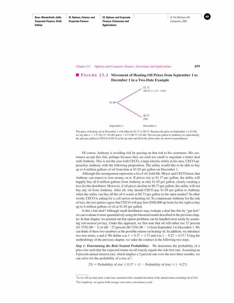
Ross−Westerfield−Jaffe: Corporate Finance, Sixth Edition
VI. Options, Futures, and Corporate Finance
23. Options and Corporate Finance: Extensions and Applications
665© The McGraw−Hill Companies, 2002
Of course, Anthony is avoiding risk by passing on that risk to his customers. His cus-tomers accept this risk, perhaps because they are each too small to negotiate a better dealwith Anthony. This is not the case with CECO, a large electric utility in his area. CECO ap-proaches Anthony with the following proposition. The utility would like to be able to buyup to 6 million gallons of oil from him at $1.05 per gallon on December 1.
Although this arrangement represents a lot of oil, both Mr. Meyer and CECO know thatAnthony can expect to lose money on it. If prices rise to $1.37 per gallon, the utility willhappily buy all 6 million gallons from Anthony at only $1.05 per gallon, clearly creating aloss for the distributor. However, if oil prices decline to $0.73 per gallon, the utility will notbuy any oil from Anthony. After all, why should CECO pay $1.05 per gallon to Anthonywhen the utility can buy all the oil it wants at $0.73 per gallon in the open market? In otherwords, CECO is asking for a call option on heating oil. To compensate Anthony for the riskof loss, the two parties agree that CECO will pay him $500,000 up front for the right to buyup to 6 million gallons of oil at $1.05 per gallon.
Is this a fair deal? Although small distributors may evaluate a deal like this by “gut feel,”we can evaluate it more quantitatively using the binomial model described in the previous chap-ter. In that chapter, we pointed out that option problems can be handled most easily by assum-ing risk-neutral pricing. Under this approach, we first note that oil will either rise 37 percent($1.37/$1.00 � 1) or fall �27 percent ($0.73/$1.00 � 1) from September 1 to December 1. Wecan think of these two numbers as the possible returns on heating oil. In addition, we introducetwo new terms, u and d. We define u as 1 � 0.37 � 1.37 and d as 1 � 0.27 � 0.73.2 Using themethodology of the previous chapter, we value the contract in the following two steps.
Step 1: Determining the Risk-Neutral Probabilities We determine the probability of aprice rise such that the expected return on oil exactly equals the risk-free rate. Assuming an8 percent annual interest rate, which implies a 2 percent rate over the next three months, wecan solve for the probability of a rise as3:
2% � Probability of rise � 0.37 � (1 � Probability of rise) � (�0.27)
Chapter 23 Options and Corporate Finance: Extensions and Applications 659
$1.37($0.32 = 1.37 –1.05)
$0.73($0)
December 1
$1.00
September 1
� FIGURE 23.1 Movement of Heating-Oil Prices from September 1 toDecember 1 in a Two-Date Example
The price of heating oil on December 1 will either be $1.37 or $0.73. Because the price on September 1 is $1.00,we say that u � 1.37 ($1.37 / $1.00) and d � 0.73 ($0.73 / $1.00). The loss per gallon to Anthony (or, equivalently,the gain per gallon to CECO) of $0.32 in the up-state and $0 in the down-state are shown in parentheses.
2As we will see later, here u and d are consistent with a standard deviation of the annual return on heating oil of 0.63.3For simplicity, we ignore both storage costs and a convenience yield.
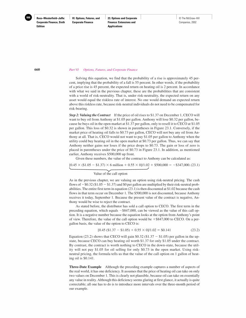
Ross−Westerfield−Jaffe: Corporate Finance, Sixth Edition
VI. Options, Futures, and Corporate Finance
23. Options and Corporate Finance: Extensions and Applications
666 © The McGraw−Hill Companies, 2002
Solving this equation, we find that the probability of a rise is approximately 45 per-cent, implying that the probability of a fall is 55 percent. In other words, if the probabilityof a price rise is 45 percent, the expected return on heating oil is 2 percent. In accordancewith what we said in the previous chapter, these are the probabilities that are consistentwith a world of risk-neutrality. That is, under risk-neutrality, the expected return on anyasset would equal the riskless rate of interest. No one would demand an expected returnabove this riskless rate, because risk-neutral individuals do not need to be compensated forrisk-bearing.
Step 2:Valuing the Contract If the price of oil rises to $1.37 on December 1, CECO willwant to buy oil from Anthony at $1.05 per gallon. Anthony will lose $0.32 per gallon, be-cause he buys oil in the open market at $1.37 per gallon, only to resell it to CECO at $1.05per gallon. This loss of $0.32 is shown in parentheses in Figure 23.1. Conversely, if themarket price of heating oil falls to $0.73 per gallon, CECO will not buy any oil from An-thony at all. That is, CECO would not want to pay $1.05 per gallon to Anthony when theutility could buy heating oil in the open market at $0.73 per gallon. Thus, we can say thatAnthony neither gains nor loses if the price drops to $0.73. The gain or loss of zero isplaced in parentheses under the price of $0.73 in Figure 23.1. In addition, as mentionedearlier, Anthony receives $500,000 up front.
Given these numbers, the value of the contract to Anthony can be calculated as:
[0.45 � ($1.05 � $1.37) � 6 million � 0.55 � 0]/1.02 � $500,000 � �$347,000. (23.1)
Value of the call option
As in the previous chapter, we are valuing an option using risk-neutral pricing. The cashflows of �$0.32 ($1.05 � $1.37) and $0 per gallon are multiplied by their risk-neutral prob-abilities. The entire first term in equation (23.1) is then discounted at $1.02 because the cashflows in that term occur on December 1. The $500,000 is not discounted, because Anthonyreceives it today, September 1. Because the present value of the contract is negative, An-thony would be wise to reject the contract.
As stated before, the distributor has sold a call option to CECO. The first term in thepreceding equation, which equals �$847,000, can be viewed as the value of this call op-tion. It is a negative number because the equation looks at the option from Anthony’s pointof view. Therefore, the value of the call option would be �$847,000 to CECO. On a per-gallon basis, the value of the option to CECO is:
[0.45 ($1.37 � $1.05) � 0.55 � 0]/1.02 � $0.141 (23.2)
Equation (23.2) shows that CECO will gain $0.32 ($1.37 � $1.05) per gallon in the up-state, because CECO can buy heating oil worth $1.37 for only $1.05 under the contract.By contrast, the contract is worth nothing to CECO in the down-state, because the util-ity will not pay $1.05 for oil selling for only $0.73 in the open market. Using risk-neutral pricing, the formula tells us that the value of the call option on 1 gallon of heat-ing oil is $0.141.
Three-Date Example Although the preceding example captures a number of aspects ofthe real world, it has one deficiency. It assumes that the price of heating oil can take on onlytwo values on December 1. This is clearly not plausible, because oil can take on essentiallyany value in reality. Although this deficiency seems glaring at first glance, it actually is quitecorrectable; all one has to do is to introduce more intervals over the three-month period ofour example.
660 Part VI Options, Futures, and Corporate Finance
Ross−Westerfield−Jaffe: Corporate Finance, Sixth Edition
VI. Options, Futures, and Corporate Finance
23. Options and Corporate Finance: Extensions and Applications
667© The McGraw−Hill Companies, 2002
For example, consider Figure 23.2, which shows the price movement of heating oilover two intervals of 11⁄2 months each.4 As shown in the figure, the price will be either $1.25or $0.80 on October 15. We refer to $1.25 as the price in the up-state and $0.80 as the pricein the down-state. Thus, heating oil has returns of 25 percent ($1.25/$1) and �20 percent($0.80/$1) in the two states.
We assume the same variability as we move forward from October 15 to December 1.That is, given a price of $1.25 on October 15, the price on December 1 will be either $1.56($1.25 � 1.25) or $1 ($1.25 � 0.80). Similarly, given a price of $0.80 on October 15, theprice on December 1 will be either $1 ($0.80 � 1.25) or $0.64 ($0.80 � 0.80). This as-sumption of constant variability is quite plausible, because the rate of new informationimpacting heating oil (or most commodities or assets) is likely to be similar from monthto month.
Note that there are three possible prices on December 1, but there are two possibleprices on October 15. Also note that there are two paths, both generating a price of $1 onDecember 1. The price could rise to $1.25 on October 15 before falling back down to $1 onDecember 1 or, alternatively, the price could fall to $0.80 on October 15 before going backup to $1 on December 1. In other words, the model has symmetry, where an up-movementfollowed by a down-movement yields the same price on December 1 as a down-movementfollowed by an up-movement.
Chapter 23 Options and Corporate Finance: Extensions and Applications 661
$1.25($0.237)
$0.80($0)
October 15
$1.00($0.110)
September 1
$0.64($0)
December 1
$1.56($0.51 = $1.56 – $1.05)
$1.00($0)
� FIGURE 23.2 Movement of Heating-Oil Prices in a Three-Date Model
The figure shows the prices of a gallon of heating oil on three dates, given u � 1.25 and d � 0.80. There are three possible prices for heating oil on December 1. For each one ofthese three prices, we calculate the price on December 1 of a call option on a gallon ofheating oil with an exercise price of $1.05. These numbers are in parentheses. Call pricesat earlier dates are determined by the binomial model and are also shown in parentheses.
4Though it is not apparent at first glance, we will see later that the price movement in Figure 23.2 is consistentwith the price movement in Figure 23.1.
Ross−Westerfield−Jaffe: Corporate Finance, Sixth Edition
VI. Options, Futures, and Corporate Finance
23. Options and Corporate Finance: Extensions and Applications
668 © The McGraw−Hill Companies, 2002
How do we value CECO’s option in this three-date example? We employ the same pro-cedure that we used in the two-date example, although we will now need an extra step be-cause of the extra date:
Step 1: Determining the Risk-Neutral Probabilities As we did in the two-date example,we determine what the probability of a price rise would be such that the expected return onheating oil exactly equals the riskless rate. However, in this case, we work with an interval of11⁄2 months. Assuming an 8 percent annual rate of interest, which implies a 1 percent rate overa 11⁄2 month interval,5 we can solve for the probability of a rise as:
1% � Probability of rise � 0.25 � (1 � Probability of rise) � (�0.20)
Solving the equation, we find that the probability of a rise here is 47 percent, implying thatthe probability of a fall is 53 percent. In other words, if the probability of a rise is 47 per-cent, the expected return on heating oil is 1 percent per each 11⁄2-month interval. Again, theseprobabilities are determined under the assumption of risk-neutral pricing.
Note that the probabilities of 47 percent and 53 percent hold for both the interval fromSeptember 1 to October 15 and the interval from October 15 to December 1. This is the casebecause the return in the up-state is 25 percent and the return in the down-state is �20 per-cent for each of the two intervals. Thus, the preceding equation must apply to each of theintervals separately.
Step 2: Valuing the Option as of October 15 As indicated in Figure 23.2, the optionto CECO will be worth $0.51 per gallon on December 1 if the price of heating oil hasrisen to $1.56 on that date. That is, CECO can buy oil from Anthony at $1.05 when itwould otherwise have to pay $1.56 in the open market. However the option will beworthless on December 1 if the price of a gallon of heating oil is either $1 or $0.64 onthat date. Here, the option is out of the money because the exercise price of $1.05 isabove either $1 or $0.64.
Using these implicit option prices on December 1, we can calculate the value of the call op-tion on October 15. If the price of a gallon of heating oil is $1.25 on October 15, Figure 23.2 showsus that the call option will either be worth $0.51 or $0 on December 1. Thus, if the price of heat-ing oil is $1.25 on October 15, the value of the option on 1 gallon of heating oil at that time is:
[0.47 � 0.51 � 0.53 � 0]/1.01 � $0.237
Here, we are valuing an option using the same risk-neutral pricing approach that we usedin the earlier two-date example. This value of $0.237 is shown in parentheses in Figure 23.2
We also want to value the option on October 15 if the price at that time is $0.80.However, the value here is clearly zero, as indicated by the calculation:
[0.47 � $0 � 0.53 � $0]/1.01 � 0
This is obvious, once one looks at Figure 23.2. We see from the figure that the call must endup out of the money on December 1 if the price of heating oil is $0.80 on October 15. Thus,the call must have zero value on October 15 if the price of heating oil is $0.80 on that date.
Step 3: Valuing the Option on September 1 In the previous step, we saw that the priceof the call on October 15 would be $0.237 if the price of a gallon of heating oil were $1.25on that date. Similarly, the price of the option on October 15 would be $0 if oil were sell-ing at $0.80 on that date. From these values, we can calculate the call option value onSeptember 1 as:
[0.47 � $0.237 � 0.53 � $0]/1.01 � $0.110
662 Part VI Options, Futures, and Corporate Finance
5For simplicity, we ignore interest compounding.
Ross−Westerfield−Jaffe: Corporate Finance, Sixth Edition
VI. Options, Futures, and Corporate Finance
23. Options and Corporate Finance: Extensions and Applications
669© The McGraw−Hill Companies, 2002
Notice that this calculation is completely analogous to the calculation of the optionvalue in the previous step, as well as the calculation of the option value in the two-date ex-ample that we presented earlier. In other words, the same approach applies regardless of thenumber of intervals used. As we will see later, we can move to many intervals, which pro-duces greater realism, yet still maintain the same basic methodology.
The previous calculation has given us the value of CECO of its option on 1 gallon ofheating oil. Now we are ready to calculate the value of the contract to Anthony. Given thecalculations from the previous equation, the contract’s value can be written as:
�$0.110 � 6,000,000 � $500,000 � �$160,000
That is, Anthony is giving away an option worth $0.110 for each of the 6 million gallons ofheating oil. In return, he is receiving only $500,000 up front. On balance, he is losing$160,000. Of course, the value of the contract to CECO is the opposite, so the value to thisutility is $160,000.
Extension to Many Dates We have looked at the contract between CECO and Anthonyusing both a two-date example and a three-date example. The three-date case is more real-istic because more possibilities for price movements are allowed here. However, why stopat just three dates? Moving to 4 dates, 5 dates, 50 dates, 500 dates, and so on, should giveus ever more realism. Note that, as we move to more dates, we are merely shortening theinterval between dates without increasing the overall time period of three months (Septem-ber 1 to December 1).
For example, imagine a model with 90 dates over the three months. Here, each inter-val is approximately one day long, because there are about 90 days in a three-month period.The assumption of two possible outcomes in the binomial model is more plausible over aone-day interval than it is over a 11⁄2-month interval, let alone a three-month interval. Ofcourse, we could probably achieve greater realism still by going to an interval of, say, onehour or one minute.
How does one adjust the binomial model in order to accommodate increases in thenumber of intervals? It turns out that two simple formulas relate u and d to the standard de-viation of the return of the underlying asset6:
u � e�/ and d � 1/u
where � is the standard deviation of the annualized return on the underlying asset (heatingoil, in this case) and n is the number of intervals over a year.
When we created the heating oil example, we assumed that the annualized standard de-viation of the return on heating oil was 0.63 (or, equivalently, 63 percent). Because thereare four quarters in a year, u � e0.63/ � 1.37 and d � 1/1.37 � 0.73, as shown in the two-date example of Figure 23.1. In the three-date example of Figure 23.2, where each intervalis 11⁄2 months long, u � e0.63/ � 1.25 and d � 1/1.25 � 0.80. Thus, the binomial modelcan be applied in practice if the standard deviation of the return of the underlying asset canbe estimated.
We stated earlier that the value of the call option on a gallon of heating oil was esti-mated to be $0.141 in the two-date model and $0.110 in the three-date model. How doesthe value of the option change as we increase the number of intervals, while keeping thetime period constant at three months (from September 1 to December 1)? We have calcu-
�8
�4
�n
Chapter 23 Options and Corporate Finance: Extensions and Applications 663
6See John C. Hull, Options, Futures, and Other Derivatives, 4th ed. (Upper Saddle River, N.J.: Prentice Hall,1999) for a derivation of these formulas.
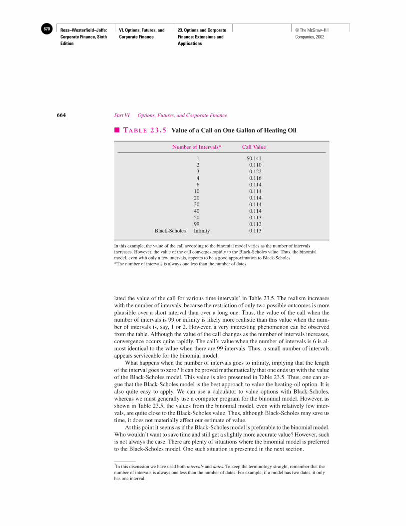
Ross−Westerfield−Jaffe: Corporate Finance, Sixth Edition
VI. Options, Futures, and Corporate Finance
23. Options and Corporate Finance: Extensions and Applications
670 © The McGraw−Hill Companies, 2002
lated the value of the call for various time intervals7 in Table 23.5. The realism increaseswith the number of intervals, because the restriction of only two possible outcomes is moreplausible over a short interval than over a long one. Thus, the value of the call when thenumber of intervals is 99 or infinity is likely more realistic than this value when the num-ber of intervals is, say, 1 or 2. However, a very interesting phenomenon can be observedfrom the table. Although the value of the call changes as the number of intervals increases,convergence occurs quite rapidly. The call’s value when the number of intervals is 6 is al-most identical to the value when there are 99 intervals. Thus, a small number of intervalsappears serviceable for the binomial model.
What happens when the number of intervals goes to infinity, implying that the lengthof the interval goes to zero? It can be proved mathematically that one ends up with the valueof the Black-Scholes model. This value is also presented in Table 23.5. Thus, one can ar-gue that the Black-Scholes model is the best approach to value the heating-oil option. It isalso quite easy to apply. We can use a calculator to value options with Black-Scholes,whereas we must generally use a computer program for the binomial model. However, asshown in Table 23.5, the values from the binomial model, even with relatively few inter-vals, are quite close to the Black-Scholes value. Thus, although Black-Scholes may save ustime, it does not materially affect our estimate of value.
At this point it seems as if the Black-Scholes model is preferable to the binomial model.Who wouldn’t want to save time and still get a slightly more accurate value? However, suchis not always the case. There are plenty of situations where the binomial model is preferredto the Black-Scholes model. One such situation is presented in the next section.
664 Part VI Options, Futures, and Corporate Finance
7In this discussion we have used both intervals and dates. To keep the terminology straight, remember that thenumber of intervals is always one less than the number of dates. For example, if a model has two dates, it onlyhas one interval.
� TABLE 23.5 Value of a Call on One Gallon of Heating Oil
Number of Intervals* Call Value
1 $0.1412 0.1103 0.1224 0.1166 0.114
10 0.11420 0.11430 0.11440 0.11450 0.11399 0.113
Black-Scholes Infinity 0.113
In this example, the value of the call according to the binomial model varies as the number of intervalsincreases. However, the value of the call converges rapidly to the Black-Scholes value. Thus, the binomialmodel, even with only a few intervals, appears to be a good approximation to Black-Scholes.*The number of intervals is always one less than the number of dates.
Ross−Westerfield−Jaffe: Corporate Finance, Sixth Edition
VI. Options, Futures, and Corporate Finance
23. Options and Corporate Finance: Extensions and Applications
671© The McGraw−Hill Companies, 2002
23.4 SHUTDOWN AND REOPENING DECISIONS
Some of the earliest and most important examples of special options occur in the natural re-sources and mining industries.
Valuing a Gold MineThe “Woe Is Me” gold mine was founded in 1878 on one of the richest veins of gold in theWest. Thirty years later, by 1908, the mine had been played out, but occasionally, depend-ing on the price of gold, it is reopened. Currently gold is not actively mined at Woe Is Me,but its stock is still traded on the exchange under the ticker symbol, WOE. WOE has no debtand, with about 20 million outstanding shares, it has a market value (stock price times num-ber of shares outstanding) well above $1 billion. WOE owns about 160 acres of land sur-rounding the mine and has a 100-year government lease to mine gold there. However, landin the desert has a market value of only a few thousand dollars. WOE holds cash and secu-rities and other assets worth about $30 million. What could possibly explain why a com-pany with $30 million in assets and a closed gold mine that is producing no cash flow what-soever has the market value that WOE has?
The answer lies in the options that WOE implicitly owns in the form of a gold mine.Assume that the current price of gold is about $320 per ounce and the cost of extraction andprocessing at the mine is about $350 per ounce. It is no wonder that the mine is closed. Everyounce of gold extracted costs $350 and can be sold for only $320 for a loss of $30 per ounce.Presumably, if the price of gold were to rise, the mine could be opened. It costs $2 millionto open the mine and when it is opened, production is 50,000 ounces per year. Geologists be-lieve that the amount of gold in the mine is essentially unlimited, and WOE has the right tomine it for the next 100 years. Under the terms of its lease, WOE cannot stockpile gold andmust sell each year all the gold it mines that year. Closing the mine requires equipment to bemothballed and some environmental precautions to be put in place and costs $1 million. Wewill refer to the $2 million required to open the mine as the entry fee or investment and the$1 million to close it as the closing or abandonment cost. (There is no way to avoid the aban-donment cost by simply keeping the mine open and not operating.)
From a financial perspective, WOE is really just a package of options on the price ofgold disguised as a company and a mine. The basic option is a call on the price of goldwhere the exercise price is the $350 extraction cost. The option is complicated by havingan exercise fee of $2 million—the opening cost—whenever it is exercised and a closing feeof $1 million when it is abandoned. It is also complicated by the fact that it is a perpetualoption with no final maturity.
The Abandonment and Opening DecisionsBefore trying to figure out the exact value of the option implicit in WOE or, for that mat-ter, in any real option problem, it is useful to see what we can say by just applying com-mon sense. To begin with, the mine should only be opened when the price of gold is suf-ficiently above the extraction cost of $350 per ounce. Because it costs $2 million to openthe mine, the mine should not be opened whenever the price of gold is only slightlyabove $350. At a gold price of, say, $350.10, the mine wouldn’t be opened because theten-cent profit per ounce translates into $5,000 per year (50,000 ounces � $0.10/ounce).This would not begin to cover the $2 million opening costs. More significantly, though,the mine probably would not be opened if the price rose to $360 per ounce even thougha $10 profit per ounce—$500,000 per year—would pay the $2 million opening costs at
Chapter 23 Options and Corporate Finance: Extensions and Applications 665
Ross−Westerfield−Jaffe: Corporate Finance, Sixth Edition
VI. Options, Futures, and Corporate Finance
23. Options and Corporate Finance: Extensions and Applications
672 © The McGraw−Hill Companies, 2002
any reasonable discount rate. The reason is that here, as in all option problems, volatil-ity, in this case the volatility of gold, plays a significant role. Because the gold price isvolatile the price has to rise sufficiently above $350 per ounce to make it worth openingthe mine. If the price at which the mine is opened is too close to the extraction price of$350 per ounce, say at $360 per ounce, for example, then we would wind up opening themine every time the price jogged above $360 and finding ourselves operating at a lossor facing a closing decision whenever the gold price jogged down $10 per ounce or only3 percent down.
The estimated volatility of the return on gold is about 15 percent per year. Thismeans that a single annual standard deviation movement in the gold price is 15 percentof $320 or $48 per year. Surely with this amount of random movement in the gold price,a threshold of $352 is much too low at which to open the mine. A similar logic appliesto the closing decision. If the mine is open, then we will clearly keep it open as long asthe gold price is above the extraction cost of $350 per ounce since we are profiting onevery ounce of gold mined. But, we also won’t close the mine down simply because thegold price drops below $350 per ounce. We will tolerate a running loss to keep alive thepossibility that the gold price will rise above $350 and to avoid the necessity of havingto pay the $1 million abandonment cost only to have to pay another $2 million to reopenthe mine.
To summarize, if the mine is currently closed, then it will be opened—at a cost of$2 million—whenever the price of gold rises sufficiently above the extraction cost of$350 per ounce. If the mine is currently operating, then it will be closed down—at a costof $1 million—whenever the price of gold falls sufficiently below the extraction cost of$350 per ounce. WOE’s problem is to find these two threshold prices at which it opensa closed mine and closes an open mine. We call these prices popen and pclose, respec-tively, where
popen � $350/ounce � pclose
In other words, WOE will open the mine if the gold price option is sufficiently in the moneyand will close it when the option is sufficiently out of the money.
We know that the more volatile the gold price, the further away popen and pclosewill be from $350 per ounce. We also know that the greater the cost of opening the minethe higher popen will be and the greater the cost of abandoning the mine the lower willbe pclose. Interestingly, we should also expect that popen will be higher if the aban-donment cost is increased. After all, if it costs more to abandon the mine WOE will needto be more assured that the price will stay above the extraction cost when it decides toopen the mine. Otherwise, WOE might soon face the costly choice between abandon-ment and operating at a loss if the price falls below $350 per ounce. Similarly, raisingthe cost of opening the mine will make WOE more reluctant to close an open mine. Asa result, pclose will be lower.
The above arguments have enabled us to reduce the problem of valuing WOE to twostages. First, we have to determine the threshold prices, popen and pclose. Second, giventhe best choices for these thresholds, we must determine the value of a gold option that isexercised for a cost of $2 million when the gold price rises above popen and is shut downfor a cost of $1 million whenever the gold price is below pclose.
When the mine is open, i.e., when the option is exercised, the annual cash flow is equalto the difference between the gold price and the extraction cost of $350 per ounce times50,000 ounces. When the mine is shut down, it generates no cash flow.
The following diagram describes the decisions available at each point in time.
666 Part VI Options, Futures, and Corporate Finance
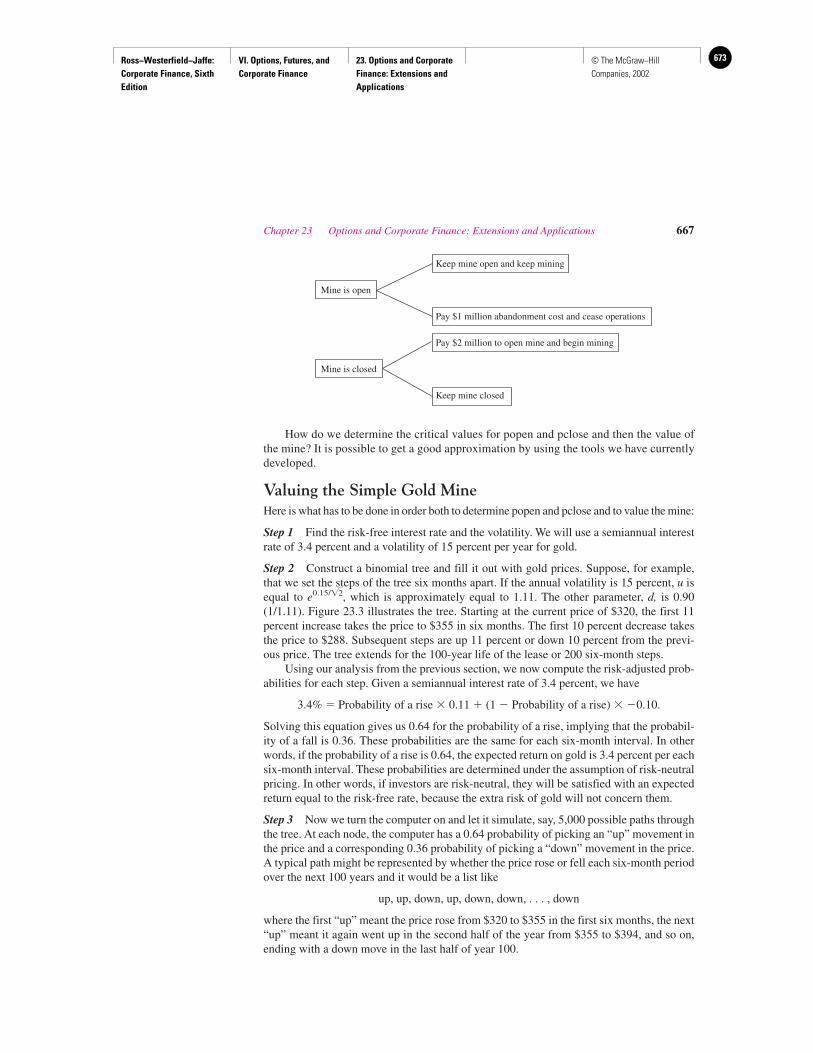
Ross−Westerfield−Jaffe: Corporate Finance, Sixth Edition
VI. Options, Futures, and Corporate Finance
23. Options and Corporate Finance: Extensions and Applications
673© The McGraw−Hill Companies, 2002
Keep mine open and keep mining
Mine is open
Pay $1 million abandonment cost and cease operations
Pay $2 million to open mine and begin mining
Mine is closed
Keep mine closed
How do we determine the critical values for popen and pclose and then the value ofthe mine? It is possible to get a good approximation by using the tools we have currentlydeveloped.
Valuing the Simple Gold MineHere is what has to be done in order both to determine popen and pclose and to value the mine:
Step 1 Find the risk-free interest rate and the volatility. We will use a semiannual interestrate of 3.4 percent and a volatility of 15 percent per year for gold.
Step 2 Construct a binomial tree and fill it out with gold prices. Suppose, for example,that we set the steps of the tree six months apart. If the annual volatility is 15 percent, u isequal to e0.15/ , which is approximately equal to 1.11. The other parameter, d, is 0.90(1/1.11). Figure 23.3 illustrates the tree. Starting at the current price of $320, the first 11percent increase takes the price to $355 in six months. The first 10 percent decrease takesthe price to $288. Subsequent steps are up 11 percent or down 10 percent from the previ-ous price. The tree extends for the 100-year life of the lease or 200 six-month steps.
Using our analysis from the previous section, we now compute the risk-adjusted prob-abilities for each step. Given a semiannual interest rate of 3.4 percent, we have
3.4% � Probability of a rise � 0.11 � (1 � Probability of a rise) � �0.10.
Solving this equation gives us 0.64 for the probability of a rise, implying that the probabil-ity of a fall is 0.36. These probabilities are the same for each six-month interval. In otherwords, if the probability of a rise is 0.64, the expected return on gold is 3.4 percent per eachsix-month interval. These probabilities are determined under the assumption of risk-neutralpricing. In other words, if investors are risk-neutral, they will be satisfied with an expectedreturn equal to the risk-free rate, because the extra risk of gold will not concern them.
Step 3 Now we turn the computer on and let it simulate, say, 5,000 possible paths throughthe tree. At each node, the computer has a 0.64 probability of picking an “up” movement inthe price and a corresponding 0.36 probability of picking a “down” movement in the price.A typical path might be represented by whether the price rose or fell each six-month periodover the next 100 years and it would be a list like
up, up, down, up, down, down, . . . , down
where the first “up” meant the price rose from $320 to $355 in the first six months, the next“up” meant it again went up in the second half of the year from $355 to $394, and so on,ending with a down move in the last half of year 100.
�2
Chapter 23 Options and Corporate Finance: Extensions and Applications 667
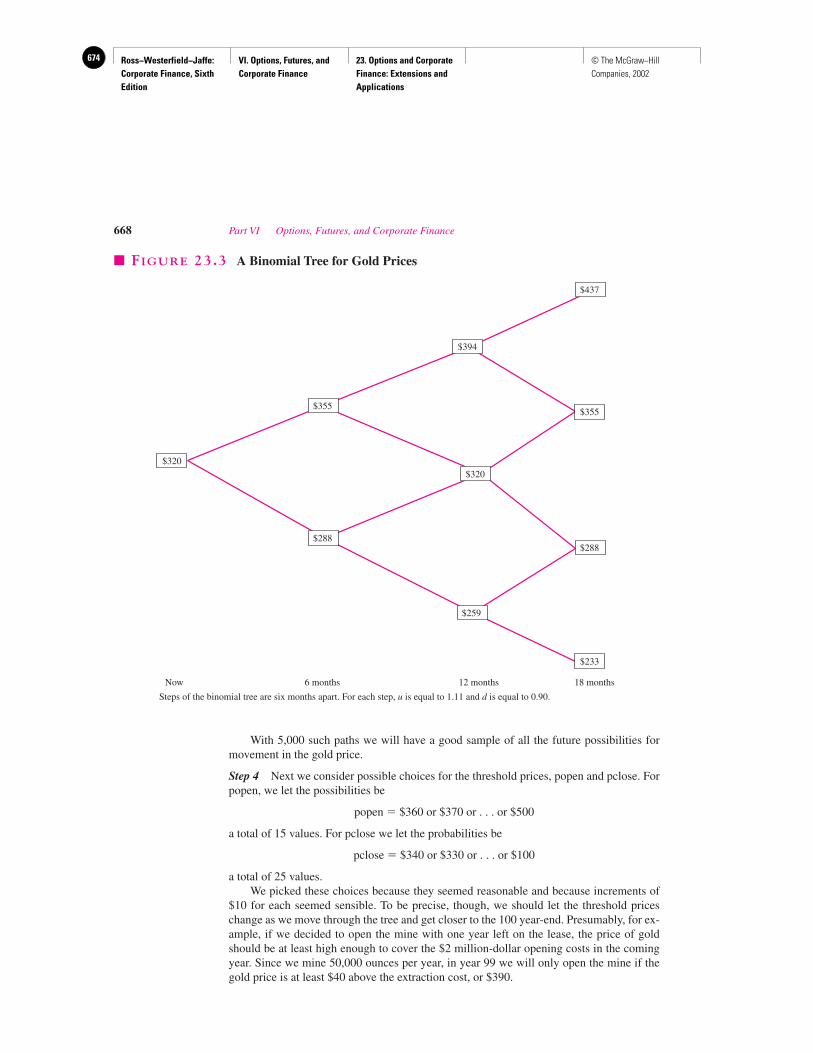
Ross−Westerfield−Jaffe: Corporate Finance, Sixth Edition
VI. Options, Futures, and Corporate Finance
23. Options and Corporate Finance: Extensions and Applications
674 © The McGraw−Hill Companies, 2002
With 5,000 such paths we will have a good sample of all the future possibilities formovement in the gold price.
Step 4 Next we consider possible choices for the threshold prices, popen and pclose. Forpopen, we let the possibilities be
popen � $360 or $370 or . . . or $500
a total of 15 values. For pclose we let the probabilities be
pclose � $340 or $330 or . . . or $100
a total of 25 values.We picked these choices because they seemed reasonable and because increments of
$10 for each seemed sensible. To be precise, though, we should let the threshold priceschange as we move through the tree and get closer to the 100 year-end. Presumably, for ex-ample, if we decided to open the mine with one year left on the lease, the price of goldshould be at least high enough to cover the $2 million-dollar opening costs in the comingyear. Since we mine 50,000 ounces per year, in year 99 we will only open the mine if thegold price is at least $40 above the extraction cost, or $390.
668 Part VI Options, Futures, and Corporate Finance
$320
$355
$288
18 months12 months6 monthsNow
$394
$259
$320
$288
$233
$355
$437
� FIGURE 23.3 A Binomial Tree for Gold Prices
Steps of the binomial tree are six months apart. For each step, u is equal to 1.11 and d is equal to 0.90.
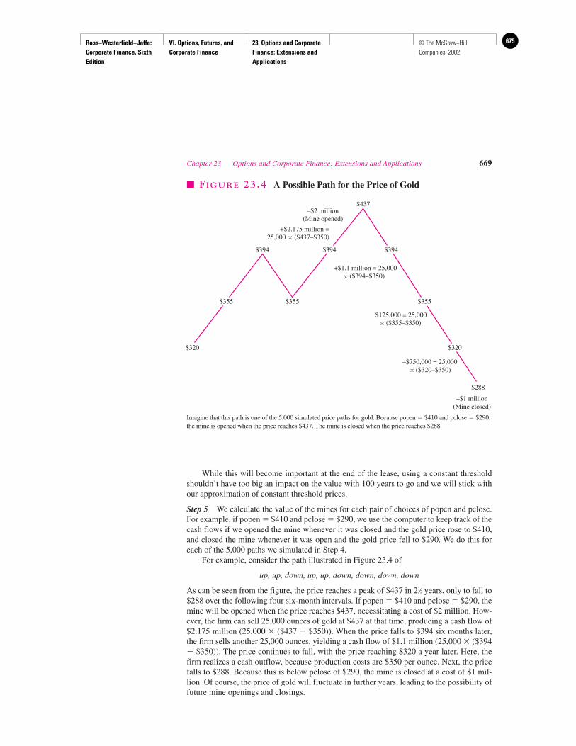
Ross−Westerfield−Jaffe: Corporate Finance, Sixth Edition
VI. Options, Futures, and Corporate Finance
23. Options and Corporate Finance: Extensions and Applications
675© The McGraw−Hill Companies, 2002
While this will become important at the end of the lease, using a constant thresholdshouldn’t have too big an impact on the value with 100 years to go and we will stick withour approximation of constant threshold prices.
Step 5 We calculate the value of the mines for each pair of choices of popen and pclose.For example, if popen � $410 and pclose � $290, we use the computer to keep track of thecash flows if we opened the mine whenever it was closed and the gold price rose to $410,and closed the mine whenever it was open and the gold price fell to $290. We do this foreach of the 5,000 paths we simulated in Step 4.
For example, consider the path illustrated in Figure 23.4 of
up, up, down, up, up, down, down, down, down
As can be seen from the figure, the price reaches a peak of $437 in 21⁄2 years, only to fall to$288 over the following four six-month intervals. If popen � $410 and pclose � $290, themine will be opened when the price reaches $437, necessitating a cost of $2 million. How-ever, the firm can sell 25,000 ounces of gold at $437 at that time, producing a cash flow of$2.175 million (25,000 � ($437 � $350)). When the price falls to $394 six months later,the firm sells another 25,000 ounces, yielding a cash flow of $1.1 million (25,000 � ($394� $350)). The price continues to fall, with the price reaching $320 a year later. Here, thefirm realizes a cash outflow, because production costs are $350 per ounce. Next, the pricefalls to $288. Because this is below pclose of $290, the mine is closed at a cost of $1 mil-lion. Of course, the price of gold will fluctuate in further years, leading to the possibility offuture mine openings and closings.
Chapter 23 Options and Corporate Finance: Extensions and Applications 669
–$2 million(Mine opened)
–$1 million(Mine closed)
–$750,000 = 25,000 ($320–$350)
$125,000 = 25,000 ($355–$350)
+$1.1 million = 25,000 ($394–$350)
+$2.175 million =25,000 ($437–$350)
$320 $320
$288
$355 $355
$394 $394
$437
$355
$394
� FIGURE 23.4 A Possible Path for the Price of Gold
Imagine that this path is one of the 5,000 simulated price paths for gold. Because popen � $410 and pclose � $290,the mine is opened when the price reaches $437. The mine is closed when the price reaches $288.
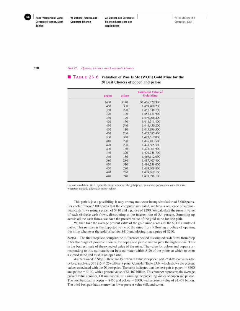
Ross−Westerfield−Jaffe: Corporate Finance, Sixth Edition
VI. Options, Futures, and Corporate Finance
23. Options and Corporate Finance: Extensions and Applications
676 © The McGraw−Hill Companies, 2002
This path is just a possibility. It may or may not occur in any simulation of 5,000 paths.For each of these 5,000 paths that the computer simulated, we have a sequence of semian-nual cash flows using a popen of $410 and a pclose of $290. We calculate the present valueof each of these cash flows, discounting at the interest rate of 3.4 percent. Summing upacross all the cash flows, we have the present value of the gold mine for one path.
We then take the average present value of the gold mine across all the 5,000 simulatedpaths. This number is the expected value of the mine from following a policy of openingthe mine whenever the gold price hits $410 and closing it at a price of $290.
Step 6 The final step is to compare the different expected discounted cash flows from Step5 for the range of possible choices for popen and pclose and to pick the highest one. Thisis the best estimate of the expected value of the mine. The value for pclose and popen cor-responding to this estimate is our best estimate (within $10) of the points at which to opena closed mine and to shut an open one.
As mentioned in Step 3, there are 15 different values for popen and 25 different values forpclose, implying 375 (15 � 25) different pairs. Consider Table 23.6, which shows the presentvalues associated with the 20 best pairs. The table indicates that the best pair is popen � $400and pclose � $140, with a present value of $1.467 billion. This number represents the averagepresent value across 5,000 simulations, all assuming the preceding values of popen and pclose.The next best pair is popen � $460 and pclose � $300, with a present value of $1.459 billion.The third best pair has a somewhat lower present value still, and so on.
670 Part VI Options, Futures, and Corporate Finance
� TABLE 23.6 Valuation of Woe Is Me (WOE) Gold Mine for the 20 Best Choices of popen and pclose
Estimated Value ofpopen pclose Gold Mine
$400 $140 $1,466,720,900460 300 1,459,406,200380 290 1,457,838,700370 100 1,455,131,900360 190 1,449,708,200420 150 1,448,711,400430 340 1,448,450,200430 110 1,445,396,500470 200 1,435,687,400500 320 1,427,512,000410 290 1,426,483,500420 290 1,423,865,300400 160 1,423,061,900360 320 1,420,748,700360 180 1,419,112,000380 280 1,417,405,400450 310 1,416,238,000450 280 1,409,709,800440 220 1,408,269,100440 240 1,403,398,100
For our simulation, WOE opens the mine whenever the gold price rises above popen and closes the minewhenever the gold price falls below pclose.
Ross−Westerfield−Jaffe: Corporate Finance, Sixth Edition
VI. Options, Futures, and Corporate Finance
23. Options and Corporate Finance: Extensions and Applications
677© The McGraw−Hill Companies, 2002
Of course, our estimate of the value of the mine is $1.467 billion, the present value ofthe best pair of choices. The market capitalization (price � number of shares outstanding)of WOE should reach this value if the market makes the same assumptions that we did. Notethat the value of the firm is quite high using an option framework. However, as stated ear-lier, WOE would appear worthless if a regular discounted cash-flow approach were used.This occurs because the initial price of gold of $320 is below the extraction cost of $350.
This example is not easy, either in terms of concepts or in terms of implementation.However, we believe that the extra work involved in mastering this example is worth it, be-cause it illustrates the type of modeling that actually occurs in corporate finance depart-ments in the real world.
Furthermore, the example illustrates the benefits of the binomial approach. One merelycalculates the cash flows associated with each of a number of simulations, discounts thecash flows from each simulation, and averages present values across the simulations.Because the Black-Scholes model is not amenable to simulations, it cannot be used for thistype of problem. In addition, there are a number of other situations where the binomialmodel is more appropriate than is the Black-Scholes model. For example, it is well knownthat the Black-Scholes model cannot properly handle options with dividend payments priorto the expiration date. This model also does not adequately handle the valuation of anAmerican put. By contrast, the binomial model can easily handle both these situations.
Thus, any student of corporate finance should be well versed with both models. TheBlack-Scholes model should be used whenever appropriate, because it is simpler to use thanis the binomial model. However, for the more complex situations where the Black-Scholesmodel breaks down, the binomial model becomes a necessary tool.
23.5 SUMMARY AND CONCLUSIONS
This chapter extends the intuitions of one of the most significant concepts in finance: optionpricing theory. We describe four different types of special options:
Executive stock options.The embedded option in a start-up company.The option in simple business contracts.The option to shut down and reopen a project.
We try to keep the presentation simple and straightforward from a mathematical point of view.We extend the binomial approach to option pricing in Chapter 22 to many periods. Thisadjustment brings us closer to the real world, because the assumption of only two prices at theend of an interval is more plausible when the interval is short.
SUGGESTED READINGS
An excellent practical treatment of real options can be found in:Amran, Martha, and Nalin Kulatilaka. Real Options. Cambridge: Harvard Business School
Press, 1999.
Chapter 23 Options and Corporate Finance: Extensions and Applications 671
Ross−Westerfield−Jaffe: Corporate Finance, Sixth Edition
VI. Options, Futures, and Corporate Finance
23. Options and Corporate Finance: Extensions and Applications
678 © The McGraw−Hill Companies, 2002
A more academic treatment can be found in:Brennan, Michael, and L. Trigeorgis, eds. Flexibility, Natural Resources, and Strategic Options.
Oxford: Oxford University Press, 1998.Copeland, Tom, and Vladimir Antikarov. Real Options: A Practitioner’s Guide. Texere LLC, 2001.
QUESTIONS AND PROBLEMS
Executive Stock Options23.1 William Hurt is the Chief Executive Officer of the First Pacific Trading Company (FPTC).
His annual straight salary is $1 million.The current value of FPTC stock is $50 per share. Mr. Hurt has just been granted
options on $1 million in shares of FPTC stock at the money by FPTC’s board of directors.The risk-free rate is 6 percent. The options have a maturity of four years. The volatility ofFPTC stock has been about 25 percent on an annual basis. Determine the value of Mr.Hurt’s stock options.
23.2 Mr. Hurt has been quoted as saying that he doesn’t want stock options. He has said hewould be satisfied with straight pay of $1.25 million. The board of directors disagrees.Who is right?
Flexible Production23.3 The market for golf putters is notoriously fickle. One year mallet head putters can be the
hottest seller and the next it can be blade putters that are in demand. Tims Golf Company(TGC) has a difficult decision to make. It can build a flexible plant that can produce eitherblade or mallet head putters. The plant would have a capacity of 150,000 putters a year andcould produce either type but not both at the same time. In fact, it could be switched onlyonce, one year from now, and the lifetime of the plant is ten years. Currently, there is a highdemand for blade putters and TGC forecasts it will need to produce 150,000 for the nextyear. One year from now there is a 50-50 chance that the company will need to producemallet head putters rather than blade putters. The company can also build a plant that couldonly produce blade putters. Both plants would have the same capacity. The profit for theflexible plant is $10 per blade putter and $15 per mallet putter. A fixed putter plant couldproduce only blade putters but could do so more efficiently. The profit from having a fixedplant produce blade putters is $20 per unit. The relevant discount rate is 12 percent.
In one year, it will be known if the demand for blade putters will continue for ninemore years or it will drop by 50 percent.
The company has a choice. It can either invest $1 million in a fixed plant that willproduce blade putters only or it can invest $1.5 million in a flexible plant capable ofswitching from blades to mallets. What should TGC’s decision be?
Waiting to Invest23.4 John Lusk is a real estate developer who owns the right to put up an office building on a
parcel of land in downtown Los Angeles. The office building will cost $50 million. JohnLusk does not actually plan to own and run the office building but instead he will build it,rent it, and then sell it to a long-term investor at the end of one year. John Lusk estimatesthat the building can be sold one year from now for $55 million. The IRR of the project is10 percent and so John Lusk has determined that this is a zero NPV project. However, oneyear from now there is a 50-50 chance that the cost of capital will be either 11 percent or 9percent. John Lusk has received an offer on his option for $500. Should he take it?
672 Part VI Options, Futures, and Corporate Finance

Ross−Westerfield−Jaffe: Corporate Finance, Sixth Edition
VI. Options, Futures, and Corporate Finance
23. Options and Corporate Finance: Extensions and Applications
679© The McGraw−Hill Companies, 2002
The Option to Shut Down or Reopen a Project23.5 We are examining a new project. We expect to sell 10,000 units a year of a new golf video
at $200 net cash flow each for the next five years. The relevant discount is 15 percent andthe initial required investment is $7 million.a. What is the base case NPV?b. After the first year, the golf video project can be abandoned and the machinery sold for
$100,000. At what level of sales would it make sense to abandon the project?
23.6 Suppose in the previous problem, you think it is likely that expected sales will be revisedupward to 15,000 units if the first year is a success and downward to zero units if the firstyear is a failure. Success or failure are equally likely. What is the NPV of the project?
Chapter 23 Options and Corporate Finance: Extensions and Applications 673

Ross−Westerfield−Jaffe: Corporate Finance, Sixth Edition
VI. Options, Futures, and Corporate Finance
24. Warrants and Convertibles
680 © The McGraw−Hill Companies, 2002
Warrants andConvertibles
CH
AP
TE
R24
EXECUTIVE SUMMARY
We study two financing instruments in this chapter, warrants and convertibles. Awarrant gives the holder the right to buy common stock for cash. In this sense, itis very much like a call. Warrants are generally issued with privately placed
bonds, though they are also combined with new issues of common stock and preferredstock. In the case of new issues of common stock, warrants are sometimes given to invest-ment bankers as compensation for underwriting services.
A convertible bond gives the holder the right to exchange the bond for common stock.Therefore, it is a mixed security blurring the traditional line between stocks and bonds.There is also convertible preferred stock.
The chapter describes the basic features of warrants and convertibles. Here are someof the most important questions concerning warrants and convertibles:
1. How can warrants and convertibles be valued?
2. What impact do warrants and convertibles have on the value of the firm?
3. What are the differences between warrants, convertibles, and call options?
4. Why do some companies issue bonds with warrants and convertible bonds?
5. Under what circumstances are warrants and convertibles converted into common stock?
24.1 WARRANTS
Warrants are securities that give holders the right, but not the obligation, to buy shares ofcommon stock directly from a company at a fixed price for a given period of time. Eachwarrant specifies the number of shares of stock that the holder can buy, the exercise price,and the expiration date.
From the preceding description of warrants, it is clear that they are similar to call op-tions. The differences in contractual features between warrants and the call options that tradeon the Chicago Board Options Exchange are small. For example, warrants have longer ma-turity periods.1 Some warrants are actually perpetual, meaning that they never expire at all.
Warrants are referred to as equity kickers because they are usually issued in combina-tion with privately placed bonds.2 In most cases, warrants are attached to the bonds when is-sued. The loan agreement will state whether the warrants are detachable from the bond, thatis, whether they can be sold separately. Usually the warrant can be detached immediately.
1Warrants are usually protected against stock splits and dividends in the same way that call options are.2Warrants are also issued with publicly distributed bonds and new issues of common stock.

Ross−Westerfield−Jaffe: Corporate Finance, Sixth Edition
VI. Options, Futures, and Corporate Finance
24. Warrants and Convertibles
681© The McGraw−Hill Companies, 2002
EXAMPLE
Safeway, Inc., is one of the nation’s largest supermarket chains. On November 24,1986, Safeway was acquired in a levered buyout by the private investment firmKohlberg Kravis Roberts and Co. (KKR). Each share of old common stock wasconverted into a junior subordinated debenture (i.e., junk bond) and a “merger”warrant. Each warrant gave the holder the right to purchase .279 shares of new com-mon stock for $1.052 per warrant. To purchase one share of common stock, a holderhad to give up 3.584 warrants and pay an amount of $3.7691 per warrant. This madethe exercise price of the Safeway warrants equal to $13.5085 (3.584 � $3.7691 �$13.5085). The warrants expired on November 24, 1996. They are called mergerwarrants because Safeway issued the warrants in a buyout of old shares.
When Safeway was acquired by KKR, it was a private firm with no publiclytraded common stock or warrants. However, KKR took Safeway public on April 26,1990, by issuing 10 million shares in a new issue of common stock. The stock waslisted on the New York Stock Exchange. On that day, several thousand warrants weretraded at a closing price of 31⁄8. The price of the Safeway common stock was 121⁄8.
The relationship between the value of Safeway’s warrants and its stock price can beviewed like the relationship between a call option and its stock price, described in a previ-ous chapter. Figure 24.1 depicts the relationship for Safeway warrants. The lower limit onthe value of the warrants is zero if Safeway’s stock price is below $13.5085 per share. If theprice of Safeway’s common stock rises above $13.5085 per share, the lower limit is thestock price minus $13.5085 divided by 3.584.3 The upper limit is the price of Safeway’scommon stock divided by 3.584. A warrant to buy one share of common stock cannot sellat a price above the price of the underlying common stock.
The price of Safeway warrants on April 26, 1990, was higher than the lower limit. Theheight of the warrant price above the lower limit will depend on the following:
1. The variance of Safeway’s stock returns.
2. The time to expiration date.
Chapter 24 Warrants and Convertibles 675
Value ofwarrant
Value of a shareof common stock
Upper limiton warrant value
Actual warrantvalue curve
Lower limiton warrant value
Actual stockprice = $12 1
–8
Exerciseprice = $13.5085
Price ofwarrant = $3 1
–
8
� FIGURE 24.1 Safeway Warrants on April 26, 1990
3We need to divide by 3.584 because it takes 3.584 warrants to purchase one share of stock.
Ross−Westerfield−Jaffe: Corporate Finance, Sixth Edition
VI. Options, Futures, and Corporate Finance
24. Warrants and Convertibles
682 © The McGraw−Hill Companies, 2002
3. The risk-free rate of interest.
4. The stock price of Safeway.
5. The exercise price.
These are the same factors that determine the value of a call option.
24.2 THE DIFFERENCE BETWEEN WARRANTS
AND CALL OPTIONS
From the holder’s point of view, warrants are similar to call options on common stock. Awarrant, like a call option, gives its holder the right to buy common stock at a specifiedprice. Warrants usually have an expiration date, though in most cases they are issued withlonger lives than call options. From the firm’s point of view, however, a warrant is very dif-ferent from a call option on the company’s common stock.
The most important difference between call options and warrants is that call optionsare issued by individuals and warrants are issued by firms. When a warrant is exercised, afirm must issue new shares of stock. Each time a warrant is exercised, then, the number ofshares outstanding increases.
To illustrate, suppose the Endrun Company issues a warrant giving holders the right tobuy one share of common stock at $25. Further suppose the warrant is exercised. Endrunmust print one new stock certificate. In exchange for the stock certificate, it receives $25from the holder.
In contrast, when a call option is exercised, there is no change in the number of sharesoutstanding. Suppose Ms. Eager holds a call option on the common stock of the EndrunCompany. The call option gives Ms. Eager the right to buy one share of the common stockof the Endrun Company for $25. If Ms. Eager chooses to exercise the call option, a seller,say Mr. Swift, is obligated to give her one share of Endrun’s common stock in exchange for$25. If Mr. Swift does not already own a share, he must enter the stock market and buy one.The call option is a side bet between buyers and sellers on the value of the EndrunCompany’s common stock. When a call option is exercised, one investor gains and the otherloses. The total number of shares outstanding of the Endrun Company remains constant,and no new funds are made available to the company.
EXAMPLE
To see how warrants affect the value of the firm, imagine that Mr. Gould and Ms.Rockefeller are two investors who have together purchased six ounces of plat-inum. At the time they bought the platinum, Mr. Gould and Ms. Rockefeller eachcontributed one-half of the cost, which we will assume was $3,000 for six ounces,or $500 an ounce (they each contributed $1,500). They incorporated, printed twostock certificates, and named the firm the GR Company. Each certificate repre-sents a one-half claim to the platinum. Mr. Gould and Ms. Rockefeller each ownone certificate. Mr. Gould and Ms. Rockefeller have formed a company with plat-inum as its only asset.
A Call Is Issued Suppose Mr. Gould later decides to sell to Mrs. Fiske a call op-tion issued on Mr. Gould’s share. The call option gives Mrs. Fiske the right to buyMr. Gould’s share for $1,800 within the next year. If the price of platinum rises
676 Part VI Options, Futures, and Corporate Finance
Ross−Westerfield−Jaffe: Corporate Finance, Sixth Edition
VI. Options, Futures, and Corporate Finance
24. Warrants and Convertibles
683© The McGraw−Hill Companies, 2002
above $600 per ounce, the firm will be worth more than $3,600 and each share willbe worth more than $1,800. If Mrs. Fiske decides to exercise her option, Mr. Gouldmust turn over his stock certificate and receive $1,800.
How would the firm be affected by the exercise? The number of shares will re-main the same. There will still be two shares, now owned by Ms. Rockefeller and Mrs.Fiske. If the price of platinum rises to $700 an ounce, each share will be worth $2,100($4,200/2). If Mrs. Fiske exercises her option at this price, she will profit by $300.
A Warrant Is Issued Instead This story changes if a warrant is issued. Supposethat Mr. Gould does not sell a call option to Mrs. Fiske. Instead, Mr. Gould and Ms.Rockefeller have a stockholders’ meeting. They vote that GR Company will issue awarrant and sell it to Mrs. Fiske. The warrant will give Mrs. Fiske the right to receivea share of the company at an exercise price of $1,800.4 If Mrs. Fiske decides to ex-ercise the warrant, the firm will issue another stock certificate and give it to Mrs.Fiske in exchange for $1,800.
From Mrs. Fiske’s perspective, the call option and the warrant seem to be thesame. The exercise prices of the warrant and the call are the same: $1,800. It is stilladvantageous for Mrs. Fiske to exercise the option when the price of platinum ex-ceeds $600 per ounce. However, we will show that Mrs. Fiske actually makes lessin the warrant situation due to dilution.
The GR Company must also consider dilution. Suppose the price of plat-inum increases to $700 an ounce and Mrs. Fiske exercises her warrant. Twothings will occur:
1. Mrs. Fiske will pay $1,800 to the firm.
2. The firm will print one stock certificate and give it to Mrs. Fiske. The stock cer-tificate will represent a one-third claim on the platinum of the firm.
Because Mrs. Fiske contributes $1,800 to the firm, the value of the firm increases.It is now worth
New value of firm � Value of platinum � Contribution to the firm by Mrs. Fiske� $4,200 � $1,800� $6,000
Because Mrs. Fiske has a one-third claim on the firm’s value, her share isworth $2,000 ($6,000/3). By exercising the warrant, Mrs. Fiske gains $2,000 �$1,800 � $200. This is illustrated in Table 24.1.
Dilution Why does Mrs. Fiske only gain $200 in the warrant case while gaining$300 in the call option case? The key is dilution, that is, the creation of anothershare. In the call option case, she contributes $1,800 and receives one of the twooutstanding shares. That is, she receives a share worth $2,100 (1⁄2 � $4,200). Hergain is $300 ($2,100 � $1,800). We rewrite this gain as
Gain on Exercise of Call:
(24.1)$4,200
2� $1,800 � $300
Chapter 24 Warrants and Convertibles 677
4The sale of the warrant brings cash into the firm. We assume that the sale proceeds immediately leave the firmthrough a cash dividend to Mr. Gould and Ms. Rockefeller. This simplifies the analysis, because the firm withwarrants then has the same total value as the firm without warrants.
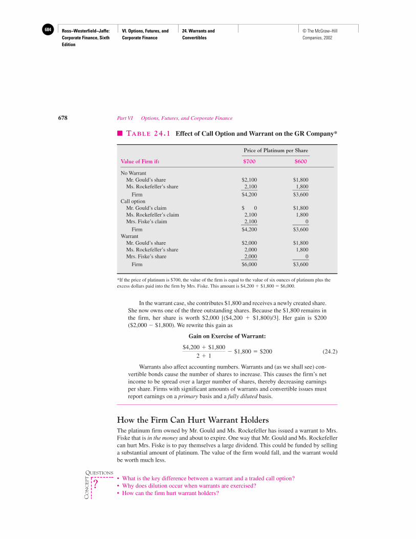
Ross−Westerfield−Jaffe: Corporate Finance, Sixth Edition
VI. Options, Futures, and Corporate Finance
24. Warrants and Convertibles
684 © The McGraw−Hill Companies, 2002
In the warrant case, she contributes $1,800 and receives a newly created share.She now owns one of the three outstanding shares. Because the $1,800 remains inthe firm, her share is worth $2,000 [($4,200 � $1,800)/3]. Her gain is $200($2,000 � $1,800). We rewrite this gain as
Gain on Exercise of Warrant:
(24.2)
Warrants also affect accounting numbers. Warrants and (as we shall see) con-vertible bonds cause the number of shares to increase. This causes the firm’s netincome to be spread over a larger number of shares, thereby decreasing earningsper share. Firms with significant amounts of warrants and convertible issues mustreport earnings on a primary basis and a fully diluted basis.
How the Firm Can Hurt Warrant HoldersThe platinum firm owned by Mr. Gould and Ms. Rockefeller has issued a warrant to Mrs.Fiske that is in the money and about to expire. One way that Mr. Gould and Ms. Rockefellercan hurt Mrs. Fiske is to pay themselves a large dividend. This could be funded by sellinga substantial amount of platinum. The value of the firm would fall, and the warrant wouldbe worth much less.
• What is the key difference between a warrant and a traded call option?• Why does dilution occur when warrants are exercised?• How can the firm hurt warrant holders?
$4,200 � $1,800
2 � 1� $1,800 � $200
678 Part VI Options, Futures, and Corporate Finance
� TABLE 24.1 Effect of Call Option and Warrant on the GR Company*
Price of Platinum per Share
Value of Firm if: $700 $600
No WarrantMr. Gould’s share $2,100 $1,800Ms. Rockefeller’s share 2,100 1,800______ ______
Firm $4,200 $3,600Call option
Mr. Gould’s claim $ 0 $1,800Ms. Rockefeller’s claim 2,100 1,800Mrs. Fiske’s claim 2,100 0______ ______
Firm $4,200 $3,600Warrant
Mr. Gould’s share $2,000 $1,800Ms. Rockefeller’s share 2,000 1,800Mrs. Fiske’s share 2,000 0______ ______
Firm $6,000 $3,600
*If the price of platinum is $700, the value of the firm is equal to the value of six ounces of platinum plus theexcess dollars paid into the firm by Mrs. Fiske. This amount is $4,200 � $1,800 � $6,000.
QUESTIONS
CO
NC
EP
T
?
Ross−Westerfield−Jaffe: Corporate Finance, Sixth Edition
VI. Options, Futures, and Corporate Finance
24. Warrants and Convertibles
685© The McGraw−Hill Companies, 2002
24.3 WARRANT PRICING AND THE BLACK-SCHOLES
MODEL (ADVANCED)
We now wish to express the gains from exercising a call and a warrant in more generalterms. The gain on a call can be written as
Gain from Exercising a Single Call:
(24.3)
(Value of a share of stock)
Equation (24.3) generalizes equation (24.1). We define the firm’s value net of debt tobe the total firm value less the value of the debt. The total firm value is $4,200 in our ex-ample and there is no debt. The # stands for the number of shares outstanding, which is 2in our example. The ratio on the left is the value of a share of stock. The gain on a warrantcan be written as
Gain from Exercising a Single Warrant:
(24.4)
(Value of a share of stock after warrant is exercised)
Equation (24.4) generalizes (24.2). The numerator of the left-hand term is the firm’s valuenet of debt after the warrant is exercised. It is the sum of the firm’s value net of debt priorto the warrant’s exercise plus the proceeds the firm receives from the exercise. The proceedsequal the product of the exercise price multiplied by the number of warrants. The numberof warrants appears as #w. (Our analysis uses the plausible assumption that all warrants inthe money will be exercised.) Note that #w � 1 in our numerical example. The denomina-tor, # � #w, is the number of shares outstanding after the exercise of the warrants. The ra-tio on the left is the value of a share of stock after exercise. By rearranging terms, equation(24.4) can be rewritten as5
Gain from Exercising a Single Warrant:
(24.5)
(Gain from a call on a firm with no warrants)
Formula (24.5) relates the gain on a warrant to the gain on a call. Note that the term withinparentheses is (24.3). Thus, the gain from exercising a warrant is a proportion of the gainfrom exercising a call in a firm without warrants. The proportion #/(# � #w) is the ratio ofthe number of shares in the firm without warrants to the number of shares after all the war-rants have been exercised. This ratio must always be less than 1. Thus, the gain on a war-rant must be less than the gain on an identical call in a firm without warrants. Note that #/(#� #w) � 2⁄3 in our example, which explains why Mrs. Fiske gains $300 on her call yet gainsonly $200 on her warrant.
#
# � #w
� �Firm,s value net of debt
#� Exercise price�
Firm,s value net of debt � Exercise price � #w
# � #w
� Exercise price
Firm,s value net of debt
#� Exercise price
Chapter 24 Warrants and Convertibles 679
5To derive formula (24.5), one should separate “Exercise price” in (24.4). This yields
By rearranging terms, one can obtain formula (24.5).
Firm,s value net of debt
# � #w
�#
# � #w
� Exercise price
Ross−Westerfield−Jaffe: Corporate Finance, Sixth Edition
VI. Options, Futures, and Corporate Finance
24. Warrants and Convertibles
686 © The McGraw−Hill Companies, 2002
The preceding implies that the Black-Scholes model must be adjusted for warrants.When a call option is issued to Mrs. Fiske, we know that the exercise price is $1,800 andthe time to expiration is one year. Though we have posited neither the price of the stock, thevariance of the stock, nor the interest rate, we could easily provide these data for a real-world situation. Thus, we could use the Black-Scholes model to value Mrs. Fiske’s call.
Suppose that the warrant is to be issued tomorrow to Mrs. Fiske. We know the numberof warrants to be issued, the warrant’s expiration date, and the exercise price. Using our as-sumption that the warrant proceeds are immediately paid out as a dividend, we could usethe Black-Scholes model to value the warrant. We would first calculate the value of an iden-tical call. The warrant price is the call price multiplied by the ratio #/(# � #w). As mentionedearlier, this ratio is 2⁄3 in our example.
24.4 CONVERTIBLE BONDS
A convertible bond is similar to a bond with warrants. The most important difference isthat a bond with warrants can be separated into distinct securities and a convertible bondcannot. A convertible bond gives the holder the right to exchange it for a given number ofshares of stock anytime up to and including the maturity date of the bond.
Preferred stock can frequently be converted into common stock. A convertible pre-ferred stock is the same as a convertible bond except that it has an infinite maturity date.
EXAMPLE
Seagate Technology is one of the most important manufacturers of rigid magneticdisk drives for computers. Its stock is traded on the New York Stock Exchange.
On November 1, 1993, Seagate raised $300 million by issuing 6.75 percentconvertible subordinated debentures due in 2012. It planned to use the proceeds toinvest in new plant and equipment. Like typical debentures, they had a sinkingfund and were callable. Seagate’s bonds differed from other debentures in theirconvertible feature: Each bond was convertible into 23.53 shares of common stockof Seagate anytime before maturity. The number of shares received for each bond(23.53 in this example) is called the conversion ratio.
Bond traders also speak of the conversion price of the bond. This is cal-culated as the ratio of the face value of the bond to the conversion ratio. Be-cause the face value of each Seagate bond was $1,000, the conversion price was$42.5 ($1,000/23.53). The bondholders of Seagate could give up bonds with aface value of $1,000 and receive 23.53 shares of Seagate common stock. Thiswas equivalent to paying $42.5 ($1,000/23.53) for each share of Seagate com-mon stock received.
When Seagate issued its convertible bonds, its common stock was tradingat $22.625 per share. The conversion price of $42.5 was 88 percent higher thanthe actual common stock price. This 88 percent is referred to as the conversionpremium. It reflects the fact that the conversion option in Seagate convertiblebonds was out of the money. This conversion premium is typical.
Convertibles are almost always protected against stock splits and stock divi-dends. If Seagate’s common stock had been split two for one, the conversion ratiowould have been increased from 23.53 to 47.06.
680 Part VI Options, Futures, and Corporate Finance
Ross−Westerfield−Jaffe: Corporate Finance, Sixth Edition
VI. Options, Futures, and Corporate Finance
24. Warrants and Convertibles
687© The McGraw−Hill Companies, 2002
Conversion ratio, conversion price, and conversion premium are well-known terms inthe real world. For that reason alone, the student should master the concepts. However, con-version price and conversion premium implicitly assume that the bond is selling at par. Ifthe bond is selling at another price, the terms have little meaning. By contrast, conversionratio can have a meaningful interpretation regardless of the price of the bond.
• What are the conversion ratio, the conversion price, and the conversion premium?
24.5 THE VALUE OF CONVERTIBLE BONDS
The value of a convertible bond can be described in terms of three components: straight bondvalue, conversion value, and option value.6 We examine these three components below.
Straight Bond ValueThe straight bond value is what the convertible bonds would sell for if they could not beconverted into common stock. It will depend on the general level of interest rates and on thedefault risk. Suppose that straight debentures issued by Seagate had been rated A, and A-rated bonds were priced to yield 4 percent on November 1, 1995. The straight bond valueof Seagate convertible bonds can be determined by discounting the $33.75 semiannualcoupon payment and principal amount at 4 percent.7
� $646.06 � $234.3� $880.36
The straight bond value of a convertible bond is a minimum value. The price of Seagate’sconvertible could not have gone lower than the straight bond value.
Figure 24.2 illustrates the relationship between straight bond value and stock price. InFigure 24.2 we have been somewhat dramatic and implicitly assumed that the convertiblebond is default free. In this case the straight bond value does not depend on the stock priceand so it is graphed as a straight line.
Conversion ValueThe value of convertible bonds depends on conversion value. Conversion value is what thebonds would be worth if they were immediately converted into the common stock at currentprices. Typically, conversion value is computed by multiplying the number of shares of commonstock that will be received when the bond is converted by the current price of the common stock.
� $33.75 � A
370.04 �
$1,000�1.04� 37
Straight bond � 37
t �1
$33.75
1.04t �$1,000�1.04� 37
Chapter 24 Warrants and Convertibles 681
QUESTION
CO
NC
EP
T
?
6For a similar treatment see Richard Brealey and Stewart Myers, Principles of Corporate Finance, 2nd ed. (NewYork: McGraw-Hill, 1984), Chapter 23; and James C. Van Horne, Financial Markets and Flows, 2nd ed.(Englewood Cliffs, N.J.: Prentice Hall, 1987) Chapter 11.7This formula assumes that coupons are paid annually.
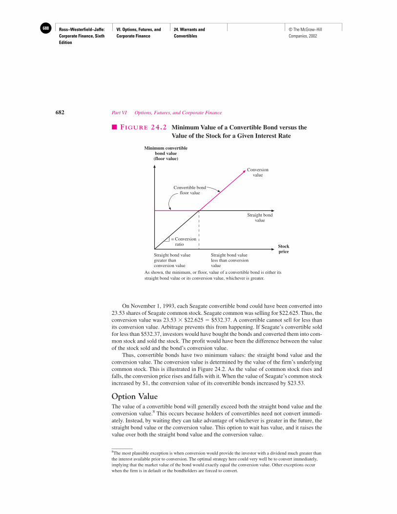
Ross−Westerfield−Jaffe: Corporate Finance, Sixth Edition
VI. Options, Futures, and Corporate Finance
24. Warrants and Convertibles
688 © The McGraw−Hill Companies, 2002
On November 1, 1993, each Seagate convertible bond could have been converted into23.53 shares of Seagate common stock. Seagate common was selling for $22.625. Thus, theconversion value was 23.53 � $22.625 � $532.37. A convertible cannot sell for less thanits conversion value. Arbitrage prevents this from happening. If Seagate’s convertible soldfor less than $532.37, investors would have bought the bonds and converted them into com-mon stock and sold the stock. The profit would have been the difference between the valueof the stock sold and the bond’s conversion value.
Thus, convertible bonds have two minimum values: the straight bond value and theconversion value. The conversion value is determined by the value of the firm’s underlyingcommon stock. This is illustrated in Figure 24.2. As the value of common stock rises andfalls, the conversion price rises and falls with it. When the value of Seagate’s common stockincreased by $1, the conversion value of its convertible bonds increased by $23.53.
Option ValueThe value of a convertible bond will generally exceed both the straight bond value and theconversion value.8 This occurs because holders of convertibles need not convert immedi-ately. Instead, by waiting they can take advantage of whichever is greater in the future, thestraight bond value or the conversion value. This option to wait has value, and it raises thevalue over both the straight bond value and the conversion value.
682 Part VI Options, Futures, and Corporate Finance
Minimum convertiblebond value
(floor value)
Stockprice
Conversionvalue
Straight bondvalue
Convertible bondfloor value
= Conversion ratio
Straight bond valuegreater thanconversion value
Straight bond valueless than conversionvalue
� FIGURE 24.2 Minimum Value of a Convertible Bond versus theValue of the Stock for a Given Interest Rate
As shown, the minimum, or floor, value of a convertible bond is either itsstraight bond value or its conversion value, whichever is greater.
8The most plausible exception is when conversion would provide the investor with a dividend much greater thanthe interest available prior to conversion. The optimal strategy here could very well be to convert immediately,implying that the market value of the bond would exactly equal the conversion value. Other exceptions occurwhen the firm is in default or the bondholders are forced to convert.
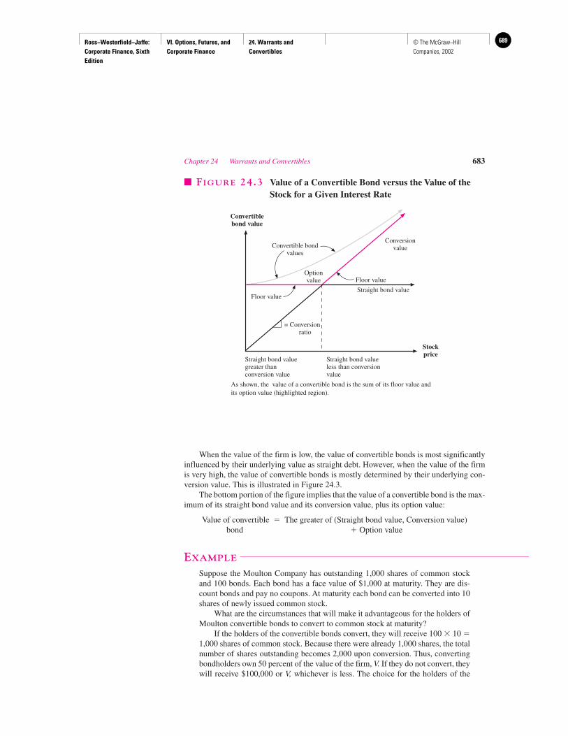
Ross−Westerfield−Jaffe: Corporate Finance, Sixth Edition
VI. Options, Futures, and Corporate Finance
24. Warrants and Convertibles
689© The McGraw−Hill Companies, 2002
When the value of the firm is low, the value of convertible bonds is most significantlyinfluenced by their underlying value as straight debt. However, when the value of the firmis very high, the value of convertible bonds is mostly determined by their underlying con-version value. This is illustrated in Figure 24.3.
The bottom portion of the figure implies that the value of a convertible bond is the max-imum of its straight bond value and its conversion value, plus its option value:
Value of convertible � The greater of (Straight bond value, Conversion value)bond � Option value
EXAMPLE
Suppose the Moulton Company has outstanding 1,000 shares of common stockand 100 bonds. Each bond has a face value of $1,000 at maturity. They are dis-count bonds and pay no coupons. At maturity each bond can be converted into 10shares of newly issued common stock.
What are the circumstances that will make it advantageous for the holders ofMoulton convertible bonds to convert to common stock at maturity?
If the holders of the convertible bonds convert, they will receive 100 � 10 �1,000 shares of common stock. Because there were already 1,000 shares, the totalnumber of shares outstanding becomes 2,000 upon conversion. Thus, convertingbondholders own 50 percent of the value of the firm, V. If they do not convert, theywill receive $100,000 or V, whichever is less. The choice for the holders of the
Chapter 24 Warrants and Convertibles 683
Convertiblebond value
Stockprice
Conversionvalue
Straight bond value
Convertible bondvalues
= Conversion ratio
Straight bond valuegreater thanconversion value
Straight bond valueless than conversionvalue
Floor value
Floor valueOptionvalue
� FIGURE 24.3 Value of a Convertible Bond versus the Value of theStock for a Given Interest Rate
As shown, the value of a convertible bond is the sum of its floor value andits option value (highlighted region).
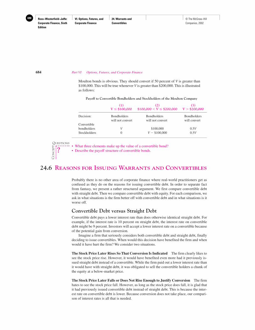
Ross−Westerfield−Jaffe: Corporate Finance, Sixth Edition
VI. Options, Futures, and Corporate Finance
24. Warrants and Convertibles
690 © The McGraw−Hill Companies, 2002
Moulton bonds is obvious. They should convert if 50 percent of V is greater than$100,000. This will be true whenever V is greater than $200,000. This is illustratedas follows:
Payoff to Convertible Bondholders and Stockholders of the Moulton Company
(1) (2) (3)V � $100,000 $100,000 V � $200,000 V � $200,000
Decision: Bondholders Bondholders Bondholderswill not convert will not convert will convert
Convertiblebondholders V $100,000 0.5VStockholders 0 V � $100,000 0.5V
• What three elements make up the value of a convertible bond?• Describe the payoff structure of convertible bonds.
24.6 REASONS FOR ISSUING WARRANTS AND CONVERTIBLES
Probably there is no other area of corporate finance where real-world practitioners get asconfused as they do on the reasons for issuing convertible debt. In order to separate factfrom fantasy, we present a rather structured argument. We first compare convertible debtwith straight debt. Then we compare convertible debt with equity. For each comparison, weask in what situations is the firm better off with convertible debt and in what situations is itworse off.
Convertible Debt versus Straight DebtConvertible debt pays a lower interest rate than does otherwise identical straight debt. Forexample, if the interest rate is 10 percent on straight debt, the interest rate on convertibledebt might be 9 percent. Investors will accept a lower interest rate on a convertible becauseof the potential gain from conversion.
Imagine a firm that seriously considers both convertible debt and straight debt, finallydeciding to issue convertibles. When would this decision have benefited the firm and whenwould it have hurt the firm? We consider two situations.
The Stock Price Later Rises So That Conversion Is Indicated The firm clearly likes tosee the stock price rise. However, it would have benefited even more had it previously is-sued straight debt instead of a convertible. While the firm paid out a lower interest rate thanit would have with straight debt, it was obligated to sell the convertible holders a chunk ofthe equity at a below-market price.
The Stock Price Later Falls or Does Not Rise Enough to Justify Conversion The firmhates to see the stock price fall. However, as long as the stock price does fall, it is glad thatit had previously issued convertible debt instead of straight debt. This is because the inter-est rate on convertible debt is lower. Because conversion does not take place, our compari-son of interest rates is all that is needed.
684 Part VI Options, Futures, and Corporate Finance
QUESTIONS
CO
NC
EP
T
?
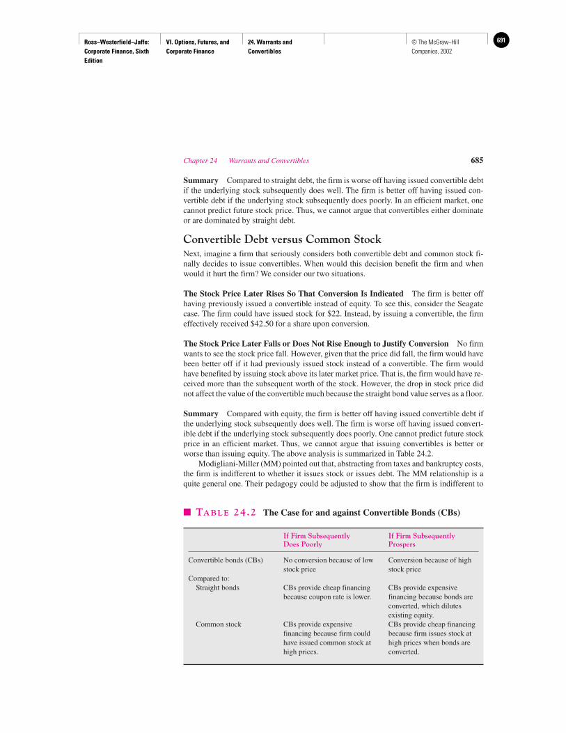
Ross−Westerfield−Jaffe: Corporate Finance, Sixth Edition
VI. Options, Futures, and Corporate Finance
24. Warrants and Convertibles
691© The McGraw−Hill Companies, 2002
Summary Compared to straight debt, the firm is worse off having issued convertible debtif the underlying stock subsequently does well. The firm is better off having issued con-vertible debt if the underlying stock subsequently does poorly. In an efficient market, onecannot predict future stock price. Thus, we cannot argue that convertibles either dominateor are dominated by straight debt.
Convertible Debt versus Common StockNext, imagine a firm that seriously considers both convertible debt and common stock fi-nally decides to issue convertibles. When would this decision benefit the firm and whenwould it hurt the firm? We consider our two situations.
The Stock Price Later Rises So That Conversion Is Indicated The firm is better offhaving previously issued a convertible instead of equity. To see this, consider the Seagatecase. The firm could have issued stock for $22. Instead, by issuing a convertible, the firmeffectively received $42.50 for a share upon conversion.
The Stock Price Later Falls or Does Not Rise Enough to Justify Conversion No firmwants to see the stock price fall. However, given that the price did fall, the firm would havebeen better off if it had previously issued stock instead of a convertible. The firm wouldhave benefited by issuing stock above its later market price. That is, the firm would have re-ceived more than the subsequent worth of the stock. However, the drop in stock price didnot affect the value of the convertible much because the straight bond value serves as a floor.
Summary Compared with equity, the firm is better off having issued convertible debt ifthe underlying stock subsequently does well. The firm is worse off having issued convert-ible debt if the underlying stock subsequently does poorly. One cannot predict future stockprice in an efficient market. Thus, we cannot argue that issuing convertibles is better orworse than issuing equity. The above analysis is summarized in Table 24.2.
Modigliani-Miller (MM) pointed out that, abstracting from taxes and bankruptcy costs,the firm is indifferent to whether it issues stock or issues debt. The MM relationship is aquite general one. Their pedagogy could be adjusted to show that the firm is indifferent to
Chapter 24 Warrants and Convertibles 685
� TABLE 24.2 The Case for and against Convertible Bonds (CBs)
If Firm Subsequently If Firm SubsequentlyDoes Poorly Prospers
Convertible bonds (CBs) No conversion because of low Conversion because of high stock price stock price
Compared to:Straight bonds CBs provide cheap financing CBs provide expensive
because coupon rate is lower. financing because bonds are converted, which dilutesexisting equity.
Common stock CBs provide expensive CBs provide cheap financing financing because firm could because firm issues stock at have issued common stock at high prices when bonds are high prices. converted.
Ross−Westerfield−Jaffe: Corporate Finance, Sixth Edition
VI. Options, Futures, and Corporate Finance
24. Warrants and Convertibles
692 © The McGraw−Hill Companies, 2002
whether it issues convertibles or issues other instruments. To save space (and the patienceof students), we have omitted a full-blown proof of MM in a world with convertibles.However, the above results are perfectly consistent with MM. Now we turn to the real-worldview of convertibles.
The “Free Lunch” StoryThe preceding discussion suggests that issuing a convertible bond is no better and no worsethan issuing other instruments. Unfortunately, many corporate executives fall into the trapof arguing that issuing convertible debt is actually better than issuing alternative instru-ments. This is a free lunch type of explanation, of which we are quite critical.
EXAMPLE
The stock price of RW Company is $20. Suppose this company can issue subor-dinated debentures at 10 percent. It can also issue convertible bonds at 6 percentwith a conversion value of $800. The conversion value means that the holders canconvert a convertible bond into 40 ($800/$20) shares of common stock.
A company treasurer who believes in free lunches might argue that convert-ible bonds should be issued because they represent a cheaper source of financingthan either subordinated bonds or common stock. The treasurer will point out thatif the company does poorly and the price does not rise above $20, the convertiblebondholders will not convert the bonds into common stock. In this case, the com-pany will have obtained debt financing at below-market rates by attaching worth-less equity kickers. On the other hand, if the firm does well and the price of itscommon stock rises to $25 or above, convertible holders will convert. The com-pany will issue 40 shares. The company will receive a bond with face value of$1,000 in exchange for issuing 40 shares of common stock, implying a conversionprice of $25. The company will have issued common stock de facto at $25 pershare, or 20 percent above the $20 common-stock price prevailing when the con-vertible bonds were issued. This enables it to lower its cost of equity capital. Thus,the treasurer happily points out, regardless of whether the company does well orpoorly, convertible bonds are the cheapest form of financing.
Although this argument may sound quite plausible at first glance, there is aflaw. The treasurer is comparing convertible financing with straight debt when thestock subsequently falls. However, the treasurer compares convertible financingwith common stock when the stock subsequently rises. This is an unfair mixing ofcomparisons. By contrast, our analysis of Table 24.2 was fair, because we exam-ined both stock increases and decreases when comparing a convertible with eachalternative instrument. We found that no single alternative dominated convertiblebonds in both up and down markets.
The “Expensive Lunch” StorySuppose we stand the treasurer’s argument on its head by comparing (1) convertible fi-nancing with straight debt when the stock rises and (2) convertible financing with equitywhen the stock falls.
From Table 24.2, we see that convertible debt is more expensive than straight debt whenthe stock subsequently rises. The firm’s obligation to sell convertible holders a chunk of theequity at a below-market price more than offsets the lower interest rate on a convertible.
686 Part VI Options, Futures, and Corporate Finance
Ross−Westerfield−Jaffe: Corporate Finance, Sixth Edition
VI. Options, Futures, and Corporate Finance
24. Warrants and Convertibles
693© The McGraw−Hill Companies, 2002
Also from Table 24.2, we see that convertible debt is more expensive than equity whenthe stock subsequently falls. Had the firm issued stock, it would have received a price higherthan its subsequent worth. Therefore, the expensive lunch story implies that convertibledebt is an inferior form of financing. Of course, we dismiss both the free lunch and the ex-pensive lunch arguments.
A ReconciliationIn an efficient financial market there is neither a free lunch nor an expensive lunch. Con-vertible bonds can be neither cheaper nor more expensive than other instruments. A con-vertible bond is a package of straight debt and an option to buy common stock. The differ-ence between the market value of a convertible bond and the value of a straight bond is theprice investors pay for the call-option feature. In an efficient market this is a fair price.
In general, if a company prospers, issuing convertible bonds will turn out to be worsethan issuing straight bonds and better than issuing common stock. In contrast, if a companydoes poorly, convertible bonds will turn out to be better than issuing straight bonds andworse than issuing common stock.
• What is wrong with the simple view that it is cheaper to issue a bond with a warrant or aconvertible feature because the required coupon is lower?
• What is wrong with the Free Lunch story?• What is wrong with the Expensive Lunch story?
24.7 WHY ARE WARRANTS AND CONVERTIBLES ISSUED?
From studies it is known that firms that issue convertible bonds are different from otherfirms. Here are some of the differences:
1. The bond ratings of firms using convertibles are lower than those of other firms.9
2. Convertibles tend to be used by smaller firms with high growth rates and more financialleverage.10
3. Convertibles are usually subordinated and unsecured.
The kind of company that uses convertibles provides clues to why they are issued. Hereare some explanations that make sense.
Matching Cash FlowsIf financing is costly, it makes sense to issue securities whose cash flows match those of thefirm. A young, risky, and, it hopes, growing firm might prefer to issue convertibles or bondswith warrants because these will have lower initial interest costs. When the firm is suc-cessful, the convertibles (or warrants) will be converted. This causes expensive dilution, butit occurs when the firm can most afford it.
Risk SynergyAnother argument for convertible bonds and bonds with warrants is that they are usefulwhen it is very costly to assess the risk of the issuing company. Suppose you are evaluating
Chapter 24 Warrants and Convertibles 687
QUESTIONS
CO
NC
EP
T
?
9E. F. Brigham, “An Analysis of Convertible Debentures,” Journal of Finance 21 (1966).10W. H. Mikkelson, “Convertible Calls and Security Returns,” Journal of Financial Economics 9 (September1981), p. 3.
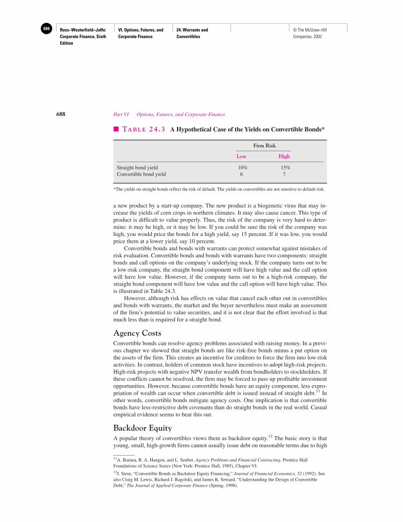
Ross−Westerfield−Jaffe: Corporate Finance, Sixth Edition
VI. Options, Futures, and Corporate Finance
24. Warrants and Convertibles
694 © The McGraw−Hill Companies, 2002
a new product by a start-up company. The new product is a biogenetic virus that may in-crease the yields of corn crops in northern climates. It may also cause cancer. This type ofproduct is difficult to value properly. Thus, the risk of the company is very hard to deter-mine: it may be high, or it may be low. If you could be sure the risk of the company washigh, you would price the bonds for a high yield, say 15 percent. If it was low, you wouldprice them at a lower yield, say 10 percent.
Convertible bonds and bonds with warrants can protect somewhat against mistakes ofrisk evaluation. Convertible bonds and bonds with warrants have two components: straightbonds and call options on the company’s underlying stock. If the company turns out to bea low-risk company, the straight bond component will have high value and the call optionwill have low value. However, if the company turns out to be a high-risk company, thestraight bond component will have low value and the call option will have high value. Thisis illustrated in Table 24.3.
However, although risk has effects on value that cancel each other out in convertiblesand bonds with warrants, the market and the buyer nevertheless must make an assessmentof the firm’s potential to value securities, and it is not clear that the effort involved is thatmuch less than is required for a straight bond.
Agency CostsConvertible bonds can resolve agency problems associated with raising money. In a previ-ous chapter we showed that straight bonds are like risk-free bonds minus a put option onthe assets of the firm. This creates an incentive for creditors to force the firm into low-riskactivities. In contrast, holders of common stock have incentives to adopt high-risk projects.High-risk projects with negative NPV transfer wealth from bondholders to stockholders. Ifthese conflicts cannot be resolved, the firm may be forced to pass up profitable investmentopportunities. However, because convertible bonds have an equity component, less expro-priation of wealth can occur when convertible debt is issued instead of straight debt.11 Inother words, convertible bonds mitigate agency costs. One implication is that convertiblebonds have less-restrictive debt covenants than do straight bonds in the real world. Casualempirical evidence seems to bear this out.
Backdoor EquityA popular theory of convertibles views them as backdoor equity.12 The basic story is thatyoung, small, high-growth firms cannot usually issue debt on reasonable terms due to high
688 Part VI Options, Futures, and Corporate Finance
11A. Barnea, R. A. Haugen, and L. Senbet, Agency Problems and Financial Contracting, Prentice HallFoundations of Science Series (New York: Prentice Hall, 1985), Chapter VI.12J. Stein, “Convertible Bonds as Backdoor Equity Financing,” Journal of Financial Economics, 32 (1992). Seealso Craig M. Lewis, Richard J. Ragolski, and James K. Seward, “Understanding the Design of ConvertibleDebt,” The Journal of Applied Corporate Finance (Spring, 1998).
� TABLE 24.3 A Hypothetical Case of the Yields on Convertible Bonds*
Firm Risk
Low High
Straight bond yield 10% 15%Convertible bond yield 6 7
*The yields on straight bonds reflect the risk of default. The yields on convertibles are not sensitive to default risk.
Ross−Westerfield−Jaffe: Corporate Finance, Sixth Edition
VI. Options, Futures, and Corporate Finance
24. Warrants and Convertibles
695© The McGraw−Hill Companies, 2002
financial distress costs. However, the owners may be unwilling to issue equity if currentstock prices are too low.
Lewis, Ragolski, and Sewart examine the risk shifting and backdoor equity theories ofconvertible bond debt. They find evidence for both theories.
• Why do firms issue convertible bonds and bonds with warrants?
24.8 CONVERSION POLICY
There is one aspect of convertible bonds that we have omitted so far. Firms are frequentlygranted a call option on the bond. The typical arrangements for calling a convertible bond aresimple. When the bond is called, the holder has about 30 days to choose between the following:
1. Converting the bond to common stock at the conversion ratio.
2. Surrendering the bond and receiving the call price in cash.
What should bondholders do? It should be obvious that if the conversion value of thebond is greater than the call price, conversion is better than surrender; and if the conversionvalue is less than the call price, surrender is better than conversion. If the conversion valueis greater than the call price, the call is said to force conversion.
What should financial managers do? Calling the bonds does not change the value ofthe firm as a whole. However, an optimal call policy can benefit the stockholders at the ex-pense of the bondholders. Because we are speaking of dividing a pie of fixed size, the op-timal call policy is very simple: Do whatever the bondholders do not want you to do.
Bondholders would love the stockholders to call the bonds when the bond’s marketvalue is below the call price. Shareholders would be giving bondholders extra value.Alternatively, should the value of the bonds rise above the call price, the bondholders wouldlove the stockholders not to call the bonds, because bondholders would be allowed to holdonto a valuable asset.
There is only one policy left. This is the policy that maximizes shareholder value andminimizes bondholder value. This policy is
Call the bond when its value is equal to the call price.
It is a puzzle that firms do not always call convertible bonds when the conversion valuereaches the call price. Ingersoll examined the call policies of 124 firms between 1968 and1975.13 In most cases he found that the company waited to call the bonds until the conver-sion value was much higher than the call price. The median company waited until the con-version value of its bonds was 44 percent higher than the call price. This is not even closeto the above optimal strategy. Why?
One reason is that if firms attempt to implement the above optimal strategy, it may not betruly optimal. Recall that bondholders have 30 days to decide whether to convert bonds to com-mon stock or to surrender bonds for the call price in cash. In 30 days, the stock price could drop,forcing the conversion value below the call price. If so, the convertible is “out of the money”
Chapter 24 Warrants and Convertibles 689
QUESTION
CO
NC
EP
T
?
13J. Ingersoll, “An Examination of Corporate Call Policies on Convertible Bonds,” Journal of Finance (May1977). See also M. Harris and A. Raviv, “A Sequential Signalling Model of Convertible Debt Policy,” Journal ofFinance (December 1985). Harris and Raviv describe a signal equilibrium that is consistent with Ingersoll’sresult. They show that managers with favorable information will delay calls to avoid depressing stock prices.
Ross−Westerfield−Jaffe: Corporate Finance, Sixth Edition
VI. Options, Futures, and Corporate Finance
24. Warrants and Convertibles
696 © The McGraw−Hill Companies, 2002
and the firm is giving away money. The firm would be giving up cash for common stock worthmuch less. Because of this possibility, firms in the real world usually wait until the conversionvalue is substantially above the call price before they trigger the call.14 This is sensible.
• Why will convertible bonds not be voluntarily converted to stock before expiration?• When should firms force conversion of convertibles? Why?
24.9 SUMMARY AND CONCLUSIONS
1. A warrant gives the holder the right to buy shares of common stock at an exercise price for agiven period of time. Typically, warrants are issued in a package with privately placed bonds.Afterward they become detached and trade separately.
2. A convertible bond is a combination of a straight bond and a call option. The holder can giveup the bond in exchange for shares of stock.
3. Convertible bonds and warrants are like call options. However, there are some importantdifferences:a. Warrants and convertible securities are issued by corporations. Call options are traded
between individual investors.i. Warrants are usually issued privately and are combined with a bond. In most cases the
warrants can be detached immediately after the issue. In some cases warrants are issuedwith preferred stock, with common stock, or in executive compensation programs.
ii. Convertibles are usually bonds that can be converted into common stock.iii. Call options are sold separately by individual investors (called writers of call options).
b. Warrants and call options are exercised for cash. The holder of a warrant gives thecompany cash and receives new shares of the company’s stock. The holder of a call optiongives another individual cash in exchange for shares of stock. When someone converts abond, it is exchanged for common stock. As a consequence, bonds with warrants andconvertible bonds have different effects on corporate cash flow and capital structure.
c. Warrants and convertibles cause dilution to the existing shareholders. When warrants areexercised and convertible bonds converted, the company must issue new shares ofcommon stock. The percentage ownership of the existing shareholders will decline. Newshares are not issued when call options are exercised.
4. Many arguments, both plausible and implausible, are given for issuing convertible bonds andbonds with warrants. One plausible rationale for such bonds has to do with risk. Convertiblesand bonds with warrants are associated with risky companies. Lenders can do several thingsto protect themselves from high-risk companies:
690 Part VI Options, Futures, and Corporate Finance
14See Paul Asquith, “Convertible Bonds Are Not Called Late,” Journal of Finance (September 1995). On theother hand, the stock market usually reacts negatively to the announcement of a call. For example, see A. K.Singh, A. R. Cowan, and N. Nayan, “Underwritten Calls of Convertible Bonds,” Journal of FinancialEconomics (March 1991) and M. A. Mazzeo and W. T. Moore, “Liquidity Costs and Stock Price Response toConvertible Security Calls,” Journal of Business (July 1992).
Most recently, Ederington, Caton, and Campbell test various theories on when it is optimal to callconvertibles. They find evidence consistent for the preceding 30-day “safety margin” theory. They also find thatcalls of in-the-money convertibles are highly unlikely if dividends to be received (after conversion) exceed thecompany’s interest payment. See Louis H. Ederington, Gary L. Caton, and Cynthia J. Campbell, “To Call or Notto Call Convertible Debt,” Financial Management (Spring 1997).
QUESTIONS
CO
NC
EP
T
?

Ross−Westerfield−Jaffe: Corporate Finance, Sixth Edition
VI. Options, Futures, and Corporate Finance
24. Warrants and Convertibles
697© The McGraw−Hill Companies, 2002
a. They can require high yields.b. They can lend less or not at all to firms whose risk is difficult to assess.c. They can impose severe restrictions on such debt.Another useful way to protect against risk is to issue bonds with equity kickers. This givesthe lenders the chance to benefit from risks and reduces the conflicts between bondholdersand stockholders concerning risk.
5. A puzzle particularly vexes financial researchers: Convertible bonds usually have callprovisions. Companies appear to delay calling convertibles until the conversion value greatlyexceeds the call price. From the shareholders’ standpoint, the optimal call policy would be tocall the convertibles when the conversion value equals the call price.
KEY TERMS
Conversion premium 680 Convertible bond 680Conversion price 680 Force conversion 689Conversion ratio 680 Warrants 674Conversion value 681
SUGGESTED READINGS
The following articles analyze when it is optimal to force conversion of convertible bonds:Asquith, P. “Convertible Bonds Are Not Called Late.” Journal of Finance (September 1995).Brennan, M., and E. Schwartz. “Convertible Bonds: Valuation and Optimal Strategies for Call
Conversion.” Journal of Finance (December 1977).
Michael Brennan examines the conventional arguments for and against convertible bonds andoffers a new “risk synergy” rationale:Brennan, M. “The Case for Convertibles.” In J. M. Stern and D. H. Crew, eds. The Revolution in
Corporate Finance. New York: Basil Blackwell, 1986.
QUESTIONS AND PROBLEMS
24.1 Define:a. Warrantsb. Convertibles
Warrants24.2 Explain why the following limits on warrant prices exist.
a. The lower limit is zero if the stock price is below the exercise price.b. The lower limit is stock price less exercise price if the stock price is above the exercise
price.c. The upper limit is the price of the stock.
24.3 a. What is the primary difference between warrants and calls?b. What is the implication of that difference?
24.4 Suppose the GR Company, which was discussed in the text, sells Mrs. Fiske a warrant.Prior to the sale, the company has two shares outstanding. Mr. Gould owns one share andMs. Rockefeller owns the other share. The assets of the firm are seven ounces of platinum,
Chapter 24 Warrants and Convertibles 691

Ross−Westerfield−Jaffe: Corporate Finance, Sixth Edition
VI. Options, Futures, and Corporate Finance
24. Warrants and Convertibles
698 © The McGraw−Hill Companies, 2002
which were purchased at $500 per ounce. The exercise price of the warrant is $1,800. Allfunds that enter the firm are used to purchase more platinum. Mrs. Fiske is sold thewarrant moments after incorporation for $500.a. What is the price of GR stock before the warrant is sold?b. At what price for platinum will Mrs. Fiske exercise her warrant?c. Suppose the price of platinum suddenly rises to $520 per ounce.
i. What is the value of GR?ii. What will Mrs. Fiske do?
iii. What is the new price per share of GR stock?iv. What was Mrs. Fiske’s gain from the exercise?
d. What would Mrs. Fiske’s gain have been if Mr. Gould had sold her a call?e. Why are Mrs. Fiske’s gains different?
24.5 General Autos has its warrants traded in the market and they will expire five years fromtoday. Each warrant is entitled to purchase 0.25 shares of General Autos common stock at$10 per share.a. Suppose General Autos stock is currently selling for $8. What is the lower limit on the
warrant value? What is the upper limit?b. Suppose General Autos stock is currently selling for $12. What is the lower limit on
the warrant value? What is the upper limit?
24.6 Pace Western Crystal, Inc., has outstanding 10 million common shares and 200,000warrants. Each warrant can purchase five shares of common stock at $15 per share.Warrant holders exercised all of their warrants today. Pace Western’s stock price beforethe exercise was $17. What should the new stock price be after the exercise? Assumethere is no information content on the exercise of the warrants.
24.7 A warrant entitles the holder to buy 10 shares of common stock at $21 per share. Whenthe market price of the stock is $15, will the market price of the warrant equal zero? Whyor why not?
24.8 Grand Mills Corporation has 4 million shares of common stock outstanding. Thecompany has 500,000 warrants being traded in the market. Each warrant has the right tobuy one share of common stock at $20 per share. The warrant will expire one year fromtoday. Grand Mills stock is selling for $22 per share and the variance of the return onthe stock is 0.005. The risk-free rate is 5 percent. Use the Black-Scholes model to pricethe warrant.
24.9 Express Transportation’s current market-balance sheet shows assets of the firm are$150 million. The market value of the debt Express has issued is $47 million. Expresshas 1.5 million shares of common stock outstanding. Tomorrow, Express will issue100,000 warrants. Each warrant has the option to buy five shares of Express commonstock for one year. The proceeds of the issue will be used to pay the dividend that isdue tomorrow. Call options on the firm’s stock with similar terms are currently sellingfor $4.70. What will be the price of Express warrants?
24.10 Consider the following warrants.
Warrant X: For each warrant held, three shares of common stock can be purchased atan exercise price of $20 per share.Warrant Y: For each warrant held, two shares of common stock can be purchased atan exercise price of $30 per share.
The current market price of stock X is $30 per share. The current market price of stock Yis $40 per share.a. What is the minimum value of warrant X?b. What is the minimum value of warrant Y?
692 Part VI Options, Futures, and Corporate Finance
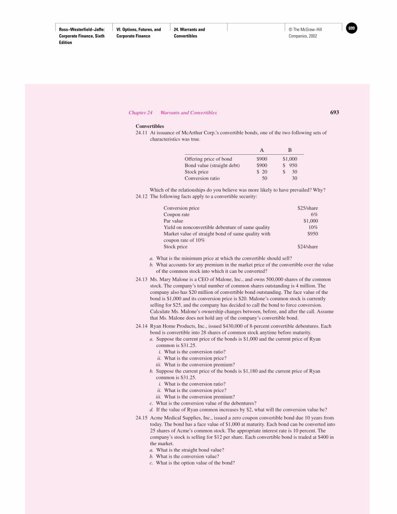
Ross−Westerfield−Jaffe: Corporate Finance, Sixth Edition
VI. Options, Futures, and Corporate Finance
24. Warrants and Convertibles
699© The McGraw−Hill Companies, 2002
Convertibles24.11 At issuance of McArthur Corp.’s convertible bonds, one of the two following sets of
characteristics was true.
A B
Offering price of bond $900 $1,000Bond value (straight debt) $900 $ 950Stock price $ 20 $ 30Conversion ratio 50 30
Which of the relationships do you believe was more likely to have prevailed? Why?24.12 The following facts apply to a convertible security:
Conversion price $25/shareCoupon rate 6%Par value $1,000Yield on nonconvertible debenture of same quality 10%Market value of straight bond of same quality with $950coupon rate of 10%Stock price $24/share
a. What is the minimum price at which the convertible should sell?b. What accounts for any premium in the market price of the convertible over the value
of the common stock into which it can be converted?
24.13 Ms. Mary Malone is a CEO of Malone, Inc., and owns 500,000 shares of the commonstock. The company’s total number of common shares outstanding is 4 million. Thecompany also has $20 million of convertible bond outstanding. The face value of thebond is $1,000 and its conversion price is $20. Malone’s common stock is currentlyselling for $25, and the company has decided to call the bond to force conversion.Calculate Ms. Malone’s ownership changes between, before, and after the call. Assumethat Ms. Malone does not hold any of the company’s convertible bond.
24.14 Ryan Home Products, Inc., issued $430,000 of 8-percent convertible debentures. Eachbond is convertible into 28 shares of common stock anytime before maturity.a. Suppose the current price of the bonds is $1,000 and the current price of Ryan
common is $31.25.i. What is the conversion ratio?
ii. What is the conversion price?iii. What is the conversion premium?
b. Suppose the current price of the bonds is $1,180 and the current price of Ryancommon is $31.25.
i. What is the conversion ratio?ii. What is the conversion price?
iii. What is the conversion premium?c. What is the conversion value of the debentures?d. If the value of Ryan common increases by $2, what will the conversion value be?
24.15 Acme Medical Supplies, Inc., issued a zero coupon convertible bond due 10 years fromtoday. The bond has a face value of $1,000 at maturity. Each bond can be converted into25 shares of Acme’s common stock. The appropriate interest rate is 10 percent. Thecompany’s stock is selling for $12 per share. Each convertible bond is traded at $400 inthe market.a. What is the straight bond value?b. What is the conversion value?c. What is the option value of the bond?
Chapter 24 Warrants and Convertibles 693

Ross−Westerfield−Jaffe: Corporate Finance, Sixth Edition
VI. Options, Futures, and Corporate Finance
24. Warrants and Convertibles
700 © The McGraw−Hill Companies, 2002
24.16 A $1,000 par convertible debenture has a conversion price for common stock of $180 pershare. With the common stock selling at $60, what is the conversion value of the bond?
24.17 You are a financial analyst hired to value a new 30-year callable, convertible bond. Thebond has a 6-percent coupon payable annually. The conversion price is $125. The stockcurrently sells for $35. The stock price is expected to rise 15 percent per year. The bondis callable at $1,100. The required return on the bond is 10 percent.a. What is the straight bond value?b. What is the conversion value?c. How long would it take for the conversion value to exceed a call price?
694 Part VI Options, Futures, and Corporate Finance
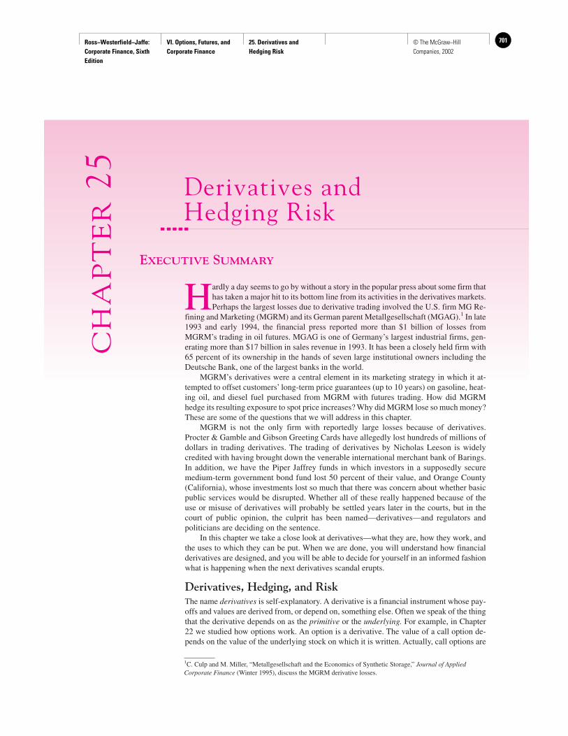
Ross−Westerfield−Jaffe: Corporate Finance, Sixth Edition
VI. Options, Futures, and Corporate Finance
25. Derivatives and Hedging Risk
701© The McGraw−Hill Companies, 2002
Derivatives and Hedging Risk
CH
AP
TE
R25
EXECUTIVE SUMMARY
Hardly a day seems to go by without a story in the popular press about some firm thathas taken a major hit to its bottom line from its activities in the derivatives markets.Perhaps the largest losses due to derivative trading involved the U.S. firm MG Re-
fining and Marketing (MGRM) and its German parent Metallgesellschaft (MGAG).1 In late1993 and early 1994, the financial press reported more than $1 billion of losses fromMGRM’s trading in oil futures. MGAG is one of Germany’s largest industrial firms, gen-erating more than $17 billion in sales revenue in 1993. It has been a closely held firm with65 percent of its ownership in the hands of seven large institutional owners including theDeutsche Bank, one of the largest banks in the world.
MGRM’s derivatives were a central element in its marketing strategy in which it at-tempted to offset customers’ long-term price guarantees (up to 10 years) on gasoline, heat-ing oil, and diesel fuel purchased from MGRM with futures trading. How did MGRMhedge its resulting exposure to spot price increases? Why did MGRM lose so much money?These are some of the questions that we will address in this chapter.
MGRM is not the only firm with reportedly large losses because of derivatives.Procter & Gamble and Gibson Greeting Cards have allegedly lost hundreds of millions ofdollars in trading derivatives. The trading of derivatives by Nicholas Leeson is widelycredited with having brought down the venerable international merchant bank of Barings.In addition, we have the Piper Jaffrey funds in which investors in a supposedly securemedium-term government bond fund lost 50 percent of their value, and Orange County(California), whose investments lost so much that there was concern about whether basicpublic services would be disrupted. Whether all of these really happened because of theuse or misuse of derivatives will probably be settled years later in the courts, but in thecourt of public opinion, the culprit has been named—derivatives—and regulators andpoliticians are deciding on the sentence.
In this chapter we take a close look at derivatives—what they are, how they work, andthe uses to which they can be put. When we are done, you will understand how financialderivatives are designed, and you will be able to decide for yourself in an informed fashionwhat is happening when the next derivatives scandal erupts.
Derivatives, Hedging, and RiskThe name derivatives is self-explanatory. A derivative is a financial instrument whose pay-offs and values are derived from, or depend on, something else. Often we speak of the thingthat the derivative depends on as the primitive or the underlying. For example, in Chapter22 we studied how options work. An option is a derivative. The value of a call option de-pends on the value of the underlying stock on which it is written. Actually, call options are
1C. Culp and M. Miller, “Metallgesellschaft and the Economics of Synthetic Storage,” Journal of AppliedCorporate Finance (Winter 1995), discuss the MGRM derivative losses.
Ross−Westerfield−Jaffe: Corporate Finance, Sixth Edition
VI. Options, Futures, and Corporate Finance
25. Derivatives and Hedging Risk
702 © The McGraw−Hill Companies, 2002
quite complicated examples of derivatives. The vast majority of derivatives are simpler thancall options. Most derivatives are forward or futures agreements or what are called swaps,and we will study each of these in some detail.
Why do firms use derivatives? The answer is that derivatives are tools for changing thefirm’s risk exposure. Someone once said that derivatives are to finance what scalpels are tosurgery. By using derivatives, the firm can cut away unwanted portions of risk exposure andeven transform the exposures into quite different forms. A central point in finance is thatrisk is undesirable. In our chapters on risk and return, we pointed out that individuals wouldchoose risky securities only if the expected return compensated for the risk. Similarly, afirm will accept a project with high risk only if the return on the project compensates forthis risk. Not surprisingly, then, firms are usually looking for ways to reduce their risk.When the firm reduces its risk exposure with the use of derivatives, it is said to be hedging.Hedging offsets the firm’s risk, such as the risk in a project, by one or more transactions inthe financial markets.
Derivatives can also be used to merely change or even increase the firm’s risk exposure.When this occurs, the firm is speculating on the movement of some economic variables—those that underlie the derivative. For example, if a derivative is purchased that will rise invalue if interest rates rise, and if the firm has no offsetting exposure to interest rate changes,then the firm is speculating that interest rates will rise and give it a profit on its derivativesposition. Using derivatives to translate an opinion about whether interest rates or some othereconomic variable will rise or fall is the opposite of hedging—it is risk enhancing.Speculating on your views on the economy and using derivatives to profit if that view turnsout to be correct is not necessarily wrong, but the speculator should always remember thatsharp tools cut deep, and if the opinions on which the derivatives position is based turn outto be incorrect, then the consequences can prove costly. Efficient market theory teaches howdifficult it is to predict what markets will do. Most of the sad experiences with derivativeshave occurred not from their use as instruments for hedging and offsetting risk, but, rather,from speculation.
25.1 FORWARD CONTRACTS
We can begin our discussion of hedging by considering forward contracts. One frequentlyhears the one-liner about the gentleman who was shocked to find he had been speakingprose all his life. Forward contracts are a lot like that; you have probably been dealing inthem your whole life without knowing it. Suppose you walk into a bookstore on, say, Feb-ruary 1 to buy the best-seller Eating Habits of the Rich and Famous. The cashier tells youthat the book is currently sold out, but he takes your phone number, saying that he will re-order it for you. He says the book will cost $10.00. If you agree on February 1 to pick upand pay $10.00 for the book when called, you and the cashier have engaged in a forwardcontract. That is, you have agreed both to pay for the book and to pick it up when the book-store notifies you. Since you are agreeing to buy the book at a later date, you are buying aforward contract on February 1. In commodity parlance, you will be taking delivery whenyou pick up the book. The book is called the deliverable instrument.
The cashier, acting on behalf of the bookstore, is selling a forward contract.(Alternatively, we say that he is writing a forward contract.) The bookstore has agreed toturn the book over to you at the predetermined price of $10.00 as soon as the book arrives.The act of turning the book over to you is called making delivery. Table 25.1 illustrates thebook purchase. Note that the agreement takes place on February 1. The price is set and the
696 Part VI Options, Futures, and Corporate Finance
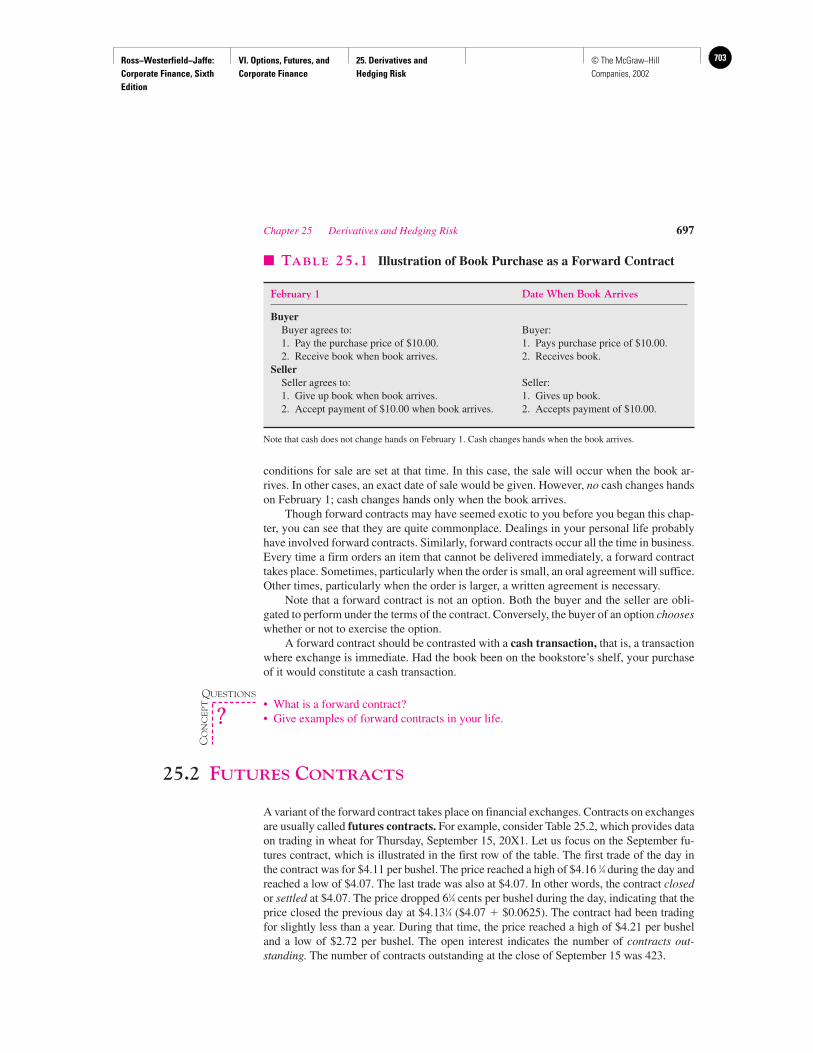
Ross−Westerfield−Jaffe: Corporate Finance, Sixth Edition
VI. Options, Futures, and Corporate Finance
25. Derivatives and Hedging Risk
703© The McGraw−Hill Companies, 2002
conditions for sale are set at that time. In this case, the sale will occur when the book ar-rives. In other cases, an exact date of sale would be given. However, no cash changes handson February 1; cash changes hands only when the book arrives.
Though forward contracts may have seemed exotic to you before you began this chap-ter, you can see that they are quite commonplace. Dealings in your personal life probablyhave involved forward contracts. Similarly, forward contracts occur all the time in business.Every time a firm orders an item that cannot be delivered immediately, a forward contracttakes place. Sometimes, particularly when the order is small, an oral agreement will suffice.Other times, particularly when the order is larger, a written agreement is necessary.
Note that a forward contract is not an option. Both the buyer and the seller are obli-gated to perform under the terms of the contract. Conversely, the buyer of an option chooseswhether or not to exercise the option.
A forward contract should be contrasted with a cash transaction, that is, a transactionwhere exchange is immediate. Had the book been on the bookstore’s shelf, your purchaseof it would constitute a cash transaction.
• What is a forward contract?• Give examples of forward contracts in your life.
25.2 FUTURES CONTRACTS
A variant of the forward contract takes place on financial exchanges. Contracts on exchangesare usually called futures contracts. For example, consider Table 25.2, which provides dataon trading in wheat for Thursday, September 15, 20X1. Let us focus on the September fu-tures contract, which is illustrated in the first row of the table. The first trade of the day inthe contract was for $4.11 per bushel. The price reached a high of $4.16 1⁄4 during the day andreached a low of $4.07. The last trade was also at $4.07. In other words, the contract closedor settled at $4.07. The price dropped 61⁄4 cents per bushel during the day, indicating that theprice closed the previous day at $4.131⁄4 ($4.07 � $0.0625). The contract had been tradingfor slightly less than a year. During that time, the price reached a high of $4.21 per busheland a low of $2.72 per bushel. The open interest indicates the number of contracts out-standing. The number of contracts outstanding at the close of September 15 was 423.
Chapter 25 Derivatives and Hedging Risk 697
� TABLE 25.1 Illustration of Book Purchase as a Forward Contract
February 1 Date When Book Arrives
BuyerBuyer agrees to: Buyer:1. Pay the purchase price of $10.00. 1. Pays purchase price of $10.00.2. Receive book when book arrives. 2. Receives book.
SellerSeller agrees to: Seller:1. Give up book when book arrives. 1. Gives up book.2. Accept payment of $10.00 when book arrives. 2. Accepts payment of $10.00.
Note that cash does not change hands on February 1. Cash changes hands when the book arrives.
QUESTIONS
CO
NC
EP
T
?
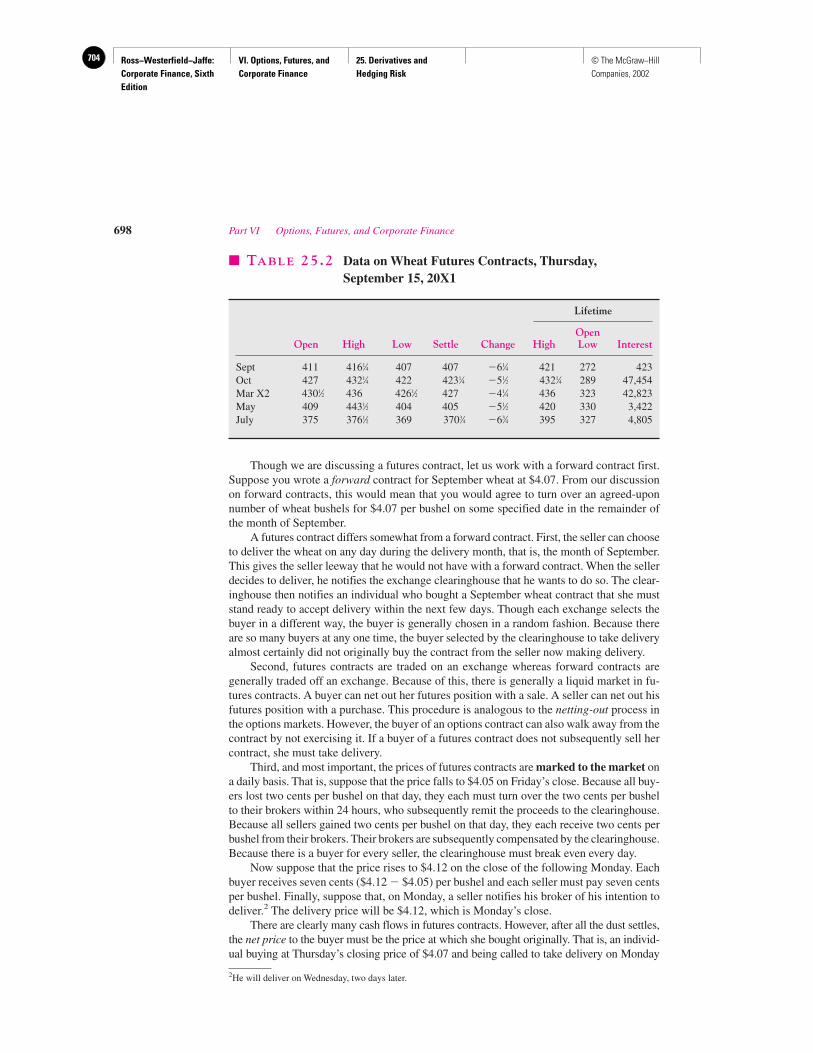
Ross−Westerfield−Jaffe: Corporate Finance, Sixth Edition
VI. Options, Futures, and Corporate Finance
25. Derivatives and Hedging Risk
704 © The McGraw−Hill Companies, 2002
Though we are discussing a futures contract, let us work with a forward contract first.Suppose you wrote a forward contract for September wheat at $4.07. From our discussionon forward contracts, this would mean that you would agree to turn over an agreed-uponnumber of wheat bushels for $4.07 per bushel on some specified date in the remainder ofthe month of September.
A futures contract differs somewhat from a forward contract. First, the seller can chooseto deliver the wheat on any day during the delivery month, that is, the month of September.This gives the seller leeway that he would not have with a forward contract. When the sellerdecides to deliver, he notifies the exchange clearinghouse that he wants to do so. The clear-inghouse then notifies an individual who bought a September wheat contract that she muststand ready to accept delivery within the next few days. Though each exchange selects thebuyer in a different way, the buyer is generally chosen in a random fashion. Because thereare so many buyers at any one time, the buyer selected by the clearinghouse to take deliveryalmost certainly did not originally buy the contract from the seller now making delivery.
Second, futures contracts are traded on an exchange whereas forward contracts aregenerally traded off an exchange. Because of this, there is generally a liquid market in fu-tures contracts. A buyer can net out her futures position with a sale. A seller can net out hisfutures position with a purchase. This procedure is analogous to the netting-out process inthe options markets. However, the buyer of an options contract can also walk away from thecontract by not exercising it. If a buyer of a futures contract does not subsequently sell hercontract, she must take delivery.
Third, and most important, the prices of futures contracts are marked to the market ona daily basis. That is, suppose that the price falls to $4.05 on Friday’s close. Because all buy-ers lost two cents per bushel on that day, they each must turn over the two cents per bushelto their brokers within 24 hours, who subsequently remit the proceeds to the clearinghouse.Because all sellers gained two cents per bushel on that day, they each receive two cents perbushel from their brokers. Their brokers are subsequently compensated by the clearinghouse.Because there is a buyer for every seller, the clearinghouse must break even every day.
Now suppose that the price rises to $4.12 on the close of the following Monday. Eachbuyer receives seven cents ($4.12 � $4.05) per bushel and each seller must pay seven centsper bushel. Finally, suppose that, on Monday, a seller notifies his broker of his intention todeliver.2 The delivery price will be $4.12, which is Monday’s close.
There are clearly many cash flows in futures contracts. However, after all the dust settles,the net price to the buyer must be the price at which she bought originally. That is, an individ-ual buying at Thursday’s closing price of $4.07 and being called to take delivery on Monday
698 Part VI Options, Futures, and Corporate Finance
� TABLE 25.2 Data on Wheat Futures Contracts, Thursday,September 15, 20X1
Lifetime
OpenOpen High Low Settle Change High Low Interest
Sept 411 4161⁄4 407 407 �61⁄4 421 272 423Oct 427 4321⁄4 422 4231⁄4 �51⁄2 4321⁄4 289 47,454Mar X2 4301⁄2 436 4261⁄2 427 �41⁄4 436 323 42,823May 409 4431⁄2 404 405 �51⁄2 420 330 3,422July 375 3761⁄2 369 3703⁄4 �63⁄4 395 327 4,805
2He will deliver on Wednesday, two days later.
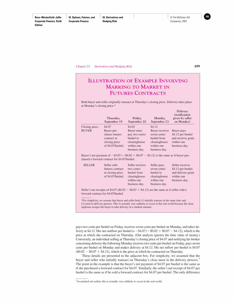
Ross−Westerfield−Jaffe: Corporate Finance, Sixth Edition
VI. Options, Futures, and Corporate Finance
25. Derivatives and Hedging Risk
705© The McGraw−Hill Companies, 2002
pays two cents per bushel on Friday, receives seven cents per bushel on Monday, and takes de-livery at $4.12. Her net outflow per bushel is �$4.07 (�$0.02 � $0.07 � $4.12), which is theprice at which she contracted on Thursday. (Our analysis ignores the time value of money.)Conversely, an individual selling at Thursday’s closing price of $4.07 and notifying his brokerconcerning delivery the following Monday receives two cents per bushel on Friday, pays sevencents per bushel on Monday and makes delivery at $4.12. His net inflow per bushel is $4.07($0.02 � $0.07 � $4.12), which is the price at which he contracted on Thursday.
These details are presented in the adjacent box. For simplicity, we assumed that thebuyer and seller who initially transact on Thursday’s close meet in the delivery process.3
The point in the example is that the buyer’s net payment of $4.07 per bushel is the same asif she purchased a forward contract for $4.07. Similarly, the seller’s net receipt of $4.07 perbushel is the same as if he sold a forward contract for $4.07 per bushel. The only difference
Chapter 25 Derivatives and Hedging Risk 699
3As pointed out earlier, this is actually very unlikely to occur in the real world.
ILLUSTRATION OF EXAMPLE INVOLVING
MARKING TO MARKET IN
FUTURES CONTRACTS
Both buyer and seller originally transact at Thursday’s closing price. Delivery takes placeat Monday’s closing price.*
Delivery(notification
Thursday, Friday, Monday, given by sellerSeptember 19 September 20 September 23 on Monday)
Closing price: $4.07 $4.05 $4.12BUYER Buyer pur- Buyer must Buyer receives Buyer pays
chases futures pay two cents/ seven cents/ $4.12 per bushelcontract at bushel to bushel from and receives grainclosing price clearinghouse clearinghouse within one of $4.07/bushel. within one within one business day.
business day. business day.
Buyer’s net payment of �$4.07 (�$0.02 � $0.07 � $4.12) is the same as if buyer pur-chased a forward contract for $4.07/bushel.
SELLER Seller sells Seller receives Seller pays Seller receivesfutures contract two cents/ seven cents/ $4.12 per bushelat closing price bushel from bushel to and delivers grainof $4.07/bushel. clearinghouse clearinghouse within one
within one within one business day.business day. business day.
Seller’s net receipts of $4.07 ($0.02 � $0.07 � $4.12) are the same as if seller sold aforward contract for $4.07/bushel.
*For simplicity, we assume that buyer and seller both (1) initially transact at the same time and(2) meet in delivery process. This is actually very unlikely to occur in the real world because the clear-inghouse assigns the buyer to take delivery in a random manner.
Ross−Westerfield−Jaffe: Corporate Finance, Sixth Edition
VI. Options, Futures, and Corporate Finance
25. Derivatives and Hedging Risk
706 © The McGraw−Hill Companies, 2002
is the timing of the cash flows. The buyer of a forward contract knows that he will make asingle payment of $4.07 on the expiration date. He will not need to worry about any othercash flows in the interim. Conversely, though the cash flows to the buyer of a futures con-tract will net to exactly $4.07 as well, the pattern of cash flows is not known ahead of time.
The mark-to-the-market provision on futures contracts has two related effects. The firstconcerns differences in net present value. For example, a large price drop immediately fol-lowing purchase means an immediate outpayment for the buyer of a futures contract.Though the net outflow of $4.07 is still the same as under a forward contract, the presentvalue of the cash outflows is greater to the buyer of a futures contract. Of course, the pres-ent value of the cash outflows is less to the buyer of a futures contract if a price rise fol-lowed purchase.4 Though this effect could be substantial in certain theoretical circum-stances, it appears to be of quite limited importance in the real world.5
Second, the firm must have extra liquidity to handle a sudden outflow prior to expira-tion. This added risk may make the futures contract less attractive.
Students frequently ask, “Why in the world would managers of the commodity ex-changes ruin perfectly good contracts with these bizarre mark-to-the-market provisions?”Actually, the reason is a very good one. Consider the forward contract of Table 25.1 con-cerning the bookstore. Suppose that the public quickly loses interest in Eating Habits of theRich and Famous. By the time the bookstore calls the buyer, other stores may have droppedthe price of the book to $6.00. Because the forward contract was for $10.00, the buyer hasan incentive not to take delivery on the forward contract. Conversely, should the book be-come a hot item selling at $15.00, the bookstore may simply not call the buyer.
As indicated, forward contracts have a very big flaw. Whichever way the price of thedeliverable instrument moves, one party has an incentive to default. There are many caseswhere defaults have occurred in the real world. One famous case concerned Coca-Cola.When the company began in the early 20th century, Coca-Cola made an agreement to sup-ply its bottlers and distributors with cola syrup at a constant price forever. Of course, sub-sequent inflation would have caused Coca-Cola to lose large sums of money had they hon-ored the contract. After much legal effort, Coke and its bottlers put an inflation-escalatorclause in the contract. Another famous case concerned Westinghouse. It seems the firm hadpromised to deliver uranium to certain utilities at a fixed price. The price of uranium sky-rocketed in the 1970s, making Westinghouse lose money on every shipment. Westinghousedefaulted on its agreement. The utilities took Westinghouse to court but did not recoveramounts anything near what Westinghouse owed them.
The mark-to-the-market provisions minimize the chance of default on a futures con-tract. If the price rises, the seller has an incentive to default on a forward contract. However,after paying the clearinghouse, the seller of a futures contract has little reason to default. Ifthe price falls, the same argument can be made for the buyer. Because changes in the valueof the underlying asset are recognized daily, there is no accumulation of loss, and the in-centive to default is reduced.
Because of this default issue, forward contracts generally involve individuals andinstitutions who know and can trust each other. But as W. C. Fields said, “Trust every-body, but cut the cards.” Lawyers earn a handsome living writing supposedly air-tightforward contracts, even among friends. The genius of the mark-to-the-market system isthat is can prevent default where it is most likely to occur—among investors who do not
700 Part VI Options, Futures, and Corporate Finance
4The direction is reversed for the seller of a futures contract. However, the general point that the net presentvalue of cash flows may differ between forward and futures contracts holds for sellers as well.5See John C. Cox, John E. Ingersoll, and Steven A. Ross. “The Relationship between Forward and FuturePrices,” Journal of Financial Economics (1981).

Ross−Westerfield−Jaffe: Corporate Finance, Sixth Edition
VI. Options, Futures, and Corporate Finance
25. Derivatives and Hedging Risk
707© The McGraw−Hill Companies, 2002
know each other. Textbooks on futures contracts from one or two decades ago usuallyinclude a statement such as “No major default has ever occurred on the commodity ex-changes.” No textbook published after the Hunt Brothers defaulted on silver contracts inthe 1970s can make that claim. Nevertheless, the extremely low default rate in futurescontracts is truly awe-inspiring.
Futures contracts are traded in three areas: agricultural commodities, metals and pe-troleum, and financial assets. The extensive array of futures contracts is listed in Table 25.3.
• What is a futures contract?• How is a futures contract related to a forward contract?• Why do exchanges require futures contracts to be marked to the market?
Chapter 25 Derivatives and Hedging Risk 701
� TABLE 25.3 Futures Contracts Listed in The Wall Street Journal
Contract Contract Size Exchange
Agricultural (grain and oilseeds)Corn 5,000 bushels Chicago Board of Trade (CBT)Oats 5,000 bushels CBTSoybeans 5,000 bushels CBTSoybean meal 400 tons CBTSoybean oil 60,000 lbs. CBTWheat 5,000 bushels CBTWheat 5,000 bushels Kansas City (KC)Wheat 5,000 bushels MinneapolisBarley 20 metric tons Winnipeg (WPG)Flaxseed 20 metric tons WPGRapeseed 20 metric tons WPGWheat 20 metric tons WPGRye 20 metric tons WPG
Agricultural (livestock and meat)Cattle (feeder) 44,000 lbs. Chicago Mercantile Exchange (CME)Cattle (live) 40,000 lbs. CMEHogs 30,000 lbs. CMEPork bellies 40,000 lbs. CME
Agricultural (food, fiber, and wood)Cocoa 10 metric tons Coffee, Sugar and Cocoa Exchange
(CSCE)Coffee 37,500 lbs. CSCECotton 50,000 lbs. New York Cotton Exchange (CTN)Orange juice 15,000 lbs. CTNSugar (world) 112,000 lbs. CSCESugar (domestic) 142,000 lbs. CSCELumber 150,000 board feet CME
QUESTIONS
CO
NC
EP
T
?

Ross−Westerfield−Jaffe: Corporate Finance, Sixth Edition
VI. Options, Futures, and Corporate Finance
25. Derivatives and Hedging Risk
708 © The McGraw−Hill Companies, 2002
702 Part VI Options, Futures, and Corporate Finance
� TABLE 25.3 (concluded)
Contract Contract Size Exchange
Metals and petroleumCopper (standard) 25,000 lbs. Commodity Exchange in New York
(CMX)Gold 100 troy oz. CMXPlatinum 50 troy oz. New York Mercantile (NYM)Palladium 100 troy oz. NYMSilver 5,000 troy oz. CMXSilver 1,000 troy oz. CBTCrude oil (light sweet) 1,000 barrels NYMHeating oil no. 2 42,000 gallons NYMGas oil 100 metric tons International Petroleum Exchange of
London (IPEL)Gasoline unleaded 42,000 gallons NYM
FinancialBritish pound 62,500 pounds International Monetary Market in
Chicago (IMM)Australian dollar 100,000 dollars IMMCanadian dollar 100,000 dollars IMMJapanese yen 12.5 million yen IMMSwiss franc 125,000 francs IMMGerman mark 125,000 marks IMMEurodollar $1 million London International Financial
Futures Exchange (LIFFE)
FinancialSterling 500,000 pounds LIFFETreasury bonds $1 million LIFFELong gilt 250,000 pounds LIFFEEurodollar $1 million IMMU.S. Dollar Index 500 times Index Financial Instrument Exchange in
New York (FINEX)CRB Index 500 times Index New York Futures Exchange (NYFE)Treasury bonds $100,000 CBTTreasury notes $100,000 CBT5-year Treasury notes $100,000 CBT5-year Treasury notes $100,000 FINEXTreasury bonds $50,000 MCETreasury bonds $1 million IMM
Financial indexesMunicipal bonds 1,000 times Bond CBT
Buyer IndexS&P 500 Index 500 times Index CMENYSE Composite 500 times Index NYFEKansas City Value Line Index 500 times Index KCMajor Market Index 250 times Index CBT
Ross−Westerfield−Jaffe: Corporate Finance, Sixth Edition
VI. Options, Futures, and Corporate Finance
25. Derivatives and Hedging Risk
709© The McGraw−Hill Companies, 2002
25.3 HEDGING
Now that we have determined how futures contracts work, let us talk about hedging. Thereare two types of hedges, long and short. We discuss the short hedge first.
EXAMPLE
In June, Bernard Abelman, a Midwestern farmer, anticipates a harvest of 50,000bushels of wheat at the end of September. He has two alternatives.
1. Write Futures Contracts against His Anticipated Harvest. The Septemberwheat contract on the Chicago Board of Trade is trading at $3.75 a bushel on June 1.He executes the following transaction:
Date ofTransaction Transaction Price per Bushel
June 1 Write 10 September $3.75futures contracts
He notes that transportation costs to the designated delivery point in Chicago are30 cents/bushel. Thus, his net price per bushel is $3.45 � $3.75 � $0.30.
2. Harvest the Wheat without Writing a Futures Contract. Alternatively, Mr.Abelman could have harvested the wheat without benefit of a futures contract. Therisk would be quite great here since no one knows what the cash price in Septemberwill be. If prices rise, he will profit. Conversely, he will lose if prices fall.
We say that strategy 2 is an unhedged position because there is no attempt touse the futures markets to reduce risk. Conversely, strategy 1 involves a hedge.That is, a position in the futures market offsets the risk of a position in the physi-cal, that is, in the actual, commodity.
Though hedging may seem quite sensible to you, it should be mentioned thatnot everyone hedges. Mr. Abelman might reject hedging for at least two reasons.
First, he may simply be uninformed about hedging. We have found that noteveryone in business understands the hedging concept. Many executives have toldus that they do not want to use futures markets for hedging their inventories be-cause the risks are too great. However, we disagree. While there are large pricefluctuations in these markets, hedging actually reduces the risk that an individualholding inventories bears.
Second, Mr. Abelman may have a special insight or some special informationthat commodity prices will rise. He would not be wise to lock in a price of $3.75if he expects the cash price in September to be well above this price.
The hedge of strategy 1 is called a short hedge, because Mr. Abelman reduceshis risk by selling a futures contract. The short hedge is very common in business.It occurs whenever someone either anticipates receiving inventory or is holding in-ventory. Mr. Abelman was anticipating the harvest of grain. A manufacturer ofsoybean meal and oil may hold large quantities of raw soybeans, which are alreadypaid for. However, the price to be received for meal and oil are not known becauseno one knows what the market price will be when the meal and oil are produced.The manufacturer may write futures contracts in meal and oil to lock in a sales
Chapter 25 Derivatives and Hedging Risk 703
Ross−Westerfield−Jaffe: Corporate Finance, Sixth Edition
VI. Options, Futures, and Corporate Finance
25. Derivatives and Hedging Risk
710 © The McGraw−Hill Companies, 2002
price. An oil company may hold large inventories of petroleum to be processedinto heating oil. The firm could sell futures contracts in heating oil in order to lockin the sales price. A mortgage banker may assemble mortgages slowly before sell-ing them in bulk to a financial institution. Movements of interest rates affect thevalue of the mortgages during the time they are in inventory. The mortgage bankercould sell Treasury-bond futures contracts in order to offset this interest-rate risk.(This last example is treated later in this chapter.)
EXAMPLE
On April 1, Moon Chemical agreed to sell petrochemicals to the U.S. governmentin the future. The delivery dates and prices have been determined. Because oil isa basic ingredient of the production process, Moon Chemical will need to havelarge quantities of oil on hand. The firm can get the oil in one of two ways:
1. Buy the Oil As the Firm Needs It. This in an unhedged position because, asof April 1, the firm does not know the prices it will later have to pay for the oil. Oilis quite a volatile commodity, so Moon Chemical is bearing a good bit of risk. Thekey to this risk-bearing is that the sales price to the U.S. government has alreadybeen fixed. Thus, Moon Chemical cannot pass on increased costs to the consumer.
2. Buy Futures Contracts.6 The firm can buy futures contracts with expira-tion months corresponding to the dates the firm needs inventory. The futures con-tract locks in the purchase price to Moon Chemical. Because there is a crude-oilfutures contract for every month, selecting the correct futures contract is not diffi-cult. Many other commodities have only five contracts per year, frequently neces-sitating buying contracts one month away from the month of production.
As mentioned earlier, Moon Chemical is interested in hedging the risk of fluc-tuating oil prices because it cannot pass any cost increases on to the consumer.Suppose, alternatively, that Moon Chemical was not selling petrochemicals onfixed contract to the U.S. government. Instead, imagine that the petrochemicalswere to be sold to private industry at currently prevailing prices. The price of petro-chemicals should move directly with oil prices, because oil is a major componentof petrochemicals. Because cost increases are likely to be passed on to the con-sumer, Moon Chemical would probably not want to hedge in this case. Instead, thefirm is likely to choose strategy 1, buying the oil as it is needed. If oil prices in-crease between April 1 and September 1, Moon Chemical will, of course, find thatits inputs have become quite costly. However, in a competitive market, its revenuesare likely to rise as well.
Strategy 2 is called a long hedge because one purchases a futures contract toreduce risk. In other words, one takes a long position in the futures market. In gen-eral, a firm institutes a long hedge when it is committed to a fixed sales price. Oneclass of situations involves actual written contracts with customers, such as MoonChemical had with the U.S. government. Alternatively, a firm may find that it can-not easily pass on costs to consumers or does not want to pass on these costs. For
704 Part VI Options, Futures, and Corporate Finance
6Alternatively, the firm could buy the oil on April 1 and store it. This would eliminate the risk of pricemovement, because the firm’s oil costs would be fixed upon the immediate purchase. However, this strategywould be inferior to strategy 2 in the common case where the difference between the futures contract quoted onApril 1 and the April 1 cash price is less than storage costs.
Ross−Westerfield−Jaffe: Corporate Finance, Sixth Edition
VI. Options, Futures, and Corporate Finance
25. Derivatives and Hedging Risk
711© The McGraw−Hill Companies, 2002
example, a group of students opened a small meat market called What’s Your Beefnear the University of Pennsylvania in the late 1970s.7You may recall that this wasa time of volatile consumer prices, especially food prices. Knowing that their fel-low students were particularly budget-conscious, the owners vowed to keep foodprices constant, regardless of price movements in either direction. They accom-plished this by purchasing futures contracts in various agricultural commodities.
CASE STUDY Making the Decision to Use Derivatives: The Case of Metallgesellschaft
Earlier in the chapter we introduced MG Refining and Marketing (MGRM), a U.S. subsidiary of Met-allgesellschaft AG (MGAG).8 MGRM reportedly lost more than $1 billion from trading deriva-
tives. Essentially, MGRM sold gasoline, heating oil, and diesel fuel at fixed prices for up to 10 years inthe future.This is called “selling forward.” In 1993 MGRM had sold forward more than 150 millionbarrels of petroleum products.As in any “selling forward program,” MGRM would lose if the pricesof petroleum products rose over time. For example, suppose MGRM had agreed to sell 150 millionbarrels of heating oil 10 years from now at $25 per barrel. In 10 years, if the actual price of heatingoil turned out to be $35 per barrel, MGRM would stand to lose $10 for every barrel it must sell.
There are several things that MGRM could do to hedge this exposure.
1. MGRM could have attempted to acquire 150 million barrels of oil for forward delivery 10 yearsfrom now. If the 10-year forward price had been $25 per barrel, MGRM would have broken even.In theory, this would have been a perfect hedge.Unfortunately, it is almost impossible to find firmswho will commit to buying or selling 150 million barrels of oil 10 years in the future.There is noorganized 10-year forward market in petroleum products.
2. MGRM could have tried to buy a futures contract that would guarantee delivery of 150 millionbarrels of oil 10 years from now at $25 per barrel. But, as with forward trading, there is no 10-year futures market for petroleum products.
3. Because no 10-year futures contract existed, MGRM employed a “rolling stack” strategy.That is,they first bought a short-term, say, a one-year, futures contract instead of the 10-year contract.At the end of one year, when the futures contract matured, MGRM wrote another one-year fu-tures contract.The strategy called for a series of 10 one-year futures contracts over the 10 years.
The strategy can be best understood in a two-year example.At date 0,MGRM would sell oil forward10 years, at, say, $25 a barrel, to its customers. Simultaneously, MGRM would buy a one-year futurescontract, also at $25 a barrel.9 Now assume that the spot price of oil, i.e., the price for immediatedelivery, rises to $30 a barrel at date 1.Also, at date 2, the price of the one-year futures contract sellsat $30 a barrel. Here, MGRM would break even and at date 1, would gain $5 on its first one-year fu-tures contract.That is, its futures contract issued at date 0 requires it to pay $25 for a barrel of oil
Chapter 25 Derivatives and Hedging Risk 705
7Ordinarily, an unusual firm name in this textbook is a tip-off that it is fictional. This, however, is a true story.8For a spirited debate on what caused the MGRM derivative trading losses, please read: F. R. Edwards and M. S.Canter, “The Collapse of Metallgesellschaft: Unhedgeable Risks, Poor Hedging Strategy or Just Bad Luck,”Journal of Applied Corporate Finance (Spring 1995); A. S. Mello and J. E. Parsons, “Maturity Structure of aHedge Matters: Lessons from the Metallgesellschaft Debacle,” Journal of Applied Corporate Finance (Spring1995); C. Culp and M. Miller, “Hedging in the Theory of Corporate Finance: A Reply to Our Critics,” Journalof Applied Corporate Finance (Spring 1995).9For simplicity, we assume a level “term structure” of oil prices. A case of nonlevel prices, while morecomplex, would lead to the same conclusion. We also use the term of one year when rolling stacks are usuallyin terms of months.
Ross−Westerfield−Jaffe: Corporate Finance, Sixth Edition
VI. Options, Futures, and Corporate Finance
25. Derivatives and Hedging Risk
712 © The McGraw−Hill Companies, 2002
at date 1. It could immediately sell this oil in the spot market at $30 a barrel. However, at date 2, itwould lose $5.That is, its futures contract issued at date 1 requires it to buy oil at $30 a barrel atdate 2.This oil must be sold to its customers for only $25 at date 2.
Unfortunately, there are two potential problems with this hedge. First, the entire term struc-ture of oil prices need not move together. For example, if the spot price of oil was only $29 at date1 while the one-year futures contract was quoted at $30 on that date, the firm would lose $1.Thatis, the gain on the first contract of $4 ($29 � $25) would be less than the loss of $5 ($30 � $25)on the second contract.
Second, the first contract must be settled before the second contract, necessitating liquidityproblems. For example, if oil prices fell at date 1, the loss on the first contract would be settled tothat date.The gain on the second contract would occur at date 2.10 In fact, oil prices did fall overmuch of the 10-year life of MGRM’s hedge, causing large liquidity problems.
The above shows that risks arise even when a position is hedged.However,MGRM created a thirdrisk (and perhaps greater risk) by eliminating their hedge in the middle. Suppose, in our example, thatMGRM bought the first futures contract at date 0 but did not buy the second futures contract at date1.That is, they did not “roll over” their hedge. Since the firm had previously sold oil forward for twoyears, they would be unhedged over the second year.A rise in oil prices over the second year to pay$35 would mean that MGRM would have to buy oil in the spot market at $35 on date 2 in order to simultaneously sell oil to its customers at $25.While MGRM in the real world had a 10-year contract,the effect was similar.After MGRM failed to roll over its stacked hedge, i.e., failed to buy futures con-tracts in later years, oil prices rose. MGRM suffered great losses because of this.
Was the decision to terminate the right one? No one can really know the answer to this im-portant question. It may be that the funding requirements from margin calls forced MGRM into liq-uidating the futures leg of the hedge, precipitating the collapse. It is possible that the rolling stackhedge was not well designed and had more risks than was initially perceived. It is also possible thatthe program was terminated prematurely and, had MGRM hung on, the hedge would have been op-erative. Nevertheless, it must be pointed out that MGRM incurred quite a bit of bad luck. Oil pricesfell when MGRM was hedged, leading to liquidity problems.Oil prices rose after the hedge was lifted,leading to losses.
• Define short and long hedges.• Under what circumstances is each of the two hedges used?• What is a rolling stack strategy?
25.4 INTEREST-RATE FUTURES CONTRACTS
In this section we consider interest-rate futures contracts. Our examples deal with futurescontracts on Treasury bonds because of their high popularity. We first price Treasury bondsand Treasury-bond forward contracts. Differences between futures and forward contractsare explored. Hedging examples are provided next.
Pricing of Treasury BondsAs mentioned earlier in the text, a Treasury bond pays semiannual interest over its life. Inaddition, the face value of the bond is paid at maturity. Consider a 20-year, 8-percentcoupon bond that was issued on March 1. The first payment is to occur in six months, thatis, on September 1. The value of the bond can be determined as
706 Part VI Options, Futures, and Corporate Finance
10In addition, since futures contracts are marked-to-the-market daily, gains and losses on the first contract mustbe settled each day over the first year. If oil prices fell, margin calls would have occurred over the first year.
QUESTIONS
CO
NC
EP
T
?
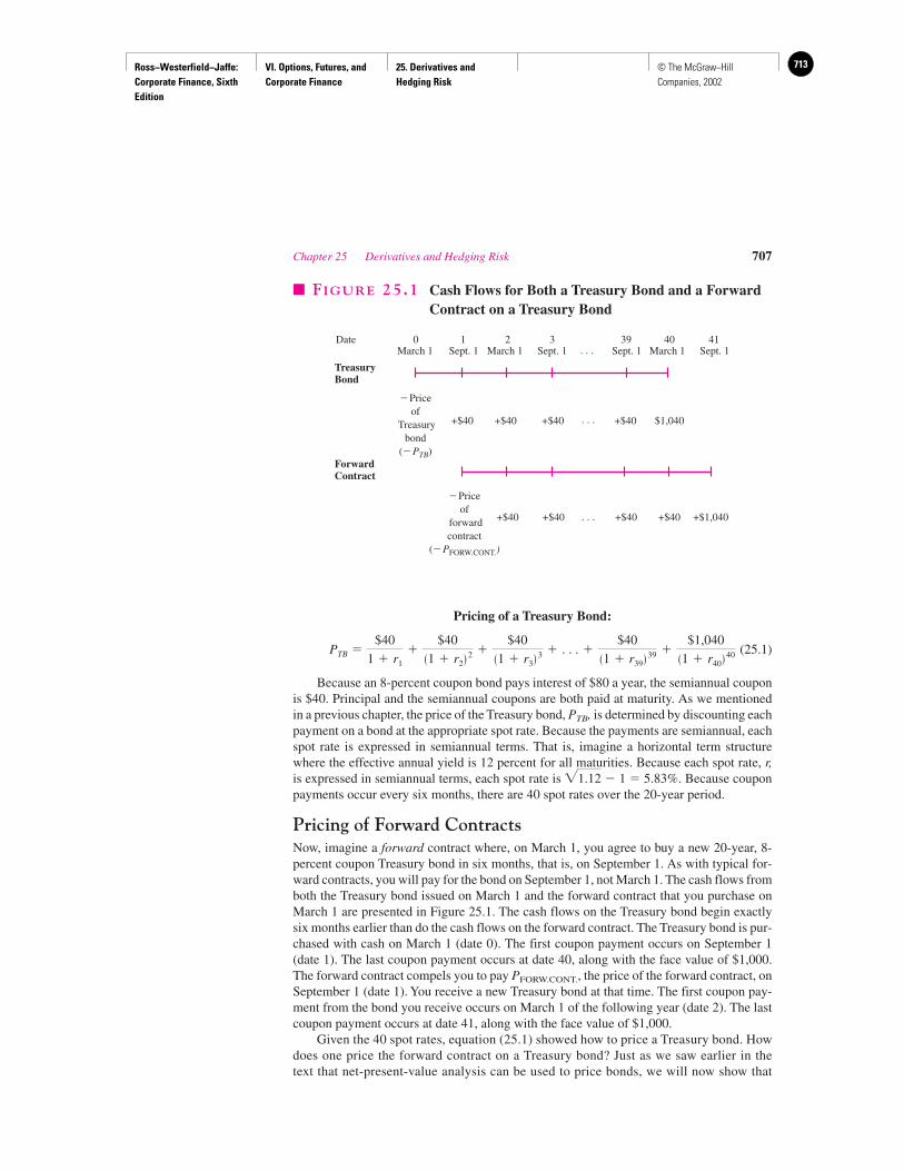
Ross−Westerfield−Jaffe: Corporate Finance, Sixth Edition
VI. Options, Futures, and Corporate Finance
25. Derivatives and Hedging Risk
713© The McGraw−Hill Companies, 2002
Pricing of a Treasury Bond:
(25.1)
Because an 8-percent coupon bond pays interest of $80 a year, the semiannual couponis $40. Principal and the semiannual coupons are both paid at maturity. As we mentionedin a previous chapter, the price of the Treasury bond, PTB, is determined by discounting eachpayment on a bond at the appropriate spot rate. Because the payments are semiannual, eachspot rate is expressed in semiannual terms. That is, imagine a horizontal term structurewhere the effective annual yield is 12 percent for all maturities. Because each spot rate, r,is expressed in semiannual terms, each spot rate is � 1 � 5.83%. Because couponpayments occur every six months, there are 40 spot rates over the 20-year period.
Pricing of Forward ContractsNow, imagine a forward contract where, on March 1, you agree to buy a new 20-year, 8-percent coupon Treasury bond in six months, that is, on September 1. As with typical for-ward contracts, you will pay for the bond on September 1, not March 1. The cash flows fromboth the Treasury bond issued on March 1 and the forward contract that you purchase onMarch 1 are presented in Figure 25.1. The cash flows on the Treasury bond begin exactlysix months earlier than do the cash flows on the forward contract. The Treasury bond is pur-chased with cash on March 1 (date 0). The first coupon payment occurs on September 1(date 1). The last coupon payment occurs at date 40, along with the face value of $1,000.The forward contract compels you to pay PFORW.CONT., the price of the forward contract, onSeptember 1 (date 1). You receive a new Treasury bond at that time. The first coupon pay-ment from the bond you receive occurs on March 1 of the following year (date 2). The lastcoupon payment occurs at date 41, along with the face value of $1,000.
Given the 40 spot rates, equation (25.1) showed how to price a Treasury bond. Howdoes one price the forward contract on a Treasury bond? Just as we saw earlier in thetext that net-present-value analysis can be used to price bonds, we will now show that
�1.12
PTB �$40
1 � r1
�$40
�1 � r2� 2 �$40
�1 � r3� 3 � . . . �$40
�1 � r39� 39 �$1,040
�1 � r40� 40
Chapter 25 Derivatives and Hedging Risk 707
Date 0 1 2 3 39 40 41March 1 Sept. 1 March 1 Sept. 1 Sept. 1 March 1 Sept. 1
TreasuryBond
ForwardContract
�Priceof
Treasurybond
(�PTB)
+$40 +$40 +$40 +$40 $1,040
�Priceof
forwardcontract
(�PFORW.CONT.)
+$40 +$40 +$40 +$40 +$1,040
. . .
. . .
. . .
� FIGURE 25.1 Cash Flows for Both a Treasury Bond and a ForwardContract on a Treasury Bond
Ross−Westerfield−Jaffe: Corporate Finance, Sixth Edition
VI. Options, Futures, and Corporate Finance
25. Derivatives and Hedging Risk
714 © The McGraw−Hill Companies, 2002
net-present-value analysis can be used to price forward contracts. Given the cash flowsfor the forward contract in Figure 25.1, the price of the forward contract must satisfy thefollowing equation:
(25.2)
The right-hand side of equation (25.2) discounts all the cash flows from the delivery in-strument (the Treasury bond issued on September 1) back to date 0 (March 1). Because thefirst cash flow occurs at date 2 (March 1 of the subsequent year), it is discounted by 1/(1 �r2)2. The last cash flow of $1,040 occurs at date 41, so it is discounted by 1/(1 � r41)41. Theleft-hand side represents the cost of the forward contract as of date 0. Because the actualoutpayment occurs at date 1, it is discounted by 1/(1 � r1).
Students often ask, “Why are we discounting everything back to date 0, when we areactually paying for the forward contract on September 1?” The answer is simply that we ap-ply the same techniques to equation (25.2) that we apply to all capital-budgeting problems;we want to put everything in today’s (date 0’s) dollars. Given that the spot rates are knownin the marketplace, traders should have no more trouble pricing a forward contract by equa-tion (25.2) than they would have pricing a Treasury bond by (25.1).
Forward contracts are similar to the underlying bonds themselves. If the entire termstructure of interest rates unexpectedly shifts upward on March 2, the Treasury bond issuedthe previous day should fall in value. This can be seen from equation (25.1). A rise in eachof the spot rates lowers the present value of each of the coupon payments. Hence, the valueof the bond must fall. Conversely, a fall in the term structure of interest rates increases thevalue of the bond.
The same relationship holds with forward contracts, as can be seen from rewriting(25.2) as
(25.3)
We went from (25.2) to (25.3) by multiplying both the left- and the right-hand sides by (1 � r1). If the entire term structure of interest rates unexpectedly shifts upward on March 2,the first term on the right-hand side of equation (25.3) should fall in value.11 That is, bothr1 and r2 will rise an equal amount. However, r2 enters as a squared term, 1/(1 � r2)2, so anincrease in r2 more than offsets the increase in r1. As we move further to the right, an in-crease in any spot rate, ri, more than offsets an increase in r1. Here ri enters as the ith power,1/(1 � ri)
i. Thus, as long as the entire term structure shifts upward an equal amount onMarch 2, the value of a forward contract must fall on that date. Conversely, as long as theentire term structure shifts downward an equal amount on March 2, the value of a forwardcontract must rise.
� . . . �$40 � �1 � r1�
�1 � r40� 40 �$1,040 � �1 � r1�
�1 � r41� 41
PFORW.CONT. �$40 � �1 � r1�
�1 � r2� 2 �$40 � �1 � r1�
�1 � r3� 3 �$40 � �1 � r1�
�1 � r4� 4
� . . . �$40
�1 � r40� 40 �$1,040
�1 � r41� 41
PFORW.CONT.
1 � r1
�$40
�1 � r2� 2 �$40
�1 � r3� 3 �$40
�1 � r4� 4
708 Part VI Options, Futures, and Corporate Finance
11We are assuming that each spot rate shifts the same amount. For example, suppose that, on March 1, r1 � 5%,r2 � 5.4%, and r3 � 5.8%. Assuming that all rates increase by 1/2 percent on March 2, r1 becomes 5.5 percent(5% � 1/2%), r2 becomes 5.9 percent, and r3 becomes 6.3 percent.
Ross−Westerfield−Jaffe: Corporate Finance, Sixth Edition
VI. Options, Futures, and Corporate Finance
25. Derivatives and Hedging Risk
715© The McGraw−Hill Companies, 2002
Futures ContractsThe above discussion concerned a forward contract in U.S. Treasury bonds, that is, a for-ward contract where the deliverable instrument is a U.S. Treasury bond. What about a fu-tures contract on a Treasury bond?12 We mentioned earlier that futures contracts and for-ward contracts are quite similar, though there are a few differences between the two. First,futures contracts are generally traded on exchanges, whereas forward contracts are nottraded on an exchange. In this case, the Treasury-bond futures contract is traded on theChicago Board of Trade. Second, futures contracts generally allow the seller a period oftime in which to deliver, whereas forward contracts generally call for delivery on a partic-ular day. The seller of a Treasury-bond futures contract can choose to deliver on any busi-ness day during the delivery month.13 Third, futures contracts are subject to the mark-to-the-market convention, whereas forward contracts are not. Traders in Treasury-bill futurescontracts must adhere to this convention. Fourth, there is generally a liquid market for fu-tures contracts allowing contracts to be quickly netted out. That is, a buyer can sell his fu-tures contract at any time, and a seller can buy back her futures contract at any time. Con-versely, because forward markets are generally quite illiquid, traders cannot easily net outtheir positions. The popularity of the Treasury-bond futures contract has produced liquid-ity even higher than that on other futures contracts. Positions in that contract can be nettedout quite easily.
The above discussion is not intended to be an exhaustive list of differences between theTreasury-bond forward contract and the Treasury-bond futures contract. Rather, it is in-tended to show that both contracts share fundamental characteristics. Though there are dif-ferences, the two instruments should be viewed as variations of the same species, not dif-ferent species. Thus, the pricing equation of (25.3), which is exact for the forward contract,should be a decent approximation for the futures contract.
Hedging in Interest-Rate FuturesNow that we have the basic institutional details under our belt, we are ready for examplesof hedging using either futures contracts or forward contracts on Treasury bonds. Becausethe T-bond futures contract is extremely popular whereas the forward contract is traded spo-radically, our examples use the futures contract.
EXAMPLE
Ron Cooke owns a mortgage-banking company. On March 1, he made a commit-ment to loan a total of $1 million to various homeowners on May 1. The loans are20-year mortgages carrying a 12-percent coupon, the going interest rate on mort-gages at the time. Thus, the mortgages are made at par. Though homeowners wouldnot use the term, we could say that he is buying a forward contract on a mortgage.That is, he agrees on March 1 to give $1 million to his borrowers on May 1 in ex-change for principal and interest from them every month for the next 20 years.
Like many mortgage bankers, he has no intention of paying the $1 million outof his own pocket. Rather, he intends to sell the mortgages to an insurance com-pany. Thus, the insurance company will actually loan the funds and will receiveprincipal and interest over the next 20 years. Mr. Cooke does not currently have an
Chapter 25 Derivatives and Hedging Risk 709
12Futures contracts on bonds are also called interest-rate futures contracts.13Delivery occurs two days after the seller notifies the clearinghouse of her intention to deliver.
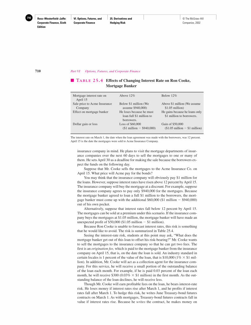
Ross−Westerfield−Jaffe: Corporate Finance, Sixth Edition
VI. Options, Futures, and Corporate Finance
25. Derivatives and Hedging Risk
716 © The McGraw−Hill Companies, 2002
insurance company in mind. He plans to visit the mortgage departments of insur-ance companies over the next 60 days to sell the mortgages to one or many ofthem. He sets April 30 as a deadline for making the sale because the borrowers ex-pect the funds on the following day.
Suppose that Mr. Cooke sells the mortgages to the Acme Insurance Co. onApril 15. What price will Acme pay for the bonds?
You may think that the insurance company will obviously pay $1 million forthe loans. However, suppose interest rates have risen above 12 percent by April 15.The insurance company will buy the mortgage at a discount. For example, supposethe insurance company agrees to pay only $940,000 for the mortgages. Becausethe mortgage banker agreed to loan a full $1 million to the borrowers, the mort-gage banker must come up with the additional $60,000 ($1 million � $940,000)out of his own pocket.
Alternatively, suppose that interest rates fall below 12 percent by April 15.The mortgages can be sold at a premium under this scenario. If the insurance com-pany buys the mortgages at $1.05 million, the mortgage banker will have made anunexpected profit of $50,000 ($1.05 million � $1 million).
Because Ron Cooke is unable to forecast interest rates, this risk is somethingthat he would like to avoid. The risk is summarized in Table 25.4.
Seeing the interest-rate risk, students at this point may ask, “What does themortgage banker get out of this loan to offset his risk-bearing?” Mr. Cooke wantsto sell the mortgages to the insurance company so that he can get two fees. Thefirst is an origination fee, which is paid to the mortgage banker from the insurancecompany on April 15, that is, on the date the loan is sold. An industry standard incertain locales is 1 percent of the value of the loan, that is $10,000 (1% � $1 mil-lion). In addition, Mr. Cooke will act as a collection agent for the insurance com-pany. For this service, he will receive a small portion of the outstanding balanceof the loan each month. For example, if he is paid 0.03 percent of the loan eachmonth, he will receive $300 (0.03% � $1 million) in the first month. As the out-standing balance of the loan declines, he will receive less.
Though Mr. Cooke will earn profitable fees on the loan, he bears interest-raterisk. He loses money if interest rates rise after March 1, and he profits if interestrates fall after March 1. To hedge this risk, he writes June Treasury-bond futurescontracts on March 1. As with mortgages, Treasury-bond futures contracts fall invalue if interest rates rise. Because he writes the contract, he makes money on
710 Part VI Options, Futures, and Corporate Finance
� TABLE 25.4 Effects of Changing Interest Rate on Ron Cooke,Mortgage Banker
Mortgage interest rate on Above 12% Below 12%April 15
Sale price to Acme Insurance Below $1 million (We Above $1 million (We assumeCompany assume $940,000) $1.05 million)
Effect on mortgage banker He loses because he must He gains because he loans only loan full $1 million to $1 million to borrowers.borrowers.
Dollar gain or loss Loss of $60,000 Gain of $50,000 ($1 million � $940,000) ($1.05 million � $1 million)
The interest rate on March 1, the date when the loan agreement was made with the borrowers, was 12 percent.April 15 is the date the mortgages were sold to Acme Insurance Company.

Ross−Westerfield−Jaffe: Corporate Finance, Sixth Edition
VI. Options, Futures, and Corporate Finance
25. Derivatives and Hedging Risk
717© The McGraw−Hill Companies, 2002
these contracts if they fall in value. Therefore, with an interest-rate rise, the losshe endures in the mortgages is offset by the gain he earns in the futures market.Conversely, Treasury-bond futures contracts rise in value if interest rates fall. Be-cause he writes the contracts, he suffers losses on them when rates fall. With an interest-rate fall, the profit he makes on the mortgages is offset by the loss he suf-fers in the futures markets.
The details of this hedging transaction are presented in Table 25.5. The col-umn on the left is labeled “Cash markets,” because the deal in the mortgage mar-ket is transacted off an exchange. The column on the right shows the offsettingtransactions in the futures market. Consider the first row. The mortgage banker en-ters into a forward contract on March 1. He simultaneously writes Treasury-bondfutures contracts. Ten contracts are written because the deliverable instrument oneach contract is $100,000 of Treasury bonds. The total is $1 million (10 �$100,000), which is equal to the value of the mortgages. Mr. Cooke would preferto write May Treasury-bond futures contracts. Here, Treasury bonds would be de-livered on the futures contract during the same month that the loan is funded. Be-cause there is no May T-bond futures contract, Mr. Cooke achieves the closestmatch through a June contract.
If held to maturity, the June contract would obligate the mortgage banker todeliver Treasury bonds in June. Interest-rate risk ends in the cash market when theloans are sold. Interest-rate risk must be terminated in the futures market at thattime. Thus, Mr. Cooke nets out his position in the futures contract as soon as theloan is sold to Acme Insurance.
Chapter 25 Derivatives and Hedging Risk 711
� TABLE 25.5 Illustration of Hedging Strategy for Ron Cooke,Mortgage Banker
Cash Markets Futures Markets
March 1 Mortgage banker makes forward Mortgage banker writes 10 June contracts to loan $1 million at Treasury-bond futures contracts.12 percent for 20 years. The loansare to be funded on May 1. No cash changes hands on March 1.
April 15 Loans are sold to Acme Insurance Mortgage banker buys back all Company. Mortgage banker will the futures contracts.receive sale price from Acme onthe May 1 funding date.
If interest rates rise: Loans are sold at a price below Each futures contract is bought $1 million. Mortgage banker back at a price below the sales loses because he receives less price, resulting in profit.than the $1 million he must give Mortgage banker’s profit in to borrowers. futures market offsets loss in
cash market.If interest rates fall: Loans are sold at a price above Each futures contract is bought
$1 million. Mortgage banker back at a price above the sales gains because he receives more price, resulting in loss.than the $1 million he must give Mortgage banker’s loss in to borrowers. futures market offsets gain in
cash market.
Ross−Westerfield−Jaffe: Corporate Finance, Sixth Edition
VI. Options, Futures, and Corporate Finance
25. Derivatives and Hedging Risk
718 © The McGraw−Hill Companies, 2002
Risk is clearly reduced via an offsetting transaction in the futures market. However, isrisk totally eliminated? Risk would be totally eliminated if losses in the cash markets wereexactly offset in the futures markets and vice versa. This is unlikely to happen because mort-gages and Treasury bonds are not identical instruments. First, mortgages may have differ-ent maturities than Treasury bonds. Second, Treasury bonds have a different paymentstream than do mortgages. Principal is only paid at maturity on T-bonds, whereas principalis paid every month on mortgages. Because mortgages pay principal continuously, these in-struments have a shorter effective time to maturity than do Treasury bonds of equal matu-rity.14 Third, mortgages have default risk whereas Treasury bonds do not. The term struc-ture applicable to instruments with default risk may change even when the term structurefor risk-free assets remains constant. Fourth, mortgages may be paid off early and hencehave a shorter expected maturity than Treasury bonds of equal maturity.
Because mortgages and Treasury bonds are not identical instruments, they are not iden-tically affected by interest rates. If Treasury bonds are less volatile than mortgages, finan-cial consultants may advise Mr. Cooke to write more than 10 T-bond futures contracts.Conversely, if these bonds are more volatile, the consultant may state that less than 10 fu-tures contracts are indicated. An optimal ratio of futures to mortgages will reduce risk asmuch as possible. However, because the price movements of mortgages and Treasury bondsare not perfectly correlated, Mr. Cooke’s hedging strategy cannot eliminate all risk.
The above strategy is called a short hedge because Mr. Cooke sells futures contracts inorder to reduce risk. Though it involves an interest-rate futures contract, this short hedge isanalogous to short hedges in agricultural and metallurgical futures contracts. We argued atthe beginning of this chapter that individuals and firms institute short hedges to offset in-ventory price fluctuation. Once Mr. Cooke makes a contract to loan money to borrowers,the mortgages effectively become his inventory. He writes a futures contract to offset theprice fluctuation of his inventory.
We now consider an example where a mortgage banker institutes a long hedge.
EXAMPLE
Margaret Boswell is another mortgage banker. Her firm faces problems similar tothose facing Mr. Cooke’s firm. However, she tackles the problems through the useof advance commitments, a strategy the opposite of Mr. Cooke’s. That is, shepromises to deliver loans to a financial institution before she lines up borrowers. OnMarch 1, her firm agreed to sell mortgages to No-State Insurance Co. The agree-ment specifies that she must turn over 12-percent coupon mortgages with a facevalue of $1 million to No-State by May 1. No-State is buying the mortgages at par,implying that they will pay Ms. Boswell $1 million on May 1. As of March 1, Ms.Boswell had not signed up any borrowers. Over the next two months, she will seekout individuals who want mortgages beginning May 1.
As with Mr. Cooke, changing interest rates will affect Ms. Boswell. If inter-est rates fall before she signs up a borrower, the borrower will demand a premiumon a 12-percent coupon loan. That is, the borrower will receive more than par onMay 1.15 Because Ms. Boswell receives par from the insurance company, she mustmake up the difference.
712 Part VI Options, Futures, and Corporate Finance
14Alternatively, we can say that mortgages have shorter duration than do Treasury bonds of equal maturity. Aprecise definition of duration is provided later in this chapter.15Alternatively, the mortgage would still be at par if a coupon rate below 12 percent were used. However, this isnot done since the insurance company only wants to buy 12-percent mortgages.

Ross−Westerfield−Jaffe: Corporate Finance, Sixth Edition
VI. Options, Futures, and Corporate Finance
25. Derivatives and Hedging Risk
719© The McGraw−Hill Companies, 2002
Conversely, if interest rates rise, a 12-percent coupon loan will be made at a dis-count. That is, the borrower will receive less than par on May 1. Because Ms.Boswell receives par from the insurance company, the difference is pure profit to her.
The details are provided in the left-hand column of Table 25.6. As did Mr.Cooke, Ms. Boswell finds the risk burdensome. Therefore, she offsets her advancecommitment with a transaction in the futures markets. Because she loses in thecash market when interest rates fall, she buys futures contracts to reduce the risk.When interest rates fall, the value of her futures contracts increases. The gain inthe futures market offsets the loss in the cash market. Conversely, she gains in thecash markets when interest rates rise. The value of her futures contracts decreaseswhen interest rates rise, offsetting her gain.
We call this a long hedge because Ms. Boswell offsets risk in the cash mar-kets by buying a futures contract. Though it involves an interest-rate futures con-tract, this long hedge is analogous to long hedges in agricultural and metallurgicalfutures contracts. We argued at the beginning of this chapter that individuals andfirms institute long hedges when their finished goods are to be sold at a fixed price.Once Ms. Boswell makes the advance commitment with No-State Insurance, shehas fixed her sales price. She buys a futures contract to offset the price fluctuationof her raw materials, that is, her mortgages.
Chapter 25 Derivatives and Hedging Risk 713
� TABLE 25.6 Illustration of Advance Commitment for Margaret Boswell, Mortgage Banker
Cash Markets Futures Markets
March 1 Mortgage banker makes a forward Mortgage banker buys 10 June contract (advance commitment) Treasury-bond futures contracts.to deliver $1 million of mortgages to No-State Insurance. The insurance company will pay par to Ms. Boswell for the loans on May 1. The borrowers are to receive their funding from mortgage banker on May 1. The mortgages are to be 12-percent coupon loans for 20 years.
April 15 Mortgage banker signs up borrowers Mortgage banker sells all futures to 12-percent coupon, 20-year contracts.mortgages. She promises that the borrowers will receive funds on May 1.
If interest rates rise: Mortgage banker issues mortgages to Futures contract is sold at a price borrowers at a discount. Mortgage below purchase price, resulting banker gains because she receives in loss. Mortgage banker’s loss par from insurance company. in futures market offsets gain in
cash market.If interest rates fall: Loans to borrowers are issued at a Futures contract is sold at a price
premium. Mortgage banker loses above purchase price, resulting because she receives only par in gain. Mortgage banker’s gain from insurance company. in futures market offsets loss in
cash market.
Ross−Westerfield−Jaffe: Corporate Finance, Sixth Edition
VI. Options, Futures, and Corporate Finance
25. Derivatives and Hedging Risk
720 © The McGraw−Hill Companies, 2002
• How are forward contracts on bonds priced?• What are the differences between forward contracts on bonds and futures contracts on bonds?• Give examples of hedging with futures contracts on bonds.
25.5 DURATION HEDGING
The last section concerned the risk of interest-rate changes. We now want to explore thisrisk in a more precise manner. In particular, we want to show that the concept of durationis a prime determinant of interest-rate risk. We begin by considering the effect of interest-rate movements on bond prices.
The Case of Zero-Coupon BondsImagine a world where the interest rate is 10 percent across all maturities. A one-year purediscount bond pays $110 at maturity. A five-year pure discount bond pays $161.05 at ma-turity. Both of these bonds are worth $100, as given by16
Value of One-Year Pure Discount Bond:
Value of Five-Year Pure Discount Bond:
Which bond will change more when interest rates move? To find out, we calculate the value ofthese bonds when interest rates are either 8 or 12 percent. The results are presented in Table 25.7.As can be seen, the five-year bond has greater price swings than does the one-year bond. Thatis, both bonds are worth $100 when interest rates are 10 percent. The five-year bond is worthmore than the one-year bond when interest rates are 8 percent and worth less than the one-yearbond when interest rates are 12 percent. We state that the five-year bond is subject to more pricevolatility. This point, which was mentioned in passing in an earlier section of the chapter, is notdifficult to understand. The interest-rate term in the denominator, 1 � r, is taken to the fifth powerfor a five-year bond and only to the first power for the one-year bond. Thus, the effect of a chang-ing interest rate is magnified for the five-year bond. The general rule is
The percentage price changes in long-term pure discount bonds are greater than the percentageprice changes in short-term pure discount bonds.
The Case of Two Bonds with the Same Maturity but with Different CouponsThe previous example concerned pure discount bonds of different maturities. We now wantto see the effect of different coupons on price volatility. To abstract from the effect of dif-fering maturities, we consider two bonds with the same maturity but with different coupons.
$100 �$161.05�1.10� 5
$100 �$110
1.10
QUESTIONS
CO
NC
EP
T
?
714 Part VI Options, Futures, and Corporate Finance
16Alternatively, we could have chosen bonds that pay $100 at maturity. Their values would be $90.91($100/1.10) and $62.09 [$100/(1.10)5]. However, our comparisons to come are made easier if both have thesame initial price.
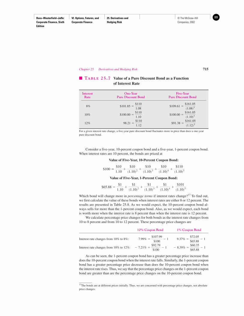
Ross−Westerfield−Jaffe: Corporate Finance, Sixth Edition
VI. Options, Futures, and Corporate Finance
25. Derivatives and Hedging Risk
721© The McGraw−Hill Companies, 2002
Consider a five-year, 10-percent coupon bond and a five-year, 1-percent coupon bond.When interest rates are 10 percent, the bonds are priced at
Value of Five-Year, 10-Percent Coupon Bond:
Value of Five-Year, 1-Percent Coupon Bond:
Which bond will change more in percentage terms if interest rates change?17 To find out,we first calculate the value of these bonds when interest rates are either 8 or 12 percent. Theresults are presented in Table 25.8. As we would expect, the 10-percent coupon bond al-ways sells for more than the 1-percent coupon bond. Also, as we would expect, each bondis worth more when the interest rate is 8 percent than when the interest rate is 12 percent.
We calculate percentage price changes for both bonds as the interest rate changes from10 to 8 percent and from 10 to 12 percent. These percentage price changes are
10% Coupon Bond 1% Coupon Bond
Interest rate changes from 10% to 8%:
Interest rate changes from 10% to 12%:
As can be seen, the 1-percent coupon bond has a greater percentage price increase thandoes the 10-percent coupon bond when the interest rate falls. Similarly, the 1-percent couponbond has a greater percentage price decrease than does the 10-percent coupon bond whenthe interest rate rises. Thus, we say that the percentage price changes on the 1-percent couponbond are greater than are the percentage price changes on the 10-percent coupon bond.
� 8.39% �$60.35
$65.88� 1� 7.21% �
$92.79
$100� 1
9.37% �$72.05
$65.88� 17.99% �
$107.99
$100� 1
$65.88 �$1
1.10�
$1�1.10� 2 �
$1�1.10� 3 �
$1�1.10� 4 �
$101�1.10� 5
$100 �$10
1.10�
$10�1.10� 2 �
$10�1.10� 3 �
$10�1.10� 4 �
$110�1.10� 5
Chapter 25 Derivatives and Hedging Risk 715
� TABLE 25.7 Value of a Pure Discount Bond as a Function of Interest Rate
Interest One-Year Five-YearRate Pure Discount Bond Pure Discount Bond
8%
10%
12%
For a given interest rate change, a five-year pure discount bond fluctuates more in price than does a one-yearpure discount bond.
$91.38 �$161.05�1.12� 598.21 �
$110
1.12
$100.00 �$161.05�1.10� 5$100.00 �
$110
1.10
$109.61 �$161.05�1.08� 5$101.85 �
$110
1.08
17The bonds are at different prices initially. Thus, we are concerned with percentage price changes, not absoluteprice changes.
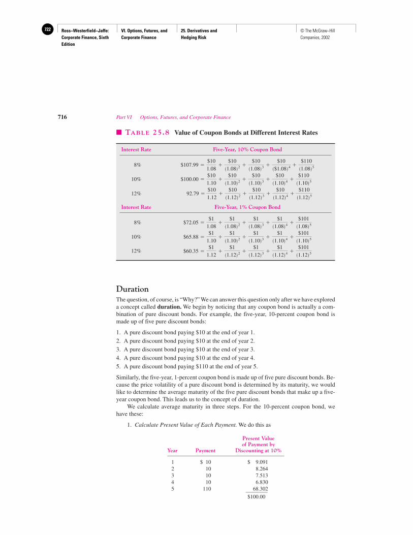
Ross−Westerfield−Jaffe: Corporate Finance, Sixth Edition
VI. Options, Futures, and Corporate Finance
25. Derivatives and Hedging Risk
722 © The McGraw−Hill Companies, 2002
DurationThe question, of course, is “Why?” We can answer this question only after we have exploreda concept called duration. We begin by noticing that any coupon bond is actually a com-bination of pure discount bonds. For example, the five-year, 10-percent coupon bond ismade up of five pure discount bonds:
1. A pure discount bond paying $10 at the end of year 1.
2. A pure discount bond paying $10 at the end of year 2.
3. A pure discount bond paying $10 at the end of year 3.
4. A pure discount bond paying $10 at the end of year 4.
5. A pure discount bond paying $110 at the end of year 5.
Similarly, the five-year, 1-percent coupon bond is made up of five pure discount bonds. Be-cause the price volatility of a pure discount bond is determined by its maturity, we wouldlike to determine the average maturity of the five pure discount bonds that make up a five-year coupon bond. This leads us to the concept of duration.
We calculate average maturity in three steps. For the 10-percent coupon bond, wehave these:
1. Calculate Present Value of Each Payment. We do this as
Present Valueof Payment by
Year Payment Discounting at 10%
1 $ 10 $ 9.0912 10 8.2643 10 7.5134 10 6.8305 110 68.302________
$100.00
716 Part VI Options, Futures, and Corporate Finance
� TABLE 25.8 Value of Coupon Bonds at Different Interest Rates
Interest Rate Five-Year, 10% Coupon Bond
8%
10%
12%
Interest Rate Five-Year, 1% Coupon Bond
8%
10%
12% $60.35 �$1
1.12�
$1�1.12� 2 �
$1�1.12� 3 �
$1�1.12� 4 �
$101�1.12� 5
$65.88 �$1
1.10�
$1�1.10� 2 �
$1�1.10� 3 �
$1�1.10� 4 �
$101�1.10� 5
$72.05 �$1
1.08�
$1�1.08� 2 �
$1�1.08� 3 �
$1�1.08� 4 �
$101�1.08� 5
92.79 �$10
1.12�
$10�1.12� 2 �
$10�1.12� 3 �
$10�1.12� 4 �
$110�1.12� 5
$100.00 �$10
1.10�
$10�1.10� 2 �
$10�1.10� 3 �
$10�1.10� 4 �
$110�1.10� 5
$107.99 �$10
1.08�
$10�1.08� 2 �
$10�1.08� 3 �
$10�$1.08� 4 �
$110�1.08� 5
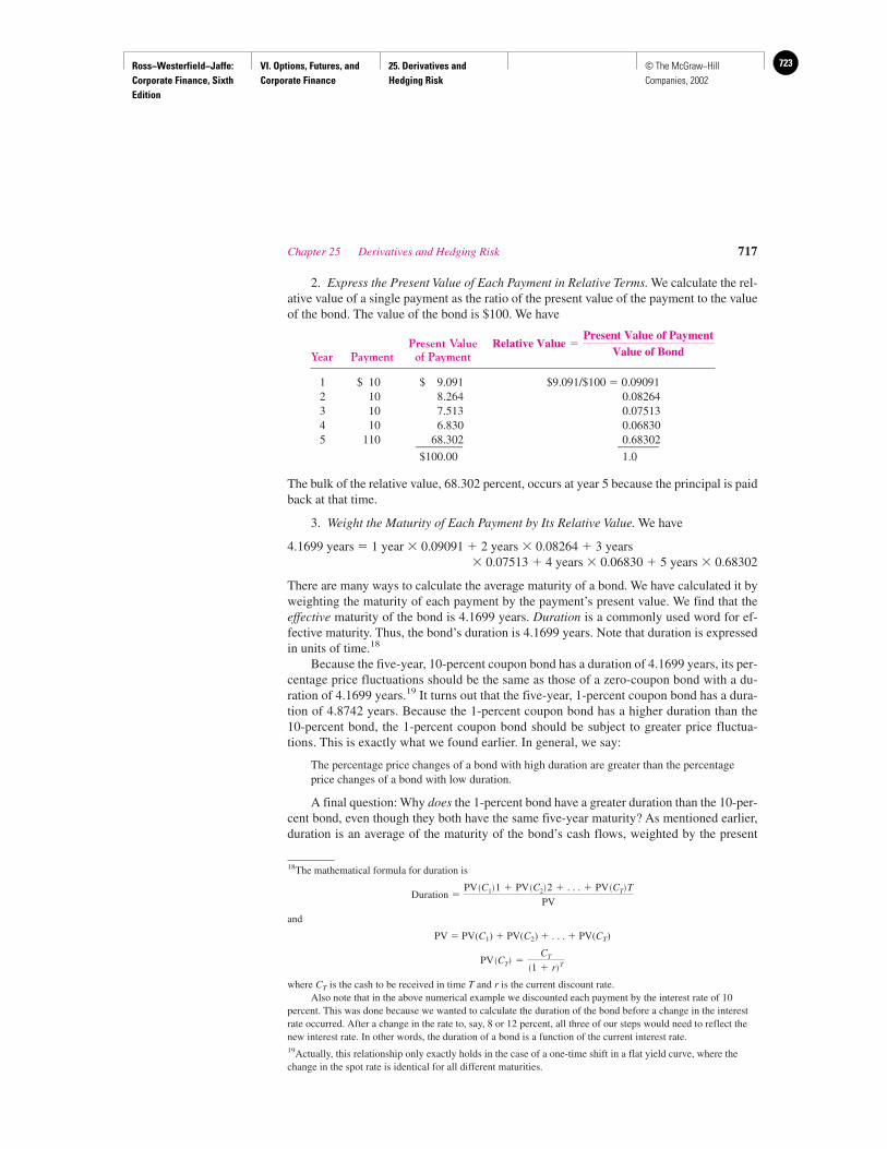
Ross−Westerfield−Jaffe: Corporate Finance, Sixth Edition
VI. Options, Futures, and Corporate Finance
25. Derivatives and Hedging Risk
723© The McGraw−Hill Companies, 2002
2. Express the Present Value of Each Payment in Relative Terms. We calculate the rel-ative value of a single payment as the ratio of the present value of the payment to the valueof the bond. The value of the bond is $100. We have
Present ValueYear Payment of Payment
1 $ 10 $ 9.091 $9.091/$100 � 0.090912 10 8.264 0.082643 10 7.513 0.075134 10 6.830 0.068305 110 68.302 0.68302________ _______
$100.00 1.0
The bulk of the relative value, 68.302 percent, occurs at year 5 because the principal is paidback at that time.
3. Weight the Maturity of Each Payment by Its Relative Value. We have
4.1699 years � 1 year � 0.09091 � 2 years � 0.08264 � 3 years � 0.07513 � 4 years � 0.06830 � 5 years � 0.68302
There are many ways to calculate the average maturity of a bond. We have calculated it byweighting the maturity of each payment by the payment’s present value. We find that theeffective maturity of the bond is 4.1699 years. Duration is a commonly used word for ef-fective maturity. Thus, the bond’s duration is 4.1699 years. Note that duration is expressedin units of time.18
Because the five-year, 10-percent coupon bond has a duration of 4.1699 years, its per-centage price fluctuations should be the same as those of a zero-coupon bond with a du-ration of 4.1699 years.19 It turns out that the five-year, 1-percent coupon bond has a dura-tion of 4.8742 years. Because the 1-percent coupon bond has a higher duration than the10-percent bond, the 1-percent coupon bond should be subject to greater price fluctua-tions. This is exactly what we found earlier. In general, we say:
The percentage price changes of a bond with high duration are greater than the percentageprice changes of a bond with low duration.
A final question: Why does the 1-percent bond have a greater duration than the 10-per-cent bond, even though they both have the same five-year maturity? As mentioned earlier,duration is an average of the maturity of the bond’s cash flows, weighted by the present
Relative Value �Present Value of Payment
Value of Bond
Chapter 25 Derivatives and Hedging Risk 717
18The mathematical formula for duration is
and
PV � PV(C1) � PV(C2) � . . . � PV(CT)
where CT is the cash to be received in time T and r is the current discount rate.Also note that in the above numerical example we discounted each payment by the interest rate of 10
percent. This was done because we wanted to calculate the duration of the bond before a change in the interestrate occurred. After a change in the rate to, say, 8 or 12 percent, all three of our steps would need to reflect thenew interest rate. In other words, the duration of a bond is a function of the current interest rate.19Actually, this relationship only exactly holds in the case of a one-time shift in a flat yield curve, where thechange in the spot rate is identical for all different maturities.
PV �CT� �CT
�1 � r�T
Duration �PV �C1�1 � PV �C2�2 � . . . � PV �CT�T
PV
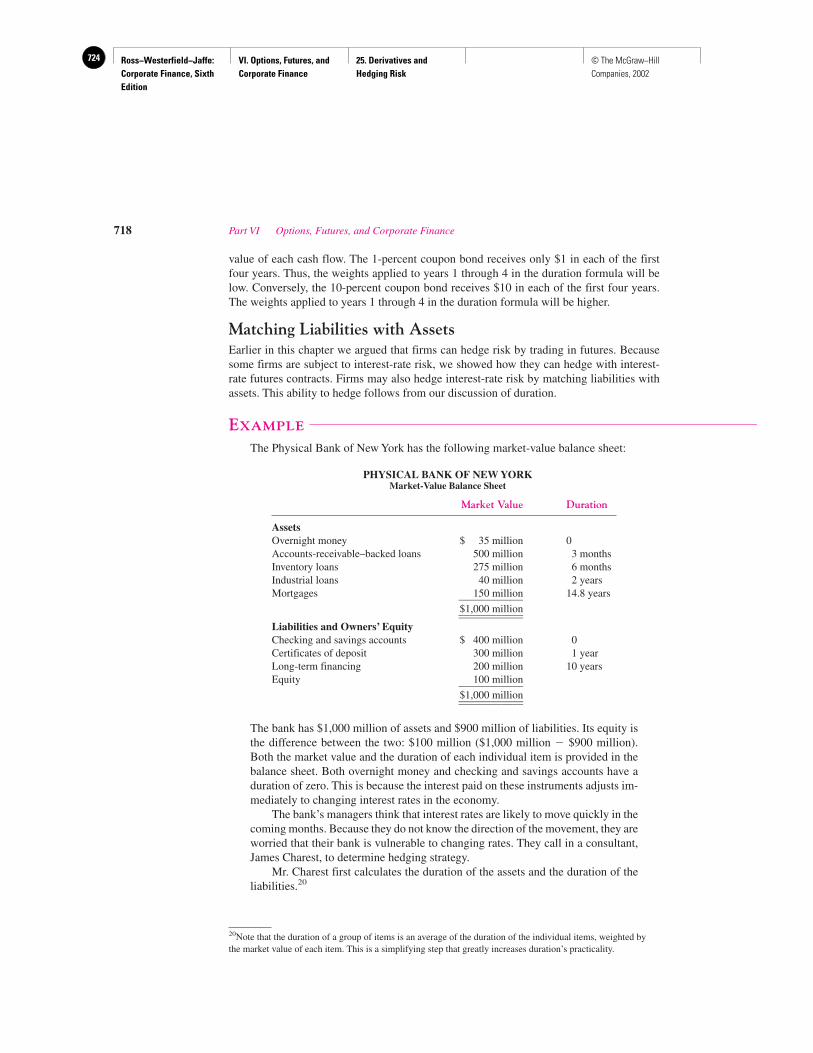
Ross−Westerfield−Jaffe: Corporate Finance, Sixth Edition
VI. Options, Futures, and Corporate Finance
25. Derivatives and Hedging Risk
724 © The McGraw−Hill Companies, 2002
value of each cash flow. The 1-percent coupon bond receives only $1 in each of the firstfour years. Thus, the weights applied to years 1 through 4 in the duration formula will below. Conversely, the 10-percent coupon bond receives $10 in each of the first four years.The weights applied to years 1 through 4 in the duration formula will be higher.
Matching Liabilities with AssetsEarlier in this chapter we argued that firms can hedge risk by trading in futures. Becausesome firms are subject to interest-rate risk, we showed how they can hedge with interest-rate futures contracts. Firms may also hedge interest-rate risk by matching liabilities withassets. This ability to hedge follows from our discussion of duration.
EXAMPLE
The Physical Bank of New York has the following market-value balance sheet:
PHYSICAL BANK OF NEW YORKMarket-Value Balance Sheet
Market Value Duration
AssetsOvernight money $ 35 million 0Accounts-receivable–backed loans 500 million 3 monthsInventory loans 275 million 6 monthsIndustrial loans 40 million 2 yearsMortgages 150 million 14.8 years____________
$1,000 million________________________Liabilities and Owners’ EquityChecking and savings accounts $ 400 million 0Certificates of deposit 300 million 1 yearLong-term financing 200 million 10 yearsEquity 100 million____________
$1,000 million________________________
The bank has $1,000 million of assets and $900 million of liabilities. Its equity isthe difference between the two: $100 million ($1,000 million � $900 million).Both the market value and the duration of each individual item is provided in thebalance sheet. Both overnight money and checking and savings accounts have aduration of zero. This is because the interest paid on these instruments adjusts im-mediately to changing interest rates in the economy.
The bank’s managers think that interest rates are likely to move quickly in thecoming months. Because they do not know the direction of the movement, they areworried that their bank is vulnerable to changing rates. They call in a consultant,James Charest, to determine hedging strategy.
Mr. Charest first calculates the duration of the assets and the duration of theliabilities.20
718 Part VI Options, Futures, and Corporate Finance
20Note that the duration of a group of items is an average of the duration of the individual items, weighted bythe market value of each item. This is a simplifying step that greatly increases duration’s practicality.
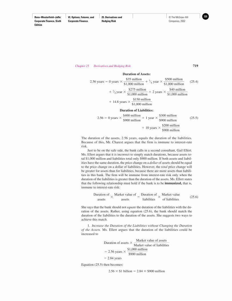
Ross−Westerfield−Jaffe: Corporate Finance, Sixth Edition
VI. Options, Futures, and Corporate Finance
25. Derivatives and Hedging Risk
725© The McGraw−Hill Companies, 2002
Duration of Assets:
(25.4)
Duration of Liabilities:
(25.5)
The duration of the assets, 2.56 years, equals the duration of the liabilities. Because of this, Mr. Charest argues that the firm is immune to interest-raterisk.
Just to be on the safe side, the bank calls in a second consultant, Gail Ellert.Ms. Ellert argues that it is incorrect to simply match durations, because assets to-tal $1,000 million and liabilities total only $900 million. If both assets and liabil-ities have the same duration, the price change on a dollar of assets should be equalto the price change on a dollar of liabilities. However, the total price change willbe greater for assets than for liabilities, because there are more assets than liabili-ties in this bank. The firm will be immune from interest-rate risk only when theduration of the liabilities is greater than the duration of the assets. Ms. Ellert statesthat the following relationship must hold if the bank is to be immunized, that is,immune to interest-rate risk:
(25.6)
She says that the bank should not equate the duration of the liabilities with the du-ration of the assets. Rather, using equation (25.6), the bank should match the duration of the liabilities to the duration of the assets. She suggests two ways toachieve this match.
1. Increase the Duration of the Liabilities without Changing the Durationof the Assets. Ms. Ellert argues that the duration of the liabilities could be increased to
� 2.84 years
Equation (25.5) then becomes:
2.56 � $1 billion � 2.84 � $900 million
� 2.56 years �$1,000 million
$900 million
Duration of assets �Market value of assets
Market value of liabilities
Duration of
assets�
Market value of
assets�
Duration of
liabilities�
Market value
of liabilities
� 10 years �$200 million
$900 million
2.56 � 0 years �$400 million
$900 million� 1 year �
$300 million
$900 million
� 14.8 years �$150 million
$1,000 million
� 1⁄2 year �$275 million
$1,000 million� 2 years �
$40 million
$1,000 million
2.56 years � 0 years �$35 million
$1,000 million� 1⁄4 year �
$500 million
$1,000 million
Chapter 25 Derivatives and Hedging Risk 719
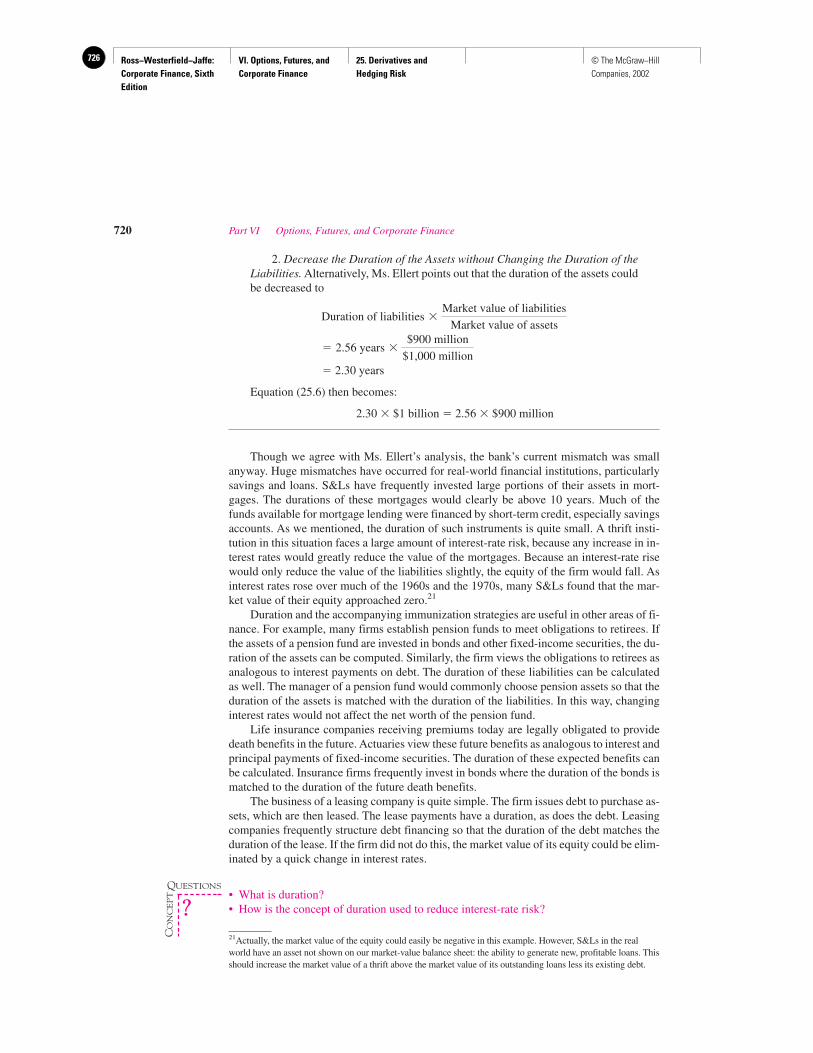
Ross−Westerfield−Jaffe: Corporate Finance, Sixth Edition
VI. Options, Futures, and Corporate Finance
25. Derivatives and Hedging Risk
726 © The McGraw−Hill Companies, 2002
2. Decrease the Duration of the Assets without Changing the Duration of theLiabilities. Alternatively, Ms. Ellert points out that the duration of the assets couldbe decreased to
� 2.30 years
Equation (25.6) then becomes:
2.30 � $1 billion � 2.56 � $900 million
Though we agree with Ms. Ellert’s analysis, the bank’s current mismatch was smallanyway. Huge mismatches have occurred for real-world financial institutions, particularlysavings and loans. S&Ls have frequently invested large portions of their assets in mort-gages. The durations of these mortgages would clearly be above 10 years. Much of thefunds available for mortgage lending were financed by short-term credit, especially savingsaccounts. As we mentioned, the duration of such instruments is quite small. A thrift insti-tution in this situation faces a large amount of interest-rate risk, because any increase in in-terest rates would greatly reduce the value of the mortgages. Because an interest-rate risewould only reduce the value of the liabilities slightly, the equity of the firm would fall. Asinterest rates rose over much of the 1960s and the 1970s, many S&Ls found that the mar-ket value of their equity approached zero.21
Duration and the accompanying immunization strategies are useful in other areas of fi-nance. For example, many firms establish pension funds to meet obligations to retirees. Ifthe assets of a pension fund are invested in bonds and other fixed-income securities, the du-ration of the assets can be computed. Similarly, the firm views the obligations to retirees asanalogous to interest payments on debt. The duration of these liabilities can be calculatedas well. The manager of a pension fund would commonly choose pension assets so that theduration of the assets is matched with the duration of the liabilities. In this way, changinginterest rates would not affect the net worth of the pension fund.
Life insurance companies receiving premiums today are legally obligated to providedeath benefits in the future. Actuaries view these future benefits as analogous to interest andprincipal payments of fixed-income securities. The duration of these expected benefits canbe calculated. Insurance firms frequently invest in bonds where the duration of the bonds ismatched to the duration of the future death benefits.
The business of a leasing company is quite simple. The firm issues debt to purchase as-sets, which are then leased. The lease payments have a duration, as does the debt. Leasingcompanies frequently structure debt financing so that the duration of the debt matches theduration of the lease. If the firm did not do this, the market value of its equity could be elim-inated by a quick change in interest rates.
• What is duration?• How is the concept of duration used to reduce interest-rate risk?
� 2.56 years �$900 million
$1,000 million
Duration of liabilities �Market value of liabilities
Market value of assets
720 Part VI Options, Futures, and Corporate Finance
21Actually, the market value of the equity could easily be negative in this example. However, S&Ls in the realworld have an asset not shown on our market-value balance sheet: the ability to generate new, profitable loans. Thisshould increase the market value of a thrift above the market value of its outstanding loans less its existing debt.
QUESTIONS
CO
NC
EP
T
?
Ross−Westerfield−Jaffe: Corporate Finance, Sixth Edition
VI. Options, Futures, and Corporate Finance
25. Derivatives and Hedging Risk
727© The McGraw−Hill Companies, 2002
25.6 SWAPS CONTRACTS
Swaps are close cousins to forwards and futures contracts. Swaps are arrangements be-tween two counterparts to exchange cash flows over time. There is enormous flexibility inthe forms that swaps can take, but the two basic types are interest-rate swaps or currencyswaps. Often these are combined when interest received in one currency is swapped for in-terest in another currency.
Interest-Rate SwapsLike other derivatives, swaps are tools that firms can use to easily change their risk exposuresand their balance sheets.22 Consider a firm that has borrowed and carried on its books an ob-ligation to repay a 10-year loan for $100 million of principal with a 9-percent coupon rate paidannually. Ignoring the possibility of calling the loan, the firm expects to have to pay couponsof $9 million every year for 10 years and a balloon payment of $100 million at the end of the10 years. Suppose, though, that the firm is uncomfortable with having this large fixed obliga-tion on its books. Perhaps the firm is in a cyclical business where its revenues vary and could,conceivably, fall to a point where it would be difficult to make the debt payment.
Suppose, too, that the firm earns a lot of its revenue from financing the purchase of itsproducts. Typically, for example, a manufacturer might help its customers finance their pur-chase of its products through a leasing or credit subsidiary. Usually these loans are for rel-atively short time periods and are financed at some premium over the prevailing short-termrate of interest. This puts the firm in the position of having revenues that move up and downwith interest rates while its costs are relatively fixed.
This is a classic situation where a swap can be used to offset the risk. When interestrates rise, the firm would have to pay more on the loan, but it would be making more on itsproduct financing. What the firm would really prefer is to have a floating-rate loan ratherthan a fixed-rate loan. It can use a swap to accomplish this.
Of course, the firm could also just go into the capital markets and borrow $100 millionat a variable interest rate and then use the proceeds to retire its outstanding fixed-rate loan.While this is possible, it is generally quite expensive, requiring underwriting a new loan andthe repurchase of the existing loan. The ease of entering into a swap is its inherent advantage.
The particular swap would be one that exchanged its fixed obligation for an agreementto pay a floating rate. Every six months it would agree to pay a coupon based on whateverthe prevailing interest rate was at the time in exchange for an agreement from a counter-party to pay the firm’s fixed coupon.
A common reference point for floating-rate commitments is called LIBOR. LIBORstands for the London Interbank Offered Rate, and it is the rate that most international bankscharge one another for dollar-denominated loans in the London market. LIBOR is com-monly used as the reference rate for a floating-rate commitment, and, depending on thecreditworthiness of the borrower, the rate can vary from LIBOR to LIBOR plus one pointor more over LIBOR.
If we assume that our firm has a credit rating that requires it to pay LIBOR plus 50 basispoints, then in a swap it would be exchanging its fixed 9-percent obligation for the obligationto pay whatever the prevailing LIBOR rate is plus 50 basis points. Figure 25.2 displays howthe cash flows on this swap would work. In the figure we have assumed that LIBOR starts at8 percent and rises for four years to 11 percent and then drops to 7 percent. As the figure
Chapter 25 Derivatives and Hedging Risk 721
22Under current accounting rules, most derivatives do not usually show up on firms’ balance sheets since theydo not have an historical cost (i.e., the amount a dealer would pay on the initial transaction day).
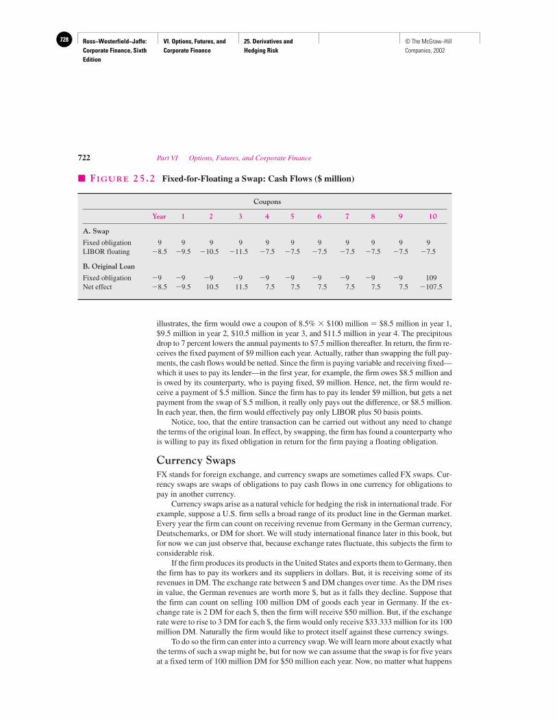
Ross−Westerfield−Jaffe: Corporate Finance, Sixth Edition
VI. Options, Futures, and Corporate Finance
25. Derivatives and Hedging Risk
728 © The McGraw−Hill Companies, 2002
illustrates, the firm would owe a coupon of 8.5% � $100 million � $8.5 million in year 1,$9.5 million in year 2, $10.5 million in year 3, and $11.5 million in year 4. The precipitousdrop to 7 percent lowers the annual payments to $7.5 million thereafter. In return, the firm re-ceives the fixed payment of $9 million each year. Actually, rather than swapping the full pay-ments, the cash flows would be netted. Since the firm is paying variable and receiving fixed—which it uses to pay its lender—in the first year, for example, the firm owes $8.5 million andis owed by its counterparty, who is paying fixed, $9 million. Hence, net, the firm would re-ceive a payment of $.5 million. Since the firm has to pay its lender $9 million, but gets a netpayment from the swap of $.5 million, it really only pays out the difference, or $8.5 million.In each year, then, the firm would effectively pay only LIBOR plus 50 basis points.
Notice, too, that the entire transaction can be carried out without any need to changethe terms of the original loan. In effect, by swapping, the firm has found a counterparty whois willing to pay its fixed obligation in return for the firm paying a floating obligation.
Currency SwapsFX stands for foreign exchange, and currency swaps are sometimes called FX swaps. Cur-rency swaps are swaps of obligations to pay cash flows in one currency for obligations topay in another currency.
Currency swaps arise as a natural vehicle for hedging the risk in international trade. Forexample, suppose a U.S. firm sells a broad range of its product line in the German market.Every year the firm can count on receiving revenue from Germany in the German currency,Deutschemarks, or DM for short. We will study international finance later in this book, butfor now we can just observe that, because exchange rates fluctuate, this subjects the firm toconsiderable risk.
If the firm produces its products in the United States and exports them to Germany, thenthe firm has to pay its workers and its suppliers in dollars. But, it is receiving some of itsrevenues in DM. The exchange rate between $ and DM changes over time. As the DM risesin value, the German revenues are worth more $, but as it falls they decline. Suppose thatthe firm can count on selling 100 million DM of goods each year in Germany. If the ex-change rate is 2 DM for each $, then the firm will receive $50 million. But, if the exchangerate were to rise to 3 DM for each $, the firm would only receive $33.333 million for its 100million DM. Naturally the firm would like to protect itself against these currency swings.
To do so the firm can enter into a currency swap. We will learn more about exactly whatthe terms of such a swap might be, but for now we can assume that the swap is for five yearsat a fixed term of 100 million DM for $50 million each year. Now, no matter what happens
722 Part VI Options, Futures, and Corporate Finance
� FIGURE 25.2 Fixed-for-Floating a Swap: Cash Flows ($ million)
Coupons
Year 1 2 3 4 5 6 7 8 9 10
A. Swap
Fixed obligation 9 9 9 9 9 9 9 9 9 9 9LIBOR floating �8.5 �9.5 �10.5 �11.5 �7.5 �7.5 �7.5 �7.5 �7.5 �7.5 �7.5
B. Original Loan
Fixed obligation �9 �9 �9 �9 �9 �9 �9 �9 �9 �9 109Net effect �8.5 �9.5 10.5 11.5 7.5 7.5 7.5 7.5 7.5 7.5 �107.5
Ross−Westerfield−Jaffe: Corporate Finance, Sixth Edition
VI. Options, Futures, and Corporate Finance
25. Derivatives and Hedging Risk
729© The McGraw−Hill Companies, 2002
to the exchange rate between DM and $ over the next five years, as long as the firm makes100 million DM each year from the sale of its products, it will swap this for $50 millioneach year.
We have not addressed the question of how the market sets prices for swaps, eitherinterest-rate swaps or currency swaps. In the fixed-for-floating example and in the cur-rency swap, we just quoted some terms. We won’t go into great detail on exactly how itis done, but we can stress the most important points.
Swaps, like forwards and futures, are essentially zero-sum transactions, which is to saythat in both cases the market sets prices at a fair level, and neither party has any substantialbargain or loss at the moment the deal is struck. For example, in the currency swap, the swaprate is some average of the market expectation of what the exchange rate will be over thelife of the swap. In the interest-rate swap, the rates are set as the fair floating and fixed ratesfor the creditor, taking into account the creditworthiness of the counterparties. We can ac-tually price swaps fairly once we know how to price forward contracts. In our interest-rateswap example, the firm swapped LIBOR plus 50 basis points for a 9-percent fixed rate, allon a principal amount of $100 million. This is equivalent to a series of forward contractsextending out the life of the swap. In year 1, for example, having made the swap, the firmis in the same position that it would be if it had sold a forward contract entitling the buyerto receive LIBOR plus 50 basis points on $100 million in return for a fixed payment of $9million (9 percent on $100 million). Similarly, the currency swap can also be viewed as aseries of forward contracts.
• Show that a currency swap is equivalent to a series of forward contracts.
ExoticsUp to now we have dealt with the meat and potatoes of the derivatives markets, swaps, op-tions, forwards, and futures. Exotics are the complicated blends of these that often producethe surprising results for the buyers.
One of the more interesting types of exotics is called an inverse floater. In our fixed-for-floating swap, the floating payments fluctuated with LIBOR. An inverse floater is onethat fluctuates inversely with some rate such as LIBOR. For example, the floater might payan interest rate of 20 percent minus LIBOR. IF LIBOR is 9 percent, then the inverse pays11 percent, and if LIBOR rises to 12 percent, the payments on the inverse would fall to 8percent. Clearly the purchaser of an inverse profits from the inverse if interest rates fall.
Both floaters and inverse floaters have a supercharged version called superfloaters andsuperinverses that fluctuate more than one for one with movements in interest rates. As anexample of a superinverse floater, consider a floater that pays an interest rate of 30 percentminus twice LIBOR. When LIBOR is 10 percent, the inverse pays
30% � 2 � 10% � 30% � 20% � 10%
and if LIBOR falls by 3 percent to 7 percent, then the return on the inverse rises by 6 per-cent from 10 percent to 16 percent,
30% � 2 � 7% � 30% � 14% � 16%
Sometimes derivatives are combined with options to bound the impact of interest rates. Themost important of these instruments are called caps and floors. A cap is so named becauseit puts an upper limit or a cap on the impact of a rise in interest rates. A floor, conversely,provides a floor below which the interest rate impact is insulated.
Chapter 25 Derivatives and Hedging Risk 723
QUESTION
CO
NC
EP
T
?
Ross−Westerfield−Jaffe: Corporate Finance, Sixth Edition
VI. Options, Futures, and Corporate Finance
25. Derivatives and Hedging Risk
730 © The McGraw−Hill Companies, 2002
To illustrate the impact of these, consider a firm that is borrowing short-term and isconcerned that interest rates might rise. For example, using LIBOR as the reference inter-est rate, the firm might purchase a 7 percent cap. The cap pays the firm the difference be-tween LIBOR and 7 percent on some principal amount, provided that LIBOR is greater than7 percent. As long as LIBOR is below 7 percent, the holder of the cap receives no payments.
By purchasing the cap the firm has assured itself that even if interest rates rise above 7 per-cent, it will not have to pay more than a 7 percent rate. Suppose that interest rates rise to 9 per-cent. While the firm is borrowing short-term and paying 9 percent rates, this is offset by the cap,which is paying the firm the difference between 9 percent and the 7 percent limit. For any LI-BOR rate above 7 percent, the firm receives the difference between LIBOR and 7 percent, and,as a consequence, it has capped its cost of borrowing at 7 percent.
On the other side, consider a financial firm that is in the business of lending short-termand is concerned that interest rates—and, consequently, its revenues—might fall. The firmcould purchase a floor to protect itself from such declines. If the limit on the floor is 7 per-cent, then the floor pays the difference between 7 percent and LIBOR whenever LIBOR isbelow 7 percent, and nothing if LIBOR is above 7 percent. Thus, if interest rates were tofall to, say, 5 percent while the firm is only receiving 5 percent from its lending activities,the floor is paying it the difference between 7 percent and 5 percent, or an additional 2 per-cent. By purchasing the floor, the firm has assured itself of receiving no less than 7 percentfrom the combination of the floor and its lending activities.
We have only scratched the surface of what is available in the world of derivatives.Derivatives are designed to meet marketplace needs, and the only binding limitation is thehuman imagination. Nowhere should the buyer’s warning caveat emptor be taken more se-riously than in the derivatives markets, and this is especially true for the exotics. If swapsare the meat and potatoes of the derivatives markets, then caps and floors are the meat andpotatoes of the exotics. As we have seen, they have obvious value as hedging instruments.But, much attention has been focused on truly exotic derivatives, some of which appear tohave arisen more as the residuals that were left over from more straightforward deals. Wewon’t examine these in any detail, but suffice it to say that some of these are so volatile andunpredictable that market participants have dubbed them “toxic waste.”
25.7 ACTUAL USE OF DERIVATIVES
Because derivatives do not usually appear in financial statements, it is much more difficultto observe the use of derivatives by firms when compared to, say, bank debt. Much of ourknowledge of corporate derivative use comes from academic surveys. Most surveys reportthat the use of derivatives appears to vary widespread among large publically traded firms.It appears that about one-half of all publically traded nonfinancial firms use derivatives ofsome kind.23 Large firms are far more likely to use derivatives than small firms. Table 25.9shows that for firms that use derivatives, foreign-currency and interest-rate derivatives arethe most frequently used.24
724 Part VI Options, Futures, and Corporate Finance
23Gordon M. Bodnar, Gregory S. Hayt, and Richard Marston, “1998 Wharton Survey of Finance RiskManagement by U.S. Non-Financial Firms,” Financial Management (Winter 1998).24Howton and Perfect report that interest rate derivatives are the most frequently used derivatives. Shawn D.Howton and Steven B. Perfect, “Currency and Interest-Rate Derivatives Use in U.S. Firms,” FinancialManagement (Winter 1998).
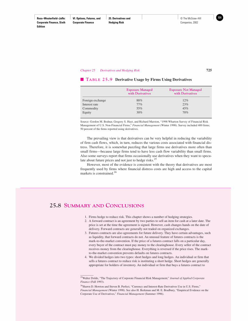
Ross−Westerfield−Jaffe: Corporate Finance, Sixth Edition
VI. Options, Futures, and Corporate Finance
25. Derivatives and Hedging Risk
731© The McGraw−Hill Companies, 2002
The prevailing view is that derivatives can be very helpful in reducing the variabilityof firm cash flows, which, in turn, reduces the various costs associated with financial dis-tress. Therefore, it is somewhat puzzling that large firms use derivatives more often thansmall firms—because large firms tend to have less cash flow variability than small firms.Also some surveys report that firms occasionally use derivatives when they want to specu-late about future prices and not just to hedge risks.25
However, most of the evidence is consistent with the theory that derivatives are mostfrequently used by firms where financial distress costs are high and access to the capitalmarkets is constrained.26
25.8 SUMMARY AND CONCLUSIONS
1. Firms hedge to reduce risk. This chapter shows a number of hedging strategies.2. A forward contract is an agreement by two parties to sell an item for cash at a later date. The
price is set at the time the agreement is signed. However, cash changes hands on the date ofdelivery. Forward contracts are generally not traded on organized exchanges.
3. Futures contracts are also agreements for future delivery. They have certain advantages, suchas liquidity, that forward contracts do not. An unusual feature of futures contracts is themark-to-the-market convention. If the price of a futures contract falls on a particular day,every buyer of the contract must pay money to the clearinghouse. Every seller of the contractreceives money from the clearinghouse. Everything is reversed if the price rises. The mark-to-the-market convention prevents defaults on futures contracts.
4. We divided hedges into two types: short hedges and long hedges. An individual or firm thatsells a futures contract to reduce risk is instituting a short hedge. Short hedges are generallyappropriate for holders of inventory. An individual or firm that buys a futures contract to
Chapter 25 Derivatives and Hedging Risk 725
� TABLE 25.9 Derivative Usage by Firms Using Derivatives
Exposure Managed Exposure Not Managedwith Derivatives with Derivatives
Foreign exchange 88% 12%Interest rate 77% 23%Commodity 55% 45%Equity 30% 70%
Source: Gordon M. Bodnar, Gregory S. Hayt, and Richard Marston, “1998 Wharton Survey of Financial RiskManagement of U.S. Non-Financial Firms,” Financial Management (Winter 1998). Survey included 400 firms;50 percent of the firms reported using derivatives.
25Walter Dolde, “The Trajectory of Corporate Financial Risk Management,” Journal of Applied CorporateFinance (Fall 1993).26Shawn D. Howton and Steven B. Perfect, “Currency and Interest-Rate Derivatives Use in U.S. Firms,”Financial Management (Winter 1998). See also H. Berkman and M. E. Bradbury, “Empirical Evidence on theCorporate Use of Derivatives,” Financial Management (Summer 1996).

Ross−Westerfield−Jaffe: Corporate Finance, Sixth Edition
VI. Options, Futures, and Corporate Finance
25. Derivatives and Hedging Risk
732 © The McGraw−Hill Companies, 2002
reduce risk is instituting a long hedge. Long hedges are typically used by firms with contractsto sell finished goods at a fixed price.
5. An interest-rate futures contract employs a bond as the deliverable instrument. Because oftheir popularity, we worked with Treasury-bond futures contracts. We showed that Treasury-bond futures contracts can be priced using the same type of net-present-value analysis that isused to price Treasury bonds themselves.
6. Many firms are faced with interest-rate risk. They can reduce this risk by hedging with interest-rate futures contracts. As with other commodities, a short hedge involves the sale of a futurescontract. Firms that are committed to buying mortgages or other bonds are likely to instituteshort hedges. A long hedge involves the purchase of a futures contract. Firms that have agreedto sell mortgages or other bonds at a fixed price are likely to institute long hedges.
7. Duration measures the average maturity of all the cash flows in a bond. Bonds with highduration have high price variability. Firms frequently try to match the duration of their assetswith the duration of their liabilities.
8. Swaps are agreements to exchange cash flows over time. The first major type is an interest-rate swap in which one pattern of coupon payments, say, fixed payments, is exchanged foranother, say, coupons that float with LIBOR. The second major type is a currency swap inwhich an agreement is struck to swap payments denominated in one currency for paymentsin another currency over time.
KEY TERMS
Advance commitments 712 Immunized 719Cash transaction 697 Interest-rate swaps 721Currency swaps 721 Long hedge 704Deliverable instrument 696 Making delivery 696Duration 716 Marked to the market 698Exotics 723 Short hedge 703Forward contract 696 Speculating 696Futures contract 697 Swaps 721Hedging 696 Taking delivery 696
SUGGESTED READINGS
Several cases that illustrate the concepts, tools, and markets for hedging can be found inTufano, Peter. “How Financial Engineering Can Advance Corporate Strategy.” Harvard
Business Review (January–February 1996).
An advanced article on the empirical implications of very recent models for pricing swapscontracts is inMinton, Bernadette A. “An Empirical Examination of Basic Valuation Models for Plain Vanilla
U.S. Interest Rate Swaps.” Journal of Financial Economics 44 (Winter 1997).
QUESTIONS AND PROBLEMS
Futures and Forward Contracts25.1 Define:
a. Forward contractb. Futures contract
25.2 Explain the three ways in which futures contracts and forward contracts differ.
726 Part VI Options, Futures, and Corporate Finance

Ross−Westerfield−Jaffe: Corporate Finance, Sixth Edition
VI. Options, Futures, and Corporate Finance
25. Derivatives and Hedging Risk
733© The McGraw−Hill Companies, 2002
25.3 The following table lists the closing prices for wheat futures contracts. Suppose youbought one contract at $5.00 at the opening of trade on March 15.
March 15 $5.03March 16 $5.08March 17 $5.12March 18 $5.10March 19 $4.98
a. Suppose that on March 18 you receive from your broker a notice of delivery on that day.i. What is the delivery price?
ii. What price did you pay for wheat?iii. List the cash flows associated with this contract.
b. Suppose that on March 19 you receive from your broker a notice of delivery on that day.i. What is the delivery price?
ii. What price did you pay for wheat?iii. List the cash flows associated with this contract.
25.4 Two days ago, you agreed to buy a 10-year, zero-coupon bond that would be issued in ayear. Today, both the 1-year and 11-year spot rates unexpectedly shifted downward anequal amount. What should today’s price of the forward contract be?
25.5 a. How is a short hedge created?b. In what type of situation is a short hedge a wise strategy?c. How is a long hedge created?d. In what type of situation is a long hedge a wise strategy?
25.6 A speculator is an investor who uses his or her private information to profit from futurescontracts. Mary Johnson is a speculator, who believes that wheat futures prices will fall ina month. What position would Mary Johnson take?
25.7 A classmate of yours recently entered the import/export business. During a visit with himlast week, he said to you, “If you play the game right, this is the safest business in theworld. By hedging all my transactions in the foreign-exchange futures market, I eliminateall risk.”
Do you agree with your friend’s assessment of hedging? Why or why not?
25.8 This morning you agreed to buy a two-year Treasury bond six months from today. Thebond carries a 10-percent coupon rate and has a $1,000 face. Below are listed the expectedspot rates of interest for the life of the bond. These rates are semiannual rates.
Time from Today Semiannual Rate
6 months 0.04812 months 0.05018 months 0.05224 months 0.05530 months 0.057
a. How much should you have paid for this forward contract?b. Suppose that shortly after you purchased the forward contract, all semiannual rates
increased 30 basis points; that is, the six-month rate increased from 0.048 to 0.051.i. State what you expect will happen to the value of the forward contract.
ii. What is the value of the forward contract?
25.9 Derive the relationship between the spot price (S0) and the futures price (F) by comparingthe following two strategies:
Strategy 1: Buy the silver at S0 today and hold it for one month.Strategy 2: Take a long position on the silver futures contract expiring in one month.Lend money that will be equal to the futures price in one month. The lending rate forthe period is the risk-free rate, rf.
Chapter 25 Derivatives and Hedging Risk 727

Ross−Westerfield−Jaffe: Corporate Finance, Sixth Edition
VI. Options, Futures, and Corporate Finance
25. Derivatives and Hedging Risk
734 © The McGraw−Hill Companies, 2002
25.10 Aiko Miyazawa is a Japanese student who is planning a one-year stay in America forstudying English. She expects to leave for America in eight months. Since she is worriedabout the unstable exchange rates, she has decided to lock in the current exchange rates.What should Aiko’s hedging position be?
25.11 After reading the text’s example about Ron Cooke, the mortgage banker, you decide toenter the business. You begin small; you agree to provide $300,000 to an old collegeroommate to finance the purchase of her home. The loan is a 20-year loan and has a 10-percent interest rate. Ten percent is the current market rate of interest. For ease ofcomputation, assume the mortgage payments are made annually. Your former roommateneeds the money four months from today. You do not have $300,000, but you intend tosell the mortgage to MAX Insurance Corp. The president of MAX is also an old friend,so you know with certainty that he will buy the mortgage. Unfortunately, he isunavailable to meet with you until three months from today.a. What is your former roommate’s mortgage payment?b. What is the most significant risk you face in this deal?c. How can you hedge this risk?
25.12 Refer to question 25.11. There are four-month T-bond futures available. A single contractis for $100,000 of T-bonds.a. Suppose that between today and your meeting with the president of MAX, the market
rate of interest rises to 12 percent.i. How much is MAX’s president willing to pay you for the mortgage?
ii. What will happen to the value of the T-bond futures contract?iii. What is your net gain or loss if you wrote a futures contract?
b. Suppose that between today and your meeting with the president of MAX, the marketrate of interest falls to 9 percent.
i. How much is MAX’s president willing to pay you for the mortgage?ii. What will happen to the value of the T-bond futures contract?
iii. What is your net gain or loss if you wrote a futures contract?
Duration25.13 Available are three zero-coupon, $1,000 face-value bonds. All of these bonds are initially
priced using an 11-percent interest rate. Bond A matures one year from today, bond Bmatures five years from today, and bond C matures 10 years from today.a. What is the current price of each bond?b. If the market rate of interest rises to 14 percent, what will be the prices of these bonds?c. Which bond experienced the greatest percentage change in price?
25.14 Calculate the duration of a perpetuity that pays $100 at each year-end. Assume the annualdiscount rate of 12 percent. What if the discount rate is 10 percent?
25.15 Consider two four-year bonds. Each bond has a $1,000 face value. Bond A’s coupon rateis 7 percent, while bond B’s coupon rate is 11 percent.a. What is the price of each bond when the market rate of interest is 10 percent?b. What is the price of each bond when the market rate of interest is 7 percent?c. Which bond experienced the greatest percentage change in price?d. Explain your (c) result.
25.16 Calculate the duration of a three-year, $1,000 face-value bond with a 9-percent couponrate, selling at par.
25.17 Calculate the duration of a four-year, $1,000 face-value bond with a 9-percent couponrate, selling at par.
25.18 Calculate the duration of a four-year, $1,000 face-value bond with a 5-percent couponrate, selling at par.
25.19 Mr. and Mrs. Chaikovski have a son who is going to enter a music college three yearsfrom today. Annual school expenses of $20,000 will occur at the beginning of each yearfor four years. What is the duration of Mr. and Mrs. Chaikovski’s liability as parents?Assume the annual borrowing rate of 15 percent.
728 Part VI Options, Futures, and Corporate Finance

Ross−Westerfield−Jaffe: Corporate Finance, Sixth Edition
VI. Options, Futures, and Corporate Finance
25. Derivatives and Hedging Risk
735© The McGraw−Hill Companies, 2002
25.20 The following balance sheet is for Besdall Community Bank.
Market Value Duration
AssetsFederal funds deposits $ 43 million 0Accounts-receivable loans 615 million 4 monthsShort-term loans 345 million 9 monthsLong-term loans 55 million 5 yearsMortgages 197 million 15 years
Liabilities and EquityChecking and savings deposits $490 million 0Certificates of deposit 370 million 18 monthsLong-term financing 250 million 10 yearsEquity 145 million
a. What is the duration of Besdall’s assets?b. What is the duration of Besdall’s liabilities?c. Is Besdall Community Bank immune from interest-rate risk?
25.21 Refer to the previous problem. To what values must the durations of Besdall CommunityBank change to make the bank immune from interest-rate risk ifa. Only the durations of the liabilities change?b. Only the durations of the assets change?
25.22 Consider the following balance sheet for California Commercial Bank.
CALIFORNIA COMMERCIAL BANKMarket Value Balance Sheet
Market Value($ million) Duration
AssetsOvernight money $ 100 0Loans 500 1 yearMortgages 1,200 12 years______
$1,800____________
Liabilities and EquityChecking and savings accounts $ 300 0Certificates of deposit 400 1.1 yearLong-term debt 500 18.9 yearsEquity 600______
$1,800____________
a. What is the duration of California’s assets? What is the duration of liabilities?b. Is the bank immunized from interest-rate risk?
Swaps25.23 The Miller Company and the Edwards Company both need to raise money to fund
facilities improvements at their manufacturing plants in New York. Miller has been inbusiness for 40 years and has a very good credit rating. It can borrow money at either 10percent or at the LIBOR � .03 percent floating rate. The Edwards Company hasexperienced some financial distress recently and does not have a strong credit history. Itcan borrow funds at 15 percent or 2 percent over the LIBOR rate.a. Is there an opportunity for the Miller Company and the Edwards Company to benefit
from a swap?b. Show how you would structure a swap transaction between Miller and Edwards.
Chapter 25 Derivatives and Hedging Risk 729
Ross−Westerfield−Jaffe: Corporate Finance, Sixth Edition
VII. Financial Planning and Short−Term Finance
Introduction736 © The McGraw−Hill Companies, 2002
Financial Planning andShort-Term Finance
PA
RT
VII
26 Corporate Financial Models and Long-Term Planning 73227 Short-Term Finance and Planning 74628 Cash Management 77129 Credit Management 798
FINANCIAL planning establishes the blueprint for change in a firm. It is necessary be-cause (1) it includes putting forth the firm’s goals to motivate the organization and
provide benchmarks for performance measurement, (2) the firm’s financing and invest-ment decisions are not independent and their interaction must be identified, and (3) thefirm must anticipate changing conditions and surprises.
Most of Chapter 26 is devoted to long-term financial planning. Long-term financialplanning incorporates decisions such as capital budgeting, capital structure, and divi-dend policy. An important part of Chapter 26 is the discussion of building corporate fi-nancial models. Here we introduce the concept of sustainable growth and show that afirm’s growth rate depends on its operating characteristics (profit margin and assetturnover) and financial policies (dividend policy and capital structure).
In Chapter 27 we introduce short-term financial planning, which involves short-livedassets and liabilities. We discuss two aspects of short-term financial planning: (1) the sizeof the firm’s investment in current assets, such as cash, accounts receivable, and inven-tory, and (2) how to finance short-term assets. We describe the primary tool for short-termfinancial planning, the cash budget. It incorporates the short-term financial goals of thefirm and tells the financial manager the amount of necessary short-term financing.
In Chapter 28 we describe the management of a firm’s investment in cash. The chap-ter divides cash management into three separate areas:
1. Determining the appropriate target cash balance.
2. Collecting and disbursing cash.
3. Investing the excess cash in marketable securities.
Chapter 29 describes what is involved when a firm makes the decision to grant credit toits customers. This decision involves three types of analysis:
1. A firm must decide on the conditions under which it sells its goods and services forcredit. These conditions are the terms of the sale.
2. Before granting credit, the firm must analyze the risk that the customer will not pay;this is called credit analysis.
3. After credit is extended, the firm must determine how to collect its cash.
Ross−Westerfield−Jaffe: Corporate Finance, Sixth Edition
VII. Financial Planning and Short−Term Finance
26. Corporate Financial Models and Long−Term Planning
737© The McGraw−Hill Companies, 2002
Corporate FinancialModels and Long-TermPlanning
CH
AP
TE
R26
EXECUTIVE SUMMARY
Financial planning establishes guidelines for change in the firm. These guidelinesshould include (1) an identification of the firm’s financial goals, (2) an analysis of thedifferences between these goals and the current financial status of the firm, and (3) a
statement of the actions needed for the firm to achieve its financial goals. In other words,as one member of GM’s board was heard to say, “Planning is a process that at best helpsthe firm avoid stumbling into the future backwards.”
The basic policy elements of financial planning have been put forth in various chaptersin this book. They comprise (1) the investment opportunities the firm elects to take advan-tage of, (2) the degree of financial leverage the firm chooses to employ, and (3) the amountof cash the firm thinks is necessary and appropriate to pay shareholders. These are the fi-nancial policies that the firm must decide upon for its growth and profitability.
Almost all firms use an explicit, companywide growth rate as a major component oftheir long-run financial planning. In one famous case International Business Machines’stated growth goal was simple but typical: to match the growth of the computer industry,which was projected to 15 percent per year through the end of the 1990’s.1 Though wemay have had some doubts about IBM’s ability to sustain a 15-percent growth rate, weare certain there are important financial implications of the strategies that IBM will adoptto achieve that rate. There are direct connections between the growth that a company canachieve and its financial policy. One purpose of this chapter is to look at the financial as-pects of strategic decisions.
The chapter first describes what is usually meant by corporate financial planning.Mostly we talk about long-term financial planning. Short-term financial planning is dis-cussed in the next chapter. We examine what the firm can accomplish by developing a long-term financial plan. This enables us to make an important point: Investment and financingdecisions frequently interact. The different interactions of investment and financing deci-sions can be analyzed in the planning model.
Finally, financial planning forces the corporation to think about goals. The goal mostfrequently espoused by corporations is growth. Indeed, one of the consequences of accept-ing positive NPV projects is growth. We show how financial-planning models can be usedto better understand how growth is achieved.
1See The Wall Street Journal, June 12, 1985. IBM’s actual annual growth rate in revenues was considerablylower than 15 percent. From 1985 to 1994, IBM’s growth in annual revenues was closer to 6 percent. In the lastfive years, its revenues have grown at an annual rate of 2.5 percent.
Ross−Westerfield−Jaffe: Corporate Finance, Sixth Edition
VII. Financial Planning and Short−Term Finance
26. Corporate Financial Models and Long−Term Planning
738 © The McGraw−Hill Companies, 2002
26.1 WHAT IS CORPORATE FINANCIAL PLANNING?
Financial planning formulates the method by which financial goals are to be achieved. Ithas two dimensions: a time frame and a level of aggregation.
A financial plan is a statement of what is to be done in a future time. The GM boardmember was right on target when he explained the virtues of financial planning. Most de-cisions have long lead times, which means they take a long time to implement. In an un-certain world, this requires that decisions be made far in advance of their implementation.If a firm wants to build a factory in 2003, it may need to line up contractors in 2001. It issometimes useful to think of the future as having a short run and a long run. The shortrun, in practice, is usually the coming 12 months. Initially, we focus our attention on fi-nancial planning over the long run, which is usually taken to be a two-year to five-yearperiod of time.
Financial plans are compiled from the capital-budgeting analyses of each of a firm’sprojects. In effect, the smaller investment proposals of each operational unit are added upand treated as a big project. This process is called aggregation.
Financial plans always entail alternative sets of assumptions. For example, suppose acompany has two separate divisions: one for consumer products and one for gas turbine en-gines. The financial-planning process might require each division to prepare three alterna-tive business plans for the next three years.
1. A Worst Case. This plan would require making the worst possible assumptions aboutthe company’s products and the state of the economy. It could mean divestiture andliquidation.
2. A Normal Case. This plan would require making the most likely assumptions about thecompany and the economy.
3. A Best Case. Each division would be required to work out a case based on the most op-timistic assumptions. It could involve new products and expansion.
Because the company is likely to spend a lot of time preparing proposals on differentscenarios that will become the basis for the company’s financial plan, it seems reasonableto ask what the planning process will accomplish.
1. Interactions. The financial plan must make the linkages between investment proposalsfor the different operating activities of the firm and the financing choices available tothe firm explicit. IBM’s 15-percent growth target goes hand in hand with its financingprogram.
2. Options. The financial plan provides the opportunity for the firm to work through vari-ous investment and financing options. The firm addresses questions of what financingarrangements are optimal, and evaluates options of closing plants or marketing newproducts.
3. Feasibility. The different plans must fit into the overall corporate objective of maximiz-ing shareholder wealth.
4. Avoiding Surprises. Financial planning should identify what may happen in the fu-ture if certain events take place. Thus, one of the purposes of financial planning is toavoid surprises.
• What are the two dimensions of the financial planning process?• Why should firms draw up financial plans?
Chapter 26 Corporate Financial Models and Long-Term Planning 733
QUESTIONS
CO
NC
EP
T
?
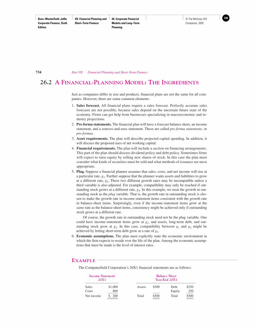
Ross−Westerfield−Jaffe: Corporate Finance, Sixth Edition
VII. Financial Planning and Short−Term Finance
26. Corporate Financial Models and Long−Term Planning
739© The McGraw−Hill Companies, 2002
26.2 A FINANCIAL-PLANNING MODEL: THE INGREDIENTS
Just as companies differ in size and products, financial plans are not the same for all com-panies. However, there are some common elements:
1. Sales forecast. All financial plans require a sales forecast. Perfectly accurate salesforecasts are not possible, because sales depend on the uncertain future state of theeconomy. Firms can get help from businesses specializing in macroeconomic and in-dustry projections.
2. Pro forma statements. The financial plan will have a forecast balance sheet, an incomestatement, and a sources-and-uses statement. These are called pro forma statements, orpro formas.
3. Asset requirements. The plan will describe projected capital spending. In addition, itwill discuss the proposed uses of net working capital.
4. Financial requirements. The plan will include a section on financing arrangements.This part of the plan should discuss dividend policy and debt policy. Sometimes firmswill expect to raise equity by selling new shares of stock. In this case the plan mustconsider what kinds of securities must be sold and what methods of issuance are mostappropriate.
5. Plug. Suppose a financial planner assumes that sales, costs, and net income will rise ata particular rate, g1. Further suppose that the planner wants assets and liabilities to growat a different rate, g2. These two different growth rates may be incompatible unless athird variable is also adjusted. For example, compatibility may only be reached if out-standing stock grows at a different rate, g3. In this example, we treat the growth in out-standing stock as the plug variable. That is, the growth rate in outstanding stock is cho-sen to make the growth rate in income-statement items consistent with the growth ratein balance-sheet items. Surprisingly, even if the income-statement items grow at thesame rate as the balance-sheet items, consistency might be achieved only if outstandingstock grows at a different rate.
Of course, the growth rate in outstanding stock need not be the plug variable. Onecould have income-statement items grow at g1, and assets, long-term debt, and out-standing stock grow at g2. In this case, compatibility between g1 and g2 might beachieved by letting short-term debt grow at a rate of g3.
6. Economic assumptions. The plan must explicitly state the economic environment inwhich the firm expects to reside over the life of the plan. Among the economic assump-tions that must be made is the level of interest rates.
EXAMPLE
The Computerfield Corporation’s 20X1 financial statements are as follows:
Income Statement Balance Sheet20X1 Year-End 20X1
Sales $1,000 Assets $500 Debt $250Costs 800 Equity 250______ ____ ____Net income $ 200 Total $500 Total $500______ ____ __________ ____ ____
734 Part VII Financial Planning and Short-Term Finance
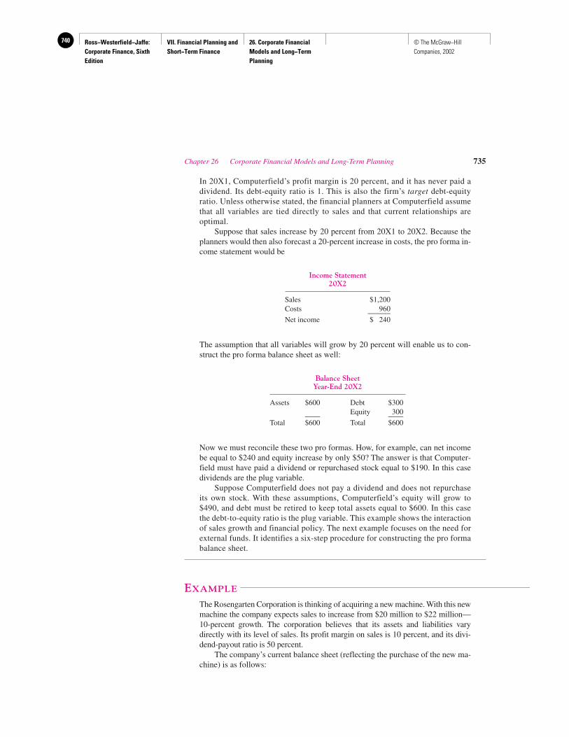
Ross−Westerfield−Jaffe: Corporate Finance, Sixth Edition
VII. Financial Planning and Short−Term Finance
26. Corporate Financial Models and Long−Term Planning
740 © The McGraw−Hill Companies, 2002
In 20X1, Computerfield’s profit margin is 20 percent, and it has never paid adividend. Its debt-equity ratio is 1. This is also the firm’s target debt-equity ratio. Unless otherwise stated, the financial planners at Computerfield assumethat all variables are tied directly to sales and that current relationships are optimal.
Suppose that sales increase by 20 percent from 20X1 to 20X2. Because theplanners would then also forecast a 20-percent increase in costs, the pro forma in-come statement would be
Income Statement20X2
Sales $1,200Costs 960______Net income $ 240
The assumption that all variables will grow by 20 percent will enable us to con-struct the pro forma balance sheet as well:
Balance SheetYear-End 20X2
Assets $600 Debt $300Equity 300____ ____
Total $600 Total $600
Now we must reconcile these two pro formas. How, for example, can net incomebe equal to $240 and equity increase by only $50? The answer is that Computer-field must have paid a dividend or repurchased stock equal to $190. In this casedividends are the plug variable.
Suppose Computerfield does not pay a dividend and does not repurchaseits own stock. With these assumptions, Computerfield’s equity will grow to$490, and debt must be retired to keep total assets equal to $600. In this casethe debt-to-equity ratio is the plug variable. This example shows the interactionof sales growth and financial policy. The next example focuses on the need forexternal funds. It identifies a six-step procedure for constructing the pro formabalance sheet.
EXAMPLE
The Rosengarten Corporation is thinking of acquiring a new machine. With this newmachine the company expects sales to increase from $20 million to $22 million—10-percent growth. The corporation believes that its assets and liabilities vary directly with its level of sales. Its profit margin on sales is 10 percent, and its divi-dend-payout ratio is 50 percent.
The company’s current balance sheet (reflecting the purchase of the new ma-chine) is as follows:
Chapter 26 Corporate Financial Models and Long-Term Planning 735
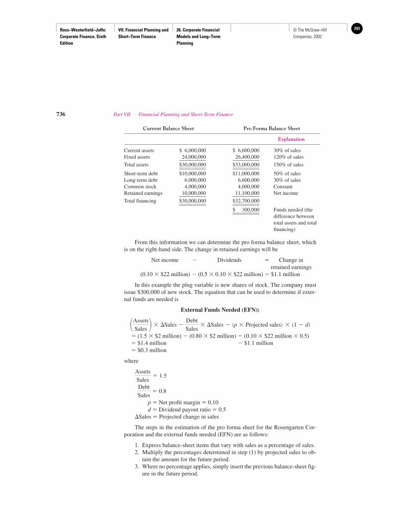
Ross−Westerfield−Jaffe: Corporate Finance, Sixth Edition
VII. Financial Planning and Short−Term Finance
26. Corporate Financial Models and Long−Term Planning
741© The McGraw−Hill Companies, 2002
Current Balance Sheet Pro Forma Balance Sheet
Explanation
Current assets $ 6,000,000 $ 6,600,000 30% of salesFixed assets 24,000,000 26,400,000 120% of sales__________ __________Total assets $30,000,000 $33,000,000 150% of sales__________ ____________________ __________Short-term debt $10,000,000 $11,000,000 50% of salesLong-term debt 6,000,000 6,600,000 30% of salesCommon stock 4,000,000 4,000,000 ConstantRetained earnings 10,000,000 11,100,000 Net income__________ __________Total financing $30,000,000 $32,700,000__________ ____________________ __________
$ 300,000 Funds needed (the ____________________difference betweentotal assets and totalfinancing)
From this information we can determine the pro forma balance sheet, whichis on the right-hand side. The change in retained earnings will be
Net income � Dividends � Change inretained earnings
(0.10 � $22 million) � (0.5 � 0.10 � $22 million) � $1.1 million
In this example the plug variable is new shares of stock. The company mustissue $300,000 of new stock. The equation that can be used to determine if exter-nal funds are needed is
External Funds Needed (EFN):
� (1.5 � $2 million) � (0.80 � $2 million) � (0.10 � $22 million � 0.5)� $1.4 million � $1.1 million� $0.3 million
where
p � Net profit margin � 0.10d � Dividend payout ratio � 0.5
�Sales � Projected change in sales
The steps in the estimation of the pro forma sheet for the Rosengarten Cor-poration and the external funds needed (EFN) are as follows:
1. Express balance-sheet items that vary with sales as a percentage of sales.2. Multiply the percentages determined in step (1) by projected sales to ob-
tain the amount for the future period.3. Where no percentage applies, simply insert the previous balance-sheet fig-
ure in the future period.
Debt
Sales� 0.8
Assets
Sales� 1.5
�Assets
Sales � � �Sales �Debt
Sales� �Sales � �p � Projected sales� � �1 � d�
736 Part VII Financial Planning and Short-Term Finance
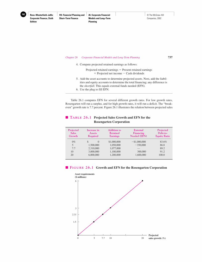
Ross−Westerfield−Jaffe: Corporate Finance, Sixth Edition
VII. Financial Planning and Short−Term Finance
26. Corporate Financial Models and Long−Term Planning
742 © The McGraw−Hill Companies, 2002
4. Compute projected retained earnings as follows:
Projected retained earnings � Present retained earnings� Projected net income � Cash dividends
5. Add the asset accounts to determine projected assets. Next, add the liabil-ities and equity accounts to determine the total financing; any difference isthe shortfall. This equals external funds needed (EFN).
6. Use the plug to fill EFN.
Table 26.1 computes EFN for several different growth rates. For low growth rates,Rosengarten will run a surplus, and for high growth rates, it will run a deficit. The “break-even” growth rate is 7.7 percent. Figure 26.1 illustrates the relation between projected sales
Chapter 26 Corporate Financial Models and Long-Term Planning 737
� TABLE 26.1 Projected Sales Growth and EFN for the Rosengarten Corporation
Projected Increase in Addition to External ProjectedSales Assets Retained Financing Debt-to-
Growth Required Earnings Needed (EFN) Equity Ratio
0% $ 0 $1,000,000 �$1,000,000 83.6%5 1,500,000 1,050,000 �350,000 86.87.7 2,310,000 1,077,000 — 89.2
10 3,000,000 1,100,000 300,000 91.220 6,000,000 1,200,000 1,600,000 100.0
Asset requirements($ millions)
6
3
2.31
1.5
50 7.7 10 20Projectedsales growth (%)
� FIGURE 26.1 Growth and EFN for the Rosengarten Corporation
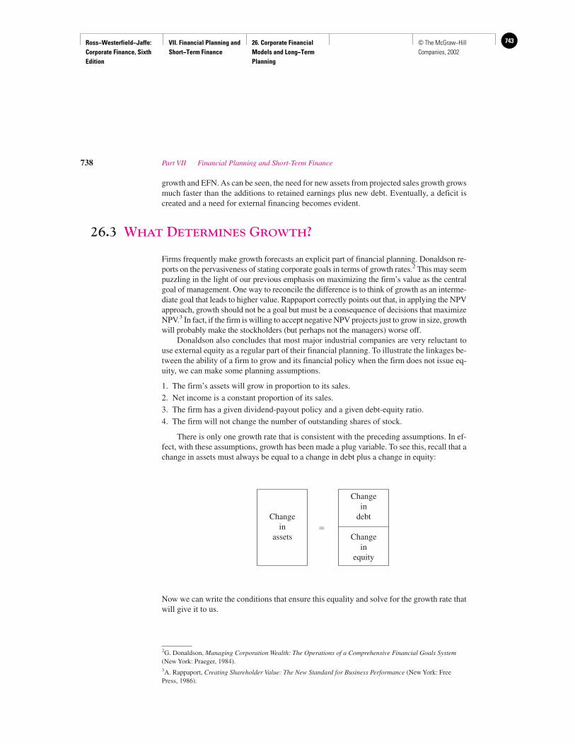
Ross−Westerfield−Jaffe: Corporate Finance, Sixth Edition
VII. Financial Planning and Short−Term Finance
26. Corporate Financial Models and Long−Term Planning
743© The McGraw−Hill Companies, 2002
growth and EFN. As can be seen, the need for new assets from projected sales growth growsmuch faster than the additions to retained earnings plus new debt. Eventually, a deficit iscreated and a need for external financing becomes evident.
26.3 WHAT DETERMINES GROWTH?
Firms frequently make growth forecasts an explicit part of financial planning. Donaldson re-ports on the pervasiveness of stating corporate goals in terms of growth rates.2 This may seempuzzling in the light of our previous emphasis on maximizing the firm’s value as the centralgoal of management. One way to reconcile the difference is to think of growth as an interme-diate goal that leads to higher value. Rappaport correctly points out that, in applying the NPVapproach, growth should not be a goal but must be a consequence of decisions that maximizeNPV.3 In fact, if the firm is willing to accept negative NPV projects just to grow in size, growthwill probably make the stockholders (but perhaps not the managers) worse off.
Donaldson also concludes that most major industrial companies are very reluctant touse external equity as a regular part of their financial planning. To illustrate the linkages be-tween the ability of a firm to grow and its financial policy when the firm does not issue eq-uity, we can make some planning assumptions.
1. The firm’s assets will grow in proportion to its sales.
2. Net income is a constant proportion of its sales.
3. The firm has a given dividend-payout policy and a given debt-equity ratio.
4. The firm will not change the number of outstanding shares of stock.
There is only one growth rate that is consistent with the preceding assumptions. In ef-fect, with these assumptions, growth has been made a plug variable. To see this, recall that achange in assets must always be equal to a change in debt plus a change in equity:
�
Now we can write the conditions that ensure this equality and solve for the growth rate thatwill give it to us.
738 Part VII Financial Planning and Short-Term Finance
2G. Donaldson, Managing Corporation Wealth: The Operations of a Comprehensive Financial Goals System(New York: Praeger, 1984).3A. Rappaport, Creating Shareholder Value: The New Standard for Business Performance (New York: FreePress, 1986).
Change in
assets
Change in
debt
Change in
equity
Ross−Westerfield−Jaffe: Corporate Finance, Sixth Edition
VII. Financial Planning and Short−Term Finance
26. Corporate Financial Models and Long−Term Planning
744 © The McGraw−Hill Companies, 2002
The variables used in this demonstration are the following:
T � The ratio of total assets to salesp � The net profit margin on salesd � The dividend-payout ratioL � The debt-equity ratio
S0 � Sales this year�S � The change in sales (S1 � S0 � �S)S1 � Next year’s projected sales
RE � Retained earnings � Net income � Retention ratio � S1 � p � (1 � d)NI � Net income � S1 � p
If the firm is to increase sales by �S during the year, it must increase assets by T�S.The firm is assumed not to be able to change the number of shares of stock outstanding, sothe equity financing must come from retained earnings. Retained earnings will depend onnext year’s sales, the payout ratio, and the profit margin. The amount of borrowing will de-pend on the amount of retained earnings and the debt-equity ratio.
New equity: S1 � p � (1 � d)plus
Borrowing: [S1 � p � (1 � d)] � Lequals
Capital spending: T�S
Moving things around a little gives the following:
T�S � [S1 � p � (1 � d)] � [S1 � p � (1 � d) � L]
and
(26.1)
This is the growth-rate equation. Given the profit margin (p), the payout ratio (d), the debt-equity ratio (L), and the asset-requirement ratio (T), the growth rate can be determined.4 Itis the only growth possible with the preset values for the four variables. Higgins has referredto this growth rate as the firm’s sustainable growth rate.5
EXAMPLE
Table 26.2 shows the current income statement, the sources-and-uses-of-fundsstatement, and the balance sheet for the Hoffman Corporation. Net income for thecorporation was 16.5 percent ($1,650/$10,000) of sales revenue. The company paidout 72.4 percent ($1,195/$1,650) of its net income in dividends. The interest rateon debt was 10 percent, and the long-term debt was 50 percent ($5,000/$10,000) ofassets. (Notice that, for simplicity, we use the single term net working capital, in
�S
S0
�p � �1 � d� � �1 � L�
T � �p � �1 � d� � �1 � L� �� Growth rate in sales
Chapter 26 Corporate Financial Models and Long-Term Planning 739
4This is approximately equal to the rate of return on equity (ROE) multiplied by the retention rate (RR):ROE � RR. This expression is only precisely equal to equation (26.1) above in continuous time; otherwiseit is an approximation. More precisely,
5R. C. Higgins, “Sustainable Growth under Inflation,” Financial Management (Autumn 1981). The definition ofsustainable growth was popularized by the Boston Consulting Group and others.
Growth rate in sales �ROE � RR
1 � �ROE � RR�
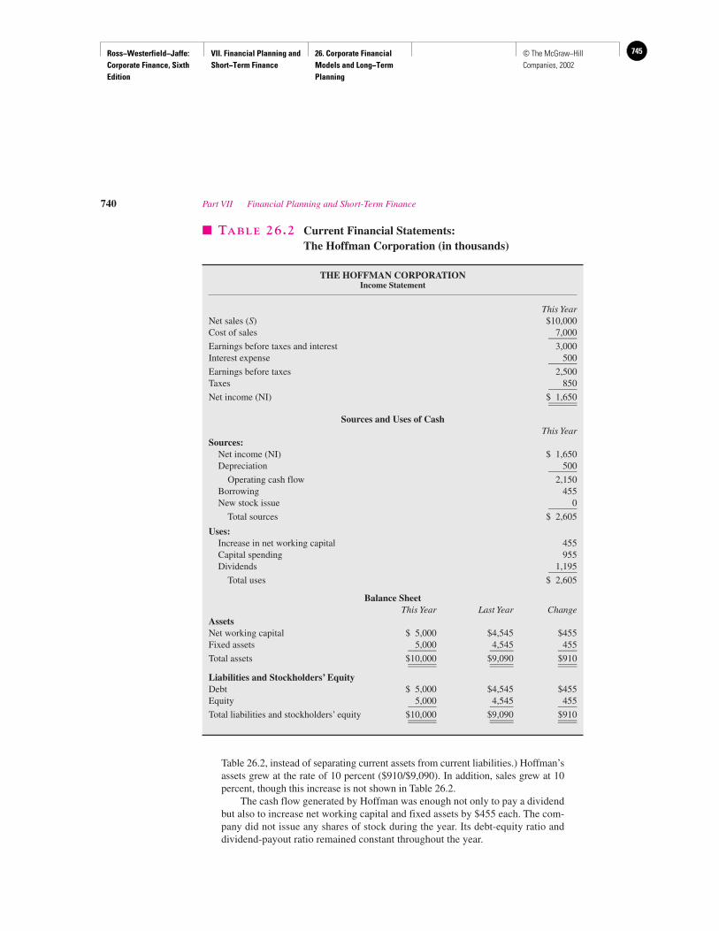
Ross−Westerfield−Jaffe: Corporate Finance, Sixth Edition
VII. Financial Planning and Short−Term Finance
26. Corporate Financial Models and Long−Term Planning
745© The McGraw−Hill Companies, 2002
Table 26.2, instead of separating current assets from current liabilities.) Hoffman’sassets grew at the rate of 10 percent ($910/$9,090). In addition, sales grew at 10percent, though this increase is not shown in Table 26.2.
The cash flow generated by Hoffman was enough not only to pay a dividendbut also to increase net working capital and fixed assets by $455 each. The com-pany did not issue any shares of stock during the year. Its debt-equity ratio anddividend-payout ratio remained constant throughout the year.
740 Part VII Financial Planning and Short-Term Finance
� TABLE 26.2 Current Financial Statements:The Hoffman Corporation (in thousands)
THE HOFFMAN CORPORATIONIncome Statement
This YearNet sales (S) $10,000Cost of sales 7,000______Earnings before taxes and interest 3,000Interest expense 500______Earnings before taxes 2,500Taxes 850______Net income (NI) $ 1,650____________
Sources and Uses of CashThis Year
Sources:Net income (NI) $ 1,650Depreciation 500______
Operating cash flow 2,150Borrowing 455New stock issue 0______
Total sources $ 2,605
Uses:Increase in net working capital 455Capital spending 955Dividends 1,195______
Total uses $ 2,605
Balance SheetThis Year Last Year Change
AssetsNet working capital $ 5,000 $4,545 $455Fixed assets 5,000 4,545 455______ _____ ____Total assets $10,000 $9,090 $910______ _____ __________ _____ ____
Liabilities and Stockholders’ EquityDebt $ 5,000 $4,545 $455Equity 5,000 4,545 455______ _____ ____Total liabilities and stockholders’ equity $10,000 $9,090 $910______ _____ __________ _____ ____
Ross−Westerfield−Jaffe: Corporate Finance, Sixth Edition
VII. Financial Planning and Short−Term Finance
26. Corporate Financial Models and Long−Term Planning
746 © The McGraw−Hill Companies, 2002
The sustainable growth rate for the Hoffman Corporation is 10 percent, or
However, suppose its desired growth rate was to be 20 percent. It is possible forHoffman’s desired growth to exceed its sustainable growth because Hoffman isable to issue new shares of stock. A firm can do several things to increase its sus-tainable growth rate as seen from the Hoffman example:
1. Sell new shares of stock.2. Increase its reliance on debt.3. Reduce its dividend-payout ratio.4. Increase profit margins.5. Decrease its asset-requirement ratio.
Now we can see the use of a financial-planning model to test the feasibility ofthe planned growth rate. If sales are to grow at a rate higher than the sustainablegrowth rate, the firm must improve operating performance, increase financialleverage, decrease dividends, or sell new shares. Of course, the planned rates ofgrowth should be the result of a complete NPV-based planning process.
• When might the goals of growth and value maximization be in conflict, and when wouldthey be aligned?
• What are the determinants of growth?
26.4 SOME CAVEATS OF FINANCIAL-PLANNING MODELS
Financial-planning models suffer from a great deal of criticism. We present two commonlyvoiced attacks below.
First, financial-planning models do not indicate which financial policies are the best.For example, our model could not tell us whether Hoffman’s decision to issue new equityto achieve a higher growth rate raises the NPV of the firm.
Second, financial-planning models are too simple. In reality, costs are not always pro-portional to sales, assets need not be a fixed percentage of sales, and capital-budgeting in-volves a sequence of decisions over time. These assumptions are generally not incorporatedinto financial plans.
Financial-planning models are necessary to assist in planning the future investment andfinancial decisions of the firm. Without some sort of long-term financial plan, the firm mayfind itself adrift in a sea of change without a rudder for guidance. But, because of the as-sumptions and the abstractions from reality necessary in the construction of the financialplan, we also think that they should carry the label: Let the user beware!
0.165 � 0.276 � 2
1 � �0.165 � 0.276 � 2�� 0.1
Chapter 26 Corporate Financial Models and Long-Term Planning 741
QUESTIONS
CO
NC
EP
T
?
Ross−Westerfield−Jaffe: Corporate Finance, Sixth Edition
VII. Financial Planning and Short−Term Finance
26. Corporate Financial Models and Long−Term Planning
747© The McGraw−Hill Companies, 2002
26.5 SUMMARY AND CONCLUSIONS
Financial planning forces the firm to think about and forecast the future. It involves the following:
1. Building a corporate financial model.2. Describing different scenarios of future development from worst to best cases.3. Using the models to construct pro forma financial statements.4. Running the model under different scenarios (conducting sensitivity analysis).5. Examining the financial implications of ultimate strategic plans.
Corporate financial planning should not become a purely mechanical activity. If it does, it willprobably focus on the wrong things. In particular, plans are formulated all too often in terms of agrowth target with an explicit linkage to creation of value. Nonetheless, the alternative tofinancial planning is stumbling into the future.
742 Part VII Financial Planning and Short-Term Finance
IN THEIR OWN WORDS
Robert C. Higgins on Sustainable Growth
Most financial officers know intuitively that it takesmoney to make money. Rapid sales growth
requires increased assets in the form of accounts receiv-able, inventory, and fixed plant, which, in turn, requiremoney to pay for assets. They also know that if theircompany does not have the money when needed, it canliterally “grow broke.” The sustainable growth equationstates these intuitive truths explicitly.
Sustainable growth is often used by bankers and otherexternal analysts to assess a company’s credit-worthiness.They are aided in this exercise by several sophisticatedcomputer software packages that provide detailedanalyses of the company’s past financial performance,including its annual sustainable growth rate.
Bankers use this information in several ways. Quickcomparison of a company’s actual growth rate to itssustainable rate tells the banker what issues will be at thetop of management’s financial agenda. If actual growthconsistently exceeds sustainable growth, management’sproblem will be where to get the cash to finance growth.The banker thus can anticipate interest in loan products.Conversely, if sustainable growth consistently exceedsactual, the banker had best be prepared to talk about invest-ment products, because management’s problem will bewhat to do with all the cash that keeps piling up in the till.
Bankers also find the sustainable growth equationuseful for explaining to financially inexperiencedsmall business owners and overly optimistic entrepre-neurs that, for the long-run viability of their business,it is necessary to keep growth and profitability inproper balance.
Finally, comparison of actual to sustainable growthrates helps a banker understand why a loan applicantneeds money and for how long the need might continue.In one instance, a loan applicant requested $100,000 topay off several insistent suppliers and promised to repayin a few months when he collected some accounts receiv-able that were coming due. A sustainable growth analysisrevealed that the firm had been growing at four to sixtimes its sustainable growth rate and that this pattern waslikely to continue in the foreseeable future. This alertedthe banker that impatient suppliers were only a symptomof the much more fundamental disease of overly rapidgrowth, and that a $100,000 loan would likely prove tobe only the down payment on a much larger, multiyearcommitment.
Robert C. Higgins is Professor of Finance at the University ofWashington. He pioneered the use of sustainable growth as atool for financial analysis.

Ross−Westerfield−Jaffe: Corporate Finance, Sixth Edition
VII. Financial Planning and Short−Term Finance
26. Corporate Financial Models and Long−Term Planning
748 © The McGraw−Hill Companies, 2002
KEY TERMS
Aggregation 733 Plug 734Asset requirements 734 Pro forma statements 734Economic assumptions 734 Sales forecast 734Financial requirements 734 Sustainable growth rate 739
SUGGESTED READINGS
Approaches to building a financial planning model are contained in:Carleton, W. T., and C. L. Dick, Jr. “Financial Policy Models: Theory and Practice.” Journal of
Financial and Quantitative Analysis 8 (1973).Francis, J. C., and D. R. Rowell. “A Simultaneous-Equation Model of the Firm for Financial
Analysis and Planning.” Financial Management (Spring 1978).Myers, S. C., and G. A. Pogue. “A Programming Approach to Corporate Financial
Management.” Journal of Finance 29 (May 1974).Warren, J. M., and J. R. Shelton. “A Simultaneous-Equation Approach to Financial Planning.”
Journal of Finance (December 1971).
The most extensive textbook treatment of financial planning:Lee, C. F. Financial Analysis and Planning: Theory and Application. Reading, Mass.: Addison-
Wesley, 1985.
For a critical discussion of sustainable growth, see:Rappaport, A. Creating Shareholder Value: The New Standard for Business Performance. New
York: Free Press, 1986.
QUESTIONS AND PROBLEMS
Financial-Planning Models: The Ingredients26.1 After examining patterns from recent years, management found the following regression-
estimated relationships between some company balance sheets and income statementaccounts and sales.
CA � 0.5 million � 0.25SFA � 1.0 million � 0.50SCL � 0.1 million � 0.10SNP � 0.0 million � 0.02S
where
CA � Current assetsFA � Fixed assetsCL � Current liabilitiesNP � Net profit after taxes
S � Sales
The company’s sales for last year were $10 million. The year-end balance sheet isreproduced below.
Current assets $3,000,000 Current liabilities $1,100,000Fixed assets 6,000,000 Bonds 2,500,000
Common stock 2,000,000Retained earnings 3,400,000_________ _________
Total $9,000,000 Total $9,000,000_________ __________________ _________
Chapter 26 Corporate Financial Models and Long-Term Planning 743
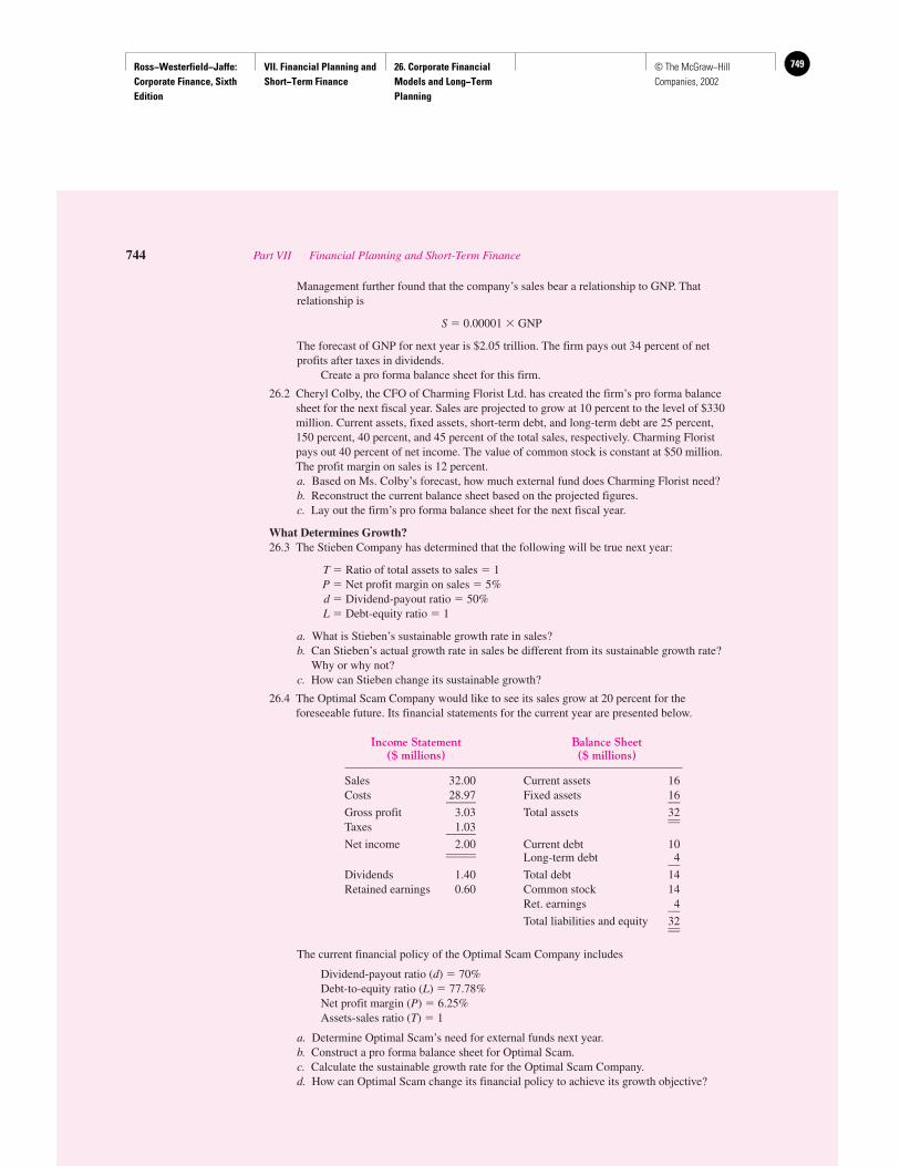
Ross−Westerfield−Jaffe: Corporate Finance, Sixth Edition
VII. Financial Planning and Short−Term Finance
26. Corporate Financial Models and Long−Term Planning
749© The McGraw−Hill Companies, 2002
Management further found that the company’s sales bear a relationship to GNP. Thatrelationship is
S � 0.00001 � GNP
The forecast of GNP for next year is $2.05 trillion. The firm pays out 34 percent of netprofits after taxes in dividends.
Create a pro forma balance sheet for this firm.
26.2 Cheryl Colby, the CFO of Charming Florist Ltd. has created the firm’s pro forma balancesheet for the next fiscal year. Sales are projected to grow at 10 percent to the level of $330million. Current assets, fixed assets, short-term debt, and long-term debt are 25 percent,150 percent, 40 percent, and 45 percent of the total sales, respectively. Charming Floristpays out 40 percent of net income. The value of common stock is constant at $50 million.The profit margin on sales is 12 percent.a. Based on Ms. Colby’s forecast, how much external fund does Charming Florist need?b. Reconstruct the current balance sheet based on the projected figures.c. Lay out the firm’s pro forma balance sheet for the next fiscal year.
What Determines Growth?26.3 The Stieben Company has determined that the following will be true next year:
T � Ratio of total assets to sales � 1P � Net profit margin on sales � 5%d � Dividend-payout ratio � 50%L � Debt-equity ratio � 1
a. What is Stieben’s sustainable growth rate in sales?b. Can Stieben’s actual growth rate in sales be different from its sustainable growth rate?
Why or why not?c. How can Stieben change its sustainable growth?
26.4 The Optimal Scam Company would like to see its sales grow at 20 percent for theforeseeable future. Its financial statements for the current year are presented below.
Income Statement Balance Sheet($ millions) ($ millions)
Sales 32.00 Current assets 16Costs 28.97 Fixed assets 16_____ __Gross profit 3.03 Total assets 32____Taxes 1.03_____Net income 2.00 Current debt 10__________ Long-term debt 4__Dividends 1.40 Total debt 14Retained earnings 0.60 Common stock 14
Ret. earnings 4__Total liabilities and equity 32____
The current financial policy of the Optimal Scam Company includes
Dividend-payout ratio (d) � 70%Debt-to-equity ratio (L) � 77.78%Net profit margin (P) � 6.25%Assets-sales ratio (T) � 1
a. Determine Optimal Scam’s need for external funds next year.b. Construct a pro forma balance sheet for Optimal Scam.c. Calculate the sustainable growth rate for the Optimal Scam Company.d. How can Optimal Scam change its financial policy to achieve its growth objective?
744 Part VII Financial Planning and Short-Term Finance

Ross−Westerfield−Jaffe: Corporate Finance, Sixth Edition
VII. Financial Planning and Short−Term Finance
26. Corporate Financial Models and Long−Term Planning
750 © The McGraw−Hill Companies, 2002
26.5 The MBI Company does not want to grow. The company’s financial management believesit has no positive NPV projects. The company’s operating financial characteristics are
Profit margin � 10%Assets-sales ratio � 150%Debt-equity ratio � 100%Dividend-payout ratio � 50%
a. Calculate the sustainable growth rate for the MBI Company.b. How can the MBI Company achieve its stated growth goal?
26.6 Throughout this text, you have learned that financial managers should select positive net-present-value projects. How does this project-selection criterion relate to financial-planning models?
26.7 Your firm recently hired a new MBA. She insists that your firm is incorrectly computingits sustainable growth rate. Your firm computes the sustainable growth rate using thefollowing formula:
P � Net profit margin on salesd � Dividend-payout ratioL � Debt-equity ratioT � Ratio of total assets to sales
Your new employee claims that the correct formula is ROE � (1 � d) where ROE is netprofit divided by net worth and d is dividends divided by net profit. Is your new employeecorrect?
26.8 Atlantic Transportation Co. has a payout ratio of 60 percent, debt-equity ratio of 50percent, return on equity of 16 percent, and an assets-sales ratio of 175 percent.a. What is its sustainable growth rate?b. What must its profit margin be in order to achieve its sustainable growth rate?
Some Caveats of Financial-Planning Models26.9 What are the shortcomings of financial-planning models that we should be aware of?
P � �1 � d� � �1 � L�T � P � �1 � d� � �1 � L�
Chapter 26 Corporate Financial Models and Long-Term Planning 745
Ross−Westerfield−Jaffe: Corporate Finance, Sixth Edition
VII. Financial Planning and Short−Term Finance
27. Short−Term Finance and Planning
751© The McGraw−Hill Companies, 2002
Short-Term Finance and Planning
CH
AP
TE
R27
EXECUTIVE SUMMARY
Up to now we have described many of the decisions of long-term finance: capitalbudgeting, dividend policy, and capital structure. This chapter introduces short-term finance. Short-term finance is an analysis of decisions that affect current as-
sets and current liabilities and will frequently have an impact on the firm within a year.The term net working capital is often associated with short-term financial decision
making. Net working capital is the difference between current assets and current liabilities.The focus of short-term finance on net working capital seems to suggest that it is an ac-counting subject. However, making net working capital decisions still relies on cash flowand net present value.
There is no universally accepted definition of short-term finance. The most importantdifference between short-term and long-term finance is the timing of cash flows. Short-termfinancial decisions involve cash inflows and outflows within a year or less. For example, ashort-term financial decision is involved when a firm orders raw materials, pays in cash, andanticipates selling finished goods in one year for cash, as illustrated in Figure 27.1. A long-term financial decision is involved when a firm purchases a special machine that will re-duce operating costs over the next five years, as illustrated in Figure 27.2.
Here are some questions of short-term finance:
1. What is a reasonable level of cash to keep on hand (in a bank) to pay bills?
2. How much raw material should be ordered?
3. How much credit should be extended to customers?
This chapter introduces the basic elements of short-term financial decisions. First, wedescribe the short-term operating activities of the firm, and then we identify alternativeshort-term financial policies. Finally, we outline the basic elements in a short-term finan-cial plan and describe short-term financing instruments.
27.1 TRACING CASH AND NET WORKING CAPITAL
In this section we trace the components of cash and net working capital as they change fromone year to the next. Our goal is to describe the short-term operating activities of the firmand their impact on cash and working capital.
Current assets are cash and other assets that are expected to be converted to cashwithin the year. Current assets are presented in the balance sheet in order of their ac-counting liquidity—the ease with which they can be converted to cash at a fair price andthe time it takes to do so. Table 27.1 gives the balance sheet and income statement of theTradewinds Manufacturing Corporation for 20X2 and 20X1. The four major items foundin the current asset section of the Tradewinds balance sheet are cash, marketable securi-ties, accounts receivable, and inventories.
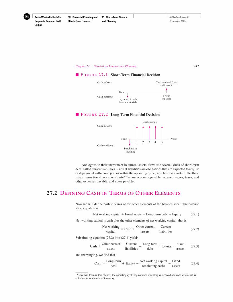
Ross−Westerfield−Jaffe: Corporate Finance, Sixth Edition
VII. Financial Planning and Short−Term Finance
27. Short−Term Finance and Planning
752 © The McGraw−Hill Companies, 2002
Chapter 27 Short-Term Finance and Planning 747
Cash inflows
Cash outflows
Time:
Payment of cashfor raw materials
1 year(or less)
Cash received fromsold goods
� FIGURE 27.1 Short-Term Financial Decision
Cash inflows
Cash outflows
Time:
Purchase ofmachine
Cost savings
Years1 2 3 4 5
� FIGURE 27.2 Long-Term Financial Decision
Analogous to their investment in current assets, firms use several kinds of short-termdebt, called current liabilities. Current liabilities are obligations that are expected to requirecash payment within one year or within the operating cycle, whichever is shorter.1 The threemajor items found as current liabilities are accounts payable; accrued wages, taxes, andother expenses payable; and notes payable.
27.2 DEFINING CASH IN TERMS OF OTHER ELEMENTS
Now we will define cash in terms of the other elements of the balance sheet. The balancesheet equation is
Net working capital � Fixed assets � Long-term debt � Equity (27.1)
Net working capital is cash plus the other elements of net working capital; that is,
(27.2)
Substituting equation (27.2) into (27.1) yields
(27.3)
and rearranging, we find that
(27.4)Cash �Long-term
debt� Equity �
Net working capital�excluding cash�
�Fixed
assets
Cash �Other current
assets�
Current
liabilities�
Long-term
debt� Equity �
Fixed
assets
Net working
capital� Cash �
Other current
assets�
Current
liabilities
1As we will learn in this chapter, the operating cycle begins when inventory is received and ends when cash iscollected from the sale of inventory.
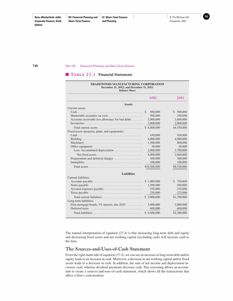
Ross−Westerfield−Jaffe: Corporate Finance, Sixth Edition
VII. Financial Planning and Short−Term Finance
27. Short−Term Finance and Planning
753© The McGraw−Hill Companies, 2002
The natural interpretation of equation (27.4) is that increasing long-term debt and equityand decreasing fixed assets and net working capital (excluding cash) will increase cash tothe firm.
The Sources-and-Uses-of-Cash StatementFrom the right-hand side of equation (27.4), we can see an increase in long-term debt and/orequity leads to an increase in cash. Moreover, a decrease in net working capital and/or fixedassets leads to a decrease in cash. In addition, the sum of net income and depreciation in-creases cash, whereas dividend payments decrease cash. This reasoning allows an accoun-tant to create a sources-and-uses-of-cash statement, which shows all the transactions thataffect a firm’s cash position.
748 Part VII Financial Planning and Short-Term Finance
� TABLE 27.1 Financial Statements
TRADEWINDS MANUFACTURING CORPORATIONDecember 31, 20X2, and December 31, 20X1
Balance Sheet
20X2 20X1
AssetsCurrent assets:
Cash . . . . . . . . . . . . . . . . . . . . . . . . . . . . . . . . . . . . . . . . . . $ 500,000 $ 500,000Marketable securities (at cost) . . . . . . . . . . . . . . . . . . . . . . 500,000 450,000Accounts receivable less allowance for bad debts . . . . . . . 2,000,000 1,600,000Inventories . . . . . . . . . . . . . . . . . . . . . . . . . . . . . . . . . . . . . 3,000,000 2,000,000_________ _________
Total current assets . . . . . . . . . . . . . . . . . . . . . . . . . . . . . $ 6,000,000 $4,550,000Fixed assets (property, plant, and equipment):
Land . . . . . . . . . . . . . . . . . . . . . . . . . . . . . . . . . . . . . . . . . . 450,000 450,000Building . . . . . . . . . . . . . . . . . . . . . . . . . . . . . . . . . . . . . . . 4,000,000 4,000,000Machinery . . . . . . . . . . . . . . . . . . . . . . . . . . . . . . . . . . . . . 1,500,000 800,000Office equipment . . . . . . . . . . . . . . . . . . . . . . . . . . . . . . . . 50,000 50,000
Less: Accumulated depreciation . . . . . . . . . . . . . . . . . . 2,000,000 1,700,000_________ _________Net fixed assets . . . . . . . . . . . . . . . . . . . . . . . . . . . . . 4,000,000 3,600,000
Prepayments and deferred charges . . . . . . . . . . . . . . . . . . 400,000 300,000Intangibles . . . . . . . . . . . . . . . . . . . . . . . . . . . . . . . . . . . . . 100,000 100,000_________ _________
Total assets . . . . . . . . . . . . . . . . . . . . . . . . . . . . . . . . . . . $10,500,000 $8,550,000_________ __________________ _________
LiabilitiesCurrent liabilities:
Accounts payable . . . . . . . . . . . . . . . . . . . . . . . . . . . . . . . . $ 1,000,000 $ 750,000Notes payable . . . . . . . . . . . . . . . . . . . . . . . . . . . . . . . . . . . 1,500,000 500,000Accrued expenses payable . . . . . . . . . . . . . . . . . . . . . . . . . 250,000 225,000Taxes payable . . . . . . . . . . . . . . . . . . . . . . . . . . . . . . . . . . . 250,000 225,000_________ _________
Total current liabilities . . . . . . . . . . . . . . . . . . . . . . . . . . $ 3,000,000 $1,700,000Long-term liabilities:
First mortgage bonds, 5% interest, due 2025 . . . . . . . . . . 3,000,000 3,000,000Deferred taxes . . . . . . . . . . . . . . . . . . . . . . . . . . . . . . . . . . 600,000 600,000_________ _________
Total liabilities . . . . . . . . . . . . . . . . . . . . . . . . . . . . . . . . $ 6,600,000 $5,300,000
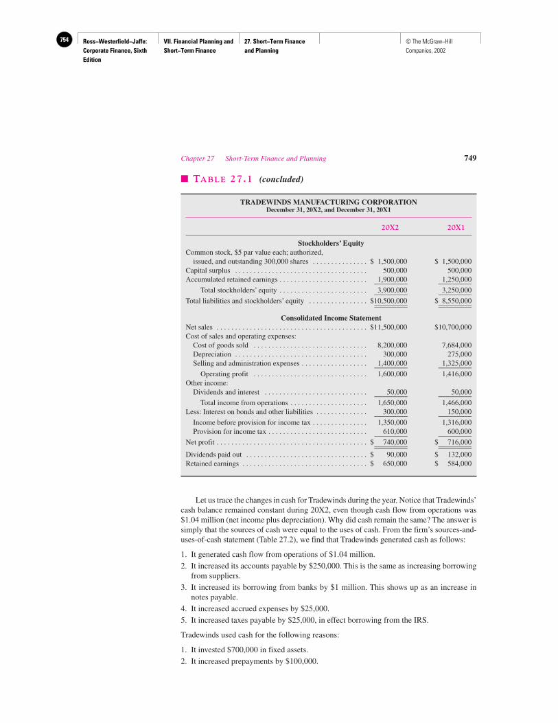
Ross−Westerfield−Jaffe: Corporate Finance, Sixth Edition
VII. Financial Planning and Short−Term Finance
27. Short−Term Finance and Planning
754 © The McGraw−Hill Companies, 2002
Let us trace the changes in cash for Tradewinds during the year. Notice that Tradewinds’cash balance remained constant during 20X2, even though cash flow from operations was$1.04 million (net income plus depreciation). Why did cash remain the same? The answer issimply that the sources of cash were equal to the uses of cash. From the firm’s sources-and-uses-of-cash statement (Table 27.2), we find that Tradewinds generated cash as follows:
1. It generated cash flow from operations of $1.04 million.
2. It increased its accounts payable by $250,000. This is the same as increasing borrowingfrom suppliers.
3. It increased its borrowing from banks by $1 million. This shows up as an increase innotes payable.
4. It increased accrued expenses by $25,000.
5. It increased taxes payable by $25,000, in effect borrowing from the IRS.
Tradewinds used cash for the following reasons:
1. It invested $700,000 in fixed assets.
2. It increased prepayments by $100,000.
Chapter 27 Short-Term Finance and Planning 749
� TABLE 27.1 (concluded)
TRADEWINDS MANUFACTURING CORPORATIONDecember 31, 20X2, and December 31, 20X1
20X2 20X1
Stockholders’ EquityCommon stock, $5 par value each; authorized,
issued, and outstanding 300,000 shares . . . . . . . . . . . . . . . $ 1,500,000 $ 1,500,000Capital surplus . . . . . . . . . . . . . . . . . . . . . . . . . . . . . . . . . . . . 500,000 500,000Accumulated retained earnings . . . . . . . . . . . . . . . . . . . . . . . . 1,900,000 1,250,000_________ _________
Total stockholders’ equity . . . . . . . . . . . . . . . . . . . . . . . . 3,900,000 3,250,000_________ _________Total liabilities and stockholders’ equity . . . . . . . . . . . . . . . . $10,500,000 $ 8,550,000_________ __________________ _________
Consolidated Income StatementNet sales . . . . . . . . . . . . . . . . . . . . . . . . . . . . . . . . . . . . . . . . . $11,500,000 $10,700,000Cost of sales and operating expenses:
Cost of goods sold . . . . . . . . . . . . . . . . . . . . . . . . . . . . . . . 8,200,000 7,684,000Depreciation . . . . . . . . . . . . . . . . . . . . . . . . . . . . . . . . . . . . 300,000 275,000Selling and administration expenses . . . . . . . . . . . . . . . . . . 1,400,000 1,325,000_________ _________
Operating profit . . . . . . . . . . . . . . . . . . . . . . . . . . . . . . . 1,600,000 1,416,000Other income:
Dividends and interest . . . . . . . . . . . . . . . . . . . . . . . . . . . . 50,000 50,000_________ _________Total income from operations . . . . . . . . . . . . . . . . . . . . . 1,650,000 1,466,000
Less: Interest on bonds and other liabilities . . . . . . . . . . . . . . 300,000 150,000_________ _________Income before provision for income tax . . . . . . . . . . . . . . . 1,350,000 1,316,000Provision for income tax . . . . . . . . . . . . . . . . . . . . . . . . . . . 610,000 600,000_________ _________
Net profit . . . . . . . . . . . . . . . . . . . . . . . . . . . . . . . . . . . . . . . . . $ 740,000 $ 716,000_________ __________________ _________Dividends paid out . . . . . . . . . . . . . . . . . . . . . . . . . . . . . . . . . $ 90,000 $ 132,000Retained earnings . . . . . . . . . . . . . . . . . . . . . . . . . . . . . . . . . . $ 650,000 $ 584,000
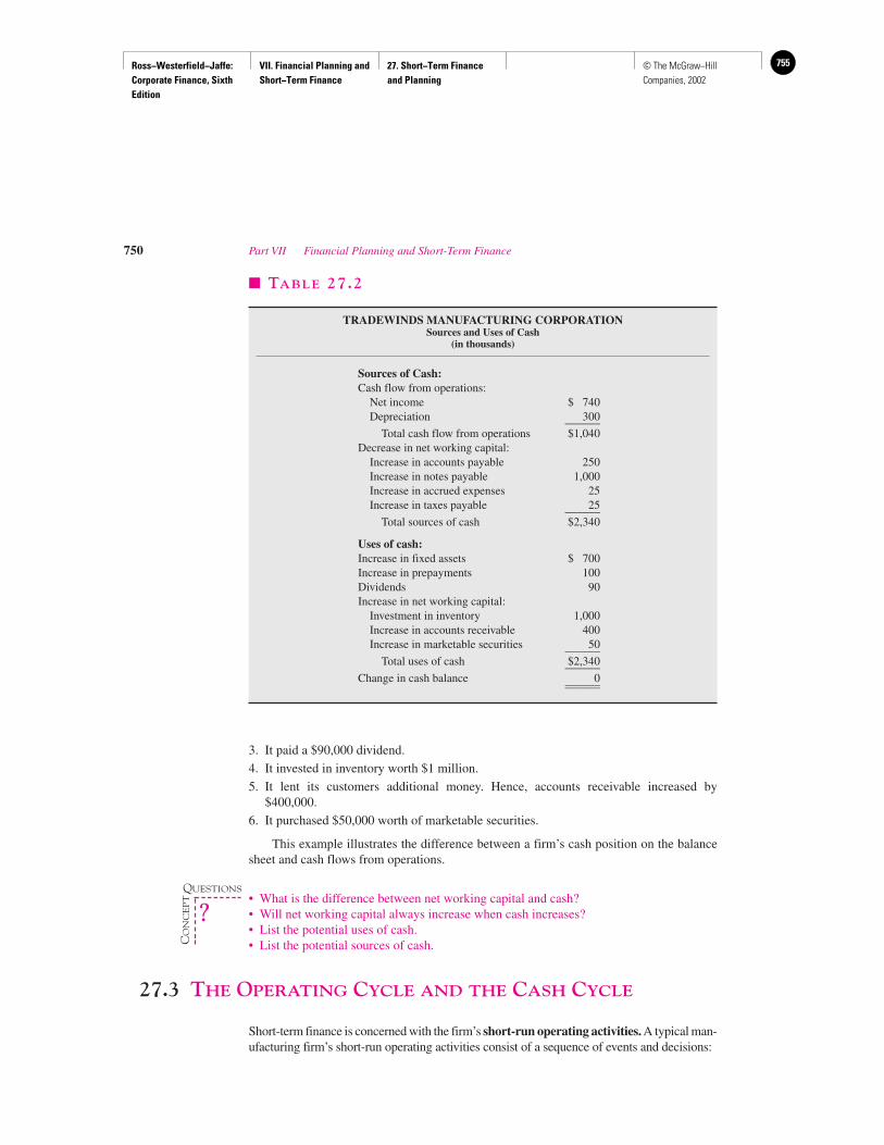
Ross−Westerfield−Jaffe: Corporate Finance, Sixth Edition
VII. Financial Planning and Short−Term Finance
27. Short−Term Finance and Planning
755© The McGraw−Hill Companies, 2002
3. It paid a $90,000 dividend.
4. It invested in inventory worth $1 million.
5. It lent its customers additional money. Hence, accounts receivable increased by$400,000.
6. It purchased $50,000 worth of marketable securities.
This example illustrates the difference between a firm’s cash position on the balancesheet and cash flows from operations.
• What is the difference between net working capital and cash?• Will net working capital always increase when cash increases?• List the potential uses of cash.• List the potential sources of cash.
27.3 THE OPERATING CYCLE AND THE CASH CYCLE
Short-term finance is concerned with the firm’s short-run operating activities. A typical man-ufacturing firm’s short-run operating activities consist of a sequence of events and decisions:
750 Part VII Financial Planning and Short-Term Finance
� TABLE 27.2
TRADEWINDS MANUFACTURING CORPORATIONSources and Uses of Cash
(in thousands)
Sources of Cash:Cash flow from operations:
Net income $ 740Depreciation 300______
Total cash flow from operations $1,040Decrease in net working capital:
Increase in accounts payable 250Increase in notes payable 1,000Increase in accrued expenses 25Increase in taxes payable 25______
Total sources of cash $2,340
Uses of cash:Increase in fixed assets $ 700Increase in prepayments 100Dividends 90Increase in net working capital:
Investment in inventory 1,000Increase in accounts receivable 400Increase in marketable securities 50______
Total uses of cash $2,340______Change in cash balance 0____________
QUESTIONS
CO
NC
EP
T
?
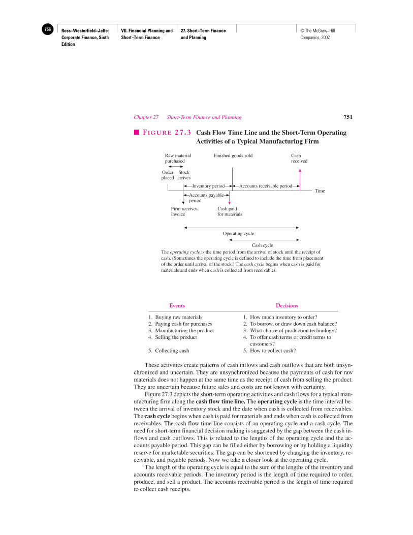
Ross−Westerfield−Jaffe: Corporate Finance, Sixth Edition
VII. Financial Planning and Short−Term Finance
27. Short−Term Finance and Planning
756 © The McGraw−Hill Companies, 2002
Events Decisions
1. Buying raw materials 1. How much inventory to order?2. Paying cash for purchases 2. To borrow, or draw down cash balance?3. Manufacturing the product 3. What choice of production technology?4. Selling the product 4. To offer cash terms or credit terms to
customers?5. Collecting cash 5. How to collect cash?
These activities create patterns of cash inflows and cash outflows that are both unsyn-chronized and uncertain. They are unsynchronized because the payments of cash for rawmaterials does not happen at the same time as the receipt of cash from selling the product.They are uncertain because future sales and costs are not known with certainty.
Figure 27.3 depicts the short-term operating activities and cash flows for a typical man-ufacturing firm along the cash flow time line. The operating cycle is the time interval be-tween the arrival of inventory stock and the date when cash is collected from receivables.The cash cycle begins when cash is paid for materials and ends when cash is collected fromreceivables. The cash flow time line consists of an operating cycle and a cash cycle. Theneed for short-term financial decision making is suggested by the gap between the cash in-flows and cash outflows. This is related to the lengths of the operating cycle and the ac-counts payable period. This gap can be filled either by borrowing or by holding a liquidityreserve for marketable securities. The gap can be shortened by changing the inventory, re-ceivable, and payable periods. Now we take a closer look at the operating cycle.
The length of the operating cycle is equal to the sum of the lengths of the inventory andaccounts receivable periods. The inventory period is the length of time required to order,produce, and sell a product. The accounts receivable period is the length of time requiredto collect cash receipts.
Chapter 27 Short-Term Finance and Planning 751
Raw materialpurchased
Finished goods sold Cashreceived
Inventory period Accounts receivable period
Firm receivesinvoice
Cash paidfor materials
Operating cycle
Cash cycle
Orderplaced
Stockarrives
TimeAccounts payableperiod
� FIGURE 27.3 Cash Flow Time Line and the Short-Term OperatingActivities of a Typical Manufacturing Firm
The operating cycle is the time period from the arrival of stock until the receipt ofcash. (Sometimes the operating cycle is defined to include the time from placementof the order until arrival of the stock.) The cash cycle begins when cash is paid formaterials and ends when cash is collected from receivables.
Ross−Westerfield−Jaffe: Corporate Finance, Sixth Edition
VII. Financial Planning and Short−Term Finance
27. Short−Term Finance and Planning
757© The McGraw−Hill Companies, 2002
The cash cycle is the time between cash disbursement and cash collection. It can bethought of as the operating cycle less the accounts payable period, that is
Cash cycle � Operating cycle � Accounts payable period
The accounts payable period is the length of time the firm is able to delay payment on thepurchase of various resources, such as wages and raw materials.
In practice, the inventory period, the accounts receivable period, and the accountspayable period are measured by days in inventory, days in receivables, and days in payables,respectively. We illustrate how the operating cycle and the cash cycle can be measured inthe following example.
EXAMPLE
Tradewinds Manufacturing is a diversified manufacturing firm with the balancesheet and income statement shown in Table 27.1 for 20X1 and 20X2. The operat-ing cycle and the cash cycle can be determined for Tradewinds after calculatingthe appropriate ratios for inventory, receivables, and payables. Consider inventoryfirst. The average inventory is
The terms in the numerator are the ending inventory in the second and first years,respectively.
We next calculate the inventory-turnover ratio:
This implies that the inventory cycle occurs 3.3 times a year. Finally, we cal-culate days in inventory:
Our calculation implies that the inventory cycle is slightly more than 110 days.We perform analogous calculations for receivables and payables.2
�365
9.4� 38.8 days
Days in
payables
�Cost of goods sold
Average payables�
$8.2 million
$0.875 million� 9.4
Accounts payable
deferral period
�$1.0 million � $0.75 million
2� $0.875 million
Average
payables
�365
6.4� 57 days
Days in
receivables
�Credit sales
Average accounts receivable�
$11.5 million
$1.8 million� 6.4
Average
receivable turnover
�$2.0 million � $1.6 million
2� $1.8 million
Average
accounts receivable
Days in inventory �365 days
3.3� 110.6 days
�Cost of goods sold
Average inventory�
$8.2 million
$2.5 million� 3.3
Inventory-
turnover ratio
Average inventory �$3 million � $2 million
2� $2.5 million
752 Part VII Financial Planning and Short-Term Finance
2We assume that Tradewinds Manufacturing makes no cash sales.
Ross−Westerfield−Jaffe: Corporate Finance, Sixth Edition
VII. Financial Planning and Short−Term Finance
27. Short−Term Finance and Planning
758 © The McGraw−Hill Companies, 2002
The preceding calculations allow us to determine both the operating cycle andthe cash cycle.
� 110.6 days � 57 days � 167.6 days
� 167.6 days � 38.8 days � 128.8 days.
The need for short-term financial decision making is suggested by the gap between thecash inflows and cash outflows. This is related to the lengths of the operating cycles and ac-counts payable period. This gap can be filled either by borrowing or by holding a liquidityreserve for marketable securities. The gap can be shortened by changing the inventory, re-ceivable, and payable periods. Now we take a closer look at this aspect of short-term fi-nancial policy.
• What does it mean to say that a firm has an inventory-turnover ratio of four?• Describe the operating cycle and the cash cycle. What are the differences between them?
27.4 SOME ASPECTS OF SHORT-TERM FINANCIAL POLICY
The policy that a firm adopts for short-term finance will be composed of at least twoelements:
1. The Size of the Firm’s Investment in Current Assets. This is usually measured relative tothe firm’s level of total operating revenues. A flexible or accommodative short-term fi-nancial policy would maintain a high ratio of current assets to sales. A restrictive short-term financial policy would entail a low ratio of current assets to sales.
2. The Financing of Current Assets. This is measured as the proportion of short-term debtto long-term debt. A restrictive short-term financial policy means a high proportion ofshort-term debt relative to long-term financing, and a flexible policy means less short-term debt and more long-term debt.
The Size of the Firm’s Investment in Current AssetsFlexible short-term financial policies include:
1. Keeping large balances of cash and marketable securities.
2. Making large investments in inventory.
3. Granting liberal credit terms, which results in a high level of accounts receivable.
Restrictive short-term financial policies are:
1. Keeping low cash balances and no investment in marketable securities.
2. Making small investments in inventory.
3. Allowing no credit sales and no accounts receivable.
Cash
cycle�
Operating
cycle�
Days in
payables
Operating
cycle�
Days in
inventory�
Days in
receivables
Chapter 27 Short-Term Finance and Planning 753
QUESTIONS
CO
NC
EP
T
?
Ross−Westerfield−Jaffe: Corporate Finance, Sixth Edition
VII. Financial Planning and Short−Term Finance
27. Short−Term Finance and Planning
759© The McGraw−Hill Companies, 2002
Determining the optimal investment level in short-term assets requires an identifica-tion of the different costs of alternative short-term financing policies. The objective is totrade off the cost of restrictive policies against those of the flexible ones to arrive at the bestcompromise.
Current asset holdings are highest with a flexible short-term financial policy and low-est with a restrictive policy. Thus, flexible short-term financial policies are costly in thatthey require higher cash outflows to finance cash and marketable securities, inventory, andaccounts receivable. However, future cash inflows are highest with a flexible policy. Salesare stimulated by the use of a credit policy that provides liberal financing to customers. Alarge amount of inventory on hand (“on the shelf”) provides a quick delivery service to cus-tomers and increases in sales.3 In addition, the firm can probably charge higher prices forthe quick delivery service and the liberal credit terms of flexible policies. A flexible policyalso may result in fewer production stoppages because of inventory shortages.4
Managing current assets can be thought of as involving a trade-off between costs thatrise with the level of investment and costs that fall with the level of investment. Costs thatrise with the level of investment in current assets are called carrying costs. Costs that fallwith increases in the level of investment in current assets are called shortage costs.
Carrying costs are generally of two types. First, because the rate of return on currentassets is low compared with that of other assets, there is an opportunity cost. Second, thereis the cost of maintaining the economic value of the item. For example, the cost of ware-housing inventory belongs here.
Shortage costs are incurred when the investment in current assets is low. If a firm runsout of cash, it will be forced to sell marketable securities. If a firm runs out of cash and can-not readily sell marketable securities, it may need to borrow or default on an obligation.(This general situation is called cash-out.) If a firm has no inventory (a stock-out) or if itcannot extend credit to its customers, it will lose customers.
There are two kinds of shortage costs:
1. Trading or Order Costs. Order costs are the costs of placing an order for more cash (bro-kerage costs) or more inventory (production set-up costs).
2. Costs Related to Safety Reserves. These are costs of lost sales, lost customer goodwill,and disruption of production schedule.
Figure 27.4 illustrates the basic nature of carrying costs. The total costs of investing incurrent assets are determined by adding the carrying costs and the shortage costs. The min-imum point on the total cost curve (CA*) reflects the optimal balance of current assets. Thecurve is generally quite flat at the optimum, and it is difficult, if not impossible, to find theprecise optimal balance of shortage and carrying costs. Usually we are content with achoice near the optimum.
If carrying costs are low and/or shortage costs are high, the optimal policy calls for sub-stantial current assets. In other words, the optimal policy is a flexible one. This is illustratedin the middle graph of Figure 27.4.
If carrying costs are high and/or shortage costs are low, the optimal policy is a restric-tive one. That is, the optimal policy calls for modest current assets. This is illustrated in thebottom graph of the figure.
754 Part VII Financial Planning and Short-Term Finance
3This is true of some types of finished goods.4This is true of inventory of raw material but not of finished goods.
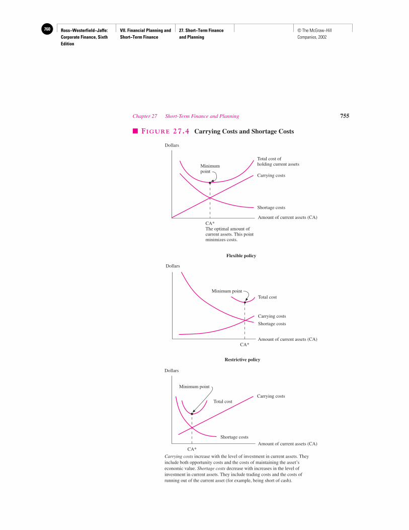
Ross−Westerfield−Jaffe: Corporate Finance, Sixth Edition
VII. Financial Planning and Short−Term Finance
27. Short−Term Finance and Planning
760 © The McGraw−Hill Companies, 2002
Chapter 27 Short-Term Finance and Planning 755
Dollars
Minimumpoint
Total cost ofholding current assets
Carrying costs
Shortage costs
Amount of current assets (CA)CA*The optimal amount ofcurrent assets. This pointminimizes costs.
Flexible policy
Dollars
Minimum pointTotal cost
Carrying costs
Shortage costs
CA*
Restrictive policy
Dollars
CA*
Minimum point
Total costCarrying costs
Shortage costsAmount of current assets (CA)
Amount of current assets (CA)
� FIGURE 27.4 Carrying Costs and Shortage Costs
Carrying costs increase with the level of investment in current assets. Theyinclude both opportunity costs and the costs of maintaining the asset’seconomic value. Shortage costs decrease with increases in the level ofinvestment in current assets. They include trading costs and the costs ofrunning out of the current asset (for example, being short of cash).
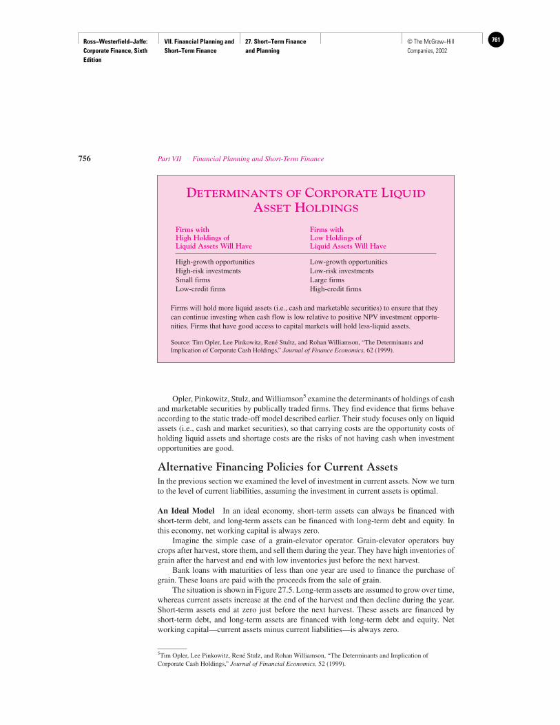
Ross−Westerfield−Jaffe: Corporate Finance, Sixth Edition
VII. Financial Planning and Short−Term Finance
27. Short−Term Finance and Planning
761© The McGraw−Hill Companies, 2002
756 Part VII Financial Planning and Short-Term Finance
Opler, Pinkowitz, Stulz, and Williamson5 examine the determinants of holdings of cashand marketable securities by publically traded firms. They find evidence that firms behaveaccording to the static trade-off model described earlier. Their study focuses only on liquidassets (i.e., cash and market securities), so that carrying costs are the opportunity costs ofholding liquid assets and shortage costs are the risks of not having cash when investmentopportunities are good.
Alternative Financing Policies for Current AssetsIn the previous section we examined the level of investment in current assets. Now we turnto the level of current liabilities, assuming the investment in current assets is optimal.
An Ideal Model In an ideal economy, short-term assets can always be financed withshort-term debt, and long-term assets can be financed with long-term debt and equity. Inthis economy, net working capital is always zero.
Imagine the simple case of a grain-elevator operator. Grain-elevator operators buycrops after harvest, store them, and sell them during the year. They have high inventories ofgrain after the harvest and end with low inventories just before the next harvest.
Bank loans with maturities of less than one year are used to finance the purchase ofgrain. These loans are paid with the proceeds from the sale of grain.
The situation is shown in Figure 27.5. Long-term assets are assumed to grow over time,whereas current assets increase at the end of the harvest and then decline during the year.Short-term assets end at zero just before the next harvest. These assets are financed byshort-term debt, and long-term assets are financed with long-term debt and equity. Networking capital—current assets minus current liabilities—is always zero.
DETERMINANTS OF CORPORATE LIQUID
ASSET HOLDINGS
Firms with Firms withHigh Holdings of Low Holdings ofLiquid Assets Will Have Liquid Assets Will Have
High-growth opportunities Low-growth opportunitiesHigh-risk investments Low-risk investmentsSmall firms Large firmsLow-credit firms High-credit firms
Firms will hold more liquid assets (i.e., cash and marketable securities) to ensure that theycan continue investing when cash flow is low relative to positive NPV investment opportu-nities. Firms that have good access to capital markets will hold less-liquid assets.
Source: Tim Opler, Lee Pinkowitz, René Stultz, and Rohan Williamson, “The Determinants andImplication of Corporate Cash Holdings,” Journal of Finance Economics, 62 (1999).
5Tim Opler, Lee Pinkowitz, René Stulz, and Rohan Williamson, “The Determinants and Implication ofCorporate Cash Holdings,” Journal of Financial Economics, 52 (1999).
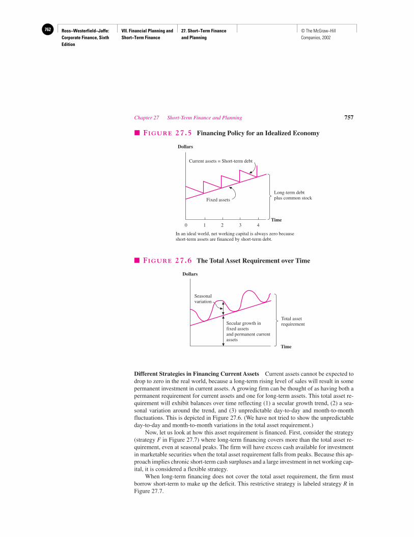
Ross−Westerfield−Jaffe: Corporate Finance, Sixth Edition
VII. Financial Planning and Short−Term Finance
27. Short−Term Finance and Planning
762 © The McGraw−Hill Companies, 2002
Different Strategies in Financing Current Assets Current assets cannot be expected todrop to zero in the real world, because a long-term rising level of sales will result in somepermanent investment in current assets. A growing firm can be thought of as having both apermanent requirement for current assets and one for long-term assets. This total asset re-quirement will exhibit balances over time reflecting (1) a secular growth trend, (2) a sea-sonal variation around the trend, and (3) unpredictable day-to-day and month-to-monthfluctuations. This is depicted in Figure 27.6. (We have not tried to show the unpredictableday-to-day and month-to-month variations in the total asset requirement.)
Now, let us look at how this asset requirement is financed. First, consider the strategy(strategy F in Figure 27.7) where long-term financing covers more than the total asset re-quirement, even at seasonal peaks. The firm will have excess cash available for investmentin marketable securities when the total asset requirement falls from peaks. Because this ap-proach implies chronic short-term cash surpluses and a large investment in net working cap-ital, it is considered a flexible strategy.
When long-term financing does not cover the total asset requirement, the firm mustborrow short-term to make up the deficit. This restrictive strategy is labeled strategy R inFigure 27.7.
Chapter 27 Short-Term Finance and Planning 757
Time
Dollars
Current assets = Short-term debt
Fixed assets
Long-term debtplus common stock
0 1 2 3 4
In an ideal world, net working capital is always zero becauseshort-term assets are financed by short-term debt.
� FIGURE 27.5 Financing Policy for an Idealized Economy
Dollars
Seasonalvariation
Secular growth infixed assetsand permanent currentassets
Time
Total assetrequirement
� FIGURE 27.6 The Total Asset Requirement over Time
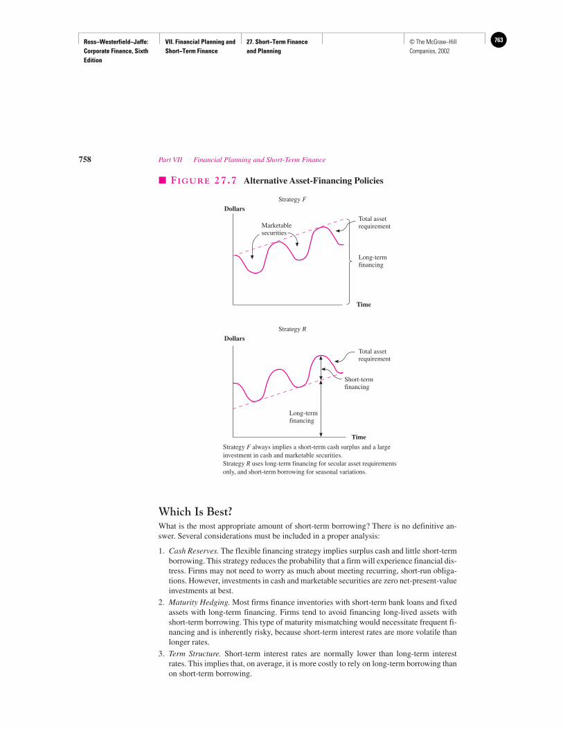
Ross−Westerfield−Jaffe: Corporate Finance, Sixth Edition
VII. Financial Planning and Short−Term Finance
27. Short−Term Finance and Planning
763© The McGraw−Hill Companies, 2002
Which Is Best?What is the most appropriate amount of short-term borrowing? There is no definitive an-swer. Several considerations must be included in a proper analysis:
1. Cash Reserves. The flexible financing strategy implies surplus cash and little short-termborrowing. This strategy reduces the probability that a firm will experience financial dis-tress. Firms may not need to worry as much about meeting recurring, short-run obliga-tions. However, investments in cash and marketable securities are zero net-present-valueinvestments at best.
2. Maturity Hedging. Most firms finance inventories with short-term bank loans and fixedassets with long-term financing. Firms tend to avoid financing long-lived assets withshort-term borrowing. This type of maturity mismatching would necessitate frequent fi-nancing and is inherently risky, because short-term interest rates are more volatile thanlonger rates.
3. Term Structure. Short-term interest rates are normally lower than long-term interestrates. This implies that, on average, it is more costly to rely on long-term borrowing thanon short-term borrowing.
758 Part VII Financial Planning and Short-Term Finance
Dollars
Time
Marketablesecurities
Strategy F
Total assetrequirement
Long-termfinancing
Strategy R
Dollars
Time
Total assetrequirement
Long-termfinancing
Short-termfinancing
� FIGURE 27.7 Alternative Asset-Financing Policies
Strategy F always implies a short-term cash surplus and a largeinvestment in cash and marketable securities.Strategy R uses long-term financing for secular asset requirementsonly, and short-term borrowing for seasonal variations.
Ross−Westerfield−Jaffe: Corporate Finance, Sixth Edition
VII. Financial Planning and Short−Term Finance
27. Short−Term Finance and Planning
764 © The McGraw−Hill Companies, 2002
• What keeps the real world from being an ideal one where net working capital could al-ways be zero?
• What considerations determine the optimal compromise between flexible and restrictivenet working capital policies?
27.5 CASH BUDGETING
The cash budget is a primary tool of short-run financial planning. It allows the financial man-ager to identify short-term financial needs (and opportunities). It will tell the manager the re-quired borrowing for the short term. It is the way of identifying the cash-flow gap on the cash-flow time line. The idea of the cash budget is simple: It records estimates of cash receipts anddisbursements. We illustrate cash budgeting with the following example of Fun Toys.
EXAMPLE
All of Fun Toys’ cash inflows come from the sale of toys. Cash budgeting for FunToys starts with a sales forecast for the next year, by quarter:
First Second Third FourthQuarter Quarter Quarter Quarter
Sales ($ millions) $100 $200 $150 $100
Fun Toys’fiscal year starts on July 1. Fun Toys’sales are seasonal and are usually veryhigh in the second quarter, due to Christmastime sales. But Fun Toys sells to depart-ment stores on credit, and sales do not generate cash immediately. Instead, cash comeslater from collections on accounts receivable. Fun Toys has a 90-day collection period,and 100 percent of sales are collected the following quarter. In other words,
Collections � Last quarter’s sales
This relationship implies that
(27.5)
We assume that sales in the fourth quarter of the previous fiscal year were $100million. From equation (27.5), we know that accounts receivable at the end of thefourth quarter of the previous fiscal year were $100 million and collections in thefirst quarter of the current fiscal year are $100 million.
The first quarter sales of the current fiscal year of $100 million are added tothe accounts receivable, but $100 million of collections are subtracted. Therefore,Fun Toys ended the first quarter with accounts receivable of $100 million. The ba-sic relation is
Table 27.3 shows cash collections for Fun Toys for the next four quarters. Though col-lections are the only source of cash here, this need not always be the case. Other sourcesof cash could include sales of assets, investment income, and long-term financing.
Ending accounts
receivable �
Starting accounts
receivable� Sales � Collections
Accounts receivable
at end of last quarter �
Last quarter ,s
sales
Chapter 27 Short-Term Finance and Planning 759
QUESTIONS
CO
NC
EP
T
?
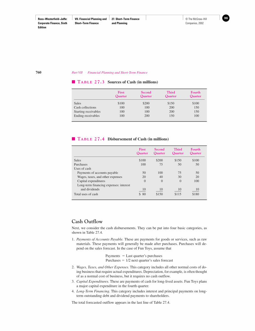
Ross−Westerfield−Jaffe: Corporate Finance, Sixth Edition
VII. Financial Planning and Short−Term Finance
27. Short−Term Finance and Planning
765© The McGraw−Hill Companies, 2002
Cash OutflowNext, we consider the cash disbursements. They can be put into four basic categories, asshown in Table 27.4.
1. Payments of Accounts Payable. These are payments for goods or services, such as rawmaterials. These payments will generally be made after purchases. Purchases will de-pend on the sales forecast. In the case of Fun Toys, assume that
Payments � Last quarter’s purchasesPurchases � 1/2 next quarter’s sales forecast
2. Wages, Taxes, and Other Expenses. This category includes all other normal costs of do-ing business that require actual expenditures. Depreciation, for example, is often thoughtof as a normal cost of business, but it requires no cash outflow.
3. Capital Expenditures. These are payments of cash for long-lived assets. Fun Toys plansa major capital expenditure in the fourth quarter.
4. Long-Term Financing. This category includes interest and principal payments on long-term outstanding debt and dividend payments to shareholders.
The total forecasted outflow appears in the last line of Table 27.4.
760 Part VII Financial Planning and Short-Term Finance
� TABLE 27.3 Sources of Cash (in millions)
First Second Third FourthQuarter Quarter Quarter Quarter
Sales $100 $200 $150 $100Cash collections 100 100 200 150Starting receivables 100 100 200 150Ending receivables 100 200 150 100
� TABLE 27.4 Disbursement of Cash (in millions)
First Second Third FourthQuarter Quarter Quarter Quarter
Sales $100 $200 $150 $100Purchases 100 75 50 50Uses of cash
Payments of accounts payable 50 100 75 50Wages, taxes, and other expenses 20 40 30 20Capital expenditures 0 0 0 100Long-term financing expenses: interest
and dividends 10 10 10 10____ ____ ____ ____Total uses of cash $ 80 $150 $115 $180
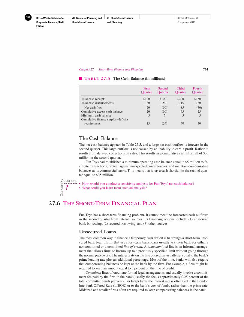
Ross−Westerfield−Jaffe: Corporate Finance, Sixth Edition
VII. Financial Planning and Short−Term Finance
27. Short−Term Finance and Planning
766 © The McGraw−Hill Companies, 2002
The Cash BalanceThe net cash balance appears in Table 27.5, and a large net cash outflow is forecast in thesecond quarter. This large outflow is not caused by an inability to earn a profit. Rather, itresults from delayed collections on sales. This results in a cumulative cash shortfall of $30million in the second quarter.
Fun Toys had established a minimum operating cash balance equal to $5 million to fa-cilitate transactions, protect against unexpected contingencies, and maintain compensatingbalances at its commercial banks. This means that it has a cash shortfall in the second quar-ter equal to $35 million.
• How would you conduct a sensitivity analysis for Fun Toys’ net cash balance?• What could you learn from such an analysis?
27.6 THE SHORT-TERM FINANCIAL PLAN
Fun Toys has a short-term financing problem. It cannot meet the forecasted cash outflowsin the second quarter from internal sources. Its financing options include: (1) unsecuredbank borrowing, (2) secured borrowing, and (3) other sources.
Unsecured LoansThe most common way to finance a temporary cash deficit is to arrange a short-term unse-cured bank loan. Firms that use short-term bank loans usually ask their bank for either anoncommitted or a committed line of credit. A noncommitted line is an informal arrange-ment that allows firms to borrow up to a previously specified limit without going throughthe normal paperwork. The interest rate on the line of credit is usually set equal to the bank’sprime lending rate plus an additional percentage. Most of the time, banks will also requirethat compensating balances be kept at the bank by the firm. For example, a firm might berequired to keep an amount equal to 5 percent on the line of credit.
Committed lines of credit are formal legal arrangements and usually involve a commit-ment fee paid by the firm to the bank (usually the fee is approximately 0.25 percent of thetotal committed funds per year). For larger firms the interest rate is often tied to the LondonInterbank Offered Rate (LIBOR) or to the bank’s cost of funds, rather than the prime rate.Midsized and smaller firms often are required to keep compensating balances in the bank.
Chapter 27 Short-Term Finance and Planning 761
� TABLE 27.5 The Cash Balance (in millions)
First Second Third FourthQuarter Quarter Quarter Quarter
Total cash receipts $100 $100 $200 $150Total cash disbursements 80 150 115 180____ ____ ____ ____
Net cash flow 20 (50) 85 (30)Cumulative excess cash balance 20 (30) 55 25Minimum cash balance 5 5 5 5Cumulative finance surplus (deficit)
requirement 15 (35) 50 20
QUESTIONS
CO
NC
EP
T
?
Ross−Westerfield−Jaffe: Corporate Finance, Sixth Edition
VII. Financial Planning and Short−Term Finance
27. Short−Term Finance and Planning
767© The McGraw−Hill Companies, 2002
Compensating balances are deposits the firm keeps with the bank in low-interest ornoninterest-bearing accounts. Compensating balances are commonly on the order of 2 to 5percent of the amount used. By leaving these funds with the bank without receiving inter-est, the firm increases the effective interest earned by the bank on the line of credit. For ex-ample, if a firm borrowing $100,000 must keep $5,000 as a compensating balance, the firmeffectively receives only $95,000. A stated interest rate of 10 percent implies yearly inter-est payments of $10,000 ($100,000 � 0.10). The effective interest rate is 10.53 percent($10,000/$95,000).
Secured LoansBanks and other finance companies often require security for a loan. Security for short-termloans usually consists of accounts receivable or inventories.
Under accounts receivable financing, receivables are either assigned or factored.Under assignment, the lender not only has a lien on the receivables but also has recourse tothe borrower. Factoring involves the sale of accounts receivable. The purchaser, who iscalled a factor, must then collect on the receivables. The factor assumes the full risk of de-fault on bad accounts.
As the name implies, an inventory loan uses inventory as collateral. Some commontypes of inventory loans are
1. Blanket Inventory Lien. The blanket inventory lien gives the lender a lien against all theborrower’s inventories.
2. Trust Receipt. Under this arrangement, the borrower holds the inventory in trust for thelender. The document acknowledging the loan is called the trust receipt. Proceeds fromthe sale of inventory are remitted immediately to the lender.
3. Field-Warehouse Financing. In field-warehouse financing, a public warehouse companysupervises the inventory for the lender.
Other SourcesThere are a variety of other sources of short-term funds employed by corporations. Themost important of these are the issuance of commercial paper and financing throughbanker’s acceptances. Commercial paper consists of short-term notes issued by large andhighly rated firms. Typically these notes are of short maturity, ranging up to 270 days (be-yond that limit the firm must file a registration statement with the SEC). Because the firmissues these directly and because it usually backs the issue with a special bank line of credit,the rate the firm obtains is often significantly below the prime rate the bank would chargeit for a direct loan.
A banker’s acceptance is an agreement by a bank to pay a sum of money. Theseagreements typically arise when a seller sends a bill or draft to a customer. The cus-tomer’s bank accepts this bill and notes the acceptance on it, which makes it an obliga-tion of the bank. In this way a firm that is buying something from a supplier can effec-tively arrange for the bank to pay the outstanding bill. Of course, the bank charges thecustomer a fee for this service.
• What are the two basic forms of short-term financing?• Describe two types of secured loans.
762 Part VII Financial Planning and Short-Term Finance
QUESTIONS
CO
NC
EP
T
?

Ross−Westerfield−Jaffe: Corporate Finance, Sixth Edition
VII. Financial Planning and Short−Term Finance
27. Short−Term Finance and Planning
768 © The McGraw−Hill Companies, 2002
27.7 SUMMARY AND CONCLUSIONS
1. This chapter introduces the management of short-term finance. Short-term finance involvesshort-lived assets and liabilities. We trace and examine the short-term sources and uses ofcash as they appear on the firm’s financial statements. We see how current assets and currentliabilities arise in the short-term operating activities and the cash cycle of the firm. From anaccounting perspective, short-term finance involves net working capital.
2. Managing short-term cash flows involves the minimization of costs. The two major costs arecarrying costs—the interest and related costs incurred by overinvesting in short-term assetssuch as cash—and shortage costs, the cost of running out of short-term assets. The objectiveof managing short-term finance and short-term financial planning is to find the optimal trade-off between these two costs.
3. In an ideal economy the firm could perfectly predict its short-term uses and sources of cash,and net working capital could be kept at zero. In the real world, net working capital providesa buffer that lets the firm meet its ongoing obligations. The financial manager seeks theoptimal level of each of the current assets.
4. The financial manager can use the cash budget to identify short-term financial needs. Thecash budget tells the manager what borrowing is required or what lending will be possible inthe short run. The firm has available to it a number of possible ways of acquiring funds tomeet short-term shortfalls, including unsecured and secured loans.
KEY TERMS
Accounts receivable financing 762 Compensating balance 762Banker’s acceptances 762 Inventory loan 762Carrying costs 754 Liquidity 746Cash budget 759 Operating cycle 751Cash cycle 751 Shortage costs 754Cash flow time line 751 Short-run operating activities 750Commercial paper 762
SUGGESTED READINGS
A book that describes working capital management is:Fabozzi, F., and L. N. Masonson. Corporate Cash Management Techniques and Analyses.
Homewood, Ill.: Dow Jones–Irwin, 1985.Kallberg, J. G., and K. Parkinson. Corporate Liquidity: Management and Measurement. Burr
Ridge, IL: Irwin/McGraw Hill, 1996.
QUESTIONS AND PROBLEMS
Tracing Cash and Net Working Capital27.1 Derive the cash equation from the basic balance sheet equation: assets � liabilities � equity.
27.2 Indicate whether the following corporate actions increase, decrease, or cause no changeto cash.
Chapter 27 Short-Term Finance and Planning 763
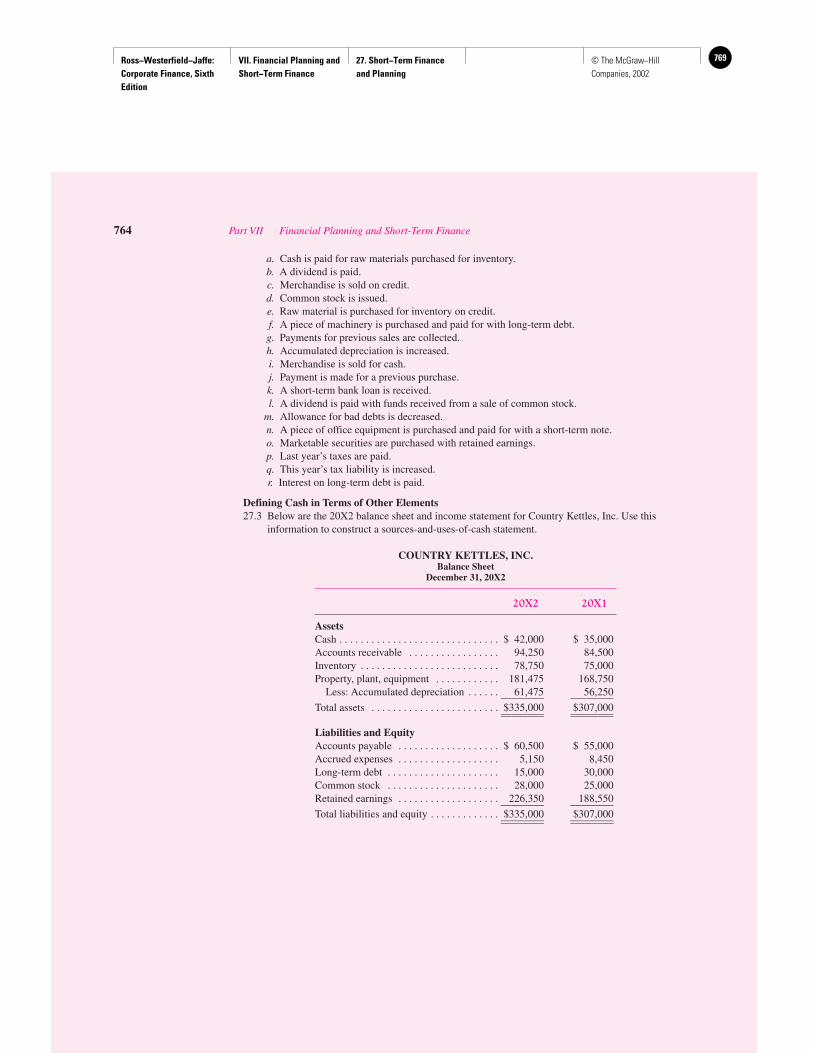
Ross−Westerfield−Jaffe: Corporate Finance, Sixth Edition
VII. Financial Planning and Short−Term Finance
27. Short−Term Finance and Planning
769© The McGraw−Hill Companies, 2002
a. Cash is paid for raw materials purchased for inventory.b. A dividend is paid.c. Merchandise is sold on credit.d. Common stock is issued.e. Raw material is purchased for inventory on credit.f. A piece of machinery is purchased and paid for with long-term debt.g. Payments for previous sales are collected.h. Accumulated depreciation is increased.i. Merchandise is sold for cash.j. Payment is made for a previous purchase.k. A short-term bank loan is received.l. A dividend is paid with funds received from a sale of common stock.
m. Allowance for bad debts is decreased.n. A piece of office equipment is purchased and paid for with a short-term note.o. Marketable securities are purchased with retained earnings.p. Last year’s taxes are paid.q. This year’s tax liability is increased.r. Interest on long-term debt is paid.
Defining Cash in Terms of Other Elements27.3 Below are the 20X2 balance sheet and income statement for Country Kettles, Inc. Use this
information to construct a sources-and-uses-of-cash statement.
COUNTRY KETTLES, INC.Balance Sheet
December 31, 20X2
20X2 20X1
AssetsCash . . . . . . . . . . . . . . . . . . . . . . . . . . . . . . $ 42,000 $ 35,000Accounts receivable . . . . . . . . . . . . . . . . . 94,250 84,500Inventory . . . . . . . . . . . . . . . . . . . . . . . . . . 78,750 75,000Property, plant, equipment . . . . . . . . . . . . 181,475 168,750
Less: Accumulated depreciation . . . . . . 61,475 56,250________ ________Total assets . . . . . . . . . . . . . . . . . . . . . . . . $335,000 $307,000________ ________________ ________
Liabilities and EquityAccounts payable . . . . . . . . . . . . . . . . . . . $ 60,500 $ 55,000Accrued expenses . . . . . . . . . . . . . . . . . . . 5,150 8,450Long-term debt . . . . . . . . . . . . . . . . . . . . . 15,000 30,000Common stock . . . . . . . . . . . . . . . . . . . . . 28,000 25,000Retained earnings . . . . . . . . . . . . . . . . . . . 226,350 188,550________ ________Total liabilities and equity . . . . . . . . . . . . . $335,000 $307,000________ ________________ ________
764 Part VII Financial Planning and Short-Term Finance
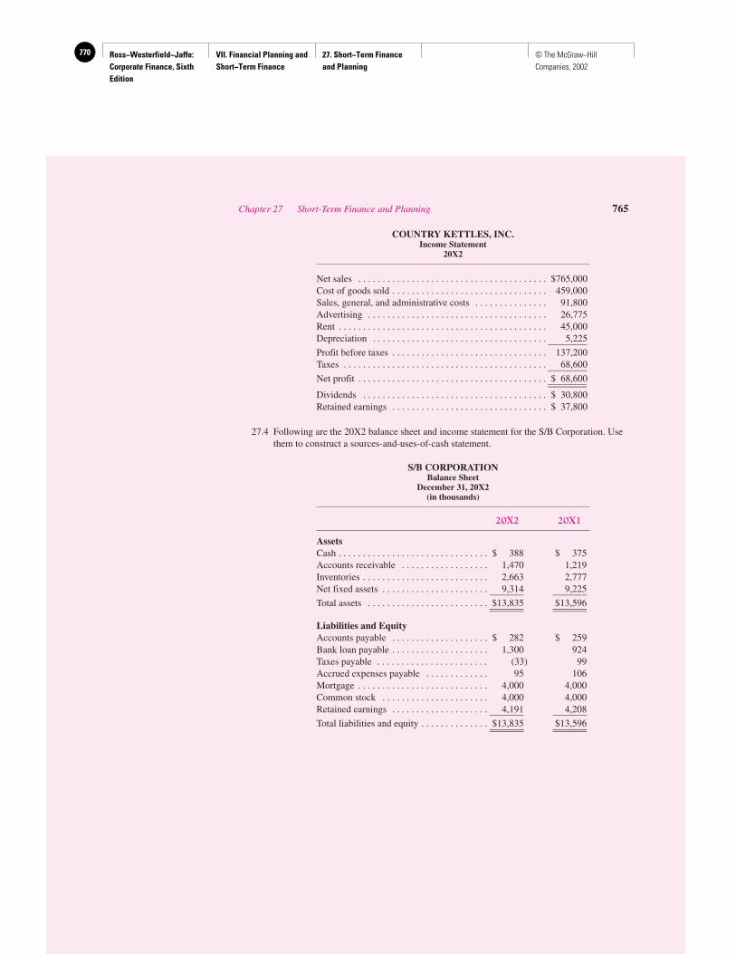
Ross−Westerfield−Jaffe: Corporate Finance, Sixth Edition
VII. Financial Planning and Short−Term Finance
27. Short−Term Finance and Planning
770 © The McGraw−Hill Companies, 2002
COUNTRY KETTLES, INC.Income Statement
20X2
Net sales . . . . . . . . . . . . . . . . . . . . . . . . . . . . . . . . . . . . . . . $765,000Cost of goods sold . . . . . . . . . . . . . . . . . . . . . . . . . . . . . . . . 459,000Sales, general, and administrative costs . . . . . . . . . . . . . . . 91,800Advertising . . . . . . . . . . . . . . . . . . . . . . . . . . . . . . . . . . . . . 26,775Rent . . . . . . . . . . . . . . . . . . . . . . . . . . . . . . . . . . . . . . . . . . . 45,000Depreciation . . . . . . . . . . . . . . . . . . . . . . . . . . . . . . . . . . . . 5,225________Profit before taxes . . . . . . . . . . . . . . . . . . . . . . . . . . . . . . . . 137,200Taxes . . . . . . . . . . . . . . . . . . . . . . . . . . . . . . . . . . . . . . . . . . 68,600________Net profit . . . . . . . . . . . . . . . . . . . . . . . . . . . . . . . . . . . . . . . $ 68,600________________Dividends . . . . . . . . . . . . . . . . . . . . . . . . . . . . . . . . . . . . . . $ 30,800Retained earnings . . . . . . . . . . . . . . . . . . . . . . . . . . . . . . . . $ 37,800
27.4 Following are the 20X2 balance sheet and income statement for the S/B Corporation. Usethem to construct a sources-and-uses-of-cash statement.
S/B CORPORATIONBalance Sheet
December 31, 20X2(in thousands)
20X2 20X1
AssetsCash . . . . . . . . . . . . . . . . . . . . . . . . . . . . . . . $ 388 $ 375Accounts receivable . . . . . . . . . . . . . . . . . . 1,470 1,219Inventories . . . . . . . . . . . . . . . . . . . . . . . . . . 2,663 2,777Net fixed assets . . . . . . . . . . . . . . . . . . . . . . 9,314 9,225_______ _______Total assets . . . . . . . . . . . . . . . . . . . . . . . . . $13,835 $13,596_______ ______________ _______
Liabilities and EquityAccounts payable . . . . . . . . . . . . . . . . . . . . $ 282 $ 259Bank loan payable . . . . . . . . . . . . . . . . . . . . 1,300 924Taxes payable . . . . . . . . . . . . . . . . . . . . . . . (33) 99Accrued expenses payable . . . . . . . . . . . . . 95 106Mortgage . . . . . . . . . . . . . . . . . . . . . . . . . . . 4,000 4,000Common stock . . . . . . . . . . . . . . . . . . . . . . 4,000 4,000Retained earnings . . . . . . . . . . . . . . . . . . . . 4,191 4,208_______ _______Total liabilities and equity . . . . . . . . . . . . . . $13,835 $13,596_______ ______________ _______
Chapter 27 Short-Term Finance and Planning 765
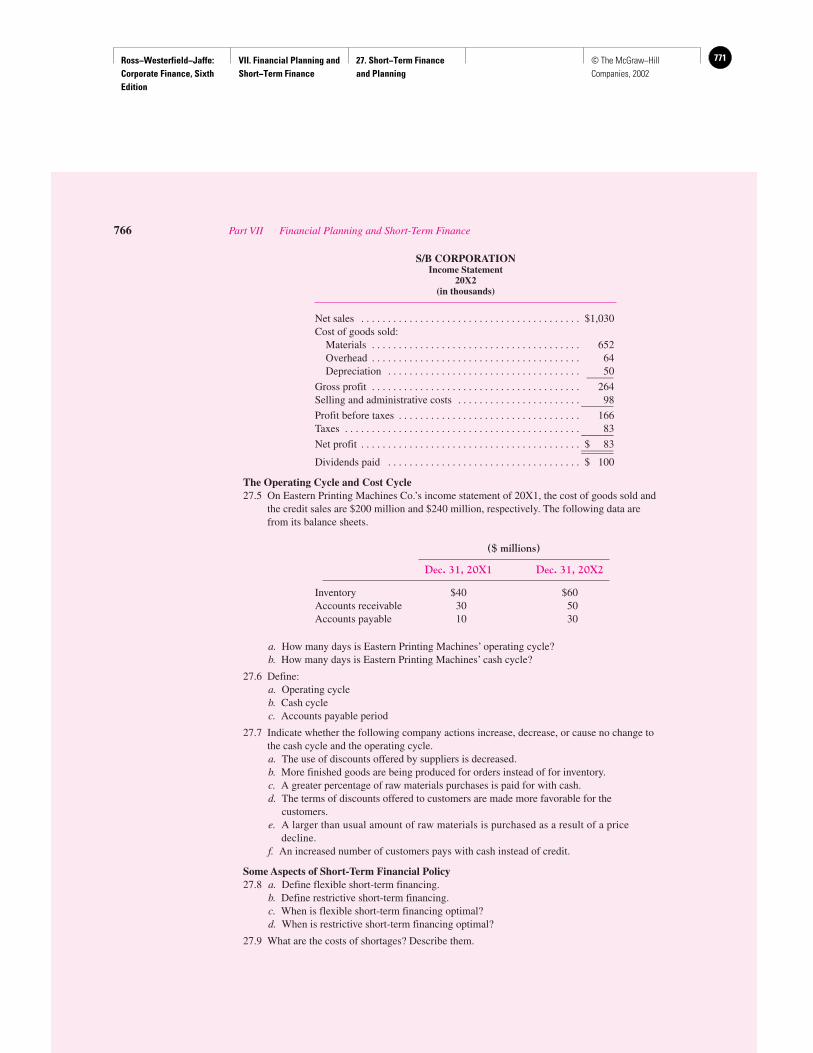
Ross−Westerfield−Jaffe: Corporate Finance, Sixth Edition
VII. Financial Planning and Short−Term Finance
27. Short−Term Finance and Planning
771© The McGraw−Hill Companies, 2002
S/B CORPORATIONIncome Statement
20X2(in thousands)
Net sales . . . . . . . . . . . . . . . . . . . . . . . . . . . . . . . . . . . . . . . . . $1,030Cost of goods sold:
Materials . . . . . . . . . . . . . . . . . . . . . . . . . . . . . . . . . . . . . . . 652Overhead . . . . . . . . . . . . . . . . . . . . . . . . . . . . . . . . . . . . . . . 64Depreciation . . . . . . . . . . . . . . . . . . . . . . . . . . . . . . . . . . . . 50_____
Gross profit . . . . . . . . . . . . . . . . . . . . . . . . . . . . . . . . . . . . . . . 264Selling and administrative costs . . . . . . . . . . . . . . . . . . . . . . . 98______Profit before taxes . . . . . . . . . . . . . . . . . . . . . . . . . . . . . . . . . . 166Taxes . . . . . . . . . . . . . . . . . . . . . . . . . . . . . . . . . . . . . . . . . . . . 83______Net profit . . . . . . . . . . . . . . . . . . . . . . . . . . . . . . . . . . . . . . . . . $ 83____________Dividends paid . . . . . . . . . . . . . . . . . . . . . . . . . . . . . . . . . . . . $ 100
The Operating Cycle and Cost Cycle27.5 On Eastern Printing Machines Co.’s income statement of 20X1, the cost of goods sold and
the credit sales are $200 million and $240 million, respectively. The following data arefrom its balance sheets.
($ millions)
Dec. 31, 20X1 Dec. 31, 20X2
Inventory $40 $60Accounts receivable 30 50Accounts payable 10 30
a. How many days is Eastern Printing Machines’ operating cycle?b. How many days is Eastern Printing Machines’ cash cycle?
27.6 Define:a. Operating cycleb. Cash cyclec. Accounts payable period
27.7 Indicate whether the following company actions increase, decrease, or cause no change tothe cash cycle and the operating cycle.a. The use of discounts offered by suppliers is decreased.b. More finished goods are being produced for orders instead of for inventory.c. A greater percentage of raw materials purchases is paid for with cash.d. The terms of discounts offered to customers are made more favorable for the
customers.e. A larger than usual amount of raw materials is purchased as a result of a price
decline.f. An increased number of customers pays with cash instead of credit.
Some Aspects of Short-Term Financial Policy27.8 a. Define flexible short-term financing.
b. Define restrictive short-term financing.c. When is flexible short-term financing optimal?d. When is restrictive short-term financing optimal?
27.9 What are the costs of shortages? Describe them.
766 Part VII Financial Planning and Short-Term Finance
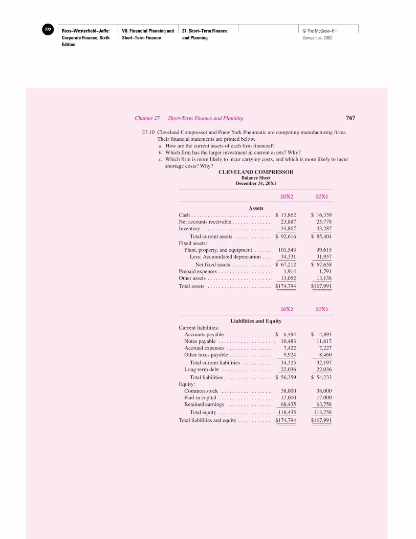
Ross−Westerfield−Jaffe: Corporate Finance, Sixth Edition
VII. Financial Planning and Short−Term Finance
27. Short−Term Finance and Planning
772 © The McGraw−Hill Companies, 2002
27.10 Cleveland Compressor and Pnew York Pneumatic are competing manufacturing firms.Their financial statements are printed below.a. How are the current assets of each firm financed?b. Which firm has the larger investment in current assets? Why?c. Which firm is more likely to incur carrying costs, and which is more likely to incur
shortage costs? Why?CLEVELAND COMPRESSOR
Balance SheetDecember 31, 20X1
20X2 20X1
AssetsCash . . . . . . . . . . . . . . . . . . . . . . . . . . . . . . $ 13,862 $ 16,339Net accounts receivable . . . . . . . . . . . . . . . 23,887 25,778Inventory . . . . . . . . . . . . . . . . . . . . . . . . . . 54,867 43,287_______ _______
Total current assets . . . . . . . . . . . . . . $ 92,616 $ 85,404Fixed assets:
Plant, property, and equipment . . . . . . . 101,543 99,615Less: Accumulated depreciation . . . . 34,331 31,957_______ _______
Net fixed assets . . . . . . . . . . . . . . . $ 67,212 $ 67,658Prepaid expenses . . . . . . . . . . . . . . . . . . . . 1,914 1,791Other assets . . . . . . . . . . . . . . . . . . . . . . . . 13,052 13,138_______ _______Total assets . . . . . . . . . . . . . . . . . . . . . . . . $174,794 $167,991_______ ______________ _______
20X2 20X1
Liabilities and EquityCurrent liabilities:
Accounts payable . . . . . . . . . . . . . . . . . $ 6,494 $ 4,893Notes payable . . . . . . . . . . . . . . . . . . . . . 10,483 11,617Accrued expenses . . . . . . . . . . . . . . . . . 7,422 7,227Other taxes payable . . . . . . . . . . . . . . . . 9,924 8,460_______ _______
Total current liabilities . . . . . . . . . . . 34,323 32,197Long-term debt . . . . . . . . . . . . . . . . . . . 22,036 22,036_______ _______
Total liabilities . . . . . . . . . . . . . . . . . . $ 56,359 $ 54,233Equity:
Common stock . . . . . . . . . . . . . . . . . . . 38,000 38,000Paid-in capital . . . . . . . . . . . . . . . . . . . . 12,000 12,000Retained earnings . . . . . . . . . . . . . . . . . 68,435 63,758_______ _______
Total equity . . . . . . . . . . . . . . . . . . . . 118,435 113,758_______ _______Total liabilities and equity . . . . . . . . . . . . . $174,794 $167,991_______ ______________ _______
Chapter 27 Short-Term Finance and Planning 767
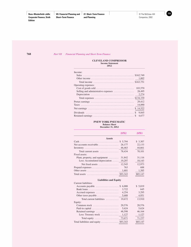
Ross−Westerfield−Jaffe: Corporate Finance, Sixth Edition
VII. Financial Planning and Short−Term Finance
27. Short−Term Finance and Planning
773© The McGraw−Hill Companies, 2002
CLEVELAND COMPRESSORIncome Statement
20X2
Income:Sales . . . . . . . . . . . . . . . . . . . . . . . . . . . . . . . . . . . . . . . . $162,749Other income . . . . . . . . . . . . . . . . . . . . . . . . . . . . . . . . . . 1,002_______
Total income . . . . . . . . . . . . . . . . . . . . . . . . . . . . . . . . $163,751Operating expenses:
Cost of goods sold . . . . . . . . . . . . . . . . . . . . . . . . . . . . . . 103,570Selling and administrative expenses . . . . . . . . . . . . . . . . 28,495Depreciation . . . . . . . . . . . . . . . . . . . . . . . . . . . . . . . . . . 2,274_______
Total expenses . . . . . . . . . . . . . . . . . . . . . . . . . . . . . . . $134,339_______Pretax earnings . . . . . . . . . . . . . . . . . . . . . . . . . . . . . . . . . . 29,412Taxes . . . . . . . . . . . . . . . . . . . . . . . . . . . . . . . . . . . . . . . . . . 14,890_______Net earnings . . . . . . . . . . . . . . . . . . . . . . . . . . . . . . . . . . . . $ 14,522______________Dividends . . . . . . . . . . . . . . . . . . . . . . . . . . . . . . . . . . . . . . $ 9,845Retained earnings . . . . . . . . . . . . . . . . . . . . . . . . . . . . . . . . $ 4,677
PNEW YORK PNEUMATICBalance Sheet
December 31, 20X2
20X2 20X1
AssetsCash . . . . . . . . . . . . . . . . . . . . . . . . . . . . . . . $ 5,794 $ 3,307Net accounts receivable . . . . . . . . . . . . . . . . 26,177 22,133Inventory . . . . . . . . . . . . . . . . . . . . . . . . . . . 46,463 44,661_______ _______
Total current assets . . . . . . . . . . . . . . . 78,434 70,101Fixed assets:
Plant, property, and equipment . . . . . . . . 31,842 31,116Less: Accumulated depreciation . . . . . 19,297 18,143_______ _______
Net fixed assets . . . . . . . . . . . . . . . . 12,545 12,973Prepaid expenses . . . . . . . . . . . . . . . . . . . . . 763 688Other assets . . . . . . . . . . . . . . . . . . . . . . . . . 1,601 1,385_______ _______Total assets . . . . . . . . . . . . . . . . . . . . . . . . . $93,343 $85,147_______ ______________ _______
Liabilities and EquityCurrent liabilities:
Accounts payable . . . . . . . . . . . . . . . . . . $ 6,008 $ 5,019Bank loans . . . . . . . . . . . . . . . . . . . . . . . . 3,722 645Accrued expenses . . . . . . . . . . . . . . . . . . 4,254 3,295Other taxes payable . . . . . . . . . . . . . . . . . 5,688 4,951_______ _______
Total current liabilities . . . . . . . . . . 19,672 13,910Equity:
Common stock . . . . . . . . . . . . . . . . . . . . 20,576 20,576Paid-in capital . . . . . . . . . . . . . . . . . . . . . 5,624 5,624Retained earnings . . . . . . . . . . . . . . . . . . 48,598 46,164
Less: Treasury stock . . . . . . . . . . . . . . 1,127 1,127_______ _______Total equity . . . . . . . . . . . . . . . . . . . 73,671 71,237_______ _______
Total liabilities and equity . . . . . . . . . . . . . . $93,343 $85,147_______ ______________ _______
768 Part VII Financial Planning and Short-Term Finance
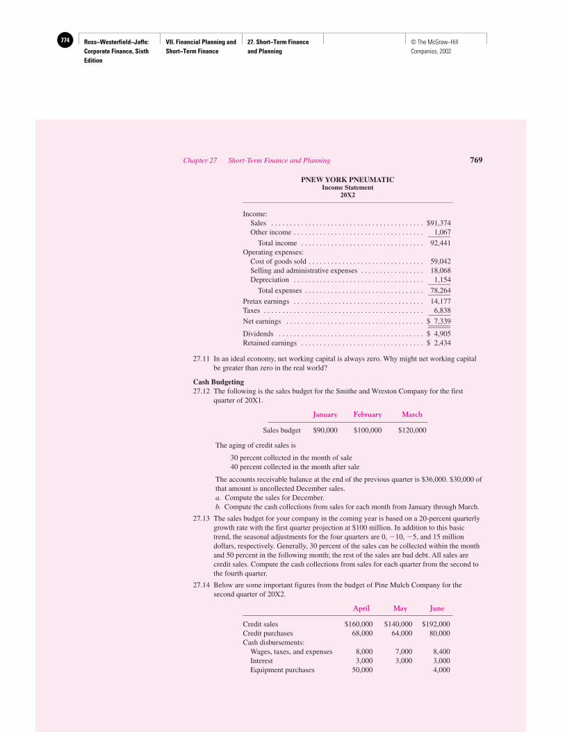
Ross−Westerfield−Jaffe: Corporate Finance, Sixth Edition
VII. Financial Planning and Short−Term Finance
27. Short−Term Finance and Planning
774 © The McGraw−Hill Companies, 2002
PNEW YORK PNEUMATICIncome Statement
20X2
Income:Sales . . . . . . . . . . . . . . . . . . . . . . . . . . . . . . . . . . . . . . . . . $91,374Other income . . . . . . . . . . . . . . . . . . . . . . . . . . . . . . . . . . . 1,067______
Total income . . . . . . . . . . . . . . . . . . . . . . . . . . . . . . . . . 92,441Operating expenses:
Cost of goods sold . . . . . . . . . . . . . . . . . . . . . . . . . . . . . . . 59,042Selling and administrative expenses . . . . . . . . . . . . . . . . . 18,068Depreciation . . . . . . . . . . . . . . . . . . . . . . . . . . . . . . . . . . . 1,154______
Total expenses . . . . . . . . . . . . . . . . . . . . . . . . . . . . . . . . 78,264______Pretax earnings . . . . . . . . . . . . . . . . . . . . . . . . . . . . . . . . . . . 14,177Taxes . . . . . . . . . . . . . . . . . . . . . . . . . . . . . . . . . . . . . . . . . . . 6,838______Net earnings . . . . . . . . . . . . . . . . . . . . . . . . . . . . . . . . . . . . . $ 7,339____________Dividends . . . . . . . . . . . . . . . . . . . . . . . . . . . . . . . . . . . . . . . $ 4,905Retained earnings . . . . . . . . . . . . . . . . . . . . . . . . . . . . . . . . . $ 2,434
27.11 In an ideal economy, net working capital is always zero. Why might net working capitalbe greater than zero in the real world?
Cash Budgeting27.12 The following is the sales budget for the Smithe and Wreston Company for the first
quarter of 20X1.
January February March
Sales budget $90,000 $100,000 $120,000
The aging of credit sales is
30 percent collected in the month of sale40 percent collected in the month after sale
The accounts receivable balance at the end of the previous quarter is $36,000. $30,000 ofthat amount is uncollected December sales.a. Compute the sales for December.b. Compute the cash collections from sales for each month from January through March.
27.13 The sales budget for your company in the coming year is based on a 20-percent quarterlygrowth rate with the first quarter projection at $100 million. In addition to this basictrend, the seasonal adjustments for the four quarters are 0, �10, �5, and 15 milliondollars, respectively. Generally, 30 percent of the sales can be collected within the monthand 50 percent in the following month; the rest of the sales are bad debt. All sales arecredit sales. Compute the cash collections from sales for each quarter from the second tothe fourth quarter.
27.14 Below are some important figures from the budget of Pine Mulch Company for thesecond quarter of 20X2.
April May June
Credit sales $160,000 $140,000 $192,000Credit purchases 68,000 64,000 80,000Cash disbursements:
Wages, taxes, and expenses 8,000 7,000 8,400Interest 3,000 3,000 3,000Equipment purchases 50,000 4,000
Chapter 27 Short-Term Finance and Planning 769
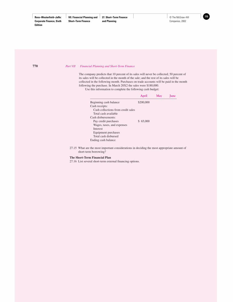
Ross−Westerfield−Jaffe: Corporate Finance, Sixth Edition
VII. Financial Planning and Short−Term Finance
27. Short−Term Finance and Planning
775© The McGraw−Hill Companies, 2002
The company predicts that 10 percent of its sales will never be collected; 50 percent ofits sales will be collected in the month of the sale; and the rest of its sales will becollected in the following month. Purchases on trade accounts will be paid in the monthfollowing the purchase. In March 20X2 the sales were $180,000.
Use this information to complete the following cash budget:
April May June
Beginning cash balance $200,000Cash receipts:
Cash collections from credit salesTotal cash available
Cash disbursements:Pay credit purchases $ 65,000Wages, taxes, and expensesInterestEquipment purchasesTotal cash disbursed
Ending cash balance
27.15 What are the most important considerations in deciding the most appropriate amount ofshort-term borrowing?
The Short-Term Financial Plan27.16 List several short-term external financing options.
770 Part VII Financial Planning and Short-Term Finance
Ross−Westerfield−Jaffe: Corporate Finance, Sixth Edition
VII. Financial Planning and Short−Term Finance
28. Cash Management776 © The McGraw−Hill Companies, 2002
Cash Management
CH
AP
TE
R28
EXECUTIVE SUMMARY
The balance sheet of Singapore Airlines showed total assets of $8.7 billion inMarch 1994. On this basis, Singapore Airlines was one of the largest transporta-tion firms in the world. In addition, Singapore Airlines held $62.4 million in cash.
This cash included currency, demand deposits at commercial banks, and undepositedchecks.1
Since cash earns no interest, why would Singapore Airlines hold cash? It wouldseem more sensible for Singapore Airlines to put its cash into marketable securities,such as Treasury bills, and get some investment income. Of course, one reasonSingapore Airlines holds cash is to pay for goods and services. Singapore Airlinesmight prefer to pay its employees in Treasury bills, but the minimum denomination ofTreasury bills is $10,000! The firm must use cash because cash is more divisible thanTreasury bills.2
This chapter is about how firms manage cash. The basic objective in cash managementis to keep the investment in cash as low as possible while still operating the firm’s activitiesefficiently and effectively. This chapter separates cash management into three steps:
1. Determining the appropriate target cash balance.
2. Collecting and disbursing cash efficiently.
3. Investing excess cash in marketable securities.
Determining the appropriate target cash balance involves an assessment of the trade-off between the benefit and cost of liquidity. The benefit of holding cash is the conveniencein liquidity it gives the firm. The cost of holding cash is the interest income that the firmcould have received from investing in Treasury bills and other marketable securities. If thefirm has achieved its target cash balance, the value it gets from the liquidity provided by itscash will be exactly equal to the value forgone in interest on an equivalent holding ofTreasury bills. In other words, a firm should increase its holding of cash until the net pres-ent value from doing so is zero. The incremental liquidity value of cash should decline asmore of it is held.
After the optimal amount of liquidity is determined, the firm must establish proceduresso that cash is collected and disbursed as efficiently as possible. This usually reduces to thedictum, “collect early and pay late.”
Firms must invest temporarily idle cash in short-term marketable securities. These se-curities can be bought and sold in the money market. Money-market securities have very lit-tle risk of default and are highly marketable.
1It was somewhat unusual for Singapore Airlines to report cash in this way. Usually, a firm’s reported cashincludes cash equivalents, such as Treasury bills.2Cash is liquid. One property of liquidity is divisibility, that is, how easily an asset can be divided into parts.
Ross−Westerfield−Jaffe: Corporate Finance, Sixth Edition
VII. Financial Planning and Short−Term Finance
28. Cash Management 777© The McGraw−Hill Companies, 2002
28.1 REASONS FOR HOLDING CASH
The term cash is a surprisingly imprecise concept. The economic definition of cash includescurrency, checking account deposits at commercial banks, and undeposited checks. How-ever, financial managers often use the term cash to include short-term marketable securi-ties. Short-term marketable securities are frequently referred to as “cash equivalents” andinclude Treasury bills, certificates of deposit, and repurchase agreements. (Several differ-ent types of short-term marketable securities are described at the end of this chapter.) Thebalance sheet item “cash” usually includes cash equivalents.3
The previous chapter discussed the management of net working capital. Net workingcapital includes both cash and cash equivalents. This chapter is concerned with cash, notnet working capital, and it focuses on the narrow economic definition of cash.
The basic elements of net working capital management such as carrying costs, short-age costs, and opportunity costs are relevant for cash management. However, cash man-agement is more concerned with how to minimize cash balances by collecting and disburs-ing cash effectively.
There are two primary reasons for holding cash. First, cash is needed to satisfy thetransactions motive. Transactions-related needs come from normal disbursement and col-lection activities of the firm. The disbursement of cash includes the payment of wages andsalaries, trade debts, taxes, and dividends. Cash is collected from sales from operations, salesof assets, and new financing. The cash inflows (collections) and outflows (disbursements) arenot perfectly synchronized, and some level of cash holdings is necessary to serve as a buffer. Ifthe firm maintains too small a cash balance, it may run out of cash. If so, it must sell marketablesecurities or borrow. Selling marketable securities and borrowing involve trading costs.
Another reason to hold cash is for compensating balances. Cash balances are kept atcommercial banks to compensate for banking services rendered to the firm. A minimum re-quired compensating balance at banks providing credit services to the firm may impose alower limit on the level of cash a firm holds.
The cash balance for most firms can be thought of as consisting of transactions bal-ances and compensating balances. However, it would not be correct for a firm to add theamount of cash required to satisfy its transactions needs to the amount of cash needed tosatisfy its compensatory balances to produce a target cash balance. The same cash can beused to satisfy both requirements.
The cost of holding cash is, of course, the opportunity cost of lost interest. To deter-mine the target cash balance, the firm must weigh the benefits of holding cash against thecosts. It is generally a good idea for firms to figure out first how much cash to hold to sat-isfy the transactions needs. Next, the firm must consider compensating-balance require-ments, which will impose a lower limit on the level of the firm’s cash holdings. Becausecompensating balances merely provide a lower limit, we shall ignore compensating bal-ances for the following discussion of the target cash balance.
772 Part VII Financial Planning and Short-Term Finance
3Many firms hold very large balances of cash and cash equivalents. In 1997 the largest balances included:
(in $ billions)
Ford $18.5General Motors 10.1Microsoft 9.1Intel 8.5IBM 6.5
The reasons firms hold large balances of cash and equivalents include precautionary balances such as in the caseof a recession or large anticipated spending on dividends, stock repurchases, stock options, or capital investment.
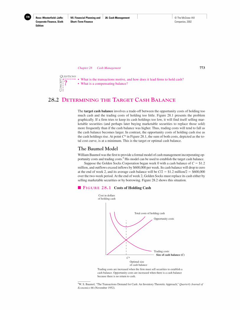
Ross−Westerfield−Jaffe: Corporate Finance, Sixth Edition
VII. Financial Planning and Short−Term Finance
28. Cash Management778 © The McGraw−Hill Companies, 2002
• What is the transactions motive, and how does it lead firms to hold cash?• What is a compensating balance?
28.2 DETERMINING THE TARGET CASH BALANCE
The target cash balance involves a trade-off between the opportunity costs of holding toomuch cash and the trading costs of holding too little. Figure 28.1 presents the problemgraphically. If a firm tries to keep its cash holdings too low, it will find itself selling mar-ketable securities (and perhaps later buying marketable securities to replace those sold)more frequently than if the cash balance was higher. Thus, trading costs will tend to fall asthe cash balance becomes larger. In contrast, the opportunity costs of holding cash rise asthe cash holdings rise. At point C* in Figure 28.1, the sum of both costs, depicted as the to-tal cost curve, is at a minimum. This is the target or optimal cash balance.
The Baumol ModelWilliam Baumol was the first to provide a formal model of cash management incorporating op-portunity costs and trading costs.4 His model can be used to establish the target cash balance.
Suppose the Golden Socks Corporation began week 0 with a cash balance of C � $1.2million, and outflows exceed inflows by $600,000 per week. Its cash balance will drop to zeroat the end of week 2, and its average cash balance will be C/2 � $1.2 million/2 � $600,000over the two-week period. At the end of week 2, Golden Socks must replace its cash either byselling marketable securities or by borrowing. Figure 28.2 shows this situation.
Chapter 28 Cash Management 773
4W. S. Baumol, “The Transactions Demand for Cash: An Inventory Theoretic Approach,” Quarterly Journal ofEconomics 66 (November 1952).
C*
Cost in dollarsof holding cash
Total costs of holding cash
Opportunity costs
Trading costsSize of cash balance (C)
Optimal sizeof cash balance
� FIGURE 28.1 Costs of Holding Cash
Trading costs are increased when the firm must sell securities to establish acash balance. Opportunity costs are increased when there is a cash balancebecause there is no return to cash.
QUESTIONS
CO
NC
EP
T
?
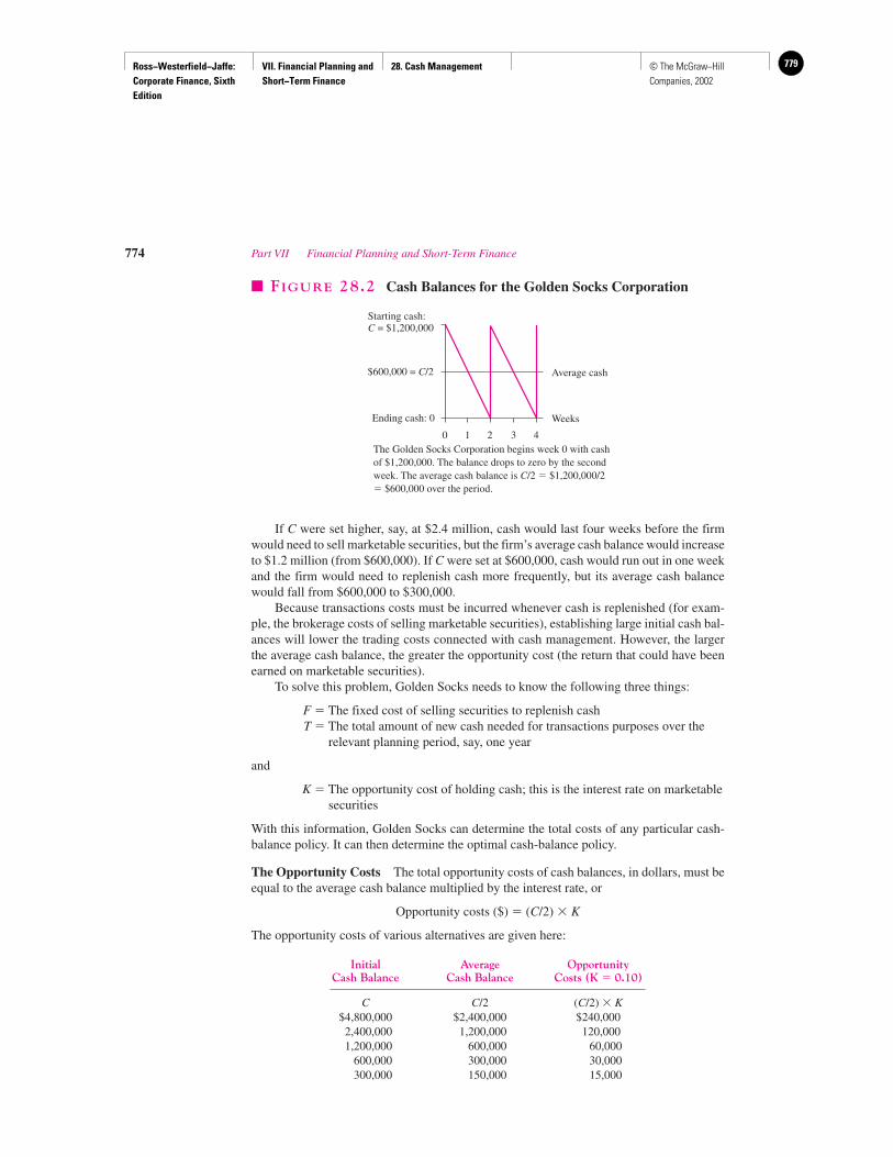
Ross−Westerfield−Jaffe: Corporate Finance, Sixth Edition
VII. Financial Planning and Short−Term Finance
28. Cash Management 779© The McGraw−Hill Companies, 2002
If C were set higher, say, at $2.4 million, cash would last four weeks before the firmwould need to sell marketable securities, but the firm’s average cash balance would increaseto $1.2 million (from $600,000). If C were set at $600,000, cash would run out in one weekand the firm would need to replenish cash more frequently, but its average cash balancewould fall from $600,000 to $300,000.
Because transactions costs must be incurred whenever cash is replenished (for exam-ple, the brokerage costs of selling marketable securities), establishing large initial cash bal-ances will lower the trading costs connected with cash management. However, the largerthe average cash balance, the greater the opportunity cost (the return that could have beenearned on marketable securities).
To solve this problem, Golden Socks needs to know the following three things:
F � The fixed cost of selling securities to replenish cashT � The total amount of new cash needed for transactions purposes over the
relevant planning period, say, one year
and
K � The opportunity cost of holding cash; this is the interest rate on marketablesecurities
With this information, Golden Socks can determine the total costs of any particular cash-balance policy. It can then determine the optimal cash-balance policy.
The Opportunity Costs The total opportunity costs of cash balances, in dollars, must beequal to the average cash balance multiplied by the interest rate, or
Opportunity costs ($) � (C/2) � K
The opportunity costs of various alternatives are given here:
Initial Average OpportunityCash Balance Cash Balance Costs (K � 0.10)
C C/2 (C/2) � K$4,800,000 $2,400,000 $240,000
2,400,000 1,200,000 120,0001,200,000 600,000 60,000
600,000 300,000 30,000300,000 150,000 15,000
774 Part VII Financial Planning and Short-Term Finance
Weeks
Starting cash:C = $1,200,000
$600,000 = C/2
Ending cash: 0
0 1 2 3 4
Average cash
� FIGURE 28.2 Cash Balances for the Golden Socks Corporation
The Golden Socks Corporation begins week 0 with cashof $1,200,000. The balance drops to zero by the secondweek. The average cash balance is C/2 � $1,200,000/2� $600,000 over the period.
Ross−Westerfield−Jaffe: Corporate Finance, Sixth Edition
VII. Financial Planning and Short−Term Finance
28. Cash Management780 © The McGraw−Hill Companies, 2002
The Trading Costs Total trading costs can be determined by calculating the number oftimes that Golden Socks must sell marketable securities during the year. The total amountof cash disbursement during the year is $600,000 � 52 weeks � $31.2 million. If the ini-tial cash balance is set at $1.2 million, Golden Socks will sell $1.2 million of marketablesecurities every two weeks. Thus, trading costs are given by
The general formula is
Trading costs ($) � (T/C) � F
A schedule of alternative trading costs follows:
Total Initial TradingDisbursements Cash Costs
during Relevant Period Balance (F � $1,000)
T C (T/C) � F$31,200,000 $4,800,000 $ 6,50031,200,000 2,400,000 13,00031,200,000 1,200,000 26,00031,200,000 600,000 52,00031,200,000 300,000 104,000
The Total Cost The total cost of cash balances consists of the opportunity costs plus thetrading costs:
Total cost � Opportunity costs � Trading costs� (C/2) � K � (T/C) � F
Cash Total�
Opportunity�
TradingBalance Cost Costs Costs
$4,800,000 $246,500 $240,000 $ 6,5002,400,000 133,000 120,000 13,0001,200,000 86,000 60,000 26,000
600,000 82,000 30,000 52,000300,000 119,000 15,000 104,000
The Solution We can see from the preceding schedule that a $600,000 cash balance re-sults in the lowest total cost of the possibilities presented: $82,000. But what about$700,000 or $500,000 or other possibilities? To determine minimum total costs precisely,Golden Socks must equate the marginal reduction in trading costs as balances rise with themarginal increase in opportunity costs associated with cash balance increases. The targetcash balance should be the point where the two offset each other. This can be calculated byusing either numerical iteration or calculus. We will use calculus, but if you are unfamiliarwith such an analysis, you can skip to the solution.
Recall that the total cost equation is
Total cost (TC) � (C/2) � K � (T/C) � F
$31.2 million
$1.2 million� F � 26F
Chapter 28 Cash Management 775
Ross−Westerfield−Jaffe: Corporate Finance, Sixth Edition
VII. Financial Planning and Short−Term Finance
28. Cash Management 781© The McGraw−Hill Companies, 2002
If we differentiate the TC equation with respect to the cash balance and set the derivativeequal to zero, we will find that
The solution for the general cash balance, C*, is obtained by solving this equation for C:
If F � $1,000, T � $31,200,000, and K � 0.10, then C* � $789,936.71. Given the valueof C*, opportunity costs are
Trading costs are
Hence, total costs are
$39,496.84 � $39,496.84 � $78,993.68
Limitations The Baumol model represents an important contribution to cash manage-ment. The limitations of the model include the following:
1. The Model Assumes the Firm Has a Constant Disbursement Rate. In practice, disburse-ments can be only partially managed, because due dates differ and costs cannot be pre-dicted with certainty.
2. The Model Assumes There Are No Cash Receipts during the Projected Period. In fact,most firms experience both cash inflows and outflows on a daily basis.
3. No Safety Stock Is Allowed For. Firms will probably want to hold a safety stock of cashdesigned to reduce the possibility of a cash shortage or cash-out. However, to the extentthat firms can sell marketable securities or borrow in a few hours, the need for a safetystock is minimal.
The Baumol model is possibly the simplest and most stripped-down sensible model fordetermining the optimal cash position. Its chief weakness is that it assumes discrete, certaincash flows. We next discuss a model designed to deal with uncertainty.
The Miller-Orr ModelMerton Miller and Daniel Orr developed a cash-balance model to deal with cash inflowsand outflows that fluctuate randomly from day to day.6 In the Miller-Orr model, both cashinflows and cash outflows are included. The model assumes that the distribution of daily
�T�C* � � F �$31,200,000
$789,936.71� $1,000 � $39,496.84
�C*�2� � K �$789,936.71
2� 0.10 � $39,496.84
C* � �2TF�K
K
2�
TF
C2
Marginal
total
cost
�
Marginal
opportunity
costs
�
Marginal
trading
costs
5
dTC
dC�
K
2�
TF
C2 � 0
776 Part VII Financial Planning and Short-Term Finance
5Marginal trading costs are negative because trading costs are reduced when C is increased.6M. H. Miller and D. Orr, “A Model of the Demand for Money by Firms,” Quarterly Journal of Economics(August 1966).
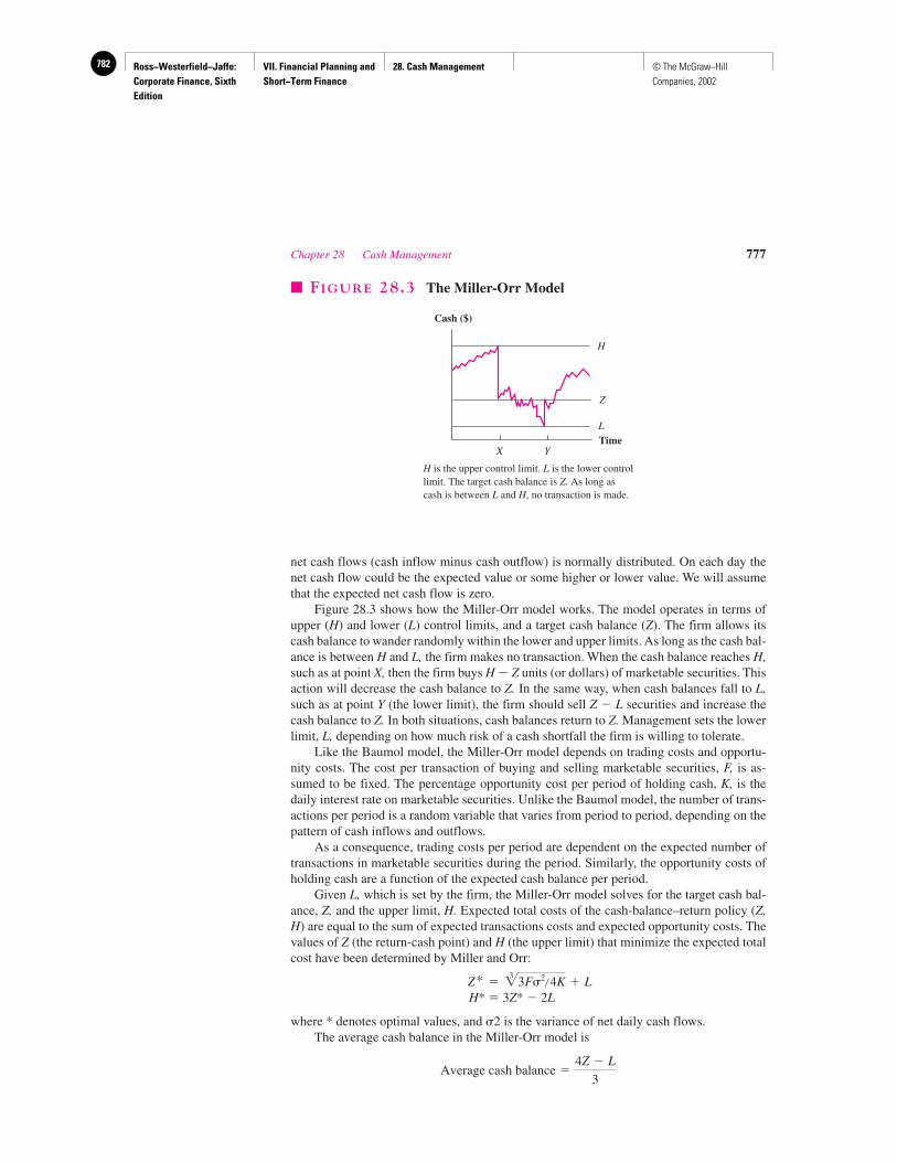
Ross−Westerfield−Jaffe: Corporate Finance, Sixth Edition
VII. Financial Planning and Short−Term Finance
28. Cash Management782 © The McGraw−Hill Companies, 2002
net cash flows (cash inflow minus cash outflow) is normally distributed. On each day thenet cash flow could be the expected value or some higher or lower value. We will assumethat the expected net cash flow is zero.
Figure 28.3 shows how the Miller-Orr model works. The model operates in terms ofupper (H) and lower (L) control limits, and a target cash balance (Z). The firm allows itscash balance to wander randomly within the lower and upper limits. As long as the cash bal-ance is between H and L, the firm makes no transaction. When the cash balance reaches H,such as at point X, then the firm buys H � Z units (or dollars) of marketable securities. Thisaction will decrease the cash balance to Z. In the same way, when cash balances fall to L,such as at point Y (the lower limit), the firm should sell Z � L securities and increase thecash balance to Z. In both situations, cash balances return to Z. Management sets the lowerlimit, L, depending on how much risk of a cash shortfall the firm is willing to tolerate.
Like the Baumol model, the Miller-Orr model depends on trading costs and opportu-nity costs. The cost per transaction of buying and selling marketable securities, F, is as-sumed to be fixed. The percentage opportunity cost per period of holding cash, K, is thedaily interest rate on marketable securities. Unlike the Baumol model, the number of trans-actions per period is a random variable that varies from period to period, depending on thepattern of cash inflows and outflows.
As a consequence, trading costs per period are dependent on the expected number oftransactions in marketable securities during the period. Similarly, the opportunity costs ofholding cash are a function of the expected cash balance per period.
Given L, which is set by the firm, the Miller-Orr model solves for the target cash bal-ance, Z, and the upper limit, H. Expected total costs of the cash-balance–return policy (Z,H) are equal to the sum of expected transactions costs and expected opportunity costs. Thevalues of Z (the return-cash point) and H (the upper limit) that minimize the expected totalcost have been determined by Miller and Orr:
H* � 3Z* � 2L
where * denotes optimal values, and �2 is the variance of net daily cash flows.The average cash balance in the Miller-Orr model is
Average cash balance �4Z � L
3
Z* �3�3F�2
�4K � L
Chapter 28 Cash Management 777
Cash ($)
Time
H
Z
L
X Y
� FIGURE 28.3 The Miller-Orr Model
H is the upper control limit. L is the lower controllimit. The target cash balance is Z. As long ascash is between L and H, no transaction is made.
Ross−Westerfield−Jaffe: Corporate Finance, Sixth Edition
VII. Financial Planning and Short−Term Finance
28. Cash Management 783© The McGraw−Hill Companies, 2002
EXAMPLE
To clarify the Miller-Orr model, suppose F � $1,000, the interest rate is 10 per-cent annually, and the standard deviation of daily net cash flows is $2,000. Thedaily opportunity cost, K, is
(1 � K)365 � 1.0 � 0.10
K � 0.000261
The variance of daily net cash flows is
�2 � (2,000)2 � 4,000,000
Let us assume that L � 0:
H* � 3 � $22,568 � $67,704
Implications of the Miller-Orr Model To use the Miller-Orr model, the manager mustdo four things.
1. Set the lower control limit for the cash balance. This lower limit can be related to a min-imum safety margin decided on by management.
2. Estimate the standard deviation of daily cash flows.
3. Determine the interest rate.
4. Estimate the trading costs of buying and selling marketable securities.
These four steps allow the upper limit and return point to be computed. Miller and Orrtested their model using nine months of data for cash balances for a large industrial firm.The model was able to produce average daily cash balances much lower than the averagesactually obtained by the firm.7
The Miller-Orr model clarifies the issues of cash management. First, the model showsthat the best return point, Z*, is positively related to trading costs, F, and negatively relatedto K. This finding is consistent with and analogous to the Baumol model. Second, theMiller-Orr model shows that the best return point and the average cash balance are posi-tively related to the variability of cash flows. That is, firms whose cash flows are subject togreater uncertainty should maintain a larger average cash balance.
Other Factors Influencing the Target Cash Balance
Borrowing In our previous examples, the firm has obtained cash by selling marketablesecurities. Another alternative is to borrow cash. Borrowing introduces additional consid-erations to cash management.
Average cash balance �4 � $22,568
3� $30,091
�3��$11,493,900,000,000 � $22,568
Z* �3��3 � $1,000 � 4,000,000� � �4 � 0.000261� � 0
1 � K �365�1.10 � 1.000261
778 Part VII Financial Planning and Short-Term Finance
7D. Mullins and R. Hamonoff discuss tests of the Miller-Orr model in “Applications of Inventory CashManagement Models,” in Modern Developments in Financial Management, ed. by S. C. Myers (New York:Praeger, 1976). They show that the model works very well when compared to the actual cash balances of severalfirms. However, simple rules of thumb do as good a job as the Miller-Orr model.
Ross−Westerfield−Jaffe: Corporate Finance, Sixth Edition
VII. Financial Planning and Short−Term Finance
28. Cash Management784 © The McGraw−Hill Companies, 2002
1. Borrowing is likely to be more expensive than selling marketable securities because theinterest rate is likely to be higher.
2. The need to borrow will depend on management’s desire to hold low cash balances. Afirm is more likely to need to borrow to cover an unexpected cash outflow the greater itscash flow variability and the lower its investment in marketable securities.
Compensating Balance The costs of trading securities are well below the lost incomefrom holding cash for large firms. Consider a firm faced with either selling $2 millionof Treasury bills to replenish cash or leaving the money idle overnight. The daily op-portunity cost of $2 million at a 10-percent annual interest rate is 0.10/365 � 0.027 per-cent per day. The daily return earned on $2 million is 0.00027 � $2 million � $540. Thecost of selling $2 million of Treasury bills is much less than $540. As a consequence, alarge firm will buy and sell securities many times a day before it will leave substantialamounts idle overnight.
However, most large firms hold more cash than cash-balance models imply. Here aresome possible reasons.
1. Firms have cash in the bank as a compensating balance in payment for banking services.
2. Large corporations have thousands of accounts with several dozen banks. Sometimes itmakes more sense to leave cash alone than to manage each account on a daily basis.
• What is a target cash balance?• What are the strengths and weaknesses of the Baumol model and the Miller-Orr model?
28.3 MANAGING THE COLLECTION AND
DISBURSEMENT OF CASH
A firm’s cash balance as reported in its financial statements (book cash or ledger cash) isnot the same thing as the balance shown in its bank account (bank cash or collected bankcash). The difference between bank cash and book cash is called float and represents thenet effect of checks in the process of collection.
EXAMPLE
Imagine that General Mechanics, Inc., (GMI) currently has $100,000 on depositwith its bank. It purchases some raw materials, paying its vendors with a checkwritten on July 8 for $100,000. The company’s books (that is, ledger balances)are changed to show the $100,000 reduction in the cash balance. But the firm’sbank will not find out about this check until it has been deposited at the vendor’sbank and has been presented to the firm’s bank for payment on, say, July 15. Un-til the check’s presentation, the firm’s bank cash is greater than its book cash, andit has positive float.
Position Prior to July 8:
Float � Firm’s bank cash � Firm’s book cash� $100,000 � $100,000� 0
Chapter 28 Cash Management 779
QUESTIONS
CO
NC
EP
T
?
Ross−Westerfield−Jaffe: Corporate Finance, Sixth Edition
VII. Financial Planning and Short−Term Finance
28. Cash Management 785© The McGraw−Hill Companies, 2002
Position from July 8 through July 14:
Disbursement float � Firm’s bank cash � Firm’s book cash� $100,000 � 0� $100,000
During the period of time that the check is clearing, GMI has a balance with thebank of $100,000. It can obtain the benefit of this cash while the check is clearing.For example, the bank cash could be invested in marketable securities. Checkswritten by the firm generate disbursement float, causing an immediate decrease inbook cash but no immediate change in bank cash.
EXAMPLE
Imagine that GMI receives a check from a customer for $100,000. Assume, as be-fore, that the company has $100,000 deposited at its bank and has a neutral floatposition. It deposits the check and increases its book cash by $100,000 on No-vember 8. However, the cash is not available to GMI until its bank has presentedthe check to the customer’s bank and received $100,000 on, say, November 15. Inthe meantime, the cash position at GMI will reflect a collection float of $100,000.
Position Prior to November 8:
Float � Firm’s bank cash � Firm’s book cash� $100,000 � $100,000� 0
Position from November 8 through November 14:
Collection float � Firm’s bank cash � Firm’s book cash� $100,000 � $200,000� �$100,000
Checks received by the firm represent collection float, which increases book cash imme-diately but does not immediately change bank cash. The firm is helped by disbursement floatand is hurt by collection float. The sum of disbursement float and collection float is net float.
A firm should be more concerned with net float and bank cash than with book cash. Ifa financial manager knows that a check will not clear for several days, he or she will be ableto keep a lower cash balance at the bank than might be true otherwise. Good float manage-ment can generate a great deal of money. For example, the average daily sales of Exxon areabout $248 million. If Exxon speeds up the collection process or slows down the disburse-ment process by one day, it frees up $248 million, which can be invested in marketable se-curities. With an interest rate of 10 percent, this represents overnight interest of approxi-mately $68,000 [($248 million/365) � 0.10].
Float management involves controlling the collection and disbursement of cash. Theobjective in cash collection is to reduce the lag between the time customers pay their billsand the time the checks are collected. The objective in cash disbursement is to slow downpayments, thereby increasing the time between when checks are written and when checksare presented. In other words, collect early and pay late. Of course, to the extent that thefirm succeeds in doing this, the customers and suppliers lose money, and the trade-off is theeffect on the firm’s relationship with them.
780 Part VII Financial Planning and Short-Term Finance
Ross−Westerfield−Jaffe: Corporate Finance, Sixth Edition
VII. Financial Planning and Short−Term Finance
28. Cash Management786 © The McGraw−Hill Companies, 2002
Collection float can be broken down into three parts: mail float, in-house processingfloat, and availability float:
1. Mail Float is the part of the collection and disbursement process where checks aretrapped in the postal system.
2. In-House Processing Float is the time it takes the receiver of a check to process the pay-ment and deposit it in a bank for collection.
3. Availability Float refers to the time required to clear a check through the banking sys-tem. The clearing process takes place using the Federal Reserve check collection ser-vice, using correspondent banks, or using local clearinghouses.
EXAMPLE
A check for $1,000 is mailed from a customer on Monday, September 1. Be-cause of mail, processing, and clearing delays, it is not credited as available cashin the firm’s bank until the following Monday, seven days later. The float for thischeck is
Float � $1,000 � 7 days � $7,000
Another check for $7,000 is mailed on September 1. It is available on the next day.The float for this check is
Float � $7,000 � 1 day � $7,000
The measurement of float depends on the time lag and the dollars involved.The cost of float is an opportunity cost, because the cash is unavailable for use dur-ing the time checks are tied up in the collection process. The cost of float can bedetermined by (1) estimating the average daily receipts, (2) calculating the aver-age delay in obtaining the receipts, and (3) discounting the average daily receiptsby the delay-adjusted cost of capital.
EXAMPLE
Suppose that Concepts, Inc., has two receipts each month:
Number of Amount Days’ Delay Float
Item 1 $5,000,000 � 3 � $15,000,000Item 2 3,000,000 � 5 � 15,000,000_________ __________
Total $8,000,000 $30,000,000
The average daily float over the month is equal to
Average Daily Float:
Another procedure that can be used to calculate average daily float is to determineaverage daily receipts and multiply by the average daily delay.
Total float
Total days�
$30,000,000
30� $1,000,000
Chapter 28 Cash Management 781
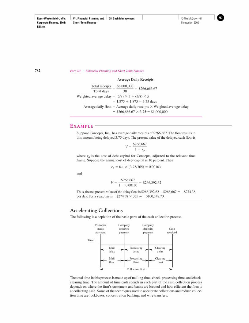
Ross−Westerfield−Jaffe: Corporate Finance, Sixth Edition
VII. Financial Planning and Short−Term Finance
28. Cash Management 787© The McGraw−Hill Companies, 2002
Average Daily Receipts:
Weighted average delay � (5/8) � 3 � (3/8) � 5
� 1.875 � 1.875 � 3.75 days
Average daily float � Average daily receipts � Weighted average delay
� $266,666.67 � 3.75 � $1,000,000
EXAMPLE
Suppose Concepts, Inc., has average daily receipts of $266,667. The float results inthis amount being delayed 3.75 days. The present value of the delayed cash flow is
where rB is the cost of debt capital for Concepts, adjusted to the relevant timeframe. Suppose the annual cost of debt capital is 10 percent. Then
rB � 0.1 � (3.75/365) � 0.00103
and
Thus, the net present value of the delay float is $266,392.62 � $266,667 � �$274.38per day. For a year, this is �$274.38 � 365 � �$100,148.70.
Accelerating CollectionsThe following is a depiction of the basic parts of the cash collection process.
Customer Company Companymails receives deposits Cash
payment payment payment received
Time
Mail Processing Clearingdelay delay delay
Mail Processing Clearingfloat float float
Collection float
The total time in this process is made up of mailing time, check-processing time, and check-clearing time. The amount of time cash spends in each part of the cash collection processdepends on where the firm’s customers and banks are located and how efficient the firm isat collecting cash. Some of the techniques used to accelerate collections and reduce collec-tion time are lockboxes, concentration banking, and wire transfers.
V �$266,667
1 � 0.00103� $266,392.62
V �$266,667
1 � rB
Total receipts
Total days�
$8,000,000
30� $266,666.67
782 Part VII Financial Planning and Short-Term Finance
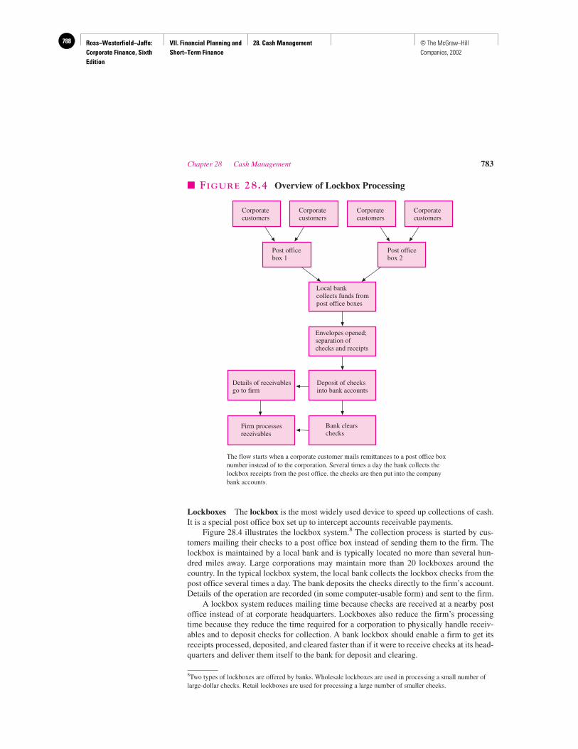
Ross−Westerfield−Jaffe: Corporate Finance, Sixth Edition
VII. Financial Planning and Short−Term Finance
28. Cash Management788 © The McGraw−Hill Companies, 2002
Lockboxes The lockbox is the most widely used device to speed up collections of cash.It is a special post office box set up to intercept accounts receivable payments.
Figure 28.4 illustrates the lockbox system.8 The collection process is started by cus-tomers mailing their checks to a post office box instead of sending them to the firm. Thelockbox is maintained by a local bank and is typically located no more than several hun-dred miles away. Large corporations may maintain more than 20 lockboxes around thecountry. In the typical lockbox system, the local bank collects the lockbox checks from thepost office several times a day. The bank deposits the checks directly to the firm’s account.Details of the operation are recorded (in some computer-usable form) and sent to the firm.
A lockbox system reduces mailing time because checks are received at a nearby postoffice instead of at corporate headquarters. Lockboxes also reduce the firm’s processingtime because they reduce the time required for a corporation to physically handle receiv-ables and to deposit checks for collection. A bank lockbox should enable a firm to get itsreceipts processed, deposited, and cleared faster than if it were to receive checks at its head-quarters and deliver them itself to the bank for deposit and clearing.
Chapter 28 Cash Management 783
Corporatecustomers
Corporatecustomers
Corporatecustomers
Corporatecustomers
Post officebox 1
Post officebox 2
Local bankcollects funds frompost office boxes
Envelopes opened;separation ofchecks and receipts
Details of receivablesgo to firm
Deposit of checksinto bank accounts
Firm processesreceivables
Bank clearschecks
� FIGURE 28.4 Overview of Lockbox Processing
The flow starts when a corporate customer mails remittances to a post office boxnumber instead of to the corporation. Several times a day the bank collects thelockbox receipts from the post office. the checks are then put into the companybank accounts.
8Two types of lockboxes are offered by banks. Wholesale lockboxes are used in processing a small number oflarge-dollar checks. Retail lockboxes are used for processing a large number of smaller checks.
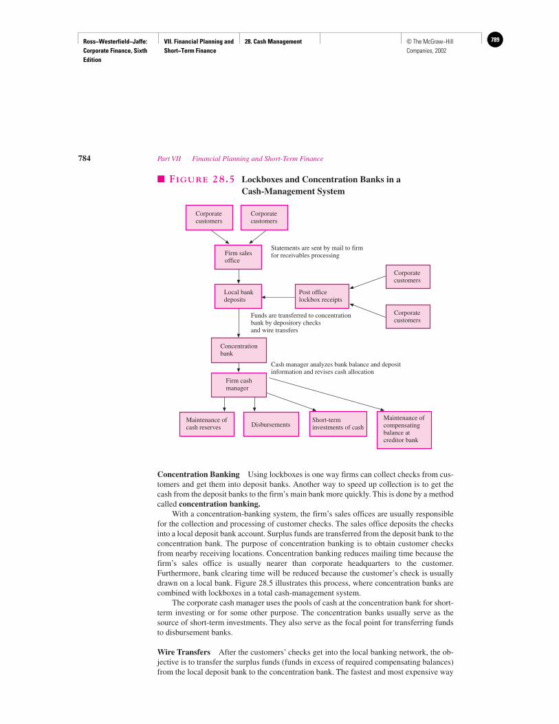
Ross−Westerfield−Jaffe: Corporate Finance, Sixth Edition
VII. Financial Planning and Short−Term Finance
28. Cash Management 789© The McGraw−Hill Companies, 2002
Concentration Banking Using lockboxes is one way firms can collect checks from cus-tomers and get them into deposit banks. Another way to speed up collection is to get thecash from the deposit banks to the firm’s main bank more quickly. This is done by a methodcalled concentration banking.
With a concentration-banking system, the firm’s sales offices are usually responsiblefor the collection and processing of customer checks. The sales office deposits the checksinto a local deposit bank account. Surplus funds are transferred from the deposit bank to theconcentration bank. The purpose of concentration banking is to obtain customer checksfrom nearby receiving locations. Concentration banking reduces mailing time because thefirm’s sales office is usually nearer than corporate headquarters to the customer.Furthermore, bank clearing time will be reduced because the customer’s check is usuallydrawn on a local bank. Figure 28.5 illustrates this process, where concentration banks arecombined with lockboxes in a total cash-management system.
The corporate cash manager uses the pools of cash at the concentration bank for short-term investing or for some other purpose. The concentration banks usually serve as thesource of short-term investments. They also serve as the focal point for transferring fundsto disbursement banks.
Wire Transfers After the customers’ checks get into the local banking network, the ob-jective is to transfer the surplus funds (funds in excess of required compensating balances)from the local deposit bank to the concentration bank. The fastest and most expensive way
784 Part VII Financial Planning and Short-Term Finance
Firm cashmanager
Corporatecustomers
Corporatecustomers
Firm salesoffice
Local bankdeposits
Concentrationbank
Maintenance ofcash reserves Disbursements
Short-terminvestments of cash
Maintenance ofcompensatingbalance atcreditor bank
Cash manager analyzes bank balance and depositinformation and revises cash allocation
Funds are transferred to concentrationbank by depository checksand wire transfers
Post officelockbox receipts
Corporatecustomers
Corporatecustomers
Statements are sent by mail to firmfor receivables processing
� FIGURE 28.5 Lockboxes and Concentration Banks in a Cash-Management System
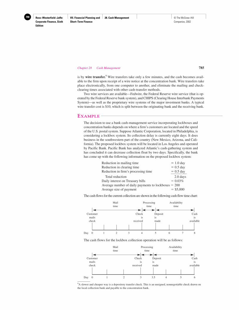
Ross−Westerfield−Jaffe: Corporate Finance, Sixth Edition
VII. Financial Planning and Short−Term Finance
28. Cash Management790 © The McGraw−Hill Companies, 2002
is by wire transfer.9 Wire transfers take only a few minutes, and the cash becomes avail-able to the firm upon receipt of a wire notice at the concentration bank. Wire transfers takeplace electronically, from one computer to another, and eliminate the mailing and check-clearing times associated with other cash-transfer methods.
Two wire services are available—Fedwire, the Federal Reserve wire service (that is op-erated by the Federal Reserve bank system), and CHIPS (Clearing House Interbank PaymentsSystem)—as well as the proprietary wire systems of the major investment banks. A typicalwire transfer cost is $10, which is split between the originating bank and the receiving bank.
EXAMPLE
The decision to use a bank cash-management service incorporating lockboxes andconcentration banks depends on where a firm’s customers are located and the speedof the U.S. postal system. Suppose Atlantic Corporation, located in Philadelphia, isconsidering a lockbox system. Its collection delay is currently eight days. It doesbusiness in the southwestern part of the country (New Mexico, Arizona, and Cali-fornia). The proposed lockbox system will be located in Los Angeles and operatedby Pacific Bank. Pacific Bank has analyzed Atlantic’s cash-gathering system andhas concluded it can decrease collection float by two days. Specifically, the bankhas come up with the following information on the proposed lockbox system:
Reduction in mailing time � 1.0 dayReduction in clearing time � 0.5 dayReduction in firm’s processing time � 0.5 day_________
Total reduction 2.0 daysDaily interest on Treasury bills � 0.03%Average number of daily payments to lockboxes � 200Average size of payment � $5,000
The cash flows for the current collection are shown in the following cash flow time chart:
Mail Processing Availabilitytime time time
Customer Check Deposit Cashmails is is ischeck received made available
Day 0 1 2 3 4 5 6 7 8
The cash flows for the lockbox collection operation will be as follows:
Mail Processing Availabilitytime time time
Customer Check Deposit Cashmails is is ischeck received made available
Day 0 1 2 3 3.5 4 5 6
Chapter 28 Cash Management 785
9A slower and cheaper way is a depository transfer check. This is an unsigned, nonnegotiable check drawn onthe local collection bank and payable to the concentration bank.
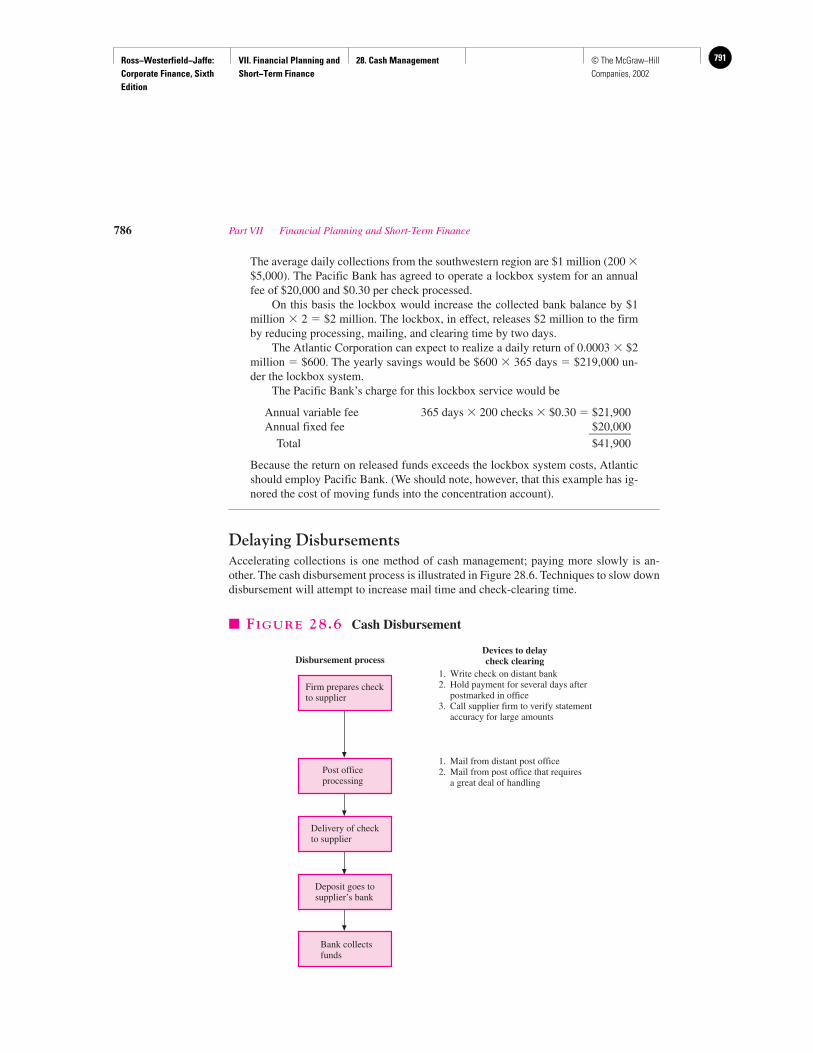
Ross−Westerfield−Jaffe: Corporate Finance, Sixth Edition
VII. Financial Planning and Short−Term Finance
28. Cash Management 791© The McGraw−Hill Companies, 2002
The average daily collections from the southwestern region are $1 million (200 �$5,000). The Pacific Bank has agreed to operate a lockbox system for an annualfee of $20,000 and $0.30 per check processed.
On this basis the lockbox would increase the collected bank balance by $1million � 2 � $2 million. The lockbox, in effect, releases $2 million to the firmby reducing processing, mailing, and clearing time by two days.
The Atlantic Corporation can expect to realize a daily return of 0.0003 � $2million � $600. The yearly savings would be $600 � 365 days � $219,000 un-der the lockbox system.
The Pacific Bank’s charge for this lockbox service would be
Annual variable fee 365 days � 200 checks � $0.30 � $21,900Annual fixed fee $20,000_______
Total $41,900
Because the return on released funds exceeds the lockbox system costs, Atlanticshould employ Pacific Bank. (We should note, however, that this example has ig-nored the cost of moving funds into the concentration account).
Delaying DisbursementsAccelerating collections is one method of cash management; paying more slowly is an-other. The cash disbursement process is illustrated in Figure 28.6. Techniques to slow downdisbursement will attempt to increase mail time and check-clearing time.
786 Part VII Financial Planning and Short-Term Finance
Firm prepares checkto supplier
Post officeprocessing
Delivery of checkto supplier
Deposit goes tosupplier’s bank
Bank collectsfunds
Disbursement processDevices to delaycheck clearing
1. Write check on distant bank2. Hold payment for several days after
postmarked in office3. Call supplier firm to verify statement
accuracy for large amounts
1. Mail from distant post office2. Mail from post office that requires
a great deal of handling
� FIGURE 28.6 Cash Disbursement
Ross−Westerfield−Jaffe: Corporate Finance, Sixth Edition
VII. Financial Planning and Short−Term Finance
28. Cash Management792 © The McGraw−Hill Companies, 2002
Disbursement Float (“Playing the Float Game”)Even though the cash balance at the bank may be $1 million, a firm’s books may show only$500,000 because it has written $500,000 in payment checks. The disbursement float of$500,000 is available for the corporation to use until the checks are presented for payment.Float in terms of slowing down payment checks comes from mail delivery, check-processingtime, and collection of funds. This is illustrated in Figure 28.6. Disbursement float can beincreased by writing a check on a geographically distant bank. For example, a New Yorksupplier might be paid with checks drawn on a Los Angeles bank. This will increase thetime required for the checks to clear through the banking system.
Zero-Balance AccountsSome firms set up a zero-balance account (ZBA) to handle disbursement activity. The ac-count has a zero balance as checks are written. As checks are presented to the zero-balanceaccount for payment (causing a negative balance), funds are automatically transferred infrom a central control account. The master account and the ZBA are located in the samebank. Thus, the transfer is automatic and involves only an accounting entry in the bank.
DraftsFirms sometimes use drafts instead of checks. Drafts differ from checks because they arenot drawn on a bank but on the issuer (the firm) and are payable by the issuer. The bank actsonly as an agent, presenting the draft to the issuer for payment. When a draft is transmittedto a firm’s bank for collection, the bank must present the draft to the issuing firm for ac-ceptance before making payment. After the draft has been accepted, the firm must depositthe necessary cash to cover the payment. The use of drafts rather than checks allows a firmto keep lower cash balances in its disbursement accounts because cash does not need to bedeposited until the drafts are presented to it for payment.
Ethical and Legal QuestionsThe cash manager must work with cash balances collected by the bank and not the firm’sbook balance, which reflects checks that have been deposited but not collected. If not, acash manager could be drawing on uncollected cash as a source for making short-term in-vestments. Most banks charge a penalty for use of uncollected funds. However, banks maynot have good enough accounting and control procedures to be fully aware of the use of un-collected funds. This raises some ethical and legal questions for the firm.
In May 1985, Robert Fomon, chairman of E. F. Hutton, pleaded guilty to 2,000 chargesof mail and wire fraud in connection with a scheme the firm had operated from 1980 to 1982.E. F. Hutton employees wrote checks totaling hundreds of millions of dollars in uncollectedcash, which were invested in short-term money-market assets. E. F. Hutton’s systematicoverdrafting of accounts is apparently not a widespread practice among corporations, andsince the E. F. Hutton affair, firms have been much more careful in managing their cash ac-counts. Generally, firms are scrupulous in investing only the cash they actually have on hand.E. F. Hutton paid a $2 million fine, reimbursed the government (the U.S. Department ofJustice) $750,000, and reserved $8 million for restitution to defrauded banks.
• Describe collection and disbursement float.• What are lockboxes? Concentration banks? Wire transfers?• Suppose an overzealous financial manager writes checks on uncollected funds. Aside
from legal issues, who is the financial loser in this situation?
Chapter 28 Cash Management 787
QUESTIONS
CO
NC
EP
T
?
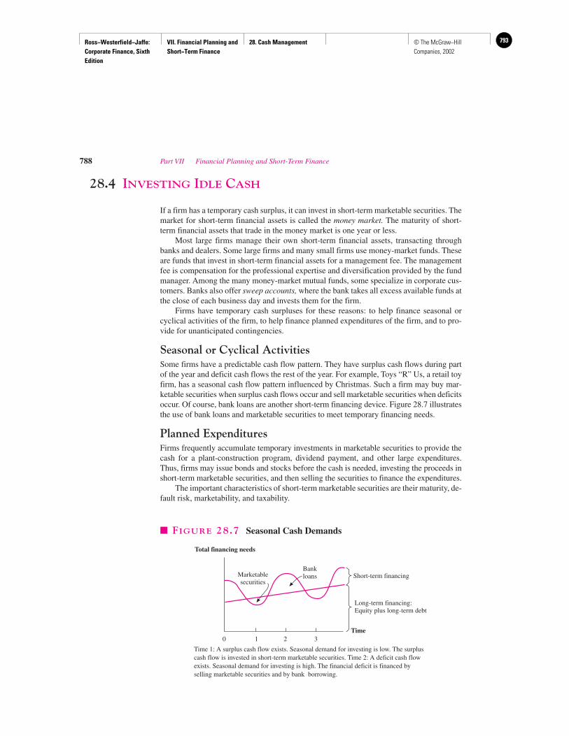
Ross−Westerfield−Jaffe: Corporate Finance, Sixth Edition
VII. Financial Planning and Short−Term Finance
28. Cash Management 793© The McGraw−Hill Companies, 2002
28.4 INVESTING IDLE CASH
If a firm has a temporary cash surplus, it can invest in short-term marketable securities. Themarket for short-term financial assets is called the money market. The maturity of short-term financial assets that trade in the money market is one year or less.
Most large firms manage their own short-term financial assets, transacting throughbanks and dealers. Some large firms and many small firms use money-market funds. Theseare funds that invest in short-term financial assets for a management fee. The managementfee is compensation for the professional expertise and diversification provided by the fundmanager. Among the many money-market mutual funds, some specialize in corporate cus-tomers. Banks also offer sweep accounts, where the bank takes all excess available funds atthe close of each business day and invests them for the firm.
Firms have temporary cash surpluses for these reasons: to help finance seasonal orcyclical activities of the firm, to help finance planned expenditures of the firm, and to pro-vide for unanticipated contingencies.
Seasonal or Cyclical ActivitiesSome firms have a predictable cash flow pattern. They have surplus cash flows during partof the year and deficit cash flows the rest of the year. For example, Toys “R” Us, a retail toyfirm, has a seasonal cash flow pattern influenced by Christmas. Such a firm may buy mar-ketable securities when surplus cash flows occur and sell marketable securities when deficitsoccur. Of course, bank loans are another short-term financing device. Figure 28.7 illustratesthe use of bank loans and marketable securities to meet temporary financing needs.
Planned ExpendituresFirms frequently accumulate temporary investments in marketable securities to provide thecash for a plant-construction program, dividend payment, and other large expenditures.Thus, firms may issue bonds and stocks before the cash is needed, investing the proceeds inshort-term marketable securities, and then selling the securities to finance the expenditures.
The important characteristics of short-term marketable securities are their maturity, de-fault risk, marketability, and taxability.
788 Part VII Financial Planning and Short-Term Finance
Total financing needs
Time
Marketablesecurities
Bankloans Short-term financing
Long-term financing:Equity plus long-term debt
0 1 2 3
� FIGURE 28.7 Seasonal Cash Demands
Time 1: A surplus cash flow exists. Seasonal demand for investing is low. The surpluscash flow is invested in short-term marketable securities. Time 2: A deficit cash flowexists. Seasonal demand for investing is high. The financial deficit is financed byselling marketable securities and by bank borrowing.
Ross−Westerfield−Jaffe: Corporate Finance, Sixth Edition
VII. Financial Planning and Short−Term Finance
28. Cash Management794 © The McGraw−Hill Companies, 2002
Maturity Maturity refers to the time period over which interest and principal paymentsare made. For a given change in the level of interest rates, the prices of longer-maturity se-curities will change more than those for shorter-maturity securities. As a consequence,firms that invest in long-term maturity securities are accepting greater risk than firms thatinvest in securities with short-term maturities. This type of risk is usually called interest-rate risk. Most firms limit their investments in marketable securities to those maturing inless than 90 days. Of course, the expected return on securities with short-term maturities isusually less than the expected return on securities with longer maturities.
Default Risk Default risk refers to the probability that interest or principal will not bepaid on the due date and in the promised amount. In previous chapters we observed that var-ious financial reporting agencies, such as Moody’s Investors Service and Standard &Poor’s, compile and publish ratings of various corporate and public securities. These rat-ings are connected to default risk. Of course, some securities have negligible default risk,such as U.S. Treasury bills. Given the purposes of investing idle corporate cash, firms typ-ically avoid investing in marketable securities with significant default risk.
Marketability Marketability refers to how easy it is to convert an asset to cash. Some-times marketability is referred to as liquidity. It has two characteristics:
1. No Price-Pressure Effect. If an asset can be sold in large amounts without changing themarket price, it is marketable. Price-pressure effects are those that come about when theprice of an asset must be lowered to facilitate the sale.
2. Time. If an asset can be sold quickly at the existing market price, it is marketable. In con-trast, a Renoir painting or antique desk appraised at $1 million will likely sell for muchless if the owner must sell on short notice.
In general, marketability is the ability to sell an asset for its face market value quickly andin large amounts. Perhaps the most marketable of all securities are U.S. Treasury bills.
Taxability Several kinds of securities have varying degrees of tax exemption.
1. The interest on the bonds of state and local governments is exempt from federal taxes,and usually from the state and local taxes where the bonds are issued. Pretax expectedreturns on state and local bonds must be lower than on similar taxable investments andtherefore are more attractive to corporations in high marginal tax brackets.
2. Seventy percent of the dividend income on preferred and common stock is exempt fromcorporate income taxes.
The market price of securities will reflect the total demand and supply of tax influences.The position of the firm may be different from that of the market.
Different Types of Money-Market SecuritiesMoney-market securities are generally highly marketable and short term. They usually havelow risk of default. They are issued by the U.S. government (for example, U.S. Treasurybills), domestic and foreign banks (for example, certificates of deposit), and business cor-porations (commercial paper, for example).
U.S. Treasury bills are obligations of the U.S. government that mature in 90, 180, 270,or 360 days. They are pure discount securities. The 90-day and 180-day bills are sold byauction every week, and 270-day and 360-day bills are sold every month.
U.S. Treasury notes and bonds have original maturities of more than one year. They areinterest-bearing securities. The interest is exempt from state and local taxes.
Chapter 28 Cash Management 789
Ross−Westerfield−Jaffe: Corporate Finance, Sixth Edition
VII. Financial Planning and Short−Term Finance
28. Cash Management 795© The McGraw−Hill Companies, 2002
Federal agency securities are securities issued by corporations and agencies created bythe U.S. government, such as the Federal Home Loan Bank Board and the GovernmentNational Mortgage Association (Ginnie Mae). The interest rates on agency issues are higherthan those on comparable U.S. Treasury issues. This is true because agency issues are notas marketable as U.S. Treasury issues, and they have more default risk.
Short-term tax exempts are short-term securities issued by states, municipalities, localhousing agencies, and urban renewal agencies. They have more default risk than U.S.Treasury issues and are less marketable. The interest is exempt from federal income tax. Asa consequence, the pretax yield on tax exempts is lower than those on comparable securi-ties, such as U.S. Treasury bills.
Commercial paper refers to short-term securities issued by finance companies, banks,and corporations. Commercial paper typically is unsecured notes. Maturities range from afew weeks to 270 days. There is no active secondary market in commercial paper. As a con-sequence, their marketability is low. (However, firms that issue commercial paper will di-rectly repurchase before maturity.) The default risk of commercial paper depends on the fi-nancial strength of the issuer. Moody’s and Standard & Poor’s publish quality ratings forcommercial paper.
Certificates of deposit (CDs) are short-term loans to commercial banks. There are ac-tive markets in CDs of 3-month, 6-month, 9-month, and 12-month maturities.
Repurchase agreements are sales of government securities (for example, U.S. Treasurybills) by a bank or securities dealer with an agreement to repurchase. An investor typicallybuys some Treasury securities from a bond dealer and simultaneously agrees to sell themback at a later date at a specified higher price. Repurchase agreements are usually very shortterm—overnight to a few days.
Eurodollar CDs are deposits of dollars with foreign banks.Banker’s acceptances are time drafts (orders to pay) issued by a business firm (usually
an importer) that have been accepted by a bank that guarantees payment.
• Why do firms find themselves with idle cash?• What are the types of money-market securities?
28.5 SUMMARY AND CONCLUSIONS
The chapter discussed how firms manage cash.
1. A firm holds cash to conduct transactions and to compensate banks for the various servicesthey render.
2. The optimal amount of cash for a firm to hold depends on the opportunity cost of holdingcash and the uncertainty of future cash inflows and outflows. The Baumol model and theMiller-Orr model are two transactions models that provide rough guidelines for determiningthe optimal cash position.
3. The firm can make use of a variety of procedures to manage the collection and disbursementof cash in such a way as to speed up the collection of cash and slow down payments. Somemethods to speed up collection are lockboxes, concentration banking, and wire transfers. Thefinancial manager must always work with collected company cash balances and not with thecompany’s book balance. To do otherwise is to use the bank’s cash without the bank knowingit, raising ethical and legal questions.
790 Part VII Financial Planning and Short-Term Finance
QUESTIONS
CO
NC
EP
T
?

Ross−Westerfield−Jaffe: Corporate Finance, Sixth Edition
VII. Financial Planning and Short−Term Finance
28. Cash Management796 © The McGraw−Hill Companies, 2002
4. Because of seasonal and cyclical activities, to help finance planned expenditures, or as areserve for unanticipated needs, firms temporarily find themselves with cash surpluses. Themoney market offers a variety of possible vehicles for parking this idle cash.
KEY TERMS
Compensating balances 772 Target cash balance 773Concentration banking 784 Transactions motive 772Float 779 Wire transfer 785Lockbox 783 Zero-balance account (ZBA) 787
SUGGESTED READINGS
The following are general readings in cash management:Hill, Ned. C., and William L. Sartoris. Short-Term Financial Management. New York:
Macmillan Publishing Company, 1992.Maness, Terry S., and John T. Zietlow. Short-Term Financial Management. Minneapolis/St.
Paul: West Publishing Company, 1993.
QUESTIONS AND PROBLEMS
Reasons for Holding Cash28.1 What are the reasons for holding cash?
Determining the Target Cash Balance28.2 Indicate whether the following actions increase, decrease, or cause no change in a
company’s cash balance.a. Interest rates paid on money-market securities rise.b. Commissions charged by brokers increase.c. The compensating-balance requirement of a bank is lowered.d. The cost of borrowing decreases.e. The firm’s credit rating declines.f. Direct fees for banking services are established.
28.3 A company’s weekly average cash balances are as follows:
Week 1 $24,000Week 2 34,000Week 3 10,000Week 4 15,000
If the annual interest rate is 12 percent, what return can be earned on the average cashbalances?
28.4 The Casablanca Piano Company is currently holding $800,000 in cash. It projects that overthe next year its cash outflows will exceed its cash inflows by $345,000 per month. Eachtime securities are bought or sold through a broker, the company pays a fee of $500. Theannual interest rate on money-market securities is 7 percent.a. How much of this cash should be retained and how much should be used to increase
the company’s holdings of marketable securities?b. After the initial investment of excess cash, how many times during the next 12 months
will securities be sold?
Chapter 28 Cash Management 791

Ross−Westerfield−Jaffe: Corporate Finance, Sixth Edition
VII. Financial Planning and Short−Term Finance
28. Cash Management 797© The McGraw−Hill Companies, 2002
28.5 Lisa Tylor, CFO of Purple Rain Co., concluded from the Baumol model that the optimalcash balance for the firm is $20 million. The annual interest rate on marketable securitiesis 7.5 percent. The fixed cost of selling securities to replenish cash is $5,000. PurpleRain’s cash flow pattern is well approximated by the Baumol model. What can you inferabout Purple Rain’s average weekly cash disbursement?
28.6 The variance of the daily net cash flows for the Tseneg Asian Import Company is $1.44million. The opportunity cost to the firm of holding cash is 8 percent per year. The fixedcost of buying and selling securities is $600 per transaction.
What should the target cash level and upper limit be, if the tolerable lower limit hasbeen established at $20,000?
28.7 Gold Star Co. and Silver Star Co. both manage their cash flows according to the Miller-Orr model. Gold Star’s daily cash flow is controlled between $100,000 and $200,000,whereas Silver Star’s daily cash flow is controlled between $150,000 and $300,000. Theannual interest rates Gold Star and Silver Star can get are 10 percent and 9 percent,respectively, and the costs per transaction of trading securities are $2,000 and $2,500,respectively.a. What are their respective target cash balances?b. Which firm’s daily cash flow is more volatile?
Managing the Collection and Disbursement of Cash28.8 Garden Groves, Inc., a Florida-based company, has determined that a majority of its
customers are located in the New York City area. Therefore, it is considering using alockbox system offered by a bank located in New York. The bank has estimated that useof the system will reduce collection float by three days. Based on the followinginformation, should the lockbox system be adopted?
Average number of payments per day: 150Average value of payment: $15,000Fixed annual lockbox fee: $80,000Variable lockbox fee: $0.50/transactionAnnual interest rate on money-market securities: 7.5 percent
28.9 A large New England lumber producer, Salisbury Stakes, Inc., is planning to use alockbox system to speed collections from its customers located in the midwestern UnitedStates. A Chicago-area bank will provide this service for an annual fee of $15,000 plus$0.25 per transaction. The estimated reduction in collection and processing time is twodays. Treasury bills are currently yielding 6 percent per year.
If the average customer payment in this region is $4,500, how many customers eachday, on average, must use the system to make it profitable?
28.10 Each business day, on average, a company writes checks totaling $12,000 to pay itssuppliers. The usual clearing time for these checks is five days. Each day, the companyreceives payments from its customers in the form of checks totaling $15,000. The cashfrom the payments is available to the firm after three days.
Calculate the company’s disbursement float, collection float, and net float.How would these values change if the collected funds were available in four days
instead of three?
28.11 It takes the Herman Company about seven days to receive and deposit checks fromcustomers. The top management of the Herman Company is considering a lockbox system.It is expected that the lockbox system will reduce float time to four days. Average dailycollections are $100,000. The marketwide interest rate is 12 percent. a. What would the reduction in outstanding cash balances be as a result of implementing
the lockbox system?b. What is the return that could be earned on these savings?c. What is the maximum monthly charge the Herman Company should pay for this
lockbox system?
792 Part VII Financial Planning and Short-Term Finance
Ross−Westerfield−Jaffe: Corporate Finance, Sixth Edition
VII. Financial Planning and Short−Term Finance
28. Cash Management798 © The McGraw−Hill Companies, 2002
28.12 The Walter Company disburses checks every two weeks that average $200,000 in totaland take three days to clear. How much cash can the Walter Company save annually if itdelays the transfer of funds from an interest-bearing account that pays 0.04 percent perday for these three days?
28.13 The Miller Company has an agreement with the First National Bank by which the bankhandles $4 million in collections each day and requires a $500,000 compensatingbalance. Miller is contemplating canceling the agreement and dividing its eastern regionso that two other banks will handle its business. Banks 1 and 2 will each handle $2million of collections each day, requiring a compensating balance of $300,000. Miller’sfinancial management expects that collections will be accelerated by one day if theeastern region is divided. The T-bill rate is 7 percent. Should the Miller Companyimplement the new system? What will the annual net savings be?
28.14 Anthony Marino, CFO of Thousand Years Inc., is evaluating two alternatives of floatmanagement: lockbox and concentration banking. The average number of dailypayments to lockboxes is 250 with the average size of each payment at $7,500. Thelockbox system can reduce the collection float by 1.5 days and concentration bankingcan reduce the collection float by 1 day. However, the bank charges an annual fee of$30,000 and $0.30 per check processed for the lockbox service. Which method is moreeconomical for Thousand Years, the lockbox system or the concentration-bankingsystem? Assume daily interest on Treasury bills is 0.03 percent.
Investing Idle Cash28.15 What are the important characteristics of short-term marketable securities?
Appendix 28A ADJUSTABLE-RATE PREFERRED STOCK,AUCTION-RATE PREFERRED STOCK, AND
FLOATING-RATE CERTIFICATES OF DEPOSIT
Corporate cash managers are continually seeking new ways to improve the return on theirsurplus cash. Many of the sophisticated investment vehicles developed over the last decadeare too illiquid or too risky or have an inappropriate time horizon for use in cash manage-ment. However, three instruments—adjustable-rate preferred stock, auction-rate preferredstock, and floating-rate CDs or notes—offer substantial benefits and are currently em-ployed by corporations in their cash-management activities.
Adjustable-Rate Preferred StockAdjustable-rate preferred stock (ARPS) is designed to offer rates of return competitive withmore traditional money-market instruments while still affording the corporate investor the80-percent tax exclusion on dividend income—a tax advantage that makes equity invest-ments extremely attractive.
Agencies such as Moody’s or Standard & Poor’s give issues credit ratings, so the cashmanager has a gauge to judge the creditworthiness of the instruments relative to other in-vestments. The dividend rate on these issues is adjusted quarterly at a fixed spread over orunder the highest of the 90-day T-bill rate, the 10-year T-note rate, or the 20-year T-bondrate prevailing on the reset date. The spread is specified by each issuer. ARPS issues havecollars—minimum and maximum dividend-rate levels—that, when hit, result in the issuetaking on the characteristics of a fixed-rate preferred instrument.
Chapter 28 Cash Management 793
Ross−Westerfield−Jaffe: Corporate Finance, Sixth Edition
VII. Financial Planning and Short−Term Finance
28. Cash Management 799© The McGraw−Hill Companies, 2002
The floating-rate feature keeps the dividend rate (and thus the overall pretax return) inline with alternative investments and reduces price volatility caused solely by changes ininterest rates. The floating rate does not, however, eliminate all of the incremental risk as-sociated with these instruments.
Risk is present in the ARPS market and can be broken down into three categories. Cashmanagers must continually reevaluate the market in light of changes that might occur in anyof the three areas.
The greatest risk in the ARPS market is derived from the limited number of issuers andtheir clustering in certain industry groups, most notably banking, and the ever-present riskof downgraded ratings. Like any other credit instrument, ARPS is subject to volatility basedon the market’s perceptions of the strength of the issuer and industry group. The possibil-ity of impaired principal is a real one for ARPS purchasers, because concerns about creditcould govern the floating-rate dividend between and on reset dates. The cash manager mustbe aware that substantial month-to-month volatility (the normal time horizon for corporateevaluation of their cash portfolios) could exist with ARPS investments.
A second risk factor centers around the narrowness of the primary and secondary mar-kets for ARPS. The demand for these issues comes primarily from corporate investors, andthe limited nature of this investment base is a factor in evaluating the depth of the market.If a cash manager must liquidate a position quickly, a thin market could exacerbate pricepressure. As a result, most corporate investors employ mutual-fund managers who special-ize in the ARPS market to run their portfolios. Liquidity is normally next-day with the funds(although principal is by no means guaranteed), and mutual-fund managers represent themost active players in the market.
Finally, changes in the tax code have a great impact on the price of ARPS issues, becausetheir main feature is the tax advantage of the dividend exclusion. The Tax Reform Act of 1986reduced this exclusion from 85 to 70 percent. Assuming a 46-percent tax rate, a corporate in-vestor in the ARPS market would have found its dividend income being taxed at 13.8 percent(30 percent taxed at 46 percent) instead of 6.9 percent (15 percent taxed at 46 percent). Suchan increase would have undoubtedly resulted in substantial price declines for existing issues.Luckily for both ARPS issuers and purchasers, the top corporate tax rate is now lower than46 percent, resulting in only a small change for recipients of dividend income. The issue oftax advantage is crucial, because ARPS as an investment is evaluated on an after-tax risk-ad-justed basis relative to other instruments. If the added risk inherent in the instrument beginsto eclipse the tax advantage, the instrument will become increasingly unattractive.
The adjustable-rate preferred market has not fared as well as early proponents hadhoped, primarily because the floating-rate dividend failed to compensate for credit concernsabout the issuers. This has resulted in many issues trading below par and has prompted thedevelopment of several related instruments. The most successful of these new vehicles isauction-rate preferred stock.
Auction-Rate Preferred StockThe similarity between ARPS and auction-rate preferred stock extends only to the fact thatboth have a floating dividend rate and afford the corporate investor the same exclusion oftaxes on dividends. Auction rates differ from ARPS in the way the dividend is set and in theway these portfolios are managed.
The dividend rate for auction-rate preferred is set not by the issuers but by the marketthrough a process called a Dutch auction. The auction permits investors to determine thedividend yield for the 49-day period that is standard between reset dates. The InternalRevenue Service requires that a corporate investor hold dividend-paying stock for at least
794 Part VII Financial Planning and Short-Term Finance
Ross−Westerfield−Jaffe: Corporate Finance, Sixth Edition
VII. Financial Planning and Short−Term Finance
28. Cash Management800 © The McGraw−Hill Companies, 2002
45 days to be eligible for the dividend exclusion; 49 days was chosen so the auctions willalways occur on the same day of the week for the life of individual issues.
An auction-rate preferred stock is auctioned as follows. Each bidder (someone who al-ready owns shares and wishes to continue to hold them, or a new purchaser) submits to theagent in charge of the auction the number of shares desired and at what dividend level. Thelowest rate that sells out the available shares will be the dividend for the 49 days until thenext reset/auction. Investors who already own shares going into the auction have the optionto take their shares at whatever dividend is set (called rolling) or bid the lowest rate theywould accept and risk losing some or all of the shares to another bidder who would be will-ing to take a lower dividend. Of course, shareholders also have the right to simply sell allof their shares at the auction. Although the process is essentially independent, the dividendrate for most issues is usually set at approximately 60 to 80 percent of the 60-day AA com-mercial paper rate prevailing on auction day.
Auction-rate preferred stock offers the corporate investor several important features:
1. The 49-day reset period is shorter than the 90-day period found in the ARPS market, re-ducing the potential for price volatility resulting from both interest-rate movement andcredit concerns.
2. The auction method of determining the dividend level makes it more likely that the is-sue will trade at par, minimizing principal impairment. The shorter reset period also of-fers the cash manager increased liquidity in the event funds are needed for corporate op-erations between auctions. The auction-rate investor sacrifices some return relative toARPS because of these features, but still garners a substantial after-tax benefit relativeto alternative money-market investments.
3. The auction-rate preferred market is more accessible to the corporate investor, allowingit to invest individually rather than through a mutual fund. Many cash managers preferthe added control this gives them over their portfolios.
The risks associated with auction-rate preferred stock are smaller than those associatedwith ARPS but must still be considered substantial for the cash manager who may need im-mediate liquidity or who faces strict return criteria. These risks include the following:
1. Failed Auctions. If the agent supervising an auction does not receive enough bids tomatch offers to sell for existing shares of a particular issue, the auction is considered tohave failed. There have been several auction failures, but it is not as catastrophic as itsounds. It means that the dividend rate for the subsequent 49-day period will be set at110 percent of the 60-day AA commercial paper rate. A seller would therefore be facedwith a capital loss if it wished to liquidate.
2. Issuer Credit Quality. As with ARPS, all auction-rate preferred issues receive a ratingfrom Moody’s or Standard & Poor’s. They remain susceptible to perceived or actualchanges in that credit quality between reset periods. To facilitate the new market, somelarge brokers were even guaranteeing to redeem auction-rate preferred at par betweenreset periods to generate investor participation.
3. Changes in the Tax Code. Major changes in the tax code will affect the auction-rate pre-ferred market in much the same manner as they would the APRS market. Once again, itis crucial to remember that these instruments are judged on an after-tax risk-adjusted ba-sis relative to alternative investments.
Auction-rate preferred stock has been extremely well received by the corporate market-place. The key to its continued success will be diversification of issuers, orderly and successfulauctions, and an ongoing after-tax yield advantage relative to other money-market investments.
Chapter 28 Cash Management 795
Ross−Westerfield−Jaffe: Corporate Finance, Sixth Edition
VII. Financial Planning and Short−Term Finance
28. Cash Management 801© The McGraw−Hill Companies, 2002
Floating-Rate Certificates of DepositA third investment available to the cash manager looking to increase the return on surpluscash is the floating-rate certificate of deposit or note. Our discussion centers on the CD, butthe same argument applies to the short-term note, adjusting for time-horizon considerations.
The floating-rate certificate of deposit (FRCD) market presents substantial investmentopportunities for the manager of short-term cash. Frequently reset coupons, the hallmark ofthe FRCD, allow the investor to combine the yield of an intermediate-term instrument withthe liquidity of a short-term one. This combination also reduces interest-rate risk and pro-vides for capital maintenance, while continuing to provide attractive returns.
Two issues must be addressed when evaluating the FRCD market:
1. How are the issues priced?
2. Which base rate should be selected?
Floating-rate CDs are priced at a spread above or below a well-known market indexsuch as the London Interbank Offered Rate (LIBOR), T-bills, or commercial paper. Thewidth of the spread reflects the issuer’s credit, the maturity of the issue, its liquidity, and theoverall level of rates at the time of issuance. In general, this spread is fixed over the life ofthe security, but some new issues do have a floating spread. When the market perception ofcredit quality changes significantly from that implied in the spread to the base rate, the priceof the security will decline as the market compensates investors for the increased risk.
The actual coupon paid (the index rate plus or minus the predetermined spread) to theinvestor will be reset periodically, usually monthly, quarterly, or semiannually. It is thefloating nature of the coupon that keeps most FRCDs within one to two points of par at alltimes, as the issue is continually repriced relative to existing market conditions. Price sta-bility will increase with the frequency of reset.
Most FRCDs also feature redemption specifications in the form of call or put options.In the case of a call, the issuer has the option to call the security back from an investor atpar, usually within three to five years of issuance. The security can be called on any coupon-payment date, and, as would be expected, the option is usually exercised when the securityis trading at a premium. For the put option, the investor has the right to sell the security backto the issuer at par before maturity. The option is usually exercised when the security is trad-ing at a discount. These features must be incorporated into yield calculations, with the callor put dates generally substituted for the maturity date.
The initial price of the FRCD will adapt to reflect market demand for the issue, liquid-ity, and favorable aspects of the issue’s structure. Whether the security trades at a premiumor discount to par depends on changes in the market’s perception of these and the other fac-tors discussed previously. However, given frequently reset coupons, only drastic changes inissuer quality or quality spreads will prompt significant deterioration of principal.
The price of an FRCD will also be affected if a change occurs in the relationship be-tween index rates, such as a widening of the T-bill/Eurodollar spread. Assume that twoFRCDs are priced to identical yields, one at a spread over LIBOR and the other at a spreadabove T-bills. If the T-bill/Eurodollar spread widens, the FRCDs indexed to LIBOR will ex-perience a price decline. This will occur regardless of the absolute level of interest rates orany shift in market perception of specific credit risk.
In evaluating an FRCD, the selection of an issue based on its index rate can be as im-portant as selection of an issue based on the issuer’s credit ratings or maturity. The choice ofan index reflects the perception of how the issuer’s industry fundamentals will behave rela-tive to that index. For instance, the choice of T-bills as the base implies an analysis of howthe issuer will perform relative to a risk-free measure; the choice of commercial paper im-plies an analysis of the issuer’s prospects relative to companies with access to that market.
796 Part VII Financial Planning and Short-Term Finance

Ross−Westerfield−Jaffe: Corporate Finance, Sixth Edition
VII. Financial Planning and Short−Term Finance
28. Cash Management802 © The McGraw−Hill Companies, 2002
The base rate will also be important when general quality concerns arise in the market.A LIBOR index will reflect those concerns, and the price of an FRCD indexed to LIBORshould not change drastically, because its coupon is linked directly to a market-determinedcost of funds. An FRCD indexed to T-bills, however, might exhibit substantial price volatil-ity over the same time period. The greater the index’s sensitivity to market movement, thegreater the issue’s price stability.
Although the FRCD does not offer the tax advantage of ARPS or auction-rate preferredstock, it gives the cash manager an opportunity to keep returns on excess cash in line withchanging interest rates. The secondary market for FRCDs is still developing but is consid-erably deeper than that for preferred securities.
All of these investments were designed for cash-management activities that allow forinvestment of cash for longer periods of time. Generally, a cash manager will be using atleast a 9-month to 12-month horizon before considering investing in these vehicles. Moneyshould not be committed to these investments unless the manager can be reasonably surethat it will not be needed for corporate operations for at least one year.
Chapter 28 Cash Management 797
Ross−Westerfield−Jaffe: Corporate Finance, Sixth Edition
VII. Financial Planning and Short−Term Finance
29. Credit Management 803© The McGraw−Hill Companies, 2002
Credit Management
CH
AP
TE
R29
EXECUTIVE SUMMARY
When a firm sells goods and services it can (1) be paid in cash immediately or(2) wait for a time to be paid, that is, extend credit to customers. Granting creditis investing in a customer, an investment tied to the sale of a product or service.
This chapter examines the firm’s decision to grant credit.An account receivable is created when credit is granted. These receivables include
credit granted to other firms, called trade credit, and credit granted consumers, called con-sumer credit. About one-sixth of all the assets of industrial firms are in the form of accountsreceivable. Trade credit extended by a firm’s supplier to the firm appears as an accountspayable. Figure 29.1 illustrates this aspect of trade credit.
The investment in accounts receivable for any firm depends on both the amount ofcredit sales and the average collection period. For example, if a firm’s credit sales per dayequal $1,000 and its average collection period is 30 days, its accounts receivable will beequal to $30,000. Thus, a firm’s investment in accounts receivable depends on factors in-fluencing credit sales and collection. A firm’s credit policy affects these factors.
The following are the components of credit policy:
1. Terms of the sale. A firm must decide on certain conditions when selling its goods andservices for credit. For example, the terms of sale may specify the credit period, the cashdiscount, and the type of credit instrument.
2. Credit analysis. When granting credit, a firm tries to distinguish between customers thatwill pay and customers that will not pay. Firms use a number of devices and proceduresto determine the probability that customers will pay.
3. Collection policy. Firms that grant credit must establish a policy for collecting the cashwhen it becomes due.
This chapter discusses each of the components of credit policy that makes up the decisionto grant credit.
In some ways, the decision to grant credit is connected to the cash collection process de-scribed in the previous chapter. This is illustrated in Figure 29.2 with a cash-flow diagram.
The typical sequence of events when a firm grants credit is (1) the credit sale is made,(2) the customer sends a check to the firm, (3) the firm deposits the check, and (4) the firm’saccount is credited for the amount of the check.
29.1 TERMS OF THE SALE
The terms of sale refer to the period for which credit is granted, the cash discount, and thetype of credit instrument. For example, suppose a customer is granted credit with terms of2/10, net 30. This means that the customer has 30 days from the invoice date within which
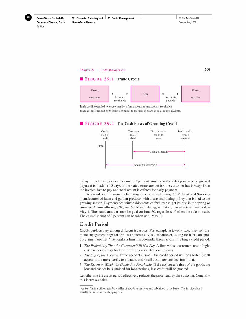
Ross−Westerfield−Jaffe: Corporate Finance, Sixth Edition
VII. Financial Planning and Short−Term Finance
29. Credit Management804 © The McGraw−Hill Companies, 2002
Chapter 29 Credit Management 799
to pay.1 In addition, a cash discount of 2 percent from the stated sales price is to be given ifpayment is made in 10 days. If the stated terms are net 60, the customer has 60 days fromthe invoice date to pay and no discount is offered for early payment.
When sales are seasonal, a firm might use seasonal dating. O. M. Scott and Sons is amanufacturer of lawn and garden products with a seasonal dating policy that is tied to thegrowing season. Payments for winter shipments of fertilizer might be due in the spring orsummer. A firm offering 3/10, net 60, May 1 dating, is making the effective invoice dateMay 1. The stated amount must be paid on June 30, regardless of when the sale is made.The cash discount of 3 percent can be taken until May 10.
Credit PeriodCredit periods vary among different industries. For example, a jewelry store may sell dia-mond engagement rings for 5/30, net 4 months. A food wholesaler, selling fresh fruit and pro-duce, might use net 7. Generally a firm must consider three factors in setting a credit period:
1. The Probability That the Customer Will Not Pay. A firm whose customers are in high-risk businesses may find itself offering restrictive credit terms.
2. The Size of the Account. If the account is small, the credit period will be shorter. Smallaccounts are more costly to manage, and small customers are less important.
3. The Extent to Which the Goods Are Perishable. If the collateral values of the goods arelow and cannot be sustained for long periods, less credit will be granted.
Lengthening the credit period effectively reduces the price paid by the customer. Generallythis increases sales.
1An invoice is a bill written by a seller of goods or services and submitted to the buyer. The invoice date isusually the same as the shipping date.
Firm's
customerFirm
Accountsreceivable
Accountspayable
Firm's
supplier
� FIGURE 29.1 Trade Credit
Customermailscheck
Time
Cash collection
Creditsale ismade
Firm depositscheck in
bank
Bank creditsfirm’s
account
Accounts receivable
� FIGURE 29.2 The Cash Flows of Granting Credit
Trade credit extended to a customer by a firm appears as an accounts receivable.
Trade credit extended by the firm’s supplier to the firm appears as an accounts payable.
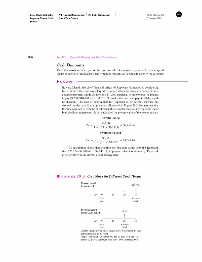
Ross−Westerfield−Jaffe: Corporate Finance, Sixth Edition
VII. Financial Planning and Short−Term Finance
29. Credit Management 805© The McGraw−Hill Companies, 2002
Cash DiscountsCash discounts are often part of the terms of sale. One reason they are offered is to speedup the collection of receivables. The firm must trade this off against the cost of the discount.
EXAMPLE
Edward Manalt, the chief financial officer of Ruptbank Company, is consideringthe request of the company’s largest customer, who wants to take a 3-percent dis-count for payment within 20 days on a $10,000 purchase. In other words, he intendsto pay $9,700 [$10,000 � (1 � 0.03)]. Normally, this customer pays in 30 days withno discount. The cost of debt capital for Ruptbank is 10 percent. Edward hasworked out the cash flow implications illustrated in Figure 29.3. He assumes thatthe time required to cash the check when the customer receives it is the same underboth credit arrangements. He has calculated the present value of the two proposals:
Current Policy:
Proposed Policy:
His calculation shows that granting the discount would cost the Ruptbankfirm $271.34 ($9,918.48 � $9,647.14) in present value. Consequently, Ruptbankis better off with the current credit arrangement.
PV �$9,700
1 � �0.1 � 20 �365�� $9,647.14
PV �$10,000
1 � �0.1 � 30�365�� $9,918.48
800 Part VII Financial Planning and Short-Term Finance
Current creditterms (net 30) $10,000
Days 0 10 20 30
Saledate
Receivecheck
$9,700
Days 0 10 20 30
Saledate
Receivecheck
Proposed creditterms (3/20, net 30)
� FIGURE 29.3 Cash Flows for Different Credit Terms
Current situation: Customers usually pay 30 days from the saledate and receive no discount.Proposed situation: Customer will pay 20 days from the saledate at a 3-percent discount from the $10,000 purchase price.
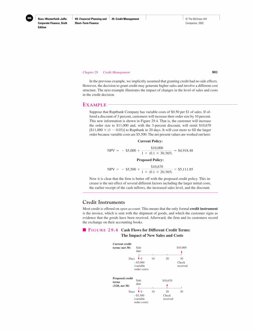
Ross−Westerfield−Jaffe: Corporate Finance, Sixth Edition
VII. Financial Planning and Short−Term Finance
29. Credit Management806 © The McGraw−Hill Companies, 2002
In the previous example, we implicitly assumed that granting credit had no side effects.However, the decision to grant credit may generate higher sales and involve a different coststructure. The next example illustrates the impact of changes in the level of sales and costsin the credit decision.
EXAMPLE
Suppose that Ruptbank Company has variable costs of $0.50 per $1 of sales. If of-fered a discount of 3 percent, customers will increase their order size by 10 percent.This new information is shown in Figure 29.4. That is, the customer will increasethe order size to $11,000 and, with the 3-percent discount, will remit $10,670[$11,000 � (1 � 0.03)] to Ruptbank in 20 days. It will cost more to fill the largerorder because variable costs are $5,500. The net present values are worked out here:
Current Policy:
Proposed Policy:
Now it is clear that the firm is better off with the proposed credit policy. This in-crease is the net effect of several different factors including the larger initial costs,the earlier receipt of the cash inflows, the increased sales level, and the discount.
Credit InstrumentsMost credit is offered on open account. This means that the only formal credit instrumentis the invoice, which is sent with the shipment of goods, and which the customer signs asevidence that the goods have been received. Afterward, the firm and its customers recordthe exchange on their accounting books.
NPV � � $5,500 �$10,670
1 � �0.1 � 20 �365�� $5,111.85
NPV � � $5,000 �$10,000
1 � �0.1 � 30 �365�� $4,918.48
Chapter 29 Credit Management 801
Saledate
$10,000
Days 0 10 20 30
Current creditterms (net 30)
–$5,000(variableorder costs)
Checkreceived
0 10 20 30
$10,670
Checkreceived
–$5,500(variableorder costs)
Proposed creditterms(3/20, net 30)
Days
Saledate
� FIGURE 29.4 Cash Flows for Different Credit Terms:The Impact of New Sales and Costs
Ross−Westerfield−Jaffe: Corporate Finance, Sixth Edition
VII. Financial Planning and Short−Term Finance
29. Credit Management 807© The McGraw−Hill Companies, 2002
At times, the firm may require that the customer sign a promissory note, or IOU. This isused when the order is large and when the firm anticipates a problem in collections.Promissory notes can eliminate controversies later about the existence of a credit agreement.
One problem with promissory notes is that they are signed after delivery of the goods.One way to obtain a credit commitment from a customer before the goods are delivered isthrough the use of a commercial draft. The selling firm typically writes a commercial draftcalling for the customer to pay a specific amount by a specified date. The draft is then sentto the customer’s bank with the shipping invoices. The bank has the buyer sign the draft be-fore turning over the invoices. The goods can then be shipped to the buyer. If immediatepayment is required, it is called a sight draft. Here, funds must be turned over to the bankbefore the goods are shipped.
Frequently, even the signed draft is not enough for the seller. In this case, he might de-mand that the banker pay for the goods and collect the money from the customer. When thebanker agrees to do so in writing, the document is called a banker’s acceptance. That is, thebanker accepts responsibility for payment. Because banks generally are well-known andwell-respected institutions, the banker’s acceptance becomes a liquid instrument. In otherwords, the seller can then sell (discount) the banker’s acceptance in the secondary market.
A firm can also use a conditional sales contract as a credit instrument. This is anarrangement where the firm retains legal ownership of the goods until the customer hascompleted payment. Conditional sales contracts usually are paid off in installments andhave interest costs built into them.
• What considerations enter into the determination of the terms of sale?
29.2 THE DECISION TO GRANT CREDIT: RISK AND INFORMATION
Locust Industries has been in existence for two years. It is one of several successful firmsthat develop computer programs. The present financial managers have set out two alterna-tive credit strategies: The firm can offer credit, or the firm can refuse credit.
Suppose Locust has determined that, if it offers no credit to its customers, it can sell itsexisting computer software for $50 per program. It estimates that the costs to produce a typ-ical computer program are equal to $20 per program.
The alternative is to offer credit. In this case, customers of Locust will pay one periodlater. With some probability, Locust has determined that if it offers credit, it can chargehigher prices and expect higher sales.
Strategy 1: Refuse Credit If Locust refuses to grant credit, cash flows will not be delayed,and period 0 net cash flows, NCF, will be
P0Q0 � C0Q0 � NCF
The subscripts denote the time when the cash flows are incurred, where
P0 � Price per unit received at time 0
C0 � Cost per unit received at time 0
Q0 � Quantity sold at time 0
802 Part VII Financial Planning and Short-Term Finance
QUESTION
CO
NC
EP
T
?
Ross−Westerfield−Jaffe: Corporate Finance, Sixth Edition
VII. Financial Planning and Short−Term Finance
29. Credit Management808 © The McGraw−Hill Companies, 2002
The net cash flows at period 1 are zero, and the net present value to Locust of refusingcredit will simply be the period 0 net cash flow:
NPV � NCF
For example, if credit is not granted and Q0 � 100, the NPV can be calculated as
($50 � 100) � ($20 � 100) � $3,000
Strategy 2: Offer Credit Alternatively, let us assume that Locust grants credit to all cus-tomers for one period. The factors that influence the decision are listed below.
Strategy 1 Strategy 2Refuse Credit Offer Credit
Price per unit P0 � $50Quantity sold Q0 � 100Cost per unit C0 � $20Probability of payment h � 1 h � 0.90Credit period 0 1 periodDiscount rate 0 rB � 0.01
The prime (′) denotes the variables under the second strategy. If the firm offers credit andthe new customers pay, the firm will receive revenues of one period hence, but itscosts, , are incurred in period 0. If new customers do not pay, the firm incurs costs
and receives no revenues. The probability that customers will pay, h, is 0.90 in theexample. Quantity sold is higher with credit, because new customers are attracted. The costper unit is also higher with credit because of the costs of operating a credit policy.
The expected cash flows for each policy are set out as follows:
Expected Cash Flows
Time 0 Time 1
Refuse credit P0Q0 � C0Q0 0Offer credit
Note that granting credit produces delayed expected cash inflows equal to .The costs are incurred immediately and require no discounting. The net present value ifcredit is offered is
Locust’s decision should be to adopt the proposed credit policy. The NPV of grantingcredit is higher than that of refusing credit. This decision is very sensitive to the probabil-ity of payment. If it turns out that the probability of payment is 81 percent, Locust Softwareis indifferent to whether it grants credit or not. In this case the NPV of granting credit is$3,000, which we previously found to be the NPV of not granting credit:
h � 80.8%
$8,000 � h �$50 � 200
1.01
$3,000 � h �$50 � 200
1.01� $5,000
�0.9 � $50 � 200
1.01� $5,000 � $3,910.89
NPV �offer� �h � P
′0 Q
′01 � rB
� C
′0 Q
′0
h � P
′0 Q
′0
h � P ′0 Q
′0�C ′0 Q
′0
C ′0 Q ′0C ′0 Q ′0
P ′0 Q ′0
C
′0 � $25Q
′0 � 200P
′0 � $50
Chapter 29 Credit Management 803
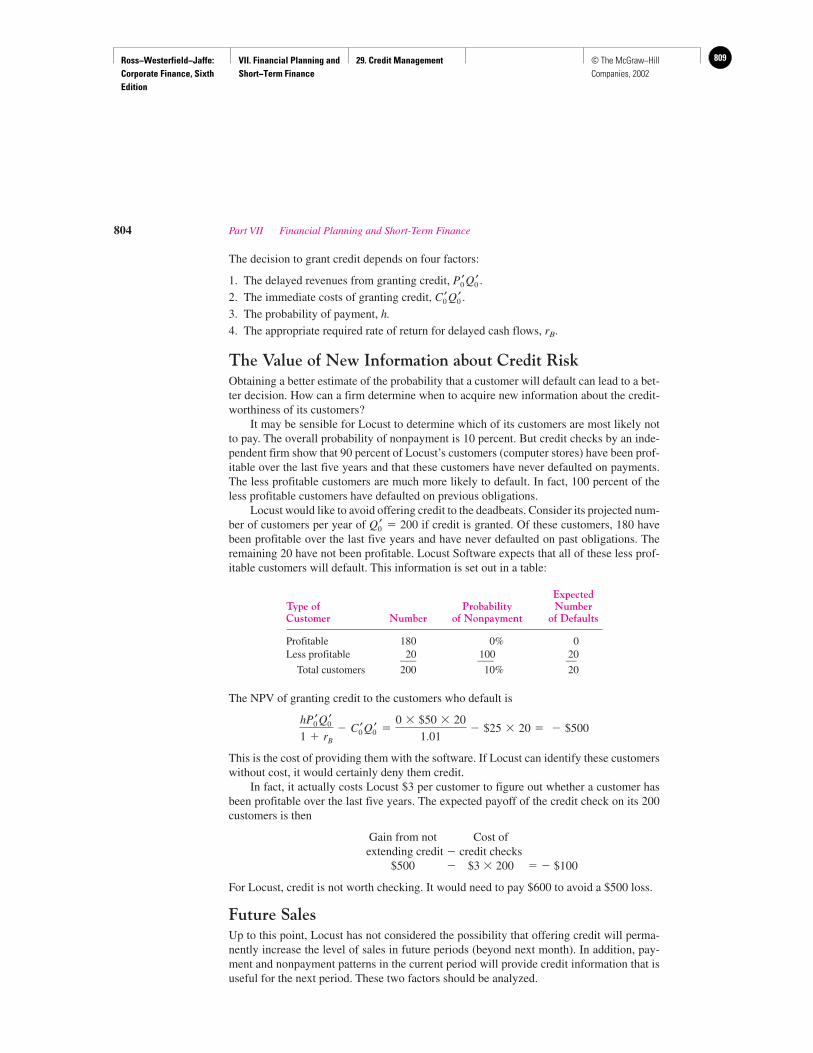
Ross−Westerfield−Jaffe: Corporate Finance, Sixth Edition
VII. Financial Planning and Short−Term Finance
29. Credit Management 809© The McGraw−Hill Companies, 2002
The decision to grant credit depends on four factors:
1. The delayed revenues from granting credit, .
2. The immediate costs of granting credit, .
3. The probability of payment, h.
4. The appropriate required rate of return for delayed cash flows, rB.
The Value of New Information about Credit RiskObtaining a better estimate of the probability that a customer will default can lead to a bet-ter decision. How can a firm determine when to acquire new information about the credit-worthiness of its customers?
It may be sensible for Locust to determine which of its customers are most likely notto pay. The overall probability of nonpayment is 10 percent. But credit checks by an inde-pendent firm show that 90 percent of Locust’s customers (computer stores) have been prof-itable over the last five years and that these customers have never defaulted on payments.The less profitable customers are much more likely to default. In fact, 100 percent of theless profitable customers have defaulted on previous obligations.
Locust would like to avoid offering credit to the deadbeats. Consider its projected num-ber of customers per year of � 200 if credit is granted. Of these customers, 180 havebeen profitable over the last five years and have never defaulted on past obligations. Theremaining 20 have not been profitable. Locust Software expects that all of these less prof-itable customers will default. This information is set out in a table:
ExpectedType of Probability NumberCustomer Number of Nonpayment of Defaults
Profitable 180 0% 0Less profitable 20 100 20___ ___ __
Total customers 200 10% 20
The NPV of granting credit to the customers who default is
This is the cost of providing them with the software. If Locust can identify these customerswithout cost, it would certainly deny them credit.
In fact, it actually costs Locust $3 per customer to figure out whether a customer hasbeen profitable over the last five years. The expected payoff of the credit check on its 200customers is then
Gain from not Cost ofextending credit � credit checks
$500 � $3 � 200 � � $100
For Locust, credit is not worth checking. It would need to pay $600 to avoid a $500 loss.
Future SalesUp to this point, Locust has not considered the possibility that offering credit will perma-nently increase the level of sales in future periods (beyond next month). In addition, pay-ment and nonpayment patterns in the current period will provide credit information that isuseful for the next period. These two factors should be analyzed.
hP
′0 Q
′01 � rB
� C
′0 Q
′0 �0 � $50 � 20
1.01� $25 � 20 � � $500
Q
′0
C
′0 Q
′0
P
′0 Q
′0
804 Part VII Financial Planning and Short-Term Finance
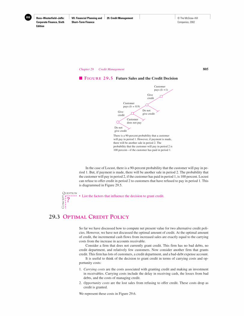
Ross−Westerfield−Jaffe: Corporate Finance, Sixth Edition
VII. Financial Planning and Short−Term Finance
29. Credit Management810 © The McGraw−Hill Companies, 2002
In the case of Locust, there is a 90-percent probability that the customer will pay in pe-riod 1. But, if payment is made, there will be another sale in period 2. The probability thatthe customer will pay in period 2, if the customer has paid in period 1, is 100 percent. Locustcan refuse to offer credit in period 2 to customers that have refused to pay in period 1. Thisis diagrammed in Figure 29.5.
• List the factors that influence the decision to grant credit.
29.3 OPTIMAL CREDIT POLICY
So far we have discussed how to compute net present value for two alternative credit poli-cies. However, we have not discussed the optimal amount of credit. At the optimal amountof credit, the incremental cash flows from increased sales are exactly equal to the carryingcosts from the increase in accounts receivable.
Consider a firm that does not currently grant credit. This firm has no bad debts, nocredit department, and relatively few customers. Now consider another firm that grantscredit. This firm has lots of customers, a credit department, and a bad-debt expense account.
It is useful to think of the decision to grant credit in terms of carrying costs and op-portunity costs:
1. Carrying costs are the costs associated with granting credit and making an investmentin receivables. Carrying costs include the delay in receiving cash, the losses from baddebts, and the costs of managing credit.
2. Opportunity costs are the lost sales from refusing to offer credit. These costs drop ascredit is granted.
We represent these costs in Figure 29.6.
Chapter 29 Credit Management 805
Customerpays (h =1)
Givecredit
Customerpays (h = 0.9)
Givecredit
Do notgive credit
Do notgive credit
Customerdoes not pay
� FIGURE 29.5 Future Sales and the Credit Decision
There is a 90-percent probability that a customerwill pay in period 1. However, if payment is made,there will be another sale in period 2. Theprobability that the customer will pay in period 2 is100 percent—if the customer has paid in period 1.
QUESTION
CO
NC
EP
T
?
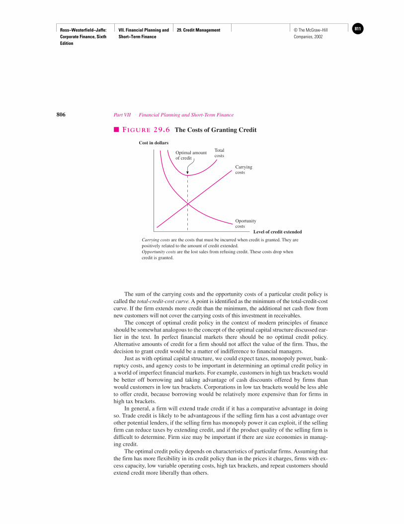
Ross−Westerfield−Jaffe: Corporate Finance, Sixth Edition
VII. Financial Planning and Short−Term Finance
29. Credit Management 811© The McGraw−Hill Companies, 2002
The sum of the carrying costs and the opportunity costs of a particular credit policy iscalled the total-credit-cost curve. A point is identified as the minimum of the total-credit-costcurve. If the firm extends more credit than the minimum, the additional net cash flow fromnew customers will not cover the carrying costs of this investment in receivables.
The concept of optimal credit policy in the context of modern principles of financeshould be somewhat analogous to the concept of the optimal capital structure discussed ear-lier in the text. In perfect financial markets there should be no optimal credit policy.Alternative amounts of credit for a firm should not affect the value of the firm. Thus, thedecision to grant credit would be a matter of indifference to financial managers.
Just as with optimal capital structure, we could expect taxes, monopoly power, bank-ruptcy costs, and agency costs to be important in determining an optimal credit policy ina world of imperfect financial markets. For example, customers in high tax brackets wouldbe better off borrowing and taking advantage of cash discounts offered by firms thanwould customers in low tax brackets. Corporations in low tax brackets would be less ableto offer credit, because borrowing would be relatively more expensive than for firms inhigh tax brackets.
In general, a firm will extend trade credit if it has a comparative advantage in doingso. Trade credit is likely to be advantageous if the selling firm has a cost advantage overother potential lenders, if the selling firm has monopoly power it can exploit, if the sellingfirm can reduce taxes by extending credit, and if the product quality of the selling firm isdifficult to determine. Firm size may be important if there are size economies in manag-ing credit.
The optimal credit policy depends on characteristics of particular firms. Assuming thatthe firm has more flexibility in its credit policy than in the prices it charges, firms with ex-cess capacity, low variable operating costs, high tax brackets, and repeat customers shouldextend credit more liberally than others.
806 Part VII Financial Planning and Short-Term Finance
Cost in dollars
Optimal amountof credit
Totalcosts
Carryingcosts
Oportunitycosts
Level of credit extended
� FIGURE 29.6 The Costs of Granting Credit
Carrying costs are the costs that must be incurred when credit is granted. They arepositively related to the amount of credit extended.Opportunity costs are the lost sales from refusing credit. These costs drop whencredit is granted.
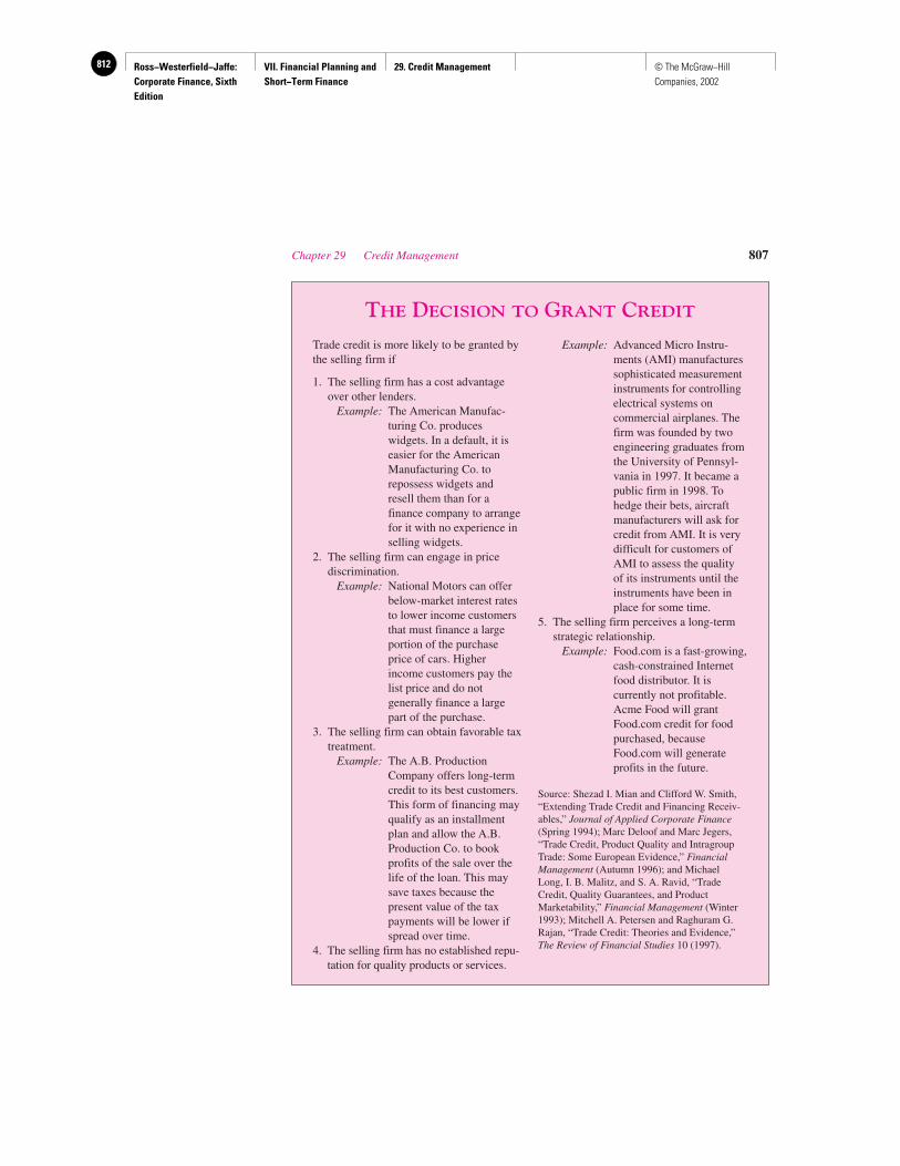
Ross−Westerfield−Jaffe: Corporate Finance, Sixth Edition
VII. Financial Planning and Short−Term Finance
29. Credit Management812 © The McGraw−Hill Companies, 2002
Chapter 29 Credit Management 807
THE DECISION TO GRANT CREDIT
Trade credit is more likely to be granted bythe selling firm if
1. The selling firm has a cost advantageover other lenders.
Example: The American Manufac-turing Co. produceswidgets. In a default, it iseasier for the AmericanManufacturing Co. torepossess widgets andresell them than for afinance company to arrangefor it with no experience inselling widgets.
2. The selling firm can engage in pricediscrimination.
Example: National Motors can offerbelow-market interest ratesto lower income customersthat must finance a largeportion of the purchaseprice of cars. Higherincome customers pay thelist price and do notgenerally finance a largepart of the purchase.
3. The selling firm can obtain favorable taxtreatment.
Example: The A.B. ProductionCompany offers long-termcredit to its best customers.This form of financing mayqualify as an installmentplan and allow the A.B.Production Co. to bookprofits of the sale over thelife of the loan. This maysave taxes because thepresent value of the taxpayments will be lower ifspread over time.
4. The selling firm has no established repu-tation for quality products or services.
Example: Advanced Micro Instru-ments (AMI) manufacturessophisticated measurementinstruments for controllingelectrical systems oncommercial airplanes. Thefirm was founded by twoengineering graduates fromthe University of Pennsyl-vania in 1997. It became apublic firm in 1998. Tohedge their bets, aircraftmanufacturers will ask forcredit from AMI. It is verydifficult for customers ofAMI to assess the qualityof its instruments until theinstruments have been inplace for some time.
5. The selling firm perceives a long-termstrategic relationship.
Example: Food.com is a fast-growing,cash-constrained Internetfood distributor. It iscurrently not profitable.Acme Food will grantFood.com credit for foodpurchased, becauseFood.com will generateprofits in the future.
Source: Shezad I. Mian and Clifford W. Smith,“Extending Trade Credit and Financing Receiv-ables,” Journal of Applied Corporate Finance(Spring 1994); Marc Deloof and Marc Jegers,“Trade Credit, Product Quality and IntragroupTrade: Some European Evidence,” FinancialManagement (Autumn 1996); and MichaelLong, I. B. Malitz, and S. A. Ravid, “TradeCredit, Quality Guarantees, and ProductMarketability,” Financial Management (Winter1993); Mitchell A. Petersen and Raghuram G.Rajan, “Trade Credit: Theories and Evidence,”The Review of Financial Studies 10 (1997).

Ross−Westerfield−Jaffe: Corporate Finance, Sixth Edition
VII. Financial Planning and Short−Term Finance
29. Credit Management 813© The McGraw−Hill Companies, 2002
29.4 CREDIT ANALYSIS
When granting credit, a firm tries to distinguish between customers that will pay and cus-tomers that will not pay. There are a number of sources of information for determining cred-itworthiness.
Credit InformationInformation commonly used to assess creditworthiness includes the following:
1. Financial Statements. A firm can ask a customer to supply financial statements. Rulesof thumb based on financial ratios can be calculated.
2. Credit Reports on Customer’s Payment History with Other Firms. Many organizationssell information on the credit strength of business firms. The best known and largest firmof this type is Dun & Bradstreet, which provides subscribers with a credit-referencebook and credit reports on individual firms. The reference book has credit ratings onmany thousands of businesses.
3. Banks. Banks will generally provide some assistance to their business customers in ac-quiring information on the creditworthiness of other firms.
4. The Customer’s Payment History with the Firm. The most obvious way to obtain anestimate of a customer’s probability of nonpayment is whether he or she has paid pre-vious bills.
Credit ScoringOnce information has been gathered, the firm faces the hard choice of either granting or re-fusing credit. Many firms use the traditional and subjective guidelines referred to as the“five Cs of credit”:
1. Character. The customer’s willingness to meet credit obligations.
2. Capacity. The customer’s ability to meet credit obligations out of operating cashflows.
3. Capital. The customer’s financial reserves.
4. Collateral. A pledged asset in the case of default.
5. Conditions. General economic conditions.
Conversely, firms such as credit-card issuers have developed elaborate statistical mod-els (called credit-scoring models) for determining the probability of default. Usually all therelevant and observable characteristics of a large pool of customers are studied to find theirhistoric relation to default. Because these models determine who is and who is not credit-worthy, not surprisingly they have been the subject of government regulation. For example,if a model were to find that women default more than men, it might be used to deny womencredit. This regulation removes such models from the domain of the statistician and makesthem the subject of politicians.
• What is credit analysis?• What are the five Cs of credit?
808 Part VII Financial Planning and Short-Term Finance
QUESTIONS
CO
NC
EP
T
?

Ross−Westerfield−Jaffe: Corporate Finance, Sixth Edition
VII. Financial Planning and Short−Term Finance
29. Credit Management814 © The McGraw−Hill Companies, 2002
29.5 COLLECTION POLICY
Collection refers to obtaining payment of past-due accounts. The credit manager keeps arecord of payment experiences with each customer.
Average Collection PeriodAcme Compact Disc Players sells 100,000 compact disc players a year at $300 each. Allsales are for credit with terms of 2/20, net 60.
Suppose that 80 percent of Acme’s customers take the discounts and pay on day 20;the rest pay on day 60. The average collection period (ACP) measures the average amountof time required to collect an account receivable. The ACP for Acme is 28 days:
0.8 � 20 days � 0.2 � 60 days � 28 days
(The average collection period is frequently referred to as days’ sales outstanding or daysin receivables.)
Of course, this is an idealized example where customers pay on either one of two dates.In reality, payments arrive in a random fashion, so that the average collection period mustbe calculated differently.
To determine the ACP in the real world, firms first calculate average daily sales. Theaverage daily sales (ADS) equal annual sales divided by 365. The ADS of Acme are
If receivables today are $2,301,376, the average collection period is
In practice, firms observe sales and receivables on a daily basis. Consequently, an averagecollection period can be computed and compared to the stated credit terms. For example,suppose Acme had computed its ACP at 40 days for several weeks, versus its credit termsof 2/20, net 60. With a 40-day ACP, some customers are paying later than usual. It may bethat some accounts are overdue.
However, firms with seasonal sales will often find the calculated ACP changing dur-ing the year, making the ACP a somewhat flawed tool. This occurs because receivables arelow before the selling season and high after the season. Thus, firms may keep track of sea-sonal movement in the ACP over past years. In this way, they can compare the ACP for to-day’s date with the average ACP for that date in previous years. To supplement the infor-mation in the ACP, the credit manager may make up an accounts receivable aging schedule.
Aging ScheduleThe aging schedule tabulates receivables by age of account. In the following schedule, 75percent of the accounts are on time, but a significant number are more than 60 days pastdue. This signifies that some customers are in arrears.
� 28 days
�$2,301,736
$82,192
Average collection period �Accounts receivable
Average daily sales
Average daily sales �$300 � 100,000
365 days� $82,192
Chapter 29 Credit Management 809
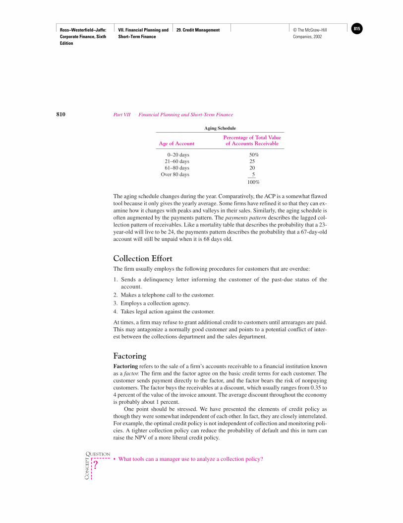
Ross−Westerfield−Jaffe: Corporate Finance, Sixth Edition
VII. Financial Planning and Short−Term Finance
29. Credit Management 815© The McGraw−Hill Companies, 2002
Aging Schedule
Percentage of Total ValueAge of Account of Accounts Receivable
0–20 days 50%21–60 days 2561–80 days 20
Over 80 days 5___100%
The aging schedule changes during the year. Comparatively, the ACP is a somewhat flawedtool because it only gives the yearly average. Some firms have refined it so that they can ex-amine how it changes with peaks and valleys in their sales. Similarly, the aging schedule isoften augmented by the payments pattern. The payments pattern describes the lagged col-lection pattern of receivables. Like a mortality table that describes the probability that a 23-year-old will live to be 24, the payments pattern describes the probability that a 67-day-oldaccount will still be unpaid when it is 68 days old.
Collection EffortThe firm usually employs the following procedures for customers that are overdue:
1. Sends a delinquency letter informing the customer of the past-due status of the account.
2. Makes a telephone call to the customer.
3. Employs a collection agency.
4. Takes legal action against the customer.
At times, a firm may refuse to grant additional credit to customers until arrearages are paid.This may antagonize a normally good customer and points to a potential conflict of inter-est between the collections department and the sales department.
FactoringFactoring refers to the sale of a firm’s accounts receivable to a financial institution knownas a factor. The firm and the factor agree on the basic credit terms for each customer. Thecustomer sends payment directly to the factor, and the factor bears the risk of nonpayingcustomers. The factor buys the receivables at a discount, which usually ranges from 0.35 to4 percent of the value of the invoice amount. The average discount throughout the economyis probably about 1 percent.
One point should be stressed. We have presented the elements of credit policy asthough they were somewhat independent of each other. In fact, they are closely interrelated.For example, the optimal credit policy is not independent of collection and monitoring poli-cies. A tighter collection policy can reduce the probability of default and this in turn canraise the NPV of a more liberal credit policy.
• What tools can a manager use to analyze a collection policy?
810 Part VII Financial Planning and Short-Term Finance
QUESTION
CO
NC
EP
T
?
Ross−Westerfield−Jaffe: Corporate Finance, Sixth Edition
VII. Financial Planning and Short−Term Finance
29. Credit Management816 © The McGraw−Hill Companies, 2002
29.6 HOW TO FINANCE TRADE CREDIT
In addition to unsecured debt instruments described earlier in this chapter, there are threegeneral ways of financing accounting receivables: secured debt, a captive finance company,and securitization.
Use of secured debt is usually referred to as asset-based receivables financing. This isthe predominant form of receivables financing. Many lenders will not lend without securityto firms with substantive uncertainty or little equity. With secured debt, if the borrower getsinto financial difficulty, the lender can repossess the asset and sell it for its fair market value.
Many large firms with good credit ratings use captive finance companies. The captivefinance companies are subsidiaries of the parent firm. This is similar to the use of secureddebt because the creditors of the captive finance company have a claim on its assets and, asa consequence, the accounts receivable of the parent firm. A captive finance company is at-tractive if economies of scale are important and if an independent subsidiary with limitedliability is warranted.
Securitization occurs when the selling firm sells its accounts receivable to a financialinstitution. The financial institution pools the receivables with other receivables and issuessecurities to finance items.
29.7 SUMMARY AND CONCLUSIONS
1. The components of a firm’s credit policy are the terms of sale, the credit analysis, and thecollection policy.
2. The terms of sale describe the amount and period of time for which credit is granted and thetype of credit instrument.
3. The decision to grant credit is a straightforward NPV decision, and can be improved byadditional information about the payment characteristics of the customers. Additionalinformation about the customers’ probability of defaulting is valuable, but this value must betraded off against the expense of acquiring the information.
4. The optimal amount of credit the firm offers is a function of the competitive conditions inwhich it finds itself. These conditions will determine the carrying costs associated withgranting credit and the opportunity costs of the lost sales from refusing to offer credit. Theoptimal credit policy minimizes the sum of these two costs.
5. We have seen that knowledge of the probability that customers will default is valuable. Toenhance its ability to assess customers’ default probability, a firm can score credit. Thisrelates the default probability to observable characteristics of customers.
6. The collection policy is the method of dealing with past-due accounts. The first step is toanalyze the average collection period and to prepare an aging schedule that relates the age ofaccounts to the proportion of the accounts receivable they represent. The next step is todecide on the collection method and to evaluate the possibility of factoring, that is, selling theoverdue accounts.
Chapter 29 Credit Management 811

Ross−Westerfield−Jaffe: Corporate Finance, Sixth Edition
VII. Financial Planning and Short−Term Finance
29. Credit Management 817© The McGraw−Hill Companies, 2002
KEY TERMS
Aging schedule 809 Credit instrument 801Average collection period (ACP) 809 Credit periods 799Average daily sales (ADS) 809 Credit scoring 808Cash discounts 800 Factoring 810Collection policy 798 Invoice 798Credit analysis 798 Terms of the sale 798
SUGGESTED READINGS
The following articles are important for an understanding of how to make short-term financialdecisions:Sartoris, W. L., and N. C. Hill. “Evaluating Credit Policy Alternatives: A Present Value
Framework.” Journal of Financial Research 4 (Spring 1981), p. 1.______ “A Generalized Cash Flow Approach to Short-Term Financial Decisions.” Journal of
Finance 38 (May 1983), p. 3.
Our treatment of the credit decision owes much to:Bierman, H., Jr., and W. H. Hausman. “The Credit Granting Decision.” Management Science 16
(April 1970), and Mian, Shezad I., and Clifford W. Smith. “Extending Trade Credit andFinancial Receivables.” Journal of Applied Corporate Finance (Spring 1994).
Three recent articles that establish a theoretical framework and some empirical work on tradecredit:Mian, S. I., and C. Smith. “Extending Trade Credit and Financing Receivables.” Journal of
Applied Corporate Finance (Spring 1994).Long, M. S.; I. B. Malitz; and S. A. Ravid. “Trade Credit, Quality Guarantees, and Product
Marketability.” Financial Management (Winter 1993).Lee, Y. W., and J. D. Stowe. “Product Risk, Asymmetric Introduction and Trade Credit.” Journal
of Financial and Quantitative Analysis (June 1993).
An interesting normative article on how to establish trade credit limits is:Scherr, F. C. “Optimal Trade Credit Limits.” Financial Management (Spring 1996).
QUESTIONS AND PROBLEMS
Terms of the Sale29.1 The North County Publishing Company has provided the following data:
Annual credit sales � $10 million
Average collection period � 60 days
Terms: Net 30
Interest rate � 10%
North County Publishing proposes to offer a discount policy of 2/10, net 30. It anticipatesthat 50 percent of its customers will take advantage of this new policy. As a result, thecollection period will be reduced to 30 days. Should the North County PublishingCompany offer the new credit terms?
29.2 The Webster’s Company sells on credit terms of net 45. Its accounts are on average 45days past due. If annual credit sales are $5 million, what is the company’s balance inaccounts receivable?
812 Part VII Financial Planning and Short-Term Finance
Ross−Westerfield−Jaffe: Corporate Finance, Sixth Edition
VII. Financial Planning and Short−Term Finance
29. Credit Management818 © The McGraw−Hill Companies, 2002
29.3 The Tropeland Company has obtained the following information:
Annual credit sales � $30 million
Collection period � 60 days
Terms: Net 30
Interest rate � 12%
The company is considering offering terms of 4/10, net 30. It anticipates that 50 percent ofits customers will take advantage of the discount. The collection period is expected todecrease by one month. Should the new credit policy be adopted?
The Decision to Grant Credit: Risk and Information29.4 Berkshire Sports, Inc., operates a mail-order running-shoe business. Management is
considering dropping its policy of no credit. The credit policy under consideration byBerkshire follows:
No Credit Credit
Price per unit $35 $40Cost per unit $25 $32Quantity sold 2,000 3,000Probability of payment 100% 85%Credit period 0 1Discount rate 0 3%
a. Should Berkshire offer credit to its customers?b. What must the probability of payment be before Berkshire would adopt the policy?
29.5 The Theodore Bruin Corporation, a manufacturer of high-quality stuffed animals, does notextend credit to its customers. A study has shown that, by offering credit, the company canincrease sales from the current 750 units to 1,000 units. The cost per unit, however, willincrease from $43 to $45, reflecting the expense of managing accounts receivable. Thecurrent price of a toy is $48. The probability of a customer making a payment on a creditsale is 92 percent, and the appropriate discount rate is 2.7 percent.
By how much should Theodore Bruin increase the price to make offering credit anattractive strategy?
29.6 Fast Typing Co. is in the business of manufacturing and selling Fast-Line Typewriters. Itdoes not offer any credit sales currently. The per unit price and cost of each Fast-Linetypewriter are $900 and $600, respectively. Fast Typing Co. is considering the possibilityof credit sales. The market price of the typewriter will stay the same with credit sales, butit is expected that the annual sales will increase from 5,000 units to 9,000 units and the perunit cost will go up by $50 due to implementation cost of credit sales. The credit periodwill be two months and the appropriate discount rate for the credit period is 1.5 percent.What is the minimum probability of repayment that can make Fast Typing Co. indifferentbetween whether or not to implement the new credit policy?
29.7 The Silver Spokes Bicycle Shop has decided to offer credit to its customers during thespring selling season. Sales are expected to be 300 cycles. The average cost to the shop ofa cycle is $240. The owner knows that only 95 percent of the customers will be able tomake their payments. To identify the remaining 5 percent, she is considering subscribingto a credit agency. The initial charge for this service is $500, with an additional charge of$4 per individual report. Should she subscribe to the agency?
Optimal Credit Policy29.8 In principle, how should we decide the optimal credit policy?
Chapter 29 Credit Management 813

Ross−Westerfield−Jaffe: Corporate Finance, Sixth Edition
VII. Financial Planning and Short−Term Finance
29. Credit Management 819© The McGraw−Hill Companies, 2002
Credit Analysis29.9 What is the information commonly used to assess creditworthiness of a client?
Collection Policy29.10 Major Electronics sells 85,000 personal stereos each year at a price per unit of $55. All
sales are on credit; the terms are 3/15, net 40. The discount is taken by 40 percent of thecustomers. What is the investment in accounts receivable?
In reaction to a competitor, Major Electronics is considering changing its creditterms to 5/15, net 40, to preserve its sales level. Describe qualitatively how this policychange will affect the company’s investment in accounts receivable.
29.11 The Allen Company has monthly credit sales of $600,000. The average collection periodis 90 days. The cost of production is 70 percent of the selling price. What is the AllenCompany’s average investment in accounts receivable?
29.12 The factoring department of Inter American Bank (IAB) is processing 100,000 invoicesper year with average invoice value of $1,500. IAB buys the accounts receivable at 4percent off the invoice value. The average collection period is 30 days. Currently 2percent of the accounts receivable turns out to be bad debt. The annual interest rate is 10percent. The annual operating expense of this department is $400,000. What is the grossprofit before interest and tax for the factoring department of IAB?
814 Part VII Financial Planning and Short-Term Finance

Ross−Westerfield−Jaffe: Corporate Finance, Sixth Edition
VIII. Special Topics Introduction820 © The McGraw−Hill Companies, 2002
Special Topics
PA
RT
VIII
30 Mergers and Acquisitions 81631 Financial Distress 85432 International Corporate Finance 872
IN Part VIII we discuss three special topics: mergers and acquisitions, financial dis-tress, and international corporate finance.
Chapter 30 describes the corporate finance of mergers and acquisitions. The acqui-sition of one firm by another is a capital-budgeting decision, and the basic principles ofNPV apply; that is, a firm should be acquired if it generates positive NPV to the share-holders of the acquiring firm. The purpose of Chapter 30 is to discuss how to value anacquisition candidate. However, the NPV of an acquisition candidate is more difficult todetermine than that of a typical investment project because of complex accounting, tax,and legal effects.
Chapter 31 discusses what happens when a firm experiences financial distress. Fi-nancial distress is a special circumstance when a firm’s cash flow falls below its con-tractually required payments. Financial restructuring involving private workouts or for-mal bankruptcy usually follows financial distress.
Our last chapter concerns international corporate finance. Many firms have signifi-cant foreign operations and must consider special financial factors that do not directlyaffect purely domestic firms. These factors include foreign exchange rates, interest ratesthat vary from country to country, and complex accounting, legal, and tax rules.
Ross−Westerfield−Jaffe: Corporate Finance, Sixth Edition
VIII. Special Topics 30. Mergers and Acquisitions
821© The McGraw−Hill Companies, 2002
Mergers and Acquisitions
CH
AP
TE
R30
EXECUTIVE SUMMARY
There is no more dramatic or controversial activity in corporate finance than the ac-quisition of one firm by another or the merger of two firms. This chapter addressestwo basic questions: Why does a firm choose to merge with or acquire another firm
and how does it happen?The acquisition of one firm by another is, of course, an investment made under un-
certainty. The basic principle of valuation applies: a firm should be acquired if it generatesa positive net present value to the shareholders of the acquiring firm. However, becausethe NPV of an acquisition candidate is very difficult to determine, mergers and acquisi-tions are interesting topics in their own right. Here are some of the special features of thisarea of finance:
1. The benefits from acquisitions are called synergies. It is hard to estimate synergies us-ing discounted cash flow techniques.
2. There are complex accounting, tax, and legal effects when one firm is acquired by an-other.
3. Acquisitions are an important control device of shareholders. It appears that some ac-quisitions are a consequence of an underlying conflict between the interests of existingmanagers and of shareholders. Acquisition by another firm is one way that shareholderscan remove managers with whom they are unhappy.
4. Acquisition analysis frequently focuses on the total value of the firms involved. But usu-ally an acquisition will affect the relative values of stocks and bonds, as well as their to-tal value.
5. Mergers and acquisitions sometimes involve unfriendly transactions. Thus, when onefirm attempts to acquire another, it does not always involve quiet, gentlemanly negotia-tions. The sought-after firm may use defensive tactics, including poison pills, greenmail,and white knights.
This chapter starts by introducing the basic legal, accounting, and tax aspects of ac-quisitions. When one firm acquires another, it must choose the legal framework, the ac-counting method, and tax status. These choices will be explained throughout the chapter.
The chapter discusses how to determine the NPV of an acquisition candidate. TheNPV of an acquisition candidate is the difference between the synergy from the mergerand the premium to be paid. We consider the following types of synergy: (1) revenue en-hancement, (2) cost reduction, (3) lower taxes, and (4) lower cost of capital. The pre-mium paid for an acquisition is the price paid minus the market value of the acquisitionprior to the merger. The premium depends on whether cash or securities are used to fi-nance the offer price.
Ross−Westerfield−Jaffe: Corporate Finance, Sixth Edition
VIII. Special Topics 30. Mergers and Acquisitions
822 © The McGraw−Hill Companies, 2002
30.1 THE BASIC FORMS OF ACQUISITIONS
There are three basic legal procedures that one firm can use to acquire another firm:(1) merger or consolidation, (2) acquisition of stock, and (3) acquisition of assets.
Merger or ConsolidationA merger refers to the absorption of one firm by another. The acquiring firm retains itsname and its identity, and it acquires all of the assets and liabilities of the acquired firm. Af-ter a merger, the acquired firm ceases to exist as a separate business entity.
A consolidation is the same as a merger except that an entirely new firm is created. Ina consolidation, both the acquiring firm and the acquired firm terminate their previous le-gal existence and become part of the new firm. In a consolidation, the distinction betweenthe acquiring and the acquired firm is not important. However, the rules for mergers andconsolidations are basically the same. Acquisitions by merger and consolidation result incombinations of the assets and liabilities of acquired and acquiring firms.
EXAMPLE
Suppose firm A acquires firm B in a merger. Further, suppose firm B’s sharehold-ers are given one share of firm A’s stock in exchange for two shares of firm B’sstock. From a legal standpoint, firm A’s shareholders are not directly affected bythe merger. However, firm B’s shares cease to exist. In a consolidation, the share-holders of firm A and firm B would exchange their shares for the share of a newfirm (e.g., firm C). Because the differences between mergers and consolidationsare not all that important for our purposes, we shall refer to both types of reor-ganizations as mergers.
There are some advantages and some disadvantages to using a merger to acquire a firm:
1. A merger is legally straightforward and does not cost as much as other forms of acqui-sition. It avoids the necessity of transferring title of each individual asset of the acquiredfirm to the acquiring firm.
2. A merger must be approved by a vote of the stockholders of each firm.1 Typically, votesof the owners of two-thirds of the shares are required for approval. In addition, share-holders of the acquired firm have appraisal rights. This means that they can demand thattheir shares be purchased at a fair value by the acquiring firm. Often the acquiring firmand the dissenting shareholders of the acquired firm cannot agree on a fair value, whichresults in expensive legal proceedings.
Acquisition of StockA second way to acquire another firm is to purchase the firm’s voting stock in exchange forcash, shares of stock, or other securities. This may start as a private offer from the manage-ment of one firm to another. At some point the offer is taken directly to the selling firm’s stock-holders. This can be accomplished by use of a tender offer. A tender offer is a public offer tobuy shares of a target firm. It is made by one firm directly to the shareholders of another firm.
Chapter 30 Mergers and Acquisitions 817
1Mergers between corporations require compliance with state laws. In virtually all states the shareholders ofeach corporation must give their assent.
Ross−Westerfield−Jaffe: Corporate Finance, Sixth Edition
VIII. Special Topics 30. Mergers and Acquisitions
823© The McGraw−Hill Companies, 2002
The offer is communicated to the target firm’s shareholders by public announcements such asnewspaper advertisements. Sometimes a general mailing is used in a tender offer. However, ageneral mailing is very difficult because it requires the names and addresses of the stock-holders of record, which are not usually available.
The following are factors involved in choosing between an acquisition of stock anda merger:
1. In an acquisition of stock, no shareholder meetings must be held and no vote is required.If the shareholders of the target firm do not like the offer, they are not required to acceptit and they will not tender their shares.
2. In an acquisition of stock, the bidding firm can deal directly with the shareholders of atarget firm by using a tender offer. The target firm’s management and board of directorscan be bypassed.
3. Acquisition of stock is often unfriendly. It is used in an effort to circumvent the targetfirm’s management, which is usually actively resisting acquisition. Resistance by thetarget firm’s management often makes the cost of acquisition by stock higher than thecost by merger.
4. Frequently a minority of shareholders will hold out in a tender offer, and thus the targetfirm cannot be completely absorbed.
5. Complete absorption of one firm by another requires a merger. Many acquisitions ofstock end with a formal merger later.
Acquisition of AssetsOne firm can acquire another firm by buying all of its assets. A formal vote of the share-holders of the selling firm is required. This approach to acquisition will avoid the potentialproblem of having minority shareholders, which can occur in an acquisition of stock. Ac-quisition of assets involves transferring title to assets. The legal process of transferring as-sets can be costly.
A Classification SchemeFinancial analysts have typically classified acquisitions into three types:
1. Horizontal Acquisition. This is an acquisition of a firm in the same industry as the ac-quiring firm. The firms compete with each other in their product market.
2. Vertical Acquisition. A vertical acquisition involves firms at different steps of the pro-duction process. The acquisition by an airline company of a travel agency would be avertical acquisition.
3. Conglomerate Acquisition. The acquiring firm and the acquired firm are not related toeach other. The acquisition of a food-products firm by a computer firm would be con-sidered a conglomerate acquisition.
A Note on TakeoversTakeover is a general and imprecise term referring to the transfer of control of a firm from onegroup of shareholders to another.2 A firm that has decided to take over another firm is usuallyreferred to as the bidder. The bidder offers to pay cash or securities to obtain the stock or as-sets of another company. If the offer is accepted, the target firm will give up control over itsstock or assets to the bidder in exchange for consideration (i.e., its stock, its debt, or cash).
2Control may be defined as having a majority vote on the board of directors.
818 Part VIII Special Topics
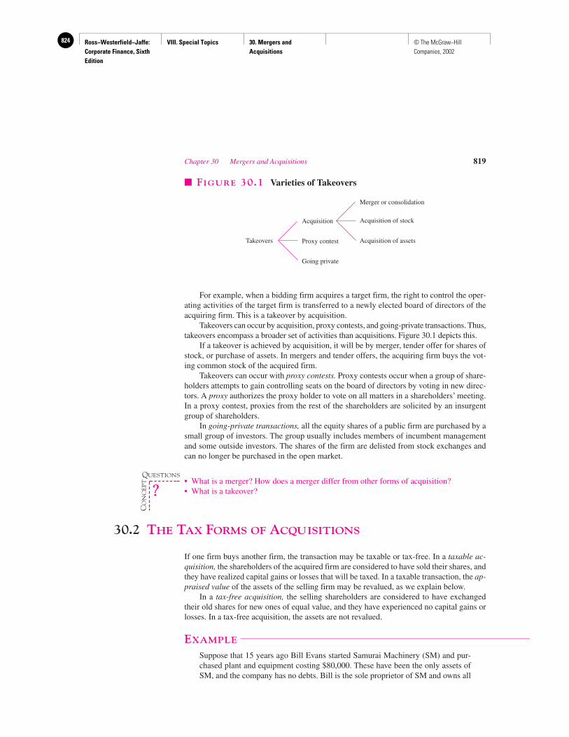
Ross−Westerfield−Jaffe: Corporate Finance, Sixth Edition
VIII. Special Topics 30. Mergers and Acquisitions
824 © The McGraw−Hill Companies, 2002
For example, when a bidding firm acquires a target firm, the right to control the oper-ating activities of the target firm is transferred to a newly elected board of directors of theacquiring firm. This is a takeover by acquisition.
Takeovers can occur by acquisition, proxy contests, and going-private transactions. Thus,takeovers encompass a broader set of activities than acquisitions. Figure 30.1 depicts this.
If a takeover is achieved by acquisition, it will be by merger, tender offer for shares ofstock, or purchase of assets. In mergers and tender offers, the acquiring firm buys the vot-ing common stock of the acquired firm.
Takeovers can occur with proxy contests. Proxy contests occur when a group of share-holders attempts to gain controlling seats on the board of directors by voting in new direc-tors. A proxy authorizes the proxy holder to vote on all matters in a shareholders’ meeting.In a proxy contest, proxies from the rest of the shareholders are solicited by an insurgentgroup of shareholders.
In going-private transactions, all the equity shares of a public firm are purchased by asmall group of investors. The group usually includes members of incumbent managementand some outside investors. The shares of the firm are delisted from stock exchanges andcan no longer be purchased in the open market.
• What is a merger? How does a merger differ from other forms of acquisition?• What is a takeover?
30.2 THE TAX FORMS OF ACQUISITIONS
If one firm buys another firm, the transaction may be taxable or tax-free. In a taxable ac-quisition, the shareholders of the acquired firm are considered to have sold their shares, andthey have realized capital gains or losses that will be taxed. In a taxable transaction, the ap-praised value of the assets of the selling firm may be revalued, as we explain below.
In a tax-free acquisition, the selling shareholders are considered to have exchangedtheir old shares for new ones of equal value, and they have experienced no capital gains orlosses. In a tax-free acquisition, the assets are not revalued.
EXAMPLE
Suppose that 15 years ago Bill Evans started Samurai Machinery (SM) and pur-chased plant and equipment costing $80,000. These have been the only assets ofSM, and the company has no debts. Bill is the sole proprietor of SM and owns all
Chapter 30 Mergers and Acquisitions 819
Takeovers
Acquisition
Proxy contest
Going private
Merger or consolidation
Acquisition of stock
Acquisition of assets
� FIGURE 30.1 Varieties of Takeovers
QUESTIONS
CO
NC
EP
T
?
Ross−Westerfield−Jaffe: Corporate Finance, Sixth Edition
VIII. Special Topics 30. Mergers and Acquisitions
825© The McGraw−Hill Companies, 2002
the shares. For tax purposes the assets of SM have been depreciated using thestraight-line method over 10 years, and have no salvage value. The annual depre-ciation expense has been $8,000 ($80,000/10). The machinery has no accountingvalue today (i.e., it has been written off the books). However, because of inflation,the fair market value of the machinery is $200,000. As a consequence, the S. A.Steel Company has bid $200,000 for all of the outstanding stock of Samurai.
Tax-Free Transaction If Bill Evans receives shares of S. A. Steel worth $200,000, theIRS will treat the sale as a tax-free transaction. Thus, Bill will not have to pay taxes on anygain received from the stock. In addition, S. A. Steel will be allowed the same depreciationdeduction that Samurai Machinery was allowed. Because the asset has already been fullydepreciated, S. A. Steel will receive no depreciation deduction.
Taxable Transaction If S. A. Steel pays $200,000 in cash for Samurai Machinery, it willbe a taxable transaction. There will be a number of tax consequences:
1. In the year of the merger, Bill Evans must pay taxes on the difference between the mergerprice of $200,000 and his initial contribution to the firm of $80,000. Thus, his taxableincome is $120,000 ($200,000 � $80,000).
2. S. A. Steel may elect to write up the value of the machinery. In this case, S. A. Steel willbe able to depreciate the machinery from an initial tax basis of $200,000. If S. A. Steel de-preciates straight-line over 10 years, depreciation will be $20,000 ($200,000/10) per year.
If S. A. Steel elects to write up the machinery, S. A. Steel must treat the $200,000write-up as taxable income immediately.3
3. Should S. A. Steel not elect the write-up, there is no increase in depreciation. Thus, de-preciation remains zero in this example. In addition, because there is no write-up, S. A.Steel does not need to recognize any additional taxable income.
Because the tax benefits from depreciation occur slowly over time and the taxableincome is recognized immediately, the acquirer generally elects not to write up the valueof the machinery in a taxable transaction.
Because the write-up is not allowed for tax-free transactions and generally not chosenfor taxable ones, the only real tax difference between the two types of transactions concernsthe taxation of the selling shareholders. Because these individuals can defer taxes under atax-free situation but must pay taxes immediately under a taxable situation, the tax-freetransaction has better tax consequences. The tax implications for both types of transactionsare displayed in Table 30.1.
30.3 ACCOUNTING FOR ACQUISITIONS
Earlier in this text we mentioned that firms keep two distinct sets of books: the stockhold-ers’ books and the tax books. The previous section concerned the effect of acquisitions onthe tax books. We now consider the stockholders’ books. When one firm acquires anotherfirm, the acquisition will be treated as either a purchase or a pooling of interests on thestockholders’ books.
820 Part VIII Special Topics
3Technically, Samurai Machinery pays this tax. However, because Samurai is now a subsidiary of S. A. Steel,S. A. Steel is the effective taxpayer.
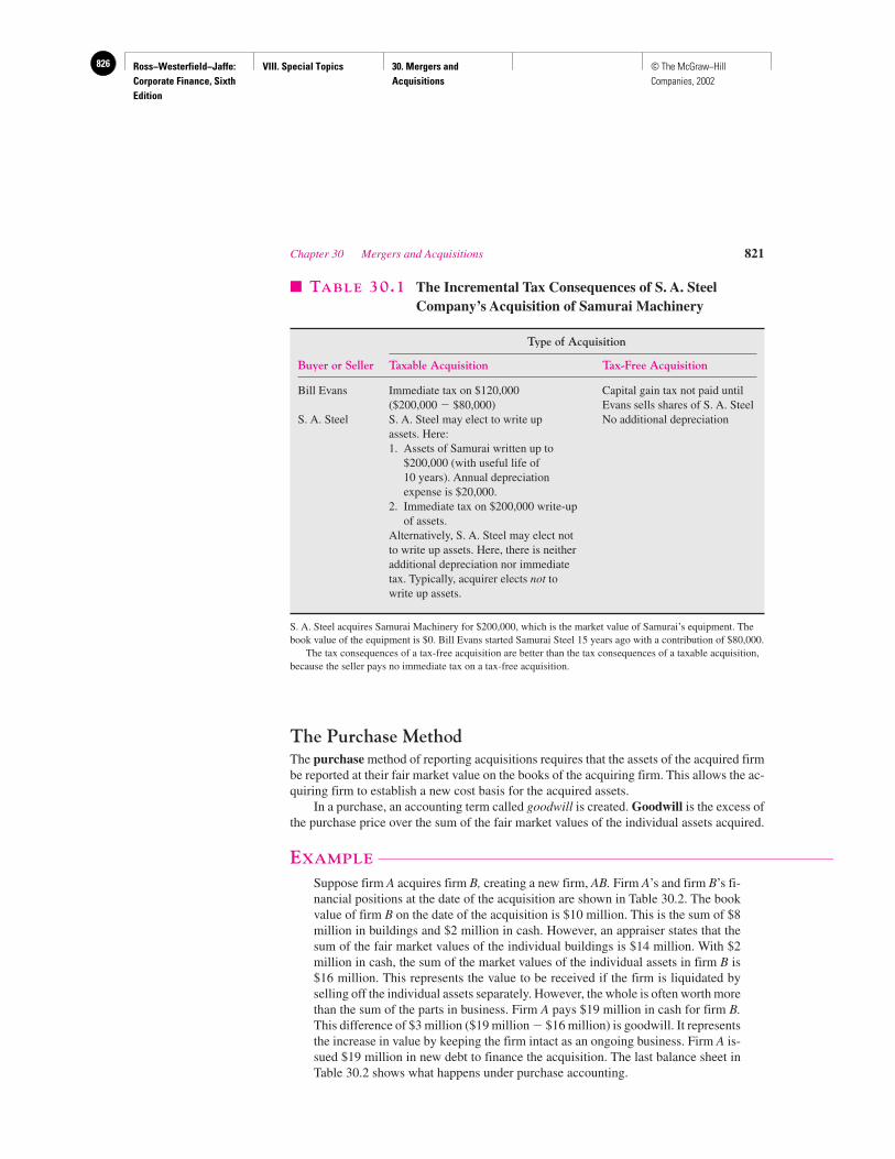
Ross−Westerfield−Jaffe: Corporate Finance, Sixth Edition
VIII. Special Topics 30. Mergers and Acquisitions
826 © The McGraw−Hill Companies, 2002
The Purchase MethodThe purchase method of reporting acquisitions requires that the assets of the acquired firmbe reported at their fair market value on the books of the acquiring firm. This allows the ac-quiring firm to establish a new cost basis for the acquired assets.
In a purchase, an accounting term called goodwill is created. Goodwill is the excess ofthe purchase price over the sum of the fair market values of the individual assets acquired.
EXAMPLE
Suppose firm A acquires firm B, creating a new firm, AB. Firm A’s and firm B’s fi-nancial positions at the date of the acquisition are shown in Table 30.2. The bookvalue of firm B on the date of the acquisition is $10 million. This is the sum of $8million in buildings and $2 million in cash. However, an appraiser states that thesum of the fair market values of the individual buildings is $14 million. With $2million in cash, the sum of the market values of the individual assets in firm B is$16 million. This represents the value to be received if the firm is liquidated byselling off the individual assets separately. However, the whole is often worth morethan the sum of the parts in business. Firm A pays $19 million in cash for firm B.This difference of $3 million ($19 million � $16 million) is goodwill. It representsthe increase in value by keeping the firm intact as an ongoing business. Firm A is-sued $19 million in new debt to finance the acquisition. The last balance sheet inTable 30.2 shows what happens under purchase accounting.
Chapter 30 Mergers and Acquisitions 821
� TABLE 30.1 The Incremental Tax Consequences of S. A. SteelCompany’s Acquisition of Samurai Machinery
Type of Acquisition
Buyer or Seller Taxable Acquisition Tax-Free Acquisition
Bill Evans Immediate tax on $120,000 Capital gain tax not paid until ($200,000 � $80,000) Evans sells shares of S. A. Steel
S. A. Steel S. A. Steel may elect to write up No additional depreciationassets. Here:1. Assets of Samurai written up to
$200,000 (with useful life of 10 years). Annual depreciation expense is $20,000.
2. Immediate tax on $200,000 write-up of assets.
Alternatively, S. A. Steel may elect not to write up assets. Here, there is neither additional depreciation nor immediate tax. Typically, acquirer elects not to write up assets.
S. A. Steel acquires Samurai Machinery for $200,000, which is the market value of Samurai’s equipment. Thebook value of the equipment is $0. Bill Evans started Samurai Steel 15 years ago with a contribution of $80,000.
The tax consequences of a tax-free acquisition are better than the tax consequences of a taxable acquisition,because the seller pays no immediate tax on a tax-free acquisition.
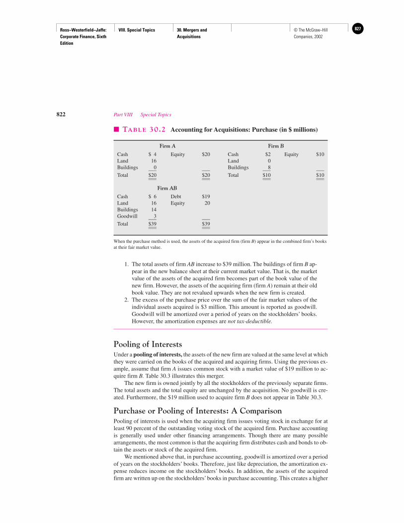
Ross−Westerfield−Jaffe: Corporate Finance, Sixth Edition
VIII. Special Topics 30. Mergers and Acquisitions
827© The McGraw−Hill Companies, 2002
1. The total assets of firm AB increase to $39 million. The buildings of firm B ap-pear in the new balance sheet at their current market value. That is, the marketvalue of the assets of the acquired firm becomes part of the book value of thenew firm. However, the assets of the acquiring firm (firm A) remain at their oldbook value. They are not revalued upwards when the new firm is created.
2. The excess of the purchase price over the sum of the fair market values of theindividual assets acquired is $3 million. This amount is reported as goodwill.Goodwill will be amortized over a period of years on the stockholders’ books.However, the amortization expenses are not tax-deductible.
Pooling of InterestsUnder a pooling of interests, the assets of the new firm are valued at the same level at whichthey were carried on the books of the acquired and acquiring firms. Using the previous ex-ample, assume that firm A issues common stock with a market value of $19 million to ac-quire firm B. Table 30.3 illustrates this merger.
The new firm is owned jointly by all the stockholders of the previously separate firms.The total assets and the total equity are unchanged by the acquisition. No goodwill is cre-ated. Furthermore, the $19 million used to acquire firm B does not appear in Table 30.3.
Purchase or Pooling of Interests: A ComparisonPooling of interests is used when the acquiring firm issues voting stock in exchange for atleast 90 percent of the outstanding voting stock of the acquired firm. Purchase accountingis generally used under other financing arrangements. Though there are many possiblearrangements, the most common is that the acquiring firm distributes cash and bonds to ob-tain the assets or stock of the acquired firm.
We mentioned above that, in purchase accounting, goodwill is amortized over a periodof years on the stockholders’ books. Therefore, just like depreciation, the amortization ex-pense reduces income on the stockholders’ books. In addition, the assets of the acquiredfirm are written up on the stockholders’ books in purchase accounting. This creates a higher
822 Part VIII Special Topics
� TABLE 30.2 Accounting for Acquisitions: Purchase (in $ millions)
Firm A Firm B
Cash $ 4 Equity $20 Cash $2 Equity $10Land 16 Land 0Buildings 0 Buildings 8___ ___ ___ ___Total $20 $20 Total $10 $10___ ___ ___ ______ ___ ___ ___
Firm AB
Cash $ 6 Debt $19Land 16 Equity 20Buildings 14Goodwill 3___ ___Total $39 $39___ ______ ___
When the purchase method is used, the assets of the acquired firm (firm B) appear in the combined firm’s booksat their fair market value.
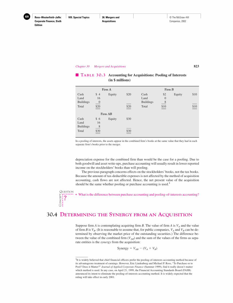
Ross−Westerfield−Jaffe: Corporate Finance, Sixth Edition
VIII. Special Topics 30. Mergers and Acquisitions
828 © The McGraw−Hill Companies, 2002
depreciation expense for the combined firm than would be the case for a pooling. Due toboth goodwill and asset write-ups, purchase accounting will usually result in lower reportedincome on the stockholders’ books than will pooling.
The previous paragraph concerns effects on the stockholders’ books, not the tax books.Because the amount of tax-deductible expenses is not affected by the method of acquisitionaccounting, cash flows are not affected. Hence, the net present value of the acquisitionshould be the same whether pooling or purchase accounting is used.4
• What is the difference between purchase accounting and pooling-of-interests accounting?
30.4 DETERMINING THE SYNERGY FROM AN ACQUISITION
Suppose firm A is contemplating acquiring firm B. The value of firm A is VA and the valueof firm B is VB. (It is reasonable to assume that, for public companies, VA and VB can be de-termined by observing the market price of the outstanding securities.) The difference be-tween the value of the combined firm (VAB) and the sum of the values of the firms as sepa-rate entities is the synergy from the acquisition:
Synergy � VAB � (VA � VB)
Chapter 30 Mergers and Acquisitions 823
� TABLE 30.3 Accounting for Acquisitions: Pooling of Interests (in $ millions)
Firm A Firm B
Cash $ 4 Equity $20 Cash $2 Equity $10Land 16 Land 0Buildings 0 Buildings 8___ ___ ___ ___Total $20 $20 Total $10 $10___ ___ ___ ______ ___ ___ ___
Firm AB
Cash $ 6 Equity $30Land 16Buildings 8___ ___Total $30 $30___ ______ ___
In a pooling of interests, the assets appear in the combined firm’s books at the same value that they had in eachseparate firm’s books prior to the merger.
4It is widely believed that chief financial officers prefer the pooling-of-interests accounting method because ofits advantageous treatment of earnings. However, Eric Lindenberg and Michael P. Ross, “To Purchase or toPool? Does it Matter?” Journal of Applied Corporate Finance (Summer 1999), find it really doesn’t matterwhich method is used. In any case, on April 21, 1999, the Financial Accounting Standards Board (FASB)announced its intent to eliminate the pooling-of-interests accounting method. It is widely expected that theruling will take effect in early 2001.
QUESTION
CO
NC
EP
T
?
Ross−Westerfield−Jaffe: Corporate Finance, Sixth Edition
VIII. Special Topics 30. Mergers and Acquisitions
829© The McGraw−Hill Companies, 2002
The acquiring firm must generally pay a premium for the acquired firm. For example,if stock of the target is selling for $50, the acquirer might need to pay $60 a share, imply-ing a premium of $10 or 20 percent. Firm A will want to determine the synergy before en-tering into negotiations with firm B on the premium.
The synergy of an acquisition can be determined from the usual discounted cash flowmodel:
Synergy �
where �CFt is the difference between the cash flows at date t of the combined firm and thesum of the cash flows of the two separate firms. In other words, �CFt is the incrementalcash flow at date t from the merger. The term, r, is the risk-adjusted discount rate appropri-ate for the incremental cash flows. This is generally considered to be the required rate of re-turn on the equity of the target.
From the chapters on capital budgeting we know that the incremental cash flows canbe separated into four parts:
�CFt � �Revt � �Costst � �Taxest � �Capital Requirementst
where �Revt is the incremental revenue of the acquisition, �Costst is the incremental costsof the acquisition, �Taxest is the incremental acquisition taxes, and �Capital Requirementst
is the incremental new investment required in working capital and fixed assets.
30.5 SOURCE OF SYNERGY FROM ACQUISITIONS
It follows from our classification of incremental cash flows that the possible sources of syn-ergy fall into four basic categories: revenue enhancement, cost reduction, lower taxes, andlower cost of capital.5
Revenue EnhancementOne important reason for acquisitions is that a combined firm may generate greater rev-enues than two separate firms. Increased revenues may come from marketing gains, strate-gic benefits, and market power.
Marketing Gains It is frequently claimed that mergers and acquisitions can produce greateroperating revenues from improved marketing. Improvements can be made in the following:
T
t�1
�CFt
�1 � r� t
824 Part VIII Special Topics
5Many reasons are given by firms to justify mergers and acquisitions. When two firms merge, the boards ofdirectors of the two firms adopt an agreement of merger. The agreement of merger of U.S. Steel and MarathonOil is typical. It lists the economic benefits that shareholders can expect from the merger (key words have beenitalicized):
U.S Steel believes that the acquisition of Marathon provides U.S. Steel with an attractive opportunity todiversify into the energy business. Reasons for the merger include, but are not limited to, the facts thatconsummation of the merger will allow U.S. Steel to consolidate Marathon into U.S. Steel’s federal incometax return, will also contribute to greater efficiency, and will enhance the ability to manage capital bypermitting the movement of cash between U.S. Steel and Marathon. Additionally, the merger will eliminatethe possibility of conflicts of interests between the interests of minority and majority shareholders and willenhance management flexibility. The acquisition will provide Marathon shareholders with a substantialpremium over historical market prices for their shares. However, shareholders will no longer continue toshare in the future prospects of the company.
Ross−Westerfield−Jaffe: Corporate Finance, Sixth Edition
VIII. Special Topics 30. Mergers and Acquisitions
830 © The McGraw−Hill Companies, 2002
1. Previously ineffective media programming and advertising efforts.
2. A weak existing distribution network.
3. An unbalanced product mix.
Strategic Benefits Some acquisitions promise a strategic advantage.6 This is an opportu-nity to take advantage of the competitive environment if certain situations materialize. In thisregard, a strategic benefit is more like an option than it is a standard investment opportunity.For example, imagine that a sewing machine company acquired a computer company. Thefirm will be well positioned if technological advances allow computer-driven sewing ma-chines in the future. Michael Porter has used the word beachhead in his description of theprocess of entering a new industry to exploit perceived opportunities.7 The beachhead is usedto spawn new opportunities based on intangible relationships. He uses the example of Proc-ter & Gamble’s initial acquisition of the Charmin Paper Company as a beachhead that al-lowed Procter & Gamble to develop a highly interrelated cluster of paper products—dispos-able diapers, paper towels, feminine hygiene products, and bathroom tissue.
Market or Monopoly Power One firm may acquire another to reduce competition. If so,prices can be increased and monopoly profits obtained. Mergers that reduce competition donot benefit society and may be challenged by the U.S. Department of Justice or the FederalTrade Commission.
The empirical evidence does not suggest that increased market power is a significantreason for mergers. If monopoly power is increased through an acquisition, all firms in theindustry should benefit as the price of the industry’s product is increased. However,Stillman’s and Eckbo’s examination of the share prices of firms that compete with themerger target when a merger announcement is made indicate that this is not the case.8 Theyfind no consistent tendency for the share prices of rivals to increase, and, thus, the Stillman-Eckbo data do not support the monopoly-power theory.
Cost ReductionOne of the most basic reasons for merger is that a combined firm may operate more effi-ciently than two separate firms. Thus, when Bank of America agreed to acquire SecurityPacific, lower costs were cited as the primary reason. A firm can obtain greater operatingefficiency in several different ways through a merger or an acquisition.
Economies of Scale If the average cost of production falls while the level of productionincreases, there is said to be an economy of scale. Figure 30.2 illustrates that economies ofscale result while the firm grows to its optimal size. After this point, diseconomies of scaleoccur. In other words, average cost increases with further firm growth.
Though the precise nature of economy of scale is not known, it is one obvious benefitof horizontal mergers. The phrase spreading overhead is frequently used in connection witheconomies of scale. This refers to the sharing of central facilities such as corporate head-quarters, top management, and a large mainframe computer.
Chapter 30 Mergers and Acquisitions 825
6For a discussion of the financial side of strategic planning, see S. C. Myers, “Finance Theory and FinanceStrategy,” Interfaces 14 (January–February 1984), p. 1.7M. Porter, Competitive Advantage (New York: Free Press, 1985).8R. Stillman, “Examining Antitrust Policy toward Horizontal Mergers,” Journal of Financial Economics 11(April 1983); and E. B. Eckbo, “Horizontal Mergers, Collusion and Stockholder Wealth,” Journal of FinancialEconomics 11 (April 1983).
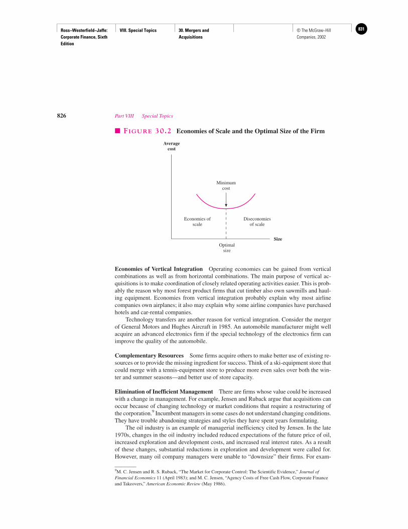
Ross−Westerfield−Jaffe: Corporate Finance, Sixth Edition
VIII. Special Topics 30. Mergers and Acquisitions
831© The McGraw−Hill Companies, 2002
Economies of Vertical Integration Operating economies can be gained from verticalcombinations as well as from horizontal combinations. The main purpose of vertical ac-quisitions is to make coordination of closely related operating activities easier. This is prob-ably the reason why most forest product firms that cut timber also own sawmills and haul-ing equipment. Economies from vertical integration probably explain why most airlinecompanies own airplanes; it also may explain why some airline companies have purchasedhotels and car-rental companies.
Technology transfers are another reason for vertical integration. Consider the mergerof General Motors and Hughes Aircraft in 1985. An automobile manufacturer might wellacquire an advanced electronics firm if the special technology of the electronics firm canimprove the quality of the automobile.
Complementary Resources Some firms acquire others to make better use of existing re-sources or to provide the missing ingredient for success. Think of a ski-equipment store thatcould merge with a tennis-equipment store to produce more even sales over both the win-ter and summer seasons—and better use of store capacity.
Elimination of Inefficient Management There are firms whose value could be increasedwith a change in management. For example, Jensen and Ruback argue that acquisitions canoccur because of changing technology or market conditions that require a restructuring ofthe corporation.9 Incumbent managers in some cases do not understand changing conditions.They have trouble abandoning strategies and styles they have spent years formulating.
The oil industry is an example of managerial inefficiency cited by Jensen. In the late1970s, changes in the oil industry included reduced expectations of the future price of oil,increased exploration and development costs, and increased real interest rates. As a resultof these changes, substantial reductions in exploration and development were called for.However, many oil company managers were unable to “downsize” their firms. For exam-
826 Part VIII Special Topics
Averagecost
Minimumcost
Economies ofscale
Diseconomiesof scale
Optimalsize
Size
� FIGURE 30.2 Economies of Scale and the Optimal Size of the Firm
9M. C. Jensen and R. S. Ruback, “The Market for Corporate Control: The Scientific Evidence,” Journal ofFinancial Economics 11 (April 1983); and M. C. Jensen, “Agency Costs of Free Cash Flow, Corporate Financeand Takeovers,” American Economic Review (May 1986).
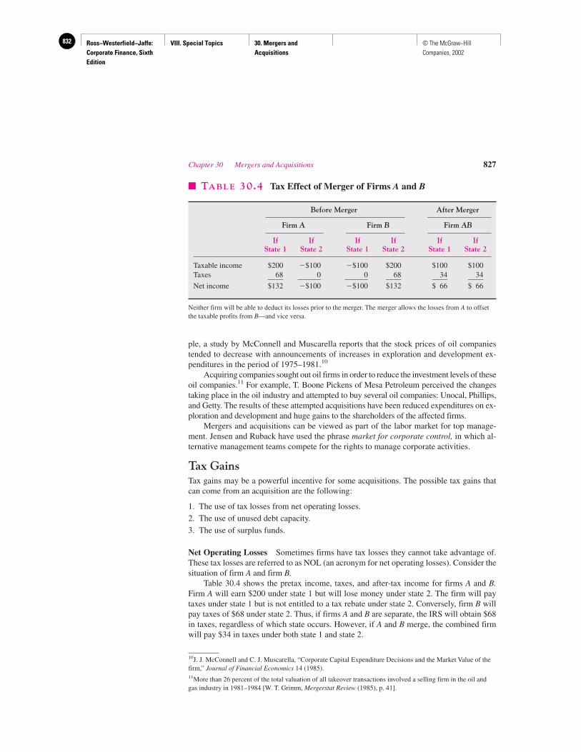
Ross−Westerfield−Jaffe: Corporate Finance, Sixth Edition
VIII. Special Topics 30. Mergers and Acquisitions
832 © The McGraw−Hill Companies, 2002
ple, a study by McConnell and Muscarella reports that the stock prices of oil companiestended to decrease with announcements of increases in exploration and development ex-penditures in the period of 1975–1981.10
Acquiring companies sought out oil firms in order to reduce the investment levels of theseoil companies.11 For example, T. Boone Pickens of Mesa Petroleum perceived the changestaking place in the oil industry and attempted to buy several oil companies: Unocal, Phillips,and Getty. The results of these attempted acquisitions have been reduced expenditures on ex-ploration and development and huge gains to the shareholders of the affected firms.
Mergers and acquisitions can be viewed as part of the labor market for top manage-ment. Jensen and Ruback have used the phrase market for corporate control, in which al-ternative management teams compete for the rights to manage corporate activities.
Tax GainsTax gains may be a powerful incentive for some acquisitions. The possible tax gains thatcan come from an acquisition are the following:
1. The use of tax losses from net operating losses.
2. The use of unused debt capacity.
3. The use of surplus funds.
Net Operating Losses Sometimes firms have tax losses they cannot take advantage of.These tax losses are referred to as NOL (an acronym for net operating losses). Consider thesituation of firm A and firm B.
Table 30.4 shows the pretax income, taxes, and after-tax income for firms A and B.Firm A will earn $200 under state 1 but will lose money under state 2. The firm will paytaxes under state 1 but is not entitled to a tax rebate under state 2. Conversely, firm B willpay taxes of $68 under state 2. Thus, if firms A and B are separate, the IRS will obtain $68in taxes, regardless of which state occurs. However, if A and B merge, the combined firmwill pay $34 in taxes under both state 1 and state 2.
Chapter 30 Mergers and Acquisitions 827
10J. J. McConnell and C. J. Muscarella, “Corporate Capital Expenditure Decisions and the Market Value of thefirm,” Journal of Financial Economics 14 (1985).11More than 26 percent of the total valuation of all takeover transactions involved a selling firm in the oil andgas industry in 1981–1984 [W. T. Grimm, Mergerstat Review (1985), p. 41].
� TABLE 30.4 Tax Effect of Merger of Firms A and B
Before Merger After Merger
Firm A Firm B Firm AB
If If If If If IfState 1 State 2 State 1 State 2 State 1 State 2
Taxable income $200 �$100 �$100 $200 $100 $100Taxes 68 0 0 68 34 34____ ______ ______ ____ ____ ____Net income $132 �$100 �$100 $132 $ 66 $ 66
Neither firm will be able to deduct its losses prior to the merger. The merger allows the losses from A to offsetthe taxable profits from B—and vice versa.
Ross−Westerfield−Jaffe: Corporate Finance, Sixth Edition
VIII. Special Topics 30. Mergers and Acquisitions
833© The McGraw−Hill Companies, 2002
It is obvious that if firms A and B merge, they will pay lower taxes than if they remainseparate. Without merger, they do not take advantage of potential tax losses.
The message of the preceding example is that firms need taxable profits to take ad-vantage of potential tax losses. Mergers can sometimes accomplish this. However, there aretwo qualifications to the previous example:
1. The federal tax laws permit firms that experience alternating periods of profits and lossesto equalize their taxes by carryback and carryforward provisions. A firm that has beenprofitable but has a loss in the current year can get refunds of income taxes paid in threeprevious years and can carry the loss forward for 15 years. Thus, a merger to exploit un-used tax shields must offer tax savings over and above what can be accomplished byfirms via carryovers.12
2. The IRS may disallow an acquisition if the principal purpose of the acquisition is toavoid federal tax. This is one of the Catch 22s of the Internal Revenue Code.
Unused Debt Capacity We argued earlier in the text that the optimal debt-equity ratio isthe one where the marginal tax benefit from additional debt is equal to the marginal increasein the financial distress costs from additional debt. Because some diversification occurswhen firms merge, the cost of financial distress is likely to be less for the combined firmthan is the sum of these present values for the two separate firms. Thus, the acquiring firmmight be able to increase its debt-equity ratio after a merger, creating additional tax bene-fits—and additional value.13,14
Surplus Funds Another quirk in the tax laws involves surplus funds. Consider a firm thathas free cash flow. That is, it has cash flow available after payment of all taxes and after all pos-itive net present value projects have been provided for. In this situation, aside from purchasingfixed-income securities, the firm has several ways to spend the free cash flow, including
1. Pay dividends.
2. Buy back its own shares.
3. Acquire shares in another firm.
We have already seen in our previous discussion of dividend policy that an extra divi-dend will increase the income tax paid by some investors. Investors pay lower taxes in ashare repurchase. However, this is not a legal option if the sole purpose is to avoid taxes thatwould otherwise have been paid by shareholders.
The firm can buy the shares of another firm. This accomplishes two objectives. First,the firm’s shareholders avoid taxes from dividends that would have been paid. Second, thefirm pays little corporate tax on dividends received from the shares of the firm it has pur-chased, because 70 percent of the dividend income received from the acquired firm is ex-cluded from the corporate income tax. However, under Section 532 of the tax code the IRSmight disallow the tax benefits from a continual strategy of this type.
828 Part VIII Special Topics
12Under the 1986 Tax Reform Act a corporation’s ability to carry forward net operating losses (and other taxcredits) is limited when more than 50 percent of the stock changes hands over a three-year period.13Unused debt capacity is cited as a benefit in many mergers. An example was the proposed merger of HospitalCorporation of America and American Hospital Supply Corporation in 1985. Insiders were quoted as sayingthat the combined companies could borrow as much as an additional $1 billion, 10 times the usual borrowingcapacity of Hospital Corporation alone (The Wall Street Journal, April 1, 1985). (The merger never took place.)14Michael C. Jensen [“Agency Costs of Free Cash Flow, Corporate Finance and Takeovers,” American EconomicReview (May 1986)] offers another reason why debt is frequently used in mergers and acquisitions. He arguesthat using more debt provides incentives for the new management to create efficiencies so that debt can be repaid.
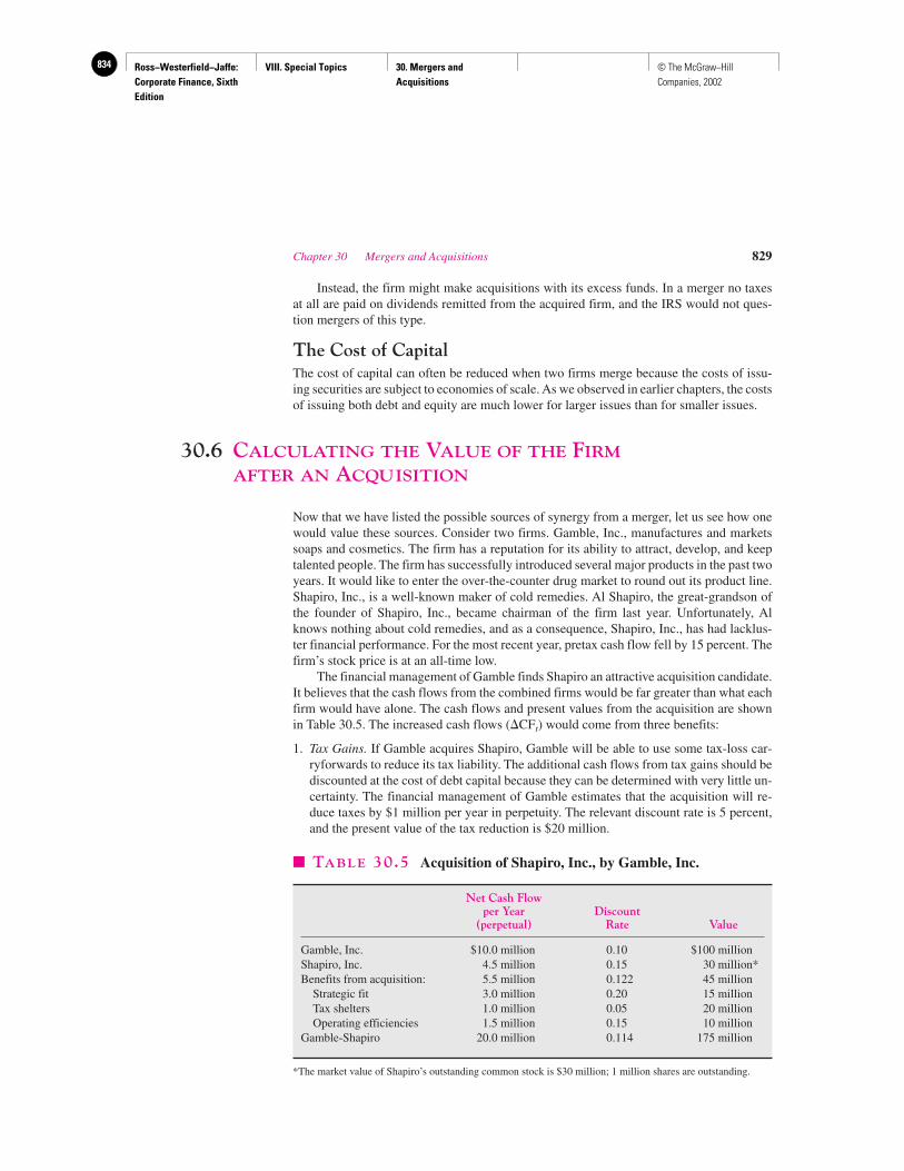
Ross−Westerfield−Jaffe: Corporate Finance, Sixth Edition
VIII. Special Topics 30. Mergers and Acquisitions
834 © The McGraw−Hill Companies, 2002
Instead, the firm might make acquisitions with its excess funds. In a merger no taxesat all are paid on dividends remitted from the acquired firm, and the IRS would not ques-tion mergers of this type.
The Cost of CapitalThe cost of capital can often be reduced when two firms merge because the costs of issu-ing securities are subject to economies of scale. As we observed in earlier chapters, the costsof issuing both debt and equity are much lower for larger issues than for smaller issues.
30.6 CALCULATING THE VALUE OF THE FIRM
AFTER AN ACQUISITION
Now that we have listed the possible sources of synergy from a merger, let us see how onewould value these sources. Consider two firms. Gamble, Inc., manufactures and marketssoaps and cosmetics. The firm has a reputation for its ability to attract, develop, and keeptalented people. The firm has successfully introduced several major products in the past twoyears. It would like to enter the over-the-counter drug market to round out its product line.Shapiro, Inc., is a well-known maker of cold remedies. Al Shapiro, the great-grandson ofthe founder of Shapiro, Inc., became chairman of the firm last year. Unfortunately, Alknows nothing about cold remedies, and as a consequence, Shapiro, Inc., has had lacklus-ter financial performance. For the most recent year, pretax cash flow fell by 15 percent. Thefirm’s stock price is at an all-time low.
The financial management of Gamble finds Shapiro an attractive acquisition candidate.It believes that the cash flows from the combined firms would be far greater than what eachfirm would have alone. The cash flows and present values from the acquisition are shownin Table 30.5. The increased cash flows (�CFt) would come from three benefits:
1. Tax Gains. If Gamble acquires Shapiro, Gamble will be able to use some tax-loss car-ryforwards to reduce its tax liability. The additional cash flows from tax gains should bediscounted at the cost of debt capital because they can be determined with very little un-certainty. The financial management of Gamble estimates that the acquisition will re-duce taxes by $1 million per year in perpetuity. The relevant discount rate is 5 percent,and the present value of the tax reduction is $20 million.
Chapter 30 Mergers and Acquisitions 829
� TABLE 30.5 Acquisition of Shapiro, Inc., by Gamble, Inc.
Net Cash Flowper Year Discount
(perpetual) Rate Value
Gamble, Inc. $10.0 million 0.10 $100 millionShapiro, Inc. 4.5 million 0.15 30 million*Benefits from acquisition: 5.5 million 0.122 45 million
Strategic fit 3.0 million 0.20 15 millionTax shelters 1.0 million 0.05 20 millionOperating efficiencies 1.5 million 0.15 10 million
Gamble-Shapiro 20.0 million 0.114 175 million
*The market value of Shapiro’s outstanding common stock is $30 million; 1 million shares are outstanding.
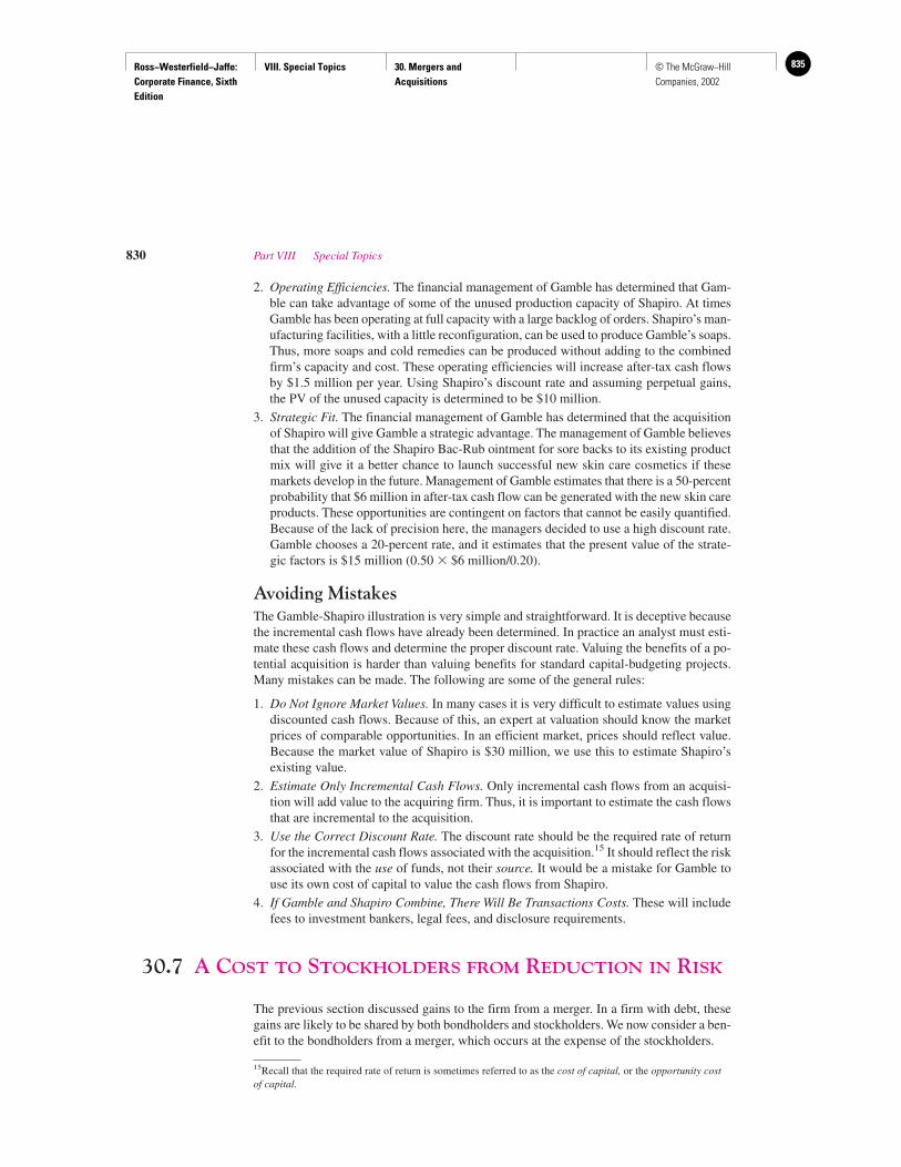
Ross−Westerfield−Jaffe: Corporate Finance, Sixth Edition
VIII. Special Topics 30. Mergers and Acquisitions
835© The McGraw−Hill Companies, 2002
2. Operating Efficiencies. The financial management of Gamble has determined that Gam-ble can take advantage of some of the unused production capacity of Shapiro. At timesGamble has been operating at full capacity with a large backlog of orders. Shapiro’s man-ufacturing facilities, with a little reconfiguration, can be used to produce Gamble’s soaps.Thus, more soaps and cold remedies can be produced without adding to the combinedfirm’s capacity and cost. These operating efficiencies will increase after-tax cash flowsby $1.5 million per year. Using Shapiro’s discount rate and assuming perpetual gains,the PV of the unused capacity is determined to be $10 million.
3. Strategic Fit. The financial management of Gamble has determined that the acquisitionof Shapiro will give Gamble a strategic advantage. The management of Gamble believesthat the addition of the Shapiro Bac-Rub ointment for sore backs to its existing productmix will give it a better chance to launch successful new skin care cosmetics if thesemarkets develop in the future. Management of Gamble estimates that there is a 50-percentprobability that $6 million in after-tax cash flow can be generated with the new skin careproducts. These opportunities are contingent on factors that cannot be easily quantified.Because of the lack of precision here, the managers decided to use a high discount rate.Gamble chooses a 20-percent rate, and it estimates that the present value of the strate-gic factors is $15 million (0.50 � $6 million/0.20).
Avoiding MistakesThe Gamble-Shapiro illustration is very simple and straightforward. It is deceptive becausethe incremental cash flows have already been determined. In practice an analyst must esti-mate these cash flows and determine the proper discount rate. Valuing the benefits of a po-tential acquisition is harder than valuing benefits for standard capital-budgeting projects.Many mistakes can be made. The following are some of the general rules:
1. Do Not Ignore Market Values. In many cases it is very difficult to estimate values usingdiscounted cash flows. Because of this, an expert at valuation should know the marketprices of comparable opportunities. In an efficient market, prices should reflect value.Because the market value of Shapiro is $30 million, we use this to estimate Shapiro’sexisting value.
2. Estimate Only Incremental Cash Flows. Only incremental cash flows from an acquisi-tion will add value to the acquiring firm. Thus, it is important to estimate the cash flowsthat are incremental to the acquisition.
3. Use the Correct Discount Rate. The discount rate should be the required rate of returnfor the incremental cash flows associated with the acquisition.15 It should reflect the riskassociated with the use of funds, not their source. It would be a mistake for Gamble touse its own cost of capital to value the cash flows from Shapiro.
4. If Gamble and Shapiro Combine, There Will Be Transactions Costs. These will includefees to investment bankers, legal fees, and disclosure requirements.
30.7 A COST TO STOCKHOLDERS FROM REDUCTION IN RISK
The previous section discussed gains to the firm from a merger. In a firm with debt, thesegains are likely to be shared by both bondholders and stockholders. We now consider a ben-efit to the bondholders from a merger, which occurs at the expense of the stockholders.
830 Part VIII Special Topics
15Recall that the required rate of return is sometimes referred to as the cost of capital, or the opportunity costof capital.
Ross−Westerfield−Jaffe: Corporate Finance, Sixth Edition
VIII. Special Topics 30. Mergers and Acquisitions
836 © The McGraw−Hill Companies, 2002
When two firms merge, the variability of their combined values is usually less thanwould be true if the firms remained separate entities. A reduction of the variability of firmvalues can occur if the values of the two firms are less than perfectly correlated. The re-duction in variability can reduce the cost of borrowing and make the creditors better off thanbefore. This will occur if the probability of financial distress is reduced by the merger.
Unfortunately, the shareholders are likely to be worse off. The gains to creditors are atthe expense of the shareholders if the total value of the firm does not change. The relation-ship among the value of the merged firm, debt capacity, and risk is very complicated. Wenow consider two examples.
The Base CaseConsider a base case where two all-equity firms merge. Table 30.6 gives the net present val-ues of firm A and firm B in three possible states of the economy—prosperity, average, anddepression. The market value of firm A is $60, and the market value of firm B is $40. Themarket value of each firm is the weighted average of the values in each of the three states.For example, the value of firm A is
$60 � $80 � 0.5 � $50 � 0.3 � $25 � 0.2
The values in each of the three states for firm A are $80, $50, and $25, respectively. Theprobabilities of each of the three states occurring are 0.5, 0.3, and 0.2, respectively.
Chapter 30 Mergers and Acquisitions 831
IN THEIR OWN WORDS
Michael C. Jensen on Mergers and Acquisitions
Economic analysis and evidence indicate thattakeovers, LBOs, and corporate restructurings are
playing an important role in helping the economy adjustto major competitive changes in the last two decades.The competition among alternative management teamsand organizational structures for control of corporateassets has enabled vast economic resources to movemore quickly to their highest-valued use. In the process,substantial benefits for the economy as a whole as wellas for shareholders have been created. Overall gains toselling-firm shareholders from mergers, acquisitions,leveraged buyouts, and other corporate restructurings inthe 12-year period 1977–1988 total over $500 billion in1988 dollars. I estimate gains to buying-firm share-holders to be at least $50 billion for the same period.These gains equal 53 percent of the total cash dividends(valued in 1988 dollars) paid to investors by the entirecorporate sector in the same period.
Mergers and acquisitions are a response to new tech-nologies or market conditions which require a strategicchange in a company’s direction or use of resources.Compared to current management, a new owner is often
better able to accomplish major change in the existingorganizational structure. Alternatively, leveraged buyoutsbring about organizational change by creating entrepre-neurial incentives for management and by eliminatingthe centralized bureaucratic obstacles to maneuverabilitythat are inherent in large public corporations.
When managers have a substantial ownership interestin the organization, the conflicts of interest betweenshareholders and managers over the payout of thecompany’s free cash flow are reduced. Management’sincentives are focused on maximizing the value of theenterprise, rather than building empires—often throughpoorly conceived diversification acquisitions—withoutregard to shareholder value. Finally, the requiredrepayment of debt replaces management’s discretion inpaying dividends and the tendency to overretain cash.Substantial increases in efficiency are thereby created.
Michael C. Jensen is Edsel Bryant Ford Professor of BusinessAdministration at Harvard University. An outstanding scholarand researcher, he is famous for his path-breaking analysis ofthe modern corporation and its relations with its stockholders.
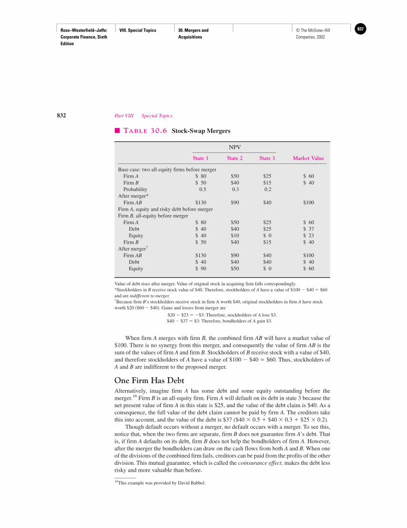
Ross−Westerfield−Jaffe: Corporate Finance, Sixth Edition
VIII. Special Topics 30. Mergers and Acquisitions
837© The McGraw−Hill Companies, 2002
When firm A merges with firm B, the combined firm AB will have a market value of$100. There is no synergy from this merger, and consequently the value of firm AB is thesum of the values of firm A and firm B. Stockholders of B receive stock with a value of $40,and therefore stockholders of A have a value of $100 � $40 � $60. Thus, stockholders ofA and B are indifferent to the proposed merger.
One Firm Has DebtAlternatively, imagine firm A has some debt and some equity outstanding before themerger.16 Firm B is an all-equity firm. Firm A will default on its debt in state 3 because thenet present value of firm A in this state is $25, and the value of the debt claim is $40. As aconsequence, the full value of the debt claim cannot be paid by firm A. The creditors takethis into account, and the value of the debt is $37 ($40 � 0.5 � $40 � 0.3 � $25 � 0.2).
Though default occurs without a merger, no default occurs with a merger. To see this,notice that, when the two firms are separate, firm B does not guarantee firm A’s debt. Thatis, if firm A defaults on its debt, firm B does not help the bondholders of firm A. However,after the merger the bondholders can draw on the cash flows from both A and B. When oneof the divisions of the combined firm fails, creditors can be paid from the profits of the otherdivision. This mutual guarantee, which is called the coinsurance effect, makes the debt lessrisky and more valuable than before.
832 Part VIII Special Topics
� TABLE 30.6 Stock-Swap Mergers
NPV
State 1 State 2 State 3 Market Value
Base case: two all-equity firms before mergerFirm A $ 80 $50 $25 $ 60Firm B $ 50 $40 $15 $ 40Probability 0.5 0.3 0.2
After merger*Firm AB $130 $90 $40 $100
Firm A, equity and risky debt before mergerFirm B, all-equity before merger
Firm A $ 80 $50 $25 $ 60Debt $ 40 $40 $25 $ 37Equity $ 40 $10 $ 0 $ 23
Firm B $ 50 $40 $15 $ 40After merger†
Firm AB $130 $90 $40 $100Debt $ 40 $40 $40 $ 40Equity $ 90 $50 $ 0 $ 60
Value of debt rises after merger. Value of original stock in acquiring firm falls correspondingly.*Stockholders in B receive stock value of $40. Therefore, stockholders of A have a value of $100 � $40 � $60and are indifferent to merger.†Because firm B’s stockholders receive stock in firm A worth $40, original stockholders in firm A have stockworth $20 ($60 � $40). Gains and losses from merger are
$20 � $23 � �$3: Therefore, stockholders of A lose $3.$40 � $37 � $3: Therefore, bondholders of A gain $3.
16This example was provided by David Babbel.
Ross−Westerfield−Jaffe: Corporate Finance, Sixth Edition
VIII. Special Topics 30. Mergers and Acquisitions
838 © The McGraw−Hill Companies, 2002
The bonds are worth $40 after the merger. Thus, the bondholders of AB gain $3($40 � $37) from the merger.
The stockholders of firm A lose $3 ($20 � $23) from the merger. That is, firm A’sstock is worth $23 prior to the merger. The stock is worth $60 after the merger. However,stockholders in firm B receive $40 of stock in firm A. Hence, those individuals who werestockholders in firm A prior to the merger have stock worth only $20 ($60 � $40) afterthe merger.
There is no net benefit to the firm as a whole. The bondholders gain the coinsuranceeffect, and the stockholders lose the coinsurance effect. Some general conclusions emergefrom the preceding analysis.
1. Bondholders in the aggregate will usually be helped by mergers and acquisitions. Thesize of the gain to bondholders depends on the reduction of bankruptcy states after thecombination. That is, the less risky the combined firm is, the greater are the gains tobondholders.
2. Stockholders of the acquiring firm will be hurt by the amount that bondholders gain.
3. The conclusions apply to mergers and acquisitions where no synergy is present. In thecase of synergistic combinations, much depends on the size of the synergy.
How Can Shareholders Reduce Their Losses from the Coinsurance Effect?The coinsurance effect allows some mergers to increase bondholder values by reducingshareholder values. However, there are at least two ways that shareholders can reduce oreliminate the coinsurance effect. First, the shareholders in firm A could retire its debt be-fore the merger announcement date and reissue an equal amount of debt after the merger.Because debt is retired at the low, pre-merger price, this type of refinancing transaction canneutralize the coinsurance effect to the bondholders.
Also, note that the debt capacity of the combined firm is likely to increase because theacquisition reduces the probability of financial distress. Thus, the shareholders’ second al-ternative is simply to issue more debt after the merger. An increase in debt following themerger will have two effects, even without the prior action of debt retirement. The interestdeduction from new corporate debt raises firm value. In addition, an increase in debt afterthe merger raises the probability of financial distress, thereby reducing or eliminating thebondholders’ gain from the coinsurance effect.
30.8 TWO “BAD” REASONS FOR MERGERS
Earnings GrowthAn acquisition can create the appearance of earnings growth, which may fool investorsinto thinking that the firm is worth more than it really is. Suppose Global Resources,Ltd., acquires Regional Enterprises. The financial positions of Global and Regional be-fore the acquisition are shown in Table 30.7. Regional has had very poor earnings growthand sells at a price-earnings ratio much lower than that of Global. The merger creates noadditional value. If the market is smart, it will realize that the combined firm is worththe sum of the values of the separate firms. In this case, the market value of the com-bined firm will be $3,500, which is equal to the sum of the values of the separate firmsbefore the merger.
Chapter 30 Mergers and Acquisitions 833
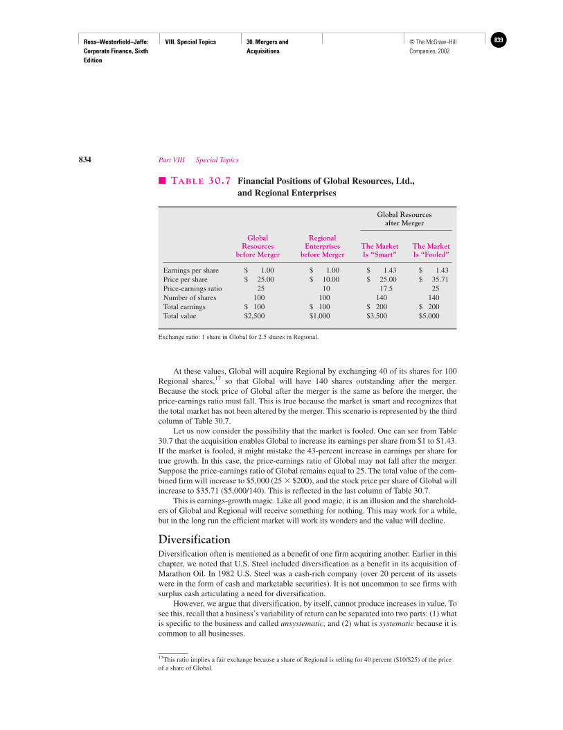
Ross−Westerfield−Jaffe: Corporate Finance, Sixth Edition
VIII. Special Topics 30. Mergers and Acquisitions
839© The McGraw−Hill Companies, 2002
At these values, Global will acquire Regional by exchanging 40 of its shares for 100Regional shares,17 so that Global will have 140 shares outstanding after the merger.Because the stock price of Global after the merger is the same as before the merger, theprice-earnings ratio must fall. This is true because the market is smart and recognizes thatthe total market has not been altered by the merger. This scenario is represented by the thirdcolumn of Table 30.7.
Let us now consider the possibility that the market is fooled. One can see from Table30.7 that the acquisition enables Global to increase its earnings per share from $1 to $1.43.If the market is fooled, it might mistake the 43-percent increase in earnings per share fortrue growth. In this case, the price-earnings ratio of Global may not fall after the merger.Suppose the price-earnings ratio of Global remains equal to 25. The total value of the com-bined firm will increase to $5,000 (25 � $200), and the stock price per share of Global willincrease to $35.71 ($5,000/140). This is reflected in the last column of Table 30.7.
This is earnings-growth magic. Like all good magic, it is an illusion and the sharehold-ers of Global and Regional will receive something for nothing. This may work for a while,but in the long run the efficient market will work its wonders and the value will decline.
DiversificationDiversification often is mentioned as a benefit of one firm acquiring another. Earlier in thischapter, we noted that U.S. Steel included diversification as a benefit in its acquisition ofMarathon Oil. In 1982 U.S. Steel was a cash-rich company (over 20 percent of its assetswere in the form of cash and marketable securities). It is not uncommon to see firms withsurplus cash articulating a need for diversification.
However, we argue that diversification, by itself, cannot produce increases in value. Tosee this, recall that a business’s variability of return can be separated into two parts: (1) whatis specific to the business and called unsystematic, and (2) what is systematic because it iscommon to all businesses.
834 Part VIII Special Topics
� TABLE 30.7 Financial Positions of Global Resources, Ltd.,and Regional Enterprises
Global Resourcesafter Merger
Global RegionalResources Enterprises The Market The Market
before Merger before Merger Is “Smart” Is “Fooled”
Earnings per share $ 1.00 $ 1.00 $ 1.43 $ 1.43Price per share $ 25.00 $ 10.00 $ 25.00 $ 35.71Price-earnings ratio 25 10 17.5 25Number of shares 100 100 140 140Total earnings $ 100 $ 100 $ 200 $ 200Total value $2,500 $1,000 $3,500 $5,000
Exchange ratio: 1 share in Global for 2.5 shares in Regional.
17This ratio implies a fair exchange because a share of Regional is selling for 40 percent ($10/$25) of the priceof a share of Global.
Ross−Westerfield−Jaffe: Corporate Finance, Sixth Edition
VIII. Special Topics 30. Mergers and Acquisitions
840 © The McGraw−Hill Companies, 2002
Systematic variability cannot be eliminated by diversification, so mergers will noteliminate this risk at all. By contrast, unsystematic risk can be diversified away throughmergers. However, the investor does not need widely diversified companies such as GeneralElectric to eliminate unsystematic risk. Shareholders can diversify more easily than corpo-rations by simply purchasing common stock in different corporations. For example, theshareholders of U.S. Steel could have purchased shares in Marathon if they believed therewould be diversification gains in doing so. Thus, diversification through conglomeratemerger may not benefit shareholders.18
Diversification can produce gains to the acquiring firm only if two things are true:
1. Diversification decreases the unsystematic variability at lower costs than by investorsvia adjustments to personal portfolios. This seems very unlikely.
2. Diversification reduces risk and thereby increases debt capacity. This possibility wasmentioned earlier in the chapter.
• Why can a merger create the appearance of earnings growth?
30.9 THE NPV OF A MERGER
Firms typically use NPV analysis when making acquisitions.19 The analysis is relativelystraightforward when the consideration is cash. The analysis becomes more complex whenthe consideration is stock.
CashSuppose firm A and firm B have values as separate entities of $500 and $100, respectively.They are both all-equity firms. If firm A acquires firm B, the merged firm AB will have acombined value of $700 due to synergies of $100. The board of firm B has indicated that itwill sell firm B if it is offered $150 in cash.
Chapter 30 Mergers and Acquisitions 835
18Recent evidence suggests that diversification can actually hurt shareholders. Randall Mork, Andrei Shleifer,and Robert W. Vishney [“Do Managerial Objectives Drive Bad Acquisitions,” Journal of Finance 45 (1990),pp. 31–48] show that shareholders did poorly in firms that diversified by acquisition in the 1980s. There is alsoevidence that diversified firms trade at a discount relative to a portfolio of single-segment firms, most recentlyfrom Karl Lins and Henri Servaes, “The International Evidence on the Value of Corporate Diversification,”Journal of Finance 54 (1999). On the other hand, Matsusaka and Hubbard and Palia find some benefits todiversification in internal capital allocation. See John Matsusaka, “Takeover Motives During the ConglomerateMerge Wave,” Rand Journal of Economics 24 (1993).
See also R. Glenn Hubbard and Darius Palia, “A Reexamination of the Conglomerate Merger Wave in the1960s: An Internal Capital Markets View,” Journal of Finance (June 1999).
One interesting recent study reports a positive relationship between focus and value for diversified firms.See P. G. Berger and E. Ofek, “Diversification’s Effect on Firm Value,” Journal of Financial Economics, 37(1995). Also see P. G. Berger and E. Ofek, “Causes and Effects of Corporate Refocusing Program,” Review ofFinancial Studies 12 (1999).19The NPV framework for evaluating mergers can be found in S. C. Myers, “A Framework for EvaluatingMergers,” in Modern Developments in Financial Management, ed. by S. C. Myers (New York: Praeger, 1976).
QUESTION
CO
NC
EP
T
?
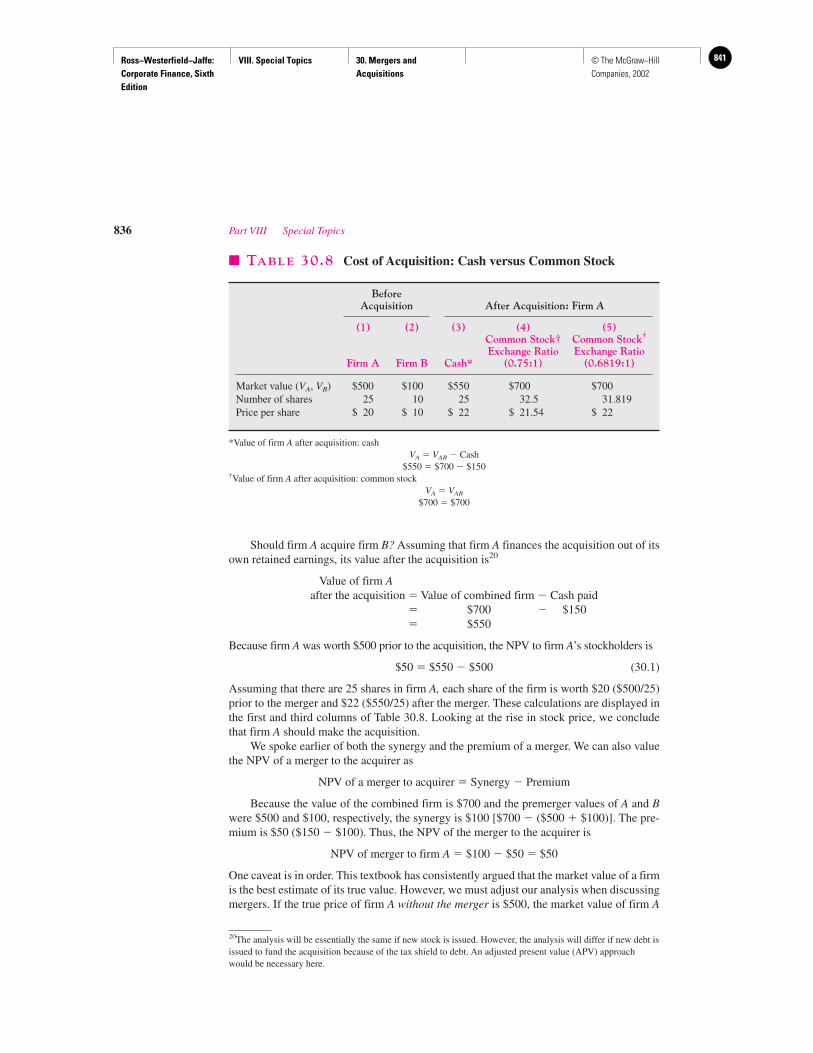
Ross−Westerfield−Jaffe: Corporate Finance, Sixth Edition
VIII. Special Topics 30. Mergers and Acquisitions
841© The McGraw−Hill Companies, 2002
Should firm A acquire firm B? Assuming that firm A finances the acquisition out of itsown retained earnings, its value after the acquisition is20
Value of firm Aafter the acquisition � Value of combined firm � Cash paid
� $700 � $150� $550
Because firm A was worth $500 prior to the acquisition, the NPV to firm A’s stockholders is
$50 � $550 � $500 (30.1)
Assuming that there are 25 shares in firm A, each share of the firm is worth $20 ($500/25)prior to the merger and $22 ($550/25) after the merger. These calculations are displayed inthe first and third columns of Table 30.8. Looking at the rise in stock price, we concludethat firm A should make the acquisition.
We spoke earlier of both the synergy and the premium of a merger. We can also valuethe NPV of a merger to the acquirer as
NPV of a merger to acquirer � Synergy � Premium
Because the value of the combined firm is $700 and the premerger values of A and Bwere $500 and $100, respectively, the synergy is $100 [$700 � ($500 � $100)]. The pre-mium is $50 ($150 � $100). Thus, the NPV of the merger to the acquirer is
NPV of merger to firm A � $100 � $50 � $50
One caveat is in order. This textbook has consistently argued that the market value of a firmis the best estimate of its true value. However, we must adjust our analysis when discussingmergers. If the true price of firm A without the merger is $500, the market value of firm A
836 Part VIII Special Topics
20The analysis will be essentially the same if new stock is issued. However, the analysis will differ if new debt isissued to fund the acquisition because of the tax shield to debt. An adjusted present value (APV) approachwould be necessary here.
� TABLE 30.8 Cost of Acquisition: Cash versus Common Stock
BeforeAcquisition After Acquisition: Firm A
(1) (2) (3) (4) (5)Common Stock† Common Stock†
Exchange Ratio Exchange RatioFirm A Firm B Cash* (0.75:1) (0.6819:1)
Market value (VA, VB) $500 $100 $550 $700 $700Number of shares 25 10 25 32.5 31.819Price per share $ 20 $ 10 $ 22 $ 21.54 $ 22
*Value of firm A after acquisition: cashVA � VAB � Cash
$550 � $700 � $150†Value of firm A after acquisition: common stock
VA � VAB
$700 � $700
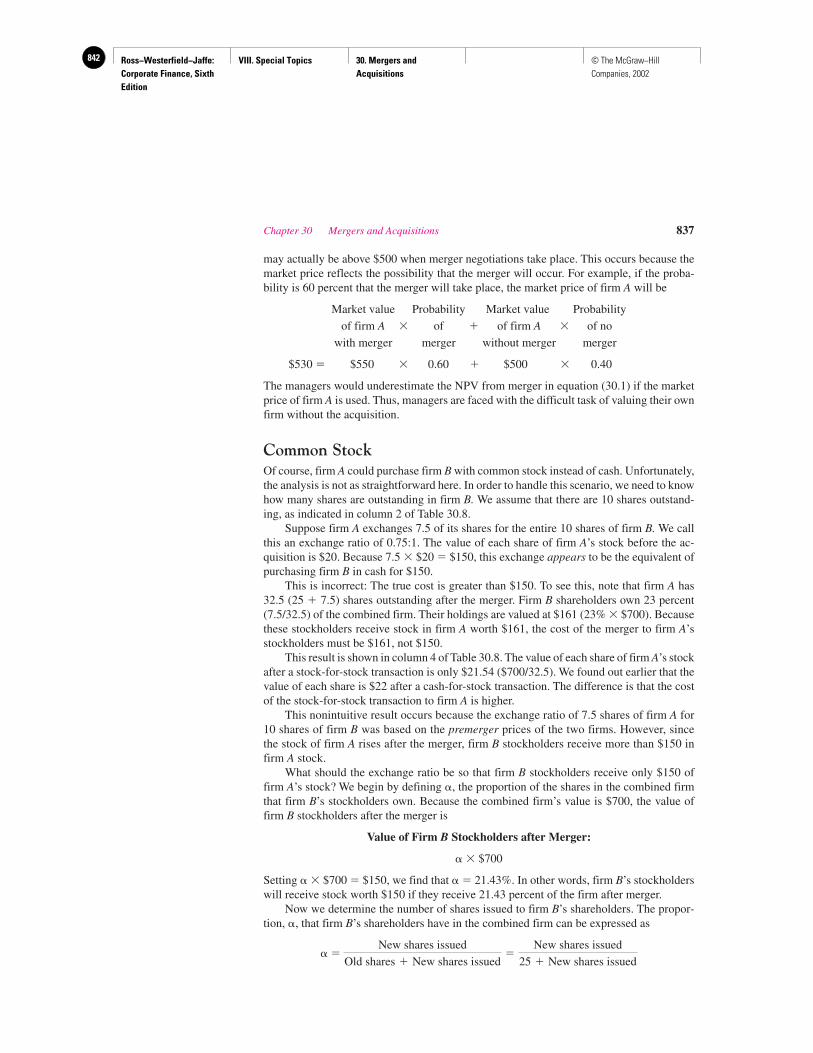
Ross−Westerfield−Jaffe: Corporate Finance, Sixth Edition
VIII. Special Topics 30. Mergers and Acquisitions
842 © The McGraw−Hill Companies, 2002
may actually be above $500 when merger negotiations take place. This occurs because themarket price reflects the possibility that the merger will occur. For example, if the proba-bility is 60 percent that the merger will take place, the market price of firm A will be
$530 � $550 � 0.60 � $500 � 0.40
The managers would underestimate the NPV from merger in equation (30.1) if the marketprice of firm A is used. Thus, managers are faced with the difficult task of valuing their ownfirm without the acquisition.
Common StockOf course, firm A could purchase firm B with common stock instead of cash. Unfortunately,the analysis is not as straightforward here. In order to handle this scenario, we need to knowhow many shares are outstanding in firm B. We assume that there are 10 shares outstand-ing, as indicated in column 2 of Table 30.8.
Suppose firm A exchanges 7.5 of its shares for the entire 10 shares of firm B. We callthis an exchange ratio of 0.75:1. The value of each share of firm A’s stock before the ac-quisition is $20. Because 7.5 � $20 � $150, this exchange appears to be the equivalent ofpurchasing firm B in cash for $150.
This is incorrect: The true cost is greater than $150. To see this, note that firm A has32.5 (25 � 7.5) shares outstanding after the merger. Firm B shareholders own 23 percent(7.5/32.5) of the combined firm. Their holdings are valued at $161 (23% � $700). Becausethese stockholders receive stock in firm A worth $161, the cost of the merger to firm A’sstockholders must be $161, not $150.
This result is shown in column 4 of Table 30.8. The value of each share of firm A’s stockafter a stock-for-stock transaction is only $21.54 ($700/32.5). We found out earlier that thevalue of each share is $22 after a cash-for-stock transaction. The difference is that the costof the stock-for-stock transaction to firm A is higher.
This nonintuitive result occurs because the exchange ratio of 7.5 shares of firm A for10 shares of firm B was based on the premerger prices of the two firms. However, sincethe stock of firm A rises after the merger, firm B stockholders receive more than $150 infirm A stock.
What should the exchange ratio be so that firm B stockholders receive only $150 offirm A’s stock? We begin by defining �, the proportion of the shares in the combined firmthat firm B’s stockholders own. Because the combined firm’s value is $700, the value offirm B stockholders after the merger is
Value of Firm B Stockholders after Merger:
� � $700
Setting � � $700 � $150, we find that � � 21.43%. In other words, firm B’s stockholderswill receive stock worth $150 if they receive 21.43 percent of the firm after merger.
Now we determine the number of shares issued to firm B’s shareholders. The propor-tion, �, that firm B’s shareholders have in the combined firm can be expressed as
� �New shares issued
Old shares � New shares issued�
New shares issued
25 � New shares issued
Market value
of firm A
with merger
�
Probability
of
merger
�
Market value
of firm A
without merger
�
Probability
of no
merger
Chapter 30 Mergers and Acquisitions 837
Ross−Westerfield−Jaffe: Corporate Finance, Sixth Edition
VIII. Special Topics 30. Mergers and Acquisitions
843© The McGraw−Hill Companies, 2002
Plugging our value of � into the equation yields
0.2143 �
Solving for the unknown, we have
New shares � 6.819 shares
Total shares outstanding after the merger are 31.819 (25 � 6.819). Because 6.819 shares offirm A are exchanged for 10 shares of firm B, the exchange ratio is 0.6819:1.
Results at the exchange ratio of 0.6819:1 are displayed in column 5 of Table 30.8. Eachshare of common stock is worth $22, exactly what it is worth in the stock-for-cash transac-tion. Thus, given that the board of firm B will sell its firm for $150, this is the fair exchangeratio, not the ratio of 0.75:1 mentioned earlier.
Cash versus Common StockWhether to finance an acquisition by cash or by shares of stock is an important decision.The choice depends on several factors, as follows:
1. Overvaluation. If in the opinion of management the acquiring firm’s stock is overval-ued, using shares of stock can be less costly than using cash.
2. Taxes. Acquisition by cash usually results in a taxable transaction. Acquisition by ex-changing stock is tax free.
3. Sharing Gains. If cash is used to finance an acquisition, the selling firm’s shareholdersreceive a fixed price. In the event of a hugely successful merger, they will not participatein any additional gains. Of course, if the acquisition is not a success, the losses will notbe shared and shareholders of the acquiring firm will be worse off than if stock were used.
• In an efficient market with no tax effects, should an acquiring firm use cash or stock?
30.10 DEFENSIVE TACTICS
Target-firm managers frequently resist takeover attempts. Resistance usually starts withpress releases and mailings to shareholders that present management’s viewpoint. It caneventually lead to legal action and solicitation of competing bids. Managerial action to de-feat a takeover attempt may make target shareholders better off if it elicits a higher offerpremium from the bidding firm or another firm. Of course, management resistance maysimply reflect pursuit of self-interest at the expense of shareholders. That is, the target man-agers may resist a takeover in order to preserve their jobs. It is also possible that the target-firm management will take corrective action to increase stock price in order to reduce thetakeover benefits. In this section we describe various defensive tactics that have been usedby target-firm managements to resist unfriendly takeover attempts.
DivestituresTarget-firm managers considering the prospect of a takeover may decide a narrowing ofstrategic focus can increase stock price, thereby making a takeover too expensive. If so, theywill consider the pros and cons of three kinds of divestitures: a sale of assets, a spin-off, andthe issuance of a tracking stock. The basic idea of all three types of divestitures is to reduce
New shares issued
25 � New shares issued
838 Part VIII Special Topics
QUESTION
CO
NC
EP
T
?
Ross−Westerfield−Jaffe: Corporate Finance, Sixth Edition
VIII. Special Topics 30. Mergers and Acquisitions
844 © The McGraw−Hill Companies, 2002
the potential diversification discount associated with commingled operations and to increasecorporate focus. The sale of a business segment is usually for cash. With a spin-off, the par-ent company distributes shares of a subsidiary to its shareholders. As a consequence, theshareholders end up with a stake in the parent as well as the subsidiary. Typically, the stockin the subsidiary is distributed pro rata to the parent-company shareholders. No actual assetsale is involved, and the subsidiary becomes a completely separate company (with its ownboard of directors, etc.). A variant of the spin-off is called an equity curveout, where the stockof the subsidiary is sold to the public in an IPO. Sometimes a spin-off and an equity curve-out are combined. A tracking stock is a class of common stock whose value is connected tothe performance of a particular segment (division or subsidiary) of the parent company’sbusiness. The intent of a tracking stock is quite similar to an asset sale or spin-off, which isto give shareholders a pure play on a particular part of the firm. The issue of tracking stockshares can be some form of combination between a pro rata distribution and an IPO. The firsttracker was when General Motors issued stock that tracked Electronic Data Systems (EDS).Recently General Motors, AT&T, and Sprint PCS have issued trackers. Tracking stock doesnot involve a separate, formal entity, as in the case of a spin-off or equity curveout.21
The Corporate CharterThe corporate charter refers to the articles of incorporation and corporate bylaws that gov-ern the firm. The corporate charter establishes the conditions that allow a takeover. Firms fre-quently amend corporate charters to make acquisitions more difficult. For example, usuallytwo-thirds of the shareholders of record must approve a merger. Firms can make it more dif-ficult to be acquired by requiring 80-percent approval by the shareholders. This is called asupermajority amendment. Another device is to stagger the election of the board members,which increases the difficulty of electing a new board of directors quickly. DeAngelo andRice, and Linn and McConnell examine the adoption of antitakeover amendments related tothe corporate charter on stock prices of the adopting firms and find no adverse effect.22
Repurchase Standstill AgreementsManagers may arrange a targeted repurchase to forestall a takeover attempt. In a targetedrepurchase, a firm buys back its own stock from a potential bidder, usually at a substantialpremium. These premiums can be thought of as payments to potential bidders to delay orstop unfriendly takeover attempts. Critics of such payments label them greenmail.
In addition, managers of target firms may simultaneously negotiate standstill agree-ments. Standstill agreements are contracts where the bidding firm agrees to limit its holdings
Chapter 30 Mergers and Acquisitions 839
21There have been several studies of tracking stocks that seem to suggest returns of about three percent upon theannouncement of a tracking stock issue. For example: M. T. Billet and D. C. Mauer, “Diversification and theValue of Internal Capital Market, The Case of Tracking Stock,” Journal of Banking and Finance (Forthcoming);D. Sousa J. and J. Jacob, “Why Firms Issue Tracking Stock,” Journal of Financial Economics, (Forthcoming);D. E. Logue, J. K. Seward, and J. P. Walsh, “Rearranging Residual Claim: A Case for Targeted Stock,”Financial Management 25, (1996).
On the other hand, Mathew T. Billet and Anand M. Vijh, “Long-Term Returns from Tracking Stocks,”University of Iowa, unpublished paper, report negative long-term returns from tracking stocks.
Several recent articles report stock-price gains from asset sales spin-offs and equity curveouts that increasea firm’s focus. See, for example: J. Desai and P. Jain, “Firm Performance and Focus: Long Run Stock MarketPerformance Following Spin-offs,” Journal of Financial Economics 54 (1999); K. John and E. Ofek, “AssetSales and Increase in Focus,” Journal of Financial Economics 37 (1999); and A. Vijh, “Long Term Returns fromEquity Curveouts,” Journal of Financial Economics 51 (1999).22H. DeAngelo and E. M. Rice, “Antitakeover Charter Amendments and Stockholder Wealth,” Journal ofFinancial Economics 11 (April 1983); and S. G. Linn and J. J. McConnell, “An Empirical Investigation of theImpact of Antitakeover Amendments on Common Stock Prices,” Journal of Financial Economics 11 (April 1983).
Ross−Westerfield−Jaffe: Corporate Finance, Sixth Edition
VIII. Special Topics 30. Mergers and Acquisitions
845© The McGraw−Hill Companies, 2002
of another firm. These agreements usually lead to cessation of takeover attempts, and an-nouncement of such agreements has had a negative effect on stock prices.
EXAMPLE
On April 2, 1986, Ashland Oil, Inc., the nation’s largest independent oil refiner,had 28 million shares outstanding. The company’s stock price closed the day be-fore at $493⁄4 per share on the New York Stock Exchange. On April 2, Ashland’sboard of directors made two decisions:
1. The board approved management’s agreement with the Belzberg family ofCanada to buy, for $51 a share, the Belzbergs’2.6 million shares in Ashland. Thiswas part of a standstill agreement that ended a takeover skirmish in which theBelzberg family offered $60 per share for all of the common stock of Ashland.
2. The board authorized the company to repurchase 7.5 million shares (27 percentof the outstanding shares) of its stock. The board simultaneously approved aproposal to establish an employee stock-ownership plan to be funded with 5.3million shares of Ashland stock.
The result of these two actions was to make Ashland invulnerable to unfriendlytakeover attempts. In effect, the company was selling about 20 percent of its stock tothe employee stock-ownership plan. Earlier Ashland had put in place a provision thatsaid 80 percent of the stockholders have to approve a takeover. Ashland’s stock pricefell by $0.25 over the next two days. Because this move can probably be explained byrandom error, there is no evidence that Ashland’s actions reduced shareholder value.
Exclusionary Self-TendersAn exclusionary self-tender is the opposite of a targeted repurchase. Here, the firm makesa tender offer for a given amount of its own stock while excluding targeted stockholders.
In one of the most celebrated cases in financial history, Unocal, a large integrated oil firm,made a tender offer for 29 percent of its shares while excluding its largest shareholder, MesaPartners II (led by T. Boone Pickens). Unocal’s self-tender was for $72 per share, which was$16 over the prevailing market price. It was designed to defeat Mesa’s attempted takeover ofUnocal by transferring wealth, in effect, from Mesa to Unocal’s other stockholders.
Going Private and Leveraged BuyoutsGoing private refers to what happens when the publicly owned stock in a firm is purchasedby a private group, usually composed of existing management. As a consequence, the firm’sstock is taken off the market (if it is an exchange-traded stock, it is delisted) and is no longertraded. Thus, in going-private transactions, shareholders of publicly held firms are forcedto accept cash for their shares.
Going-private transactions are frequently leveraged buyouts (LBOs). In a leveragedbuyout, the cash-offer price is financed with large amounts of debt. LBOs have recentlybecome quite popular because the arrangement calls for little equity capital. This equitycapital is generally supplied by a small group of investors, some of whom are likely to bemanagers of the firm being purchased.
The selling stockholders are invariably paid a premium above market price in an LBO,just as they are in a merger.23 As with a merger, the acquirer profits only if the synergy
840 Part VIII Special Topics
23H. DeAngelo, L. DeAngelo, and E. M. Rice, “Going Private: Minority Freezeouts and Shareholder Wealth,”Journal of Law and Economics 27 (1984). They show that the premiums paid to existing shareholders in LBOsand other going-private transactions are about the same as in interfirm acquisitions.
Ross−Westerfield−Jaffe: Corporate Finance, Sixth Edition
VIII. Special Topics 30. Mergers and Acquisitions
846 © The McGraw−Hill Companies, 2002
created is greater than the premium. Synergy is quite plausible in a merger of two firms, andwe delineated a number of types of synergy earlier in the chapter. However, it is much moredifficult to explain synergy in an LBO, because only one firm is involved.
There are generally two reasons given for the ability of an LBO to create value. First,the extra debt provides a tax deduction, which, as earlier chapters suggested, leads to an in-crease in firm value. Most LBOs are on firms with stable earnings and with low to moder-ate debt. The LBO may simply increase the firm’s debt to its optimum level. In fact,Congress has recently taken a skeptical look at LBOs, partly because the increase in debtreduces the U.S. Treasury’s tax revenues.
Second, the LBO usually turns the previous managers into owners, thereby increasingtheir incentive to work hard. The increase in debt is a further incentive because the man-agers must earn more than the debt service to obtain any profit for themselves.
Though it is easy to value the additional tax shields from an LBO, it is quite difficultto value the gains from increased efficiency. Nevertheless, this increased efficiency is con-sidered to be at least as important as the tax shield in explaining the LBO phenomenon.24
Of course, one cannot be entirely sure that LBOs create value at all, because the stockprice cannot be observed once the company has been taken private. Though one fre-quently hears of LBO investors achieving great wealth, this is only casual empirical evi-dence. There may be an equal number of LBO investors who are left with little value af-ter purchasing a company at a premium. The full story on LBOs has certainly not beentold at this point.
Other Devices and Jargon of Corporate TakeoversAs corporate takeovers have become more common, a new lexicon has developed. Theterms are colorful, and some are listed here:
1. Golden parachutes. Some target firms provide compensation to top-level managementif a takeover occurs. For example, when the Scoville board endorsed a $523 million ten-der offer by First City Properties, it arranged for 13 top executives to receive termina-tion payments of about $5 million. This can be viewed as a payment to management tomake it less concerned for its own welfare and more interested in stockholders whenconsidering a takeover bid. Alternatively, the payment can be seen as an attempt to en-rich management at the stockholders’ expense.
2. Crown jewels. Firms often sell major assets—crown jewels—when faced with atakeover threat. This is sometimes referred to as the scorched earth strategy.
3. Poison pill. Poison pill is a term taken from the world of espionage. Agents are sup-posed to bite a pill of cyanide rather than permit capture. Presumably this prevents en-emy interrogators from learning important secrets. In finance, poison pills are used tomake a stock repellent to others. A poison pill is generally a right to buy shares in themerged firm at a bargain price. The right is granted to the target firm’s shareholders,contingent on another firm acquiring control.25 The right dilutes the stock so muchthat the bidding firm loses money on its shares. Thus, wealth is transferred from thebidder to the target.
Chapter 30 Mergers and Acquisitions 841
24For the academic community’s view of LBOs, see “A Discussion of Corporate Restructuring,” MidlandCorporate Finance Journal (Summer 1984), which features a roundtable discussion by a number of prominentuniversity professors.25P. H. Malatesta and R. A. Walkling, “Poison Pill Securities: Stockholder Wealth, Profitability and OwnershipStructure,” Journal of Financial Economics (January/March 1988). The authors conclude that the poison pillreduces stockholder wealth. Also see R. A. Walkling and M. Long, “Agency Theory, Managerial Welfare andTakeover Bid Resistance,” Rand Journal of Economics (Spring 1984).
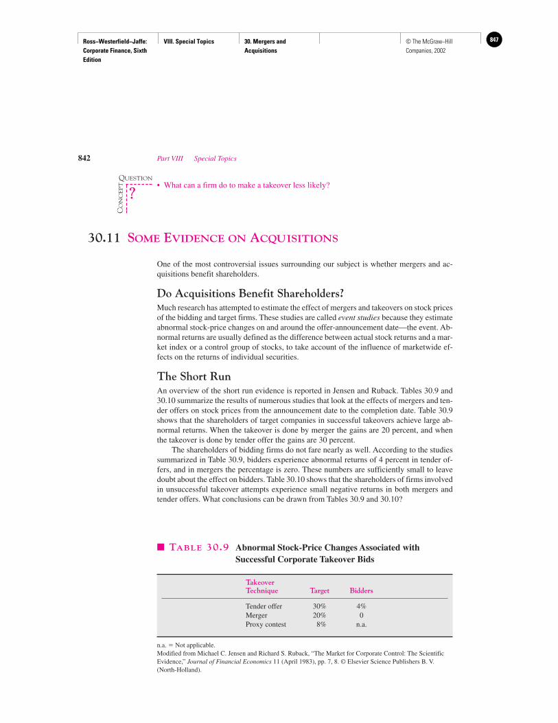
Ross−Westerfield−Jaffe: Corporate Finance, Sixth Edition
VIII. Special Topics 30. Mergers and Acquisitions
847© The McGraw−Hill Companies, 2002
• What can a firm do to make a takeover less likely?
30.11 SOME EVIDENCE ON ACQUISITIONS
One of the most controversial issues surrounding our subject is whether mergers and ac-quisitions benefit shareholders.
Do Acquisitions Benefit Shareholders?Much research has attempted to estimate the effect of mergers and takeovers on stock pricesof the bidding and target firms. These studies are called event studies because they estimateabnormal stock-price changes on and around the offer-announcement date—the event. Ab-normal returns are usually defined as the difference between actual stock returns and a mar-ket index or a control group of stocks, to take account of the influence of marketwide ef-fects on the returns of individual securities.
The Short RunAn overview of the short run evidence is reported in Jensen and Ruback. Tables 30.9 and30.10 summarize the results of numerous studies that look at the effects of mergers and ten-der offers on stock prices from the announcement date to the completion date. Table 30.9shows that the shareholders of target companies in successful takeovers achieve large ab-normal returns. When the takeover is done by merger the gains are 20 percent, and whenthe takeover is done by tender offer the gains are 30 percent.
The shareholders of bidding firms do not fare nearly as well. According to the studiessummarized in Table 30.9, bidders experience abnormal returns of 4 percent in tender of-fers, and in mergers the percentage is zero. These numbers are sufficiently small to leavedoubt about the effect on bidders. Table 30.10 shows that the shareholders of firms involvedin unsuccessful takeover attempts experience small negative returns in both mergers andtender offers. What conclusions can be drawn from Tables 30.9 and 30.10?
842 Part VIII Special Topics
� TABLE 30.9 Abnormal Stock-Price Changes Associated withSuccessful Corporate Takeover Bids
TakeoverTechnique Target Bidders
Tender offer 30% 4%Merger 20% 0Proxy contest 8% n.a.
n.a. � Not applicable.Modified from Michael C. Jensen and Richard S. Ruback, “The Market for Corporate Control: The ScientificEvidence,” Journal of Financial Economics 11 (April 1983), pp. 7, 8. © Elsevier Science Publishers B. V.(North-Holland).
QUESTION
CO
NC
EP
T
?
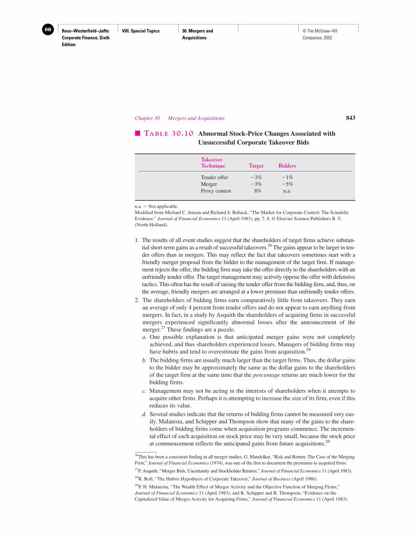
Ross−Westerfield−Jaffe: Corporate Finance, Sixth Edition
VIII. Special Topics 30. Mergers and Acquisitions
848 © The McGraw−Hill Companies, 2002
1. The results of all event studies suggest that the shareholders of target firms achieve substan-tial short-term gains as a result of successful takeovers.26 The gains appear to be larger in ten-der offers than in mergers. This may reflect the fact that takeovers sometimes start with afriendly merger proposal from the bidder to the management of the target firm. If manage-ment rejects the offer, the bidding firm may take the offer directly to the shareholders with anunfriendly tender offer. The target management may actively oppose the offer with defensivetactics. This often has the result of raising the tender offer from the bidding firm, and, thus, onthe average, friendly mergers are arranged at a lower premium than unfriendly tender offers.
2. The shareholders of bidding firms earn comparatively little from takeovers. They earnan average of only 4 percent from tender offers and do not appear to earn anything frommergers. In fact, in a study by Asquith the shareholders of acquiring firms in successfulmergers experienced significantly abnormal losses after the announcement of themerger.27 These findings are a puzzle.a. One possible explanation is that anticipated merger gains were not completely
achieved, and thus shareholders experienced losses. Managers of bidding firms mayhave hubris and tend to overestimate the gains from acquisition.28
b. The bidding firms are usually much larger than the target firms. Thus, the dollar gainsto the bidder may be approximately the same as the dollar gains to the shareholdersof the target firm at the same time that the percentage returns are much lower for thebidding firms.
c. Management may not be acting in the interests of shareholders when it attempts toacquire other firms. Perhaps it is attempting to increase the size of its firm, even if thisreduces its value.
d. Several studies indicate that the returns of bidding firms cannot be measured very eas-ily. Malatesta, and Schipper and Thompson show that many of the gains to the share-holders of bidding firms come when acquisition programs commence. The incremen-tal effect of each acquisition on stock price may be very small, because the stock priceat commencement reflects the anticipated gains from future acquisitions.29
Chapter 30 Mergers and Acquisitions 843
� TABLE 30.10 Abnormal Stock-Price Changes Associated withUnsuccessful Corporate Takeover Bids
TakeoverTechnique Target Bidders
Tender offer �3% �1%Merger �3% �5%Proxy contest 8% n.a.
n.a. � Not applicable.Modified from Michael C. Jensen and Richard S. Ruback, “The Market for Corporate Control: The ScientificEvidence,” Journal of Financial Economics 11 (April 1983), pp. 7, 8. © Elsevier Science Publishers B. V.(North-Holland).
26This has been a consistent finding in all merger studies. G. Mandelker, “Risk and Return: The Case of the MergingFirm,” Journal of Financial Economics (1974), was one of the first to document the premiums to acquired firms.27P. Asquith, “Merger Bids, Uncertainty and Stockholder Returns,” Journal of Financial Economics 11 (April 1983).28R. Roll, “The Hubris Hypothesis of Corporate Takeover,” Journal of Business (April 1986).29P. H. Malatesta, “The Wealth Effect of Merger Activity and the Objective Function of Merging Firms,”Journal of Financial Economics 11 (April 1983); and K. Schipper and R. Thompson, “Evidence on theCapitalized Value of Merger Activity for Acquiring Firms,” Journal of Financial Economics 11 (April 1983).
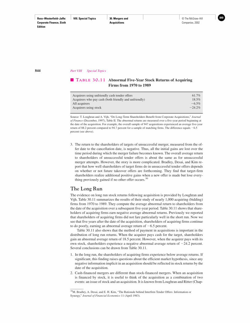
Ross−Westerfield−Jaffe: Corporate Finance, Sixth Edition
VIII. Special Topics 30. Mergers and Acquisitions
849© The McGraw−Hill Companies, 2002
3. The return to the shareholders of targets of unsuccessful merger, measured from the of-fer date to the cancellation date, is negative. Thus, all the initial gains are lost over thetime period during which the merger failure becomes known. The overall average returnto shareholders of unsuccessful tender offers is about the same as for unsuccessfulmerger attempts. However, the story is more complicated. Bradley, Desai, and Kim re-port that how well shareholders of target firms do in unsuccessful tender offers dependson whether or not future takeover offers are forthcoming. They find that target-firmshareholders realize additional positive gains when a new offer is made but lose every-thing previously gained if no other offer occurs.30
The Long RunThe evidence on long run stock returns following acquisition is provided by Loughran andVijh. Table 30.11 summarizes the results of their study of nearly 1,000 acquiring (bidding)firms from 1970 to 1989. They compute the average abnormal return to shareholders fromthe date of the acquisition over a subsequent five-year period. Table 30.11 shows that share-holders of acquiring firms earn negative average abnormal returns. Previously we reportedthat shareholders of acquiring firms did not fare particularly well in the short run. Now wesee that five years after the date of the acquisition, shareholders of acquiring firms continueto do poorly, earning an abnormal average return of �6.5 percent.
Table 30.11 also shows that the method of payment in acquisitions is important in thedistribution of long run returns. When the acquirer pays cash for the target, shareholdersgain an abnormal average return of 18.5 percent. However, when the acquirer pays with itsown stock, shareholders experience a negative abnormal average return of �24.2 percent.Several conclusions can be drawn from Table 30.11.
1. In the long run, the shareholders of acquiring firms experience below average returns. Ifsignificant, this finding raises questions about the efficient market hypothesis, since anynegative information implicit in an acquisition should be reflected in stock returns by thedate of the acquisition.
2. Cash-financed mergers are different than stock-financed mergers. When an acquisitionis financed by stock, it is useful to think of the acquisition as a combination of twoevents: an issue of stock and an acquisition. It is known from Loughran and Ritter (Chap-
844 Part VIII Special Topics
30M. Bradley, A. Desai, and E. H. Kim, “The Rationale behind Interfirm Tender Offers: Information orSynergy,” Journal of Financial Economics 11 (April 1983).
� TABLE 30.11 Abnormal Five-Year Stock Returns of AcquiringFirms from 1970 to 1989
Acquirers using unfriendly cash tender offers 61.7%Acquirers who pay cash (both friendly and unfriendly) 18.5%All acquirers �6.5%Acquirers using stock �24.2%
Source: T. Loughran and A. Vijh, “Do Long-Term Shareholders Benefit from Corporate Acquisitions,” Journalof Finance (December, 1997), Table II. The abnormal returns are measured over a five-year period beginning atthe date of the acquisition. For example, the overall sample of 947 acquisitions experienced an average five-yearreturn of 88.2 percent compared to 94.7 percent for a sample of matching firms. The difference equals �6.5percent (see above).
Ross−Westerfield−Jaffe: Corporate Finance, Sixth Edition
VIII. Special Topics 30. Mergers and Acquisitions
850 © The McGraw−Hill Companies, 2002
ter 18) that the long-term abnormal returns following new equity issues are negative. Thepoor long run performance of stock-financed mergers could be the result of new stockissues that take place with these mergers.
3. Acquirers can also be divided into friendly and unfriendly cash acquirers. The shares ofunfriendly cash acquirers have significantly outperformed those of friendly cash ac-quirers. One possible interpretation of this is that unfriendly cash bidders are more likelyto replace poor management. If so, the removal of poor managers may contribute to theabove average long run performance.
Real ProductivityThere are many potential synergies from mergers and acquisitions. Unfortunately, it is veryhard to precisely measure synergy. In the previous section, we focused on stock-marketgains or losses to the shareholders of the acquiring and acquired firms. In very generalterms, we found that target-firm shareholders experience stock-market gains and acquiring-firm shareholders experience stock-market losses. There appear to be net gains to stock-holders. This would suggest that mergers can increase real productivity. In fact, several re-cent studies suggest that mergers can increase real productivity. Healey, Palepu, and Rubackreport that merged companies’ after-tax returns increased substantially after the mergers.They trace this gain to an increase in selling activity (turnover). They find no evidence thatmerged firms cut back on positive NPV capital expenditures.31
• What does the evidence say about the benefits of mergers and acquisitions?
30.12 THE JAPANESE KEIRETSU
In Japan it has been unusual for firms to grow by large-scale mergers and acquisitions.However, in the late 1980s several Japanese firms acquired large U.S. firms.32 Most notably,Sony acquired CBS Records in November 1987 and Columbia Pictures in September 1989.Sony’s acquisition of Columbia Pictures for $3.45 billion is the largest Japanese acquisitionof a U.S. firm. The second largest was Bridgestone Corporation’s acquisition of FirestoneTire and Rubber for $2.6 billion in March 1988.
The most interesting Japanese business combinations involve reciprocal shareholdingand trading agreements. These networks are called keiretsu and involve a group of firmsaffiliated around a large bank, industrial firm, or trading firm. The Mitsubishi and the Mitsuikeiretsu groups are shown in Figure 30.3.
Participation in the Mitsubishi or Mitsui keiretsu implies significant reciprocal owner-ship of common stock. It is widely understood that firms within the keiretsu are not to sellthese cross-held shares.
Chapter 30 Mergers and Acquisitions 845
31P. Healey, K. Palepu, and R. Ruback, “Does Corporate Performance Improve After Mergers,” Journal ofFinancial Economics 31 (1997).32W. Carl Kester, Japanese Takeovers, the Global Contest for Corporate Control, Cambridge, Mass.: 1991(Harvard Business School Press). Chapter 5 describes the acquisition experience of several Japanese firms.
QUESTION
CO
NC
EP
T
?

Ross−Westerfield−Jaffe: Corporate Finance, Sixth Edition
VIII. Special Topics 30. Mergers and Acquisitions
851© The McGraw−Hill Companies, 2002
Nobody knows for sure what the main benefit of the keiretsu is. However, one of themost important features of the keiretsu is the relationship between the industrial firms andthe financial institutions. For example, Mitsubishi Motors may have an extensive relation-ship with Mitsubishi Trust and Banking, Meiji Mutual Life, and Tokio Marine and Fire.This connection between industrial firms and financial institutions within the group maybenefit the group by reducing the costs of financial distress that come from getting credi-
846 Part VIII Special Topics
� FIGURE 30.3 Japanese Keiretsu
Mitsubishi Mitsui
Financial Services Mitsubishi Bank Mitsui Taiyo Kobe BankMitsubishi Trust & Banking Mitsui Trust & BankingMeiji Mutual Life Mitsui Mutual LifeTokio Marine & Fire Taisho Marine & Fire
Computers, Electronics, Mitsubishi Electric Toshibaand Electrical Equipment
Cars Mitsubishi Motors Toyota Motor*Trading and Retailing Mitsubishi Mitsui
MitsukoshiFood and Beverage Kirin Brewery Nippon Flour MillsConstruction Mitsubishi Construction Mitsui Construction
Sanki EngineeringMetals Mitsubishi Steel Mfg. Japan Steel Works
Mitsubishi Materials Mitsui Mining & SmeltingMitsubishi AluminumMitsubishi Cable Industries
Real Estate Mitsubishi Estate Mitsui Real EstateDevelopment
Oil and Coal Mitsubishi OilRubber and Glass Asahi GlassChemicals Mitsubishi Kasei Mitsui Toatsu Chemicals
Mitsubishi Petrochemical Mitsui PetrochemicalMitsubishi Gas Chemical IndustriesMitsubishi Plastics IndustriesMitsubishi Kasei Polytec
Fibers and Textiles Mitsubishi Rayon Tory IndustriesPulp and Paper Mitsubishi Paper Mills Oji PaperMining and Forestry Mitsui Mining
Hokkaido Colliery &Steamship
Industrial Equipment Mitsubishi Heavy Industries Mitsui Engineering &Mitsubishi Kakoki Shipbuilding
Cameras and Optics NikonCement Onoda CementShipping and Transportation Nippon Yusen Mitsui OSK Lines
Mitsubishi Warehouse Mitsui Warehouse& Transportation
This table describes the network of firms in the Mitsubishi and Mitsui keiretsu.*Companies affiliated with more than one group.Source: Fortune (July 15, 1991), p. 81.
Ross−Westerfield−Jaffe: Corporate Finance, Sixth Edition
VIII. Special Topics 30. Mergers and Acquisitions
852 © The McGraw−Hill Companies, 2002
tors to agree to a restructuring if one of the keiretsu members gets into financial trouble.33
Reaching an agreement between Mitsubishi Bank and Mitsubishi Motors will be easier ifMitsubishi Motors gets into trouble because both are in the Mitsubishi keiretsu.
• Can you describe a keiretsu?• What is a benefit of a keiretsu?
30.13 SUMMARY AND CONCLUSIONS
1. One firm can acquire another in several different ways. The three legal forms of acquisitionare merger and consolidation, acquisition of stock, and acquisition of assets. Mergers andconsolidations are the least costly to arrange from a legal standpoint, but they require a voteof approval by the shareholders. Acquisition by stock does not require a shareholder vote andis usually done via a tender offer. However, it is difficult to obtain 100-percent control with atender offer. Acquisition of assets is comparatively costly because it requires more difficulttransfer of asset ownership.
2. Mergers and acquisitions require an understanding of complicated tax and accounting rules.Mergers and acquisitions can be taxable or tax-free transactions. In a taxable transaction,each selling shareholder must pay taxes on the stock’s capital appreciation. Should theacquiring firm elect to write up the assets, additional tax implications arise. However,acquiring firms do not generally elect to write up the assets for tax purposes. The sellingstockholders do not pay taxes at the time of a tax-free acquisition.
Accounting for mergers and acquisitions involves a choice of the purchase method orthe pooling-of-interests method. The choice between these two methods does not affect after-tax cash flows of the combined firm. However, most financial managers prefer the pooling-of-interests method, because net income of the combined firm under this method is higherthan it is under the purchase method.
3. The synergy from an acquisition is defined as the value of the combined firm (VAB) less thevalue of the two firms as separate entities (VA and VB), or
Synergy � VAB � (VA � VB)
The shareholders of the acquiring firm will gain if the synergy from the merger is greaterthan the premium.
4. The possible benefits of an acquisition come from the following:a. Revenue enhancementb. Cost reductionc. Lower taxesd. Lower cost of capital
In addition, the reduction in risk from a merger may actually help bondholders and hurtstockholders.
5. Some of the most colorful language of finance stems from defensive tactics in acquisitionbattles. Poison pills, golden parachutes, crown jewels, and greenmail are terms that describevarious antitakeover tactics. These tactics are discussed in this chapter.
Chapter 30 Mergers and Acquisitions 847
33This is the argument of Takeo Hoshi, Anil K. Kashyup, and David Scharfstein, “The Role of Banks in ReducingFinancial Distress in Japan.” A paper in the Finance and Economic Discussion Series, No. 134, Federal ReserveBoard, Washington, D. C. (October 1990). See also, W. Carl Kester, “Japanese Corporate Governance and theConservation of Value in Financial Distress,” Journal of Applied Corporate Finance (Summer 1991).
QUESTIONS
CO
NC
EP
T
?

Ross−Westerfield−Jaffe: Corporate Finance, Sixth Edition
VIII. Special Topics 30. Mergers and Acquisitions
853© The McGraw−Hill Companies, 2002
6. The empirical research on mergers and acquisitions is extensive. Its basic conclusions arethat, on average, the shareholders of acquired firms fare very well, while the shareholders ofacquiring firms do not gain much.
7. The keiretsu is a Japanese form of business network. It involves reciprocal shareholding andagreements among member firms.
KEY TERMS
Bidder 818 Merger 817Consolidation 817 Poison pill 841Crown jewels 841 Pooling of interests 822Golden parachutes 841 Purchase 821Goodwill 821 Tender offer 817Keiretsu 845
SUGGESTED READINGS
Several fun-to-read trade books on mergers and acquisitions have recently been published,including:Wasserstein, Bruce. Big Deal: 2000 and Beyond. Warner Books, 2000. Pitaro, Regina M. Deals,
Deals and More Deals. Gabelli University Press, 1998.
QUESTIONS AND PROBLEMS
The Basic Forms of Acquisitions30.1 The Lager Brewing Corporation has acquired the Philadelphia Pretzel Company in a
vertical merger. Lager Brewing has issued $300,000 in new long-term debt to pay for itspurchase. ($300,000 is the purchase price.) Construct the balance sheet for the newcorporation if the merger is treated as a purchase for accounting purposes. The balancesheets shown here represent the assets of both firms at their true market values. Assumethese market values are also the book values.
LAGER BREWING CORPORATIONBalance Sheet
(in $ thousands)
Current assets $ 400 Current liabilities $ 200Other assets 100 Long-term debt 100Net fixed assets 500 Equity 700______ ______Total $1,000 Total $1,000______ ____________ ______
PHILADELPHIA PRETZEL COMPANYBalance Sheet
(in $ thousands)
Current assets $ 80 Current liabilities $ 80Other assets 40 Equity 120Net fixed assets 80_____ _____Total $200 Total $200_____ __________ _____
848 Part VIII Special Topics
Ross−Westerfield−Jaffe: Corporate Finance, Sixth Edition
VIII. Special Topics 30. Mergers and Acquisitions
854 © The McGraw−Hill Companies, 2002
30.2 Suppose the balance sheet for Philadelphia Pretzel in problem 30.1 shows the assets attheir book value and not their market value of $240,000. Construct the balance sheet forthe new corporation. Again, treat the transaction as a purchase.
30.3 Keep the assumptions of 30.2. Construct the balance sheet for the new corporation. Usethe pooling-of-interests method to treat the transaction.
Source of Synergy from Acquisitions30.4 Indicate whether you think the following claims regarding takeovers are true or false. In
each case provide a brief explanation for your answer.a. By merging competitors, takeovers have created monopolies that will raise product
prices, reduce production, and harm consumers.b. Managers act in their own interests at times and, in reality, may not be answerable to
shareholders. Takeovers may reflect runaway management.c. In an efficient market, takeovers would not occur because market price would reflect
the true value of corporations. Thus, bidding firms would not be justified in payingpremiums above market prices for target firms.
d. Traders and institutional investors, having extremely short time horizons, areinfluenced by their perceptions of what other market traders will be thinking of stockprospects and do not value takeovers based on fundamental factors. Thus, they will sellshares in target firms despite the true value of the firms.
e. Mergers are a way of avoiding taxes because they allow the acquiring firm to write upthe value of the assets of the acquired firm.
f. Acquisitions analysis frequently focuses on the total value of the firms involved. Anacquisition, however, will usually affect relative values of stocks and bonds, as well astheir total value.
Calculating the Value of the Firm after an Acquisition30.5 The following table shows the projected cash flows and their respective discount rates after
the acquisition of Small Fry Co. by Whale Co. Fill in the blanks and calculate the stock priceof the new firm if it has $100 million of debt and 5 million shares of stock outstanding.
Net Cash Flow perYear (Perpetual) Value(in $ millions) Discount Rate (%) (in $ millions)
Small Fry Co. $ 8. 16% ?Whale Co. 20 10 ?Benefits from acquisition 5 ? 42.5
Revenue enhancement 2.5 ? 12.5Cost reduction 2 10 ?Tax shelters 0.5 5 ?
Whale-Co. 33 ? ?
A Cost to Stockholders from Reduction in Risk30.6 The Chocolate Ice Cream Company and the Vanilla Ice Cream Company have agreed to
merge and form Fudge Swirl Consolidated. Both companies are exactly alike except thatthey are located in different towns. The end-of-period value of each firm is determined bythe weather, as shown.
State Probability Value
Rainy 0.1 $100,000Warm 0.4 200,000Hot 0.5 400,000
The weather conditions in each town are independent of those in the other. Furthermore, eachcompany has an outstanding debt claim of $200,000. Assume that no premiums are paid in the merger.
Chapter 30 Mergers and Acquisitions 849
Ross−Westerfield−Jaffe: Corporate Finance, Sixth Edition
VIII. Special Topics 30. Mergers and Acquisitions
855© The McGraw−Hill Companies, 2002
a. What is the distribution of joint values?b. What is the distribution of end-of-period debt values and stock values after the merger?c. Show that the value of the combined firm is the sum of the individual values.d. Show that the bondholders are better off and the stockholders are worse off in the
combined firm than they would have been if the firms remained separate.
30.7 Cholern Electric Company (CEC) is a public utility that provides electricity to the centralColorado area. Recent events at its Mile-High Nuclear Station have been discouraging.Several shareholders have expressed concern over last year’s financial statements.
Income Statement Balance SheetLast Year End of Year
(in $ millions) (in $ millions)
Revenue $110 Assets $400Fuel 50 Debt 300Other expenses 30 Equity 100Interest 30____Net income $ 0
Recently, a wealthy group of individuals has offered to purchase one-half of CEC’s assetsat fair market price. Management recommends that this offer be accepted because, “Webelieve our expertise in the energy industry can be better exploited by CEC if we sell ourelectricity generating and transmission assets and enter the telecommunications business.Although telecommunications is a riskier business than providing electricity as a publicutility, it is also potentially very profitable.”
Should the management approve this transaction? Why or why not?
Two “Bad” Reasons for Mergers30.8 Refer to the Global Resources example in section 30.8 of the text. Suppose that instead of
40 shares, Global exchanges 100 of its shares for the 100 shares of Regional. The newGlobal Resources will now have 200 shares outstanding and earnings of $200. Assume themarket is smart.a. Calculate Global’s value after the merger.b. Calculate Global’s earnings per share.c. Calculate Global’s price per share.d. Redo your answers to (a), (b), and (c) if the market is fooled.
30.9 Coldran Aviation has voted in favor of being bought out by Arcadia Financial Corporation.Information about each company is presented below.
Arcadia Financial Coldran Aviation
Price-earnings ratio 16 10.8Number of shares 100,000 50,000Earnings $225,000 $100,000
Stockholders in Coldran Aviation will receive six-tenths of a share of Arcadia for eachshare they hold.a. How will the earnings per share (EPS) for these stockholders be changed?b. What will be the effect on the original Arcadia stockholders of changes in the EPS?
The NPV of a Merger30.10 Fly-By-Night Couriers is analyzing the possible acquisition of Flash-in-the-Pan
Restaurants. Neither firm has debt. The forecasts of Fly-By-Night show that the purchasewould increase its annual after-tax cash flow by $600,000 indefinitely. The current marketvalue of Flash-in-the-Pan is $20 million. The current market value of Fly-By-Night is $35million. The appropriate discount rate for the incremental cash flows is 8 percent.
850 Part VIII Special Topics
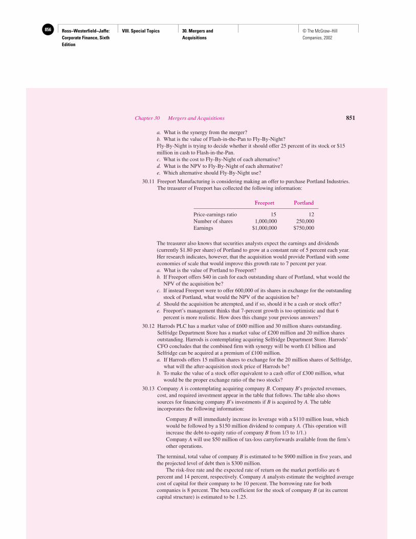
Ross−Westerfield−Jaffe: Corporate Finance, Sixth Edition
VIII. Special Topics 30. Mergers and Acquisitions
856 © The McGraw−Hill Companies, 2002
a. What is the synergy from the merger?b. What is the value of Flash-in-the-Pan to Fly-By-Night?Fly-By-Night is trying to decide whether it should offer 25 percent of its stock or $15million in cash to Flash-in-the-Pan.c. What is the cost to Fly-By-Night of each alternative?d. What is the NPV to Fly-By-Night of each alternative?e. Which alternative should Fly-By-Night use?
30.11 Freeport Manufacturing is considering making an offer to purchase Portland Industries.The treasurer of Freeport has collected the following information:
Freeport Portland
Price-earnings ratio 15 12Number of shares 1,000,000 250,000Earnings $1,000,000 $750,000
The treasurer also knows that securities analysts expect the earnings and dividends(currently $1.80 per share) of Portland to grow at a constant rate of 5 percent each year.Her research indicates, however, that the acquisition would provide Portland with someeconomies of scale that would improve this growth rate to 7 percent per year.a. What is the value of Portland to Freeport?b. If Freeport offers $40 in cash for each outstanding share of Portland, what would the
NPV of the acquisition be?c. If instead Freeport were to offer 600,000 of its shares in exchange for the outstanding
stock of Portland, what would the NPV of the acquisition be?d. Should the acquisition be attempted, and if so, should it be a cash or stock offer?e. Freeport’s management thinks that 7-percent growth is too optimistic and that 6
percent is more realistic. How does this change your previous answers?
30.12 Harrods PLC has a market value of £600 million and 30 million shares outstanding.Selfridge Department Store has a market value of £200 million and 20 million sharesoutstanding. Harrods is contemplating acquiring Selfridge Department Store. Harrods’CFO concludes that the combined firm with synergy will be worth £1 billion andSelfridge can be acquired at a premium of £100 million.a. If Harrods offers 15 million shares to exchange for the 20 million shares of Selfridge,
what will the after-acquisition stock price of Harrods be?b. To make the value of a stock offer equivalent to a cash offer of £300 million, what
would be the proper exchange ratio of the two stocks?
30.13 Company A is contemplating acquiring company B. Company B’s projected revenues,cost, and required investment appear in the table that follows. The table also showssources for financing company B’s investments if B is acquired by A. The tableincorporates the following information:
Company B will immediately increase its leverage with a $110 million loan, whichwould be followed by a $150 million dividend to company A. (This operation willincrease the debt-to-equity ratio of company B from 1/3 to 1/1.)Company A will use $50 million of tax-loss carryforwards available from the firm’sother operations.
The terminal, total value of company B is estimated to be $900 million in five years, andthe projected level of debt then is $300 million.
The risk-free rate and the expected rate of return on the market portfolio are 6percent and 14 percent, respectively. Company A analysts estimate the weighted averagecost of capital for their company to be 10 percent. The borrowing rate for bothcompanies is 8 percent. The beta coefficient for the stock of company B (at its currentcapital structure) is estimated to be 1.25.
Chapter 30 Mergers and Acquisitions 851

Ross−Westerfield−Jaffe: Corporate Finance, Sixth Edition
VIII. Special Topics 30. Mergers and Acquisitions
857© The McGraw−Hill Companies, 2002
The board of directors of company A is presented with an offer for $68.75 per shareof company B, or a total of $550 million for the 8 million shares outstanding.
Evaluate this proposal. The table produced below may help you.
Projections for Company Bif Acquired by Company A
(in $ millions)
Year 1 Year 2 Year 3 Year 4 Year 5
Sales $800 $900 $1,000 $1,125 $1,250Production costs 562 630 700 790 875Depreciation 75 80 82 83 83Other expenses 80 90 100 113 125____ ____ _____ _____ _____
EBIT 83 100 118 139 167Interest 19 22 24 25 27____ ____ _____ _____ _____
EBT 64 78 94 114 140Taxes 32 39 47 57 70____ ____ _____ _____ _____Net income 32 39 47 57 70Investments:
Net working capital 20 25 25 30 30Net fixed assets 15 25 18 12 7____ ____ _____ _____ _____
Total 35 50 43 42 37Sources of financing:
Net debt financing 35 16 16 15 12Profit retention 0 34 27 27 25____ ____ _____ _____ _____
Total $ 35 $ 50 $ 43 $ 42 $ 37
Cash Flows—Company A
Year 0 Year 1 Year 2 Year 3 Year 4 Year 5
Acquisition of B —Dividends from B 150 — — — — —Tax-loss
carryforwards 25 25 —Terminal value — — — — — —
Total — — — — — —
Defensive Tactics30.14 List the defensive tactics commonly used by target-firm managers to resist unfriendly
takeover attempts.
MINICASE: U.S. STEEL’S ACQUISITION OF MARATHON OIL
In the summer of 1981, Marathon Oil Company commissioned the First Boston Corpora-tion to prepare an analysis of the underlying asset value of Marathon based solely on pub-licly available information. Before First Boston could complete the study, Mobil Corpora-tion announced a tender offer for Marathon’s common equity, thus launching one of themost eventful takeover stories in American corporate history.
852 Part VIII Special Topics

Ross−Westerfield−Jaffe: Corporate Finance, Sixth Edition
VIII. Special Topics 30. Mergers and Acquisitions
858 © The McGraw−Hill Companies, 2002
On October 30, 1981, Mobil bid $85 per share for up to 40 million shares of Marathon’scommon equity. Before the announcement, Marathon stock traded for about $64 per shareon the New York Stock Exchange. Before trading on the new information commenced,Marathon management rejected Mobil’s offer as grossly inadequate and began seeking awhite knight merger candidate. When trading began on Monday, November 2, 1981,Marathon’s shares shot up immediately to the $90-per-share range for a one-day abnormalexcess return of more than 30 percent. The market reacted to Mobil’s offer by biddingMobil’s common stock down to $253⁄8 for a one-day abnormal return of �4.26 percent.(November 2, 1981, was also the ex-dividend date for a $0.50 per share dividend declaredearlier. The share price, however, fell $5⁄8.) These data suggest that the market viewed thepossible acquisition of Marathon by Mobil at $85 per share as a near-zero net-present-valuetransaction for Mobil. The dramatic response of Marathon’s share price was very likelycaused by anticipation of more bidding. These traders were not to be disappointed.
On November 9, the management of U.S. Steel Corporation expressed an interest inacquiring Marathon. The possible takeover price was rumored to be $100 per share in cashand notes. Presumably because the market actually valued this offer as less than Mobil’s of-fer, Marathon’s common stock showed an abnormal return for the day of �2.91 percent.The effect of the rumors on U.S. Steel’s share price was insignificant, so it may be con-cluded that the market felt that the transaction at this price would be a zero net-present-value transaction for U.S. Steel as well.
During subsequent negotiations, U.S. Steel raised its price and actually tendered $125per share for up to 30 million shares of Marathon stock on November 18. On the next trad-ing day Marathon showed a one-day abnormal excess return on its share price of almost 35percent; again the market roared its approval for the reevaluation of Marathon. U.S. Steel’scommon, however, showed significantly negative abnormal returns in response to thisnews. This indicates that the market believed U.S. Steel overbid for Marathon. Mobil’sshare price showed no significant abnormal return on November 18 and 19.
However, on November 25, Mobil raised its bid to $126 per share, and the market re-sponded by lowering the value of both Mobil and U.S. Steel by significant amounts.Apparently the market believed that at this price the merger was unattractive for both Mobiland U.S. Steel. Marathon’s stock fell in price by a significant amount in response to Mobil’soffer, perhaps because Mobil’s offer and U.S. Steel’s offer were valued nearly equally bythe market, and this signaled the end of the bidding and the end of speculating in Marathon.
Suppose that a U.S. Steel tender offer is structured in the following way. U.S. Steel willpay $125 (in cash) for 30 million shares of Marathon giving it 50.1 percent of the Marathonshares. After gaining voting control, U.S. Steel intends to merge with Marathon and willpay the remaining shareholders with seven-year notes worth about $85 per share. Further,suppose you own 10 shares of Marathon stock. Should you tender your shares?
Chapter 30 Mergers and Acquisitions 853
Ross−Westerfield−Jaffe: Corporate Finance, Sixth Edition
VIII. Special Topics 31. Financial Distress 859© The McGraw−Hill Companies, 2002
Financial Distress
CH
AP
TE
R31
EXECUTIVE SUMMARY
This chapter discusses financial distress, private workouts, and bankruptcy. A firmthat does not generate enough cash flow to make a contractually required payment,such as an interest payment, will experience financial distress. A firm that defaults
on a required payment may be forced to liquidate its assets. More often, a defaulting firmwill reorganize its financial structure. Financial restructuring involves replacing old finan-cial claims with new ones and takes place with private workouts or legal bankruptcy. Pri-vate workouts are voluntary arrangements to restructure a company’s debt, such as post-poning a payment or reducing the size of the payment. Sometimes a private workout is notpossible and formal bankruptcy is required. The largest formal bankruptcy in U.S. financialhistory occurred in April 1987 when Texaco filed Chapter 11 bankruptcy. (See Table 31.1for information on the largest U.S. bankruptcies.)
31.1 WHAT IS FINANCIAL DISTRESS?
Financial distress is surprisingly hard to define precisely. This is true partly because of thevariety of events befalling firms under financial distress. The list of events is almost end-less but here are some examples:
Dividend reductionsPlant closingsLossesLayoffsCEO resignationsPlummeting stock prices
Financial distress is a situation where a firm’s operating cash flows are not sufficient tosatisfy current obligations (such as trade credits or interest expenses) and the firm is forced totake corrective action.1 Financial distress may lead a firm to default on a contract, and it mayinvolve financial restructuring between the firm, its creditors, and its equity investors. Usuallythe firm is forced to take actions that it would not have taken if it had sufficient cash flow.
Our definition of financial distress can be expanded somewhat by linking it to insol-vency. Insolvency is defined in Black’s Law Dictionary as2
1This definition is close to the one used by Karen Wruck, “Financial Distress: Reorganization and OrganizationEfficiency,” Journal of Financial Economics 27 (1990), p. 425.2Taken from Black’s Law Dictionary, 5th ed. (St. Paul, Minn.: West Publishing Company), p. 716.
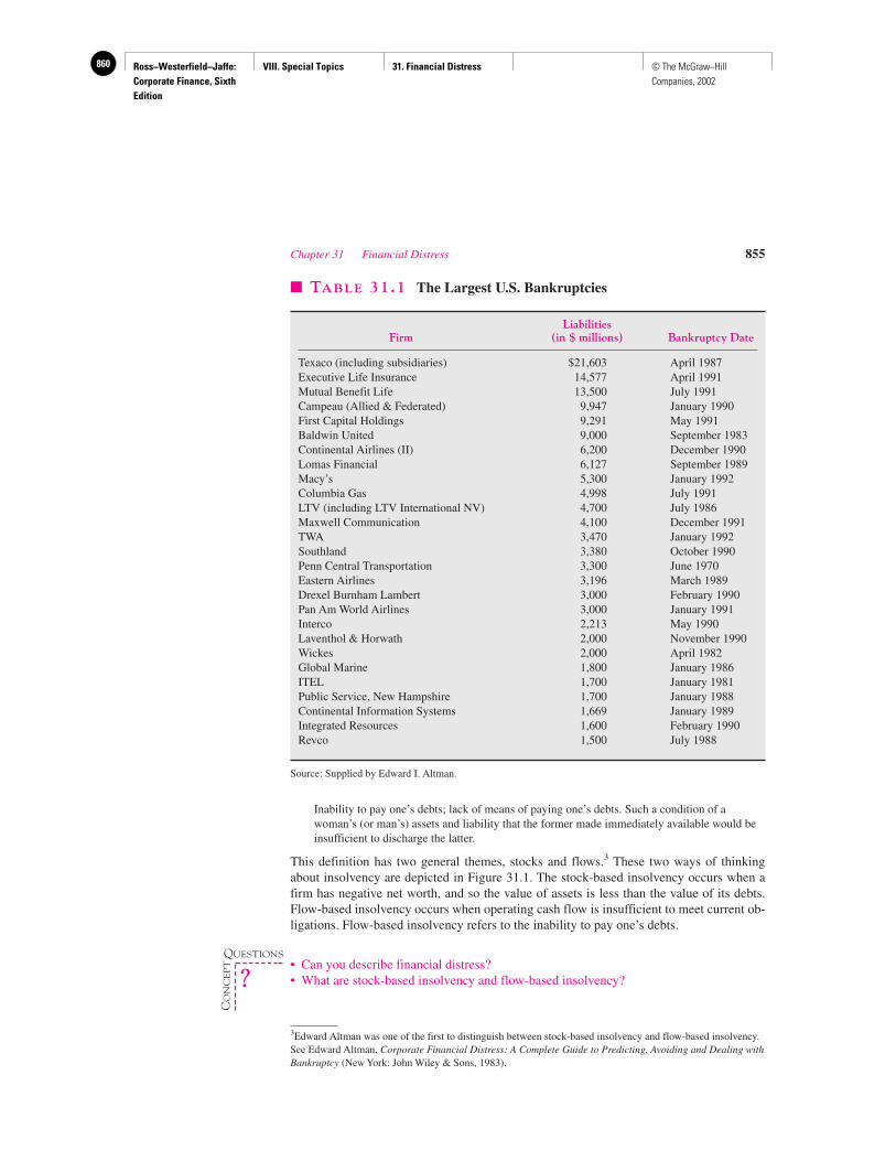
Ross−Westerfield−Jaffe: Corporate Finance, Sixth Edition
VIII. Special Topics 31. Financial Distress860 © The McGraw−Hill Companies, 2002
Inability to pay one’s debts; lack of means of paying one’s debts. Such a condition of awoman’s (or man’s) assets and liability that the former made immediately available would beinsufficient to discharge the latter.
This definition has two general themes, stocks and flows.3 These two ways of thinkingabout insolvency are depicted in Figure 31.1. The stock-based insolvency occurs when afirm has negative net worth, and so the value of assets is less than the value of its debts.Flow-based insolvency occurs when operating cash flow is insufficient to meet current ob-ligations. Flow-based insolvency refers to the inability to pay one’s debts.
• Can you describe financial distress?• What are stock-based insolvency and flow-based insolvency?
Chapter 31 Financial Distress 855
3Edward Altman was one of the first to distinguish between stock-based insolvency and flow-based insolvency.See Edward Altman, Corporate Financial Distress: A Complete Guide to Predicting, Avoiding and Dealing withBankruptcy (New York: John Wiley & Sons, 1983).
� TABLE 31.1 The Largest U.S. Bankruptcies
LiabilitiesFirm (in $ millions) Bankruptcy Date
Texaco (including subsidiaries) $21,603 April 1987Executive Life Insurance 14,577 April 1991Mutual Benefit Life 13,500 July 1991Campeau (Allied & Federated) 9,947 January 1990First Capital Holdings 9,291 May 1991Baldwin United 9,000 September 1983Continental Airlines (II) 6,200 December 1990Lomas Financial 6,127 September 1989Macy’s 5,300 January 1992Columbia Gas 4,998 July 1991LTV (including LTV International NV) 4,700 July 1986Maxwell Communication 4,100 December 1991TWA 3,470 January 1992Southland 3,380 October 1990Penn Central Transportation 3,300 June 1970Eastern Airlines 3,196 March 1989Drexel Burnham Lambert 3,000 February 1990Pan Am World Airlines 3,000 January 1991Interco 2,213 May 1990Laventhol & Horwath 2,000 November 1990Wickes 2,000 April 1982Global Marine 1,800 January 1986ITEL 1,700 January 1981Public Service, New Hampshire 1,700 January 1988Continental Information Systems 1,669 January 1989Integrated Resources 1,600 February 1990Revco 1,500 July 1988
Source: Supplied by Edward I. Altman.
QUESTIONS
CO
NC
EP
T
?
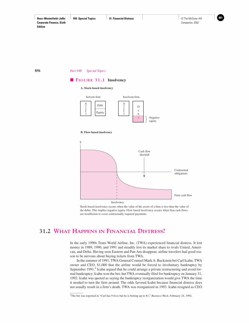
Ross−Westerfield−Jaffe: Corporate Finance, Sixth Edition
VIII. Special Topics 31. Financial Distress 861© The McGraw−Hill Companies, 2002
31.2 WHAT HAPPENS IN FINANCIAL DISTRESS?
In the early 1990s Trans World Airline, Inc. (TWA) experienced financial distress. It lostmoney in 1989, 1990, and 1991 and steadily lost its market share to rivals United, Ameri-can, and Delta. Having seen Eastern and Pan Am disappear, airline travelers had good rea-son to be nervous about buying tickets from TWA.
In the summer of 1991, TWA General Counsel Mark A. Buckstein bet Carl Icahn, TWAowner and CEO, $1,000 that the airline would be forced to involuntary bankruptcy bySeptember 1991.4 Icahn argued that he could arrange a private restructuring and avoid for-mal bankruptcy. Icahn won the bet, but TWA eventually filed for bankruptcy on January 31,1992. Icahn was quoted as saying the bankruptcy reorganization would give TWA the timeit needed to turn the firm around. The odds favored Icahn because financial distress doesnot usually result in a firm’s death. TWA was reorganized in 1993. Icahn resigned as CEO
856 Part VIII Special Topics
A. Stock-based insolvency
Solvent firm Insolvent firm
Debt
Equity
Negativeequity
B. Flow-based insolvency
Assets
Assets
Debt
$
Contractualobligations
Firm cash flow
Cash flowshortfall
Insolvency
� FIGURE 31.1 Insolvency
Stock-based insolvency occurs when the value of the assets of a firm is less than the value ofthe debts. This implies negative equity. Flow-based insolvency occurs when firm cash flowsare insufficient to cover contractually required payments.
4The bet was reported in “Carl has 9 lives but he is betting up to 81⁄2,” Business Week, February 24, 1992.
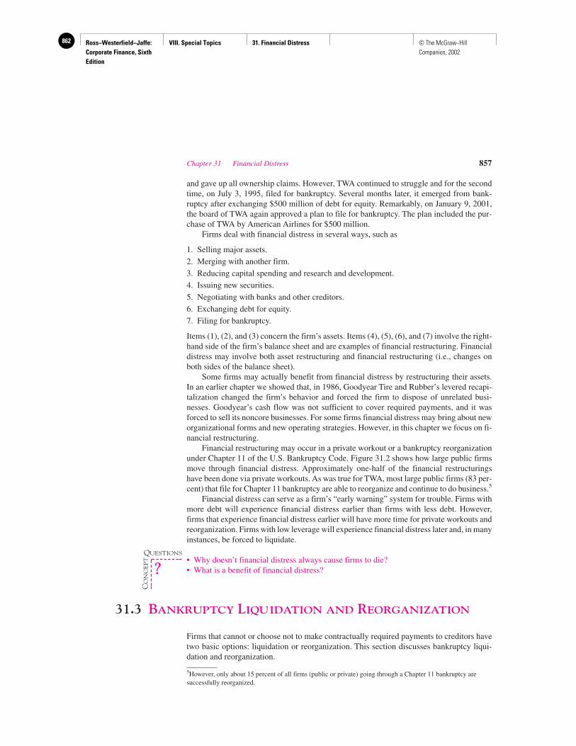
Ross−Westerfield−Jaffe: Corporate Finance, Sixth Edition
VIII. Special Topics 31. Financial Distress862 © The McGraw−Hill Companies, 2002
and gave up all ownership claims. However, TWA continued to struggle and for the secondtime, on July 3, 1995, filed for bankruptcy. Several months later, it emerged from bank-ruptcy after exchanging $500 million of debt for equity. Remarkably, on January 9, 2001,the board of TWA again approved a plan to file for bankruptcy. The plan included the pur-chase of TWA by American Airlines for $500 million.
Firms deal with financial distress in several ways, such as
1. Selling major assets.
2. Merging with another firm.
3. Reducing capital spending and research and development.
4. Issuing new securities.
5. Negotiating with banks and other creditors.
6. Exchanging debt for equity.
7. Filing for bankruptcy.
Items (1), (2), and (3) concern the firm’s assets. Items (4), (5), (6), and (7) involve the right-hand side of the firm’s balance sheet and are examples of financial restructuring. Financialdistress may involve both asset restructuring and financial restructuring (i.e., changes onboth sides of the balance sheet).
Some firms may actually benefit from financial distress by restructuring their assets.In an earlier chapter we showed that, in 1986, Goodyear Tire and Rubber’s levered recapi-talization changed the firm’s behavior and forced the firm to dispose of unrelated busi-nesses. Goodyear’s cash flow was not sufficient to cover required payments, and it wasforced to sell its noncore businesses. For some firms financial distress may bring about neworganizational forms and new operating strategies. However, in this chapter we focus on fi-nancial restructuring.
Financial restructuring may occur in a private workout or a bankruptcy reorganizationunder Chapter 11 of the U.S. Bankruptcy Code. Figure 31.2 shows how large public firmsmove through financial distress. Approximately one-half of the financial restructuringshave been done via private workouts. As was true for TWA, most large public firms (83 per-cent) that file for Chapter 11 bankruptcy are able to reorganize and continue to do business.5
Financial distress can serve as a firm’s “early warning” system for trouble. Firms withmore debt will experience financial distress earlier than firms with less debt. However,firms that experience financial distress earlier will have more time for private workouts andreorganization. Firms with low leverage will experience financial distress later and, in manyinstances, be forced to liquidate.
• Why doesn’t financial distress always cause firms to die?• What is a benefit of financial distress?
31.3 BANKRUPTCY LIQUIDATION AND REORGANIZATION
Firms that cannot or choose not to make contractually required payments to creditors havetwo basic options: liquidation or reorganization. This section discusses bankruptcy liqui-dation and reorganization.
Chapter 31 Financial Distress 857
5However, only about 15 percent of all firms (public or private) going through a Chapter 11 bankruptcy aresuccessfully reorganized.
QUESTIONS
CO
NC
EP
T
?
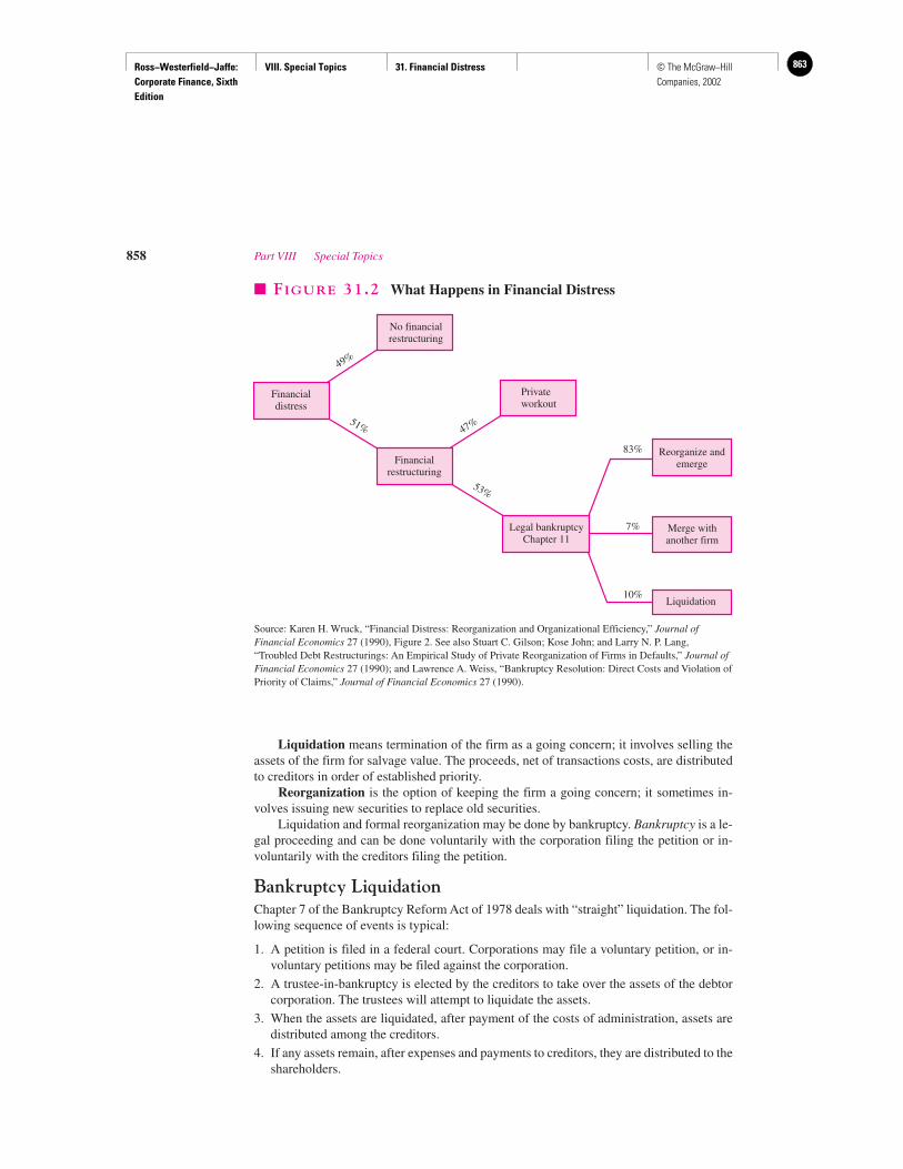
Ross−Westerfield−Jaffe: Corporate Finance, Sixth Edition
VIII. Special Topics 31. Financial Distress 863© The McGraw−Hill Companies, 2002
Liquidation means termination of the firm as a going concern; it involves selling theassets of the firm for salvage value. The proceeds, net of transactions costs, are distributedto creditors in order of established priority.
Reorganization is the option of keeping the firm a going concern; it sometimes in-volves issuing new securities to replace old securities.
Liquidation and formal reorganization may be done by bankruptcy. Bankruptcy is a le-gal proceeding and can be done voluntarily with the corporation filing the petition or in-voluntarily with the creditors filing the petition.
Bankruptcy LiquidationChapter 7 of the Bankruptcy Reform Act of 1978 deals with “straight” liquidation. The fol-lowing sequence of events is typical:
1. A petition is filed in a federal court. Corporations may file a voluntary petition, or in-voluntary petitions may be filed against the corporation.
2. A trustee-in-bankruptcy is elected by the creditors to take over the assets of the debtorcorporation. The trustees will attempt to liquidate the assets.
3. When the assets are liquidated, after payment of the costs of administration, assets aredistributed among the creditors.
4. If any assets remain, after expenses and payments to creditors, they are distributed to theshareholders.
858 Part VIII Special Topics
No financialrestructuring
Financialdistress
Privateworkout
Financialrestructuring
Reorganize andemerge
Legal bankruptcyChapter 11
Merge withanother firm
Liquidation
49%
47%
83%
7%
10%
53%
51%
� FIGURE 31.2 What Happens in Financial Distress
Source: Karen H. Wruck, “Financial Distress: Reorganization and Organizational Efficiency,” Journal ofFinancial Economics 27 (1990), Figure 2. See also Stuart C. Gilson; Kose John; and Larry N. P. Lang,“Troubled Debt Restructurings: An Empirical Study of Private Reorganization of Firms in Defaults,” Journal ofFinancial Economics 27 (1990); and Lawrence A. Weiss, “Bankruptcy Resolution: Direct Costs and Violation ofPriority of Claims,” Journal of Financial Economics 27 (1990).
Ross−Westerfield−Jaffe: Corporate Finance, Sixth Edition
VIII. Special Topics 31. Financial Distress864 © The McGraw−Hill Companies, 2002
Conditions Leading to Involuntary Bankruptcy An involuntary bankruptcy petitionmay be filed by creditors if both the following conditions are met:
1. The corporation is not paying debts as they become due.
2. If there are more than 12 creditors, at least three with claims totaling $5,000 or moremust join in the filing. If there are fewer than 12 creditors, then only one with a claim of$5,000 is required to file.
Priority of Claims Once a corporation is determined to be bankrupt, liquidation takesplace. The distribution of the proceeds of the liquidation occurs according to the fol-lowing priority:
1. Administration expenses, associated with liquidating the bankrupt’s assets.
2. Unsecured claims arising after the filing of an involuntary bankruptcy petition.
3. Wages, salaries, and commissions, not to exceed $2,000 per claimant, earned within 90days before the filing date.
4. Contributions to employee benefit plans arising within 180 days before the filing date.
5. Consumer claims, not exceeding $900.
6. Tax claims.
7. Secured and unsecured creditors’ claims.
8. Preferred stockholders’ claims.
9. Common stockholders’ claims.
The priority rule in liquidation is the absolute priority rule (APR).One qualification to this list concerns secured creditors. Liens on property are outside
APR ordering. However, if the secured property is liquidated and provides cash insufficientto cover the amount owed them, the secured creditors join with unsecured creditors in di-viding the remaining liquidating value. In contrast, if the secured property is liquidated forproceeds greater than the secured claim, the net proceeds are used to pay unsecured credi-tors and others.
EXAMPLE
The B. O. Drug Company is to be liquidated. Its liquidating value is $2.7 mil-lion. Bonds worth $1.5 million are secured by a mortgage on the B. O. DrugCompany corporate headquarters building, which is sold for $1 million;$200,000 is used to cover administrative costs and other claims (including un-paid wages, pension benefits, consumer claims, and taxes). After paying$200,000 to the administrative priority claims, the amount available to pay se-cured and unsecured creditors is $2.5 million. This is less than the amount ofunpaid debt of $4 million.
Under APR all creditors must be paid before shareholders, and the mortgage bond-holders have first claim on the $1 million obtained from the sale of the headquartersbuilding.
The trustee has proposed the following distribution:
Chapter 31 Financial Distress 859
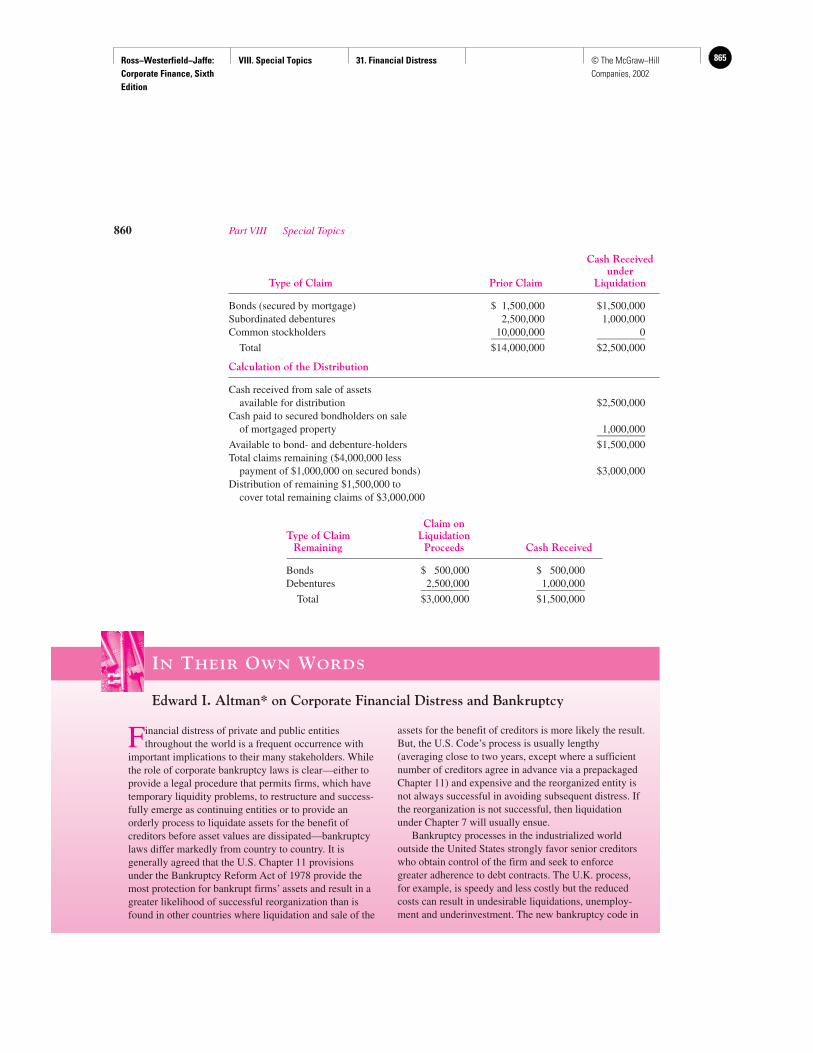
Ross−Westerfield−Jaffe: Corporate Finance, Sixth Edition
VIII. Special Topics 31. Financial Distress 865© The McGraw−Hill Companies, 2002
Cash Receivedunder
Type of Claim Prior Claim Liquidation
Bonds (secured by mortgage) $ 1,500,000 $1,500,000Subordinated debentures 2,500,000 1,000,000Common stockholders 10,000,000 0__________ _________
Total $14,000,000 $2,500,000
Calculation of the Distribution
Cash received from sale of assets available for distribution $2,500,000
Cash paid to secured bondholders on saleof mortgaged property 1,000,000_________
Available to bond- and debenture-holders $1,500,000Total claims remaining ($4,000,000 less
payment of $1,000,000 on secured bonds) $3,000,000Distribution of remaining $1,500,000 to
cover total remaining claims of $3,000,000
Claim onType of Claim Liquidation
Remaining Proceeds Cash Received
Bonds $ 500,000 $ 500,000Debentures 2,500,000 1,000,000_________ _________
Total $3,000,000 $1,500,000
860 Part VIII Special Topics
IN THEIR OWN WORDS
Edward I. Altman* on Corporate Financial Distress and Bankruptcy
Financial distress of private and public entitiesthroughout the world is a frequent occurrence with
important implications to their many stakeholders. Whilethe role of corporate bankruptcy laws is clear—either toprovide a legal procedure that permits firms, which havetemporary liquidity problems, to restructure and success-fully emerge as continuing entities or to provide anorderly process to liquidate assets for the benefit ofcreditors before asset values are dissipated—bankruptcylaws differ markedly from country to country. It isgenerally agreed that the U.S. Chapter 11 provisionsunder the Bankruptcy Reform Act of 1978 provide themost protection for bankrupt firms’ assets and result in agreater likelihood of successful reorganization than isfound in other countries where liquidation and sale of the
assets for the benefit of creditors is more likely the result.But, the U.S. Code’s process is usually lengthy(averaging close to two years, except where a sufficientnumber of creditors agree in advance via a prepackagedChapter 11) and expensive and the reorganized entity isnot always successful in avoiding subsequent distress. Ifthe reorganization is not successful, then liquidationunder Chapter 7 will usually ensue.
Bankruptcy processes in the industrialized worldoutside the United States strongly favor senior creditorswho obtain control of the firm and seek to enforcegreater adherence to debt contracts. The U.K. process,for example, is speedy and less costly but the reducedcosts can result in undesirable liquidations, unemploy-ment and underinvestment. The new bankruptcy code in

Ross−Westerfield−Jaffe: Corporate Finance, Sixth Edition
VIII. Special Topics 31. Financial Distress866 © The McGraw−Hill Companies, 2002
Chapter 31 Financial Distress 861
Germany attempts to reduce the considerable power ofsecured creditors but it is still closer to the U.K. system.In the United States, creditors and owners can negotiate“violations” to the “absolute priority rule”—this “rule”holds that more senior creditors must be paid in full,prior to any payments to more junior creditors or toowners. (However, the so-called “violations” to absolutepriority have empirically been shown to be relativelysmall, e.g., under 10 percent of firm value.) Finally, theU.S. system gives the court the right to sanction post-petition debt financing, usually with super-priority statusover existing claims, thereby facilitating the continuingoperation of the firm. Recently, France has had similarsuccessful experience.
A measure of performance of the U.S. bankruptcysystem is the proportion of firms which emerge success-fully. The results in the United States of late aresomewhat mixed, with close to 70 percent of large firmsemerging but probably less than 20 percent of smallerentities. And, a not insignificant number of firms suffersubsequent distress and may file again (Chapter 22).
Regardless of the location, one of the objectives ofbankruptcy and other distressed workout arrangements isthat creditors and other suppliers of capital clearly knowtheir rights and expected recoveries in the event of adistressed situation. When these are not transparentand/or are based on outdated processes with arbitrary andpossibly corrupt outcomes, then the entire economicsystem suffers and growth is inhibited. Such is the casein several emerging market countries. Revision of theseoutdated systems should be a priority.
In addition to the comparative benefits of differentnational restructuring systems, a number of intriguingtheoretical and empirical issues are related to thedistressed firm. Among these are corporate debt capacity,manager-creditor-owner incentives, ability to predictdistress, data and computations for default rate estima-tion, investment in securities of distressed firms andpost-reorganization performance assessment.
Corporate distress has a major impact oncreditor/debtor relationships and, combined withbusiness risk and tax considerations, affects the capitalstructure of companies. One key question is how costlyare the expected distress costs compared to theexpected tax benefits of using leverage—the so-called
trade-off theory. Most analysts agree that the sum ofdirect (e.g., legal fees) and indirect costs is in the rangeof 10–20 percent of firm value.
Whether the taking of excess risk and over-investmentare examples of agency conflicts between managers andcreditors rests upon one’s view as to who are the trueresidual owners of a distressed firm—the existing equity-holders or creditors who will more than likely be the newowners of a reorganized entity. Existing management hasthe exclusive right to file the first plan of reorganizationwithin 120 days of filing, with exclusivity extensionspossible. Their incentives and influence can be biased,however, and not always in accord with other stake-holders, primarily creditors. Limiting this exclusivitywould appear to be desirable to speed up the process andrestrict managerial abuse.
Distress prediction models have intriguedresearchers and practitioners for more than 50 years.Models have evolved from univariate financialstatement ratios to multivariate statistical classificationmodels, to contingent claim and market value basedapproaches and finally to using artificial intelligencetechniques. Most large financial institutions have one ormore of the above types of models in place as moresophisticated credit-risk management frameworks arebeing introduced, sometimes combined with aggressivecredit asset portfolio strategies. Increasingly, privatecredit assets are being treated as securities withestimates of default and recovery given default thecritical inputs to their valuation.
Perhaps the most intriguing by-product of corporatedistress is the development of a relatively new class ofinvestors known as “vultures.” These money managersspecialize in securities of distressed and defaultedcompanies. Defaulted bonds have had a small followingever since the great depression of the 1930s but this hasgrown to 50–60 institutional “vulture” specialists,actively managing over $25 billion in 1998. Distresseddebt investors have target annual rates of return of 20–25percent. Although these annual rates are sometimesearned, the overall annual rate of return from 1978–1997has been about 12 percent—similar to high yield bondsbut much below returns in the stock market.
*Max L. Heine Professor of Finance, NYU Stern School ofBusiness.
(continued)
Ross−Westerfield−Jaffe: Corporate Finance, Sixth Edition
VIII. Special Topics 31. Financial Distress 867© The McGraw−Hill Companies, 2002
Bankruptcy ReorganizationCorporate reorganization takes place under Chapter 11 of the Federal Bankruptcy ReformAct of 1978. The general objective of a proceeding under Chapter 11 is to plan to restruc-ture the corporation with some provision for repayment of creditors. A typical sequence ofevents follows:
1. A voluntary petition can be filed by the corporation, or an involuntary petition can befiled by three or more creditors (or one creditor if the total creditors are fewer than 12—see the previous section). The involuntary petition must allege that the corporation is notpaying its debts.
2. A federal judge either approves or denies the petition. If the petition is approved, a timefor filing proofs of claims of creditors and of shareholders is set.
3. In most cases, the corporation (the “debtor in possession”) continues to run the business.
4. The corporation is given 120 days to submit a reorganization plan.
5. Creditors and shareholders are divided into classes. A class of creditors accepts the planif two-thirds of the class (in dollar amount) and one-half of the class (in number) haveindicated approval.6
6. After acceptance by creditors, the plan is confirmed by the court.
7. Payments in cash, property, and securities are made to creditors and shareholders. Theplan may provide for the issuance of new securities.
EXAMPLE
Suppose B. O. Drug Co. decides to reorganize under Chapter 11. Generally, sen-ior claims are honored in full before various other claims receive anything. As-sume that the “going concern” value of B. O. Drug Co. is $3 million and that itsbalance sheet is as shown:
Assets $3,000,000Liabilities
Mortgage bonds 1,500,000Subordinated debentures 2,500,000
Stockholders’ equity �1,000,000
The firm has proposed the following reorganization plan:
New Claim withOld Security Old Claim Reorganization Plan
Mortgage bonds $1,500,000 $1,500,000Subordinated debentures 2,500,000 1,000,000
and a distribution of new securities under a new claim with a reorganization plan:
862 Part VIII Special Topics
6We are describing the standard events in a bankruptcy reorganization. The general rule is that a reorganizationplan will be accepted by the court if all of the creditor class accept it and it will be rejected if all of the creditorclass reject it. However, if one or more (but not all) of the classes accept it, the plan may be eligible for a “cramdown” procedure. A cram down takes place if the bankruptcy court finds a plan fair and equitable and acceptsthe plan for all creditors.
Ross−Westerfield−Jaffe: Corporate Finance, Sixth Edition
VIII. Special Topics 31. Financial Distress868 © The McGraw−Hill Companies, 2002
Old Security Received under Proposed Reorganization Plan
Mortgage bonds $1,000,000 in 9% senior debentures$500,000 in 11% subordinated debentures
Debentures $1,000,000 in 8% preferred stock$500,000 in common stock
However, it will be very difficult for the firm to convince secured creditors (mort-gage bonds) to consent to accepting unsecured debentures of equal face value. Inaddition, the corporation may wish to allow the old stockholders to retain someparticipation in the firm. Needless to say, this would be a violation of the absolutepriority rule and the holders of the debentures would not be happy.
• What is bankruptcy?• What is the difference between liquidation and reorganization?
31.4 PRIVATE WORKOUT OR BANKRUPTCY: WHICH IS BEST?
A firm that defaults on its debt payments will need to restructure its financial claims.Thefirm will have two choices: formal bankruptcy or private workout. The previous sectiondescribed two types of formal bankruptcies: bankruptcy liquidation and bankruptcy reor-ganization. This section compares private workouts with bankruptcy reorganizations. Bothtypes of financial restructuring involve exchanging new financial claims for old financial
Chapter 31 Financial Distress 863
ABSOLUTE PRIORITY RULE
The absolute priority rule states that senior claims are fully satisfied before junior claimsreceive anything.
Deviation from RuleEquityholders Expectation: No payout
Reality: Payout in 81 percent of cases
Unsecured creditors Expectation: Full payout after secured creditorsReality: Violation in 78 percent of cases
Secured creditors Expectation: Full payoutReality: Full payout in 92 percent of cases
Reasons for ViolationsCreditors want to avoid the expense of litigation. Debtors are given a 120-day opportunity tocause delay and harm value.
Managers often own equity and demand to be compensated.
Bankruptcy judges like consensual plans and pressure parties to compromise.
Source: Lawrence A. Weiss, “Bankruptcy Resolution: Direct Costs and Violation of Priority ofClaims,” Journal of Financial Economics 27 (1990).
QUESTIONS
CO
NC
EP
T
?
Ross−Westerfield−Jaffe: Corporate Finance, Sixth Edition
VIII. Special Topics 31. Financial Distress 869© The McGraw−Hill Companies, 2002
claims. Usually senior debt is replaced with junior debt and debt is replaced with equity.Much recent academic research has described what happens in private workouts and formalbankruptcies.7
• Historically, one-half of financial restructurings have been private but, recently, for-mal bankruptcy has dominated.
• Firms that emerge from private workouts experience stock-price increases that aremuch greater than those for firms emerging from formal bankruptcies.
• The direct costs of private workouts are much less than the costs of formal bankruptcies.
• Top management usually loses pay and sometimes jobs in both private workouts andformal bankruptcies.
These facts, when taken together, seem to suggest that a private workout is much bet-ter than a formal bankruptcy. We then ask the question: Why do firms ever use formal bank-ruptcies to restructure?
The Marginal FirmFor the average firm a formal bankruptcy is more costly than a private workout, but for otherfirms formal bankruptcy is better. Formal bankruptcy allows firms to issue debt that is sen-ior to all previously incurred debt. This new debt is “debtor in possession” (DIP) debt. Forfirms that need a temporary injection of cash, DIP debt makes bankruptcy reorganizationan attractive alternative to a private workout. There are some tax advantages to bankruptcy.Firms do not lose tax carryforwards in bankruptcy, and the tax treatment of the cancellationof indebtness is better in bankruptcy. Also, interest on prebankruptcy unsecured debt stopsaccruing in formal bankruptcy.
HoldoutsBankruptcy is usually better for the equity investors than it is for the creditors. Using DIPdebt and stopping prebankruptcy interest on unsecured debt helps the stockholders andhurts the creditors. As a consequence, equity investors can usually hold out for a better dealin bankruptcy. The absolute priority rule, which favors creditors over equity investors, isusually violated in formal bankruptcies. One recent study found that in 81 percent of recentbankruptcies the equity investor obtained some compensation.8 Under Chapter 11 the cred-itors are often forced to give up some of their seniority rights to get management and theequity investors to agree to a deal.
864 Part VIII Special Topics
7For example, see Stuart Gilson, “Managing Default: Some Evidence on How Firms Choose between Workoutsand Bankruptcy,” Journal of Applied Corporate Finance (Summer 1991); and Stuart C. Gilson, Kose John, andLarry N. P. Lang, “Troubled Debt Restructuring: An Empirical Study of Private Reorganization of Firms inDefaults,” Journal of Financial Economics 27 (1990).8Lawrence A. Weiss, “Bankruptcy Dissolution: Direct Costs and Violation of Priority and Claims,” Journal ofFinancial Economics 23 (1990). However, W. Beranek, R. Boehmer, and B. Smith, in “Much Ado aboutNothing: Absolute Priority Deviations in Chapter 11,” Financial Management (Autumn 1996), find 33.8 percentof bankruptcy reorganizations leave the stockholders with nothing. They also point out deviations from theabsolute priority rule are to be expected because the bankruptcy code allows creditors to waive their rights ifthey perceive a waiver to be in their best interests. A rejoinder can be found in Allan C. Eberhart and LawrenceA. Weiss, “The Importance of Deviations from the Absolute Priority Rule in Chapter 11 BankruptcyProceedings,” Financial Management 27 (1998).
Ross−Westerfield−Jaffe: Corporate Finance, Sixth Edition
VIII. Special Topics 31. Financial Distress870 © The McGraw−Hill Companies, 2002
ComplexityA firm with a complicated capital structure will have more trouble putting together a pri-vate workout. Firms with secured creditors and trade creditors such as Macy’s and CarterHale will usually use formal bankruptcy because it is too hard to reach an agreement withmany different types of creditors.
Lack of InformationThere is an inherent conflict of interest between equity investors and creditors, and the con-flict is accentuated when both have incomplete information about the circumstances of fi-nancial distress. When a firm initially experiences a cash flow shortfall, it may not knowwhether the shortfall is permanent or temporary. If the shortfall is permanent, creditors willpush for a formal reorganization or liquidation. However, if the cash flow shortfall is tem-porary, formal reorganization or liquidation may not be necessary. Equity investors willpush for this viewpoint. This conflict of interest cannot easily be resolved.
These last two points are especially important. They suggest that financial distress willbe more expensive (cheaper) if complexity is high (low) and information is incomplete(complete). Complexity and lack of information make cheap workouts less likely.
• What are two ways a firm can restructure its finances?• Why do firms use formal bankruptcy?
31.5 PREPACKAGED BANKRUPTCY9
On October 1, 1986, the Crystal Oil Company filed for protection from its creditors underChapter 11 of the U.S. Bankruptcy Code. Given the firm’s heavy indebtedness, perhaps theoutcome was not very surprising. However, less than three months later Crystal Oil cameout of bankruptcy with a different capital structure. This surprised many people because,traditionally, bankruptcy has been very costly and often takes many years to emerge from.Crystal Oil avoided a lengthy bankruptcy by negotiating a reorganization plan with its cred-itors several months before the bankruptcy filing date.
This new reorganization arrangement has been called prepackaged bankruptcy.Table 31.2 lists several recent prepackaged bankruptcies of large firms. Prepackaged bank-ruptcy is a combination of private workout and legal bankruptcy. In prepackaged bank-ruptcy the firm and most of its creditors agree to private reorganization outside formalbankruptcy. After the private reorganization is put together (i.e., prepackaged), the firmfiles a formal bankruptcy under Chapter 11.
Prepackaged bankruptcy arrangements require that most creditors reach agreement pri-vately. Prepackaged bankruptcy doesn’t seem to work when there are thousands of reluctanttrade creditors, such as in the case of a retail trading firm like Macy’s and Revco D. S.10
Chapter 31 Financial Distress 865
9John McConnell and Henri Servaes “The Economics of Pre-packaged Bankruptcy,” Journal of AppliedCorporate Finance (Summer 1991), describe prepackaged bankruptcy and the Crystal Oil Company.10S. Chattergee, U. S. Dhillon, and G. G. Ramirez, in “Prepackaged Bankruptcies and Workouts,” FinancialManagement (Spring 1996), find that firms using prepackaged bankruptcy arrangements are smaller, in betterfinancial shape, and have greater short-term liquidity problems than firms using private workouts or Chapter 11.
QUESTIONS
CO
NC
EP
T
?
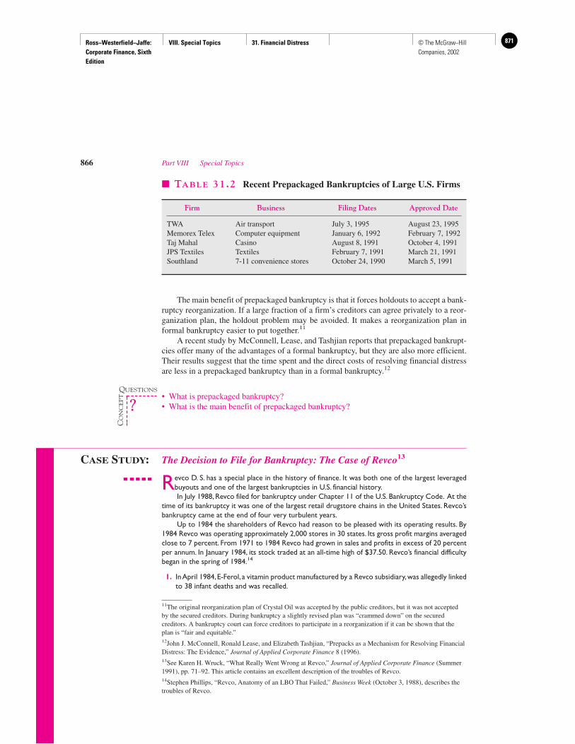
Ross−Westerfield−Jaffe: Corporate Finance, Sixth Edition
VIII. Special Topics 31. Financial Distress 871© The McGraw−Hill Companies, 2002
The main benefit of prepackaged bankruptcy is that it forces holdouts to accept a bank-ruptcy reorganization. If a large fraction of a firm’s creditors can agree privately to a reor-ganization plan, the holdout problem may be avoided. It makes a reorganization plan informal bankruptcy easier to put together.11
A recent study by McConnell, Lease, and Tashjian reports that prepackaged bankrupt-cies offer many of the advantages of a formal bankruptcy, but they are also more efficient.Their results suggest that the time spent and the direct costs of resolving financial distressare less in a prepackaged bankruptcy than in a formal bankruptcy.12
• What is prepackaged bankruptcy?• What is the main benefit of prepackaged bankruptcy?
CASE STUDY: The Decision to File for Bankruptcy: The Case of Revco13
Revco D. S. has a special place in the history of finance. It was both one of the largest leveragedbuyouts and one of the largest bankruptcies in U.S. financial history.In July 1988, Revco filed for bankruptcy under Chapter 11 of the U.S. Bankruptcy Code. At the
time of its bankruptcy it was one of the largest retail drugstore chains in the United States. Revco’sbankruptcy came at the end of four very turbulent years.
Up to 1984 the shareholders of Revco had reason to be pleased with its operating results. By1984 Revco was operating approximately 2,000 stores in 30 states. Its gross profit margins averagedclose to 7 percent. From 1971 to 1984 Revco had grown in sales and profits in excess of 20 percentper annum. In January 1984, its stock traded at an all-time high of $37.50. Revco’s financial difficultybegan in the spring of 1984.14
1. In April 1984,E-Ferol, a vitamin product manufactured by a Revco subsidiary,was allegedly linkedto 38 infant deaths and was recalled.
866 Part VIII Special Topics
� TABLE 31.2 Recent Prepackaged Bankruptcies of Large U.S. Firms
Firm Business Filing Dates Approved Date
TWA Air transport July 3, 1995 August 23, 1995Memorex Telex Computer equipment January 6, 1992 February 7, 1992Taj Mahal Casino August 8, 1991 October 4, 1991JPS Textiles Textiles February 7, 1991 March 21, 1991Southland 7-11 convenience stores October 24, 1990 March 5, 1991
11The original reorganization plan of Crystal Oil was accepted by the public creditors, but it was not acceptedby the secured creditors. During bankruptcy a slightly revised plan was “crammed down” on the securedcreditors. A bankruptcy court can force creditors to participate in a reorganization if it can be shown that theplan is “fair and equitable.”12John J. McConnell, Ronald Lease, and Elizabeth Tashjian, “Prepacks as a Mechanism for Resolving FinancialDistress: The Evidence,” Journal of Applied Corporate Finance 8 (1996).13See Karen H. Wruck, “What Really Went Wrong at Revco,” Journal of Applied Corporate Finance (Summer1991), pp. 71–92. This article contains an excellent description of the troubles of Revco.14Stephen Phillips, “Revco, Anatomy of an LBO That Failed,” Business Week (October 3, 1988), describes thetroubles of Revco.
QUESTIONS
CO
NC
EP
T
?
Ross−Westerfield−Jaffe: Corporate Finance, Sixth Edition
VIII. Special Topics 31. Financial Distress872 © The McGraw−Hill Companies, 2002
2. In May 1984, Revco acquired Odd Lot Trading, Inc., for over $100 million of Revco commonstock.The acquisition gave Barnard Marden and Isaac Perlmutter, owners of Odd Lot Trading, 12percent ownership in Revco. However, Perlmutter and Marden were not passive investors, andthey had many new ideas for “improving” Revco. Eventually, hostility broke out between Perl-mutter and Marden and Stanley Dworkin, the CEO of Revco.
3. In 1985 Revco’s competitors, Rite-Aid and Eckerd, adopted aggressive pricing tactics in an at-tempt to gain market share.
4. In July 1985, Revco bought out Marden’s and Perlmutter’s stakes in Revco for $98 million.5. On December 29, 1986, Revco announced a leveraged buyout (LBO) with a private investor
group.Because of the LBO,Revco’s long-term debt increased from $44.7 million in 1985 to over$700 million after the LBO in 1986. Eventually, its total debt rose to $1.3 billion, and, in April1988, Revco announced that it could not make the interest payment on its subordinated notes.
6. In March 1987, Revco decided to change its strategic orientation. Instead of “everyday lowprices” on a narrow product line, Revco expanded its product line to include TVs, furniture, andappliances, and used selective promotions.
7. The new strategic orientation did not work, and Revco generated large losses in 1987.8. In July 1988, Revco filed for bankruptcy under Chapter 11 of the Bankruptcy Code.9. Four years later, Revco emerged from bankruptcy.
10. On June 2, 1997, Revco was merged into CVS in a $2.9 billion stock swap, making CVS the sec-ond largest drugstore chain in the United States. It was reported that CVS would close Revco’sheadquarters in Twinsburg, Ohio, and reduce costs by eliminating redundant corporate officesand outlets.
Why did Revco file for formal bankruptcy instead of private restructuring? What were the costsof the Revco bankruptcy? There are no easy answers to these questions.
1. The Direct Costs of Bankruptcy. Formal bankruptcy can be expensive and time-consuming. Revcowas in Chapter 11 bankruptcy for almost four years and paid out over $40.5 million in directbankruptcy costs (2.7 percent of the buyout price).15 Below are some of the direct bankruptcyfees (in millions).
Law firmsBaker & Hostetler $ 7.5Fried Frank 3.2
Accounting firmsArthur Andersen 7.4Ernst & Young 4.2
Investment bankersLazard Freres 3.5Other 14.3
$40.5
2. The Indirect Costs of Financial Distress. There are many indirect costs of financial distress, includingmanagement distractions, loss of customers, and loss of reputation.The indirect costs of financialdistress may occur whether or not formal bankruptcy is declared. In the case of Revco, financialdistress caused a costly change in management and strategic direction.
3. The Costs of a Complicated Financial Structure. Firms such as Revco that have bank loans, senior sub-ordinated debt, and junior subordinated debt will have a very hard time getting all claimholdersto agree to an out-of-court settlement. For a retailer like Revco private agreements are especiallydifficult because of the large number of trade creditors. It is axiomatic that the more complicateda firm’s financial structure, the more difficult it will be to work out private arrangements to avoidbankruptcy. Conflicts between managers, shareholders, and creditors make reaching a privateagreement difficult.There is a natural tendency for each group to try to gain value at the expenseof the others.
Chapter 31 Financial Distress 867
15George Anders, “Revco Saga: On How the Buy Out Bonanza Became a Frenzy of Fees in Chapter 11,” TheWall Street Journal (May 16, 1991).
Ross−Westerfield−Jaffe: Corporate Finance, Sixth Edition
VIII. Special Topics 31. Financial Distress 873© The McGraw−Hill Companies, 2002
• Why did it take Revco D. S. so long to emerge from bankruptcy?• What are some of the costs of the Revco D. S. bankruptcy?
31.6 SUMMARY AND CONCLUSIONS
This chapter examines what happens when firms experience financial distress.
1. Financial distress is a situation where a firm’s operating cash flow is not sufficient to covercontractual obligations. Financially distressed firms are often forced to take corrective actionand undergo financial restructuring. Financial restructuring involves exchanging newfinancial claims for old ones.
2. Financial restructuring can be accomplished with a private workout or formal bankruptcy.Financial restructuring can involve liquidation or reorganization. However, liquidation is notcommon.
3. Corporate bankruptcy involves Chapter 7 liquidation or Chapter 11 reorganization. Anessential feature of the U.S. Bankruptcy Code is the absolute priority rule. The absolutepriority rule states that senior creditors are paid in full before junior creditors receiveanything. However, in practice the absolute priority rule is often violated.
4. A new form of financial restructuring is prepackaged bankruptcy. It is a hybrid of a privateworkout and formal bankruptcy.
5. One of the most well-known bankruptcies involved Revco D. S. Revco’s bankruptcy waslong and costly. The main reason was Revco’s complicated financial structure, which madeagreement among creditors very difficult.
KEY TERMS
Absolute priority rule 859 Prepackaged bankruptcy 865Financial distress 854 Private workout 863Liquidation 858 Reorganization 858
SUGGESTED READINGS
An excellent book on financial distress by one of the leading authorities isAltman, Edward I. Corporate Financial Distress: A Complete Guide to Predicting, Avoiding and
Dealing with Bankruptcy (New York: John Wiley & Sons, 1983).
Many recent academic articles on financial distress can be found inJenson, Michael, and Richard Rubeck, eds. “Symposium on the Structure and Governance of
Enterprise Part II.” Journal of Financial Economics 27 (1990). Articles by Lawrence Weiss,Stuart G. Gilson, Kose John, Larry N. P. Lang, Steven Kaplan, David Reishus, FrankEasterbrook, and Karen H. Wruck appear.
Senbet, L., and James Seward. “Financial Distress, Bankruptcy and Reorganization.” Chapter28 in Handbooks in OR and MS, Vol. 9, R. A. Jarrow, V. Maksimovic, and W. T. Ziembe,eds. (1995).
868 Part VIII Special Topics
QUESTIONS
CO
NC
EP
T
?
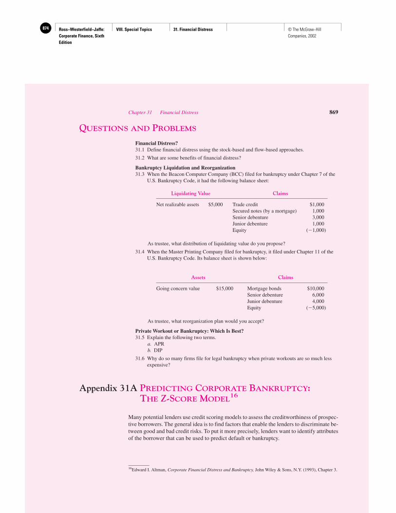
Ross−Westerfield−Jaffe: Corporate Finance, Sixth Edition
VIII. Special Topics 31. Financial Distress874 © The McGraw−Hill Companies, 2002
QUESTIONS AND PROBLEMS
Financial Distress?31.1 Define financial distress using the stock-based and flow-based approaches.
31.2 What are some benefits of financial distress?
Bankruptcy Liquidation and Reorganization31.3 When the Beacon Computer Company (BCC) filed for bankruptcy under Chapter 7 of the
U.S. Bankruptcy Code, it had the following balance sheet:
Liquidating Value Claims
Net realizable assets $5,000 Trade credit $1,000Secured notes (by a mortgage) 1,000Senior debenture 3,000Junior debenture 1,000Equity (�1,000)
As trustee, what distribution of liquidating value do you propose?
31.4 When the Master Printing Company filed for bankruptcy, it filed under Chapter 11 of theU.S. Bankruptcy Code. Its balance sheet is shown below:
Assets Claims
Going concern value $15,000 Mortgage bonds $10,000Senior debenture 6,000Junior debenture 4,000Equity (�5,000)
As trustee, what reorganization plan would you accept?
Private Workout or Bankruptcy: Which Is Best?31.5 Explain the following two terms.
a. APRb. DIP
31.6 Why do so many firms file for legal bankruptcy when private workouts are so much lessexpensive?
Appendix 31A PREDICTING CORPORATE BANKRUPTCY: THE Z-SCORE MODEL
16
Many potential lenders use credit scoring models to assess the creditworthiness of prospec-tive borrowers. The general idea is to find factors that enable the lenders to discriminate be-tween good and bad credit risks. To put it more precisely, lenders want to identify attributesof the borrower that can be used to predict default or bankruptcy.
Chapter 31 Financial Distress 869
16Edward I. Altman, Corporate Financial Distress and Bankruptcy, John Wiley & Sons, N.Y. (1993), Chapter 3.
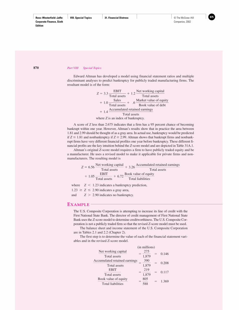
Ross−Westerfield−Jaffe: Corporate Finance, Sixth Edition
VIII. Special Topics 31. Financial Distress 875© The McGraw−Hill Companies, 2002
Edward Altman has developed a model using financial statement ratios and multiplediscriminant analyses to predict bankruptcy for publicly traded manufacturing firms. Theresultant model is of the form:
where Z is an index of bankruptcy.
A score of Z less than 2.675 indicates that a firm has a 95 percent chance of becomingbankrupt within one year. However, Altman’s results show that in practice the area between1.81 and 2.99 should be thought of as a gray area. In actual use, bankruptcy would be predictedif Z � 1.81 and nonbankruptcy if Z � 2.99. Altman shows that bankrupt firms and nonbank-rupt firms have very different financial profiles one year before bankruptcy. These different fi-nancial profits are the key intuition behind the Z-score model and are depicted in Table 31A.1.
Altman’s original Z-score model requires a firm to have publicly traded equity and bea manufacturer. He uses a revised model to make it applicable for private firms and non-manufacturers. The resulting model is
where Z 1.23 indicates a bankruptcy prediction,
1.23 � Z � 2.90 indicates a gray area,
and Z � 2.90 indicates no bankruptcy.
EXAMPLE
The U.S. Composite Corporation is attempting to increase its line of credit with theFirst National State Bank. The director of credit management of First National StateBank uses the Z-score model to determine creditworthiness. The U.S. Composite Cor-poration is not a publicly traded firm so that the revised Z-score model must be used.
The balance sheet and income statement of the U.S. Composite Corporationare in Tables 2.1 and 2.2 (Chapter 2).
The first step is to determine the value of each of the financial statement vari-ables and in the revised Z-score model.
(in millions)
� 0.146
� 0.208
� 0.117
� 1.369�805
588 Book value of equity
Total liabilities
�219
1,879
EBIT
Total assets
�390
1,879 Accumulated retained earnings
Total assets
�275
1,879 Net working capital
Total assets
� 1.05 EBIT
Total assets� 6.72
Book value of equity
Total liabilities
Z � 6.56 Net working capital
Total assets� 3.26
Accumulated retained earnings
Total assets
� 1.4 Accumulated retained earnings
Total assets
� 1.0 Sales
Total assets� .6
Market value of equity
Book value of debt
Z � 3.3 EBIT
Total assets� 1.2
Net working capital
Total assets
870 Part VIII Special Topics
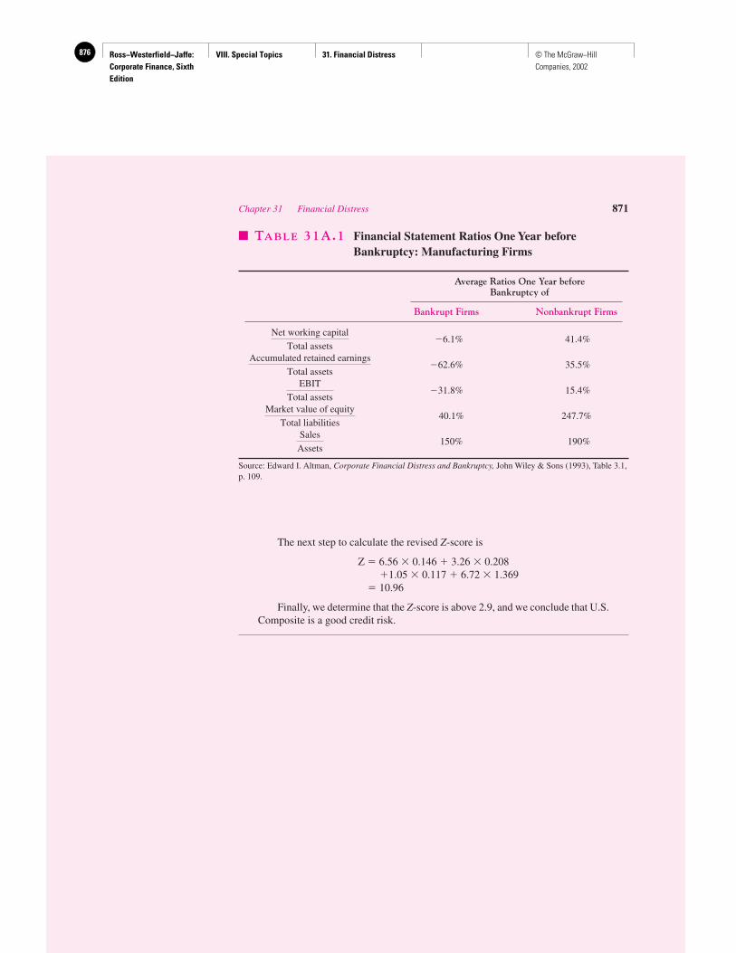
Ross−Westerfield−Jaffe: Corporate Finance, Sixth Edition
VIII. Special Topics 31. Financial Distress876 © The McGraw−Hill Companies, 2002
The next step to calculate the revised Z-score is
Z � 6.56 � 0.146 � 3.26 � 0.208�1.05 � 0.117 � 6.72 � 1.369
� 10.96
Finally, we determine that the Z-score is above 2.9, and we conclude that U.S.Composite is a good credit risk.
Chapter 31 Financial Distress 871
� TABLE 31A.1 Financial Statement Ratios One Year beforeBankruptcy: Manufacturing Firms
Average Ratios One Year beforeBankruptcy of
Bankrupt Firms Nonbankrupt Firms
�6.1% 41.4%
�62.6% 35.5%
�31.8% 15.4%
40.1% 247.7%
150% 190%
Source: Edward I. Altman, Corporate Financial Distress and Bankruptcy, John Wiley & Sons (1993), Table 3.1,p. 109.
Sales
Assets
Market value of equity
Total liabilities
EBIT
Total assets
Accumulated retained earnings
Total assets
Net working capital
Total assets
Ross−Westerfield−Jaffe: Corporate Finance, Sixth Edition
VIII. Special Topics 32. International Corporate Finance
877© The McGraw−Hill Companies, 2002
International Corporate Finance
CH
AP
TE
R32
EXECUTIVE SUMMARY
Corporations that have significant foreign operations are often referred to as interna-tional corporations or multinationals. Table 32.1 lists the largest international cor-porations using several different measures. There are many familiar names on this
list. International corporations must consider many financial factors that do not directly af-fect purely domestic firms. These include foreign exchange rates, different interest ratesfrom country to country, complex accounting methods for foreign operations, foreign taxrates, and foreign government intervention.
The basic principles of corporate finance still apply to international corporations;like domestic companies, they seek to invest in projects that create more value for theshareholders than they cost and to arrange financing that raises cash at the lowest pos-sible cost. That is, the net present value principle holds for both foreign and domesticoperations. However, it is usually more complicated to apply the NPV principle to for-eign operations.
Perhaps the most important complication of international finance is foreign exchange.The foreign exchange markets provide information and opportunities for an internationalcorporation when it undertakes capital-budgeting and financing decisions. The relationshipamong foreign exchange, interest rates, and inflation is defined by the basic theories of ex-change rates: purchasing-power parity, interest-rate parity, and the expectations theory.
Typically, international financing decisions involve a choice of three basic approaches:
1. Export domestic cash to the foreign operations.
2. Borrow in the country where the investment is located.
3. Borrow in a third country.
We discuss the merits of each approach.
32.1 TERMINOLOGY
A common buzzword for the student of finance is globalization. The first step in learningabout the globalization of financial markets is to conquer the new vocabulary. Here aresome of the most common terms used in international finance and in this chapter:
1. An American Depository Receipt (ADR) is a security issued in the United States to rep-resent shares of a foreign stock, allowing that stock to be traded in the United States. For-eign companies use ADRs, which are issued in U.S. dollars, to expand the pool of poten-tial U.S. investors. ADRs are available in two forms for about 690 foreign companies:
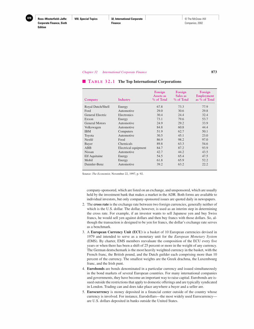
Ross−Westerfield−Jaffe: Corporate Finance, Sixth Edition
VIII. Special Topics 32. International Corporate Finance
878 © The McGraw−Hill Companies, 2002
company-sponsored, which are listed on an exchange, and unsponsored, which are usuallyheld by the investment bank that makes a market in the ADR. Both forms are available toindividual investors, but only company-sponsored issues are quoted daily in newspapers.
2. The cross rate is the exchange rate between two foreign currencies, generally neither ofwhich is the U.S. dollar. The dollar, however, is used as an interim step in determiningthe cross rate. For example, if an investor wants to sell Japanese yen and buy Swissfrancs, he would sell yen against dollars and then buy francs with those dollars. So, al-though the transaction is designed to be yen for francs, the dollar’s exchange rate servesas a benchmark.
3. A European Currency Unit (ECU) is a basket of 10 European currencies devised in1979 and intended to serve as a monetary unit for the European Monetary System(EMS). By charter, EMS members reevaluate the composition of the ECU every fiveyears or when there has been a shift of 25 percent or more in the weight of any currency.The German deutschemark is the most heavily weighted currency in the basket, with theFrench franc, the British pound, and the Dutch guilder each comprising more than 10percent of the currency. The smallest weights are the Greek drachma, the Luxembourgfranc, and the Irish punt.
4. Eurobonds are bonds denominated in a particular currency and issued simultaneouslyin the bond markets of several European countries. For many international companiesand governments, they have become an important way to raise capital. Eurobonds are is-sued outside the restrictions that apply to domestic offerings and are typically syndicatedin London. Trading can and does take place anywhere a buyer and a seller are.
5. Eurocurrency is money deposited in a financial center outside of the country whosecurrency is involved. For instance, Eurodollars—the most widely used Eurocurrency—are U.S. dollars deposited in banks outside the United States.
Chapter 32 International Corporate Finance 873
� TABLE 32.1 The Top International Corporations
Foreign Foreign ForeignAssets as Sales as Employment
Company Industry % of Total % of Total as % of Total
Royal Dutch/Shell Energy 67.8 73.3 77.9Ford Automotive 29.0 30.6 29.8General Electric Electronics 30.4 24.4 32.4Exxon Energy 73.1 79.6 53.7General Motors Automotive 24.9 29.2 33.9Volkswagen Automotive 84.8 60.8 44.4IBM Computers 51.9 62.7 50.1Toyota Automotive 30.5 45.1 23.0Nestlé Food 86.9 98.2 97.0Bayer Chemicals 89.8 63.3 54.6ABB Electrical equipment 84.7 87.2 93.9Nissan Automotive 42.7 44.2 43.5Elf Aquitaine Energy 54.5 65.4 47.5Mobil Energy 61.8 65.9 52.2Daimler-Benz Automotive 39.2 63.2 22.2
Source: The Economist, November 22, 1997, p. 92.
Ross−Westerfield−Jaffe: Corporate Finance, Sixth Edition
VIII. Special Topics 32. International Corporate Finance
879© The McGraw−Hill Companies, 2002
6. Foreign bonds, unlike Eurobonds, are issued by foreign borrowers in another nation’scapital market and traditionally denominated in that nation’s currency. Yankee bonds, forexample, are issued in the United States by a foreign country, bank, or company; in re-cent years, however, some Yankee offerings have been denominated in currencies otherthan the U.S. dollar. Often the country in which these bonds are issued will draw dis-tinctions between them and bonds issued by domestic issuers, including different taxlaws, restrictions on the amount of issues, or tougher disclosure rules.
Foreign bonds often are nicknamed for the country of issuance: Yankee bonds(United States), Samurai bonds (Japan), Rembrandt bonds (the Netherlands), and Bull-dog bonds (Britain). Partly because of tougher regulations and disclosure requirements,the foreign-bond market hasn’t grown in the past several years with the vigor of the Eu-robond market. Nearly half of all foreign bonds are issued in Switzerland.
7. Gilts, technically, are British and Irish government securities, although the term also in-cludes issues of local British authorities and some overseas public-sector offerings.
8. The London Interbank Offered Rate (LIBOR) is the rate that most internationalbanks charge one another for loans of Eurodollars overnight in the London market.LIBOR is a cornerstone in the pricing of money-market issues and other short-termdebt issues by both governments and corporate borrowers. Less creditworthy issuerswill often borrow at a rate of more than one point over LIBOR.
9. There are two basic kinds of swaps: interest rate and currency. An interest-rate swap oc-curs when two parties exchange debt with a floating-rate payment for debt with a fixed-rate payment, or vice versa. Currency swaps are agreements to deliver one currencyagainst another currency. Often both types of swaps are used in the same transactionwhen debt denominated in different currencies is swapped.
• What is the difference between a Eurobond and a foreign bond?
32.2 FOREIGN EXCHANGE MARKETS AND EXCHANGE RATES
The foreign exchange market is undoubtedly the world’s largest financial market. It is themarket where one country’s currency is traded for another’s. Most of the trading takes placein a few currencies: the U.S. dollar ($), German deutschemark (DM), British pound sterling(£), Japanese yen (¥), Swiss franc (SF), and French franc (FF).
The foreign exchange market is an over-the-counter market. There is no single locationwhere traders get together. Instead, traders are located in the major commercial and invest-ment banks around the world. They communicate using computer terminals, telephones,and other telecommunication devices. One element in the communications network for for-eign transactions is the Society for Worldwide Interbank Financial Telecommunications(SWIFT). It is a Belgian not-for-profit cooperative. A bank in New York can send messagesto a bank in London via SWIFT’s regional processing centers. The connections are throughdata-transmission lines.
The many different types of participants in the foreign exchange market include thefollowing:
1. Importers who convert their domestic currency to foreign currency to pay for goods fromforeign countries.
874 Part VIII Special Topics
QUESTION
CO
NC
EP
T
?
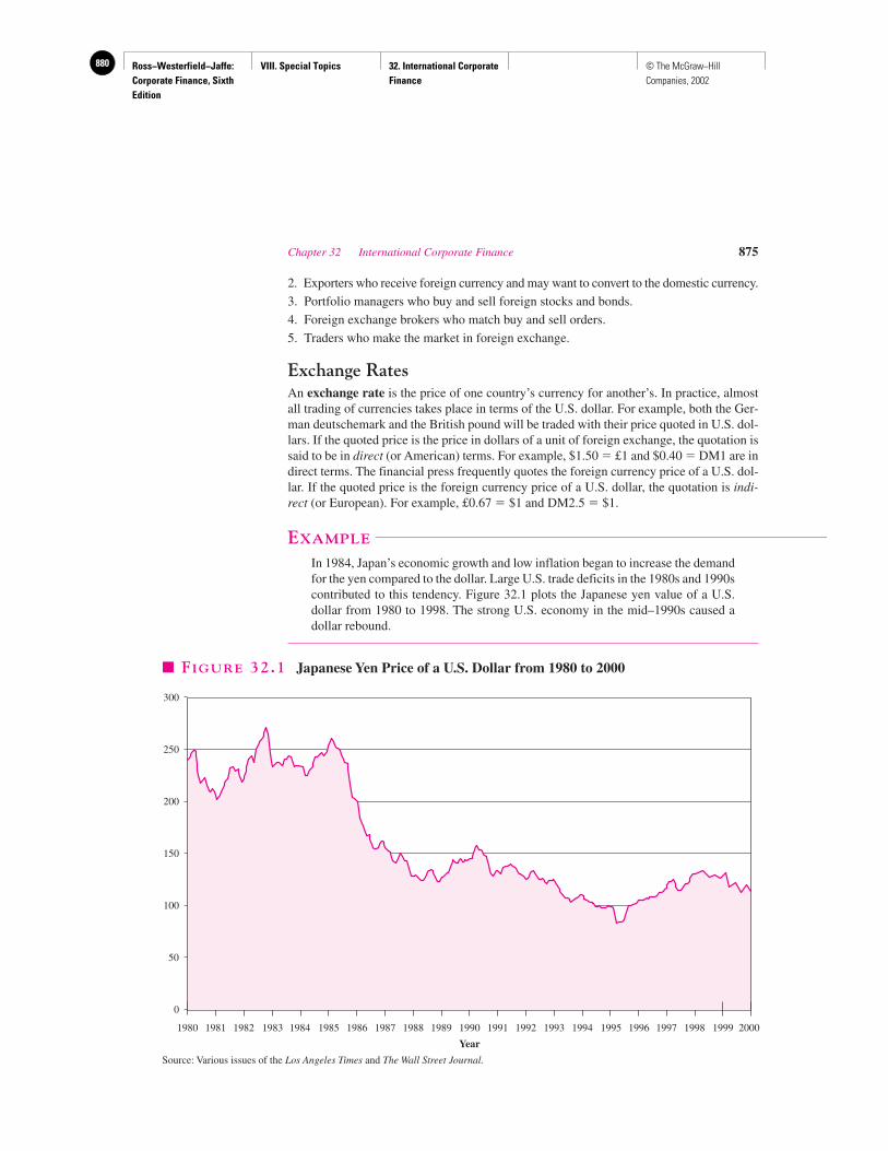
Ross−Westerfield−Jaffe: Corporate Finance, Sixth Edition
VIII. Special Topics 32. International Corporate Finance
880 © The McGraw−Hill Companies, 2002
2. Exporters who receive foreign currency and may want to convert to the domestic currency.
3. Portfolio managers who buy and sell foreign stocks and bonds.
4. Foreign exchange brokers who match buy and sell orders.
5. Traders who make the market in foreign exchange.
Exchange RatesAn exchange rate is the price of one country’s currency for another’s. In practice, almostall trading of currencies takes place in terms of the U.S. dollar. For example, both the Ger-man deutschemark and the British pound will be traded with their price quoted in U.S. dol-lars. If the quoted price is the price in dollars of a unit of foreign exchange, the quotation issaid to be in direct (or American) terms. For example, $1.50 � £1 and $0.40 � DM1 are indirect terms. The financial press frequently quotes the foreign currency price of a U.S. dol-lar. If the quoted price is the foreign currency price of a U.S. dollar, the quotation is indi-rect (or European). For example, £0.67 � $1 and DM2.5 � $1.
EXAMPLE
In 1984, Japan’s economic growth and low inflation began to increase the demandfor the yen compared to the dollar. Large U.S. trade deficits in the 1980s and 1990scontributed to this tendency. Figure 32.1 plots the Japanese yen value of a U.S.dollar from 1980 to 1998. The strong U.S. economy in the mid–1990s caused adollar rebound.
Chapter 32 International Corporate Finance 875
300
1980
250
200
150
100
50
0
1981 1982 1983 1984 1985 1986 1987 1988 1989 1990 1991 1992 1993 1994 1995 1996 1997 1998 1999 2000
Year
� FIGURE 32.1 Japanese Yen Price of a U.S. Dollar from 1980 to 2000
Source: Various issues of the Los Angeles Times and The Wall Street Journal.
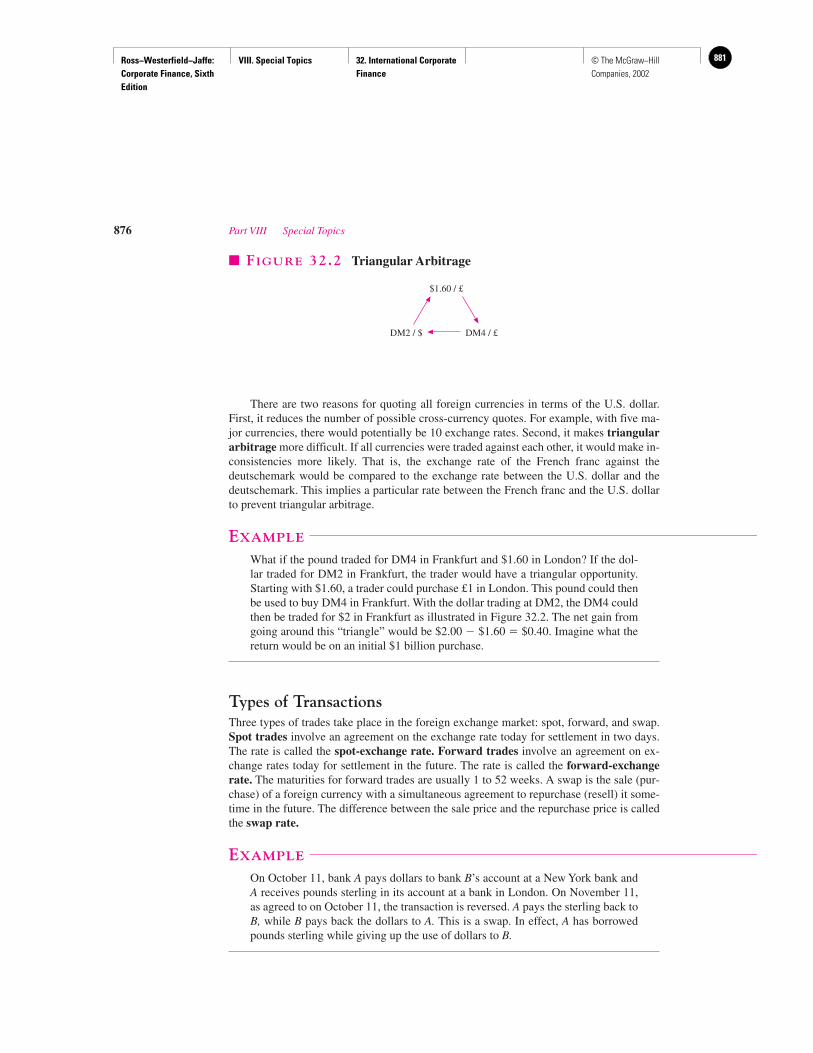
Ross−Westerfield−Jaffe: Corporate Finance, Sixth Edition
VIII. Special Topics 32. International Corporate Finance
881© The McGraw−Hill Companies, 2002
There are two reasons for quoting all foreign currencies in terms of the U.S. dollar.First, it reduces the number of possible cross-currency quotes. For example, with five ma-jor currencies, there would potentially be 10 exchange rates. Second, it makes triangulararbitrage more difficult. If all currencies were traded against each other, it would make in-consistencies more likely. That is, the exchange rate of the French franc against thedeutschemark would be compared to the exchange rate between the U.S. dollar and thedeutschemark. This implies a particular rate between the French franc and the U.S. dollarto prevent triangular arbitrage.
EXAMPLE
What if the pound traded for DM4 in Frankfurt and $1.60 in London? If the dol-lar traded for DM2 in Frankfurt, the trader would have a triangular opportunity.Starting with $1.60, a trader could purchase £1 in London. This pound could thenbe used to buy DM4 in Frankfurt. With the dollar trading at DM2, the DM4 couldthen be traded for $2 in Frankfurt as illustrated in Figure 32.2. The net gain fromgoing around this “triangle” would be $2.00 � $1.60 � $0.40. Imagine what thereturn would be on an initial $1 billion purchase.
Types of TransactionsThree types of trades take place in the foreign exchange market: spot, forward, and swap.Spot trades involve an agreement on the exchange rate today for settlement in two days.The rate is called the spot-exchange rate. Forward trades involve an agreement on ex-change rates today for settlement in the future. The rate is called the forward-exchangerate. The maturities for forward trades are usually 1 to 52 weeks. A swap is the sale (pur-chase) of a foreign currency with a simultaneous agreement to repurchase (resell) it some-time in the future. The difference between the sale price and the repurchase price is calledthe swap rate.
EXAMPLE
On October 11, bank A pays dollars to bank B’s account at a New York bank andA receives pounds sterling in its account at a bank in London. On November 11,as agreed to on October 11, the transaction is reversed. A pays the sterling back toB, while B pays back the dollars to A. This is a swap. In effect, A has borrowedpounds sterling while giving up the use of dollars to B.
876 Part VIII Special Topics
$1.60 / £
DM2 / $ DM4 / £
� FIGURE 32.2 Triangular Arbitrage
Ross−Westerfield−Jaffe: Corporate Finance, Sixth Edition
VIII. Special Topics 32. International Corporate Finance
882 © The McGraw−Hill Companies, 2002
32.3 THE LAW OF ONE PRICE AND PURCHASING-POWER
PARITY
What determines the level of the spot-exchange rate? One answer is the law of one price(LOP). The law of one price says that a commodity will cost the same regardless of thecountry in which it is purchased. More formally, let S£(t) be the spot-exchange rate, that is,the number of dollars needed to purchase a British pound at time t.1 Let PUS(t) and PUK(t)be the current U.S. and British prices of a particular commodity, say, apples. The law of oneprice says that
PUS(t) � S£(t) PUK(t)for apples.
The rationale behind LOP is similar to that of triangular arbitrage. If LOP did not hold,arbitrage would be possible by moving apples from one country to another. For example,suppose that apples in New York are selling for $4 per bushel, while in London the price is£2.50 per bushel. Then the law of one price implies that
$4 � S£(t) � £2.50
and
S£(t) � $1.60/£
That is, the LOP implied spot-exchange rate is $1.60 per pound.Suppose instead that the actual exchange rate is $2.00 per pound. Starting with $4, a
trader could buy a bushel of apples in New York, ship it to London, and sell it there for£2.50. The pounds sterling could then be converted into dollars at the exchange rate, $2/£,yielding a total of $5 for $1 ($5 � $4) gain.
The rationale of the LOP is that if the exchange rate is not $1.60/£ but is instead, say,$2/£, then forces would be set in motion to change the rate and/or the price of apples. In ourexample, there would be a whole lot of apples flying from New York to London. Thus, de-mand for apples in New York would raise the dollar price for apples there, and the supplyin London would lower the pound-sterling price. The apple traders converting pounds ster-ling into dollars, that is, supplying pounds sterling and demanding dollars, would also putpressure on the exchange rate to fall from $2/£.
As you can see, for the LOP to be strictly true, three assumptions are needed:
1. The transactions cost of trading apples—shipping, insurance, wastage, and so on—mustbe zero.
2. No barriers to trading apples, such as tariffs or taxes, can exist.
3. Finally, an apple in New York must be identical to an apple in London. It won’t do foryou to send red apples to London if the English eat only green apples.
Given the fact that the transaction costs are not zero and that the other conditions arerarely exactly met, the LOP is really applicable only to traded goods, and then only to veryuniform ones. The LOP does not imply that a Mercedes costs the same as a Ford or that anuclear power plant in France costs the same as one in New York. In the case of the cars,they are not identical. In the case of the power plants, even if they were identical, they areexpensive and very difficult to ship.
Chapter 32 International Corporate Finance 877
1Throughout this chapter, we quote foreign exchange in direct or American terms.
Ross−Westerfield−Jaffe: Corporate Finance, Sixth Edition
VIII. Special Topics 32. International Corporate Finance
883© The McGraw−Hill Companies, 2002
Because consumers purchase many goods, economists speak of purchasing-powerparity (PPP), the idea that the exchange rate adjusts so that a market basket of goods coststhe same, regardless of the country in which it is purchased. In addition, a relative versionof purchasing-power parity has evolved. Relative purchasing-power parity (RPPP) saysthat the rate of change in the price level of commodities in one country relative to the rateof change in the price level in another determines the rate of change of the exchange ratebetween the two countries. Formally,
� �
1 � U.S. 1 � Change in 1 � Britishinflation rate
�foreign exchange rate
�inflation rate
This states that the rate of inflation in the United States relative to that in Great Britain de-termines the rate of change in the value of the dollar relative to that of the pound duringthe interval t to t � 1. It is common to write �US as the rate of inflation in the United States.1 � �US is equal to PUS(t � 1)/PUS(t). Similarly, �UK is the rate of inflation in GreatBritain. 1 � �UK is equal to PUK(t � 1)/PUK(t).
Using � to represent the rate of inflation, the preceding equation can be rearranged as
(32.1)
We can rewrite this in an appropriate form as
where•S£/S£ now stands for the rate of change in the dollars-per-pound exchange rate.
As an example, suppose that inflation in France during the year is equal to 4 percentand inflation in the United States is equal to 10 percent. Then, according to the RPPP, theprice of the French franc in terms of the U.S. dollar should rise; that is, the U.S. dollar de-clines in value in terms of the French franc. Using our approximation, the dollars-per-francexchange rate should rise by
� 10% � 4%� 6%
where •SFF/SFF stands for the rate of change in the dollars-per-franc exchange rate. That is,
if the French franc is worth $0.20 at the beginning of the period, it should be worth ap-proximately $0.212 ($0.20 � 1.06) at the end of the period.
The RPPP says that the change in the ratio of domestic commodity prices of two coun-tries must be matched in the exchange rate. This version of the law of one price suggests thatto estimate changes in the spot rate of exchange, it is necessary to estimate the difference inrelative inflation rates. In other words, we can express our formula in expectational terms as
If we expect the U.S. inflation rate to exceed the French inflation rate, we should expect thedollar price of French francs to rise, which is the same as saying that the dollar is expectedto fall against the franc.
E�•SFF
SFF� � E ��US� � E ��F�
•SFF
SFF
� �US � �F
�US � �UK �•S£
S£
1 � �US
1 � �UK
�S£ �t � 1�
S£ �t�
PUK �t � 1�PUK �t�
S£ �t � 1�S£ �t�
PUS �t � 1�PUS �t�
878 Part VIII Special Topics
Ross−Westerfield−Jaffe: Corporate Finance, Sixth Edition
VIII. Special Topics 32. International Corporate Finance
884 © The McGraw−Hill Companies, 2002
The more exact relationship of equation (32.1) can be expressed in expectational terms as
(32.2)
• What is the law of one price? What is purchasing-power parity?• What is the relationship between inflation and exchange-rate movements?
32.4 INTEREST RATES AND EXCHANGE RATES: INTEREST-RATE PARITY
The forward-exchange rate and the spot-exchange rate are tied together by the same sort ofarbitrage that underlies the law of one price. First, here is some useful terminology. If forward-exchange rates are greater than the spot-exchange rate in a particular currency, the forwardforeign currency is said to be at a premium (this implies the domestic currency is at a dis-count). If the values of forward-exchange rates are less than the spot-exchange rate, the for-ward rate of foreign currency is at a discount.
Suppose we observe that the spot DM rate is DM2.50 � $1.00 and the one-month forwardDM is DM2.40 � $1.00. Because fewer marks are needed to buy a dollar at the forward ratethan are needed to buy a dollar at the spot rate, the mark is more valuable in the forward marketthan in the spot market. This means that the one-month forward DM is at a premium. Of course,whatever we say for the mark must be the opposite of what we say for the dollar. In this exam-ple, the dollar is at a discount because the forward value is less than the spot value. Forward ex-change is quoted in terms of the premium or discount that is to be added onto the spot rate.
Whether forward rates are at a premium or a discount when compared to a domesticcurrency depends on the relative interest rates in the foreign and domestic currency mar-kets. The interest-rate–parity theorem implies that, if interest rates are higher domesti-cally than in a particular foreign country, the foreign country’s currency will be selling at apremium in the forward market; and if interest rates are lower domestically, the foreign cur-rency will be selling at a discount in the forward market.
We need some notation to develop the interest-rate–parity theorem. Let S(0) be the cur-rent domestic-currency price of spot foreign exchange (current time is denoted by 0). If thedomestic currency is the dollar and the foreign exchange is the deutschemark, we might ob-serve S(0) � $0.40/DM. S(0) is in direct or U.S. terms. Let F(0,1) be the current domestic-currency price of forward exchange for a contract that matures in one month. Thus, the con-tract is for forward exchange one month hence. Let i and i* be the yearly rates of interestpaid on Eurocurrency deposits denominated in the domestic (i) and foreign (i*) currencies,respectively. Of course, the maturity of the deposits can be chosen to coincide with the ma-turity of the forward contract. Now consider a trader who has access to the interbank mar-ket in foreign exchange and Eurocurrency deposits. Suppose the trader has some dollars toinvest for one month. The trader can make a dollar loan or a deutschemark loan. The annualinterest rate is 10 percent in deutschemarks and 6 percent in dollars. Which is better?
The Dollar InvestmentGiven an annual interest rate of 6 percent, the one-month rate of interest is 0.5 percent, ig-noring compounding. If the trader invests $1 million now, the trader will get $1 million �1.005 � $1.005 million at the end of the month. Following is an illustration:
E �1 � �US�E �1 � �UK�
�E S£ �t � 1� �
S£ �t�
Chapter 32 International Corporate Finance 879
QUESTIONS
CO
NC
EP
T
?
Ross−Westerfield−Jaffe: Corporate Finance, Sixth Edition
VIII. Special Topics 32. International Corporate Finance
885© The McGraw−Hill Companies, 2002
Time 0 Time 1
Lend 1 unit of dollars Obtain 1 � i � (1/12) units of domestic currency$1,000,000 $1,000,000 � (1 � 0.005) � $1,005,000
The Deutschemark InvestmentThe current spot rate is $0.40/DM. This means the trader can currently obtain $1 mil-lion/0.40 � DM2.5 million. The rate of interest on one-year DM loans is 10 percent. Forone month, the interest rate is 0.10/12 � 0.0083. Thus, at the end of one month the traderwill obtain DM2.5 million � 1.0083 � DM2,520,750. Of course, if the trader wants dol-lars at the end of the month, the trader must convert the deutschemarks back into dollars.The trader can fix the exchange rate for one-month conversion. Suppose the one-month for-ward is $0.39869/DM. Then the trader can sell deutschemarks forward. This will ensurethat the trader gets DM2,520,750 � 0.39869 � $1.005 million at the end of the month. Thegeneral relationships are set forth here:
Time 0 Time 1
Purchase 1 unit [1/S(0)] Deposit matures and paysof foreign exchange [1/S(0)] � [1 � i � (1/12)]
units of foreign exchangeDM2,500,000 DM2,500,000 � 1.0083 � DM2,520,750
Sell forward Deliver foreign exchange in fulfillment[1/S(0)] � [1 � i* � (1/12)] of forward contract, receivingunits of forward exchangeat the forward rate F(0,1) [1/S(0)] � [1 � i* � (1/12)] � [F(0,1)]
DM2,500,000 � 1.0083 � 0.39869 � $1,005,000
In our example, the investments earned exactly the same rate of return and 1 � [i �(1/12)] � [1/S(0)] � [1 � i* � (1/12)] � [F(0,1)]. In competitive financial markets, thismust be true for risk-free investments. When the trader makes the deutschemark loan, heor she gets a higher interest rate. But the return is the same because the deutschemarkmust be sold forward at a lower price than it can be exchanged for initially. If the domesticinterest rate were different from the covered foreign interest rate, the trader would havearbitrage opportunities.
To summarize, to prevent arbitrage possibilities from existing, we must have equalityof the U.S. interest rate and covered foreign interest rates:
or
(32.3)
The last equation is the famous interest-rate–parity theorem. It relates the forward-ex-change rate and the spot-exchange rate to interest-rate differentials. Notice that, if i � i*,the spot rate (expressed as dollars per unit of foreign currency) will be less than the for-ward rate.
1 � i
1 � i* �F �0,1�S �0�
1 � i �1
S �0�� �1 � i* � � F �0,1�
880 Part VIII Special Topics
Ross−Westerfield−Jaffe: Corporate Finance, Sixth Edition
VIII. Special Topics 32. International Corporate Finance
886 © The McGraw−Hill Companies, 2002
EXAMPLE
Let the spot rate S(0) � $0.40/DM and the one-year forward rate F(0,1) �$0.42/DM. Let the one-year rates on Eurodollar deposits and Euro-DM depositsbe, respectively, i � 11.3% and i* � 6%. Then, comparing the return on domes-tic borrowing with the return on covered foreign lending,
$(1 � i) � $(1 � 0.113) � $1.113$[1/S(0)] � (1 � i*) � F(0,1) � $(1/0.40) � (1 � 0.06) � $0.42 � $1.113
For each dollar borrowed domestically, a trader must repay $1.113. The returnfrom using the $1.00 to buy spot foreign exchange, placing the deposit at the for-eign rate of interest, and selling the total return forward would be $1.113. Thesetwo amounts are equal, so it would not be worth anyone’s time to try to exploit thedifference. In this case, interest parity can be said to hold.
The Forward-Discount and Expected Spot RatesA close connection exists between forward-exchange rates and expected spot rates. Atrader’s buy and sell decisions in today’s forward market are based on the trader’s mar-ket expectation of the future spot rate. In fact, if traders were completely indifferent torisk, the forward rate of exchange would depend solely on expectations about the fu-ture spot rate. For example, suppose the one-year forward rate of deutschemarks is$0.40/DM [that is, F(0,1) � $0.40/DM]. This must mean that traders expect the spotrate to be $0.40/DM in one year [E(S(1)) � $0.40/DM]. If they thought it would behigher, it would create an arbitrage opportunity. Traders would buy deutschemarks for-ward at the low price and sell deutschemarks one year later at the expected higher price.This implies that the forward rate of exchange is equal to the expected spot, or (in gen-eral terms)
F(0,1) � E[S(1)]
and
(32.4)
An equilibrium is achieved only when the forward discount (or premium) equals the ex-pected change in the spot-exchange rate.
Exchange-Rate RiskExchange-rate risk is the natural consequence of international operations in a world whereforeign currency values move up and down. International firms usually enter into some con-tracts that require payments in different currencies. For example, suppose that the treasurerof an international firm knows that one month from today the firm must pay £2 million forgoods it will receive in England. The current exchange rate is $1.50/£, and if that rate pre-vails in one month, the dollar cost of the goods to the firm will be $1.50/£ � £2 million �$3 million. The treasurer in this case is obligated to pay pounds in one month. (Alternately,we say that he is short in pounds.) A net short or long position of this type can be very risky.If the pound rises in the month to $2/£, the treasurer must pay $2/£ � £2 million � $4 mil-lion, an extra $1 million.
F �0,1�S �0�
�E S �1� �
S �0�
Chapter 32 International Corporate Finance 881
Ross−Westerfield−Jaffe: Corporate Finance, Sixth Edition
VIII. Special Topics 32. International Corporate Finance
887© The McGraw−Hill Companies, 2002
This is the essence of foreign exchange risk. The treasurer may want to hedge his po-sition. When forward markets exist, the most convenient means of hedging is the purchaseor sale of forward contracts. In this example, the treasurer may want to consider buying 2million pounds sterling one month forward. If the one-month forward rate quoted today isalso $1.50/£, the treasurer will fulfill the contract by exchanging $3 million for £2 millionin one month. The £2 million he receives from the contract can then be used to pay for thegoods. By hedging today, he fixes the outflow one month from now to exactly $3 million.
Should the treasurer hedge or speculate? There are usually two reasons why the trea-surer should hedge:
1. In an efficient foreign exchange-rate market, speculation is a zero NPV activity. Unlessthe treasurer has special information, nothing will be gained from foreign exchangespeculation.
2. The costs of hedging are not large. The treasurer can use forward contracts to hedge, andif the forward rate is equal to the expected spot, the costs of hedging are negligible. Ofcourse, there are ways to hedge foreign exchange risk other than to use forward con-
882 Part VIII Special Topics
IN THEIR OWN WORDS
Richard M. Levich on Forward Exchange Rates
What is the relationship between today’s three-month forward exchange rate, which can be
observed in the market, and the spot exchange rate ofthree months from today, which cannot be observed untilthe future? One popular answer is that there is no rela-tionship. As every bank trader knows, the possibility ofcovered interest arbitrage between domestic and foreignsecurities establishes a close link between the forwardpremium and the interest rate differential. At anymoment, a trader can check his screen and observe thatthe forward premium and the interest rate differentialsare nearly identical, especially when Eurocurrencyinterest rates are used. Thus the trader might say, “Theforward rate reflects today’s interest differential. It hasnothing to do with expectations.”
To check the second popular belief, that the forwardrate reflects exchange rate expectations, takes a bit morework. Take today’s three-month forward rate as ofJanuary 15 and compare it to the spot exchange rate thatactually exists three months later on April 15. Thisproduces one observation on the forward rate as a fore-caster—not enough to accept or reject a theory. The ideathat the forward rate might be an unbiased predictor ofthe future spot rate suggests that, on average and lookingat many observations, the prediction error is small. Socollect more data using the forward rate of April 15 andmatch it with the spot rate of July 15, and then the
forward rate of July 15 matched to the spot rate ofOctober 15, and so on. Look at the data for 8–10 years tohave a large sample of observations.
The data suggest that in the early 1980s when thedollar was very strong, the forward rate significantlyunderestimated the strength of the dollar, and the forwardrate was a biased predictor. But from 1985–1987 whenthe dollar depreciated sharply, the forward rate tended tooverestimate the strength of the dollar, and the forwardrate was again a biased predictor, but with the oppositesign as the earlier period. Looking at all of the 1980s—you guessed it—the forward rate was on average veryclose to the future spot exchange rate.
There are two messages here. First, even if there were“no relationship” between the forward rate and the futurespot rate, the treasurer of General Motors would want toknow exactly what that “nonrelationship” was. Becauseif the forward rate were consistently 3 percent higherthan, or consistently 5 percent lower than, the future spotrate, the treasurer would be facing a tantalizing profitopportunity. A watch that is three minutes fast or fiveminutes slow is a very useful watch, as long as the bias isknown and consistent.
Richard M. Levich is Professor of Finance and InternationalBusiness at New York University. He has written extensively onexchange rates and other issues in international economics andfinance.
Ross−Westerfield−Jaffe: Corporate Finance, Sixth Edition
VIII. Special Topics 32. International Corporate Finance
888 © The McGraw−Hill Companies, 2002
tracts. For example, the treasurer can borrow dollars and buy pounds sterling in the spotmarket today and lend them for one month in London. By the interest-rate–parity theo-rem, this will be the same as buying the pounds sterling forward.
Which Firms Hedge Exchange-Rate Risk?Not all firms with exchange-rate risk exposure hedge. Géczy, Minton, and Schrand reportabout 41 percent of Fortune 500 firms with foreign currency risk actually attempt tohedge these risks.2 They find that larger firms with greater growth opportunities are morelikely to use currency derivatives to hedge exchange-rate risk than smaller firms withfewer investment opportunities. This suggests that some firms hedge to make sure thatthey have enough cash on hand to finance their growth. In addition, firms with greatergrowth opportunities will tend to have higher indirect bankruptcy costs. For these firms,hedging exchange-rate risk will reduce these costs and increase the probability that theywill not default on their debt obligations.
The fact that larger firms are more likely to use hedging techniques suggests that thecosts of hedging are not insignificant. There may be fixed costs of establishing a hedgingoperation, in which case, economies of scale may explain why smaller firms hedge less thanlarger firms.
• What is the interest-rate-parity theorem?• Why is the forward rate related to the expected future spot rate?• How can one offset foreign exchange risk through a transaction in the forward markets?
32.5 INTERNATIONAL CAPITAL BUDGETING
Kihlstrom Equipment, a U.S.-based international company, is evaluating an investment inFrance. Kihlstrom’s exports of drill bits have increased to such a degree that the companyis considering operating a plant in France. The project will cost FF20 million, and it is ex-pected to produce cash flows of FF8 million a year for the next three years. The current spot-exchange rate for French francs is S(0) � $0.20/FF. How should Kihlstrom calculate the netpresent value of the projects in U.S. dollars?
Nothing about the fact that the investment is made abroad alters Kihlstrom’s NPV crite-rion. Kihlstrom must identify incremental cash flows and discount them at the appropriatecost of capital. After making the required discounted cash flow calculations, Kihlstrom shouldundertake projects with a positive NPV. However, two major factors that complicate such in-ternational NPV calculations are foreign exchange conversion and repatriation of funds.
Foreign Exchange ConversionThe simplest way for Kihlstrom to calculate the NPV of the investment is to convert allFrench-franc cash flows to U.S. dollars. This involves a three-step process:
Step 1. Estimate future cash flows in French francs.Step 2. Convert to U.S. dollars at the predicted exchange rate.Step 3. Calculate NPV using the cost of capital in U.S. dollars.
Chapter 32 International Corporate Finance 883
2C. Géczy, B. Minton, and C. Schrand, “Why Firms Use Currency Derivatives,” Journal of Finance (September1997). See also D. R. Nance, C. Smith, Jr., and C. W. Smithson, “On the Determinants of Corporate Hedging,”Journal of Finance, 1993.
QUESTIONS
CO
NC
EP
T
?
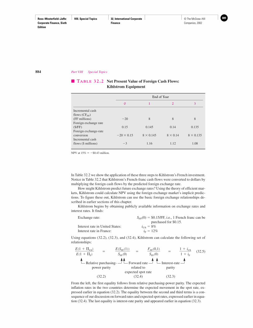
Ross−Westerfield−Jaffe: Corporate Finance, Sixth Edition
VIII. Special Topics 32. International Corporate Finance
889© The McGraw−Hill Companies, 2002
In Table 32.2 we show the application of these three steps to Kihlstrom’s French investment.Notice in Table 32.2 that Kihlstrom’s French-franc cash flows were converted to dollars bymultiplying the foreign cash flows by the predicted foreign exchange rate.
How might Kihlstrom predict future exchange rates? Using the theory of efficient mar-kets, Kihlstrom could calculate NPV using the foreign exchange market’s implicit predic-tions. To figure these out, Kihlstrom can use the basic foreign exchange relationships de-scribed in earlier sections of this chapter.
Kihlstrom begins by obtaining publicly available information on exchange rates andinterest rates. It finds:
Exchange rate: SFF(0) � $0.15/FF, i.e., 1 French franc can bepurchased for $0.15.
Interest rate in United States: iUS � 8%Interest rate in France: iF � 12%
Using equations (32.2), (32.3), and (32.4), Kihlstrom can calculate the following set ofrelationships:
� � � (32.5)
— Relative purchasing- — — Forward rate — — Interest-rate —power parity related to parity
expected spot rate(32.2) (32.4) (32.3)
From the left, the first equality follows from relative purchasing-power parity. The expectedinflation rates in the two countries determine the expected movement in the spot rate, ex-pressed earlier in equation (32.2). The equality between the second and third terms is a con-sequence of our discussion on forward rates and expected spot rates, expressed earlier in equa-tion (32.4). The last equality is interest-rate parity and appeared earlier in equation (32.3).
1 � iUS
1 � iF
FFF �0,1�SFF �0�
E �SFF �1� �SFF �0�
E �1 � �US�E �1 � �F�
884 Part VIII Special Topics
� TABLE 32.2 Net Present Value of Foreign Cash Flows:Kihlstrom Equipment
End of Year
0 1 2 3
Incremental cashflows (CFFF)(FF millions) �20 8 8 8Foreign exchange rate($/FF) 0.15 0.145 0.14 0.135Foreign exchange-rateconversion �20 � 0.15 8 � 0.145 8 � 0.14 8 � 0.135Incremental cashflows ($ millions) �3 1.16 1.12 1.08
NPV at 15% � �$0.43 million.
Ross−Westerfield−Jaffe: Corporate Finance, Sixth Edition
VIII. Special Topics 32. International Corporate Finance
890 © The McGraw−Hill Companies, 2002
We now compare the left-hand term to the right-hand term. We have
If the expected inflation rate in the United States is 8 percent, it follows that the expectedinflation rate in France is 12 percent:
Using relative purchasing-power parity, Kihlstrom can compute the expected spot-ex-change rate in one year:
which implies E[SFF(1)] � 0.145. The exchange rate expected at the end of year 2 is ob-tained from
For year 3, the expected exchange rate is obtained from
Finally, the NPV of the project is computed:
where CFFF(t) refers to the French francs forecasted to be received in each of the next threeyears. The discount rate we use is Kihlstrom’s U.S. cost of capital. We do not use the U.S.risk-free rate of 8 percent because Kihlstrom’s project is risky; a risk-adjusted discount ratemust be used. Because the NPV at 15 percent is �$430,000, Kihlstrom should not investin a subsidiary in France.
In this example we used the foreign exchange market’s implicit forecast of future ex-change rates. Why not use management’s own forecast of foreign exchange rates in the cal-culations? Suppose that the financial management of Kihlstrom feels optimistic about theFrench franc. If its forecasts are sufficiently optimistic and they are used, Kihlstrom’s in-vestment in a French subsidiary will generate a positive NPV. But, in general, it is a goodidea to separate the economic prospects of an investment and the foreign exchangeprospects, and it is unwise to use the latter projections in the NPV calculation. If Kihlstromwishes to speculate on an increase in the French franc relative to the U.S. dollar, the bestway to do this is to buy French francs in the forward foreign exchange market. By using theforward-exchange rates implicit in the domestic and foreign interest rates, the firm is using
NPV � 3
t�0
CFFF �t� � E SFF �t� ��1 � r * �t
0.15 � �1.08
1.12�3
� 0.135
0.15 � �1.08
1.12�2
� 0.14
1.08
1.12�
E SFF �1� �0.15
E �1 � �US�E �1 � �F�
�E SFF �1� �
SFF �0�
E ��F� � 12%
1.08
1.12�
1.08
E �1 � �F�
1.08
1.12�
E �1 � �US�E �1 � �F�
1 � iUS
1 � iF
�E �1 � �US�E �1 � �F�
Chapter 32 International Corporate Finance 885
Ross−Westerfield−Jaffe: Corporate Finance, Sixth Edition
VIII. Special Topics 32. International Corporate Finance
891© The McGraw−Hill Companies, 2002
the actual dollar flows that it could, in principle, lock in today by borrowing in the foreigncurrency. This makes the foreign cash flows equivalent to domestic cash flows.
Unremitted Cash FlowsThe previous example assumed that all after-tax cash flows from the foreign investment wereremitted to the parent firm. The remittance decision is similar to the dividend for a purely do-mestic firm. Substantial differences can exist between the cash flows of a project and theamount that is actually remitted to the parent firm. Of course, the net present value of a proj-ect will not be changed by deferred remittance if the unremitted cash flows are reinvested ata rate of return equal (as adjusted for exchange rates) to the domestic cost of capital.
A foreign subsidiary can remit funds to a parent in many ways, including the following:
1. Dividends.
2. Management fees for central services.
3. Royalties on the use of trade names and patents.
International firms must pay special attention to remittance for two reasons. First, theremay be present and future exchange controls. Many governments are sensitive to the chargeof being exploited by foreign firms. Therefore, governments are tempted to limit the abilityof international firms to remit cash flows. Another reason is taxes. It is always necessary todetermine what taxes must be paid on profits generated in a foreign country. Internationalfirms must usually pay foreign taxes on their foreign profits. The total taxes paid by an inter-national firm may be a function of the time of remittance. For example, Kihlstrom’s Frenchsubsidiary would need to pay taxes in France on the profits it earns in France. Kihlstrom willalso pay taxes on dividends it remits to the United States. In most cases Kihlstrom can offsetthe payment of foreign taxes against the U.S. tax liability. Thus, if the French corporate in-come tax is 34 percent, Kihlstrom will not be liable for additional U.S. taxes.
The Cost of Capital for International FirmsAn important question for firms with international investments is whether the required re-turn for international projects should be different from that of similar domestic projects.
Lower Cost of Capital from International Firm Diversification In the previous chap-ter, we expressed some skepticism concerning the benefits of diversification. We can makea stronger case for diversification in international firms than for purely domestic firms. Sup-pose barriers prevented shareholders in the United States from holding foreign securities;the financial markets of different countries would be segmented. Further suppose that firmsin the United States were not subject to the same barriers. In such a case, a firm engagingin international investing could provide indirect diversification for U.S. shareholders thatthey could not achieve by investing within the United States. This could lead to the lower-ing of the risk premium on international projects. In general, if the costs of investing abroadare lower for a firm than for its shareholders, there is an advantage to international diversi-fication by firms, and this advantage will be reflected in a lower risk-adjusted discount rate.
Alternatively, if there were no barriers to international investing for shareholders, share-holders could obtain the benefit of international diversification for themselves by buying for-eign securities. In this case the project cost of capital for a firm in the United States would notdepend on whether the project was in the United States or in a foreign country. In practice,holding foreign securities involves substantial expenses. These expenses include taxes, thecosts of obtaining information, and trading costs. This implies that although U.S. investors arefree to hold foreign securities, they will not be perfectly internationally diversified.
886 Part VIII Special Topics
Ross−Westerfield−Jaffe: Corporate Finance, Sixth Edition
VIII. Special Topics 32. International Corporate Finance
892 © The McGraw−Hill Companies, 2002
Lower Cost of Capital from International Shareholder Diversification Recall our dis-cussion of the CAPM and the market portfolio. Consider the U.S. stock market and a U.S.investor who is not internationally diversified but, instead, is invested only in U.S. stocks.From our previous discussion of diversification, we know this investor would be bearingmore risk than if she were able to diversify in the stocks of different countries. Now imag-ine she can invest in many foreign stocks by diversifying internationally. She should be ableto reduce the variance (or standard deviation) of her portfolio significantly.
For this investor, the market-risk premium will be lower than for investors who cannotdiversify internationally. In internationally integrated markets, investors with internation-ally diversified portfolios will measure the risk of an individual stock in terms of a world-market portfolio and global betas. Therefore, the cost of capital of a particular firm will bein terms of a global CAPM, such as
E(RI) � rF � BG [E(RG) � rF]
where RI is the required return on a stock when markets are global, rF is the risk free rate,BG is the global beta, and RG is the return on the world-market portfolio. A firm with inter-nationally diversified investors will have a cost of capital with a lower market-risk premium[i.e., E(RG � rF)] and a global beta when compared to a firm with investors that cannot di-versify internationally.
Solnik has presented evidence that suggests that international diversification significantlyreduces risk for shareholders.3 He shows that the variance of an internationally diversifiedportfolio of common stocks is about 33 percent of the variance of individual securities. A di-versified portfolio of U.S. stocks will reduce variance by only 50 percent. Table 32.3 showsthat a world portfolio has lower risk than a portfolio of stocks within a single country. For ex-ample, a citizen of Hong Kong can reduce risk from 12.8 percent to 4.2 percent by investingin a world portfolio. This evidence is consistent with a lower global market-risk premium thanis a purely domestic-risk premium. Global betas will be different than purely domestic betas.Stulz has argued that the preceding claim for why internationalization reduces the cost of cap-ital doesn’t capture the complete picture. He agrees that the global market-risk premium islikely to be substantially lower than the risk premium for an isolated country. In addition, heargues that global investing is likely to improve corporate governance and reduce agencycosts. The argument goes something like this: Firms in countries with less-developed fi-nancial markets will need to improve their governance so that they can raise capital in well-developed capital markets such as the U.S. Foreign firms raising capital in the U.S. must ap-peal to more sophisticated investors and better market architectures with superior monitoringabilities.4 Table 32.3 also shows that the systematic risk of foreign stock investment can bevery low, as is the case of Austria, or very high, as is the case of Hong Kong.
Foreign Political Risks Firms may determine that international investments inherentlyinvolve more political risk than domestic investments. This extra risk may offset the gainsfrom international diversification. Firms may increase the discount rate to allow for the riskof expropriation and foreign exchange remittance controls.
Chapter 32 International Corporate Finance 887
3B. H. Solnik, “Why Not Diversify Internationally Rather than Domestically?” Financial Analysts Journal(July–August 1974). A recent estimate of the benefits of international diversification can be found in GeorgioDeSantis and Bruno Gerard, “International Asset Pricing and Portfolio Diversification with Time-Varying Risk,Journal of Finance 52 (1997). They estimate that an internationally diversified portfolio will reduce standarddeviation by 20 percent when compared to investing in U.S. stocks only.4René M. Stulz, “Globalization, Corporate Finance, and the Cost of Capital,” Journal of Applied CorporateFinance 12 (1999). See also Ronald M. Schramm and Henry N. Wang, “Measuring the Cost of Capital in anInternational CAPM Framework,” Journal of Corporate Finance 12 (1999) and Thomas I. O’Brian, “TheGlobal CAPM and a Firm’s Cost of Capital in Different Currencies,” Journal of Corporate Finance 12 (1999).
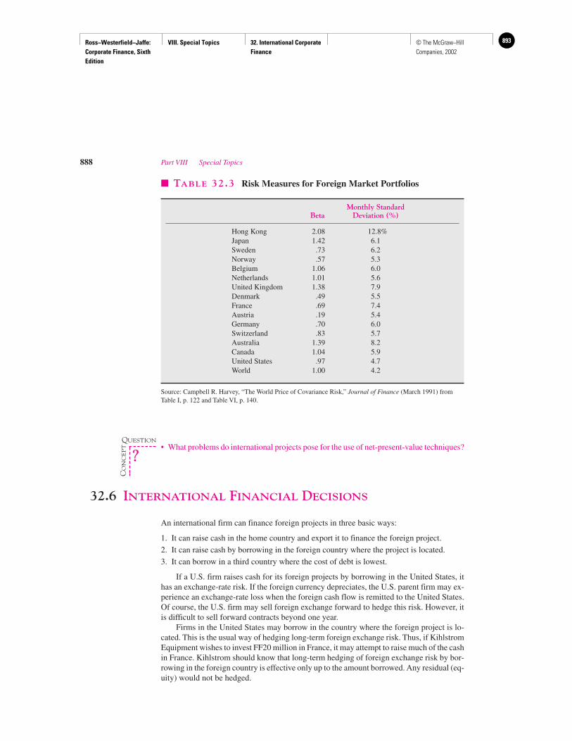
Ross−Westerfield−Jaffe: Corporate Finance, Sixth Edition
VIII. Special Topics 32. International Corporate Finance
893© The McGraw−Hill Companies, 2002
• What problems do international projects pose for the use of net-present-value techniques?
32.6 INTERNATIONAL FINANCIAL DECISIONS
An international firm can finance foreign projects in three basic ways:
1. It can raise cash in the home country and export it to finance the foreign project.
2. It can raise cash by borrowing in the foreign country where the project is located.
3. It can borrow in a third country where the cost of debt is lowest.
If a U.S. firm raises cash for its foreign projects by borrowing in the United States, ithas an exchange-rate risk. If the foreign currency depreciates, the U.S. parent firm may ex-perience an exchange-rate loss when the foreign cash flow is remitted to the United States.Of course, the U.S. firm may sell foreign exchange forward to hedge this risk. However, itis difficult to sell forward contracts beyond one year.
Firms in the United States may borrow in the country where the foreign project is lo-cated. This is the usual way of hedging long-term foreign exchange risk. Thus, if KihlstromEquipment wishes to invest FF20 million in France, it may attempt to raise much of the cashin France. Kihlstrom should know that long-term hedging of foreign exchange risk by bor-rowing in the foreign country is effective only up to the amount borrowed. Any residual (eq-uity) would not be hedged.
888 Part VIII Special Topics
� TABLE 32.3 Risk Measures for Foreign Market Portfolios
Monthly StandardBeta Deviation (%)
Hong Kong 2.08 12.8%Japan 1.42 6.1Sweden .73 6.2Norway .57 5.3Belgium 1.06 6.0Netherlands 1.01 5.6United Kingdom 1.38 7.9Denmark .49 5.5France .69 7.4Austria .19 5.4Germany .70 6.0Switzerland .83 5.7Australia 1.39 8.2Canada 1.04 5.9United States .97 4.7World 1.00 4.2
Source: Campbell R. Harvey, “The World Price of Covariance Risk,” Journal of Finance (March 1991) fromTable I, p. 122 and Table VI, p. 140.
QUESTION
CO
NC
EP
T
?
Ross−Westerfield−Jaffe: Corporate Finance, Sixth Edition
VIII. Special Topics 32. International Corporate Finance
894 © The McGraw−Hill Companies, 2002
Another alternative is to find a country where interest rates are low. However, foreigninterest rates may be lower because of lower expected foreign inflation. Thus, financialmanagers must be careful to look beyond nominal interest rates to real interest rates.
Short-Term and Medium-Term FinancingIn raising short-term and medium-term cash, U.S. international firms often have a choicebetween borrowing from a U.S. bank at the U.S. interest rate or borrowing Eurodollars inthe Eurocurrency market.
A Eurodollar is a dollar deposited in a bank outside the United States. For example,dollar deposits in Paris, France, are Eurodollars. The Eurocurrency markets are the banks(Eurobanks) that make loans and accept deposits in foreign currencies. Most Eurocurrencytrading involves the borrowing and lending of time deposits at Eurobanks. For example, aEurobank receives a Eurodollar deposit from a domestic U.S. bank. Afterward, the Eurobankwill make a dollar-denominated loan to a borrowing party. This is the Eurocurrency market.It is not a retail bank market. The customers are corporations and governments.
One important characteristic of the Eurocurrency market is that loans are made on afloating-rate basis. The interest rates are set at a fixed margin above the London InterbankOffered Rate for the given period and currency involved. For example, if the margin is 0.5percent for dollar loans and the current LIBOR is 8 percent for dollar loans, the dollar bor-rower will pay an interest rate of 8.5 percent. This rate is usually changed every six months.The dollar loans will have maturities ranging from 3 to 10 years.
It is obvious that in a perfectly competitive financial market the interest rate on aEurodollar loan in a Eurocurrency market must be the same as the interest rate in the U.S.loan market. If the interest rate on a Eurodollar loan were higher than that on a domestic-dollar loan, arbitrageurs would borrow in the domestic-dollar market and lend in theEurodollar market. This type of arbitrage trading would force interest rates to be the samein both dollar markets. However, from time to time there are differences between theEurodollar loan rate and the domestic loan rate. Risk, government regulations, and taxes ex-plain most of the differences.
International Bond MarketsThe worldwide public bond market is made up of $21.5 trillion in bonds issued in manycurrencies. Table 32.4 shows that bonds denominated in dollars make up 44.6 percent of thetotal. The total worldwide bond market can be divided into domestic bonds and interna-tional bonds. Domestic bonds are those issued by a firm in its home country. Internationalbonds are those issued by firms in another currency than the currency of the home country.
Trading in international bonds is over the counter and takes place in loosely connectedindividual markets. These individual markets are closely tied to the corresponding domes-tic bond markets. International bonds can be divided into two main types: foreign bonds andEurobonds.
Foreign Bonds Foreign bonds are bonds that are issued by foreign borrowers in a partic-ular country’s domestic bond market. They are often nicknamed for the country of issuance.They are denominated in the country’s domestic currency. For example, suppose a Swisswatch company issues U.S. dollar-denominated bonds in the United States.
These foreign bonds would be called Yankee bonds. Like all foreign bonds issued inthe United States,Yankee bonds must be registered under the Securities Act of 1933. Yankeebonds are usually rated by a bond-rating agency such as Standard & Poor’s Corporation.Many Yankee bonds are listed on the New York Stock Exchange.
Chapter 32 International Corporate Finance 889
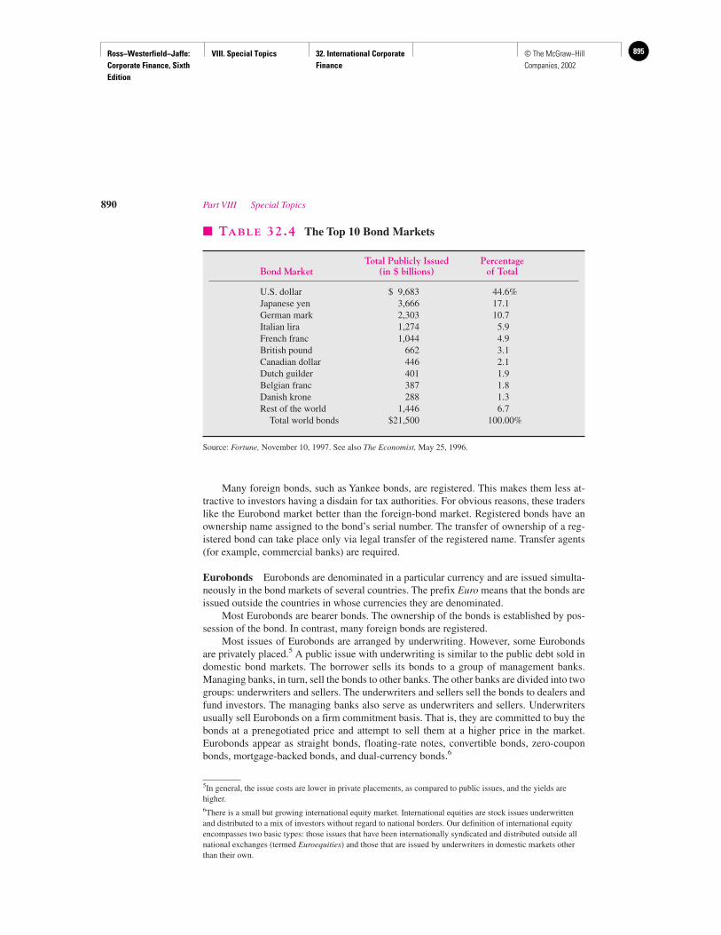
Ross−Westerfield−Jaffe: Corporate Finance, Sixth Edition
VIII. Special Topics 32. International Corporate Finance
895© The McGraw−Hill Companies, 2002
Many foreign bonds, such as Yankee bonds, are registered. This makes them less at-tractive to investors having a disdain for tax authorities. For obvious reasons, these traderslike the Eurobond market better than the foreign-bond market. Registered bonds have anownership name assigned to the bond’s serial number. The transfer of ownership of a reg-istered bond can take place only via legal transfer of the registered name. Transfer agents(for example, commercial banks) are required.
Eurobonds Eurobonds are denominated in a particular currency and are issued simulta-neously in the bond markets of several countries. The prefix Euro means that the bonds areissued outside the countries in whose currencies they are denominated.
Most Eurobonds are bearer bonds. The ownership of the bonds is established by pos-session of the bond. In contrast, many foreign bonds are registered.
Most issues of Eurobonds are arranged by underwriting. However, some Eurobondsare privately placed.5 A public issue with underwriting is similar to the public debt sold indomestic bond markets. The borrower sells its bonds to a group of management banks.Managing banks, in turn, sell the bonds to other banks. The other banks are divided into twogroups: underwriters and sellers. The underwriters and sellers sell the bonds to dealers andfund investors. The managing banks also serve as underwriters and sellers. Underwritersusually sell Eurobonds on a firm commitment basis. That is, they are committed to buy thebonds at a prenegotiated price and attempt to sell them at a higher price in the market.Eurobonds appear as straight bonds, floating-rate notes, convertible bonds, zero-couponbonds, mortgage-backed bonds, and dual-currency bonds.6
890 Part VIII Special Topics
� TABLE 32.4 The Top 10 Bond Markets
Total Publicly Issued PercentageBond Market (in $ billions) of Total
U.S. dollar $ 9,683 44.6%Japanese yen 3,666 17.1German mark 2,303 10.7Italian lira 1,274 5.9French franc 1,044 4.9British pound 662 3.1Canadian dollar 446 2.1Dutch guilder 401 1.9Belgian franc 387 1.8Danish krone 288 1.3Rest of the world 1,446 6.7
Total world bonds $21,500 100.00%
Source: Fortune, November 10, 1997. See also The Economist, May 25, 1996.
5In general, the issue costs are lower in private placements, as compared to public issues, and the yields arehigher.6There is a small but growing international equity market. International equities are stock issues underwrittenand distributed to a mix of investors without regard to national borders. Our definition of international equityencompasses two basic types: those issues that have been internationally syndicated and distributed outside allnational exchanges (termed Euroequities) and those that are issued by underwriters in domestic markets otherthan their own.
Ross−Westerfield−Jaffe: Corporate Finance, Sixth Edition
VIII. Special Topics 32. International Corporate Finance
896 © The McGraw−Hill Companies, 2002
EXAMPLE
A French automobile firm issues 50,000 bonds with a face value of $1,000 each.When the bonds are issued, they are managed by London merchant bankers andlisted on the London Stock Exchange. These are Eurobonds. Each bond has a fixedcoupon rate of 6 percent paid annually on August 15.
EXAMPLE
An American firm makes an offering of $500 million of floating-rate notes.The notes are offered in London. The notes mature in 2020 and have semian-nual interest of 0.5 percent above the six-month London Interbank OfferedRate. When the bonds are issued, the six-month LIBOR is 10 percent. Thus, inthe first six months the American firm will pay interest (at the annual rate) of10% � 0.5% � 10.5%.
32.7 REPORTING FOREIGN OPERATIONS
When a U.S. company prepares consolidated financial statements, the firm translates the lo-cal-currency accounts of foreign subsidiaries into the currency that is used for reportingpurposes, usually the currency of the home country (that is, dollars). If exchange rateschange during the accounting period, accounting gains or losses can occur.
Suppose a U.S. firm acquired a British company in 1982. At that time the exchange ratewas £1 � $2. The British firm performed very well during the next few years (according tosterling measurements). During the same period, the value of the pound fell to $1.25. Didthe corresponding increase in the value of the dollar make the U.S. company better off?Should the increase be reflected in the measurement of income?
These questions have been among the most controversial accounting questions in re-cent years. Two issues seem to arise:
1. What is the appropriate exchange rate to use for translating each balance-sheet account?
2. How should unrealized accounting gains and losses from foreign-currency translationbe handled?
Currency is currently translated under complicated rules set out in FinancialAccounting Standards Boards (FASB) Statement Number 52, which was issued inDecember 1981. For the most part, FASB Number 52 requires that all assets and liabilitiesbe translated from the subsidiary’s currency into the parent’s, using the exchange rate thatcurrently prevails. Gains and losses are accumulated in a special account within the share-holders’ equity section of the balance sheet. Thus, the impact of translation gains and losseswill not be recognized explicitly in net income until the underlying assets and liabilities aresold or liquidated.
• What issues arise when reporting foreign operations?
Chapter 32 International Corporate Finance 891
QUESTION
CO
NC
EP
T
?

Ross−Westerfield−Jaffe: Corporate Finance, Sixth Edition
VIII. Special Topics 32. International Corporate Finance
897© The McGraw−Hill Companies, 2002
32.8 SUMMARY AND CONCLUSIONS
The international firm has a more complicated life than the purely domestic firm. Managementmust understand the connection between interest rates, foreign-currency exchange rates, andinflation, and it must become aware of a large number of different financial market regulationsand tax systems.
1. This chapter describes some fundamental theories of international finance:
• The purchasing-power–parity theorem (law of one price).
• The expectations theory of exchange rates.
• The interest-rate–parity theorem.
2. The purchasing-power–parity theorem states that $1 should have the same purchasing powerin each country. This means that an apple costs the same whether you buy it in New York orin Tokyo. One version of the purchasing-power–parity theorem states that the change inexchange rates between the currencies of two countries is connected to the inflation rates inthe countries’ commodity prices.
3. The expectations theory of exchange rates states that the forward rate of exchange is equal tothe expected spot rate.
4. The interest-rate–parity theorem states that the interest-rate differential between twocountries will be equal to the difference between the forward-exchange rate and the spot-exchange rate. This equality must prevail to prevent arbitrageurs from devising get-rich-quickstrategies. The equality requires the rate of return on risk-free investments in the UnitedStates to be the same as that in other countries.
Of course, in practice the purchasing-power–parity theorem and the interest-rate-paritytheorem cannot work perfectly. Government regulations and taxes prevent this. However,there is much empirical work and intuition that suggests that these theories describeinternational financial markets in an approximate way.
5. The chapter also describes some of the problems of international capital budgeting. The net-present-value rule is still the appropriate way to choose projects, but the main problem is tochoose the correct cost of capital. We argue that it should be equal to the rate thatshareholders can expect to earn on a portfolio of domestic and foreign securities. This rateshould be about the same as is true for a portfolio of domestic securities. However, twoadjustments may be necessary:a. The cost of capital of an international firm may be lower than that of a domestic
counterpart because of the benefits of international diversification.b. The cost of capital of an international firm may be higher because of the extra foreign
political risks.6. We briefly describe international financial markets. International firms may want to consider
borrowing cash in the local financial market or in Eurocurrency and Eurobond markets. Theinterest rates are likely to appear different in these markets. Thus, international firms must becareful to consider differences in taxes and government regulations.
892 Part VIII Special Topics

Ross−Westerfield−Jaffe: Corporate Finance, Sixth Edition
VIII. Special Topics 32. International Corporate Finance
898 © The McGraw−Hill Companies, 2002
KEY TERMS
American Depository Receipt (ADR) 872 Globalization 872Cross rate 873 Interest-rate–parity theorem 879Eurobanks 889 Law of one price (LOP) 877Eurobonds 873 London Interbank Offered Rate (LIBOR) 874Eurocurrency 873 Purchasing-power parity (PPP) 878Eurodollar 889 Relative purchasing-power parity (RPPP) 878European Currency Unit (ECU) 873 Spot-exchange rate 876Exchange rate 875 Spot trades 876Foreign bonds 874 Swap rate 876Foreign exchange market 874 Swaps 874Forward-exchange rate 876 Triangular arbitrage 876Forward trades 876 Yankee bonds 889Gilts 874
SUGGESTED READINGS
Some of the latest academic research in international finance appears in the Journal of AppliedCorporate Finance: “Global Finance” (Fall 1999); “Emerging Markets and the Asian Crisis”(Fall 1998); “Global Finance and Risk Management” (Fall 1997).
QUESTIONS AND PROBLEMS
Some Basics32.1 Use Table 32.5 to answer the following questions:
a. What is the quote in direct terms for the British pound sterling and the U.S. dollar on spotexchange? What is it in European terms for the West German mark and the U.S. dollar?
b. Is the Japanese yen at a premium or a discount to the U.S. dollar in the forward markets?c. To which type of foreign exchange participants would the forward prices of the
Japanese yen be important? Why? What types of transactions might these participantsuse to cover their exposed risk in the foreign exchange markets?
d. Suppose you are a Swiss exporter of watches. If you are to be paid in U.S. dollars threemonths from now for a shipment made to the United States worth $100,000, how manySwiss francs would you receive if you locked in the price today with a forwardcontract? Would you buy or sell the dollar forward?
e. Calculate the U.K. pound–West German deutschemark cross rate for spot exchange interms of the U.S. dollar. Do the same for the yen–Swiss franc cross rate.
f. In the text a swap transaction is described. Why might both banks profit from the use ofsuch a mutual agreement?
32.2 Determine whether arbitrage opportunities exist given the following foreign exchange rates.a. $1.8/L DM2/$ DM4/Lb. ¥100/$ DM2/$ ¥50/DMc. HKD7.8/$ ¥100/$ ¥14/HKD
The Law of One Price and Purchasing-Power Parity32.3 Are the following statements true or false? Explain.
a. If the general price index in Japan rises faster than that in the United States (assumingthat there are zero transaction costs, that no barriers to trade exist, and that productsare identical in both countries), we would expect the yen to appreciate with respect tothe dollar.
Chapter 32 International Corporate Finance 893

Ross−Westerfield−Jaffe: Corporate Finance, Sixth Edition
VIII. Special Topics 32. International Corporate Finance
899© The McGraw−Hill Companies, 2002
894 Part VIII Special Topics
� TABLE 32.5 Foreign Exchange, Week Ended Thursday, April 16, 200X
Foreign Currency Dollar inin Dollars Foreign Currency
f-Argent (Austral) 0.6515 1.5350Australia (Dollar) 0.7160 1.3966Austria (Schilling) 0.0784 12.76c-Belgium (Franc) 0.0267 37.52f-Belgium (Franc) 0.0264 37.82Brazil (Cruzado) 0.0419 23.88Britain (Pound) 1.6317 0.6129
30-day fut 1.6277 0.614460-day fut 1.6238 0.615890-day fut 1.6204 0.6171
Canada (Dollar) 0.7593 1.317030-day fut 0.7591 1.317360-day fut 0.7588 1.317990-day fut 0.7584 1.3185
y-Chile (Peso) 0.0047 211.34Colombia (Peso) 0.0043 230.50Denmark (Krone) 0.1466 6.8220c-Egypt (Pound) 0.7353 1.3600f-Ecuador (Sucre) 0.006325 158.10Finland (Mark) 0.2270 4.4050France (Franc) 0.1661 6.0220Greece (Drachma) 0.0075 132.75Hong Kong (Dollar) 0.1282 7.8015y-India (Rupee) 0.0779 12.8400Indonesia (Rupiah) 0.000611 1635.75Ireland (Punt) 1.4710 0.6798Israel (Shekel) 0.6246 1.6010Italy (Lira) 0.000775 1290.50Japan (Yen) 0.006993 143.00
30-day fut 0.007009 142.6660-day fut 0.007027 142.3090-day fut 0.007042 142.01
Jordan (Dinar) 3.0211 0.33100Kuwait (Dinar) 3.6740 0.27218Lebanon (Pound) 0.00813 123.00z-Mexico (Peso) 0.000860 1163.00Netherlands (Guilder) 0.4900 2.0410New Zealand (Dollar) 0.5800 1.7241Norway (Krone) 0.1477 6.7700Pakistan (Rupee) 0.0578 17.30y-Peru (Inti) 0.0673 14.85z-Philippines (Peso) 0.0494 20.2500Portugal (Escudo) 0.007153 139.80Saudi Arabia (Rijal) 0.2666 3.7505Singapore (Dollar) 0.4690 2.1320S. Korea (Won) 0.001183 845.50S. Africa (Rand) 0.4975 2.01010Spain (Peseta) 0.007890 126.75Sweden (Krona) 0.1586 6.3070
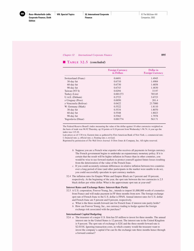
Ross−Westerfield−Jaffe: Corporate Finance, Sixth Edition
VIII. Special Topics 32. International Corporate Finance
900 © The McGraw−Hill Companies, 2002
b. Suppose you are a French wine exporter who receives all payments in foreign currency.The French government begins to undertake an expansionary monetary policy. If it iscertain that the result will be higher inflation in France than in other countries, youwould be wise to use forward markets to protect yourself against future losses resultingfrom the deterioration of the value of the French franc.
c. If you could accurately estimate differences in relative inflation between two countriesover a long period of time (and other participants in the market were unable to do so),you could successfully speculate in spot currency markets.
32.4 The inflation rates for Empire White and Empire Black are 5 percent and 10 percent,respectively. At the beginning of the year, the spot rate between the two currencies is 2.5black dollars per white dollar. What is the approximate spot rate at year-end?
Interest Rates and Exchange Rates: Interest-Rate Parity32.5 A U.S. corporation, Forever Young, Inc., intends to import $1,000,000 worth of cosmetics
from France and will make payment in FF three months from now. The foreign exchangespot rate of French franc to the U.S. dollar is FF6/$. Annual interest rates for U.S. dollarand French franc are 5 percent and 8 percent, respectively.a. What is the three-month forward rate for French franc if interest-rate parity holds?b. How can Forever Young, Inc., use currency trading to hedge against the foreign
exchange risk associated with the purchase?
International Capital Budgeting32.6 a. The treasurer of a major U.S. firm has $5 million to invest for three months. The annual
interest rate in the United States is 12 percent. The interest rate in the United Kingdomis 9 percent. The spot rate of exchange is $2/£ and the three-month forward rate is$2.015/£. Ignoring transaction costs, in which country would the treasurer want toinvest the company’s capital if he can fix the exchange rate three months hence througha forward contract?
Chapter 32 International Corporate Finance 895
� TABLE 32.5 (concluded)
Foreign Currency Dollar inin Dollars Foreign Currency
Switzerland (Franc) 0.6691 1.494530-day fut 0.6710 1.490460-day fut 0.6730 1.485890-day fut 0.6743 1.4830
Taiwan (NT $) 0.0294 33.97Turkey (Lira) 0.001273 785.85U.A.E. (Dirham) 0.2723 3.6723z-Uruguay (Peso) 0.0050 201.4z-Venezuela (Bolivar) 0.0422 23.7000W. Germany (Mark) 0.5522 1.8110
30-day fut 0.5534 1.807060-day fut 0.5548 1.802390-day fut 0.5562 1.7978
Yugoslavia (Dinar) 0.001774 563.71
The Federal Reserve Board’s index measuring the value of the dollar against 10 other currencies weighted onthe basis of trade was 96.92 Thursday, up 18 points or 0.18 percent from Wednesday’s 96.74. A year ago theindex was 115.10.Late prices as of 3:30 P.M. Eastern time as gathered by First American Bank of New York. c, commercial rate; f, financial rate; y, official rate; z, floating rate; r, revised.Reprinted by permission of The Wall Street Journal. © Dow Jones & Company, Inc. All rights reserved.
Ross−Westerfield−Jaffe: Corporate Finance, Sixth Edition
VIII. Special Topics 32. International Corporate Finance
901© The McGraw−Hill Companies, 2002
b. The spot rate of foreign exchange between the United States and the United Kingdomat time t is $1.50/£. If the interest rate in the United States is 13 percent and 8 percentin the United Kingdom, what would you expect the one-year forward rate to be if noimmediate arbitrage opportunities existed?
c. If you are an exporter who must make payments in foreign currency three months afterreceiving each shipment and you predict that the domestic currency will appreciate invalue over this period, is there any value in hedging your currency exposure?
32.7 a. Suppose it is your task to evaluate two different investments in new subsidiaries foryour company, one in your own country and the other in a foreign country. Youcalculate the cash flows of both projects to be identical after exchange-rate differences.Under what circumstances might you choose to invest in the foreign subsidiary? Givean example of a country where certain factors might influence you to alter this decisionand invest at home.
b. Suppose Strom Equipment comes across another investment in Germany. The project costsDM10 million and is expected to produce cash flows of DM4 million in year 1 and DM3million in each of years 2 and 3. The current spot-exchange rate is $0.5/DM1 and thecurrent risk-free rate in the United States is 11.3 percent, compared to that in Germany of 6 percent. The appropriate discount rate for the project is estimated to be 15 percent, theU.S. cost of capital for the company. In addition, the subsidiary can be sold at the end ofthree years for an estimated DM2.1 million. What is the NPV of the project?
c. An investment in a foreign subsidiary is estimated to have a positive NPV, after thediscount rate used in the calculations is adjusted for political risk and any advantagesfrom diversification. Does this mean the project is acceptable? Why or why not?
d. If a U.S. firm raises funds for a foreign subsidiary, what are the disadvantages toborrowing in the United States? How would you overcome them?
International Financial Decisions32.8 a. What is a Euroyen?
b. If financial markets are perfectly competitive and the Eurodollar rate is above thatoffered in the U.S. loan market, you would immediately want to borrow money in theUnited States and invest it in Eurodollars. True or false? Explain.
c. What distinguishes a Eurobond from a foreign bond? Which particular feature makesthe Eurobond more popular than the foreign bond?
d. How would you describe a bond issued by a Canadian firm in the United States withpayments denominated in U.S. dollars?
896 Part VIII Special Topics

Finance
McGraw−Hill Primis
ISBN: 0−390−32000−5
Text: Corporate Finance, Sixth EditionRoss−Westerfield−Jaffe
Corporate Fiance
David Whitehurst
UMIST
Volume 2
McGraw-Hill/Irwin���

Finance
http://www.mhhe.com/primis/online/Copyright ©2003 by The McGraw−Hill Companies, Inc. All rights reserved. Printed in the United States of America. Except as permitted under the United States Copyright Act of 1976, no part of this publication may be reproduced or distributed in any form or by any means, or stored in a database or retrieval system, without prior written permission of the publisher. This McGraw−Hill Primis text may include materials submitted to McGraw−Hill for publication by the instructor of this course. The instructor is solely responsible for the editorial content of such materials.
111 FINA ISBN: 0−390−32000−5
This book was printed on recycled paper.

Finance
Volume 2
Ross−Westerfield−Jaffe • Corporate Finance, Sixth Edition
Back Matter 903
Appendix A: Mathematical Tables 903Appendix B: Solutions to Selected End−of−Chapter Problems 919Glossary 923Name Index 939Subject Index 942End Papers 959
iii


Ross−Westerfield−Jaffe: Corporate Finance, Sixth Edition
Back Matter Appendix A: Mathematical Tables
903© The McGraw−Hill Companies, 2002
Mathematical Tables
AP
PE
ND
IXA
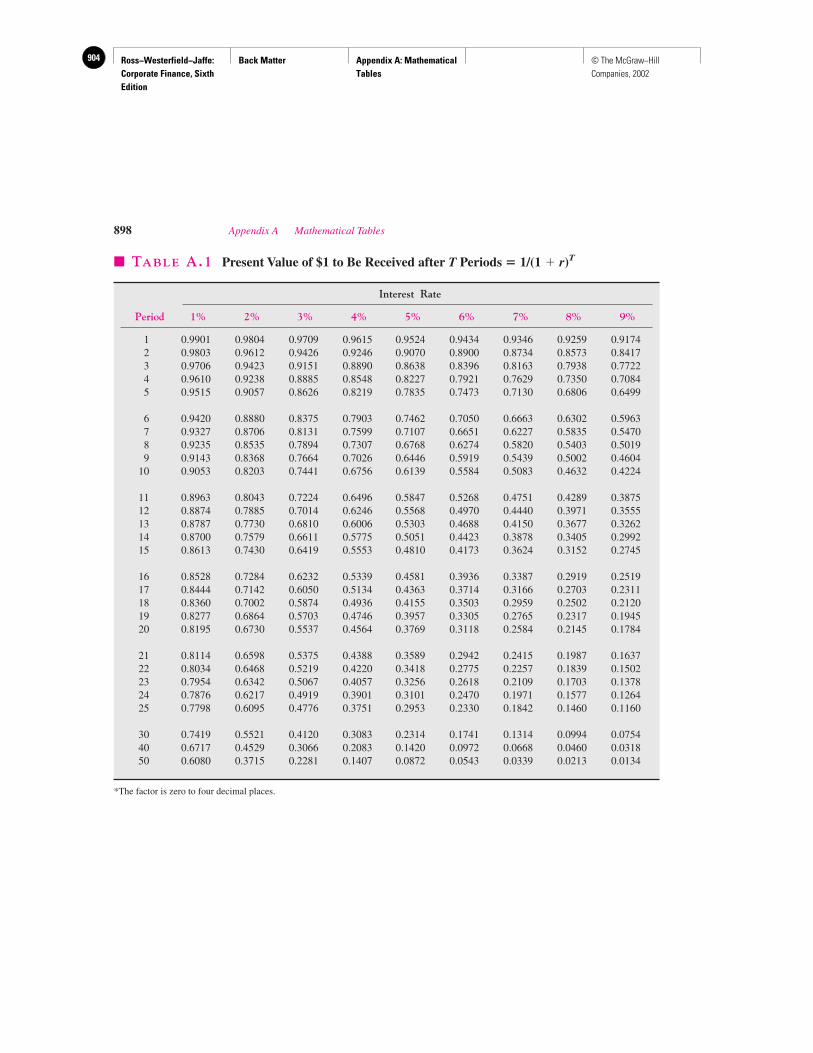
Ross−Westerfield−Jaffe: Corporate Finance, Sixth Edition
Back Matter Appendix A: Mathematical Tables
904 © The McGraw−Hill Companies, 2002
898 Appendix A Mathematical Tables
� TABLE A.1 Present Value of $1 to Be Received after T Periods � 1/(1 � r)T
Interest Rate
Period 1% 2% 3% 4% 5% 6% 7% 8% 9%
1 0.9901 0.9804 0.9709 0.9615 0.9524 0.9434 0.9346 0.9259 0.91742 0.9803 0.9612 0.9426 0.9246 0.9070 0.8900 0.8734 0.8573 0.84173 0.9706 0.9423 0.9151 0.8890 0.8638 0.8396 0.8163 0.7938 0.77224 0.9610 0.9238 0.8885 0.8548 0.8227 0.7921 0.7629 0.7350 0.70845 0.9515 0.9057 0.8626 0.8219 0.7835 0.7473 0.7130 0.6806 0.6499
6 0.9420 0.8880 0.8375 0.7903 0.7462 0.7050 0.6663 0.6302 0.59637 0.9327 0.8706 0.8131 0.7599 0.7107 0.6651 0.6227 0.5835 0.54708 0.9235 0.8535 0.7894 0.7307 0.6768 0.6274 0.5820 0.5403 0.50199 0.9143 0.8368 0.7664 0.7026 0.6446 0.5919 0.5439 0.5002 0.4604
10 0.9053 0.8203 0.7441 0.6756 0.6139 0.5584 0.5083 0.4632 0.4224
11 0.8963 0.8043 0.7224 0.6496 0.5847 0.5268 0.4751 0.4289 0.387512 0.8874 0.7885 0.7014 0.6246 0.5568 0.4970 0.4440 0.3971 0.355513 0.8787 0.7730 0.6810 0.6006 0.5303 0.4688 0.4150 0.3677 0.326214 0.8700 0.7579 0.6611 0.5775 0.5051 0.4423 0.3878 0.3405 0.299215 0.8613 0.7430 0.6419 0.5553 0.4810 0.4173 0.3624 0.3152 0.2745
16 0.8528 0.7284 0.6232 0.5339 0.4581 0.3936 0.3387 0.2919 0.251917 0.8444 0.7142 0.6050 0.5134 0.4363 0.3714 0.3166 0.2703 0.231118 0.8360 0.7002 0.5874 0.4936 0.4155 0.3503 0.2959 0.2502 0.212019 0.8277 0.6864 0.5703 0.4746 0.3957 0.3305 0.2765 0.2317 0.194520 0.8195 0.6730 0.5537 0.4564 0.3769 0.3118 0.2584 0.2145 0.1784
21 0.8114 0.6598 0.5375 0.4388 0.3589 0.2942 0.2415 0.1987 0.163722 0.8034 0.6468 0.5219 0.4220 0.3418 0.2775 0.2257 0.1839 0.150223 0.7954 0.6342 0.5067 0.4057 0.3256 0.2618 0.2109 0.1703 0.137824 0.7876 0.6217 0.4919 0.3901 0.3101 0.2470 0.1971 0.1577 0.126425 0.7798 0.6095 0.4776 0.3751 0.2953 0.2330 0.1842 0.1460 0.1160
30 0.7419 0.5521 0.4120 0.3083 0.2314 0.1741 0.1314 0.0994 0.075440 0.6717 0.4529 0.3066 0.2083 0.1420 0.0972 0.0668 0.0460 0.031850 0.6080 0.3715 0.2281 0.1407 0.0872 0.0543 0.0339 0.0213 0.0134
*The factor is zero to four decimal places.
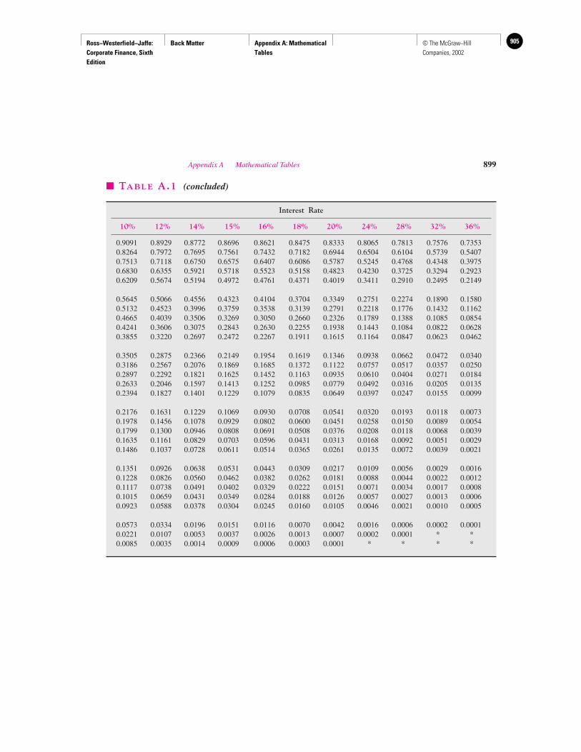
Ross−Westerfield−Jaffe: Corporate Finance, Sixth Edition
Back Matter Appendix A: Mathematical Tables
905© The McGraw−Hill Companies, 2002
Appendix A Mathematical Tables 899
� TABLE A.1 (concluded)
Interest Rate
10% 12% 14% 15% 16% 18% 20% 24% 28% 32% 36%
0.9091 0.8929 0.8772 0.8696 0.8621 0.8475 0.8333 0.8065 0.7813 0.7576 0.73530.8264 0.7972 0.7695 0.7561 0.7432 0.7182 0.6944 0.6504 0.6104 0.5739 0.54070.7513 0.7118 0.6750 0.6575 0.6407 0.6086 0.5787 0.5245 0.4768 0.4348 0.39750.6830 0.6355 0.5921 0.5718 0.5523 0.5158 0.4823 0.4230 0.3725 0.3294 0.29230.6209 0.5674 0.5194 0.4972 0.4761 0.4371 0.4019 0.3411 0.2910 0.2495 0.2149
0.5645 0.5066 0.4556 0.4323 0.4104 0.3704 0.3349 0.2751 0.2274 0.1890 0.15800.5132 0.4523 0.3996 0.3759 0.3538 0.3139 0.2791 0.2218 0.1776 0.1432 0.11620.4665 0.4039 0.3506 0.3269 0.3050 0.2660 0.2326 0.1789 0.1388 0.1085 0.08540.4241 0.3606 0.3075 0.2843 0.2630 0.2255 0.1938 0.1443 0.1084 0.0822 0.06280.3855 0.3220 0.2697 0.2472 0.2267 0.1911 0.1615 0.1164 0.0847 0.0623 0.0462
0.3505 0.2875 0.2366 0.2149 0.1954 0.1619 0.1346 0.0938 0.0662 0.0472 0.03400.3186 0.2567 0.2076 0.1869 0.1685 0.1372 0.1122 0.0757 0.0517 0.0357 0.02500.2897 0.2292 0.1821 0.1625 0.1452 0.1163 0.0935 0.0610 0.0404 0.0271 0.01840.2633 0.2046 0.1597 0.1413 0.1252 0.0985 0.0779 0.0492 0.0316 0.0205 0.01350.2394 0.1827 0.1401 0.1229 0.1079 0.0835 0.0649 0.0397 0.0247 0.0155 0.0099
0.2176 0.1631 0.1229 0.1069 0.0930 0.0708 0.0541 0.0320 0.0193 0.0118 0.00730.1978 0.1456 0.1078 0.0929 0.0802 0.0600 0.0451 0.0258 0.0150 0.0089 0.00540.1799 0.1300 0.0946 0.0808 0.0691 0.0508 0.0376 0.0208 0.0118 0.0068 0.00390.1635 0.1161 0.0829 0.0703 0.0596 0.0431 0.0313 0.0168 0.0092 0.0051 0.00290.1486 0.1037 0.0728 0.0611 0.0514 0.0365 0.0261 0.0135 0.0072 0.0039 0.0021
0.1351 0.0926 0.0638 0.0531 0.0443 0.0309 0.0217 0.0109 0.0056 0.0029 0.00160.1228 0.0826 0.0560 0.0462 0.0382 0.0262 0.0181 0.0088 0.0044 0.0022 0.00120.1117 0.0738 0.0491 0.0402 0.0329 0.0222 0.0151 0.0071 0.0034 0.0017 0.00080.1015 0.0659 0.0431 0.0349 0.0284 0.0188 0.0126 0.0057 0.0027 0.0013 0.00060.0923 0.0588 0.0378 0.0304 0.0245 0.0160 0.0105 0.0046 0.0021 0.0010 0.0005
0.0573 0.0334 0.0196 0.0151 0.0116 0.0070 0.0042 0.0016 0.0006 0.0002 0.00010.0221 0.0107 0.0053 0.0037 0.0026 0.0013 0.0007 0.0002 0.0001 * *0.0085 0.0035 0.0014 0.0009 0.0006 0.0003 0.0001 * * * *
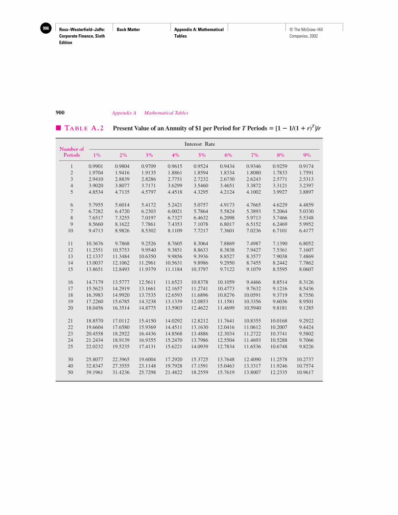
Ross−Westerfield−Jaffe: Corporate Finance, Sixth Edition
Back Matter Appendix A: Mathematical Tables
906 © The McGraw−Hill Companies, 2002
900 Appendix A Mathematical Tables
� TABLE A.2 Present Value of an Annuity of $1 per Period for T Periods � [1 � 1/(1 � r)T]/r
Interest Rate
1% 2% 3% 4% 5% 6% 7% 8% 9%
1 0.9901 0.9804 0.9709 0.9615 0.9524 0.9434 0.9346 0.9259 0.91742 1.9704 1.9416 1.9135 1.8861 1.8594 1.8334 1.8080 1.7833 1.75913 2.9410 2.8839 2.8286 2.7751 2.7232 2.6730 2.6243 2.5771 2.53134 3.9020 3.8077 3.7171 3.6299 3.5460 3.4651 3.3872 3.3121 3.23975 4.8534 4.7135 4.5797 4.4518 4.3295 4.2124 4.1002 3.9927 3.8897
6 5.7955 5.6014 5.4172 5.2421 5.0757 4.9173 4.7665 4.6229 4.48597 6.7282 6.4720 6.2303 6.0021 5.7864 5.5824 5.3893 5.2064 5.03308 7.6517 7.3255 7.0197 6.7327 6.4632 6.2098 5.9713 5.7466 5.53489 8.5660 8.1622 7.7861 7.4353 7.1078 6.8017 6.5152 6.2469 5.9952
10 9.4713 8.9826 8.5302 8.1109 7.7217 7.3601 7.0236 6.7101 6.4177
11 10.3676 9.7868 9.2526 8.7605 8.3064 7.8869 7.4987 7.1390 6.805212 11.2551 10.5753 9.9540 9.3851 8.8633 8.3838 7.9427 7.5361 7.160713 12.1337 11.3484 10.6350 9.9856 9.3936 8.8527 8.3577 7.9038 7.486914 13.0037 12.1062 11.2961 10.5631 9.8986 9.2950 8.7455 8.2442 7.786215 13.8651 12.8493 11.9379 11.1184 10.3797 9.7122 9.1079 8.5595 8.0607
16 14.7179 13.5777 12.5611 11.6523 10.8378 10.1059 9.4466 8.8514 8.312617 15.5623 14.2919 13.1661 12.1657 11.2741 10.4773 9.7632 9.1216 8.543618 16.3983 14.9920 13.7535 12.6593 11.6896 10.8276 10.0591 9.3719 8.755619 17.2260 15.6785 14.3238 13.1339 12.0853 11.1581 10.3356 9.6036 8.950120 18.0456 16.3514 14.8775 13.5903 12.4622 11.4699 10.5940 9.8181 9.1285
21 18.8570 17.0112 15.4150 14.0292 12.8212 11.7641 10.8355 10.0168 9.292222 19.6604 17.6580 15.9369 14.4511 13.1630 12.0416 11.0612 10.2007 9.442423 20.4558 18.2922 16.4436 14.8568 13.4886 12.3034 11.2722 10.3741 9.580224 21.2434 18.9139 16.9355 15.2470 13.7986 12.5504 11.4693 10.5288 9.706625 22.0232 19.5235 17.4131 15.6221 14.0939 12.7834 11.6536 10.6748 9.8226
30 25.8077 22.3965 19.6004 17.2920 15.3725 13.7648 12.4090 11.2578 10.273740 32.8347 27.3555 23.1148 19.7928 17.1591 15.0463 13.3317 11.9246 10.757450 39.1961 31.4236 25.7298 21.4822 18.2559 15.7619 13.8007 12.2335 10.9617
Number ofPeriods
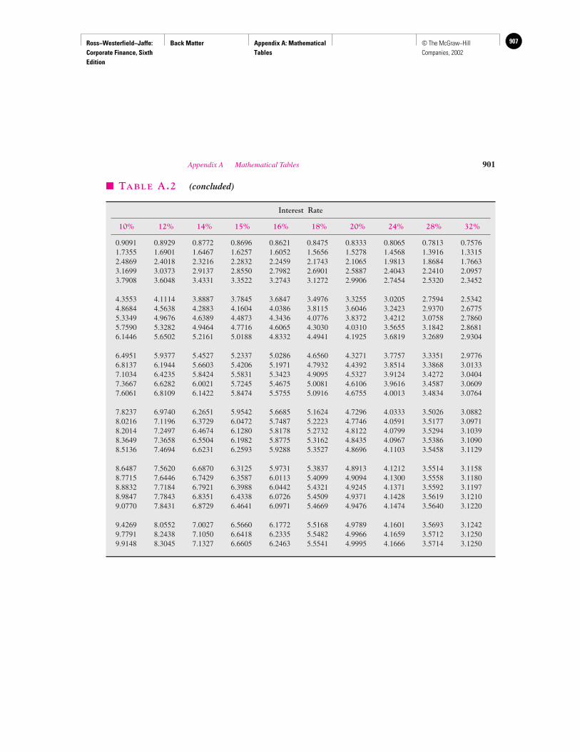
Ross−Westerfield−Jaffe: Corporate Finance, Sixth Edition
Back Matter Appendix A: Mathematical Tables
907© The McGraw−Hill Companies, 2002
Appendix A Mathematical Tables 901
� TABLE A.2 (concluded)
Interest Rate
10% 12% 14% 15% 16% 18% 20% 24% 28% 32%
0.9091 0.8929 0.8772 0.8696 0.8621 0.8475 0.8333 0.8065 0.7813 0.75761.7355 1.6901 1.6467 1.6257 1.6052 1.5656 1.5278 1.4568 1.3916 1.33152.4869 2.4018 2.3216 2.2832 2.2459 2.1743 2.1065 1.9813 1.8684 1.76633.1699 3.0373 2.9137 2.8550 2.7982 2.6901 2.5887 2.4043 2.2410 2.09573.7908 3.6048 3.4331 3.3522 3.2743 3.1272 2.9906 2.7454 2.5320 2.3452
4.3553 4.1114 3.8887 3.7845 3.6847 3.4976 3.3255 3.0205 2.7594 2.53424.8684 4.5638 4.2883 4.1604 4.0386 3.8115 3.6046 3.2423 2.9370 2.67755.3349 4.9676 4.6389 4.4873 4.3436 4.0776 3.8372 3.4212 3.0758 2.78605.7590 5.3282 4.9464 4.7716 4.6065 4.3030 4.0310 3.5655 3.1842 2.86816.1446 5.6502 5.2161 5.0188 4.8332 4.4941 4.1925 3.6819 3.2689 2.9304
6.4951 5.9377 5.4527 5.2337 5.0286 4.6560 4.3271 3.7757 3.3351 2.97766.8137 6.1944 5.6603 5.4206 5.1971 4.7932 4.4392 3.8514 3.3868 3.01337.1034 6.4235 5.8424 5.5831 5.3423 4.9095 4.5327 3.9124 3.4272 3.04047.3667 6.6282 6.0021 5.7245 5.4675 5.0081 4.6106 3.9616 3.4587 3.06097.6061 6.8109 6.1422 5.8474 5.5755 5.0916 4.6755 4.0013 3.4834 3.0764
7.8237 6.9740 6.2651 5.9542 5.6685 5.1624 4.7296 4.0333 3.5026 3.08828.0216 7.1196 6.3729 6.0472 5.7487 5.2223 4.7746 4.0591 3.5177 3.09718.2014 7.2497 6.4674 6.1280 5.8178 5.2732 4.8122 4.0799 3.5294 3.10398.3649 7.3658 6.5504 6.1982 5.8775 5.3162 4.8435 4.0967 3.5386 3.10908.5136 7.4694 6.6231 6.2593 5.9288 5.3527 4.8696 4.1103 3.5458 3.1129
8.6487 7.5620 6.6870 6.3125 5.9731 5.3837 4.8913 4.1212 3.5514 3.11588.7715 7.6446 6.7429 6.3587 6.0113 5.4099 4.9094 4.1300 3.5558 3.11808.8832 7.7184 6.7921 6.3988 6.0442 5.4321 4.9245 4.1371 3.5592 3.11978.9847 7.7843 6.8351 6.4338 6.0726 5.4509 4.9371 4.1428 3.5619 3.12109.0770 7.8431 6.8729 6.4641 6.0971 5.4669 4.9476 4.1474 3.5640 3.1220
9.4269 8.0552 7.0027 6.5660 6.1772 5.5168 4.9789 4.1601 3.5693 3.12429.7791 8.2438 7.1050 6.6418 6.2335 5.5482 4.9966 4.1659 3.5712 3.12509.9148 8.3045 7.1327 6.6605 6.2463 5.5541 4.9995 4.1666 3.5714 3.1250
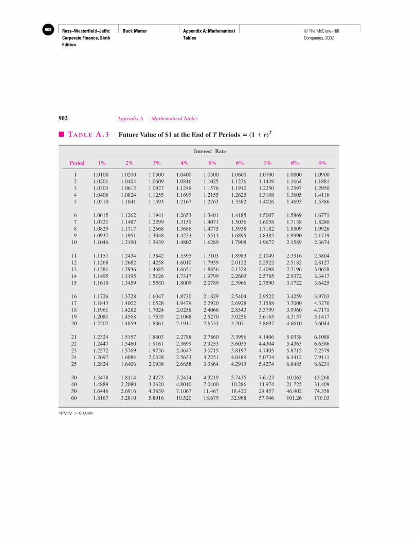
Ross−Westerfield−Jaffe: Corporate Finance, Sixth Edition
Back Matter Appendix A: Mathematical Tables
908 © The McGraw−Hill Companies, 2002
902 Appendix A Mathematical Tables
� TABLE A.3 Future Value of $1 at the End of T Periods � (1 � r)T
Interest Rate
Period 1% 2% 3% 4% 5% 6% 7% 8% 9%
1 1.0100 1.0200 1.0300 1.0400 1.0500 1.0600 1.0700 1.0800 1.09002 1.0201 1.0404 1.0609 1.0816 1.1025 1.1236 1.1449 1.1664 1.18813 1.0303 1.0612 1.0927 1.1249 1.1576 1.1910 1.2250 1.2597 1.29504 1.0406 1.0824 1.1255 1.1699 1.2155 1.2625 1.3108 1.3605 1.41165 1.0510 1.1041 1.1593 1.2167 1.2763 1.3382 1.4026 1.4693 1.5386
6 1.0615 1.1262 1.1941 1.2653 1.3401 1.4185 1.5007 1.5869 1.67717 1.0721 1.1487 1.2299 1.3159 1.4071 1.5036 1.6058 1.7138 1.82808 1.0829 1.1717 1.2668 1.3686 1.4775 1.5938 1.7182 1.8509 1.99269 1.0937 1.1951 1.3048 1.4233 1.5513 1.6895 1.8385 1.9990 2.1719
10 1.1046 1.2190 1.3439 1.4802 1.6289 1.7908 1.9672 2.1589 2.3674
11 1.1157 1.2434 1.3842 1.5395 1.7103 1.8983 2.1049 2.3316 2.580412 1.1268 1.2682 1.4258 1.6010 1.7959 2.0122 2.2522 2.5182 2.812713 1.1381 1.2936 1.4685 1.6651 1.8856 2.1329 2.4098 2.7196 3.065814 1.1495 1.3195 1.5126 1.7317 1.9799 2.2609 2.5785 2.9372 3.341715 1.1610 1.3459 1.5580 1.8009 2.0789 2.3966 2.7590 3.1722 3.6425
16 1.1726 1.3728 1.6047 1.8730 2.1829 2.5404 2.9522 3.4259 3.970317 1.1843 1.4002 1.6528 1.9479 2.2920 2.6928 3.1588 3.7000 4.327618 1.1961 1.4282 1.7024 2.0258 2.4066 2.8543 3.3799 3.9960 4.717119 1.2081 1.4568 1.7535 2.1068 2.5270 3.0256 3.6165 4.3157 5.141720 1.2202 1.4859 1.8061 2.1911 2.6533 3.2071 3.8697 4.6610 5.6044
21 1.2324 1.5157 1.8603 2.2788 2.7860 3.3996 4.1406 5.0338 6.108822 1.2447 1.5460 1.9161 2.3699 2.9253 3.6035 4.4304 5.4365 6.658623 1.2572 1.5769 1.9736 2.4647 3.0715 3.8197 4.7405 5.8715 7.257924 1.2697 1.6084 2.0328 2.5633 3.2251 4.0489 5.0724 6.3412 7.911125 1.2824 1.6406 2.0938 2.6658 3.3864 4.2919 5.4274 6.8485 8.6231
30 1.3478 1.8114 2.4273 3.2434 4.3219 5.7435 7.6123 10.063 13.26840 1.4889 2.2080 3.2620 4.8010 7.0400 10.286 14.974 21.725 31.40950 1.6446 2.6916 4.3839 7.1067 11.467 18.420 29.457 46.902 74.35860 1.8167 3.2810 5.8916 10.520 18.679 32.988 57.946 101.26 176.03
*FVIV � 99,999.
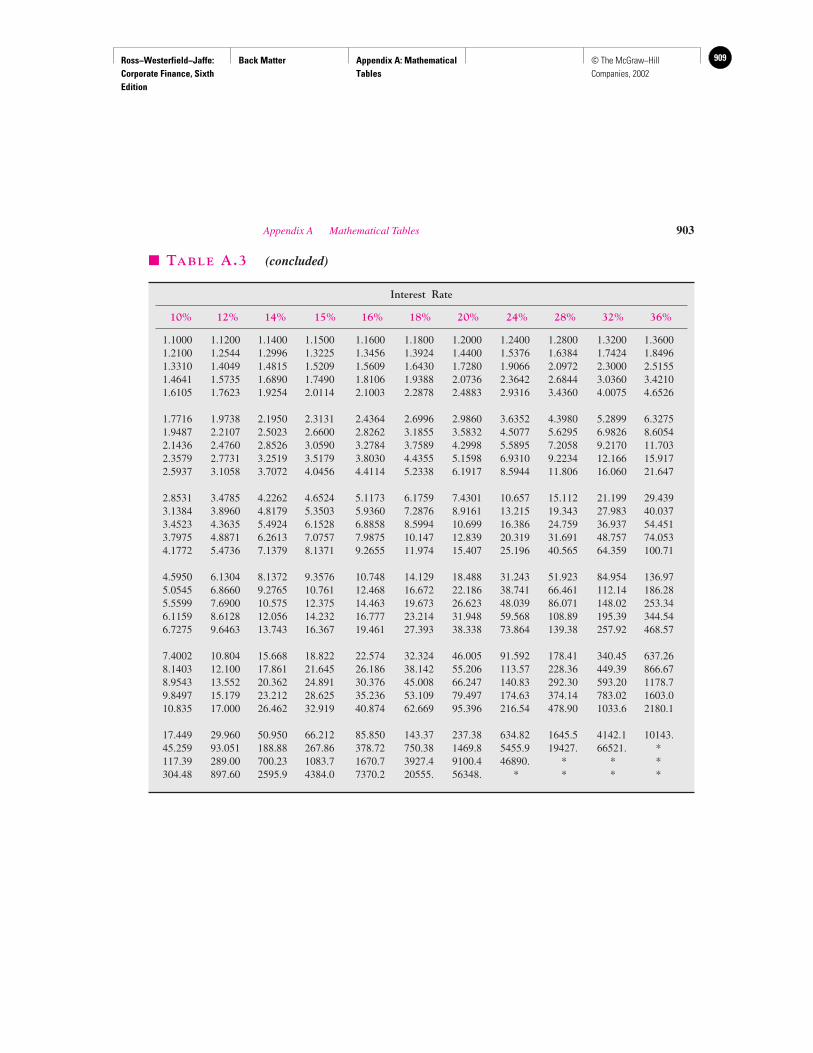
Ross−Westerfield−Jaffe: Corporate Finance, Sixth Edition
Back Matter Appendix A: Mathematical Tables
909© The McGraw−Hill Companies, 2002
Appendix A Mathematical Tables 903
� TABLE A.3 (concluded)
Interest Rate
10% 12% 14% 15% 16% 18% 20% 24% 28% 32% 36%
1.1000 1.1200 1.1400 1.1500 1.1600 1.1800 1.2000 1.2400 1.2800 1.3200 1.36001.2100 1.2544 1.2996 1.3225 1.3456 1.3924 1.4400 1.5376 1.6384 1.7424 1.84961.3310 1.4049 1.4815 1.5209 1.5609 1.6430 1.7280 1.9066 2.0972 2.3000 2.51551.4641 1.5735 1.6890 1.7490 1.8106 1.9388 2.0736 2.3642 2.6844 3.0360 3.42101.6105 1.7623 1.9254 2.0114 2.1003 2.2878 2.4883 2.9316 3.4360 4.0075 4.6526
1.7716 1.9738 2.1950 2.3131 2.4364 2.6996 2.9860 3.6352 4.3980 5.2899 6.32751.9487 2.2107 2.5023 2.6600 2.8262 3.1855 3.5832 4.5077 5.6295 6.9826 8.60542.1436 2.4760 2.8526 3.0590 3.2784 3.7589 4.2998 5.5895 7.2058 9.2170 11.7032.3579 2.7731 3.2519 3.5179 3.8030 4.4355 5.1598 6.9310 9.2234 12.166 15.9172.5937 3.1058 3.7072 4.0456 4.4114 5.2338 6.1917 8.5944 11.806 16.060 21.647
2.8531 3.4785 4.2262 4.6524 5.1173 6.1759 7.4301 10.657 15.112 21.199 29.4393.1384 3.8960 4.8179 5.3503 5.9360 7.2876 8.9161 13.215 19.343 27.983 40.0373.4523 4.3635 5.4924 6.1528 6.8858 8.5994 10.699 16.386 24.759 36.937 54.4513.7975 4.8871 6.2613 7.0757 7.9875 10.147 12.839 20.319 31.691 48.757 74.0534.1772 5.4736 7.1379 8.1371 9.2655 11.974 15.407 25.196 40.565 64.359 100.71
4.5950 6.1304 8.1372 9.3576 10.748 14.129 18.488 31.243 51.923 84.954 136.975.0545 6.8660 9.2765 10.761 12.468 16.672 22.186 38.741 66.461 112.14 186.285.5599 7.6900 10.575 12.375 14.463 19.673 26.623 48.039 86.071 148.02 253.346.1159 8.6128 12.056 14.232 16.777 23.214 31.948 59.568 108.89 195.39 344.546.7275 9.6463 13.743 16.367 19.461 27.393 38.338 73.864 139.38 257.92 468.57
7.4002 10.804 15.668 18.822 22.574 32.324 46.005 91.592 178.41 340.45 637.268.1403 12.100 17.861 21.645 26.186 38.142 55.206 113.57 228.36 449.39 866.678.9543 13.552 20.362 24.891 30.376 45.008 66.247 140.83 292.30 593.20 1178.79.8497 15.179 23.212 28.625 35.236 53.109 79.497 174.63 374.14 783.02 1603.010.835 17.000 26.462 32.919 40.874 62.669 95.396 216.54 478.90 1033.6 2180.1
17.449 29.960 50.950 66.212 85.850 143.37 237.38 634.82 1645.5 4142.1 10143.45.259 93.051 188.88 267.86 378.72 750.38 1469.8 5455.9 19427. 66521. *117.39 289.00 700.23 1083.7 1670.7 3927.4 9100.4 46890. * * *304.48 897.60 2595.9 4384.0 7370.2 20555. 56348. * * * *
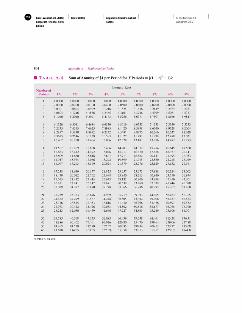
Ross−Westerfield−Jaffe: Corporate Finance, Sixth Edition
Back Matter Appendix A: Mathematical Tables
910 © The McGraw−Hill Companies, 2002
904 Appendix A Mathematical Tables
� TABLE A.4 Sum of Annuity of $1 per Period for T Periods � [(1 � r)T� 1]/r
Interest Rate
1% 2% 3% 4% 5% 6% 7% 8% 9%
1 1.0000 1.0000 1.0000 1.0000 1.0000 1.0000 1.0000 1.0000 1.00002 2.0100 2.0200 2.0300 2.0400 2.0500 2.0600 2.0700 2.0800 2.09003 3.0301 3.0604 3.0909 3.1216 3.1525 3.1836 3.2149 3.2464 3.27814 4.0604 4.1216 4.1836 4.2465 4.3101 4.3746 4.4399 4.5061 4.57315 5.1010 5.2040 5.3091 5.4163 5.5256 5.6371 5.7507 5.8666 5.9847
6 6.1520 6.3081 6.4684 6.6330 6.8019 6.9753 7.1533 7.3359 7.52337 7.2135 7.4343 7.6625 7.8983 8.1420 8.3938 8.6540 8.9228 9.20048 8.2857 8.5830 8.8932 9.2142 9.5491 9.8975 10.260 10.637 11.0289 9.3685 9.7546 10.159 10.583 11.027 11.491 11.978 12.488 13.021
10 10.462 10.950 11.464 12.006 12.578 13.181 13.816 14.487 15.193
11 11.567 12.169 12.808 13.486 14.207 14.972 15.784 16.645 17.56012 12.683 13.412 14.192 15.026 15.917 16.870 17.888 18.977 20.14113 13.809 14.680 15.618 16.627 17.713 18.882 20.141 21.495 22.95314 14.947 15.974 17.086 18.292 19.599 21.015 22.550 24.215 26.01915 16.097 17.293 18.599 20.024 21.579 23.276 25.129 27.152 29.361
16 17.258 18.639 20.157 21.825 23.657 25.673 27.888 30.324 33.00317 18.430 20.012 21.762 23.698 25.840 28.213 30.840 33.750 36.97418 19.615 21.412 23.414 25.645 28.132 30.906 33.999 37.450 41.30119 20.811 22.841 25.117 27.671 30.539 33.760 37.379 41.446 46.01820 22.019 24.297 26.870 29.778 33.066 36.786 40.995 45.762 51.160
21 23.239 25.783 28.676 31.969 35.719 39.993 44.865 50.423 56.76522 24.472 27.299 30.537 34.248 38.505 43.392 49.006 55.457 62.87323 25.716 28.845 32.453 36.618 41.430 46.996 53.436 60.893 69.53224 26.973 30.422 34.426 39.083 44.502 50.816 58.177 66.765 76.79025 28.243 32.030 36.459 41.646 47.727 54.865 63.249 73.106 84.701
30 34.785 40.568 47.575 56.085 66.439 79.058 94.461 113.28 136.3140 48.886 60.402 75.401 95.026 120.80 154.76 199.64 259.06 337.8850 64.463 84.579 112.80 152.67 209.35 290.34 406.53 573.77 815.0860 81.670 114.05 163.05 237.99 353.58 533.13 813.52 1253.2 1944.8
*FVIFA � 99,999.
Number ofPeriods
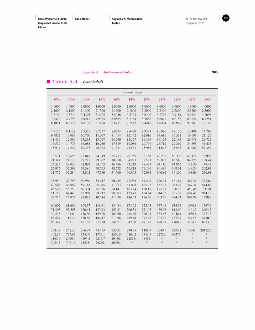
Ross−Westerfield−Jaffe: Corporate Finance, Sixth Edition
Back Matter Appendix A: Mathematical Tables
911© The McGraw−Hill Companies, 2002
Appendix A Mathematical Tables 905
� TABLE A.4 (concluded)
Interest Rate
10% 12% 14% 15% 16% 18% 20% 24% 28% 32% 36%
1.0000 1.0000 1.0000 1.0000 1.0000 1.0000 1.0000 1.0000 1.0000 1.0000 1.00002.1000 2.1200 2.1400 2.1500 2.1600 2.1800 2.2000 2.2400 2.2800 2.3200 2.36003.3100 3.3744 3.4396 3.4725 3.5056 3.5724 3.6400 3.7776 3.9184 4.0624 4.20963.6410 4.7793 4.9211 4.9934 5.0665 5.2154 5.3680 5.6842 6.0156 6.3624 6.72516.1051 6.3528 6.6101 6.7424 6.8771 7.1542 7.4416 8.0484 8.6999 9.3983 10.146
7.7156 8.1152 8.5355 8.7537 8.9775 9.4420 9.9299 10.980 12.136 13.406 14.7999.4872 10.089 10.730 11.067 11.414 12.142 12.916 14.615 16.534 18.696 21.12611.436 12.300 13.233 13.727 14.240 15.327 16.499 19.123 22.163 25.678 29.73213.579 14.776 16.085 16.786 17.519 19.086 20.799 24.712 29.369 34.895 41.43515.937 17.549 19.337 20.304 21.321 23.521 25.959 31.643 38.593 47.062 57.352
18.531 20.655 23.045 24.349 25.733 28.755 32.150 40.238 50.398 63.122 78.99821.384 24.133 27.271 29.002 30.850 34.931 39.581 50.895 65.510 84.320 108.4424.523 28.029 32.089 34.352 36.786 42.219 48.497 64.110 84.853 112.30 148.4727.975 32.393 37.581 40.505 43.672 50.818 59.196 80.496 109.61 149.24 202.9331.772 37.280 43.842 47.580 51.660 60.965 72.035 100.82 141.30 198.00 276.98
35.950 42.753 50.980 55.717 60.925 72.939 87.442 126.01 181.87 262.36 377.6940.545 48.884 59.118 65.075 71.673 87.068 105.93 157.25 233.79 347.31 514.6645.599 55.750 68.394 75.836 84.141 103.74 128.12 195.99 300.25 459.45 700.9451.159 64.440 78.969 88.212 98.603 123.41 154.74 244.03 385.32 607.47 954.2857.275 72.052 91.025 102.44 115.38 146.63 186.69 303.60 494.21 802.86 1298.8
64.002 81.699 104.77 118.81 134.84 174.02 225.03 377.46 633.59 1060.8 1767.471.403 92.503 120.44 137.63 157.41 206.34 271.03 469.06 812.00 1401.2 2404.779.543 104.60 138.30 159.28 183.60 244.49 326.24 582.63 1040.4 1850.6 3271.388.497 118.16 158.66 184.17 213.98 289.49 392.48 723.46 1332.7 2443.8 4450.098.347 133.33 181.87 212.79 249.21 342.60 471.98 898.09 1706.8 3226.8 6053.0
164.49 241.33 356.79 434.75 530.31 790.95 1181.9 2640.9 5873.2 12941. 28172.3442.59 767.09 1342.0 1779.1 2360.8 4163.2 7343.9 22729. 69377. * *1163.9 2400.0 4994.5 7217.7 10436. 21813. 45497. * * * *3034.8 7471.6 18535. 29220. 46058. * * * * * *

Ross−Westerfield−Jaffe: Corporate Finance, Sixth Edition
Back Matter Appendix A: Mathematical Tables
912 © The McGraw−Hill Companies, 2002
906 Appendix A Mathematical Tables
� TABLE A.5 Future Value of $1 with a Continuously Compounded Rate r for T Periods: Values of erT
Continuously Compounded Rate (r)
1% 2% 3% 4% 5% 6% 7% 8% 9% 10%
1 1.0101 1.0202 1.0305 1.0408 1.0513 1.0618 1.0725 1.0833 1.0942 1.10522 1.0202 1.0408 1.0618 1.0833 1.1052 1.1275 1.1503 1.1735 1.1972 1.22143 1.0305 1.0618 1.0942 1.1275 1.1618 1.1972 1.2337 1.2712 1.3100 1.34994 1.0408 1.0833 1.1275 1.1735 1.2214 1.2712 1.3231 1.3771 1.4333 1.49185 1.0513 1.1052 1.1618 1.2214 1.2840 1.3499 1.4191 1.4918 1.5683 1.64876 1.0618 1.1275 1.1972 1.2712 1.3499 1.4333 1.5220 1.6161 1.7160 1.82217 1.0725 1.1503 1.2337 1.3231 1.4191 1.5220 1.6323 1.7507 1.8776 2.01388 1.0833 1.1735 1.2712 1.3771 1.4918 1.6161 1.7507 1.8965 2.0544 2.22559 1.0942 1.1972 1.3100 1.4333 1.5683 1.7160 1.8776 2.0544 2.2479 2.4596
10 1.1052 1.2214 1.3499 1.4918 1.6487 1.8221 2.0138 2.2255 2.4596 2.718311 1.1163 1.2461 1.3910 1.5527 1.7333 1.9348 2.1598 2.4109 2.6912 3.004212 1.1275 1.2712 1.4333 1.6161 1.8221 2.0544 2.3164 2.6117 2.9447 3.320113 1.1388 1.2969 1.4770 1.6820 1.9155 2.1815 2.4843 2.8292 3.2220 3.669314 1.1503 1.3231 1.5220 1.7507 2.0138 2.3164 2.6645 3.0649 3.5254 4.055215 1.1618 1.3499 1.5683 1.8221 2.1170 2.4596 2.8577 3.3201 3.8574 4.481716 1.1735 1.3771 1.6161 1.8965 2.2255 2.6117 3.0649 3.5966 4.2207 4.953017 1.1853 1.4049 1.6653 1.9739 2.3396 2.7732 3.2871 3.8962 4.6182 5.473918 1.1972 1.4333 1.7160 2.0544 2.4596 2.9447 3.5254 4.2207 5.0531 6.049619 1.2092 1.4623 1.7683 2.1383 2.5857 3.1268 3.7810 4.5722 5.5290 6.685920 1.2214 1.4918 1.8221 2.2255 2.7183 3.3201 4.0552 4.9530 6.0496 7.389121 1.2337 1.5220 1.8776 2.3164 2.8577 3.5254 4.3492 5.3656 6.6194 8.166222 1.2461 1.5527 1.9348 2.4109 3.0042 3.7434 4.6646 5.8124 7.2427 9.025023 1.2586 1.5841 1.9937 2.5093 3.1582 3.9749 5.0028 6.2965 7.9248 9.974224 1.2712 1.6161 2.0544 2.6117 3.3201 4.2207 5.3656 6.8210 8.6711 11.023225 1.2840 1.6487 2.1170 2.7183 3.4903 4.4817 5.7546 7.3891 9.4877 12.182530 1.3499 1.8221 2.4596 3.3204 4.4817 6.0496 8.1662 11.0232 14.8797 20.085535 1.4191 2.0138 2.8577 4.0552 5.7546 8.1662 11.5883 16.4446 23.3361 33.115540 1.4918 2.2255 3.3201 4.9530 7.3891 11.0232 16.4446 24.5235 36.5982 54.598245 1.5683 2.4596 3.8574 6.0496 9.4877 14.8797 23.3361 36.5982 57.3975 90.017150 1.6487 2.7183 4.4817 7.3891 12.1825 20.0855 33.1155 54.5982 90.0171 148.413255 1.7333 3.0042 5.2070 9.0250 15.6426 27.1126 46.9931 81.4509 141.1750 244.691960 1.8221 3.3201 6.0496 11.0232 20.0855 36.5982 66.6863 121.5104 221.4064 403.4288
Period(T)

Ross−Westerfield−Jaffe: Corporate Finance, Sixth Edition
Back Matter Appendix A: Mathematical Tables
913© The McGraw−Hill Companies, 2002
Appendix A Mathematical Tables 907
� TABLE A.5 (continued)
Continuously Compounded Rate (r)
11% 12% 13% 14% 15% 16% 17% 18% 19% 20% 21%
1.1163 1.1275 1.1388 1.1503 1.1618 1.1735 1.1853 1.1972 1.2092 1.2214 1.23371.2461 1.2712 1.2969 1.3231 1.3499 1.3771 1.4049 1.4333 1.4623 1.4918 1.52201.3910 1.4333 1.4770 1.5220 1.5683 1.6161 1.6653 1.7160 1.7683 1.8221 1.87761.5527 1.6161 1.6820 1.7507 1.8221 1.8965 1.9739 2.0544 2.1383 2.2255 2.31641.7333 1.8221 1.9155 2.0138 2.1170 2.2255 2.3396 2.4596 2.5857 2.7183 2.85771.9348 2.0544 2.1815 2.3164 2.4596 2.6117 2.7732 2.9447 3.1268 3.3201 3.52542.1598 2.3164 2.4843 2.6645 2.8577 3.0649 3.2871 3.5254 3.7810 4.0552 4.34922.4109 2.6117 2.8292 3.0649 3.3201 3.5966 3.8962 4.2207 4.5722 4.9530 5.36562.6912 2.9447 3.2220 3.5254 3.8574 4.2207 4.6182 5.0531 5.5290 6.0496 6.61943.0042 3.3201 3.6693 4.0552 4.4817 4.9530 5.4739 6.0496 6.6859 7.3891 8.16623.3535 3.7434 4.1787 4.6646 5.2070 5.8124 6.4883 7.2427 8.0849 9.0250 10.07443.7434 4.2207 4.7588 5.3656 6.0496 6.8210 7.6906 8.6711 9.7767 11.0232 12.42864.1787 4.7588 5.4195 6.1719 7.0287 8.0045 9.1157 10.3812 11.8224 13.4637 15.33294.6646 5.3656 6.1719 7.0993 8.1662 9.3933 10.8049 12.4286 14.2963 16.4446 18.91585.2070 6.0496 7.0287 8.1662 9.4877 11.0232 12.0871 14.8797 17.2878 20.0855 23.33615.8124 6.8210 8.0045 9.3933 11.0232 12.9358 15.1803 17.8143 20.9052 24.5325 28.78926.4883 7.6906 9.1157 10.8049 12.8071 15.1803 17.9933 21.3276 25.2797 29.9641 35.51667.2427 8.6711 10.3812 12.4286 14.8797 17.8143 21.3276 25.5337 30.5694 36.5982 43.81608.0849 9.7767 11.8224 14.2963 17.2878 20.9052 25.2797 30.5694 36.9661 44.7012 54.05499.0250 11.0232 13.4637 16.4446 20.0855 24.5325 29.9641 36.5982 44.7012 54.5982 66.6863
10.0744 12.4286 15.3329 18.9158 23.3361 28.7892 35.5166 43.8160 54.0549 66.6863 82.269511.2459 14.0132 17.4615 21.7584 27.1126 33.7844 42.0980 52.4573 65.3659 81.4509 101.494012.5535 15.7998 19.8857 25.0281 31.5004 39.6464 49.8990 62.8028 79.0436 99.4843 125.211014.0132 17.8143 22.6464 28.7892 36.5982 46.5255 59.1455 75.1886 95.5835 121.5104 154.470015.6426 20.0855 25.7903 33.1155 42.5211 54.5982 70.1054 90.0171 115.5843 148.4132 190.566327.1126 36.5982 49.4024 66.6863 90.0171 121.5104 164.0219 221.4064 298.8674 403.4288 544.571946.9931 66.6863 94.6324 134.2898 190.5663 270.4264 383.7533 544.5719 772.7843 1096.633 1556.19781.4509 121.5104 181.2722 270.4264 403.4288 601.8450 897.8473 1339.431 1998.196 2980.958 4447.067
141.1750 221.4064 347.2344 544.5719 854.0588 1339.431 2100.646 3294.468 5166.754 8103.084 12708.17244.6919 403.4288 665.1416 1096.633 1808.042 2980.958 4914.769 8103.084 13359.73 22026.47 36315.50424.1130 735.0952 1274.106 2208.348 3827.626 6634.244 11498.82 19930.37 34544.37 59874.14 103777.0735.0952 1339.431 2440.602 4447.067 8103.084 14764.78 26903.19 49020.80 89321.72 162754.8 296558.6

Ross−Westerfield−Jaffe: Corporate Finance, Sixth Edition
Back Matter Appendix A: Mathematical Tables
914 © The McGraw−Hill Companies, 2002
908 Appendix A Mathematical Tables
� TABLE A.5 (concluded)
Continuously Compounded Rate (r)
22% 23% 24% 25% 26% 27% 28%
1 1.2461 1.2586 1.2712 1.2840 1.2969 1.3100 1.32312 1.5527 1.5841 1.6161 1.6487 1.6820 1.7160 1.75073 1.9348 1.9937 2.0544 2.1170 2.1815 2.2479 2.31644 2.4109 2.5093 2.6117 2.7183 2.8292 2.9447 3.06495 3.0042 3.1582 3.3201 3.4903 3.6693 3.8574 4.05526 3.7434 3.9749 4.2207 4.4817 4.7588 5.0351 5.36567 4.6646 5.0028 5.3656 5.7546 6.1719 6.6194 7.09938 5.8124 6.2965 6.8210 7.3891 8.0045 8.6711 9.39339 7.2427 7.9248 8.6711 9.4877 10.3812 11.3589 12.4286
10 9.0250 9.9742 11.0232 12.1825 13.4637 14.8797 16.444611 11.2459 12.5535 14.0132 15.6426 17.4615 19.4919 21.758412 14.0132 15.7998 17.8143 20.0855 22.6464 25.5337 28.789213 17.4615 19.8857 22.6464 25.7903 29.3708 33.4483 38.091814 21.7584 25.0281 28.7892 33.1155 38.0918 43.8160 50.400415 27.1126 31.5004 36.5982 42.5211 49.4024 57.3975 66.686316 33.7844 39.6464 46.5255 54.5982 64.0715 75.1886 88.234717 42.0980 49.8990 59.1455 70.1054 83.0963 98.4944 116.745918 52.4573 62.8028 75.1886 90.0171 107.7701 129.0242 154.470019 65.3659 79.0436 95.5835 115.5843 139.7702 169.0171 204.383920 81.4509 99.4843 121.5104 148.4132 181.2722 221.4064 270.426421 101.4940 125.2110 154.4700 190.5663 235.0974 290.0345 357.809222 126.4694 157.5905 196.3699 244.6919 304.9049 379.9349 473.428123 157.5905 198.3434 249.6350 314.1907 395.4404 497.7013 626.406824 196.3699 249.6350 317.3483 403.4288 512.8585 651.9709 828.817525 244.6919 314.1907 403.4288 518.0128 665.1416 854.0588 1096.63330 735.0952 992.2747 1339.431 1808.042 2440.602 3294.468 4447.06735 2208.348 3133.795 4447.067 6310.688 8955.293 12708.17 18033.7440 6634.244 9897.129 14764.78 22026.47 32859.63 49020.80 73130.4445 19930.37 31257.04 49020.80 76879.92 120571.7 189094.1 296558.650 59874.14 98715.77 162754.8 268337.3 442413.4 729416.4 120260455 179871.9 311763.4 540364.9 936589.2 1623346 2813669 487680160 540364.9 984609.1 1794075 3269017 5956538 10853520 19776403
Period(T)
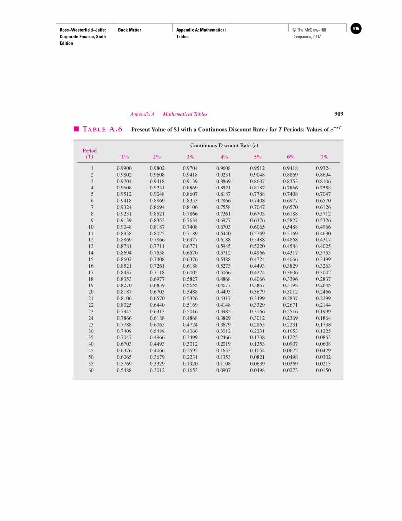
Ross−Westerfield−Jaffe: Corporate Finance, Sixth Edition
Back Matter Appendix A: Mathematical Tables
915© The McGraw−Hill Companies, 2002
Appendix A Mathematical Tables 909
� TABLE A.6 Present Value of $1 with a Continuous Discount Rate r for T Periods: Values of e�rT
Continuous Discount Rate (r)
1% 2% 3% 4% 5% 6% 7%
1 0.9900 0.9802 0.9704 0.9608 0.9512 0.9418 0.93242 0.9802 0.9608 0.9418 0.9231 0.9048 0.8869 0.86943 0.9704 0.9418 0.9139 0.8869 0.8607 0.8353 0.81064 0.9608 0.9231 0.8869 0.8521 0.8187 0.7866 0.75585 0.9512 0.9048 0.8607 0.8187 0.7788 0.7408 0.70476 0.9418 0.8869 0.8353 0.7866 0.7408 0.6977 0.65707 0.9324 0.8694 0.8106 0.7558 0.7047 0.6570 0.61268 0.9231 0.8521 0.7866 0.7261 0.6703 0.6188 0.57129 0.9139 0.8353 0.7634 0.6977 0.6376 0.5827 0.5326
10 0.9048 0.8187 0.7408 0.6703 0.6065 0.5488 0.496611 0.8958 0.8025 0.7189 0.6440 0.5769 0.5169 0.463012 0.8869 0.7866 0.6977 0.6188 0.5488 0.4868 0.431713 0.8781 0.7711 0.6771 0.5945 0.5220 0.4584 0.402514 0.8694 0.7558 0.6570 0.5712 0.4966 0.4317 0.375315 0.8607 0.7408 0.6376 0.5488 0.4724 0.4066 0.349916 0.8521 0.7261 0.6188 0.5273 0.4493 0.3829 0.326317 0.8437 0.7118 0.6005 0.5066 0.4274 0.3606 0.304218 0.8353 0.6977 0.5827 0.4868 0.4066 0.3396 0.283719 0.8270 0.6839 0.5655 0.4677 0.3867 0.3198 0.264520 0.8187 0.6703 0.5488 0.4493 0.3679 0.3012 0.246621 0.8106 0.6570 0.5326 0.4317 0.3499 0.2837 0.229922 0.8025 0.6440 0.5169 0.4148 0.3329 0.2671 0.214423 0.7945 0.6313 0.5016 0.3985 0.3166 0.2516 0.199924 0.7866 0.6188 0.4868 0.3829 0.3012 0.2369 0.186425 0.7788 0.6065 0.4724 0.3679 0.2865 0.2231 0.173830 0.7408 0.5488 0.4066 0.3012 0.2231 0.1653 0.122535 0.7047 0.4966 0.3499 0.2466 0.1738 0.1225 0.086340 0.6703 0.4493 0.3012 0.2019 0.1353 0.0907 0.060845 0.6376 0.4066 0.2592 0.1653 0.1054 0.0672 0.042950 0.6065 0.3679 0.2231 0.1353 0.0821 0.0498 0.030255 0.5769 0.3329 0.1920 0.1108 0.0639 0.0369 0.021360 0.5488 0.3012 0.1653 0.0907 0.0498 0.0273 0.0150
Period(T)

Ross−Westerfield−Jaffe: Corporate Finance, Sixth Edition
Back Matter Appendix A: Mathematical Tables
916 © The McGraw−Hill Companies, 2002
910 Appendix A Mathematical Tables
� TABLE A.6 (continued)
Continuous Discount Rate (r)
8% 9% 10% 11% 12% 13% 14% 15% 16% 17%
1 0.9231 0.9139 0.9048 0.8958 0.8869 0.8781 0.8694 0.8607 0.8521 0.84372 0.8521 0.8353 0.8187 0.8025 0.7866 0.7711 0.7558 0.7408 0.7261 0.71183 0.7866 0.7634 0.7408 0.7189 0.6977 0.6771 0.6570 0.6376 0.6188 0.60054 0.7261 0.6977 0.6703 0.6440 0.6188 0.5945 0.5712 0.5488 0.5273 0.50665 0.6703 0.6376 0.6065 0.5769 0.5488 0.5220 0.4966 0.4724 0.4493 0.42746 0.6188 0.5827 0.5488 0.5169 .04868 0.4584 0.4317 0.4066 0.3829 0.36067 0.5712 0.5326 0.4966 0.4630 0.4317 0.4025 0.3753 0.3499 0.3263 0.30428 0.5273 0.4868 0.4493 0.4148 0.3829 0.3535 0.3263 0.3012 0.2780 0.25769 0.4868 0.4449 0.4066 0.3716 0.3396 0.3104 0.2837 0.2592 0.2369 0.2165
10 0.4493 0.4066 0.3679 0.3329 0.3012 0.2725 0.2466 0.2231 0.2019 0.182711 0.4148 0.3716 0.3329 0.2982 0.2671 0.2393 0.2144 0.1920 0.1720 0.154112 0.3829 0.3396 0.3012 0.2671 0.2369 0.2101 0.1864 0.1653 0.1466 0.130013 0.3535 0.3104 0.2725 0.2393 0.2101 0.1845 0.1620 0.1423 0.1249 0.109714 0.3263 0.2837 0.2466 0.2144 0.1864 0.1620 0.1409 0.1225 0.1065 0.092615 0.3012 0.2592 0.2231 0.1920 0.1653 0.1423 0.1225 0.1054 0.0907 0.078116 0.2780 0.2369 0.2019 0.1720 0.1466 0.1249 0.1065 0.0907 0.0773 0.065917 0.2567 0.2165 0.1827 0.1541 0.1300 0.1097 0.0926 0.0781 0.0659 0.055618 0.2369 0.1979 0.1653 0.1381 0.1153 0.0963 0.0805 0.0672 0.0561 0.046919 0.2187 0.1809 0.1496 0.1237 0.1023 0.0846 0.0699 0.0578 0.0478 0.039620 0.2019 0.1653 0.1353 0.1108 0.0907 0.0743 0.0608 0.0498 0.0408 0.033421 0.1864 0.1511 0.1225 0.0993 0.0805 0.0652 0.0529 0.0429 0.0347 0.028222 0.1720 0.1381 0.1108 0.0889 0.0714 0.0573 0.0460 0.0369 0.0296 0.023823 0.1588 0.1262 0.1003 0.0797 0.0633 0.0503 0.0400 0.0317 0.0252 0.020024 0.1466 0.1153 0.0907 0.0714 0.0561 0.0442 0.0347 0.0273 0.0215 0.016925 0.1353 0.1054 0.0821 0.0639 0.0498 0.0388 0.0302 0.0235 0.0183 0.014330 0.0907 0.0672 0.0498 0.0369 0.0273 0.0202 0.0150 0.0111 0.0082 0.006135 0.0608 0.0429 0.0302 0.0213 0.0150 0.0106 0.0074 0.0052 0.0037 0.002640 0.0408 0.0273 0.0183 0.0123 0.0082 0.0055 0.0037 0.0025 0.0017 0.001145 0.0273 0.0174 0.0111 0.0071 0.0045 0.0029 0.0018 0.0012 0.0007 0.000550 0.0183 0.0111 0.0067 0.0041 0.0025 0.0015 0.0009 0.0006 0.0003 0.000255 0.0123 0.0071 0.0041 0.0024 0.0014 0.0008 0.0005 0.0003 0.0002 0.000160 0.0082 0.0045 0.0025 0.0014 0.0007 0.0004 0.0002 0.0001 0.0001 0.0000
Period(T)
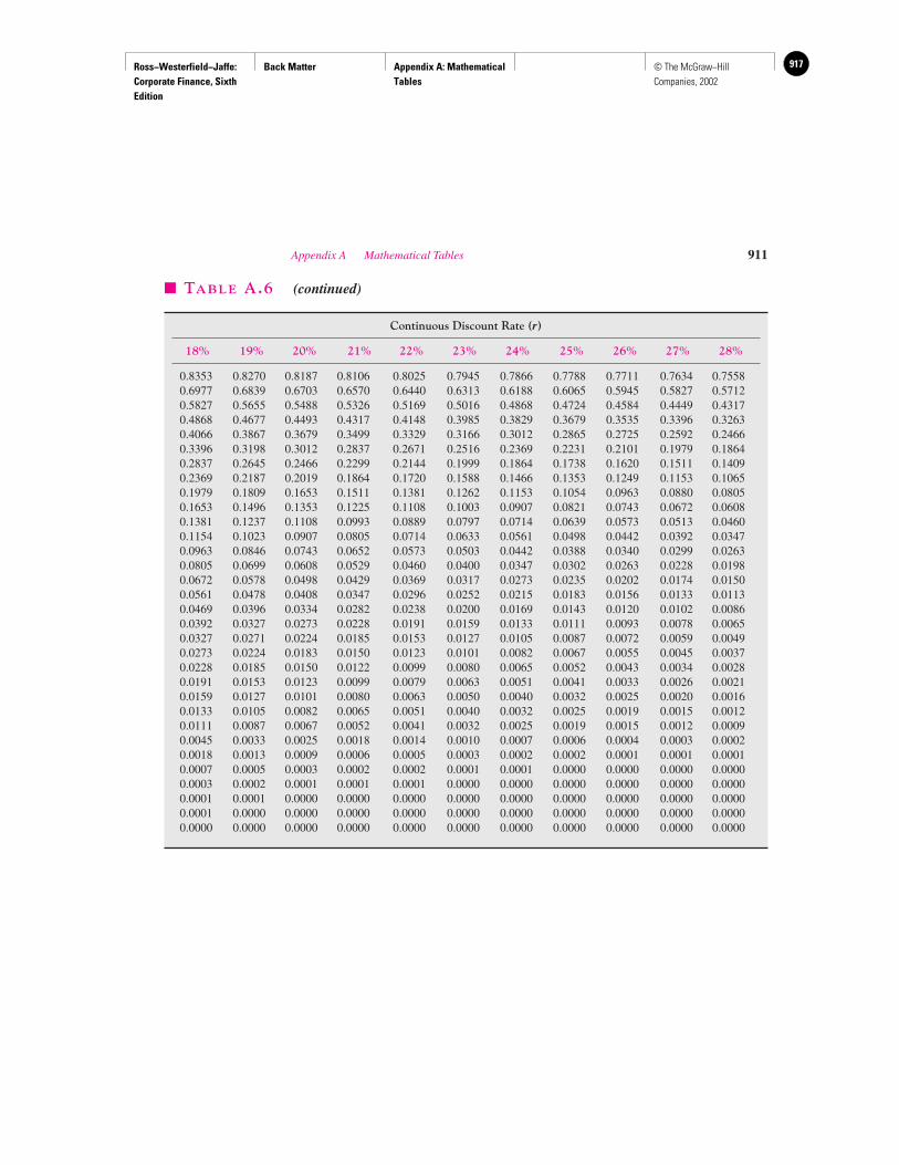
Ross−Westerfield−Jaffe: Corporate Finance, Sixth Edition
Back Matter Appendix A: Mathematical Tables
917© The McGraw−Hill Companies, 2002
Appendix A Mathematical Tables 911
� TABLE A.6 (continued)
Continuous Discount Rate (r)
18% 19% 20% 21% 22% 23% 24% 25% 26% 27% 28%
0.8353 0.8270 0.8187 0.8106 0.8025 0.7945 0.7866 0.7788 0.7711 0.7634 0.75580.6977 0.6839 0.6703 0.6570 0.6440 0.6313 0.6188 0.6065 0.5945 0.5827 0.57120.5827 0.5655 0.5488 0.5326 0.5169 0.5016 0.4868 0.4724 0.4584 0.4449 0.43170.4868 0.4677 0.4493 0.4317 0.4148 0.3985 0.3829 0.3679 0.3535 0.3396 0.32630.4066 0.3867 0.3679 0.3499 0.3329 0.3166 0.3012 0.2865 0.2725 0.2592 0.24660.3396 0.3198 0.3012 0.2837 0.2671 0.2516 0.2369 0.2231 0.2101 0.1979 0.18640.2837 0.2645 0.2466 0.2299 0.2144 0.1999 0.1864 0.1738 0.1620 0.1511 0.14090.2369 0.2187 0.2019 0.1864 0.1720 0.1588 0.1466 0.1353 0.1249 0.1153 0.10650.1979 0.1809 0.1653 0.1511 0.1381 0.1262 0.1153 0.1054 0.0963 0.0880 0.08050.1653 0.1496 0.1353 0.1225 0.1108 0.1003 0.0907 0.0821 0.0743 0.0672 0.06080.1381 0.1237 0.1108 0.0993 0.0889 0.0797 0.0714 0.0639 0.0573 0.0513 0.04600.1154 0.1023 0.0907 0.0805 0.0714 0.0633 0.0561 0.0498 0.0442 0.0392 0.03470.0963 0.0846 0.0743 0.0652 0.0573 0.0503 0.0442 0.0388 0.0340 0.0299 0.02630.0805 0.0699 0.0608 0.0529 0.0460 0.0400 0.0347 0.0302 0.0263 0.0228 0.01980.0672 0.0578 0.0498 0.0429 0.0369 0.0317 0.0273 0.0235 0.0202 0.0174 0.01500.0561 0.0478 0.0408 0.0347 0.0296 0.0252 0.0215 0.0183 0.0156 0.0133 0.01130.0469 0.0396 0.0334 0.0282 0.0238 0.0200 0.0169 0.0143 0.0120 0.0102 0.00860.0392 0.0327 0.0273 0.0228 0.0191 0.0159 0.0133 0.0111 0.0093 0.0078 0.00650.0327 0.0271 0.0224 0.0185 0.0153 0.0127 0.0105 0.0087 0.0072 0.0059 0.00490.0273 0.0224 0.0183 0.0150 0.0123 0.0101 0.0082 0.0067 0.0055 0.0045 0.00370.0228 0.0185 0.0150 0.0122 0.0099 0.0080 0.0065 0.0052 0.0043 0.0034 0.00280.0191 0.0153 0.0123 0.0099 0.0079 0.0063 0.0051 0.0041 0.0033 0.0026 0.00210.0159 0.0127 0.0101 0.0080 0.0063 0.0050 0.0040 0.0032 0.0025 0.0020 0.00160.0133 0.0105 0.0082 0.0065 0.0051 0.0040 0.0032 0.0025 0.0019 0.0015 0.00120.0111 0.0087 0.0067 0.0052 0.0041 0.0032 0.0025 0.0019 0.0015 0.0012 0.00090.0045 0.0033 0.0025 0.0018 0.0014 0.0010 0.0007 0.0006 0.0004 0.0003 0.00020.0018 0.0013 0.0009 0.0006 0.0005 0.0003 0.0002 0.0002 0.0001 0.0001 0.00010.0007 0.0005 0.0003 0.0002 0.0002 0.0001 0.0001 0.0000 0.0000 0.0000 0.00000.0003 0.0002 0.0001 0.0001 0.0001 0.0000 0.0000 0.0000 0.0000 0.0000 0.00000.0001 0.0001 0.0000 0.0000 0.0000 0.0000 0.0000 0.0000 0.0000 0.0000 0.00000.0001 0.0000 0.0000 0.0000 0.0000 0.0000 0.0000 0.0000 0.0000 0.0000 0.00000.0000 0.0000 0.0000 0.0000 0.0000 0.0000 0.0000 0.0000 0.0000 0.0000 0.0000

Ross−Westerfield−Jaffe: Corporate Finance, Sixth Edition
Back Matter Appendix A: Mathematical Tables
918 © The McGraw−Hill Companies, 2002
912 Appendix A Mathematical Tables
� TABLE A.6 (concluded)
Continuous Discount Rate (r)
29% 30% 31% 32% 33% 34% 35%
1 0.7483 0.7408 0.7334 0.7261 0.7189 0.7118 0.70472 0.5599 0.5488 0.5379 0.5273 0.5169 0.5066 0.49663 0.4190 0.4066 0.3946 0.3829 0.3716 0.3606 0.34994 0.3135 0.3012 0.2894 0.2780 0.2671 0.2567 0.24665 0.2346 0.2231 0.2122 0.2019 0.1920 0.1827 0.17386 0.1755 0.1653 0.1557 0.1466 0.1381 0.1300 0.12257 0.1313 0.1225 0.1142 0.1065 0.0993 0.0926 0.08638 0.0983 0.0907 0.0837 0.0773 0.0714 0.0659 0.06089 0.0735 0.0672 0.0614 0.0561 0.0513 0.0469 0.0429
10 0.0550 0.0498 0.0450 0.0408 0.0369 0.0334 0.030211 0.0412 0.0369 0.0330 0.0296 0.0265 0.0238 0.021312 0.0308 0.0273 0.0242 0.0215 0.0191 0.0169 0.015013 0.0231 0.0202 0.0178 0.0156 0.0137 0.0120 0.010614 0.0172 0.0150 0.0130 0.0113 0.0099 0.0086 0.007415 0.0129 0.0111 0.0096 0.0082 0.0071 0.0061 0.005216 0.0097 0.0082 0.0070 0.0060 0.0051 0.0043 0.003717 0.0072 0.0061 0.0051 0.0043 0.0037 0.0031 0.002618 0.0054 0.0045 0.0038 0.0032 0.0026 0.0022 0.001819 0.0040 0.0033 0.0028 0.0023 0.0019 0.0016 0.001320 0.0030 0.0025 0.0020 0.0017 0.0014 0.0011 0.000921 0.0023 0.0018 0.0015 0.0012 0.0010 0.0008 0.000622 0.0017 0.0014 0.0011 0.0009 0.0007 0.0006 0.000523 0.0013 0.0010 0.0008 0.0006 0.0005 0.0004 0.000324 0.0009 0.0007 0.0006 0.0005 0.0004 0.0003 0.000225 0.0007 0.0006 0.0004 0.0003 0.0003 0.0002 0.000230 0.0002 0.0001 0.0001 0.0001 0.0001 0.0000 0.000035 0.0000 0.0000 0.0000 0.0000 0.0000 0.0000 0.000040 0.0000 0.0000 0.0000 0.0000 0.0000 0.0000 0.000045 0.0000 0.0000 0.0000 0.0000 0.0000 0.0000 0.000050 0.0000 0.0000 0.0000 0.0000 0.0000 0.0000 0.000055 0.0000 0.0000 0.0000 0.0000 0.0000 0.0000 0.000060 0.0000 0.0000 0.0000 0.0000 0.0000 0.0000 0.0000
Period(T)

Ross−Westerfield−Jaffe: Corporate Finance, Sixth Edition
Back Matter Appendix B: Solutions to Selected End−of−Chapter Problems
919© The McGraw−Hill Companies, 2002
Solutions to SelectedEnd-of-Chapter Problems
AP
PE
ND
IXB
Chapter 22.1 Total assets � $128,000
Common stock � $ 88,000
2.2 Common stock � $110,000,000RE � $ 22,000,000
2.7 Total cash flow to investors � ($5,000)
2.8 a. $25b. � $25
Chapter 33.1 $65,000
3.2 $73,600
3.8 a. $11 millionb. ii. $11 million � ($5 million � 1.1) � $5.5 million
Chapter 44.1 a. $1,628.89
b. $1,967.15c. $2,653.30d. $628.89
4.4 $92.30
4.5 $187,780.23
4.6 a. PV1 � $10,000 PV2 � $20,000b. PV1 � $ 9,090.91 PV2 � $12,418.43c. PV1 � $ 8,333.33 PV2 � $ 8,037.55d. r � 18.921%
4.9 $6,714.61
4.10 $1,609,866.18
4.15 a. $1,259.71b. $1,265.32c. $1,270.24d. $1,271.25
4.19 P � $800
4.22 a. $10,000b. $ 4,545.45c. $20,000
4.28 NPV � $201.88
4.29 $16,834.884.31 9.0648%4.32 a. $4,347.26
b. $17,824.65
4.36 Option 1 value � $1,201,178.88Option 2 value � $1,131,897.47
4.38 18.921%
4.39 PV of both children’s education (today) � $14,880.44Required payment � $14,880.44/A15
15% �$2,544.80
4.42 $457,611.46
4.43 NPV � $282.87, purchase the machine
Chapter 55.2 a. $1,000.00
b. $828.41c. $1,231.15
5.6 a. 12.36%b. $748.48c. $906.15
5.16 2,754 Shares
5.19 $26.95
5.21 P � $23.75
Chapter 66.1 a. Project A
b. Project B
6.3 a. 56.25%
6.5 a.
6.7 For Project A: IRR1 � 0%;IRR2 � 100%
For Project B: IRR � 36.1944%
6.9 a. IRR (Project A) � 25.69%IRR (Project B) � 19.43%
e. 19.09%g. NPVA � $689.98
NPVB � $5,671.08Choose Project B

Ross−Westerfield−Jaffe: Corporate Finance, Sixth Edition
Back Matter Appendix B: Solutions to Selected End−of−Chapter Problems
920 © The McGraw−Hill Companies, 2002
6.16 a. Project Ab. AAR (Sunday) � 22.22%
AAR (Saturday) � 19.05%
Chapter 77.4 E(Salary) � $295,000
PV � $1,594,825.68
7.6 EPS � $4NPVGO � $3
Price � $36.33
7.8 NPV � �$7,722.52, No
7.13 NPVA � $1,446.76NPVB � $119.17Choose Project A
7.15 $705,882.35
7.23 $150,100
7.31 Bang EAC � $47,456IOU EAC � $49,592
Chapter 88.5 350 units
8.6 a. 265,625 abalonesb. $28,600
Chapter 99.1 a. $1 per share
b. $1,500c. 8.11%
9.4 15.865%
9.6 E(R) � 14.7%
9.11 b. 8.49%
9.12 a. 0.088b. 0.03311
9.13 a. E(R) � 0.056b. Standard deviation � 3.137%
9.14 a. R�M � 15.3%b. R�T � 6.28%
Chapter 1010.1 a. R� � 10.57%
b. � � 7.20%
10.4 Weight of Atlas stock � 23
Weight of Babcock stock � 13
10.5 R�p � 16.2%
�p � 18.23%
10.14 b. 13.5%
10.19 a. 5.9375%b. xA � 2
3
xB � 13
c. �2p � 0. This is a riskless portfolio.
10.27 � � 1.4
Chapter 1111.4 a. RA � 10.5 � 1.2 � (RM � 14.2) � A
RB � 13.0� 0.98 � (RM � 14.2) � B
RC � 15.7 � 1.37 � (RM � 14.2) � C
b. Rp � 12.925 � 1.1435 � (RM � 14.2) � 0.30A
� 0.45B � 0.25C
c. Rp � 13.8398%
11.6 a. Var(R1p) � .0225Var(R2p) � .00225A risk-averse investor will prefer to invest in thesecond market.
b. Var(R1p) � .0585Var(R2p) � .0025A risk-averse investor will prefer to invest in thesecond market.
c. Var(R1p) � .0225Var(R2p) � .0225Indifferent between investing in the two markets.
d. Indifference implies that the variances of theportfolios in the two markets are equal.Corr (2i,2j) � Corr (1i,1j) � .5
Chapter 1212.5 a. R�T � 0.01633; �T � 1.0032
12.6 b. i. R�M � 0.18iii. �M � 0.01265
d. i. R�j � 0.2ii. �2
j � 0.00048e. Corr (Rm,Ri) � 0.635f. �j � 1.1
Chapter 1414.1 a. 67,715 shares
b. Average price � $5 per sharec. Book value � $40 per share
14.2 a. Common stock � $500Total � $150,500
Chapter 1515.3 0.125
15.7 a. 18%b. rs � 20%
15.9 a. Value � $300 millionb. Value � $300 millionc. rs � 10.14%
914 Appendix B Solutions to Selected End-of-Chapter Problems

Ross−Westerfield−Jaffe: Corporate Finance, Sixth Edition
Back Matter Appendix B: Solutions to Selected End−of−Chapter Problems
921© The McGraw−Hill Companies, 2002
15.15 a. VU � $1,530,000
b. $273,000
15.16 $2,800,000
Chapter 1616.11 a. Total cash flow to stakeholders:
Equity plan � $1,260,000Debt plan � $1,638,000
b. Taxes (Debt) � $1,362,000Taxes (Equity) � $1,740,000
c. VU � $ 6,300,000VL � $11,700,000
d. Total cash flow to stakeholders:Equity plan � $1,440,000
Debt plan � $1,399,500
16.14 a. Value � $15,000b. i. V � $15,000
ii. B � $7,500iii. S � $7,500
c. i. rs � 30%ii. ro � .20 � 20%
d. i. VL � $12,000e. i. $9,000 Debt no longer adds value to the firm.
ii. $6,500 Debt lowers the value of the firm.
Chapter 1717.1 a. I � $350,625.29
b. B/C NPV � $18,285.17APV � $40,005.51
c. I � $403,222.85
17.6 a. rs � 17.576%b. rB � 10%, pre-tax
After-tax cost of debt � 6.6%c. 13.917%
17.7 a. i. WACC � 0.1047ii. WACC � 0.1173iii. WACC � 0.1047
17.8 �S � 1.21; rS � 17.293%V � $84,000,000; WACC � 14.426%NPV � $3.084 million
Chapter 1818.5 a. P � $15
b. Each year you receive $4,613.38
18.6 a. Value � $1,412,000b. Ex-dividend price � $138c. ii. P � $136.95
Number of shares sold � 76.67
18.13 a. P0 � $19.17b. P0 � $20.00
18.15 a. 0.0891b. 11%c. Preferred Stock Debt
i. 8.91% 11.00%ii. 8.00% 7.26%
iii. 6.42% 7.92%
Chapter 1919.6 At $40, P � $40.00
At $20, P � $33.33At $10, P � $30.00
19.10 a. 800,000 sharesb. 3c. $15 and three rights
19.11 a. Ex-rights price � $24.55b. Value of a right � $0.45c. Value � $2,700,500
19.13 a. $36.25b. $ 8.75
Chapter 2020.6 a. P � $1,266.41
20.8 a. VNC � $1,164.61b. C � $77.63c. $130.12
20.10 NPV � $17,857,143
Chapter 2121.7 a. Lease vs. buy NPV � $3,177.78
c. $18,177.78
Chapter 2222.6 a. $5
b. $0
22.7 a. $0
b. $5
22.10 $42.36
22.16 $0.5974
22.19 C � $1.6122.21 a. C � $5.89
b. P � $11.28
Chapter 2323.3 NPV (Fixed Plant) � $12,382,644.67
NPV (Flexible Plant) � $8,759,346.74Choose Fixed Plant
23.4 The value of the option is worth $229,400. Mr. Lusk should reject the $500 offer
Appendix B Solutions to Selected End-of-Chapter Problems 915

Ross−Westerfield−Jaffe: Corporate Finance, Sixth Edition
Back Matter Appendix B: Solutions to Selected End−of−Chapter Problems
922 © The McGraw−Hill Companies, 2002
Chapter 2424.4 a. $1,750
b. $514.29c. i. $3,640
iii. $5,440/3 � $1,813.33iv. Gain � $13.33
d. $20
24.5 a. Lower limit � $0Upper limit � $2
b. Lower limit � $.5Upper limit � $3
24.14 a. i. 28ii. $35.71
iii. 14.27%b. i. 28
ii. The conversion price is only meaningful if thebond is selling at par.
c. $875d. Method One � $931
Method Two � $931
24.16 $333.33
Chapter 2525.3 a. i. $5.10
ii. $5.00b. i. $4.98
ii. $5.00
25.11 a. C � $35,237.89
25.13 a. A � $900.90; B � $593.45; C � $352.18b. A � $877.19; B � $519.37; C � $269.74c. A � �2.63%; B � �12.48%; C � �23.41%
25.17 3.5315 years25.20 a. 2.943 years
b. 2.752 years25.21 a. 3.327 years
b. 2.434 years
Chapter 2626.3 a. 5.26%
26.5 a. 7.14%b. Increase dividend payout ratio to d � 1.
Chapter 2727.3 Total sources � $82,325
27.4 Total sources � $646,000
27.12 a. S � $42,857b. January � $44,143
February � $66,000March � $76,000
Chapter 2828.3 $2,631.6228.4 a. Retain $243,193 in cash.
b. 17 times
28.6 Z* � $34,536H* � $63,608
28.8 Reduction in float � $6,750,000Cost of lockbox � $107,375
28.9 N � 33.43
28.12 $5,793.12 in present value terms
Chapter 2929.1 PV(Old) � $26,948.12
T � 50 days (for customers not taking the discount)
29.2 $1,232,876.71
29.3 PV(New) � $29,110,225.07
29.4 a. NPV(Credit) � $3,029.13b. 99.57%
29.10 Accounts receivable � $384,247
Chapter 3030.6 b. Prob (Joint value � $200,000) � 0.01
Prob (Joint value � $600,000) � 0.40Prob (Debt value � $300,000) � 0.08Prob (Debt value � $400,000) � 0.91Prob (Stock value � $0) � 0.25
c. Value of each company � $290,000d. Total debt value before merger � $380,000
Total debt value after merger � $390,000
30.10 a. $7,500,000b. V � $27,500,000c. Cash: $15,000,000
Stock: $15,625,000
30.11 a. $14,815,385
30.13 NPV � �$21.2
Chapter 3232.1 a. In direct terms, $1.6317/£
In European terms, DM 1.8110/£e. £ 0.3384/DM
¥ 95.6813/SF
32.7 b. E[$/DM(1)] � $0.525/DME[$/DM(3)] � $0.5788/DM
NPV � $17,582
916 Appendix B Solutions to Selected End-of-Chapter Problems
Ross−Westerfield−Jaffe: Corporate Finance, Sixth Edition
Back Matter Glossary 923© The McGraw−Hill Companies, 2002
Glossary
AAR Average accounting return.
ACRS Accelerated cost recovery system.
APT Arbitrage pricing theory.
Absolute priority rule (APR) Establishes priority ofclaims under liquidation.
Accelerated cost recovery system (ACRS) A system usedto depreciate assets for tax purposes. The current system, en-acted by the 1986 Tax Reform Act, is very similar to theACRS established in 1981. The current system specifies thedepreciable lives (recovery periods) and rates for each of sev-eral classes of property.
Accounting insolvency Total liabilities exceed total assets.A firm with negative net worth is insolvent on the books.
Accounting liquidity The ease and quickness with whichassets can be converted to cash.
Accounts payable Money the firm owes to suppliers.
Accounts receivable Money owed to the firm by customers.
Accounts receivable financing A secured short-term loanthat involves either the assigning of receivables or the factor-ing of receivables. Under assignment, the lender has a lien onthe receivables and recourse to the borrower. Factoring in-volves the sale of accounts receivable. Then the purchaser,called the factor, must collect on the receivables.
Accounts receivable turnover Credit sales divided by av-erage accounts receivable.
Additions to net working capital Component of cash flowof firm, along with operating cash flow and capital spending.
Advance commitment A promise to sell an asset before theseller has lined up purchase of the asset. This seller can offsetrisk by purchasing a futures contract to fix the sales price.
Agency costs Costs of conflicts of interest among stock-holders, bondholders, and managers. Agency costs are thecosts of resolving these conflicts. They include the costs ofproviding managers with an incentive to maximize share-holder wealth and then monitoring their behavior, and the costof protecting bondholders from shareholders. Agency costsare borne by stockholders.
Agency theory The theory of the relationship betweenprincipals and agents. It involves the nature of the costs of re-solving conflicts of interest between principals and agents.
Aggregation Process in corporate financial planning wherebythe smaller investment proposals of each of the firm’s opera-tional units are added up and in effect treated as a big picture.
Aging schedule A compilation of accounts receivable bythe age of account.
American Depository Receipt (ADR) A security issued inthe United States to represent shares of a foreign stock, en-abling that stock to be traded in the United States.
American option An option contract that may be exercisedanytime up to the expiration date. A European option may beexercised only on the expiration date.
Amortization Repayment of a loan in installments.
Angels Individuals providing venture capital.
Annualized holding-period return The annual rate of re-turn that when compounded T times, would have given thesame T-period holding return as actually occurred from pe-riod 1 to period T.
Annuity A level stream of equal dollar payments that lastsfor a fixed time. An example of an annuity is the coupon partof a bond with level annual payments.
Annuity factor The term used to calculate the present valueof the stream of level payments for a fixed period.
Annuity in advance An annuity with an immediate initialpayment.
Annuity in arrears An annuity with a first payment onefull period hence, rather than immediately. That is, the firstpayment occurs on date 1 rather than on date 0.
Appraisal rights Rights of shareholders of an acquiredfirm that allow them to demand that their shares be purchasedat a fair value by the acquiring firm.
Arbitrage Buying an asset in one market at a lowerprice and simultaneously selling an identical asset in another market at a higher price. This is done with no costor risk.
Arbitrage pricing theory (APT) An equilibrium assetpricing theory that is derived from a factor model by usingdiversification and arbitrage. It shows that the expected re-turn on any risky asset is a linear combination of variousfactors.
Arithmetic average The sum of the values observed di-vided by the total number of observations—sometimes re-ferred to as the mean.
Assets Anything that the firm owns.
Assets requirements A common element of a financialplan that describes projected capital spending and the pro-posed uses of net working capital.
Ross−Westerfield−Jaffe: Corporate Finance, Sixth Edition
Back Matter Glossary924 © The McGraw−Hill Companies, 2002
Auction market A market where all traders in a certaingood meet at one place to buy or sell an asset. The NYSE isan example.
Autocorrelation The correlation of a variable with itselfover successive time intervals.
Availability float Refers to the time required to clear acheck through the banking system.
Average accounting return (AAR) The average projectearnings after taxes and depreciation divided by the averagebook value of the investment during its life.
Average collection period Average amount of time re-quired to collect an account receivable. Also referred to asdays sales outstanding.
Average cost of capital A firm’s required payout to thebondholders and the stockholders expressed as a percentageof capital contributed to the firm. Average cost of capital iscomputed by dividing the total required cost of capital by thetotal amount of contributed capital.
Average daily sales Annual sales divided by 365 days.
Balance sheet A statement showing a firm’s accountingvalue on a particular date. It reflects the equation, Assets �Liabilities � Stockholders’ equity.
Balloon payment Large final payment, as when a loan isrepaid in installments.
Banker’s acceptance Agreement by a bank to pay a givensum of money at a future date.
Bankruptcy State of being unable to pay debts. Thus theownership of the firm’s assets is transferred from the stock-holders to the bondholders.
Bankruptcy costs See Financial distress costs.
Bargain-purchase-price option Gives lessee the option topurchase the asset at a price below fair market value when thelease expires.
Basic IRR rule Accept the project if IRR is greater than thediscount rate; reject the project if IRR is less than the discountrate.
Bearer bond A bond issued without record of the owner’sname. Whoever holds the bond (the bearer) is the owner.
Best-efforts underwriting An offering in which an under-writer agrees to distribute as much of the offering as possibleand to return any unsold shares to the issuer.
Beta coefficient A measure of the sensitivity of a security’sreturn to movements in an underlying factor. It is a measuredsystematic risk.
Bidder A firm or person that has made an offer to take overanother firm.
Black-Scholes call pricing equation An exact formula forthe price of a call option. The formula requires five vari-ables: the risk-free interest rate, the variance of the underlyingstock, the exercise price, the price of the underlying stock, andthe time to expiration.
Blanket inventory lien A secured loan that gives the lendera lien against all the borrower’s inventories.
Bond A long-term debt of a firm. In common usage, theterm bond often refers to both secured and unsecured debt.
Book cash A firm’s cash balance as reported in its financialstatements. Also called ledger cash.
Book value per share Per-share accounting equity value ofa firm. Total accounting equity divided by the number of out-standing shares.
Borrow To obtain or receive money on loan with the prom-ise or understanding of returning it or its equivalent.
Break-even analysis Analysis of the level of sales at whicha project would make zero profit.
Bubble theory (of speculative markets) Security pricessometimes move wildly above their true values.
Business failure The risk that the firm’s stockholders bearif the firm is financed only with equity.
Buying the index Purchasing the stocks in the Standard &Poor’s 500 in the same proportion as the index to achieve thesame return.
CAPM Capital asset pricing model.
CAR Cumulative abnormal return.
Call option The right—but not the obligation—to buy afixed number of shares of stock at a stated price within a spec-ified time.
Call premium The price of a call option on common stock.
Call price of a bond Amount at which a firm has the rightto repurchase its bonds or debentures before the stated matu-rity date. The call price is always set at equal to or more thanthe par value.
Call protected Describes a bond that is not allowed to becalled, usually for a certain early period in the life of the bond.
Call provision A written agreement between an issuingcorporation and its bondholders that gives the corporation theoption to redeem the bond at a specified price before the ma-turity date.
Callable Refers to a bond that is subject to be repurchasedat a stated call price before maturity.
Capital asset pricing model (CAPM) An equilibrium as-set pricing theory that shows that equilibrium rates of ex-pected return on all risky assets are a function of their covari-ance with the market portfolio.
Capital budgeting Planning and managing expendituresfor long-lived assets.
Capital gains The positive change in the value of an asset.A negative capital gain is a capital loss.
Capital market line The efficient set of all assets, bothrisky and riskless, which provides the investor with the bestpossible opportunities.
Capital markets Financial markets for long-term debt andfor equity shares.
918 Glossary

Ross−Westerfield−Jaffe: Corporate Finance, Sixth Edition
Back Matter Glossary 925© The McGraw−Hill Companies, 2002
Capital rationing The case where funds are limited to a fixeddollar amount and must be allocated among competing projects.
Capital structure The mix of the various debt and equitycapital maintained by a firm. Also called financial structure.The composition of a corporation’s securities used to financeits investment activities; the relative proportions of short-termdebt, long-term debt, and owners’ equity.
Capital surplus Amounts of directly contributed equitycapital in excess of the par value.
Carrying costs Costs that increase with increases in thelevel of investment in current assets.
Carrying value Book value.
Cash budget A forecast of cash receipts and disbursementsexpected by a firm in the coming year. It is a short-term fi-nancial planning tool.
Cash cow A company that pays out all earnings per share tostockholders as dividends.
Cash cycle In general, the time between cash disbursementand cash collection. In net working capital management, itcan be thought of as the operating cycle less the accountspayable payment period.
Cash discount A discount given for a cash purchase. Onereason a cash discount may be offered is to speed up the col-lection of receivables.
Cash flow Cash generated by the firm and paid to creditorsand shareholders. It can be classified as (1) cash flow fromoperations, (2) cash flow from changes in fixed assets, and(3) cash flow from changes in net working capital.
Cash flow after interest and taxes Net income plus depreciation.
Cash-flow time line Line depicting the operating activitiesand cash flows for a firm over a particular period.
Cash offer A public equity issue that is sold to all interestedinvestors.
Cash transaction A transaction where exchange is imme-diate, as contrasted to a forward contract, which calls for fu-ture delivery of an asset at an agreed-upon price.
Cashout Refers to situation where a firm runs out of cashand cannot readily sell marketable securities.
Certificates of deposit Short-term loans to commercialbanks.
Change in net working capital Difference between networking capital from one period to another.
Changes in fixed assets Component of cash flow that equalssales of fixed assets minus the acquisition of fixed assets.
Characteristic line The line relating the expected return ona security to different returns on the market.
Clearing The exchanging of checks and balancing of ac-counts between banks.
Clientele effect Argument that stocks attract clientelesbased on dividend yield or taxes. For example, a tax clientele
effect is induced by the difference in tax treatment of dividendincome and capital gains income; high tax-bracket individu-als tend to prefer low-dividend yields.
Coinsurance effect Refers to the fact that the merger of twofirms decreases the probability of default on either’s debt.
Collateral Assets that are pledged as security for paymentof debt.
Collateral trust bond A bond secured by a pledge of com-mon stock held by the corporation.
Collection float An increase in book cash with no immedi-ate change in bank cash, generated by checks deposited by thefirm that have not cleared.
Collection policy Procedures followed by a firm in at-tempting to collect accounts receivable.
Commercial draft Demand for payment.
Commercial paper Short-term, unsecured promissorynotes issued by corporations with a high credit standing. Theirmaturity ranges up to 270 days.
Common equity Book value.
Common stock Equity claims held by the “residual own-ers” of the firm, who are the last to receive any distribution ofearnings or assets.
Compensating balance Deposit that the firm keeps withthe bank in a low-interest or non-interest-bearing account tocompensate banks for bank loans or services.
Competitive offer Method of selecting an investmentbanker for a new issue by offering the securities to the under-writer bidding highest.
Composition Voluntary arrangement to restructure a firm’sdebt, under which payment is reduced.
Compound interest Interest that is earned both on the ini-tial principal and on interest earned on the initial principal inprevious periods. The interest earned in one period becomesin effect part of the principal in a following period.
Compound value Value of a sum after investing it over oneor more periods. Also called future value.
Compounding Process of reinvesting each interest pay-ment to earn more interest. Compounding is based on the ideathat interest itself becomes principal and therefore also earnsinterest in subsequent periods.
Concentration banking The use of geographically dis-persed collection centers to speed up the collection of ac-counts receivable.
Conditional sales contract An arrangement whereby thefirm retains legal ownership of the goods until the customerhas completed payment.
Conflict between bondholders and stockholders Thesetwo groups may have interests in the corporation that conflict.Sources of conflict include dividends, dilution, distortion ofinvestment, and underinvestment. Protective covenants workto resolve these conflicts.
Glossary 919
Ross−Westerfield−Jaffe: Corporate Finance, Sixth Edition
Back Matter Glossary926 © The McGraw−Hill Companies, 2002
Conglomerate acquisition Acquisition in which the ac-quired firm and the acquiring firm are not related, unlike ahorizontal or a vertical acquisition.
Consol A bond that carries a promise to pay a coupon forever;it has no final maturity date and therefore never matures.
Consolidation A merger in which an entirely new firm iscreated.
Consumer credit Credit granted to consumers. Tradecredit is credit granted to other firms.
Contingent claim Claim whose value is directly dependenton, or is contingent on, the value of its underlying assets. Forexample, the debt and equity securities issued by a firm derivetheir value from the total value of the firm.
Contingent pension liability Under ERISA, the firm is li-able to the plan participants for up to 30 percent of the networth of the firm.
Continuous compounding Interest compounded continu-ously, every instant, rather than at fixed intervals.
Contribution margin Amount that each additional prod-uct, such as a jet engine, contributes to after-tax profit of thewhole project: (Sales price � Variable cost) � (1 � Tc),where Tc is the corporate tax rate.
Conversion premium Difference between the conversionprice and the current stock price divided by the current stockprice.
Conversion price The amount of par value exchangeablefor one share of common stock. This term really refers to thestock price and means the dollar amount of the bond’s parvalue that is exchangeable for one share of stock.
Conversion ratio The number of shares per $1,000 bond(or debenture) that a bondholder would receive if the bondwere converted into shares of stock.
Conversion value What a convertible bond would be worthif it were immediately converted into the common stock at thecurrent price.
Convertible bond A bond that may be converted into an-other form of security, typically common stock, at the optionof the holder at a specified price for a specified period of time.
Corporation Form of business organization that is createdas a distinct “legal person” composed of one or more actualindividuals or legal entities. Primary advantages of a corpora-tion include limited liability, ease of ownership, transfer, andperpetual succession.
Correlation A standardized statistical measure of the de-pendence of two random variables. It is defined as the covari-ance divided by the standard deviations of two variables.
Cost of equity capital The required return on the com-pany’s common stock in capital markets. It is also called theequity holders’ required rate of return because it is what eq-uity holders can expect to obtain in the capital market. It is acost from the firm’s perspective.
Coupon The stated interest on a debt instrument.
Covariance A statistical measure of the degree to whichrandom variables move together.
Credit analysis The process of determining whether acredit applicant meets the firm’s standards and what amountof credit the applicant should receive.
Credit instrument Device by which a firm offers credit,such as an invoice, a promissory note, or a conditional salescontract.
Credit period Time allowed a credit purchaser to remit thefull payment for credit purchases.
Credit scoring Determining the probability of defaultwhen granting customers credit.
Creditor Person or institution that holds the debt issued bya firm or individual.
Cross rate The exchange rate between two foreign curren-cies, neither of which is generally the U.S. dollar.
Crown jewels An antitakeover tactic in which major assets—the crown jewels—are sold by a firm when facedwith a takeover threat.
Cum dividend With dividend.
Cumulative abnormal return (CAR) Sum of differencesbetween the expected return on a stock and the actual returnthat comes from the release of news to the market.
Cumulative dividend Dividend on preferred stock thattakes priority over dividend payments on common stock.Dividends may not be paid on the common stock until all pastdividends on the preferred stock have been paid.
Cumulative probability The probability that a drawingfrom the standardized normal distribution will be below a par-ticular value.
Cumulative voting A procedure whereby a shareholdermay cast all of his or her votes for one member of the boardof directors.
Current asset Asset that is in the form of cash or that is ex-pected to be converted into cash in the next 12 months, suchas inventory.
Current liabilities Obligations that are expected to requirecash payment within one year or the operating period.
Current ratio Total current assets divided by total currentliabilities. Used to measure short-term solvency of a firm.
Date of payment Date that dividend checks are mailed.
Date of record Date on which holders of record in a firm’sstock ledger are designated as the recipients of either divi-dends or stock rights.
Dates convention Treating cash flows as being received onexact dates—date 0, date 1, and so forth—as opposed to theend-of-year convention.
Days in receivables Average collection period.
Days sales outstanding Average collection period.
De facto Existing in actual fact although not by officialrecognition.
920 Glossary
Ross−Westerfield−Jaffe: Corporate Finance, Sixth Edition
Back Matter Glossary 927© The McGraw−Hill Companies, 2002
Dealer market A market where traders specializing in par-ticular commodities buy and sell assets for their own account.The OTC market is an example.
Debenture An unsecured bond, usually with maturity of 15 years or more. A debt obligation backed by the generalcredit of the issuing corporation.
Debt Loan agreement that is a liability of the firm. An obli-gation to repay a specified amount at a particular time.
Debt capacity Ability to borrow. The amount a firm canborrow up to the point where the firm value no longer increases.
Debt displacement The amount of borrowing that leasingdisplaces. Firms that do a lot of leasing will be forced to cutback on borrowing.
Debt ratio Total debt divided by total assets.
Debt service Interest payments plus repayments of princi-pal to creditors, that is, retirement of debt.
Decision trees A graphical representation of alternativesequential decisions and the possible outcomes of those decisions.
Declaration date Date on which the board of directorspasses a resolution to pay a dividend of a specified amount toall qualified holders of record on a specified date.
Dedicated capital Total par value (number of shares issuedmultiplied by the par value of each share). Also called dedi-cated value.
Deed of trust Indenture.
Deep-discount bond A bond issued with a very lowcoupon or no coupon and selling at a price far below parvalue. When the bond has no coupon, it is also called a pure-discount or original-issue-discount bond.
Default risk The chance that interest or principal will notbe paid on the due date and in the promised amount.
Defeasance A debt-restructuring tool that enables a firm toremove debt from its balance sheet by establishing an irrevo-cable trust that will generate future cash flows sufficient toservice the decreased debt.
Deferred call A provision that prohibits the company fromcalling the bond before a certain date. During this period thebond is said to be call protected.
Deferred nominal life annuity A monthly fixed-dollarpayment beginning at retirement age. It is nominal becausethe payment is fixed in dollar amount at any particular time,up to and including retirement.
Deferred taxes Noncash expense.
Deficit The amount by which a sum of money is less thanthe required amount; an excess of liabilities over assets, oflosses over profits, or of expenditure over income.
Deliverable instrument The asset in a forward contractthat will be delivered in the future at an agreed-upon price.
Denomination Face value or principal of a bond.
Depreciation A noncash expense, such as the cost of plantor equipment, charged against earnings to write off the cost ofan asset during its estimated useful life.
Depreciation tax shield Portion of an investment that canbe deducted from taxable income.
Dilution Loss in existing shareholders’ value. There are sev-eral kinds of dilution: (1) dilution of ownership, (2) dilution ofmarket value, and (3) dilution of book value and earnings, aswith warrants and convertible issues. Firms with significantamounts of warrants or convertible issues outstanding are re-quired to report earnings on a “fully diluted” basis.
Direct lease A lease under which a lessor buys equipmentfrom a manufacturer and leases it to a lessee.
Disbursement float A decrease in book cash but no imme-diate change in bank cash, generated by checks written by the firm.
Discount If a bond is selling below its face value, it is saidto sell at a discount.
Discount rate Rate used to calculate the present value offuture cash flows.
Discounted payback period rule An investment decisionrule in which the cash flows are discounted at an interest rateand the payback rule is applied on these discounted cash flows.
Discounting Calculating the present value of a futureamount. The process is the opposite of compounding.
Distribution A type of dividend paid by a firm to its own-ers from sources other than current or accumulated retainedearnings.
Diversifiable risk A risk that specifically affects a singleasset or a small group of assets. Also called unique or unsys-tematic risk.
Dividend Payment made by a firm to its owners, either incash or in stock. Also called the “income component” of thereturn on an investment in stock.
Dividend growth model A model wherein dividends areassumed to be at a constant rate in perpetuity.
Dividend payout Amount of cash paid to shareholders ex-pressed as a percentage of earnings per share.
Dividend yield Dividends per share of common stock di-vided by market price per share.
Dividends per share Amount of cash paid to shareholdersexpressed as dollars per share.
Double-declining balance depreciation Method of accel-erated depreciation.
DuPont system of financial control Highlights the factthat return on assets (ROA) can be expressed in terms of theprofit margin and asset turnover.
Duration The weighted average time of an asset’s cashflows. The weights are determined by present value factors.
EAC Equivalent annual cost.
Glossary 921

Ross−Westerfield−Jaffe: Corporate Finance, Sixth Edition
Back Matter Glossary928 © The McGraw−Hill Companies, 2002
EBIT Earnings before interest and taxes.
EMH Efficient market hypothesis.
ERISA Employee Retirement Income Security Act of 1974.
Economic assumptions Economic environment in whichthe firm expects to reside over the life of the financial plan.
Effective annual interest rate The interest rate as if it werecompounded once per time period rather than several timesper period.
Efficient market hypothesis (EMH) The prices of se-curities fully reflect available information. Investors buy-ing bonds and stocks in an efficient market should expectto obtain an equilibrium rate of return. Firms should expectto receive the “fair” value (present value) for the securitiesthey sell.
Efficient set Graph representing a set of portfolios thatmaximize expected return at each level of portfolio risk.
End-of-year convention Treating cash flows as if they oc-cur at the end of a year (or, alternatively, at the end of a pe-riod), as opposed to the date convention. Under the end-of-year convention, the end of year 0 is the present, end of year1 occurs one period hence, and so on.
Equilibrium rate of interest The interest rate that clearsthe market. Also called market-clearing interest rate.
Equity Ownership interest of common and preferred stock-holders in a corporation. Also, total assets minus total liabili-ties, or net worth.
Equity kicker Used to refer to warrants because they usu-ally are issued in combination with privately placed bonds.
Equity share Ownership interest.
Equivalent annual cost (EAC) The net present value ofcost divided by an annuity factor that has the same life as theinvestment.
Equivalent loan The amount of the loan that makes leasingequivalent to buying with debt financing in terms of debt ca-pacity reduction.
Erosion Cash-flow amount transferred to a new projectfrom customers and sales of other products of the firm.
Eurobanks Banks that make loans and accept deposits inforeign currencies.
Eurobond An international bond sold primarily in coun-tries other than the country in whose currency the issue isdenominated.
Eurocurrency Money deposited in a financial center out-side of the country whose currency is involved.
Eurodollar A dollar deposited in a bank outside the UnitedStates.
Eurodollar CD Deposit of dollars with foreign banks.
European Currency Unit (ECU) An index of foreign ex-change consisting of about 10 European currencies, originallydevised in 1979.
European option An option contract that may be exercisedonly on the expiration date. An American option may be ex-ercised any time up to the expiration date.
Event study A statistical study that examines how the re-lease of information affects prices at a particular time.
Ex rights or ex dividend Phrases used to indicate that astock is selling without a recently declared right or dividend.The ex-rights or ex-dividend date is generally four businessdays before the date of record.
Exchange rate Price of one country’s currency for another’s.
Exclusionary self-tender The firm makes a tender offer fora given amount of its own stock while excluding targetedstockholders.
Ex-dividend date Date four business days before the dateof record for a security. An individual purchasing stock beforeits ex-dividend date will receive the current dividend.
Exercise price Price at which the holder of an option canbuy (in the case of a call option) or sell (in the case of a putoption) the underlying stock. Also called the striking price.
Exercising the option The act of buying or selling the un-derlying asset via the option contract.
Expectations hypothesis (of interest rates) Theory thatforward interest rates are unbiased estimates of expected fu-ture interest rates.
Expected return Average of possible returns weighted bytheir probability.
Expiration date Maturity date of an option.
Extension Voluntary arrangements to restructure a firm’sdebt, under which the payment date is postponed.
Extinguish Retire or pay off debt.
Face value The value of a bond that appears on its face.Also referred to as par value or principal.
Factor A financial institution that buys a firm’s accounts re-ceivables and collects the debt.
Factor model A model in which each stock’s return is gener-ated by common factors, called the systematic sources of risk.
Factoring Sale of a firm’s accounts receivable to a financialinstitution known as a factor.
Fair market value Amount at which common stock wouldchange hands between a willing buyer and a willing seller,both having knowledge of the relevant facts. Also called mar-ket price.
Feasible set Opportunity set.
Federal agency securities Securities issued by corpora-tions and agencies created by the U.S. government, such asthe Federal Home Loan Bank Board and GovernmentNational Mortgage Association (Ginnie Mae).
Field warehouse financing A form of inventory loan inwhich a public warehouse company acts as a control agent tosupervise the inventory for the lender.
922 Glossary
Ross−Westerfield−Jaffe: Corporate Finance, Sixth Edition
Back Matter Glossary 929© The McGraw−Hill Companies, 2002
Financial Accounting Standards Board (FASB) The gov-erning body in accounting.
Financial distress Events preceding and including bank-ruptcy, such as violation of loan contracts.
Financial distress costs Legal and administrative costs ofliquidation or reorganization (direct costs); an impaired abil-ity to do business and an incentive toward selfish strategiessuch as taking large risks, underinvesting, and milking theproperty (indirect costs).
Financial intermediaries Institutions that provide the mar-ket function of matching borrowers and lenders or traders.Financial institutions may be categorized as depository, con-tractual savings, and investment-type.
Financial lease A long-term noncancelable lease, generallyrequiring the lessee to pay all maintenance fees.
Financial leverage Extent to which a firm relies on debt.Financial leverage is measured by the ratio of long-term debtto long-term debt plus equity.
Financial markets Markets that deal with cash flows overtime, where the savings of lenders are allocated to the financ-ing needs of borrowers.
Financial requirements In the financial plan, financingarrangements that are necessary to meet the overall corporateobjective.
Financial risk The additional risk that the firm’s stockholdersbear when the firm is financed with debt as well as equity.
Firm commitment underwriting An underwriting inwhich an investment banking firm commits to buy the entireissue and assumes all financial responsibility for any unsoldshares.
Firm’s net value of debt Total firm value minus value of debt.
First principle of investment decision making An invest-ment project is worth undertaking only if it increases therange of choices in the financial markets. To do this, it mustbe at least as desirable as what is available to shareholders inthe financial markets.
Fixed asset Long-lived property owned by a firm that is usedby a firm in the production of its income. Tangible fixed assetsinclude real estate, plant, and equipment. Intangible fixed as-sets include patents, trademarks, and customer recognition.
Fixed cost A cost that is fixed in total for a given period oftime and for given volume levels. It is not dependent on theamount of goods or services produced during the period.
Fixed-dollar obligations Conventional bonds for whichthe coupon rate is set as a fixed percentage of the par value.
Flat benefit formula Method used to determine a partici-pant’s benefits in a defined benefit plan by multiplyingmonths of service by a flat monthly benefit.
Float The difference between bank cash and book cash.Float represents the net effect of checks in the process of col-
lection, or clearing. Positive float means the firm’s bank cashis greater than its book cash until the check’s presentation.Checks written by the firm generate disbursement float, caus-ing an immediate decrease in book cash but no change in bankcash. In neutral float position, bank cash equals book cash.Checks written by the firm represent collection float, whichincreases book cash immediately but does not immediatelychange bank cash. The sum of disbursement float and collec-tion float is net float.
Floater Floating-rate bond.
Floating-rate bond A debt obligation with an adjustablecoupon payment.
Forced conversion If the conversion value of a convertibleis greater than the call price, the call can be used to force con-version.
Foreign bonds An international bond issued by foreignborrowers in another nation’s capital market and traditionallydenominated in that nation’s currency.
Foreign exchange market Market in which arrangementsare made today for future exchange of major currencies; usedto hedge against major swings in foreign exchange rates.
Forward contract An arrangement calling for future deliv-ery of an asset at an agreed-upon price.
Forward exchange rate A future day’s exchange rate be-tween two major currencies.
Forward trade An agreement to buy or sell based on ex-change rates established today for settlement in the future.
Frequency distribution The organization of data to showhow often certain values or ranges of values occur.
Fully diluted See Dilution.
Funded debt Long-term debt.
Future value Value of a sum after investing it over one ormore periods. Also called compound value.
Futures contract Obliges traders to purchase or sell an as-set at an agreed-upon price on a specified future date. Thelong position is held by the trader who commits to purchase.The short position is held by the trader who commits to sell.Futures differ from forward contracts in their standardization,exchange trading, margin requirements, and daily settling(market to market).
GAAP Generally Accepted Accounting Principles.
General cash offer A public issue of a security that is soldto all interested investors, rather than only to existing share-holders.
General partnership Form of business organization inwhich all partners agree to provide some portion of the workand cash and to share profits and losses. Each partner is liablefor the debts of the partnership.
Generally Accepted Accounting Principles (GAAP) Acommon set of accounting concepts, standards, and proce-dures by which financial statements are prepared.
Glossary 923
Ross−Westerfield−Jaffe: Corporate Finance, Sixth Edition
Back Matter Glossary930 © The McGraw−Hill Companies, 2002
Geometric mean Annualized holding-period return.
Gilts British and Irish government securities.
Going-private transactions Publicly owned stock in a firmis replaced with complete equity ownership by a privategroup. The shares are delisted from stock exchanges and canno longer be purchased in the open market.
Golden parachute Compensation paid to top-level man-agement by a target firm if a takeover occurs.
Goodwill The excess of the purchase price over the sum ofthe fair market values of the individual assets acquired.
Greenmail Payments to potential bidders to cease un-friendly takeover attempts.
Green-shoe provision A contract provision that gives theunderwriter the option to purchase additional shares at the of-fering price to cover overallotments.
Growing perpetuity A constant stream of cash flows with-out end that is expected to rise indefinitely. For example, cashflows to the landlord of an apartment building might be ex-pected to rise a certain percentage each year.
Growth opportunity Opportunity to invest in profitableprojects.
Hedging Taking a position in two or more securities that arenegatively correlated (taking opposite trading positions) to re-duce risk.
High-yield bond Junk bond.
Holder-of-record date The date on which holders ofrecord in a firm’s stock ledger are designated as the recipientsof either dividends or stock rights. Also called date of record.
Holding period Length of time that an individual holds asecurity.
Holding-period return The rate of return over a given period.
Homemade dividends An individual investor can undocorporate dividend policy by reinvesting excess dividends orselling off shares of stock to receive a desired cash flow.
Homemade leverage Idea that as long as individuals borrow(and lend) on the same terms as the firm, they can duplicate theeffects of corporate leverage on their own. Thus, if levered firmsare priced too high, rational investors will simply borrow on per-sonal accounts to buy shares in unlevered firms.
Homogeneous expectations Idea that all individuals havethe same beliefs concerning future investments, profits, anddividends.
Horizontal acquisition Merger between two companiesproducing similar goods or services.
IPO Initial public offering.
IRR Internal rate of return.
Idiosyncratic risk An unsystematic risk.
Immunized Immune to interest-rate risk.
In the money Describes an option whose exercise wouldproduce profits. Out of the money describes an option whoseexercise would not be profitable.
Income bond A bond on which the payment of income iscontingent on sufficient earnings. Income bonds are com-monly used during the reorganization of a failed or failingbusiness.
Income statement Financial report that summarizes afirm’s performance over a specified time period.
Incremental cash flows Difference between the firm’scash flows with and without a project.
Incremental IRR IRR on the incremental investment fromchoosing a large project instead of a smaller project.
Indenture Written agreement between the corporate debtissuer and the lender, setting forth maturity date, interest rate,and other terms.
Independent project A project whose acceptance or rejec-tion is independent of the acceptance or rejection of otherprojects.
Inflation An increase in the amount of money in circula-tion, resulting in a fall in its value and rise in prices.
Inflation-escalator clause A clause in a contract providingfor increases or decreases in inflation based on fluctuations inthe cost of living, production costs, and so forth.
Information-content effect The rise in the stock price fol-lowing the dividend signal.
In-house processing float Refers to the time it takes the re-ceiver of a check to process the payment and deposit it in abank for collection.
Initial public offering (IPO) The original sale of a com-pany’s securities to the public. Also called an unseasoned new issue.
Inside information Nonpublic knowledge about a corpora-tion possessed by people in special positions inside a firm.
Instruments Financial securities, such as money market in-struments or capital market instruments.
Interest coverage ratio Earnings before interest and taxesdivided by interest expense. Used to measure a firm’s abilityto pay interest.
Interest on interest Interest earned on reinvestment of eachinterest payment on money invested.
Interest rate The price paid for borrowing money. It is therate of exchange of present consumption for future consump-tion, or the price of current dollars in terms of future dollars.
Interest rate on debt The firm’s cost of debt capital. Alsocalled return on the debt.
Interest-rate-parity theorem The interest rate differentialbetween two countries will be equal to the difference betweenthe forward-exchange rate and the spot-exchange rate.
Interest-rate risk The chance that a change in the interestrate will result in a change in the value of a security.
Interest subsidy A firm’s deduction of the interest pay-ments on its debt from its earnings before it calculates its taxbill under current tax law.
924 Glossary
Ross−Westerfield−Jaffe: Corporate Finance, Sixth Edition
Back Matter Glossary 931© The McGraw−Hill Companies, 2002
Internal financing Net income plus depreciation minusdividends. Internal financing comes from internally generatedcash flow.
Internal rate of return (IRR) A discount rate at which thenet present value of an investment is zero. The IRR is amethod of evaluating capital expenditure proposals.
Inventory A current asset, composed of raw materials to beused in production, work in process, and finished goods.
Inventory loan A secured short-term loan to purchase in-ventory. The three basic forms are a blanket inventory lien, atrust receipt, and field warehouse financing.
Inventory turnover ratio Ratio of annual sales to averageinventory that measures how quickly inventory is producedand sold.
Investment bankers Financial intermediaries who performa variety of services, including aiding in the sale of securities,facilitating mergers and other corporate reorganizations, act-ing as brokers to both individual and institutional clients, andtrading for their own accounts.
Investment grade bond Debt that is rated BBB and aboveby Standard & Poor’s or Baa and above by Moody’s.
Invoice Bill written by a seller of goods or services and sub-mitted to the purchaser.
Irrelevance result The MM theorem that a firm’s capitalstructure is irrelevant to the firm’s value.
Junk bond A speculative grade bond, rated Ba or lower byMoody’s, or BB or lower by Standard & Poor’s, or an unratedbond. Also called a high-yield or low-grade bond.
LBO Leveraged buyout.
LIBOR London interbank offered rate.
Law of one price (LOP) A commodity will cost the sameregardless of what currency is used to purchase it.
Lease A contractual arrangement to grant the use of spe-cific fixed assets for a specified time in exchange for pay-ment, usually in the form of rent. An operating lease is gen-erally a short-term cancelable arrangement, whereas afinancial, or capital, lease is a long-term noncancelableagreement.
Ledger cash A firm’s cash balance as reported in its finan-cial statements. Also called book cash.
Legal bankruptcy A legal proceeding for liquidating or re-organizing a business.
Lend To provide money temporarily on the condition that itor its equivalent will be returned, often with an interest fee.
Lessee One that receives the use of assets under a lease.
Lessor One that conveys the use of assets under a lease.
Letter of comment A communication to the firm from theSecurities and Exchange Commission that suggests changesto a registration statement.
Level-coupon bond Bond with a stream of coupon pay-ments that are the same throughout the life of the bond.
Leveraged buyout Takeover of a company by using bor-rowed funds, usually by a group including some member ofexisting management.
Leveraged equity Stock in a firm that relies on financialleverage. Holders of leveraged equity face the benefits andcosts of using debt.
Leveraged lease Tax-oriented leasing arrangement that in-volves one or more third-party lenders.
Liabilities Debts of the firm in the form of financial claimson a firm’s assets.
Limited partnership Form of business organization thatpermits the liability of some partners to be limited by theamount of cash contributed to the partnership.
Limited-liability instrument A security, such as a call op-tion, in which all the holder can lose is the initial amount putinto it.
Line of credit A noncommitted line of credit is an informalagreement that allows firms to borrow up to a previously spec-ified limit without going through the normal paperwork. Acommitted line of credit is a formal legal arrangement and usu-ally involves a commitment fee paid by the firm to the bank.
Lintner’s observations John Lintner’s work (1956) sug-gested that dividend policy is related to a target level of divi-dends and the speed of adjustment of change in dividends.
Liquidating dividend Payment by a firm to its ownersfrom capital rather than from earnings.
Liquidation Termination of the firm as a going concern.Liquidation involves selling the assets of the firm for salvagevalue. The proceeds, net of transaction costs, are distributedto creditors in order of established priority.
Liquidity Refers to the ease and quickness of convertingassets to cash. Also called marketability.
Liquidity-preference hypothesis Theory that the forwardrate exceeds expected future interest rates.
Lockbox Post office box set up to intercept accounts re-ceivable payments. Lockboxes are the most widely used de-vice to speed up collection of cash.
London Interbank Offered Rate (LIBOR) Rate the mostcreditworthy banks charge one another for large loans ofEurodollars overnight in the London market.
Long hedge Protecting the future cost of a purchase by pur-chasing a futures contract to protect against changes in theprice of an asset.
Long run A period of time in which all costs are variable.
Long-term debt An obligation having a maturity of more thanone year from the date it was issued. Also called funded debt.
Low-grade bond Junk bond.
MM Proposition I A proposition of Modigliani and Miller(MM) which states that a firm cannot change the total valueof its outstanding securities by changing its capital structureproportions. Also called an irrelevance result.
Glossary 925
Ross−Westerfield−Jaffe: Corporate Finance, Sixth Edition
Back Matter Glossary932 © The McGraw−Hill Companies, 2002
MM Proposition II A proposition by Modigliani andMiller (MM) which states that the cost of equity is a linearfunction of the firm’s debt-equity ratio.
Mail float Refers to the part of the collection and disburse-ment process where checks are trapped in the postal system.
Make a market The obligation of a specialist to offer tobuy and sell shares of assigned stocks. It is assumed that thismakes the market liquid because the specialist assumes therole of a buyer for investors if they wish to sell and a seller ifthey wish to buy.
Making delivery Refers to the seller’s actually turning overto the buyer the asset agreed upon in a forward contract.
Marked to market Describes the daily settlement of obli-gations on futures positions.
Market capitalization Price per share of stock multipliedby the number of shares outstanding.
Market clearing Total demand for loans by borrowersequals total supply of loans from lenders. The market clearsat the equilibrium rate of interest.
Market model A one-factor model for returns where the in-dex that is used for the factor is an index of the returns on thewhole market.
Market portfolio In concept, a value-weighted index of allsecurities. In practice, it is an index, such as the S&P 500, thatdescribes the return of the entire value of the stock market, orat least the stocks that make up the index. A market portfoliorepresents the average investor’s return.
Market price The current amount at which a security istrading in a market.
Market risk Systematic risk. This term emphasizes the factthat systematic risk influences to some extent all assets in themarket.
Market value The price at which willing buyers and sellerstrade a firm’s assets.
Marketability Refers to the ease and quickness of convert-ing an asset to cash. Also called liquidity.
Marketed claims Claims that can be bought and sold in fi-nancial markets, such as those of stockholders and bondholders.
Market-to-book (M/B) ratio Market price per share ofcommon stock divided by book value per share.
Maturity date The date on which the last payment on abond is due.
Merger Combination of two or more companies.
Minimum variance portfolio The portfolio of risky assetswith the lowest possible variance. By definition, this portfo-lio must also have the lowest possible standard deviation.
Money markets Financial markets for debt securities thatpay off in the short term (usually less than one year).
Money purchase plan A defined benefit contribution planin which the participant contributes some part and the firmcontributes at the same or a different rate. Also called an in-dividual account plan.
Mortgage securities A debt obligation secured by a mort-gage on the real property of the borrower.
Multiple rates of return More than one rate of return fromthe same project that make the net present value of the proj-ect equal to zero. This situation arises when the IRR methodis used for a project in which negative cash flows follow pos-itive ones.
Multiples Another name for price/earnings ratios.
Mutually exclusive investment decisions Investment deci-sions in which the acceptance of a project precludes the ac-ceptance of one or more alternative projects.
NPV Net present value.
NPVGO model A model valuing the firm in which netpresent value of new investment opportunities is explicitly ex-amined. NPVGO stands for net present value of growth op-portunities.
Negative covenant Part of the indenture or loan agreementthat limits or prohibits actions that the company may take.
Negotiated offer The issuing firm negotiates a deal withone underwriter to offer a new issue rather than taking com-petitive bidding.
Net cash balance Beginning cash balance plus cash re-ceipts minus cash disbursements.
Net float Sum of disbursement float and collection float.
Net investment Gross, or total, investment minusdepreciation.
Net operating losses (NOL) Losses that a firm can take ad-vantage of to reduce taxes.
Net present value (NPV) The present value of future cashreturns, discounted at the appropriate market interest rate, mi-nus the present value of the cost of the investment.
Net present value rule An investment is worth making if ithas a positive NPV. If an investment’s NPV is negative, itshould be rejected.
Net working capital Current assets minus current liabilities.
Netting out To get or bring in as a net; to clear as profit.
Neutral flat position See Float.
Nominal cash flow A cash flow expressed in nominal termsif the actual dollars to be received (or paid out) are given.
Nominal interest rate Interest rate unadjusted for inflation.
Noncash item Expense against revenue that does not di-rectly affect cash flow, such as depreciation and deferred taxes.
Nonmarketed claims Claims that cannot be easily boughtand sold in the financial markets, such as those of the govern-ment and litigants in lawsuits.
Normal annuity form The manner in which retirementbenefits are paid out.
Normal distribution Symmetric bell-shaped frequency dis-tribution that can be defined by its mean and standard deviation.
Note Unsecured debt, usually with maturity of less than 15 years.
926 Glossary
Ross−Westerfield−Jaffe: Corporate Finance, Sixth Edition
Back Matter Glossary 933© The McGraw−Hill Companies, 2002
Odd lot Stock trading unit of less than 100 shares.
Off balance sheet financing Financing that is not shown asa liability on a company’s balance sheet.
One-factor APT A special case of the arbitrage pricing the-ory that is derived from the one-factor model by using diver-sification and arbitrage. It shows the expected return on anyrisky asset is a linear function of a single factor. The CAPMcan be expressed as one-factor APT in which a single factoris the market portfolio.
Open account A credit account for which the only formalinstrument of credit is the invoice.
Operating activities Sequence of events and decisions that create the firm’s cash inflows and cash outflows. Theseactivities include buying and paying for raw materials, manu-facturing and selling a product, and collecting cash.
Operating cash flow Earnings before interest and deprecia-tion minus taxes. It measures the cash generated from operations,not counting capital spending or working capital requirements.
Operating cycle The time interval between the arrival ofinventory stock and the date when cash is collected from re-ceivables.
Operating lease Type of lease in which the period of con-tract is less than the life of the equipment and the lessor paysall maintenance and servicing costs.
Operating leverage The degree to which a company’scosts of operation are fixed as opposed to variable. A firmwith high operating costs compared to a firm with a low op-erating leverage, and hence relatively larger changes in EBITwith respect to a change in the sales revenue.
Opportunity cost Most valuable alternative that is givenup. The rate of return used in NPV computation is an oppor-tunity interest rate.
Opportunity set The possible expected return—standarddeviation pairs of all portfolios that can be constructed from aset of assets. Also called a feasible set.
Option A right—but not an obligation—to buy or sell under-lying assets at a fixed price during a specified time period.
Original-issue-discount bond A bond issued with a dis-count from par value. Also called a deep-discount or pure-discount bond.
Out of the money Describes an option whose exercisewould not be profitable. In the money describes an optionwhose exercise would produce profits.
Oversubscribed issue Investors are not able to buy all theshares they want, so underwriters must allocate the sharesamong investors. This occurs when a new issue is underpriced.
Oversubscription privilege Allows shareholders to pur-chase unsubscribed shares in a rights offering at the subscrip-tion price.
Over-the-counter (OTC) market An informal network ofbrokers and dealers who negotiate sales of securities (not aformal exchange).
Par value The nominal or face value of stocks or bonds. Forstock, it is a relatively unimportant value except for book-keeping purposes.
Partnership Form of business organization in which two ormore co-owners form a business. In a general partnershipeach partner is liable for the debts of the partnership. Limitedpartnership permits some partners to have limited liability.
Payback period rule An investment decision rule whichstates that all investment projects that have payback periodsequal to or less than a particular cutoff period are accepted,and all of those that pay off in more than the particular cutoffperiod are rejected. The payback period is the number of yearsrequired for a firm to recover its initial investment required bya project from the cash flow it generates.
Payments pattern Describes the lagged collection patternof receivables, for instance the probability that a 72-day-oldaccount will still be unpaid when it is 73 days old.
Payout ratio Proportion of net income paid out in cashdividends.
Pecking order in long-term financing Hierarchy of long-term financing strategies, in which using internally generatedcash is at the top and issuing new equity is at the bottom.
Perfect markets Perfectly competitive financial markets.
Perfectly competitive financial markets Markets in whichno trader has power to change the price of goods or services.Perfect markets are characterized by the following conditions:(1) Trading is costless, and access to the financial markets isfree. (2) Information about borrowing and lending opportunitiesis freely available. (3) There are many traders, and no singletrader can have a significant impact on market prices.
Performance shares Shares of stock given to managers onthe basis of performance as measured by earnings per shareand similar criteria—a control device used by shareholders totie management to the self-interest of shareholders.
Perpetuity A constant stream of cash flows without end. A British consol is an example.
Perquisites Management amenities such as a big office, acompany car, or expense-account meals. “Perks” are agencycosts of equity, because managers of the firm are agents of thestockholders.
Pie model of capital structure A model of the debt-equityratio of the firms, graphically depicted in slices of a pie thatrepresents the value of the firm in the capital markets.
Plug A variable that handles financial slack in the finan-cial plan.
Poison pill Strategy by a takeover target company to makea stock less appealing to a company that wishes to acquire it.
Pooling of interests Accounting method of reporting ac-quisitions under which the balance sheets of the two compa-nies are simply added together item by item.
Portfolio Combined holding of more than one stock, bond,real estate asset, or other asset by an investor.
Glossary 927
Ross−Westerfield−Jaffe: Corporate Finance, Sixth Edition
Back Matter Glossary934 © The McGraw−Hill Companies, 2002
Portfolio variance Weighted sum of the covariances andvariances of the assets in a portfolio.
Positive covenant Part of the indenture or loan agreementthat specifies an action that the company must abide by.
Positive float See Float.
Post Particular place on the floor of an exchange wheretransactions in stocks listed on the exchange occur.
Preemptive right The right to share proportionally in anynew stock sold.
Preferred stock A type of stock whose holders are given cer-tain priority over common stockholders in the payment of divi-dends. Usually the dividend rate is fixed at the time of issue.Preferred stockholders normally do not receive voting rights.
Premium If a bond is selling above its face value, it is saidto sell at a premium.
Present value The value of a future cash stream discountedat the appropriate market interest rate.
Present value factor Factor used to calculate an estimate ofthe present value of an amount to be received in a future period.
Price takers Individuals who respond to rates and prices byacting as though they have no influence on them.
Priced out Means the market has already incorporated in-formation, such as a low dividend, into the price of a stock.
Price-to-earnings (P/E) ratio Current market price ofcommon stock divided by current annual earnings per share.
Primary market Where new issues of securities are of-fered to the public.
Principal The value of a bond that must be repaid at matu-rity. Also called the face value or par value.
Principle of diversification Highly diversified portfolioswill have negligible unsystematic risk. In other words, unsys-tematic risks disappear in portfolios, and only systematicrisks survive.
Private placement The sale of a bond or other security di-rectly to a limited number of investors.
Pro forma statements Projected income statements, bal-ance sheets, and sources and uses statements for future years.
Profit margin Profits divided by total operating revenue.The net profit margin (net income divided by total operatingrevenue) and the gross profit margin (earnings before interestand taxes divided by the total operating revenue) reflect thefirm’s ability to produce a good or service at a high or low cost.
Profitability index A method used to evaluate projects. It isthe ratio of the present value of the future expected cash flowsafter initial investment divided by the amount of the initial in-vestment.
Promissory note Written promise to pay.
Prospectus The legal document that must be given to everyinvestor who contemplates purchasing registered securities inan offering. It describes the details of the company and theparticular offering.
Protective covenant A part of the indenture or loan agree-ment that limits certain actions a company takes during theterm of the loan to protect the lender’s interest.
Proxy A grant of authority by the shareholder to transfer hisor her voting rights to someone else.
Proxy contest Attempt to gain control of a firm by solicit-ing a sufficient number of stockholder votes to replace the ex-isting management.
Public issue Sales of securities to the public.
Purchase accounting Method of reporting acquisitions re-quiring that the assets of the acquired firm be reported at theirfair market value on the books of the acquiring firm.
Purchasing power parity (PPP) Idea that the exchange rateadjusts to keep purchasing power constant among currencies.
Pure discount bond Bonds that pay no coupons and onlypay back face value at maturity. Also referred to as “bullets”and “zeros.”
Put option The right to sell a specified number of shares ofstock at a stated price on or before a specified time.
Put provision Gives holder of a floating-rate bond the rightto redeem his or her note at par on the coupon payment date.
Put-call parity The value of a call equals the value of buy-ing the stock plus buying the put plus borrowing at the risk-free rate.
Q ratio or Tobin’s Q ratio Market value of firm’s assets di-vided by replacement value of firm’s assets.
Quick assets Current assets minus inventories.
Quick ratio Quick assets (current assets minus inventories)divided by total current liabilities. Used to measure short-term solvency of a firm.
R squared (R2) Square of the correlation coefficient pro-portion of the variability explained by the linear model.
Random walk Theory that stock price changes from day today are at random; the changes are independent of each otherand have the same probability distribution.
Real cash flow A cash flow is expressed in real terms if thecurrent, or date 0, purchasing power of the cash flow is given.
Real interest rate Interest rate expressed in terms of realgoods; that is, the nominal interest rate minus the expected in-flation rate.
Receivables turnover ratio Total operating revenues di-vided by average receivables. Used to measure how effec-tively a firm is managing its accounts receivable.
Red herring First document released by an underwriter ofa new issue to prospective investors.
Refunding The process of replacing outstanding bonds,typically to issue new securities at a lower interest rate thanthose replaced.
Registration statement The registration that discloses allthe pertinent information concerning the corporation thatwants to make the offering. The statement is filed with theSecurities and Exchange Commission.
928 Glossary
Ross−Westerfield−Jaffe: Corporate Finance, Sixth Edition
Back Matter Glossary 935© The McGraw−Hill Companies, 2002
Regular cash dividend Cash payment by firm to its share-holders, usually four times a year.
Regulation A The securities regulation that exempts smallpublic offerings (those valued at less than $1.5 million) frommost registration requirements.
Relative purchasing power parity (RPPP) Idea that therate of change in the price level of commodities in one coun-try relative to the price level in another determines the rate ofthe exchange rate between the two countries’ currencies.
Reorganization Financial restructuring of a failed firm.Both the firm’s asset structure and its financial structure arechanged to reflect their true value, and claims are settled.
Replacement value Current cost of replacing the firm’s assets.
Replacement-chain problem Idea that future replacementdecisions must be taken into account in selecting amongprojects.
Repurchase agreement (repos) Short-term, often overnight,sales of government securities with an agreement to repurchasethe securities at a slightly higher price.
Repurchase of stock Device to pay cash to firm’s sharehold-ers that provides more preferable tax treatment for shareholdersthan dividends. Treasury stock is the name given to previouslyissued stock that has been repurchased by the firm.
Residual dividend approach An approach that suggeststhat a firm pay dividends if and only if acceptable investmentopportunities for those funds are currently unavailable.
Residual losses Lost wealth of the shareholders due to di-vergent behavior of the managers.
Residual value Usually refers to the value of a lessor’sproperty at the time the lease expires.
Restrictive covenants Provisions that place constraints on theoperations of borrowers, such as restrictions on working capital,fixed assets, future borrowing, and payment of dividend.
Retained earnings Earnings not paid out as dividends.
Retention ratio Retained earnings divided by net income.
Return Profit on capital investment or securities.
Return on assets (ROA) Income divided by average totalassets.
Return on equity (ROE) Net income after interest andtaxes divided by average common stockholders’ equity.
Reverse split The procedure whereby the number of out-standing stock shares is reduced; for example, two outstand-ing shares are combined to create only one.
Rights offer An offer that gives a current shareholder theopportunity to maintain a proportionate interest in the com-pany before the shares are offered to the public.
Risk averse A risk-averse investor will consider risky port-folios only if they provide compensation for risk via a riskpremium.
Risk class A partition of the universal set of risk measure sothat projects that are in the same risk class can be comparable.
Risk premium The excess return on the risky asset that isthe difference between expected return on risky assets and thereturn on risk-free assets.
Round lot Common stock trading unit of 100 shares ormultiples of 100 shares.
S&P 500 Standard & Poor’s Composite Index.
SEC Securities and Exchange Commission.
SML Security market line.
SMP Security market plane.
Safe harbor lease A lease to transfer tax benefits of own-ership (depreciation and debt tax shield) from the lessee, if thelessee could not use them, to a lessor that could.
Sale and lease-back An arrangement whereby a firm sellsits existing assets to a financial company which then leasesthem back to the firm. This is often done to generate cash.
Sales forecast A key input to the firm’s financial planningprocess. External sales forecasts are based on historical expe-rience, statistical analysis, and consideration of variousmacroeconomic factors; internal sales forecasts are obtainedfrom internal sources.
Sales-type lease An arrangement whereby a firm leases itsown equipment, such as IBM leasing its own computers,thereby competing with an independent leasing company.
Scale enhancing Describes a project that is in the same riskclass as the whole firm.
Scenario analysis Analysis of the effect on the project ofdifferent scenarios, each scenario involving a confluence of factors.
Seasoned new issue A new issue of stock after the com-pany’s securities have previously been issued. A seasonednew issue of common stock can be made by using a cash of-fer or a rights offer.
Secondary markets Already-existing securities are boughtand sold on the exchanges or in the over-the-counter market.
Security market line (SML) A straight line that shows the equilibrium relationship between systematic risk and ex-pected rates of return for individual securities. According tothe SML, the excess return on a risky asset is equal to the ex-cess return on the market portfolio multiplied by the beta co-efficient.
Security market plane (SMP) A plane that shows theequilibrium relationship between expected return and the betacoefficient of more than one factor.
Semistrong-form efficiency Theory that the market is effi-cient with respect to all publicly available information.
Seniority The order of repayment. In the event of bank-ruptcy, senior debt must be repaid before subordinated debtreceives any payment.
Sensitivity analysis Analysis of the effect on the projectwhen there is some change in critical variables such as salesand costs.
Glossary 929
Ross−Westerfield−Jaffe: Corporate Finance, Sixth Edition
Back Matter Glossary936 © The McGraw−Hill Companies, 2002
Separation principle The principle that portfolio choicecan be separated into two independent tasks: (1) determina-tion of the optimal risky portfolio, which is a purely technicalproblem, and (2) the personal choice of the best mix of therisky portfolio and the risk-free asset.
Separation theorem The value of an investment to an in-dividual is not dependent on consumption preferences. All investors will want to accept or reject the same invest-ment projects by using the NPV rule, regardless of personalpreference.
Serial covariance The covariance between a variable andthe lagged value of the variable; the same as autocovariance.
Set of contracts perspective View of corporation as a setof contracting relationships among individuals who have con-flicting objectives, such as shareholders or managers. Thecorporation is a legal contrivance that serves as the nexus forthe contracting relationships.
Shareholder Holder of equity shares. The terms share-holders and stockholders usually refer to owners of commonstock in a corporation.
Shelf life Number of days it takes to get goods purchasedand sold, or days in inventory.
Shelf registration An SEC procedure that allows a firm tofile a master registration statement summarizing planned fi-nancing for a two-year period, and then file short statementswhen the firm wishes to sell any of the approved master state-ment securities during that period.
Shirking The tendency to do less work when the return issmaller. Owners may have more incentive to shirk if they issueequity as opposed to debt, because they retain less ownership in-terest in the company and therefore may receive a smaller return.Thus, shirking is considered an agency cost of equity.
Short hedge Protecting the value of an asset held by sellinga futures contract.
Short run That period of time in which certain equipment,resources, and commitments of them are fixed.
Short sale Sale of a security that an investor doesn’t ownbut has instead borrowed.
Shortage costs Costs that fall with increases in the level ofinvestment in current assets.
Short-run operating activities Events and decisions con-cerning the short-term finance of a firm, such as how much in-ventory to order and whether to offer cash terms or creditterms to customers.
Short-term debt An obligation having a maturity of oneyear or less from the date it was issued. Also called un-funded debt.
Short-term tax exempts Short-term securities issued bystates, municipalities, local housing agencies, and urban re-newal agencies.
Side effects Effects of a proposed project on other parts ofthe firm.
Sight draft A commercial draft demanding immediatepayment.
Signaling approach Approach to the determination of op-timal capital structure asserting that insiders in a firm have in-formation that the market does not; therefore the choice ofcapital structure by insiders can signal information to out-siders and change the value of the firm. This theory is alsocalled the asymmetric information approach.
Simple interest Interest calculated by considering only theoriginal principal amount.
Sinking fund An account managed by the bond trustee forthe purpose of repaying the bonds.
Small issues exemption Securities issues that involve lessthan $1.5 million are not required to file a registration state-ment with the Securities and Exchange Commission. Insteadthey are governed by Regulation A, for which only a brief of-fering statement is needed.
Sole proprietorship A business owned by a single individ-ual. The sole proprietorship pays no corporate income tax buthas unlimited liability for business debts and obligations.
Spot-exchange rate Exchange rate between two currenciesfor immediate delivery.
Spot-interest rate Interest rate fixed today on a loan that ismade today.
Spot trade An agreement on the exchange rate today forsettlement in two days.
Spread underwriting Difference between the under-writer’s buying price and the offering price. The spread is afee for the service of the underwriting syndicate.
Spreadsheet A computer program that organizes numericaldata into rows and columns on a terminal screen, for calculat-ing and making adjustments based on new data.
Stakeholders Both stockholders and bondholders.
Stand-alone principle Investment principle that states afirm should accept or reject a project by comparing it with se-curities in the same risk class.
Standard deviation The positive square root of the vari-ance. This is the standard statistical measure of the spread ofa sample.
Standardized normal distribution A normal distributionwith an expected value of 0 and a standard deviation of 1.
Standby fee Amount paid to an underwriter who agrees topurchase any stock that is not subscribed to the public investorin a rights offering.
Standby underwriting An agreement whereby an under-writer agrees to purchase any stock that is not purchased bythe public investor.
Standstill agreements Contracts where the bidding firm in atakeover attempt agrees to limit its holdings of another firm.
Stated annual interest rate The interest rate expressed as apercentage per annum, by which interest payment is determined.
930 Glossary
Ross−Westerfield−Jaffe: Corporate Finance, Sixth Edition
Back Matter Glossary 937© The McGraw−Hill Companies, 2002
Static theory of capital structure Theory that the firm’scapital structure is determined by a trade-off of the value oftax shields against the costs of bankruptcy.
Stock dividend Payment of a dividend in the form of stockrather than cash. A stock dividend comes from treasury stock,increasing the number of shares outstanding, and reduces thevalue of each share.
Stock split The increase in the number of outstanding sharesof stock while making no change in shareholders’ equity.
Stockholder Holder of equity shares in a firm. The termsstockholder and shareholders usually refer to owners of com-mon stock.
Stockholders’ books Set of books kept by firm manage-ment for its annual report that follows Financial AccountingStandards Board rules. The tax books follow the IRS rules.
Stockholders’equity The residual claims that stockholdershave against a firm’s assets, calculated by subtracting total li-abilities from total assets; also net worth.
Stockout Running out of inventory.
Straight voting A shareholder may cast all of his or hervotes for each candidate for the board of directors.
Straight-line depreciation A method of depreciationwhereby each year the firm depreciates a constant proportionof the initial investment less salvage value.
Striking price Price at which the put option or call optioncan be exercised. Also called the exercise price.
Strong-form efficiency Theory that the market is efficientwith respect to all available information, public or private.
Subordinate debt Debt whose holders have a claim on thefirm’s assets only after senior debtholders’ claims have beensatisfied.
Subscription price Price that existing shareholders are al-lowed to pay for a share of stock in a rights offering.
Sum-of-the-year’s-digits depreciation Method of acceler-ated depreciation.
Sunk cost A cost that has already occurred and cannot beremoved. Because sunk costs are in the past, such costsshould be ignored when deciding whether to accept or rejecta project.
Super-majority amendment A defensive tactic that re-quires 80 percent of shareholders to approve a merger.
Surplus funds Cash flow available after payment of taxesin the project.
Sustainable growth rate The only growth rate possiblewith preset values for four variables: profit margin, payout ra-tio, debt-equity ratio, and asset utilization ratio, if the firm is-sues no new equity.
Swap Exchange between two securities or currencies.One type of swap involves the sale (or purchase) of a for-eign currency with a simultaneous agreement to repurchase(or sell) it.
Swap rate The difference between the sale (purchase) priceand the price to repurchase (resell) it in a swap.
Sweep account Account in which the bank takes all excessavailable funds at the close of each business day and investsthem for the firm.
Syndicate A group of investment banking companies thatagree to cooperate in a joint venture to underwrite an offeringof securities for resale to the public.
Systematic Common to all businesses.
Systematic risk Any risk that affects a large number of as-sets, each to a greater or lesser degree. Also called market riskor common risk.
Systematic risk principle Only the systematic portion ofrisk matters in large, well-diversified portfolios. Thus, the ex-pected returns must be related only to systematic risk.
T-bill Treasury bill.
T-period holding-period return The percentage returnover the T-year period an investment lasts.
Takeover General term referring to transfer of control of afirm from one group of shareholders to another.
Taking delivery Refers to the buyer’s actually assumingpossession from the seller of the asset agreed upon in a for-ward contract.
Target cash balance Optimal amount of cash for a firm tohold, considering the trade-off between the opportunity costs ofholding too much cash and the trading costs of holding too little.
Target firm A firm that is the object of a takeover by an-other firm.
Target payout ratio A firm’s long-run dividend-to-earningsratio. The firm’s policy is to attempt to pay out a certain per-centage of earnings, but it pays a stated dollar dividend and ad-justs it to the target as increases in earnings occur.
Targeted repurchase The firm buys back its own stockfrom a potential bidder, usually at a substantial premium, toforestall a takeover attempt.
Tax books Set of books kept by firm management for theIRS that follows IRS rules. The stockholders’ books followFinancial Accounting Standards Board rules.
Taxable acquisition An acquisition in which shareholdersof the acquired firm will realize capital gains or losses thatwill be taxed.
Taxable income Gross income less a set of deductions.
Tax-free acquisition An acquisition in which the sellingshareholders are considered to have exchanged their oldshares for new ones of equal value, and in which they have ex-perienced no capital gains or losses.
Technical analysis Research to identify mispriced securitiesthat focuses on recurrent and predictable stock price patterns.
Technical insolvency Default on a legal obligation of thefirm. For example, technical inventory occurs when a firmdoesn’t pay a bill.
Glossary 931
Ross−Westerfield−Jaffe: Corporate Finance, Sixth Edition
Back Matter Glossary938 © The McGraw−Hill Companies, 2002
Tender offer Public offer to buy shares of a target firm.
Term structure Relationship between spot-interest ratesand maturities.
Terms of sale Conditions on which firm proposes to sell itsgoods and services for cash or credit.
Time value of money Price or value put on time. Timevalue of money reflects the opportunity cost of investing at arisk-free rate. The certainty of having a given sum of moneytoday is worth more than the certainty of having an equal sumat a later date because money can be put to profitable use dur-ing the intervening time.
Tobin’s Q Market value of assets divided by replacementvalue of assets. A Tobin’s Q ratio greater than 1 indicates thefirm has done well with its investment decisions.
Tombstone An advertisement that announces a public offer-ing of securities. It identifies the issuer, the type of security, theunderwriters, and where additional information is available.
Total asset-turnover ratio Total operating revenue dividedby average total assets. Used to measure how effectively afirm is managing its assets.
Total cash flow of the firm Total cash inflow minus totalcash outflow.
Trade acceptance Written demand that has been acceptedby a firm to pay a given sum of money at a future date.
Trade credit Credit granted to other firms.
Trading costs Costs of selling marketable securities andborrowing.
Trading range Price range between highest and lowestprices at which a security is traded.
Transactions motive A reason for holding cash that arisesfrom normal disbursement and collection activities of the firm.
Treasury bill Short-term discount debt maturing in lessthan one year. T-bills are issued weekly by the federal gov-ernment and are virtually risk free.
Treasury bond or note Debt obligations of the federal gov-ernment that make semiannual coupon payments and are soldat or near par value in denominations of $1,000 or more. Theyhave original maturities of more than one year.
Treasury stock Shares of stock that have been issued andthen repurchased by a firm.
Triangular arbitrage Striking offsetting deals amongthree markets simultaneously to obtain an arbitrage profit.
Trust receipt A device by which the borrower holds the in-ventory in “trust” for the lender.
Underpricing Issuing of securities below the fair marketvalue.
Underwriter An investment firm that buys an issue of se-curity from the firm and resells it to the investors.
Unfunded debt Short-term debt.
Unit benefit formula Method used to determine a partici-pant’s benefits in a defined benefit plan by multiplying yearsof service by the percentage of salary.
Unseasoned new issue Initial public offering (IPO).
Unsystematic What is specific to a firm.
Unsystematic risk See Diversifiable risk.
VA principle Value additivity principle.
Value additivity (VA) principle In an efficient market thevalue of the sum of two cash flows is the sum of the values ofthe individual cash flows.
Variable cost A cost that varies directly with volume and iszero when production is zero.
Variance of the probability distribution The expectedvalue of squared deviation from the expected return.
Venture capital Early-stage financing of young companiesseeking to grow rapidly.
Vertical acquisition Acquisition in which the acquiredfirm and the acquiring firm are at different steps in the pro-duction process.
WACC Weighted average cost of capital.
Waiting period Time during which the Securities andExchange Commission studies a firm’s registration statement.During this time the firm may distribute a preliminaryprospectus.
Warrant A security that gives the holder the right—but notthe obligation—to buy shares of common stock directly froma company at a fixed price for a given time period.
Wash Gains equal losses.
Weak-form efficiency Theory that the market is efficientwith respect to historical price information.
Weighted average cost of capital (WACC) The averagecost of capital on the firm’s existing projects and activities.The weighted average cost of capital for the firm is calculatedby weighting the cost of each source of funds by its propor-tion of the total market value of the firm. It is calculated on abefore- and after-tax basis.
Weighted average maturity A measure of the level ofinterest-rate risk calculated by weighting cash flows by thetime to receipt and multiplying by the fraction of total pres-ent value represented by the cash flow at that time.
Winner’s curse The average investor wins—that is, getsthe desired allocation of a new issue—because those whoknew better avoided the issue.
Wire transfer An electronic transfer of funds from onebank to another that eliminates the mailing and check-clearingtimes associated with other cash-transfer methods.
Yankee bonds Foreign bonds issued in the United States byforeign banks and corporations.
Yield to maturity The discount rate that equates the pres-ent value of interest payments and redemption value with thepresent price of the bond.
Zero-balance account (ZBA) A checking account inwhich a zero balance is maintained by transfer of funds froma master account in an amount only large enough to coverchecks presented.
932 Glossary

Ross−Westerfield−Jaffe: Corporate Finance, Sixth Edition
Back Matter Name Index 939© The McGraw−Hill Companies, 2002
Index I–1
Name IndexAggarwal, Reena, 560Agrawal, Anup, 449Ahn, D., 363nAllen, Franklin, 525Allen, Robert, 203Altinkilic, Oya, 545n, 560Altman, Edward I., 426–427, 574, 575, 576,
583, 855, 860, 868, 869n, 870, 871Amihud, Y., 324n, 326–327, 576nAmran, Martha, 671Anders, George, 867nAndrade, Gregor, 426–427Ang, J., 517, 605, 607Antikarov, Vladimir, 672Ariel, R. A., 355nArmstrong, Michael, 203Asquith, Paul, 514, 544, 576n, 690n, 691, 843
Bagwell, Laurie S., 506nBali, R., 497nBanz, R. W., 354nBarnea, A., 688nBar-Or, Yuval, 427Barry, Christopher, 557nBartov, Eli, 353nBaumol, William S., 773Bautista, A. J., 606Beatty, R., 540nBeranek, W., 864nBerens, J. L., 441n, 443nBerger, P. G., 835nBerkman, H., 725nBethal, Jennifer, F., 555Bhagat, S., 541n, 554Bhattacharya, S., 515nBiddle, G. C., 360Bierman, H., Jr., 812Billet, Matthew T., 839nBlack, Fischer, 68, 284n, 511, 645Block, S. B., 161Blume, M., 516Bodenheimer, Henry, 333Bodie, Zvi, 125, 570nBodnar, Gordon M., 724n, 725Boehmer, R., 864nBooth, 553Bosignore, Michael R., 651, 653Bourdain, Anthony, 161Bower, D. H., 302Bower, R. S., 302Bowman, R. G., 606Boyle, Barbara, 162Bradbury, M. E., 725nBradley, M., 844Brav, A., 363nBrealey, Richard, 681nBreen, William J., 284n
Brennan, Michael J., 215, 324n, 510–511,672, 691
Brigham, E. F., 687nBrumer, Robert, 178Bruno, A. V., 557Buckstein, Mark A., 856
Caesar, Julius, 74Campbell, Cynthia J., 690nCanter, M. S., 705nCarleton, W. T., 743Carter, R., 540nCaton, Gary L., 690nChambers, Donald, 341nChambers, John T., 651, 653Chan, Su Han, 202nChattergee, S., 865nChen, Hsuan-Chi, 545n, 560Chen, N., 299nChew, Donald H., Jr., 334n, 455, 513n, 516n,
579n, 580n, 691Childs, John, 516Chung, Kee H., 39nColler, M., 327Copeland, Tom, 189, 329, 450n, 531, 672Cornell, Bradford, 236, 579nCornett, M., 450nCowan, A. R., 690nCox, John C., 579n, 700nCrawford, P. J., 606Crockett, J., 516Crutchley, Claire, 544nCulp, C., 695n, 705nCuny, C. L., 441n, 443nCutler, David M., 427
DeAngelo, Harry, 376, 448n, 513, 839, 840nDeAngelo, Linda, 376, 513, 840mDeloof, Marc, 807Demetz, H., 531nDesai, A., 844Desai, J., 839nDeSantis, Georgio, 887nDescartes, René, 152nDevlin, Robert M., 651, 653Dhillon, U. S., 865nDick, C. L., Jr., 743Dill, D. A., 606Dirksen, Everett M., 430nDobrzynski, Judith H., 201nDolde, Walter, 725nDonaldson, Gordon G., 382, 738Donaldson. O., 16Dunsby, Adam, 506nDye, E., 214n
Easterbrook, Frank, 868Ebbers, Bernard J., 651, 653
Eberhart, Allan C., 864nEckbo, E. B., 363n, 825Ederington, Louis H., 690nEdwards, F. R., 705nEdwards, Robert Davis, 345nEllis, Katrina, 560Elton, N., 497Esrey, William T., 651, 653Ezzel, J. R., 323n, 329, 410n, 485
Fabozzi, Frank J., 584, 584n, 763Fabozzi, T. D., 584Fama, Eugene F., 63, 284, 329, 356, 357, 366,
440n, 511, 517, 518, 519, 525Fields, W. C., 700Fiorina, Carly S., 651, 653Fisher, Irving G., 63Flath, D., 603Fohrer, Alan J., 453, 520Fomon, Robert, 787Francis, J. C., 743Frank, M., 497nFranklin, Benjamin, 70Franks, J. R., 606French, Kenneth R., 284, 329, 356, 357, 358,
440n, 511, 517, 518, 519, 525Friend, I., 302, 516Frohman, Clay, 162
Garvey, Gerald T., 16nGault, Stanley, 467Géczy, C., 363n, 883Gerard, Bruno, 887nGerjsbeek, W. R., Jr., 160nGibbons, M. R., 355nGilson, Stuart G., 864n, 868Goetzmann, W. N., 236Golub, Harvey, 651, 653Gompers, P. A., 363nGordon, M., 512Gordon, R. H., 21Graham, John R., 160–161, 309n, 329, 447,
449n, 455Grimm, W. T., 826–827Gruber, M., 497Grundhofer, John, 651, 653
Haddad, M., 105nHammergree, John H., 651, 653Hamonoff, R., 778nHansen, Robert S., 513n, 540, 541n, 545n, 560Harper, C. P., 606Harris, M., 689nHarvey, Campbell R., 160–161, 309n, 329, 888Haugen, Robert A., 426n, 455, 544n, 688nHausman, W. H., 812Havokimian, Armen, 440n

Ross−Westerfield−Jaffe: Corporate Finance, Sixth Edition
Back Matter Name Index940 © The McGraw−Hill Companies, 2002
I–2 Name Index
Hayes, P. A., 581Hayt, Gregory S., 724n, 725Healey, P. M., 514, 845Helms, B. P., 105nHershman, A., 554Hess, Pat, 355n, 516nHiggins, Robert C., 739, 742Hilbert, Stephen C., 651, 653Hill, Ned C., 791, 812Hirschleifer, J., 63Hite, G. L., 497nHodges, S. D., 606Holthausen, Robert W., 572nHong, H., 360Hoshi, Takeo, 847nHowton, Shawn D., 724n, 725nHubbard, R. Glenn, 835nHull, John C., 628n, 645, 663nHunt Brothers, 701
Ibbotson, Roger G., 73, 139n, 225, 226, 227,228, 229, 231, 233, 236, 299, 541, 545n
Icahn, Carl, 856Ikenberry, David, 363, 509nIngersoll, John E., 579n, 689n, 700nInselbag, Isik, 474n, 485, 493n
Jacob, J., 839nJagannathan, R., 497nJain, P., 839nJamail, Joe, 427Jarrell, Gregg, 202nJarrow, R. A., 525, 541n, 868Jegers, Marc, 807Jensen, Michael C., 15n, 117, 284n, 435,
437n, 504, 826–827, 828n, 831,842–843, 868
Jobs, Steven, 521Joehnk, M. D., 572n, 581John, J., 839nJohn, Kose, 864n, 868Johnson, R. E., 606, 607Johnson, W. B., 353nJorion, P., 236
Kallberg, J. G., 763Kane, A., 125Kaplan, R. S., 359–360Kaplan, Steven L., 426–427, 868Kashyup, Anil K., 847nKaufold, Howard, 474n, 485, 489n, 493nKealy, Bill, 516nKeim, Donald B., 354, 364–365Kensinger, John, 202nKester, W. Carl, 845n, 847nKeynes, John Maynard, 433Khanna, Naveen, 541nKieso, D. E., 31Kim, E. H., 844Koller, T., 189, 329Koraczyk, Robert A., 284nKorwar, A. N., 544Kothari, S. P., 284n, 356Kraus, A., 569n, 570Krinsky, Itzhak, 353nKulatilaka, Nalin, 671Kumar, Raman, 513n
Lakonishok, Joseph, 363, 509nLang, Larry N. P., 437n, 864n, 868LaPorta, R., 21Lease, Ronald C., 376, 516, 517, 606, 866Lee, C. F., 743Lee, Inmoo, 545, 546, 547, 577Lee, Won Heum, 450nLee, Y. W., 812Leeson, Nicholas, 695Leftwich, Richard W., 572nLemmon, Michael, 455Levich, Richard M., 882Lewellen, W., 516, 517Lewis, Craig M., 688n, 689Lindahl, F. W., 360Lindberg, E. B., 39nLindenberg, Eric, 823nLindley, J. T., 105nLinn, S. G., 839Lins, Karl, 835nLintner, John, 273, 277, 285n, 518–520Litwak, Mark, 162nLitzenberger, Robert, 510–511, 516nLockhead, Scott, 545, 546, 547, 577Logue, D. E., 302, 541n, 839nLong, H., 214nLong, Michael S., 807, 812, 841nLopez-De-Silanes, F., 21Loughran, Tim, 355, 361, 362, 363, 844Luehrman, T. A., 485
MacBeth, James, 284nMackie-Mason, J. K., 21Madhavan, A., 364–365Magee, John, 345Magee, R. P., 353nMaier, J. B., 556Majd, S., 214Maksimovic, V., 525, 868Malatesta, P. H., 841n, 843Malitz, I. B., 807, 812Malkiel, Burton G., 348n, 357n, 359, 366Manaster, S., 540nMandelker, G., 360, 843nManess, Terry S., 791Marcus, A., 125Marden, Bernard, 867Markowitz, Harry, 259n, 277Marr, M. W., 554Marsh, P., 451nMarshall, John, 15nMarston, Richard, 724n, 725Martin, John, 202nMasonson, L. N., 763Masulis, R. W., 363n, 448n, 450n, 544Matsusaka, John, 835nMauer, D. C., 839nMazzeo, M. A., 690nMcColl, Hugh L., Jr., 651, 653McConnell, John J., 117, 201–202, 376, 580,
606, 607, 827, 839, 865n, 866McGuire, William W., 651, 653Meadows, W. C., 171–172Meeking, William, 15n, 435Mehra, Rajnish, 240–241Melicher, R. W., 581Mello, A. S., 705n
Mendelson, H., 324n, 326–327, 576nMian, Shehzad I., 807, 812Michaely, Roni, 514, 525, 560Mikkelson, W. H., 376, 544, 687nMiles, J. A., 323n, 329, 410n, 485Milken, Michael, 574Miller, I. M., 515nMiller, M., 21, 695n, 705nMiller, Merton H., 63, 340–341, 395–396,
405, 406, 417, 441n, 455, 462–463, 499,502, 511, 512, 513, 525, 776
Minton, Bernadette A., 726, 883Minuit, Peter, 74Modigliani, Franco, 395–396, 405, 406, 417,
499, 502, 512, 525Moore, W. T., 690nMork, Randall, 835nMoyer, R. C., 607Mullins, David W., Jr., 514, 544, 576n, 778nMurrin, J., 189, 329Muscarella, Chris J., 117, 201–202, 557n, 827Muzka, D., 556nMyers, Stewart C., 214, 382n, 438n, 439n,
440n, 606, 681n, 743, 778n, 825n, 835n
Nagarajan, Nandu J., 353n, 449Nance, D. R., 883nNayan, N., 690nNevitt, P. K., 584nNewman, H. A., 353nNorli, O., 363n
O’Brian, Thomas I., 887nOgden, J. P., 572nO’Hara, Maureen, 560O’Neill, Paul, 651, 653Opler, Tim, 440n, 756Orr, Daniel, 776Otek, E., 835n, 839n
Palepu, K. G., 514, 845Palia, Darius, 835nParkinson, K., 763Parsons, J. E., 541n, 705nPartch, M. M., 544Pastor, Lubos, 354Peavey, John W., III, 557nPenman, Stephen H., 360Perfect, Steven B., 724n, 725nPerlmutter, Isaac, 867Perry, K., 578Petersen, Mitchell A., 807Peterson, D., 517Peterson, P. P., 517, 605, 607Phillips, Stephen, 866nPickens, T. Boone, 827, 840Pinkowitz, Lee, 756Pogue, G. A., 743Porter, Michael E., 825Poterba, James M., 358Pratt, S. E., 554n, 556, 557Prescott, Edward C., 240–241Protopapadakis, A., 509nPruitt, Stephen W., 39n
Radhakrishnan, Suresh, 353nRagolski, Richard J., 688n, 689

Ross−Westerfield−Jaffe: Corporate Finance, Sixth Edition
Back Matter Name Index 941© The McGraw−Hill Companies, 2002
Name Index I–3
Rajan, Raghuram G., 455, 807Ramaswamy, K., 510–511Ramirez, G. G., 865nRanking, G., 532Rappaport, A., 738, 743Ravid, S. A., 807, 812Raviv, A., 541n, 689nReilly, F., 572nReinganum, M. R., 354nReinhart, U. E., 216Reishus, David, 868Rice, E. M., 839, 840nRitter, Jay R., 361, 362, 363, 538–539, 540n,
541, 542, 545, 546, 547, 560, 577Robichek, A., 214Rock, K., 515n, 543nRockefeller family, 556Rogowski, R., 554nRoll, Richard, 299n, 303, 353n, 359–360,
505n, 843Ross, Marc, 164Ross, Michael P., 823nRoss, Stephen A., 39n, 285n, 299n, 302, 515n,
579n, 700nRowell, D. R., 743Rozeff, Michael, 513nRuback, Richard S., 826–827, 842–843,
845, 868
Sartoris, William L., 791, 812Schall, L. D., 160n, 164, 607Schallheim, James S., 455, 606, 607Scharfstein, David, 847nScherr, F. C., 812Schipper, K., 843Schlarbaum, G. C., 516, 517, 580Scholes, Myron S., 284n, 364–365, 511, 513,
628, 645Schramm, Ronald M., 887nSchrand, C., 883Schwartz, E. S., 215, 691Senbet, Lemma, 426n, 455, 688n, 868Servaes, Henri, 835n, 865nSeward, James K., 688n, 689, 839n, 868Seyhun, H. N., 359nShah, K., 450Shanken, Jay, 284n, 356Shapiro, Alan, 466nSharpe, William F., 273, 277Shelton, J. R., 743Shiller, Robert S., 236Shivdasani, A., 363n
Shleifer, Andrei, 835nShleiter, A., 21Shome Dilip K., 513nShoven, John B., 506nSiegel, Jeremy, 241Sigler, Andrew, 201nSimpson, Ron, 162Singh, A. K., 690nSinquefield, Rex A., 73, 139n, 225, 226, 227,
228, 229, 231, 233, 236, 299Sirri, Drik R., 555Sivarama, K. V., 607Sloane, Richard G., 284n, 356, 360Smith, Adam, 435Smith, B., 864nSmith, Clifford W., Jr., 431, 551n, 552, 553,
605, 607, 807, 812, 883nSmith, Frederick, 428Smith, R., 553Smithson, C. W., 883nSolnik, B. H., 887Sorenson, E., 554nSorenson, O. W., 607Sousa, D., 839nStambaugh, Robert F., 354Stanley, K. L., 516, 517Stanley, M. T., 161Statman, Meir, 262Stein, J., 688nStern, Joel M., 334n, 513n, 516n, 579n,
580n, 691Stevenson, H., 556nStewart, G. B., 334nStice, Earl, 532Stillman, R., 825Stoll, H., 531nStowe, J. D., 812Stulz, René, 437n, 756, 887Suggitt, Heather J., 583Summers, Lawrence H., 427Sundem, G., 160n, 164Sunder, L. S., 440nSwan, Peter L., 16nSzewczyk, S. H., 352
Taggart, R. A., 451n, 570n, 578Tamarowski, C., 324nTashjian, Elizabeth, 866Thaler, R. H., 514Thompson, G. R., 554Thompson, R., 843Thornley, Anthony S., 454, 520
Timmons, J., 556nTitman, Sheridan, 440nTong, Wilson, 356Travlos, N., 450nTreynor, Jack, 285nTrigeorgis, L., 672Truman, Harry, 495Tsetsekos, George P., 352Tufano, Peter, 341n, 726Tyebjee, T. T., 557
Van Horne, James C., 214, 681nVarma, Raj, 341nVermaelen, Theo, 363, 509nVetsuypens, Michael R., 557nVijh, Anand M., 839n, 844Vishney, Robert W., 835n
Wakeman, L. M., 605, 607Walker, D., 556Walkling, R. A., 437n, 841nWalsh, J. P., 839nWang, Henry N., 887nWarner, J. B., 426, 431Warren, J. M., 743Wasserstein, Bruce, 848Weill, Sanford J., 651–654Weinstein, M., 572nWeiss, Lawrence A., 426, 863, 864n, 868Welch, John F., Jr., 651, 653Werners, R., 353nWetzel, W. E., 556–557Weygandt, J. J., 31White, M. J., 96, 426Willet, Joseph T., 516Williamson, O., 15Williamson, Rohan, 756Willliams, Vanessa, 93nWolff, Eric D., 576nWomack, K., 514Woolridge, J. Randall, 202Wozniak, Stephen, 521Wruck, Karen H., 854, 866n, 868
Yohn, T., 327
Zantout, Zaher, 352Zhang, Xiao-Jun, 360Zhao, Quanshui, 545, 546, 547, 577Ziemba, W. T., 525, 868Zietlow, John T., 791Zingales, Luigi, 455

Ross−Westerfield−Jaffe: Corporate Finance, Sixth Edition
Back Matter Subject Index942 © The McGraw−Hill Companies, 2002
Capital Structure andDividend Policy
Abandon, option to, 213Abnormal return, 351–352, 545Absolute priority rule, 859, 863, 864Accelerated depreciation, 123Accounting
for acquisitions, 820–823completed contract method, 123and efficient markets, 359–361and leasing, 589–590and P/E ratios, 122percentage-of-completion method, 123pooling-of-interests method, 822–823purchase method, 821–822
Accounting costs, 27Accounting income, 26
compared to cash flows, 169–170and leasing, 604
Accounting liquidity, 22–23measures of, 33
Accounting profit, break-even point, 211Accounts payable, 33, 760Accounts payable period, 751–753Accounts receivable financing, 762Accounts receivable period, 751–752Acquisitions; see also Leveraged buyouts;
Mergers; Takeoversaccounting for, 820–823by asset acquisition, 818avoiding mistakes, 830benefits to shareholders, 842–845case, 852–853classification scheme, 818consolidations, 817cost reductions from, 825–827defensive tactics, 838–841determining synergy, 823–824and diversification, 834–835for earnings growth, 833–834economic analysis, 831instead of dividends, 504–505as investment made under
uncertainty, 816Japanese keiretsu, 845–846long-run evidence on, 844–485as market for corporate control, 827mergers, 817pooling-of-interests method, 822–823purchase method accounting, 821–822real productivity in, 845reducing cost of capital, 829short-run evidence on, 842–844sources of synergy, 824–829by stock acquisition, 817–818strategic advantage, 825takeovers, 818–819tax forms of, 819–820
tax gains from, 827–829value of the firm after, 829–830
Activity ratios, 34–35Additions to net working capital, 28Adjustable-rate preferred stock, 793–794Adjusted basis, 172nAdjusted-present-value method, 468–470
compared to flow-to-equity method, 474compared to weighted-average-cost-of-
capital method, 473example of, 478–481formula, 485guidelines, 474–476for leasing, 608–610for leveraged buyouts, 489–494side effects, 468–469
Administrative expenses, 27, 425–426, 859Advance commitments, 712Adverse selection
costs of, 327and liquidity, 325–326
After-tax interest rate, 592, 609Agency costs, 15
case, 467of convertibles and warrants, 688and high-dividend policy, 513of leasing, 604selfish strategies, 427–430
Agency costs of equity, 435–437effect on debt-equity financing, 437and free cash flow hypothesis, 437
Aggregation, 733Aging schedule, 809–810Agreement of merger, 824nAlex. Brown and Sons, 540All-equity financing assumption, 473All-equity value, 478–479, 609Allied Products, case, 332–333Alternative minimum tax, 42American Airlines, 856American Depository Receipts, 872–873American option, 612
expiration date and value, 622factors affecting value, 625
American Research and Development, 556American Stock Exchange, 18, 365, 517Amortization, 378Analysts
security, 327technical, 345
Angels, 556Anheuser-Busch, 371, 372, 373, 375, 379Announcements
effect on markets, 286–288of new issue, 543–544
Annual compounding, 79, 82
Annual percentage rate, 79Annuity, 86–91
delayed, 88–89formula, 95growing, 91–93infrequent, 90tables, 900–901, 904–905
Annuity factor, 88Annuity in advance, 89–90Annuity in arrears, 90Apple Computer, 38, 556, 587
case, 521–523Appraisal rights, 817Appraisal value of assets, 819–820Appropriate discount rate, 75–76APT; see Arbitrage pricing theoryAPV; see Adjusted-present-value methodArbitrage, 52
and interest-rate parity, 879law of one price, 877triangular, 876
Arbitrage pricing theory, 220and capital asset pricing model, 285,
298–299in one-factor model, 297risk-based model, 300
Arbitrage profit, 621Arthur Rock and Company, 556Articles of incorporation, 12Asset acquisition, 818Asset-based receivables financing, 811Asset beta, 318–319Asset pricing
capital asset pricing model versus APT,298–299
empirical models, 300–301in factor models, 286–297style portfolios, 301
Asset requirementsin financial plan, 734financing of, 757
Assets, 3, 22appraisal value, 819–820and debt-equity ratio, 451economic value of, 26quick assets, 33
Assigned receivables, 762Asymmetric information, pecking-order
theory, 438Atlantis Casino, 426AT&T, 16, 107, 213, 839
case, 202–203Auction market, 18–19Auction-rate preferred stock, 794–795Authorized common stock, 372Availability float, 781
Subject Index

Ross−Westerfield−Jaffe: Corporate Finance, Sixth Edition
Back Matter Subject Index 943© The McGraw−Hill Companies, 2002
Average accounting returnanalysis of, 146definition, 144–145steps, 145–146
Average collection period, 34, 809Average daily float, 781–782Average daily sales, 809Average of distribution, 231–232Average receivables, 34Average return, 231–232Average stock returns, 232–233Average total assets, 34
Backdoor equity, 688–689Balance sheet
accounting definition, 22accounting liquidity, 22–23debt and equity on, 24defining cash on, 746–750market-value, 402values versus costs, 24
Balance sheet model, 3–4Baldwin Company, case, 171–177
analysis of bowling ball project, 172–175cash flows, 173depreciation, 174incremental cash flows, 174interest expense, 177operating revenues and costs, 173working capital, 176
Balloon payments, 568, 590Bank cash, 779Bank drafts, 787Banker’s acceptance, 762, 790, 802Bank of America, 825Bank of England, 105Bankruptcy, 375, 377
absolute priority rule, 859, 863case, 866–867direct costs of, 867economic analysis, 860–861expected, 426impaired ability to conduct business,
426–427involuntary, 859largest cases in U. S., 855and liquidation, 425–426Orange County, Calif., 425prepackaged, 865–866priority of claims in, 859versus private workout, 863–864and reorganization, 425–426Z-score model, 869–871
Bankruptcy costs, 422–425as claim to cash flow, 433–434and debt consolidation, 432of liquidation/reorganization, 425–426
Bankruptcy liquidation, 857–863Bankruptcy Reform Act of 1978, 858–860Bankruptcy reorganization, 862–863Bankruptcy risk, 422–425Banks, 47
credit information from, 808immunized, 719long-term loans, 581–583sales of foreign bonds, 890n
secured loans, 762sweep accounts, 788unsecured loans, 761–762zero-balance, 787
Barings Bank, 695Basic IRR rule, 147Baumol model, 773–776
implications of, 776Beachhead, 825Bearer bonds, 566, 890nBearer instruments, 47Benchmark, 301, 319Best-efforts cash offer, 537Best efforts offering, 538–539Beta, 220
asset, 318–319in capital asset pricing model, 273–274company, 312–313and cyclicality of revenues, 315–316of debt, 318definition, 270equity, 318–319estimation of, 310–315and expected return, 295–298and expected return on individual security, 273and financial leverage, 318–319formula, 271future of, 283–284global, 888illustration of, 269–270industry, 313–315and leverage, 481–484levered, 484and operating leverage, 316–317for pulp/paper industry, 323real-world, 312for selected stocks, 271stability of, 312–313and systematic risk, 288–291unlevered, 483–484
Beta coefficient, 289, 291Bid-ask spread, 325, 531Bidder, 818–819Billboard magazine, 2Binomial model
applications, 658–671function, 626–628
Black-Scholes model, 625–626, 628–633,650, 664
for executive stock options, 652–654formula, 629parameters, 629for valuing a start-up, 656–658warrant pricing, 679–680
Black’s Law Dictionary, 854Blanket inventory lien, 762Block trades, 364–365Boeing Company, 169, 177, 178Bondholders, 24
benefits of mergers, 830–833and cash flow of firm, 635effects of sinking fund, 568and loan guarantees, 638and put option terms, 636versus shareholders, 513
Bond market reporting, 107–108
Bond marketsinternational, 889–891top ten, 890
Bond prices, 104n, 105future estimation, 134–136and interest rates, 106
Bond ratings, 572–578Bonds, 2, 377
basic terms, 565–566bearer form, 566callable, 378, 569–572call provision, 563, 568collateral trust, 566consols, 105convertible, 680–690debenture, 567deep-discount, 579–580defaulted, 861definition, 102at discount, 102–103, 106dual-currency, 890duration concept, 716–718duration hedging, 714–716face value, 565–566features of, 564floating-rate, 578–579foreign, 874, 889–891income bonds, 580junk bonds, 572, 573–578level-coupon, 103–105long-term corporate, 225long-term government, 225maturity date, 102noncallable, 569as options, 633–638at premium, 106present value formula, 107protective covenants, 567public issue, 564–568pure discount, 102–103returns on, 232–233security of, 566–567sinking fund for, 567–568and term structure of interest rates, 130–139yield to maturity, 106–107zero-coupon, 102
Bonds registered, 890Book cash, 779Book-debt ratio, 386Book equity to market equity ratio, 511Book value, 24, 372, 373–374
versus market value, 386–387Bop analysis, 206Borrowers, 376–377Borrowing
example, 54–56in financial markets, 46–53in option pricing model, 627riskless, 264–268short-term, 758target cash balance, 778–779
Bounding value of a call, 621Break-even analysis, 209–212Break-even point, 211–212, 395Bridgestone Corporation, 845Brokerage costs, 754
Subject Index I–5

Ross−Westerfield−Jaffe: Corporate Finance, Sixth Edition
Back Matter Subject Index944 © The McGraw−Hill Companies, 2002
Brokerage fees, 325Bubble theory, 357–359Bulldog bonds, 874Bullet bond, 102Business appraiser, 94Business plans, 733Bylaws, 12
Cadence Design, 315Calculated average collection period, 809Call
delta of, 627floating-rate CDs, 796force conversion, 689gain on a, 679lower bound, 621in the money, 613out of the money, 613upper bound, 621
Callable bonds, 378, 569–572effect of interest rates, 569–572timing of, 572
Call optionson bonds, 689compared to warrants, 675–678definition, 613as derivatives, 695–696firms expressed in terms of, 624–635selling, 616–617value at expiration, 613–614
Call option valuesfactors determining, 622–624variables, 625
Call premium, 568Call price, 378Call protected bond, 568Call provision, 105, 563, 568
and interest-rate risk, 571merits of, 569–572and taxes, 571
Capital asset pricing model, 220, 296and arbitrage pricing theory, 285,
298–299empirical testing of, 283–284expected return on individual security,
273–274expected return on market, 272–273expected return under, 302formula, 273–274global, 887linearity, 274–275and portfolios, 275risk-based model, 300and security market line, 274–275
Capital budgeting, 4, 160–162adjusted-present-value method, 468–470,
478–481compared to performance measurement, 333comparison of methods, 473–476and cost of equity capital, 307–310equivalent annual cost method, 184–186estimating discount rate, 476–478firm versus project, 319–323flow-to-equity method, 470–471and inflation, 177–183international, 883–886
options in, 642–644projects versus dividends, 501with risky cash flows, 220and value creation, 339–341weighted-average-cost-of-capital method,
471–472Capital expenditures, 4, 760Capital gain
definition, 223versus dividends, 108–109, 512, 517–518dollar returns, 221–222percentage returns, 222–224
Capital gains tax, 42, 503Capital in excess of par, 372Capital lease, 589–590Capital loss, 223Capital market line, 275Capital markets, 18; see also Efficient capital
markets; Financial marketsreturn statistics, 231–232
Capital rationing, 159Capital structure, 4–5
alternatives, 390and dividend policy, 520–521equity versus debt, 395–398establishing, 448–452firm value versus shareholder interests,
391–393formula, 461–462and free cash flow hypothesis, 437interindustry differences, 451Miller model, 447–448MM Proposition I on, 395–397MM Proposition II on, 398–407Modigliani-Miller results, 405–407Modigliani-Miller thesis, 422optimal, 393–398and options, 639–640pecking-order theory, 438–440pie model, 390–391, 408, 433–434recent trends, 385–387static trade-off theory, 433and taxes, 408–416
Capital surplusCAPM; see Capital asset pricing modelCaps, 723–724Captive finance companies, 811Carrying costs, 754–756
in credit costs, 805–806Carrying value, 24Carter Hale, 865Cash
compensating balance, 772components of, 746–750economic definition, 772idle, 788–790liquidity of, 771in NPV of mergers, 835–837, 838reasons for holding, 771–772transactions motive, 772
Cash balances, 671, 772costs of, 773ethical and legal questions, 787in financial statements, 779opportunity cost of, 774target, 773–779
total cost of holding, 775–776trading costs, 775
Cash budgeting, 759–761cash balance, 761cash outflow, 760
Cash collection, 772, 779–787accelerating, 783–786process, 782
Cash cow, 115, 121Cash cycle, 750–753Cash disbursement, 772, 779–787
delaying, 786–787process, 786
Cash discounts, 800–801Cash dividends
kinds of, 495standard payment method, 496–497taxes on, 503
Cash equivalents, 772Cash flow, 27–30; see also Incremental cash
flows; Statement of cash flowscompared to net working capital, 28for different credit terms, 80, 800dividend equal to, 498financial claims to, 433–434in financial markets, 46–48from financing activities, 41between firms and financial markets, 8of granting credit, 799growing perpetuity, 84–86identification of, 5–7and inflation, 180–181initial dividend greater than, 498–499from investing activities, 41of leasing, 591–593levered, 470–471matching, 687and net present value, 141nominal versus real, 181–182from operating activities, 40–41from operations, 28, 30paid to creditors, 29paid to stockholders, 29within payback period, 142from perpetuity, 83–84and personal taxes, 444–445present value of, 78riskless, 593–594risk of, 8–9risky, 220seasonal or cyclical, 788from selling new debt, 29timing of, 7–8total, 30in U. S. 1999, 382unlevered, 470–471, 472, 473unremitted, 886
Cash flow management, 4Cash flow time line, 751Cash-for-stock transactions, 640Cash management
with adjustable-rate preferred stock, 793–794areas of, 731with auction-rate preferred stock, 794–795collection and disbursement, 779–787ethical and legal questions, 787
I–6 Subject Index

Ross−Westerfield−Jaffe: Corporate Finance, Sixth Edition
Back Matter Subject Index 945© The McGraw−Hill Companies, 2002
with floating-rate CDs, 796–797investing idle cash, 788–790steps, 771target cash balance, 773–779
Cash offer, 535, 537–543best efforts method, 538–539competitive, 541firm commitment, 538Green Shoe provision, 538and investment banks, 539–541negotiated, 541offering price, 541–543underpricing, 541–543
Cash-out, 754Cash outflow, 760Cash reserves, 758Cash surpluses, 788Cash transaction, 697CBS Records, 845Certificates of deposit
Eurodollar, 790floating-rate, 796–797
Certification, 540, 553Change in fixed assets, 28Change in net working capital, 27, 176Chapter 7 bankruptcy, 858–860Chapter 11 bankruptcy, 857, 862–863, 865–866Characteristic line, 269–270Charmin Paper Company, 825Check clearing, 780Chemical Venture Capital Corporation, 556Chicago Board of Trade, 703, 709Chicago Board Options Exchange, 613, 617, 676Chief financial officers, 7Chrysler Corporation, 426, 638Citibank, 578Citicorp Venture Capital, 556Citigroup, 380, 581, 652–654Clearing House Interbank Payments
System, 785Clearing of checks, 780Clientele, 515Clientele effect, 515–516Coca-Cola Company, 700Coinsurance effect, 833Collars, 793Collateral, 566–567Collateral trust bonds, 566Collected bank cash, 779Collection effect, 810Collection float, 780–781Collection policy, 798
aging schedule, 809–810average collection period, 809collection effort, 810factoring, 810
Columbia Pictures, 845Commercial aircraft market, 332–333Commercial draft, 802Commercial paper, 762, 790Committed lines of credit, 761Common stock, 371–376
authorized versus issued, 372book value, 373–374capital surplus, 372classes of, 375–376
constant growth, 109–111versus convertible debt, 685–686and convertibles, 674definition, 371differentiated growth, 111–112dividends, 375dividends versus capital gains, 108–109histogram of returns 1926-1999, 231holding period, 108large-company, 225market value, 373–374in NPV of mergers, 837–838par and no-par, 371present value of, 108–112replacement value, 373–374and retained earnings, 372–373shareholder rights, 374–375small-company, 225treasury stock, 373and warrants, 674zero-growth, 109–111
Company betas, 312–313Companywide growth rate, 732Compaq Computer, 320Compensating balance, 779Competitive firm cash offer, 537Competitive offer, 541Complementary resources, 826Completed contract method, 123Complicated financial structure, 867Compounding, 70–73
continuous, 81–82over many years, 81power of, 73–74
Compounding periods, 79–82Compound interest, 70–71Compound value, 66Concentration banking, 784Conditional sales contract, 802Conglomerate acquisition, 818Consideration, 818–819Consolidated Edison, 119Consolidations, 817Consols, 83, 105, 377Constant-growth stock, 109–111Consumer credit, 798Consumption choices, 48–51Contingent claims, 9–10Contingent value rights, 612, 640Continuation of returns, 349Continuous compounding, 81–82Contribution margin, 210Conversion policy, 689–690Conversion premium, 680–681Conversion price, 680–681Conversion ratio, 680–681Conversion value, 681–682Convertible bonds, 674
agency costs, 689as backdoor equity, 688–689case for and against, 685conversion policy, 689–690conversion value, 681–682definition, 680–681kinds of issues, 687–689option value, 682–684
reasons for issuing, 684–687risk synergy, 688–689straight bond value, 681
Convertible debtversus common stock, 685–686versus straight debt, 684–685
Convertible preferred stock, 680–681Corporate bond market, 107Corporate charter, 839Corporate discount rate, 319Corporate finance, 5–9; see also Financing;
International financebalance sheet model, 3–4basic concerns, 2capital structure, 4–5separation theorem, 56
Corporate financial planning; see Financialplanning
Corporate strategy analysisbreak-even analysis, 209–212decision trees, 203–206discounted cash flow and options, 213–215option to abandon, 213option to expand, 212–213and positive NPV, 200–203scenario analysis, 206–209sensitivity analysis, 206–209and stock market, 201–202
Corporate taxesdiscounts and debt capacity with, 592–595expected return and leverage under, 411–413MM Proposition I, 410–411stock prices and leverage under, 414–415valuation under, 445–448and weighted average cost of capital,
413–414Corporate tax rate, 42–43Corporate wealth, 17Corporations; see also Firms
agency costs, 15characteristics, 12–13compared to partnerships, 14federal tax rate, 42–43goals of, 14–17investment decisions, 60–62lowering trading costs, 327managerial goals, 15–16separation of ownership and control, 16–17set-of-contracts perspective, 15shareholders and managerial behavior, 17world’s largest, 16
Correlation, 245–247calculating, 246definition, 242–243formula, 246, 247
Correlation coefficient, 248Cost of capital, 319; see also Weighted
average cost of capitalfor all-equity firm, 399calculating, 476–477with debt, 320–323delay-adjusted, 781for international firms, 886–888at International Paper, 323–324liquidity and expected return, 325reduced by acquisitions, 829
Subject Index I–7

Ross−Westerfield−Jaffe: Corporate Finance, Sixth Edition
Back Matter Subject Index946 © The McGraw−Hill Companies, 2002
reducing, 324–327and security market line, 320
Cost of debt, 324Cost of debt capital, 423nCost of equity, 324, 399Cost of equity capital, 307–310
and determinants of beta, 315–319estimation of beta, 310–315
Cost of float, 781Cost reduction, 340
from complementary resources, 826economies of scale, 825economies of vertical integration, 826elimination of inefficient management,
826–827Costs, 207
of holding cash, 771, 773kinds of, 26–27of new securities issues, 544–547versus values, 24
Costs of financial distress; see Financialdistress
Coupon of floating-rate CDs, 796Coupon rate, 104Coupons, 103–105Covariance, 245–247, 250
calculating, 246definition, 242–243formula, 246, 247, 252
Covered-call strategy, 620Credit
five Cs of, 808line of, 761–762
Credit analysis, 731, 798credit information, 808credit scoring, 808
Credit instruments, 801–802Creditors, 4, 376Credit period, 799Credit policy
collections, 809–810components, 798credit analysis, 808and credit risk, 804and future sales, 804–805optimal, 805–807risk and information, 802–805terms of sale, 798–802trade credit financing, 811
Credit reports, 808Credit risk, 804Cross rate, 783Crown jewels, 841Crystal Oil Company, 865–866Cum dividend, 497Cumulative abnormal returns, 352Cumulative dividends, 380Cumulative probability, 630–632Cumulative voting, 374Currency swaps, 722–723, 874Current assets, 3, 746
different strategies in, 757–758financing of, 732, 756–759ideal financial model, 756–757size of investment in, 753–756
Current income, and stock price, 512
Current liabilities, 4, 747Current ratio, 33Current taxes, 26Cutoff rate, 319Cyclical activities, 788Cyclicality of revenues, 315–316
Dart-throwing efficiency, 348Data mining, 300Date of payment, 497Date of record, 496Dates convention, 86Days in receivables, 809Days’ sales outstanding, 809Dead-weight costs explanation, 580Dealer markets, 18–19Dean Witter Reynolds, 540Debenture, 377, 567Debt, 2
additional effects of, 609–610on balance sheet, 24beta of, 318as contingent claims, 9–10convertible versus straight, 684–685cost of, 324cost of capital with, 320–323definition, 376versus equity, 395–398and financial leverage, 35–36and free cash flow hypothesis, 437interest expense, 36payment in kind variety, 490npreferred stock as, 380pressures on firms from, 422–425reducing costs of, 430–432riskless, 439secured, 811subordinated, 378tax disadvantage, 408–410types of securities, 377
Debt-asset ratio, 448–449Debt capacity, 36, 433, 440, 544
with corporate taxes, 592–595purposes of, 598–599unused, 828
Debt consolidation, 432Debt displacement
basic concept of, 596–597definition, 598and lease valuation, 596–599and optimal debt level, 597–599
Debt-equity financing, 437Debt-equity ratio, 35, 407
choosing, 390–391and growth, 441–443in Japan, 432target, 735targeting, 451–452
Debt financing, 3–4, 403–405; see alsoBonds; Long-term debt
aversion to, 449case, 466–467case against, 454case for, 453versus equity, 381flotation costs, 479
leveraged buyouts, 489–494long-term, 376–377in Miller model, 447–448, 462–464nonmarket rate, 480–481subsidies, 469tax subsidy, 479–480
Debtor, 376–377Debtor-in-possession debt, 864Debt ratio, 35–36Debt securities, 17–18, 376Debt service, 24, 29Decision trees, 203–206, 644Declaration date, 496Dedicated capital, 371Deed of trust, 564Deep-discount bonds, 579–580Default, 375
futures contracts, 700on guaranteed loans, 638
Defaulted bonds, 861Default rate, 575, 576Default risk, 789Deferral accounting method, 360Deferred call, 568Deferred taxes, 26Delay-adjusted cost of capital, 781Delayed annuity, 88–89Deliverable instrument, 696Delta Air Lines, 856Delta of a call, 627Denomination of bond certificate, 103Denomination of bonds, 565Department of Justice, 825Depository transfer check, 785nDepreciation, 26, 145, 174–175, 359
classes of property, 199half-year convention, 199total investment equal to, 113
Derivatives, 255n, 695–696actual use of, 724–725case, 705–706duration hedging, 714–720exotics, 723–724financial, 695forward contracts, 696–697futures contracts, 697–702hedging with, 703–706interest rate futures, 606–713reasons for using, 696swap contracts, 721–723, 874
Deutsche Bank, 695Diageo PLC, 612, 640Differentiated growth stock, 111–112Digital Equipment Corporation, 556Dilution, 677–678Direct leases, 587Direct placement, 537
of bonds, 580–581Direct rights offer, 537Disbursement float, 780, 787Discount, 538
of banker’s acceptance, 802Discount bonds, 102–103Discounted cash flow analysis, 824
and corporate options, 213–215for positive NPV, 200
I–8 Subject Index

Ross−Westerfield−Jaffe: Corporate Finance, Sixth Edition
Back Matter Subject Index 947© The McGraw−Hill Companies, 2002
Discounted payback period rule, 143–144Discounting, 74–78
with corporate taxes, 592–595dividends versus earnings, 118
Discount rate, 69–70, 114–115appropriate, 75–76calculating, 471in capital budgeting, 476–478case, 93function of risk, 242in lease-or-buy decision, 596with levered beta, 484nominal versus real, 181–183and price-earnings ratios, 122risk-adjusted, 310with unlevered beta, 484
Discount selling, 106Distress prediction models, 861Distribution, 495
spread dispersion of, 234symmetric, 234
Diversifiable risk, 262–263Diversification, 834–835
lower cost of capital from, 886–887Diversification effect, 251–252, 254,
260–264, 293–295Divestiture, 838–839Dividend discount model, 108–109
estimates of parameters, 112–115versus growth model, 118
Dividend growth model, 119Dividend payout, 496Dividend per share, 496Dividend policy
case, 521–523clientele effect, 515–516current and alternative, 500factors favoring high dividends, 512–513homemade dividends, 500–501indifference proposition, 499irrelevance of, 498–503market information from, 520means of avoiding payment, 504–506Modigliani-Miller thesis, 506, 512parameters, 518–519purpose of, 495sensible, 520–521unknown factors in, 516–521
Dividendsalternatives to, 504–505versus capital gains, 108–109cash payment method, 496–497characteristics, 375cumulative or noncumulative, 380default on, 375dollar returns, 221–222expected returns, 509–511fewer companies paying, 517–518firms without sufficient cash for, 503–504firms with sufficient cash for, 504–506greater than cash flow, 498–499growth in, 117–118homemade, 500–501information content of, 514–515versus interest, 376–377and investment policy, 502
payment procedure, 496percentage returns, 222–224and personal taxes, 509–511present value of, 111–112pros and cons, 521ratio to aggregate earnings, 518set equal to cash flow, 498versus stock repurchase, 507taxation of, 444–445tax-disadvantages, 517–518taxes and issuance costs, 503–506types of, 495–496in U. S. economy, 516–518
Dividends-to-earnings ratio, 519–520Dividend valuation model, 309nDividend yield, 39, 114, 223, 496
definition, 510neffect on pretax expected returns, 510and marginal tax rate, 517
Dollar investment, 879Dollar returns, 221–222Downsizing, 826–827Down-state price, 661Draft, 787
commercial, 802sight, 802
Drexel Burnham Lambert, 556, 574–575Dribble method of new issuance, 554Dual-currency bonds, 890Due diligence, 540Dumb dentists, 557Du Pont system of financial control, 37Duration, 716–718
of assets and liabilities, 718–720formula, 717n
Duration hedging, 714–720Dutch auction, 794–795
E. F. Hutton, 787EAIR; see Effective annual interest rateEarly warning distress signal, 857Earnings
compared to cash flows, 169–170falling, 544growth in, 117–118ratio of dividends to, 518reporting of, 678short-term versus long-term, 201–202
Earnings before interest, 394–395Earnings before interest and taxes, 25, 316n,
410–411, 441–442Earnings growth, reasons for mergers,
833–834Earnings per share, 115, 394–395
and market value, 507Eastern Airlines, 856EBIT; see Earnings before interest and taxesEconomic assumptions in financial planning,
734–735Economic value added, 333–336
formula, 335Economies of scale, 825Edison International, 453, 520Effective annual interest rate, 80Effective annual yield, 80Effective tax rate, 503
Efficient capital markets, 123, 339,341–343
Efficient frontier, 255Efficient market hypothesis, 342–343, 344
contrary views, 354–359evidence on semistrong form, 350–359evidence on strong form, 359evidence on weak form, 349–350misconceptions about, 348–349semistrong form, 346–347strong form, 346–347summary of, 363weak form, 343–346
Efficient marketsand accounts, 359–361price-pressure effects, 364–365tests of, 353
Efficient setfor many securities, 257–260for two assets, 252–257
Electronic Data Systems, 839Electronics firms, 121–122Empirical models, 300–301End-of-the-year convention, 86English consols, 105Eo Company, 213Equilibrium rate of interest, 48, 49Equity, 2
agency costs of, 435–437on balance sheet, 22, 24as contingent claims, 9–10cost of, 324versus debt, 395–398dribble method of new issuance, 554international market, 890nmarket price, 38market risk premium, 240–241performance shares, 17private market, 554–558tax disadvantage, 408–410timing decision, 361–363trading in securities, 18–19
Equity beta, 318–319Equity contract, 15Equity curveout, 839Equity financing, 4, 402–403; see also
Securities; Stockversus debt, 381
Equity kicker, 674Equity multiplier, 35Equity premium puzzle, 240–241Equity risk premium puzzle, 240–241Equity securities, 17–18, 376; see also
Securities; StockEquivalent annual cost, 187, 211–212Equivalent annual cost method, 184–186Erosion of cash flows, 171Eurobanks, 889Eurobonds, 783Eurocurrency, 783Eurocurrency market, 889Eurodollar, 889Eurodollar CDs, 790Euroequities, 890nEuropean Currency Unit, 783European Monetary System, 783
Subject Index I–9

Ross−Westerfield−Jaffe: Corporate Finance, Sixth Edition
Back Matter Subject Index948 © The McGraw−Hill Companies, 2002
European option, 612, 622nEvent studies, 349, 351–352Excess return on the risky asset, 232Exchange-rate risk, 881–883Exchange rates, 875–876
and interest rates, 879–883and reporting foreign operations, 891table, 894–895
Exclusionary self-tenders, 840Ex-dividend date, 496Executive compensation
elements of, 650–651valuing, 652–655
Executive stock optionsBlack-Scholes model, 652–654reasons for, 650–652top 15 corporate grants, 651
Exercise price, 612and call-option values, 622
Exercising the option, 612Exotics, 723–724Expectations hypothesis, 137, 139Expected return, 286
and beta, 295–298under capital asset pricing model, 302definition, 242and dividends, 509–511in empirical models, 300equal to risk-free rate, 628on individual security, 273–274leverage under corporate taxes, 411–413liquidity and cost of capital, 325on market, 272–273on portfolios, 248–249on risky securities, 220
Expected spot rate, 881Expense preference, 15–16Expensive-lunch story, 686–687Expiration date, 612, 622Ex-rights date, 549External financing, 382External funds needed, 736–738Extinguished debt, 378Extra cash dividend, 495
Face valueof bonds, 102–103, 377, 565–566of options, 651
Factor, 810surprises and expected returns, 286–287
Factored receivables, 762Factoring, 810Factor models
betas and expected return, 295–298betas and systematic risk, 288–291CAPM versus APT, 298–299definition, 290–291for portfolios, 291–295
Fair market value, 38Feasible set, 255Federal agency securities, 790Federal Express, 428–429Federal Home Loan Bank Board, 790Federal Trade Commission, 825Fedwire, 785Field-warehousing financing, 762
FIFO (first-in, first-out) accounting, 122–123,359–360
Financial Accounting Standards Board, 175,589–590, 891
on pooling-of-interests method, 823nFinancial assets, purchase of, instead of
dividends, 505Financial break-even point, 212Financial distress
agency costs, 427–430bankruptcy, 860–861case, 467characteristics of, 854–855costs of, 422–425, 451, 469dealing with, 856–857direct costs, 425–426, 867indirect costs, 426–427integrating costs with tax effects, 432–434kinds of, 377prediction models, 861private workout versus bankruptcy, 863–864reducing costs of, 430–432and uncertain operating income, 451–452
Financial failure, 377Financial instruments, 2, 47–48; see also
Bonds; Stockderivatives, 695–696exotics, 723–724forward contracts, 696–697futures contracts, 697–702interest-rate futures contracts, 707–714main types in U. S., 225new, 340–341options, 612stock options, 650–655swaps contracts, 721–723warrants, 674–676
Financial intermediaries, 47Financial leases, 588Financial leverage, 35–36
and beta, 318–319effect on firm value, 450effects of corporate and personal taxes,
445–448MM Proposition II on, 399–401and returns to shareholders, 393–395and risk to equity holders, 398–399and value of the firm, 393–398
Financial managersin efficient markets, 339skills needed, 5–9
Financial markets, 5, 8anonymous, 47basic principles, 52–53borrowing, 54–56capital market, 18and consumption choices, 48–51exchange trading, 19functions, 46–47functions of, 17–19lending, 53–54listing, 19market clearing, 47–48money market, 18perfectly competitive, 51–52primary market, 18
secondary market, 18separation theorem, 62
Financial performance measures, 333–336Financial planning
accomplishments, 733basic policy elements, 732and determinants of growth, 738–741guidelines, 732long-term, 731nature of, 733purposes of, 731scenarios, 733short-term, 731
Financial planning modelcriticisms of, 741external funds needed, 736–738ingredients, 738
Financial ratios; see Ratio analysisFinancial slack, 440
case, 467Financial statement analysis
activity ratios, 34–35financial leverage, 35–36market value ratios, 38–40profitability, 36–38short-term solvency, 33sustainable growth rate, 38
Financial statements; see also Balance sheet;Income statement; Statement of cash flows
cash balances in, 779for credit analysis, 808pro forma, 359, 734
Financial structurecomplicated, 867formula, 461–462
Financing; see also International financeacquisitions, 816contingent value rights, 612first-round, 557forms of, 3–4off-balance-sheet, 589patterns of, 382–385by venture capitalists, 554, 556–558
Financing decisions, 1, 4equity versus debt, 395–398by nonfinancial corporations, 384pecking-order theory, 438–440role of options, 650timing of, 361–363and value creation, 339–341
Financing opportunities, 340–341Financing patterns
international 1991-1996, 385in U. S. 1979-1999, 383
Firestone Tire and Rubber, 845Firm commitment offering, 537, 538
economic rationale for, 540Firms; see also Corporations; Partnerships
balance sheet model, 3–4capital structure, 4–5expressed in terms of call options, 624–635expressed in terms of put options, 635–636financial managers, 5–9financing decisions, 1growth opportunities, 115–119growth rate formula, 113
I–10 Subject Index

Ross−Westerfield−Jaffe: Corporate Finance, Sixth Edition
Back Matter Subject Index 949© The McGraw−Hill Companies, 2002
kinds of, 10–14lowering trading costs, 327Modigliani-Miller results, 405–407no-dividend, 118–119stock repurchase, 506–509with sufficient cash for dividends, 504–506top option grants, 650–651, 653use of derivatives, 696without sufficient cash for dividends,
503–504Firm’s value net of debt, 679First Boston, 852–853First City Properties, 841First-dollar obligations, 578First principle of investment decision making,
52–53First-round financing, 557Five Cs of credit, 808Fixed assets, 3, 23
changes in, 28Fixed costs, 26–27, 207, 316Fixed dollar obligation, 578Float, 779–782Floated stock issue, 402Floating-rate bonds, 578–579Floating-rate CDs, 796–797Floating-rate preferred stock, 794Floor-and-ceiling provisions, 578Floors, 723–724Flotation costs, 479, 552Flow-based insolvency, 855–856Flow-to-equity method, 470–471, 473
compared to APV and CAPM, 474formula, 485
Force conversion, 689Ford Motor Company, 247, 375Forecasting
for financial planning, 738–739sales forecasts, 734
Foreign bonds, 874Foreign exchange conversion, 883–886Foreign exchange markets
description, 874–875Eurocurrency market, 889participants, 874–875types of transactions, 876
Foreign exchange risk, 881–882Foreign operations, reporting, 891Foreign political risks, 887–888Forward contracts, 696–697
compared to futures, 698flaws in, 700on mortgages, 709–712pricing of, 707–708
Forward discount rate, 881Forward exchange rate, 876, 879, 882Forward rate, 132–134
versus spot rate, 137Forward trade, 876Free cash flow, 30n, 828Free cash flow hypothesis, 437Free-lunch story, 686French Revolution, 357Frequency distribution, 231–232Fully diluted basis reporting of earnings, 678Funded debt, 377, 563
Future sales, 804Futures contracts, 697–702
hedging with, 703–705interest-rate, 707–714listed, 701–702marked to the market, 698–700trading in, 698Treasury bonds, 709
Future value, 59, 66case, 93and compounding, 70–73with compounding, 81formula, 71tables, 902–903, 906–908
GenenTech, 123General cash offer, 534–535General Electric, 123–124, 313, 314, 429General expenses, 27Generally accepted accounting principles
and balance sheet, 24and income statement, 26
General Mills, 612, 640–642General Motors, 213, 247, 266–267, 292, 349,
377, 379, 434, 436, 732, 733, 826, 839General partnership, 11General replacement decision, 187–188Geometric series, 83German bankruptcy code, 860–861Getty Oil, 427, 827Gibson Greeting Cards, 695Gilts, 874Ginnie Mae; see Government National
Mortgage AssociationGlobal betas, 888Globalization, 872Going on margin, 266nGoing private, 840–841Going-private transactions, 819Golden parachute, 841Goldman Sachs, 537, 541Goodweek Tires, Inc., case, 198–199Goodwill, 821–822Goodyear Tire and Rubber, 857
case, 466–467Government bailouts, 638Government National Mortgage
Association, 790Graduated income tax, 462–464Greenmail, 839Green Mountain Power, 270Green Shoe option, 538, 545Gross national product beta, 289–290Gross profit margin, 36Growing annuity, 91–93
formula, 95Growing perpetuity, 84–86
formula, 95Growth
and debt-equity ratio, 441–443determinants of, 738–741in earnings and dividends, 117–118
Growth opportunities, 115–119versus growth in earnings and dividends,
117–118and price-earnings ratios, 121–123
Growth rateactual versus sustainable, 742companywide, 732estimating, 112–115
Growth-rate equation, 739Growth rate formula, 113Growth stock, 301, 355–356Guide to Venture Capital, 556, 557
Head-and shoulders pattern, 345Hedge, 250Hedging, 695–696
case, 705–706definition, 696duration, 714–720exchange-rate risk, 882–883with forward contracts, 696–697with futures contracts, 697–702in interest-rate futures, 709–713kinds of, 703–705by matching liabilities with assets, 718–720with swaps, 721–723
Hewlett-Packard, 320High-dividend policy
agency costs, 513and desire for current income, 512rationale for, 516tax arbitrage, 513uncertainty resolution, 512
High-risk projects, 639–640Hockey-stick diagram, 613–614Holding period, 108Holding-period returns, 225–231Homemade dividends, 500–501Homemade leverage strategy, 396–397Homogeneous expectations, 268, 499Horizontal acquisition, 818Hughes Aircraft, 826Hurdle rate, 319Hybrid securities, 377
IBM, 38, 122, 247, 266–267, 320, 343, 350,587, 613, 732, 733
Idiosyncratic risk, 288Idle cash
investing, 788–790planned expenditures, 788–789seasonal or cyclical, 788
Illiquid assets, 398Immunization strategies, 720Immunized bank, 719Income
accounting versus taxable, 26and consumption choices, 48–51desire for, 512
Income bonds, 580Income statement
accounting definition, 25generally accepted accounting principles, 26noncash items, 26sections of, 25–26time and costs, 26–27
Incremental cash flowscase, 171–177compared to earnings, 169–170and erosion, 171
Subject Index I–11

Ross−Westerfield−Jaffe: Corporate Finance, Sixth Edition
Back Matter Subject Index950 © The McGraw−Hill Companies, 2002
net present value of, 157and opportunity cost, 170and sunk costs, 170
Incremental IRR, 154–155Indenture, 376, 378, 564
protective covenants, 430–431Independent projects, 149
and profitability index, 159Indifference proposition, 499Individual securities
covariance and correlation, 245–247expected return, 273–274expected return and variance, 243–245returns on, 286–287risk and return, 242–247
Industry betas, 313–315Inflation
and capital budgeting, 177–183and cash flow, 180–181and deep-discount bonds, 579–580and interest rates, 170–180and purchasing power parity, 878–879and year-by-year returns, 225, 229
Inflation beta, 289–290Inflation escalator clause, 700Inflation risk, 579Information content effect of dividends, 514–515Information sets, 346–347Infrequent annuity, 90In-house processing float, 781Initial public offerings, 361–362, 537
case, 558–559underpricing, 541–543by venture capitalists, 557–558
Innovation, 287Insolvency, 854–856Intangible assets, 3, 23Intel Corporation, 429Interest
compound, 70–71versus dividends, 376–377simple, 70–71
Interest coverage ratio, 36Interest expense, 36, 177Interest on interest, 70, 797Interest payment, 46Interest rate
after-tax, 592, 609annual percentage rate, 79and bond prices, 106and call-option values, 624caps and floors, 723–724in competitive markets, 51–52and consumption choices, 48–51effective annual, 80effect on callable bonds, 569–572equilibrium, 48, 49and exchange rates, 879–883expectations hypothesis, 137growing perpetuity, 86and inflation, 170–180market, 103nominal versus real, 179–180stated annual, 79term structure, 130–139
Interest rate arbitrage, 52
Interest-rate beta, 289–290Interest-rate forecasting, 571Interest-rate futures contracts
hedging in, 709–713pricing of forward contracts, 707–708pricing of Treasury bonds, 706–707
Interest-rate parity, 879–883Interest-rate parity theorem, 879–880Interest-rate risk, 789
and call provision, 571and duration hedging, 714–720and hedging, 710–711immune to, 719matching liabilities with assets, 718–720
Interest-rate swaps, 721–722, 874Internal financing, 382, 439Internal rate of return, 146–149, 155–157
basic rule, 147incremental, 154–155independent or mutually exclusive projects,
149–153problems with, 149–157redeeming qualities of, 157–158scale problem, 153–155
Internal Revenue Service, 175on auction-rate preferred stock, 794–795rules on leasing, 590–591
International bond markets, 889–891International capital budgeting
cost of capital, 886–888foreign exchange conversion, 883–886and political risk, 887–888unremitted cash flows, 886
International corporations, 872largest, 873
International equity market, 890nInternational finance
approaches, 872exchange-rate risk, 881–883exchange rates and interest rates,
879–883foreign exchange markets, 874–876law of one price, 877purchasing power parity, 878reporting foreign operations, 891terminology for, 872–874
International financial decisions, 888–891bond markets, 889–891medium-term financing, 889short-term financing, 889
International Paper, 323–324International price-earnings ratios, 122Internet stock purchases, 327In the money call, 613Intuit, 429Inventory, 23Inventory accounting, 122–123Inventory loan, 762Inventory period, 751–753Inventory turnover ratio, 35Inventory valuation, 359Inventory warehousing costs, 754Inverse floater, 723Investment banks
functions of, 539–541methods of issuing securities, 538–539
reputation capital, 540services of, 537
Investment decisions, 60–62average accounting return, 145–146discounted payback period rule, 143–144first principle of, 52–53illustration of, 56–60and IRR, 146–149net present value analysis, 140–141payback period rule, 141–143problems with IRR, 149–158and profitability index, 158–159separation principle, 267–268
Investment policy, and dividend policy, 502Investments; see also Expected return; Returns
efficient set for many securities, 257–260efficient set for two assets, 252–257goals of, 45of idle cash, 788–790made under uncertainty, 816in mutually exclusive projects, 149net present value of, 68–69net present value rule, 59–60present value, 74–78replacement-chain problem, 184–186stock repurchase, 508–509
Investors; see also Portfolioclientele effect, 515and efficient market hypothesis,
342–343, 344expectations hypothesis, 137fooling, 340homogeneous expectations, 268liquidity-preference hypothesis, 138–139and rights offerings, 547–551and risk, 263–264risk-neutral, 628and risky securities, 220tax brackets, 515
Invoice date, 798–799Involuntary bankruptcy, 859IRR. see Internal rate of returnIssued common stock, 372
Japandebt-equity ratios, 432high stock prices, 358
Japanese keiretsu, 845–846Japanese stock market, 122Junk bonds, 424, 572, 573–578
Kansas City Power and Light, 119Keiretsu, 845–847K-factor model, 290–291Kohlberg, Kravis and Roberts, 490–494, 675
L. L. Bean, 37Lambda Fund of Drexel Burnham Lambert, 556Large-company common stock, 225Law of one price, 877Lease-or-buy decision, 587
and discount rate, 596lessor view of, 600–601net present value analysis, 595–596net present value calculation, 599optimal debt level, 594–595
I–12 Subject Index

Ross−Westerfield−Jaffe: Corporate Finance, Sixth Edition
Back Matter Subject Index 951© The McGraw−Hill Companies, 2002
present value of riskless cash flows,592–594
riskless cash flow, 594–595Leases
basics of, 586–587capital lease, 589–590and debt, 605financial, 588offered by manufacturers, 605offered by third parties, 605operating, 587parties to, 586and taxes, 590–591types of assets preferred, 605
Leasingand accounting, 589–590and accounting income, 604adjusted-present-value method, 608–610cash flows of, 591–593and debt displacement, 596–599lessor view of, 600–601one hundred percent financing, 604reduction of uncertainty by, 603tax advantages, 601–603transaction costs, 603
Ledger cash, 779Lenders, 376
seniority, 378Lending
example, 53–54in financial markets, 46–53riskless, 264–268
Lessee, 586reservation payment, 602
Lessors, 586manufacturer, 605reservation payment, 603third-party, 605view of leases, 600–601
Letter of comment, 535Level-coupon bonds, 103–105Leverage; see also Financial leverage;
Operating leverageaversion to, 449and beta, 481–484under corporate taxes, 414–415expected return under corporate taxes,
411–413target amount of, 440
Leveraged buyouts, 436, 474; see alsoAcquisitions
adjusted-present value method, 489–494defense against takeovers, 840–841definition, 489–490with junk bonds, 575
Leveraged equity formula, 413Leveraged leases, 588Levered beta, 484Levered cash flow, 470–471Levered firm, 391
capital budgeting methods, 468–476value of, 410–411
Liabilities, 4, 22, 24dividends as, 496leases as, 589
Liability-to-equity ratio, 596–597
LIFO (last-in, first-out) accounting, 122–123,359–360
Limited liability, 13Limited-liability instrument, 613Limited partnership, 11, 555Linear interpolation, 631nLinearity, 274–275Line of credit, 761–762Liquid assets, 756Liquidating dividend, 495Liquidation, 377
by bankruptcy, 857–863legal and administrative costs, 425–426
Liquidity, 746–747and adverse selection, 325–326characteristics, 789and expected return, 325and futures contracts, 700optimal amount of, 771of stock, 325
Liquidity-preference hypothesis, 138–139Listing requirements, 19Loan covenants, 430–431Loan guarantees, 638Loans
in Eurocurrency market, 889secured, 762unsecured, 761–762
Lockboxes, 783–784Lockheed Corporation, 638London Interbank Offer Rate, 721, 723–724,
761, 796–797, 889definition, 874
Long hedge, 704–705, 712–713Long run, 26–27, 240–241Long-term corporate bonds, 225Long-term debt
bond ratings, 572–578bond refunding, 568–572direct placement versus public issue, 580–581features of, 377indenture, 378with junk bonds, 573–578kinds of bonds, 578–580overview, 563public issue of bonds, 564–568repayment, 378security, 378seniority, 378syndicated bank loans, 581–583types of, 377
Long-term financial planning, 731Long-term financing, 760; see also Leasing
with common stock, 371–376with debt, 376–377feature, 382–385pecking order, 384with preferred stock, 379–381private equity market, 554–558public issue of equities, 534–547rights issue of equities, 547–553with venture capital, 556–559
Long-term government bonds, 225Loss carrybacks, 43Loss carryforward, 43, 828Lower bound of option price, 621
MACRS; see Modified accelerated costrecovery system
Macy’s, 865Magnification factor, 270Mail and wire fraud, 787Mail float, 781Make a market, 19Making delivery, 696Management, inefficient, 826–827Management team, 15Managerial goals, 15–16Managerial information, 544Managers
and net present value rule, 62and shareholder control, 17
Manufacturer lessors, 605Manufacturers Hanover Venture Capital
Corporation, 556Marathon Oil, 824n
case, 852–853Marginal firm, 864Marginal tax rate, 517Marked to the market, 698–700Marketability, 789Market basket of goods, 878–879Market capitalization, 354Market clearing, 47–48Market-debt ratio, 387Marketed claims, 434Market efficiency, timing decision, 361–363Market-equilibrium portfolio, 268–272Market for corporate control, 827Market-impact costs, 325Marketing, 540Marketing gains, 824–825Market interest rate, 103Market model, 291Market portfolio, 268–269
definition of risk, 269–271and one-factor model, 297–298
Market power, from acquisitions, 825Market price, 38Market risk, 263, 288Market risk premium, 240–241Market-to-book value, 39–40, 374Market value, 24, 373–374
versus book value, 386–387and earnings per share, 507
Market-value balance sheet, 402Market value ratios, 38–40Market-value weights, 322Marshall Industries, 453Matching cash flows, 687Matching cycles, 184–185Matrix approach to portfolios, 250, 259, 261Maturity, 789
calculation of, 716–718of long-term debt, 563
Maturity date, 102–103, 377face value, 102
Maturity hedging, 758Maturity mismatching, 758McCaw Cellular Communications, 202–203McDonald’s Corporation, 118Mean of the distribution, 231–232Medium-term financing, 889
Subject Index I–13

Ross−Westerfield−Jaffe: Corporate Finance, Sixth Edition
Back Matter Subject Index952 © The McGraw−Hill Companies, 2002
Medstone International, Inc., case, 558–559Meiji Mutual Life, 846Mergers; see also Acquisitions; Leveraged
buyouts; Takeoversbad reasons for, 833–835cost to shareholders, 830–833definition, 817NPV analysis, 835–838and options, 640–642
Merrill Lynch, 537Mesa Petroleum, 827, 840Metallgesellschaft AG, 695
case, 705–706Mezzanine financing, 575MG Refining and Marketing, 695
case, 705–706Microsoft Corporation, 617Middle South Utilities, 554Midland Company, 6–9Midwest Stock Exchange, 18Milking the property, 429Miller model
of capital structure, 447–448and graduated income tax, 462–464of personal taxes, 445–448
Miller-Orr model, 776–778implications of, 778
Miller-Scholes tax arbitrage strategy, 513Minimum variance portfolio, 255Mitsubishi Bank, 847Mitsubishi Group, 845Mitsubishi Motors, 846, 847Mitsubishi Trust and Banking, 846Mitsui, 845MM Proposition I, 395–397
under corporate taxes, 410–411definition, 397illustration, 401–405key assumptions, 397–398summary of, 407, 416
MM Proposition II, 398–407under corporate taxes, 411–413definition, 399and financial leverage, 399–401formula, 400illustration, 401–405summary of, 407, 416
Mobil Corporation, 852–853Modified accelerated cost recovery system, 199Modigliani-Miller thesis; see also MM
Proposition entrieson capital structure, 422with corporate taxes, 416on dividend policy, 499, 502, 506, 512interpretation of results, 405–407on stock versus debt, 685–686value of the firm, 432
Momenta International Corporation, 213Money management style, 301Money market, 18, 771, 788Money market banks, 18Money market securities, 789–790Monitoring, 540Monopoly power, from acquisitions, 825Moody’s Investors Service, 572–573, 789,
790, 793
Mortgage, 378, 709–713Mortgage-backed bonds, 890Mortgage securities, 566Mortgage-trust indenture, 566Motorola, 213Multinational corporations, 802
largest, 873Multiple rates of return, 151–153Multiples, 121Mutual funds, 531
record of, 353–354Mutually exclusive projects, 149, 427–428
and profitability index, 159replacement-chain problem, 184–186scale problem, 153–155timing problem, 155–157
NASDAQ, 18, 517National Association of Securities Dealers, 18NCR Corporation, case, 202–203Negative beta, 220, 270Negative correlation, 247Negative covariance, 246Negative covenant, 430, 567Negative inflation beta, 289Negative net present value, 117Negotiated offer, 541Net float, 780Net income, 30Net investment, 113Net operating losses, 827–828Net present value, 59, 66–95; see also
Positive NPVattributes, 141case, 175compared to internal rate of return,
146–149compounding periods, 79–82formula, 68, 307of investment, 68–69of lease-or-buy decision, 599multiperiod case, 70–78negative, 117one-period case, 66–70and problems with IRR, 149–157
Net present value analysisand break-even analysis, 209–212decision trees, 203–206and discounted cash flow analysis, 213–215of granting credit, 803–804international capital budgeting, 883–886of investment decisions, 140–141lease-or-buy decision, 595–596of mergers, 835–838option pricing, 626scenario analysis, 206–209sensitivity analysis, 206–209
Net present value of growth opportunitymodel, 116–117, 119–121
Net present value rule, 59–60versus average accounting return
method, 146in investment decisions, 60–62
Net profit margin, 36Netstockdirect.com, 327Netting-out process, 698
Net working capital, 4, 27, 172, 739, 772additions to, 28changes in, 176compared to cash flow, 28definition, 746tracing, 746–747
Neutral float position, 780New York Stock Exchange, 18–19, 225, 325,
364–365, 373, 517, 889bond market, 107market value of listed securities, 19
New York Times, 123Niagara Mohawk, 554No-dividend firms, 118–119No-growth condition, 441Nominal cash flow, 181–182Nominal interest rate, 179–180Noncallable bonds, 569Noncash items, N6Noncommitted lines of credit, 761Noncumulative dividends, 380Nonmarketed claims, 434Nonmarket-rate financing, 480–481Nontraditional cash offer, 537Nonventure equity markets, 555No-par value, 371Normal distribution, 234–235, 630Normal return, 286Notes, 377Notes payable, 33NPV; see Net present valueNPVGO; see Net present value of growth
opportunity model
Odd-lot form of securities, 530Off-balance-sheet financing, 589Offering price, 541–543One-factor model, 291, 292
expected return for individual stocks,296–297
and market portfolio, 297–298One hundred percent financing, 604One-year discount bonds, 102Open account, 801Open-end bond issue, 566Operating cash flow, 4, 28, 30, 40–41Operating cycle, 750–753Operating efficiencies, 830Operating income, uncertain, 451–452Operating leases, 587Operating leverage, and beta, 316–317Opportunity cost, 754
of cash balances, 774in credit costs, 805–806of float, 781in incremental cash flows, 170of lost interest, 772
Opportunity set, 255–257Optimal credit policy, 805–807Optimal debt level, 594–595, 597–599Optimal portfolio, 266–268Option-pricing formula, 625–633
binomial model, 658–671Black-Scholes model, 625–626, 628–633,
650, 652–654failure of NVP, 626
I–14 Subject Index

Ross−Westerfield−Jaffe: Corporate Finance, Sixth Edition
Back Matter Subject Index 953© The McGraw−Hill Companies, 2002
two-state option model, 626–628Options
call options, 613–614and capital structure policy, 639–640combinations of, 618–620covered-call strategy, 620definition, 612executive stock options, 650–655in financing decisions, 650and investment in real projects, 642–644and mergers, 640–642put-call parity, 619puts, 614selling, 616–617start-up valuation, 656–658stock and bond, 633–638terminology for, 612trading, 617valuing, 620–625variability of underlying asset, 623–624Wall Street Journal quotes, 617
Option to abandon, 213Option to buy, 547Option to expand, 212–213Option value of a bond, 682–684Oracle Corporation, 315Orange County, Calif., bankruptcy, 425, 695Order costs, 754Organizational independence, 17Organizational survival, 17Organization chart, 6Original equipment manufacturer, 198Original-issue discount bonds, 579Origination fee, 710Out of the money bond, 680, 689–690Out of the money call, 613Oversubscribing, 543Oversubscription privilege, 551Over-the-counter market, 18
bond sales, 107foreign exchange market, 874
Overvaluation, 838
Pacific Enterprises, 520Pacific Gas and Electric, 554Pan American Airways, 856Partnerships, 11–12
compared to corporations, 14Par value
of bonds, 565of long-term debt, 377of stock, 371
Payback period ruledefinition, 141–142discounted, 143–144managerial perspective, 143problems with, 142summary of, 143
Payment in kind debt, 490nPayment ratio, 114–115Payments pattern, 810Payout ratio, 38Pecking order, 384Pecking-order theory, 438–440
implications of, 440rules of, 439–440
Pennzoil, 427Percentage-of-completion method, 123Percentage returns, 222–224Perfectly competitive financial markets,
51–52Performance shares, 17Period costs, 27Perpetuity, 83–84
formula, 95Perquisites, 436Personal taxes, 422, 443–448
and dividends, 509–511Miller model, 445–448
Phillips Petroleum, 827PI decision rule, 159Pie model of capital structure, 390–391, 408,
433–434Pillsbury, 612, 640–642Piper Jaffrey, 695Plain-vanilla bonds, 578Planned expenditures, 788–789PLM International, Inc, case, 13–14Plug variable, 734Poison pills, 841Political risk, 887–888Pooling-of-interests accounting, 822–823Population distribution, 235–236Portfolio, 247
and CAPM, 275diversification effect, 251–252, 254,
260–264, 293–295efficient set for many securities,
257–260efficient set for two assets, 252–257expected return, 248–249factor models, 291–295growth stock, 301hedge, 250internationally diversified, 888investor risk, 263–264market-equilibrium, 268–272matrix approach, 250, 259, 261minimum variance, 255opportunity set, 255–257optimal, 266–268risk and return, 247–252risk-free securities, 264–266standard deviation, 250–252, 259–260value stock, 301variance, 249–252, 259–260, 261–262
Portfolio risk, 262–263for equally weighted portfolio, 295
Positive correlation, 247Positive covariance, 246Positive covenant, 430, 567Positive float, 779–780Positive NPV, 200
case, 202–203and corporate strategy analysis, 200–203creating, 201
Post, 19Preemptive right, 375Preference, 379Preferred stock
adjustable-rate, 793–794auction-rate, 794–795
as consol, 105convertible, 680–681as debt, 380definition, 379dividends, 380stated value, 379
Preferred stock puzzle, 381Premium, currency at, 879Premium selling, 106Prepackaged bankruptcy, 865–866Present value, 59
algebraic formula, 78of annuity, 86–91break-even point, 211–212of common stock, 108–112and discounting, 74–78of dividends, 111–112of firm, 94–95formula for bonds, 107formulas, 95of growing annuity, 91–93of growing perpetuity, 84–86of perpetuity, 83–84of projects, 469–470of pure discount bond, 103of riskless cash flow, 592–594tables, 898–901, 909–912of tax shield, 409–410, 492–493of two annuities, 90–91of unlevered cash flow, 492
Present value analysis, 67Present value factor, 765Price conversion, 689Price-earnings ratios, 38–39, 121–123
accounting methods, 122and discount rate, 122factors determining, 123international, 122Japanese stock market, 122
Price fluctuations, 348Price movements, 661Price-pressure effects, 364–365Price takers, 51Price-taking assumption, 51Primary basis report of earnings, 678Primary market, 18Principal, 103, 376, 377Principal repayment, 46Principal value, of bonds, 565Private equity firm, 555Private placement, 18
of bonds, 580–581equity securities, 554–555new securities, 537
Private workout, 857, 863–864Privileged subscription, 537Probability theory, 262Procter and Gamble, 695, 825Product costs, 27Production set-up costs, 745Profitability index, 158–159Profitability ratios, 36–38Profit margins, 36Pro forma financial statements, 359, 734Promissory note, 802Prospectus, 534–535
Subject Index I–15

Ross−Westerfield−Jaffe: Corporate Finance, Sixth Edition
Back Matter Subject Index954 © The McGraw−Hill Companies, 2002
Protective covenants, 430–431, 563, 567; seealso Restrictive covenants
and investment opportunities, 571Proxy contests, 819Proxy fight, 375Proxy voting, 375Public issue
announcement and firm value, 543–544of bonds, 564–568, 580–581cash offer, 537–543costs of, 544–547kinds of, 535–537steps, 534–535
Purchase method of accounting, 821–822Purchase-sale arrangement, 538Purchasing power parity, 878–879Pure discount bonds, 102–103, 579Put, floating-rate CDs, 796Put-call parity, 619, 636Put options
definition, 614factors determining values, 624–625firms expressed in terms of, 635–636selling, 616–617value at expiration, 614–616
Put provision, 578
Q ratio, 39–40Qualcomm, 454, 520Quarterly compounding, 79Quartiles, 301Quick assets, 33Quick ratio, 33Quote, 325
Random walk, 344Random walk hypothesis, 349–350Ratio analysis
activity ratios, 34–35current ratio, 33debt ratio, 35–36dividend yield, 39interest coverage, 36inventory turnover, 35market price, 38market-to-book value ratio, 39–40market value ratios, 38–40payout ratio, 38price-earnings ratio, 38–39, 121–123profitability, 36–38profit margin, 36quick ratio, 33receivables turnover, 34retention ratio, 38return on assets, 37return on equity, 37sustainable growth rate, 38Tobin’s Q, 39–40total asset turnover, 34
Real cash flow, 181–182Real interest rate, 179–180Real-world betas, 312Receivables, assigned or factored, 762Receivables turnover ratio, 34Red herring, 534–535Refunding, 568–572
Registered bonds, 890Registration requirement, 18Registration statement, 534
for bonds, 564Regression, 312Regular cash dividends, 495Regulation A, 534Relative purchasing power parity, 878–879Rembrandt bonds, 874Reopening decision, 665–671Reorganization, 857–863, 862–863
legal and administrative costs, 425–426Repayment, 378Replacement-chain problem, 184–186Replacement market, 198Replacement value, 373–374Repurchase agreements, 790Repurchase of stock; see Stock repurchaseRepurchase standstill agreements, 839–840Reputation capital, 540Required return on equity, 399Reservation payment, 602–603Residual losses, 15Residual value, 603Restrictive covenants, 378, 431Restructuring, at TWA, 856–857Retained earnings, 113–114, 372–373Retention ratio, 38, 113–114Return and risk; see Risk and returnReturn on assets, 37
and economic value added, 334–335Return on equity, 37, 113Return on the retained earnings, 113–114Returns; see also Expected return; Risk-free
returnsabnormal, 351–352average stock returns, 232–233comparison of financial instruments, 233continuation of, 349and cost of capital, 325dollar returns, 221–222holding-period, 225–231on individual securities, 286–287and market capitalization, 354parameters for, 293percentage, 222–224reversal of, 349on risky securities, 220stock versus government securities, 240–241and temporal anomalies, 354–355value versus growth stocks, 355–356variability of, 834–835
Return statistics, 231–232Revco, 865
case, 866–867Revenue enhancement, 824–825Revenue recognition, 26Revenues, 206
cyclicality of, 315–316Reversal returns, 349Reverse split, 531Rights, 547, 548–549Rights offer, 535
definition, 547effect on stock price, 549–551effects on shareholders, 550–551
mechanics of, 547–548number of rights needed, 548–549subscription price, 548underwriting arrangements, 551
Rights puzzle, 551–553Risk; see also Derivatives; Hedging
in adjustable-rate preferred stock, 794in auction-rate preferred stock, 795of cash flow, 8–9in credit policy, 802–805with derivatives, 695–696diversifiable, 262–263market, 263and market portfolio, 269–271portfolio, 262–263and selfish investment strategy, 427–429and sensible investors, 263–264and separation principle, 267–268systematic and unsystematic, 287–288total, 262unsystematic, 262–263
Risk and return, 219and capital asset pricing model, 272–275CAPM versus APT, 298–299efficient set for two assets, 252–257frequency distribution, 233, 234for individual securities, 242–247market-equilibrium portfolio, 268–271in one-factor model, 296–297optimal portfolio, 266–268for portfolios, 247–252in U.S. capital markets, 225–231for world stocks, 257
Risk-averse investors, 138, 263, 423nRisk-based models, 300Risk exposure, 348Risk-free rate, 274, 628Risk-free returns, 232–233Risk-free securities, 264–266Riskless cash flow
optimal debt level and, 594–595present value of, 593–594
Riskless debt, 439Riskless tax shield, 482Risk-neutral investors, 138Risk-neutral pricing, 659Risk-neutral probabilities, 659–660, 662Risk-neutral valuation, 627–628Risk premium, 232–233, 272
historical, 240–241Risk statistics, 234–236, 242–247
covariance and correlation, 245–247expected return and variance, 243–245normal distribution, 234–235standard deviation, 234variance, 234
Risk synergy, 687–688Risky return, 286RJR Nabisco buyout, 490–494, 575Rolling, 795Roll over, 579Round lot, 530–531Rule 144A, 555
Saab automobiles, 212–213Safety reserves costs, 754
I–16 Subject Index

Ross−Westerfield−Jaffe: Corporate Finance, Sixth Edition
Back Matter Subject Index 955© The McGraw−Hill Companies, 2002
Safeway, Inc., 675SAIR; see Stated annual interest rateSale-and-lease-back, 588Sale-of-assets divestiture, 838–839Sales forecasts, 734Sales-type leasing, 587Salomon Smith Barney, 537Sampling error, 236Samurai bonds, 874Scale-enhancing project, 483–484Scale problem, 153–155Scenario analysis, 206–209Scorched earth strategy, 841Scoville, 841Seagate Technology, 680, 681–682Sears, 315Seasonal activities, 788Seasoned new issue, 537Secondary market, 18Secured debt, 811Secured loans, 762Securities; see also Bonds; Expected return;
Returns; Stockadjustable-rate preferred stock, 793–794American Depository Receipts, 872–873announcement of new issue, 543–544auction-rate preferred stock, 794–795bearer instruments, 47beta of, 269–271, 283–284cash management with floating-rate CDs,
796–797characteristic line, 269–270as contingent claims, 9–10costs of new issues, 469, 544–547creative view of, 340–341dribble method of new issuance, 554hybrid, 377kinds of, 2, 17–18marketing of, 18methods of issuing, 537money market, 789–790private equity market, 554–558private placement, 554–555public offerings, 534–535rights offering, 547–553risk-free, 264–266round lots, 530–531shelf registration, 553–554short-term marketable, 788–789tracking stock, 838–839trading, 534trading range, 530–531
Securities Act of 1933, 534, 889Securities and Exchange Commission, 359, 524
bond registration, 564letter of comment, 535on private placement, 554–555registration requirement, 18, 534Rule 144A, 555shelf registration, 553–554
Securities dealers, 18Securities Exchange Act of 1934, 534, 553Securitization, 811Security
of bonds, 566–567of debt, 378
Security analysts, 327Security market line, 274–275, 296–297
compared to dividend valuation model, 309nand cost of capital, 320to estimate risk-adjusted discount rate, 310
Seed-money, 557Selfish investment strategy
costs of, 430by firms, 427–428by shareholders, 428–429
Selling a covered call, 620Selling expenses, 27Semiannual compounding, 79, 82Semistrong-form efficiency, 346–347
event studies, 351–352evidence on, 350–354record of mutual funds, 353–354
Semivariance, 235nSempra Energy, 119Seniority, 378Sensitivity analysis, 206–209Separation of ownership and control, 12–13,
16–17Separation principle/theorem, 56, 62,
267–268Serial correlation, 349–350Serial correlation coefficients
largest U. S. companies, 350positive and negative, 349–350
Set-of-contracts viewpoint, 15Shareholder disinterest, 348–349Shareholder diversification, 887Shareholders, 4, 371
and acquisitions, 817appraisal rights, 817and bankruptcy costs, 424benefits of acquisitions, 842–845versus bondholders, 513and cash flow of firm, 634–635coinsurance effect, 833contingent value rights, 612, 640cost of mergers, 830–833effect of rights offering, 550–551interests of, versus value of the firm,
391–393leverage and returns to, 393–395and loan guarantees, 638and managerial behavior, 17and managerial goals, 15of preferred stock, 380and put option terms, 635–636and rights offerings, 547–551risk of financial leverage, 398–399
Shareholders’ books, 175Shareholders’ equity, 4, 22, 24Shareholders’ rights, 374–375Shares, 371Share warrants, 547Shelf cash offer, 537Shelf life, 35Shelf registration, 553–554Shirking, 435Shiva Corporation, 541Shortage costs, 754–756Short hedge, 703–704, 712Short run, 26–27
Short-run operating activities, 750–751Short-term borrowing, 758Short-term debt, 563Short-term financial planning, 731
banker’s acceptance, 762carrying costs, 754–756cash budgeting, 759–761cash cycle, 750–753commercial paper, 762financing current assets, 753, 756–759flexible versus restrictive, 753–754international, 889net working capital in, 746operating cycle, 750–753secured loans, 762shortage costs, 754–756and size of investment in current assets,
753–756tracing cash and working capital, 746–747unsecured loans, 761–762
Short-term marketable, 788–789Short-term solvency, 33Short-term tax-exempts, 790Shutdown decision, 665–671Sight draft, 802Simple interest, 70–71Singapore Airlines, 771Singer Asset Finance Company, case, 93Sinking fund, 378, 567–568Skewed distribution, 234Small-company common stock, 225Small-issues exemption, 534Smell-of-death explanation, 580Society for Worldwide Interbank Financial
Telecommunications, 874Sole proprietorship, 11Sony Corporation, 845Sources-and-uses-of-cash statement,
748–750Southern California Edison, 453Southern Company, 554South Sea Bubble, 357Specific risk, 287Speculating, 696Speculative markets, 357–359Spin-off divestiture, 838–839Spot exchange rate, 876
interest-rate parity, 879and law of one price, 877
Spot rate, 130–139expected, 881
Spot trades, 876Spread, 538, 544Spread discount, 544Spreading overhead, 825Spread of a distribution, 234Sprint PCS, 839Staggering, 374Staggering board elections, 839Standard and Poor’s Corporation, 572–573,
789, 790, 793, 889Standard and Poor’s 500 Index, 225, 299,
312, 313as benchmark, 301market portfolio, 268–269standard deviation, 252, 253
Subject Index I–17

Ross−Westerfield−Jaffe: Corporate Finance, Sixth Edition
Back Matter Subject Index956 © The McGraw−Hill Companies, 2002
Standard deviation, 234calculating, 244definition, 242formula, 245implications of normal distribution,
234–236of portfolio, 250–252in portfolio of many assets, 259–260S&P 500 Index, 252, 253
Standardized normal distribution, 630–632Standby fee, 551Standby rights offer, 537Standby underwriting, 551Standstill agreements, 839–840Start-up, 557
valuing, 655–658Stated annual interest rate, 79
compared to effective rate, 80Stated liquidation value of share, 379Statement of cash flows, 27–30
cash flow from financing activities, 41cash flow from investing activities, 41cash flow from operating activities, 40–41
Statement of consolidated cash flows, 42Statements of Financial Accounting
StandardsNo. 13, 589–590No. 52, 891
Static trade-off theory, 433versus pecking-order theory, 440
Stock, 2; see also Expected return; Returnsabnormal returns, 351–352block trades, 364–365dribble method of new issuance, 554exchange trading, 19growth portfolios, 355–356information sources, 342–343issuance costs and dividends, 503–506issued to pay dividends, 504liquidity of, 325listings, 19as options, 633–638public issue, 524–527surprises and announcements, 286–287synthetic, 619tracking stock, 838–839value portfolios, 355–356
Stock acquisition, 817–818Stock-based insolvency, 855–856Stock dividends, 496, 529–532Stock exchanges, 18–19Stock-for-stock transactions, 640Stockholders; see ShareholdersStock market
bubble theory, 357–359and corporate strategy analysis, 201–202information from dividend policy, 520and price-earnings ratios, 122random walk, 344reaction to new issue announcement,
543–544returns on, 221–232
Stock market crash of 1929, 356–357Stock market crash of 1987, 356Stock market reporting, 123–124Stock options, 612
Stockpower.com, 327Stock prices
in binomial model, 626–628in Black-Scholes model, 628–633and call option price, 613and convertible bonds, 684–685under corporate taxes, 414–415and debt-equity ratio, 450–451effect of rights offering, 549–551fluctuations, 348and increase in dividends, 504information sets, 346–347and IPOs, 361–362in Japan, 358manipulation of, 201–202price-pressure effects, 364–365and stock issues, 361
Stock repurchase, 506–509versus dividend payouts, 507and earnings per share, 507exclusionary self-tenders, 840as investment, 508–509targeted, 508, 839–840and taxes, 508
Stock split, 326–327, 496, 529–532Straight bond value, 681Straight debt versus convertible debt,
684–685Straight-line depreciation, 26, 123, 145, 359Straight voting, 374Strategic benefits of acquisitions, 825Strategic fit, 830Strike price, 612
and call option values, 622–624Strong-form efficiency, 346–347
evidence on, 359Style portfolios, 301Subordinated debt, 378Subscription price, 548Subsidies, 340Sunk costs, 170Superfloaters, 723Superinverse floaters, 723Supermajority amendment, 839Surplus funds, 828–829Surprises, 287Sustainable growth, 731, 742Sustainable growth rate, 38, 739–741Swap rate, 876Swaps contracts, 874
currency swaps, 722–723interest-rate, 721–722
Sweep accounts, 788Symmetric distribution, 234–235Syndicate, 538Syndicated bank loans, 581–583Synergy, 816
determining, 823–824measuring, 845sources of, 824–829
Synthetic stock, 619Systematic risk, 287–288
and beta coefficient, 289and betas, 288–291of foreign stock investment, 887–888
Systematic variability, 834–835
Takeovers, 17, 818–819; see alsoAcquisitions; Mergers
crown jewels, 841defenses against, 838–841and golden parachutes, 841poison pill, 841
Taking delivery, 696Tangible fixed assets, 3, 23Target cash balance
Baumol model, 773–776and borrowing, 778–779compensating cash balance, 779Miller-Orr model, 776–778
Target debt-equity ratio, 735Targeted repurchase, 839Targeted stock repurchase, 508Taxability, 789Taxable acquisition, 819–820Taxable income, 26Tax arbitrage, 513Tax books, 175Tax code, quirk in, 408–409Tax deductibility
limited, 448unlimited, 447
Taxesbasics of, 408and call provision, 571current, 26and debt-equity ratio, 451deferred, 26and dividends, 375, 444–445, 503–506and financial distress costs, 432–434graduated income tax, 462–464and leases, 590–591personal, 443–448and preferred stock, 381quirk in tax code, 408–409and stock repurchase, 508value of leveraged firm, 410–411
Taxes advantages of leasing, 601–603Tax-free acquisition, 819–820, 838Tax gains
from acquisitions, 819–820, 827–829from mergers, 829
Tax operating loss, 43Tax rates, real-world, 447Tax Reform Act of 1986, 13, 175, 199,
794, 828nTax shield, 474
from debt, 410from flotation costs, 479and leasing, 609present value of, 409–410, 492–493riskless, 482
Tax subsidy, 479–480TCI, Inc., 203Technical analysis, 345Technical analysts, 345Temporal anomalies, 354–355Tender offer, 817–818Term loans, 580–581Terms of sale, 798–802
cash discounts, 800–801credit instruments, 801–802credit period, 799
I–18 Subject Index

Ross−Westerfield−Jaffe: Corporate Finance, Sixth Edition
Back Matter Subject Index 957© The McGraw−Hill Companies, 2002
Term structure of interest rates,130–139, 758
forward rate, 132–134Texaco, 427Texas State Court, 427Textron, 556Theoretical distribution, 235Third-party lessors, 605Time horizon, 138Time preference theory, 48–51Time value of money, 307
compounding periods, 79–82definition, 66future value and compounding, 70–73future value concept, 66power of compounding, 73–74present value and discounting, 74–78present value concept, 67–68
Timing assumption, 86Timing of decisions, 361–363Timing problem, 155–157Tobin’s Q, 39–40, 374Tokio Marine and Fire, 846Tokyo Stock Market, 122Tombstone advertisement, 535, 536Total annual return, 233Total asset turnover ratio, 34Total cash flow, 28, 30Total cost curve, 754–755Total cost of cash balances, 775–776Total-credit-cost curve, 806Total dollar return, 222Total investment, 113Total return, 223
year-by-year, 229–230Total risk, 262–263Toys “R” Us, 788Tracking stock, 838–839Trade credit, 798Trade credit financing, 811Trade-off theory; see Static trade-off
theoryTrading costs, 754, 772, 775Trading range, 530–531Transaction costs
of leasing, 603of reverse split, 531of stock splits and dividends, 531
Transactions motive, 772Trans World Airways, 856–857Treasury bills, 225, 789
returns on, 232–233Treasury bonds, 789
futures contracts, 709pricing of, 706–707
Treasury notes, 789Treasury stock, 373–374Triangular arbitrage, 876Triple tops pattern, 345True distribution, 235–236Trust deed, 566Trust receipt, 762Tulip craze, 357Two-state option model, 626–628
amount of borrowing, 627applications, 658–671
determining delta, 627risk-neutral valuation, 627–628
Two-year discount bonds, 102
Uncertain return, 286Uncertainty resolution, 512Underinvestment, 428–429Underlying asset
of derivatives, 695–696variability of, 623–624
Underpricing, 541–543, 545Undersubscription, 551Underwriters
of Eurobonds, 890functions, 540and rights offerings, 551, 553top U. S., 538
Underwriting discount, 544Underwriting risk, 540Underwriting syndicate, 18, 538Unfunded debt, 563Unique risk, 263United Airlines, 856United States
federal tax rates, 42–43historical financing patterns, 383largest bankruptcies, 855
United States Bankruptcy Code, 857United States government bonds, 232–233United States Steel, 359, 824n
case, 852–853Unlevered beta, 483–484Unlevered cash flow, 470–471, 472, 473
present value of, 492Unocal, 827, 840Unremitted cash flows, 886Unseasoned new issue, 537Unsecured loans, 761–762Unsystematic risk, 262–263, 287–288
in APT, 298in diversified portfolio, 296, 297
Unsystematic variability, 834–835Unused debt capacity, 828Upper bound of option price, 621Up-state price, 661USX Corporation, 359
Valuationadjusted-present-value method, 468–470,
478–481comparison of methods, 473–476of convertible bonds, 681–684of executive compensation, 652–655of executive stock options, 654–655flow-to-equity method, 470–471of leasing, 596–599in leveraged buyouts, 490–494of options, 620–625under personal/corporate taxes, 445–448risk-neutral, 627–628of start-up, 655–658weighted-average-cost-of-capital method,
471–472Value
of American options, 625of assets, 26
of bonds, 102–105of a call option, 613–614of cash cow, 121of common stock, 108–112versus cost, 24of put option, 614–616, 624–625
Value creation, 339–341Value Line Investment Survey, 332Value of levered firm, 410–411Value of the firm, 4, 28, 94–95
and acquisitions, 816after acquisition, 829–830and changes in financial leverage, 450and financial leverage, 393–398and growth rate, 112–115and marketed claims, 434in Miller model, 448Modigliani-Miller thesis, 432net of debt, 679and new issue announcement, 543–544versus shareholder interests, 391–393and taxes, 408–416
Value stock, 301, 355–356Variability of return, 834–835Variable costs, 26–27, 207, 316Variables
for call-option values, 625negatively correlated, 247plug, 734positively correlated, 247uncorrelated, 247
Variance, 234calculating, 244definition, 242formula, 250matrix approach, 250, 259of portfolio, 249–252, 261–262in portfolio of many assets, 259–260
Venture capitalcase, 558–559and IPOs, 557–558market for, 554stages of financing, 556–557suppliers of, 556–557
Vertical acquisition, 818Vertical integration, 826Video Product Company, 2
WACC; see Weighted average cost ofcapital
Wages, taxes, and other expenses, 760Waiting period, 534–535Walk-away-from option, 613Wall Street Journal, 104, 107, 123, 352n,
701–702Warrants, 674–676
Black-Scholes model, 679–680compared to call potions, 675–678kinds of issues, 687–689reasons for issuing, 684–687
Weak-form efficiency, 333–346evidence on, 349–353
Weighted average cost of capital, 321–323,324, 399, 401
and corporate taxes, 413–414determining, 484
Subject Index I–19

Ross−Westerfield−Jaffe: Corporate Finance, Sixth Edition
Back Matter Subject Index958 © The McGraw−Hill Companies, 2002
Weighted-average-cost-of-capital method,471–472
compared to adjusted-present valuemethod, 473
compared to flow-to-equity method, 474formula, 485guidelines, 474–476for tax shield, 492–493
Weighted average of betas, 293Weighted average of expected returns, 248,
251, 293Weighted average of standard deviations,
251, 252
Weighted average of unsystematic risk, 293Westinghouse, 700What-if analysis, 206White knight, 853Winner’s curse, 543Wire transfers, 784–786Working capital, 176
Xerox Corporation, 122, 288
Yankee bonds, 874, 889–890Yield to maturity, 106–107, 130–139
Zero-balance account, 787Zero bond, 102Zero-coupon bonds, 102, 130–139, 579
duration hedging, 714Zero covariance, 247Zero-growth stock, 109–111Zero inflation beta, 289Zero-sum transactions, 723Z-score model, 869–871
I–20 Subject Index

Ross−Westerfield−Jaffe: Corporate Finance, Sixth Edition
Back Matter End Papers 959© The McGraw−Hill Companies, 2002
AR Abnormal return
APT Arbitrage pricing theory
CAPM Capital asset pricing model
CAR Cumulative abnormal return
Ct Cash flow at period t
Corr(x,y) Correlation between x and yor �xy
Cov(x,y) Covariance between x and yor �xy
d Dividend payout ratio
Dep Depreciation
Divt Dividend payment at period t
e 2,71828 (base for natural logarithms)
E Exercise price of option
EBIT Earnings before interest and taxes
EPS Earnings per share
g Growth rate
IRR Internal rate of return
Lt Lease payment in year t
NPV Net present value
Pt Price of stock at time t
PV Present value
Rm Return on market portfolio
Rp Return on portfolio P
rB Cost of debt
rB(1 �TC) After-tax cost of debt
rF Risk-free interest rate
rn Nominal interest rate
rr Real interest rate
rS Cost of equity
R� or E(R) Expected returns
R2 R squared
RP Risk premium
S£(t) Spot exchange rate between British pound and U.S. dollar at time t
SML Security market line
Tc Corporate income tax rate
VL Value of a levered firm
(VL � B � S)
VU Value of an unlevered firm (VU � S)
rWACC Weighted average cost of capital
� Beta; the slope of the market model; a measure of risk
�asset Asset beta or firm beta
�equity Equity beta
� Standard deviation
�2 Variance
� Inflation rate
� Sum of
Some Commonly Used Notations

Ross−Westerfield−Jaffe: Corporate Finance, Sixth Edition
Back Matter End Papers960 © The McGraw−Hill Companies, 2002
Some Useful Formulas
1 Present Value (Chapters 3 and 4)The discounted value of T future cash flows
PV � � � . . . � � �T
t � 1
2 Net Present Value (Chapters 3 and 4)Present value minus initial costsNPV � PV � CostCO � � Cost
NPV � CO � �T
t � 1
3 Perpetuity (Chapter 4)The value of C received each year, forever
PV �
4 Annuity (Chapter 4)The value of C received each year for T years
PV � [1 � 1/(l � r)t]
5 Growing Perpetuity (Chapter 4)The value of a perpetuity that grows at rate g, where the first payment is C
PV �
6 Growing Annuity (Chapter 4)The value of a T-period annuity that grows at the rate g, where the firstpayment is C
PV � C � � � � �T�7 Measures of Risk for Individual Assets (Chapter 10)
Var (RA) � �2A � Expected value of (RA � R�A)2
SD (RA) � �A � �V�ar� (�R�A)�Cov (RA,RB) � �AB � Expected value of [(RA �R�A) (RB � R�B)]
Corr (RA,RB) � AB � Cov (RARB)/�A�B
8 Expected Return on a Portfolio of Two Assets (Chapter 10)R�p � XAR�A � XBR�B
9 Variance of a Portfolio of Two Assets (Chapter 10)�2
p � X2A � �2
A � 2XAXB � �AB � X2B � �2
B
1 � g�l � r
1�r � g
1�r � g
C�r � g
C�r
C�r
Ct�(l � r)t
Ct�(1 � r)t
CT�(1 � r)T
C2�(1 � r)2
C1�1 � r

Ross−Westerfield−Jaffe: Corporate Finance, Sixth Edition
Back Matter End Papers 961© The McGraw−Hill Companies, 2002
10 Beta of a Security (Chapter 10)
�A �
11 Capital Asset Pricing Model (Chapter 10)R�A � RF � �A � (R�M � RF)
12 k-Factor Model (Chapter 11)Ri � RF � �i1F1 � �i2F2 � . . . � �ikFk � i
13 Leverage and the Cost of Equity (Chapter 12)Before tax:
rS � rO � (rO � rB)
After tax:
rS � � (1 � TC)( � rB)
14 Value of the Firm under Corporate Taxes (Chapter 15)VL � VU � TCB
15 Weighted Average Cost of Capital (Chapter 15)
� � rS � � � rB (1 � TC)
16 Equity Beta (Chapter 17)
No-tax case: �Unlevered firm � � �Equity
Corporate tax case: �Unlevered firm � � �Equity
17 Black-Scholes Model (Chapter 22)
C � SN(d1) � Ee�rt N(d2)
where d1 � [ln (S/E) � (r � 1⁄2�2)t]/���2�t�d2 � d1 � ���2�t�
18 Sustainable Growth (Chapter 26)
Growth �P � (1 � d ) � 1 � L)
����T � [P � (1 � d ) � (1 � L)]
Equity���Equity � (1 � TC) Debt
Equity��Debt � Equity
B�S � B
S�S � B
B�S
B�S
Cov (RA, RM)��
�2(RM)

Related Documents