Final_Report_Rohit-Neha

Practical Algorithms to Compute

Treedecompositions of Graphs

Students: Rohit Agarwal, Neha Agarwal

Supervisor: Nicolas Nisse, Guillaume Ducoffe

Projet etudiant M1 2015-2016

Issue Date: June 17, 2016

Abstract

In this report, we show our study on practical algorithms to compute

tree-decomposition of graphs.

More precisely:

• The first step was to become familiar with tree-decompositions and

know more about characterizations of graphs with small width.

• The second step was to implement two algorithms to compute (not

necessarily optimal) tree-decompositions of graphs. The first one has

been proposed in [1]. It is based on a DFS traversal of the graph and

is known to achieve good performances in graphs with small induced

cycles. The second one is proposed in [2]. It is based on particular

BFS traversal of the graphs and actually computes decompositions

with bags of small diameter.

• The last step was to analyze the performances of the two algorithms

in various graph classes.

Contents

1 Introduction 1

1.1 Motivation . . . . . . . . . . . . . . . . . . . . . . . . . . . . . . . . . 2

2 State of the Art 3

3 Progress 5

3.1 Concepts . . . . . . . . . . . . . . . . . . . . . . . . . . . . . . . . . . 5

3.2 Algorithm Overview . . . . . . . . . . . . . . . . . . . . . . . . . . . 8

3.2.1 KLNS15 Paper [1] . . . . . . . . . . . . . . . . . . . . . . . . 8

3.2.2 LexM Paper [2] . . . . . . . . . . . . . . . . . . . . . . . . . . 9

3.3 Problems . . . . . . . . . . . . . . . . . . . . . . . . . . . . . . . . . . 11

3.3.1 General Problems . . . . . . . . . . . . . . . . . . . . . . . . . 11

3.3.2 Implementation Problems . . . . . . . . . . . . . . . . . . . . 11

4 Simulations and Analysis of results 12

5 Conclusion 26

Bibliography 27

i

Chapter 1

Introduction

The concept of tree decompositions was originally introduced by Rudolf Halin (1976).

Later it was re-discovered by Neil Robertson and Paul Seymour (1984).[14]

Tree-decompositions of graphs are a way to decompose a graph into small ”pieces”

(called bags) with a tree shape. To every tree decomposition of a graph a measure

is associated (its width). When a graph admits a good tree decomposition (with

small width), many NP-hard problems can be solved efficiently using dynamic pro-

gramming (e.g., the famous Courcelle’s Theorem) [6]. NP-hard problems are those

problems which are computationally difficult to solve. From travelling salesman to

vertex colouring problem, all these problems are feasible to solve for a really small

size of input. If the input size is big then it can take a lot of time to solve, even years

to get the answer.

For ex: - A dynamic programming solution of travelling salesman problem has a com-

plexity of O(N2.2N). So when N = 20, number of operations performed is around

∼ 420-Million which on a standard processor of 1GHz would take roughly ∼ 0.5

secs but as soon as we make N = 22, the operations shoots up to ∼ 2-Billion. The

same processor will now take ∼ 2 secs by adding just 2 cities. When N = 50, it will

take roughly 89 years to find the answer in the same processor, whereas the same

problem has linear time complexity, once the problem admits a good tree decom-

position. Unfortunately, computing a good decomposition is a hard task by itself.

More precisely, computing an optimal tree-decomposition of a graph is an NP-hard

problem.Therefore, a lot of research effort has been done to find efficient algorithms

to compute tree-decompositions.

Before going in depth, let us quickly see some basic terminologies used in tree de-

compositions. The following definitions are informally explained now but they will

1

be covered more in detail in the next chapter.

Tree decomposition decomposes a graph G = (V,E) in a set of bags B1, B2 , B3 .

. . BN such that each of these bags contains some set of vertices vi ε V and the bags

are connected in such a way that they form a tree.

Tree width is the maximum size of the bags minimized over all the possible tree-

decomposition of a graph. (Indeed, many tree decompositions can exist for a graph

G = (V,E))

Chordal graph A chordal graph is one in which all cycles of four or more ver-

tices have a chord, which is an edge that is not part of the cycle but connects two

vertices of the cycle. Equivalently, every induced cycle in the graph should have at

most three vertices.They may be recognized in polynomial time, and several prob-

lems that are hard on other classes of graphs such as graph coloring may be solved in

polynomial time when the input is chordal. The treewidth of an arbitrary graph may

be characterized by the size of the cliques in the chordal graphs that contain it.[18]

Separators A k-separator of a graph G = (V,E) is a set U ⊆ V , such that V −U can

be partitioned into two disjoint sets A and B of at most k vertices each and no vertex

in A is adjacent to a vertex in B [4].The concept of separators are intensively used in

the [1] algorithm. More details about them are mentioned in the next chapter.

1.1 Motivation

The main motivation of this project comes from the fact that NP-hard problems could

be solved in polynomial time through an optimal tree decomposition. However, to find

an optimal tree decomposition itself is an NP Hard problem. So, we need algorithms

which can give us near optimal tree decompositions. Therefore, we studied algorithms

[1] and [2] which can find a tree-decomposition with a small width. We mentioned

some other algorithms as well in the ”State of the Art” chapter but they aren’t

feasible for large graphs. So, we have implemented and tested these two algorithms

over many different kind of graph classes with varying size and we also analyzed their

performances and the kind of tree decomposition we got (in terms of width). The

results give us an idea how these algorithms behave in different graph classes. (Please

see the results chapter for detailed analysis of these testing.)

2

Chapter 2

State of the Art

There exists many algorithms to find a tree decomposition of a graph. The under-

mentioned algorithm are some of them :-

For a graph G = (V,E).

• Exact Algorithms

– NP-Hard [Arnborg, Corneil , Prokurowski 87]

– FPT: algorithm in O(2k3n) [Bodlaender, Kloks 96]

– Practical algorithms only for graph with treewidth ≤ 4 [Sanders 96]

• Approximation/Heuristics Algorithms

– KLNS15 [1]

∗ The time complexity of this algorithm is: O(E2)

∗ The width obtained from this algorithm is: O(k.∆) where (k = chordal-

ity of the input graph , ∆ = max degree of a node.)

∗ The tree diameter of this algorithm is: O(k) where (k = chordality of

the input graph)

– DG07/LexM [2]

∗ The time complexity of this algorithm is: O(V.E)

∗ The width obtained from this algorithm is: O(1)

∗ The tree diameter of this algorithm is: O(k/2) where ( k = chordality

of the input graph)

– Bodlaender et al. 13

∗ The time complexity of this algorithm is O(2k.N)

3

∗ The width obtained in this algorithm is ≤ 5 . tree-width.

– Paper [7] [Paul Seymour and Robin Thomas]

∗ Time complexity of this algorithm is O(n4)

∗ 3/2 approximation on the tree width.

∗ Applicable only for Planar graphs.

– Paper [8] [Qian-Ping Gu and Hisao Tamaki]

∗ Time complexity of this algorithm is O(n3)

∗ The width obtained is (1.5 + c).treewidth.

∗ Applicable for planar graphs only.

The reason we didn’t implement the other algorithms is because:-

• Exact algorithms

– They are computationally difficult and infeasible to solve for graph with

large tree width.

– Paper of [Sanders 96] does provide a practical algorithm to solve but it’s

limited to graphs of treewidth ≤ 4

• Approximation and Heuristics

– The paper of [Bodlaender et al. 13] becomes already infeasible for small k.

– Paper [7] and [8] seems promising but they work only for planar graphs

which may not be the case all the time.

4

Chapter 3

Progress

During these past months, we have studied, implemented and tested both these al-

gorithms in C++/Python. Implementing the algorithm wasn’t very difficult but

understanding them and proving that they do indeed deliver what they say was a

little challenging and took some time.

Before we see the algorithms, let’s see the terms we defined earlier in the intro-

duction part in more detail.

3.1 Concepts

1. Tree - Decomposition :

Formally, a tree decomposition of G = (V,E) consists of a tree T and a subset

Vt ⊆ V associated with each node t ε T . We will call the subsets Vt bags of the

tree decomposition. T and Vt : t ε T must satisfy:

• (Node coverage) Every node of G belongs to at least one bag Vt. It simply

states that all the nodes of the graph G should be there in the tree T .

• (Edge coverage) This states that, for all edges (v, w) ε E, there exists a

bag Xi which has both v and w.

• (Coherence) Let t1, t2 and t3 be three bags of T such that t2 lies on the

path from t1 to t3. Then, if a node v of G belongs to both Vt1 and Vt3 , it

also belongs to Vt2 . [13]

Tree width : Tree-width is the maximum size of the bags minimized over all

the possible tree-decomposition of a graph. A graph can have many possible tree

decomposition and a width of a tree decomposition T is given by the maximum

5

Figure 3.1: Tree decomposition example.

size of the bag present in T − 1. Tree-width is simply the minimum width over

all possible tree decomposition.

Tree-width is important feature because, many NP-Hard problems have been

shown to be linear time solvable for graphs of bounded treewidth.[1]. For ex:-

Vertex colouring problem have a time complexity of O(kk+O(1).N), where k and

N are tree-width and number of nodes respectively. [11]. Please check this

website [15] to see the approach to solve this problem with tree-decomposition.

Diameter of a Bag: Diameter of a bag is the maximum distance of any

two vertices (say u , v) present inside the bag. By distance, we are referring to

the number of edges we need to cross to reach from u to v in the graph G.

For every induced subgraph H of G, the diameter of H in G is diamG(H) =

maxx,yεV (T )dG(x,y) where dG(x,y) denotes the distance between x and y. [5]

Length of a decomposition: Length of a decomposition is the maximum di-

ameter over all bags in the tree decomposition. length(T)= maxXεV (T )diamG(X)

[5]

Tree Length: Tree length is the minimum length of a decomposition overall

possible tree decomposition of Graph G. denoted by tl(G)[5]

In the Figure 2.1:

• Width of the decomposition is 2 (Size of the maximum bag - 1).

• Diameter of bag 1 is 1

• Length of the decomposition is 1

6

A point to notice in this figure is that, all cycle of length 3 are actually in the

bags of the final tree decomposition. This is because of the property that a

clique can’t be divided and be put inside many bags. [2]

We have already mentioned the importance of tree width but what about tree

length?

Tree-length is yet another important property of tree decomposition. Several

applications of tree length are mentioned below:-

(a) It gives an upper bound on hyperbolicity. [1]

(b) PTAS for TSP in bounded tree-length graphs [Krauthgamer, Lee 06]

(c) Compact Routing [5]

However, the original motivation to come up with tree-length was for the ap-

plication (c) i.e to reduce the size of bits used in routing tables.[5]

2. Chordal Graphs :

Chordal graph is of interest to us because of the property that, any clique

present inside a graph, would definitely be a bag of the final tree-decomposition

[4]. Hence, saving time to find the elements of the bags.

A chordal graph is a graph where all cycles of four or more vertices have a

chord (LHS of Fig 2.1 is a chordal graph). The chordal graphs may also be

characterized as the graphs that have perfect elimination orderings, and the

graphs in which each minimal separator is a clique, and the intersection graphs

of subtrees of a tree. [3]

Several problems that are hard on other classes of graphs such as graph colour-

ing may be solved in polynomial time when the input graph is chordal.

Treewidth of G can also be defined as the minimum clique number among all

chordal supergraph of G[5]

7

3.2 Algorithm Overview

3.2.1 KLNS15 Paper [1]

This paper uses the properties of induced path and separators.

• Induced path:

Induced path is sequence of vertices v1, v2, ...vN of graph G = (V,E) such that,

∀ i from 1 to n − 1, (vi, vi + 1) ε E and there must not be any other edges

between them.

• Separators:

A separator of a n−vertex graph G = (V,E) is a subset S ⊆ V such that G\Sis a set of connected components of graph G with no edges in between the

connected components.

• Closed Neighborhood:

Closed neighbourhood of vertex v are set of vertices N = v ∪ wi such that

(v, wi) ε E and N ε V

The general idea of this algorithm is that it first finds an induced path say I whose

neighborhood will separate the graph. After removing the separator it computes set

of connected components in V \N and recursively repeats these steps until all vertices

are covered. The separators we find here are assigned as the bags of the final tree de-

composition. For an input graph G = (V,E) and an integer k, the algorithm returns

either a tree decomposition of G or an induced cycle of length k+ 1. [1]. Please note

that, in the actual implementation we dont have k as input because we dont want an

induced cycle as output but an actual tree decomposition of the graph.

The algorithm has a time complexity: O(E2). The intuition being, we visit all the

edges of the graph once O(E) during the exploration of the induced path and at each

step we find dis-joint connected components of the graph which takes time O(E).

Algorithm:

1: Pick any vertex v from graph G = (V,E) and add it to induced path I = φ.

2: Explore its closed neighbours N , add them in a new bag and remove N from the

graph G.

3: Find all the connected components of this reduced graph.

8

4: If the connected components are >= 1 then recursively find a vertex wi in each

connected component Ci which has a neighbor in N\p and add it to I. Perform steps

2 - 3 for each connected component recursively. i.e find again the the set N for the

new induced path and create new bags and connect them to the current bag. However,

before we add the vertex wi to I, we perform a contraction of the existing induced

path I if possible, this is done to minimize the width of the final tree decomposition.

5: If no connected components found, then return the tree we found and terminate.

3.2.2 LexM Paper [2]

Before we begin the explanation of this paper it’s important that we understand what

is perfect elimination ordering.

A perfect elimination ordering in a graph is an ordering of the vertices of the graph

such that, for each vertex v, v and the neighbors of v that occur after v in the order

form a clique [12]. Moreover, a graph is chordal iff it has a perfect elimination or-

dering [12] [Fulkerson Gross 1965].

The algorithm discussed here gives a chordal graph of any graph G = (V,E) by adding

some new edges in the existing graph and returns a perfect elimination ordering of

the vertices of the obtained graph G. Using this ordering we can create bags of the

final tree decomposition. Earlier, we mentioned that a maximal clique present inside

a graph G will definitely be a bag of the final tree decomposition. So, by traversing

the ordered vertices v1 , v2 ... vn we can add neighbors of each vi except the ones

already considered before.

Interesting properties of LexM:

• Let G be a graph, and T be the tree-decomposition of G computed by Algorithm

LexM, then length(T ) 6 3.tl(G) + 1. [5]

• LexM cannot be used to approximate the tree-width of an arbitrary graph G.

[5]

These lemmas prove the proposition that a tree decomposition of chordal graphs

in maximal cliques can be done in linear time but the proof is not trivial. LexM

Paper [2] explain the proof of these lemmas.

9

The algorithm uses a lexicographic ordering scheme . The vertices are numbered

N to 1 . α(i) denotes the vertex numbered i and α−1(u) denotes the number assigned

to u. Each vertex u has also a label, denoted by label(u), consisting of the numbers

1..N ordered in decreasing order. Given two labels L1 = p1, ..., pk and L2 = q1, ..., qk,

we define L1 < L2 if, for some j , pi = qifori = 1, ..., j − 1 and pj < qj , or if pi = qi

for i = 1, ..., k and k < l.

Algorithm:

1: Assign label to all the vertices.

2: let i be the number of vertices which decreases with each iteration.

3: Select : pick an unnumbered vertex v with the largest label, assign v a number i ,

α(i) = u.

4: Update : for the unnumbered vertex w with a chain (v = v1, v2, v3, v4, vk + 1 = w)

with vj unnumbered and label(vj) < label(w) and assign label(w) as i and add v, w

to E.

5: Repeat from 3 for each vertex of the graph.

The ordering is a perfect elimination ordering of H (the graph obtained), so H

is chordal. For each update operation we add an edge v, w in E giving a chordless

cycle C passing w, v then two vertices in H are either adjacent in G or at a distance

at most k/2 in G , giving us the cliques.

Once we have all the cliques, we can simply make them as bags, which are nodes

of the tree decomposition. Now, whats left is their interconnection to form a tree. To

achieve that, we have two techniques :-

1: For each bag : B , we create an edge with all other bags. The edge will have a

weight w associated to it. w is the size of the intersection of two bags |Bagi ∩Bagj|.This will create a new graph G. We find the maximum spanning tree over this new

graph G. This would be the desired tree decomposition.

2: Same as technique 1 but instead of finding the maximum spanning tree we do

a LexBFS to get the vertex elimination scheme and connect the bags accordingly.

10

3.3 Problems

This section describes the problems we faced during the project period. It is catego-

rized into two parts:-

1. The general problems with tree decompositions

2. The challenges we faced during implementation and testing

3.3.1 General Problems

• For some special graphs the algorithms we studied can give a very poor tree

decomposition. By poor tree decomposition we mean for a graph G = (V,E)

the width of its tree decomposition can be entire set V . Unfortunately, we don’t

have any work around for this.

• The algorithms assume that the given input graph is connected, which may not

be the case all the time.

3.3.2 Implementation Problems

• The main problem we faced was understanding the algorithms and concepts

of tree decomposition. It was a bit challenging for us at the beginning but

thankfully, we received a lot of help from our supervisors.

• During the initial implementation of Paper [1] there was a bug in the code

which made a linear tree instead of a standard tree. This was soon debugged

and solved.

• Choosing Maximum spanning tree algorithm after implementing algorithm [2]

took a long time for large graphs as it was doing a set intersection over all

possible pairs of bags and resulting in a V 3 algorithm.

11

Chapter 4

Simulations and Analysis of results

Here we present the analysis of few graph classes on the basis of their clique number,

edges and maximum average degree. In addition to it, we also analyzed the time taken

by the two algorithms and the width of tree decomposition obtained by running LexM

[2] and KLNS15 [1] over these graphs. The graph classes we took are :-

• Random Tree: A randomly generated tree.

• Interval graph: An interval graph is the intersection graph of a family of intervals

on the real line. It has one vertex for each interval in the family, and an edge

between every pair of vertices corresponding to intervals that intersect. [Wiki]

• Grid graph: A Grid graph, is a graph whose drawing, embedded in some Eu-

clidean space Rn, forms a regular tiling. [Wiki]

• Random Bi-partite graph: A bipartite graph (or bigraph) is a graph whose

vertices can be divided into two disjoint sets U and V and (that is, U and V

are each independent sets) such that every edge connects a vertex U in to one

in V .

• Random Barabasi Albert: A grpah with two exhibits growth and preferential

attachments where growth mean the number of nodes in the graph will strictly

increase and preferential means that a new node is more likely to be connected

to a node with high degree.

• Random GNP: A graph where each edge is inserted independently with proba-

bility p.

• Random Triangulation: It is a planar graph where all of the faces are triangles

(3-cycles).

12

Please be aware that there are many limitations to this testing because we didn’t

had time to cover many test-cases so we decided to take some test cases like

• Interval Graph as interval of only 2.

• Grid graph has only two columns for all the test cases.

• Random Bi-partite graph has only 2 nodes in one set and N − 2 in the other.

• LexM implementation doesn’t actually give the full tree but only the width of

the tree unlike KLNS15 which gives both. The reason being, to give the full

tree it took V 3 time which was way beyond the V.E time complexity.

This testing can be made more rigid by adding more test-cases to it and not

limiting it to only the above mentioned kind of graphs.

Random Tree

Figure 4.1: Random Tree propertiesThe Clique Number is 2 as there are no cycles in a tree.Maximum Average Degree of the graph reaches 2 as the size increases.

13

Figure 4.2: Random Tree Execution time for KLNS15, LexMIn this plot, we can see that the LexM has a better time complexity than KLNS15because in KLNS, the algorithm speed depends upon the size of the separator, heresince the maximum average degree is 2 the separator would not cover many ver-tices whereas for LexM the graph is already chordal, so it doesn’t need to make anymodification to the graph. Hence, it shows a better time than KLNS15.

Figure 4.3: Random Tree width for KLNS15, LexMIn this plot, we see that KLNS15 gives a width of 2, this is because the maximumaverage degree of each node is 2 which means that when considering a bag, we areadding only 3 nodes in it each time, Hence the width is 2 (width = size of the bags -1) whereas for LexM each bag holds the maximal clique of the graph and in this casethe maximal clique size is 2. Therefore, the width is 1.

14

Interval Graph

Figure 4.4: Interval Graph PropertiesThe length of each interval we took is 2. An interval graph is built from a list (ai,bi): 1 ≤ i ≤ n of intervals : to each interval of the list is associated one vertex, twovertices being adjacent if the two corresponding (closed) intervals intersect.

Figure 4.5: Interval Graph Execution time for KLNS 15, LexMIn this plot, KLNS15 is unable to process graphs of size greater than (N = 1300, E =2597) due to stack overflow caused by recursion.These interval graphs have interval length as 2 therefore making the graph as chordalwhich boosted up the speed of LexM.

15

Figure 4.6: Interval Graph width for KLNS 15, LexMFor LexM we see that the width is 2. This is because the maximal clique size presentin this graph has size 3. Whereas, KLNS15 shows a width of 4 due to the fact thatthe max average degree number is 4 for these graphs. So, each node has at-most 4neighbors. The algorithm is putting all these 5 nodes in one bag and no bag exceeds5 elements.

16

Grid Graph

Figure 4.7: Grid Graph PropertiesIn this plot, we see that the clique number is 2 for all the cases, this is because thegraph is arranged in a 2D grid of (N rows and 2 columns) and the maximal cliquewhich is present is an edge. Therefore, the clique number is 2. The max averagedegree number is 3 as the graph increases.

17

Figure 4.8: Grid Graph Execution time for KLNS 15, LexMIn this plot, we see that KLNS15 takes more to give a tree decomposition, this isbecause the maximum average degree number is small compared to the size of thegraph which restricts the size of the separator and leading to more number of itera-tions to finish. As for LexM, it takes lesser time than KLNS15 due to the fact thatthere are cycles of length only 4 and no more, so it just have to add one extra edgeto each of these cycles. we believe this may be the reason why LexM is running so fast.

18

Figure 4.9: Grid Graph width for KLNS 15, LexMWe see that LexM has a width of 2, this is because the maximal clique present in thegraph has a size of 3. Therefore, making the width as 2. Whereas, for KLNS15 wesee that the width is 4, this is because of the fact that the maximum average degreenumber of this graph is 3 which means that each node has at-most 3 neighbors, andthe length of the maximum induced path is 2 [1] (4-chordal connected graph has copnumber at-most 2). So, induced path along with its neighbors results in 5 nodeswhich are put inside a bag. Hence, making the width as 4.

19

Random Bipartite

Figure 4.10: Random Bipartite propertiesIn this Bipartite graphs we have 2 nodes in one set (S1) and N-2 nodes in the otherset (S2) and there exists an edge between all possible pairs (u , v) such that u ε S1

and v ε S2. We see that the clique number is 2. This is because, the maximal cliquepresent in the graph is an edge.

Figure 4.11: Random Bipartite Execution time for KLNS 15, LexMLexM requires less time as compared to KLNS15 because for KLNS15 the size of themax avg degree number is confined to 4 for all the size of the graphs, which in turnconstricts the size of the separator, hence requiring more number of iterations to finish.

20

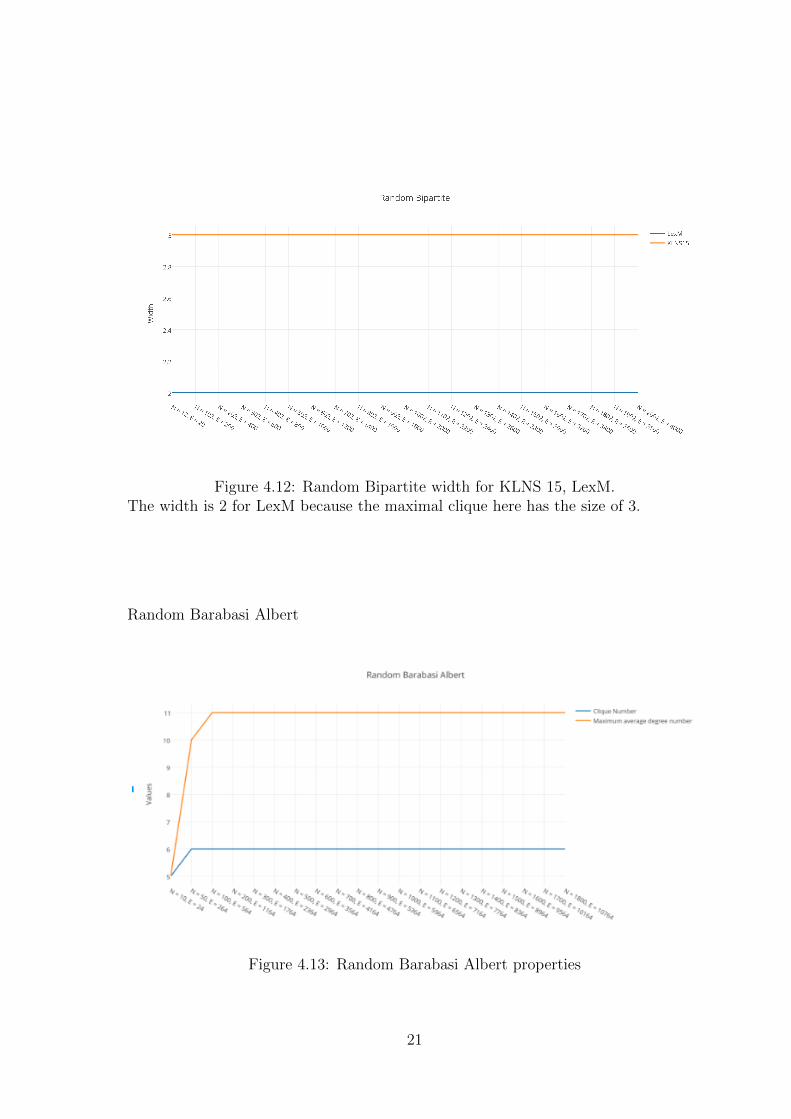
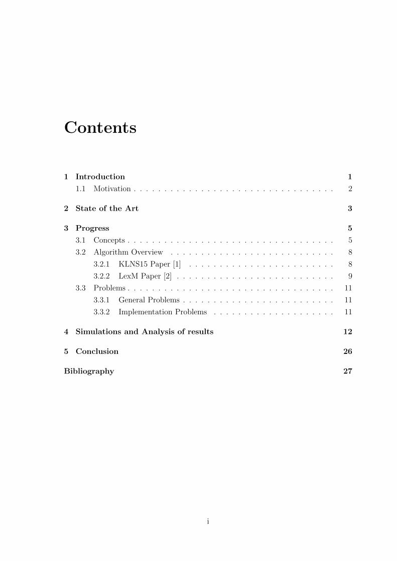
Figure 4.12: Random Bipartite width for KLNS 15, LexM.The width is 2 for LexM because the maximal clique here has the size of 3.

Random Barabasi Albert

Figure 4.13: Random Barabasi Albert properties

21

Figure 4.14: Random Barabasi Albert Execution time for KLNS 15, LexMIn this plot we see that both these algorithms are almost giving the same executiontime.KLNS15 is showing better results in this graph because the graph has high degreenumber, therefore, making the size of the separator big which reduces the number ofiterations. As for LexM the graph is not chordal graph so it takes much more timethan the previous graph classes because it tries to make it chordal for large cycles.The size of the graph is also big here which as well affects the execution time for bothof them.

Figure 4.15: Random Barabasi Albert width for KLNS 15, LexM.In this plot, we see that the width increases almost linearly for both algorithms asthe input increase. This is because of the fact that, this class of graph favours noneof the algorithm in terms of width.

22

Random GNP

Figure 4.16: Random GNP propertiesThe Clique Number and Maximum Average Degree increases linearly with thenumber of nodes as the connection in the graph becomes more dense.

Figure 4.17: Random GNP Execution time for KLNS 15, LexMKLNS15 - Performs better than LexM because for KLNS15 the separator sizeconsidered in each step is large which reduces the number of iterations. Theseparator size is large because of large maximum average degree number.

23

Figure 4.18: Random GNP width for KLNS 15, LexM.The width of KLNS15 is directly dependent on the size of the separator which in-turndepends on maximum average degree number. Since we have linear relationshipbetween max. avg. degree number and the size of the graph, we have a linearrelationship in width as well. As for LexM, the maximal clique size we get afterexecuting LexM is the entire graph, which is put in one bag. Hence, the width is thesame as the number of nodes in the graph - 1.

Random Triangulation

Figure 4.19: Random Triangulation properties

24

Figure 4.20: Random Triangulation Execution time for KLNS15, LexMIn this plot, we see that KLNS15 takes more time than LexM this is because, thegraph is already chordal for LexM whereas for KLNS15, the execution time dependson the max avg degree number which becomes constant after a certain stage, whichmakes it under-perform for large graphs.

Figure 4.21: Random Triangulation width for KLNS15, LexM.In this plot, we see that LexM has smaller width than the KLNS15 algorithm.

25

Chapter 5

Conclusion

After performing the tests on various kind of graphs, we conclude that in terms of:-

1. Time Efficiency:

LexM algorithm runs faster in Random tree, Interval graphs of interval length

2, grid graph with N rows and 2 columns, Random Bi-partite graphs with one

set having two nodes only, Random Barabasi Albert and Random Triangulation

graph. KLNS15 runs faster than LexM in RandomGNP graphs.

2. Width:

LexM has lower width in Random Tree, Interval graphs of interval length 2,

grid graph with N rows and 2 columns, Random Bi-partite graphs with one set

having two nodes only, Random Barabasi Albert and Random Triangulation.

For RandomGNP graphs both the algorithm outputs the same width.

In the end these algorithms are indeed practical algorithms to find tree decom-

position with small width. However not for all types of graph because some tree

decompositions give very large width which are not practical at all to solve NP hard

problems. The graph classes which gives small width are:-

1. Random Tree.

2. Interval graph with interval length as 2.

3. Grid Graph with N rows and 2 columns.

4. Random Bi-Partite graphs with one set having 2 elements and other set having

N elements.

26

Bibliography

[1] Adrian Kosowski, Bi Li, Nicolas Nisse, Karol Suchan k-Chordal Graphs: From

Cops and Robber to Compact Routing via Treewidth.

[2] Rose, D. J. Tarjan R.E , Lueker, G. S. Algorithmic aspects of vertex elimination

on graphs SIAM Journal on Computing, 5(2): 266283, 1976.

[3] Hans L. Bodlaender Treewidth: structure and algorithms

[4] Hans L. Bodlaender Tutorial - A partial k-arboretum of graphs with bounded

treewidth.

[5] Yon Dourisboure, Cyril Gavoille Tree-decompositions with bags of small diameter

[6] Nicolas Nisse Guillaume Ducoffe Introductory project paper of Practical Algo-

rithms to compute Tree-decompositions of Graphs

[7] Paul D. Seymour and Robin Thomas. Call routing and the ratcatcher. Combina-

torica, 14(2):217241, 1994.

[8] Qian-Ping Gu and Hisao Tamaki. Optimal branch-decomposition of planar

graphs in O(n3) time. ACM Transactions on Algorithms, 4(3), 2008

[9] Hans L. Bodlaender A linear time algorithm for finding tree decompositions of

small tree width.

[10] Algorithms Finding Tree-Decompositions of Graphs

http://people.math.gatech.edu/ thomas/PAP/algofind.pdf

[11] Tree width

https://en.wikipedia.org/wiki/Treewidth

[12] Tree width

https://en.wikipedia.org/wiki/Chordalgraph

27

[13] Tree decomposition definition

https://www.mi.fu-berlin.de/en/inf/groups/abi/teaching/lectures past/WS

0910/V Discrete Mathematics for Bioinformatics P1/material/scripts/

treedecomposition1.pdfh

[14] Tree Decomposition

https://en.wikipedia.org/wiki/Treedecomposition

[15] Vertex Coloring using Tree decomposition

https://www2.informatik.hu-berlin.de/logik/lehre/SS10/Para/HC5treewidthonline.pdf

[16] A.Parra, P.Scheffler Characterizations and algorithmic applications of chordal

graphs embeddings Discrete Appl, Math . 79 (1-3) (1997) 171-188.

[17] C.Gavoille, M.Katz,N.A.Katz , C.Paul , D.Peleg Approximate distance labeling

scheme Research report RR-1250-00, LaBRI, University of Bordeaux, 351, cours

de la liberation, 33405 Talence Cedex France Dec 2000

[18] Chordal Graph

https://en.wikipedia.org/wiki/Chordal graph

28