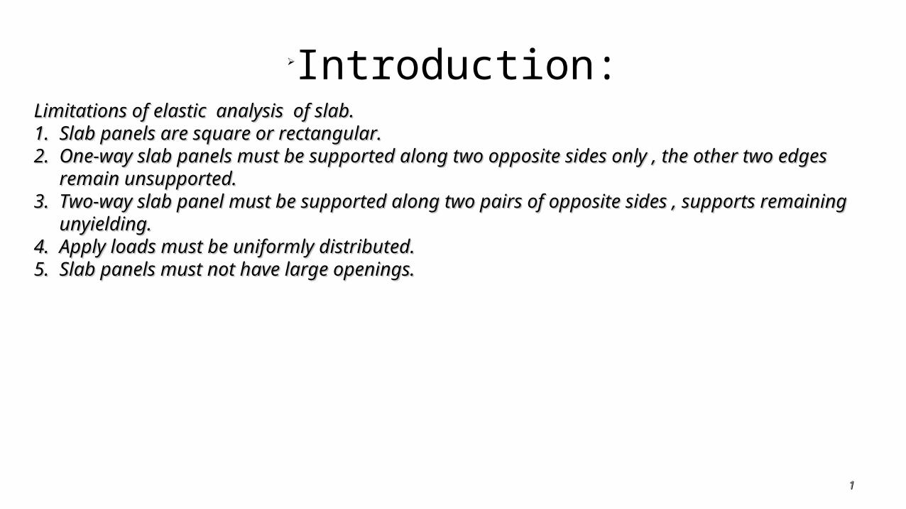
1 Introduction: Limitations of elastic analysis of slab. Limitations of elastic analysis of slab. 1. 1. Slab panels are square or rectangular. Slab panels are square or rectangular. 2. 2. One-way slab panels must be supported along two opposite sides only , the other two edges One-way slab panels must be supported along two opposite sides only , the other two edges remain unsupported. remain unsupported. 3. 3. Two-way slab panel must be supported along two pairs of opposite sides , supports remaining Two-way slab panel must be supported along two pairs of opposite sides , supports remaining unyielding. unyielding. 4. 4. Apply loads must be uniformly distributed. Apply loads must be uniformly distributed. 5. 5. Slab panels must not have large openings. Slab panels must not have large openings.

Final Yield Line
Dec 26, 2015
Final Yield Line
Welcome message from author
This document is posted to help you gain knowledge. Please leave a comment to let me know what you think about it! Share it to your friends and learn new things together.
Transcript
11
Introduction:Limitations of elastic analysis of slab.Limitations of elastic analysis of slab.1.1. Slab panels are square or rectangular.Slab panels are square or rectangular.2.2. One-way slab panels must be supported along two opposite sides only , the other two edges remain One-way slab panels must be supported along two opposite sides only , the other two edges remain
unsupported.unsupported.3.3. Two-way slab panel must be supported along two pairs of opposite sides , supports remaining unyielding.Two-way slab panel must be supported along two pairs of opposite sides , supports remaining unyielding.4.4. Apply loads must be uniformly distributed.Apply loads must be uniformly distributed.5.5. Slab panels must not have large openings.Slab panels must not have large openings.
22
History Yield Line Theory as we know it today was pioneered in the 1940s by the Danish engineer and researcher K Yield Line Theory as we know it today was pioneered in the 1940s by the Danish engineer and researcher K
W Johansen. W Johansen.
As early as 1922, the Russian, A Ingerslev presented a paper to the Institution of Structural Engineers in As early as 1922, the Russian, A Ingerslev presented a paper to the Institution of Structural Engineers in London on the collapse modes of rectangular slabs. London on the collapse modes of rectangular slabs.
Authors such as R H Wood, L L Jones, A Sawczuk and T Jaeger, R Park, K O Kemp, C T Morley, M Kwiecinski Authors such as R H Wood, L L Jones, A Sawczuk and T Jaeger, R Park, K O Kemp, C T Morley, M Kwiecinski and many others, consolidated and extended Johansen’s original work so that now the validity of the and many others, consolidated and extended Johansen’s original work so that now the validity of the theory is well established making Yield Line Theory a formidable international design tool.theory is well established making Yield Line Theory a formidable international design tool.
In the 1960s 70s and 80s a significant amount of theoretical work on the application of Yield Line Theory In the 1960s 70s and 80s a significant amount of theoretical work on the application of Yield Line Theory to slabs and slab-beam structures was carried out around the world and was widely reported.to slabs and slab-beam structures was carried out around the world and was widely reported.

DEFINITION:
A yield line is a crack in a reinforced concrete slab across which the reinforcing bars have yielded and along which plastic rotation occurs.
Yield Line Theory is an ultimate load analysis. It establishes either the moments in an element (e.g. Yield Line Theory is an ultimate load analysis. It establishes either the moments in an element (e.g. a loaded slab) at the point of failure or the load at which an element will fail. It may be applied to a loaded slab) at the point of failure or the load at which an element will fail. It may be applied to many types of slab, both with and without beams.many types of slab, both with and without beams.

BASIC PRINCIPLE OF YIELD LINE THEORY:

ASSUMPTIONS:1. The elastic deformations of a part of a slab between the yield lines negligible as compared to
plastic deformations along the yield line. It is assumed that the deformations take place only along the yield lines and the individual parts of the slab between the yield line remain planes.
2. As the intersection between the inclined planes are the straight lines it follows that the yield lines are straight.
3. Yield line passes through the intersection of the axes of the rotation of the adjacent slab elements.
Continue..Continue..
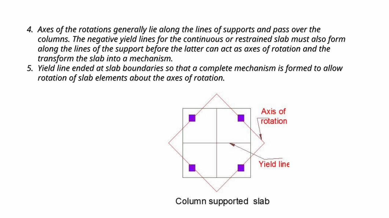
4.4. Axes of the rotations generally lie along the lines of supports and pass over the columns. The Axes of the rotations generally lie along the lines of supports and pass over the columns. The negative yield lines for the continuous or restrained slab must also form along the lines of the negative yield lines for the continuous or restrained slab must also form along the lines of the support before the latter can act as axes of rotation and the transform the slab into a support before the latter can act as axes of rotation and the transform the slab into a mechanism.mechanism.
5.5. Yield line ended at slab boundaries so that a complete mechanism is formed to allow rotation Yield line ended at slab boundaries so that a complete mechanism is formed to allow rotation of slab elements about the axes of rotation.of slab elements about the axes of rotation.
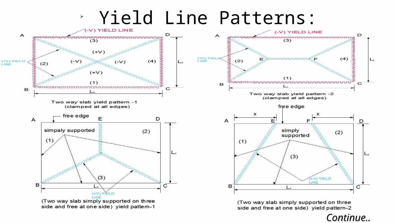
Yield Line Patterns:
Continue..Continue..
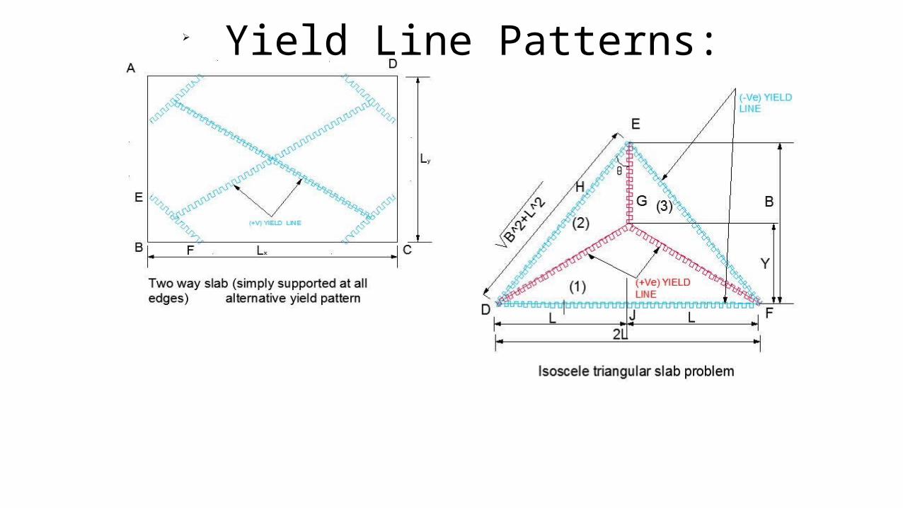
Yield Line Patterns:
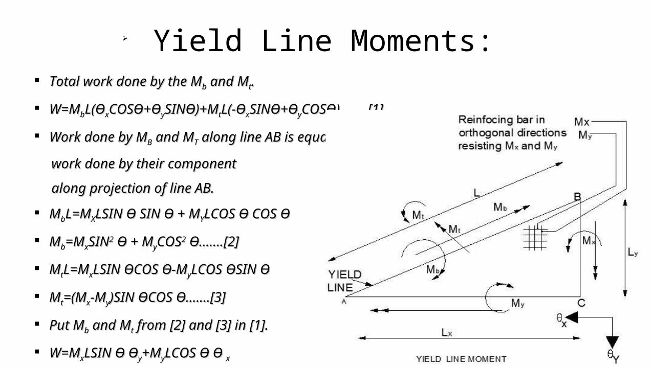
Yield Line Moments: Total work done by the MTotal work done by the Mbb and M and Mtt..
W=MW=MbbL(ӨL(ӨxxCOSӨ+ӨCOSӨ+ӨyySINӨ)+MSINӨ)+MttL(-ӨL(-ӨxxSINӨ+ӨSINӨ+ӨyyCOSӨ)……..[1]COSӨ)……..[1]
Work done by MWork done by MBB and M and MTT along line AB is equal to along line AB is equal to
work done by their componentwork done by their component
along projection of line AB.along projection of line AB.
MMbbL=ML=MXXLSIN Ө SIN Ө + MLSIN Ө SIN Ө + MYYLCOS Ө COS ӨLCOS Ө COS Ө
MMbb=M=MxxSINSIN22 Ө + M Ө + MyyCOSCOS22 Ө…….[2] Ө…….[2]
MMttL=ML=MxxLSIN ӨCOS Ө-MLSIN ӨCOS Ө-MyyLCOS ӨSIN ӨLCOS ӨSIN Ө
MMtt=(M=(Mxx-M-Myy)SIN ӨCOS Ө.……[3])SIN ӨCOS Ө.……[3]
Put MPut Mbb and M and Mtt from [2] and [3] in [1]. from [2] and [3] in [1].
W=MW=MxxLSIN Ө ӨLSIN Ө Өyy+M+MyyLCOS Ө Ө LCOS Ө Ө xx
W=MW=MxxLLy y ӨӨyy+M+MyyLLxx Ө Өxx
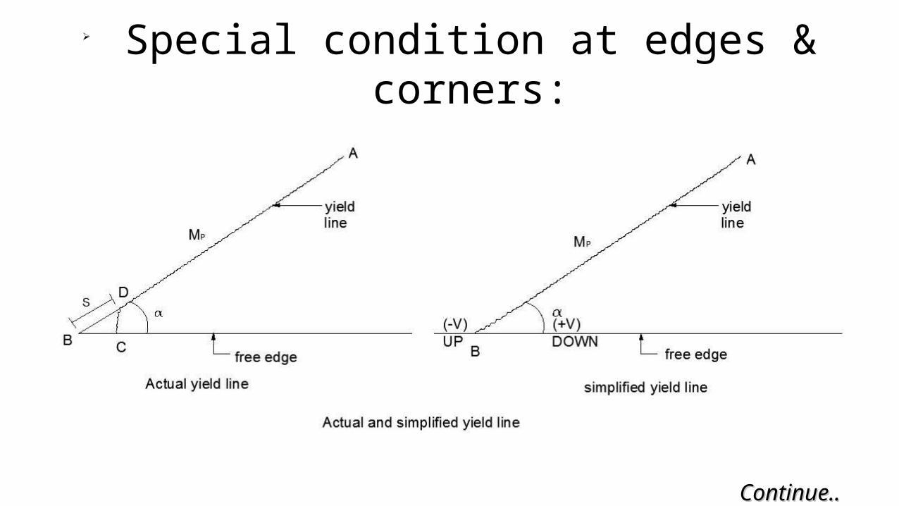
Special condition at edges & corners:
Continue..Continue..

Continue..Continue..

Taking moment about the line AC and equating to zero,Taking moment about the line AC and equating to zero, MMyy(L(Lxx+dL+dLxx)COS(α-dα)-M)COS(α-dα)-MyyLLxxCOSCOS(α-d α)+M(α-d α)+MxxLLyySIN(α-d α)-MSIN(α-d α)-MxxLLyySIN(α-d α)- VdLSIN(α-d α)- VdLxxSIN(α-dα)=0SIN(α-dα)=0
VSIN (α-d α)=MVSIN (α-d α)=MyyCOS(α-d α)COS(α-d α)
V(SIN α COSd α -COS α SINd α)=MV(SIN α COSd α -COS α SINd α)=Myy(COS α COSd α +SIN α SINd α)(COS α COSd α +SIN α SINd α)
V=MV=MyyCOT αCOT α When α=90,When α=90, V=0,means that the yield line intersects the free edge at right angle.V=0,means that the yield line intersects the free edge at right angle.

Method of yield line analysis:1)1) Method of segmental equilibrium:Method of segmental equilibrium: Steps:-Steps:-1.1. Predict possible trial yield line patterns and axes of rotation.Predict possible trial yield line patterns and axes of rotation.2.2. Draw free body diagram of each element of the slab.Draw free body diagram of each element of the slab.3.3. Compute nodal forces keeping in view that:Compute nodal forces keeping in view that: Resultant of nodal forces is zero at the junction or node of yield lines.Resultant of nodal forces is zero at the junction or node of yield lines. A free edge is considered to be a yield line of zero strength.A free edge is considered to be a yield line of zero strength. Nodal forces appears when a yield line intersects a free edge at angle other than 90°Nodal forces appears when a yield line intersects a free edge at angle other than 90°4. Formulate equilibrium equations for each element considering the load on it, and the moments4. Formulate equilibrium equations for each element considering the load on it, and the moments and nodal forces on the bounding yield lines. and nodal forces on the bounding yield lines.
Continue..Continue..
1414
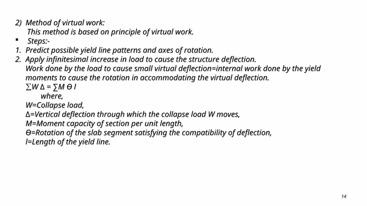
2)2) Method of virtual work:Method of virtual work: This method is based on principle of virtual work.This method is based on principle of virtual work. Steps:-Steps:-1.1. Predict possible yield line patterns and axes of rotation.Predict possible yield line patterns and axes of rotation.2.2. Apply infinitesimal increase in load to cause the structure deflection.Apply infinitesimal increase in load to cause the structure deflection.
Work done by the load to cause small virtual deflection=internal work done by the yield moments Work done by the load to cause small virtual deflection=internal work done by the yield moments to cause the rotation in accommodating the virtual deflection.to cause the rotation in accommodating the virtual deflection.∑∑W ∆ = ∑M Ө lW ∆ = ∑M Ө l
where,where,W=Collapse load,W=Collapse load,∆∆=Vertical deflection through which the collapse load W moves,=Vertical deflection through which the collapse load W moves,M=Moment capacity of section per unit length,M=Moment capacity of section per unit length,Ө=Rotation of the slab segment satisfying the compatibility of deflection,Ө=Rotation of the slab segment satisfying the compatibility of deflection,l=Length of the yield line.l=Length of the yield line.

Analysis of two way slab(pattern:1):1)1) Method of segmental equilibrium:Method of segmental equilibrium: for segment 1,moment of the all the forces and for segment 1,moment of the all the forces and moment of segment about edge AB is zero.moment of segment about edge AB is zero. (⅟(⅟22)(L)(Lxx/2)(L/2)(Lyy)W(L)W(Lxx/6)-V(L/6)-V(Lxx/2)-M/2)-MnxnxLLyy-M-MpxpxLLyy=0=0 WLWLxxLLyy-12V=24(M-12V=24(Mpxpx+M+Mnxnx)(L)(Lyy/L/Lxx)……[1])……[1]
for segment 2,moment of the all the forces and for segment 2,moment of the all the forces and moment of segment about edge BC is zero.moment of segment about edge BC is zero. (⅟(⅟22)(L)(Lyy/2)(L/2)(Lxx)W(L)W(Lyy/6)+V(L/6)+V(Lyy/2)-M/2)-MnynyLLxx-M-MpypyLLxx=0=0 WLWLxxLLyy+12V=24(M+12V=24(Mpypy+M+Mnxnx)(L)(Lxx/L/Lyy)……[2])……[2]
adding [1] and [2],neglecting V,adding [1] and [2],neglecting V, W=12{(MW=12{(Mpxpx+M+Mnxnx)/Lx)/Lx22+(M+(Mpypy+M+Mnyny)/L)/Lyy
22}.......[3]}.......[3]
Continue..Continue..
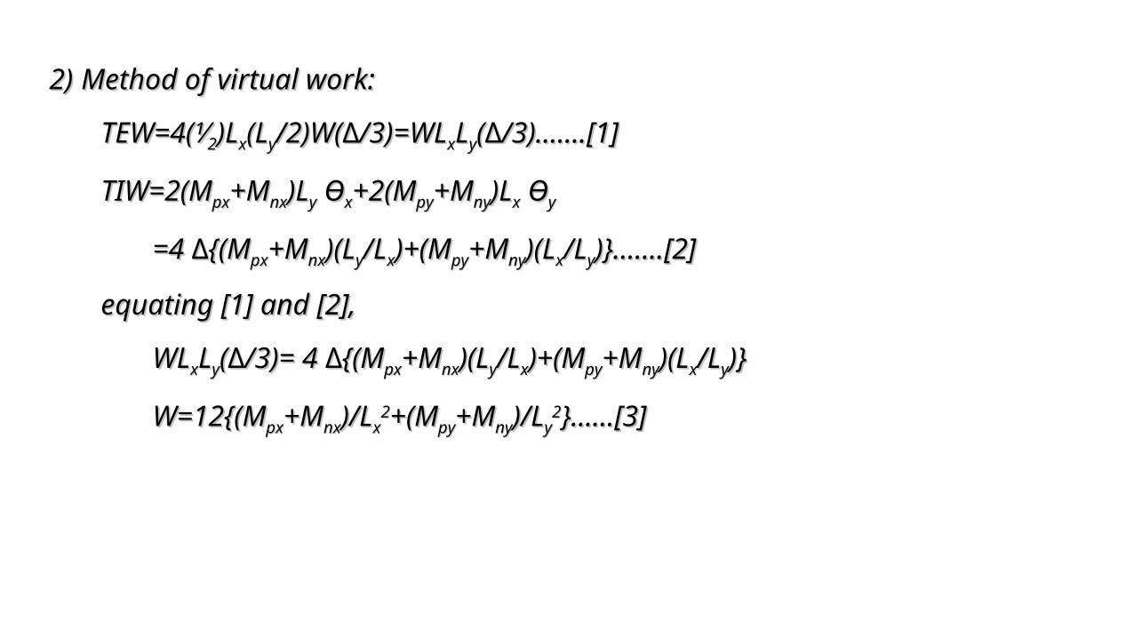
2)2) Method of virtual work:Method of virtual work:
TEW=4(⅟TEW=4(⅟22)L)Lxx(L(Lyy/2)W(∆/3)=WL/2)W(∆/3)=WLxxLLyy(∆/3)…….[1](∆/3)…….[1]
TIW=2(MTIW=2(Mpxpx+M+Mnxnx)L)Lyy Ө Өxx+2(M+2(Mpypy+M+Mnyny)L)Lxx Ө Өyy
=4 ∆{(M=4 ∆{(Mpxpx+M+Mnxnx)(L)(Lyy/L/Lxx)+(M)+(Mpypy+M+Mnyny)(L)(Lxx/L/Lyy)}…….[2])}…….[2]
equating [1] and [2],equating [1] and [2],
WLWLxxLLyy(∆/3)= 4 ∆{(M(∆/3)= 4 ∆{(Mpxpx+M+Mnxnx)(L)(Lyy/L/Lxx)+(M)+(Mpypy+M+Mnyny)(L)(Lxx/L/Lyy)})}
W=12{(MW=12{(Mpxpx+M+Mnxnx)/L)/Lxx22+(M+(Mpypy+M+Mnyny)/L)/Lyy
22}......[3]}......[3]
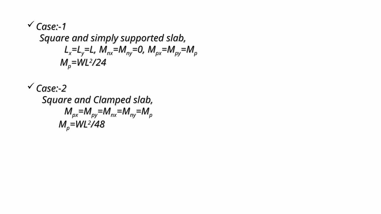
Case:-1Case:-1 Square and simply supported slab,Square and simply supported slab, LLxx=L=Lyy=L, M=L, Mnxnx=M=Mnyny=0, M=0, Mpxpx=M=Mpypy=M=Mpp
MMpp=WL=WL22/24/24
Case:-2Case:-2 Square and Clamped slab,Square and Clamped slab, MMpxpx=M=Mpypy=M=Mnxnx=M=Mnyny=M=Mp p
MMpp=WL=WL22/48/48

Analysis of two way slab(pattern:2):Analysis of two way slab(pattern:2):1)1) Method of segmental equilibrium:Method of segmental equilibrium: for segment 1,moment of the all the forces andfor segment 1,moment of the all the forces and moment of segment about edge AB is zero.moment of segment about edge AB is zero. (⅟(⅟22)(L)(Lyy)W(X/3)-(M)W(X/3)-(Mpxpx+M+Mnxnx)L)Lyy=0=0 W=6(MW=6(Mpxpx+M+Mnxnx)(X)(X22)……[1])……[1]
for segment 2,moment of the all the forces andfor segment 2,moment of the all the forces and moment of segment about edge BC is zero.moment of segment about edge BC is zero. (⅟(⅟22)X(L)X(Lyy/2)W(L/2)W(Lyy/6)2+W(L/6)2+W(LXX-2X)(L-2X)(Lyy/2) (L/2) (Lyy/4)-(M/4)-(Mpypy+M+Mnyny)L)Lxx=0=0 W=24(MW=24(Mpypy+M+Mnyny)L)Lxx/{2XL/{2XLyy
2 2 +3L+3Lyy22(L(Lxx-2X)}……[2]-2X)}……[2]
equating [1] and [2],equating [1] and [2], 6(M6(Mpxpx+M+Mnxnx)/X)/X22=24(M=24(Mpypy+M+Mnyny)L)Lxx/{2XL/{2XLyy
22+3L+3Lyy22(L(LXX-2X)}-2X)}
4(M4(Mpypy+M+Mnyny)L)Lxx22+4(M+4(Mpxpx+M+Mnxnx)L)Lyy
22X-3((MX-3((Mpxpx+M+Mnxnx)L)LxxLLyy2 2 = 0= 0Continue..Continue..

2)2) Method of virtual work:Method of virtual work:
TEW=2W1+2(W21+W22+W23)TEW=2W1+2(W21+W22+W23)
=2W{(⅟=2W{(⅟22)XL)XLyy(∆/3)}+2W{(⅟2)X(L(∆/3)}+2W{(⅟2)X(Lyy/2)(∆/3)}+2W{(L/2)(∆/3)}+2W{(Lxx-2X)(L-2X)(Lyy/2)(∆/2)}/2)(∆/2)}
=(W∆/6)(3L=(W∆/6)(3LxxLLyy-2xL-2xLyy)…….[1])…….[1]
TIW=2(MTIW=2(Mpxpx+M+Mnxnx)L)Lyy Ө Өxx+2(M+2(Mpypy+M+Mnyny)L)Lxx Ө Өyy
=2 (M=2 (Mpxpx+M+Mnxnx)(∆/X) L)(∆/X) Lyy +2(M +2(Mpypy+M+Mnyny)(2∆/L)(2∆/Lyy) L) Lxx…….[2]…….[2]
equating [1] and [2],equating [1] and [2],
(W∆/6)(3L(W∆/6)(3LxxLLyy-2xL-2xLyy)= 2 (M)= 2 (Mpxpx+M+Mnxnx)(∆/X) L)(∆/X) Lyy +2(M +2(Mpypy+M+Mnyny)(2∆/L)(2∆/Lyy) L) Lxx
W={12(MW={12(Mpxpx+M+Mnxnx)L)Lyy22+24(M+24(Mpypy+M+Mnyny)XL)XLxx}/L}/Lyy
22(3XL(3XLxx-2X-2X22)........[3])........[3]
To get the minimum collapse load,To get the minimum collapse load, dW/dX = 0dW/dX = 0
4(M4(Mpypy+M+Mnyny)L)Lxx22+4(M+4(Mpxpx+M+Mnxnx)L)Lyy
22X-3((MX-3((Mpxpx+M+Mnxnx)L)LxxLLyy2 2 = 0= 0
Continue..Continue..

Case:-Case:- Rectangle and clamped slab (Interior panel),Rectangle and clamped slab (Interior panel), LLxx=1.1L=1.1Ly y , X=L, X=Lxx/2, M/2, Mnyny=1.33M=1.33Mpy py , M, Mnxnx=1.33M=1.33Mpxpx , , M Mpxpx=0.85M=0.85Mpypy
Short span coefficients αShort span coefficients αy y =0.032 (Positive)=0.032 (Positive)
ααy y =0.043 (Negative)=0.043 (Negative) Long span coefficients αLong span coefficients αx x =0.027 (Positive)=0.027 (Positive)
ααx x =0.036 (Negative)=0.036 (Negative)

References:References: Yield line analysis for slabs : Module 12, Lesson 30,31,32 (NPTEL)Yield line analysis for slabs : Module 12, Lesson 30,31,32 (NPTEL) – – IIT KharagpurIIT Kharagpur Practical Yield line design : Perencanaan-Praktis-Garis-Leleh1Practical Yield line design : Perencanaan-Praktis-Garis-Leleh1 Concrete structure : By V N Vazirani & M.M RatwaniConcrete structure : By V N Vazirani & M.M Ratwani Design of reinforced concrete structure : M L GhambhirDesign of reinforced concrete structure : M L Ghambhir Design of reinforced concrete structure : B C punamiaDesign of reinforced concrete structure : B C punamia I S 456 : Plain & reinforced concrete code of practiceI S 456 : Plain & reinforced concrete code of practice
THANK YOUTHANK YOU
Related Documents